Embed Size (px)
Citation preview

TECHNI CAL REPORT ◦ JUNE 2014
Riparian Restoration Framework
for the Upper Gila River, Arizona
P R E P A R E D F O R P R E P A R E D B Y
Gila Watershed Partnership of Arizona 711 South 14th Avenue Safford, AZ 85546 F U N D E D B Y
Walton Family Foundation Freshwater Initiative P.O. Box 2030 Bentonville, AR 72712
Bruce K Orr – Stillwater Sciences
Glen T Leverich – Stillwater Sciences
Zooey E Diggory – Stillwater Sciences
Tom L Dudley – Marine Science Institute, U.C. Santa Barbara
James R Hatten – Columbia River Research Laboratory, U.S. Geological Survey
Kevin R Hultine – Desert Botanical Garden
Matthew P Johnson – Colorado Plateau Research Station, Northern Arizona University
Devyn A Orr – Marine Science Institute, U.C. Santa Barbara
Riparian Restoration Framework
for the Upper Gila River, Arizona
Bruce K. Orr1, Glen T. Leverich1, Zooey E. Diggory1,
Tom L. Dudley2, James R. Hatten3, Kevin R. Hultine4,
Matthew P. Johnson5, and Devyn A. Orr2
1 Stillwater Sciences, Berkeley, CA
2 Marine Science Institute, U.C. Santa Barbara, CA 3Columbia River Research Laboratory, U.S. Geological Survey, Cook, WA
4Desert Botanical Garden, Phoenix, AZ 5Colorado Plateau Research Station, Northern Arizona University, AZ
June 2014

Riparian Restoration Framework
Technical Report for the Upper Gila River, Arizona
June 2014 Orr et al. i
Contacts:
Bruce Orr, Ph.D.
Principal Ecologist
Stillwater Sciences
(510) 848-8098 ext. 111
Glen Leverich, P.G.
Senior Geomorphologist
Stillwater Sciences
(510) 848-8098 ext. 156
Cover graphics:
Upper left: Photograph of tamarisk stands along the upper Gila River near Safford, Arizona (photo taken
on August 22, 2012 by T. Dudley)
Upper right: Restoration suitability mapping produced by Stillwater Sciences from ecohydrological
analysis: oblique view using Google Earth is of the river looking north toward Ft. Thomas, Arizona
Bottom left: Breeding-habitat suitability modeled by J. Hatten along the upper Gila River near Ft.
Thomas, Arizona for southwestern willow flycatcher
Bottom right: Photograph of a mixed stand of cottonwood (Populus fremontii) and Goodding’s willow
(Salix gooddingii) trees located near Ft. Thomas, Arizona (photo taken May 3, 2013 by B. Orr)
Acknowledgements:
Our sincere thanks go to Ms. Jan Holder of the Gila Watershed Partnership of Arizona for coordinating
development of the Riparian Restoration Framework for the Gila River Restoration Planning Area, and to
Mr. Tim Carlson and Ms. Margaret Bowman for facilitating project funding through the Walton Family
Foundation, Freshwater Initiative Program. We acknowledge valuable assistance from the Cross-Watershed
Network, Southwest Decision Resources, and Tamarisk Coalition, as well as representatives from Bureau
of Land Management, Bureau of Reclamation, Freeport McMoRan Copper & Gold, Inc., Graham County,
and Salt River Project. And, Mr. Bill Brandau of the Graham County Cooperative Extension of University
of Arizona provided invaluable watershed information and assistance with river access.
Project team:
The Restoration Science Team included: Dr. Bruce Orr and Glen Leverich of Stillwater Sciences, Dr. Tom
Dudley of the Marine Science Institute at U.C. Santa Barbara; Jim Hatten of the Columbia River Research
Laboratory, U.S. Geological Survey; Dr. Kevin Hultine of the Desert Botanical Garden, and Matthew
Johnson of the Colorado Plateau Research Station at Northern Arizona University.
Report compilation was led by Stillwater Sciences. The project team at Stillwater Sciences included Dr.
Bruce Orr as the principal investigator, Glen Leverich as lead hydrologist/geomorphologist and project
manager, Zooey Diggory as lead riparian botanist, Rafael Real de Asua as lead GIS analyst, and Karley
Rodriguez as support GIS analyst and cartographer.
Field surveys and supplemental analysis were assisted by Devyn Orr and Dan Koepke.
Remote sensing data collection and processing conducted for this study were led by Drs. Christopher Neale
and Robert Pack at Utah State University’s Remote Sensing/Geographical Information Systems Laboratory
(http://www.gis.usu.edu/).
Suggested citation:
Orr, B. K., G. T. Leverich, Z. E. Diggory, T. L. Dudley, J. R. Hatten, K. R. Hultine, M. P. Johnson, and D.
A. Orr. 2014. Riparian restoration framework for the upper Gila River in Arizona. Compiled by Stillwater
Sciences in collaboration with Marine Science Institute at U.C. Santa Barbara, Columbia River Research
Laboratory of U.S. Geological Survey, Desert Botanical Garden, and Colorado Plateau Research Station at
Northern Arizona University. Prepared for the Gila Watershed Partnership of Arizona.

Riparian Restoration Framework
Technical Report for the Upper Gila River, Arizona
June 2014 Orr et al. ii
Table of Contents
1 INTRODUCTION................................................................................................................... 1
1.1 Planning Area Location ............................................................................................... 1 1.2 Need for Riparian Restoration ..................................................................................... 1
1.2.1 Tamarisk leaf beetle arrival ................................................................................... 3 1.2.2 Flood disturbance .................................................................................................. 4 1.2.3 Wildfire exacerbation ............................................................................................ 5
1.3 Purpose of the Restoration Framework ........................................................................ 5 1.4 Physical Setting ............................................................................................................ 6
2 ECOHYDROLOGICAL ASSESSMENT ............................................................................. 8
2.1 Remote-Sensing Data Collection ................................................................................. 8 2.2 Flood-Scour Analysis .................................................................................................. 8
2.2.1 Hydrogeomorphic characterization ....................................................................... 9 2.2.2 Aerial imagery analysis ....................................................................................... 19 2.2.3 Results of flood-scour analysis ............................................................................ 19
2.3 Riparian Vegetation Characterization ........................................................................ 20 2.3.1 Plot surveys and remote sensing methods ........................................................... 20 2.3.2 Vegetation types and distribution patterns .......................................................... 21 2.3.3 Vegetation restoration opportunities and constraints .......................................... 31
2.4 SWFL Habitat Evaluation and Modeling .................................................................. 32 2.4.1 Existing conditions and challenges ..................................................................... 33 2.4.2 SWFL breeding habitat modeling ....................................................................... 34
2.5 Soils and Groundwater Monitoring ........................................................................... 35 2.5.1 Soil sampling ....................................................................................................... 35 2.5.2 Groundwater-level monitoring ............................................................................ 35
2.6 Potentially Suitable Vegetation Restoration Areas .................................................... 37
3 SUMMARY OF FINDINGS AND RECOMMENDATIONS ........................................... 48
3.1 Summary of Ecohydrological Assessment and Other Information............................ 48 3.2 Synthesis of Findings ................................................................................................. 51
4 REFERENCES ...................................................................................................................... 54
Riparian Restoration Framework
Technical Report for the Upper Gila River, Arizona
June 2014 Orr et al. iii
Tables Table 2-1. USGS discharge gaging stations on the upper Gila River used in the
Ecohydrological Assessment. ................................................................................ 9 Table 2-2. Description of hydrogeomorphic reaches delineated along the upper Gila
River in the Gila Valley for the Ecohydrological Assessment. ........................... 18 Table 3-1. Top 20 parcels in the Planning Area having the most predicted “High” and
“Medium” Priority Restoration Areas. ................................................................ 52 Figures
Figure 1-1. Map of the upper Gila River watershed in eastern Arizona and the Gila Valley
Restoration Planning Area. .................................................................................... 2 Figure 2-1. Monthly mean discharge at five long-term streamflow gages on the mainstem
upper Gila River and lower San Francisco River used in this study. .................. 10 Figure 2-2. Mean daily flow duration curves and statistics for the five long-term streamflow
gages on the mainstem upper Gila River and lower San Francisco River used in
this study. ............................................................................................................ 11 Figure 2-3. Historical flood peaks through water year 2013 at five long-term streamflow
gages on the mainstem upper Gila River and lower San Francisco River used in
the Ecohydrological Assessment. ........................................................................ 12 Figure 2-4. Flood frequency [Log-Pearson III] for the five long-term streamflow gages used
in the Ecohydrological Assessment. .................................................................... 14 Figure 2-5. Location of hydrogeomorphic reaches delineated along the upper Gila River in
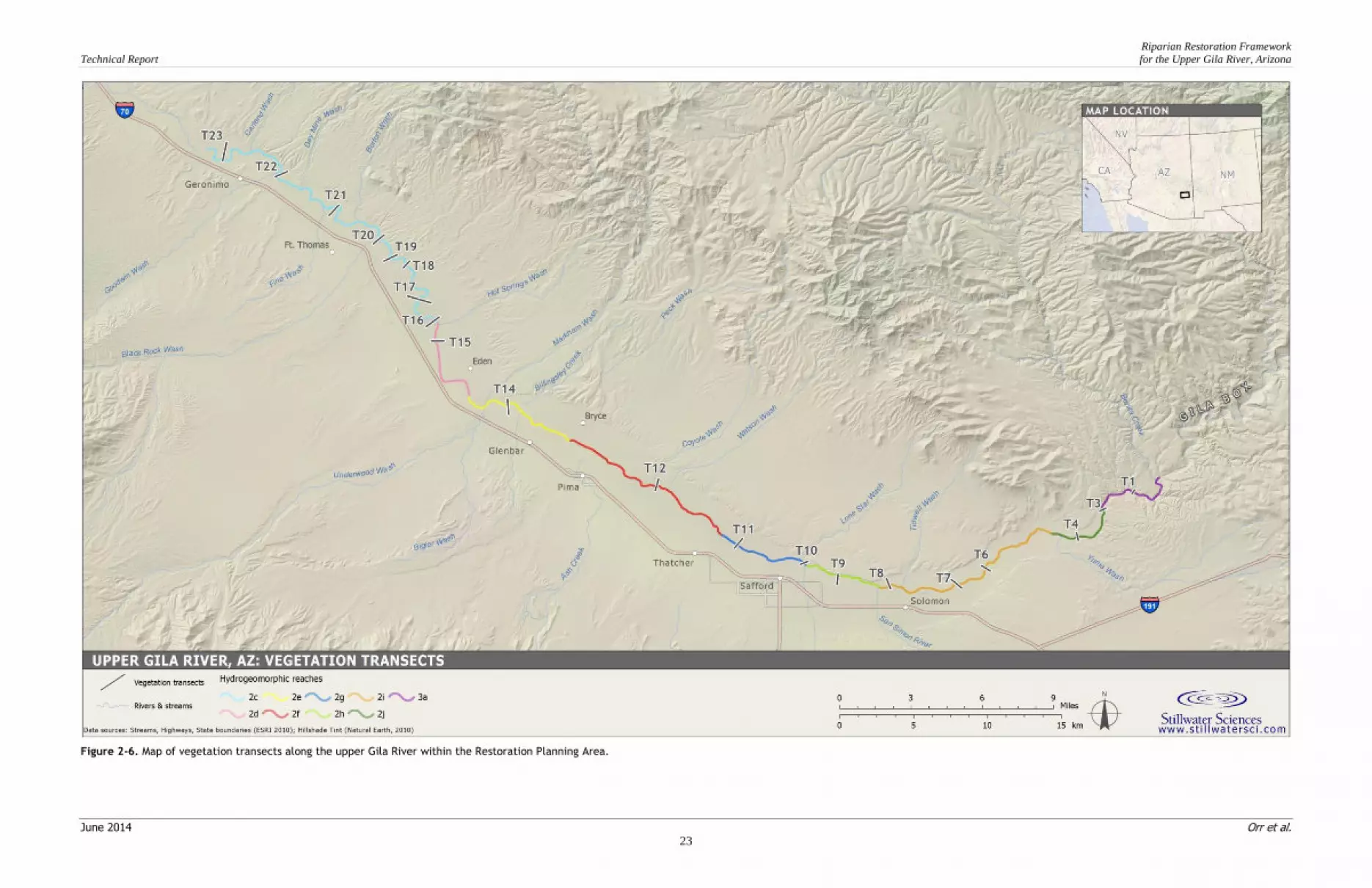
the Gila Valley for the Ecohydrological Assessment. ......................................... 17 Figure 2-6. Map of vegetation transects along the upper Gila River within the Restoration
Planning Area. ..................................................................................................... 23 Figure 2-7. Illustration of the typical cross-sectional distribution of vegetation in the Gila
Valley Planning Area downstream of Pima. ....................................................... 24 Figure 2-8. Histogram of Fremont cottonwood and Goodding’s willow occurrence by
relative elevation above the low-flow river channel water surface. .................... 27 Figure 2-9. Histogram of mulefat and narrowleaf willow occurrence by relative elevation
above the low-flow river channel water surface. ................................................. 28 Figure 2-10. Plot of measured groundwater depths in the Planning Area taken in January
2014. .................................................................................................................... 36 Figure 2-11. Process of the Ecohydrological Assessment to identify the Potentially Suitable
Vegetation Restoration Areas in the Planning Area. ........................................... 40 Figure 2-12. Upper Gila River Potentially Suitable Vegetation Restoration Areas. ................ 42 Figure 2-13. Histogram of sizes of the riparian corridor, Flood Reset Zone, and Potentially
Suitable Vegetation Restoration Areas within the Planning Area and each of the
hydrogeomorphic reaches. ................................................................................... 47 Appendices
Appendix A. Technical Documentation for Remote-Sensing Data Collection – USU RS/GIS
Appendix B. Flood-Scour Analysis Supporting Information and Maps – Stillwater Sciences
Appendix C. Riparian Vegetation Transect-Plot Data – Stillwater Sciences
Appendix D. Riparian Plant Species Requirements – Stillwater Sciences
Appendix E. SWFL Existing Conditions Summary – Matthew P. Johnson
Appendix F. SWFL Breeding Habitat Prediction Modeling – James R. Hatten and Matthew P.
Johnson
Appendix G. Restoration Site Monitoring: Vegetation, Soils, and Groundwater – Tom L. Dudley,
Kevin R. Hultine, and Devyn A. Orr
Riparian Restoration Framework
Technical Report for the Upper Gila River, Arizona
June 2014 Orr et al. 1
1 INTRODUCTION
This technical report summarizes the methods and results of a comprehensive riparian restoration
planning effort for the Gila Valley Restoration Planning Area, an approximately 53-mile portion
of the upper Gila River in Arizona (Figure 1-1). This planning effort has developed a Restoration
Framework intended to deliver science-based guidance on suitable riparian restoration actions
within the ecologically sensitive river corridor. The framework development was conducted by a
restoration science team, led by Stillwater Sciences with contributions from researchers at the
Desert Botanical Garden (DBG), Northern Arizona University (NAU), University of California at
Santa Barbara (UCSB), and U.S. Geological Survey (USGS). All work was coordinated by the
Gila Watershed Partnership of Arizona (GWP), whose broader Upper Gila River Project Area is
depicted in Figure 1-1, with funding from the Walton Family Foundation’s Freshwater Initiative
Program.
1.1 Planning Area Location
The overarching project area of the Gila Watershed Partnership of Arizona entails the 120 miles
(193 km) of the upper Gila River in Arizona upstream of the San Carlos Reservoir, and the lower
40 miles (64 km) of its major tributary, the San Francisco River (both reaches within Arizona
only). The current restoration planning effort focuses primarily on the Gila Valley area of the
upper Gila River in Graham County, Arizona: the “Gila Valley Restoration Planning Area,” or
simply “Planning Area.” This more focused extent was selected in order to provide effective
guidance for high priority restoration implementation projects in 2014–2015. The Planning Area
spans approximately 53 miles (85 km) along the riparian corridor from the Gila Box east of
Solomon (at the Bonita Creek confluence) downstream to the eastern boundary of the San Carlos
Apache Reservation near Geronimo (see Figure 1-1).
1.2 Need for Riparian Restoration
Like many ecologically important riverine systems in the
southwest, the upper Gila River and its major tributary,
the San Francisco River, are sensitive to natural and
anthropogenic stressors, including invasion by non-native
plants, flooding, wildfire, urban encroachment, and
various land- and water-use activities. The riparian
corridor is thus under constant pressure as it responds to
these ongoing perturbations. In the Gila Valley, invasion
by salt cedar (Tamarix ramosissima and other Tamarix
species or hybrids, hereafter “tamarisk”) is particularly
intense as it has become the dominant woody plant
species in the riparian corridor since it was first
introduced in the early 20th century to control river
erosion (see photo at right). Tamarisk has now densely
covered the riparian corridor out-competing native tree
species, including Fremont cottonwood (Populus
fremontii) and Goodding’s willow (Salix gooddingii).
Tamarisk along the upper Gila River (Photo by Stillwater Sciences)

Riparian Restoration Framework
Technical Report for the Upper Gila River, Arizona
June 2014 Orr et al. 2
Figure 1-1. Map of the upper Gila River watershed in eastern Arizona and the Gila Valley Restoration Planning Area.
Riparian Restoration Framework
Technical Report for the Upper Gila River, Arizona
June 2014 Orr et al. 3
Despite the dominance by tamarisk and impacts from other
natural and anthropogenic factors, the riparian corridor continues
to provide some active breeding habitat for the endangered
southwestern willow flycatcher (Empidonax traillii extimus;
SWFL) (see photo at right), along with habitats of other sensitive
fish and wildlife species. In 2011, the U.S. Fish and Wildlife
Service (USFWS) designated the upper Gila River as Critical
Habitat for SWFL, as it is known to be occupied by the species
during the breeding season and provides the primary constituent
elements essential to the species’ long-term conservation. It is
therefore a major goal of the federal designation and the SWFL
Recovery Plan (USFWS 2002) that habitat conservation on the
upper Gila and San Francisco rivers will lead to species recovery
throughout the region.
1.2.1 Tamarisk leaf beetle arrival
A key concern in the watershed and, accordingly, the impetus
for the present riparian restoration planning effort, is the
anticipated arrival of the tamarisk leaf beetle (Diorhabda
elongata species group) which has the potential to disturb
existing riparian habitat conditions, particularly for SWFL.
Four of five distinct species of the D. elongata complex were
introduced into portions of Colorado, Nevada, Texas, Utah,
and Wyoming during 2001–2009 by the U.S. Department of
Agriculture (USDA) for biological control of tamarisk (Tracy
and Robbins 2009, Tamarisk Coalition 2009). As intended,
the beetle expanded its range and has led to widespread
defoliation of tamarisk-dominated habitats in many other
southwestern watersheds (see photo at left). Individual plant
mortality typically occurs after 3+ years of repeat defoliation
(Bean et al. 2013). Somewhat surprising is that the “northern
leaf beetle” (D. carinulata) has evolved its physiological
ability to establish farther south than the originally introduced insects would have tolerated (south
of 38°N latitude), so it is likely that that species is, or will soon be, capable of establishment in
the Gila Valley (near 33°N latitude). Currently, D. carinulata is present to the northeast (upper
Rio Grande River), north (San Juan and Little Colorado Rivers), and west (Virgin River/Lake
Mead), and beetle establishment in 2012 below Hoover Dam marks their arrival into the lower
Colorado River basin. The “subtropical leaf beetle” species (D. sublineata) released in Texas on
the Rio Grande River is now moving westward through New Mexico (J. Tracy, pers. comm.,
2014). Thus, one or more species of the tamarisk leaf beetle is likely to arrive in the Gila Valley
in the foreseeable future (potentially within 2–3 years) and have impacts to tamarisk similar to
those seen elsewhere.
While there are numerous benefits to tamarisk suppression (e.g., water conservation, riparian
habitat recovery, fire risk reduction), and by biocontrol in particular (e.g., reduction in biomass
allowing restoration practitioners to more easily treat affected tamarisk and simultaneously
replant native species in a more cost-effective manner), short-term negative consequences are
Tamarisk leaf beetles (Diorhabda carinulata) feeding on tamarisk near the Virgin River, Nevada (Photo by Tom Dudley, UCSB)
Southwestern willow flycatcher nest and female in dense tamarisk (Photo by USGS)

Riparian Restoration Framework
Technical Report for the Upper Gila River, Arizona
June 2014 Orr et al. 4
also possible. Tamarisk defoliation from the leaf beetle will
be problematic in the Gila Valley as virtually all SWFL nest
sites are currently located in tamarisk along the river. If
defoliation by the beetle occurs simultaneously with nesting,
the loss of cover could result in juvenile mortality, as has
recently been observed along the lower Virgin River (see
photo at right). Other special status wildlife species, such as
the proposed threatened western population of yellow-billed
cuckoo (Coccyzus americanus), are also associated with
many riparian systems in which tamarisk is a major
component. It is thus important to plan now for the arrival of
the leaf beetle in the Gila Valley, both to take advantage of
the biocontrol benefits and to mitigate for its indirect impacts
to SWFL and other potentially sensitive wildlife.
Alternatively, inaction has the very real probability of leading
to declines in the local SWFL population.
1.2.2 Flood disturbance
Flooding through the upper watershed is
another concern of land- and water-use and
restoration planners due to the dramatic
changes that have taken place along the river
corridor. The river has experienced several
notable floods, most recently in 1983, 1993,
and 2005. The flood records reveal a relatively
quiescent period during the middle half of the
20th century, followed by a period of larger,
more frequent flood events since the late
1960s (see Section 2.1 Flood-Scour Analysis
below). This recent hydrological condition
reinforces the importance of considering flood
dynamics in any restoration planning effort on
the Gila and San Francisco rivers, especially in
light of its influence on tamarisk density in the
riparian corridor, and vice-versa.
It has been well documented that tamarisk acts
as a positive feedback on river morphology and flood dynamics through resisting erosion, which
is why the species was originally introduced in the early 1900s (e.g., Auerbach et al. 2013) (see
photos above left). Dense stands of tamarisk provide greater stability to the river and floodplain
substrates than do native vegetation (e.g., willows and cottonwoods) and, as an unintended
consequence, progressively narrow the active channel thereby increasing the frequency of
floodplain inundation (Graf 1978). Tamarisk is further favored over natives in this setting due to
its longer seed-release timing that extends into late summer when monsoon-induced floods can
re-expose fresh surfaces upon which tamarisk may more readily colonize (Shafroth et al. 1998).
Repeat views of the river near Calva: from 1932 showing a wide, braided channel bordered by a willow-cottonwood forest (top); and from 2000 following several large flood events showing dense establishment of tamarisk (bottom) (Photos
from USGS archives)
An exposed SWFL nest and female in defoliated tamarisk along the Virgin River (Photo by Utah Division
of Wildlife Resources)
Riparian Restoration Framework
Technical Report for the Upper Gila River, Arizona
June 2014 Orr et al. 5
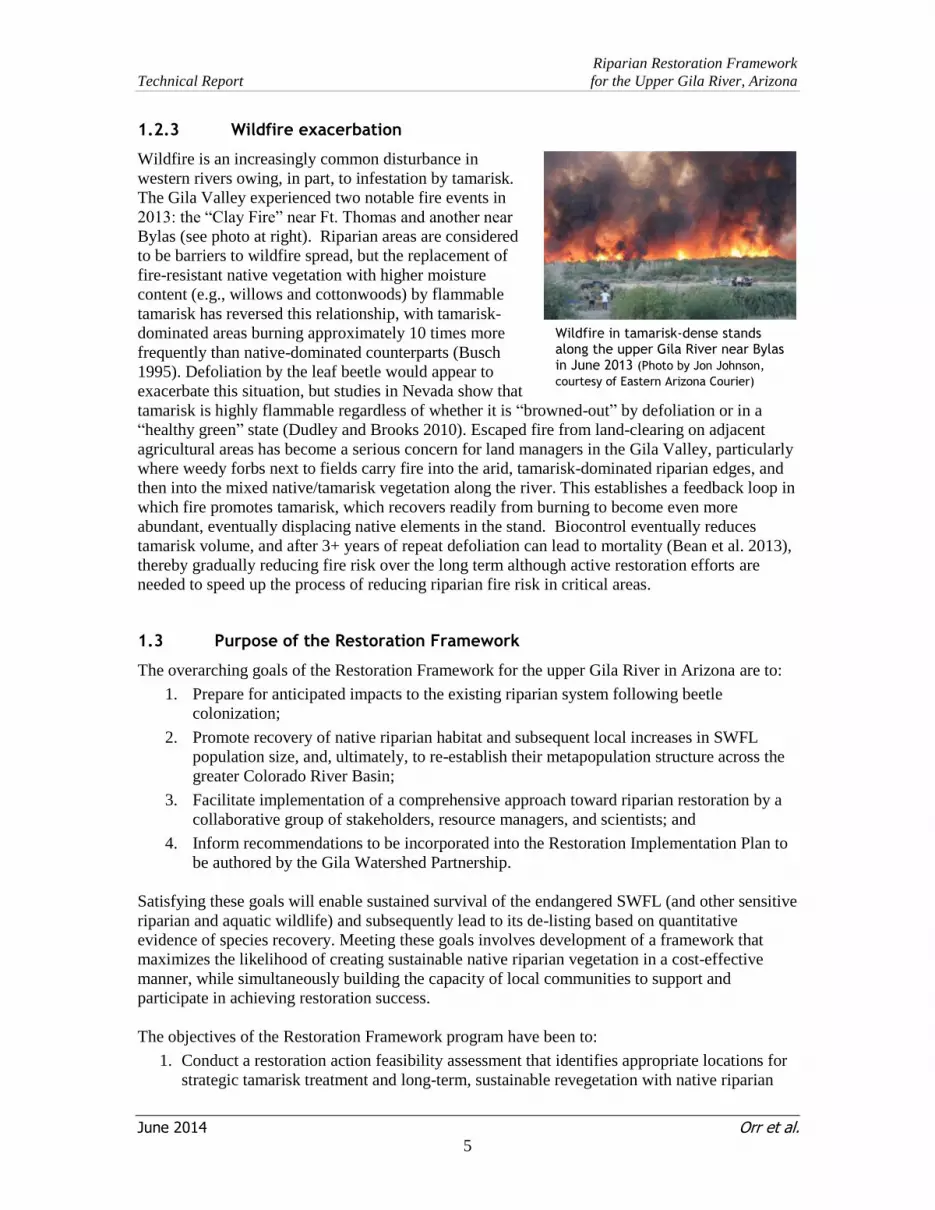
1.2.3 Wildfire exacerbation
Wildfire is an increasingly common disturbance in
western rivers owing, in part, to infestation by tamarisk.
The Gila Valley experienced two notable fire events in
2013: the “Clay Fire” near Ft. Thomas and another near
Bylas (see photo at right). Riparian areas are considered
to be barriers to wildfire spread, but the replacement of
fire-resistant native vegetation with higher moisture
content (e.g., willows and cottonwoods) by flammable
tamarisk has reversed this relationship, with tamarisk-
dominated areas burning approximately 10 times more
frequently than native-dominated counterparts (Busch
1995). Defoliation by the leaf beetle would appear to
exacerbate this situation, but studies in Nevada show that
tamarisk is highly flammable regardless of whether it is “browned-out” by defoliation or in a
“healthy green” state (Dudley and Brooks 2010). Escaped fire from land-clearing on adjacent
agricultural areas has become a serious concern for land managers in the Gila Valley, particularly
where weedy forbs next to fields carry fire into the arid, tamarisk-dominated riparian edges, and
then into the mixed native/tamarisk vegetation along the river. This establishes a feedback loop in
which fire promotes tamarisk, which recovers readily from burning to become even more
abundant, eventually displacing native elements in the stand. Biocontrol eventually reduces
tamarisk volume, and after 3+ years of repeat defoliation can lead to mortality (Bean et al. 2013),
thereby gradually reducing fire risk over the long term although active restoration efforts are
needed to speed up the process of reducing riparian fire risk in critical areas.
1.3 Purpose of the Restoration Framework
The overarching goals of the Restoration Framework for the upper Gila River in Arizona are to:
1. Prepare for anticipated impacts to the existing riparian system following beetle
colonization;
2. Promote recovery of native riparian habitat and subsequent local increases in SWFL
population size, and, ultimately, to re-establish their metapopulation structure across the
greater Colorado River Basin;
3. Facilitate implementation of a comprehensive approach toward riparian restoration by a
collaborative group of stakeholders, resource managers, and scientists; and
4. Inform recommendations to be incorporated into the Restoration Implementation Plan to
be authored by the Gila Watershed Partnership.
Satisfying these goals will enable sustained survival of the endangered SWFL (and other sensitive
riparian and aquatic wildlife) and subsequently lead to its de-listing based on quantitative
evidence of species recovery. Meeting these goals involves development of a framework that
maximizes the likelihood of creating sustainable native riparian vegetation in a cost-effective
manner, while simultaneously building the capacity of local communities to support and
participate in achieving restoration success.
The objectives of the Restoration Framework program have been to:
1. Conduct a restoration action feasibility assessment that identifies appropriate locations for
strategic tamarisk treatment and long-term, sustainable revegetation with native riparian
Wildfire in tamarisk-dense stands along the upper Gila River near Bylas in June 2013 (Photo by Jon Johnson,
courtesy of Eastern Arizona Courier)
Riparian Restoration Framework
Technical Report for the Upper Gila River, Arizona
June 2014 Orr et al. 6
species, based on ecological and hydrological factors—an Ecohydrological Assessment.
Integrate vegetation and wildlife status into the framework to promote natural plant
recruitment processes and enhance the capacity of SWFL and other wildlife species of
interest to respond based on current distributions and habitat associations. Avoid tamarisk-
treatment impacts to SWFL and other wildlife. Help organize plant propagation capacity
for riparian restoration applications using genetically appropriate native plants.
2. Begin to implement an ecosystem assessment protocol to evaluate progress toward
restoration program objectives and to apply adaptive management to enhance the
likelihood of success in achieving those objectives. Monitoring would provide baseline
information to evaluate and plan for anticipated future establishment of the tamarisk leaf
beetle.
3. Lay the foundation for implementing, in a subsequent project phase, rapid active
restoration of appropriate native vegetation to create refugia for avian species potentially
displaced by tamarisk defoliation.
1.4 Physical Setting
The Gila River is the last major tributary to the Colorado River and courses 650 mi (1,040 km)
from its headwaters in western New Mexico nearly due west across the southern part of Arizona.
As part of the Mexican Highland section of the Basin and Range physiographic province, the
watershed drains a vast area of rugged mountain ranges and broad desert lowlands totaling about
58,000 mi2 (150,000 km
2). The “upper watershed” is most often considered as that part of the
drainage area upstream of Coolidge Dam (Cohen et al. 1997) (see Figure 1-1). The Gila Valley,
within which the Planning Area is situated, is a broad, alluvial basin trending southeast-to-
northwest between the Gila Box canyon and Coolidge Dam. High-relief mountain ranges border
the valley: the Gila Mountains to the east and the Pinaleno-Santa Teresa mountains to the west.
The valley is topographically extended outside the Planning Area up through the San Simon
River Valley from its upper end near the town of Solomon. Both valleys are composed of a
~3,000-ft (~900-m) thick sequence of young alluvium overlying deep basin-fill (lacustrine and
conglomerate) deposits, which in turn overlie much older volcaniclastic rocks (Houser et al.
1985).
The region experiences a warm, high desert climate with air temperatures varying seasonally. The
average monthly maximum temperature occurs in June (99 °F [33 °C]) and minimum temperature
occurs in December (29 °F [-2 °C]), as recorded at the Safford Agricultural Center during 1981–
2010 (NOAA NCDC 2013). Evaporation rates follow the same seasonal trend with June having
the highest monthly average rate of about 15 in. and December with the lowest of about 2.5 in. (6
cm), as monitored in Safford during 1948–2005 (WRCC 2013). Precipitation patterns are bi-
seasonal, with cold, winter frontal storms arriving between December through March and tropical
monsoons arriving in July through October. The wettest month is typically August (1.9 in. [4.8
cm]) while the driest month is May (0.25 in. [0.6 cm]), based on rainfall measurements in Safford
during 1981–2010 (NOAA NCDC 2013). River hydrology closely follows the rainfall patterns,
Develop Restoration Framework
Identify suitable restoration sites and strategies
Initiate restoration monitoring protocols
Implement active
restoration

Riparian Restoration Framework
Technical Report for the Upper Gila River, Arizona
June 2014 Orr et al. 7
exhibiting perennial flow punctuated by flashy runoff events during winter storms and summer
monsoons (see Section 2.1.1.1 Hydrology below).
Vegetation coverage through the upper watershed includes montane conifer forests on higher-
altitude mountain ranges, desert scrub and semi-desert grasslands on the river terraces and
uplands, and riparian vegetation along the river corridor. Historically, the river bottom was lined
with willow, cottonwood, and mesquite based on surveys made in the mid- to late-1800s (Burkam
1972, Turner 1974, Webb et al. 2007). It was
noted that most of this native riparian
vegetation was severely scoured during the
1905–1909 flood period and subsequently
replaced by tamarisk soon after its introduction
in the early 1920s (Burkham 1972) (see graphic
at right). Tamarisk was planted along the river
channel to control riverbank erosion, thereby
protecting adjacent cultivated fields. Tamarisk
continues to be the dominate tree species in the
riparian corridor, while some isolated stands of
native species, including Fremont cottonwood
(Populus fremontii), Goodding’s willow (Salix
gooddingii), narrowleaf (coyote) willow (Salix
exigua), mulefat (Baccharis salicifolia), and
mesquite (Prosopis spp.) persist (see Section
2.2 Riparian Vegetation Characterization
below).
The majority of the valley floor is privately
owned and cotton farming has been the
dominant land-use activity since the mid-20th
century (see Figure 2-5 below). While much of
the area is sparsely developed, the largest urban
center (and County Seat) is in Safford, which
supports a growing population of around 10,000
according to the 2010 U.S. Census. Much of
the upland areas are held by the Bureau of Land
Management, including the Riparian National
Conservation Area in the Gila Box. In recent
years, several parcels overlapping the river
corridor have been purchased by Freeport
McMoRan Copper & Gold (formerly Phelps
Dodge Corporation)—an international mining
company headquartered in Phoenix—to serve as
mitigation sites. The Salt River Project (SRP)
also manages a group of mitigation parcels near
Ft. Thomas (see Figure 2-13 below for their
locations).
Repeat map views of the river corridor near Calva showing spread of tamarisk (“salt cedar” in purple color) and reduction of native trees (green, pink, and brown colors) between 1914 and 1964 (Maps adapted from Turner 1974)
Riparian Restoration Framework
Technical Report for the Upper Gila River, Arizona
June 2014 Orr et al. 8
2 ECOHYDROLOGICAL ASSESSMENT
The “ecohydrological assessment,” which is the centerpiece of the Restoration Framework,
considers reach-scale river hydrology, geomorphology, vegetation conditions, and wildlife needs
to identify potentially suitable areas for active restoration. The selection process is further refined
with site-scale information on plant productivity, soil conditions and salinity, surface and
groundwater availability, and SWFL-habitat suitability. This chapter describes methods and
results of the ecohydrological assessment, beginning with discussion on its individual component
studies, and concluding with identification of the “potentially suitable vegetation restoration
areas.”
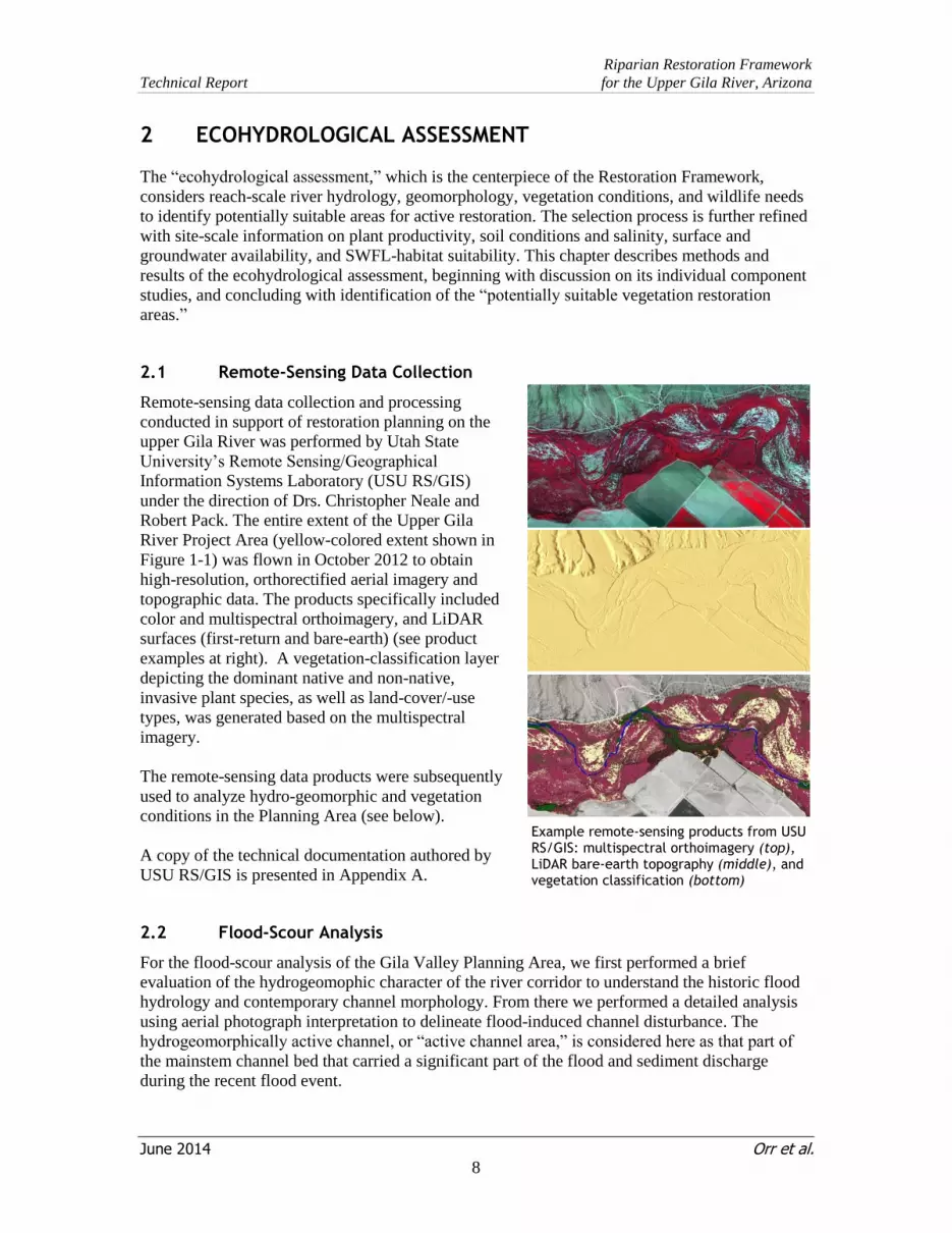
2.1 Remote-Sensing Data Collection
Remote-sensing data collection and processing
conducted in support of restoration planning on the
upper Gila River was performed by Utah State
University’s Remote Sensing/Geographical
Information Systems Laboratory (USU RS/GIS)
under the direction of Drs. Christopher Neale and
Robert Pack. The entire extent of the Upper Gila
River Project Area (yellow-colored extent shown in
Figure 1-1) was flown in October 2012 to obtain
high-resolution, orthorectified aerial imagery and
topographic data. The products specifically included
color and multispectral orthoimagery, and LiDAR
surfaces (first-return and bare-earth) (see product
examples at right). A vegetation-classification layer
depicting the dominant native and non-native,
invasive plant species, as well as land-cover/-use
types, was generated based on the multispectral
imagery.
The remote-sensing data products were subsequently
used to analyze hydro-geomorphic and vegetation
conditions in the Planning Area (see below).
A copy of the technical documentation authored by
USU RS/GIS is presented in Appendix A.
2.2 Flood-Scour Analysis
For the flood-scour analysis of the Gila Valley Planning Area, we first performed a brief
evaluation of the hydrogeomophic character of the river corridor to understand the historic flood
hydrology and contemporary channel morphology. From there we performed a detailed analysis
using aerial photograph interpretation to delineate flood-induced channel disturbance. The
hydrogeomorphically active channel, or “active channel area,” is considered here as that part of
the mainstem channel bed that carried a significant part of the flood and sediment discharge
during the recent flood event.
Example remote-sensing products from USU RS/GIS: multispectral orthoimagery (top), LiDAR bare-earth topography (middle), and vegetation classification (bottom)

Riparian Restoration Framework
Technical Report for the Upper Gila River, Arizona
June 2014 Orr et al. 9
2.2.1 Hydrogeomorphic characterization
Characterization of the upper Gila River’s hydrology and geomorphology, along with riparian
ecology, relied on review of available literature and remote sensing products, in addition to field
reconnaissance along much of the river. A key technical study utilized here was the U.S. Bureau
of Reclamation’s (BOR’s) Fluvial Geomorphology Study conducted in the early 2000s (e.g., BOR
2004). Other useful information sources included the U.S. Geological Survey’s (USGS’s) Gila
River Phreatophyte Project conducted in the early 1970s (e.g., Burkham 1970, 1972), along with
historic flow records held by the USGS and geologic maps published by the USGS and the
Arizona Geological Survey.
2.2.1.1 Hydrology
The arid climate in eastern Arizona is interrupted by periods of intense winter and late-summer
storms that often flood the mostly quiescent rivers and ephemeral tributaries. Streamflow data
from five long-term gaging stations along the mainstem upper Gila River and the lower San
Francisco River were obtained from the USGS’s National Water Information System website:
http://waterdata.usgs.gov/nwis. These spatially distributed stations provide a reliable
characterization of the river’s average daily flows, as well as its episodic hydrologic regime
responsible for driving the flood-scour processes and geomorphic expression that are a primary
subject of our ecohydrological assessment. Basic information for the five gages is summarized in
Table 2-1. The two lowermost gages listed here are located at approximately the upstream and
downstream ends of the Gila Valley and therefore best represent hydrologic conditions within the
Planning Area. Table 2-1. USGS discharge gaging stations on the upper Gila River used in the Ecohydrological
Assessment.
USGS gaging
station a
[upstream to
downstream]
Total period of
record in water
years b, c
Drainage
area d
Maximum peak
discharge
(cfs)
Mean daily
discharge
(cfs) (mi2) (km
2)
09432000 Gila
River below Blue
Creek, near
Virden, NM
1927–present 3,203 8,296 52,700
[Dec 19,1978] 210
09442000 Gila
River near Clifton,
AZ
1911–1917,
1928–1946,
1948–present
4,010 10,386 57,000
[Dec 19, 1978] 194
09444500 San
Francisco River at
Clifton, AZ
1891,
1905–1907,
1911–present
2,763 7,156 90,900
[Oct 2, 1983] 215
099448500 Gila
River at head of
Safford Valley,
near Solomon, AZ
1914–present 7,896 20,451 132,000
[Oct 2, 1983] 453
09466500 Gila
River at Calva, AZ
1916,
1930–present 11,470 29,707
150,000
[Oct 3, 1983] 363
Table footnotes continued on next page.
Riparian Restoration Framework
Technical Report for the Upper Gila River, Arizona
June 2014 Orr et al. 10
a Weblinks to source data: 1 http://waterdata.usgs.gov/nwis/inventory?agency_code=USGS&site_no=09432000 2 http://waterdata.usgs.gov/nwis/inventory?agency_code=USGS&site_no=09442000 3 http://waterdata.usgs.gov/nwis/inventory?agency_code=USGS&site_no=09444500 4 http://waterdata.usgs.gov/nwis/inventory?agency_code=USGS&site_no=09448500 5 http://waterdata.usgs.gov/nwis/inventory?agency_code=USGS&site_no=09466500
b Water year (WY) is the 12-month period from October 1 through September 30. c Period of records utilized in the flood-frequency and daily-duration analyses slightly differ from the total period of
record due to data gaps and/or unreliable historical data: 1 Flood-frequency analysis: Virden=WY 1927–2013; Clifton=WY 1911–1917, 1928–1946, 1948–2013; SF at
Clifton=WY 1911–2013; Solomon=1914–2013; and Calva=1930–2013. 2 Daily-duration analysis: Virden=July 1, 1927–Sept 30, 2013; Clifton=Nov 1, 1910–Sept 30, 2013; SF at
Clifton=Oct 23, 1910–Sept 30, 2013-09-30; Solomon=Oct 1, 1920–Sept 30, 2013; and Calva=Oct 1, 1929–Sept
30, 2013. d Drainage areas from USGS station information.
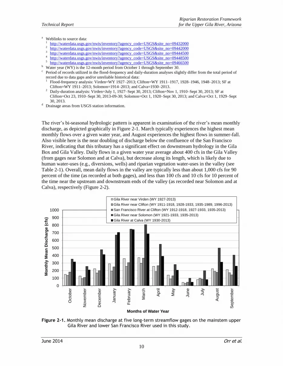
The river’s bi-seasonal hydrologic pattern is apparent in examination of the river’s mean monthly
discharge, as depicted graphically in Figure 2-1. March typically experiences the highest mean
monthly flows over a given water year, and August experiences the highest flows in summer-fall.
Also visible here is the near doubling of discharge below the confluence of the San Francisco
River, indicating that this tributary has a significant effect on downstream hydrology in the Gila
Box and Gila Valley. Daily flows in a given water year average about 400 cfs in the Gila Valley
(from gages near Solomon and at Calva), but decrease along its length, which is likely due to
human water-uses (e.g., diversions, wells) and riparian vegetation water-uses in the valley (see
Table 2-1). Overall, mean daily flows in the valley are typically less than about 1,000 cfs for 90
percent of the time (as recorded at both gages), and less than 100 cfs and 10 cfs for 10 percent of
the time near the upstream and downstream ends of the valley (as recorded near Solomon and at
Calva), respectively (Figure 2-2).
Figure 2-1. Monthly mean discharge at five long-term streamflow gages on the mainstem upper Gila River and lower San Francisco River used in this study.
0
100
200
300
400
500
600
700
800
900
1000
Octo
ber
Novem
ber
Decem
ber
January
Febru
ary
Marc
h
April
May
Ju
ne
July
August
Septe
mber
Mo
nth
ly M
ean
Dis
ch
arg
e (
cfs
)
Months of Water Year
Gila River near Virden (WY 1927-2013)
Gila River near Clifton (WY 1911-1918, 1928-1933, 1935-1989, 1996-2013)
San Francisco River at Clifton (WY 1912-1918, 1927-1933, 1935-2013)
Gila River near Solomon (WY 1921-1933, 1935-2013)
Gila River at Calva (WY 1930-2013)

Riparian Restoration Framework
Technical Report for the Upper Gila River, Arizona
June 2014 Orr et al. 11
a)
b)
Figure 2-2. Mean daily flow duration curves and statistics for the five long-term streamflow gages on the mainstem upper Gila River and lower San Francisco River used in this study.
1
10
100
1000
10000
100000
0.1 1.0 10.0 100.0
Dail
y M
ean
Dis
ch
arg
e (
cfs
)
Exceedance Probability (%)[Percent of time indicated discharge was equaled or exceeded]
Gila River near Virden (WY 1927-2013)
Gila River near Clifton (WY 1911-1918, 1928-1933, 1935-1989, 1996-2013)
San Francisco River at Clifton (WY 1912-1918, 1927-1933, 1935-2013)
Gila River near Solomon (WY 1921-1933, 1935-2013)
Gila River at Calva (WY 1930-2013)
Gila River
near
Virden
Gila River
near Clifton
SF River at
Clifton
Gila River
near
Solomon
Gila River
at Calva
1927–2013
1911–1917,
1928–1946,
1948–2013
1911–2013 1914–2013 1930–2013
30,986 30,955 33,016 33,391 30,680
209.91 194.41 215.45 452.54 362.75
584.7 526.0 767.8 1,422.5 1,601.0
1.0 3.7 5.6 13.0 0
100% 1 4 6 13 0
90% 23 19 34 63 3
80% 44 29 45 91 12
70% 63 42 54 118 26
60% 78 60 63 145 44
50% 92 77 74 175 70
40% 110 100 95 212 115
30% 145 134 129 289 188
20% 218 207 203 454 333
10% 435 416 415 954 761
5% 756 759 771 1,710 1,580
1% 1,890 1,880 2,108 4,100 4,160
0.1% 7,540 6,243 9,329 17,061 17,532
0.01% 33,100 27,100 52,200 90,000 90,000
33,100 27,100 52,200 90,000 90,000
Stream Gage Location
Exceedance
Probability
(%)
Flow
(cfs)
Maximum
Number of Samples
Mean
Std. Dev.
Minimum
Parameter
Water Years

Riparian Restoration Framework
Technical Report for the Upper Gila River, Arizona
June 2014 Orr et al. 12
Annual peak flows in the Gila Valley can be characterized as “flashy”: they are massive in
comparison with the mean daily flows (e.g., 453 cfs versus 132,000 cfs [see Table 2-1]), but
usually span only a few hours to days. The 10 largest floods recorded to date in the valley
occurred in water years (WY) 1915, 1916, 1917, 1973, 1979, 1984, 1985, 1993, 1995, and 2005,
based on gage data from the Solomon and Calva stations. A graphical plot of peak discharge
measured at the five gages is presented below as Figure 2-3, which was used to help select the
three most recent flood-scour events for the ecohydrological assessment. These records highlight
the flood period initially observed in the early 20th century, a relatively quiescent 50-year period
up through the mid-1960s, and a 40-year period of larger, more frequent flood events since the
late 1960s.
Figure 2-3. Historical flood peaks through water year 2013 at five long-term streamflow gages on the mainstem upper Gila River and lower San Francisco River used in the Ecohydrological Assessment. Flood-scour mapping focused on three of the most recent large flood peaks, as indicated with blue circles.
While the data shown in Figure 2-3 suggest that the recent large-flood period has been waning in
absolute magnitude since the 1990s, it should be cautioned that the potential for channel-scouring
floods to occur in the near-future remains high in any given water year. To further characterize
the river’s flood hydrology for this assessment, we calculated the flood recurrence intervals at the
five gages using available data through water year (WY) 2013 (Figure 2-4). The flood-frequency
analysis (Log-Pearson III) was performed using the Natural Resources Conservation Service’s
(NRCS’s) Frequency Curve Determination spreadsheet tool (NRCS 2012). These data
individually provide a statistical basis of flood-level prediction for a given recurrence interval
-
500
1,000
1,500
2,000
2,500
3,000
3,500
4,000
4,500
0
20,000
40,000
60,000
80,000
100,000
120,000
140,000
160,000
1900
1905
1910
1915
1920
1925
1930
1935
1940
1945
1950
1955
1960
1965
1970
1975
1980
1985
1990
1995
2000
2005
2010
Dis
ch
arg
e (
cm
s)
Dis
ch
arg
e (
cfs
)
Date
USGS 09432000 Gila River near Virden, NMUSGS 09442000 Gila River near Clifton, AZUSGS 09444500 San Francisco River near Clifton, AZUSGS 09448500 Gila River near Solomon, AZUSGS 09466500 Gila River at Calva, AZ
Mapped floods
Quiescent Period Large Flood Period
Historic Flood Period
Riparian Restoration Framework
Technical Report for the Upper Gila River, Arizona
June 2014 Orr et al. 13
(RI) at each gaging station. The data can in turn be used to determine the RI-value per flood
event, such as those considered in our study. Our computed values are similar to those previously
computed for the BOR’s fluvial geomorphology study (BOR 2001a), which provides an added
level of confidence when using these updated values for restoration planning purposes.
Differences between the BOR and our updated RI values are chiefly due to differences in the
analyzed time periods. The Calva gage data best represents the largest flood events experienced
near the downstream end of the Gila Valley:
October 3, 1983: 150,000 cfs RI≈101 yrs
January 20, 1993: 109,000 cfs RI≈57 yrs
December 19, 1978: 100,000 cfs RI≈51 yrs
October 20, 1972: 80,000 cfs RI≈35 yrs
January 6, 1995: 64,500 cfs RI≈25 yrs
December 29, 1984: 53,700 cfs RI≈19 yrs
March 3, 1991: 46,400 cfs RI≈15 yrs
February 14, 2005: 40,100 cfs RI≈12 yrs
a)
b)
(Figure 2-4 is continued on next page.)
100
200
300
400500600
8001000
2000
3000
400050006000
800010000
20000
30000
400005000060000
80000100000
99.99
7.090
99.8 99 98 95 90 80 70 60 50 40 30 20 10 5 2 1 .5 .2 .1 .05 .01
Dis
ch
arg
e (
cfs
)
exceedance probability
Return Period (years)
recurrence interval = 100/probability
100 5005020102
plot position: Weibull
Return Period
(years)
Discharge
(cfs)
1.2 1,800
1.5 3,400
2 5,300
5 12,000
10 17,800
50 34,100
100 42,400
500 64,300
1000 74,900
[WY 1927–2013]
USGS 09432000 GILA
RIVER BELOW BLUE
CREEK, NEAR VIRDEN, NM
100
200
300
400500600
8001000
2000
3000
400050006000
800010000
20000
30000
400005000060000
80000100000
99.99
7.090
99.8 99 98 95 90 80 70 60 50 40 30 20 10 5 2 1 .5 .2 .1 .05 .01
Dis
ch
arg
e (
cfs
)
exceedance probability
GILA RIVER NEAR CLIFTON, AZ
recurrence interval = 100/probability
100 5005020102
plot position: Weibull
Return Period
(years)
Discharge
(cfs)
1.2 2,300
1.5 3,800
2 5,700
5 12,100
10 17,900
50 35,400
100 45,000
500 72,900
1000 87,700
[WY 1911–1917,
1928–1946, 1948–2013]
USGS 09442000 GILA
RIVER NEAR CLIFTON, AZ

Riparian Restoration Framework
Technical Report for the Upper Gila River, Arizona
June 2014 Orr et al. 14
c)
d)
e)
Figure 2-4. Flood frequency [Log-Pearson III] for the five long-term streamflow gages used in the Ecohydrological Assessment, including (from upstream to downstream): Gila River near Virden (a), Gila River near Clifton (b), San Francisco River near Clifton (c), Gila River near Solomon (d), and Gila River at Calva (e).
100
200
300400500600800
1000
2000
30004000500060008000
10000
20000
3000040000500006000080000
100000
200000
300000400000500000600000800000
1000000
99.99
7.090
99.8 99 98 95 90 80 70 60 50 40 30 20 10 5 2 1 .5 .2 .1 .05 .01
Dis
ch
arg
e (
cfs
)
exceedance probability
SAN FRANCISCO RIVER AT CLIFTON, AZ
recurrence interval = 100/probability
100 5005020102
plot position: Weibull
Return Period
(years)
Discharge
(cfs)
1.2 1,800
1.5 3,600
2 6,000
5 16,100
10 26,600
50 63,600
100 86,000
500 157,400
1000 198,000
[WY 1911–2013]
USGS 09444500 SAN
FRANCISCO RIVER AT
CLIFTON, AZ
100
200
300400500600800
1000
2000
30004000500060008000
10000
20000
3000040000500006000080000
100000
200000
300000400000500000600000800000
1000000
99.99
7.090
99.8 99 98 95 90 80 70 60 50 40 30 20 10 5 2 1 .5 .2 .1 .05 .01
Dis
ch
arg
e (
cfs
)
exceedance probability
GILA RIVER AT HEAD OF SAFFORD VALLEY, NR SOLOMON, AZ
recurrence interval = 100/probability
100 5005020102
plot position: Weibull
Return Period
(years)
Discharge
(cfs)
1.2 3,100
1.5 5,700
2 9,200
5 23,700
10 38,900
50 92,600
100 125,800
500 234,300
1000 297,600
USGS 09448500 GILA
RIVER AT HEAD OF
SAFFORD VALLEY, NR
SOLOMON, AZ
[WY 1914–2013]
Return Period
(years)
Discharge
(cfs)
1.2 1,800
1.5 3,500
2 5,900
5 17,900
10 32,700
50 99,300
100 149,100
500 347,800
1000 485,800
USGS 09466500 GILA
RIVER AT CALVA, AZ
[WY 1930–2013]
100
200
300400500600800
1000
2000
30004000500060008000
10000
20000
3000040000500006000080000
100000
200000
300000400000500000600000800000
1000000
99.99 99.8 99 98 95 90 80 70 60 50 40 30 20 10 5 2 1 .5 .2 .1 .05 .01
Dis
ch
arg
e (
cfs
)
Annual Exceedance Probability (%)
GILA RIVER AT CALVA, AZ
recurrence interval = 100/probability
100 5005020102
plot position: Weibull
Riparian Restoration Framework
Technical Report for the Upper Gila River, Arizona
June 2014 Orr et al. 15
In summary, the upper Gila River naturally experiences a wide variation of flows, punctuated
episodically by short-duration but intensive high-flow events. These flashy discharge dynamics,
which are common to large, dryland riverine systems, periodically result in dramatic geomorphic
change (Graf 1988). And while climate change models predict less total precipitation for the
southwest region, increased frequency of intense storms and more precipitation falling as rain
versus snow are expected to make southwest rivers more susceptible to flooding (USGCRP
2009). Thus, any restoration planning effort on the upper Gila River demands consideration of
flood dynamics to best ensure long-term success.
2.2.1.2 Sub-reach delineation
The hydrogeomorphic character of the river varies widely along its entire run, but is essentially a
broad, low-gradient (0.18%), braided system in the Gila Valley where it also retains much of its
historic floodplain within which to laterally adjust in response to large runoff events. There are,
however, reach-level differences in channel morphology that strongly influence the types of
management and restoration actions that may be suitably applied. For example, the active channel
is broader in the upper end of the valley than it is downstream of Safford, where the channel
becomes progressively narrower (and more densely vegetated).
To assist our ecohydrological assessment, we sub-
divided the river channel into discrete,
hydrogeomorphically similar reaches based on
dominant physical characteristics. Our reach
locations are shown in Figure 2-5, and their salient
attributes are summarized in Table 2-2. The
designated reaches covered the entire river length
in the valley beginning at the San Carlos Reservoir
and continuing upstream to the Gila Box. We
elected to include the river portions downstream of
the current Planning Area to allow consistency in
reach delineation and numbering starting from a
logical downstream location: Coolidge Dam. This
is the first continuous reach delineation in the Gila
Valley; the aforementioned USGS Gila River
Phreatophyte Project (e.g., Burkham 1970, 1972)
and BOR (2004) Fluvial Geomorphology Study
each developed their own reach designations, but
these were limited to isolated river segments.
Within the Planning Area, the river is generally a
vegetated, low-gradient, braided river corridor
bordered by a broad floodplain supporting crop
cultivation and some urban developments. The
corridor generally ranges in width from 1,000 to
4,600 ft (300–1,400 m), and typically narrows
where it encounters mountain-front cliffs and
coalesced alluvial fans (bajadas). Along its course
through the valley, the corridor transitions from a
canyon-confined, coarse- grained (gravel/cobble-
bedded) channel with limited floodplain and some
Downstream views in the Planning Area: mouth of Gila Box in reach 3a (top); near Safford in reach 2g (middle); and near Eden in reach 2d (bottom) (Photos by Stillwater Sciences)
Riparian Restoration Framework
Technical Report for the Upper Gila River, Arizona
June 2014 Orr et al. 16
native riparian forest (cottonwood-willow galleries) at the mouth of the Gila Box (reach 3a), to a
wide, drier, braided/ meandering channel with sparse to moderately dense riparian vegetation
(mostly tamarisk) bordered by a broad, cultivated and developed floodplain near Safford (reaches
2f–2j), and finally to a moister, fine-grained, braided/ meandering channel system composed of a
narrow single-thread channel during lower flows that is encroached upon by dense riparian
vegetation (mostly tamarisk), which is in turn bordered by a broad, cultivated floodplain with few
developments downstream of Pima (reaches 2c–2e) (see photos insert above). During high-flow
events, side-channels also convey flow giving a more pronounced braided appearance to the river
corridor. The entire corridor and some portion of its floodplain become inundated during the
largest floods.
The natural flow and sediment-transport regime is also strongly influenced by the presence of in-
channel irrigation diversions, bridge crossings, and agricultural levees. A total of 6 irrigation
canal diversion dams span at least part of the river corridor in the Planning Area (listed from
upstream to downstream): Brown, San Jose, Graham, Smithville, Curtis, and Ft. Thomas.
Additionally, there are 6 bridge crossings (listed from upstream to downstream): East Sanchez
Road, North 8th Avenue, North Reay Lane, Bryce Road, Bryce-Eden Road, and River Road. The
BOR’s (2004a) Fluvial Geomorphology Study mapped numerous occurrences of historic and
existing levees and pilot channels, all of which appear to have been constructed in response to
flooding.

Riparian Restoration Framework
Technical Report for the Upper Gila River, Arizona
June 2014 Orr et al. 17
Figure 2-5. Location of hydrogeomorphic reaches delineated along the upper Gila River in the Gila Valley for the Ecohydrological Assessment. See Table 2-2 for descriptions of reach attributes.
Riparian Restoration Framework
Technical Report for the Upper Gila River, Arizona
June 2014 Orr et al. 18
Table 2-2. Description of hydrogeomorphic reaches delineated along the upper Gila River in the Gila Valley for the Ecohydrological Assessment. See Figure 2-5 for locations of sub-reaches.
Reach
group
Sub-reach
number
Sub-reach
name
Sub-reach
end feature
(upstream limit)
Sub-reach length a
Sub-reach description b
(mi) (km)
San Carlos
Reservoir
San
Car
los
Ap
ach
e R
eser
vat
ion
1a Main Reservoir
San Carlos River
(drowned)
confluence
8.0 12.9 Reservoir-drowned, lowermost reach of upper Gila River between Coolidge Dam and San Carlos River confluence (near Graham-Gila county line); fed
by short washes and alluvial fans from mountain ridges and cliffs along both sides (north and south sides)
1b Reservoir
Backwater
Bone Spring Canyon
confluence
(at railway bridge)
15.7 25.3 Narrow, single-thread river channel meandering through a broad, very densely vegetated (tamarisk) floodplain fed by short washes and alluvial fans along
both sides (north and south sides); no agriculture within hydraulic backwater zone of San Carlos Reservoir
Gila Valley
2a Calva Highway 70 bridge 7.0 11.3 Densely vegetated (tamarisk), braided river corridor with a dominant single-thread river channel meandering through a broad floodplain fed by short
washes and alluvial fans on both sides; cultivated fields limited to upstream end on right-bank (north) side
2b Bylas
Eastern boundary of
San Carlos Apache
Reservation
8.6 13.8
Densely vegetated (tamarisk), braided river corridor with a dominant single-thread river channel meandering through a broad floodplain bordered by Gila
Mountains' bajadas on right-bank (east) side and some cultivated fields and town of Bylas on left-bank (west) side; Salt Creek feeds into reach on right-
bank side across from Bylas
Res
tora
tio
n P
lan
nin
g A
rea
2c Ft. Thomas
Hot Springs-Wide
Hallow-Spring Creek
channeled
confluence
17.1 27.5
Well vegetated (mostly tamarisk), braided river corridor with a dominant single-thread river channel (with some agricultural levees) meandering through
a broad floodplain bordered by Gila Mountains’ bajadas and some narrow, disconnected floodplain areas on right-bank (east) side and cultivated fields
and town of Ft. Thomas on left-bank (west) side; Goodwin and Black Rock washes drain Pinaleno Mountains feeding into reach on left-bank side near Ft.
Thomas
2d Eden Ft. Thomas Canal
Diversion Dam 3.9 6.3
Narrow single-thread, well vegetated (mostly tamarisk) river corridor constricted by agricultural levees and bordered by broad, densely cultivated
floodplain along both sides; hydrology also influenced at upstream end by Ft. Thomas Canal Diversion Dam (near natural valley constriction at Markham
Wash confluence on right-bank [north] side and Underwood Wash confluence on left-bank [south] side)
2e Bryce Curtis Canal
Diversion Dam 5.1 8.2
Braided river corridor with dominant single-thread river channel meandering through well vegetated riparian forest (mostly tamarisk) bordered by some
agricultural levees and broad, densely cultivated floodplain on both sides; receives irrigation runoff via drainage ditches; downstream end at valley
constriction near Markham and Underwood washes; hydrology also influenced at upstream end by Curtis Canal Diversion Dam (near Peck Wash on right-
bank [north] Cottonwood Wash and town of Pima on left-bank [south] side)
2f Pima Smithville Canal
Diversion Dam 7.5 12.1
Moderately vegetated, braided river corridor bordered by some agricultural levees and broad, densely cultivated floodplain on both sides and urban
centers of Pima, Central, and Thatcher on left-bank (west) side; receives irrigation runoff via drainage ditches and channelized tributary confluences (e.g.,
Ash Creek draining Mt. Graham); hydrology also influenced at upstream end by Smithville Canal Diversion Dam (near town of Thatcher)
2g Safford Graham Canal
Diversion Dam 3.6 5.8
Moderately vegetated, braided river corridor with dominant single-thread river channel bordered by some agricultural levees and broad, densely cultivated
floodplain on both sides and urban centers of Thatcher and Safford on left-bank (southwest) side; receives irrigation and urban runoff via drainage ditches
and channelized tributary confluences; hydrology also influenced at upstream end by Graham Canal Diversion Dam (near Stockton Wash draining Mt.
Graham)
2h East Safford San Simon River
confluence 2.8 4.5
Moderately vegetated, braided river corridor with dominant single-thread river channel bordered by upland terrace at base of Gila Mountains on right-
bank (north) side and densely cultivated floodplain and urban developments between Safford and Solomon on left-bank (south) side; receives irrigation
and urban runoff via drainage ditches and channelized tributary confluences; hydrology also influenced by San Simon River confluence at upstream
end—largest tributary in the Gila Valley
2i Solomon San Jose Canal
Diversion Dam 8.2 13.2
Sparsely vegetated, coarse-grained, braided river corridor with dominant single-thread river channel bordered by broad, mostly continuous, densely
cultivated floodplain on both sides; valley narrows in upstream direction toward transition with Gila Box; receives modest ir rigation and tributary runoff;
hydrology also influenced by San Jose Canal Diversion Dam at upstream end
2j Earven Flat
Brown Canal
Diversion Dam at
Gila Box mouth
3.1 5.0
Upstream extent of Gila Valley: sparsely vegetated, coarse-grained, mostly braided river corridor with dominant single-thread river channel narrowly
bordered by cultivated floodplain on right-bank (north) side and short washes and alluvial fans on left-bank (south) side; hydrology also influenced by
Brown Canal Diversion Dam
Gila Box 3a Lower Box Bonita Creek
confluence 3.4 5.5
Downstream end of Gila Box: moderately vegetated (cottonwood-willow gallery forests), confined river corridor meandering through sinuous canyon
bottom bordered by short washes and alluvial fans draining arid uplands
a Sub-reach length measured in a GIS along a digitized interpretation of the low-flow channel pathway visible in 2011 aerial imagery. b Names of physical features from USGS topographical quadrangle maps.
Riparian Restoration Framework
Technical Report for the Upper Gila River, Arizona
June 2014 Orr et al. 19
2.2.2 Aerial imagery analysis
Historical aerial imagery was utilized in a geographic information system (GIS; ESRI ArcGIS 10)
to delineate areas of flood disturbance for selected historical floods along the upper Gila River in
the Planning Area. Three of the most recent, large flood events were selected: 1983, 1993, and
2005. Also utilized, although not mapped here, were the remote-sensing products generated in
support of this project by USU RS/GIS based on the flight made in October 2012 of the entire
Upper Gila River Project Area (see Section 2.1: Remote-Sensing Data Collection above and
Appendix A). Many aspects of our flood-scour analysis were modeled on similar work done by
Graf (2000), Tiegs et al. (2005), and Tiegs and Pohl (2005). Details of the methods employed
here and the mapping products are summarized in Appendix B.
For purposes of aerial-photographic interpretation, the flood-scour areas were defined as follows:
High disturbance: These areas were characterized by distinct channel and floodplain areas
severely disturbed by flow (i.e., scoured to bare substrate), typically with 10% or less apparent
remaining riparian vegetative cover.
Medium disturbance: These areas were characterized by distinct areas of low to moderate
apparent disturbance by flow, typically defined as areas with more than 10% but less than 80%
apparent riparian vegetative cover.
Low disturbance (riparian vegetation): These areas were characterized by distinct zones of
apparently natural riparian vegetation with little to no apparent disturbance by flood, typically
containing more than 80% riparian vegetation.
All flood-scour areas were then classified as being either within or outside of the “active
channel,” with the active channel defined as areas of medium to high disturbance. Areas of
riparian or non-riparian vegetation with no apparent disturbance were excluded.
2.2.3 Results of flood-scour analysis
The results of our flood-scour analysis are presented graphically in two sets of maps: “Areal
extent of active channel in successive floods” and “Frequency of active channel position” (see
Appendix B). The first set of maps represents the active-channel areas during the 1983, 1993,
and 2005 flood events. The second set of maps highlight those channel areas most frequently
disturbed by repeat flood events.
The flood-scour analysis reveals that the low-flow channel position changes rapidly and
completely during flood events according to the magnitude of the event and other factors,
whereas the boundary of the broader active-channel area changes less frequently. Also revealed is
that the >66% frequency flood-scour area decreases in the downstream direction, which is
primarily a reflection of the scour patterns of the 2005 flood event that were concentrated in the
upper half of the Planning Area. Thus, the flood-scour extent is generally greater above Pima,
and lower below.
The “Flood Reset Zone” was then identified to inform restoration area suitability as part of the
ecohydrological assessment—suitable restoration areas are considered to be found safely outside
of the Flood Reset Zone (see Section 2.6 Potentially Suitable Vegetation Restoration Areas
below). This zone includes areas having both 100% flood-scour frequency (i.e., scoured in 3 out
Riparian Restoration Framework
Technical Report for the Upper Gila River, Arizona
June 2014 Orr et al. 20
of the 3 mapped events [1983, 1993, and 2005]) and “high” flood-disturbance activity—areas
severely disturbed by flow, typically scoured to bare substrate retaining <10% apparent riparian
vegetative cover—during the most recent flood of 2005. The size of the Flood Reset Zone
progressively decreases in the downstream direction below the Gila Box (i.e., reaches 2c–2j),
where it accounts for over 80% of the riparian corridor near the upstream end of the Planning
Area (reach 2j) and only about 20% near the downstream end (reach 2c) (see Section 2.3 for
explanation of characterizing vegetation within the riparian corridor).
The maps presented in Appendix B are meant to guide restoration planning and implementation at
multiple scales, ranging from restoration strategy development at the full river corridor and reach
levels to site-specific restoration design and implementation. However, the maps are only one
tool and need to be combined with a variety of other information to develop the most effective
and efficient strategies and designs for riparian restoration, such as riparian vegetation
classification (see below). In particular, more detailed field-based information and geomorphic
interpretation may be warranted to refine the fine-scale delineation of the Flood Reset Zone and
predictions of likely future flood paths when designing and implementing site-specific plans for
invasive species removal and revegetation of native riparian species.
2.3 Riparian Vegetation Characterization
Here we describe methods and results of our effort to characterize riparian vegetation
composition and distribution patterns in the Planning Area, and to better understand the
relationships between vegetation and physical conditions in the riparian corridor. The primary
goal of the vegetation characterization was to inform the selection of suitable restoration areas
based on the understanding of the physical conditions that do, and could, support the
establishment and growth of native riparian trees and shrubs. A secondary objective of the effort
was to review the remotely-sensed datasets produced by USU RS/GIS for the Restoration
Framework.
2.3.1 Plot surveys and remote sensing methods
To characterize riparian vegetation patterns in the Planning Area, we collected vegetation
composition and physical condition data for over 80 plots spread across 20 transects (Figure 2-6,
Appendix C). We first reviewed aerial photography, flood-scouring mapping, hydrogeomorphic
reach boundaries, relative elevation data, available vegetation data, and USU RS/GIS’s
vegetation-classification map to select transects that represented the variety of hydrogeomorphic
and vegetation conditions in the Planning Area. The available vegetation data included a
vegetation-communities map prepared by SRP for their Ft. Thomas Preserve properties and
vegetation plot data collected by UCSB in support of developing monitoring protocols for the
Restoration Framework.
Transects spanned the entire width of the active channel, ranging in length from 1,000 to 4,600 ft
(300 to 1,400 m), and were positioned to overlap with as much existing native vegetation as
possible. Each transect was visited in early November 2013, after obtaining permission to access
the mix of private and publically owned parcels in which selected transects were located, by a
two-person field crew with knowledge of the plant species of the Gila River Valley and Sonoran
Desert. In the field, and using aerial photographs and field maps of relative elevation and USU
RS/GIS’s vegetation map, the field crew identified distinct bands of vegetation and relative
elevation across each transect and collected data at plots in as many of those distinct bands as
possible.

Riparian Restoration Framework
Technical Report for the Upper Gila River, Arizona
June 2014 Orr et al. 21
The number of plots sampled across each transect ranged from 3 to 6, depending on vegetation
complexity, topographic complexity, and plot accessibility. Plots varied in size based on the
stature of the vegetation and the area visible to the field crew, but were typically 400 m2 (20 x 20
m). At each plot, a geotagged photograph was taken to both record the location of the plot and
document plot conditions, and the following data was recorded:
Estimated time since last flooded: <1, 1–2, 3–5, 6–10, or >10 years
Soil texture: gravel, silt, loam, clay, sand
Topography: convex, flat, concave, undulating
Percent ground cover of: water, vegetation, organic debris, cobble/boulder, gravel, and
fine sediments
Evidence of: flooding, fire, soil moisture, and agricultural return flows
Types and intensities of unnatural disturbances: competition from nonnative invasive
species, off-road vehicle use, and bulldozing/earth moving
Vegetation-type dominance: trees, shrubs, or forbs
Tree, shrub, and herb phenology: early, peak, or late
Species: name, age (e.g., seedling, mature, decadent), and percent cover of all prevalent
plants
Vegetation type: name and vegetation type name of any adjacent, un-sampled vegetation
Before leaving each transect, the field crew delineated the boundaries of the various vegetation
types encountered across the transect. Back in the office, the relative elevation, canopy height,
our flood frequency, USU RS/GIS’s vegetation type, and NRCS’s soil type of each plot were
queried in GIS and appended to the field-collected data in a Microsoft Excel spreadsheet. The
frequency at which several native species occur in different elevation zones above the stream
channel (referred to as relative elevation) was plotted. All plot data, whether collected in the field
or derived in GIS, are tabulated in Appendix C.
2.3.2 Vegetation types and distribution patterns
The following sections describe the primary vegetation types in the Planning Area, as
documented during the transect surveys, and the major cross-sectional and longitudinal patterns
in their distribution in the Planning Area. The vegetation types correspond to either the group or
alliance level of the U.S. National Vegetation Classification (NVC) system (http://usnvc.org/).
For readers unfamiliar with species’ scientific names and/or NVC classification terminology, we
have used the common name and typical structure of the dominant species to name each
vegetation type. To facilitate comparison and coordination with the NVC, however, we also
provide the NVC association and/or group name in the description.
During the plot surveys, distinct patterns in the cross-sectional distribution of vegetation types
were observed, and a representative example is illustrated in Figure 2-7. There are, however,
variations in this cross-sectional distribution and in the composition of vegetation types
depending on their location along the river. Three transects were located upstream of the San Jose
Diversion Dam, in hydrogeomorphic reaches 2j and 3a (see Figure 2-6). These reaches are the
narrowest in the Planning Area with a large proportion of the floodplain affected by flood scour
(see Figures B-2.1 through B-2.10 in Appendix B), have little to no adjacent agriculture, and are
subjected to the least consumptive water use, which together help explain much of the difference

Riparian Restoration Framework
Technical Report for the Upper Gila River, Arizona
June 2014 Orr et al. 22
in vegetation patterns observed in these reaches. Seven transects were located within the drier
reaches between the San Jose Diversion Dam and the town of Pima (reaches 2f through 2i).
Because they are immediately downstream of the San Jose Diversion Dam, with less opportunity
for tributary contributions or agricultural return flows, riparian vegetation in these reaches
appears to be the most negatively affected by water diversion. These reaches are also subject to
significant amounts of flood scour (see Figures B-2.1 through B-2.10 in Appendix B). Ten
transects were located downstream of Pima, in reaches 2c through 2e, where the river corridor
supports a much more dense riparian cover benefiting from agricultural return flows and reduced
flood scour in portions of the floodplain compared to upstream reaches, although that vegetation
is overwhelmingly dominated by tamarisk. The cross-sectional illustration in Figure 2-7 is based
on transect 19, which was one of the transects located downstream of Pima (see Figure 2-6,
Appendix C). The influence of reach characteristics on vegetation-type composition and
distribution is described in greater detail below.
Riparian Restoration Framework
Technical Report for the Upper Gila River, Arizona
June 2014 Orr et al. 23
Figure 2-6. Map of vegetation transects along the upper Gila River within the Restoration Planning Area.

Riparian Restoration Framework
Technical Report for the Upper Gila River, Arizona
June 2014 Orr et al. 24
Figure 2-7. Illustration of the typical cross-sectional distribution of vegetation in the Gila Valley Planning Area downstream of Pima.

Riparian Restoration Framework
Technical Report for the Upper Gila River, Arizona
June 2014 Orr et al. 25
2.3.2.1 Tamarisk semi-natural shrubland/Tamarisk-mixed riparian shrubland
The most common vegetation types in the Planning
Area are tamarisk-dominated shrublands and, as
shown in Figure 2-7 (specifically the 3–5 m
relative elevation band on river left), are found
under a relatively wide range of conditions and are
generally the most widely distributed vegetation
types across a typical channel cross-section.
“Tamarisk semi-natural shrublands” refer to areas
where tamarisk is very nearly the only species
present (see photo inserts at right), while
“tamarisk-mixed riparian shrublands” include areas
where tamarisk is still the dominant species, but
Fremont cottonwood (Populus fremontii),
Goodding’s willow (Salix gooddingii), narrowleaf
willow (S. exigua) (also known as coyote willow),
mulefat (Baccharis salicifolia), desert broom (B.
sarothroides), Emory’s baccharis (B. emoryi),
and/or mesquite (Prosopis glandulosa and/or P.
velutina) occasionally occur at very low cover.
Vegetation density can range widely, from nearly
continuous to only 10% tamarisk cover, and
canopy heights are typically no more than 16 ft (5
m). Native species face extreme competitive
pressure in these tamarisk dominated stands and
woody material from dead cottonwoods and
willows is often present. The herbaceous layer in
tamarisk-dominated shrublands is low in floristic
diversity, comprised mostly of a sparse cover of
bermudagrass (Cynodon dactylon) or johnsongrass
(Sorghum halepense). Tamarisk-dominated
shrublands typically occur on silty substrates, but
may also be found on sand and gravel. Soil
moisture conditions in these vegetation types can
vary from wet to dry, depending on the proximity
to the river, relative elevation from the low-flow
channel, time since last rain or flood, and
agricultural return flows. Tamarisk-dominated
shrublands can tolerate a wide variety of flood and scour frequencies, and are found from stream
banks to more mesic upland areas. Tamarisk semi-natural shrubland and tamarisk-mixed riparian
shrubland correspond most closely to the NVC’s Tamarix spp. Temporarily Flooded Semi-natural
Shrubland alliance in the Southwest North American Ruderal Riparian Scrub Group.
Downstream of Pima, tamarisk-dominated shrublands are typically continuous to moderately
dense tamarisk shrubs, with occasional Fremont cottonwood and Goodding’s willow trees, and a
sparse to absent understory (see Figure 2-7 and photo inserts above). Tamarisk is highly
flammable and has fueled a number of fires in the riparian corridor of the Planning Area. In areas
burned by the Clay Fire in March 2013 near Fort Thomas, nearly all of the tamarisk biomass was
burned away—only the main trunks and branches remain, as illustrated in Figure 2-7—and there
Dense, tall tamarisk semi-natural shrubland downstream of Pima (top), dead and dying tamarisk between San Jose Diversion Dam and Pima (middle), and burnt tamarisk with vigorous re-sprouting near Ft. Thomas
(bottom) (Photos by Stillwater Sciences)

Riparian Restoration Framework
Technical Report for the Upper Gila River, Arizona
June 2014 Orr et al. 26
is typically a bit more understory vegetation, as would be expected with less shading by tamarisk.
Nearly all burnt tamarisk trees were observed to be re-sprouting vigorously from the base (see
photo insert above), indicating there is only a fairly limited window of opportunity to establish
native species before tamarisk biomass once again dominates the site. Between the San Jose
Diversion Dam and Pima, tamarisk-dominated shrublands are typically much less dense and tall,
and much of the tamarisk appears to be stressed or even dying. Upstream of the San Jose
Diversion Dam, this zone is much narrower and typically with a higher proportion of native
shrubs and trees.
2.3.2.2 Fremont cottonwood-Gooding’s willow woodland
The “Fremont cottonwood-Goodding’s willow woodland” vegetation types typically have
Fremont cottonwood and/or Goodding’s willow trees present at 20–60% cover each, which form
a dense, high canopy 15–30 ft (4.5–10 m) tall (see photos insert below). In the Planning Area,
most Fremont cottonwood and Goodding’s willow trees are mature or decadent appearing to have
been established soon after the 1993 flood event, and there appears to be very little to no recent
natural recruitment of either species. Tamarisk, and less often mesquite, dominates the sub-
canopy. Emory’s baccharis, mulefat, and/or desert broom typically occur in the shrub layer at 10–
60% cover. Bulrush (Schoenoplectus spp.) may occur in low-laying swales where water can pond
within these vegetation types, while common reed (Phragmites australis), arundo (Arundo
donax), and bermudagrass may occur where these vegetation types are adjacent to the river
channel. In general, however, the herbaceous layer is very sparse to absent and the ground layer
has a moderate cover of downed wood and other organic litter. Fremont cottonwood-Goodding’s
willow woodland typically occurs where substrates are silty or sandy, and generally dry, and at
elevations where they are frequently inundated by lower velocity floods but are not subject to
intense scouring. This vegetation type corresponds to the NVC’s Populus fremontii-Salix
gooddingii Woodland alliance in the Sonoran-Chihuahuan Warm Desert Riparian Scrub Group.
Fremont cottonwood-Goodding’s
willow woodland is not illustrated
in Figure 2-7 because areas with
sufficient cover of these native tree
species to be classified separately
from tamarisk-mixed riparian
shrubland are relatively uncommon.
They occur most frequently
downstream of Pima, typically
along the outer margin of the
riparian corridor and the banks of
abandoned and/or high flow
channels, and upstream of the San
Jose Diversion Dam in the Gila
Box, typically near the river
channel or along the outer margin
of high-flow floodplains. Fremont
cottonwood-Goodding’s willow
woodland is nearly entirely absent in the reach between the San Jose Diversion Dam and Pima.
Fremont cottonwood and Goodding’s willow trees were documented in 29 and 20 plots,
respectively (see Appendix C), and were found to occur most frequently between 10 and 13 ft (3
and 4 m) above the low-flow river channel (Figure 2-8).
Fremont cottonwood-Goodding’s willow woodland downstream of Pima (left), and Fremont cottonwood-Goodding’s willow woodland upstream of the San Jose Diversion Dam (right) (Photos by Stillwater Sciences)

Riparian Restoration Framework
Technical Report for the Upper Gila River, Arizona
June 2014 Orr et al. 27
Figure 2-8. Histogram of Fremont cottonwood and Goodding’s willow occurrence by relative elevation above the low-flow river channel water surface.
2.3.2.3 Mixed riparian shrubland/Narrowleaf willow-mulefat shrubland
Mixed riparian shrubland and narrowleaf willow-mulefat shrubland are both characterized as
sparse shrublands usually found along the river banks, with a total vegetative cover ranging from
25–70%. A combination of tamarisk, mulefat, and/or narrowleaf willow typically dominant the
shrub layer, while bermudagrass, sacaton (Sporobolus spp.), and/or johnsongrass may occur at
low cover in the herb layer. The tree layer is nearly always absent, although Goodding’s willow
can occasionally occur at low cover. Typically 30–40% of the area is unvegetated sand or silt.
These vegetation types occur along the active channel, as well as side channels, on silty, typically
moist substrates, where they are frequently inundated. Mixed riparian and narrowleaf willow-
mulefat shrublands correspond most closely to the NVC’s Salix exigua-Baccharis salicifolia
Shrubland alliance in the North American Warm Desert Riparian Low Bosque and Shrubland
Group.
Both downstream of Pima and upstream of the San
Jose Diversion Dam, mixed riparian shrubland—a
mix of tamarisk, narrowleaf willow, mulefat,
and/or Emory’s baccharis shrubs, with patches of
grass in the understory—or narrowleaf willow
shrubland occur more or less continuously in
narrow, sparse strips along the banks of the active
channel (see the riverbanks in Figure 2-7 and photo
insert at right). Between Pima and the San Jose
Diversion Dam these vegetation types are
relatively uncommon and even narrower in
distribution (generally only one-shrub wide) when
they do occur, and are typically replaced by
0
1
2
3
4
5
6
7
8
9
10
11
12
<1 1 2 3 4 5 6 > 6
Fre
qu
en
cy (
# o
f in
div
idu
als
)
Relative elevation (m)
Fremont cottonwood
Goodding's willow
Sparse patches of mixed riparian shrubland along the stream bank downstream of Pima (Photo by Stillwater Sciences)

Riparian Restoration Framework
Technical Report for the Upper Gila River, Arizona
June 2014 Orr et al. 28
tamarisk wash and floodplain herbaceous vegetation (see descriptions below). In many instances,
these vegetation types appear to be limited in extent as a result of shading from adjacent and
taller-stature tamarisk-dominated shrublands (as illustrated in Figure 2-7). Narrowleaf willow and
mulefat, both of which can be important nesting habitat for SWFL, were documented in 27 and
21 plots, respectively (see Appendix C), and were found to occur most frequently between 2 and
3 m above the river channel (Figure 2-9).
Figure 2-9. Histogram of mulefat and narrowleaf willow occurrence by relative elevation above the low-flow river channel water surface.
2.3.2.4 Burrobush wash
Burrobrush washes are sparsely vegetated shrublands that are
dominated by burrobrush (Hymenoclea monogyra), although
this species may only occur at 15–25% cover. Desert broom
and/or tamarisk are also frequently present at less than 5%
cover. Herbaceous species can include prickly Russian thistle
(also referred to as tumbleweed, Salsola tragus), common
purslane (Portulaca oleracea), and other annual grasses and
forbs, and typically account for 25–50% of the total cover.
Mesquite may very rarely be present at 0–10% cover.
Burrobrush wash typically occurs on flat to undulating
floodplains with silt and gravel substrates that are 7–10 ft (2–3
m) above the active channel (see Figure 2-7 and photo insert at
right). Although these areas are not generally adjacent to the
river channel and soils are typically dry, burrobrush wash
appears to occur where there is regular and intense flood scour.
They are also frequently subject to disturbances from
bulldozing, levee maintenance, and off-road vehicles.
Burrobrush wash corresponds to the NVC’s Hymenoclea monogrya Thicket Shrubland alliance in
the Warm Semi-Desert Shrub and Herb Wash-Arroyo Group.
0
1
2
3
4
5
6
7
8
9
10
11
12
<1 1 2 3 4 5 6 > 6
Fre
qu
en
cy (
# o
f in
div
idu
als
)
Relative elevation (m)
Mulefat
Narrowleaf willow
Burrobrush wash on coarse-grained river substrates (Photo by Stillwater Sciences)
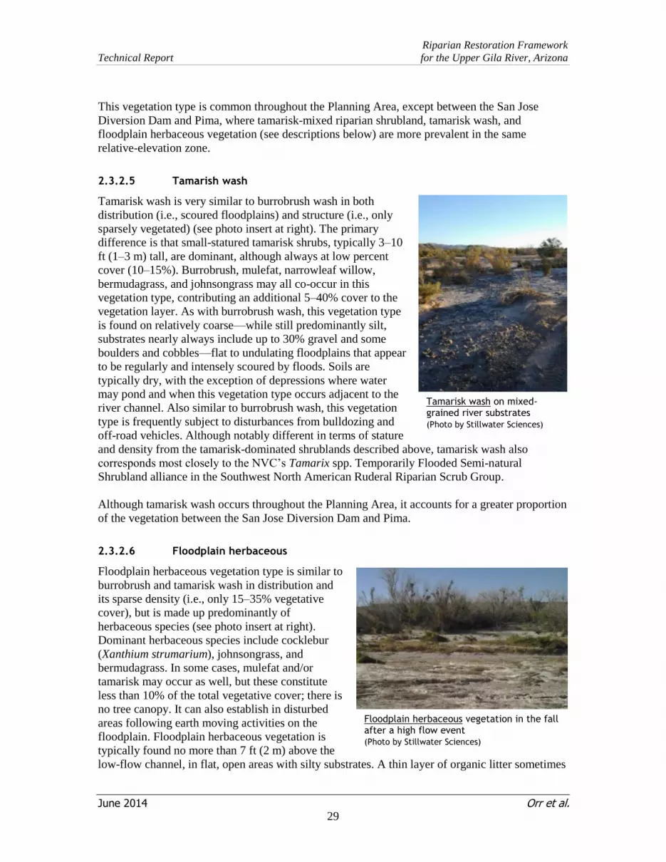
Riparian Restoration Framework
Technical Report for the Upper Gila River, Arizona
June 2014 Orr et al. 29
This vegetation type is common throughout the Planning Area, except between the San Jose
Diversion Dam and Pima, where tamarisk-mixed riparian shrubland, tamarisk wash, and
floodplain herbaceous vegetation (see descriptions below) are more prevalent in the same
relative-elevation zone.
2.3.2.5 Tamarish wash
Tamarisk wash is very similar to burrobrush wash in both
distribution (i.e., scoured floodplains) and structure (i.e., only
sparsely vegetated) (see photo insert at right). The primary
difference is that small-statured tamarisk shrubs, typically 3–10
ft (1–3 m) tall, are dominant, although always at low percent
cover (10–15%). Burrobrush, mulefat, narrowleaf willow,
bermudagrass, and johnsongrass may all co-occur in this
vegetation type, contributing an additional 5–40% cover to the
vegetation layer. As with burrobrush wash, this vegetation type
is found on relatively coarse—while still predominantly silt,
substrates nearly always include up to 30% gravel and some
boulders and cobbles—flat to undulating floodplains that appear
to be regularly and intensely scoured by floods. Soils are
typically dry, with the exception of depressions where water
may pond and when this vegetation type occurs adjacent to the
river channel. Also similar to burrobrush wash, this vegetation
type is frequently subject to disturbances from bulldozing and
off-road vehicles. Although notably different in terms of stature
and density from the tamarisk-dominated shrublands described above, tamarisk wash also
corresponds most closely to the NVC’s Tamarix spp. Temporarily Flooded Semi-natural
Shrubland alliance in the Southwest North American Ruderal Riparian Scrub Group.
Although tamarisk wash occurs throughout the Planning Area, it accounts for a greater proportion
of the vegetation between the San Jose Diversion Dam and Pima.
2.3.2.6 Floodplain herbaceous
Floodplain herbaceous vegetation type is similar to
burrobrush and tamarisk wash in distribution and
its sparse density (i.e., only 15–35% vegetative
cover), but is made up predominantly of
herbaceous species (see photo insert at right).
Dominant herbaceous species include cocklebur
(Xanthium strumarium), johnsongrass, and
bermudagrass. In some cases, mulefat and/or
tamarisk may occur as well, but these constitute
less than 10% of the total vegetative cover; there is
no tree canopy. It can also establish in disturbed
areas following earth moving activities on the
floodplain. Floodplain herbaceous vegetation is
typically found no more than 7 ft (2 m) above the
low-flow channel, in flat, open areas with silty substrates. A thin layer of organic litter sometimes
Tamarisk wash on mixed-grained river substrates (Photo by Stillwater Sciences)
Floodplain herbaceous vegetation in the fall after a high flow event (Photo by Stillwater Sciences)

Riparian Restoration Framework
Technical Report for the Upper Gila River, Arizona
June 2014 Orr et al. 30
covers up to 15% of the ground surface, resulting in moderate, patchy exposure of bare soil. Soils
where this vegetation type occurs may retain moisture in depressions where water can pond, but
are otherwise dry. Floodplain herbaceous vegetation corresponds most closely to the NVC’s Iva
annua–(Xanthium strumarium) Temporary Flooded Herbaceous Vegetation alliance in the
Southeastern Ruderal Wet Meadow and Marsh Group.
Floodplain herbaceous vegetation is found throughout the Planning Area, although most notably
immediately downstream of the San Jose Diversion Dam, on portions of the floodplain subject to
frequent flood-scour activity, along with tamarisk wash.
2.3.2.7 Floodplain wetland
Floodplain wetland vegetation type typically has
high cover (50-100%), but with low species
diversity. Cattails (Typha spp.) are typically the
most common species and contribute to a thick
litter layer, although bulrush and narrowleaf willow
may also be present at low densities. Tamarisk
saplings are often abundant and can exert high
competitive pressure on native species; tamarisk is
able to significantly out-compete species such as
cattails in ponded areas, as well as species such as
narrowleaf willow along drier banks. The
herbaceous layer is typically absent or very sparse.
Floodplain wetland vegetation corresponds most
closely to the NVC’s Typha domingensis Western
Herbaceous Vegetation alliance in the Arid West Emergent Marsh Group.
Areas where floodplain wetland vegetation occurs are always flat to convex, allowing water to
pond, and substrates are typically silty. Floodplain wetland vegetation is primarily found
downstream of Pima, where it occurs in isolated patches independent of relative elevation from
the channel (see photo insert at right). Floodplain wetland vegetation is highly influenced by
agricultural return flows; nearly all wetland areas are supported by a drainage ditch or pond
where water flows from adjacent fields.
2.3.2.8 Mesquite bosque
Mesquite bosque vegetation type occurs broadly
throughout the Sonoran Desert. The tree canopy is
moderately open, with only 25–50% cover, and is
composed entirely of mesquite, which rarely
exceeds 30 ft (10 m) in height (see photo insert at
right). A variety of shrubs and other understory
vegetation are also supported, such as wheelscale
saltbush (Atriplex elegans), desert willow
(Chilopsis linearis), rabbitbrush (Ericameria spp.),
Torrey wolfberry (Lycium torreyi), creosote
(Larrea tridentata), palo verde (Parkinsonia
aculeatae), prickly Russian thistle, seepweed
(Suaeda spp.), and annual grasses. Tamarisk may
Dense floodplain wetland (cattails) vegetation near Pima (Photo by Stillwater Sciences)
Mesquite bosque along upland boundary of riparian corridor (Photo by Stillwater Sciences)

Riparian Restoration Framework
Technical Report for the Upper Gila River, Arizona
June 2014 Orr et al. 31
also be present at very low cover (<5%). This vegetation type corresponds most closely to the
NVC’s Prosopis glandulosa-Atriplex spp. Shrubland in the Tamaulipan Dry Mesquite and
Thornscrub Group.
Subjected to only infrequent flood events, mesquite bosque occurs in dry silty or sandy soils with
generally flat topography. Patches of mesquite bosque are found along the upland boundary of the
riparian corridor throughout the Planning Area, occurring along xeric portions of the floodplain
greater than approximately 16 ft (5 m) above the active channel (see the >5 m relative elevation
band in Figure 2-7) and at the mouths of incoming arroyos.
2.3.3 Vegetation restoration opportunities and constraints
The following is a summary of considerations that should be taken during riparian restoration
planning, based on the vegetation transect-plot data collected and general observations made
during the field effort.
Very few instances of natural recruitment of native riparian trees and shrubs were observed
during the plot surveys, and much of what was observed appeared to have been recruited in
association with the 1993 flood event. Recruitment potential under more recent conditions
appears to be limited by high density of tamarisk coverage and sufficient water availability.
This condition indicates that active planting will be needed to restore native species
downstream of the San Jose Diversion Dam. Upstream of the San Jose Diversion Dam
(reaches 2j and 3a), however, where there are fewer water diversions and a greater
proportion of native trees and shrubs, natural recruitment may be adequate to restore native
species as tamarisk dies back following the arrival of the tamarisk beetle.
Active planting and restoration infrastructure should generally be avoided in the Flood
Reset Zone to prevent the loss of restoration resources. Between the San Jose Diversion
Dam and Pima, where there are few areas suitable for restoration outside of the Flood
Reset Zone (see Section 2.6 Potentially Suitable Vegetation Restoration Areas below),
opportunities to replace tamarisk wash with burrobrush wash could be evaluated if
desirable, although these functionally equivalent vegetation types provide little to no
potential habitat for SWFL.
Vegetation composition and cross-sectional distribution, and the physical conditions that
shape these attributes, vary as a function of position along the river corridor (i.e., specific
to hydrogeomorphic reach). Upstream of the San Jose Diversion Dam in reaches 2j and 3a,
the higher proportion of native species, fewer water diversions, and higher potential for
natural recruitment suggest that these reaches are of relatively lower priority for
restoration. Between the San Jose Diversion Dam and Pima in reaches 2f though 2i, the
sparse vegetation, relatively greater influence of water diversion, and large areas of flood
scour suggest that successful restoration will require careful planning to avoid scour and to
provide adequate soil moisture. Downstream of Pima, the extent and density of vegetation
and influence of agricultural return flows suggest that a greater variety of vegetation types
could be successfully restored with minimal or no long-term irrigation.
Fire-contingent restoration actions such as herbicide applications on re-sprouting tamarisk
and/or active planting of native species should be planned for suitable areas downstream of
Pima, and to a lesser extent upstream of the San Jose Diversion Dam, to take advantage of
the removal of tamarisk biomass by wildfire. The suppression of tamarisk cover for just a
few years may be sufficient for Fremont cottonwood and Goodding’s willow cuttings or
poles planted shortly after a fire to grow above the existing tamarisk canopy.

Riparian Restoration Framework
Technical Report for the Upper Gila River, Arizona
June 2014 Orr et al. 32
Current locations of native riparian plant species are indicative of where these species,
once restored, should persist in the future. However, many other areas are likely to have
suitable biophysical conditions for successful restoration as well but natural recruitment of
natives is not occurring and/or tamarisk has out-competed all other species. As such, it is
recommended that the physical conditions under which native species have been
documented to occur be used to help select restoration sites, rather than the locations of
natives themselves, which is likely to underestimate the area potentially suitable for
restoration. Figures 2-8 and 2-9, which present the range of relative elevations under which
several native riparian trees and shrubs were observed during the plot surveys, were
specifically developed for this purpose. In addition, the height of the current vegetation
canopy, even in tamarisk-dominated stands, provides a useful indicator of site productivity
for native woody species.
Many occurrences of native trees and shrubs, and nearly all occurrences of floodplain
wetlands, in the Planning Area appear to be highly influenced by, if not dependent upon,
channelized tributary and/or agricultural return flows. The presence of such flows should
be a factor considered in the selection of restoration sites, since they offer opportunities to
successfully establish and grow native species without the need for irrigation. However,
during this consideration, the seasonality and constancy of the tributary and/or agricultural
return flows should be assessed, as flow patterns may vary depending upon the water year
type and crop(s) being grown. The strong influence of channelized tributary and/or
agricultural return flows as suggests that, outside of these zones of influence, irrigation
may be needed to establish some native species in certain areas.
Although they are miniscule in extent in comparison with tamarisk-dominated shrublands,
unique native vegetation types, such as freshwater wetlands, burrobrush wash, mesquite
bosque, and herbaceous species tolerant of more saline soils, occur in the Planning Area.
These vegetation types may be appropriate to restore in less-suitable areas in order to
enhance vegetation and habitat diversity. Similarly, where areas become available for
restoration, but may not be appropriate for the planting of Fremont cottonwood,
Goodding’s willow, mulefat, or narrowleaf willow, these other native vegetation types
could be considered. To help inform such planning, the growing requirements for many of
the native plant species that may be appropriate to restore in the Planning Area, as
identified by the USDA, are provided in Appendix D.
2.4 SWFL Habitat Evaluation and Modeling
Information on reach-scale SWFL conditions supported by habitat-prediction modeling
performed specifically for the Restoration Framework is briefly presented here. Field surveys
were conducted in 2013 to characterize existing and potential SWFL-habitat quality throughout
the Planning Area. Background information on general species conditions are presented in
Appendix E, as authored by Matthew Johnson of NAU. Methods and results of the SWFL habitat
modeling are presented in Appendix F, as authored by James Hatten of the USGS and Matthew
Johnson.
The objectives of the SWFL existing conditions review and habitat prediction modeling are to:
1. Develop a conceptual model of SWFL breeding requirements (see Figure F-1 in Appendix
F), which include physiological and other environmental processes that were identified by
previous research as important determinants of species survival and reproduction, and are
conceptual links to the spatially and temporally comprehensive variables that were
available for us to use in our statistical modeling.
Riparian Restoration Framework
Technical Report for the Upper Gila River, Arizona
June 2014 Orr et al. 33
2. Gather and synthesize historical SWFL presence/absence and breeding data along the
upper Gila River (Arizona/New Mexico boundary–Gila River/San Pedro Confluence);
3. Estimate existing potentially suitable breeding habitat for SWFL in the Planning Area by
characterizing existing habitat conditions and running the SWFL habitat models (satellite
and vegetation aerial);
4. Apply two sets of models to estimate potential suitable habitat for SWFLs within the
Planning Area: (1) satellite models, which characterize vegetation from Landsat Thematic
Mapper (TM) imagery; and (2) aerial models using finer-scale remote sensing data,
characterizing vegetation from orthorectified digital aerial photography and LiDAR
collected in October 2012;
5. Incorporate the effects that tamarisk biocontrol will have on SWFL habitat over a period of
3 to 5 years following expansion of the beetle into the Gila Valley area. The modeling
effort can potentially map likely defoliated areas under future scenarios and help detect
trends in SWFL habitat suitability caused by changes in vegetation over time; and
6. Communicate the progress of model development and results with Gila Watershed
Partnership, U.S. Fish and Wildlife Service, Bureau of Reclamation, Arizona Game and
Fish, and Salt River Project.
2.4.1 Existing conditions and challenges
SWFLs are present in the Planning Area, which has been designated as critical habitat for the
species by the USFWS. They typically establish nesting territories, build nests, and forage where
mosaics of relatively dense and expansive growths of trees and shrubs are established near or
adjacent to surface water and/or underlain by saturated soil (Sogge et al. 2010). SWFL exist and
interact as groups of metapopulations—a group of geographically separate breeding populations
connected to each other by immigration and emigration—and are considered most stable where
many connected sites or large populations exist. Metapopulation persistence or stability is more
likely to improve by adding more breeding sites rather than expanding existing sites, which
would distribute birds across a greater geographical range, minimize risk of simultaneous
catastrophic population loss, and avoid genetic isolation. Approximately twice the amount of
suitable habitat is therefore needed to support the numerical territory goals because the long-term
persistence of SWFL populations cannot be assured by protecting only those habitats in which the
species currently breeds.
It is also important to recognize that most breeding habitats are susceptible to future changes in
site hydrology (natural or human-related), human impacts such as development or fire, and
natural catastrophic events such as flood or drought (Hatten and Sogge 2007). Furthermore, as the
vegetation at sites matures, it can lose the structural characteristics that make it suitable for
breeding individuals. These and other factors can destroy or degrade breeding sites making their
suitability ultimately ephemeral. Thus, it is necessary to have additional suitable habitat available
to which SWFLs can readily move if displaced by such habitat loss or change.
The recent establishment of the tamarisk leaf beetle in parts of the southwest introduces a new
dynamic factor affecting habitat suitability. Therefore, measuring and predicting SWFL habitat—
either to identify areas that may develop into appropriate habitat for SWFL or that, with
intervention by active restoration could support future SWFL nesting—requires knowledge of
recent/current/future habitat conditions and an understanding of the dynamic processes and
ecological factors that determine SWFL use of riparian breeding sites.

Riparian Restoration Framework
Technical Report for the Upper Gila River, Arizona
June 2014 Orr et al. 34
Within the Planning Area, SWFL habitat observations are regularly performed by SRP on their
Ft. Thomas Preserve properties (SRP 2013) and were made in spring/summer 2013 at nearby
parcels by NAU and UCSB in support of the Restoration Framework development1. NAU will
survey and evaluate SWFL habitat at all proposed Planning Area sites in spring/summer 2014.
2.4.2 SWFL breeding habitat modeling
In 1999, Arizona Game and Fish Department (AGFD) developed a GIS-based model (Hatten and
Paradzick 2003) to identify SWFL breeding habitat from Landsat Thematic Mapper (TM)
imagery and 30-m resolution digital elevation models (DEMs). The model was developed with
presence-absence survey data acquired along the San Pedro and (lower) Gila rivers, and from the
Salt River and Tonto Creek inlets to Roosevelt Lake. This GIS-based model has been tested by
predicting SWFL breeding habitat at multiple locations around Arizona and New Mexico, and has
performed as expected by identifying riparian areas with the highest SWFL nest densities (Hatten
and Sogge 2007, Hatten et al. 2010).
2.4.2.1 SWFL satellite model
We have successfully applied the “SWFL
Satellite Model” (30-m resolution) to the
Planning Area using Landsat 8 imagery.
Satellite-model output included a
continuous probability grid, a five-class
probability grid, and a binary habitat grid,
with higher cell values in each case
indicating relatively better SWFL habitat.
Figure F-2 in Appendix F displays the
results of the five-class probability grid,
with green areas representing the greatest
breeding habitat suitability and red areas
representing the lowest suitability (see
graphic at right). The highest quality areas
are concentrated downstream of Thatcher in reaches 2c–2f.
In addition, we created a habitat time series for the project area by populating the SWFL Satellite
Model with 27 Landsat scenes from 1986–2013. The habitat time series served two purposes: (1)
it allowed us to create a bar graph that depicts how much potential SWFL breeding habitat was in
the project area between 1986 and 2013 (Figure F-3 in Appendix F); and (2) it enabled us to
create time-lapse videos of how SWFL habitat changes year to year between 1986 and 2013 over
the entire project area. We now have a baseline of SWFL suitable habitat that can be compared to
future conditions.
2.4.2.2 SWFL LiDAR model
We are currently in the process of incorporating additional critical landscape and vegetation
features to improve the SWFL model’s ability to identify nest site suitability. This will integrate
1 Because of the sensitive nature of publically distributing locational information on endangered species,
locations of observed SWFL activity in the Planning Area are not published herein. These data may be
provided by request through the U.S. Fish and Wildlife Service office in Phoenix, Arizona
(http://www.fws.gov/southwest/es/arizona/).
Example mapping results from the “SWFL Satellite Model” downstream of Ft. Thomas, where suitability grades from
green (greatest) to red (least) (see Figure F-2 in Appendix F)

Riparian Restoration Framework
Technical Report for the Upper Gila River, Arizona
June 2014 Orr et al. 35
vegetation species composition and structural traits from aerial imagery and field surveys with
landscape-level vegetation height and channel topography generated from the LiDAR dataset
collected by USU RS/GIS in October 2012. The results of the “SWFL LiDAR Model” will be
concluded after the 2014 spring/summer field season when we have a larger set of observed
SWFL territories from which to build a more robust model. This larger set will be obtained from
the 2014 SWFL surveys to be conducted by NAU at the proposed Planning Area sites.
2.5 Soils and Groundwater Monitoring
Information on site-scale soil sampling and groundwater-level monitoring performed for the
Restoration Framework is briefly presented here. The results briefly reported here helped confirm
reach-scale soil and groundwater conditions, as estimated with a relative-elevation surface and
regional soil mapping compiled for the ecohydrological assessment, which all together helped
further characterize planting suitability in the Planning Area. Additional details on the site
monitoring efforts performed by DBG and UCSB are presented in Appendix G, as authored by
Tom Dudley, Kevin Hultine, and Devyn Orr.
2.5.1 Soil sampling
Shallow soil samples collected at the initial vegetation-monitoring sites located near Ft. Thomas
were analyzed for soil texture, electrical conductivity (EC), and pH to assess suitability of active
planting in the Planning Area. Measurements of EC and pH help to characterize soil physical and
chemical properties, namely salinity, which can be a limiting factor for successful propagation of
many types of riparian vegetation, such as cottonwood and willows.
The sampled soils were found to be composed of medium-sized sands with variable proportions
of finer-grained silts and sands and coarser-grained sands and gravels. The measured EC values
were broad, ranging from about 0.1 to 2.6 millimhos per centimeter (mmhos/cm) (100 to 2600
microSiemens per centimeter [uS/cm]). The shallower profiles sampled (0–10 cm below ground
surface [bgs]) generally had greater EC values than the deeper profiles sampled (20–30 cm bgs).
Measured values of soil pH exhibited a narrow range between about 7.8 and 8.6 for both sampled
soil profiles, indicating the soils were slightly alkaline. All results are reported in Appendix G.
Riparian plant species requirements are described in Appendix D, with specific values of key
environmental factors (e.g., soil texture, salinity) summarized in Table D-1 for the native species
likely to be planted with active restoration efforts in the Planning Area. Overall, the soil sampling
results indicate that the measured soil texture, and salinity and alkalinity levels were within the
ranges of tolerance for most species. Thus, shallow soils (<30 cm [<1 ft]) present near the
sampled locations should be suitable to support plantings of cottonwood, narrowleaf and
Goodding’s willow, and other native woody riparian (e.g., Baccharis spp.) and upland species
(e.g., Atriplex spp.). The soils in a few areas may, however, be too saline and/or alkaline to
support plantings of some native species, such as willow and cottonwood, which have low
tolerance for salinity or higher pH (see Table D-1).
2.5.2 Groundwater-level monitoring
Shallow groundwater levels were monitored close to the active river channel at 6 locations
throughout the Planning Area to better understand shallow groundwater patterns and, ultimately,
water availability for active plantings. Paired piezometer wells were aligned perpendicular to the
primary river channel with one well located near the water’s edge and the second well located
Riparian Restoration Framework
Technical Report for the Upper Gila River, Arizona
June 2014 Orr et al. 36
farther out into the riparian forest. The initial groundwater measurements made in January 2014
reveal that depth to the water table was fairly shallow (~6–16 ft bgs), and remained fairly static
across the width of the riparian corridor and was not wholly dependent on proximity to the wetted
river channel (Figure 2-10).
As part of the ecohydrological assessment, the initial groundwater measurements were compared
to relative elevations at each of the piezometer locations (see Figure 2-10). A relative-elevation
surface was produced by Stillwater Sciences using the high-resolution, bare-earth topographic
data produced from USU RS/GIS’s October 2012 LiDAR data. This surface represents the land
surface height above the low-flow channel, which is intended to serve as a proxy for depth to
groundwater. Comparisons between the groundwater measurements and the corresponding
relative-elevation values at all but two of the piezometer locations reveal close agreement (<1 ft
difference), indicating that use of the relative elevation surface to estimate depths to groundwater
is an appropriate method for restoration planning in the Gila Valley. The two locations with
greater differences (>1 ft) are believed to be caused by recording error in the GPS-recorded
coordinates, for which we recommend re-taking of the coordinates during future monitoring
efforts.
Figure 2-10. Plot of measured groundwater depths in the Planning Area taken in January 2014. Measurements are compared to relative ground-surface elevations above the low-flow river channel water surface elevation.
0.0
2.0
4.0
6.0
8.0
10.0
12.0
14.0
16.0
18.0
1a 1b 2a 2b 2c 3a 3b 4a 4b 5a 5b 6a 6b
57 549 1532 132 43 69 351 456 TBD 504 485 722 186
Dep
th t
o g
rou
nd
wate
r b
elo
w g
rou
nd
su
rface (
ft)
Piezometer ID# and distance (ft) from wetted river channel
Measured depth to groundwater (ft)
Relative elevation (ft) Poor GPS recording;need to take
new coordinates

Riparian Restoration Framework
Technical Report for the Upper Gila River, Arizona
June 2014 Orr et al. 37
2.6 Potentially Suitable Vegetation Restoration Areas
Here we describe how the results of the ecohydrological assessment and its supporting studies
were synthesized to identify areas within the Planning Area’s riparian corridor having the greatest
potential for effective and successful native vegetation restoration. Briefly, the “Potentially
Suitable Vegetation Restoration Areas” were based on those areas of the riparian corridor outside
of the Flood Reset Zone, near modeled high-quality SWFL habitat, within non-saline to slightly
saline soils, and within low-lying areas relative to the low-flow channel. Vegetation-growth
potential was used to further refine the priority areas into those having highest and medium
priority. The analysis was performed in a GIS using spatial data for the environmental factors
having restoration-suitability criteria pre-determined during our field surveys and related
analyses. The environmental factors considered and methods of the data synthesis are described
below. Figure 2-11 graphically describes the data-synthesis process.
Although not included here, it is important to note that many other ecological factors, including
shade tolerance and other competitive abilities, proximity to seed source, intensity of herbivory,
and presence of disease, can contribute to the success of plant establishment and species
distributions within riparian zones and should be considered when determining site-specific
restoration activities. In addition, this level of screening does not incorporate a variety of other
important factors that will need to be considered in identifying specific sites and priorities for the
next phase of restoration planning, design, and implementation. Such factors include, but are not
limited to, landowner willingness, existing conservation easements or related land use
requirements, presence of key infrastructure, water rights, and initial and long-term costs and
maintenance requirements.
Riparian corridor
Areas considered suitable for active restoration were within the boundaries of the Planning
Area’s riparian corridor. The riparian corridor was mapped in GIS using color aerial imagery
collected by USU RS/GIS in October 2012 and was based essentially on the existing river bottom
comprised of the active channel and forested portions of the valley floor, including a few well-
connected tributary mouths. The riparian corridor did not include cultivated or urbanized
floodplain or other upland areas.
Flood Reset Zone
Suitable active vegetation restoration areas would generally be those found safely outside of
the Flood Reset Zone, which was mapped during the flood-scour analysis previously described
in Section 2.2 Flood-Scour Analysis and shown in Figures B-2.1 through B-2.10. Again, the
Flood Reset Zone includes areas having both >66% flood-scour frequency (i.e., scoured in 3 out
of 3 of the mapped events [1983, 1993, and 2005]) and “high” flood-disturbance activity—areas
severely disturbed by flow, typically scoured to bare substrate retaining <10% apparent riparian
vegetative cover—during the most recent flood of 2005.
Modeled SWFL habitat
Suitable vegetation restoration areas would be those found near areas modeled to currently
host high quality SWFL habitat, which was represented in the “SWFL Satellite Model” results
described in Section 2.4.2 SWFL Breeding Habitat Modeling and Appendix F, and shown in
Figure F-2. Because the high quality areas correspond strongly with vegetation density and, as
already understood, the riparian vegetation is mostly composed of tamarisk, it is anticipated that
these areas will experience the greatest impact initially following beetle colonization unless
strategic planting of native vegetation is undertaken in 2014–2015.

Riparian Restoration Framework
Technical Report for the Upper Gila River, Arizona
June 2014 Orr et al. 38
Shallow groundwater depth (relative elevation)
Existing information in the scientific literature and personal observations and unpublished data
indicate that native riparian plant species tend to occur in particular topographic positions relative
to the river channel. In particular, we have found that relative elevation above the low-flow, or
baseflow, water surface in the river channel is a useful indicator for restoration potential. Relative
elevation in a floodplain is generally correlated with depth to groundwater, and frequency of
surface saturation and inundation.
Thus relative elevation, which combined with other GIS layers and field data, provides a
powerful tool for assessing restoration potential via passive (natural recruitment processes) or
active (horticultural restoration) approaches. Although successful germination of native riparian
seedlings depends on a variety of hydrologic and geomorphic variables, seedling survival of
phreotophytes such as cottonwoods and willows following germination (or of planted cuttings or
container stock under horticultural restoration) is above all contingent on constant contact with
the water table and/or its capillary fringe throughout the growing season (McBride and Strahan
1984, Stromberg et al. 1991). Research indicates that when the water table decline is more rapid
over a long period than the rate of root growth, seedlings of phreatophytic species become
isolated from their water source and suffer high mortality (McBride et al. 1989, Stromberg et al.
1996). In addition to the importance of groundwater levels for seedling survival, research
indicates that groundwater levels play an integral role in determining sapling survivorship and
adult riparian community composition (Smith et al. 1991).
Furthermore, comparative studies indicate that some non-native invasive plant species (such as
tamarisk) tend to be more drought-tolerant than natives, and thus better able to compete along
reaches with extreme inter- and intra-annual water table fluctuations (Smith et al. 1991, Friedman
et al. 1995, Shafroth et al. 1998, 2000). Thus, in order to restore self-sustaining hardwood riparian
forest, we need to better understand the role of groundwater in species survivorship across time
and across species.
In the absence of a Planning Area-wide compilation of shallow groundwater levels, relative
elevation can serve as a very useful proxy. As previously mentioned in Section 2.5.2
Groundwater-level monitoring, we produced a relative-elevation surface using the available
LiDAR data. The initial groundwater measurements shown in Figure 2-10 (and further described
in Appendix G) helped to validate the use of the relative elevation surface to estimate depths to
groundwater in the Planning Area. Our vegetation-transect surveys described in Section 2.3
Riparian Vegetation Characterization found that native willows and cottonwoods are most
numerous upon surfaces situated within 4 m of the low-flow channel (see Figures 2-8 and 2-9).
Therefore, suitable areas for active restoration included those lying within the 0–4 m
elevation range above the low-flow channel. These areas were delineated for the
ecohydrological assessment using the bare-earth LiDAR data.
Soil salinity
Analysis of soils data contributes to more realistic projections of potential woody riparian
vegetation expected under various management scenarios, as we can exclude areas with soils
unsuitable for hardwoods such as cottonwoods and willows by using NRCS information on
salinity at the reach scale. By linking our understanding of natural riparian vegetation recruitment
processes and native woody plant life history requirements with soils information, our predictions
of locations and total area suitable for passive revegetation (i.e., revegetation via restoration of
natural seed dispersal/germination/root growth/inundation and water table recession processes)
can be made more reliable. However, our primary purpose in the present analysis is to use soils
Riparian Restoration Framework
Technical Report for the Upper Gila River, Arizona
June 2014 Orr et al. 39
data to explore the potential for use of active revegetation techniques (i.e., horticultural
restoration) to establish various native riparian trees, shrubs, and herbaceous species in the study
area to restore or enhance suitable habitat for SWFL and other wildlife species of interest.
Salinity tolerances reported for plant species common to the Planning Area area described in
Appendix D. Species such as cottonwood, narrowleaf willow, and Goodding’s willow have a
“None” to “Low” tolerance for saline soils, whereas some other native woody riparian (e.g.,
Baccharis spp.) and upland species (e.g., Atriplex spp.) have “High” tolerance (see Table D-1).
The tolerance categories are as follows:
None (i.e., minimal tolerance): 0–2 mmhos/cm
Low: 2–4 mmhos/cm
Medium: 4–8 mmhos/cm
High (i.e., maximum tolerance): >8 mmhos/cm
While the soil sampling efforts in the Ft. Thomas area provided initial confirmation that salinity
levels were generally low and will likely not pose an issue to active plantings, we utilized the
NRCS’s SSURGO spatial dataset to locate saline soils throughout the entire Planning Area.
Again, soil salinity was based on the EC attribute in the SSURGO dataset (section 618.20 of
NRCS Soil Properties and Qualities). Salinity classes present within the Planning Area include:
Non-saline: 0–<2 mmhos/cm
Very slightly saline: 2–4
Slightly saline: 4–8
Moderately saline: 8–16
Strongly saline: >16
Suitable areas for active restoration included those with soils having non-saline to very
slightly saline conditions, and excluded those areas with soils having slightly saline to
strongly saline conditions. Overall, the vast majority of the riparian corridor was composed of
soils of lower salinity and alkalinity.
Vegetation canopy height
The Planning Area is dominated by dense stands of tamarisk, particularly downstream of Pima,
with smaller patches of Goodding’s and narrowleaf willows, Fremont cottonwood, and other
native vegetation (see Section 2.3 Riparian Vegetation Characterization above). The main patches
of Fremont cottonwood and Goodding’s willow can be identified in a GIS using vegetation
canopy height information derived from the LiDAR data. Specifically, the canopy surface is
formed from the first-return data points contained in the LiDAR data (as opposed to the bare-
earth data). Mature trees of Fremont cottonwood and Goodding’s willow tend to form an
emergent crown greater than 7 m in height, which extends above the typically dense layer of
tamarisk, so we can readily pick up individual trees and stands by mapping all vegetation >7 m in
canopy height. Most tamarisk stands do not exceed 5 m in canopy height, but in the most
productive sites taller plants are found and canopy height may be in the 5–7 m range. If other
factors (such as relative elevation and soil salinity) are suitable, these taller, more productive
tamarisk stands can be used as an indicator of areas likely to be suitable for revegetation by native
woody species. The relationships between vegetation canopy height and presence of Fremont
cottonwood and Goodding’s willow, and likely restoration potential, are also supported by our
Riparian Restoration Framework
Technical Report for the Upper Gila River, Arizona
June 2014 Orr et al. 40
November 2013 vegetation-transect surveys and careful review of natural color aerial imagery
collected by USU RS/GIS in October 2012.
Using canopy height as a proxy for vegetation productivity potential, the Potentially Suitable
Vegetation Restoration Areas determined from synthesis of above environmental factors were
further refined based on canopy height criteria to locate areas having the highest and medium
priority for immediate, active restoration; the remainder being considered to have the lowest
priority. That is, the high and medium priority areas included those areas having lower-lying
elevations (i.e., shallow water table) and tall canopy heights (i.e., most productive for woody
vegetation growth). The criteria were as follows:
“High” restoration priority:
o Relative elevation = <0–0.5 m and Canopy height = >5 m
o Relative elevation = 0.5–2 m and Canopy height = >7 m
“Medium” restoration priority:
o Relative elevation = 0.5–2 m and Canopy height = 5–7 m
o Relative elevation = 2–3 m and Canopy height = >5 m
Figure 2-11. Process of the Ecohydrological Assessment to identify the Potentially Suitable Vegetation Restoration Areas in the Planning Area.
Within riparian corridor
Outside of Flood
Reset Zone
Within 4 m of low-flow
channel
Within low salinity
soils
Potentially Suitable Vegetation Restoration
Areas
Within Low Lying & High Productivity
Areas
High and Medium Priority Restoration
Areas
Near modeled
high-quality SWFL
habitat
Riparian Restoration Framework
Technical Report for the Upper Gila River, Arizona
June 2014 Orr et al. 41
The above analysis resulted in a series of map tiles of the Potentially Suitable Vegetation
Restoration Areas (green) along the riparian corridor within the Planning Area. Also produced
were distributions of color-coded pixels representing points of “High” (purple) or “Medium”
(blue) restoration potential. The pixel-distributions displayed discrete groupings of suitable areas
that were finalized by manually encircling groupings larger than 10 acres with polygons of the
same priority classification.
The High and Medium Priority Restoration Areas are presented in Figure 2-12 below. Also
shown for reference on the maps are the previously established restoration/mitigation sites
managed by Freeport McMoRan Copper & Gold, Inc. (FMI) and the Salt River Project (SRP).
The results shown in the below maps reveal that nearly half, or 42%, of the riparian corridor
qualifies for inclusion in the general Potentially Suitable Vegetation Restoration Area category,
amounting to about 4,800 total acres (Figure 2-13). The size of the areas within any given
hydrogeomorphic reach generally increases with downstream direction, with those below
Thatcher (reaches 2c–2f) each having more compared with those reaches upstream of Thatcher
(reaches 2g–3a). Further, the areas accounted for at least half of the riparian corridor in each of
the lower reaches (2c–2f), while areas accounted for as low as a tenth of the riparian corridor in
the upper reaches and were generally confined to the outer margins of the corridor (e.g., 2j and
3a). Not surprisingly, the High and Medium Priority Areas were more abundant in the lower
reaches, and were all but absent in the upper reaches by virtue of there being minimal low-lying
areas supporting tall woody vegetation. In total, the High and Medium Priority Areas each
account for nearly 400 acres (750 acres in total)—a manageable size for rapid active restoration
involving tamarisk removal and native re-planting in 2014.
While the results presented here are based upon the best available science, we caution any
potential user of these results that the areas identified here have been done so without regard to
land ownership or owner interest. The GWP or others with plans to implement tamarisk
treatment and/or vegetation restoration will still need to consider site-specific opportunities or
constraints related to nearby land uses.

Riparian Restoration Framework
Technical Report for the Upper Gila River, Arizona
June 2014 Orr et al. 42
a)
b)
c)
d)
Figure 2-12.1. Upper Gila River Potentially Suitable Vegetation Restoration Areas for lower Reach 2c. See map-tile index in Figure B-1 in Appendix B.

Riparian Restoration Framework
Technical Report for the Upper Gila River, Arizona
June 2014 Orr et al. 43
a)
b)
c)
d)
Figure 2-12.2. Upper Gila River Potentially Suitable Vegetation Restoration Areas for upper Reach 2c upstream to lower Reach 2e. See map-tile index in Figure B-1 in Appendix B.

Riparian Restoration Framework
Technical Report for the Upper Gila River, Arizona
June 2014 Orr et al. 44
a)
b)
c)
d)
Figure 2-12.3. Upper Gila River Potentially Suitable Vegetation Restoration Areas for upper Reach 2e upstream to lower Reach 2g. See map-tile index in Figure B-1 in Appendix B.
Riparian Restoration Framework
Technical Report for the Upper Gila River, Arizona
June 2014 Orr et al. 45
a)
b)
c)
d)
Figure 2-12.4. Upper Gila River Potentially Suitable Vegetation Restoration Areas for Reach 2g upstream to lower Reach 2i. See map-tile index in Figure B-1 in Appendix B.
Riparian Restoration Framework
Technical Report for the Upper Gila River, Arizona
June 2014 Orr et al. 46
a)
b)
c)
d)
Figure 2-12.5. Upper Gila River Potentially Suitable Vegetation Restoration Areas for upper Reach 2i upstream to Reach 3a. See map-tile index in Figure B-1 in Appendix B.

Riparian Restoration Framework
Technical Report for the Upper Gila River, Arizona
June 2014 Orr et al. 47
Figure 2-13. Histogram of sizes of the riparian corridor, Flood Reset Zone, and Potentially Suitable Vegetation Restoration Areas within the Planning Area and each of the hydrogeomorphic reaches.
0
1,000
2,000
3,000
4,000
5,000
6,000
2c 2d 2e 2f 2g 2h 2i 2j 3a TotalPlanning
Area
Siz
e o
f a
rea
s (
ac
res
)
Hydrogeomorphic reaches and Planning Area
Riparian corridor
Flood Reset Zone
Potentially Suitable Vegetation Restoration Areas
"High" Priority Restoration Areas
"Medium" Priority Restoration Areas
11,525 acrestotal area of riparian corridor in Planning Area
downstream direction

Riparian Restoration Framework
Technical Report for the Upper Gila River, Arizona
June 2014 Orr et al. 48
3 SUMMARY OF FINDINGS AND RECOMMENDATIONS
This chapter presents a synthesis of the results of our ecohydrological assessment and supporting
studies conducted as part of the Restoration Framework. The results have been integrated to
identify restoration opportunities and constraints that, together, inform recommendations to be
incorporated into the Restoration Implementation Plan to be authored by the Gila Watershed
Partnership.
3.1 Summary of Ecohydrological Assessment and Other Information
Planning for any manner of riparian restoration in the tamarisk-dominated Gila Valley will
require consideration of the following environmental factors:
Hydrogeomorphic conditions
The upper Gila River naturally experiences a wide variation of flows, punctuated
episodically by short-duration (“flashy”) but intensive flood events most frequently
experienced in March (winter storms) and August (summer monsoons).
Three distinct hydrologic periods have been recorded over the past hundred years,
beginning with a flood period in the early 20th century, followed by a relatively quiescent
~50-year period between about 1918 and 1965, and a ~40-year period of larger, more
frequent flood events through at least 2005.
The potential for channel-scouring floods to occur in any given year remains high despite
an apparent lessening of large flood occurrence since the 1990s. Climate change
predictions for the region estimate a likely increase in extreme events despite the
expected increase in average temperatures and decrease in annual precipitation.
Three dominant hydrogeomorphic reach characteristics are observed in the river corridor
as it courses downstream through the Planning Area: a canyon-confined, coarse-grained
channel with limited floodplain and some native riparian forest at the mouth of the Gila
Box (reach 3a); a wide, drier, braided channel with sparse or disconnected riparian forest
bordered by a broad, cultivated and developed floodplain (reaches 2f–2j); and a moister,
fine-grained, braided channel dominated by a narrow, single-thread channel during lower
flows that is encroached upon by dense riparian forest (mostly tamarisk), which is in turn
bordered by a broad, cultivated floodplain with few developments downstream of Pima
(reaches 2c–2e).
River hydrology and geomorphic character are strongly influenced by the 6 irrigation
canal diversion dams, 6 bridge crossings, and network of earthen levees which together
modify the natural flow regime and potential for geomorphic change.
Flood-scour dynamics and risks
Position of the low-flow channel(s) changes rapidly and completely during flood events,
while the boundary of the broader active-channel changes less frequently.
Flood-scour extent has generally been greater upstream of Pima, with an overall
decreasing trend in the extent of the “high” (>66%) frequency flood-scour area in the
downstream direction.
Similarly, the areal extent of the Flood Reset Zone experiences a decreasing trend in the
downstream direction below the Gila Box (i.e., reaches 2c–2j), where the Flood Reset

Riparian Restoration Framework
Technical Report for the Upper Gila River, Arizona
June 2014 Orr et al. 49
Zone accounts for over 80% of the riparian corridor near the upstream end of the
Planning Area (reach 2j) and only about 20% near the downstream end (reach 2c).
Restoration opportunities outside of the Flood Reset Zone are greater downstream of
Pima (reaches 2c–2e) (i.e., more than half of the riparian corridor is available).
Vegetation conditions
The riparian corridor currently supports mostly tamarisk-dominated shrublands, although
several other vegetation types are present, including Fremont cottonwood-Goodding’s
willow woodland and narrowleaf willow-mulefat shrubland.
There are pronounced variations in vegetation composition and distribution along the
length of the riparian corridor in the Planning Area:
o The upstream end of the Planning Area (reaches 2j and 3a above the San Jose
Diversion Dam) hosts a higher proportion of native species and greater potential for
natural recruitment, which appears to be correlated with a minimal presence of
adjacent agriculture and little consumptive water use.
o The middle of the Planning Area (reaches 2f–2i between the San Jose Diversion Dam
and Pima) is sparsely vegetated, likely due to a greater influence of water diversion
and larger extent of flood-scour activity.
o The downstream end of the Planning Area (reaches 2c–2e below Pima) supports a
much denser riparian cover, albeit mostly tamarisk, benefiting from more abundant
agricultural return flow and less pronounced flood-scour activity.
The general pattern of vegetation composition and distribution across the riparian
corridor is: mixed riparian shrubland/narrowleaf willow-mulefat shrubland in a narrow
band closest to the wetted channel; tamarisk semi-natural shrubland/tamarisk-mixed
riparian shrubland next out from the channel within low-lying areas; burrobrush
wash/tamarisk wash sparsely distributed upon slightly higher surfaces; and mesquite
bosque sparsely distributed upon the highest surfaces (see Figure 2-9).
The two main native vegetation types, narrowleaf willow-mulefat and Fremont
cottonwood-Goodding’s willow, were observed to be most commonly present upon low-
lying surfaces being within 3 m (10 ft) and 4 m (13 ft) relative elevation, respectively,
above the low-flow channel water surface.
Natural recruitment of native riparian tree and shrub species appears to be limited by high
density of tamarisk coverage and water availability; much of the observed native tree and
shrub stands appear to have been recruited in association with the 1993 flood event.
Because revegetation success is strongly influenced by water availability and avoidance
of flood-scour activity, restoration opportunities appear greatest downstream of Pima
(reaches 2c–2e) where a greater variety of vegetation types could be successfully restored
with minimal or no long-term irrigation.
SWFL conditions and model-predicted high-quality areas
SWFLs continue to inhabit portions of the Planning Area during the breeding season
(spring/summer), and are most commonly present in the more densely vegetated riparian
areas (mostly consisting of tamarisk) downstream of Pima.
Nests are typically placed in trees where plant growth is most dense, where trees and
shrubs have vegetation near ground level, and where there is a tall but low-density
canopy. SWFL are generally not found in areas without willows, tamarisk, or both.

Riparian Restoration Framework
Technical Report for the Upper Gila River, Arizona
June 2014 Orr et al. 50
SWFL metapopultions are considered most stable where many connected sites or large
populations exist and, thus, are more likely to improve by restoring/creating twice the
amount of suitable breeding sites to distribute birds across a greater geographical range,
minimize risk of simultaneous catastrophic population loss, and avoid genetic isolation.
Similarly, it is necessary to restore/create additional breeding habitat given that its
suitability is quite sensitive to hydrological and structural changes, such as water
availability, human developments, flood and wildfire disturbance, and tamarisk leaf
beetle induced defoliation.
Based on the “SWFL Satellite Model,” the predicted highest quality areas are
concentrated downstream of Thatcher (reaches 2c–2f), which generally correspond with
those areas densely vegetated and outside of the Flood Reset Zone.
Soils and groundwater conditions
Surficial soils sampled near the Ft. Thomas area and mapped throughout the Planning
Area by NRCS are primarily composed of medium-sized sands with variable proportions
of finer-grained silts and sands and coarser-grained sands and gravels. Soil salinity is
generally low and pH is slightly alkaline.
Measured soil sampling results and published reach-scale NRCS soils maps indicate soil
texture, salinity, alkalinity are within the range of tolerance for most native riparian plant
species. Shallow soils should generally be able to support plantings of cottonwood,
narrowleaf and Goodding’s willow, and other native woody riparian (e.g., Baccharis
spp.) and upland species (e.g., Atriplex spp.), but may be too saline and/or alkaline to in a
few areas to support plantings of native cottonwoods and willows.
Groundwater measurements made throughout the Planning Area reveal generally shallow
depths to the water table (6–16 ft bgs), which remain fairly static across the width of the
riparian corridor regardless of proximity to the wetted channel.
Comparisons between the groundwater measurements and the corresponding relative-
elevation values at all but two of the piezometer locations reveal close agreement (<1 ft
difference), indicating that use of the relative elevation surface to estimate depths to
groundwater is an appropriate method for restoration planning in the Gila Valley.
Restoration Area Suitability
From the ecohydrological assessment, nearly half of the riparian corridor of the Planning
Area was predicted to be suitable—"Potentially Suitable Vegetation Restoration Area"—
for supporting active riparian restoration, amounting to about 4,800 acres.
The "High" and "Medium" Priority Areas each account for nearly 400 acres (750 acres in
total), which is a more manageable size for rapid and effective active restoration
involving some level of tamarisk removal and native re-planting beginning in 2014.
The Potentially Suitable Vegetation Restoration Areas are concentrated more
downstream of Thatcher where flood-scour risks are lower, vegetation-growth potential is
greater, SWFL habitat quality is greater, soil salinity and alkalinity are reasonably low,
and lower-lying areas potentially supporting wetter soils are readily available.

Riparian Restoration Framework
Technical Report for the Upper Gila River, Arizona
June 2014 Orr et al. 51
3.2 Synthesis of Findings
Our recommendations for restoration site selection and strategies are as follows:
Based on consideration of our ecohydrological assessment and supporting studies,
highest priority for active tamarisk treatment and native plantings should be focused
downstream of Thatcher within reaches 2c–2f.
The property parcels predicted to contain the greatest amount of “High” and “Medium”
Priority Restoration Areas (from the ecohydrological assessment) are listed in Table 3-1.
Also listed is the acreage of the highest predicted SWFL-breeding habitat suitability
(from the “SWFL Satellite Model”) for each identified parcel. (It should be noted again
that land-ownership and/or land-use conflicts may exist at any of these parcels which
may limit or prevent any alteration of existing vegetation coverage.)
More immediate restoration prioritization should be given to the most suitable locations
within those parcels burned during the “Clay Fire” near Ft. Thomas in early 2013 (see
bottom of Table 3-1) and more recently (e.g., the smaller burn area near Bylas). The
riparian vegetation, mostly tamarisk, was highly impacted during the fire, thus priming it
for rapid, cost-effective restoration action specifically involving herbicide treatment of
the re-sprouting tamarisk and then replanting with native species.
More intensive active riparian restoration should involve a phased, patch-work
(“Propagule Islands”) approach to: preserve much of the existing taller SWFL-suitable
tamarisk structure (to minimize disturbances to existing viable SWFL-nesting habitat);
remove/treat lower tamarisk structure (in patches) and replace with native plantings well
suited to site conditions; and gradually expand treatment and revegetation footprint
before and following beetle colonization.
Lower effort restoration strategies should also be considered throughout the remainder of
the Planning Area following disturbance from fires or floods that have removed much of
the tamarisk biomass. Fire-contingent restoration actions such as herbicide applications
on re-sprouting tamarisk and/or active planting of native species should be planned for
Priority Areas downstream of Thatcher (reaches 2c–2f). Post-flood-scour restoration
actions can follow a similar approach taking advantage of newly cleared areas to treat
remaining tamarisk and/or revegetate with native species.
Given the greater occurrences of native trees and shrubs, as well as nearly all occurrences
of floodplain wetland, that appear to be highly influenced by channelized tributary and/or
agricultural return flows, active restoration actions should attempt to take advantage of
such conditions through selection of sites with a known steady runoff supply or
coordination with land managers to negotiate a viable water supply where natural sources
are insufficient. Such sites should have higher success rates for both revegetation of
native riparian species (i.e., higher survival and growth rates for planted trees and shrubs)
and for creating or enhancing SWFL habitat (i.e., presence of surface water or saturated
soils during the breeding season).
Prior to any treatment/removal activity, coordination with the Phoenix office of the
USFWS will be necessary to first secure the prerequisite permits for carrying out such
work that could potentially be considered an unauthorized “take” of SWFL or other
federally listed fish or wildlife in the implementation area, or determines activities can
safely be undertaken without risking take. GWP has already initiated discussions with
USFWS regarding the least impactful restoration strategies in the Planning Area, and will
commence with preparation of a Biological Assessment and Section 10(A)(1)(a)
Recovery Permit in summer 2014.

Riparian Restoration Framework
Technical Report for the Upper Gila River, Arizona
June 2014 Orr et al. 52
Creation of suitable SWFL habitat elsewhere in the Gila Valley, such as upstream of
Thatcher, is also recommended as it would expand the existing areal extent of viable
habitat and provide additional resiliency to the system following beetle colonization.
However, it is recognized that such an effort would require some combination of
earthmoving, soil conditioning, and/or irrigation to support active plantings and creation
of suitable breeding habitat, thus necessitating more detailed site designs, grading plans,
and environmental permits (e.g., USACE Section 404).
Finally, pre- and post-implementation monitoring is recommended to evaluate restoration
success (see Appendix G). Restoration site monitoring plans should focus on factors
such as: vegetation composition, density, and structure; physical and chemical soil
properties; soil moisture/depth to groundwater; and avian/wildlife occupation and re-
occupation.
Table 3-1. Top 20 parcels in the Planning Area having the most predicted “High” and
“Medium” Priority Restoration Areas.
Parcel
number a
Hydro-
geomorphic
reach
Ownership
type
Area of overlap (acres)
Proximity to SRP and
FMI restoration sites
“High” +
“Medium”
Potential
Priority
Restoration
Areas b
Highest
predicted
SWFL-
breeding
habitat
suitability c
105-10-006B 2f FMI 56 63 Overlaps FMI site RRSA4
109-40-002 2d Private 30 21 Adjacent to south side of
FMI site RRSA3
109-32-008B 2c BOR 27 75 Overlaps SRP site
BR/Hancock
109-39-003 2d Private 26 41 Adjacent to southeast
corner of FMI site RRSA3
109-32-006A 2c BOR 25 69 Overlaps SRP site
BR/Bellman
105-10-009 2f Private 23 32 Adjacent to east side of
FMI site RRSA4
109-33-006A 2d Private 19 27
Adjacent to SRP sites
BR/Bellman and
BR/Hancock and to FMI
site RRSA3
109-11-003 2c Private 19 46
Overlaps SRP sites
SRPCE1 and SRPCE2 and
adjacent to south side of
FMI site RRSA1 and
north side of FMI site
RRSA2
109-33-005B 2d FMI 19 24 Overlaps FMI site RRSA3
and adjacent to south side
of SRP site BR/Bellman
109-33-001D 2c BOR 14 42
Overlaps SRP site
BR/Bellman and adjacent
to north side of FMI site
RRSA3
105-27-002 2f Private 14 0.4 Adjacent to FMI’s Pima
Habitat Mitigation Site
109-63-006 2e Private 14 17 Adjacent to west side of

Riparian Restoration Framework
Technical Report for the Upper Gila River, Arizona
June 2014 Orr et al. 53
Parcel
number a
Hydro-
geomorphic
reach
Ownership
type
Area of overlap (acres)
Proximity to SRP and
FMI restoration sites
“High” +
“Medium”
Potential
Priority
Restoration
Areas b
Highest
predicted
SWFL-
breeding
habitat
suitability c
FMI site RRSA4
109-34-005A 2d Private 14 23 Adjacent to east side of
FMI site RRSA3
109-39-001C 2d Private 13 16 Adjacent to southeast
corner of FMI site RRSA3
108-19-002 2c Private 13 44 Adjacent to east side of
FMI’s Habitat Mitigation
Site
105-09-002 2f Private 12 34 --
108-15-001 2c Private 11 45 --
108-13-002 2c Private 11 42 --
108-11-001 2c Private 11 21 --
109-34-006A 2d Private 11 21 Adjacent to east side of
FMI site RRSA3
Parcels burned during March 2013 Clay Fire near Ft. Thomas (Fire Contingent Restoration Sites)
108-25-008 2c FMI 10 0.2 Overlaps SRP site
SRPCE4 and FMI site
RRSA1
109-12-005B 2c FMI 5 0 Overlaps SRP site
SRPCE4 and FMI site
RRSA1
109-11-001 2c FMI 0 6 Overlaps SRP site
SRPCE1 and FMI site
RRSA1
109-11-004 2c FMI 0 0 Overlaps SRP site
SRPCE4 and FMI site
RRSA1
a. Source: Graham County Assessor’s Office b. Derived from Potentially Suitable Vegetation Restoration Areas from the ecohydrological assessment (see Figure 2-
12) c. Derived from the “SWFL Satellite Model’s” highest quality classes (classes 4 and 5) (see Figure F-2 in Appendix
F).
Riparian Restoration Framework
Technical Report for the Upper Gila River, Arizona
June 2014 Orr et al. 54
4 REFERENCES
Auerbach, D. A., D. M. Merritt, and P. B. Shafroth. 2013. Tamarix, hydrology, and fluvial
geomorphology. Pages 99–122 in Sher, A. and M. F. Quigley, eds., Tamarix: A case study of
ecological change in the American West. Oxford University Press.
Bean, D. W., T. L. Dudley and K. Hultine. 2013. Bring on the beetles! The biology of tamarisk
biocontrol. Pages 377–403 in Sher, A. and M. F. Quigley, eds., Tamarix: A case study of
ecological change in the American West. Oxford University Press.
BOR (Bureau of Reclamation). 2000. Upper Gila River fluvial geomorphology study:
background information and summary. Prepared by the Fluvial Hydraulics & Geomorphology
Team, Technical Service Center, Denver, CO.
BOR. 2001a. Upper Gila River fluvial geomorphology study: flood frequency and flow duration
analyses, Arizona. Prepared by the Fluvial Hydraulics & Geomorphology Team, Technical
Service Center, Denver, CO.
BOR. 2001b. Upper Gila River fluvial geomorphology study: catalog of historical changes,
Arizona. Prepared by the Fluvial Hydraulics & Geomorphology Team, Technical Service Center,
Denver, CO.
BOR. 2001c. Upper Gila River fluvial geomorphology study: background information and
summary addendum, Arizona. Prepared by the Fluvial Hydraulics & Geomorphology Team,
Technical Service Center, Denver, CO.
BOR. 2002. Upper Gila River fluvial geomorphology study: stable channel analysis, Arizona,
revised. Prepared by the Fluvial Hydraulics & Geomorphology Team, Technical Service Center,
Denver, CO.
BOR. 2003a. Upper Gila River fluvial geomorphology study: geomorphic map, Arizona.
Prepared by the Fluvial Hydraulics & Geomorphology Team, Technical Service Center, Denver,
CO.
BOR. 2003b. Upper Gila River fluvial geomorphology study: geomorphic analysis, Arizona.
Prepared by the Fluvial Hydraulics & Geomorphology Team, Technical Service Center, Denver,
CO.
BOR. 2004a. Upper Gila River fluvial geomorphology study: geomorphic map, Arizona, revised.
Prepared by the Fluvial Hydraulics & Geomorphology Team, Technical Service Center, Denver,
CO.
BOR. 2004b. Upper Gila River fluvial geomorphology study: final report, Arizona. Prepared by
the Fluvial Hydraulics & Geomorphology Team, Technical Service Center, Denver, CO.
BOR. 2004c. Upper Gila River fluvial geomorphology study: stream corridor assessment,
Arizona. Prepared by the Fluvial Hydraulics & Geomorphology Team, Technical Service Center,
Denver, CO.

Riparian Restoration Framework
Technical Report for the Upper Gila River, Arizona
June 2014 Orr et al. 55
Burkham, D. E. 1970. Precipitation, streamflow, and major floods at selected sites in the Gila
River drainage basin above Coolidge Dam, Arizona. U.S. Geological Survey Professional Paper
655-B.
Burkham, D. E. 1972. Channel changes of the Gila River in Safford Valley, Arizona 1846–1970.
U.S. Geological Survey Professional Paper 655-G.
Busch, David E. 1995. Effects of fire on southwestern riparian plant community structure. The
Southwestern Naturalist 40: 259–267.
Cohen, J., S. Dahnad, L. Dommisse, Z. Fang, K. Keener, S. Smith, and D. Stevens, D. 1997.
Upper Gila River watershed inventory and analysis. School of Planning and Landscape
Architecture, Arizona State University, Tempe, AZ.
Dudley, T. L. and M. Brooks. 2011. Effectiveness monitoring of springfed wetlands and riparian
restoration treatments: progressive management of invasive tamarisk in the southern Nevada
Region. Final report, Clark County Desert Conservation Program, Project 2005-UCSB-552-P.
Friedman, J. M., M. L. Scott, and W. M. Lewis, Jr. 1995. Restoration of riparian forest using
irrigation, artificial disturbance, and natural seedfall. Environmental Management 19: 547–557.
Graf, W. L. 1978. Fluvial adjustments to the spread of tamarisk in the Colorado Plateau region.
Geological Society of America Bulletin 89: 1491–1501.
Graf, W. L. 1988. Fluvial processes in dryland rivers. Springer-Verlag, New York.
Graf, W. L. 2000. Locational probability for a dammed, urbanizing stream: Salt River, Arizona,
USA. Environmental Management 25: 321–335.
Hatten, J.R., E. H. Paxton, and M. K. Sogge. 2010. Modeling the dynamic habitat and breeding
population of southwestern willow flycatcher. Ecological Modeling 221:1676–1688.
Hatten, J. R. and C. E. Paradzick. 2003. A multiscaled model of southwestern willow flycatcher
breeding habitat. Journal of Wildlife Management 67: 774-788.
Hatten, J.R. and M. K. Sogge. 2007. Using a remote sensing/GIS model to predict southwestern
willow flycatcher breeding habitat along the Rio Grande, New Mexico. U.S. Geological Survey
Open-File Report 2007-1207. Available at: http://pubs.usgs.gov/of/2007/1207/ [Accessed
December 15, 2013].
Houser, B. B., D. H. Richter, and M. Shafiqullah. 1985. Geologic map of the Safford quadrangle,
Graham County, Arizona. Scale 1:48,000. U.S. Geological Survey Map I-1617.
McBride, J. R., and J. Strahan. 1984. Establishment and survival of woody riparian species on
gravel bars of an intermittent stream. The American Midland Naturalist 112: 235–245.
McBride, J. R., N. Sugihara, and E. Norberg. 1989. Growth and survival of three riparian
woodland species in relation to simulated water table dynamics. Prepared for Pacific Gas and
Electric Company, Department of Research and Development, San Ramon, CA.

Riparian Restoration Framework
Technical Report for the Upper Gila River, Arizona
June 2014 Orr et al. 56
NOAA NCDC (National Oceanic and Atmospheric Administration, National Climatic Data
Center). 2013. Climate Data Online website: Safford Agricultural Center, AZ, 1981–2010 station
normals of temperature, precipitation, and heating and cooling degree days. Available at:
http://www.ncdc.noaa.gov/cdo-web/ [Accessed November 5, 2013].
NRCS (Natural Resources Conservation District). 2012. The NRCS frequency curve
determination spreadsheet, version 3.02. Available at: http://go.usa.gov/KS6 [Accessed
November 5, 2013].
Shafroth, P. B., G. T. Auble, J. C. Stromberg, and D. T. Patten. 1998. Establishment of woody
riparian vegetation in relation to annual patterns of streamflow, Bill Williams River, Arizona.
Wetlands 18: 577–590.
Shafroth, P. B., J. C. Stromberg, and D. T. Patten. 2000. Woody riparian vegeation response to
different alluvial water table regimes. Western North American Naturalist 60: 66–76.
Smith, S. D., A. B. Wellington, J. L. Nachlinger, and C. A. Fox. 1991. Functional responses of
riparian vegetation to streamflow diversion in the eastern Sierra Nevada. Ecological Applications
1: 89–97.
Sogge, M. K., D. Ahlers, Darrell, and S. J. Sferra. 2010. A natural history summary and survey
protocol for the Southwestern Willow Flycatcher: U.S. Geological Survey Techniques and
Methods 2A-10. Available at: http://pubs.usgs.gov/tm/tm2a10/pdf/tm2a10.pdf [Accessed
December 15, 2013].
SRP (Salt River Project). 2013. Baseline inventory Fort Thomas Preserve, Gila River, Graham
County, Arizona. Compiled by SRP Siting and Studies Division, Environmental Services
Department.
Stromberg, J. C., D. T. Patten, and B. D. Richter. 1991. Flood flows and dynamics of Sonoran
riparian forests. Rivers 2: 221–235.
Stromberg, J. C., R. Tiller, and B. Richter. 1996. Effects of groundwater decline on riparian
vegetation of semiarid regions: the San Pedro, Arizona. Ecological Applications 6: 113–131.
Tamarisk Coalition. 2009. Colorado River Basin tamarisk and Russian olive assessment.
Prepared for the Parties to the Memorandum of Understanding: Central Arizona Water
Conservation District, Colorado Water Conservation Board, New Mexico Interstate Stream
Commission, Six Agency Committee, Southern Nevada Water Authority, Utah Division of Water
Resources, and Wyoming State Engineer’s Office.
Tiegs, S. D. and M. Pohl. 2005. Planform channel dynamics of the lower Colorado River: 1976-
2000. Geomorphology 69: 14–27.
Tiegs, S. D., J. F. O’Leary, M. M. Pohl, and C. L. Munill. 2005. Flood disturbance and riparian
diversity on the Colorado River Delta. Biodiversity and Conservation 14: 1175–1194.
Tracy, J. L. and T. O. Robbins. 2009. Taxonomic revision and biogeography of Tamarix-feeding
Diorhabda elongata (Brullé, 1832) species group (Coleoptera: Chrysomelidae: Galerucinae:

Riparian Restoration Framework
Technical Report for the Upper Gila River, Arizona
June 2014 Orr et al. 57
Galerucini) and analysis of their potential in biological control of Tamarisk. Zootaxa 2101.
Magnolia Press, Auckland, New Zealand
Turner, R. M. 1974. Quantitative and historical evidence of vegetation changes along the upper
Gila River, Arizona. U.S. Geological Survey Professional Paper 655-H.
USGCRP (United States Global Change Research Program). 2009. Global climate change
impacts in the United States. Karl, T.R., J.M. Melillo, and T.C. Peterson, editors. Cambridge
University Press, New York, NY, USA. Available at:
http://library.globalchange.gov/downloads/download.php?id=102 [Accessed November 5, 2013].
Webb, R. H., S. A. Leake, and R. M. Turner. 2007. The ribbon of green: change in riparian
vegetation in the southwestern United States. The University of Arizona Press, Tucson.
WRCC (Western Regional Climate Center). 2013. Pan evaporation stations website: Safford
Agricultural Center, Arizona 1948–2005. Available at:
http://www.wrcc.dri.edu/htmlfiles/westevap.final.html [Accessed November 5, 2013].

Riparian Restoration Framework
Technical Report for the Upper Gila River, Arizona
Appendix A
Technical Documentation for Remote-Sensing Data
Collection – USU RS/GIS
Document will be submitted separately by USU RS/GIS

Riparian Restoration Framework
Technical Report for the Upper Gila River, Arizona
Appendix B
Flood-Scour Analysis Supporting Information and Maps
– Stillwater Sciences
Technical Report Riparian Restoration Framework Appendix B: Flood-Scour Analysis for the Upper Gila River, Arizona
June 2014 Stillwater Sciences B-1
B1 INTRODUCTION
This appendix presents supplemental information on the methods and results of the flood-scour analysis performed for the ecohydrological assessment described in the main report (see Section 2.1: Flood-Scour Analysis).
B1.1 Remote-sensing Analysis Methods
Historical aerial imagery was utilized in a geographic information system (GIS) to delineate areas of flood disturbance for selected historical floods along the upper Gila River in the Planning Area. Three of the most recent, large flood events were selected: 1983, 1993, and 2005 (see Figure 2-3 in the main report). Also utilized, although not mapped here, were the remote-sensing products generated in support of this project by USU RS/GIS based on a flight made in October 2012 of the entire Upper Gila River Project Area (see Section 2.1: Remote-Sensing Data Collection above and Appendix A). Many aspects of our flood-scour analysis were modeled on similar work done by Graf (2000), Tiegs et al. (2005), and Tiegs and Pohl (2005).
B1.1.1 Photo acquisition
Historical aerial photography immediately following the first two flood events (1983 and 1993) was generously provided by the Bureau of Reclamation (BOR) from their imagery collection originally compiled for their Fluvial Geomorphology Study conducted on the upper Gila River in the early 2000s (e.g., BOR 2004). This photography was shared as non-georeferenced, hard-copy prints, which were subsequent scanned by a third-party vendor at resolutions ranging from 600 dots per square inch (dpi) to 1200 dpi. Aerial photography following the most recent flood event (2005) was obtained from the U.S. Department of Agriculture. This photography was downloaded as orthorectified digital imagery1. Table B-1 summarizes these three photosets.
1 Georeferencing refers to the process of “rubber-sheeting” or matching features in an image to a “real-world” coordinate system. Georeferencing typically only considers horizontal referencing, whereas an orthorectified image will be referenced using both horizontal and vertical components, resulting in a more accurate representation of earth’s surface.

Technical Report Riparian Restoration Framework Appendix B: Flood-Scour Analysis for the Upper Gila River, Arizona
June 2014 Stillwater Sciences B-2
Table B-1. Aerial photography sets used in the upper Gila River ecohydrological flood-scour analyses.
Flood date
Peak discharge (cfs)
Closest imagery year(s)
Imagery type A
Scale / Resolution
Photo source B
Gila
Riv
er n
ear
Vir
den,
NM
Gila
Riv
er n
ear
Clif
ton,
AZ
SF R
iver
at C
lifto
n,
AZ
Gila
Riv
er n
ear
Solo
mon
, AZ
Gila
Riv
er a
t Cal
va,
AZ
Upstream to downstream
Oct 2–3, 1983 15,500 15,300 90,900 132,000 150,000 Oct 7,
1983
B&W non-
rectified 1:20,000 Cooper
Aerial
Jan 11–20, 1993 30,000 35,500 42,900 86,200 109,000 Mar 11–
12, 1993
B&W non-
rectified 1:6,000 USDA
NRCS
Feb 12–14, 2005 32,700 30,700 21,800 39,000 40,100
Jul 2–Sep 17,
2005 (county-
wide)
Color DOQs 1 meter USDA
NAIP
A B&W = black and white image; DOQs = Digital Orthophoto Quadrangle image B USDA NRCS = U.S. Dept. of Agriculture Natural Resources Conservation Service; USDA NAIP = U.S. Dept. of
Agriculture National Agriculture Imagery Program
B1.1.2 Georeferencing
In order to extract and accurately compare river planform data from the acquired aerial photography, a common spatial context was necessary. Using a GIS, the 1983 and 1993 imagery were georeferenced to a single spatial projection (UTM Zone 12S; NAD 83). The ESRI® ArcGIS georeferencing toolset was utilized to georeference the scanned hardcopy contact prints and digital imagery to the high-resolution 2005 and 2012 orthophotography, the latter of which was rectified by USU RS/GIS with the high-resolution LiDAR topography, thus providing a highly accurate standard control point source for the entire photographic record. Control points were typically located using old buildings, bridges, intersections, and other features that appeared unchanged between photos sets. Georeferencing methods utilized at least 10 control points per photograph; thin plate splines were used to produce a smooth (continuous and differentiable) surface. Orthorectified imagery was acquired at pixel resolutions ranging from about 0.25 to 1 m. Spatial error in certain portions of photo sets due to imagery registration errors were occasionally significant, as high as 60 ft (~20 m). These errors were typically associated with image distortion at the outer edges of older photos, due to sub-standard aerial photography techniques, standard lens distortion, or oblique camera angles. However, spatial errors between most photo sets generally ranged between 10 and 50 ft (3 and 15 m), and sometimes were as low as 3 ft (1 m).
Technical Report Riparian Restoration Framework Appendix B: Flood-Scour Analysis for the Upper Gila River, Arizona
June 2014 Stillwater Sciences B-3
B1.1.3 Flood-scour digitizing
Each set of spatially referenced photography (each representing a particular flood) was used in a GIS to interpret two levels of flood-caused disturbance in the channel and floodplain areas. In addition, areas of low-disturbance or areas apparently retaining natural riparian vegetation coverage2 within the floodplain after the flood were also mapped. Continuous examination of the high-resolution 2012 LiDAR topographic surface alongside the aerial imagery in a GIS provided an excellent means to delineate the static floodplain boundaries. For purposes of photographic interpretation, the flood-scour areas were defined as follows: High disturbance: These areas are characterized by distinct channel and floodplain areas severely disturbed by flow (i.e., scoured to bare substrate), typically with 10% or less apparent remaining riparian vegetative cover. This category may include agricultural or developed lands with a high level of apparent disturbance by flood flows, thus identification of this type is not always based upon vegetative cover, sometimes relying on patterns of obvious scour or deposition. Additionally, certain channel-adjacent areas surrounded by scour were classified as high disturbance, despite having high coverage of herbaceous or nascent vegetation; this characterization was assigned when vegetation appeared to have grown post-flood and prior to the aerial photograph date. Medium disturbance: This class is characterized by distinct areas of low to moderate apparent disturbance by flow, typically defined as areas with more than 10% but less than 80% apparent riparian vegetative cover. This type includes agricultural or developed lands with low to moderate apparent disturbance by flood flows, thus, as with the high disturbance class, identification of this type is not always based upon vegetative cover. Low disturbance (riparian vegetation): These areas were characterized by distinct zones of apparently natural riparian vegetation with little to no apparent disturbance by flood, typically containing more than 80% riparian vegetation. Areas in this class may have been inundated by floodwaters, but did not show significant signs of scouring or other disturbance that removed vegetation. In addition to flood disturbance level, all polygons were classified as being either within or outside of the “active channel.” Polygons within the active channel were those that appeared to have been directly affected by the river during the prior flood event and/or subsequent flows—areas of medium to high disturbance. Areas of riparian or non-riparian vegetation with no apparent disturbance were excluded. Areas of medium to high disturbance affected by flows from tributaries at their confluence with the river. To record these areas, polygons were delineated around features within each flood year photo set using heads-up digitizing at a scale of 1:3000 in the GIS; in certain areas, shadow or dense vegetation made it necessary to sometimes digitize at scales of 1:2000 or, in cases of extremely low visibility, 1:1000. While methods for digitizing generally followed those described by Tiegs and Pohl (2005), the data generated in this study were not converted to a raster format for
2 In the context of the floodplain vegetation communities of the upper Gila River, “riparian vegetation” includes all visible plant species, which may include a mixture of native and non-native species. It may also include vegetation types more typical of upland communities. Agricultural lands within the river's floodplain were also included as Low Disturbance, but were excluded from the active channel area in the absence of recent flood-scour.

Technical Report Riparian Restoration Framework Appendix B: Flood-Scour Analysis for the Upper Gila River, Arizona
June 2014 Stillwater Sciences B-4
analysis, but rather kept as polygons in an ESRI shapefile format (.shp), as originally digitized. All subsequent analyses were conducted using the polygon representation, which allowed for a finer scale of resolution in analysis output. In addition to spatial error related to georeferencing, polygon delineation likely resulted in unknown spatial errors due to difficulties in interpreting features of interest. These types of error are most likely to occur with older images (e.g., 1983) used in this study. Older photographic film typically had a coarser grain than more modern films resulting in lower feature resolution once the image was scanned and georeferenced, making interpretation of riparian vegetation and other floodplain features more difficult.
B1.1.4 Quality control
Each flood-year polygon dataset was checked extensively for spatial and interpretive accuracy by a GIS supervisor and a senior geomorphologist who were not associated with the digitization process. This process ensured that the datasets were consistent and accurate within and across years. Assessments of spatial error were conducted by a GIS analyst who was not directly involved in the georeferencing or digitization processes.
B1.1.5 GIS analyses
The planform data digitized from the aerial photography sets were used to conduct two distinct spatial analyses to support understanding of fluvial dynamics in the mainstem river. These analyses included display of active channel area per flood event and calculation of historical flood disturbance probability.
B1.1.1.1 Width of active channel bed in successive floods
Knowledge of the last known flood disturbance for any particular area of the floodplain is critical to understanding the age of geomorphic surfaces and thus the approximate age of riparian vegetation growing there. All active channel layers were thus overlain in order of oldest to most recent event to produce a map displaying the active channel width (or extent) per event (see Figures B-2.1 through B-2.10 below). Additionally, the Low Disturbance areas from each flood-year layer were merged to represent the cumulative floodplain extent, an equally valuable component of the active channel maps for restoration planners seeking to identify potential sites safely outside the flood-disturbance areas but within the floodplain boundaries.
B1.1.1.2 Locational probability model
The methods and nomenclature discussed below have been generally based on those of Graf (2000) and Tiegs et al. (2005). For this analysis, we define a locational probability model as a graphical representation of the historical probability that any particular area within the floodplain and channel of the river was scoured (i.e., the High Disturbance and Medium Disturbance categories described above) by a major flood. As discussed above, aerial photographs chosen for use in this study were taken after major floods (see Table B-1) and thus represent the post-flood channel configuration for a particular flood. Because the Virgin River is a flood-event dominated system and each set of photography was taken shortly after a major flood event, it can be assumed that each photo set represents the dominant planform configuration of the channel until the next large flood documented by aerial photography. This approach differs from that of Graf (2000), Tiegs et al. (2005), and Tiegs and

Technical Report Riparian Restoration Framework Appendix B: Flood-Scour Analysis for the Upper Gila River, Arizona
June 2014 Stillwater Sciences B-5
Pohl (2005), who assume that each photo set is representative of general channel conditions for a period of time from one photo set to the previous photo set. Thus, their approach does not appear to explicitly consider whether the photo is representative of the effects of particular floods, but rather describes general channel conditions over time. There are numerous caveats to our assumption discussed above, the most important being that smaller floods occur between the photograph sets and likely result in at least some reworking of the channel; however, it remains that major changes to the channel and floodplain of the river are accomplished by large floods. To derive a disturbance probability model, the photo sets needed to be weighted based on the amount of time each represented in the overall study period. The weighting values were calculated for each flood year using the following equation:
𝑊𝑒𝑖𝑔ℎ𝑡𝑖𝑛𝑔 𝑣𝑎𝑙𝑢𝑒 (𝑊𝑛) =𝑦𝑒𝑎𝑟𝑠 𝑟𝑒𝑝𝑟𝑒𝑠𝑒𝑛𝑡𝑒𝑑 𝑏𝑦 𝑔𝑖𝑣𝑒𝑛 𝑝ℎ𝑜𝑡𝑜𝑔𝑟𝑎𝑝ℎ (𝑡𝑛)
𝑡𝑜𝑡𝑎𝑙 𝑛𝑢𝑚𝑏𝑒𝑟 𝑜𝑓 𝑦𝑒𝑎𝑟𝑠 𝑖𝑛 𝑝ℎ𝑜𝑡𝑜𝑔𝑟𝑎𝑝ℎ𝑖𝑐 𝑟𝑒𝑐𝑜𝑟𝑑 (𝑚)
The value of tn is the number of years between the documented flood of interest and the next photo documented flood. The value of m is the total number of years documented by aerial photography, from earliest photography set to most recent. Working through the equation for each flood year gave the results displayed in Tables B-2 and B-3. Weighting values were assigned to flood year polygon layers in the GIS. All of the flood year layers for each analysis were then combined in the GIS (using the “union” function), resulting in numerous smaller polygons, all of which retained their original assigned probability for each year. For each individual polygon, all the years weighting values were summed, resulting in a probability of scour for each. The probability field was then used to illustrate locational probability in a map (see Figures B-2.1 through B-2.10 below). Table B-2. Years represented by individual flood photography and total number of years in the
photographic record for the upper Gila River.
Reach Years of photography Number of years represented by
given flood photography (tn) Number of years in
photographic record through 2013 (m) 1983 1993 2005
All Reaches 1983, 1993, 2005 10 12 8 30
Table B-3. Weighting values for individual floods photography and reaches of the upper Gila River.
Reach Years of photography Weighting value (Wn)
1983 1993 2005 All Reaches 1983, 1993, 2005 0.33 0.40 0.27

Technical Report Riparian Restoration Framework Appendix B: Flood-Scour Analysis for the Upper Gila River, Arizona
June 2014 Stillwater Sciences B-6
B2.1 Results of Flood-Scour Analysis
As a predominantly braided but dryland river, the mainstem channel of the upper Gila River largely comprises a primary low-flow channel and various short-lived secondary channels. The flood-scour analysis performed here reveals that the low-flow channel boundary changes rapidly and completely during flood events according to the magnitude of the event and other factors, whereas the boundary of the larger mainstem channel changes less frequently. The results of our flood-scour analysis are presented graphically in two sets of maps: “Areal extent of active channel in successive floods” and “Frequency of active channel position.” As described above, the former category presents the active-channel areas per mapped flood event. The latter category maps highlight those channel areas most frequently disturbed by repeat flood events. The Flood Reset Zone therefore depends on those more active areas, and are considered henceforth to include those areas found to have both >66% flood-scour frequency (i.e., scoured in 3 out of the 3 mapped events [1983, 1993, and 2005]) and “high” flood-disturbance activity—areas severely disturbed by flow, typically scoured to bare substrate retaining <10% apparent riparian vegetative cover—during the most recent flood of 2005. The size of the Flood Reset Zone progressively decreases in the downstream direction below the Gila Box (i.e., reaches 2c–2j), where it accounts for over 80% of the riparian corridor near the upstream end of the Planning Area (reach 2j) and only about 20% near the downstream end (reach 2c). Figure B-1 presents an index map to the numerous flood-scour maps that are presented in Figures B-2.1 through B-2.10. The individual flood-scour maps are grouped by location, and presented in downstream to upstream order beginning in Reach 2c near Geronimo. These maps are meant to guide restoration planning and implementation at multiple scales, ranging from restoration strategy development at the full river corridor and reach levels to site-specific restoration design and implementation. However, the maps are only one tool and need to be combined with a variety of other information to develop the most effective and efficient strategies and designs for riparian restoration, such as riparian vegetation classification (see Section 3: Riparian Vegetation Characterization in the main report). In particular, more detailed field-based information and geomorphic interpretation may be warranted to refine the fine-scale delineation of the Flood Reset Zone and predictions of likely future flood paths when designing and implementing site-specific plans for invasive species removal and revegetation of native riparian species.
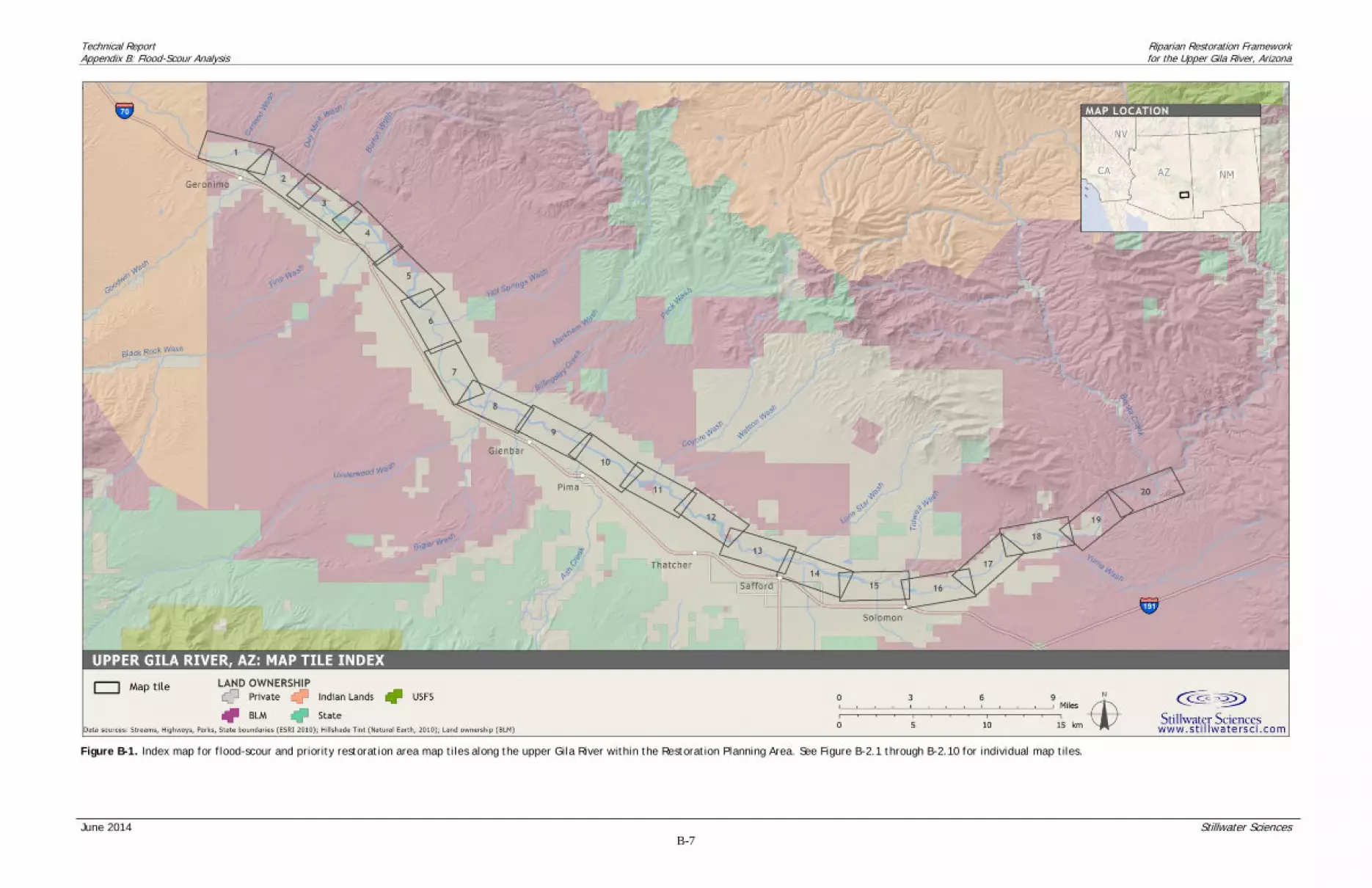
Technical Report Riparian Restoration Framework Appendix B: Flood-Scour Analysis for the Upper Gila River, Arizona
June 2014 Stillwater Sciences B-7
Figure B-1. Index map for flood-scour and priority restoration area map tiles along the upper Gila River within the Restoration Planning Area. See Figure B-2.1 through B-2.10 for individual map tiles.
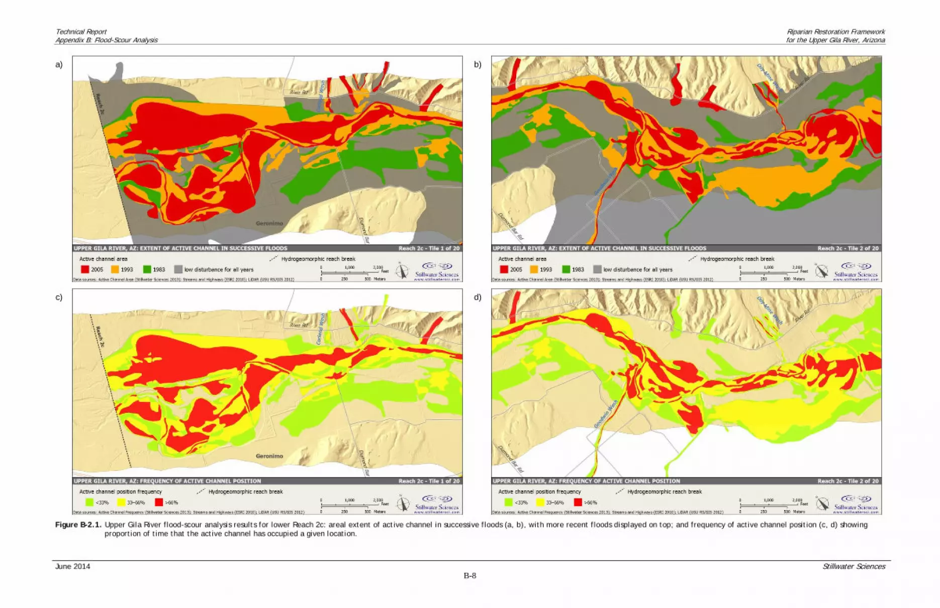
Technical Report Riparian Restoration Framework Appendix B: Flood-Scour Analysis for the Upper Gila River, Arizona
June 2014 Stillwater Sciences B-8
a)
b)
c)
d)
Figure B-2.1. Upper Gila River flood-scour analysis results for lower Reach 2c: areal extent of active channel in successive floods (a, b), with more recent floods displayed on top; and frequency of active channel position (c, d) showing proportion of time that the active channel has occupied a given location.
Technical Report Riparian Restoration Framework Appendix B: Flood-Scour Analysis for the Upper Gila River, Arizona
June 2014 Stillwater Sciences B-9
a)
b)
c)
d)
Figure B-2.2. Upper Gila River flood-scour analysis results for middle Reach 2c: areal extent of active channel in successive floods (a, b), with more recent floods displayed on top; and frequency of active channel position (c, d) showing proportion of time that the active channel has occupied a given location.
Technical Report Riparian Restoration Framework Appendix B: Flood-Scour Analysis for the Upper Gila River, Arizona
June 2014 Stillwater Sciences B-10
a)
b)
c)
d)
Figure B-2.3. Upper Gila River flood-scour analysis results for upper Reach 2c and lower Reach 2d: areal extent of active channel in successive floods (a, b), with more recent floods displayed on top; and frequency of active channel position (c, d) showing proportion of time that the active channel has occupied a given location.

Technical Report Riparian Restoration Framework Appendix B: Flood-Scour Analysis for the Upper Gila River, Arizona
June 2014 Stillwater Sciences B-11
a)
b)
c)
d)
Figure B-2.4. Upper Gila River flood-scour analysis results for upper Reach 2d and lower Reach 2e: areal extent of active channel in successive floods (a, b), with more recent floods displayed on top; and frequency of active channel position (c, d) showing proportion of time that the active channel has occupied a given location.

Technical Report Riparian Restoration Framework Appendix B: Flood-Scour Analysis for the Upper Gila River, Arizona
June 2014 Stillwater Sciences B-12
a)
b)
c)
d)
Figure B-2.5. Upper Gila River flood-scour analysis results for upper Reach 2e and lower Reach 2f: areal extent of active channel in successive floods (a, b), with more recent floods displayed on top; and frequency of active channel position (c, d) showing proportion of time that the active channel has occupied a given location.

Technical Report Riparian Restoration Framework Appendix B: Flood-Scour Analysis for the Upper Gila River, Arizona
June 2014 Stillwater Sciences B-13
a)
b)
c)
d)
Figure B-2.6. Upper Gila River flood-scour analysis results for upper Reach 2f and lower Reach 2g: areal extent of active channel in successive floods (a, b), with more recent floods displayed on top; and frequency of active channel position (c, d) showing proportion of time that the active channel has occupied a given location.

Technical Report Riparian Restoration Framework Appendix B: Flood-Scour Analysis for the Upper Gila River, Arizona
June 2014 Stillwater Sciences B-14
a)
b)
c)
d)
Figure B-2.7. Upper Gila River flood-scour analysis results for Reach 2g and lower Reach 2h: areal extent of active channel in successive floods (a, b), with more recent floods displayed on top; and frequency of active channel position (c, d) showing proportion of time that the active channel has occupied a given location.

Technical Report Riparian Restoration Framework Appendix B: Flood-Scour Analysis for the Upper Gila River, Arizona
June 2014 Stillwater Sciences B-15
a)
b)
c)
d)
Figure B-2.8. Upper Gila River flood-scour analysis results for upper Reach 2h and lower Reach 2i: areal extent of active channel in successive floods (a, b), with more recent floods displayed on top; and frequency of active channel position (c, d) showing proportion of time that the active channel has occupied a given location.
Technical Report Riparian Restoration Framework Appendix B: Flood-Scour Analysis for the Upper Gila River, Arizona
June 2014 Stillwater Sciences B-16
a)
b)
c)
d)
Figure B-2.9. Upper Gila River flood-scour analysis results for upper Reach 2i and lower Reach 2j: areal extent of active channel in successive floods (a, b), with more recent floods displayed on top; and frequency of active channel position (c, d) showing proportion of time that the active channel has occupied a given location.

Technical Report Riparian Restoration Framework Appendix B: Flood-Scour Analysis for the Upper Gila River, Arizona
June 2014 Stillwater Sciences B-17
a)
b)
c)
d)
Figure B-2.10. Upper Gila River flood-scour analysis results for upper Reach 2j and Reach 3a: areal extent of active channel in successive floods (a, b), with more recent floods displayed on top; and frequency of active channel position (c, d) showing proportion of time that the active channel has occupied a given location.

Technical Report Riparian Restoration Framework Appendix B: Flood-Scour Analysis for the Upper Gila River, Arizona
June 2014 Stillwater Sciences B-18
B2 REFERENCES
BOR. 2004. Upper Gila River fluvial geomorphology study: final report, Arizona. Prepared by the Fluvial Hydraulics & Geomorphology Team, Technical Service Center, Denver, CO. Graf, W. L. 2000. Locational probability for a dammed, urbanizing stream: Salt River, Arizona, USA. Environmental Management 25: 321–335. Tiegs, S. D. and M. Pohl. 2005. Planform channel dynamics of the lower Colorado River: 1976-2000. Geomorphology 69: 14–27. Tiegs, S. D., J. F. O’Leary, M. M. Pohl, and C. L. Munill. 2005. Flood disturbance and riparian diversity on the Colorado River Delta. Biodiversity and Conservation 14: 1175–1194.

Riparian Restoration Framework
Technical Report for the Upper Gila River, Arizona
Appendix C
Riparian Vegetation Transect-Plot Data
– Stillwater Sciences

Width
(m)
Length
(m)
Radius
(m)Local form
Relative
elevation
[from 2012
LiDAR] (m)
TextureMoisture
(Y/N)
Moisture
source
NRCS soil
texture
Years
since last
flooded
Flood
evidence
Flood
frequency
[from flood-
scour
analysis]
Ag return-
flow
influence
(Y/N)
Disturbance
type 1
Intensity of
type 1
Disturbance
type 2
Intensity of
type 2
Disturbance
type 3
Intensity of
type 3
boulder /
cobblegravel fines water vegetation
organic
debrisDominance
Herb
phenology
Shrub
phenology
Tree
phenology
Species 1
(Age, %)
Species 2
(Age, %
Cover)
Species 3
(Age, %
Cover)
Species 4
(Age, %
Cover)
Species 5
(Age, %
Cover)
Species 6
(Age, %
Cover)
Species 7
(Age, %
Cover)
Species 8
(Age, %
Cover)
Vegetation
type
Adjacent veg
type
Utah State
University
vegetation
class
Canopy
height [from
2012
LiDAR] (m)
1 20 20 undulating 6.604004 Sand no >10 medium no 0 0 15 0 75 10 Trees Late Late Late
Prosopis
glandulosa
(mature; 25)
Chilopsis
linearis
(mature; 1)
Parkinsonia
aculeatae
(mature; 3)
Larrea
tridentata
(mature; 1)
Annual
grasses (<0.3
m; 35)
Salsola spp.
(>0.3 m; 10)
Mesquite
bosqueSalt Cedar -0.001038
2 5 20 flat 6.971985 Silt no 1 to 2Debris
depositsmedium no 1 0 60 0 39 0 Shrubs Late Peak n/a
Hymenoclea
monogyra
(mature; 15)
Baccharis
sarothroides
(mature; 10)
Prosopis
glandulosa
(mature; 10)
Tamarix spp.
(mature; 2)
Annual
grasses (<0.3
m; 20)
Burrobrush
wash
Sand and
Rock-0.005981
3 5 20 convex 0.055969 Sand yes River <1 Drift lines high no 0 0 10 0 90 0 Trees Late Late Peak
Populus
fremontii
(mature; 5)
Salix
gooddingii
(mature; 20)
Salix exigua
(mature; 10)
Baccharis
salicifolia
(decadent; 15)
Prosopis
glandulosa
(mature; 5)
Tamarix spp.
(mature; 5)
Cynodon
dactylon (<0.3
m; 20)
Fremont
cottonwood-
Goodding’s
willow
woodland
Sand and
Rock (Water)0
4 5 20 flat 3.145996 Sand yes River <1 Drift lines high no 10 10 20 60 Trees Late Peak PeakSalix exigua
(mature; 20)
Salix
gooddingii
(pole; 40)
Cynodon
dactylon (<0.3
m; 10)
Fremont
cottonwood-
Goodding’s
willow
woodland
Salt Cedar
(Bare soil and
dry
vegetation)
0.283997
5 10 40 convex 0.036011 Silt yes River 1 to 2Sediment
depositmedium no
Competition
from exoticsLow 25 75 Trees Late Peak Peak
Populus
fremontii
(mature; 40)
Salix
gooddingii
(mature; 20)
Tamarix spp.
(mature; 20)
Salix exigua
(mature; 10)
Prosopis
glandulosa
(mature; 15)
Fremont
cottonwood-
Goodding’s
willow
woodland
Mesquite
bosque
Water (Bare
soil and dry
vegetation)
0
1 20 20 flat 5.314026 Silt nocoarse-
loamy6 to 10 low no 10 80 10 Trees n/a n/a Late
Populus
fremontii
(mature; 30)
Prosopis
glandulosa
(mature; 50)
Mesquite
bosque
Cottonwood/
Goodding
Willow
10.852966
2 20 20 undulating 3.472046 Silt nocoarse-
loamy<1 high no
Competition
from exoticsHigh 20 60 20 Shrubs n/a Late Late
Populus
fremontii
(mature; 10)
Tamarix spp.
(mature; 50)
Prosopis
glandulosa
(mature; 5)
Baccharis
sarothroides
(mature; 5)
Baccharis
salicifolia
(mature; 5)
Tamarisk-
mixed riparian
shrubland
Defoliated
Salt Cedar0
3 flat 2.588013 Gravel no sandy <1 high noCompetition
from exoticsLow 80 5 15 Shrubs n/a Late n/a
Tamarix spp
(mature; 5)
Hymenoclea
monogyra
(mature; 15)
Burrobrush
wash
Sand and
Rock0
4 convex 0.748962 Silt yes sandy <1 high noCompetition
from exoticsLow 30 30 30 Shrubs n/a Late n/a
Salix exigua
(mature; 25)
Tamarix spp.
(mature; 5)
Narrowleaf
willow-
mulefat
shrubland
Willow 1.414001
1 20 20 undulating 1.174011 Silt yescoarse-
loamy<1
Drift lines,
soil crackshigh no
Competition
from exoticsHigh ORV activity Low 0 0 80 0 20 0 Shrubs Peak n/a n/a
Tamarix spp.
(mature; 15)
Baccharis
salicifolia
(mature; 5)
Salix exigua
(mature; 2)
Tamarisk
shrubland
(low density)
Salt Cedar 1.197021
2 10 20 undulating 3.291016 Gravel no n/a 6 to 10Debris, drift
lineshigh no
Competition
from exoticsLow Earth moving High 10 10 20 0 60 10 Shrubs n/a n/a n/a
Hymenoclea
monogyra
(decadent; 25)
Tamarix spp.
(mature; 2)
Salsola spp.
(>0.3 m; 5)
Portulaca
oleracea (<0.3
m; 25)
Annual
grasses (<0.3
m; 25)
Burrobrush
washSalt Cedar 0.01001
3 5 20 flat 0.619019 Gravel nosandy-
skeletal<1
Drift lines,
bent veghigh no
Competition
from exoticsHigh 10 10 20 0 50 10 Shrubs Peak Peak n/a
Tamarix spp.
(mature; 20)
Baccharis
salicifolia
(mature; 20)
Cynodon
dactylon (<0.3
m; 10)
Tamarisk-
mixed riparian
shrubland
Bare soil and
dry vegetation0.036011
4 20 40 undulating 2.083008 Silt yes Riversandy-
skeletal1 to 2
Drift lines,
debrismedium no
Competition
from exoticsMedium 0 10 20 70 0 Shrubs Late Late n/a
Tamarix spp.
(mature; 20)
Baccharis
salicifolia
(mature; 5)
Salix exigua
(mature; 45)
Narrowleaf
willow-
mulefat
shrubland
Burrobrush
wash,
Mequite
bosque
Defoliated
Salt Cedar
(Salt Cedar)
0.003967
5 10 40 concave 1.528992 Silt yes Ag runoffcoarse-
loamy>10 high yes
Competition
from exoticsHigh 10 10 3 0 95 2 Shrubs Peak Late Peak
Tamarix spp.
(mature; 50)
Baccharis
salicifolia
(mature; 5)
Populus
fremontii
(mature; 10)
Salix exigua
(mature; 10)
Atriplex
canescens
(mature; 5)
Tamarisk-
mixed riparian
shrubland
Cottonwood/
Goodding
Willow
0.938965
1 25 40 convex 0.666992 Silt yes Riversandy-
skeletal<1
Drift lines,
debrishigh uncertain 0 0 5 30 60 5 Shrubs Late Late n/a
Salix exigua
(mature; 35)
Tamarix spp.
(mature; 25)
Baccharis
salicifolia
(mature; 5)
Salix
gooddingii
(mature; 5)
Sorghum
halepense
(>0.3 m; 5)
Cynodon
dactylon
(<0.3 m; 10)
Narrowleaf
willow-
mulefat
shrubland
Willow 0.004028
2 40 40 flat 1.473022 Silt nocoarse-
loamy<1 Drift lines high no
Competition
from exoticsHigh 10 65 0 15 10 Shrubs Late Late n/a
Tamarix spp.
(mature; 10)
Sorghum
halepense
(>0.3 m ; 5)
Tamarisk
wash
Sand and
Rock0.003967
3 20 20 undulating 2.655029 Silt yes Swalesandy-
skeletal3 to 5 Debris medium no 0 0 15 0 35 50 Trees Late Peak n/a
Tamarix spp.
(mature; 20)
Heliomeris
longifolia var.
annua (<0.3
m ; 15)
Tamarisk
shrubland
Defoliated
Salt Cedar0.435974
4 10 30 convex 4.042969 Silt yes Ag runoffcoarse-
loamy>10 n/a yes Agriculture Low 0 0 5 0 85 10 Trees Late Peak Late
Populus
fremontii
(mature; 90)
Salix
gooddingii
(mature; 18)
Prosopis
glandulosa
(mature; 10)
Baccharis
salicifolia
(mature; 5)
Sarcostemma
cynanchoides
(mature; 1)
Sorghum
halepense
(>0.3 m; 10)
Fremont
cottonwood-
Goodding’s
willow
woodland
Tamarisk
shrubland
Cottonwood/
Goodding
Willow
3.637024
1 20 30 convex 2.491028 Silt yescoarse-
loamy<1 Debris high uncertain
Competition
from exoticsMedium 10 0 10 40 40 10 Shrubs Late Late Late
Tamarix spp.
(mature; 25)
Salix exigua
(mature; 10)
Salix
gooddingii
(seedling; 2)
Sorghum
halepense
(>0.3 m ; 2)
Cynodon
dactylon (<0.3
m; 5)
Tamarisk-
mixed riparian
shrubland
Tamarisk
wash
Salt Cedar
(Defoliated
Salt Cedar)
1.130981
2 5 20 undulating 2.757019 Silt nocoarse-
loamy3 to 5
Debris,wate
r cracksn/a uncertain
Competition
from exoticsLow 0 0 10 0 80 10 Trees Late Late Late
Populus
fremontii
(decadent; 50)
Bassia
scoparia (>0.3
m ; 10)
Datura
wrightii (>0.3
m; 2)
Tamarix spp.
(mature; 15)
Fremont
cottonwood-
Goodding’s
willow
woodland
Tamarisk
wash,
Tamarisk
shrubland
Cottonwood/
Goodding
Willow
0
3 20 20 flat 0.982971 Silt no
coarse-
loamy over
sandy or
sandy-
skeletal
>10 high no ORV activity LowCompetition
from exoticsLow 0 0 50 0 30 20 Trees Late Late n/a
Baccharis
sarothroides
(decadent; 15)
Atriplex
canescens
(mature; 10)
Lycium
torreyi
(mature; 1)
Tamarix spp.
(mature; 5)
Acacia greggii
(seedling; 2)
Salsola spp.
(>0.3 m; 2)
Amaranth
spp. (>0.3 m;
5)
Mixed
shrubland
Tamarisk
wash
Sand and
Rock0
1 20 20 flat 0.45697 Silt yes Rivercoarse-
loamy<1
Matted
grasshigh no ORV activity Low
Competition
from exoticsMedium 30 50 15 5 Shrubs Late Late n/a
Tamarix spp.
(mature; 10)
Hymenoclea
monogyra
(mature; 5)
Sorghum
halepense
(>0.3 m; 3)
Cynodon
dactylon (<0.3
m; 1)
Tamarisk
washSalt Cedar 2.10199
2 10 20 convex 0.541992 Sand yes River
coarse-
loamy over
sandy or
sandy-
skeletal
<1 Bent veg high no
Recreational
use (non-
ORV)
LowCompetition
from exoticsLow ORV activity Low 5 95 Shrubs Late Peak n/a
Tamarix spp.
(mature; 15)
Baccharis
salicifolia
(mature; 30)
Salix exigua
(mature; 20)
Sorghum
halepense
(>0.3 m ; 60)
Mixed
riparian
shrubland
Sand and
Rock-0.001038
3 10 10 flat 3.454041 Silt nosandy-
skeletal6 to 10 medium no
Competition
from exoticsHigh 10 15 75 Shrubs n/a Late n/a
Tamarix spp.
(mature; 12)
Datura
wrightii (>0.3
m ; 1)
Salsola spp.
(>0.3 m; 2)
Tamarisk
shrubland
Defoliated
Salt Cedar0
4 20 20 flat 3.30603 Silt yes Swale
coarse-
loamy over
sandy or
sandy-
skeletal
6 to 10 high noCompetition
from exoticsHigh 40 50 10 Shrubs Late Late n/a
Tamarix spp.
(mature; 20)
Heliomeris
longifolia var.
annua (<0.3
m ; 15)
Trianthema
portulacastru
m (<0.3 m;
15)
Chameasyce
sp. (<0.3 m;
15)
Baccharis
sarothroides
(mature; 2)
Salsola spp.
(>0.3 m; 10)
Tamarisk
shrubland
Defoliated
Salt Cedar-0.005005
5 5 20 flat 1.325989 Silt yes Rivercoarse-
loamy<1
Debris, bent
veghigh no
Competition
from exoticsMedium 15 70 15 Shrubs Late Late n/a
Tamarix spp.
(mature; 15)
Sorghum
halepense
(>0.3 m ; 40)
Cynodon
dactylon (<0.3
m; 30)
Salix exigua
(mature; 2)
Baccharis
salicifolia
(mature; 2)
Tamarisk
washWillow 0.04303
Vegetation Cover TypesHydro-
geomorphic
reach
(upstream to
downstream
order)
TransectPlot
number
Plot dimensions (m)
Fire
evidence
(Y/N)
Disturbance & Intensity Type % CoverSoil Conditions HydrologyTopography
1
3
4
6
7
8
3a
2j
2i

1 10 30 undulating 3.692017 Loam uncertainLots of leaf
litter
coarse-
loamy over
sandy or
sandy-
skeletal
6 to 10 n/a yesCompetition
from exoticsMedium Agriculture Medium 100 Trees Late Late Late
Salix
gooddingii
(mature; 60)
Tamarix spp.
(mature; 30)
Pluchea
sericea
(mature; 15)
Sporobolus
spp. (>0.3 m ;
10)
Sarcostemma
cynanchoides
(mature; 2)
Fremont
cottonwood-
Goodding’s
willow
woodland
Salt Cedar 9.953003
2 15 15 flat 3.465027 Silt noLots of leaf
litter
coarse-
loamy over
sandy or
sandy-
skeletal
6 to 10 n/a noCompetition
from exoticsHigh 20 30 50 Shrubs Peak Late n/a
Tamarix spp.
(decadent; 20)
Trianthema
portulacastum
(<0.3 m ; 10)
Brassica
tournefortii
(<0.3 m; 5)
Heliomeris
longfolia var.
annua (<0.3
m; 10)
Tamarisk
shrubland
Salt Cedar
(Defoliated
Salt Cedar)
2.294983
3 28 40 flat 2.719971 Silt uncertain n/a 6 to 10 n/a noCompetition
from exoticsHigh 10 80 10 Shrubs n/a Late Late
Tamarix spp.
(decadent; 60)
Populus
fremontii
(mature; 5)
Salix
gooddingii
(mature; 5)
Salix exigua
(decadent; 20)
Tamarisk
shrubland
Tamarisk
wash
Defoliated
Salt Cedar1.057007
1 10 15 undulating 0.385986 Silt yesSide
channel
sandy-
skeletal1 to 2
Debris drift
lineshigh no
Competition
from exoticsMedium 10 90 5 Shrubs Late Late <n/a>
Tamarix spp.
(mature; 15)
Salix exigua
(mature; 70)
Baccharis
salicifolia
(mature; 5)
Narrowleaf
willow-
mulefat
shrubland
Burrobrush
washSalt Cedar 2.973999
2 10 15 flat 3.171997 Silt no n/a 6 to 10 low noCompetition
from exoticsHigh 30 40 30 Shrubs Late Late Late
Tamarix spp.
(decadent; 30)
Prosopis
glandulosa
(mature; 10)
Salsola spp.
(>0.3 m; 10)
Datura
wrightii (>0.3
m; 5)
Trianthema
portulacastru
m (<0.3 m; 5)
Tamarisk
shrubland
Narrowlead
willow-
mulefat
shrubland
Sand and
Rock1.536011
3 40 40 flat 2.184021 Silt nosandy-
skeletal1 to 2
Debris
depositshigh no
Competition
from exoticsLow ORV activity Medium 10 15 40 30 5 Shrubs Late Late n/a
Hymenoclea
monogyra
(mature; 10)
Tamarix spp.
(decadent; 5)
Annual
grasses and
forbs (<0.3 m;
15)
Burrobrush
wash
Tamarisk
shrubland
(low density)
Sand and
Rock0.013
1 10 10 flat 1.43103 Silt yes Ag runoff fine-silty 3 to 5 Moist soil, n/a yes 100 Shrubs n/a Late n/aTypha spp.
(mature; 100)
Floodplain
wetlandSalt Cedar 0.06897
2 10 10 flat 1.289001 Silt yes Ag runoffcoarse-
loamy3 to 5
Silt
deposits,
bent veg
n/a yesCompetition
from exoticsHigh 2 98 Shrubs Late Late n/a
Tamarix spp.
(mature; 98)
Baccharis
emoryi
(mature; 1)
Paspalum sp.
(>0.3 m; 2)
Tamarisk
shrubland
Cottonwood/
Goodding
Willow
3.73999
3 15 15 flat 1.677979 Silt yes Ag runoff fine-silty 3 to 5
Silt
deposits,
bent veg
low yesCompetition
from exoticsHigh 10 80 10 Trees Late Late Late
Tamarix spp.
(mature; 10)
Baccharis
emoryi
(mature; 15)
Populus
fremontii
(decadent; 5)
Salix
gooddingii
(mature; 60)
Salix exigua
(mature; 10)
Baccharis
sarothroides
(mature; 5)
Paspalum sp.
(>0.3 m; 1)
Cyperus sp.
(>0.3 m; 1)
Fremont
cottonwood-
Goodding’s
willow
woodland
Salt Cedar 10.093994
4 30 30 convex -0.049011 Silt yes Rivercoarse-
loamy<1 Drift lines high no
Competition
from exoticsHigh 10 10 20 30 30 Shrubs n/a Late n/a
Baccharis
salicifolia
(mature; 7)
Tamarix spp.
(mature; 15)
Salix exigua
(mature; 8)
Sorghum
halepense
(>0.3 m ; 10)
Cynodon
dactylon (<0.3
m; 5)
Mixed
riparian
shrubland
Tamarisk
washWillow -0.054016
5 convex -1.265991 Silt yes Pond n/a 6 to 10 high uncertainCompetition
from exoticsHigh 20 50 30 Shrubs Late Late n/a
Tamarix spp.
(seedling; 5)
Typha spp.
(<0.3 m; 2)
Salix exigua
(mature; 3)
Floodplain
wetland
Tamarisk
shrubland,
Floodplain
herbaceous
Bare soil and
dry vegetation0.927979
6 10 30 convex 0.736023 Silt uncertaincoarse-
loamy6 to 10 low uncertain yes
Competition
from exoticsHigh 70 30 Shrubs n/a Late Late
Tamarix spp.
(mature; 60)
Salix
gooddingii
(mature; 2)
Populus
fremontii
(decadent; 8)
Tamarisk-
mixed riparian
shrubland
Defoliated
Salt Cedar
(Salt Cedar)
-0.005005
1 60 60 convex 3.284973 Gravel yes Rivercoarse-
loamy<1
Debris
depositshigh no
Competition
from exoticsHigh 5 20 20 15 30 10 Shrubs Late Late Late
Tamarix spp.
(mature; 30)
Hymenoclea
monogyra
(mature; 3)
Salix exigua
(mature; 5)
Tamarisk
shrubland
(low density)
Bare soil and
dry vegetation0.129028
2 15 38 flat 2.031982 Silt yescoarse-
loamy<1
Debris
depositshigh uncertain
Competition
from exoticsMedium 70 15 15 Herbs Late Late n/a
Sorghum
halepense
(>0.3 m; 10)
Tamarix spp.
(mature; 5)
Floodplain
herbaceous
Sand and
Rock0.02002
3 10 30 convex 3.670044 Silt nocoarse-
loamy6 to 10 medium uncertain
Competition
from exoticsHigh 5 90 5 Shrubs Late Late Late
Populus
fremontii
(decadent; 10)
Salix
gooddingii
(mature; 10)
Tamarix spp.
(mature; 70)
Tamarisk-
mixed riparian
shrubland
Cottonwood/
Goodding
Willow
3.312012
4 10 30 flat 3.388 Silt yes Recent raincoarse-
loamy3 to 5 Bent veg low uncertain
Competition
from exoticsHigh 98 2 Shrubs Late Late Late
Populus
fremontii
(mature; 30)
Salix exigua
(mature; 15)
Tamarix spp.
(mature; 65)
Tamarisk-
mixed riparian
shrubland
Salt Cedar
(Defoliated
Salt Cedar)
0
5 20 20 convex 1.77002 Silt yes Recent rain
coarse-
loamy over
sandy or
sandy-
skeletal
<1Bent veg,
moist soilslow no
Competition
from exoticsHigh 5 3 90 2 Shrubs Late Late Late
Populus
fremontii
(decadent; 30)
Salix
gooddingii
(decadent; 20)
Tamarix spp.
(mature; 50)
Baccharis
emoryi
(mature; 2)
Phragmites
australis (>0.3
m; 1)
Schoenoplect
us spp. (>0.3
m; 1)
Fremont
cottonwood-
Goodding’s
willow
woodland
Salt Cedar
(Cottonwood/
Goodding
Willow)
0.115967
6 20 20 flat 3.239014 Silt yes Recent rain
coarse-
loamy over
sandy or
sandy-
skeletal
3 to 5Debris
depositslow no
Competition
from exoticsHigh 20 75 5 Shrubs Late Late Late
Tamarix spp.
(decadent; 30)
Suaeda spp.
(>0.3 m; 5)
Atriplex
lentiformis
(mature; 10)
Trianthema
portulacastru
m (<0.3 m;
20)
Amaranth
spp. (<0.3 m;
5)
Tamarisk
shrubland
(low density)
Defoliated
Salt Cedar0
1 20 30 undulating 2.849976 Silt uncertaincoarse-
loamy<1 Drift lines high no
Competition
from exoticsHigh 15 85 Trees n/a Late Late
Tamarix spp
(mature; 50)
Populus
fremontii
(mature; 15)
Baccharis
salicifolia
(mature; 1)
Baccharis
emoryi
(mature; 3)
Baccharis
sarothroides
(mature; 1)
Salix
gooddingii
(mature; 25)
Arundo donax
(mature; 2)
Fremont
cottonwood-
Goodding’s
willow
woodland
Tamarisk
shrubland
(low density)
Cottonwood/
Goodding
Willow (Salt
Cedar)
0.682007
2 20 undulating 3.512024 Silt yes Uncertain fine-silty 1 to 2 Drift lines low noCompetition
from exoticsHigh 60 40 Shrubs n/a Late n/a
Tamarix spp.
(mature; 40)
Tamarisk
shrubland
Tamarisk
shrublandSalt Cedar 1.731995
3 30 30 flat 2.544006 Silt yescoarse-
loamy6 to 10
Silt on
brancheslow uncertain
Competition
from exoticsHigh 75 25 Shrubs n/a Late Late
Populus
fremontii
(decadent; 10)
Salix
gooddingii
(mature; 15)
Tamarix spp.
(mature; 15)
Baccharis
emoryi
(mature; 35)
Salix exigua
(mature; 2)
Fremont
cottonwood-
Goodding’s
willow
woodland
Salt Cedar
(Cottonwood/
Goodding
Willow)
5.541992
4 20 flat 3.195007 Silt nocoarse-
loamy3 to 5 low no
Competition
from exoticsHigh 65 30 5 Shrubs Late Late <n/a>
Tamarix spp.
(decadent; 30)
Annual herbs
(<0.3 m; 10)
Tamarisk
shrubland
(low density)
Tamarisk-
mixed riparian
shrubland
Sand and
Rock-0.051025
1 20 15 flat 2.411987 Silt yesSecondary
channel
coarse-
loamy3 to 5 Wet soils low uncertain
Competition
from exoticsHigh 100 Trees n/a Late Late
Tamarix spp.
(mature; 70)
Populus
fremontii
(mature; 25)
Salix
gooddingii
(mature; 15)
Tamarisk-
mixed riparian
shrubland
Cottonwood/
Goodding
Willow
4.737
2 15 20 flat 1.888 Silt yesRecent
inundation
coarse-
loamy<1
Bent veg,
wet soilmedium no
Competition
from exoticsHigh 5 90 5 Shrubs Late Late n/a
Tamarix spp.
(mature; 90)
Salix exigua
(mature; 3)
Atriplex
lentiformis
(mature; 5)
Tamarisk
shrubland
(high density)
Tamarisk
shrublandSalt Cedar 0.158997
3 28 20 undulating 1.641052 Silt yesRecent
inundation
coarse-
loamy over
sandy or
sandy-
skeletal
<1Bent veg,
wet soilhigh no
Competition
from exoticsHigh 45 50 5 Shrubs Peak Late Late
Tamarix spp.
(mature; 45)
Populus
fremontii
(mature; 2)
Baccharis
salicifolia
(mature; 5)
Baccharis
emoryi
(mature; 1)
Tamarisk
shrubland
Tamarisk
shrubland
Bare soil and
dry vegetation
(Sand and
Rock)
0.509949
4 10 10 flat 1.883057 Silt uncertainRecent
inundationsandy 6 to 10
Silt on
debrislow no
Competition
from exoticsHigh 100 Shrubs Late Late n/a
Tamarix spp.
(mature; 100)
Sarcostemma
cynanchoides
(mature; 25)
Tamarisk
shrubland
(high density)
Tamarisk
shrublandSalt Cedar 5.626953
off transect 15 30 flat 2.717041 Silt noRecent
inundation
coarse-
loamy6 to 10 n/a yes
Competition
from exoticsHigh 95 5 Shrubs Peak Late Late
Tamarix spp.
(mature; 45)
Populus
fremontii
(mature; 30)
Salix
gooddingii
(mature; 5)
Baccharis
emoryi
(mature; 10)
Prosopis
glandulosa
(mature; 5)
Fremont
cottonwood-
Goodding’s
willow
woodland
Cottonwood/
Goodding
Willow
9.335999
1 15 15 undulating 3.517029 Silt yes Ag runoff fine-silty 3 to 5 n/a uncertainCompetition
from exoticsLow 10 90 0 Herbs Late Late n/a
Baccharis
emoryi
(mature; 40)
Suaeda spp.
(>0.3 m; 45)
Tamarix spp.
(mature; 5)
Sporobolus
spp. (>0.3 m ;
5)
Mixed
riparian
shrubland
Fremont
cottonwood
woodland
Salt Cedar 3.151978
2e
2c
92h
2g
2f
10
11
12
14
15
2d
16

2 20 undulating 2.619995 Silt yes Recent raincoarse-
loamy6 to 10 n/a uncertain Earth moving Medium 100 Trees n/a n/a Late
Populus
fremontii
(mature; 50)
Tamarix spp.
(mature; 50)
Baccharis
emoryi
(mature; 10)
Fremont
cottonwood-
Goodding’s
willow
woodland
Cottonwood/
Goodding
Willow
9.382996
3 20 undulating 2.815002 Silt no fine-silty 3 to 5 Bent veg high noCompetition
from exoticsHigh 50 50 0 Shrubs Late Late Late
Tamarix spp.
(mature; 40)
Salix exigua
(mature; 10)
Populus
fremontii
(mature; 3)
Baccharis
emoryi
(mature; 2)
Tamarisk
shrubland
(low density)
Salt Cedar 0.586975
4 10 flat 2.313965 Silt yes Uncertaincoarse-
loamy<1
Bent veg,
debris,
sediment
low noCompetition
from exoticsMedium 50 90 10 Trees Late Late Late
Tamarix spp.
(mature; 80)
Baccharis
emoryi
(mature; 1)
Populus
fremontii
(decadent; 50)
Baccharis
salicifolia
(mature; 1)
Fremont
cottonwood-
Goodding’s
willow
woodland
Cottonwood/
Goodding
Willow (Salt
Cedar)
4.813049
5 15 20 convex 0.542969 Silt yes Rivercoarse-
loamy<1
Bent veg,
debrishigh no
Competition
from exoticsHigh 50 40 60 10 Shrubs Late Late n/a
Tamarix spp.
(mature; 40)
Salix exigua
(mature; 5)
Arundo donax
(mature; 2)
Baccharis
emoryi
(mature; 1)
Cynodon
dactylon (<0.3
m; 15)
Tamarisk-
mixed riparian
shrubland
Tamarisk
shrubland
Cottonwood/
Goodding
Willow
3.069031
1 15 20 convex 3.534973 Silt yes Rivercoarse-
loamy<1
Bent trees,
water lineshigh no
Competition
from exoticsHigh 20 30 50 Shrubs n/a Late n/a
Tamarix spp.
(mature; 40)
Salix exigua
(mature; 3)
Baccharis
emoryi
(mature; 3)
Tamarisk
shrubland
Tamarisk
shrubland
(low density)
Sand and
Rock0.363037
2 30 50 undulating 2.109009 Silt yes Rivercoarse-
loamy<1 Bent veg high no
Competition
from exoticsHigh 25 70 5 Shrubs Late Late Peak
Tamarix spp.
(mature; 20)
Salix exigua
(mature; 15)
Sorghum
halepense
(>0.3 m; 40)
Populus
fremontii
(mature; 5)
Salix
gooddingii
(mature; 1)
Baccharis
emoryi
(mature; 1)
Tamarisk-
mixed riparian
shrubland
Sand and
Rock-0.040039
3 10 10 flat 3.540955 Silt yes Recent rain fine-silty 6 to 10 n/a uncertainCompetition
from exoticsHigh Earth moving Low 100 Shrubs n/a Late n/a
Tamarix spp.
(mature; 100)
Tamarisk
shrubland
Salt Cedar
(Cottonwood/
Goodding
Willow)
5.057007
4 15 30 flat 3.784973 Silt nocoarse-
loamy6 to 10 n/a uncertain
Competition
from exoticsHigh 95 5 Shrubs n/a Late Late
Populus
fremontii
(mature; 30)
Suaeda spp.
(>0.3 m; 20)
Tamarix spp.
(mature; 55)
Fremont
cottonwood-
Goodding’s
willow
woodland
Salt Cedar 4.419006
1 10 15 undulating 1.929993 Silt yes Recent raincoarse-
loamy3 to 5 low no
Competition
from exoticsHigh 3 95 2 Shrubs n/a Late n/a
Tamarix spp.
(mature; 95)
Tamarisk
shrublandSalt Cedar 4.308044
2 15 20 convex 1.765991 Silt yes Rivercoarse-
loamy<1 bent veg low no
Competition
from exoticsHigh 5 50 40 5 Shrubs n/a Late n/a
Tamarix spp.
(mature; 30)
Salix exigua
(mature; 10)
Baccharis
emoryi
(mature; 2)
Tamarisk-
mixed riparian
shrubland
Salt Cedar
(Cottonwood/
Goodding
Willow)
1.379028
3 20 20 flat 1.297974 Silt yes Uncertaincoarse-
loamy6 to 10
Silt
depositionn/a no
Competition
from exoticsLow 98 2 Trees n/a n/a Late
Tamarix spp.
(mature; 15)
Populus
fremontii
(seedling; 70)
Salix
gooddingii
(seedling; 10)
Salix exigua
(mature; 5)
Fremont
cottonwood-
Goodding’s
willow
woodland
Cottonwood/
Goodding
Willow
5.530029
4 15 30 undulating 1.177002 Sand uncertain uncertaincoarse-
loamy3 to 5
Silt
deposition,
drift line
high noCompetition
from exoticsHigh 60 40 Shrubs n/a Late Late
Tamarix spp.
(mature; 30)
Populus
fremontii
(decadent; 5)
Baccharis
salicifolia
(mature; 5)
Tamarisk
shrubland
(low density)
Tamarisk
shrubland
(high density)
Sand and
Rock-0.046021
1 10 10 undulating 3.749023 Silt yes uncertaincoarse-
loamy1 to 2 Bent veg medium uncertain yes
Competition
from exoticsHigh 100 Shrubs n/a n/a Late
Tamarix spp.
(mature; 100)
Tamarisk
shrublandSalt Cedar 3.299988
2 20 30 convex 3.756042 Silt yes Rivercoarse-
loamy<1
Recent silt
depositionlow no yes
Competition
from exoticsHigh 10 50 40 Shrubs n/a Late n/a
Tamarix spp.
(mature; 40)
Baccharis
emoryi
(mature; 2)
Tamarisk
shrubland
Salt Cedar
(Cottonwood/
Goodding
Willow)
1.703979
3 5 20 undulating 1.252991 Silt yes Uncertaincoarse-
loamy3 to 5
Drift line,
sed Deposithigh no
Competition
from exoticsHigh 1 98 1 Shrubs n/a Late Late
Tamarix spp.
(mature; 75)
Populus
fremontii
(mature; 15)
Baccharis
salicifolia
(mature; 1)
Tamarisk-
mixed riparian
shrubland
Salt Cedar 4.007996
4 20 20 flat 1.95697 Silt nocoarse-
loamy3 to 5 Bent veg high no
Competition
from exoticsMedium 25 50 25 Shrubs n/a n/a n/a
Hymenoclea
monogyra
(mature; 20)
Tamarix spp.
(mature; 5)
Baccharis
sarothroides
(mature; 1)
Burrobrush
wash
Sand and
Rock0.005005
5 10 10 flat 7.784973 Silt nocoarse-
loamy>10 n/a uncertain 1 25 70 15 Trees Late Late Late
Prosopis
glandulosa
(mature; 50)
Atriplex
elegans
(mature; 5)
Lycium
torreyi
(mature; 15)
Mesquite
bosque
Salt Cedar
(Bare soil and
dry
vegetation)
1.455017
1 convex 4.866028 Gravel nocoarse-
loamy<1 low no yes
Competition
from exoticsHigh 10 30 60 Shrubs n/a Late n/a
Tamarix spp.
(mature; 60)
Tamarisk-
mixed riparian
shrubland
Salt Cedar 0.737976
2 20 20 convex 1.192017 Silt yes Rivercoarse-
loamy<1 Drift lines medium no yes
Competition
from exoticsHigh 10 50 40 Shrubs Late Late n/a
Tamarix spp.
(mature; 40)
Cynodon
dactylon (<0.3
m; 5)
Tamarisk
shrublandSalt Cedar 5.505005
3 20 25 convex 2.31604 Sand yes uncertaincoarse-
loamy1 to 2 Bent veg medium uncertain
Competition
from exoticsHigh 50 45 5 Shrubs n/a Late Late
Tamarix spp.
(mature; 30)
Populus
fremontii
(mature; 15)
Tamarisk-
mixed riparian
shrubland
Tamarisk
shrubland
Sand and
Rock-0.030029
1 10 20 flat 4.248047 Silt no fine-silty >10 n/a noCompetition
from exoticsLow 5 80 5 Shrubs Late Late Late
Lycium
torreyi
(mature; 5)
Prosopis
glandulosa
(mature; 40)
Tamarix spp.
(mature; 5)
Atriplex
polycarpa
(mature; 30)
Ericameria
spp. (mature;
15)
Suaeda spp.
(>0.3 m; 10)
Mesquite
bosque
Sand and
Rock0
2 10 10 undulating 3.932983 Silt no fine-silty 6 to 10 n/a noCompetition
from exoticsHigh 95 5 Shrubs n/a Late n/a
Tamarix spp.
(mature; 95)
Tamarisk
shrublandSalt Cedar 0.264038
1 20 40 convex 5.327026 Silt yes Rivercoarse-
loamy1 to 2
Wet soils,
some debrislow no
Competition
from exoticsHigh 5 25 75 Shrubs Late Late Late
Populus
fremontii
(mature; 15)
Salix
gooddingii
(mature; 10)
Tamarix spp.
(mature; 45)
Salix exigua
(mature; 5)
Cynodon
dactylon (<0.3
m; 5)
Tamarisk-
mixed riparian
shrubland
Agriculture
Cottonwood/
Goodding
Willow
7.432007
2 40 40 flat 2.78595 Silt nocoarse-
loamy3 to 5 n/a no yes
Competition
from exoticsHigh 50 50 Shrubs n/a Late n/a
Tamarix spp.
(mature; 50)
Tamarisk
shrubland
Tamarisk-
mixed riparian
shrubland
Salt Cedar 4.762024
1 15 20 convex 1.755981 Silt yes Rivercoarse-
loamy1 to 2 Bent veg low no yes
Competition
from exoticsHigh 10 50 40 Shrubs Peak Late n/a
Baccharis
salicifolia
(mature; 10)
Tamarix spp.
(decadent; 30)
Cynodon
dactylon (<0.3
m; 15)
Tamarisk
shrublandn/a 1.445007
2 20 20 flat 1.578979 Silt nocoarse-
loamy3 to 5 Silt deposit medium no
Competition
from exoticsLow 65 35 2 Herbs Late Late n/a
Cynodon
dactylon (<0.3
m; 10)
Xanthium
strumarium
(<0.3 m; 20)
Tamarix spp.
(mature; 3)
Baccharis
salicifolia
(mature; 3)
Floodplain
herbaceousn/a 0
3 20 20 flat 2.466003 Silt no fine-silty 3 to 5 medium no yesCompetition
from exoticsLow Agriculture Low 20 80 Shrubs Late Late n/a
Baccharis
sarothroides
(mature; 10)
Tamarix spp.
(mature; 5)
Baccharis
salicifolia
(mature; 2)
Annual grass
and herbs
(<0.3 m; 5)
Mixed
riparian
shrubland
n/a 0
20 flat 3.475037 Silt yescoarse-
loamy<1
Silt on
stemsmedium no yes
Competition
from exoticsHigh 15 65 20 Trees n/a Late Late
Populus
fremontii
(decadent; 40)
Tamarix spp.
(mature; 30)
Baccharis
salicifolia
(mature; 5)
Fremont
cottonwood-
Goodding’s
willow
woodland
n/a 8.024963
20 20 flat 4.582031 Silt uncertain fine-silty 6 to 10 Water lines low uncertain yesCompetition
from exoticsHigh 95 5 Shrubs Late Late n/a
Tamarix spp.
(mature; 80)
Salix
gooddingii
(mature; 5)
Baccharis
emoryi
(mature; 5)
Sporobolus
spp. (>0.3 m ;
5)
Tamarisk-
mixed riparian
shrubland
Salt Cedar
(Bare soil and
dry
vegetation)
1.927979
2c
23
off transect
17
18
19
20
21
22
16

Riparian Restoration Framework
Technical Report for the Upper Gila River, Arizona
Appendix D
Riparian Plant Species Requirements
– Stillwater Sciences
Technical Report Riparian Restoration Framework Appendix D: Riparian Plant Species Requirements for the Upper Gila River, Arizona
June 2014 Stillwater Sciences D-1
D1 INTRODUCTION
This appendix presents supplemental information on growing requirements for many of the native plant species that may be appropriate to restore in the Planning Area.
D1.1 Background Information and Data Definitions
Wetland and riparian vegetation dynamics are tightly coupled with hydrogeomorphic processes. Inputs of water, sediment, nutrients, and other ecological factors provide the raw materials that are shaped by physical forces such as groundwater-surface water interactions, flooding, tidal forces, erosion, sediment deposition, and chemical exchanges to develop wetland, channel and floodplain habitats. These inputs strongly influence plant species composition, distribution, and physical structure. Vegetation structure and composition, in turn, provide habitat, shade, cover, food, energy, and organic matter inputs for wildlife and aquatic communities and influence their population and food web dynamics. Plant species are distributed along gradients of resource availability (e.g., light, water, nutrients), chronic environmental stress (e.g., salinity, inundation duration), and episodic physical disturbance (e.g., fire, flood, scour). Each plant species has evolved a unique suite of life history traits to cope with its environmental conditions, and its distribution across the landscape reflects the tradeoffs of its particular stress-tolerance and resource-capture strategies. Riparian and wetland plants can be classified by their tolerances to drought, inundation, shade, salt, and herbivory. Other factors such as soil texture, rooting depth, and water use efficiency affect the ways plant species use below-ground resources and thus influence their distributions among suitable sites. A list of native riparian trees, shrubs, forbs, and herbs found in the Gila Valley Planning Area was developed (Table D-1), and information on water availability/use factors, soil conditions, and other environmental characteristics (shade tolerance, tolerance to hedging, minimum temperature) necessary for growth and survival of each species were identified from the USDA PLANTS Database (NRCS 2002). The contents of Table D-1 are defined in the following sections. This information can be used to identify and prioritize potential riparian vegetation restoration areas within the Planning Area based on physical and other biological factors.
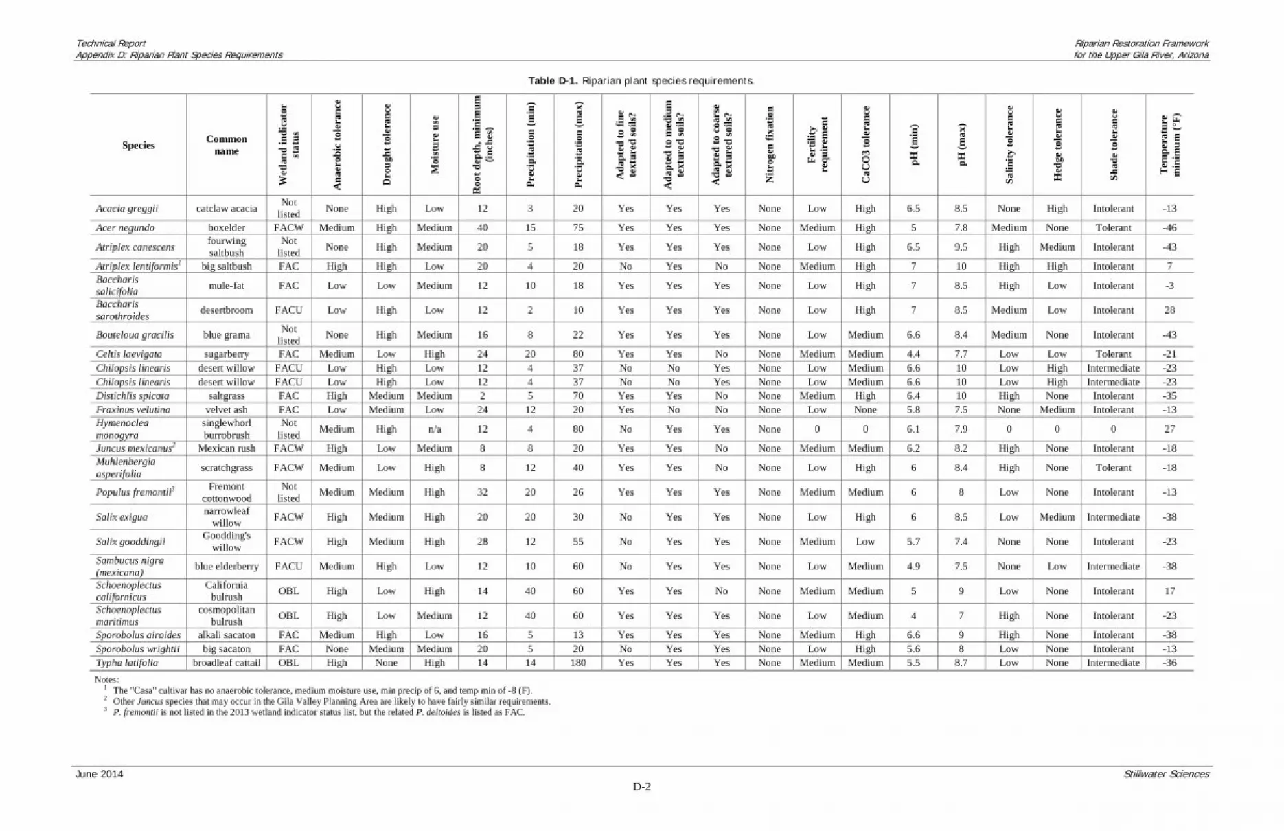
Technical Report Riparian Restoration Framework Appendix D: Riparian Plant Species Requirements for the Upper Gila River, Arizona
June 2014 Stillwater Sciences D-2
Table D-1. Riparian plant species requirements.
Species Common name
Wet
land
indi
cato
r st
atus
Ana
erob
ic to
lera
nce
Dro
ught
tole
ranc
e
Moi
stur
e us
e
Roo
t dep
th, m
inim
um
(inch
es)
Prec
ipita
tion
(min
)
Prec
ipita
tion
(max
)
Ada
pted
to fi
ne
text
ured
soils
?
Ada
pted
to m
ediu
m
text
ured
soils
?
Ada
pted
to c
oars
e te
xtur
ed so
ils?
Nitr
ogen
fixa
tion
Fert
ility
re
quir
emen
t
CaC
O3
tole
ranc
e
pH (m
in)
pH (m
ax)
Salin
ity to
lera
nce
Hed
ge to
lera
nce
Shad
e to
lera
nce
Tem
pera
ture
m
inim
um (°
F)
Acacia greggii catclaw acacia Not listed None High Low 12 3 20 Yes Yes Yes None Low High 6.5 8.5 None High Intolerant -13
Acer negundo boxelder FACW Medium High Medium 40 15 75 Yes Yes Yes None Medium High 5 7.8 Medium None Tolerant -46
Atriplex canescens fourwing saltbush
Not listed None High Medium 20 5 18 Yes Yes Yes None Low High 6.5 9.5 High Medium Intolerant -43
Atriplex lentiformis1 big saltbush FAC High High Low 20 4 20 No Yes No None Medium High 7 10 High High Intolerant 7 Baccharis salicifolia mule-fat FAC Low Low Medium 12 10 18 Yes Yes Yes None Low High 7 8.5 High Low Intolerant -3
Baccharis sarothroides desertbroom FACU Low High Low 12 2 10 Yes Yes Yes None Low High 7 8.5 Medium Low Intolerant 28
Bouteloua gracilis blue grama Not listed None High Medium 16 8 22 Yes Yes Yes None Low Medium 6.6 8.4 Medium None Intolerant -43
Celtis laevigata sugarberry FAC Medium Low High 24 20 80 Yes Yes No None Medium Medium 4.4 7.7 Low Low Tolerant -21 Chilopsis linearis desert willow FACU Low High Low 12 4 37 No No Yes None Low Medium 6.6 10 Low High Intermediate -23 Chilopsis linearis desert willow FACU Low High Low 12 4 37 No No Yes None Low Medium 6.6 10 Low High Intermediate -23 Distichlis spicata saltgrass FAC High Medium Medium 2 5 70 Yes Yes No None Medium High 6.4 10 High None Intolerant -35 Fraxinus velutina velvet ash FAC Low Medium Low 24 12 20 Yes No No None Low None 5.8 7.5 None Medium Intolerant -13 Hymenoclea monogyra
singlewhorl burrobrush
Not listed Medium High n/a 12 4 80 No Yes Yes None 0 0 6.1 7.9 0 0 0 27
Juncus mexicanus2 Mexican rush FACW High Low Medium 8 8 20 Yes Yes No None Medium Medium 6.2 8.2 High None Intolerant -18 Muhlenbergia asperifolia scratchgrass FACW Medium Low High 8 12 40 Yes Yes No None Low High 6 8.4 High None Tolerant -18
Populus fremontii3 Fremont cottonwood
Not listed Medium Medium High 32 20 26 Yes Yes Yes None Medium Medium 6 8 Low None Intolerant -13
Salix exigua narrowleaf willow FACW High Medium High 20 20 30 No Yes Yes None Low High 6 8.5 Low Medium Intermediate -38
Salix gooddingii Goodding's willow FACW High Medium High 28 12 55 No Yes Yes None Medium Low 5.7 7.4 None None Intolerant -23
Sambucus nigra (mexicana) blue elderberry FACU Medium High Low 12 10 60 No Yes Yes None Low Medium 4.9 7.5 None Low Intermediate -38
Schoenoplectus californicus
California bulrush OBL High Low High 14 40 60 Yes Yes No None Medium Medium 5 9 Low None Intolerant 17
Schoenoplectus maritimus
cosmopolitan bulrush OBL High Low Medium 12 40 60 Yes Yes Yes None Low Medium 4 7 High None Intolerant -23
Sporobolus airoides alkali sacaton FAC Medium High Low 16 5 13 Yes Yes Yes None Medium High 6.6 9 High None Intolerant -38 Sporobolus wrightii big sacaton FAC None Medium Medium 20 5 20 No Yes Yes None Low High 5.6 8 Low None Intolerant -13 Typha latifolia broadleaf cattail OBL High None High 14 14 180 Yes Yes Yes None Medium Medium 5.5 8.7 Low None Intermediate -36 Notes:
1 The "Casa" cultivar has no anaerobic tolerance, medium moisture use, min precip of 6, and temp min of -8 (F). 2 Other Juncus species that may occur in the Gila Valley Planning Area are likely to have fairly similar requirements. 3 P. fremontii is not listed in the 2013 wetland indicator status list, but the related P. deltoides is listed as FAC.

Technical Report Riparian Restoration Framework Appendix D: Riparian Plant Species Requirements for the Upper Gila River, Arizona
June 2014 Stillwater Sciences D-3
D2.1 Environmental Factors
D2.1.1 Wetland indicators status
The U.S. Fish and Wildlife Service has prepared a National List of Plant Species That Occur in Wetlands: 1988 National Summary (USFWS 1988) and the 2103 Updated List (Lichvar 2013). Indicator categories are:
• Obligate Wetland (OBL). Occur almost always (estimated probability >99%) under natural conditions in wetlands.
• Facultative Wetland (FACW). Usually occur in wetlands (estimated probability 67%-99%), but occasionally found in non-wetlands.
• Facultative (FAC). Equally likely to occur in wetlands or non-wetlands (estimated probability 34%-66%).
• Facultative Upland (FACU). Usually occur in non-wetlands (estimated probability 67%-99%), but occasionally found in wetlands (estimated probability 1%-33%).
• Obligate Upland (UPL). Occur in wetlands in another region, but occur almost always (estimated probability >99%) under natural conditions in non-wetlands in the region specified.
The wetland indicator categories should not be equated to degrees of wetness. Many Obligate Wetland species occur in permanently or semi-permanently flooded wetlands, but a number also occur and some are restricted to wetlands that are only temporarily or seasonally flooded. The Facultative Upland species include a diverse collection of plants that range from weedy species adapted to a number of environmentally stressful or disturbed sites (including wetlands) to species in which a portion of the gene pool (an ecotype) always occur in wetlands. Both the weedy and ecotype representatives of the facultative upland category occur in a variety of wetland habitats, ranging from the driest wetlands to semi-permanently flooded wetlands. Species not included in the 1988 or 2013 lists are typically considered non-wetland species.
D2.1.2 Water availability/use factors
Anaerobic Tolerance: What is the plant’s tolerance of anaerobic conditions of the growth medium, relative to other species? (Low, Medium, High, None) Drought Tolerance: What is the tolerance of the plant to drought conditions relative to other species in the same plant type and same geographical region? (Low, Medium, High, None) Moisture Use: What is the degree to which this plant uses available soil moisture, relative to other species in the plant type? (Low, Medium, High) Minimum Precipitation: The 2 in 10 year average minimum precipitation (inches) across years, of the driest climate station within the known geographical range of the plant. For cultivars, the geographical range is defined as the area to which the cultivar is well adapted rather than marginally adapted. Maximum Precipitation: The annual average precipitation (inches) of the wettest climate station within the known geographical range of the plant. For cultivars, the geographical range is defined as the area to which the cultivar is well adapted rather than marginally adapted.

Technical Report Riparian Restoration Framework Appendix D: Riparian Plant Species Requirements for the Upper Gila River, Arizona
June 2014 Stillwater Sciences D-4
D2.1.3 Soil-related factors
Minimum Root Depth: The minimum depth of soil required for good growth in inches. Plants that do not have roots such as rootless aquatic plants (floating or submerged) and epiphytes are assigned a minimum root depth value of zero. Adapted To Fine/Medium/Coarse Textured Soils: Can this plant establish and grow in soil with a fine/medium/coarse textured surface layer? (Yes, No) Refer to Table D-2.
Table D-2. VegSpec soil texture groups and corresponding soil texture classes.
VegSpec soil texture group 1 Corresponding soil texture classes from the Soil Texture Triangle 2
Coarse Sand Coarse sand Fine sand
Loamy course sand Loamy fine sand Loamy very fine sand Very fine sand Loamy sand
Medium
Silt Sandy clay loam Very find sandy loam Silty clay loam Silt loam Loam
Fine sandy loam Sandy loam Coarse sandy loam Clay loam
Fine Sandy clay Silty clay Clay Notes:
1 Source: The soil texture classes are from the Soil Science Society of America, http://www.soils.org/. An NRCS team partitioned the soil textures into the 3 groups.
2 The United States Department of Agriculture (USDA) defines particle sizes as: sand 2.0–0.05 mm; silt 0.05–0.002 mm; and clay <0.002 mm in diameter.
Nitrogen Fixation: What is the amount of nitrogen fixed by this plant relative to other species? (None, Low, Moderate, High, Unknown (blank)) Fertility Requirement: What is the level of nutrients (N, P, K) required for normal growth and development relative to other species? (Low, Medium, High) CaCO3 Tolerance: Want is the plant's tolerance to calcareous soil relative to other species. We define calcareous soil as soil containing sufficient free CaCO3 and other carbonates to effervesce visibly or audibly when treated with cold 0.1M HCl. These soils usually contain from 10 to almost 1000g/kg CaCO3 equivalent. (Low, Medium, High, None, Unknown (blank)) Minimum/Maximum pH: The minimum/maximum soil pH within the plant’s known geographical range. For cultivars, the geographical range is defined as the area to which the cultivar is well adapted rather than marginally adapted. Salinity Tolerance: What is the plant’s tolerance to soil salinity? Tolerance to a soil salinity level is defined as only a slight reduction (not greater than 10%) in plant growth. None = tolerant to a soil salinity of 0–2 mmhos/cm; Low = tolerant to a soil salinity of 2.1-4.0 mmho/cm; Medium = tolerant to a soil salinity of 4.1–8.0 mmhos/cm; High = tolerant to a soil salinity greater than 8.0 mmhos/cm.
D2.1.4 Other environmental factors
Shade Tolerance: What is the tolerance for this plant, relative to other species, to grow in shade conditions? Refer to Table D-3. (Intolerant, Intermediate, Tolerant)

Technical Report Riparian Restoration Framework Appendix D: Riparian Plant Species Requirements for the Upper Gila River, Arizona
June 2014 Stillwater Sciences D-5
Table D-3. Comparison of shade tolerance classes.
Silvics of North America classes
Corresponding VegSpec classes
Very Intolerant and Intolerant Intolerant Intermediate Intermediate Very Tolerant and Tolerant Tolerant
Hedge Tolerance: What is the tolerance of the woody perennial to hedging (close cropping) by livestock or wildlife. Forbs, grasses and non-woody vines are classified as "None.” (Low, Medium, High, None, Unknown (blank)) Minimum Temperature: The 2 in 10 year average minimum temperature (F°) across years, of the coldest climate station within the known geographical range of the plant. For cultivars, the geographical range is defined as the area to which the cultivar is well adapted rather than marginally adapted.

Technical Report Riparian Restoration Framework Appendix D: Riparian Plant Species Requirements for the Upper Gila River, Arizona
June 2014 Stillwater Sciences D-6
D2 REFERENCES
Lichvar, R. W. 2013. The national wetland plant list: 2013 wetland ratings. Phytoneuron 49: 1–241. NRCS (Natural Resources Conservation Service). 2002. The PLANTS Database, Version 3.5 (http://plants.usda.gov). National Plant Data Center, Baton Rouge, Louisiana. USFWS (U.S. Fish and Wildlife Service). 1988. National list of vascular plant species that occur in wetlands. USFWS Biological Report 88 (24).
Riparian Restoration Framework
Technical Report for the Upper Gila River, Arizona
Appendix E
SWFL Existing Conditions Summary
– Matthew P Johnson
Technical Report Riparian Restoration Framework Appendix E: SWFL Existing Conditions Summary for the Upper Gila River, Arizona
June 2014 Johnson E-1
E1 INTRODUCTION
The following descriptions and evaluation of Southwestern Willow Flycatcher (Empidonax traillii extimus) (SWFL) habitat occurred in 2013 within the Gila Valley Restoration Planning Area (see Figure 1-1 in the main report). This evaluation is based on direct habitat observations of each site using the NRCS southwestern willow flycatcher habitat methods established in 2012. This method was developed for riparian habitats within the state of Utah and was modified for conditions along the Gila River within the proposed Planning Area. The following habitat evaluations are only a portion of the proposed sites currently being considered in the Planning Area. In spring/summer 2014, we will survey and evaluate habitat for willow flycatcher at all proposed Planning Area sites. Because of the sensitive nature of publically distributing locational information on endangered species, like the flycatcher, results of our habitat evaluation are not presented below. These data may be provided by request through the U.S. Fish and Wildlife Service office in Phoenix, Arizona (http://www.fws.gov/southwest/es/arizona/).
E1.1 Range Wide Southwestern Willow Flycatcher Breeding Population Sustainability, Habitat, Water and Food Background
Twice the amount of suitable habitat is needed to support the numerical territory goals because the long-term persistence of flycatcher populations cannot be assured by protecting only those habitats in which flycatchers currently breed (USFWS 2002). It is important to recognize that most flycatcher breeding habitats are susceptible to future changes in site hydrology (natural or human-related), human impacts such as development or fire, and natural catastrophic events such as flood or drought (USFWS 2002). Furthermore, as the vegetation at sites matures, it can lose the structural characteristics that make it suitable for breeding flycatchers (USFWS 2002). These and other factors can destroy or degrade breeding sites, such that one cannot expect any given breeding site to remain suitable in perpetuity (USFWS 2002). Thus, it is necessary to have additional suitable habitat available to which flycatchers can readily move if displaced by such habitat loss or change (USFWS 2002).
E1.1.1 Habitat criteria
The flycatcher currently breeds in areas from near sea level to over 2,600 meters (m) (8,500 feet (ft) (Durst et al. 2008) in vegetation alongside rivers, streams, or other wetlands (riparian habitat). It establishes nesting territories, builds nests, and forages where mosaics of relatively dense and expansive growths of trees and shrubs are established, near or adjacent to surface water or underlain by saturated soil (Sogge et al. 2010). Habitat characteristics such as dominant plant species, size and shape of habitat patch, tree canopy structure, vegetation height, and vegetation density vary widely among breeding sites. Nests are typically placed in trees where the plant growth is most dense, where trees and shrubs have vegetation near ground level, and where there is a low-density canopy. Some of the more common tree and shrub species currently known to comprise nesting habitat include Gooddings willow (Salix gooddingii), coyote willow (Salix exigua), Geyer’s willow (Salix geyeriana), arroyo willow (Salix lasiolepis), red willow (Salix laevigata), yewleaf willow (Salix taxifolia), boxelder (Acer negundo), tamarisk (also known as saltcedar, Tamarix ramosissima), and Russian olive (Elaeagnus angustifolia) (USFWS 2002). While there are exceptions, generally flycatchers are not found nesting in areas without willows, tamarisk, or both.
Technical Report Riparian Restoration Framework Appendix E: SWFL Existing Conditions Summary for the Upper Gila River, Arizona
June 2014 Johnson E-2
E1.1.2 Water criteria
Southwestern willow flycatcher nesting habitat is associated with perennial stream flow that can support the vegetation characteristics needed by breeding flycatchers. Flycatcher nesting habitat can also persist on intermittent (ephemeral) streams that retain local conditions favorable to riparian vegetation (USFWS 2002). The range and variety of stream flow conditions (frequency, magnitude, duration, and timing) (Poff et al. 1997) that will establish and maintain flycatcher habitat can arise in different types of both regulated and unregulated flow regimes throughout its range (USFWS 2002). Also, flow conditions that will establish and maintain flycatcher habitat can be achieved in regulated streams, depending on scale of operation and the interaction of the primary physical characteristics of the landscape (USFWS 2002). Flowing streams with a wide range of stream flow conditions that support expansive riparian vegetation are also an essential physical feature of flycatcher habitat. The most common stream flow conditions are largely perennial (persistent) stream flow with a natural hydrologic regime (frequency, magnitude, duration, and timing). However, in the Southwest, hydrological conditions can vary, causing some flows to be intermittent, but the floodplain can retain surface moisture conditions favorable to expansive and flourishing riparian vegetation. These appropriate conditions can be supported by managed water sources and hydrological cycles that mimic key components of the natural hydrologic cycle.
E1.1.3 Food criteria
The southwestern willow flycatcher is somewhat of an insect generalist (USFWS 2002), taking a wide range of invertebrate prey including flying, ground and vegetation-dwelling species of terrestrial and aquatic origins (Drost et al. 2003). Flycatchers employ a “sit and wait” foraging tactic, with foraging bouts interspersed with longer periods of perching (Prescott and Middleton 1988). Flycatcher food availability may be largely influenced by the density and species of vegetation, proximity to and presence of water, saturated soil levels, and microclimate features such as temperature and humidity (USFWS 2002). Flycatchers forage within and above the tree canopy, along the patch edge, in openings within the territory, over water, and from tall trees as well as herbaceous ground cover (Bent 1960, McCabe 1991).
E1.2 SWFL Evaluation Guide
The following is a re-presentation of the Natural Resources Conservation Service’s (NRCS) Wildlife Habitat Evaluation Guide for southwestern willow flycatcher (May 2013 version: http://efotg.sc.egov.usda.gov/references/public/NM/Rangewide_SWFL_WHEG(5-15-2013).xlsx). A SWFL evaluation area is a discrete area of vegetation and hydrology. Plant species and composition, age, and height are considered in the evaluation area. Due to the wide variety of habitat used by the species across its range, the evaluator will need to interpret the questions to their situation.

Technical Report Riparian Restoration Framework Appendix E: SWFL Existing Conditions Summary for the Upper Gila River, Arizona
June 2014 Johnson E-3
E1.2.1 Habitat configuration
• Two or more large patches consisting of dense (difficult to walk through) woody riparian vegetation. Patches are mostly > 33 feet wide and > 20 acres in size.
• Two or more large patches consisting of dense (difficult to walk through) woody riparian vegetation. Patches are mostly > 33 feet wide and are >10 acres but < 20 acres in size.
• A multiple patch complex with one large patch consisting of dense (difficult to walk through) woody riparian vegetation. Large patch is mostly > 33 feet wide and least 10 acres in size. Additional patches are > 2.5 acres but < 10 acres.
• Multiple patches consisting of dense (difficult to walk through) woody riparian vegetation. Patches are at least 33 feet wide and > 2.5 acres and < 4.5 acres in size.
• A single patch of dense riparian vegetation at least 33 feet wide and > 2.5 acres, but < 4.5 acres in size, or is < 2.5 ac but is connected to other patches.
• A single, narrow strip of riparian vegetation that does not extend from or connect to a larger patch and AVERAGE WIDTH is less than 33 feet wide and is <2.5 acres and is not connected to another patch.
E1.2.2 Habitat structure
• Mature multi-storied riparian vegetation with canopy heights ranging from approximately 35 to 65 feet tall, with mosaics of densely vegetated understory’s of shorter trees (greater than 15 feet tall that are difficult to walk through).
• Young stands of regenerating riparian vegetation with similar heights of vegetation approximately 15 feet in height (that are difficult to walk through).
• Mature woody riparian vegetation with canopies greater than 15 feet with multiple canopy gaps containing younger trees less than 15 feet in height.
• Young stands of regenerating vegetation with varying heights, most <15 feet in height. • Canopy height for entire patch is less than 15 feet in height, consisting of mature,
somewhat interconnected trees and with little to no regeneration. • No connected trees; little to no regeneration. Trees are not capable of reaching above 15' in
height.
E1.2.3 Habitat composition—woody
• Woody riparian vegetation composed of native species (i.e., typically woody species such as willow, cottonwood) and no exotic vegetation (such as tamarisk, and Russian olive).
• Woody riparian vegetation dominated by >75% native vegetation (i.e. typically woody species such as willow, cottonwood) with a smaller component of exotic vegetation (most likely tamarisk, and possibly Russian olive).
• Woody riparian vegetation dominated >50% native vegetation (i.e. typically woody species such as willow, cottonwood) with a smaller component of exotic woody species (most likely tamarisk, and possibly Russian olive).
• Woody riparian vegetation composed of >50% exotic vegetation (mostly likely tamarisk, and possibly Russian olive).
• Little to no woody riparian vegetation flycatcher’s use for nesting; or site potential is for herbaceous only. Abundant wetland vegetation like cattails or arundo do not comprise flycatcher habitat.
Technical Report Riparian Restoration Framework Appendix E: SWFL Existing Conditions Summary for the Upper Gila River, Arizona
June 2014 Johnson E-4
E1.2.4 Habitat composition—herbaceous (grass, forb, sedge)
• Native understory > 2 ft tall. • Native with some non-native understory > 2 ft tall. • Native with some non-native understory 6 in – 2 ft tall. • Understory dominated by non-natives or is < 6 inches tall. • Little to no understory of grasses, forbs, or sedges.
E1.2.5 Water depletions
• No river diversion or groundwater pumping. • Limited river diversion or groundwater pumping that does not reduce the water available
for riparian or lake bottom habitat regeneration, growth, maintenance, distribution, or abundance.
• River diversion or groundwater pumping that reduces the water available for riparian or lake bottom habitat regeneration, growth, maintenance, distribution, or abundance; minimum suitable habitat maintained in most years.
• River diversion or groundwater pumping that reduces the water available for riparian habitat regeneration, growth, maintenance, distribution, or abundance: minimum suitable habitat only available in wettest years.
• River diversion or groundwater pumping to the extent that water is not available for riparian habitat regeneration, growth, maintenance, distribution, or abundance.
E1.2.6 General hydrology (especially May 15–Aug 1)
• Perennial surface flow with elevated groundwater within or adjacent to assessment area. • Intermittent streams that provide surface water during the breeding season. • Mostly perennial surface flow, with some intermittent sections or short durations of
intermittent flow and elevated groundwater maintains moist soils • Intermittent or perennial surface flows during the breeding season with elevated
groundwater. • No surface flow or rare occurrence of surface flow; breeding season in most years without
moist soils and elevated groundwater.
E1.2.7 Flood frequency
• Regular flooding every 1.5–2 years. Flood plain wetlands (oxbows, backwater wetlands) are still hydrologically connected to the river. High flows in the river channel result in surface water saturation of these floodplain features.
• Overbank flooding occurs every 3–4 years. Channel is slightly incised. Flood plain wetlands (oxbows, backwater wetlands) are still hydrologically connected to the river. High flows in the river channel result in surface water saturation of these floodplain features.
• Flooding every 5-6 years. Most floodplain wetlands are wetted when river levels rise.
Technical Report Riparian Restoration Framework Appendix E: SWFL Existing Conditions Summary for the Upper Gila River, Arizona
June 2014 Johnson E-5
• Flooding every 7–10 years. Only the deepest floodplain wetlands are wetted when river levels rise. Some runoff water available to help establish woody vegetation.
• No flooding. The channel is deeply incised or confined by structures such as levees. Floodplain wetlands are no longer hydrologically connected to the river. Runoff cannot provide enough water to establish dense woody vegetation.
E1.2.8 Site disturbance
• No human disturbance occurs in the assessment area. • SWFL Habitat quality factors are maintained with minimal disturbance. Access is limited
to the non-breeding/brood rearing season. Land management, such as livestock grazing and fire wood harvest are conducted so that the timing and intensity avoids or minimizes disturbance. No vehicular recreational activities within or adjacent to assessment area. All disturbance activities occurs outside the breeding season: all grazing will be consistent with NRCS grazing plans specific to SWFL management.
• SWFL habitat quality factors are maintained with noticeable, short term impacts to habitat quality from land management such as livestock grazing, and fire wood harvest, and other land management. No vehicular recreational activities within or adjacent to patch: grazing will follow NRCS approved grazing plan specific to SWFL management. Grazing plan may include part of the growing season (but not nesting season) some years.
• SWFL habitat quality factors are present but long term impacts to habitat quality are apparent. Land management decisions are applied without regard for the SWFL nesting season. Livestock grazing is conducted without an NRCS plan. No vehicular recreational activities within or adjacent to assessment area.
• Low-quality SWFL habitat due to human activities and land management. Physical and auditory disturbances during the nesting season are common. Vehicular recreational activities within or adjacent to assessment area.

Technical Report Riparian Restoration Framework Appendix E: SWFL Existing Conditions Summary for the Upper Gila River, Arizona
June 2014 Johnson E-6
E2 REFERENCES
Bent, A. C. 1960. Life histories of North American flycatchers, larks, swallows and their allies. Dover Press, New York, New York. Drost, C. A., M. K. Sogge, and E. Paxton. 1997. Preliminary diet study of the endangered southwestern willow flycatcher. USGS Colorado Plateau Field Station, Flagstaff, Arizona. Durst, S. L., M. K. Sogge, S. D. Stump, H. A. Walker, B. E. Kus, and S. J. Sferra. 2008. U.S. Geological Survey Open-File Report 2008-1303. McCabe, R. A. 1991. The little green bird: ecology of the willow flycatcher. Palmer publications, Inc., Amherst, Wisconsin. Poff, N. L., J. D. Allan, M. B. Bain, J. R. Karr, K. L. Prestegaard, B. D. Richter, and J. C. Stromberg. 1997. The natural flow regime: A paradigm for river conservation and restoration. BioScience 47: 769–784. Prescott, D. R. C. and A. L. A. Middleton. 1988. Feeding-time minimization and the territorial behavior of the willow flycatcher (Empidonax traillii). Auk 105: 17–28. Sogge, M. K., D. Ahlers, and S. J. Sferra. 2010. A natural history summary and survey protocol for the Southwestern Willow Flycatcher: U.S. Geological Survey Techniques and Methods 2A-10. USFWS (U. S. Fish and Wildlife Service). 2002. Southwestern Willow Flycatcher Final Recovery Plan. U.S. Fish and Wildlife Service, Albuquerque, New Mexico.

Riparian Restoration Framework
Technical Report for the Upper Gila River, Arizona
Appendix F
SWFL Breeding Habitat Prediction Modeling – James R. Hatten and Matthew P. Johnson

Technical Report Riparian Restoration Framework Appendix F: SWFL Breeding Habitat Prediction Modeling for the Upper Gila River, Arizona
June 2014 Hatten and Johnson F-1
F1 INTRODUCTION
The Southwestern Willow Flycatcher (Empidonax traillii extimus) (SWFL) is a federally endangered bird (USFWS 1995) that breeds in riparian areas in portions of New Mexico, Arizona, southwestern Colorado, extreme southern Utah and Nevada, and southern California (USFWS 2002). Across this range, it uses a variety of plant species as nesting/breeding habitat, but in all cases prefers sites with dense vegetation, high canopy, and proximity to surface water or saturated soils (Sogge et. al 2010). A key challenge facing the management and conservation of willow flycatchers is that riparian areas are dynamic, with individual habitat patches subject to cycles of creation, growth, and loss due to drought, flooding, fire, and other disturbances (Hatten and Sogge 2007, Paxton et al. 2007). The recent establishment of the tamarisk leaf beetle introduces a new dynamic factor affecting habitat suitability (Paxton et al. 2011). Measuring and predicting SWFL habitat—either to identify areas that may develop into appropriate habitat for SWFLs or that, with intervention by active restoration could support future flycatcher nesting—requires knowledge of recent/current/future habitat conditions and an understanding of the dynamic processes and ecological factors that determine willow flycatchers’ use of riparian breeding sites. Breeding site assessment has typically been based on qualitative criteria (e.g., “dense vegetation” or “large patches”) that require on-the-ground field evaluations by local or regional flycatcher experts. While this has proven valuable in locating many of the currently known breeding sites, it is nearly impossible to apply this approach effectively over large geographic areas (e.g., the Gila River). The SWFL Recovery Plan (USFWS 2002) recognizes the importance of developing new approaches to habitat identification, and recommends the development of drainage-scale, quantitative habitat models. In particular, the plan suggests using models based on remote sensing and GIS technology that can capture the relatively dynamic habitat changes that occur in southwestern riparian systems. Southwestern willow flycatchers are present in the Gila Valley Restoration Planning Area (hereafter “Planning Area”), an 85-km section of the upper Gila River in Arizona (see Figure 1-1 in the main report), which has been designated as critical habitat for the species by the USFWS. They typically establish nesting territories, build nests, and forage where mosaics of relatively dense and expansive growths of trees and shrubs are established near or adjacent to surface water and/or underlain by saturated soil (Sogge et al. 2010). SWFLs exist and interact as groups of metapopulations—a group of geographically separate breeding populations connected to each other by immigration and emigration—and are considered most stable where many connected sites or large populations exist. Metapopulation persistence or stability is more likely to improve by adding more breeding sites rather than expanding existing sites, which would distribute birds across a greater geographical range, minimize risk of simultaneous catastrophic population loss, and avoid genetic isolation. Approximately twice the amount of suitable habitat is therefore needed to support the numerical territory goals because the long-term persistence of SWFL populations cannot be assured by protecting only those habitats in which the species currently breeds (USFWS 2002). It is also important to recognize that most breeding habitats are susceptible to future changes in site hydrology (natural or human-related), human impacts such as development or fire, and natural catastrophic events such as flood or drought (Hatten and Sogge 2007). Furthermore, as the vegetation at sites mature, it can lose the structural characteristics that make it suitable for breeding individuals. These and other factors can destroy or degrade breeding sites making their

Technical Report Riparian Restoration Framework Appendix F: SWFL Breeding Habitat Prediction Modeling for the Upper Gila River, Arizona
June 2014 Hatten and Johnson F-2
suitability ultimately ephemeral. Thus, it is necessary to have additional suitable habitat available to which SWFLs can readily move if displaced by such habitat loss or change. Information on reach-scale SWFL conditions supported by habitat-prediction modeling performed specifically for the Planning Area is presented here. Field surveys were conducted in 2013 to characterize existing and potential SWFL-habitat quality throughout the Planning Area. The findings of these field surveys, in additional to supporting information on general species conditions, are presented in Appendix E, as authored by Matt Johnson of Northern Arizona University. In spring/summer 2014, additional willow flycatcher surveys and habitat evaluations will be conducted in proposed restoration sites in order to validate the model results discussed in this report and continue to better characterize the potential SWFL habitat quality within the Planning Area. There are six objectives of the SWFL existing-conditions review and habitat prediction modeling:
1. Develop a conceptual model of SWFL breeding requirements (Figure F-1), which include physiological and other environmental processes that were identified by previous research as important determinants of species survival and reproduction, and are conceptual links to the spatially and temporally comprehensive variables that were available for us to use in our statistical modeling.
2. Gather and synthesize historical SWFL presence/absence and breeding data along the upper Gila River (Arizona/New Mexico boundary–Gila River/San Pedro Confluence).
3. Estimate potential breeding habitat for SWFL in the Planning Area by characterizing existing habitat conditions through field surveys.
4. Apply two sets of models to estimate SWFL habitat within the Planning Area: (a) satellite models, which characterize vegetation from Landsat Thematic Mapper (TM) imagery; and (b) aerial models, which use fine-scale data to characterize vegetation from orthorectified digital aerial photography and LiDAR collected in October 2012.
5. Incorporate the effects that tamarisk biocontrol will have on SWFL habitat over a period of three to five years following expansion of the beetle into the Gila Valley area. The modeling effort can potentially map likely defoliated areas under future scenarios and help detect trends in SWFL habitat suitability caused by changes in vegetation over time.
6. Communicate the progress of model development and results with Gila Watershed Partnership, U.S. Fish and Wildlife Service, Bureau of Reclamation, Arizona Game and Fish, and Salt River Project.
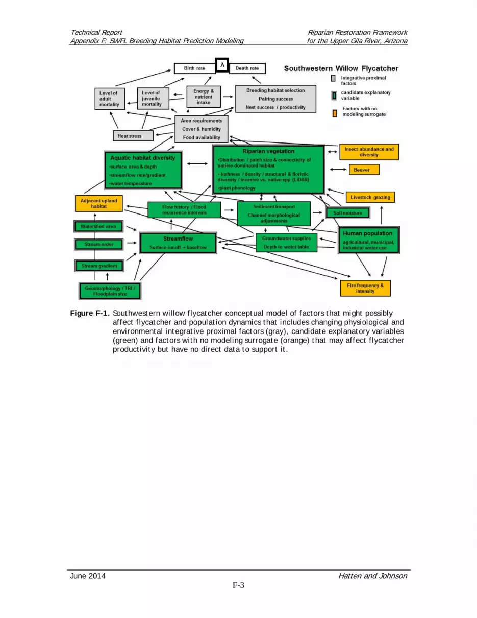
Technical Report Riparian Restoration Framework Appendix F: SWFL Breeding Habitat Prediction Modeling for the Upper Gila River, Arizona
June 2014 Hatten and Johnson F-3
Figure F-1. Southwestern willow flycatcher conceptual model of factors that might possibly
affect flycatcher and population dynamics that includes changing physiological and environmental integrative proximal factors (gray), candidate explanatory variables (green) and factors with no modeling surrogate (orange) that may affect flycatcher productivity but have no direct data to support it.

Technical Report Riparian Restoration Framework Appendix F: SWFL Breeding Habitat Prediction Modeling for the Upper Gila River, Arizona
June 2014 Hatten and Johnson F-4
F2 METHODS
F2.1 SWFL Satellite Model
In 1999 the Arizona Game and Fish Department (AGFD) developed a GIS-based model (Hatten and Paradzick 2003) to identify willow flycatcher breeding habitat from Landsat Thematic Mapper (TM) imagery and a 30-m resolution digital elevation model (DEM). The GIS-based model (hereafter called “satellite model”) was developed with presence/absence survey data acquired along the San Pedro and Gila rivers, and from the Salt River and Tonto Creek inlets to Roosevelt Lake in southern Arizona. The satellite model has been tested by predicting SWFL breeding habitat at multiple locations around Arizona and New Mexico, performing as expected by identifying riparian areas with the highest flycatcher nest densities (Hatten and Sogge 2007, Hatten et al. 2010). Thus, our first modeling objective was to assist with site restoration and planning through application of the satellite model in the Planning Area. We applied the satellite model to identify and map potential SWFL breeding habitat in 2013 along the entire Planning Area. For modeling purposes, we developed four spatially explicit predictor variables (grids) extracted off of Landsat imagery and a 30-m resolution DEM (Table F-1). We used binary logistic regression (Hosmer and Lemeshow 1989) and Arc/Info® GRID (ESRI, 1992) to calculate and map the relative quality of breeding habitat within 0.09-ha (30m×30m) cells. We calculated the relative quality of breeding habitat (P) with the following equation:
( )
( )xg
xg
eeP+
=1
(Eq. 1)
where g(x) is the linear combination of parameter estimates obtained from the logistic regression (Hosmer and Lemeshow 1989, Keating and Cherry 2004). In Eq. (1), the relative quality of flycatcher breeding habitat is linked to the probability of a flycatcher territory occurring. The satellite model assigns cells a probability between 1 and 99%, which we reclassified into 1 of 5 probability classes: (1) 1–20%, (2) 21–40%, (3) 41–60%, (4) 61–80%, and (5) 81–99%. Larger probability classes (classes 4 and 5) have been found to contain higher densities of breeding flycatchers in Arizona and New Mexico (Paxton et al. 2007, Hatten and Sogge 2007). Table F-1. Four predictor variables the satellite model uses to identify and map potential SWFL
habitat in the Planning Area.
Variable Description
ND_BEST4 Amount (i.e., number) of cells with NDVI values >0.41 within a 120-m radius
ND_TOP3 Binary (cells with NDVI > 0.33 = 1; NDVI < 0.33 = 0)
ND_SD4 Variability (SD) in NDVI within a 120-m radius
FLOOD30 Amount of floodplain or flat area within a 360-m radius from a 30-m DEM)
NVDI=Normalized Difference Vegetation Index

Technical Report Riparian Restoration Framework Appendix F: SWFL Breeding Habitat Prediction Modeling for the Upper Gila River, Arizona
June 2014 Hatten and Johnson F-5
F2.2 Habitat Time Series
One of the great advantages of the satellite model is its utility for change detection and habitat time-series analysis since it reimages the same location every 16 days (Aronoff 1989). Thus, we created a habitat time series for the Planning Area by populating the SWFL satellite model with 27 Landsat scenes from 1986–2013. The habitat time series served two purposes: (1) it allowed us to create a bar graph that depicts how much potential SWFL breeding habitat was in the Planning Area between 1986 and 2013; and (2) it enabled us to create a time-lapse video that depicts how SWFL habitat changes year to year between 1986 and 2013 over the entire Planning Area. The habitat time series also will provide a baseline of predicted SWFL habitat that can be compared to future conditions.
F2.3 SWFL LiDAR Model
Identification of functional relationships between birds and the structure and composition of vegetation is a key step toward predicting how changes in specific land-cover types may affect various taxonomic assemblages. Most habitat suitability models are based on digital maps that very often describe the environment at a human scale and, hence miss ecological features such as structure that are important for wildlife. LiDAR (Light Detection And Ranging) data, laser scanning acquired by remote sensing, can fill this gap by providing useful information not only on the spatial extent of habitat types but also information on the vertical height. The advantage of LiDAR derived variables lays also in the availability at a large scale, instead of just in the survey sites. LiDAR data are beginning to be used in wildlife modelling and ecological studies with interesting results, especially for woodland species, where vegetation structure plays an important role in occupying a site and successfully breeding (Vierling et al. 2008, Martinuzzi et al. 2010, Müller and Brandl 2009, Flaspohler et al. 2010). The LiDAR data are acquired by active remote sensing utilizing a laser scanning technique. The LiDAR sensor, usually mounted on an airplane, is a device that sends an infrared signal and registers the type and number of echoes of that signal received from the ground and from objects located above the ground such as trees and shrubs (Lefsky 2002). Standard processing of LiDAR data provides high resolution Digital Surface Models (DSMs) and Digital Terrain Models (DTMs) from which it is possible to derive useful information not only on the spatial extent of habitat types but also on the vertical height and structure of vegetation such as canopy height, stem diameter, canopy cover, and biomass (Goetz et al. 2007, Kaartinen and Hyyppä 2008, Lefsky 2002). Already, the benefits of LiDAR imagery are substantial enough that some authors have suggested that these measurements may begin to replace field measurements of vegetation structure traditionally used to describe wildlife habitat (Vierling et al. 2008). Here we investigate LiDAR measurements of canopy height and heterogeneity to describe habitat associations for southwestern willow flycatcher in the Planning Area. Specifically, we use these measurements to conduct a multiscale analysis that compares the predictive power of models using variables (measurements) of canopy height and heterogeneity at a spatial resolution of 0.2 to 50 ha as predictor variables. Specifically, our objectives are to: (1) evaluate the utility of LiDAR measurements to provide information about habitat associations of riparian vegetation for southwestern willow flycatcher, and projected restoration sites along the Gila River; (2) evaluate the predictive performance of fine-scale vegetation measurements (canopy height, stem diameter, canopy cover) at 1-4 meter resolution to habitat measurements obtained at a coarser scale (30 m); and (3) compare the classification accuracies of the LiDAR habitat model to the satellite habitat model.

Technical Report Riparian Restoration Framework Appendix F: SWFL Breeding Habitat Prediction Modeling for the Upper Gila River, Arizona
June 2014 Hatten and Johnson F-6
F2.4 Model Fit and Accuracy Assessment
We assessed the fit of the satellite model with nest and territory locations collected at Fort Thomas, by Salt River Project (SRP) personnel (SRP 2004–2012). Nest density is calculated by dividing territory numbers within each probability class by the area (hectares, ha) found within each probability class (Hatten and Paradzick 2003). The satellite model works as expected when territory/nest densities increase in higher probability classes. Conversely, we assessed model accuracy with omission (sensitivity) and commission (specificity) errors. An omission error occurs when a territory location falls outside of predicted habitat, thus omission errors change according to what probability cut point is selected (Hatten and Paradzick 2003). If the model is working correctly, omission errors should increase as the cut point is raised because less riparian vegetation is predicted as suitable for breeding.
Technical Report Riparian Restoration Framework Appendix F: SWFL Breeding Habitat Prediction Modeling for the Upper Gila River, Arizona
June 2014 Hatten and Johnson F-7
F3 RESULTS
F3.1 SWFL Satellite Model
We successfully applied the SWFL satellite model (30-m resolution) to the Planning Area using Landsat 5 and 8 imagery (Landsat 5 prior to 2012, Landsat 8 afterwards). Satellite-model output included a continuous probability grid, a five-class probability grid, and a binary habitat grid, with higher cell values in each case indicating relatively better SWFL habitat. Figure F-2 displays the results of the five-class probability grid, with green areas representing the greatest breeding habitat suitability and red areas representing the lowest suitability. The satellite model identified the largest amounts of high-probability breeding habitat in planning Reaches 2c–2f, which is the downstream portion of the Planning Area. Reaches 2g–2j, and 3f, contained very little high-probability breeding habitat and are in the upstream portion of the Planning Area. The habitat time series (Figure F-3) revealed that predicted SWFL habitat, as determined from the satellite model, fluctuates year to year, with a low of 589 ha (2002) and a high of 1,762 ha (2008). The yearly mean of predicted habitat was 1,112 ha, with a standard deviation (SD) of 288 and a coefficient of variation of 25.9%. We assessed the accuracy of the satellite model with 2009 data since surveyors georeferenced 63 nest locations near Fort Thomas that summer. According to the satellite model, 63 nests occurred inside class-5 habitat while 6 were in class-4 habitat (Figure F-4). There were no omission errors (i.e., all nests fell within high-probability habitat), as determined from the satellite model. Furthermore, no nest locations occurred in lower-probability classes (1–3), demonstrating the excellent performance of the satellite model.
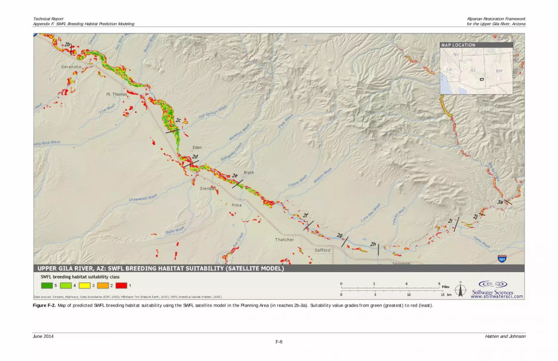
Technical Report Riparian Restoration Framework Appendix F: SWFL Breeding Habitat Prediction Modeling for the Upper Gila River, Arizona
June 2014 Hatten and Johnson F-8
Figure F-2. Map of predicted SWFL breeding habitat suitability using the SWFL satellite model in the Planning Area (in reaches 2b–3a). Suitability value grades from green (greatest) to red (least).

Technical Report Riparian Restoration Framework Appendix F: SWFL Breeding Habitat Prediction Modeling for the Upper Gila River, Arizona
June 2014 Hatten and Johnson F-9
Figure F-3. Amount of predicted SWFL breeding habitat in the Planning Area (Bonita Creek to
reservation boundary), obtained with the SWFL satellite model. The dashed line is a two-year running average. The year 2012 was unavailable due to a lapse in Landsat coverage.
Figure F-4. Southwestern willow flycatcher nest locations in 2009 inside the Planning Area,
near Fort Thomas (reaches 2c–2f), overlaid on five probability classes output by the satellite model. Larger probability classes are more suitable than smaller probability classes. A Landsat image is displayed in the background.

Technical Report Riparian Restoration Framework Appendix F: SWFL Breeding Habitat Prediction Modeling for the Upper Gila River, Arizona
June 2014 Hatten and Johnson F-10
F3.2 SWFL LiDAR Model
The results of the LiDAR SWFL habitat modeling will be concluded after the 2014 spring/summer field season when we have a larger set of observed SWFL territories to build a more robust model. This larger set will be obtained from the 2014 SWFL surveys conducted at Fort Thomas and the proposed restoration Planning Area.
Technical Report Riparian Restoration Framework Appendix F: SWFL Breeding Habitat Prediction Modeling for the Upper Gila River, Arizona
June 2014 Hatten and Johnson F-11
F4 DISCUSSION
The satellite model identified the largest amounts of high-probability breeding habitat in planning Reaches 2c–2f, which were wetter and lusher than upstream reaches (Figure F-2). The habitat time series (Figure F-3) revealed that predicted SWFL habitat in the Planning Area fluctuated ~25% year to year, between 589 ha (2002) and 1,762 ha (2008). The habitat time series dates back to 1986 and provides us with an excellent baseline to compare future conditions. For instance, when the tamarisk beetle invades the Planning Area, we will be able to determine if SWFL breeding habitat significantly deviates from the 2-yr running average. Most of the fluctuations are likely due to changes in leaf moisture and surface area, which NDVI is highly sensitive to (Avery and Berlin 1992). In addition, drought and fire negatively affect the amount of predicted SWFL breeding habitat on an annual or decadal cycle, while wet conditions increase NDVI and habitat estimates (Paxton et al. 2007, Hatten et al. 2010). For example, the satellite model found years 2000 and 2002 had the lowest amounts of predicted SWFL breeding habitat between 1986 and 2013, which coincided with severe drought conditions that affected vegetation vigor in the Planning Area. The satellite model allows managers to track changes in riparian vegetation and SWFL habitat on a bi-weekly basis since Landsat 8 reimages the same location every 16 days. This will enable us to establish how vegetation vigor and predicted flycatcher habitat respond to environmental factors at different times of the breeding season, as well as among years. The time-lapse videos we produced from the satellite model’s habitat time series shows an environment changing annually in response to environmental conditions. Flood, fire, and drought are currently the stressors that appear to affect the SWFL habitat predictions most, but we will soon be able to add insect infestation to the list when tamarisk beetle begins to defoliate the tamarisk favored by southwestern willow flycatchers (Paxton et al. 2011). The satellite model provides a baseline that will enable us to carefully implement riparian restoration activities along the Gila River within the proposed Planning Area as well as assess environmental stressors on SWFL habitat.

Technical Report Riparian Restoration Framework Appendix F: SWFL Breeding Habitat Prediction Modeling for the Upper Gila River, Arizona
June 2014 Hatten and Johnson F-12
F5 ACKNOWLEDGEMENTS
We thank Ruth Valencia (Salt River Project) for providing territory/nest data so that we could evaluate the satellite model. We are grateful to Ken Tiffan and Deborah Reusser, U.S. Geological Survey, for their constructive comments that improved this report. We appreciate Jan Holder, Executive Director, Gila Watershed Partnership, for providing project oversight and coordination. Lastly, we thank the Walton Family Foundation for providing the funding for this project. Any use of trade, firm, or product names is for descriptive purposes only and does not imply endorsement of the U.S. Government.

Technical Report Riparian Restoration Framework Appendix F: SWFL Breeding Habitat Prediction Modeling for the Upper Gila River, Arizona
June 2014 Hatten and Johnson F-13
F6 REFERENCES
Avery, T. E. and G. L. Berlin. 1992. Fundamentals of remote sensing and airphoto interpretation. Fifth edition. Macmillan Publishing Company, New York, New York. Aronoff, S. 1989. Geographic information systems: a management perspective. WDL Publications, Ottawa, Ontario. Environmental Systems Research Institute (ESRI). 1992. Cell-based Modeling with GRID, second edition. ESRI, Redlands, California. Flaspohler, D. J., C. P. Giardina, G. P. Asner, P. Hart, J. Price, C. K. Lyons, and X. Castaneda. 2010. Long-term effects of fragmentation and fragment properties on bird species richness in hawaiian forests. Biological Conservation 143: 280–288. Goetz, S., D. Steinberg, R. Dubayah, and B. Blair. 2007. Laser remote sensing of canopy habitat heterogeneity as a predictor of bird species richness in an eastern temperate forest, USA. Remote Sensing of Environment 108: 254–263. Hatten, J. R. and C. E. Paradzick. 2003. A multiscaled model of southwestern willow flycatcher breeding habitat. Journal of Wildlife Management 67: 774-788. Hatten, J. R. and M. K. Sogge. 2007. Using a remote sensing/GIS model to predict southwestern willow flycatcher breeding habitat along the Rio Grande, New Mexico. U.S. Geological Survey Open-File Report 2007, 1207. Hatten, J. R., E. H. Paxton, and M. K. Sogge. 2010. Modeling the dynamic habitat and breeding population of southwestern willow flycatcher. Ecological Modelling 221: 1,674–1,686. Hosmer, D.W. and S. Lemeshow. 1989. Applied logistic regression, first edition. John Wiley & Sons, New York, New York. Keating, K. A. and S. Cherry. 2004. Use and interpretation of logistic regression in habitat selection studies. Journal of Wildlife Management 68: 774–789. Kaartinen, H. and J. Hyyppä. 2008. Tree extraction. Tech. Rep. 53, European spatial data research—EuroSDR project, Frankfurt a.M. Available at: http://bono.hostireland.com/eurosdr/publications/53.pdf. Lefsky, M. 2002. Lidar remote sensing for ecosystem studies. BioScience 52: 19. Martinuzzi, S., L. A. Vierling, W. A. Gould, W.A., and K. T. Vierling. 2010. Improving the characterization and mapping of wildlife habitats with LiDAR data: measurement priorities for the inland northwest, USA. In J. Maxwell, K. Gergely, editors. Gap Analysis Bulletin No. 16. USGS/BRD/Gap Analysis Program, Moscow, Idaho. Müller, J. and R. Brandl. 2009. Assessing biodiversity by remote sensing in mountainous terrain: the potential of LiDAR to predict forest beetle assemblages. Journal of Applied Ecology 46: 897–905.

Technical Report Riparian Restoration Framework Appendix F: SWFL Breeding Habitat Prediction Modeling for the Upper Gila River, Arizona
June 2014 Hatten and Johnson F-14
Paxton, E. H., M. K. Sogge, S. L. Durst, S.L. T. C. Theimer, and J. R. Hatten. 2007. The ecology of the southwestern willow flycatcher in central Arizona—a 10-year synthesis report. U.S. Geological Survey Open-File Report 2007. Paxton, E. H., M. K. Sogge, and T.C. Theimer. 2011. Biocontrol of exotic tamarisk through introduced beetle defoliation: potential demographic consequences for riparian passerine birds in the southwestern United States. Condor 113: 255–265. Sogge, M. K., D. Ahlers, and S. J. Sferra. 2010. A natural history summary and survey protocol for the southwestern willow flycatcher. U.S. Geological Survey Techniques and Methods 2A-10. USFWS (United States Fish and Wildlife Service). 1995. Final rule determining endangered status for the southwestern willow flycatcher. Federal Register 60: 10,694–10,715. USFWS. 2002. Southwestern Willow Flycatcher Final Recovery Plan. U.S. Fish and Wildlife Service, Albuquerque, New Mexico. Vierling, K. T., L. A. Vierling, W. A. Gould, S. Martinuzzi, and R. M. Clawges, R.M. 2008. LiDAR: shedding new light on habitat characterization and modeling. Frontiers in Ecology and the Environment 6: 90–98.
Riparian Restoration Framework
Technical Report for the Upper Gila River, Arizona
Appendix G
Restoration Site Monitoring:
Vegetation, Soils, and Groundwater – Tom L. Dudley, Kevin R. Hultine, and Devyn A. Orr
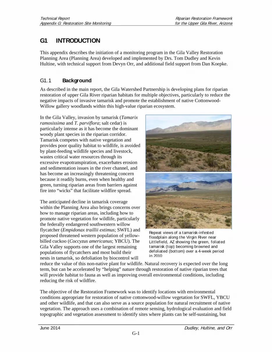
Technical Report Riparian Restoration Framework Appendix G: Restoration Site Monitoring for the Upper Gila River, Arizona
June 2014 Dudley, Hultine, and Orr G-1
G1 INTRODUCTION
This appendix describes the initiation of a monitoring program in the Gila Valley Restoration Planning Area (Planning Area) developed and implemented by Drs. Tom Dudley and Kevin Hultine, with technical support from Devyn Orr, and additional field support from Dan Koepke.
Background G1.1
As described in the main report, the Gila Watershed Partnership is developing plans for riparian restoration of upper Gila River riparian habitats for multiple objectives, particularly to reduce the negative impacts of invasive tamarisk and promote the establishment of native Cottonwood-Willow gallery woodlands within this high-value riparian ecosystem. In the Gila Valley, invasion by tamarisk (Tamarix ramosissima and T. parviflora; salt cedar) is particularly intense as it has become the dominant woody plant species in the riparian corridor. Tamarisk competes with native vegetation and provides poor quality habitat to wildlife, is avoided by plant-feeding wildlife species and livestock, wastes critical water resources through its excessive evapotranspiration, exacerbates erosion and sedimentation issues in the river channel, and has become an increasingly threatening concern because it readily burns, even when healthy and green, turning riparian areas from barriers against fire into “wicks” that facilitate wildfire spread. The anticipated decline in tamarisk coverage within the Planning Area also brings concerns over how to manage riparian areas, including how to promote native vegetation for wildlife, particularly the federally endangered southwestern willow flycatcher (Empidonax traillii extimus; SWFL) and proposed threatened western population of yellow-billed cuckoo (Coccyzus americanus; YBCU). The Gila Valley supports one of the largest remaining populations of flycatchers and most build their nests in tamarisk, so defoliation by biocontrol will reduce the value of this non-native plant for wildlife. Natural recovery is expected over the long term, but can be accelerated by “helping” nature through restoration of native riparian trees that will provide habitat to fauna as well as improving overall environmental conditions, including reducing the risk of wildfire. The objective of the Restoration Framework was to identify locations with environmental conditions appropriate for restoration of native cottonwood-willow vegetation for SWFL, YBCU and other wildlife, and that can also serve as a source population for natural recruitment of native vegetation. The approach uses a combination of remote sensing, hydrological evaluation and field topographic and vegetation assessment to identify sites where plants can be self-sustaining, but
Repeat views of a tamarisk-infested floodplain along the Virgin River near Littlefield, AZ showing the green, foliated tamarisk (top) becoming browned and defoliated (bottom) over a 4-week period in 2010

Technical Report Riparian Restoration Framework Appendix G: Restoration Site Monitoring for the Upper Gila River, Arizona
June 2014 Dudley, Hultine, and Orr G-2
also at low risk of flood scouring. Combined with documentation of historic and current SWFL habitat use, restoration sites are intended to also have high potential for colonization by the bird. In some restoration sites, tamarisk may require moderate control measure to open up space and facilitate establishment of native plants. But because biocontrol will eventually reduce plant volume and the remaining plants provide structural benefits for wildlife, the intent is to minimize weed treatments, in part because prior analyses have shown that physical disturbance promotes secondary invasion of other noxious weeds such as Russian thistle, knapweeds, or perennial pepperweed that interfere with riparian recovery. On the other hand, the impacts of increasingly frequent wildfire on the Gila River, fueled by abundant tamarisk vegetation and often within SWFL nesting territories, can be turned into an asset if we can implement restoration efforts where fire has reduced weed biomass. This requires rapid herbicide treatment, however, because tamarisk readily re-sprouts and can regain high vegetative cover within a single growth season. All these elements are brought together in planning for successful and cost-effective riparian restoration, what we term “Integrative Ecosystem Pest Management.”
Purpose of Monitoring Program G1.2
In support of the Restoration Framework we initiated a pre-biocontrol monitoring program from which future efforts to monitor environmental conditions in the Planning Area may reasonably follow and to compare results as conditions respond to beetle colonization. Specifically, the monitoring program is intended to provide a quantitative system for evaluating the conditions of vegetation and associated ecosystem variables as they relate to current and future suitability for occupation by SWFL. It is also meant to build the capacity to evaluate the effectiveness of restoration actions in meeting the primary objective of enhancing habitat for SWFL in the face of future tamarisk defoliation by the leaf beetle. The program also provides an environmental framework for assessing future impacts of tamarisk biocontrol, involving the documentation of tamarisk distribution, abundance, health and genetic make-up. The monitoring program was employed at several sites identified during the ecohydrological assessment and SWFL habitat modeling as exhibiting relatively high suitability for active tamarisk treatment and/or native vegetation plantings.
Technical Report Riparian Restoration Framework Appendix G: Restoration Site Monitoring for the Upper Gila River, Arizona
June 2014 Dudley, Hultine, and Orr G-3
G2 MATERIALS AND METHODS
G2.1 Vegetation Monitoring
The objectives of the vegetation monitoring task was to: (1) document vegetation status (plant species composition and condition, stem densities, canopy structure, biocontrol impacts, non-native plant abundance, etc.) prior to and during the course of restoration actions at current and proposed restoration sites for SWFL habitat enhancement; and (2) assess SWFL reproductive needs by applying monitoring protocol to existing nesting sites in order to describe reference conditions as a target for designing restoration treatments. Monitoring was initiated in the spring of 2013, targeting potentially suitable restoration sites and a representative subset of currently occupied sites to provide reference conditions for SWFL nest site choice. The monitoring protocol was applied immediately prior to anticipated SWFL return from over-wintering regions to document vegetation conditions as closely as possible to the nesting period without interfering with reproductive activity. Monitoring stations were established to provide two general types of information: (1) to document vegetation and soils conditions at sites currently or recently known to be occupied by SWFL, as a guide to the target ecosystem conditions to be replicated in restoration efforts; and (2) to characterize potential restoration locations in order to provide baseline, pre-treatment conditions to be used both for determining best management practices suited for ecosystem conditions currently at those sites, and for evaluating the effectiveness of treatments and anticipated recovery responses once projects are implemented.
G2.1.1 Vegetation survey overview
Survey teams consisted of a minimum of three technicians, with one team leader designated for the full course of site monitoring to maintain sampling consistency throughout the exercise. Owing to the objective of characterizing riparian habitat for SWFL usage, the team leader was also qualified for surveying of riparian bird species and habitat, and specifically certified for SWFL monitoring. Sites considered to be “Occupied” were chosen based on prior avian surveys conducted by SRP wildlife biologists (SRP 2013). However, because we were monitoring site conditions prior to return from over-wintering grounds, it was not possible to verify whether conditions at these locations were still suitable for breeding. Only one pre-nesting sampling exercise was implemented—during April and May (once vegetation had fully leafed out)—to avoid potential habitat disturbance if sensitive bird species were present. There was furthermore not a substantial enough change in site conditions between pre- and post-breeding season dates to merit a second round of monitoring.
G2.1.2 Spatial allocation of vegetation sampling units
Vegetation was monitored at the 7 sites selected within the Planning Area with the highest number of confirmed SWFL detections in previous years, based on data collected by SRP (2013). These sites were located between the towns of Pima and Fort Thomas on properties owned and/or managed by Freeport-McMoRan Copper & Gold (FMI), Salt River Project (SRP), Bureau of Land Management (BLM), and Bureau of Reclamation (BOR). The sites, which are shown in their respective maps in the results section below, are as follows (listed in upstream order):
1. FMI’s Riparian Restoration Study Area site #1 (FMI-RRSA-1) and SRP’s Conservation Easement site #4 (SRPCE-4), which overlay the “Clay Fire (2013)” burn area
2. FMI-owned SRPCE-1 (immediately south of FMI-RRSA-1)

Technical Report Riparian Restoration Framework Appendix G: Restoration Site Monitoring for the Upper Gila River, Arizona
June 2014 Dudley, Hultine, and Orr G-4
3. FMI-RRSA-2 and SRPCE-2 4. BLM-owned SRP mitigation site #1 (SRP-1) (east of FMI-RRSA-2) 5. SRP-owned SRP mitigation site #2 (SRP-2) (east of FMI-RRSA-2) 6. BOR-owned SRP mitigation site “BR/Bellman” (SRP-BR/Bellman) (south of FMI-
RRSA-2) 7. FMI-RRSA-3
At each of these sites, 8 plots were established along two independent transects, for a total of 16 plots per site. The zone of suitable SWFL habitat at prior occupied sites tended to be narrow, leading us to establish survey plots in a general linear array following contours of the stream channel. All plots were located within 200 meters (m) of the active channel except for SRPCE-1, where SWFL have nested up to 350 m from the river; most were within 100 m. The 16 plots were arranged on a transect grid overlaying the general target area. The length of transects was determined by the habitat patch dimensions, with a minimum length of 20 m if habitat was narrow in breadth, while up to 100 m length where the habitat zone was broad. Each plot had an area of approximately 50 square meters (m2), with each center point arranged along a transect at a minimum distance of 10 m between each plot (Figure G-1). Plots formed a diamond shape, extending 5 m in both directions along the transect and 5-m perpendicular from the center point; 5-m ropes or measuring tapes formed each radial, with a longer rope or tape connecting each end-point to form a series of 4 triangular sectors. Vegetation traits were assessed as described below for stem densities and other variables. Associated with each plot, three 1 x 1-m quadrats for understory species composition and primary cover analysis were set at 0, 5, and 10 m (beginning, middle, and end of plot), while vertical structure was estimated at 1-m intervals along the diagonal transect (10 points).
Figure G-1. Diagram of one vegetation survey plot (left) and typical plot arrangement along
each transect (right)
Technical Report Riparian Restoration Framework Appendix G: Restoration Site Monitoring for the Upper Gila River, Arizona
June 2014 Dudley, Hultine, and Orr G-5
G2.1.3 Total plot measurements
Density, percent cover, and species identity of all woody perennial plants (shrubs, trees, etc.) and non-woody plants over 1.5 m in height were counted within each 50 m2 plot. Stem counts were taken on a plane 10 centimeter (cm) above the ground for all woody plants present on site. To be counted, a stem needed to originate from a woody plant exceeding 1.5 m in height, and the base of the stem had to be entirely within the plot. Stem diameters exceeding 8 cm (at 10 cm height) were measured with a sliding caliper and recorded; stems with a diameter <2 cm (at 10 cm height) were excluded from the count. To characterize plot surface traits, we estimated the percent of the plot occupied by bare substrate. Qualitative notes were taken to indicate attributes of relevant substrate (i.e., moist, wet, dry, sandy, silty, loam, clay). In addition, we estimated the total percent of the plot occupied by leaf litter (Tamarix spp. or non-Tamarix source), dead wood, cobble, and standing water coverage (for which an average depth was also estimated).
G2.1.4 Quadrant measurements
Density, primary cover and species identity of all woody and herbaceous plants were counted within each 1 m2 quadrat. For each species, total number of stems and condition (alive or dead) were recorded, as well as an estimate of percent cover. Percent cover of leaf litter, woody debris, and exposed substrate were estimated, along with average litter depth and species composition of leaf litter (Tamarix spp. or non-Tamarix source). A qualitative assessment of substrate type (sand, gravel, cobble, etc.) was made. A densitometer reading was taken at each quadrat to determine percent foliar cover. Signs of any animal activity (tracks, bite marks, fecal material, etc.) was also noted.
G2.1.5 Vertical point / canopy cover measurements
Vertical intercepts of vegetation within each plot were measured using the “hits to a pole” method of Mills et al. (1991). From ground level to maximum shrub/tree height, the number of hits per meter layer were counted by species. For this project, both dead and live material were included, but recorded separately. A “hit” occurred when plant material was within a 10 cm radius of the center of the pole. All woody and herbaceous plants were recorded.
G2.2 Soils Monitoring
Soil samples were collected at the 7 vegetation-monitoring sites along the established site transects. At each transect, soil samples were collected every 10–20 m at two depths: 0–10 cm and 20–30 cm. Each soil sample was placed in a paper bag and allowed to air-dry before processing soil texture (i.e., percent, sand, silt, and clay), electrical conductivity (EC), and pH. Texture was determined by separating and dry-weighing incremental grain size material using a nested sieve set of standard mesh openings. Coarse sand ranged from #4–10 sieve mesh size, medium sand ranged from #10–40 mesh size, and fine sand was from #40–200 mesh size. Silt and clay content were determined using a #200 and #230 mesh size. Proportions of total weight in each size fraction yielded a measure of percent “fines”—an indicator of water holding and infiltration capacity. The number of transects per site ranged from 1 to 6, and the number of sample locations ranged from 8 to 40 per site. The coordinates of the soil sample locations are given in Table G-2.

Technical Report Riparian Restoration Framework Appendix G: Restoration Site Monitoring for the Upper Gila River, Arizona
June 2014 Dudley, Hultine, and Orr G-6
G2.3 Groundwater Monitoring
Shallow groundwater levels were monitored close to the active river channel at 6 locations in the Planning Area. Some, but not all, of the groundwater monitoring locations were generally near the vegetation and soil monitoring sites. Two well piezometers were installed at each location to monitor groundwater depth throughout the season. The paired wells (i.e., nest) were aligned perpendicular to the primary river channel with one well located near the edge of the channel and the second well located near the outer edge of the riparian vegetation corridor. One site (Site 2) has three wells: two are along a single transect, and a third placed approximately one mile upstream from the other two installations. Site 4 only has one well because access to the second location was not feasible. The coordinates of each piezometer are given in Table G-3.

Technical Report Riparian Restoration Framework Appendix G: Restoration Site Monitoring for the Upper Gila River, Arizona
June 2014 Dudley, Hultine, and Orr G-7
G3 Monitoring Results
G3.1 Vegetation Monitoring Results
G3.1.1 Vegetation composition and structure at all monitoring sites
Occupied sites varied from monotypic, single strata stands to habitat patches with multiple species and more complex canopy and subcanopy structure. Tamarisk formed a nearly continuous, closed canopy (with no distinct overstory layer). Canopy height generally averaged from 5 to 10 m, with canopy density uniformly high. Live foliage density was relatively low from 0 to 2 m above the ground, typical of the interior of tamarisk stands, but increased higher in the canopy. Within the patches, there are numerous small openings in the canopy and understory. The numerous dead branches and twigs provided for most of the structural density in the lower 2 to 3 m strata. In normal or wet precipitation years, surface water is adjacent to or within tamarisk habitat patches, as evidenced by the desiccated remains of wetland species in the understory of some plots; however due to the ongoing drought in this region, all consistent water at our monitoring sites was constrained to the main channel and agricultural runoff ditches. Compiled results from the vegetation monitoring effort are briefly summarized in Table G-1 and Figures G-2, G-3, and G-4. SWFL nesting sites were characterized by fairly monotypic tamarisk stands, with very low density of natives. Only four native species were present within our survey plots: Fremont cottonwood (Populus fremontii), Goodding’s willow (Salix gooddingii), coyote willow (Salix exigua), and mulefat (Baccharis salicifolia). The herbaceous layer at all locations was sparse and not a significant habitat component; typically no more than one or two herbaceous species were detected—bermuda grass (Cynodon dactylon) and johnsongrass (Sorghum halepense)—and total ground cover was well below 10%. Dead material at all sites accounted for a significant proportion of the vegetation structure. Elsewhere on the monitoring sites, desert broom (B. sarothroides), Emory’s baccharis (B. emoryi), and/or mesquite (Prosopis glandulosa and/or P. velutina) occasionally occurred at very low cover. Vegetation density of all species across sites was highly variable. Substrates were composed predominantly of silt and clay, with sand occurring along both old and current channels. These tamarisk-dominated shrublands and tamarisk-willow woodlands typically occur on silty substrates. Soil moisture conditions varied from wet to dry, depending on the proximity to the river, relative elevation from the low-flow channel, time since last rain or flood, and agricultural return flows; however, beyond 2 m of an active channel, our plots all exhibited dry soils. Results of the sampled soils are presented below. Due to the within-site patchiness of vegetation in the monitoring area, vertical foliar density was determined to be a more meaningful measurement of site suitability than average stem density. Tree stem density varied greatly depending on stand age; at SRP 1, stem density was high and fairly uniform, while at SRP-BR/Bellman and SRPCE-1, trees were older, taller, and larger in diameter, resulting in lower near-ground stem cover. However, this variation had less effect on canopy density and vertical stem structure above 1–2 m. Looking at vertical foliar density at each site, there is a significant increase in density from 1–3 m. Typically, plots have a well-defined litter layer, and an uneven distribution of fallen woody debris, (ranging from 0-90% quadrat ground cover with an average of 10% cover). Herbaceous ground cover was sparse to absent across all sites. Due to the particularly dry season during our surveys, no plots contained standing water. Canopy height varied from site to site (typically 5–10 m), but FMI-RSSA-3 had an uncharacteristically high canopy of 15 m due to the presence of cottonwoods at this site.
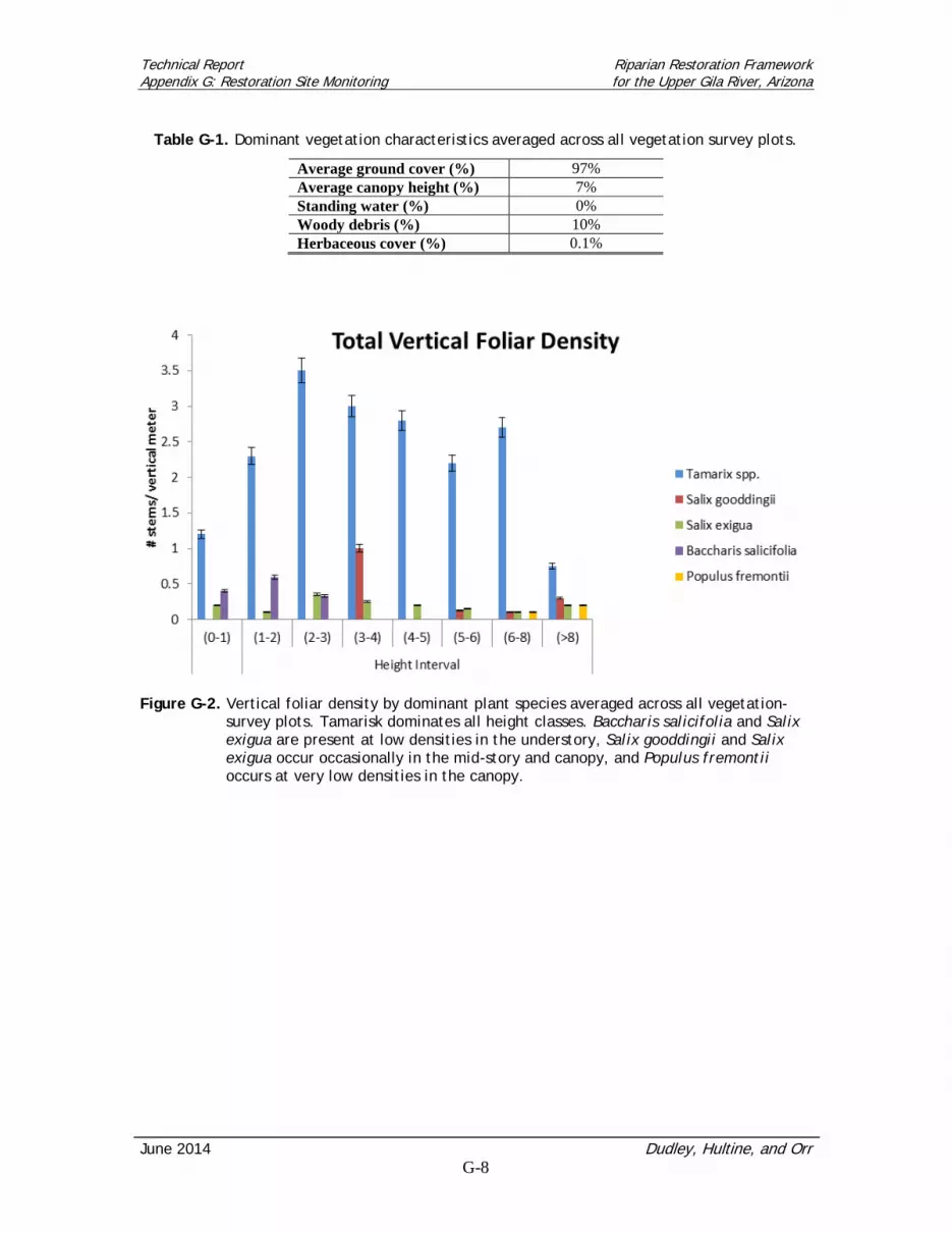
Technical Report Riparian Restoration Framework Appendix G: Restoration Site Monitoring for the Upper Gila River, Arizona
June 2014 Dudley, Hultine, and Orr G-8
Table G-1. Dominant vegetation characteristics averaged across all vegetation survey plots.
Average ground cover (%) 97% Average canopy height (%) 7% Standing water (%) 0% Woody debris (%) 10% Herbaceous cover (%) 0.1%
Figure G-2. Vertical foliar density by dominant plant species averaged across all vegetation-
survey plots. Tamarisk dominates all height classes. Baccharis salicifolia and Salix exigua are present at low densities in the understory, Salix gooddingii and Salix exigua occur occasionally in the mid-story and canopy, and Populus fremontii occurs at very low densities in the canopy.

Technical Report Riparian Restoration Framework Appendix G: Restoration Site Monitoring for the Upper Gila River, Arizona
June 2014 Dudley, Hultine, and Orr G-9
Figure G-3. Stem density by dominant plant species averaged across all vegetation-survey
plots. Tamarisk snag currently accounts for over 50% of tamarisk density at sites utilized by SWFL.
Figure G-4. Percent open canopy cover at each of the vegetation-survey sites. Canopy cover
varied from 4–50% across sites; excluding the burn site, all sites fell between 45–50% cover.

Technical Report Riparian Restoration Framework Appendix G: Restoration Site Monitoring for the Upper Gila River, Arizona
June 2014 Dudley, Hultine, and Orr G-10
G3.1.2 Site-specific vegetation conditions
FMI-RRSA-1 / SRPCE-4 The increased fire susceptibility of tamarisk relative to native vegetation types is a notable threat to the persistence of suitable habitat along this portion of the river. In March 2013 near Fort Thomas, nearly all of the tamarisk and willow biomass was burned on the upstream section of FMI-RRSA-1 during the Clay Fire. In previous years, this site hosted a number of SWFL breeding pairs. During our April surveys, one willow flycatcher individual was observed singing from a dead tamarisk branch overhanging the main river channel. Although this was prior to the breeding season and the individual did not remain at the site, its presence suggests there is still a good possibility of re-colonization of this site once the vegetation has recovered, either through tamarisk growth or restoration of native species. Overall, the site is characterized by bare, dry and silty substrates, with sand and gravel present in the scour zone, and with little organic or litter component remaining owing to fire intensity (Figures G-5 and G-6). During our April survey, no live biomass was present, except for a 1–2 m strand immediately adjacent to the main channel in some reaches, where presumably conditions were moist enough to protect vegetation from mortality during the fire. Cover of all species was low (<15%). However, by the beginning of May, nearly all burnt tamarisk trees were observed to be re-sprouting vigorously from the base, indicating there is only a limited window of opportunity to establish native species before tamarisk biomass once again dominates the site. The channel is only moderately incised, with approximately 3 m difference between surface water and the surrounding terrace, indicating that groundwater should be sufficiently close to the surface to support restoration plant materials; however, preliminary assessment indicates that depth to groundwater is progressively deeper at distance from the stream, as expected in a “losing reach” (sub-surface flows generally downward). One piezometer is now installed, and an array at different distances from the stream channel is needed to describe seasonal water available dynamics for planning location-specific restoration methods and target species (see groundwater monitoring results presented below). The area potentially suitable for active restoration of SWFL habitat is approximately 30 hectares (ha). Some portions would potentially benefit habitat for other species such as yellow-billed cuckoo, as well as to provide a fire-resistant, native vegetation buffer zone to inhibit future penetration of fire into the riparian area.

Technical Report Riparian Restoration Framework Appendix G: Restoration Site Monitoring for the Upper Gila River, Arizona
June 2014 Dudley, Hultine, and Orr G-11
Figure G-5. Map of the FMI-RRSA-1 / SRPCE-4 site showing vegetation monitoring locations. The
approximate burned area boundary is shown in orange within which the target restoration zone is indicated by the green polygon. Red lines indicated vegetation transects completed in June 2013 across primary. Blue boundary is property line of FMI land, with BLM-managed federal land on the eastern portion.
Figure G-6. Vertical foliar density at the FMI-RRSA-1 / SRPCE-4 site. Most of the tamarisk
biomass is dead material in the wake of the Clay Fire, except under 3 m where re-sprouting has occurred. Natives are a very minor habitat component.
Monitoring Locations

Technical Report Riparian Restoration Framework Appendix G: Restoration Site Monitoring for the Upper Gila River, Arizona
June 2014 Dudley, Hultine, and Orr G-12
SRPCE-1 Vegetation at this site is characterized by monotypic tamarisk (Figures G-7 and G-8). Density is variable, with percent cover ranging from 20–90%. Most individuals are under 10 m in height. Substrates are silt and clay, with moisture ranging from dry to very moist (see additional soils results below).
Figure G-7. Map of the SRPCE-1 site showing vegetation monitoring locations.
Figure G-8. Vertical foliar density at the SRPCE-1 site. Tamarisk dominates all height
categories, with greatest densities from 2–3 m and 6–8 m.
Monitoring Sites
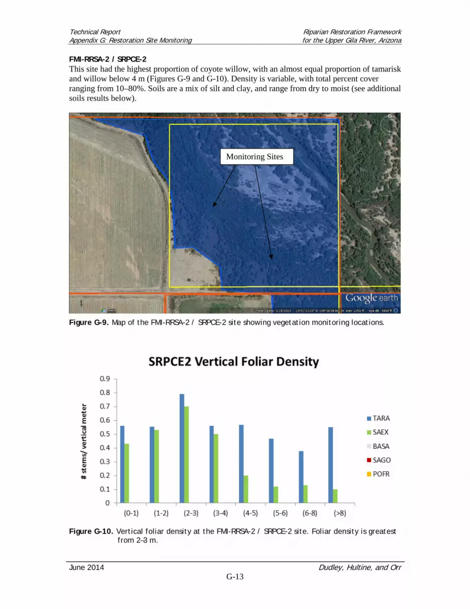
Technical Report Riparian Restoration Framework Appendix G: Restoration Site Monitoring for the Upper Gila River, Arizona
June 2014 Dudley, Hultine, and Orr G-13
FMI-RRSA-2 / SRPCE-2 This site had the highest proportion of coyote willow, with an almost equal proportion of tamarisk and willow below 4 m (Figures G-9 and G-10). Density is variable, with total percent cover ranging from 10–80%. Soils are a mix of silt and clay, and range from dry to moist (see additional soils results below).
Figure G-9. Map of the FMI-RRSA-2 / SRPCE-2 site showing vegetation monitoring locations.
Figure G-10. Vertical foliar density at the FMI-RRSA-2 / SRPCE-2 site. Foliar density is greatest
from 2–3 m.
Monitoring Sites

Technical Report Riparian Restoration Framework Appendix G: Restoration Site Monitoring for the Upper Gila River, Arizona
June 2014 Dudley, Hultine, and Orr G-14
SRP-1 and SRP-2 Vegetation at both sites is characterized by monotypic tamarisk (Figures G-11, G-12, G-13, and G-14). Density is variable, with percent cover ranging from 10–90%. Individual height and trunk diameter also varied greatly, with some trees well over 10 m tall. Substrates are silt and clay, with moisture ranging from dry to very moist (see additional soils results below).
Figure G-11. Map of the SRP-1 site showing vegetation monitoring locations.
Figure G-12. Vertical foliar density at the SRP-1 site. Foliar density is greatest from 2–3 m.
Monitoring Sites

Technical Report Riparian Restoration Framework Appendix G: Restoration Site Monitoring for the Upper Gila River, Arizona
June 2014 Dudley, Hultine, and Orr G-15
Figure G-13. Map of the SRP-2 site showing vegetation monitoring locations.
Figure G-14. Vertical foliar density at the SRP-2 site. Tamarisk dominates all layers, with
greatest densities from 2–3 m and 6–8 m.
Monitoring Sites
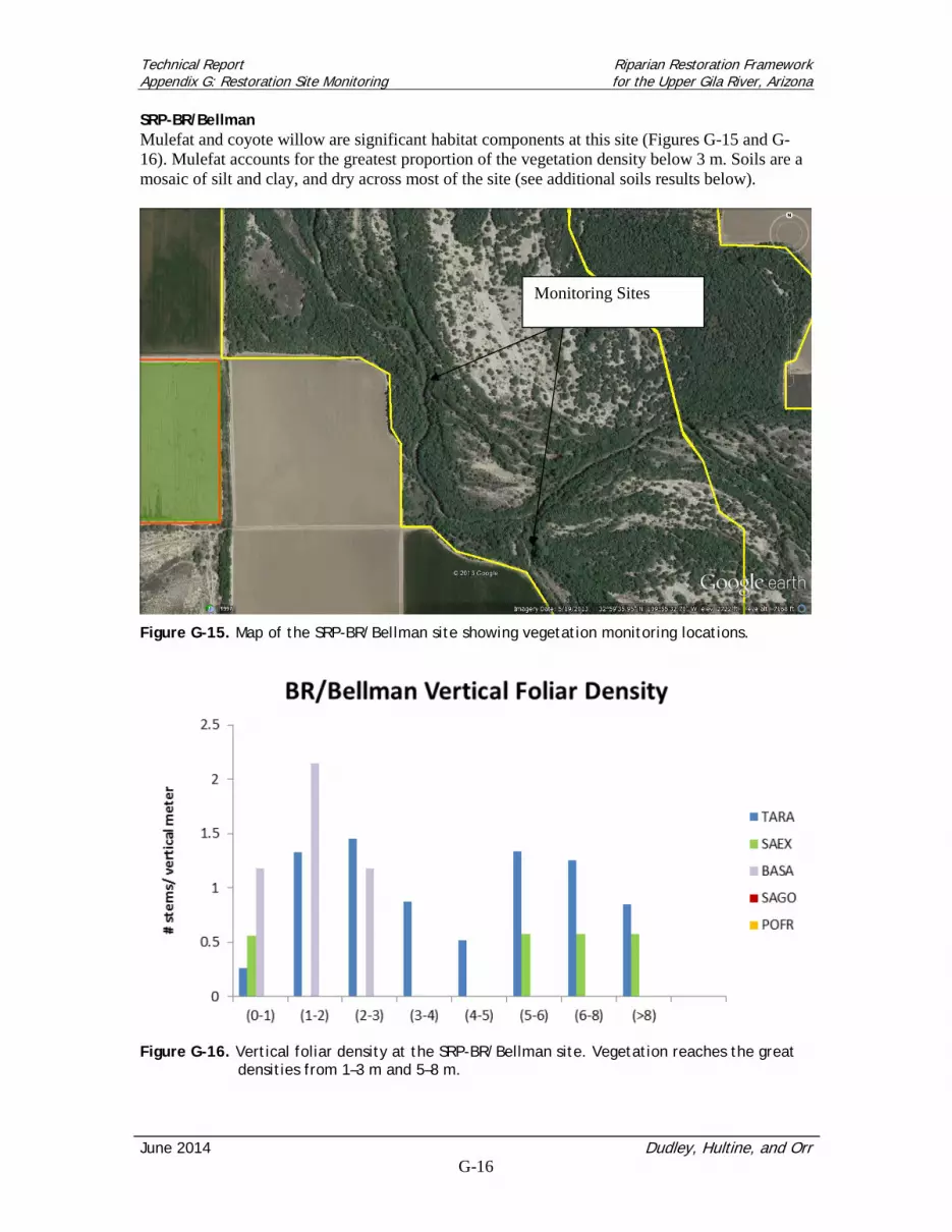
Technical Report Riparian Restoration Framework Appendix G: Restoration Site Monitoring for the Upper Gila River, Arizona
June 2014 Dudley, Hultine, and Orr G-16
SRP-BR/Bellman Mulefat and coyote willow are significant habitat components at this site (Figures G-15 and G-16). Mulefat accounts for the greatest proportion of the vegetation density below 3 m. Soils are a mosaic of silt and clay, and dry across most of the site (see additional soils results below).
Figure G-15. Map of the SRP-BR/Bellman site showing vegetation monitoring locations.
Figure G-16. Vertical foliar density at the SRP-BR/Bellman site. Vegetation reaches the great
densities from 1–3 m and 5–8 m.
Monitoring Sites

Technical Report Riparian Restoration Framework Appendix G: Restoration Site Monitoring for the Upper Gila River, Arizona
June 2014 Dudley, Hultine, and Orr G-17
FMI-RRSA-3 This is the only site we monitored having a significant Fremont cottonwood-Goodding’s willow woodland, although monotypic tamarisk still covers over half the property (Figures G-17 and G-18). Here, the cottonwood stand occurs between the edge of the agricultural fields and the outer margin of the riparian corridor, on the bank of a high-flow channel. Cottonwood and Goodding’s willow are present at 20–60% cover, and form a dense, high canopy (8–14 m). Trees are mature or decadent, with low levels of recruitment. The shrub layer is composed of Baccaris spp. and tamarisk at 10% cover. There is a thick leaf litter layer, and much of the ground is covered by downed wood; soils are a mosaic of sand, silt, and clay with varying moisture levels (see additional soils results below). Common reed (Phragmites australis), arundo (Arundo donax), and bermudagrass occur at lower densities at this site, adjacent to the river channel. The rest of the site is a tamarisk-Goodding’s willow mixed type, where Goodding’s willow is present at 10–30% cover near the channel and then drops out at higher elevations of the floodplain where soils are drier. One yellow-billed cuckoo pair was incidentally detected on this property in the cottonwood canopy late in the season.
Figure G-17. Map of the FMI-RRSA-3 site showing vegetation monitoring locations.
Monitoring Locations

Technical Report Riparian Restoration Framework Appendix G: Restoration Site Monitoring for the Upper Gila River, Arizona
June 2014 Dudley, Hultine, and Orr G-18
Figure G-18. Vertical foliar density at the FMA-RRSA-3 site. Mulefat and coyote willow occur at
low densities in the understory. Goodding’s willow and cottonwood make up 30-60% of the canopy.
G3.2 Soils Monitoring Results
Overall, the sampled soils (Table G-2) were generally composed of fine sand (Figure G-19). Soil EC was generally higher in the upper 0–10 cm layer (Figure G-20), while soil pH was generally the same at the two depths (Figure G-21). More detailed results are described below for each of the sampled sites. Table G-2. Soil sample site names, location, number of transects per site, and total number of
soil samples per site.
Monitoring site
Soil sampling site ID
Longitude, Latitude (NAD83)
Number of transects
Total number of soils samples
FMI-RRSA-1 / SRPCE-4
“Burn North” 33.04016, -109.95011 5 31 “Burn South” 33.0371, -109.94686 5 40
SRPCE-1 “SRPCE 1-2” 33.02741, -109.94540 1 8 “SRPCE 1-1” 33.02633, -109.94506 1 8
FMI-RRSA-2 / SRPCE-2 “SRPCE 2-1, 2-2” 33.02107, -109.93491 2 16
SRP-1 “SRP 1-1” 33.02033, -109.92565 1 8 “SRP 1-2” 33.00703, -109.92205 1 8
SRP-BR/Bellman “BR/Bellman” 32.9936, -109.93725 2 16
FMI-RRSA-3 “FMI 3” 32.98131, -109.91800 6 31 “FRRS 3-1, 3-2” 32.98062, -109.91875 2 16

Technical Report Riparian Restoration Framework Appendix G: Restoration Site Monitoring for the Upper Gila River, Arizona
June 2014 Dudley, Hultine, and Orr G-19
FMI-RRSA-1 / SRPCE-4 Soil texture of the samples collected at the “Burn North” and “Burn South” locations was composed primarily of fine to medium-sized sand (Figure G-19). For each of the five transects sampled at the two sites (n=10 sites), the upper soil layer (0–10 cm) had a consistently higher EC than the lower layer (20–30 cm) (Figure G-20). However, only two of the five “Burn North” samples were significantly different (P <0.05), and no significant differences were detected at the “Burn South” sites. The range of mean EC for 0–10 cm was 372 to 1200 micro-siemens per centimeter (uS/cm), and 124 to 482 uS/cm for the 20–30 cm depths. Measured pH in soil samples collected at the “Burn North” site were consistently lower in the upper soil layer (0–10 cm) (Figure G-21). Mean pH values in the upper layer ranged between 8.0 to 8.6, while mean values in the lower layer (20–30 cm) ranged between 8.3 and 8.6. SRPCE-1 and FMI-RRSA-2/SRPCE-2 The soil texture of samples collected at the “SRPCE 1-1” and “SRPCE 1-2” sites were fairly evenly distributed. Soils sampled from the “SRPCE 2-1” and “SRPCE 2-2” sites contained a greater proportion of course-textured sand. The measured EC values were generally greater in the upper soil layer (0–10 cm). The range of mean EC for 0–10 cm was 1075 to 2047 uS/cm, and 603 to 1365 uS/cm for 20–30cm. The mean pH ranged from 8.0 to 8.4, with the lower pH values measured in the upper soil profile, but no significant differences occurred. SRP-1 The soil texture of samples collected at the “SRP 1-1” and “SRP 1-2” sites were composed mostly of course-textured sand intermixed with medium textured sand. The measured EC values were inconsistent between the two sampling sites. Mean values were greater in the lower soil layer (20–30 cm) at the “SRP 1-1” site, but greater in the upper soil layer (0–10 cm) at the “SRP 1-2” site. The range of mean EC for 0–10 cm was 1441 to 1695 uS/cm, and 908 to 2557 uS/cm for 20–30cm. The mean pH ranged from 7.9 to 8.6 and was consistently lower in the upper soil layers. SRP-BR/Bellman The soil texture of samples collected at the “BR/Bellman” site was composed mostly of coarse to medium sands. The measured EC values were greater for the lower soil layer (20–30 cm) for both transects; it was significantly greater for one and almost significantly higher for the other (P=0.014 and P=0.064, respectively). The range of mean EC was 581 to 1000 uS/cm for the 0–10 cm layer, and 316 to 457 uS/cm for the 20–30 cm layer. The mean pH values were greater but not significantly so for the two transects of the 20–30 cm layer compared to the 0–10 cm profiles. The range of pH for the 0–10 cm layer was 7.9 to 8.2, and 8.2 to 8.4 for the 20–30 cm layer. FMI-RRSA-3 The soil texture of samples collected at the “FMI-3” site for the upper soil layer (0–10 cm) were slightly skewed toward course sand, but texture at the lower soil layer (20–30 cm) were widely distributed from course sand to finer silts and clays. Soil texture of samples collected at the “FRRS 3-1” and “FRRS 3-2” sites mostly ranged from medium sand to silt. At the “FMI-3” site there were no significant differences detected in mean EC values between soil profile depths, but all 6 transects had greater EC values at the 0–10 compared to 20–30 cm profile. The range of mean EC values was 189 to 571 uS/cm for the 0–10 cm layer, and 175 to 280 uS/cm for the 20–30 cm layer. All transects had a higher pH for the 20–30 cm profile, but no statistical differences between this lower layer with the upper layer were detected. The range of mean pH values was 7.8 to 8.3 for the 0–10 cm layer, and 8.0 to 8.4 for the 20–30 cm layer.

Technical Report Riparian Restoration Framework Appendix G: Restoration Site Monitoring for the Upper Gila River, Arizona
June 2014 Dudley, Hultine, and Orr G-20
Both transects at the “FRRS 3-1” and “FRRS 3-2” sites had greater EC values in the upper soil layer, but only one was statistically greater (P=0.0071). The range of EC values was 348 to 483 uS/cm for the 0–10 cm layer, and 173 to 206 uS/cm for the 20–30 cm layer. The mean pH values were greater in the lower soil layer, with one transect yielding a significant difference (P = 0.0134). The range of mean pH was 8.3 to 8.4 for the 0–10 cm layer, and 8.5 to 8.6 for the 20–30 cm layer.
Figure G-19. The mean (se; n=6) soil texture sieve or mesh sizes of the 0-10 cm soil profile for
each of the five transects of “Burn North” sample location at the FMI-RRSA-1 / SRPCE-4 site.
Figure G-20. The mean (se; n=6) soil electrical conductivity (EC) of the 0-10 cm and 20-30 cm
soil profiles for each of the five transects of “Burn North” sample location at the FMI-RRSA-1 / SRPCE-4 site.

Technical Report Riparian Restoration Framework Appendix G: Restoration Site Monitoring for the Upper Gila River, Arizona
June 2014 Dudley, Hultine, and Orr G-21
Figure G-21. The mean (se; n=6) soil pH of the 0-10 cm and 20-30 cm soil profiles for each of
the five transects of “Burn North” sample location at the FMI-RRSA-1 / SRPCE-4 site. Only Site 4 was significant.
G3.3 Groundwater Monitoring Results
The initial results of our groundwater monitoring efforts are summarized in Table G-3 and Figure G-22 below. We anticipate that the well nests and overall well network will serve several important functions for guiding restoration efforts. The well nests will allow managers to assess groundwater patterns across the width of the riparian area. Where the reach is “loosing,” or where there is significant channel down-cutting, we would expect greater depth to groundwater on the outer edge of the riparian area. However, our initial measurements conducted in January 2014 generally suggest that depth to groundwater remains fairly static across the width of the riparian area and is not wholly dependent on proximity to the wetted river channel. Future measurements during periods of low flow will provide a greater detail of groundwater patterns. A second important function of the well nests is that combined, the wells will provide a more detailed view of groundwater depth over a fairly large reach of the Gila River that will improve groundwater mapping and future ecohydrological assessment of this section of river targeted for near-future restoration. As part of the ecohydrological assessment, the initial groundwater measurements were compared to relative elevations estimated at each of the piezometer locations (see related sections in the main report). The relative-elevation surface was produced from the 2012 LiDAR data collected for this project. The relative elevations values represent the land surface height above the low-flow channel, which is intended to serve as a proxy for depth to groundwater. Comparisons between the initial groundwater measurements and the corresponding relative-elevation values at all but two of the piezometer locations reveal close agreement (<1 ft difference), suggesting that use of the relative elevation surface to estimate depths to groundwater is a suitable method for restoration planning in the Gila Valley. The two piezometer locations with greater differences (>1 ft) are at 5a and 6a. We suspect that the differences are due to recording error with the GPS coordinates and, thus, recommend their coordinates be re-recorded during subsequent monitoring.
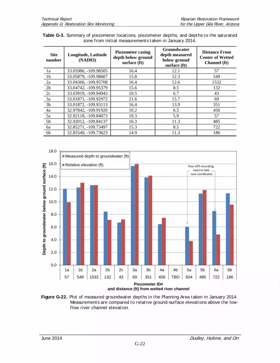
Technical Report Riparian Restoration Framework Appendix G: Restoration Site Monitoring for the Upper Gila River, Arizona
June 2014 Dudley, Hultine, and Orr G-22
Table G-3. Summary of piezometer locations, piezometer depths, and depths to the saturated zone from initial measurements taken in January 2014.
Site number
Longitude, Latitude (NAD83)
Piezometer casing depth below ground
surface (ft)
Groundwater depth measured below ground
surface (ft)
Distance From Center of Wetted
Channel (ft)
1a 33.05986, -109.98505 16.4 12.1 57 1b 33.05879, -109.98607 15.8 12.3 549 2a 33.04366, -109.95708 16.4 12.6 1532 2b 33.04742, -109.95379 15.6 8.5 132 2c 33.03919, -109.94943 10.5 6.7 43 3a 33.01871, -109.92972 21.6 15.7 69 3b 33.01872, -109.93113 16.4 13.9 351 4a 32.97842, -109.91920 10.2 6.5 456 5a 32.92118, -109.84073 10.3 5.9 57 5b 32.92012, -109.84137 16.3 11.3 485 6a 32.85271, -109.73497 15.3 8.5 722 6b 32.85540, -109.73623 14.9 11.3 186
Figure G-22. Plot of measured groundwater depths in the Planning Area taken in January 2014.
Measurements are compared to relative ground-surface elevations above the low-flow river channel elevation.
0.0
2.0
4.0
6.0
8.0
10.0
12.0
14.0
16.0
18.0
1a 1b 2a 2b 2c 3a 3b 4a 4b 5a 5b 6a 6b
57 549 1532 132 43 69 351 456 TBD 504 485 722 186
Dep
th to
gro
undw
ater
bel
ow g
roun
d su
rfac
e (ft
)
Piezometer ID# and distance (ft) from wetted river channel
Measured depth to groundwater (ft)
Relative elevation (ft) Poor GPS recording;need to take
new coordinates
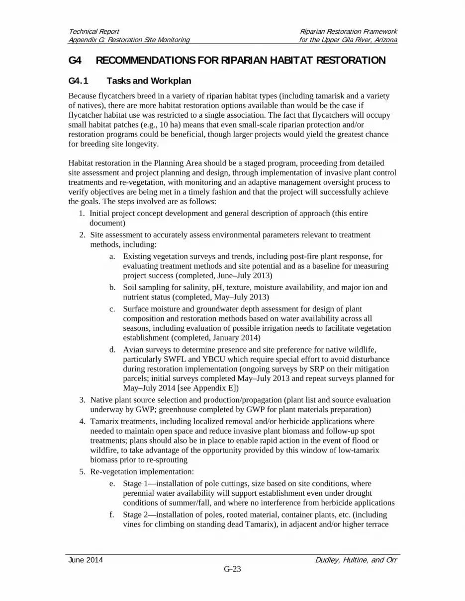
Technical Report Riparian Restoration Framework Appendix G: Restoration Site Monitoring for the Upper Gila River, Arizona
June 2014 Dudley, Hultine, and Orr G-23
G4 RECOMMENDATIONS FOR RIPARIAN HABITAT RESTORATION
G4.1 Tasks and Workplan
Because flycatchers breed in a variety of riparian habitat types (including tamarisk and a variety of natives), there are more habitat restoration options available than would be the case if flycatcher habitat use was restricted to a single association. The fact that flycatchers will occupy small habitat patches (e.g., 10 ha) means that even small-scale riparian protection and/or restoration programs could be beneficial, though larger projects would yield the greatest chance for breeding site longevity. Habitat restoration in the Planning Area should be a staged program, proceeding from detailed site assessment and project planning and design, through implementation of invasive plant control treatments and re-vegetation, with monitoring and an adaptive management oversight process to verify objectives are being met in a timely fashion and that the project will successfully achieve the goals. The steps involved are as follows:
1. Initial project concept development and general description of approach (this entire document)
2. Site assessment to accurately assess environmental parameters relevant to treatment methods, including:
a. Existing vegetation surveys and trends, including post-fire plant response, for evaluating treatment methods and site potential and as a baseline for measuring project success (completed, June–July 2013)
b. Soil sampling for salinity, pH, texture, moisture availability, and major ion and nutrient status (completed, May–July 2013)
c. Surface moisture and groundwater depth assessment for design of plant composition and restoration methods based on water availability across all seasons, including evaluation of possible irrigation needs to facilitate vegetation establishment (completed, January 2014)
d. Avian surveys to determine presence and site preference for native wildlife, particularly SWFL and YBCU which require special effort to avoid disturbance during restoration implementation (ongoing surveys by SRP on their mitigation parcels; initial surveys completed May–July 2013 and repeat surveys planned for May–July 2014 [see Appendix E])
3. Native plant source selection and production/propagation (plant list and source evaluation underway by GWP; greenhouse completed by GWP for plant materials preparation)
4. Tamarix treatments, including localized removal and/or herbicide applications where needed to maintain open space and reduce invasive plant biomass and follow-up spot treatments; plans should also be in place to enable rapid action in the event of flood or wildfire, to take advantage of the opportunity provided by this window of low-tamarix biomass prior to re-sprouting
5. Re-vegetation implementation: e. Stage 1—installation of pole cuttings, size based on site conditions, where
perennial water availability will support establishment even under drought conditions of summer/fall, and where no interference from herbicide applications
f. Stage 2—installation of poles, rooted material, container plants, etc. (including vines for climbing on standing dead Tamarix), in adjacent and/or higher terrace
Technical Report Riparian Restoration Framework Appendix G: Restoration Site Monitoring for the Upper Gila River, Arizona
June 2014 Dudley, Hultine, and Orr G-24
sites when seasonal precipitation will support growth, as well as where irrigation would facilitate establishment in higher stress sites
g. Stage 3—propagated understory and other plant species installed to enhance species and habitat diversity at multiple canopy layers
6. Monitoring and adaptive management: h. Survival and growth rates of restoration planting censused to evaluate most
successful methods i. Site environmental conditions and vegetation assessment continues for
comparison with baseline conditions j. Avian surveys continue to determine if and when SWFL and other species of
interest re-colonized restoration sites k. All data and other information, including climate and hydrology/geomorphology
trends, evaluated to change management actions to enhance survival and self-sustaining recruitment of native vegetation
G4.2 Tamarisk Re-Sprout Treatment at Burned Sites
Immediate tamarisk treatment is recommended at the recently burned FMI-RRSA-1 / SRPCE-4 site to take advantage of the cleared vegetation biomass with minimal impacts to avian wildlife. Biomass removal by the fire was greater than 90% with few plants undamaged (mostly isolated plants with little value to SWFL). Thus, no mechanical treatments were thought necessary at the time of the vegetation surveys in summer 2013. Survival of burned plants, however, has been revealed to be high, with over 94% showing basal re-growth of foliage within 2 months of the fire, and we recommend immediate treatment of these sprouts with herbicide to enable re-vegetation of native plants within this growing season. A triclopyr compound (commonly Garlon-4) can safely be used adjacent to aquatic habitats and is effective on tamarisk, with appropriate surfactant, as a foliar application. Back-pack hand-sprayers are likely appropriate at this scale of operation, by qualified applicators. As the site is no longer suitable for SWFL nesting (documented by D. Orr, June 2013), herbicide-use would presumably be applied without concern for listed avian species. Potential effects to other sensitive wildlife (e.g., listed fisheries) should be evaluated despite that the EPA assessment states that triclopyr has no significant impacts to aquatic vertebrates. Herbicides should be applied prior to any re-vegetation with native plant materials to avoid drift and over-spray impacts, although spot re-treatments may be suitable at a later date with proper precautions. While the immediate focus of restoration is on potential SWFL habitat, it would be important to treat all Tamarix re-sprouts within the burn area while biomass is low and enabling rapid restoration across the burned area as is feasible and meets overall resource management objectives. Treatments should be as soon as is possible for all sites, ideally to yield mortality (although greatest impact is achieved during Fall when plants are translocating metabolites into roots prior to winter senescence of foliage) The total burn area requiring herbicide treatment, including both moist areas and higher terraces, is approximately 40 ha (100 ac), still feasible using hand methods but potentially mechanical weed sprayers for lower-sensitivity areas would provide greater cost-effectiveness. Figures G-23 and G-24 present predicted vegetation responses under two post-biocontrol treatment scenarios for the recently burned FMI-RRSA-1 / SRPCE-4 site. Scenario 1 assumes that no active tamarisk biomass removal would occur following beetle-induced mortality (Figure G-23), whereas Scenario 2 assumes that roughly two-thirds of the standing tamarisk biomass
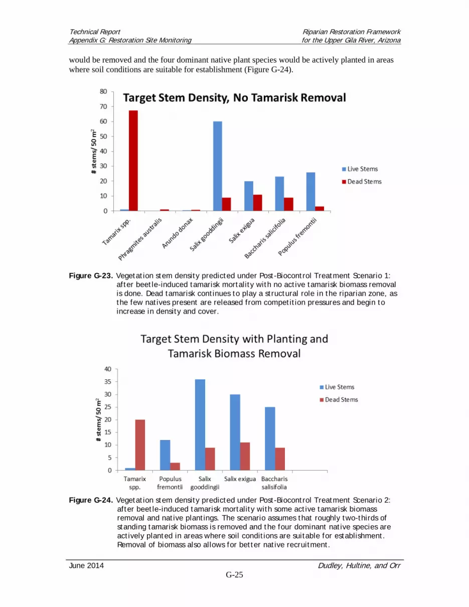
Technical Report Riparian Restoration Framework Appendix G: Restoration Site Monitoring for the Upper Gila River, Arizona
June 2014 Dudley, Hultine, and Orr G-25
would be removed and the four dominant native plant species would be actively planted in areas where soil conditions are suitable for establishment (Figure G-24).
Figure G-23. Vegetation stem density predicted under Post-Biocontrol Treatment Scenario 1:
after beetle-induced tamarisk mortality with no active tamarisk biomass removal is done. Dead tamarisk continues to play a structural role in the riparian zone, as the few natives present are released from competition pressures and begin to increase in density and cover.
Figure G-24. Vegetation stem density predicted under Post-Biocontrol Treatment Scenario 2:
after beetle-induced tamarisk mortality with some active tamarisk biomass removal and native plantings. The scenario assumes that roughly two-thirds of standing tamarisk biomass is removed and the four dominant native species are actively planted in areas where soil conditions are suitable for establishment. Removal of biomass also allows for better native recruitment.

Technical Report Riparian Restoration Framework Appendix G: Restoration Site Monitoring for the Upper Gila River, Arizona
June 2014 Dudley, Hultine, and Orr G-26
G4.3 Plant Propagation, Installation, and Monitoring
G4.3.1 Plant materials
The primary restoration species will be willows, including narrow-leafed willow (Salix exigua) and black or Goodding’s willow (S. gooddingii), and other less common willow. These are fast-growing species anticipated to achieve sufficient size to be suitable for SWFL nesting within 3–4 years. The latter is an arboreal species while S. exigua is shrubby and produces new shoots from lateral roots, creating the dense, multi-layer canopy structure favored by the flycatcher. Additional higher level canopy structure would be provided by cottonwood (Populus fremontii) that is a high-value habitat element for yellow-billed cuckoo, another species of conservation concern in Arizona (and soon to be federally listed as threatened). To provide greater understory structure and promote faster habitat renewal at this site, we recommend propagated various forbs, vines, and shrubs in the project greenhouse for outplanting. Several species can be to both fill in gaps between planted woody species, as well as to stabilize soils and resist secondary invasion by noxious weeds. Native vines such as canyon grape (Vitus arizonica), woodbine (Parthenocissus vitacea), virgin’s bower (Clematis spp.), and others could be grown within residual tamarisk biomass, or “skeletons” (i.e., dead stems remaining post-fire), to rapidly provide habitat and shading for wildlife and insects that are food for birds, lizards, and other vertebrates.
G4.3.2 Re-vegetation methods
Methods for implementing restoration will vary based on site conditions and timing, particularly whether near-surface water is sufficient to support growth without irrigation. SWFL nest sites are restricted to locations where surface water or high humidity are found, thus there would be no need to irrigate in sites intended specifically for enhancing their habitat. At these “wet” sites pole cuttings can be cut nearby, treated with rooting hormone, and installed directly into the soils. Planting depth of 1 meter or more is desirable for promoting adequate root development, and can be attained by driving in solid stake and removing to subsequently insert tree poles. Alternatively, a high pressure water drilling unit, or “stinger,” can be used to prepare a hole for stem insertion, with the advantage of immediately bathing the site with water. For those taxa that do not grow readily from pole cuttings, plants will be grown from seed or cuttings in the greenhouse, and again inserted into moist soils with bare roots or root/soil intact, depending on conditions. At greater distance from surface water or where groundwater depth is greater than about 1 meter, alternative methods and/or timing of re-vegetation will be used. Once depth to water is determined, larger poles of native trees can be cut and inserted to greater depth to ensure direct and perennial access to water. Such methods have been used successfully for cottonwoods and other plants with very large pole cuttings such as stems 4 or 5 meters long and correspondingly large diameter so that the majority of the stem is buried, with only a portion a meter or so in length remains aboveground. This method can be used to establish relatively large plants or trees in a short period of time, but require heavier machinery, such as gas-powered auger, to attain sufficient depth for the planting hole. According to the minimum standards that members of the Restoration Science Team and the SWFL Technical Advisory Committee have developed for application to SWFL habitat enhancement, a minimum of about 4 ha (10 ac) is desired in SWFL site restoration. Vegetated patches can be relatively narrow but based on pre-treatment assessment of occupied sites we consider about a 30-m wide patch as a practical minimum while 100-m wide patches are excellent, particularly with the stream or permanently moist element within the patch. Thus, we

Technical Report Riparian Restoration Framework Appendix G: Restoration Site Monitoring for the Upper Gila River, Arizona
June 2014 Dudley, Hultine, and Orr G-27
propose implementing restoration for about 1 km of stream length with an average width of 50 m. The actual project plans will likely be more detailed, based on site surveys and soil moisture and groundwater assessment. At a later stage, or if resources become available, a larger area would be targeted for SWFL enhancement within the burned area of site FMI-RRSA-1 / SRPCE-4, ideally for all suitable micro-habitat within the river segment. Restoration should also be targeted at higher surfaces on the floodplain where tamarisk has burned in order to provide a buffer to the core SWFL habitat, to reduce the potential for tamarisk re-growth to promote future destructive wildfire, and serve as habitat for other sensitive but less restricted riparian wildlife species. On these higher and drier terraces, moisture is less dependable and unless deep planting techniques (4+ m poles extended to groundwater depth) can be used, it would be better to wait until the fall/winter seasons when water availability would be greater and water demands by vegetation lower. In the interim it may be necessary to apply herbicide treatment to tamarix re-growth to prevent re- accumulation of weed biomass.
G4.3.3 Implementation timing
Re-vegetation should be staged, based on pre-planting treatments, substrate conditions, plant phenology, and availability of propagation material. For permanently moist/saturated sites willows and some other taxa can be installed at any season, and could be planted as early as summer 2014 after SWFL nesting has ended, and once materials and labor are available. Initial focus during this time period should be near known SWFL nesting areas to maximize plant-establishment times before the 2015 nesting season. The remaining SWFL-suitable areas, as well as higher terrace sites, could be planted in late fall 2014/winter 2015 based on availability of moisture from seasonal precipitation, once tamarisk treatments are to a stage where planting is feasible. In these zones temporary irrigation may be appropriate to facilitate initial establishment, but site conditions and planting method will be determined so that cost- and labor-intensive irrigation needs are minimized, and intended for removal within one or two years of planting. Plant materials propagated in the EAC greenhouse from seed or stem material will be installed when winter moisture is available to create diversity of species composition and vegetation structure.
G4.3.4 Monitoring
Several elements of site monitoring needed to design restoration treatments, and to evaluate effectiveness, include:
1. Pre-treatment site monitoring for environmental conditions: a. Vegetation monitoring—vegetation surveys consisting of ten 100-m transects
starting from water’s edge across lower surface for species composition and density of canopy and understory plant species, vertical vegetative structure, canopy density/light penetration and substrate condition including litter/organic debris (soil collections from 20-m intervals along each transect)
b. Soil characterization—soil texture, salinity/conductivity, pH, carbon (C) and nitrogen (N) content and major cations analyses from sampled from hand-augered soil cores collected at 0–10 and 20–30 cm depths
c. Soil moisture/depth to groundwater monitoring—installation of a series of digital piezometers to document soil moisture/shallow groundwater status, both prior to implementation and continuously over course of season to track depth to groundwater; installations should consist of at least 2 piezometers set

Technical Report Riparian Restoration Framework Appendix G: Restoration Site Monitoring for the Upper Gila River, Arizona
June 2014 Dudley, Hultine, and Orr G-28
perpendicular to the stream channel from near stream margin (but high enough that washout risk is minor) and extending to upper floodplain terrace
d. Avian monitoring—SWFL and riparian bird censuses pre-treatment and during treatment by qualified and permitted avian specialist, including arthropod sampling to evaluate wildlife food resource availability as well as to detect potential presence of tamarisk leaf beetle (biocontrol agent)
2. Post-treatment site monitoring: e. Vegetation monitoring— maintain vegetation transects to monitor growth and
survival of re-vegetated plants, with advisory for adaptive management to promote successful establishment of native vegetation
f. Soil characterization—soil samples collected annually to assess change in soil productivity and anticipated decline in salinity with reduction in tamarisk dominance
g. Soil moisture/depth to groundwater monitoring—continue quarterly (or more frequent) groundwater monitoring to assess change in shallow groundwater levels in association with reduction in tamarisk dominance
h. Avian monitoring—continue seasonal SWFL and avian/wildlife surveys to detect re-occupation of sites following treatment activities and/or beetle-induced reduction in tamarisk dominance

Technical Report Riparian Restoration Framework Appendix G: Restoration Site Monitoring for the Upper Gila River, Arizona
June 2014 Dudley, Hultine, and Orr G-29
G5 REFERENCES
Mills, G. M., J. B. Dunning, Jr., and J. M. Bates. 1991. The relationship between breeding bird density and vegetation volume. Wilson Bulletin 103: 468–479. SRP (Salt River Project). 2013. Baseline inventory, Fort Thomas Preserve, Gila River, Graham County, Arizona. Compiled by SRP, Siting and Studies Division, Environmental Services Department, Phoenix, AZ.


