Investment and Finance when Liquidation is Costly

INVESTMENT AND FINANCE WHEN LIQUIDATION IS COSTLY***

BY

ALLARD BRUINSHOOFD* AND WILKO LETTERIE**

Summary

In this paper we investigate to what extent expected liquidation costs affect the dependence of a firm’sinvestment decision on available finance. We hypothesise that comovement of firm and industry salesmeasures such costs, which create a premium on external finance and make investment more sensi-tive to the availability of internal funds. Supportive evidence for this conjecture is obtained from theinvestment behaviour of a sample of 206 large Dutch manufacturing firms observed during the period1983-1996. We also demonstrate that our measure of expected liquidation costs has additional ex-planatory power over other proxies for the premium on external finance – like leverage, retentionpractice and firm size.

Key words: investment, finance, liquidation cost

1 INTRODUCTION

The relevance of the observed connection between investment and finance riseson the policy agenda when the economic tide turns. An environment of down-ward revisions of earnings forecasts and accompanied cuts in budgets for corpo-rate investment serves to re-accentuate how financing constraints at the firm-levelcan propagate downturns in the aggregate output growth of an economy. Eco-nomic downturns furthermore revive the perception of liquidation as possible real-world events when even large firms see reserves evaporating rapidly.

* Corresponding author: De Nederlandsche Bank, Research Department, P.O. Box 98, 1000 AB Am-sterdam, The Netherlands.** Department of Management Sciences, Maastricht University.*** We thank Bertrand Candelon, Martin Carree, Martin Fase �the editor�, Clemens Kool, GerardPfann, Fabio Schiantarelli, Elmer Sterken, Bas ter Weel, participants in internal seminars at Maas-tricht University, BIRC’s seminar on Investment Decisions by Firms, Statistics Netherlands’ seminaron Dutch Micro-Data Research and the SMYE2000 in Copenhagen and two anonymous referees fortheir useful comments. Letterie acknowledges support by the Dutch Foundation for Scientific Re-search PIONIER program. The research is furthermore supported by a grant from the Maastricht re-search school on Economics of TEchnology and ORganisations �METEOR� and was partially carriedout at the Centre for Research of Economic Micro-data �CeREM� of Statistics Netherlands. The viewsexpressed are those of the individual authors and do not necessarily reflect official positions of Sta-tistics Netherlands or De Nederlandsche Bank.

DE ECONOMIST 152, NO. 1, 2004

De Economist 152, 21–45, 2004.© 2004 Kluwer Academic Publishers. Printed in the Netherlands.

In this paper we examine to what extent costly liquidation has an impact onthe dependence of corporate investment on available finance. The underlying ideais as follows. The firm’s ability to finance planned investment improves if thefirm can provide collateral to a creditor when it takes out a loan. A firm is moreable to provide collateral if – all else equal – its expected liquidation costs arelow, i.e. its assets are expected to fetch a good price in a fire sale. Hence, afirm’s ability to raise �collateralized� debt improves when expected liquidationcosts are low. In contrast, when liquidation costs are expected to be high, weexpect that a firm will find it difficult to raise additional collateralized debt. Afirm may then reconsider its investment plans or resort to uncollateralized loans,which are typically more expensive �cf. Hubbard �1998��.1

The connection between expected liquidation costs and the capital structure isillustrated by Shleifer and Vishny �1992�, who consider theoretically expected liq-uidation costs for firms that operate in sectors characterised by mainly idiosyn-cratic or industry-wide performance shocks. They argue that specifically in thelatter case fire sales attract few industry insiders, because that is the scenariowhere all industry insiders face poor performance at the same time. In conjunc-tion with sector specificity of assets this implies that liquidation costs are higherfor firms that operate in sectors with mainly industry-wide performance shocks.Such firms have lower debt capacity as a result. Worthington �1995� explores therole of sector specificity of assets in the connection between investment and fi-nance empirically. She finds that firms operating in sectors for which assets arehighly specific or ‘sunk’ have more difficulty in raising external finance for in-vestment. The contribution of the present paper is that we examine the role offirm-specific liquidation cost perceptions on the dependence of investment on fi-nance. Specifically, assuming sector specificity of assets, we consider whetherfirms experience idiosyncratic or industry-wide performance shocks by taking thecyclical performance of a firm relative to its direct environment as a measure ofthe probability that assets may be sold to industry peers in a fire sale.

We estimate reduced-form investment equations on a balanced panel of 206large Dutch firms. In addition to expected firm-specific liquidation costs, forbenchmarking purposes we also assess the impact of a few alternative firm-levelproxies for financing constraints on the sensitivity of investment to financial var-iables. Our main empirical findings are the following. First, firms for which weexpect liquidation costs to be lowest are also the firms for which investment isleast dependent on increases in net worth, suggesting that costly liquidation islinked with financing constraints in investment. Second, we find that firms withlow expected liquidation costs do not retain a typically large or small fraction ofearnings, nor are they particularly larger or smaller than their peers with highexpected liquidation costs. Their degree of leverage does not differ either. This

1 Borrowing without providing collateral may also lead to credit rationing �cf. Stiglitz and Weiss�1981��.

22 ALLARD BRUINSHOOFD AND WILKO LETTERIE

leads us to conclude that costly liquidation has additional explanatory power overother proxies for financing constraints – like retention practice, firm size, and le-verage – that have frequently been used in the literature.2

The paper proceeds as follows. Section 2 discusses the empirical analysis ofinvestment subject to financing constraints. In section 3 we discuss the theoreti-cal connections between liquidation, finance, and investment. Here we also intro-duce the data and describe our empirical measure of liquidation costs. Estimationresults are presented and discussed in section 4. There, we also examine to whatextent our classification of firms on the basis of liquidation costs reflects the in-formation embedded in some well-known classification schemes. Section 5 sum-marises and concludes.

2 THE EMPIRICAL INVESTMENT EQUATION

We characterise optimal firm-level investment with a simple sales accelerator typeinvestment model:

It

Kt � 1

� �0 � �1

It � 1

Kt � 2

� �2 lnSt

St � 1

� �3 lnSt

Kt � 1

� �t , �1�

where I captures investment in fixed assets, S stands for sales, K for capital stock,and � is an error term.3 Equation �1� is an empirical characterization of a capitalstock optimisation problem that does not consider the financing decision. This isjustified under the assumption of perfect capital markets so that the irrelevancetheorem holds. However, financing becomes non-trivial in the investment deci-sion when firms face binding financing constraints. In the latter case, a propercharacterisation of investment should take into account the financing side as well.In particular the investment decision now also depends on changes in internallyavailable funds �cf. Fazzari et al. �1988��. We add cash flow �Cf� to the invest-ment equation to capture this financing channel. We expect cash flow to affectinvestment positively – after controlling for investment opportunities – when fi-nancing constraints are relevant and more strongly so when we expect firms to

2 For studies using retention practice, see for instance Fazzari et al. �1988�, Oliner and Rudebusch�1990�, Bond and Meghir �1994�, Gilchrist and Himmelberg �1995�, van Ees et al. �1998�; for studiesusing firm size see for instance Devereux and Schiantarelli �1990�, Carpenter et al. �1994�, Gilchristand Himmelberg �1995�, Hu and Schiantarelli �1998�, van Ees et al. �1998�; for studies using lever-age see for instance Whited �1992�, van Ees et al. �1998�, Hu and Schiantarelli �1998�. Refer toSchiantarelli �1996� or Hubbard �1998� for more elaborate overviews.3 This investment function results for instance from a simple neo-classical demand-for-capital func-tion, if we impose an ADL�2,1� specification of the capital stock adjustment process, and disregard�changes in� the real rental price of capital �cf. Bond and van Reenen �1999��. For alternative theo-retical models resulting in empirical investment equations very similar to �1�, see for instance Gale-otti et al. �1994�, Harris et al. �1994�, or Schiantarelli and Sembenelli �2000�.

23INVESTMENT AND FINANCE WHEN LIQUIDATION IS COSTLY

face binding constraints with a larger probability, for example because they havehigher expected liquidation costs. There is by now a lively debate in the litera-ture concerning the interpretation of the �excess� sensitivity of investment to cashflow. On the one hand, Erickson and Whited �2000� demonstrate that the empiri-cal finding that investment of financially constrained firms is excessively sensi-tive to cash flow may be due to a measurement error in investment opportunities.On the other hand, Gilchrist and Himmelberg �1998� take into account that cashflow may contain information about unobserved innovations in investment oppor-tunities and still find patterns of investment cash flow sensitivity that are support-ive of a financing constraints explanation. Our approach to limit the possibilitythat cash flow accounts for unobserved investment opportunities captured by theerror term is to treat it as a potentially endogenous variable and instrument itwith lags of its own value.

Additionally, we implement the idea developed by Fazzari and Petersen �1993�that the impact of working capital investment �� Wc� in the �fixed capital� in-vestment equation also signals the relevance of financing constraints. Here weapply the idea that investment in working capital is important to the firm in ad-dition to investment in fixed capital. Now suppose that, despite our use of aninstrumental variables approach, a positive cash flow sensitivity of investment isstill artificial and reflects nothing more than the correlation of �predicted� cashflow with unobserved innovations in investment opportunities.4 In this scenario,an unobserved improvement in investment opportunities would provide an incen-tive for the firm to increase investment in both fixed and working capital. Hence,unobserved innovations to investment opportunities would produce not only aspurious �positive� correlation between cash flow and fixed capital formation, butlikewise between investment in fixed and working capital. Suppose, alternatively,that a positive cash flow sensitivity correctly measures the impact of financingconstraints. Then, working capital competes with investment in fixed assets for alimited pool of internal funds. Hence, investment in fixed capital – given theamount of internal finance available – can be expanded only at the expense oflower investment in working capital. A negative parameter estimate on workingcapital investment is the result.

Investment in working capital is therefore added to the investment equation toprovide additional insight into the relevance of financing constraints. A negativeparameter estimate for working capital investment signals the competition of fixedand working capital investment for limited internal resources and therefore sup-ports the interpretation of a positive cash flow sensitivity of investment as stem-

4 For instance, cash flow may be a leading indicator of future investment opportunities. Then cashflow predictions based on past cash flow realisations may still correlate with �unobserved� innovationsin investment opportunities.


ming from financing constraints.5 Similar to the case of cash flow, we expectworking capital investment to compete particularly strongly with fixed assets forfunding when the firm has a larger probability of facing binding financing con-straints. As in the case of cash flow, however, we have to consider the possibilitythat working capital investment may be endogenous in the fixed capital invest-ment equation. Specifically, the argument can be made that firms facing a posi-tive shock to investment opportunities may reduce working capital investment notbecause of binding financing constraints, but simply because this is the leastcostly short-run adjustment.6 Hence we also instrument working capital invest-ment �with lags of its own value�.

The empirical investment equation is then:

Iit

Ki �t � 1�

� �0

Ii �t � 1�

Ki �t � 2�

� �1 lnSit

Si �t � 1�

� �2 lnSit

Ki �t � 1�

� �3

Cfit

Ki �t � 1�

� �4

�Wcit

Ki �t � 1�

� �it , �2�

where the variables are indexed by firm �i� and year �t�, � � �i � �t � �it is theerror term that contains both time ��t� and firm ��i� specific effects and a re-sidual white noise term ��it�.

7

For unbiased estimates on sales growth and the sales-to-assets ratio, we alsoinstrument these variables appropriately in the empirical analysis. Lastly, sincelagged investment enters on the right hand side of the regression equation andwe model a firm specific error component, we have to consider and correct forthe correlation between lagged investment and the regression error. We use theArellano and Bond �1991� dynamic panel estimation methodology to computeconsistent parameter estimates and refer to Appendix A for the details.

3 LIQUIDATION, FINANCE, AND INVESTMENT

In this section we elaborate on the theoretical arguments that relate costly liqui-dation to the interdependence of corporate investment and finance. Specifically,in subsection 3.1 we first examine the role of costly liquidation on the cost ofexternal finance and subsequently we discuss how liquidation costs – via costlyreversibility – affect corporate investment demand. We then turn to the empirical

5 Furthermore, Fazzari and Petersen �1993� suggest that if working capital is excluded from theempirical model, cash flow sensitivities may be underestimated.6 See Shyam-Sunder and Myers �1999� for a similar argument in the case of capital structure ad-justment.7 For the remainder of the analysis the book value of assets proxies for a firm’s capital stock, whichis an admissable, though imperfect proxy �e.g. Weigand and Audretsch �1999��.


measurement of liquidation costs. In subsection 3.2 we introduce the data and insubsection 3.3 we present and explain our proxy for liquidation costs.

3.1 Theoretical Considerations

Reversibility of investment affects both the demand for external funds and itssupply. We discuss these two issues in turn. On the one hand, costly liquidationaffects the interdependence of corporate investment and finance via the supply ofcostly external finance. Shleifer and Vishny �1992� illustrate the argument theo-retically by considering expected liquidation costs for firms that operate in sec-tors characterised by mainly idiosyncratic or industry-wide performance shocks.In case of idiosyncratic shocks, firms forced to liquidate likely find well-perform-ing industry peers – considered to be the next-best users of a firm’s assets – whoare interested in purchasing its assets. These industry peers are willing to pay aprice close to the true value of the assets. In contrast, if performance shocks aremainly industry-wide, industry peers find no interest in purchasing the assets of aliquidating firm. Then, assets must be sold to industry outsiders at values belowtheir true value. The discount arises from the lower value that industry outsidersderive from a firm’s specific assets, but also from their fear to overpay as theycannot value them properly �effectively considering these assets as lemons�. Thismakes liquidation costly and assets less valuable as collateral to loans. The resultis rising marginal costs of debt and possibly a lower debt capacity or a bindingdebt capacity constraint �cf. Hubbard �1998��. For a given demand for invest-ment, therefore, we expect firms to be more financially constrained when liqui-dation costs are higher.

On the other hand, costly liquidation associates with costly reversibility, orpartial irreversibility, because of the wedge it drives between purchase and sell-ing price of a firm’s capital stock �eg. Abel and Eberly �1994��. Let us brieflyconsider how costly reversibility affects a firm’s optimal investment demand. Dixitand Pindyck �1994� consider costly reversibility of investment when the firm hasthe option to invest now or wait until uncertainty over the profitability of invest-ment is resolved. Uncertainty in combination with costly reversibility may delayinvestment when there is an option to start the same project at a later date. Thislowers current investment demand and – in a financing constraints setting with agiven level of internal funds – reduces the probability that a firm is in need ofcostly external finance.

Theoretically, therefore, the impact of costly liquidation on the probability thatfirms experience financing constraints is ambiguous. On the one hand, high liq-uidation costs limit the supply of external funds and/or raise its price. Throughthis supply channel, liquidation costs increase the probability that firms face fi-nancing constraints. Hence the sensitivity of investment to cash flow rises withexpected liquidation costs when this channel dominates. On the other hand, costlyliquidation makes waiting more valuable and reduces current investment demand.


This lowers the demand for external funds and results in a lower probability thatfirms face financing constraints. We thus hypothesise empirically that if this de-mand channel dominates, then the cash flow sensitivity of investment for firmswith the highest expected liquidation costs should be lowest. Which of these twochannels dominates must ultimately be assessed empirically.

3.2 The Data

In the empirical analysis we make use of Statistics Netherlands’ SFGO sample,which collects balance sheet and income statement data on a nonrandom sampleof Dutch firms. The sample is devised to collect information on the entire popu-lation of Dutch firms for which the total balance sheet length exceeds DFL 20million in current prices. In practice, the annual response rate is roughly eightypercent, so that the SFGO sample includes nearly 30,000 firm-years of observa-tion, covering the period 1977-1997. We extract from this sample a balancedpanel of Dutch manufacturing firms �sectors 20-39 according to SBI74 classifi-cation�. In this, we follow the majority of papers in this field of research. Due toattrition, we only select the years ranging from 1983 to 1996 so that we haveinformation on all the relevant variables in the investment equation for a total of206 firms.

Our sample thus consists very clearly of particularly large Dutch firms. Fur-thermore, the choice for a balanced panel possibly selects from this data the mostfinancially healthy firms and likely also the most mature firms. Large and maturefirms are typically regarded to face the smallest premium on external finance.8 Interms of the present analysis, therefore, we may be using a sample that is par-ticularly biased against finding any effects of financing constraints in investment.Hence our estimated investment cash flow sensitivities are conservative and theimplied relevance of liquidation costs in explaining financing constraints shouldbe considered as a lower bound of its importance in the representative Dutchmanufacturing firm.

3.3 Measuring Liquidation Costs

We compute an empirical measure of expected liquidation costs that corroborateswith Worthington’s �1995� empirical application of asset liquidity to the depen-dence of corporate investment on the availability of finance. Specifically, Wor-thington �1995� argues that liquidation costs are expected to be higher for firmsthat operate assets that are highly specific or ‘sunk,’ which translates empiricallyinto firms operating assets for which an active second-hand or rental market is

8 See for instance Devereux and Schiantarelli �1990�, Oliner and Rudebusch �1992�, Schaller �1993�,Carpenter et al. �1994�, Galeotti et al. �1994�, Chirinko and Schaller �1995�, Gilchrist and Himmel-berg �1995� and �1998�, Hubbard et al. �1995�, and Jaramillo et al. �1996�.


lacking. Worthington assesses the extent of a second-hand or rental market on asectoral basis. We agree with the emphasis on asset specificity in the explanationof financing constraints, but feel uncomfortable with a sectoral assessment of liq-uidation costs, as it by-passes interesting within-sector variation in expected liq-uidation costs.

Instead, we propose a measure of liquidation costs that emphasizes to whatextent firms suffer from idiosyncratic or industry-wide performance shocks. Withthis emphasis, liquidation costs may differ widely between firms in the same sec-tor, as is already illustrated by Shleifer and Vishny’s �1992� prediction that‘growth assets such as high technology firms and cyclical assets �...� are illiquidbecause industry buyers of these assets are likely to be themselves severely creditconstrained when the owners of these assets need to sell’ �Shleifer and Vishny�1992�, p. 1359�. While some economic sectors are clearly more technologicallyadvanced than others – suggesting sector-specific liquidation costs – also withinsectors there are technological leaders and laggards. We therefore characterize liq-uidation costs at the firm level as proposed by Guiso and Parigi �1999� and ‘con-struct an indicator of asset liquidity at the firm level �by� measuring the corre-lation �of output� of the firm with its industry’ �Guiso and Parigi �1999�, p. 208�.The higher this correlation, the more firm performance comoves with industryperformance, resulting in lower asset liquidity and higher expected liquidationcosts. Comovement – which is how we label this correlation for the remainder ofthis analysis – relates to liquidation costs by the following argument. High-co-movement firms perform exceptionally well when the sector as a whole performswell, but also perform exceptionally poor when the sector as a whole performspoorly. Hence, when the high-comovement firm approaches financial distress, itsindustry peers – due to asset specificity the next-best users of its assets – alsoexperience poor performance, resulting in high expected liquidation costs forhigh-comovement firms.

One explanation of why some firms display high and others low comovementmay be offered in terms of differing technological or innovative content of theproduct sold. Along this line of reasoning, high comovement firms offer productsof average technological or innovative content in large quantities, which makesthem susceptible to demand constraints and implies that their sales follow indus-try performance. In contrast, low comovement firms – by offering products ofeither superior or inferior technological or innovative content – operate on sepa-rate segments of the sector’s sales market and are therefore less susceptible todemand constraints. Unfortunately, our data lack information on product hetero-geneity and hence do not allow us to explore this conjecture empirically.

It is important to stress at this point that an empirical measure of expectedliquidation costs results from the cyclical performance of a firm relative to itsindustry peers. As such, we do not intend to sort out as high-comovement firmsthose firms that perform well on average. Rather, we intend to sort out the firmsthat perform well when the sector as a whole performs well, but perform poorly


when the performance of the sector deteriorates. Put differently, firms that per-form well regardless of what happens to sector performance are unlikely to scorepoints in terms of comovement.9

The innovative feature of our measure of expected liquidation costs is that itis specific to a firm and builds on the relation between a firm and its environ-ment. Specifically, we measure comovement as the correlation between firm andindustry real sales growth rates.10 To that end, we sort the 206 firms in our sampleinto nineteen 2-digit manufacturing sectors and obtain sector real sales growthrates from Statistics Netherlands �see Appendix B for computational details�. Weuse the period 1983-1991 to compute comovement.11 The resulting comovementvariable varies from –0.90 to 0.92 among firms, but for each firm separately it isa constant. Mean and median comovement is 0.07 and 0.11, respectively. We ad-mit that the 9-year correlation between firm and sector sales as a proxy for thecyclical performance of a firm relative to its peers likely contains some noise.For that reason, we do not want to consider uninformatively small differences incomovement as differences in the expected liquidation costs of a firm �cf. Fazzariet al. �2000��. Instead, for the remainder of the analysis we define three relativelybroad classes of comovement. We consider firms with comovement measuresamong the bottom 25 percent of the comovement distribution to display low co-movement �for these firms comovement is below –0.21�. Similarly, the top 25percent of this distribution is considered to display high comovement �for thesefirms comovement is in excess of 0.36�. The remaining firms constitute our ref-erence group; they display medium comovement.

Table 1 indicates which types of firms are considered to be financially con-strained on the basis of comovement. Investment is roughly equal for low andmedium comovement firms, but considerably lower for high comovement firms.This observation is supportive of a financing constraints explanation; costly ex-ternal finance curtails a firm’s investment. We also observe from the table thathigh-comovement firms display a slower sales growth and a lower rate of longterm debt accumulation. Especially this last observation fits the hypothesis thatcomovement associates with financing constraints through a lower expected liq-uidation value of a firm’s assets: more costly liquidation makes assets less valu-able as collateral to loans and thus hampers debt accumulation. At the same time,

9 In the next section we will demonstrate empirically that our classification of firms as least or mostlikely to face financing constraints on the basis of comovement does not mimic the results of a clas-sification based on average firm-level sales growth.10 Alternatively, we have measured comovement as the correlation between firm and industry realsales levels. This does not change any of the conclusions that we draw later on, however.11 We can only use the 1983-1992 or the 1993-1996 period to compute this correlation due to arevision of the standard industry classification from 1992 to 1993. We use the longer period to mini-mise the impact of outliers and get a better estimate of structural comovement. We omit 1992 toensure that the estimation period is long enough as discussed later in section 4.2. Furthermore, due todata limitations we cannot compute comovement for fourteen firms �see Appendix B�.


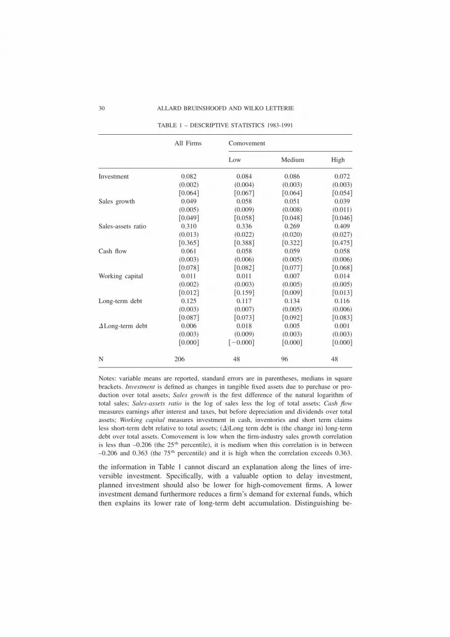
the information in Table 1 cannot discard an explanation along the lines of irre-versible investment. Specifically, with a valuable option to delay investment,planned investment should also be lower for high-comovement firms. A lowerinvestment demand furthermore reduces a firm’s demand for external funds, whichthen explains its lower rate of long-term debt accumulation. Distinguishing be-

TABLE 1 – DESCRIPTIVE STATISTICS 1983-1991

All Firms Comovement

Low Medium High

Investment 0.082 0.084 0.086 0.072�0.002� �0.004� �0.003� �0.003��0.064� �0.067� �0.064� �0.054�

Sales growth 0.049 0.058 0.051 0.039�0.005� �0.009� �0.008� �0.011��0.049� �0.058� �0.048� �0.046�

Sales-assets ratio 0.310 0.336 0.269 0.409�0.013� �0.022� �0.020� �0.027��0.365� �0.388� �0.322� �0.475�

Cash flow 0.061 0.058 0.059 0.058�0.003� �0.006� �0.005� �0.006��0.078� �0.082� �0.077� �0.068�

Working capital 0.011 0.011 0.007 0.014�0.002� �0.003� �0.005� �0.005��0.012� �0.159� �0.009� �0.013�

Long-term debt 0.125 0.117 0.134 0.116�0.003� �0.007� �0.005� �0.006��0.087� �0.073� �0.092� �0.083�

�Long-term debt 0.006 0.018 0.005 0.001�0.003� �0.009� �0.003� �0.003��0.000� ��0.000� �0.000� �0.000�

N 206 48 96 48

Notes: variable means are reported, standard errors are in parentheses, medians in squarebrackets. Investment is defined as changes in tangible fixed assets due to purchase or pro-duction over total assets; Sales growth is the first difference of the natural logarithm oftotal sales; Sales-assets ratio is the log of sales less the log of total assets; Cash flowmeasures earnings after interest and taxes, but before depreciation and dividends over totalassets; Working capital measures investment in cash, inventories and short term claimsless short-term debt relative to total assets; ��Long term debt is �the change in� long-termdebt over total assets. Comovement is low when the firm-industry sales growth correlationis less than –0.206 �the 25th percentile�, it is medium when this correlation is in between–0.206 and 0.363 �the 75th percentile� and it is high when the correlation exceeds 0.363.


tween these two alternative explanations requires a more careful look at the in-vestment decision, to which we turn now.

4 ESTIMATION RESULTS

4.1 Comovement and Financing Constraints

We estimate equation �2� for the period 1986-1996 and present the estimationresults in Table 2.12 A noteworthy observation in the estimates reported in col-umn �1� pertains to the significant and negative estimate on sales growth, whichis counterintuitive and likely follows from the omission of non-linear cash floweffects �note that sales growth has a positive estimated parameter in columns �2�to �5��. Furthermore, note that the effects of cash flow �positive� and workingcapital investment �negative� have the expected signs and are also statisticallysignificant. As explained in section 2, we are particularly interested in the effectson investment of these two variables for firms that are most and least likely toface financing constraints. Hence, we have interacted these variables with dum-mies indicating low comovement �DLC � and high comovement �DHC � in columns�2� and �3� of the table.

The results in column �2� show that investment of low comovement firms isless sensitive to the inflow of cash than investment of medium and high comove-ment firms, but the same applies to the sensitivity of investment to cash flow forthe high comovement firms relative to medium comovement firms. Similar re-sults obtain when interactions with working capital investment are added to theempirical investment equation, as shown in column �3�. There we observe thatfor low comovement firms working capital investment is least threatening as acompetitor to investment in fixed assets for internal funds.13 As before for cashflow, however, working capital investment is also less threatening as a competitorfor high comovement firms when compared to the medium comovement firms.

These results support our conjecture that low comovement associates with arelatively high value of a firm’s assets as collateral to loans. Put differently, theinteraction effects with DLC support the dominance of the supply channel – dis-cussed in section 3.1 – arguing that although these are the firms for which the

12 Including lagged investment in the regression equation; requiring at least the presence of invest-ment lagged two periods as an instrument, and; first-differencing in the estimation procedure eachconsume 1 year of data. Note that none of the specification tests in the table reject 1� our assumptionconcerning the absence of serial correlation in the error term, or 2� our choice of instruments. Referto Appendix A for a more elaborate exposition of the econometric methods.13 The magnitude of the parameter estimate is much lower than that presented in for instance Faz-zari and Petersen �1993�. Their estimate, derived from a Q-model, is –0.43 �–0.18� for �un�con-strained firms. For regressions including sales, they still find a working capital impact of –0.22. Ourfindings are more in line with Weigand and Audretsch �1999�, who find a working capital impact oninvestment of –0.12 within a reduced-form investment equation approach.


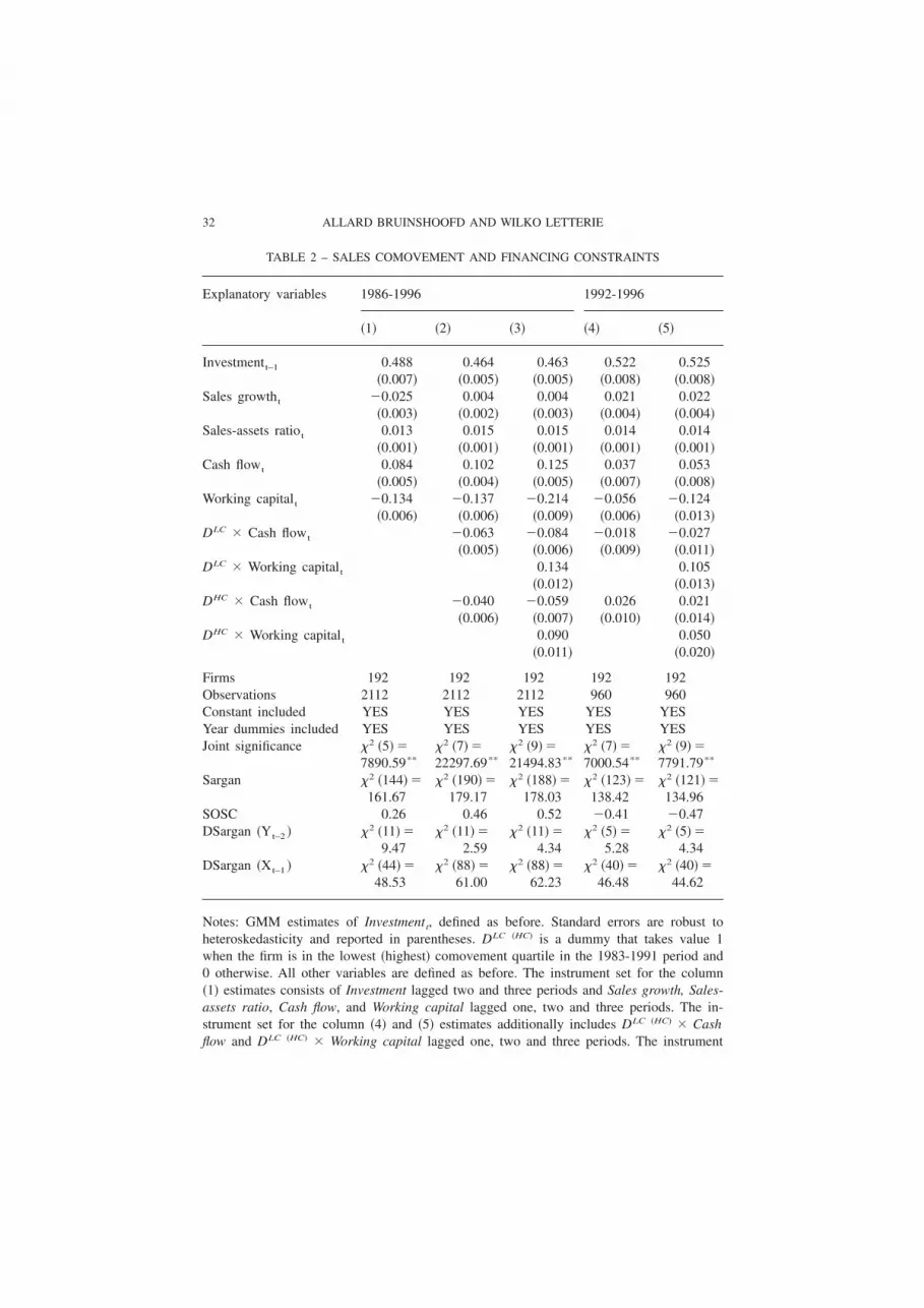
TABLE 2 – SALES COMOVEMENT AND FINANCING CONSTRAINTS

Explanatory variables 1986-1996 1992-1996

�1� �2� �3� �4� �5�

Investmentt–1 0.488 0.464 0.463 0.522 0.525�0.007� �0.005� �0.005� �0.008� �0.008�

Sales growtht �0.025 0.004 0.004 0.021 0.022�0.003� �0.002� �0.003� �0.004� �0.004�

Sales-assets ratiot 0.013 0.015 0.015 0.014 0.014�0.001� �0.001� �0.001� �0.001� �0.001�

Cash flowt 0.084 0.102 0.125 0.037 0.053�0.005� �0.004� �0.005� �0.007� �0.008�

Working capitalt �0.134 �0.137 �0.214 �0.056 �0.124�0.006� �0.006� �0.009� �0.006� �0.013�

DLC � Cash flowt �0.063 �0.084 �0.018 �0.027�0.005� �0.006� �0.009� �0.011�

DLC � Working capitalt 0.134 0.105�0.012� �0.013�

DHC � Cash flowt �0.040 �0.059 0.026 0.021�0.006� �0.007� �0.010� �0.014�

DHC � Working capitalt 0.090 0.050�0.011� �0.020�

Firms 192 192 192 192 192Observations 2112 2112 2112 960 960Constant included YES YES YES YES YESYear dummies included YES YES YES YES YESJoint significance �2 �5� �

7890.59**

�2 �7� �22297.69**

�2 �9� �21494.83**

�2 �7� �7000.54**

�2 �9� �7791.79**

Sargan �2 �144� �161.67

�2 �190� �179.17

�2 �188� �178.03

�2 �123� �138.42

�2 �121� �134.96

SOSC 0.26 0.46 0.52 �0.41 �0.47DSargan �Yt–2 � �2 �11� �

9.47�2 �11� �

2.59�2 �11� �

4.34�2 �5� �

5.28�2 �5� �

4.34DSargan �Xt–1 � �2 �44� �

48.53�2 �88� �

61.00�2 �88� �

62.23�2 �40� �

46.48�2 �40� �

44.62

Notes: GMM estimates of Investmentt, defined as before. Standard errors are robust toheteroskedasticity and reported in parentheses. DLC �HC� is a dummy that takes value 1when the firm is in the lowest �highest� comovement quartile in the 1983-1991 period and0 otherwise. All other variables are defined as before. The instrument set for the column�1� estimates consists of Investment lagged two and three periods and Sales growth, Sales-assets ratio, Cash flow, and Working capital lagged one, two and three periods. The in-strument set for the column �4� and �5� estimates additionally includes DLC �HC� � Cashflow and DLC �HC� � Working capital lagged one, two and three periods. The instrument


demand for external finance is probably strongest, the superior collateral value oftheir assets facilitates access to external funding and reduces the incidence of fi-nancing constraints. More importantly, these are not the expected results if co-movement affects investment primarily – via partial irreversibility – through thedemand channel. Then the interaction effects with DLC should have pointed inthe other direction.

In contrast, for high comovement firms, the demand channel appears impor-tant. According to this channel, high comovement firms choose a more cautiousinvestment path, which results in them running into binding financing constraintsless often. This explains why our empirical results show that their investment isless sensitive to the generation of cash flow and why working capital investmentappears less threatening as a competitor to investment in fixed assets for internalfunds.

We support this seemingly contradictory explanation of the results by notingthat the estimation period contains a reasonable period in the eighties, where un-certainty concerning the economic recovery may have had a strong influence onboth the access of firms to external sources of finance and their conservatism inseizing uncertain investment opportunities. This conjecture is inspected in col-umns �4� and �5�, where we report estimates for the period 1992-1996.14 At leastthree features of these results are interesting in this regard. First, the sensitivityof investment to cash flow is considerably lower in this sub period than it wasbefore when assessed over the entire sample period. This suggests that financingconstraints were indeed less relevant during the period 1992-1996 than they werein the second half of the eighties.15 Second, for high comovement firms the re-

14 This estimation period conveniently coincides with the one used and motivated in the next sub-section.15 Credit and stock market information confirms the claim that the 1992-1996 period was morefavourable for firms to attract external finance than the years before. For instance due to favourablestock price developments, proceeds from stock issues for firms from 1992 onwards – excepting 1995

�

set for the column �2� and �3� estimates is similar, but excludes the third lags of all ex-planatory variables �excluding lagged Investment� to prevent an explosion of the numberof instruments. Joint significance for all variables in the model �except for a constant andthe time dummies� is tested with a Wald test. Sargan refers to the Sargan test for overi-dentifying restrictions and is also heteroskedasticity-consistent �cf. Arellano and Bond�1991��. SOSC tests for second-order autocorrelation and is based on estimates of the re-siduals in first differences �cf. Arellano and Bond �1998��. The Difference Sargan �DSar-gan� statistics restrict the instrument set. Defining the instrument set upon which the esti-mates are based as Yt–2, Yt–3, Xt–1, Xt–2, Xt–3 �with X the vector of explanatory variables�,DSargan �Yt–2 � excludes Yt–2 from this set and re-assesses the overidentifying restrictions.Refer to Appendix A for a more elaborate exposition of the estimation procedure and thetest statistics. For all test statistics, significance at the 5 and 1 percent error level is indi-cated by * and **, respectively.


sults suggest that the supply channel effect now dominates – as it did and stilldoes for low comovement firms – since interactions of DHC with cash flow havechanged sign compared to columns �2� and �3� and are now significantly posi-tive.16 This is in line with the view that uncertainty regarding the timing of eco-nomic recovery may have been relevant in the second half of the eighties, butwas largely resolved in the 1992-1996 period. The third interesting observationbolsters this conclusion. Namely, firms respond more strongly to expected prof-itability of investment when there is a low degree of aggregate uncertainty andfinancing constraints are alleviated, which shows in the significant and positiveresponsiveness of investment to sales growth in the 1992-1996 period.

4.2 Comovement: Old Wine in New Bottles?

The aim of this paper is to understand to what extent costly liquidation affectsthe dependence of investment on cash flow. To the extent that our classificationon comovement sorts out typical firms in terms of leverage, maturity, or retentionpractice, however, it has no additional explanatory power over these alternativeproxies for the extent to which firms face financing constraints. For the remain-der of this section, therefore, we consider three firm-specific classificationschemes that have frequently appeared in the literature to identify constrainedfirms. First, we check whether they sort out as constrained the same firms thatwe sorted out using comovement. Second, we briefly assess whether they asso-ciate with observed investment cash flow sensitivity patterns as is documented inthe literature.

We have argued that comovement reduces the value of a firm’s assets as col-lateral to loans. This makes high comovement firms more likely to run into bind-ing debt capacity constraints. Insofar as high comovement sorts out low leveragefirms and vice versa as a result, our findings merely repeat those obtained from asplit on leverage as studied by for instance Whited �1992� and Hu and Schian-tarelli �1998�. Hence we consider the dependence of leverage and comovementclassifications. Furthermore, to the extent that young firms perform more volatilerelative to mature firms, comovement may also sort out firms on the basis ofmaturity. While we have no direct measure of the maturity of the firms in oursample, we assume that mature firms are typically large and retain a relatively

– were 3 to 7 times larger than those in the years 1986-1991 �source: De Nederlandsche Bank�. Fur-thermore, the growth of credit granted by financial institutions to the private sector – more or lessconstant up to the end of 1993 – started picking up and increased up until late 1998 �source: DeNederlandsche Bank�. See for instance van Ees et al. �1997� for an empirical demonstration of fi-nancing constraints being more relevant in bust periods than in boom periods.16 Note, though, that the interaction term with working capital investment still has the wrong signin this respect.


small fraction of earnings �i.e. they pay generous dividends�.17 This motivates anassessment of the dependence of size, retention and comovement classifications.

When sorting firms on the basis of easily adjustable variables such as the re-tention rate or leverage �but also size through takeovers and divestitures� we mustconsider the possibility that firms self-select into the constrained or unconstrainedclasses following unobserved innovations in investment opportunities. Hence wedistinguish between a classification and an estimation period in order to ensurethat the classification scheme is reasonably exogenous to the investment decisionof the firm.18 We classify firms during the years 1983-1991 and estimate equa-tion �2� over the remaining period 1992-1996. On the one hand this relativelylong classification period ensures that if we classify a firm to be constrained dur-ing this period, it is likely to reflect a more or less structural status, which in-creases the likelihood that such a firm remains constrained for a substantial partof the estimation period. The latter period, on the other hand, is still sufficientlylong to obtain meaningful parameter estimates �and coincides with the period forwhich comovement results are reported in columns �4� and �5� of Table 2�.

Panel A of Table 3 shows the distribution of firms across constrained and un-constrained classes.19 We note that the size classification effectively sorts out the45 largest Dutch firms: the average value of total assets for large firms in 1991was NLG 2,974 million, as compared to NLG 196 million for the other firms.This reflects the structure of the Dutch corporate sector well, where there is asmall group of very large multinationals. It also sorts out the most mature firms,which have access to external finance not only through Dutch, but also throughinternational capital markets. Our leverage classification sorts out 52 highly le-veraged firms with an average debt to assets ratio of 0.65. For the remaining 154firms, the corresponding figure is only 0.44.

For the purpose of the present analysis, we are specifically interested in theextent to which the status of a firm according to our comovement classification isindependent from the status of a firm according to an alternative classification

17 See footnote 8 for studies on size and maturity in relation to financing constraints. The notionthat high retention firms are more likely to face binding financing constraints is well-established. Seefor instance Fazzari et al. �1988�, Oliner and Rudebusch �1992�, Bond and Meghir �1994�, Hubbardet al. �1995�, Elston �1996�, and van Ees et al. �1998� to name just a few.18 Note that it is more difficult to imagine that firms can or want to adjust the way they operaterelative to their environment following such innovations, which is why we did not stress this distinc-tion in the analysis of comovement’s effect on investment behaviour.19 Retention practice could not be determined for 5 firms as they had not issued shares for a mean-ingful part of the classification period. Also, Fazzari et al. �1988� consider a medium retention classand we do not, because only 10 firms satisfy the criterion �i.e. retention rates of 80-90%� and wid-ening this medium class �to retention rates of 75-90% and even 70-90%� did not solve this problemsufficiently. For size and leverage, separate low and medium classes were identified, but merged onthe basis of initial estimation results.


scheme.20 Panel B therefore presents statistics on the degree of association be-tween the rank orders that result from our classifications. Specifically, the top-right shows Pearson’s �2 to indicate whether the distribution of firms across con-strained and unconstrained classes is independent for any pair of classificationschemes. The bottom left reports Spearman’s to indicate the direction of asso-ciation between the status of a firm in any two classification schemes �see Ap-pendix C for the details�. From the first row we conclude that independence ofthe comovement classification and any one of the alternative classifications can-

20 As such, for example the explanatory power of liquidation costs in the firm’s capital structure –i.e. the correlation of the raw comovement data with raw leverage ratios – is not a topic that fallswithin the main scope of this paper.

TABLE 3 – WHAT COMOVEMENT DOES NOT PROXY FOR

Panel A Alternative classifications of firms

Comovement Retention Size Leverage

Low/Small 48 192 161 154Medium 96High/Large 48 82 45 52

Total 192 201 206 206

Panel B The relationships among alternative classifications

Comovement Retention Size Leverage

Comovement �2 �2� � 2.064 �2 �2� � 0.093 �2 �2� � 3.370Retention 0.054 �2 �1� � 4.689* �2 �1� � 16.116**

Size 0.018 �0.153* �2 �1� � 1.997Leverage �0.017 0.283** 0.098

Notes: all classification schemes use the 1983-1991 period. Comovement is low, medium,and high as defined before. Retention is high if the firm paid out less than ten percent ofearnings in dividends in 6 years or more. A firm is large when the value of its assets isabove the 75th percentile of the total assets distribution of its 2-digit SBI93 sector for 6years or more. Leverage is high when the firm’s average leverage ratio is above the 75th

percentile of the sample. Independence of pairs of classifications is assessed using a non-parametric goodness-of-fit test based on the difference between observed and expected clas-sification frequencies under the null of independence: the upper-right triangle reports theconcomitant Pearson �2 test statistics. The lower-left triangle reports Spearman’s to in-dicate the direction of association between any pair of classification criteria. Refer to Ap-pendix C for more details on and the contingency tables underlying Pearsons �2 and Spear-man’s . Significance at the 5 and 1 percent error level is indicated by * and **,respectively.


not be rejected at conventional levels of confidence.21 Dependence is more mean-ingful and correlations considerably higher among the alternative classifications;firms that retain a relatively small fraction of earnings are typically large andhave low leverage ratios.

21 As indicated in the previous section, one may suspect a connection between our comovementclassification and a sales growth classification �Hubbard and Kashyap �1992�, van Ees et al. �1997�,and Elston �1998� all associate financing constraints with poor growth performance�. However, apply-ing Pearson’s test of independence to our comovement classification and a simple sales growth clas-sification provides no indication of statistical dependence. See appendix C for the contingency table.

TABLE 4 – ALTERNATIVE CLASSIFICATIONS AND FINANCING CONSTRAINTS: 1992-1996

Retention Size Leverage

Investmentt–1 0.579 0.546 0.529�0.010� �0.011� �0.010�

Sales growtht �0.002 �0.003 0.006�0.005� �0.005� �0.006�

Sales-assets ratiot 0.012 0.012 0.012�0.002� �0.002� �0.001�

Cash flowt 0.009 0.059 0.031�0.016� �0.010� �0.013�

Working capitalt �0.122 �0.093 �0.096�0.020� �0.016� �0.019�

DHigh/Large � Cash flowt 0.080 �0.045 0.070�0.016� �0.012� �0.013�

DHigh/Large � Working capitalt �0.029 0.013 �0.016�0.026� �0.022� �0.021�

Firms 201 206 206Observations 1005 1030 1030Constant included YES YES YESYear dummies included YES YES YESJoint significance �2 �7� � 6970.78** �2 �7� � 6019.40** �2 �7� � 7326.68**

Sargan �2 �93� � 102.76 �2 �93� � 109.05 �2 �93� � 100.42SOSC �0.61 �0.31 �0.12DSargan �Yt–2 � �2 �5� � 3.00 �2 �5� � 1.27 �2 �5� � 2.86DSargan �Xt–1 � �2 �30� � 27.87 �2 �30� � 37.29 �2 �30� � 31.07

Notes: GMM estimates of Investmentt, defined as before. Standard errors are robust toheteroskedasticity and reported in parentheses. See Table 3 for the definition of the respec-tive dummies and Table 1 for that of all other variables. The instrument sets consist ofInvestment lagged two and three periods and all other variables �including interactionterms� lagged one, two and three periods. See Table 2 for the interpretation of the teststatistics.


We also apply the firm-specific classification schemes to our empirical invest-ment equation and report the estimation results in Table 4. We find investmentcash flow sensitivity patterns that are very much in line with findings well-docu-mented in the literature. In particular, we find that investment of high retentionfirms is most sensitive to cash flow. The observation from Table 3 that these firmsare typically small and have high leverage ratios is also reflected in the findingsthat the investment of small firms and heavily indebted firms is most sensitive tocash flow.

5 SUMMARY AND CONCLUSIONS

Liquidation is costly and a firm’s investment decision may reflect the incidenceof these costs. In this paper we have demonstrated that liquidation costs – esti-mated as the firm-industry sales comovement – influence the sensitivity of a firm’sinvestment decision to financial factors. In particular, in the empirical evaluationof the investment equation low liquidation costs are clearly associated with alower sensitivity of corporate investment to financial variables. Specifically, thecash flow sensitivity of investment is lowest for firms with relatively weak co-movement. We find mixed and inconclusive evidence for high-comovement firms.

Using firm-industry sales comovement as our measure of liquidation costs, weemphasise the way the firm performs in relation to its environment in explainingthe working of financing constraints. In this regard we want to point out thatclassification schemes using firm-level characteristics such as leverage, retentionpractice and size – although they associate with excess sensitivity patterns in away that is in line with the literature – do not associate with our classificationusing comovement. This is true even though amongst themselves, these classifi-cations on firm-specific characteristics tell more or less the same story; it is typi-cally the mature firm – the one that has grown large, that pays generous divi-dends, and has a relatively low leverage ratio – that decides on investment mostlyindependent of financial considerations. Comovement therefore adds new insightsinto the working of financing constraints: it is the way the firm performs relativeto its environment that essentially drives the dependence of investment on inter-nal finance by making liquidation, and concomitantly external finance, costly.

APPENDIX A

GMM ESTIMATION OF THE DYNAMIC INVESTMENT EQUATION

The aim of this appendix is to illustrate the basic procedure used in this paperfor the estimation of a dynamic panel data model, not to provide an exhaustiveoverview of dynamic panel data estimation. Readers interested in further details


on the methodology used in this paper are referred to Arellano and Bond �1991�and �1998�.

The model we estimate is a single equation with individual effects of theform:

yit � �yi �t � 1� � ��xit � �t � �i � �it , �A1�

where � and � are individual and time specific effects, respectively xit is a vectorof explanatory variables – that can be strictly exogenous, predetermined, or en-dogenous with respect to �it – with � the vector of associated parameters. Thenumber of time periods available on each firm �T � is 14 when we use all avail-able years in the sample. The number of firms �N � is at most 206 and varieswhen we consider alternative classification schemes, as explained in the main text.

Let us express the investment equation for firm i as

yi � Wi � �i �i � �it , �A2�

where is a vector that includes �, the �’s and the �’s, and Wi contains vectorsof the lagged dependent variable, the xit’s and the time dummies. �i is a vector ofones to capture the firm-specific effect. In estimating a dynamic model, we areparticularly concerned with the possible correlation between the explanatory var-iables and the firm-specific effect. Therefore, to make a search for instrumentsuncorrelated with the specific effects redundant �see Arellano and Bond �1998�for a more elaborate discussion�, first differences are taken of equation �A2�. LetWi

* and yi* denote first-differences of Wi and yi. GMM estimates of then have

the general form

| � ��i

Wi* �Zi� AN �

iZi

� Wi*�� 1�

iWi

* �Zi� AN �i

Zi� yi

*� , �A3�

where Zi is a matrix that contains all variables used as instruments and

AN � �1

Ni

Zi� Hi Zi� � 1

�A4�

with Hi a weighing matrix. We compute one-step estimates where we use

Hi � Hi1 ��

2 � 1 � 0 0

� 1 2 � 0 0

� � � � �

0 0 � 2 � 1

0 0 � � 1 2� . �A5�


The results reported in the main text are two-step estimates with heteroskedas-ticity-consistent standard errors, which uses

Hi � Hi2 � �̂i

* �̂i* � , �A6�

where �̂i* are one-step residuals.

The consequence of the first-differencing transformation on the choice of theinstrument set is the following. Ignoring the explanatory variables and the timeeffects, first-differencing of equation �A1� yields

�yit � yi �t � 1�� yi �t � 1� � yi �t � 2�� it � �i �t � 1�� . �A7�

Since yi�t � 2� and further lags of the level of yi are uncorrelated with ��it � �i�t � 1��they are valid instruments, provided that the �it are serially uncorrelated. Thiscondition is checked by assessing whether second order serial correlation is ab-sent in the first-differenced residuals, i.e.

E��it � �i �t � 1�� i �t � 2� � �i �t � 3�� 0 �A8�

�refer to Arellano and Bond �1991� for technical details and proof of the proper-ties of this test and further tests discussed in this appendix�. More generally, in-strument validity is assessed using Sargan tests of overidentifying restrictions:

S � �i

�̂i* � Zi� AN �

iZi

� �̂i*� , �A9�

which is asymptotically chi-squared distributed with as many degrees of freedomas there are overidentifying restrictions. This test checks whether E��i

* Zi� is suf-ficiently close to zero. The validity of subsets of instruments in Zi can be as-sessed using difference Sargan tests. Let ZIi be a subset of Zi , where we havedropped suspected invalid instruments. SI is the accompanying Sargan test statis-tic:

SI � �i

�̂Ii* � ZIi� AIN �

iZIi

� �̂Ii* � . �A10�

Then the difference Sargan test compares the Sargan test statistic for the full setof instruments �A9� with the Sargan test statistic for the restricted set of instru-ments �A10�: DSargan � S � SI , which has as many degrees of freedom as thenumber of restrictions imposed on the instrument set �and equals the differencein overidentifying restrictions for the two tests�.


APPENDIX B

MEASURING FIRM-INDUSTRY SALES COMOVEMENT

We consider the following sectors �sectors 20-39 in the SBI74 classification�:Food and goodies �20/21�, Textile �22�, Clothing �23�, Leather, shoes and leath-erware �24�, Wood and furniture �25�, Paper and related �26�, Graphic industryand publishers �27�, Petroleum �28�, Chemical �29�, Synthetic strings and fibres�30�, Rubber and synthetics processing �31�, Building materials, pottery, glass�32�, Basic metal �33�, Metal products �34�, Machines �35�, Electronics �36�,Transports �37�, �Optical� instruments �38�, and Other �39�. The sector sales dataat the two-digit SBI74 level can be found in ‘Samenvattend overzicht van deindustrie, K-160.’ Price information is confidential.

We cannot compute our measure of comovement for firms in sectors 27 and38 as price indices are not available for these sectors and hence sales cannot bedeflated. Fourteen firms are in these two sectors. In addition, sales data are notavailable for sectors 20 and 21 separately, but only for both sectors jointly. There-fore, we deflate these combined sector sales with the average price index of thetwo sectors and treat these two sectors as a single one. The correlation of theprice indices of the individual sectors is nearly 90 percent in levels and 70 per-cent in growth rates. Therefore, the loss in accuracy using the aggregate deflatoris probably not large. For sectors 29 and 30 sales are likewise not reported forthe sectors separately but only for the two sectors jointly. Moreover, the priceindex for sector 30 is unavailable as well. Since approximately ten percent of oursample consists of firms in sector 29 �but none in sector 30�, we are reluctant toeliminate these observations. Instead, we deflate the combined sales of sectors 29and 30 with the price index for sector 29. Our estimation results presented in thenext section are not affected by excluding sectors 29 and 30. To save space wedo not report these.

APPENDIX C

TESTING THE INDEPENDENCE OF CLASSIFICATION CRITERIA

The contingency of one classification on another is assessed using the Pearson �2

test for independence. Let �ij denote the underlying bivariate probability distri-bution. For illustration, if i denotes a firm’s classification based on comovementand j denotes its classification based on retention, then �LH is the probability thata firm has low comovement in combination with high retention. Let �i and �j

denote the marginal distributions. Then the null hypothesis of statistical indepen-


dence of any pair of classification criteria is H0 � �ij � �i�j . With the estimatedbivariate probability distribution Pij and marginal distributions Pi and Pj , we ex-pect Pi Pj n � Eij observations in the ith row and the jth column of the contin-gency table. Pearson’s �2 test for independence is based on the difference be-tween observed and expected frequencies:

Pearson’s �2 ij

�Oij � Eij�2

Eij

d.f. � �I � 1��J � 1� ,

where I and J are the number of rows and columns in the contingency table,respectively.

Because rejection of the null provides no indication of the direction of asso-ciation between classification criteria, we also report Spearman’s , a measure ofcorrelation between rank orders. Together, Pearson’s �2 and Spearman’s pro-vide an assessment of the dependence of any pair of classification criteria, aswell as an indication of the direction of association between them. Table A1shows the contingency tables used to compute these statistics �as reported in Table3 in the main text� for comovement, retention practice, size and leverage as clas-sification criteria. Table A2 shows the contingency table for comovement and asales growth classification.

TABLE A1 – CONTINGENCY TABLES USED TO ASSESS INDEPENDENCE BETWEEN PAIRS

OF CLASSIFICATION CRITERIA

Retention Size Leverage

Low High Small Large Low High

Comovement Low 31 16 38 10 38 10Medium 49 43 76 20 66 30High 28 20 37 11 39 9

Retention Low 88 31 102 17High 71 11 50 32

Size Small 124 37Large 30 15

Note: observed frequencies in cells.


TABLE A2 – CONTINGENCY TABLE COMOVEMENT – AVERAGE SALES GROWTH

Growth

Low Medium High

Comovement Low 8 25 15 Pearson’s �2 �4� �P-value �Spearman’s �P-value �

3.050.55

�0.090.20

Medium 27 47 22

High 14 22 12

Note: observed frequencies in cells. A firm’s growth rate is low �high� when its averageannual sales growth rate is below �above� the 25th �75th � percentile of the sample duringthe period 1983-1991. Low growth firms exhibit an average annual sales growth rate of12.6%, medium growth firms grew at an average 5.2% and low growth firms contractedannually by 3.3%.

REFERENCES

Abel, A.B. and J.C. Eberly �1994�, ‘A Unified Model of Investment Under Uncertainty,’ AmericanEconomic Review, 84, pp. 1369-1384.

Arellano, M. and S.R. Bond �1991�, ‘Some Tests of Specification for Panel Data: Monte Carlo Evi-dence and an Application to Employment Equations,’ Review of Economic Studies, 58, pp. 277-297.

Arellano, M. and S.R. Bond �1998�, ‘Dynamic Panel Data Estimation using DPD98 for Gauss: AGuide for Users,’ Institute for Fiscal Studies Working Paper, 88/15.

Bond, S.R. and C. Meghir �1994�, ‘Dynamic Investment Models and the Firm’s Financial Policy,’Review of Economic Studies, 61, pp. 197-222.

Bond, S.R. and J. van Reenen �1999�, Microeconometric Models of Investment and Employment,manuscript, Institute for Fiscal Studies, London.

Carpenter, R.E., S.M. Fazzari and B.C. Petersen �1994�, ‘Inventory Investment, Internal-Finance Fluc-tuations, and the Business Cycle,’ Brookings Papers on Economic Activity, pp. 75-122.

Chirinko, R.S. and H. Schaller �1995�, ‘Why Does Liquidity Matter in Investment Equations,’ Jour-nal of Money, Credit, and Banking, 27, pp. 527-548.

Devereux, M. and F. Schiantarelli �1990�, ‘Investment, Financial Factors, and Cash Flow: Evidencefrom UK Panel Data,’ in: R. G. Hubbard �ed.�, Asymmetric Information, Corporate Finance andInvestment, Chicago, University of Chicago Press, pp. 279-306.

Dixit, A.K. and R.S. Pindyck �1994�, Investment Under Uncertainty, Princeton, Princeton UniversityPress.

Ees, H. van, H. Garretsen, L. de Haan, and E. Sterken �1998�, ‘Investment and Debt Constraints:Evidence from Dutch Panel Data,’ in: S. Brakman, H. van Ees and S. K. Kuipers �eds.�, MarketBehaviour and Macroeconomic Modelling, London, Macmillan Press, pp. 159-179.

Ees, H. van, G.H. Kuper and E. Sterken �1997�, ‘Investment, Finance and the Business Cycle: Evi-dence from the Dutch Manufacturing Sector,’ Cambridge Journal of Economics, 21, pp. 395-407.


Elston, J.A. �1996�, ‘Dividend Policy and Investment: Theory and Evidence from US Panel Data,’Managerial and Decision Economics, 17, pp. 267-275.

Elston, J.A. �1998�, ‘Investment, Liquidity Constraints, and Bank Relationships: Evidence from Ger-man Manufacturing Firms,’ in: S.W. Black and M. Moersch �eds.�, Competition and Convergencein Financial Markets: The German and Anglo-American Models; Advances in Finance, Investmentand Banking, 5, Amsterdam, New York and Tokio, Elsevier Science, North-Holland, pp. 135-150.

Erickson, T. and T.M. Whited �2000�, ‘Measurement Error and the Relationship between Investmentand Q,’ Journal of Political Economy, 108, pp. 1027-1057.

Fazzari, S.M., R.G. Hubbard and B.C. Petersen �1988�, ‘Financing Constraints and Corporate Invest-ment,’ Brookings Papers on Economic Activity, pp. 141-195.

Fazzari, S.M., R.G. Hubbard and B.C. Petersen �2000�, ‘Investment-Cash Flow Sensitivities Are Use-ful: A Comment on Kaplan and Zingales,’ Quarterly Journal of Economics, 125, pp. 695-705.

Fazzari, S.M. and B.C. Petersen �1993�, ‘Working Capital and Fixed Investment: New Evidence onFinance Constraints,’ RAND Journal of Economics, 24, pp. 328-342.

Galeotti, M., F. Schiantarelli and F. Jaramillo �1994�, ‘Investment Decisions and the Role of Debt,Liquid Assets and Cash Flow: Evidence from Italian Panel Data,’ Applied Financial Economics, 4,pp. 121-132.

Gilchrist, S. and C.P. Himmelberg �1995�, ‘Evidence on the Role of Cash Flow in Reduced-FormInvestment Equations,’ Journal of Monetary Economics, 36, pp. 541-572.

Gilchrist, S. and C.P. Himmelberg �1998�, ‘Investment, Fundamentals and Finance,’ National Bureauof Economic Research �NBER� Working Paper Series, 6652.

Guiso, L. and G. Parigi �1999�, ‘Investment and Demand Uncertainty,’ Quarterly Journal of Econom-ics, 114, pp. 185-227.

Harris, J.R., F. Schiantarelli and M.G. Siregar �1994�, ‘The Effect of Financial Liberalization on theCapital Structure and Investment Decisions of Indonesian Manufacturing Establishments,’ WorldBank Economic Review, 8, pp. 17-47.

Hu, X. and F. Schiantarelli �1998�, ‘Investment and Capital Market Imperfections: A Switching Re-gression Approach using U.S. Firm Level Panel Data,’ Review of Economics and Statistics, 80, pp.466-479.

Hubbard, R.G. �1998�, ‘Capital-Market Imperfections and Investment,’ Journal of Economic Litera-ture, 36, pp. 198-225.

Hubbard, R.G. and A.K. Kashyap �1992�, ‘Internal Net Worth and the Investment Process: An Appli-cation to US Agriculture,’ Journal of Political Economy, 100, pp. 506-534.

Hubbard, R.G., A.K. Kashyap and T.M. Whited �1995�, ‘Internal Finance and Firm Investment,’ Jour-nal of Money, Credit, and Banking,’ 27, pp. 683-701.

Jaramillo, F., F. Schiantarelli and A. Weiss �1996�, ‘Capital Market Imperfections Before and AfterFinancial Liberalization: An Euler Equation Approach to Panel Data for Equadorian Firms,’ Jour-nal of Development Economics, 51, pp. 367-386.

Oliner, S.D. and G.D. Rudebusch �1992�, ‘Sources of the Financing Hierarchy for Business Invest-ment,’ Review of Economics and Statistics, 74, pp. 643-654.

Schaller, H. �1993�, ‘Asymmetric Information, Liquidity Constraints, and the Canadian Investment,’Canadian Journal of Economics, 26, pp. 552-574.

Schiantarelli, F. �1996�, ‘Financial Constraints and Investment: Methodological Issues and Interna-tional Evidence,’ Oxford Review of Economic Policy, 12, pp. 70-89.

Schiantarelli, F. and A. Sembenelli �2000�, ‘Form of Ownership and Financial Constraints: Panel DataEvidence from Flow of Funds and Investment Equations,’ Empirica, 27, pp. 175-192.


Shleifer, A. and R. Vishny �1992�, ‘Liquidation Values and Debt Capacity: A Market EquilibriumApproach,’ Journal of Finance, 47, pp. 1343-1366.

Shyam-Sunder, L. and S.C. Myers �1999�, ‘Testing Static Tradeoff against Pecking Order Models ofCapital Structure,’ Journal of Financial Economics, 51, pp. 219-244.

Stiglitz, J.E. and A. Weiss �1981�, ‘Credit Rationing in Markets with Imperfect Information,’ Ameri-can Economic Review, 71, pp. 393-410.

Weigand, J. and D.B. Audretsch �1999�, ‘Does Science Make a Difference? Investment, Finance andCorporate Governance in German Industries,’ Centre for Economic Policy Research �CEPR� Work-ing Paper, 2056.

Whited, T.M. �1992�, ‘Debt, Liquidity Constraints, and Corporate Investment: Evidence from PanelData,’ Journal of Finance, 47, pp. 1425-1470.

Worthington, P.R. �1995�, ‘Investment, Cash Flow, and Sunk Costs,’ Journal of Industrial Economics,43, pp. 49-61.


Documents

Investment and Finance when Liquidation is Costly