Embed Size (px)
Citation preview

Telecommun Syst (2013) 52:907–918DOI 10.1007/s11235-011-9584-3
WDM network re-optimization avoiding costly traffic disruptions
Fernando Solano · Michał Pióro
Published online: 23 August 2011© The Author(s) 2011. This article is published with open access at Springerlink.com
Abstract Network re-optimization is a process that must betriggered periodically in order to improve the inefficient re-source allocation of online routing heuristics due to the un-certainty of online lightpath demand arrivals and departures.Network re-optimization involves two tasks: a) finding newlightpaths for a (sub)set of current demands, i.e. rerouting,and b) migrating the current traffic to the new configura-tion diminishing traffic disruptions, i.e. lightpath reconfig-uration. If not controlled, excessive traffic disruptions maybe a cause of violations of clients’ Service Level Agreement,which should be compensated by the network operator withpenalization fees.
So far, rerouting and reconfiguration tasks of a re-optimization process have been done separately, hence, ef-forts in trying to achieve the best network performance(rerouting) yields to solutions incurring on unacceptabletraffic disruptions (reconfiguration) and vice-versa. In thispaper, given a time-disruption threshold for reconfiguringevery demand, we present a novel methodology consistingon two procedures that collaboratively find the best networkperformance without incurring on penalization fees.
Our numerical results are extremely encouraging: in ourscenarios, it is always possible to achieve an optimal routingperformance without incurring on penalization fees.
F. Solano (�) · M. PióroInstitute of Telecommunications, Warsaw Universityof Technology, Warsaw, Polande-mail: [email protected]
M. Pióroe-mail: [email protected]
M. PióroDepartment of Electro and Information Technologies,Lund University, Lund, Sweden
Keywords Network reoptimization · Networkreconfiguration · Routing · Optical networks · WDM ·Lightpath · Trafic disruption
1 Introduction
In wavelength-switched networks, demands for lightpath es-tablishments may arrive at any time, and the duration of theconnection is unknown most of the times. This fact causesnetwork performance to degrade, regardless of the employedonline routing algorithm, as time passes by.
Therefore, with the objective of maximizing revenues,the network operator may need to trigger a Network Re-optimization process seeking a more efficient allocation ofnetwork resources for the existing traffic. In WDM net-works, network reoptimization (also named network consol-idation) consists of two tasks:
– REROUTING: given a subset of traffic demands and a mapof available resources in the network, find a set of (new)lightpaths whose allocation improves the overall perfor-mance metric of the network. The set of ‘available re-sources’ consists of free resources (those that are not em-ployed at the moment by any lightpath) and, depending onthe reconfiguration strategy, re-allocable resources (thosethat are currently used by the given subset of demands).
– RECONFIGURATION: Here, we are given two lightpathconfigurations (or virtual topologies): a) the working con-figuration of lighpaths and b) the new configuration oflightpaths that improves the overall resource utilizationof the network; and we need to find the best sequence ofsteps in order to migrate the traffic from one configurationto the other. The consideration of re-allocable resources atthe rerouting stage may cause that some resources seizedby working lightpaths must be used for some of the new

908 F. Solano, M. Pióro
lightpaths, generating a complex sequence of steps thatmay originate traffic disruptions, violations of SLAs andpenalization fees for the network operator.
We explain these two tasks and their trade-off in the fol-lowing example.
1.1 Illustrative example
Let us consider a topology with seven nodes and four con-nections: a, b, c and d . Let us assume that there is onewavelength channel per fiber. Due to the dynamism of con-nection and disconnection requests, let us assume that theonline routing algorithm has allocated resources for thesefour demands as depicted in Fig. 1(a); this is our workingconfiguration. Let us assume in our example that our net-work performance metric is wavelength occupancy, for easeof explanation. In this sense, we say that the routing cost ofthis configuration is 12 (as 12 wavelengths are occupied).
In order to obtain a better network performance, let usassume that we can count on all existing wavelengths as re-allocable resources. In this way, we find the optimal config-uration shown in Fig. 1(b) with routing cost 6.
However, reconfiguring to the optimal configuration istricky, if we assume that the wavelengths depicted for bothconfigurations are the same. For instance, the reconfigura-tion of connections a and b are in a deadlock since each oftheir new lightpaths need the resources that are allocated tothe working lightpath of the other connection: wavelengths2 → 3 and 5 → 4. The same situation is faced by connec-tions c and d (observe wavelengths 5 → 6 and 2 → 1). Inaddition, the new lightpath for c needs the wavelength in2 → 5 currently allocated to a. The same situation is expe-rienced by lightpaths d and b on wavelength 5 → 2.
The solution consists on the temporarily disruption oftwo connections—let us assume connections a and c—outof the four connections, in order to proceed with the recon-figuration, which is shown in Fig. 2.
If we assume that the time needed to signal the establish-ment or the disconnection of a lighptath is 2 units of time1
per hop, 6 units of time are needed for disconnecting theworking lightpath of connection a (3 hops in Fig. 1(a)) and 2more units to establish its new lightpath (1 hop in Fig. 1(b)).In summary, the reconfiguration of connections a and c
would need 8 and 10 units of time, respectively. If we as-sume that the SLA allows a maximum disruption time of9 units of time within a fixed time-window, a penalizationfee proportional to 1 unit of time must be reimbursed to theclient of connection c.
1In practice one unit of time corresponds to the time needed by anoptical switch to adjust it components, which is approximately 50 msif it is a MEMS-based implementation.
Fig. 1 Example of re-optimization solutions
In Fig. 1(c) we show routing configuration of lower (sub-optimal) cost of 8. Even though not depicted, in this se-quence no SLAs are violated since all the disruption timesare allowed by the SLA, i.e., below 9 units of time.
Summarizing, we have shown the trade-off between rout-ing cost and penalization fees during a re-optimization pro-cess: two new configurations in which the one with the low-est routing cost incurs in a (higher) penalization fee than theother configuration with a higher routing cost.

WDM network re-optimization avoiding costly traffic disruptions 909
Fig. 2 Representation of thereconfiguration sequence of therouting solution of Fig. 1(b).The order in time of thesequence is from left to right. Inthis case, working lightpath fora is torn down, then the newlightpath for b is established,then the working lightpath for b
is disconnected, and so on. Thissequence incurs in 1 SLAviolation
In this paper we present a methodology that seeks theoptimal rerouting without exceeding a threshold in the dis-ruption time for some demands. The importance of thiswork is that network operators will be able to reoptimizethe network—obtaining the best usage of their resourcesas possible—bounding the violation of the Service LevelAgreements (SLA) of the clients. It is important to highlightthat previously several Routing and Wavelength Assignment(RWA) methods have been proposed to find an optimal con-figuration, but none of them restricts the aforementionedcounter-effect on traffic disruption, as we do.
This paper is organized as follows. In Sect. 3 we pro-vide an analysis of the problem of finding the sequence ofsteps in a reconfiguration that minimizes the penalizationfee. In Sect. 4 we explain our proposed methodology for re-optimizing the network without penalization fees. In Sect. 5we present some numerical results depicting metrics trade-offs. We provide conclusions and further work in Sect. 6.
2 Related work
The most common way of dealing with this problem inthe literature is re-optimizing one lightpath at a time, as itis the case in e.g., [1–3]. In [4] the authors consider thatbackup lightpaths can be taken as free resources during re-optimization of working lightpaths, and vice versa. In allthese cases, the network performance achieved is not thebest. The reader is referred to [5] for a survey of the lit-erature of years prior 2004 concerning reoptimization. Theremaining of this section focuses on the state of the art ofthe reconfiguration problem solely, i.e., excluding the possi-bility of computing the new routes in the problem.
In earlier years (prior to 2004), Jose and Somani in [6]studied a different objective function: minimizing the to-tal disruption during reconfiguration. This problem directlymaps to the Minimum Feedback Vertex Set (MFVS) [7],whose complexity is well-known. The most efficient algo-rithm solving this problem was proposed by in [8].
Most of the research in the area of WDM reconfigurationproblems have been done by Coudert and by the authors in-tensively since 2004. The objective function studied was the
minimization of the maximum disruption experienced dur-ing the reconfiguration of the network. While Coudert hasfocused on the analysis and modeling of some reconfigura-tion problems (see, e.g., [9–11]), the authors have opted forproposing heuristics and evaluating its performance on realproblem instances (see, e.g., [12] and [13]).
With the aim of modeling the problem closer to the realneeds of network operators, the authors have opted for an-alyzing a different objective function, which has not beenstudied previously.
3 Analysis of lightpath reconfiguration andpenalization fees
In this section, we explain how to calculate the penalizationfees (and disruption times) of a reconfiguration process. Forthis, we first introduce the necessary notion of a dependencygraph and a feedback vertex set.
3.1 Background: dependency graph
We explain the concept of a dependency graph [6], which isa building-stone for circuit reconfiguration problems. A de-pendency graph is a directed graph that is built as follows:
– map each connection of the reconfiguration problem to avertex of the dependency graph
– if the new lightpath for a connection, say a, needs someresources that are currently allocated to the working light-path of another connection, say b, then create an arc fromthe vertex representing the first connection, a, to the ver-tex representing the second connection, b, in the depen-dency graph.2
In Fig. 3 we show the dependency graph considering theworking configuration (see Fig. 1(a)) and the optimal rerout-ing configuration (see Fig. 1(b)) depicted in the previous ex-ample.
2Due to the way in which optical switches and signaling protocols op-erate, a new lightpath of a connection can reuse the resources that areallocated to its working lightpath without disruption its traffic.

910 F. Solano, M. Pióro
Fig. 3 Dependency graph andfeedback vertex set for theworking and optimal reroutingconfiguration
All connections can be reconfigured (without disrup-tions) if and only if the dependency graph is acyclic [6]. Infact, the reconfiguration steps can be computed efficientlywith a simple polynomial algorithm [6], if the conditionholds.
In graph theory, a subset of vertices of a digraph thatbreaks all the cycles in the graph is called a feedback ver-tex set. Given a cyclic dependency graph, the only way toperform the reconfiguration is by finding a feedback vertexset and disrupting the associate connections [6]. In the ex-ample depicted previously, one of the feedback vertex setswith minimal cardinality in Fig. 3 are the two shaded ver-tices, i.e., a and c.
3.2 Problem modeling
Given a dependency graph G(D,E), let F ⊆ D be a feed-back vertex set of G. As pointed out previously, let us as-sume that all the working lightpaths of demands associatedwith vertices in the given feedback vertex set F are torndown initially, causing a traffic disruption. For all the otherdemands, i.e. D\F , we first establish the new lightpath—namely reconnection operation henceforth—before tearingdown the working one—namely a disconnection operation.This yields the following two rules of succession relation-ship in any cost optimal reconfiguration sequence:
– ∀d ∈ D\F , the disconnection operation follows immedi-ately after its reconnection operation;
– a reconnection operation is performed just after all thenecessary disconnection operations are performed.
Let us use the variable t−i and t+i for representing theinstant of time in which the disconnect and reconnect oper-ations, respectively, start for demand i ∈ D. It is clear that:a) t−i < t+i for those demands i in F , and b) t−i > t+i forthose demand i not in F . We will use later the nomenclaturet ′i as a variable to symbolize either a reconnection or discon-nection operation on i and, if present in the same expres-sion, t ′′i to symbolize the opposite operation over the samedemand.
Let us denote by δ−i and δ+
i the amount of time requiredfor tearing down the working connection and establishingthe new connection, respectively, of demand i.
The aforementioned two rules can be formulated as fol-lows (written down in the same order):
∀i ∈ D\F, t−i = t+i + δ+i (1)
∀i ∈ D, t+i = maxj∈a(i)
{t−j + δ−j }, (2)
with a(i) being the set of vertices with incoming arcs fromvertex i in the dependency graph.
The elapsed time in which a connection is disrupted canbe described easily as (t+i − t−i ), ∀i ∈ F , or generally asmax{t+i − t−i ,0}, ∀i ∈ D. We consider that the penalizedtime is, hence, the amount of disrupted time that exceeds agiven threshold, and its penalization fee is proportional tothe penalized time. Concretely, we define it as follows:
ωi · max{t+i + δ+i − t−i − μi,0}, ∀i ∈ D (3)
where μi is the time threshold for which demand i is al-lowed to be disrupted without being penalized and ωi rep-resents the unitary cost for its penalization (if the disruptiontime exceeds the threshold μi ). As a consequence, the totalpenalization fee of a reconfiguration sequence is:
c(F ) =∑
i∈F
ωi · max{t+i + δ+i − t−i − μi,0} (4)
As the reader could observe, the value of c(F )—hencethe optimality of our solution—depends only on the value oft−i for i ∈ F , since all other values—i.e., t+i ,∀i ∈ D, and t−i ,∀i ∈ D\F —are set by the previously mentioned two rules.
The optimal penalization fee—or which is the same, theoptimal starting times of the disconnection operations of theconnections represented by the vertices in F —can be com-puted with a simple linear problem, according to the equa-tions mentioned previously. At this point, we conjecture thatthe problem discussed in this section, i.e., computing thevalues of t−i such that minimizes c(F ), can be solved inpolynomial time by an algorithm. In this section we presentan algorithm that finds a good solution in polynomial time.
3.3 Algorithmic solution
Along our explanation, we will use the dependency graphshown in Fig. 4 for better visualization of the concepts andthe algorithm. The example consists of five demands: a, b, c,d and e that are dependent on each other for reconfigurationin a double chain structure, creating four simple cycles inthe dependency graph.
Concepts In any cost optimal reconfiguration sequence,there is at least one required operation that immediately fol-lows in time the next operation. For instance, recalling (2), areconnection operation is only performed once all requireddisconnections have been finished. However, it may happen

WDM network re-optimization avoiding costly traffic disruptions 911
that some of these disconnections are finished at differenttimes, creating a gap between the reconnection operationand some of its previous disconnection operations. We saythat an operation t ′i is tightly bound to t ′′j when t ′i = t ′′j + δ′′
j
and j ∈ a(i). In the example solution of Fig. 5(a), t+b istightly bound to t−a but not to t−c —note that there are 4 unitsof gap between t−c + δ−
c and t+b .W.l.o.g., we assume that an operation can be tightly
bound to at most one (different) operation. Because of this, aset of operations that are tightly bound to each other conforma tree structure where the root of the tree is a disconnectionoperation. We will use s(t ′i ) to denote the set of operationsthat are tightly bound to t ′i and
S(t ′i ) =⋃
t ′′j ∈s(t ′i )S(t ′′j ) ∪ s(t ′i )
to denote the set of operations conforming the tree as-suming t ′i as a root. In the example of Fig. 5(a), S(t−a ) ={t+b , t−b , t+a , t+c }, S(t−c ) is empty, and S(t−e ) = {t+d , t−d , t+e }.
Initial solution We start with an initial feasible solution,where all disconnections of the demands in F occur attime 0. The time for all other operations are computed fol-lowing the succession rules previously described. This solu-tion is the one depicted in Fig. 5(a).
Fig. 4 Dependency graph example. The values in parenthesis corre-spond to (δ−
i , δ+i ,μi ,ωi)
Iteration We compute for each demand i ∈ F the changein the value of c(F ), namely �i , that would occur if wedelay the disconnection operation of demand d one unit oftime later. The value of �i could change after delaying thedisconnection operation one unit of time, for instance, as itdepends on the time gaps between related operations. Forsimplification, we use κi to symbolize the maximum lengthof time for which �i is still accurate. In each iteration wedelay the demand that reduces the value of c(F ) the most,i.e., the one with the largest negative value of �i · κi . Oncedelayed, we recompute the values of �i and κi and repeatthe procedure while there is a demand with a negative valueof �i . To complete our explanation, we proceed to explainhow �i and κi are computed.
When the disconnection operation of a demand i is de-layed, say one unit of time, all tightly bounded operations re-lated to i and its descendants—namely S(t−i )—are delayedas well one unit of time. This may affect the disruption timesof some other demands in F , if the reconnection operation ofthose demands is tightly bound through several operations tothe disconnection of i. For example, if t−a is delayed, it willincrease the disruption time of demand c. A similar situationwould occur with the disruption time of demand c, if t−e isdelayed more than 2 units of time, since t+c would becometightly bound to t−d after delaying t−e one unit of time.
According to our previous observation, the value of �i
can be given by:
�i =
⎧⎪⎪⎪⎪⎪⎨
⎪⎪⎪⎪⎪⎩
0, if t+i ≤ t−i + μi or
t+i ∈ S(t−i ) or i ∈ F∑
ωj
j,t+j ∈S(t−i ),
t+j >t−j +μj
− ωi, otherwise (5)
Fig. 5 Initial and optimal solution for the problem of finding the optimal reconfiguration sequence

912 F. Solano, M. Pióro
Table 1 Value of the mainvariable algorithms through theiterations when solving theproblem depicted in Fig. 4
Iteration t−c t−e Total Demand of delayed �i κi
disruption disconnection (i)
Initial 0 0 105 c 0 − ωc = −5 t+d − t−c − δ−c = 2
1st 2 0 95 c ωe − ωc = −4 t+c − t−d − δ−d = 1
2nd 3 0 91 e 0 − ωe = −1 t+d − t−e − δ−e = 1
3rd 3 1 90 – – –
where j refers to those demands in F whose reconnec-tion operation is tightly bound through several operationto t−i and contribute positively to c(F ). In our example inFig. 5(a), both �a and �e are zero as their reconnection op-eration is tightly bounded through several operations to theirrespective disconnection operation; hence, any delay in thedisconnection time of, say, a will not affect the disruptiontime of a. However, the situation is different for demand c.In this case, �c has the value of −5 (equal to −ωc), sincedelaying the disconnection of c will not affect the disruptiontimes of any other demand (because no other operation istightly bound to t−c ) but only itself at this point. Since �c
is the only variable with a negative value, the algorithm willopt for delaying the disconnection time of c some units oftime in its first iteration.
Now we have to calculate how much time each connec-tion i could be delayed while preserving the same gain ratio�i . The idea is that the disconnection of i can be pushed aslong as it does not push other operations outside S(t−i ). Asmentioned before, this is represented by the variable κi . Itcan be computed as:
κi = minj,t−j ∈S(t−i )∪t−i
(min
k∈a(j)\{i} t+k − t−j − δ−
j
),
∀i,�i < 0 (6)
In our example, κc = mink∈a(c)\{c} t+k − t−c − δ−c =
min{t+b , t+d } − t−c − δ−c in the first iteration, which takes the
value of 2.The cardinality of the set S(t−i ) increases, in each itera-
tion as the disconnection operation of i is delayed, by addingthe adjacent operations to the operations in S(t−i ) that set thevalue of κi in the previous expression.
It is worth noticing that since the cardinality of the setS(t−i ) increases through iterations, the value of κi tends toreduce, and the value of �i increases (towards 0). As a wayto show it, and for completeness, we present in Table 1 thevalues of the main variables of our algorithm when the prob-lem instance of Fig. 4 is considered. The optimal final solu-tion3 can be observed in Fig. 5(b). We omit the values forconnection a as it experiences no changes through the algo-rithm’s iterations.
3Note that delaying one unit of time more t−c and t−e would provide asolution of equal cost.
4 Reoptimizing considering penalization fees
We have analyzed and described the way of computing a re-configuration sequence of minimum penalization fee given adependency graph and a feedback vertex set. In this section,we focus on the embracing problem of how to reoptimizethe network—by calculating the new lightpaths—in such away that the minimum penalization fee of the resulting re-configuration problem is zero, if possible.
The methodology consists of two procedures that jointlyfind the best solution to the constrained re-optimizationproblem. The first procedure is an ILP model for rerout-ing, named Constrained Rerouting (CR) and the second isa branching procedure, named Deadlock Reconfiguration(DR), that finds the best feedback vertex set. These two pro-cedures are run one after the other, several times, until thebest solution is found. We proceed to explain how these twoprocedures collaborate with each other.
CR is a path-based formulation for a traditional multi-commodity flow problem (minimum-cost routing of all thedemands in the network) with some additional combinato-rial constraints that relates it to DR. DR is a tool for deter-mining which demands of the last solution of CR are ex-ceeding the disruption time threshold during reconfigura-tion. The main idea is simple: DR detects which lightpathscause penalization fees at iteration qt , and then, we ask CRto find a new lightpath configuration by forbidding this com-bination of lightpaths in iteration q + 1.
The main iteration of our procedure is drafted as follows:
1. Run CR considering that all the resources are re-allocable.We will obtain a new lightpath configuration, namelyL(0).
2. Set q to 0.3. Build the dependency graph Gq by taking into account
the input working configuration, namely L, and L(q).4. If Gq is acyclic, return L(q).5. Run DR and find which new lightpaths are causing dead-
lock reconfigurations with unacceptable disruption times.If none found, return L(q).
6. Let C ∈ 2D be a family of sets of demands, where eachelement Cj ∈ C,0 < j ≤ |C| represents a set of connec-tion for which there is deadlock incurring in unacceptabledisruption time.

WDM network re-optimization avoiding costly traffic disruptions 913
Fig. 6 Pseudo-code of thecomplete routine
7. Run CR constraining the selection of all the new light-paths in Cv at the same time, for 0 < v ≤ |C|.
8. Increase q and go to 3.
The routine can be seen in Fig. 6.Let us name zL(q) the routing cost of configuration solu-
tion at iteration q , i.e., L(q). It is not hard to prove that afterq iterations:
zL(0) ≤ zL(1) ≤ · · · ≤ zL(q−1) ≤ zL(q) ≤ zL (7)
We proceed to detail the CR ILP and the DR algorithm.
4.1 Constrained rerouting
In CR we are given a set of candidate paths for every demandand we have to choose a subset of them that minimizes a per-formance metric cost and satisfies some reconfiguration con-ditions. In this article we consider: a) that the performancemetric is the total number of wavelength occupancy in thenetwork and b) that there are no wavelength conversion ca-pabilities. However, the methodology can be easily extendedtowards other objective functions and the support of wave-length conversion.
The set C(q) consists of a set of path combinations thatcannot occur in any routing solution of CR at iteration q
or later; we name them the set of forbidden combinations.This set is updated at every iteration with information com-ing from DR, as previously mentioned. We explain how el-ements are added to C(q) in the next subsection.
We assume that each demand i ∈ D is of one lightpathconnection using the capacity of one wavelength channel.The ILP model presented here works with aggregated de-mands, viz., we use a parameter to quantify how many wave-length channels are demanded between a pair of nodes:h(n,m) counts the number of demands that have n as sourceand m as destination.
We employ the following constants and variables in ourmodel. Constant ρ
p,f
(n,m) is set to 1 when fiber f is used by
the p-th candidate path from n to m. The variable xw,p
(n,m) isset to 1 when a lightpath using wavelength w and followingthe p-th candidate path from n to m is taken as part of theoutput configuration L(q), 0 otherwise.
zL(q) = min∑
f,w,p,n,m
ρp,f
(n,m) · xw,p
(n,m) (8a)
∑
w,p
xw,p
(n,m) ≥ h(n,m), ∀(n,m) (8b)
∑
p,n,m|ρp,f
(n,m)=1
xw,p
(n,m)≤ 1, ∀f,w (8c)
∑
w,p,n,m|{w,p,n,m}∈Cv
xw,p
(n,m) ≤ |Cv| − 1, ∀Cv ∈ C(q) (8d)
xw,p
(n,m) ∈ {0,1}, ∀w,p,n,m (8e)
Equation (8a) is our objective function. Constraint (8b)assures that there are h(n,m) lightpaths between n and m.Constraint (8c) constrains the usage of the same wavelength-fiber by two lightpaths. Constraint (8d) forbids the usage ofsome combination of lightpaths, as given by the previousiteration of DR.
4.2 Reconfiguration fees detection
We are given two configurations and we build its depen-dency graph. The recursive procedure in Fig. 7 finds thefeedback vertex set with minimum penalization fee, i.e.,considering (4) as a cost function.
The procedures works as follows. It receives a feedbackvertex set F . It attempts to create another feedback vertex
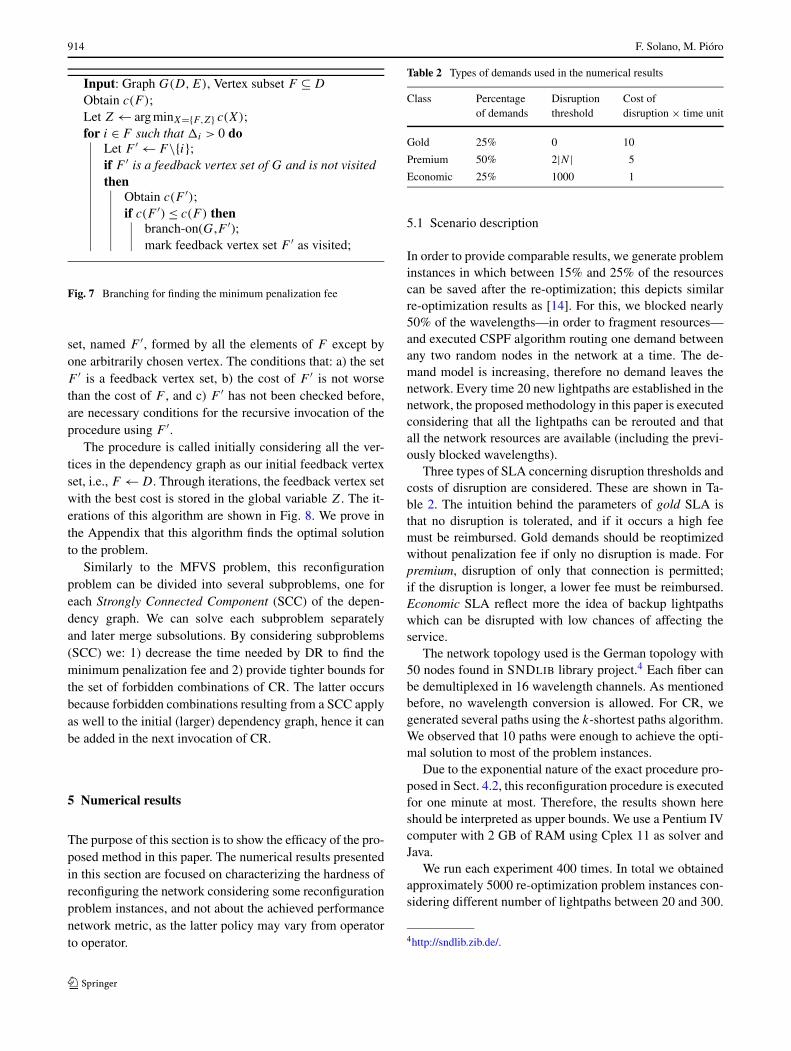
914 F. Solano, M. Pióro
Input: Graph G(D,E), Vertex subset F ⊆ D
Obtain c(F );Let Z ← arg minX={F,Z} c(X);for i ∈ F such that �i > 0 do
Let F ′ ← F\{i};if F ′ is a feedback vertex set of G and is not visitedthen
Obtain c(F ′);if c(F ′) ≤ c(F ) then
branch-on(G,F ′);mark feedback vertex set F ′ as visited;
Fig. 7 Branching for finding the minimum penalization fee
set, named F ′, formed by all the elements of F except byone arbitrarily chosen vertex. The conditions that: a) the setF ′ is a feedback vertex set, b) the cost of F ′ is not worsethan the cost of F , and c) F ′ has not been checked before,are necessary conditions for the recursive invocation of theprocedure using F ′.
The procedure is called initially considering all the ver-tices in the dependency graph as our initial feedback vertexset, i.e., F ← D. Through iterations, the feedback vertex setwith the best cost is stored in the global variable Z. The it-erations of this algorithm are shown in Fig. 8. We prove inthe Appendix that this algorithm finds the optimal solutionto the problem.
Similarly to the MFVS problem, this reconfigurationproblem can be divided into several subproblems, one foreach Strongly Connected Component (SCC) of the depen-dency graph. We can solve each subproblem separatelyand later merge subsolutions. By considering subproblems(SCC) we: 1) decrease the time needed by DR to find theminimum penalization fee and 2) provide tighter bounds forthe set of forbidden combinations of CR. The latter occursbecause forbidden combinations resulting from a SCC applyas well to the initial (larger) dependency graph, hence it canbe added in the next invocation of CR.
5 Numerical results
The purpose of this section is to show the efficacy of the pro-posed method in this paper. The numerical results presentedin this section are focused on characterizing the hardness ofreconfiguring the network considering some reconfigurationproblem instances, and not about the achieved performancenetwork metric, as the latter policy may vary from operatorto operator.
Table 2 Types of demands used in the numerical results
Class Percentage Disruption Cost ofof demands threshold disruption × time unit
Gold 25% 0 10
Premium 50% 2|N | 5
Economic 25% 1000 1
5.1 Scenario description
In order to provide comparable results, we generate probleminstances in which between 15% and 25% of the resourcescan be saved after the re-optimization; this depicts similarre-optimization results as [14]. For this, we blocked nearly50% of the wavelengths—in order to fragment resources—and executed CSPF algorithm routing one demand betweenany two random nodes in the network at a time. The de-mand model is increasing, therefore no demand leaves thenetwork. Every time 20 new lightpaths are established in thenetwork, the proposed methodology in this paper is executedconsidering that all the lightpaths can be rerouted and thatall the network resources are available (including the previ-ously blocked wavelengths).
Three types of SLA concerning disruption thresholds andcosts of disruption are considered. These are shown in Ta-ble 2. The intuition behind the parameters of gold SLA isthat no disruption is tolerated, and if it occurs a high feemust be reimbursed. Gold demands should be reoptimizedwithout penalization fee if only no disruption is made. Forpremium, disruption of only that connection is permitted;if the disruption is longer, a lower fee must be reimbursed.Economic SLA reflect more the idea of backup lightpathswhich can be disrupted with low chances of affecting theservice.
The network topology used is the German topology with50 nodes found in SNDLIB library project.4 Each fiber canbe demultiplexed in 16 wavelength channels. As mentionedbefore, no wavelength conversion is allowed. For CR, wegenerated several paths using the k-shortest paths algorithm.We observed that 10 paths were enough to achieve the opti-mal solution to most of the problem instances.
Due to the exponential nature of the exact procedure pro-posed in Sect. 4.2, this reconfiguration procedure is executedfor one minute at most. Therefore, the results shown hereshould be interpreted as upper bounds. We use a Pentium IVcomputer with 2 GB of RAM using Cplex 11 as solver andJava.
We run each experiment 400 times. In total we obtainedapproximately 5000 re-optimization problem instances con-sidering different number of lightpaths between 20 and 300.
4http://sndlib.zib.de/.

WDM network re-optimization avoiding costly traffic disruptions 915
Fig. 8 Iterations of thebranching procedure. Darkervertices represent the feedbackvertex set. Solutions in a circlehave a cost of 0, other solutionshave a cost of 1. We do notshow solutions where a FVS isnot obtained, since they are notexplored
How much routing cost must be sacrificed in order to obtaina zero penalization fee? We observe in nearly our 5000 re-optimization problem instances that, after several iterations,an equal-cost routing lightpath configuration of lowest rout-ing cost without penalization fee exists, that is:
zL(0) = zL(q)
This means that it was always possible to find the optimalrouting solution without any degradation of its cost becauseof avoiding penalization fees.
How many iterations are needed to obtain a zero penal-ization fee? Throughout all our experiments, although ex-tremely unlikely, we observe that a maximum of 395 it-erations are needed in order to find a zero penalizationfee re-optimization for 140, 200 and 240 lightpaths. Weproceed to analyze the distribution of the number of re-optimization problem instances according to the number ofiterations required to achieve a zero penalization fee recon-figuration.
We classify each experiment according to the maximumnumber of iterations that were needed in order to find azero penalization fee. We have categories for experimentsincurring in a number of iterations between 10x + 1 and11x, where x is the number of the category starting at 0.In figure Fig. 9, we show the distribution of experiments ac-cording to these categories. When 200 lightpaths are consid-ered, We observe that nearly 91% of the experiments needless than 30 iterations to find a zero penalization fee re-optimization.
Fig. 9 Distribution of the number of iterations needed to obtain a zeropenalization fee using our method with a load of 140, 200 and 240lightpaths
We observe also that varying the number of lightpathsalters the number of iterations required to obtain a zero pe-nalization fee reconfiguration. For instance, 30% of the ex-periment using 240 lightpaths required 10 or less iterations,while this percentage for 140 lightpaths is 92%.
How many demands should be disrupted? In Fig. 10 weshow the average number of demands that need to be tem-porarily disrupted by MFVS and our proposal. It shows thatour proposal needs to disrupt between 2 and 4 times moredemands. Even though our method disrupt more demands,the reconfiguration is performed without penalization fees.

916 F. Solano, M. Pióro
Fig. 10 Comparison of the average number of demands temporarilydisrupted incurred by MFVS and our proposal
Fig. 11 Comparison of the average penalization fee incurred byMFVS and our proposal
What would the penalization fee of not using this method?In Fig. 11 we show the average penalization fee when usingMFVS [6] and the average penalization fee through the iter-ations of the method presented in this paper (labeled as PF).We can clearly observed that, on average, using MVFS mayyield a penalization fee twice as big as the average foundthrough the iterations of our methods.
6 Conclusions
In this paper we proposed a new scheme for lightpath re-optimization that bounds the possible unacceptable disrup-tions on the traffic caused during the resulting reconfigura-tion process. Our scheme works iteratively. In each iterationit finds a new configuration trying to avoid previously de-tected reconfiguration deadlocks that may cause penaliza-tion fees.
In all our experiments, numerical results showed that itwas always possible to achieve new routing configurationswith optimal performance such that the reconfiguration pro-cess do not incur on penalization fees. Considering a normalnetwork load (70% of resource usage), nearly 90% of thetimes it was possible to compute this new routing configura-tion using a 2 GHz Intel PC in less than 30 minutes, whichwe consider as an accurate window time for provisioning inASON. In addition, we observe that the penalization fees in-curred by previously proposed methods are extremely high:almost twice the average of our solution.
Acknowledgements We acknowledge the Polish Ministry of Sci-ence and Higher Education because of its grants: MNiSW, grantno. N517 397334: Optimization Models for NGI Core Networks,and MNiSW, grant 58/N-EUREKA/2007/0: Management Platform forNext Generation Optical Networks within the EU CELTIC projectMANGO CP4-17.
Open Access This article is distributed under the terms of the Cre-ative Commons Attribution Noncommercial License which permitsany noncommercial use, distribution, and reproduction in any medium,provided the original author(s) and source are credited.
Appendix: Proof
The proposed algorithm takes in each iteration a FeedbackVertex Set (FVS) F and explores derived solutions by re-moving one vertex, namely i, from F . If F\{i} is a FVSand its cost, i.e., c(F\{i}), is greater than the cost of its par-ent solution, i.e., c(F ), then the algorithm does not performconsecutive explorations based on F\{i}.
The key point to proof is that no other proper subset of F
can have a lower cost than c(F ) in these circumstances. Inother words, we need to proof that:
If ∀i ∈ F,c(F ) < c(F\{i}) then c(F ) ≤ c(F ′), ∀F ′ ⊂ F
In order to simplify our explanation, we will initially as-sume that any considered set F and any subset of F men-tioned in this appendix is a FVS, unless otherwise explicitlystated. W.l.o.g., we consider the values of ωi and μi set to 1and 0, respectively.
Since reconnection operation of a connection i ∈ F canonly be performed once all the necessary operations are fin-ished, we need to estimate the longest elapsed time sinceany of the disconnection operation of the connections in F
necessary for reconnecting i. A lower bound for the elapsedtime is obtained by finding the longest path between verticesof the feedback vertex set in the dependency graph consid-ering δ+
i + δ−i as the weight of the vertex i.
Definition Let us define the l-path of k ∈ F as the longestsimple5 path from vertex k to any other vertex in F in the
5With no cycles.

WDM network re-optimization avoiding costly traffic disruptions 917
given graph. We represent the l-path from a vertex k in asolution F as QF (k). Let dF (k) ∈ F be the destination (lastvertex) in the l-path from k in the solution F , i.e., QF (k).
Theorem 1 If c(F\{i}) > c(F ), for some i ∈ F , thenQF\{i}(k) = QF (k) ⊕ QF (i), ∀k ∈ QF (i) ∩ F .
Since c(F\{i}) > c(F ), the length of the l-path for somevertex k in F\{i} should be greater than the length of its l-path in F , meaning, |QF\{i}(k)| > |QF (k)|. Since the l-pathfrom k can only get longer by not including i in the solution,vertex i must be traversed in the longest path from k, other-wise we would stay with the same l-path in the solution F .Since dF (k) is the farthest vertex from i, hence it is from k
in the solution F\{i}, i.e., dF (k) = dF\{i}(k). Therefore, asi is the only connecting point from k to dF (k) (excluding allother vertices in F ), QF\{i}(k) = QF (k) ⊕ QF (i).
Now we proceed with our final proof. Let F be a FVSfor which the removal of any vertex induces a solution ofhigher cost. In order to proof that any subset of F also in-duces a solution of higher cost, we proceed by induction.We prove that if c(F\{i}) > c(F ) and c(F\{j}) > c(F ), forsome i, j ∈ F , then c(F\{i, j}) > c(F ).
If we focus on the solution F , there are three possibleways in which i and j could be related in this solution:
CASE 1. dF (i) = j and dF (j) = i. By Theorem 1, thel-path in solution F\{i} for the vertices in QF (i) are dis-joint from the l-path in the solution F\{j} for the vertices inQF (j). As a consequence, the cost of the solution F\{i, j}can be computed as c(F\{i, j}) = (c(F\{i}) − c(F )) +(c(F\{j}) − c(F )) + c(F ) > c(F ).
CASE 2. dF (i) = j and dF (j) = i. Consider the solu-tion F\{i}. Following the same reasoning of the proof ofTheorem 1, we can show that the l-path from the verticesin QF\{i}(j) end in dF\{i}(j) when vertex j is removedfrom this solution. As a consequence, the cost of the solu-tion F\{i, j} can be computed as c(F\{i, j}) = c(F\{i}) +|QF\{i}(j)| · ∑k∈n(QF (i)) ωk > c(F\{i}) > c(F ).
CASE 3. dF (i) = j and dF (j) = i. Vertices i and j can-not be removed at the same time from F as there would becycles.
References
1. Chu, X., Bu, T., & Li, X. y. (2007). A study of lightpath rerout-ing schemes in wavelength-routed WDM networks. In Proceed-ings of IEEE international conference on communications (ICC)(pp. 2400–2405), Glasgow, Scotland, June.
2. Sreenath, N., Panesar, G., & Siva Ram Murthy, C. (2001).A two-phase approach for virtual topology reconfiguration ofwavelength-routed wdm optical networks. In Proceedings ofthe 9th international conf. on networks (ICON) (pp. 371–376),Bangkok, Thailand, October.
3. Takagi, H., Zhang, Y., & Jia, X. (2000). Virtual topology reconfig-uration for wide-area wdm networks. In IEEE international con-ference on communications, circuits and systems and West Sinoexpositions (pp. 835–839), Chengdu, China, June.
4. Xin, Y., Shayman, M., La, R., & Marcus, S. (2006). Recon-figuration of survivable mpls/wdm networks. In Proceedings ofIEEE global communications (Globecom) (pp. 1–5), San Fran-cisco, USA, November.
5. Golab, W., & Boutaba, R. (2004). Policy-driven automated recon-figuration for performance management in wdm optical networks.IEEE Communications Magazine, 42(1), 44–51.
6. Jose, N., & Somani, A. (2003). Connection rerouting/network re-configuration. In IEEE design of reliable communication networks(DRCN) (pp. 23–30), Banff, Canada, October.
7. Garey, M. R., & Johnson, D. S. (1979). Computers and in-tractability: a guide to the theory of NP-completeness. Series ofBooks in the Mathematical Sciences. New York: Freeman.
8. Lin, H.-M., & Jou, J.-Y. (1999). Computing minimum feedbackvertex sets by contraction operations and its applications on cad. InIEEE int. conf. on computer design (ICCD) (pp. 364–369), Austin,USA, October.
9. Coudert, D., Pérennes, S., Pham, Q.-C., & Sereni, J.-S. (2005).Rerouting requests in WDM networks. In AlgoTel’05 (pp. 17–20),Presqu’le de Giens, France, May.
10. Coudert, D., & Mazauric, D. Network reconfiguration using cops-and-robber games. (Research Report RR-6694). INRIA, 2008.
11. Couder, D., Huc, F., Mazauric, D., Nisse, N., & Sereni, J.-S.(2009). Reconfiguration of the routing in wdm networks withtwo classes of services. In Proc. of the optical network designand modeling conference (pp. 146–151), Braunschweig, Germany,February.
12. Solano, F. (2009). Analyzing two different objectives of the WDMnetwork reconfiguration problem. In IEEE global communications(Globecom), Honolulu, USA, December.
13. Solano, F., & Pioro, M. (2010). Lightpath reconfiguration inWDM networks. IEEE Journal of Optical Communications andNetworking, 2(12), 1010–1021.
14. Ahmed, J., Solano, F., Monti, P., & Wosinska, L. (2011). Trafficre-optimization strategies for dynamically provisioned wdm net-works. In Proc. of the IEEE international conference on opticalnetworking design and modeling, Bologna, Italy, February.
Fernando Solano received the PhDdegree with emphasis in Informa-tion Technologies from the Uni-versity of Girona, Spain, in 2007.He received the BSEE degree withhonors from Universidad del Norte,Barranquilla, Colombia, in March2003.Currently, he is an Assistant Profes-sor at the Institute of Telecommuni-cations of the Warsaw University ofTechnology. His research interestsinclude Optical Transport Networksdesign and analysis, Sensor Net-works, Network Optimization and
Algorithms. He has participated in the Mango Celtic Project and he isthe coordinator of the Goldfish project funded by FP7.

918 F. Solano, M. Pióro
Michał Pióro is a full professor andthe head of the Computer Networksand Switching Division in the Insti-tute of Telecommunications at theWarsaw University of Technology,Poland, and a full professor at De-partment of Electrical and Informa-tion Technology at Lund University,Sweden. He received a PhD degreein telecommunications in 1979 anda DSc degree, also in telecommu-nications, in 1990, both from theWarsaw University of Technology.In 2002 he received a Polish StateProfessorship. His research inter-
ests concentrate on modeling, design and performance evaluation oftelecommunication networks. He is an author of four books and morethan 150 technical papers presented in the telecommunication and ORjournals and conference proceedings. He has lead many national andinternational research projects for telecom industry and EC in the field.


