INTERNATIONAL DIVERSIFICATION

WITH AMERICAN DEPOSITORY RECEIPTS (ADRs)

By:

M. Humayun Kabir Department of Finance, Banking & Property

Massey University Palmerston North, New Zealand

Email: M.H.Kabir@massey.ac.nz

Neal Maroney Department of Economics & Finance

University of New Orleans New Orleans, LA 70148, USA

Email: nmaroney@uno.edu

M. Kabir Hassan Department of Economics & Finance

University of New Orleans New Orleans, LA 70148, USA

Email: mhassan@uno.edu

2

INTERNATIONAL DIVERSIFICATION

WITH AMERICAN DEPOSITORY RECEIPTS (ADRs)

Abstract

The objective of the paper is to analyze whether U.S. investors can achieve diversification benefits from American Depository Receipts (ADRs) beyond what is achievable through investing directly in country indices. Our findings show substitutability between ADRs and country indices in developed region in the late 1990s, whereas the investors need to invest both ADRs and country indices in Latin America and only ADRs in Asian region. However, large numbers of ADRs issuing countries irrespective of regions show such substitutability between ADRs and country indices. The findings are both statistically and economically significant. We also find time variation in diversification benefits across countries. JEL classification: G11, Portfolio choice; G15, International financial markets; Keywords: ADRs, International diversification, Asset Pricing, Wavelet analysis

3

1. INTRODUCTION

With the globalization of capital markets, an increasing number of foreign firms have

chosen to enter the U.S. market with the issuance of American Depository Receipts1

The objective of the present study is to find the diversification potential of ADRs in

different regions, and in countries from the perspective of an U.S. investor. Given the

opportunity to invest directly in the shares of stocks in the developed (DCs) and emerging (EM)

markets, it is interesting to know whether the U.S. investors can potentially gain any benefits by

investing in ADRs. It is already well known that U.S. investors can achieve higher gains by

investing directly in emerging markets (Harvey, 1995; Bekaert and Urias, 1997; De Santis and

(ADRs) in

order to broaden the shareholders base, raise additional equity capital by taking advantage of

liquidity of U.S. market. Over the last decades the number of foreign firms listed as ADRs in the

U.S. market has gone up dramatically. Lins, Strickland, and Zenner (2000), in their recent study,

found that the greater access to external capital markets is an important benefit of a U.S. stock

market listing, especially for emerging markets firms. The enlisted foreign firms that are subject

to SEC reporting and disclosure requirements, reduce informational disadvantages, and agency

costs of controlling shareholders due to better protections for firms coming from countries with

poor investors’ rights. As a result, firms with higher growth opportunities coming from countries

with poor investors’ rights are valued highly (Doidge, Karolyi, and Stulz, 2001).

1 The ADRs are negotiable certificates or financial instruments issued by U.S. depository banks that hold the underlying securities in the country of origin through the custodian banks. The ADRs, denominated in U.S. currency, provide American investors the ownership rights to stocks in a foreign country, and are considered as an alternative to cross-border direct investment in foreign equities. The ADRs are traded in the U.S. market like shares in the home market. As a result, it is easy and less costly to invest in ADRs rather than in foreign securities directly. It eliminates global custody safekeeping charges saving investors up to 35 basis points per annum (JP Morgan, 2000). Moreover, an ADR is just as liquid as the shares in the home market. The supply of ADRs is not constrained by U.S. trading volumes. If the U.S. investors (or their brokers) want to build positions in an ADR, they can have ADRs ‘created’ by purchasing the underlying shares and depositing them in the ADR facility.

4

Gerard, 1997; De Santis, 1997). Since ADRs are traded in the U.S. market they have been

considered as an alternative to such cross-border investments while ensuring a higher

diversification benefits. However, a small fraction of these ADRs are, in fact, enlisted on major

U.S. exchanges. Most of the ADRs are unlisted, and traded OTC (level I), and they maintain

home country accounting standard, and do not require SEC registration. Only level II and level

III ADRs are enlisted, and comply with SEC regulations2

Most of the studies on ADRs show how combining ADRs with U.S. market or other

funds can reduce risk without sacrificing expected returns. A host of studies (Parto, 2000; Choi

and Kim, 2000; Kim, Szakmary and Mathur, 2000; Alanagar and Bhar, 2001) find the

determinants of ADR returns in the context of a single or multi-factor models. Bekaert and Uris

(1999) conduct a mean-variance spanning test for closed-end funds, open-end funds, and ADRs

of emerging market with a set of benchmark for the period of September 1993 to August 1996,

and found the diversification benefits for closed-end funds and ADRs. The contribution of the

present study is that we attempt to show how the case of diversification with ADRs varies not

only across regions over different sample periods but also with the size of ADR markets

measured by the number of ADRs irrespective of country of origins. We also explore the

possible combination of assets the U.S. investors require to hold in different regions and

countries with respect to diversification. We also focus on the significance of diversification

. These ADRs can be considered as the

subset of country shares. Moreover, ADRs traded in the U.S. market are mostly big firms in their

home countries, and it is likely that they have lower diversification benefits than a typical foreign

firm. Solnik (1991) also expressed his doubt on higher diversification from ADRs. As s result we

pose the question: can ADRs provide as much diversification gains as the country indices?

5

benefits in a framework of utility based measure of certainty equivalence. In order to see whether

diversification benefits are time-varying we employ a new method called wavelet analysis to

estimate correlation at different time scales.

While we use both regression based and SDF-based spanning tests, we address the

shortcomings of an ill-defined benchmark conduct in standard empirical tests like index models.

If the market portfolio is not mean variance efficient, one can incorrectly conclude real assets are

“good” diversifiers. Secondly, the case for diversification depends on the temporal stability and

significance of a set of assets in an investor’s portfolio, and these assets’ correlation structure. If

asset correlations vary widely, then diversification benefits are questionable as an optimized

portfolio becomes expensive or impossible to maintain in the face of uncertain correlations.

Unlike the index models, spanning tests are not subject to benchmarking error, as they do not

rely on a specific benchmark asset pricing model.3

2. A REVIEW OF RELEVENT LITERATURE

We use spanning test proposed by Hansen

and Jagannathan (1991) based on stochastic discount factors (SDFs).

There are some studies that concentrate on ADRs returns behavior, their determinants,

and the opportunities for diversification gains in both U.S. and international context. Officer and

Hoffmeister (1988) show that ADRs lower portfolio risk when added to portfolio of U.S. stocks.

In fact adding as few as four ADRs in a representative U.S. Stock portfolio reduce risk by as

much as 20 percent to 25 percent without any sacrifice in expected returns. The authors use

monthly return data of 45 pairs of ADRs and underlying shares of developed countries mostly

traded on NYSE and AMEX exchanges for the period of 1973-1983.

3 A number of researchers have used spanning tests including Huberman and Kandel (1987), De Santis (1994), Dahlquist and Soderlind (1999), and Maroney and Protopapadakis (2002). DeRon and Nijiman (2001) provide extensive survey of this literature.

6

Wahab and Khandwala (1993) use weekly and daily return data of 31 pairs of ADRs and

the underlying shares of mostly developed countries (UK, Japan, France, Germany, Australia, S.

Africa, Sweden, Norway, Luxembourg), and with the use of active portfolio management

strategies they show that ADRs provide expected returns that are similar to their respective

underlying shares. However, the greater the investment proportion in ADRs, or the higher the

number of ADRs given assumed investment weights, the larger the percentage decline in daily

returns on the combined portfolio in comparison to the standard deviation of returns on

S&P500.Thus ADRs potentially provide better risk reduction benefit, and have been stable over

several sub-periods.

Johnson and Walther (1992) show that while combining ADRs, direct foreign shares, and

international mutual funds substantially increases portfolio returns per unit of risk, ADRs and

direct foreign shares alike would have offered more attractive portfolio risk and return

improvements when compared to domestic diversification strategy.

Callaghan, Kleiman, and Sahu (1996), using Compustat data of 134 cross-listed firms for

1983-1992 sample period, find that ADRs have lower P/E multiples, higher dividend yields,

lower market-to-book ratios than international benchmark, as measured by MSCIP. Moreover,

ADRs provide a higher monthly return and a higher standard deviation than the MSCIP, while

both the ADR sample and MSCIP have lower betas than the S&P 500, and ADRs offer greater

return per unit of risk than the MSCIP. Jorion and Miller (1997) find that while emerging market

country portfolio returns of ADRs are highly correlated with the IFCI composite emerging

market index, it is low with S&P 500 index. And ADRs receipts can be used to replicate or track

the emerging market IFC index.

7

Alaganar and Bhar (2001) find that ADRs have significantly higher reward-to-risk than

underlying stocks. On the other hand, ADRs have a low correlation with the US market under

high states of global and regional shocks. Kim, Szakmary, and Mathur (2000) document that

while the price of underlying shares are most important, the exchange rate and the US market

also have an impact on ADR prices in explaining ADR returns. Parto, 2000; Choi and Kim

(2000) find that local factors (market and industry), and their underlying stock returns across

both countries and industries perform better than the world factor, especially for emerging

markets. On the other hand, a multi-factor model with world market return and the home market

return as the risk factors performs better than models with just the world return, the home market

return or a set of global factors as the risk factors.

Errunza, Hogan, and Hung (1999) create home-made diversified portfolios consisting of

MNCs, country mutual funds, ADRs along with U.S. index, and different industry indices, and

apply unconditional spanning test for seven developed and nine emerging markets. Their results

show achievable diversification benefits beyond those attainable through home-made

diversification. And the incremental gains from international diversification beyond home-made

diversification portfolios have diminished over time. However, this study uses only a few ADRs

while constructing the diversified portfolio.

Bekaert and Uris (1999) conduct a mean-variance spanning test for closed-end funds,

open-end fund and ADRs of emerging market with some global return indices such as FT-

Actuaries, U.S. index, U.K. index. European less U.K. index, and Pacific index as the

benchmark. For comparison, they also examine the diversification benefits of investing in the

corresponding IFC ingestible indexes. The sample period consists of two sub-periods: September

1990 – August 1993 for closed-end funds, and September 1993 August 1996 for closed-end,

8

opened-end funds, and ADRs. The study finds that the U.S. closed-end funds appear to offer

diversification benefits in line with comparable ADRs during the test period. However, the

benefits are sensitive to time period of the tests.

3. Motivation and Hypotheses

Harvey (1995), Bekaert and Urias (1997), De Santis and Gerard (1997) has found that an

U.S. investor can gain diversification benefits by investing directly in Emerging markets. De

Santis (1997), however, shows that Latin American countries provide the highest level of

diversification among emerging countries. Recent popularity of ADRs as an investment vehicle

raises a reasonable question: Is ADR an alternative to investing directly in stocks in different

countries? In other words, can a U.S. investor achieve diversification benefits beyond what is

achievable through investing directly in country index? The ADRs traded in the U.S. market are

mostly big firms in their home countries, it is likely that they have lower diversification benefits

than a typical foreign firms. Solnik (1991) also expresses his doubt on higher diversification

benefits from ADRs. Moreover the level of economic integration and asymmetry of information

are different between developed and emerging countries, even within the emerging countries.

Bekaert, Harvey, and Lumsdaine (2002) find that the first ADR issuance as one of the important

measure of market liberalization events. As a result, we want to test the extent of such

diversification benefits across countries, and across regions (developed, Latin America, Asia,

Emerging markets). Moreover, a huge number of ADRs, especially from emerging countries,

have been enlisted in the U.S. market in 1990s. It is also interesting to look how such influx of

foreign shares in the U.S. market has changed the gains from investment. We hypothesize that

ADRs provide as much diversification benefits as the country indices. In other words, our

spanning question is: Can ADRs and U.S. market indices mimic country returns? If the

9

hypothesis is not rejected then it implies an achievable diversification benefits by investing in

ADRs, and U.S. investors can gain, at least, the same level of benefits from their investment in

ADRs, which can be regarded as the substitute of cross-border investment. However,

substitutability may not be the only outcome. Investors may require holding both ADRs and

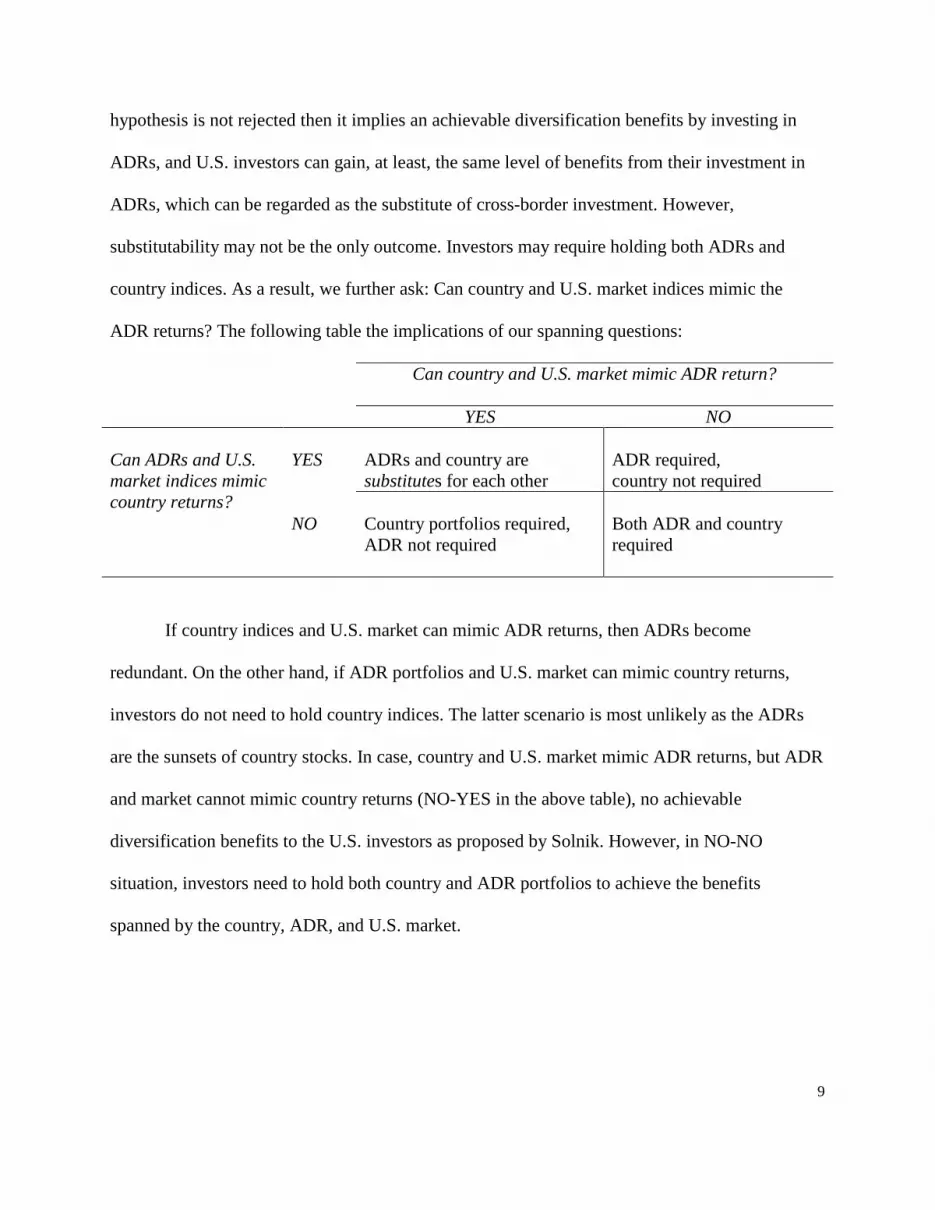
country indices. As a result, we further ask: Can country and U.S. market indices mimic the

ADR returns? The following table the implications of our spanning questions:

Can country and U.S. market mimic ADR return?

YES NO Can ADRs and U.S. market indices mimic country returns?

YES

ADRs and country are substitutes for each other

ADR required, country not required

NO

Country portfolios required, ADR not required

Both ADR and country required

If country indices and U.S. market can mimic ADR returns, then ADRs become

redundant. On the other hand, if ADR portfolios and U.S. market can mimic country returns,

investors do not need to hold country indices. The latter scenario is most unlikely as the ADRs

are the sunsets of country stocks. In case, country and U.S. market mimic ADR returns, but ADR

and market cannot mimic country returns (NO-YES in the above table), no achievable

diversification benefits to the U.S. investors as proposed by Solnik. However, in NO-NO

situation, investors need to hold both country and ADR portfolios to achieve the benefits

spanned by the country, ADR, and U.S. market.

10

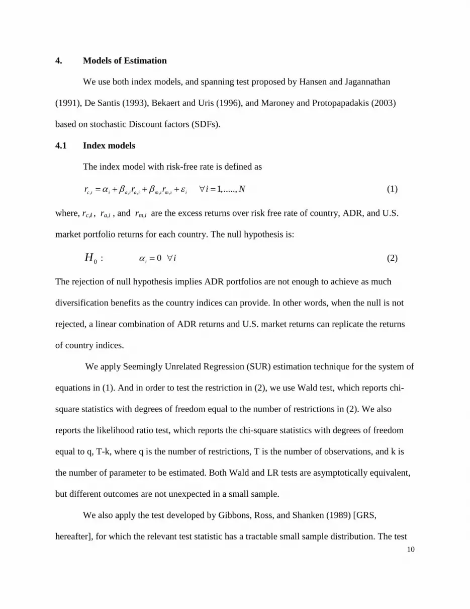
4. Models of Estimation

We use both index models, and spanning test proposed by Hansen and Jagannathan

(1991), De Santis (1993), Bekaert and Uris (1996), and Maroney and Protopapadakis (2003)

based on stochastic Discount factors (SDFs).

4.1 Index models

The index model with risk-free rate is defined as

, , , , ,c i i a i a i m i m i ir r rα β β ε= + + + 1,.....,i N∀ = (1)

where, rc,i , ra,i , and rm,i are the excess returns over risk free rate of country, ADR, and U.S.

market portfolio returns for each country. The null hypothesis is:

0H : 0iα = i∀ (2)

The rejection of null hypothesis implies ADR portfolios are not enough to achieve as much

diversification benefits as the country indices can provide. In other words, when the null is not

rejected, a linear combination of ADR returns and U.S. market returns can replicate the returns

of country indices.

We apply Seemingly Unrelated Regression (SUR) estimation technique for the system of

equations in (1). And in order to test the restriction in (2), we use Wald test, which reports chi-

square statistics with degrees of freedom equal to the number of restrictions in (2). We also

reports the likelihood ratio test, which reports the chi-square statistics with degrees of freedom

equal to q, T-k, where q is the number of restrictions, T is the number of observations, and k is

the number of parameter to be estimated. Both Wald and LR tests are asymptotically equivalent,

but different outcomes are not unexpected in a small sample.

We also apply the test developed by Gibbons, Ross, and Shanken (1989) [GRS,

hereafter], for which the relevant test statistic has a tractable small sample distribution. The test

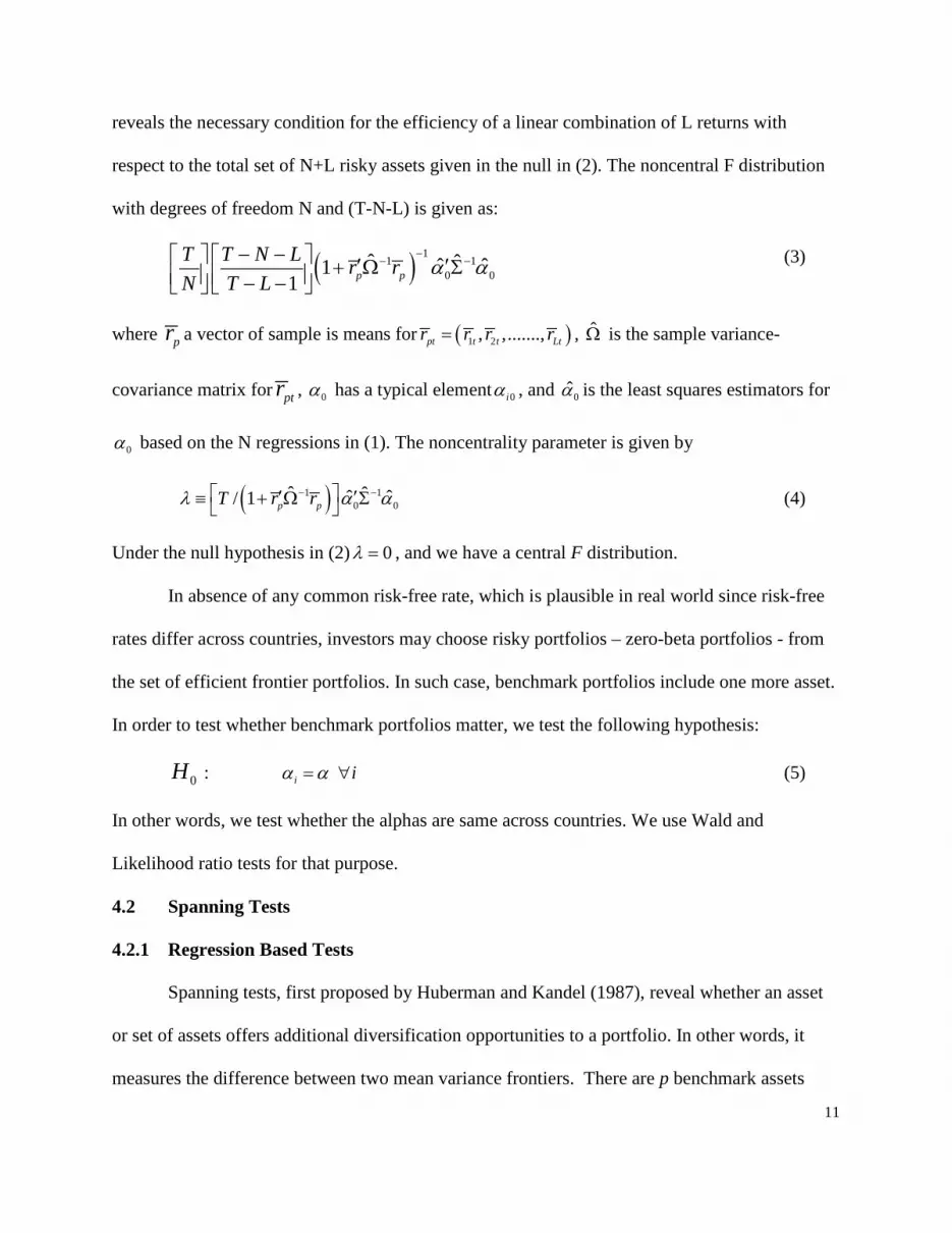
11

reveals the necessary condition for the efficiency of a linear combination of L returns with

respect to the total set of N+L risky assets given in the null in (2). The noncentral F distribution

with degrees of freedom N and (T-N-L) is given as:

( ) 11 1

0 0ˆ ˆˆ ˆ1

1 p pT T N L r rN T L

α α−

− −− − ′ ′+ Ω Σ − − (3)

where pr a vector of sample is means for ( )1 2, ,.......,pt t t Ltr r r r= , Ω is the sample variance-

covariance matrix for ptr , 0α has a typical element 0iα , and 0α is the least squares estimators for

0α based on the N regressions in (1). The noncentrality parameter is given by

( )1 10 0

ˆ ˆˆ ˆ/ 1 p pT r rλ α α− − ′ ′≡ + Ω Σ (4)

Under the null hypothesis in (2) 0λ = , and we have a central F distribution.

In absence of any common risk-free rate, which is plausible in real world since risk-free

rates differ across countries, investors may choose risky portfolios – zero-beta portfolios - from

the set of efficient frontier portfolios. In such case, benchmark portfolios include one more asset.

In order to test whether benchmark portfolios matter, we test the following hypothesis:

0H : iα α= i∀ (5)

In other words, we test whether the alphas are same across countries. We use Wald and

Likelihood ratio tests for that purpose.

4.2 Spanning Tests

4.2.1 Regression Based Tests

Spanning tests, first proposed by Huberman and Kandel (1987), reveal whether an asset

or set of assets offers additional diversification opportunities to a portfolio. In other words, it

measures the difference between two mean variance frontiers. There are p benchmark assets

12

common to both frontiers and the other q test assets are only included in the construction of one

of the frontiers. The frontier MVp+q will always encompass MVp because it contains more assets

used in its construction. The null hypothesis of spanning states that both frontiers statistically

coincide, H0: MVp+q = MVp . (6)

It is sufficient to measure the distance between frontiers at two points, as all other points are

convex combinations4

ttt RR εβα ++= 12

. A confirmation of the spanning hypothesis implies that additional test

assets q will not offer diversification opportunities relative to those already included in the

portfolio of benchmark assets p. Evidence against the spanning hypothesis means the inclusion

of test assets takes advantage of diversification opportunities not available in the benchmark

assets, thus these test assets should be included in any well-diversified portfolio.

Let R1t is a p-vector of returns on p benchmark assets and R2t is a q-vector of returns on q

test assets. By projecting R2t on R1t, we have

(7)

with E[εt] = 0q and E[εtR′1t] = 0qxp , where is 0q is an q-vector of zeros and 0qxp is an q by p

matrix of zeros. The conditions for spanning can be expressed as

H0: α = 0q, δ =0q, (8)

Where δ = 1q - β1p with 1q is n q-vector of ones. HK proposed Likelihood ratio (LR) test for the

above restrictions. Kan and Zhou (2001) proposed Wald (W) and Lagrange multiplier (LM) tests

as well, and have shown that using asymptotic distributions might lead to severe over-rejection

problem for both W and LR tests. In that case, LM test appears to be preferable. Kan and Zhou

(2001) modify LM statistics for small sample.

4 A mean-variance frontier is a parabola therefore fully describe by two points in mean-variance space.

13

Under the non-normality condition, when the error term exhibits conditional

heteroskedasticity, none of the previously mentioned test statistics is asymptotically chi-square

distributed under the null hypothesis (Kan and Zhou, 2001). As a result, GMM tests of spanning

used by Ferson, Foerster, and Keim (1993) under the regression approach are more appropriate5

4.2.2 SDF Based Tests

.

We report the probability of rejection of null hypothesis using LM statistics adjusted for small

sample, and GMM based Wald statistics.

The advantage of the Stochastic Discount Factor (SDF) based spanning tests is that it

guarantees portfolios used in spanning tests lie on the mean variance frontier of assets used in

their construction. These tests are based on Hansen and Jagannathan (1991), HJ, volatility

bounds that give a lower boundary on the volatility of all stochastic discount factors SDFs such

that the Law of One Price (LOP) is not violated. Spanning tests exploit the mean variance

efficiency of the HJ bounds: selecting two points on the mean variance frontier is the same as

selecting two points on the HJ bounds. HJ bounds are model-free in the sense that they do not

require one to specify a specific benchmark model and therefore avoid the joint hypothesis

problem inherent in using CAPM or Multifactor benchmarks. The LOP is the present value

relation at the heart of asset pricing:

( ) ttt PmXE =++ 11 , or equivalently ( ) 111 =++ tt mRE , (9a, 9b)

where X, and R are a t+1 payoffs and gross returns on N assets, m is the SDF and P is vector of

today’s asset prices.

5 Kan and Zhou (2001) derive the Wald statistics of GMM test for regression approach of spanning test.

14

Expand (9b) using the definition of covariance and suppressing time subscripts for clarity

yields, 1],[][][][ =+= mRCovmERERmE . (10)

HJ prove m is linear in returns: [ ] β'rmEm += , (11)

where r’=R-E[R] is vector of N return deviations from their times series means, is a vector of

weights on N assets, and E[m] is the expected value of the discount factor.

To form the parabola that is the HJ volatility bound, HJ treat E[m] as an unknown

parameter c, and the standard deviation of the SDF with expectation c, (mc) is plotted against c.

This forms the lower bound on all SDFs constructed from a set of returns that satisfy the LOP.

Any other SDF must have higher variance than the one along the bound to price all the assets.

Spanning tests use two SDFs with expectations E(m1), and E(m2) chosen in a reasonable

range to measure the difference between frontier portfolios at two points. Following Maroney

and Protopapadakis (2002), the empirical form of spanning tests is:

( ) ( )

( ) ( ) ,0,,0,

222

111

==−==−

εεεε

EmREREmRER

(12)

where,

( )( )

( )j

jj mE

RmmRE

cov1−= , and ( ) qjqpjpjj rrmEm ββ ′+′+= ; 2,1=j .

With N assets there are 2N orthogonality conditions and without restrictions the system is just

identified and linear with coefficients 2211 ,,, qpqp ββββ . Without restrictions all orthoga1ity

conditions are satisfied and sample averages are replicated using either SDF--by construction.

The restriction given by spanning implies the two SDFs produced from p benchmark assets will

15

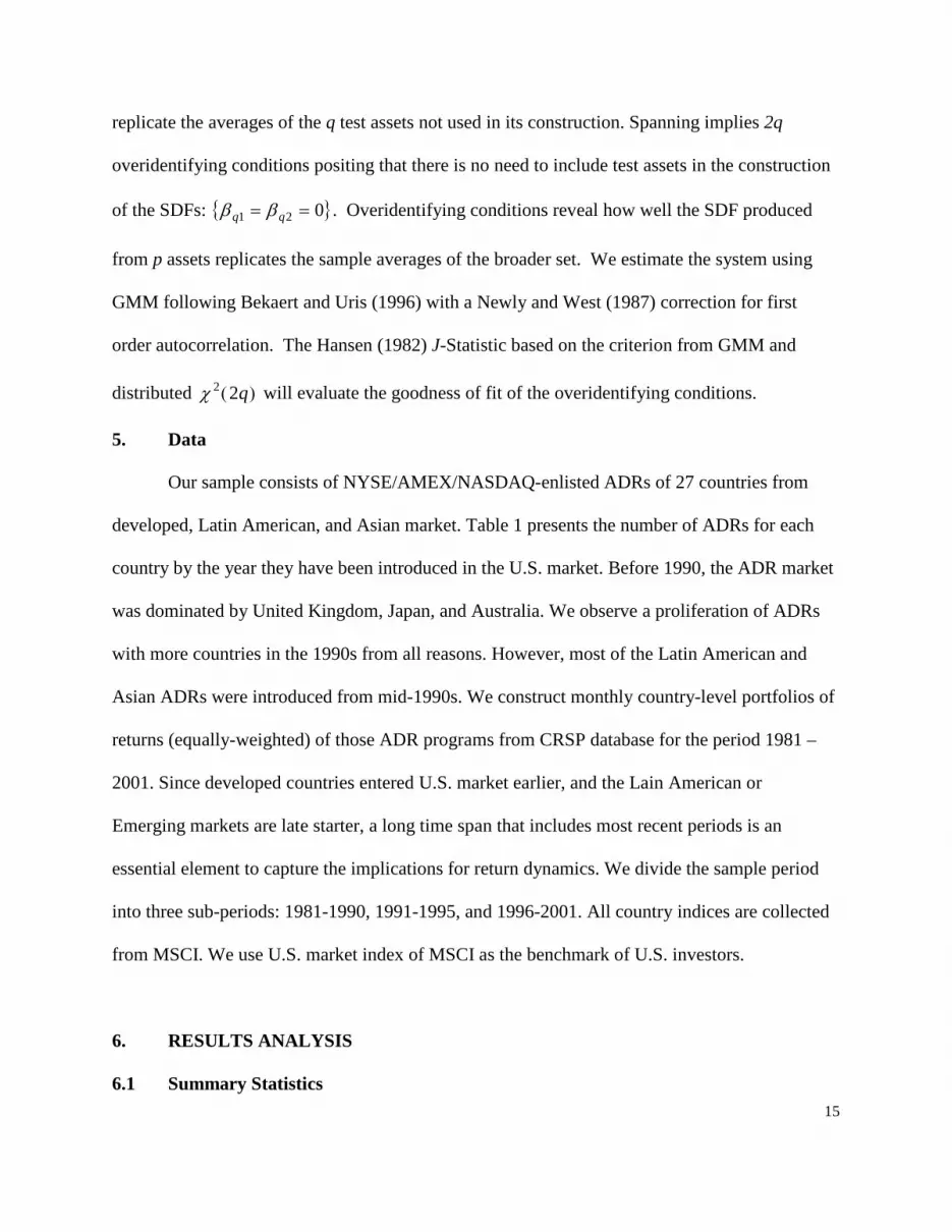
replicate the averages of the q test assets not used in its construction. Spanning implies 2q

overidentifying conditions positing that there is no need to include test assets in the construction

of the SDFs: 021 == qq ββ . Overidentifying conditions reveal how well the SDF produced

from p assets replicates the sample averages of the broader set. We estimate the system using

GMM following Bekaert and Uris (1996) with a Newly and West (1987) correction for first

order autocorrelation. The Hansen (1982) J-Statistic based on the criterion from GMM and

distributed ( )q22χ will evaluate the goodness of fit of the overidentifying conditions.

5. Data

Our sample consists of NYSE/AMEX/NASDAQ-enlisted ADRs of 27 countries from

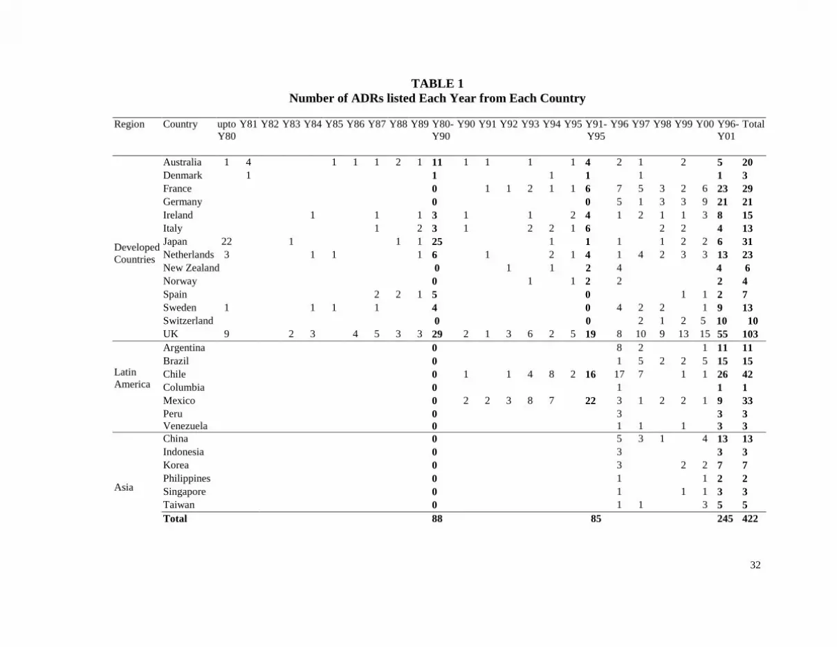
developed, Latin American, and Asian market. Table 1 presents the number of ADRs for each

country by the year they have been introduced in the U.S. market. Before 1990, the ADR market

was dominated by United Kingdom, Japan, and Australia. We observe a proliferation of ADRs

with more countries in the 1990s from all reasons. However, most of the Latin American and

Asian ADRs were introduced from mid-1990s. We construct monthly country-level portfolios of

returns (equally-weighted) of those ADR programs from CRSP database for the period 1981 –

2001. Since developed countries entered U.S. market earlier, and the Lain American or

Emerging markets are late starter, a long time span that includes most recent periods is an

essential element to capture the implications for return dynamics. We divide the sample period

into three sub-periods: 1981-1990, 1991-1995, and 1996-2001. All country indices are collected

from MSCI. We use U.S. market index of MSCI as the benchmark of U.S. investors.

6. RESULTS ANALYSIS

6.1 Summary Statistics

16

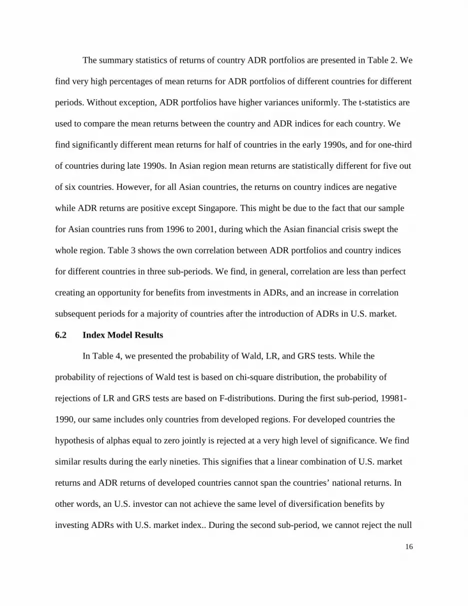
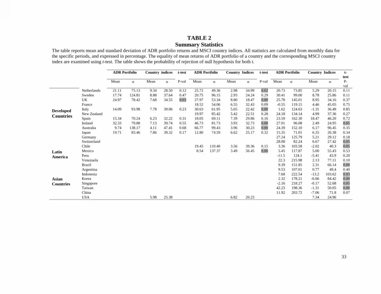
The summary statistics of returns of country ADR portfolios are presented in Table 2. We

find very high percentages of mean returns for ADR portfolios of different countries for different

periods. Without exception, ADR portfolios have higher variances uniformly. The t-statistics are

used to compare the mean returns between the country and ADR indices for each country. We

find significantly different mean returns for half of countries in the early 1990s, and for one-third

of countries during late 1990s. In Asian region mean returns are statistically different for five out

of six countries. However, for all Asian countries, the returns on country indices are negative

while ADR returns are positive except Singapore. This might be due to the fact that our sample

for Asian countries runs from 1996 to 2001, during which the Asian financial crisis swept the

whole region. Table 3 shows the own correlation between ADR portfolios and country indices

for different countries in three sub-periods. We find, in general, correlation are less than perfect

creating an opportunity for benefits from investments in ADRs, and an increase in correlation

subsequent periods for a majority of countries after the introduction of ADRs in U.S. market.

6.2 Index Model Results

In Table 4, we presented the probability of Wald, LR, and GRS tests. While the

probability of rejections of Wald test is based on chi-square distribution, the probability of

rejections of LR and GRS tests are based on F-distributions. During the first sub-period, 19981-

1990, our same includes only countries from developed regions. For developed countries the

hypothesis of alphas equal to zero jointly is rejected at a very high level of significance. We find

similar results during the early nineties. This signifies that a linear combination of U.S. market

returns and ADR returns of developed countries cannot span the countries’ national returns. In

other words, an U.S. investor can not achieve the same level of diversification benefits by

investing ADRs with U.S. market index.. During the second sub-period, we cannot reject the null

17

for Latin American countries implying a potential diversification benefits from investing in Latin

American ADRs. During the third sub-period (1996-2001) LR test accept the null, while GRS

test reject the hypothesis for developed regions. Similarly, we reject the null according to GRS

test only for Latin America. In Asia, all test tests report significantly different from zero alphas

jointly.

We report the test results of the null hypothesis that the intercepts are joint same across

portfolios. Except for developed regions, the hypothesis is rejected for all countries in Latin

America and Asia. This is plausible as the developed countries are more integrated

economically, whereas the emerging markets face varying levels of integration so that zero-beta

returns vary across countries. This finding also indicates that the benchmark assets matter in

pricing the emerging markets’ assets, and risk-free rates are not same across countries.

6.3 Spanning Test Results

6.3.1 Regional diversification benefits

In case of regional diversification test, our benchmark assets are all country indices, all

ADR portfolios and the U.S. market except the set of country indices (ADR portfolios) for a

region, which are considered as test assets. Both the regression and SDF based spanning test

results for three regions are presented in Table 5. In Table 5A, we report the results when ADRs

are test assets, and in Table 5B, we report the results when country indices are test assets. Since

our sample size is small the SDF-based spanning tests can potentially be bias. In order to resolve

the problem with sample size, we use the bootstrap technique, for which we conduct 3,000

iterations by randomizing the e i= r - E(r), and generate J-statistics sample. Based on the sample

we find the probability of our original J-statistics from the GMM estimations.

18

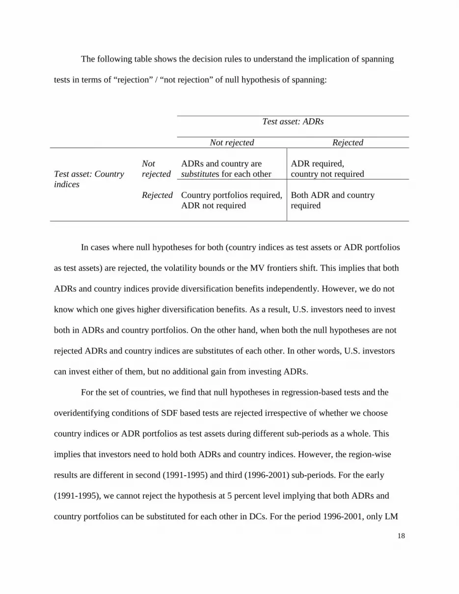
The following table shows the decision rules to understand the implication of spanning

tests in terms of “rejection” / “not rejection” of null hypothesis of spanning:

Test asset: ADRs

Not rejected Rejected Test asset: Country indices

Not rejected

ADRs and country are substitutes for each other

ADR required, country not required

Rejected

Country portfolios required, ADR not required

Both ADR and country required

In cases where null hypotheses for both (country indices as test assets or ADR portfolios

as test assets) are rejected, the volatility bounds or the MV frontiers shift. This implies that both

ADRs and country indices provide diversification benefits independently. However, we do not

know which one gives higher diversification benefits. As a result, U.S. investors need to invest

both in ADRs and country portfolios. On the other hand, when both the null hypotheses are not

rejected ADRs and country indices are substitutes of each other. In other words, U.S. investors

can invest either of them, but no additional gain from investing ADRs.

For the set of countries, we find that null hypotheses in regression-based tests and the

overidentifying conditions of SDF based tests are rejected irrespective of whether we choose

country indices or ADR portfolios as test assets during different sub-periods as a whole. This

implies that investors need to hold both ADRs and country indices. However, the region-wise

results are different in second (1991-1995) and third (1996-2001) sub-periods. For the early

(1991-1995), we cannot reject the hypothesis at 5 percent level implying that both ADRs and

country portfolios can be substituted for each other in DCs. For the period 1996-2001, only LM

19

test of regression-based spanning reject the null hypothesis at 5% level in DC region when ADRs

portfolios are considered as test assets. Such substitutability might be related to explosion of

ADRs in the 1990s from developed countries. During the period 1981-1990, we find only nine

developed countries, which have ADRs in the U.S. market. The total number of ADRs during

this period was 88 as shown in table 2. This number went up to 137 by the year 1995, and 300 by

2001. Such proliferation of ADRs may have changed the dynamics of market. An increase in

own correlation between ADR returns and country indices indicate a more integrated nature of

market. As a result, investors can substitute the ADRs for country with no additional benefits to

gain.

For the sub-period 1991-1995, we do not have any Asian country in our sample. We have

Mexican and Chilean ADR portfolios from Latin America. Both the null hypotheses for Latin

America are rejected implying the necessity to hold both ADR and country indices. During the

period 1996-2001 we have four more Latin American countries. Among all tests, only GMM

Wald test can not reject the null when country indices are used as test assets. Thus our findings

support the view that investors need to hold both ADRs and country indices. For Asian countries,

null hypothesis is rejected irrespective of tests when ADR portfolios are considered as test assets.

However, when we use country indices as test assets, we can not reject the null. This implies that

U.S. investors need to invest in ADR portfolios with market index to achieve diversification

benefits.

6.3.2 Portfolios sorted by number of ADRs

We observe a significant increase in ADRs in the 1990s from different countries. We also

find substitutability between ADR portfolios and country indices in the later periods for

developed region, whereas they provide diversification benefits independently in the 1980s. In

20

order to find whether such proliferation of ADRs each country became representative of those

countries so that investors do not need ADRs in their portfolios, we form portfolios based on the

number of ADRs irrespective of regions. For each t-period returns, we form equally-weighted

portfolios based on (t-1)-period ranking of countries with respect to the number of ADRs for

each country and divide the countries in three different groups: largest, medium, and smallest.

We continue to follow the same process for each years starting from 1980 to 2001. Then we

stacked the data for the whole period, and conduct our spanning test. The benchmark assets

consist of all three – largest, medium, and smallest - ADR portfolios, three equally-weighted

country portfolios, and the U.S. market except one of the ADR (country) portfolios that is

considered as test asset.

The spanning test results are presented in Table 6. We find that null hypotheses in

regression-based tests and the overidentifying conditions of SDF based tests are rejected

irrespective of whether we choose country indices or ADR portfolios as test assets except the

largest one in the third sub-period. In other words, the null hypothesis that the ADR and the U.S.

market can mimic country or the country and the U.S. market can mimic cannot be rejected at

conventional significance levels for the largest portfolios during the period 1996-2001. Thus our

results support the investors can substitute country for ADRs for those countries that have higher

number of ADRs listed in the U.S. market. However, for the whole period, both the nulls are

rejected showing the requirement to hold both ADRs and country in the portfolios.

7. Economic Significance of Portfolio Diversification

It is pre-dominant in finance literature to measure the value of adding new assets in an

existing portfolio using the sharpe ratio. Such measure of portfolio performance has been

criticized by Bernardo and Ledoit (2000) and Goetzmann et al (2002). A proper economic

21

measure should take into account investor’s risk tolerance. This can be done with a mean-

variance utility function which the investors want to maximize for a given level of risk tolerance.

Consider a standard utility function that the investor wants to maximize:

( ) ( )ptpt RVarAREU2

−= (13)

where, an is N X 1 vector of return of risky assets, and A is the coefficient of relative risk

aversion. For a given parameter of A, the tangency portfolio that corresponds to maximization of

utility in mean-variance framework yields optimal portfolio weights for risky assets. A higher A

indicates an investor is more risk-averse or less risk tolerant, and vice versa. We can interpret the

utility value from a certain portfolio strategy as a certainty equivalent rate of return, CER. Thus,

CER defines the rate that risk-free investments would need to offer with certainty to be

considered equally attractive as risky portfolios.

We first calculate the certainty equivalent, CERB for the benchmark portfolios consisting

of all country indices and U.S. market, then we proceed with adding ADR returns to calculate the

certainty equivalent, CERA for the expanded portfolio. The difference between CERA and CERB

gives us the economic value of diversification with ADRs. Following Grauer and Hakansson

(1987) and Grauer and Shen (2000), we set up a portfolio strategy: at the beginning month t, the

investors observe the risk-free return for month t, and the realized returns of portfolios for the

previous k months (we consider k = 24 months). The portfolio problem is solved for a given risk

aversion parameter with the estimates of portfolio weights of all portfolios. At the end of month

t, the realized returns are observed. Using the weights selected at the beginning of the month, the

realized return on portfolios for month t is recorded. This procedure results in the ex ante

22

certainty equivalent measure at time t as each investor maximizes the ex ante utility. We follow

the procedure for all subsequent months. This gives us a time series of ex ante certainty

equivalent measure for both benchmark portfolios and the expanded portfolios. The ex post

utility of certainty equivalent can be measured by taking the average of the time series of ex ante

utility. Then we compare whether the ex post certainty equivalent of expanded portfolios is

greater than the ex post certainty equivalent of benchmark portfolios using a one-tail T-test.

In table 7, we report the difference between CERA and CERB for three risk-aversion

coefficients 1, 3, and 5 in regional diversification case when ADR portfolios are included with

the benchmark. As the value of risk aversion coefficients increases the differences go down

uniformly irrespective of region and time period. In other words, highly risk-averse investors are

less aggressive resulting in lower benefits of having ADRs in their portfolio. In all cases, the

investment opportunity sets when broadened by including ADRs with benchmark portfolios

results in higher certainty equivalent rates so that CERA is statistically significantly higher than

CERB as indicated by one-tail t-test in table 7. During the 1990s the economically significant

diversification gains are relatively higher for all regions compared to 1980s irrespective of

investors’ risk aversion. This results contradict are in contrast to what we found using spanning

tests. However, what is still important is that relatively higher diversification benefits are driven

by Latin American and Asian ADRs. For example, the annualized certainty equivalent rates of

returns of expanded portfolios with only developed country ADRs is 4.04%, and with only Latin

American ADRs is 5.55% resulting in a 1.5% higher gains in Latin America for the least risk

aversion coefficient in period 1991-1995. Similarly, we find 2% and 1% higher gains for Asian

and Latin American ADRs respectively in the period 1996-2001.

23

When the countries are sorted by number of ADRs irrespective of regions, and divided in

large, medium, and small groups, and calculate the certainty equivalent rates, we find the results

that are quite similar to spanning tests results in panel B of table 6. In table 7, we report the

difference between CERA and CERB for three risk-aversion coefficients 1, 3, and 5 in size-based

diversification case when ADR portfolios are included with the respective benchmark. In all

cases the certainty equivalent rates of expanded portfolio sets augmented by ADRs are

statistically higher than respective benchmark portfolios except the large size case for the period

1996-2001.

8. Are Diversification Benefits Time-varying?

In our analysis of spanning tests for different sub-periods, we assume the correlation

between the ADR returns, country indices and U.S. market index remain constant for specific

sub-period. On the other hand, we observe that as market becomes more integrated with more

and more ADR issuance the benefits of diversification also change across regions and country. A

better understanding of such benefits requires a close examination of correlation, specially,

between ADR returns and U.S. market returns with question in mind: Are the correlation time-

varying? To find the answer to the question, we use a new but important technique: wavelet

analysis6

Wavelet analysis is an important vehicle to study the time-series data at multi-scale

levels. It decomposes the time-series data into different time-horizons to reveal the dynamic or

time-varying properties at different time-scales. This decomposition process isolate the low

(smooth) and high (detail) frequency components in the data. In other words, low frequency

.

24

components captured by father wavelets, φ(t) represent the trend components, and high

frequency components captured by mother wavelets, ψ(t) represent the deviation from the trend

with their properties:

1)( =∫ dttφ and ∫ = 0)( dttψ (14)

In the wavelet domain, the function f(t), then, can be represented as

∑ ∑∑∑ ++++= −−k k

kkkJkJk

kJkJk

kJkJ tdtdtdtstf )(.......)()()()( ,1,1,1,1,,,, φφψφ (15)

where, ∫= dttfts kJkJ )()(,, φ and ∫= dttftd kjkJ )()(,, ψ for j = 1,2,…,J

where, k ranges from 1 to the number of coefficients, and kJs , , kJd , , …., kd ,1 are the wavelet

coefficients with kJs , representing smooth coefficients (trend) and kJd , , …., kd ,1 representing

progressively finer deviation from smooth or trend.

Let x be a dyadic length of a vector (N=2J) of observation. The length of N vector of

discrete wavelet coefficients w is obtained via

Wxw = (16)

where W is an N X N orthogonal matrix defining discrete wavelet transformation. The vector of

wavelet coefficients can be arranged into J+1 vectors:

[ ]1 2, ,........, , TJ Jw w w w v= (17)

where, vJ is a length N / 2J vector of scaling coefficients associated with smooth component, and

wj is a length of N / 2J vector of scaling coefficients associated with changes on a scale of length

6 There are already two books on wavelet method with application in economics and finance: Percival and Walden (2000) and Gencay, Selcuk and Whitcher (2001). Some published articles are: In and Kim (forthcoming), Kim and In (2005), Gencay and Selcuk and Whitcher (2003),

25

λj = 2j-1, i.e., deviation from smooth. The multiresolution decomposition of a function, therefore,

can be written as

, , , ( )J k J k J kk

S s tφ=∑ and , , , ( )J k j k j kk

D d tψ=∑ for j = 1,2,…,J (18)

In other words, the function f(t) can be expressed as

, , 1, 1,( ) ......J k J k J k kf t S D D S−= + + + + (19)

In our analysis, we use maximal overlap discrete wavelet transformation (MODWT)

which can handle any sample size. Moreover, since our objective is to calculate the correlation

based on variance and covariance estimates, MODWT wavelet variance estimator is

asymptotically more efficient than same estimator based on DWT (Percival, 1995). MODWT

decomposes the variance and covariance of time series on a scale-by-scale basis. The wavelet

variance for scale λj = 2j-1 can be defined as

21

2,

1

1( ) , ,j

Nl

j j tt Lj

d l X YN

σ λ−

= −

= = ∑

(20)

where, ,lj td is the MODWT wavelet coefficients of variables l at scale λj, jN = N – Lj + 1 is the

number of coefficients unaffected by the boundary, and Lj =(2j – 1)(L – 1) + 1 is the length of

the scale λj wavelet filter.

Similarly, the wavelet covariance between two time-series Xt and Yt for scale λj = 2j-1 can

be defined as

1

, ,1

1( )j

NX Y

XY j j t j tt Lj

Cov d dN

λ−

= −

= ∑

(21)

The MODWT estimator of wavelet correlation for scale λj can be expressed using the

variance and covariance estimators as follows

26

( )

( )( ) ( )

XY jXY j

X j Y j

Cov λρ λ

σ λ σ λ= (22)

We can calculate the correlation for different scales representing different lengths of time. As a

result, the wavelet correlation estimates are convenient way to examine the time-varying pattern

of diversification benefits. In other words, we can observe patterns of correlation at different

time-scales, rather than only in short-run or long-run as we are used to define the time horizon in

conventional way in economics and finance literature. We can also check the statistical

significance of the estimated correlation. The confidence interval of the estimates is based on

chi-square distribution.

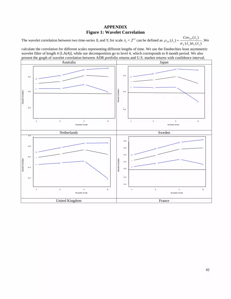
Considering the sample size of return data we decide to use the Daubechies least

asymmetric wavelet filter of length 4 [LA(4)], while our decomposition go to level 4, which

corresponds to 8 month period. The wavelet-based correlation estimates between country indices

and corresponding ADR portfolio returns, and between ADR portfolio returns and U.S. market

returns are presented in table 10, panel A and B respectively. We also present the graph of

wavelet correlation between ADR portfolio returns and U.S. market returns with confidence

interval in figure 1 in the appendix.

Panel A of table 9 shows that own wavelet correlation between ADR portfolio returns

and country indices increases for most of the countries with higher scales or longer period of

time. For countries like Netherlands, United Kingdom, Spain and Argentina the correlation are

relatively stable at all scales. However, France, Italy, Switzerland, and Chili show some

fluctuations in correlation at different scales or time horizons, while at scale 4 that corresponds to

8 months time length, the correlation estimates actually drops substantially for France (0.48),

27

Italy (0.48), Ireland (0.25), and Chili (0.81). For all other Latin American and Asian economies

the correlation structure shows an upward pattern.

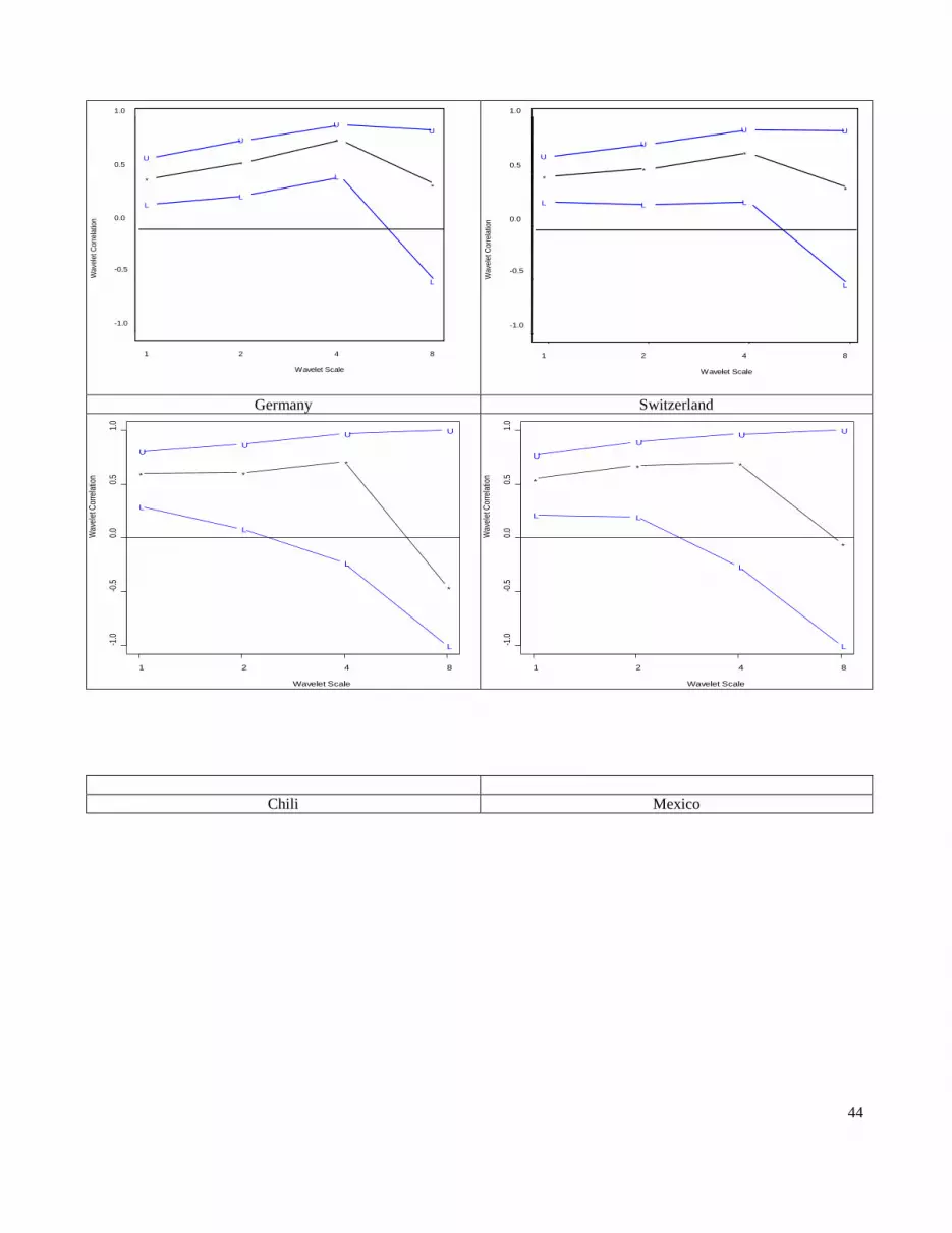
Panel B reports the wavelet correlation between ADR portfolio returns and MSCI U.S.

market index, the pattern of which is more important from the point of view of diversification

benefits with ADRs. Figure 1 in the appendix shows the plot of correlation at different scale with

confidence intervals. For most of the countries, the correlation increases up to the scale 3

(corresponding 4 months time period). After that, at scale 4, the correlation estimates decline for

developed countries like France (from 0.36 at scale 1 to -0.10), Italy (from 0.32 at scale 1 to

0.17), Spain (from 0.43 at scale 1 to 0.37), Ireland (from 0.45 at scale 1 to 0.35), Germany (from

0.61 at scale 1 to -0.40), and Switzerland (from 0.55 at scale 1 to -0.05), and Latin American

country like Brazil (from 0.62 at scale 1 to 0.33). This implies that investing in ADRs of these

countries for a longer-term might yield more diversification benefits. For ADRs from Australia,

Japan, Netherlands, Sweden, United Kingdom, New Zealand, Mexico, and Chile U.S. investors

can get benefits at a very short-term period. Among Asian countries, we generally find increases

in wavelet correlation in two to four months periods. Beyond four months correlation remains

relatively stable for countries like Indonesia (close to 0.60), Korea (close to 0.70). For China and

Singapore, there are some fluctuations in correlation between ADR returns and U.S. market

index over 8 months period. In general, investment in Asian ADRs for relatively shorter horizon

might result in higher diversification benefits. However, we need to be cautious in interpreting

the findings since the sample period covered for Asian countries in this paper is relatively

shorter (1996-2001), the period during which Asian financial crisis swept the region.

28

9. Conclusion

The objective of the present study is to measure the diversification benefits of different

country ADRs portfolios from the perspective of an U.S. investor. Studies on ADRs show

indirect evidence of achievable diversification benefits. Given the opportunity to invest directly

in the shares of stocks in the developed (DCs) and emerging (EM) markets, it is interesting to

know whether the U.S. investors can potentially gain any benefits by investing in ADRs. Our

findings show that U.S. investors needed to invest in both ADRs and country portfolios in

developed in the eighties and in Latin American countries in the nineties. During the early and

late nineties, we find substitutability between ADRs and country portfolios in DCs. As more and

more ADRs are enlisted in the US market from developed countries over time, the ADRs

become substitutes to country. Similarly, countries with higher number of ADRs irrespective of

regions show the same pattern of substitutability between ADRs and country indices. However,

such substitutability does not exist for countries with the highest number of ADRs by the end of

sample period, 2001. The certainty equivalent approach identifies that such substitutability are

economically significant. On the other hand, U.S. investors can achieve the diversification

benefits by investing ADRs along with U.S. market index in Asia. By utilizing the wavelet

correlation analysis, we find that diversification benefits vary across countries over time. Higher

diversification gains may be achievable in relatively longer period-holding (more than 4 months

period) of ADRs from some countries like France, Italy, Spain, Germany, Ireland, Switzerland,

and Brazil. For ADRs from Australia, Japan, Netherlands, Sweden, United Kingdom, New

Zealand, Mexico, and Chile U.S. investors can get benefits at a very short-term period.

Investment in Asian ADRs, in general, for relatively shorter horizon might result in higher

diversification benefits even tough we find some fluctuations in correlation for a few countries.

29

However, we need to be cautious in interpreting the findings since the sample period covered for

Asian countries in this paper is relatively shorter (1996-2001), the period during which Asian

financial crisis swept the region.

30

References

1. Bekaert, G, 1996, “Market Integration and Investment Barriers in Emerging Equity Markets. 2. Bekaert, G, and M. S. Urias, 1996 “Diversification, Integration, and Emerging Market

Closed-end Funds”, Journal of Finance, 51, 835-870. 3. Bekaert, G, and M. S. Urias, 1999 “Is there a free lunch in emerging market equities?”,

Journal of Portfolio Management, Vol 25, No. 3, 83-95. 4. Bekaert, G., C.R. Harvey, and C. Lumsdaine, 2002, “Dating the Integration of World Capital

Markets”, Journal of Financial Economics 65 (2), 203-248. 5. Bernardo, A.E., and O. Leodit, 2000, “Gain, Loss and Asset Pricing”, Journal of Political

Economy, 108, 144-172. 6. Callaghan, J.H., R. T. Kleiman, and A. P. Sahu, 1996 The investment characteristics of

American depository receipts”, Multinational Business Review, Vol. 4, 29-39. 7. De Santis, G., “Volatility Bounds for SDFs: Tests and Implications from International Stock

Returns”, 1993, Unpublished Ph.D. dissertation, University of Chicago. 8. De Santis, G., “Asset pricing and portfolio diversification: evidence from emerging financial

markets”, in Investing in Emerging Markets, Euromoney Books, 1997. 9. De Santis, G., B. Gerald, 1997, “International Asset Pricing and Portfolio Diversification

with Time-varying Risk”, Journal of Finance, 52, 1881-1912. 10. Gencay, R., F. Selcuk, and B. Whitcher, 2001, “An Introduction to Wavelets and other

Filtering Methods in Finance and Economics”, London, UK: Academic Press. 11. Gencay, R., F. Selcuk, and B. Whitcher, 2003, “Systematic Risk and Time Scales”,

Quantitative Finance, Vol. 3, 108-116. 12. Gibbons, Michael, Stephen A. Ross, and Jay Shanken, 1989, “A test of the efficiency of a

given portfolio”, Econometrica, V 57, Issue 5, pp.1121-1152. 13. Goetzmann, W.N., J. Ingersoll, M. Spiegel, and I. Welch, 2002, “Sharpening the Sharp

Ratio”, Working Paper, Yale International Center for Finance. 14. Grauer, R.R., and N.H. Hakansson, 1987, “Gains from International Diversification: 1968-85

Returns on Portfolios of Stocks and Bonds”, Journal of Finance, 42, 721-739. 15. Grauer, R.R., and F.C. Sen, 2000, “Do Constraints Improve Portfolio Performance?”,

Journal of Banking & Finance, 24, 1253-1274. 16. Hansen, L.P. and R. Jaganathan, 1991, “Implications of Securities Market Data for Models of

Dynamic Economies”, Journal of Political Economy, vol. 99 - 262. 17. Harvey, C.R., 1995, “Predictable Risk and Returns in Emerging Markets, Review of

Financial Studies, 8, 773-816. 18. In, F., and S. Kim, (forthcoming), “The Hedge Ratio and the Empirical Relationship between

the Stock and Futures Markets: A New Approach using Wavelet Analysis”, Journal of Business.

19. Jorion, P. and D. Miller, 1997, “Investing in emerging markets using depository receipts”, Emerging Markets Quarterly, Vol. 1, 7-13.

20. Kim, M., A. C. Szakmary, and I. Mathur, 2000, “Price transmission dynamics between ADRs and their underlying foreign securities”, Journal of Banking and Finance, Vol. 24, 1359-1382.

31

21. Kim, S., and F. In, 2005, “Stock Return and Inflation: New Evidence from Wavelet Analysis”, Journal of Empirical Finance.

22. Lins, Karl, and Deon Strickland, 2000, “Do non-U.S. Firms Issue Equity on U.S. Stock Exchanges to Relax Capital Constraints?”, NBER Working Paper.

23. Maroney, N, and A. Protopapadakis, 1999, “The Book-to-market and Size Effects in a General Asset Pricing Model: Evidence from Seven National Markets”, European Financial Management, 2003.

24. Officer, D. T. and J. R. Hoffmeister, 1987, “ADRs: a substitute for the real thing?”, Journal of Portfolio Management, Vol 13, 61-65.

25. Percival, D.B., A.T. Walden, 2000, “Wavelet Methods for Time Series Analysis”, Cambridge, UK, Cambridge University Press.

26. Solnik, International Finance, 2nd edition, Addision-Wessley, 1991 27. Wahab, M., and A. Khandwala, 1993, “Why not diversify internationally with ADRs?”,

Journal of Portfolio Management, Vol. 19, 75-82. 28. Wahab, M., M. Lashgari, and R. Cohn, 1992, “Arbitrage opportunity in the American

depository receipts market revisited”, Journal of International Financial Markets Institutions, and Money, Vol 2, 97-130.

32

TABLE 1 Number of ADRs listed Each Year from Each Country

Region Country upto

Y80 Y81 Y82 Y83 Y84 Y85 Y86 Y87 Y88 Y89 Y80-

Y90 Y90 Y91 Y92 Y93 Y94 Y95 Y91-

Y95 Y96 Y97 Y98 Y99 Y00 Y96-

Y01 Total

Developed Countries

Australia 1 4 1 1 1 2 1 11 1 1 1 1 4 2 1 2 5 20 Denmark 1 1 1 1 1 1 3 France 0 1 1 2 1 1 6 7 5 3 2 6 23 29 Germany 0 0 5 1 3 3 9 21 21 Ireland 1 1 1 3 1 1 2 4 1 2 1 1 3 8 15 Italy 1 2 3 1 2 2 1 6 2 2 4 13 Japan 22 1 1 1 25 1 1 1 1 2 2 6 31 Netherlands 3 1 1 1 6 1 2 1 4 1 4 2 3 3 13 23 New Zealand 0 1 1 2 4 4 6 Norway 0 1 1 2 2 2 4 Spain 2 2 1 5 0 1 1 2 7 Sweden 1 1 1 1 4 0 4 2 2 1 9 13 Switzerland 0 0 2 1 2 5 10 10 UK 9 2 3 4 5 3 3 29 2 1 3 6 2 5 19 8 10 9 13 15 55 103

Latin America

Argentina 0 8 2 1 11 11 Brazil 0 1 5 2 2 5 15 15 Chile 0 1 1 4 8 2 16 17 7 1 1 26 42 Columbia 0 1 1 1 Mexico 0 2 2 3 8 7 22 3 1 2 2 1 9 33 Peru Venezuela

0 0

3 1

1

1

3 3

3 3

Asia

China 0 5 3 1 4 13 13 Indonesia 0 3 3 3 Korea 0 3 2 2 7 7 Philippines 0 1 1 2 2 Singapore 0 1 1 1 3 3 Taiwan 0 1 1 3 5 5 Total 88 85 245 422

33

TABLE 2 Summary Statistics

The table reports mean and standard deviation of ADR portfolio returns and MSCI country indices. All statistics are calculated from monthly data for the specific periods, and expressed in percentage. The equality of mean returns of ADR portfolio of a country and the corresponding MSCI country index are examined using t-test. The table shows the probability of rejection of null hypothesis for both t. ADR Portfolio Country indices t-test ADR Portfolio Country Indices t-test ADR Portfolio Country Indices t-

test Mean σ Mean σ P-val Mean σ Mean σ P-val Mean σ Mean σ P-

val Developed Countries

Netherlands 21.11 75.13 9.34 28.50 0.12 25.72 49.36 2.98 34.99 0.02 20.73 73.85 5.29 20.15 0.11 Sweden 17.74 124.81 8.88 37.64 0.47 20.75 96.15 2.93 24.24 0.29 30.41 99.00 8.78 25.86 0.11 UK 24.97 78.42 7.68 34.55 0.03 27.97 53.34 8.80 18.47 0.00 25.78 145.01 8.95 34.16 0.37 France 18.52 54.06 6.55 32.43 0.09 -0.55 119.15 4.46 45.05 0.75 Italy 14.09 93.98 7.78 39.06 0.23 30.63 61.95 5.65 22.42 0.00 1.62 124.63 -1.31 36.49 0.85 New Zealand 19.97 85.42 5.42 22.51 0.28 24.18 134.14 4.99 37.36 0.27 Spain 15.34 70.24 6.23 32.22 0.31 18.05 69.11 7.39 29.86 0.16 23.59 162.30 18.47 46.20 0.72 Ireland 32.33 79.88 7.13 39.74 0.55 46.73 81.73 3.93 32.73 0.00 27.01 96.08 2.49 24.95 0.05 Australia 9.74 138.17 4.11 47.41 0.68 66.77 99.43 3.96 30.23 0.00 24.39 152.10 6.17 96.45 0.35 Japan 19.71 83.46 7.86 39.32 0.17 12.80 74.59 6.62 25.17 0.32 15.35 71.01 6.35 26.38 0.34 Germany 27.24 125.79 5.21 29.12 0.18

Latin America

Switzerland 28.08 82.24 6.67 27.42 0.05 Chile 19.45 110.40 3.56 39.36 0.15 3.36 103.58 -2.02 40.3 0.05 Mexico 8.54 137.37 3.49 56.45 0.00 5.45 117.87 5.00 55.43 0.53 Peru -11.5 124.1 -5.41 43.9 0.20 Venezuela 22.3 215.98 2.13 77.11 0.10 Brazil 9.39 151.85 2.31 66.14 0.00 Argentina 9.53 107.01 0.77 49.4 0.40 Indonesia 7.68 222.54 -13.2 103.62 0.03

Asian Countries

Korea 2.32 178.21 -6.66 84.42 0.00 Singapore -2.16 218.27 -0.17 52.68 0.05 Taiwan 42.23 198.36 -1.31 50.05 0.00 China 11.92 203.72 -7.06 71.8 0.07 USA 5.98 25.38 6.82 20.23 7.34 24.96

34

TABLE 3

Correlations between ADR Portfolio, Country Indices and MSCI U.S. Market Returns

Panel A: Own Correlation Between ADR portfolio Returns and Country Indices

Period

Aus

tralia

Japa

n

Net

herla

nds

Swed

en

Uni

ted

Kin

gdom

Fran

ce

Italy

New

Ze

alan

d

Spai

n

Irel

and

Ger

man

y

Switz

erla

nd

Chi

li

Mex

ico

Peru

Ven

ezue

la

Bra

zil

Arg

entin

a

Indo

nesi

a

Kor

ea

Sing

apor

e

Taiw

an

Chi

na

1981-1990 0.50 0.80 0.85 0.74 0.93 - 0.59 - 0.83 0.59 - - - - - - - - - - - - - 1991-1995 0.62 0.92 0.89 0.92 0.80 0.75 0.58 0.70 0.95 0.95 - - 0.36 0.34 - - - - - - - - - 1996-2001 0.70 0.81 0.88 0.90 0.90 0.75 0.82 0.86 0.83 0.94 0.39 0.42 0.91 0.87 0.74 0.60 0.85 0.95 0.70 0.69 0.56 0.65 0.91

Panel B: Correlation Between ADR portfolio Returns and MSCI U.S. Market Index

Period

Aus

tralia

Japa

n

Net

herla

nds

Swed

en

Uni

ted

Kin

gdom

Fran

ce

Italy

New

Ze

alan

d

Spai

n

Irel

and

Ger

man

y

Switz

erla

nd

Chi

li

Mex

ico

Peru

Ven

ezue

la

Bra

zil

Arg

entin

a

Indo

nesi

a

Kor

ea

Sing

apor

e

Taiw

an

Chi

na

1981-1990 0.33 0.43 0.53 0.29 0.60 - 0.24 - 0.40 0.30 - - - - - - - - - - - - - 1991-1995 0.33 0.45 0.56 0.32 0.61 0.34 0.25 0.42 0.42 0.32 - - 0.26 0.26 - - - - - - - - - 1996-2001 0.50 0.70 0.56 0.42 0.42 0.31 0.40 0.43 0.56 0.60 0.19 0.34 0.39 0.62 0.35 0.27 0.46 0.53 0.50 0.49 0.62 0.37 0.36

Panel C: Correlation Between Country Indices and MSCI U.S. Market Index

Period

Aus

tralia

Japa

n

Net

herla

nds

Swed

en

Uni

ted

Kin

gdom

Fran

ce

Italy

New

Ze

alan

d

Spai

n

Irel

and

Ger

man

y

Switz

erla

nd

Chi

li

Mex

ico

Peru

Ven

ezue

la

Bra

zil

Arg

entin

a

Indo

nesi

a

Kor

ea

Sing

apor

e

Taiw

an

Chi

na

1981-1990 0.40 0.37 0.65 0.42 0.70 - 0.29 - 0.41 0.40 - - - - - - - - - - - - - 1991-1995 0.44 0.49 0.56 0.44 0.45 0.39 0.32 0.52 0.45 0.53 - - 0.21 0.20 - - - - - - - - - 1996-2001 0.51 0.65 0.69 0.60 0.69 0.39 0.45 0.52 0.57 0.61 0.59 0.49 0.48 0.67 0.38 0.37 0.53 0.55 0.47 0.38 0.57 0.49 0.42

35

Table 4 Test Results of Index Models

The index model with risk-free rate is defined as , , , , ,c i i a i a i m i m i ir r rα β β ε= + + + 1,.....,i N∀ = where, rc,i , ra,i , and rm,i are the excess returns over risk free rate of each country indices, ADR portfolio returns, and U.S. market portfolio returns. All country indices and U.S. market index have been collected from MSCI. ADR returns have been collected from CRSP. We construct equally weighted ADR portfolio for each country. We have 6, 12, and 15 countries from developed region for the period 1981-1990, 1991-1995, and 1996-2001 respectively. A total of 2 countries have been included for the period 1991-1995, and 7 countries for the period 1006-2001 in Latin American region. We have 6 Asian countries in the period 1996-2001. As a result we have system of equations for each sample period. We hypothesize: 0H : 0iα = i∀ . The rejection of null implies that ADR portfolio cannot provide as much diversification benefits as the country indices. In panel A, we report the p-values of three different tests: Wald (chi-square), Likelihood Ratio, LR (F-statistics), and Gibbons, Ross, Shanken, GRS (F-statistics). In Panel 2, we test the hypothesis: 0H : iα α= i∀ , that is, each country have the same alpha. In other words, the reject of the null implies that each country has different zero-beta asset. Time Period Region Index Model

H0: αi =0 ∀ I Index Model (zero beta)

H0: αi=α ∀ i Wald Test LR Test GRS Test Wald Test LR Test

P-value P-value P-value P-value P-value 1981-1990

Developed

0.000 0.000 0.000 0.004 0.021

1991-1995

Developed

0.000 0.000 0.000 0.003 0.074

Latin America

0.296 0.306 0.323 0.816 0.871

1996-2001

Developed

0.154 0.052 0.276 0.125 0.107

Latin America

0.000 0.000 0.201 0.663 0.058

Asia

0.000 0.000 0.000 0.297 0.401

36

TABLE 5 Results of Spanning Tests: By Region

For Regression-based test, let R1t is a p-vector of returns on p benchmark assets and R2t is a q-vector of returns on q test assets. By projecting R2t on R1t,

we have ttt RR εβα ++= 12 with E[εt] = 0q and E[εtR′1t] = 0qxp , where is 0q is an q-vector of zeros and 0qxp is an q by p matrix of zeros. The

conditions for spanning can be expressed as H0:α = 0q, δ =0q, Where δ = 1q - β1p with 1q is n q-vector of ones. We report the probability of rejection of null hypothesis using LM statistics adjusted for small sample, and GMM based Wald statistics. For SDF-based test, let there are p benchmark assets, and the remaining, q =n-p are test assets. If the n assets are spanned by the benchmark assets, then the volatility bound constructed from the benchmark and test assets remain unchanged when test assets are excluded. The null hypothesis is that p benchmark assets are sufficient to span all n=p+q assets, It means that if q test assets are excluded from the SDF, then the volatility bound does not change. In other words, the null hypothesis is: ,1 , 2 0l lβ β= = . That is the overidentifying condition. For q test assets the number of overidentifying conditions is 2q. Hansen J-statistics are used to evaluate the conditions, which is a chi-square distribution with degrees of freedom equal to 2q. GMM technique is used to estimate the equations. Our benchmark assets are all country indices, all ADR portfolios, and the U.S. market except the country indices (ADR portfolios) for a region. Panel A: Can country plus U.S. market indices mimic ADR returns? (Benchmark Assets: Country Indices plus MSCI U.S. Market Index)

Test Assets

1981 – 1990 (P-values)

1991 – 1995 (P-values)

1996 2001 (P-values)

Regression SDF Regression SDF Regression SDF LM Wald

GMM Asymptotic Bootstrap LM Wald

GMM Asymptotic Bootstrap LM Wald

GMM Asymptotic Bootstrap

All ADR 0.00 0.00 0.00 0.00 0.00 0.00 0.00 0.00 0.00 0.00 0.00 0.00 DC ADR 0.00 0.00 0.00 0.00 0.07 0.32 0.19 0.10 0.05 0.39 0.34 0.30 LA ADR - - - - 0.00 0.03 0.00 0.00 0.04 0.03 0.05 0.04 AS ADR - - - - - - - - 0.00 0.01 0.00 0.00

Panel B: Can ADRs plus U.S. market indices mimic country returns? (Benchmark Assets: ADR Returns plus MSCI U.S. Market Index)

Test Assets

1981 – 1990 (P-values)

1991 – 1995 (P-values)

1996 2001 (P-values)

Regression SDF Regression SDF Regression SDF LM Wald

GMM Asymptotic Bootstrap LM Wald

GMM Asymptotic Bootstrap LM Wald

GMM Asymptotic Bootstrap

All Country 0.00 0.00 0.00 0.00 0.00 0.00 0.00 0.00 0.00 0.00 0.00 0.00 DC Country 0.00 0.00 0.00 0.00 0.16 0.39 0.21 0.15 0.09 0.46 0.33 0.32 LA Country - - - - 0.00 0.04 0.00 0.00 0.05 0.15 0.02 0.01 AS Country - - - - - - - - 0.11 0.49 0.07 0.10

37

TABLE 6 Results of Spanning Tests: By Size

In panel A, for each t-period returns, we form equally-weighted portfolios based on (t-1)-period ranking of countries with respect to the number of ADRs for each country. We divide the countries in three different groups: largest, medium, and smallest based on the rank each year. We continue to follow the same process for each years starting from 1980 to 2001. Then we stacked the data for the different periods, and conduct our spanning test. The benchmark assets consist of all three – largest, medium, and smallest - ADR portfolios, three equally-weighted country portfolios, and the U.S. market except one of the ADR (country) portfolios that is considered as test asset. In panel B, we divide country and ADR portfolios into the largest, medium, and the smallest groups based on the number of ADRs in the year 1990, 1995, and 2001. Hansen J-statistics are used to evaluate the overidentifying conditions of the spanning test, which is a chi-square distribution with degrees of freedom equal to 2q. GMM technique is used to estimate the equations. Panel A: Can country plus U.S. market indices mimic ADR returns? (Benchmark Assets: Country Indices plus MSCI U.S. Market Index)

Test Assets

1981 – 1990 (P-values)

1991 – 1995 (P-values)

1996 - 2001 (P-values)

1981 - 2001 (P-values)

Regression SDF Regression SDF Regression SDF Regression SDF LM Wald

GMM LM Wald

GMM LM Wald

GMM LM Wald

GMM Large ADR 0.00 0.00 0.00 0.00 0.00 0.00 0.18 0.55 0.22 0.01 0.05 0.01 Medium ADR 0.01 0.00 0.00 0.00 0.00 0.00 0.01 0.02 0.01 0.03 0.02 0.00 Small ADR 0.00 0.05 0.02 0.00 0.00 0.00 0.04 0.05 0.05 0.01 0.01 0.00 Panel B: Can ADRs plus U.S. market indices mimic country returns? (Benchmark Assets: ADR Returns plus MSCI U.S. Market Index)

Test Assets

1981 – 1990 (P-values)

1991 – 1995 (P-values)

1996 - 2001 (P-values)

1981 – 2001 (P-values)

Regression SDF Regression SDF Regression SDF Regression SDF LM Wald

GMM LM Wald

GMM LM Wald

GMM LM Wald

GMM Large Country 0.00 0.00 0.00 0.00 0.00 0.00 0.20 0.59 0.30 0.01 0.06 0.02 Medium Country 0.00 0.03 0.01 0.02 0.06 0.03 0.02 0.05 0.03 0.00 0.03 0.00 Small Country 0.00 0.00 0.00 0.00 0.00 0.00 0.05 0.06 0.05 0.00 0.00 0.00

38

39

Table 7 Economic Significance of Diversification By Regions

The table reports the diversification benefits or differences in annualized certainty equivalent rates of return (%) between benchmark portfolios and the expanded portfolios when investment opportunity sets are broadened by including ADRs with benchmark portfolios consists of country indices and S&P 500 index. We first calculate the certainty equivalent, CERB for the benchmark portfolios consisting of all country indices and U.S. market, then proceed with adding ADR returns to calculate the certainty equivalent, CERA for the expanded portfolio. The difference between CERA and CERB gives us the economic value of diversification with ADRs. We compare whether the certainty equivalent of expanded portfolios is greater than the ex post certainty equivalent of benchmark portfolios using a one-tail T-test. Period Risk Aversion

Coefficient All ADRs Developed Country

ADRs Only Latin American

ADRs Only Asian country

ADRs Only 1981 - 1990

1 4.59*** 4.59*** - - 2 2.26*** 2.26*** - - 3 1.65*** 1.65*** - -

1991 – 1995

1 7.01*** 4.04** 5.55** - 2 5.66*** 1.92** 3.89** - 3 2.05*** 1.01** 2.04** -

1996 - 2001

1 7.08*** 3.99** 5.00** 5.99** 2 5.22*** 2.25** 4.51** 4.56** 3 3.77*** 1.66** 2.85** 3.05**

Note: ***, **, and * stand for statistical significance at 1%, 5%, and 10% levels respectively.

40

Table 8 Economic Significance of Diversification By Size

The table reports the diversification benefits or differences in annualized certainty equivalent rates of return (%) between benchmark portfolios and the expanded portfolios when investment opportunity sets are broadened by including ADRs with benchmark portfolios consists of country indices and S&P 500 index. We first calculate the certainty equivalent, CERB for the benchmark portfolios consisting of all country indices and U.S. market, then proceed with adding ADR returns to calculate the certainty equivalent, CERA for the expanded portfolio. The difference between CERA and CERB gives us the economic value of diversification with ADRs. We compare whether the certainty equivalent of expanded portfolios is greater than the ex post certainty equivalent of benchmark portfolios using a one-tail T-test. Period Risk Aversion Coefficient Large ADRs Only Medium ADRs Only Small ADRs Only 1981 - 1990

1 5.69*** 5.99*** 6.29*** 2 4.52*** 3.96*** 4.22*** 3 1.98*** 2.01*** 2.42***

1991 – 1995

1 5.66** 5.39*** 6.66*** 2 4.62** 4.00*** 4.55*** 3 2.21** 2.30*** 2.98***

1996 - 2001

1 3.51 5.67** 6.91*** 2 1.00 3.58** 4.56*** 3 0.61 2.16** 3.49***

Note: ***, **, and * stand for statistical significance at 1%, 5%, and 10% levels respectively.

41

TABLE 9 Wavelet Correlation Analysis

The wavelet correlation between two time-series Xt and Yt for scale λj = 2j-1 can be defined as ( )

( )( ) ( )

XY jXY j

X j Y j

Cov λρ λ

σ λ σ λ= .We calculate the correlation for different

scales representing different lengths of time. We use the Daubechies least asymmetric wavelet filter of length 4 [LA(4)], while our decomposition go to level 4, which corresponds to 8 month period.

Panel A: Wavelet Correlation Between ADR portfolio Returns and Country Indices

Scal

e

Perio

d (m

onth

s)

Aus

tralia

Japa

n

Net

herla

nds

Swed

en

Uni

ted

Kin

gdom

Fran

ce

Italy

New

Ze

alan

d

Spai

n

Irel

and

Ger

man

y

Switz

erla

nd

Chi

li

Mex

ico

Peru

Ven

ezue

la

Bra

zil

Arg

entin

a

Indo

nesi

a

Kor

ea

Sing

apor

e

Taiw

an

Chi

na

d1 1 0.68 0.58 0.85 0.75 0.85 0.72 0.73 0.82 0.93 0.37 0.13 0.53 0.76 0.88 0.79 0.80 0.85 0.95 0.68 0.69 0.44 0.54 0.88 d2 2 0.75 0.85 0.85 0.73 0.85 0.66 0.67 0.74 0.94 0.54 0.51 0.50 0.87 0.93 0.63 0.71 0.94 0.95 0.73 0.59 0.80 0.64 0.93 d3 4 0.74 0.82 0.87 0.85 0.85 0.73 0.66 0.80 0.95 0.66 0.75 0.39 0.93 0.96 0.68 0.73 0.96 0.95 0.71 0.63 0.63 0.84 0.96 d4 8 0.71 0.84 0.86 0.83 0.82 0.48 0.48 0.96 0.98 0.25 0.79 0.80 0.81 0.98 0.85 0.80 0.92 0.98 0.84 0.90 0.83 0.91 0.96

Panel B: Wavelet Correlation Between ADR portfolio Returns and MSCI U.S. Market Index

scal

e

Perio

d (m

onth

s)

Aus

tralia

Japa

n

Net

herla

nds

Swed

en

Uni

ted

Kin

gdom

Fran

ce

Italy

New

Ze

alan

d

Spai

n

Irel

and

Ger

man

y

Switz

erla

nd

Chi

li

Mex

ico

Peru

Ven

ezue

la

Bra

zil

Arg

entin

a

Indo

nesi

a

Kor

ea

Sing

apor

e

Taiw

an

Chi

na

d1 1 0.31 0.34 0.60 0.27 0.65 0.36 0.32 0.35 0.43 0.45 0.61 0.55 0.52 0.73 0.31 0.25 0.62 0.57 0.49 -0.08 0.59 0.50 0.42 d2 2 0.38 0.40 0.68 0.42 0.66 0.37 0.51 0.59 0.58 0.53 0.61 0.68 0.56 0.64 0.39 0.46 0.52 0.40 0.54 0.28 0.71 0.35 0.43 d3 4 0.58 0.51 0.76 0.60 0.71 0.63 0.67 0.73 0.79 0.67 0.71 0.69 0.79 0.73 0.60 0.76 0.52 0.64 0.60 0.70 0.63 0.59 0.31 d4 8 0.54 0.29 0.65 0.63 0.75 -

0.10 0.17 0.71 0.37 0.35 -0.40 -0.05 0.85 0.86 0.51 0.88 0.33 0.79 0.63 0.66 0.83 0.66 0.70

42

APPENDIX Figure 1: Wavelet Correlation

The wavelet correlation between two time-series Xt and Yt for scale λj = 2j-1 can be defined as ( )

( )( ) ( )

XY jXY j

X j Y j

Cov λρ λ

σ λ σ λ= .We

calculate the correlation for different scales representing different lengths of time. We use the Daubechies least asymmetric wavelet filter of length 4 [LA(4)], while our decomposition go to level 4, which corresponds to 8 month period. We also present the graph of wavelet correlation between ADR portfolio returns and U.S. market returns with confidence interval.

Australia Japan

* * *

*

-0.5

0.0

0.5

Wavelet Scale

Wav

elet C

orre

lation

L L L

L

U U

U U

1 2 4 8

* * *

*

-0.5

0.0

0.5

Wavelet Scale W

avele

t Cor

relat

ion L L L

L

U U

U U

1 2 4 8

Netherlands Sweden

* *

* *

0.2

0.4

0.6

0.8

1.0

Wavelet Scale

Wav

elet C

orre

lation

L L L

L

U U

U U

1 2 4 8

* *

* *

-0.4

-0.2

0.0

0.2

0.4

0.6

0.8

Wavelet Scale

Wav

elet C

orre

lation

L L

L L

U U

U U

1 2 4 8

United Kingdom France

43

* * * *

-0.2

0.0

0.2

0.4

0.6

0.8

Wavelet Scale

Wav

elet C

orre

lation

L L L

L

U U U

U

1 2 4 8

* * *

*

-1.0

-0.5

0.0

0.5

1.0

Wavelet Scale

Wav

elet

Cor

rela

tion L

L L

L

U U U

U

1 2 4 8

Italy New Zealand

* *

*

*

-1.0

-0.5

0.0

0.5

1.0

Wavelet Scale

Wav

elet C

orre

lation

L L L

L

U U

U U

1 2 4 8

* *

* *

-1.0

-0.5

0.0

0.5

1.0

Wavelet Scale

Wav

elet

Cor

rela

tion L

L L

L

U U

U U

1 2 4 8

Spain Ireland

44

* *

*

*

-1.0

-0.5

0.0

0.5

1.0

Wavelet Scale

Wav

elet C

orre

lation

L L L

L

U U

U U

1 2 4 8

* * *

*

-1.0

-0.5

0.0

0.5

1.0

Wavelet Scale

Wav

elet C

orre

lation

L L L

L

U U

U U

1 2 4 8

Germany Switzerland

* **

*

-1.0

-0.5

0.00.5

1.0

Wavelet Scale

Wav

elet C

orre

lation

L

L

L

L

UU

U U

1 2 4 8

*

* *

*

-1.0

-0.5

0.00.5

1.0

Wavelet Scale

Wav

elet C

orre

lation

L L

L

L

U

UU U

1 2 4 8

Chili Mexico

45

**

**

-1.0

-0.5

0.00.5

1.0

W l t S l

Wav

elet C

orrela

tion

L

L L

L

UU

U U

1 2 4 8

**

*

*

-1.0

-0.5

0.00.5

1.0

Wavelet Scale

Wav

elet C

orre

lation L

L

L

L

U UU U

1 2 4 8

Peru Venezuela

**

**

-1.0

-0.5

0.00.5

1.0

Wavelet Scale

Wav

elet C

orrela

tion

LL

L

L

U

U

UU

1 2 4 8

*

*

*

*

-1.0

-0.5

0.00.5

1.0

Wavelet Scale

Wav

elet C

orre

lation

LL

L

L

U

U

U U

1 2 4 8

Brazil Argentina

** *

*

-1.0

-0.5

0.00.5

1.0

Wavelet Scale

Wav

elet C

orre

lation

L

L

L

L

U UU

U

1 2 4 8

*

*

*

*

-1.0

-0.5

0.00.5

1.0

Wavelet Scale

Wav

elet C

orre

lation

L

LL

L

U U

UU

1 2 4 8

Indonesia Korea

46

**

* *

-1.0

-0.5

0.00.5

1.0

Wavelet Scale

Wav

elet C

orrela

tion

L

L

L

L

UU

UU

1 2 4 8

*

*

* *

-1.0

-0.5

0.00.5

1.0

Wavelet Scale

Wav

elet C

orre

lation

L

L

L

L

U

U

UU

1 2 4 8

Singapore Taiwan

*

**

*

-1.0

-0.5

0.00.5

1.0

Wavelet Scale

Wav

elet C

orrela

tion

L L

L

L

UU U

U

1 2 4 8

*

*

**

-1.0

-0.5

0.00.5

1.0

Wavelet Scale

Wav

elet C

orre

lation

L

LL

L

U U

UU

1 2 4 8

China

* *

*

*

-1.0

-0.5

0.00.5

1.0

Wavelet Scale

Wav

elet C

orre

lation

L

L

L

L

UU

U

U

1 2 4 8