Embed Size (px)
Citation preview

Eidgenössisches Departement für
Umwelt, Verkehr, Energie und Kommunikation UVEK
Bundesamt für Energie BFE
E:\Geothermie-PL\Projekte-abgeschlossen\Thermalresponse\Phase2\Deckblatt-SB.doc
Schlussbericht 19. Dezember 2008
Innovative Improvements of Thermal Response Tests

2/2
E:\Geothermie-PL\Projekte-abgeschlossen\Thermalresponse\Phase2\Deckblatt-SB.doc
Auftraggeber: Bundesamt für Energie BFE Forschungsprogramm Geothermie CH-3003 Bern www.bfe.admin.ch Auftragnehmer: Arbeitsgemeinschaft TRT c/o AF-Colenco AG Täfernstrasse 26, 5405 Baden www.af-colenco.com Autoren: Joachim Poppei, Rainer Schwarz, AF-Colenco AG, [email protected] Hervé Péron, Claire Silvani, Gilbert Steinmann, Lyesse Laloui, EPFL-LMS, Lausanne Roland Wagner, Tobias Lochbühler, Ernst Rohner, Geowatt AG, Zürich BFE-Bereichsleiter: Gunter Siddiqi BFE-Programmleiter: Rudolf Minder BFE-Vertrags- und Projektnummer: 152‘907 / 101'690 Für den Inhalt und die Schlussfolgerungen sind ausschliesslich die Autoren dieses Berichts verantwortlich.

Project Nr. 101'690 Commissioned by Contract Nr. 152'907 Swiss Federal Office of Energy (BFE)
Final Report December 2008
Innovative Improvements of Thermal Response Tests
Prepared by Joachim Poppei & Rainer Schwarz 1)
Hervé Peron, Claire Silvani, Gilbert Steinmann & Lyesse Laloui 2)
Roland Wagner, Tobias Lochbühler & Ernst Rohner 3)
1) AF-Colenco AG
Täfernstrasse 26, 5405 Baden 2) Ecole Polytechnique Fédérale de Lausanne
Laboratory of Soil Mechanics Station 18, 1015 Lausanne
3) Geowatt AG Dohlenweg 28, 8050 Zürich
Project Nr. 101'690 Contract Nr. 152'907
Commissioned by Swiss Federal Office of Energy (BFE)
2
Table of Contents 1 Introduction .................................................................................................................. 3
1.1 Background............................................................................................................ 3 1.2 Objectives .............................................................................................................. 3 1.3 Approach ............................................................................................................... 4
2 Evaluation of methods.................................................................................................. 4 2.1 Review of the international state-of-the-art on TRT analysis .................................. 4 2.2 Assessment of requirements, potential and limits of application of Mini-Module..... 9 2.3 Assessment of requirements, potential and limits of application of NIMO-T ..........11 2.4 Assessment of hydraulic testing methods with respect to their suitability for TRT .13
2.4.1 Similarities and differences between pressure and temperature testing ............13 2.4.2 Diagnostic plots as an interpretation tool...........................................................14 2.4.3 Numerical simulations as interpretation tool ......................................................17 2.4.4 Signal of thermal conductivity heterogeneities...................................................18 2.4.5 Influence of groundwater flow on calculated results ..........................................18
2.5 Method used to estimate the sensitivity.................................................................18 2.6 Mathematical definition of the uncertainty .............................................................19 2.7 Method to estimate mathematical uncertainty ranges ...........................................19 2.8 Estimation of confidence intervals.........................................................................20
3 Application of methods ................................................................................................21 3.1 TRT field campaign...............................................................................................21
3.1.1 Site selection.....................................................................................................21 3.1.2 Test schedule and objectives ............................................................................22
3.2 Results of the test campaign.................................................................................24 3.2.1 Test 1: first circulation phase (without heating)..................................................24 3.2.2 Test 2: short term TRT ......................................................................................24 3.2.3 Test 3: recovery without circulation ...................................................................26 3.2.4 Test 4: long term TRT .......................................................................................27 3.2.5 Test 5: recovery with circulation ........................................................................29 3.2.6 Test 6: long term TRT with laminar flow conditions ...........................................30 3.2.7 Test 7: recovery after long term TRT with laminar flow conditions.....................31 3.2.8 Test 8: circulation phase with ambient air temperature......................................31 3.2.9 Partial conclusions ............................................................................................32
3.3 Application of adapted and newly developed TRT analysis methods ....................33 3.3.1 Analysis in generic and practical terms .............................................................33 3.3.2 Influence of power disturbances........................................................................34 3.3.3 Uncertainties and confidence intervals ..............................................................36 3.3.4 Application for the laminar flow tests .................................................................39
3.4 Outlook on 3D effects ...........................................................................................41 3.4.1 Monte Carlo resolution studies ..........................................................................41 3.4.2 General NIMO-T resolution studies ...................................................................43 3.4.3 Influence of Groundwater flow...........................................................................45 3.4.4 Test No 5: Stratigraphic effects .........................................................................46
4 Conclusions and recommendations.............................................................................48 4.1 General.................................................................................................................48 4.2 Field campaign .....................................................................................................49 4.3 Analysis ................................................................................................................50
5 Glossary......................................................................................................................51 6 References..................................................................................................................52 Appendix A: Additional Results of the Thermal Resistance Thermal (TRT) Field Campaign (EPfL)..................................................................................................................55 Appendix B: Practical guideline for efficient thermal response testing (EPfL) ....................59 Appendix C: Utilization of natural stimulations and evaluating the response (AF-Colenco)61
Project Nr. 101'690 Contract Nr. 152'907
Commissioned by Swiss Federal Office of Energy (BFE)
3
1 Introduction
1.1 Background
Thermal response tests are used to investigate thermophysical properties of the ground for the purpose of dimensioning borehole heat exchangers. In a conventional thermal response test (TRT), a fluid circulating in a borehole withdraws a constant heat capacity from the formation – or feeds a constant heat capacity to it. The temperature changes of the fluid associated with this process are recorded over a sufficient period of time and then analyzed for an integral of the thermal conductivity of the formation in the immediate borehole vicinity and the thermal resistance of the borehole. In general, the rock thermal conductivity is related to the slope of the average TRT temperature versus the natural logarithm of time. The fact that the results obtained from this simple and conventional method tend to be relatively poor with respect to the effort expended to perform the test hampers its application in practice. The consequence is that heat exchanger facilities are often dimensioned on the basis of rudimentary rules of thumb instead, thereby compromising the efficiency of this form of geothermal energy utilization. Recent technical developments in borehole investigation tools provide a promising prerequisite for improved estimates of thermal conductivity. The EPFL developed a mini-module (DIS-Projekt 101'189, 2005) which is suitable for fast and flexible thermal response testing. Geowatt developed a wireless miniature data logger for continuous temperature recordings in borehole heat exchangers up to a depth of 350 m (DIS-Projekt 47’974 2003) which allows for high resolution vertical temperature profiling in boreholes. The effective application of these tools requires adaptations in the analytical methods in order to pave the way for an advanced form of thermal response testing.
1.2 Objectives
The overall objectives of this project are to develop, test and propagate new and innovative methods for the better performance and analysis of thermal response tests. Newly developed testing equipment provides the technical premise to retrieve more information on conditions of the underground and to do so more efficiently. It is one aim of this project to develop new analytical methods or to adapt methods from the analysis of hydraulic tests to process the new types of borehole measurements in order to enhance the understanding of the lateral and radial thermophysical conditions at a site. Eventually, these technical and analytical developments bring about an optimization of thermal response testing in terms of time, cost and results for the most favorable design of heat exchanger facilities.

Project Nr. 101'690 Contract Nr. 152'907
Commissioned by Swiss Federal Office of Energy (BFE)
4
1.3 Approach
The project approach followed the general logic of compiling relevant information on suitable methods and tools, adapting and enhancing them, and assessing their application. As a general guideline the project was divided into the following steps:
I) Evaluation of methods and procedures for their suitability for thermal response testing
II) Testing the procedures using generic or existing field data III) Testing the procedures in practical applications by accompanying ongoing
investigations IV) Derivation of recommendations and conclusions
The project schedule was split into two phases: Phase One from November 2005 to April 2006 and Phase Two from January 2007 to December 2007. Phase One concerned Step I and the initiation of Step II while Phase Two was dedicated to the remaining steps. The steps were further divided into project tasks which were distributed among the three participants according to experience and expertise. These tasks are basically reflected by the table of contents for this report.
2 Evaluation of methods
2.1 Review of the international state-of-the-art on TRT analysis
With an increasing number of installations of geothermal heat pumps, the demand for the accurate design of the heat system is also growing. In-situ Thermal Response Tests (TRT) provide a method to evaluate the site specific ground thermal properties necessary in the design of Ground Coupled Heat Pump (GCHP) systems. Since the first mobile TRT rigs were developed in 1995, the technique has become a routine tool in several countries. GCHP systems use the earth as a heat source or heat sink by combining a geothermal heat pump with a borehole heat exchanger (BHE). The technology dates back over 50 years and is now well established. Geothermal heat pumps are one of the fastest growing applications of renewable energy in the world, with annual increase in the number of installations with 10% in about 30 countries over the last 10 years (Lund et al., 2004). GCHP systems exist worldwide and the largest market is today in the US. Switzerland has the highest number of geothermal heat pumps per capita (Rybach and Sanner, 2000). However, the market penetration is still modest throughout Europe (Sanner, 2003) but is likely to grow with further improvements in the technology, increasing need for energy savings, and environmental legislation coupled to incentive schemes. The size and cost of a GCHP system is highly dependent on the ground thermal properties. A good design requires certain site-specific parameters, most importantly the ground thermal conductivity λλλλ, the borehole thermal resistance R b and the undisturbed ground temperature T 0. Estimations of these parameters are vital to the design, yet very difficult to make. Without good estimations, the GCHP system is likely to be disproportioned, resulting in either unnecessary costs if oversized or in less energy savings than predicted if undersized. Traditional estimations (made from tabulated data or lab testing) lead to a crude design, making a method of more accurate estimation of the ground thermal properties highly desirable, which is motivating the research and development of in-situ TRT.
Project Nr. 101'690 Contract Nr. 152'907
Commissioned by Swiss Federal Office of Energy (BFE)
5
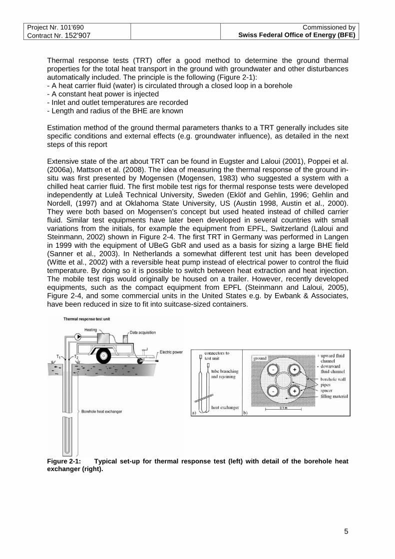
Thermal response tests (TRT) offer a good method to determine the ground thermal properties for the total heat transport in the ground with groundwater and other disturbances automatically included. The principle is the following (Figure 2-1): - A heat carrier fluid (water) is circulated through a closed loop in a borehole - A constant heat power is injected - Inlet and outlet temperatures are recorded - Length and radius of the BHE are known Estimation method of the ground thermal parameters thanks to a TRT generally includes site specific conditions and external effects (e.g. groundwater influence), as detailed in the next steps of this report Extensive state of the art about TRT can be found in Eugster and Laloui (2001), Poppei et al. (2006a), Mattson et al. (2008). The idea of measuring the thermal response of the ground in-situ was first presented by Mogensen (Mogensen, 1983) who suggested a system with a chilled heat carrier fluid. The first mobile test rigs for thermal response tests were developed independently at Luleå Technical University, Sweden (Eklöf and Gehlin, 1996; Gehlin and Nordell, (1997) and at Oklahoma State University, US (Austin 1998, Austin et al., 2000). They were both based on Mogensen’s concept but used heated instead of chilled carrier fluid. Similar test equipments have later been developed in several countries with small variations from the initials, for example the equipment from EPFL, Switzerland (Laloui and Steinmann, 2002) shown in Figure 2-4. The first TRT in Germany was performed in Langen in 1999 with the equipment of UBeG GbR and used as a basis for sizing a large BHE field (Sanner et al., 2003). In Netherlands a somewhat different test unit has been developed (Witte et al., 2002) with a reversible heat pump instead of electrical power to control the fluid temperature. By doing so it is possible to switch between heat extraction and heat injection. The mobile test rigs would originally be housed on a trailer. However, recently developed equipments, such as the compact equipment from EPFL (Steinmann and Laloui, 2005), Figure 2-4, and some commercial units in the United States e.g. by Ewbank & Associates, have been reduced in size to fit into suitcase-sized containers.
Figure 2-1: Typical set-up for thermal response test (left) with detail of the borehole heat exchanger (right).

Project Nr. 101'690 Contract Nr. 152'907
Commissioned by Swiss Federal Office of Energy (BFE)
6
The following TRT procedure is the one used with the compact equipment from EPFL; it is a representative example of the TRT practice. The thermal energy is transmitted from the ground to the circulating fluid by means of a borehole heat exchanger whereby PE pipes are inserted into a borehole in the shape of a U-tube (or double U-tube) loop. The space between the pipes and the borehole wall is filled with bentonite or another fill material to ensure good thermal contact and prevent vertical circulation of ground water. The heat exchanger is either connected directly to the reinforcement in the foundation structure or installed in a borehole of appropriate depth, which is determined by the energy demand of the planned building and the expected ground conditions at the particular site. The outlet tube branches into two tubes after leaving the heater and then rejoins after emerging from the ground. The heat exchanger tubes are directly connected to the test unit through 25 mm connectors. TRT is now widely spread in Europe, North America and East Asia. The method has also reached South America. The following list of countries with operational rigs was given in (Gehlin and Hellström, 2000): Canada, Chile, China, Germany, Netherland, Norway, South Korea, Sweden, Switzerland, Turkey, United Kingdom, United States. As a consequence to the market expansion, the need for standardisation and quality insurance has been recognized. A draft of guidelines for thermal response testing has been developed by a group of experts (Annex 13 of the Implementing Agreement on Energy Conservation through Energy Storage of the International Energy Agency, IEA). For small installations, the German design guidelines VDI 4640 are available and will be incorporated into the next version of the IEA guidelines. The TRT analysis is based almost exclusively on analytical solutions for a line source or a cylindrical probe with approximations for sufficiently long time periods (e.g. Gehlin, 1998; Gehlin and Hellström, 2003). The temperature T at a distance r from a line source with constant heat output q [W/m] in an infinitely large, homogeneous and isotropic medium with thermal conductivity λ and thermal diffusivity a is given by
γ−
πλ+≅
πλ+= ∫
∞ −
20
at4r
u
0 rat4
ln4
qTdu
ue
4q
T)t,r(T2
(1)
The approximation is valid for ar4t
2> . It does not include borehole effects. To include the
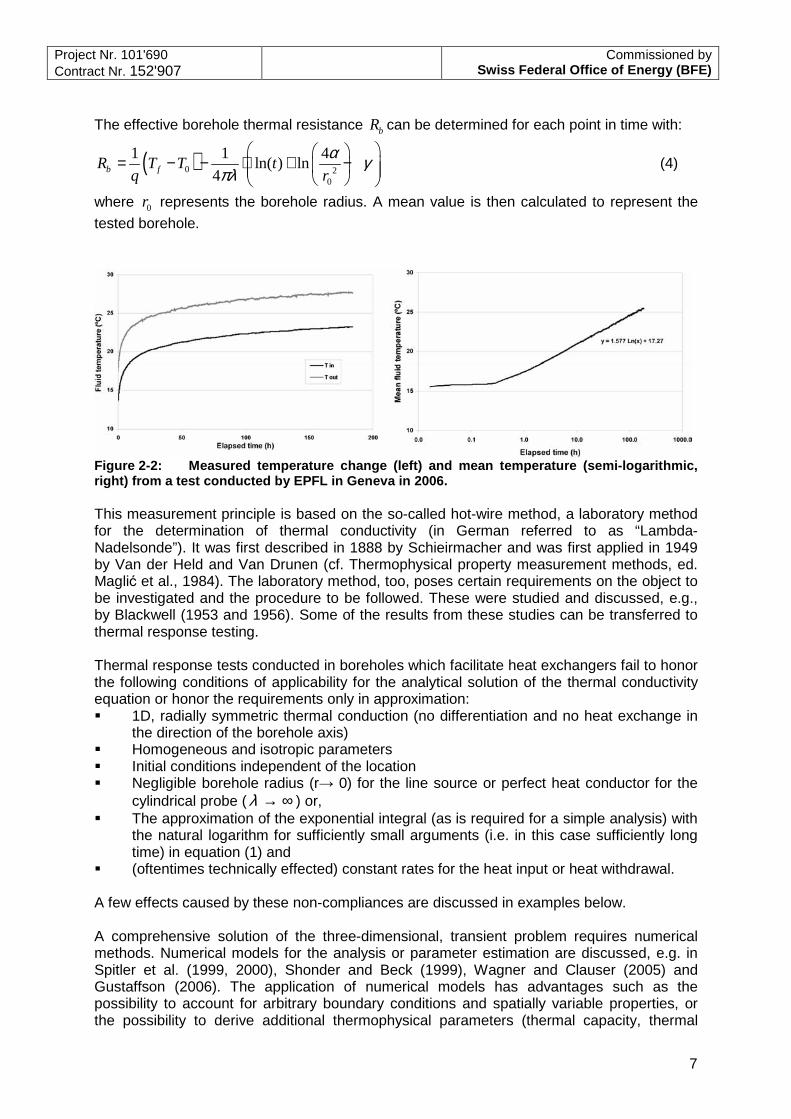
borehole resistance the thermal resistance Rb has to be added to equation (1). The equation (1) will be extend by an additional summand q· Rb. Accordingly, the temperature change is proportional to ln(t) and inversely proportional to thermal conductivity λ after a sufficiently long period of time. This relationship is used to determine the “effective” thermal conductivity of the formation penetrated by the borehole. The plot on the left-hand-side of Figure 2-2 shows a typical temperature curve from a TRT. The other plot shows the linear rise in temperature on a logarithmic time scale. In general, Thermal Response Tests are usually evaluated by the method shown in Figure 2-2 (left side). The effective thermal conductivity λ can be computed by plotting the fluid mean temperature versus the logarithm of time (Figure 2-2 right hand side), and assessing the slope k of the linear part of the plot. One has:
4
q
kλ
π= (2)
where q is the heat injection rate. The heat transfer rate can easily be converted from the
power level Q [W] recorded during the test and the height of the borehole H with:
Q q H= ⋅ (3)
Project Nr. 101'690 Contract Nr. 152'907
Commissioned by Swiss Federal Office of Energy (BFE)
7
The effective borehole thermal resistance bR can be determined for each point in time with:
( )0 20
1 1 4ln( ) ln
4b fR T T tq r
α γπλ
= − − ⋅ + −
(4)
where 0r represents the borehole radius. A mean value is then calculated to represent the
tested borehole.
Figure 2-2: Measured temperature change (left) and mean temperature (semi-logarithmic, right) from a test conducted by EPFL in Geneva in 2006. This measurement principle is based on the so-called hot-wire method, a laboratory method for the determination of thermal conductivity (in German referred to as “Lambda-Nadelsonde”). It was first described in 1888 by Schieirmacher and was first applied in 1949 by Van der Held and Van Drunen (cf. Thermophysical property measurement methods, ed. Maglić et al., 1984). The laboratory method, too, poses certain requirements on the object to be investigated and the procedure to be followed. These were studied and discussed, e.g., by Blackwell (1953 and 1956). Some of the results from these studies can be transferred to thermal response testing. Thermal response tests conducted in boreholes which facilitate heat exchangers fail to honor the following conditions of applicability for the analytical solution of the thermal conductivity equation or honor the requirements only in approximation: � 1D, radially symmetric thermal conduction (no differentiation and no heat exchange in
the direction of the borehole axis) � Homogeneous and isotropic parameters � Initial conditions independent of the location � Negligible borehole radius (r→ 0) for the line source or perfect heat conductor for the
cylindrical probe ( ∞→λ ) or, � The approximation of the exponential integral (as is required for a simple analysis) with
the natural logarithm for sufficiently small arguments (i.e. in this case sufficiently long time) in equation (1) and
� (oftentimes technically effected) constant rates for the heat input or heat withdrawal. A few effects caused by these non-compliances are discussed in examples below. A comprehensive solution of the three-dimensional, transient problem requires numerical methods. Numerical models for the analysis or parameter estimation are discussed, e.g. in Spitler et al. (1999, 2000), Shonder and Beck (1999), Wagner and Clauser (2005) and Gustaffson (2006). The application of numerical models has advantages such as the possibility to account for arbitrary boundary conditions and spatially variable properties, or the possibility to derive additional thermophysical parameters (thermal capacity, thermal

Project Nr. 101'690 Contract Nr. 152'907
Commissioned by Swiss Federal Office of Energy (BFE)
8
diffusivity) and, if necessary, even their spatial distribution. Numerical models are very computing time expensive and require time consuming meshing procedures. Therefore, in practice, the algorithms based on analytical solutions dominate the analytical work. A more general case is when the heat extraction rate changes is time dependant, e.g. is given by step-wise constant values (Eskilson, 1987):
<<
<<<<
=
+1NNN
322
211
ttt q
...
...
ttt q
ttt q
)t(q
Then, the fluid Temperature T is
1N2bN20 t/5rt ,
4ln
41
)(4
)( +<<+
−
+++= ta
ra
Rqtq
TtTb
bNNref γ
πλτ
πλ (5)
The dimensionless parameter )t(Nτ is
)ttln(q
)qq()qq()t( n
ref
1nnN
1n1nnN −−−=τ −
=−∑ ,
where qref is an arbitrary chosen reference specific energy yield, e.q. qref=q1. Vertical profiling The analysis of vertical effects such as thermal conductivity variations with depth requires temperature logging in the BHE. NIMO-T is a small, light and wireless probe with p and T sensors and a programmable microprocessor, which is designed for measurements in BHE. The wireless probe is lowered into one tube of the BHE where it sinks under its adjustable weight and records pressure and temperature while going down, at pre-selected time intervals (Figure 2-3). After the probe has reached the U-tube bottom it stops there and is flushed back to the surface by a small pump for recovery and data retrieval. A measurement run in a 300 m deep BHE takes less than 60 minutes. The depth-temperature-profile allows determination of rock thermal conductivity, if vertical heat flow is known at the location of the BHE.

Project Nr. 101'690 Contract Nr. 152'907
Commissioned by Swiss Federal Office of Energy (BFE)
9
Figure 2-3: Left side: Wireless NIMO-T probe (185mmx22mm), right side: lowering NIMO-T into a BHE.
2.2 Assessment of requirements, potential and limits of application of Mini-Module
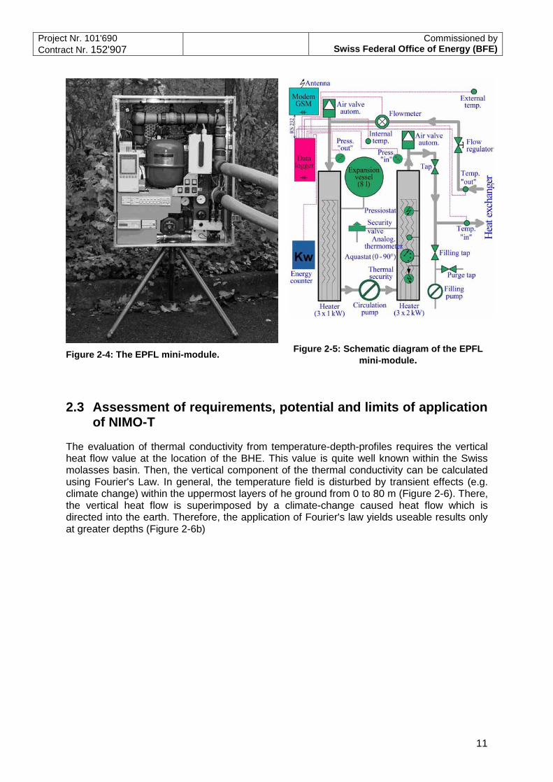
The Soil Mechanics Laboratory (LMS) at the Swiss Federal Institute of Technology in Lausanne (EPFL) has developed test apparatus for in-situ thermal response tests since 1998, which has been financially supported by the Swiss Federal Office of Energy (SFOE/OFEN). The latest apparatus (EPFL mini-module, Figure 2-4), developed in 2005, is compact and fits into a “flight case” (0.6m × 0.3m × 0.7m). The update of the equipment also includes a data transmission system whereby the test can be followed and certain functions controlled remotely using an internet connection. The mini-module enables the time and cost of the test to be reduced and offer more flexibility and application potential for in-situ thermal response testing. Thanks to these optimized features, the mini-module has been extensively used in the frame of the present project. The equipment obtained the ISO/CEI 17025 accreditation which represents a major improvement towards quality control. Figure 2-5 describes the pipe layout, locations and connection of the instruments.

Project Nr. 101'690 Contract Nr. 152'907
Commissioned by Swiss Federal Office of Energy (BFE)
10
The Heater The heater (Figure 2-5) was manufactured by the French company GRETEL with a maximum power of 9kW adjustable in steps of 1kW. The circulation pump has a three step adjustable speed (2050, 1650 and 1200 rpm), where the maximum speed mounts to 8m3/h. The heater has a flow regulating valve to maintain constant flow. A security system (Pressiostat) disrupts the heater in case of shortage of water where the pressure falls below 1bar, caused by for example a breach in the tubes. High pressure (>3 bar), is released by a regulating valve. In order to protect the materials within the borehole heat exchanger, a thermostat (Aquastat) regulates the temperature by temporarily cutting the electrical power supply if the temperature exceeds 80°C. This is und esirable since it results in a variation in power level and often means that the test has to be restarted. In addition, the heater has a second thermal security system with an emergency switch-off at 95°C. After a switch-off, the system needs to be restarted manually. The electrical network The power supply of the mini-module is achieved by a three-phase current with a voltage of 400V and a maximum current of 15 A. Instrumentation and hydraulic circuit PVC pipes have been used for the hydraulic circuit for practical reasons and to limit the weight. Two automatic air valves are placed on high points of the tubes and taps are placed on the circuit to control and stop the flow. The measurement devices are mounted directly on the hydraulic circuit inside the module and comprise a flow meter, pressure meters and thermometers. Data is recorded every minute for the following eight parameters: - Incoming and outgoing fluid temperatures - Internal and external temperature of the test unit - Pressure of the heat-conducting fluid (input and output) of the heat exchanger tubes - Flow rate of the heat-conducting fluid - Energy consumption The test apparatus is also equipped with a remote data transmission system, whereby a modem installed inside the test unit transmits the information recorded by the data-logger to an internet-connected server. Thus the test performance can be followed in real time from any location. With the latest adaptation it is also possible to switch flow and power on and off as well as altering the power level by sending an SMS. Hence the test operator only needs to be on site for the installation and dismantling of the test apparatus, which enables great savings in time and cost.
Project Nr. 101'690 Contract Nr. 152'907
Commissioned by Swiss Federal Office of Energy (BFE)
11
Figure 2-4: The EPFL mini-module.
Figure 2-5: Schematic diagram of the EPFL mini-module .
2.3 Assessment of requirements, potential and limits of application of NIMO-T
The evaluation of thermal conductivity from temperature-depth-profiles requires the vertical heat flow value at the location of the BHE. This value is quite well known within the Swiss molasses basin. Then, the vertical component of the thermal conductivity can be calculated using Fourier's Law. In general, the temperature field is disturbed by transient effects (e.g. climate change) within the uppermost layers of he ground from 0 to 80 m (Figure 2-6). There, the vertical heat flow is superimposed by a climate-change caused heat flow which is directed into the earth. Therefore, the application of Fourier's law yields useable results only at greater depths (Figure 2-6b)

Project Nr. 101'690 Contract Nr. 152'907
Commissioned by Swiss Federal Office of Energy (BFE)
12
Groundwater flow
Climate effect Disturbed Temperature field
Figure 2-6: a) NIMO-T temperature profile, measured in a 250 m deep BHE in Zürich. The difference between the dotted line and the temperature between 0 and 70 m is caused by transient temperature effects like climate change and groundwater flow. b) Temperature gradient. The temperature gradient is proportional to rock thermal conductivity below approximately 100 m, where transient effects vanish. However, the thermal conductivity can be evaluated even in disturbed temperature fields by combining vertical temperature measurement and TRT experiments. The evaluation of stratigraphical effects requires at least two temperature depth profiles. The temperature in the BHE is measured (1) before the response test and (2) after approximately one and/or two more days, when the temperature field in the ground recovers and approaches more or less to its undisturbed state. The temporal behavior of the temperature-depth-profiles (temperature-logs, t-logs) reproduces the vertical variation of the ground thermal conductivity in the vicinity of the BHE. This method of evaluation is called eTRT (enhanced TRT method, Geowatt Pat. DE 10 2007 008 039). The eTRT is interpreted quantitatively by numerical simulation using a highly resolved 3D FE mesh. The model reproduces the BHE tubes, the BHE fluid, the backfilling material, and the surrounding ground with sufficient accuracy. The thermal properties of the ground may vary with depth. The temporal cycle of the response test is simulated. The numerically simulated temperature in the BHE tubes is compared to the measured t-logs. The ground thermal properties are changed gradually until a satisfying correlation between measurement and simulation is reached. The quality of the results is not influenced by measurement techniques but mainly by the very long simulation time for each 3D FE-model. At the moment, the model resolution is limited to 10 equidistant layers over the entire length of the BHE.
Project Nr. 101'690 Contract Nr. 152'907
Commissioned by Swiss Federal Office of Energy (BFE)
13
2.4 Assessment of hydraulic testing methods with respect to their suitability for TRT
2.4.1 Similarities and differences between pressure and temperature testing
Hydraulic tests in various types of formations have a long tradition and have undergone many modifications. The main goal of these tests is the determination of the hydraulic transmissivity (kf·H) with kf – hydraulic conductivity, H – effective thickness of the formation or of the region to be tested. The processing of field measurements is based on analytical solutions of the partial differential equation for transport which is based on the Darcy equation hkv f ∇⋅−=
r (6)
The Darcy equation describes laminar flow of an incompressible fluid and is of the same mathematical form as the
Fourier equation TqH ∇⋅λ−=v& (7)
(λ – thermal conductivity; Hqv& – heat flow density [W/m2]), the basis of heat conduction.
For time-dependent processes, these equations both lead to the parabolic differential equation
( ) ( )2
2
xt,xu
at
t,xu∂
∂=∂
∂ (8)
where u stands for the hydraulic potential h or the temperature T; and a for the diffusivity which differs for thermal and hydraulic processes. Accordingly, equivalent solutions may be derived for certain initial boundary-value problems of the differential equation. These are then used for the determination of formation properties (inverse problem). The analysis of time-dependent drawdown of the groundwater table in a pumping test with constant rate after Theis (1935) corresponds, for example, exactly with the procedure described above for the line source to determine the thermal conductivity in the hot-wire procedure (Maglić et al., 1984). In recent decades the hydraulic test interpretation has led to the development of methodologies and procedures (e.g. Earlougher, 1977; Horne, 1995) which, in part, may also be applied for thermal response tests. The application does require, however, that certain specifics of the processes in question are considered. These may be, for example: o The hydraulic conductivity kf (or the underlying permeability) generally has a log-normal
distribution and, for real rock formations, varies over a range of up to 10 orders of magnitude. The thermal conductivity varies by about a factor 3 in rock formations and is normally distributed.
o The skin factor in hydraulics accommodates altered hydraulic properties in the vicinity of the borehole (e.g. due to drilling). The “inner zone” in thermal tests is a complex sequence of thermal resistances between the circulating fluid and the undisturbed rock with (velocity-dependent) heat transfer in the tube, lining and filling (see also

Project Nr. 101'690 Contract Nr. 152'907
Commissioned by Swiss Federal Office of Energy (BFE)
14
Eppelbaum and Kutasov, 2006). Also, U or double-U tubes do not have a radially symmetric geometry.
o For porous aquifers, the hydraulic diffusivity a (as a quotient of hydraulic conductivity and storage coefficient) generally is relatively high (1 to 10+2 m2/s) which means that
certain criteria of the Fourier number (dimensionless time), 2br
taFo ⋅= , e.g. for the
approximation of the exponential integral through the logarithm, are reached relatively quickly. For thermal response tests, the thermal diffusivity a is the ratio of thermal conductivity and heat capacity and tends to reach orders of magnitude (10-7 to 10-6 m2/s) which correspond to very low permeability formations in the hydraulic-test equivalent. Accordingly, the penetration depth of a thermal signal grows only very slowly and sufficiently long recording times are necessary to meet certain criteria. This is the reason why a TRT may not be cut off arbitrarily.
2.4.2 Diagnostic plots as an interpretation tool
So called diagnostic plots are an important aid when analyzing hydraulic tests and characterizing tests and reservoirs. Diagnostic plots show the test response and its temporal derivative in a semi-logarithmic and a log-log format. They may also find their way into the TRT interpretation.
2.4.2.1 Semi-logarithmic plots
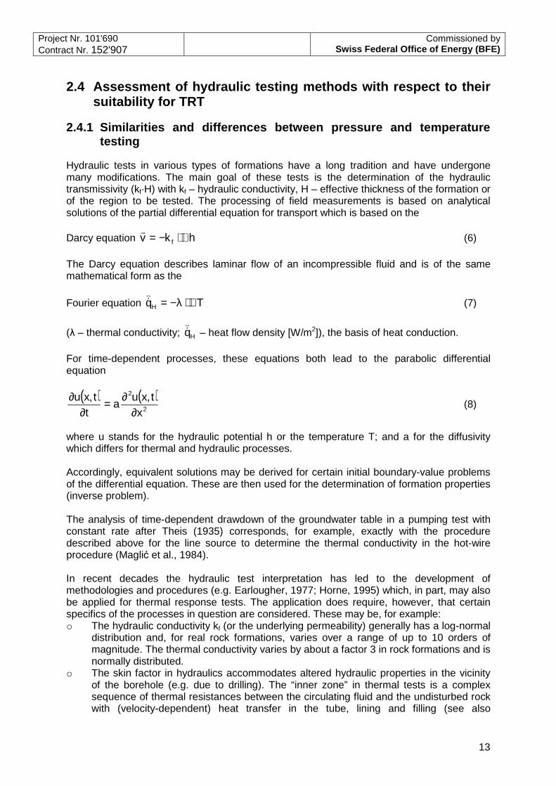
The most widely used semi-logarithmic hydraulic analysis method is the Jacob method (Cooper and Jacob, 1946). For the recovery periods of hydraulic tests, the Horner method (Horner, 1951) is most often applied. The Jacob method is similar to the straight-line method used for the interpretation of a TRT (Ingersoll and Plass, 1948). The Horner method is applied for the analysis of recovery phases and uses the principle of superposition to take into account the pumping period just before the recovery period. Certain characteristics in the temporal evolution of the response provide insight on reservoir characteristics (Figure 2-7).
Project Nr. 101'690 Contract Nr. 152'907
Commissioned by Swiss Federal Office of Energy (BFE)
15
Figure 2-7: Diagnostic plots for the interpretation of hydraulic tests according to Earlougher (1977).
2.4.2.2 Double-logarithmic plots
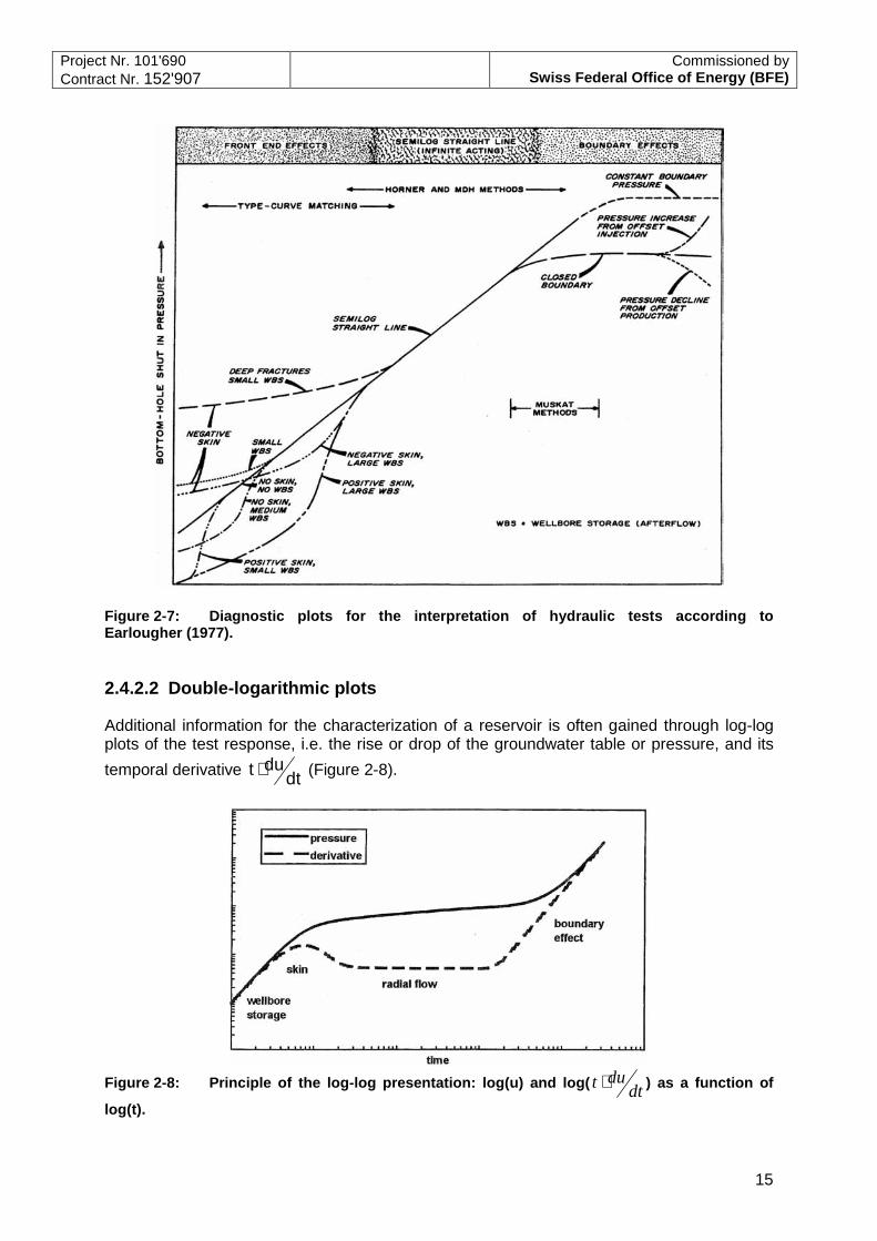
Additional information for the characterization of a reservoir is often gained through log-log plots of the test response, i.e. the rise or drop of the groundwater table or pressure, and its
temporal derivative dtdut ⋅ (Figure 2-8).
Figure 2-8: Principle of the log-log presentation: log(u) and log( dt
dut ⋅ ) as a function of
log(t).

Project Nr. 101'690 Contract Nr. 152'907
Commissioned by Swiss Federal Office of Energy (BFE)
16
Horne (1995) introduced many such plots for the determination of certain reservoir characteristics such as preferred flow paths, double-porosity behavior etc.. Up until now, diagnostic plots have not been used in the analysis of TRTs.
2.4.2.3 Normalized derivative plots
A new generalized technique of diagnostics was introduced for hydraulic tests by Enachescu et al. (2004). This technique uses the normalized presentation of the logarithmic derivative of the hydraulic head and can also be used for the logarithmic derivative of the temperature change during a TRT or the subsequent temperature recovery. The method essentially uses test data to characterize small to medium scale formation behavior and provides a means for continuous improvement in understanding the surroundings of the well. Used for the thermal test analysis, the technique unifies the analysis of tests and allows for a direct comparison between the different periods (e.g. heating or cooling and following recovery period) in terms of the conductivity. The basis of the technique is the hydraulic head/temperature change during one period
)tt(u)t(u)t(u 0=−=∆ with u as potential (hydraulic head or temperature) and the time t.
Using the conventional hydraulic normalization methods (e.g. Horne, 1995), the semi-logarithmic transformation equation is given by (Enachescu et al., 2004):
Hk2
)t(Pgq)t(p
f
DDhydr
πρ
=∆ and Hk2
tlogd)t(Pd
gq
tlogd)t(pd
f
D
DDhydr
π
ρ=∆
,
with the normalized pressure PD and the normalized time tD, the flow rate qhydr, the density ρ, the gravity constant g and the transmissivity (kfH). The logarithmic derivative becomes 0.5 for an infinite acting radial flow (IARF). Assuming an IARF, the transmissivity therefore is given by (Enachescu et al., 2004):
)t(pdtlogd
4
gq)Hk( hydr
IARFf ∆πρ
=
Taking into account that ∆T is equivalent to ∆h = ∆p/ρg, this equation can be written in thermal terms:
( ))t(Tdtlogd
4Q
H IARF ∆π=λ
Using this equation it is possible to normalize the derivatives of each test period and to express it in terms of thermal conductivity units. Accordingly, for each point on the derivative curve that fulfills the IARF assumptions – which means a flat shape of the derivative –, the thermal conductivity equivalent of radial flow is equal to the Y-coordinate of the point in a plot vs. the elapsed time. A further transformation of time into distance is possible using the expression for the hydraulic radius of investigation (Bourdarout, 1996):

Project Nr. 101'690 Contract Nr. 152'907
Commissioned by Swiss Federal Office of Energy (BFE)
17
tinv c
tK4r
φµ=
where φ is porosity, µ is viscosity and ct is total system compressibility. Taking into account
that the product φµct represents the storage term, the transformation of this equation into thermal terms becomes:
finv C
t4r
λ=
with the heat capacity Cf = ρ·cf. Assuming a constant heat capacity the transformation can be performed and plotted. The result is a plot of a radial flow equivalent conductivity vs. the equivalent distance from the borehole.
2.4.3 Numerical simulations as interpretation tool
The past decades have seen the birth of many numerical simulators for the analysis of hydraulic borehole tests. Colenco has developed a numerical simulator which is specifically geared toward the requirements of testing in low permeability formations. For this reason, it is particularly well suited as a starting point for the development of a numerical simulator for the analysis of thermal borehole tests. The base for the adaptation is the mathematical similarity of the two fundamental transport equations. The program is based on a finite-volume definition of the spatial and temporal interdependence. The spatial discretization follows a cylindrical partitioning with the test interval, i.e. the borehole, in the centre. The temporal discretization follows the course of the test. The system of equations is defined and solved numerically. The computation takes several seconds. With this, the program allows for quick parameter variations for the evaluation of the influence of parameters and to solve the inverse problem (i.e. to determine parameters) within a few minutes. The numerically based analysis improves, for example, the representation of the inner boundary condition of the heat exchanger through: � The integration of temporal temperature changes (direct integration of the
measurements) � The consideration of a temporally variable performance of the heat source or sink
(direct use of measured data and, thereby, implicit superpositioning of test phases of differing heat supply)
� The simulation of the temporal and spatial extent of the alterations in the temperature field resulting from the test
� If required, consideration of temporal changes of material property values, e.g. of installations in the borehole etc.
Through the application of the Barker model it is also possible to vary and assess the influence of the dimension of the heat propagation, i.e. the effect of linear, radial and spherical heat propagation in the rock formation. Spatial constraints may be varied and their influences estimated and, through this, improve the quality of the results and determine their band widths. The results of the simulation are the temperature change with time and the heat source or sink in the test interval as well as the temperature profile at arbitrary points in time or the temporal temperature evolution at points of arbitrary distance from the interval.
Project Nr. 101'690 Contract Nr. 152'907
Commissioned by Swiss Federal Office of Energy (BFE)
18
Last but not least, the numerical approach makes it possible to solve the inverse problem, to determine parameters with a gradient approach (Levenberg-Marquardt algorithm) and to predict the evolution of the temperature field.
2.4.4 Signal of thermal conductivity heterogeneities
In a more detailed view (with respect to line source theory), the heat flow between the BHE and surrounding rock is determined according to the Fourier law by the temperature gradient and the thermal conductivity. Radial heat flow may vary along a BHE due to the changing difference between fluid temperature and ground and when the subsurface is stratified. The effective thermal conductivity may then be dominated by one specific layer. In this study, different ground models with the same average thermal conductivity but different vertical distribution of thermal conductivity heterogeneities were simulated and analyzed with the line source theory. The results show that the effective thermal conductivity is influenced by the layers close to the surface. This means that the analysis with the 1D-approach over- or underestimates the real average thermal conductivity of the ground. The identification of vertical thermal conductivity variations requires temperature logging. The influence of stratigraphic effects on vertical temperature measurements in a BHE during a TRT was investigated by combining thermal response test data with vertical temperature measurements in the borehole during the test. This method was tested using generic data. The numerical tests showed that the temperature resolution of the temperature sensor is sufficient to derive the ground thermal conductivity of 4 layers by Monte Carlo method.
2.4.5 Influence of groundwater flow on calculated results
The influence of groundwater flow on TRT evaluation has been observed in several field experiments e.g. Gehlin, 1998; Witte et al., 2002). Heat transport due to groundwater flow is a major deviation from the line source theory assumption. Therefore, the results from line source theory evaluation yield a higher thermal conductivity, which does not represent the real average thermal conductivity of the underground. This effect is analyzed in more detail in Chapter 3.4.3
2.5 Method used to estimate the sensitivity
The sensitivity of parameters to the temperature recorded throughout a TRT can be analyzed with a number of forward simulations. This procedure computes the so-called sensitivity coefficients as function of time for each parameter of interest. For each parameter of interest (e.g. the thermal conductivity λ), the relative change in temperature (∆T/T) corresponding to a relative change in the parameter (e.g. ∆ λ / λ) is computed for each time. A linear approximation of the scaled sensitivity coefficient (relative to the parameter thermal
conductivity λ) is given by the expression: λ∆
λ⋅∆=∆λ TT
.
The impact of the parameters on the temperature becomes evident when plotting these coefficients over time, for each parameter of interest. The sensitivity coefficients for the thermal response generally are given using a relative change of 1% for each parameter considered.

Project Nr. 101'690 Contract Nr. 152'907
Commissioned by Swiss Federal Office of Energy (BFE)
19
2.6 Mathematical definition of the uncertainty
The uncertainty or margin of error is commonly stated in terms of a range of values which are likely to enclose the true value. This may be denoted by error bars on a graph, or by the notation ‘measured value ± uncertainty’. Often, the uncertainty of a measurement is found by repeating the measurement a sufficient number of times to get a good estimate of the standard deviation of the values. Then, presuming a normal distribution of the error, any single value has an uncertainty equal to the standard deviation. However, if the values are averaged, then the mean measurement value has a much smaller uncertainty and is equal to the standard error of the mean, which is the standard deviation divided by the square root of the number of measurements. When the uncertainty represents the standard error of the measurement, then about 68% of the time, the true value of the measured quantity falls within the stated uncertainty range. E.g., it is likely that for 32% of the atomic mass values given in the list of elements, the true value of the atomic mass lies outside of the stated range. If the width of the interval is doubled, then probably only 4.6% of the true values lie outside the doubled interval, and if the width is tripled, probably only 0.3% lie outside. These values follow from the properties of the normal distribution, and they apply only if the measurement process produces normally distributed errors. In that case, the quoted standard errors are easily converted to 68% (σ), 95.4% (2σ) or 99.7% (3σ) confidence intervals. The same is valid for any linear combination of values which are normally distributed.
2.7 Method to estimate mathematical uncertainty ranges
Any test may be simulated numerically. By applying a suitable merit function to this numerical representation it is possible to derive a set of best-fit parameters. Such methods are described, for example, by Press et al. (1996). The most commonly applied method is the least squares fit as a maximum likelihood estimator. Gradient approaches like the Levenberg-Marquardt method are often applied for nonlinear models. In these cases, the solution is found by determining gradients and the Hessian matrix (cf., e.g., Press et al., 1996). Another solution approach is the Monte Carlo / bootstrap method (Efron, 1982). It offers the option of directly determining the uncertainty ranges based on the values of the merit function, like described in the example in the paragraph above. Unfortunately, the method draws very heavily on computing time despite the excellent sampling algorithms. By comparison, gradient approaches for the determination of uncertainty ranges are relatively fast and require little computing effort. Their drawbacks are various assumptions (cf. Press et al., 1996). Based on the assumption of a region-specific normal distribution of the error near the solution (which has been found by solving the problem inversely), it is possible to use the quantitative relationship between the ∆χ2 distribution and the correlation matrix Cij of the solution to determine the uncertainty. This has been demonstrated, e.g. by Press et al. (1996). This approach saves computation time but requires a linearization of the mathematical and/or physical description.
Project Nr. 101'690 Contract Nr. 152'907
Commissioned by Swiss Federal Office of Energy (BFE)
20
2.8 Estimation of confidence intervals
As shown in text books, like Press et al. (1996), the determination of the confidence intervals is based on the mathematical description of the physical framework of interest in which all parameters (M) used in the mathematical description receive their own confidence interval. Frequently, one is interested not in the full M-dimensional confidence region, but in individual confidence regions for some smaller number of parameters (u). In that case, the natural confidence regions in the u-dimensional subspace of the M-dimensional parameter space are the projections of the M-dimensional regions defined by fixed ∆χ2 distribution into the u-dimensional spaces of interest. But the error distribution of the problem is often not normally distributed. However, the formal covariance matrix that comes out of the ∆χ2 minimization has a unambiguous quantitative interpretation only if the errors actually are normally distributed. In the case of a non-normal error distribution, it is “permitted” � to fit for parameters by minimizing ∆χ2 � to use a contour of constant ∆χ2 as the boundary of the confidence region � to use Monte Carlo / bootstrap methods or detailed analytic calculation to determine
which contour ∆χ2 is the collective one for the desired confidence level � to take the covariance matrix Cij as the "formal covariance matrix of the fit”.
If the measurement errors are normally distributed it is also permitted � to use formulas which establish quantitative relationships among ∆χ2, Cij and the
confidence level. In order to take advantage of this last bullet point, it is necessary to linearize the problem. This can be achieved with a parameter transformation of the fundamental equations, i.e., parameters under the logarithm (x) are integrated as the logarithm of their value (y = log(x)). This approach is also applied in the analysis of hydraulic tests, e.g., by nSight (Intera). As is shown in text books like Press et al. (1996), a relation between the confidence interval,
given by 002
0 Ca χ∆±=δ , and the formal standard error, which is given by 000 C≡δ ,
can be given for an individual parameter a. Given that the error is normally distributed the 68% confidence interval is ±σ, the 95% confidence interval is ±2σ. As mentioned before, these considerations hold not just for the individual parameters a, but also for any linear combination of these parameters, as it is demonstrated, e.g., in Press et al. (1996). The confidence intervals, therefore, can be computed based on the covariance matrix Cij. The covariance matrix may also be used to derive the correlations among individual parameters.

Project Nr. 101'690 Contract Nr. 152'907
Commissioned by Swiss Federal Office of Energy (BFE)
21
3 Application of methods
As discussed in Chapter 1 and 2, TRT data are usually evaluated by plotting the average between in- and outlet temperatures at the wellhead versus logarithm of elapsed time, ln(t). The average ground thermal conductivity is then inversely proportional to the slope of a line, which fits the data. The measurement duration and the time interval, which is used to fit the data is an on-going discussion. The problem is, that the slope is influenced strongly by near borehole effects if the evaluation-interval is defined at early times, and is strongly influenced by boundary effects and measurement errors, if the time interval is defined at times greater than 50-100 h. One of the aims of this project is to present methods, which bear down this major evaluation problem. In Chapter 3.1, several TRT experiments are described which were performed during this project. The TRT's were performed at the same test site, but with different flow conditions in the BHE tubes and different duration times. These tests were evaluated (Chapter 3.2) by the very simple "line-fitting"-method. It is interesting that the results differ quite significantly for the different test, although they should yield the same results. Consequently, the potential of inverse methods is demonstrated in Chapter 3.3. As a result, this inverse method outreaches the conventional valuation method. In contrast to conventional TRT evaluation, the inverse method can also be applied, if the power of the TRT during the experiment is not stable. In Chapter 3.4, 3D effects like groundwater flow and thermal conductivity heterogeneities are discussed in order to quantify these effects on TRT results.
3.1 TRT field campaign
3.1.1 Site selection
The long-term TRT experiments were performed at a 250 m deep BHE at ETH Zürich, Hönggerberg. The BHE will be labeled BHE ZH in this report. The owner granted a permit to EPFL and GEOWATT to use this BHE for TRT and temperature profile measurements. This BHE had never been used for heat extraction before. The TRT could be installed safely with short wire length and safe power supply. Additionally, this BHE provided five thermal conductivity values from measurements on cutting-samples (Table 3-1, Table 3-1 and Table 3-2) Table 3-1: Thermal conductivity of rock samples from BHE ZH Sample No.
Depth interval [m] Facies Thermal conductivity [W/m/K]
E 3 12 12-20 Gravel 3.69 E 3 42 42-48 Fine coarse sandstone with marl 2.71 E 3 90 90-96 Fine coarse sandstone 3.00 E 3 158 158-164 Average coarse sandstone 3.06 E 3 194 194-202 Fine coarse sandstone 2.86 E 3 242 242-250 Fine coarse sandstone 3.30
Project Nr. 101'690 Contract Nr. 152'907
Commissioned by Swiss Federal Office of Energy (BFE)
22
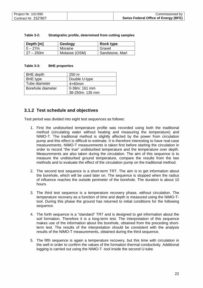
Table 3-2: Stratigrahic profile, determined from cutting samples Depth [m] Geology Rock type 0 – 27m Moraine Gravel 27 – 250m Molasse (OSM) Sandstone, Marl
Table 3-3: BHE properties BHE depth 250 m BHE type Double U-type Tube diameter 4×40mm Borehole diameter 0-38m: 161 mm
38-250m: 135 mm
3.1.2 Test schedule and objectives
Test period was divided into eight test sequences as follows:
1. First the undisturbed temperature profile was recorded using both the traditional method (circulating water without heating and measuring the temperature) and NIMO-T. The traditional method is slightly affected by the power from circulation pump and this effect is difficult to estimate. It is therefore interesting to have real-case measurements. NIMO-T measurements is taken first before starting the circulation in order to record “the true” undisturbed temperature and the temperature over depth. Measurements are also taken during the circulation. The aim of this sequence is to measure the undisturbed ground temperature, compare the results from the two methods and to evaluate the effect of the circulation pump on the traditional method.
2. The second test sequence is a short-term TRT. The aim is to get information about
the borehole, which will be used later on. The sequence is stopped when the radius of influence reaches the outside perimeter of the borehole. The duration is about 10 hours.
3. The third test sequence is a temperature recovery phase, without circulation. The
temperature recovery as a function of time and depth is measured using the NIMO-T-tool. During this phase the ground has returned to initial conditions for the following sequence.
4. The forth sequence is a “standard” TRT and is designed to get information about the
soil formation. Therefore it is a long-term test. The interpretation of this sequence makes use of the information about the borehole, obtained from the preceding short-term test. The results of the interpretation should be consistent with the analysis results of the NIMO-T measurements, obtained during the third sequence.
5. The fifth sequence is again a temperature recovery, but this time with circulation in
the well in order to confirm the values of the formation thermal conductivity. Additional logging is carried out using the NIMO-T -tool inside the second U-tube.
Project Nr. 101'690 Contract Nr. 152'907
Commissioned by Swiss Federal Office of Energy (BFE)
23
6. The sixth sequence concerns the flow rate within the heat exchanger, which is set to laminar flow. In practice, sites often use laminar flow conditions. So, a measurement under laminar flow conditions should enhance our understanding of the heat transfer process. The test conditions were tried to be kept the same as for a standard test. Moreover, it should be kept in mind that the temperature measurements taken during this test could be a bit unreliable since the laminar flow is likely to allow zones of different temperature within the heat carrier fluid.
7. The seventh sequence is a final temperature recovery with circulation keeping the
laminar flow regime.
8. The last sequence is a circulation phase without insulation, so as to use the ambient air temperature as a possible signal for estimation of thermal conductivity.
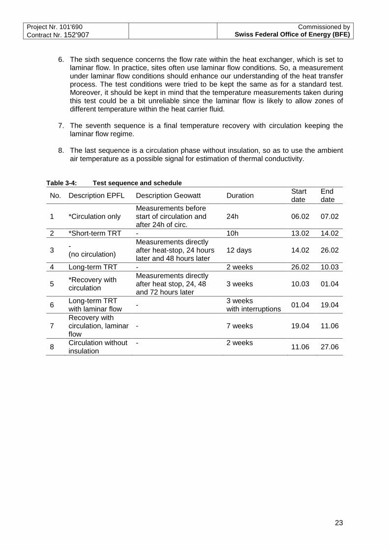
Table 3-4: Test sequence and schedule
No. Description EPFL Description Geowatt Duration Start date
End date
1 *Circulation only Measurements before start of circulation and after 24h of circ.
24h 06.02 07.02
2 *Short-term TRT - 10h 13.02 14.02
3 - (no circulation)
Measurements directly after heat-stop, 24 hours later and 48 hours later
12 days 14.02 26.02
4 Long-term TRT - 2 weeks 26.02 10.03
5 *Recovery with circulation
Measurements directly after heat stop, 24, 48 and 72 hours later
3 weeks 10.03 01.04
6 Long-term TRT with laminar flow - 3 weeks
with interruptions 01.04 19.04
7 Recovery with circulation, laminar flow
- 7 weeks 19.04 11.06
8 Circulation without insulation
-
2 weeks 11.06 27.06
Project Nr. 101'690 Contract Nr. 152'907
Commissioned by Swiss Federal Office of Energy (BFE)
24
3.2 Results of the test campaign
3.2.1 Test 1: first circulation phase (without heating)
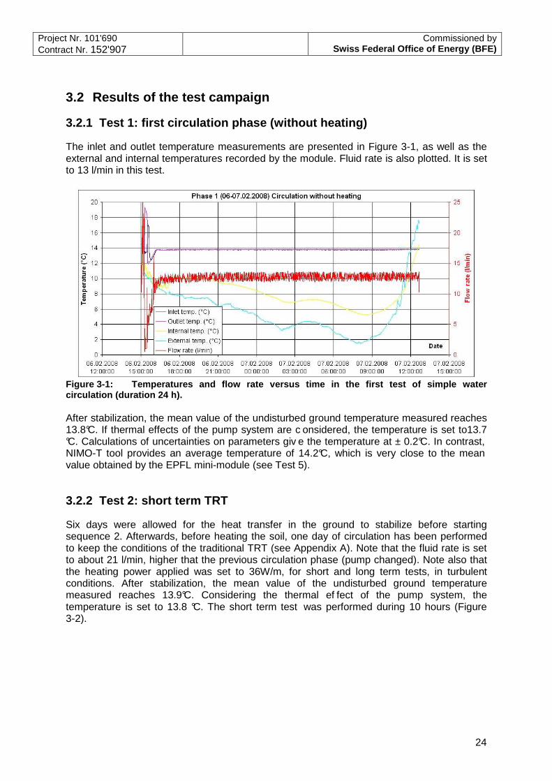
The inlet and outlet temperature measurements are presented in Figure 3-1, as well as the external and internal temperatures recorded by the module. Fluid rate is also plotted. It is set to 13 l/min in this test.
Figure 3-1: Temperatures and flow rate versus time in the first test of simple water circulation (duration 24 h). After stabilization, the mean value of the undisturbed ground temperature measured reaches 13.8°C. If thermal effects of the pump system are c onsidered, the temperature is set to13.7 °C. Calculations of uncertainties on parameters giv e the temperature at ± 0.2°C. In contrast, NIMO-T tool provides an average temperature of 14.2°C, which is very close to the mean value obtained by the EPFL mini-module (see Test 5).
3.2.2 Test 2: short term TRT
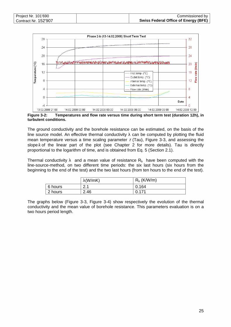
Six days were allowed for the heat transfer in the ground to stabilize before starting sequence 2. Afterwards, before heating the soil, one day of circulation has been performed to keep the conditions of the traditional TRT (see Appendix A). Note that the fluid rate is set to about 21 l/min, higher that the previous circulation phase (pump changed). Note also that the heating power applied was set to 36W/m, for short and long term tests, in turbulent conditions. After stabilization, the mean value of the undisturbed ground temperature measured reaches 13.9°C. Considering the thermal ef fect of the pump system, the temperature is set to 13.8 °C. The short term test was performed during 10 hours (Figure 3-2).
Project Nr. 101'690 Contract Nr. 152'907
Commissioned by Swiss Federal Office of Energy (BFE)
25
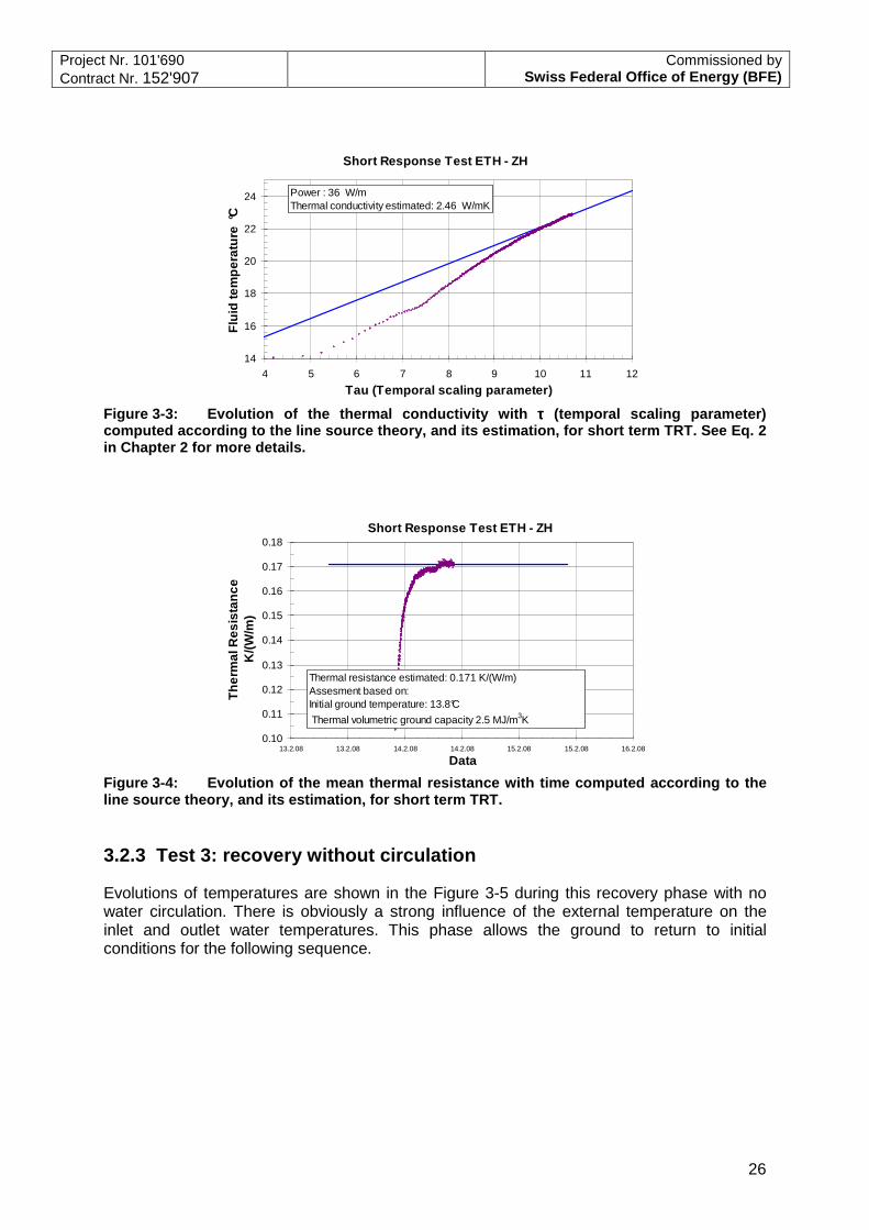
Figure 3-2: Temperatures and flow rate versus time during short term test (duration 12h), in turbulent conditions. The ground conductivity and the borehole resistance can be estimated, on the basis of the line source model. An effective thermal conductivity λ can be computed by plotting the fluid mean temperature versus a time scaling parameter τ (Tau), Figure 3-3, and assessing the slope k of the linear part of the plot (see Chapter 2 for more details). Tau is directly proportional to the logarithm of time, and is obtained from Eq. 5 (Section 2.1). Thermal conductivity λ and a mean value of resistance Rb have been computed with the line-source-method, on two different time periods: the six last hours (six hours from the beginning to the end of the test) and the two last hours (from ten hours to the end of the test).
λ(W/mK) Rb (K/W/m)
6 hours 2.1 0.164 2 hours 2.46 0.171
The graphs below (Figure 3-3, Figure 3-4) show respectively the evolution of the thermal conductivity and the mean value of borehole resistance. This parameters evaluation is on a two hours period length.
Project Nr. 101'690 Contract Nr. 152'907
Commissioned by Swiss Federal Office of Energy (BFE)
26
Short Response Test ETH - ZH
14
16
18
20
22
24
4 5 6 7 8 9 10 11 12
Tau (Temporal scaling parameter)
Flu
id te
mpe
ratu
re °
C
Power : 36 W/mThermal conductivity estimated: 2.46 W/mK
Figure 3-3: Evolution of the thermal conductivity with ττττ (temporal scaling parameter) computed according to the line source theory, and its estimation, for short term TRT. See Eq. 2 in Chapter 2 for more details.
Short Response Test ETH - ZH
0.10
0.11
0.12
0.13
0.14
0.15
0.16
0.17
0.18
13.2.08 13.2.08 14.2.08 14.2.08 15.2.08 15.2.08 16.2.08
Data
The
rmal
Res
ista
nce
K
/(W/m
)
Thermal resistance estimated: 0.171 K/(W/m)Assesment based on:Initial ground temperature: 13.8°C
Thermal volumetric ground capacity 2.5 MJ/m3K
Figure 3-4: Evolution of the mean thermal resistance with time computed according to the line source theory, and its estimation, for short term TRT.
3.2.3 Test 3: recovery without circulation
Evolutions of temperatures are shown in the Figure 3-5 during this recovery phase with no water circulation. There is obviously a strong influence of the external temperature on the inlet and outlet water temperatures. This phase allows the ground to return to initial conditions for the following sequence.

Project Nr. 101'690 Contract Nr. 152'907
Commissioned by Swiss Federal Office of Energy (BFE)
27
Figure 3-5: Temperatures and flow rate versus time in recovery phase without circulation after short term test (13 days).
3.2.4 Test 4: long term TRT
Before heating the soil, the usual one day (20 hours) circulation period has been followed. The fluid rate is set to about 21 l/min, like in the short term test (see Appendix A). The fluid was circulated in only one tube. The long term test was performed during 2 weeks (Figure 3-6). Thermal conductivity and a mean value of resistance Rb have been computed (Figure 3-7 and Figure 3-8) on the hypothesis on the line source model over the entire period of the heating (after 6 hours of heating and during 13 days). The results obtained are: Effective thermal conductivity λ =2.74 W/mK Mean value of resistance bR =0.164 K/(W/m)
The short term TRT thermal conductivity is 10 to 23% smaller than the long term TRT one. But, the borehole resistance in the short term TRT is very close to that evaluated in the long term TRT (the difference is maximum 2%).

Project Nr. 101'690 Contract Nr. 152'907
Commissioned by Swiss Federal Office of Energy (BFE)
28
Figure 3-6: Temperatures and flow rate versus time during long term test in turbulent conditions (duration 2 weeks).
Figure 3-7: Evolution of the thermal conductivity with ττττ (temporal scaling parameter) computed according to the line source theory, and its estimation for long term TRT.
Figure 3-8: Evolution of the mean thermal resistance with time computed according to the line source theory, and its estimation, for long term TRT.
Project Nr. 101'690 Contract Nr. 152'907
Commissioned by Swiss Federal Office of Energy (BFE)
29
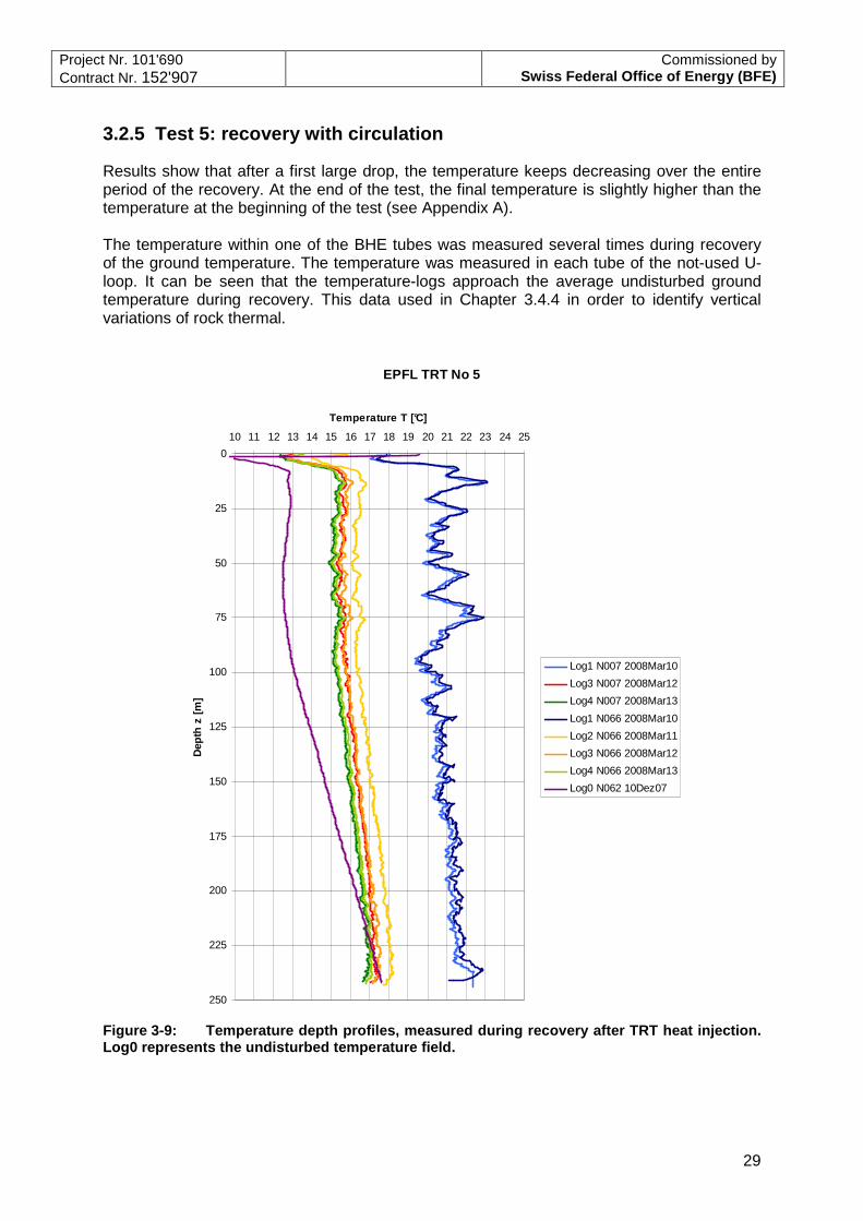
3.2.5 Test 5: recovery with circulation
Results show that after a first large drop, the temperature keeps decreasing over the entire period of the recovery. At the end of the test, the final temperature is slightly higher than the temperature at the beginning of the test (see Appendix A). The temperature within one of the BHE tubes was measured several times during recovery of the ground temperature. The temperature was measured in each tube of the not-used U-loop. It can be seen that the temperature-logs approach the average undisturbed ground temperature during recovery. This data used in Chapter 3.4.4 in order to identify vertical variations of rock thermal.
EPFL TRT No 5
0
25
50
75
100
125
150
175
200
225
250
10 11 12 13 14 15 16 17 18 19 20 21 22 23 24 25
Temperature T [°C]
Dep
th z
[m]
Log1 N007 2008Mar10
Log3 N007 2008Mar12
Log4 N007 2008Mar13
Log1 N066 2008Mar10
Log2 N066 2008Mar11
Log3 N066 2008Mar12
Log4 N066 2008Mar13
Log0 N062 10Dez07
Figure 3-9: Temperature depth profiles, measured during recovery after TRT heat injection. Log0 represents the undisturbed temperature field.
Project Nr. 101'690 Contract Nr. 152'907
Commissioned by Swiss Federal Office of Energy (BFE)
30
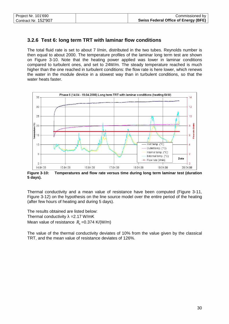
3.2.6 Test 6: long term TRT with laminar flow conditions
The total fluid rate is set to about 7 l/min, distributed in the two tubes. Reynolds number is then equal to about 2000. The temperature profiles of the laminar long term test are shown on Figure 3-10. Note that the heating power applied was lower in laminar conditions compared to turbulent ones, and set to 24W/m. The steady temperature reached is much higher than the one reached in turbulent conditions: the flow rate is here lower, which renews the water in the module device in a slowest way than in turbulent conditions, so that the water heats faster.
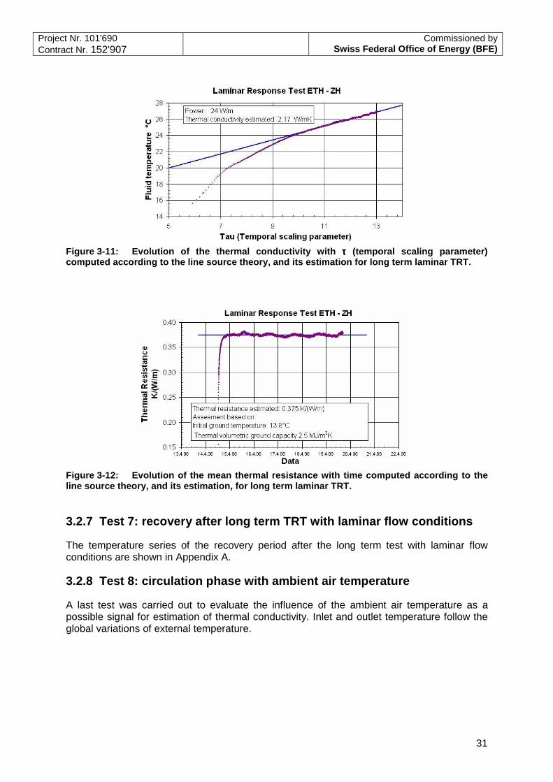
Figure 3-10: Temperatures and flow rate versus time during long term laminar test (duration 5 days). Thermal conductivity and a mean value of resistance have been computed (Figure 3-11, Figure 3-12) on the hypothesis on the line source model over the entire period of the heating (after few hours of heating and during 5 days). The results obtained are listed below: Thermal conductivity λ =2.17 W/mK Mean value of resistance bR =0.374 K/(W/m)
The value of the thermal conductivity deviates of 10% from the value given by the classical TRT, and the mean value of resistance deviates of 126%.
Project Nr. 101'690 Contract Nr. 152'907
Commissioned by Swiss Federal Office of Energy (BFE)
31
Figure 3-11: Evolution of the thermal conductivity with ττττ (temporal scaling parameter) computed according to the line source theory, and its estimation for long term laminar TRT.
Figure 3-12: Evolution of the mean thermal resistance with time computed according to the line source theory, and its estimation, for long term laminar TRT.
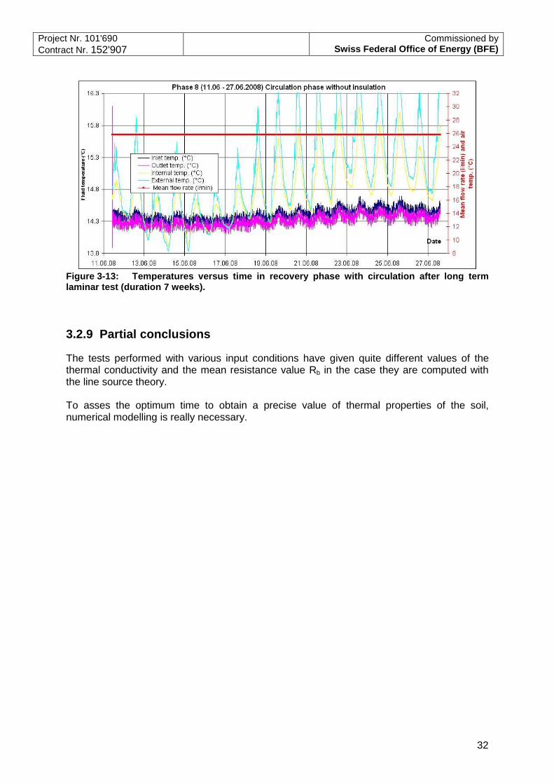
3.2.7 Test 7: recovery after long term TRT with laminar flow conditions
The temperature series of the recovery period after the long term test with laminar flow conditions are shown in Appendix A.
3.2.8 Test 8: circulation phase with ambient air temperature
A last test was carried out to evaluate the influence of the ambient air temperature as a possible signal for estimation of thermal conductivity. Inlet and outlet temperature follow the global variations of external temperature.
Project Nr. 101'690 Contract Nr. 152'907
Commissioned by Swiss Federal Office of Energy (BFE)
32
Figure 3-13: Temperatures versus time in recovery phase with circulation after long term laminar test (duration 7 weeks).
3.2.9 Partial conclusions
The tests performed with various input conditions have given quite different values of the thermal conductivity and the mean resistance value Rb in the case they are computed with the line source theory. To asses the optimum time to obtain a precise value of thermal properties of the soil, numerical modelling is really necessary.

Project Nr. 101'690 Contract Nr. 152'907
Commissioned by Swiss Federal Office of Energy (BFE)
33
3.3 Application of adapted and newly developed TRT analysis methods
3.3.1 Analysis in generic and practical terms
3.3.1.1 Estimation of minimum test duration
Onsite diagnostic methods and TRT optimization The following discussion of a TRT conducted on a construction site in Zürich illustrates the added benefits drawn from applying methods known from hydraulic testing in the context of a TRT. Figure 3-14 shows the measured response (mean temperature) for a short-term test run for 12 hours, the subsequent thermal recovery and a long-term test run for nearly 300 hours.
Figure 3-14: Temperature measurements recorded during two thermal response tests conducted at the same site. The virtues of diagnostic plots for test interpretation and reservoir characterization purposes were described above. Of particular interest is the generalized diagnostic method introduced in chapter 2.4.2 for the comparison of different test periods and sequences at one site. As has been said above, it involves plotting the semi-logarithmic derivative of the measurement in units of the thermal conductivity over time. Figure 3-15 shows the application of the transferential transformation on the semi-logarithmic derivative of the measured temperature difference (wrt. undisturbed temperature) after the normalized time for the two test phases presented in Figure 3-14. Also shown in the graph is the equivalent radius of investigation (slanted line). It is apparent from the plot (Figure 3-15) that the first test (short-term test) was too short for a determination of the thermal formation properties and that the second test (long-term test) could have been abandoned earlier, i.e. after about 100 hours, as is indicated by the stabilization of the derivative.

Project Nr. 101'690 Contract Nr. 152'907
Commissioned by Swiss Federal Office of Energy (BFE)
34
Figure 3-15: Normalized plot of the semi-logarithmic derivative of temperature change throughout the two test phases shown in Figure 3-14 This procedure can also be applied to the temperature recovery periods by using a superpositioning method and it may be used onsite for the optimization of a test. The TRT can be stopped when a nearly stable zone is recognized. This stable feature should stretch over at least half of a logarithmic cycle. In this way, the generalized diagnostic technique makes it possible to estimate the thermal conductivity and the radius of investigation at any time while the test is being performed.
3.3.2 Influence of power disturbances
A TRT conducted by EPFL in Perpignan demonstrates the influence of power disturbances on a TRT. The test was interrupted repeatedly by power outages so that the time intervals between the outages are, on the one hand, considered to be complete TRTs and, on the other, each TRT is viewed to have influenced the subsequent TRT. This is clearly seen in the analysis of the “first TRT” (03.08.06) and the “last TRT” (06.-07.08.06), where the thermal conductivities are found to be 1.9 – 6.6 W/mK with a semi-logarithmic analysis (Figure 3-16) and no certain conclusion may be drawn on the conductivity.

Project Nr. 101'690 Contract Nr. 152'907
Commissioned by Swiss Federal Office of Energy (BFE)
35
Figure 3-16: Result of the semi-logarithmic analysis of the „first TRT“ (left) and the „last TRT“ (right).
Figure 3-17: Result of the inverse numerical simulation under consideration of the measured power fluctuations. Figure 3-17 shows the comparison between the measured and the calculated temperature, whereby the latter was calculated with the parameters from the inverse simulation. It may be concluded that a numerical determination of the thermal conductivity is possible but an assessment of the uncertainty involved in the very low value of 1.52 W/mK is not possible. The determination of the sensitivity and, eventually, of the range of confidence for this situation would be essential to assess the results and to draw well founded conclusions.
Project Nr. 101'690 Contract Nr. 152'907
Commissioned by Swiss Federal Office of Energy (BFE)
36
3.3.3 Uncertainties and confidence intervals
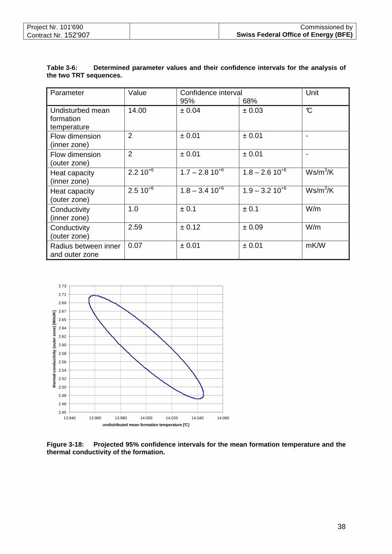
A numerical solution approach provides the opportunity to assess the uncertainties inherent in the determined parameters, i.e. thermal borehole resistance, thermal conductivity of the formation etc. One such assessment method relies on the application of the covariance matrix of a gradient approach, e.g. Levenberg-Marquart method (Marquardt, 1963) or the Monte Carlo / Bootstrap method (Efron, 1982). An example of how the parameters are correlated is Table 3-5. The table shows the correlation coefficients to be determined for the test sequences described in Chapter 3.1.2. It is a good example of the commonly observed correlation between the parameters of the backfill (inner zone) and the formation (outer zone). Table 3-6 provides the results of the numerical analysis of the two test phases. The results agree well with the estimates of thermal conductivity obtained through the application of the generalized diagnostic method (Figure 3-15). The determination of the confidence intervals was based on the matrix of covariances, the inverse of the Hessian matrix (see, e.g., Press et al., 1996). The uncertainty ranges are derived by considering a selective set of parameters of interest as is discussed in chapter 2.6. The more parameters are considered and the fewer the mathematical and physical constraints inherent to this set of parameters, the larger is the uncertainty range. In other words, the resulting uncertainty ranges are influenced by the selection of parameters. To deal with the resulting ambiguity in the calculated uncertainty ranges, one often relies on the opinion of an expert to extract plausible uncertainty ranges from the calculated values. The two-zone model shows a clear differentiation between the thermal conductivity of the backfill (inner zone) and that of the formation (outer zone). As an example, Figure 3-18 illustrates the 95% confidence interval and the correlation of the determined thermal conductivity of the formation and the undisturbed mean formation temperature. The parameter values are a result of the inverse numerical simulation and are listed in Table 3-6. Figure 3-19 presents the simulated temperature evolution inside the borehole in comparison to the measurements. The entire test sequence can be reproduced well from the results. The result of the numerical simulation with the values from Table 3-6 is shown in Figure 3-19. The entire test sequence can be reproduced well from the results.

Project Nr. 101'690 Contract Nr. 152'907
Commissioned by Swiss Federal Office of Energy (BFE)
37
Table 3-5: Correlation matrix of the relevant parameters for the numerical analysis of the two TRT sequences.
Und
istu
rbed
mea
n fo
rmat
ion
tem
pera
ture
Flo
w d
imen
sion
(in
ner
zone
)
Flo
w d
imen
sion
(o
uter
zon
e)
Hea
t cap
acity
(in
ner
zone
)
Hea
t cap
acity
(o
uter
zon
e)
Con
duct
ivity
(in
ner
zone
)
Con
duct
ivity
(o
uter
zon
e)
Rad
ius
betw
een
inne
r an
d ou
ter
zone
Undisturbed mean formation temperature 1
Flow dimension (inner zone) 0.53 1
Flow dimension (outer zone) 0.64 0.95 1
Heat capacity (inner zone -0.04 -0.34 -0.09 1
Heat capacity (outer zone) -0.55 -0.99 -0.98 0.19 1
Conductivity (inner zone) -0.53 -0.99 -0.96 0.31 0.99 1
Conductivity (outer zone) -0.69 -0.90 -0.99 0.04 0.94 0.91 1
Radius between inner and outer zone 0.53 0.99 0.96 -0.27 -0.99 -0.99 -0.92 1
Project Nr. 101'690 Contract Nr. 152'907
Commissioned by Swiss Federal Office of Energy (BFE)
38
Table 3-6: Determined parameter values and their confidence intervals for the analysis of the two TRT sequences. Parameter Value Confidence interval Unit 95% 68% Undisturbed mean formation temperature
14.00 ± 0.04 ± 0.03 °C
Flow dimension (inner zone)
2 ± 0.01 ± 0.01 -
Flow dimension (outer zone)
2 ± 0.01 ± 0.01 -
Heat capacity (inner zone)
2.2 10+6 1.7 – 2.8 10+6 1.8 – 2.6 10+6 Ws/m3/K
Heat capacity (outer zone)
2.5 10+6 1.8 – 3.4 10+6 1.9 – 3.2 10+6 Ws/m3/K
Conductivity (inner zone)
1.0 ± 0.1 ± 0.1 W/m
Conductivity (outer zone)
2.59 ± 0.12 ± 0.09 W/m
Radius between inner and outer zone
0.07 ± 0.01 ± 0.01 mK/W
Figure 3-18: Projected 95% confidence intervals for the mean formation temperature and the thermal conductivity of the formation.
2.45
2.46
2.48
2.50
2.52
2.54
2.56
2.58
2.60
2.62
2.64
2.65
2.67
2.69
2.71
2.73
13.940 13.960 13.980 14.000 14.020 14.040 14.060
undistributed mean formation temperature [°C]
ther
mal
con
duct
ivity
(out
er z
one)
[W/m
/K]

Project Nr. 101'690 Contract Nr. 152'907
Commissioned by Swiss Federal Office of Energy (BFE)
39
Figure 3-19: Comparison of measured (blue) and simulated (red) temperature.
3.3.4 Application for the laminar flow tests
As presented before the test sequence was continued with a laminar flow test sequence. Figure 3-20 presents the mean temperature measured at the wellhead.
Figure 3-20: Temperature measurements recorded during four thermal response tests conducted at the same site.
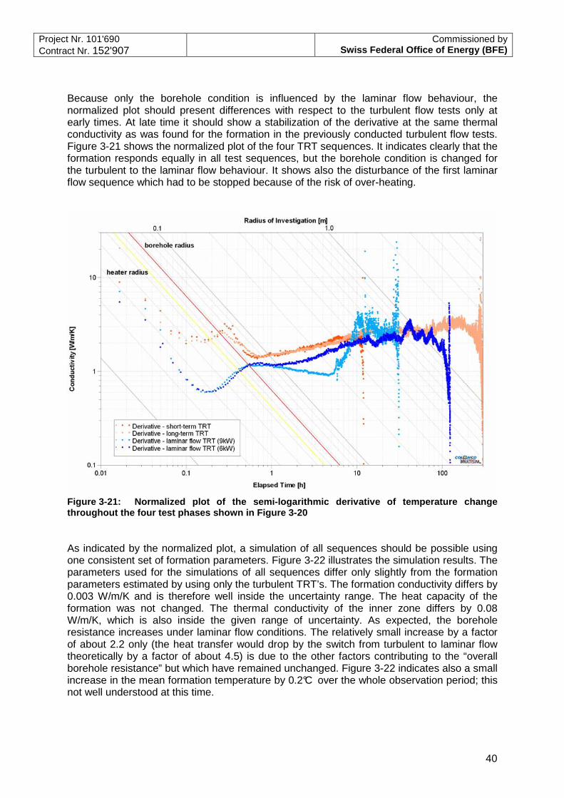
Project Nr. 101'690 Contract Nr. 152'907
Commissioned by Swiss Federal Office of Energy (BFE)
40
Because only the borehole condition is influenced by the laminar flow behaviour, the normalized plot should present differences with respect to the turbulent flow tests only at early times. At late time it should show a stabilization of the derivative at the same thermal conductivity as was found for the formation in the previously conducted turbulent flow tests. Figure 3-21 shows the normalized plot of the four TRT sequences. It indicates clearly that the formation responds equally in all test sequences, but the borehole condition is changed for the turbulent to the laminar flow behaviour. It shows also the disturbance of the first laminar flow sequence which had to be stopped because of the risk of over-heating.
Figure 3-21: Normalized plot of the semi-logarithmic derivative of temperature change throughout the four test phases shown in Figure 3-20 As indicated by the normalized plot, a simulation of all sequences should be possible using one consistent set of formation parameters. Figure 3-22 illustrates the simulation results. The parameters used for the simulations of all sequences differ only slightly from the formation parameters estimated by using only the turbulent TRT’s. The formation conductivity differs by 0.003 W/m/K and is therefore well inside the uncertainty range. The heat capacity of the formation was not changed. The thermal conductivity of the inner zone differs by 0.08 W/m/K, which is also inside the given range of uncertainty. As expected, the borehole resistance increases under laminar flow conditions. The relatively small increase by a factor of about 2.2 only (the heat transfer would drop by the switch from turbulent to laminar flow theoretically by a factor of about 4.5) is due to the other factors contributing to the “overall borehole resistance” but which have remained unchanged. Figure 3-22 indicates also a small increase in the mean formation temperature by 0.2°C over the whole observation period; this not well understood at this time.
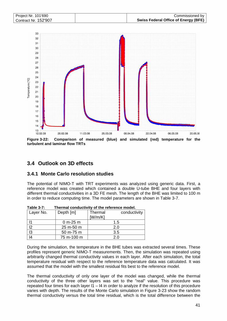
Project Nr. 101'690 Contract Nr. 152'907
Commissioned by Swiss Federal Office of Energy (BFE)
41
Figure 3-22: Comparison of measured (blue) and simulated (red) temperature for the turbulent and laminar flow TRTs
3.4 Outlook on 3D effects
3.4.1 Monte Carlo resolution studies
The potential of NIMO-T with TRT experiments was analyzed using generic data. First, a reference model was created which contained a double U-tube BHE and four layers with different thermal conductivities in a 3D FE mesh. The length of the BHE was limited to 100 m in order to reduce computing time. The model parameters are shown in Table 3-7. Table 3-7: Thermal conductivity of the reference model. Layer No. Depth [m] Thermal conductivity
[W/m/K] l1 0 m-25 m 1.5 l2 25 m-50 m 2.0 l3 50 m-75 m 3.5 l4 75 m-100 m 2.0
During the simulation, the temperature in the BHE tubes was extracted several times. These profiles represent generic NIMO-T measurements. Then, the simulation was repeated using arbitrarily changed thermal conductivity values in each layer. After each simulation, the total temperature residual with respect to the reference temperature data was calculated. It was assumed that the model with the smallest residual fits best to the reference model. The thermal conductivity of only one layer of the model was changed, while the thermal conductivity of the three other layers was set to the "real" value. This procedure was repeated four times for each layer l1 – l4 in order to analyze if the resolution of this procedure varies with depth. The results of the Monte Carlo simulation in Figure 3-23 show the random thermal conductivity versus the total time residual, which is the total difference between the
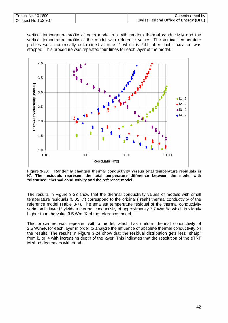
Project Nr. 101'690 Contract Nr. 152'907
Commissioned by Swiss Federal Office of Energy (BFE)
42
vertical temperature profile of each model run with random thermal conductivity and the vertical temperature profile of the model with reference values. The vertical temperature profiles were numerically determined at time t2 which is 24 h after fluid circulation was stopped. This procedure was repeated four times for each layer of the model.
1.0
1.5
2.0
2.5
3.0
3.5
4.0
0.01 0.10 1.00 10.00
Residuals [K^2]
The
rmal
con
duct
ivity
[W/m
/K]
l1_t2
l2_t2
l3_t2
l4_t2
Figure 3-23: Randomly changed thermal conductivity versus total temperature residuals in K2. The residuals represent the total temperature difference between the model with "disturbed" thermal conductivity and the reference model. The results in Figure 3-23 show that the thermal conductivity values of models with small temperature residuals (0.05 K2) correspond to the original ("real") thermal conductivity of the reference model (Table 3-7). The smallest temperature residual of the thermal conductivity variation in layer l3 yields a thermal conductivity of approximately 3.7 W/m/K, which is slightly higher than the value 3.5 W/m/K of the reference model. This procedure was repeated with a model, which has uniform thermal conductivity of 2.5 W/m/K for each layer in order to analyze the influence of absolute thermal conductivity on the results. The results in Figure 3-24 show that the residual distribution gets less "sharp" from l1 to l4 with increasing depth of the layer. This indicates that the resolution of the eTRT Method decreases with depth.

Project Nr. 101'690 Contract Nr. 152'907
Commissioned by Swiss Federal Office of Energy (BFE)
43
1.0
1.5
2.0
2.5
3.0
3.5
4.0
0.01 0.10 1.00 10.00
Residuals [K^2]
The
rmal
con
duct
ivity
[W/m
/K]
l1_t2
l2_t2
l3_t2
l4_t2
Figure 3-24: Randomly changed thermal conductivity versus total temperature residuals. The residuals represent the total temperature difference between the model with "disturbed" thermal conductivity and the reference model, which in this case has a constant thermal conductivity of 2.5 W/m/K. The results demonstrate that the Monte-Carlo technique is suitable to find the original ground thermal properties of the reference model. Here, 2000 simulations correspond to 2000¼≈7 independent thermal conductivity values for each layer. If the thermal conductivity is assumed to vary between 1 and 4 W/m/K, this yields an average resolution of 0.4 W/m/K for each layer. The resolution can be improved if the total range of probable thermal conductivity values can be constricted by laboratory measurements. A better resolution can be achieved by increasing the number of Monte Carlo simulations. As a result, the total simulation time will grow linearly with the number of simulation runs. Here, the simulation time already exceeds 5 days for 2000 simulations.
3.4.2 General NIMO-T resolution studies
Although the Monte Carlo approach resolves the vertical variation of thermal conductivity reasonably, its routine use is impractical due to the required simulation time. Therefore a simpler, iterative approach has been followed. The temporal cycle of the response test is simulated. The numerical simulated temperatures in the BHE tubes are compared to the measured t-logs. The ground thermal properties are changed gradually, until a satisfying correlation between measurement and simulation is reached. In practice, about 10 simulations yield satisfying result with minimum temperature residuals. In order to further investigate the resolution effect on more realistic generic models, a single TRT experiment was simulated with a much higher resolved FE mesh. The numerical TRT was performed with a power of 8 kW over a total circulation period of 7 days on a 250 m deep double-U BHE in a homogeneous soil with 2.0 W/m/K. Vertical temperature profiles were calculated 24 h (NIMO-T1) and 48 h (NIMO-T2) after circulation stop. These

Project Nr. 101'690 Contract Nr. 152'907
Commissioned by Swiss Federal Office of Energy (BFE)
44
temperature logs are shown as bold lines in Figure 3-25a. The blue line represents the undisturbed ground temperature (NIMO-T0).
a b
Figure 3-25: Influence of stratigraphic effects on temperature profiles. The blue line displays the undisturbed ground temperature of a reference model with a homogeneous thermal conductivity of 2.0 W/m/K. The bold red and orange lines display the temperature in the BHE 24 h and 48 h after TRT stop. Additionally, three other TRT were simulated using the same parameters, but increased thermal conductivity in one layer of 25 m thickness (thin lines). The vertical position of these layers was changed in each model. On the right side, the total temperature differences of the models with thermal conductivity variations are show with respect to the homogeneous reference model This TRT simulation was repeated three times with small thermal conductivity-changes in three different layers of 25 m thickness in different depths. Therefore, the thermal conductivity was set to 3 W/m/K instead of 2 W/m/K between 50 m and 75 m (variation 1), between 125 m and 150 m (variation 2) and between 200 m and 225 m depth. The corresponding temperature profiles are also shown in Figure 3-25a. The absolute temperature differences with respect to the reference model are shown in Figure 3-25b. It is obvious that the temperature-deviation due to thermal-conductivity change and thus the resolution of the eTRT method decreases with depth, as assumed from the Monte Carlo simulations. The total temperature deviation dT seems to decrease linearly with depth for constant thermal conductivity deviations. The reason for this might be the vertical variation of radial heat flow during the TRT experiment. At shallow depth, the temperature difference between ground and circulation fluid is much greater than at the bottom of the BHE. Therefore, the energy flow to the ground decreases with depth and the effect of thermal conductivity variation becomes less visible.

Project Nr. 101'690 Contract Nr. 152'907
Commissioned by Swiss Federal Office of Energy (BFE)
45
3.4.3 Influence of Groundwater flow
The same FE model was used to analyze the influence of groundwater flow on the results of TRT. Groundwater flow yields higher effective thermal conductivities. The effect of groundwater flow on the effective thermal conductivity, calculated from classic line source theory (LST) was analyzed by using different Darcy velocities in aquifers at different depths. Darcy velocity is varied between 10-8 and 10-4 m/s. The effective ground thermal conductivity is calculated after LST by evaluating the TRT output temperature over time. The results are compared with the results from a model without groundwater flow. The results are summarized in Figure 3-26. The figure shows the relative increase of the effective ground thermal conductivity as a function of Darcy velocities in aquifers at different depths. The horizontal yellow line indicates the generally accepted accuracy limit of the classic LST method. Again, the effect decreases with depth of the aquifer (layer 3: 50-75m; layer 6: 150-175 m; layer 9: 200-225 m). The effect of groundwater flow in a layer with a thickness of a tenth (25 m) of the total BHE length (250 m) is visible for Darcy velocities greater than 10-6 m/s.
0
10
20
30
40
50
60
70
80
90
100
-8.0 -7.0 -6.0 -5.0 -4.0log(v/[m/s])
Dev
iatio
n (%
)
layer 3
layer 6
layer 9
error limit
Figure 3-26: Increase of the effective thermal conductivity, calculated from LST, for different Darcy velocities in aquifers.
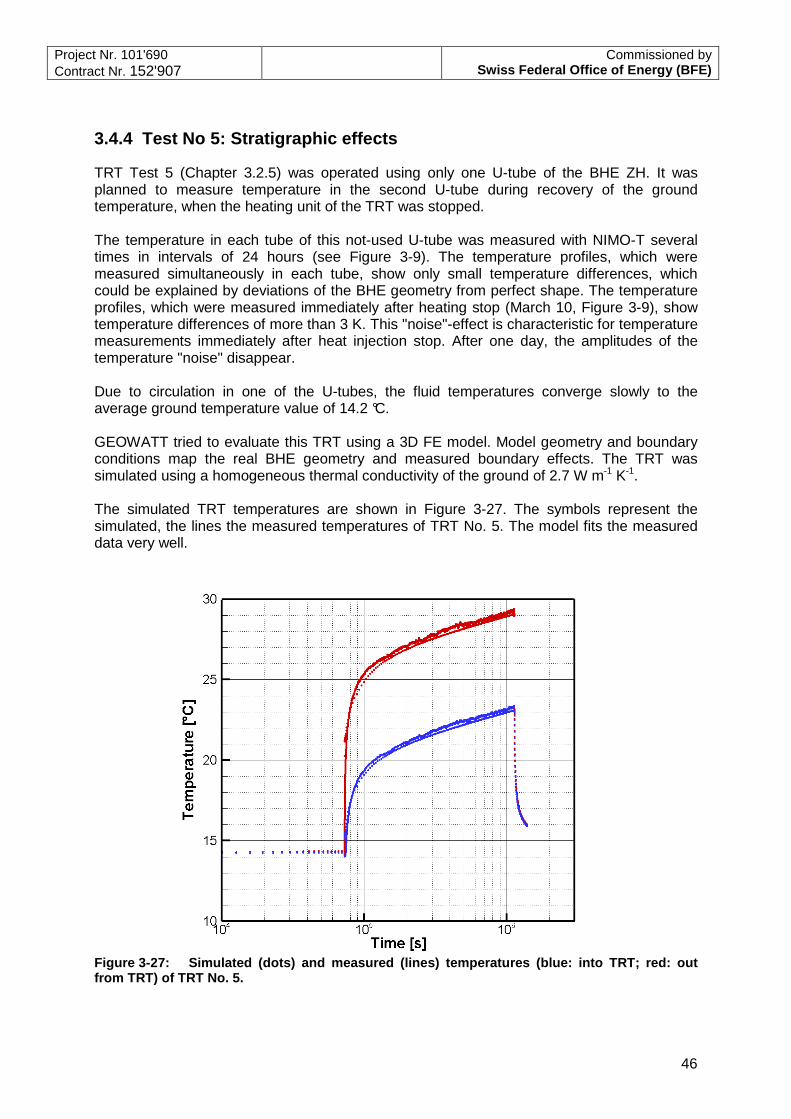
Project Nr. 101'690 Contract Nr. 152'907
Commissioned by Swiss Federal Office of Energy (BFE)
46
3.4.4 Test No 5: Stratigraphic effects
TRT Test 5 (Chapter 3.2.5) was operated using only one U-tube of the BHE ZH. It was planned to measure temperature in the second U-tube during recovery of the ground temperature, when the heating unit of the TRT was stopped. The temperature in each tube of this not-used U-tube was measured with NIMO-T several times in intervals of 24 hours (see Figure 3-9). The temperature profiles, which were measured simultaneously in each tube, show only small temperature differences, which could be explained by deviations of the BHE geometry from perfect shape. The temperature profiles, which were measured immediately after heating stop (March 10, Figure 3-9), show temperature differences of more than 3 K. This "noise"-effect is characteristic for temperature measurements immediately after heat injection stop. After one day, the amplitudes of the temperature "noise" disappear. Due to circulation in one of the U-tubes, the fluid temperatures converge slowly to the average ground temperature value of 14.2 °C. GEOWATT tried to evaluate this TRT using a 3D FE model. Model geometry and boundary conditions map the real BHE geometry and measured boundary effects. The TRT was simulated using a homogeneous thermal conductivity of the ground of 2.7 W m-1 K-1. The simulated TRT temperatures are shown in Figure 3-27. The symbols represent the simulated, the lines the measured temperatures of TRT No. 5. The model fits the measured data very well.
Figure 3-27: Simulated (dots) and measured (lines) temperatures (blue: into TRT; red: out from TRT) of TRT No. 5.
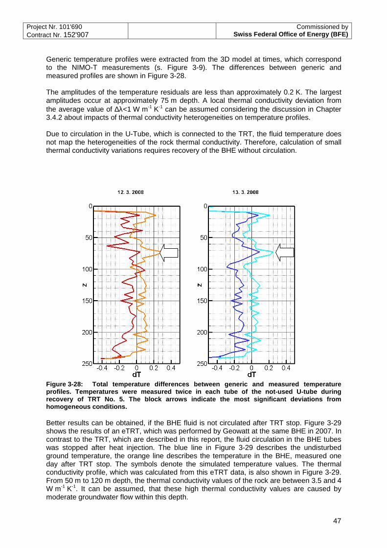
Project Nr. 101'690 Contract Nr. 152'907
Commissioned by Swiss Federal Office of Energy (BFE)
47
Generic temperature profiles were extracted from the 3D model at times, which correspond to the NIMO-T measurements (s. Figure 3-9). The differences between generic and measured profiles are shown in Figure 3-28. The amplitudes of the temperature residuals are less than approximately 0.2 K. The largest amplitudes occur at approximately 75 m depth. A local thermal conductivity deviation from the average value of ∆λ<1 W m-1 K-1 can be assumed considering the discussion in Chapter 3.4.2 about impacts of thermal conductivity heterogeneities on temperature profiles. Due to circulation in the U-Tube, which is connected to the TRT, the fluid temperature does not map the heterogeneities of the rock thermal conductivity. Therefore, calculation of small thermal conductivity variations requires recovery of the BHE without circulation.
Figure 3-28: Total temperature differences between generic and measured temperature profiles. Temperatures were measured twice in each tube of the not-used U-tube during recovery of TRT No. 5. The block arrows indicate the most significant deviations from homogeneous conditions. Better results can be obtained, if the BHE fluid is not circulated after TRT stop. Figure 3-29 shows the results of an eTRT, which was performed by Geowatt at the same BHE in 2007. In contrast to the TRT, which are described in this report, the fluid circulation in the BHE tubes was stopped after heat injection. The blue line in Figure 3-29 describes the undisturbed ground temperature, the orange line describes the temperature in the BHE, measured one day after TRT stop. The symbols denote the simulated temperature values. The thermal conductivity profile, which was calculated from this eTRT data, is also shown in Figure 3-29. From 50 m to 120 m depth, the thermal conductivity values of the rock are between 3.5 and 4 W m-1 K-1. It can be assumed, that these high thermal conductivity values are caused by moderate groundwater flow within this depth.
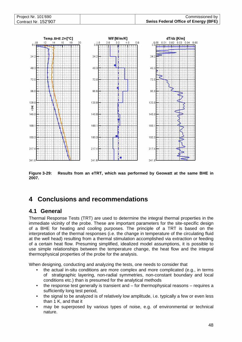
Project Nr. 101'690 Contract Nr. 152'907
Commissioned by Swiss Federal Office of Energy (BFE)
48
Figure 3-29: Results from an eTRT, which was performed by Geowatt at the same BHE in 2007.
4 Conclusions and recommendations
4.1 General Thermal Response Tests (TRT) are used to determine the integral thermal properties in the immediate vicinity of the probe. These are important parameters for the site-specific design of a BHE for heating and cooling purposes. The principle of a TRT is based on the interpretation of the thermal responses (i.e. the change in temperature of the circulating fluid at the well head) resulting from a thermal stimulation accomplished via extraction or feeding of a certain heat flow. Presuming simplified, idealized model assumptions, it is possible to use simple relationships between the temperature change, the heat flow and the integral thermophysical properties of the probe for the analysis. When designing, conducting and analyzing the tests, one needs to consider that
• the actual in-situ conditions are more complex and more complicated (e.g., in terms of stratigraphic layering, non-radial symmetries, non-constant boundary and local conditions etc.) than is presumed for the analytical methods
• the response test generally is transient and – for thermophysical reasons – requires a sufficiently long test period,
• the signal to be analyzed is of relatively low amplitude, i.e. typically a few or even less than 1 K, and that it
• may be superposed by various types of noise, e.g. of environmental or technical nature.

Project Nr. 101'690 Contract Nr. 152'907
Commissioned by Swiss Federal Office of Energy (BFE)
49
Even though the influence of some of these effects may be quantified and reduced with complex numerical analyses, the following considerations for the field procedures of a TRT serve well for the purpose of quality assurance.
4.2 Field campaign Specific recommendations concerning the technical procedures to be followed in the field are provided in Appendix B. In addition, there are some general recommendations to consider:
• Before commencing with any measurements it is necessary to design the tests to be conducted in terms of defining the heating or cooling power and flow rate, estimating the expected temperature difference and test period. These preparatory measures may be supported by prognostic numerical calculations. The power is to be defined such that for turbulent flow conditions the expected temperature difference is no less than 3 K1.
• Immediately before beginning the test, it is essential to circulate the fluid with no thermal stimulation to obtain a good measurement of the mean formation temperature. The circulation should comprise at least one complete exchange of the volume inside the probe, and the data at the well head need to be recorded for the full period of circulation.
• During the test, the rate (heating or cooling and circulation flow) should be kept as constant as possible and measurements should be taken with a high quality standard and resolution with a frequency of at least once per minute. The recorded measurement data (the ambient temperature needs to be recorded continually throughout the entire test phase as well) should, if possible, be made accessible to an external access for the regulation of the measurement process.
• The data should be analyzed continually with diagnostic procedures throughout the entire test. The test may be terminated only when the radius of investigation has clearly exceeded the borehole radius.
• The test may (for an adequately constant rate) be terminated once the temporal derivative of the temperature has stabilized and the stabilization has been observed for at least half of a logarithmic cycle. This criterion has to be applied to the normalized plot.
• Once the test phase has ended, the data should be recorded further until conditions have returned to their original state. The recovery phase may be used for two measurements:
o Measurements with NIMO for a survey of vertical profiling; in this case circulation must be stopped; the data is recorded at the end of the active phase and again after two or three days
o Measurement of the temperature field recovery as an additional test phase; in this case the circulation is to be continued without heating or cooling and the temperature is continually recorded at the well head
• When natural fluctuations in the ambient temperature are to be used for thermal stimulation (i.e. when no constant source for heating or cooling is used), this should be done only when the mean air temperature is clearly distinguishable from the mean formation temperature (in the probe).
1 If for technical reasons a laminar regime is used, the maximum heating power has to be limited as well to avoid over-heating.
Project Nr. 101'690 Contract Nr. 152'907
Commissioned by Swiss Federal Office of Energy (BFE)
50
4.3 Analysis If the requirements for the analysis of the TRT with a line source or cylindrical source are fulfilled, then the conventional methods could be applied. The application of diagnostic methods is recommended for the optimization of the field campaign. They provide first approximations and may justify the termination of the test. Numerical analysis methods are sensible and suitable in the following cases:
• Unstable or failed power supply in the period of active stimulation • Strong disturbances due to environmental influences while the test is conducted • Obvious – in the diagnostic plots recognizable – deviations from the requirements for
the analytical methods (e.g. recognizable boundary conditions of the thermal formation properties, apparent thermal conductivities > 3.5 W/mK etc.)
• Required (or for the dimensioning of the facility useful) information concerning the stratigraphic distribution of the thermophysical properties.
Numerical methods for the analysis provide the means to use, in principle, any number of stimulations for the analysis. For this reason, they are the only suitable analytical tool if technical problems occur during the test. In addition, they allow for the sensitivity and the correlation of parameters to be assessed. Through the application of inverse problem solving methods for the determination of parameters, it is also possible to draw conclusions on their confidence intervals (uncertainty ranges). These intervals are the base for an objective rating of the quality of the results. When recording the temperatures at the well head alone, a vertical profiling of the thermal conductivity is not – or generally not sufficiently – detectable with the integral analysis method. In addition, high apparent thermal conductivities (> 3 … 3.5 W/mK) indicate groundwater flow. In these cases, the supportive measurements with NIMO-T upgrade the method. It makes sense to analyze the vertical profiles with numerical approaches like the Monte Carlo analysis. In summary, we recommend the following points to be honored when analyzing a TRT in order to obtain the best possible results:
• Diagnostic methods should be applied already while conducting the test in the field. • Numerical methods should be used for the subsequent analysis when a) a
quantification of the confidence intervals of the results is required and/or b) boundary conditions during the test (control of the heat flow, variable environmental conditions, significant deviations from homogeneous underground conditions) do not permit an analysis with conventional methods.
• The recovery phase following the test should be used for an additional investigation. When the option exists, vertical profiling with NIMO-T should be preferred over the recording of the temperature field recovery at the well head (for continued circulation) because more information may be gained from the former than from a further reinforcement of the integral result from the active test phase.
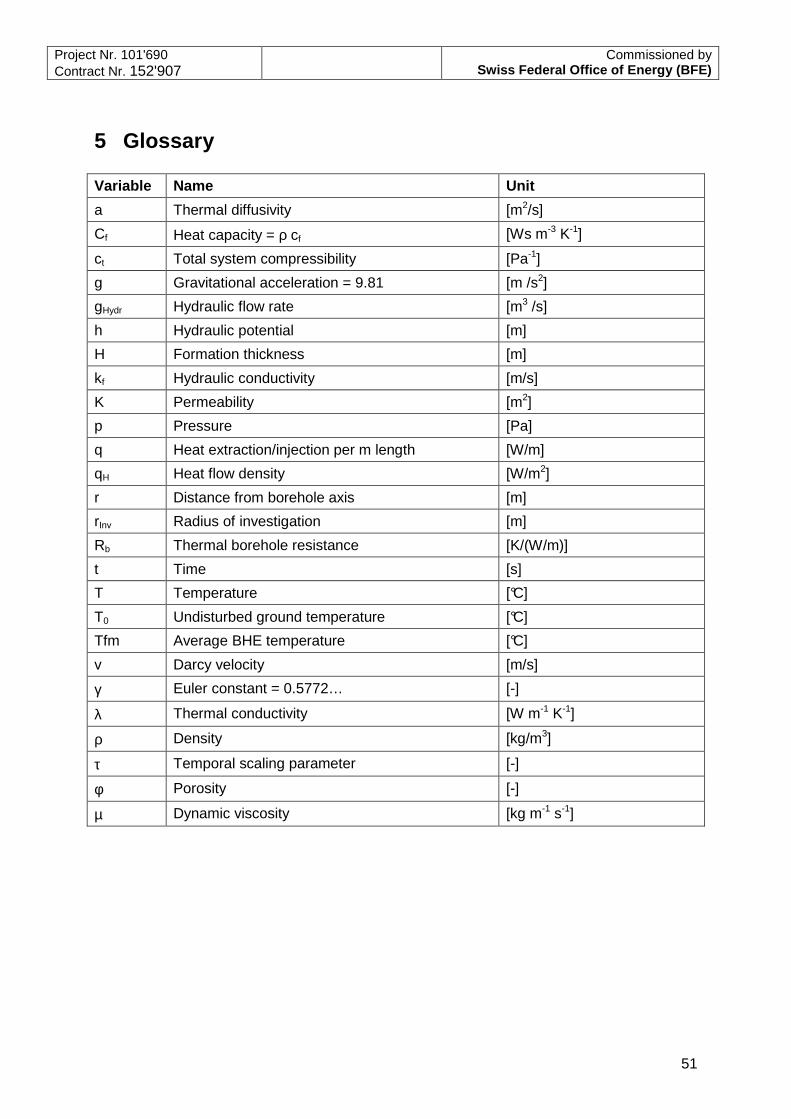
Project Nr. 101'690 Contract Nr. 152'907
Commissioned by Swiss Federal Office of Energy (BFE)
51
5 Glossary Variable Name Unit
a Thermal diffusivity [m2/s]
Cf Heat capacity = ρ cf [Ws m-3 K-1]
ct Total system compressibility [Pa-1]
g Gravitational acceleration = 9.81 [m /s2]
gHydr Hydraulic flow rate [m3 /s]
h Hydraulic potential [m]
H Formation thickness [m]
kf Hydraulic conductivity [m/s]
K Permeability [m2]
p Pressure [Pa]
q Heat extraction/injection per m length [W/m]
qH Heat flow density [W/m2]
r Distance from borehole axis [m]
rInv Radius of investigation [m]
Rb Thermal borehole resistance [K/(W/m)]
t Time [s]
T Temperature [°C]
T0 Undisturbed ground temperature [°C]
Tfm Average BHE temperature [°C]
v Darcy velocity [m/s]
γ Euler constant = 0.5772… [-]
λ Thermal conductivity [W m-1 K-1]
ρ Density [kg/m3]
τ Temporal scaling parameter [-]
φ Porosity [-]
µ Dynamic viscosity [kg m-1 s-1]
Project Nr. 101'690 Contract Nr. 152'907
Commissioned by Swiss Federal Office of Energy (BFE)
52
6 References Austin, W. (1998). Development of an in-situ system for measuring ground thermal properties, MSc-thesis, Oklahoma State University, 164 p. Austin, W., C. Yavuzurk and J.D Spitler (2000). Development of and In-Situ System for Measuring Ground Thermal Properties. ASHRAE Transactions, 106(1), pp 365-379. Blackwell, J. H. (1953). Radial-axial heat flow in regions bounded internally by circular cylinders; Can. J. Phys. 31(1953) 472-479. Blackwell, J. H. (1956). The axial-flow error in the thermal-conductivity probe; Can. J. Phys., 34(1956) 412-417. Bourdarot, G. (1996). Essais de puits: methods d’interprétation; Édition technip, Paris. Colenco, EPFL, Geowatt (2008). Innovative Improvements of Thermal Response Tests; Intermediate report, April 2008; Schweizerisches Bundesamt für Energie, Projekt Nr. 101’690. Cooper, H.H. and C.E. Jacob (1946). A generalized graphical method for evaluating formation constants and summarizing well field history. Am. Geophys. Union Trans., Vol. 27, pp. 526-534. Earlougher, R.C. (1977). Advances in Well Test Analysis; Soc. Petrol. Eng. AIME. Efron, B. (1982). The Jackknife, the Bootstrap, and Other Resampling Plans (Philadelphia: S.I.A.M.). Eklöf, C. and S. Gehlin (1996). TED - a mobile equipment for thermal response test, MSc Thesis 1996:198E, Lulea University of Technology, 62 p. Enachescu C., B. Frieg and J. Wozniewicz (2004.: A New Visual Synthesis Tool for Transient Test Data; U.S. EPA/NGWA Fractured Rock Conference: State of Science and Measuring Success in Remediation. Eppelbaum, L.V. and I.M. Kutasov (2006). Pressure and temperature drawdown well testing: similarities and differences; Journ. Geophys. Eng. 3(2006) 12-20. Eskilson, P. (1987). Thermal Analysis of Heat Extraction Boreholes, Thesis, Department of Mathematical Physics, Lund University. Eugster, W.J. and L. Laloui, (eds.) (2001). Proceedings Workshop Geothermische Response Tests, Lausanne, GtV, 132 p. Gehlin, S. and B. Nordell (1997). Thermal Response Test – A mobile Equipment for Determining Thermal Resistance of Boreholes, Proceedings Megastock’97, Sapporo, Japan, pp 103-108. Gehlin, S. (1998). Thermal Response Test – In-Situ Measurement of Thermal Properties in Hard Rock, Licentiate Thesis, Lulea University of Technology, 1998:37.
Project Nr. 101'690 Contract Nr. 152'907
Commissioned by Swiss Federal Office of Energy (BFE)
53
Gehlin, S. and G. Hellström (2000). Recent Status of In-situ Thermal Response Tests for BTES Applications in Sweden. Proceedings of Terrastock 2000, Stuttgart, Germany, pp 159-164. Gehlin, S. and G. Hellström (2003a). Comparison of Four Models for Thermal Response Test Evaluation; ASHRAE Trans. Res. 109 pp. 131-142. Horne, R. (1995). Modern Well test Analysis – A Computer-Aided Approach; Petroway Inc., Palo Alto, Ca.. Horner, D.R. (1951). Pressure Build-Up in Wells, Third World Pet. Congress, E.J. Brill, Leiden II, pp. 503-521. Ingersoll, L.R. and H.J. Plass (1948). Theory of the ground pipe heat source for the heat pump. Heating, Piping and Air Conditioning 20/7, pp 119-122. Laloui L., M. Moreni, G. Steinmann, L. Vulliet, A. Fromentin, D. Pahud (1999). Test en conditions réelles du comportement statique d’un pieu soumis à des sollicitations thermo-mécaniques. Report of the Swiss Federal Office of Energy OFEN. Laloui, L. and G. Steinmann (2002) Finalisation du module de l’EPFL pour les tests de réponses (in French), ENET_Swiss Energy, Nº220188. Lund, J., B. Sanner, L. Rybach, G. Curtis, G. Hellström (2004). Geothermal (Ground-Source) Heat Pumps – a World Overview, GHC Bulletin, September 2004. Maglić, K.D. et al. eds. (1984). Compendium of Thermophysical Property Measurement Methods; Survey of Measurement Techniques, Plenum Press, New York. Marquardt, D.W. (1963). An algorithm for least-squares estimation of nonlinear parameters. Journal of the Society for Industrial and Applied Mathematics, Vol. 11(2), pp. 431-441. Mattsson, N.; G. Steinmann; L. Laloui (2008). Advanced Compact Device for the In-situ Determination of Geothermal Characteristics of Soils. Energy and Buildings, Vol. 40, pp. 1344-1352 Mogensen, P. (1983). Fluid to Duct Wall Heat Transfer in Duct System Heat Storages, Proceedings from International Conference on Subsurface Heat Storage in Theory and Practice, Stockholm, 652-657. Poppei, J., G. Mayer, R. Schwarz (2006a): Groundwater Energy Designer – computergestütztes Auslegungstool zur Wärme- und Kältenutzung von Grundwasser, Vorhaben des Schweizerischen Bundesamtes für Energie 101'144; Schlussbericht, Publikationsnummer 260043, (http://www.bfe.admin.ch/dokumentation/energieforschung/index.html?lang=de&project=101144) Poppei, J., R. Schwarz, N. Mattson, G. Steinmann and L. Laloui (2006b). Innovative Verbesserungen bei Thermal Response Tests; 9. Geothermische Fachtagung, 15.-17. November 2006, Karlsruhe; Tagungsband S. 281-292 Press, W.H., S.A. Teukolsky, W.T. Vetterling and B.P. Flannery (1996). Numerical Recipes in C, The Art of Scientific Computing, Second Edition, Cambridge University Press Rybach, L. and B. Sanner (2000). Ground-source heat pump systems – the European experience, GHC Bulletin, March.
Project Nr. 101'690 Contract Nr. 152'907
Commissioned by Swiss Federal Office of Energy (BFE)
54
Sanner, B. (2003). Current status of ground source heat pumps in Europe, Futurstock, Warsaw. Sanner, B., E. Mands and M.K. Sauer (2003). Larger geothermal heat pump plants in the central region of Germany, Geothermics 32, pp 589-602, Elsevier. Shonder, J.A. and J.V. Beck (1999). Determining Effective Soil Formation Thermal Properties from Field Data Using a Parameter Estimation Technique; ASHRAE Trans. Symposia, CH-99-2-4 458-466. Spitler, J.D. et al. (1999). Refinement and Validation of In Situ Parameter Estimation Models, Short Report, OSU 03/10/99. Spitler, J.D. et al. (2000). In Situ Measurement of Ground Thermal Properties, Terrastock, Stuttgart. Steinmann, G. and L. Laloui (2005). Thermal response tests; in-situ determination of geothermal characteristics of soils, IGA News, Nº62, pp.7-10. Theis, C. V. (1935). The relation between lowering of the piezometric surface and rate and duration of discharge of a well using groundwater storage. Transactions of the American Geophysical Union, 16, 519-524 Wagner, R. and C. Clauser (2005). Evaluating thermal response tests using parameter estimation for thermal conductivity and thermal capacity, Journal of geophysics and engineering no 2, pp 349-356. Witte, H.J.L., G.J. van Gelder, J.D. Spitler (2002). In-situ measurement of ground thermal conductivity: The Dutch Perspective, ASHRAE Transactions 108(1).

Project Nr. 101'690 Contract Nr. 152'907
Commissioned by Swiss Federal Office of Energy (BFE)
55
Appendix A: Additional Results of the Thermal Resistance Thermal (TRT) Field Campaign (EPfL)
A.1. TRT field campaign in Zürich
• Test 2 (short term TRT): results of the one day circulation period, performed to keep the conditions of the traditional TRT before heating the soil.
Figure A-1: Temperatures and flow rate versus time in circulation phase before short term test.
• Test 4 (long term TRT): results of the one day circulation period (20 hours), performed to keep the conditions of the traditional TRT before heating the soil.
Figure A-2: Temperatures and flow rate versus time in circulation phase before long term test.
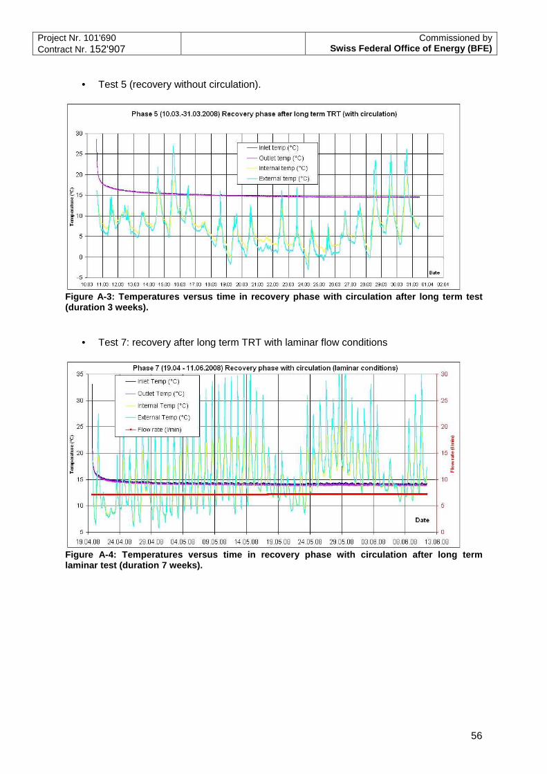
Project Nr. 101'690 Contract Nr. 152'907
Commissioned by Swiss Federal Office of Energy (BFE)
56
• Test 5 (recovery without circulation).
Figure A-3: Temperatures versus time in recovery phase with circulation after long term test (duration 3 weeks).
• Test 7: recovery after long term TRT with laminar flow conditions
Figure A-4: Temperatures versus time in recovery phase with circulation after long term laminar test (duration 7 weeks).
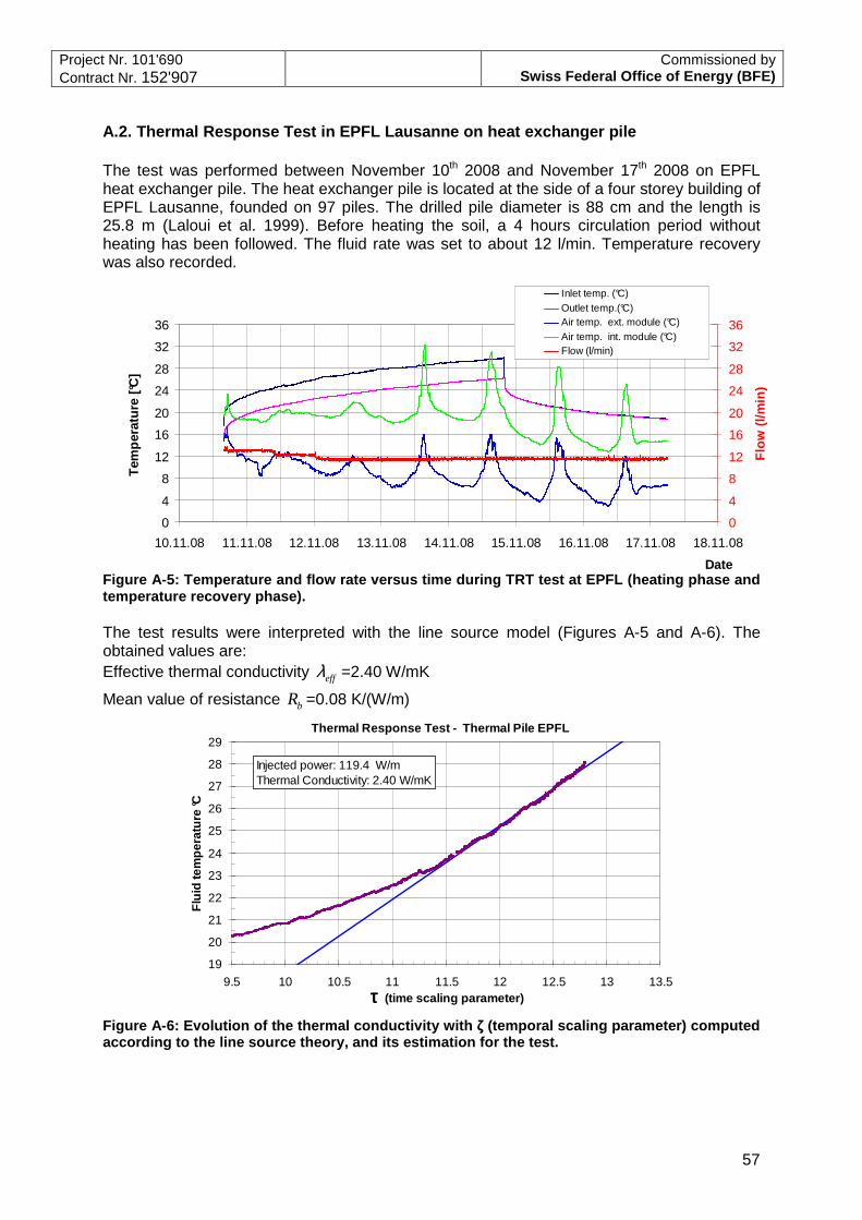
Project Nr. 101'690 Contract Nr. 152'907
Commissioned by Swiss Federal Office of Energy (BFE)
57
A.2. Thermal Response Test in EPFL Lausanne on heat exchanger pile The test was performed between November 10th 2008 and November 17th 2008 on EPFL heat exchanger pile. The heat exchanger pile is located at the side of a four storey building of EPFL Lausanne, founded on 97 piles. The drilled pile diameter is 88 cm and the length is 25.8 m (Laloui et al. 1999). Before heating the soil, a 4 hours circulation period without heating has been followed. The fluid rate was set to about 12 l/min. Temperature recovery was also recorded.
0
4
8
12
16
20
24
28
32
36
10.11.08 11.11.08 12.11.08 13.11.08 14.11.08 15.11.08 16.11.08 17.11.08 18.11.08
Date
Tem
pera
ture
[°C
]
0
4
8
12
16
20
24
28
32
36
Flo
w (
l/min
)
Inlet temp. (°C)Outlet temp.(°C)Air temp. ext. module (°C)Air temp. int. module (°C)Flow (l/min)
Figure A-5: Temperature and flow rate versus time during TRT test at EPFL (heating phase and temperature recovery phase). The test results were interpreted with the line source model (Figures A-5 and A-6). The obtained values are: Effective thermal conductivity effλ =2.40 W/mK
Mean value of resistance bR =0.08 K/(W/m)
Thermal Response Test - Thermal Pile EPFL
19
20
21
22
23
24
25
26
27
28
29
9.5 10 10.5 11 11.5 12 12.5 13 13.5ττττ (time scaling parameter)
Flu
id te
mpe
ratu
re °C
Injected power: 119.4 W/mThermal Conductivity: 2.40 W/mK
Figure A-6: Evolution of the thermal conductivity with ζ (temporal scaling parameter) computed according to the line source theory, and its estimation for the test.
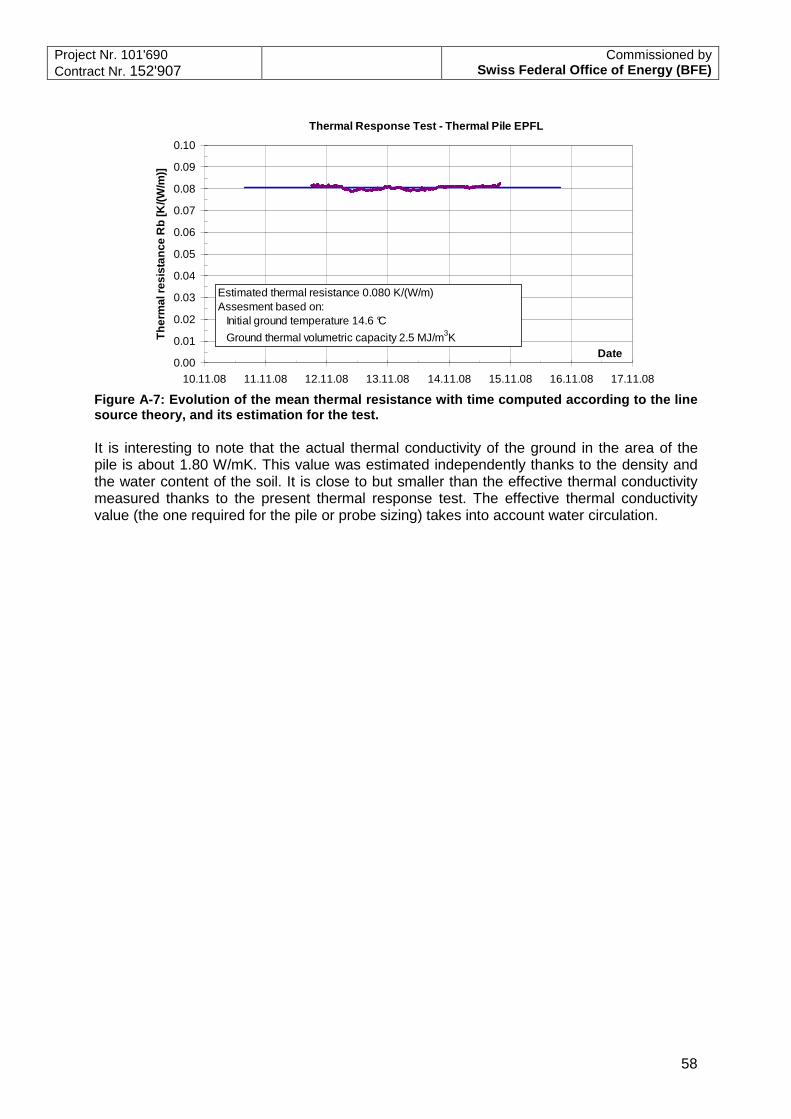
Project Nr. 101'690 Contract Nr. 152'907
Commissioned by Swiss Federal Office of Energy (BFE)
58
Thermal Response Test - Thermal Pile EPFL
0.00
0.01
0.02
0.03
0.04
0.05
0.06
0.07
0.08
0.09
0.10
10.11.08 11.11.08 12.11.08 13.11.08 14.11.08 15.11.08 16.11.08 17.11.08
Date
The
rmal
resi
stan
ce R
b [K
/(W/m
)]
Estimated thermal resistance 0.080 K/(W/m)Assesment based on: Initial ground temperature 14.6 °C
Ground thermal volumetric capacity 2.5 MJ/m3K
Figure A-7: Evolution of the mean thermal resistance with time computed according to the line source theory, and its estimation for the test. It is interesting to note that the actual thermal conductivity of the ground in the area of the pile is about 1.80 W/mK. This value was estimated independently thanks to the density and the water content of the soil. It is close to but smaller than the effective thermal conductivity measured thanks to the present thermal response test. The effective thermal conductivity value (the one required for the pile or probe sizing) takes into account water circulation.

Project Nr. 101'690 Contract Nr. 152'907
Commissioned by Swiss Federal Office of Energy (BFE)
59
Appendix B: Practical guideline for efficient thermal response testing (EPfL)
In what follows, some general recommendations for thermal response testing are listed. These recommendations are based on several years of field experimentation. They could be seen as a practical guideline for efficient thermal response testing. B.1. Recommendation for test progress The following steps should be mandatorily followed: 1. Test and calibration of all the sensors. 2. Setting of the device in the field and power supply connection. The site requirements are
detailed in Section A.2. 3. Connection to the borehole heat exchanger, thermal insulation of the tubing and joints
from the ground surface to the module. 4. Filling of the test loop with water to sufficient pressure and air flushing. 5. Checking of the watertightness. 6. Setting of the level of flow rate and heat power. Recommendations for power level setting
are given in Section A.3. 7. Data-logging setting. 8. Test beginning: determination of the initial undisturbed ground temperature by fluid
circulation without heating, over a several hours period (possibly one night), in any case up to equality of incoming and outgoing temperatures is obtained.
9. Checking of the watertightness and of any anomaly that could be spotted during the
circulation without heating. 10. Possible data-logging re-setting: during the heating phase, data should be recorded with
a sufficiently short time step (typically one minute) for the following eight parameters: • incoming and outgoing fluid temperatures, • internal and external temperature of the test unit, • pressure of the heat-conducting fluid (input and output) of the heat exchanger tubes, • flow rate of the heat-conducting fluid, • heater energy consumption.
11. Setting of the power level and starting of the heating. B2. Site requirements The installation of the borehole and the heat exchanger should be done by the building contractor at least 2 weeks prior to the beginning of the thermal response test. The borehole installed for the thermal response test needs to fulfil the following requirements:
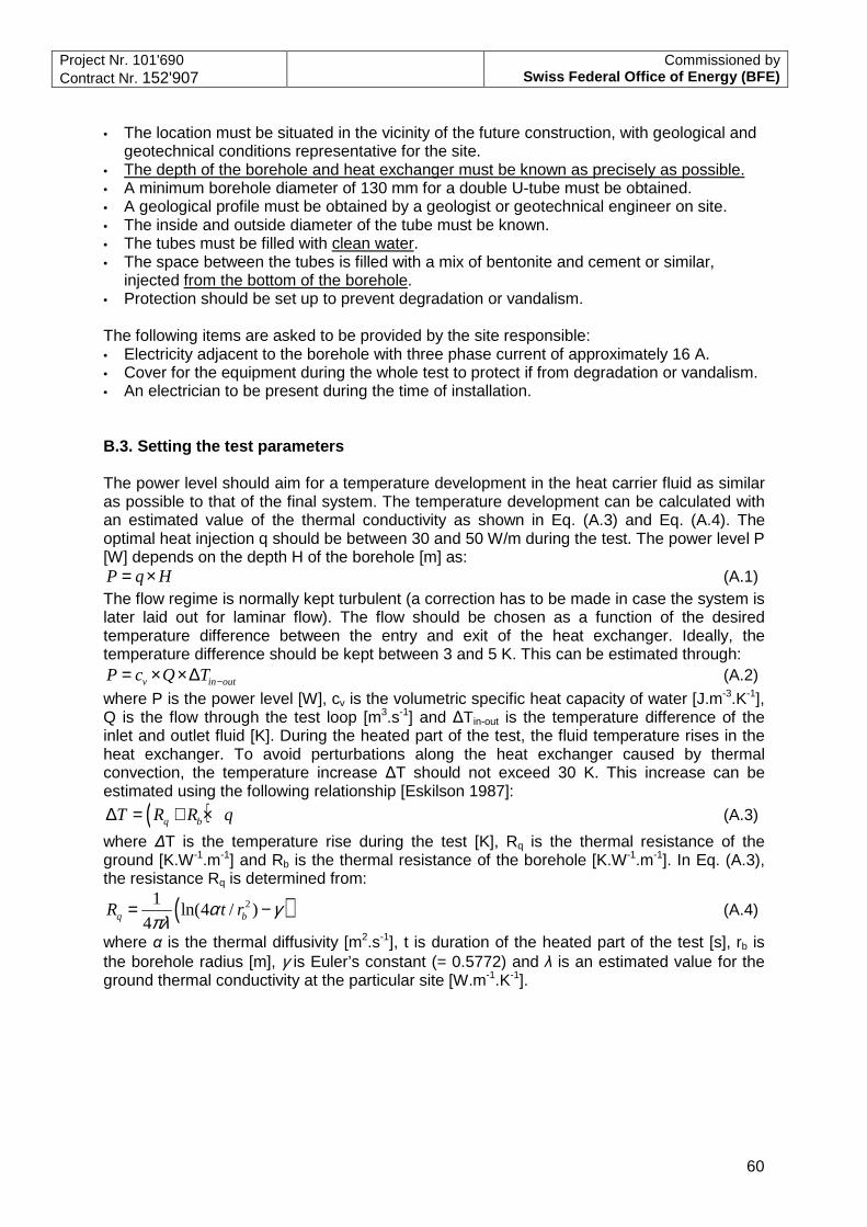
Project Nr. 101'690 Contract Nr. 152'907
Commissioned by Swiss Federal Office of Energy (BFE)
60
• The location must be situated in the vicinity of the future construction, with geological and geotechnical conditions representative for the site.
• The depth of the borehole and heat exchanger must be known as precisely as possible. • A minimum borehole diameter of 130 mm for a double U-tube must be obtained. • A geological profile must be obtained by a geologist or geotechnical engineer on site. • The inside and outside diameter of the tube must be known. • The tubes must be filled with clean water. • The space between the tubes is filled with a mix of bentonite and cement or similar,
injected from the bottom of the borehole. • Protection should be set up to prevent degradation or vandalism. The following items are asked to be provided by the site responsible: • Electricity adjacent to the borehole with three phase current of approximately 16 A. • Cover for the equipment during the whole test to protect if from degradation or vandalism. • An electrician to be present during the time of installation. B.3. Setting the test parameters The power level should aim for a temperature development in the heat carrier fluid as similar as possible to that of the final system. The temperature development can be calculated with an estimated value of the thermal conductivity as shown in Eq. (A.3) and Eq. (A.4). The optimal heat injection q should be between 30 and 50 W/m during the test. The power level P [W] depends on the depth H of the borehole [m] as: P q H= × (A.1) The flow regime is normally kept turbulent (a correction has to be made in case the system is later laid out for laminar flow). The flow should be chosen as a function of the desired temperature difference between the entry and exit of the heat exchanger. Ideally, the temperature difference should be kept between 3 and 5 K. This can be estimated through:
v in outP c Q T −= × × ∆ (A.2)
where P is the power level [W], cv is the volumetric specific heat capacity of water [J.m-3.K-1], Q is the flow through the test loop [m3.s-1] and ∆Tin-out is the temperature difference of the inlet and outlet fluid [K]. During the heated part of the test, the fluid temperature rises in the heat exchanger. To avoid perturbations along the heat exchanger caused by thermal convection, the temperature increase ∆T should not exceed 30 K. This increase can be estimated using the following relationship [Eskilson 1987]:
( )q bT R R q∆ = + × (A.3)
where ∆T is the temperature rise during the test [K], Rq is the thermal resistance of the ground [K.W-1.m-1] and Rb is the thermal resistance of the borehole [K.W-1.m-1]. In Eq. (A.3), the resistance Rq is determined from:
( )21ln(4 / )
4q bR t rα γπλ
= − (A.4)
where α is the thermal diffusivity [m2.s-1], t is duration of the heated part of the test [s], rb is the borehole radius [m], γ is Euler’s constant (= 0.5772) and λ is an estimated value for the ground thermal conductivity at the particular site [W.m-1.K-1].
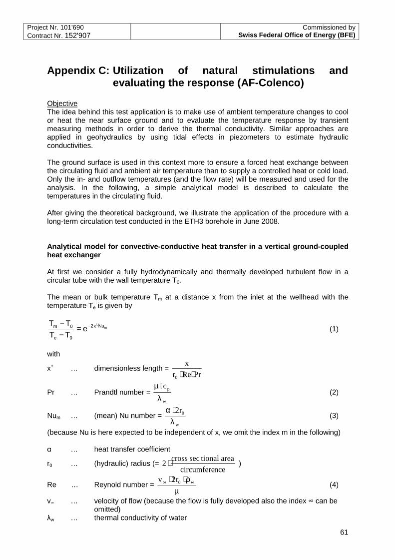
Project Nr. 101'690 Contract Nr. 152'907
Commissioned by Swiss Federal Office of Energy (BFE)
61
Appendix C: Utilization of natural stimulations and evaluating the response (AF-Colenco)
Objective The idea behind this test application is to make use of ambient temperature changes to cool or heat the near surface ground and to evaluate the temperature response by transient measuring methods in order to derive the thermal conductivity. Similar approaches are applied in geohydraulics by using tidal effects in piezometers to estimate hydraulic conductivities. The ground surface is used in this context more to ensure a forced heat exchange between the circulating fluid and ambient air temperature than to supply a controlled heat or cold load. Only the in- and outflow temperatures (and the flow rate) will be measured and used for the analysis. In the following, a simple analytical model is described to calculate the temperatures in the circulating fluid. After giving the theoretical background, we illustrate the application of the procedure with a long-term circulation test conducted in the ETH3 borehole in June 2008. Analytical model for convective-conductive heat transfer in a vertical ground-coupled heat exchanger At first we consider a fully hydrodynamically and thermally developed turbulent flow in a circular tube with the wall temperature T0. The mean or bulk temperature Tm at a distance x from the inlet at the wellhead with the temperature Te is given by
mNux2
0e
0m eTT
TT +−=−−
(1)
with
x+ … dimensionless length = PrRer
x
0 ⋅⋅
Pr … Prandtl number = w
pc
λ⋅µ
(2)
Num … (mean) Nu number = w
0r2
λ⋅α
(3)
(because Nu is here expected to be independent of x, we omit the index m in the following) α … heat transfer coefficient
r0 … (hydraulic) radius (= ncecircumfere
areationalseccross2 ⋅ )
Re … Reynold number = µ
ρ⋅⋅∞ w0r2v (4)
v∞ … velocity of flow (because the flow is fully developed also the index ∞ can be omitted)
λw … thermal conductivity of water

Project Nr. 101'690 Contract Nr. 152'907
Commissioned by Swiss Federal Office of Energy (BFE)
62
µ … viscosity (of water) cp … specific heat capacity (of water) ρw … density (of water) Inserting equations (2) to (4) into (1) we get
pw
0
mcm
rx2
Nux2
0e
0m eeTT
TT &
⋅⋅α⋅π−
− ==−− +
(5)
with
wm& … mass flow rate (of circulated water)
We replace formally the heat transfer coefficient α with a radial overall (serial) transfer coefficient U
( )
λ+
λ+
α
=
a
m
g
a
0
a
PE
0
r
trln
r
r
rln
r1
1U (6)
which implies the local heat transfer at the wall, the thermal resistance of the tube (index PE) as well as the increasing thermal resistance of the affected rock with λg … thermal conductivity of surrounding rock
PE0
a
PE
Rr
rln
1 =
λ... thermal resistance of the (PE-) tube with the outer radius ra
rm(t) … thermal entrance depth (also known as “cooling shell”).
By substituting ( ) ( )tf
r
trln
a
m =
and introducing the abbreviation a
( ) pa
0
aPEg
w
g
g
cm
1
tfr
rR
Nu
1
2a
⋅⋅
+⋅λ+λλ
πλ=
& (7)
equation (5) becomes
ax
0e
0m eTT
TT −=−−
(8)
The transient thermal effect (long-term “cooling shell”) f(t) depends on the boundary condition imposed at the inner surface of the tube. For the Cauchy type boundary conditions prevailing here, there is no closed-form solution available. But the effect is supposed to be somewhere between Dirichlet and Neumann conditions at the surface with
( ) ( )Fo1lntf ⋅π+= … for Dirichlet boundary conditions (9)
( )2
Fo41
Eitf
−−= … for Neumann boundary conditions (10)
with
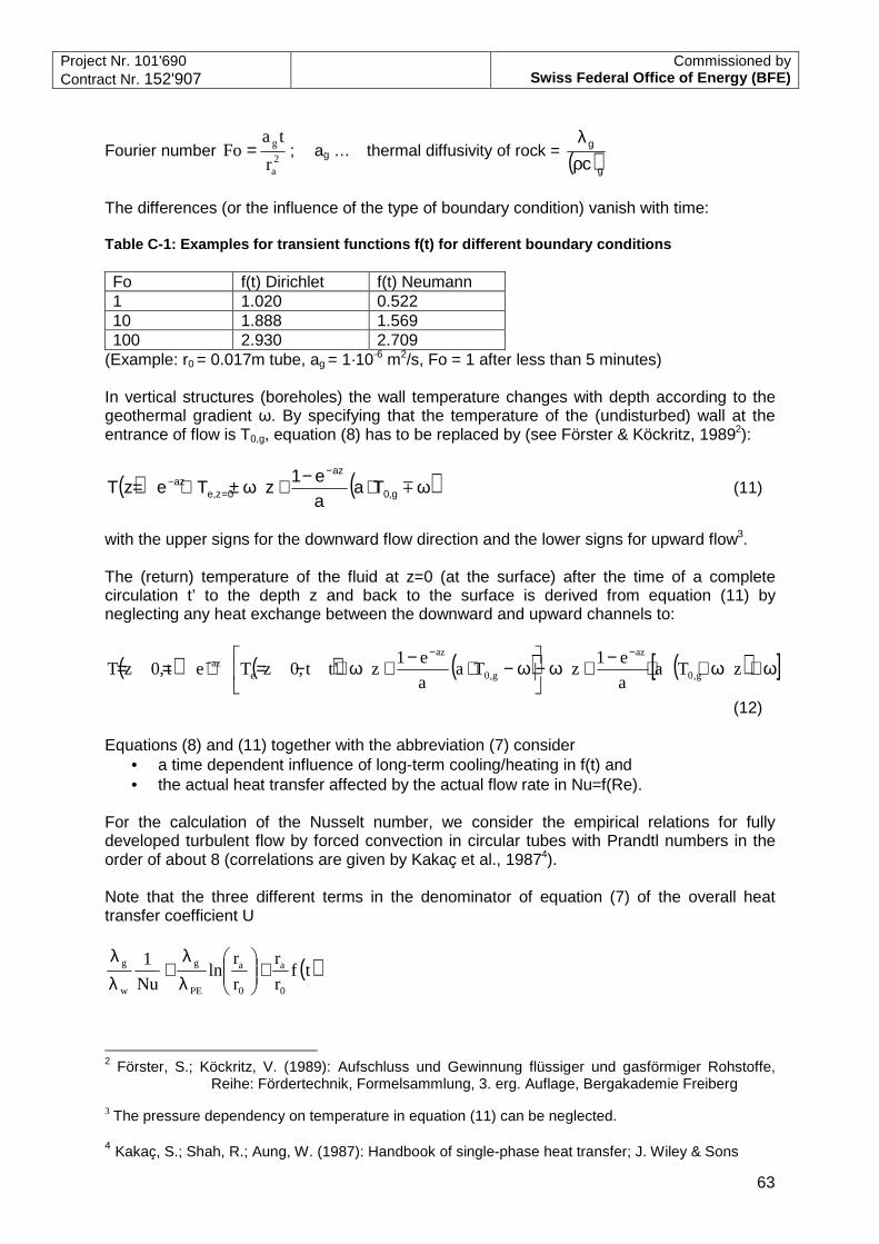
Project Nr. 101'690 Contract Nr. 152'907
Commissioned by Swiss Federal Office of Energy (BFE)
63
Fourier number 2a
g
r
taFo = ; ag … thermal diffusivity of rock = ( )g
g
cρλ
The differences (or the influence of the type of boundary condition) vanish with time: Table C-1: Examples for transient functions f(t) for different boundary conditions Fo f(t) Dirichlet f(t) Neumann 1 1.020 0.522 10 1.888 1.569 100 2.930 2.709
(Example: r0 = 0.017m tube, ag = 1·10-6 m2/s, Fo = 1 after less than 5 minutes) In vertical structures (boreholes) the wall temperature changes with depth according to the geothermal gradient ω. By specifying that the temperature of the (undisturbed) wall at the entrance of flow is T0,g, equation (8) has to be replaced by (see Förster & Köckritz, 19892):
( ) ( )ϖ⋅−+ϖ±⋅=−
=−
mg,0
az
0z,eaz Ta
ae1
zTezT (11)
with the upper signs for the downward flow direction and the lower signs for upward flow3. The (return) temperature of the fluid at z=0 (at the surface) after the time of a complete circulation t’ to the depth z and back to the surface is derived from equation (11) by neglecting any heat exchange between the downward and upward channels to:
( ) ( ) ( ) ( )[ ]ϖ+ϖ+⋅−+ϖ−
ϖ−⋅−+ϖ+−=⋅==
−−− zTa
a
e1zTa
a
e1z'tt,0zTet,0zT g,0
az
g,0
az
eaz
(12) Equations (8) and (11) together with the abbreviation (7) consider
• a time dependent influence of long-term cooling/heating in f(t) and • the actual heat transfer affected by the actual flow rate in Nu=f(Re).
For the calculation of the Nusselt number, we consider the empirical relations for fully developed turbulent flow by forced convection in circular tubes with Prandtl numbers in the order of about 8 (correlations are given by Kakaç et al., 19874). Note that the three different terms in the denominator of equation (7) of the overall heat transfer coefficient U
( )tfr
r
r
rln
Nu
1
0
a
0
a
PE
g
w
g +
λλ
+λλ
2 Förster, S.; Köckritz, V. (1989): Aufschluss und Gewinnung flüssiger und gasförmiger Rohstoffe,
Reihe: Fördertechnik, Formelsammlung, 3. erg. Auflage, Bergakademie Freiberg 3 The pressure dependency on temperature in equation (11) can be neglected. 4 Kakaç, S.; Shah, R.; Aung, W. (1987): Handbook of single-phase heat transfer; J. Wiley & Sons
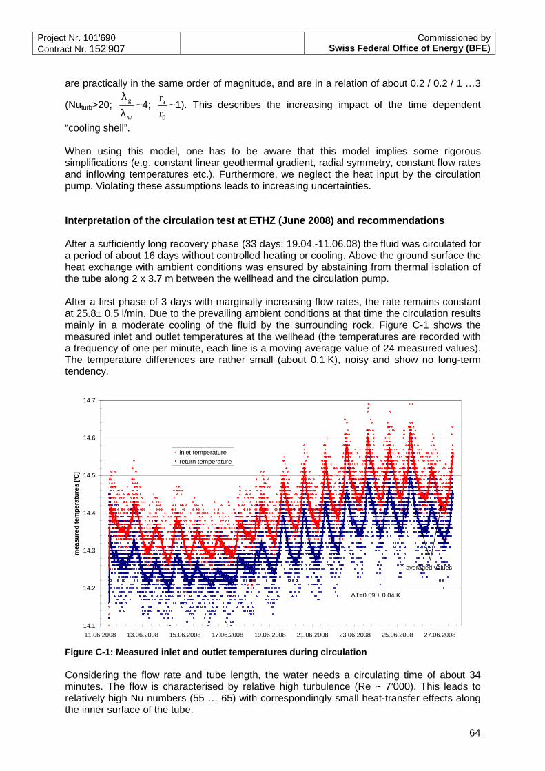
Project Nr. 101'690 Contract Nr. 152'907
Commissioned by Swiss Federal Office of Energy (BFE)
64
are practically in the same order of magnitude, and are in a relation of about 0.2 / 0.2 / 1 …3
(Nuturb>20; w
g
λλ
~4; 0
a
r
r~1). This describes the increasing impact of the time dependent
“cooling shell”. When using this model, one has to be aware that this model implies some rigorous simplifications (e.g. constant linear geothermal gradient, radial symmetry, constant flow rates and inflowing temperatures etc.). Furthermore, we neglect the heat input by the circulation pump. Violating these assumptions leads to increasing uncertainties. Interpretation of the circulation test at ETHZ (June 2008) and recommendations After a sufficiently long recovery phase (33 days; 19.04.-11.06.08) the fluid was circulated for a period of about 16 days without controlled heating or cooling. Above the ground surface the heat exchange with ambient conditions was ensured by abstaining from thermal isolation of the tube along 2 x 3.7 m between the wellhead and the circulation pump. After a first phase of 3 days with marginally increasing flow rates, the rate remains constant at 25.8± 0.5 l/min. Due to the prevailing ambient conditions at that time the circulation results mainly in a moderate cooling of the fluid by the surrounding rock. Figure C-1 shows the measured inlet and outlet temperatures at the wellhead (the temperatures are recorded with a frequency of one per minute, each line is a moving average value of 24 measured values). The temperature differences are rather small (about 0.1 K), noisy and show no long-term tendency.
14.1
14.2
14.3
14.4
14.5
14.6
14.7
11.06.2008 13.06.2008 15.06.2008 17.06.2008 19.06.2008 21.06.2008 23.06.2008 25.06.2008 27.06.2008
mea
sure
d te
mpe
ratu
res
[°C]
inlet temperature
return temperature
averaged values
∆T=0.09 ± 0.04 K
Figure C-1: Measured inlet and outlet temperatures during circulation Considering the flow rate and tube length, the water needs a circulating time of about 34 minutes. The flow is characterised by relative high turbulence (Re ~ 7’000). This leads to relatively high Nu numbers (55 … 65) with correspondingly small heat-transfer effects along the inner surface of the tube.
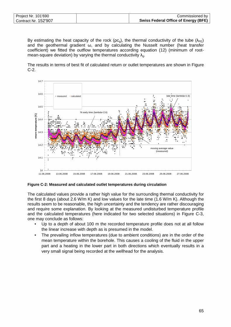
Project Nr. 101'690 Contract Nr. 152'907
Commissioned by Swiss Federal Office of Energy (BFE)
65
By estimating the heat capacity of the rock (ρcg), the thermal conductivity of the tube (λPE) and the geothermal gradient ω, and by calculating the Nusselt number (heat transfer coefficient) we fitted the outflow temperatures according equation (12) (minimum of root-mean-square deviation) by varying the thermal conductivity λg. The results in terms of best fit of calculated return or outlet temperatures are shown in Figure C-2.
14
14.1
14.2
14.3
14.4
14.5
14.6
14.7
11.06.2008 13.06.2008 15.06.2008 17.06.2008 19.06.2008 21.06.2008 23.06.2008 25.06.2008 27.06.2008
retu
rn te
mpe
ratu
re [°
C]
measured calculated
moving average value (measured)
late time (lambda=1.6)
fit early time (lambda=2.6)
Figure C-2: Measured and calculated outlet temperatures during circulation The calculated values provide a rather high value for the surrounding thermal conductivity for the first 8 days (about 2.6 W/m K) and low values for the late time (1.6 W/m K). Although the results seem to be reasonable, the high uncertainty and the tendency are rather discouraging and require some explanation. By looking at the measured undisturbed temperature profile and the calculated temperatures (here indicated for two selected situations) in Figure C-3, one may conclude as follows:
• Up to a depth of about 100 m the recorded temperature profile does not at all follow the linear increase with depth as is presumed in the model.
• The prevailing inflow temperatures (due to ambient conditions) are in the order of the mean temperature within the borehole. This causes a cooling of the fluid in the upper part and a heating in the lower part in both directions which eventually results in a very small signal being recorded at the wellhead for the analysis.
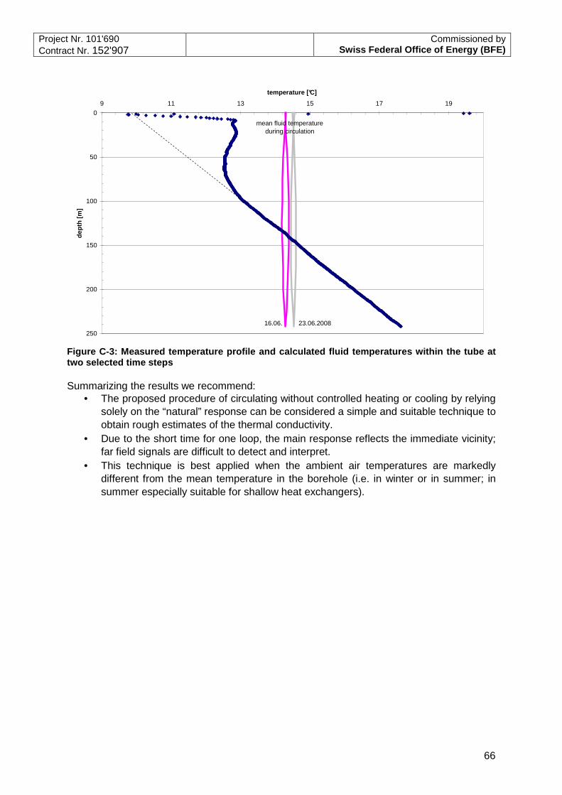
Project Nr. 101'690 Contract Nr. 152'907
Commissioned by Swiss Federal Office of Energy (BFE)
66
0
50
100
150
200
250
9 11 13 15 17 19
temperature [°C]
dept
h [m
]
mean fluid temperatureduring circulation
16.06. 23.06.2008
Figure C-3: Measured temperature profile and calculated fluid temperatures within the tube at two selected time steps Summarizing the results we recommend:
• The proposed procedure of circulating without controlled heating or cooling by relying solely on the “natural” response can be considered a simple and suitable technique to obtain rough estimates of the thermal conductivity.
• Due to the short time for one loop, the main response reflects the immediate vicinity; far field signals are difficult to detect and interpret.
• This technique is best applied when the ambient air temperatures are markedly different from the mean temperature in the borehole (i.e. in winter or in summer; in summer especially suitable for shallow heat exchangers).