Geospatial Technologies for Land Degradation

Assessment and Management

http://www.taylorandfrancis.com

Geospatial Technologies for Land Degradation

Assessment and Management

R. S. Dwivedi

CRC PressTaylor & Francis Group6000 Broken Sound Parkway NW, Suite 300Boca Raton, FL 33487-2742

© 2019 by Taylor & Francis Group, LLCCRC Press is an imprint of Taylor & Francis Group, an Informa business

No claim to original U.S. Government works

Printed on acid-free paper

International Standard Book Number-13: 978-1-4987-4960-2 (Hardback)

This book contains information obtained from authentic and highly regarded sources. Reasonable efforts have been made to publish reliable data and information, but the author and publisher cannot assume responsibility for the validity of all materials or the consequences of their use. The authors and publishers have attempted to trace the copyright holders of all material reproduced in this publication and apologize to copyright holders if permission to publish in this form has not been obtained. If any copyright material has not been acknowledged, please write and let us know so we may rectify in any future reprint.

Except as permitted under U.S. Copyright Law, no part of this book may be reprinted, reproduced, transmitted, or utilized in any form by any electronic, mechanical, or other means, now known or hereafter invented, including photocopying, microfilming, and recording, or in any information storage or retrieval system, without written permission from the publishers.

For permission to photocopy or use material electronically from this work, please access www.copyright.com (http://www.copyright.com/) or contact the Copyright Clearance Center, Inc. (CCC), 222 Rosewood Drive, Danvers, MA 01923, 978-750-8400. CCC is a not-for-profit organization that provides licenses and registration for a variety of users. For organizations that have been granted a photocopy license by the CCC, a separate system of payment has been arranged.

Trademark Notice: Product or corporate names may be trademarks or registered trademarks, and are used only for identification and explanation without intent to infringe.

Visit the Taylor & Francis Web site athttp://www.taylorandfrancis.com

and the CRC Press Web site athttp://www.crcpress.com

Dedicated to

my beloved wife

Asha

http://www.taylorandfrancis.com

vii

Contents

List of Figures ............................................................................................................................. xviiList of Tables .............................................................................................................................. xxixForeword .................................................................................................................................... xxxiPreface .......................................................................................................................................xxxiiiAcknowledgments ................................................................................................................... xxxvAuthor ......................................................................................................................................xxxvii

1 An Introduction to Geospatial Technology ......................................................................11.1 Introduction ...................................................................................................................1

1.1.1 Geospatial Technology ....................................................................................11.2 History of Remote Sensing ..........................................................................................21.3 Electromagnetic Radiation ..........................................................................................3

1.3.1 Particle Model ...................................................................................................31.3.2 Wave Model ......................................................................................................31.3.3 Amplitude .........................................................................................................41.3.4 Phase ..................................................................................................................41.3.5 Polarization .......................................................................................................4

1.4 Electromagnetic Spectrum ..........................................................................................61.4.1 The Ultraviolet Spectrum ...............................................................................61.4.2 The Visible Spectrum ......................................................................................61.4.3 The Infrared Spectrum ...................................................................................61.4.4 The Microwave Spectrum...............................................................................7

1.5 Energy–Matter Interactions in the Atmosphere .......................................................71.5.1 Scattering ..........................................................................................................8

1.5.1.1 Rayleigh Scattering ..........................................................................81.5.1.2 Mie Scattering ...................................................................................81.5.1.3 Nonselective Scattering ...................................................................8

1.5.2 Absorption ........................................................................................................81.5.3 Emission ............................................................................................................9

1.6 Atmospheric Windows .................................................................................................91.6.1 Atmospheric Windows in Optical Region ...................................................91.6.2 Atmospheric Windows in Microwave Region ........................................... 10

1.7 Energy–Matter Interactions with the Terrain ......................................................... 111.7.1 Reflection Mechanism ................................................................................... 111.7.2 Transmission Mechanism ............................................................................. 121.7.3 Absorption Mechanism ................................................................................ 121.7.4 Emission Mechanism .................................................................................... 13

1.8 EMR Laws .................................................................................................................... 131.8.1 Planck’s Law ................................................................................................... 131.8.2 Stefan–Boltzmann Law ................................................................................. 141.8.3 Wein’s Radiation Law .................................................................................... 151.8.4 Rayleigh–Jeans Law ....................................................................................... 161.8.5 Kirchhoff’s Law .............................................................................................. 16

viii Contents

1.9 Spectral Response Pattern ......................................................................................... 161.10 Hyperspectral Remote Sensing ................................................................................. 171.11 Remote Sensing Process ............................................................................................. 20

1.11.1 The Source of Illumination ........................................................................... 201.11.2 The Sensor ....................................................................................................... 201.11.3 Platforms ......................................................................................................... 201.11.4 Data Reception ............................................................................................... 211.11.5 Data Product Generation .............................................................................. 211.11.6 Data Analysis/Interpretation .......................................................................221.11.7 Data/Information Storage ............................................................................221.11.8 Archival and Distribution ............................................................................22

1.12 Geographical Information System ............................................................................231.12.1 Components of GIS ........................................................................................ 24

1.12.1.1 Hardware ......................................................................................... 241.12.1.2 Software ........................................................................................... 241.12.1.3 Data ..................................................................................................25

1.13 Global Navigation Satellite Systems .........................................................................251.13.1 GPS Segments ................................................................................................. 26

1.13.1.1 Space Segment ................................................................................ 261.13.1.2 Control Segment ............................................................................. 261.13.1.3 The User Segment .......................................................................... 27

1.13.2 Operating Principle of GPS .......................................................................... 271.13.3 Navigation .......................................................................................................28

1.13.3.1 Stand-Alone Satellite Navigation .................................................281.13.3.2 Differential GNSS Navigation ...................................................... 291.13.3.3 Network-Assisted GNSS Navigation ........................................... 291.13.3.4 Carrier-Phase Differential (Kinematic) GPS .............................. 29

1.14 Organization of This Book ........................................................................................ 29References ...............................................................................................................................30

2 Passive Remote Sensing ...................................................................................................... 312.1 Introduction ................................................................................................................. 312.2 Remote Sensing Platforms ......................................................................................... 32

2.2.1 Airborne Platforms ........................................................................................ 322.2.2 Spaceborne Platforms ....................................................................................34

2.2 .2.1 Geosynchronous Satellites ............................................................342.2.2.2 Polar Orbiting Satellites .................................................................34

2.3 Passive Sensors ............................................................................................................352.3.1 The Optics .......................................................................................................352.3.2 Detectors ......................................................................................................... 37

2.3.2.1 Quantum Detectors .......................................................................382.3.2.2 Photoemissive Detectors ...............................................................382.3.2.3 Semiconductor Detectors ..............................................................382.3.2.4 Photoconductive Detectors ...........................................................382.3.2.5 Photovoltaic Detectors ................................................................... 392.3.2.6 Thermal Detectors .......................................................................... 39

2.4 Optical Sensors ............................................................................................................402.4.1 Conventional Photographic Cameras .........................................................402.4.2 Digital Aerial Cameras.................................................................................. 41

ixContents

2.4.3 Video Cameras ............................................................................................... 412.4.4 Radiometers .................................................................................................... 41

2.4.4.1 Radiometers Operating in Optical Region ................................. 412.4.4.2 Radiometers Operating in Microwave Region ..........................432.4.4.3 Imaging Spectrometer ...................................................................46

2.5 Resolution of a Sensor ................................................................................................ 472.5.1 Spatial Resolution ..........................................................................................482.5.2 Spectral Resolution ........................................................................................ 492.5.3 Radiometric Resolution ................................................................................. 492.5.4 Temporal Resolution ......................................................................................502.5.5 Angular Resolution .......................................................................................50

2.6 Spaceborne Missions with Passive Sensors .............................................................502.6.1 The Landsat Mission .....................................................................................502.6.2 The SPOT Mission.......................................................................................... 512.6.3 Pleiades Mission ............................................................................................. 522.6.4 The Indian Earth Observation Mission ......................................................53

2.6.4.1 Resourcesat-1 ...................................................................................532.6.4.2 Resourcesat-2...................................................................................532.6.4.3 Resourcesat-2A ...............................................................................53

2.6.5 The Earth Observing System Mission ........................................................542.6.5.1 Terra (EO-AM) ................................................................................542.6.5.2 Aqua (EOS PM-1) ............................................................................54

2.6.6 Earth Observing-1 Mission (EO-1) ...............................................................562.6.7 RapidEye .........................................................................................................562.6.8 Hyperspatial Resolution Earth Missions .................................................... 57

2.6.8.1 WorldView Mission ........................................................................ 572.6.8.2 Cartosat Mission .............................................................................582.6.8.3 GeoEye-1 .......................................................................................... 59

2.6.9 Passive Microwave Missions ........................................................................602.6.9.1 National Oceanic and Atmospheric Administration

AMSU-A ..........................................................................................602.6.9.2 Defense Meteorological Satellite Program .................................602.6.9.3 Aqua (EO: PM-1) ............................................................................. 612.6.9.4 Soil Moisture and Ocean Salinity Mission ................................. 612.6.9.5 Soil Moisture Active Passive Mission..........................................63

2.7 Conclusion ....................................................................................................................64References ...............................................................................................................................64

3 Active Remote Sensing ........................................................................................................ 673.1 Introduction ................................................................................................................. 673.2 Active Microwave Sensors ......................................................................................... 67

3.2.1 Imaging Sensors ............................................................................................. 673.2.1.1 Real Aperture Radar ......................................................................683.2.1.2 Synthetic Aperture Radar ............................................................. 713.2.1.3 The Operating Modes of SAR ....................................................... 73

3.2.2 Non-imaging Microwave Sensors ...............................................................753.2.2.1 Scatterometers ................................................................................. 763.2.2.2 Radar Altimeter .............................................................................. 78

3.3 Spaceborne Radars Systems ......................................................................................80

x Contents

3.3.1 RISAT Mission ................................................................................................803.3.1.1 RISAT-1 .............................................................................................803.3.1.2 RISAT-2.............................................................................................80

3.3.2 Sentinel Mission ............................................................................................. 813.3.2.1 Sentinel-1 ......................................................................................... 813.3.2.2 Sentinel-2 ......................................................................................... 813.3.2.3 Sentinel-3 ......................................................................................... 813.3.2.4 Sentinel-4 ......................................................................................... 813.3.2.5 Sentinel-5 ......................................................................................... 823.3.2.6 Sentinel-5P ....................................................................................... 82

3.3.3 CryoSat ............................................................................................................ 823.3.4 Soil Moisture and Ocean Salinity Mission................................................. 82

3.3.4.1 Measurement Principle .................................................................833.3.5 Soil Moisture Active Passive ........................................................................833.3.6 RADARSAT Mission .....................................................................................85

3.3.6.1 RADARSAT Constellation ............................................................853.3.7 The Advanced Land Observing Satellite-2 ................................................863.3.8 TerraSAR-X and TanDEM-X ......................................................................... 87

3.4 Light Detection And Ranging ................................................................................... 893.4.1 Discrete Return LiDAR ................................................................................. 893.4.2 Waveform LiDAR ........................................................................................... 913.4.3 Scanning Mechanism .................................................................................... 91

3.4.3.1 Oscillating Mirror Scanning Mechanism ................................... 913.4.3.2 Rotating Polygon Scanning Mechanism ..................................... 933.4.3.3 Nutating Mirror Scanning System .............................................. 933.4.3.4 Fiber Pointing System .................................................................... 933.4.3.5 Spaceborne LiDAR Mission .......................................................... 943.4.3.6 Cloud Profiling Radar (CPR) ........................................................ 95

3.5 Conclusion .................................................................................................................... 95References ............................................................................................................................... 96

4 Digital Image Processing .................................................................................................... 974.1 Introduction ................................................................................................................. 974.2 Data Storage Media .....................................................................................................99

4.2.1 Compact Disc ..................................................................................................994.2.2 Digital Versatile Disk ....................................................................................994.2.3 Memory Sticks ................................................................................................99

4.3 Digital Data Format .................................................................................................. 1004.3.1 Generic Binary .............................................................................................. 1004.3.2 Graphic Interchange Format ...................................................................... 1004.3.3 JPEG ............................................................................................................... 1004.3.4 TIFF and GeoTIFF ........................................................................................ 1014.3.5 Portable Network Graphics ........................................................................ 101

4.4 Image Preprocessing................................................................................................. 1014.4.1 Radiometric Correction ............................................................................... 101

4.4.1.1 Atmospheric Effects ..................................................................... 1014.4.1.2 Absolute Atmospheric Correction ............................................. 1024.4.1.3 Relative Atmospheric Correction ............................................... 1044.4.1.4 Instrumental Errors ..................................................................... 104

xiContents

4.4.2 Corrections for Solar Illumination Variation ........................................... 1054.4.3 Noise Removal ............................................................................................. 1054.4.4 Geometric Image Correction ...................................................................... 107

4.4.4.1 Correction for Systemic Distortions .......................................... 1084.4.4.2 Correction of Nonsystemic Errors ............................................. 109

4.4.5 Image Processing Levels ............................................................................. 1104.5 Image Enhancement ................................................................................................. 111

4.5.1 Contrast Modification ................................................................................. 1114.5.1.1 Density Slicing .............................................................................. 1124.5.1.2 Contrast Enhancement ................................................................ 1124.5.1.3 Edge Enhancement and Detection ............................................ 117

4.5.2 Multiple Image Manipulation .................................................................... 1184.5.2.1 Band Ratioing ............................................................................... 1184.5.2.2 Vegetation Indices ........................................................................ 1184.5.2.3 Image Transformation ................................................................. 119

4.6 Image Classification .................................................................................................. 1264.6.1 Unsupervised Classification ...................................................................... 126

4.6.1.1 Unsupervised Classification using the Chain Method .......... 1264.6.1.2 Unsupervised Classification using the ISODATA Method .... 1264.6.1.3 K-Means Clustering Algorithm .................................................. 127

4.6.2 Supervised Classification............................................................................ 1274.6.2.1 Parallelepiped Classification ...................................................... 1274.6.2.2 Minimum Distance Classification ............................................. 1284.6.2.3 Maximum Likelihood Classification ......................................... 1284.6.2.4 k-Nearest Neighbors .................................................................... 1284.6.2.5 Mahalanobis Spectral Distance .................................................. 1294.6.2.6 Artificial Neural Networks ......................................................... 1304.6.2.7 Object-Oriented Classification ................................................... 1304.6.2.8 Spectral Angular Mapper Algorithm........................................ 1314.6.2.9 Spectral Correlation Classifier .................................................... 1324.6.2.10 Support Vector Machines Classifier .......................................... 133

4.7 Digital Change Detection ........................................................................................ 1344.7.1 Image Enhancement Techniques ............................................................... 135

4.7.1.1 Univariate Image Differencing................................................... 1354.7.1.2 Image Regression ......................................................................... 1354.7.1.3 Image Ratioing .............................................................................. 1354.7.1.4 Principal Component Analysis .................................................. 1364.7.1.5 Multivariate Alteration Detection .............................................. 1364.7.1.6 Post-Classification Comparison ................................................. 1364.7.1.7 Artificial Neural Network-Based Change Detection .............. 137

4.8 Accuracy Assessment ............................................................................................... 1374.8.1 Uni-Temporal Thematic Maps .................................................................... 138

4.8.1.1 Sampling Scheme ......................................................................... 1384.8.1.2 Accuracy Assessment .................................................................. 1384.8.1.3 Kappa Coefficient (K)................................................................... 139

4.8.2 Multi-Temporal Thematic Maps ................................................................ 1404.9 Conclusions ................................................................................................................ 143References ............................................................................................................................. 144

xii Contents

5 An Introduction to Land Degradation ........................................................................... 1495.1 Introduction ............................................................................................................... 149

5.1.1 Components of Land Degradation ............................................................ 1505.1.1.1 Soil Degradation ........................................................................... 1515.1.1.2 Vegetation Degradation ............................................................... 1595.1.1.3 Water Degradation ....................................................................... 1595.1.1.4 Climate Deterioration .................................................................. 1595.1.1.5 Losses to Urban/Industrial Development ................................ 160

5.2 Extent and Spatial Distribution............................................................................... 1605.3 Land Degradation Assessment ............................................................................... 162

5.3.1 Expert opinion/GLASOD Approach ........................................................ 1625.3.2 Remote Sensing-Based Approach .............................................................. 163

5.3.2.1 Computation of NDVI Indicators ............................................... 1645.3.2.2 NDVI-to-NPP Conversion ........................................................... 1645.3.2.3 Identification of the Areas Experiencing Land Degradation .....164

5.3.3 Biophysical Models ...................................................................................... 1655.3.4 Abandonment of Agricultural Lands ....................................................... 1655.3.5 The Land Degradation Impact Index ........................................................ 166

5.4 Conclusions ................................................................................................................ 166References ............................................................................................................................. 167

6 Water Erosion....................................................................................................................... 1716.1 Introduction ............................................................................................................... 1716.2 Factors of Water Erosion .......................................................................................... 171

6.2.1 Climatic Factors ............................................................................................ 1726.2.2 Land Factors ................................................................................................. 172

6.2.2.1 Soil Texture and Clay Mineralogy ............................................. 1726.2.2.2 Organic Matter ............................................................................. 1726.2.2.3 Sodium and Other Cations ......................................................... 1736.2.2.4 Iron and Aluminum Oxides ....................................................... 1736.2.2.5 Antecedent Soil Moisture ............................................................ 1736.2.2.6 Soil Crusting ................................................................................. 1736.2.2.7 Topography ................................................................................... 1736.2.2.8 Vegetation ...................................................................................... 174

6.3 Water Erosion Models .............................................................................................. 1746.3.1 Empirical Models ......................................................................................... 1746.3.2 Physically Based Models ............................................................................. 175

6.3.2.1 Water Erosion Prediction Project Model ................................... 1756.3.3 Mixed Models ............................................................................................... 175

6.3.3.1 CREAMS ........................................................................................ 1756.3.3.2 ANSWERS ..................................................................................... 176

6.4 Role of Remote Sensing ............................................................................................ 1766.4.1 Spectral Response Pattern of Eroded Soils .............................................. 1766.4.2 Airborne Sensor Data .................................................................................. 1776.4.3 Spaceborne Multispectral Data .................................................................. 178

6.4.3.1 Detection of Erosion Features and Eroded Areas ................... 1786.4.3.2 Monitoring Eroded Lands .......................................................... 1846.4.3.3 Detection of Erosion Consequences .......................................... 1856.4.3.4 Erosion Controlling Factors ........................................................ 186

xiiiContents

6.4.3.5 Soil Erosion Risk ........................................................................... 1866.4.3.6 Assimilation of Remote Sensing Data into Runoff and

Erosion Models ............................................................................. 1886.5 Conclusion .................................................................................................................. 189References ............................................................................................................................. 190

7 Wind Erosion ....................................................................................................................... 1977.1 Introduction ............................................................................................................... 1977.2 Background ................................................................................................................ 197

7.2.1 Wind Erosion Processes .............................................................................. 1987.2.2 Causative Factors ......................................................................................... 198

7.2.2.1 Soil Erodibility .............................................................................. 1997.2.2.2 Soil Surface Conditions ............................................................... 1997.2.2.3 Soil Texture....................................................................................2007.2.2.4 Climate ...........................................................................................2007.2.2.5 Vegetation ......................................................................................2007.2.2.6 Soil Moisture ................................................................................. 201

7.3 Global Scenario .......................................................................................................... 2017.4 Role of Remote Sensing ............................................................................................ 202

7.4.1 Airborne Sensors Data ................................................................................ 2027.4.2 Orbital Sensor Data ..................................................................................... 203

7.4.2.1 Detection of Wind Erosion Features and Eroded Areas ........ 2047.4.2.2 Characterization of Dune Activity ............................................ 2067.4.2.3 Measuring Sand Availability ...................................................... 2067.4.2.4 Erosion Control Measures and Impact Assessment................ 208

7.5 Modeling Wind Erosion ........................................................................................... 2147.5.1 Field Scale Wind Erosion Models .............................................................. 214

7.5.1.1 Wind Erosion Equation ............................................................... 2147.5.1.2 Revised Wind Erosion Equation ................................................ 2147.5.1.3 Wind Erosion Prediction System ............................................... 2157.5.1.4 Texas Erosion Analysis Model ................................................... 2157.5.1.5 Wind Erosion Stochastic Simulator ........................................... 215

7.5.2 Regional Scale Models ................................................................................ 2167.5.2.1 Wind Erosion on European Light Soils ..................................... 2167.5.2.2 Wind Erosion Assessment Model .............................................. 2177.5.2.3 Integrated Wind Erosion Modeling System ............................. 217

7.5.3 Global Scale Models .................................................................................... 2177.5.3.1 Dust Production Model ............................................................... 2187.5.3.2 Dust Entrainment and Deposition Model ................................ 219

7.5.4 Other Global Dust Models.......................................................................... 2197.6 Conclusion .................................................................................................................. 220References ............................................................................................................................. 224

8 Soil Salinization and Alkalinization .............................................................................229Coauthored by Dr. Jamshid Fareftih

8.1 Introduction ...............................................................................................................2298.2 Origin of Salts ............................................................................................................2308.3 Nature of Salt-Affected Soils ................................................................................... 231

xiv Contents

8.4 Extent and Spatial Distribution............................................................................... 2328.5 Soil Salinity Symptoms ............................................................................................233

8.5.1 Surface Manifestation .................................................................................2338.5.2 The Presence of Halophytic Plants ............................................................2348.5.3 Crop Performance ........................................................................................235

8.6 Proximal Sensing ......................................................................................................2358.6.1 Spectral Measurements in Laboratory ......................................................2358.6.2 In situ Spectral Measurements ................................................................... 2378.6.3 Frequency-Domain Electromagnetic Techniques ...................................2388.6.4 Ground Penetrating Radar Measurements .............................................. 239

8.7 Inventory and Monitoring of Salt-Affected Soils ................................................. 2398.7.1 Airborne Sensors Data ................................................................................ 240

8.7.1.1 Aerial Photographs, Videography, and Digital Multispectral Camera Images .................................................... 240

8.7.2 Orbital Sensor Data ..................................................................................... 2418.7.2.1 Multispectral Visible, NIR, and Thermal IR Sensor Data ...... 2428.7.2.2 Computer-Assisted Digital Analysis ......................................... 246

8.7.3 State-of-the-Art ............................................................................................. 2478.7.3.1 Temporal Behavior of Salt-Affected Soils ................................. 2488.7.3.2 Spaceborne Microwave Sensor Data ......................................... 2528.7.3.3 Spaceborne Hyperspectral Sensor Data ....................................253

8.8 Solute Transport Modeling ......................................................................................2548.9 Conclusion ..................................................................................................................254References .............................................................................................................................255

9 Soil Acidification ................................................................................................................ 2639.1 Introduction ............................................................................................................... 2639.2 Background ................................................................................................................ 2639.3 Global Scenario ..........................................................................................................2649.4 Development of Soil Acidity ................................................................................... 265

9.4.1 Causative Factors of Soil Acidification ..................................................... 2659.4.1.1 Acidic Precipitation ...................................................................... 2659.4.1.2 Acidifying Gases and Particles .................................................. 2669.4.1.3 Acidifying Fertilizers and Legumes ......................................... 2669.4.1.4 Nutrient Uptake by Crops and Root Exudates ........................ 2679.4.1.5 Mineralization .............................................................................. 267

9.4.2 The Impact of Soil Acidification ................................................................ 2679.4.3 Soil Acidity and Base Saturation and Buffering Capacity ..................... 2689.4.4 Soil Acidity and Crop Responses .............................................................. 268

9.5 Delineation and Mapping of Acid Soils................................................................. 2699.5.1 Aerial Photographs ...................................................................................... 269

9.5.1.1 Aspect/Elemental Analysis ........................................................ 2709.5.1.2 Physiographic Analysis ............................................................... 2709.5.1.3 Morphogenetic Analysis ............................................................. 270

9.5.2 Spaceborne Multispectral Measurements ................................................ 2719.5.2.1 Visual Interpretation .................................................................... 2719.5.2.2 Computer-Assisted Digital Analysis ......................................... 276

9.5.3 Mapping Vegetation-Covered Soils .......................................................... 2799.5.4 Digital Soil Mapping ................................................................................... 279

xvContents

9.6 Conclusion .................................................................................................................. 281References ............................................................................................................................. 281

10 Waterlogging .......................................................................................................................28510.1 Introduction ...............................................................................................................28510.2 The Effects of Waterlogging .................................................................................... 286

10.2.1 The Effects on Soils ...................................................................................... 28610.2.2 Plant Responses to Waterlogging .............................................................. 286

10.3 Norms for Categorization ........................................................................................28810.4 Role of Remote Sensing ............................................................................................288

10.4.1 In situ Spectral Reflectance Studies ........................................................... 28910.4.2 Aerial Photographs and Airborne Spectral Measurements .................. 29010.4.3 Spaceborne Multispectral Measurements ................................................ 290

10.4.3.1 Optical Sensor Data ..................................................................... 29010.4.3.2 Thermal Sensor Data ................................................................... 294

10.4.4 Geophysical Techniques ............................................................................. 29510.4.4.1 Ground-Penetrating Radar (GPR) .............................................. 29510.4.4.2 Electromagnetic Induction (EMI) Sensors ................................ 296

10.5 Using Models to Simulate Plant Responses to Waterlogging ............................. 29710.6 Conclusions ................................................................................................................ 298References ............................................................................................................................. 298

11 Land Degradation due to Mining, Aquaculture, and Shifting Cultivation ...........30311.1 Introduction ...............................................................................................................30311.2 Global Distribution ...................................................................................................30411.3 Role of Remote Sensing ............................................................................................305

11.3.1 Aerial Photographs ......................................................................................30511.3.1.1 Mining ...........................................................................................30511.3.1.2 Aquaculture ..................................................................................30511.3.1.3 Shifting Cultivation......................................................................306

11.3.2 Sapaceborne Multispectral Measurements ..............................................30611.3.2.1 Mining ...........................................................................................30611.3.2.2 Aquaculture .................................................................................. 31011.3.2.3 Shifting Cultivation...................................................................... 315

11.4 Conclusions ................................................................................................................ 317References ............................................................................................................................. 317

12 Drought ................................................................................................................................. 32112.1 Introduction ............................................................................................................... 32112.2 Background ................................................................................................................ 321

12.2.1 Drought Indicators....................................................................................... 32312.3 Global Scenario .......................................................................................................... 32412.4 Drought Assessment and Monitoring ................................................................... 325

12.4.1 Meteorological Indicators ........................................................................... 32612.4.1.1 Deciles ............................................................................................ 32612.4.1.2 Percent of Normal Precipitation ................................................. 32612.4.1.3 Palmer Drought Severity Index.................................................. 32612.4.1.4 Standardized Precipitation Index .............................................. 32712.4.1.5 Crop Moisture Index .................................................................... 32712.4.1.6 Standardized Precipitation Evapotranspiration Index ........... 328

xvi Contents

12.4.1.7 Soil Moisture Deficit Index ......................................................... 32812.4.1.8 Surface Water Supply Index ........................................................ 329

12.4.2 Remote Sensing-Based Methods ............................................................... 32912.4.2.1 Estimation of Meteorological Parameters .................................33012.4.2.2 Drought Impacts ........................................................................... 332

12.4.3 Process-Based Indicators ............................................................................ 33712.4.4 Water Balance Approach ............................................................................338

12.5 Drought Forecasting ................................................................................................. 33912.5.1 Regression Analysis .................................................................................... 33912.5.2 Time Series Analysis ................................................................................... 33912.5.3 Probability Models ......................................................................................34012.5.4 ANN Model ..................................................................................................34012.5.5 Hybrid Models ............................................................................................. 341

12.6 Long-Lead Drought Forecasting ............................................................................. 34112.7 Drought Monitoring Systems: Global Scenario .................................................... 341

12.7.1 Global Integrated Drought Monitoring and Prediction System ...........34212.7.1.1 Approach .......................................................................................342

12.7.2 European Drought Monitoring System ....................................................34312.7.3 Drought Monitoring System for South Asia ............................................34412.7.4 Indian National Agricultural Drought Assessment and

Monitoring System .....................................................................................34412.8 Conclusion ..................................................................................................................346References .............................................................................................................................347

13 Land Degradation Information Systems ....................................................................... 35513.1 Introduction ............................................................................................................... 35513.2 Background ................................................................................................................ 356

13.2.1 Components of an IS ................................................................................... 35613.3 Database ..................................................................................................................... 358

13.3.1 Database Model ............................................................................................ 35813.3.1.1 Hierarchical Model ...................................................................... 35813.3.1.2 Network Model ............................................................................. 35813.3.1.3 Relational Model .......................................................................... 35913.3.1.4 Object-Oriented Model ................................................................360

13.4 Land Degradation ISs ............................................................................................... 36113.4.1 Soil Database ................................................................................................ 362

13.4.1.1 Data Acquisition ........................................................................... 36213.4.1.2 Geo-referencing and Creation of Digital Data ......................... 36213.4.1.3 Data Verification and Editing .....................................................36313.4.1.4 Data Updation ...............................................................................36313.4.1.5 Soil Degradation Data..................................................................36313.4.1.6 Soil ISs ............................................................................................363

13.5 Gladis/GIS System .................................................................................................... 36913.5.1 Panning Method .......................................................................................... 374

13.5.1.1 Metadata, Formats and Resolution Information, Layers ........ 37413.6 Conclusion .................................................................................................................. 375References ............................................................................................................................. 376

Index .............................................................................................................................................379

xvii

List of Figures

Figure 1.1 The electromagnetic radiation ..............................................................................3

Figure 1.2 Wavelength and amplitude of the electromagnetic radiation .........................4

Figure 1.3 The concept of the phase of electromagnetic radiation ....................................5

Figure 1.4 (a) Horizontally polarized wave is one for which the electric field lies only in the y–z plane. (b) Vertically polarized wave is one for which the electric field lies only in the x–z plane ..........................................................5

Figure 1.5 The electromagnetic spectrum .............................................................................6

Figure 1.6 The atmospheric windows in visible and infrared regions ........................... 10

Figure 1.7 Absorption bands in microwave region............................................................ 10

Figure 1.8 Schematic of a reflection from a specular reflector ......................................... 12

Figure 1.9 Near-perfect diffuse reflector and Lambertian surface .................................... 12

Figure 1.10 Reflection/scattering, absorption, transmission, and emission .................... 13

Figure 1.11 Spectral distribution of energy radiated by blackbodies at various temperatures ......................................................................................................... 15

Figure 1.12 Spectral reflectance pattern of water and other major terrain features ....... 17

Figure 1.13 A Comparison of multispectral and hyperspectral response patterns of vegetation ......................................................................................................... 18

Figure 1.14 The concept of hyperspectral imagery. Image measurements are made at many narrow contiguous wavelength bands, resulting in a complete spectrum for each pixel ...................................................................... 19

Figure 1.15 Two-dimensional projection of a hyperspectral cube .................................... 19

Figure 1.16 The remote sensing system. A = energy source/illumination; B = radiation and the atmosphere; C = interaction with the object; D = recording of energy by the sensor; E = transmission, reception, and processing; F = interpretation/analysis; and G = applications .............. 20

Figure 1.17 Three major components of a Geographic Information System. These components consist of input, computer hardware and software, and output subsystems ............................................................................................... 24

Figure 1.18 GIS data–thematic data layers ............................................................................25

Figure 1.19 GPS nominal satellite constellation ................................................................... 26

Figure 1.20 A GPS receiver ...................................................................................................... 27

Figure 1.21 Third dimension positioning using GPS ..........................................................28

Figure 2.1 Remote sensing platforms ..................................................................................33

xviii List of Figures

Figure 2.2 Schematic of a geostationary orbits. Polar as well as low-earth orbits are also shown .......................................................................................................34

Figure 2.3 Schematic representation of a sun-synchronous orbit.....................................35

Figure 2.4 Schematic of a conventional photographic camera ..........................................40

Figure 2.5 Sketch of an opto-mechanical scanner ...............................................................42

Figure 2.6 Sketch of a push-broom scanner .........................................................................43

Figure 2.7 Schematic diagram of a microwave radiometer using heterodyne principle ..................................................................................................................44

Figure 2.8 Schematic diagram showing working principle of a microwave radiometer ..............................................................................................................45

Figure 2.9 Various types of scanning mechanisms. In imaging spectrometer both line array detectors and area array detectors are used. Area array detector is, however, very common .................................................................... 47

Figure 2.10 An illustration of the effects of spatial resolution on detectability of terrain features ...................................................................................................... 49

Figure 2.11 Showing the effect of malfunctioning of scan line corrector (SLC) (a), sketch of part of the uncorrected image (b), and after correction (c) Data gaps produced from the SLC-off mode have alternating wedges with the widest parts occurring at the scene edge .......................................... 51

Figure 2.12 Cartosat 1 stereo and wide swath imaging ....................................................... 62

Figure 2.13 The microwave imaging radiometer with aperture synthesis (MIRAS) ......63

Figure 3.1 Schematic of a typical active microwave system components ........................68

Figure 3.2 Imaging geometry of a side-looking airborne real aperture radar ................ 70

Figure 3.3 Relationship between real aperture and synthetic aperture radar. Where D is real aperture; β is real beam width, βs is synthetic aperture beam, h is height, ∆Ls is azimuth resolution, ψ is off-nadir angle .................72

Figure 3.4 The strip map SAR operation mode ................................................................... 73

Figure 3.5 Bore sight imaging geometry: the antenna pointing angle is equal to 90° ..... 74

Figure 3.6 Squinted imaging geometry: the antenna pointing angle is different from 90° ................................................................................................................... 74

Figure 3.7 Spotlight SAR operation mode ............................................................................ 75

Figure 3.8 Scan SAR operation mode; two-sub swath case ............................................... 75

Figure 3.9 NSCAT viewing geometry ...................................................................................77

Figure 3.10 SeaWinds viewing geometry...............................................................................77

Figure 3.11 The concept of deramp technique ...................................................................... 79

Figure 3.12 Artist’s rendition of SMOS mission ....................................................................83

xixList of Figures

Figure 3.13 Artist’s rendition of the Soil Moisture Active Passive (SMAP) spacecraft in orbit ..................................................................................................84

Figure 3.14 The RADARSAT-1 spacecraft and illustration of observation geometries ..... 85

Figure 3.15 Artist’s rendition of the RADARSAT constellation mission imaging concept ....................................................................................................................86

Figure 3.16 RADARSAT constellation imaging modes ........................................................ 87

Figure 3.17 The imaging modes of ALOS-2 mission ............................................................88

Figure 3.18 An airborne LiDAR system .................................................................................90

Figure 3.19 Observational differences between discrete-return and full-waveform LiDAR .....................................................................................................................90

Figure 3.20 Various kinds of commonly used laser scanners (clock-wise) oscillating mirror scanner, Palmer scanner, fibre scanner and rotating polygon ................................................................................................................... 92

Figure 3.21 Oscillating mirror scanning pattern .................................................................. 92

Figure 3.22 Rotating polygon scanning pattern ................................................................... 93

Figure 3.23 Nutating mirror scanning pattern ..................................................................... 94

Figure 3.24 Fiber scanning pattern ......................................................................................... 94

Figure 3.25 Illustration of the CloudSat spacecraft .............................................................. 95

Figure 4.1 Digital image ......................................................................................................... 98

Figure 4.2 An illustration of the contents of a Resourcesat-2 LISS-IV digital data (digital numbers—DN values) for vegetation, soils, and water body. Note the low DN values for water body in columns 8, 9, and 10, and rows 18–20 in all the spectral bands .................................................................. 98

Figure 4.3 Stripping in satellite image and its correction ............................................... 106

Figure 4.4 Vertical striping correction in Resourcesat-1 AWiFS image. The vertical stripes highlighted with red box (left) have been removed (right) ............... 106

Figure 4.5 Noise correction in spectral band 2 of Resourcesat-2 LISS-IV image. The image in the left (a) displays vertical stripping—characteristics of push-broom sensors—and (b) shows the image after employing necessary noise corrections .............................................................................. 107

Figure 4.6 Pixel dropouts in Resourcesat-1 LISS-IV-band 2 image ................................ 107

Figure 4.7 Bow-tie effect in Terra/Aqua MODIS image................................................... 109

Figure 4.8 Landsat-MSS band 4 (0.7–1.1 µm) of March 2, 1985 raw digital data (a), linearly stretched data (b), and corresponding histograms of raw digital data and linear-stretched data area given in (c) ................................ 112

Figure 4.9 Landsat-MSS band 4 (0.7–1.1 µm) of March 2, 1985 raw digital data (a) and nonlinear-stretched data (b). The histograms of the raw digital data and nonlinear-stretched data area given in (c) ...................................... 113

xx List of Figures

Figure 4.10 An illustration of histogram equalization: raw digital LISS-IV image (a), corresponding histogram (b), histogram-equalized image (c), and the histogram of the stretched image (d) ........................................................ 114

Figure 4.11 An illustration of histogram matching. The first principal component (pc1) of LISS-IV multispectral image (a), Cartosat-1 2.5 m-PAN image (b), and histogram-matched image of pc1 (c) ................................................. 115

Figure 4.12 An example of spatial filtering of resourcesat-2 LISS-IV data (a), 3 × 3 high-pass-filtered data (b), 3 × 3 median-filtered data (c), and 3 × 3 low-pass-filtered data (d) ........................................................................................... 116

Figure 4.13 Cartosat-2 PAN raw image (a) and Fourier-transformed image (b) ............ 117

Figure 4.14 Edge enhancement and detection. Cartosat-1 2.5 m-PAN image (a), and the image background with edges (b) ............................................................. 118

Figure 4.15 The ratio image of Resourcesat-2 LISS-IV dada of October 1, 2015. The spectral band-2 by band-3 image (a), and spectral band-3 by band-2 image (b). Note the regular-shaped very light gray to white agricultural fields in center of the image as well as upper-right and lower-left corner of image (b). Although these features are also conspicuous in image (a), they stand out much better in band 3 by 2 image ..................................................................................................................... 119

Figure 4.16 Principal component analysis of Landsat-8 OLI data ................................... 120

Figure 4.17 Kauth-Thomas transformation ......................................................................... 122

Figure 4.18 The standard FCC of Landsat-8 OLI data (a), and the tasseled cap-transformed image (b) ....................................................................................... 123

Figure 4.19 Models of IHS color spaces: (a) The color cube model (b) The color cylinder model .................................................................................................... 123

Figure 4.20 An illustration of digital image fusion for Cartosat-1 PAN data with 2.5 m spatial resolution and Resourcesat-2 LISS-IV image generated through the Brovey, IHS, and principal component transformations ................................................................................................... 125

Figure 4.21 Resourcesat-2 LISS-IV digital raw image acquired on March 7, 2017 (a) and Salt-affected soil map derived using ISODATA classifier (b). Biege color denotes severely salt-affected soils, magenta moderately salt-affected soils, yellow crop with very good vigor, and green crop with moderate vigor .................................................................................................... 127

Figure 4.22 Resourcesat-2 LISS-III digital raw image (a) and thematic map derived using K-mean classifier (b). Pink color indicates moderately deep to deep ravines, cyan shallow ravines, yellow cropland with very good vigor, sienne crop with moderate vigor .......................................................... 129

Figure 4.23 Salt-affected soil map of the area shown in Figure 4.21a developed using maximum likelihood classifier. The pink color denotes salt-affected soils, yellow crop, and blue water body ........................................... 129

xxiList of Figures

Figure 4.24 Salt-affected soil map of the area shown in Figure 4.21a developed using Mahalanobis spectral distance classifier. Pink color denotes salt-affected soils, yellow crop, and blue indicates water body ................... 130

Figure 4.25 The concept of an artificial neural network. Each circular node represents an artificial neuron and an arrow represents a connection from the output of one neuron to the input of another ................................. 132

Figure 4.26 Salt-affected soil map of the area shown in Figure 4.21a developed using spectral angle mapper classifier. Pink color denotes salt-affected soils, yellow color cropland ............................................................................... 133

Figure 4.27 Salt-affected soil map of the area shown in Figure 4.21a developed using spectral correlation classifier. Pink color denotes salt-affected soils, yellow color cropland ............................................................................... 134

Figure 4.28 Map showing mining areas in part of Andhra Pradesh, southern India. The map has been developed using support vector machine algorithm .............................................................................................................. 141

Figure 4.29 An illustration of the framework for accuracy assessment of single-date and multi-temporal change detection approaches (Macleod and Congalton, 1998; http://info.asprs.org/publications/pers/98journal/march/1998_mar_207-216.pdf, accessed on June 10, 2017) ............................ 143

Figure 5.1a Soil and water being splashed by the impact of a single raindrop.............. 152

Figure 5.1b In spite of across slope tillage operation sheet erosion is taking place due to the absence of adequate protective vegetation cover during rainy season ........................................................................................................ 152

Figure 5.1c Deep gully formstion due to vertical erosion owing poor soil structure ..... 152

Figure 5.1d Rill erosion as observed in the field ................................................................. 153

Figure 5.2 A schematic of wind erosion process............................................................... 153

Figure 5.3 Human-induced soil degradation around the world .................................... 161

Figure 5.4 Global Assessment of Human-induced Soil Degradation (GLASOD) (Oldeman et al., 1991) .......................................................................................... 162

Figure 6.1 Sheet and rill erosion around Nagireddipalle village, Kurnool district, Andhra Pradesh, southern India as seen in Resourcesat-1 LISS-III image ..... 179

Figure 6.2 Sheet erosion as seen in Resourcesat-1 LISS-III images during three cropping seasons, namely kharif (rainy season), November 2005, rabi (winter season), February 2006, and zaid crop April 2006. The ground photograph of the area experiencing sheet erosion could be seen adjacent to April 2006 image ............................................................................. 179

Figure 6.3 Rills and gullies as seen in Resourcesat-1 LISS-III images during three cropping seasons, namely kharif (rainy season), October 2004; rabi (winter season), February 2005; and zaid crop April 2005. The ground photograph of the area experiencing sheet erosion could be seen adjacent to April 2005 image ............................................................................. 180

Figure 6.4 Rills and gullies as seen in Landsat-TM image covering part of Belgaum district, Karnataka, southern India ................................................... 181

xxii List of Figures

Figure 6.5 (a) Shallow ravines in part of Mahoba district, Uttar Pradesh, northern India. (b) Valley land in the foreground (lower left) with fallow agricultural land amidst medium deep ravines. (c) Very deep ravines along the river Chambal bordering Uttar Pradesh and Madhya Pradesh, northern India. The elevated terrain in the background indicates the original elevation of the terrain before it had turned into ravines. Similarly, the isolated two structures- a shrine and an isolated house (d) attest the extent to which the terrain has been deformed due to very severe water erosion ................................................................................ 181

Figure 6.6 Ravines in parts of northern India along the river Chambal as seen in Resourcesat-1 LISS-III images during three cropping seasons, namely kharif (rainy season), October 2004; rabi (winter season), February 2005; and zaid crop, April 2005. The February image provides ample contrast with the agricultural crop background (seen in different hues of red color). Whereas moderately deep-to-deep ravines exhibit dark bluish green color shallow ravines confining to peripheral land show up in light bluish color. The ground photographs vividly show the magnitude of dissection (erosion) of the terrain .............................................. 182

Figure 6.7 Ravines as seen along the river Chambal and Yamuna, in Landsat MSS image of February 28, 1975. As evident from the image ravines have devastated a fairly large areas of erstwhile fertile agricultural lands .......... 183

Figure 6.8 Resourcesat-2 LISS-IV image with 5.8 m spatial resolution and acquired on February 24, 2017 showing meandering Yamuna river in blue colour, standing winter season crops in red colour on river terraces. Deep to very deep ravines- network of gullies, with varying widths and side slopes in green and reddish brown colour indicating scrubs. Etawah town is located at the upper right corner .......................................................... 184

Figure 7.1 The effect of vegetation cover on wind transport ............................................ 201

Figure 7.2 Degraded dry land area susceptible to wind erosion. Note that the white areas are non-degraded: the Sahara sand desert e.g. is not considered as being degraded ............................................................................. 202

Figure 7.3 Active barchan (crescent-shaped) dunes in part of Thar desert, Rajasthan, western India as captured by Resourcesat-1 LISS-III sensor in October, January, and April images during 2005–2005. The establishment of vegetation cover seen adjacent to April 2006 image. Of the three-period LISS-III images, the post-monsoon (October 2005) shows vegetation in light pinkish color. Blue circle indicates sand sheet and green color unstabilized barchans dunes .................................................. 204

Figure 7.4 Partially stabilized longitudinal dunes (finger-like structures) in part of Thar desert, Rajasthan, western India as captured by Resourcesat-1 LISS-III sensor in October, January, and April images during 2005–2006. The establishment of vegetation cover (ground photo) seen adjacent to April 2006 image. Of the three-period LISS-III images, the post-monsoon (October 2005) image shows vegetation in light pinkish color ........................................................................................................................205

xxiiiList of Figures

Figure 7.5 Shelterbelt in part of Ganganagar district, Rajasthan, western India, for protection of crops from wind erosion as captured by Resourcesat-1 LISS-IV ..................................................................................... 208

Figure 7.6 Illustrating the effect of protecting the areas with wind erosion activities from cattle grazing and human encroachments in an area around western Rajasthan, western India ................................................... 209

Figure 7.7 Development of crop land due to introduction of canal irrigation around Suratgarh, part of Ganganagar district, Rajasthan, western India ................................................................................................................... 210

Figure 7.8 Waterlogged areas and other land use/land cover categories in (a) 1975, (b) 1985, (c) 1990, (d) 1995, and (e) 2002 ................................................. 211

Annexure 7a A ground photo showing severe wind erosion encroaching boundary wall in village in western Rajasthan, western India ................ 221

Annexure 7b A ground photo stabilized dunes in western Rajasthan, western India .................................................................................................................. 221

Annexure 7c A ground photograph sowing mixed pearl millet crop on a stabilized sand dune in part of Thar desert, Rajasthan, western India ...................... 222

Annexure 7d Mobile dune encroaching the village in part of Thar desert, Rajasthan, western India ................................................................................222

Annexure 7e Barchan dunes in part of Thar desert, Rajasthan, western India .............223

Annexure 7f Fresh sand deposition in an active wind erosion terrain in the periphery of Thar desert, Rajasthan, western India ....................................223

Figure 8.1 Excessive soil degradation caused by soil salinity, Southeast Iran (Farifteh, 1988) ..................................................................................................230

Figure 8.2 Severely salt-affected soils in (a and b) Dashat-e-Kavir, Iran, (c) Northeast of Thailand, (d) South of Spain; Laguna de Fuente de Piedra (Farifteh, 2007) ..................................................................................... 232

Figure 8.3 Global distribution of solanchalks based on WRB and FAO/UNESCO soil map of the world (FAO, 1998) ................................................ 232

Figure 8.4 Surface features formed as the results of excessive salt accumulation in soil: (a) Dashat-e-Kavir, Iran; (b) South Spain; (c) Tedej, Northeast Hungary; and (d) Northeast of Thailand .....................................................234

Figure 8.5 Pocket of saline soils encapsulated in agricultural fields: (a) Southwest Australia, (b) Northeast Thailand, (c) Southeast Iran, and (d) South Spain .................................................................................................234

Figure 8.6 Laboratory spectra of salt-affected soils from soil materials impregnated by different evaporate minerals .............................................236

Figure 8.7 Thermal infrared emissivity laboratory spectra of salt minerals including chloride (halite), sulfate (gypsum), and carbonate (magnesite and calcite). Spectra are offset for clarity ................................. 237

xxiv List of Figures

Figure 8.8 Salt-affected soils in black soils (Vertisols) as seen in IRS-1C LISS-III image with 24 m spatial resolution in part of Guntur district, Andhra Pradesh, southern India. Here salt-affected soils are confined to the stream beds. The source rock for sodium bearing mineral (plagioclase feldspar) that impart salinity and/or sodicity to the soils are located in the upper slope. After weathering of rock the mineral is released and is carried away by fluvial activities .................................................................. 243

Figure 8.9 Resourcesat-2 LISS-IV image over an alluvial plain, part of Etah district, Uttar Pradesh, northern India. Salt-affected soils could be seen in different shades white color. The light reddish brown color represents salt-affected soils under different stages of reclamation ........... 244

Figure 8.10 Salt-affected soils developed on the Indo-Gangetic alluvium as seen in IKONOS-2 image in part of Sitapur district, Uttar Pradesh, northern India (after Dwivedi, 2008). By virtue of higher spatial resolution, even individual mango tree is also seen ................................................................... 244

Figure 8.11 QuickBird image of Northeast Thailand. The letter ‘S’ indicates saline soils ....................................................................................................................... 245

Figure 8.12 Salt-affected soil map derived from Resourcesat-2 LISS-IV digital data of March 7, 2017 using ISODATA classifier. Beige color denotes severely salt-affected soils, magenta moderately salt-affected soils, yellow crop with very good vigor and green crop with moderate vigor ..... 247

Figure 8.13 An illustration of intra-annual variations in spectral response patterns of salt-affected soil in part of Etah district, Uttar Pradesh, northern India. Note the manifestation of a pocket of salt-affected soils in the lowerleft of image acquired on March 6, 2014 seen as white color (adjacent to canal-linear feature in blue color) on three other dates (April 23, May 9, and June 26, 2014). During the month of March when rabi (winter season) crop is in its maximum vegetative growth stage it provides very good image contrast that helps in improved delineation of these soils ......................................................................................................... 249

Figure 8.14 Temporal behavior of salt-affected soil as seen in Landsat images for 1973, 1975, 1998, 2011, and 2014. The numeral ‘1’ indicates salt-affected soils. The red color background shows standing winter crop and the linear features are irrigation canals. As evident from the unclassified images (raw images) of different years there has been substantial shrinkage in the spatial extent of salt-affected soils during 41 years period .................................................................................................................... 249

Figure 8.15 Temporal behaviour of salt-affected soils in part of Jaunpur and Varanasi distiricts of Uttar Pradesh, northern India as seen in thematic maps derived from Landsat MSS data of March, 1975 (a) and Landsat TM data of March, 1992 (b). Yellow colour indicates cropland and purple colour salt-affectes soils ................................................250

Figure 8.16 Spatio-temporal behavior of salt-affected soils in Periyar–Vaigai command area, part of Tamil Nadu, southern India .....................................250

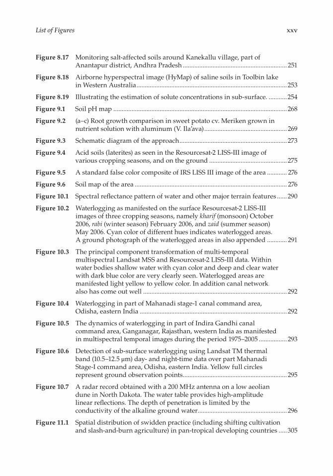
xxvList of Figures

Figure 8.17 Monitoring salt-affected soils around Kanekallu village, part of Anantapur district, Andhra Pradesh ............................................................... 251

Figure 8.18 Airborne hyperspectral image (HyMap) of saline soils in Toolbin lake in Western Australia ...........................................................................................253

Figure 8.19 Illustrating the estimation of solute concentrations in sub-surface. ...........254

Figure 9.1 Soil pH map ......................................................................................................... 268

Figure 9.2 (a–c) Root growth comparison in sweet potato cv. Meriken grown in nutrient solution with aluminum (V. Ila’ava) .................................................. 269

Figure 9.3 Schematic diagram of the approach ................................................................. 273

Figure 9.4 Acid soils (laterites) as seen in the Resourcesat-2 LISS-III image of various cropping seasons, and on the ground ............................................... 275

Figure 9.5 A standard false color composite of IRS LISS III image of the area ............ 276

Figure 9.6 Soil map of the area ............................................................................................ 276

Figure 10.1 Spectral reflectance pattern of water and other major terrain features ...... 290

Figure 10.2 Waterlogging as manifested on the surface Resourcesat-2 LISS-III images of three cropping seasons, namely kharif (monsoon) October 2006, rabi (winter season) February 2006, and zaid (summer season) May 2006. Cyan color of different hues indicates waterlogged areas. A ground photograph of the waterlogged areas in also appended ............ 291

Figure 10.3 The principal component transformation of multi-temporal multispectral Landsat MSS and Resourcesat-2 LISS-III data. Within water bodies shallow water with cyan color and deep and clear water with dark blue color are very clearly seen. Waterlogged areas are manifested light yellow to yellow color. In addition canal network also has come out well ....................................................................................... 292

Figure 10.4 Waterlogging in part of Mahanadi stage-1 canal command area, Odisha, eastern India ......................................................................................... 292

Figure 10.5 The dynamics of waterlogging in part of Indira Gandhi canal command area, Ganganagar, Rajasthan, western India as manifested in multispectral temporal images during the period 1975–2005 ................. 293

Figure 10.6 Detection of sub-surface waterlogging using Landsat TM thermal band (10.5–12.5 µm) day- and night-time data over part Mahanadi Stage-I command area, Odisha, eastern India. Yellow full circles represent ground observation points ............................................................... 295

Figure 10.7 A radar record obtained with a 200 MHz antenna on a low aeolian dune in North Dakota. The water table provides high-amplitude linear reflections. The depth of penetration is limited by the conductivity of the alkaline ground water...................................................... 296

Figure 11.1 Spatial distribution of swidden practice (including shifting cultivation and slash-and-burn agriculture) in pan-tropical developing countries .....305

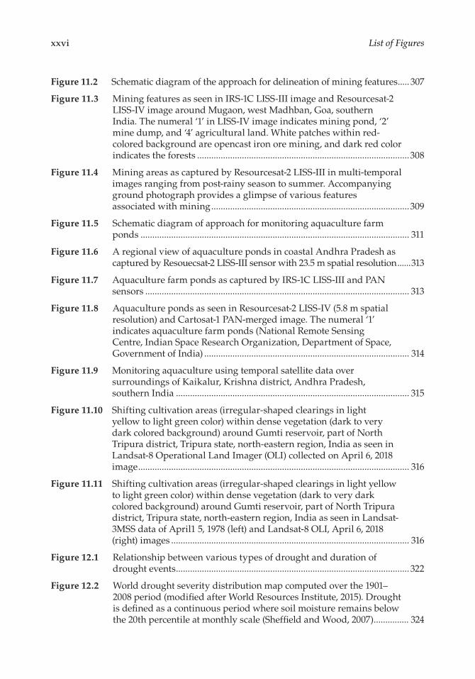
xxvi List of Figures

Figure 11.2 Schematic diagram of the approach for delineation of mining features ..... 307

Figure 11.3 Mining features as seen in IRS-1C LISS-III image and Resourcesat-2 LISS-IV image around Mugaon, west Madhban, Goa, southern India. The numeral ‘1’ in LISS-IV image indicates mining pond, ‘2’ mine dump, and ‘4’ agricultural land. White patches within red-colored background are opencast iron ore mining, and dark red color indicates the forests ..........................................................................................308

Figure 11.4 Mining areas as captured by Resourcesat-2 LISS-III in multi-temporal images ranging from post-rainy season to summer. Accompanying ground photograph provides a glimpse of various features associated with mining ....................................................................................309

Figure 11.5 Schematic diagram of approach for monitoring aquaculture farm ponds .................................................................................................................. 311

Figure 11.6 A regional view of aquaculture ponds in coastal Andhra Pradesh as captured by Resouecsat-2 LISS-III sensor with 23.5 m spatial resolution ......313

Figure 11.7 Aquaculture farm ponds as captured by IRS-1C LISS-III and PAN sensors ................................................................................................................ 313

Figure 11.8 Aquaculture ponds as seen in Resourcesat-2 LISS-IV (5.8 m spatial resolution) and Cartosat-1 PAN-merged image. The numeral ‘1’ indicates aquaculture farm ponds (National Remote Sensing Centre, Indian Space Research Organization, Department of Space, Government of India) ....................................................................................... 314

Figure 11.9 Monitoring aquaculture using temporal satellite data over surroundings of Kaikalur, Krishna district, Andhra Pradesh, southern India ................................................................................................... 315

Figure 11.10 Shifting cultivation areas (irregular-shaped clearings in light yellow to light green color) within dense vegetation (dark to very dark colored background) around Gumti reservoir, part of North Tripura district, Tripura state, north-eastern region, India as seen in Landsat-8 Operational Land Imager (OLI) collected on April 6, 2018 image ................................................................................................................... 316

Figure 11.11 Shifting cultivation areas (irregular-shaped clearings in light yellow to light green color) within dense vegetation (dark to very dark colored background) around Gumti reservoir, part of North Tripura district, Tripura state, north-eastern region, India as seen in Landsat-3MSS data of April1 5, 1978 (left) and Landsat-8 OLI, April 6, 2018 (right) images ..................................................................................................... 316

Figure 12.1 Relationship between various types of drought and duration of drought events ................................................................................................... 322

Figure 12.2 World drought severity distribution map computed over the 1901–2008 period (modified after World Resources Institute, 2015). Drought is defined as a continuous period where soil moisture remains below the 20th percentile at monthly scale (Sheffield and Wood, 2007) ............... 324

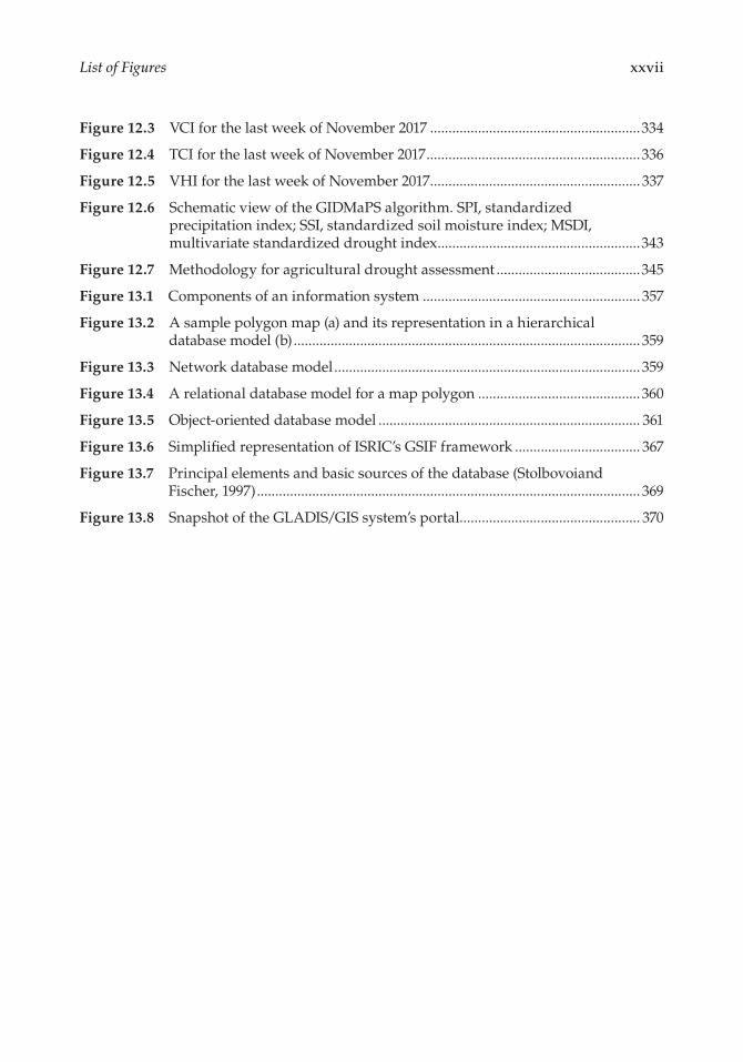
xxviiList of Figures

Figure 12.3 VCI for the last week of November 2017 .........................................................334

Figure 12.4 TCI for the last week of November 2017 ..........................................................336

Figure 12.5 VHI for the last week of November 2017 ......................................................... 337

Figure 12.6 Schematic view of the GIDMaPS algorithm. SPI, standardized precipitation index; SSI, standardized soil moisture index; MSDI, multivariate standardized drought index .......................................................343

Figure 12.7 Methodology for agricultural drought assessment .......................................345

Figure 13.1 Components of an information system ........................................................... 357

Figure 13.2 A sample polygon map (a) and its representation in a hierarchical database model (b) .............................................................................................. 359

Figure 13.3 Network database model ................................................................................... 359

Figure 13.4 A relational database model for a map polygon ............................................360

Figure 13.5 Object-oriented database model ....................................................................... 361

Figure 13.6 Simplified representation of ISRIC’s GSIF framework .................................. 367

Figure 13.7 Principal elements and basic sources of the database (Stolbovoiand Fischer, 1997) ........................................................................................................ 369

Figure 13.8 Snapshot of the GLADIS/GIS system’s portal................................................. 370

http://www.taylorandfrancis.com

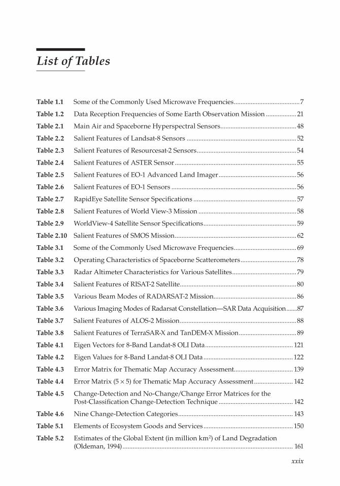
xxix

List of Tables

Table 1.1 Some of the Commonly Used Microwave Frequencies .......................................7

Table 1.2 Data Reception Frequencies of Some Earth Observation Mission .................. 21

Table 2.1 Main Air and Spaceborne Hyperspectral Sensors .............................................48

Table 2.2 Salient Features of Landsat-8 Sensors ................................................................. 52

Table 2.3 Salient Features of Resourcesat-2 Sensors ...........................................................54

Table 2.4 Salient Features of ASTER Sensor ........................................................................55

Table 2.5 Salient Features of EO-1 Advanced Land Imager ..............................................56

Table 2.6 Salient Features of EO-1 Sensors ..........................................................................56

Table 2.7 RapidEye Satellite Sensor Specifications ............................................................. 57

Table 2.8 Salient Features of World View-3 Mission ..........................................................58

Table 2.9 WorldView-4 Satellite Sensor Specifications ....................................................... 59

Table 2.10 Salient Features of SMOS Mission ........................................................................ 62

Table 3.1 Some of the Commonly Used Microwave Frequencies ..................................... 69

Table 3.2 Operating Characteristics of Spaceborne Scatterometers ................................. 78

Table 3.3 Radar Altimeter Characteristics for Various Satellites ...................................... 79

Table 3.4 Salient Features of RISAT-2 Satellite .....................................................................80

Table 3.5 Various Beam Modes of RADARSAT-2 Mission .................................................86

Table 3.6 Various Imaging Modes of Radarsat Constellation—SAR Data Acquisition .......87

Table 3.7 Salient Features of ALOS-2 Mission .....................................................................88

Table 3.8 Salient Features of TerraSAR-X and TanDEM-X Mission .................................. 89

Table 4.1 Eigen Vectors for 8-Band Landat-8 OLI Data .................................................... 121

Table 4.2 Eigen Values for 8-Band Landat-8 OLI Data ..................................................... 122

Table 4.3 Error Matrix for Thematic Map Accuracy Assessment................................... 139

Table 4.4 Error Matrix (5 × 5) for Thematic Map Accuracy Assessment ....................... 142

Table 4.5 Change-Detection and No-Change/Change Error Matrices for the Post-Classification Change-Detection Technique ............................................ 142

Table 4.6 Nine Change-Detection Categories .................................................................... 143

Table 5.1 Elements of Ecosystem Goods and Services ..................................................... 150

Table 5.2 Estimates of the Global Extent (in million km2) of Land Degradation (Oldeman, 1994) ..................................................................................................... 161

xxx List of Tables

Table 7.1 Some of the Sources of Free or Low-Cost Remote Sensing Data Suitable for Wind Erosion Studies ..................................................................................... 203

Table 7.2 Aerial Extent of Waterlogged Areas and Other Land Use/Land Cover Categories ............................................................................................................... 212

Table 8.1 Soil Salinity Classes in Terms of ECe (Richards, 1954) .................................... 231

Table 8.2 Extent of Salt-Affected Soils (Szabolcs, 1979) ....................................................233

Table 8.3 Keys to Degree of Soil Salinity and/or Alkalinity ........................................... 245

Table 9.1 Physical and Chemical Properties Soils of Virangipura Series ......................277

Table 12.1 Drought Categories Based on PDSI .................................................................... 327

Table 12.2 SPI Drought Categories ........................................................................................ 328

Table 13.1 Elements of Ecosystem Goods and Services ..................................................... 362

Table 13.2 GLADIS Global Databases. Inputs and outputs ............................................... 371

xxxi

Foreword

Land and soil degradation are increasingly important issues because of the ever-expanding demands of the growing and increasingly affluent world population. The world population (billion people) was 2.5 in 1950, 7.6 in 2017, and is projected to be 8.6 in 2030, 9.8 in 2050, and 11.2 in 2100. Similarly, the population of India (million people) was 376 in 1950, 1339 in 2017, and is projected to be 1513 in 2013, 1659 in 2050, and 1517 in 2100. Thus, it is the decline in per capita availability of land/soil resources which is the major cause of concern. Further, the concern is aggravated by the decrease in productivity and delivery of essential ecosystems services because of the decline of soil quality and health by a range of degradation processes. Important among these are physical (decline in soil structure leading to slaking, crusting, compaction, hard setting, erosion, runoff, inundation, drought), chemical (elemental imbalance leading to salinization, acidification, nutrient depletion, toxicity of certain heavy metals, decline in cation exchange capacity), biological (depletion of soil organic carbon concentration ad stock, decline in activity and species diversity of soil biota, methanogenesis, nitrification and denitrification, reduction in enzyme activity), and ecological (disruption in biogeochemical and biogeophysical cycling, perturbation of hydrological and energy balance, change in climax vegetation and the surface cover, decline in gross, net ecosystem and biome productivity).

Despite the widespread severity of the problem, the credible estimates of land area affected by diverse soil degradation processes are not available. Global estimates of the total land area affected by diverse degradation processes range from 1 to over 6 billion hectares, with a large range in estimates of spatial/geographical distribution; the annual rate of degradation; economical and ecological impacts; and predominant processes, causes and factors affecting the extent and severity. Similarly, the recent estimates of soil degradation in India range from 114 to 147 Mha.

It is widely believed that what cannot be precisely measured cannot be improved or restored. Peter Drucker stated that “You can’t manage what you can’t measure.” To know whether one is successful in restoration of degraded soils, it is important to know precisely what is being changed and by what criteria. It was Edward Deming who stated that “There are many things that cannot be measured and still must be managed.” Soil degradation is one such issue which, with the present state-of-the-knowledge, cannot be precisely measured. In addition to the lack of credible data on the extent and severity of degradation by different processes, there is also an insufficient knowledge regarding the threshold levels and critical limits of key soil properties in relation to specific land use (e.g., arable, pastoral, plantations, horticultural crops). Key soil properties, which can also differ among soil types, land uses, and climates, include bulk density soil organic carbon concentration, plant available water capacity, infiltration rate, air porosity at field moisture capacity, pH,  EC, CEC, nutrient reserves (macro and micro), enzyme activity, microbial biomass C, respiration quotient, etc. These critical properties are important to “soil functionality.”

Soil functionality refers to the capacity of soil to perform numerous functions. Important among these, and adversely affected by soil degradation, are (1) production of biomass, (2) moderation of climate, (3) cycling of elements, (4) decomposition of waste, (5) renewal and purification of water, (6) providing habitat for biodiversity, (7) creating media for plant growth, (8) being foundation of civil structures, (9) source of archive of human and planetary history, and (10) providing spiritual, aesthetical, cultural, and recreational

xxxii Foreword

opportunities. These functions are difficult to measure directly and are estimated through indices of soil quality and soil health. Soil degradation, its extent and severity, can also be estimated by assessing indices of soil quality and health.

Land/soil degradation is also relevant to several global issues. It affects food and nutritional security by reducing agronomic productivity and jeopardizing nutritional quality. Degradation aggravates the emission of greenhouse gases from soil into the atmosphere especially of CO2, CH4, and N2O. Gaseous emission is exacerbated by accelerated erosion, and inundation and anaerobiosis which increase methanogenesis, nitrification, denitrification, and mineralization. Water quality and renewability are adversely affected because of the increase in non-point source pollution and transport of dissolved and suspended loads. Algal bloom is aggravated by surface runoff from watersheds prone to soil degradation. Depletion of organic carbon and vegetation cover in ecosystem and soils reduce energy supply and habitat and adversely impact above-and below-ground biodiversity. Degraded landscapes are mirror images of the people who depend on it, and their well-being is adversely impacted by reduction in soil functionality.

The 13-chapter volume addresses pertinent themes related to the specific title such as in chapters: (1–3) Remote Sensing, (4) Digital Image Processing, (5–12) Soil Degradation Processes, and (13) Land Degradation Information Systems. These chapters address pertinent information on commonly observed and widely distributed degradation types. In addition to the processes addressed in these 13 chapters, soils of India and elsewhere in developing countries are also prone to degradation by depletion of plant nutrients and soil organic carbon, removal of topsoil or scalping to ~1 m depth for brickmaking, pollution and contamination by industrial effluent and radioactive wastes, encroachment by urbanization and surface sealing, etc. These, rather uncommon but important, degradation processes are adversely impacting soil health and reducing the per capita availability of scarce but pre-cious land resources. Therefore, land/soil degradation by these unconventional processes must also be assessed, restored, and managed. Yet, this volume is complimentary to several other books such as Characterization and Classification of Salt-Affected Soils by J.K. Jena and P. Parichita, and Remote Sensing for Soil Erosion Prediction by A.S. Budiharso.

Satellite imagery and remote sensing techniques, used to measure landscape parameters and terrain attributes, can be important tools in assessing the extent and severity of land/soil degradation, temporal changes, and geospatial distribution. It is precisely in this context that this volume “Geospatial Technology for Land Degradation Assessment and Management” by Dr. R. S. Dwivedi is timely and highly pertinent. The state-of-the- knowledge presented in the book is of interest to researchers but also to land managers and policymakers. The information presented is also relevant to advancing the Sustainable Development Goals (SDGs) of the United Nations and in implementing programs adopted by COP 21 (4 per Thousand) and COP 22 (Adapting African Agriculture). I commend Dr. R. S. Dwivedi for undertaking this timely initiative.

Rattan Lal,Distinguished University Professor of Soil Science, SENR

Director, Carbon Management and Sequestration CenterPresident, International Union of Soil Sciences

xxxiii

Preface

In order to ensure food security, bringing additional land under agriculture and enhanc-ing the productivity of available agricultural land are prerequisites. Globally, an estimated 1.9 billion hectares land is subject to land degradation—defined as a decline in land quality caused by human activities (Oldeman, 1994). Land degradation covers various forms of soil degradation, adverse human impacts on water resources, deforestation, and lower-ing of the productive capacity of rangelands and loss of biodiversity. The consequences of land degradation are reduced land productivity, socioeconomic problems, including uncertainty in food security, migration, limited development, and damage to ecosystems. Information on nature, magnitude, spatial extent, and dynamics of land degradation is a prerequisite for developing strategies to combat these processes and mitigate their effects at the land-management and policy level. Remote sensing and allied technologies like Geographic Information System (GIS), Personal Digital Assistant (PDA), Global Positioning System (GPS), and internet technology—collectively known as geospatial technologies—provide such information in timely and cost-effective manner.

The book initially introduces the geospatial technologies—basics of remote sensing, GIS and GPS remote sensors and systems, digital data processing, and data analysis/ interpretation techniques. It is followed by an overview of various land degradation processes. The subsequent chapters are dedicated to applications of geospatial technologies to major individual land degradation processes, namely soil erosion by water and wind, soil salinization and/or alkalinization, and waterlogging. Other land degradation processes like soil acidification, mining, aquaculture and shifting cultivation are also addressed appropriately in other chapters. The drought which accelerates the land degradation pro-cess is dealt with in the next chapter. The last chapter addresses the development of the information system on degraded lands that would enable updation and dissemination of digital data on degraded lands to the end users.

It is shown how remote sensing data may be utilized for inventorying, assessing, and monitoring affected ecosystems and how this information may be assimilated into integrated interpretation and modeling concepts. Additionally, case studies demonstrating the utility of geospatial technologies in generating information on degraded lands required for their rehabilitation are embedded in the frame of different local settings. Lastly, the future challenges in applications of geospatial technologies in land degradation studies are also enumerated.

R. S. DwivediHyderabad, India

Reference

Oldeman, L.R., 1994. The global extent of land degradation. In: Greenland, D.J., and Szabolcs,  I., (eds.) Land Resilience and Sustainable Land Use. CABI, Wallingford, pp. 99–118.

http://www.taylorandfrancis.com

xxxv

Acknowledgments

At the outset, I express my heartfelt thanks to Krish, my grandson, for inspiration that I received for the stupendous task of preparing the manuscript of the book. In fact, I conceived the idea of this task when I was in Fremont, California, USA with him. My sincere thanks also go to Dr. Ram Shankar Dwivedi, brother, and Ms. Suman Dwivedi, sister-in-law for their blessings in this endeavor. Furthermore, the incessant encouragement and moral support received from Ms. Dolly Dwivedi, daughter, and Shri Karik Vittal, son-in-law, is beyond the words of expression. The concepts and illustrations are the soul of any literary work. In this context, the technical support received from Shri Samik Saha, Team Lead, Ms. M.S. Mahathi, Associate Analyst, Content Engineering Global Logic Technologies Pvt. Ltd., Hyderabad in generating the illustration from digital images has been apt and timely. I express my sincere gratitude to Prof. Rattan Lal, Distinguished University Professor of Soil Science, Ohio State University, USA for sparing his valuable in giving foreword of the book.

I am indebted to Dr. Y.V.N. Krishnamurthy, Distinguished Scientist and Director, National Remote Sensing Centre (NRSC), Indian Space Research Organization, Hyderabad for pro-viding satellite data, and thematic maps and library facility that have added strength to the technical content of the book. Special thanks are due to Dr. T. Ravisankar, Group Director Land Resources, Land Use Mapping and Monitoring Group, NRSC for providing illustrations on potential of Resourcesesat-2 LISS-III data for mapping land degradation. Besides, timely technical and logistics support provided by Shri P. Ravinder, In-charge Library, NRSC, and his colleagues. Ms. Seema Kukarni and Ms. Suman S. Paul have been instrumental in preparing the manuscript.

I am extremely thankful to Dr. Ch V. Rao, Group Head, Special Products, NRSC for offering necessary suggestions and comments on the chapter on Digital Image Processing. Discussions with Dr. M.V.R. Sesha Sai, Deputy Director, Earth and Atmospheric Sciences Area, Dr. T. Ravisankar, and Dr. K. Srinivas, NRSC have been of immense help in final-izing the manuscript.

I also express my sincere thanks to Dr. N. Aparna, Group Head, NDC and her Associate Ms. K. Swarupa Rani for sharing promotional satellite data products, and to Shri G.P. Swamy, IRS Optical Data Processing Group, and Shri R. Anjaneyulu, Shri E. Venkateswarulu and Ms. Asra Majid, Senior Research Fellow, NRSC for providing sample images of the Indian Earth observation mission data and necessary technical support.

I am also thankful to the Food and Agriculture Organization (FAO) and International Soil Reference and Information Centre (ISRIC) for generously granting the permission to use and reproduce the material related to maps on land degradation. Thanks are also due to Dr. Reich Paul, USDA-NRCS, Soil Science Division, World Soil Resources for permitting to reproduce soil pH map of the world. The technical support received from the CRC Press publisher-deserves special thanks.

The encouragement and moral support provided by Shri J. Venkatesh, Associate Professor, Prof. K. Ramamohan Reddy, Prof. C. Sarala and Prof. M. Vishwanadham, Centre for Spatial Information Technology (CSIT), JNTUH is duly acknowledged. Thanks are also due to Shri L. Ravi, Doctoral scholar, Shri Ballu Harish, Faculty, CSIT for providing necessary technical support, and to Shri R. Naresh for secretarial support in finalizing the manuscript. Last but not the least, I am also thankful to all the authors of articles and the books that I have referred to and to those who have directly or indirectly contributed to the success of this mission.

http://www.taylorandfrancis.com

xxxvii

Author

Dr. R. S. Dwivedi earned his master’s and PhD degrees in Agricultural Chemistry from University of Allahabad, India, in 1973 and 1977, respectively, and Advanced Diploma in Remote Sensing from the University of Berlin, Germany, in 1979. He had joined the National Remote Sensing Agency (now National Remote Sensing Centre), Department of Space, Government of India, in December 1977. Dr. Dwivedi pursued his research career at National Remote Sensing Agency in applications of remote sensing technology for inven-tory and mapping of soil resources including land degradation. The author played a key role in mapping of salt-affected soils, wastelands, and land use/land cover mapping and monitoring for the Indian subcontinent. He is endowed with around 40 years’ experience in applications of remote sensing. The testimony of such an achievement is reflected in terms of research articles (84) in national and international journals, awards (from Indian Society of Remote Sensing, and Doreen Mashler Team Award from International Crops Research Institute for Semi-arid Tropics, Hyderabad), and fellowships of the National Academy of Agricultural Sciences, India, Indian Geophysical Union and A.P. Academy of Sciences. He has contributed 13 book chapters, co-edited two books—Remote Sensing Applications and Geospatial Technology for Integrated Natural Resources Management. Also he authored a book titled “Remote Sensing of Soils” with Springer-Verlag, Germany. Furthermore, he had also lead a team of soil scientists, as Head Land Degradation Division, and superannu-ated as group director, Land Resources in 2011. He has been offered assignments from the Government of Ethiopia as a professor, Soil Science for a period of 2 years (2013 and 2014) at Hamaraya University, and at Mekelle University from October 2015 to September 2017. He has been associated with Jawaharlal Nehru Technological University, Hyderabad (JNTUH), India, since 2012 as a guest faculty member. Currently, he is academic adviser at, Geospatial Information Technology, JNTUH.

http://www.taylorandfrancis.com

1

1An Introduction to Geospatial Technology

1.1 Introduction

Derived from two Latin words—remotus, meaning far away or distant in time or place, and sensus meaning to detect a stimulus by means of any of the five senses—remote sensing refers to detecting an object/feature/phenomenon with an observation device that is not in intimate physical contact with it. According to Colwell (1966), the term remote sensing in its broadest sense merely means “reconnaissance at a distance.” The process of making measurements or taking observations in the laboratory or field is termed proximal sensing. Remote sensing thus differs from proximal sensing in the way information is gathered about an object/feature or phenomenon. While the instruments are immersed in, or physically touch, the objects of measurement in proximal sensing or in situ measurements, the sensing device is invariably not in physical contact with the objects in the case of remote sensing. In the context of Earth observations and environmental management practice, remote sensing refers, in general sense, to the instrumentation, techniques, and methods used to observe, or sense, the surface of the Earth usually by the formation of an image in a position, station-ary or mobile, at a certain distance from that surface (Buiten and Clevers, 1993).

During the pre-1960s period, the concept of remote sensing was confined to the devel-opment of different components of photography, i.e., various types of films, camera, film processing and printing systems, interpretation techniques, and photogrammetry. By the early 1960s, many new types of sensing devices were being introduced that could detect electromagnetic radiation (EMR) in spectral regions far beyond the range of visible spec-trum or human vision and photographic films. In order to accommodate these develop-ments, Evelyn L. Pruitt, a geographer formerly with the US Office of Naval Research, coined the term remote sensing to replace the more limiting term aerial photographs.

1.1.1 Geospatial Technology

With the development of computer technology in 1960s and realization of the potential of integrating the information on natural resources to derive more comprehensive and meaningful information and arriving at decisions for planning and management of nat-ural resources and environment, the concept of a new technology called Geographical Information System (GIS) was developed. In this context, precise location of features assumes greater significance. For precise location of observations and information on nat-ural resources and environment, satellite-based navigation system was developed in 1960.

Developments of Internet technology and its integration with the computer technology ultimately culminated into the development of personal digital assistant (PDA) devices that enabled transmitting the in situ observations on natural disasters and other highly

2 Geospatial Technologies

dynamic phenomenon requiring real-or near-real-time field data for analysis and/or inter-pretation of remote sensing data. In an attempt to accommodate a host of these newly developed technologies, i.e., remote sensing, GIS, satellite-based navigation, and PDAs, a new term, geospatial technology or geomatics or geoinformatics, was coined.

Geospatial technology refers to equipment used in visualization, measurement, and analysis of Earth’s features, typically involving such systems as remote sensing, GIS, and global positioning system (GPS). In other words, the term geospatial technology is used to define the collective data and associated technology that has a geographic or locational component. It has been defined as“ An integrated science and technology that deals with acquisition and manipulation of geographical data, transforming it into useful informa-tion using geoscientific, analytical, and visualization techniques for making better deci-sions” (Jaganathan, 2011). Geoinformatics—another term used sometimes as synonym to geospatial technology—has been defined as “a descriptive which integrates the acquisition, modeling, analysis and management of spatially referenced data” (Lein, 2012).

In remote sensing systems, the information from the object/target is carried through EMR. That is to say, the EMR acts as a carrier of information from the object/target to the sensing instrument(s). The radiant energy thus captured by the sensing instruments is used by the image interpreter/analysts to derive information on the object/target. In the case of spectral measurements in the laboratory or in situ (field), the radiation reflected/scattered or emitted is captured as it is without any interference by the medium between the objects/target and sensing instruments. This is also true to some extent in case of airborne sensors operating in the optical region of the electromagnetic spectrum (EMS). When the spectral measurements are made from the space, the intervening atmosphere modulates both radiant energy emanating from the source to the object/target and that reflected/scattered from the target reaching the sensing instruments. The sensors capture reflected/emitted/backscattered EMR from the object/feature. These sensors/instruments are of two types, i.e., passive sensors and active sensors. Passive sensors detect natural energy (radiation) that is reflected or emitted by the object. Reflected sunlight is the most com-mon source of radiation measured by passive sensors. Examples of passive remote sensors include film photography, charge-coupled devices, and radiometers. Active sensors, on the other hand, have their own source of energy to illuminate the object or terrain and record the backscattered energy from there. Radar and LiDAR are examples of active sensors where the time delay between disseminated and return radiation is measured and is used for establishing the location, height, speed, and direction of an object/feature.

1.2 History of Remote Sensing

Historically, the airborne remote sensing was primarily focused on surveying, reconnais-sance, strategic land use mapping, and military surveillance during the First and Second World Wars. The focus was shifted subsequently to early space-borne systems dominated by the launch of Sputnik-1 and Explorer-1 erstwhile USSR and USA in 1957 and 1958, respectively. The launch of advanced meteorological satellites, namely Television Infrared Observation Satellite (TIROS) series in 1960, marked the beginning of space-borne Earth observation systems. In fact, the major breakthrough in Earth observation from space was achieved with the launch of Landsat-1 in 1972. Several satellites, namely Landsat series, Landsat-2 through -8, le Système Pour Observation de la Terre (SPOT), and Indian Remote

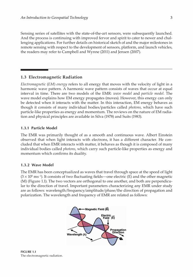
3An Introduction to Geospatial Technology

Sensing series of satellites with the state-of-the-art sensors, were subsequently launched. And the process is continuing with improved fervor and spirit to cater to newer and chal-lenging applications. For further details on historical sketch of and the major milestones in remote sensing with respect to the development of sensors, platform, and launch vehicles, the readers may refer to Campbell and Wynne (2011) and Jensen (2007).

1.3 Electromagnetic Radiation

Electromagnetic (EM) energy refers to all energy that moves with the velocity of light in a harmonic wave pattern. A harmonic wave pattern consists of waves that occur at equal interval in time. There are two models of the EMR: wave model and particle model. The wave model explains how EM energy propagates (moves). However, this energy can only be detected when it interacts with the matter. In this interaction, EM energy behaves as though it consists of many individual bodies/particles called photons, which have such particle-like properties as energy and momentum. The reviews on the nature of EM radia-tion and physical principles are available in Silva (1978) and Suits (1983).

1.3.1 Particle Model

The EMR was primarily thought of as a smooth and continuous wave. Albert Einstein observed that when light interacts with electrons, it has a different character. He con-cluded that when EMR interacts with matter, it behaves as though it is composed of many individual bodies called photons, which carry such particle-like properties as energy and momentum which confirms its duality.

1.3.2 Wave Model

The EMR has been conceptualized as waves that travel through space at the speed of light (3 × 108 ms−1). It consists of two fluctuating fields—one electric (E) and the other magnetic (M) (Figure 1.1). The two vectors are orthogonal to one another, and both are perpendicu-lar to the direction of travel. Important parameters characterizing any EMR under study are as follows: wavelength/frequency/amplitude/phase/the direction of propagation and polarization. The wavelength and frequency of EMR are related as follows:

FIGURE 1.1The electromagnetic radiation.

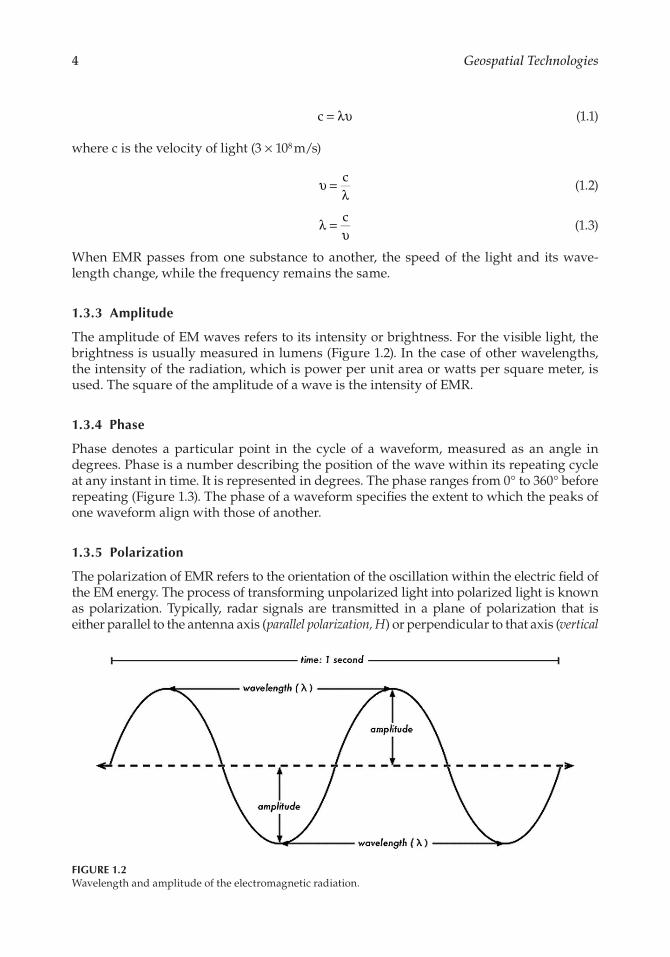
4 Geospatial Technologies

c = λυ (1.1)

where c is the velocity of light (3 × 108 m/s)

cυ =λ

(1.2)

cλ =υ

(1.3)

When EMR passes from one substance to another, the speed of the light and its wave-length change, while the frequency remains the same.

1.3.3 Amplitude

The amplitude of EM waves refers to its intensity or brightness. For the visible light, the brightness is usually measured in lumens (Figure 1.2). In the case of other wavelengths, the intensity of the radiation, which is power per unit area or watts per square meter, is used. The square of the amplitude of a wave is the intensity of EMR.

1.3.4 Phase

Phase denotes a particular point in the cycle of a waveform, measured as an angle in degrees. Phase is a number describing the position of the wave within its repeating cycle at any instant in time. It is represented in degrees. The phase ranges from 0° to 360° before repeating (Figure 1.3). The phase of a waveform specifies the extent to which the peaks of one waveform align with those of another.

1.3.5 Polarization

The polarization of EMR refers to the orientation of the oscillation within the electric field of the EM energy. The process of transforming unpolarized light into polarized light is known as polarization. Typically, radar signals are transmitted in a plane of polarization that is either parallel to the antenna axis (parallel polarization, H) or perpendicular to that axis (vertical

FIGURE 1.2Wavelength and amplitude of the electromagnetic radiation.

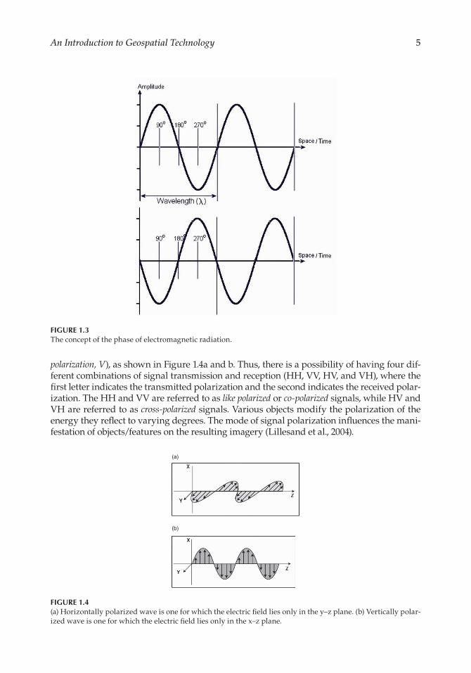
5An Introduction to Geospatial Technology

polarization, V), as shown in Figure 1.4a and b. Thus, there is a possibility of having four dif-ferent combinations of signal transmission and reception (HH, VV, HV, and VH), where the first letter indicates the transmitted polarization and the second indicates the received polar-ization. The HH and VV are referred to as like polarized or co-polarized signals, while HV and VH are referred to as cross-polarized signals. Various objects modify the polarization of the energy they reflect to varying degrees. The mode of signal polarization influences the mani-festation of objects/features on the resulting imagery (Lillesand et al., 2004).

FIGURE 1.3The concept of the phase of electromagnetic radiation.

(a)

(b)

FIGURE 1.4(a) Horizontally polarized wave is one for which the electric field lies only in the y–z plane. (b) Vertically polar-ized wave is one for which the electric field lies only in the x–z plane.

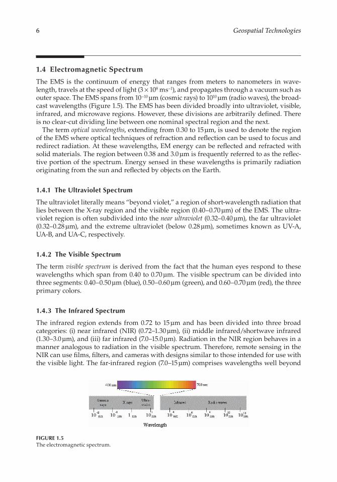
6 Geospatial Technologies

1.4 Electromagnetic Spectrum

The EMS is the continuum of energy that ranges from meters to nanometers in wave-length, travels at the speed of light (3 × 108 ms−1), and propagates through a vacuum such as outer space. The EMS spans from 10−10 µm (cosmic rays) to 1010 µm (radio waves), the broad-cast wavelengths (Figure 1.5). The EMS has been divided broadly into ultraviolet, visible, infrared, and microwave regions. However, these divisions are arbitrarily defined. There is no clear-cut dividing line between one nominal spectral region and the next.

The term optical wavelengths, extending from 0.30 to 15 µm, is used to denote the region of the EMS where optical techniques of refraction and reflection can be used to focus and redirect radiation. At these wavelengths, EM energy can be reflected and refracted with solid materials. The region between 0.38 and 3.0 µm is frequently referred to as the reflec-tive portion of the spectrum. Energy sensed in these wavelengths is primarily radiation originating from the sun and reflected by objects on the Earth.

1.4.1 The Ultraviolet Spectrum

The ultraviolet literally means “beyond violet,” a region of short-wavelength radiation that lies between the X-ray region and the visible region (0.40–0.70 µm) of the EMS. The ultra-violet region is often subdivided into the near ultraviolet (0.32–0.40 µm), the far ultraviolet (0.32–0.28 µm), and the extreme ultraviolet (below 0.28 µm), sometimes known as UV-A, UA-B, and UA-C, respectively.

1.4.2 The Visible Spectrum

The term visible spectrum is derived from the fact that the human eyes respond to these wavelengths which span from 0.40 to 0.70 µm. The visible spectrum can be divided into three segments: 0.40–0.50 µm (blue), 0.50–0.60 µm (green), and 0.60–0.70 µm (red), the three primary colors.

1.4.3 The Infrared Spectrum

The infrared region extends from 0.72 to 15 µm and has been divided into three broad categories: (i) near infrared (NIR) (0.72–1.30 µm), (ii) middle infrared/shortwave infrared (1.30–3.0 µm), and (iii) far infrared (7.0–15.0 µm). Radiation in the NIR region behaves in a manner analogous to radiation in the visible spectrum. Therefore, remote sensing in the NIR can use films, filters, and cameras with designs similar to those intended for use with the visible light. The far-infrared region (7.0–15 µm) comprises wavelengths well beyond

FIGURE 1.5The electromagnetic spectrum.

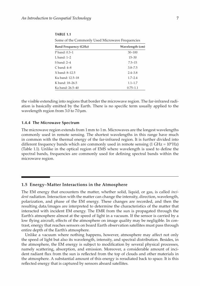
7An Introduction to Geospatial Technology

the visible extending into regions that border the microwave region. The far-infrared radi-ation is basically emitted by the Earth. There is no specific term usually applied to the wavelength region from 3.0 to 7.0 µm.

1.4.4 The Microwave Spectrum

The microwave region extends from 1 mm to 1 m. Microwaves are the longest wavelengths commonly used in remote sensing. The shortest wavelengths in this range have much in common with the thermal energy of the far-infrared region. It is further divided into different frequency bands which are commonly used in remote sensing (1 GHz = 109 Hz) (Table 1.1). Unlike in the optical region of EMS where wavelength is used to define the spectral bands, frequencies are commonly used for defining spectral bands within the microwave region.

1.5 Energy–Matter Interactions in the Atmosphere

The EM energy that encounters the matter, whether solid, liquid, or gas, is called inci-dent radiation. Interaction with the matter can change the intensity, direction, wavelength, polarization, and phase of the EM energy. These changes are recorded, and then the resulting data/images are interpreted to determine the characteristics of the matter that interacted with incident EM energy. The EMR from the sun is propagated through the Earth’s atmosphere almost at the speed of light in a vacuum. If the sensor is carried by a low flying aircraft, effects of the atmosphere on image quality may be negligible. In con-trast, energy that reaches sensors on board Earth observation satellites must pass through entire depth of the Earth’s atmosphere.

Unlike a vacuum where nothing happens, however, atmosphere may affect not only the speed of light but also its wavelength, intensity, and spectral distribution. Besides, in the atmosphere, the EM energy is subject to modification by several physical processes, namely scattering, absorption, and emission. Moreover, a considerable amount of inci-dent radiant flux from the sun is reflected from the top of clouds and other materials in the atmosphere. A substantial amount of this energy is reradiated back to space. It is this reflected energy that is captured by sensors aboard satellites.

TABLE 1.1

Some of the Commonly Used Microwave Frequencies

Band Frequency (GHz) Wavelength (cm)

P band: 0.3–1 30–100

L band: 1–2 15–30

S band: 2–4 7.5–15

C band: 4–8 3.8–7.5

X band: 8–12.5 2.4–3.8

Ku band: 12.5–18 1.7–2.4

K band: 18–26.5 1.1–1.7

Ka band: 26.5–40 0.75–1.1

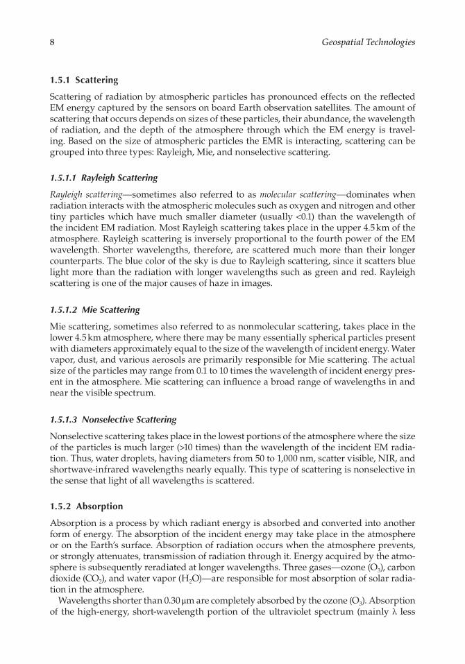
8 Geospatial Technologies

1.5.1 Scattering

Scattering of radiation by atmospheric particles has pronounced effects on the reflected EM energy captured by the sensors on board Earth observation satellites. The amount of scattering that occurs depends on sizes of these particles, their abundance, the wavelength of radiation, and the depth of the atmosphere through which the EM energy is travel-ing. Based on the size of atmospheric particles the EMR is interacting, scattering can be grouped into three types: Rayleigh, Mie, and nonselective scattering.

1.5.1.1 Rayleigh Scattering

Rayleigh scattering—sometimes also referred to as molecular scattering—dominates when radiation interacts with the atmospheric molecules such as oxygen and nitrogen and other tiny particles which have much smaller diameter (usually <0.1) than the wavelength of the incident EM radiation. Most Rayleigh scattering takes place in the upper 4.5 km of the atmosphere. Rayleigh scattering is inversely proportional to the fourth power of the EM wavelength. Shorter wavelengths, therefore, are scattered much more than their longer counterparts. The blue color of the sky is due to Rayleigh scattering, since it scatters blue light more than the radiation with longer wavelengths such as green and red. Rayleigh scattering is one of the major causes of haze in images.

1.5.1.2 Mie Scattering

Mie scattering, sometimes also referred to as nonmolecular scattering, takes place in the lower 4.5 km atmosphere, where there may be many essentially spherical particles present with diameters approximately equal to the size of the wavelength of incident energy. Water vapor, dust, and various aerosols are primarily responsible for Mie scattering. The actual size of the particles may range from 0.1 to 10 times the wavelength of incident energy pres-ent in the atmosphere. Mie scattering can influence a broad range of wavelengths in and near the visible spectrum.

1.5.1.3 Nonselective Scattering

Nonselective scattering takes place in the lowest portions of the atmosphere where the size of the particles is much larger (>10 times) than the wavelength of the incident EM radia-tion. Thus, water droplets, having diameters from 50 to 1,000 nm, scatter visible, NIR, and shortwave-infrared wavelengths nearly equally. This type of scattering is nonselective in the sense that light of all wavelengths is scattered.

1.5.2 Absorption

Absorption is a process by which radiant energy is absorbed and converted into another form of energy. The absorption of the incident energy may take place in the atmosphere or on the Earth’s surface. Absorption of radiation occurs when the atmosphere prevents, or strongly attenuates, transmission of radiation through it. Energy acquired by the atmo-sphere is subsequently reradiated at longer wavelengths. Three gases—ozone (O3), carbon dioxide (CO2), and water vapor (H2O)—are responsible for most absorption of solar radia-tion in the atmosphere.

Wavelengths shorter than 0.30 μm are completely absorbed by the ozone (O3). Absorption of the high-energy, short-wavelength portion of the ultraviolet spectrum (mainly λ less

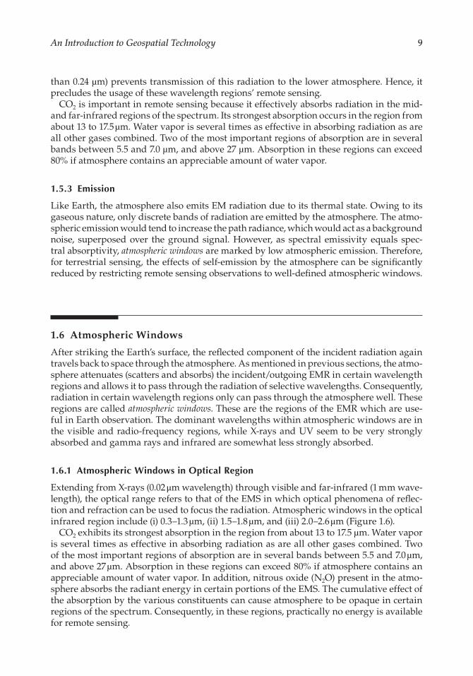
9An Introduction to Geospatial Technology

than 0.24 µm) prevents transmission of this radiation to the lower atmosphere. Hence, it precludes the usage of these wavelength regions’ remote sensing.

CO2 is important in remote sensing because it effectively absorbs radiation in the mid- and far-infrared regions of the spectrum. Its strongest absorption occurs in the region from about 13 to 17.5 µm. Water vapor is several times as effective in absorbing radiation as are all other gases combined. Two of the most important regions of absorption are in several bands between 5.5 and 7.0 µm, and above 27 µm. Absorption in these regions can exceed 80% if atmosphere contains an appreciable amount of water vapor.

1.5.3 Emission

Like Earth, the atmosphere also emits EM radiation due to its thermal state. Owing to its gaseous nature, only discrete bands of radiation are emitted by the atmosphere. The atmo-spheric emission would tend to increase the path radiance, which would act as a background noise, superposed over the ground signal. However, as spectral emissivity equals spec-tral absorptivity, atmospheric windows are marked by low atmospheric emission. Therefore, for terrestrial sensing, the effects of self-emission by the atmosphere can be significantly reduced by restricting remote sensing observations to well-defined atmospheric windows.

1.6 Atmospheric Windows

After striking the Earth’s surface, the reflected component of the incident radiation again travels back to space through the atmosphere. As mentioned in previous sections, the atmo-sphere attenuates (scatters and absorbs) the incident/outgoing EMR in certain wavelength regions and allows it to pass through the radiation of selective wavelengths. Consequently, radiation in certain wavelength regions only can pass through the atmosphere well. These regions are called atmospheric windows. These are the regions of the EMR which are use-ful in Earth observation. The dominant wavelengths within atmospheric windows are in the visible and radio-frequency regions, while X-rays and UV seem to be very strongly absorbed and gamma rays and infrared are somewhat less strongly absorbed.

1.6.1 Atmospheric Windows in Optical Region

Extending from X-rays (0.02 μm wavelength) through visible and far-infrared (1 mm wave-length), the optical range refers to that of the EMS in which optical phenomena of reflec-tion and refraction can be used to focus the radiation. Atmospheric windows in the optical infrared region include (i) 0.3–1.3 µm, (ii) 1.5–1.8 µm, and (iii) 2.0–2.6 µm (Figure 1.6).

CO2 exhibits its strongest absorption in the region from about 13 to 17.5 µm. Water vapor is several times as effective in absorbing radiation as are all other gases combined. Two of the most important regions of absorption are in several bands between 5.5 and 7.0 µm, and above 27 µm. Absorption in these regions can exceed 80% if atmosphere contains an appreciable amount of water vapor. In addition, nitrous oxide (N2O) present in the atmo-sphere absorbs the radiant energy in certain portions of the EMS. The cumulative effect of the absorption by the various constituents can cause atmosphere to be opaque in certain regions of the spectrum. Consequently, in these regions, practically no energy is available for remote sensing.

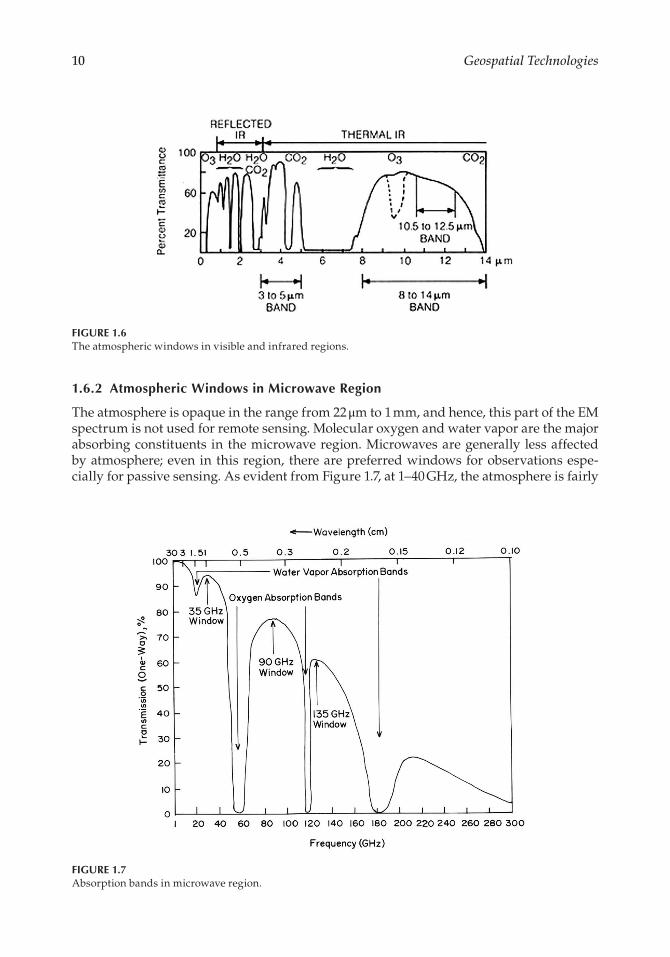
10 Geospatial Technologies

1.6.2 Atmospheric Windows in Microwave Region

The atmosphere is opaque in the range from 22 μm to 1 mm, and hence, this part of the EM spectrum is not used for remote sensing. Molecular oxygen and water vapor are the major absorbing constituents in the microwave region. Microwaves are generally less affected by atmosphere; even in this region, there are preferred windows for observations espe-cially for passive sensing. As evident from Figure 1.7, at 1–40 GHz, the atmosphere is fairly

FIGURE 1.6The atmospheric windows in visible and infrared regions.

FIGURE 1.7Absorption bands in microwave region.

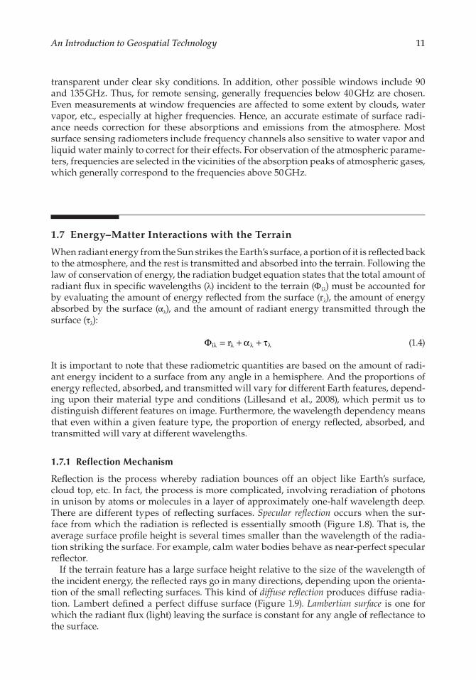
11An Introduction to Geospatial Technology

transparent under clear sky conditions. In addition, other possible windows include 90 and 135 GHz. Thus, for remote sensing, generally frequencies below 40 GHz are chosen. Even measurements at window frequencies are affected to some extent by clouds, water vapor, etc., especially at higher frequencies. Hence, an accurate estimate of surface radi-ance needs correction for these absorptions and emissions from the atmosphere. Most surface sensing radiometers include frequency channels also sensitive to water vapor and liquid water mainly to correct for their effects. For observation of the atmospheric parame-ters, frequencies are selected in the vicinities of the absorption peaks of atmospheric gases, which generally correspond to the frequencies above 50 GHz.

1.7 Energy–Matter Interactions with the Terrain

When radiant energy from the Sun strikes the Earth’s surface, a portion of it is reflected back to the atmosphere, and the rest is transmitted and absorbed into the terrain. Following the law of conservation of energy, the radiation budget equation states that the total amount of radiant flux in specific wavelengths (λ) incident to the terrain (Φiλ) must be accounted for by evaluating the amount of energy reflected from the surface (rλ), the amount of energy absorbed by the surface (αλ), and the amount of radiant energy transmitted through the surface (τλ):

riΦ = + α + τλ λ λ λ (1.4)

It is important to note that these radiometric quantities are based on the amount of radi-ant energy incident to a surface from any angle in a hemisphere. And the proportions of energy reflected, absorbed, and transmitted will vary for different Earth features, depend-ing upon their material type and conditions (Lillesand et al., 2008), which permit us to distinguish different features on image. Furthermore, the wavelength dependency means that even within a given feature type, the proportion of energy reflected, absorbed, and transmitted will vary at different wavelengths.

1.7.1 Reflection Mechanism

Reflection is the process whereby radiation bounces off an object like Earth’s surface, cloud top, etc. In fact, the process is more complicated, involving reradiation of photons in unison by atoms or molecules in a layer of approximately one-half wavelength deep. There are different types of reflecting surfaces. Specular reflection occurs when the sur-face from which the radiation is reflected is essentially smooth (Figure 1.8). That is, the average surface profile height is several times smaller than the wavelength of the radia-tion striking the surface. For example, calm water bodies behave as near-perfect specular reflector.

If the terrain feature has a large surface height relative to the size of the wavelength of the incident energy, the reflected rays go in many directions, depending upon the orienta-tion of the small reflecting surfaces. This kind of diffuse reflection produces diffuse radia-tion. Lambert defined a perfect diffuse surface (Figure 1.9). Lambertian surface is one for which the radiant flux (light) leaving the surface is constant for any angle of reflectance to the surface.

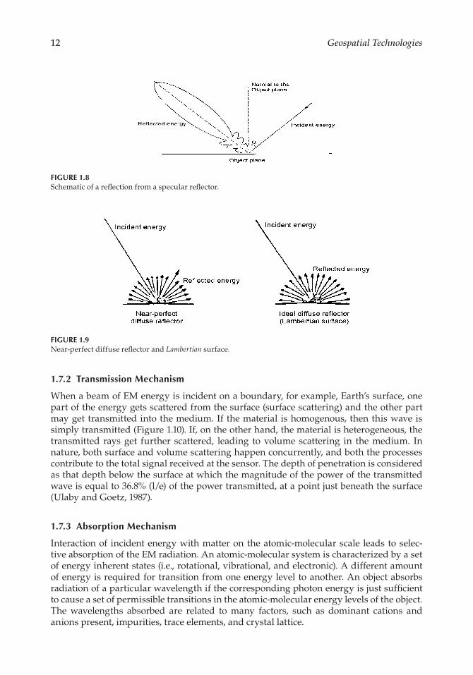
12 Geospatial Technologies

1.7.2 Transmission Mechanism

When a beam of EM energy is incident on a boundary, for example, Earth’s surface, one part of the energy gets scattered from the surface (surface scattering) and the other part may get transmitted into the medium. If the material is homogenous, then this wave is simply transmitted (Figure 1.10). If, on the other hand, the material is heterogeneous, the transmitted rays get further scattered, leading to volume scattering in the medium. In nature, both surface and volume scattering happen concurrently, and both the processes contribute to the total signal received at the sensor. The depth of penetration is considered as that depth below the surface at which the magnitude of the power of the transmitted wave is equal to 36.8% (l/e) of the power transmitted, at a point just beneath the surface (Ulaby and Goetz, 1987).

1.7.3 Absorption Mechanism

Interaction of incident energy with matter on the atomic-molecular scale leads to selec-tive absorption of the EM radiation. An atomic-molecular system is characterized by a set of energy inherent states (i.e., rotational, vibrational, and electronic). A different amount of energy is required for transition from one energy level to another. An object absorbs radiation of a particular wavelength if the corresponding photon energy is just sufficient to cause a set of permissible transitions in the atomic-molecular energy levels of the object. The wavelengths absorbed are related to many factors, such as dominant cations and anions present, impurities, trace elements, and crystal lattice.

FIGURE 1.8Schematic of a reflection from a specular reflector.

FIGURE 1.9Near-perfect diffuse reflector and Lambertian surface.

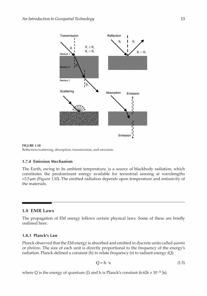
13An Introduction to Geospatial Technology

1.7.4 Emission Mechanism

The Earth, owing to its ambient temperature, is a source of blackbody radiation, which constitutes the predominant energy available for terrestrial sensing at wavelengths >3.5 μm (Figure 1.10). The emitted radiation depends upon temperature and emissivity of the materials.

1.8 EMR Laws

The propagation of EM energy follows certain physical laws. Some of these are briefly outlined here.

1.8.1 Planck’s Law

Planck observed that the EM energy is absorbed and emitted in discrete units called quanta or photons. The size of each unit is directly proportional to the frequency of the energy’s radiation. Planck defined a constant (h) to relate frequency (υ) to radiant energy (Q):

Q h= ⋅ υ (1.5)

where Q is the energy of quantum (J) and h is Planck’s constant (6.626 × 10−34 Js).

FIGURE 1.10Reflection/scattering, absorption, transmission, and emission.

14 Geospatial Technologies

By substituting Q for hυ, we can express the wavelength associated with a quantum of energy as

hcQ

λ = (1.6)

or

Qhc=λ

(1.7)

where c is the speed of light (3 × 108 ms−1).The above equation implies that the longer the wavelength involved, the lower is its

energy content. It has relevance in remote sensing in that when we are measuring the reflected/emitted EMR from the objects or features at longer wavelengths, in order to have detectable signals, the reflected or emitted energy from a larger area needs to be inte-grated. It implies that while other conditions remain constant, the spatial resolutions of the sensor become coarser with increasing wavelengths.

Planck’s law allows us to calculate the total energy radiated in all directions from a blackbody (radiator) for a particular temperature and wavelength:

Mc

(e 1)W (m m)1

5 c T2

2= ε

λ −µλ λ (1.8)

where Mλ = spectral radiant exitance, W/(m2 µm)ε = emittance (emissivity), dimensionlessC1 = first radiation constant, 3.74 × 10−8 W (µm)4/m2

C2 = second radiation constant, 1.43884 × 104 µm Kλ = radiation wavelength, µmT = absolute temperature, K

The Earth radiates roughly like the 300 K curve and the Sun like the 5,800 K curve (Figure 1.11). It may be noted that the maximum of the Sun’s radiation is at the wavelengths that are visible to human eyes.

1.8.2 Stefan–Boltzmann Law

The Stefan–Boltzmann law states that the total emitted radiation from a blackbody (M) measured in Watts per square meter is proportional to the fourth power of its absolute temperature (T) measured in kelvin. This is expressed as

M Tb4= σ (1.9)

where σ is the Stefan–Boltzmann constant (5.6697 × 10−8 Wm−2 K−4) and T is the absolute temperature in kelvin.

A blackbody is a theoretical construct that absorbs all the radiant that falls on it and radi-ates at the maximum possible rate per unit area at each wavelength for any given tempera-ture (Mulligan, 1980). The emissivity of blackbody, also known as Planckian radiator, is

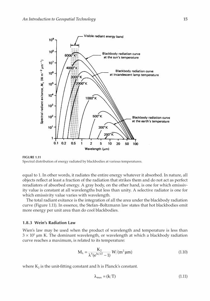
15An Introduction to Geospatial Technology

equal to 1. In other words, it radiates the entire energy whatever it absorbed. In nature, all objects reflect at least a fraction of the radiation that strikes them and do not act as perfect reradiators of absorbed energy. A gray body, on the other hand, is one for which emissiv-ity value is constant at all wavelengths but less than unity. A selective radiator is one for which emissivity value varies with wavelength.

The total radiant exitance is the integration of all the area under the blackbody radiation curve (Figure 1.11). In essence, the Stefan–Boltzmann law states that hot blackbodies emit more energy per unit area than do cool blackbodies.

1.8.3 Wein’s Radiation Law

Wien’s law may be used when the product of wavelength and temperature is less than 3 × 103 µm K. The dominant wavelength, or wavelength at which a blackbody radiation curve reaches a maximum, is related to its temperature:

MK

(e 1)W (m m)2

5 hc T2=

λ −µλ λ (1.10)

where K2 is the unit-fitting constant and h is Planck’s constant.

(k T)maxλ = (1.11)

FIGURE 1.11Spectral distribution of energy radiated by blackbodies at various temperatures.

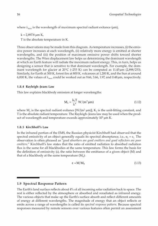
16 Geospatial Technologies

where λmax is the wavelength of maximum spectral radiant exitance (µm),

k = 2,897.8 µm K,T is the absolute temperature in K.

Three observations may be made from this diagram. As temperature increases, (i) the emis-sive power increases at each wavelength, (ii) relatively more energy is emitted at shorter wavelengths, and (iii) the position of maximum emissive power shifts toward shorter wavelengths. The Wien displacement law helps us determining the dominant wavelength at which an Earth feature will radiate the maximum radiant energy. This, in turn, helps us designing a sensor that is sensitive to that dominant wavelength. For example, the dom-inant wavelength for glacier at 20°C (~253 K) can be computed as 11.45 µm (2,898/253). Similarly, for Earth at 300 K, forest fire at 800 K, volcanoes at 1,200 K, and the Sun at around 6,000 K, the values of λmax could be worked out as 9.66, 3.66, 1.97, and 0.48 µm, respectively.

1.8.4 Rayleigh–Jeans Law

This law explains blackbody emission at longer wavelengths:

=λ

µλMk T

W (m m)14

2 (1.12)

where Mλ is the spectral radiant exitance [W/(m2 µm)], K1 is the unit-fitting constant, and T is the absolute radiant temperature. The Rayleigh–Jeans law may be used when the prod-uct of wavelength and temperature exceeds approximately 105 µm K.

1.8.5 Kirchhoff’s Law

In the infrared portion of the EMS, the Russian physicist Kirchhoff had observed that the spectral emissivity of an object generally equals its spectral absorptance, i.e., αλ = ελ. The observation is often phrased as “good absorbers are good emitters and good reflectors are poor emitters.” Kirchhoff’s law states that the ratio of emitted radiation to absorbed radiation flux is the same for all blackbodies at the same temperature. This law forms the basis for the definition of emissivity (є), the ratio between the emittance of a given object (M) and that of a blackbody at the same temperature (Mb):

=M Mbε (1.13)

1.9 Spectral Response Pattern

The Earth’s land surface reflects about 4% of all incoming solar radiation back to space. The rest is either reflected by the atmosphere or absorbed and reradiated as infrared energy. The various objects that make up the Earth’s surface absorb and reflect different amounts of energy at different wavelengths. The magnitude of energy that an object reflects or emits across a range of wavelengths is called its spectral response pattern. Because spectral responses measured by remote sensors over various features often permit an assessment

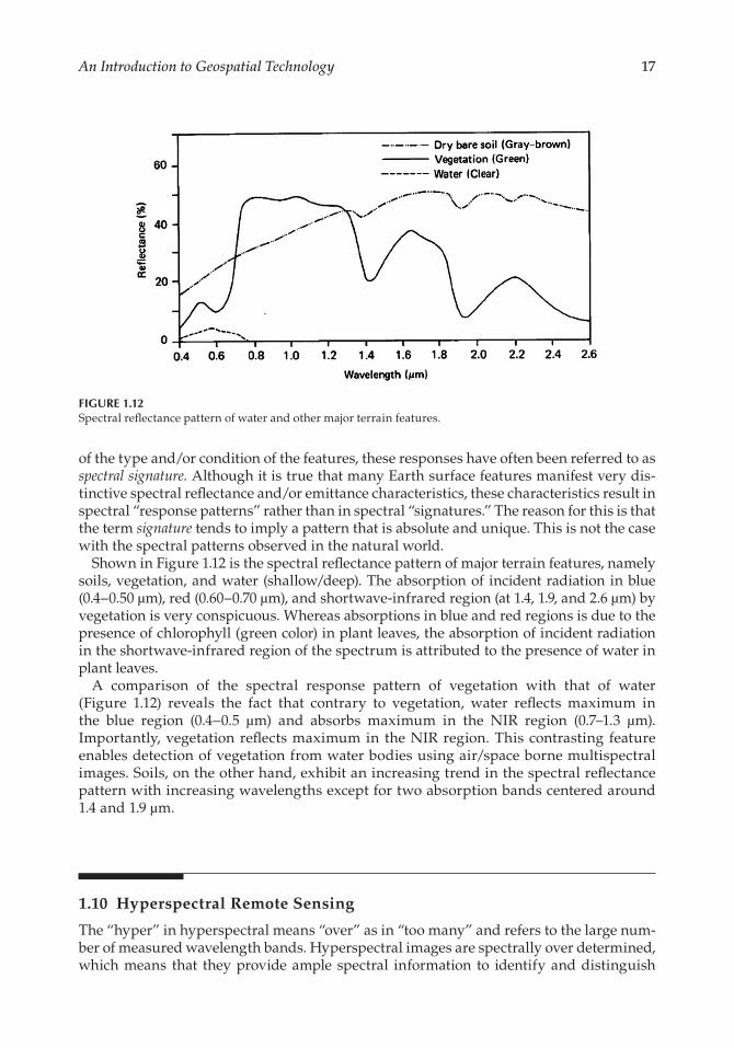
17An Introduction to Geospatial Technology

of the type and/or condition of the features, these responses have often been referred to as spectral signature. Although it is true that many Earth surface features manifest very dis-tinctive spectral reflectance and/or emittance characteristics, these characteristics result in spectral “response patterns” rather than in spectral “signatures.” The reason for this is that the term signature tends to imply a pattern that is absolute and unique. This is not the case with the spectral patterns observed in the natural world.

Shown in Figure 1.12 is the spectral reflectance pattern of major terrain features, namely soils, vegetation, and water (shallow/deep). The absorption of incident radiation in blue (0.4–0.50 µm), red (0.60–0.70 µm), and shortwave-infrared region (at 1.4, 1.9, and 2.6 µm) by vegetation is very conspicuous. Whereas absorptions in blue and red regions is due to the presence of chlorophyll (green color) in plant leaves, the absorption of incident radiation in the shortwave-infrared region of the spectrum is attributed to the presence of water in plant leaves.

A comparison of the spectral response pattern of vegetation with that of water (Figure  1.12) reveals the fact that contrary to vegetation, water reflects maximum in the blue region (0.4–0.5 µm) and absorbs maximum in the NIR region (0.7–1.3 µm). Importantly, vegetation reflects maximum in the NIR region. This contrasting feature enables detection of vegetation from water bodies using air/space borne multispectral images. Soils, on the other hand, exhibit an increasing trend in the spectral reflectance pattern with increasing wavelengths except for two absorption bands centered around 1.4 and 1.9 µm.

1.10 Hyperspectral Remote Sensing

The “hyper” in hyperspectral means “over” as in “too many” and refers to the large num-ber of measured wavelength bands. Hyperspectral images are spectrally over determined, which means that they provide ample spectral information to identify and distinguish

FIGURE 1.12Spectral reflectance pattern of water and other major terrain features.

18 Geospatial Technologies

spectrally unique materials. Hyperspectral imagery provides the potential for more accu-rate and detailed information extraction than possible with any other type of remotely sensed data. Although most hyperspectral sensors measure hundreds of wavelengths, it is not the number of measured wavelengths that defines a sensor as hyperspectral. Rather, it is the narrowness and contiguous nature of the measurements. For example, a sensor that measured only 20 bands could be considered hyperspectral if those bands were contigu-ous and, say, 10 nm wide. If a sensor measured 20 wavelength bands that were, say, 100 nm wide, or that were separated by non-measured wavelength ranges, the sensor would no longer be considered hyperspectral.

Every object—both living and nonliving—has a distinctive spectral signature embed-ded in the spectra of the light reflected or emitted by it. These spectral characteristics of the object are unique and are determined by the electronic and vibrational energy states of the constituent substances. In turn, these spectral characteristics allow that object or substance to be identified through various spectral analyses techniques.

Most multispectral imagers (e.g., Landsat-Operational Land Imager, SPOT-HRV, NOAA-AVHRR) measure radiation reflected from a surface at a few wide, separated wavelength bands. As a result, subtle spectral features associated with certain material characteristics are not available in multispectral spectra (Figure 1.13).

In an example given here, the strength of the measurements of spectral response patterns in several narrow and contiguous spectral bands is demonstrated. The spectral bands of Landsat -TM are indicated with numerals 1 to 7 along with their band width in discrete blue lines. The spectral response of green vegetation at 7 points within 350 to 2,500 nm region has been joined and assigned blue color. Hyperspectral response pattern of green vegetation is portrayed in continuous green color. Except for the region between 1,800 to 2,000 nm, spectral response pattern of green vegetation is continuous.

Owing to discrete and broad spectral bands Thematic Mapper could not capture the water absorptions band centered around 1,400 nm, and two absorption features at around 1,000 nm and 1,200 nm within near infrared plateau.

FIGURE 1.13A Comparison of multispectral and hyperspectral response patterns of vegetation (Source: http://www.iasri.res.in/ebook/GIS_TA/M2_4_HYSRS.pdf. Accessed on 03-06-2018).

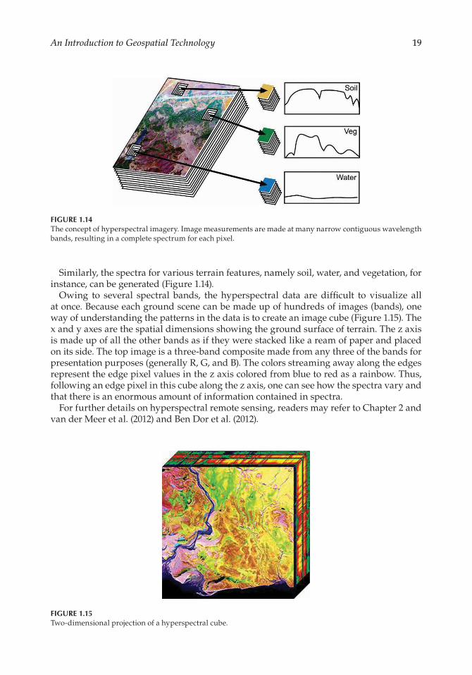
19An Introduction to Geospatial Technology

Similarly, the spectra for various terrain features, namely soil, water, and vegetation, for instance, can be generated (Figure 1.14).

Owing to several spectral bands, the hyperspectral data are difficult to visualize all at once. Because each ground scene can be made up of hundreds of images (bands), one way of understanding the patterns in the data is to create an image cube (Figure 1.15). The x and y axes are the spatial dimensions showing the ground surface of terrain. The z axis is made up of all the other bands as if they were stacked like a ream of paper and placed on its side. The top image is a three-band composite made from any three of the bands for presentation purposes (generally R, G, and B). The colors streaming away along the edges represent the edge pixel values in the z axis colored from blue to red as a rainbow. Thus, following an edge pixel in this cube along the z axis, one can see how the spectra vary and that there is an enormous amount of information contained in spectra.

For further details on hyperspectral remote sensing, readers may refer to Chapter 2 and van der Meer et al. (2012) and Ben Dor et al. (2012).

FIGURE 1.14The concept of hyperspectral imagery. Image measurements are made at many narrow contiguous wavelength bands, resulting in a complete spectrum for each pixel.

FIGURE 1.15Two-dimensional projection of a hyperspectral cube.

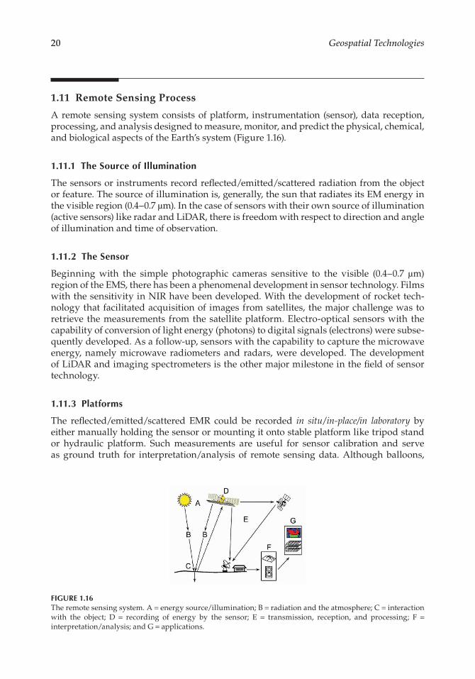
20 Geospatial Technologies

1.11 Remote Sensing Process

A remote sensing system consists of platform, instrumentation (sensor), data reception, processing, and analysis designed to measure, monitor, and predict the physical, chemical, and biological aspects of the Earth’s system (Figure 1.16).

1.11.1 The Source of Illumination

The sensors or instruments record reflected/emitted/scattered radiation from the object or feature. The source of illumination is, generally, the sun that radiates its EM energy in the visible region (0.4–0.7 µm). In the case of sensors with their own source of illumination (active sensors) like radar and LiDAR, there is freedom with respect to direction and angle of illumination and time of observation.

1.11.2 The Sensor

Beginning with the simple photographic cameras sensitive to the visible (0.4–0.7 µm) region of the EMS, there has been a phenomenal development in sensor technology. Films with the sensitivity in NIR have been developed. With the development of rocket tech-nology that facilitated acquisition of images from satellites, the major challenge was to retrieve the measurements from the satellite platform. Electro-optical sensors with the capability of conversion of light energy (photons) to digital signals (electrons) were subse-quently developed. As a follow-up, sensors with the capability to capture the microwave energy, namely microwave radiometers and radars, were developed. The development of LiDAR and imaging spectrometers is the other major milestone in the field of sensor technology.

1.11.3 Platforms

The reflected/emitted/scattered EMR could be recorded in situ/in-place/in laboratory by either manually holding the sensor or mounting it onto stable platform like tripod stand or hydraulic platform. Such measurements are useful for sensor calibration and serve as ground truth for interpretation/analysis of remote sensing data. Although balloons,

FIGURE 1.16The remote sensing system. A = energy source/illumination; B = radiation and the atmosphere; C = interaction with the object; D = recording of energy by the sensor; E = transmission, reception, and processing; F = interpretation/analysis; and G = applications.

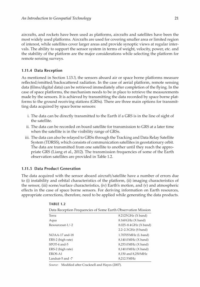
21An Introduction to Geospatial Technology

aircrafts, and rockets have been used as platforms, aircrafts and satellites have been the most widely used platforms. Aircrafts are used for covering smaller area or limited region of interest, while satellites cover larger areas and provide synoptic views at regular inter-vals. The ability to support the sensor system in terms of weight, velocity, power, etc. and the stability of the platform are the major considerations while selecting the platform for remote sensing surveys.

1.11.4 Data Reception

As mentioned in Section 1.13.3, the sensors aboard air or space borne platforms measure reflected/emitted/backscattered radiation. In the case of aerial platform, remote sensing data (films/digital data) can be retrieved immediately after completion of the flying. In the case of space platforms, the mechanism needs to be in place to retrieve the measurements made by the sensors. It is achieved by transmitting the data recorded by space borne plat-forms to the ground receiving stations (GRSs). There are three main options for transmit-ting data acquired by space borne sensors:

i. The data can be directly transmitted to the Earth if a GRS is in the line of sight of the satellite.

ii. The data can be recorded on board satellite for transmission to GRS at a later time when the satellite is in the visibility range of GRSs.

iii. The data can also be relayed to GRSs through the Tracking and Data Relay Satellite System (TDRSS), which consists of communication satellites in geostationary orbit. The data are transmitted from one satellite to another until they reach the appro-priate GRS (Liang et al., 2012). The transmission frequencies of some of the Earth observation satellites are provided in Table 1.2.

1.11.5 Data Product Generation

The data acquired with the sensor aboard aircraft/satellite have a number of errors due to (i) instability and orbital characteristics of the platform, (ii) imaging characteristics of the sensor, (iii) scene/surface characteristics, (iv) Earth’s motion, and (v) and atmospheric effects in the case of space borne sensors. For deriving information on Earth resources, appropriate corrections, therefore, need to be applied while generating the data products.

TABLE 1.2

Data Reception Frequencies of Some Earth Observation Mission

Terra 8.2125 GHz (X band)Aqua 8.160 GHz (X band)Resourcesat-1/-2 8.025–8.4 GHz (X band)

2.2–2.3 GHz (S band)

NOAA-17 and-18 1.70705 MHz (L band)ERS-2 (high rate) 8,140.0 MHz (X band)SPOT-4 and-5 8,253.0 MHz (X band)ERS-2 (high rate) 8,140.0 MHz (X band)EROS-A1 8,150 and 8,250 MHzLandsat-5 and -7 8,212.5 MHz

Source: Modified after Cracknell and Hayes (2007).

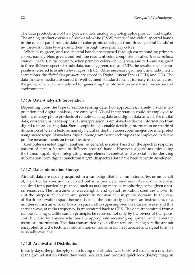
22 Geospatial Technologies

The data products are of two types, namely analog or photographic product, and digital. The analog product consists of black-and-white (B&W) prints of individual spectral bands in the case of panchromatic data or color prints developed from three spectral bands’ of multispectral data by exposing them through three primary colors.

When blue, green, and red spectral bands are exposed through corresponding primary colors, namely blue, green, and red, the resultant color composite is called true or natural color composite. On the contrary, when primary colors—blue, green, and red—are assigned to three different spectral bands data, namely green, red, and NIR, the resultant color com-posite is referred to as false color composite (FCC). After necessary geometric and radiometric corrections, the digital data products are stored in Digital Linear Tapes (DLTs) and CDs. The data in these media are stored in well-defined standard format for easy retrieval across the globe, which can be analyzed for generating the information on natural resources and environment.

1.11.6 Data Analysis/Interpretation

Depending upon the type of remote sensing data, two approaches, namely visual inter-pretation and digital analysis, are employed. Visual interpretation could be employed to both hard-copy photo products of remote sensing data and digital data as well. For digital data, on-screen or heads-up visual interpretation is employed to derive information from digital remote sensing data. Stereoscopic images enable deriving information on the third dimension of terrain feature, namely height or depth. Stereoscopic images are interpreted using stereoscope. Nowadays, digital photogrammetric techniques are employed to derive precise measurements on terrain features.

Computer-assisted digital analysis, in general, is solely based on the spectral response pattern of terrain features in different spectral bands. However, algorithms mimicking the human capability of integrating image elements, context, and association for deriving information from digital panchromatic/multispectral data have been recently developed.

1.11.7 Data/Information Storage

Aircraft data are usually acquired in a campaign that is commissioned by, or on behalf of, a particular user and is carried out in a predetermined area. Aerial data are also acquired for a particular purpose, such as making maps or monitoring some given natu-ral resources. The instruments, wavelengths, and spatial resolution used are chosen to suit the purpose. Such data are, generally, not available in public domain. In the case of Earth observation space borne missions, the output signal from an instrument, or a number of instruments, on board a spacecraft is superimposed on a carrier wave, and this carrier wave, at radio frequency, is transmitted back to GRS. The data transmitted from a remote sensing satellite can, in principle, be received not only by the owner of the space-craft but also by anyone who has the appropriate receiving equipment and necessary technical information. The data transmitted by a civilian remote sensing satellite are not encrypted, and the technical information on transmission frequencies and signal formats is usually available.

1.11.8 Archival and Distribution

In early days, the philosophy of archiving distribution was to store the data in a raw state at the ground station where they were received, and produce quick look (B&W) image in

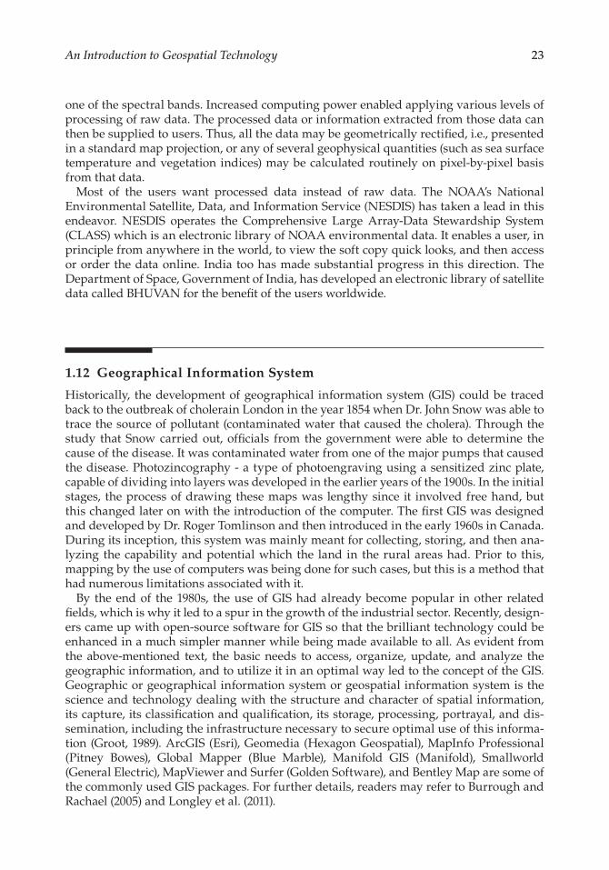
23An Introduction to Geospatial Technology

one of the spectral bands. Increased computing power enabled applying various levels of processing of raw data. The processed data or information extracted from those data can then be supplied to users. Thus, all the data may be geometrically rectified, i.e., presented in a standard map projection, or any of several geophysical quantities (such as sea surface temperature and vegetation indices) may be calculated routinely on pixel-by-pixel basis from that data.

Most of the users want processed data instead of raw data. The NOAA’s National Environmental Satellite, Data, and Information Service (NESDIS) has taken a lead in this endeavor. NESDIS operates the Comprehensive Large Array-Data Stewardship System (CLASS) which is an electronic library of NOAA environmental data. It enables a user, in principle from anywhere in the world, to view the soft copy quick looks, and then access or order the data online. India too has made substantial progress in this direction. The Department of Space, Government of India, has developed an electronic library of satellite data called BHUVAN for the benefit of the users worldwide.

1.12 Geographical Information System

Historically, the development of geographical information system (GIS) could be traced back to the outbreak of cholerain London in the year 1854 when Dr. John Snow was able to trace the source of pollutant (contaminated water that caused the cholera). Through the study that Snow carried out, officials from the government were able to determine the cause of the disease. It was contaminated water from one of the major pumps that caused the disease. Photozincography - a type of photoengraving using a sensitized zinc plate, capable of dividing into layers was developed in the earlier years of the 1900s. In the initial stages, the process of drawing these maps was lengthy since it involved free hand, but this changed later on with the introduction of the computer. The first GIS was designed and developed by Dr. Roger Tomlinson and then introduced in the early 1960s in Canada. During its inception, this system was mainly meant for collecting, storing, and then ana-lyzing the capability and potential which the land in the rural areas had. Prior to this, mapping by the use of computers was being done for such cases, but this is a method that had numerous limitations associated with it.

By the end of the 1980s, the use of GIS had already become popular in other related fields, which is why it led to a spur in the growth of the industrial sector. Recently, design-ers came up with open-source software for GIS so that the brilliant technology could be enhanced in a much simpler manner while being made available to all. As evident from the above-mentioned text, the basic needs to access, organize, update, and analyze the geographic information, and to utilize it in an optimal way led to the concept of the GIS. Geographic or geographical information system or geospatial information system is the science and technology dealing with the structure and character of spatial information, its capture, its classification and qualification, its storage, processing, portrayal, and dis-semination, including the infrastructure necessary to secure optimal use of this informa-tion (Groot, 1989). ArcGIS (Esri), Geomedia (Hexagon Geospatial), MapInfo Professional (Pitney Bowes), Global Mapper (Blue Marble), Manifold GIS (Manifold), Smallworld (General Electric), MapViewer and Surfer (Golden Software), and Bentley Map are some of the commonly used GIS packages. For further details, readers may refer to Burrough and Rachael (2005) and Longley et al. (2011).

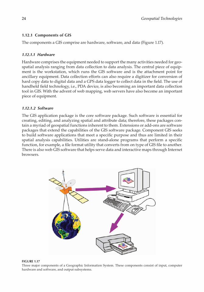
24 Geospatial Technologies

1.12.1 Components of GIS

The components a GIS comprise are hardware, software, and data (Figure 1.17).

1.12.1.1 Hardware

Hardware comprises the equipment needed to support the many activities needed for geo-spatial analysis ranging from data collection to data analysis. The central piece of equip-ment is the workstation, which runs the GIS software and is the attachment point for ancillary equipment. Data collection efforts can also require a digitizer for conversion of hard copy data to digital data and a GPS data logger to collect data in the field. The use of handheld field technology, i.e., PDA device, is also becoming an important data collection tool in GIS. With the advent of web mapping, web servers have also become an important piece of equipment.

1.12.1.2 Software

The GIS application package is the core software package. Such software is essential for creating, editing, and analyzing spatial and attribute data; therefore, these packages con-tain a myriad of geospatial functions inherent to them. Extensions or add-ons are software packages that extend the capabilities of the GIS software package. Component GIS seeks to build software applications that meet a specific purpose and thus are limited in their spatial analysis capabilities. Utilities are stand-alone programs that perform a specific function, for example, a file format utility that converts from on type of GIS file to another. There is also web GIS software that helps serve data and interactive maps through Internet browsers.

FIGURE 1.17Three major components of a Geographic Information System. These components consist of input, computer hardware and software, and output subsystems.

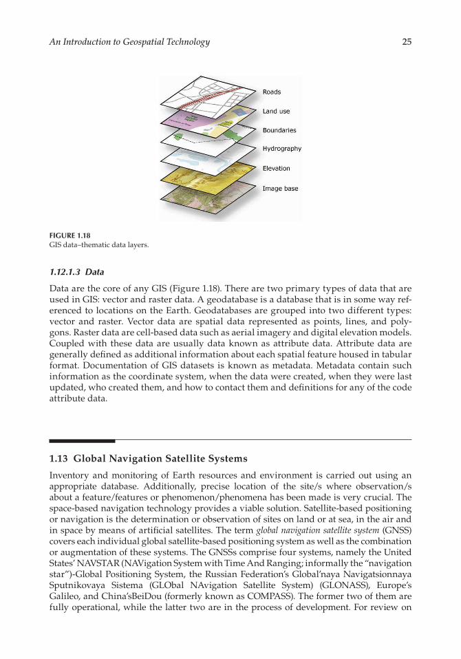
25An Introduction to Geospatial Technology

1.12.1.3 Data

Data are the core of any GIS (Figure 1.18). There are two primary types of data that are used in GIS: vector and raster data. A geodatabase is a database that is in some way ref-erenced to locations on the Earth. Geodatabases are grouped into two different types: vector and raster. Vector data are spatial data represented as points, lines, and poly-gons. Raster data are cell-based data such as aerial imagery and digital elevation models. Coupled with these data are usually data known as attribute data. Attribute data are generally defined as additional information about each spatial feature housed in tabular format. Documentation of GIS datasets is known as metadata. Metadata contain such information as the coordinate system, when the data were created, when they were last updated, who created them, and how to contact them and definitions for any of the code attribute data.

1.13 Global Navigation Satellite Systems

Inventory and monitoring of Earth resources and environment is carried out using an appropriate database. Additionally, precise location of the site/s where observation/s about a feature/features or phenomenon/phenomena has been made is very crucial. The space-based navigation technology provides a viable solution. Satellite-based positioning or navigation is the determination or observation of sites on land or at sea, in the air and in space by means of artificial satellites. The term global navigation satellite system (GNSS) covers each individual global satellite-based positioning system as well as the combination or augmentation of these systems. The GNSSs comprise four systems, namely the United States’ NAVSTAR (NAVigation System with Time And Ranging; informally the “navigation star”)-Global Positioning System, the Russian Federation’s Global’naya Navigatsionnaya Sputnikovaya Sistema (GLObal NAvigation Satellite System) (GLONASS), Europe’s Galileo, and China’sBeiDou (formerly known as COMPASS). The former two of them are fully operational, while the latter two are in the process of development. For review on

FIGURE 1.18GIS data–thematic data layers.

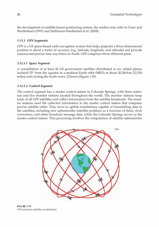
26 Geospatial Technologies

the development of satellite-based positioning system, the readers may refer to Guier and Weiffenbach (1997) and Hoffmann-Waellenhof et al. (2008).

1.13.1 GPS Segments

GPS is a US space-based radio navigation system that helps pinpoint a three-dimensional position to about a meter of accuracy (e.g., latitude, longitude, and altitude) and provide nanosecond precise time anywhere on Earth. GPS comprises three different parts.

1.13.1.1 Space Segment

A constellation of at least 24 US government satellites distributed in six orbital planes inclined 55° from the equator in a medium Earth orbit (MEO) at about 20,200 km (12,550 miles) and circling the Earth every 12 hours (Figure 1.19).

1.13.1.2 Control Segment

The control segment has a master control station in Colorado Springs, with three anten-nas and five monitor stations located throughout the world. The monitor stations keep track of all GPS satellites and collect information from the satellite broadcasts. The moni-tor stations send the collected information to the master control station that computes precise satellite orbits. They serve as uplink installations, capable of transmitting data to the satellites, including new ephemerides (satellite positions as a function of time), clock corrections, and other broadcast message data, while the Colorado Springs serves as the master control station. This processing involves the computation of satellite ephemerides

FIGURE 1.19GPS nominal satellite constellation.

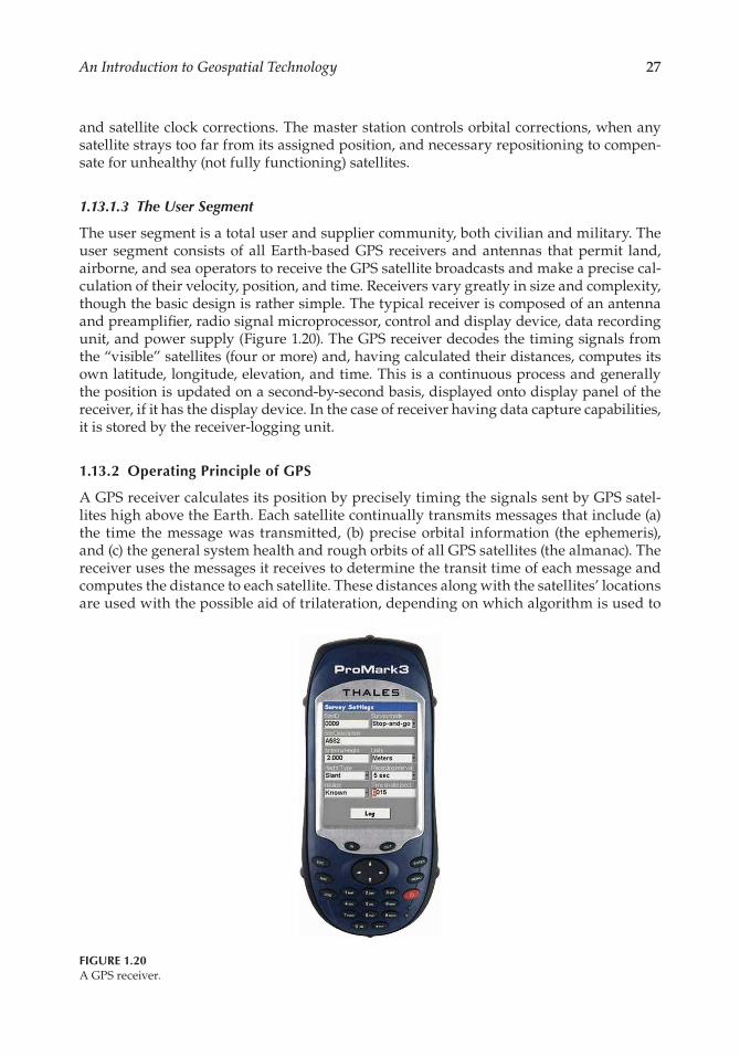
27An Introduction to Geospatial Technology

and satellite clock corrections. The master station controls orbital corrections, when any satellite strays too far from its assigned position, and necessary repositioning to compen-sate for unhealthy (not fully functioning) satellites.

1.13.1.3 The User Segment

The user segment is a total user and supplier community, both civilian and military. The user segment consists of all Earth-based GPS receivers and antennas that permit land, airborne, and sea operators to receive the GPS satellite broadcasts and make a precise cal-culation of their velocity, position, and time. Receivers vary greatly in size and complexity, though the basic design is rather simple. The typical receiver is composed of an antenna and preamplifier, radio signal microprocessor, control and display device, data recording unit, and power supply (Figure 1.20). The GPS receiver decodes the timing signals from the “visible” satellites (four or more) and, having calculated their distances, computes its own latitude, longitude, elevation, and time. This is a continuous process and generally the position is updated on a second-by-second basis, displayed onto display panel of the receiver, if it has the display device. In the case of receiver having data capture capabilities, it is stored by the receiver-logging unit.

1.13.2 Operating Principle of GPS

A GPS receiver calculates its position by precisely timing the signals sent by GPS satel-lites high above the Earth. Each satellite continually transmits messages that include (a) the time the message was transmitted, (b) precise orbital information (the ephemeris), and (c) the general system health and rough orbits of all GPS satellites (the almanac). The receiver uses the messages it receives to determine the transit time of each message and computes the distance to each satellite. These distances along with the satellites’ locations are used with the possible aid of trilateration, depending on which algorithm is used to

FIGURE 1.20A GPS receiver.

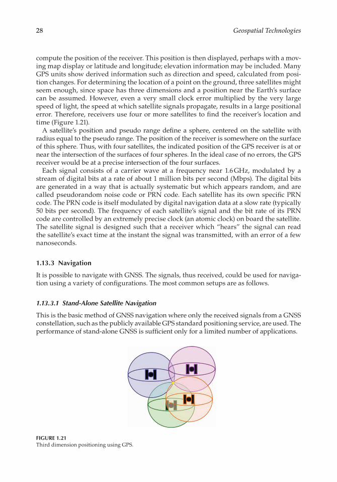
28 Geospatial Technologies

compute the position of the receiver. This position is then displayed, perhaps with a mov-ing map display or latitude and longitude; elevation information may be included. Many GPS units show derived information such as direction and speed, calculated from posi-tion changes. For determining the location of a point on the ground, three satellites might seem enough, since space has three dimensions and a position near the Earth’s surface can be assumed. However, even a very small clock error multiplied by the very large speed of light, the speed at which satellite signals propagate, results in a large positional error. Therefore, receivers use four or more satellites to find the receiver’s location and time (Figure 1.21).

A satellite’s position and pseudo range define a sphere, centered on the satellite with radius equal to the pseudo range. The position of the receiver is somewhere on the surface of this sphere. Thus, with four satellites, the indicated position of the GPS receiver is at or near the intersection of the surfaces of four spheres. In the ideal case of no errors, the GPS receiver would be at a precise intersection of the four surfaces.

Each signal consists of a carrier wave at a frequency near 1.6 GHz, modulated by a stream of digital bits at a rate of about 1 million bits per second (Mbps). The digital bits are generated in a way that is actually systematic but which appears random, and are called pseudorandom noise code or PRN code. Each satellite has its own specific PRN code. The PRN code is itself modulated by digital navigation data at a slow rate (typically 50 bits per second). The frequency of each satellite’s signal and the bit rate of its PRN code are controlled by an extremely precise clock (an atomic clock) on board the satellite. The satellite signal is designed such that a receiver which “hears” the signal can read the satellite’s exact time at the instant the signal was transmitted, with an error of a few nanoseconds.

1.13.3 Navigation

It is possible to navigate with GNSS. The signals, thus received, could be used for naviga-tion using a variety of configurations. The most common setups are as follows.

1.13.3.1 Stand-Alone Satellite Navigation

This is the basic method of GNSS navigation where only the received signals from a GNSS constellation, such as the publicly available GPS standard positioning service, are used. The performance of stand-alone GNSS is sufficient only for a limited number of applications.

FIGURE 1.21Third dimension positioning using GPS.

29An Introduction to Geospatial Technology

1.13.3.2 Differential GNSS Navigation

Relative or differential GPS carries the triangulation principles one step further, with a second receiver at a known reference point. The differential GNSS (DGNSS) navigation facilitates determination of a point’s position, relative to the known Earth surface point, which demands collection of an error-correcting message from the reference receiver. Differential corrections may be used in real time or later, with post-processing techniques. The reference station is placed on the control point, a triangulated position, the control point coordinate. This allows for a correction factor to be calculated and applied to other roving GPS units used in the same area and in the same time series.

1.13.3.3 Network-Assisted GNSS Navigation

Whenever any communication network is used to relay information to a GNSS rece-iver,  it can be said to be receiving assistance. This is called network-assisted GNSS (A-GNSS). The DGNSS described above can be thought of as a subset of A-GNSS. This assistance is often a correction to raw measurements calculated elsewhere and sent over a radio link to remote receivers. However, unlike DGNSS, in A-GNSS this assistance can often include more basic information used to assist the receiver in performing an accelerated position fix or to extend the validity of the satellite information used during positioning.

1.13.3.4 Carrier-Phase Differential (Kinematic) GPS

The differential correction technique described above applies to code-phase GPS receivers, which use the transmitted GNSS code information to compute pseudo ranges (distances) from the Earth to the GPS satellites in space. When a receiver operates in carrier-phase mode, it is measuring a different GNSS observable, namely the GNSS carrier wave. In order to obtain high accuracy with carrier-phase measurements, it is necessary for a rov-ing GPS receiver to use information from a base receiver to compute the integer number of GPS wavelengths between the roving GPS receiver’s antenna and the satellite(s). This technique yields accuracies in the cm range and can yield mm-level accuracies in static environments. In dynamic environments (called “real-time kinematic,” or RTK), GNSS is capable of providing accuracies in the 1–5 cm range.

1.14 Organization of This Book

Beginning with the introduction to geospatial technology, namely remote sensing, GIS and GNSS, the author intends to take the readers to different kind of remote sensing sen-sors operating in different portions of the EMS; data processing and analysis/interpreta-tion techniques to derive information on various land degradation processes. It is followed logically by an introduction to land degradation, and the applications of geospatial tech-nologies to the assessment and management of soil erosion by water and wind, soil sali-nization and/or alkalization, waterlogging, mining, aquaculture and shifting cultivation, soil acidification and drought in subsequent chapters. The book concludes with the devel-opment of information systems for degraded lands.

30 Geospatial Technologies

References

Ben Dor, E., Malthus, T., Plaza, A., and Schläpfer, D., 2012. Hyperspectral remote sensing. In: Wendisch, M., and Brenguier, J.L., (eds.) Airborne Measurements for Environmental Research, Wiley, Hobcon, New Jersey, USA, pp. 419–691.

Buiten, H.J., and Clevers, J.G.P.W., 1993. Gordon and Breach Science Publishers. 642 pp.Burrough, P.A., and McDonnell, R.A., 2005. Principles of Geographic Information Systems. Oxford

University Press, Oxford.Campbell, J.B., and Wynne, R.H., 2011. Introduction to Remote Sensing, 5th edn. The Guilford Press,

London, NY, 622 pp.Colwell, R.N., 1966. Manual of Photographic Interpretation. American Society of Photogrammetry, Falls

Church, VA.Cracknell, A.P., and Hayes, 2007. Introduction to Remote Sensing. CRC Press, Taylor & Francis Group,

Boca Raton, FL.Groot, R., 1989. Meeting educational requirements in Geomatics. ITC Journal, 1:1–4.Guier, W.H., and Weiffenbach, G.C., 1997. Genesis of satellite navigation. John Hopkins APL Technical

Digest, 18(2):178–181.Hoffmann-Waellenhof, B., Listenegger, H., and Wasle, E., 2008. GNSS-Global Navigation Satellite

Systems; GPS, GLONASS, Galileo, and More. Springer Wien, New York.Jaganathan, C., 2011. Geoinformatics: An overview and recent trends. In: Anbazhgan, S.,

Subramanian, S.K., and Yang, X., (eds.), Geoinformatics in Applied Geomorphology. CRC Press, Taylor & Francis Group, Boca Raton, FL.

Jensen, J.R., 2007. Remote Sensing of the Environment-An Earth Resources Perspective. Prentice Hall, Upper Saddle River, NJ.

Lein, J.K., 2012. Environmental Sensing: Analytical Techniques for Earth Observations. Springer-Verlag, Berlin.

Liang, S., Li, X., and Wang, J., 2012. Advanced Remote Sensing: Terrestrial Information Extraction and Applications. Elsevier. Amsterdam, The Netherlands 800 pp.

Lillesand, T.M., Kiefer, R.W., and Chipman, J.W., 2004. Remote Sensing and Image Interpretation, 5th edn. John Willey and Sons, New York, 724 pp.

Lillesand, T.M., Kiefer, R.W., and Chipman, J.W., 2008. Remote Sensing and Image Interpretation, 6th edn. John Willey and Sons, New York, 756 pp.

Longley, P.A., Goodchild, M.F., Maguire, D.J., and Rhind, D.W., 2011. Geographic Information Systems and Science. Wiley, Hoboken, NJ.

Mulligan, J.F., 1980. Practical Physics: The production and Conservation of Energy. McGraw Hill, New York, 526 pp.

Silva, L.F., 1978. Radiation and instrumentation in remote sensing. In: Swain, P.S., and Davis, S.M., (eds.) Remote Sensing: The Quantitative Approach. McGraw Hill, New York, pp. 21–135.

Suits, G.H., 1983. The nature of electromagnetic radiation. In: Colwell, R.N., (ed.) Manual of remote Sensing. American Society of Photogrammetry, Falls Church, VA, pp. 37–60.

Ulaby, F.T., and Goetz, A.F.H., 1987. Remote sensing techniques. Encyclopedia of physical science and tech-nology. Vol.12. Academic Press, New York, pp. 164–196.

Van der Meer, F.D., van der Werff, H.M.A., Ruitenbeek, F.J.A., Hecker, C., Bakker, W.H., Noomen, M.F., van der Meijde, M., Carranza, E.J.M., and Boudewijn de Smeth, J., 2012. Multi- and hyper-spectral geologic remote sensing: A review. International Journal of Applied Earth Observation and Geo-information 14 (1):112–128.

An Introduction to Geospatial Technology Ben Dor, E. , Malthus, T. , Plaza, A. , and Schläpfer, D. , 2012. Hyperspectral remote sensing. In: Wendisch, M., and Brenguier, J.L. , (eds.) Airborne Measurements for Environmental Research, Wiley, Hobcon, New Jersey,USA, pp. 419–691. Buiten, H.J. , and Clevers, J.G.P.W. , 1993. Gordon and Breach Science Publishers. 642 pp. Burrough, P.A. , and McDonnell, R.A. , 2005. Principles of Geographic Information Systems. Oxford UniversityPress, Oxford. Campbell, J.B. , and Wynne, R.H. , 2011. Introduction to Remote Sensing, 5th edn. The Guilford Press,London, NY, 622 pp. Colwell, R.N. , 1966. Manual of Photographic Interpretation. American Society of Photogrammetry, FallsChurch, VA. Cracknell, A.P. , and Hayes, R.H. , 2007. Introduction to Remote Sensing. CRC Press, Taylor & Francis Group,Boca Raton, FL. Groot, R. , 1989. Meeting educational requirements in Geomatics. ITC Journal, 1:1–4. Guier, W.H. , and Weiffenbach, G.C. , 1997. Genesis of satellite navigation. John Hopkins APL TechnicalDigest, 18(2):178–181. Hoffmann-Waellenhof, B. , Listenegger, H. , and Wasle, E. , 2008. GNSS-Global Navigation Satellite Systems;GPS, GLONASS, Galileo, and More. Springer Wien, New York. Jaganathan, C. , 2011. Geoinformatics: An overview and recent trends. In: Anbazhgan, S. , Subramanian, S.K., and Yang, X. , (eds.), Geoinformatics in Applied Geomorphology. CRC Press, Taylor & Francis Group, BocaRaton, FL. Jensen, J.R. , 2007. Remote Sensing of the Environment-An Earth Resources Perspective. Prentice Hall,Upper Saddle River, NJ. Lein, J.K. , 2012. Environmental Sensing: Analytical Techniques for Earth Observations. Springer-Verlag,Berlin. Liang, S. , Li, X. , and Wang, J. , 2012. Advanced Remote Sensing: Terrestrial Information Extraction andApplications. Elsevier. Amsterdam, The Netherlands 800 pp. Lillesand, T.M. , Kiefer, R.W. , and Chipman, J.W. , 2004. Remote Sensing and Image Interpretation, 5th edn.John Willey and Sons, New York, 724 pp. Lillesand, T.M. , Kiefer, R.W. , and Chipman, J.W. , 2008. Remote Sensing and Image Interpretation, 6th edn.John Willey and Sons, New York, 756 pp. Longley, P.A. , Goodchild, M.F. , Maguire, D.J. , and Rhind, D.W. , 2011. Geographic Information Systems andScience. Wiley, Hoboken, NJ. Mulligan, J.F. , 1980. Practical Physics: The production and Conservation of Energy. McGraw Hill, New York,526 pp. Silva, L.F. , 1978. Radiation and instrumentation in remote sensing. In: Swain, P.S. , and Davis, S.M. , (eds.)Remote Sensing: The Quantitative Approach. McGraw Hill, New York, pp. 21–135. Suits, G.H. , 1983. The nature of electromagnetic radiation. In: Colwell, R.N. , (ed.) Manual of remote Sensing.American Society of Photogrammetry, Falls Church, VA, pp. 37–60. Ulaby, F.T. , and Goetz, A.F.H. , 1987. Remote sensing techniques. Encyclopedia of physical science andtechnology. Vol.12. Academic Press, New York, pp. 164–196. Van der Meer, F.D. , van der Werff, H.M.A. , Ruitenbeek, F.J.A. , Hecker, C. , Bakker, W.H. , Noomen, M.F. ,van der Meijde, M. , Carranza, E.J.M. , and Boudewijn de Smeth, J. , 2012. Multi- and hyperspectral geologicremote sensing: A review. International Journal of Applied Earth Observation and Geo-information 14(1):112–128.

Passive Remote Sensing Cambone, S.A. , Krieg, K.J. , Pace, P. , and Wells, L. , 2005. ‘USA’s Unmanned Aircraft Roadmap, 2005-2030,National Defense. Chao, H. , Cao, Y.C. , and Chen, Y.Q. , 2010. Autopilots for small unmanned aerial vehicles: A survey,International Journal of Control, Automation, and Systems 8(1):36–44. Chuvieco, E. , and Huete, A. , 2010. Fundamentals of Satellite Remote Sensing. CRC Press, Taylor & FrancisGroup, Boca Raton, FL. Diner, D.J. , Asner, G.P. , Davies, R. , Knyazikhin, Y. , Muller, J.P. , Nolin, A.W. , Pinty, B. , and Stroeve, J. ,1999. New directions in earth observing: Scientific applications of multiangle remote sensing. Bulletin of theAmerican Meteorological Society 80:2209–2228. Goetz, A.F.H. , Vane, G. , Solomo, J.E. , and Rock, B.N. , 1985. Imaging spectrometry for earth remotesensing. Science 228:1147–1153.

Jensen, J.R. , 2000. Remote Sensing of the Environment-An Earth Resources Perspective. Prentice Hall,Upper Saddle River, NJ. Jensen, J.R. , 2007. Remote Sensing of the Environment-An Earth Resources Perspective. Prentice Hall,Upper Saddle River, NJ. Joseph, G. , 2003. Fundamentals of Remote Sensing. University Press, Hyderabad, 433 pp. Kerr, Y.H. , Waldteufel, P. , Wigneron, J.P. , Martinuzzi, J. , Font, J. , and Berger, M. , 2001. Soil moistureretrieval from space: The Soil Moisture and Ocean Salinity (SMOS) mission. IEEE Transactions on Geoscienceand Remote Sensing 39(8):1729–1735. Vorovenci, I. , 2009. The hyperspectral sensors used in satellite and aerial remote sensing. Bulletin of theTransilvania University of Braşov 2:51–56. Wu, H. , Sun, D. , and Zhou, Z. , 2004. Micro air vehicle: Configuration, analysis, fabrication, and test.IEEE/ASME Transactions on Mechatronics 9(1):108–117. Yang, J. , and Huang, T. , 2011. Image super- resolution: Historical overview and future challenges. In:Milanfar, P. , (ed.) Super Resolution Imaging. CRC Press, Taylor & Francis Group, Boca Raton, FL.

Active Remote Sensing Fernandez-Diaz, J.C. , 2011. Lifting the canopy veil—Airborne LiDAR for archeology of forested areas. ImagingNotes, 26(2):31–34 pp. Franceschetti, G. , and Lanari, R. , 1999. Synthetic Aperture Radar Processing. CRC Press, BocaRaton, FL. Henderson, F.M. , and Lewis, A.J. , (eds.) 1998. Principles & applications of imaging radar. Manual of RemoteSensing, 3rd Edition, Volume 2. John Wiley & Sons, Inc., New York. Hug, C. , Krzystek, P. , and Fuchs, W. , 2004. Advanced LIDAR Processing with Las Tools. IAPRS, 35, Part B,pp. 832. Kerr, Y.H. , Waldteufel, P. , Wigneron, J.P. , Martinuzzi, J. , Font, J. , and Berger, M. , 2001. Soil moistureretrieval from space: The Soil Moisture and Ocean Salinity (SMOS) mission. IEEE Transactions on Geoscienceand Remote Sensing, 39(8):1729–1735. Kramer, H.J. , 1994. Observation of the Earth and its Environment. Springer-Verlag, New York. Long, D.G. , and Drinkwater, M.R. , 2000. Azimuth variation in microwave scatterometer and radiometer dataover Antarctica. IEEE Transactions on Geosciences and Remote Sensing, 38(4):1857–1870. Rosmorduc, V. , Benveniste, J. , Bronner, E. , Dinardo, S. , Lauret, O. , Maheu, C. , Milagro, M. , Picot, N. ,Ambrozio, A. , Escolà, R. , Garcia-Mondejar, A. , Restano, M. , Schrama, E. , Terra-Homem, M. , RadarAltimetry Tutorial; Benveniste, J. , and Picot, N. , (eds.) 2016, European Space Agency, CNES.www.altimetry.info. Spencer, M.W. , Wu, C. , and Long, D.G. , 2000. Improved resolution backscatter measurements with the SeaWinds pencil-beam scatterometer. IEEE Transactions on Geosciences and Remote Sensing, 38(1):89–104. Wehr, A. and Lohr, U. , 1999. Airborne laser scanning—an introduction and overview. ISPRS Journal ofPhotogrammetry and Remote Sensing, 54:68–82.

Digital Image Processing Adler-Golden, S.M. , Matthew, M.W. , Bernstein, L.S. , Levine, R.Y. , Berk, A. , Richtsmeier, S.C. , Acharya,P.K. , Anderson, G.P. , Felde, G. , Gardner, J. , Hoke, M. , Jeong, L.S. , Pukall, B. , Ratkowski, A. , and Burke,H.K. , 1999. “Atmospheric Correction for Short-wave Spectral Imagery Based on MODTRAN4,” in Summariesof the Eighth Annual JPL Earth Science Workshop, Vol. I, available at http://makalu.jpl.nasa.gov. Al-Wassai, F.A. , Kalyankar, N.V. , and Al-Zaky, A.A. , 2012. Multisensor images fusion based on feature-level.International Journal of Latest Technology in Engineering, Management and Applied Science (IJLTEMAS),I(V):124–138. Bannari, A. , Morin, D. , Bonn, F. , and Huete, A.R. , 1995. A review of vegetation indices. Remote SensingReviews, 13(1–2):95–120. Biging, G.S. , Colby, D.R. , and Congalton, R.G. , 1999. Sampling system for change detection accuracyassessment. In: Lunetta, R.S. , and Elvidge, C.D. , (eds.) Remote Sensing Change Detection: EnvironmentalMonitoring Methods and Applications. Taylor and Francis, Milton Park. Bishop, Y. M. M. ; Fienberg, S. E. ; Holland, P. W. 1975. Discrete multivariate analysis: Theory and practice.MIT Press, Cambridge, MA, 557 p. Blaschke, T. , Lang, S. , Lorup, E. , Strobl, J. , and Zeil, P. , 2000. Object-oriented image processing in anintegrated GIS/remote sensing environment and perspectives for environmental applications. In: Cremers, A. ,and Greve, K. , (eds.) Environmental Information for Planning, Politics and the Public, vol. II. Metropolis-Verlag,Marburg, pp. 555–570.

Boardman , 1992. SIPS User’s Guide Spectral Image Processing System, Version 1.2. Center for the Study ofEarth from Space, Boulder, 88 pp. Campbell, J.B. , 2007. Introduction to Remote Sensing, 4th edn. The Guilford Press, New York. Campbell, J.B. , and Wynne, R.H. , 2011. Introduction to Remote Sensing, 4th edn. The Guillford Press, NewYork, London. Carper, W.J. , Lilesand, T.W. , and Kieffer, R.W. , 1990. The use of intensity–hue–saturation transformation formerging SPOT panchromatic and multispectral image data. Photogrammetric Engineering and RemoteSensing, 56(4):459–467. Chavez, P.S. , 1975. Atmospheric, solar, and M.T.F. corrections for ERTS digital imagery. Chavez, Jr. P.S. , 1988. An improved dark object subtraction technique for atmospheric scattering correction ofmultispectral data. Remote Sensing of Environment, 24:459–479. Chavez, P.S. , and Kwarteng, A.Y. , 1989. Extracting spectral contrast in Landsat thematic mapper image datausing selective principal component analysis. Photogrammetric Engineering and Remote Sensing, 55:339–348. Chavez, P. , 1996. Image-based atmospheric corrections—revisited and improved. PhotogrammetricEngineering and Remote Sensing, 62:1025–1036. Coppin, P.R. , and Bauer, M.E. , 1996. Digital change detection in forest ecosystems with remote sensingimagery. Remote Sensing Reviews, 13:207–234. Coppin, P. , Jonckheere, I. , Nackaerts, K. , Muys, B. , and Lambin, E. , 2004. Digital change detection methodsin ecosystem monitoring a review. International Journal of Remote Sensing, 25(9), pp. 1565–1596. Cracknell, A.P. , and Hays, L.W. , 1993. Atmospheric corrections to passive satellite remote sensing data. In:Introduction to Remote Sensing. Taylor and Francis, London, pp. 116–158. Daubechies, I. , 1992. Ten lectures on wavelets volume 61 of CMBS-NSF regional conference series in appliedmathematics (Philadelphia: Society for Industrial and Applied Mathematics (S.I.A.M.)): pp 1–16. Davenport, T. , and Vellon, M. , 1987. Tag image file format (Rev 4.0), www.martinreddy.net/gfx/2d/TIFF-4.txt. Deer, P.J. , 1995. Digital change detection techniques: Civilian and military applications. 2396 D. Lu et al.International Symposium on Spectral Sensing Research 1995 Report (Greenbelt, MD: Goddard Space FlightCenter), www.gsfc.nasa.gov/ISSSR-95/digitalc.htm. Duda, R.O. , Hart, P.E. , and Stork, D.G. , 2001. Pattern Classification and Scene Analysis. Wiley, New York. Dwivedi, R.S. , 2017. Remote Sensing of SAOILS. Springer-Verlag, Germany, 532 p. Gao, B. , and Goetz, A.F.H. 1990. Column atmospheric water vapor and vegetation liquid water retrievals fromairborne imaging spectrometer data. Journal of Geophysical Research, 95(D4):3549–3564. Gao, B.C. , Heidebrecht, K.B. , and Goetz, A.F.H. , 1999. ATmospheric REMoval (ATREM) Model User’sGuide, Version 3.1. Centre for the Study of Earth from Space, Boulder, CO, 31 p. Gao, J. , 2009. Digital Analysis of Remotely Sensed Imagery. Mc-Graw Hill, New York. Gonzalez, R.C. , and Woods, R.E. , 1992. Digital Image Processing. Addison-Wesley, Reading, MA. González-Audícana, M. , Saleta, J.L. , Catalán, R.G. , and García, R. , 2004. Fusion of multispectral andpanchromatic images using improved IHS and PCA mergers based on wavelet decomposition. IEEETransactions on Geosciences and Remote Sensing, 42(6):1291–1299. Gomez-Landesa, E. , Rango, A. , and Bleiweiss, M. , 2004. An algorithm to address the MODIS bowtie effect,Canadian Journal of Remote Sensing, 30(4):644–650. Guangmeng, G. , 2003. Eliminating bowtie effect of MODIS Data without ephemeris, Remote SensingTechnology and Application, 18(3):172–175. Gualtieri, J.A. , and Cromp, R.F. , 1998. Support vector machines for hyperspectral remote sensingclassification. In: Proceedings of the 27th AIPR Workshop: Advances in Assisted Recognition, Washington, DC,October 14–16th, 1998 (Washington, DC: SPIE), pp. 221–232. Hallada, W.A. , and Cox, S. 1983. “Image sharpening for mixed spatial and spectral resolution satellitesystems,” Proc. of the 17th International Symposium on Remote Sensing of Environment, 9–13 May, pages1023–1032. Hemmleb, M. , and Wiedemann, A. , 1997. Digital rectification and generation of orthoimages in architecturalphotogrammetry. CIPA International Symposium, IAPRS, XXXII, Part 5C1B: 261–267, International Archives ofPhotogrammetry and Remote Sensing, Göteborg, Sweden. Holben, B.N. , 1986. Characteristics of maximum-value composite images from temporal AVHRR data,International Journal of Remote Sensing, 7:1417–1434. Jensen, J.R. , 2005. Introductory Digital Image Processing: A Remote Sensing Perspective, 3rd edn, PrenticeHall, Upper Saddle River, NJ, 526 p. Jensen, J.R. , 2007, Remote Sensing of the Environment-An Earth Resources Perspective. Prentice Hall,Upper Saddle River, NJ. Jianya, G. , Haigang, S. , Guorui, M. , and Qiming, Z. , 2008. A review of multi-temporal remote sensing datachange detection algorithms. The International Archives of the Photogrammetry, Remote Sensing and SpatialInformation Sciences. Vol. XXXVII. Part B7. Beijing 2008. Jinghui, Y. , Jixian, Z. , Haitao, L. , Yushan, S. , and Pengxian, P. , 2010. Pixel level fusion methods for remotesensing images: a current review. In: Wagner, W. and Székely, B. (eds.) ISPRS TC VII Symposium—100 YearsISPRS, Vienna, Austria, July 5–7, 2010 , IAPRS, Vol. XXXVIII, Part 7B.

Kauth, R.J. , and Thomas, G. , 1976. The tasselled cap—a graphic description of the spectral-temporaldevelopment of agricultural crops as seen by LANDSAT, Proceedings of the Symposium on MachineProcessing of Remotely Sensed Data; Purdue University, West Lafayette, Indiana. 159. Khorram, S. , Biging, G. , Colby, D. , Congalton, R. , Dobson, J. , Ferguson, R. , Goodchils, M. , Jensen, J. ,and Mace, T. , 1999. Accuracy Assessment of Remote Sensing-Derived Change Detection, PhotogrammetricEngineering and Remote Sensing. ASPRS, Bethesda, MD, 64 p. Kruse, F.A. , Boardman, J.W. , Lefkoff, A.B. , Heidebrecht, K.B. , Shapiro, A.T. , Barloon, P.J. , and Goetz,A.F.H. , 1993. The Spectral Image Processing System (SIPS) – Interactive Visualization and Analysis ofImaging Spectrometer Data. Remote Sensing of Environment, 44:145–163. Lambin, E.F. , and Strahler, A.H. , 1994. Change vector analysis in multitemporal space: a tool to detect andcategorize land-cover change processes using high temporal resolution satellite data. Remote Sensing ofEnvironment, 48:231–244. Levin, N. , (ed.) 1999. Fundamentals of remote sensing. E-book. Lillesand, T.M. , and Kiefer, R.W. , 1994. Remote Sensing and Image Interpretation, 3rd edn. Wiley, New York. Lillesand, T. M. , Kiefer, R. W. , and Chipman, J.W. , 2004. Remote Sensing and Image Interpretation, JohnWiley & Sons, New York, 763. Lillesand, T. , Kiefer, R.W. , and Chipman, J. , 2015. Remote Sensing and Image Interpretation, 7th edn. Wiley,New York. Lu, D. , Mausel, P. , Brondízio, E. , and Moran, E. , 2003. Change detection techniques. International Journal ofRemote Sensing, 25:2365–2407. Macleod, R. , Congalton, R. , and Short, F. , 1995. Using quantitative accuracy assessment techniques tocompare various change detection algorithms for monitoring eelgrass distribution in Great Bay, NH generatedfrom Landsat-TM data. Proceedings of the Sixty First Annual Meeting of the American Society ofPhotogrammetry and Remote Sensing, Charlone, N.C, Vol. 3, pp. 876–885, 1995. Macleod, R.D. , and Congalton, R.G. , 1998. A quantitative comparison of change-detection algorithms formonitoring eelgrass from remotely sensed data. Photogrammetric Engineering and Remote Sensing,64:207–216. Mallat, S.G. , 1989. A theory for multiresolution signal decomposition: The wavelet representation. IEEETransactions on Pattern Analysis and Machine Intelligence, 11:674–693. Mas, F.J. , 1999. Monitoring land-cover changes: a comparison of change detection techniques, InternationalJournal of Remote Sensing, 20:139–152. Mashao, D. , 2004. Comparing SVM and GMM on parametric feature-sets. In: Proceedings of the 15th AnnualSymposium of the Pattern Recognition Association of South Africa, Cape Town, South Africa. November27–29th, 2004 . Mather, P.M. , 2004. Computer processing of remotely-sensed images: An Introduction models by applyingenvironmental and climatic information: Part I. Assessment of net primary production. International Journal ofRemote Sensing, 19(1):97–117. Melgani, F. , and Bruzzone, L. , 2004. Classification of hyperspectral remote sensing images with SupportVector Machines. IEEE Transactions on Geoscience and Remote Sensing, 42:1778–1790. INPE (Instituto Nacional de Pesquisas Espaciais) and CAST, Radiometric Quality Assessment of CBERS-2 ,2004. Pohl, C. , and van Genderen, J.L. , 1998. Multi-sensor image fusion in remote sensing: Concepts, methods andapplications. International Journal of Remote Sensing, 19(5):823–854. Radke, R.J. , Srinivas, A. , Omar, A.K. , and Badrinath, R. , 2005. Image change detection algorithms: Asystematic survey. IEEE Transactions on Image Processing, 14(3):294–307. Ranchin, T. , Wald, L. , and Mangolini, M. , 1996. The ARSIS method: a general solution for improving spatialresolution of images by the means of sensor fusion. Fusion of Earth Data, Proceedings EARSeL Conference,held in Cannes, France, February 6–8, 1996 , pp. 53–58. Ranchin, T. , Wald, L. , and Mangolini, M. , 2001. Improving the spatial resolution of images by means ofsensor fusion. A general solution: the ARSIS method. In: Remote Sensing and Urban Analysis. Donnay, J.P. ,and Barnsley, M. , (eds.) Taylor and Francis, Great Britain, pp. 19–34. Rasmussen, M.S. , 1998. Developing simple, operational, consistent NDVI-vegetation models by applyingenvironmental and climatic information: Part I. Assessment of net primary production, International Journal ofRemote Sensing, 19(1):97–117. Research Systems Inc (RSI) . 2003. ENVI User’s Guide, ENVI Version 4.0. Research Systems Inc,Pennsylvania State University. 1084 p. Richards, J.A. , and Jia, X. , 2006. Remote Sensing Digital Image Analysis: An Introduction, Springer-Verlag,Berlin, Heidelberg. Richards, J.A. , 2013. Remote Sensing Digital Image Analysis. Springer. Ritter, N. , and Ruth, M. , 1997. The GeoTIFF data interchange standard for raster geographic images.International Journal of Remote Sensing, 18(7):1637–1647. Sabins, F.F. , 2000. Remote Sensing: Principles and Interpretation. W.H. Freeman & Co. New York.

Schowengerdt, R. , 1997. Remote Sensing: Models and Methods for Image Processing, 2nd edn. AcademicPress, London. Shafri, H.Z.M. , Suhaili, A. , and Mansor, S. , 2007. The performance of maximum likelihood, spectral anglemapper, neural network and decision tree classifiers in hyperspectral image analysis. J. Comput. Sci.,3:419–423 Shao, F. , 2006. Research on change information extraction of remote sensing images based on ANN. MasterDissertation Shandong University of Science and Technology, China (in Chinese). Singh, A. , 1989. Digital change detection techniques using remotely sensed data. International Journal ofRemote Sensing, 10:989–1003. Song, C. , Woodcock, C.E. , Seto, K.C. , Lenny, M.P. , and Macomber, S.A. , 2001. Classification and changeDetection using Landsat TM data: When and How to Correct Atmospheric Effects? Remote Sensing ofEnvironment, 75:230–244. Switzer, P. , Kowalick, W.S. , and Lyon, R.J.P. , 1981. Estimation of atmospheric path-radiance by thecovariance matrix method. Photogrammetric Engineering and Remote Sensing, 47:1469–1476. Tanre, D. , Deroo, C. , Duhaut, P. , Herman, M. , Morchrette, J.J. , Perbos, J. , and Deschamps, P.Y. , 1986.Simulation of the satellite signal in the solar spectrum (5S), Users’s Guide (U. S. T. de Lille, 59655 Villeneuved’ascq, France: Laboratoire d’Optique Atmospherique). Vapnik, V.N. , 1995. The Nature of Statistical LearningTheory. Springer-Verlag, New York. Vermote, E.F. , Tanré, D. , Deuzé, J.L. , Herman, M. , and Morcrette, J.J. , 1997. Second Simulation of theSatellite Signal in the Solar Spectrum, 6S. IEEE Transactions on Geoscience and Remote Sensing,35:675–686.

An Introduction to Land Degradation . 1991. Waterlogging, soil salinity and alkalinity. Report of the Working Group on Problem identification inirrigated areas with Suggested Remedial Measures. Ministry of Water Resources, Government of India, NewDelhi. Aubreville, A. , 1949. Climats, Forêts et Désertification de l’Afrique Tropicale. Paris, Société d’EditionsGéographiques, Maritimes et Coloniales. Bai, Z.G. , Dent, D.L. , Olsson, L. , and Schaepman, M.E. , 2008. Global assessment of land degradation andimprovement. Identification by remote sensing. Report 2008/01, ISRIC—World Soil Information, Wageningen. Beck, C. , Grieser, J. , and Bruno, R. , (2004). A new monthly precipitation climatology for the global land areasfor the period 1951 to 2000 (ftp://ftp-anon.dwd.de/pub/data/gpcc/PDF/pdf_28_precipitation.pdf). Black, A.B. , 1992. Soil Fertility Evaluation and Control. Lewis Publisher, London. Blaikie, P. , and Brookfield, H. , 1987. Land Degradation and Society. Methuen, London & New York. Cardille, J.A. , and Foley, M.H. , 2002. Costa characterizing patterns of agricultural land use in Amazonia bymerging satellite classifications and census data. Global Biogeochemical Cycles, 16(3):11–18–12–18. Cook, M.G. , 1992. Sustainable agriculture in a survival setting. In Tato, K. , and Hurni, H. , (eds.) SoilConservation for Survival. Soil and Water Conservation Society, Ankeny, IA. Csillag, F. , Pasztor, L. , and Biehl, L.L. , 1993. Spectral band selection for the Characterization of salinity statusof soils. Remote Sensing of Environment, 43:231–242. De Jong, S.M. , 1994. Applications of reflective remote sensing for land degradation studies in a Mediterraneanenvironment. Netherlands Geographical Studies, 177:240 pp. Doolitte, J.A. , 1987. Using ground—penetrating radar to increase the quality and efficiency of soil surveys. In:Soil Survey Techniques. Soil Science Society of American Spectral Publication No. 20. Madison, Wisconsin,USA 11–32. Douglas, M.G. , 1994. Sustainable use of agricultural soils. A review of the prerequisites for success or failure.Development and Environment Reports No. 11, Group for Development and Environment, Institute forGeography, University of Berne, Switzerland. Dregne, H.E. , and Chou, N.T. , 1994. Global desertification dimensions and costs. In: Dregne, H.E. (ed.)Degradation and Restoration of Arid Lands. Texas Technical University, Lubbock. Ehrlich, P.R. , and Ehrlich, A.H. , 1991. Healing the Planet: Strategies for Resolving the Environmental Crisis.Addison-Wesley Publishing Company, Reading, Massachusetts. Eswaran, H. , Lal, R. , and Reich, P.F. , 2001. Land degradation: An overview. In: Bridges, E.M. , Hannam, I.D., Oldeman, L.R. , Pening de Vries, F.W.T. , Scherr, S.J. , and Sompatpanit, S. , (eds.) Responses to LandDegradation. Proceedings of 2nd International Conference on Land Degradation and Desertification, KhonKaen, Thailand. Oxford Press, New Delhi, India. Eswaran, H. , Lal, R. , Reich, P.F. , 2001a. Land degradation: an overview. In: Bridges, E.M. , Hannam, I.D. ,Penning de Vries, F.W.T. , Scherr, S.J. , and Sombatpanit, S. , (eds.) Response to Land Degradation. Sci.Publishers, Enfield, pp. 13–19.

Fageria, N.K. , and Baligar, V.C. , 2008. Ameliorating soil acidity of tropical oxisols by liming for sustainablecrop production. In: Sparks, D.L. , (ed.) Advances in Agronomy. Academic Press, Brazil, pp. 345–389. FAO , 1979. A Provisional Methodology for Soil Degradation Assessment. FAO, Rome. FAO , 1994. Cherish the Earth—Soil Management for Sustainable Agriculture and Environmental Protection inthe Tropics. Land and Water Development Division, FAO, Rome. FAO , 1988. Salt-affected soils and their management, by Abrol, I.P. , Yadav, J.S.P. and Massoud, F.I. FAOSoils Bulletin No. 39. Rome. Fensholt, R. , Sandholt, I. , Rasmussen, M.S. , Stison, S. , and Diouf, A. , 2006. Evaluation of satellite-basedprimary production modelling in the semi-arid Sahel. Remote Sensing of the Environment, 105:173–188. Fischer, G. , van Velthuizen, H.T. , Shah, M.M. , and Nachtergaele, F.O. (2002). Global agro-ecologicalassessment for agriculture in the 21st Century: Methodology and results. Laxenburg, Austria: InternationalInstitute for Applied Systems Analysis. Food and Agriculture Organization , 2013. Land Degradation Assessment in Drylands: Methodology andresults, Technical report. Gebremichael, M. , and Barros, A.P. , 2006. Evaluation of MODIS gross primary productivity (GPP) in tropicalmonsoon regions. Remote Sensing of Environment, 100:150–166. Ghassemi, F. , Jakeman, A.J. , and Nix, H.A. , 1995. Salinization of land and water resources: Human causes,extent, management and case studies, Canberra, Australia. The Australian National University, Wallingford,Oxon. Gibbs, H.K. , and Salmon, J.M. , 2015. Mapping the world’s degraded lands. Applied Geography, 57:12–21. Goldewijk, K.K. , 2001. Estimating global land use change over the past 300 years: the HYDE database. GlobalBiogeochemical Cycles, 15(2):417–433. Harrison, P. , 1987. The Greening of Africa. IIED-Earthscan study. Paladin, London. Hudson, N.W. , 1992. Land Husbandry. Batsford, London. Hurni, H. , With the assistance of an international group of contributors, 1996. Precious Earth From Soil andWater Conservation to Sustainable Land Management. International Soil and Water Conservation Organization(ISCO), and Centre for Development and Environment, Berne. Hurni, H. , (eds.) 1996. Precious earth: From Soil and Water Conservation to Sustainable Land Management.International Soil Conservation Organization (ISCO) and Centre for Development and Environment (CDE),Berne, 89 pp. Lal, R. , 1979. Physical Characteristics of Soils in the Tropics: Determination and Management. In: Lal, R. , andGreenland, D.J. , (eds.) Soil Physical Properties and Crop Production in the Tropics. John Wiley: Chichester. Lal, R. , 1990. Managing soil carbon in tropical agro-ECOSYSTEMS. EPA Workshop on Sequestering Carbonin Soils. Corvallis Oregon USA, Feb 26–28, 1990 . Liniger, H. , van Lynden, G. , Nachtergaele, F. , Schwilch, G. , 2008. A questionnaire for mapping landdegradation and sustainable land management. CDE/WOCAT, FAO/LADA, ISRIC. Lubchenco, J. , Risser, P.G. , Janetos, A.C. , Gosz, J.R. , Gold, B.D. , and Holland, M.M. , 1993. Priorities foran environmental science agenda for the Clinton-Gore administration: Recommendations for transitionplanning. Bulletin of the Ecological Society of America, 74:4–8. Mainguet, M. , 1994. Desertification: Natural Background and Human Mismanagement, 2nd edn. Springer-Verlag Press, Germany. McCauley, A. , Jones, C. , andJacobsen, J. , 2009. Soil pH and organic matter. In: Nutrients ManagementsModule. Montana State University Extension, Bozeman, Montana, USA. 8:1–12. Metternicht, G.I. , and Zinck, J.A. , 2003. Remote sensing of soil salinity: potentials and constraints. RemoteSensing of Environment, 85:1–20. MEA , 2005. Watson R. et al. (49 authors). Living beyond our means: Natural assets and human well-being.Statement from the Millennium Ecosystem Assessment Board. Milner, C. , and Douglas, M.G. , 1989. Problems of Land Degradation in Commonwealth Africa—A Study on theScope for Commonwealth Action. Commonwealth Secretariat, London. Nachtergaele, F. , Biancalani, R. , Bunning, S. , and Hubert George, H. , 2010. Land degradation assessment:The LADA approach. 19th World Congress of Soil Science, Soil Solutions for a Changing World, August 1–6,2010 , Brisbane, Australia. Published on DVD. Nachtergaele, F. , Petri, M. , and Biancalani, R. , 2011. Land degradation. In: Lal, R. , and Stewart, B.A. , (eds.)World Soil Resources and Food Security Advances in Soil Sciences, Taylor and Francis, CRC Press, 574 p. Nachtergaele, F. , Petri, M. , Van Velthuizen, H. , Biancalani, R. , Van Lynden, G. , and George, H. , 2009.Forthcoming. Global Land Degradation Information System (GLADIS in preparation). LADA internal document.FAO. Oldeman, L.R. , Hakkeling, R.T.A. , and Sombrock, W.G. , et al., 1990. World Map of the Status of HumanInduced Soil Degradation. An Explanatory Note. ISRIC/UNEP. Wageningen. Oldeman, L.R. , Hakkeling, R.T.A. , Sombroek, W.G. , 1991. World Map of the Status of Human-Induced SoilDegradation: An explanatory Note (rev. ed.), UNEP and ISRIC, Wageningen, 35 p. Oldeman, L.R. , Hakkeling, R.T.A. , and Sombrock, W.G. , 1992. World Map of the Status of Human-inducedSoil Degradation: An Explanatory Note. Global Assessment of Soil Degradation (GLASOD). ISRIC,

Wageningen. Oldeman, L.R. , 1994. The global extent of land degradation. In: Greenland, D.J. , and Szabolcs, I. , (eds.) LandResilience and Sustainable Land Use. CABI, Wallingford, pp. 99–118. Oldeman, L.R. , Hakkeling, R.T.A. , Sombrock, W.G. , and Batjes, N.H. , 2014. Global Assessment of Human-induced Soil Degradation (GLASOD). ISRIC—World Soil Information Dataset. Plummer, S. , 2006. On validation of the MODIIS gross primary production product. IEEE Transactions onGeosciences and Remote Sensing, 44(7):1936–1938. Ramankutty, N. , and Foley, J.A. , 1999. Estimating historical changes in global land cover: croplands from1700 to 1992. Global Biogeochemical Cycles, 13(4):997–1027. Renaud, F.G. , and Bogardi, J.J. , 2006. Forced migrations due to degradation of arid lands: Concepts, debateand policy requirements. Paper presented at the Joint International Conference Desertification and theInternational Policy Initiative, Algiers, December 17–19, 2006 . Rey, C. , Scoones, I. , and Toulmin, C. , 1998. Sustaining the soil: indigenous soil and water conservation inAfrica. In: Sustaining the Soil (pp. 1–27). Richards, L.A. , (ed.) 1954. Diagnosis and improvement of saline and alkali soils. U.S. Department ofAgriculture Hand Book No.60, U.S. Government Printing Office, Washington, DC. Richardson, C.J. , 1994. Ecological functions and human values in wetlands: a framework for assessingforestry impacts. Wetlands, 14:1–9. Running, S.W. , Heinsch, F.A. , Zhao, M. , Reeves, M. , and Hashimoto, H. , 2004. A continuous satellite-derived measure of global terrestrial production. Bioscience, 54:547–560. Schneider, U. , Fuchs, T. , Meyer-Christoffer, A. , and Rudolf, B. , 2008. Global Precipitation Analysis Productsof the GPCC. Global Climatology Centre (GPCC), DWD, Internet Publication, 1–12 pp. Available online athttp://gpcc.dwd.de/. Sparks, D.L. , 1995. Environmental Soil Chemistry. Academic Press, Inc., San Diego, pp. 219–232. Swift, M.J. , and Sanchez, P.A. , 1984. Biological management of tropical soil fertility for sustained productivity.Nature and Resources, 20:2-10. Szabolcs, I. , 1974. Salt Affected Soils in Europe. Martinus Nijhoff, The Hague, p. 63. Tarussov, A. , Bonn, F. , and Judge, A. , 1994. Soil survey from light research aircraft using a groundpenetrating radar. Proceedings of the First International Airborne Remote Sensing Conference and Exhibition,Strasbourg, France, September 11–15, 1994 . Thomas, D.S. , 1993. Sandstorm in a teacup? Understanding desertification. Geographical Journal,159(3):318–331. Timberlake, L. , 1985. Africa in Crisis. Earthscan, London. Tisdale, S.L. , Nelson, W.L. , Beaton, J.D. , and Havlin, J.L. , 1993. Soil acidity and basicity, pp. 364–404. In:Soil Fertility and Fertilizers, 5th edn. Macmillan Publication, New York. United Nations , 1997. Glossary of environment statistics, studies in methods, Series F, No. 67, United Nations,New York. Turner, D.P. , Ritts, W.D. , Cohen, W.B. et al., 2006. Evaluation of MODIS NPP and GPP products acrossmultiplebiomes. Remote Sensing of Environment 102:282–292. United States Salinity Laboratory Staff , 1954. Diagnosis and Improvement of Saline and Alkali Soils.Agriculture Hand book No. 60. United States Department of Agriculture. van Lynden, G.W.J. , 1995. Guidelines for the Assessment of the Status of Human-induced Soil Degradation inSouth and Southeast Asia. ISRIC Working Paper and Preprint 95/2. Young, R.A. , 1976. Managing aquifer over-exploitation: economics and policies. Selected papers on AquiferOverexploitation, International Association of Hydro-geologists, Heise, Hannover 3: 199–222. WRI , 1997. The Diversity and Dynamics of Shifting Cultivation: Myths, Realities, and Policy Implications. WorldResources Institute, Washington, D.C. Zhao, H.L. , Yi, X.Y. , Zhou, R.L. , Zhao, X.Y. , Zhang, T.H. , Drake, S. , 2006. Wind erosion and sandaccumulation effects on soil properties in Horqin Sandy Farmland, Inner Mongolia. Catena, 65:71–79.

Water Erosion Baghdadi, N. , King, C. , Bourguignon, A. , Remond, A. , 2002. Potential of ERS and Radarsat data for surfaceroughness monitoring over bare agricultural fields: application to catchments in Northern France. InternationalJournal of Remote Sensing 23(17):3427–3442. Baret, F. , Guyot, G. , 1991. Potentials and limits of vegetation indices for LAI an APAR assessment. RemoteSensing of Environment 35(2–3):161–173. Beasley, D.B. , Huggins, L.F. , Monke, E.J. , 1980. ANSWERS: A model for watershed planning. Transactionsof the ASAE 23:938–944. Beaulieu, A. , Gaonac’h, H. , 2002. Scaling of differentially eroded surfaces in the drainage network of theEthiopian Plateau. Remote Sensing of Environment 82(1):111–122.

Ben-Dor, E. , Goldshleger, N. , Benyamini, Y. , Agassi, M. , Blumberg, D.G. , 2003. The spectral reflectanceproperties of soil structural crusts in the 1.2- to 2.5-Am spectral region. Soil Science Society of America Journal67(1):289–299. Ben-Dor, E. , Chabrillat, S. , Demattê, J.A.M. , Taylor, G.R. , Hill, J. , Whiting, M.L. , Sommer, S. , 2009. UsingImaging spectrometry to study soil properties. Remote Sensing of Environment 13(1):S38–S55. Ben-Dor, E. , Demattê, J.A.M. , 2015. Remote sensing of soil in the optical domains. In: Thenkabail, P.S. , (ed.)Land Resources Monitoring, Modeling, and Mapping with Remote Sensing. CRC Press, Boca Raton, FL, pp.733–787. Ben-Dor, E. , Goldshleger, N. , Braun, O. , Kindel, B. , Goetz, A.F.H. , Bonfil, D. , Margalit, N. , Binaymini, Y. ,Karnieli, A. , Agassi, M. , 2004. Monitoring infiltration rates in semiarid soils using airborne hyperspectraltechnology. International Journal of Remote Sensing 25:2607–2624. Ben-Hur, M. , Shainberg, I. , Bakker, D. , Keren, R. , 1985. Effect of soil texture and CaC03 content on waterinfiltration in crusted soil as related to water salinity. Irrigation Science 6:281–294. Bhuyan, S.J. , Marzen, L.J. , Koelliker, J.K. , Harrington Jr., J.A. , Barnes, P.L. , 2002. Assessment of runoffand sediment yield using remote sensing, GIS, and AGNPS. Journal of Soil and Water Conservation57(6):351–364. Bishop, M.P. , Shroder Jr., J.F. , 2001. Remote sensing and geomorphometric assessment of topographiccomplexity and erosion dynamics in the Nanga Parbat massif. In: Khan, M.A. , Treloar, P.J. , Searle, M.P. , Jan,M.Q. , (eds.) Tectonics of the Nanga Parbat Syntaxis and the Western Himalaya, vol. 170. Special Publication,Geological Society, London, pp. 181–200. Bocco, G. , Palacio, J.L. , Valenzuela, C.R. , 1991. Gully erosion modelling using GIS and geomorphologicalknowledge. ITC Journal 1991(3):253–261. Bocco, G. , Valenzuela, C.R. , 1988. Integration of GIS and image processing in soil erosion studies usingILWIS. ITC Journal 4:309–319. Bradford, J.M. , Ferris, J.E. , Remley, P.A. , 1987. Interrill soil erosion processes. II: Relationship of splashdetachment to soil properties. Soil Science Society of America 51:1571–1575. Bricklemyer, R.S. , Lawrence, R.S. , Miller, P.R. , Battogtokh, N. , 2002. Predicting tillage practices andagricultural soil disturbance in north central Montana with Landsat imagery. Agriculture Ecosystems andEnvironment 114(2-4):210–216. Brisco, B. , Brown, R.J. , Snider, B. , Sofko, G.J. , Koehler, J.A. , Wacker, A.G. , 1991. Tillage effects on theradar backscattering coefficient of grain stubble fields. International Journal of Remote Sensing12(11):2283–2298. Chabrillat, S. , Milewski, R. , Schmid, T. , Rodriguez, M. , Escribano, P. , Pelayo, M. , Palacios-Orueta, A.Potential of hyperspectral imagery for the spatial assessment of soil erosion stages in agricultural semi-aridSpain at different scales. In: Proceedings of the 2014 IEEE Geoscience and Remote Sensing Symposium,Quebec City, QC, Canada, 13–18 July 2014 ; pp. 2918–2921. Chacontorres, A. , Ross, L.G. , Beveridge, M.C.M. , Watson, A.I. , 1992. The application of SPOT multispectralimagery for the assessment of water quality in Lake Patzcuaro, Mexico. International Journal of RemoteSensing 13(4):587–603. Choubey, V.K. , 1998. Laboratory experiment, field and remotely sensed data analysis for the assessment ofsuspended solids concentration and Secchi depth of the reservoir surface water. International Journal ofRemote Sensing 19(17):3349–3360. Coldwell, A.E. , 1957. Importance of channel erosion as a source of sediment. American Geophysical UnionTransactions 38:908–912. Conforti, M. , Buttafuoco, G. , Leone, A.P. , Aucelli, P.P.C. , Robustelli, G. , Scarciglia, F. , 2013. Studying therelationship between water-induced soil erosion and soil organic matter using VIS-NIR spectroscopy andgeomorphological analysis: A case study in southern Italy. Catena 110:44–58. Coppin, P. , Jonckheere, I. , Nackaerts, K. , Muys, B. , Lambin, E. , 2004. Digital change detection methods inecosystem monitoring: a review. International Journal of Remote Sensing 25(9):1565–1596. Cox, C. , Madramootoo, C. , 1998. Application of geographic information systems in watershed managementplanning in St. Lucia. Computers and Electronics in Agriculture 20(3):229–250. Curran, P.J. , Novo, E.M.M. , 1988. The relationship between suspended sediment concentration and remotelysensed spectral radiance: a review. Journal of Coastal Research 4(3):351–368. Curwick, P.B. , Jennings, M.E. , 1982. Evaluation of rainfall-runoff models for the hydrologic characterization ofsurface-mined lands. In: Applied modeling in catchment hydrology: Proceedings of the International Symposiumon Rainfall — Runoff modeling held May 18-21, 1981 at Mississippi State University, Mississippi State,Mississippi, pp. 259–274. Cyr, L. , Bonn, F. , Pesant, A. , 1995. Vegetation indices derived from remote sensing for an estimation of soilprotection against water erosion. Ecological Modelling 79(1–3):277–285. Darboux, F. , Davy, Ph. , Gascuel-Odoux, C. , 2002. Effect of depression storage capacity on overland-flowgeneration for rough horizontal surfaces: water transfer distance and scaling. Earth Surface Processes andLandforms 27(2):177–191. Datta, P.S. , Schack-Kirchner, H. , 2010. Erosion relevant topographical parameters derived from differentDEMs—A comparative study from the Indian lesser Himalayas. Remote Sensing 2:1941–1961.

De Jong, S.M. , 1994a. Applications of reflective remote sensing for land degradation studies in aMediterranean Environment. PhD thesis, Utrecht University, The Netherlands, 237 pp. De Jong, S.M. , 1994b. Derivation of vegetative variables from a Landsat TM image for modelling soil erosion.Earth Surface Processes and Landforms 19(2):165–178. de Roo, A.P.J. , 1993. Validation of the ANSWERS catchment model for runoff and soil erosion simulation incatchments in the Netherlands and the United Kingdom. In: Applications of Geographic Information Systems inHydrology and Water Resources Management. Proceedings of International Conference, Vienna, 1993, pp:465–474. DeCoursey, D.G. , 1985. Mathematical models for nonpoint water pollution control. Journal of Soil and WaterConservation 40(5):408–413. DeGloria, S.D. , Wall, S.L. , Benson, A.S. , Whiting, M.L. , 1986. Monitoring conservation tillage practices usingLandsat multispectral data. Journal of Soil and Water Conservation 41(3):187–190. Dekker, A.G. , Malthus, T.J.M. , Hoogenboom, H.J. , 1995. The remote sensing of inland water quality. In:Danson, F.M. , and Plummer, S.E. , (eds.) Advances in Environmental Remote Sensing. Wiley, Chichester. Dhakal, A.S. , Amada, T. , Aniya, M. , Sharma, R.R. , 2002. Detection of areas associated with flood anderosion caused by a heavy rainfall using multi-temporal Landsat TM data. Photogrammetric Engineering andRemote Sensing 68(3):233–239. Dwivedi, R.S. , Kumar, A.B. , Tewari, K.N. , 1997a. The utility of multi-sensor data for mapping eroded lands.International Journal of Remote Sensing 18(11):2303–2318. Dwivedi, R.S. , Ramana, K.V. , 2003. The delineation of reclamative groups of ravines in the Indo-Gangeticalluvial plains using IRS-1D LISS-III data. International Journal of Remote Sensing 24(22):4347–4355. Dwivedi, R.S. , Sankar, T.R. , Venkaratnam, L. , Karale, R.L. , Gawande, S.P. , Rao, K.V.S. , Senchaudhary, S., Bhaumik, K.R. , Mukharjee, K.K. , 1997b. The inventory and monitoring of eroded lands using remote sensingdata. International Journal of Remote Sensing 18(1):107–119. Ekwue, E.L. , 1990. Effect of organic matter on splash detachment and the process involved. Earth SurfaceProcesses and Landforms 15:175–181. El-Swaify, S.A. , Dangler, E.W. , 1977. Erodibility of selected tropical soils in relation to structural andhydrologic parameters. In: Soil Erosion: Prediction and Control, Special Publication. 21. Escadafal, R. , 1994. Soil spectral properties and their relationships with environmental parameters: Examplesfrom arid regions. In: Hill, J. , Me´gier, J. , (eds.) Imaging Spectrometry—a Tool for EnvironmentalObservations. Kluwer Academic Publishers, Dordrecht, pp. 71–87. Flacke, W. , Auerswald, K. , Neufang, L. , 1990. Combining a modified universal soil loss equation with a digitalterrain model for computing high resolution maps of soil loss resulting from rain wash. CATENA 17:383–397. Floras, S.A. , Sgouras, I.D. , 1999. Use of geoinformation techniques in identifying and mapping areas oferosion in a hilly landscape of central Greece. International Journal of Applied Earth Observation andGeoinformation 1(1):68–77. Flugel, W.A. , Ma¨rker, M. , Moretti, S. , Rodolfi, G. , Sidorchuk, A. , 2003. Application of geographic informationsystems and remote sensing for quantifying patterns of erosion and water quality. Hydrological Processes17:929–942. Foster, G.R. , 1990. Process-based modelling of soil erosion by water on agricultural land. In: Boardman, J. ,Foster, I.D.L. , Dearing, J.A. , (eds.) Soil Erosion on Agricultural Land. John Wiley & Sons Ltd, Hoboken, NJ,429–445. Frank, T.D. , 1984. Assessing change in surficial character of a semiarid environment with Landsat residualimage. Photogrammetric Engineering and Remote Sensing 50(4):471–480. Gallaher, R.N. , Hawf, L. , 1997. Role of conservation tillage in production of a wholesome food supply.Partners for A, 23. Gorrie, R.M. , 1935. The use and misuse of land. In: Oxford Forestry Memoirs, pp. 37–47 and 66–67. Gowda, P.H. , Dalzell, B.J. , Mulla, D.J. , Kollman, F. , 2001. Mapping tillage practices with Landsat thematicmapper based logistic regression models. Journal of Soil and Water Conservation 56(2):91–96. Grieve, I. C. , Hipkin, J.A. , and Davidson, D.A. , 1994. Soil erosion sensitivity in upland Scotland. ScottishNatural Heritage Research Survey and Monitoring Reports 24. Scottish Natural Heritage, Edinburgh. Haboudane, D. , Bonn, F. , Royer, A. , Sommer, S. , Mehl, W. , 2002. Land degradation and erosion riskmapping by fusion of spectrally-based information and digital geomorphometric attributes. International Journalof Remote Sensing 23(18):3795–3820. Haubrock, S. , Chabrillat, S. , Kaufmann, H. , 2005. Application of hyperspectral imaging for the quantification ofsurface soil moisture in erosion monitoring and modeling, Proceeding of the 4th Workshop on ImagingSpectroscopy: New Quality in Environmental Studies, 197–206. Hensel, H. , Bork, H.R. , 1987. EDV—gestutzte Bilanzierung von Erosion und akkumulationin kleineEinzugsgebieten unter Verwendung der modifizierten Universal Soil Loss Equation. Landschaftsoko logischesMessen und Auswerten 2.2/3, Braunschweig. Hill, J. , Mehl, W. , Altherr, M. , 1994. Land degradation and soil erosion mapping in a Mediterraneanecosystem. In: Hill Jr., J. , Mégier, J. , (eds.) Imaging Spectrometry—A Tool for Environmental Observations.Kluwer Academic Publishers, Dordrecht, pp. 237–260.

Hill, J. , Mégier, J. , Mehl, W. , 1995. Land degradation, soil erosion and desertification monitoring inMediterranean ecosystems. Remote Sensing Reviews 12:107–130. Hochschild, V. , Märker, M. , Rodolfi, G. , Staudenrausch, H. , 2003. Delineation of erosion classes in semi-aridsouthern African grasslands using vegetation indices from optical remote sensing data. Hydrological Processes17(5):917–928. Hudson, N.W. , 1985. A world view of the development of soil conservation. Agricultural History 59:327–339. Izenberg, N.R. , Arvidson, R.E. , Brackett, R.A. , Saatchi, S.S. , Osburn, G.R. , Dohrenwend, J. , 1996.Erosional and depositional patterns associated with the 1993 Missouri River floods inferred from SIR-C andTOPSAR radar data. Journal of Geophysical Research 101(E10):23149–23167. Jain, S.K. , Singh, P. , Seth, S.M. , 2002. Assessment of sedimentation in Bhakra Reservoir in the westernHimalayan region using remotely sensed data. Hydrological Sciences Journal 47(2):203–212. Judson, S. 1965. Physical Geology, 3rd edn. Prentice Hall, Upper Saddle River, NJ, pp. 143–144. Kamphrost, A. , Iyer, H.S. , 1972. Application of aerial photo-interpretation of ravine surveys in India. TwelfthCongress of International Society of Photogrammetry. Ottawa, 1972. Karale, R.L. , Saini, K.M. , Narula, K.K. , 1988. Mapping and monitoring ravines using remotely sensed data.Journal of Soil and Water Conservation, India 32(1,2):75. Khan, N.I. , Islam, A. , 2003. Quantification of erosion pattern in the Brahmaputra-Jamuna River usinggeographical information system and remote sensing techniques. Hydrological Processes 17(5):959–966. Khawlie, M. , Awad, M. , Shaban, A. , Kheir, R.B. , Abdallah, C. , 2002. Remote sensing for environmentalprotection of the eastern Mediterranean rugged mountainous areas, Lebanon. ISPRS Journal ofPhotogrammetry and Remote Sensing 57(1–2):13–23. Knisel, W.G. , 1980. CREAMS: A Field Scale Model for Chemicals, Runoff and Erosion from AgriculturalManagement Systems. USDA, Washington, D.C. Lal, R. , 2001. Soil degradation by erosion. Land Degradation & Development 12(6):519–539. Latz, K. , Weismiller, R.A. , Scoyoc, G.E.V. , Baumgardner, M.F. , 1984. Characteristic variations in spectralreflectance of selected eroded Alfisols. Soil Science Society of America Journal 48(5):1130–1134. Le Bissonnais, Y. , 1990. Experimental study and modelling of soil surface crusting process. CatenaSupplement 17:13–28. Lee, S. , 2004. Soil erosion assessment and its verification using the universal soil loss equation andgeographic information system: A case study at Boun, Korea. Environmental Geology 45:457–465. Lee, H. , Liu, J.G. , 2001. Analysis of topographic decorrelation in SAR interferometry using ratio coherenceimagery. IEEE Transactions on Geoscience and Remote Sensing 39(2):223–232. Leek, R. , Solberg, R. , 1995. Using remote sensing for monitoring of autumn tillage in Norway. InternationalJournal of Remote Sensing 16(3):447–466. Lehmann, R. , 1992. Terrace degradation and soil erosion on Naxos Island, Greece. In: Wicherek, S. , (ed.)Farm Land Erosion in Temperate Plains Environment and Hills. Proceedings of the Symposium on Saint-Cloud,Paris, pp. 429–450. Leuder, D.R. , 1959. Aerial Photographic Interpretation (Principles and Applications). McGraw-Hill BookCompany, Inc., New York. Liddaman, L. , 2008. Geospatial patterning and the hydro-morphological functioning of eroding blanket peat,Unpublished PhD Thesis, Department of Geography, University of Manchester. 275p. Liu, Y. , Anisul Islamand, M.d. , Gao, J. , 2003. Quantification of shallow water quality parameters by means ofremote sensing. Progress in Physical Geography 27(1):24–43. Liu, J.G. , Hilton, F. , Mason, P. , Lee, H. , 2000. A RS/GIS study of rapid erosion in SE Spain using ERS SARmulti-temporal interferometric coherence imagery. In: Owe, M. , Zilioli, E. , D’Urso, G. , (eds.) Remote Sensingfor Agriculture, Ecosystems, and Hydrology II, Proceedings of SPIE, vol. 4171. SPIE International, Barcelona,Spain, pp. 367–375. Liu, J.G. , Mason, P. Hilton, F. , Lee, H. , 2004. Detection of rapid erosion in SE Spain: A GIS approach basedon ERS SAR coherence imagery. Photogrammetric Engineering and Remote Sensing 70:1179–1185. Mannaerts, C.M. , Saavedra, C.P. , 2003. Regional scale erosion modelling and monitoring using remotelysensed data: some spatial data scale issues. In: Gabriels, D. , Cornelis, W. , (eds.) Proceedings of theInternational Symposium on 25 Years of Assessment of Erosion. Ghent University, Ghent, Belgium, pp.433–440. Mathieu, R. , King, C. , Bissonnais, Y.L. , 1997. Contribution of multi-temporal SPOT data to the mapping of asoil erosion index: The case of the loamy plateaux of northern France. Soil Technology 10(2):99–110. McBratney, A.B. , Mendon Santosb, M.L. , Minasny, B. , 2003. On digital soil mapping. Geoderma 117(1-2):3–52. McNairn, H. , Wood, D. , Gwyn, Q.H.J. , Brown, R.J. , Charbonneau, F. , 1998. Mapping tillage and cropresidue management practices with RADARSAT. Canadian Journal of Remote Sensing 24(1):28–35. Merritt, W.S. , Letcher, R.A. , Jakeman, A.J. , 2003. A review of erosion and sediment transport models.Environmental Modeling and Software 18:761–799. Metternicht, G.I. , Zinck, J.A. , 1998. Evaluating the information content of JERS-1 SAR and Landsat TM datafor discrimination of soil erosion features. ISPRS Journal of Photogrammetry and Remote Sensing

53(3):143–153. Miller, W.P. , Baharuddin, M.K. , 1986. Relationship of soil dispersibility to infiltration and erosion ofsoutheastern soils. Soil Science 142:235–240. Millington, A.C. , Townshend, J.R.G. , 1984. Remote sensing applications in African erosion and sedimentationstudies. In: Walling, D.E. , Foster, S.S.D. , Wurzel, P. , (eds.) Challenges in African Hydrology and WaterResources: Proceedings of the Harare Symposium. IAHS Publication, vol. 144. IAHS Press, pp. 373–384. Moore, D.C. , Singer, M.J. , 1990. Crust formation effect on soil erosion processes. Soil Science Society ofAmerica Journal 54:1117–1123. Moran, M.S. , Hymer, D.C. , Qi, J. , Kerr, Y. , 2002. Comparison of ERS-2 SAR and Landsat TM imagery formonitoring agricultural crop and soil conditions. Remote Sensing of Environment 79(2–3):243–252. Morgan, R.P.C. , Morgan, D.D.V. , Finney, H.J. , 1984. A Predictive Model for the Assessment of Soil ErosionRisk. Journal of Agricultural Engineering Research 30:245–253. Nellis, M.D. , Harrington, Jr., J.A. , Wu, J. , 1998. Remote sensing of temporal and spatial variations in poolsize, suspended sediment, turbidity, and Secchi depth in Tuttle Creek Reservoir, Kansas: 1993.Geomorphology 21(3–4):281–293. Panayiotopoulos, K.P. , Kostopoulou, S. , 1989. Aggregate stability dependence on size, cultivation and varioussoil constituents in red Mediterranean soils (alfisols). Soil Technology 2:79–89. Paringit, E.C. , Nadaoka, K. , 2003. Sediment yield modelling for small agricultural catchments: land-coverparameterization based on remote sensing data analysis. Hydrological Processes 17(9):1845–1866. Pelletier, R.E. , 1985. Evaluating nonpoint pollution using remotely sensed data in soil erosion models. Journalof Soil and Water Conservation 40(4):332–335. Pellikkaa, P.K.E. , Clarka, B.J.F. , Sirviöa, T. , Masalina, K. , 2005. Environmental change monitoring applyingsatellite and airborne remote sensing data in the Taita Hills, Kenya. Remote sensing and geo-informationprocessing in the assessment and monitoring of land degradation and desertification, Trier, Germany, 2005. Perez-Trejo, F. , 1986. Review of Existing Watershed Models for the Delft Hydraulics Laboratory. ColoradoState University, Fort Collins, CO, p. 20. Pickup, G. , Nelson, J. , 1984. Use of Landsat radiance parameters to distinguish soil erosion, stability, anddeposition in arid Central Australia. Remote Sensing of Environment 16(3):195–209. Porêba, G.J. , 2006. Caesium-137 as a soil erosion tracer: a review. Geochronometria 25:37–46. Rabus, B. , Eineder, M.A.R. , Bamler, R. , 2003. The shuttle radar topography mission: a new class of digitalelevation models acquired by spaceborne radar. ISPRS Journal of Photogrammetry and Remote Sensing57(4):241–262. Renard, K.G. , Foster, G.R. , Weesies, G.A. , McCool, D.K. , Yoder, D.C. , 1997. Predicting Soil Erosion byWater: A Guide to Conservation Planning with the Revised Universal Soil Loss Equation (RUSLE). AgriculturalHandbook No. 703, U. S. Department of Agriculture, Washington DC, p. 384. Reusing, M. , Schneider, T. , Ammer, U. , 2000. Modelling soil loss rates in the Ethiopian Highlands byintegration of high resolution MOMS-02/D2-stereo-data in a GIS. International Journal of Remote Sensing21(9):1885–1896. Ritchie, J.C. , Schiebe, F.R. , 2000. Water quality. In: Schultz, G.A. , Engman, E.T. , (eds.) Remote Sensing inHydrology and Water Management. Springer-Verlag, Berlin, pp. 287–303, and 351–352. Ritchie, J.C. , Schiebe, F.R. , McHenry, J.R. , 1976. Remote sensing of suspended sediment in surface water.Photogrammetric Engineering and Remote Sensing 42(12):1539–1545. Roberson, E. B. , Sarig, S. , Firestone, M.K. , 1991. Cover crop management of polysaccharides-mediatedaggregation in an orchard soil. Soil Science Society of America Journal 55:734–739. Schmid, T. , Manuel Rodríguez-Rastrero, M. , Escribano, P. , Alicia Palacios-Orueta, A. , Ben-Dor, E. , Plaza,A. , Milewski, R. Huesca, M. , Ashley Bracken, A. , Víctor Cicuéndez, V. , Marta Pelayo, M. and SabineChabrillat, S. , 2016. Characterization of soil erosion indicators using hyperspectral data from a Mediterraneanrainfed cultivated region. IEEE Journal of Selected Topics In Applied Earth Observations and Remote Sensing9 (2):845–860. Schwertmann, U. , 1982. Die Vorausschatzung des Bodenabtrags durch Wasser in Bayern. Bayer. Staatsmin.Landwirtsch. Forsten, Munchen, pp. 126. Sharma, K.D. , Singh, S. , 1995. Satellite remote sensing for soil erosion modelling using the ANSWERSmodel. Hydrological Sciences Journal 40(2):259–272, 10.1080/02626669509491408. Shoshany, M. , Goldshleger, N. , Chudnovsky, A. , 2013. Monitoring of agricultural soil degradation by remote-sensing methods: A review. International Journal of Remote Sensing 34:6152–6181. Singh, A.N. , Sharma, Y.K. , Singh, S. , 1998. Evaluation of IRS-1C PAN Data for Monitoring Gullied andRavinous Lands of Western U.P. Remote Sensing and Geographic Information System for Natural ResourcesManagement. A Joint Publication of Indian Society of Remote Sensing and NNRMS, Department of Space,Government of India, Bangalore, pp.149–160. Smith, R.E. , Ferreira, V.A. , 1986. Effect of soil hydraulic properties on root zone transport processes. In:Proceedings of AGU Front Range Branch Hydrology Days. pp. 123–137. Ft. Collins: Hydrology DaysPublications. Colorado State University. Smith, L.C. , Alsdorf, D.E. , Magilligan, F.J. , Gomez, B. , Mertes, L.A.K. , Smith, N.D. , Garvin, J.D. , 2000.Estimation of erosion, deposition, and net volumetric change caused by the 1996 Skeiðara´rsandur jo¨ kulhlaup,

Iceland, from synthetic aperture radar interferometry. Water Resources Research 36(6):1583–1594. Sreenivas, K. , Dwivedi, R.S. , 2010. Personal communication. Stern, R. , Ben-Hur, M. , Shainberg, I. , 1991. Clay mineralogy effect on rain infiltration, seal formation and soillosses. Soil Science 152:455–462. Symeonakis, E. , Drake, N. , 2004. Monitoring desertification and land degradation over sub-Saharan Africa.International Journal of Remote Sensing 25(3):573–592. Thiam, A.K. , 2003. The causes and spatial pattern of land degradation risk in southern Mauritania usingmultitemporal AVHRR-NDVI imagery and field data. Land Degradation and Development 14(1):133–142. Thornes, J.B. , 1985. The ecology of erosion. Geography 70:222–234. Trott, K.E. , Singer, M.J. , 1983. Relative erodibility of 20 California range and forest soils. Soil Science Societyof America Journal 47:749–753. Tucker, C.J. , 1979. Red and photographic infrared linear combinations for monitoring vegetation. RemoteSensing of Environment 8(2):127–150. Ulaby, F.T. , Bradley, G.A. , Dobson, M.C. , 1979. Microwave backscatter using GIS and geomorphologicalknowledge. ITC Journal 1991(3):253–261. van Deventer, A.P. , Ward, A.D. , Gowda, P.H. , Lyon, J.G. , 1997. Using Thematic Mapper data to identifycontrasting soil plains and tillage practices. Photogrammetric Engineering and Remote Sensing 63(1):87–93. Vrieling, A. , 2006. Satellite remote sensing for water erosion assessment: A review. Catena 65:2–18. Vrieling, A. , Rodrigues, S.C. , 2004. Erosion assessment in the Brazilian Cerrados using multi-temporal SARimagery. Proceedings of the 2004 Envisat and ERS Symposium. SP-572. ESA, Salzburg, Austria. Weismiller, R.A. , Van Scoyoc, P.E. , Pazar, S.E. , Latz, K. , Baumgardner, M.F. , 1985. Use of soil spectralproperties for monitoring soil erosion. In: Soil Erosion and Conservation. Soil Conservation Society of America,Ankeny, IA. Williams, J.R. , Brendt, H.D. , 1977. Sediment yield prediction based on watershed hydrology. Transactions ofthe ASAE 20:1100–1104. Wischmeier, H. , Smith, D.D. , 1978. Predicting Rainfall Erosion Losses: A Guide to Conservation Planning.Agriculture Handbook 537. U.S. Government Printing Office, Washington, DC. Yalin, M.S. , 1963. An expression for bed load transportation. Journal of Hydraulics Division, American Societyof Civil Engineers 98(HY3):221–250. Young, R.A. , Onstad, C.A. , Bosch, D.D. , Anderson, W. , 1989. AGNPS: a nonpoint-source pollution model forevaluating agricultural watersheds. Journal of Soil and Water Conservation 44(2):168–173. Yuliang, Q. , Yun, Q. , 2002. Fast soil erosion investigation and dynamic analysis in the Loess Plateau of Chinaby using information composite technique. Advances in Space Research 29(1), 85–88.

Wind Erosion Bailey, S.D. , Bristow, C.S. , 2004. Migration of parabolic dunes at Abberffraw, Anglesey, north Wales.Geomorphology 59: 165–174. Beinhauer, R. , Kruse, B. , 1994. Soil erosivity by wind in moderate climates. Ecological Modelling 75–76:279–287. Böhner, J. , Schafer, W. , Conrad, O. , Gross, J. , Ringeler, A. , 2003. The WEELS model: methods, results andlimitations. CATENA 52(3–4): 289–308. Brown, D.G. , Arbogast, A.F. , 1999. Digital photogrammetric change analysis as applied to active coastaldunes in Michigan. Photogrammsetric Engineering and Remote Sensing 65: 467–474. Bryan, R.B. , 1968. The development, use and efficiency of indices of soil erodibility. Geoderma 2: 5–26. Buckley, R. , 1987. The effect of sparse vegetation cover on the transport of dune sand by wind. Nature 325:426–428. Budyko, M.I. , 1958. The Heat Balance of the Earth’s Surface. Department of Commerce, Weather Bureau,144–155. Chavez, Jr., P.S. , Mackinnon, D.J. , Reynolds, R.L. , Velasco, M.G. 2002. Monitoring dust storms and mappinglandscape vulnerability to wind erosion using satellite and ground-based digital images. Arid Lands NewsLetter, no. 51. Chen, W. , Fryrear, D.W. , 1996. Grain-size distributions of wind eroded material above a flat bare soil. PhysicalGeography 17: 554–584. Chepil, W.S. , 1955. Influence of moisture on erodibility of soil by wind. SSSAJ 20(2): 288–292. Dwivedi, R.S. , Ravisankar, T. , Venkataratnam, L. and Rao, D.P. 1992. Detection and delineation of variousdesert terrain features using Landsat-TM derived image transforms. Journal of Arid Environment 25: 151–162. Embabi, N.S. , Asour, M.M. , 1992. Sand dunes in Qatar. Proceedings of the International Symposium onEvolution of Deserts. Ahmedabad, India, February 11–19, 1992 .

Escadafal, R. 1992. Remote sensing of north African sand seas with medium resolution satellite imagery(Nimbus-CZCS). International Symposium on Evolution of Deserts. Ahmedabad, India. February 11–19, 1992 . Fadhil, A.M. , 2009. Land degradation detection using geo-information technology for some sites in Iraq.Journal of Al-Nahrain University 12(3): 94–108. Fécan, F. , Marticorena, B. , Bergametti, G. , 1999. Parameterization of the increase of theaeolian erosionthreshold wind friction velocity due to soil moisture for arid and semiarid areas. Annales Geophysicae 17(1):149–157. Fryrear, D.W. , Bilbro, J.D. , Saleh, A. , Schomberg, H.M. , Stout, J.E. , Zobeck, T.M. , 2000. RWEQ: improvedwind erosion technology. Journal of Soil and Water Conservation 55(2): 183–189. Gay Jr., S.P. , 1999. Observations regarding the movement of barchan sand dunes in the Nazca to Tanacaarea of southern Peru. Geomorphology 27: 279–293. Geeves, G.W. , Leys, J.F. , McTainsh, G.H. , 2000. Soil erodibility. In: Charman, P.E.V. , Murphy, B.W. (eds.),Soils: Their Properties and Management. New York: Oxford University Press, 205–220. Gillette, D.A. , Marticorena, B. , Bergametti, G. , 1998. Change in the aerodynamic roughness height bysaltating grains: experimental assessment, test of theory, and operational parameterization. Journal ofGeophysical Research 103(D6): 6203–6210. Ginoux, P. , Chin, M. , Tegen, I. , Prospero, J. , Holben, B. , Dubivik, O. , Lin, S.J. , 2001. Sources anddistributions of dust aerosols simulated with the GOCART model. Journal of Geophysical Research 106: 20,273–20,555. Goossens, E.B. , de Roover , Goossens, R. , 1992. A digital approach to separation of parabolic sand dunearea from interdunal using Landsat MSS data. Proceedings of the International Symposium on Evolution ofDeserts. Ahmedabad, India, February 11–19, 1992 . Goudie, A. , 1994. Geomorphological Techniques, 2nd edn, edited for the British Geomorphological ResearchGroup. London and New York: Routledge, 570 pp. Greeley, R. , Iversen, J.D. , 1985. Wind as a geological process on Earth, Mars, Venus and Titan. Cambridge:Cambridge University Press, 333 pp. Hagen, L.J. , 1991. A wind erosion prediction system to meet user needs. Journal of Soil and WaterConservation 46: 106–111. Hagen, L.J. , 2008. Updating soil surface conditions during wind erosion events using the wind erosionprediction system (WEPS). American Society of Agricultural and Biological Engineers 51(1): 129–137. Hopkins, E.S. , Palmer, A.E. and W.S. Chepil , 1937. Soil drifting control in the prarie. provinces, CanadaDepartment of Agriculture Farmers Bulletin, 32. 51 pp. Hugenholtz, C.H. , Levin, N. , Barchyn, T.E. , Baddock, M.C. , 2012. Remote sensing and spatial analysis ofaeolian sand dunes: review and outlook. Earth-Science Reviews 111: 319–334. Hugenholtz, C.H. , Wolfe, S.A. , 2005. Recent stabilization of active sand dunes on the Canadian prairies andrelation to recent climate variations. Geomorphology 68: 131–147. Hugenholtz, C.H. , Wolfe, S.A. , Moorman, B.J. , 2007. Sand-water flows on cold-climate eolian dunes:environmental analogs for the eolian rock record and Martian sand dunes. Journal of Sedimentary Research77: 1–8. Iversen, J.D. , White, B.R. , 1982. Saltation threshold on Earth, Mars and Venus . Sedimentology 29: 111–119. Karnieli, A. , 1997. Development and implementation of spectral crust index over dune sands. Int J RemoteSensing 18(6): 1207–1220. Kharin, N.G. 1986. Multipurpose desertification maps and a methodology for compiling them from spaceimages. Soviet Journal of Remote Sensing 5: 69–80. Lancaster, N. , 1999. Geomorphology of desert sand seas. In: Goudie, A.S. , Livingstone, I. , Stokes, S. (eds.).Aeolian Environments, Sediments and Landforms. Chichester: John Wiley & Sons, 49–70. Levin, N. , 2011. Climate-driven changes in tropical cyclone intensity shape dune activity on Earth’s largestsand island. Geomorphology 125: 239–252. Levin, N. , Ben-Dor, E. , 2004. Monitoring sand dune stabilization along the coastal dunes of Ashdod-Nizanim,Israel, 1945–1999. Journal of Arid Environments 58: 335–355. Levin, N. , Kidron, G.J. , Ben-Dor, E. , 2006. The spatial and temporal variability of sand erosion across astabilizing coastal dune field. Sedimentology 53: 697–715. Levin, N. , Kidron, G.J. , Ben-Dor, E. , 2007. Surface properties of stabilizing coastal dunes—combiningspectral and field analyses. Sedimentology 54: 771–788. Levin, N. , Kidron, G.J. , Ben-Dor, E. , 2008. A field quantification of the adaptations of costal dune plants toerosion and deposition of sand. Sedimentology 55: 751–772. Levin, N. , Tsoar, H. , Herrmann, H.J. , Claudino-Sales, V. , Maia, L.P. , 2009. Modeling the formation ofarcuate vegetated dune ridges behind barchan dunes in NE Brazil. Sedimentology 56: 1623–1641. Leys, J.F. , McTainsh, G. , Strong, C. , Heidenreich, S. , Biesaga, K. , 2008. DustWatch: using communitynetworks to improve wind erosion monitoring in Australia. Earth Surface Processes and Landforms 33(12):1912–1926. Livingstone, I. , Wiggs, G.F.S. , Weaver, C.M. , 2007. Quantifying controls on aeolian dune processes anddynamics: a review of current understanding. Earth-Science Reviews 80: 239–257.

Livingstone, I. , Bristow, C. , Bryant, R.G. , Bullard, J. , White, K. , Wiggs, G.F.S. , Baas, A.C.W. , Bateman,M.D. , and Thomas, D.S.G. , 2010. The Namib sand sea digital database of aeolian dunes and key forcingvariables. Aeolian Research, 2: 93–104. Lu, H. , Shao, Y. , 2001. Toward quantitative prediction of dust storms: an integrated wind erosion modellingsystem and its applications. Environmental Modelling and Software 16(3): 233–249. Luo, C. , Mahowald, N.M. , del Corral, J. , 2003. Sensitivity study of meteorological parameters on mineralaerosol mobilzation, transport and deposition. Journal of Geophysical Research 108(D15): 4447. Lyles, L. , 1975. Possible effects of wind erosion on soil productivity. The Journal of Soil and WaterConservation 30(6): 279–283. Mann, H.S. , 1985. Wind erosion and its control. FAO Conservation Guide No. 10. Rome, FAO. Marticorena, B. , Bergametti, G. , 1995. Modeling the atmospheric dust cycle: 1. Design of a soil-derived dustemission scheme. Journal of Geophysical Research 100(D8): 16,415–16,430. Marticorena, B. , Bergametti, G. , Aumont, B. , Callot, Y. , N’Doume, C.N. , Legrand, M. , 1997. Modeling theatmospheric dust cycle: 2. Simulation of Saharan dust sources. Journal of Geophysical Research 102(D4):4387–4404. McTainsh, G.H. , 1998. Dust storm index. In: Sustainable Agriculture: Assessing Australia’s RecentPerformance, Report of the National Collaborative Programme on Indicators for Sustainable Agriculture, 56–62. McTainsh, G.H. , Lynch, A.W. , Burgess, R.C. , 1990. Winderosion in Eastern Australia. Australian Journal ofSoil Research 28(2): 323–339. Mitra, D.S. & R. Bhoj . 1992. Dune forms in space images-A case study from Shahgarh and Myajlar areas ofwestern Rajasthan. Proceedings of the International Symposium on Evolution of Deserts. Ahmedabad, India,February 11–19, 1992 . Necsoiu, M. , Leprince, S. , Hooper, D.M. , Dinwiddie, C.L. , McGinnis, R.N. , Walter, G.R. , 2009. Monitoringmigration rates of an active subarctic dune field using optical imagery. Remote Sensing of Environment 113:2441–2447. Nordstrom, K.F. , Hotta, S. , 2004. Wind erosion from cropland in the USA: a review of problems, solutions andprospects. Geoderma 121: 157–167. Ojeda, J. , Vellejo, I. , Malvarez, G.C. , 2005. Morphometric evolution of the active dunes system of the DoñanaNational Park, Southern Spain (1977–1999). Journal of Coastal Research SI 49: 40–45. O’Neill, A.L. , 1994. Reflectance spectra of microphytic soil crusts in semi-arid Australia. International Journal ofRemote Sensing 15: 675–681. Owen, P.R. , 1964. Saltation of uniform grains in air. Journal of Fluid Mechanics 20: 225–242. Pandey, S. , Singh, S. , Ghosh, B. , 1964. Orientation, distribution and origin of sand-dunes in the central Lunibasin. Proceedings of the Symposium on Problems of Indian Arid Zone, Jodhpur (Rajasthan), November 23 toDecember 2, 1964. Perlwitz, J. , Tegen, I. , Miller, R.L. , 2001. Interactive soil dust aerosol model in the GISS GCM, 1, Sensitivity ofthe soil dust cycle to radiative properties of soil dust aerosols. Journal of Geophysical Research 106(D16):18167–18192. Potter, K.N. , Williams, J.R. , Larney, F.J. , Bullock, M.S. , 1998. Evaluation of EPIC’s wind erosion submodelusing data from southern Alberta. Canadian Journal of Soil Science 78: 485–492. Raupach, M.R. , Gillette, D.A. , Leys, J.F. , 1993. The effect of roughness elements on wind erosion threshold.Journal of Geophysical Research 98(D2): 3023–3029. Raupach, M.R. , Lu, H. , 2004. Representation of land-surface processes in aeolian transport models.Environmental Modelling and Software 19: 93–112. Rotstayn, L.D. , Collier, M.A. , Dix, M.R. , Feng, Y. , Gordon, H.B. , O’Farrell, S.P. , Smith, I.N. , Syktus, J. ,2010. Improved simulation of Australian climate and ENSO-related rainfall variability in a global climate modelwith an interactive aerosol treatment. International Journal of Climatology 30: 1067–1088. Rutherford, S. , Macintosh, K.I. , Jarvinen, K.A. , McTainsh, G.H. , Chan, A. , 2003. Characterisation and healthimpacts of the October 2002 dust event in Queensland: a preliminary investigation. In: National Clean AirConference: Linking Air Pollution Science, Policy and Management, November 23–27, 2003 , Newcastle, NSW.Newcastle: Clean Air Society of Australia and New Zealand. Scheidt, S. , Ramsey, M. , Lancaster, N. , 2010. Determining soil moisture and sediment availability at WhiteSands Dune field, New Mexico, from apparent thermal inertia data. Journal of Geophysical Research 115:F02019. Shao, Y. , 2001. A model for mineral dust emission. Journal of Geophysical Research 106(D17): 20239–20254. Shao, Y. , Leslie, L.M. , 1997. Wind erosion prediction over the Australian continent. Journal of GeophysicalResearch 102(D25): 30,091–30,105. Shao, Y. , Raupach, M. , Short, D. , 1994. Preliminary assessment of wind erosion patterns in the Murray-Darling Basin. Australian Journal of Soil and Water Conservation 7(3): 46–51. Shao, Y. , Raupach, M.R. , Leys, J.F. , 1996. A model for predicting aeolian sand drift and dust entrainment onscales from paddock to region. Australian Journal of Soil Research 34: 309–342. Singh, S. , Kar, A. , Joshi, D.C. , Ram, B. , Kumar, S. , Vats, P.C. , Singh, N. , Kolarkar, A.S. , Dhir, R.P. , 1992.Desertification mapping in western Rajasthan. Annals of Arid Zone 31(4): 237–246.

Singh, U.B. , Gregory, J.M. , Wilson, G.R. , 1999. Texas erosion analysis model: theory and validation. In:Skidmore, E.L. , Tatarko, J. (eds.), Wind Erosion – Proceedings of an International Symposium/Workshop,June 3–5, 1997 , United States Department of Agriculture (USDA), Agricultural Research Service, Wind ErosionResearch Unit, Kansas State University, Manhattan, Kansas, 23. Skidmore, E.L. , 1986. Wind erosion climate erosivity. Climatic Change 9: 195–208. Stephens, P. , Cock, J. , 1991. Changes in vegetation and sand-dunes from digitized aerial photographs andSPOT data: changes over a period of 23 years. In: Murai, S. (ed.), Applications of Remote Sensing in Asia andOceania: Environmental Change Monitoring. Japan: Asian Association on Remote Sensing, 175–179. Tsoar, H. , Karnieli, A. , 1996. What determines the spectral reflectance of the Negev–Sinai sand dunes.International Journal of Remote Sensing 17: 513–525. UNEP (1997). World Atlas of Desertification. Arnold, London. USDA-Agricultural Research Service , 1961. A universal equation for measuring wind erosion. USDA-ARS,22–69. Van Pelt, R.S. , Zobeck, T.M. , 2004. Validation of the Wind Erosion Equation (WEQ) for discrete periods.Environmental Modelling and Software 19(2): 199–203. Vermeesch, P. , Drake, N. , 2008. Remotely sensed dune celerity and sand flux measurements of the world’sfastest barchans (Bodélé, Chad). Geophysical Research Letters 35: L24404. Webb, N.P. , McGowan, H.A. , Phinn S.R. et al., 2009. A model to predict land susceptibility to wind erosion inwestern Queensland, Australia. Environmental Modelling and Software 24: 214–227. Webb, N.P. , 2008. Modelling land susceptibility to wind erosion in western Queensland, Australia. TheUniversity of Queensland in August 2008. The University of Queensland in August 2008. Wolfe, S.A. , Hugenholtz, C.H. , 2009. Barchan dunes stabilized under recent climate warming on the northernGreat Plains. Geology 37: 1039–1042. Woodruff, N.P. , Siddoway, F.H. , 1965. A Wind Erosion Equation. Soil Science Society of AmericaProceedings 29(5): 602–608. Xiao, J. , Shen, Y. , Tateishi, R. , Bayaer, W. , 2006. Development of topsoil grain size index for monitoringdesertification in arid land using remote sensing. International Journal of Remote Sensing 27(12): 2411–2422. Zender, C.S. , Bian, H. , Newman, D. , 2003. The Mineral Dust Entrainment and Deposition (DEAD) model:description and 1990s dust climatology. Journal of Geophysical Research 108(D14): 4416–4439. Zhibao, D. , Weinan, C. , Guangrong, D. , Guangting, C. , Zhenshan, L. , Zuotao, Y. , 1996. Influences ofvegetation cover on the wind erosion of sandy soil. Acta Scientiae Circumstantiae. 1996-0422.

Soil Salinization and Alkalinization Ahmed, I. , and Andraianasolo, H. , 1997. Comparative of multisensory data suitability in study of the soilsalinity using remote sensing and GIS in the Fordwah irrigation division, Pakistan. In: Proceedings of theGeosciences and Remote Sensing symposium, Toronto, Canada. 4, 1627–1629. Alhammadi, M.S. , and Glenn, E.P. , 2008. Detecting date palm trees health and vegetation greenness changeon the Eastern Coast of the United Arab Emirates Using SAVI. International Journal of Remote Sensing,29(6):1745–1765. Allen, D. , 2004. A review of geophysical instruments applied to ground water and soil investigation. A report tothe ANVIS/sustainable irrigation travel fellowship. Available athttp://downloads.lwa2.com/downloads/final_reports/Davis/Allen_Felloship_report_04–05.pdf (accessed Nov 6,2007). Aly, Z. , Bonn, F.J. and Magagi, R. , 2007. Analysis of the backscattering coefficient of salt-affected soils usingmodeling and RADARSAT-1 SAR data. IEEE Transactions on Geoscience and Remote Sensing45(2):332–341. Bell, D. , Menges, C. , Ahmad, W. , and van Zyl, J.J. , 2001. The application of dielectric retrieval algorithms formapping soil salinity in a tropical coastal environment using polarimetric SAR. Remote Sensing of Environment,75:375–384. Ben-Dor, E. , Irons, J. R. , and Epema, G. , 1999. Soil reflectance studies in manual of remote sensing. In:Rencz, A.N. , (ed.) Remote Sensing for the Earth Sciences, Manual of Remote Sensing, Vol. 3, 3rd edn. Wiley,New York, pp. 111–189. Ben-Dor, E. , Patkin, K. , Banin, A. , and Karnieli, A. , 2002. Mapping of several soil properties using DAIS7915hyperspectral scanner data. A case study over clayey soils in Israel. International Journal of Remote Sensing,23:1043–1062. Bishop, Y. , Fienberg, S. , and Holland, P. , 1975. Discrete Multivariate Analysis-Theory and Practices. MITPress, Cambridge, MA, 575p. Brunner, P. , Kinzelbach, W. , and Li, H. , 2004. Generating large-scale soil salinity maps with geophysics andremote sensing. Geophysical research Abstracts, 6:0474 5.

Butters, G.L. , Jury, W.A. , 1989. Field scale transport of bromide in an unsaturated soil: 2. Dispersionmodelling. Water Resources Research, 25:1583–1589. Cassel, F. , Adhikari, D. , and Gorahoo, D. , 2005. Salinity Mapping of Fields Irrigated with Winery Effluents.Irrigation Association, Falls Church, VA. Castaneda, C. , and Herrero, J. , 2009. Application of Landsat and ERS imagery to the study of saline wetlandsin semi-arid agricultural areas of northeast Spain. In: Graciela, M. , and Zinck, A. , (eds.) Remote Sensing ofSoil Salinization: Impact on Land Management. CRC Press, Boca Raton, pp. 175–198. Chaturvedi, L. , Carver, K.R. , Harlan, J.C. , Hancock, G.D. , Small, F.V. , and Dalstead, K.J. , 1983.Multispectral remote sensing of saline seeps. IEEE Transactions on Geosciences and Remote Sensing,21(3):239–250. Clark, R.N. , and Roush, T.L. , 1984. Reflectance spectroscopy: Quantitative analysis techniques for remotesensing applications. Journal of Geophysical Research, 89:632–634. Clarke, F.W. , 1924. The data of geochemistry. U.S. Geological Survey Bulletin 770, 841pp, Ed.5. Cocks, T. , Jensen, R. , Stewart, A. , Wilson, I. , and Shields, T. , 1998. The HypMap airborne hyperspectralsensor, the system, calibration and performance. In: Proceedings of the 1st EARSEL Workshop on ImagingSpectrometry, Zurich, Switzerland, pp. 37–42. Cook, P.G. , and Walker, G.R. , 1992. Depth profiles of electrical conductivity from linear combinations ofelectromagnetic induction measurements. Water Resources Research, 28:2953–2961. Corwin, D.L. , Sorensen, M. , Rhoades, J.D. , 1989. Field-testing of models which identify soils susceptible tosalinity development. Geoderma, 45(1):31–64. Congalton, R. , Oderwald, R. , and Mead, R. , 1983. A quantitative method to test for consistency andcorrectness in photo interpretation. Photogrammetric Engineering & Remote Sensing, 49 (1): 69–74. Crowley, J.K. , 1991. Visible and near-infrared (0.4–2.5  μm) reflectance spectra of playa evaporite minerals.Journal of Geochemical Research, 96(B10):16231–16240. Csillag, F. , Pasztor, L. , and Biehl, L.L. , 1993. Spectral band selection for the characterization of salinity statusof soils. Remote Sensing of Environment, 43:231–242. Dale, P.E.R. , Hulsman, K. , and Chandica, A.L. 1986. Classification of reflectance on colour infrared aerialphotographs and sub-tropical salt-marsh vegetation types. International Journal of Remote Sensing7(12):1783–1788. De Jong, S.M. , 1994. Applications of reflective remote sensing for land degradation studies in a Mediterraneanenvironment. The Netherlands Geographical Studies, 177. de valle, H.F. , Blanco, P.D. , Sione, W. , Rostango, C.M. , and Elissalde, N.O. , 2009. Assessment of salt-affected soils using multisensory radar data: A case study from Northeastern Patagonia, Argentina. In:Graciela, M. , and Zinck, A. , (eds.) Remote Sensing of Soil Salinization: Impact on Land Management. CRCPress, Boca Raton, pp. 155–174. Dehaan, R. , and Taylor, G.R. , 2003. Image-derived spectral end members as indicators of salinization.International Journal of Remote Sensing, 24(4):775–794. Dehaan, R. , and Taylor, G.R. , 2002. Field-derived spectra of salinized soils and vegetation as indicators ofirrigation-induced soil salinization. Remote Sensing of Environment, 80:406–417. Derriman, M. , and Agar, R.A. , 1990. Gold and base metal exploration in the Pelbara craton, Western Australiausing the Geoscan airborne multispectral scanner. In: Proceedings of the International Geoscience and RemoteSensing Symposium, Washington, DC, pp. 1715–1718. Dehni, A. , and Lounis, M. , 2012. Remote sensing techniques for salt affected soil mapping: Application to theOran region of Algeria. Procedia Engineering, 33: 188–198. Dutkiewicz, A. , 2006. Evaluating hyperspectral imagery for mapping the surface symptoms of dryland salinity.PhD dissertation, University of Adelaide, Australia. Dwivedi, R.S. , Ramana, K.V. , Thammappa, S.S. , Singh, A.N. , 2001. The utility of IRS-1C LISS-III and PAN-merged data for mapping salt-affected soils. Photogrammetric Engineering and Remote Sensing,67(10):1167–1175. Dwivedi, R.S. , and Rao, B.R.M. , 1992. The selection of the best possible Landsat—TM band combinations fordelineating salt-affected soils. International Journal of Remote Sensing, 13(11):2051–2058. Dwivedi, R.S. , Ramana, K.V. , and Singh, A.N. , 2008. Generation of farm-level information on salt-affectedsoils using IKONOS-II multispectral data. In: Graciela, M. , and Zinck, A. , (eds.) Remote Sensing of SoilSalinization: Impact on Land Management. CRC Press, Boca Raton, pp. 73–89. Dwivedi, R.S. , and Venkataratnam, L. , 1992. Land degradation studies using IRS-1A data. In: Karale, R.L. ,(ed.) Natural Resources Management. A New Perspective. NNRMS, Bangalore, pp. 153–169. El-Kadi, A.I. , Oloufa, A.A. , Eltahan, A.A. , and Malik, H.U. , 1994. Use of a geographic information system insite-specific groundwater modelling. Ground Water, 32:617–625. Elnaggar, A.A. , and Noller, J.S. , 2010. Application of remote-sensing data and decision-tree analysis tomapping salt-affected soils over large areas. Remote Sensing, 2:151–165. Everitt, J.H. , Gertermann, H. , and Cuellar, J.Q. 1977. Distinguishing saline from non-saline range lands withSkylab. Photogrammetric Engineering and Remote Sensing 43:1041–1047.

Everitt, J. , Escobar, D. , Gerbermann, A. , and Alaniz, M. , 1988. Detecting saline soils with video imagery.Photogrammetric Engineering and Remote Sensing. 54:1283–1287. FAO , 1988. Salt-affected soils and their management, by I.P. Abrol , J.S.P. Yadav & F.I. Massoud . FAO SoilsBulletin No. 39. Rome. FAO , 2000. Extent and causes of salt-affected soils in participating countries. Global network on integrated soilmanagement for sustainable use of salt-affected soils. FAO-AGL website. Farifteh, J. , Farshad, A. , and George, R.J. , 2006. Assessing salt-affected soils using remote sensing, solutemodelling and geophysics. Geoderma, 130:191–206. Farifteh, J. , 2007. Imaging spectroscopy of salt-affected soils: Model-based integrated method, InternationalInstitute for Geo-information Science and Earth Observation (ITC) and Utrecht University, 215p (PhD thesis). Farifteh, J. , 2008. Model-based integrated methods for quantitative estimation of soil salinity fromhyperspectral remote sensing data. In: Metternicht, G. , and Zinck, J.A. , (eds.) Remote Sensing of SoilSalinization: Impact and Land Management. CRC Press, Taylor & Francis group, New York, pp. 305–339. Farifteh, J. , 2011. Interference of salt and moisture on soil reflectance spectra. International Journal of RemoteSensing, 32(23): 8711–8724. Farifteh, J. , Van der Meer, F. , Atzberger, C. , and Carranza, E.J.M. , 2007a. Quantitative analysis of salt-affected soil reflectance spectra: A comparison of two adaptive methods (PLSR and ANN). Remote Sensing ofEnvironment, 110(1):59–78. Farifteh, J. , Van der Meer, F. , and Carranza, E.J.M. , 2007b. Similarity measures for spectral discrimination ofsalt-affected soils. International journal of remote sensing, 28(23): 5273–5293. Farifteh, J. , van der Meer, F. , Van der Meijde, M. , and Atzberger, C. , 2008. Spectral characteristics of salt-affected soils: A laboratory experiment. Geoderma, 145(3–4):196–206. Farifteh, J. , Tolpekin, V. , Van der Meer, F. , and Sukchan, S. , 2010. Salinity modelling by inverted Gaussianparameters of soil reflectance spectra. International Journal of Remote Sensing, 31(12): 3195–3210. Fernandez-Buces, N. , Siebe, C. , Cram, S. , and Palacio, J.L. , 2006. Mapping soil salinity using a combinedspectral response index for bare soil and vegetation: A case study in the Former Lake Texcoco, Mexico.Journal of Arid Environments, 65(4):644–667. Ghassemi, F. , Jakeman, A.J. , and Nix, H.A. , 1995. Salinization of Land and Water Resources: Humancauses, extent, Management and case studies. The Australian National University, Canberra, Australia andCAB International, Wallingford. Glenn, E.P. , Jed Brown, J. , and Blumwald, E. , 1999. Salt tolerance and crop potential of halophytes. CriticalReviews in Plant Sciences, 18(2):227–255. Goldshlegera, N. , Chudnovskyb, A. , and Ben-Binyamina, R. , 2013. Predicting salinity in tomato using soilreflectance spectra. International Journal of Remote Sensing, 34(17): 6079–6093. Hallet, M. , 1994. Groundwater and salinity studies using airborne geophysics. Australian Journal of Soil andWater Conservation, 7:24–27. Hick, R.T. , and Russell, W.G.R. , 1990. Some spectral considerations for remote sensing of soil salinity.Australian Journal of Soil Research, 28:417–431. Hillel, D. , 2000. Salinity Management for Sustainable Irrigation: Integrating Science, Environment, andEconomics. World Bank Publications, Washington, DC. http://dx.doi.org/10.1596/0-8213-4773. Hilwig, F.W. , and Karale, R.L. , 1973. Physiographic systems and elements of photo-interpretation as appliedto soil survey in Ganges plain. Journal of Indian Society of Soil Science, 21(2):205–212. Hollinger, A. , Bergeron, M. , Maskievicz, M. , Qian, S. , Othman, H. , Staenz, K. , Neville, R. , andGoodenough, D. , 2006. Recent developments in Hyperspectral Environment and Resource Observer (HERO)mission. In: Proceedings of the Geosciences and Remote Sensing Symposium, Denver, CO, pp. 1623–1629. Honey, F. , 1989. Technical specifications of the Geoscan MarkII AMSS, Unpublished report of Geoscan Pvt.Ltd. Howari, F.M. , GoodelL, P.C. , and Miyamoto, S. , 2002. Spectral properties of salt crust formed on saline soils.Journal of Environmental Quality, 31:1454–1461. Hunt, G.R. , 1980. Electromagnetic radiation: The communications link in remote sensing. In: Siegal, B.S. , andGillespie, A.R. , (eds.) Remote Sensing in Geology. Wiley, New York, p. 545. Jolly, I.D. , 1998. The impact of flooding on modeling salt transport processes to streams. EnvironmentalModelling and Software, 13:87–104. Jury, W.A. , 1982. Simulation of solute transport using a transfer function model. Water Resources Research,18:363–368. Karale, R.L. , and Venugopal, K. , 1970. Soil survey of Ganges plain in Meerut. Project Report, Indian Instituteof Photo-interpretation and Remote Sensing (Indian Institute of Remote Sensing), National Remote SensingAgency, Hyderabad, India. Koohafkan, P. , 2012. Water and Cereals in Drylands. The Food and Agriculture Organization of the UnitedNations and Earthscan, Rome. Lane, M.D. , 2002. Upcoming THEIS investigation of salt of Mars. Lunar and Planetary Science XXXII 1749. Leonardo, P.M. , Weigand, C.L. , Hector, S.S. , and Carlos, R.Z. , 1996. Using Landsat—TM and SPOTsatellite images to identify salinity in irrigated areas of Mexico. Proceedings of 16th International Congress on

Irrigation Drainage, Cairo Egypt, Sep 15–22, 1996 . Lesch, S.M. , Herrero, J. , and Rhoades, J.D. , 1998. Monitoring temporal changes in soil salinity usingelectromagnetic induction techniques. Soil Science Society of America Journal, 62:232–242. Lobell, D.B. , Leschb, S.M. , Corwinc, D.L. , Ulmerd, M.G. , Andersone, K.A. , Pottsf, D.J. , Doolittleg, J.A. ,Matosh, M.R. , and Baltes, M.J. , 2010. Regional-scale assessment of soil salinity in the Red River Valley UsingMulti-Year MODIS EVI and NDVI. Journal of Environmental Quality, 39(1):35–41. Lu, D. , Mausel, P. , Brondi´zio, E. , and Moran, E. , 2003. Change detection techniques, International JournalofRemote Sensing, 25(12):2365–2407. Lobell, D.B. , Ortiz-Monasterio, J.I. , Gurrola, F.C. , and Valenzuela, L. , 2007. Identification of saline soils withmultiyear remote sensing of crop yields. Soil Science Society of America Journal, 71(3):777–783.http://dx.doi.org/10.2136/sssaj2006.0306. Manchanda, M.L. , and Iyer, H.S. , 1983. Use of Landsat imagery and aerial photographs for delineation andcategorization of salt-affected soils of part of north-west India. Journal of Indian Society of Soil Science, 31:263–271. Manchanda, M.L. , and Khanna, S.K. , 1979. Use of aerial photographs for study of soil salinity and landscaperelationship in parts of Haryana. Journal of Indian Society of Remote Sensing, VII(1): 27–34. Matinfar, H.R. , et al., 2013. Detection of soil salinity changes and mapping land cover types based uponremotely sensed data. Arabian Journal of Geosciences, 6(3):913–919. McNeill, J.D. , 1980. Electromagnetic Terrain Conductivity Measurements At Low Induction Numbers. TechnicalnoteTN-6Geonics Ltd., Mississauga, ON. Metternicht, G. , 2001. Assessing temporal and spatial changes of salinity using fuzzy logic, remote sensingand GIS. Ecological Modelling, 144(2–3): 163–179. Metternicht, G.I. , 1998a. Fuzzy classification of JERS-1SAR data: An evaluation of its performance for soilsalinity mapping. Ecological Modelling, 111:61–74. Metternicht, G.I. , 1998b. Analyzing the relationship between ground based reflectance and environmentindicators of salinity processes in the Cochabamba Valley (Bolivia), International Journal of Ecology andEnvironmental Sciences, 24(4): 359–370. Metternicht, G.I. , and Zinck, J.A. , 2003. Remote sensing of soil salinity: Potentials and constraints. RemoteSensing of Environment, 85:1–20. Metternicht, G.I. , and Zinck, J.A. , 1997. Spatial discrimination of salt- and sodium affected soil surfaces.International Journal of Remote Sensing, 18:2571–2586. Mougnet, B. , Pouget, M. , and Epima, G.F. , 1993. Remote sensing of salt-affected soils. Remote SensingReviews, 7:241–259. Mulders, M.A. , 1987. Remote Sensing in Soil Science, Developments in Soil Science. Elsevier, Amsterdam, p.379. Nagar, S.C. , and Singh, D. , 1979. Semi-detailed soil survey of part of district Hardoi, Uttar Pradesh. ProjectReport Indian Photo-interpretation Institute (Indian Institute of Remote Sensing), National Remote SensingAgency, Hyderabad, India. National Remote Sensing Agency , 1995. Study of land degradation problems in Sharda Sahayak commandarea for sustainable agriculture development. Project report. National Remote Sensing Agency, ISRO,Department of Space, Government of India. National Remote Sensing Agency , 2008. Mapping salt-affected soils of India. Project report, National RemoteSensing Agency, ISRO, Hyderabad, India. Nield, S.J. , Boettinger, J.L. , and Ramsey, R.D. , 2007. Digitally mapping gypsic and natric soil areas usingLandsat ETM data. Soil Science Society of America Journal. 71:245–252. Nogue, J. , Robinson, D.A. , and Herrero, J. , 2006. Incorporating electromagnetic induction methods intoregional soil salinity survey of irrigation districts. Soil Science Society of America Journal, 70:2075–2085. Oldeman, L.R. , Hakkeling, R.T.A. , and Sombroek, W.G. , 1991. Word Map of the Status of Human-InducedSoil Degradation, Andexplanatory Notes. Global Assessment of Soil Degradation (GLASOD), ISRIC,Wageningen. Pishkar, A.R. , 2003. Analysis of the relationship between soil salinity dynamics and geopedologic properties, acase study of the Goorband area, Iran. MSc thesis, ITC, Enschede, The Netherlands. Rao, B.R.M. , and Venkataratnam, L. , 1991. Monitoring of salt-affected soils: A case study using aerialphotographs and Salyute-7 space photographs, and Landsat-TM data. Geocarto International, 6:5–11. Rao, B.R.M. , Ravi Sankar, T. , Dwivedi, R.S. , Thammappa, S.S. , Venkataratnam, L. , Sharma, R.C. , andDas, S.N. , 1995. Spectral behaviour of salt-affected soils. International Journal of Remote Sensing,16(12):2125–2136. Rhoades, J.D. , and Corwin, D.L. , 1981. Determining soil electrical conductivity—depth relations using aninductive electromagnetic soil conductivity meter. Soil Science Society of America Journal, 45:255–260. Rhoades, J.D. , and Corwin, D.L. , 1990. Soil electrical conductivity: Effects of soil properties application tosalinity appraisal. Communications in Soil Science and Plant Analysis, 21:837–860. Rhoades, J.D. , Raats, P.A.C. , and Prarther, R.J. , 1976. Effects of liquid-phase electrical conductivity, watercontent and surface conductivity on bulk soil electrical conductivity. Soil Science Society of America Journal,

40:651–655. Richards, L.A. , (ed.) 1954. Diagnosis and Improvement of Saline and Alkali Soils. U. S. Department ofAgriculture Hand Book No.60 U. S. Government Printing Office, Washington, DC. Schmid, T. , Gumuzzio, J. , Koch, M. , Mather, P. , and Solana, J. , 2007. Characterizing and monitoring semi-arid wetlands using multiangle hyperspectral and multispectral data. In Proceedings Envisat Symposium 2007,ESA SP-636, Montreux Switzerland, pp. 1–6. Schmullius, C. , and Evans, L. , 1997. Table summary of SIR-C/X-SAR results: SAR frequency and polarizationrequirements for applications in ecology and hydrology. In: Proceedings of the IGARSS’97, Singapore, pp.1734–1736. Shao, Y. , Guo, H. , Hu, Q. , and Han, C. , 2002. Study on complex dielectric properties of saline soils. In:Proceedings of the Geosciences and Remote Sensing symposium, Toronto, ON, Vol. 3, pp. 1541–1541b. Sharma, R.C. , Saxena, R.K. , and Verma, K.S. , 2000. Reconnaissance mapping and management of salt-affected soils using satellite images. International journal of Remote Sensing, 21: 3209–3218. Shephered, K.D. , and Walsh, M.G. , 2002. Development of reflectance spectra libraries for characterization ofsoil properties. Soil Science Society of America Journal, 66:988–998. Shuya, H. , Qinhuo, L. , and Xiaowen, L. , 2005. Spectral model of soil salinity IN Xinjiang of China. In:Proceedings of the Geosciences and Remote Sensing symposium, Seoul, Korea, Vol.6, pp. 4458–4460. Siegal, B.S. , and Goetz, A.F.H. , 1977. Effects of vegetation on rock and soil type discrimination.Photogrammetric Engineering and Remote Sensing, 43(2):191–196. Siegel, B. , and Gillespie, A. 1980. Remote Sensing in Geology. John Wiley, New York. Singh. A. , 1989. Digital change detection techniques using remotely-sensed data. International JournalRemote Sensing, 10(6):989–1003. Singh, A.N. , and Dwivedi, R.S. , 1989. Delineation of salt-affected soils through digital analysis of Landsat-MSS data. International Journal of Remote Sensing, 10(1):83–92. Singh, A.N. , Baumgardner, M.F. , and Kristof, S.T. , 1977. Delineating salt-affected soils in part of Indo-Gangetic plain by digital analysis of Landsat data, Tech. Report 111477, LARS, Purdue University, WestLafayette, Indiana. Soil Survey Staff , 1951. Soil Survey Manual, Agriculture Hand book No.18, USDA. Soil Survey Staff,Washington, DC. Sparks, D.L. , 1995. Environmental Soil Chemistry. Academic Press, San Diego, CA. Sreenivas, K. , Vennkatratnam, L. , and Rao, P.V.N. , 1995, Dielectric properties of salt-affected soils.International Journal of Remote Sensing, 16: 641–649. Street, G.J. , and Duncan, A.C. , 1992. The application of airborne geophysical surveys for land management.In: 7th ISCO Conference Proceedings—Helping People Protect Their Land, pp. 762–770. Szabolcs, I. , 1974. Salt Affected Soils in Europe. Martinus Nijhoff, The Hague, The Netherlands, p. 63. Szabolcs, I. , 1979. Review of research on salt affected soils. Natural Resources Research XV, UNESCO,Paris. Szabolcs, I. , 1989. Amelioration of soils in salt-affected areas. Soil Technology, 2(4):331–344. Taylor, G.R. , Mah, A.H. , Kruse, F.A. , Kierein-Young, K.S. , Hewson, R.D. , and Bennett, B.A. , 1996.Characterization of saline soils using airborne radar imagery. Remote Sensing of Environment, 57:127–142. Taylor, G.R. , Bennett, B.A. , Mah, A.H. , and Hewson, R.D. , 1994. Spectral properties of salinized land andimplications for interpretation of 24-channel imaging spectrometry. In: Proceedings of the First InternationalAirborne Remote Sensing Conference and Exhibition. Strasbourg, France, Sep 11–15, 1994 . Teggi, S. , et al., 2012. SPOT 5 Imagery for Soil Salinity Assessment in Iraq. In: Proceedings of SPIE—EarthRe-sources and Environmental Remote Sensing/GIS Applications III, Vol. 8538, 2012, pp. 85380V-85380V–12. Ulaby, F.T. , Moore, R.K. , and Fung, A.K. , 1986. Microwave Remote Sensing Active and Passive-FromTheory to Applications. Vol. 3, Artech House, Dedham, MA. United States Salinity Laboratory Staff , 1954. Diagnosis and Improvement of Saline and Alkali Soils.Agriculture Hand book No. 60. United States Department of Agriculture. Van Dam, J.C. , Huygen, J. , Wesseling, J.G. , Feddes, R.A. , Kabat, P. , van Walsum, P.E.V. , Groenendijk, P., and Van Diepen, C.A. , 1997. Theory of SWAP version 2.0. Simulation of Water Flow, Solute Transport andPlant Growth in the Soil–Water–Atmosphere–Plant Environment, Technical Document, Vol. 45. DLO WinandStaring Centre, Wageningen, The Netherlands. Verma, K.S. , Saxena, R.K. , BArthwal, A.K. , and Deshmukh, S.K. , 1994. Remote sensing techniques formapping salt-affected soils. International Journal of Remote Sensing, 15:1901–1914. Viscarra Rossel, R.A. , Adamchuk, V.I. , Sudduth, K.A. , McKenzie, N.J. , and Lobsey, C. , 2011. Proximal soilsensing: An effective approach for soil measurements in space and time, Chapter 5. Advances in Agronomy,113:237–283. Wiegand, C. , Rhoades, J.D. , Escobar, D.E. , and Everitt, J.H. , 1996. Photographic and videographicobservations for determining and mapping the response of cotton to soil salinity. Remote Sensing ofEnvironment, 49(3):212–223. Wiegand, C.L. , Escobar, D.E. , and Lingle, S.E. , 1994. Detecting growth variation and salt stress in sugarcaneusing videography. In: Proceedings of the Biennial Workshop on Colour Aerial Photography and Videography

for Resource Monitoring. American Society of Photogrammetric Engineering and Remote Sensing, pp.185–199. Wiegand, C.L. , Leamer, R.W. , Weber, D.A. , and Gerbermann, A.H. 1971. Multibase and multi-emulsionspace photos for crops and soils. Photogram, Eng. XXXVII: 147–156. Wiegand, C.L. , Everitt, J.H. , and Richardson, A.J. , 1992. Comparison of multispectral video and SPOT-1hrvobservations for cotton affected by soil salinity. International Journal Remote Sensing, 13:1511–1525. Wiegand, C.L. , Richardson, A. , Escobar, D. , and Gerbermann, D. , 1991. Vegtation indices in cropassessment. Remote Sensing of Environment, 35:105–119. WRI-IIED-UNEP , 1988. World resources 1988–89. An assessment of the resource basethat supports theglobal economy. New York. Yun, S. , Qingrong, H. , Huadong, G. , Yuan, L. , Qing, D. , and Chunming, H. , 2003. Effect of dielectricproperties of moist salinized soils on backscattering coefficients extracted from RADARSAT images. IEEETransactions on Geosciences and Remote Sensing, 41:1879–1888. Zhang, Y. , Gao, J. , and Wang, J. , 2007. Detailed mapping of a salt farm from Landsat TM imagery usingneural network and maximum likelihood classifiers: a comparison, International Journal of Remote Sensing,28(10):2077–2089. Zhang, T.T. , et al., 2011. Using hyperspectral vegetation indices as a proxy to monitor soil salinity. EcologicalIndicators, 11(6):1552–1562.

Soil Acidification Agbu, P.A. , Niziyimana, E. , 1991. Comparisons between spectral units derived from SPOT image texture andfield soil map units. Photogrammetric Engineering and Remote Sensing 4:397–405. Bartholomeus, H. , Epema, G. , Schaepman, M.E. , 2007. Determining iron content in Mediterranean soils inpartly vegetated areas, using spectral reflectance and imaging spectroscopy. International Journal of AppliedEarth Observation and Geoinformation 9(2):194–203. Baret, F. , Guyot, G. , Major, D.J. , 1989. TSAVI: a vegetation index which minimizes soil brightness effects onLAI and APAR estimation, Geosciences and Remote Sensing Symposium, 1989. IGARSS’89/12th InternationalCanadian Symposium on Remote Sensing. IEEE, New York, Vancouver, pp. 1355–1358. Bennema, J. , Gelens, H.F. , 1969a. Aerial Photo-Interpretation for Soil Surveys. Lecture Notes ITC, Enschede,pp. 1–87. Bennema, J. , Gelens, H.F. , 1969b. Aerial Photo-Interpretation for Soil Surveys. International Institute for AerialSurveys and Earth Science, Delft, p 87. Berga, L. , Siriri, D. , Ebanyat, P. , 2001. Effect of soil amendments on bacterial wilt incidence and yield ofpotatoes in southernwestern Uganda. African Crop Science Journal 9(1):267–278. Bishop, Y. , Fienberg, S. , Holland, P. , 1975. Discrete Multivariate Analysis-Theory and Practices. MIT Press,Cambridge, MA, 575 p. Bolan, N.S. , Hedley, M.J. , 2003. Role of carbon, nitrogen and sulfur cycles in soil acidification. In: Rengel, Z. ,(ed.) Handbook of Soil Acidity. New York, pp. 29–56. Buringh, P. , 1960. The Application of Aerial Photography in Soil Surveys. Manual of PhotographicInterpretation, American Society of Photogrammetry, pp 631–666 Budianta, D. , Vanderdeelen, J. , 1995. Dynamics of Exchangeable Aluminium in Ultisol. InternationalConference on Soil Resources and Sustainable Agriculture; Kuala Lumpur, Malaysia 1995. Carré, F. , McBratney, A.B. , Mayr, T. , Montanarella, L. , 2007. Digital soil assessments: beyond DSM.Geoderma 142:67–69. Carson, C.D. , Dixon, J.B. , 1979. Acidity. The Encyclopedia of Soil Science. Hutchinson & Ross Inc.,Stroudsburg, PA, pp. 1–3. Chen, D. , Lan, Z. , Bai, X. , Grace, J.B. , Bai, Y. , 2013. Evidence that acidification-induced declines in plantdiversity and productivityare mediated by changes in below-ground communities and soil properties in a semi-arid steppe. Journal of Ecology 101:1322–1334. Christian, C.S. , Stewart, G.A. , 1968. Methodology of integrated surveys. In: Aerial Surveys and IntegratedStudies. Proceedings Toulouse Conference. 1964. Natural Resources Service, UNESCO 6. Congalton, R. , Oderwald, R. , Mead, R. , 1983. A quantitative method to test for consistency and correctness inphoto interpretation. Photogrammetric Engineering & Remote Sensing 49 (1):69–74. Crawford, T.W. , Singh, U. , Breman, H. , 2008. Solving agricultural problems related to soil acidity in centralAfrica’s great lakes region. CATALIST project report. Alabama: International center for soil fertility andagriculture development. Defra , 2010. The Fertiliser Manual (RB209). TSO, London. Dorigo, W.A. , Zurita-Milla, R. , de Wit, A.J.W. , Brazile, J. , Singh, R. , Schaepman, M.E. , 2007. A review onreflective remote sensing and data assimilation techniques for enhanced agroecosystem modeling.International Journal of Applied Earth Observation and Geoinformation 9:165–193.

Dwivedi, R.S. , 1984. Utility of some image enhancement techniques for reconnaissance soil mapping: A casestudy from Southern India. In: Proceedings of the International Symposium on Machine Processing of RemotelySensed Data with Special reference to Thematic Mapper Data and Geographic Information System Laboratoryfor Applications of Remote Sensing, Purdue University, Indiana, USA, June 12–14, 1984 . Dwivedi, R.S. , 2017. Remote Sensing of Soils. Springer-Verlag, Berlin, Heidelberg. Fageria, N.K. , Baligar, V.C. , 2008. Ameliorating soil acidity of tropical Oxisols by liming for sustainable cropproduction. In: Sparks, D.L. , (ed.) Advances in Agronomy. Academic Press, Brazil, pp. 345–389. FAO and ITPS , 2015. Status of the World’s Soil Resources (SWSR)—Main Report. Food and AgricultureOrganization of the United Nations and Intergovernmental Technical Panel on Soils, Rome, Italy. Food and Agriculture Organization , 1974. FAO-UNESCO soil map of the world: Vol. 1, Legend. UNESCO,Paris. IUSS Working Group WRB, 2015. Goosen, D. , 1967. Aerial Photo-Interpretation in Soil Survey. FAO Soils Bulletin No.6: pp.1–55. Goulding, K.W.T. , Bailey, N.J. , Bradbury, N.J. , Hargreaves, P. , Howe, M.T. , Murphy, D.V. , Poulton, P.R. ,Willison, T.W. , 1998. Nitrogen deposition and its contribution to nitrogen cycling and associated soil processes.New Phytologist 139:49–58. Grunwald, S. 2010. The current state of digital soil mapping and what is next. In: Boetinger, D.W. , Howell, A.C., Moore , Hartemink, A.E. , Kienst-Brown, S. , (eds.) Digital Soil Mapping: Bridging Research, Production andEnvironmental Applications. Springer, Heidelberg, pp. 3–12. Grunwald, S. , 2011. Digital soil mapping and modeling at continental scales: Finding solutions for globalissues. Soil Science Society of America Journal 75(4):1201–1213. Guo, J.H. , et al., 2010. Significant acidification in major Chinese croplands. Science 327:1008–1010. Hardy, D.H. , Raper, C.D. , Miner, G.S. , 1990. Chemical restrictions of root in Ultisol subsoils lessened by long-term management. Soil Science Society of America Journal 54:1657–1660. Havlin, J.L. , Beaton, J.D. , Tisdale, S.L. , Nelson, W.L. , 2005. Soil Fertility and Fertilizers: An Introduction toNutrient Management. Pearson prentice hall, Upper Saddle River, NJ. Haynes, R.J. , 1984. Lime and phosphate in the soil–plant system. Advances in Agronomy 37:249–315. Hinsinger, P. , Plassard, C. , Tang, C. , Jaillard, B. , 2003. Origins of rootmediated pH changes in therhizosphere and their responses to environmental constraints: a review. Plant and Soil 248:43–59. Huete, A.R. , 1988. A soil-adjusted vegetation index (SAVI). Remote Sensing of Environment 25(3):295–309. IPCC , 2013. Climate change 2013: The physical science basis. Contribution of working group I to the fifthAssessment Report of the Intergovernmental Panel on Climate Change, Stocker, T.F. , et al., (ed.) (Cambridge:Cambridge University Press). IUSS Working Group WRB , 2015. World reference base for soil resources 2014: International soil classificationsystem for naming soils and creating legends for soil maps-Update 2015. Food and Agriculture Organization ofthe United Nations Rome, 2015. Jenny, H. , 1941. Factors of Soil Formation: A System of Quantitative Pedology, McGraw Hill Book Company,Inc., New York. Johnston, A.E. , Goulding, K.W.T. , Poulton, P.R. , 1986. Soil acidification during more than 100 years underpermanent grassland and woodland at Rothamsted. Soil Use and Management 2:3–10. Kariuki, S.K. , Zhang, H. , Schroder, J.L. , Edwards, J.E. , Payton, M. , Carver, B.F. , et al., 2007. Hard redwinter wheat cultivar responses to a pH and aluminium concentration gradient. Agron Journal 99:88–98. Kiiya, W.W. , Mwwogam, S.W. , Obura, R.K. , Musandu, A.O. , 2006. Soil acidity amelioration as a method ofsheep sorrel (rumex acetosella) weed management in Potato (Solanum tuberosum L.) in cool highlands of thenorth Rift, Kenya. KARI Biannual scientific conference; Nairobi: KARI; 2006. Lagacherie, P. , McBratney, A.B. , Voltz, M. , (ed.), 2007. Digital Soil Mapping: An Introductory Perspective.Developments in Soil Science, 31. Elsevier, Amsterdam. Lozano-Garcia, D.F. , Fernandez, R.N. , Johannsen, C.J. , 1991. Assessment of regional biomass–soilrelationships using vegetation indexes. IEEE Transactions on Geoscience and Remote Sensing 29(2):331–339. Lucas, R.W. , Klaminder, J. , Futter, M.N. , Bishop, K.H. , Egnell, G , Laudon, H. , Hogberg, P. , 2011. A meta-analysis of the effects of nitrogen additions on base cations: Implications for plants, soils, and streams, ForestEcology Manage 262:95–104. Marschner, P. , (ed.), 2012. Marschner’s Mineral Nutrition of Higher Plants, 3rd edn. Academic Press, London. McBratney, A.B. , Odeh, I.O.A. , Bishop, T.F.A. , Dunbar, M.S. , Shatar, T.M. , 2000. An overview of pedometrictechniques for use in soil survey. Geoderma 97:293–327. McBratney, A.B. , Mendon Santosb, M.L. , Minasny, B. , 2003. On digital soil mapping. Geoderma 117:3–52. McCauley, A. , Jones, C. , Olson-Rutz, K. , 2009. Soil pH and organic matter, nutrients managements module.Montana State University, Bozeman. McFarland, M.L. , Harby, V.A. , Redmon, L.A. , Bade, D.H. , 2001. Managing Soil Acidity. Texas AgriculturalExperiment Station, Texas. McGrath, S.P. , Zhao F.J. , 1995. A risk assessment of sulphur deficiency in cereals using soil and atmosphericdeposition data. Soil Use and Management 11:110–114. Moore, I.D. , Gessler, P.E. , Nielsen, G.A. , Peterson, G.A. , 1993. Soil attribute prediction using terrainanalysis. Soil Science Society of America Journal 57(2):447–452.

Mulder, M.A. , 1987. Remote Sensing in Soil Science. Elsevier, Oxford. Mulder, V.L. , Bruin, S. , de Schaepman, M.E. , Mayr, T.R. , 2011. The use of remote sensing in soil and terrainmapping-A review. Geoderma 162(2011):1–19. National Remote Sensing Agency , 2008. Development of diagnostic spectral response pattern for some terrainfeatures using field spectroradiometer. Technical report. National Remote Sensing Agency, Indian SpaceResearch Organization, Department of Space, Government of India. O’Sullivan, J.N. , Asher, C.J. , Blarney, F.P.C. , 1997. Nutrient disorders of sweet potato. ACIAR Monograph No48, 136 p. Peñuelas, J. , Poulter, B. , Sardans, J. , Ciais, P. , van der Velde, M. , Bopp, L. , Boucher, O. , Godderis, Y. ,Hinsinger, P. , Llusia, J. , Nardin, E. , Vicca, S. , Obersteiner, M. , Janssens, I.A. , 2013. Human-inducednitrogen-phosphorus imbalances alter natural and managed ecosystems across the globe. NatureCommunication. Article no. 42934. Peterson, J.B. , Goodrick, F.E. , Melhorn, W.N. , 1975. Delineation of the boundaries of a buried pre-glacialvalley with Landsat-1 data. Proc. 1st NASA Earth Resources Survey Symposium, Houston, Texas, 97–103. Rondeaux, G. , Steven, M. , Baret, F. , 1996. Optimization of soil-adjusted vegetation indices. Remote Sensingof Environment 55(2):95–107. Rogan, J. , Yool, S.R. , 2001. Mapping fire-induced vegetation depletion in the Peloncillo Mountains, Arizonaand New Mexico. International Journal of Remote Sensing 22(16), 3101–3121. RoTAP . 2012. Review of transboundary air pollution: Acidification, eutrophication, ground level ozone andheavy metals in the UK. Contract Report to the Department for Environment, Food and Rural Affairs. Centre forEcology & Hydrology. ISBN 9781906698225, 294 pp. Saby, N.P.A. , Marchant, B.P. , Lark, R.M. , Jolivet, C.C. , Arrouays, D. , 2011. Robust geostatistical predictionof trace elements across France. Geoderma 162(3–4):303–311. Singh, D. , et al., 2006. Environmental degradation analysis using NOAA/AVHRR data. Advances in SpaceResearch 37(4):720–727. Soil Survey Division Staff , 1993. Soil Survey Manual. US Department of Agriculture Handbook. USGovernment Printing Office, Washington, DC. Sumfleth, K. , Duttmann, R. , 2008. Prediction of soil property distribution in paddy soil landscapes using terraindata and satellite information as indicators. Ecological Indicators 8(5):485–501. Tisdale, S.L. , Nelson, W.L. , Beaton, J.D. , Havlin, J.L. , 1993. Soil Acidity and Basicity, 5th edn. MacmillanPublishing, New York. Tucker, C.J. , Vanpraet, C.L. , Sharman, M.J. , van Ittersum, G. , 1985. Satellite remote sensing of totalherbaceous biomass production in the Senegalese Sahel: 1980–1984. Remote Sensing of Environment17(3):233–249. Uchida, R. , Hue, N.V. , 2000. Soil Acidity and Liming. Plant Nutrient Management in Hawaii soils, Approachesfor Tropical and Subtropical Agriculture. College of tropical agriculture and human resources, University ofHawaii, Manoa, HI. Van Straaten, P. , 2002. Rocks for Crops: Agrominerals of Sub-Saharan Africa. ICRAF, Nairobi. Vink, A.P.A. , 1964. Aerial photographs and soil sciences. Proceedings of the Toulouse Conference on AerialSurveys and Integrated Studies: pp. 81–141. von Uexküll, H.R. , Mutert, E. , 1995. Global extent, development and economic impact of acid soils. Plant Soil171(1):1–15. 10.1007/BF00009558. Wang, X. , Xie, H. , Guan, H. , Zhou, X. , 2007. Different responses of MODIS-derived NDVI to root-zone soilmoisture in semi-arid and humid regions. Journal of Hydrology 340(1–2):12–24. Webster, R. , 1994. The development of pedometrics. Geoderma 62:1–15. Weismiller, R.A. , Persinger, I.D. , Montgomery, O.L. , 1977. Soil inventory for digital analysis of satellitescanner and topographic data. Soil Science Society of America Journal 41:1166–1170. World Reference Base for Soil Resources 2014, Update 2015. International soil classification system fornaming soils and creating legends for soil maps. World Soil Resources Reports No. 106, Rome: FAO. Wright, R.F. , Alewell, C. , Cullen, J.M. , Evans, C.D. , Marchetto, A. , Moldan, F. , Prechteland, A. , Rogora, M., 2001. Trends in nitrogen deposition and leaching in acid-sensitive streams in Europe, Hydrology and EarthSystem Sciences 5:299–310. Wulf, H. , Mulder, T. , Schaepman, M.E. , Keller, A. , Jörg, P. , 2015. Zurich Open Repository and Archive,University of Zurich. Yang, Y. , et al., 2012. Significant soil acidification across northern China’s grasslands during 1980s–2000s,Global Change Biology 18:2292–2300.

Waterlogging Alkhaier, G. , Flerchinger, N. , Su, Z. , 2012. Shallow groundwater effect on land surface temperature andsurface energy balance under bare soil conditions: modeling and description. Hydrology and Earth SystemSciences 16, 1817–1831. , 1991. Waterlogging, soil salinity and alkalinity. Report of the Working Group on Problem Identification inIrrigated Areas with Suggested Remedial Measures, Ministry of Water Resources, Government of India. Asseng, S. , Keating, B.A. , Huth, N.I. , Eastham, J. , 1997. Simulation of perched watertables in a duplex soil.In: Proceedings of the International Congress on Modelling and Simulation – MODSIM97, Hobart, Tasmania,Modelling and Simulation Society of Australia, Canberra, pp. 538–543. Asseng, S. , Keating, B.A. , Fillery, I.P.R. , Gregory, P.J. , Bowden, J.W. , Turner, N.C. , Palta, J.A. , Abrecht,D.G. , 1998. Performance of the APSIM-wheat module in Western Australia. Field Crops Research 57,163–179. Baber, J.J. Jr. , 1982. Detection of crop conditions with low-altitude aerial photography. In: Remote Sensing forResource Management, C.J. Johannsen , J.L. Sanders , eds., Soil Conservation Society of America, 407–412. Basso, B. , Ritchie, J.T. , Grace, P.R. , Sartori, L. , 2006. Simulation of tillage systems impact on soilbiophysical properties using the SALUS model. Italian Journal of Agronomy 4, 677–688. Baumgardner, M.F. , Silva, L.F. , Biehl, L.L. , Stoner, E.R. , 1985. Reflectance properties of soils. Advances inAgronomy 38, 1–44. Boote, K.J. , Jones, J.W. , Hoogenboom, G. , Pickering, N.B. , 1998. The CROPGRO model for grain legumes.In: Understanding Options for Agricultural Production, G.Y. Tsuji , G. Hoogenboom , P.K. Thornton , eds.,Kluwer Academic Publishers, Wageningen, the Netherlands, 99–128. Bramley, H. , Turner, D.W. , Tyerman, S.D. , Turner, N.C. , 2007. Waterflow in the roots of crop species: theinfluence of root structure, aquaporin activity and waterlogging. Advances in Agronomy 96, 133–196. Cannell, R. , 1977. Soil aeration and compaction in relation to rootgrowth and soil management. AppliedBiology 2, 1–86. Cartwright, K. , 1968. Temperature prospecting for shallow glacial and alluvial aquifers in Illinois. Illinois StateGeological Survey Circular 433, Urbana, Illinois. Chase, M.E. , 1969. Airborne remote sensing for ground water studies in a prairie environment. CanadianJournal of Earth Sciences 6, 737–741. Chaubey, V.K. , Chaubey, R. , 2000. Remote sensing of waterlogged areas in Sri Ram Sagar command. In:Proceedings of the Eighth ICID International Drainage Workshop, New Delhi, India, 31st January to 4thFebruary, 2000 , Vol. II, pp. 375–385. Clark, R.N. , 1981. The reflectance of water-mineral mixture at low temperatures. Journal of GeophysicalResearch 86, 3074–3086. Dawoud, M.A. , Allam, A.R. , 2004. Effect of new Nag Hammadi Barrage on ground water and drainageconditions and suggestion of mitigation measures. Water Resources Management 18(4), 321–337. Doolittle, J.A. , Jenkinson, B.J. , Franzmeier, D.P. , Lynn, W. , 2000. Improved radar interpretations of water-table depths and ground-water flow patterns using predictive equations. In: Noon, D. Proceedings EightInternational Conference on Ground-Penetrating Radar, Goldcoast, Queensland, Australia, May 23–26, 2000 ,The University of Queensland, pp. 488–495. Drew, M.C. , 1997. Oxygen deficiency and root metabolism: injury and acclimation under hypoxia and anoxia.Annual Review of Plant Physiology and Plant Molecular Biology 48, 223–250. Dwivedi, R.S. , 1997. Mapping waterlogged areas in part of Indo-Gangetic plains using remote sensing data.Geocarto International 12(3), 65–70. Dwivedi, R.S. , Sreenivas, K. , Ramana, K.V. , 1999. Inventory of salt-affected soils and waterlogged areas: Aremote sensing approach. International Journal of Remote Sensing 20(8):1589–1599. Etherington, J.R. , Armstrong, W. , 1975. Environment and Plant Ecology, Willey Eastern Ltd., New Delhi, p.126. Gates, T.K. , Burkhalter, J.P. , Labadie, J.W. , Valliant, J.C. , Broner, I. , 2002. Monitoring and modeling flowand salt transport in a salinity threatened irrigated valley. Journal of Irrigation and Drainage Engineering 128(2),87–99. Girton, R.E. , 1979. Effect of oxygen concentration on the respiration of excised root tip segments of maize andrice, and germinating grains of rice and buckwheat. Physiologia Plantarum 46, 58–62. 10.1111/j.1399-3054.1979.tb03186.x. Hardjoamidjojo, S. , Skaggs, R.W. , Schwab, G.O. , 1982. Corn yield response to excessive soil waterconditions. Transactions of the American Society of Agricultural Engineers 25, 922–927. Hassanpour, B. , Parsineejad, M. , Yazdani, M.R. , Salahshour Dalivand, F. , Kossari, H. , 2011. Evaluation ofmodified DRAINMOD in predicting groundwater table fluctuations and yield of canola in paddy fields undersnowy conditions (case study: Rasht, Iran). Irrigation and Drainage Systems 60, 660–667. 10.1002/ird.614. Heilman, J.L. , Moore, D.G. , 1982. Evaluating depth to shallow ground water table using Heat CapacityMapping Mission (HCMM) data. Photogrammetric Engineering and Remote Sensing 48(12), 1903–1906. Irrigation Commission , 1972. Report of the Irrigation Commission, Vol. I, Ministry of Irrigation and Power,Government of India, New Delhi.

Jackson, M.B. , 2002. Long distance signalling from roots to shoots assessed: the flooding story. Journal ofExperimental Botany 53, 175–181. Jones, J.W. , Tsuji, G.Y. , Hoogenboom, G. , Hunt, L.A. , Thornton, P.K. , Wilkens, P.W. , Imamura, D.T. ,Bowen, W.T. , Singh, U. , 1998. Decision support system for agrotechnology transfer: DSSAT v3. In: Tsuji, G.Y., Hoogenboom, G. , and Thornton, P.K. , (eds) Understanding Options for Agricultural Production. SystemsApproaches for Sustainable Agricultural Development, vol. 7, Springer, Dordrecht, pp. 157–177. Kale, S. , 2011. Estimating effects of drainage design parameters on crop yields under irrigated lands usingDRAINMOD. Scientific Research and Essays 14, 2955–2963. Kalubarme, M.H. , Sahai, B. , Bapat, M.V. , 1981. Remote sensing of waterlogged and salt-affected soils in theMahi command area. Presented at the National Symposium on Development and Management of WaterResources, 1981. Kappelmeyer, O. , 1957. The use of near surface temperature measurements for discovering anomalies due tocauses at depths. Geophysical Prospecting 5, 239–258. Keating, B.A. , Carberry, P.S. , Hammer, G.L. , Probert, M.E. , Robertson, M.J. , Holzworth, D. , Huth, N.I. ,Hargreaves, J.N.G. , Meinke, H. , Hochman, Z. , McLean, G. , Verburg, K. , Snow, V. , Dimes, J.P. , Silburn, M., Wang, E. , Brown, S. , Bristow, K.L. , Asseng, S. , Chapman, S. , McCown, R.L. , Freebairn, D.M. , Smith, C.J., 2003. An overview of APSIM, a model designed for farming systems simulation. European Journal ofAgronomy 18, 267–288. 10.1016/S1161–0301(02)00108-9SOILWAT. Konikow, L.F. , Bredehoeft, J.D. , 1974. Modeling flow and chemical quality changes in an irrigated stream-aquifer system. Water Resources Research 10(3), 546–562. Kramer, P.J. , Jackson, W.T. , 1954. Causes of injury to flooded tobacco plants. Plant Physiology 29, 241–245. Littleboy, M. , Silburn, D.M. , Freebairn, D.M. , Woodruff, D.R. , Hammer, G.L. , 1989. PERFECT—A computersimulation model of Productivity, Erosion, Runoff Functions to Evaluate Conservation Techniques, QueenslandDepartment of Primary Industries, Brisbane. Mahmoudzadeh, M.R. , Francés, A.P. , Lubczynski, M. , Lambot, S. , 2012. Using ground penetrating radar toinvestigate the water table depth in weathered granites —Sardon case study, Spain. Journal of AppliedGeophysics 79, 17–26. McFarlane, D.J. , Wheaton, G.A. , Negus, T.R. , Wallace, J.F. , 1992. Effects of waterlogging on crop andpasture production in the Upper Great Southern, Western Australia. Technical Bulletin No. 86, Department ofAgriculture, and Western Australia. Meyer, W.S. , Barrs, H.D. , Smith, R.C.G. , White, N.S. , Heritage, A.G. , Short, D.L. , 1985. Effect of irrigationon soil oxygen status and root shoot growth of wheat in a clay soil. Australian Journal of Agricultural Research36:171–185. Meyer, W.S. , Godwin, D.C. , White, R.J.G. , 1996. SWAGMAN® Destiny: A tool to predict productivity changedue to salinity, waterlogging and irrigation management. In: Proceedings of the 8th Australian AgronomyConference, Toowomba, Queensland, pp. 425–428. National Commission on Agriculture , 1976. Report of the National Commission on Agriculture, Parts V, IX andAbridged Report. Ministry of Agriculture and Irrigation, Government of India, New Delhi. National Remote Sensing Agency , 1995. Study of land degradation problems in Sharada Sahayak commandarea for sustainable development. Technical report, National Remote Sensing Agency, Hyderabad. National Remote Sensing Agency , 1997. Satellite assessment of waterlogging and soil salinity/alkalinity inPeriyar-Vaigai command area, Technical Report, National Remote Sensing Agency, Hyderabad . National Remote Sensing Agency , 2001. Assessment and monitoring of waterlogging and soil salinity andalkalinity in Mahanadi Stage-1 command area, Orissa. Project report, National Remote Sensing AgencyHyderabad, Department of Space, Government of India. Neumann, G. , Romheld, V. , 2012. Rhizosphere chemistry in relation to plant nutrition. In: Marschner’s MineralNutrition of Higher Plants, 3rd edn, P. Marschner , ed., Elsevier Limited, UK, pp. 347–368. Ohlsson, T. , 1979. Redox reactions in soil sequence of redox reactions in a waterlogged soil. Nordic Hydrology10, 89–98. Oldeman, L.R. , Hakkeling, R.T.A. , and Sombrock, W.G. , 1992. World Map of the Status of Human-inducedSoil Degradation: An Explanatory Note. Global Assessment of Soil Degradation (GLASOD). ISRIC,Wageningen. Patrick, W.H. Jr. , 1978. Critique of “Measurement and Prediction of Anaerobics in soils”. In: Nitrogen in theEnvironment, Vol. 1, D.R. Neilson , J.G. McDonald , eds., Nitrogen Behaviour in Field Soil, Academic Press,London, pp. 449–457. Ponnamperuma, F.N. , 1972. The chemistry of submerged soils. Advanced agronomy 24, 29–95. Ramana, D.V. , Rai, S.N. , Singh, R.N. , 1995. Water table fluctuations due to transient recharge in a 2D aquifersystem with inclined base. Water Resources Management 9(2), 127–138. Ritchie, J.T. , Singh, U. , Godwin, D. , Bowen, W.T. , 1998. Cereal growth, development and yield. In:Understanding Options for Agricultural Production, G.Y. Tsuji , G. Hoogenboom , P.K. Thornton , eds., pp.79–98. Ross, S. , 1989. Soil Processes: A Systematic Approach, Routledge, London. Saglio, P.H. , Rancillac, F. , Bruzen, F. , Prader, A. , 1984. Critical oxygen for growth and respiration of excisedand intact roots. Plant Physiology 76, 151–154. 10.1104/pp.76.1.151.

Sahai, B. , Kalubarme, M.H. , 1985. Ecological studies in the Ukai command area. International Journal ofRemote Sensing 6(3, 4), 401–409. Sellmann, P.V. , Arcone, S.A. , Delaney, A.J. , 1983. Radar profiling of buried reflectors and the ground watertable. USA Cold Region Research and Engineering Laboratory Report 83-11, Hanover, New Hampshire. Setter, T.L. , Waters, I. , 2003. Review of prospects for germ plasm improvement for waterlogging tolerance inwheat, barley and oats. Plant and Soil 253, 1–34. Setter, T.L. , Waters, I. , Sharma, S.K. , Singh, K.N. , Kulshreshtha, N. , Yaduvanshi, N.P.S. , Ram, P.C. ,Singh, B.N. , Rane, J. , McDonald, G. , Khabaz-Saberi, H. , Biddulph, T.B. , Wilson, R. , Barclay, I. , McLean, R., Cakir, M. , 2009. Review of wheat improvement for waterlogging tolerance in Australia and India: theimportance of anaerobiosis and element toxicities associated with different soils. Annals of Botany103(2):221–235. Sharma, R.C. , Bhargava, G.P. , 1988. Landsat imageries for mapping saline soils and wetlands in north-westIndia. International journal of Remote Sensing, 39–44. Shaw, R.E. , Meyer, W.S. , McNeill, A. , Tyerman, S.D. , 2013. Waterlogging in Australian agriculturallandscapes: a review of plant responses and crop models. Crop and Pasture Science 64, 549–562.10.1071/CP13080. Sherlock, M.D. , McDonnell, J.J. , 2003. A new tool for hill slope hydrologists: spatially distributed groundwaterlevel and soil water content measured using electromagnetic induction. Hydrology Process 17, 1965–1977. Skaggs, R.W. , 2008. DRAINMOD: a simulation model for shallow water table soils. In: South Carolina WaterResources Conference, Clemson University Restoration Institute, Clemson, SC. Smith, M.C. , Vellidis, G. , Thomas, D.L. , Breve, M.A. , 1992. Measurement of water table fluctuations in asandy soil using ground penetrating radar. Transactions of the American Society of Agricultural Engineers 35,1161–1166. Sreenivas, K. , Dwivedi, R.S. , Singh, A.N. , Raviprakash, S. , 2010. Detection of sub-surface waterloggingusing Terra-1 MODIS data. Journal of the Indian Society of Remote Sensing 38(1), 119–132. Sujatha, G. , Dwivedi, R.S. , Sreenivas, K. , Venkataratnam, L. , 2000. Mapping and monitoring of degradedlands in part of Jaunpur district of Uttar Pradesh using temporal spaceborne multispectral data. InternationalJournal of Remote Sensing 21(3), 519–531. Stockle, C.O. , Nelson, R. , Kemanian, A. , Donatelli, M. , Bechini, L. , Ferrer, F. , Van Evert, F. , Campbell,G.S. , McCool, D. , Debaeke, P. , 2013. CropSyst Abstract, Washington State University. Taylor, G.R. , Bennett, B.A. , Mah, A.H. , Hewson, R.D. , 1994. Spectral properties of salinated land andimplications for interpretation of 24 channel imaging spectrometer data. Presented at the International AirborneRemote Sensing Conference and Exhibition, Strasburg, France, September 11–15, 1994 . van den Bouwhuysen, J.N.A. , 1934. The thermocouple proves useful on a geophysical survey. Engineeringand Mining Journal 135, 342–344. Wallace, J.F. , Campbell, N.A. , Wheaton, G.A. , McFarlane, D.J. , 1993. Spectral discrimination and mappingof cereal crops in Western Australia. International Journal of Remote Sensing 14(14), 2731–2743. Wang, X. , Mosley, C.T. , Frankenberger, J.R. , Kladivko, E.J. , 2006. Subsurfaced rain flow and crop yieldpredictions for different drain spacings using DRAINMOD. Agricultural Water Management 79, 113–136.10.1016/j.agwat.2005.02.002. Wildman, W.E. , 1982. Detection and management of soil, irrigation and drainage problems. In: RemoteSensing for Resource Management, C.J. Johannsen , J.L. Sanders , eds., Soil Conservation Society ofAmerica, 387–401. Zabalza, A. , van Dongen, J.T. , Froehlich, A. , Oliver, S.N. , Faix, B. , Gupta, K.J. , Schmalzlin, E. , Igal, M. ,Orcaray, L. , Royuela, M. , Geigenberger, P. , 2009. Regulation of respiration and fermentation to control theplant internal oxygen concentration. Plant Physiology 149, 1087–1098.

Land Degradation due to Mining, Aquaculture, and Shifting Cultivation Anderson, A.T. , 1980. Evaluating the environmental effects of past and present surface mining: a remotesensing applied research review. In: Proceedings of 14th International Symposium on Remote Sensing ofEnvironment held at San Jose, Costa Rica in April 1980 (Ann Arbor, Michigan: Environmental ResearchInstitute, Michigan), pp. 23–30. Avery, T.A. , and Berlin, G.L. , 1992. Fundamentals of Remote Sensing and Air Photo Interpretation. PrenticeHall, Upper Saddle River, NJ. Avnimelech, Y. , 2009. Biofloc Technology. A Practical Guide Book, The World Aquaculture Society, BatonRouge, LA. Brookfield, H. , and Padoch, C. , 1994. Appreciating Agrodiversity: a look at the dynamism and diversity ofindigenous farming practices. Environment: Science and Policy for Sustainable Development 36(5): 6–21. Brondizio, E. , 2009. Agriculture intensification, economic identity, and shared invisibility in Amazonianpeasantry: Caboclos and colonists in comparative perspective. In: Adams, C. , Harris, M. , and Murrieta, R. ,

(eds.) Amazon Peasant Societies in a Changing Environment: Political Ecology, Invisibility and Modernity in theRain Forest. Springer, São Paulo, p. 181–214. Carrel, J.E. , Johannsen, T.W. , Barney, T.W. , and McFarland, W. , 1978. Remote measurement of vegetativecover in surface mines. In: Proceedings of the 14th International Symposium on Remote Sensing of theEnvironment, April 20–26th, 1978. Centre for Remote Sensing Information and Analysis., EnvironmentalResearch Institute of Michigan (Ann Arbor Michigan, E. R. I. M), III, pp. 1653–1664. Carter, V. , Malone, D.L. , and Burbank, J.H. , 1979. Wetland classification and mapping in western Tennessee.Photogrammetric Engineering and Remote Sensing 45:273–284. Carter, V. , and Stewart, W.R. , 1977. Seasonal color infrared photographs for mapping inland wetlands on U.S.Geological Survey 7.5-minute quadrangles, in 5th Bienn. Color Aerial Photography Workshop, Sioux Falls, S. 0,Aug. 19–21, 1975, Proceedings of the American Society of Photogrammetry, p. 143–161. Cohen, W.B. , Kushla, J.D. , Ripple, W.J. , and Garman, S.L. , 1996. An introduction to digital methods inremote sensing of forested ecosystems: Focus on the Pacific Northwest, USA. Environmental Management20:421–435. Crab, R. , Avnimelech, Y. , Defoirdt, T. , Bossier, P. , and Verstraete, W. , 2007. Nitrogen removal techniques inaquaculture for a sustainable production. Aquaculture 270(1–4):1–14. Dakhole, W.M. , Narula, K.K. , and Shrivastava, S.I. , 1997. Land degradation mapping using IRS-1C LISS-IIIdata: A case study of Jhabua district of Madhya Pradesh. Proc (Abstract) National Conference on Soil andWater Conservation for sustainable Farming Systems. February 6–8, 1997, Nagpur. Dwivedi, R.S. , and Ravi Sankar, T. , 1991. Monitoring shifting cultivation areas using spaceborne multispectraland multitemporal data. International Journal Remote Sensing 12(3):427–433. Ehrenberg, J.E. , and Lytle, D.W. , 1972. Acoustic techniques for estimating fish abundance. GeoscienceElectronics, IEEE Transactions 10 (3):138–145. FAO , 2006. El Estado Mundial de la Pesca y Acuicultura. FAO, Rome. Focardi, S. , Corsi, I. , and Franchi, E. , 2005. Safety issues and sustainable development of Europeanaquaculture: new tools for environmentally sound aquaculture. Aquaculture International 13(1–2):3–17. Fisheries and Oceans Canada , 2006. A Scientific Review of the Potential Environmental Effects of Aquaculturein Aquatic Ecosystems. Volume V. Behavioural Interactions Between Farm and Wild Salmon: Potential forEffects on Wild Populations ( Laura K. Weir and Ian A. Fleming ); Overview of the Environmental Impacts ofCanadian Freshwater Aquaculture ( C.L. Podemskiand P.J. Blanchfield ); A Scientific Review of BivalveAquaculture: Interaction Between Wild and Cultured Species ( T. Landry , M. Skinner , A. LeBlanc , D. Bourque, C. McKindsey , R. Tremblay , P. Archambault , L. Comeau , S. Courtenay , F. Hartog , M. Ouellette and J.M.Sevigny ). Fensham, R.J. , and Fairfax, R.J. , 2002. Aerial photography for assessing vegetation change: A review ofapplications and the relevance of findings for Australian vegetation history. Australian Journal of Botany50:415–429. Geist, H.J. , and Lambin, E.F. , 2001. What drives tropical deforestation? A meta-analysis of proximate andunderlying causes of deforestation based on subnational case study evidence; LUCC International ProjectOffice: Louvain-la-Neuve, Belgium, p. 116. Photogrammetric Engineering and Remote Sensing Irons, J.R. , Lachhowski, H. , and Peterson, C. , 1980. Remote sensing of surface mines: A comparative studyof sensor systems. In: Proceedings of the 14th International Symposium on Remote Sensing of theEnvironment. San Jose, Costa Rica, April, 1990, Ann Arbor Michigan: Environmental Research Institute ofMichigan. pp. 1041–1053. Kleinman, P. , Bryant, R.B. , and Pimentel, D. , 1996. Assessing ecological sustainability of slash-and-burnagriculture through soil fertility indicators. Agron Journal 88:122–127. Kushwaha, S.P.S. , 1991. Remote sensing of shining cultivation in North-East India. In: Murai, S. ,(ed.)Applications of Remote Sensing in Asia and Oceania Environmental Change Monitoring. Asian Association ofRemote Sensing, pp. 60–77. Lathrop, R.G. , and Lillesand, T.M. , 1986. Utility of thematic mapper data to assess water quality in SouthernGreen Bay and West-Central Lake, Michigan. Photogrammetric Engineering and Remote Sensing 52:671–680. Legg, C.A. , 1986. Monitoring of open cast coal mining and reclamation works in the United Kingdom usingMSS and TM imagery. In: Proceedings of the 20th International Symposium on Remote Sensing of theEnvironment. San Jose, Costa Rica April, 1990. (Ann Arbor Michigan: Environmental Research Institute ofMichigan) 2, pp. 931–941. Lillesand, T.M. , Lathrop, R.G. , and Vandre Castle, J.R. , 1987. Towards an integrated system for satelliteremote sensing of water quality in the Great Lakes. In: Proceedings of the Falls ASPRS Meeting, Reno N. V.(Virginia: American Society for Photogrammetry and Remote Sensing) pp. 342–347. Li, P. , Feng, Z , Jiang, L , Liao, C. , and Zhang, J. , 2014. A Review of Swidden Agriculture in Southeast Asia.Remote Sensing 6:1654–1683. Mallinis, G. , and Koutsias, N. , 2012. Comparing ten classification methods for burned area mapping in aMediterranean environment using Landsat TM satellite data. International Journal of Remote Sensing33:4408–4433. Markham, B.L. , & Barker, J.L. (1986). Landsat MSS and TM post-calibration dynamic ranges, exoatmosphericreflectances and at-satellite temperatures. Earth Observation Satellite Co., Lanham, MD, Landsat Tech. Note 1.

Martinez-Cordova, L.R. , and Enriquez-Ocana, F. , 2007. Study of the benthic fauna in a discharge lagoon of ashrimp faro with special emphasis on polychaeta. Journal of Biological Sciences 7:12–17. Martinez-Porchas, M. , and Martinez-Cordova, L.R. , 2012. World aquaculture: Environmental impacts andtroubleshooting alternatives. The Scientific World Journal 9, 10.1100/2012/389623. Mechaffie, P.H. , and Seargent, R.E. , 1985. Detection and delineation of mine related subsidence in WesternKentucky coalfields. ASCM-ASPRS Fall Meet Proceedings, Indianapolis, September 8–13, 1985 (Falls ChurchVirginia: American Society for Photogrammetry and Remote Sensing and American Congress on Surveyingand Mapping), pp. 538–554. Mertz, O. , 2009. Trends in shifting cultivation and the REDD mechanism. Current Opinion in EnvironmentalSustainability 1:156–160. Millie, D.F. , Baker, M.C. , Tucker, C.S. , Vinyard, B.T. , and Dionigi, C.P. , 1992. High-Resolution AirborneRemote Sensing of Bloom-Forming Phytoplankton. Journal of Phycology JPYLAJ 28(3):281–290. Moore, G.K. , and North, G.W. , 1974. Flood inundation in the southeastern United States from aircraft andsatellite imagery. Water Resources Bulletin 10(5):1082–1097. Mroczynski, T.P. , and Weismiller, R.A. , 1982. Aerial photography: A tool for strip mine reclamation. In:Johannsen, C.J. , and Sanders, J.L. , (eds.) Remote Sensing for Resources Management. Soil ConservationSociety of America, Ankeny, IA, pp. 331–337. Murthy, M.S.R. , Subramanian, S.K. , and Dutt, C.B.S. , 1997. Environmental impact analysis of bauxite mining,Eastern Ghats, Andhra Pradesh using remote sensing data. NNRMS Bulletin. Department of Space,Government of India, Bangalore. (B) 21:30–35. National Remote Sensing Agency , 1992. Airborne scanner survey and data analysis for underground andsurface coal mine fire detection in Jharia coalfield, Bihar. Technical report no. NRSA-AG-GD-TR-2/92. National Remote Sensing Agency , 2002. Assessment of land degradation due to mining and aquaculture,Project report National Remote Sensing Agency, Department of Space, Government of India. Hyderabad. Paez-Osuna, F. , 2001. The environmental impact of shrimp aquaculture: causes, effects, and mitigatingalternatives. Environmental Management 28(1):131–140. Paine, D.P. , and Kiser, J.D. , 2003. Aerial Photography and Image Interpretation, 2nd edn. Wiley, Hoboken,NJ. Parks, N.F. , Peterson, G.W. , and Baumer, G.M. , 1987. High resolution remote sensing of spatially andspectrally complex coal surface mines of Central Pennsylvania: A comparison between SPOT, MSS andLandsat-TM. Photogrammetric Engineering and Remote Sensing 53:415–420. Ponsford, A.M. , Sevgi, L. , and Chan, H.C. , 2001. An integrated maritime surveillance system based on high-frequency surface-wave radars. 2. Operational status and system performance. Raytheon Syst. Canada Ltd.,Waterloo, Ont., Canada; This paper appears in: Antennas and Propagation Magazine, IEEE Publication Date:Oct. 2001 Volume: 43, Issue: 5 On page(s): 52–63. Prakash, A. , and Gupta, R.P. , 1998. Land use mapping and change detection in a coal mining area: A Casestudy in the Jharia coat field, India. International Journal of Remote Sensing 19(3):391–410. Quader, M.O. , Pramanik, M.A.H. , Khan, F.A. , and Polcyn, F.C. , 1986. Mangrove Ecosystem Study ofChakoria Sunderban of Chittagong with Special Emphasis on Shrimp Ponds by Remote Sensing Techniques.Marine interfaces Ecohydrodynamics, Elsevier Oceanography series, 42, Amsterdam/Tokyo, pp. 646–653. Rathore, C.S. , and Wright, R. , 1993. Monitoring environmental impacts of surface coal mining. InternationalJournal of Remote Sensing 14(6):1021–1042. Repic, R.L. , Lee, J.K. , and Mausel, P.W. , 1991. An analysis of selected water parameters in surface coalmines using multispectral videography. Photogrammetric Engineering and Remote Sensing. 57:1589–1596. Richards, Jr., W. , 1983. Geological applications. In: Colwell. R. N. , (ed.) Manual of Remote Sensing. AmericanSociety of Photogrammetry and Remote Sensing, Falls Church, VA. Rodríguez-Valencia, J.A. , Crespo, D. , and L´opez-Camacho, M. , 2010, La camaroniculturay lasustentabilidad del Golfo de California, 2010. Ruthenberg, H. , 1980. Farming Systems in the Tropics. Clarendon Press, Oxford. Schmidt-Vogt, D. , Leisz, S.J. , Mertz, O. , Heinimann, A. , Thiha, T. , Messerli, P. , Epprecht, M. , Cu, P.V. ,Chi, V.K. , and Hardiono, M. , et al., 2009. An assessment of trends in the extent of swidden in southeast Asia.Human Ecology 37:269–280. Shahid, M.A. , Pramanic, M.A.H. , Jabar, M.A. , and Ali, S. , 1992. Remote sensing application to study thecoastal shrimp farming areas in Bangladesh. Geocarto International 7(2):5–14. Smith, M.D. , Roheim, C.A. , Crowder, L.B. , Halpern, B.S. , Turnipseed, M. , Anderson, J.L. , Asche, F. ,Bourillon, L. , Guttorm-sen, A.G. , Khan, A. , Liguori, L.A. , McNevin, A. , O’Connor, M.I. , Squires, D. ,Tyedmers, P. , Brownstein, C. , Carden, K. , Klinger, D.H. , Sagarin, R. , and Selkoe, K.A. , 2010. Sustainabilityand global seafood. Science 327(5967):84–786. Solomon, J.L. , Miller, W.F. , and Quattrochi, D.A. , 1979. Development of a tree classifier for discrimination ofsurface mine activity from Landsat digital data. Proceedings of the American Society of photogrammetry 45thAnnual meeting held at Washington, DC on 18–24 march 1979 (Falls Church, Virginia: American society ofPhotogrammetry), II, pp. 607–613. Spencer, J.E. , 1966. Shifting Cultivation in Southeastern Asia, Vol. 1 9. University of California Press,Berkeley, CA.

Stanton, T. , and Clay, C. , 1986. Sonar echo statistics as a remote-sensing tool: Volume and sea floor, IEEEJournal of Oceanic Engineering 11(1):79–96. Stickney, R.R. , and McVey, J.P. , 2002. Responsible Marine Aquaculture, World Aquaculture Society, NewYork. Thayalan, S. , and Nagabhushana, S.R. , 1987. Impact of mining and land cover in Kudremukh area,Karnataka. Proceedings (Abstract) National Symposium on Land Transformation and Management. Dec 21–23,1987, Hyderabad. pp. 58–59. Thrupp, L.A. , Hecht, S. , Browder, J.O. , Lynch, O.J. , Megateh, N. , and O’Bnen, W. , 1997. The Diversity andDynamics of Shifting Cultivation: Myths, Realities and Policy Implications. World Resources Institute,Washington, DC. Tripathi, N.K. , Annachhatre, A. , and Patil, A.A. , 2000. On the role of remote sensing in environmental impactanalysis of shrimp farming. Map India 2000. Tuominen, S. , and Pekkarinen, A. , 2005. Performance of different spectral and textural aerial photographfeatures in multi-source forest inventory. Remote Sensing of Environment 94:256–268. van Vliet, N. , Adams, C. , Vieira, I.C.G. , and Mertz, O. , 2013. Slash and burn and shifting cultivation systemsin forest agriculture frontiers from the Brazilian amazon. Society & Natural Resources; 26(12):1454–1467. Van Vliet, N. , Mertz, O. , Heinimann, A. , Langanke, T. , Pascual, U. , Schmook, B. , Adams, C. , Schmidt-Vogt,D. , Messerli, P. , Leisz, S.J. , Castella, J.C. , Jørgensen, L. , Birch-Thomsen, T. , Hett, C. , Bech-Bruun, T. ,Ickowitz, A. , Vu, K.C. , Yasuyuki, K. , Fox, J. , Padoch, C. , Dressler, W. , and Ziegler, A.D. , 2012. Trends,drivers and impacts of changes in swidden cultivation in tropical forest-agriculture frontiers: A globalassessment. Global Environmental Change 22:418–429. Venkataratnam, L. , Thammappa, S.S. , and Ravishankar, T. , 1997. Mapping and monitoring prawn farmingareas through remote sensing techniques. Geocarto International 12(2):23–29. Vibulsresth, S. , Ratanasermpong, S. , Dowreang, D. , and Silapathong, C. , 1993, Mangrove monitoring usingsatellite data. TRSC Newsletter 10(1):1–2. Volk, P. , Hayden, R. , and Saradeth, S. , 1990. Landsat and SPOT data—important tools for environmentalassessment and hydrogeological applications. Proceedings of the Conference on Remote Sensing: Anoperational Technology for Mining and Petroleum Industries. London 29–31 October, 1990. Vosti, S.A. , Witcover, J. , and Carpentier, C.L. , 2002. Agricultural Intensification by Smallholders in theWestern Brazilian Amazon: from Deforestation to Sustainable Land Use. International Food Policy ResearchInstitute, Washington, DC. Wier, C.W. , Wobber, F.J. , Orville, R.R. , and Amato, R.V. , 1973. Fracture mapping and strip mine inventory inthe mid-west by using ERTS-1 imagery. In: Proceedings of the Symposium on Significant Results Obtainedfrom the EARTH Resources Technology Satellite-1. Maryland, USA, March 5–9, 1973 (Washington, DC:National Aeronautics and Space Administration), pp. 553–560.

Drought Acácio, V. , Andreu, J. , Assimacopoulos, D. , Bifulco, C. , di Carli, A. , Dias, S. , Kampragou, E. , Monteagudo,D.H. , Rego, F. , Seidl, I. , Vasiliou, E. , Wolters, W. , 2013. Review of current drought monitoring systems andidentification of (further) monitoring requirements. Technical report No.6. Adegoke, J.O. , Carleton, A.M. , 2002. Relations between soil moisture and satellite vegetation indices in theUS corn belt. J. Hydrometeorol., 3(4): 395–405, 10.1175/1525-7541(2002)003<0395:RBSMAS>2.0.CO;2. Adler, R.F. , Huffman, G.J. , Chang, A. , Ferraro, R. , Xie, P.P. , Janowiak, J. , Rudolf, B. , Schneider, U. ,Curtis, S. , Bolvin, D. , Gruber, A. , Susskind, J. , Arkin, P. , Nelkin, E. , 2003. The version-2 Global PrecipitationClimatology Project (GPCP) monthly precipitation analysis (1979–present), J. Hydrometeorol., 4(6):1147–1167. AghaKouchak, A. , Farahmand, A. , Melton, F.S. , Teixeira, J. , Anderson, M.C. , Wardlow, B.D. and Hain, C.R., 2015. Remote sensing of drought: Progress, challenges and opportunities. Reviews of Geophysics., 53(2):452–480. Alley, W.M. , 1984. The Palmer Drought Severity Index: limitations and assumptions. J. Clim. Appl. Meteor., 23:1100–1109. Anderson, M.C. , Kustas, W.P. , Norman, J.M. , Hain, C.R. , Mecikalski, J.R. , Schultz, L. , Gonzalez-Dugo,M.P. , Cammalleri, C. , d’Urso, G. , Pimstein, A. , Gao, F. , 2011. Mapping daily evapotranspiration at field tocontinental scales using geostationary and polar orbiting satellite imagery. Hydrol. Earth Syst. Sci., 15:223–239. Anjum, S.A. , Xie, X. , Wang, L. , Salem, M.F. , ManCand Lei, W. , 2011. Morphological, physiological andbiochemical responses of plants to drought stress. Afr. J. Agric. Res., 6(9): 2026–2032. ASCE Task Committee on Application of Artificial Neural Networks in Hydrology , 2000. Artificial neuralnetworks in hydrology. I. Preliminary concepts. J. Hydrol. Eng., 5(2): 124–137.

Asrar, G. , Fuchs, M. , Kanemasu, E. , Hatfield, J. , 1984. Estimating absorbed photosynthetic radiation and leafarea index from spectral reflectance in wheat. Agron. J., 76(2): 300–306,10.2134/agronj1984.00021962007600020029x. Bastiaanssen, W.G.M. , 1998. Remote Sensing in Water Resources Management: The state of the art, IWMIpublication, Colombo, p. 118. Bates, B.C. , Kundzewicz, Z.W. , Wu, S. , et al., 2009. Technical Paper, International Panel on Climate Change(IPCC) Secretariat, Geneva, 210 pp. Available from: www.ipcc.ch/pdf/technical-papers/climate-change-water-en.pdf. Bosilovich, M.G. , Robertson, F.R. , Chen, J. , 2011. Global energy and water budgets in MERRA. J. Climate,24: 5721–5739. Box, G.E.P. , Jenkins, G.M. , Reinsel, G.C. , 2005. Time Series Analysis: Forecasting and Control, 3rd ed., Post& Telecommunications Press, Beijing, 327 pp. Chang, F.C. , Wallace, J.M. , 1987. Meteorological conditions during heat waves and droughts in the UnitedStates great plains. Mon. Weather Rev., 115(7): 1253–1269. Chang, T.J. , Teoh, C.B. , 1995. Use of the Kriging method for studying characteristics of ground waterdroughts. J. Am. Water Resour. Assoc., 257: 1001–1007. Chiew, F.H.S. , McMahon, T.A. , 2002. Global ENSO-stream flow teleconnection, stream flow forecasting andinterannual variability. Hydrol. Sci. J., 47: 505–522. Day, G.N. , 1985. Extended streamflow forecasting using NWSRFS. J. Water Resour. Plann. Manag. 111:157–170. De Pauw, E. , 2005. Monitoring agricultural drought in the Near East. Monitoring and Predicting AgriculturalDrought: a global study, 208–226. Donohue, R.J. , McVicar, T. , Roderick, M.L. , 2009. Climate-related trends in Australian vegetation cover asinferred from satellite observations, 1981–2006, Global Change Biol., 15(4): 1025–1039, 10.1111/j.1365-2486.2008.01746.x. Dozier, J. , Green, R.O. , Nolin, A.W. , Painter, T.H. , 2009. Interpretation of snow properties from imagingspectrometry. Remote Sens. Environ., 113(1): S25–S37. Durand, M. , Kim, E.J. , Margulis, S.A. , 2008. Quantifying uncertainty in modeling snow microwave radiance fora mountain snowpack at the point-scale, including stratigraphic effects. IEEE Trans. Geosci. Remote Sens.,46(6): 1753–1767, 10.1109/TGRS.2008.916221. Eltahir, E.A.B. , Yeh, P.J.F. , 1999. On the asymmetric response of aquifer water level to floods and droughts inIllinois. Water Resour. Res., 35(4): 1199–1217. Entekhabi, D. , et al., 2010. The soil moisture active passive (SMAP) mission. Proc. IEEE, 98(5): 704–716. European Communities , 2007. Addressing the challenge of water scarcity and droughts in the EuropeanUnion. Commission of the European communities 2007, 414 Final, Brussels. FAO , 2008. A Review of Drought Occurrence and Monitoring and Planning Activities in the Near East Region.Cairo, Egypt. Available from:www.ais.unwater.org/ais/pluginfile.php/516/course/section/175/Drought%20Occurrence%20and%20Activities%20in%20the%20Near%20East.pdf. Ferguson, I.M. , Dracup, J.A. , Duffy, P.B. , Philip, P. , Siegfried, S. , 2010. Influence of SST Forcing onStochastic Characteristics of Simulated Precipitation and Drought. J. Hydrometeorol., 11: 754–769. Foster, J.L. , Sun, C. , Walker, J.P. , Kelly, R. , Chang, A. , Dong, J. , Powell, H. , 2005. Quantifying theuncertainty in passive microwave snow water equivalent observations. Remote Sens. Environ., 94(2): 187–203. Funk, C. , 2009. New satellite observations and rainfall forecasts help provide earlier warning of Africandrought. The Earth Obs., 21: 23–27. Gao, B.C. , 1996. NDWI a normalized difference water index for remote sensing of vegetation liquid water fromspace. Remote Sens. Environ., 58(3): 257–266. Gibbs, W.J. , Meher, J.V. , 1967. Rainfall deciles as drought indicators, Bureau of Meteorology, Melbourne,Australia, Bulletin No. 48, 117. Goddard, L. , Mason, S.J. , Zebiak, S.E. , Ropelewski, C.F. , Basher, R. , Cane, M.A. , 2001. Currentapproaches to seasonal to interannual climate predictions. Int. J. Climatol., 21: 1111–1152. González, J. , Valdés, J. , 2006. New drought frequency index: Definition and comparative performanceanalysis. Water Resour. Res., 42(11): W11421. Goodison, B.E. , 1989. Determination of areal snow water equivalent on the Canadian prairies using passivemicrowave satellite data, in Geoscience and Remote Sensing Symposium, 1989. IGARSS’89. 12th CanadianSymposium on Remote Sensing, vol. 3, pp. 1243–1246, IEEE. Govindaraju, R.S. , Rao, A.R. , 2000. Artificial Neural Networks in Hydrology, Kluwer Academic Publishers,Amsterdam. Grasso, V.F. , Singh, A. , 2011. Early warning systems: State-of-art analysis and future directions, UnitedNations Environment Programme. Grody, N.C. , Basist, A.N. , 1996. Global identification of snow cover using SSM/I measurements. IEEE Trans.Geosci. Remote Sens., 34(1): 237–249, 10.1109/36.481908.

Gu, Y. , Brown, J.F. , Verdin, J.P. , Wardlow, B. , 2007. A five-year analysis of MODIS NDVI and NDWI forgrassland drought assessment over the central Great Plains of the United States. Geophys. Res. Lett., 34:L06407. Gutman, G.G. , 1990. Towards monitoring droughts from space. J. Clim., 3(2): 282–295. Haan, C.T. , 2002. Statistical Methods in Hydrology, The Iowa State University Press, Ames, IA. Hall, D.K. , Riggs, G.A. , Salomonson, V.V. , DiGirolamo, N.E. , Bayr, K.J. , 2002. MODIS snow-cover products.Remote Sens. Environ., 83(1): 181–194. Hao, Z. , AghaKouchak, A. , 2013. Multivariate standardized drought index: a parametric multi-index model.Adv. Water Res., 57: 12–18. Hao, Z. , AghaKouchak, A. , Nakhjiri, N. , Farahmand, A. , 2014. Global integrated drought monitoring andprediction system. Scientific Data, 1: 140001. Published online 2014 Mar 11. Hayes, M.J. , 2006. Drought indices. Van Nostrand’s Scientific Encyclopedia, John Wiley and Sons Inc.,Hoboken, NJ. Hazaymeh, K. , Hassan, Q.K. , 2016. Remote sensing of agricultural drought monitoring: a state of art review.AIMS Environ. Sci., 3(4): 604–630. Hong, Y. , Hsu, K. , Gao, X. , Sorooshian, S. , 2004. Precipitation estimation from remotely sensed imageryusing an artificial neural network cloud classification system. J. Appl. Meteorol. Climatol., 43(12): 1834–1853,10.1175/JAM2173.1. Huffman, G. , Adler, R. , Bolvin, D. , Gu, G. , Nelkin, E. , Bowman, K. , Stocker, E. , Wolff, D. , 2007. The TRMMMulti-satellite Precipitation Analysis: Quasi-global, multiyear, combined-sensor precipitation estimates at finescale. J. Hydrometeorol., 8(1): 38–55. Jackson, R. D. , Pinter, P. J. Jr. , Reginato, R. J. , and Idso, S. B. , 1980. Hand-held radiometry, USDA-SEA-AR, Agricultural Reviews and Manuals, W-19, pp. 66. Jackson, T.J. , Schmugge, T.J. , Wang, J.R. , 1982. Passive microwave sensing of soil moisture undervegetation canopies. Water Resour. Res., 18: 1137–1142. Jain, S.K. , Keshri, R. , Goswami, A. , Sarkar, A. , Chaudhry, A. , 2009. Identification of drought-vulnerableareas using NOAA AVHRR data. Int. J. Remote Sens., 30(10): 2653–2668. Joyce, R. , Janowiak, J. , Arkin, P. , Xie, P. , 2004. CMORPH: A method that produces global precipitationestimates from passive microwave and infrared data at high spatial and temporal resolution. J. Hydrometeorol.,5(3): 487–503. Karl, T.R. , Knight, R.W. , 1985. Atlas of Monthly Palmer Hydrological Drought Indices (1931–1983) for theContiguous United States, Historical Climatology Series 3–7, National Climatic Data Center, Asheville, NC. Karnieli, A. , Agam, N. , Pinker, R.T. , Anderson, M. , Imhoff, M.L. , Gutman, G.G. , Panov, N. , Goldberg, A. ,2010. Use of NDVI and land surface temperature for drought assessment: Merits and limitations. J. Clim.,23(3): 618–633. Kidd, C. , 2001. Satellite rainfall climatology: A review. Int. J. Climatol., 21(9): 1041–1066, 10.1002/joc.635. Kogan, F. , 1995. Application of vegetation index and brightness temperature for drought detection. Adv. SpaceRes., 15(11): 91–100, 10.1016/0273-1177(95)00079-T. Kogan, F.N. , 2001. Operational space technology for global vegetation assessment. Bull. Am. Meteorol. Soc.,82(9): 1949–1964. Kogan, F. , Sullivan, J. , 1993. Development of global drought-watch system using NOAA/AVHRR data. Adv.Space Res., 13(5): 219–222. Kongoli, C. , Dean, C.A. , Helfrich, S.R. , Ferraro, R.R. , 2007. Evaluating the potential of a blended passivemicrowave-interactive multi-sensor product for improved mapping of snow cover and estimations of snow waterequivalent. Hydrol. Processes, 21(12): 1597–1607, 10.1002/hyp.6722. Kongoli, C. , Romanov, P. , Ferraro, R. , 2012. Snow cover monitoring from remote sensing satellites, inRemote Sensing of Drought: Innovative Monitoring Approaches, pp. 359–386, CRC Press. Kummerow, C. , Hong, Y. , Olson, W. , Yang, S. , Adler, R. , McCollum, J. , Ferraro, R. , Petty, G. , Shin, D.B. ,Wilheit, T. , 2001. The evolution of the Goddard profiling algorithm (GPROF) for rainfall estimation from passivemicrowave sensors. J. Appl. Meteorol., 40(11): 1801–1820. Levizzani, V. , Bauer, P. , Turk, F.J. (eds.), 2007. Measuring Precipitation From Space: EURAINSAT and theFuture, Springer, Dordrecht, Netherlands. Li, J. , Heap, A.D. , 2014. Spatial interpolation methods applied in the environmental sciences: a review.Environ. Model Softw., 53: 173–189. McKee, T.B. , Doesken, N.J. , Kleist, J. , 1993. The relationship of drought frequency and duration to timescales. Preprints, AMS 8th Conference on Applied Climatology, pp. 179–184. January 17–22, Anaheim, CA. McVicar, T.R. , Jupp, D.L. , 1998. The current and potential operational uses of remote sensing to aid decisionson drought exceptional circumstances in Australia: a review. Agric. Syst., 57(3): 399–468, 10.1016/S0308-521X(98)00026-2. McVicar, T.R. , Jupp, D.L. , 2002. Using covariates to spatially interpolate moisture availability in theMurray–Darling Basin: A novel use of remotely sensed data. Remote Sens. Environ., 79(2): 199–212. Meesters, A.G.C.A. , De Jeu, R.A.M. , Owe, M. , 2005. Analytical derivation of the vegetation optical depth fromthe microwave polarization difference index. IEEE Geosci. Remote. Sens. Lett., 2: 121–123.

Mishra, A.K. , Desai, V.R. , 2005. Drought forecasting using stochastic models. J. Stoch. Environ. Res. RiskAssess., 19: 326–339. Mishra, A.K. , Singh, V.P. , 2010. A review of drought concepts. J. Hydrol, 391(2010): 202–216. Mishra, A.K. , Singh, V.P. , 2011. Drought modelling—a review. J. Hydrol., 403(1–2): 157–175. Mo, T. , Schmugge, T. , 1987. A parameterization of the effect of surface roughness on microwave emission.IEEE Trans. Geosci. Remote Sens., 25: 481–486. Moran, M. , 2004. Thermal infrared measurement as an indicator of planet ecosystem health. Therm. RemoteSens. L. Surf. Process: 257–282. Morid, S. , Smakhtin, V. , Moghaddasi, M. , 2006. Comparison of seven meteorological indices for droughtmonitoring in Iran. Int. J. Climatol., 26: 971–985. Morillas, L. , Leuning, R. , Villagarcía, L. , García, M. , Serrano-Ortiz, P. , Domingo, F. , 2013. Improvingevapotranspiration estimates in Mediterranean drylands: The role of soil evaporation. Water Resour. Res., 49:6572–6586. Mu, Q. , Zhao, M. , Kimball, J.S. , McDowell, N.G. , Running, S.W. , 2013. A remotely sensed global terrestrialdrought severity index. J. Am. Meteorol. Soc., 10.1175/BAMS-D-11-00213.1. URL:http://droughtmonitor.unl.edu/. Murthy, C.S. , Seshasai, M.V.R. , 2010. Agricultural drought monitoring and assessment. In: P.S. Roy , R.S.Dwivedi , D. Vijayan (eds.), Remote Sensing Applications, National Remote Sensing Centre, Indian SpaceResearch Organization, India. Narasimhan, B. , Srinivasan, R. , 2005. Development and evaluation of Soil Moisture Deficit Index (SMDI) andEvapotranspiration Deficit Index (ETDI) for agricultural drought monitoring. Agric. For. Meteorol., 133(1): 69–88. NDMC , 2006. Impacts of Drought. National Climatic Data Center, Asheville, NC. Niemeyer, S. , 2008. New drought indices. Options Méditerranéennes. Série A: Séminaires Méditerranéens, 80:267–274. Njoku, E.G. , Jackson, T.J. , Lakshmi, V. , et al., 2003. Soil moisture retrieval from AMSR-E. IEEE Trans.Geosci. Remote Sens., 41: 215–228. Painter, T.H. , Seidel, F.C. , Bryant, A.C. , McKenzie Skiles, S. , Rittger, K. , 2013. Imaging spectroscopy ofalbedo and radiative forcing by light-absorbing impurities in mountain snow. J. Geophys. Res. Atmos., 118:9511–9523, 10.1002/jgrd.50520. Palmer, W.C. , 1965. Meteorological drought. Weather Bureau Research Paper No. 45, US Department ofCommerce, Washington, DC, 58 pp. Palmer, W.C. , 1968. Keeping track of crop moisture conditions, nationwide: The new Crop Moisture Index.Weatherwise, 21(4): 156–161. Palmer, T.N. , Anderson, D.L.T. , 1994. The prospects for seasonal forecasting. Quart. J. Roy. Meteorol. Soc.,120: 755–793. Park, J.S. , Kim, K.T. , Choi, Y.S. , 2008. Application of vegetation condition index and standardized vegetationindex for assessment of spring drought in South Korea, in Geoscience and Remote Sensing Symposium, 2008.IGARSS 2008. IEEE International, vol. 3, pp. 774–777, IEEE, Boston, Mass. Payero, J. , Neale, C. , Wright, J. , 2004. Comparison of eleven vegetation indices for estimating plant height ofalfalfa and grass. Appl. Eng. Agric., 20(3): 385–393. Pozzi, W. , et al., 2013. Toward global drought early warning capability. Bull. Amer. Meteor. Soc., 94. Reichle, R.H. , Koster, R.D. , Dong, J. , Berg, A.A. , 2004. Global soil moisture from satellite observations, landsurface models, and ground data: Implications for data assimilation. J. Hydrometeorol., 5(3): 430–442. Rodell, M. , Famiglietti, J. , 2002. The potential for satellite-based monitoring of groundwater storage changesusing GRACE: The high plains aquifer, central US. J. Hydrol., 263(1): 245–256. Rodell, M. , Chen, J. , Kato, H. , Famiglietti, J.S. , Nigro, J. , Wilson, C.R. , 2007. Estimating groundwaterstorage changes in the Mississippi River Basin (USA) using GRACE. Hydrogeol. J., 15(1): 159–166. Rodell, M. , 2012. Satellite gravimetry applied to drought monitoring, in B. D. Wardlow , M. C. Anderson , and J.P. Verdin (eds.). Remote Sensing of Drought: Innovative Monitoring Approaches, CRC Press/Taylor & Francis.Also available at http://digitalcommons.unl.edu/nasapub/218. Romanov, P. , Gutman, G. , Csiszar, I. , 2000. Automated monitoring of snow cover over North America withmultispectral satellite data. J. Appl. Meteorol., 39(11): 1866–1880. Ropelewski, C.F. , Halpert, M.S. , 1996. Quantifying southern oscillation–precipitation relationships. J. Climate,9: 1043–1059. Ross, T. , Lott, N. , 2003. A climatology of 1980–2003 extreme weather and climate events. National ClimaticData Center Technical Report No. 2003-01. NOAA/NESDIS. National Climatic Data Center, Asheville, NC,2003. Rouse, J. , Haas, R. , Schell, J. , Deering, D. , Harlan, J. , 1974. Monitoring the Vernal Advancement andRetrogradation (Greenwave Effect) of Natural Vegetation, 362 pp., Texas A & M Univ., Remote Sens. Cent.,College Station, Tex. Sánchez, N. , González-Zamora, Á. , Piles, M. , Martínez-Fernández, J. , 2016. A new soil moisture agriculturaldrought index (SMADI) integrating MODIS and SMOS products: a case of study over the Iberian Peninsula.Remote Sens., 8: 287.

Sesha Sai, M.V.R. , Murthy, C.S. , Chandrasekar, K. , Jeyaseelan, A.T. , Diwakar, P.G. , Dadhwal, V.K. , 2016.Agricultural drought: assessment & monitoring. Mausam, 67(1): 131–142. Shafer, B.A. , Dezman, L.E. , 1982. Development of a Surface Water Supply Index (SWSI) to Assess theSeverity of Drought Conditions in Snowpack Runoff Areas. Proceedings of the Western Snow Conference,Colorado State University, Fort Collins, CO, 164–175. Sheffield, J. , Wood, E.F. , 2007. Characteristics of global and regional drought, 1950–2000: analysis of soilmoisture data from off-line simulation of the terrestrial hydrologic cycle. J. Geophys. Res., 112: D17115. Sheffield, J. , Wood, E. , Lettenmaier, D. , Lipponen, A. , 2008. Experimental drought monitoring for Africa.GEWEX News, 18: 4–6. Shukla, S. , Steinemann, A.C. , Lettenmaier, D.P. , 2011. Drought monitoring for Washington State: indicatorsand applications. J. Hydrometeorol., 12: 66–83. Silleos, N.G. , Alexandridis, T.K. , Gitas, I.Z. , Perakis, K. , 2006. Vegetation indices: advances made inbiomass estimation and vegetation monitoring in the last 30 years. Geocarto. Int., 21(4): 21–28. Singh, R.P. , Roy, S. , Kogan, F. , 2003. Vegetation and temperature condition indices from NOAA AVHRRdata for drought monitoring over India. Int. J. Remote Sens., 24(22): 4393–4402. Steinemann, A. , 2006. Using climate forecasts for drought management. J. Appl. Meteorol. Climatol., 75:1353–1361. Steinemann, A.C. , Hayes, M.J. , Cavalcanti, L. , 2005. Drought indicators and triggers. Drought and watercrises: Science, technology, and management issues. CRC Press, Boca Raton, FL, p. 71. Svoboda, M. , LeComte, D. , Hayes, M. , Heim, R. , Gleason, K. , Angel, J. , Rippey, B. , Tinker, R. , Palecki, M., Stooksbury, D. , Miskus, D. , Stephens, S. , 2002. The drought monitor. Bull. Am. Meteorol. Soc., 83(8):1181–1190. Thiam, A.K. , 1997. Geographic Information Systems and Remote Sensing Methods for Assessing andMonitoring Land Degradation in the Sahel: The Case of Southern Mauritania. Doctoral Dissertation, ClarkUniversity, Worcester Massachusetts. Tsakiris, G. , Vangelis, H. , 2004. Towards a drought watch system based on spatial SPI. Water Res. Manag.,18(1): 1–12. Tucker, C.J. , Choudhury, B.J. , 1987. Satellite remote sensing of drought conditions. Remote Sens. Environ.,23(2): 243–251. Turk, F.J. , Rohaly, G.D. , Hawkins, J. , Smith, E.A. , Marzano, F.S. , Mugnai, A. , Levizzani, V. , 1999.Meteorological applications of precipitation estimation from combined SSM/I, TRMM and infrared geostationarysatellite data. In: Microwave Radiometry and Remote Sensing of the Earth’s Surface and Atmosphere, P.Pampaloni , S. Paloscia (eds.), VSP Int. Sci. Publisher, Utrecht, Netherlands, Passive, pp. 353–363. United Nations , 2006. Global survey of early warning systems. (United Nations Report, 2006). Vicente-Serrano, S.M. , Beguería, S. , López-Moreno, J.I. , 2010. A multiscalar drought index sensitive to globalwarming: the standardized precipitation evapotranspiration index. J. Clim., 23(7): 1696–1718. Wan, Z. , Wang, P. , Li, X. , 2004. Using MODIS land surface temperature and normalized difference vegetationindex products for monitoring drought in the southern Great Plains, USA. Int. J. Remote Sens., 25(1): 61–72. Wang, L. , Qu, J.J. , 2007. NMDI: A Normalized Multi-band Drought Index for monitoring soil and vegetationmoisture with satellite remote sensing. Geophys. Res. Lett., 34: L20405. Wang, L. , Qu, J.J. , Hao, X. , Zhu, Q. , 2008. Sensitivity studies of the moisture effects on MODIS SWIRreflectance and vegetation water indices. Int. J. Remote Sens., 29(24): 7065–7075. Wang, A. , Bohn, T.J. , Mahanama, S.P. , Koster, R.D. , Lettenmaier, D.P. , 2009. Multimodel ensemblereconstruction of drought over the continental United States. J. Clim., 22(10): 2694–2712. Wegren, S.K. , 2011. Food security and Russia’s 2010 drought. Eurasian Geogr. Econ., 2: 140–156. Werick, W. , Willeke, G. , Guttman, N. , Hosking, J. , Wallis, J. , 1994. National drought atlas developed. EOSTrans. AGU, 75(8): 89. Wheaton, E.E. , Wittrock, V. , Kulshreshtha, S. , et al., 2005. Lessons learned from the Canadian drought yearsof 2001 and 2002: synthesis report. Saskatchewan Research Council, Publication No. 11602-46E03. Wigneron, J.P. , Calvet, J.C. , Pellarin, T. , Wigneron, J.P. , Calvet, J.C. , Pellarin, T. , Van de Griend, A.A. ,Berger, M. , Ferrazzol, P. , 2003. Retrieving near-surface soil moisture from microwave radiometricobservations: Current status and future plans. Remote Sens. Environ., 85: 489–506. Wilhite, D.A. , 1992. Preparing for Drought: A Guidebook for Developing Countries, Climate Unit, UnitedNations Environment Program, Nairobi, Kenya. Wilhite, D.A. , 2000a. Drought as a natural hazard: Concepts and definitions. In: Drought: A GlobalAssessment, D.A. Wilhite (ed.), Routledge, Abingdon, 3–18. Wilhite, D.A. , 2000b. Chapter 1 Drought as a Natural Hazard: Concepts and Definitions. Drought MitigationCenter Faculty Publications. 69. Wilhite, D.A. , 2004. Drought as a natural hazard. In: International Perspectives on Natural Disasters:Occurrence, Mitigation, and Consequences, J.P. Stoltman , J. Lidstone , L.M. Dechano (eds.), KluwerAcademic Publishers, Dordrecht, Netherlands, pp. 147–162. Wilhite, D.A. , Svoboda, M.D. , Hayes, M.J. , 2007. Understanding the complex impacts of drought: A key toenhancing drought mitigation and preparedness. Water Resour. Manag., 21: 763–774.

WMO , 2009. Inter-Regional Workshop on Indices and Early Warning Systems for Drought, WorldMeteorological Organization, Lincoln, Nebraska, 8–11 December 2009. Wong, G. , Lambert, M.F. , Leonard, M. , Metcalfe, A.V. , 2010. Drought analysis using trivariate copulasconditional on climatic states. J. Hydrol. Eng., 15: 129–141. World Bank , 2003. Report on financing rapid onset natural disaster losses in India: A risk managementapproach. Report No. 26844-IN, Washington, DC. Available from:www.gfdrr.org/sites/gfdrr/files/publication/India%20Financing%20Rapid%20Onset%20Natural%20Disaster%20Losses%20in%20India-A%20Risk%20Management%20. World Resources Institute , 2015. Available from: www.wri.org/applications/maps/aqueduct-atlas/#x=39.92&y=18.14&s=ws!20!28!c&t=waterrisk&w=def&g=0&i=BWS-16!WSV-16!SV-2!HFO-4!DRO-4!STOR2&tr=ind-1!prj-1&l=3&b=ter (accessed on 23-01-2018 ). Remote sensing of agricultural drought monitoring: A state of art review (PDF Download Available) . Availablefrom:www.researchgate.net/publication/308776690_Remote_sensing_of_agricultural_drought_monitoring_A_state_of_art_review (accessed on 23-01-2018 ). Yang, Y. , Shang, S. , 2013. A hybrid dual-source scheme and trapezoid framework-based evapotranspirationmodel (HTEM) using satellite images: Algorithm and model test. J. Geophys. Res. Atmos., 118: 2284–2300,10.1002/jgrd.50259. Zargar, A. , Sadiq, R. , Naser, B. , Khan, F.I. , 2011. A review of drought indices. Environ. Rev., 19: 333–349. Zhang, N. , Hong, Y. , Qin, Q. , Liu, L. , 2013. VSDI: A Visible and Shortwave infrared Drought Index formonitoring soil and vegetation moisture based on optical remote sensing. Int. J. Remote Sens., 34(13):4585–4609. www.unescap.org/our-work/ict-disaster-risk-reduction/regional-space-cooperation mechanismsdrought-monitoring-and-sustainable-development/about (accessed on 14-07-2017 ). www.drought.unl.edu/risk/impacts.htm (accessed on 22-04-2011 ). http://swat.tamu.edu/software/swat-executables. http://droughtmonitor.unl.edu. http://cordis.europa.eu/result/rcn/176011_en.html. www.ais.unwater.org/ais/pluginfile.php/516/course/section/175/Drought%20Occurrence%20and%20Activities%20in%20the%20Near%20East.pdf. www.agr.gc.ca/eng/programs-and-services/list-of-programs-and-services/drought-watch/managing-agroclimate-risk/lessons-learned-from-the-canadian-drought-years-2001-and-2002/?d=1463593613430. www.wri.org/applications/maps/aqueductatlas/#x=39.92&y=18.14&s=ws!20!28!c&t=waterrisk&w=def&g=0&i=BWS-16!WSV-16!SV-2!HFO-4!DRO-4!STOR-8!GW-8!WRI-4!ECOS-2!MC-4!WCG-8!ECOV-2&tr=ind-1!prj-1&l=3&b=terr. www.eea.europa.eu/policy-documents/addressing-the-challenge-of-water. www.ipcc.ch/pdf/technical-papers/climate-change-water-en.pdf. www.gfdrr.org/sites/gfdrr/files/publication/India%20Financing%20Rapid%20Onset%20Natural%20Disaster%20Losses%20in%20India-A%20Risk%20Management%20. http://wwa.colorado.edu/climate/iwcs/archive/IWCS_2007_July_feature.pdf (accessed on 21-07-2017 ). http://drought.unl.edu/ranchplan/DroughtBasics/WeatherDrought/MeasuringDrought.asp (accessed on 21-07-2017 ). www.geo.uio.no/edc. http://cordis.europa.eu/result/rcn/176011_en.html (accessed on 25-09-2017 ). www.aimspress.com/journal/environmental. www.drought.gov/drought/data-maps-tools/soil-moisture (accessed on 21-07-2017 ).

Land Degradation Information Systems Anderson, G. , and Moreno-Sanchez. R. , 2003. Building web-based spatial information solutions around openspecifications and open source software. Transactions in GIS, 7(4), 447–466. Batjes, N.H. , 2009. Harmonized soil profile data for applications at global and continental scales: updates tothe WISE database. Soil Use and Management, 25, 124–127. Batjes, N.H. , Reuter, H.I. , Tempel, P. , Hengl, T. , Leenaars, J.G.B. , and Bindraban, P.S. , 2013.Development of global soil information facilities. Data Science Journal, 12, WDS70–WDS74. Burrough, P.A. , and McDonnell, R.A. , 2005. Principles of Geographic Information Systems. Oxford UniversityPress, Oxford. Carvalho, J.A. , 1999. Information System? Which One Do You Mean? In: Falkenberg, E. , Lyytinen, K. , andVerrijn-Stuart, A. , (eds.) Information Systems Concepts: An Integrated Discipline Emerging (Proceedings of theISCO 4 Conference, Leiden, Holanda, September 20–22, 1999), Kluwer. Academic Publishers, 2000, pp.259–280.

Ehrlich, P.R. , and Ehrlich, A.H. , 1991. Healing the Planet: Strategies for Resolving the Environmental Crisis.Reading, Mass. Addison-Wesley Publishing Co. FAO , 1971–1981. FAO-UNESCO Soil Map of the World, 1:5,000,000 (Vol. 1 to 10). United NationsEducational, Scientific, and Cultural Organization, Paris; FAO, IIASA, ISRIC, ISSCAS, & Organization of theUnited Nations (FAO), International Institute for Applied Systems Analysis (IIASA), ISRIC—World SoilInformation, Institute of Soil Science—Chinese Academy of Sciences (ISSCAS), Joint Research Centre of theEuropean Commission (JRC). FAO, IIASA, ISRIC, ISSCAS, and JRC , 2009. Harmonized World Soil Database (version 1.1). Food andAgriculture Organization of the United Nations (FAO), International Institute for Applied Systems Analysis(IIASA), ISRIC—World Soil Information, Institute of Soil Science—Chinese Academy of Sciences (ISSCAS),Joint Research Centre of the European Commission (JRC), Laxenburg, Austria. FAO-UNESCO , 1974. FAO-UNESCO Soil Map of the World: Vol. 1, Legend. UNESCO, Paris. FAO , 2005. An inventory and comparison of globally consistent geospatial databases and libraries.Environmental and Natural Resources Working Paper 19. FAO , 2009. Coping with water scarcity: the role of agriculture. A framework for action. A report submitted inpreparation for the Expert Consultation—Coping with water scarcity—The role of agriculture, organized at FAOHeadquarters, Rome, December 14–16, 2009. FRA , 2005. Global Forest Resources Assessment 2005, Food and Agricultural Organization. Available athttp://www.fao.org/forest-resources-assessment/past-assessments/fra-2005/en/. Hengl, T. , MacMillan, R.A. , Walsh, M.G. , and Reuter, H.I. , 2011. Global Soil Information Facilities: AMethodological Framework for Open Soil Information. ISRIC—World Soil Information, Wageningen, p. 231 Hengl, T. , de Jesus, J.M. , MacMillan, R.A. , Batjes, N.H. , and Heuvelink, G.B.M. , et al., 2014 SoilGrids 1km—Global soil information based on automated mapping. PLoS One, 9(8), e105992.10.1371/journal.pone.0105992. IUSS Working Group WRB , 2006. World reference base for soil resources: A framework for internationalclassification, correlation and communication. World Soil Resources Report 103. Food and AgricultureOrganization of The United Nations, Rome, 2006. Kellner, K. , Risoli, C. , and Metz, M. , 2011. Land Degradation Assessment in Drylands (LADA), TerminalEvaluation of the UNEP/FAO/GEF Project Evaluation Office, United Nations Environment Programme May2011. Kenneth, C. , Laudon, K.C. , Laudon, J.P. , and Elragal, A.A. , 2013. Management Information Systems:Managing the Digital Firm. Prentice Hall, Upper Saddle River, NJ. Lebedys, A. , 2008. Contribution of the forestry sector to national economies, 1990-2006. Forest FinanceWorking Papers Working Paper FSFM/ACC/08. Lee, T.M. , and Jetz, W. , 2008. Future battlegrounds for conservation under global change. Proceedings of theRoyal Society B Biological Sciences 275, 1261–1270. Lubchenco, J. , Risser, P.G. , Janetos, A.C. , Gosz, J.R. , Gold, B.D. , and Holland, M.M. , 1993. Priorities foran environmental science agenda for the Clinton-Gore Administration: Recommendations for transitionplanning. Bulletin of the Ecological Society of America, 74, 4–8. Maji, A.K. , Reddy, G.P.O. , CCPI-Regional Centres, 2004. NATP-(MM) Project on Integrated NationalAgricultural Resource Information System (INARIS Sub-Project- Soil Resource Database, Annual Report, 2004,pp. 47–51. Nachtergaele, F.O. , Petri, M. , 2008. Mapping Land Use Systems at global and regional scales for landdegradation assessment. LADA Technical Report #8, FAO, Rome. Nachtergaele, F.O. , Petri, M. , Biancalani, R. , van Lynden, G. , van Velthuizen, H. , and Bloise, M. , 2011.Global Land Degradation Information System (GLADIS). Version 1.0. An Information database for LandDegradation Assessment at Global Level. LADA Technical Report No.17. Nelson, A. , 2008. Estimated Travel Time to the Nearest City of 50,000 or More People in Year 2000. GlobalEnvironment Monitoring Unit - Joint Research Centre of the European Commission, Ispra, Italy. Available athttp://bioval.jrc.ec.europa.eu/products/gam/. Nelson, G.C. , Robertson, R.D. , 2008. Green Gold or Green Wash: Environmental Consequences of Biofuelsin the Developing World. Review of Agricultural Economics, 30(3), 517–529 Olson, D.M. , and Dinerstein, E. , 2002. The Global 200: Priority ecoregions for global conservation. (PDF file).Annals of the Missouri Botanical Garden 89, 125–126. Panagos, P. , Jones, A. , Bosco, C. , and Kumar, P.S.S. , 2011. European digital archive on soil maps(EuDASM): Preserving important soil data for public free access. International Journal of Digital Earth, 4,434–443. Paresi, C.M. , 1998. Study guide, Information Systems Development, Introduction to Information Systems;Development and to Information Systems; Development methodologies; ITC. Richardson, C.J. , 1994. Ecological functions and human values in wetlands: A framework for assessingforestry impacts. Wetlands, 14, 1–9. Sanchez, P.A. , Ahamed, S. , Carré, F. , Hartemink, A.E. , Hempel, J. , Huising, J. , et al., 2009. Digital soil mapof the world. Science 325:680–681. 10.1126/science.1175084

Shoba, S. , Alyabina, I. , and Kolesnikova, V. , 2010. Soil-Geographic Database of Russia: DatabaseManagement System Soil-DB. 19th World Congress of Soil Science, Soil Solutions for a Changing World 1–6August 2010, Brisbane, Australia. Published on DVD. Stolbovoi, V. , and Fischer, G. , 1997. A New Digital Georeferenced Database of Soil Degradation in Russia.IIASA Interim Report. IIASA, Laxenburg, Austria: IR–084–97. Soil Survey Staff , 1975. Soil Taxonomy: A Basic System of Soil Classification for Making and Interpreting SoilSurveys. Agricultural Handbook 436. US Govt, Printing Office, Washington D.C. Tempel, P. , and van Kraalingen, D. , 2011. Global Soil Information Facility: Database component.ISRIC—World Soil Information, ISRIC Report 2011/03. UNWTO , 2009. Tourism Highlights 2009 Edition. United Nations World Tourism Organization. Available athttps://www.e-unwto.org/doi/book/10.18111/9789284413591. Valacich, J. , and Schneider, C. , 2010. Information Systems Today: Managing in the Digital World, 4th edn.Prentice Hall, Upper Saddle River, NJ. Van Engelen, V.W.P. , (2011) Standardizing soil data (e-SOTER regional pilot platform as EU contribution to aGlobal Soil Information System). International Innovation June, pp. 48–49. WDPA , 2009. The World Dataset on Protected Areas. Available at https://www.iucn.org/theme/protected-areas/our-work/world-database-protected-areas.