Development of geospatial analysis tools for inventory and mapping of soils of the

Chongwe Region of Zambia

A DISSERTATION

SUBMITTED TO THE FACULTY OF THE GRADUATE SCHOOL OF THE UNIVERSITY OF MINNESOTA

BY

Chizumba Shepande

IN PARTIAL FULFILLMENT OF THE REQUIREMENTS FOR THE DEGREE OF

DOCTOR OF PHILOSOPHY

Dr. Marvin Bauer, Adviser

July 2010

© Chizumba Shepande

i

Acknowledgements

I wish to express my gratitude to all of several individuals who made my graduate studies and this

thesis possible.

Particular gratitude is due to my academic advisor Dr. Marvin Bauer for his patience,

encouragement, expert advice and for guiding me through the entire process of thesis writing. I

thank the members of my advisory committee, Paul Bolstad, Ken Brooks and Jay Bell for their

input and suggestions. The guidance and expertise of Jay Bell for the soil analysis and

classification was especially useful and highly appreciated. He spent uncounted hours interpreting

the FAO classification system to the USDA Soil Taxonomy.

I am very grateful to the Forest Resources Department Head, Alan Ek; the Director of Graduate

Studies Michael Kilgore; and the NRSM graduate program assistants, Jennifer Welsh, Lisa Wiley

and Kay Ellingson for all the support they rendered to me. I want to acknowledge the technical

assistance I received from Trent Erickson on ArcGIS and ERDAS Imagine software.

I am also grateful to all those who helped me with data collection in the field, especially Mr. Jere

and students from the natural Resources Development college.

My special thanks go to my lovely wife Annie and my son Shanyati for their support and patience

while I spent many hours away from home.

Above all, I thank my beloved late father, Paul M. Shepande (deceased), who passed on during

the final stages of my thesis writing. This thesis is dedicated to him with endless love and

wonderful memories.

Finally, I thank the Fulbright Organization, the Inter-Disciplinary Center for the Study of Global

Change (ICGC), the natural Resources Development College (NRDC) and the Department of

Forest Resources for funding support during my studies.

ii

Dedication

This thesis is dedicated to my late father, Paul M. Shepande, with endless love and good

memories.

iii

Abstract

Designing a methodology for mapping and studying soils in a quick and inexpensive way is

critical especially in developing countries which lack detailed soil surveys. The main aim of this

research was to explore the potential of Landsat ETM data combined with various forms of

ancillary data in mapping soils in Chongwe, a semi arid region in Zambia. The study also

examines how spectral maps produced by digital analysis of Landsat ETM data compare with

field observation data.

The study area, covering 54 000 ha, is located about 45 km to the east of the capital city, Lusaka,

Zambia. It encompasses five main landscapes: hilland, piedmont, plateau, alluvial plain and

valley dambos (seasonally waterlogged depressions). Geospatial tools were applied in four related

chapters, (1) a review and discussion on the application of geospatial tools to aid soil mapping,

(2) identification and characterization of soils in different landscapes in the Chongwe region of

Zambia, (3) digital analysis of Landsat ETM data and its application to soil mapping, and (4)

summary of the results, conclusions and suggestions for future research.

This research has shown that visual interpretation and digital analysis of Landsat images have the

capacity to map soils with reasonable accuracy. It demonstrates the utility of Landsat data to

delineate soil patterns, especially when acquired during the dry season when there are long

periods of cloud free skies, low soil moisture and minimal vegetation cover.

When the accuracy of the Landsat ETM image was tested the agreement between Landsat ETM

data and field reference data was 72%, indicating a definite relationship between Landsat imagery

and soils types. Furthermore, the study revealed that overall, upland areas have a better agreement

with Landsat spectral data compared to lowland areas, probably due to diverse origin of

sediments and low spatial extent of most geomorphic units in lowland areas

In terms of soilscape boundary delineation, the Landsat derived map was better than the

conventional soil map. Landsat data delineated more areas within the conventional soil map

polygons. Examining the spectral responses in different bands, it was found that spectral bands,

3, 5, and 7 provide images of optimum contrast for the delineation of soilscapes.

iv

Table of Contents

Acknowledgments………………………………………………………………………..i

Dedication………………………………………………………………………………..ii

Abstract………………………………………………………………………………….iii

Table of contents………………………………………………………………………...iv

List of tables……………………………………………………………………………..vi

List of figures……………………………………………………………………………vii

Chapter 1 Introduction………………………………………………………………….1

Chapter 2 Application of geospatial tools to aid soil mapping………………………..4

Introduction……………………………………………………………………………5

Background…………………………………………………………………………….7

Factors that influence soil reflectance…………………………………………………7

Application of satellite imagery in soil mapping……………………………………..13

Discussion and conclusions…………………………………………………………..20

Chapter 3 Soil resource inventory: Identification and characterization of soils in

different landscapes and landforms in the Chongwe region of

Zambia………………………………………………………………………………….22

Introduction…………………………………………………………………………...22

Methods……………………………………………………………………………….26

Study area……………………………………………………………………………...26

Climate………………………………………………………………………………...28

Geology and geomorphology………………………………………………………….29

Soil forming factors in the study area………………………………………………….33

Field data collection and analysis………………………………………………………35

Results and discussion……………………………………………………………….....37

Conclusions………………………………………………………………………….....55

v

Chapter 4 Digital analysis of Landsat data as applied to soil survey in the Chongwe

region of Zambia……………………………………………………………………….56

Introduction…………………………………………………………………………..56

Methods………………………………………………………………………………57

Physical setting……………………………………………………………………….57

Atmospheric correction……………………………………………………………….58

Image classification…………………………………………………………………..59

Results and discussion ……………………………………………………………….60

Classification accuracy……………………………………………………………….72

Conclusions…………………………………………………………………………...76

Chapter 5 Conclusions and recommendations………………………………………..77

Summary……………………………………………………………………………....77

Significance……………………………………………………………………………78

Recommendations……………………………………………………………………..79

Bibliography………………………………………………………………………….…..80

Appendix …………………………………………………………………………………93

vi

List of Tables

Table 1. Climatic data for the study area………………………….......................... 29

Table 2. Geological super position sequence of the study area………………….. 32

Table 3. Physiographic description of the study area…………………………….. 39

Table 4. Classes derived from supervised classification of Landsat ETM+ data… 63

Table 5. Correlation and classification of upland soil units………………............. 65

Table 6. Correlation and classification of upland soil units………………............. 65

Table 7. Accuracy assessment for classification of soil units……………………...72

vii

List of Figures

Figure 1. Location of the study area in the Chongwe region of Zambia…...………………27

Figure 2. False color image from bands 3, 5, and 7……………………………………... 38

Figure 3. Quartzite outcrops in the hilland……………………………………………… 41

Figure 4. Rhodic Haplustox (Rhodic ferrasols) in the upper piedmont…………… ……….41

Figure 5. Transition from hilland into upper and lower plateau areas…………………. 42

Figure 6. Zoomed in area of false color image in bands 3, 5, and 7

for distinguishing upland soilscape units…………………………………………. ………45

Figure 7. Washed down strong brown termite mound on the plateau summit........ ………46

Figure 8. Washed down yellowish red termite mound in the upper plateau……… ………48

Figure 9. Distinguishing lowland soilscape units in bands 3, 5, and 7 of

Landsat……………………………………………………………………………………..52

Figure 10. Identification of soilscape boundaries in hillland areas based on

topographical data………………………………………………………………… ……….61

Figure 11. Landsat-derived soil mapping units prepared by supervised

classification of the Landsat ETM data…………………………………………… ……….64

Figure 12. Digitized conventional soil survey map covering a small portion

of the project area……………………………………………………………………….. 69

Figure 13. Conventional soil map covering part of the study area interfaced

with Landsat-derived soilscape map……………………………………………… ……….70

Figure 14. Parts of the project area in which soil color is influenced by the

color of termite mounds…………………………………………………………… ……….74

1

Chapter 1

Introduction

Soil inventory and soil mapping in the Chongwe region of Zambia are required to identify which

areas are susceptible to land degradation, which soils are productive or fragile and also to decide

which lands are suitable for specific land uses. Most state owned areas as those in the Chongwe

region of Zambia are vulnerable to mismanagement and subsequent environmental degradation.

Therefore, mapping and characterization of soils in this region will provide farmers and land use

planners with a means to easily assess the nature of land and divide it into meaningful

management zones.

Land in this area is state owned and is considered to have good potential for agricultural

production. The government is in the process of demarcating this land and leasing it to

individuals interested in farming activities. The diverse range of geomorphic units, landforms,

long periods of cloud free skies and easy accessibility makes it a good area to develop a

methodology and to evaluate the potential and utility of Landsat ETM data as a tool for soil

inventory and mapping. Three related studies were conducted to examine the capability of

Landsat ETM data as an aid to soil mapping.

Study 1. This study was conducted to answer the following question: Can remote sensing

and other geospatial tools improve the capability for mapping soils? Chapter 2, ―Application

of geospatial tools to aid soil mapping,‖ is a detailed review of the literature that analyzes the

potential use of soil spectral characteristics to identify and classify soils, factors that influence

soil reflectance and a discussion of practical application of Landsat imagery in soil mapping, its

potentials and limitations.

The potential use of Landsat imagery for soil inventory has gained a lot of attention in soil

science with many attempts to map soil units using Landsat data. Successful use of satellite

imagery for soil mapping depends on the correlation between soil features and their responses in

the satellite imagery. Soil spectral reflectance is an expression that defines the electromagnetic

radiation reflected by the soil surface. This spectral reflectance is dependent on various soil

2

properties. Chapter 2 discusses in detail the factors that influence soil reflectance. The chapter

also addresses the advantage of remotely sensed data in soil mapping compared to traditional soil

survey methods.

Study 2. What are the main soil types in the Chongwe region of Zambia? How useful is

Landsat ETM data in separating physiographic units for soilscape identification? Chapter

3, ―Soil resource inventory: Identification and characterization of soils in different landscapes and

landforms in the Chongwe region of Zambia,‖ discusses an approach to identify soilscape

boundaries using Landsat imagery as a base map supported by various representations of

ancillary data and field reference data. False color composites prepared from bands 3, 5, and 7

gave the optimum contrast for distinguishing physiographic units.

Five landscapes were identified: Hilland, piedmont, Plateau, alluvial plain and valley dambos.

Using monoscopic interpretation of Landsat false color composite supported by field checks these

landscapes were further sub-divided into 15 landforms. Features observable on Landsat color

imagery which were used for identifying soilscape boundaries include color, texture, drainage and

land use patterns. Two images, one acquired in the rainy season and the other in the dry season

were assessed for their potential application in delineating soilscapes. The dry season image

visually revealed a better correspondence with soilscapes while the rainy season image was not

well related to ground observations.

A total of 20 soil subgroups were identified and classified according to the world reference base

for soil resources and translated into the soil Taxonomy. The information provided in Table 3

indicates that there is relationship among physiographic units, image characteristics and soils of

the study area.

Study 3. How do spectral maps produced by digital analysis of Landsat ETM data compare

with field observation data? How reliable are they? In situations where there is poor

agreement between Landsat ETM data and field reference data, what causes these

discrepancies? These questions are discussed in Chapter 4, ―Digital analysis of Landsat data as

applied to soil survey in the Chongwe region of Zambia.‖ The study attempted to determine how

the soil spectral maps produced by digital analysis of Landsat data compared with field

3

observation data. Spectral classes of soil were correlated with individual soil types at the sub-

group level for all mapping units in the study area. Also, in situations where there was poor

agreement between Landsat data and field observation data, possible causes of such discrepancies

were explored and determined.

Soil inventory of the Chongwe region of Zambia was prepared using computer-aided analysis of

Landsat 7 ETM+ data to determine the feasibility of Landsat data in soil mapping and how

accurate spectral soil maps produced by digital analysis of Landsat data can be and how such

maps can improve the quality of soil survey in the study area. Thirteen spectral classes were

produced. Overall, there was a good agreement between Landsat spectral data and field

observation data with a classification accuracy of 72%. The upland soil units were classified with

higher accuracy compared to lowland units. The study has also shown that the best time for

Landsat image acquisition for the purpose of soil studies in semi arid regions is in the dry season.

Chapter 5. This chapter is a synthesis of the whole research work. In particular, it discusses the

importance and potential of Landsat ETM+ in soil mapping, highlights the scholarly and practical

needs for this research, and summarizes the findings from Chapters 2, 3, and 4. In addition, it

discusses the significance of this research, and proposes a direction for future research on related

topics in the study area.

4

Chapter 2

Application of geospatial tools to aid soil mapping

Soil information is required by diverse categories of people and institutions. Farmers need soils

information in order to plan their farm enterprises such as deciding on what crops to grow, where

to grow them and what soil management technologies and practices to adopt. Researchers need

soils information in order to interpret and relate research results to determine where technological

transfer and extrapolations can be made and extended for practical application in the provisions of

relevant solutions to farming and environmental problems. Environmental managers need soils

information in order to assess the robustness and vulnerability of the environment. Therefore,

approaches and methods to map the variability of soil in a quick, efficient and inexpensive way

are needed to provide information for sound land use planning. In developing countries, this

information has been acquired mostly through conventional soil survey methods which are

tedious, time consuming and inefficient for the rugged and highly inaccessible terrain. Aerial

photographs have been used in soil surveys since the late 1920s for soil boundary detection based

on tonal qualities associated with the spatial patterns of soils. However, their cost, especially for

large study areas is prohibitive. In reaction to this, and also thanks to the advances in the fields of

remote sensing and GIS, a new paradigm, called digital soil mapping, is emerging. The

emergence of satellite imagery and GIS-based terrain analysis has enhanced and broadened the

opportunities for efficient and inexpensive soil mapping approaches (Lagacherie, 2007). For

example, Liengsakul et al. (1993) estimate time savings of about 60-80 % when using satellite

imagery for soil mapping, compared with manual methods. Advances have been made in the

technology of measuring radiance from the earth‘s surface using satellite imagery. In recent

years, researchers have studied the potential of satellite imagery in mapping soil related features

on the ground surface (Singh and Dwivedi, 1986; Lee, 1988; Zidat et al, 2003; Dobos, 2000).

5

1. Introduction

One of the driving forces in the study of soil spectral reflectance data has been the need to

improve our capabilities to inventory and monitor soil resources. With the rapid development of

aerospace sensors which can obtain soils reflectance globally on a repetitive basis, the need for

understanding the relationships between soil reflectance and other soil properties for soil mapping

becomes more important (Baumgardner et al, 1986). Soil mapping may be defined as the spatial

demarcation of soil types, whereas a soil type is determined on the basis of soil composition

(Abuzar and Ryan, 2001). Fifty years after black and white aerial photographs were first used for

soil mapping, digital analysis of Landsat reflectance data were first used to make a spectral base

map to aid detailed soil survey of Jasper County, Indiana (Weismiller et al, 1979). Earlier,

however, Kristof and Zachary (1971) reported partial success in identifying and delineating soil

series in an Alfisol-Mollisol region by digital analysis of aerial MSS data. In later years, field

surveyors found the spectral maps useful in delineating boundaries between soils and in assessing

the homogeneity of soil map units. Soil is a complex material and is highly variable both in

composition and spatial distribution. How much variability in soil can be captured by a sensor

depends on its spectral and spatial resolution (Barrett and Curtis, 1982). Advances have been

made in the technology of measuring radiance from the earth surface using a range of sensors.

Concurrently, advances have also been made in the application of computer-based pattern

recognition and analysis techniques to these remotely sensed data. These tools have improved the

capability for mapping various earth surface features with extreme rapidity and varying degrees

of accuracy (Kristof and Zachary, 1971)

Land resource inventory with particular attention to soil mapping using Landsat Thematic

Mapper images and topographic data shows good potential for soil pattern delineation (Lee,

1988). Since the characteristics of radiation reflected from a material are a function of material

properties, observations of soil reflectance can provide information on the properties of the soil.

One possible application of this concept is the observation of soil spectral characteristics to

identify and classify soils. In being able to identify variations in soil features, computer based

pattern recognition and analysis of remotely sensed data can be an effective aid to soil surveying.

Variations in features related to soil tone, for example drainage pattern and organic matter

content, are easily seen (Kristof and Zachary, 1971). Changes in soil texture also affect the

spectral reflectance properties of the soil. As previous research has demonstrated, remotely

6

sensed data are appropriate for delineation of soil patterns (Dobos et al., 2000). Due to the higher

spectral resolution provided by Landsat data, they have an advantage over aerial photography in

differentiating the surface material. In addition, Landsat data provides the possibility of on-screen

digitizing, thereby removing the requirement to draw soil boundaries manually. Furthermore, the

digital approach of image interpretation is quantitatively oriented, which allows automated

classification methods, pixel by pixel (Buiten, 1993).

The spectral-radiometric responses of Landsat data result from soils and soil cover reflectance.

Lee (1988) contends that the problem of using Landsat data for soil identification is that the

digital value of a TM pixel is a mixture of vegetative and soil spectral properties. For this reason,

arid and semi arid regions characterized by a scarcity of vegetation cover are considered most

ideal for the application of remote sensing to study soils (Leone et al., 1995). Zachary et al.

(1972) investigated spectral properties of bare soil surfaces with mapping units of interest to soil

surveyors. The study revealed that some soil types could be differentiated by their spectral

properties while other soils with similar surface colors and textures could not be distinguished

spectrally. Overall, they concluded that spectral maps are useful for delineating boundaries

between soils in many cases.

In some cases, soil mapping units extend across several spectral classes. It means that Landsat

data alone may not be enough to discriminate the soil mapping units (Lee, 1988). However,

integrating Landsat data with various representations of topographic data can improve the

mapping of soil patterns since topography is one of the classical factors of soil formation (Jenny,

1941). In testing this hypothesis, Moore et al. (1993) used GIS to correlate terrain attributes to

variability of soil surface properties in Colorado and reported changes in soil properties as a

function of topography. A similar study by Hammer et al. (1995) showed that soils vary in space

as a function of topography. These findings point to the potential of using various representations

of topographic data to aid soil mapping.

7

2. Background

Radiant energy incident on any surface is distributed through three different processes namely

transmission, absorptance and reflection (Bowers and Hanks, 1965). However, transmittance with

opaque surfaces like soil is equal to zero and increasing reflectance decreases the absorptance an

equivalent amount. Since the characteristics of radiation reflected from a material are a function

of material properties, observations of soil reflectance can provide information on the properties

of the soil. This hypothesis is in agreement with one of the fundamental assumptions implicit in

remote sensing data acquisition and analysis that there is a very high degree of correlation

between the ground attributes to be studied, the optical properties of the ground cover and the

spectral characteristics of the acquired image (Duggin and Robinove, 1990). The correlation

between ground attributes and the attributes of multispectral imagery has increased the potential

of satellite imagery for soil mapping and has in recent years stimulated much interest among

researchers. Mulders (1987) hypothesized that owing to the good relationship between ground

features and their responses on the satellite imagery, ideally, the spectral response should be

homogenous within the soil mapping unit boundary, and different from adjacent units.

Attempts have been made to delineate soil mapping units using satellite data. In some cases, high

accuracy with respect to soil-landscape boundary delineation has been achieved (Singh and

Dwivedi, 1986). This depends on the relationship between ground features and their responses on

the satellite imagery. For this reason, the need for understanding the relationships between soil

reflectance and other soil properties is critical. Research by Thompson (1984) showed that

Landsat TM bands, especially bands 5 and 7 have good potential for responding to differences in

soil properties and hence the separation of soil types. It should be noted that these are middle

infrared spectral bands that are not available with film-based sensors.

2.1. Factors that influence soil reflectance

Soil spectral reflectance is an expression that characterizes the electromagnetic radiation reflected

by soil surface. It is a cumulative property which derives from inherit spectral behavior of the

heterogeneous combination of organic, mineral and fluid matter that comprises mineral soils

(Stoner and Baumgardner, 1981). Extensive literature exists that describes the effects of different

soil constituents on soil spectral reflectance (Bowers and Hanks, 1965; Conduit, 1970; Stoner

and Baumgardner, 1981; Baumgardner et al., 1986). Several studies have investigated the soil

8

constituents that influence the spectral reflectance of soils; they include organic matter, moisture,

particle size distribution, iron oxides, structure, mineralogy, parent material, color and soluble

salts (Shepherd and Walsh, 2002; Bowers and Hanks1965; Baumgardner et al., 1986; Stoner et

al., 1980; Cipra et al., 1980; Stoner and Baumgardner, 1981; Conduit, 1970; Montgomery, 1976).

Based on this, satellite images can be effectively used to map different soils when the soil

constituents that influence spectral reflectance are different, resulting in spectral differences

between soils. Advances in laboratory techniques and field spectroradiometers have made it

possible for researchers to measure quantitatively the effects of soil constituents on soil

reflectance. This section reviews the findings of different researchers on soil parameters which

mostly influence soil reflectance.

0rganic matter

Organic matter, which influences a number of physical and chemical properties of soil, is a

primary determinant of soil color, and hence has a strong influence on soil reflectance. It

influences the shape and albedo of the spectral curve throughout the optical spectrum (Stoner and

Baumgardner, 1981). Bowers and Hanks (1965) found that over the entire optical spectrum,

spectral reflectance was higher in soil samples where organic matter was removed by oxidation

with 30% hydrogen peroxide. A similar observation was made by Demattê (2004) who observed

that a decrease in organic matter resulted in increased soil spectral reflectance from 440 to 2400

nm.

Organic matter can also have a masking effect on reflectance properties of other soil constituents.

For example, as observed by Demattê (2004) organic matter levels exceeding 17g per kg of soil

obliterates the reflectance of iron oxides. Baumgardner et al. (1986) also observed that organic

matter content of more than 2% would obliterate the reflectance effects of other soil constituents.

Related studies proved that soils with high organic matter content (128g per kg of soil) have very

low reflectance in the region of 500 to 1150 nm (Mathews, 1973; Krishnan, 1980). Both authors

concluded that there exists a very strong correlation coefficient (0.87-0.98) between soil organic

matter and soil spectral reflectance such that spectral reflectance can be reliably used to predict

soil organic matter content. This is supported by Coleman and Montgomery, (1987) whose work

revealed that with increasing soil organic matter and soil moisture, there is a decrease in spectral

reflectance of the soil, and that the region from 760 to 900 nm was the best for predicting soil

9

organic matter. However, Gausman (1975) obtained slightly different results based on his

quantitative assessment of soil reflectance. He concluded that the best correlation between soil

organic matter and soil spectral reflectance was in the range of 520 to 620 nm

In organic soils, different stages of plant material decomposition (fibric, hemic and sapric) reflect

radiant energy differently. Fully decomposed organic fibers (sapric) have lower spectral

reflectance as compared to well preserved fibers or fibric materials with high reflectance in the

infrared region (Gausman, 1975). He observed that higher infrared reflectance in minimally

decomposed materials is attributable to a large number of air voids which provide more air-cell

interfaces for increased reflection. The author argued that the high reflectance of fibric materials

is similar to infrared reflection of senesced leaves. In addition to different stages of plant material

decomposition, organic matter constituents such as humic and fulvic acids have different

influences on soil reflectance. Humic acids are characterized with lower reflectance as compared

to fulvic acids (Henderson, 1992)

Particle size distribution

The study of soil texture is considered very important because it influences many important

geomorphic, ecological and soil processes in arid and semiarid soils (Gregory and Thomas,

2004). One of the relatively early studies by Bowers and Hanks (1965) on the influence of

particle size on soil spectral reflectance revealed a rapid exponential increase in reflectance with

decreasing particle size at all wavelengths from 400 to 1000 nm. They determined this using

various fractions of kaolinite and bentonite and measuring the reflectance from each fraction with

a spectrophotometer. In subsequent studies, Bowers (1971) observed that as particle size

decreases, the surface becomes smoother, which results in increased reflectance. On the contrary,

coarse aggregates have an irregular shape with many interaggregate spaces in which incident light

is trapped and extinguished (Baumgardner et al., 1986). They concluded that spectral reflectance

of bare soils is dependent upon particle size. This was confirmed by subsequent studies conducted

by Gregory and Thomas (2004), who investigated the effect of grain size on spectral reflectance

of sandy desert surfaces of southeastern California. Conducting their measurements over a

mineralogically homogenous soil with varying particle size caused by wind fractionation,

Gregory and Thomas (2004) validated the previously established negative correlation between

grain size and soil spectral reflection. Using Gates' (1963) data in conjunction with their studies

10

on kaolinite reflectance curves, Bowers and Hanks (1965) calculated that by increasing the

particle size from 22 μ to 2650 μ, at least an additional 14.6 % of direct solar energy would be

absorbed. All these studies show that soil texture influences soil spectral reflectance in a way that

is measurable by remote sensing and thus provides a new avenue for the application of remote

sensing methods for soil texture studies.

Soil moisture

Soils appear darker when wet than when dry as a result of decreased reflectance of incident

radiation over the reflective region of the spectrum (Baumgardner et al, 1986). Bowers and

Hanks (1965) studied reflectance of four Kansas soils in the 400-2500 nm region of the

electromagnetic spectrum. They found that surface moisture strongly influenced reflectance of

solar radiant energy by soils in the form of an inverse relationship. This was later validated by

Hoffer and Johannsen (1969) who also showed that wet soils have a lower spectral reflectance in

the 400- 2500 nm wavelength region compared to dry soils. Their observation pointed to the

potential of reflectance measurements for determining surface soil moisture content as proved by

Bowers et al. (1972) that soil moisture content can be estimated by transmitting a beam of 1.94

μm energy through a methanol-soil extract. In fact, Bowers (1971) observed that as soil moisture

increased, absorption also increased at all wavelengths measured and concluded that energy

absorption may partially explain the increased initial evaporation rates from soils after a rain or

irrigation. Previous studies have shown that the band at 1940 nm is the most sensitive to moisture

and has been most useful in studying relationships between spectral reflectance and soil moisture

content (Bowers and Hanks, 1965). In his studies, Stoner (1979) also concluded that of the

several soil constituents investigated, soil moisture had the greatest influence on soil spectral

reflectance especially in the 2080-2320 nm bands. Recent studies by Lobell and Asner (2002) on

moisture effects on soil reflectance in the 400-2500 nm wavelength region also revealed that soil

spectral reflectance decreased with increasing moisture in the four soils that were studied.

Parent material

Parent material is the material, from which soil develops, and maybe rock that has decomposed in

place or material that has been deposited by wind, or water. Soil parent material profoundly

influences soil characteristics (Brandy, 1999). Researchers have shown the influence of parent

material on soil reflectance (Baumgardner et al., 1986; Mathews, 1973; Weismiller, 1979;

Stoner, 1979).

11

Using Landsat MSS data, Mathews (1973) was able to separate shale, sandstone, limestone and

colluvial soils with a high degree of accuracy. Stoner (1979) used similar techniques to study soil

spectral reflectance and revealed that parent material is a major factor for explaining spectral

reflectance differences in soils. Based on these concepts, Weismiller (1979) was able to separate

drainage classes within parent material groups. Earlier, studying the influence of igneous rocks on

spectral reflectance, Hunt et al. (1973) found that acidic igneous had a higher reflectance

compared to basic igneous rocks. As observed by Baumgardner et al. (1986) parent material

strongly influences soil spectral characteristics which can be used to separate soils.

Iron oxides

Different colors of iron oxides are due to selective absorption of light in the visible portion the

spectrum (Baumgardner, 1986). In heterogeneous samples, the reddish hue of hematite masks the

yellow hue of goethite even when the ratio of hematite to goethite + hematite is quite low

(Resende, 1976). These minerals are prominent in many tropical regions and affect the physical-

chemical and spectral behavior of the soil. According to Sinha (1986), lateritic soils (35% Fe2O3)

which are common in tropical regions show a characteristic decrease in reflectance in the

reflective wavebands. He concluded that more absorption of incident light in the visible section is

attributable to iron oxide. This relationship of iron content and reflection in rock forming silicates

was confirmed by White and Keester (1966). One of the earliest studies by Obukhov and Orlov

(1964) also reported decreases in reflectance with increasing iron oxide percentage in the visible

region of the spectrum (500-640 nm). Stoner (1979) reported that higher correlations between

iron oxide contents and spectral reflectance occur at wavelengths 1550 to 2320 nm. Baumgardner

et al. (1986) reported that although there are some Landsat TM bands suitable to predict the other

soil properties, TM bands are too broad to detect the narrow iron absorption bands at 700, 900

and 1000 nm. However, Ben-Dor (1997) argued that it is possible to determine the levels of iron

in the soil using spectral reflectance by observing the interaction between iron oxide and other

constituents of the soil.

Mineral composition

Mineral composition is strongly dependant on the degree of weathering of soil and its source

material. Knowledge of mineralogical composition is essential for evaluating the spectral

response of the soil. Research by Mathews et al. (1973b) showed that the clay type present in the

sample influences spectral reflectance through the 500-2600 nm range. They observed that

12

nontronite showed a differential response in the range of 1400-1900 nm and a weak response at

the 2300 nm band, indicating the influence of adsorbed water and also the structural hydroxyl. In

the spectral curve of kaolinite, the authors observed that the strong absorption occurring in the

region of 2200 nm indicates the influence of the structural hydroxyl. Compared to kaolinite and

nontronite, illite showed low reflectance for bands less than 1700 nm, and low intensity

absorption bands of water and hydroxyl. Through the 400-2000 nm range the reflectance of

silicate rock powders increases with silicate size. This observation led Adams and Filice (1967)

to conclude that mineralogy and particle size were the most important factors affecting the

spectral reflectance of ultra-basic rock, crystalline acidic rock, and rock glass. In addition to

silicate clay minerals, Baumgardner et al. (1986) observed that sesquioxides, commonly found in

old weathered soils present reflectance spectra dominated by ferric iron. Iron oxide content plays

a significant role in soil spectral reflectance and its behavior has been adequately discussed in the

preceding section.

Soluble salts

Salts accumulate naturally in some surface soils of arid and semiarid regions due to insufficient

rainfall to flush them out of the upper soil horizons. They may be formed from weathering rocks

and in some cases brought to soils through irrigation (Brandy, 1999). Although there is a wealth

of literature describing the physical and chemical characteristics of soluble salts, there are very

few references to the effects of soluble salts on soil spectral reflectance (Baumgardner et al,

1986). Using tonal and color patterns, Sharma and Bhargava (1988) applied Landsat-2 MSS data

to delineate salt affected soils in northwest India. The authors successfully determined the areal

extent and spatial distribution of salt affected soils. A similar methodology was used by Singh

and Dwivedi (1989) to map salt affected soils over the parts of Uttar Pradesh in northern India.

Based on the spectral response of the soils and subsequent field verification, they were able to

delineate salt affected soils in addition to normal soils, forests, water bodies, river sand and

ravines. Studying bidirectional reflectance factor characteristics of all the 10 soil orders, Stoner

(1979) revealed that Aridosols, characterized with high salinity, had the highest average spectral

reflectance in the 520-900 nm region of the electromagnetic spectrum.

Surface conditions

Surface condition is another factor that influences soil spectral reflectance (Bowers, 1971 and

Dwivedi et al., 1981). Sinha (1986) analyzed the reflectance behavior of five soil types under

13

different field conditions and observed that plowed soils were characterized with lower

reflectance compared to unplowed (bare) soil. This is in agreement with findings by Cipra et al.

(1971) that crusted surfaces reflect more energy than soils with broken crust. Low reflectance in

soils with broken crust is attributed to the scattering of light and shadowing effect. They

concluded that either or both of these factors can cause the low reflectance.

2.2. Application of satellite imagery in soil mapping

The potential application of satellite imagery for soil mapping has stimulated much interest

among researchers with many attempts to delineate soil mapping units using satellite data. In

some cases, high accuracy with respect to soil-landscape boundary delineation has been achieved

(Singh and Dwivedi, 1986). This depends on the relationship between ground features and their

responses on the satellite imagery. For this reason, the need for understanding the relationships

between soil reflectance and other soil properties is critical. Soils do not occur randomly; instead,

they form as natural bodies in response to the factors of soil formation acting over time (Jenny,

1941) . These factors vary in space resulting in variation of spatial distribution of soils in a

landscape. Satellite images can be effectively used to separate different soils when soil factors

that influence soil reflectance are different resulting in different spectral patterns on the imagery

(Henderson et al., 1989). Ideally, the spectral response should be homogeneous within the soil

mapping unit boundary, and different from the neighboring units (Mulders, 1987). Using a

Landsat TM image, Coleman et al. (1991) successfully differentiated soil types with an accuracy

of 97.2%. Research by (Thompson et al., 1984) showed that Landsat TM bands, especially bands

5 and 7, have good potential for responding to differences in soil properties and hence the

separation of soil types. Cipra et al. (1980) tested the efficacy of Landsat spectral measurements

on non-vegetated soils and found that Landsat measurements were in agreement with those from

a spectroradiometer. The authors also found that soil colors could be distinguished better with

Landsat data than with spectroradiometer data.

In recent years, satellite imagery has gained a broad base of application in preparing soil maps as

well as mapping individual soil-related features on the ground. Terrain attributes derived from

digital elevation models and satellite imagery have been used to aid the delineation of soil

boundaries (McBratney, 2003).

14

Work conducted by Singh and Dwivedi, (1986) investigated the use of Landsat MSS data,

topographic maps, and limited field checks for soil mapping. False color composites prepared

from bands 4, 5 and 7 were enlarged to 1:250,000 scale for monoscopic visual interpretation. The

contour information of topographic maps was superimposed over the imagery after delineating

broad lithological units. Based on this approach, the authors delineated the physiographic units.

With field checks that followed, the physiographic units were further subdivided based on

drainage pattern, land use and erosion hazards. Using the FAO guidelines for soil profile

description, soils in each physiographic unit were studied and classified according to the soil

taxonomy (USDA, 1975).

Similar work by Zidat, et al. (2003) investigated the use of Landsat TM images and topographic

data to assist in differentiating areas which represent soil mapping units. Based on the air photo

derived digital elevation model, a 3-D view of Landsat TM proved to be very effective in

differentiating soil mapping units. Sayago, (1982) investigated the interpretability of Landsat

images for physiography and soil mapping in the sub-humid region of northeast Argentina. This

study described the relief-soil relations of the units in the study area including the interpretability

of Landsat images as related to distribution and soil characterization.

Satellite imagery has also been applied in the mapping of individual soil related-features. For

example, Metternicht (1998) investigated the use of Landsat TM and JERS-1 SAR data covering

the visible, near infrared, thermal infrared and microwave regions of the spectrum to detect and

map erosion features in the Sacamba Valley. The combination of Landsat and JERS-1 SAR data

provided a unique combination, which made it possible to distinguish badlands, slightly eroded

areas, miscellaneous land and moderately eroded areas as compared to the results obtained by

Landsat TM alone.

Another study conducted by Moore et al. (2007) focused on the use of Landsat-5 TM data for

quantifying basal rock outcrops in NRCS soil mapping units. Mapping rock outcrops by

transecting is very costly and time consuming. Because of this, the researchers used Landsat 30-m

resolution data acquired in July 2006 along with NAIP 1-m resolution othoimagery, black and

white National Aerial Photograph Program (NAPP) stereo photography, a DEM, a geology map

and GPS ground reference data. For this project, outcrops of 30-m or greater size were mapped

15

with 30-m resolution Landsat data. However, the use of NAIP photography made relief more

apparent and easier to locate the rock outcrops

Surface moisture is an important parameter in modeling plant growth and development. The use

of remotely sensed data is potentially of great interest in such a context. Yongnian et al. (2004)

developed a methodology to detect soil moisture condition using surface temperature (Ts) and

vegetation index (NDVI) derived from Landsat ETM+ data. They then applied this method to the

semiarid area and mapped the spatial distribution of soil moisture.

Research has shown the advantages of remotely sensed spectral data compared to traditional soil

analyses that are expensive and time-consuming. Shepherd and Walsh (2002) designed a scheme

for development and use of soil properties based on analysis of diffuse reflectance spectroscopy.

To test this approach, a collection of over 1000 archived top soils were used. This library

included soils from Zambia, Zimbabwe, Kenya, Rwanda, Tanzania, Uganda and Malawi. The

following soil taxonomy orders were classified: Oxisoils, Mollisols, Vertislols, Aridisols,

Alfisols, Andisols, Histosols, Entisols and Ultisols. Soil properties were calibrated to soil

reflectance using multivariate adaptive regression splines. The resultant calibrations between soil

functional attributes and soil reflectance were then used to predict the

soil functional attributes for

the entire soil library and for new samples that belong to the same population as the library

soils.

There is no doubt that the spectral library approach has opened up new possibilities for soil

evaluations in land use applications as well as the possibility to use soil reflectance in

pedotransfer functions for prediction of soil functional attributes (Lagacherie and McBratney,

2007; McBratney, 2003)

In a related study of Brazilian soils, Nanni and Dematte (2006) obtained laboratory spectral

reflectance data using a spectroradiometer. They obtained satellite reflectance values from

geometrically corrected Landsat TM images. Soil attributes such as particle size distribution,

organic matter, total iron, sum of cations and aluminum saturation were analyzed in the

laboratory. The authors developed statistical analysis and multiple regression equations for soil

attribute predictions using radiometric data. Though different to some extent, both laboratory

spectral reflectance and satellite spectral reflectance data showed high correlations with

traditional laboratory analyses.

16

As already mentioned, characteristics of radiation reflected from soil are a function of soil

properties; observations of soil reflectance can provide information on the properties of the soil.

For this reason, remote sensing provides good possibilities for soil mapping. Landsat data have

advantages over aerial photography in differentiating surface material because it has a better

spectral resolution and more spectral bands. In addition, it provides for on-screen digitizing,

thereby removing the requirement to draw manually soil boundaries on hard copies. This removes

the potential for error and reduces the soil map production time.

The spectral resolution of Landsat ETM and its spatial resolution of 30m are useful characteristics

for soil mapping. Landsat imagery provides a spectral resolution of six bands in the visible and

short wave infrared and a seventh thermal band. It is important to find a good relationship

between ground features and their responses on the satellite imagery. Work by Lee (1988)

showed that Landsat ETM data could be successfully used on a nearly level outwash plain to

determine the boundaries between sandy well-drained soils and histosols.

Landsat data in soil survey is either by digital analysis of images or by visual interpretation of

false color composites. The digital analysis approach is based on automated classification

methods, pixel by pixel (Buiten, 1993). This approach has been used by researchers for soil

mapping mainly at reconnaissance levels. Mapping of soils using Landsat ETM data, however, is

not very useful at the level of detail applied in conventional soil surveys. As already pointed out,

in some cases, soil mapping units extend across several spectral classes.

According to Trotter (1991), visual image interpretation can yield better results than digital image

classification. The main contention is that, without ground reference information, visual image

interpretation can achieve a higher level of accuracy in soil unit delineation. In addition, it is less

expensive and more expedient and interpreters can use their own knowledge and experience to

improve the delineation of soil mapping units. Singh and Dwivedi (1986) tested an approach that

used visual interpretation of Landsat imagery in conjunction with topographical data for soil

boundary delineation. They found the Landsat derived soil map was better than the conventional

soil map in terms of soilscape boundary delineation.

17

Different image band combinations should be investigated to identify which one provides optimal

visual differentiation. Different band combinations have been found to provide images of

optimum contrast for the identification of physiographic units, landforms, and catchment

characteristics for example, bands 4, 5 and 7 (Liengsakul et al., 1993); band 5 or 7 with band 3 or

4 (Mulders, 1987). Texture, color tone, pattern recognition, shape and size are some of the

characteristics that are used in these investigations (Reddy and Hilwig, 1993).

Zidat et al. (2003) calculated the gray level ranges (maximum minus minimum value) within

complete soil polygons in the Badia project area of Jordan. The range within each soil mapping

unit was standardized by dividing by the range for the whole study area, to enable comparison

between bands. In this way, it was possible to identify bands with the lowest gray level variation

within soil mapping units, which might indicate their potential for soil mapping. The researchers

used the gray level values only to relate quantitatively the variation of each band within soil

mapping unit boundaries in order to select the three bands to view a false color composite for the

visual interpretation and subsequent analysis. The gray level variations in band 5 and 7 were

lower than the other bands in most cases, thereby supporting the findings of Liengsakul, et al.

(1993). In addition to bands 5 and 7, a third band was selected to display a false color composite

for the purposes of visual interpretation. They found that band 3 also shows low variation in gray

levels. In the final analysis, the study concluded that false color composite of bands 1, 5, and 7

revealed a better correspondence with the soil mapping unit polygons than that of bands 3, 5 and

7.

Images acquired on different dates of the year also show different levels of variability within soil

mapping unit boundaries. Zidat et al. (2003) studied the gray level variability within soil mapping

units for images acquired in different seasons of the year (March 1992, May, 1998 and August

1989). The August 1989 (dry season) image had the lowest gray level variability within soil

mapping unit boundaries for bands 5 and 7 compared with other image dates. The March 1992

(wet season) image had the highest variations in gray level of all the dates and bands studied. This

was attributed to the above average rain fall in this season which affected the spectral response

from the soil surface through the increase in moisture content and vegetation cover. Generally, it

was observed that the three dates of acquisition affected pixel value comparisons due to

differences in vegetation, moisture status, and soil surface condition, and hence affected the

18

potential of the Landsat TM images of distinguishing soil types. This was assessed by draping the

soil mapping unit boundaries over each image. The image acquired in August 1989 (during the

dry season) showed best correspondence between satellite imagery and the underlying soil

mapping units indicating that the best time to acquire Landsat imagery for soil mapping is in the

dry season. This was attributed to minimal crop and vegetation cover, minimal effect of surface

roughness, and very low moisture content in the soil (Zidat, 2003). Even then, the agreement

between the dry season image and the soil mapping unit boundaries was not complete, showing

that Landsat ETM data alone are not enough to discriminate soil mapping units (Lee et al., 1988).

Kornblau and Cipra (1983) conducted a study of soils and rangeland vegetation using Landsat

MSS data. They produced a soil map that agreed 47% of the time with 11 soil units in the area.

The low accuracy suggests that Landsat spectral data alone are not effective in hilly terrain. Zidat

et al (2003) also found that the agreement between one of the best images in the Badia region of

Jordan and the soil mapping unit boundaries was not complete. In their study, a comparison of

three dates of satellite imagery showed that some soil polygons match reflectance values in the

imagery, meaning that the spectral response was homogeneous within some of the mapping units.

However, the images also recorded some features which did not relate to soil boundaries. For

example, irrigated farms appeared as dark areas, due to high absorption by soil moisture in the

Landsat bands. These farms do not necessarily follow certain patterns of soil variation, hence

masking the differentiation of soil pattern. They concluded that even the best image was not

completely effective on its own to visually map the soil at a given level of detail. This is partly

because the response recorded in the image is not only due to soil variations. It could be due to

irrigation, plowing and vegetation. Also, the image does not explicitly use any information about

topography, and yet topography is one of the most important factors of soil formation (Jenny,

1941; Birkeland, 1984; Zinck, 1987).

The potential for correlating soil attributes with terrain attributes that are easy to measure and

have physical meaning is a promising development (Moore et al., 1993). Information derived

from digital elevation models such as elevation, slope, aspect, curvature and wetness index can be

used with images to improve their capabilities for soil mapping. A combination of Landsat

imagery with terrain data would not only reduce the cost and time for soil mapping, but also

increase the detail and accuracy in discriminating the soil mapping units (Green, 1992). This is in

19

agreement with the hypothesis that boundaries drawn by landscape analysis separate most of the

variation in the soils, that sample areas are representative and their soil pattern can be reliably

extrapolated to unvisited map units. Other ancillary data, such as topographic maps, digitized

contour maps, watershed boundaries and geological maps could be used with Landsat images to

improve their visual interpretability. As observed by Florinsky (1998) attributes related to soil-

landscape features are important for separating soils using remote sensing data. Production of

digital elevation models from different sources opens the way for 3-D viewing of the landscape,

which enhances representation of features and human perception of spatial entities and helps the

visual interpretation of images and the understanding of relationships between landscape

elements (Green, 1992).

Research conducted by Moore et al. (1993) revealed a strong correlation between quantified

terrain attributes and measured soil attributes. This is based on the strong integration of

geomorphology and pedology (Zinck, 1989); they found that terrain attributes most highly

correlated with surface soil attributes are slope and wetness index. These two attributes accounted

for most of the variability in organic matter content, pH, A-horizon thickness, extractable

phosphorus and sand contents. Bell et al. (1994) used landscape attributes like parent material,

terrain and surface drainage feature variables to create soil drainage class maps at a scale of

1:20,000 with an accuracy of 67%. Biggs and Slater (1998) carried out a medium scale soil

survey using a 15-meter DEM and its derivatives: elevation, slope, curvature and topographic

wetness index. The rapid soil attribute map with a scale of 1:100,000 enhanced field validation

and increased soil mapping confidence. Bolstad (2008) points out the necessity to conduct a

series of transects in the study area in order to evaluate the relationship between soil mapping

units on one hand and terrain, vegetation and land use on the other. All these observations point

to a strong relationship between soil characteristics and terrain attributes. Work conducted by

Astle et al. (1969) in the Luangwa valley of Zambia showed that there is a close association

between physiographic features, parent materials and soils.

The use of integrated terrain and Advanced Very High Resolution Radiometer (AVHRR) data for

small scale soil delineation of Hungarian soils was tested by Dobos et al. (2000). They found that

the classification accuracy of the integrated AVHRR-terrain data base was improved significantly

over the case when only AVHRR data was in the model.

20

As suggested by most researchers, satellite data have to be complemented with terrain

information to provide additional data for soil mapping (Dobos et al., 2000). Most techniques

used to integrate Landsat imagery with various forms of topographic data have been developed as

ways to improve forest land cover classification and for automated determination of geomorphic

units to characterize landforms (Hutchinson, 1982; Hinton, 1996). The use of these capabilities

has not been extensively studied for discriminating soil mapping units. More research is therefore

required to examine the usefulness of Landsat data for soil mapping.

3. Discussion and conclusions

The potential and utility of remotely sensed data for soil mapping have been clearly proven.

Approaches and methods to map soils in a quick, efficient and inexpensive way are important to

properly guide the use of soil resources. For this reason, designing approaches for mapping and

studying soils presents an enormous challenge to researchers. Sound planning of land use requires

a thorough knowledge of soils and a reliable estimate of their potentials and limitations so that

correct predictions and recommendations on their use can be made. In many parts of the world,

especially in developing countries, soil mapping is conducted mostly through conventional soil

survey methods which are tedious, time consuming and inefficient for some of the rugged and

highly inaccessible terrain. Although aerial photographs have been used in soil surveys for soil

boundary detection and tonal qualities associated with spatial patterns of soils, their cost,

especially for large study areas is prohibitive.

As a reaction to and also due to the advances in the fields of remote sensing and GIS, a new

paradigm called digital soil mapping is emerging, were the emphasis is focused on soil attributes,

assuming that these are continuously varying in space (Lagacherie and McBratney, 2007;

Lagacherie et al., 2007; McBratney et al., 2003). The emergence of satellite and GIS-based

terrain analysis has enhanced and broadened the opportunities of efficient and inexpensive soil

mapping approaches. For example, Liengsakul et al. (1993) estimate time savings of 60-80%

when using satellite imagery for soil mapping compared with manual methods. In recent years,

researchers have studied the potential of satellite imagery in mapping soil related features on the

ground surface (Singh and Dwivedi, 1986; Sharma and Bhargava, 1988; Lee et al., 1988;

Liengsakul et al., 1993; Dobos et al., 2000; Zidat, 2003). Terrain attributes, when integrated with

satellite images have the potential to aid and increase the detail of accuracy in the delineation of

21

soil boundaries. This is because changes in topography will indicate changes in soil patterns,

which justifies the use of geomorphology in delineating soil boundaries on the basis of conceptual

relationships between geomorphic features and soils in a landscape.

The spectral behavior of soils is of great interest to soil surveyors as it is helpful in identification,

delineation and mapping of soils using Landsat data. In spite of the widespread application of

Landsat imagery for studying soils, and in spite of being located in a semi-arid region considered

most ideal for the application remote sensing to soil investigation, this technique has not been

studied for discriminating soil mapping units in Zambia. In Zambia, the venue for this research,

soil mapping is conducted mostly using traditional soil survey methods which are not only

expensive but time consuming and prone to error. The current study focuses on the use of Landsat

ETM data for soil mapping in the semi-arid conditions of Zambia. As observed by Leone et al.

(1995), arid and semi-arid regions are considered ideal for the application of remote sensing to

soil investigation mainly due to long periods of cloud-free skies, low soil moisture, scarcity of

vegetation cover and close relationship between terrain units and soil associations.

22

Chapter 3

Soil resource inventory: Identification and characterization of soils in different landscapes

and landforms in the Chongwe region of Zambia

Soil resource inventory and creation of soil maps are required for land evaluation and subsequent

land use planning in the Chongwe region of Zambia. Understanding of landscape features is

important for predicting the behavior of soils for a variety of uses such as agriculture and for

environmental evaluations. This chapter discusses the approach taken on mapping and description

of soils in the Chongwe region, located in the Lusaka province of Zambia. The study area covered

54,000 hectares. As a first step, the study area was field mapped at 1:50,000 scale, giving

considerable attention to detail. An integrated approach combining Landsat ETM+ data,

topographical map, geological map, land use map and soil sampling was followed for soil survey,

using a Landsat false-color image (bands 3, 5 and 7) as a base map. Thus a false color image of

bands 3, 5, and 7 acquired on July 9, 2002 enhanced the separation of physiographic units which

enabled soil soilscape delineation. This delineation was not always possible, however, on the

rainy season imagery obtained on January 17, 2003 because its spectral responses were not

sufficiently related to ground observations.

1. Introduction

Soil surveys are carried out to obtain information about the spatial distribution of soils in a given

area and to classify them according to a standard system of classification (USDA, 2003 and FAO-

UNESCO, 1994). Information on the nature and extent of soils is a prerequisite for land use

planning of any region. This soil information is obtained through soil mapping which involves

identification, description and delineation of different types of soils based on direct field

observations and on indirect references from sources such as aerial photos and satellite images.

Soil mapping involves grouping of soils by some property, behavior or genesis of the soils

(Birkeland 1984; Zonn 1986; Brandy 1999; Rossiter 2004). Soil mapping enables the soil

surveyor to estimate areas of different soils in the soil map, group soils by their similarity in

composition and provide recommendations for proper land management of a mapped area. Thus,

as stated by (Zonn 1986) a soil map vividly presents the results of field studies of soils. Such

studies help to verify the genesis and nomenclature of soils, as well as to find the best ways and

techniques for their rational use.

23

Jenny's (1941) conceptual model describing soil formation has gained wide application in soil

mapping. His famous equation which he intended as a model for soil development is written as

follows: S = f (C, O, R, P, A), where:

C = climate of the environment at a point, O = organisms, R= topography, including terrain

attributes, P = parent material, including lithology, and A = time factor, age.

This model has generated the hypothesis that soils do not occur randomly, but instead, they form

as natural bodies in response to the interacting factors of soil formation over time, resulting in

variation of spatial distribution of soils in a landscape. Parent material, climate, and living

organisms are commonly considered as soil forming factors. Since soils change with time and

undergo changes through weathering and leaching, time is also considered a soil forming factor.

Topography, which modifies the water relationships in soils as well as influences soil erosion, is

also designated as a soil forming factor. As noted by Chittleborough (1978), field mapping of

soils is commonly done by finding external expressions of soil forming factors and drawing lines

where these changes occur, thereby separating most of the variation in soils.

Basically, the conceptual model of soil formation (Jenny, 1941) is used in soil survey to develop a

mental model of soil landscape by helping the surveyor to:

a. Understand the soil forming factors working in a given landscape and identify the most

important ones,

b. Know what soils are expected with each combination of soil forming factors, and

c. Determine what external factors are correlated with the soil and confirm the model with

detailed observations.

McBratney et al. (2003) generalized Jenney‘s equation of soil formation by proposing a generic

framework called SCORPAN, which in addition to the five factors included soil (s) and space (n).

Although Jenny‘s factors were initially intended as a qualitative list for studying soil forming

factors, several researchers have adopted it as a quantitative approach to study relationships

between these soil forming factors and other soil properties (McBratney et al., 2003). A study to

assess Jenny‘s theory was conducted by Barshad (1958) who investigated the effect of parent

material, climate and vegetation on amount of clay formation. This study revealed that clay

formation is greater from basic rocks compared to acidic rocks and that grass-type vegetation

24

yields more clay formation than tree-type vegetation. In addition, he found that increases in

moisture and temperature enhance clay formation.

Studies by Noy-Meir (1974) on a 240,000 km2 area in south-eastern Australia revealed a spatial

variation of soil properties as a function of vegetation. Hay (1960) developed a quantitative

chronofunction in his studies of clay formation in a 4000-year old volcanic ash soil. He found that

clay formation was exponentially related with time. Spatial variation of soil properties as a

function of topography has been studied comprehensively by Anderson and Furley (1975). The

authors found that there is a linear relationship between nitrogen, organic carbon, pH on one hand

and slope on the other. Work by Walker et al. (1968) had earlier revealed that slope and elevation

are the most strongly correlated with soil properties. Bell et al. (1992) used terrain and soil-

landscape models to predict soil drainage classes indicating that soil drainage characteristics can

be reliably derived from spatial patterns of relief. This is in agreement with the observation

(Troeh 1964) that the shape of the land surface is the most readily observable feature of the soil

and therefore is very useful in identifying soil areas. Climate has also been widely documented as

one of the soil-forming factors. Quantitative climofuctions developed by Abrol et al. (1988)

showed that salt depth increases with increasing annual rainfall. The role of climate as a soil

forming factor was also studied by Jones (1973) who showed that low levels of organic matter in

savanna soils arise from the relatively low rainfall.

The understanding of soil forming factors as well as interaction between them is potentially

important for soil surveyors who need detailed soil patterns for soil mapping. As already

mentioned, the conceptual model of soil formation (Jenny 1941) is meant to help a soil surveyor

develop a mental model of the soil landscape so as to understand the soil forming factors working

in a given landscape. Astle et al. (1969) however contend that in soil survey, it is not possible for

different individuals to develop exactly the same mental model of the same environment due to

differences in thought processes. This is the potential cause of disagreement in the spatial extents

of soils mapped by different individuals. To overcome this, several researchers have proposed

using Landsat imagery as an alternative to identify soil boundaries (Lewis et al.,1975;

Westin,1976; Weismiller, 1977; Thompson, 1981; Abuzar and Ryan, 2001).

25

Researchers have succeeded with reasonable accuracy to stratify soil associations by manual

interpretations of Landsat color composite imagery in areas where soil properties of polypedons

are related to such soil forming factors topography, vegetation and drainage. For example, using

land use patterns, color, tone and drainage patterns on a Landsat color composite, Westin (1976)

was able to identify soil boundaries and to prepare a soilscape map which was further refined

after field checking. Some spectral band combinations have been found to provide images of

optimum contrast for distinguishing physiographic units, landforms, catchment characteristics,

soil drainage and land use. One such combination observed by Mulders (1987) includes bands 3,

5 and 7 or bands 1, 5 and 7. Singh and Dwivedi (1986) used Landsat false color composite prints

prepared from bands 4, 5 and 7 for monoscopic visual interpretation to delineate soil mapping

units of Bundelkhand region of India. In most cases, the image characteristics used in these

studies are color/tone, texture, shape, pattern recognition and size (Reddy and Hilwig, 1993;

Lewis et al., 1975; Sharma and Bhargava, 1988; Reddy et al., 1993). However, Weismiller et al.

(1977) reported that although a spectral classification of soils alone cannot distinguish between

widely different soils with similar spectral responses, it can provide general information in

recognizing meaningful divisions of soils.

The majority of the early soil survey work conducted with Landsat data has been accomplished

using Landsat images that had only four wide spectral bands and a course spatial resolution of 79

m (Lewis et al., 1975; Westin, 1976; Weismiller, 1977; Sharma and Bhargava, 1988; Singh and

Dwivedi, 1986). Limited work has been done using Landsat 7 ETM + as an aid in recognizing

soil boundaries. Launched in April 1999, Landsat 7 ETM+ replicates the capabilities of TM

instruments on Landsat 4 and 5; but in addition, it includes a 15 m spatial resolution

panchromatic band and a thermal infrared band with 60 m spatial resolution.

The purpose of this study was to identify and characterize the soils and to determine the utility of

Landsat 7 ETM+ data as a base map in conjunction with ancillary data and fieldwork for soil

mapping of the Chongwe region of Zambia. The key research question in this study was: How

useful is Landsat ETM data in separating physiographic units for soilscape identification?

26

2. Methods

2.1. Study area

2.1.1. Location

The research site is situated in the Lusaka province of Zambia, about 45 km east of the capital

city, Lusaka. It is bordered on the east and north by the Chipata power line and Chongwe rivers,

respectively. The western boundary is marked by the main power line from Lusaka to the

Copperbelt, while the southern boundary passes through Palabana and Mwanga hills. The study

area covers about 54000 hectares and has great potential for agricultural activities. Land in this

area is mainly state owned and consists of different groups of people with different interests in

terms of land use (crop production, animal husbandry, ranching, poultry and recreation). In recent

years, the area has been heavily settled by farmers from Zimbabwe, who are engaged

predominantly in crop production. Under the influence of past climatic fluctuations, tectonic

movements and lithologic-structural controls, the area is characterized with some terraces, old

river channels, active streams, high flat surfaces and isolated hills.

27

Figure 1. Location of the study area in the Chongwe Region of Zambia

The Chongwe region of Zambia was selected as the study site for this project because:

a. Soil information in this region is of great importance because of its high potential for

agriculture

b. It has a diverse range of geological units, geomorphic units, landforms and land uses, all

which can be exploited to identify soil mapping units and soils

c. It is located in a semi-arid region considered ideal for the application of remote sensing to

soil investigation due to scarcity of vegetation and long periods of cloud free skies,

Project area

rivers ´

28

d. The site is easily accessible for field work and verification, and

e. A small portion of the study area has a completed soil survey to which the results of our

inventory can be compared

2.1.2. Climate

The nearest source of meteorological data for the study area is at the Lusaka International Airport

(Lat. 15° 19‘S, Long 28

° 27‘E, 1154 m above sea level) located about 8 km west of the survey

area and assumed to be representative of the whole site. Climatic records for this area have been

kept since 1974. The climate of this area is semi-arid with a long dry season (April – October)

and a relatively shorter wet season (November – March). The mean annual rainfall is 883 mm.

The annual potential evapotranspiration calculated according to the Penman method (Doorenbos

and Pruitt, 1975) is about 1358 mm, representing a 475 mm moisture deficit. Under these

conditions, the soils will have ustic moisture regime in which all parts of the soil moisture control

section are dry for more than 90 cumulative days, unless influenced by ground water table

(Brandy 1999).

The mean annual temperature is 20.0 C. The mean monthly temperature ranges from 15.1C in

June/July to 23.8C in October. The mean annual maximum and minimum temperature is 27.3 C

and 13.5 C, respectively. The absolute maximum temperature is 37.0

C in October and the

absolute minimum temperature is 0.2 C in June. The mean daily temperature is above the

physiologically limiting temperature of 6.5 C throughout the year. Therefore, temperature is not a

limiting factor to crop growth in this area.

Soil moisture and temperature regimes

The soil moisture regime as applied in soil taxonomy (USDA 2003) refers to the presence or

absence of either of ground water or of water held at a tension <1500 KPa in the soil in specific

horizons during the year. The soil moisture is dominantly a function of the precipitation and the

occurrence of groundwater table or incidence of flooding (Spaargaren 1987). The soil moisture

regime for the study area is ustic. The soil temperature regime in soil taxonomy is based on the

temperature at 50cm soil depth (USDA, 2003 and Brandy, 1999). In Zambia, soil temperature

data are only obtained at 5, 10, 20, 30 and 120 cm soil depth. Spaargaren (1987) used

interpolation and regression techniques to estimate the soil temperature at 50 cm depth for various

meteorological stations in Zambia. Through such techniques, he estimated that the soil

29

temperature regime for the Chongwe region which includes the study area, is isohyperthermic,

i.e. the mean annual soil temperature is > 22.0 0 C. Table 1 is a summary of climatic conditions of

the study area.

Table 1. Climatic data for the study area, source: Lusaka International Airport (2006)

1974-2006.

Month Mean Temp 0C

Mean Max Temp 0C

ABS Max Temp 0C

Mean Min Temp 0C

ABS Min Temp 0C

Mean Dew Temp 0C

Mean Vap. Pres (mb)

Mean Sun Shine Hr/d

Mean Glob. Rad L/d

Mean Mon. Rain (mm)

Jan 21.6 26.9 32.5 17.3 13.0 18.0 20.6 5.8 419 224

Feb 21.5 27.0 31.1 17.1 13.1 18.0 20.6 6.0 423 180

Mar 21.0 27.0 32.7 16.0 10.8 17.0 19.4 6.6 427 108

Apr 19.9 27.0 32.8 14.0 8.0 14.0 16.0 7.8 432 33

May 17.7 26.9 31.2 10.4 5.0 10.0 12.3 8.9 432 5

Jun 15.1 23.5 29.9 7.7 0.2 7.0 10.0 8.8 397 0

Jul 15.1 23.9 29.5 7.0 1.6 6.0 9.3 9.9 425 0

Aug 17.6 26.5 31.7 9.1 2.8 6.0 9.3 9.9 481 0

Sept 21.4 30.0 36.1 12.9 5.8 7.0 10.0 9.9 527 2

Oct 23.2 31.7 37.0 16.2 9.0 10.0 12.3 9.3 535 16

Nov 23.2 30.0 35.7 17.2 10.8 14.0 16.0 7.4 475 102

Dec 21.8 27.4 34.7 17.7 13.2 17.0 19.4 6.5 408 213

Annual 20.0 27.3 37.0 13.5 0.2 12.0 14.6 7.9 448 885

2.1.3. Geology and geomorphology

The study area is predominantly underlain by Precambrian metasidements of what is called the

Basement Complex comprising the gneiss group, which includes granite-gneiss, possible

paragneiss, feldspathised schist and a younger sequence of Rufunsa quartzites, schists, limestones

and dolomites assigned to the Katanga system (Garrard 1968). All the lithological contacts have

been sheared, and the original sedimentary relationship between the Katanga rocks and the gneiss

of the Basement complex is in doubt.

According to Simpson et al. (1963) granitization in the basement was accomplished prior to the

deposition of the Katanga System rocks. Thus, the basement complex was deformed,

30

metamorphosed and intruded before the deposition of the Katanga System. Cairney's (1967)

geological report indicates that the Katanga rocks were in turn deformed by the Lufilian oregony,

most of which was so deeply eroded that no trace of its original mountainous topography remains.

A study by Smith et al. (1959) grouped the rocks of the area into three categories of different

geologic episodes: older metamorphic sequences, younger unmetomorphosed sediments and

Pleistocene to Recent deposits. Pleistocene to recent sediments include alluvium, calcareous tufa

and laterite. Owing to the structural complexity, no geological study has been able to establish a

detailed chronological sequence, and only a structural superposition sequence can be erected

(Table 2).

Basement rocks underlie extensive areas in the north-east and south-west, where they are named

respectively the Chalenga and the Mphande Gneiss. In addition, large tectonic slices of basement

gneisses outcrop in areas of Katanga System sediments. Mineralization is widespread in the area

and some metallic deposits are potentially important. Syngenetic copper and iron deposits of

possible economic importance occur in rocks of the Katanga System; concentrations of copper

minerals are found in shear zones close to the basement-Katanga boundary. The junction between

Katanga and basement rocks strikes northwest and is roughly followed by the Chongwe River.

According to Garrard, (1968) contacts are rarely exposed. He also observed no evidence of coarse

basal deposits such as conglomerates, but marker horizons of ironstone and epidote quartzite in

the oldest Katanga rocks appeared to be parallel to the basement-Katanga junction, suggesting

that if the contact is a tectonic one, it lies parallel to the bedding.

The geomorphology of the study area is quite complex and is controlled by the geology. The area

is described by Dixey (1945) as part of the mid-tertiary (Miocene) peneplain of central Africa,

which stands about 4200 feet above sea level. The flat-topped hills in the north and south of the

study area, marking quartzite horizons, are assumed to be remnants of the late Cretaceous surface

(Brandt, 1958). In our physiographic legend, these hills were described as outlier hills (see

physiographic description of the study area) where the soils are shallow and stony (Table 3).

The piedmont (footslope) areas are comprised of contoured rocks of the Rufunsa quartzites and

are composed of pale brown or pink sugary quartzites (often owing their color to traces of iron

31

oxide) inter-banded with schist (English and Sokotela, 1981). Quartz veins vary from very fine to

very course, the majority having an intermediate texture. Quartzite grains are common in the soils

of the hill foot slopes. These soils frequently have a sandy loam texture, the soil matrix often

containing quartzite fragments up to 0.5 cm in size. The schist appears as soft weathered silvery

rocks composed mainly of muscovite mica, quartz and feldspar (Brandt, 1958).

A greater part of the area is a plateau in which ferricrete (laterite) nodules and patches of angular

quartz fragments occur. Underlying rock types exercise a measure of control over the type of soil

(Trapnell and Clothier, 1957). For example, the variable nature of the basement gneiss is reflected

in soils ranging from pale yellow through grey brown to brown, and from fine to medium-coarse

grain. Large boulders of quartzite are spread on the lower plateau, while much of the finer soil

material has been carried into the plateau depressions and stream valleys (Garrard, 1968).

Accumulation of colluvial materials in this manner probably accounts for the comparatively

subdued topographic expression of the plateau area. Areas in between the major rivers are

practically featureless and make up the terraced alluvial plains with unusually thick soils. Recent

alluvium, presumably derived from schist is predominant in these landscapes (Simpson et al.,

1963).

Other common features in the study area are seasonally waterlogged bottomlands regionally

known as dambos, which according to many researchers were initiated in a series of early tertiary

(Paleocene) pulsatory downwarps (Dixey,1955; Drysdall 1958; Smith et al., 1959; Cairney,

1967). In general, these are shallow treeless troughs in which water from the interfluves collects

during the rainy season. Their soils, modifications of the surrounding plateau soils, consist of a

thin, dark organic horizon at the surface, which supports rank grass, underlain by a horizon of

pale-grey or bleached clayey sand or sandy clay, sometimes slightly mottled, which appears to

consist of a mixture of fine quartz grains and a white clay mineral, possibly kaolinite. Blocks of

cemented laterite were observed along dambo edges suggesting that they may be widespread at

deeper levels. In fact, Simpson et al. (1963) attributed waterlogged conditions in dambo areas to

the presence of cemented cretaceous laterite in deeper horizons.

Recent geomorphological and hydrological studies have contributed to better understanding of

the nature and function of dambos in the study area. Contrary to the general perception that

32

dambos were formed by pulsatory downwarps, McFarlane and Whitlow (2006) assembled

evidence to show that dambos are not fossil fluviatile systems, nor is their clay infill alluvial.

They argue that dambos are depressions of a land surface irregularly lowered by differential

leaching and that dambo clay consists of variable proportions of smectite (montmorillonite) and

kaolinite, together with sand (predominantly quartz). Thompson (1975) reported that occurrences

of smectite and kaolinite in these dambos relate to areas of basic and acid rocks respectively.

Work by Mackel (1974) showed that dambo clays originate in the colluvial mantle of the

interfluves and are transported to the dambos by surface wash or shallow throughflow. A high

proportion of smectites makes dambo clays susceptible to shrinkage on drying out. This results in

development of deep and wide cracking.

The study area is entirely within the Zambezi drainage basin; most of the rivers are actively

eroding and flow south-eastwards. The north eastern half of the area is drained by the Chongwe

River, which flows to the Zambezi. Smaller streams with shallower gradients flow north wards to

the `Chongwe River. Meander terraces have been produced locally by the Chongwe and the

Chalimbana Rivers. Several hills such as Mwanga (4376 feet) are incompletely planned whilst

Palabana hill (4867 feet) rises from the floor of the Chalimbana trough. A greater part of the

study area appears to correspond to Dixey‘s (1945) mid tertiary peneplain. The soil pattern seems

to be related more to geomorphology than geology.

Table 2. Geological super position sequence (Simpson et al., 1963; Garrard, 1968).

Rock system Rock type Local name

Plestocene –recent Alluvium, laterite, calcareous tufa Post-Lufilian intrusives

Katanga system Dolomitic limestone Mampompo limestone

Muscovite-biotite schist Chunga Schist

Quartzites Mapembe quartzite

Semi-pelitc schist Chongwe schist

Basement complex Sugary quartzite Rufunsa quartzite

Granite-gneiss, paragneiss felspathised

schist,

Gneiss group

33

2.1.4. Soil forming factors in the study area

As stated earlier, soils form as a result of the interaction of climate, living organisms, relief and

drainage on parent material over a period of time (Jenny 1941). These factors have affected soil

formation in the study area with varying degrees of influence.

Parent material is the original material from which the soil was formed. In the study area this is

usually a rock such as gneiss, sandstone, dolomitic limestone, quartzite, schist, as well as river

alluvium and dambo clay (Garrard, 1968; Trapnell and Clothier, 1957; Zambia Department of

Agriculture-Research, 1971) . Parent materials in the study area have played a significant role in

determining the texture of soil. For example granites, gneiss and sandstone consist mainly quartz,

which does not weather under normal soil conditions; soils derived from such rocks, such as those

on the plateau summit and upper plateau are usually sandy, while some are gravelly or stony. In

most parts of the study area, soils over granites and sandstones range from pale-colored sands to

red sandy clays.

Trapnell and Clothier (1957) observed that limestone in this area weather to produce large

amounts of clay and iron. Under well drained conditions, such as those on upper plateau areas,

these rocks provide dark red clays. Dambo and river alluvium in the alluvial plain and valley

areas provide dark colored cracking clays such as those in overflow basins, old river channels and

broad dambos.

Climate is a very important factor of soil formation in the study area. High temperatures and

moisture in the rainy season provide ideal conditions for chemical weathering of rock materials

(Zambia Department of Agriculture-Research, 1971). Rain falling on the soil and passing through

it has moved clay and other chemical compounds released by weathering from upper part of the

soil to lower parts or out of the soil altogether.

Relief and drainage is an important soil forming factor in the study area because of diverse

geomorphic units and landforms. On steep slopes, such as those on the scarps and outlier hills, the

soils are shallow and rocky. On level as well as on gentle upland slopes, erosion usually proceeds

slowly and the soils are usually deep. This is especially the case on plateau summits as well as the

terraces of the alluvial plain.

34

Under well drained conditions on plateau summits, upper and lower plateau areas, iron is most

strongly oxidized and soil colors are often red or yellowish red. Towards the bottom of the slope,

as well as in plateau depressions where the soils remain moist (not wet) for a longer period, the

iron is less strongly oxidized and the subsoil color is yellower. Differences in drainage conditions

thus led to soils of different color being developed on different parts of the relief.

However, in the study area not all soils developed under the same drainage conditions have the

same color. Soil color partly depends also on the color of termite mounds, which when washed on

the ground surfaces influence the color of the soil. These differences are clear on the plateau

summit (strong brown), as well as on the upper plateau (yellowish red) and lower plateau (light

red to yellowish red) areas, whose soil colors are influenced by the color of termite mounds.

Living organisms modify the material produced by rock wreathing in several ways. In the study

area, the most important in this respect are termites, both those which produce mounds and those

which merely make covered channels on the ground surface. These termites retrieve soil materials

from deep layers to the ground surface, which over a long period of time has been washed over

the ground surface, thereby influencing the soil color and texture.

The influence of different kinds of vegetation on the soils has been little studied in the study area.

It is difficult to separate the cause and effect in soil-vegetation relationships too. Miombo

woodland dominated by Brachystegia and Julbernardia is typical of strongly weathered soils on

upper and lower piedmont areas; acacia woodland is typical of relatively less weathered soils in

the gently sloping uplands. Mopane woodlands often occur on shallow rocky soils on scarps and

outlier hills. Soils subject to seasonal or permanent wetness usually support only grasses and

sedges. Trapnell and Clothier (1957) observed that in the study area, deep rooted trees bring up

nutrients into their leaves and stems which are released in the soil when they fall and decay. This

is the basis of the cut and burn system of agriculture, where branches and tree trunks from a large

area are drawn together onto a small piece of land and burned. This provides nutrients in the ash

which makes the soil on the site sufficiently fertile to produce one or two cultivated crops.

Age is an important soil forming factor in the study area. This was recognized by an early study

conducted in the area by Trapnell and Clothier (1957), which separated plateau summit, lower

35

plateau and valley soils. Soils that occur widely on the plateau summit have been there for a long

time, some of them for more than one million years. Almost all minerals that could weather have

weathered and plateau summit soils are typically strongly weathered and strongly leached to a

great depth. The authors also observed that soils formed on lower plateau areas where old plateau

summit soils have been removed by erosion in the past million years or so are relatively less

weathered.

Although these landscapes are weathered and deeply leached, in some cases the weathering rock

is usually recognizable within 3 to 5 meters. This is within range of tree roots and mound building

termites which can bring nutrients and fresh mineral matter to the soil surface. These soils are

therefore better supplied with nutrients than typical plateau soils (Zambia Department of

Agriculture-Research, 1971; Trapnell and Clothier, 1957). Valley soils are much younger, less

strongly and deeply weathered. Young soils are also common in dambo and alluvial plains that

receive fresh alluvium. However, dambo and floodplain soils that do not receive new alluvium

when they are flooded become strongly weathered and strongly acid in the top soil.

2.2. Field data collection and analysis

2.2.1. Data set formulation

Clear and cloud free Landsat 7 ETM + data acquired on July 9, 2002 and January 17, 2003 were

utilized for preliminary soil unit delineation in conjunction with ancillary data to improve their

interpretation. Ancillary data included topographic maps, contour maps, geological maps and

digitized streams/rivers. Various spectral band combinations were examined to determine which

ones would provide images of optimum contrast for the identification of physiographic units,

landforms and catchment characteristics. Due to poor pattern recognition on the rainy season

image acquired on January 17, 2003, it was not processed further. Landsat 7 ETM acquisition of

July 9, 2002 represented an optimum time for separating soils due to scarcity of vegetation and

long periods of cloud free skies in a semi-arid environment. Thus a false color composite

generated from Landsat imagery obtained in bands 3, 5, and 7 on July 9, 2002 to enhance spectral

reflectance confirmed the separation of physiographic units which allowed for soil soilscape

delineation.

36

False color composites of July image prepared from bands 3, 5, and 7 were enlarged to 1:50000

scale for the initial monoscopic visual interpretation. Streams and contour information were

superimposed over the imagery after delineating broad lithological units. This helped in

delineating broad physiographic units. Thus a tentative legend in terms of lithology and

physiography was constructed. The false color composite was most useful for interpretation of

boundaries between soilscape areas. Subsequently, field visits were made for spot identification

and image correlation. Further subdivisions were made in each broad physiographic unit based on

soil drainage, color of termite mounds, changes in slope or changes from convex to concave

slope, stream drainage patterns, topographic features and land cover/land-use as observed in the

field as well as indicated by differences in pattern, tone, shape, texture and color on the Landsat

images.

After field verification, the physiographic legend was modified to include land forms that were

not in the initial legend such as old river channels and narrow dambos. Thus a hypothetical

soilscape map was made which needed to be tested by planning and making a sufficient number

of traverses and observations in each physiographic unit recognized.

2.2.2. Soil survey and classification

Field visits were made to define the soil composition of the units. Traverses of 100-150 meters

apart were made along which detailed soil profile observations and many additional small

inspection holes (auger holes) were made to locate soil boundaries accurately. Guided by changes

in relief, drainage, land use, lithology as well as changes in color of plowed fields and termite

mounds, inspection holes were made where ever we thought different soils might occur. Where

soil boundaries were not apparent from surface features, they were ‗dug for‘ (not always to full

depth and not always described) until we observed a difference in one or more of the main soil

properties, indicating a change to a different soil. Then a detailed soil description was made.

This procedure was followed along the traverses throughout the survey area and as new soils

were recognized, they were described and a suitable symbol for them recorded. The soil

descriptions were built up into a soil identification legend which indicates the features by which

individual soils are differentiated from each other. As the survey progressed, soil boundaries were

linked up with those on neighboring traverses by observation of associated ground features.

37

Occasionally, additional traverses, or off-sets between traverses were needed to fix some soil

boundaries. Sufficient observations were made to cover the variation of main soil properties

within each soilscape unit. Field knowledge was used to decisions in determining in which parts

of the landscape or landform to sample. Some soilscape units with similar terrain characteristics

where combined in the extrapolation process.

Soil profiles and auger holes were studied at selected locations in each physiographic unit and

described according to the FAO guidelines for soil profile description (FAO 1990) and the field

book for describing and sampling soils (USDA 2002). A total of 53 soil profiles and 89 auger

holes were studied. Described soils were classified according to the World Reference Base for

soil resources (ISRIC 1998) and then translated to the soil taxonomy (USDA 2003).

3. Results and discussion

Soil survey was conducted according to the geopedological mapping approach of Zinck (1989). A

geopedological unit includes both geomorphology (landscape, relief, lithology and detailed

landform) and soils. Based on this approach, the study area encompasses five main landscapes:

hillands, piedmonts, plateaus, alluvial plains and valley dambos. These were divided by

monoscopic visual interpretation of the July 9, 2002 image, supported by field checks, into map

units defined by relief, lithology and landform. Visual analysis of tonal patterns of physiographic

units revealed that bands 1, 2, and 3 do not provide optimum contrast between various units as do

bands 3, 5, and 7. Field observations also indicated that these bands provide information that is

related to soil units. Thus Landsat color composites were interpreted to produce a soilscape map

for the project area.

The features observable on Landsat color composite which were used for interpreting soilscape

boundaries included texture, color, drainage patterns and land use patterns. These units were

translated into soil taxa and the final legend showing the association of subgroups was

constructed. Table 3 shows the most important characteristics of the soilscape units mapped and

illustrates a reasonable amount of correlation among physiographic units, Landsat image

characteristics (bands 3, 5, and 7) and soils of the area. Figure 2 shows the false color image from

bands 3, 5, and 7.

38

Figure 2. False color image (July 2002) from bands 3, 5, and 7 interfaced with digitized

streams and field sample points showing relationships between soilscapes and image

characteristics.

Hilland

Hilland HillandHilland

Hilland

Broad damboBroad dambo

Broad damboBroad dambo

Broad dambo

Broad damboBroad dambo

Broad dambo

Broad dambo

Broad dambo

Narrow dambo

Narrow dambo

Narrow dambo

Narrow dambo

Narrow damboNarrow dambo

Narrow damboNarrow dambo

Narrow dambo

Narrow damboNarrow dambo

Narrow dambo

Upper piedmontUpper piedmont

Upper piedmont

Upper piedmont

Upper piedmontUpper piedmontUpper piedmont

Upper piedmont

Upper piedmontUpper piedmont

Upper piedmont

Plateau summit

Plateau summit

Plateau summit

Plateau summit

Plateau summit

Plateau summit

Plateau summit

Plateau summit

Plateau summitPlateau summit

Overflow Basin

Overflow BasinOverflow BasinOverflow Basin

Overflow BasinOverflow Basin

Lower piedmont

Lower piedmontLower piedmont

Lower piedmont

Lower piedmont

Lower piedmont

Lower piedmont

Lower piedmont

Higher terrace

Higher terrace

Higher terrace

Higher terrace

Higher terraceHigher terrace

Higher terrace

Higher terrace

Higher terrace

Higher terraceHigher terrace

Higher terrace

Higher terrace

lower terrace_R

lower terrace_R

lower terrace_T

lower terrace_R

lower terrace_R

lower terrace_T

lower terrace_R

lower terrace_T

lower terrace_T

lower terrace_R

lower terrace_R

lower terrace_R

Old river Channel

Old river Channel

Old river Channel

Old river ChannelOld river Channel

Old river Channel

Old river Channel

Old river Channel

Old river Channel

Plateau Depression

Plateau Depression

Plateau DepressionPlateau Depression

Plateau Depression

Plateau Depression

Plateau Depression

Plateau Depression

Plateau Depression

Plateau Depression

Upper /lowerPlateau

Upper /lowerPlateau

Upper /lowerPlateau

Upper /lowerPlateauUpper /lowerPlateau

Upper /lowerPlateau

Upper /lowerPlateau

Upper /lowerPlateau_L

Upper /lowerPlateau_L

Upper /lowerPlateau_LUpper /lowerPlateau_L

Upper /lowerPlateau_L

Irrigated higher terracesIrrigated higher terraces

Irrigated higher terraces

Irrigated higher terraces

/Legend

rivers

Field_sample_points

39

Table 3. Physiographic description of the study area.

Landscape Relief type Lithology FCC (3,5,7) Landform Code Soil composition

FAO

Soil composition

USDA Soil Taxonomy

1. Hilland

Scarp Quartzite

Dark green Scarp Hl 1.1 Rhodic Ferrasols Rhodic Haplustox

Outlier hills Dark green Slope complex Hl 1.2 Rhodic Ferrasols Rhodic Haplustox

2. Piedmont Upper

piedmont

Schist/quartzite Dark purple Upper

piedmont

Pt 2.1 Plinthic & Rhodic

Ferrasols

Plinthic Haplustox, Rhodic

Haplustox,

Typic Haplustox

Lower

piedmont

Schist/gneiss Purple Lower

piedmont

Pt 2.2 Ferric Acrisols &

Haplic Arenosols

Typic Rhodustults, Typic

Paleustults, Typic Dystrustepts

3. Plateau Plateau

Summit

Gneiss Light green Flat surfaces Plt 3.1 Ferric Acrisols Typic haplustults, Typic

Paleustults,

Upper plateau Quartz/Mica Schist &

dolomitic limestone

Whitish Upper slope Plt 3.2 Ferric Luvisols Typic Paleustults, Typic

Rhodustults

Lower plateau Colluvial sands,

dolomitic limestone

Whitish Lower slope Plt 3.3 Ferralic Arenosols Ustic Quartzpsamments,

AquicUstorthents

Plateau

depression

Quartzite/Schist Light purple Plateau

depression

Plt 3.4 Ferric Cambisols Aquic Haplustepts, Typic

Endoaquepts, Typic Haplustepts,

4. Alluvial

plain

High terrace Alluvium Yellowish

green

Tread /riser RP 4.1 Umbric fluvisols Aquic Ustifluvents, Typic

Ustifluvents,

Lower terrace Recent alluvium

Light green Riser RP 4.2 Umbric fluvisols Typic Ustifluvents, Typic

Udifluvents

Light green Tread RP 4.3 Chromic Luvisols Typic Kandiustults, Rhodic

Kandiustults

Black Overflow basin RP 4.4 Chromic Vertisols Typic Calciaquerts

Vale Alluvium Green Paleochannel RP 4.5 Vertic Luvisols Vertic Endoaqualfs, Typic

Ustifluvents

5. Valley

dambo

Narrow head Colluvial deposits

over dambo alluvium

Black Narrow

depression

VD 5.1 Dystric Gleysols Typic Fluvaquents

Broad head Very dark

brown

Broad

depression

VD 5.2 Eutric Gleysols Mollic Endoaqualfs

40

The Landsat ETM false-color image in bands 3, 5, and 7 (Figure 2) provides optimum contrast for

distinguishing soilscape units and landforms based on such image characteristic as color-tone,

shape, texture, drainage and land use patterns. As seen from the image, these characteristics were

very useful in identifying soil mapping units. Table 3 shows that the identified landforms

correlate well with Landsat characteristics. For example, most upland units are imaged in lighter

tones/colors, while lowland units appear mainly in darker colors. It can be seen from Table 3 and

Figure 2 that each soilscape unit corresponds to a specific color on the false color image.

Landforms that could not be distinguished by color, tone or texture were identified by their

unique shapes. This, for example, was the basis on which overflow basins and narrow dambos

which were both imaged in black color were distinguished.

3.1. Description of Landscapes

After the monoscopic visual interpretation of false color composites and field checks, a

physiographic description of the study area was compiled and adjusted accordingly as field work

progressed. Five main landscapes were identified as follows:

3.1.1. Hilland

The Chansaka, Mwanga and Palabana hill in the south and north-west of the area rise about 1334

meters above sea level and approximately 250 meters above the plateau. The strike of the hills is

east-west with slopes more than 8%. The hill range is deeply dissected by a series of intermittent

streams, some of which follow existing weaknesses and fault lines in the underlying rock. The

slopes are rocky erosion surfaces with localized pockets of soil supporting a stunted growth of

mopane woodland. At the base of the slopes there is a clear transitional belt from an erosional to a

depositional environment on the piedmont below.

1

1 The term soilscape is a contraction of soil landscape discussed by Buol et al. (1973), p.300, as an

assemblage of soil bodies on a land surface in a particular landscape.

41

Figure 3. Quartzite rock outcrops in the Hilland.

3.1.2. Piedmont

The upper boundary of the piedmont is marked by a transition from work slope to regolith which

is comprised of colluvial deposits derived from the hilland above. The slopes are locally strewn

with boulders from the hills. Slopes vary from 3-7% on the upper piedmont to 1-4 on lower

slopes where the piedmont levels out on the plateau surface below. The unit is dissected by

streams which emerge from the hills; however, during our field work (in the dry season) most of

these channels did not carry water.

Figure 4. Rhodic Haplustox (Rhodic ferrasols) in the upper piedmont.

3.1.3. Plateau

A greater part of the of the area adjacent to the hilland and piedmont is comprised of a very

gently sloping dissected plateau surface averaging 1,120 meters above sea level. It is

characterized with a dense network of small streams and depressions all flowing towards the

42

Chongwe River. Quartzite rock outcrops and localized areas of shallow soils, gravel and laterite

are common. Slopes are generally, very gentle, 1-3%, occasionally increasing to 4% near plateau

depressions. Often, these plateau areas level out on the flat river plains below.

Figure 5. Landscape transition from Hilland into upper and lower plateau areas.

3.1.4. Alluvial plain

This landscape occupies most of the central part of the study area. Topographically, it is lower

than the surrounding plateau area and is characterized with many fluvial related geomorphic

features such as old river channels, overflow basins and meander terraces. Deposition of fluvial

materials from the Chongwe and Chalimbana rivers is clearly evident. Generally, this is a large,

flat low-lying area characterized with gentle slopes (0-1%).

3.1.4. Valley Dambos

Adjacent to alluvial plain areas, dambos are bordered by relatively steep slopes (1-4%)

characterized by gravelly soils and laterite. Dambos are areas of extensive though complex

deposition. Mostly they are seasonally waterlogged though some retain a water table close

beneath the surface even throughout the dry season. This water is fed from ground water from

adjacent interfluves as well as by surface runoff (McFarlane and Whitlow, 2006). Deposition of

colluvial sands (derived from Rufunsa quartzite) over dambo clay is common. Gullying and

43

erosion was observed on the sides of dambos, particularly where the soil has been exposed on

tracks and footpaths.

3.2. Description of soil mapping units and relationships with physiography

The distribution of soils is closely related to the configuration and geomorphology of the

landscape. The soils have therefore been grouped according to their physiographic position.

Landscape features such as landform, topography, vegetation, land use and hydrology also proved

to be good indicators of the nature of soils and how and where they change. This helped us to

establish the homogeneity of different mapping units. Amongst various image elements tone was

found to be prominent in the identification and delineation of soil mapping units. For example,

dambos and other water logged areas appeared in black or dark brown/green tones, while dry

soils were imaged in shades of white, light brown, purple and gray on the false color composite

imagery (Table 3).

The types of mapping units that were mapped in this area are consociations and associations of

subgroups. During field work 15 soil mapping units were identified which were later combined

into 12 units. Field observable physical properties formed the primary criteria on which the

legend was formulated. Soil series names are provisional local names having been designated to

the various soil groups described.

The section below gives a general description of soils in the mapping units. For specific and

detailed profile descriptions refer to Appendix.

3.2.1. Map unit HL 1.1 and HL1.2 - Scarp and outlier hills of the hilland (Palabana Hills

series)

These map units are characterized with scarps and outlier hills to the north, south and west of the

study area. The soils lie on the top and slope of the hills and are characterized by a general

thinness and a high frequency of quartzite outcrops. Soil depth is very variable depending upon

conditions of erosion and stripping. These units bear characteristics of an erosion surfaces with

slopes frequently in excess of 8%, which are too steep for the land to be of any value. Reddish

yellow sandy loams to loamy sands often with a coarse gritty texture probably due to numerous

quartz fragments derived from the underlying quartzite occur as major inclusions in these map

units which are predominantly bare quartzite rock outcrops.

44

The pockets of soils found in map unit HL 1.2 (outlier hills) are of two types: the predominant

one is the shallow phase and the subdominant is the gravelly phase occurring on slope breaks.

Due to hard surfaces and difficulties in digging and accessibility, no detailed soil profile

examinations were made; therefore, these map units are not represented by any profile pits and

their soils were not classified.

3.2.2. Map unit Pt 2.1 – Upper piedmont (Kalomo series)

Lying between the hilland and the lower piedmont, these soils are comprised of colluvial

materials deposited by streams flowing from the hills or by slope wash materials. Soil depth

varies according to local frequencies of quartzite stones or boulders. Slopes vary between 3-4%.

The surface horizon is about 20 cm in thickness and consists of brown sandy loam soils. The

subsoil is either sandy loam or sandy clay loam with a weak subangular blocky structure. The

upper subsoil ranges in color from reddish brown to red. Soils are usually deep (more than 1m)

and friable in most horizons. Upper piedmonts often contain plinthite in deeper horizons and in

one profile pit (Upt 20), a plinthite hard pan more than 30 cm thick was encountered. Profiles

Upt 19 and Upt 20 are representative of this unit. Profile Upt 17 is also included in this unit

(Appendix)

3.2.3. Map unit Pt 2.2 – Lower piedmont (Kalomo series)

Soils in this unit are similar to those on the upper piedmont though in the lower piedmont the

frequency of boulders and stones is somewhat less marked. Slopes range from 2-3%. Soil texture

and color vary depending upon local mixing. Heavier textures, sandy clays and sandy clay loams

are predominant in this unit, whilst mixing with pale colored sands makes the soil look brown.

The profiles often contain numerous quartz fragments probably derived from Rufunsa quartzites

in the adjacent hills. Mica and fragments of quartz were observed in almost all horizons.

Vertically oriented thin and moderate patchy cutans were often present in the B horizon

representing pedogenic movement of clay in deeper horizons. Profile Lpt 13 and Lpt 07 are

representative of this series and profile Lpt 23 is an inclusion in this mapping unit.

45

Figure 6. Zoomed in area of the false color image in bands 3, 5, and 7 providing optimum

contrast for distinguishing upland soilscape units.

Upper piedmonts

Plateau summits

Lower piedmonts ´

46

3.2.4. Map unit Plt 3.1 – Plateau summit (Sibanda series)

These soils occupy the high flat lands just below the lower piedmont where relief is less

pronounced and slopes rarely exceed 1%. They are generally deep and less stony compared to

lower piedmont soils, though localized patches of quartzite gravel do occur. The soil color ranges

from dark yellowish brown in the surface layers to strong brown in the deeper layers. Texture

ranges from sandy loam in the surface layers to sandy clay in the subsoil. The structure is fine and

medium subangular blocky in the surfaces layers and medium and coarse subangular blocky in

the subsoil. Poorly formed stone line in clay matrix containing poorly sorted, rounded subangular

gravels are common as observed in soil profile pit Plt 03 (Appendix)

Strong brown (7.5YR 5/8) termite mounds are very common as a result of termite activities that

have been influential in defining the soil characteristics in this unit as they bring material from

deep layers to the ground surface. Over a long period of time, this material is washed over the

ground surface (Figure 7). Termite mounds have had a strong influence on the soil color and

texture in this unit. The color of most termite mounds in this unit is similar to that of most sub

soil horizons (7.5 YR 5/8), indicating that termite mounds contain materials brought up from

deeper horizons (see profiles Plt 02 and Plt 03 in appendix). Also, since termites can only carry

material up to about 2 mm in diameter, their activity leads to sorting out of soil material. In most

soils affected with termite activity in this area, this is the reason for the separation of an upper soil

layer containing only fine earth (sand, clay) from a lower layer containing gravel and stones.

Figure 7. Washed down strong brown (7.5YR 5/8) termite mounds on the plateau summit.

47

In some areas of the large termite mounds, such as are found in this unit, the gravel layer may be

buried by 1-2 meters of fine earth. This unit was distinguished from other units by its very light

green color on the Landsat imagery.

A report by the Zambia Department of Agriculture-Research (1971) revealed that in some areas

of the plateau summit where soils are not very deeply weathered, termite mounds may contain

rock particles which termites have brought up from the weathering rock zone. In this unit, some

termite mounds occur which contain tiny lime particles, obviously brought up from very deep

layers below the soils since the adjoining soils are very acidic. It seems probable that this constant

bringing up of rock particles in this unit helps to keep the soils well provided with weatherable

minerals. Most areas in this unit are cultivated for corn and beans. Soil profiles Plt 02, Plt 03 and

Plt 12 are representative of this unit (Appendix)

3.2.5. Map unit Plt 3.2 – Upper plateau (Kawama series)

This unit is comprised of soils which have been stripped of most of their original covering of top

soil, leaving shallow gravelly land with frequent outcrops of laterite and occasional outcrops of

quartzite. In some areas, poor agricultural practices have worsened the erosion problem,

particularly in areas adjacent to the plateau summit, where slopes are steeper. Relief is slight

though slope values of 2-3 percent were noticed near the plateau depressions. Yellowish red

(5YR 4/6) to dark yellowish brown (10 YR 4/6) termite mounds with pH values above 8 are

common in this unit (Figure 8). The color of termite mounds is similar to that of most sub soil

horizons, indicating the influence of termite activities on soil color. On Landsat imagery, this unit

was identifiable by its white color.

Generally soils in this unit are well drained, over hematite banded quartzite and crystalline

dolomitic limestone. The surface layer is predominantly dark brown (7.5YR 4/4). The subsoil

ranges from reddish brown (5YR4/4) to yellowish red (5YR 4/6). The texture of the surface layer

ranges from sandy loam to sandy clay loam. The subsoil texture ranges from sandy clay to clay.

The structure is weak fine to moderate coarse sub-angular blocky; broken, moderately thick, faint

to distinct cutans start at 22-39 cm in most soil pits. This unit is represented by soil profiles Plt 36

and Plt 37. Plt 35 is also included in this unit (Appendix).

48

Figure 8. Washed down yellowish red (5YR 4/6) termite mound in the upper plateau.

3.2.6. Map unit Plt 3.3 – Lower plateau (Chansongo Series)

Adjacent to and below the upper plateau erosion has deposited colluvial sands on the lower

plateau. Apparently, colluvial deposition is still active in this unit. It lies on the upper edge of the

high terraces of the alluvial plain, and is therefore well drained and less susceptible to seasonal

wetness. Generally, these sands occupy large tracts of land and are adjacent to lower piedmont,

plateau summit and upper plateau soils. In most places, the boundary between piedmont (unit Pt

2.2) and Chansongo sands is very well defined. These sands are probably the result of colluvial

deposition of sands and gravel from the sloping upland. The original parent material is likely to

be the same as in the sloping uplands (Rufunsa quartzites) and the textures being dominantly

coarse sands with brown to pale brown colors. The structure ranges from very weak, fine sub-

angular blocky to structureless. Yellowish red (5 YR 4/6) termite mounds were observed in this

unit although its soil color is mainly influenced by colluvial deposits from the adjacent upper

plateau. Spectrally, this unit was not distinguished from the upper plateau. Soil profile Plt 04 is

representative of this unit while soil pit Plt 06 is an inclusion that occurs adjacent to the upper

plateau. Like the upper plateau, this unit appears white on the satellite imagery.

3.2.7. Map unit Plt 3.4 – Plateau depression (Kasakula Series)

These are poorly drained and moderately structured yellowish brown clayey soils over mica

schist. The ground water comes as high as 54-65 cm. Drainage conditions are therefore poor. The

49

color of the surface layer varies from very dark grayish brown (10YR 3/2) to dark brown (10YR

3/3). In the subsoil it varies from dark yellowish brown (10YR 4/4) to yellowish brown (10YR

5/4). The texture is clay throughout and the structure is medium sub-angular blocky, except in the

surface layer which is crumb. Mottles are faint and medium; their color varies from yellowish red

(5YR 4/6) to red (2.5 YR 4/6).

Profiles Plt 21 and Plt 27 in appendix are representative of the typical soil in this unit. Profile Plt

31 is an inclusion which occurs near the adjacent uplands, where the soil texture is predominantly

coarse sand with a weak granular structure. This unit is imaged very light purple in the Landsat

false color composite.

3.2.8. Map unit Rp 4.1- Tread/riser complex (Cheta Series)

These soils occur on the upper terraces of the Chongwe and Chalimbana River plains. This unit

consists of medium and fine textured alluvial soils. The slope is generally less than 1% with a few

areas slightly steeper; it neither receives nor sheds water. Soils in this unit are deep and

moderately well drained. The surface and upper subsoil to a depth of about 40 cm consist of very

dark gray to very dark grayish brown loam or clay loam. The subsoil consists of stratified clay

loam and sandy clay loam or local areas of clay or sandy loam. Colors range from very dark gray

to grayish brown or yellowish brown. There is a weak grade of sub-angular blocky structure.

White mycelia of calcium arbonate were observed in the lower subsoil in two soil pits of this unit

(Rp 22 and Rp 26). Dark yellowish brown staining and gray mottling indicates a tendency

towards wetness. The ground water table was not observed but is probably below 2 meters.

Profiles Rp 14 and Rp 22 are representative of this series; Profile Rp 26 (appendix 1) is also

included in this unit.

3.2.9. Map unit Rp 4.2- Riser (Cheta Series, overwash phase)

Adjacent to and below the higher terrace is the riser of the lower terrace. It is mapped as an

overwash phase of the Cheta series. Soils similar to those described in unit Rp 4.1 (tread/riser

complex) occur at depths ranging from 100 to 140 cm or more below the surface. The overwash

material is stratified and consists of dusky red, dark grayish brown or brown fine sandy loam or

loamy fine sand with thinner strata of clay loam. The overwash material rests abruptly on the

black surface horizon of the original soil.

50

The slope of this unit ranges from 2-3% although it is steeper near the upper terrace where the

overwash material is thickest. Profile Rp 24 is representative of this typical soil in this unit, while

profile Rp 25 is an inclusion which occurs near the river valley.

3.2.10. Map unit Rp 4.3-Tread (Mikita Series)

These soils occur on the lower terraces of the river plains on recent alluvium. Chalimbana and

Chongwe fluvial deposits, mainly in form of coarse round gravel are clearly evident in most parts

of this unit. The upper horizons consist of dark reddish brown to brown sandy loam or loamy

sand. Deeper horizons are characterized with a reddish brown color. The texture ranges from

sandy clay to sandy clay loam, while the soil structure varies from weak to moderate sub-angular

blocky. The slope of this unit rarely exceeds 1%. Soil pits Rp 30 and Rp 32 are representative of

this soil. Rp 29 is also an inclusion of this unit (Appendix)

3.2.11. Map unit Rp 4.4- Overflow basin (Mzungaile Series)

Soils in this unit occur in areas adjacent to the main rivers and streams. Deposition of fluvial

materials is still active in certain areas as was noticed during field survey. These concave-shaped

landforms have a slope ranging from 1-3%. Soils in this unit are heavy textured and

susceptibility to flooding precludes the use of this land for agricultural production, especially in

the wet season. There is a clear stratification of clay properties owing to the deposition of river

materials.

In the upper horizons, soils in this unit vary from very dark gray to very dark brown clay. The soil

structure ranges from moderate, medium columnar to moderate coarse sub-angular blocky. The

subsoil is dark gray to very dark sandy clay with a moderate platy to sub-angular blocky

structure. This unit is imaged in black on the Landsat false color composite. Soil pit Rp 01 and Rp

28 (Appendix) are representative of this soil unit.

3.2.12. Map unit Rp 4.5- Old river channel (Mulonga Series)

Situated on the vale of the river plain, soils in this unit are to some extent similar to those in the

overflow basins (Rp 4.4) owing to similar depositional environments. The slope ranges from 2-3

percent. The surface layer varies from very dark grayish brown to dark brown sandy clay loam to

sandy clay. The subsoil is mainly very dark gray to dark gray and texturally clay. Mottles are

mainly strong brown or yellowish brown; they range from many, coarse and distinct to common

51

medium and prominent. The structure is mainly strong, coarse angular blocky, except in the

surface layer where it is moderate medium sub-angular blocky.

Mulonga series is characteristically along paleo-channels with soils developed from river

alluvium. The presence of calcium carbonates in the subsoil is a feature unique to this soil. Soil

pit Rp 33 (Appendix) is representative of this soil series, while soil pit Rp 10 is also included in

this unit.

52

Figure 9. Distinguishing lowland soilscape units based on false color image in bands 3, 5,

and 7.

´Old river channels

Overflow basins

rivers

53

3.2.13. Map unit Vd 5.1- Narrow dambo (Katuba Series)

These soils are less extensive compared to other soil series. They occur in linear dambos most of

which contain a stream or a small river. These areas are flat, though slopes of 1-2% are common

near dambo edges. The soils are poorly drained and mottles in most cases extend to the surface.

The water table is rarely below 2 meters during the dry season. Traces of iron occur in surface

root channels. These soils are dominated by sands and sandy loams with frequent outcrops of

laterite and gravels in alluvium and thick colluvial deposits. Kaolinite is the most common clay

mineral in these soils. The surface layer color ranges from dark olive gray to black, while the

subsoil varies from light gray to grayish brown. They range from structureless to weak, fine

granular structure. On the false color composite, these areas were imaged in shades of black

owing to the water logged conditions.

Soil pits Vd 05, Vd 11 and Vd 38 (Appendix) are typical for this unit.

3.2.13. Map unit Vd 5.2-Broad dambo (Matipa series)

Broad dambos are areas of seasonal wetness denoted by well mottled subsoil and represent zones

of seepage which drain directly or indirectly via a system of tributary dambos into streams. River

channels are rare in this unit though occasionally lines of seepage are indicated by marshy ground

and sedges. The slopes range from 0-1%.

There is sorting from the dambo fringes to the dambo centre with finer textures occurring at the

center of the dambo. Clay content increases with depth and also laterally towards the dambo

center. This unit is dominantly composed of clayey soils; clay is deposited either by surface wash

or by shallow throughflow. The surface layer varies from very dark gray to black sandy clay loam

to clay. The subsoil ranges from dark gray to greenish black clay. Medium to coarse distinct

strong brown mottles extend to the surface. The structure is mainly weak to moderate medium

sub-angular blocky.

54

Kaolinite increases towards dambo margins while smectite increases towards dambo centers. A

high proportion of smectite makes dambo centers susceptible to shrinkage on drying out resulting

in development of deep and wide cracking in dambo centers. Observation of herbaceous

vegetation of dambos during fieldwork (dry season) gave an indication of moisture availability.

The grass was found to be dry and dead in the central parts of the broad dambos and cracking of

smectite clays was wide and deep. Towards the kaolinite dominated margins of broad dambos,

cracks are much less well developed and grasses become much greener, giving the

characteristically darker toned rim to dambos. This characteristic facilitated identification and

mapping of broad dambo soils both in the field and on Landsat 7 images. These areas appeared

very dark brown on the false color image.

Soil pits Vd 15 and Vd 16 (appendix) are typical for this unit, while pit Vd 34 is an inclusion that

occurs at the bottom center of broad dambos.

55

4. Conclusions

The successful identification of soilscape boundaries using Landsat imagery as a base map

supported by various representations of ancillary data validates the hypothesis that Landsat

imagery is a valuable resource in identification of soil mapping units. The study has demonstrated

the utility of Landsat 7 ETM imagery as a base map for soil mapping. Using land use patterns,

color, texture and drainage patterns on a Landsat color composite in conjunction with

topographical, lithological and other collateral data and information from fieldwork, we were able

to identify physiographic units and soil boundaries in the Chongwe region of Zambia.

False color composite prints from bands 3, 5 and 7 provided optimum contrast for distinguishing

physiographic units, landforms, catchment characteristics, soil drainage and land use patterns, the

basis on which we delineated the soil mapping units. In most cases, examination of soils within

areas that appear similar on the false color composite image indicates that soils within these areas

are similar.

The study area encompasses five main landscapes according to the geopedological mapping

approach of (Zinck 1989): Hilland, piedmont, plateau, alluvial plain, and valley dambos. These

were further subdivided by monoscopic visual interpretation supported by field checks into units

defined by relief, lithology and land form (Table 3). Detailed examination of map units revealed

that they vary in terms of relief, parent material, and soil composition and consequently in their

spectral signatures. Due to this variation, different map units exhibited, to a reasonable extent,

different spectral characteristics on the Landsat imagery. Details of the correlation between

different soils and their Landsat spectral characteristics are discussed in Chapter 4.

A total of 20 subgroups were identified and classified according to the World Reference Base for

soil resources (ISRIC 1998) and later translated into the Soil taxonomy (USDA 2003).

56

Chapter 4

Digital analysis of Landsat data as applied to soil survey in the Chongwe region of Zambia

Soil inventory of the Chongwe region of Zambia was prepared using computer-aided analysis of

Landsat 7 ETM+ data to determine the feasibility of Landsat data in soil mapping and how

accurate spectral soil maps produced by digital analysis of Landsat data can be and how such

maps can improve the quality of soil survey in the area which presently lacks a detailed soil

survey. The study attempted to determine how the soil spectral maps produced by digital analysis

of Landsat data compared with field observation data. Spectral classes of soil were correlated

with individual soil types at the sub-group level for all mapping units in the study area. Also, in

situations where there was poor agreement between Landsat data and field observation data,

possible causes of such discrepancies where explored and determined. Although spectral

classification of soils alone is not enough to discriminate genetically different but spectrally

similar soils, it can aid in identifying meaningful divisions of soils.

1. Introduction

Remote sensing techniques are continuously being evaluated to determine where they are

appropriate and applicable. Weismiller et al. (1977) reviewed the characteristics of Landsat data

and concluded that these data are applicable to soil survey because of synoptic view, ability to

collect temporal data, multispectral data collection and possible correlation of soil patterns with

spectral characteristics. Studying reflectance of some typical soils of India, Dwivedi et al. (1981)

concluded that different soils can be separated using spectral reflectance data.

The use of Landsat data for soil mapping is either by digital analysis of images or by visual

interpretation of false color images. Reddy and Hilwig (1993) and Buiten (1993) favor the digital

approach of image interpretation because it is quantitatively oriented and it applies automated

classification methods, pixel by pixel. This is confirmed by earlier work conducted by Zachary et

al. (1972). Using remotely sensed data to study the soils of Indiana, the authors found that there is

a definite relationship between multispectral imagery and soil types. This work also revealed that

large areas of bare soil can be mapped rapidly by digital analysis, a position supported by Cipra et

al. (1980), who observed a good agreement between Landsat spectral characteristics and soil

properties from non-vegetated sites. Studies conducted earlier (Kristof and Zachary, 1971;

57

Mathews et al., 1973a and Weismiller et al., 1979) also indicate that digital analysis of

multispectral imagery can be successfully used to aid soil mapping.

In-spite of the wide-spread use of Landsat data for mapping natural resources, digital analysis of

Landsat ETM data has not been studied as applied to soil survey in semi arid Zambia. The

objectives of this research were to determine how spectral soil maps produced by digital analysis

of Landsat ETM data compared with field observation data in the Chongwe region of Zambia. In

addition, where good agreement was not obtained between Landsat imagery spectral

characteristics and field reference data, an attempt was made to determine why the discrepancies

occurred.

2. Methods

2.1. Physical setting

Geologically, the project area comprises Precambrian metasediments of the Basement complex

made up of the gneiss group, a younger sequence of Rufunsa quartzite, schist and limestone.

Pleistocene to recent sediments include alluvium, calcareous tufa and laterite. Physiographically,

the area is mainly a peneplain consisting of plateau, irregular piedmonts, outlier hills, dambo

areas and an undulating river plain marked with paleochannels, terraces and overflow basins. The

climate of the area is semi-arid with ustic and isohyperthemic soil moisture and temperature

regimes, respectively. The vegetation is predominantly acacia, interspaced with isolated pockets

of drought resistant shrubs. Except for wet dambo areas, most of the land is bare during the dry

season.

2.2. Data set formulation

Clear and cloud free Landsat 7 ETM + data were acquired on July 9, 2002 and January 17, 2003

for path 171 and row 71, an area covering the eastern part of Lusaka district where the project site

is located. These data were utilized as the main data source for this study. This scene was chosen

for the following reasons: 1) The Zambian government through the department of agricultural

research was just about to initiate a soil survey program to map the soils in the area, 2) Soils

within this area represent a wide range of soil mapping units, a necessary condition to test the

capability of Landsat ETM data to separate them, 3) The Landsat ETM data covering the area

were of high quality, 4) Data were acquired when row crop land was in bare soil state during long

58

periods of cloud free skies which represents an optimum time for separating soil properties in

semi arid conditions (Zidat, et al., 2003).

The portion of the scene containing Chongwe region was selected for preprocessing. The Landsat

data collected on July 9, 2002 was rectified to UTM zone 35S, Clark 1880, Arc 1950 using 42

well defined, spatially small and evenly distributed ground control points selected from the

Zambia Sheet 1528 B3 topographic map (1:50000) covering the study area. The rectification

process met the criteria for accuracy as the image was rectified with a root mean square error of

4.96, which is less than one quarter pixel of a 30 meter resolution image. The image was

resampled using the nearest neighbor method to calculate the new pixel values. This procedure

produced a data set of 1:50000 scale and registered geographic points in the image data to their

exact ground position. The January 17, 2003 image was registered to the rectified image using the

Auto Sync operations in ERDAS Imagine.

Using the topographic map, other topographic features were digitized and overlaid on the Landsat

data. These features included rivers and broad physiographic boundaries (valleys, plains and

piedmonts). A 90 meter SRTM digital elevation model produced by NASA and contour lines

were downloaded and processed. A soil survey map at 1:50000 scale which covers a small

portion in the middle part of the study area was also digitized and overlaid on the image. This soil

map covers a commercial pivot-irrigated farm area which was mapped and classified using

traditional soil survey methods through visual interpretation of 1:50000 scale aerial photographs.

2.3. Atmospheric correction

The atmosphere affects the radiance received at the satellite by scattering, absorbing and

refracting light (Dozier and Frew 1981; Chavez 1989; Moran et al. 1992). Corrections for these

effects must be included in radiometric procedures that are used to convert satellite-recorded

digital counts to ground reflectances. Different procedures for atmospheric correction have been

proposed for digital data in the visible and near-infrared (Singh 1988; Otterman and Fraser, 1976;

Dozier and Frew 1981).

In this study, atmospheric and radiometric correction of Landsat 7 ETM data was done using the

COST model of Chavez (1996). This image-based technique for atmospheric correction has been

59

combined with radiometric calibration in a model which streamlines this time consuming but

important processing step. Some scene dependant inputs are required to obtain the necessary

model constants after which raw DN values are easily converted to atmospherically corrected

reflectance values.

The scene dependant inputs required to run the model include solar elevation angle, date of image

acquisition, the earth-sun distance and minimum DN values for each band. All other constants are

already encoded in the COST model example. Below is an example of the Chavez (1996) model

equation used for atmospheric correction for band 7 with the necessary radiometric constants.

Where,

X = Minimum DN value for band 7

d= Earth-sun distance in astronomical units

α= Sun elevation angle in decimal degrees

The minimum DN values for each band where obtained from each spectral band in the image in

pseudo color mode in ERDAS Imagine, while earth-sun distance and sun elevation angles were

obtained from the image header. With all required inputs added we ran the model to obtain

atmospherically and radiometrically corrected reflectances.

2.4. Image classification

Because of concern for a natural grouping of natural landscapes, the first step of image

classification involved a generalized unsupervised classification to segment the image data into

21 clusters of different spectral radiometric classes. The classes were later merged after field

observation since in some cases one soil unit was represented by two or more spectral classes.

While in the field, polygons were drawn around some soil units that would help locate training

pixels for supervised classification.

60

The unsupervised image with merged classes was used to create another image by supervised

classification. This technique used samples of known identity to classify pixels of unknown

identity. The supervised classification scheme with 13 classes was based on the geomorphic units

identified in the study area and other local knowledge sources. Recognition of pixels in the

unsupervised image that represented the soil units of interest was very useful in identifying

training sites for each unit.

Training data were obtained by on-screen digitizing of polygons over the rectified raster image in

ERDAS Imagine. Eight to ten polygons were digitized for each soil unit category to ensure

sufficient and representative information to create the spectral signatures. Each training area

constituted an area with multiple pixels. The soil units of interest are listed in Table 3 (Chapter 3).

Ellipses of training data were examined on scatter plots of the image data to see if there were

areas without training. Additional training was set up for such areas. The maximum likelihood

classifier was used in assigning each pixel to its most likely class. Out of the 142 sample areas, 93

were used for training the classifier, while 49 were used for accuracy assessment. Post-

classification filtering was done using a 3x3 majority filter in ERDAS Imagine to show only the

dominant classification.

3. Results and discussion

Viewing the 90-meter DEM and satellite data together made it possible to examine the same

soilscapes in both formats at the same time. In practice, the digital elevation model (DEM) did

not add significantly to the soilscape information extractable from the satellite image. The DEM

was too coarse for this scale of mapping and was therefore not helpful due to lack of sufficient

detail. Other than a few outlier hills, the study area is mainly gently sloping to almost flat with the

dominant slope being less than 4%. Therefore, the topographic information added by the DEM

was not enough to clarify most of the soil boundaries. However, in isolated locations with steeper

slopes as those in outlier hills in the southern part of the study area, the position of soilscape

boundary was identifiable (Figure 11).

61

Figure 10. Identification of soilscape boundaries based on topographic data in hilland areas

in the southern part of the study area.

´

Legend

Rivers and streams

Hill areas

62

Landsat 7 ETM data were examined for the images representing different seasons. The January

17, 2003 image represents the beginning of the rainy season and the July 9, 2002 image

represents the long dry season characterized with scarcity of vegetation and long periods of cloud

free skies.

In January, vegetation was dormant due to the preceding long dry season and most of the pastures

had been extensively grazed. The spectral responses for this image were not well related to

ground reference information, mostly because response differences in vegetation were obscured

by overgrazing and insignificant re-growth due to drought in the preceding season. In portions of

the study area that were not overgrazed, the stress free vegetation was growing vigorously and the

soil properties were masked by the uniform appearance of vigorous vegetation cover. The spectral

properties of the soil were therefore not directly observable. In these areas, it was difficult to

relate soil cover to soilscapes. Since pattern recognition was poor, data for the January 2003

image were not processed further.

The July 9, 2002 Landsat image (dry season image) showed patterns similar to those observed on

the ground. The false color composite of this image in bands 3, 5, and 7 visually revealed a better

correspondence with the soilscapes as shown in Figure 2. These results indicate that the best time

for acquiring soil information via Landsat data from natural landscapes in semi arid regions of

Zambia is in the dry season. This is attributed to low soil moisture, long periods of cloud-free

skies and minimal crop and vegetation cover (Zidat et al., 2003).

In the supervised classification, 17 spectral classes were contained within the inventory of the

study area. The informational classes represented by the 17 spectral classes, their proportion, and

the number of spectral classes in each information class are shown in table 4. In vegetated

portions of the study area, the spectral characteristics of the soil were not directly observable. In

these circumstances vegetated portions that were not sampled during field work were assigned to

the adjacent soil units, while those that were sampled were assigned to their respective soil

classes. On this basis, the original 17 spectral classes where merged into 13 (Table 5 and 6).

63

Table 4. Classes derived from supervised classification of Landsat 7 ETM+ data.

Informational class Number of spectral classes Area coverage (%)

Bare soil 13 92

Vegetation (Trees, shrubs, grass) 3 7

Water 1 <1

The 13 spectral classes shown in Tables 5 and 6 are understandable to pedologists and are rational

in the sense that they include groups of soil that differ in landscape position, in composition, age,

as well as in natural soil drainage. Tables 5 and 6 show that in most cases there is not a direct one

to one correspondence between soil subgroups and spectral classes.

This was also evident when the soil observation points were plotted on the classified image. For

example, in some cases one spectral class represents two or more soil subgroups, and in other

cases a single soil subgroup is represented by one or more spectral classes. However, due to the

use of sub-group level for classification and the use of landforms as mapping units many of the

soil types within a spectral group are in close genetic relationship. Tables 5 and 6 show the

correlations of spectral classes with individual subgroups for the upland and lowland soil units,

respectively.

64

Figure11. Landsat-derived soil mapping units generated from supervised classification of

the Landsat ETM+ data.

Legend

rivers

Upper/lowerPlateau

Upper piedmont

Plateau summit

Plateau Depression

Overflow Basin

Old river Channel

Narrow dambo

Lower terrace

Lower piedmont

Irrigated higher terraces

Hilland

Higher terrace

Broad dambo

65

Table 5. Correspondence of spectral classes and soil characteristics in upland units.

Spectral class Landform (soilscape) Subgroup Drainage class

1 Hilland (outlier Hills and

scarps)

Rhodic Haplustox Well drained

2 Upper piedmont Plinthic Haplustox

Rhodic Haplustox

Typic Haplustox,

Well drained

3 Lower piedmont Typic Rhodustults,

Typic Dystrustepts

Well drained

4 Plateau Summit Typic Haplustults,

Typic Paleustults,

Well drained

5 Upper/lower plateau Typic Paleustults,

Ustic Quartzsamments

Well drained

6 Plateau depression Aquic Haplustepts,

Typic Haplustepts,

Typic Endoaquepts

Medium drained

Table 6. Correspondence of spectral classes and soil characteristics in lowland units.

Spectral class Landform (soilscape) Subgroup Drainage class

7 Higher terrace Aquic Ustifluvents Well drained

8 Higher terrace (Irrigated) Aquic Ustifluvents Well drained

9 Lower terrace Typic Ustifluvents,

Typic Udifluvents,

Well drained

10 Overflow basin Typic Calciaquerts Poorly drained

11 Old river channel Vertic Endoaqualfs

Typic Ustifluvents

Poorly drained

12 Narrow depression Typic Fluvaquents Poorly drained

13 Broad depression Mollic Endoaquafs Poorly drained

66

Although overall, there was good agreement between Landsat spectral data and field reference

data, some discrepancies occurred between the two sets of data. Field investigation identified 15

soilscapes/mapping units as shown in the physiographic description of the study area (Table 3),

while the final supervised classification image has only13 units. This can be attributed to the fact

that related physiographic units with similar spectral characteristics could not be spectrally

separated; these were instead grouped and classified as one unit.

Soils of the quartzite upper plateau (Plt 3.2) were spectrally not differentiated from quartzite-

derived colluvial sands of the lower plateau (Plt 3.3). Examination of field reference data

indicates that the color of the topsoil in both units is yellowish red (5 YR4/6), the same color as

that of the many termite mounds observed in both units (figure 8). Over years these termite

mounds are washed down and hence influencing the color of the soil in both units and

demonstrating the influence of termite activities (bioturbation) on soil color. In addition colluvial

material deposited from upper plateau areas onto the lower plateau enhances the similarity of soil

color in these two units. It is clear from the spectral behavior of these two units that soil color has

an overriding influence on their spectral characteristics. The predominant soil group in this unit is

Typic Paleustults. Ustic quartzisamments occur as inclusions adjacent to the upper plateau.

The riser (Rp 4.2) and tread (Rp 4.3) landforms on recent alluvium were also spectrally

inseparable probably due to similarities in depositional environments. These two units occur

adjacent to the Chongwe and Chalimbana rivers as well as their tributaries. Fluvial deposits from

Chongwe and Chalimbana rivers are very common in both units. Field identification of these

landforms was based on slope steepness (2-3% for riser and 0-1% for tread). Possible

misinterpretation of slope data in some locations could lead to a mix-up in the identification of

these two landforms. This could have been avoided if a high resolution digital elevation model

was available for the interpretation of these landforms. Field reference data show that the topsoil

in both units is reddish brown to brown due to the similar depositional environment and hence

their similarities in spectral behavior. The predominant sub-group in this unit is Typic

Ustifluvents, although our field data indicate inclusions of typic kandiustults especially in areas

adjacent to the higher terraces.

67

Quartzite scarps and outlier hills of the hilland area were spectrally inseparable. Field data

indicate that these landforms are both characterized by a general thinness of soils and high

frequency of quartzite outcrops. In addition, both units bear characteristics of an erosion surface

with a thin layer of reddish yellow sandy loams to loamy sands. It is probably due to these

characteristic similarities that these landforms are spectrally homogenous. No detailed soil profile

examinations were made in these areas due to hard surfaces and inaccessibility.

The Landsat image also recorded some features which do not relate to soil boundaries, for

instance, center pivot irrigated farms which appear as reddish circular patterns are spectrally

different than surrounding areas due to high absorption by soil moisture in the Landsat bands.

These areas, which were mapped as irrigated higher terraces (spectral class 8, Table 6) on the

Landsat derived map do not necessarily follow certain patterns of soil variation. Field

examination, which included detailed soil profile descriptions, revealed that soils in this mapping

unit are genetically similar to those in the higher terraces (spectral class 7). Soils in these

spectrally different but genetically similar landforms (higher terraces and irrigated higher

terraces) were found to be the same and were both classified as Aquic Ustifluvents (Umbric

Fluvisols).

When a digitized soil survey map covering a small portion in the middle of the project area was

interfaced with the classified July 2002 image (Figure 14) most soil polygons matched the

spectral patterns in the imagery. This indicates that some soil polygons in the soil survey map

match reflectance values in the Landsat image. The Landsat ETM-derived soil map is presented

in Figure 12 and the conventional soil survey map is shown in Figure 13. To determine the

reliability of the soil map derived from Landsat ETM data we compared it with the conventional

soil survey map which was prepared by the Soil survey Unit of the department of Agriculture-

Zambia (1988). This map was made through systematic visual interpretation of 1:50000 scale

aerial photographs. It is seen from the conventional soil survey map that the boundaries of

polygons A, B, C, F, L , and Q are mapped almost similar to the Landsat–derived soil map.

Polygons A, B, C, F, L and Q correspond respectively to the higher terrace, plateau summit,

lower terrace, lower terrace, overflow basin, and upper/lower plateau on the Landsat-derived soil

map.

68

Polygon T in the south west corner of the conventional soil survey map was also mapped similar

to the Landsat derived-derived soil map. The only discrepancy is that on the conventional soil

map this area is mapped as Aquic Ustifluvents, whereas on the Landsat-based map, it was

mapped as Typic Ustifluvents.

Polygon S on the conventional soil map corresponds to the overflow basin on the Landsat soil

map. However, its areal extent on the Landsat map is comparatively less as part of it is mapped as

an old river channel. Furthermore, the conventional soil map classifies polygon S as acquic

Calciaquerts, whereas on the Landsat-derived soil map it is classified as typic calciaquerts.

Within polygon S, the Landsat-derived soil map also delineates an old river channel classified as

vertic endoaqualfs.

With respect to delineation of boundaries, the Landsat derived soil map appears better than the

conventional soil map. For example, two soil units namely overflow basin and old river channel

were mapped within the polygon S of the conventional soil map. The conventional soil map did

not separate the two units probably due to similar depositional environment in the overflow basin

and the old river channel.

69

Typic Rhodustults aquic Ustifluvents

Aquic Ustifluvents

Aquic Ustifluvents

Aquic ustifluvents

Typic ustifluvents

Typic ustifluvents

Aquic Ustifluvents

Typic RhodustultsTypic ustifluvents

Typic Paleustults

Aquic Calciaquerts

aquic Ustifluvents

Aquic Calciaquerts

Aquic Ustifluvents

Typic ustifluvents

Aquic Ustifluvents

Vertic Endoaqualfs

Typic Paleustults

Typic Rhodustults

Aquic UstifluventsVertic Endoaqualfs

Typic Paleustults

´Figure 12. Digitized conventional soil survey map covering a small portion of the project area.

70

I

EH

J

P

K

G

D

O

C

S

L

A

R

F

T

M

N

W

Q

UV

B

Soils map ´Figure 13. Conventional soil survey map interfaced with Landsat-derived soil map.

Letters A-Q represent soil polygons on the conventional soil map.

71

Similarly, the Landsat derived map separates higher terraces from lower terraces in polygon J on

the conventional soil survey map. Our soil profile descriptions show that these are two different

soils and should be mapped differently; soil material deposited near the stream (lower terrace-

Typic Ustifluvents) has higher sand content and is better drained than that deposited further from

the stream (higher terrace-Aquic Ustifluvents). The conventional soil survey map however

classifies the whole area as aquic ustifluvents.

Furthermore, the Landsat derived map delineates at least three soil units (plateau summit, higher

terrace upper/lower plateau) within polygon H of the conventional soil survey map. Within this

polygon, the Landsat-derived soil map distinguishes Typic Haplustults, Typic Paleustults and

Aquic Ustifluvents, whereas the conventional soil map classifies the whole area as Typic

Rhodustults.

In the southeast corner of the soil survey map mapped as polygon M, the Landsat-based map

shows that there are two mapping units, old river channel and broad dambo, which were

classified as vertic Endoaqualfs and Mollic Endoaqualfs, respectively. Both the false color

composite as well as our field observation indicates that there are wetter areas adjacent to the

abandoned river channel in this location. However, on the conventional soil map, this whole area

is mapped as Aquic Endoaqualfs.

The genetically similar but spectrally different higher terraces and irrigated higher terraces were

both mapped as Aquic Ustifluvents on both the conventional soil survey map and the Landsat-

based soil map.

In unit K of the conventional soil map the soil composition is given as Aquic Ustifluvents where

as on the Landsat-based map the unit appears to have an association of two soil sub-groups Vertic

Endoaqualfs and Typic Ustifluvents. Map unit W which has more than one map unit on the

Landsat-based map was mapped as one unit on the conventional soil survey map (Typic

Paleustults). Two main sub-groups are mapped in this polygon: Typic Ustifluvents and Typic

Rhodustults.

72

The area mapped I on the conventional soil map was classified as typic ustifluvents on both the

conventional soil survey map as well as on the Landsat-derived soil map. However, field

examination revealed no reason why the Landsat-derived map shows an additional unit or

landform of plateau summit (Typic Haplustults).

3.1. Classification accuracy

Since the conventional soil map only covered a small portion of the study area, it could not be

used to assess the classification accuracy for the whole classified image. For this reason accuracy

assessment of the Landsat-based map was done by comparing the classified image with our field

reference data. An overall classification accuracy of 72% was attained, meaning that 72% of the

pixels from both the reference data and the classified image have the same classification category

assigned to them. The overall Kappa statistic was 0.67. Accuracy assessment for the geomorphic

soil units and the conditional Kappa for each category is presented in Table 7.

Table 7. Accuracy assessment for classification of soil units in the Chongwe region, Zambia.

Maping Unit Dominant sub-group

Area (%)

Producer’s (%)

User’s (%)

Kappa

Hilland Rhodic Haplustox 0.86 75 62 0.82

Upper Piedmont Plinthic Haplustox 4.62 71 67 0.64

Lower Piedmont Typic Rhodustults 13.75 75 86 0.82

Plateau Summit Typic Haplustults 15.47 77 88 0.85

Upper/Lower Plateau Typic Paleustults 7.77 66 70 0.67

Plateau Depression Aquic Haplustepts 11.84 65 54 0.48

Higher Terrace Aquic Ustifluvents 14.61 62 81 0.76

Higher Terrace-Irrigated Aquic Ustifluvents 0.95 75 60 0.59

Lower Terrace Typic Ustifluvents 23.84 61 59 0.52

Overflow Basin Typic calciaquerts 0.33 54 39 0.58

Old River Channel Vertic Endoaquafs 2.44 37 60 0.58

Narrow Dambos Typic Fluaquents 0.99 50 20 0.19

Broad Dambos Mollic Endoaqualfs 2.52 78 67 0.66

Overall accuracy = 72%, Overall Kappa statistic = 0.67

73

Overall, upland areas (hilland, upper piedmont, lower piedmont, plateau summit, upper/ lower

plateau) had the greatest accuracies. Most of these areas have characteristic features that make it

easy to identify them as well as their spatial extent in the field.

Upper piedmont and lower piedmonts have high spatial extent, making it somewhat easy to pick

enough training pixels to define the class characteristics. Plateau summits had the highest

classification accuracy because they were very easy to identify in the field owing to the unique

color of their top soil (strong brown-7.5YR 5/8) derived from the color of termite mounds. The

color of the top soil in this unit made it spectrally different than other units, making it easy to find

homogenous training pixels. This also applies to the upper/lower plateau areas whose top soil

color is also influenced by the color of the termite mounds (yellowish red-5YR4/6). However, the

comparatively lower classification accuracy for this category can be attributed to colluvial

deposits in this unit. The field data indicate that colluvial sand deposition in this unit is still

active. Generally, these sands occupy tracts of land adjacent to lower piedmont, plateau summit

and upper plateau soils. These sands of varying nature may negatively affect the classification

accuracy of this category. Sandier surface texture and brighter color in some parts of the unit may

have caused this problem.

74

Yellowish red (5YR4/6)

Strong brown (7.5YR5/8

Not affected

Figure 14. Parts of the project area in which soil color is influenced by the color of termite mounds.

75

Lowland areas (lower terrace, overflow basin, old river channel, and narrow dambo) have the

lowest classification accuracy. The lower terrace has relatively lower classification accuracy. The

error in this category may be due to diverse origins of the alluvial sediments. Examination of field

reference data indicates that there is considerable variability within this mapping unit. The soil

material deposited near streams has a higher sand content is well drained compared to compared

to the material deposited further away from the stream.

The low classification accuracy for overflow basins and narrow dambos can be attributed to the

size of the areas. As seen from the Landsat-derived map and from Table 7, these two classes have

very low spatial extent, making it difficult to obtain enough training pixels to adequately define

the class characteristics. The classification results for the old river channel have low accuracy

probably due to the low spatial extent and coarse resolution of the data. Field examination

revealed that old river channels in the study area are not very broad; most of them are only 15-20

meters wide. Since this width is less than a Landsat ETM pixel (30 meter), the classifier

algorithms may not have been well trained for this class.

Broad dambos had a higher classification accuracy compared to other lowland units. The most

common clay mineral in these areas is smectite which increases towards dambo centers making

them susceptible to shrinkage on drying out. This leads to formation of wide cracks. Field

investigation showed that most of the grass was dead and dry in the central parts of the dambos,

while towards the dambo margins dominated by kaolinite grass is greener, giving a darker toned

rim to broad dambos. This made it easier to identify broad dambos both on the ground and on the

Landsat imagery. They were imaged in very dark brown color on the false color image with

darker tones on the margins.

76

4. Conclusions

The study has shown that digital analysis of Landsat ETM data has the capability to delineate

soilscape boundaries with reasonable accuracy. An overall classification accuracy of 72% was

attained. A good agreement was found between Landsat data and field reference data, validating

the hypothesis that spectral maps produced by digital analysis of Landsat ETM data compare

favorably with field data. It is clear from the findings that upland soilscapes have higher

classification accuracies compared to lowland soilscapes due to low spatial extent and diverse

origin of surface materials in the lowlands.

The study has also demonstrated that Landsat data delineates soil boundaries better than

conventional soil maps. (Westin, 1976) also noted more soil areas delineated on the Landsat-

derived soil map compared to conventional soil maps. This means there is a strong relationship

between spectral reflectance of soils and certain soil properties important to soil classification.

The role of termite mounds in influencing soil color and subsequently the spectral characteristics

of the soil plays a significant role in delineating soilscapes in the Chongwe region of Zambia.

Termite activities seem to be more prominent in upland soils, which is probably the main reason

why soils on the plateau summit and the upper plateau were easily delineated in the field and

classified with high accuracy on the Landsat image.

The study has also revealed that the best time for acquiring soil information using Landsat data

from natural landscapes in semi arid regions is in the dry season when long periods of cloud free

skies, low soil moisture and minimal vegetation cover.

To demonstrate quantitatively that different mapping units and their soil sub-groups can be

separated on the basis of spectral data, the mean relative reflectance values were plotted against

their respective spectral bands. In most cases, the mean values are distinctly separable, indicating

that soil sub-groups can separated on the basis of spectral data.

77

Chapter 5

Conclusions and recommendations

Summary

The lack of reliable and harmonized soil information has hampered sustainable land management,

environmental impact studies and land degradation assessment in many developing countries

(FAO, 1976). Therefore, designing a methodology for mapping and studying soils in a quick and

inexpensive way is very important. This research has demonstrated that visual interpretation and

digital analysis of Landsat images have the capacity to map soils with reasonable accuracy.

Landsat data are often used for land cover studies but their application in soil survey in semi arid

regions has not yet been fully proved. This study demonstrates that Landsat data can be used to

delineate soil patterns, especially when acquired during the dry season when there are long

periods of cloud free skies, low soil moisture and minimal vegetation cover.

When the accuracy of the Landsat ETM image was tested the agreement between Landsat ETM

data and field reference data was 72% (Table 7), indicating a definite relationship between

Landsat imagery and soils types. The coarse digital elevation model was assumed to limit the

sensitivity of the methodology, although its influence would be less pronounced in the study area

which is relatively flat. In spite of this limitation our findings indicate that there is a good

agreement between Landsat spectral characteristics and soil types.

Furthermore, the study revealed that overall, upland areas have a better agreement with Landsat

spectral data compared to lowland areas probably due to diverse origin of sediments and low

spatial extent of most geomorphic units in lowland areas. Broad dambos had higher classification

accuracy because of their unique characteristic features discussed in Chapter 4.

In terms of soilscape boundary delineation, the Landsat derived map was better than the

conventional soil map as it is able to classify the image pixel by pixel. The results show that

Landsat data delineated more areas within the conventional soil map polygons. Examining the

spectral responses in different bands, it was found that spectral bands 3, 5, and 7 provide images

of optimum contrast for the delineation of soilscapes.

The role of termites and the subsequent influence of termite mounds on soil color and spectral

characteristics were previously not well known. The findings presented here provide information

78

on the role played by termite mounds in influencing soil spectral characteristics especially on

plateau summits and upper plateau areas. The strong brown (7.5YR 5/8) color of surface soils and

yellowish red (5YR 4/6) soils on the plateau summit and upper plateau, respectively is derived

directly from that of termite mounds as indicated by field data. These colors have a direct bearing

on the spectral behavior of the soil and hence play a significant role in soil mapping via Landsat

imagery.

In general the study has revealed that Landsat ETM+ data can be successfully used to aid soil

mapping in the semi arid regions of Zambia. Most soil mapping units delineated by supervised

classification of Landsat ETM+ imagery have a similar pattern to those separated using

conventional soil survey methods (Figure 11). Landsat-derived soilscape units were of sufficient

accuracy (72%) to be useful in determining the location of soils.

While the Landsat ETM data are a very promising tool for soil inventory, the results and

conclusions were based on the conditions of the study area. Similar studies with different climate,

vegetation, relief, soils and land use in other parts of the world must be carefully validated.

Significance

This study extends the field of Landsat-based soil mapping to a new region of the world with

different soils and landscapes than most previous studies and should stimulate more interest in

remote sensing and its potential application in soil survey in semi arid regions of the world. In

addition, the research provides a foundation for improving the quality of soil survey in an area

which at present lacks a detailed soil survey. The methodology of the study is a clear step-by-step

approach and ensures that other researchers gain a good grasp of the subject so they can apply it

on their own in other parts of the world.

This study is the largest soil survey project in the area meaning that diverse categories of people

and institutions will benefit from it. Soil information is required by farmers in order to plan their

farm enterprises such as deciding which crops to grow and where. Researchers need soil

information in order to relate soil research results to determine where extrapolations can be made

and extended for practical application. Similarly, environmentalists require soils information to

assess the robustness and vulnerability of the environment. Policy makers and land-use planners

equally will use this soil information for sound land use planning. This study has identified and

characterized the soils of the Chongwe region of Zambia; these soils were previously not known.

79

The detailed soil profile descriptions in this study (see appendix) would be a guide and a

reference point for researchers who intend to carry further research in the area.

This study provides a methodology for mapping soils in a quick, efficient and inexpensive way

and may soon replace the tedious and time consuming conventional soil survey methods which

are sometimes inefficient and susceptible to errors.

Furthermore, the study has added a new dimension to the field of remote sensing and soil science

by assessing and determining the role of termite mounds in influencing soil spectral

characteristics. The authors discovered that landscapes which are characterized with termite

mounds are easy to map on the ground and that their spectral behavior allows for easy separation

from other soil spectral groups.

Recommendations

In spite of the numerous findings in the present work, there are certainly many interesting features

remaining for future investigation in this area. Potential research areas that could be explored

further include characterization and quantification of termites as soil forming factors in this area.

Evaluation of soil conditions that enhance their active role in bioturbation would make a good

research study.

This study has proved the potential and utility of Landsat ETM data for mapping soils in the semi

arid region of Zambia. Assessing the potential of expensive but high resolution sensors such as

IKONOS, Orbview, QuickBird, RapidEye and SPOT would lend valuable information to soil

mapping. Other research tools such as the new Aster global DEM and lidar can also be explored

to generate high resolution digital elevation models that were not available for this study due to

budgetary constraints.

Based on the soil information gathered in this study, further research is required to evaluate the

potential of the area and its suitability for specific land uses. Preliminary field investigation

revealed that the population around this area consists of different groups and individuals, each

with their own interests (e.g., crop production and animal husbandry). Consequently, there are

bound to be land use conflicts and environmental problems. A land suitability study would

establish guidelines on land use to ensure that land is used according to its potential.

80

Bibliography

Abrol, I.P., Yadav, J.S.P., Massoud, F.I. 1988. Salt affected soils and their management.

Rome, Italy: FAO.

Abuzar, M. and Ryan, S. 2001. Integrating multi-source remote sensing data for soil

mapping in Victoria. Geoscience and remote sensing 6:2495-2497

Adams, J. B., and A. L. Filice. 1967. Spectral Reflectance 0.4 to 2.0 microns of silicate

rock powders. Journal of Geophysical Research 72:5705-5715.

Anderson, K.E. and Furley, P.A. 1975. Assessment of the relationship between surface

properties of chalk soils and slope form using principal component analysis. European

Journal of Soil Science 26(2):130-143.

Astle, W.L., Webster, R., and Lawrance, C.J. 1969. Land classification for management

planning in the Luangwa Valley of Zambia. Journal of Applied Ecology 6(2):143-169.

Barrett, E.C. and Curtis, L.F. 1982. Introduction to environmental remote sensing. 3rd ed.

London: Chapman.

Barshad, I. 1958. Factors affecting clay formation. Clays and clay minerals, Report

56:110-132.

Baumgardner, M.F., Sliva L.F., Biehl, L. L, and Stoner E.R. 1986. Reflectance properties of

soils. Advances in Agronomy 38:1-44.

Bell, J.C., Cunningham, R.L, and Havens, M.W. 1994. Soil drainage class probability

mapping using a soil landscape model. Soil Science Society of America Journal 58:464-470.

Bell, J.C., Cunningham, R.L., and Havens, M.W. 1992. Calibration and validation of a soil-

landscape model for predicting soil drainage class. Soil Science Society of America

Journal 56(6):1860-1866.

81

Ben-Dor, E. 1997. The reflectance spectra of organic matter in the visible near-infrared

and short wave infrared region (400-2500) during a controlled decomposition process.

Remote Sensing of Environment 61:1-15.

Biggs, A. and Slater, B. 1998. Using landscape and digital elevation models to provide

rapid medium scale soil surveys on Eastern Darling Downs, Queensland. Proceedings of

the 16th World Congress of Soil Science.

Birkeland, P. W. 1984. Soils and geormorphology. Oxford Univ. Press, New York.

Bolstad, P. 2008. GIS fundamentals. A first text book on geographic information

systems.in GIS fundamentals. A first text book on geographic information systems. White Bear

Lake, Minnesota.

Bowers, S. A. 1971. Reflectance of radiant energy from soils. Kansas State University,

Manhattan, Kansas.

Bowers, S.A., and Hanks, R.J. 1965. Reflection of radiant energy from soils. Soil Science

100(2): 130-138.

Bowers, S.A., Smith, S.J. and Miller, G.E. 1972. Soil water measurement with an

inexpensive spectrophotometer. Soil Science Society of America Journal 18:978-980.

Brandt, R. T. 1958. The geological structure of the upper Chalimbana area, east of

Lusaka, Northern Rhodesia. 2nd

ed. Lusaka, Northern Rhodesia

Brandy, N. C. 1999. The Nature and Properties of Soils. 12th ed. New York, USA

Buiten, H. J. 1993. Image interpretation:visual or digital. Current Topics in Remote

Sensing 3:507-513.

Cairney, T. 1967. The geology of the Leopards Hill area. Explanation of degree sheet

1528, SE. Quarter.

82

Chavez, P. S., Jr. 1996. Image-based atmospheric corrections—revisited and revised.

Photogrammetric Engineering and Remote Sensing 62(9):1025-1036.

Chavez, P. S., Jr. 1996. 1989. Radiometric calibration of Landsat Thematic Mapper and

multispectral images. Photogrammetric Engineering and Remote Sensing 55:1285-1294.

Chittleborough, D. J. 1978. Soil variability within land systems and land units at

Monarto, South Australia. Australia Journal of Soil Research 16(2):137-155.

Cipra,J.E., Baumgardner,M.F., Stoner,E.R., and MacDonald,R.B. 1971. Measuring radiance

characteristics of soil with a field spectroradiometer. Soil Science Society of America

Journal 35(6):1014-1017.

Cipra,J.E., Franzmeier, D.P., Bauer,M.E., and Boyd,R.K. 1980. Comparison of multispectral

measurements from some nonvegetated soils using Landsat digital data a and

spectroradiometer. Soil Science Society of America Journal 44(1):80-84.

Coleman, T.L. and Montgomery, O.L. 1987. Soil moisture, organic matter and iron

content effect on the spectral characteristics of selected vertisols and alfisols in Alabama.

Photogrammetric Engineering and Remote Sensing 53:1659-1663.

Coleman, T.L., Agbu, P. A., Montgomery, O. L., GAO, T., and Pradsat, S. 1991. Spectral

band selection for quantifying selected properties in highly weathered soils. Soil Science

151:355-361.

Conduit, H. R. 1970. The spectral reflectance of American soils. Photogrammetric

Engineering and Remote Sensing 36:955-966.

Demattê, José A. M., Rogério C. Campos, Marcelo C. Alves, Peterson R. Fiorio and

Marcos R. Nanni. 2004. Visible–NIR reflectance: a new approach on soil evaluation.

Geoderma 121(1-2):95-112.

Dixey, F. 1955. Some aspects of the geomorphology of central and Southern Africa.

Geological Society of South Africa 58(2):6-25.

83

Dixey, F. 1945. The Geomorphology of Northern Rhodesia. Geological Society of South Africa

47(1):9-45.

Dobos, E., Micheli, E., Baumgardner, M. F., Biehl, L., and Helt, T. 2000. Use of

combined digital elevation model and satellite radiometric data for regional soil mapping.

Geoderma 97(3-4):367-391.

Doorenbos, J. and Pruitt, W.O. 1975. Crop water requirements: Irrigation and drainage

paper Rome, Italy: FAO.

Dozier, J. and Frew, J. 1981. Atmospheric corrections to satellite radiometric data over

rugged terrain. Remote Sensing of Environment 11:191-205.

Drysdall, A. R. 1958. The geology of Lusaka. Recreational Geological Survey of

Northern Rhodesia 1:6-25.

Duggin, M.J., Robinove, C.J. 1990. Assumpitions implicit in remote sensing data

aquisition and analysis. International Journal of Remote Sensing 11(10):1669-1694.

Dwivedi, R. S., Singh, A. N., and Raju, K. K. 1981. Spectral reflectance of some typical

Indian soils as affected by tillage and cover types. Journal of the Indian Society of

Remote Sensing 9(2):33-40.

English, E and Sokotela S.B. 1981. Semi-detailed soil and land capability survey of the

proposed state farm, Kanakantapa, Lusaka province, Zambia.

FAO, 1990. Guidelines for soil profile description. Third Edition ed. Rome, Italy: Food

and agriculture Organization.

FAO, 1990. 1976. A framework for land evaluation.

FAO-UNESCO. 1994. Soil Map of the world. Revised legend with corrections.

Wageningen, The Netherlands: ISRIC.

Florinsky, I. V. 1998. Combined analysis of digital terrain models and remotely sensed.

84

Progress in Physical Geography 22:33-60.

Garrard, P. 1968. The geology of the Chainama Hills area. Explanation of degree sheet

1528, NE. quarter.

Gates, D. M. 1963. The energy environment in which we live. American Scientist

51(3):331-332.

Gausman, H. W., A. H. Gerbermann, C. L. Wiegand, R. W. Leamer, R. R. Rodriguez and

J. R. Noriega. 1975. Reflectance differences between crop residues and bare soils. Soil

Science Society of America Journal 39(4):752-755.

Green., K. 1992. Spatial imagery and GIS, integrated data for natural resources

management. Journal of Forestry 90:32-36.

Gregory, S.O. and Thomas, H. P. 2004. Effect of grain size on remotely sensed spectral

reflectance of sandy desert surfaces. Remote Sensing of Environment 89:272-280.

Hammer, R. D., F. J. Young, T. W. Haithcoate, N. C. Wollenhaupt and T. L. Barney.

1995. Slope class maps from soil survey and digital elevation models. Soil Science

Society of America Journal 59(2):509-519.

Hay, R. L. 1960. Rate of clay formation and mineral alteration in a 4000-year-old

volcanic ash soil on Saint Vincent. American Journal of Science 258(5):354-368.

Henderson,T. L., Szilagyi, A., Baumgardner, M. F., Chen, C., Thomas, L. and David, A.

1989. Spectral band Sselection for classification of oil organic matter ontent. Soil Science

Society of America Journal 53(6):1778-1784.

Henderson, T. L., M. F. Baumgardner, D. P. Franzmeier, D. E. Stott and D. C. Coster.

1992. High Dimensional Reflectance Analysis of Soil Organic Matter. Soil Science

Society of America Journal 56(3):865-872.

Hinton, J. C. 1996. GIS and remote sensing integration for environmental applications.

85

International Journal of Geographic Information Science 10(7):877-890.

Hoffer, R. M. and Jahannsen ,C.J. 1969. Ecological potentials in spectral analysis. Annual

Review of Ecology and Systematics 6:189-210

Hunt, G.R., Salisbury, J.W. and Lenhoff, C.J. 1973. Visible and near-infrared spectra of

minerals and rocks: VIII — Intermediate igneous rocks. Modern Geology 4:244-273.

Hutchinson., C. F. 1982. Techniques for combining Landsat and ancillary data for digital

classification improvement. Photogrammetric Engineering and Remote Sensing 48:123-

130.

ISRIC. 1998. World reference base for soil resources. Food and agriculture

Organization. Rome, Italy.

Jenny, H. 1941. Factors of soil formation. McGraw Hill. New York.

Jones, M. J. 1973. The organic matter content of the savanna soils of West Africa.

Journal of Soil Science 24:42-53.

Kornblau, M.L. and Cipra, J.E. 1983. Investigation of digital landsat data for mapping

soils under range vegetation. Remote Sensing of Environment 13(2):103-112.

Krishnan, P., John D. Alexander, B. J. Butler and John W. Hummel. 1980. Reflectance

technique for predicting soil organic matter. Soil Science Society of America Journal

44(6):1282-1285.

Kristof, S.J. and Zachary, A.L. 1971. Mapping soil types from multispectral scanner data.

Remote Sensing of Environment 3:2095-2108.

Lagacherie, P. and McBratney, A.B. 2007. Spatial soil information systems and spatial

soil inference systems: Perspectives for digital soil mapping in spatial soil information

systems and spatial soil inference systems.

Lagacherie, P., McBratney, A.B., and Voltz, M. 2007. Digital soil mapping: an

86

introductory perspective. First ed. Amsterdam; Boston: Elsevier.

Lee, K., Lee, G.B., and Tyler, E.J. 1988. Thematic Mapper and digital elevation modeling

of soil characteristics in hilly terrain. Soil Science Society of America Journal

52(4):1104-1107.

Lee, K., Lee, G.B., Tyler, E.J. 1988. Determination of soil characteristics from Thematic

Mapper data of a cropped organic-inorganic soil landscape. Soil Science Society of

America Journal 52(4):1100-1104.

Leone, A. P. Wright, G. G. Corves, C. 1995. The application of satellite remote sensing

for soil studies in upland areas of Southern Italy. International Journal of Remote Sensing

16( 6):1087-1105.

Lewis, D.T., Seevers, P.M. and Drew, J.V. 1975. Use of satellite imagery to delineate

soil associations in the Sand Hills Region of Nebraska. Soil Science Society of America

Journal 39(2):330-335.

Liengsakul, M., Mekpaiboonwatana, S., Pramojanee, P., Bronsveld, K., and Huizing, H.

1993. Use of GIS and remote sensing for soil mapping and for locating new sites for

permanent cropland — A case study in the ―highlands‖ of northern Thailand. Geoderma

60(1-4):293-307.

Lobell, D. B. and Asner,G.P. 2002. Moisture effects on soil reflectance. Soil Science

Society of America Journal 66(3):722-727.

Lusaka International Airport. 2006. Climatic conditions of Lusaka: annual weather

report. Lusaka, Zambia: Dept of Meteorology.

Mackel, R. 1974. Dambos: a study of morphodynamic activity on the plateau regions of

Zambia. Catena 1:327-365.

Mathews, H.L., Cunningham, R.L., Cipra, J.E., West, T.R. 1973a. Application of

87

multispectral remote sensing to soil survey research in Southeastern Pennsylvania. Soil

Science Society of America Journal 37(1):88-93.

Mathews, H. L., R. L. Cunningham and G. W. Petersen. 1973b. Spectral reflectance of

selected Pennsylvania soils. Soil Science Society of America 37:421-424.

McBratney, A.B., Mendonça, S.M.L., Minasny, B. 2003. On digital soil mapping.

Geoderma 117(1-2):3-52.

McFarlane, M.J., and Whitlow, R. 2006. Key factors affecting the initiation and progress

of gullying in dambos in parts of Zimbabwe and Malawi. Land Degradation and

Development 3(3):215-235.

Metternicht, G. I. and J. A. Zinck. 1998. Evaluating the information content of JERS-1

SAR and Landsat TM data for discrimination of soil erosion features. ISPRS Journal of

Photogrammetry and Remote Sensing 53(3):143-153.

Montgomery, O. L. 1976. An investigation of the relationship between spectral

reflectance and the chemical, physical and genetic characteristics of soils. Ph.D. Thesis, Purdue

University, West Lafayette, Indiana.

Moore, C.A. Hoffmann, G.A. Glenn N.F. 2007. Quantifying basalt rock outcrops in

NRCS soil map units using landsat-5 data. Soil Survey Horizons 48:59-62.

Moore, I.D., Gessler, P.E., Nielsen, G.A., and Peterson, G.A. 1993. Soil Attribute

Prediction Using Terrain Analysis. Soil Science Society of America Journal 57(2):443-

452.

Moran, M. S., Ray D. Jackson, Philip N. Slater and Philippe M. Teillet. 1992. Evaluation

of simplified procedures for retrieval of land surface reflectance factors from satellite

sensor output. Remote Sensing of Environment 41(2-3):169-184.

Mulders, M. A. 1987. Remote sensing in soil science. Elsevier. Amsterdam, The Netherlands.

Nanni,M. R., and Dematte, J. A. M. 2006. Spectral reflectance methodology in

88

comparison to traditional soil analysis. Soil Science Society of America Journal

70(2):393-407.

Noy-Meir, I. 1974. Multivariate analysis of the semiarid vegetation in south eastern

Australia. Australian Journal of Botany 22:115-140.

Obukhov, A.I. and Orlov, D.S. 1964. Spectral reflectivity of the major soil groups and

possibility of using diffuse reflection of soil investigation. Soviet Soil Science 2:178-184.

Otterman, J. and Fraser, R.S. 1976. Earth-atmosphere system and surface reflectivities in

arid regions from Landsat MSS data. Remote Sensing of Environment 5:247-266.

Reddy, R.S. and Hilwig, F.W. 1993. Color additive viewing techniques for small scale

soil mapping in an area of Karimnagar district, Andhra-Pradesh, India. International

Journal of Remote Sensing 14:1705-1714.

Resende, M. 1976. Mineralogy, chemistry, morphology and geomorphology of some

soils of central plateau of Brazil. Purdue University, West Lafayette, Indiana.

Rossiter, D. G. 2004. Digital soil resource inventories: Status and prospectus. Soil Use

and Management 20(3):296-301.

Sayago, J. M. 1982. Interpretability of Landsat images for physiography and soil

mapping in the sub-humid region region of the Northeast of Argentina. Defense

Technical Information Center.

Sharma, R. C. and Bhargava, G. P. 1988. Landsat imagery for mapping saline soils and

wet lands in north-west India. International Journal of Remote Sensing 9(1):39-44.

Shepherd,K.D., and Walsh, M.G. 2002. Development of reflectance spectral libraries for

characterization of soil properties. Soil Science Society of America Journal 66(3):988-

998.

Simpson, J.G., Drysdall, A.R., and Lambert, H.H.J. 1963. The geology and ground water

resources of the Lusaka area: Explanation of degree sheet 1528 NW. quarter. N.

89

Rhodesia: Geological Survey.

Singh, A. N. and Dwivedi, R.S. 1989. Delineation of salt-affected soils through digital

analysis of Landsat MSS data. International Journal of Remote Sensing 10(1):83-92.

Singh, A. N. and Dwivedi, R.S. 1986. The utility of LANDSAT imagery as an integral

part of the data-base for small-scale soil mapping 7 (9):1099-1108.

Singh, S. M. 1988. Estimation of multiple reflection and lowest order adjacency effects

on remotely sensed data. International Journal of Remote Sensing 9:1433-1450.

Sinha, A. K. 1986. Spectral reflectance characteristics of soils and its correlation with

soil properties and surface conditions. Journal of the Indian Society of Remote Sensing

14(1):1-8.

Smith, A. G., Simpson, J.G., Philips, K.A., Newton, A.R., and Drysdall, A.R. 1959.

precambrian stratigraphy of part of the central province. Rec. Geological Survey of Northern

Rhodesia 19:20-25.

Soil Survey Unit of the Department of Agriculture-Zambia. 1988. Detailed soil survey of

farms. 1:50000 (Lusaka, Zambia).

Spaargaren, O. C. 1987. Soil moisture and soil temperature regimes in Zambia. Lusaka,

Zambia: Soil Survey Unit.

Stoner, E. R. 1979. Physicochemical, site and bi-directional reflectance factor

characteristics of uniformly moist soils. Ph.D. thesis, Purdue University, Lafayette, Indiana.

Stoner, E.R. and Baumgardner, M.F. 1981. Characteristic variations in reflectance of

surface soils. Soil Science Society of America 45:1161-1165.

Stoner, E.R., Baumgardner, F.N., Biehl, N.l., and Robinson, B.F. 1980. Atlas of soil

reflectance properties. Purdue University. West Lafayette, Indiana.

90

Thompson, D.R., Henderson, K. E., Houston, A.G., and Pitts, D. E. 1984. Variation in

alluvial-derived soils as measured by Landsat Thematic Mapper. Soil Science Society

of America Journal 48(1):137-142.

Thompson, J. G. 1975. Granite soils in Southern Rhodesia. Rhodesia Agricultural Journal

54(2):121-128.

Thompson, D.R., Haas, R.H. and Milford, M.H. 1981. Evaluation of Landsat multispectral

scanner data for mapping vegetated soil Landscapes. Soil Science Society of America

Journal 45(1):91-95.

Trapnell, C.G., and Clothier, N.J. 1957. The soils, vegetation and agricultural systems of

North-Western Rhodesia. 2nd ED ed. Lusaka, Zambia: N.R. Government Printer.

Troeh, F. R. 1964. Landform parameters correlated to soil drainage. Soil Science

Society of America Journal 28(6):808-812.

Trotter, C. M. 1991. Remotely-sensed data as an information source for geographical

information systems in natural resource management a review. International Journal of

Geographic Information Science 5(2):225-239.

USDA. 2003. Keys to Soil Taxonomy. 9th ed. Washington DC: Government

Printing Office.

USDA. 2003. Field book for describing and sampling soils. Lincoln, Nebraska: National

Soil Survey Center.

Walker, P.H., Hall, G.F., Protz, R. 1968. Relation between landform parameters and soil

properties. Soil Science Society of America Journal 32(1):101-104.

Weismiller, R.A., Persinger, I.D. and Montgomery, O.L. 1977. Soil inventory from digital

analysis of satellite scanner and topographic data. Soil Science Society of America

Journal 41(6):1166-1170.

91

Weismiller,R.A., Persinger,I.D., and Montgomery,O. L. 1979. Soil inventory prepared

from digital analysis of satellite multispectral scanner data and digitized topographic data.

Laboratory for Applications of Remote Sensing, Purdue University. West Lafayette, Indiana

Westin, F. C. a. F.,C.J. 1976. Landsat data, its use in a soil survey program. Soil Science

Society of America Journal 40(1):81-89.

White, W.B. and Keester, K.L. 1966. Optical absorption spectra of iron in the rock

forming silicates. American Mineralogist 51:774-791.

Yongnian, Z. Zhaodong, F. Nanping, X. 2004. Assessment of soil moisture using ETM+

temperature/vegetation index in semiarid environment. International Geoscience and

Remote sensing conference, 6:4306-4309. Anchorage, Alaska. 20-24 September 2004.

Zachary, J.E., Cipra, R.I., Diderickson, S.J., Kristof, S.J., Baumgardner, M.F. 1972.

Application of multispectral remote sensing to soil survey research in Indiana.

Agricultural experiment station, Purdue University, West Lafayette, Indiana.

Zambia Department of Agriculture-Research. 1971. Soils of Zambia. Lusaka, Zambia:

Ministry of Rural development.

Zidat, F.M., Taylor, J.C. Brewer, T.R. 2003. Merging Landsat TM imagery with

topographic data to aid soil mapping in the Badia region of Jordan. Journal of Arid

Environments 54:527-541.

Zinck, J. A. 1987. Physiography and soils. International Institute of Geo-information

Science and Earth Observation. Eschede, The Netherlands.

Zinck, J. A. 1989. Physiography and soils. International Institute of Geo-information

Science and Earth Observation. Eschede, The Netherlands.

Zonn, S. V. 1986. Tropical and Subtropical Soil Science. Patrice Lumumba University Mir,

Moscow, Russia.

92

Appendix

Soil Profile ID: RP 01 Geomorphic unit: Overflow basin

Landscape: River/Alluvial Plain Author/s: C. Shepande

Date: July 08 Loc. (UTM zone 35 S): 673328, 8297474

Elevation: 1017 m above sea level Slope: 3%, Concave slope

Parent Material: Recent alluvium Ground water depth: 98 cm

Erosion: None

Drainage: Imperfectly to poorly drained Land use: Dry season vegetables

Classification:

FAO: Chromic Calcic Vertisol

USDA: Typic Calciaquerts

Horizon Depth (cm) Description

A1g 0-10 Very dark brown(10YR 2/2) moist, and very dark grayish brown (10

YR 3/2) dry; Clay; moderate medium columnar structure; slightly

firm, slightly plastic, slightly sticky; many fine pores; common, fine,

distinct yellowish brown mottles; clear smooth boundary; pH H20 6.1

A2g 10-25 Dark brown (7.5 YR3/2) moist; Clay; strong coarse columnar

structure; very hard, very firm, very plastic, very sticky; many fine

pores; common, medium, distinct yellowish brown mottles; clear

wavy boundary pH H20 8.1

Bkg1 25-55 Dark gray (N3/0) moist; Clay; moderate medium sub-angular blocky

structure; firm, plastic, sticky; common fine pores; many, coarse

prominent yellowish brown mottles; clear smooth boundary pH H20

9.4

Bkg2 55-98 Dark gray( 10 YR 4/1) moist; Clay; weak, medium sub-angular

blocky structure; slightly firm, plastic, sticky; many coarse prominent

yellowish brown mottles; few medium pores; pH H20 7.2

Remarks: Very shallow water table (98 cm). Columnar cracks observed on the surface and

down to 30 cm deep.

93

Soil Profile ID: Plt 02 Geomorphic unit: Plateau summit

Landscape: Plateau Author/s: C. Shepande, Jere

Date: July 08 Loc. (UTM zone 35 S): 671084, 8302550

Elevation: 1149 m above sea level Slope: 0-1%, almost flat

Parent Material: Quartzite Ground water depth: more than 200 cm

Erosion: None

Drainage: Well drained Land use: Maize and sunflower production

Classification:

FAO: Ferric Acrisol

USDA: Typic Haplustults

Horizon Depth (cm) Description

AP 0-13 Dark yellowish brown(10YR 4/4) moist, and light brownish gray (10

YR 6/2) dry; Sandy loam; very weak medium sub-angular blocky

structure; slightly hard, friable, plastic, slightly sticky; many fine

pores; gradual smooth boundary; pH H20 7.3

B1 13-37 Dark yellowish brown (10 YR 4/6) moist and very pale brown (10YR

7/4) dry; Sandy loam; weak medium sub-angular blocky structure;

very hard, friable, plastic, slightly sticky; many fine pores; few

medium roots; abrupt irregular boundary; pH H20 5.6

Bt2 37-88 Strong brown (7.5 YR 5/8) moist; Sandy clay; weak medium sub-

angular blocky structure; very hard, firm, plastic, sticky; common fine

pores; few medium roots; irregular boundary; pH H20 5.8

Btg3 88-134 Strong brown (7.5 YR 5/8) moist; Sandy clay loam; weak medium

sub-angular blocky structure; hard, firm, plastic, sticky; few fine

distinct red mottles; pH H20 6.0

Btg4 134-200 Strong brown (7.5 YR 5/8) moist; Sandy clay loam; weak medium

sub-angular blocky structure; hard, firm, plastic, sticky; common

medium distinct red mottles; pH H20 6.1

Remarks: 0-13 cm top soil is extensively mixed due to plowing, while horizon 13-37 has a

hard plow pan. Many (strong brown) termite mounds in vicinity. Fragments of

quartz were observed in the Btg horizon.

94

Soil Profile ID: Plt 03 Geomorphic unit: Plateau summit

Landscape: Plateau Author/s: C. Shepande, Jere

Date: July 08 Loc. (UTM zone 35 S): 670778, 8303003

Elevation: 1145 m above sea level Slope: 0 %, flat

Parent Material: Quartzite Ground water depth: more than 160 cm

Erosion: None

Drainage: Well drained Land use: Maize and beans production

Classification:

FAO: Ferric Acrisol

USDA: Typic Haplustults

Horizon Depth (cm) Description

A 0-15 Very dark grayish brown(10YR 3/2) moist, and brown (10 YR 5/3)

dry; Sandy loam; weak fine sub-angular blocky structure; extremely

hard, firm, slightly plastic, sticky; many fine pores; many fine roots;

gradual smooth boundary; pH H20 7.0

Bt1 13-50 Strong brown (7.5 YR 5/6) moist and (7.5YR 5/6) dry; Sandy clay;

weak coarse sub-angular blocky structure; very hard, firm, plastic,

sticky; patchy thin cutans; many fine pores; few medium roots;

gradual smooth boundary; pH H20 5.4

Bt2 50-92 Strong brown (7.5 YR 5/8) moist; Sandy clay; weak medium sub-

angular blocky structure; very hard, firm, plastic, sticky; common fine

pores; few medium roots; gradual wavy boundary; pH H20 5.6

Bt3 92-122 Strong brown (7.5 YR 5/8); Poorly formed stone line in clay matrix

containing poorly sorted, round sub-angular gravels; pH H20 6.0

Cs 122-160 Accumulation of sesquioxides, no texture or color, weakly cemented;

pH H20 6.1

R 160 + Weathered gneiss

Remarks: Laterised layer and weathered gneiss beneath a poorly sorted stone line. Many

(strong brown) termite mounds in vicinity.

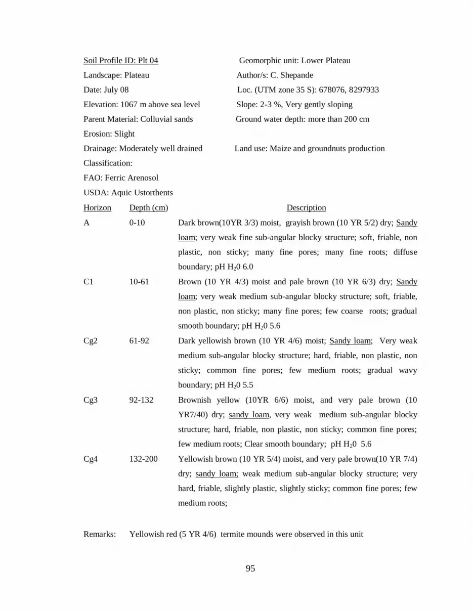
95

Soil Profile ID: Plt 04 Geomorphic unit: Lower Plateau

Landscape: Plateau Author/s: C. Shepande

Date: July 08 Loc. (UTM zone 35 S): 678076, 8297933

Elevation: 1067 m above sea level Slope: 2-3 %, Very gently sloping

Parent Material: Colluvial sands Ground water depth: more than 200 cm

Erosion: Slight

Drainage: Moderately well drained Land use: Maize and groundnuts production

Classification:

FAO: Ferric Arenosol

USDA: Aquic Ustorthents

Horizon Depth (cm) Description

A 0-10 Dark brown(10YR 3/3) moist, grayish brown (10 YR 5/2) dry; Sandy

loam; very weak fine sub-angular blocky structure; soft, friable, non

plastic, non sticky; many fine pores; many fine roots; diffuse

boundary; pH H20 6.0

C1 10-61 Brown (10 YR 4/3) moist and pale brown (10 YR 6/3) dry; Sandy

loam; very weak medium sub-angular blocky structure; soft, friable,

non plastic, non sticky; many fine pores; few coarse roots; gradual

smooth boundary; pH H20 5.6

Cg2 61-92 Dark yellowish brown (10 YR 4/6) moist; Sandy loam; Very weak

medium sub-angular blocky structure; hard, friable, non plastic, non

sticky; common fine pores; few medium roots; gradual wavy

boundary; pH H20 5.5

Cg3 92-132 Brownish yellow (10YR 6/6) moist, and very pale brown (10

YR7/40) dry; sandy loam, very weak medium sub-angular blocky

structure; hard, friable, non plastic, non sticky; common fine pores;

few medium roots; Clear smooth boundary; pH H20 5.6

Cg4 132-200 Yellowish brown (10 YR 5/4) moist, and very pale brown(10 YR 7/4)

dry; sandy loam; weak medium sub-angular blocky structure; very

hard, friable, slightly plastic, slightly sticky; common fine pores; few

medium roots;

Remarks: Yellowish red (5 YR 4/6) termite mounds were observed in this unit

96

Soil Profile ID: Vd 05 Geomorphic unit: Narrow dambo

Landscape: Valley Dambo Author/s: C. Shepande

Date: July 08 Loc. (UTM zone 35 S): 669432, 8300829

Elevation: 1010 m above sea level Slope: 0-1 %, almost flat

Parent Material: Colluvial sands Ground water depth: 145 cm

Erosion: None

Drainage: Poorly drained Land use: Free range grazing

Classification:

FAO: Dystric Gleysol

USDA: Typic Fluvaquents

Horizon Depth (cm) Description

Ag 0-13 Black(10YR 2/1) moist, grayish brown (10 YR 5/2) dry; Sand;

common medium distinct red mottles with rusty root channels;

structureless; soft, friable, non plastic, non sticky; many fine pores;

many fine roots; gradual smooth boundary; pH H20 6.1

Cg1 13-22 Brown (10 YR 5/3) moist and pale brown (10 YR 6/3) dry; Sand;

structureless, many, fine-medium distinct red mottles; loose, friable,

non plastic, non sticky; many fine pores; few coarse roots; clear

wavy boundary; pH H20 6.5

Cg2 22-71 Light brownish gray (10 YR 6/2) moist; Sand; structureless; common

medium distinct red mottles, soft, friable, non plastic, non sticky;

common fine pores; few medium roots; clear wavy boundary; pH H20

7.2

Cg3 71-92 Grayish brown (10YR 5/2) moist; sand, many, coarse, prominent red

mottles; structureless; friable, non plastic, non sticky; common fine

pores; no roots; Clear wavy boundary; pH H20 8.1

Cg4 92-148 Gray (10 YR 6/1) moist; sandy loam; structureless; common coarse

prominent red mottles; firm, slightly plastic, slightly sticky; few

medium pores; no roots; pH H20 8.3

Remarks: Soil is well mottled to the ground surface. Animal grazing in the dry season is

common around this area

97

Soil Profile ID: Plt 06 Geomorphic unit: Lower Plateau

Landscape: Plateau Author/s: C. Shepande, Jere

Date: July 08 Loc. (UTM zone 35 S): 670871, 8297392

Elevation: 1075 m above sea level Slope: 2-3 %, Very gently sloping

Parent Material: Colluvial sands Ground water depth: more than 110 cm

Erosion: Slight

Drainage: Well drained Land use: Maize and groundnuts production

Classification:

FAO: Ferric Arenosol

USDA: Ustic Quartzipsamments

Horizon Depth (cm) Description

A 0-8 Very dark gray(10YR 3/1) moist, gray (10 YR 5/1) dry; Sand;

structureless ; soft, friable, non plastic, non sticky; many fine pores;

few fine roots; diffuse boundary

C1 8-36 Brown (10 YR 5/3) moist and grayish brown (10 YR 5/2) dry; Sand;

structureless; soft, friable, non plastic, non sticky; many fine pores;

few coarse roots; diffuse boundary

C2 36-80 Pale brown (10 YR 6/3) moist, and light gray (10 YR 7/1) Sand;

structureless; soft, friable, non plastic, non sticky; many fine pores;

few medium roots; diffuse boundary

C3 80-111 Brownish yellow (10YR 6/3) moist, and very pale brown (10 YR7/1)

dry; sand, structureless; slightly hard, friable, non plastic, non sticky;

common fine pores; no roots; Clear smooth boundary

m 111+ Weakly cemented iron concentrations

Remarks: Limiting layer- laterite comprised of weekly cemented concretions

PH data not available

98

Soil Profile ID: Lpt 07 Geomorphic unit: Lower Piedmont

Landscape: Piedmont Author/s: C. Shepande, Jere

Date: July 08 Loc. (UTM zone 35 S): 666568, 8295850

Elevation: 1205 m above sea level Slope: 4 %,

Parent Material: Gneiss Ground water depth: more than 171 cm

Erosion: None

Drainage: Well drained Land use: Tobacco and cotton production

Classification:

FAO: Ferric Acrisol

USDA: Typic Rhodustults

Horizon Depth (cm) Description

A 0-10 Dark reddish brown (5 YR 3/2) moist, reddish brown (5 YR 4/3) dry;

Sandy loam; weak crumb structure ;soft, friable, slightly sticky,

slightly plastic, many fine pores; many fine roots; clear wavy

boundary; pH H20 6.2

Bt 10-70 Dark reddish brown (5 YR 3/3) moist and reddish brown (5 YR 4/3)

dry; Sand clay; weak medium sub-angular blocky structure; very

hard, firm, plastic, sticky; many fine pores; few coarse, common fine

roots; diffuse boundary; pH H20 6.1

B2 70-95 Dark reddish brown (2.5 YR 3/4) moist, and red (2.5 YR 4/6) dry;

Sandy clay loam; weak medium sub-angular blocky structure; very

hard, friable, slightly plastic, slightly sticky; few medium, many fine

pores; common medium roots; diffuse boundary; pH H20 5.9

B3 95-122 Red (2.5 YR 4/6) moist and red (2.5 YR 4/8)dry; sandy clay loam,

weak, medium sub-angular block structure; very hard, friable, slightly

plastic, slightly sticky; many fine pores; few fine, common medium

roots; diffuse boundary; pH H20 5.9

C 122-171 Red (2.5 YR 4/8) moist and red (2.5 YR 5/8) dry; sandy clay loam,

weak medium sub-angular blocky structure, very hard, friable, plastic,

sticky, many fine pores, few medium roots; pH H20 5.8

Remarks: Few red (2.5 YR 4/8 termite mounds in vicinity of the soil profile

99

Soil Profile ID: Rp 10 Geomorphic unit: Old River channel (Paleochannel)

Landscape: River/Alluvial plain Author/s: C. Shepande

Date: July 08 Loc. (UTM zone 35 S): 683480, 8294129

Elevation: 1015 m above sea level Slope: 2-3 %, gently sloping, concave slope

Parent Material: Alluvium Ground water depth: more than 77 cm

Erosion: None

Drainage: Poorly drained Land use: Maize and sunflower production

Classification:

FAO: Umbric Fluvisol

USDA: Typic Ustifluvents

Horizon Depth (cm) Description

A 0-20 Black (7.5YR 2.5/1) moist, gray (7.5 YR 5/1) dry; Sand clay loam;

Moderate fine-medium sub-angular blocky structure ; hard, friable,

plastic, sticky; many medium pores; common coarse roots; clear

smooth boundary pH H20 6.5

AB 20-40 Brown (7.5 YR 4/2) moist and gray (7.5 YR 6/1) dry; Sandy clay

loam; Moderate fine-medium sub-angular blocky structure; hard,

friable, plastic, sticky; many fine pores; few coarse roots; clear

gradual boundary pH H20 6.5

C1 40-63 brown (7.5 YR 5/3) moist, light gray (10 YR 7/1) Sandy loam; weak

medium sub-angular blocky structure; soft, friable, plastic, sticky; few

fine pores; few fine roots; clear gradual boundary pH H20 6.4

C2 63-77 Brown (7.5YR 5/4) moist, and light gray (10 YR7/1) dry; clay loam,

weak fine-medium sub-angular blocky structure; slightly hard, friable,

plastic, sticky; few fine pores; few fine roots; pH H20 6.1

Remarks: Areas that are not under maize and sunflower production are under extensive

grazing and ranching. The soil is moist in lower parts of the profile.

100

Soil Profile ID: Vd 11 Geomorphic unit: Narrow dambo

Landscape: Valley Dambo Author/s: C. Shepande, Jere

Date: July 08 Loc. (UTM zone 35 S): 669591, 8299863

Elevation: 1012 m above sea level Slope: 0-1 %, almost flat

Parent Material: Dambo alluvium Ground water depth: more than 100 cm

Erosion: None

Drainage: Poorly drained Land use: Free range grazing

Classification:

FAO: Dystric Gleysol

USDA: Typic Fluvaquents

Horizon Depth (cm) Description

Ah 0-50 Black(N 2/0) moist; clay loam; weak fine granular structure; soft,

friable, plastic, sticky; many fine pores; many fine roots; diffuse

boundary;

B 50-60 Very dark gray (10 YR 3/1) moist; Loam to clay loam; weak medium

sub-angular blocky structure; soft, friable, plastic, sticky; many fine

pores; many fine roots; clear wavy boundary;

C 60-100 Light gray (10 YR 7/1) moist; loam; structureless; common medium

prominent red mottles, soft, friable, slightly plastic, slightly sticky;

common fine pores; few medium roots; clear wavy boundary

Remarks: Kaolinite is the most common clay mineral in these soils. The soils developed in

water logged conditions and show characteristics of a hydric soil.

101

Soil Profile ID: Plt 12 Geomorphic unit: Plateau summit

Landscape: Plateau Author/s: C. Shepande

Date: July 08 Loc. (UTM zone 35 S): 670654, 8302537

Elevation: 1130 m above sea level Slope: 0 %, flat

Parent Material: Quartzite Ground water depth: Not observed

Erosion: None

Drainage: Well drained Land use: Maize and beans production

Classification:

FAO: Ferric Acrisol

USDA: Typic Haplustults

Horizon Depth (cm) Description

A 0-9 Very dark brown(10YR 2/2) moist, and dark grayish brown (10 YR

4/2) dry; Sandy loam; weak medium sub-angular blocky structure;

hard, friable, slightly plastic, slightly sticky; common fine pores;

many fine roots; clear smooth boundary; pH H20 7.3

BA 9-20 Dark brown (7.5 YR 3/4) moist and brown (7.5YR 5/3) dry; Sandy

loam; weak fine-medium sub-angular blocky structure; hard, firm,

slightly plastic, slightly sticky; few medium pores; few fine roots;

diffuse boundary; pH H20 6.4

Bt 20-71 Yellowish red (5 YR 4/6) moist, and reddish yellow (5 YR

6/6);Sandy clay; weak medium sub-angular blocky structure; hard,

firm, plastic, sticky; common fine pores; few medium roots; thin

patch cutans; pH H20 6.4

R 71 + Solid quartzite bedrock

Remarks: There are quartzite rock outcrops within 30 meters of the profile pit. At 70 cm depth

there is a solid quartzite bedrock beyond which we could not dig. Patchy cutans

were observed in the 20-70 cm horizon. Strong brown termite mounds are common

and were observed within 5-10 meters of the soil profile.

102

Soil Profile ID: Lpt 13 Geomorphic unit: Lower Piedmont

Landscape: Piedmont Author/s: C. Shepande, Jere

Date: July 08 Loc. (UTM zone 35 S): 666052, 8289444

Elevation: 1241 m above sea level Slope: 2-3 %,

Parent Material: Quartzite Ground water depth: more than 109 cm

Erosion: Slight

Drainage: Well drained Land use: Tobacco and cotton production

Classification:

FAO: Ferric Acrisol

USDA: Typic Paleustults

Horizon Depth (cm) Description

A 0-20 Dark brown (7.5 YR 3/3) moist, brown (7.5 YR 5/4) dry; Sandy

loam; very weak crumb (almost structureless) ; many fine pores;

many fine roots; clear wavy boundary

BA 20-36 Strong brown (7.5 YR 4/6) moist and reddish yellow (7.5 YR 6/8)

dry; Sand clay loam; weak medium sub-angular blocky structure;

very hard, friable, slightly plastic, slightly sticky; many fine pores;

few coarse roots; diffuse boundary

Bt1 36-80 Strong brown (7.5 YR 5/8) moist, and reddish yellow (7.5 YR 6/8)

Sandy clay; weak fine sub-angular blocky structure; soft, friable,

plastic, sticky; many fine pores; few medium roots; diffuse boundary

Bt2 80-112 Strong brown (7.5 YR 5/8) moist; Clay, moderate, medium sub-

angular block structure; slightly firm, plastic, sticky; moderate patchy

cutans, many fine pores; few fine-medium roots; diffuse boundary

Bt3 112-195 Reddish yellow (7.5 YR 6/6) moist, clay, weak fine-medium sub-

angular blocky structure, slightly firm, plastic, sticky, thin patchy

cutans, many fine pores, few fine medium coarse roots

Remarks: Mica and fragments of quartz were observed in all horizons. There is a hard pan

layer (cultivation pan) in the 20-36 horizon. Thin to moderate patchy cutans were

observed in the 80-112 and 112-195 horizons.

103

Soil Profile ID: Rp 14 Geomorphic unit: Tread-riser complex

Landscape: River/Alluvial plain Author/s: C. Shepande

Date: July 08 Loc (UTM zone 35 S): 674784, 8295462

Elevation: 1072 m above sea level Slope: 0.5-1 %, nearly level

Parent Material: Alluvium Ground water depth: more than 130 cm

Erosion: Moderate sheet erosion

Drainage: Moderately well drained Land use: Maize and groundnuts production

Classification:

FAO: Umbric Fluvisol

USDA: Typic Ustifluvents

Horizon Depth (cm) Description

Ah 0-20 Very dark grayish brown(10YR 3/2) moist, brown (10 YR 4/3) dry;

Sandy clay loam; moderate medium to coarse sub-angular blocky

structure ; hard, friable, plastic, slightly sticky; many coarse pores;

few coarse roots; clear smooth boundary; pH H20 5.5

AB 20-34 Dark brown (10 YR 3/3) moist and dark brown (10 YR 3/1) dry;

Sandy clay loam; moderate fine-medium sub-angular blocky

structure; slightly hard, friable, plastic, slightly sticky; common fine

pores; few medium-coarse coarse roots; clear smooth boundary;

pH H20 5.5

2Ah 34-70 Very dark gray (10 YR 3/1) moist, and dark gray (10 YR 4/1) dry

Sand clay loam; moderate medium sub-angular blocky structure;

hard, friable, plastic, slightly sticky; many fine pores; common fine

roots; wavy diffuse boundary; pH H20 6.5

C1 70-110 Very dark gray (10YR 3/2) moist, and dark gray (10 YR4/1) dry;

sandy clay loam, moderate medium sub-angular blocky structure;

hard, friable, plastic, slightly sticky; common fine pores; no roots;

Clear smooth boundary; pH H20 6.5

C2 110-130 Dark brown (10YR 3/3) moist and brown (10 YR 4/3) dry; Sandy

loam, moderate medium sub-angular blocky structure; slightly hard,

friable, slightly plastic, slightly sticky; pH H20 6.5

Remarks: At 34-70 depth a buried horizon was observed

104

Soil Profile ID: Vd 15 Geomorphic unit: Broad dambo

Landscape: Valley Dambo Author/s: C. Shepande, Jere

Date: July 08 Loc. (UTM zone 35 S): 668598, 8299951

Elevation: 1009 m above sea level Slope: 0-1 %, flat

Parent Material: Dambo alluvium Ground water depth: 120 cm

Erosion: None

Drainage: Poorly drained Land use: Cabbage production and cattle grazing

Classification:

FAO: Eutric Gleysol

USDA: Mollic Endoaqualfs

Horizon Depth (cm) Description

Ahg 0-15 Black(10 YR 2/1) moist; sandy clay; weak fine crumb to sub-angular

blocky structure; few fine faint-distinct strong brown (7.5 YR 5/6)

mottles; friable, slightly plastic, slightly sticky; many fine pores;

many fine roots; gradual smooth boundary; pH H20 8.8

Btg 15-24 Very dark gray (2.5 YR 2.5/1) moist; clay; moderate medium sub-

angular blocky structure; many medium-coarse distinct strong brown

(7.5 YR 5/6) mottles friable, plastic, sticky; few fine-medium pores;

many fine roots; diffuse smooth boundary; pH H20 6.7

Cg1 24-71 Dark grayish brown (10 YR 4/2) moist; Sandy loam; structureless;

many medium distinct strong brown (7.5 YR 5/6)mottles; friable, non

plastic, non sticky; common fine pores; few fine roots; abrupt wavy

boundary; pH H20 7.3

Cg2 71-82 Dark gray (7.5 YR 4/1) moist, Clayey loam, weak medium sub-

angular blocky structure; many medium distinct strong brown (7.5

YR 5/6) mottles; firm, plastic, sticky; abrupt wavy boundary; pH H20

7.5

Cg3 82-120 Greenish black ((5G 2.5/1) moist, Clay; weak medium sub-angular

block structure, non-mottled, firm, very plastic, sticky; few medium,

common fine pores; few fine roots

Remarks: Water table at 120 cm dept. All horizons micaceous

105

Soil Profile ID: Vd 16 Geomorphic unit: Broad dambo

Landscape: Valley Dambo Author/s: C. Shepande, Jere

Date: July 08 Loc. (UTM zone 35 S): 668889, 8299467

Elevation: 1012 m above sea level Slope: 0-1 %, flat

Parent Material: Dambo alluvium Ground water depth: 138 cm

Erosion: None

Drainage: Poorly drained Land use: Cabbage production and cattle grazing

Classification:

FAO: Eutric Gleysol

USDA: Mollic Endoaqualfs

Horizon Depth (cm) Description

Ah 0-12 Black(10 YR 2/1) moist; sandy clay loam; weak fine sub-angular

blocky structure; many fine distinct red (2.5 YR 5/6) mottles; soft,

friable, slightly plastic, slightly sticky; many fine pores; many fine

roots; diffuse boundary; pH H20 6.1

Bt1 12-25 Dark brown (10 YR 3/3) moist; Sandy clay; weak medium sub-

angular blocky structure; common fine faint red (2.5 YR 5/6)

mottles; friable, plastic, sticky; few fine-medium pores; many fine

roots; diffuse boundary; pH H20 6.5

Bt2g 25-48 Dark gray (2.5 YR 4/1) moist; clay; weak coarse sub-angular blocky

structure; common fine faint yellowish red (5 YR 5/6)mottles; firm,

very plastic, very sticky; common fine pores; common medium, few

fine roots; diffuse boundary; pH H20 7.2

Bt3g 48-109 Dark brown (2.5 YR 4/1) moist, clay, weak medium-coarse sub-

angular blocky structure; common medium distinct yellowish red (5

YR 5/6)mottles; firm, very plastic, sticky; clear wavy boundary; pH

H20 8.1

Bt4g 109-138 Gray (2.5 Y 5/1) moist, Gritty clay; weak medium sub-angular block

structure, many medium prominent yellowish red (5 YR 5/6) mottles,

firm, very plastic, very sticky; few medium, common fine pores; no

roots

Remarks: The soil pit is well mottled from surface to water table (138 cm

106

Soil Profile ID: Upt 17 Geomorphic unit: Upper Piedmont

Landscape: Piedmont Author/s: C. Shepande

Date: July 08 Loc. (UTM zone 35 S): 668057, 8288704

Elevation: 1248 m above sea level Slope: 3-4 %,

Parent Material: Schist or quartzite Ground water depth: more than 129 cm

Erosion: Slight

Drainage: Well drained Land use: Acacia tree species

Classification:

FAO: Rhodic Ferrasol

USDA: Typic Haplustox

Horizon Depth (cm) Description

A 0-11 Dark brown (7.5 YR 3/2) moist, brown (7.5 YR 4/2) dry; Loamy sand;

weak fine granular to single grain; loose, non sticky, non plastic; many

fine pores; many fine roots; clear wavy boundary, pH H20 6.8

B1 11-22 Yellowish red (5 YR 4/6) moist and (5 YR 5/8) dry; loamy sand; weak

fine granular structure; loose, non plastic, non sticky; many fine pores;

few coarse roots; diffuse boundary; pH H20 6.5

B2 22-37 Yellowish red (5 YR 5/8) moist, and yellowish red (7.5 YR /6) Sandy

loam; weak medium sub-angular blocky structure; soft, friable,

slightly plastic, slightly sticky; many fine pores; few medium roots;

clear smooth boundary; pH H20 6.5

B3 37-64 Light reddish brown (2.5 YR 6/4) moist and light red (2.5 YR 6/6) dry;

Sandy clay loam, weak, medium sub-angular block structure; soft,

friable, slightly plastic, slightly sticky; many fine pores; few fine-

medium roots; clear wavy boundary; pH H20 6.2

C 64-118 Red (2.5 YR 5/6) moist and (2.2 YR 5/8) dry, sandy clay loam, weak

medium sub-angular blocky structure, soft, friable, slightly plastic,

slightly sticky, many fine pores, gradual boundary; pH H20 6.5

2C 118-129 Red (2.5 YR 5/6) moist and (2.2 YR 5/8) dry, gravelly sandy clay

loam, weak medium sub-angular blocky structure; loose, friable,

slightly plastic, slightly sticky; many fine-medium pores; pH H20 6.7

Remarks: Quartzite outcrops observed within 10 m of the soil pit.

107

Soil Profile ID: Upt 19 Geomorphic unit: Upper Piedmont

Landscape: Piedmont Author/s: C. Shepande

Date: July 08 Loc. (UTM zone 35 S): 668274, 8289264

Elevation: 1239 m above sea level Slope: 3-4 %,

Parent Material: Schist Ground water depth: more than 177 cm

Erosion: Slight

Drainage: Well drained Land use: Bare land

Classification:

FAO: Rhodic Ferrasol

USDA: Rhodic Haplustox

Horizon Depth (cm) Description

Ap 0-22 Dark reddish brown (5 YR 3/4) moist, reddish brown (5 YR 4/4) dry;

Sandy loam; weak fine granular structure; soft, friable, non sticky, non

plastic; many fine, common medium pores; many fine, few coarse

roots; abrupt boundary, pH H20 7.1

B1 22-45 Yellowish red (5 YR 4/6) moist and (5 YR 5/8) dry; sandy loam; weak

fine sub-angular blocky structure; soft, very friable, slightly plastic,

slightly sticky; many fine pores; few coarse roots; clear wavy

boundary; pH H20 7.0

B2 45-127 Dark red (2.5 YR 3/6) moist, and red (2.5 YR 4/6) Sandy clay loam;

weak fine sub-angular blocky structure; soft, very friable, slightly

plastic, sticky; many fine pores; few medium roots; diffuse boundary;

pH H20 6.5

B3 127-170 Red (2.5 YR 5/6) moist and l red (2.5 YR 4/8) dry; Sandy clay loam,

weak, fine sub-angular block structure; soft, very friable, slightly

plastic, sticky; many fine pores; few fine-medium roots; gradual

boundary; pH H20 6.4

C 170-177 Red (2.5 YR 4/8) moist, weathered schist; The upper part of the

horizon is sub-angular blocky grading into more angular with depth

Remarks: Laterite fragments were observed on the ground surface. Weathered schist was

observed in the 170 -177 cm depth.

108

Soil Profile ID: Upt 20 Geomorphic unit: Upper Piedmont

Landscape: Piedmont Author/s: C. Shepande

Date: July 08 Loc. (UTM zone 35 S): 665462, 8304462

Elevation: 1241 m above sea level Slope: 3-4 %,

Parent Material: Schist or quartzite Ground water depth: more than 152 cm

Erosion: Slight

Drainage: Well drained Land use: Logging

Classification:

FAO: Plinthic Ferrasol

USDA: Plinthic Haplustox

Horizon Depth (cm) Description

Ap 0-15 Dark reddish brown (2.5 YR 3/4) moist, dark red (2.5 YR 3/6) dry;

Sandy clay loam; structureless-massive structure; soft, slightly sticky,

slightly plastic; many fine pores; many fine, few coarse roots; clear

wavy boundary, pH H20 7.3

B1 15-38 Dark reddish brown (2.5 YR 3/4) moist and reddish brown (2.5 YR

4/4) dry; sandy clay loam; weak fine sub-angular blocky structure;

soft, friable, slightly plastic, sticky; many fine, few medium pores;

many fine, few coarse roots; gradual boundary; pH H20 7.2

B2 38-118 Red (2.5 YR 4/6) moist, and (2.5 YR 5/6) Sandy clay loam; weak

fine sub-angular blocky structure; soft, friable, slightly plastic, sticky;

many fine pores; few medium roots; diffuse boundary; pH H20 6.7

Bv3 118-152 Red (10 R 5/8) moist and red (2.5 R 4/8) dry; irregular aggregates of

plinthite; Platy and brick-like material; pH H20 6.2

Remarks: A plinthite hard pan horizon, too hard to cut with a spade was observed in the Bv3

horizon at 118-152 depth.

109

Soil Profile ID: Plt 21 Geomorphic unit: Plateau depression

Landscape: Plateau Author/s: C. Shepande

Date: July 08 Loc. (UTM zone 35 S): 677465, 8307264

Elevation: 1081 m above sea level Slope: 0-1 %, flat to slightly concave

Parent Material: Mica schist Ground water depth: 54 cm

Erosion: none

Drainage: Poorly drained Land use: Small scale vegetable production

Classification:

FAO: Ferric Cambisol

USDA: Typic Endoaquepts

Horizon Depth (cm) Description

Ah 0-7 Very dark grayish brown (10 YR 3/2) moist; clay; moderate medium

crumb structure; firm, sticky, plastic; many fine, common medium

pores; many fine, few coarse roots; abrupt boundary, pH H20 6.6

Bw 7-16 Dark yellowish brown (10 YR 4/4) moist; clay; moderate medium sub-

angular blocky structure; friable, plastic, sticky; many fine pores; few

coarse roots; clear wavy boundary; pH H20 6.9

Bg1 16-24 Dark grayish brown (10 YR 4/2) moist; clay; moderate medium sub-

angular blocky structure; common, medium faint yellowish red (5 YR

4/6) mottles; friable, plastic, sticky; many fine pores; few medium

roots; diffuse boundary; pH H20 7.1

Bg2 24-54 Grayish brown (10 YR 5/2) moist; clay , moderate medium sub-

angular block structure; many medium prominent red (2.5 YR 4/6)

mottles; friable, plastic, sticky; many fine pores; few fine-medium

roots; gradual boundary; pH H20 7.4

54+ Ground water table

Remarks: Permeability is slow due to high clay content. The ground water comes as high as 54

cm; drainage conditions are therefore poor.

110

Soil Profile ID: Rp 22 Geomorphic unit: Tread-riser complex

Landscape: River/Alluvial plain Author/s: C. Shepande

Date: July 08 Loc. (UTM zone 35 S): 674075, 8299099

Elevation: 1070 m above sea level Slope: 0.5-1 %, nearly level

Parent Material: Alluvium Ground water depth: more than 188 cm

Erosion: None

Drainage: Moderately well drained Land use: Groundnuts cultivation

Classification:

FAO: Umbric Fluvisol

USDA: Typic Ustifluvents

Horizon Depth (cm) Description

Ap 0-20 Very dark brown(10YR 2/2) moist, very dark grayish brown (10 YR

3/2) dry; loam; weak medium sub-angular blocky structure ; soft,

friable, slightly plastic, slightly sticky; many coarse pores; few coarse

roots; abrupt boundary; pH H20 6.9

A 20-55 Very dark brown (10 YR 2/2) moist; very dark grayish brown (10 YR

3/) dry; clay loam; weak medium sub-angular blocky; slightly hard,

firm, slightly plastic, slightly sticky; common fine pores; few medium-

roots; gradual boundary; pH H20 7.0

Ac 55-81 Dark gray (10 YR 4/1) moist, and dark grayish brown (10 YR 4/2) dry;

clay; moderate coarse prismatic blocky structure; hard, firm, plastic,

sticky; many fine pores; common fine roots; gradual boundary; pH H20

7.0

C1 81-114 Dark grayish brown (10YR 4/2) moist, and dark yellowish brown (10

YR4/4) dry; clay loam, weak coarse prismatic structure; hard, firm,

slightly plastic, slightly sticky; common fine pores; no roots; gradual

boundary; pH H20 7.5

C2 114-165 Yellowish brown (10YR 5/6) moist; brown (10 YR 5/8) dry; clay loam;

weak, medium prismatic structure; few fine faint (10 YR 5/1) mottles;

hard, firm, slightly plastic, sticky; gradual boundary; pH H20 7.5

C3 165-188 Yellowish brown (10YR 5/6) moist; clay; weak medium prismatic

structure; common medium distinct gray (N6/) mottles; pH H20 6.5

111

Soil Profile ID: Lpt 23 Geomorphic unit: Lower Piedmont

Landscape: Piedmont Author/s: C. Shepande

Date: July 08 Loc. (UTM zone 35 S): 665719, 8305543

Elevation: 1207 m above sea level Slope: 2-3 %,

Parent Material: Quartzite Ground water depth: more than 167 cm

Erosion: Slight

Drainage: Well drained Land use: Small sunflower plots

Classification:

FAO: Haplic Arenosols

USDA: Typic Dystrustents

Horizon Depth (cm) Description

Ap 0-20 Brown (7.5 YR 4/4) moist, strong brown (7.5 YR 4/6) dry; Sandy

loam; weak fine granular to single grain structure; very friable, soft,

slightly sticky, slightly plastic, many fine, few medium pores; many

fine, few coarse roots; abrupt boundary; pH H20 5.7

C1 20-55 Yellowish red (5 YR 4/6) moist, and (5 YR 5/6) dry; Sand loam;

weak fine granular to single grain structure; soft, very friable, slightly

plastic, slightly sticky; many fine pores; few coarse roots; gradual

boundary; pH H20 5.6

C2 55-111 Yellowish red (5 YR 5/6) moist, and (5 YR 5/8) dry, Sandy loam;

weak fine granular to single grain structure; soft, very friable, slightly

plastic, non sticky; many fine pores; few medium roots; diffuse

boundary; pH H20 5.6

C3 111-167 Yellowish red 5 YR 5/6) moist and (5 YR 5/8) dry; sandy loam, weak

fine , single grain structure; soft, very friable, non plastic, non

sticky; few fine pores; diffuse boundary pH H20 5.4;

2C 167+ Quartz gravel line

Remarks: Loosely packed quartz gravel was observed at 167 cm depth. A few quartzite rock

outcrops were observed within 10-15 m of the soil pit.

112

Soil Profile ID: Rp 24 Geomorphic unit: Riser

Landscape: River/Alluvial plain Author/s: C. Shepande

Date: July 08 Loc. (UTM zone 35 S): 668243, 8296730

Elevation: 1025 m above sea level Slope: 1-2 %, very gently slopping

Parent Material: Recent alluvium Ground water depth: more than 190 cm

Erosion: None

Drainage: Moderately well drained Land use: Groundnuts cultivation

Classification:

FAO: Umbric Fluvisol

USDA: Typic Ustifluvents

Horizon Depth (cm) Description

Ap 0-25 Dark grayish brown(10YR 4/2) moist, brown (10 YR 4/3) dry; loamy

fine sand; structureless ; loose, non plastic, non sticky; many coarse

pores; common medium, few coarse roots; abrupt boundary; pH H20 6.7

C1 25-129

Stratified

horizon

25-26 cm brown-yellowish brown (10YR4/3-5/6) clay loam;

structureless to weak fine sub-angular blocky structure

36-66 cm Brown (10YR 4/3) fine sandy loam; structureless, few fine

faint yellowish brown (10YR 5/8) mottles

66-129 cm Yellowish brown (10YR 5/4) sand; structureless

C2 129-162 Grayish brown (10 YR 5/2); silty clay loam; weak fine sub-angular

blocky structure; fine faint yellowish brown (10 YR 5/8) mottles;

abrupt boundary; pH H20 6.9

2A 162-182 Black (10YR 2/1); clay loam, weak fine sub-angular blocky structure;

very friable, slightly plastic, slightly sticky; Dark red (2.5 YR 3/6)

staining on root channels; common fine pores; few fine roots; gradual

boundary; pH H20 7.9

2C 182-190 Very dark grayish brown (10YR 3/2); clay loam; weak, fine sub-

angular blocky structure; few fine distinct yellowish brown (10 YR 5/8)

mottles; very friable, slightly plastic, slightly sticky; gradual boundary;

pH H20 7.6

Remark Over wash material (mainly fluvial) rests abruptly on the black surface horizon of the

original soil. The horizon 25-129 is stratified with fine, medium and coarse strata

sand. The strata listed in the 25-129 horizon was selected as typical

113

Soil Profile ID: Rp 25 Geomorphic unit: Riser

Landscape: River/Alluvial plain Author/s: C. Shepande

Date: July 08 Loc. (UTM zone 35 S): 677434, 8295925

Elevation: 1022 m above sea level Slope: 1-2 %, very gently slopping

Parent Material: Recent alluvium Ground water depth: more than 193 cm

Erosion: None

Drainage: Moderately well drained Land use: Maize and sunflower production

Classification:

FAO: Umbric Fluvisol

USDA: Typic Udifluvents

Horizon Depth (cm) Description

Ap 0-25 Dusky red (2.5 YR 3/2); fine sandy loam; weak fine sub-angular

blocky structure; soft, friable, slightly plastic, slightly sticky; many

coarse pores; many coarse roots; abrupt boundary; pH H20 6.8

C1 25-60 Reddish brown (10 YR 4/3); fine sandy loam; weak fine sub-angular

blocky structure; soft, friable, slightly sticky, slightly plastic; many

medium pores, many coarse roots, abrupt boundary; pH H20 6.8

C2 60-144 Reddish brown (10 YR 4/3); clay loam; weak medium sub-angular

blocky structure; few, fine faint dark reddish brown (2.5 YR 3/4)

mottles; friable, soft, sticky, plastic; abrupt boundary; pH H20 6.9

2A 144-160 Black (10YR 2/1); loamy fine sand, weak fine sub-angular blocky

structure; friable, soft slightly plastic, slightly sticky; few fine faint

reddish brown (10 YR 4/4) mottles; common fine pores; few fine roots;

gradual boundary; pH H20 7.9

2C 160-171 Yellowish brown (10YR 5/6); sandy clay loam; weak, fine sub-angular

blocky structure; few fine faint yellowish red (5 YR 4/6) mottles;

friable, slightly plastic, slightly sticky; gradual boundary; pH H20 7.8

3C 171-193 Yellowish brown (10YR 5/4); fine sandy loam; weak fine sub-angular

blocky structure; few fine faint yellowish red (5 YR4/6) mottles;

friable, slightly sticky slightly plastic; pH H20 6.4

Remark Filamentous calcium carbonate (CaCo3) observed in the 144-160 horizon (2A)

114

Soil Profile ID: Rp 26 Geomorphic unit: Tread-riser complex

Landscape: River/Alluvial plain Author/s: C. Shepande

Date: July 08 Loc. (UTM zone 35 S): 676686, 8299767

Elevation: 1113 m above sea level Slope: 0.5-1 %, nearly level

Parent Material: Alluvium Ground water depth: more than 173 cm

Erosion: None

Drainage: Moderately well drained Land use: Maize and sunflower production

Classification:

FAO: Umbric Fluvisol

USDA: Aquic Ustifluvents

Horizon Depth (cm) Description

Ap 0-20 Very dark grayish brown(10YR 2/2); fine sandy loam; massive

structure ; very friable, slightly plastic, slightly sticky; many coarse

pores; few coarse roots; abrupt boundary; pH H20 6.8

C1 20-40 Very dark grayish brown (10 YR 3/2); sandy clay loam; massive

structure; very friable, slightly plastic, slightly sticky; many fine pores;

few medium-roots; abrupt boundary; pH H20 6.7

C2 40-76 Dark grayish brown (10 YR 4/2); clay loam; weak fine sub-angular

blocky structure; many fine faint brown (10 YR 4/3) mottles; friable,

slightly plastic, sticky; many fine pores; common medium roots;

gradual boundary; pH H20 7.3

2A 76-99 Black (10YR 2/1; clay loam, weak coarse prismatic to sub-angular

structure; few fine distinct brown (7.5 YR 4/4) mottles; friable, slightly

plastic, slightly sticky; common fine pores; few fine roots; gradual

boundary; pH H20 7.5

2C1 99-127 Very dark gray (10YR 3/1); sandy clay loam; weak, coarse prismatic-

sub angular blocky structure; common fine distinct brown (7.5YR 4/4)

mottles; friable, slightly plastic, sticky; gradual boundary; pH H20 7.7

2C2 127-173 Dark grayish brown (10YR 4/2) sandy loam; weak medium sub-

angular blocky structure; few fine faint dark yellowish brown (10 YR

4/4) mottles; friable, slightly plastic, slightly sticky; pH H20 6.4

Remarks: White mycelia of calcium carbonate (CaCo3 ) observed in the following horizons: 40-

76 cm (C2), 76-99 cm (2A) and 99-127 (2C1)

115

Soil Profile ID: Plt 27 Geomorphic unit: Plateau depression

Landscape: Plateau Author/s: C. Shepande

Date: July 08 Loc. (UTM zone 35 S): 678525, 8304744

Elevation: 1080 m above sea level Slope: 1 %, flat to slightly concave

Parent Material: Mica schist/limestone Ground water depth: 65 cm

Erosion: none

Drainage: Poorly drained Land use: Small scale vegetable production

Classification:

FAO: Ferric Cambisol

USDA: Aquic Haplustepts

Horizon Depth (cm) Description

Ah 0-12 Dark brown (10 YR 3/3); clay; moderate medium sub-angular blocky

structure; friable, sticky, plastic; many fine, common medium pores;

many fine, few coarse roots; clear wavy boundary, pH H20 6.8

AB 12-19 Dark yellowish brown (10 YR 3/4); clay; moderate medium sub-

angular blocky structure; friable, plastic, sticky; many fine pores; few

coarse, common medium roots; clear wavy boundary; pH H20 6.9

Bw 19-33 Dark yellowish brown (10 YR 4/4); clay; moderate medium sub-

angular blocky structure; friable, plastic, sticky; many fine, few coarse

pores; few medium roots; diffuse boundary; pH H20 7.0

Bg1 33-57 Brown (10 YR 4/3); clay ; moderate medium sub-angular block

structure; common medium faint yellowish red (5 YR 4/6) mottles;

friable, plastic, sticky; many fine pores; few fine-medium roots;

gradual boundary; pH H20 7.2

Bg2 57-65 Brown (10 YR 5/3); clay; weak medium sub-angular block structure;

common medium faint yellowish red (5 YR 4/6) mottles; friable,

plastic, sticky; few fine, common medium pores, common fine roots;

pH H20 7.2

Remarks: Water table observed at 65 cm from the ground surface

116

Soil Profile ID: RP 28 Geomorphic unit: Overflow basin

Landscape: River/Alluvial Plain Author/s: C. Shepande

Date: July 08 Loc. (UTM zone 35 S): 673328, 8297474

Elavation: 1015 m above sea level Slope: 3%, Concave slope

Parent Material: Recent alluvium Ground water depth: more than 170 cm

Erosion: None

Drainage: Imperfectly to poorly drained Land use: Dry season vegetable production

Classification:

FAO: Chromic Calcic Vertisol

USDA: Typic Calciausterts

Horizon Depth (cm) Description

Ap 0-20 Very dark gray (10YR 3/1); Clay; moderate medium sub-angular

blocky structure; friable, plastic, sticky; many fine pores; common

fine roots ;clear smooth boundary; pH H20 7.1

ABk 20-37 Very dark gray (10 YR3/1) ; Clay; strong coarse sub-angular blocky

structure; friable, plastic, very sticky; many fine pores; common fine,

few medium pores, common fine roots; clear wavy boundary pH H20

8.1

Bk 37-85 Dark reddish brown 2.5 YR 3/3); clay; strong very coarse angular

blocky structure; extremely firm, very sticky, plastic; many fine

pores; common fine roots ;clear smooth boundary; pH H20 8.7

CBkg 85-113 Weak red (2.5 YR 4/2); sandy lay; massive, very coarse platy

structure; very firm, plastic, sticky; common fine pores; common, fine

distinct, yellowish brown (10 YR 5/6) mottles; clear smooth

boundary pH H20 8.2

Cg 113-170 Reddish brown ( 2.5 YR 5/4) ; fine sandy clay; moderate , coarse

platy structure; very firm, plastic, sticky; many medium distinct

yellowish brown (10 YR 5/6) mottles; few medium pores; pH H20

8.2

Remarks: Columnar cracks were observed on the ground surface. Insect holes were observed

throughout horizon 0-20 cm (Ap). Horizon Bk (37-85 cm) is strongly calcareous.

117

Soil Profile ID: Rp 29 Geomorphic unit: Tread

Landscape: River/Alluvial plain Author/s: C. Shepande, Jere

Date: July 08 Loc. (UTM zone 35 S): 669672, 8299135

Elevation: 1027 m above sea level Slope: 0-1 %, flat to nearly level

Parent Material: Recent alluvium Ground water depth: more than 170 cm

Erosion: None

Drainage: Moderately well drained Land use: Cropland-maize and sunflower

Classification:

FAO: Chromic-haplic luvisol

USDA: Rhodic Kandiustults

Horizon Depth

(cm)

Description

Ap 0-16 Dark reddish brown (2.5 YR 3/3); fine sandy loam; weak very coarse

sub-angular blocky structure; soft, friable, slightly plastic, slightly

sticky; many fine pores; many fine, common medium roots; clear

abrupt boundary; pH H20 6.0

Bt1 16-37 Dark reddish brown (10 YR 3/4); sandy clay; moderate, very coarse

sub-angular blocky structure; soft, firm, sticky, plastic; many fine pores,

many fine, few medium roots, diffuse smooth boundary; pH H20 5.9

Bt2 37-97 Dark reddish brown (2.5 YR 3/4); fine sandy clay; moderate very

coarse sub-angular blocky structure; friable, soft, sticky, plastic; many

fine, very few medium roots; many fine, few medium pores gradual

smooth boundary; pH H20 6.1

Bt3 97-170 Dark red (2.5 YR 3/6); fine sandy clay, moderate very coarse sub-

angular blocky structure; very friable, soft, plastic, sticky; many fine

pores, few medium pores; many fine, very few medium roots; pH H20

6.4

Remark All four horizons are acidic and non-calcareous. Distinct, thin clay skins were

observed on vertical pedfaces in all the 3 argillic (Bt) horizons. In addition there are

spherical lined termite holes in local concentrations in the first 2 horizons.

118

Soil Profile ID: Rp 30 Geomorphic unit: Tread

Landscape: River/Alluvial plain Author/s: C. Shepande

Date: July 08 Loc. (UTM zone 35 S): 672016, 8298759

Elevation: 1023 m above sea level Slope: 0-1 %, flat to nearly level

Parent Material: Recent alluvium Ground water depth: more than 168 cm

Erosion: None

Drainage: Moderately well drained Land use: Cropland-maize and sunflower

Classification:

FAO: Chromic-haplic luvisol

USDA: Typic Kandiustults

Horizon Depth (cm) Description

Ap 0-20 Dark reddish brown (5 YR 3/3); sandy loam; weak coarse sub-angular

blocky structure; soft, very friable, non plastic, non sticky; many fine,

common medium pores; many fine, many medium roots; abrupt and

smooth boundary; pH H20 5.7

Bt1 20-60 Reddish brown (5 YR 4/3); coarse sandy clay loam; weak, very coarse

sub-angular blocky structure; hard, very friable, slightly sticky, slightly

plastic; many fine, few medium pores, many fine, few medium roots,

gradual smooth boundary; pH H20 5.5

Bt2 60-114 Yellowish red (5 YR 4/6); fine sandy clay loam; weak very coarse

sub-angular blocky structure; very friable, soft, sticky, plastic; many

fine, very few medium roots; many fine, few medium pores gradual

smooth boundary; pH H20 5.4

Bt3 114-150 Yellowish red (5 YR 4/6); very fine sandy clay loam, weak very coarse

sub-angular blocky structure; very friable, soft, plastic, sticky; many

fine pores, few medium pores; many fine, very few medium roots; pH

H20 5.6

C 150-168 Yellowish red (2.5 YR 4/6); stony sandy clay loam; local discontinuous,

weakly cemented sesquioxides (Fe, Al, Mn)

Remark Clay skins were observed on both horizontal and vertical pedfaces. 60-70 %stony

fragments were observed in the C horizon

119

Soil Profile ID: Plt 31 Geomorphic unit: Plateau depression

Landscape: Plateau Author/s: C. Shepande, Jere

Date: July 08 Loc (UTM zone 35 S): 674356, 8306345

Elevation: 1095 m above sea level Slope: 1 %, flat to slightly concave

Parent Material: Quartzite Ground water depth: More than 160 cm

Erosion: none

Drainage: Poorly drained Land use: Small scale vegetable production

Classification:

FAO: Ferric Cambisol

USDA: Typic Haplustepts

Horizon Depth (cm) Description

Ap 0-27 Dark brown (10 YR 3/3); fine loamy sand; single grain granular

structure; loose, non sticky, non plastic; many fine, common medium

pores; many fine, common medium roots; abrupt smooth boundary, pH

H20 5.0

Bw 27-47 Weak red (2.5 YR 4/2); fine loamy sand; moderate medium sub-

angular blocky structure; very friable, non plastic, non sticky; many

medium common fine pores; few coarse, common medium roots;

clear smooth boundary; pH H20 5.7

C 47-81 Light reddish brown (2.5 YR 6/4); coarse sand; massive granular

structure; loose, non plastic, non sticky; many fine, few coarse pores;

few medium roots; diffuse boundary; pH H20 7.4

2Cg 81-92 Brown (10 YR 4/2); coarse loamy sand ; massive granular structure;

many medium faint dark reddish brown (10 YR 4/6) mottles; friable,

non plastic, slightly sticky; many fine pores; few fine-medium roots;

abrupt and smooth boundary; pH H20 7.4

3Cg 92-105 Gray (10 YR 6/1); coarse sand; massive granular structure; many

medium faint dark reddish brown (10 YR 4/6) mottles; very friable,

non plastic, non sticky; many medium, common fine pores, few fine

roots; abrupt and smooth boundary; pH H20 7.9

4Cg 105-160 Grayish brown (10 YR 5/2); coarse loamy sand; massive granular

structure; many medium faint dark reddish brown (10YR 4/6) mottles;

friable non sticky non plastic; many fine pores; pH H20 7.9

120

Soil Profile ID: Rp 32 Geomorphic unit: Tread

Landscape: River/Alluvial plain Author/s: C. Shepande

Date: July 08 Loc. (UTM zone 35 S): 674996, 8300807

Elevation: 1035 m above sea level Slope: 0 %, flat

Parent Material: Recent alluvium Ground water depth: more than 170 cm

Erosion: None

Drainage: Moderately well drained Land use: Cropland-maize, sunflower and soybeans

Classification:

FAO: Chromic luvisol

USDA: Typic Kandiustults

Horizon Depth (cm) Description

Ap 0-20 Brown (7.5 YR 4/4); fine loamy sand; weak coarse sub-angular blocky

structure; very friable, non plastic, non sticky; many fine, many

medium pores; many fine, many medium roots; abrupt and smooth

boundary; pH H20 5.0

Bt1 20-60 Dark reddish brown (5 YR 3/4); coarse sandy clay loam; weak, very

coarse sub-angular blocky structure; friable, slightly sticky, slightly

plastic; many fine, many medium pores, many fine, few medium roots,

gradual smooth boundary; pH H20 5.0

Bt2 60-100 Reddish brown (5 YR 4/4); fine sandy clay loam; moderate very

coarse sub-angular blocky structure; friable, sticky, plastic; many fine,

very few medium roots; many fine, few medium pores clear smooth

boundary; pH H20 6.0

Btk 100-130 Reddish brown (5 YR 4/4); sandy clay; moderate very coarse sub-

angular blocky structure; friable, plastic, sticky; many fine, few medium

pores; many fine, very few medium roots; pH H20 8.3

Cs 130-150 Poorly sorted stone line weakly cemented with iron; coarse sub-angular

rock fragments

R 150-170 Weathered rock- very micaceous schist

Remark Termite holes partly filled with termite excretal and nest materials were observed

throughout the Bt horizons (60-130 cm depth). Soft powdery lime was observed in the

strongly effervescence Btk horizon (100-130 cm).

121

Soil Profile ID: Rp 33 Geomorphic unit: Old River channel (Paleochannel)

Landscape: River/Alluvial plain Author/s: C. Shepande, Jere

Date: July 08 Loc. (UTM zone 35 S): 678223, 8296880

Elevation: 1018 m above sea level Slope: 2-3 %, gently sloping, concave slope

Parent Material: Alluvium Ground water depth: more than 160 cm

Erosion: None

Drainage: Poorly drained Land use: Subsistence maize production

Classification:

FAO: Vertic Luvisol

USDA: Vertic Endoaqualfs

Horizon Depth (cm) Description

Ap 0-15 Very dark grayish brown (10 YR 3/2); fine sand clay loam; Moderate

medium sub-angular blocky structure; very friable, plastic, slightly

sticky; many fine pores; many fine, common medium roots; abrupt

smooth boundary pH H20 8.2

Btk1 15-48 Brown (10 YR 4/3); Sandy clay; Moderate medium sub-angular

blocky structure; many coarse distinct strong brown (7.5 YR 4/6)

mottles; friable, plastic, sticky; many fine pores; many fine, few

coarse roots; clear smooth boundary pH H20 8.4

Btk2 48-77 Dark grayish brown (10 YR 4/2); fine sandy clay; strong coarse sub-

angular blocky structure; many coarse distinct strong brown (7.5 YR

4/6) mottles; firm, plastic, sticky; many fine pores; many fine roots;

clear smooth boundary pH H20 8.1

Btgk 77-142 Very dark gray (2.5Y 3/1); clay, strong coarse angular blocky

structure; common medium prominent yellowish brown (10 YR 5/6)

mottles; very firm, very plastic, very sticky; common medium pores;

few medium roots; clear smooth boundary; pH H20 8.2

Cgk 142-160 Dark gray (2.5Y 4/1); clay, medium coarse angular blocky structure;

common medium prominent yellowish brown (10 YR 5/8) mottles;

very firm, very plastic, very sticky; common medium pores; common

fine roots; pH H20 8.2

Remarks: All horizons are strongly effervescence and calcareous

122

Soil Profile ID: Vd 34 Geomorphic unit: Broad dambo

Landscape: Valley Dambo Author/s: C. Shepande, Jere

Date: July 08 Loc. (UTM zone 35 S): 672688, 8303151

Elevation: 1007 m above sea level Slope: flat

Parent Material: Dambo alluvium Ground water depth: 87 cm

Erosion: None

Drainage: Poorly drained Land use: Cabbage production and cattle grazing

Classification:

FAO: Eutric Gleysol

USDA: Mollic Fluvuaquents

Horizon Depth (cm) Description

Ap 0-22 Very dark gray (2.5 Y 3/1) moist; clay; strong medium and coarse

angular blocky structure; very hard, firm, plastic, sticky; many fine

pores; many fine, common medium roots; clear diffuse boundary;

pH H20 7.7

B1 22-40 Very dark gray (2.5 Y 3/1); clay; strong medium coarse angular

blocky structure; very hard, firm, plastic, sticky; few fine-medium

pores; common fine roots; clear diffuse boundary; pH H20 8.2

B2g 40-62 Dark gray (2.5 YR 4/1); clay; moderate medium angular blocky

structure; common medium distinct light olive brown (2.5 Y

5/4)mottles; firm, plastic, sticky; common fine pores; common

medium, few fine roots; clear wavy boundary; pH H20 8.3

B3g 62-87 Grayish brown (2.5 Y 5/2); clay, moderate fine-medium angular

blocky structure; common medium distinct olive yellow (2.5 Y

6/6)mottles; friable, plastic, sticky; pH H20 8.4

87+ Ground water table

123

Soil Profile ID: Plt 35 Geomorphic unit: Upper Plateau

Landscape: Plateau Author/s: C. Shepande, Jere

Date: July 08 Loc. (UTM zone 35 S): 665579, 8301412

Elevation: 1099 m above sea level Slope: 05-1 %, nearly level

Parent Material: sandstone and quartzite Ground water depth: more than 143 cm

Erosion: None

Drainage: Well drained Land use: Bare land

Classification:

FAO: Ferric Luvisol

USDA: Typic paleustults

Horizon Depth (cm) Description

Ap1 0-9 Dark brown(10YR 3/3); Sandy loam; weak fine and medium sub-

angular blocky structure; friable, non plastic, non sticky; many fine

pores; many fine roots; clear smooth boundary; pH H20 4.5

Ap2 9-27 Very dark grayish brown (10 YR 3/2); Sandy loam; moderate fin-

medium sub-angular blocky structure; friable, non plastic, non sticky;

many fine few medium pores; few fine roots; clear smooth boundary

pH H20 5.2

E 27-45 Dark brown (7.5YR 4/4); sandy loam; weak fine and medium sub-

angular blocky structure; friable, non plastic, non sticky; many fine

few medium pores; few fine roots; clear smooth boundary pH H20

5.4

Bt1 45-71 Yellowish red (5 YR 4/6); Sand clay loam; moderate medium sub-

angular blocky structure; friable, slightly plastic, slightly sticky; many

fine few medium pores; few medium roots; gradual smooth boundary;

pH H20 5.6

Bt2 71-143 Yellowish red (5YR 4/6); sand clay, moderate medium and coarse

sub-angular blocky structure; friable, plastic, sticky; many fine few

medium pores; few fine roots; pH H20 6.0

C 143+ Unconsolidated/decomposing micaceous sandstone

Remarks: This soil is formed on micaceous sandstone and hematite banded quartzite. The

decomposing micaceous sandstone was visible at 143 cm depth. Patchy thin faint

cutans were observed in all the Bt horizons (45-143 cm depth.

124

Soil Profile ID: Plt 36 Geomorphic unit: Upper Plateau

Landscape: Plateau Author/s: C. Shepande

Date: July 08 Loc. (UTM zone 35 S): 665788, 8298573

Elevation: 1095 m above sea level Slope: 05-1 %, nearly level

Parent Material: Dolomitic limestone Ground water depth: more than 162 cm

Erosion: Slight

Drainage: Well drained Land use: Bare land

Classification:

FAO: Ferric Luvisol

USDA: Typic paleustults

Horizon Depth (cm) Description

Ap1 0-12 Dark brown(10YR 3/3); Sandy loam; moderate fine and medium sub-

angular blocky structure; friable, non plastic, non sticky; many fine

pores; many fine roots; clear smooth boundary; pH H20 6.2

Ap2 12-39 Brown (7.5 YR 4/4); Sandy loam; moderate fin-medium sub-angular

blocky structure; friable, non plastic, non sticky; many fine few

medium pores; few fine roots; gradual smooth boundary ; pH H20 4.7

Bt1 39-71 Dark brown (7.5 YR 3/4); Sand clay loam; moderate medium sub-

angular blocky structure; friable, slightly plastic, slightly sticky; many

fine few medium pores; few medium roots; gradual smooth boundary;

pH H20 5.5

Bt2 71-119 Yellowish red (5YR 4/6); sand clay, moderate medium and coarse

sub-angular blocky structure; friable, plastic, sticky; many fine few

medium pores; few fine roots; diffuse smooth boundary; pH H20 5.4

Bt3 119-162 Yellowish red (5YR 4/6); sand clay, moderate medium and coarse

sub-angular blocky structure; friable, plastic, sticky; many fine few

medium pores; no roots; pH H20 5.8

Remarks: Patchy moderate distinct clay cutans were observed in the Bt horizons (39-162 cm).

Many yellowish red (5YR 4/6) termite mounds within vicinity of the profile pit.

125

Soil Profile ID: Plt 37 Geomorphic unit: Upper Plateau

Landscape: Plateau Author/s: C. Shepande, Jere

Date: July Loc. (UTM zone 35 S): 665788, 8298573

Elevation: 1100 m above sea level Slope: 1-2 %, very gently sloping

Parent Material: Dolomitic limestone Ground water depth: more than 180 cm

Erosion: None

Drainage: Well drained Land use: Maize, soybeans

Classification:

FAO: Ferric Luvisol

USDA: Typic paleustults

Horizon Depth (cm) Description

Ap1 0-8 Brown (7.5YR 4/4); sandy loam; weak medium sub-angular blocky

structure; very friable, non plastic, non sticky; many fine pores; many

fine roots; clear smooth boundary; pH H20 5.5

Ap2 8-22 Brown (7.5 YR 4/4); sandy loam; moderate -medium sub-angular

blocky structure; friable, non plastic, non sticky; many fine few

medium pores; common fine roots; abrupt smooth boundary ; pH H20

5.5

Bt1 22-49 Reddish brown (5 YR 4/4); clay; moderate medium sub-angular

blocky structure; friable, slightly plastic, slightly sticky; many fine

few medium pores; common fine roots; gradual smooth boundary; pH

H20 6.4

Bt2 49-86 Reddish brown (5YR 4/4); clay, moderate medium and coarse sub-

angular blocky structure; friable, plastic, sticky; many fine common

medium pores; few fine roots; diffuse smooth boundary; pH H20 5.6

Bt3 86-141 Yellowish red (5YR 4/6); clay, moderate medium and coarse sub-

angular blocky structure; friable, plastic, sticky; many fine common

medium pores; many fine common medium roots; pH H20 5.8

Bt4 141-180 Yellowish red (5YR 4/6); clay, weak medium sub-angular blocky

structure; friable, slightly plastic, slightly sticky; many fine few

medium pores; many fine common medium roots; pH H20 6.0

Remarks: Abrupt textural change was observed at 22 cm depth. Yellowish red (5YR 4/6) to

dark yellowish brown (10 YR 4/6) termite mounds are very common

126

Soil Profile ID: Vd 38 Geomorphic unit: Narrow dambo

Landscape: Valley Dambo Author/s: C. Shepande

Date: July 08 Loc. (UTM zone 35 S): 669591, 8299863

Elevation: 1090 m above sea level Slope: 0-1 %, almost flat

Parent Material: Dambo alluvium Ground water depth: 52 cm

Erosion: None

Drainage: Very poorly drained Land use: Free range grazing

Classification:

FAO: Dystric Gleysol

USDA: Typic Fluvaquents

Horizon Depth (cm) Description

Ag 0-20 Dark grayish brown(2.5 Y 4/2); Sand; structureless common medium

distinct dark yellowish brown (10YR 4/6) mottles; loose, non plastic,

non sticky; many medium pores; many fine roots; clear wavy

boundary; pH H20 5.6

Bg 20-52 Grayish brown (2.5 YR 5/2); sandy loam; structureless; few medium

faint light olive brown (2.5 Y 5/6) mottles; loose, non plastic, non

sticky; many fine pores; many fine roots;; pH H20 5.7

52+ Water table

Remarks: This soil is very poorly drained due to high ground water table which comes to the

surface during the rainy season.