STATISTICA, anno LXX, n. 3, 2010

GENERALIZED LINEAR MODELS AND CAPTURE-RECAPTURE METHOD IN A CLOSED POPULATION: STRENGTHS AND WEAKNESSES

G. Rossi, P. Pepe, O. Curzio, M. Marchi

1. INTRODUCTION

The Capture-Recapture Method is one of the most common method to esti-mate the size of an unknown population. This methodology was initially devel-oped in ecology to estimate the size of wildlife populations. Animals were trapped, marked, and released on a number of occasions, and the individual trap-ping histories were then used to estimate the size of the whole population.

The first application to human populations data occurred in 1949 by Sekar and Deming. In this case, “being captured by the sample i” is replaced by “being in-cluded in the list i ”. In epidemiology the Capture-Recapture method is attempt to estimate or adjust for the extent of incomplete ascertainment using informa-tion from overlapping lists of cases from distinct sources (see International Working Group for Disease Monitoring and Forecasting, 1995a,b).

This technique has been widely used to estimate the prevalence of drug users (see for example Frischer, 2001; Gemmell, 2004; Hope, 2005) and the number of people infected with the Human Immunodeficiency Virus (Abeni, 1994; Davies et al., 1999; Bartolucci and Forcina, 2006). Other areas of application include the estimation of deaths due to traffic accidents (Razzak and Luby, 1998), prostitu-tion (Roberts and Brewer, 2006) and the prevalence of other diseases (see for ex-ample Tilling and Stern, 2001; Zwane and van der Heijden 2005).

In a closed Capture-Recapture Model, we assume that there are no births, deaths or migrations, so that the population size is constant over trapping times. The demographic closure assumption is usually valid for data collected in a rela-tively short time.

Traditionally, discrete-time capture-recapture models assume that the samples are independent, but in epidemiology lists dependence and heterogeneity (the be-haviour component) are the norm and Log-Linear Models are particularly useful in modeling these phenomena (Schwarz and Seber, 1999).

The dependence may be due to dependence between lists within each subject (the capture in one sample has a direct causal effect on the subject capture in an

G. Rossi, P. Pepe, O. Curzio, M. Marchi 372

other sample) and/or to heterogeneity among subjects (the capture probability may be influenced by subject’s characteristics). Recently Hwang and Huggins (2005) have demonstrated that the effect of ignoring heterogeneous capture probabilities may lead to biased estimates of the population size.

This can be overcome by modeling the heterogeneity and using covariates or auxiliary variables in the statistical analysis of capture-recapture data (Pollock et al., 1984; Huggins, 1989; Ahlo, 1990; Pledger, 2000; Pollock, 2002).

In presence of continuous covariates the standard Log-Linear Model assumes that the covariates are stratified. As the stratification is subjective, it is possible that for the same data set researchers using different stratifications can arrive at different estimates of the population size. Furthermore, the direct dependence between lists is incorporated by introducing interaction terms between lists, while continuous covariates can be introduced using a dummy variable for each value of the covariate. In this case the dimension of the parameters space can be large. When this dimension is close to the number of observations, the maximum like-lihood estimate may be inconsistent or biased (Baker 1994, Tilling e Stern 1999) and the Multinomial Conditional Logit Model (MCLM) is preferable because al-lows to treat continuous covariates in their original scale (Zwane and van der Hei-jden, 2005).

In this work we show some open problems in using the MCLM in a closed population, particularly in the presence of a large number of lists and one or more continuous covariates.

Finally, a comparison with a Multinomial Bayesian Model (Ghosh and Norris 2005), that allows to treat the heterogeneity in absence of observed covariates, will be showed.

2. MATERIALS

2.1. Simulated datasets

Three datasets, different in terms of dependence among three lists and ob-served heterogeneity, were generated with an expected population size of 4000 subjects:

A. Independence among the three lists + continuous covariate effect B. Dependence among the first two lists + continuous covariate effect C. Dependence among the first two lists + dependence with continuous covariate.

A. The first generated dataset is characterized by independence between sources and a significant effect of the continuous covariate.

We started by randomly assigning to each subject of a population of 4000 indi-viduals a value of covariate extracted from a Gaussian density function N(40,6). Then, we proceeded to divide these values into quintiles. Finally, using these five classes as strata we extracted independently 3 samples of 400 subjects so that the proportion of subjects for each strata was equal to 10%, 15%, 20%, 25%, 30% respectively.

Generalized linear models and Capture-Recapture Method in a closed population etc. 373

B. In the second dataset, besides the significant effect of the continuous co-variate we introduce a dependency between the first two sources.

The following extraction technique was applied to a population of 4000 indi-viduals, each of which was associated with a value of a random normal vector N(40,6) and then categorized in five strata as in the previous point. First, we ex-tracted a sample of 400 subjects so that the percentage of subjects for each strata was equal to 10%, 15%, 20%, 25%, 30% respectively. Then, we set aside the 20% of these subjects (80 subjects) and added the remaining 80% to the 3600 subjects not captured in the first instance to get a new population of 3600+400*0.8 = 3920 subjects. From this new population we drew a sample of 320 subjects in or-der to have a percentage of subjects in the five strata equal to 10%, 15%, 20%, 25%, 30% respectively.

Finally, we added this 320 subjects to the 400 * 0.2 = 80 subjects set apart after the first extraction in order to obtain an overall number of individuals marginally captured on the second occasion of 400 subjects. This technique allowed us to introduce dependency between the first and the second source. In fact, not all subjects captured the first time have the same chance of being captured in the second occasion because 80 of them are forced to be captured on both occasions. Finally, we extracted from the whole population of 4000 individuals a sample of 400 subjects, proportionally in the five strata as we did in the first occasion.

C. In the third and last dataset, besides the dependency between the first two sources and a significant effect of the covariate, we introduced also an association between the first two sources and the covariate.

The simulation procedure follows essentially that adopted in B with the only difference that the 20% of the 400 subjects drawn in the first capture (the 80 sub-jects set aside) was extracted proportionally from the five strata in the following proportions: 10%, 15%, 20%, 25%, 30% respectively.

For each of the three simulated datasets, the number of subjects captured from

only one source (s1, s2, s3), two sources (s12, s13, s23) and three sources (s123) are reported in table 1.

TABLE 1

Capture profiles of the simulated datasets

Type of datasets s0 s1 s2 S3 s12 s13 s23 s123 A ? 314 307 312 40 35 42 11 B ? 233 321 312 120 29 41 18 C ? 242 314 309 112 37 45 9

2.1. Real datasets: Drug users in Liguria Region(2002)

The Capture-Recapture method was widely used to assess the estimated preva-lence of drug abuse in Europe: Glasgow (Frisher 1991); Dundee (Hay 1996); Am-sterdam (Buster 1997); Barcelona (Brugal 1999); Cheshire (Hickman 1999); North East Scotland (Hay 2000); Brighton, Liverpool and London (Hickman 2004); Manchester (Gemmel 2004). Moreover, studies of this type was done in Australia

G. Rossi, P. Pepe, O. Curzio, M. Marchi 374

(Hall, 2000), Bangkok (Bohning, 2004) and Russia (Platt 2004). Following the di-rectives of the Italian National Observatory, which in turn operates in conjunc-tion with the European one, an integration of data from four distinct capture sources was activated in the Liguria Region. It is essential in the implementation of prevalence studies to identify and define the connection between information sources, connecting health information flows with those of social nature.

According to above considerations in this study we will take into account data-base from:

s1) Public services for drug addiction (SerT); s2) Operational units for Drug Addiction at the Prefectures (NOT), dealing

with subjects identified by the police and in possession of illegal substances, Arti-cle 75 (possession for personal use) and 121 (compulsory treatment) of the D.P.R. 309/90;

s3) Accredited private social services, therapeutic communities (CT); s4) The hospital discharge records (SDO). In the SerT list there are people with a chronic problem of drug use. Subjects

in SDO list, identified by hospital discharge records, have received an ICD 9 di-agnosis that refers to dependence, abuse, or poisoning by specific drug. Moreover these diagnoses have also subcategories indicating if this dependence, abuse or poisoning is continuous/episodic/in remission. The therapeutic community list (CT list) generally contains people who received a clinical evaluation and were identified as patients that may prevent chronicity if treated properly. Finally the NOT list (preventive social services list) includes subjects arrested for possession and who use illegal drugs.

Each person has an anonymous identification code and the following auxiliary variables: kind of drug, gender and age. As can be seen in Table 2 the observed data for the cocaine are much less numerous than those for the opiates. Furthermore, in some crosses there are not observed subjects and, as we will see later, this could bring to a questionable convergence in the Maximum Likelihood Estimation.

TABLE 2

Capture profiles of the drug users in Liguria Region (2002)

Drug s0 s1 s2 s3 s4 s12 s13 s14 s23 s24 s34 s123 s124 s134 s234 s1234 Cocaine ? 292 108 37 68 13 7 2 0 0 3 0 0 1 0 0 Opiate ? 3590 165 180 226 149 201 220 2 3 16 12 14 39 3 5

3. METHODS 3.1. Capture-Recapture Method in a closed population

The simplest capture-recapture model consists of two catches and can be set out in a 2x2 table. The goal is to estimate the number of subjects not caught in both the occasions ( 00n ). This number can be estimated using the information on subjects captured in both samples and on subjects captured only in one sample, thus providing the total population size N.

Generalized linear models and Capture-Recapture Method in a closed population etc. 375

The capture-recapture model requires that three assumptions are satisfied: A. There is no change in the population during the period under investigation;

that is, there are no births, deaths or migrants (closed population). This implies that each individual in the population has a non-zero probability of being ob-served in all the samples.

B. For each sample, each individual has the same chance of being included in the sample (homogeneity of inclusion probabilities). If the assumption A does not hold also the assumption B will not hold, as the cases which stay in the popu-lation are clearly likely to have higher “catchability” than those who migrate or die.

C. The two samples are independent. This assumption actually follows from assumption B since the latter implies that marked and unmarked individuals have the same probability of being caught in the second sample, so that the capture in the first sample does not affect the capture in the second sample.

If the three assumptions hold, then the estimated number of subjects not caught in both the occasions ( 00n ) is given by the well known Petersen-Estimator (or Dual-System Estimator):

10 0100

11

ˆn n

nn

(1)

and the resulting estimate of the total population size will be

00 10 01 11ˆ ˆN n n n n

Usually, the first assumption may be controlled by the researcher as it is suffi-cient to carry the two captures at a relatively short time. In contrast, the second and third assumption may not always be controlled because they are related to intrinsic characteristics of individuals belonging to the population.

In this case the estimate obtained by (1) will be distorted. For example, con-sider the situation where two groups of the same species have different sizes and hence the larger has a higher probability of being captured than the smaller.

Ignoring the size of the animal we violate the assumption B and hence the C, as we induce dependence between the two catches. When there are only two sources of capture, the information regarding covariates is available and the co-variates may somehow affect the capture probability, a commonly used approach is to stratify the population by the covariates, to estimate the missing number in each strata by using the estimator (1) and then to pool these estimates to obtain the total population size.

Moreover, when two or more sources of capture are available, instead of strati-fying according to the observed covariates, it is possible to handle the direct de-pendence between sources and to model the observed heterogeneity induced by covariates by using the Generalized Linear Model (GLM).

This class of models is certainly one of the most common in Epidemiology to solve problems in the capture-recapture field because it allows to treat in an easy way simultaneously both the dependence among sources and the heterogeneity.

G. Rossi, P. Pepe, O. Curzio, M. Marchi 376

3.1.1. Classical Log Linear Model and Capture-Recapture Method

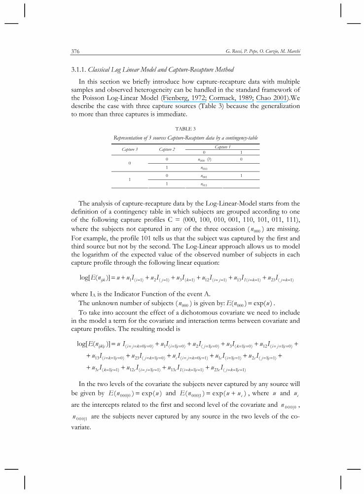
In this section we briefly introduce how capture-recapture data with multiple samples and observed heterogeneity can be handled in the standard framework of the Poisson Log-Linear Model (Fienberg, 1972; Cormack, 1989; Chao 2001).We describe the case with three capture sources (Table 3) because the generalization to more than three captures is immediate.

TABLE 3

Representation of 3 sources Capture-Recapture data by a contingency-table

Capture 1 Capture 3 Capture 2 0 1

0 000n (?) 0 0

1 010n

0 001n 1 1

1 011n

The analysis of capture-recapture data by the Log-Linear-Model starts from the definition of a contingency table in which subjects are grouped according to one of the following capture profiles C = (000, 100, 010, 001, 110, 101, 011, 111), where the subjects not captured in any of the three occasion ( 000n ) are missing. For example, the profile 101 tells us that the subject was captured by the first and third source but not by the second. The Log-Linear approach allows us to model the logarithm of the expected value of the observed number of subjects in each capture profile through the following linear equation:

1 ( 1) 2 ( 1) 3 ( 1) 12 ( 1) 13 ( 1) 23 ( 1)log[ ( )]ijk i j k i j I i k j kE n u u I u I u I u I u I u I

where IA is the Indicator Function of the event A. The unknown number of subjects ( 000n ) is given by: 000( ) exp( )E n u . To take into account the effect of a dichotomous covariate we need to include

in the model a term for the covariate and interaction terms between covariate and capture profiles. The resulting model is

| ( 0| 0) 1 ( 1| 0) 2 ( 1| 0) 3 ( 1| 0) 12 ( 1| 0)

13 ( 1| 0) 23 ( 1| 0) ( 0| 1) 1 ( 1| 1) 2 ( 1| 1)

3 ( 1| 1) 12 ( 1| 1) 13

log[ ( )]ijk c i j k c i c j c k c i j c

i k c j k c c i j k c c i c c j c

c k c c i j c c

E n u I u I u I u I u I

u I u I u I u I u I

u I u I u

( 1| 1) 23 ( 1| 1)I i k c c j k cI u I

In the two levels of the covariate the subjects never captured by any source will be given by 000|0( ) exp( )E n u and 000|1( ) exp( )cE n u u , where u and cu

are the intercepts related to the first and second level of the covariate and 000|0n ,

000|1n are the subjects never captured by any source in the two levels of the co-

variate.

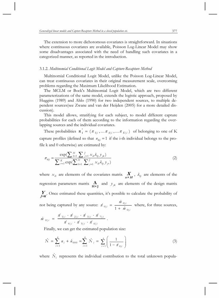
Generalized linear models and Capture-Recapture Method in a closed population etc. 377

The extension to more dichotomous covariates is straightforward. In situations where continuous covariates are available, Poisson Log-Linear Model may show some disadvantages associated with the need of handling such covariates in a categorized manner, as reported in the introduction.

3.1.2. Multinomial Conditional Logit Model and Capture-Recapture Method

Multinomial Conditional Logit Model, unlike the Poisson Log-Linear Model, can treat continuous covariates in their original measurement scale, overcoming problems regarding the Maximum Likelihood Estimation.

The MCLM or Bock's Multinomial Logit Model, which are two different parameterizations of the same model, extends the logistic approach, proposed by Huggins (1989) and Ahlo (1990) for two independent sources, to multiple de-pendent sources(see Zwane and van der Heijden (2005) for a more detailed dis-cussion).

This model allows, stratifying for each subject, to model different capture probabilities for each of them according to the information regarding the over-lapping sources and the individual covariates.

These probabilities 1| | |( , . . . , . . . )i k i K i 'iπ of belonging to one of K

capture profiles (defined so that | 1k in if the i-th individual belongs to the pro-

file k and 0 otherwise) are estimated by:

1 1|

1 1 1

exp( )

exp( )

H Jh j ih hj jk

k i H JKr ih hj jrh j

x y

x y

(2)

where ihx are elements of the covariates matrix n× HX , hj are elements of the

regression parameters matrix H× JΛ and jky are elements of the design matrix

J×KY . Once estimated these quantities, it’s possible to calculate the probability of

not being captured by any source: 0|0|

0|

ˆˆ

ˆ1i

ii

m

m

where, for three sources,

1| 2| 3| 7|0|

4| 5| 6|

ˆ ˆ ˆ ˆ

ˆ ˆ ˆˆ i i i i

ii i i

m

.

Finally, we can get the estimated population size:

0001 1

ˆ ˆˆn n

i ii i

N n n N

1 0|ˆ

1

1

n

i i

(3)

where ˆiN represents the individual contribution to the total unknown popula-

G. Rossi, P. Pepe, O. Curzio, M. Marchi 378

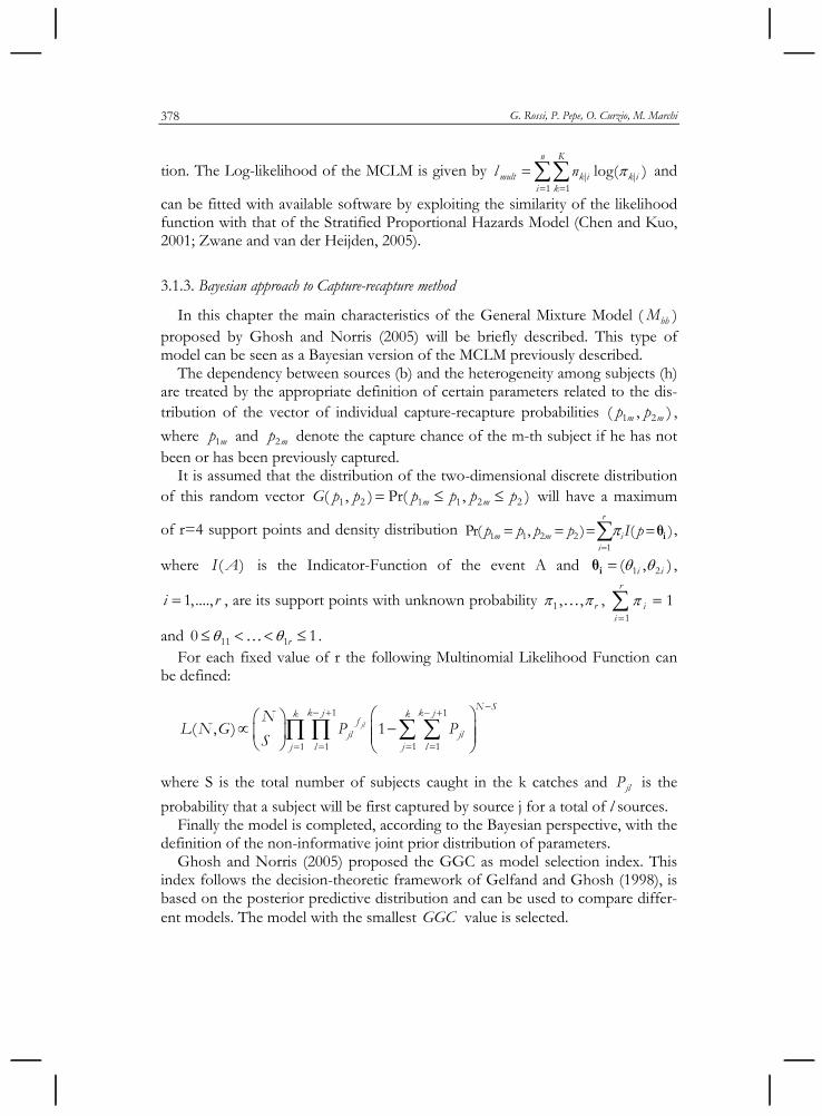
tion. The Log-likelihood of the MCLM is given by | |1 1

log( )n K

mult k i k ii k

l n

and

can be fitted with available software by exploiting the similarity of the likelihood function with that of the Stratified Proportional Hazards Model (Chen and Kuo, 2001; Zwane and van der Heijden, 2005).

3.1.3. Bayesian approach to Capture-recapture method

In this chapter the main characteristics of the General Mixture Model ( bhM ) proposed by Ghosh and Norris (2005) will be briefly described. This type of model can be seen as a Bayesian version of the MCLM previously described.

The dependency between sources (b) and the heterogeneity among subjects (h) are treated by the appropriate definition of certain parameters related to the dis-tribution of the vector of individual capture-recapture probabilities 1 2( , )m mp p ,

where 1mp and 2mp denote the capture chance of the m-th subject if he has not been or has been previously captured.

It is assumed that the distribution of the two-dimensional discrete distribution of this random vector 1 2 1 1 2 2( , ) Pr( , )m mG p p p p p p will have a maximum

of r=4 support points and density distribution 1 1 2 21

Pr( , ) ( )r

m m ii

p p p p I p

iθ ,

where ( )I A is the Indicator-Function of the event A and 1 2( , )i i iθ ,

1,....,i r , are its support points with unknown probability 1 , , r , 1

1r

ii

and 11 10 1r . For each fixed value of r the following Multinomial Likelihood Function can

be defined:

1 1

1 11 1

( , ) 1jl

N Sk j k jk k

fjl jl

j lj l

NL N G P P

S

where S is the total number of subjects caught in the k catches and jlP is the

probability that a subject will be first captured by source j for a total of l sources. Finally the model is completed, according to the Bayesian perspective, with the

definition of the non-informative joint prior distribution of parameters. Ghosh and Norris (2005) proposed the GGC as model selection index. This

index follows the decision-theoretic framework of Gelfand and Ghosh (1998), is based on the posterior predictive distribution and can be used to compare differ-ent models. The model with the smallest GGC value is selected.

Generalized linear models and Capture-Recapture Method in a closed population etc. 379

3.2. Model selection

One of the most critical point in the capture-recapture analysis using GLMs is the selection of the best model. In fact, it is not always easy to evaluate all possi-ble models because of their fast growth with increasing sources and/or covari-ates. For example, if we consider only the capture sources, the number of all pos-sible models is:

1

0

!1

!( )!

n

k

nN

k n k

, where

1

2

!1

!( )!

f

h

fn

h f h

N = number of all possible models f = number of sources n = number of parameters h = order of the interaction between sources k = combination of parameters

Of course, with two sources there is only one model to be evaluated, with three sources there are 8 models and with four sources we have 1024 possible models.

With four capture sources the number of models is very large and their evalua-tion is impractical. So a solution may be to consider only hierarchical models. In this case the total number of model reduces to 79, according to the following formula:

1

2

!1

!( )!

f

Gh

mN

l m l

where

!

!( )

fm

h f h

GN = all possible hierarchical models f = number of sources h = order of the interaction between sources m = number of parameters into hierarchy l = number of combinations of parameters into hierarchy

At this point, if we want to insert some covariates in the analysis we come back to a situation where to evaluate all possible models is again not feasible in practice.

These considerations led us to consider alternative strategies to search the best model according to the number of involved sources and covariates:

a) to evaluate all possible models with only sources effect and, after adding and selecting covariates effects, to choose the best one according to AIC, BIC or BW-0.05 (only significant coefficients are present in the model). This can be consid-ered the best strategy, but increasing the number of sources and/or covariates there are too many models to be evaluated and then it’s necessary to find alterna-tive strategies.

b) to evaluate all possible hierarchical models with only source effects and, af-ter adding and selecting covariates effects, to choose the best one according to

G. Rossi, P. Pepe, O. Curzio, M. Marchi 380

AIC, BIC or BW-0.05. Furthermore, in order to restrict the analysis to a minor number of models, it can be convenient to evaluate covariates effects only on those models i having a distance 10i (in terms of AIC or BIC) from the model with minimum index.

c) to select directly the best model from all possible hierarchical models with only sources effects according to AIC, BIC or BW-0.05 and then, after adding and selecting covariate effects, to choose the best one.

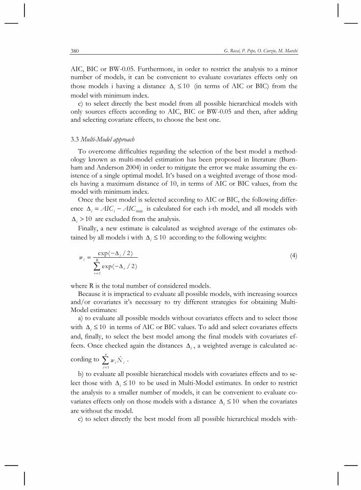
3.3 Multi-Model approach

To overcome difficulties regarding the selection of the best model a method-ology known as multi-model estimation has been proposed in literature (Burn-ham and Anderson 2004) in order to mitigate the error we make assuming the ex-istence of a single optimal model. It’s based on a weighted average of those mod-els having a maximum distance of 10, in terms of AIC or BIC values, from the model with minimum index.

Once the best model is selected according to AIC or BIC, the following differ-ence mini iAIC AIC is calculated for each i-th model, and all models with

10i are excluded from the analysis. Finally, a new estimate is calculated as weighted average of the estimates ob-

tained by all models i with 10i according to the following weights:

1

exp( / 2 )

exp( / 2 )

ii R

rr

w

(4)

where R is the total number of considered models. Because it is impractical to evaluate all possible models, with increasing sources

and/or covariates it’s necessary to try different strategies for obtaining Multi-Model estimates:

a) to evaluate all possible models without covariates effects and to select those with 10i in terms of AIC or BIC values. To add and select covariates effects and, finally, to select the best model among the final models with covariates ef-fects. Once checked again the distances i , a weighted average is calculated ac-

cording to 1

ˆn

i ii

w N .

b) to evaluate all possible hierarchical models with covariates effects and to se-lect those with 10i to be used in Multi-Model estimates. In order to restrict the analysis to a smaller number of models, it can be convenient to evaluate co-variates effects only on those models with a distance 10i when the covariates are without the model.

c) to select directly the best model from all possible hierarchical models with-

Generalized linear models and Capture-Recapture Method in a closed population etc. 381

out covariates effects according to AIC or BIC values. Then, after adding and se-lecting the effects of the covariates, to use all models with a 10i into the weighted average.

4. RESULTS

4.1. Analysis of simulated datasets

We analyzed the three simulated datasets characterized by different types of as-sociation among capture sources and between sources and a continuous covari-ate. The results obtained by the MCLM and the Bayesian approach are shown and compared.

4.1.1 MCLM estimates

In this section the results obtained by the MCLM are showed. We verified that the three model selection strategies, just described in Section 3.2, lead to select the same optimal models.

The analytical estimates of the total population (N), the Bootstrap-estimates and the confidence intervals, both parametric and nonparametric (Zwane and van der Heijden, 2003), are reported in Table 4.

TABLE 4

Estimated population size (N), Bootstrap Mean, Median and 95% C.I.

Type of dataset

Selected model Selection index

Analytical N

Bootstrap Mean

C.I. (95%) Parametric

Bootstrap Median

C.I. (95%) Non-parametric

A s1 s2 s3 s1x s2x s3x AIC, BIC, BW-0.05 3843 3901 3150 - 4652 3877 3250 - 4760

B s1 s2 s3 s12 s1x s2x s3x

AIC, BIC, BW-0.05 4001 4062 3253 - 4871 4027 3368 - 5009

s1 s2 s3 s12 s1x s2x s3x s12x

AIC, BW-0.05 3957 4037 3082 - 4992 3987 3252 - 5150

C s1 s2 s3 s12 BIC 3336 3356 2816 - 3896 3342 2845 - 3972

x: covariate

It has already been discussed at length that the symmetric (or asymptotic) con-fidence intervals are inappropriate for capture recapture studies. The Interna-tional Working Group for Disease Monitoring and Forecasting (1995a) noted that for all models proposed in Capture-Recapture literature the distribution of the population size estimate is skewed. In literature several authors have used a nonparametric bootstrap in the presence of continuous covariates (see Huggins, 1989; Tilling and Sterne, 1999) but, as noted by Norris and Pollock (1996), this bootstrap method could result in a variance estimate which is likely to be smaller than the true variance.

For each of the three simulated datasets we selected the optimal model accord-ing to AIC, BIC or BW-0.05. Then, from each dataset we extracted with replace-ment 1,000 samples of sample size equal to that observed.

G. Rossi, P. Pepe, O. Curzio, M. Marchi 382

For each of these samples the total population size (N) was estimated using the model selected on the starting dataset. This procedure conducts to a final distri-bution of the parameter N which can be used to produce point statistics and con-fidence intervals both parametric and nonparametric. For each of the three simu-lated datasets the models selected according to the AIC showed exactly the in-tended simulated effects. The models selected according to the AIC and BW-0.05 estimated a total population size very close to that of the real population of 4000 subjects. In the third dataset the model selected according to the BIC yielded a heavy underestimate of the population size.

4.1.2 Multi-Model estimates

Here we compare the estimates derived from the models selected by AIC and BIC with those obtained by the Multi-Model technique. When three capture sources and one covariate are present, all the three strategies previously described in 3.3 can be applied. However, our results (Table 5) did not show to be a great advantage in applying the Multi-Model technique. For BIC selected models the Multi-Model technique essentially confirmed results obtained using the best model only. For the C dataset both estimation methods underestimated the real population size. Regarding the models selected by the AIC, the estimates ob-tained by the Multi-Model technique seem to be slightly worse than those ob-tained by the single best model.

TABLE 5

Estimated population size by the optimal model and the Multi-Model technique according to AIC and BIC selection index

Best Model estimates Multi-Model estimates (Strategy a and b)

Multi-Model estimates (Strategy c)

Type of dataset

AIC BIC AIC BIC AIC BIC A 3843 3843 4033 3843 3843 3830 B 4001 4001 4180 4001 4166 4008 C 3957 3336 3107 3328 3957 3338

4.1.3 Bayesian estimates

The simulated datasets were also processed using the Bayesian methodology. Recent developments in the software for the statistical analysis (WinBUGS, Spiegelhalter et al. 2001) permitted to apply these models and to overcome the problem of performing complex integrations, which has severely limited the ap-plication of this approach in the past. The software implements Gibbs sampling with Metropolis-Hasting steps to obtain samples from the posterior distribution. Practically, through a proper definition of the prior distribution and a Multino-mial-Likelihood function we arrive to a posterior distribution of the total popula-tion size (N) by using Markov Chain Monte Carlo (MCMC) method. Point esti-mates and confidence intervals can be derived from the posterior distribution.

Some problems were encountered by using this methodology such as: a long waiting times to obtain posterior distribution, the need to define a priori an upper

Generalized linear models and Capture-Recapture Method in a closed population etc. 383

bound of the total population size, the lack of functionality of the proposed selec-tion-index (GGC) and a non-convergence of the MCMC method in some cir-cumstances.

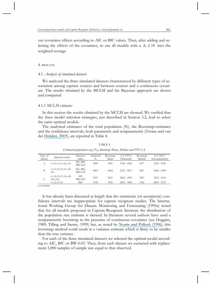
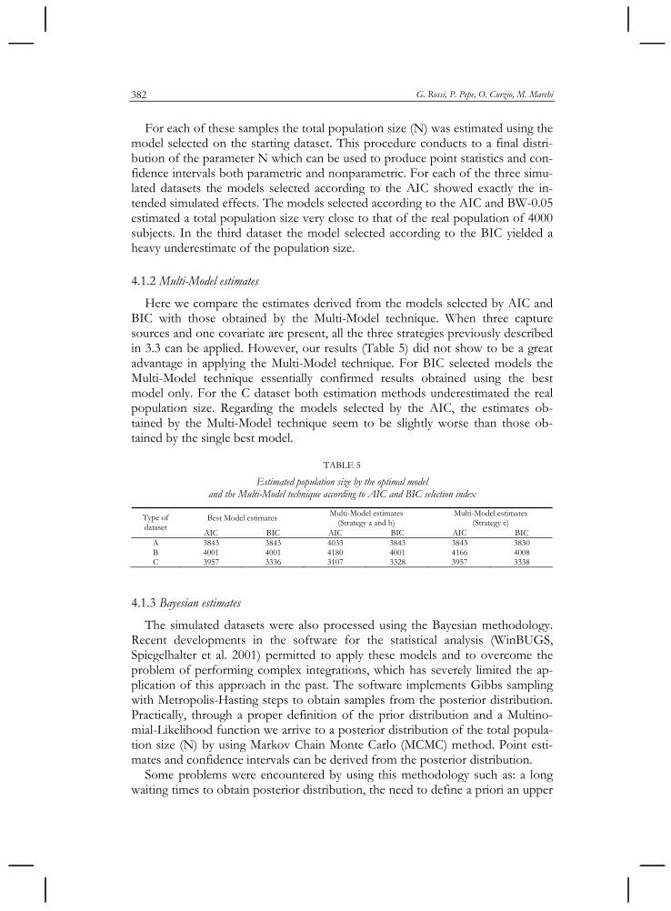
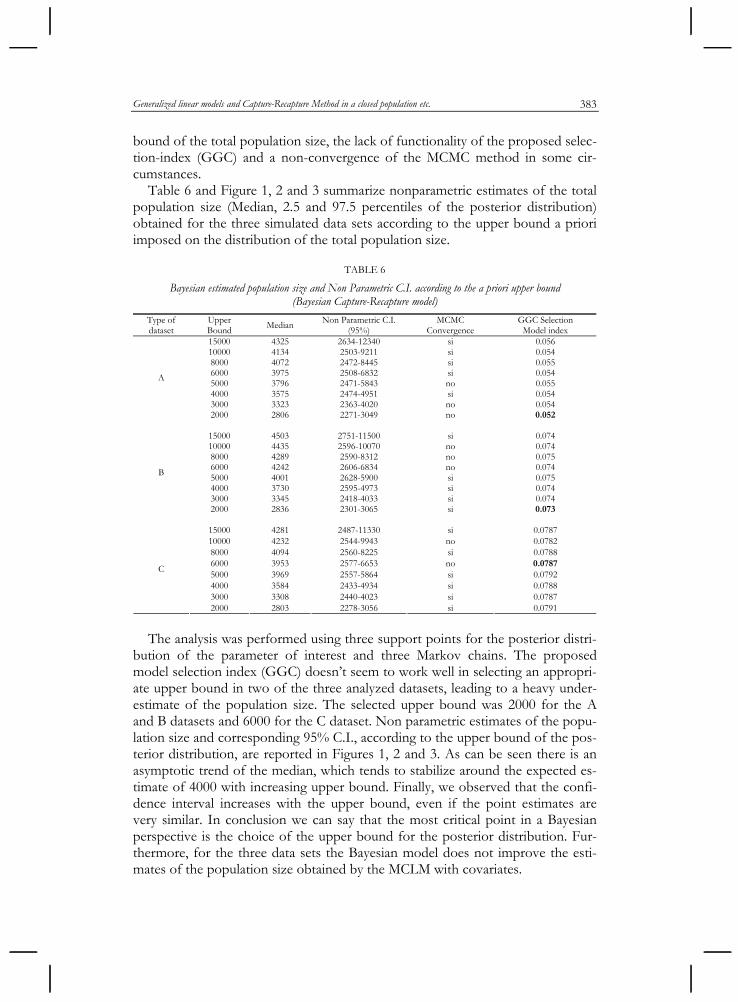
Table 6 and Figure 1, 2 and 3 summarize nonparametric estimates of the total population size (Median, 2.5 and 97.5 percentiles of the posterior distribution) obtained for the three simulated data sets according to the upper bound a priori imposed on the distribution of the total population size.

TABLE 6

Bayesian estimated population size and Non Parametric C.I. according to the a priori upper bound (Bayesian Capture-Recapture model)

Type of dataset

Upper Bound

Median Non Parametric C.I. (95%)

MCMC Convergence

GGC Selection Model index

15000 4325 2634-12340 si 0.056 10000 4134 2503-9211 si 0.054 8000 4072 2472-8445 si 0.055 6000 3975 2508-6832 si 0.054 5000 3796 2471-5843 no 0.055 4000 3575 2474-4951 si 0.054 3000 3323 2363-4020 no 0.054

A

2000 2806 2271-3049 no 0.052

15000 4503 2751-11500 si 0.074 10000 4435 2596-10070 no 0.074 8000 4289 2590-8312 no 0.075 6000 4242 2606-6834 no 0.074 5000 4001 2628-5900 si 0.075 4000 3730 2595-4973 si 0.074 3000 3345 2418-4033 si 0.074

B

2000 2836 2301-3065 si 0.073

15000 4281 2487-11330 si 0.0787 10000 4232 2544-9943 no 0.0782 8000 4094 2560-8225 si 0.0788 6000 3953 2577-6653 no 0.0787 5000 3969 2557-5864 si 0.0792 4000 3584 2433-4934 si 0.0788 3000 3308 2440-4023 si 0.0787

C

2000 2803 2278-3056 si 0.0791

The analysis was performed using three support points for the posterior distri-

bution of the parameter of interest and three Markov chains. The proposed model selection index (GGC) doesn’t seem to work well in selecting an appropri-ate upper bound in two of the three analyzed datasets, leading to a heavy under-estimate of the population size. The selected upper bound was 2000 for the A and B datasets and 6000 for the C dataset. Non parametric estimates of the popu-lation size and corresponding 95% C.I., according to the upper bound of the pos-terior distribution, are reported in Figures 1, 2 and 3. As can be seen there is an asymptotic trend of the median, which tends to stabilize around the expected es-timate of 4000 with increasing upper bound. Finally, we observed that the confi-dence interval increases with the upper bound, even if the point estimates are very similar. In conclusion we can say that the most critical point in a Bayesian perspective is the choice of the upper bound for the posterior distribution. Fur-thermore, for the three data sets the Bayesian model does not improve the esti-mates of the population size obtained by the MCLM with covariates.

G. Rossi, P. Pepe, O. Curzio, M. Marchi 384

0

4000

8000

12000

16000

0 5000 10000 15000 20000

Upper Bound

Est

imate

s

Low ( 2.5% ) Median Up ( 97.5% )

Figure 1 – Dataset A) Independence among sources and significant effect of continuous covariate: non parametric point estimates of the population size and 95% C.I. according to the upper bound (Bayesian Capture-Recapture model).

0

4000

8000

12000

16000

0 5000 10000 15000 20000

Upper Bound

Est

imate

s

Low ( 2.5% ) Median Up ( 97.5% )

Figure 2 – Dataset B) Independence among sources and a significant effect of continuous covariate: non parametric point estimates of the population size and 95% C.I. according to the upper bound (Bayesian Capture-Recapture model).

0

4000

8000

12000

16000

0 5000 10000 15000 20000

Upper Bound

Est

imate

s

Low( 2.5% ) Median Up ( 97.5% )

Figure 3 – Dataset C) Independence among sources and a significant effect of continuous covariate: non parametric point estimates of the population size and 95% C.I. according to the upper bound (Bayesian Capture-Recapture model).

Generalized linear models and Capture-Recapture Method in a closed population etc. 385

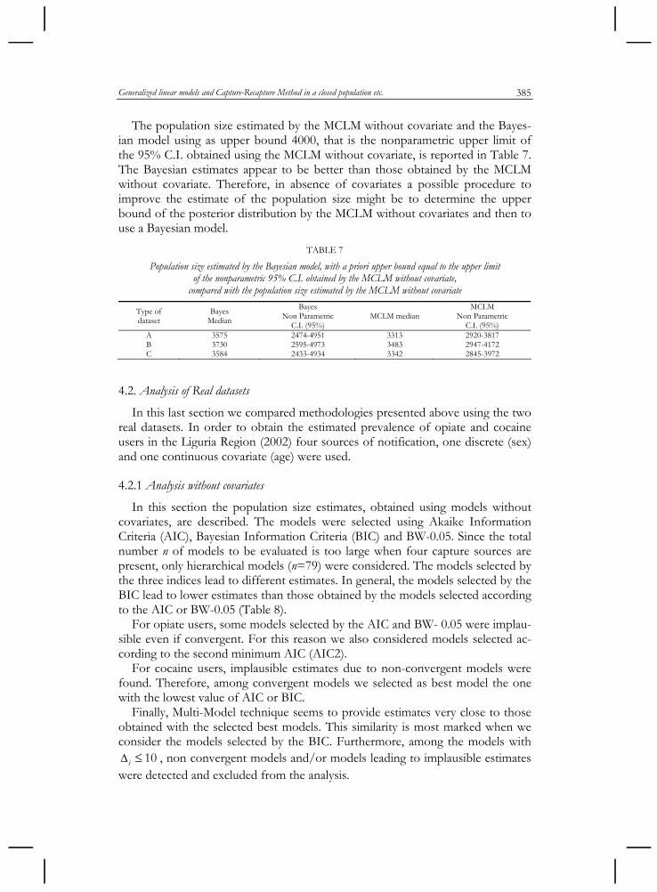
The population size estimated by the MCLM without covariate and the Bayes-ian model using as upper bound 4000, that is the nonparametric upper limit of the 95% C.I. obtained using the MCLM without covariate, is reported in Table 7. The Bayesian estimates appear to be better than those obtained by the MCLM without covariate. Therefore, in absence of covariates a possible procedure to improve the estimate of the population size might be to determine the upper bound of the posterior distribution by the MCLM without covariates and then to use a Bayesian model.

TABLE 7

Population size estimated by the Bayesian model, with a priori upper bound equal to the upper limit of the nonparametric 95% C.I. obtained by the MCLM without covariate,

compared with the population size estimated by the MCLM without covariate

Type of dataset

Bayes Median

Bayes Non Parametric

C.I. (95%) MCLM median

MCLM Non Parametric

C.I. (95%) A 3575 2474-4951 3313 2920-3817 B 3730 2595-4973 3483 2947-4172 C 3584 2433-4934 3342 2845-3972

4.2. Analysis of Real datasets

In this last section we compared methodologies presented above using the two real datasets. In order to obtain the estimated prevalence of opiate and cocaine users in the Liguria Region (2002) four sources of notification, one discrete (sex) and one continuous covariate (age) were used.

4.2.1 Analysis without covariates

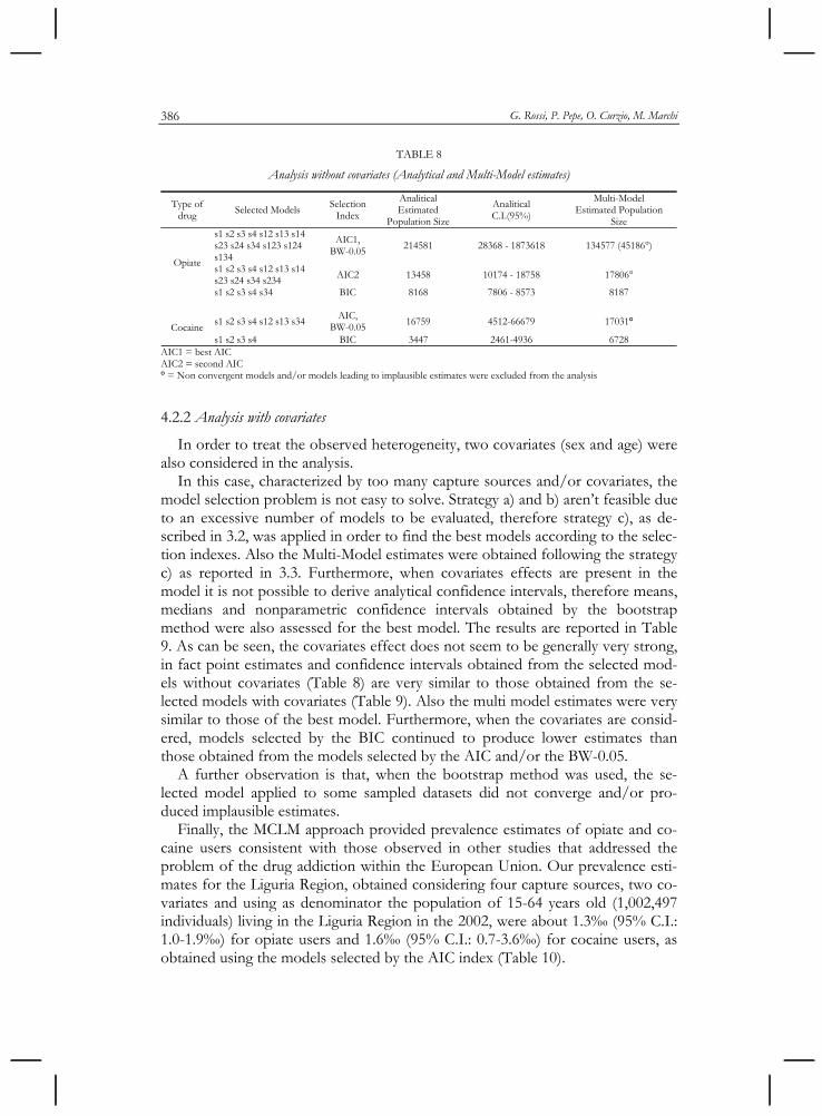
In this section the population size estimates, obtained using models without covariates, are described. The models were selected using Akaike Information Criteria (AIC), Bayesian Information Criteria (BIC) and BW-0.05. Since the total number n of models to be evaluated is too large when four capture sources are present, only hierarchical models (n=79) were considered. The models selected by the three indices lead to different estimates. In general, the models selected by the BIC lead to lower estimates than those obtained by the models selected according to the AIC or BW-0.05 (Table 8).

For opiate users, some models selected by the AIC and BW- 0.05 were implau-sible even if convergent. For this reason we also considered models selected ac-cording to the second minimum AIC (AIC2).

For cocaine users, implausible estimates due to non-convergent models were found. Therefore, among convergent models we selected as best model the one with the lowest value of AIC or BIC.

Finally, Multi-Model technique seems to provide estimates very close to those obtained with the selected best models. This similarity is most marked when we consider the models selected by the BIC. Furthermore, among the models with

10i , non convergent models and/or models leading to implausible estimates were detected and excluded from the analysis.

G. Rossi, P. Pepe, O. Curzio, M. Marchi 386

TABLE 8

Analysis without covariates (Analytical and Multi-Model estimates)

Type of drug Selected Models

Selection Index

Analitical Estimated

Population Size

Analitical C.I.(95%)

Multi-Model Estimated Population

Size s1 s2 s3 s4 s12 s13 s14 s23 s24 s34 s123 s124 s134

AIC1, BW-0.05 214581 28368 - 1873618 134577 (45186°)

s1 s2 s3 s4 s12 s13 s14 s23 s24 s34 s234 AIC2 13458 10174 - 18758 17806°

Opiate

s1 s2 s3 s4 s34 BIC 8168 7806 - 8573 8187

s1 s2 s3 s4 s12 s13 s34 AIC,

BW-0.05 16759 4512-66679 17031° Cocaine

s1 s2 s3 s4 BIC 3447 2461-4936 6728 AIC1 = best AIC AIC2 = second AIC ° = Non convergent models and/or models leading to implausible estimates were excluded from the analysis

4.2.2 Analysis with covariates

In order to treat the observed heterogeneity, two covariates (sex and age) were also considered in the analysis.

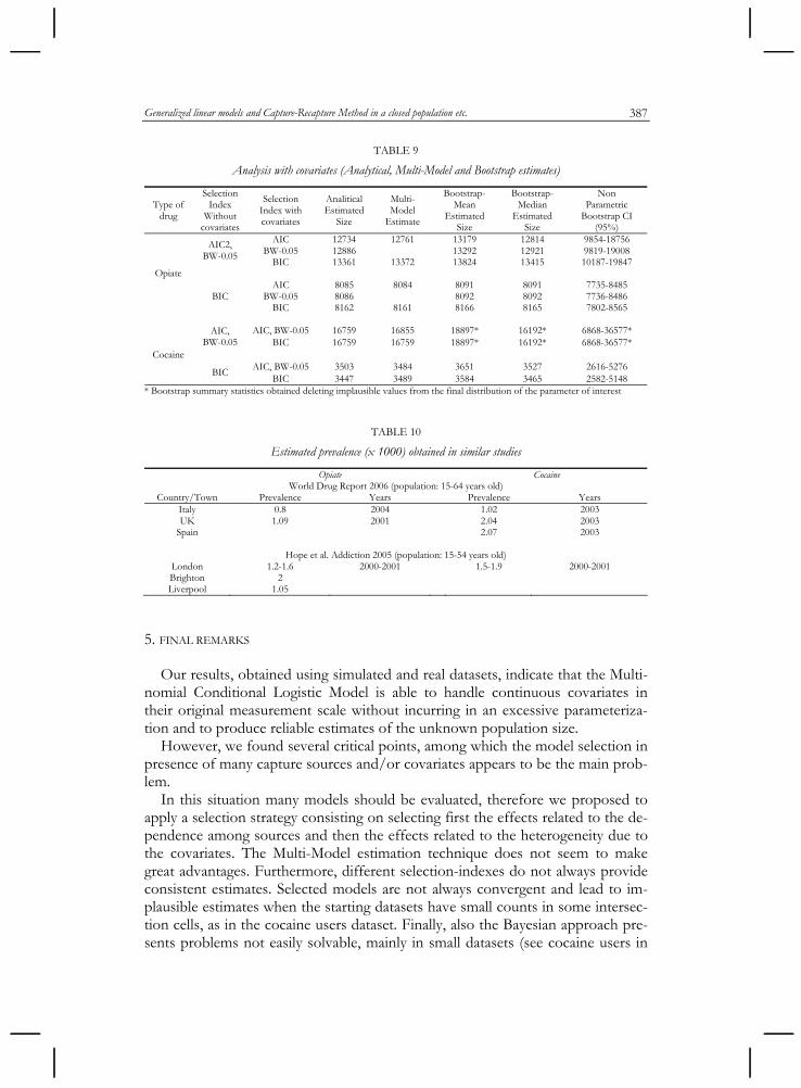
In this case, characterized by too many capture sources and/or covariates, the model selection problem is not easy to solve. Strategy a) and b) aren’t feasible due to an excessive number of models to be evaluated, therefore strategy c), as de-scribed in 3.2, was applied in order to find the best models according to the selec-tion indexes. Also the Multi-Model estimates were obtained following the strategy c) as reported in 3.3. Furthermore, when covariates effects are present in the model it is not possible to derive analytical confidence intervals, therefore means, medians and nonparametric confidence intervals obtained by the bootstrap method were also assessed for the best model. The results are reported in Table 9. As can be seen, the covariates effect does not seem to be generally very strong, in fact point estimates and confidence intervals obtained from the selected mod-els without covariates (Table 8) are very similar to those obtained from the se-lected models with covariates (Table 9). Also the multi model estimates were very similar to those of the best model. Furthermore, when the covariates are consid-ered, models selected by the BIC continued to produce lower estimates than those obtained from the models selected by the AIC and/or the BW-0.05.

A further observation is that, when the bootstrap method was used, the se-lected model applied to some sampled datasets did not converge and/or pro-duced implausible estimates.

Finally, the MCLM approach provided prevalence estimates of opiate and co-caine users consistent with those observed in other studies that addressed the problem of the drug addiction within the European Union. Our prevalence esti-mates for the Liguria Region, obtained considering four capture sources, two co-variates and using as denominator the population of 15-64 years old (1,002,497 individuals) living in the Liguria Region in the 2002, were about 1.3‰ (95% C.I.: 1.0-1.9‰) for opiate users and 1.6‰ (95% C.I.: 0.7-3.6‰) for cocaine users, as obtained using the models selected by the AIC index (Table 10).

Generalized linear models and Capture-Recapture Method in a closed population etc. 387

TABLE 9

Analysis with covariates (Analytical, Multi-Model and Bootstrap estimates)

Type of drug

Selection Index

Without covariates

Selection Index with covariates

Analitical Estimated

Size

Multi- Model

Estimate

Bootstrap- Mean

Estimated Size

Bootstrap- Median

Estimated Size

Non Parametric

Bootstrap CI (95%)

AIC 12734 12761 13179 12814 9854-18756 BW-0.05 12886 13292 12921 9819-19008

AIC2, BW-0.05

BIC 13361 13372 13824 13415 10187-19847

AIC 8085 8084 8091 8091 7735-8485 BW-0.05 8086 8092 8092 7736-8486

Opiate

BIC BIC 8162 8161 8166 8165 7802-8565

AIC, BW-0.05 16759 16855 18897* 16192* 6868-36577* AIC,

BW-0.05 BIC 16759 16759 18897* 16192* 6868-36577*

AIC, BW-0.05 3503 3484 3651 3527 2616-5276 Cocaine

BIC BIC 3447 3489 3584 3465 2582-5148

* Bootstrap summary statistics obtained deleting implausible values from the final distribution of the parameter of interest

TABLE 10

Estimated prevalence (x 1000) obtained in similar studies

Opiate Cocaine World Drug Report 2006 (population: 15-64 years old)

Country/Town Prevalence Years Prevalence Years Italy 0.8 2004 1.02 2003 UK 1.09 2001 2.04 2003

Spain 2.07 2003

Hope et al. Addiction 2005 (population: 15-54 years old) London 1.2-1.6 2000-2001 1.5-1.9 2000-2001 Brighton 2 Liverpool 1.05

5. FINAL REMARKS

Our results, obtained using simulated and real datasets, indicate that the Multi-nomial Conditional Logistic Model is able to handle continuous covariates in their original measurement scale without incurring in an excessive parameteriza-tion and to produce reliable estimates of the unknown population size.

However, we found several critical points, among which the model selection in presence of many capture sources and/or covariates appears to be the main prob-lem.

In this situation many models should be evaluated, therefore we proposed to apply a selection strategy consisting on selecting first the effects related to the de-pendence among sources and then the effects related to the heterogeneity due to the covariates. The Multi-Model estimation technique does not seem to make great advantages. Furthermore, different selection-indexes do not always provide consistent estimates. Selected models are not always convergent and lead to im-plausible estimates when the starting datasets have small counts in some intersec-tion cells, as in the cocaine users dataset. Finally, also the Bayesian approach pre-sents problems not easily solvable, mainly in small datasets (see cocaine users in

G. Rossi, P. Pepe, O. Curzio, M. Marchi 388

Table 2). Likewise, it is unclear what criterion to use for determining the upper bound of the posterior distribution.

However, on simulated data, the choice of an upper bound equal to the upper limit of the nonparametric 95% C.I. obtained from the MCLM without covariates and selected by the AIC seems to achieve results consistent with those obtained by the MCLM with covariates. Unit of Epidemiology and Biostatistics, GIUSEPPE ROSSI Institute of Clinical Physiology, PASQUALE PEPE CNR, Pisa, Italy OLIVIA CURZIO

Department of Statistics “G. Parenti”, MARCO MARCHI University of Florence, Florence, Italy

REFERENCES

D.D. ABENI, G. BRANCATO, C.A. PERUCCI (1994), Capture-recapture to estimate the size of the popula-tion with human immunodeficiency virus type 1 infection, “Epidemiology”, 5, pp. 410-414.

J.M. ALHO (1990), Logistic regression in capture-recapture models, “Biometrics”, 46, pp. 623-635. G. BAKER STUART (1994), The multinomial-Poisson transformation, “The Statistician”, 43, pp.

495-504. F. BARTOLUCCI, A. FORCINA (2006). A class of latent marginal models for capture-recapture data with

continuous covariates, “Journal of the American Statistical Association”, 101, pp. 786-794. D. BOHNING, B. SUPPAWATTANABODEE, W. KUSOLVISITKUL, C..VIWATWONGKASEM (2004), Estimat-

ing the number of drug users in Bangkok 2001: A Capture-Recapture Approach Using Repeated Entries in one list, “European Journal of Epidemiology”, 19, pp. 1075-1083.

M.T. BRUGAL, A. DOMINGO-SALVANY, A. MAGUIRE, J.A. CAYLA, J.R. VILLALBI, R. HARTNOLL (1999), A small area analysis estimating the prevalence of addiction to opioids in Barcelona, “Journal of Epi-demiology & Community Health”, 53, 488-494.

K. P. BURNHAM, D. R. ANDERSON (2004), Multimodel Inference. Understanding AIC e BIC in Model Selection, “Sociological Methods and Research”, 33, pp. 261-304.

M.C. BUSTER, G.H. VAN BRUSSEL, W. VAN DEN BRINK (2001), Estimating the number of opiate users in Amsterdam by capture-recapture: the importance of case definition, “European Journal of Epi-demiology”, 17, pp. 935-942.

A. CHAO (2001), An overview of closed Capture-Recapture Models, “Journal of Agricultural, Bio-logical, and Environmental Statistics”, 6, pp. 158-175.

Z. CHEN, L. KUO (2001), A note on the estimation of the multinomial Logit Model with Random effects, “The American Statistician”, 55, pp. 89-95.

R.M. CORMACK (1989), Log-linear Models for Capture-Recapture, “Biometrics”, 45, pp. 395-413. A. DAVIES, R. CORMACK, AND A. RICHARDSON (1999). Estimation of injecting drug users in the City of

Edinburgh, Scotland, and the number infected with human immunodeficiency virus, “International Journal of Epidemiology”, 28, pp. 117-121.

S. FIENBERG (1972), The multiple recapture census for closed populations and incomplete 2k contingency tables, “Biometrika”, 59, pp. 591-603.

M. FRISCHER, M. BLOOR, A. FINLAY, D. GOLDBERG, S. GREEN, S. HAW, N. MCKEGANEY, S. PLATT (1991), A new method of estimating prevalence of injecting drug use in an urban population: results from a Scottish city, “International Journal of Epidemiology”, 20, pp. 997-1000.

M. FRISCHER, M. HICKMAN, L. KRAUS, F. MARIANI, L. WIESSING (2001), A comparison of different meth-

Generalized linear models and Capture-Recapture Method in a closed population etc. 389

ods for estimating the prevalence of problematic drug misure in Great Britain, “Addiction”, 96, pp. 1465-1476.

A. E. GELFAND AND S. K. GHOSH (1998), Model choice: A minimum posterior predictive loss approach, “Biometrika”, 85, pp. 1-11.

I. GEMMELL, T. MILLAR, G. HAY (2004), Capture-recapture estimates of problem drug use and the use of simulation based confidence intervals in a stratified analysis, “Journal of Epidemiology & Community Health”, 58, pp. 758-765.

S.K. GHOSH, J.L. NORRIS (2004), Bayesian Capture-Recapture Analysis and Model Selection Allowing for Heterogeneity and Behavioral Effects, NCSU Institute of Statistics, Mimeo Series 2562, pp. 1-27.

G. HAY, N. MCKEGANEY (1996), Estimating the prevalence of drug misure in Dundee, Scotland: an ap-plication of capture-recapture methods, “Journal of Epidemiology & Community Health”, 50, pp. 469-472.

G. HAY (2000), Capture-recapture estimates of drug misure in urban and non-urban settings in the north east of Scotland, “Addiction”, 95, pp. 1795-1803.

W.D. HALL, J.E. ROSS, M.T. LYNSKEY, M.G. LAW, L.J. DEGENHARDT (2000), How many dependent heroin users are there in Australia? “The Medical Journal of Australia”, 173, pp. 528-531.

M. HICKMAN, S. COX, J HARVEY, S. HOWES, M. FARRELL, M. FRISCHER, G. STIMSON, C. TAYLOR, K. TILL-

ING (1999), Estimating the prevalence of problem drug use in inner London: a discussion of three capture-recapture studies, “Addiction”, 94, pp. 1653-1662.

M. HICKMAN, V. HIGGINS, V. HOPE, M. BELLIS, K. TILLING, A. WALKER (2004), Injecting drug use in Brighton, Liverpool, and London: best estimates of prevalence and coverage of public health indicators, “Journal of Epidemiology & Community Health”, 58, pp. 766-771.

V.D. HOPE, M. HICKMAN, K. TILLING (2005). Capturing crack cocaine use: estimating the prevalence of crack cocaine use in London using capture-recapture with covariates. “Addiction”, 11, pp. 1701-1708.

R. M. HUGGINS (1989), On the statistical analysis of capture experiments, “Biometrika”, 76, pp. 133-140.

W. H. HWANG AND R. M. HUGGINS (2005), An examination of the effect of heterogeneity on the estima-tion of population size using capture-recapture data, “Biometrika”, 92, pp. 229-233.

INTERNATIONAL WORKING GROUP FOR DISEASE MONITORING AND FORECASTING (1995a), Capture-recapture and multiple record systems estimation 1: history and theoretical development. “American Journal of Epidemiology”, 142, pp. 1047-1058.

INTERNATIONAL WORKING GROUP FOR DISEASE MONITORING AND FORECASTING (1995b), Capture-recapture and multiple record systems estimation 2: applications, “American Journal of Epide-miology”, 142, pp. 1059-1068.

J. NORRIS AND K. POLLOCK (1996), Including model uncertainty in estimating variances in multiple cap-ture studies,” Environmental and Ecological Statistics”, 3, pp. 235-244.

L. PLATT, M. HICKMAN, T. RHODES, L. MIKHAILOVA, V. KARAVASHKIN, A. VLASOV, K. TILLING, V. HOPE, M. KHUTORKSOY, A. RENTON (2004), The prevalence of injecting drug use in a Russian city: implica-tions for harm reduction and coverage, “Addiction”, 99, pp. 1430-1438.

S. PLEDGER (2000), Unified maximum likelihood estimates for closed capture-recapture models using mixtures, “Biometrics”, 56, 443-450.

K. H.POLLOCK, J. E. HINES,AND J. D. NICHOLS (1984), The use of auxiliary variables in capture-recapture and removal experiments, “Biometrics”, 40, pp. 329-340.

K. H. POLLOCK (2002), The use of auxiliary variables in capture-recapture modeling: an overview, “Journal of Applied Statistics”, 29, 85-102.

J. RAZZAK, AND S. LUBY (1998), Estimating deaths and injuries due to road traffic accidents in Karachi, Pakistan, through the capture-recapture method, “International Journal of Epidemiology”, 27, pp. 866-870.

G. Rossi, P. Pepe, O. Curzio, M. Marchi 390

M. JOHN ROBERTS JR, DEVON D. BREWER (2006), Estimating the prevalence of male clients of prostitute women in Vancouver with a simple capture-recapture method, “Journal of the Royal Statistical Society: Series A”, 169, pp. 745-756.

C. SCHWARZ, AND G. SEBER (1999), A review of estimating animal abundance III, “Statistical Sci-ence”, 14, pp. 427-456.

D. SPIEGELHALTER, A. THOMAS, N. BEST AND D. LUNN (2001), WinBUGS User Manual version 1.4, MRC Biostatistics Unit, Cambridge, UK. http://www.mrc-bsu.cam.ac.uk/bugs

K. TILLING, J. STERNE (1999), Capture-recapture models including covariate effects, “American Jour-nal of Epidemiology”, 49, pp. 392-400.

K. TILLING, J. STERNE (2001), Estimation of the incidence of stroke using a capture-recapture model in-cluding covariates, “International Journal of Epidemiology”, 30, pp. 1351-1359.

E. ZWANE, P. VAN DER HEIJDEN (2003), Implementing the parametric bootstrap in capture-recapture models with continuous covariates, “Statistics and Probability Letters”, 65, pp. 121-125.

E. ZWANE, P. VAN DER HEIJDEN (2005), Population estimation using the multiple system estimator in the presence of continuous covariates, “Statistical Modelling”, 5, pp. 39-52.

SUMMARY

Generalized linear models and Capture-Recapture Method in a closed population: strengths and weaknesses

Capture-recapture methods are used by epidemiologists in order to estimate the size of hidden populations using incomplete and overlapping lists of cases. These models can be both continuous and discrete time and the particular population we want to obtain a quantitative evaluation can be assumed to be closed or open.

Here we specifically consider discrete-time models for closed population. The problem was treated using Generalized Linear Models as they allow to treat simultaneously both forms of dependence between sources than observed heterogeneity due to covariates ef-fects.

Specifically, we analyzed the strengths and weaknesses of Multinomial Conditional Lo-gistic Model and presented a comparison with a correspondent Bayesian approach. The estimates obtained on simulated and real data appear to be enough reliable.