Geoderma 155 (2010) 193–202

Contents lists available at ScienceDirect

Geoderma

j ourna l homepage: www.e lsev ie r.com/ locate /geoderma

Functional evaluation of PTF prediction uncertainty: An application at hillslope scale

G.B. Chirico a,⁎, H. Medina b, N. Romano a

a Department of Agricultural Engineering, University of Naples Federico II, Naples, Italyb Agrarian University of Havana, Havana, Cuba

⁎ Corresponding author. Dipartimento di Ingegneria ANapoli Federico II, Via Università, 100, 80055 Portici2539415; fax: +39 081 2539412.

E-mail address: gchirico@unina.it (G.B. Chirico).

0016-7061/$ – see front matter © 2009 Elsevier B.V. Aldoi:10.1016/j.geoderma.2009.06.008

a b s t r a c t

a r t i c l e i n f o

Article history:Received 31 May 2008Received in revised form 18 March 2009Accepted 10 June 2009Available online 16 July 2009

Keywords:Pedotransfer functionsSoil hydraulic functionsSpatial variabilityUncertainty analysisFunctional evaluation

This study presents a methodology to assess uncertainties resulting from the use of pedotransfer functions(PTFs) when soil water budget is modelled at a hillslope scale. Two sources of uncertainty are examined:(i) errors in the assessment of the soil physical and chemical properties at unsampled locations, as related tothe spatial spacing of the sample measurements across the entire study area, and (ii) errors associated to thePTF relations and parameters. This methodology is applied to an experimental hillslope in Southern Italy,where an intensive field campaign has been conducted to gather several soil physical and chemicalproperties and soil hydraulic properties. A sequential Gaussian simulation algorithm is used to generatemultiple equally probable images of PTF input soil data, consistent with the estimated spatial structure andconditioned to the measured soil core properties. Two PTFs commonly used in Europe, Vereecken's PTF[Vereecken, H., Diels, J., van Orshoven, J., Feyen, J., Bouma, J., 1992. Functional evaluation of pedotransferfunctions for the estimation of soil hydraulic properties. Soil Sci. Soc. Am. J. 56, 1371–1378] and HYPRES PTF[Wösten, J.H.M., Lilly, A., Nemes, A., Le Bas, C., 1999. Development and use of a database of hydraulicproperties of European soils. Geoderma 90, 169–185] are applied to predict the soil hydraulic properties,which in turn are employed into a soil–vegetation–atmosphere model to evaluate the propagateduncertainty in simulated target variables, such as evaporation, transpiration and root zone soil watercontent variation during a wet-to-dry transition season. The outcomes of this case study suggest thataccurate estimates of transpiration and soil water storage variation at the hillslope scale are obtained evenwhen PTF input data are collected with a relatively coarse sampling strategy. The examined PTFs show worselevel of performance with respect to the simulated evaporation. The simulated evaporation is much moreaffected by the PTF model error than by the input data error. A major implication of these results is that if onewould reduce the prediction uncertainty in simulated evaporation, the PTF model structure has to beimproved prior of reducing the uncertainty into the PTF input data.

© 2009 Elsevier B.V. All rights reserved.

1. Introduction

Modelling soil hydrologic processes across different landscapeelements is of prime importance for many studies applied toenvironmental and land-use planning problems. Nevertheless, theapplication of soil hydrological models at large spatial scales is oftenlimited, mainly because it requires the determination of soil hydraulicparameters that are unfeasible to be assessed by direct observationsover relatively large land areas. Pedotransfer functions (PTFs) arebeing developed as simplified methods to assess soil hydraulicparameters from soil physical and chemical properties which aremuch less laborious and expensive to determine and more routinelymeasured than the actual soil hydraulic properties (Bouma, 1989).

graria, Università degli Studi di, Napoli, Italy. Tel.: +39 081

l rights reserved.

The application of a simpler method, such as a PTF compared to adirect measurement, generally involves a cost in terms of increaseduncertainty in the predictions. Therefore, an important aspect thatneeds consideration when a simpler method is applied, is to assesswhether the increase of uncertainty is acceptable, given the objectivesof the research or the type of decisions that are to be made.

Nowadays, the uncertainty analysis is becoming fundamental inapplications which are employed for assessing environmental risksand guiding decision makers in planning mitigation strategies.Uncertainty analysis is also useful for model developers, who needto evaluate the performance of different modelling strategies, assessthemain sources of prediction uncertainties and identify the prioritiesto be followed within a research program aiming at improving theoverall model performance.

Model prediction uncertainties arise from errors in evaluation data,input variables, andmodel structure and parameters. At the local scale,error in input variables can be originated by measurement errors.Minasny et al. (1999) analysed the uncertainty in water retentionpredictions at local scale, accounting for both measurement errors in

194 G.B. Chirico et al. / Geoderma 155 (2010) 193–202

input variables and uncertainties in PTF parameters. They showed thatthe predictions are much more affected by errors in input variablesthan by the errors in model parameters.

From a practical perspective, one is interested in evaluating the PTFprediction uncertainty at relatively larger scales, i.e. at the hillslope orcatchment scales, since these are the scales at which PTFs result asprime alternatives to direct measurements. At non-local scale, theuncertainty of the input variables due to local measurement errors isenhanced by the uncertainty in their spatial variability. Since PTFinput variables are observed only in a limited number of locations, theassessment of the input variables at unsampled locations can beachieved only by interpolation. However, the results of any interpola-tion procedure are affected by uncertainty. Chirico et al. (2007)explored the uncertainty in PTF model predictions at the hillslopescale due to the error in the estimated soil physical and chemicalproperties at unsampled locations and to the PTF model error,including both model structure and parameter errors. The uncertaintyof the predicted soil water retention function due to the PTF modelerror resulted as much as or more significant than the uncertaintyassociated with the estimated input variables, even for a relativelycoarse sampling resolution. Moreover, the study showed that theuncertainty in the predicted saturated soil hydraulic conductivity isdominated by the model error, while the contribution of the inputerrors is negligible.

Determining soil hydraulic properties is not in itself the aim ofhydrological applications, rather it is essential for simulating waterflow and transport processes in the unsaturated soil zone. Thus theuncertainty analysis should be extended toward evaluating thepropagation of PTF prediction uncertainties in the results of specificapplications. This type of analysis is equivalent to a “functionalevaluation” of PTFs, as firstly proposed by Wösten et al. (1986) andthen applied by quite a few studies focused on local-scale analysis.Vereecken et al. (1992) assessed the effect of the PTF prediction errorin a model of soil water dynamics. Cresswell and Paydar (2000)evaluated the performance of different methods for estimating soilhydraulic properties in Australia, by comparing the cumulativeevapotranspiration and drainage simulated with a soil water budgetmodel over a 5 year period for 66 different soil horizons. Christiaensand Feyen (2001) used a Latin Hypercube sampling strategy toevaluate how the uncertainties in the predicted soil hydraulicproperties propagate into the output of a distributed model appliedto a 1 km2 catchment, assuming homogenous soil properties withinland units. Minasny and McBratney (2002b) evaluated how measure-ment errors of the PTF input variables affect the uncertainty in thesimulated soil water budget. They concluded that the soil waterbudget is more sensitive to input uncertainties during dry periodsrather during wet periods.

This study extends the analysis of Chirico et al. (2007) in a functionalway, to assess how the simulated soil water budget is affected byuncertainty when PTFs are used to estimate the soil hydraulicparameters at the hillslope scale. The paper is structured as follows.The overall method is described in the next section. The experimentalhillslope and sample data are discussed in the third section,whereas thesoil water budget model is presented in the fourth section. The fifthsection describes the procedure followed for representing the uncer-tainty of the soil hydraulic parameters predicted with PTFs across theexperimental hillslope. The sixth section analyses the propagateduncertainty in the simulated soil water budget components. The lastsection is devoted to the conclusions.

2. Method

The overall methodology is structured in two stages (see Fig. 1).The first stage is focused on the stochastic generation of patterns ofsoil hydraulic functions across the hillslope. The second stage isfocused on the soil water budget modelling and on the analysis of the

propagated PTF prediction uncertainty into the simulated soil waterbudget components.

The first stage has been developed by Chirico et al. (2007). Datacollected along an experimental hillslope transect, together withterrain attributes taken as ancillary information, are employed toidentify the spatial structure of the PTF input variables. Hereinafter,the PTF input variables are named “basic soil properties”, while anensemble of patterns representing the basic soil properties across thehillslope is named “set of basic soil properties”. A multivariategeostatistical analysis is carried out to identify the structure of thespatial variability of the basic soil properties at the support scale of thesoil samples, while choosing the hillslope as spatial extent. Thedeterministic component of the spatial variability is first identified,accounting for the correlation of the soil properties with the terrainattributes through linear regressions. The residual stochastic compo-nent is then derived accounting for the auto- and cross-correlation ofthe basic soil properties.

Then a multivariate stochastic simulation is performed for gen-erating a high-resolution set of basic soil properties, hereafter referredto as the “full dataset”. The simulation is performed on a spatialdomain corresponding to the hillslope surrounding the experimentaltransect. The stochastic component identified along the experimentaltransect is assumed stationary across the entire study hillslope. Thedeterministic component is computed according to the hillslopeterrain through the regression rules identified along the transect.

The “full dataset” is generated as conditioned to the valuesobserved across the hillslope transect. The conditional simulation isperformed by employing the Gstat software package on S (R/S Plus)(Pebesma, 2004). The generation of independent realizations in theGstat package is carried out from a sequential simulation algorithm(Gómez-Hernández and Journel, 1993).

The full dataset is taken as the true representation of the hillslopesoil variability and is considered as reference “measured” set of basicsoil properties for the subsequent uncertainty analysis. Since themajoraim of this study is to quantify the propagation of the PTF predictionuncertainty due to both PTF model error and input estimation errorfrom sparse samples, the full dataset is sampled and multivariatestochastic simulations are then performed to generate sets of basic soilproperties conditioned to these sparse samples. These stochasticsimulations are employed to describe the PTF input uncertaintyassociated to the assessment of the unknown input variables atunsampled locations by interpolation of sparselymeasured values. Therealisations of the PTF input variables are then employed to performMonte Carlo simulations of the soil hydraulic properties to be used asparameters for the subsequent runs of the soil water budget model.The support scale of the input realisations corresponds to the supportscale at which the soil water budget model is applied.

Each generated set of basic soil properties is named as “image” ofthe “full dataset”. The full dataset and its images are translated intopatterns of soil hydraulic functions by applying PTFs.

At the end of the first stage, three types of soil hydraulic functionsare available for the subsequent simulations: 1) soil hydraulicfunctions derived from observations along the experimental transect,referred to as “observed soil hydraulic functions”; 2) soil hydraulicfunctions derived by applying PTFs to the full dataset, considered as“measured” basic soil properties across the entire hillslope, referred toas “indirect soil hydraulic functions”; 3) soil hydraulic functionsderived by applying PTFs to the images of the full dataset, referred toas “image soil hydraulic functions”.

The study conducted in the second stage is the main advance withrespect towhat has already beenpresented in Chirico et al. (2007). A soilwater budget model is executed across the entire hillslope in order toevaluate thepropagationof thePTF input errors andmodel error into thesimulated soil water budget. The above patterns of hydraulic functionsare employed for parameterising the soil water budgetmodel, while theinitial and boundary conditions as well as the vegetation cover and

Fig. 1. Schematic diagram of the overall methodology for the analysis of the uncertainty propagation in the simulated soil water budget. The double arrows at the bottom representthe type of comparisons that are to be made for subsequent analysis of the propagated PTF prediction uncertainty.

195G.B. Chirico et al. / Geoderma 155 (2010) 193–202

rooting characteristics are assumed spatially uniform. Thus thedifferences between the simulated soil water budget componentsamong the different patterns are due solely to the differences in theapplied soil hydraulic functions.

After the second stage, three types of simulations are available for thesubsequent uncertaintyanalysis: 1) simulations obtainedwith observedsoil hydraulic properties, referred to as “direct simulations”; 2)simulations obtained with soil hydraulic properties that are derivedfromPTFs using “measured” basic soil properties, referred to as “indirectsimulations”; 3) simulationsobtainedwith soil hydraulic properties thatare derived from PTFs using basic soil properties generated fromstochastic simulations, referred to as “image simulations”.

The propagated PTF prediction uncertainties due to the input errorsare assessed by comparing the image to the indirect simulations. Therelative importance of the model error to the input errors can beassessed along the transect locations, by comparing the differencesbetween indirect and direct simulations, to the standard deviation ofthe image simulations. A functional evaluation of the PTF predictionuncertainty at the hillslope scale can be achieved by aggregating at thehillslope scale the simulation outputs obtained at the model supportscales (Heuvelink and Pebesma, 1999). This procedure is computa-

tionally heavy, since for eachMonte Carlo realisation, thewater budgetmodel needs to be executed in many locations across the hillslope. Analternative could be to upscale the input variables at the hillslope scaleand thus performing a single model run with upscaled parameters.However, thiswould require identifying effective upscaling proceduresof the model parameters.

The study does not consider the uncertainty due to measurementerrors. Measurement errors can be assumed spatially uncorrelatedand therefore can be addressed by local scale analyses as in Minasnyand McBratney (2002b).

3. Experimental framework

The study area is a hillslope located at the west side of theFiumarella di Corleto River catchment (Basilicata Region, SouthernItaly). The area is characterised by sub-humid climate, with annualaverage temperature of 12 °C and an annual average rainfall of790 mm. The rainfall in concentrated from September to April, withabundant snow from December to February. The study hillslope spansfor about 2200 m, from the catchment ridge at 1200 m above meansea-level to the right riverbank at 770 m above mean sea-level. The

Fig. 2. Average soil water content profiles measured with neutron probes.

Fig. 3. Observed daily rainfall and reference evapotranspiration (top panel) and meansoil water content within top 60 cm (bottom panel).

196 G.B. Chirico et al. / Geoderma 155 (2010) 193–202

average slope is 16% and the average aspect is 100° clockwise to thenorth (south-east direction). The hillslope terrain has been definedwith a 1 m grid DEM obtained by a Laser-Scan technology.

This study employs data of soil cores sampled 50 m apart, along alinear transect 2200 m long, using steel cylinders (7.2 cm in innerdiameter and 7.0 cm in length), at depths from 5 to 12 cm, runningfrom the top of the hillslope to the river bank. This sample set is part ofa larger dataset collected in the same area (Romano and Palladino,2002). All cores were subjected to laboratory measurements todetermine the particle-size distribution, organic carbon content (OC),bulk density (BD) and soil hydraulic characteristics. Sand (SA), silt(SI), and clay (CL) contents were expressed as percentage by mass ofthe fine-earth fraction (0.2 cm). Saturated hydraulic conductivity (KS),was measured on undisturbed soil cores by the falling head method(Reynolds and Elrick, 2002). Drying soil water retention data pointswere measured at several matric pressure heads using a suction tableapparatus. To allow comparisons between PTF predicted andmeasured soil hydraulic properties, thewater retention characteristicsobserved for each soil core are assumed to be described by vanGenuchten's closed-form relationship:

θ − θrθ0 − θr

� �= 1 + jαh jn� �−m ð1Þ

where θ (cm3 cm−3) is the volumetric water content, h is the matricpressure head (in cm), θ0 is thewater content ath=0(assumedequal tothe measured saturated water content, θs), θr is residual water content(i.e. the water content when h tends to −∞), while α (N0, in cm−1),n (nN1) and m are other model parameters. The unknown parametersθ0, θr,α, n andmwere estimated by fitting Eq. (1) to themeasuredwaterretention points, with the classic constraintm=1−1/n. No significantdifferences were found in the quality of fit with other hypothesesconcerning the dependency ofm and n.

An intensive hydrological monitoring campaign has been con-ducted in an experimental plot close to the study area by Damianiet al. (2008). The data of this monitoring campaign have beenemployed for setting the model for the subsequent soil water budgetsimulations, although without any specific evaluation of the differ-ences between the simulated and the observed variables, since thiswas not of interest for the following study.

The plot is 40 m long and 15 wide, with an average longitudinalslope of 14%. The plot was provided with interceptor drains andvertical plastic barriers to a depth of 1.3 m to isolate the soilhydraulically and to obtain well defined boundary conditions. Thesevertical barriers were about 0.2 m above the soil surface to isolate theplot from external runoff (Santini et al., 1995). In 1997 surface and

subsurface flows were monitored at the toe of the plots, while soilmoisture was monitored in 6 locations with TDR probes up to a depthof 60 cm and in three locations with neutron probes up to a depth of110 cm. Matric pressure heads have been also monitored at a depth of80 cm and 100 cm. The field data show that during the rainy seasonlateral redistribution of the soil water content may occur, enhanced bypreferential flow paths established along soil macropores. After therainy season, no lateral flow occurs along the hillslope, rather the soilwater content decreases mainly due to vertical fluxes of evapotran-spiration, with the largest soil moisture variation occurring within thetop 50 cm. Fig. 2 shows the average soil moisture profiles observedwith neutron probes, while Fig. 3 (bottom panel) shows the observedreduction in the average soil moisturewithin the top 60 cm during thetransition from the wet to the dry season (Damiani et al., 2008).

The prediction of the soil hydraulic transport parameters control-ling lateral movement along the preferential flow-path, as affected bythe soil macro-structures, cannot be achieved by common PTFs. Thus,for a more reliable functional evaluation of the PTFs predictionperformance at the hillslope scale, the subsequent soil water budgetsimulations have been performed only during the wet-to-dry transi-tion period, when the soil hydrological processes are controlled by thesoil matric pressure head and the soil water budget can be modelledacross the hillslope with 1-D soil water dynamic models applied toindependent soil columns. Specifically, the selected period runs fromthe 15th ofMay to the 15th of August, when the atmospheric boundarycondition is determined only by the potential evapotranspiration,since a negligible amountof rainfall occurs. Fig. 3 (top panel) illustratesthe reference evapotranspiration computed with the Penman–Mon-teith equation based on local climatic observations.

4. Soil water budget model

SWAP model (van Dam et al., 1997) is employed to simulate theone-dimensional movement of water in the soil–atmosphere–plantsystem across the study hillslope. To predict the vertical watermovement into the unsaturated soil and the root water uptake byplants, SWAP numerically integrates the following one-dimensionalRichards equation:

C hð ÞAhAt

=A K hð Þ Ah

Az + 1� �� �Az

− S z;h; Tp�

ð2Þ

where t denotes the time, z is the soil depth (positive upward), C(h) isthe differential water capacity function (C(h)=dθ/dh), K(h) is the hy-draulic conductivity function, S(z,h,Tp) is the plant root water extractionrate function, and Tp is the potential transpiration rate. The numerical

Fig. 4. Transpiration efficiency β as a function of soil pressure head h in the root zoneand potential evapotranspiration, defined according Feddes et al. (1978). Solid line forETp=0.5 cm/day, dashed line for ETp=0.1 cm/day.

Fig. 5. Targeted soil water budget components simulated for a sample set of soil hydraulicproperties.

Table 1Statistics of the soil water budget simulated along the transect, using soil hydraulicparameters assessed by direct measurements.

Statistics ΔS E T

(cm)

p0.95 −3.90 8.83 6.22p0.05 −11.46 0.21 3.99µ −6.05 3.12 5.09CV (%) 35.40 86.32 14.99

p0.95=95th percentile; p0.05=5th percentile; µ=mean; CV=σ/|µ|, coefficient ofvariation; ΔS=root zone soil water storage variation (cm); E=cumulative evaporation(cm); T=cumulative transpiration (cm).

197G.B. Chirico et al. / Geoderma 155 (2010) 193–202

integration of Eq. (2) is performed by a finite difference scheme, withcomputational nodes applied to the centre of a finite number of soilcompartments.

SWAP parameterises the soil hydraulic functions according to vanGenuchten (1980), defining the soil water retention function as inEq. (1) and the hydraulic conductivity function as follows:

KK0

=θ−θrθ0−θr

� �λ1− 1− θ−θr

θ0−θr

� �1m

" #m( )2

ð3Þ

where K0 the hydraulic conductivity at h=0 (assumed equal tosaturated hydraulic conductivity, KS), m=1−1/n, while λ is a modelparameter, assumed equal to−1 in this study, as suggested by Schaapand Leij (2000).

The plant root water extraction rate is modelled according toFeddes et al. (1978), with vertically uniform root density:

S z;h; Ep�

= β h; Tp� Tp

zrzr V z b 0 ð4Þ

S z;h; Ep�

= 0 z b zr ð5Þ

where zr denotes the root zone depth, ETp is the potential evapo-transpiration rate, β is the transpiration efficiency function.

In this study, the SWAP model is applied to 2-m deep uniform soilprofiles, split into 12 compartments with thickness ranging from 2 cmin the uppermost part of the profile up to 20 cm at the lower end.

The transpiration efficiency function is parameterized according tothe curve in Fig. 4, representative of pasture vegetation, while rootzone depth is set to 60 cm. The transpiration efficiency function andthe root depth are assumed to be stationary during the simulationperiod.

All numerical simulations are run with the same initial andboundary conditions. The initial conditions are defined by a givenmatric pressure head profile at the beginning of the simulation period:

h = hin zð Þ t = 0 z V 0 ð6Þ

The average soil water content profile θin (z) measured on the 15thof May 1997 at the experimental plot (see Fig. 2) is transformed intoan initial matric pressure head profile hin (z) by applying the averagesoil water retention curve for the experimental plot as determined bySantini et al. (1995). The initial soil matric pressure head at depth

below 110 cm is set according to a unit total hydraulic gradient. Thebottom boundary of the soil profile is set to “free drainage” condition,i.e. a condition enabling continuous drainage to occur under a unittotal hydraulic gradient. The upper boundary condition is defined bythe potential evaporation rate Ep, which is calculated in the SWAPmodel as a fraction of the potential evapotranspiration rate ETp ac-cording to the following equation:

Ep = ETpe−κLAI ð7Þ

where κ is the extinction coefficient for global solar radiation insidethe canopy, and LAI is the leaf area index. These two parameters areassumed constant for the reference vegetation cover of this study:κ=0.3 and LAI=2. The residual fraction of the potential evapotran-spiration is assumed equal to the potential transpiration:

Tp = ETp − Ep ð8Þ

Tp is employed in Eq. (4) for calculating the root water uptake.The simulated variables selected for the subsequent uncertainty

propagation analysis are the root zone soil water content variation(ΔS), the cumulative transpiration (T) and the cumulative evaporation(E), resulting from the soil water budget simulation from the 15th ofMay to the 15th of August 2007, with the atmospheric boundaryconditions set according to the potential evapotranspiration estimatedfor the same period, as depicted in Fig. 3. Fig. 5 provides an example ofthe simulated cumulative variation of the targeted variables for asample set of soil hydraulic properties.

Table 1 summarises the statistics of the soil water budgetcomponents simulated along the transect locations, after parameter-ising Eqs. (1) and (3) according to the observed soil water retentionvalues and saturated hydraulic conductivity.

198 G.B. Chirico et al. / Geoderma 155 (2010) 193–202

5. Stochastic generation of patterns of soil hydraulic functionsestimated with PTFs

Amultivariate geostatistical analysis has been performed to modelthe spatial variability of the basic soil properties, being used as PTFinput variables. Details concerning the analysis of the spatial structureof the basic soil properties are illustrated in Chirico et al. (2007).Linear regression models have been adopted to describe part of thespatial variability of the clay content and of the bulk density,respectively as deterministic functions of the terrain slope and ofthe elevation. The following three variables have been examinedwithin the stochastic framework: i) the regression residual of the claycontent with respect to the slope angle; ii) the regression residual ofthe bulk density with respect to the elevation above sea level; and iii)the logarithm of the organicmatter content. Spherical semivariogramshave been adopted to describe the observed spatial autocorrelation ofthe three variables, plus the observed cross-correlation between theresidual of the clay content and the decimal logarithm of the organicmatter content. The experimental and the modelled variograms areillustrated in Chirico et al. (2007, Fig. 3). The nugget variance could bepoorly estimated due to the regular sampling design, which is noteffective for evaluating the spatial variation at distances smaller thanthe 50 m sample spacing.

A set of basic soil properties, referred to as the “full dataset”, hasbeen firstly simulated conditioned to the sample data collected alongthe transect. As depicted in Fig. 6, the sample nodes of this patternconsist of the transect sampling points along with a combination oftwo sampling grids, with sizes of 50 m and 100 m, respectively, not-centred one on the other. The “full dataset” has been then sampled inthe nodes of the 50 m grid, with three different sampling densities:50m,100m and 200m. These sampling densities have been chosen sothat the spacing among the sampling points is lower than theminimum correlation length observed in the experimental data.Hereinafter, the set of basic soil properties, simulated conditionally tothese sparse samples, is referred to as the “image” of the “full dataset”.The effect of different sample spacing on the estimated variograms isnot included in the following uncertainty analysis (e.g. Western andBlöschl, 1999), rather the spatial structure of the simulated variables isassumed to be known and always equal to that defined for generatingthe full dataset.

For each of the three sampling densities, 100 sets of multiplepatterns of soil properties (clay regression residuals, bulk densityregression residuals and organic matter) have been generatedconditioned to the corresponding data sampled from the full dataset,in order to describe the uncertainty associated to spatial variability ofthe input variables assessed from sparse samples. At the end, 3 sets of100 multiple patterns of clay regression residuals, bulk densityresiduals and organic matter, have been generated, covering allsample nodes of the exhaustive dataset. All these patterns showgood agreement with the imposed spatial structure. The number of

Fig. 6. Sample nodes represented on contour map of the elevation (m a.s.l. in colou

realisations has been chosen to keep the computational load feasible(Heuvelink and Pebesma, 1999), considering that the model had to beexecuted in hundreds of generation nodes for each realisation (from aminimum of 265 up to a maximum of 825 nodes). The underlyingassumption is that 100 realisations are sufficient for a reliableassessment of the first and second order error statistics computed asaverage values of hundreds of generation nodes.

As illustrated in Chirico et al. (2007), the soil property values aresimulated at the unsampled locations with a precision generally oneorderofmagnitude larger than theprecision in laboratorymeasurementsand four to five times larger than the precision in field measurements.

The generated patterns have been then employed for defining thebasic properties required as input data for the PTFs. Clay and organicmatter contents have been computed by adding the deterministiccomponent, as resulting from the application of the regressionequations with the terrain variables, to the corresponding stochasticresiduals.

The following two pedotransfer functions have been selected astest cases: the continuous pedotransfer function developed from theHYPRES soil database (Wösten et al., 1999) and the Vereecken'spedotransfer function (Vereecken et al., 1992). These two types ofPTFs have been chosen since they are commonly employed PTFs inEurope, without any consideration concerning their performance forour specific dataset, as this is not an aim of the present study.

The HYPRES PTF predicts the water retention function of soilsindirectly by estimating parameters θ0, α and n of van Genuchten'sequation (see Eq. (1)), while setting m=1−1/n. It also provides anestimation of parameters KS and λ featuring in Eq. (3). The parameterθr is set at the constant value of 0.01, according to the value reported inHYPRES class PTF for soils with similar texture.

Vereecken's PTF adopts Eq. (1) for thewater retention function, butwith m=1. It also provides an estimation of KS, but it employs theGardner hydraulic relationship (Gardner, 1965) for describing the soilhydraulic conductivity as a function of the matric pressure head, h. Inorder to parameterise the SWAPmodel according to Eqs. (1) and (3), awater retention curve θVG (h; αVG, nVG; mVG=1−1/nVG) has beenfitted to each water retention curve estimated with Vereecken's PTFθVER (h; αVER, nVER; mVER=1), by identifying the parameter valuesαVG and nVG which minimize the integral root mean square deviation(IRMSD), defined as follows:

IRMSD αVG;nVGð Þ = f 1nu − nl

Z nu

nl½θVER n;αVER;nVER;mVER=1ð Þ

−θVG n;αVG;nVG;mVG=1−1=nVGð Þ�2dngð9Þ

where ξ=log(|h|), ξl=log(|−1 cm|), ξ=log(|−104 cm|).Moreover, the soil water retention and hydraulic conductivity func-

tions have been assumed univocally identified by the water retention

r scale). The squares are the sample locations along the experimental transect.

199G.B. Chirico et al. / Geoderma 155 (2010) 193–202

parameters and the saturated hydraulic conductivity value, according toEqs. (1) and (3).

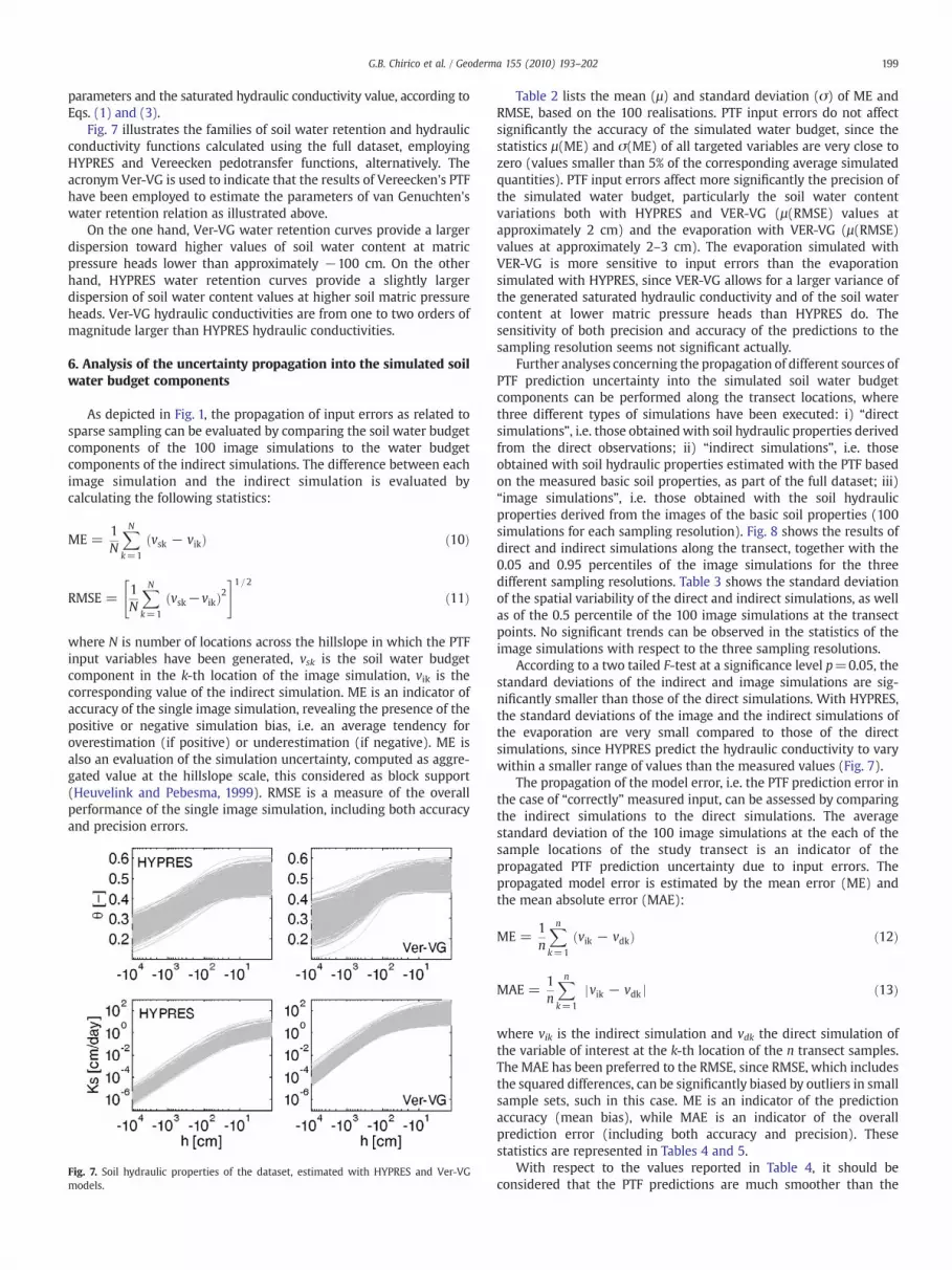
Fig. 7 illustrates the families of soil water retention and hydraulicconductivity functions calculated using the full dataset, employingHYPRES and Vereecken pedotransfer functions, alternatively. Theacronym Ver-VG is used to indicate that the results of Vereecken's PTFhave been employed to estimate the parameters of van Genuchten'swater retention relation as illustrated above.

On the one hand, Ver-VG water retention curves provide a largerdispersion toward higher values of soil water content at matricpressure heads lower than approximately −100 cm. On the otherhand, HYPRES water retention curves provide a slightly largerdispersion of soil water content values at higher soil matric pressureheads. Ver-VG hydraulic conductivities are from one to two orders ofmagnitude larger than HYPRES hydraulic conductivities.

6. Analysis of the uncertainty propagation into the simulated soilwater budget components

As depicted in Fig. 1, the propagation of input errors as related tosparse sampling can be evaluated by comparing the soil water budgetcomponents of the 100 image simulations to the water budgetcomponents of the indirect simulations. The difference between eachimage simulation and the indirect simulation is evaluated bycalculating the following statistics:

ME =1N

XNk=1

vsk − vikð Þ ð10Þ

RMSE =1N

XNk=1

vsk−vikð Þ2" #1=2

ð11Þ

where N is number of locations across the hillslope in which the PTFinput variables have been generated, vsk is the soil water budgetcomponent in the k-th location of the image simulation, vik is thecorresponding value of the indirect simulation. ME is an indicator ofaccuracy of the single image simulation, revealing the presence of thepositive or negative simulation bias, i.e. an average tendency foroverestimation (if positive) or underestimation (if negative). ME isalso an evaluation of the simulation uncertainty, computed as aggre-gated value at the hillslope scale, this considered as block support(Heuvelink and Pebesma, 1999). RMSE is a measure of the overallperformance of the single image simulation, including both accuracyand precision errors.

Fig. 7. Soil hydraulic properties of the dataset, estimated with HYPRES and Ver-VGmodels.

Table 2 lists the mean (µ) and standard deviation (σ) of ME andRMSE, based on the 100 realisations. PTF input errors do not affectsignificantly the accuracy of the simulated water budget, since thestatistics µ(ME) and σ(ME) of all targeted variables are very close tozero (values smaller than 5% of the corresponding average simulatedquantities). PTF input errors affect more significantly the precision ofthe simulated water budget, particularly the soil water contentvariations both with HYPRES and VER-VG (µ(RMSE) values atapproximately 2 cm) and the evaporation with VER-VG (µ(RMSE)values at approximately 2–3 cm). The evaporation simulated withVER-VG is more sensitive to input errors than the evaporationsimulated with HYPRES, since VER-VG allows for a larger variance ofthe generated saturated hydraulic conductivity and of the soil watercontent at lower matric pressure heads than HYPRES do. Thesensitivity of both precision and accuracy of the predictions to thesampling resolution seems not significant actually.

Further analyses concerning the propagation of different sources ofPTF prediction uncertainty into the simulated soil water budgetcomponents can be performed along the transect locations, wherethree different types of simulations have been executed: i) “directsimulations”, i.e. those obtainedwith soil hydraulic properties derivedfrom the direct observations; ii) “indirect simulations”, i.e. thoseobtained with soil hydraulic properties estimated with the PTF basedon the measured basic soil properties, as part of the full dataset; iii)“image simulations”, i.e. those obtained with the soil hydraulicproperties derived from the images of the basic soil properties (100simulations for each sampling resolution). Fig. 8 shows the results ofdirect and indirect simulations along the transect, together with the0.05 and 0.95 percentiles of the image simulations for the threedifferent sampling resolutions. Table 3 shows the standard deviationof the spatial variability of the direct and indirect simulations, as wellas of the 0.5 percentile of the 100 image simulations at the transectpoints. No significant trends can be observed in the statistics of theimage simulations with respect to the three sampling resolutions.

According to a two tailed F-test at a significance level p=0.05, thestandard deviations of the indirect and image simulations are sig-nificantly smaller than those of the direct simulations. With HYPRES,the standard deviations of the image and the indirect simulations ofthe evaporation are very small compared to those of the directsimulations, since HYPRES predict the hydraulic conductivity to varywithin a smaller range of values than the measured values (Fig. 7).

The propagation of the model error, i.e. the PTF prediction error inthe case of “correctly” measured input, can be assessed by comparingthe indirect simulations to the direct simulations. The averagestandard deviation of the 100 image simulations at the each of thesample locations of the study transect is an indicator of thepropagated PTF prediction uncertainty due to input errors. Thepropagated model error is estimated by the mean error (ME) andthe mean absolute error (MAE):

ME =1n

Xnk=1

vik − vdkð Þ ð12Þ

MAE =1n

Xnk=1

jvik − vdk j ð13Þ

where vik is the indirect simulation and vdk the direct simulation ofthe variable of interest at the k-th location of the n transect samples.The MAE has been preferred to the RMSE, since RMSE, which includesthe squared differences, can be significantly biased by outliers in smallsample sets, such in this case. ME is an indicator of the predictionaccuracy (mean bias), while MAE is an indicator of the overallprediction error (including both accuracy and precision). Thesestatistics are represented in Tables 4 and 5.

With respect to the values reported in Table 4, it should beconsidered that the PTF predictions are much smoother than the

Table 2Errors statistics of the simulated soil water budget components: mean (µ) and standarddeviation (σ) of the mean error (ME, difference between image and indirectsimulations) and the root mean square error (RMSE).

Sampling resolution 50 m 100 m 200 m

ΔS E T ΔS E T ΔS E T

HYPRES µ(ME) 0.0 0.0 0.0 −0.1 0.0 0.1 −0.1 0.0 0.1σ(ME) 0.1 0.0 0.0 0.1 0.0 0.0 0.2 0.0 0.1µ(RMSE) 1.8 0.5 0.6 1.9 0.5 0.6 2.0 0.5 0.6σ(RMSE) 0.4 0.0 0.0 0.4 0.0 0.0 0.4 0.0 0.0

Vereecken µ(ME) 0.0 0.2 0.0 −0.3 0.1 0.0 −0.3 0.1 0.0σ(ME) 0.2 0.1 0.0 0.2 0.1 0.0 0.3 0.1 0.1µ(RMSE) 2.3 2.3 0.9 2.6 2.7 0.8 2.7 2.8 0.8σ(RMSE) 0.6 0.1 0.0 0.6 0.1 0.0 0.6 0.1 0.0

ΔS=root zone soil water storage variation (cm); E=cumulative evaporation (cm);T=cumulative transpiration (cm).

200 G.B. Chirico et al. / Geoderma 155 (2010) 193–202

measurements and the resulting model errors are spatially correlated.This implies that the spatially aggregated model error (ME values)tend to be averaged out more strongly than the original input errors.

According to the results in Table 4, the indirect simulations of thecumulative transpiration, T, and the soil water content variation, ΔS, are

Fig. 8. Evaluation of the simulation uncertainty of soil water budget components accountinindirect simulations to the 0.05 and 0.95 percentiles of the simulations from generated imaand 200 m).

quite accurate with both PTFs. Ver-VG provides a ME of 0.1 cm for ΔSand −0.3 cm for T, corresponding in absolute value respectively to 2%and 6% of the average values provided by direct simulation (µ(ΔS)=−6.0 cm and µ(T)=5.09 cm, as reported inTable 1). HYPRES provides aME of 0.8 cm for ΔS and −0.1 cm for T, corresponding in absolutevalue respectively to 13% and 2%of the average values provided by directsimulation. The indirect simulations of the evaporation are less accurate,with ME values of −1.9 cm for HYPRES and 2.4 cm for Ver-VG,corresponding in absolute value respectively to 60% and 76% ofthe average direct simulation (µ(E)=3.1 cm as reported in Table 1).It is interesting to note that the evaporation predictions obtained withVer-VG and HYPRES have similar absolute bias, but with oppositesign, namely a positive sign for Ver-VG and a negative sign for HYPRES.

The indirect simulations of ΔS and T performed with HYPRES andVer-VG show similar level of precision. By comparing values reportedin Table 5 to the corresponding values in Table 1, it can be observedthat the mean absolute errors of the soil water content variation, MAE(ΔS), obtained with HYPRES and Ver-VG are equal respectively to 25%and 28% of the mean soil content variation, µ(ΔS), provided by thedirect simulations. Themean absolute errors of the transpiration, MAE(T), obtained with HYPRES and Ver-VG are equal respectively to 12%

g for both indirect estimation models (HYPRES and Ver-VG), by comparing direct andges conditioned to different sampling resolutions across the hillslope (x=50 m, 100 m,

Table 5Mean absolute error of the soil water budget simulation compared to the meansimulation standard deviations due to the input uncertainty at the transect locations.

ΔS E T

HYPRES MAE (cm) 1.5 2.3 0.6MAE/σ50 m (−) 1.02 9.59 2.03MAE/σ100 m (−) 0.89 10.19 2.00MAE/σ200 m (−) 0.93 8.76 1.81

Ver-VG MAE (cm) 1.7 3.4 1.0MAE/σ50 m (−) 0.82 2.39 1.95MAE/σ100 m (−) 0.72 1.90 1.97MAE/σ200 m (−) 0.76 2.10 1.91

ΔS=standard deviation of the root zone soil water storage variation; E=cumulativeevaporation (cm); T=cumulative transpiration (cm).MAE, mean absolute error of the soil water budget components.σx standard deviation of the simulations due to input uncertainty from differentsampling resolutions across the hillslope (x=50, 100, and 200 m).

Table 3Standard deviations of the root zone soil water budget components simulated along thetransect.

σΔS σ E σ T

HYPRES Direct simulations 2.14 2.69 0.76Indirect simulations 0.44 0.22 0.34p0.5 50 m 0.32 0.12 0.21p0.5 100 m 0.22 0.09 0.13p0.5 200 m 0.20 0.11 0.14

Ver-VG Indirect simulations 0.86 1.97 0.67p0.5 50 m 0.47 0.77 0.38p0.5 100 m 0.39 1.00 0.26p0.5 200 m 0.30 1.05 0.29

σΔS=standard deviation (std) of the root zone soil water storage variation (cm);E=std of the cumulative evaporation (cm); T=std of the cumulative transpiration(cm).Direct simulations=simulations with soil hydraulic properties estimated from directmeasurements.Indirect simulations=simulations with hydraulic properties estimated with indirectmethods, applying HYPRES and Ver-VG models.p0.5×m=0.5 percentile of soil water budget components simulated with hydraulicproperties from the stochastic images of the basic soil properties, conditioned tosampling grids with x=50 m, 100 m, and 200 m sample spacing.

201G.B. Chirico et al. / Geoderma 155 (2010) 193–202

and 20% of the mean transpiration, µ(T), obtained by directsimulations. The indirect simulations of the evaporation show alower level of precision. The mean absolute errors of the evaporation,MAE(E), obtained with HYPRES and Ver-VG are equal respectively to73% and 108% of the mean evaporation, µ(E), obtained by directsimulations.

The ratios of ME and MAE values to the corresponding standarddeviations of the image simulations (σx) are computed for evaluatingthe relative importance of the model error versus the input errors inthe uncertainty of the simulated soil water budget. These statistics arealso listed in Tables 4 and 5.

For both HYPRES and Ver-VG, ME values of ΔS and T are smallerthan 65% of the corresponding σx values. Thus, for what concerns theaccuracy of the simulated ΔS and T, the model error is less significantthan the input errors.

MAE values of ΔS range from 72% to 102% of the corresponding σx

values. Thus, for what concerns the precision of the simulated ΔS, themodel error is less or as much significant as the input errors. MAEvalues of T are almost twice the corresponding σx of T. Thus, for whatconcerns the precision of the simulated T, the model error is moresignificant than the input errors.

The model error is certainly more significant than the input errorsfor the simulated evaporation, both in terms of accuracy and precision,particularly for HYPRES, whose MAE and ME values are 8 to 10 timeslarger than the corresponding σx. The role of the model error is stillsignificant, although less pronounced, for the evaporation simulated

Table 4Mean error of the soil water budget simulation compared to the mean simulationstandard deviations due to the input uncertainty at the transect locations.

ΔS E T

HYPRES ME (cm) 0.8 −1.9 −0.1ME/σ50 m (−) 0.53 −7.82 −0.47ME/σ100 m (−) 0.47 −8.31 −0.47ME/σ200 m (−) 0.49 −7.14 −0.42

Ver-VG ME (cm) 0.1 2.4 −0.3ME/σ50 m (−) 0.06 1.69 −0.64ME/σ100 m (−) 0.05 1.34 −0.64ME/σ200 m (−) 0.05 1.49 −0.62

ΔS=standard deviation of the root zone soil water storage variation; E=cumulativeevaporation (cm); T=cumulative transpiration (cm).ME, mean error (difference between indirect and direct simulations) of the soil waterbudget components.σx standard deviation of the simulations due to input uncertainty from differentsampling resolutions across the hillslope (x=50, 100, and 200 m).

with Ver-VG, as MAE and ME values range from 1.3 times up to2.4 times the corresponding σx.

The differences in the prediction performances of the evaporationcompared to the transpiration and the soil water content variation canbe explained by the different sensitivity of these variables to theestimated soil hydraulic parameters. Evaporation rate is more directlycontrolled by the soil hydraulic conductivity at the soil surface. Thussignificant PTF model prediction errors in the estimated soil hydraulicconductivity (Chirico et al., 2007) correspond to significant modelprediction errors in the evaporation rate. On the other hand,transpiration and soil water content variation in the root zone aremore sensitive to the soil water availability as described by the bulk ofthe soil water retention function, which is predicted by the PTFs withhigher precision and accuracy (Chirico et al., 2007).

7. Conclusions

Computer model predictions are always affected by uncertainty,which arises from the chosenmodel structure and parameters, as wellas from errors in the boundary conditions and model validation data.As environmental model predictions are nowadays increasinglyemployed in the decision making process involving not merelyeconomic, but also social costs, uncertainty analysis of modelpredictions is becoming an unavoidable task of any application ofenvironmental models (Pappenberger and Beven, 2006).

In soil hydrological studies, characterisation of soil hydraulicbehaviour is one of the main sources of uncertainties, particularly atthe scale of interest for practical applications. Given the largevariability of soil hydraulic properties, the application of a largeamount of relatively cheap but imprecise estimates of the soilhydraulic properties, such as those provided by PTFs, can be moreefficient than the application of expensive direct measurements of soilhydraulic properties in a limited number of locations (Minasny andMcBratney, 2002a).

By employing two different PTFs to parameterise a soil waterbudget model applied across the study hillslope, the predictionperformances for the transpiration and the soil water contentvariations were different from those obtained for the evaporation.Results for the simulated transpiration and soil water contentvariations can be summarised as follows:

- the accuracy of the predictions at the hillslope scale is generallyhigh, being more affected by the uncertainty than the PTF modelerror;

- the precision of the predictions (particularly of the transpiration)is generally more affected by the PTFmodel error than by the inputuncertainty.

Accuracy and precision of the simulated evaporation are both verylow and significantly affected by the PTF model error.

202 G.B. Chirico et al. / Geoderma 155 (2010) 193–202

These results can be explained by the fact that evaporation isdirectly affected by the large uncertainty of the PTF estimates of thehydraulic conductivity, which directly controls the evaporation rate atthe top boundary of the soil column. Whereas the best performancesare observed for those variables that are more sensitive to the bulk ofthe soil water retention, which can be more efficiently predicted bythe PTFs commonly applied.

It is important to stress that the performance of PTFs outside itsdevelopment dataset is generally unknown. The results reported inthis study are strictly related to the specific PTFs applied and theparticular hillslope, which have been derived from soil databasesdominated by North-West European soils.

Acknowledgements

This study has been partly supported by P.O.N. project “AQUATEC—New technologies of control, treatment, and maintenance for thesolution of water emergency”. Hanoi Medina contributed to this paperduring a visiting period at the University of Napoli Federico II, with afellowship from the Italian–Latin American Institute (IILA). The datadisplayed in Figs. 2 and 3 were provided by Guido Ciollaro, AntonioCoppola and Paolo Damiani, who conducted the field hydrologicalmonitoring campaign in the experimental plot. The final version of thispaper benefited from the constructive comments of two anonymousreviewers and the thoughtful appraisal of the Editor.

References

Bouma, J., 1989. Using soil survey data for quantitative land evaluation. Adv. Soil Sci. 9,177–213.

Chirico, G.B., Medina, H., Romano, N., 2007. Uncertainty in predicting soil hydraulicproperties at the hillslope scale with indirect methods. J. Hydrol. 334, 405–422.

Christiaens, K., Feyen, J., 2001. Analysis of uncertainties associated with differentmethods to determine soil hydraulic properties and their propagation in thedistributed hydrological MIKE SHE model. J. Hydrol. 246, 63–81.

Cresswell, H.P., Paydar, Z., 2000. Functional evaluation of methods for predicting soilwater characteristic. J. Hydrol. 227, 160–172.

Damiani, P., Ciollaro, G., Coppola, A., 2008. Effect of tillage layering on the hydrologicalbehaviour of a structured soil. J. Agric. Eng. 39 (2), 45–51 (in Italian, with Englishabstract).

Feddes, R.A., Kowalik, P.J., Zaradny, H., 1978. Simulation of Field Water Use and CropYield. Simulation Monograph, PUDOC. Centre for Agricultural Publishing andDocumentation, Wageningen. 189 pp.

Gardner, W.R.,1965. Dynamics of soil water availability to plants. Annu. Rev. Plant Physiol.16, 323–342.

Gómez-Hernández, J.J., Journel, A.G., 1993. Joint sequential simulation of multiGaussianfields. In: Soares, A. (Ed.), Geostatistics Tróia. InKluwer, Dordrecht, pp. 85–94.

Heuvelink, G.B.M., Pebesma, E.J., 1999. Spatial aggregation and soil process modelling.Geoderma 89, 47–65.

Minasny, B., McBratney, A.B., 2002a. The efficiency of various approaches to obtainingestimates of soil hydraulic properties. Geoderma 107, 55–70.

Minasny, B., McBratney, A.B., 2002b. Uncertainty analysis for pedotransfer functions.Eur. J. Soil Sci. 53, 417–429.

Minasny, B., McBratney, A.B., Bristow, K.L., 1999. Comparison of different approaches tothe development of pedotransfer functions for water retention curves. Geoderma93, 225–253.

Pappenberger, F., Beven, K.J., 2006. Ignorance is bliss: or seven reasons not to useuncertainty analysis. Water Resour. Res. 42, W050302.

Pebesma, E.J., 2004. Multivariable geostatistics in S: the gstat package. Comp. Geosci. 30,683–691.

Reynolds, W.D., Elrick, D.E., 2002. Falling head soil core (tank) method. In: Dane, J.H.,Topp, G.C. (Eds.), Methods of Soil Analysis — Part 4: Physical Methods. InSoilScience Society of America, Madison, Wisconsin, USA.

Romano, N., Palladino, M., 2002. Prediction of soil water retention using soil physicaldata and terrain attributes. J. Hydrol. 265, 56–75.

Santini, A., Romano, N., Ciollaro, G., Comegna, V., 1995. Evaluation of a laboratoryinverse method for determining unsaturated hydraulic properties of a soil underdifferent tillage practices. Soil Sci. 160, 340–351.

Schaap, M.G., Leij, F.J., 2000. Improved prediction of unsaturated hydraulic conductivitywith the Mualem–van Genuchten Model. Soil Sci. Soc. Am. J. 64, 843–851.

van Dam, J.C., Huygen, J., Wesseling, J.G., Feddes, R.A., Kabat, P., van Walsum, P.E.V.,Groenendijk, P., van Diepen, C.A., 1997. Theory of SWAP version 2.0. Simulation ofwater flow, solute transport and plant growth in the Soil–Water–Atmosphere–Plantenvironment. Report 71, Subdep. Water Resources, Wageningen University,Technical document 45, Alterra Green World Research, Wageningen.

van Genuchten, M.Th., 1980. A closed-form equation for predicting the hydraulicconductivity of unsaturated soils. Soil Sci. Soc. Am. J. 44, 892–898.

Vereecken, H., Diels, J., van Orshoven, J., Feyen, J., Bouma, J., 1992. Functional evaluationof pedotransfer functions for the estimation of soil hydraulic properties. Soil Sci. Soc.Am. J. 56, 1371–1378.

Western,A.W., Blöschl,G.,1999.On the spatial scalingof soilmoisture. J.Hydrol. 217, 203–224.Wösten, J.H.M., Bannink, M.H., de Gruijter, J.J., Bouma, J., 1986. A procedure to identify

different groups of hydraulic conductivity and moisture retention curves for soilhorizons. J. Hydrol. 86, 133–145.

Wösten, J.H.M., Lilly, A., Nemes, A., Le Bas, C., 1999. Development and use of a databaseof hydraulic properties of European soils. Geoderma 90, 169–185.