A tracer budget quantifying soil redistribution on

hillslopes after forest harvesting

P.J. Wallbrink a,b,*, B.P. Roddy c, J.M. Olley a,b

aCooperative Research Centre Catchment Hydrology, P.O. Box 1666, Canberra ACT, 2601, AustraliabCSIRO, Land and Water, P.O. Box 2601, Canberra, ACT 1666, Australia

c7 Fitzroy St., Tumut. NSW, 2720, Australia

Received 26 April 2001; received in revised form 20 August 2001; accepted 14 September 2001

Abstract

Managing the impacts of erosion after forest harvesting requires knowledge of erosion sources;

rates of sediment transport and storage; as well as losses from the system. We construct a tracer-

based (137Cs) sediment budget to quantify these parameters. The budget shows significant

redistribution, storage and transport of sediment between landscape elements and identifies the snig

tracks and log landings as the major impact sites in the catchment. Annual sediment losses from them

were estimated to be 25F 11 and 101F15 t ha� 1 year� 1, respectively, however, it is probable that

most of this is due to mechanical displacement of soil at the time of harvesting. The budget showed

greatest net transport of material occurring from snig tracks; representing some 11F 4% of the 137Cs

budget. Of the latter amount, 18%, 28% and 43% was accounted for within the cross banks, filter

strip and General Harvest Area (GHA), respectively. The 137Cs budget also showed the GHA to be a

significant sediment trap. The filter strip played a fundamental role in the trapping of material

generated from the snig tracks, the mass delivery to them from this source was calculated to be

1.7F 0.6 kg m2 year� 1. Careful management of these remains critical. Overall we could account for

97F 10% of 137Cs. This retention suggests that (within errors) the overall runoff management

system of dispersing flow (and sediment) from the highly compacted snig tracks, by cross banks, into

the less compacted (and larger area) GHA and filter strips has effectively retained surface soil and

sediment mobilised as a result of harvesting at this site. Crown Copyright D 2002 Published by

Elsevier Science B.V. All rights reserved.

Keywords: Sediment budget; 137Cs; Tracers; Soil redistribution; Forest harvesting; Snig track erosion; Filter strips

0341-8162/02/$ - see front matter. Crown Copyright D 2002 Published by Elsevier Science B.V. All rights

reserved.

PII: S0341-8162 (01 )00185 -0

* Corresponding author. CSIRO Land and Water, GPO Box 1666, Canberra ACT 2601, Australia. Fax: +61-

2-6246-5800.

E-mail address: peter.wallbrink@csiro.au (P.J. Wallbrink).

www.elsevier.com/locate/catena

Catena 47 (2002) 179–201

1. Introduction

1.1. Quantifying sediment redistribution after harvesting

The impact of harvesting operations on sediment delivery has generally been assessed

by measurement of the suspended solids flux at the stream or catchment outlet (Tebo,

1955; Gilmour, 1971; Olive and Reiger, 1985; Anderson and Potts, 1987; Borg et al.,

1987; Cornish and Binns, 1987). However, these measurements reveal little about the

source of the eroded material, or about the specific impact of harvesting on sediment

redistribution upstream of that point (Croke et al., 1999a). Sediment budgets can be used

to construct a more complete picture of sediment generation and distribution within

catchments (Dietrich and Dunne, 1978; Kelsey et al., 1981; Reid et al., 1981; Trimble,

1983; Roberts and Church, 1986). However, these budgets require quantification of the

inputs, outputs and storages associated with the study area. To address this, a range of

studies has been undertaken to quantify rates of material transport from, or deposition

within, various landscape elements. For example, rates of loss from roads (e.g., Reid and

Dunne, 1984; Fahey and Coker, 1989; Montgommery, 1994) snig tracks, (Croke et al.,

1999a) snig tracks and cross banks (Hairsine et al., 2001) as well as slope erosion rates and

channel storage (Best et al., 1995; Madej, 1995).

In spite of these studies, data gaps invariably exist for some of these terms, while others

simply remain difficult to quantify. For example, very little is known about sediment

redistribution at the hillslope scale in forestry environments, particularly in terms of the

relative transfer and storage of material that occurs between erosion units such as haulage

tracks and storage sites such as the cross banks and filter strips. The sediment budget

remains incomplete where there is a lack of detail about these processes.

In this paper, we use the redistribution of fallout 137Cs as the basis of a sediment

budget. We use our budget to examine the issue of onslope sediment redistribution

processes; in particular to quantify the transfer and storage of material that occurs within

and between different elements of harvested slopes. The budget can also be used to

quantify the losses of sediment from the catchment after harvesting, and thus assess the

overall effectiveness of erosion mitigation practices at the study area.

1.2. Using tracer budgets

We use fallout 137Cs as the basis of our work. Its utility in soil erosion studies was first

investigated by Rogowski and Tamura (1965), who demonstrated a linear relationship

between soil loss and 137Cs depletion. This basic relationship has been used by many

subsequent authors to characterise geomorphic processes (see references in review by

Ritchie and McHenry, 1990). In particular, sediment budgets based on tracers such as 137Cs

can also provide a powerful framework for soil redistribution studies (Ritchie et al., 1974;

Walling et al., 1986, 1996; Loughran et al., 1992; Quine et al., 1994; Owens et al., 1997).

In its simplest form, constructing a tracer-based budget requires the measurement of

three terms: (1) the initial inventories, that is the amount of the tracer present in the soil prior

to disturbance; (2) the spatial extent of the landscape elements of interest; and (3) the

amount of tracer left in each landscape element after disturbance. The product of the initial

P.J. Wallbrink et al. / Catena 47 (2002) 179–201180

tracer inventories and surface area gives the total amount of each tracer initially contained

within each element. Comparison of the tracer amounts remaining in the hillslope elements

with that calculated to be present prior to disturbance reveals net losses from the system.

Differences in radionuclide amounts between the landscape elements (both before and after

harvesting) reflect the relative flow of material between elements; revealing much about the

transfer and storage occurring on hillslopes after harvesting. In the study presented here, the

landscape elements are defined as the log landing areas (otherwise known as log dumps)

snig tracks, (otherwise known as skid tracks or skid trails), the General forest Harvesting

Area (hereafter termed the GHA), and filter strip areas retained for wildlife and riparian

protection. In total they account for the entire surface area of the study catchment.

There are three factors that may complicate the application (or interpretation) of 137Cs

to tracer-based sediment budget studies. The first is the initial spatial variability (coefficient

of variation, CV) of 137Cs in soils, which in reference areas may be as large as 40%

(Fredericks et al., 1988; Sutherland, 1994; Wallbrink et al., 1994). The second is the

affinity of 137Cs to particles of different sizes (Wallbrink et al., 1999). The third is

accounting for natural erosion that has occurred in the period between the initial fallout of137Cs and the beginning of the disturbance regime. These factors are addressed

specifically within the ‘experimental design’. The radionuclide used as the basis for this

study is described below.

1.3. Fallout caesium-137

Caesium is an alkali metal with a chemistry similar to that of sodium, potassium and

other elements of Group I in the Periodic Table. Caesium-137 has a half life of f 30 years

and is found in the environment as a consequence of above ground nuclear weapons testing

between 1945 and 1974 (Wise, 1980; Longmore, 1982; Ritchie and McHenry, 1990).

Fallout in the northern hemisphere was about an order of magnitude higher than in the

southern hemisphere (Ritchie and McHenry, 1990). Fallout of this nuclide was strongly

related to local patterns and rates of precipitation (Davis, 1963; Longmore, 1982; Basher et

al., 1995). Upon reaching the soil surface, 137Cs not only complexes strongly with the soil

particles, but appears to occur in an almost non-exchangeable form. Lomenick and Tamura

(1965) reported that they removed less than 1% of 137Cs from sediment by a variety of salt,

base, oxidizing, weak acid, and water solutions. In undisturbed soils 137Cs is generally

found with a maximum concentration slightly below the soil surface (f 10 mm), from

where concentrations decrease exponentially to below detection limits at f 200- to 250-

mm depth (Wallbrink and Murray, 1993; Zhang et al., 1994; Basher et al., 1995; Wallbrink

et al., 1999).

2. Study site

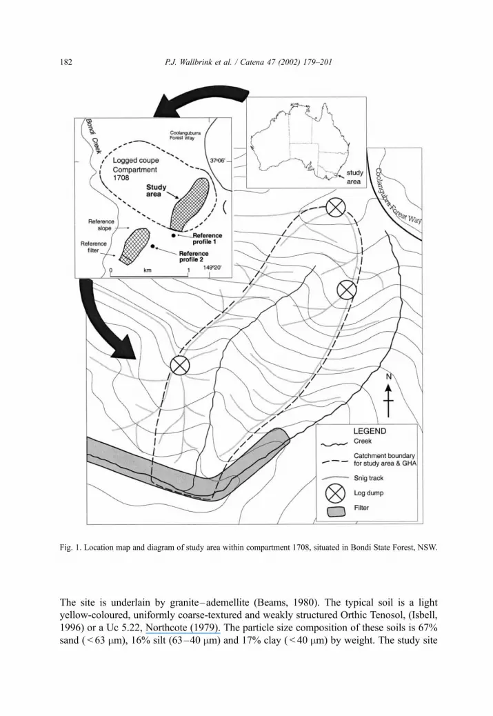
2.1. Physical characteristics

The study area is a small basin (f 12 ha) within compartment 1708 in the Bondi State

Forest, approximately 24 km south of Bombala in the south east of NSW, Australia (Fig. 1).

P.J. Wallbrink et al. / Catena 47 (2002) 179–201 181

The site is underlain by granite–ademellite (Beams, 1980). The typical soil is a light

yellow-coloured, uniformly coarse-textured and weakly structured Orthic Tenosol, (Isbell,

1996) or a Uc 5.22, Northcote (1979). The particle size composition of these soils is 67%

sand ( < 63 mm), 16% silt (63–40 mm) and 17% clay ( < 40 mm) by weight. The study site

Fig. 1. Location map and diagram of study area within compartment 1708, situated in Bondi State Forest, NSW.

P.J. Wallbrink et al. / Catena 47 (2002) 179–201182

is 650 m above sea level and has a mean annual rainfall of f 1000 mm. Rainfall is

variable and episodic. Lowest rainfall occurs from midwinter to early spring; the highest

rainfall from midsummer to early winter (State Forests of NSW, 1994). The dominant tree

species at the study site are Silvertop Ash (Eucalyptus sieberi), Grey Gum (E.

cypellocarpa) and Brown Barrel (E. fastigata). Regrowth vegetation consists mainly of

smaller eucalypts, acacias and Musk Daisy Bush (Olearia argophylla) (Croke et al.,

1997). A well-incised ephemeral stream, f 300 m long, is the major drainage feature of

the study area. It has vertical banks of about 1 m at its headwaters, and about four m at the

outlet.

2.2. Logging treatment for compartment 1708

Timber extraction occurred in compartment 1708 from May to October 1990. The

trees were cut by chainsaw, the branches and crowns were left in situ. The logs were

dragged (or snigged) by bulldozers along snig tracks to log landings where they were

stripped of bark, and loaded onto log trucks for transport out of the coupe via the

compartment road (Fig. 1). The compartment, and our study area within it, was harvested

under the Standard Erosion Mitigation Guidelines (CaLM, 1993). This prescribed,

among other conditions, that drainage lines in catchments greater than 40 ha are

protected by a 20-m wide filter strip of undisturbed vegetation. Trees were harvested

from this zone, but only if they could be felled and snigged without machinery entering

the zone.

After harvesting, the in-situ crowns, leaves, and slash were burnt to reduce the residual

fuel load available for wildfire. The aim is to reduce the fine fuel available for fires byf 80% (State Forests of NSW, 1994). In Australia, burning also facilitates regeneration of

trees by releasing nutrients and initiating seed release. The log landings usually become

compacted during harvesting. In order to promote regeneration of these areas, the log

landings are treated by first blading off the surface soil and placing this in large mounds

adjacent to the landing area. Some of this material is then spread back onto the landing

after harvesting. The surface is then ripped and the log landings commonly replanted with

E. nitens.

2.3. Erosion mitigation strategies

Treatments to reduce post-harvest sediment loss principally involved the construction

of cross banks on the snig tracks and the provision of the filter strip along the major

drainage line. The cross banks were typically spaced between 20 and 30 m, depending on

the slope. The control on the spacing is to reduce contributing area for runoff generation,

thus reducing water velocity and discharge volume, (Croke et al., 1999b). The cross

banks are designed to divert water and sediment from the snig tracks onto the GHA. The

cross banks are constructed by blading material off the snig track (with a bulldozer) to

form a mound of material at right angles to the predominant direction of water flow on

the track. In this paper, the term ‘cross banks’ also includes the mounds of material,

sometimes called ‘windrows’ that are created alongside the snig tracks during their

construction.

P.J. Wallbrink et al. / Catena 47 (2002) 179–201 183

3. Experimental design and research methods

3.1. Requirements for constructing a tracer-based budget

As described in the Introduction, the approach is based on determining the total amount

of 137Cs within the study area, and also within each of its individual landscape elements,

both before and after harvesting. Thus, in order to construct a tracer budget we need to

determine: (a) the surface areas of each landscape element, (b) the activity (Bq kg� 1) of137Cs within each of these elements, (c) a reference inventory for 137Cs from an

undisturbed coupe, with similar soils, aspect, and rainfall to the logged study area.

Because natural ‘background’ erosion has occurred within the study area over the lastf 30 years (the period since the main 137Cs fallout input), we also need to determine: (d)

the amount of natural 137Cs (and thus soil) redistribution which is not due to forest

harvesting. Finally, in order to better interpret the 137Cs tracer budget we also investigate:

(e) the dependence of 137Cs activity on particle size and organic matter content.

3.2. Calculating the surface area of the different landscape elements and cross bank

volumes

The areas of the different landscape elements within the study area were determined by

digitising a 1:25,000 aerial photo using ARC/INFO GIS. Coverages were created for the

snig tracks, log landings, and the buffer strip. The area of the GHA was obtained by

subtracting the sum of the areas of the log landings, snig tracks and filter strip from the

total study area. Digitising aerial photos creates errors due to optical distortion and relief

displacement (Avery, 1968; Curran, 1985). Image stretching can also occur when geo-

referencing points on the digitised aerial photo are aligned with the same points in the

ARC/INFO coverage. The four location points formed a rectangle around the study area

with sides of f 1000 m. The final image was stretched about 49 m when overlaid onto the

contour map representing an error of f 5% for the entire image. This is used as an upper

estimate of the uncertainty associated with the area of each of the landscape elements, and

these uncertainty values are given in Table 1. The approximate mass of soil within the

cross banks was calculated by multiplying their ‘average’ width, depth and height

Table 1

Landscape element proportions determined by ARC/INFO analysis of 1:25,000 digitised aerial photograph

Landscape element Area (m2) Fraction of study area (%)

Snig track 22,2001100a 18

Log landing 3150160 3

Filter strip 6850300 6

General harvest area 91,7004600 74

Total 123,9006200 101b

Uncertainties are given in the least significant figure and represent those derived from landscape element area

calculations, as per discussion in text.a Snig track area calculated by multiplying total snig track length by survey width of 4.5 m.b Due to rounding of area calculations.

P.J. Wallbrink et al. / Catena 47 (2002) 179–201184

dimensions by their total number and their mean bulk density. A similar approach was

adopted for the snig track ‘windrows’ adjacent to the snig tracks.

3.3. Measuring the 137CS inventory within the landscape elements and reference area

The distribution of 137Cs can be quite heterogeneous in forests (Wallbrink and Murray,

1996a) and a large number of cores can be required to characterise it properly in these

environments. Sutherland (1994) presents formula demonstrating that the number of

samples required to determine a mean 137Cs reference inventory with an allowable error of

10% at the 90% confidence limit was about 11, if the sample Coefficient of Variation (CV)

(Relative Standard Deviation) was f 20%. Wallbrink et al. (1994) show that the CV for137Cs reference inventories within Australia is f 40%. Applying the formula of Suther-

land under the same confidence limits but with the higher Australian CV, suggests that a

minimum number of samples required to determine a mean reference inventory is about

45. Related to this, Wallbrink et al. (1994) showed that 137Cs inventories of bulked soil

cores from reference sites were less variable than those of the individual cores that

comprised them. Further, bulking allowed an accurate estimate of the mean reference

inventory (and standard error) to be determined with fewer analyses, although the standard

deviation of the individual cores was more difficult to obtain. Consequently, because our

budget calculations only required the mean (and standard error) of the various reference

site and landscape element terms, bulking of material from soil cores was used in this

study. This also allowed us to take many cores from each location (providing confidence

that the distribution of 137Cs had been adequately sampled) without increasing the demand

on analytical facilities.

For example, the 137Cs ‘reference’ inventory was measured in an unlogged, undisturbed

native forest adjacent to the study area. It had similar slopes (10–20�), surface area (f 11

ha), aspect (SSW), rainfall and vegetation (Fig. 1). Eighty individual cores were taken in a

grid pattern from within the reference slope. For each core a metal ring of 100-mm

diameter and height 20 mm was first hammered into the ground. The ring prevented the

hole from collapsing and defined a specific surface area and volume of soil, which was

then excavated by auger. The first ring was then extracted and a second ring of height of

50 mm was then located in the soil, and the enclosed material from 20- to 50-mm depth

extracted. Depth increments within the ranges 50–100, 100–200 and 200–300 mm were

then taken using a narrower auger of 80 mm diameter. A further 30 samples were also

taken using the same method from within a strip of forest of equivalent width to the study

area filter strip at the base of this slope. Samples from corresponding depth units were

bulked together in groups of 10 for each of these elements. Each bulked group was then

counted as a single sample. Analysing the separate depth units allowed a better

discrimination of nuclide distributions with depth. The procedure in the above situation

provided eight independent inventory analyses for the reference area, and three for the

reference filter strip.

The same procedure for soil coring was also used to obtain 80 cores from the GHA

(with the largest surface area), and 30 each from the log landings, snig tracks and cross

banks, respectively. Individual depth increments from these cores were mixed together in

P.J. Wallbrink et al. / Catena 47 (2002) 179–201 185

groups of 10 as above. Forty-five cores were taken from the filter strip at the base of the

harvested slope. Depth increments here were mixed together in groups of 15, again each

bulked group was counted as a single sample. The snig tracks, filter strips and cross

banks were sampled linearly (20-m spacing), the remainder on a grid (sample spacing at

each 10� 10 m). In this study, the sediment trapped in front of the cross banks adjacent

to the log landing was included in the sampling of the log landing. A similar procedure

was adopted for the cross banks on the snig tracks. The sediment tongues that developed

from the cross banks and extended into the GHA, were included in the sampling of the

GHA.

3.4. Determining depth distributions of 137Cs and 210Pbex for soil loss calculations

In this study, the amount of soil lost from the snig tracks and log landings was

quantified using the 210Pbex to 137Cs inventory ratio method described in Wallbrink and

Murray (1996a). Briefly, fallout 210Pb is also known as 210Pb excess (210Pbex) and is

generated from the decay of 222Rn in the atmosphere. It has a half-life of f 22 years and

is continually precipitated on the soil surface by rainfall. It is usually defined as the excess

of 210Pb activity over that produced in situ by its parent 226Ra. Maximum concentrations

of 210Pbex in soils are usually found at the surface; decreasing approximately exponentially

with depth, and reaching typically undetectable levels at depths of f 100 mm (Wallbrink

et al., 1999). The soil loss estimation procedure requires detailed depth distribution curves

for both 137Cs and 210Pbex to be determined at reference sites. This was undertaken by

excavating soil profiles at two sites within the adjacent undisturbed forest area, approx-

imately 100 and 250 m, respectively from the coupe boundary (Fig. 1). Detailed depth

penetration information at these sites was obtained by cutting thin layers of soil

sequentially down through the soil with a known surface area (0.16 m2). One-millimeter

layers were taken down to 2-m depth. Two-millimeter layers were then taken to 24-mm

depth; 10-mm layers from 24 to 104 mm; 20-mm layers from 104 down to 204 mm, and

50-mm layers from 204 mm down to the final depth of 304 mm. This was undertaken

using apparatus described in Wallbrink and Murray (1996b).

3.5. Radioactivity in the filter strips resulting from natural erosion

As mentioned above, one factor in developing a budget is accounting for any natural

sediment redistribution occurring at the site prior to harvesting. In this respect, the

radionuclide content of the study area harvested filter strip comprises radioactivity from:

(i) direct 137Cs fallout, (ii) soil particles deposited as a function of natural pre-harvesting

sediment redistribution processes, and (iii) soil particles trapped within the filter as a result

of post-harvesting disturbance. The first component (item (i)) can be simply derived from

the local reference inventory, and item (iii) is what we wish to derive. An estimate of item

(ii) can be obtained from the amount by which the 137Cs inventory (Bq m� 2) of the filter

strip in the reference area was elevated above that of the upslope reference area. This value

was then subtracted from the inventory for the study area filter strip (Bq m � 2) for use in

the subsequent budget calculations.

P.J. Wallbrink et al. / Catena 47 (2002) 179–201186

3.6. Sampling and processing of soil material for particle size analyses

A separate suite of soil samples collected from the reference area was used for particle

size analysis. Samples consisted of material taken by hand auger to a depth of 0–20 mm

from 36 cores on a 100-m grid on the reference slope. All the material was mixed together,

the total dry mass was f 5.5 kg. A 300-g sub-sample was taken from the dry mass and

analysed separately. The remainder was slaked in water and mechanically agitated through

sieves with apertures of 500, 250, 125, and 63 mm. Each sample was then washed again by

hand in the appropriate sieve until only clear water emerged from the base of the sieves.

The < 63-mm fraction was then separated into 63–40, 40–20, 20–10, 10–2, and < 2 mmfractions by settling. The material comprising each of these size fractions was placed in a

dehydrator at 40 �C until dry. Water was added to the dry samples and the organic fraction

floated off. This process was repeated three times. The organic material from each fraction

was combined, dried and weighed. The mineral material from each particle size fraction

was then also dried, weighed and ground. The individual fractions (including organic

fractions) were then analysed by gamma spectrometry (described below) to determine their

concentrations of 137Cs (Bq kg� 1).

3.7. Preparation of soil samples

All soil samples were initially weighed, dried at 40 �C for 48 h, and weighed again to

determine field moisture content, and bulk density. Typically, 300 g was extracted for

analysis and the remainder archived. The samples were ashed in a muffle furnace at 400

�C for 48 h to determine the Loss on Ignition (LOI); then ground in a rock mill to a fine

powder. This powder was then cast in a polyester resin matrix in either a ‘cup’ (f 250 g),

‘disk’ (f 30 g), or ‘stick’ (f 10 g), geometry depending on the sample size. All of the

above field samples were collected and analysed during 1996 and 1997. All data are time-

corrected to 1996.

3.8. Gamma spectrometry methods for analysis of low level radioactivity

137Cs is a gamma emitter at 662 keVand 210Pb at 46 keV. Both are readily detectable by

routine high resolution gamma spectrometry techniques (Hamada and Kruger, 1965).

Analysis for these nuclides at the CSIRO laboratories follows the methods described by

Murray et al. (1987). The detectors used in this study are ‘n’-type closed ended co-axials.

Detection limits are about F 0.3 Bq kg� 1 for 137Cs and F 3.0 Bq kg� 1 for 210Pbex.

Typical count times were in the order of f 84 ks. Independent checks on detector

calibrations were undertaken by participating in International Atomic Energy Association

(IAEA) intercomparisons.

4. Results

4.1. Detailed depth distributions of 137Cs and 210Pbex

The 137Cs and 210Pbex activities (Bq kg� 1) associated with the two detailed depth

profiles from the reference site are given in Fig. 2. As expected, maximum activities of

P.J. Wallbrink et al. / Catena 47 (2002) 179–201 187

Fig. 2. 137Cs and 210Pbex activity distribution with depth from profiles 1 and 2 within the reference area adjacent

to compartment 1708.

P.J. Wallbrink et al. / Catena 47 (2002) 179–201188

210Pbex occur at the soil surface, while those of 137Cs occur just below the soil surface.

These are both consistent with other profiles described in the literature cited above. The

cumulative inventory ratio values (Wallbrink and Murray, 1996a) for these are 3.05F 0.2

and 3.09F 0.3 for profiles 1 and 2, respectively.

4.2. Particle size separation experiment

The relative affinity of 137Cs for different particle size fractions is given in Table 2.

There is a systematic trend for 137Cs to be preferentially associated with smaller size

particles. The highest activities (Bq kg� 1) are found on the < 2-mm material, the lowest on

>500-mm specimen. This trend is consistent with the results observed by He and Owens

(1995) and Wallbrink et al. (1999) for 137Cs, 210Pbex and7Be. Of the total of 39.4 Bq, the

highest proportion was retained in the 2–10 mm range (9.1%) and the lowest in the 40–63

mm range (1.6%).

4.3. Caesium-137 activities in the different landscape elements

Table 3 presents the 137Cs inventories (Bq m� 2) for each of the landscape elements as

well as those for the reference slope, and reference filter strip. The highest 137Cs

inventories were in the filter strip at the base of the harvested slope 860F 90 Bq m� 2.

The lowest values were measured in the log landings and snig tracks, 150F 90 and

190F 90 Bq m� 2, respectively. The mean from the reference slope was 493F 25 Bq

m� 2 (n = 80 cores, n = 8 bulked samples). This was below that calculated for the GHA

525F 25 Bq m� 2. The difference between the 137Cs reference value and the study area

filter strip is f 360 Bq m � 2. This is significantly greater than the equivalent difference

between the reference area slope and the reference area filter strip, i.e. 85 Bq m � 2. The

latter value represents the amount by which background erosion has contributed tracer

Table 2

Affinity of 137Cs, for different particle sizes at the study site

Size (mm) Dry

weight

(g)

137Cs activity

(Bq kg� 1)

Total 137Cs

activity (Bq)

137Cs (%) Cumulative activity

by integrated

size class

(Bq kg� 1)

< 2 90 571 5.10.1 13.10.4 56.90.72–10 262 351 9.10.1 23.00.7 40.31.110–20 143 201 2.90.1 7.40.3 34.61.920–40 124 161 2.00.1 5.10.2 30.92.640–63 147 111 1.60.1 4.10.1 27.13.263–125 406 1015 4.20.4 10.71.1 21.34.7125–250 508 4.30.4 2.20.2 5.60.6 16.25.2250–500 911 3.60.4 3.20.4 8.20.9 11.75.1> 500 1910 1.60.1 3.10.3 7.90.4 7.43.9Organics 503 120 5.90.0 14.90.4 7.94.2Total 5006 39.41.3 1002.4

Analytical uncertainties equivalent to 1 standard error are given as subscripts in the least significant figure.

P.J. Wallbrink et al. / Catena 47 (2002) 179–201 189

activity to the reference slope filter areas (described above) and has been subtracted from

the study area filter strip inventory when incorporated into the 137Cs tracer budget

described below.

The cross banks do not have an inventory value in Table 3. This is because they have

been created from material bladed off the snig tracks and log landings during and after

harvesting. Consequently, the 137Cs contained within them is distributed throughout the

entire soil matrix of the bank and not just within the top 20 cm or so of the soil. Their total

Table 3

Inventories of 137Cs for landscape elements within the study area, and adjacent reference slope near Bombala,

NSW

Landscape element Number of cores within

sample (actual counted)

137Cs (Bq m� 2)

General Harvest Area (GHA) 10 (1) 5908010 (1) 5204010 (1) 5604010 (1) 3107010 (1) 5404010 (1) 5804010 (1) 6105010 (1) 48040

Mean 80 (8) 52525Log landing 10 (1) 40130

10 (1) 2205010 (1) 20061

Mean 30 (3) 15090Snig tracks 10 (1) 30040

10 (1) 2108010 (1) 5080

Mean 30 (3) 19090Filter Strip 15 (1) 72060

15 (1) 10307015 (1) 83060

Mean 45 (3) 86090 (775130)!

Reference slope 10 (1) 4703010 (1) 4005010 (1) 6205010 (1) 5306010 (1) 5606010 (1) 4903010 (1) 4504010 (1) 43070

Mean 80 (8) 49325Reference filter strip 10 (1) 57040

10 (1) 5004010 (1) 66040

Mean 30 (3) 58090

Uncertainties equivalent to one standard error are given as subscripts. Uncertainties for means are derived from

analysis of entire data set.

P.J. Wallbrink et al. / Catena 47 (2002) 179–201190

activity has therefore been calculated by multiplying their average 137Cs concentration (Bq

kg� 1) by the total mass of soil (kg) contained within them. The concentration is derived

from soil coring and the total mass from the measured volumes and bulk density (f 1.52

Mg m� 3) described above. The total amount of 137Cs (MBq) contained within the cross

banks is given in Table 4.

4.4. Comparison of study period with long-term rainfall record

Table 5 presents the rainfall record for the township of Bombala, the nearest measure-

ment site to the study area. The period of record is continuous for 117 years. It can be seen

that the monthly means and medians over the 6-year study period are consistent with the

longer term trends, as are the total annual amounts. The Median annual rainfall is 639 mm

for the entire 117 years, and 613 mm for the study period. These are in close agreement.

Also given is the maximum daily rainfall that has occurred within each month for both

periods of record. It is interesting that the highest daily rainfall (108 mm) for all the July

months in the 117-year record, occurred in 1991, the first year after harvesting. Total

rainfall in this month was 178 mm, which followed 189 mm in the month of June, 1991.

Table 4

Total activity of 137Cs contained within the cross banks of the study area in compartment 1708

Tracer Total volume

(m3)

Total mass

(kg)

Average activity

(Bq kg� 1)

Total activity

(MBq)

137Cs 45020 67827033914 1.780.89 1.210.6

Uncertainties equivalent to one standard error are given as subscripts.

Table 5

Comparison of rainfall for 6-year study period with 117-year rainfall record for Bombala

Period

(year)

Monthly

rain (mm)

Jan Feb Mar Apr May Jun Jul Aug Sep Oct Nov Dec Ann

1990 36 116 24 108 47 9 19 72 55 61 20 25 590

1991 109 32 33 67 32 189 178 44 40 22 18 87 851

1992 144 54 20 51 21 63 20 41 94 76 88 76 748

1993 53 66 122 13 20 32 56 28 58 81 48 62 639

1994 25 109 39 87 22 28 5 10 25 57 122 33 562

1995 121 19 16 18 68 31 20 10 37 139 81 97 656

1996 61 42 37 32 61 16 47 20 54 35 106 44 554

1990–1996 Mean 78 63 41 54 39 52 49 32 52 67 69 60 657

1990–1996 Median 61 54 33 51 32 31 20 28 54 61 81 62 639

1885–2001 Mean 66 57 60 46 45 60 46 41 45 56 63 65 647

1885–2001 Median 59 46 47 33 30 38 30 31 38 49 53 55 613

1885–2001 Highest 334 390 204 166 283 377 247 157 166 175 279 207 1189

1885–2001 Lowest 0.3 0.0 0.5 0.8 1.6 2.8 0.0 1.8 2.5 2.5 0.3 1 308

1885–2001 highest

daily

142 249 86 64 110 122 108 83 61 69 125 96

1990–1996 highest

daily

77 34 55.6 51 29.4 83 108 19.6 35.4 29.4 44 58

P.J. Wallbrink et al. / Catena 47 (2002) 179–201 191

These two monthly totals are well above the longer-term medians of 38 and 30 for June

and July, respectively. This implies that the period of June and July 1991 in the first year

after harvesting was significantly wetter than average at the study site.

5. Discussion

5.1. Combining tracer activity and landscape element data

As indicated above, construction of a tracer budget requires values for the total amount

of 137Cs (in Bq) within the catchment prior to harvesting, as well as within each landscape

element before and after harvesting. This is obtained by multiplying the surface area (m2) of

the catchment, or landscape elements, (Table 1) by their measured areal inventories in Bq

m � 2 (Table 3). For example, the study area is 123900 m2 (12.4 ha). The 137Cs reference

inventory is 493F 25 Bq m � 2. Consequently, the total amount of 137Cs contained within

the study area (including filter strip) prior to logging is calculated to be 61.1F 4.3 MBq.

The log landings occupy 3200 m2 and contain 1.6F 0.1 MBq prior to harvesting. After

harvesting the amount was only 0.5F 0.3 MBq, as the inventory was reduced to 150F 90

Bq m� 2. Similar calculations can be undertaken for each landscape element (Table 6). Note

that the total activity contained within the cross banks is derived from Table 4.

Table 6 shows that the highest overall loss of 137Cs (6.8F 2.1 MBq) occurred from the

snig tracks, this is because the 137Cs depletion associated with these tracks was significant

and they occupy a large area (Table 1). This emphasises the importance of roads and tracks

as sources of sediment, and is consistent with the work of others, (i.e., Megahan and Kidd,

1972; Grayson et al., 1993). The losses from the log landings and snig tracks (in MBq)

represent 2% and 11% of the total initial 137Cs budget, respectively. Gains of 2.9F 5.0 and

1.9F 0.7 MBq occurred in the GHA and filter strips, respectively, totalling some 8% of the

initial 137Cs fallout. A further 2% of the initial 137Cs budget was stored within the cross

banks and lateral windrows (1.2F 0.6 MBq). Total 137Cs losses were 13F 4%, whilst total

gains added to 10F 8%. About 1.8 MBq, or 3%, of the total initial amount was

unaccounted for. Overall, some 97F 10% of the initial 137Cs deposited at the site could

be accounted for. The confidence limits used in these calculations represent the cumulative

errors of the analytical precision of 137Cs measurements, and the calculation of the

inventories and areal coverages. These become additive, and thus larger, when adding or

subtracting one component from another.

The same pattern is revealed when the absolute changes in pre- and post-harvesting

tracer activity amount for each landscape element are compared (Table 6). The snig tracks

and log landings lost 62F 30% and 69F 40% of their initial 137Cs inventories. In contrast,

the inventories associated with the GHA and filter strip increased by 6F 0.8% and

56F 8%, respectively.

5.2. Sediment redistribution based on 137Cs tracer budgets

The 137Cs data of (Tables 3, 4 and 6) has been expressed graphically in Fig. 3 to

describe the flow of 137Cs (and sediment) within and between the various landscape

P.J. Wallbrink et al. / Catena 47 (2002) 179–201192

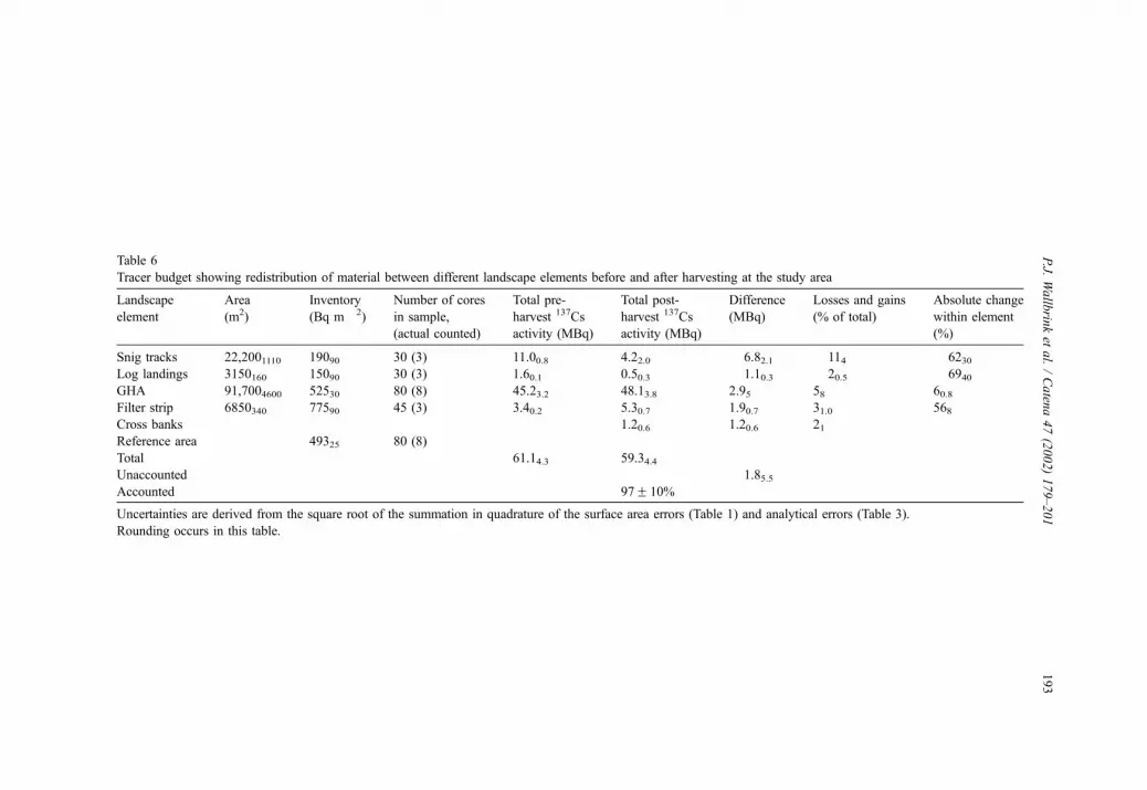
Table 6

Tracer budget showing redistribution of material between different landscape elements before and after harvesting at the study area

Landscape

element

Area

(m2)

Inventory

(Bq m� 2)

Number of cores

in sample,

(actual counted)

Total pre-

harvest 137Cs

activity (MBq)

Total post-

harvest 137Cs

activity (MBq)

Difference

(MBq)

Losses and gains

(% of total)

Absolute change

within element

(%)

Snig tracks 22,2001110 19090 30 (3) 11.00.8 4.22.0 � 6.82.1 � 114 � 6230Log landings 3150160 15090 30 (3) 1.60.1 0.50.3 � 1.10.3 � 20.5 � 6940GHA 91,7004600 52530 80 (8) 45.23.2 48.13.8 2.95 58 60.8Filter strip 6850340 77590 45 (3) 3.40.2 5.30.7 1.90.7 31.0 568Cross banks 1.20.6 1.20.6 21Reference area 49325 80 (8)

Total 61.14.3 59.34.4Unaccounted � 1.85.5Accounted 97F 10%

Uncertainties are derived from the square root of the summation in quadrature of the surface area errors (Table 1) and analytical errors (Table 3).

Rounding occurs in this table.

P.J.

Wallb

rinket

al./Caten

a47(2002)179–201

193

elements of the study area. As discussed above, the sum of the tracer amounts within the

landscape elements, can be compared to the amount calculated as initially present, and be

used to quantify any net losses from the system. Fig. 3 shows that the 137Cs budget

balances within the confidence limits, i.e., 97F 10%. This is consistent with no net loss of

material occurring from the study area. However, soil and sediment redistribution has

clearly occurred within it, and the diagram illustrates the flow of material. As indicated

above, losses totalling some 13F 4% of the total 137Cs budget, have occurred from the

snig tracks and log landings. This transport is illustrated as arrows leaving the respective

landscape element. The placement of cross banks is designed to divert this eroded material

onto high infiltration, high surface roughness areas such as the GHA and filter strip (Croke

et al., 1999b). This has clearly occurred, as there is net deposition and storage of 137Cs

within the GHA, filter strip and cross banks. These deposition amounts are represented by

arrows entering into these elements.

Fig. 3. Tracer budget for study area within compartment 1708, f 6 years after harvesting showing areas of

erosion and deposition in various landscape elements, based on measurements of fallout 137Cs. Note: Values

within arrows represent tracer amounts either transported from or deposited within each element, as a fraction of

total initial input. Values in parentheses represent the amount of activity contained within each element before and

after harvesting as a percent of total inputs. Uncertainties are given as subscripts and are derived cumulatively

from measurement errors and element area derivations.

P.J. Wallbrink et al. / Catena 47 (2002) 179–201194

The total amount of 137Cs transported from the snig tracks was 6.8F 2.1 MBq. Of this

amount, 18% (1.2F 0.6 MBq) could be accounted for within the cross banks; 28%

(1.9F 0.7 MBq) within the filter strip; and the remainder 43% within the GHA. The

material contained within the crossbanks is presumably derived from mechanical action

at the time of their construction. The amount of 137Cs retained within the filter increased

by f 60% (Table 6) from a background reference of 493F 25 to 775F 90 Bq m� 2 in

the f 6 years post-harvesting. This increase is due to harvesting associated erosion

alone, as the natural erosion component has been taken into account.

5.3. Sediment delivery to the filter strip

Given the important role of the filters as a ‘last line of defence’ in mitigating offsite

transport of material; the transport pathway, and size characteristics of material delivered

to them is worth further consideration. For example, Croke et al. (1999a,b) use rainfall

simulator experiments to show that runoff generation and sediment transport from within

the GHA itself is negligible compared to that from snig tracks. They also demonstrate

that coarse-grained (>63 mm) sediment transported into the GHA from the snig tracks is

effectively deposited, either in front of the cross bank, or within 5 m of its entry to the

GHA. Fine grained sediment diverted by the cross bank however was observed being

transported in plumes within the GHA, some 15–20 m downslope from cross banks

under extreme rainfall intensities (110 mm h� 1). The potential for similar incursions of

sediment plumes from cross banks through the GHA to stream side vegetation has also

been modelled probabilistically by Hairsine et al. (2001). Thus, combining the observa-

tions of Croke et al. (1999a,b) with the tracer measurements described above, leads us to

conclude that the additional 137Cs (and sediment) entering the filters is derived from snig

tracks.

The rate of sediment accumulation in the Filter strip can be calculated from the

available data. Firstly it has been shown that the material entering the Filters is probably

derived as cross bank runoff from erosion of snig tracks. The overall loss of 137Cs from the

snig tracks has been calculated as 6.8F 2.1 MBq. Of this amount some 28F 13% (Table

6), or 1.9F 0.7 MBq can be accounted for within the Filter strip. From the rainfall

simulator work of Croke et al. (1999a,b) we know that the predominant grain size

delivered to these filters is fine grained, < 63 mm. The average 137Cs concentration of

material in this size range is 27F 2 Bq kg� 1, from Table 2. At this 137Cs concentration,

1.9F 0.7 MBq is equivalent to a total of some 70F 25 t of material; or 11.7F 4 t year per

year over the 6 years post-harvesting. The surface area of the filters is (6900 m2, Table 1)

thus representing an annual mass deposition to them, of 1.7F 0.6 kg m � 2 year� 1. This

figure however is an upper estimate, as it assumes that the depositing material is

uniformally < 63 mm grain size. If depositing material is finer than this, i.e. < 20 mmthen the mass deposition amount would be smaller. Nonetheless, these soils have high

hydraulic conductivities (Moore et al., 1986; Croke et al., 1999b) and so the fine grained

sediment delivered to them is likely to be deposited into the soil matrix with infiltrating

runoff, as much as onto the soil surface. The close agreement between the pre- and post-

budgets also suggests that, within uncertainties, little leakage of sediment has occurred

from the system as a whole, and the filters in particular.

P.J. Wallbrink et al. / Catena 47 (2002) 179–201 195

5.4. Loss of soil from log landings and snig tracks

The 137Cs budget indicates net losses of material from the snig tracks and log landings.

The amount of soil removed from these can be quantified by comparing their residual210Pbex to 137Cs inventory ratios with that calculated for the detailed profiles in the

reference area. Fig. 4 shows the inventory ratio curve calculated from the mean of the two

detailed depth profiles. The method works by calculating the ratio of the cumulative

inventories of 210Pbex to137Cs with depth in a reference location and comparing this with

the residual inventory ratio left behind in areas where soil has been removed. The point at

which the disturbed area residual ratio intersects the reference inventory ratio curve

represents the depth of soil that has been removed from the system. The soil depth loss

amounts can then be converted to a total net loss in tonnes per hectare using the measured

bulk density from the surface layers of the reference soil cores (1.12 Mg m � 3, n = 10).

The mean residual inventory ratios for the log landings and snig tracks (calculated by

dividing the average 210Pbex and 137Cs inventories within each of them) are 0.40F 0.18

and 1.68F 0.51 (Table 7). These are plotted in Fig. 4, and are equivalent to soil depth

losses of 54F 8 and 13.5F 6 mm, respectively. It should be noted that our tracer-based

values give total cumulative losses, including mechanical removal of soil by bulldozer

blading, export on truck wheels, tyres and chassis, as well as losses due to wind and water

erosion. The majority of this depth loss presumably occurs during or immediately after

Fig. 4. Calculated depth loss for log landings and snig tracks using 210Pbex/137Cs cumulative inventory ratio

profile calculated from average of detailed depth profiles 1 and 2, given in Fig. 2.

P.J. Wallbrink et al. / Catena 47 (2002) 179–201196

harvesting; probably resulting from construction of these features. It should also be noted

that the period June–July 1991 represented above average months of rainfall for this

region. The method also assumes that the soil density in the reference area is similar to that

in the disturbed areas. Compaction of the disturbed log landings and snig tracks would

effect this comparison to some degree, and any depth losses calculated would be upper

estimates. This is especially so if the entire soil profile is compacted, although as indicated

above, much of the overlaying ‘eroded’ material is scraped off mechanically and so

density variations become less important. Nonetheless, these depth losses can be

recalculated to annual losses of 25F 11 t ha � 1 year � 1 for the snig tracks and

101F15 t ha� 1 year � 1 for the log landings, using the f 6-year gap between harvesting

and the measured soil density. These snig track values can also be partially compared to

those of 4–5.8 t ha� 1 measured from single high rainfall intensity events using a rainfall

simulator on snig tracks within the study area. This also suggests that the water derived

component of erosion may be small compared to mechanical impacts at this site.

5.5. Comparison of the 137Cs budget, eroded sediment and the measured 137Cs depth

distributions

It is also worthwhile examining whether the estimates of soil losses predicted above are

consistent with the 137Cs budget, the concentrations of 137Cs eroded sediment and the

measured 137Cs depth distributions. For example, the total loss of 137Cs from the log

landings and snig tracks was calculated to be 1.1F 0.3 and 6.8F 2.1 MBq (Table 6),

respectively. The corresponding depth losses for these were 54F 8 and 13.5F 6 mm,

giving a total soil depletion mass of 191F 28 and 355F 109 t for each of them, after

accounting for their different surface areas. Dividing the total 137Cs loss (Bq) by the mass

loss (kg) provides estimated concentrations on eroded material from the log landings and

snig tracks of f 6F 1.6 and f 19F 6 Bq kg� 1, respectively. If erosion is assumed to be

integrated to the same erosion depths as above, then similar concentrations on eroded

sediment can be independently estimated from the known depth profiles. For example,

using the data of Fig. 1, the average 137Cs concentrations of material eroded to depths of

54 and 13.5 mm would be 5.8F 1.5 and 13F 2.1 Bq kg � 1, respectively. Within

uncertainties, and allowing for particle size effects (Table 2), these are consistent with

the calculated concentrations on eroded material from the log landings and snig tracks

from above (i.e., f 6F 1.6 and f 19F 6 Bq kg� 1). Overall, these calculations provide

some confidence that the estimates of depth loss are internally consistent with the 137Cs

budget and the predicted 137Cs concentrations on eroded material.

Table 7210Pbex/

137Cs inventory ratio values for reference profiles, log landings and snig tracks

Landscape element Number of cores in sample,

(actual counted)

137Cs/210Pbex inventory

(ratio value)

Reference profiles 2 (detailed profiles) 3.070.23Log landings 30 (3) 0.400.18Snig tracks 30 (3) 1.680.51

P.J. Wallbrink et al. / Catena 47 (2002) 179–201 197

6. Conclusions

Managing the impacts of forest erosion requires knowledge of the erosion sources, the

rates of soil movement from them, its transport and storage, as well as any losses from the

system. We have presented a new approach using a tracer-based sediment budget that

enabled us to quantify many of these parameters. The 137Cs budget showed no net loss of

soil material from within the study area after harvesting within uncertainties (97F 10%).

However, it did reveal that significant redistribution, storage and transport of sediment had

occurred between landscape elements. There was a net transport of material from the snig

tracks and log landings (11 and 2% of total 137Cs), net losses from them were calculated to

be 25F 11 and 101F15 t ha� 1 year � 1, respectively. Although this is presented as an

average rate, the majority of this may have been displaced due to mechanical erosion.

There were also 2 months of well above average rainfall in the period 1 year after

harvesting. Overall however, these are identified as the major erosion impact sites in the

catchment. The erosion rate was highest in the log landings; the greatest net transport

occurred from snig tracks. Of the tracer activity transported from the snig tracks 18%, 28%

and 43% was accounted for within the cross banks, filter strip and GHA, respectively.

The 137Cs budget showed the GHA to be a significant region of sediment trapping. The

filter strip also played a fundamental role in the trapping of material generated from the

snig tracks; the mass delivery to them from this source was calculated to be 1.7F 0.6 kg

m2 year � 1. Careful management of these remains critical. Our work suggests that (within

errors) the overall runoff management system of dispersing flow from the highly

compacted snig tracks, by cross banks, into the less compacted (and larger area) GHA

and filter strips has effectively retained soil and sediment mobilised as a result of

harvesting at this site. This confirms the utility, and necessity, of having filter strips to

trap and store inflowing sediment, they remain a very important part of any erosion

mitigation strategy for retaining sediment mobilised from upslope sources.

In summary, the use of tracer-based budgets can provide detailed information on rates,

storages and transfers of transported material. These terms are difficult to measure by

traditional means. In particular we have quantified the redistribution of material within and

between different landscape elements on slopes following harvesting and used this to

assess the effectiveness of erosion mitigation controls at the study site.

Acknowledgements

This work was partially funded by the New South Wales Environment Protection

Authority (NSWEPA). Work was undertaken in Bondi State Forest under State Forests

NSW (SFNSW) special purposes permit 04991. The authors would like to thank Dr.

Andrew Murray (Riso), Dr. Ross Higginson (NSWEPA), Mr. Steve Lacey (SFNSW), Drs.

Croke and Hairsine (CSIRO Land and Water and CRCCH), Mr. Peter Fogarty (consultant)

and Professor Bob Wasson (ANU) for their advice and scientific input into this work. Mr.

Matt Rake (CSIRO) helped prepare some of the samples, Mr. Haralds Alksnis (CSIRO)

assisted in the gamma spectromic analyses. Mr. Heinz Buettikoffer (CSIRO) created the

location diagram. The comments of Dr. Peter Hairsine CSIRO L&W, Dr. Philip Ryan

P.J. Wallbrink et al. / Catena 47 (2002) 179–201198

(CSIRO FFP), Professor Des Walling (Exeter) and Professor Dan Pennock (Saskatchewan)

who reviewed the manuscript are gratefully acknowledged.

References

Anderson, B., Potts, D.F., 1987. Suspended sediment and turbidity following road construction and logging in

western Montana. Water Res. Bull. 23, 681–690.

Avery, E.T., 1968. Interpretation of Aerial Photographs. 2nd edn. Burgess, Minneapolis.

Basher, L.R., Matthews, K.M., Zhi, L., 1995. Surface erosion assessment in the South Canterbury downlands,

New Zealand using 137Cs distribution. Aust. J. Soil Res. 33, 787–803.

Beams, S.D., 1980. The magmatic evolution of the Southeast Lachlan Fold Belt. PhD thesis, LaTrobe University,

Victoria.

Best, D.W., Kelsey, H.M., Hagans, D.K., Alpert, M., 1995. Role of fluvial hillslope erosion and road construction

in the sediment budget of Garrett Creek, Humboldt County, California. U. S. Geol. Surv., Prof. Pap., 1454-(M).

Borg, H., King, P.D., Loh, I.C., 1987. Stream and ground water response to logging and subsequent regeneration

in the southern forest of Western Australia. Interim results from paired catchment studies. Water Authority of

Western Australia Report No. 34.

CaLM, 1993. Erosion Mitigation in logging Operations in New South Wales. Department of Conservation and

Land Management, NSW, 18 pp.

Cornish, P.M., Binns, D., 1987. Stream Water quality following logging and wildfire in a dry sclerophyl forest in

south east Australia. For. Ecol. Manage. 22, 1–28.

Croke, J., Hairsine, P., Fogarty, P., Mockler, S., Brophy, J., 1997. Surface runoff and sediment movement on

logged hillslopes in the Eden management area of south eastern NSW. Cooperative Research Centre for

Catchment Hydrology, Report 97/2.

Croke, J., Hairsine, P., Fogarty, P., 1999a. Sediment transport, redistribution and storage on logged forest hill-

slopes in south-eastern Australia. Hydrol. Processes 13, 2705–2720.

Croke, J., Hairsine, P., Fogarty, P., 1999b. Runoff generation and redistribution on disturbed forest hillslopes, in

south-eastern Australia. J. Hydrol. 216, 55–77.

Curran, P.J., 1985. Principles of Remote Sensing. Longman.

Davis, J.J., 1963. Cesium and its relationship to potassium in ecology. In: Shultz, V., Klement, A.W. (Eds.),

Radioecology. Reinhold, NY, pp. 539–556.

Dietrich, W.E., Dunne, T., 1978. Sediment budget for a small catchment in mountainous terrain. Z. Geomorphol.

29, 191–206.

Fahey, B.D., Coker, R.J., 1989. Forest road erosion in the granite terrain of South-West Nelson, New Zealand. J.

Hydrol. (NZ) 28, 123–141.

Fredericks, D.J., Norris, V., Perrens, S.J., 1988. Estimating erosion using caesium-137: I. Measuring caesium-137

activity in a soil. IAHS Publ. 174, 225–231.

Gilmour, D.A., 1971. The effects of logging on streamflow and sedimentation in a north Queensland rain forest

catchment. Commonwealth For. Rev. 50, 38–49.

Grayson, R.B., Haydon, S.R., Jayasuriya, M.D.A., Finlayson, B.L., 1993. Water quality in mountain ash for-

ests—separating the impacts of roads from those of logging operations. J. Hydrol. 150, 459–480.

Hairsine, P.B., Croke, J.C., Mathews, H., Fogarty, P., Mockler, S.P., 2001. Modelling plumes of overland flow

from roads and logging tracks. Hydrol. Process.

Hamada, G.H., Kruger, P., 1965. Methods of assessing fallout. In: Fowler, E.B. (Ed.), Radioactive Fallout, Soils,

Plants, Foods, Man. Elsevier, Amsterdam, The Netherlands, pp. 287–303.

He, Q., Owens, P., 1995. Determination of suspended sediment provenance using Caesium-137, unsupported

Lead-210 and Radium-226: a numerical mixing model approach. In: Foster, I.D., Gurnell, A.M., Webb, B.W.

(Eds.), Sediment and Water Quality in River Catchments. John Wiley and Sons Ltd, pp. 207–227.

Isbell, R.F., 1996. The Australian Soil Classification. CSIRO Publishing, Collingwood, 143 pp.

Kelsey, H., Madej, M.A., Pitlick, J., Stroud, P., Coghlan, M., 1981. Major sediment sources and limits to the

effectiveness of erosion control techniques in the highly erosive watersheds of north coastal California.

Erosion and Sediment Transport in Pacific Rim Steeplands. IAHS–AIHS Publ., vol. 132, pp. 493–509.

P.J. Wallbrink et al. / Catena 47 (2002) 179–201 199

Lomenick, T.F., Tamura, T., 1965. Naturally occurring fixation of 137Cs on sediments of lacustrine origin. Soil

Sci. Soc. Am. J. 29, 383–387.

Longmore, M.E., 1982. The Caesium-137 dating technique and associated applications in Australia: a review. In:

Ambrose, W., Duerden, P. (Eds.), Archaeometry: An Australasian Perspective. A.N.U. Press, Canberra, pp.

310–321.

Loughran, R.J., Campbell, B.L., Shelly, D.J., Elliott, G.L., 1992. Developing a sediment budget for a small

drainage basin, Australia. Hydrol. Processes 6, 145–158.

Madej, M.A., 1995. Changes in channel-stored sediment, Redwood Creek, Northwestern California, 1947–1980.

U. S. Geol. Sur., Prof. Pap., 1454-O.

Megahan, W.F., Kidd, W.J., 1972. Effects of logging and logging roads on erosion and sediment deposition from

steep terrain. J. For. 70, 136–141.

Montgommery, D.R., 1994. Road surface drainage, channel initiation and slope instability. Water Res. Res. 30

(6), 1925–1932.

Moore, I.D., Burch, G.J., Wallbrink, P.J., 1986. Preferential flow and hydraulic conductivity of forest soils. Soil

Sci. Soc. Am. J. 50, 4.

Murray, A.S., Marten, R., Johnston, A., Martin, P., 1987. Analysis for naturally occurring radionuclides at

environmental concentrations by gamma spectrometry. J. Radioanal. Nucl. Chem., Artic. 115, 263–288.

Northcote, K.H., 1979. A Factual Key for the Recognition of Australian Soils. 4th edn. Rellim Tech. Pubs.,

Glenside, S.A.

Olive, L.J., Reiger, W.A., 1985. Variation in suspended sediment concentration during storms in five small

catchments in south-eastern New South Wales. Aust. Geogr. Stud. 23, 38–51.

Owens, P.N., Walling, D.E., He, Q., Shanahan, J., Foster, I.D., 1997. The use of Caesium-137 measurements to

establish a sediment budget for the Start catchment, Devon, UK. Hydrol. Sci. J. 42, 405–423.

Quine, T.A., Navas, A., Walling, D.E., Machin, J., 1994. Soil eroison and redistribution on cultivated and

uncultivated land near Las Bardenas in the central Ebro river basin, Spain. Land Degradation Rehabil. 5,

41–55.

Reid, L.M., Dunne, T., 1984. Sediment production from forest road surfaces. Water Resour. Res. 20, 1753–1761.

Reid, L.M., Dunne, T., Cederholm, C.J., 1981. Application of sediment budget studies to the evaluation of

logging road impact. J. Hydrol. (N. Z.) 20 (1), 1743–1753.

Ritchie, J.C., McHenry, J.R., 1990. Radioactive fallout 137Cs for measuring soil erosion and sediment accumu-

lation rates and patterns: a review. J. Environ. Qual. 19, 215–233.

Ritchie, J.C., McHenry, J.R., Gill, A.C., 1974. Fallout 137Cs in the soils and sediments of three small watersheds.

Ecology 55, 887–890.

Roberts, R.G., Church, M., 1986. The sediment budget in severely disturbed watersheds, Queen Charlotte

Ranges, British Columbia. Can. J. For. Res. 16 (5), 1092–1106.

Rogowski, A.S., Tamura, T., 1965. Movement of 137Cs by runoff, erosion and infiltration on the alluvial Captina

silt loam. Health Phys. 11, 1333–1340.

State Forests of N.S.W., 1994. Environmental Impact Statement. Proposed Forestry Operations in Eden Manage-

ment Area. Volumes A, B, C. Main Report. November 1994.

Sutherland, R.A., 1994. Spatial variability of 137Cs and the influence of sampling on estimates of sediment

redistribution. Catena 21, 57–71.

Tebo, L.R., 1955. Effects of siltation, resulting from improper logging on the bottom fauna of a small trout stream

in Southern Appalachians. Prog. Fish Cult. 12, 64–70.

Trimble, S.W., 1983. A sediment budget for Coon Creek Basin in the driftless area, Wisconsin. Am. J. Sci. 283,

454–474.

Wallbrink, P.J., Murray, A.S., 1993. Use of fallout radionuclides as indicators of erosion processes. Hydrol.

Process 7, 297–304.

Wallbrink, P.J., Murray, A.S., 1996a. Measuring soil loss using the inventory ratio of 210Pbex to137Cs. Soil Sci.

Soc. Am. J. 60 (4), 1201–1208.

Wallbrink, P.J., Murray, A.S., 1996b. Distribution and variability of 7Be in soils under different surface cover

conditions and its potential for describing soil redistribution processes. Water Resour. Res. 32, 467–476.

Wallbrink, P.J., Olley, J.M., Murray, A.S., 1994. Measuring soil movement using 137Cs: implications of reference

site variability. Variability in Stream Erosion and Sediment Transport. IAHS Publ., vol. 224, pp. 95–103.

P.J. Wallbrink et al. / Catena 47 (2002) 179–201200

Wallbrink, P.J., Murray, A.S., Olley, J.M., 1999. Relating suspended sediment to its original soil depth using

fallout radionuclides. Soil Sci. Soc. Am. J. 63/2, 369–378.

Walling, D.E., Bradley, S.B., Wilkinson, C.J., 1986. A Ceasium-137 budget approach to the investigation of

sediment delivery from a small agricultural drainage basin in Devon, UK. In: Hadley, R.F. (Ed.), Drainage Basin

Sediment Delivery. Proceedings of the Albuquerque Symposium, August 1986. IAHS Press, Wallingford

Publ., vol. 159.

Walling, D.E., He, Q., Quine, T., 1996. Use of fallout radionuclide measurements in sediment budget inves-

tigations. Geomorphologie 3, 17–28.

Wise, S.M., 1980. 137Cs and 210Pb: a review of the techniques and some applications in geomorphology. Time

Scales in Geomorphology. Wiley, Chichester, pp. 109–127.

Zhang, X., Quine, T.A., Walling, D.E., Li, X., 1994. Application of the Caesium-137 technique in a study of soil

erosion on gully slopes in a Yuan area of the Loess plateau near Xifeng, Gansu Province, China. Geogr. Ann.

76A, 103–120.

P.J. Wallbrink et al. / Catena 47 (2002) 179–201 201