This article appeared in a journal published by Elsevier. The attachedcopy is furnished to the author for internal non-commercial researchand education use, including for instruction at the authors institution

and sharing with colleagues.

Other uses, including reproduction and distribution, or selling orlicensing copies, or posting to personal, institutional or third party

websites are prohibited.

In most cases authors are permitted to post their version of thearticle (e.g. in Word or Tex form) to their personal website orinstitutional repository. Authors requiring further information

regarding Elsevier’s archiving and manuscript policies areencouraged to visit:

http://www.elsevier.com/copyright

Author's personal copy

Comparison of conceptual landscape metrics to define hillslope-scale sedimentdelivery ratio

O. Vigiak a,⁎, L. Borselli b, L.T.H. Newham c, J. McInnes a, A.M. Roberts a

a Department of Primary Industries, Future Farming Systems Research Division, Rutherglen Centre, RMB 1145 Chiltern Valley Road, Rutherglen, VIC 3685, Australiab Instituto de Geologia, Fac. De Ingegneria, Universitad autonoma de San Luis Potosì (UASLP), Av. Dr Manuel Nava 5, C.P. 78240 San Luis Potosì, S.L.P., Mexicoc Integrated Catchment Assessment and Management Centre, The Fenner School of Environment and Society, the Australian National University, Canberra, ACT 0200, Australia

a b s t r a c ta r t i c l e i n f o

Article history:Received 23 November 2010Received in revised form 25 August 2011Accepted 25 August 2011Available online 1 September 2011

Keywords:Sediment delivery ratioRegionalisationSedimentological connectivityFlux connectivityAvon-RichardsonSoutheast Australia

The aim of this study was to evaluate four metrics to define the spatially variable (regionalised) hillslope sed-iment delivery ratio (HSDR). A catchment model that accounted for gully and streambank erosion and flood-plain deposition was used to isolate the effects of hillslope gross erosion and hillslope delivery from otherlandscape processes. The analysis was carried out at the subcatchment (~40 km2) and the cell scale(400 m2) in the Avon-Richardson catchment (3300 km2), south-east Australia. The four landscape metricsselected for the study were based on sediment travel time, sediment transport capacity, flux connectivity,and residence time. Model configurations with spatially-constant or regionalised HSDR were calibratedagainst sediment yield measured at five gauging stations. The impact of using regionalised HSDR was evalu-ated in terms of improved model performance against measured sediment yields in a nested monitoring net-work, the complexity and data requirements of the metric, and the resulting spatial relationship betweenhillslope erosion and landscape factors in the catchment and along hillslope transects. The introduction ofa regionalised HSDR generally improved model predictions of specific sediment yields at the subcatchmentscale, increasing model efficiency from 0.48 to N0.6 in the best cases. However, the introduction of regiona-lised HSDR metrics at the cell scale did not improve model performance. The flux connectivity was the mostpromising metric because it showed the largest improvement in predicting specific sediment yields, was easyto implement, was scale-independent and its formulation was consistent with sedimentological connectivityconcepts. These properties make the flux connectivity metric preferable for applications to catchments whereclimatic conditions can be considered homogeneous, i.e. in small-medium sized basins (up to approximately3000 km2 for Australian conditions, with the Avon-Richardson catchment being at the upper boundary). Theresidence time metric improved model assessment of sediment yields and enabled accounting for climaticvariability on sediment delivery, but at the cost of greater complexity and data requirements; this metricmight be more suitable for application in catchments with important climatic gradients, i.e. large basinsand at the regional scale. The application of a regionalised HSDRmetric did not increase data or computation-al requirements substantially, and is recommended to improve assessment of hillslope erosion in empirical,semi-lumped erosion modelling applications. However, more research is needed to assess the quality of spa-tial patterns of erosion depicted by the different landscape metrics.

Crown Copyright © 2011 Published by Elsevier B.V. All rights reserved.

1. Introduction

Sediment yield measured at a river monitoring station is equal tocatchment sediment upstream production (gross erosion) less depo-sition. A sediment delivery ratio (SDR) is the fraction of gross erosionthat is transported from a given catchment in a given time interval. Ineffect, SDR is a scaling factor that relates sediment availability and de-position at different spatial scales (Lu et al., 2006).

In erosion modelling, SDR has for a long time been treated as a con-stant parameter; however, there has been increasing interest in

accounting for deposition and applying spatially variable or regiona-lised SDR (e.g. Fraser et al., 1998; McHugh et al., 2002; Verstraetenet al., 2007; Boomer et al., 2008; Diodato and Grauso, 2009; Vigiaket al., 2009; Ali and De Boer, 2010). This interest stems partly from therecognition of the limits of empirical models developed at the plot/field scale in performing acceptably at the catchment scale (Jetten etal., 1999); and evenmore importantly, from the shift in natural resourcemanagement focus from on-site effects of erosion (i.e. loss of fertileland) toward off-side effects (i.e. impairment of downstream waterquality; de Vente et al., 2008). It has been shown that accounting forvariability of sediment delivery in space has important influence on as-sessment of sediment yields and on the location of areas contributingthe greatest sediment to downstream assets, where management

Geomorphology 138 (2012) 74–88

⁎ Corresponding author. Tel.: +61 2 60304560; fax: +61 2 60304600.E-mail address: olga.vigiak@dpi.vic.gov.au (O. Vigiak).

0169-555X/$ – see front matter. Crown Copyright © 2011 Published by Elsevier B.V. All rights reserved.doi:10.1016/j.geomorph.2011.08.026

Contents lists available at SciVerse ScienceDirect

Geomorphology

j ourna l homepage: www.e lsev ie r .com/ locate /geomorph

Author's personal copy

interventions would be more effective (Verstraeten et al., 2007; deVente et al., 2008; Vigiak et al., 2009).

Regionalised SDR could improve capability inmodelling the sources ofsediment affecting stream water quality, and in prioritising natural re-source management investments, particularly when empirically-based,semi-lumped catchment models are used (Lenhart et al., 2005; deVente et al., 2008). Several approaches have been proposed to representSDR variability in space (i.e. regionalisation). Catchment SDR has been re-lated to upslope area, climatic conditions, or shape and slope of the catch-ment (Maner, 1958; Vanoni, 1975; Walling, 1983; Wasson, 1994; FerroandMinacapilli, 1995; Lu et al., 2006; Diodato and Grauso, 2009). Severalalgorithms have also been proposed to accountmore explicitly for topog-raphy (Ferro and Minacapilli, 1995; Mitasova et al., 1996; Yagov et al.,1998) as well as hydrologic conditions, vegetation, surface roughness,and sediment properties (Fraser et al., 1998; Rustomji and Prosser,2001; McHugh et al., 2002; Lu et al., 2006; Borselli et al., 2007, 2008).

The accuracy of spatial patterns depicted by regionalised SDR has sel-dom been evaluated. Boomer et al. (2008) found that the application offive SDR algorithms (three lumped at the catchment scale, and two spa-tially distributed) did not improve theperformance of aUSLE-based sed-iment budget model, particularly for uncalibrated watersheds. Otherstudies report that regionalisation of SDR or sediment transport capacitycan improve catchment model assessment of sediment yields (Lenhartet al., 2005; Borselli et al., 2007, 2008; Verstraeten et al., 2007; Diodatoand Grauso, 2009). Interpretation of these contrasting findings on thebenefits of adopting a regionalised SDR parameter is difficult becausesediment yields measured at gauging stations result from complex in-teractions of several erosion and deposition processes, such as hillslopeerosion (comprising sheet, interrill, and rill erosion), gully or stream-bank erosion, or floodplain deposition (e.g. Boomer et al., 2008).

It may be helpful to think SDR as conceptually composed of twoparts: the fraction of hillslope gross erosion that is delivered to stream(hillslope-SDR), and the fraction of sediments in the stream that reachesa given gauging station (in-stream-SDR) (Lu et al., 2006). The distinctionis meaningful because processes regulating the two fractions are verydifferent. The hillslope-SDR fraction (hereafter simply referred to asHSDR) relates to interrill and rill erosion, and accounts for depositionof particles due to reduction of the overlandflow sediment transport ca-pacity across the hillslope. Using sedimentation in farm dams data,Verstraeten et al. (2007) estimated that sediment transport capacityin cropland was twice that of degraded pastures, and 20 times higherthan in areas of good pastures or native forest in the Murrumbidgeecatchment in south-east Australia. By calibrating sediment transport ca-pacity parameters according to land cover, model performance in esti-mating hillslope erosion and deposition was improved; and theresulting sediment delivery ratio ranged from 1% to 11%. Conversely, in-stream sediment delivery is regulated by hydraulic conditions of the con-centrated flow in the stream network and the dynamic equilibrium be-tween suspended sediment loads and sediment transport capacity thatdictates entrainment or deposition of suspended sediments from thestream bed. In Australian conditions, rivers are generally supply-limitedand in-stream accretion over decades is considered negligible (Oliveand Walker, 1982; Williams, 1989). Sediment deposition occurs mainlyas floodplain deposition during overbank flood events or in reservoirs(Prosser et al., 2001). Sediment delivery from gully erosion acts at ascale between these two systems (Nacthergaele et al., 2002). Wheregullies are connected to the streams, i.e. the gully mouth reaches astream, gullies can be considered as part of the stream network and in-stream delivery rules should apply. Where, instead, gullies are discon-nected from the stream, and deposit sediments in large fans at theirmouth, hillslope processes dominate the entrainment and transport ofsediments from these fans to the stream, and hillslope sediment deliveryrules should apply (Croke et al., 2005; Whitford et al., 2010; Fuller andMarden, 2011).

HSDR can also be considered ameasure of sedimentological connec-tivity of hillslope erosion, i.e. a measure of the ease of sediment

transport between two points on a hillslope. Bracken and Croke(2007) offer a comprehensive review of processes and factors regulat-ing sedimentological connectivity. The spatial variability of sedimenttransport capacity and sedimentological connectivity, hence of HSDR,depends on several factors including climate (rainfall regime and runoffdistributions), topography (upslope area, slope and distance from sedi-ment sinks), soil roughness, sediment composition, and anthropogenicstructures that may alter the hydrologic pathways. Above all factors,HSDR depends on time: in the geological scale HSDR equals 1, but atthe event scale it can be extremely variable, being greater for eventswith high hydrological connectivity and flow energy (e.g. Reaney etal., 2007).

The aim of this study was to evaluate four metrics to define spatiallyvariable (regionalised) HSDR. The four landscape metrics were based ondifferent geomorphological concepts, i.e. travel time (TT), sediment trans-port capacity (ST),flux connectivity (IC), and residence time (RT). A catch-ment erosion model (Vigiak et al., 2011) that accounted for gully andstreambank erosion, and for sediment deposition on floodplains wasused to isolate the effects of hillslope gross erosion and hillslope deliveryfrom other landscape processes. The analysis was carried out at the sub-catchment (~40 km2) and the cell scale (400 m2) in the Avon-Richardsoncatchment (3300 km2), south-east Australia. The intent was to focus onHSDR at the annual or decadal scale, at which the impact of natural re-source management on water quality has been measured (Simpson,2010).

2. Materials and methods

2.1. Selected landscape metrics to regionalise HSDR

2.1.1. Travel time (TT)Four conceptual metrics were selected for defining HSDR in space

(Table 1). Ferro and Minacapilli (1995) proposed that sediment deliv-ery ratio of a morphological unit to the stream should depend on thetravel time TT of overland flow to the stream, which can be expressedas the ratio of flow path length by the square root of the slope. A co-efficient bU for a spatial unit U is calibrated for a given catchment toreflect catchment roughness and runoff along the hydraulic pathway(Ferro and Porto, 2000). The approach is embedded in the SEDDmodel (Ferro and Porto, 2000). Morphologic units may correspondto fields, but the model can equally be applied at the cell scale (Fuet al., 2006; Bhattarai and Dutta, 2007; 2008). This metric emphasisesthe role of downslope pathway to the stream in controlling HSDR.

2.1.2. Sediment transport capacity (ST)Following a dimensional analysis of the sediment transport capac-

ity of flow, Rustomji and Prosser (2001) proposed that sediment de-livery potential for a hillslope to the valley floor could be expressedas a power function of the upslope contributing area and the localgradient. The sediment transport capacity metric does not calculateHSDR per se; rather, it can be used as a landscape metric fromwhich HSDR can be derived assuming an appropriate functional rela-tionship (see Section 2.1.5). Verstraeten et al. (2007) offer a differentapproach for using the sediment transport capacity equation to esti-mate sediment delivery. Contrary to the TT metric, the ST approachemphasises the control of upslope conditions to HSDR.

2.1.3. Flux connectivity (IC)Borselli et al. (2008) proposed a metric to measure hillslope hydro-

logic connectivity to the stream network that has two components. Theupslope component represents the potential for down-routing, i.e. thepotential for run-on at a given location; the downslope component ac-counts for potential flow sinks between that location and the streamnetwork. The RUSLE crop factor C is used as a proxy of surface roughnessto measure the resistance of runoff passing through a cell. The ICmetricis dimensionless and in practical terms is a rate between two weighted

75O. Vigiak et al. / Geomorphology 138 (2012) 74–88

Author's personal copy

distances calculated at any givenpoint in the landscape. Due to thewiderange of this rate in proximity of streams or at hillslope divides, themet-ric is logarithmic, indicating the need to express the rate as an order ofmagnitude. As for the ST approach, a functional relationship was as-sumed to transform the IC metric into HSDR values (see Section 2.1.5).This metric relates HSDR to both upslope and downslope conditions.

2.1.4. Residence time approach (RT)Lu et al. (2006) proposed to regionalise catchment-SDR by assuming

two stores of sediment, i.e. the hillslope and channel components, andby differentiating in space three time variables: (i) the effective stormdu-ration ter that depends on rainfall characteristics; (ii) the mean channelresidence time tn that depends on the travel distance in channel and chan-nel flow velocity; and (iii) the mean hillslope residence time th that de-pends on travel distance and velocity of overland flow or shallowconcentrated flow. SDR values are calculated for particle size classes(clay, silt, and sandb1000 μm) assuming adequate settling velocity foreach particle class. Thefinal SDR value for each spatial unit is theweighted

average for the particles composing the topsoil. In its original formulation,the residence time approach also includes in-stream-SDR, and overallcatchment-SDR depends on catchment outlet position. To isolate theHSDR fraction, in this study travel time in permanent streamswas exclud-ed by masking permanent stream features. The in-stream-SDR fractionwas adjusted for by adding a linear, catchment-wide constant calibrationparameter eU in the final step of HSDR calculation (Table 1).

2.1.5. Linking landscape connectivity metrics to HSDRFollowing Borselli et al. (2007), a functional relationship between

the ST and IC metrics and HSDR was assumed to be a Boltzmann-typesigmoid curve:

HSDRU ¼ HSDRmax;U 1þ expΨ0−ΨU

k

� �� �−1ð1Þ

where the subscript U indicates the spatial unit at which the analysisis conducted, i.e. either a subcatchment j or a cell c; HSDRmax,U is the

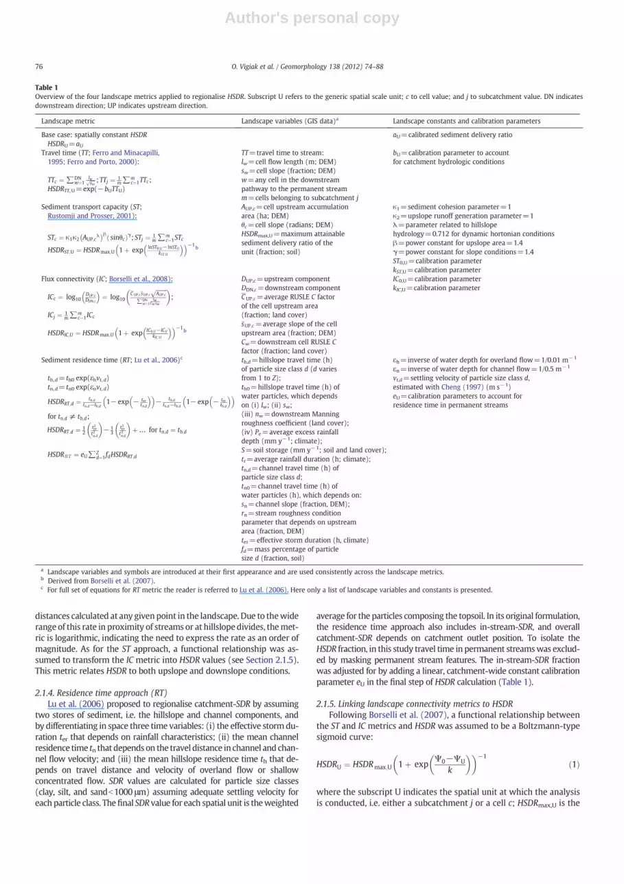
Table 1Overview of the four landscape metrics applied to regionalise HSDR. Subscript U refers to the generic spatial scale unit; c to cell value; and j to subcatchment value. DN indicatesdownstream direction; UP indicates upstream direction.

Landscape metric Landscape variables (GIS data)a Landscape constants and calibration parameters

Base case: spatially constant HSDRHSDRU=aU

aU=calibrated sediment delivery ratio

Travel time (TT; Ferro and Minacapilli,1995; Ferro and Porto, 2000):

TTc ¼ ∑DNw¼1

lwffiffiffiffisw

p ; TTj ¼ 1m∑m

c¼1TTc;HSDRTT, U=exp(−bUTTU)

TT=travel time to stream:lw=cell flow length (m; DEM)sw=cell slope (fraction; DEM)w=any cell in the downstreampathway to the permanent streamm=cells belonging to subcatchment j

bU=calibration parameter to accountfor catchment hydrologic conditions

Sediment transport capacity (ST;Rustomji and Prosser, 2001):

STc ¼ κ1κ2 AUP;cλ

� �β sinθcð Þγ; STj ¼ 1m∑m

c¼1STc

HSDRST;U ¼ HSDRmax;U 1þ exp lnST0;U− lnSTUkST ;U

� �� �−1b

AUP,c=cell upstream accumulationarea (ha; DEM)θc=cell slope (radians; DEM)HSDRmax,U=maximum attainablesediment delivery ratio of theunit (fraction; soil)

κ1=sediment cohesion parameter=1κ2=upslope runoff generation parameter=1λ=parameter related to hillslopehydrology=0.712 for dynamic hortonian conditionsβ=power constant for upslope area=1.4γ=power constant for slope conditions=1.4ST0,U=calibration parameterkST,U=calibration parameter

Flux connectivity (IC; Borselli et al., 2008):

ICc ¼ log10DUP;cDDN;c

� �¼ log10

C UP;c sUP;cffiffiffiffiffiffiffiffiAUP;c

p∑DN

w¼1lw

Cwsw

� �;

ICj ¼ 1m∑m

c¼1ICc

HSDRIC;U ¼ HSDRmax;U 1þ exp IC0;U−ICU

kIC;U

� �� �−1b

DUP,c=upstream componentDDN,c=downstream componentCUP;c=average RUSLE C factorof the cell upstream area(fraction; land cover)sUP;c=average slope of the cellupstream area (fraction; DEM)Cw=downstream cell RUSLE Cfactor (fraction; land cover)

IC0,U=calibration parameterkIC,U=calibration parameter

Sediment residence time (RT; Lu et al., 2006)c

th,d= th0 exp(εhvt,d)tn,d= tn0 exp(εnvt,d)

HSDRRT;d ¼ tn;dtn;d−th;d

1− exp − tertn;d

� �� �− th;d

tn;d−th;d1− exp − ter

th;d

� �� �for tn;d ≠ th;d;

HSDRRT;d ¼ 12

t2ert2n;d

� �− 1

3t3ert3n;d

� �þ… for tn;d ¼ th;d

HSDRRT ¼ eU∑Zd¼1fdHSDRRT ;d

th,d=hillslope travel time (h)of particle size class d (d variesfrom 1 to Z);th0=hillslope travel time (h) ofwater particles, which dependson (i) lw; (ii) sw;(iii) nw=downstream Manningroughness coefficient (land cover);(iv) Pe=average excess rainfalldepth (mm y−1; climate);S=soil storage (mm y−1; soil and land cover);tr=average rainfall duration (h; climate);tn,d=channel travel time (h) ofparticle size class d;tn0=channel travel time (h) ofwater particles (h), which depends on:sn=channel slope (fraction, DEM);rn=stream roughness conditionparameter that depends on upstreamarea (fraction, DEM)ter=effective storm duration (h, climate)fd=mass percentage of particlesize d (fraction, soil)

εh=inverse of water depth for overland flow=1/0.01 m−1

εn=inverse of water depth for channel flow=1/0.5 m−1

vt,d=settling velocity of particle size class d,estimated with Cheng (1997) (m s−1)eU=calibration parameters to account forresidence time in permanent streams

a Landscape variables and symbols are introduced at their first appearance and are used consistently across the landscape metrics.b Derived from Borselli et al. (2007).c For full set of equations for RT metric the reader is referred to Lu et al. (2006). Here only a list of landscape variables and constants is presented.

76 O. Vigiak et al. / Geomorphology 138 (2012) 74–88

Author's personal copy

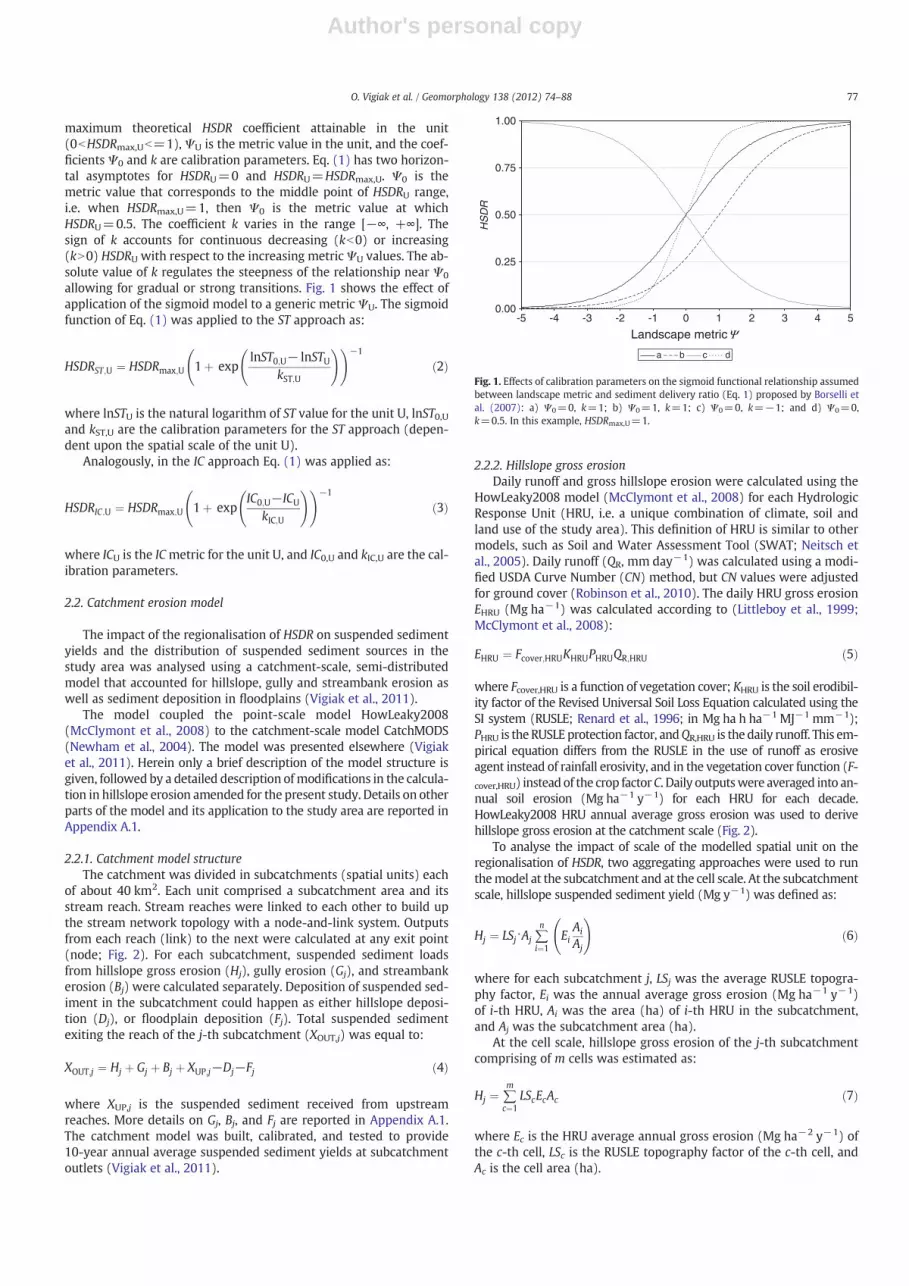
maximum theoretical HSDR coefficient attainable in the unit(0bHSDRmax,Ub=1), ΨU is the metric value in the unit, and the coef-ficients Ψ0 and k are calibration parameters. Eq. (1) has two horizon-tal asymptotes for HSDRU=0 and HSDRU=HSDRmax,U. Ψ0 is themetric value that corresponds to the middle point of HSDRU range,i.e. when HSDRmax,U=1, then Ψ0 is the metric value at whichHSDRU=0.5. The coefficient k varies in the range [−∞, +∞]. Thesign of k accounts for continuous decreasing (kb0) or increasing(kN0) HSDRU with respect to the increasing metricΨU values. The ab-solute value of k regulates the steepness of the relationship near Ψ0

allowing for gradual or strong transitions. Fig. 1 shows the effect ofapplication of the sigmoid model to a generic metric ΨU. The sigmoidfunction of Eq. (1) was applied to the ST approach as:

HSDRST;U ¼ HSDRmax;U 1þ explnST0;U− lnSTU

kST;U

! !−1

ð2Þ

where lnSTU is the natural logarithm of ST value for the unit U, lnST0,Uand kST,U are the calibration parameters for the ST approach (depen-dent upon the spatial scale of the unit U).

Analogously, in the IC approach Eq. (1) was applied as:

HSDRIC;U ¼ HSDRmax;U 1þ expIC0;U−ICU

kIC;U

! !−1

ð3Þ

where ICU is the ICmetric for the unit U, and IC0,U and kIC,U are the cal-ibration parameters.

2.2. Catchment erosion model

The impact of the regionalisation of HSDR on suspended sedimentyields and the distribution of suspended sediment sources in thestudy area was analysed using a catchment-scale, semi-distributedmodel that accounted for hillslope, gully and streambank erosion aswell as sediment deposition in floodplains (Vigiak et al., 2011).

The model coupled the point-scale model HowLeaky2008(McClymont et al., 2008) to the catchment-scale model CatchMODS(Newham et al., 2004). The model was presented elsewhere (Vigiaket al., 2011). Herein only a brief description of the model structure isgiven, followed by a detailed description ofmodifications in the calcula-tion in hillslope erosion amended for the present study. Details on otherparts of the model and its application to the study area are reported inAppendix A.1.

2.2.1. Catchment model structureThe catchment was divided in subcatchments (spatial units) each

of about 40 km2. Each unit comprised a subcatchment area and itsstream reach. Stream reaches were linked to each other to build upthe stream network topology with a node-and-link system. Outputsfrom each reach (link) to the next were calculated at any exit point(node; Fig. 2). For each subcatchment, suspended sediment loadsfrom hillslope gross erosion (Hj), gully erosion (Gj), and streambankerosion (Bj) were calculated separately. Deposition of suspended sed-iment in the subcatchment could happen as either hillslope deposi-tion (Dj), or floodplain deposition (Fj). Total suspended sedimentexiting the reach of the j-th subcatchment (XOUT,j) was equal to:

XOUT;j ¼ Hj þ Gj þ Bj þ XUP;j−Dj−Fj ð4Þ

where XUP,j is the suspended sediment received from upstreamreaches. More details on Gj, Bj, and Fj are reported in Appendix A.1.The catchment model was built, calibrated, and tested to provide10-year annual average suspended sediment yields at subcatchmentoutlets (Vigiak et al., 2011).

2.2.2. Hillslope gross erosionDaily runoff and gross hillslope erosion were calculated using the

HowLeaky2008 model (McClymont et al., 2008) for each HydrologicResponse Unit (HRU, i.e. a unique combination of climate, soil andland use of the study area). This definition of HRU is similar to othermodels, such as Soil and Water Assessment Tool (SWAT; Neitsch etal., 2005). Daily runoff (QR, mm day−1) was calculated using a modi-fied USDA Curve Number (CN) method, but CN values were adjustedfor ground cover (Robinson et al., 2010). The daily HRU gross erosionEHRU (Mg ha−1) was calculated according to (Littleboy et al., 1999;McClymont et al., 2008):

EHRU ¼ Fcover;HRUKHRUPHRUQR;HRU ð5Þ

where Fcover,HRU is a function of vegetation cover; KHRU is the soil erodibil-ity factor of the Revised Universal Soil Loss Equation calculated using theSI system (RUSLE; Renard et al., 1996; in Mg ha h ha−1 MJ−1 mm−1);PHRU is the RUSLE protection factor, andQR,HRU is the daily runoff. This em-pirical equation differs from the RUSLE in the use of runoff as erosiveagent instead of rainfall erosivity, and in the vegetation cover function (F-cover,HRU) instead of the crop factorC. Daily outputswere averaged into an-nual soil erosion (Mg ha−1 y−1) for each HRU for each decade.HowLeaky2008 HRU annual average gross erosion was used to derivehillslope gross erosion at the catchment scale (Fig. 2).

To analyse the impact of scale of the modelled spatial unit on theregionalisation of HSDR, two aggregating approaches were used to runthemodel at the subcatchment and at the cell scale. At the subcatchmentscale, hillslope suspended sediment yield (Mg y−1) was defined as:

Hj ¼ LSj⋅Aj ∑n

i¼1EiAi

Aj

!ð6Þ

where for each subcatchment j, LSj was the average RUSLE topogra-phy factor, Ei was the annual average gross erosion (Mg ha−1 y−1)of i-th HRU, Ai was the area (ha) of i-th HRU in the subcatchment,and Aj was the subcatchment area (ha).

At the cell scale, hillslope gross erosion of the j-th subcatchmentcomprising of m cells was estimated as:

Hj ¼ ∑m

c¼1LScEcAc ð7Þ

where Ec is the HRU average annual gross erosion (Mg ha−2 y−1) ofthe c-th cell, LSc is the RUSLE topography factor of the c-th cell, andAc is the cell area (ha).

0.00

0.25

0.50

0.75

1.00

-5 -4 -3 -2 -1 0 1 2 3 4 5

HS

DR

a b c d

Landscape metricΨ

Fig. 1. Effects of calibration parameters on the sigmoid functional relationship assumedbetween landscape metric and sediment delivery ratio (Eq. 1) proposed by Borselli etal. (2007): a) Ψ0=0, k=1; b) Ψ0=1, k=1; c) Ψ0=0, k=−1; and d) Ψ0=0,k=0.5. In this example, HSDRmax,U=1.

77O. Vigiak et al. / Geomorphology 138 (2012) 74–88

Author's personal copy

2.2.3. Hillslope deposition (Dj)Hillslope deposition is the fraction of gross hillslope erosion and

gully erosion generated by disconnected gullies that is not deliveredto the stream network. The deposition fraction corresponded to 1minus HSDR. In the subcatchment scale analysis, hillslope depositionwas estimated as:

Dj ¼ 1−HSDRj

� �Hj þ GD;j

� �ð8Þ

where GD,j is the suspended sediment load generated by disconnectedgullies in the j-th subcatchment, and HSDRj is HSDR of the j-th sub-catchment regionalised according to the four landscape metrics orequal to the catchment constant in the base case scenario.

In the cell-scale analysis, hillslope deposition was estimated as:

Dj ¼ ∑m

c¼11−HSDRcð ÞLScEcAc þ 1−HSDRc;j

� �GD;j ð9Þ

where HSDRc is HSDR of the c-th cell, and HSDRc;j is the mean HSDRvalue calculated at the cell scale in the subcatchment j.

2.3. Study area and data collection

The Avon-Richardson catchment is an endorheic basin that extendsover 3300 km2 of the Wimmera landscape of south-east Australia(Fig. 3). Elevation ranges from 100 m in the north to about 560 m inthe southeast. The catchment is predominantly flat; however, thesouth-eastern hills have moderate to steep slopes. Soils are mainlydeep and clayey, with uniform (red or grey Vertosols) or duplex soilprofiles (red Sodosols and red or yellow Chromosols in Isbell's (2002)soil classification; Melland et al., 2008; Vigiak et al., 2011). Urban settle-ments are small and scattered; the twomajor centres are Donald (1400inhabitants) andMarnoo (200 inhabitants); the population density is inthe range of 1–3 inhabitants per km2 (BoS, 2011). Agriculture is thedominant land use, with open forest comprising b5% catchment area.Three agro-climatic zones can be distinguished: grazed uplands in thesouth (average rainfall ~550 mm y−1),mixed farming (i.e. combinationof grazing and cropping) in the mid-catchment (average rainfall~450 mm y−1), and flat croplands in the north (average rainfall~350 mm y−1). Grazing management consists mainly of livestock(mainly sheep) set stocking on annual pastures. In the mixed farming

areas, cropping occupies about 40% of land as wheat–barley-fallow ro-tations, whilst 60% of land is devoted to grazing on annual pasture. Inthe flat croplands, cultivation of broad-acre crops occupies virtually allland; the most common rotation is a canola–wheat–barley–legume ro-tation with two tillage operations annually (Vigiak et al., 2011).

The dataset available for the present study comprised a 20 m gridDEM (DPI, 2009); a soil map (Melland et al., 2008); a 1:25,000 streamnetwork map (DSE, 2004); a gully map (Whitford et al., 2010); and aland cover map (Vigiak et al., 2011; Fig. 3). Upslope area, slope andflow lengths were derived from DEM analysis. Minimum slope wasset at 0.5%. Flow lengths were calculated until a permanent streamwas reached, setting a threshold of upstream area of 20 ha to definepermanent stream cells. The topographic factor LS was calculatedaccording to Moore and Wilson (1992).

HSDRmax,U was defined as the fraction of topsoil particles finerthan coarse sand (b1000 μm; Lu et al., 2006). HSDRmax,U was basedon the soil map, and ranged from 0.7 on duplex soils (i.e. red Sodosolsand red/yellow Chromosols) to 0.9 on Vertosols. The fractionalweights of particle class fd were based on texture of the topsoil. Parti-cle settling velocity was calculated with Cheng (1997) using mediansediment concentration measured in the stream (46 mg L−1).

Average RUSLE C values were derived using SOILLOSS (Rosewell,1993) and Manning roughness coefficients n were based on Lu et al.(2006) (Table 2). Average rainfall duration (tr) and effective stormduration (ter) were calculated following the procedure described inLu et al. (2003) using 1950–2005 rainfall data series retrieved fromthe SILO database (Jeffrey et al., 2001). Average rainfall duration ran-ged from 12 h in the northern cropped plains to 14.6 h in the grazeduplands in the south-east. Effective storm duration ranged from 3.3to 4.5 h along the same gradient. Average annual excess rainfalldepth Pe (mm y−1) was estimated using a 2-year recurrence,24 hour rainfall depth. Average soil storage (S) was estimated usingaverage HRU Curve Number (CN) values (Williams and LaSeur,1976; Robinson et al., 2010), and ranged from 57 on red/yellow Chro-mosols under open forest to 72 on hard-setting red Sodosols on crop-ping land.

Landscape metrics were calculated at the cell scale, and averagedover each subcatchment for subcatchment scale analysis. Cell extentcorresponded to that of the DEM (i.e. 20×20 m; Ac=400 m2). Thestudy analysis was conducted using ArcGIS v9.3 software (ESRI,2008).

Hillslope gross erosion (Hj)

Gully erosion (Gj)

Streambank erosion (Bj)

Howleaky2008 Gross Soil Loss

(EHRU)

Floodplain deposition

(Fj)

HSDRj Hillslope deposition (Dj)

Upstream sediment

(XUP,j)

Downstream sediment(XOUT,j)

Fig. 2. Schematic representation of the catchment sediment model scale used for the study. The oval represents a Hydrologic Response Unit (HRU) for which gross soil erosion(EHRU) was estimated with HowLeaky2008 and exported into the catchment-scale model. The diamond represents a subcatchment area. Suspended sediments are generated byhillslope erosion Hj, gully erosion Gj, and streambank erosion Bj. Hillslope deposition Dj applies to suspended sediments generated by hillslope erosion or by erosion of disconnectedgullies (GD,j) and depends on the hillslope-SDR (HSDRj). Deposition of in-stream suspended sediments Fj occurs by floodplain deposition during overbank flood events. The arrowindicates the stream reach, which receives suspended sediments from upstream areas (XUP,j) at the upstream node (a circle), and transmits the net sum of suspended sedimentXOUT,j to the downstream node.

78 O. Vigiak et al. / Geomorphology 138 (2012) 74–88

Author's personal copy

2.4. Base case scenario

The base case scenario for the analysis of regionalisation of HSDRcorresponded to the output of the catchment scale model with a sin-gle, spatially constant HSDR (i.e. HSDRU=aU for all spatial units). Thebase case catchment model, applied at the subcatchment scale, waspresented in Vigiak et al. (2011), and is only briefly summarisedherein.

The two main sources of sediments in the Avon-Richardson catch-ment were hillslope erosion and gully erosion in the main depres-sions of the southern hills. Streambank erosion was negligible andwas not modelled in this study. The Avon-Richardson catchmentwas divided into 70 subcatchments. The combination of five climaticzones, eight soil groups, and nine land cover types resulted in 360HRUs. Disconnected gullies represented 6.5% of the entire gully net-work length.

Some uncertainty existed in the identification of catchment modelparameters and the relative contributions of hillslope and gully ero-sion to the in-stream suspended sediment yields (Vigiak et al.,2011). Good model simulations were those in which the spatiallyconstant HSDR estimated at the subcatchment scale aj ranged from1.8% to 2.7%, with the optimum simulation obtained at aj=2%. Therelative contribution of hillslope erosion to total sediments reachingthe outlet was estimated at 65% (60–80%), whereas gully erosion con-tributed 35% (20–40%). The best simulation model, corresponding toaj=2% and hillslope erosion contribution to suspended sedimentloads of 65% was set as the base case scenario for the present study.In the application of regionalised HSDR, parameters other than HSDRwere kept constant and equal to this base case; therefore relative con-tributions of hillslope vs. gully erosion was not further addressed. Thefull set of the catchment model parameter of the base case scenarioare reported in Table 3.

2.5. Calibration against sediment yields

HSDR is a parameter suited to calibration against measurements atthe gauging stations. Calibration may account for errors in estimationof gross erosion (Eq. 5) or for processes that are not explicitlyaddressed in the catchment framework.

Manual calibration of all model configurations (i.e. for each land-scape metric and subcatchment and cell applications) was conductedagainst average annual sediment yields (Mg y−1) and specific sedi-ment yields (Mg km−2 y−1) estimated at the water monitoring gaug-ing stations of the catchment (Fig. 3). Water quantity and quality aremonitored at five stations in the catchment and observed data arepublicly available (DSE, 2010). Data comprise daily flow and sus-pended sediment concentrations sampled once or twice per monthat the three downstream stations. Only 168 suspended sedimentsamples had been collected in the catchment during periods ofstreamflow over the period 1963–2008, mostly at low flow. Giventhe paucity of data and the bias toward low flow conditions, annualsuspended sediment loads were estimated with the ratio method,whereby daily load is estimated as the product of daily flow timesthe ratio of the average load of the sediment concentration sample di-vided by the average discharge of the sediment concentration sample

Fig. 3. Location of the Avon-Richardson catchment in Victoria, Australia, with the two major urban centres (black square) and water quality gauging stations (white circles). Greytones indicate land cover categories; grey lines indicate the stream network; black lines indicate 50-m contour lines (from 150 to 500 m). Location of three transects selected forhillslope scale analysis (Fig. 8) is also shown.

Table 2Overview of land cover properties used in the GIS analysis.

Land cover RUSLE C (Rosewell, 1993) Manning roughness n (Lu et al., 2006)

Cropping 0.39 0.25Mixedfarming

0.24 0.32

Grazing 0.18 0.40Open forest 0.007 0.60

79O. Vigiak et al. / Geomorphology 138 (2012) 74–88

Author's personal copy

(Letcher et al., 1999). A single sediment–discharge ratio of the sedi-ment concentration sample was estimated and applied to all gaugingstations; specific sediment yields ranged from 1.7 to 5 Mg km−2 y−1

(Vigiak et al., 2011).Catchment conditions prior to 1980 were considered too different

from current conditions in terms of gully erosion and land cover andwere excluded from the analysis, which therefore was conducted forthe decades 1980–1989 and 1990–1999. As the dataset included onlyseven data-entries, the whole dataset was used for calibration. Cali-bration parameters (Table 1) were changed one at a time, using con-stant and suitable step and evaluating the goodness of fit of modelresults until the best parameter sets were identified. The goodness-of-fit of each configuration was measured with three criteria. Themodel efficiency (ME; Nash and Sutcliffe, 1970) measures the close-ness of model predictions to observations; values close to 1 indicategood performance. The relative root mean square error (RRMSE; e.g.Verstraeten et al., 2007) measures the model error variance; valuescloser to zero indicate good performance. The Akaike information cri-terion, corrected for small sample size (AICc; Burnham and Anderson,2004) measures the balance between approach accuracy and thenumber of calibration parameters; the lowest values indicate betterperformance.

3. Results

3.1. Calibration of sediment yields

At the subcatchment scale, all model configurations resulted inhigh efficiencies in sediment yield predictions (MEN0.85, Table 4).Conversely, efficiencies of specific sediment yields were lower andshowed a larger range, and were more sensitive to the spatial distri-bution of HSDR and hillslope erosion. With the exception of the TTmetric, the adoption of regionalised HSDR improved model efficien-cies and reduced model error variances considerably, particularly interms of specific sediment yields. The ICmetric had the best efficiency

in predicting specific sediment yields, but because it introduced anextra calibration parameter, AICc equalled the base case. The RT met-ric resulted in the lowest AICc values overall.

At the cell scale, model performances were generally better thanat the subcatchment scale, with efficiencies in predicting sedimentyields well (MEN0.95) in all cases (Table 5). At this scale, the intro-duction of regionalised HSDR did not improve model performance.Once again, the TT metric performed more poorly than the base casescenario, whereas the IC and RT metrics performed similarly to it.The ST metric improved predictions at the subcatchment scale, butnot at the cell scale. Notably, the IC parameter set did not change atthe two scales of analysis.

3.2. Statistical distribution of HSDR

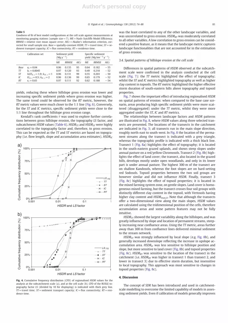
The statistical distributions of HSDR derived by the landscape met-rics varied greatly and were scale-sensitive to different degrees(Fig. 4). HSDRTT distribution was largely skewed toward low values,with most spatial units having HSDR close to zero. Only 10% of unitswere N0.02 at the subcatchment scale and N0.03 at the cell scale.HSDRTT maxima were 0.1 at the subcatchment scale and 0.93 at thecell scale.

At the subcatchment scale, HSDRST showed a smaller range (0.01–0.05) and median value of 0.016. At the cell scale, HSDRST distributionresulted in a larger number of cells with low HSDR; values rangedfrom 0.003 to 0.3, with a median value of 0.014.

HSDRIC distribution was independent of the scale of analysis.HSDRIC showed the smallest ranges (0.02–0.04 at the subcatchmentscale; 0.003–0.3 at the cell scale), with median value at 0.027 atboth scales. HSDRRT ranged from 0.003 to 0.054 (median 0.01) at thesubcatchment scale, and 0.005–0.08 (median 0.02) at the cell scale.

3.3. Spatial patterns of hillslope erosion at the subcatchment scale

Fig. 5 shows the patterns of specific sediment yields, using the dif-ferent metrics. Four subcatchments were depicted as contributingN2.5 Mg km−2 y−1 in all model configurations. These are areas withsteep slopes under annual grazing systems where hillslope gross ero-sion is very high. The TTmetric enhanced the effect of topography, re-ducing net erosion estimates to nil in flat areas and increasingsediment contribution from steeper subcatchments. ST had a similareffect, albeit to a smaller degree. The ST and ICmetrics enhanced con-tributions of hillslope erosion from the western and southern parts ofthe catchment where soils of high clay content combine with gentleslopes. The RTmetric highlighted contribution from the south-easternareas, which have higher effective storm duration ter combined withhigh slopes or higher clay topsoils.

The scatter plot of specific sediment yields with regionalised HSDRin comparison with the base case (Fig. 6) shows that the TT metricdramatically changed subcatchment hillslope specific sediment

Table 3Catchment model parameter set of the base case scenario for the Avon Richardson, 1980–1999 period.

Module Parameter description Symbol Units Value

Hydrology Fraction of HRU surplus water to streamflow f 0.4Quick flow decay coefficient αq −0.1Slow flow decay coefficient αs −0.9Slow flow volume fraction Vs 0Delay time d days 1Recurrence time for overbank flood flow trec years 2.5

Gully erosion Lateral erosion rate for active gullies (rangedepends on gully size and decade)

rq m2 y−1 0.017–0.025

Fraction of particleb63 μm Δ 0.11Bulk density of sediments ρ t m−3 1.63

Streambank erosion N/AFloodplain deposition Sediment settling velocity ν m s−1 0.0001

Table 4Goodness of fit of best model configurations at the subcatchment scale against mea-surements at monitoring gauging stations (sample size=7). ME=Nash–SutcliffeModel Efficiency; RRMSE=relative root mean square error; AICc=Akaike's informa-tion criterion, corrected for small sample size. Base=spatially-constant HSDR; TT=tra-vel time; ST=sediment transport capacity; IC=flux connectivity; RT=residence time.

Calibration set Sediment yield(Mg y−1)

Specific sediment yield(Mg km−2 y−1)

ME RRMSE AICc ME RRMSE AICc

Base aj=0.02 0.87 0.236 103 0.48 0.220 −52TT bj=0.0015 0.88 0.226 102 −0.25 0.340 −46ST lnST0,j=1.7; kST, j=1 0.98 0.104 95 0.55 0.203 −50IC IC0,j=0.5; kIC,j=2 0.97 0.107 96 0.66 0.176 −52RT ej=0.2 0.97 0.120 93 0.61 0.190 −54

80 O. Vigiak et al. / Geomorphology 138 (2012) 74–88

Author's personal copy

yields, reducing these where hillslope gross erosion was lower andincreasing specific sediment yields where gross erosion was higher.The same trend could be observed for the RT metric, however, theRTmetric values were much closer to the 1:1 line (Fig. 6). Conversely,for the ST and IC metrics, specific sediment yields were close to the1:1 line throughout the hillslope gross erosion range.

Kendall's rank coefficients τ was used to explore further correla-tions between gross hillslope erosion, the topography LS factor, andsubcatchment HSDR values (Table 6). HSDRTT and HSDRST were highlycorrelated to the topography factor and, therefore, to gross erosion.This can be expected as the TT and ST metrics are based on topogra-phy (i.e. flow length, slope and accumulation area estimates). HSDRIC

was the least correlated to any of the other landscape variables, andwas uncorrelated to gross erosion. HSDRRT was moderately correlatedto all other variables. A low correlation to gross erosion can be consid-ered a positive feature, as it means that the landscape metric captureslandscape functionalities that are not accounted for in the estimationof gross erosion.

3.4. Spatial patterns of hillslope erosion at the cell scale

Differences in spatial patterns of HSDR observed at the subcatch-ment scale were confirmed in the analysis conducted at the cellscale (Fig. 7): the TT metric highlighted the effect of topography;whilst the ST and IC metrics highlighted topography as well as higherclay content in topsoils. The RTmetric highlighted the higher effectivestorm duration of south-eastern hills above topography and topsoilproperties.

Fig. 7 shows the important effect of introducing regionalised HSDRon spatial patterns of erosion: when compared to the base case sce-nario, areas producing high specific sediment yields were more scat-tered (disaggregated) under the TT metric, whilst they were moreaggregated under the ST, IC and RT metrics.

The relationships between landscape factors and HSDR patternsare illustrated in Fig. 8, where HSDR values along three selected tran-sects are presented. The locations of the transects in the catchmentare indicated in Fig. 3; all transects run in the main slope direction,roughly north-east to south-west. In Fig. 8 the location of the perma-nent streams along the transect is indicated with a grey triangle,whereas the topographic profile is indicated with a thick black line.Transect 1 (Fig. 8a) highlights the effect of topography; it is locatedin the south-eastern grazed uplands, and shows steep slopes underannual pasture on a red/yellow Chromosols. Transect 2 (Fig. 8b) high-lights the effect of land cover; the transect, also located in the grazedhills, develops mostly under open woodlands, and only in its lowerpart is under annual pasture. The highest 300 m of the transect areon shallow Kandosols, whereas the foot slopes are on hard-settingred Sodosols. Topsoil properties between the two soil groups arehowever similar and did not influence HSDR. Finally, transect 3(Fig. 8c) highlights the effect of topsoil properties; it is located inthe mixed farming system zone, on gentle slopes. Land cover is homo-geneous mixed farming, but the transect crosses four soil groups withdistinctly different clay content in the topsoil, with Vertosols havinghigher clay content and HSDRmax,U. Note that although the transectsoffer a two-dimensional view along the main slopes, HSDR valuesare calculated using the tridimensional position of the cells, thereforeaccumulation areas and some pattern features may not be fullyintuitive.

HSDRTT showed the largest variability along the hillslopes, and wasgreatly influenced by slope and location of permanent streams, steep-ly increasing near confluence areas. Using the TT metric, areas furtheraway than 300 m from confluence lines delivered minimal sedimentto the stream network.

HSDRST was strongly influenced by local slope (e.g. Fig. 8b), andgenerally increased downslope reflecting the increase in upslope ac-cumulation area. HSDRIC was less sensitive to hillslope position andslope, but more sensitive to land cover (Fig. 8b) and topsoil properties(Fig. 8c). HSDRRT was sensitive to the location of the transect in thecatchment (i.e. HSDRRT was higher in transect 1 than transect 2, andlower in transect 3) due to effective storm duration, but insensitiveto local topography. This approach was most sensitive to changes intopsoil properties (Fig. 8c).

4. Discussion

The concept of SDR has been introduced and used in catchment-scale modelling to overcome the limited capability of models in asses-sing sediment yields. Even if calibration of models generally improves

Table 5Goodness of fit of best model configurations at the cell scale against measurements atmonitoring gauging stations (sample size=7). ME=Nash–Sutcliffe Model Efficiency;RRMSE=relative root mean square error; AICc=Akaike's information criterion, cor-rected for small sample size. Base=spatially-constant HSDR; TT=travel time; ST=se-diment transport capacity; IC=flux connectivity; RT=residence time.

Calibration set Sediment yield(Mg y−1)

Specific sedimentyield (Mg km−2 y−1)

ME RRMSE AICc ME RRMSE AICc

Base ac=0.04 0.96 0.135 95 0.64 0.182 −55TT bc=0.0045 0.97 0.120 93 0.49 0.218 −52ST lnST0, c=1.9; kST, c=1 0.96 0.131 99 0.55 0.203 −50IC IC0, c=0.5; kIC, c=2 0.96 0.136 99 0.65 0.179 −52RT ec=0.65 0.97 0.111 92 0.62 0.188 −54

0%

25%

50%

75%

100%

10.10.010.001

HSDR and LS factor

10.10.010.001

HSDR and LS factor

Cum

ulat

ive

freq

uenc

y di

strib

utio

n (%

)

LS

TT

ST

IC

RT

a)

0%

25%

50%

75%

100%

Cum

ulat

ive

freq

uenc

y di

strib

utio

n (%

)

b)

LS

TT

ST

IC

RT

/10

/10

Fig. 4. Cumulative frequency distribution (CFD) of regionalised HSDR values for theanalysis at the subcatchment scale (a), and at the cell scale (b). CFD of the RUSLE to-pography factor LS (divided by 10 for displaying) is indicated with thick grey line.TT=travel time; ST=sediment transport capacity; IC=flux connectivity; RT=resi-dence time.

81O. Vigiak et al. / Geomorphology 138 (2012) 74–88

Author's personal copy

predictions of sediment yields, correct simulation of spatial patternsof erosion remains difficult (e.g. Jetten et al., 1999). An assessmentof specific sediment yields at different points in a catchment providesa stricter measure of model performance in representing spatial pat-terns correctly. Commonly, model performance drops in this case

(e.g. Wilkinson et al., 2009), but regionalisation of SDR may improvemodel performances (Lenhart et al., 2005; Verstraeten et al., 2007).In this study, goodness-of-fit measures against specific sedimentyields enabled highlighting differences in the four landscape metricsused to regionalise HSDR.

At the subcatchment scale, with the exception of the TT metric,model performances were improved by introducing regionalisedHSDR, with higher model efficiencies and lower RRMSE (Table 4).The higher cost in term of calibration parameters as measured byAICc was generally justified, even though in this case improvementswere clearer in terms of sediment yields than specific sedimentyields.

For cell-scale application, the high performance of the base casemodel precluded measuring further performance improvements dueto regionalising HSDR (Table 5), and goodness-of-fit measures weresimilar under all model configurations.

The poor performance of the TT metric compared to the base casewas unexpected, and counters the conclusions of previous studies (DiStefano et al., 2005; Ali andDeBoer, 2010) on the ability of the approach

Fig. 5. Hillslope-erosion specific sediment yields (Mg km−2 y−1) predicted with a spatially-constant (Base) or regionalised HSDR applied at the subcatchment scale. TT=traveltime; ST=sediment transport capacity; IC=flux connectivity; RT=residence time.

0.0000001

0.00001

0.001

0.1

10

0.001 0.01 0.1 1 10

Specific sediment yield (Mg km-2 y-1) usingspatially-constant HSDR

Spe

cific

sed

imen

t yie

ld (

Mg

km-2 y

-1)

usin

g re

gion

alis

ed H

SD

R

1:1 lineTTSTICRT

Fig. 6. Scatter plot of hillslope-erosion specific sediment yields (Mg km−2 y−1) pre-dicted using regionalised HSDR compared to the spatially constant HSDR (base casescenario). TT=travel time; ST=sediment transport capacity; IC=flux connectivity;RT=residence time.

Table 6Correlation matrix (Kendall's rank coefficients τ) of gross erosion Hj, RUSLE topographyLS factor, and HSDR regionalised at subcatchment scale. Correlations that are not signif-icant at probability p=0.01 level are indicated in brackets. TT=travel time; ST=sedi-ment transport capacity; IC=flux connectivity; RT=residence time.

Gross erosion Hj LSj HSDRTT,j HSDRST,j HSDRIC,j HSDRRT,j

Gross erosion Hj 1LSj 0.817 1HSDRTT,j 0.713 0.758 1HSDRST,j 0.605 0.745 0.643 1HSDRIC,j (0.143) 0.256 0.195 0.336 1HSDRRT,j 0.458 0.526 0.625 0.540 0.258 1

82 O. Vigiak et al. / Geomorphology 138 (2012) 74–88

Author's personal copy

to improve depicting spatial patterns of hillslope erosion. Variants of theTT metric that introduce a land cover roughness coefficient to addressland cover effects on flow velocity more explicitly have been proposed(Fu et al., 2006; Bhattarai and Dutta, 2007, 2008). Such variants weretrialled, but results were very close to TT and were thus not reportedfurther. It is possible that in the heterogeneous landscapes of theAvon-Richardson catchment, travel distance to the stream may not bethe dominant factor driving HSDR distribution.

The sediment yield dataset at the gauging stations, however, waslimited and may be subject to large errors (Rode and Suhr, 2007).The contribution of sediments from gully erosion introduced furtheruncertainty in the assessment of hillslope sediment yields (Vigiak etal., 2011). Although useful, therefore, model performance againstgauging station measurements should not be the only criteria tojudge benefits in introducing regionalised HSDR.

It is interesting to note that some landscape metrics (e.g. ST) aremore sensitive to the scale of analysis than others (e.g. TT, RT, and par-ticularly IC). Scale dependency was probably linked to the smoothingeffect of topographic factors at the subcatchment scale when comparedto cell scale analysis. Fig. 4 shows the distribution of the RUSLE LS factorat the two scales (divided by 10 to facilitate display with HSDR values).At the subcatchment scale, LS values ranged from 0.01 to 6.16 (median0.28), whereas at the cell scale LS ranged four orders of magnitude(0.027–34.64, median value 0.1). The sensitivity of topography derivedmetrics such as the LS factor on DEM resolution and scale of analysis iswell known (e.g. Gertner et al., 2002; Lane et al., 2004), and is a majorreason why USLE-based catchment modelling requires calibration. Theeffect of LS onmodel calibration is quite clear on the base case scenario,where catchment-wide-SDR at the subcatchment scale was half that atthe cell scale (Tables 4 and 5).

Table 1 shows the spatial dependencies assumed in the four met-rics; it also indicates data requirements to run the analysis. The TT

metric required only the DEM and was therefore the easiest to imple-ment. However, the exponential algorithm makes calibration difficultand HSDRTT sensitive to the calibration coefficient bU. High sensitivityof coefficient bU has been reported by Fu et al. (2006), but not byBhattarai and Dutta (2007, 2008). In this study, HSDRTT sensitivity tocoefficient bU was high, not only in terms of model performance,but also in terms of HSDR range and distribution. It is likely that thesensitivity of coefficient bU depends on the distribution of the traveltimes, which are a function of the DEM resolution, the GIS analysis al-gorithms, and the geographic characteristics of the study area.

Application of the ST metric was also straightforward and did notrequire more data than was needed to assess gross erosion. The STmetric was sensitive to changes in lnST0, which depended on thechoice of the power coefficients for upstream area and slope (λ, βand γ in Table 1). Although there is enough evidence in literature toset these coefficients with confidence (Rustomji and Prosser, 2001),their values have important consequences in reflecting the topo-graphic drivers in a given landscape (Vigiak et al., 2006). The use ofthe Boltzmann-type sigmoid function to link the ST metric to HSDRSThelped the calibration process and probably smoothed the sensitivityof HSDR to the choice of landscape constants.

Similar considerations apply to the IC metric, namely that applica-tion was straightforward and did not increase data requirements. Theuse of the C factor as a proxy for land cover roughness was easily imple-mented, given the vast literature for selecting C values for each landcover (Borselli et al., 2007, 2008; Vigiak et al., 2009). Other parameters(e.g.Manning roughness) could beused instead (Cassi, 2010); however,because the ICmetric is a ratio between upslope and downslope charac-teristics, HSDRIC is insensitive to the choice of roughness parametertype. A quality of the ICmetric highlighted in this studywas the remark-able lack of scale-dependency during calibration (Tables 4 and 5 andFig. 4), which is probably due to the fact that IC is a ratio. During

Fig. 7. Hillslope-erosion specific sediment yields (Mg km−2 y−1) predicted with a spatially-constant (Base) or regionalised HSDR applied at the cell scale. TT=travel time; ST=se-diment transport capacity; IC=flux connectivity; RT=residence time.

83O. Vigiak et al. / Geomorphology 138 (2012) 74–88

Author's personal copy

calibration, the IC metric was more sensitive to kIC than to IC0. In addi-tion, the optimal IC0=0.5 found in the calibration corresponded tothat reported in previous studies in Italy (Borselli et al., 2007; Cassi,2010), which suggests that IC0 might be a property that is landscapeindependent.

RT was the most complex metric to apply, requiring more detailedanalysis of climate, soil and land cover properties. Some climatic vari-ables, i.e. ter, tr, and Pe, required long-term rainfall data; also soil stor-age S could be difficult to estimate. RT is basically a ratio type offunction linking three time variables. As for IC, this characteristic con-ferred a certain scale-independency to the metric (Fig. 4).

By isolating hillslope erosion and HSDR from other sources andsinks of sediments in the catchment, HSDR may be used to accountfor hillslope sedimentological connectivity in catchment modelling.

The aggregation degree of areas contributing sediments (Fig. 7) re-flects the topological linkages implied by the different metrics, andtheir accounting for sedimentological connectivity. Bracken andCroke (2007) listed the major factors affecting sedimentological con-nectivity: climate (runoff regime, storm intensity and duration), hill-slope runoff potential (thus run-on, infiltration, and transmissionlosses, surface roughness, land cover conditions), and landscape posi-tion (distance to the outlet, topological sequence of landscape condi-tions). Anthropogenic structures may drastically alter deliverypathways, either slowing or accelerating water and sediment move-ment, i.e. by building terraces or dams, or roads and irrigation ditches(e.g. Borselli et al., 2007; Pelacani et al., 2008; Callow and Smettem,2009; López-Vicente et al., in press). The four metrics afforded differ-ing potential to reflect the complex interactions regulating

0.0001

0.001

0.01

0.1

1

10

Distance (m)

Hill

slop

e-S

DR

(fr

actio

n)

200

220

240

260

280

Hei

ght (

m)

a)

0.0001

0.001

0.01

0.1

1

10

Hill

slop

e-S

DR

(fr

actio

n)

b)

0.0001

0.001

0.01

0.1

1

Hill

slop

e-S

DR

(fr

actio

n)

c)

Distance (m)

50

100

150

200

250

300

Hei

ght (

m)

Open woodland Annual Pasture

0 100 200 300 400 500 600 700 800 900 1000

0 200 400 600 800 1000

0 200 400 600 800 1000 1200 1400 1600 1800 2000 2200 2400 2600

Distance (m)

50

100

150

200

Hei

ght (

m)

TT ST IC RT Height

Red/Yellow Chromosol

Red Vertosol

Grey VertosolHard-setting Red Sodosol

Fig. 8. Regionalised HSDR changes along the main slope of three selected hillslope transects. X-axis indicates distances along themain slope (m); topographic profile (m) is displayed onsecondary Y-axis. Location of the permanent stream is indicated with the grey triangle. TT=travel time; ST=sediment transport capacity; IC=flux connectivity; RT=residence time. a)Transect 1=influence of topography on HSDR; land cover is annual pasture; b) transect 2=influence of land cover, indicated in the box above the graph; c) transect 3=influence oftopsoil properties; land cover ismixed farming. red/yellow Chromosol: clay fraction=0.20;HSDRmax,U=0.71. red Vertosol: clay fraction=0.50;HSDRmax,U=0.90; hard-setting red Sodo-sol: clay fraction=0.18; HSDRmax,U=0.71; grey Vertosol: clay fraction=0.53; HSDRmax,U=0.90.

84 O. Vigiak et al. / Geomorphology 138 (2012) 74–88

Author's personal copy

sedimentological connectivity (Fig. 8). The TT metric emphasised thehydrologic distance to the outlet as dominant driver of connectivitywhereas the ST metric emphasised the potential for run-on and flowenergy, and particle resistance (in terms of HSDRmax,U). The IC metricincorporated the same factors used in TT and ST, but more fully con-sidered hillslope runoff potential and landscape position, particularlythe effect of vegetation and vegetation topological sequence. The RTmetric instead highlighted the effect of climate, particularly rainfallproperties, on sedimentological connectivity.

The appropriateness in using any metric will depend on the majorlandscape drivers of a given area. Over homogeneous land cover andsoil properties, the TT metric may be sufficient. With increasingly het-erogeneous land cover, soil conditions, and climate,more complexmet-rics may become more appropriate. Overall the IC metric seems to beconceptually apt at characterising sedimentological connectivity at thehillslope scale and up to small-medium scale basins for which climaticconditions may be assumed constant. Due to its relative simplicity andability to consider the topological sequence of landscape properties,the IC metric may help in accounting for vegetation barriers on sedi-ment trapping at the catchment scale (Cassi, 2010), thus addressing acurrent modelling gap (Gumiere et al., 2010). It is also suitable to ac-count for anthropogenic structures (e.g. Borselli et al., 2007, 2008;López-Vicente et al., in press). Conversely, the RT metric seems suitedbetter for application at regional scale, where climate variability is themajor driver shaping landscapes.

In selecting the appropriate metric for HSDR regionalisation, con-sideration should also be given to the metric sensitivity to inputs(e.g. Fig. 8) in relation to the quality of the input dataset, i.e. the qual-ity of the DEM for the metrics that are sensitive to topography (TT andST), of land cover and soil maps for the IC metric, and climatic dataand soil map for the RT metric.

The regionalisation of HSDR had a major impact on spatial patternsof hillslope erosion (Figs. 5, 6, 7 and 8), confirming the difficulty in cur-rent catchment modelling to locate ‘hot spots’ of erosion even whensediment yields are well estimated (Jetten et al., 1999; Hessel et al.,2006; Vigiak et al., 2006; Verstraeten et al., 2007; de Vente et al.,2008). The goodness-of-fit measures against specific sediment yieldsgive some insights into the merit of each pattern, but cannot discernwhich one is overall more realistic than others. Data on spatial patternof sediment delivery, e.g. gross erosion less net erosion, would be re-quired to assess this properly; however, it is extremely difficult to mea-sure gross erosion and net erosion separately (Beven et al., 2005).Surveys can be helpful to locate sources and sinks of sediments butthey provide a time-bound ‘snapshot’ of an area, and therefore aremore appropriate for event-scale rather than long term assessments.Radioactive sampling, such as 137Cs mapping, may provide long termassessment of net erosion (Di Stefano et al., 2005; Warren et al.,2005); it remains however difficult to infer gross erosion, or accountingfor other processes that may mobilise sediments (e.g. Warren et al.,2005). More data addressing hillslope sedimentological connectivityand its linkages with HSDR approaches is needed.

Regionalised HSDR represents only one mechanism by which sed-imentation can be accounted for in catchment modelling. In alterna-tive, sedimentation can be assumed occurring where sedimentavailability exceeds sediment transport capacity. This modelling con-cept is adopted in empirical (e.g. MMF; Morgan, 2001) or more phys-ically based approaches (e.g. WATEM/SEDEM; Van Rompaey et al.,2001; LISEM; De Roo et al., 1996). The major problem of this conceptis however the correct representation of hydrologic routing, whichrequires a high resolution DEM, and the difficulty in setting landscapeparameters regulating the sediment transport capacity equations(Takken et al., 1999; Hessel et al., 2006; Vigiak et al., 2006; Verstraetenet al., 2007; deVente et al., 2008; Alatorre et al., 2010). Connectivity con-cepts can be helpful to correct runoff accumulation and sediment trans-port capacity within these modelling approaches (e.g. Verstraeten et al.,2007; López-Vicente et al., in press). A simple convergence/divergence

algorithm (Mitasova et al., 1996) has been proposed to simulate sedi-mentation in the catchment, and used to improve USLE-based predic-tions in the USPED model (Warren et al., 2005). The approach has themerit of being very simple and easy to apply, and allowed improvingUSLE predictions considerably (Warren et al., 2005; Pelacani et al.,2008). However it does not fully recognise topological connectivity,and sedimentmass balance is notmaintained at the cell scale. Converse-ly, the implementation of any of the regionalised HSDR metrics com-pared in this study represents a relatively straightforward means toaccount better for sedimentological connectivity in empirical, semi-lumped models.

5. Conclusions

By isolating hillslope erosion and HSDR from other sedimentsources and sinks, this study explored the benefits of regionalisingHSDR into empirical, semi-lumped catchment modelling. Regionalisa-tion of HSDR significantly improved estimation of suspended sedi-ment yields when applied at the subcatchment scale (~40 km2), butnot at the cell scale (~400 m2). At both scales, however, regionalisa-tion of HSDR had a large impact on the spatial pattern of erosionand was useful to account better for landscape factors dominatingspatial sediment delivery to streams.

The four metrics (i.e. travel time TT, sediment transport capacityST, flux connectivity IC, and residence time RT) compared in thisstudy differed in terms of improvement of model predictions of sus-pended sediment yields, complexity and data requirements, and thedegree to which landscape dependencies were accounted for. Al-though all approaches had merits, the IC metric showed several pos-itive properties, namely (i) large improvement in predicting specificsediment yields, (ii) ease of implementation, (iii) scale-independency;and (iv) a formulation capable of accounting for landscape variablesand topology in line with sedimentological connectivity concepts.These properties make the IC metric a sensible option for applicationsto catchments where homogeneous climatic conditions can be as-sumed, i.e. up to medium size basins (~3000 km2 in Australian condi-tions, for which the Avon-Richardson catchment may represent anupper limit). The RT metric improved model assessment of sedimentyields, and enabled accounting for climatic variability on sediment de-livery, but at the cost of larger complexity and data requirements; themetric may therefore be more suitable for application to catchmentsdominated by climatic gradients, i.e. very large basins and at regionalscale.

With the exception of RT, regionalisation of HSDR did not signifi-cantly increase data or computational power requirements, and istherefore recommended to improve empirical, semi-lumped catch-ment modelling. However, this study highlighted how HSDR algo-rithms affect not only model performances but especiallyidentification of major sources of hillslope sediments, i.e. where pri-ority management action would be required. More research is re-quired to assess the performances of landscape metrics to modelHSDR at different scales and in different environments.

Appendix A. Description of the catchment scale model

A.1. Spatio-temporal domain

The model is based on the coupling of the point-scale model How-Leaky2008 to the catchment scale model CatchMODS (Vigiak et al.,2011). At the point scale, simulation units are hydrologic responseunits (HRUs, i.e. unique combinations of climate, soil type and landmanagement). At the catchment scale, spatial units are subcatch-ments. The geographic properties of each subcatchment comprise aclimate zone, fractions of soil types derived from the soil map, andthe topography factor LS. Subcatchment land cover fractions areequally allocated to all soil fractions occurring in the subcatchment.

85O. Vigiak et al. / Geomorphology 138 (2012) 74–88

Author's personal copy

The combinations of climate, soil and land cover fractions determinethe composition of HRUs for the subcatchment.

Hydrologic simulation is conducted at daily time steps. Suspendedsediment budgets are based on long term erosion rates for gully andstreambank erosion; therefore model outputs are 10-year mean an-nual sediment load.

A.2. Hydrology

HRU daily water balance is estimated with HowLeaky2008 model.The model uses the water balance and erosion components of PER-FECT v3 (Littleboy et al., 1999), with modifications in the calculationof deep drainage and soil evaporation (Robinson et al., 2010). Thesoil water balance is simulated using a cascading bucket approachwith up to five soil layers. Runoff is calculated using a modifiedUSDA Curve Number (CN) method, but CN values are adjusted forground cover (Robinson et al., 2010). Soil evaporation depends onvegetation cover, soil characteristics and soil water content. Transpi-ration depends on pan evaporation and vegetation development.Water content above the field capacity of a given soil layer percolatesto the layer below at rate equal to or lower than a maximum percola-tion daily rate (Kday, mm day−1). Water that percolates below thedeepest soil layer is considered deep drainage.

At the catchment scale, daily discharge of a stream reach is calcu-lated as a fraction of the total water surplus (i.e. runoff plus deepdrainage) generated by the subcatchment HRUs:

Vj ¼ fAj ∑n

i¼1QR;i þ QD;i

� �Ai

Aj

!þ VUP;j ðA1Þ

where Vj is the daily discharge (ML day−1) of the j-th subcatchment; fis the fraction of water surplus that contributes to streamflow; Aj isthe subcatchment area (ha), QR,i and QD,i are the runoff and deepdrainage of the i-th HRU occurring in the subcatchment, Ai is the i-th HRU area (ha), and VUP,j is the streamflow received from upstreamreaches. Daily discharge is separated into quick flow and slow flow,and routed along the stream using the linear module of the IHACRESrainfall-runoff model to calculate daily streamflow (Qj, ML day−1).Daily streamflow is used to derive flow-related statistics: mean annu-al flow (QMAF,j, ML y−1), bankfull discharge (QBF,j, ML day−1, estimat-ed as the daily streamflow corresponding to a recurrence intervaltrec), and the overbank streamflow (QOB,j, ML, the median annualoverbank streamflow volume), which regulates flood volumes.

A.3. Hillslope erosion (Hj) and deposition (Dj)

See main text.

A.4. Gully erosion (Gj)

The gully erosion module assumes sediments to be sourced fromsidewall retreat of permanent gullies. The mass of suspended sedi-ment derived from gully erosion for the j-th subcatchment (t y−1)is estimated as (Whitford et al., 2010):

Gj ¼ ∑qLq;j rqρΔ ðA2Þ

where for gullies of severity class q, Lq,j is the effective length of gullies(m); rq is the annual average sidewall erosion rate (expressed as an-nual increase in gully cross section, m2 y−1); ρ is the bulk density oferoded sediments (t m−3), and Δ is the proportion of suspended sed-iment in the eroded gully material. The erosion rates rq are estimatedassuming an exponential decay in the rate of gully erosion during thestabilisation phase in which most southeast Australian gully systemsare found. In the Avon-Richardson catchment, gully severity classes

q were defined according to gully size, connectivity to streams, anddegree of activity (Whitford et al., 2010). Size referred to the averagewidth of the gully (classified as major when widthN5 m, or minorotherwise), which is linked to the age of the gully and the erosionrate. If the gully mouth reached a stream (connected gully), all sus-pended sediment load eroded from the gully is considered to enterthe stream. Conversely, if the gully mouth was removed from thestream network (disconnected), sediments are assumed to be depos-ited in fans and entrained and transported to the stream by overlandflow. Thus, sediment loads eroded in disconnected gullies (GD,j) aremultiplied by the hillslope-SDR (HSDRj). Inactive gullies are thosegullies that are in accretion phase, with vegetation and moss exten-sively covering the gully floor and walls. Erosion rates of inactivegullies are much lower than actively eroding ones, and their erosionrate is set to 1/10th of the corresponding active gully class. More de-tails on the gully classes and estimation of erosion rates can be foundin Whitford et al. (2010).

A.5. Streambank erosion (Bj)

Streambank suspended sediment load Bj is a function of the riverstream power:

Bj ¼ bρwgQBF;jRj

� �ΓjhρΔ ðA3Þ

where for each subcatchment j, ρw is the density of water, g is gravityacceleration, QBF,j is the bankfull discharge, Rj is the river bed slope, Γjis the length of eroding river banks, h is the river bank height, and ρand Δ are defined as in Eq. (A2). The term in brackets representsthe bank erosion rate (in m y−1) for the j-th subcatchment; the coef-ficient b is calibrated to give predictions in line with observations.

A.6. Flood deposition (Fj)

Flood deposition is modelled according to Prosser et al. (2001):

Fj ¼QOB;j

QMAF;jXIN;j 1− exp

−vAf ;j

QOB;j

! !ðA4Þ

where v is the settling velocity of sediment particles on the floodplain(m s−1), and Af,j is the flood area in the j-th subcatchment, and XIN,j isthe suspended sediment that enters the river reach:

XIN;j ¼ Hj þ Gj þ Bj þ XUP;j−Dj: ðA5Þ

References

Alatorre, L.C., Beguería, S., García-Ruiz, J.M., 2010. Regional scale modeling of hillslopesediment delivery: a case study in the Barasona Reservoir watershed (Spain) usingWATEM/SEDEM. Journal of Hydrology 391, 109–123.

Ali, K.F., De Boer, D.H., 2010. Spatially distributed erosion and sediment yield modelingin the upper Indus River Basin. Water Resources Research 46, W08504.doi:10.1029/2009WR008762.

Beven, K.J., Heathwaite, L., Haygart, P., Walling, D., Brazier, R., Withers, P., 2005. On theconcept of delivery of sediment and nutrients to stream channels. HydrologicalProcesses 19, 551–556.

Bhattarai, R., Dutta, D., 2007. Estimation of soil erosion and sediment yield using GIS atcatchment scale. Water Resources Management 21, 1635–1647.

Bhattarai, R., Dutta, D., 2008. A comparative analysis of sediment yield simulation byempirical and process-oriented models in Thailand. Hydrological Sciences Journal53, 1253–1269.

Boomer, K.B., Weller, D.E., Jordan, T.E., 2008. Empirical models based on the UniversalSoil Loss Equation fail to predict sediment discharges from Chesapeake Bay Catch-ments. Journal of Environmental Quality 37, 79–89.

Borselli, L., Cassi, P., Salvador Sanchis, P., Ungaro, F., 2007. Studio della dinamica dellearee sorgenti primarie di sedimento nell'area pilota del bacino di bilancino: pro-getto (BABI)— Relazione Attività di Progetto. Autorità di Bacino del Fiume Arno, Fi-renze, p. 110http://www.adbarno.it/rep/babi/Relazione_Progetto_BABI.zip. [accessed2.11.2010] (in Italian).

86 O. Vigiak et al. / Geomorphology 138 (2012) 74–88

Author's personal copy

Borselli, L., Cassi, P., Torri, D., 2008. Prolegomena to sediment and flow connectivity inthe landscape: a GIS and field numerical assessment. Catena 75, 268–277.

BoS (Australian Bureau of Statistics), 2011. Census Data 2006. http://www.abs.gov.au/websitedbs/D3310114.nsf/home/Census+data2011[accessed 23 August 2011].

Bracken, L.J., Croke, J., 2007. The concept of hydrological connectivity and its contribu-tion to understanding runoff-dominated geomorphic systems. Hydrological Pro-cesses 21, 1749–1763.

Burnham, K.P., Anderson, P.R., 2004. Multimodel inference: understanding AIC and BICin model selection. Sociological Methods and Research 33, 261–304.

Callow, J.N., Smettem, K.R.J., 2009. The effect of farm dams and constructed banks onhydrologic connectivity and runoff estimation in agricultural landscapes. Environ-mental Modelling and Software 24, 959–968.

Cassi, P., 2010. Studio e parametrizzazione della connettività dei deflussi attraverso ladefinizione di un indice di connettività. Unpublished PhD Thesis, Facoltà di Agraria,Università degli Studi di Firenze, Italy. pp 123 (in Italian).

Cheng, N.S., 1997. Effects of concentrated flow on settling velocity of sediment parti-cles. Journal of Hydraulic Engineering 123, 728–731.

Croke, J., Mockler, S., Fogarty, P., Takken, I., 2005. Sediment concentration changes inrunoff pathways from a forested road network and the resultant spatial patternof catchment connectivity. Geomorphology 68, 257–268.

De Roo, A.P.J., Wesseling, C.G., Ritsema, C.J., 1996. LISEM: a single event physically-based hydrological and soil erosion model for drainage basins. I: theory, inputand output. Hydrological Processes 10, 1107–1117.

De Vente, J., Poesen, J., Verstraeten, G., van Rompaey, A., Govers, G., 2008. Spatially dis-tributed modelling of soil erosion and sediment yield at regional scales in Spain.Global and Planetary Change 60, 393–415.

Di Stefano, C., Ferro, V., Porto, P., Rizzo, S., 2005. Testing a spatially distributed sedimentdelivery models (SEDD) in a forested basin by cesium-137 technique. Journal ofSoil and Water Conservation 60, 148–157.

Diodato, N., Grauso, S., 2009. An improved correlation model for sediment deliveryratio assessment. Environmental Earth Sciences 59, 223–231.

DPI (Department of Primary Industries of Victoria), 2009. Victoria Resources Online:http://www.dpi.vic.gov.au/dpi/vro/vrosite.nsf/pages/digital_elevation_models2009[accessed 15.03.2010].

DSE (Department of Sustainable Environment of Victoria), 2004. VicMap Hydro Layer.http://services.land,vic,gov.au/SpatialDatamart/index.jsp2004[accessed 17.03.2011].

DSE (Department of Sustainable Environment of Victoria), 2010. Victorian Water Re-sources Data Warehouse. http://www.vicwaterdata.net/vicwaterdata/home.aspx2010[accessed 15.03.2010].

ESRI, 2008. ArcGIS Version 9.3. ESRI, Redlands CA, USA. [accessed 2.11.2010] http://www.esri.com.

Ferro, V., Minacapilli, M., 1995. Sediment delivery processes at basin scale. HydrologicalSciences 40, 703–717.

Ferro, V., Porto, P., 2000. Sediment delivery distributed (SEDD) model. Journal of Hy-drologic Engineering 5, 411–422.

Fraser, R.H., Barten, P.K., Pinney, D.A., 1998. Predicting stream pathogen loading fromlivestock using a geographical information system-based delivery model. Journalof Environmental Quality 27, 935–945.

Fu, G., Chen, S., McCool, D.K., 2006. Modeling the impacts of no-till practice on soil ero-sion and sediment yield with RUSLE, SEDD, and ArcView GIS. Soil and Tillage Re-search 85, 38–49.

Fuller, I.C., Marden, M., 2011. Slope-channel coupling in steepland terrain: a field-basedconceptual model from the Tarndale gully and fan, Waipaoa catchment, New Zeal-and. Geomorphology 128, 105–115.

Gertner, G., Wang, G., Fang, S., Anderson, A.B., 2002. Effect and uncertainty of digital el-evation model spatial resolutions on predicting the topographical factor for soilloss estimation. Journal of Soil and Water Conservation 57, 164–174.

Gumiere, S.J., Le Bissonais, Y., Raclot, D., Cheviron, B., 2010. Vegetated filter effects onsedimentological connectivity of agricultural catchments in erosion modelling: areview. Earth Surface Processes and Landforms. doi:10.1002/esp.2042.

Hessel, R., van den Bosch, R., Vigiak, O., 2006. Evaluation of the LISEM soil erosionmodel in two catchments in the East African Highlands. Earth Surface Processesand Landforms 31, 469–486.

Isbell, R.F., 2002. The Australian Soils Classification Revised Edition. CSIRO Publishing,Melbourne.

Jeffrey, S.J., Carter, J.O., Moodie, K.M., Beswick, A.R., 2001. Using spatial interpolation toconstruct a comprehensive archive of Australian climate data. EnvironmentalModelling and Software 16, 309–330.

Jetten, V., de Roo, A., Favis-Mortlock, D., 1999. Evaluation of field-scale and catchment-scale erosion models. Catena 37, 521–541.

Lane, S.N., Brookes, C.J., Kirkby, M.J., Holden, J., 2004. A network-index-based version ofTOPMODEL for use with high resolution digital topographic data. Hydrological Pro-cesses 18, 191–201.

Lenhart, T., van Rompaey, A., Steegen, A., Fohrer, N., Frede, H.G., Govers, G., 2005. Con-sidering spatial distribution and deposition of sediment in lumped and semi-distributed models. Hydrological Processes 19, 785–794.

Letcher, R.A., Jakeman, A.J., Merritt, W.S., McKee, L.J., Eyre, B.D., Baginska, B., 1999. Re-view of techniques to estimate catchment exports. Technical Report EPA 99/73. En-vironmental Protection Agency of New South Wales, Sydney. 139 pp.

Littleboy, M., Freebairn, D.M., Silburn, D.M., Woodruff, D.R., Hammer, G.L., 1999. PER-FECT Version 3.0. A Computer Simulation Model of Productivity Erosion RunoffFunctions to Evaluate Conservation Techniques. Queensland Department of Prima-ry Industries.

López-Vicente, M., Poesen, J., Navas, A., Gaspar, L., in press. Predicting runoff and sedi-ment connectivity and soil erosion by water for different land use scenarios in theSpanish Pre-Pyrenees. Catena. doi: 10.1016/j.catena.2011.01.001.

Lu, H., Moran, C.J., Prosser, I.P., Raupach, M.R., Olley, J., Petheram, C., 2003. Sheet and rillerosion and sediment delivery to stream: a basin wide estimation at hillslope tomedium catchment scale. CSIRO Land and Water Technical report 15/03, Canberra.http://www.clw.csiro.au/publications/technical2003/. [accessed 07/10/2010].

Lu, H., Moran, C.J., Prosser, I.P., 2006. Modelling sediment delivery ratio over the Mur-ray Darling Basin. Environmental Modelling and Software 21, 1297–1308.

Maner, S.B., 1958. Factors affecting sediment delivery rates in the Red Hills physio-graphic area. Transactions of the American Geophysics 39, 669–675.

McClymont, D., Freebairn, D.M., Rattray, D.J., Robinson, J.B., 2008. Howleaky2008: ex-ploring water balance and water quality implication of different land uses. Agricul-tural Production Systems Research Unit; Queensland Department of PrimaryIndustries, Toowoomba. Software V2.18 http://www.apsim.info/How/HowLeaky/howleaky.htm. [accessed 23.08.2010].

McHugh, M., Wood, G., Walling, D., Morgan, R., Zhang, Y., Anthony, S., Hutchins, M.,2002. Prediction of sediment delivery to watercourses from land phase II. Environ-ment Agency R&D Technical report P2-209, Bristol, p. 106http://publications.environment-agency.gov.uk/epages/eapublications.storefront/4cbbca9403476e9c273fc0a8029606df/Product/View/SP2&2D209&2DTR1&2DE&2DE. [Accessed 15.10.2010].

Melland, A.R., Vigiak, O., Rattray, D., Ridley, A., Whitford, J., 2008. Assembling soil pa-rameters for the HowLeaky? Water balance and erosion model. Soils 2008: Austra-lian and New Zealand Joint Soils Conference. NZSSS, Palmerston North, NewZealand, Dec 2008, p. 273.

Mitasova, H., Hofierka, J., Zlocha, M., Iverson, L.R., 1996. Modeling topographic poten-tial for erosion and deposition using GIS. International Journal of GIS 10, 629–641.

Moore, I.D., Wilson, J.P., 1992. Length-slope factors for the Revised Universal Soil LossEquation: simplified method of estimation. Journal of Soil and Water Conservation47, 423–428.

Morgan, R.P.C., 2001. A simple approach to soil loss prediction: a revised Morgan–Mor-gan–Finney model. Catena 44, 305–322.

Nacthergaele, J., Poesen, J., OostwoudWijdenes, D., Vandekerckhove, L., 2002. Medium-term evloution of a gully developed in a loess-derived soil. Geomorphology 46,223–239.

Nash, J.E., Sutcliffe, J.V., 1970. River flow forecasting through conceptual models part I— a discussion of principles. Journal of Hydrology 10, 282–290.

Neitsch, S.L., Arnold, J.G., Kiniry, J.R., Williams, J.R., 2005. Soil and water assessment tooltheoretical documentation. http://swatmodel.tamu.edu/documentation2005[accessed 7.03.2011].

Newham, L.T.H., Letcher, R.A., Jakeman, A.J., Kobayashi, T., 2004. A framework for inte-grated hydrologic, sediment and nutrient export modelling for catchment scalemanagement. Environmental Modelling and Software 19, 1029–1038.

Olive, L.J., Walker, P.H., 1982. Processes in overland flow — erosion and production ofsuspended material. In: O'Loughlin, E.M., Cullen, P. (Eds.), Prediction in WaterQuality. Australian Academy of Science, Canberra, pp. 87–119.

Pelacani, S., Märker, M., Rodolfi, G., 2008. Simulation of soil erosion and deposition in achanging land use: a modelling approach to implement the support practice factor.Geomorphology 99, 329–340.

Prosser, I.P., Rustomji, P., Young, B., Moran, C., Hughes, A., 2001. Constructing riverbasin sediment budgets for the National Land and Water Resources Audit. CSIROLand and Water technical report 15/01, Canberra. .

Reaney, S.M., Bracken, L.J., Kirkby, M.J., 2007. Use of the Connectivity of Runoff Model(CRUM) to investigate the influence of storm characteristics on runoff generationand connectivity in semi-arid areas. Hydrological Processes 21, 894–906.

Renard, K.G., Foster, G.R., Weesies, G.A., McCool, D.K., Yoder, D.C., 1996. Predicting soilerosion by water: a guide to conservation planning with the Revised Universal SoilLoss Equation (RUSLE). U.S. Department of Agriculture, Agriculture Handbook 703,Tucson. . 404 pp.

Robinson, J.B., Silburn, D.M., Rattray, D., Freebairn, D.M., Biggs, A., McClymont, D., Chris-todoulou, N., 2010. Modelling shows that the high rates of deep drainage in parts ofthe Goondoola Basin in semi-arid Queensland can be reduced with changes to thefarming systems. Australian Journal of Soil Research 48, 56–68.

Rode, M., Suhr, U., 2007. Uncertainties in selected river water quality data. Hydrologyand Earth System Sciences 11, 863–874.

Rosewell, C.J., 1993. SOILOSS a program to assist in the selection of management prac-tices to reduce erosion. Technical Handbook 11. NSW Soil Conservation Service07305 5931 9. 92 pp.

Rustomji, P., Prosser, I.P., 2001. Spatial patterns of sediment delivery to valley floors:sensitivity to sediment transport capacity and hillslope hydrology relations. Hy-drological Processes 15, 1003–1018.

Simpson, T., 2010. Chesapeak Bay catchment management: lessons learned from a col-laborative, science-based approach to water quality restoration. In: Ferrier, R.C.,Jenkins, A. (Eds.), Handbook of Catchment Management. Blackwell, Oxford, pp.407–426.

Takken, I., Beuselinck, L., Nachtergaele, J., Govers, G., Poesen, J., Degraer, G., 1999. Spa-tial evaluation of a physically-based distributed erosion model (LISEM). Catena 37,431–447.

Van Rompaey, A.J.J., Verstraeten, G., Van Oost, K., Govers, G., Poesen, J., 2001. Modellingmean annual sediment yield using a distributed approach. Earth Surface Processesand Landforms 26, 1221–1236.

Vanoni, V.A., 1975. Sedimentation engineering 54. ASCE Manuals and Reports on Engi-neering Practices. ASCE, Reston, VA.

Verstraeten, G., Prosser, I.P., Fogarty, P., 2007. Predicting the spatial patterns of hill-slope sediment delivery to river channels in the Murrumbidgee catchment, Austra-lia. Journal of Hydrology 334, 440–454.

Vigiak, O., Sterk, G., Romanowicz, R.J., Beven, K.J., 2006. A semi-empirical model to as-sess uncertainty of spatial patterns of erosion. Catena 66, 198–210.

87O. Vigiak et al. / Geomorphology 138 (2012) 74–88

Author's personal copy

Vigiak, O., Newham, L.T.H.,Whitford, J., Melland, A., Borselli, L., 2009. Comparison of land-scape approaches to define spatial patterns of hillslope-scale sediment delivery ratio.In: Anderssen, R.S., Braddock, R.D., Newham, L.T.H. (Eds.), 18th World IMACS Con-gress andMODSIM09 International Congress onModelling and Simulation.Modellingand Simulation Society of Australia andNewZealand and International Association forMathematics and Computers in Simulation, July 2009. ISBN: 978-0-9758400-7-8, pp.4064–4070http://www.mssanz.org.au/modsim09/I14/vigiak.pdf.

Vigiak, O., Newham, L.T.H., Whitford, J., Roberts, A.M., Rattray, D., Melland, A.R., 2011.Integrating farming systems and landscape processes to assess management im-pacts on suspended sediment loads. Environmental Modelling and Software 26,144–162.

Walling, D.E., 1983. The sediment delivery problem. Journal of Hydrology 65, 209–237.Warren, S.D., Mitasova, H., Hohmann, M.G., Landsberger, S., Iskander, F.Y., Ruzycki, T.S.,

Senseman, G.M., 2005. Validation of a 3-D enhancement of the Universal Soil LossEquation for prediction of soil erosion and sediment deposition. Catena 64,281–296.

Wasson, R.J., 1994. Annual and decadal variation of sediment yield in Australia, andsome global comparisons. International Association of Hydrological Sciences Pub-lication 224, 269–279.

Whitford, J., Newham, L.T.H., Vigiak, O., Melland, A., Roberts, A., 2010. Rapid assessmentof contemporary rates of gully erosion and suspended sediment yields in data-poorcatchments. Geomorphology 118, 330–338.

Wilkinson, S.N., Prosser, I.P., Rustomji, P., Read, A.M., 2009. Modelling and testing spa-tially distributed sediment budgets to relate erosion processes to sediment yields.Environmental Modelling and Software 24, 489–501.

Williams, G.P., 1989. Sediment concentration versus water discharge during single hy-drologic events. Journal of Hydrology 111, 89–106.

Williams, J.R., LaSeur, W.V., 1976. Water yield model using SCS curve numbers. Amer-ican Society of Civil Engineering Journal, Hydraulics Division 102, 1241–1253.

Yagov, E.R., Schanholtz, V.O., Julian, B.A., Flagg, J.M., 1998. A water quality module forCAMPS. American Society of Agricultural Engineers Meeting Presentation Paper n88–2653. ASAE, St Joseph, MI.

88 O. Vigiak et al. / Geomorphology 138 (2012) 74–88