Embed Size (px)
Citation preview
Four-dimensional event reconstruction
in the CBM experiment
Dissertation
zur Erlangung des Doktorgrades
der Naturwissenschaften
vorgelegt beim Fachbereich Informatik
der Johann Wolfgang Goethe-Universitat
in Frankfurt am Main
von
Valentina Akishina
Frankfurt am Main 2016
(D 30)

vom Fachbereich Informatik und Mathematik der Johann Wolfgang
Goethe-Universitat
als Dissertation angenommen.
Dekan: Prof. Dr. Uwe Brinkschulte
Gutachter: Prof. Dr. Ivan Kisel
Prof. Dr. Volker Lindenstruth
Datum der Disputation: 2016

Abstract
The future heavy-ion experiment CBM (FAIR/GSI, Darmstadt, Germany) will
focus on the measurements of very rare probes, which require the experiment to
operate under extreme interaction rates of up to 10 MHz. Due to high multiplicity
of charged particles in heavy-ion collisions, this will lead to the data rates of up
to 1 TB/s. In order to meet the modern achievable archival rate, this data flow
has to be reduced online by more than two orders of magnitude.
The rare observables are featured with complicated trigger signatures and re-
quire full event topology reconstruction to be performed online. The huge data
rates together with the absence of simple hardware triggers make traditional
latency-limited trigger architectures typical for conventional experiments inap-
plicable for the case of CBM. Instead, CBM will employ a novel data acquisition
concept with autonomous, self-triggered front-end electronics.
While in conventional experiments with event-by-event processing the associ-
ation of detector hits with corresponding physical event is known a priori, it is
not true for the CBM experiment, where the reconstruction algorithms should
be modified in order to process non-event-associated data. At the highest in-
teraction rates the time difference between hits belonging to the same collision
will be larger than the average time difference between two consecutive collisions.
Thus, events will overlap in time. Due to a possible overlap of events one needs
to analyze time-slices rather than isolated events.
The time-stamped data will be shipped and collected into a readout buffer in
a form of a time-slice of a certain length. The time-slice data will be delivered
to a large computer farm, where the archival decision will be obtained after
performing online reconstruction. In this case association of hit information with
physical events must be performed in software and requires full online event
reconstruction not only in space, but also in time, so-called 4-dimensional (4D)
track reconstruction.
Within the scope of this work the 4D track finder algorithm for online re-
construction has been developed. The 4D CA track finder is able to reproduce
performance and speed of the traditional event-based algorithm.
The 4D CA track finder is both vectorized (using SIMD instructions) and
parallelized (between CPU cores). The algorithm shows strong scalability on
many-core systems. The speed-up factor of 10.1 has been achieved on a CPU
with 10 hyper-threaded physical cores.
The 4D CA track finder algorithm is ready for the time-slice-based reconstruc-
tion in the CBM experiment.
Kurzfassung
Eines der Ziele des kunftigen Schwerionenexperiments CBM (FAIR, Darm-
stadt, Deutschland) ist es, sehr seltene Teilchen zu messen, die mit extremen
Kollisionsraten von bis zu 10 MHz erzeugt werden. Diese hohe Rate und die Mul-
tiplizitat der geladenen Teilchen in Schwerionenkollisionen werden zu Datenraten
von bis zu 1 TB/s fuhren. Um zu verarbeitbaren Archivierungsraten zu gelangen,
muss der Datenfluss online um mehr als zwei Großenordnungen reduziert werden.
Einige der mit sehr niedrigen Wirkungsquerschnitten erzeugten Teilchen
weisen komplizierte Zerfalltopologien auf, die eine vollstandige Rekonstruktion
der Ereignisse in Echtzeit erforderlich machen. Latenzbeschrankte Trigger-
Architekturen, die typischerweise bei herkommlichen Experimenten eingesetzt
werden, konnen hier aufgrund der großen Datenraten und des Fehlens von
einfachen Triggersignaturen nicht eingesetzt werden. Stattdessen wird im
CBM-Experiment ein Datenerfassungskonzept mit autonomer, selbst-auslosender
Front-End-Elektronik zum Einsatz kommen.
Wahrend bei herkommlichen Experimenten die Zuordnung von Detektor-
Treffern einem physikalischen Ereignis entspricht, das uber einen Trigger definiert
wird, werden bei CBM die Detektortreffer mit einer Zeitmarke versehen und
ausgelesen, ohne dass a priori bekannt ist, zu welchem Ereignis sie gehoren.
Die Rekonstruktionsalgorithmen mussen dahingehend modifiziert werden, dass
nicht ereignisbasierte Daten verarbeitet werden konnen. Bei den hochsten Kol-
lisionsraten wird die Zeitdifferenz zwischen Treffern derselben Kollision großer
sein als die durchschnittliche Zeitdifferenz zwei aufeinanderfolgender Kollisionen.
Somit werden die Ereignisse zeitlich uberlappen. Aufgrund dieser Situation er-
folgt die Analyse auf “Zeitschnitten”. Ein Zeitschnitt umfasst dabei Daten, die
innerhalb eines Zeitintervalls registriert wurden. Die Daten werden mit einer
Zeitmarke versehen, an einen Auslesepuffer in Form eines Zeitschnitts einer be-
stimmten Dauer geschickt und dort gespeichert. Die Zeitschnittdaten werden
an eine große Computerfarm weitergeleitet, wobei die Archivierungsentscheidung
nach dem Durchfuhren der Online-Rekonstruktion erhalten wird. In diesem Fall
muss die Zuordnung von Trefferinformation zu physikalischen Ereignissen mithilfe
der Software durchgefuhrt werden. Dieses erfordert eine vollstandige Online-
Ereignisrekonstruktion nicht nur im Raum, sondern auch in der Zeit, d.h. eine
vierdimensionale (4D) Spurrekonstruktion.
Im Rahmen dieser Arbeit ist der 4D-Spurfinder-Algorithmus fur Echtzeitrekon-
struktion entwickelt worden. Der 4D-Spurfinder, der auf dem zellularen Auto-
maten (Cellular Automaton, CA) basiert, ist in der Lage, die Performanz und
die Geschwindigkeit des ereignisbasierten Algorithmus zu reproduzieren.
Der 4D-CA-Spurfinder ist sowohl vektorisiert (mittels SIMD-Befehlen) und pa-
rallelisiert (zwischen CPU-Kernen). Der Algorithmus zeigt starke Skalierbarkeit
auf Mehrkern-Systemen. Ein Beschleunigungsfaktor von 10,1 wurde mit Hyper-
Threading auf zehn physischen Kernen einer CPU erreicht.
Der 4D-CA-Spunfinder-Algorithmus ist fur zeitschnittbasierte Rekonstruktion
fur das CBM Experiment ausgearbeitet worden.

To my father.

Table of Contents
1 Introduction 3
1.1 Strongly interacting matter under extreme conditions . . . . . . . 4
1.2 The phase diagram of strongly interacting matter . . . . . . . . . 5
1.3 Probing strongly interacting matter with heavy-ion collisions . . . 8
2 The CBM experiment 10
2.1 CBM at the future FAIR facility . . . . . . . . . . . . . . . . . . . 10
2.2 The CBM physics cases and observables . . . . . . . . . . . . . . 11
2.3 The experimental setup . . . . . . . . . . . . . . . . . . . . . . . . 17
2.4 Data AcQuisition system (DAQ) . . . . . . . . . . . . . . . . . . 31
2.5 First Level Event Selection (FLES) . . . . . . . . . . . . . . . . . 33
3 High performance computing 35
3.1 Hardware architecture and its implications for parallel programming 36
3.2 Architectures specification . . . . . . . . . . . . . . . . . . . . . . 46
3.2.1 CPU architecture . . . . . . . . . . . . . . . . . . . . . . . 46
3.2.2 GPU architecture . . . . . . . . . . . . . . . . . . . . . . . 49
3.2.3 Intel Xeon Phi architecture . . . . . . . . . . . . . . . . . 51
3.3 Software tools for parallel programming . . . . . . . . . . . . . . . 53
4 Reconstruction of particles trajectories 60
4.1 Kalman-filter-based track fit . . . . . . . . . . . . . . . . . . . . . 62
4.1.1 The conventional Kalman filter method . . . . . . . . . . . 62
4.1.2 Kalman-filter-based track fit for CBM . . . . . . . . . . . 68
4.1.3 The track fit quality assurance . . . . . . . . . . . . . . . . 71
2 Table of Contents
4.2 Track finding . . . . . . . . . . . . . . . . . . . . . . . . . . . . . 72
4.2.1 An overview of the track reconstruction methods . . . . . 74
4.2.2 Cellular automaton . . . . . . . . . . . . . . . . . . . . . . 80
4.2.3 Cellular-automaton-based track finder . . . . . . . . . . . 83
4.2.4 Cellular automaton track finder for CBM . . . . . . . . . . 87
4.2.5 Track finding performance . . . . . . . . . . . . . . . . . . 93
5 Track finding at high track multiplicities 101
5.1 Challenging track multiplicities in high-energy physics . . . . . . . 101
5.2 Cellular automaton track finder at high track multiplicity . . . . . 104
5.3 Cellular automaton track finder speed vs. track multiplicity . . . . 108
6 Parallel track finder algorithm 111
6.1 General overview of parallelisation strategy . . . . . . . . . . . . . 111
6.2 Initialization and final stages . . . . . . . . . . . . . . . . . . . . . 116
6.3 Triplet building stage . . . . . . . . . . . . . . . . . . . . . . . . . 122
6.4 Track construction stage . . . . . . . . . . . . . . . . . . . . . . . 125
6.5 Cellular automaton track finder scalability . . . . . . . . . . . . . 130
7 Four-dimensional parallel track finder algorithm 132
7.1 Time-slice concept . . . . . . . . . . . . . . . . . . . . . . . . . . 134
7.2 Time-based track reconstruction . . . . . . . . . . . . . . . . . . . 136
7.3 Four-dimensional track finder performance . . . . . . . . . . . . . 140
7.4 Event building . . . . . . . . . . . . . . . . . . . . . . . . . . . . . 144
8 Summary and conclusions 149
Bibliography 160
Zusammenfassung 171
Chapter 1
Introduction
In the last decades significant experimental and theoretical efforts worldwide
have been devoted to the investigation of the properties of nuclear matter under
conditions, which are far from normal ones. A wide range of experiments, in-
cluding CBM1 [1] at FAIR2, ALICE3 [2] at CERN4, STAR5 [3] and PHENIX6 [4]
at RHIC7 are committed to exploring this topic. Heavy-ion collision experi-
ments provide a unique opportunity for creating hot and dense nuclear matter,
which can be investigated experimentally. The mission of these experiments,
which are performed worldwide, is to study the structure and the properties of
strongly-interacting matter under extreme conditions by exploring the phase dia-
gram of matter governed by the laws of Quantum-Chromo-Dynamics (QCD). In
the heavy-ion experiments, collisions generate extremely hot and dense matter,
thus recreating conditions similar to those ones, that existed during the first few
microseconds after the Big Bang. Such conditions may still exist in nature, in
the interior of neutron stars, for example.
The CBM experiment at the future FAIR facility in GSI8 is designed to run
at unprecedented in heavy-ion experiments interaction rates of up to 10 MHz.
1Compressed Baryonic Matter2Facility for Antiproton and Ion Research, GSI, Germany3A Large Ion Collider Experiment4Conseil Europeen pour la Recherche Nucleaire, Switzerland5Solenoidal Tracker6Pioneering High Energy Nuclear Interaction eXperiment7Relativistic Heavy Ion Collider, BNL, USA8Gesellschaft fur Schwerionenforschung
4 Chapter 1. Introduction
Therefore, it will play a unique role in exploring the QCD phase diagram in the
region of densities close to the neutron star core density. High-rate operation
is the key requirement necessary in order to measure with high precision and
statistics rare diagnostic probes, which are sensitive to the dense phase of nu-
clear matter. Such probes are multi-strange hyperons, lepton pairs, and particles
containing charm quarks. Their signatures are complex. This implies a novel
read-out and data acquisition concept with self-triggered front-end electronics
and free-streaming data. The data analysis must be performed in software on-
line, and requires four-dimensional reconstruction routines. This thesis is devoted
in particular to the development of the time-based tracking algorithm for online
and offline data processing in the CBM experiment.
1.1 Strongly interacting matter under extreme
conditions
It is a great challenge to understand the processes, which may have led to the
creation of the physical world as we know it. How did the Universe begin?
Throughout time these fundamental question of our existence has occupied the
minds of scientists all over the world. Modern physics has provided some theories,
but a majority of these answers have only led to more intriguing and more complex
questions and most of our assumptions are still only hypotheses. Our current
understanding of the Big Bang, the first atoms and the structure of matter is
obviously incomplete.
The Big Bang, the prevailing cosmological theory for the origin and the earliest
periods of the Universe evolution, states that our Universe was born in a massive
explosion, and was gradually cooling down from the initial state of extreme energy
densities and temperatures. Thus, the formation of baryonic matter, which is the
building blocks of matter and life as we know it, occurred as a result of the
Universe expansion. According to the theory in this explosion matter must have
gone through phases, not observed under normal conditions, like Quark-Gluon
Plasma (QGP) [5, 6, 7]. In nature matter in the QGP phase may still exist in
the interior of compact stellar objects.
1.2 The phase diagram of strongly interacting matter 5
One of the ways to study baryonic genesis and the structure of matter in the
laboratory is by means of high-energy heavy-ion collisions. For this purpose,
heavy nuclei like those of lead and gold, are collided with the highest energies so
that they form an intermediate hot and dense state, the so-called fireball.
The evolution of the Universe from the Big Bang into what it is today must
have been determined by the fundamental laws of physics that govern the small-
est elementary particles, namely quarks, leptons, and force carrying bosons like
gluons, existing in extremely small regions at huge energies. These conditions are
well beyond the levels of energies generated by high-energy physics (HEP) exper-
iments in modern accelerators. Thus, we need to look deeply into the structure
of matter to understand thoroughly its elementary constituents and the funda-
mental forces acting upon them, in order to explain the origins and the structure
of matter and the Universe.
1.2 The phase diagram of strongly interacting
matter
Under normal conditions, at nuclear matter ground state density and low temper-
atures, nuclear matter exists in the form of protons and neutrons, each containing
three color-charged valence quarks, plus a sea of virtual quark-antiquark pairs and
color-charged gluons. These color-charged particles (quarks and gluons) cannot
be found individually, but only confined with other color-charged particles into a
color neutral groups (hadrons). This property is called color confinement.
The nuclear density typically found in nuclei is less than the density of a
single nucleon (0.3 GeV/fm3) and amounts to about 0.15 GeV/fm3 [8], indicating
that the nucleons are well separated and do not overlap. If we start increasing
compression, moving towards higher densities and more extreme conditions, at
some point the volume available for a single nucleon gets smaller than the natural
size of a nucleon leaving no possibility to distinguish different nucleons. In this
case a single quark can no longer be associated with a certain nucleon, and, thus,
is not confined any more inside the nucleon. A similar effect can be reached
as the temperature increases: frequent collisions between the nucleons lead to
6 Chapter 1. Introduction
2
Abstract The CBM Collaboration proposes to build a dedicated heavy-ion experiment to investigate the properties of highly compressed baryonic matter as it is produced in nucleus-nucleus collisions at the future accelerator facility in Darmstadt. Our goal is to explore the QCD phase diagram in the region of moderate temperatures but very high baryon densities. The envisaged research program includes the study of key questions of QCD like confinement, chiral symmetry restoration and the nuclear equation of state at high densities. The most promising diagnostic probes are vector mesons decaying into dilepton pairs, strangeness and charm. We intend to perform comprehensive measurements of hadrons, electrons and photons created in collisions of heavy nuclei. CBM will be a fixed target experiment which covers a large fraction of the populated phase space. The major experimental challenge is posed by the extremely high reaction rates of up to 107 events/second. These conditions require unprecedented detector performances concerning speed and radiation hardness. The detector layout comprises a high resolution Silicon Tracking System in a magnetic dipole field for particle momentum and vertex determination, Ring Imaging Cherenkov Detectors and Transition Radiation Detectors for the identification of electrons, an array of Resistive Plate Chambers for hadron identification via TOF measurements, and an electromagnetic calorimeter for the identification of electrons, photons and muons. The detector signals are processed by a high-speed data acquisition and trigger system.
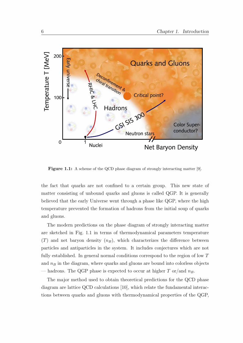
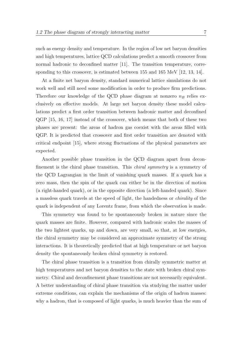
Figure 1.1: A scheme of the QCD phase diagram of strongly interacting matter [9].
the fact that quarks are not confined to a certain group. This new state of
matter consisting of unbound quarks and gluons is called QGP. It is generally
believed that the early Universe went through a phase like QGP, where the high
temperature prevented the formation of hadrons from the initial soup of quarks
and gluons.
The modern predictions on the phase diagram of strongly interacting matter
are sketched in Fig. 1.1 in terms of thermodynamical parameters temperature
(T ) and net baryon density (nB), which characterizes the difference between
particles and antiparticles in the system. It includes conjectures which are not
fully established. In general normal conditions correspond to the region of low T
and nB in the diagram, where quarks and gluons are bound into colorless objects
— hadrons. The QGP phase is expected to occur at higher T or/and nB.
The major method used to obtain theoretical predictions for the QCD phase
diagram are lattice QCD calculations [10], which relate the fundamental interac-
tions between quarks and gluons with thermodynamical properties of the QGP,
1.2 The phase diagram of strongly interacting matter 7
such as energy density and temperature. In the region of low net baryon densities
and high temperatures, lattice QCD calculations predict a smooth crossover from
normal hadronic to deconfined matter [11]. The transition temperature, corre-
sponding to this crossover, is estimated between 155 and 165 MeV [12, 13, 14].
At a finite net baryon density, standard numerical lattice simulations do not
work well and still need some modification in order to produce firm predictions.
Therefore our knowledge of the QCD phase diagram at nonzero nB relies ex-
clusively on effective models. At large net baryon density these model calcu-
lations predict a first order transition between hadronic matter and deconfined
QGP [15, 16, 17] instead of the crossover, which means that both of these two
phases are present: the areas of hadron gas coexist with the areas filled with
QGP. It is predicted that crossover and first order transition are denoted with
critical endpoint [15], where strong fluctuations of the physical parameters are
expected.
Another possible phase transition in the QCD diagram apart from decon-
finement is the chiral phase transition. This chiral symmetry is a symmetry of
the QCD Lagrangian in the limit of vanishing quark masses. If a quark has a
zero mass, then the spin of the quark can either be in the direction of motion
(a right-handed quark), or in the opposite direction (a left-handed quark). Since
a massless quark travels at the speed of light, the handedness or chirality of the
quark is independent of any Lorentz frame, from which the observation is made.
This symmetry was found to be spontaneously broken in nature since the
quark masses are finite. However, compared with hadronic scales the masses of
the two lightest quarks, up and down, are very small, so that, at low energies,
the chiral symmetry may be considered an approximate symmetry of the strong
interactions. It is theoretically predicted that at high temperature or net baryon
density the spontaneously broken chiral symmetry is restored.
The chiral phase transition is a transition from chirally symmetric matter at
high temperatures and net baryon densities to the state with broken chiral sym-
metry. Chiral and deconfinement phase transitions are not necessarily equivalent.
A better understanding of chiral phase transition via studying the matter under
extreme conditions, can explain the mechanisms of the origin of hadron masses:
why a hadron, that is composed of light quarks, is much heavier than the sum of
8 Chapter 1. Introduction
the masses of its constituents?
Moreover, there are models which predict new phases such as quarkonic
phase [18] and the color superconductor [19, 20] .
The experimental discovery of any of the above mentioned prominent land-
marks and regions of the QCD phase diagram would be a major breakthrough in
our understanding of the properties of nuclear matter.
1.3 Probing strongly interacting matter with
heavy-ion collisions
Experimentally, strongly interacting matter under extreme conditions is produced
and studied in high-energy heavy-ion collision experiments. Different experiments
worldwide are aiming to cover different regions of the QCD phase diagram in order
to get a complete scan of the diagram.
The experiments at the LHC and at top energies of RHIC and SPS9 cover
in their studies the diagram region with very high energy density and equal
numbers of particles and antiparticles, i.e. vanishing net baryon densities. This
region corresponds to conditions close to matter of the early Universe about 10
µs after the Big Bang [21].
On the other hand, the region of small temperatures at large net baryon
densities corresponds to the interior of compact stellar objects like neutron
stars [22, 23]. Several experimental programs are devoted to the exploration
of the high net baryon density region. The STAR and PHENIX experiments at
RHIC aim to scan the beam energies, and to search for the QCD critical end-
point. For the same reason, measurements are performed at CERN-SPS with the
upgraded NA61 detector. At the JINR10 a heavy-ion collider project NICA11 [24]
is planed with the goal of searching for the coexistence phase of nuclear matter.
However, not only beam energy is important in order to investigate dense
matter. The beam luminosity and data taking rate available for a certain detector
play an important role, defining the sort of measurements available for a certain
9Super Proton Synchrotron10Joint Institute for Nuclear Research, Russia11Nuclotron-based Ion Collider fAcility
1.3 Probing strongly interacting matter with heavy-ion collisions 9
experiment. The measurements, which possibly can be made by experiments,
are, for instance, the bulk observables and the rare probes.
The freeze-out phase, when no new parcticles can be produced in the col-
lisions, can be studied with measurement of “soft” hadrons production (bulk
observables). The term “bulk” denotes the fact that they directly characterize
the medium produced in the collision.
By contrast, the information of the earlier phases is carried by rare probes,
namely particles built up of heavy quarks (Λ,Σ,Ξ,Ω, J/Ψ, D ...). Moreover, in
order to obtain information on the early and dense phase of the fireball evolution,
one has to measure, for example, multi-differential observables such as the flows
of identified particles as a function of the transverse momentum (pt =√p2x + p2y)
of the particles, mass distributions of dileptons and particles containing heavy
quarks as a function of pt. These measurements require high reaction rates, fast
detection and a high-speed data acquisition system.
While every heavy-ion experiment is suited to measure bulk observables, the
sensible use of rare probes requires high luminosity beams as well as detectors
capable of high rate data taking. The collider experiments are typically limited
due to their beam luminosity, while the fixed target experiments have the oppor-
tunity to get significantly higher statistics due to higher reaction rates. In case
of fixed target experiments the reaction rate is mainly limited by the detector
capabilities. Thus, the collider experiments are often constrained to the mea-
surements of bulk observables, due to lower statistics in case of high precision
measurements of rare probes.
In contrast, the research program of the CBM experiment at FAIR is focused
on the measurement of both bulk and rare probes with unprecedented statis-
tics. A combination of high-intensity beams with a high-rate detector system is
planned to be used in order to meet this goal.
Chapter 2
The Compressed Baryonic
Matter (CBM) experiment
2.1 CBM at the Facility for Antiproton and Ion
Research (FAIR)
This chapter is devoted to the physics goals and the detector setup together with
the novel data acquisition and event selection systems of the CBM experiment.
FAIR [25] is a new accelerator facility, situated at the GSI Helmholtz Centre
for Heavy Ion Research in Darmstadt, Germany. It will deliver high intensity
beams of ions (109 particles/s for Au-ions) and antiprotons (1013 particles/s) for
experiments in the fields of nuclear, hadron, atomic and plasma physics.
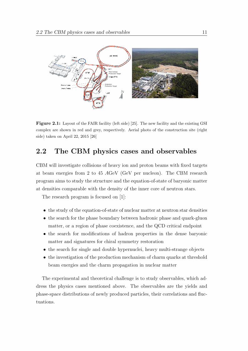
The layout of the future FAIR complex together with existing GSI facilities
is illustrated in Fig. 2.1. The core of the facility will be two large synchrotrons
with rigidities of 100 Tm and 300 Tm (SIS100 and SIS300, where SIS stands
for SchwerIonenSynchrotron). One of the scientific pillars of FAIR is the CBM
experiment aiming at exploration of the QCD phase diagram at high baryon
densities. The start version of the CBM setup is designed for ambitious nuclear-
matter research program using beams from SIS100. The experiment program
will be extended towards higher beam energies with the full version of the CBM
detector system using high-intensity beams from SIS300.
2.2 The CBM physics cases and observables 11
9
2.1 Overview
The concept of the FAIR Accelerator Facility has been developed by the international science community and the GSI Laboratory. It aims for a multifaceted forefront science program, beams of stable and unstable nuclei as well as antiprotons in a wide range of intensities and energies, with optimum beam qualities.
The concept builds and substantially expands on seminal developments made over the last 15 years at GSI and at other accelerator laboratories worldwide in the acceleration, accumulation, storage and phase space cooling of high-energy proton and heavy-ion beams. Based on that experience and adopting new developments, e.g. in fast cycling superconducting magnet design, in stochastic and in high-energy electron
cooling of ion beams, and also in ultra-high vacuum technology, a first conceptual layout of the new facility was proposed in 2001. Since then, the layout published in the Conceptual Design Report has undergone several modifications in order to accommodate additional scientific programs and optimize the layout, but also to reduce costs and to minimize the ecological impact of the project.
The present layout is shown in Fig. 2.1. A super-conducting double-synchrotron SIS100/300 with a circumference of 1,100 meters and with magnetic rigidities of 100 and 300 Tm, respectively, is at the heart of the FAIR accelerator facility. Following an upgrade for high intensities, the existing GSI accelerators UNILAC and SIS18 will serve as an injector.
2. FAIR Accelerator Facility
Figure 2.1: Layout of the existing GSI facility (UNILAC, SIS18, ESR) on the left and the planned FAIR facility on the right: the supercon-ducting synchrotrons SIS100 and SIS300, the collector ring CR, the accumulator ring RESR, the new experimental storage ring NESR, the rare isotope production target, the superconducting fragment separator Super-FRS, the proton linac, the antiproton production target, and the high energy antiproton storage ring HESR. Also shown are the experimental stations for plasma physics, relativistic nuclear collisions (CBM), radioactive ion beams (Super-FRS), atomic physics, and low-energy antiproton and ion physics (FLAIR).
Rare Isotope Production Target
Antiproton Production Target
Executive Summary
Figure 2.1: Layout of the FAIR facility (left side) [25]. The new facility and the existing GSI
complex are shown in red and grey, respectively. Aerial photo of the construction site (right
side) taken on April 22, 2015 [26]
2.2 The CBM physics cases and observables
CBM will investigate collisions of heavy ion and proton beams with fixed targets
at beam energies from 2 to 45 AGeV (GeV per nucleon). The CBM research
program aims to study the structure and the equation-of-state of baryonic matter
at densities comparable with the density of the inner core of neutron stars.
The research program is focused on [1]:
• the study of the equation-of-state of nuclear matter at neutron star densities
• the search for the phase boundary between hadronic phase and quark-gluon
matter, or a region of phase coexistence, and the QCD critical endpoint
• the search for modifications of hadron properties in the dense baryonic
matter and signatures for chiral symmetry restoration
• the search for single and double hypernuclei, heavy multi-strange objects
• the investigation of the production mechanism of charm quarks at threshold
beam energies and the charm propagation in nuclear matter
The experimental and theoretical challenge is to study observables, which ad-
dress the physics cases mentioned above. The observables are the yields and
phase-space distributions of newly produced particles, their correlations and fluc-
tuations.
12 Chapter 2. The CBM experiment
8 CHAPTER 1. THE COMPRESSED BARYONIC MATTER EXPERIMENT
The experimental challenge is to measure multi-dierential observables and particles with verylow production cross sections such as multi-strange (anti-) hyperons, particles with charm andlepton pairs with unprecedented precision. The situation is illustrated in Fig. 1.4 which depictsthe product of multiplicity times branching ratio for various particle species produced in centralAu+Au collisions at 25 AGeV. The data points are calculated using either the HSD transportcode [12] or the thermal model based on the corresponding temperature and baryon-chemicalpotential [14]. Mesons containing charm quarks are about 9 orders of magnitude less abundantthan pions (except for the Â’ meson which is even more suppressed). The dilepton decay ofvector mesons is suppressed by the square of the electromagnetic coupling constant (1/137)2,resulting in a dilepton yield which is 6 orders of magnitude below the pion yield, similar to themultiplicity of multi-strange anti-hyperons.In order to produce high statistics data even for the particles with the lowest production crosssections, the CBM experiment is designed to run at reaction rates of 100 kHz up to 1 MHz.For charmonium measurements - where a trigger on high-energy lepton pairs can be generated -reaction rates up to 10 MHz are envisaged.
Figure 1.4: Particle multiplicities times branching ratio for central Au+Au collisions at 25 AGeVas calculated with the HSD transport code [12] and the statistical model [14]. For the vectormesons (fl, Ê, „, J/Â, ÂÕ) the decay into lepton pairs was assumed, for D mesons the hadronicdecay into kaons and pions.
1.3 CBM physics cases and observablesThe CBM research program is focused on the following physics cases:The equation-of-state of baryonic matter at neutron star densities.The relevant measurements are:
• The excitation function of the collective flow of hadrons which is driven by the pressurecreated in the early fireball (SIS100);
• The excitation functions of multi-strange hyperon yields in Au+Au and C+C collisions atenergies from 2 to 11 AGeV (SIS100). At subthreshold energies, and hyperons are
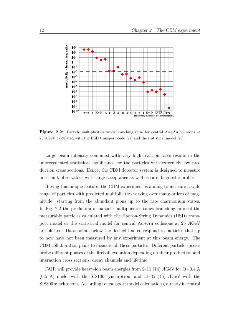
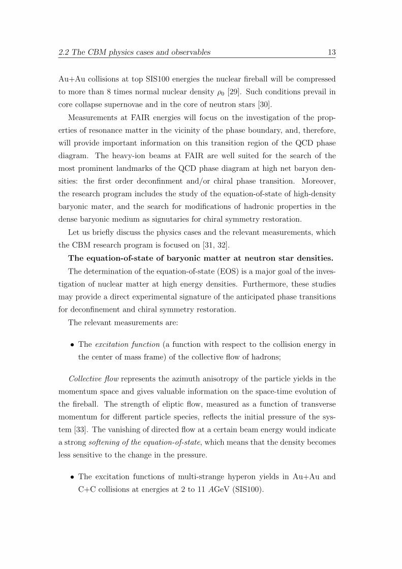
Figure 2.2: Particle multiplicities times branching ratio for central Au+Au collisions at
25 AGeV calculated with the HSD transport code [27] and the statistical model [28].
Large beam intensity combined with very high reaction rates results in the
unprecedented statistical significance for the particles with extremely low pro-
duction cross sections. Hence, the CBM detector system is designed to measure
both bulk observables with large acceptance as well as rare diagnostic probes.
Having this unique feature, the CBM experiment is aiming to measure a wide
range of particles with predicted multiplicities varying over many orders of mag-
nitude: starting from the abundant pions up to the rare charmonium states.
In Fig. 2.2 the prediction of particle multiplicities times branching ratio of the
measurable particles calculated with the Hadron-String Dynamics (HSD) trans-
port model or the statistical model for central Au+Au collisions at 25 AGeV
are plotted. Data points below the dashed line correspond to particles that up
to now have not been measured by any experiment at this beam energy. The
CBM collaboration plans to measure all these particles. Different particle species
probe different phases of the fireball evolution depending on their production and
interaction cross sections, decay channels and lifetime.
FAIR will provide heavy-ion beam energies from 2–11 (14) AGeV for Q=0.4 A
(0.5 A) nuclei with the SIS100 synchrotron, and 11–35 (45) AGeV with the
SIS300 synchrotron. According to transport model calculations, already in central
2.2 The CBM physics cases and observables 13
Au+Au collisions at top SIS100 energies the nuclear fireball will be compressed
to more than 8 times normal nuclear density ρ0 [29]. Such conditions prevail in
core collapse supernovae and in the core of neutron stars [30].
Measurements at FAIR energies will focus on the investigation of the prop-
erties of resonance matter in the vicinity of the phase boundary, and, therefore,
will provide important information on this transition region of the QCD phase
diagram. The heavy-ion beams at FAIR are well suited for the search of the
most prominent landmarks of the QCD phase diagram at high net baryon den-
sities: the first order deconfinment and/or chiral phase transition. Moreover,
the research program includes the study of the equation-of-state of high-density
baryonic mater, and the search for modifications of hadronic properties in the
dense baryonic medium as signutaries for chiral symmetry restoration.
Let us briefly discuss the physics cases and the relevant measurements, which
the CBM research program is focused on [31, 32].
The equation-of-state of baryonic matter at neutron star densities.
The determination of the equation-of-state (EOS) is a major goal of the inves-
tigation of nuclear matter at high energy densities. Furthermore, these studies
may provide a direct experimental signature of the anticipated phase transitions
for deconfinement and chiral symmetry restoration.
The relevant measurements are:
• The excitation function (a function with respect to the collision energy in
the center of mass frame) of the collective flow of hadrons;
Collective flow represents the azimuth anisotropy of the particle yields in the
momentum space and gives valuable information on the space-time evolution of
the fireball. The strength of eliptic flow, measured as a function of transverse
momentum for different particle species, reflects the initial pressure of the sys-
tem [33]. The vanishing of directed flow at a certain beam energy would indicate
a strong softening of the equation-of-state, which means that the density becomes
less sensitive to the change in the pressure.
• The excitation functions of multi-strange hyperon yields in Au+Au and
C+C collisions at energies at 2 to 11 AGeV (SIS100).
14 Chapter 2. The CBM experiment
The excitation function of strange hadron yields and phase space distributions
(including multi-strange hyperons) will provide information about the fireball
dynamics and the nuclear matter equation-of-state over a wide range of baryon
densities. At sub-threshold energies, Ξ and Ω hyperons are produced in sequential
collisions involving kaon and Λ particles, and, therefore, are sensitive to the
density in the fireball.
In-medium properties of hadrons.
The restoration of chiral symmetry in dense baryonic matter will modify the
properties of hadrons. The relevant measurements are:
• The in-medium mass distribution of vector mesons (ρ, ω, φ) decaying in
lepton pairs in heavy-ion collisions at different energies (2–45 AGeV), and
for different collision systems (SIS100/300);
The measurement of short-lived vector mesons via their decay into an electron-
positron pair provides a unique possibility for studying the properties of vector
mesons in dense baryonic matter. The lepton pair is called a “penetrating probe”
because it delivers undistorted information on the conditions inside the dense fire-
ball. The invariant masses of the measured lepton pairs permit the reconstruction
of the in-medium spectral function of the ρ, ω, φ mesons, if they decay inside the
medium. Such data is expected to shed light on the fundamental question as to
what extent chiral symmetry is restored at high baryon densities and how this
affects the hadron masses [34].
• Yields and transverse mass (mt =√m2 + p2x + p2y) distributions of charmed
mesons in heavy-ion collision as a function of collision energy (SIS100/300).
Particles containing heavy quarks, like charm, can be created in the hard pro-
cesses at the early stage of fireball evolution exclusively, especially at the FAIR
energies near the threshold for the charm-anticharm pair production.
The D-mesons, the bound states of a heavy charm quark and a light quark,
are predicted to be modified in the nuclear medium [35]. To the extent that
these modifications are partly related to in-medium changes of the light-quark
condensate, they offer another interesting option to probe the restoration of chiral
symmetry in dense hadronic matter [35].
2.2 The CBM physics cases and observables 15
Non-monotonic behavior of the inverse slope of the transverse momentum spec-
tra as a function of the beam energy would signal a change in the nuclear matter
properties at a certain net baryon density. The distribution of the inverse slope
as a function of particle mass is related to the particle freeze-out phase (phase,
when the collisions between particles cease), and, hence, may help to delineate
the early from the late collision stages.
Phase transitions from hadronic matter to quarkyonic or partonic
matter at high net-baryon densities.
A discontinuity or sudden variation in the excitation functions of sensitive
observables would be indicative of a deconfinement transition. The relevant mea-
surements are:
• The excitation function of yields, spectra, and collective flow of strange and
charmed particles in heavy-ion collisions at 6–45 AGeV (SIS100/300);
The yields of rare particles containing strangeness and charm, in particular when
produced at beam energies close to the corresponding threshold, depend on the
conditions inside the early fireball [36].
Enhanced strangeness production was proposed as a possible signal for the
QGP formation [37]. In the parton-parton interaction scenarios strange quarks
are expected to be produced more abundantly than in hadronic reaction scenarios.
As a result, the yields of strange particles, scaled by the number of participating
nucleons, are expected to be higher in heavy-ion collisions with creation of a QGP
than in p+p interactions.
The idea is that the production of strange quark pairs is energetically favored
in the quark-gluon plasma as compared to hadronic matter. The enhancement
is expected to be most pronounced for particles containing two or even three
strange quarks such as Ξ and Ω.
• The excitation function of yields and spectra of lepton pairs in heavy-ion
collisions at 6–45 AGeV (SIS100/300);
The slope of the dilepton invariant mass distribution between 1 and 2 GeV/c2
directly reflects the average temperature of the fireball. The study of the energy
dependence of this slope opens a unique possibility of measuring the caloric curve
16 Chapter 2. The CBM experiment
which would be a signature for phase coexistence [38]. This measurement would
also provide indications for the onset of deconfinement and the location of the
critical endpoint.
• Event-by-event fluctuations of conserved quantities like baryon, strange and
net-charge etc. in heavy-ion collisions with high precision as a function of
beam energy at 6–45 AGeV (SIS100/300).
The presence of a phase coexistence region is expected to cause strong fluctuations
from event to event in the charged particle number, baryon number, strangeness-
to-pion ratio, average transverse momentum, etc. Similar effects are predicted to
occur in the vicinity of the QCD critical point.
Hypernuclei, strange dibaryons and massive strange objects.
Nuclei containing at least one hyperon in addition to nucleons offer the fas-
cinating perspective of exploring the third, strange dimension of the chart of
nuclei. Their investigation provides information on the hyperon-nucleon and on
the hyperon-hyperon interaction in particular, which plays an important role in
neutron star models.
Theoretical models predict that single and double hypernuclei, strange
dibaryons and heavy multi-strange short-lived objects are produced via coa-
lescence in heavy-ion collisions with a maximum yield in the region of SIS100
energies [39, 40]. The planned measurements include:
• The decay chains of single and double hypernuclei in heavy ion collisions
at SIS100 energies;
• Search for strange matter in the form of strange dibaryons and heavy multi-
strange short-lived objects. Whether or not these multi-strange particles
decay into charged hadrons including hyperons, which can be identified via
their decay products.
Charm production mechanisms, charm propagation, and in-medium
properties of charmed particles in dense nuclear matter.
Due to the large mass, cc-quark pairs can only be produced in the hard pro-
cesses of the early stage of collision. The created charm quarks either propagate
as charmonium (hidden charm) or pick up light quarks to form pairs of D-mesons
2.3 The experimental setup 17
(open charm) or charmed baryons. The production and propagation of charm in
heavy-ion collisions are expected to be a particularly sensitive probe of the hot
and dense medium.
The majority of charmed quarks are carried away as open charm. During the
evolution of the fireball, charm quarks undergo exchange of the momentum with
the medium. The exchange process depends strongly on the properties of the
medium. Therefore, momentum distributions, correlations, and elliptic flow of
open charm hadrons is an important diagnostic probe of the prevailing degrees
of freedom in the early collision stage.
Also, charmonium states are observables sensitive to the conditions in the
fireball. The suppression of charmonium due to color screening is predicted as a
signature for the quark-gluon plasma [35].
The free color charges in the deconfined phase are expected to screen the
mutual attraction of the charmed quarks and hence prevent the formation of
charmonium states. The relevant measurements are:
• Cross sections, momentum spectra, and collective flow of open charm (D-
mesons) and charmonium in proton-nucleus and nucleus-nucleus collisions
at SIS300 energies.
As discussed above, a substantial part of the CBM physics cases can already
be addressed with beams from the SIS100 synchrotron. A general review of the
physics of compressed baryonic matter, the theoretical concepts, the available
experimental results, and predictions for relevant observables in future heavy-ion
collision experiments can be found in the CBM Physics Book [1].
2.3 The experimental setup
The challenging CBM physics program requires a high performance detector sys-
tem with two configurations: one version optimized for detection of electrons, the
other — for muons.
In the electron configuration the following detectors will be used: Micro-vertex
Detector (MVD), Silicon Tracking System (STS), both placed in a gap of 1 Tm
18 Chapter 2. The CBM experiment
14 CHAPTER 1. THE COMPRESSED BARYONIC MATTER EXPERIMENT
(which contain no signal) by a factor of 100 or more. The event selection system will be basedon a fast on-line event reconstruction running on a high-performance computer farm equippedwith many-core CPUs and graphics cards (GSI GreenIT cube). Track reconstruction, whichis the most time consuming combinatorial stage of the event reconstruction, will be based onparallel track finding and fitting algorithms, implementing the Cellular Automaton and KalmanFilter methods. For open charm production the trigger will be based on an online search forsecondary vertices, which requires high-speed tracking and event reconstruction in the STS andMVD. The highest suppression factor has to be achieved for J/Â mesons where a high-energeticpair of electrons or muons is required in the TRD or in the MUCH. For low-mass electron pairsno online selection is possible due to the large number of rings/event in the RICH caused bythe material budget of the STS. In the case of low-mass muon pairs some background rejectionmight be feasible.
Figure 1.6: The CBM experimental facility with the electron detectors RICH and TRD.
Figure 1.7: The CBM experimental facility with the muon detection system.
magnet
STS + MVD
RICH
TRD ToF ECAL
PSD
14 CHAPTER 1. THE COMPRESSED BARYONIC MATTER EXPERIMENT
(which contain no signal) by a factor of 100 or more. The event selection system will be basedon a fast on-line event reconstruction running on a high-performance computer farm equippedwith many-core CPUs and graphics cards (GSI GreenIT cube). Track reconstruction, whichis the most time consuming combinatorial stage of the event reconstruction, will be based onparallel track finding and fitting algorithms, implementing the Cellular Automaton and KalmanFilter methods. For open charm production the trigger will be based on an online search forsecondary vertices, which requires high-speed tracking and event reconstruction in the STS andMVD. The highest suppression factor has to be achieved for J/Â mesons where a high-energeticpair of electrons or muons is required in the TRD or in the MUCH. For low-mass electron pairsno online selection is possible due to the large number of rings/event in the RICH caused bythe material budget of the STS. In the case of low-mass muon pairs some background rejectionmight be feasible.
Figure 1.6: The CBM experimental facility with the electron detectors RICH and TRD.
Figure 1.7: The CBM experimental facility with the muon detection system.
magnet
STS+MVD
MuCh TRDToF
PSD
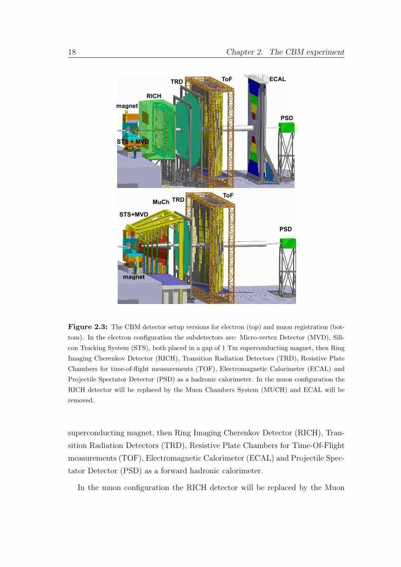
Figure 2.3: The CBM detector setup versions for electron (top) and muon registration (bot-
tom). In the electron configuration the subdetectors are: Micro-vertex Detector (MVD), Sili-
con Tracking System (STS), both placed in a gap of 1 Tm superconducting magnet, then Ring
Imaging Cherenkov Detector (RICH), Transition Radiation Detectors (TRD), Resistive Plate
Chambers for time-of-flight measurements (TOF), Electromagnetic Calorimeter (ECAL) and
Projectile Spectator Detector (PSD) as a hadronic calorimeter. In the muon configuration the
RICH detector will be replaced by the Muon Chambers System (MUCH) and ECAL will be
removed.
superconducting magnet, then Ring Imaging Cherenkov Detector (RICH), Tran-
sition Radiation Detectors (TRD), Resistive Plate Chambers for Time-Of-Flight
measurements (TOF), Electromagnetic Calorimeter (ECAL) and Projectile Spec-
tator Detector (PSD) as a forward hadronic calorimeter.
In the muon configuration the RICH detector will be replaced by the Muon
2.3 The experimental setup 19
Chambers System (MUCH) and ECAL will be removed (Fig. 2.3).
Observables MVD STS RICH MuCh TRD TOF ECAL PSD
π, K, p X (X) (X) X X
Hyperons X (X) (X) X
Open charm X X (X) (X) (X) X
Electrons X X X X X X
Muons X X (X) X
Photons X X
Photons via e± conversions X X X X X X
Table 2.1: The CBM observables. The subdetectors required for a certain observable are
marked as X. The subdetectors marked as (X) can be used optionally to suppress background.
The CBM subdetectors required for the measurement of the different observ-
ables are listed in Tab. 2.1. The system subdetectors are described in detail
below.
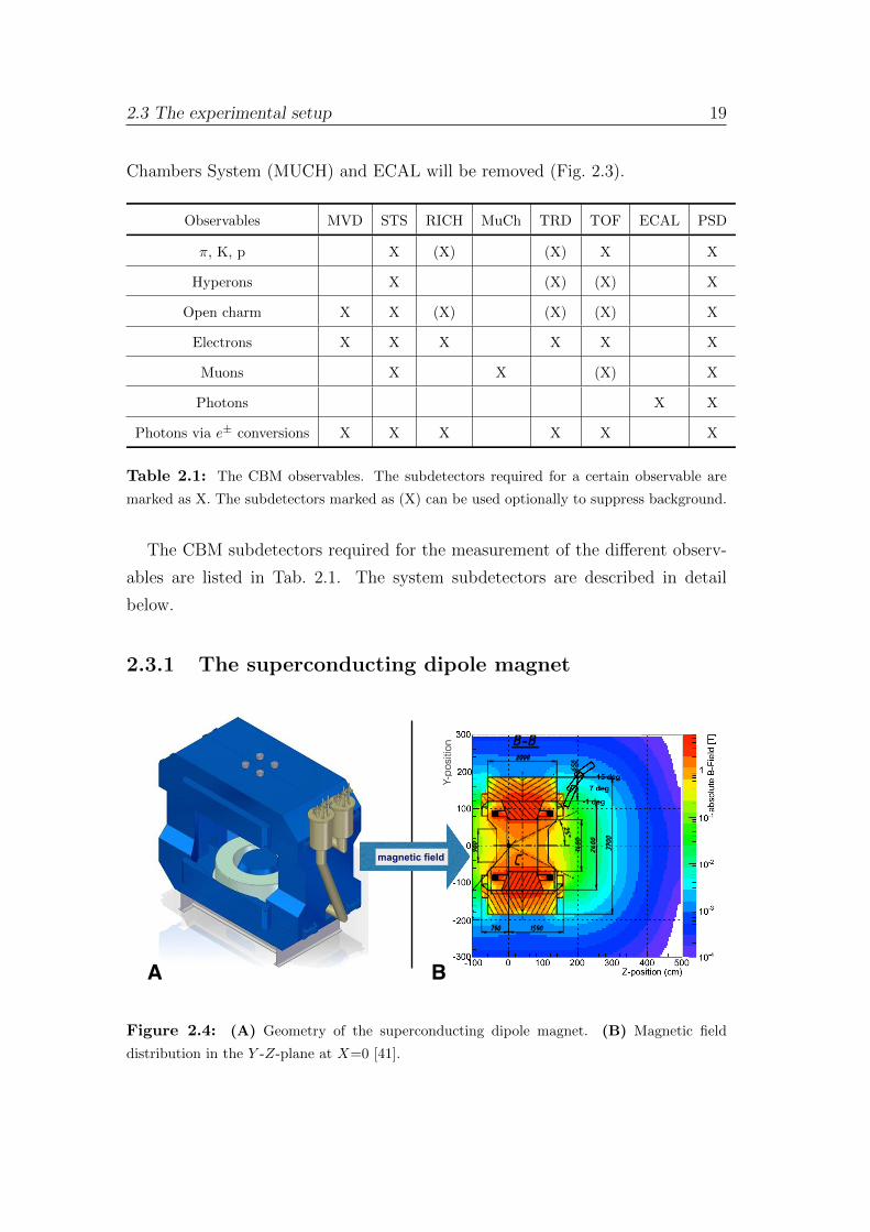
2.3.1 The superconducting dipole magnet
Y-po
sitio
n
magnetic field
A B
Figure 2.4: (A) Geometry of the superconducting dipole magnet. (B) Magnetic field
distribution in the Y -Z-plane at X=0 [41].
20 Chapter 2. The CBM experiment
The superconducting dipole magnet [41] serves to bend charged particle trajec-
tories in order to determine their momenta. The current geometry of the magnet
is shown in Fig. 2.4(A).
It will provide bending power to the tracking detectors MVD and STS. It has
a large aperture of ±25o in polar angle and provides a magnetic field integral of
1 Tm for a sufficient momentum resolution. The magnet should be large enough
to permit the installation and maintenance of the MVD and the STS, which
implies that the size of magnet should be at least 1.3×1.3 m2.
Since in order to meet the requirements the dipole magnet was chosen, the
resulting magnetic field is non-homogeneous. The magnetic field distribution,
calculated with ToSCA-program [42], for the current version of the magnet is
shown in Fig. 2.4(B).
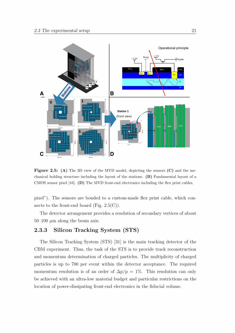
2.3.2 Micro-Vertex Detector (MVD)
The Micro-Vertex Detector [43] design is mainly driven by the goal of deter-
mining the position of a particle interaction or decay point (secondary vertex) by
tracing the reaction products to their common point of origin. In order to achieve
a high secondary vertex resolution, the MVD has to be located close to the tar-
get. The MVD consists of four layers of Monolithic Active Pixel Sensor (MAPS)
(Fig. 2.5(A)) located from 5 cm to 20 cm downstream of the target in a vacuum.
The MAPS principle was originally developed as a digital camera image
sensors. MAPS can be produced in a standard Complementary Metal-Oxide-
Semiconductor (CMOS) process. It allows for the integration of sensor pixels as
well as analog and digital signal processing circuitry on a single chip (for this
reason it is called “monolithic”).
The sensitive component of the pixel is a reversed biased diode (see
Fig. 2.5(B)), while the active volume of the sensor comprises the entire epitaxial
layer, which has a typical thickness of 12–16 µm. When a particle is travers-
ing the chip, ionizing radiation produces electron-hole pairs. The sensing diodes
collect the diffusing electrons and generate a charge signal. The charge signal is
converted into a voltage signal by a dedicated Metal-Oxide-Semiconductor Field-
Effect Transistor (MOSFET) inside the pixel (for this reason it is called “active
2.3 The experimental setup 21
Segmented Geometry
23nd
CBM
Col
labo
ratio
n M
eetin
g, G
SI, A
pril
2014
Ch
ristia
n M
üntz
(Goe
the-
Uni
v. F
rank
furt
)
5
MVD CAD model
IPHC [email protected] 8TWEPP 2013
~1.2
cm
~1 cm
SUZE
~1.2 cm² array
Discriminators
SUZE
~1.2 cm² array
Discriminators
SUZE
~1.2 cm² array
Discriminators
Serial read out RD block PLLLVDS
~1.3
cm
~1 cm
Serial read out RD block PLLLVDSSUZE
~1.3 cm² array
SUZE
~1.3 cm² array
SUZE
~1.3 cm² array
MISTRAL_in ASTRAL_inFSBB_M FSBB_A
Station 1
Mistral form factor:
2. Monolithic Active Pixel Sensoren (MAPS)
2.1. Allgemeines
2.1.1. Funktionsprinzip
Monolithic Active Pixel Sensoren (MAPS) werden in einem CMOS-Prozess als einheitlicher Chiphergestellt. Dabei wird das aktive Volumen durch eine P-dotierte Epitaxialschicht gebildet. Hebt einhochenergetisches hindurchfliegendes Teilchen in der Epitaxialschicht Elektronen in das Leitungsbandan, wandern diese durch thermische Di↵usion in der Epitaxialschicht umher, bis sie auf eine Pixeldiodetre↵en, an der sie durch das elektrische Feld in die Diode gezogen werden. Dazu wird die Pixeldiode(siehe Abb. 2.1), die aus der P-dotierten Epitaxialschicht und einem n-Well an der Oberflache besteht,in Sperrrichtung betrieben. Die bei einem Teilcheneinschlag so eingesammelte Ladung bewirkt an derKapazitat der Diode eine Spannungsanderung, die verstarkt und ausgelesen wird.
Abbildung 2.1.: Schematischer Aufbau eines Monolithic Active Pixel Sensors nach [6]. DiePixeldiode wird durch den pn-Ubergang vom schwach p-dotierten Teil derEpitaxialschicht (P-) zu dem angrenzenden n-dotierten Bereich (N+) gebil-det.
2.1.2. Latch-Ups
Bei dieser Art von Sensoren konnen sogenannte Latch-Ups auftreten. Der Begri↵ Latch-Up bezeichneteinen Kurzschluss in einem Halbleiter-Chip durch einen leitend gewordenen Bereich an einer Stelle,die einem Thyristor ahnelt. Abbildung 2.2 zeigt fur einen CMOS-Inverter zwei Transistoren, die einenThyristor bilden. Durch hochenergetische Teilchen, die genugend Ladungstrager im Halbleiter anregen,oder durch Anlegen von Spannungen außerhalb der Spezifikation kann der Thyristor zum Schaltengebracht werden, wodurch ein Kurzschluss der Versorgungsspannung entsteht.
Durch den dabei auftretenden hohen Strom konnten die Bondingdrahte, uber die der Sensor an-geschlossen ist, zerstort oder der Sensor durch Warmeentwicklung beschadigt werden. Um dies zuverhindern kann der Sensor modifiziert werden, indem fur Latch-ups weniger anfallige Strukturen ver-wendet werden, und zusatzlich empfiehlt sich eine Schutzschaltung, die die Versorgungsspannung derSensoren im Falle einer zu hohen Stromaufnahme kurzzeitig abschaltet (siehe Abschnitt 3.2.2).
13
Segmented Geometry
23nd
CBM
Col
labo
ratio
n M
eetin
g, G
SI, A
pril
2014
Ch
ristia
n M
üntz
(Goe
the-
Uni
v. F
rank
furt
)
5
MVD CAD model
IPHC [email protected] 8TWEPP 2013
~1.2
cm
~1 cm
SUZE
~1.2 cm² array
Discriminators
SUZE
~1.2 cm² array
Discriminators
SUZE
~1.2 cm² array
Discriminators
Serial read out RD block PLLLVDS
~1.3
cm
~1 cm
Serial read out RD block PLLLVDSSUZE
~1.3 cm² array
SUZE
~1.3 cm² array
SUZE
~1.3 cm² array
MISTRAL_in ASTRAL_inFSBB_M FSBB_A
Station 1
Mistral form factor:
A B
Segmented Geometry
23nd
CBM
Col
labo
ratio
n M
eetin
g, G
SI, A
pril
2014
Ch
ristia
n M
üntz
(Goe
the-
Uni
v. F
rank
furt
)
5
MVD CAD model
IPHC [email protected] 8TWEPP 2013
~1.2
cm
~1 cm
SUZE
~1.2 cm² array
Discriminators
SUZE
~1.2 cm² array
Discriminators
SUZE
~1.2 cm² array
Discriminators
Serial read out RD block PLLLVDS
~1.3
cm
~1 cm
Serial read out RD block PLLLVDSSUZE
~1.3 cm² array
SUZE
~1.3 cm² array
SUZE
~1.3 cm² array
MISTRAL_in ASTRAL_inFSBB_M FSBB_A
Station 1
Mistral form factor:
Stations
C D
Operational principle
Figure 2.5: (A) The 3D view of the MVD model, depicting the sensors (C) and the me-
chanical holding structure including the layout of the stations. (B) Fundamental layout of a
CMOS sensor pixel [44]. (D) The MVD front-end electronics including the flex print cables.
pixel”). The sensors are bonded to a custom-made flex print cable, which con-
nects to the front-end board (Fig. 2.5(C)).
The detector arrangement provides a resolution of secondary vertices of about
50–100 µm along the beam axis.
2.3.3 Silicon Tracking System (STS)
The Silicon Tracking System (STS) [31] is the main tracking detector of the
CBM experiment. Thus, the task of the STS is to provide track reconstruction
and momentum determination of charged particles. The multiplicity of charged
particles is up to 700 per event within the detector acceptance. The required
momentum resolution is of an order of ∆p/p = 1%. This resolution can only
be achieved with an ultra-low material budget and particular restrictions on the
location of power-dissipating front-end electronics in the fiducial volume.
22 Chapter 2. The CBM experiment
4.4. OPERATIONAL PRINCIPLE 67
4.4 Operational PrincipleA silicon detector is essentially a revers-biased diode with the depleted zone actingas a solid-state ionization chamber. When a charge particle passes through thesilicon detector, it can either be stopped in the detector or can traverse through it.When a particle is stopped the particle energy can be measured. However, whencharged particles pass through a silicon detector, many e-h pairs get producedalong the path of the particle. Average energy required to create a single e-h pairis about 3.6 eV for silicon. The energy loss in silicon can be measured by “counting”the total number of pairs created.
Figure 4.5: Operational principle of silicon strip detector.
Under the application of reverse-bias, the electrons drift towards the n+-side andholes to the p+-side. This charge migration induces a current pulse on the read outelectrodes and constitutes the basic electrical signal. Integration of this currentequals the total charge and hence is proportional to the energy loss of the particle.The high mobility of electrons and holes enables the charge signal to be collectedvery quickly. It may be pointed out that only the charge released in the depletionregion can be collected, whereas the charge created in the neutral, non-depletedzone recombines with the free carriers and is lost. Therefore, the silicon detectorsshould be operated with an applied voltage sufficient to fully deplete all the crys-tal volume. The principle of operation of silicon microstrip detector is shown inFig. 4.5. A Minimum Ionizing Particle (MIP) traversing a <111> oriented Si layer
2.3. DETECTOR LAYOUT 23
station 1 station 2
station 3 station 4
station 5 station 6
station 7 station 8
Figure 2.6: Layout of the STS stations. The most upstream station is shown in the upper leftcorner, the most downstream station in the bottom. The color codes within the stations denotecommonly read-out sensors. The circles indicate the acceptance between polar angles 2.5¶ and25¶. Several stations are horizontally enlarged for increased coverage of low-momentum particlesin the dipole magnetic field. Stations 5 and 6 as well as 7 and 8 are of identical construction.The two circles indicate their respective acceptance, i.e. the smaller radius is for the upstreamstation.
Station
A
B
C
Operational principle
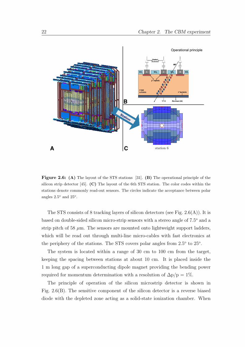
Figure 2.6: (A) The layout of the STS stations [31]. (B) The operational principle of the
silicon strip detector [45]. (C) The layout of the 6th STS station. The color codes within the
stations denote commonly read-out sensors. The circles indicate the acceptance between polar
angles 2.5o and 25o.
The STS consists of 8 tracking layers of silicon detectors (see Fig. 2.6(A)). It is
based on double-sided silicon micro-strip sensors with a stereo angle of 7.5o and a
strip pitch of 58 µm. The sensors are mounted onto lightweight support ladders,
which will be read out through multi-line micro-cables with fast electronics at
the periphery of the stations. The STS covers polar angles from 2.5o to 25o.
The system is located within a range of 30 cm to 100 cm from the target,
keeping the spacing between stations at about 10 cm. It is placed inside the
1 m long gap of a superconducting dipole magnet providing the bending power
required for momentum determination with a resolution of ∆p/p = 1%.
The principle of operation of the silicon microstrip detector is shown in
Fig. 2.6(B). The sensitive component of the silicon detector is a reverse biased
diode with the depleted zone acting as a solid-state ionization chamber. When
2.3 The experimental setup 23
wave front
Ta
riq
Ma
hm
ou
d •
CB
M W
ee
k •
GS
I • 2
4.0
4.2
015
!
3 Introduction: The RICH Concept!
CAMERA ! 2.4 m2, 55k Ch. ! MAPMT: H12700B
(Hamamatsu)
MIRROR ! SIMAX-glass, Al+MgF2 ! R = 3m, d ≤ 6mm ! 11.8 m2 (Tiles of 40×40 cm2) ! JLO OLOMOUC
RADIATOR ! CO2; γth = 33 ! pπ,th = 4.65 GeV/c
! Length=1.7 m. V ≈30 m3
photon detector
photon detector
UV-mirror
Cherenkov light cone
beam pipe
A
B
C ring
Operational principle
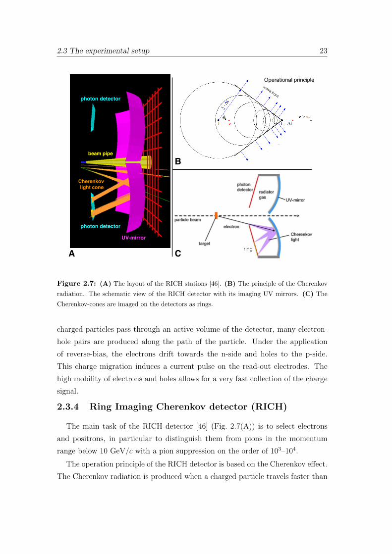
Figure 2.7: (A) The layout of the RICH stations [46]. (B) The principle of the Cherenkov
radiation. The schematic view of the RICH detector with its imaging UV mirrors. (C) The
Cherenkov-cones are imaged on the detectors as rings.
charged particles pass through an active volume of the detector, many electron-
hole pairs are produced along the path of the particle. Under the application
of reverse-bias, the electrons drift towards the n-side and holes to the p-side.
This charge migration induces a current pulse on the read-out electrodes. The
high mobility of electrons and holes allows for a very fast collection of the charge
signal.
2.3.4 Ring Imaging Cherenkov detector (RICH)
The main task of the RICH detector [46] (Fig. 2.7(A)) is to select electrons
and positrons, in particular to distinguish them from pions in the momentum
range below 10 GeV/c with a pion suppression on the order of 103–104.
The operation principle of the RICH detector is based on the Cherenkov effect.
The Cherenkov radiation is produced when a charged particle travels faster than
24 Chapter 2. The CBM experiment
the speed of light in the medium, through which it passes. The particle excites
atoms or molecules around it with the electromagnetic field and they fall back
down to ground level by emitting Cherenkov photons. The emitted Cherenkov
radiation travels at the speed of light in the medium, given by c/n, where c is
the speed of light in a vacuum and n is the index of refraction. It results in
the Cherenkov photons forming a cone-shaped front (Fig. 2.7(B)), whose half
angle is greater for faster particles and media with higher refractive indexes.
The radiation occurs mainly in the visible and UV region of the spectrum. In-
side the detector this Cherenkov light cone is reflected by a focusing mirror to
a position-sensitive photon detector, which allows reconstructing the produced
rings (Fig. 2.7(C)).
The RICH detector will be placed 1.6 m downstream from the target behind
the dipole magnet. It will consist of a 1.7 m long gas radiator at 2 mbar overpres-
sure and two arrays of mirrors (Al+MgF2 coating) and photon detector planes.
The design of the photon detector plane is based on MAPMTs (Multianode
PhotoMultiplier Tubes, e.g. H8500 from Hamamatsu) in order to provide high
granularity, high geometrical acceptance, high detection efficiency of photons also
in the UV region and a reliable operation.
According to in-beam tests with a prototype RICH of real-size length, one has
to expect the order of 100 Cherenkov rings to be seen in a central Au+Au collision
at 25 AGeV due to the large material budget in front of the detector. About
22 photons are measured per electron ring. Simulation studies predict that such
a high value of photons per ring together with high granularity (approx. 55 000
channels in total) allows the achievement of a pion suppression on the order
of 500.
2.3.5 Muon Chambers (MuCh)
Since the CBM strategy is to measure both electrons and muons in order
to combine the advantages of both probes, the muon detector is also a part
of the alternative setup version. The main experimental challenge for muon
measurements at CBM is to identify low-momentum muons in an environment
of high particle densities.
The MuCh (Muon Chamber) [47] in CBM is placed downstream of the STS,
2.3 The experimental setup 25
3.3 Basic Principles of the Straw Tube 27
3.3 Basic Principles of the Straw Tube
Straw tubes are drift chambers (first operation drift chamber [62]) made of a gas filledconducting cylinder acting as cathode, and a sense wire stretched in the axis of the cylinder.
The electromagnetic interaction between the charged particles traversing the gas insidestraw tube forms the basis of detection. Coulomb interactions between the incoming chargedparticles and bound electrons in the gaseous medium result in ionization. Due to the appliedstatic electric field in the tube, electrons of primary ionization will drift to the positivelycharged anode wire and positive ions will move to the cathode. Since the electric field inthe straw tube increases with r−1 towards the anode wire, in the vicinity of the thin wire(at rc = few wire radii) the electric field gets strong enough so that electrons producedby the primary interaction can gain enough energy to produce an avalanche like secondaryionization process called gas amplification. In Fig.3.5 the gas amplification is depicted. A
Figure 3.5: Time development of an avalanche in the Straw tube
typical drop like ionization distribution close to the anode wire develops with all electronsin the front towards the wire surface and ions outside. Because of lateral diffusion and thesmall radius of the anode, the avalanche surrounds the wire; electrons are collected andpositive ions start to drift towards the cathode. From the gas amplification or avalanche,signal amplification of 104 − 106 is obtained [63]. This leads to a significant simplification ofthe measurement electronics. Signals produced by the collected charges are further amplifiedby exterior electronics and processed by a data acquisition system (DAQ). The track of aparticle is mapped from the fired wires by registering the drift times of the electrons. Usingthese drift times, one can obtain the distance of closest approach of the track to the anodewire Fig.3.6. In a single straw the coordinate information is a ”cylinder of closest approach”.
36 CHAPTER 2. THE CBM MUON DETECTOR SYSTEM
Figure 2.14: Normalized background for different segmentation angles. We have chosen 1-degreeuniform segmentation as our baseline option.
!Figure 2.15: Schematic representation of the signal generation process in GEM
randomly along the track. Parameters of the Landau distribution are determined with theHEED [5] package.
• Determination of the number of secondary electrons emitted in the avalanche region foreach primary electron. Exponential gas gain distribution with a default mean gas gain of104 is used in this step.
• Intersection of secondary electron spots with the pad structure of a module and determina-tion of the charge arrived at each pad. The default spot radius is set to 0.6 mm as measuredfor the triple-GEM detectors during beam tests. Charge arrival time is calculated fromthe Monte-Carlo point time plus the primary electron drift time: t = d/v (d -distancetravelled by the primary electron towards the avalanche region, v - drift velocity, v = 100micro-m/ns by default).
• Time-dependent summation have been performed for charges from all Monte-Carlo pointspad-by-pad and conversion of the charge-vs-time distribution has beed done to get thetiming response of the foreseen MUCH readout electronics. Timing response on a delta-function-like charge from secondary electrons is simulated by the linear peaking period of 20ns and the falling edge described as an exponential decrease with 40 ns slope. Response toseveral delta-function-like charge signals is described as a convolution in time of responsesfrom several delta-functions. Random noise of the readout electronics is also added at thisstep.
• Application of the threshold to the readout response and determination of the time stamp(a moment when the response exceeds the threshold value): The charge information is
Much setup (SIS100/300(??))
60 (C+Pb) + 20 Fe + 20 Fe + 30 Fe + 35 Fe + 100 Fe (cm) 30 cm gap between 2 absorbers
LMVM @ SIS100 + ToF LMVM @ SIS300 + ToF
J/ψ @ SIS100-300 + ToF
STS
ToF
4 AGeV 8 AGeV
60 (C +Pb) + 20 Fe + 20 Fe + 30 Fe + 35 Fe + 100 Fe (cm)
TOF
A
B
LMVM @ SIS100 + ToFLMVM @ SIS300 + ToF
J/Ψ @ SIS100-300 + ToF
4 AGeV 8 AGeV
C
Operational principle (GEM)
Operational principle (straw tubes)
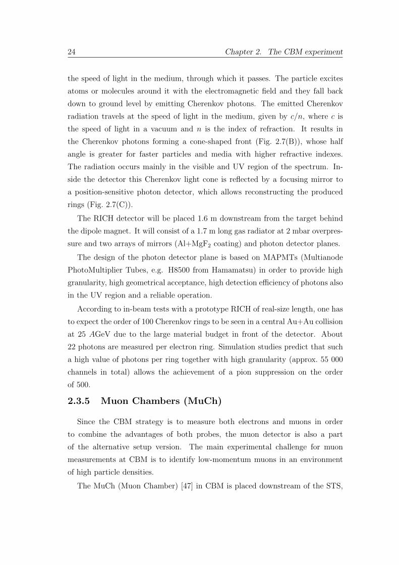
Figure 2.8: (A) The scheme of the MuCh detector configurations, optimized for different
physics cases: low-mass vector mesons (shown with red and blue frames) and J/ψ measurements
(shown with a green frame)[47]. The schematic representations of the signal generation process
in the GEM detector (C) and the straw tube detector (B).
which determines the particle momentum. The detector will exploit the standard
technique of absorber filtering.
The approved complete design of the muon detector system consists of 6 hadron
absorber layers and 18 gaseous tracking chambers organised in triplets, placed
behind each absorber slab (Fig. 2.8(A)). The first absorber is located inside the
magnet and for this reason, is made of 60 cm of nonmagnetic carbon, then iron
plates of thickness 20, 20, 20, 30, 35 and 100 cm are installed.
The muon detector system will be built in stages adapted to the beam ener-
gies available. The first two starting versions of MuCh (SIS100-A and SIS100-B)
will comprise 3 and 4 stations suitable for the measurement of low-mass vector
mesons (ρ, ω, φ) in nucleus-nucleus collisions at 4–6 AGeV and 8–14 AGeV, re-
spectively. The third version of the MuCh system (SIS100-C) will be equipped
with an additional iron absorber of 1 m thickness in order to be able to identify
muons from charmonium decay at the highest SIS100 energies.
As for tracking planes, different detector technologies will be used depending
on the hit density and the rate for a particular detector layer. The first two
26 Chapter 2. The CBM experiment
stations will consist of the triple Gas Electron Multiplier (GEM) detectors, in
order to cope with the 3 MHz/cm2 hit rate, predicted by simulations. The last
one or two stations will be made of the straw tube detectors, due to smaller hit
rates and larger areas to be covered. As the last tracking station, behind the thick
1 m absorber, four layers of the Transition Radiation Detector (TRD), which is
built for electron identification at CBM, will be used. For the full MuCh version
at SIS300, the 5th station will be made of hybrid GEM+Micromegas technology
and as the 6th station, after the 1 m iron absorber, again the four TRD layers
will be used.
The operational principle of GEM detectors (Fig. 2.8(B)) and straw
tubes (Fig. 2.8(C)) are similar and based on the avalanche effect. Straw tubes
are drift chambers consisting of a gas filled tube with a conductive inner layer
acting as a cathode and an anode wire stretched along the cylinder axis. The de-
tection is based on the electromagnetic interaction between the charged particles
traversing the gas inside a straw tube resulting in the gas ionization. Thanks to
the applied static electric field in the tube, the electrons of the primary ionization
drift towards the anode, while the ions drift towards the cathode. Due to the
high electric field strength near the thin anode wire, the drifting electrons gain
enough energy to produce an avalanche-like secondary ionization process called
gas amplification. Thus, the electric charge collected on the anode is many orders
of magnitude higher than that produced in the primary ionization.
2.3.6 Transition Radiation Detector (TRD)
The Transition Radiation Detector (TRD) [48] task is to improve identification
of electrons and positrons with respect to pions for the momenta larger than
1.5 GeV/c.
The detection is based on the the effect of transition radiation (TR) emission
by an ultrarelativistic charged particle when crossing the boundary between two
media with different dielectric constants. The total energy loss of a charged
particle during the transition depends on its Lorenz factor γ = E/mc2.
For the predicted particle momenta, the probability of producing TR by elec-
trons and positrons (γ > 1.000) is higher than by any other particle, offering the
opportunity to separate them from pions. The multiwire proportional chambers
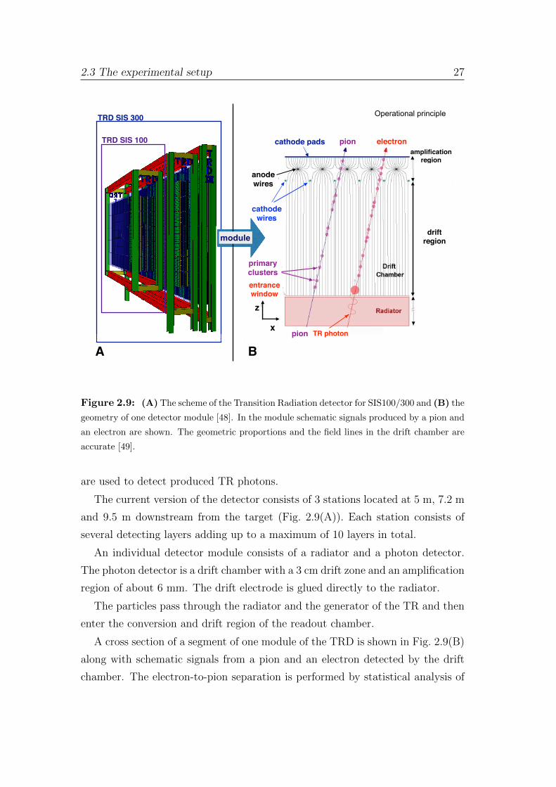
2.3 The experimental setup 27
2
23.04.2015Cyrano Bergmann CBM Collaboration Meeting: TRD
CBM TRD Design Goals
TRD design for SIS300:Detector•Geometry Max. 10 layers in 3 stations
• Electron-IdentificationPion suppression: ~ 100@ 90% electron-efficiency
• Tracking all charged particlesPosition resolution: ~200-300 µm@ high rates ( >100 kHz/cm2) and high multiplicities
•Maximum material budget ???
•Data bandwidth limitations2.5 Channels/Cluster
cathode pads electronpion
anode wires
cathode wires
primary clustersentrancewindow
pion TR photon
amplificationregion
driftregion
x
z
TRD SIS 300
TRD SIS 100
A B
module
Operational principle
Figure 2.9: (A) The scheme of the Transition Radiation detector for SIS100/300 and (B) the
geometry of one detector module [48]. In the module schematic signals produced by a pion and
an electron are shown. The geometric proportions and the field lines in the drift chamber are
accurate [49].
are used to detect produced TR photons.
The current version of the detector consists of 3 stations located at 5 m, 7.2 m
and 9.5 m downstream from the target (Fig. 2.9(A)). Each station consists of
several detecting layers adding up to a maximum of 10 layers in total.
An individual detector module consists of a radiator and a photon detector.
The photon detector is a drift chamber with a 3 cm drift zone and an amplification
region of about 6 mm. The drift electrode is glued directly to the radiator.
The particles pass through the radiator and the generator of the TR and then
enter the conversion and drift region of the readout chamber.
A cross section of a segment of one module of the TRD is shown in Fig. 2.9(B)
along with schematic signals from a pion and an electron detected by the drift
chamber. The electron-to-pion separation is performed by statistical analysis of
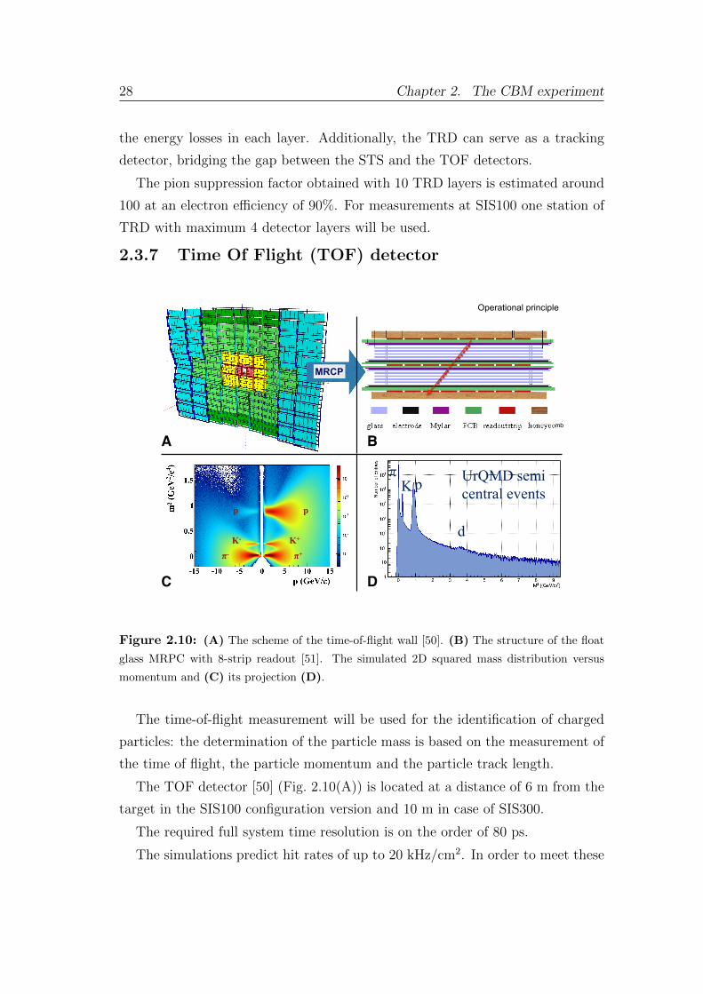
28 Chapter 2. The CBM experiment
the energy losses in each layer. Additionally, the TRD can serve as a tracking
detector, bridging the gap between the STS and the TOF detectors.
The pion suppression factor obtained with 10 TRD layers is estimated around
100 at an electron efficiency of 90%. For measurements at SIS100 one station of
TRD with maximum 4 detector layers will be used.
2.3.7 Time Of Flight (TOF) detector
pp
K+K-
π+π-
7.1. RATE CAPABILITY STUDIES 91
Figure 7.5: Strip MRPC, featuring a 10-gap 8-strip structure with float-glass electrodes of0.35 mm, 0.5 mm and 0.7 mm thickness.
Figure 7.6: Efficiency and time resolutions of the 3 modules with different electrode thicknessas function of the HV.
mb
KF Particle Finder with ToF track ID: Au+Au @ 10AGeV SIS100
10
d
p K π UrQMD semi
central events
Fragments thermal generator
MRCP
A
C D
Operational principle
B
Figure 2.10: (A) The scheme of the time-of-flight wall [50]. (B) The structure of the float
glass MRPC with 8-strip readout [51]. The simulated 2D squared mass distribution versus
momentum and (C) its projection (D).
The time-of-flight measurement will be used for the identification of charged
particles: the determination of the particle mass is based on the measurement of
the time of flight, the particle momentum and the particle track length.
The TOF detector [50] (Fig. 2.10(A)) is located at a distance of 6 m from the
target in the SIS100 configuration version and 10 m in case of SIS300.
The required full system time resolution is on the order of 80 ps.
The simulations predict hit rates of up to 20 kHz/cm2. In order to meet these
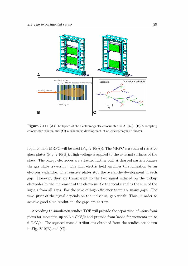
2.3 The experimental setup 29
µ = n = NA
A· pair
Electromagnetic Showers
Reminder:
X0
Dominant processes at high energies ...
Photons : Pair productionElectrons: Bremsstrahlung
Pair production:
dE
dx=
E
X0
dE
dx= 4NA
Z2
Ar2e · E ln
183
Z13
pair 7
9
4r2
eZ2 ln183
Z13
=7
9
X0
Bremsstrahlung:
E = E0ex/X0
[X0: radiation length][in cm or g/cm2]
Absorption coefficient:
After passage of one X0 electronhas only (1/e)th of its primary energy ...
[i.e. 37%]
=7
9
A
NAX0
Sampling Calorimeters
Simple shower model
! Consider only Bremsstrahlung and (symmetric) pair production
! Assume X0 ! !pair
! After t X0:
! N(t) = 2t
! E(t)/particle = E0/2t
! Process continues until E(t)<Ec
! E(tmax) = E0/2tmax = Ec
! tmax = ln(E0/Ec)/ln2
! Nmax " E0/Ec
5
Alternating layers of absorber and active material [sandwich calorimeter]
Absorber materials:[high density]
Principle:
Iron (Fe)
Lead (Pb)
Uranium (U)[For compensation ...]
Active materials:
Plastic scintillator
Silicon detectors
Liquid ionization chamber
Gas detectors
passive absorber
shower (cascade of secondaries)
active layers
incoming particle
Scheme of asandwich calorimeter
Electromagnetic shower
Lateral segmentation of the CBM ECAL (Numbers in cm). One block stands for 12x12 cm2module. The overall number of channels is 23752.
ECAL for SIS100 ECAL in CATIA
1680 mm 1080 mm 480 mm
A
B C
Operational principle
Figure 2.11: (A) The layout of the electromagnetic calorimeter ECAL [53]. (B) A sampling
calorimeter scheme and (C) a schematic development of an electromagnetic shower.
requirements MRPC will be used (Fig. 2.10(A)). The MRPC is a stack of resistive
glass plates (Fig. 2.10(B)). High voltage is applied to the external surfaces of the
stack. The pickup electrodes are attached further out. A charged particle ionizes
the gas while traversing. The high electric field amplifies this ionization by an
electron avalanche. The resistive plates stop the avalanche development in each
gap. However, they are transparent to the fast signal induced on the pickup
electrodes by the movement of the electrons. So the total signal is the sum of the
signals from all gaps. For the sake of high efficiency there are many gaps. The
time jitter of the signal depends on the individual gap width. Thus, in order to
achieve good time resolution, the gaps are narrow.
According to simulation studies TOF will provide the separation of kaons from
pions for momenta up to 3.5 GeV/c and protons from kaons for momenta up to
6 GeV/c. The squared mass distributions obtained from the studies are shown
in Fig. 2.10(B) and (C).

30 Chapter 2. The CBM experiment
2.3.8 Electromagnetic CALorimeter (ECAL)
A sampling calorimeter, in which the material that produces the particle
shower is distinct from the material that measures the deposited energy, will
be used to measure direct photons and neutral mesons decaying into photons [52]
(Fig. 2.11(A)). The passive absorber and active materials alternate with each
other as it is shown in Fig. 2.11(B).
The working principle of calorimeter is based on the total absorption of the
energy associated with the incoming particle. The particles cause an elec-
tromagnetic shower of electrons, positrons and secondary gammas, and the
summed ionization is proportional to and a good measure for the incoming energy
(Fig. 2.11(C)).
The ECAL will be composed of modules which consist of 140 layers sandwiched
of lead and scintillator sheets. The shashlik modules can be arranged either as a
wall or in a tower geometry with variable distance from the target.
2.3.9 Projectile Spectator Detector (PSD)
The determination of the reaction plane in nucleus-nucleus collisions is crucial
for several measurements, including anisotropic collective flow. The reaction
plane is defined by the impact parameter and the beam direction z (Fig. 2.12(B)).
In CBM, the reaction plane can be measured by the forward hadronic calorimeter,
referred to as the Projectile Spectator Detector [54] (Fig. 2.12(A)).
The PSD will be used to determine the collision centrality as well as the
orientation of the reaction plane. A precise characterisation of the event is of
great importance for the analysis of event-by-event observables. The study of
collective flow requires a well defined reaction plane which has to be determined
by a method not involving particles participating in the collision.
The detector is designed to measure the number of non-interacting nucleons
(spectators) from a projectile nucleus in nucleus-nucleus collisions (Fig. 2.12(B)).
The PSD is a full compensating modular lead-scintillator calorimeter, which pro-
vides very good and uniform energy resolution. It comprises 44 individual mod-
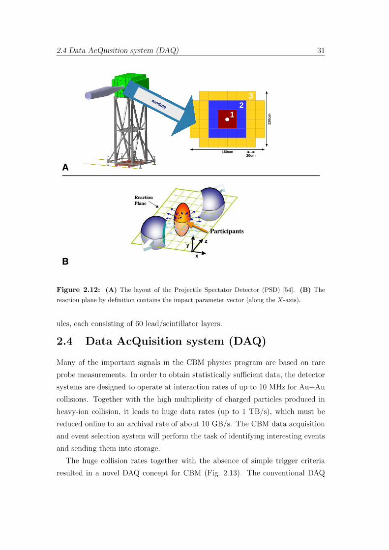
2.4 Data AcQuisition system (DAQ) 31
Projectile spectator detector 13
which contains all standard EM processes and uses a Bertini-style cascade for hadrons below 5 GeV,and the FTF (Fritiof) model for high energies above 4 GeV. As a cross check an alternative physics listQGSP_BIC_HP (which enables standard EM processes, Bertini cascade for hadrons of energy below 10GeV, and QGS model for high energies above 20 GeV) was used.
The model of the CBM subsystems used for the PSD performance study is shown in Fig. 5(left). Thegeometry includes a 250 µm thick Au target, eight silicon tracking stations (STS) [34] located 30-100cm far from the target inside the dipole magnet, the aluminum beam pipe with a variable cross sectionand thickness of a few mm, and the PSD. The optimal PSD location is at 8 (15) meters from the targetfor collision energies at SIS100 (SIS300). The transverse segmentation of the PSD is illustrated inFig. 5(right). It is elongated along the lab x direction and includes 44 modules with a 2020 cm2
cross section in the transverse plane and a beam hole formed by the inner corners of the four centralmodules which in Fig. 5(right) are marked in red color. Simulation studies performed with a smaller(and more expensive) module size of 1010 cm2 showed only marginal improvement of the reactionplane resolution.
3
2
120cm1
160cm
20cm
Fig. 5: (left) CBM detector geometry used for the PSD performance study. The simulated geometry includes (i) a250 µm thick Au target, (ii) eight silicon tracking stations STS [34] (black), (iii) a magnetic field generated by theCBM dipole magnet (dark yellow), (iv) a few mm thick aluminum beam pipe (green), and (v) the PSD (dark gray).The PSD detector is positioned at 8 (15) m from the target for performance study at SIS100 (SIS300) energies.(right) Transverse segmentation of the PSD. The PSD geometry is elongated in the horizontal direction and has 44modules with a square cross section of 2020 cm2. The central region around the beam hole (6 cm diameter) hasa 2 2 segmentation which allows to use the spectators produced very close to the beam rapidity for anisotropicflow studies. The modules used to construct subevents PSD1, PSD2, and PSD3 are marked in red, blue, and yellowcolor, respectively.
The ion beam is horizontally deflected by the field of the dipole magnet (along the x direction in thelaboratory frame) which has a nominal field integral of about 1 Tm. The PSD is shifted by xshift foreach collision energy, magnetic field strength, and detector distance to the target, such that the beamalways pass the PSD via its beam hole. The magnetic field values used in simulations and the PSD shiftalong the x direction for different detector distances from the target are shown in Tab. 1 and Fig. 6(left),respectively.
For the performance studies, the PSD modules are grouped into three classes (subevents) according to theillustration in Fig. 5(right). The subevents allow to use the PSD as a standalone detector for centralityand reaction plane determination. In the following we refer to these subevents as PSD1 (red), PSD2(blue), PSD3 (yellow), and PSD-full in case all modules are used together.
Com
pres
sed
Bar
yoni
cM
atte
rExp
erim
ent
Technical Design Reportfor the CBM Experiment
Projectile spectator detector (PSD)
The CBM Collaboration
October 2014
module
A
B (GeV/c)q/nTp
0 0.5 1 1.5 2q
/n2
v0
0.05
0.1
(a)
(GeV)q
/nTKE
0 0.5 1 1.5 2
(b) (PHENIX)-π++π
(PHENIX)-+K+K (STAR)S
0K
(PHENIX)pp+ (STAR)Λ+Λ
(STAR)+
Ξ+-Ξ
Figure 15: (left) Almond shaped overlap zone generated just after an A+A collision where theincident nuclei are moving along the ±z axis. The reaction plane by definition contains the impactparameter vector (along the x axis) [55]. (right) Measurements of elliptical-flow (v2) for identifiedhadrons plotted as v2 divided by the number of constituent quarks nq in the hadron as a functionof (a) pT /nq, (b) KET /nq [56].
plane R is defined to be along the impact parameter vector, the x axis in Fig. 15:
Ed3N
dp3=
d3N
pT dpT dyd=
d3N
2 pT dpT dy
"1 +
X
n
2vn cos n( R)
#. (2)
The expansion parameter v2, called elliptical flow, is predominant at mid-rapidity. In general,the fact that flow is observed in final state hadrons shows that thermalization is rapid, so thathydrodynamics comes into play at a time, 0, which is before the spatial anisotropy of the overlapalmond dissipates. At this early stage hadrons have not formed and it has been proposed that theconstituent quarks flow [59], so that the flow should be proportional to the number of constituentquarks nq, in which case v2/nq as a function of pT /nq would represent the constituent quark flow as afunction of constituent quark transverse momentum and would be universal. However, in relativistichydrodynamics, at mid-rapidity, the transverse kinetic energy, mT m0 = (T 1)m0 KET ,rather than pT , is the relevant variable; and in fact v2/nq as a function of KET /nq seems to exhibitnearly perfect scaling [56] (Fig. 15b).
The fact that the flow persists for pT > 1 GeV/c (Fig. 16a) implies that the viscosity is small [60],perhaps as small as a quantum viscosity bound from string theory [61], /s = 1/(4) where is theshear viscosity and s the entropy density per unit volume. This has led to the description of the“sQGP” produced at RHIC as “the perfect fluid” [9]. An estimate [62] of /s for nuclear matterand for several common fluids, as a function of the fractional di↵erence of the temperature from thecritical temperature, at fixed pressure, is shown in Fig. 16b. This particular estimate [62] for theQGP at RHIC is quite close to the quantum bound (solid line). Also, empirically, for all commonfluids /s is a minimum at or near the critical point [63] which might suggest that the conditionsat RHIC energies are near the QCD critical point.
5.1 Two-Particle Correlations and Flow
In addition to measuring flow by the correlation of individual particles to the reaction plane, it isalso possible to measure flow by the correlation of two particles to each other. The advantage of
16
Participants
Figure 2.12: (A) The layout of the Projectile Spectator Detector (PSD) [54]. (B) The
reaction plane by definition contains the impact parameter vector (along the X-axis).
ules, each consisting of 60 lead/scintillator layers.
2.4 Data AcQuisition system (DAQ)
Many of the important signals in the CBM physics program are based on rare
probe measurements. In order to obtain statistically sufficient data, the detector
systems are designed to operate at interaction rates of up to 10 MHz for Au+Au
collisions. Together with the high multiplicity of charged particles produced in
heavy-ion collision, it leads to huge data rates (up to 1 TB/s), which must be
reduced online to an archival rate of about 10 GB/s. The CBM data acquisition
and event selection system will perform the task of identifying interesting events
and sending them into storage.
The huge collision rates together with the absence of simple trigger criteria
resulted in a novel DAQ concept for CBM (Fig. 2.13). The conventional DAQ
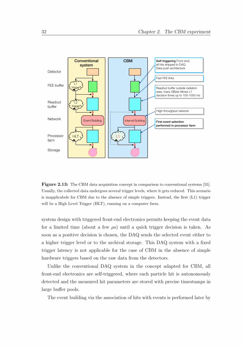
32 Chapter 2. The CBM experiment
Dirk Hutter – DPG Spring Meeting Heidelberg – 2015-03-27
CBM
Interval Building
L1
15
CBM Readout ArchitectureConventional
systemDetector
FEE buffer
Readoutbuffer
Network
Processorfarm
Storage
Self-triggering Front-end;all hits shipped to DAQ.Data push architecture
High-throughput network
First event selectionperformed in processor farm
Readout buffer outside radiation area, many GByte Allows L1 decision times up to 100-1000 ms
Fast FEE links
Typical Parameters:1% occupancy, 107 int./s
100 kHz channel hit rate 1 MByte/s per channel
whole CBM: ~ 1 TByte/s
Event Building
HLT
L1trigger
L2trigger
Figure 2.13: The CBM data acquisition concept in comparison to conventional systems [55].
Usually, the collected data undergoes several trigger levels, where it gets reduced. This scenario
is inapplicabele for CBM due to the absence of simple triggers. Instead, the first (L1) trigger
will be a High Level Trigger (HLT), running on a computer farm.
system design with triggered front-end electronics permits keeping the event data
for a limited time (about a few µs) until a quick trigger decision is taken. As
soon as a positive decision is chosen, the DAQ sends the selected event either to
a higher trigger level or to the archival storage. This DAQ system with a fixed
trigger latency is not applicable for the case of CBM in the absence of simple
hardware triggers based on the raw data from the detectors.
Unlike the conventional DAQ system in the concept adapted for CBM, all
front-end electronics are self-triggered, where each particle hit is autonomously
detected and the measured hit parameters are stored with precise timestamps in
large buffer pools.
The event building via the association of hits with events is performed later by
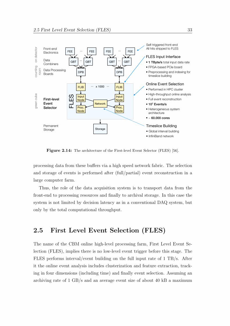
2.5 First Level Event Selection (FLES) 33
Jan de Cuveland – The CBM First-level Event Selector – DPG Spring Meeting 2015 – Heidelberg, Germany, 2015-03-26
CBM Readout Structure
4
on d
etec
tor
coun
ting
room
gree
n cu
be
Self-triggered front-endAll hits shipped to FLES
FLES Input Interface• 1 TByte/s total input data rate
• FPGA-based PCIe board
• Preprocessing and indexing for timeslice building
Timeslice Building• Global interval building
• InfiniBand network
Online Event Selection• Performed in HPC cluster
• High-throughput online analysis
• Full event reconstruction
• 107 Events/s • Heterogeneous system
architecture
• ~ 60.000 cores
FLES
FLIB
Input Node
FEE
GBT
DPB
GBT
FEE...
...
Proc. Node
FLIB
FEE
GBT
DPB
GBT
FEE...
...
Front-end Electronics
DataCombiners
Data Processing Boards
StoragePermanent Storage
First-level Event Selector
...
Input Node
Proc. Node
Network
x 1000...
Figure 2.14: The architecture of the First-level Event Selector (FLES) [56].
processing data from these buffers via a high speed network fabric. The selection
and storage of events is performed after (full/partial) event reconstruction in a
large computer farm.
Thus, the role of the data acquisition system is to transport data from the
front-end to processing resources and finally to archival storage. In this case the
system is not limited by decision latency as in a conventional DAQ system, but
only by the total computational throughput.
2.5 First Level Event Selection (FLES)
The name of the CBM online high-level processing farm, First Level Event Se-
lection (FLES), implies there is no low-level event trigger before this stage. The
FLES performs interval/event building on the full input rate of 1 TB/s. After
it the online event analysis includes clusterization and feature extraction, track-
ing in four dimensions (including time) and finally event selection. Assuming an
archiving rate of 1 GB/s and an average event size of about 40 kB a maximum
34 Chapter 2. The CBM experiment
event rate of 25 kHz can be accepted for permanent storage. Thus, if the primary
event rate is 10 MHz, the required data reduction factor is at least 400.
The FLES will be a scalable high-performance computer farm. It will consist
of different available types of computing devices, including FPGAs at the first
stages of the system and heterogeneous many-core CPU/GPU architectures to
achieve fast and efficient event reconstruction. The architecture of the First-Level
Event Selection farm is summarized in Fig. 2.14. In total, there are 1000 links at
10 GBit/s transmitting data into FLES.
Online event analysis will be performed by processing nodes estimated to
require in total approximately 60 000 cores (year 2010 equivalent). A high-
throughput network infrastructure will connect all nodes and enable interval
building at the full input data rate of 10 MHz.
Chapter 3
High Performance Computing
HEP has always been a data-intensive domain due to the fundamental feature
of quantum mechanics, namely its probabilistic nature. HEP experiments are
aiming to register rare relevant events, which can only be obtained within a large
number of observations. In order to achieve this challenging goal, particle physics
has done a long way from using bubble chambers with collision rates of about
1 collision per minute to modern HEP detectors with rates counted in MHz.
Thus, modern tracking detectors generate huge amounts of analog data at rates
equivalent to petabytes per second, that is beyond the generally known bounds
to be considered “Big Data”. It poses a great challenge of collecting, storing and
reducing these large volumes of data. The experimental information has to be
analyzed online in order to select and store relevant events, since only reducing
the data volume by orders of magnitude in real time can allow for meeting the
recording rates achievable nowadays. For this reason computing plays a crucial
role in HEP.
In fact, HEP experiments are not only one of the main consumers of High Per-
formance Computing (HPC), but also the area, which is pushing the development
in computer capability by its constantly increasing computational demands.
This chapter will give a brief overview of existing HPC hardware architectures
and software frameworks, which allow for the use of parallel hardware in a con-
venient and efficient way. Special emphasis will be given to the hardware and
software tools, which were used to develop the 4D CA track finder algorithm
within the current thesis.
36 Chapter 3. High performance computing
3.1 Hardware architecture and its implications
for parallel programming
Until 2004 software developers could improve the speed of single-threaded pro-
grams without much efforts on their part due to the constant increase in frequency
of processors. However, this trend has reached its limits due to the frequency-
power wall and physical limitations of semi-conductor technology.
Instead, all computer manufacturers have turned to a parallel architecture as
the new HPC paradigm. For the developers it meant that the so-called “free
lunch” era [57], when performance was improving with new computer architec-
tures without any contribution from the developers’ side, was replaced by the
parallel era, when the performance improvement may only be gained at the cost
of programming effort.
Modern computer technologies allow performing a number of calculations si-
multaneously. In other words computer architectures nowadays are parallel. In
order to use such architectures efficiently, one needs to exploit distributed cal-
culations within one super computer — a many- or multi-core server, equipped
with vector registers.
Multi-core processors can offer significant performance improvements over
their single-core counterparts for certain kinds of parallelized tasks, often de-
manding new programming paradigms to efficiently utilize the complex archi-
tecture involved [58]. Future trends promise that computing power will further
evolve in a parallel direction, gaining more cores per processing unit and more
elements per vector register.
In this case it is crucial to exploit the full potential of this complex hardware.
In order to get maximum performance out of future computer architectures, de-
velopers should design programs so that the speed of resulting applications scales
with the number of parallel elements in the heterogeneous system. Ideally, im-
plemented algorithms should show linear scalability in a parallel run. Modern
parallel architectures present unique challenges for the software designers since
the structure of these architectures has significant impact on the way work is
scheduled, memory is allocated, and instructions are executed.
Modern applications need to be designed with parallelism in mind from the
3.1 Hardware architecture and its implications for parallel programming 37
very beginning. However, there is no chance to write software, which fully utilize
the power of modern complicated computer architectures, without understanding
of the hardware, on which the software will be executed.
Thus, achieving this challenging goal is not possible without expertise in un-
derstanding underlying hardware architecture. In order to classify all existing
parallel systems, they were organized into a coherent and simple taxonomy.
3.1.1 Flynn’s taxonomy
By far the most commonly used computer architecture classification is the
taxonomy [59] proposed by Michael Flynn. The classification characterizes com-
puter designs in terms of the number of instructions streams issued at a time
and the number of data elements they operate on. Flynn’s taxonomy classifies
machines according to whether they have one or more than one stream of each
type (Fig. 3.1).
There are four possibilities:
• SISD (Single Instruction stream, Single Data stream),
• SIMD (Single Instruction stream, Multiple Data streams),
• MISD (Multiple Instruction streams, Single Data stream),
• MIMD (Multiple Instruction streams, Multiple Data streams).
The classical von Neumann approach can be described by Single-Instruction-
Single-Data (SISD) type. However, SISD is not necessarily completely sequential
architecture, since some instructions from the same stream may be executed
concurrently (see instruction level parallelism).
The revolutionary alternative was Single-Instruction-Multiple-Data (SIMD),
which appeared in the mid-60s and describes performing the same operation over
a multiple data set simultaneously. This can be done both in signal-threaded
and multi-threaded applications. Multiple-Instruction-Single-Data (MISD) is a
rarely used type. Although there were computer architectures to deal with this
type of parallelism (such as systolic arrays), there are few applications that can
benefit from this type of hardware.
Multiple-instruction-multiple-data (MIMD) programs are by far the most com-
mon type of parallel programs, that correspond to multiple processors, each using
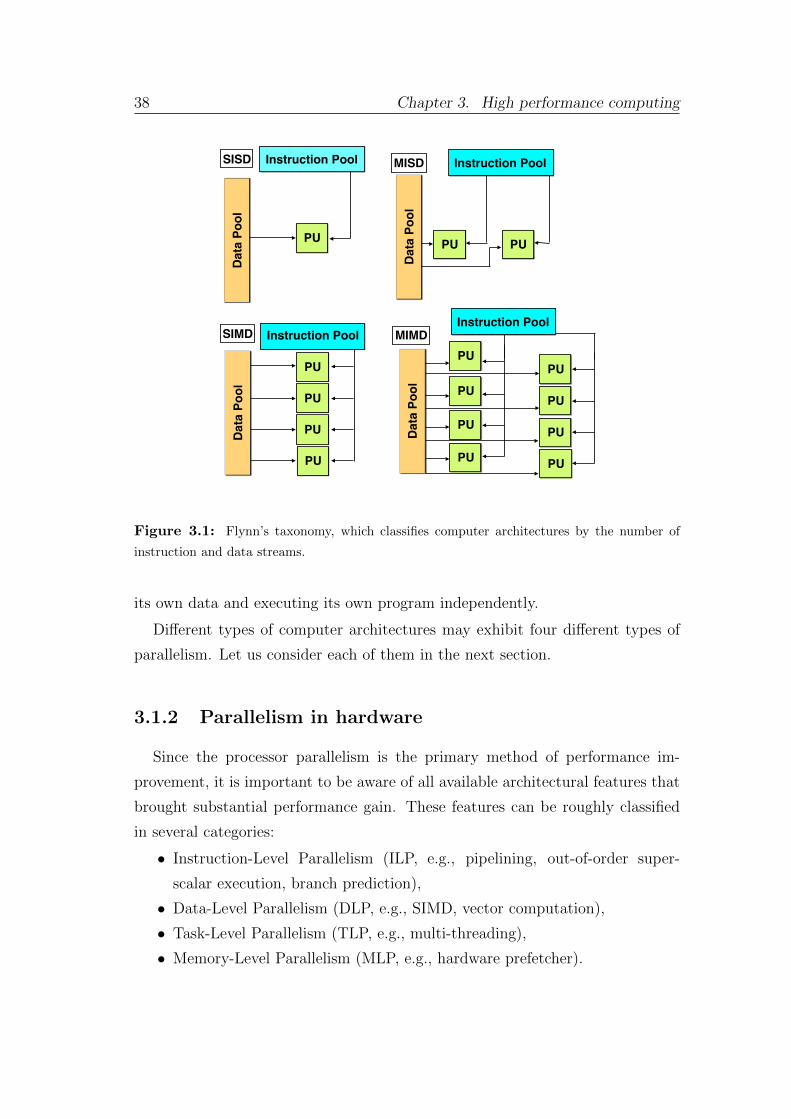
38 Chapter 3. High performance computing
PU
Instruction Pool
Dat
a Po
ol
SISD Instruction Pool
PU PU
Dat
a Po
ol
MISD
Dat
a Po
ol
Instruction Pool
PU
PU
PU
PU
SIMD
PU
PU
PU
PU
PU
PU
PU
PU
MIMD
Dat
a Po
ol
Instruction Pool
Figure 3.1: Flynn’s taxonomy, which classifies computer architectures by the number of
instruction and data streams.
its own data and executing its own program independently.
Different types of computer architectures may exhibit four different types of
parallelism. Let us consider each of them in the next section.
3.1.2 Parallelism in hardware
Since the processor parallelism is the primary method of performance im-
provement, it is important to be aware of all available architectural features that
brought substantial performance gain. These features can be roughly classified
in several categories:
• Instruction-Level Parallelism (ILP, e.g., pipelining, out-of-order super-
scalar execution, branch prediction),
• Data-Level Parallelism (DLP, e.g., SIMD, vector computation),
• Task-Level Parallelism (TLP, e.g., multi-threading),
• Memory-Level Parallelism (MLP, e.g., hardware prefetcher).
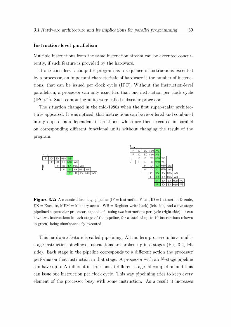
3.1 Hardware architecture and its implications for parallel programming 39
Instruction-level parallelism
Multiple instructions from the same instruction stream can be executed concur-
rently, if such feature is provided by the hardware.
If one considers a computer program as a sequence of instructions executed
by a processor, an important characteristic of hardware is the number of instruc-
tions, that can be issued per clock cycle (IPC). Without the instruction-level
parallelism, a processor can only issue less than one instruction per clock cycle
(IPC<1). Such computing units were called subscalar processors.
The situation changed in the mid-1980s when the first super-scalar architec-
tures appeared. It was noticed, that instructions can be re-ordered and combined
into groups of non-dependent instructions, which are then executed in parallel
on corresponding different functional units without changing the result of the
program.
IF ID EX MEM WB
IF ID EX MEM WB
IF ID EX WBMEM
IF ID EX MEM WB
IF ID EX WBMEM
IF ID EX MEM WBIF ID EX MEM WB
IF ID EX MEM WB
t
iIFIF
IFIF IDID
IDID
EXEX
EXEX MEM
MEM
MEM WBWB
WBWBMEM
t
i
IF ID EX MEM WB
IF ID EX MEM WBIF ID EX MEM WB
Figure 3.2: A canonical five-stage pipeline (IF = Instruction Fetch, ID = Instruction Decode,
EX = Execute, MEM = Memory access, WB = Register write back) (left side) and a five-stage
pipelined superscalar processor, capable of issuing two instructions per cycle (right side). It can
have two instructions in each stage of the pipeline, for a total of up to 10 instructions (shown
in green) being simultaneously executed.
This hardware feature is called pipelining. All modern processors have multi-
stage instruction pipelines. Instructions are broken up into stages (Fig. 3.2, left
side). Each stage in the pipeline corresponds to a different action the processor
performs on that instruction in that stage. A processor with an N -stage pipeline
can have up to N different instructions at different stages of completion and thus
can issue one instruction per clock cycle. This way pipelining tries to keep every
element of the processor busy with some instruction. As a result it increases
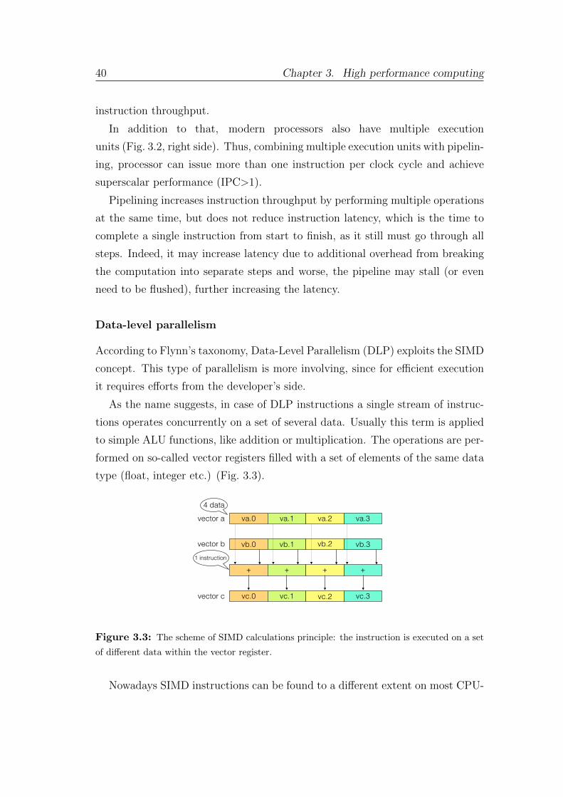
40 Chapter 3. High performance computing
instruction throughput.
In addition to that, modern processors also have multiple execution
units (Fig. 3.2, right side). Thus, combining multiple execution units with pipelin-
ing, processor can issue more than one instruction per clock cycle and achieve
superscalar performance (IPC>1).
Pipelining increases instruction throughput by performing multiple operations
at the same time, but does not reduce instruction latency, which is the time to
complete a single instruction from start to finish, as it still must go through all
steps. Indeed, it may increase latency due to additional overhead from breaking
the computation into separate steps and worse, the pipeline may stall (or even
need to be flushed), further increasing the latency.
Data-level parallelism
According to Flynn’s taxonomy, Data-Level Parallelism (DLP) exploits the SIMD
concept. This type of parallelism is more involving, since for efficient execution
it requires efforts from the developer’s side.
As the name suggests, in case of DLP instructions a single stream of instruc-
tions operates concurrently on a set of several data. Usually this term is applied
to simple ALU functions, like addition or multiplication. The operations are per-
formed on so-called vector registers filled with a set of elements of the same data
type (float, integer etc.) (Fig. 3.3).
va.0
vb.0
+
vc.0
+ + +
vb.1 vb.2 vb.3
va.1 va.2 va.3
vc.1 vc.2 vc.3
vector a
vector b
vector c
4 data
1 instruction
Figure 3.3: The scheme of SIMD calculations principle: the instruction is executed on a set
of different data within the vector register.
Nowadays SIMD instructions can be found to a different extent on most CPU-
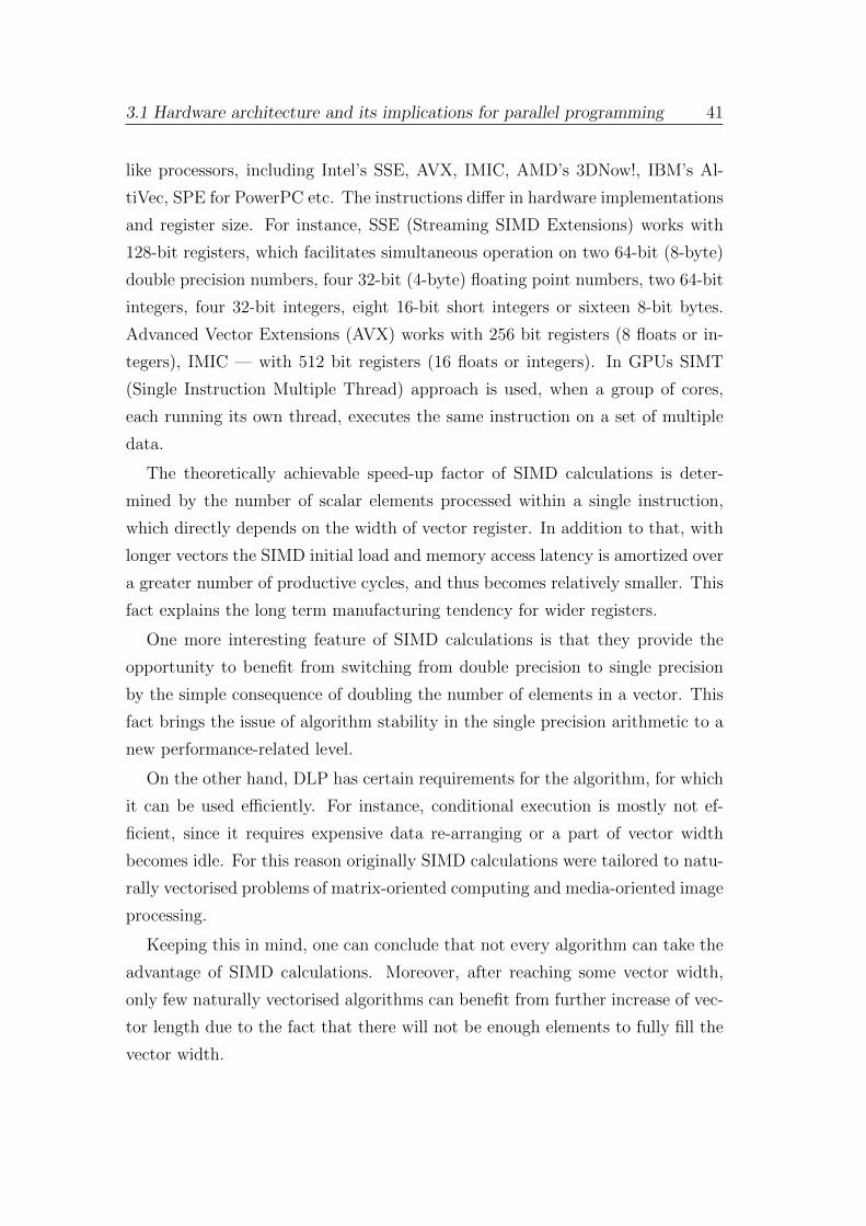
3.1 Hardware architecture and its implications for parallel programming 41
like processors, including Intel’s SSE, AVX, IMIC, AMD’s 3DNow!, IBM’s Al-
tiVec, SPE for PowerPC etc. The instructions differ in hardware implementations
and register size. For instance, SSE (Streaming SIMD Extensions) works with
128-bit registers, which facilitates simultaneous operation on two 64-bit (8-byte)
double precision numbers, four 32-bit (4-byte) floating point numbers, two 64-bit
integers, four 32-bit integers, eight 16-bit short integers or sixteen 8-bit bytes.
Advanced Vector Extensions (AVX) works with 256 bit registers (8 floats or in-
tegers), IMIC — with 512 bit registers (16 floats or integers). In GPUs SIMT
(Single Instruction Multiple Thread) approach is used, when a group of cores,
each running its own thread, executes the same instruction on a set of multiple
data.
The theoretically achievable speed-up factor of SIMD calculations is deter-
mined by the number of scalar elements processed within a single instruction,
which directly depends on the width of vector register. In addition to that, with
longer vectors the SIMD initial load and memory access latency is amortized over
a greater number of productive cycles, and thus becomes relatively smaller. This
fact explains the long term manufacturing tendency for wider registers.
One more interesting feature of SIMD calculations is that they provide the
opportunity to benefit from switching from double precision to single precision
by the simple consequence of doubling the number of elements in a vector. This
fact brings the issue of algorithm stability in the single precision arithmetic to a
new performance-related level.
On the other hand, DLP has certain requirements for the algorithm, for which
it can be used efficiently. For instance, conditional execution is mostly not ef-
ficient, since it requires expensive data re-arranging or a part of vector width
becomes idle. For this reason originally SIMD calculations were tailored to natu-
rally vectorised problems of matrix-oriented computing and media-oriented image
processing.
Keeping this in mind, one can conclude that not every algorithm can take the
advantage of SIMD calculations. Moreover, after reaching some vector width,
only few naturally vectorised algorithms can benefit from further increase of vec-
tor length due to the fact that there will not be enough elements to fully fill the
vector width.
42 Chapter 3. High performance computing
For this reason, there is a more recent trend of having more registers, each
register being quite short compared to the traditional length. This offers more
flexibility to the algorithm implementation and allows for more sophisticated
compiler optimizations, while reducing hardware complexity.
Despite the non-trivial task, some compilers provide auto-vectorization. Un-
fortunately, in this case the developer usually has no control over the process and
in the end gets poor speed-up factor in comparison with potential values.
Summarizing, exploiting SIMD instructions in the algorithm implementations
can be a tricky task and strongly depends on the algorithm choice. However
effective use of SIMD instructions promises a great speed-up potential, which
would be unwise to ignore.
Task-level parallelism
When the evolution of hardware design turned in the direction of parallel ar-
chitectures, the vendors started to clone the whole core multiple times, allowing
multiple threads to perform execution in parallel. As a first step, architects
cloned the big cores used in single-core processors multiple times to create multi-
core processors. Although these cores were operating with a lower frequency than
in an equivalent single-core processor for the lower power consumption sake, still
parallel processing provided a much bigger computing power gain than the loss
due to core frequency reduction. However full-sized core cloning is limited and
in order to gain more parallelism, the vendors have created architectures with
simpler cores running at even lower frequencies but numbered in dozens. This
massive level of parallelism of many- and multicore architecture can be exploited
only by the applications, that have a multi-threaded design.
In contrast to DLP, Thread-Level Parallelism (or TLP) exhibits more flexibil-
ity, since in this case generally speaking each thread can perform independent
task. This involves executing individual streams of instructions delegated to dif-
ferent cores of a processor simultaneously. Each process maintains its data and
instructions, so that it may be considered an independent task, even if processes
are performing parts of one global task and synchronized with each other. For
this reason this type of parallelism follows the concept of MIMD architecture, if
we consider Flynn’s taxonomy.
3.1 Hardware architecture and its implications for parallel programming 43
Tim
e 1
Problem
PARALLEL
compute unit
SCALARTask1
Problem
Task2
Task3
……
…Taskn
Tim
e 2
Tim
e 3
Tim
e k
compute unit compute
unit
compute unit
compute unit
Figure 3.4: The scheme of task-level parallelism principle. The tasks are distributed between
threads. The execution time is defined by the last thread to finish.
Conceptually, it is straightforward to see why TLP speeds up an execution.
If one considers the threads, which are truly independent, then distributing a
set of threads among available cores on a processor would reduce the elapsed
execution time to the execution time of the last thread to finish, compared to
a sequential version which would require the sum of execution times of all of
the threads. To achieve the maximum performance the work should be evenly
divided among threads in such a way, that they finish execution at the same
time. Fig. 3.4 illustrates these conceptual differences between single threading
and thread-level parallelism, assuming independence and no thread allocating or
scheduling overhead.
Unfortunately, in real life this idealistic scenario is affected by several factors.
The main performance impacting factors are: limited level of execution inde-
pendence and synchronization overhead, scheduling and disproportion in thread
load, limited thread memory.
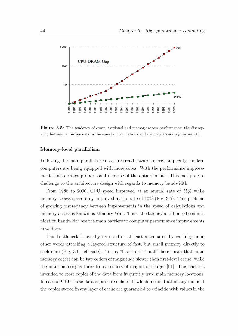
44 Chapter 3. High performance computing
Figure 3.5: The tendency of computantional and memory access performance: the discrep-
ancy between improvements in the speed of calculations and memory access is growing [60].
Memory-level parallelism
Following the main parallel architecture trend towards more complexity, modern
computers are being equipped with more cores. With the performance improve-
ment it also brings proportional increase of the data demand. This fact poses a
challenge to the architecture design with regards to memory bandwidth.
From 1986 to 2000, CPU speed improved at an annual rate of 55% while
memory access speed only improved at the rate of 10% (Fig. 3.5). This problem
of growing discrepancy between improvements in the speed of calculations and
memory access is known as Memory Wall. Thus, the latency and limited commu-
nication bandwidth are the main barriers to computer performance improvements
nowadays.
This bottleneck is usually removed or at least attenuated by caching, or in
other words attaching a layered structure of fast, but small memory directly to
each core (Fig. 3.6, left side). Terms “fast” and “small” here mean that main
memory access can be two orders of magnitude slower than first-level cache, while
the main memory is three to five orders of magnitude larger [61]. This cache is
intended to store copies of the data from frequently used main memory locations.
In case of CPU these data copies are coherent, which means that at any moment
the copies stored in any layer of cache are guarantied to coincide with values in the
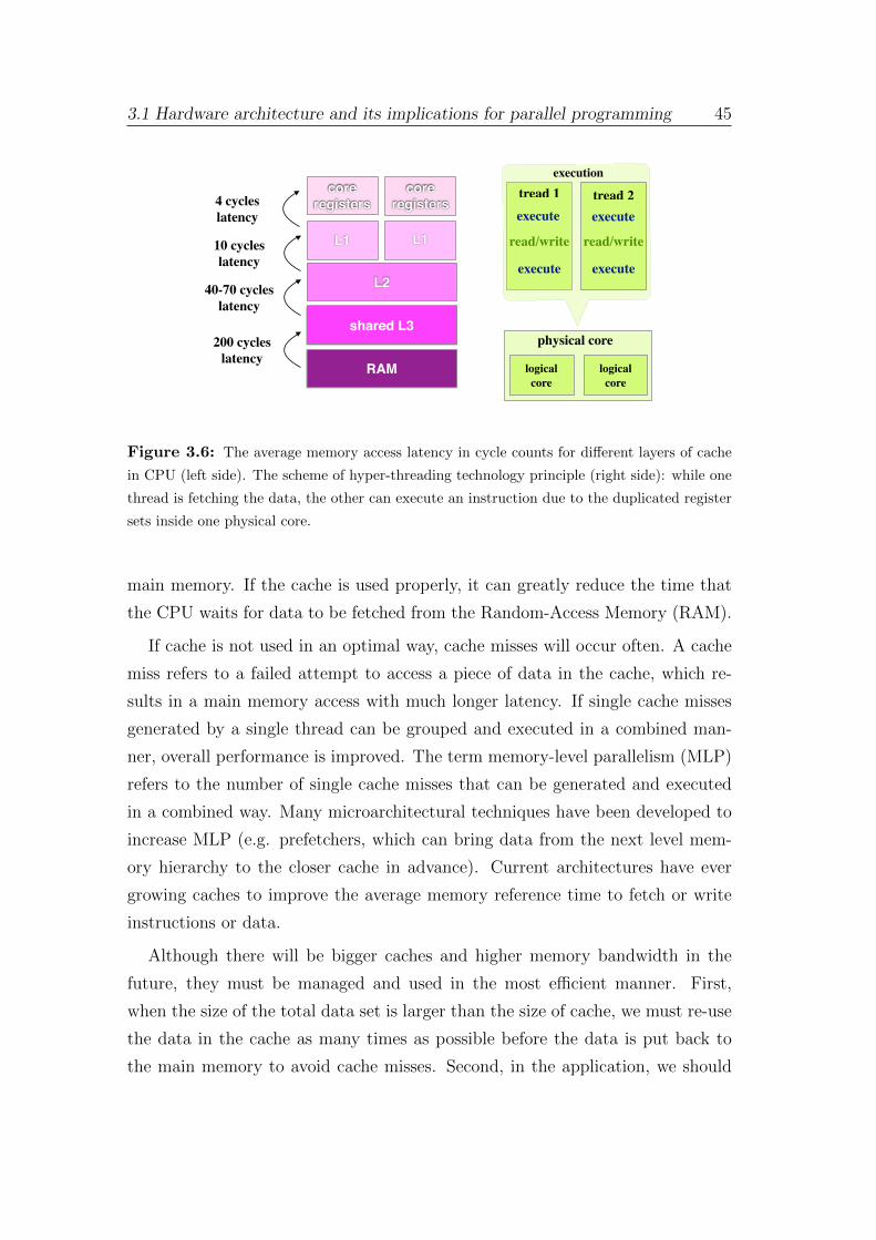
3.1 Hardware architecture and its implications for parallel programming 45
shared L3
RAM
L2
L1 L1
core registers
core registers
200 cycles latency
40-70 cycles latency
10 cycles latency
4 cycles latency
tread 1execution
…execute
read/write
execute execute
read/write
executetread 2
physical core
logical core
logical core
Figure 3.6: The average memory access latency in cycle counts for different layers of cache
in CPU (left side). The scheme of hyper-threading technology principle (right side): while one
thread is fetching the data, the other can execute an instruction due to the duplicated register
sets inside one physical core.
main memory. If the cache is used properly, it can greatly reduce the time that
the CPU waits for data to be fetched from the Random-Access Memory (RAM).
If cache is not used in an optimal way, cache misses will occur often. A cache
miss refers to a failed attempt to access a piece of data in the cache, which re-
sults in a main memory access with much longer latency. If single cache misses
generated by a single thread can be grouped and executed in a combined man-
ner, overall performance is improved. The term memory-level parallelism (MLP)
refers to the number of single cache misses that can be generated and executed
in a combined way. Many microarchitectural techniques have been developed to
increase MLP (e.g. prefetchers, which can bring data from the next level mem-
ory hierarchy to the closer cache in advance). Current architectures have ever
growing caches to improve the average memory reference time to fetch or write
instructions or data.
Although there will be bigger caches and higher memory bandwidth in the
future, they must be managed and used in the most efficient manner. First,
when the size of the total data set is larger than the size of cache, we must re-use
the data in the cache as many times as possible before the data is put back to
the main memory to avoid cache misses. Second, in the application, we should
46 Chapter 3. High performance computing
minimize the number of random memory accesses and try to keep the data locally
in order to benefit from the lined manner of cache reading. There was no efficient
random-access machine model for parallel computing established.
On the other hand, in case of many-core processors, if multiple threads attempt
to write to the same memory location at the same time, they must wait to
resolve conflicts. Thus, having threads writing to different areas of shared memory
would be preferable in decreasing the likelihood of incurring these time-consuming
conflicts.
By far the most popular solution to this problem is Non-Uniform Memory
Access (NUMA) architecture. The idea is to place data used by one particular
core physically closer to that core in the memory. The opposite situation we
could observe in so-called UMA (Uniform Memory Access) architecture, where
each processor must use the same shared bus (or another type of interconnect)
to access shared memory, resulting in a memory access time that is uniform to
all processors.
In the NUMA shared memory architecture, each processor has its own local
memory module, which it can access directly with a distinctive performance ad-
vantage. At the same time, it can also access any memory module belonging to
another processor using a shared bus.
Like most other processor architectural features, ignorance of NUMA can result
in subpar application memory performance. In order to benefit from the NUMA
architecture features, it is important that one keeps the data used by a certain
processor in the corresponding memory slot.
3.2 Architectures specification
This section will briefly illustrate modern computer architecture features on the
examples of several recent microprocessors and computer systems.
3.2.1 CPU architecture
To illustrate the complexity of modern CPUs, let us consider lxir039 server at
GSI (Fig. 3.7). Typically modern CPUs have 2 to 4 sockets. The lxir039 server
3.2 Architectures specification 47
contains 2 Intel Xeon X5550 CPUs, connected with each other via Quick Path
Interconnect (QPI) [62].
The Intel Xeon CPU X5550 is a server processor that was first available for
purchase in March 2009. It operates at a stock clock speed of 2.67 GHz. It has
a 4-core model, resulting in a high multi-tasking potential. In addition to that,
this processor supports Intel Hyper-Threading Technology (HTT) [63].
The HTT results in the fact that for each of 4 cores, that are physically present,
the operating system addresses two virtual or logical cores, and shares the work-
load between them when possible. For this reason the number of independent
instructions in the pipeline gets increased and the advantage of superscalar ar-
chitecture can be used in a more efficient way.
It becomes possible since architecturally a core with HTT consists of two
logical cores, each of which has its own processor architectural state. HTT works
by duplicating certain sections of the processor, those that store the architectural
state, but not duplicating the main execution resources.
Each logical core has its own Advanced Programmable Interrupt Controller
(APIC), and, thus, can be individually halted, interrupted or directed to execute
a specified thread, independently from the other logical processor sharing the
same physical core. Also, each logical core has its own full set of registers.
However, unlike the case of two independent physical cores, the logical core
in a hyper-threaded processor share some execution resources: execution engine,
including Arithmetic Logic Unit (ALU), Floating Point Unit (FPU), and Vector
Processing Unit (VPU), caches, and system bus interface.
The main HTT principle is illustrated in Fig. 3.6 (right side): when one logic
core stalls due to a cache miss or data dependency and is waiting for data, the
other one can use those execution resources to execute another scheduled task.
The extent to which execution can benefit from the presence of HTT depends
on the needs of a certain application and was estimated by Intel to performance
gains of up to 30% [64] .
For example, the lxir039 server at GSI (Fig. 3.7) is equipped with two Intel
Xeon X5550 processors and can operate in total with 16 threads in parallel.
Following the NUMA concept 24 GB of RAM is attached to each CPU. QPI
allows CPUs to access remote memory of each other.
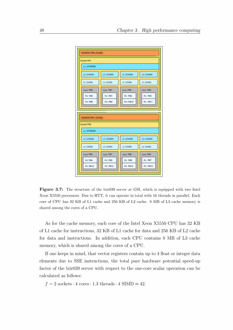
48 Chapter 3. High performance computing
NUMAN P#0 (24GB)
NUMAN P#1 (24GB)
Socket P#0
Socket P#1
(8192KB)
(8192KB)
P#0 P#1 P#2 P#3
P#0 P#1 P#2 P#3
P#0 P#1 P#2 P#3
P#8 P#9 P#10 P#11
P#4
P#12 P#13 P#14 P#15
P#5 P#6 P#7
Figure 3.7: The structure of the lxir039 server at GSI, which is equipped with two Intel
Xeon X5550 processors. Due to HTT, it can operate in total with 16 threads in parallel. Each
core of CPU has 32 KB of L1 cache and 256 KB of L2 cache. 8 MB of L3 cache memory is
shared among the cores of a CPU.
As for the cache memory, each core of the Intel Xeon X5550 CPU has 32 KB
of L1 cache for instructions, 32 KB of L1 cache for data and 256 KB of L2 cache
for data and instructions. In addition, each CPU contains 8 MB of L3 cache
memory, which is shared among the cores of a CPU.
If one keeps in mind, that vector registers contain up to 4 float or integer data
elements due to SSE instructions, the total pure hardware potential speed-up
factor of the lxir039 server with respect to the one-core scalar operation can be
calculated as follows:
f = 2 sockets · 4 cores · 1.3 threads · 4 SIMD ≈ 42.
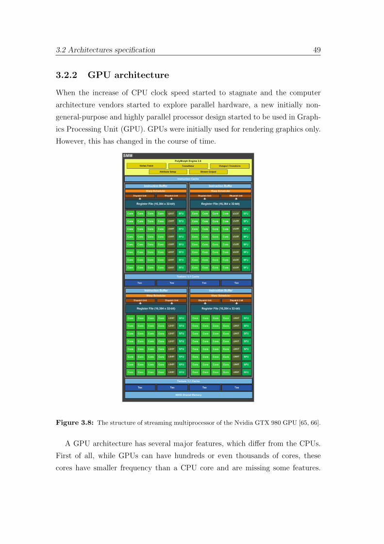
3.2 Architectures specification 49
3.2.2 GPU architecture
When the increase of CPU clock speed started to stagnate and the computer
architecture vendors started to explore parallel hardware, a new initially non-
general-purpose and highly parallel processor design started to be used in Graph-
ics Processing Unit (GPU). GPUs were initially used for rendering graphics only.
However, this has changed in the course of time.
Figure 3.8: The structure of streaming multiprocessor of the Nvidia GTX 980 GPU [65, 66].
A GPU architecture has several major features, which differ from the CPUs.
First of all, while GPUs can have hundreds or even thousands of cores, these
cores have smaller frequency than a CPU core and are missing some features.
50 Chapter 3. High performance computing
The missing features include interrupts and virtual memory, which are required
to implement a modern operating system. It has a major consequence on the way
an application for a GPU can be designed. Secondly, the speed of access between
a CPU and its larger pool of RAM is slower than GPUs, which typically contain
a smaller amount of more expensive memory that is very much faster to access.
In other words, CPUs and GPUs have significantly different architectures that
make them better suited to different tasks. A GPU can handle large amounts of
data in many streams, performing relatively simple operations on them, but is
not suited to heavy or complex processing on a single or a few streams of data.
A CPU is much faster on a per-core basis and can perform complex operations
on a single or few streams of data more easily, but is not as efficient in handling
as many streams as GPU simultaneously.
While GPU has many benefits such as more computing power, larger memory
bandwidth and low power consumption with regard to high computing ability,
there are some constraints as far as full utilization of its processing power is
concerned. These constraints make performance optimization more difficult.
On top of this, the debugging environment is not as powerful as in general
CPU. Therefore, developing a code with GPU can take more time and needs more
sophisticated work and fine-tuning. Being heavily parallel, the GPU architecture
requires a developer to cope with massive data partitioning and synchronization.
Often, the algorithms should be heavily redesigned in order to achieve the maxi-
mum possible performance running on GPU, so that a new parallel algorithm for
GPU has to be developed.
Let us consider the architecture specification of one of the most recent NVidia
GPUs — NVidia GTX 980 [65]. Following the trend towards higher core count,
this card has 2048 cuda-cores, which have a fully pipelined integer arithmetic
logic unit (ALU) and floating point unit (FPU).
The cores are grouped into streaming multiprocessors of 128 cores. The struc-
ture of the streaming multiprocessor is illustrated in Fig. 3.8. The L1 data and
instruction cache is shared by all cores within the streaming multiprocessor, while
L2 cache is available to all streaming multiprocessors. The card has 4 GB main
memory with 224.3 GB/s memory bandwidth.
3.2 Architectures specification 51
3.2.3 Intel Xeon Phi architecture
Starting in 2007, Intel was working on developing its own powerful GPU, which
they code-named Larrabee. Unlike many GPUs, Larrabee would not consist
of many special-purpose computing units but of numerous modified Pentium
processors that ran x86 code instead. Armed with experience gained from the
Tera-scale program, Intel was aiming at developing an accelerator card that could
compete with NVidia’s Tesla GPUs. After initial prototypes underwent tests in
research institutions, this resulted in an accelerator card, code-named Knights
Corner, which was commercially available as the Intel Xeon Phi since early 2013.
The Xeon Phi was aimed to combine the advantages of CPU and GPU archi-
tectures: while being highly parallel processing design it allows using standard
CPU programming tools, thanks to its PC-related architecture. For this reason
the Xeon Phi is capable of running existing software with significantly fewer mod-
ifications. It supports CPU programming tools such as MPI, OpenMP and Intel
TBB, etc. Thus, the Xeon Phi has the flexibility of a coprocessor that can also
host an operating system.
The Xeon Phi is available as a PCI Express (Peripheral Component Intercon-
nect Express) card in configurations that differ with respect to the number of
available cores (57, 60, or 61), memory size (6, 8, or 16 GB), clock speed (1053,
1100, or 1238 MHz), and cooling concept (active or passive).
The basic architecture is the same for all cards: the Xeon Phi’s CPU cores
are based on 22 nm manufacturing technology. In this architecture, a single in-
order core is replicated up to 61 times in Intel Xeon Phi [67] design and placed
in a high performance bidirectional ring network with fully coherent L2 caches
(Fig. 3.9). Each of the cores supports four hyper-threads to keep the core’s
computing process busy by pulling in data to hide latency, resulting in up to
244 threads in total.
The data cache allows simultaneous reading and writing. Thus, cache line
replacement can be done within a single cycle. The L1 cache consists of 8 ways
set associative 32 KB L1 instruction and 32 KB L1 data cache. The L1 cache
access time is approximately 3 cycles. L2 cache is 8 way set associative and
512 KB in size shared among four threads and there is a hardware prefetcher to
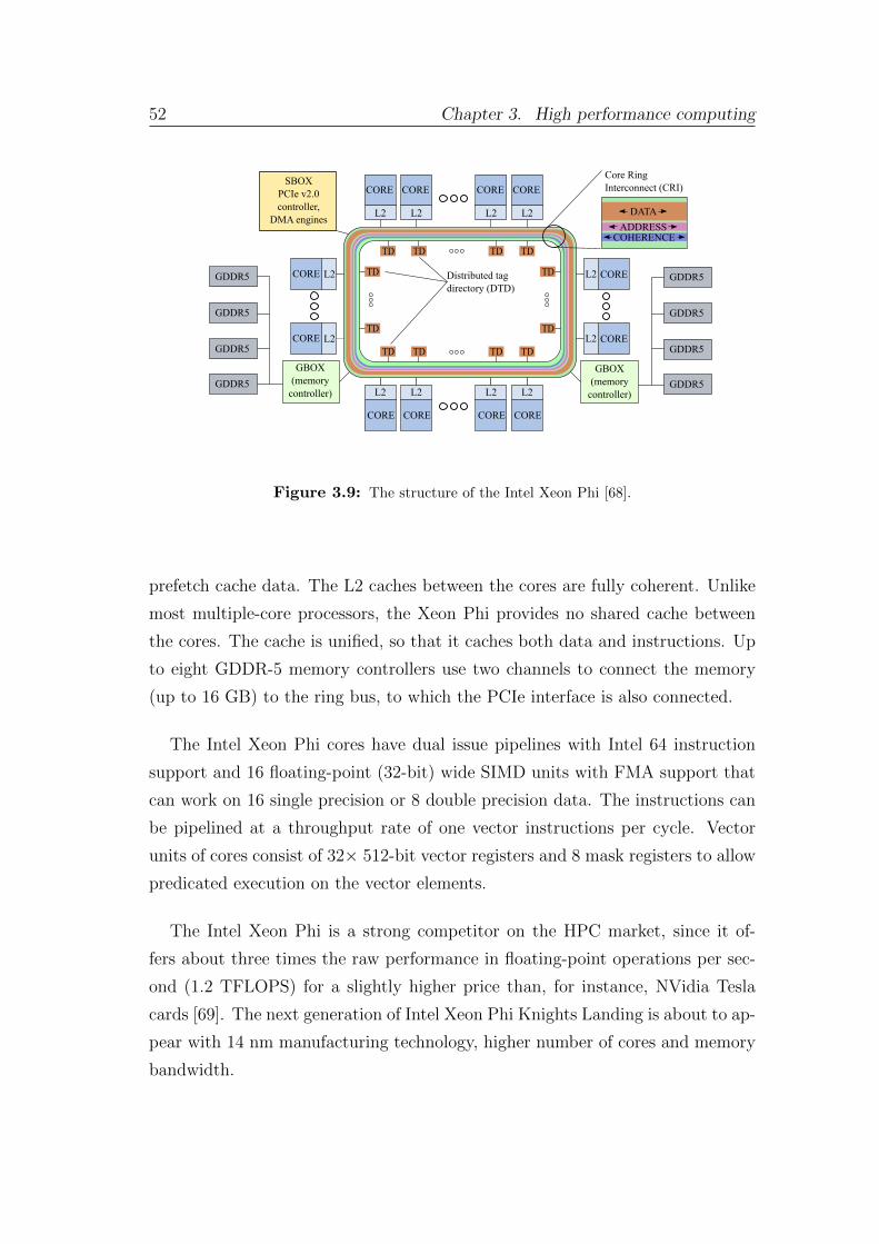
52 Chapter 3. High performance computing
Die Organization Diagram
CORE
L2
GBOX(memory
controller)
GBOX(memory
controller)
SBOXPCIe v2.0controller,
DMA enginesADDRESS
DATA
COHERENCE
Core RingInterconnect (CRI)
GDDR5
GDDR5
GDDR5
GDDR5
TD TD TD TD
TD
TD
TD TD TD TD
TD
TD
GDDR5
GDDR5
GDDR5
GDDR5
CORE
L2
CORE
L2
CORE
L2
CORE
L2
CORE
L2
CORE
L2
CORE
L2
COREL2
COREL2CORE L2
CORE L2 Distributed tag directory (DTD)
One-Day Seminar Rev. 19 Details of the MIC Architecture © Colfax International, 2013–2015
Figure 3.9: The structure of the Intel Xeon Phi [68].
prefetch cache data. The L2 caches between the cores are fully coherent. Unlike
most multiple-core processors, the Xeon Phi provides no shared cache between
the cores. The cache is unified, so that it caches both data and instructions. Up
to eight GDDR-5 memory controllers use two channels to connect the memory
(up to 16 GB) to the ring bus, to which the PCIe interface is also connected.
The Intel Xeon Phi cores have dual issue pipelines with Intel 64 instruction
support and 16 floating-point (32-bit) wide SIMD units with FMA support that
can work on 16 single precision or 8 double precision data. The instructions can
be pipelined at a throughput rate of one vector instructions per cycle. Vector
units of cores consist of 32× 512-bit vector registers and 8 mask registers to allow
predicated execution on the vector elements.
The Intel Xeon Phi is a strong competitor on the HPC market, since it of-
fers about three times the raw performance in floating-point operations per sec-
ond (1.2 TFLOPS) for a slightly higher price than, for instance, NVidia Tesla
cards [69]. The next generation of Intel Xeon Phi Knights Landing is about to ap-
pear with 14 nm manufacturing technology, higher number of cores and memory
bandwidth.
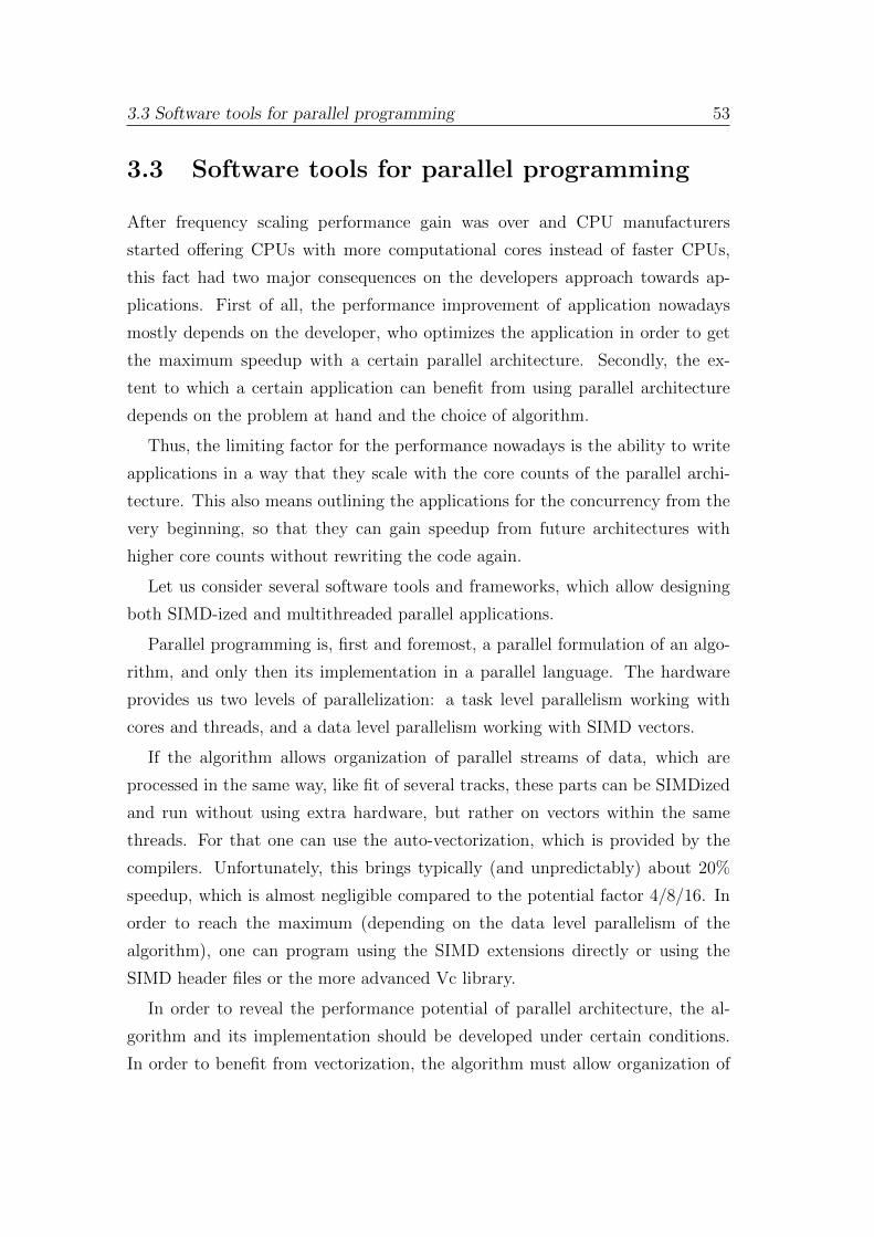
3.3 Software tools for parallel programming 53
3.3 Software tools for parallel programming
After frequency scaling performance gain was over and CPU manufacturers
started offering CPUs with more computational cores instead of faster CPUs,
this fact had two major consequences on the developers approach towards ap-
plications. First of all, the performance improvement of application nowadays
mostly depends on the developer, who optimizes the application in order to get
the maximum speedup with a certain parallel architecture. Secondly, the ex-
tent to which a certain application can benefit from using parallel architecture
depends on the problem at hand and the choice of algorithm.
Thus, the limiting factor for the performance nowadays is the ability to write
applications in a way that they scale with the core counts of the parallel archi-
tecture. This also means outlining the applications for the concurrency from the
very beginning, so that they can gain speedup from future architectures with
higher core counts without rewriting the code again.
Let us consider several software tools and frameworks, which allow designing
both SIMD-ized and multithreaded parallel applications.
Parallel programming is, first and foremost, a parallel formulation of an algo-
rithm, and only then its implementation in a parallel language. The hardware
provides us two levels of parallelization: a task level parallelism working with
cores and threads, and a data level parallelism working with SIMD vectors.
If the algorithm allows organization of parallel streams of data, which are
processed in the same way, like fit of several tracks, these parts can be SIMDized
and run without using extra hardware, but rather on vectors within the same
threads. For that one can use the auto-vectorization, which is provided by the
compilers. Unfortunately, this brings typically (and unpredictably) about 20%
speedup, which is almost negligible compared to the potential factor 4/8/16. In
order to reach the maximum (depending on the data level parallelism of the
algorithm), one can program using the SIMD extensions directly or using the
SIMD header files or the more advanced Vc library.
In order to reveal the performance potential of parallel architecture, the al-
gorithm and its implementation should be developed under certain conditions.
In order to benefit from vectorization, the algorithm must allow organization of
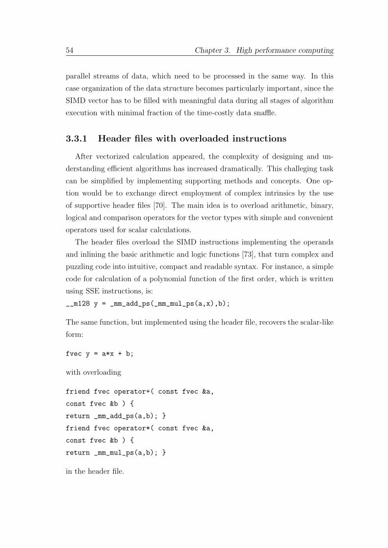
54 Chapter 3. High performance computing
parallel streams of data, which need to be processed in the same way. In this
case organization of the data structure becomes particularly important, since the
SIMD vector has to be filled with meaningful data during all stages of algorithm
execution with minimal fraction of the time-costly data snaffle.
3.3.1 Header files with overloaded instructions
After vectorized calculation appeared, the complexity of designing and un-
derstanding efficient algorithms has increased dramatically. This challeging task
can be simplified by implementing supporting methods and concepts. One op-
tion would be to exchange direct employment of complex intrinsics by the use
of supportive header files [70]. The main idea is to overload arithmetic, binary,
logical and comparison operators for the vector types with simple and convenient
operators used for scalar calculations.
The header files overload the SIMD instructions implementing the operands
and inlining the basic arithmetic and logic functions [73], that turn complex and
puzzling code into intuitive, compact and readable syntax. For instance, a simple
code for calculation of a polynomial function of the first order, which is written
using SSE instructions, is:
__m128 y = _mm_add_ps(_mm_mul_ps(a,x),b);
The same function, but implemented using the header file, recovers the scalar-like
form:
fvec y = a*x + b;
with overloading
friend fvec operator+( const fvec &a,
const fvec &b )
return _mm_add_ps(a,b);
friend fvec operator*( const fvec &a,
const fvec &b )
return _mm_mul_ps(a,b);
in the header file.
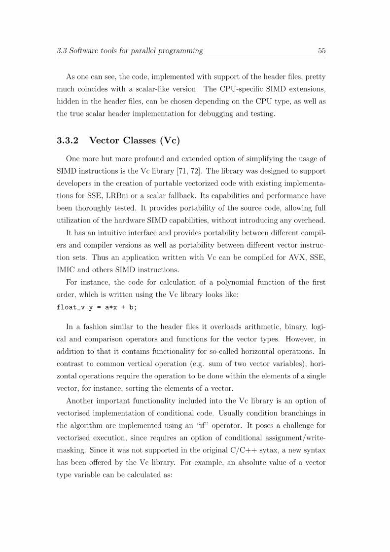
3.3 Software tools for parallel programming 55
As one can see, the code, implemented with support of the header files, pretty
much coincides with a scalar-like version. The CPU-specific SIMD extensions,
hidden in the header files, can be chosen depending on the CPU type, as well as
the true scalar header implementation for debugging and testing.
3.3.2 Vector Classes (Vc)
One more but more profound and extended option of simplifying the usage of
SIMD instructions is the Vc library [71, 72]. The library was designed to support
developers in the creation of portable vectorized code with existing implementa-
tions for SSE, LRBni or a scalar fallback. Its capabilities and performance have
been thoroughly tested. It provides portability of the source code, allowing full
utilization of the hardware SIMD capabilities, without introducing any overhead.
It has an intuitive interface and provides portability between different compil-
ers and compiler versions as well as portability between different vector instruc-
tion sets. Thus an application written with Vc can be compiled for AVX, SSE,
IMIC and others SIMD instructions.
For instance, the code for calculation of a polynomial function of the first
order, which is written using the Vc library looks like:
float_v y = a*x + b;
In a fashion similar to the header files it overloads arithmetic, binary, logi-
cal and comparison operators and functions for the vector types. However, in
addition to that it contains functionality for so-called horizontal operations. In
contrast to common vertical operation (e.g. sum of two vector variables), hori-
zontal operations require the operation to be done within the elements of a single
vector, for instance, sorting the elements of a vector.
Another important functionality included into the Vc library is an option of
vectorised implementation of conditional code. Usually condition branchings in
the algorithm are implemented using an “if” operator. It poses a challenge for
vectorised execution, since requires an option of conditional assignment/write-
masking. Since it was not supported in the original C/C++ sytax, a new syntax
has been offered by the Vc library. For example, an absolute value of a vector
type variable can be calculated as:
56 Chapter 3. High performance computing
float_m mask = ( a < 0 );
a(mask) = -a;
All negative entries of variable a will be replaced by positive values.
Additionally Vc provides the special functionality to ease the access to arrays
of scalars with vector types. It automatically aligns and pads the memory to allow
fast vector in the full index range. The random memory access functionality is
provided by the gather and scatter functions. For example: gather fills a vector
a from an array A taking elements with indexes stored in a vector I:
a.gather( A, I );
scatter does the opposite — it fills array entries from a vector:
a.scatter( A, I );
Here it is worth mentioning that Vc library with all its rich functionality is a
comprehensive package, which requires a proper installation procedure. For this
reason in some simpler cases, one does not necessarily need to install Vc library
but can use a simpler headers files approach.
3.3.3 Open Multi-Processing (OMP)
At task level parallelism one localizes independent parts of the algorithms and
run them in parallel on different cores or threads with or without synchronization
between the processes. It can be implemented using, for instance, the ITBB or
OpenMP [74] frameworks.
The OpenMP is an API (Application Programming Interface), which sup-
ports multi-platform shared-memory parallel programming. It defines a simple
interface to create a multithreaded application. The API consists of compiler
directives, library routines and environment variables.
OpenMP provides the developer with a certain flexibility, since it exploits
the fork-join parallelism programming model. Due to this programming model
the developer can decide which part of the program should be run in parallel
and which part, if needed, should stay with sequential run. In the beginning of
execution the master thread is created. At the point when the calculation should
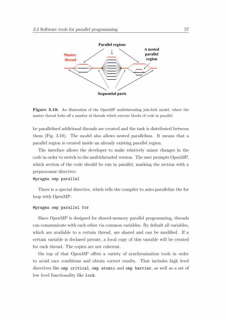
3.3 Software tools for parallel programming 57
Master thread
Sequential parts
Parallel regionsA nested parallel region
Figure 3.10: An illustration of the OpenMP multithreading join-fork model, where the
master thread forks off a number of threads which execute blocks of code in parallel.
be parallelised additional threads are created and the task is distributed between
them (Fig. 3.10). The model also allows nested parallelism. It means that a
parallel region is created inside an already existing parallel region.
The interface allows the developer to make relatively minor changes in the
code in order to switch to the multithreaded version. The user prompts OpenMP,
which section of the code should be run in parallel, marking the section with a
preprocessor directive:
#pragma omp parallel
There is a special directive, which tells the compiler to auto-parallelize the for
loop with OpenMP:
#pragma omp parallel for
Since OpenMP is designed for shared-memory parallel programming, threads
can communicate with each other via common variables. By default all variables,
which are available to a certain thread, are shared and can be modified. If a
certain variable is declared private, a local copy of this variable will be created
for each thread. The copies are not coherent.
On top of that OpenMP offers a variety of synchronization tools in order
to avoid race conditions and obtain correct results. That includes high level
directives like omp critical, omp atomic and omp barrier, as well as a set of
low level functionality like lock.
58 Chapter 3. High performance computing
OpenMP also contains a set of runtime library routines, which allow, for in-
stance, setting and checking the number of threads, checking the maximum num-
ber of threads, getting the number of a current thread, checking the number of
cores in a computer, to control the nested parallelism, operating with the simple
lock functionality etc. They can be available by including the file:
#include <omp.h>
As for enabling the OpenMP directives, the only action required from the user
is adding an appropriate flag during the compilation.
3.3.4 POSIX library
Although computer vendors have implemented threads in their operating sys-
tems for decades, there was no standardization until 1995, when a standard for
thread programming was established as part of the Portable Operating System
Interface (POSIX) standard [75, 76]. In particular, POSIX 1003.1c is the portion
of the overall POSIX standard covering threads. It includes the functions and
APIs that support multiple flows of control within a process. Threads created
and manipulated via this standard are generally referred to as Pthreads. Prior to
the establishment of Pthreads, thread APIs were hardware-vendor-specific, which
made portability of thread-parallel applications an oxymoron.
The libraries using this standard are also called Pthreads. To use this library,
the corresponding header file should be included:
#include <pthread.h>
Pthreads defines a set of C programming language types, functions and con-
stants. Pthreads allows creating and manipulating threads manually. For exam-
ple, it allows setting a permanent thread to core affinity, which can be particularly
useful in the case of NUMA architecture.
By default the threads are allocated to processors by the runtime environment,
which takes into account different factors, such as processor usage or machine
load. It can happen, that the thread can migrate to another CPU. For the NUMA
architectures it is preferable to use only local RAM for maximum performance.
And if the thread would be moved to another CPU, all data used by this thread

3.3 Software tools for parallel programming 59
would be located in the remote RAM. In order to prevent such migrations, which
can ruin the performance, each thread can be pinned to a certain core.
Chapter 4
Reconstruction of particles
trajectories
The advances in accelerator physics, improved detector technologies together with
increased computing power have enabled the HEP experiments collision rates and
energies, which were never available before. As a direct consequence, the task of
processing the experimental data is getting more and more complicated.
The increased collision energy has led to a more complicated event pattern with
a higher trajectory multiplicity. The modern event rates, in turn, are limiting
the time available to reconstruct the above mentioned complex collision patterns.
The collision patterns are reconstructed via reconstruction of trajectories (tracks)
of charged particles, which leave hit measurements as they cross detector planes.
The event reconstruction consists of four stages:
• track finding,
• track fitting,
• particle identification,
• search for short-lived particles.
Although stages of track finding and track fitting are strongly related, tradi-
tionally they have been seen as two separate tasks. Specifically, the task of track
finding (Fig. 4.1) is a pattern recognition problem of combining into groups hit
measurements from the detector data, produced by the same particle, in order to
reconstruct the trajectory of the particle. After the measured hits are grouped
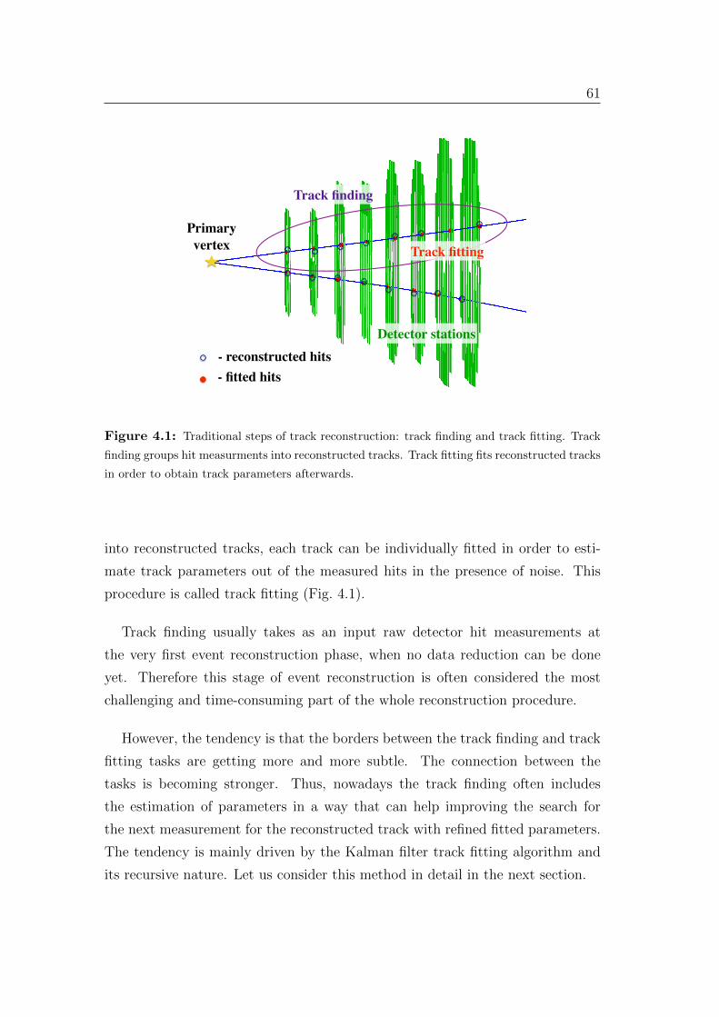
61
Track fitting
Track finding
Primary vertex
Detector stations- reconstructed hits- fitted hits
Figure 4.1: Traditional steps of track reconstruction: track finding and track fitting. Track
finding groups hit measurments into reconstructed tracks. Track fitting fits reconstructed tracks
in order to obtain track parameters afterwards.
into reconstructed tracks, each track can be individually fitted in order to esti-
mate track parameters out of the measured hits in the presence of noise. This
procedure is called track fitting (Fig. 4.1).
Track finding usually takes as an input raw detector hit measurements at
the very first event reconstruction phase, when no data reduction can be done
yet. Therefore this stage of event reconstruction is often considered the most
challenging and time-consuming part of the whole reconstruction procedure.
However, the tendency is that the borders between the track finding and track
fitting tasks are getting more and more subtle. The connection between the
tasks is becoming stronger. Thus, nowadays the track finding often includes
the estimation of parameters in a way that can help improving the search for
the next measurement for the reconstructed track with refined fitted parameters.
The tendency is mainly driven by the Kalman filter track fitting algorithm and
its recursive nature. Let us consider this method in detail in the next section.
62 Chapter 4. Reconstruction of particles trajectories
4.1 Kalman-filter-based track fit
4.1.1 The conventional Kalman filter method
As a result of track finding the detector measurements are grouped into sets of hits
which, ideally, were produced by a specific particle. The task of track fitting is to
estimate track parameters and their errors in order to get kinematical properties
of particles, which will later allow for reconstruction of short-lived particles, and,
finally, for the physics analysis.
Usually track fitting algorithm exploits the so-called track model, which is a
theoretical assumption on the equation of motion for charged particles in the
volume of a tracking detector. Several effects have an influence on the particle
motion, which the track model cannot take into account in a simple way, namely
multiple scattering, ionization and radiative energy loss. These effects add per-
turbations and affect the reconstruction of the particle kinematical properties.
Their influence on the obtained fitted parameters can be correctly taken into ac-
count with a proper track fitting method. The most common algorithm in HEP
nowadays, used for track fitting, is the Kalman filter method [77, 78, 79, 80].
In principle the track parameters can be derived from the hit measurements
by applying the least squares fit. However, in real life cases it is preferable to use
the Kalman filter method, since its recursive nature allows for a computationally
simpler and numerically optimized implementation. Namely, the method in its
calculations needs to operate with matrices, whose dimension equals to the num-
ber of fitted parameters, while the least squares fit operates with a matrix with
the dimensionality of the number of measurements in the track.
The Kalman filter method has found a wide range of applications thanks to
its features, namely:
• an optimal estimate (unbiased with minimal dispersion) as a result of the
fitting procedure,
• its recursive nature, which allows to perform the fitting of a partially re-
constructed track during track finding,
• does not need a global track model valid for the entire track length, but a
local track model valid only between consecutive measurements.
4.1 Kalman-filter-based track fit 63
Let us consider a dynamic system, whose evolution in time is fully described
with a state vector rt, consisting of several system parameters. The fitting pro-
cedure is supposed to provide as a result an estimate of the state vector rt based
on a set of measurements. The Kalman filter method obtains an optimal es-
timate r of the state vector rt based on the measurements of this state vector
mk, k = 1 . . . n, which may be contaminated with noise. The method starts
with an initial approximation r = r0 and improves this estimate in a recursive
way, consistently taking into account each measurement, providing as a result
the optimal estimate after adding the last measurement.
The estimated state vector rt can change from one measurement to the other.
For example, usually measurements are taken at different time and space points.
Therefore before adding the information of k-th measurement to the estimate,
the evaluation of the system by this time has to be taken into account. So that
the estimate and state vector correspond to the same moment. The estimate r
has always some finite precision — the error ξ, defined as the difference between
the estimate and the actual value of the estimated state vector. In order to keep
the track of the error ξ, let us introduce a covariance matrix as follows:
r = rt + ξ, (4.1a)
C = 〈ξ · ξT 〉. (4.1b)
The method assumes a linear model of measurements, which means that the
state vector should linearly depend on the measured parameters. Thus:
mk = Hkrtk + ηk, (4.2)
where Hk is called measurement model and ηk is an error of the k-th measure-
ment.
The Kalman filter method assumes that the error of the measurement and the
process noise are unbiased and uncorrelated not only mutually, but also in time
(white noise) and their covariance matrices Vk and Qk are known:
< ηk >=< ξk > = 0,
< ηk · ηTk > = Vk,
< ξk · ξTk > = Qk.
64 Chapter 4. Reconstruction of particles trajectories
The conventional Kalman filter method is derived for a linear dynamical sys-
tem, which means that the evolution of the system between two consecutive
measurements mk−1 and mk is described by a linear equation:
rtk = Fk−1rtk−1 + νk, (4.3)
where Fk−1 is a linear propagation operator, which relates the state at step (k−1)
to the state at step k, νk is a random process noise between the measurements
mk−1 and mk, which cannot be taken into account in the prediction matrix Fk−1.
The algorithm works in steps: starting with an initial approximation of the
state vector and the covariance matrix (initialization stage) it estimates the sys-
tem state at the point of the measurement (propagation stage) and corrects this
estimate and updates the covariance matrix, taking into account the measure-
ment with a certain weight (filtration stage). The algorithm performs in a loop
the propagation and the filtration stages until the last measurement is added.
Thus, the equations of Kalman filter fall into 3 groups: initialization, prediction
and filtration, as it is shown in Fig. 4.2. Let us consider specific equations for
each of the stages.
Initialization: The algorithm starts with initializing the state vector with
some initial prediction r0, if one is available, or alternatively with arbitrary val-
ues. In this case the covariance matrix reflects low confidence level of the initial
estimate r0: C0 = I · inf2, where inf stands for a large number.
Prediction/Propagation: If the state vector is expected to change between
two measurements, the estimate and its covariance matrix needs to be changed
accordingly. The current estimate of the state vector and the covariance matrix
at the measurement mk−1 are propagated to the point of the next measurement,
while taking into account the process noise:
r−k = Fk−1r+k−1, (4.4a)
C−k = Fk−1C+k−1F
Tk−1 +Qk, (4.4b)
where r+k−1, C+k−1 — the estimate and the error covariance matrix, obtained at
the previous measurement, r−k , C−k — predicted estimate of the state vector after
the influence of the process noise Qk. For the first time the initialization values
are propagated, since there are no measurements yet at this point.
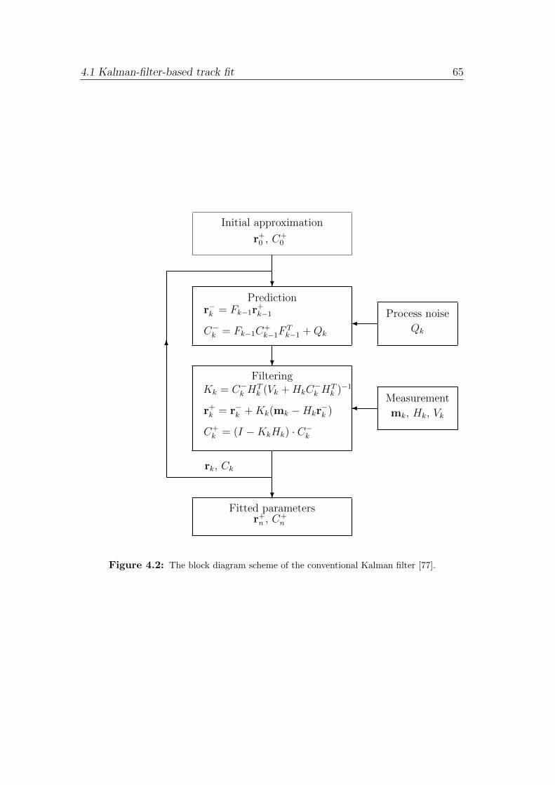
4.1 Kalman-filter-based track fit 65
Initial approximation
r+0 , C+0
?
Predictionr−k = Fk−1r
+k−1
C−k = Fk−1C+k−1F
Tk−1 +Qk
?
FilteringKk = C−k H
Tk (Vk +HkC
−k H
Tk )−1
r+k = r−k +Kk(mk −Hkr−k )
C+k = (I −KkHk) · C−k
6
rk, Ck
?
Fitted parametersr+n , C+
n
Process noise
Qk
Measurement
mk, Hk, Vk
Figure 4.2: The block diagram scheme of the conventional Kalman filter [77].
66 Chapter 4. Reconstruction of particles trajectories
Filtration/Update: The predicted state vector and the covariance matrix
are updated with the information the new measurement brings, in order to get
their optimal estimate at this stage. First, correction term — the residual, which
is the difference between the estimate and the actual measurement, is calculated:
ζk = mk −Hkr−k . (4.5)
The next element of the filtration step is the weight matrixWk, which is calculated
as the inverse covariance matrix of the residual:
Wk = (Vk +HkC−k H
Tk )−1. (4.6)
The weight matrix Wk defines the influence of the k-th measurement in the to-
tal χ2-deviation of the obtained estimate r+k from the measurements m1, . . . ,mk:
χ2k = χ2
k−1 + ζTk ·Wk · ζk. (4.7)
The state vector estimate is corrected by a weighted residual:
r+k = r−k +Kk · ζk, (4.8)
where the weight is defined by the so-called gain matrix Kk:
Kk = C−k HTk ·Wk. (4.9)
One notes that since the gain matrix is proportional to the current covariance
matrix C−k and weight matrix Wk, the strongest influence on the estimate will
have the measurements with higher weights. By contrast, the estimate, which
is already precise, and thus, has a small covariance matrix, will not be changed
significantly.
At last, the covariance matrix of the estimate is calculated:
C+k = (I −KkHk) · C−k . (4.10)
The algorithm sequentially repeats the prediction and the filtration steps for
each of the n measurements. After filtering the last measurements the vector
r+n — the resulting estimate after all the measurements are filtered is the optimal
estimate of the state vector rtn with the covariance matrix C+n .
4.1 Kalman-filter-based track fit 67
However, in real life the evolution of a system rtk+1(rtk) and the model of mea-
surements mtk(rt) dependencies often cannot be described by a linear function.
Therefore in order to apply the Kalman Filter method in non-linear cases a pro-
cedure of linearization has to be performed.
For example, in the case of a non-linear model of measurements the function
mk(rtk) ≡ hk(rtk), the function hk(rtk) needs to be expanded in a Taylor series at
the linearization point rlin:
mk(rtk) ≡ hk(rtk) + ηk ≈ hk(rlink ) +Hk(rtk − rlink ) + ηk, (4.11)
where Hk is the Jacobian of hk(rk) at rlink :
Hk(ij) =∂hk(rk)(i)
∂rk(j)
∣∣∣∣∣rk=rlink
. (4.12)
In this case the formula to calculate the residual for conventional method (4.5)
is changed in the following way:
ζk = mk − (hk(rlink ) +Hk(r−k − rlink )).
In the same manner the non-linear extrapolation equation (4.4a) can be lin-
earized:
r−k ≡ fk(r+k−1) ≈ fk(rlin) + Fk(r+k−1 − rlink−1) (4.13)
Fk(ij) =∂fk(r+k−1)(i)
∂r+k−1(j)
∣∣∣∣∣r+k−1=rlink−1
. (4.14)
The Kalman filter equations in the case of a system with non-linear evolution or
measurement model is called the extended Kalman filter method. The linearized
model differs from the original one, therefore the choice of the linearisation point
rlin is important. The usual way is to take the current estimator rk as the point
of linearization for the k−th measurement.
Unlike its linear version, the extended Kalman filter in a general case is not an
optimal estimator. Moreover, if the initial estimate of the state is wrong, or if the
68 Chapter 4. Reconstruction of particles trajectories
process is modeled incorrectly, the filter may diverge, owing to its linearization.
Having stated this, the extended Kalman filter gives a reasonable performance,
and is the standard method for fitting charged particles trajectories in HEP
experiments nowadays.
4.1.2 Kalman-filter-based track fit for CBM
One of the most important applications of the Kalman filter algorithm in HEP is
trajectory fitting in order to reconstruct the parameters of particles produced in
collisions. In this case the state vector r contains track parameters, the propaga-
tion matrix Fk extrapolates the track from one detector station to the next one in
a magnetic field, and the noise matrix Qk takes into account multiple scattering
due to interaction with the detector material.
In the case of the CBM experiment track fit the state vector of track parameters
was chosen in the following form, convenient for a forward detector geometry:
r = x, y, tx, ty, q/p, (4.15)
where z-coordinate is directed downstream the beam along the detector, x and y
are track coordinates at a certain z-position, tx ≡ tan θx and ty ≡ tan θy are the
track slopes in the xz and yz planes, and q/p is the charge to inverse momentum
ratio.
In order to estimate the state vector r with the Kalman filter method one
needs to define every needed component of the method, namely: initial values of
the state vector r0 and covariance matrix C0, the model of measurements H and
the propagation matrix Fk, as well as the noise matrix Qk.
In the case of the CBM experiment for a secure convergence the initial state
vector r0 is taken as the estimate of the least squares method using one-component
approximation of a magnetic field in the absence of multiple scattering in the
detector material.
The model of measurement is supposed to set the relation between the mea-
sured detector hits and the state vector. Since the vertex detector of the CBM
experiment consists of double-sided strip sensors, each hit measured in the STS
consists of two independent one-dimensional measurements — strips. These mea-
surements are linearly dependent on the position of particle in the detector plane.
4.1 Kalman-filter-based track fit 69
Thus, the model of measurement H is linear, namely:
Hk = cos(αk), sin(αk), 0, 0, 0 , (4.16)
where αk is the strip angle.
The propagation matrix Fk serves to define the charged particle motion in the
non-homogeneous magnetic field B. This motion is described as a Lorenz force
with the following differential equations:
dtx/dz = c(q/p)tr( ty(Bz + txBx)− (1 + t2x)By), (4.17a)
dty/dz = c(q/p)tr(−tx(Bz + tyBy) + (1 + t2y)Bx), (4.17b)
tr(z) =√t2x + t2y + 1,
here Bx, By, Bz are the field components at a given z on the particle trajectory,
c is the speed of light. These equations cannot be solved analytically in case of
a non-homogeneous magnetic field, since the field components have a complex
coordinate dependence. For this reason the standard Runge-Kutta method [81]
is used in order to obtain the function rtk+1 = fk(rtk). Since the fk(rtk) dependence
appears to be non-linear, the linearization is performed in the same manner as it
was shown in (4.4a) at the track point closest to the measurement rlink giving as
a result the desired propagation matrix Fk.
The next element of the method, which is needed in order to take into account
the multiple scattering in the detector material, is the matrix of noise Qk. The
studies with double sided silicon sensors of 300 µm thickness, similar to the
CBM STS sensors, have shown that a minimum ionizing particle, traversing this
thickness, creates about 24.000 electron-hole pairs [82]. It means that the particle
undergoes at least 24.000 scattering processes, with minimum exchanged energy
of 1.8 eV. According to the central limit theorem it makes it possible to describe
the total scattering angle of the particle with a Gauss distribution as a sum
of a large number of random variables. The width of the distribution is set
with the original Highland-Lynch-Dahl formula [83] for the width of the angular
distribution:
σ(θ) =13.6 MeV
βcpq√L/X0 [1 + 0.038 ln(L/X0)] , (4.18)
70 Chapter 4. Reconstruction of particles trajectories
where β, p, and q are particle velocity, momentum and charge number of the
incident particle, L/X0 is the true path length in radiation length unit. The
resulting matrix of noise Qk has a following form [84]:
Qk = σ2k(θ)
0 0 0 0 0
0 0 0 0 0
0 0 (t2x + 1)t2r txtyt2r 0
0 0 txtyt2r (t2y + 1)t2r 0
0 0 0 0 0
. (4.19)
The energy loss of a particle in thin material of the detector system is small in
comparison to the effects considered here and can be neglected.
Historically the Kalman filter implementation was done in a double precision.
However, for modern computer algorithms the stability in the single precision
becomes particularly important for SIMD calculations and optimal usage of cache
memory layered structure. As a result, twofold more data can be stored in the
cache and, as well, twice the size of data can later be packed into a SIMD register
at double speed. However, the direct switching to a single precision has shown
that the 32-bits precision is not sufficient for the Kalman filter track fit and
results in numerically unstable behavior of the algorithm. The main obstacle
in switching the algorithm from the double precision to the single one, is the
discrepancies, that appear due to numerical rounding. As a result one may face
poor fit quality, or even physically unacceptable results like negative diagonal
elements of the covariance matrix.
The discrepancies can arise during the step of updating covariance matrix
when the previous error estimate significantly exceeds the error that must be
taken into account while adding new measurement to the estimate. A similar
problem is faced while adding the first measurement, where infinite errors for the
estimate is replaced by a finite big number.
Therefore the Kalman filter algorithm was modified in order to avoid such
instability due to round-off errors. The algorithm single precision stability was
increased due to the following changes: the initial state vector estimate is obtained
with the least squares fit with magnetic field approximation, a special procedure
of updating the covariance matrix in order to increase correction precision and a
special procedure of filtering the first measurement [77] are introduced.
4.1 Kalman-filter-based track fit 71
4.1.3 The track fit quality assurance
While providing the state vector estimate, a very important issue is a proper
covariance matrix, which contains estimated errors of the track parameters. In
order to study the reliability of parameter error estimation at first, the residuals
ρ of the track parameters, for instance for the x-coordinate, are calculated as:
ρx = xreco − xmc, (4.20)
where xreco and xmc are the reconstructed and the true Monte Carlo values of the
x-coordinate. A measure of the reliability of the fit are the normalized residual
(pull) distributions of the fitted track parameters. Pulls are determined according
to the formula:
Px =ρx√Cxx
, (4.21)
where Cxx is the corresponding diagonal element of the covariance matrix, ob-
tained in the track fit. In the ideal case the normalized error distributions of
the track parameters should be unbiased and Gaussian distributed with a width
of 1.0.
The residuals and the pulls for all track parameters in the CBM experiment
are calculated at the first hit of each track. The distributions for the x, tx and q/p
parameters together with their Gaussian fits are shown on Fig. 7.6 (the results
for y and ty are similar). All distributions are not biased with pulls widths close
to 1.0 indicating correctness of the fitting procedure. The slight deviations from
1.0 are caused by several assumptions made in the fitting procedure, mainly in
the part of the detector material treatment. The q/p pull is the widest being the
most sensitive to these simplifications [73].
The Kalman filter track fit algorithm is used to estimate parameters of the
tracks reconstructed in the STS and MVD detectors and their errors for the
CBM experiment. The algorithm works stable in single precision and is fully
vectorized [77]. The algorithm is also used in order to fit partially reconstructed
tracks inside the Cellular automaton track finder while searching for the next hit
measurement. It will be shown in the next section, which is devoted to the track
finding task.
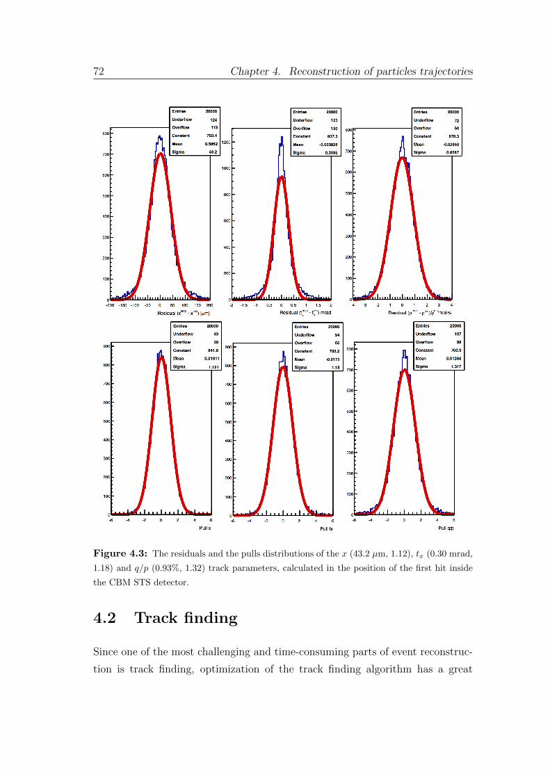
72 Chapter 4. Reconstruction of particles trajectories
Figure 4.3: The residuals and the pulls distributions of the x (43.2 µm, 1.12), tx (0.30 mrad,
1.18) and q/p (0.93%, 1.32) track parameters, calculated in the position of the first hit inside
the CBM STS detector.
4.2 Track finding
Since one of the most challenging and time-consuming parts of event reconstruc-
tion is track finding, optimization of the track finding algorithm has a great
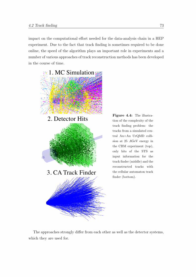
4.2 Track finding 73
impact on the computational effort needed for the data-analysis chain in a HEP
experiment. Due to the fact that track finding is sometimes required to be done
online, the speed of the algorithm plays an important role in experiments and a
number of various approaches of track reconstruction methods has been developed
in the course of time.
1. MC Simulation
2. Detector Hits
3. CA Track Finder
Figure 4.4: The illustra-
tion of the complexity of the
track finding problem: the
tracks from a simulated cen-
tral Au+Au UrQMD colli-
sion at 25 AGeV energy in
the CBM experiment (top),
only hits of the STS as
input information for the
track finder (middle) and the
reconstructed tracks with
the cellular automaton track
finder (bottom).
The approaches strongly differ from each other as well as the detector systems,
which they are used for.
74 Chapter 4. Reconstruction of particles trajectories
In the next section an overview of several track reconstruction methods will
be presented together with their advantages and disadvantages:
• conformal mapping,
• Hough transformation,
• track following,
• cellular automaton.
Due to the noise and impreciseness of detector measurements, a set of hy-
potheses is usually used in order to improve the efficiency and speed up the track
finding process. The possible hypotheses are the track model, track seeds from
other detectors and the position of track origin (for example, target region).
As far as the track model is concerned, the tracking methods can be classified
as global or local. The global methods need to treat all the measurements si-
multaneously, usually using the track model, while the local methods go through
the measurements one by one. In other words, the global methods have to con-
sider all the available measurement information while accepting or discarding a
certain track and local methods make such decisions based only on a subset of
the measurement information. Examples of global approaches considered below
are conformal mapping, Hough transform, while the track following and cellular
automaton methods are regarded as local.
The methods drastically differ in their approach, usually making a direct com-
parison difficult. Thus, usually experiments try to develop various methods in
the beginning and later decide upon the best one for the certain detector system
and the physics case. Let us consider some methods, which CBM tried to apply
for the track finding in the STS detector.
4.2.1 An overview of the track reconstruction methods
Conformal mapping
One of the standard global track reconstruction methods is Conformal map-
ping [85], which is used in the presence of a uniform magnetic field. The main
idea of the method is to simplify the event pattern by applying a map, which
transforms the circular tracks of charged primary particles in a uniform magnetic
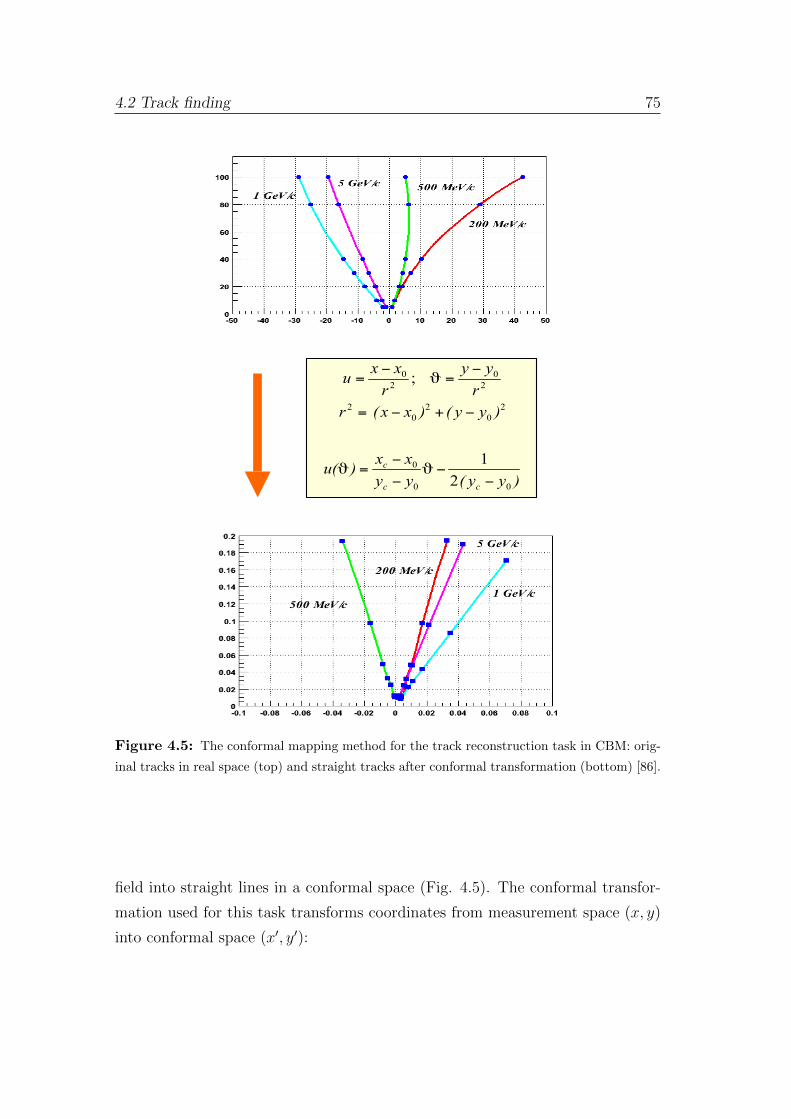
4.2 Track finding 75
Track reconstruction 7
Track finding: Conformal mapping
)yy(yyxx
)u(
)yy()xx(rryy
rxx
u
cc
c
00
0
20
20
2
20
20
21
;
−−
−
−=
−+−=
−=
−=
ϑϑ
ϑ
25 GeV Au+Au 7(>=3) station:
efficiency ∼95 % ghosts < 7 % clones < 10 %
Figure 4.5: The conformal mapping method for the track reconstruction task in CBM: orig-
inal tracks in real space (top) and straight tracks after conformal transformation (bottom) [86].
field into straight lines in a conformal space (Fig. 4.5). The conformal transfor-
mation used for this task transforms coordinates from measurement space (x, y)
into conformal space (x′, y′):
76 Chapter 4. Reconstruction of particles trajectories
x′ =x− x0
(x− x0)2 + (y − y0)2; (4.22)
y′ =y − y0
(x− x0)2 + (y − y0)2. (4.23)
Since reconstructing a straight line is much easier than searching for a circle,
in the conformal space these lines can be easily found with histograming. How-
ever, the form of the transformation immediately reveals the first obstacle of the
method: the transformation requires knowing in advance the position of the pri-
mary vertex (xpv, ypv). This problem is usually avoided by assuming a common
vertex with coordinates (0;0), which will turn the transformation equations into:
x′ =x
x2 + y2; (4.24)
y′ =y
x2 + y2. (4.25)
However, this simplification does not help to generalize the method for the search
of secondary tracks. Further simplification is done by assuming a uniform mag-
netic field, which is not true for a general case.
Despite the disadvantages, the conformal mapping method can be successfully
applied for the search of primary tracks in a simple event topologies, where it can
have a simple and fast implementation in hardware.
Hough transform
One more example of a global track finder algorithm is the Hough Transform [87].
This method converts the measurements from a real space (x, y) into the param-
eter space (a, b). Fig. 4.6 illustrates the example when the measurements of the
curved track, described by two parameters — track curvature and emission angle,
are plotted in the parameter space, providing as a result the intersection point of
the initial track parameters. Let us consider the simplest case of a straight track:
y = a · x+ b. (4.26)
In this case the transformation is:
b = − a · x+ y. (4.27)
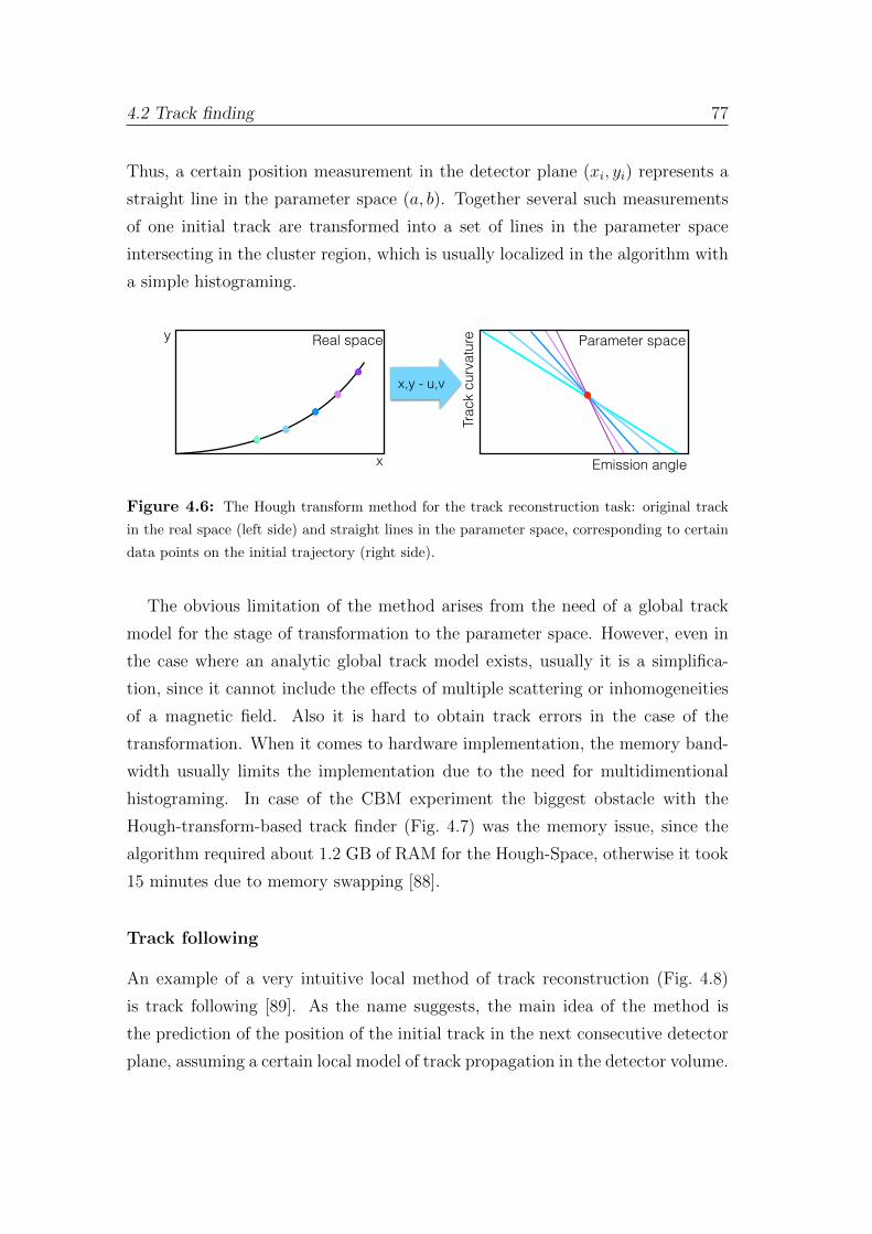
4.2 Track finding 77
Thus, a certain position measurement in the detector plane (xi, yi) represents a
straight line in the parameter space (a, b). Together several such measurements
of one initial track are transformed into a set of lines in the parameter space
intersecting in the cluster region, which is usually localized in the algorithm with
a simple histograming.
Parameter space
Trac
k cu
rvat
ure
Emission angle
Real space
x
y
x,y - u,v
Figure 4.6: The Hough transform method for the track reconstruction task: original track
in the real space (left side) and straight lines in the parameter space, corresponding to certain
data points on the initial trajectory (right side).
The obvious limitation of the method arises from the need of a global track
model for the stage of transformation to the parameter space. However, even in
the case where an analytic global track model exists, usually it is a simplifica-
tion, since it cannot include the effects of multiple scattering or inhomogeneities
of a magnetic field. Also it is hard to obtain track errors in the case of the
transformation. When it comes to hardware implementation, the memory band-
width usually limits the implementation due to the need for multidimentional
histograming. In case of the CBM experiment the biggest obstacle with the
Hough-transform-based track finder (Fig. 4.7) was the memory issue, since the
algorithm required about 1.2 GB of RAM for the Hough-Space, otherwise it took
15 minutes due to memory swapping [88].
Track following
An example of a very intuitive local method of track reconstruction (Fig. 4.8)
is track following [89]. As the name suggests, the main idea of the method is
the prediction of the position of the initial track in the next consecutive detector
plane, assuming a certain local model of track propagation in the detector volume.
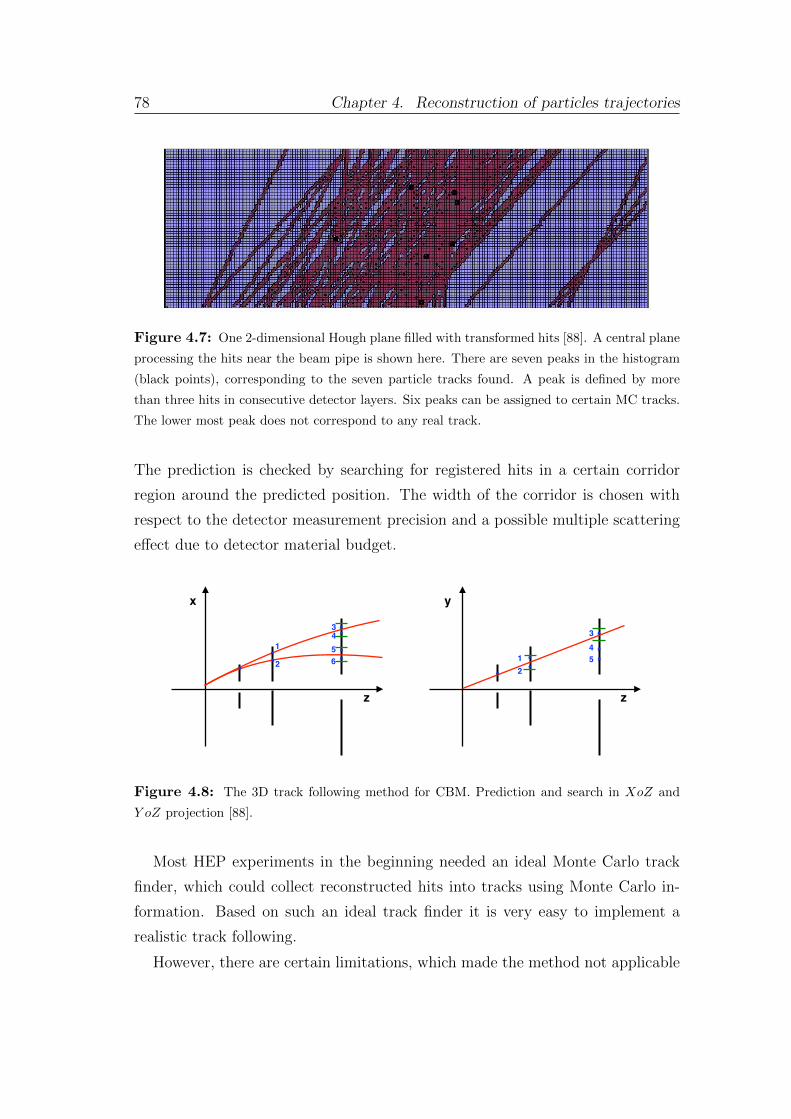
78 Chapter 4. Reconstruction of particles trajectories304 Event reconstruction
Figure 13.3: One 2-dimensional Hough plane filled with transformed hits. A central plane processing the hitsnear the beam pipe is shown here. Planes more apart from the beam pipe contain less transformed hits. There areseven peaks in the histogram (black points) corresponding to seven found particle tracks. A peak is defined bymore than three hits in consecutive detector layers. Six peaks can be assigned to certain MC tracks. The lowermost peak corresponds to no real track, but accumulates a peak from five hits of different tracks.
Figure 13.4: Track finding efficiency for tracks with hits in at least three tracking stations as function of momen-tum using the Hough transform method for central Au+Au events at different beam momenta
rate is highest for low and high momenta. At low momenta, the track multiplicity is highest and thuscombinatorial coincidences are more likely. Tracks at high momenta are less numerous, but correspondto almost straight lines near the beam pipe with high track densities. The mean numbers of efficiencyand ghost rate for the three beam momenta are given in table 13.1. While the efficiency is almost thesame, the ghost rate increases quickly with beam momentum.
Both the efficiency and the ghost rate depend on the multiplicity of the event, the number of detector
Figure 4.7: One 2-dimensional Hough plane filled with transformed hits [88]. A central plane
processing the hits near the beam pipe is shown here. There are seven peaks in the histogram
(black points), corresponding to the seven particle tracks found. A peak is defined by more
than three hits in consecutive detector layers. Six peaks can be assigned to certain MC tracks.
The lower most peak does not correspond to any real track.
The prediction is checked by searching for registered hits in a certain corridor
region around the predicted position. The width of the corridor is chosen with
respect to the detector measurement precision and a possible multiple scattering
effect due to detector material budget.
x
z z
y
1
2
3456 1
2
345
Figure 4.8: The 3D track following method for CBM. Prediction and search in XoZ and
Y oZ projection [88].
Most HEP experiments in the beginning needed an ideal Monte Carlo track
finder, which could collect reconstructed hits into tracks using Monte Carlo in-
formation. Based on such an ideal track finder it is very easy to implement a
realistic track following.
However, there are certain limitations, which made the method not applicable
4.2 Track finding 79
in certain cases. First of all, the algorithm is featured with an exponential growth
of combinatorial combinations to be considered with increasing track multiplicity.
Thus, the algorithm can work efficiently within a reasonable time only up to a
certain hit density. Another issue is raised, when it comes to implementation of
the algorithm on the compute devices. The problem is that the algorithm real-
izes a random memory access, while checking different next possible hits on the
track. This random memory access usually becomes a bottleneck for a program
implementation, due to the slow speed of such operations. Moreover, if one tries
to examine the logic of the approach, it is easy to see that during the search the
algorithm often has to repeat certain calculations several times, since some of the
results get discarded.
In the early stages of the CBM experiment, when the STS detector was still
planned as a pixel detector, the track following method was tested for the re-
construction routine (Fig. 4.8). The track reconstruction procedure was accom-
plished in 3D space on both x-z and y-z projections simultaneously [88]. The
procedure alternated between both views, predicting a track position on the next
station and searching for hits in the vicinity of the predicted position.
Starting from the middle of the target area, this point was sequentially con-
nected with all hits in the first station in y-z view, where tracks were close to
straight lines. The straight lines driven via these two points were prolonged to
the plane of the second station. All hits in an asymmetrical corridor around the
intersection point were then used for fitting a parabola in x-z view which is pro-
longed to the next station. Since several prolongations could happen, corridors
were set around each point predicted on the third station. A similar corridor was
set in the y-z view on the third station. If hits were found within these limits,
they were attached to the track.
When the STS detector was redesigned using double-sided strip detector mod-
ules, most of the methods could not cope with the increased number of hits and,
as a result, more intensive combinatorial search.
Cellular-automaton-based track finder
As was shown, one of the major obstacles to be solved by each track finder
is a huge and growing fast with track density amount of combinatorial combi-
80 Chapter 4. Reconstruction of particles trajectories
nations, which track finder has to consider in order to bind together one- or
two-dimensional measurements into five-dimensional tracks. Unfortunately, the
exponential growth of the combinatorial enumeration at high track densities usu-
ally makes it impossible to consider all combinations within a reasonable time
frame. The CBM experiment can serve as a proper illustration of this problem,
since the experiment has tried different tracking approaches for the planed pixel
version of the STS detector. Unfortunately, most of them could not work any-
more due to increased combinatorial combinations after switching from pixel to
double-sided strip version of the STS.
However, a solid solution for combinatorial optimization was provided by the
CA track finder algorithm. The CA track finder can be regarded as a local
version of the Hopfield neural network [90] and will be discussed in detail in the
next section.
4.2.2 Cellular automaton
Although the idea of everything being made up of large numbers of discrete
elements was discussed around 450 BC by Leucippus and Democritus, it was still
a long time before abstract idealizations like cellular automata were introduced.
In 1967, Konrad Zuse also suggested that the universe itself is running on a
cellular automaton or a similar computational structure. In 1969, he published
the book “Rechnender Raum” (Calculating Space) [91]. He proposed that the
physical laws of the universe are discrete by nature, and that the entire universe
is the output of a deterministic computation on a single cellular automaton. This
idea has attracted a lot of attention, since there is no physical evidence against
Zuse’s thesis. “Zuse’s Theory” became the foundation of the field of study called
digital physics.
The concept of cellular automaton as we know it today was originally proposed
in the 1940s by Stanislaw Ulam and John von Neumann in an attempt to develop
an abstract model of self-reproduction in biology, which eventually led to the
name “cellular automata”. After John Conway introduced his Game of Life [92],
the method became popular and, despite its biological name, in the course of
time the method accrued range of applications in computer science, mathematics,
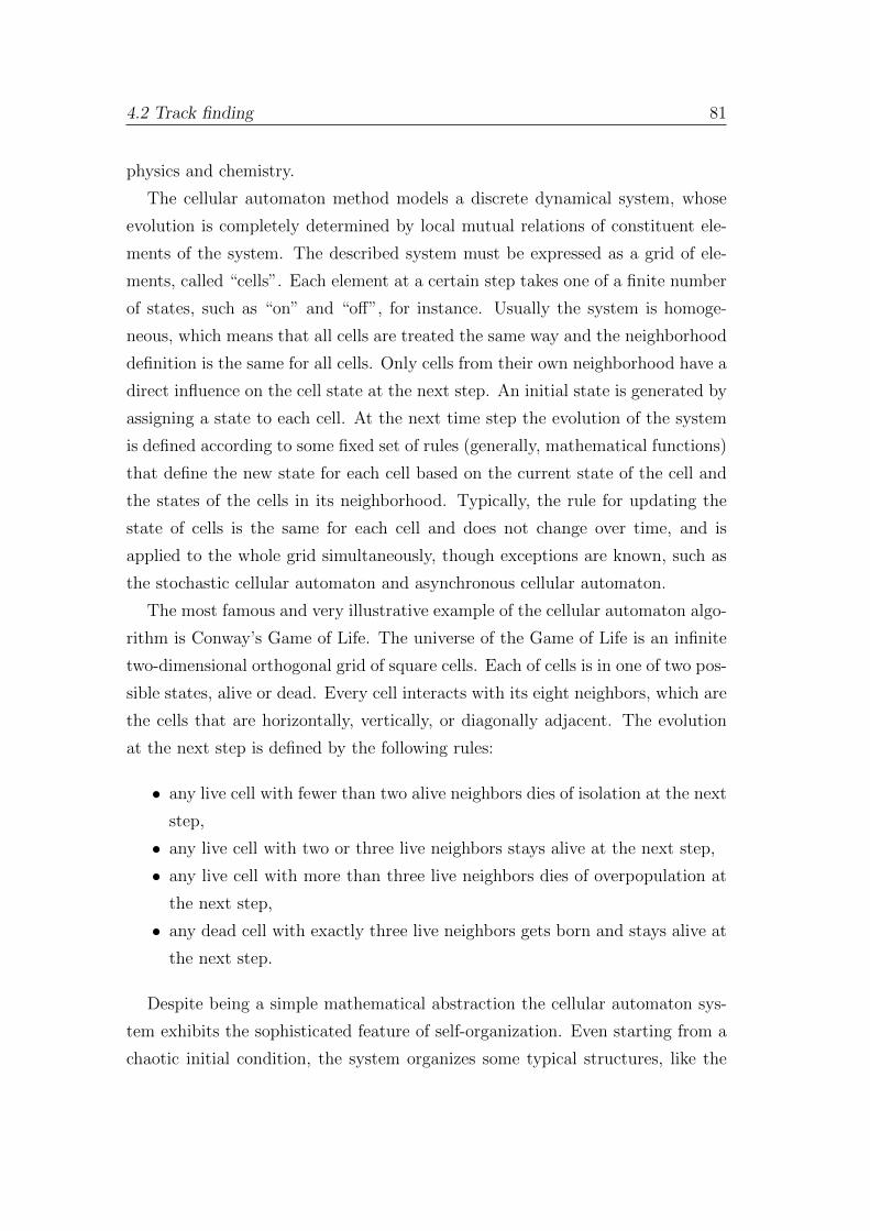
4.2 Track finding 81
physics and chemistry.
The cellular automaton method models a discrete dynamical system, whose
evolution is completely determined by local mutual relations of constituent ele-
ments of the system. The described system must be expressed as a grid of ele-
ments, called “cells”. Each element at a certain step takes one of a finite number
of states, such as “on” and “off”, for instance. Usually the system is homoge-
neous, which means that all cells are treated the same way and the neighborhood
definition is the same for all cells. Only cells from their own neighborhood have a
direct influence on the cell state at the next step. An initial state is generated by
assigning a state to each cell. At the next time step the evolution of the system
is defined according to some fixed set of rules (generally, mathematical functions)
that define the new state for each cell based on the current state of the cell and
the states of the cells in its neighborhood. Typically, the rule for updating the
state of cells is the same for each cell and does not change over time, and is
applied to the whole grid simultaneously, though exceptions are known, such as
the stochastic cellular automaton and asynchronous cellular automaton.
The most famous and very illustrative example of the cellular automaton algo-
rithm is Conway’s Game of Life. The universe of the Game of Life is an infinite
two-dimensional orthogonal grid of square cells. Each of cells is in one of two pos-
sible states, alive or dead. Every cell interacts with its eight neighbors, which are
the cells that are horizontally, vertically, or diagonally adjacent. The evolution
at the next step is defined by the following rules:
• any live cell with fewer than two alive neighbors dies of isolation at the next
step,
• any live cell with two or three live neighbors stays alive at the next step,
• any live cell with more than three live neighbors dies of overpopulation at
the next step,
• any dead cell with exactly three live neighbors gets born and stays alive at
the next step.
Despite being a simple mathematical abstraction the cellular automaton sys-
tem exhibits the sophisticated feature of self-organization. Even starting from a
chaotic initial condition, the system organizes some typical structures, like the
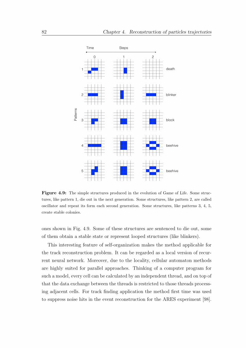
82 Chapter 4. Reconstruction of particles trajectories
0 1 2
1
2
3
4
5
Steps
Patte
rns
Time
death
blinker
block
beehive
beehive
Figure 4.9: The simple structures produced in the evolution of Game of Life. Some struc-
tures, like pattern 1, die out in the next generation. Some structures, like pattern 2, are called
oscillator and repeat its form each second generation. Some structures, like patterns 3, 4, 5,
create stable colonies.
ones shown in Fig. 4.9. Some of these structures are sentenced to die out, some
of them obtain a stable state or represent looped structures (like blinkers).
This interesting feature of self-organization makes the method applicable for
the track reconstruction problem. It can be regarded as a local version of recur-
rent neural network. Moreover, due to the locality, cellular automaton methods
are highly suited for parallel approaches. Thinking of a computer program for
such a model, every cell can be calculated by an independent thread, and on top of
that the data exchange between the threads is restricted to those threads process-
ing adjacent cells. For track finding application the method first time was used
to suppress noise hits in the event reconstruction for the ARES experiment [98].
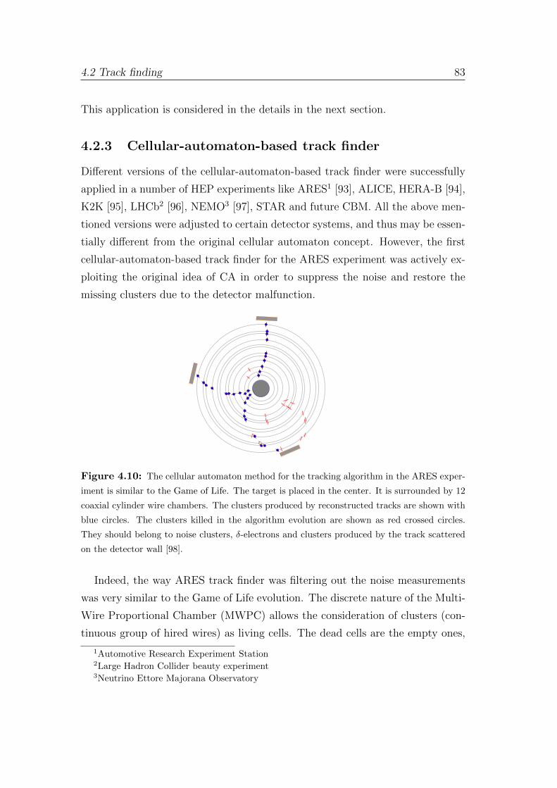
4.2 Track finding 83
This application is considered in the details in the next section.
4.2.3 Cellular-automaton-based track finder
Different versions of the cellular-automaton-based track finder were successfully
applied in a number of HEP experiments like ARES1 [93], ALICE, HERA-B [94],
K2K [95], LHCb2 [96], NEMO3 [97], STAR and future CBM. All the above men-
tioned versions were adjusted to certain detector systems, and thus may be essen-
tially different from the original cellular automaton concept. However, the first
cellular-automaton-based track finder for the ARES experiment was actively ex-
ploiting the original idea of CA in order to suppress the noise and restore the
missing clusters due to the detector malfunction.
Figure 4.10: The cellular automaton method for the tracking algorithm in the ARES exper-
iment is similar to the Game of Life. The target is placed in the center. It is surrounded by 12
coaxial cylinder wire chambers. The clusters produced by reconstructed tracks are shown with
blue circles. The clusters killed in the algorithm evolution are shown as red crossed circles.
They should belong to noise clusters, δ-electrons and clusters produced by the track scattered
on the detector wall [98].
Indeed, the way ARES track finder was filtering out the noise measurements
was very similar to the Game of Life evolution. The discrete nature of the Multi-
Wire Proportional Chamber (MWPC) allows the consideration of clusters (con-
tinuous group of hired wires) as living cells. The dead cells are the empty ones,
1Automotive Research Experiment Station2Large Hadron Collider beauty experiment3Neutrino Ettore Majorana Observatory
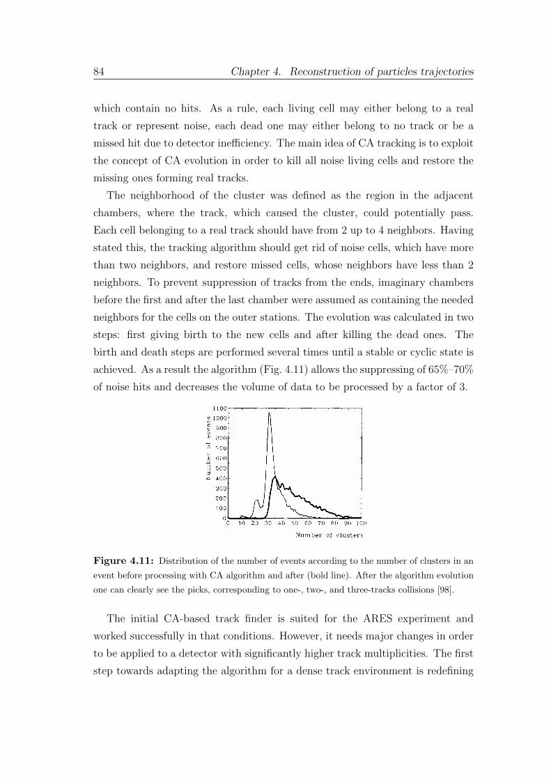
84 Chapter 4. Reconstruction of particles trajectories
which contain no hits. As a rule, each living cell may either belong to a real
track or represent noise, each dead one may either belong to no track or be a
missed hit due to detector inefficiency. The main idea of CA tracking is to exploit
the concept of CA evolution in order to kill all noise living cells and restore the
missing ones forming real tracks.
The neighborhood of the cluster was defined as the region in the adjacent
chambers, where the track, which caused the cluster, could potentially pass.
Each cell belonging to a real track should have from 2 up to 4 neighbors. Having
stated this, the tracking algorithm should get rid of noise cells, which have more
than two neighbors, and restore missed cells, whose neighbors have less than 2
neighbors. To prevent suppression of tracks from the ends, imaginary chambers
before the first and after the last chamber were assumed as containing the needed
neighbors for the cells on the outer stations. The evolution was calculated in two
steps: first giving birth to the new cells and after killing the dead ones. The
birth and death steps are performed several times until a stable or cyclic state is
achieved. As a result the algorithm (Fig. 4.11) allows the suppressing of 65%–70%
of noise hits and decreases the volume of data to be processed by a factor of 3.
Figure 4.11: Distribution of the number of events according to the number of clusters in an
event before processing with CA algorithm and after (bold line). After the algorithm evolution
one can clearly see the picks, corresponding to one-, two-, and three-tracks collisions [98].
The initial CA-based track finder is suited for the ARES experiment and
worked successfully in that conditions. However, it needs major changes in order
to be applied to a detector with significantly higher track multiplicities. The first
step towards adapting the algorithm for a dense track environment is redefining
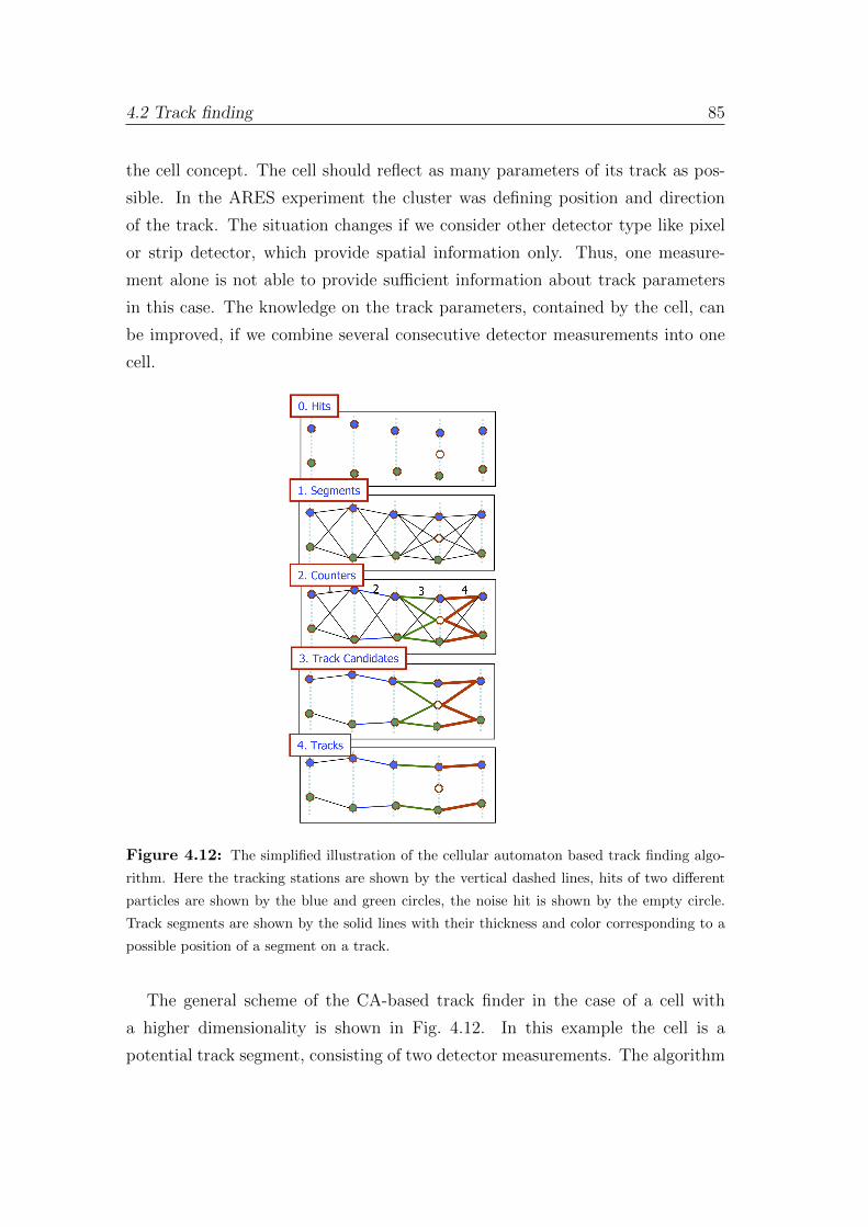
4.2 Track finding 85
the cell concept. The cell should reflect as many parameters of its track as pos-
sible. In the ARES experiment the cluster was defining position and direction
of the track. The situation changes if we consider other detector type like pixel
or strip detector, which provide spatial information only. Thus, one measure-
ment alone is not able to provide sufficient information about track parameters
in this case. The knowledge on the track parameters, contained by the cell, can
be improved, if we combine several consecutive detector measurements into one
cell.
Figure 4.12: The simplified illustration of the cellular automaton based track finding algo-
rithm. Here the tracking stations are shown by the vertical dashed lines, hits of two different
particles are shown by the blue and green circles, the noise hit is shown by the empty circle.
Track segments are shown by the solid lines with their thickness and color corresponding to a
possible position of a segment on a track.
The general scheme of the CA-based track finder in the case of a cell with
a higher dimensionality is shown in Fig. 4.12. In this example the cell is a
potential track segment, consisting of two detector measurements. The algorithm
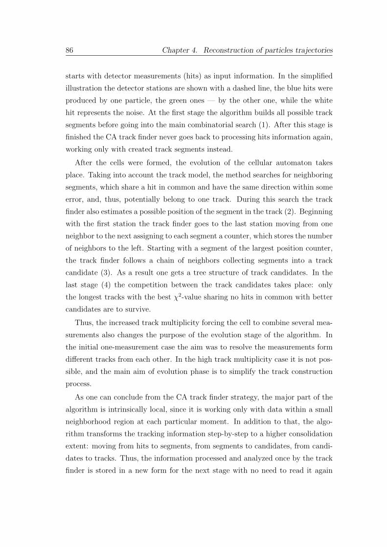
86 Chapter 4. Reconstruction of particles trajectories
starts with detector measurements (hits) as input information. In the simplified
illustration the detector stations are shown with a dashed line, the blue hits were
produced by one particle, the green ones — by the other one, while the white
hit represents the noise. At the first stage the algorithm builds all possible track
segments before going into the main combinatorial search (1). After this stage is
finished the CA track finder never goes back to processing hits information again,
working only with created track segments instead.
After the cells were formed, the evolution of the cellular automaton takes
place. Taking into account the track model, the method searches for neighboring
segments, which share a hit in common and have the same direction within some
error, and, thus, potentially belong to one track. During this search the track
finder also estimates a possible position of the segment in the track (2). Beginning
with the first station the track finder goes to the last station moving from one
neighbor to the next assigning to each segment a counter, which stores the number
of neighbors to the left. Starting with a segment of the largest position counter,
the track finder follows a chain of neighbors collecting segments into a track
candidate (3). As a result one gets a tree structure of track candidates. In the
last stage (4) the competition between the track candidates takes place: only
the longest tracks with the best χ2-value sharing no hits in common with better
candidates are to survive.
Thus, the increased track multiplicity forcing the cell to combine several mea-
surements also changes the purpose of the evolution stage of the algorithm. In
the initial one-measurement case the aim was to resolve the measurements form
different tracks from each other. In the high track multiplicity case it is not pos-
sible, and the main aim of evolution phase is to simplify the track construction
process.
As one can conclude from the CA track finder strategy, the major part of the
algorithm is intrinsically local, since it is working only with data within a small
neighborhood region at each particular moment. In addition to that, the algo-
rithm transforms the tracking information step-by-step to a higher consolidation
extent: moving from hits to segments, from segments to candidates, from candi-
dates to tracks. Thus, the information processed and analyzed once by the track
finder is stored in a new form for the next stage with no need to read it again
4.2 Track finding 87
later. This optimizes memory access, since no data is read or processed twice.
These algorithm features make it suitable for parallel implementation on modern
many-core CPU/GPU computer architectures.
Different variations of this scheme were applied in HEP experiments with
high track multiplicity. In the next section details of the CA-based track finder
algorithm for the CBM experiment are discussed.
4.2.4 Cellular automaton track finder for CBM
The CA method’s features made the algorithm an appropriate solution for the
track reconstruction in the CBM main tracking detector STS. Let us consider in
detail the CBM version of the CA track finder.
A charged particle track in a magnetic field has 5 degrees of freedom. Hence,
a particle trajectory can be fully described with five parameters. The CBM state
vector was chosen in the following form: (xi, yi, txi, tyi, q/p). Here, xi, yi are the
coordinates of the point where the particle intersects the plane of the i-th STS
detector; txi, tyi are the slopes of the track to the OZ-axis; and q/p is the particle
charge to momentum ratio.
Let us define the triplet as a group of 3 hit measurements on adjacent detector
stations, potentially produced by the same particle. Since hit includes (xi, yi)
— two measurements of intersection of a particle with a certain detector plane,
the triplet represents the set of 6 coordinate measurements and allows the unique
determination of all five parameters of a reconstructed track segment. For this
reason in CBM the cells of the CA track finder are triplets.
The triplet parameters coincide with the track parameters: (xi, yi, txi, tyi, q/p).
It gives the opportunity to estimate the χ2 deviation between the hit measure-
ments and the parameters of reconstructed track segments with the Kalman filter
method. Such strategy has proved that already at the triplet level most random
3-hit combinations can be rejected according to the χ2-value, since they are un-
likely to represent a segment of a real track.
The strategy of the algorithm can be explained with the help of the pseudocode
scheme, which is shown in Fig. 4.13. The actual tracking procedure starts with
initialisation ( Fig. 4.13: pseudocode line 1). At this stage the algorithm allocates
88 Chapter 4. Reconstruction of particles trajectories
Pseudocode for CBM CA Track Finder1 Sort_Input_Hits_According_to_Grid();23 for track_set (high_p_primary, low_p_primary, secondary, broken)45 switch (track_set) 6 case high_p_primary:7 Build_Triplets (min_momentum_for_fast_tracks,
primary_track_parameter_initilisation, triplets_wo_gaps);89 case low_p_primary:10 Build_Triplets (min_momentum_for_slow_tracks,
primary_track_parameter_initilisation, triplets_wo_gaps);1112 case secondary:13 Build_Triplets (min_momentum_for_slow_tracks,
secondary_track_parameter_initilisation, triplets_wo_gaps);14 15 case broken:16 Build_Triplets (min_momentum_for_slow_tracks,
secondary_track_parameter_initilisation, triplets_with/wo_gaps)
1718 Find_Neighbours();1920212223 for track_length := NStation to 3 do24 for station := FirstStation to NStation do25 for triplets := First_Triplet_Station to
Last_Triplet_Station do26 track_candidate = Build_Best_Candidate (triplet);272829 Save_Candidates(all_track_candidates);3031 Delete_Used_Hits();
void function Build_Triplets (min_momentum, prim/sec_track_parameter_initilisation, triplets_with/wo_gaps) for station := (NStation-2) to FirstStation do for hits_portion := First_Portion_Station to Last_Portion_Station do
Find_Singlets(hits_portion); Find_Doublets(singlets_in_portion); Find_Triplets(doublets_in_portion);
void function Find_Neighbours (All_Triplets)
for triplet := First_Triplet to Last_Triplet do
Find_Save_Neighbours(triplet); Calculate_Level(triplet);
void function Save_Candidates(All_Track_Candidate) Sort_Candidates(); for candidate := First_Candidate to Last_Candidate do if (used_hits) discard candidate else save candidate;
Figure 4.13: A pseudocode scheme for the CA track finder algorithm.
memory for the input information and prepares a special data structure to store
hits — the grid (Fig. 4.14).
The grid structure plays an important role for the speed of the algorithm,
since it provides fast access towards hits for the most time-consuming part of
triplets construction. While binding hits into triplets, one often faces a task of
finding a hit of the triplet in the certain spatial area of a station. In order to
do it quickly, a regular 2D grid is introduced on each station, with the cell size
inversely proportional to the hit density on the station. All hits are sorted and
stored in the memory in the order of their cell numbers. For each cell the pointer
to the first hit in this cell is stored.
The idea of grid approach is illustrated in Fig. 4.14. After extrapolation of the
track segment to the next station, the algorithm obtains the estimated position
(x, y) with extrapolation errors. It defines a certain region of interest on the
station, where potentially the next hit can be located. In order not to go through
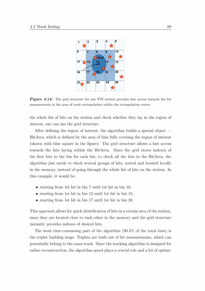
4.2 Track finding 89
(x,y)
1 2 3 4 5
6 7 8 9 10
11 12 14 15
16 17 18 19 20
21 22 23 24
13
259
87
65
4
12
3
10
1615
1413
1211
2524
2322
2120
1718
19
26
3231
3029
2827
4140
3938
3736
3334
35
42
4847
4645
4443
5756
5554
5352
4950
51
58
6463
6261
6059
Δt1
Δt2
Δt3
Δt4
y
x
t
Figure 4.14: The grid structure for one STS station provides fast access towards the hit
measurements in the area of track extrapolation within the extrapolation errors.
the whole list of hits on the station and check whether they lay in the region of
interest, one can use the grid structure.
After defining the region of interest, the algorithm builds a special object —
HitArea, which is defined by the area of bins fully covering the region of interest
(shown with blue square in the figure). The grid structure allows a fast access
towards the hits laying within the HitArea. Since the grid stores indexes of
the first hits in the bin for each bin, to check all the hits in the HitArea, the
algorithm just needs to check several groups of hits, sorted and located locally
in the memory, instead of going through the whole list of hits on the station. In
this example, it would be:
• starting from 1st hit in bin 7 until 1st hit in bin 10,
• starting from 1st hit in bin 12 until 1st hit in bin 15,
• starting from 1st hit in bin 17 until 1st hit in bin 20.
This approach allows for quick identification of hits in a certain area of the station,
since they are located close to each other in the memory and the grid structure
instantly provides indexes of desired hits.
The most time-consuming part of the algorithm (90.4% of the total time) is
the triplet building stage. Triplets are built out of hit measurements, which can
potentially belong to the same track. Since the tracking algorithm is designed for
online reconstruction, the algorithm speed plays a crucial role and a lot of optimi-
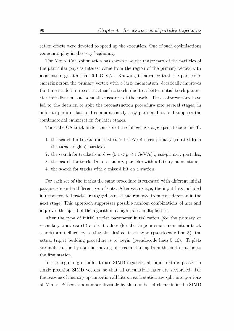
90 Chapter 4. Reconstruction of particles trajectories
sation efforts were devoted to speed up the execution. One of such optimisations
come into play in the very beginning.
The Monte Carlo simulation has shown that the major part of the particles of
the particular physics interest come from the region of the primary vertex with
momentum greater than 0.1 GeV/c. Knowing in advance that the particle is
emerging from the primary vertex with a large momentum, drastically improves
the time needed to reconstruct such a track, due to a better initial track param-
eter initialization and a small curvature of the track. These observations have
led to the decision to split the reconstruction procedure into several stages, in
order to perform fast and computationally easy parts at first and suppress the
combinatorial enumeration for later stages.
Thus, the CA track finder consists of the following stages (pseudocode line 3):
1. the search for tracks from fast (p > 1 GeV/c) quasi-primary (emitted from
the target region) particles,
2. the search for tracks from slow (0.1 < p < 1 GeV/c) quasi-primary particles,
3. the search for tracks from secondary particles with arbitrary momentum,
4. the search for tracks with a missed hit on a station.
For each set of the tracks the same procedure is repeated with different initial
parameters and a different set of cuts. After each stage, the input hits included
in reconstructed tracks are tagged as used and removed from consideration in the
next stage. This approach suppresses possible random combinations of hits and
improves the speed of the algorithm at high track multiplicities.
After the type of initial triplet parameter initialization (for the primary or
secondary track search) and cut values (for the large or small momentum track
search) are defined by setting the desired track type (pseudocode line 3), the
actual triplet building procedure is to begin (pseudocode lines 5–16). Triplets
are built station by station, moving upstream starting from the sixth station to
the first station.
In the beginning in order to use SIMD registers, all input data is packed in
single precision SIMD vectors, so that all calculations later are vectorised. For
the reasons of memory optimization all hits on each station are split into portions
of N hits. N here is a number divisible by the number of elements in the SIMD
4.2 Track finding 91
1.
2.
3.
Figure 4.15: The illustration of three types of triplets built by the CA algorithm: 1) with
the second hit missing 2) with the third hit missing 3) with no missing hits (left side). Two
neighboring triplets, combined into a track (right side).
register, since the hits are processed in a SIMD-ised manner.
Each triplet is build in 3 steps: to the starting hit consecutively second and
third hits are added, rejecting non-physical combinations according to the local
track model at each step. Thus, at first each hit on the station is considered a
starting hit of the triplet. To the starting hit we add the target with some errors,
this way obtaining a certain spatial direction. This structure is called singlet.
The singlet together with its errors is extrapolated to the next station, taking
into account track model and possible multiple scattering. While searching for
the next hit on this station, the algorithm creates a new HitArea object. All hits
within the hit area potentially belong to the same track as the singlet hit does.
Adding each hit from the hit area to the singlet, one obtains an array of doublets.
The doublets are fitted with the Kalman filter method and some of them are
rejected due to high χ2-value. In same manner each doublet is propagated to the
next station and the array of triplets for the starting hit is obtained. The major
part of random combinations are rejected due to χ2-value after adding the third
hit to triplets.
Out of triplets discussed above one can construct tracks with consecutively
registered hits in each station only. However the detector inefficiency may lead
to the fact that some hits cannot be registered. In this case a hit on a certain
92 Chapter 4. Reconstruction of particles trajectories
station will be missing. In order to make the algorithm more stable towards
detector inefficiency there is one more additional stage of building triplets with
one hit missing (Fig. 4.15). This way we introduce two additional categories of
triplets:
• with hits on k-th, (k + 1)-th and (k + 3)-th stations
• with hits on k-th, (k + 2)-th and (k + 3)-th stations,
where k — is the starting station number. Since the probability of having two
hits missing in the raw in the track is less than 0.05%, nearly all tracks can be
reconstructed with this approach. After all triplets are constructed including the
ones with missing hits, they are copied to one general array.
Now the triplets should be grouped into track candidates. Since the momen-
tum is conserved in a magnetic field, in order to find triplets potentially belonging
to the same track, one needs to take into account all five state vector parame-
ters. Such so-called neighboring triplets should coincide in position, slope and
momentum. The easiest way of fulfilling this requirement is to define neighbors
as the triplets, sharing two common hits and having the same momentum within
estimated errors (Fig. 4.15). Thus, as the next step the algorithm loops over all
triplets and finds and stores for each one the list of possible neighbors according
to this definition.
In order to further simplify the procedure of combining triplets into tracks,
one can also estimate the position of the triplet in the track. It is done with the
help of, so-called, level, which is calculated for each triplet during the search for
neighbors. The level of a triplet is defined as the length of the longest continuous
chain of neighboring triplets in the direction to the target. The level of a triplet
helps to locate the triplet on the track: the greater the value it takes, the longer
track can be potentially constructed with a certain triplet.
Having estimated the possible position in the track, the triplets can be easily
connected into a candidate tracks (pseudocode lines 23–26). The main aim of
this procedure is to build the best set of tracks according to χ2-value, that share
no hits in common. It allows suppressing of random combinations of triplets. If
two track candidates share a hit in common, the preference is given to the longest
track, since the probability of a random hit combination to represent the track
4.2 Track finding 93
model decreases exponentially with the number of hits.
Thus, the procedure of constructing tracks is designed in such a way, that it
starts with building the longest tracks first. Their hits are tagged as used and
removed from consideration. After the longest tracks are found, the algorithm
consecutively searches for tracks with one hit less and so on until the primary
tracks with 3 hits only.
Starting with the triplets with the maximum level, the chain of neighbors
with a level consecutively descending by one is connected into track candidates.
A treelike structure of potential track candidates is formed in this manner, from
which the best track is selected according to the χ2 criterion.
Having all the candidates of a certain length constructed, the algorithm sorts
them according to their χ2. After this procedure is finished, candidates one by one
sequentially are checked to contain used hits. If at least one used hit is found, the
candidate gets discarded, if not — the candidate is stored (pseudocode line 29).
After the stage of track reconstruction for the current set of tracks is finished,
the final stage of the algorithm takes place (pseudocode line 31): all the hits used
in the reconstructed track are removed from the input information for the next
stage.
4.2.5 Track finding performance
In order to quantify the performance of track finding methods, one needs to
introduce a formal definition of efficiency. Usually the reconstruction efficiency
is defined as the number of successfully reconstructed tracks as a fraction of
all possible tracks of interest. Thus, for a quantitative definition of efficiency,
one needs to define a criterion whether a certain particle has been reconstructed
together with a definition of tracks of interest.
First of all let us define tracks of interest, which potentially can be recon-
structed with a certain detector system. On one hand, this definition should be
driven by the physics motivation of the experiment. In order to reconstruct the
momentum of a charged particle one needs at least three hits, otherwise there
are not enough measurements to define all track parameters. Thus, there is no
sense in reconstructing tracks shorter than three hits.
94 Chapter 4. Reconstruction of particles trajectories
On the other hand, these tracks of interest should be potentially recon-
structable with a certain detector system. This way one excludes the detector
acceptance from the efficiency definition, so that one can compare pure algorithm
reconstruction efficiency for different detector systems.
In the case of CBM collisions at 25 AGeV beam energy simulated by UrQMD
have shown that track multiplicity in the STS and the MVD detectors is so high
that it leaves no possibility of distinguishing between secondary tracks with three
hits and random combinations of three hits. Also for a particle with momentum
lower than 0.1 GeV/c the multiple scattering in the detector material is so strong,
that it is not possible to reconstruct such a distorted track shape. Taking these
aspects into account, in CBM the track is called reconstructable if it has crossed at
least four consecutive STS stations and its momentum is higher than 0.1 GeV/c.
Now let us introduce a criterion, whether a certain particle has been recon-
structed or not. There are two generally accepted concepts [99]:
Hit matching: the method analyzes the origin of each hit in the reconstructed
track using the Monte Carlo information. If the majority of hits originates from
the same particle (not less than some definite fraction of hits was caused by
this particle), the track is called reconstructed. The exact fraction is defined
in such a way, that the reconstructed track parameters are still not affected
significantly, if the track has not more than some percentage of wrongly attached
hits. Experience has shown that in the majority of cases if at least 70% of hits
belong to the same particle, the reconstructed track parameters allow for correct
physics analysis. This method is stable in the limit of very high track densities,
but it requires the Monte Carlo information.
Parameter matching: The reconstructed parameters of a track are compared
with those of the Monte Carlo simulated particle. If the parameters agree within
certain errors (for example, 3 σ around the true Monte Carlo particle parameters),
the track is called reconstructed. This method requires less functionality from the
simulation chain. It bears the danger of accepting random coincidences between
true particles and artifacts from the pattern recognition algorithm. In extreme
cases, this can lead to the paradox impression that the track finding efficiency
improves with increasing hit density.
The efficiency is defined as the ratio between reconstructed Nreco and recon-
4.2 Track finding 95
structable tracks Naccept:
ε =Nreco
Naccept
. (4.28)
Since both hit and parameter matching concepts require Monte Carlo data,
they cannot be applied in case of real data. For real data the efficiency eval-
uation is tricky, but can be performed under certain conditions if at least two
independent track finders are available.
In this case the efficiencies of the track finder are uncorrelated and under
the assumption of the absence of wrongly reconstructed tracks, which were not
produced by any particle, the efficiency of one procedure can be determined by the
fraction of its own tracks among the tracks, found by the other procedure [100]:
If N is the total number of tracks, then:
N1 = N · ε1, (4.29)
where N1 is the number of tracks reconstructed by the 1-st track finder.
N2 = N · ε2, (4.30)
where N2 is the number of tracks reconstructed by the 2-st track finder.
N12 = N · ε1 · ε2, (4.31)
where N12 is the number of tracks reconstructed by both track finders. These
equations allow determination of the unknown efficiencies of both track finders.
However, since the CBM experiment is not operating yet, it works with sim-
ulated data and uses the hit matching version for definition of the reconstructed
track. A reconstructed track is assigned to a generated particle, if at least 70% of
its hits have been produced by this Monte Carlo particle. If the particle is found
more than once, all additionally reconstructed tracks are regarded as clones. A
reconstructed track is called a ghost, if it cannot be assigned to any generated
particle according to the 70% criterion.
The probability of reconstructing a certain particle strongly depends on its
parameters, mostly momentum and the point of origin. Fast particles with large
momentum usually have straight trajectories and are almost not influenced by
the multiple scattering. On the other hand, low momentum particles not only
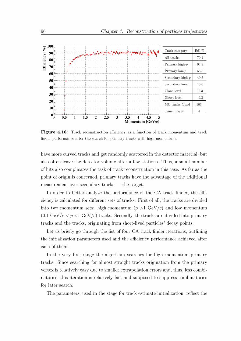
96 Chapter 4. Reconstruction of particles trajectories
Momentum [GeV/c]0 0.5 1 1.5 2 2.5 3 3.5 4 4.5 5
Effic
ienc
y [%
]
0
1020
3040
50
6070
8090
100
4.2 Track finding 103
will be investigated in the next chapter.
Momentum [GeV/c]0 0.5 1 1.5 2 2.5 3 3.5 4 4.5 5
Effic
ienc
y [%
]
0
20
40
60
80
100
Figure 4.21: Track reconstruction eciency as a func-
tion of track momentum after the search for tracks with
missing hits due to detector ineciency.
Track category E↵, %
All tracks 70.4
Primary high-p 94.9
Primary low-p 56.8
Secondary high-p 49.7
Secondary low-p 13.0
Clone level 0.3
Ghost level 0.3
MC tracks found 103
Time, ms/ev 4
Table 4.1: Track finder
performance after the search
for tracks with missing hits
due to detector ineciency.
Momentum [GeV/c]0 0.5 1 1.5 2 2.5 3 3.5 4 4.5 5
Effic
ienc
y [%
]
0
20
40
60
80
100
Figure 4.22: Track reconstruction eciency as a func-
tion of track momentum after the search for tracks with
missing hits due to detector ineciency.
Track category E↵, %
All tracks 87.8
Primary high-p 95.8
Primary low-p 91.4
Secondary high-p 84.5
Secondary low-p 54.2
Clone level 0.9
Ghost level 5.6
MC tracks found 129
Time, ms/ev 6
Table 4.2: Track finder
performance after the search
for tracks with missing hits
due to detector ineciency.
Figure 4.16: Track reconstruction efficiency as a function of track momentum and track
finder performance after the search for primary tracks with high momentum.
have more curved tracks and get randomly scattered in the detector material, but
also often leave the detector volume after a few stations. Thus, a small number
of hits also complicates the task of track reconstruction in this case. As far as the
point of origin is concerned, primary tracks have the advantage of the additional
measurement over secondary tracks — the target.
In order to better analyze the performance of the CA track finder, the effi-
ciency is calculated for different sets of tracks. First of all, the tracks are divided
into two momentum sets: high momentum (p >1 GeV/c) and low momentum
(0.1 GeV/c < p <1 GeV/c) tracks. Secondly, the tracks are divided into primary
tracks and the tracks, originating from short-lived particles’ decay points.
Let us briefly go through the list of four CA track finder iterations, outlining
the initialization parameters used and the efficiency performance achieved after
each of them.
In the very first stage the algorithm searches for high momentum primary
tracks. Since searching for almost straight tracks origination from the primary
vertex is relatively easy due to smaller extrapolation errors and, thus, less combi-
natorics, this iteration is relatively fast and supposed to suppress combinatorics
for later search.
The parameters, used in the stage for track estimate initialization, reflect the
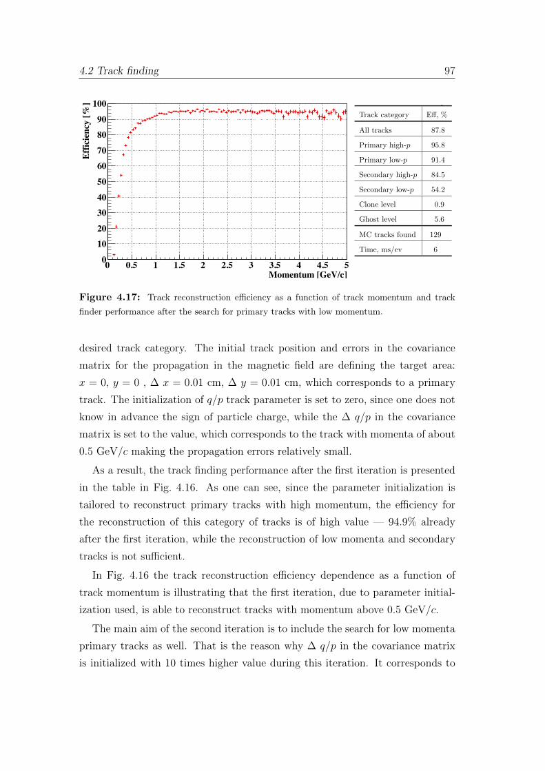
4.2 Track finding 97
Momentum [GeV/c]0 0.5 1 1.5 2 2.5 3 3.5 4 4.5 5
Effic
ienc
y [%
]
0
1020
3040
50
6070
8090
100
4.2 Track finding 103
will be investigated in the next chapter.
Momentum [GeV/c]0 0.5 1 1.5 2 2.5 3 3.5 4 4.5 5
Effic
ienc
y [%
]
0
20
40
60
80
100
Figure 4.21: Track reconstruction eciency as a func-
tion of track momentum after the search for tracks with
missing hits due to detector ineciency.
Track category E↵, %
All tracks 70.4
Primary high-p 94.9
Primary low-p 56.8
Secondary high-p 49.7
Secondary low-p 13.0
Clone level 0.3
Ghost level 0.3
MC tracks found 103
Time, ms/ev 4
Table 4.1: Track finder
performance after the search
for tracks with missing hits
due to detector ineciency.
Momentum [GeV/c]0 0.5 1 1.5 2 2.5 3 3.5 4 4.5 5
Effic
ienc
y [%
]
0
20
40
60
80
100
Figure 4.22: Track reconstruction eciency as a func-
tion of track momentum after the search for tracks with
missing hits due to detector ineciency.
Track category E↵, %
All tracks 87.8
Primary high-p 95.8
Primary low-p 91.4
Secondary high-p 84.5
Secondary low-p 54.2
Clone level 0.9
Ghost level 5.6
MC tracks found 129
Time, ms/ev 6
Table 4.2: Track finder
performance after the search
for tracks with missing hits
due to detector ineciency.
Figure 4.17: Track reconstruction efficiency as a function of track momentum and track
finder performance after the search for primary tracks with low momentum.
desired track category. The initial track position and errors in the covariance
matrix for the propagation in the magnetic field are defining the target area:
x = 0, y = 0 , ∆ x = 0.01 cm, ∆ y = 0.01 cm, which corresponds to a primary
track. The initialization of q/p track parameter is set to zero, since one does not
know in advance the sign of particle charge, while the ∆ q/p in the covariance
matrix is set to the value, which corresponds to the track with momenta of about
0.5 GeV/c making the propagation errors relatively small.
As a result, the track finding performance after the first iteration is presented
in the table in Fig. 4.16. As one can see, since the parameter initialization is
tailored to reconstruct primary tracks with high momentum, the efficiency for
the reconstruction of this category of tracks is of high value — 94.9% already
after the first iteration, while the reconstruction of low momenta and secondary
tracks is not sufficient.
In Fig. 4.16 the track reconstruction efficiency dependence as a function of
track momentum is illustrating that the first iteration, due to parameter initial-
ization used, is able to reconstruct tracks with momentum above 0.5 GeV/c.
The main aim of the second iteration is to include the search for low momenta
primary tracks as well. That is the reason why ∆ q/p in the covariance matrix
is initialized with 10 times higher value during this iteration. It corresponds to
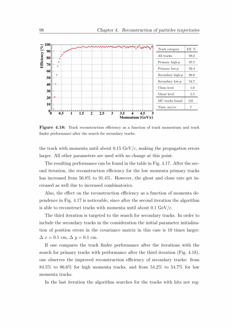
98 Chapter 4. Reconstruction of particles trajectories
Momentum [GeV/c]0 0.5 1 1.5 2 2.5 3 3.5 4 4.5 5
Effic
ienc
y [%
]
0
1020
3040
50
6070
8090
100
104 CHAPTER 4. RECONSTRUCTION OF PARTICLES TRAJECTORIES
Momentum [GeV/c]0 0.5 1 1.5 2 2.5 3 3.5 4 4.5 5
Effic
ienc
y [%
]
0
20
40
60
80
100
Figure 4.23: Track reconstruction eciency as a func-
tion of track momentum after the search for tracks with
missing hits due to detector ineciency.
Track category E↵, %
All tracks 89.2
Primary high-p 97.5
Primary low-p 92.4
Secondary high-p 86.6
Secondary low-p 54.7
Clone level 1.0
Ghost level 5.5
MC tracks found 131
Time, ms/ev 7
Table 4.3: Track finder
performance after the search
for tracks with missing hits
due to detector ineciency.
Momentum [GeV/c]0 0.5 1 1.5 2 2.5 3 3.5 4 4.5 5
Effic
ienc
y [%
]
0
20
40
60
80
100
Figure 4.24: Track reconstruction eciency as a func-
tion of track momentum after the search for tracks with
missing hits due to detector ineciency.
Track category E↵, %
All tracks 90.9
Primary high-p 97.5
Primary low-p 92.6
Secondary high-p 91.1
Secondary low-p 63.8
Clone level 1.0
Ghost level 5.9
MC tracks found 134
Time, ms/ev 8
Table 4.4:
Figure 4.18: Track reconstruction efficiency as a function of track momentum and track
finder performance after the search for secondary tracks.
the track with momenta until about 0.15 GeV/c, making the propagation errors
larger. All other parameters are used with no change at this point.
The resulting performance can be found in the table in Fig. 4.17. After the sec-
ond iteration, the reconstruction efficiency for the low momenta primary tracks
has increased from 56.8% to 91.4%. However, the ghost and clone rate get in-
creased as well due to increased combinatorics.
Also, the effect on the reconstruction efficiency as a function of momenta de-
pendence in Fig. 4.17 is noticeable, since after the second iteration the algorithm
is able to reconstruct tracks with momenta until about 0.1 GeV/c.
The third iteration is targeted to the search for secondary tracks. In order to
include the secondary tracks in the consideration the initial parameter initializa-
tion of position errors in the covariance matrix in this case is 10 times larger:
∆ x = 0.1 cm, ∆ y = 0.1 cm.
If one compares the track finder performance after the iterations with the
search for primary tracks with performance after the third iteration (Fig. 4.18),
one observes the improved reconstruction efficiency of secondary tracks: from
84.5% to 86.6% for high momenta tracks, and from 54.2% to 54.7% for low
momenta tracks.
In the last iteration the algorithm searches for the tracks with hits not reg-
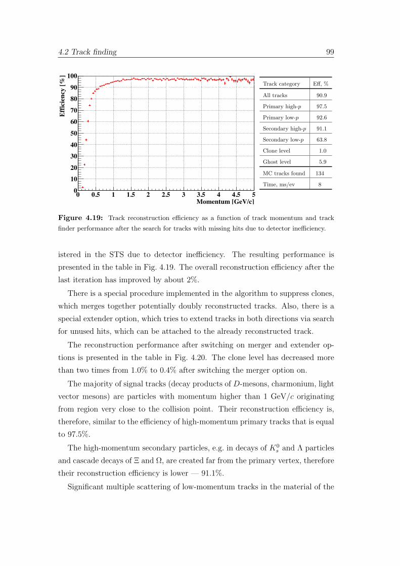
4.2 Track finding 99
Momentum [GeV/c]0 0.5 1 1.5 2 2.5 3 3.5 4 4.5 5
Effic
ienc
y [%
]
0
1020
3040
50
6070
8090
100
104 CHAPTER 4. RECONSTRUCTION OF PARTICLES TRAJECTORIES
Momentum [GeV/c]0 0.5 1 1.5 2 2.5 3 3.5 4 4.5 5
Effic
ienc
y [%
]
0
20
40
60
80
100
Figure 4.23: Track reconstruction eciency as a func-
tion of track momentum after the search for tracks with
missing hits due to detector ineciency.
Track category E↵, %
All tracks 89.2
Primary high-p 97.5
Primary low-p 92.4
Secondary high-p 86.6
Secondary low-p 54.7
Clone level 1.0
Ghost level 5.5
MC tracks found 131
Time, ms/ev 7
Table 4.3: Track finder
performance after the search
for tracks with missing hits
due to detector ineciency.
Momentum [GeV/c]0 0.5 1 1.5 2 2.5 3 3.5 4 4.5 5
Effic
ienc
y [%
]
0
20
40
60
80
100
Figure 4.24: Track reconstruction eciency as a func-
tion of track momentum after the search for tracks with
missing hits due to detector ineciency.
Track category E↵, %
All tracks 90.9
Primary high-p 97.5
Primary low-p 92.6
Secondary high-p 91.1
Secondary low-p 63.8
Clone level 1.0
Ghost level 5.9
MC tracks found 134
Time, ms/ev 8
Table 4.4:
Figure 4.19: Track reconstruction efficiency as a function of track momentum and track
finder performance after the search for tracks with missing hits due to detector inefficiency.
istered in the STS due to detector inefficiency. The resulting performance is
presented in the table in Fig. 4.19. The overall reconstruction efficiency after the
last iteration has improved by about 2%.
There is a special procedure implemented in the algorithm to suppress clones,
which merges together potentially doubly reconstructed tracks. Also, there is a
special extender option, which tries to extend tracks in both directions via search
for unused hits, which can be attached to the already reconstructed track.
The reconstruction performance after switching on merger and extender op-
tions is presented in the table in Fig. 4.20. The clone level has decreased more
than two times from 1.0% to 0.4% after switching the merger option on.
The majority of signal tracks (decay products of D-mesons, charmonium, light
vector mesons) are particles with momentum higher than 1 GeV/c originating
from region very close to the collision point. Their reconstruction efficiency is,
therefore, similar to the efficiency of high-momentum primary tracks that is equal
to 97.5%.
The high-momentum secondary particles, e.g. in decays of K0s and Λ particles
and cascade decays of Ξ and Ω, are created far from the primary vertex, therefore
their reconstruction efficiency is lower — 91.1%.
Significant multiple scattering of low-momentum tracks in the material of the
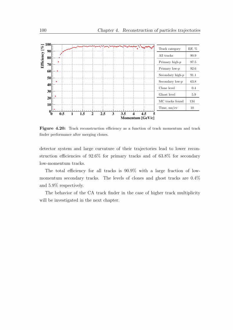
100 Chapter 4. Reconstruction of particles trajectories
Momentum [GeV/c]0 0.5 1 1.5 2 2.5 3 3.5 4 4.5 5
Effic
ienc
y [%
]
0
1020
3040
50
6070
8090
100
4.2 Track finding 105
Momentum [GeV/c]0 0.5 1 1.5 2 2.5 3 3.5 4 4.5 5
Effic
ienc
y [%
]
0
20
40
60
80
100
Figure 4.25: Track reconstruction eciency as a func-
tion of track momentum after the search for tracks with
missing hits due to detector ineciency.
Track category E↵, %
All tracks 90.9
Primary high-p 97.5
Primary low-p 92.6
Secondary high-p 91.1
Secondary low-p 63.8
Clone level 0.4
Ghost level 5.9
MC tracks found 134
Time, ms/ev 10
Table 4.5: Track finder
performance after the search
for tracks with missing hits
due to detector ineciency.
Figure 4.20: Track reconstruction efficiency as a function of track momentum and track
finder performance after merging clones.
detector system and large curvature of their trajectories lead to lower recon-
struction efficiencies of 92.6% for primary tracks and of 63.8% for secondary
low-momentum tracks.
The total efficiency for all tracks is 90.9% with a large fraction of low-
momentum secondary tracks. The levels of clones and ghost tracks are 0.4%
and 5.9% respectively.
The behavior of the CA track finder in the case of higher track multiplicity
will be investigated in the next chapter.
Chapter 5
Track finding at high track
multiplicities
5.1 Challenging track multiplicities in HEP
To validate the Standard Model, scientists aim to observe phenomena at ever
higher energy densities and to measure their parameters with the highest pos-
sible precision. To achieve this one needs accelerators which are as powerful as
possible and the most precise detectors. The multiplicity of some important rare
probes is so low, that the statistically reliable measurement for them requires
HEP experiments to operate at ever increasing collision rates. One can predict
that in the future this tendency will only get stronger.
On the other hand, in the course of time, as one looks deeper into the struc-
ture of matter, particle detectors have been evolving from simple devices with a
few channels to very complex multi-layer systems with several millions of read-
out channels. Due to the ever increasing complexity of particle detectors and
accelerators, the domain is a driving force for technology. The need to look for
rare and complex signals forces the data acquisition systems and reconstruction
algorithms to develop accordingly.
Fig. 5.1 shows the graph of the maximum trigger rates and event sizes for the
operating experiments of the past three decades. The outermost points in this
graph are clearly given by the four LHC experiments, with the general-purpose
experiments (Compact Muon Solenoid (CMS) and A Toroidal LHC Apparatus
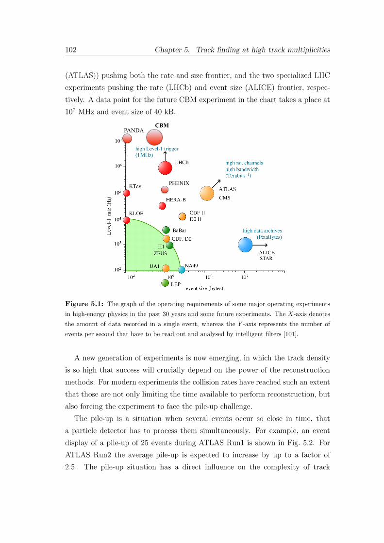
102 Chapter 5. Track finding at high track multiplicities
(ATLAS)) pushing both the rate and size frontier, and the two specialized LHC
experiments pushing the rate (LHCb) and event size (ALICE) frontier, respec-
tively. A data point for the future CBM experiment in the chart takes a place at
107 MHz and event size of 40 kB.
12
106
107
PANDA
STAR
PHENIX
CBM
Figure 5.1: The graph of the operating requirements of some major operating experiments
in high-energy physics in the past 30 years and some future experiments. The X-axis denotes
the amount of data recorded in a single event, whereas the Y -axis represents the number of
events per second that have to be read out and analysed by intelligent filters [101].
A new generation of experiments is now emerging, in which the track density
is so high that success will crucially depend on the power of the reconstruction
methods. For modern experiments the collision rates have reached such an extent
that those are not only limiting the time available to perform reconstruction, but
also forcing the experiment to face the pile-up challenge.
The pile-up is a situation when several events occur so close in time, that
a particle detector has to process them simultaneously. For example, an event
display of a pile-up of 25 events during ATLAS Run1 is shown in Fig. 5.2. For
ATLAS Run2 the average pile-up is expected to increase by up to a factor of
2.5. The pile-up situation has a direct influence on the complexity of track
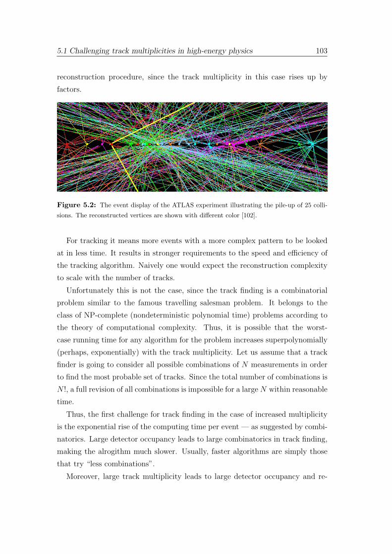
5.1 Challenging track multiplicities in high-energy physics 103
reconstruction procedure, since the track multiplicity in this case rises up by
factors.
Figure 5.2: The event display of the ATLAS experiment illustrating the pile-up of 25 colli-
sions. The reconstructed vertices are shown with different color [102].
For tracking it means more events with a more complex pattern to be looked
at in less time. It results in stronger requirements to the speed and efficiency of
the tracking algorithm. Naively one would expect the reconstruction complexity
to scale with the number of tracks.
Unfortunately this is not the case, since the track finding is a combinatorial
problem similar to the famous travelling salesman problem. It belongs to the
class of NP-complete (nondeterministic polynomial time) problems according to
the theory of computational complexity. Thus, it is possible that the worst-
case running time for any algorithm for the problem increases superpolynomially
(perhaps, exponentially) with the track multiplicity. Let us assume that a track
finder is going to consider all possible combinations of N measurements in order
to find the most probable set of tracks. Since the total number of combinations is
N !, a full revision of all combinations is impossible for a large N within reasonable
time.
Thus, the first challenge for track finding in the case of increased multiplicity
is the exponential rise of the computing time per event — as suggested by combi-
natorics. Large detector occupancy leads to large combinatorics in track finding,
making the alrogithm much slower. Usually, faster algorithms are simply those
that try “less combinations”.
Moreover, large track multiplicity leads to large detector occupancy and re-
104 Chapter 5. Track finding at high track multiplicities
sults in overlapping tracks. It naturally leads to increased number of wrongly
reconstructed tracks. A robust tracking algorithm must be able to handle large
variations in multiplicity. That is why the tracking stability becomes particularly
important for the modern HEP experiments.
The simulations of the continuous CBM beam predict that the experiment also
will have to deal with events overlapping in time. In order to test the CBM CA
track finder behavior in the high track multiplicity environment, a special study
was performed. The details of the study will be provided and discussed in the
next section.
5.2 CA track finder performance at high track
multiplicity
In order to test in a high track multiplicity environment the stability of the CA
track finder algorithm described in the previous chapter a special study has been
performed. A robust behavior of the algorithm in this test promises stability of
tracking in the case of increased track multiplicity due to a pile-up or a beam
instability.
However, the CBM experiment has some particular reasons to test tracking
routines with respect to high track multiplicities. Since the CBM experiment
will operate at extremely high interaction rates, different collisions may overlap
in time, leaving no possibility to separate them in a trivial way. Thus, the need
to analyze the so-called time-slices, which contain information from a number of
collisions, rather than isolated events, arises.
The need to work with time-slices instead of events is driven not only by
physical circumstances, but also is encouraged by computing hardware reasons.
Not only minimum bias events, but even central events have been proven to
be not big enough in order to be processed in parallel on a modern many core
computer architectures. For implementing in-event level parallelism these events
do not have enough sources of parallelism (like hits, segments, track candidates
for different reconstruction stages) in order to be reconstructed on 20 or more
CPU cores simultaneously.
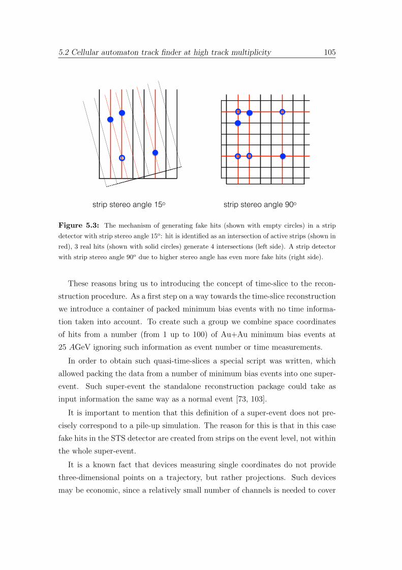
5.2 Cellular automaton track finder at high track multiplicity 105
strip stereo angle 15o strip stereo angle 90o
Figure 5.3: The mechanism of generating fake hits (shown with empty circles) in a strip
detector with strip stereo angle 15o: hit is identified as an intersection of active strips (shown in
red), 3 real hits (shown with solid circles) generate 4 intersections (left side). A strip detector
with strip stereo angle 90o due to higher stereo angle has even more fake hits (right side).
These reasons bring us to introducing the concept of time-slice to the recon-
struction procedure. As a first step on a way towards the time-slice reconstruction
we introduce a container of packed minimum bias events with no time informa-
tion taken into account. To create such a group we combine space coordinates
of hits from a number (from 1 up to 100) of Au+Au minimum bias events at
25 AGeV ignoring such information as event number or time measurements.
In order to obtain such quasi-time-slices a special script was written, which
allowed packing the data from a number of minimum bias events into one super-
event. Such super-event the standalone reconstruction package could take as
input information the same way as a normal event [73, 103].
It is important to mention that this definition of a super-event does not pre-
cisely correspond to a pile-up simulation. The reason for this is that in this case
fake hits in the STS detector are created from strips on the event level, not within
the whole super-event.
It is a known fact that devices measuring single coordinates do not provide
three-dimensional points on a trajectory, but rather projections. Such devices
may be economic, since a relatively small number of channels is needed to cover
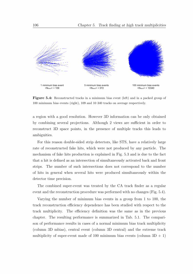
106 Chapter 5. Track finding at high track multiplicities
CBM CA Track Finding at High Track Multiplicity
Towards 4D (space + time) event reconstruction !4
Au+Au mbias events at 25 AGeV, 8 STS, 0 x 7,5 strip angles
1 minimum bias event <Nreco> = 109
5 minimum bias events <Nreco> = 572
100 minimum bias events <Nreco> = 10340
Figure 5.4: Reconstructed tracks in a minimum bias event (left) and in a packed group of
100 minimum bias events (right), 109 and 10 340 tracks on average respectively.
a region with a good resolution. However 3D information can be only obtained
by combining several projections. Although 2 views are sufficient in order to
reconstruct 3D space points, in the presence of multiple tracks this leads to
ambiguities.
For this reason double-sided strip detectors, like STS, have a relatively large
rate of reconstructed fake hits, which were not produced by any particle. The
mechanism of fake hits production is explained in Fig. 5.3 and is due to the fact
that a hit is defined as an intersection of simultaneously activated back and front
strips. The number of such intersections does not correspond to the number
of hits in general when several hits were produced simultaneously within the
detector time precision.
The combined super-event was treated by the CA track finder as a regular
event and the reconstruction procedure was performed with no changes (Fig. 5.4).
Varying the number of minimum bias events in a group from 1 to 100, the
track reconstruction efficiency dependence has been studied with respect to the
track multiplicity. The efficiency definition was the same as in the previous
chapter. The resulting performance is summarized in Tab. 5.1. The compari-
son of performance results in cases of a normal minimum bias track multiplicity
(column 3D mbias), central event (column 3D central) and the extreme track
multiplicity of super-event made of 100 minimum bias events (column 3D + 1)
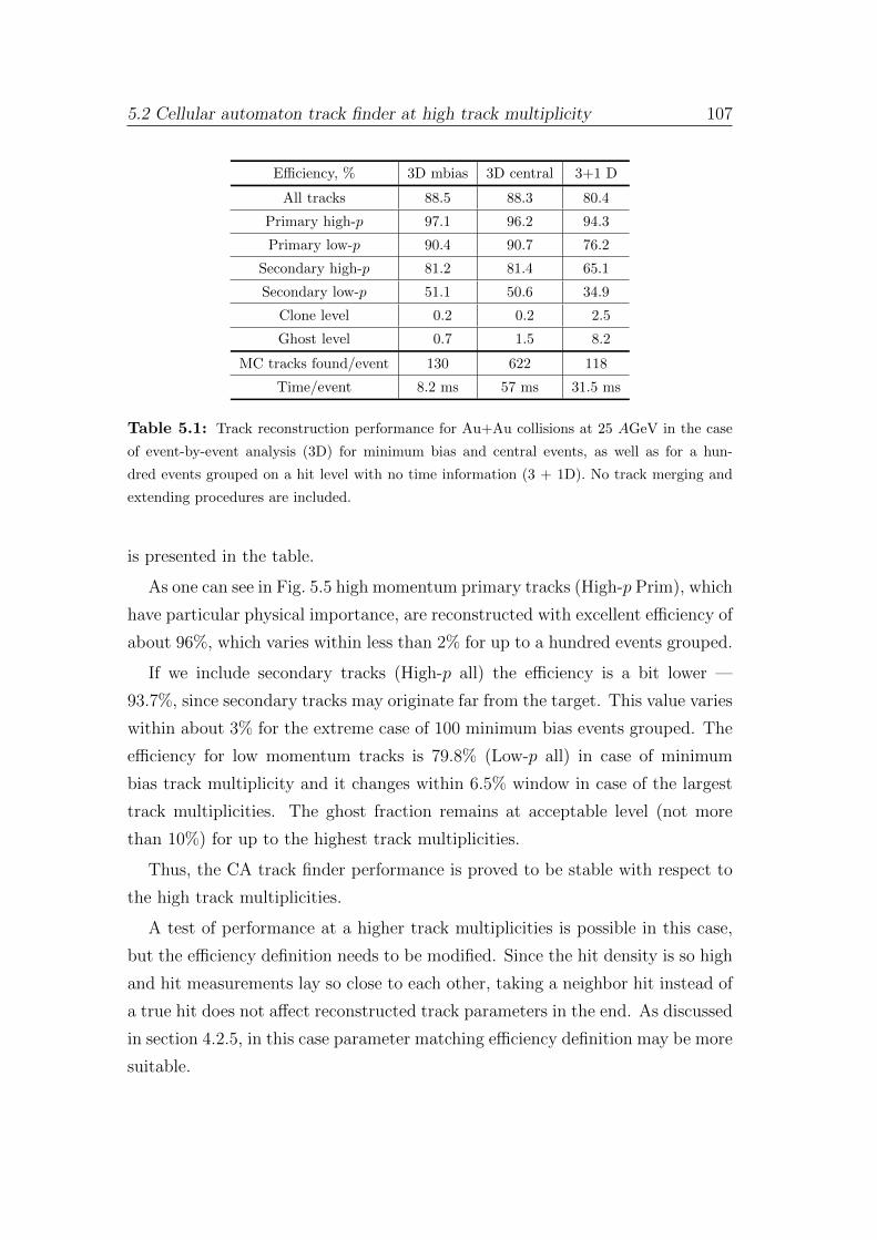
5.2 Cellular automaton track finder at high track multiplicity 107
Efficiency, % 3D mbias 3D central 3+1 D
All tracks 88.5 88.3 80.4
Primary high-p 97.1 96.2 94.3
Primary low-p 90.4 90.7 76.2
Secondary high-p 81.2 81.4 65.1
Secondary low-p 51.1 50.6 34.9
Clone level 0.2 0.2 2.5
Ghost level 0.7 1.5 8.2
MC tracks found/event 130 622 118
Time/event 8.2 ms 57 ms 31.5 ms
Table 5.1: Track reconstruction performance for Au+Au collisions at 25 AGeV in the case
of event-by-event analysis (3D) for minimum bias and central events, as well as for a hun-
dred events grouped on a hit level with no time information (3 + 1D). No track merging and
extending procedures are included.
is presented in the table.
As one can see in Fig. 5.5 high momentum primary tracks (High-p Prim), which
have particular physical importance, are reconstructed with excellent efficiency of
about 96%, which varies within less than 2% for up to a hundred events grouped.
If we include secondary tracks (High-p all) the efficiency is a bit lower —
93.7%, since secondary tracks may originate far from the target. This value varies
within about 3% for the extreme case of 100 minimum bias events grouped. The
efficiency for low momentum tracks is 79.8% (Low-p all) in case of minimum
bias track multiplicity and it changes within 6.5% window in case of the largest
track multiplicities. The ghost fraction remains at acceptable level (not more
than 10%) for up to the highest track multiplicities.
Thus, the CA track finder performance is proved to be stable with respect to
the high track multiplicities.
A test of performance at a higher track multiplicities is possible in this case,
but the efficiency definition needs to be modified. Since the hit density is so high
and hit measurements lay so close to each other, taking a neighbor hit instead of
a true hit does not affect reconstructed track parameters in the end. As discussed
in section 4.2.5, in this case parameter matching efficiency definition may be more
suitable.
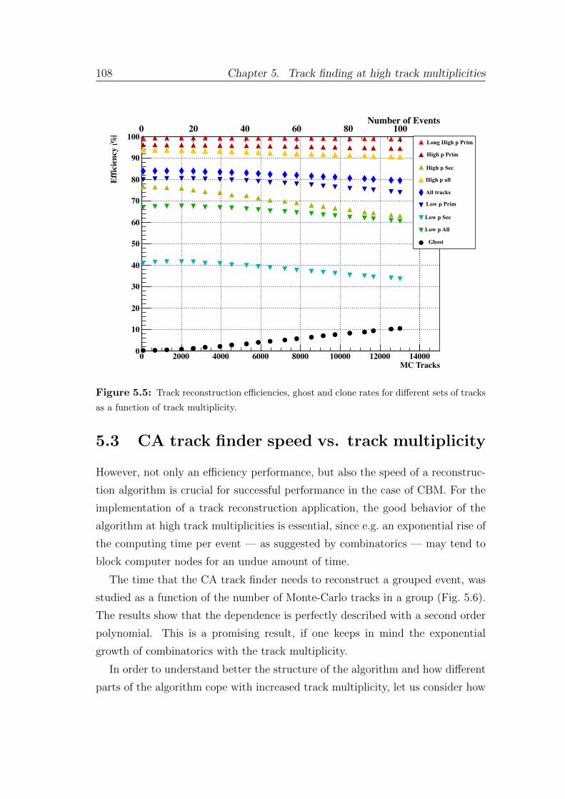
108 Chapter 5. Track finding at high track multiplicities
MC Tracks0 2000 4000 6000 8000 10000 12000 14000
Effic
ienc
y, %
0
10
20
30
40
50
60
70
80
90
100
Number of Events0 20 40 60 80 100
LongRefPrim
RefPrim
RefSec
RefSet
AllSet
ExtraPrim
ExtraSec
ExtraSet
Ghost
Long High p Prim
High p Prim
High p Sec
High p all
All tracks
Low p Prim
Low p Sec
Low p All
Ghost
Figure 5.5: Track reconstruction efficiencies, ghost and clone rates for different sets of tracks
as a function of track multiplicity.
5.3 CA track finder speed vs. track multiplicity
However, not only an efficiency performance, but also the speed of a reconstruc-
tion algorithm is crucial for successful performance in the case of CBM. For the
implementation of a track reconstruction application, the good behavior of the
algorithm at high track multiplicities is essential, since e.g. an exponential rise of
the computing time per event — as suggested by combinatorics — may tend to
block computer nodes for an undue amount of time.
The time that the CA track finder needs to reconstruct a grouped event, was
studied as a function of the number of Monte-Carlo tracks in a group (Fig. 5.6).
The results show that the dependence is perfectly described with a second order
polynomial. This is a promising result, if one keeps in mind the exponential
growth of combinatorics with the track multiplicity.
In order to understand better the structure of the algorithm and how different
parts of the algorithm cope with increased track multiplicity, let us consider how
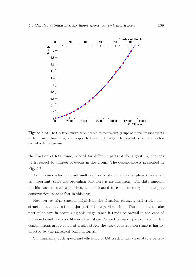
5.3 Cellular automaton track finder speed vs. track multiplicity 109
MC Tracks0 2500 5000 7500 10000 12500 15000
Tim
e, [s
]
0
0.2
0.4
0.6
0.8
1
1.2
1.4
1.6
1.8
2 / ndf 2χ 0.001229 / 18
p0 0.004993± 0.01834
p1 1.769e-06± 3.463e-05 p2 1.301e-10± 8.856e-09
/ ndf 2χ 0.001229 / 18p0 0.004993± 0.01834
p1 1.769e-06± 3.463e-05 p2 1.301e-10± 8.856e-09
Number of Events0 20 40 60 80 100
Figure 5.6: The CA track finder time, needed to reconstruct groups of minimum bias events
without time information, with respect to track multiplicity. The dependence is fitted with a
second order polynomial.
the fraction of total time, needed for different parts of the algorithm, changes
with respect to number of events in the group. The dependence is presented in
Fig. 5.7.
As one can see for low track multiplicities triplet construction phase time is not
as important, since the prevailing part here is initialization. The data amount
in this case is small and, thus, can be loaded to cache memory. The triplet
construction stage is fast in this case.
However, at high track multiplicities the situation changes, and triplet con-
struction stage takes the major part of the algorithm time. Thus, one has to take
particular care in optimizing this stage, since it tends to prevail in the case of
increased combinatorics like no other stage. Since the major part of random hit
combinations are rejected at triplet stage, the track construction stage is hardly
affected by the increased combinatorics.
Summarizing, both speed and efficiency of CA track finder show stable behav-
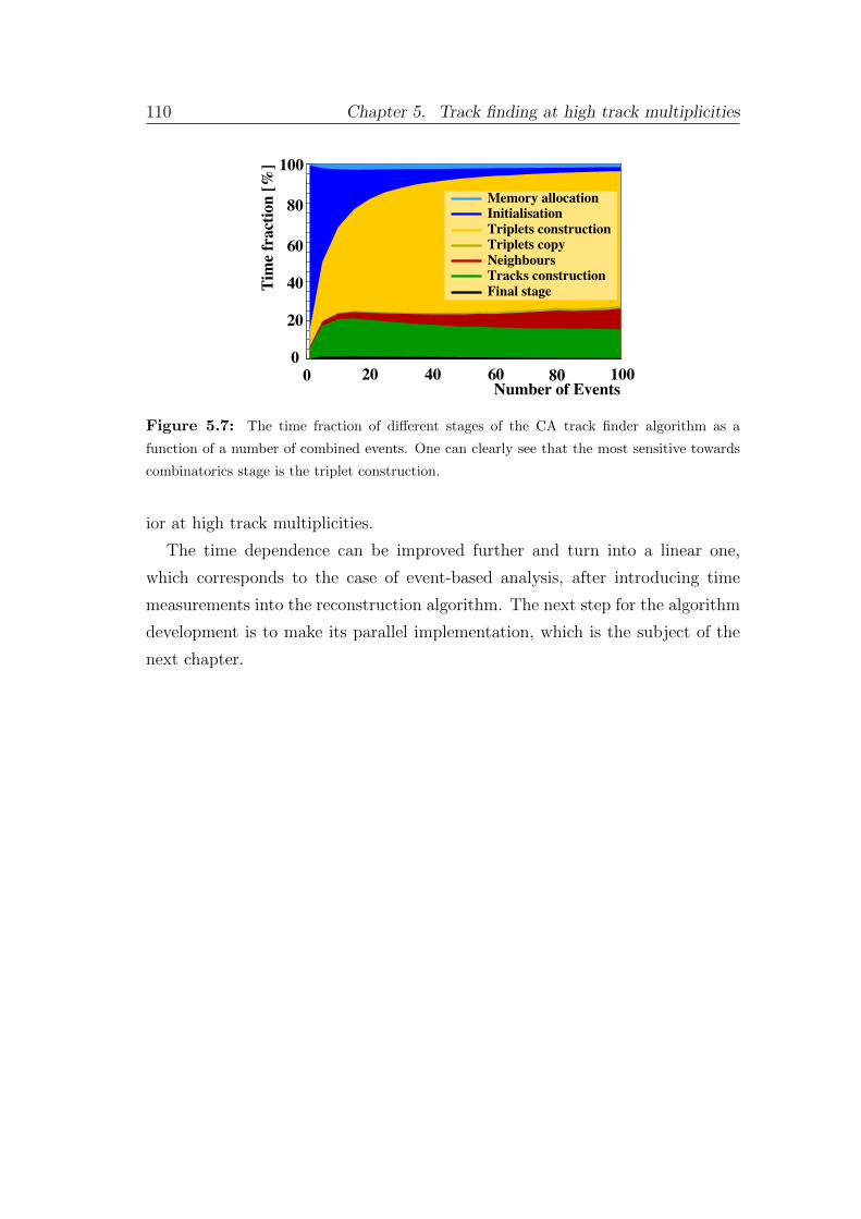
110 Chapter 5. Track finding at high track multiplicities
N Events0 20 40 60 80 100
Tim
e fr
actio
n, %
0
20
40
60
80
100
Memory allocationInitialisationTriplets constructionTriplets copyNeighboursTracks constructionFinal stage
0 20 40 60 80 100Number of Events
Tim
e fr
actio
n [%
]
0
20
40
60
80
100
Figure 5.7: The time fraction of different stages of the CA track finder algorithm as a
function of a number of combined events. One can clearly see that the most sensitive towards
combinatorics stage is the triplet construction.
ior at high track multiplicities.
The time dependence can be improved further and turn into a linear one,
which corresponds to the case of event-based analysis, after introducing time
measurements into the reconstruction algorithm. The next step for the algorithm
development is to make its parallel implementation, which is the subject of the
next chapter.
Chapter 6
Parallel CA track finder
One of the key ingredients for the successful operation of the CBM experiment is
the development of fast and precise reconstruction algorithms suitable for online
data processing. In order to benefit from the advantages of modern parallel com-
puter architectures (many-core CPU/GPU), the existing reconstruction routines
need to be redesigned with parallelism in mind. The desired efficient intrinsically
parallel algorithms should reflect the massive hardware parallelism in computa-
tional scheme and data structures.
The CA track finder algorithm was redesigned and optimized with respect to
parallelism. The algorithm demonstrates a linear scalability on a many-core CPU
server, indicating the ability to be effectively run on a complex computer farm.
While vectorisation allowed for processing in parallel data streams, many-core
execution has enabled parallelism on the task level. The details of parallel CA
track finder algorithm development as well as achieved performance are discussed
in this chapter.
6.1 General overview of parallelisation strategy
Although intrinsic parallelism and data locality are the notable features of the
CA track finder, still a lot of efforts were required in order to develop an efficient
parallel implementation out of the existing vectorised, but sequential algorithm.
Reformulating the algorithm in terms of parallelism often may mean that
it has to be drastically changed or even written from scratch, since an efficient
112 Chapter 6. Parallel track finder algorithm
sequential version is not necessarily an efficient solution for a parallel run. Parallel
implementation requires certain features for the algorithm. Firstly, in order to
get correct results, the operations performed concurrently should be independent
from each other. Secondly, one has to keep in mind that the parallel section should
always be thread-safe, so that the shared data structures are used in a manner
that guarantees safe simultaneous execution by multiple threads. This can be
achieved by allocating local data structures to each thread and summarizing
results of their work afterwards or, alternatively, introducing synchronization
into thread execution.
The synchronization usually slows down the speed of a program, since threads
have to wait for each other or exchange results of their work, so the use of this
tool should be minimized. Also memory optimization and data structure scheme
become essential in case of parallel programming, due to increased memory de-
mand.
Thus, the CA track finder algorithm had to be redesigned with the idea of per-
formant parallel processing in mind. The main goal at this stage was to create an
entirely parallel implementation for a concurrent search for tracks within a single
grouped super-event (quasi time-slice). The target implementation should show
the maximum achievable speed-up factor on the testing architecture, while still
being fast in sequential run and providing stable and reliable results. Although
this issue is closely connected with the algorithm speed, particular attention was
devoted to the data structures and memory optimization.
The vectorized, but sequential in terms of core usage, version of the CA track
finder was taken as the starting point for developing a parallel version with the
use of the OpenMP and Pthreads interfaces.
Here it is important to highlight the difference between embarrassingly parallel
reconstruction of independent events concurrently, which is to a certain extent
trivial, and the problem of distributing a bunch of dependent tasks, performed
while reconstructing tracks produced in a time-slice in a parallel run. Unlike
the case of different events, where no synchronization by default is needed, the
reconstruction of a time-slice in parallel requires synchronization, so that the
work is distributed between threads in an efficient and thread-safe manner with
no race conditions.
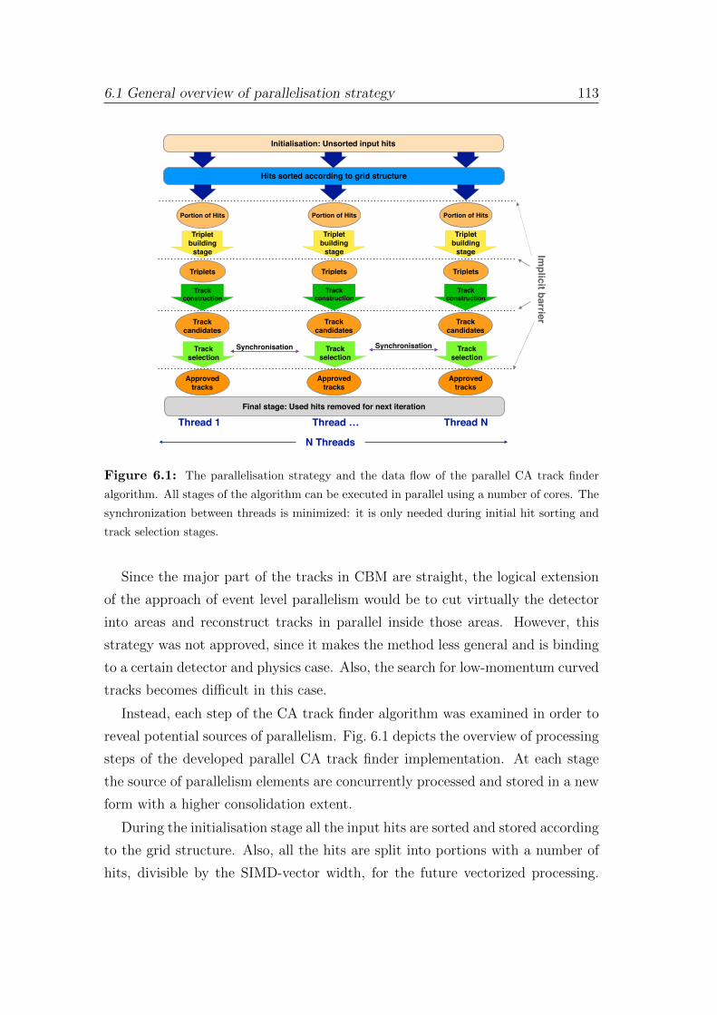
6.1 General overview of parallelisation strategy 113
Synchronisation
Final stage: Used hits removed for next iteration
Initialisation: Unsorted input hits
Hits sorted according to grid structure
Thread 1 Thread … Thread N
N Threads
Approvedtracks
Portion of Hits
Triplets
Trackcandidates
Triplet building
stage
Track construction
Track selection
Approvedtracks
Portion of Hits
Triplets
Trackcandidates
Triplet building
stage
Track construction
Track selection
Approvedtracks
Portion of Hits
Triplets
Trackcandidates
Triplet building
stage
Track construction
Track selection
Synchronisation
Implicit barrier
Figure 6.1: The parallelisation strategy and the data flow of the parallel CA track finder
algorithm. All stages of the algorithm can be executed in parallel using a number of cores. The
synchronization between threads is minimized: it is only needed during initial hit sorting and
track selection stages.
Since the major part of the tracks in CBM are straight, the logical extension
of the approach of event level parallelism would be to cut virtually the detector
into areas and reconstruct tracks in parallel inside those areas. However, this
strategy was not approved, since it makes the method less general and is binding
to a certain detector and physics case. Also, the search for low-momentum curved
tracks becomes difficult in this case.
Instead, each step of the CA track finder algorithm was examined in order to
reveal potential sources of parallelism. Fig. 6.1 depicts the overview of processing
steps of the developed parallel CA track finder implementation. At each stage
the source of parallelism elements are concurrently processed and stored in a new
form with a higher consolidation extent.
During the initialisation stage all the input hits are sorted and stored according
to the grid structure. Also, all the hits are split into portions with a number of
hits, divisible by the SIMD-vector width, for the future vectorized processing.
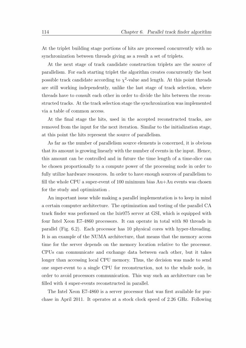
114 Chapter 6. Parallel track finder algorithm
At the triplet building stage portions of hits are processed concurrently with no
synchronization between threads giving as a result a set of triplets.
At the next stage of track candidate construction triplets are the source of
parallelism. For each starting triplet the algorithm creates concurrently the best
possible track candidate according to χ2-value and length. At this point threads
are still working independently, unlike the last stage of track selection, where
threads have to consult each other in order to divide the hits between the recon-
structed tracks. At the track selection stage the synchronization was implemented
via a table of common access.
At the final stage the hits, used in the accepted reconstructed tracks, are
removed from the input for the next iteration. Similar to the initialization stage,
at this point the hits represent the source of parallelism.
As far as the number of parallelism source elements is concerned, it is obvious
that its amount is growing linearly with the number of events in the input. Hence,
this amount can be controlled and in future the time length of a time-slice can
be chosen proportionally to a compute power of the processing node in order to
fully utilize hardware resources. In order to have enough sources of parallelism to
fill the whole CPU a super-event of 100 minimum bias Au+Au events was chosen
for the study and optimization .
An important issue while making a parallel implementation is to keep in mind
a certain computer architecture. The optimization and testing of the parallel CA
track finder was performed on the lxir075 server at GSI, which is equipped with
four Intel Xeon E7-4860 processors. It can operate in total with 80 threads in
parallel (Fig. 6.2). Each processor has 10 physical cores with hyper-threading.
It is an example of the NUMA architecture, that means that the memory access
time for the server depends on the memory location relative to the processor.
CPUs can communicate and exchange data between each other, but it takes
longer than accessing local CPU memory. Thus, the decision was made to send
one super-event to a single CPU for reconstruction, not to the whole node, in
order to avoid processors communication. This way such an architecture can be
filled with 4 super-events reconstructed in parallel.
The Intel Xeon E7-4860 is a server processor that was first available for pur-
chase in April 2011. It operates at a stock clock speed of 2.26 GHz. Following
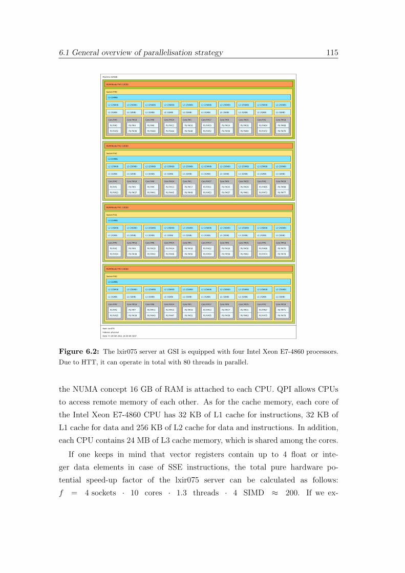
6.1 General overview of parallelisation strategy 115
Figure 6.2: The lxir075 server at GSI is equipped with four Intel Xeon E7-4860 processors.
Due to HTT, it can operate in total with 80 threads in parallel.
the NUMA concept 16 GB of RAM is attached to each CPU. QPI allows CPUs
to access remote memory of each other. As for the cache memory, each core of
the Intel Xeon E7-4860 CPU has 32 KB of L1 cache for instructions, 32 KB of
L1 cache for data and 256 KB of L2 cache for data and instructions. In addition,
each CPU contains 24 MB of L3 cache memory, which is shared among the cores.
If one keeps in mind that vector registers contain up to 4 float or inte-
ger data elements in case of SSE instructions, the total pure hardware po-
tential speed-up factor of the lxir075 server can be calculated as follows:
f = 4 sockets · 10 cores · 1.3 threads · 4 SIMD ≈ 200. If we ex-
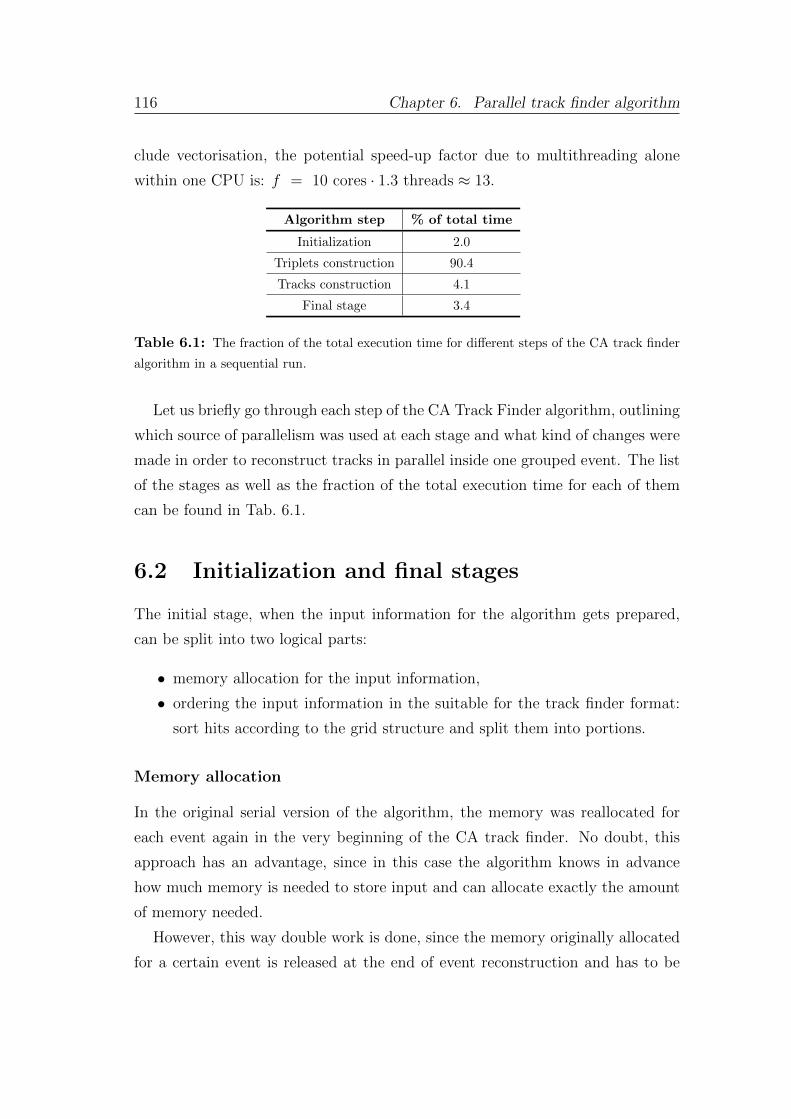
116 Chapter 6. Parallel track finder algorithm
clude vectorisation, the potential speed-up factor due to multithreading alone
within one CPU is: f = 10 cores · 1.3 threads ≈ 13.
Algorithm step % of total time
Initialization 2.0
Triplets construction 90.4
Tracks construction 4.1
Final stage 3.4
Table 6.1: The fraction of the total execution time for different steps of the CA track finder
algorithm in a sequential run.
Let us briefly go through each step of the CA Track Finder algorithm, outlining
which source of parallelism was used at each stage and what kind of changes were
made in order to reconstruct tracks in parallel inside one grouped event. The list
of the stages as well as the fraction of the total execution time for each of them
can be found in Tab. 6.1.
6.2 Initialization and final stages
The initial stage, when the input information for the algorithm gets prepared,
can be split into two logical parts:
• memory allocation for the input information,
• ordering the input information in the suitable for the track finder format:
sort hits according to the grid structure and split them into portions.
Memory allocation
In the original serial version of the algorithm, the memory was reallocated for
each event again in the very beginning of the CA track finder. No doubt, this
approach has an advantage, since in this case the algorithm knows in advance
how much memory is needed to store input and can allocate exactly the amount
of memory needed.
However, this way double work is done, since the memory originally allocated
for a certain event is released at the end of event reconstruction and has to be
6.2 Initialization and final stages 117
allocated again at the initial stage of the next event reconstruction. In case of a
single minimum bias event reconstruction this allocation time is negligible, but
in case of time-slice reconstruction it becomes significant.
One more obstacle of this approach is that memory allocation represents an es-
sentially sequential process and, thus, cannot be efficiently performed in parallel.
Keeping in mind these aspects, the decision was made to reuse the memory, once
allocated for the first reconstructed event. The memory should be allocated once
before calling the track finder routine for a grouped super-event (or, in future,
time-slice). For further reconstruction the memory volume, if needed, should be
extended.
Unfortunately, one cannot know in advance the size of input information. It
varies from one time-slice to another. For instance, it is possible that the next
reconstructed time-slice contains more hits and, thus, more memory is required
to store input information. Partial solution would be to estimate the average
size of time-slice and allocate an excessive amount of memory. But this does
not guaranty a safe execution, in case of some irregular situations. In order to
overcome this obstacle a special class, named L1Vector, was introduced for a safe
execution in case of unpredictable increase in the volume of input information.
The L1Vector class declaration is presented in List. 6.1. This class is based on
the standard library vector class, but has some extra functionality. The L1Vector
has a private member – fSize — to store the number of meaningful elements,
in addition to the normal std::size() — which corresponds to the actual size
of the vector array. If a new element is stored to the array, fSize is increased
by one, but the actual size of the array gets increased only if fSize gets larger
than std::size() (lines 8–11). Certainly, one should avoid situations when
two independent threads are trying to change the size of an array. For this
reason these lines are executed under #pragma omp critical directive to force
sequential execution at this point.
Before calling the track finder routine, the algorithm resizes all the input
vectors to the estimated size of time-slice input information. In the reconstruction
routine the algorithm tries to store input information in the already allocated
arrays, but each time checks if allocated memory is enough to do so. If not,
it will allocate additional memory. This approach avoids double work, while
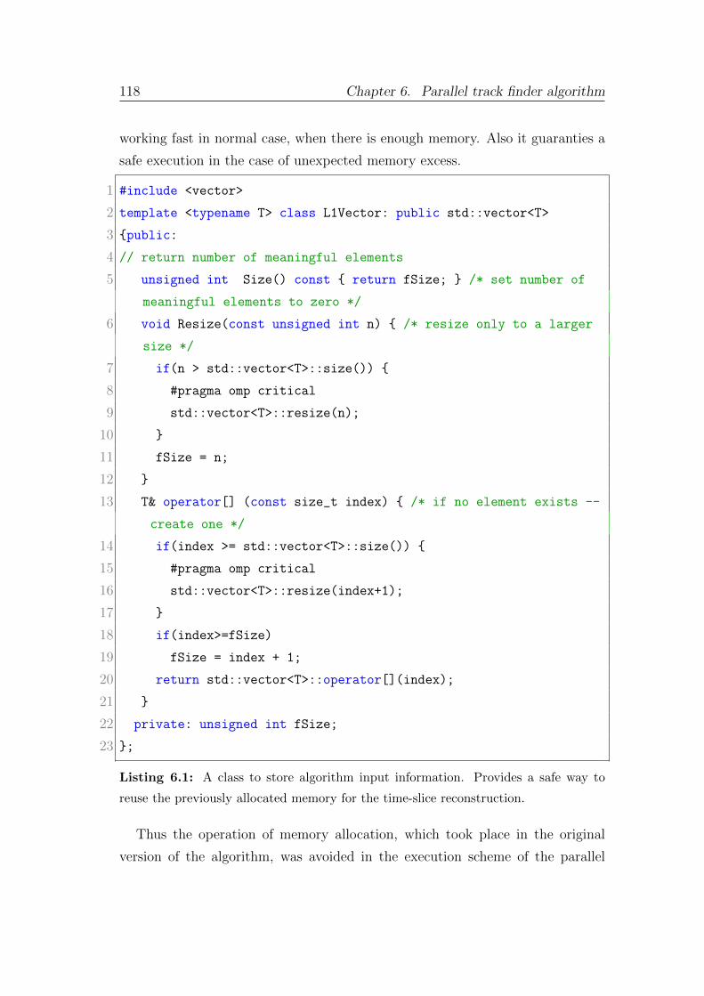
118 Chapter 6. Parallel track finder algorithm
working fast in normal case, when there is enough memory. Also it guaranties a
safe execution in the case of unexpected memory excess.
1 #include <vector>
2 template <typename T> class L1Vector: public std::vector<T>
3 public:
4 // return number of meaningful elements
5 unsigned int Size() const return fSize; /* set number of
meaningful elements to zero */
6 void Resize(const unsigned int n) /* resize only to a larger
size */
7 if(n > std::vector<T>::size())
8 #pragma omp critical
9 std::vector<T>::resize(n);
10
11 fSize = n;
12
13 T& operator[] (const size_t index) /* if no element exists --
create one */
14 if(index >= std::vector<T>::size())
15 #pragma omp critical
16 std::vector<T>::resize(index+1);
17
18 if(index>=fSize)
19 fSize = index + 1;
20 return std::vector<T>::operator[](index);
21
22 private: unsigned int fSize;
23 ;
Listing 6.1: A class to store algorithm input information. Provides a safe way to
reuse the previously allocated memory for the time-slice reconstruction.
Thus the operation of memory allocation, which took place in the original
version of the algorithm, was avoided in the execution scheme of the parallel
6.2 Initialization and final stages 119
track finder.
Grid structure
The importance of fast access towards hit measurements in a certain spacial area
of a station for the CA track finder algorithm cannot be overestimated, since it
plays the central role at the time-consuming stage of triplet building. The role
of memory access in case of parallel calculations becomes even more important,
since the data flow increases proportionally to the number of threads accessing
the memory.
In order to avoid random memory access and benefit from cache line reading
approach, a regular 2D grid data structure was used on each station in the original
event-based algorithm scheme. The memory optimization in this case allows
fitting all calculations to smaller and faster caches.
Every measurement belongs to some bin in the structure according to it’s
spacial x and y-coordinates. All hits are sorted and saved in the order of their
bin number and for each bin the index of first hit in this bin is stored.
Thus, the procedure of introducing a grid structure can be divided into several
logical steps:
• define the size of bins according to the hit density,
• order the hits according to the bin number,
• count the number of hits in each bin,
• store the index of the first hit in the bin for each bin.
In the original version of the CA track finder for the grid sorting procedure
the standard C++ library std::sort function was used, which corresponds to
quicksort algorithm with an O(Nlog2N) complexity. However, the quick sort
algorithm is not an optimal solution in this case. For example, since all possible
values of the bin number are known, one can apply the counting sort algorithm
here.
The counting sort is a very efficient, in-place, high-performance sorting algo-
rithm. For arrays of numbers it does not move the elements, but instead counts
the occurrence of each possible value, and constructs the sorted array from these
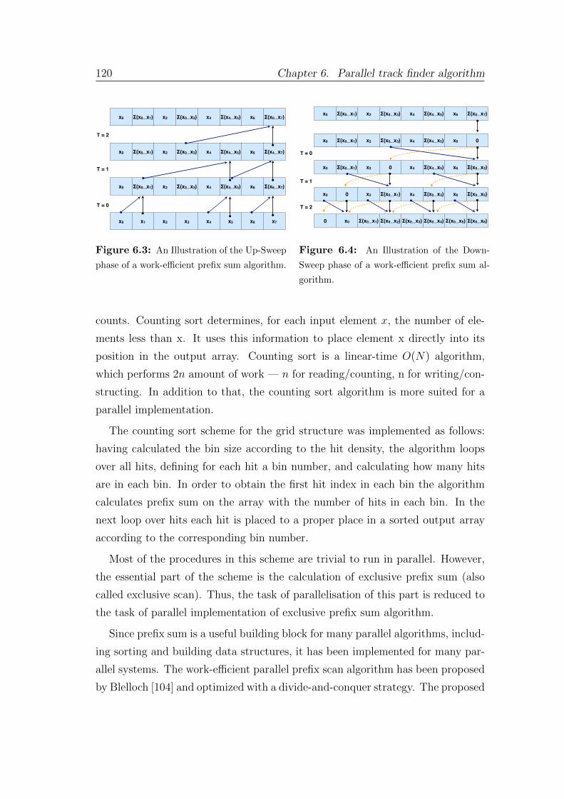
120 Chapter 6. Parallel track finder algorithm
x0 Σ(x0…x1) x2 Σ(x0…x3) x4 Σ(x4…x5) x6 Σ(x0…x7)
x0 Σ(x0…x1) x2 Σ(x0…x3) x4 Σ(x4…x5) x6 Σ(x4…x7)
x0 Σ(x0…x1) x2 Σ(x2…x3) x4 Σ(x4…x5) x6 Σ(x6…x7)
x0 x1 x2 x3 x4 x5 x6 x7
Τ = 0
Τ = 1
Τ = 2
x0 Σ(x0…x1) x2 Σ(x0…x3) x4 Σ(x4…x5) x6 Σ(x0…x7)
x0 Σ(x0…x1) x2 Σ(x0…x3) x4 Σ(x4…x5) x6 0
x0 Σ(x0…x1) x2 0 x4 Σ(x4…x5) x6 Σ(x0…x3)
x0 0 x2 Σ(x0…x1) x4 Σ(x0…x3) x6 Σ(x0…x5)
0 x0 Σ(x0…x1) Σ(x0…x2) Σ(x0…x3) Σ(x0…x4) Σ(x0…x5) Σ(x0…x6)
Τ = 0
Τ = 1
Τ = 2
Figure 6.3: An Illustration of the Up-Sweep
phase of a work-efficient prefix sum algorithm.
Figure 6.4: An Illustration of the Down-
Sweep phase of a work-efficient prefix sum al-
gorithm.
counts. Counting sort determines, for each input element x, the number of ele-
ments less than x. It uses this information to place element x directly into its
position in the output array. Counting sort is a linear-time O(N) algorithm,
which performs 2n amount of work — n for reading/counting, n for writing/con-
structing. In addition to that, the counting sort algorithm is more suited for a
parallel implementation.
The counting sort scheme for the grid structure was implemented as follows:
having calculated the bin size according to the hit density, the algorithm loops
over all hits, defining for each hit a bin number, and calculating how many hits
are in each bin. In order to obtain the first hit index in each bin the algorithm
calculates prefix sum on the array with the number of hits in each bin. In the
next loop over hits each hit is placed to a proper place in a sorted output array
according to the corresponding bin number.
Most of the procedures in this scheme are trivial to run in parallel. However,
the essential part of the scheme is the calculation of exclusive prefix sum (also
called exclusive scan). Thus, the task of parallelisation of this part is reduced to
the task of parallel implementation of exclusive prefix sum algorithm.
Since prefix sum is a useful building block for many parallel algorithms, includ-
ing sorting and building data structures, it has been implemented for many par-
allel systems. The work-efficient parallel prefix scan algorithm has been proposed
by Blelloch [104] and optimized with a divide-and-conquer strategy. The proposed

6.2 Initialization and final stages 121
solution was to make a use of balanced binary trees, which often arise in paral-
lel computing. The procedure is performed in place and consists of two phases:
the up-sweep phase and the down-sweep phase. The up-sweep phase (Fig. 6.3)
traverse tree from leaves to root, computing partial sums on the way. The down-
sweep phase (Fig. 6.4) traverse the binary tree back from root to leaves, using
the partial sums to compute the prefix sums in place.
Algorithm 1 Up-Sweep Phase
1: for d← 0 to log2(n)− 1 do
2: for all i← 0 to n− 1 by 2d+1 in parallel do
3: a[i+ 2d+1 − 1]← a[i+ 2d − 1]⊕ a[i+ 2d+1 − 1]
4: end for
5: end for
Algorithm 2 Down-Sweep Phase
1: for d← log2(n)− 1 downto 0 do
2: for all i← 0 to n− 1 by 2d+1 in parallel do
3: a[i+ 2d+1 − 1]← a[i+ 2d − 1]⊕ a[i+ 2d+1 − 1]
4: end for
5: end for
The up-sweep and the down-sweep phases have log(n) steps and the complexity
of O(n). Therefore the complete algorithm has the total complexity of O(n) and
needs 2 log n steps to compute the prefix-operation on the given array.
The parallel OpenMP implementation for the complete algorithm is given in
Listing 6.2. The parallel pragma defines a start of a parallel block. At this
point a set of N threads, where N is given at the runtime, are created, all of
which execute the next parallel block. The for directive splits the following for-
loop so that each thread in the current parallel block gets a portion of the loop
iterations for the execution. The scheduling clauses for the for-loop define the
way, how the iterations are distributed between threads. In the algorithm, the
dynamic scheduling was chosen to process the for-loop concurrently. In this case
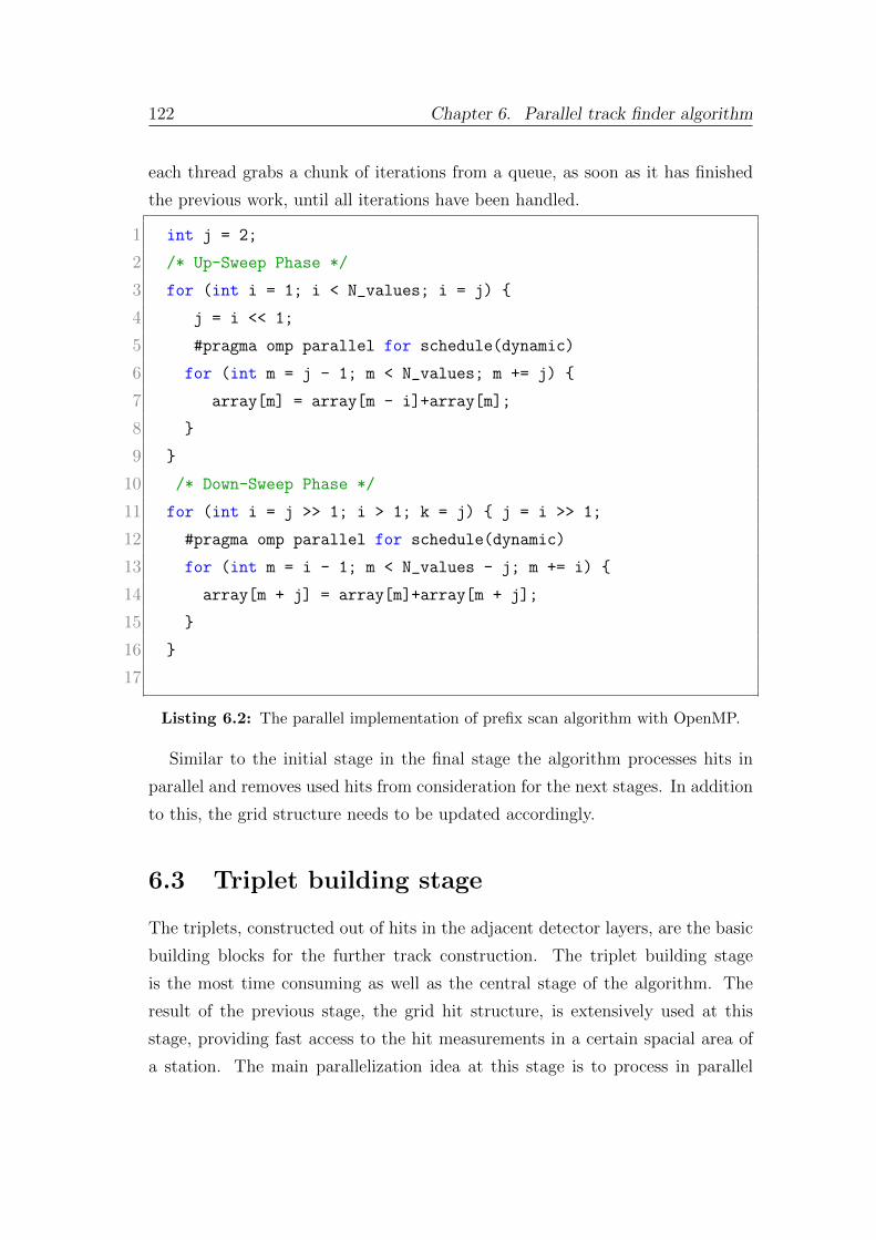
122 Chapter 6. Parallel track finder algorithm
each thread grabs a chunk of iterations from a queue, as soon as it has finished
the previous work, until all iterations have been handled.
1 int j = 2;
2 /* Up-Sweep Phase */
3 for (int i = 1; i < N_values; i = j)
4 j = i << 1;
5 #pragma omp parallel for schedule(dynamic)
6 for (int m = j - 1; m < N_values; m += j)
7 array[m] = array[m - i]+array[m];
8
9
10 /* Down-Sweep Phase */
11 for (int i = j >> 1; i > 1; k = j) j = i >> 1;
12 #pragma omp parallel for schedule(dynamic)
13 for (int m = i - 1; m < N_values - j; m += i)
14 array[m + j] = array[m]+array[m + j];
15
16
17
Listing 6.2: The parallel implementation of prefix scan algorithm with OpenMP.
Similar to the initial stage in the final stage the algorithm processes hits in
parallel and removes used hits from consideration for the next stages. In addition
to this, the grid structure needs to be updated accordingly.
6.3 Triplet building stage
The triplets, constructed out of hits in the adjacent detector layers, are the basic
building blocks for the further track construction. The triplet building stage
is the most time consuming as well as the central stage of the algorithm. The
result of the previous stage, the grid hit structure, is extensively used at this
stage, providing fast access to the hit measurements in a certain spacial area of
a station. The main parallelization idea at this stage is to process in parallel
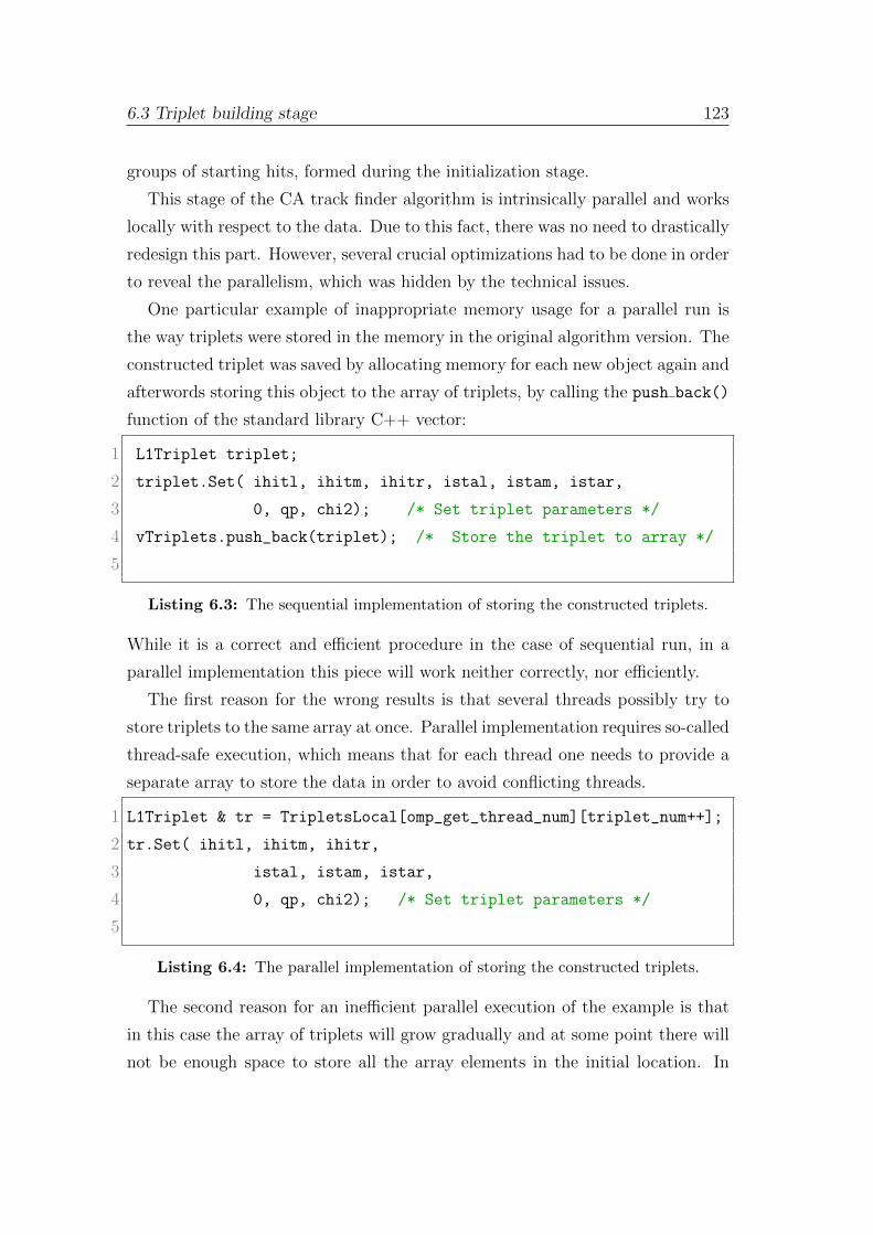
6.3 Triplet building stage 123
groups of starting hits, formed during the initialization stage.
This stage of the CA track finder algorithm is intrinsically parallel and works
locally with respect to the data. Due to this fact, there was no need to drastically
redesign this part. However, several crucial optimizations had to be done in order
to reveal the parallelism, which was hidden by the technical issues.
One particular example of inappropriate memory usage for a parallel run is
the way triplets were stored in the memory in the original algorithm version. The
constructed triplet was saved by allocating memory for each new object again and
afterwords storing this object to the array of triplets, by calling the push back()
function of the standard library C++ vector:
1 L1Triplet triplet;
2 triplet.Set( ihitl, ihitm, ihitr, istal, istam, istar,
3 0, qp, chi2); /* Set triplet parameters */
4 vTriplets.push_back(triplet); /* Store the triplet to array */
5
Listing 6.3: The sequential implementation of storing the constructed triplets.
While it is a correct and efficient procedure in the case of sequential run, in a
parallel implementation this piece will work neither correctly, nor efficiently.
The first reason for the wrong results is that several threads possibly try to
store triplets to the same array at once. Parallel implementation requires so-called
thread-safe execution, which means that for each thread one needs to provide a
separate array to store the data in order to avoid conflicting threads.
1 L1Triplet & tr = TripletsLocal[omp_get_thread_num][triplet_num++];
2 tr.Set( ihitl, ihitm, ihitr,
3 istal, istam, istar,
4 0, qp, chi2); /* Set triplet parameters */
5
Listing 6.4: The parallel implementation of storing the constructed triplets.
The second reason for an inefficient parallel execution of the example is that
in this case the array of triplets will grow gradually and at some point there will
not be enough space to store all the array elements in the initial location. In
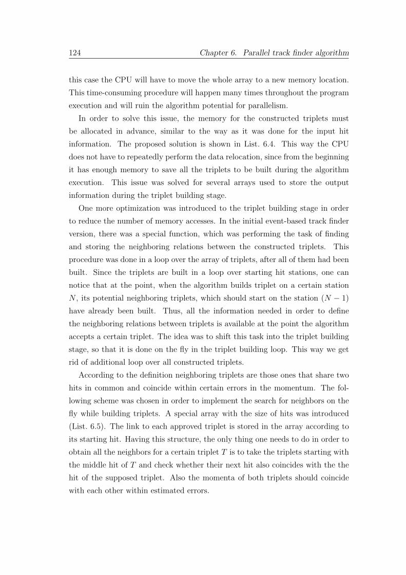
124 Chapter 6. Parallel track finder algorithm
this case the CPU will have to move the whole array to a new memory location.
This time-consuming procedure will happen many times throughout the program
execution and will ruin the algorithm potential for parallelism.
In order to solve this issue, the memory for the constructed triplets must
be allocated in advance, similar to the way as it was done for the input hit
information. The proposed solution is shown in List. 6.4. This way the CPU
does not have to repeatedly perform the data relocation, since from the beginning
it has enough memory to save all the triplets to be built during the algorithm
execution. This issue was solved for several arrays used to store the output
information during the triplet building stage.
One more optimization was introduced to the triplet building stage in order
to reduce the number of memory accesses. In the initial event-based track finder
version, there was a special function, which was performing the task of finding
and storing the neighboring relations between the constructed triplets. This
procedure was done in a loop over the array of triplets, after all of them had been
built. Since the triplets are built in a loop over starting hit stations, one can
notice that at the point, when the algorithm builds triplet on a certain station
N , its potential neighboring triplets, which should start on the station (N − 1)
have already been built. Thus, all the information needed in order to define
the neighboring relations between triplets is available at the point the algorithm
accepts a certain triplet. The idea was to shift this task into the triplet building
stage, so that it is done on the fly in the triplet building loop. This way we get
rid of additional loop over all constructed triplets.
According to the definition neighboring triplets are those ones that share two
hits in common and coincide within certain errors in the momentum. The fol-
lowing scheme was chosen in order to implement the search for neighbors on the
fly while building triplets. A special array with the size of hits was introduced
(List. 6.5). The link to each approved triplet is stored in the array according to
its starting hit. Having this structure, the only thing one needs to do in order to
obtain all the neighbors for a certain triplet T is to take the triplets starting with
the middle hit of T and check whether their next hit also coincides with the the
hit of the supposed triplet. Also the momenta of both triplets should coincide
with each other within estimated errors.
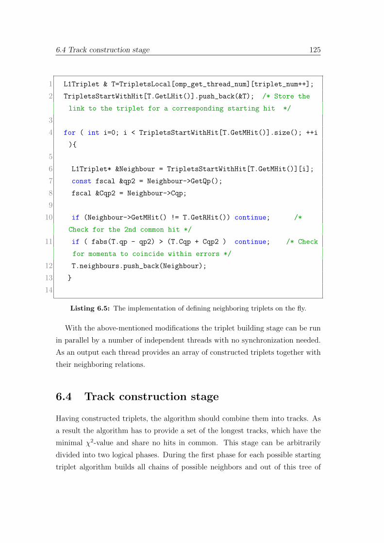
6.4 Track construction stage 125
1 L1Triplet & T=TripletsLocal[omp_get_thread_num][triplet_num++];
2 TripletsStartWithHit[T.GetLHit()].push_back(&T); /* Store the
link to the triplet for a corresponding starting hit */
3
4 for ( int i=0; i < TripletsStartWithHit[T.GetMHit()].size(); ++i
)
5
6 L1Triplet* &Neighbour = TripletsStartWithHit[T.GetMHit()][i];
7 const fscal &qp2 = Neighbour->GetQp();
8 fscal &Cqp2 = Neighbour->Cqp;
9
10 if (Neighbour->GetMHit() != T.GetRHit()) continue; /*
Check for the 2nd common hit */
11 if ( fabs(T.qp - qp2) > (T.Cqp + Cqp2 ) continue; /* Check
for momenta to coincide within errors */
12 T.neighbours.push_back(Neighbour);
13
14
Listing 6.5: The implementation of defining neighboring triplets on the fly.
With the above-mentioned modifications the triplet building stage can be run
in parallel by a number of independent threads with no synchronization needed.
As an output each thread provides an array of constructed triplets together with
their neighboring relations.
6.4 Track construction stage
Having constructed triplets, the algorithm should combine them into tracks. As
a result the algorithm has to provide a set of the longest tracks, which have the
minimal χ2-value and share no hits in common. This stage can be arbitrarily
divided into two logical phases. During the first phase for each possible starting
triplet algorithm builds all chains of possible neighbors and out of this tree of
126 Chapter 6. Parallel track finder algorithm
candidates chooses and stores the best one according to the χ2 and the length.
During the second phase the track competition takes place, when each survived
candidate gets stored only if it shares no hits in common with a better candidate
according to the χ2 and the length.
Track candidate formation stage
Let us consider the first phase of joining compatible segments into a track can-
didate (Algorithm 3). During the track candidate formation stage the algorithm
tries to join segments into track candidates, starting with the outermost layer
proceeding inwards towards the beam line. Since the level of each triplet had
been obtained at the stage of building triplets, the procedure of binning triplets
together can be performed in a fast and easy manner.
The final goal is to obtain the best set of tracks according to χ2-value and track
length. Therefore, the algorithm starts building tracks out of triplets with the
highest calculated level, since these triplets have a higher probability to construct
the longer tracks. The algorithm starts the track building procedure with an
attempt to build longer tracks at first and in a loop decreases the potential
length of the track candidate being built down to the tracks of three or four hits
(line 1, length is calculated in the number of connected triplets building up the
track).
During the search for the candidate of a certain length the algorithm must
consider as a starting triplet all triplets on each station, from which it is still
possible to build up a candidate with the length of interest (lines 2–3). Each
triplet considered as a starting triplet has to fulfill two conditions:
• should be potentially able to create a track of a certain length (line 4),
• has no hits used in the longer tracks constructed before.
For the triplet, which fulfills both conditions, a special recursive function is called.
The function creates a tree of track candidates and chooses the best track within
this tree.
The function (Algorithm 4) takes as input three arguments: the starting triplet
itself, the track candidate containing the left hit of the starting triplet (created in

6.4 Track construction stage 127
Algorithm 3 For each starting triplet build and store the best track candidate.
1: for each track length← (NStations− 3) downto minLevel=(1 or 2) do
2: for each starting Station← 0 to (NStations− 3− length) do
3: for all triplets on station do
4: if (Triplet.Level < length) continue;
5: if (Triplet.LeftHitIsUsed) continue;
6: create L1Branch candidate Cand with left hit of Triplet;
7: L1Branch BestCand = Cand;
8: ExtendCandidate(BestCand, Cand, Triplet);
9: if BestCand.Length < (length+1) continue;
10: if BestCand.Length < (minLevel +3) continue;
11: vTrackCandidates.Store(BestCand);
12: end for
13: end for
14: end for
the line 6, Algorithm 3) and the track candidate called BestCandidate, which for
the initial call coincides with the candidate (created in the line 7, Algorithm 3).
Inside the function body the algorithm checks whether the considered triplet
is the last triplet of the track (Level = 0) (line 2, Algorithm 4). If so, the
middle and last hits of the triplet are checked not to be used and added to the
BestCandidate.
If the triplet is not the last one in the chain and has neighbors (line 8, Al-
gorithm 4), then the algorithm goes through the list of its neighbors and tries
to attach each neighbor to the existing chain. On each attempt the χ2-value is
checked not to exceed the certain value (line 14, Algorithm 4). If this condition
is fulfilled the function calls itself with the updated BestCandidate.
Thus, in a recursive manner the tree of all possible candidates, which start with
the current triplet, is created and the best one is chosen. At this point function
ExtenedCandidate terminates and returns the best track candidate built for a
certain starting triplet. The length of this candidate is checked that it is not
shorter than the required value, so that the candidate should not lose more than
one hit (line 10, Algorithm 3).

128 Chapter 6. Parallel track finder algorithm
Algorithm 4 Recursive function to add next triplet to the track candidate.
1: procedure ExtendCandidate(BestCand, NewCand, Neibouhr)
2: if Triplet.Level = 0 then
3: if (! Triplet.MiddleHitIsUsed) add hit to Cand;
4: if (! Triplet.RightHitIsUsed) add hit to Cand;
5: if (Cand.Chi2 > Chi2Cut) return;
6: else BestCand=Cand return;
7: end if
8: if !Triplet.Level = 0 then
9: for each Triplet.Neibouhr do
10: if Triplet.Neibouhr.LeftHitIsUsed then BestCand = Cand;
11: else
12: L1Branch NewCand = Cand;
13: add left hit of Triplet to NewCand;
14: if (NewCand.Chi2 > Chi2Cut) continue;
15: ExtendCandidate(BestCand, NewCand, Neibouhr);
16: end if
17: end for
18: end if
19: return;
20: end procedure
Since each starting triplet is processed independently at this point, introducing
the parallelism at this stage is trivial: each tread should process a set of starting
triplets and create the best track candidate for each triplet in the set. No syn-
chronization is needed at this point. So similar to the triplet building stage, the
main performance issue here is the memory usage. The procedure of saving the
accepted track candidate has been changed accordingly.
Track competition
After all track candidates of a certain length have been constructed, the track
competition takes place. In the end of this procedure each hit should participate
6.4 Track construction stage 129
in not more than one track. This procedure is aimed at ghost suppression, since
each hit is always attached to the best possible track according to the length and
the χ2, which has a higher probability of being produced by a real particle.
This stage of the algorithm had to be essentially rewritten for the parallel
implementation, since the scheme used in the event-based reconstruction was
intrinsically serial. Originally the following scheme was used: all the tracks were
sorted according to their length and χ2-value. The best track of all the tracks
built at this stage was considered and checked to have any used hits. If the
track had no used hits it was saved. In the case of presence of used hits it was
discarded. The same procedure was done with each track in the order of their
quality rank.
If a track candidate gets discarded due to the presence of a used hit, it will be
constructed again in the next iteration during the search for a shorter candidate
with one hit less.
Thus, unlike the triplet building stage, at this point we cannot avoid synchro-
nization between threads, since in this case threads have to consult each other
in order to decide to which track-candidate a certain hit should be attached in
order to obtain the best set of tracks in the end.
It is clear that this part of the algorithm was essentially serial, since each next
iteration essentially depends on the result of the previous iterations. Therefore,
this stage of the algorithm had to be designed from scratch in a parallel manner.
The alternative approach, which allows for a parallel run, was proposed. The
information exchange between threads was implemented via the table of common
access available to all the threads. The size of table corresponds to the number
of strips, contributing to the current super-event. For each strip in the table the
index of the best, according to χ2-value and length, candidate is stored. The
table is filled out on the fly while building track candidates. At the end of this
procedure for each strip in the table the index of the best candidate is stored,
which the strip should be assigned to.
Thus, the track competition reduces to the checking whether a certain track
candidate is the best candidate for all the strips, which it involves. This check
can be done concurrently for different track candidates with no synchronization
needed.
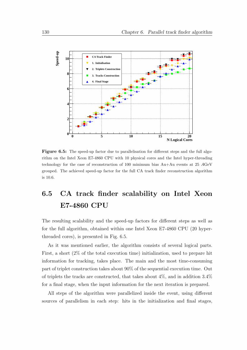
130 Chapter 6. Parallel track finder algorithm
N Logical Cores0 5 10 15 20
Spee
d-up
0
2
4
6
8
10CA Track Finder
1. Initialisation
2. Triplets Construction
3. Tracks Construction
4. Final Stage
Figure 6.5: The speed-up factor due to parallelisation for different steps and the full algo-
rithm on the Intel Xeon E7-4860 CPU with 10 physical cores and the Intel hyper-threading
technology for the case of reconstruction of 100 minimum bias Au+Au events at 25 AGeV
grouped. The achieved speed-up factor for the full CA track finder reconstruction algorithm
is 10.6.
6.5 CA track finder scalability on Intel Xeon
E7-4860 CPU
The resulting scalability and the speed-up factors for different steps as well as
for the full algorithm, obtained within one Intel Xeon E7-4860 CPU (20 hyper-
threaded cores), is presented in Fig. 6.5.
As it was mentioned earlier, the algorithm consists of several logical parts.
First, a short (2% of the total execution time) initialization, used to prepare hit
information for tracking, takes place. The main and the most time-consuming
part of triplet construction takes about 90% of the sequential execution time. Out
of triplets the tracks are constructed, that takes about 4%, and in addition 3.4%
for a final stage, when the input information for the next iteration is prepared.
All steps of the algorithm were parallelized inside the event, using different
sources of parallelism in each step: hits in the initialization and final stages,

6.5 Cellular automaton track finder scalability 131
triplets for the major part, track candidates for the track construction step.
Some steps have a better speedup for higher number of cores due to less thread
synchronization needed. The algorithm shows linear scalability. Due to the
hyper-threading one can expect a speed-up factor of about 13 on such a CPU
in the ideal case. The achieved speed-up factor is 10.6 for the full CA track
finder reconstruction algorithm on a CPU with 10 physical cores with the Intel
hyper-threading technology.
Chapter 7
Four-dimensional parallel track
finder algorithm
The unprecedented interaction rates for a heavy-ion collision experiment in CBM
require a novel read-out and data acquisition concepts.
At the collision rate of 10 MHz, the expected raw data flow is about 1 TB/s.
This is beyond the modern achievable archival rate, which means that the data
flow has to be reduced online by about two orders of magnitude. However, since
CBM is targeted to the measurement of rare observables, which are featured with
a complicated trigger signatures, the experiment requires a full event topology
reconstruction to be done online.
The huge data rates together with the absence of simple hardware triggers
make traditional latency-limited trigger architectures typical for conventional
experiments with a hardware trigger inapplicable for the case of CBM. In-
stead, CBM will employ a novel data acquisition concept with autonomous, self-
triggered front-end electronics.
The time-stamped data will be shipped and collected into a readout buffer in
a form of a time-slice of a certain length, which will be adjusted to the computa-
tional power of the reconstruction node. The time-stamped data will be delivered
to a large computer farm FLES.
This novel concept brings new challenges for software developers. CBM will
have to deal with a fraction of collisions, which overlap in time and can not be
resolved in a trivial way (Fig. 7.1). Thus, the task of defining physical events is
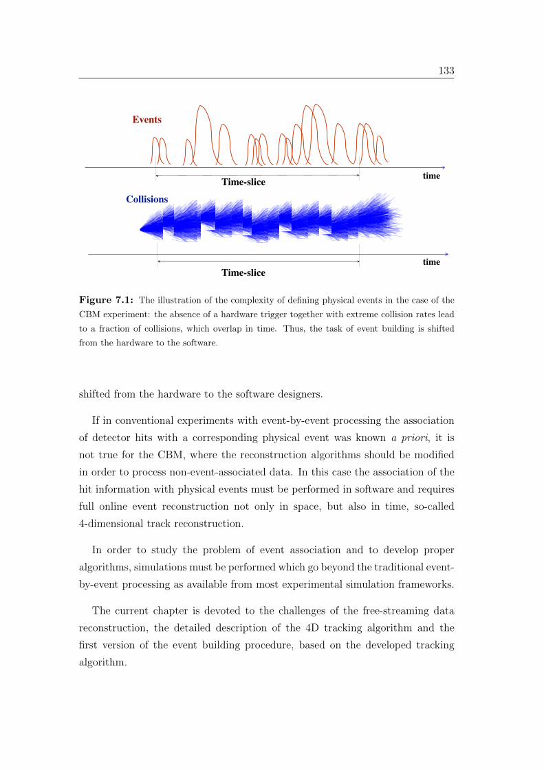
133
Events
Events
time
time
Collisions
Time-slice
Time-slice
Figure 7.1: The illustration of the complexity of defining physical events in the case of the
CBM experiment: the absence of a hardware trigger together with extreme collision rates lead
to a fraction of collisions, which overlap in time. Thus, the task of event building is shifted
from the hardware to the software.
shifted from the hardware to the software designers.
If in conventional experiments with event-by-event processing the association
of detector hits with a corresponding physical event was known a priori, it is
not true for the CBM, where the reconstruction algorithms should be modified
in order to process non-event-associated data. In this case the association of the
hit information with physical events must be performed in software and requires
full online event reconstruction not only in space, but also in time, so-called
4-dimensional track reconstruction.
In order to study the problem of event association and to develop proper
algorithms, simulations must be performed which go beyond the traditional event-
by-event processing as available from most experimental simulation frameworks.
The current chapter is devoted to the challenges of the free-streaming data
reconstruction, the detailed description of the 4D tracking algorithm and the
first version of the event building procedure, based on the developed tracking
algorithm.
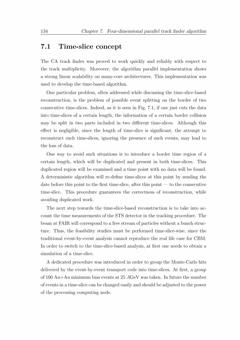
134 Chapter 7. Four-dimensional parallel track finder algorithm
7.1 Time-slice concept
The CA track finder was proved to work quickly and reliably with respect to
the track multiplicity. Moreover, the algorithm parallel implementation shows
a strong linear scalability on many-core architectures. This implementation was
used to develop the time-based algorithm.
One particular problem, often addressed while discussing the time-slice-based
reconstruction, is the problem of possible event splitting on the border of two
consecutive time-slices. Indeed, as it is seen in Fig. 7.1, if one just cuts the data
into time-slices of a certain length, the information of a certain border collision
may be split in two parts included in two different time-slices. Although this
effect is negligible, since the length of time-slice is significant, the attempt to
reconstruct such time-slices, ignoring the presence of such events, may lead to
the loss of data.
One way to avoid such situations is to introduce a border time region of a
certain length, which will be duplicated and present in both time-slices. This
duplicated region will be examined and a time point with no data will be found.
A deterministic algorithm will re-define time-slices at this point by sending the
date before this point to the first time-slice, after this point — to the consecutive
time-slice. This procedure guarantees the correctness of reconstruction, while
avoiding duplicated work.
The next step towards the time-slice-based reconstruction is to take into ac-
count the time measurements of the STS detector in the tracking procedure. The
beam at FAIR will correspond to a free stream of particles without a bunch struc-
ture. Thus, the feasibility studies must be performed time-slice-wise, since the
traditional event-by-event analysis cannot reproduce the real life case for CBM.
In order to switch to the time-slice-based analysis, at first one needs to obtain a
simulation of a time-slice.
A dedicated procedure was introduced in order to group the Monte-Carlo hits
delivered by the event-by-event transport code into time-slices. At first, a group
of 100 Au+Au minimum bias events at 25 AGeV was taken. In future the number
of events in a time-slice can be changed easily and should be adjusted to the power
of the processing computing node.
7.1 Time-slice concept 135
Time, ns0 2000 4000 6000 8000 10000 12000
Entr
ies
1
10
210
310
11
Time, ns2000 2200 2400 2600 2800 3000
Num
ber
of E
vent
s
1
10
210
310Entries
Time [ns]
Time [ns]
Entr
ies
Entr
ies
Figure 7.2: The distribution of the hit time measurements for 100 minimum bias Au+Au
collisions at 25 AGeV in the main tracking system of CBM, obtained assuming the average
interaction rate of 10 MHz and Poisson distribution of the time intervals between subsequent
events (top), the same distribution shown on a larger scale (bottom). Different collisions are
shown with a different filling and color. Events clearly overlap with each other.
Neglecting possible fluctuations in the beam intensity and, thus, non-constant
average collision rate, the CBM collision distribution in time can be described as
a Poisson process. The start time of each collision was obtained with the Poisson
distribution, assuming the average interaction rate of 107 Hz. A time stamp,
assigned to each STS hit was calculated as a sum of the start time of the event,
in which it was produced, and the time shift due to the time of flight from the
collision point to a hit position. On top of that to obtain a time measurement for
a hit in STS, the time stamp was smeared according to the Gaussian distribution
with a σ-value of the STS time measurement resolution — 5 ns.
136 Chapter 7. Four-dimensional parallel track finder algorithm
As a direct outcome of this procedure, the distribution of hit time measure-
ments in the STS detector for a time-slice of 100 mbias events at 10 MHz inter-
action rate is presented in Fig. 7.2. The distribution clearly shows that at this
interaction rate events do overlap with each other. Thus, the association of hits
with events is no longer trivial.
Therefore, event reconstruction must be performed not only in space, but
also in time. Space-time correlations must be employed, so that the tracking
procedure takes into account not just three spacial dimensions, but the fourth
dimension — time.
7.2 Time-based track reconstruction
As a first step towards development of the time-based tracking, the software
reconstruction routine was extended to deal with time-based data instead of iso-
lated events. After the algorithm was modified to be able to take time-slices as
an input, the procedure of searching for tracks should be changed accordingly, so
that the time information is used in order to improve the performance and the
speed of the track finder.
Switching to 4D tracking formally implies that the time coordinate should be
added to the state vector of a track:
(x, y, tx, ty, q/p)→ (x, y, tx, ty, q/p, t). (7.1)
and all the operations with a state vector (e.g. propagation, fitting) should involve
time coordinates to the same extent as it does spacial coordinates.
The full implementation of this approach will be added after taking into ac-
count TOF detector time measurement, since it is several orders of magnitude
more precise and should drastically improve the time coordinate resolution. For
the studies involving STS detector alone, the time is included into the track pa-
rameters, although the propagation and fitting is done, taking into account only
the spacial coordinates.
The question of how the hit time measurement can be used in the CA track
finder has a straightforward answer. Since the triplets are to be built of three
hits potentially produced by the same particle these hits should be correlated not
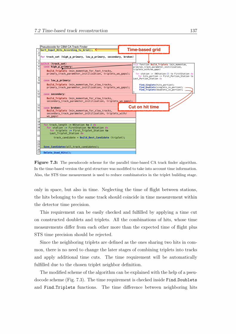
7.2 Time-based track reconstruction 137
Pseudocode for CBM CA Track Finder1 Sort_Input_Hits_According_to_Grid();23 for track_set (high_p_primary, low_p_primary, secondary, broken)45 switch (track_set) 6 case high_p_primary:7 Build_Triplets (min_momentum_for_fast_tracks,
primary_track_parameter_initilisation, triplets_wo_gaps);89 case low_p_primary:10 Build_Triplets (min_momentum_for_slow_tracks,
primary_track_parameter_initilisation, triplets_wo_gaps);1112 case secondary:13 Build_Triplets (min_momentum_for_slow_tracks,
secondary_track_parameter_initilisation, triplets_wo_gaps);14 15 case broken:16 Build_Triplets (min_momentum_for_slow_tracks,
secondary_track_parameter_initilisation, triplets_with/wo_gaps)
171819 for track_length := NStation to 3 do20 for station := FirstStation to NStation do21 for triplets := First_Triplet_Station to
Last_Triplet_Station do22 track_candidate = Build_Best_Candidate (triplet);232425 Save_Candidates(all_track_candidates);2627 Delete_Used_Hits();
void function Build_Triplets (min_momentum, prim/sec_track_parameter_initilisation, triplets_with/wo_gaps) for station := (NStation-2) to FirstStation do for hits_portion := First_Portion_Station to Last_Portion_Station do
Find_Singlets(hits_portion); Find_Doublets(singlets_in_portion); Find_Triplets(doublets_in_portion);
Cut on hit time
Time-based grid
Figure 7.3: The pseudocode scheme for the parallel time-based CA track finder algorithm.
In the time-based version the grid structure was modified to take into account time information.
Also, the STS time measurement is used to reduce combinatorics in the triplet building stage.
only in space, but also in time. Neglecting the time of flight between stations,
the hits belonging to the same track should coincide in time measurement within
the detector time precision.
This requirement can be easily checked and fulfilled by applying a time cut
on constructed doublets and triplets. All the combinations of hits, whose time
measurements differ from each other more than the expected time of flight plus
STS time precision should be rejected.
Since the neighboring triplets are defined as the ones sharing two hits in com-
mon, there is no need to change the later stages of combining triplets into tracks
and apply additional time cuts. The time requirement will be automatically
fulfilled due to the chosen triplet neighbor definition.
The modified scheme of the algorithm can be explained with the help of a pseu-
docode scheme (Fig. 7.3). The time requirement is checked inside Find Doublets
and Find Triplets functions. The time difference between neighboring hits
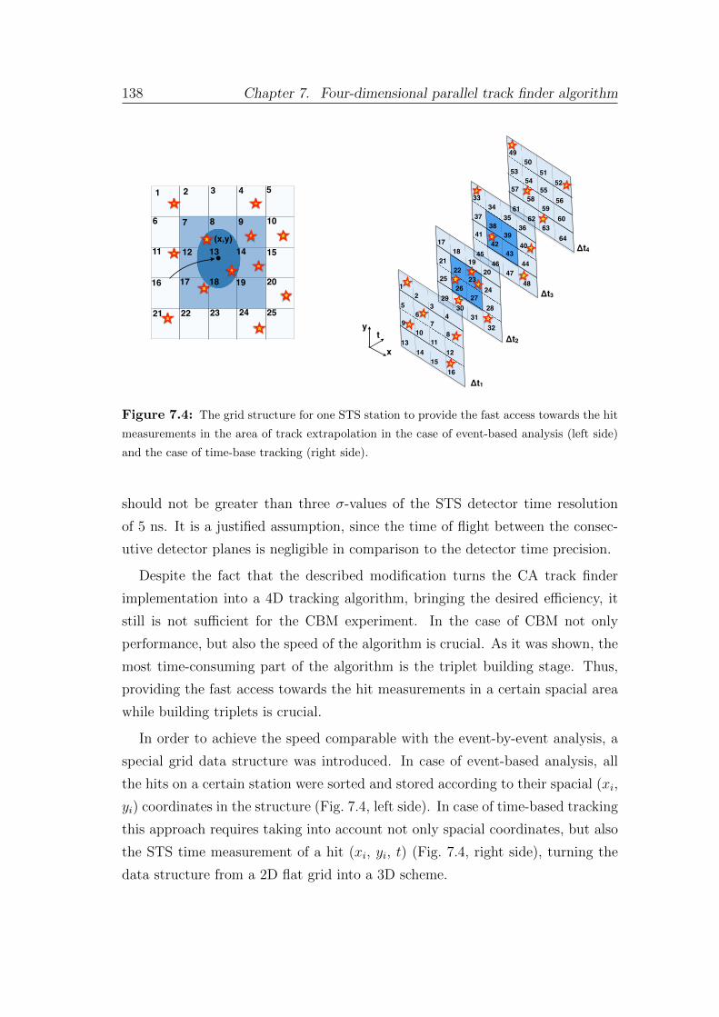
138 Chapter 7. Four-dimensional parallel track finder algorithm
(x,y)
1 2 3 4 5
6 7 8 9 10
11 12 14 15
16 17 18 19 20
21 22 23 24
13
259
87
65
4
12
3
10
1615
1413
1211
2524
2322
2120
1718
19
26
3231
3029
2827
4140
3938
3736
3334
35
42
4847
4645
4443
5756
5554
5352
4950
51
58
6463
6261
6059
Δt1
Δt2
Δt3
Δt4
y
x
t
Figure 7.4: The grid structure for one STS station to provide the fast access towards the hit
measurements in the area of track extrapolation in the case of event-based analysis (left side)
and the case of time-base tracking (right side).
should not be greater than three σ-values of the STS detector time resolution
of 5 ns. It is a justified assumption, since the time of flight between the consec-
utive detector planes is negligible in comparison to the detector time precision.
Despite the fact that the described modification turns the CA track finder
implementation into a 4D tracking algorithm, bringing the desired efficiency, it
still is not sufficient for the CBM experiment. In the case of CBM not only
performance, but also the speed of the algorithm is crucial. As it was shown, the
most time-consuming part of the algorithm is the triplet building stage. Thus,
providing the fast access towards the hit measurements in a certain spacial area
while building triplets is crucial.
In order to achieve the speed comparable with the event-by-event analysis, a
special grid data structure was introduced. In case of event-based analysis, all
the hits on a certain station were sorted and stored according to their spacial (xi,
yi) coordinates in the structure (Fig. 7.4, left side). In case of time-based tracking
this approach requires taking into account not only spacial coordinates, but also
the STS time measurement of a hit (xi, yi, t) (Fig. 7.4, right side), turning the
data structure from a 2D flat grid into a 3D scheme.
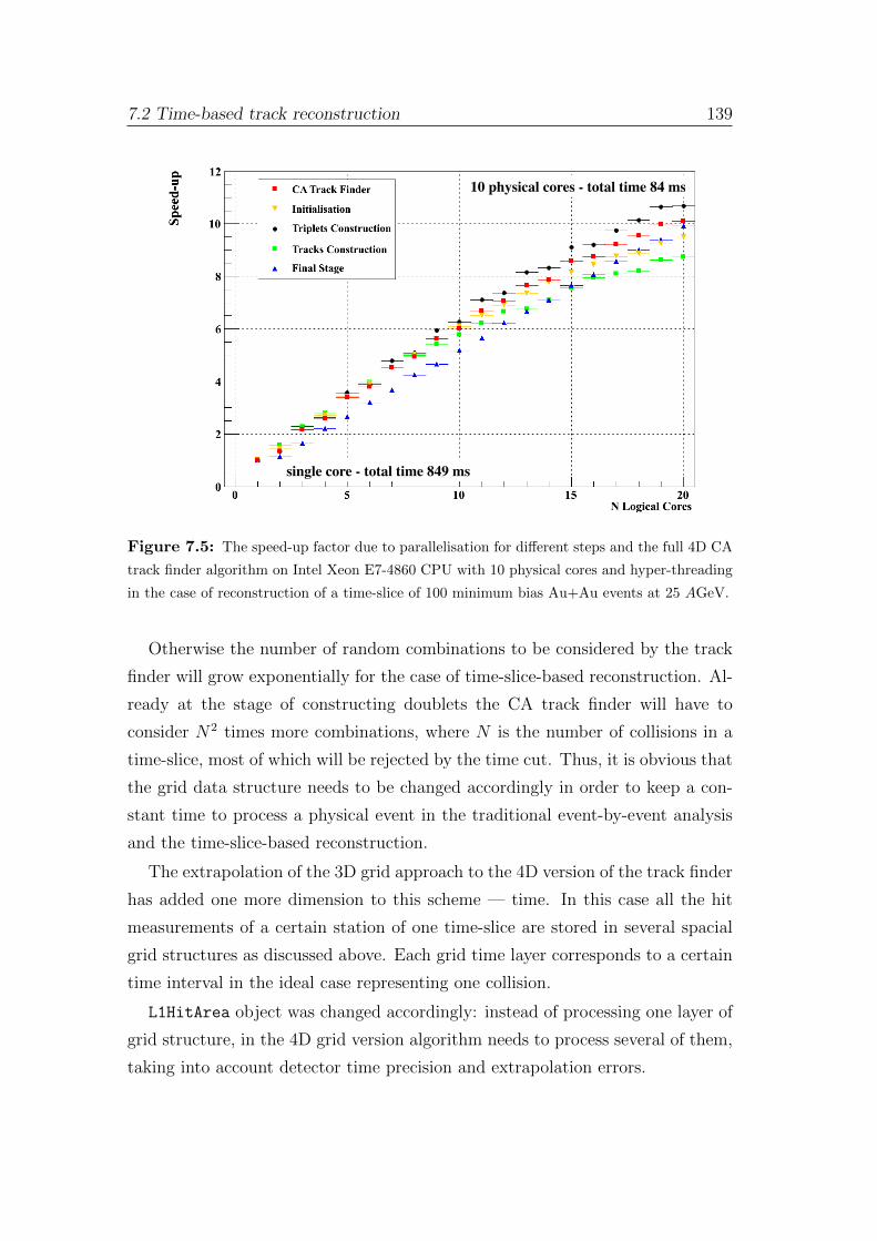
7.2 Time-based track reconstruction 139
single core - total time 849 ns
10 physical cores - total time 84 ns
single core - total time 849 ms
10 physical cores - total time 84 ms
Figure 7.5: The speed-up factor due to parallelisation for different steps and the full 4D CA
track finder algorithm on Intel Xeon E7-4860 CPU with 10 physical cores and hyper-threading
in the case of reconstruction of a time-slice of 100 minimum bias Au+Au events at 25 AGeV.
Otherwise the number of random combinations to be considered by the track
finder will grow exponentially for the case of time-slice-based reconstruction. Al-
ready at the stage of constructing doublets the CA track finder will have to
consider N2 times more combinations, where N is the number of collisions in a
time-slice, most of which will be rejected by the time cut. Thus, it is obvious that
the grid data structure needs to be changed accordingly in order to keep a con-
stant time to process a physical event in the traditional event-by-event analysis
and the time-slice-based reconstruction.
The extrapolation of the 3D grid approach to the 4D version of the track finder
has added one more dimension to this scheme — time. In this case all the hit
measurements of a certain station of one time-slice are stored in several spacial
grid structures as discussed above. Each grid time layer corresponds to a certain
time interval in the ideal case representing one collision.
L1HitArea object was changed accordingly: instead of processing one layer of
grid structure, in the 4D grid version algorithm needs to process several of them,
taking into account detector time precision and extrapolation errors.
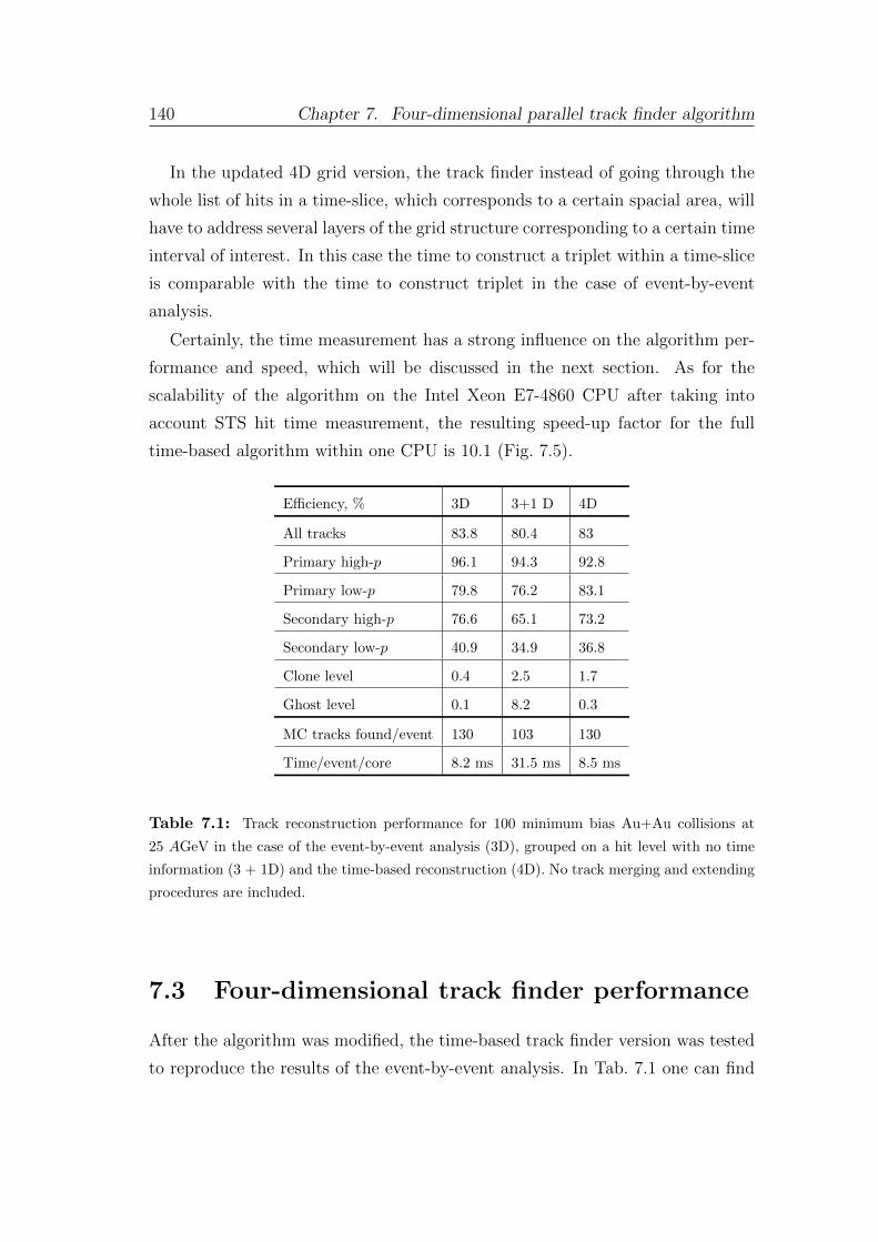
140 Chapter 7. Four-dimensional parallel track finder algorithm
In the updated 4D grid version, the track finder instead of going through the
whole list of hits in a time-slice, which corresponds to a certain spacial area, will
have to address several layers of the grid structure corresponding to a certain time
interval of interest. In this case the time to construct a triplet within a time-slice
is comparable with the time to construct triplet in the case of event-by-event
analysis.
Certainly, the time measurement has a strong influence on the algorithm per-
formance and speed, which will be discussed in the next section. As for the
scalability of the algorithm on the Intel Xeon E7-4860 CPU after taking into
account STS hit time measurement, the resulting speed-up factor for the full
time-based algorithm within one CPU is 10.1 (Fig. 7.5).
Efficiency, % 3D 3+1 D 4D
All tracks 83.8 80.4 83
Primary high-p 96.1 94.3 92.8
Primary low-p 79.8 76.2 83.1
Secondary high-p 76.6 65.1 73.2
Secondary low-p 40.9 34.9 36.8
Clone level 0.4 2.5 1.7
Ghost level 0.1 8.2 0.3
MC tracks found/event 130 103 130
Time/event/core 8.2 ms 31.5 ms 8.5 ms
Table 7.1: Track reconstruction performance for 100 minimum bias Au+Au collisions at
25 AGeV in the case of the event-by-event analysis (3D), grouped on a hit level with no time
information (3 + 1D) and the time-based reconstruction (4D). No track merging and extending
procedures are included.
7.3 Four-dimensional track finder performance
After the algorithm was modified, the time-based track finder version was tested
to reproduce the results of the event-by-event analysis. In Tab. 7.1 one can find
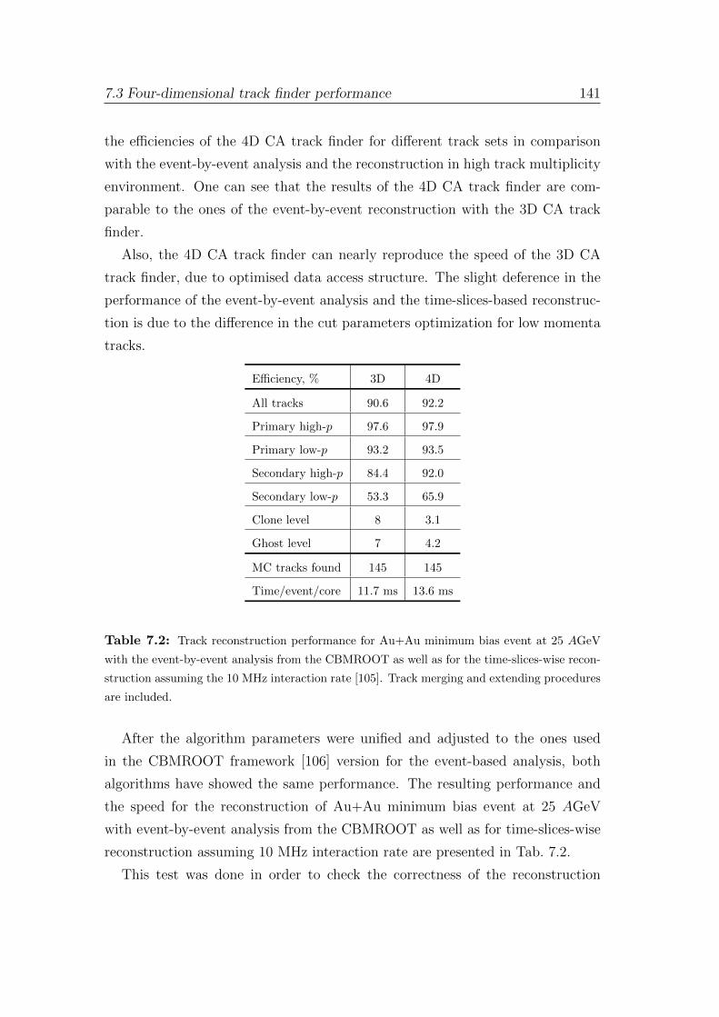
7.3 Four-dimensional track finder performance 141
the efficiencies of the 4D CA track finder for different track sets in comparison
with the event-by-event analysis and the reconstruction in high track multiplicity
environment. One can see that the results of the 4D CA track finder are com-
parable to the ones of the event-by-event reconstruction with the 3D CA track
finder.
Also, the 4D CA track finder can nearly reproduce the speed of the 3D CA
track finder, due to optimised data access structure. The slight deference in the
performance of the event-by-event analysis and the time-slices-based reconstruc-
tion is due to the difference in the cut parameters optimization for low momenta
tracks.
Efficiency, % 3D 4D
All tracks 90.6 92.2
Primary high-p 97.6 97.9
Primary low-p 93.2 93.5
Secondary high-p 84.4 92.0
Secondary low-p 53.3 65.9
Clone level 8 3.1
Ghost level 7 4.2
MC tracks found 145 145
Time/event/core 11.7 ms 13.6 ms
Table 7.2: Track reconstruction performance for Au+Au minimum bias event at 25 AGeV
with the event-by-event analysis from the CBMROOT as well as for the time-slices-wise recon-
struction assuming the 10 MHz interaction rate [105]. Track merging and extending procedures
are included.
After the algorithm parameters were unified and adjusted to the ones used
in the CBMROOT framework [106] version for the event-based analysis, both
algorithms have showed the same performance. The resulting performance and
the speed for the reconstruction of Au+Au minimum bias event at 25 AGeV
with event-by-event analysis from the CBMROOT as well as for time-slices-wise
reconstruction assuming 10 MHz interaction rate are presented in Tab. 7.2.
This test was done in order to check the correctness of the reconstruction
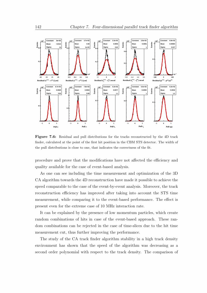
142 Chapter 7. Four-dimensional parallel track finder algorithm
m]µ) [mc - xrecoResidual (x
45− 15− 15 45
Ent
ries
0
0.2
0.4
310× Constant 3e+02
Mean 0.013−
Sigma 11
m]µ) [mc - yrecoResidual (y
0.5− 0.2− 0.1 0.4
310×
Ent
ries
0
0.5
310× Constant 3.7e+02
Mean 0.58
Sigma 1e+02
) mradmcx - treco
xResidual (t
2− 0 2
Ent
ries
0
0.2
0.4
310× Constant 2.3e+02
Mean 0.0055
Sigma 0.63
) mradmcy - treco
yResidual (t
3.5− 1.2− 1.2 3.5
Ent
ries
0
0.2
0.4
310× Constant 2.9e+02
Mean 0.0091−
Sigma 1
mc)/pmc - precoResidual (p
100− 0 100
3−10×
Ent
ries
0
0.5
1
310× Constant 6.9e+02
Mean 0.00084
Sigma 0.017
Pull x
5− 0 5
Ent
ries
0
0.5
1
310× Constant 6.7e+02
Mean 0.0029
Sigma 0.81
Pull y
5− 0 5
Ent
ries
0
0.5
1
310× Constant 7.8e+02
Mean 0.0063
Sigma 0.69
xPull t
5− 0 5
Ent
ries
0
0.5
310× Constant 5.3e+02
Mean 0.0077
Sigma 1.1
yPull t
5− 0 5E
ntri
es0
0.5
310× Constant 5.5e+02
Mean 0.0059−
Sigma 1
Pull q/p
5− 0 5
Ent
ries
0
0.5
310× Constant 6.3e+02
Mean 0.0032−
Sigma 1.2
Figure 7.6: Residual and pull distributions for the tracks reconstructed by the 4D track
finder, calculated at the point of the first hit position in the CBM STS detector. The width of
the pull distributions is close to one, that indicates the correctness of the fit.
procedure and prove that the modifications have not affected the efficiency and
quality available for the case of event-based analysis.
As one can see including the time measurement and optimization of the 3D
CA algorithm towards the 4D reconstruction have made it possible to achieve the
speed comparable to the case of the event-by-event analysis. Moreover, the track
reconstruction efficiency has improved after taking into account the STS time
measurement, while comparing it to the event-based performance. The effect is
present even for the extreme case of 10 MHz interaction rate.
It can be explained by the presence of low momentum particles, which create
random combinations of hits in case of the event-based approach. These ran-
dom combinations can be rejected in the case of time-slices due to the hit time
measurement cut, thus further improving the performance.
The study of the CA track finder algorithm stability in a high track density
environment has shown that the speed of the algorithm was decreasing as a
second order polynomial with respect to the track density. The comparison of
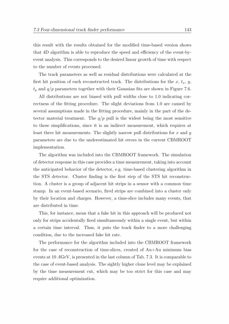
7.3 Four-dimensional track finder performance 143
this result with the results obtained for the modified time-based version shows
that 4D algorithm is able to reproduce the speed and efficiency of the event-by-
event analysis. This corresponds to the desired linear growth of time with respect
to the number of events processed.
The track parameters as well as residual distributions were calculated at the
first hit position of each reconstructed track. The distributions for the x, tx, y,
ty and q/p parameters together with their Gaussian fits are shown in Figure 7.6.
All distributions are not biased with pull widths close to 1.0 indicating cor-
rectness of the fitting procedure. The slight deviations from 1.0 are caused by
several assumptions made in the fitting procedure, mainly in the part of the de-
tector material treatment. The q/p pull is the widest being the most sensitive
to these simplifications, since it is an indirect measurement, which requires at
least three hit measurements. The slightly narrow pull distributions for x and y
parameters are due to the underestimated hit errors in the current CBMROOT
implementation.
The algorithm was included into the CBMROOT framework. The simulation
of detector response in this case provides a time measurement, taking into account
the anticipated behavior of the detector, e.g. time-based clustering algorithm in
the STS detector. Cluster finding is the first step of the STS hit reconstruc-
tion. A cluster is a group of adjacent hit strips in a sensor with a common time
stamp. In an event-based scenario, fired strips are combined into a cluster only
by their location and charges. However, a time-slice includes many events, that
are distributed in time.
This, for instance, mean that a fake hit in this approach will be produced not
only for strips accidentally fired simultaneously within a single event, but within
a certain time interval. Thus, it puts the track finder to a more challenging
condition, due to the increased fake hit rate.
The performance for the algorithm included into the CBMROOT framework
for the case of reconstruction of time-slices, created of Au+Au minimum bias
events at 10 AGeV, is presented in the last column of Tab. 7.3. It is comparable to
the case of event-based analysis. The sightly higher clone level may be explained
by the time measurement cut, which may be too strict for this case and may
require additional optimization.
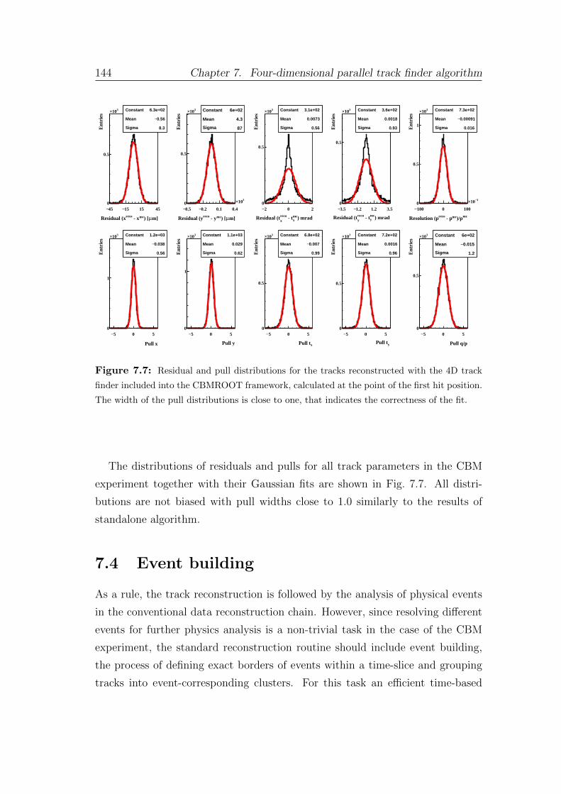
144 Chapter 7. Four-dimensional parallel track finder algorithm
Constant 6.3e+02
Mean 0.56−
Sigma 8.3
m]µ) [mc - xrecoResidual (x
45− 15− 15 45
Ent
ries
0
0.5
310× Constant 6.3e+02
Mean 0.56−
Sigma 8.3
Constant 6e+02
Mean 4.3
Sigma 87
m]µ) [mc - yrecoResidual (y
0.5− 0.2− 0.1 0.4
310×
Ent
ries
0
0.5
310× Constant 6e+02
Mean 4.3
Sigma 87
Constant 3.1e+02
Mean 0.0073
Sigma 0.56
) mradmcx - treco
xResidual (t
2− 0 2
Ent
ries
0
0.5
310× Constant 3.1e+02
Mean 0.0073
Sigma 0.56
Constant 3.6e+02
Mean 0.0018
Sigma 0.93
) mradmcy - treco
yResidual (t
3.5− 1.2− 1.2 3.5
Ent
ries
0
0.5
310× Constant 3.6e+02
Mean 0.0018
Sigma 0.93
Constant 7.3e+02
Mean 0.00091−
Sigma 0.016
mc)/pmc - precoResolution (p
100− 0 100
3−10×
Ent
ries
0
0.5
1
310× Constant 7.3e+02
Mean 0.00091−
Sigma 0.016
Constant 1.2e+03
Mean 0.038−
Sigma 0.56
Pull x
5− 0 5
Ent
ries
0
1
310× Constant 1.2e+03
Mean 0.038−
Sigma 0.56
Constant 1.1e+03
Mean 0.029
Sigma 0.62
Pull y
5− 0 5
Ent
ries
0
1
310× Constant 1.1e+03
Mean 0.029
Sigma 0.62
Constant 6.8e+02
Mean 0.007−
Sigma 0.99
xPull t
5− 0 5
Ent
ries
0
0.5
310× Constant 6.8e+02
Mean 0.007−
Sigma 0.99
Constant 7.2e+02
Mean 0.0016
Sigma 0.96
yPull t
5− 0 5E
ntri
es0
0.5
310× Constant 7.2e+02
Mean 0.0016
Sigma 0.96
Constant 6e+02
Mean 0.015−
Sigma 1.2
Pull q/p
5− 0 5
Ent
ries
0
0.5
310× Constant 6e+02
Mean 0.015−
Sigma 1.2
Figure 7.7: Residual and pull distributions for the tracks reconstructed with the 4D track
finder included into the CBMROOT framework, calculated at the point of the first hit position.
The width of the pull distributions is close to one, that indicates the correctness of the fit.
The distributions of residuals and pulls for all track parameters in the CBM
experiment together with their Gaussian fits are shown in Fig. 7.7. All distri-
butions are not biased with pull widths close to 1.0 similarly to the results of
standalone algorithm.
7.4 Event building
As a rule, the track reconstruction is followed by the analysis of physical events
in the conventional data reconstruction chain. However, since resolving different
events for further physics analysis is a non-trivial task in the case of the CBM
experiment, the standard reconstruction routine should include event building,
the process of defining exact borders of events within a time-slice and grouping
tracks into event-corresponding clusters. For this task an efficient time-based
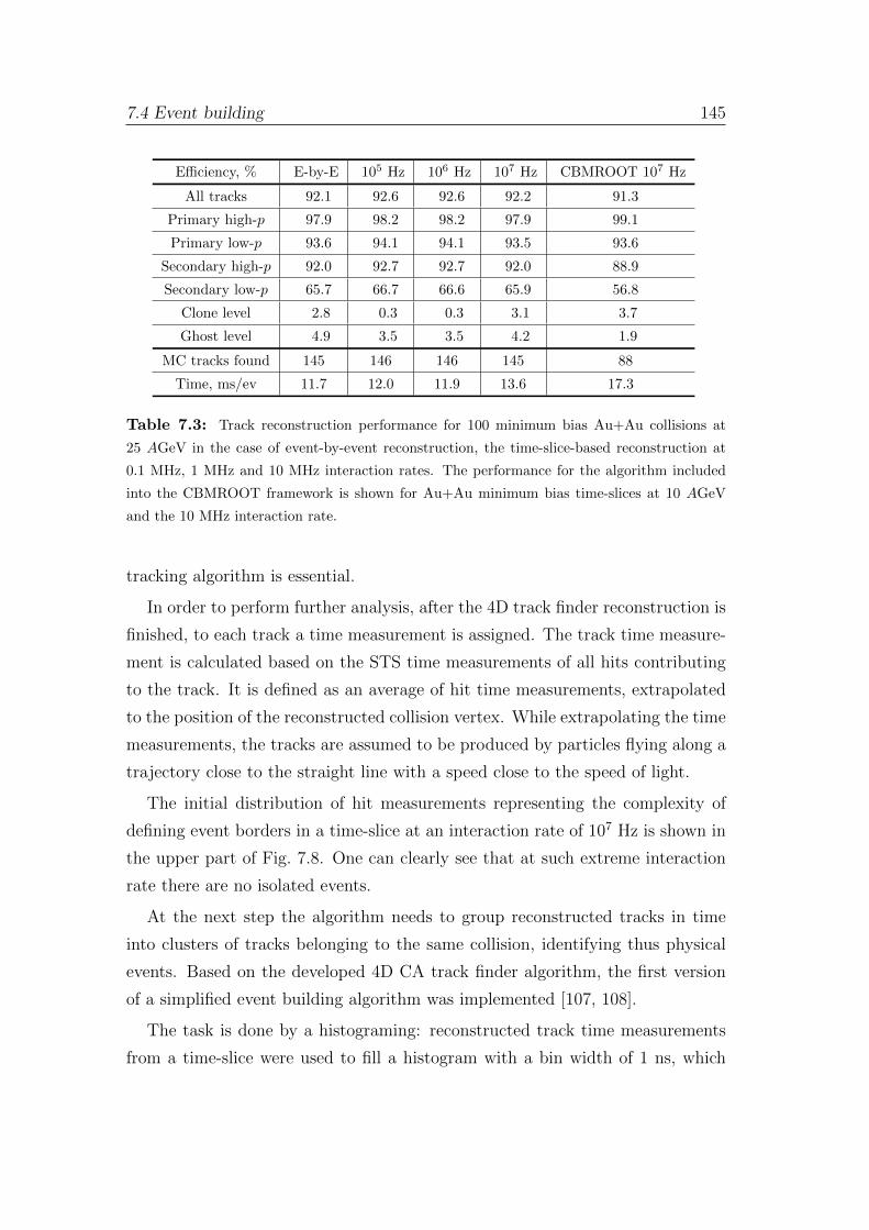
7.4 Event building 145
Efficiency, % E-by-E 105 Hz 106 Hz 107 Hz CBMROOT 107 Hz
All tracks 92.1 92.6 92.6 92.2 91.3
Primary high-p 97.9 98.2 98.2 97.9 99.1
Primary low-p 93.6 94.1 94.1 93.5 93.6
Secondary high-p 92.0 92.7 92.7 92.0 88.9
Secondary low-p 65.7 66.7 66.6 65.9 56.8
Clone level 2.8 0.3 0.3 3.1 3.7
Ghost level 4.9 3.5 3.5 4.2 1.9
MC tracks found 145 146 146 145 88
Time, ms/ev 11.7 12.0 11.9 13.6 17.3
Table 7.3: Track reconstruction performance for 100 minimum bias Au+Au collisions at
25 AGeV in the case of event-by-event reconstruction, the time-slice-based reconstruction at
0.1 MHz, 1 MHz and 10 MHz interaction rates. The performance for the algorithm included
into the CBMROOT framework is shown for Au+Au minimum bias time-slices at 10 AGeV
and the 10 MHz interaction rate.
tracking algorithm is essential.
In order to perform further analysis, after the 4D track finder reconstruction is
finished, to each track a time measurement is assigned. The track time measure-
ment is calculated based on the STS time measurements of all hits contributing
to the track. It is defined as an average of hit time measurements, extrapolated
to the position of the reconstructed collision vertex. While extrapolating the time
measurements, the tracks are assumed to be produced by particles flying along a
trajectory close to the straight line with a speed close to the speed of light.
The initial distribution of hit measurements representing the complexity of
defining event borders in a time-slice at an interaction rate of 107 Hz is shown in
the upper part of Fig. 7.8. One can clearly see that at such extreme interaction
rate there are no isolated events.
At the next step the algorithm needs to group reconstructed tracks in time
into clusters of tracks belonging to the same collision, identifying thus physical
events. Based on the developed 4D CA track finder algorithm, the first version
of a simplified event building algorithm was implemented [107, 108].
The task is done by a histograming: reconstructed track time measurements
from a time-slice were used to fill a histogram with a bin width of 1 ns, which
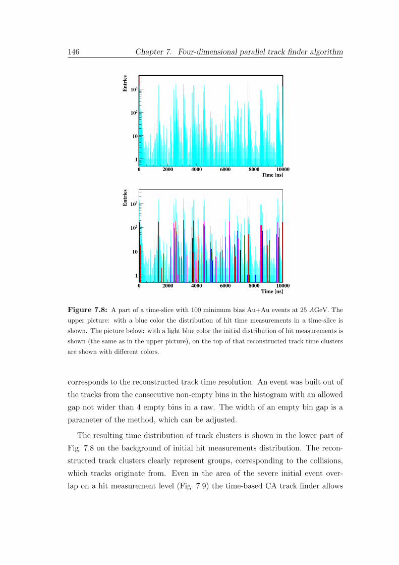
146 Chapter 7. Four-dimensional parallel track finder algorithm146 CHAPTER 7. 4D PARALLEL CA TRACK FINDER
Time [ns]0 2000 4000 6000 8000 10000
Entr
ies
1
10
210
310
Time [ns]0 2000 4000 6000 8000 10000
Entr
ies
1
10
210
310
Figure 7.8: Part of a time-slice with 100 minimum bias events. The upper picture:
with a blue color the distribution of hit time measurements in a time-slice is shown.
The picture below: with a light blue color the initial distribution of hit measurements
is shown (same as in the upper picture), on the top of that reconstructed track clusters
are shown with di↵erent colors.
which tracks originate from. Even in the area of the severe initial event overlap
on a hit measurement level(Fig. 7.9) the time-based CA track finder allows to
resolve tracks from di↵erent collisions in time.
Figure 7.8: A part of a time-slice with 100 minimum bias Au+Au events at 25 AGeV. The
upper picture: with a blue color the distribution of hit time measurements in a time-slice is
shown. The picture below: with a light blue color the initial distribution of hit measurements is
shown (the same as in the upper picture), on the top of that reconstructed track time clusters
are shown with different colors.
corresponds to the reconstructed track time resolution. An event was built out of
the tracks from the consecutive non-empty bins in the histogram with an allowed
gap not wider than 4 empty bins in a raw. The width of an empty bin gap is a
parameter of the method, which can be adjusted.
The resulting time distribution of track clusters is shown in the lower part of
Fig. 7.8 on the background of initial hit measurements distribution. The recon-
structed track clusters clearly represent groups, corresponding to the collisions,
which tracks originate from. Even in the area of the severe initial event over-
lap on a hit measurement level (Fig. 7.9) the time-based CA track finder allows
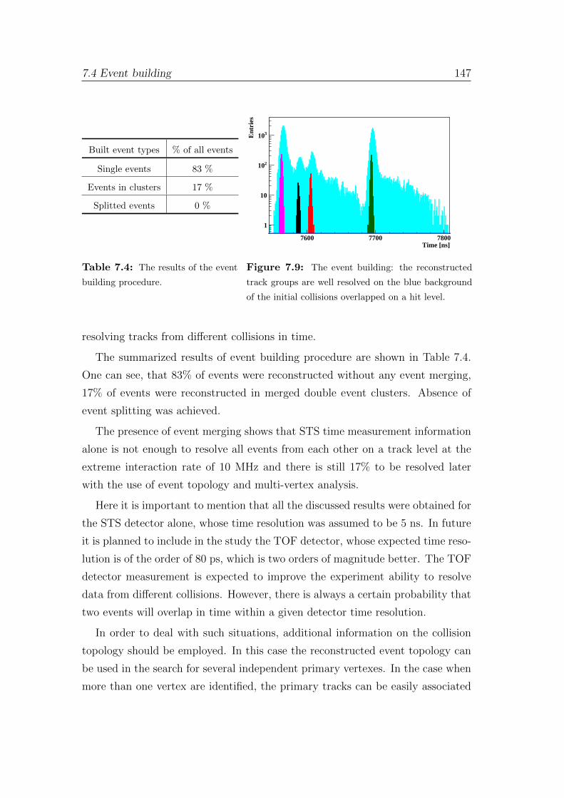
7.4 Event building 147
Built event types % of all events
Single events 83 %
Events in clusters 17 %
Splitted events 0 %
Time [ns]7600 7700 7800
Ent
ries
1
10
210
310
Table 7.4: The results of the event
building procedure.
Figure 7.9: The event building: the reconstructed
track groups are well resolved on the blue background
of the initial collisions overlapped on a hit level.
resolving tracks from different collisions in time.
The summarized results of event building procedure are shown in Table 7.4.
One can see, that 83% of events were reconstructed without any event merging,
17% of events were reconstructed in merged double event clusters. Absence of
event splitting was achieved.
The presence of event merging shows that STS time measurement information
alone is not enough to resolve all events from each other on a track level at the
extreme interaction rate of 10 MHz and there is still 17% to be resolved later
with the use of event topology and multi-vertex analysis.
Here it is important to mention that all the discussed results were obtained for
the STS detector alone, whose time resolution was assumed to be 5 ns. In future
it is planned to include in the study the TOF detector, whose expected time reso-
lution is of the order of 80 ps, which is two orders of magnitude better. The TOF
detector measurement is expected to improve the experiment ability to resolve
data from different collisions. However, there is always a certain probability that
two events will overlap in time within a given detector time resolution.
In order to deal with such situations, additional information on the collision
topology should be employed. In this case the reconstructed event topology can
be used in the search for several independent primary vertexes. In the case when
more than one vertex are identified, the primary tracks can be easily associated
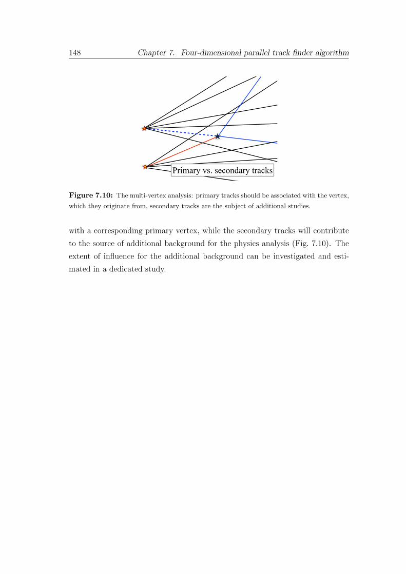
148 Chapter 7. Four-dimensional parallel track finder algorithm
Primary vs. secondary tracks
Figure 7.10: The multi-vertex analysis: primary tracks should be associated with the vertex,
which they originate from, secondary tracks are the subject of additional studies.
with a corresponding primary vertex, while the secondary tracks will contribute
to the source of additional background for the physics analysis (Fig. 7.10). The
extent of influence for the additional background can be investigated and esti-
mated in a dedicated study.
Chapter 8
Summary and conclusions
The CBM (Compressed Baryonic Matter) experiment at the upcoming FAIR
accelerator (GSI, Darmstadt, Germany) aims to explore the phase diagram of
strongly interacting matter at the highest net baryon densities by investigating
nuclear collisions from 2 to 45 AGeV. One of the most promising observables
carrying information on the early stage of collision are measurements of rare
probes (e.g. charmonium), which require unprecedented statistics for this energy
range and, thus, collision rates of up to 10 MHz. Taking into account multiplicity
of charged particles in a heavy-ion collision, one should expect a data flow rate
of 1 TB/s. Such a huge data rate makes it mandatory to select interesting events
online with a reduction factor of about two orders of magnitude in order to meet
the data recording rate of 10 GB/s.
CBM will operate on a continuous beam without bunch structure. As a result,
collisions may overlap in time, making the traditional event-based approach not
applicable. That requires the full online event reconstruction and selection not
only in space, but also in time, the so-called 4D event building and selection. The
problem is to be solved online on a dedicated many-core CPU/GPU computer
farm by the First Level Event Selection package. This requires the package to
be fast, precise and suitable for online data processing in order to use the full
potential of modern many-core computer architectures.
For the most time-consuming part of the reconstruction procedure the Cellu-
lar Automaton track finder is used. The efficiency of the algorithm proved to be
stable with respect to track multiplicity up to the extreme case of reconstruc-
150 Chapter 8. Summary and conclusions
tion of 100 minimum bias events at once without usage of the time information.
The reconstruction time dependence on the track multiplicity in these conditions
behaves as a second order polynomial.
The event-based CA track finder was adapted for time-slice-based 4D track
reconstruction, which is a requirement in case of CBM for the event building.
The 4D CA track finder is able to reproduce the performance and the speed of the
event-based CA track finder. The algorithm was included into the CBMROOT
framework.
The 4D CA track finder is both vectorized (using SIMD instructions) and
parallelized (between CPU cores). The algorithm shows strong scalability on
many-core systems. The speed-up factor of 10.1 was achieved on a CPU with 10
hyper-threaded physical cores.
The 4D event building was implemented in the standalone FLES package for
the CBM experiment. It allows resolving the major part of overlapping on a
hit level events and group tracks into event-corresponding clusters without event
splitting. About 17 % of events are merged and cannot be separated using only
the time information at an interaction rate of 10 MHz. Resolving them is a task
for further multi-vertex analysis as well as for a study with the included TOF
(Time-Of-Flight) detector.
The 4D CA track finder algorithm is ready for time-slice-based reconstruction
for the CBM experiment.
List of Figures
1.1 A scheme of the QCD phase diagram of strongly interacting matter [9]. . . . 6
2.1 Layout of the FAIR facility (left side) [25]. The new facility and the existing
GSI complex are shown in red and grey, respectively. Aerial photo of the
construction site (right side) taken on April 22, 2015 [26] . . . . . . . . . . 11
2.2 Particle multiplicities times branching ratio for central Au+Au collisions at
25 AGeV calculated with the HSD transport code [27] and the statistical
model [28]. . . . . . . . . . . . . . . . . . . . . . . . . . . . . . . . 12
2.3 The CBM detector setup versions for electron (top) and muon registra-
tion (bottom). In the electron configuration the subdetectors are: Micro-
vertex Detector (MVD), Silicon Tracking System (STS), both placed in a gap
of 1 Tm superconducting magnet, then Ring Imaging Cherenkov Detector
(RICH), Transition Radiation Detectors (TRD), Resistive Plate Chambers
for time-of-flight measurements (TOF), Electromagnetic Calorimeter (ECAL)
and Projectile Spectator Detector (PSD) as a hadronic calorimeter. In the
muon configuration the RICH detector will be replaced by the Muon Cham-
bers System (MUCH) and ECAL will be removed. . . . . . . . . . . . . . 18
2.4 (A) Geometry of the superconducting dipole magnet. (B) Magnetic field
distribution in the Y -Z-plane at X=0 [41]. . . . . . . . . . . . . . . . . 19
2.5 (A) The 3D view of the MVD model, depicting the sensors (C) and the me-
chanical holding structure including the layout of the stations. (B) Fundamen-
tal layout of a CMOS sensor pixel [44]. (D) The MVD front-end electronics
including the flex print cables. . . . . . . . . . . . . . . . . . . . . . . 21
152 List of Figures
2.6 (A) The layout of the STS stations [31]. (B) The operational principle of
the silicon strip detector [45]. (C) The layout of the 6th STS station. The
color codes within the stations denote commonly read-out sensors. The circles
indicate the acceptance between polar angles 2.5o and 25o. . . . . . . . . . 22
2.7 (A) The layout of the RICH stations [46]. (B) The principle of the Cherenkov
radiation. The schematic view of the RICH detector with its imaging UV
mirrors. (C) The Cherenkov-cones are imaged on the detectors as rings. . . 23
2.8 (A) The scheme of the MuCh detector configurations, optimized for different
physics cases: low-mass vector mesons (shown with red and blue frames) and
J/ψ measurements (shown with a green frame)[47]. The schematic representa-
tions of the signal generation process in the GEM detector (C) and the straw
tube detector (B). . . . . . . . . . . . . . . . . . . . . . . . . . . . . 25
2.9 (A) The scheme of the Transition Radiation detector for SIS100/300
and (B) the geometry of one detector module [48]. In the module schematic
signals produced by a pion and an electron are shown. The geometric propor-
tions and the field lines in the drift chamber are accurate [49]. . . . . . . . 27
2.10 (A) The scheme of the time-of-flight wall [50]. (B) The structure of the
float glass MRPC with 8-strip readout [51]. The simulated 2D squared mass
distribution versus momentum and (C) its projection (D). . . . . . . . . 28
2.11 (A) The layout of the electromagnetic calorimeter ECAL [53]. (B) A sampling
calorimeter scheme and (C) a schematic development of an electromagnetic
shower. . . . . . . . . . . . . . . . . . . . . . . . . . . . . . . . . . 29
2.12 (A) The layout of the Projectile Spectator Detector (PSD) [54]. (B) The
reaction plane by definition contains the impact parameter vector (along the
X-axis). . . . . . . . . . . . . . . . . . . . . . . . . . . . . . . . . . 31
2.13 The CBM data acquisition concept in comparison to conventional systems [55].
Usually, the collected data undergoes several trigger levels, where it gets re-
duced. This scenario is inapplicabele for CBM due to the absence of simple
triggers. Instead, the first (L1) trigger will be a High Level Trigger (HLT),
running on a computer farm. . . . . . . . . . . . . . . . . . . . . . . . 32
2.14 The architecture of the First-level Event Selector (FLES) [56]. . . . . . . . 33
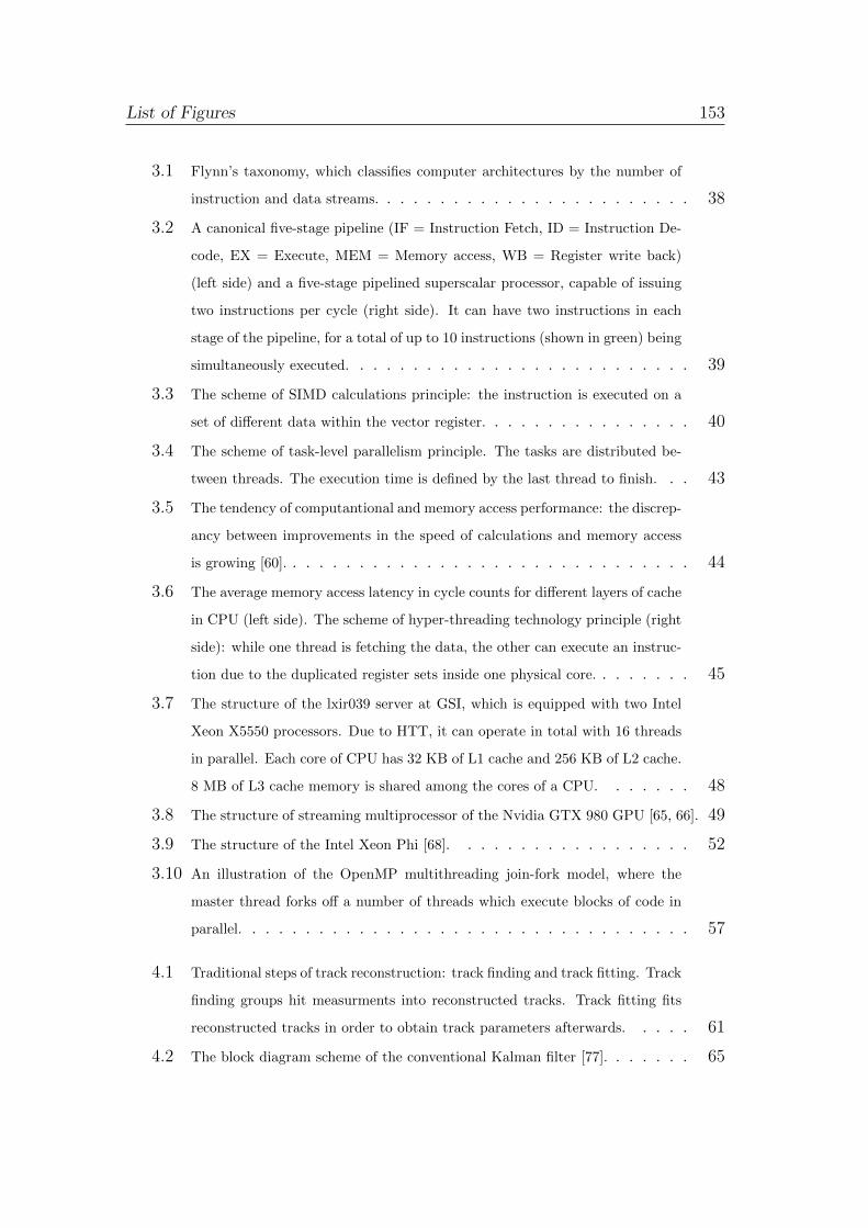
List of Figures 153
3.1 Flynn’s taxonomy, which classifies computer architectures by the number of
instruction and data streams. . . . . . . . . . . . . . . . . . . . . . . . 38
3.2 A canonical five-stage pipeline (IF = Instruction Fetch, ID = Instruction De-
code, EX = Execute, MEM = Memory access, WB = Register write back)
(left side) and a five-stage pipelined superscalar processor, capable of issuing
two instructions per cycle (right side). It can have two instructions in each
stage of the pipeline, for a total of up to 10 instructions (shown in green) being
simultaneously executed. . . . . . . . . . . . . . . . . . . . . . . . . . 39
3.3 The scheme of SIMD calculations principle: the instruction is executed on a
set of different data within the vector register. . . . . . . . . . . . . . . . 40
3.4 The scheme of task-level parallelism principle. The tasks are distributed be-
tween threads. The execution time is defined by the last thread to finish. . . 43
3.5 The tendency of computantional and memory access performance: the discrep-
ancy between improvements in the speed of calculations and memory access
is growing [60]. . . . . . . . . . . . . . . . . . . . . . . . . . . . . . . 44
3.6 The average memory access latency in cycle counts for different layers of cache
in CPU (left side). The scheme of hyper-threading technology principle (right
side): while one thread is fetching the data, the other can execute an instruc-
tion due to the duplicated register sets inside one physical core. . . . . . . . 45
3.7 The structure of the lxir039 server at GSI, which is equipped with two Intel
Xeon X5550 processors. Due to HTT, it can operate in total with 16 threads
in parallel. Each core of CPU has 32 KB of L1 cache and 256 KB of L2 cache.
8 MB of L3 cache memory is shared among the cores of a CPU. . . . . . . 48
3.8 The structure of streaming multiprocessor of the Nvidia GTX 980 GPU [65, 66]. 49
3.9 The structure of the Intel Xeon Phi [68]. . . . . . . . . . . . . . . . . . 52
3.10 An illustration of the OpenMP multithreading join-fork model, where the
master thread forks off a number of threads which execute blocks of code in
parallel. . . . . . . . . . . . . . . . . . . . . . . . . . . . . . . . . . 57
4.1 Traditional steps of track reconstruction: track finding and track fitting. Track
finding groups hit measurments into reconstructed tracks. Track fitting fits
reconstructed tracks in order to obtain track parameters afterwards. . . . . 61
4.2 The block diagram scheme of the conventional Kalman filter [77]. . . . . . . 65
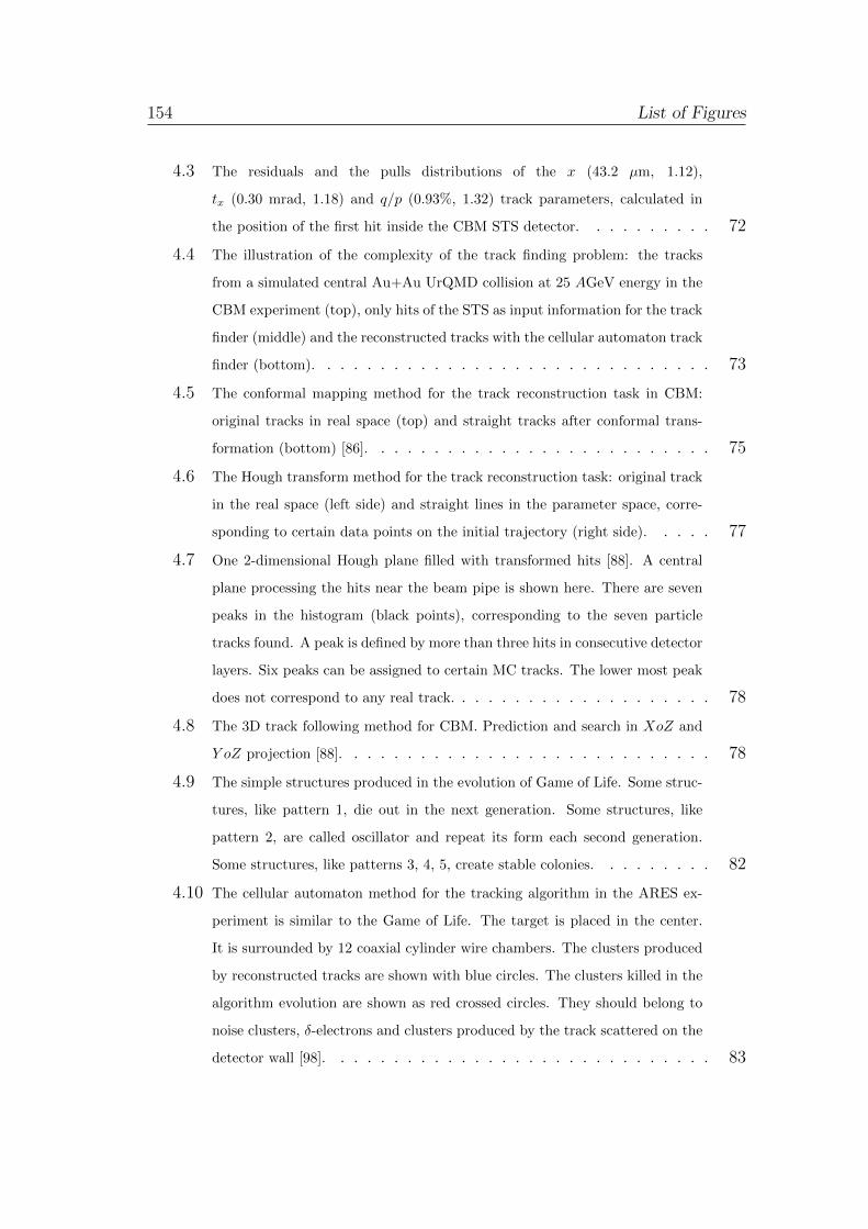
154 List of Figures
4.3 The residuals and the pulls distributions of the x (43.2 µm, 1.12),
tx (0.30 mrad, 1.18) and q/p (0.93%, 1.32) track parameters, calculated in
the position of the first hit inside the CBM STS detector. . . . . . . . . . 72
4.4 The illustration of the complexity of the track finding problem: the tracks
from a simulated central Au+Au UrQMD collision at 25 AGeV energy in the
CBM experiment (top), only hits of the STS as input information for the track
finder (middle) and the reconstructed tracks with the cellular automaton track
finder (bottom). . . . . . . . . . . . . . . . . . . . . . . . . . . . . . 73
4.5 The conformal mapping method for the track reconstruction task in CBM:
original tracks in real space (top) and straight tracks after conformal trans-
formation (bottom) [86]. . . . . . . . . . . . . . . . . . . . . . . . . . 75
4.6 The Hough transform method for the track reconstruction task: original track
in the real space (left side) and straight lines in the parameter space, corre-
sponding to certain data points on the initial trajectory (right side). . . . . 77
4.7 One 2-dimensional Hough plane filled with transformed hits [88]. A central
plane processing the hits near the beam pipe is shown here. There are seven
peaks in the histogram (black points), corresponding to the seven particle
tracks found. A peak is defined by more than three hits in consecutive detector
layers. Six peaks can be assigned to certain MC tracks. The lower most peak
does not correspond to any real track. . . . . . . . . . . . . . . . . . . . 78
4.8 The 3D track following method for CBM. Prediction and search in XoZ and
Y oZ projection [88]. . . . . . . . . . . . . . . . . . . . . . . . . . . . 78
4.9 The simple structures produced in the evolution of Game of Life. Some struc-
tures, like pattern 1, die out in the next generation. Some structures, like
pattern 2, are called oscillator and repeat its form each second generation.
Some structures, like patterns 3, 4, 5, create stable colonies. . . . . . . . . 82
4.10 The cellular automaton method for the tracking algorithm in the ARES ex-
periment is similar to the Game of Life. The target is placed in the center.
It is surrounded by 12 coaxial cylinder wire chambers. The clusters produced
by reconstructed tracks are shown with blue circles. The clusters killed in the
algorithm evolution are shown as red crossed circles. They should belong to
noise clusters, δ-electrons and clusters produced by the track scattered on the
detector wall [98]. . . . . . . . . . . . . . . . . . . . . . . . . . . . . 83
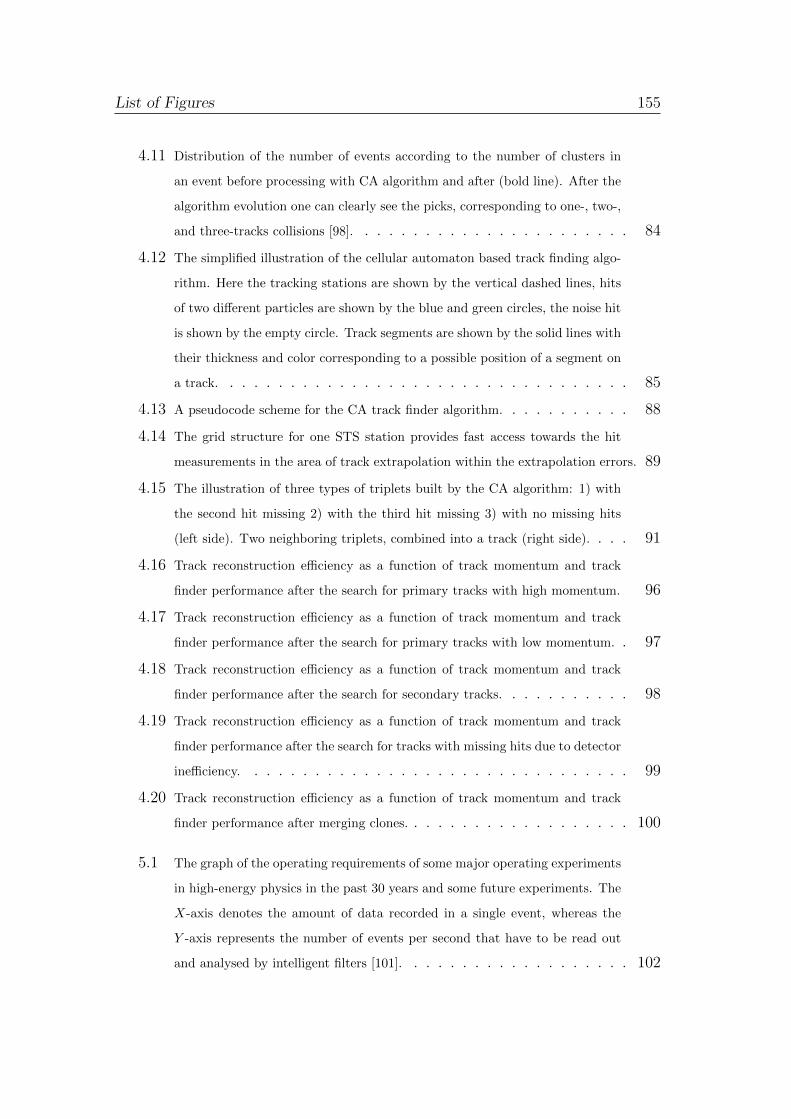
List of Figures 155
4.11 Distribution of the number of events according to the number of clusters in
an event before processing with CA algorithm and after (bold line). After the
algorithm evolution one can clearly see the picks, corresponding to one-, two-,
and three-tracks collisions [98]. . . . . . . . . . . . . . . . . . . . . . . 84
4.12 The simplified illustration of the cellular automaton based track finding algo-
rithm. Here the tracking stations are shown by the vertical dashed lines, hits
of two different particles are shown by the blue and green circles, the noise hit
is shown by the empty circle. Track segments are shown by the solid lines with
their thickness and color corresponding to a possible position of a segment on
a track. . . . . . . . . . . . . . . . . . . . . . . . . . . . . . . . . . 85
4.13 A pseudocode scheme for the CA track finder algorithm. . . . . . . . . . . 88
4.14 The grid structure for one STS station provides fast access towards the hit
measurements in the area of track extrapolation within the extrapolation errors. 89
4.15 The illustration of three types of triplets built by the CA algorithm: 1) with
the second hit missing 2) with the third hit missing 3) with no missing hits
(left side). Two neighboring triplets, combined into a track (right side). . . . 91
4.16 Track reconstruction efficiency as a function of track momentum and track
finder performance after the search for primary tracks with high momentum. 96
4.17 Track reconstruction efficiency as a function of track momentum and track
finder performance after the search for primary tracks with low momentum. . 97
4.18 Track reconstruction efficiency as a function of track momentum and track
finder performance after the search for secondary tracks. . . . . . . . . . . 98
4.19 Track reconstruction efficiency as a function of track momentum and track
finder performance after the search for tracks with missing hits due to detector
inefficiency. . . . . . . . . . . . . . . . . . . . . . . . . . . . . . . . 99
4.20 Track reconstruction efficiency as a function of track momentum and track
finder performance after merging clones. . . . . . . . . . . . . . . . . . . 100
5.1 The graph of the operating requirements of some major operating experiments
in high-energy physics in the past 30 years and some future experiments. The
X-axis denotes the amount of data recorded in a single event, whereas the
Y -axis represents the number of events per second that have to be read out
and analysed by intelligent filters [101]. . . . . . . . . . . . . . . . . . . 102
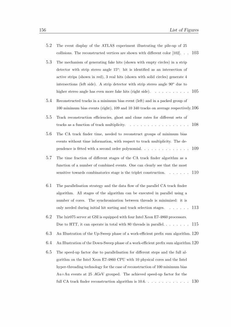
156 List of Figures
5.2 The event display of the ATLAS experiment illustrating the pile-up of 25
collisions. The reconstructed vertices are shown with different color [102]. . . 103
5.3 The mechanism of generating fake hits (shown with empty circles) in a strip
detector with strip stereo angle 15o: hit is identified as an intersection of
active strips (shown in red), 3 real hits (shown with solid circles) generate 4
intersections (left side). A strip detector with strip stereo angle 90o due to
higher stereo angle has even more fake hits (right side). . . . . . . . . . . 105
5.4 Reconstructed tracks in a minimum bias event (left) and in a packed group of
100 minimum bias events (right), 109 and 10 340 tracks on average respectively.106
5.5 Track reconstruction efficiencies, ghost and clone rates for different sets of
tracks as a function of track multiplicity. . . . . . . . . . . . . . . . . . 108
5.6 The CA track finder time, needed to reconstruct groups of minimum bias
events without time information, with respect to track multiplicity. The de-
pendence is fitted with a second order polynomial. . . . . . . . . . . . . . 109
5.7 The time fraction of different stages of the CA track finder algorithm as a
function of a number of combined events. One can clearly see that the most
sensitive towards combinatorics stage is the triplet construction. . . . . . . 110
6.1 The parallelisation strategy and the data flow of the parallel CA track finder
algorithm. All stages of the algorithm can be executed in parallel using a
number of cores. The synchronization between threads is minimized: it is
only needed during initial hit sorting and track selection stages. . . . . . . 113
6.2 The lxir075 server at GSI is equipped with four Intel Xeon E7-4860 processors.
Due to HTT, it can operate in total with 80 threads in parallel. . . . . . . . 115
6.3 An Illustration of the Up-Sweep phase of a work-efficient prefix sum algorithm. 120
6.4 An Illustration of the Down-Sweep phase of a work-efficient prefix sum algorithm.120
6.5 The speed-up factor due to parallelisation for different steps and the full al-
gorithm on the Intel Xeon E7-4860 CPU with 10 physical cores and the Intel
hyper-threading technology for the case of reconstruction of 100 minimum bias
Au+Au events at 25 AGeV grouped. The achieved speed-up factor for the
full CA track finder reconstruction algorithm is 10.6. . . . . . . . . . . . . 130
List of Figures 157
7.1 The illustration of the complexity of defining physical events in the case of the
CBM experiment: the absence of a hardware trigger together with extreme
collision rates lead to a fraction of collisions, which overlap in time. Thus, the
task of event building is shifted from the hardware to the software. . . . . . 133
7.2 The distribution of the hit time measurements for 100 minimum bias Au+Au
collisions at 25 AGeV in the main tracking system of CBM, obtained assuming
the average interaction rate of 10 MHz and Poisson distribution of the time
intervals between subsequent events (top), the same distribution shown on a
larger scale (bottom). Different collisions are shown with a different filling
and color. Events clearly overlap with each other. . . . . . . . . . . . . . 135
7.3 The pseudocode scheme for the parallel time-based CA track finder algorithm.
In the time-based version the grid structure was modified to take into account
time information. Also, the STS time measurement is used to reduce combi-
natorics in the triplet building stage. . . . . . . . . . . . . . . . . . . . 137
7.4 The grid structure for one STS station to provide the fast access towards the
hit measurements in the area of track extrapolation in the case of event-based
analysis (left side) and the case of time-base tracking (right side). . . . . . . 138
7.5 The speed-up factor due to parallelisation for different steps and the full 4D CA
track finder algorithm on Intel Xeon E7-4860 CPU with 10 physical cores and
hyper-threading in the case of reconstruction of a time-slice of 100 minimum
bias Au+Au events at 25 AGeV. . . . . . . . . . . . . . . . . . . . . . 139
7.6 Residual and pull distributions for the tracks reconstructed by the 4D track
finder, calculated at the point of the first hit position in the CBM STS de-
tector. The width of the pull distributions is close to one, that indicates the
correctness of the fit. . . . . . . . . . . . . . . . . . . . . . . . . . . . 142
7.7 Residual and pull distributions for the tracks reconstructed with the 4D track
finder included into the CBMROOT framework, calculated at the point of
the first hit position. The width of the pull distributions is close to one, that
indicates the correctness of the fit. . . . . . . . . . . . . . . . . . . . . 144
158 List of Figures
7.8 A part of a time-slice with 100 minimum bias Au+Au events at 25 AGeV. The
upper picture: with a blue color the distribution of hit time measurements in
a time-slice is shown. The picture below: with a light blue color the initial
distribution of hit measurements is shown (the same as in the upper picture),
on the top of that reconstructed track time clusters are shown with different
colors. . . . . . . . . . . . . . . . . . . . . . . . . . . . . . . . . . . 146
7.9 The event building: the reconstructed track groups are well resolved on the
blue background of the initial collisions overlapped on a hit level. . . . . . . 147
7.10 The multi-vertex analysis: primary tracks should be associated with the ver-
tex, which they originate from, secondary tracks are the subject of additional
studies. . . . . . . . . . . . . . . . . . . . . . . . . . . . . . . . . . 148
1 Eine Illustration der Komplexitat der Spurfindung (von links nach rechts): die
Spuren von einer simulierten Au+Au Kollision bei 25 AGeV; die Detektortr-
effer im STS als Eingangsinformation fur den CA-Spurfinder; die mit dem
CA-Spurfinder rekonstruierte Spuren. . . . . . . . . . . . . . . . . . . . 173
2 Die Effizienz der Spurrekonstruktion und Geisterspur-Rate in verschiedenen
Spurgruppen im Vergleich zu Spur-Multiplizitat. . . . . . . . . . . . . . . 175
3 Die Zeit, die der CA-Spurfinder benotigt, um Gruppen von Minimum-Bias-
Ereignissen ohne Zeitinformation zu rekonstruieren, als Funktion der Spuran-
zahl. Die Abhangigkeit wird mit einem Polynom zweiter Ordnung beschrieben. 177
4 Beschleunigungsfaktor aufgrund der Parallelisierung fur verschiedene Schritte
und den vollstandigen Algorithmus auf Intel Xeon E7-4860 CPU mit zehn ph-
ysischen Kernen und Hyper-Threading fur den Fall von 100 zusammenge-
fassten Minimum-Bias-Ereignissen. . . . . . . . . . . . . . . . . . . . . 177
List of Tables
2.1 The CBM observables. The subdetectors required for a certain observable
are marked as X. The subdetectors marked as (X) can be used optionally to
suppress background. . . . . . . . . . . . . . . . . . . . . . . . . . . . 19
5.1 Track reconstruction performance for Au+Au collisions at 25 AGeV in the
case of event-by-event analysis (3D) for minimum bias and central events, as
well as for a hundred events grouped on a hit level with no time information
(3 + 1D). No track merging and extending procedures are included. . . . . . 107
6.1 The fraction of the total execution time for different steps of the CA track
finder algorithm in a sequential run. . . . . . . . . . . . . . . . . . . . . 116
7.1 Track reconstruction performance for 100 minimum bias Au+Au collisions at
25 AGeV in the case of the event-by-event analysis (3D), grouped on a hit
level with no time information (3 + 1D) and the time-based reconstruction
(4D). No track merging and extending procedures are included. . . . . . . . 140
7.2 Track reconstruction performance for Au+Au minimum bias event at 25 AGeV
with the event-by-event analysis from the CBMROOT as well as for the time-
slices-wise reconstruction assuming the 10 MHz interaction rate [105]. Track
merging and extending procedures are included. . . . . . . . . . . . . . . 141
7.3 Track reconstruction performance for 100 minimum bias Au+Au collisions at
25 AGeV in the case of event-by-event reconstruction, the time-slice-based
reconstruction at 0.1 MHz, 1 MHz and 10 MHz interaction rates. The per-
formance for the algorithm included into the CBMROOT framework is shown
for Au+Au minimum bias time-slices at 10 AGeV and the 10 MHz interaction
rate. . . . . . . . . . . . . . . . . . . . . . . . . . . . . . . . . . . . 145

160 List of Tables
7.4 The results of the event building procedure. . . . . . . . . . . . . . . . . 147
1 Die Spurrekonstruktion Performanz des CBM CA-Spurfinders fur verschiedene
Satze von Spuren in den Minimum-Bias und zentralen Ereignisse bei 25 AGeV. 175
2 Effizienz (in %) der Spurrekonstruktion fur 100 Minimum-Bias Au+Au Kolli-
sionen bei 25 AGeV bei ereignisweiser Rekonstruktion als auch bei zeitschnit-
tbasierter Rekonstruktion bei 0,1 MHz, 1 MHz und 10 MHz Kollisionsraten.
Die Effizienz fur den Algorithmus, der im CBMROOT-Framework enthalten
ist, wird fur Au+Au Minimum-Bias-Zeitschnitten bei 10 AGeV und 10 MHz
Kollisionsrate gezeigt. . . . . . . . . . . . . . . . . . . . . . . . . . . 180
Bibliography
[1] B. Friman, C. Hohne, J. Knoll, S. Leupold, J. Randrup, R. Rapp and P. Sen-
ger, “The CBM physics book: Compressed baryonic matter in laboratory
experiments,” Lect. Notes Phys. 814 (2011) 980.
[2] K. Aamodt et al. [ALICE Collaboration], “The ALICE experiment at the
CERN LHC,” JINST 3 (2008) S08002.
[3] J. W. Harris [STAR Collaboration], “The STAR experiment at the relativis-
tic heavy ion collider,” Nucl. Phys. A 566 (1994) 277C.
[4] D. P. Morrison et al. [PHENIX Collaboration], “The PHENIX experiment
at RHIC,” Nucl. Phys. A 638 (1998) 565.
[5] A. Andronic et al., “Hadron Production in Ultra-relativistic Nuclear Colli-
sions: Quarkyonic Matter and a Triple Point in the Phase Diagram of QCD,”
Nucl. Phys. A 837 (2010) 65.
[6] N. Cabibbo and G. Parisi, “Exponential Hadronic Spectrum and Quark Lib-
eration,” Phys. Lett. B 59 (1975) 67.
[7] J. C. Collins and M. J. Perry, “Superdense Matter: Neutrons Or Asymptot-
ically Free Quarks?,” Phys. Rev. Lett. 34 (1975) 1353.
[8] http://www.cyberphysics.co.uk/topics/atomic/nucleus.htm
[9] Letter of Intent for the Compressed Baryonic Matter Experiment at the
Future Accelerator Facility in Darmstadt, Darmstadt, January 2004.
162 Bibliography
[10] F. Karsch and E. Laermann, “Thermodynamics and in medium hadron prop-
erties from lattice QCD,” In Hwa, R.C. (ed.) et al.: Quark gluon plasma
1-59.
[11] Y. Aoki, G. Endrodi, Z. Fodor, S. D. Katz and K. K. Szabo, “The Order of
the quantum chromodynamics transition predicted by the standard model
of particle physics,” Nature 443 (2006) 675.
[12] F. Becattini, M. Bleicher, T. Kollegger, T. Schuster, J. Steinheimer and
R. Stock, “Hadron Formation in Relativistic Nuclear Collisions and the QCD
Phase Diagram,” Phys. Rev. Lett. 111 (2013) 082302.
[13] Y. Aoki, S. Borsanyi, S. Durr, Z. Fodor, S. D. Katz, S. Krieg and K. K. Sz-
abo, “The QCD transition temperature: results with physical masses in the
continuum limit II.,” JHEP 0906 (2009) 088.
[14] A. Bazavov et al., “The chiral and deconfinement aspects of the QCD tran-
sition,” Phys. Rev. D 85 (2012) 054503.
[15] Z. Fodor and S. D. Katz, “Critical point of QCD at finite T and mu, lattice
results for physical quark masses,” JHEP 0404 (2004) 050.
[16] M. D’Elia, A. Di Giacomo and C. Pica, “Two flavor QCD and confinement,”
Phys. Rev. D 72 (2005) 114510.
[17] P. de Forcrand and O. Philipsen, “The Chiral critical line of N(f) = 2+1
QCD at zero and non-zero baryon density,” JHEP 0701 (2007) 077.
[18] R. D. Pisarski, “Phenomenology of the Chiral Phase Transition,” Phys. Lett.
B 110 (1982) 155.
[19] B. C. Barrois, “Superconducting Quark Matter,” Nucl. Phys. B 129 (1977)
390.
[20] D. Bailin and A. Love, “Superfluidity and Superconductivity in Relativistic
Fermion Systems,” Phys. Rept. 107 (1984) 325.
[21] W. A. Zajc, “The Fluid Nature of Quark-Gluon Plasma,” Nucl. Phys. A 805
(2008) 283.
Bibliography 163
[22] F. Weber, “Strangeness in neutron stars,” J. Phys. G 27 (2001) 465.
[23] J. M. Lattimer and M. Prakash, “Neutron star structure and the equation
of state,” Astrophys. J. 550 (2001) 426.
[24] http://nica.jinr.ru
[25] P. Senger, T. Galatyuk, A. Kiseleva, D. Kresan, A. Lebedev, S. Lebedev
and A. Lymanets, “The compressed baryonic matter experiment at FAIR,”
J. Phys. G 36 (2009) 064037.
[26] Photo by Till Middelhauve for FAIR.
[27] W. Cassing, E. L. Bratkovskaya and A. Sibirtsev, “Open charm production
in relativistic nucleus-nucleus collisions,” Nucl. Phys. A 691 (2001) 753.
[28] A. Andronic, P. Braun-Munzinger and J. Stachel, “Hadron production in
central nucleus-nucleus collisions at chemical freeze-out,” Nucl. Phys. A 772
(2006) 167.
[29] I. C. Arsene et al., “Dynamical phase trajectories for relativistic nuclear
collisions,” Phys. Rev. C 75 (2007) 034902.
[30] M. Orsaria, H. Rodrigues, F. Weber and G. A. Contrera, “Quark deconfine-
ment in high-mass neutron stars,” Phys. Rev. C 89 (2014) no.1, 015806.
[31] J. Heuser et al., “Technical Design Report for the CBM Silicon Tracking
System (STS),” GSI, Darmstadt (2013) 167 p.
[32] P. Senger and V. Friese, “The CBM Collaboration: Nuclear Matter Physics
at SIS-100,” GSI, Darmstadt (2012) 18 p.
[33] W. Reisdorf and H. G. Ritter, “Collective flow in heavy-ion collisions,” Ann.
Rev. Nucl. Part. Sci. 47 (1997) 663.
[34] P. M. Hohler and R. Rapp, “Is ρ-Meson Melting Compatible with Chiral
Restoration?,” Phys. Lett. B 731 (2014) 103
[35] T. Matsui and H. Satz, “J/ψ Suppression by Quark-Gluon Plasma Forma-
tion,” Phys. Lett. B 178 (1986) 416.
164 Bibliography
[36] W. Cassing and E. L. Bratkovskaya, “Hadronic and electromagnetic probes
of hot and dense nuclear matter,” Phys. Rept. 308 (1999) 65.
[37] P. Koch, B. Muller and J. Rafelski, “Strangeness in Relativistic Heavy Ion
Collisions,” Phys. Rept. 142 (1986) 167.
[38] H. van Hees, J. Weil, S. Endres and M. Bleicher, “Electromagnetic probes in
heavy-ion collisions: Messengers from the hot and dense phase,” EPJ Web
Conf. 97 (2015) 00028
[39] A. Andronic, P. Braun-Munzinger, J. Stachel and H. Stocker, “Production
of light nuclei, hypernuclei and their antiparticles in relativistic nuclear col-
lisions,” Phys. Lett. B 697 (2011) 203
[40] H. Stoecker, I. Augustin, J. Steinheimer, A. Andronic, T. Saito and P. Sen-
ger, “Highlights of strangeness physics at FAIR,” Nucl. Phys. A 827 (2009)
624C.
[41] A. Malakhov et al., “Technical Design Report for the CBM Superconducting
Dipole Magnet,” GSI, Darmstadt (2013) 80 p.
[42] J. Simkin and C. W. Trowbridge, “Three-dimensional Computer Program
(tosca) For Nonlinear Electromagnetic Fields,” RL-79-097.
[43] M. Deveaux et al., “Challenges with decay vertex detection in CBM using
an ultra-thin pixel detector system linked with the silicon tracker,” PoS
VERTEX 2008 (2008) 028.
[44] M. Deveaux et al., “Radiation tolerance of a column parallel CMOS sensor
with high resistivity epitaxial layer,” JINST 6 (2011) C02004.
[45] M. Singla, The Silicon Tracking System of the CBM experiment at FAIR-
Development of microstrip sensors and signal transmission lines for a low-
mass, low-noise system , PhD, Frankfurt am Main (2014).
https://www-alt.gsi.de/documents/DOC-2014-Aug-41.html
[46] C. Hohne et al., “Technical Design Report for the CBM Ring Imagine
Cherenkov (RICH),” GSI, Darmstadt (2013) 201 p.
Bibliography 165
[47] S. Chattopadhyay et al., “Technical Design Report for the CBM Muon
Chambers (MuCh),” GSI, Darmstadt (2014) 192 p.
[48] D. Emschermann, “Development of the Munster CBM TRD prototypes and
update of the TRD geometry to version v13a,” CBM Progress Report 2012
(2013).
[49] P. Reichelt, “Simulationsstudien zur Entwicklung des
Ubergangsstrahlungszahlers fur das CBM-Experiment,” Master Arbeit.
Institut fur Kernphysik Frankfurt, Feb. 2011.
[50] N. Herrmann et al., “Technical Design Report for the CBM Time-of-Flight
System (TOF),” GSI, Darmstadt (2014) 182 p.
[51] Z. Weiping et al., “A thin float glass MRPC for the outer region of CBM-
TOF wall,” Nucl. Instrum. Meth. A 735 (2014) 277.
[52] I. Korolko, “CBM Calorimeter for SIS100 (TDR status),” 25th CBM
Collaboration Meeting, Darmstadt, 20-24 April 2015.
https://indico.gsi.de/getFile.py/access?contribId=138&sessionId=29&resId=
1&materialId=slides&confId=2960
[53] I. E. Korolko and M. S. Prokudin, “Study of response nonuniformity for
the LHCb calorimeter module and the prototype of the CBM calorimeter
module,” Phys. Atom. Nucl. 72 (2009) 293.
[54] F. Guber et al., “Technical Design Report for the CBM Projectile spectator
detector (PSD),” GSI, Darmstadt (2014) 78 p.
[55] D. Hutter, “CBM First-level Event Selector Input Interface,” DPG Spring
Meeting 2015, Heidelberg.
https://indico.gsi.de/getFile.py/access?contribId=8&resId=0&materialId=
slides&confId=4636
[56] J. de Cuveland, “The CBM First-level Event Selector (FLES): Overview and
Status” DPG Spring Meeting 2015, Heidelberg.
166 Bibliography
[57] H. Sutter and J. Larus, “Software and the Concurrency Revolution,” Queue-
Multiprocessors, v.3 n.7 (2005) 54.
[58] G. Prinslow, “Overview of performance measurement and analytical model-
ing techniques for multi-core processors.”
http://www.cse.wustl.edu/∼jain/cse567-11/ftp/multcore/
[59] M. J. Flynn, “Some Computer Organizations and Their Effectiveness,” IEEE
Transactions on Computers, vol. C-21, no. 9 (1972) 948.
[60] D. Patterson et al., “A case for intelligent RAM,” IEEE Micro, vol. 17, no.
2 (1997) 34.
[61] P. Sanders, “Accessing Multiple Sequences Through Set Associative Caches,”
Proceedings of the 26th International Colloquium on Automata, Languages
and Programming, ( 1999) 655.
[62] Intel Corporation: Intel QPI.
http://www.intel.com/content/www/us/en/io/quickpath-technology/quickpath-
technology-general.html
[63] Intel Corporation, “Intelr XeonTM Processor Family for Servers with Hyper-
Threading Technology,” Intel White Paper.
[64] Intel Corporation: How to Determine the Effectiveness of Hyper-Threading
Technology with an Application.
https://software.intel.com/en-us/articles/how-to-determine-the-effectiveness-of-hyper-
threading-technology-with-an-application/
[65] Nvidia Corporation: Nvidia GTX 980.
http://www.geforce.com/hardware/desktop-gpus/geforce-gtx-980
[66] M. Harris, “Maxwell: The Most Advanced CUDA GPU Ever Made.”
http://devblogs.nvidia.com/parallelforall/maxwell-most-advanced-cuda-gpu-ever-
made/
[67] https://software.intel.com/en-us/articles/intel-xeon-phi-core-micro-architecture
Bibliography 167
[68] V. Karpusenko, A. Vladimirov, and R. Asai, “Parallel Programming and
Optimization with Intel Xeon Phi Coprocessors, second edition,” Colfax
International, (2015).
[69] A. Busse and J. Richling, “Intel’s powerful new Xeon Phi co-processor”.
http://www.admin-magazine.com/Articles/Exploring-the-Xeon-Phi
[70] S. Gorbunov, U. Kebschull, I. Kisel, V. Lindenstruth and W.F.J. Muller,
“Fast SIMDized Kalman filter based track fit ,” Computer Physics Commu-
nications, vol. 178, No. 5, 2008, p. 374 - 383.
[71] M. Kretz: Vector Classes.
https://github.com/VcDevel/Vc
[72] M. Kretz and V. Lindenstruth, “Vc: A C++ library for explicit vectoriza-
tion,” Software: Practice and Experience, 2011.
[73] I. Kisel, I. Kulakov, M. Zyzak, “Standalone First Level Event Selection Pack-
age for the CBM Experiment,” IEEE Transactions on Nuclear Science, vol.
60, No. 5, October 2013, p. 3703.
[74] The OpenMP API specification for parallel programming.
http://openmp.org/wp
[75] POSIX threads programming.
https://computing.llnl.gov/tutorials/pthreads
[76] K. R. Wadleigh and I. L. Crawford, “Software Optimization for High-
performance Computing,” Paperback, (2000) 377 p.
[77] S. Gorbunov, U. Kebschull, I. Kisel, V. Lindenstruth and W.F.J. Muller,
“Fast SIMDized Kalman filter based track fit,” Comp. Phys. Comm. 178
(2008) 374.
[78] R. E. Kalman, “A new approach to linear filtering and prediction problems,”
Trans. ASME, Series D, J. Basic Eng., 82 (1960) 35.
[79] D. Simon, “Optimal State Estimation: Kalman, H-infinity, and Nonlinear
Approaches,” John Wiley & Sons (2006) 526 p.
168 Bibliography
[80] R. Fruhwirth et al., “Data Analysis Techniques for High-Energy Physics.
Second Edition,” Cambridge Univ. Press (2000) 421 p.
[81] W. H. Press et. al., “Numerical Recipes in C, Second Edition,” Cambridge
Univ. Press (1992) 965 p.
http://www.nrbook.com/a/bookcpdf.php
[82] B. Alpat and G. Esposito, “Characterization of a Silicon Microstrip Detector
with Radioactive Source,” AIP Conf. Proc., 674, (2003) 296.
[83] G. R. Lynch and O. I. Dahl, “Approximations to multiple Coulomb scatter-
ing,” Nucl. Instrum. Meth. B 58 (1991) 6.
[84] E. J. Wolin and L. L. Ho, “Covariance matrices for track fitting with the
Kalman filter,” Nucl. Instrum. Meth. A 329, 493 (1993).
[85] M. Hansroul, H. Jeremie and D. Savard, “Fast Circle Fit With The Confor-
mal Mapping Method”.
[86] O. Rogachevsky, “Track finding with conformal mapping, CBM Tracking
Workshop,” Darmstadt, January 24 - 25 2005.
https://www.gsi.de/documents/DOC-2005-Jan-44-1.ppt
[87] P. V. C. Hough, “Machine Analysis Of Bubble Chamber Pictures”.
[88] “Compressed Baryonic Matter Experiment. Technical Status Report.” GSI,
Darmstadt (2005) 406 p.
[89] R. Mankel, “Application of the Kalman Filter Technique in the HERA-B
Track Reconstruction,” HERA-B public note (1995).
[90] J. J. Hopfield, “Artificial neural networks,” IEEE Circuits and Devices Mag-
azine, vol. 4, no. 5 (1988) 3.
[91] K. Zuse, “Rechnender Raum, Elektronische Datenverarbeitung,” vol. 8
(1967) 336-344.
[92] M. Gardner, “Mathematical games: The fantastic combinations of John
Conways new solitaire game Life”, Sci. Amer., 223 (1970) 120-123.
Bibliography 169
[93] B. Marchetti et al., “ARES: Accelerator Research Experiment at SINBAD,”
in Proceedings of IPAC15 (JACoW, Richmond, VA, 2015), TUPWA029.
[94] T. Zivko, V. Egorychev, “Selected HERA-B results,” Acta Phys. Polon. B
38 (2007) 925.
[95] R. J. Wilkes, “K2K: KEK to Kamioka long-baseline neutrino oscillation
experiment,” In Thomas, J.A. (ed.) et al.: Neutrino oscillations 91-113.
[96] H. Dijkstra, “The LHCb Upgrade,” eConf C 070512 (2007) 027.
[97] A. Margiotta, “Status report of the NEMO (NEutrino Mediterranean Ob-
servatory) project,” Phys. Scripta 127 (2006) 107.
[98] A. Glazov, I. Kisel, E. Konotopskaya and G. Ososkov, “Filtering tracks in
discrete detectors using a cellular automaton,” Nucl. Instrum. Meth. A 329
(1993) 262.
[99] R. Mankel, “Pattern recognition and event reconstruction in particle physics
experiments,” Rept. Prog. Phys. 67 (2004) 553.
[100] Y. Fisyak, “Real data samples: track by track evaluation,” 14 November
2011 STAR tracking review.
[101] S. Cittolin, Phil. Trans. Roy. Soc. Lond. A 370 (2012) 950.
[102] ATLAS Stand-Alone Event Displays.
https://twiki.cern.ch/twiki/bin/view/AtlasPublic/EventDisplayStandAlone#
20 vertices
[103] V. Akishina, I. Kisel, I. Kulakov and M. Zyzak, “FLES — first level
event selection package for the CBM experiment,” Proceedings of the GPU
Computing in High-Energy Physics Conference 2014, Pisa, Italy, September
10–12, 2014, DOI: 10.3204/DESY-PROC-2014-05 (2014) 23–29.
[104] G. E. Blelloch, 1990. “Prefix Sums and Their Applications.” Technical
Report CMU-CS-90-190, School of Computer Science, Carnegie Mellon
University. Prefix Sums and Their Applications, 1990
170 Bibliography
https://www.cs.cmu.edu/∼guyb/papers/Ble93.pdf
[105] V. Akishina and I. Kisel, “Time-based Cellular Automaton track finder
for the CBM experiment,” J. Phys. Conf. Ser. 599 (2015) no.1, 012024.
[106] http://cbmroot.gsi.de
[107] V. Akishina and I. Kisel, “4-Dimensional Event Building in the First-
Level Event Selection of the CBM Experiment,” J. Phys. Conf. Ser. 664
(2015) no.7, 072027.
[108] V. Akishina and I. Kisel, “Online 4-dimensional event building in the
CBM experiment,” doi:10.1109/RTC.2014.7097415
Zusammenfassung
Motivation
In den letzten Jahrzehnten sind weltweit große experimentelle und theoretische
Anstrengungen unternommen worden, um die Eigenschaften von Kernmaterie
unter extremen Bedingungen zu erforschen. Experimente mit hochenergetischen
Schwerionen bieten die einzigartige Gelegenheit, heiße und dichte Kernmaterie im
Labor zu erzeugen und experimentell zu untersuchen. Ziel der Experimente ist
es, die Struktur und die Eigenschaften stark wechselwirkender Materie, die den
Gesetzen der Quanten-Chromo-Dynamik (QCD) unterliegt, zu erforschen, und
das QCD Phasendiagramm zu untersuchen. In Schwerionenstoßen wird, je nach
Kollisionsenergie, entweder sehr heiße Materie erzeugt, ahnlich der im fruhen
Universum wenige Mikrosekunden nach dem Urknall, oder sehr komprimierte
Materie, wie man sie im Zentrum von Neutronensternen vermutet.
Das Compressed Baryonic Matter (CBM) Experiment an der zukunftigen Fa-
cility for Antiproton and Ion Research (FAIR) in Darmstadt wird eine einzig-
artige Rolle bei der Untersuchung des QCD Phasendiagramms bei hohen Ma-
teriedichten spielen, weil es darauf ausgelegt ist, Schwerionenstoße mit bisher
beispiellos hohen Reaktionsraten zu messen. Hochratenexperimente sind er-
forderlich, um seltene diagnostische Proben, die auf die Eigenschaften dichter
Kernmaterie sensitiv sind, mit hoher Prazision und Statistik zu messen, wie zum
Beispiel mehrfach-seltsame Hyperonen, Leptonenpaare und Teilchen, die Charm-
Quarks enthalten. Die Zerfallstopologien dieser Teilchen sind komplex, sodass
kein Hardware-Trigger generiert werden kann, um die Daten zu selektieren. Da-
her wurde fur das CBM-Experiment ein neuartiges Datenauslese- und Datenauf-
nahmekonzept entwickelt, das auf selbstgetriggerter (freilaufender) Front-End-
172 Zusammenfassung
Elektronik basiert. In diesem Fall muss die Datenanalyse erfolgen, was vierdi-
mensionale Rekonstruktions-Algorithmen erfordert. Diese sehr schnellen Algo-
rithmen zur online Ereignisrekonstruktion und Selektion in Echtzeit mussen an
die Architektur von Hochleistungsrechnern angepasst sein.
Die Central Processing Units (CPUs) mit Dutzenden Cores und Graphic Pro-
cessing Units (GPUs) mit tausenden Recheneinheiten sind die Hauptkomponen-
ten eines modernen Hochleistungsrechners. Diese Rechnertechnologien erlauben
die Berechnung mehrerer Aufgaben parallel und simultan. Um diese Architek-
turen effizient zu nutzen, mussen Parallelrechnungen angewendet werden. Es
ist zu erwarten, dass die Parallelisierung von Rechenleistung in Zukunft weiter
fortschreiten wird, mit mehr Cores pro CPU und mehr Elementen pro Vektor-
register. Daher ist es von entscheidender Bedeutung, das volle Potential dieser
komplexen Technologie auszunutzen. Zu diesem Zweck mussen Programme so
entworfen werden, dass die Geschwindigkeit der Anwendungen mit der Zahl der
parallelen Elemente in einem heterogenen System skaliert. Im Idealfall sollten
die Algorithmen eine starke lineare Skalierbarkeit auf parallelen Architekturen
aufweisen.
Rekonstruktion von Teilchenspuren
Die Analyse von Reaktionen in der Hochenergiephysik besteht in der moglichst
genauen Bestimmung der kinetischen Parameter der Teilchen. Geladene Teilchen,
die in der Reaktion erzeugt werden, ionisieren das Detektormaterial, und die
dadurch generierten Signale ermoglichen so eine Reihe von Positionsmessungen
entlang der Trajektorie. Die Topologie der Reaktion wird bestimmt durch die
Rekonstruktion der Spuren geladener Teilchen. Die Aufgabe der Spurrekon-
struktion besteht allgemein aus zwei Teilen: Spurfindung und Spurbestimmung.
Die Spurfindung stellt ein Problem der Mustererkennung dar, wobei ein kom-
pletter Satz von Detektorsignalen aufgelost werden muss in Signale, die nur
von einem einzigen Teilchen erzeugt wurden. Die Spurbestimmung erfolgt nach
der Spurfindung und beinhaltet die Abschatzung von Spurparametern und ihren
Fehlern, um kinematische Eigenschaften von Teilchen zu bestimmen.
Derzeit finden eine Vielzahl von Spurfindungsmethoden Verwendung, die in
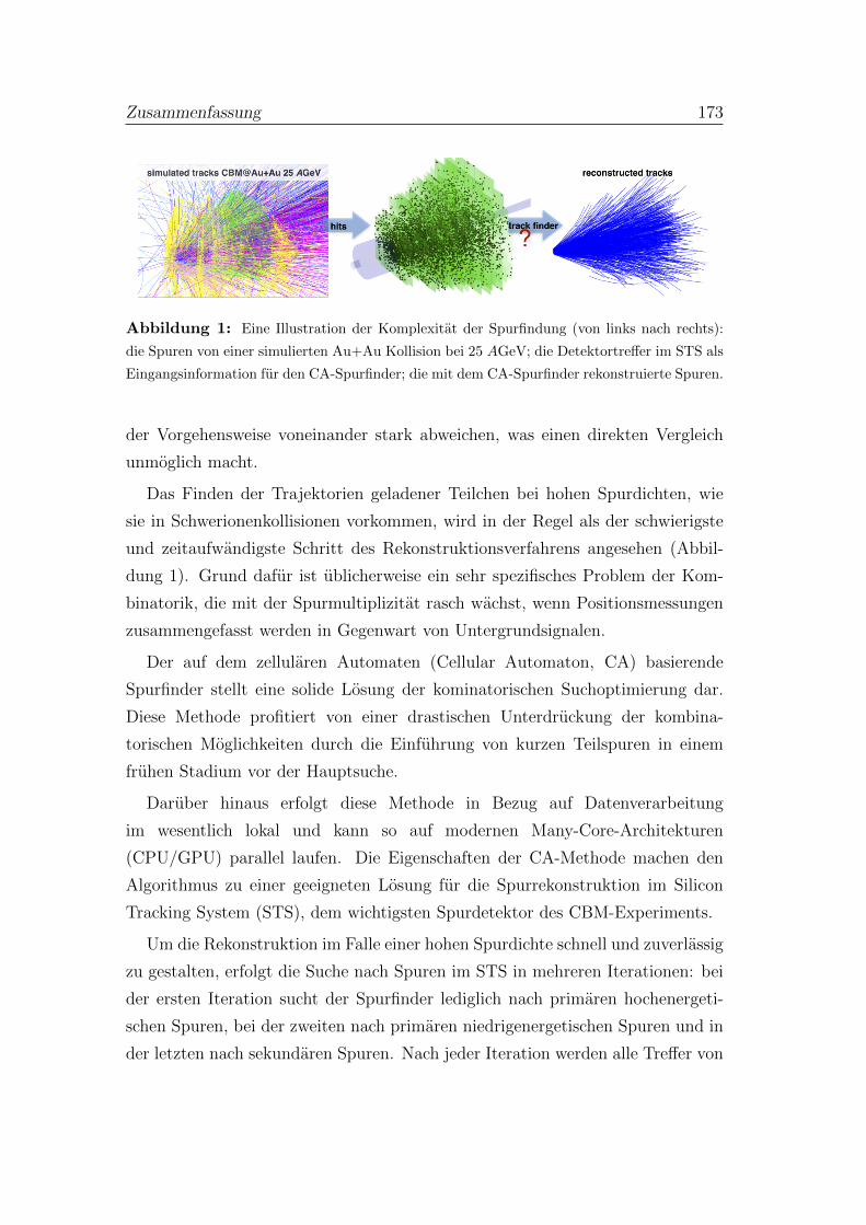
Zusammenfassung 173
Abbildung 1: Eine Illustration der Komplexitat der Spurfindung (von links nach rechts):
die Spuren von einer simulierten Au+Au Kollision bei 25 AGeV; die Detektortreffer im STS als
Eingangsinformation fur den CA-Spurfinder; die mit dem CA-Spurfinder rekonstruierte Spuren.
der Vorgehensweise voneinander stark abweichen, was einen direkten Vergleich
unmoglich macht.
Das Finden der Trajektorien geladener Teilchen bei hohen Spurdichten, wie
sie in Schwerionenkollisionen vorkommen, wird in der Regel als der schwierigste
und zeitaufwandigste Schritt des Rekonstruktionsverfahrens angesehen (Abbil-
dung 1). Grund dafur ist ublicherweise ein sehr spezifisches Problem der Kom-
binatorik, die mit der Spurmultiplizitat rasch wachst, wenn Positionsmessungen
zusammengefasst werden in Gegenwart von Untergrundsignalen.
Der auf dem zellularen Automaten (Cellular Automaton, CA) basierende
Spurfinder stellt eine solide Losung der kominatorischen Suchoptimierung dar.
Diese Methode profitiert von einer drastischen Unterdruckung der kombina-
torischen Moglichkeiten durch die Einfuhrung von kurzen Teilspuren in einem
fruhen Stadium vor der Hauptsuche.
Daruber hinaus erfolgt diese Methode in Bezug auf Datenverarbeitung
im wesentlich lokal und kann so auf modernen Many-Core-Architekturen
(CPU/GPU) parallel laufen. Die Eigenschaften der CA-Methode machen den
Algorithmus zu einer geeigneten Losung fur die Spurrekonstruktion im Silicon
Tracking System (STS), dem wichtigsten Spurdetektor des CBM-Experiments.
Um die Rekonstruktion im Falle einer hohen Spurdichte schnell und zuverlassig
zu gestalten, erfolgt die Suche nach Spuren im STS in mehreren Iterationen: bei
der ersten Iteration sucht der Spurfinder lediglich nach primaren hochenergeti-
schen Spuren, bei der zweiten nach primaren niedrigenergetischen Spuren und in
der letzten nach sekundaren Spuren. Nach jeder Iteration werden alle Treffer von
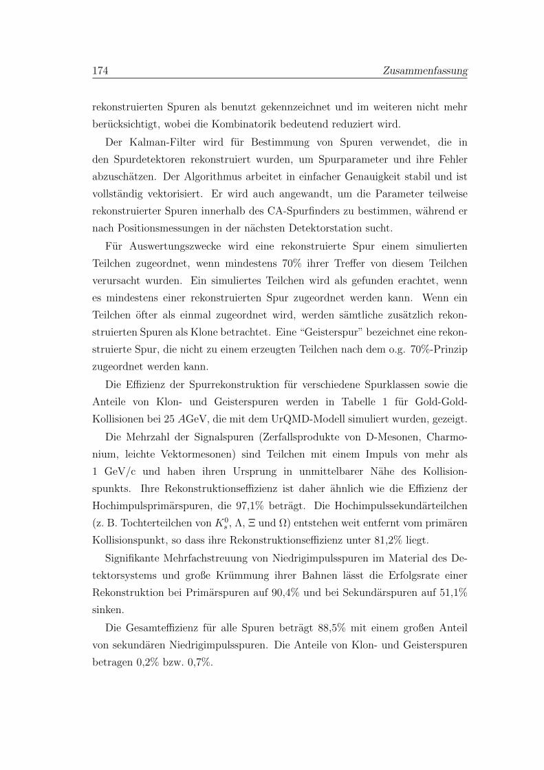
174 Zusammenfassung
rekonstruierten Spuren als benutzt gekennzeichnet und im weiteren nicht mehr
berucksichtigt, wobei die Kombinatorik bedeutend reduziert wird.
Der Kalman-Filter wird fur Bestimmung von Spuren verwendet, die in
den Spurdetektoren rekonstruiert wurden, um Spurparameter und ihre Fehler
abzuschatzen. Der Algorithmus arbeitet in einfacher Genauigkeit stabil und ist
vollstandig vektorisiert. Er wird auch angewandt, um die Parameter teilweise
rekonstruierter Spuren innerhalb des CA-Spurfinders zu bestimmen, wahrend er
nach Positionsmessungen in der nachsten Detektorstation sucht.
Fur Auswertungszwecke wird eine rekonstruierte Spur einem simulierten
Teilchen zugeordnet, wenn mindestens 70% ihrer Treffer von diesem Teilchen
verursacht wurden. Ein simuliertes Teilchen wird als gefunden erachtet, wenn
es mindestens einer rekonstruierten Spur zugeordnet werden kann. Wenn ein
Teilchen ofter als einmal zugeordnet wird, werden samtliche zusatzlich rekon-
struierten Spuren als Klone betrachtet. Eine “Geisterspur” bezeichnet eine rekon-
struierte Spur, die nicht zu einem erzeugten Teilchen nach dem o.g. 70%-Prinzip
zugeordnet werden kann.
Die Effizienz der Spurrekonstruktion fur verschiedene Spurklassen sowie die
Anteile von Klon- und Geisterspuren werden in Tabelle 1 fur Gold-Gold-
Kollisionen bei 25 AGeV, die mit dem UrQMD-Modell simuliert wurden, gezeigt.
Die Mehrzahl der Signalspuren (Zerfallsprodukte von D-Mesonen, Charmo-
nium, leichte Vektormesonen) sind Teilchen mit einem Impuls von mehr als
1 GeV/c und haben ihren Ursprung in unmittelbarer Nahe des Kollision-
spunkts. Ihre Rekonstruktionseffizienz ist daher ahnlich wie die Effizienz der
Hochimpulsprimarspuren, die 97,1% betragt. Die Hochimpulssekundarteilchen
(z. B. Tochterteilchen von K0s , Λ, Ξ und Ω) entstehen weit entfernt vom primaren
Kollisionspunkt, so dass ihre Rekonstruktionseffizienz unter 81,2% liegt.
Signifikante Mehrfachstreuung von Niedrigimpulsspuren im Material des De-
tektorsystems und große Krummung ihrer Bahnen lasst die Erfolgsrate einer
Rekonstruktion bei Primarspuren auf 90,4% und bei Sekundarspuren auf 51,1%
sinken.
Die Gesamteffizienz fur alle Spuren betragt 88,5% mit einem großen Anteil
von sekundaren Niedrigimpulsspuren. Die Anteile von Klon- und Geisterspuren
betragen 0,2% bzw. 0,7%.
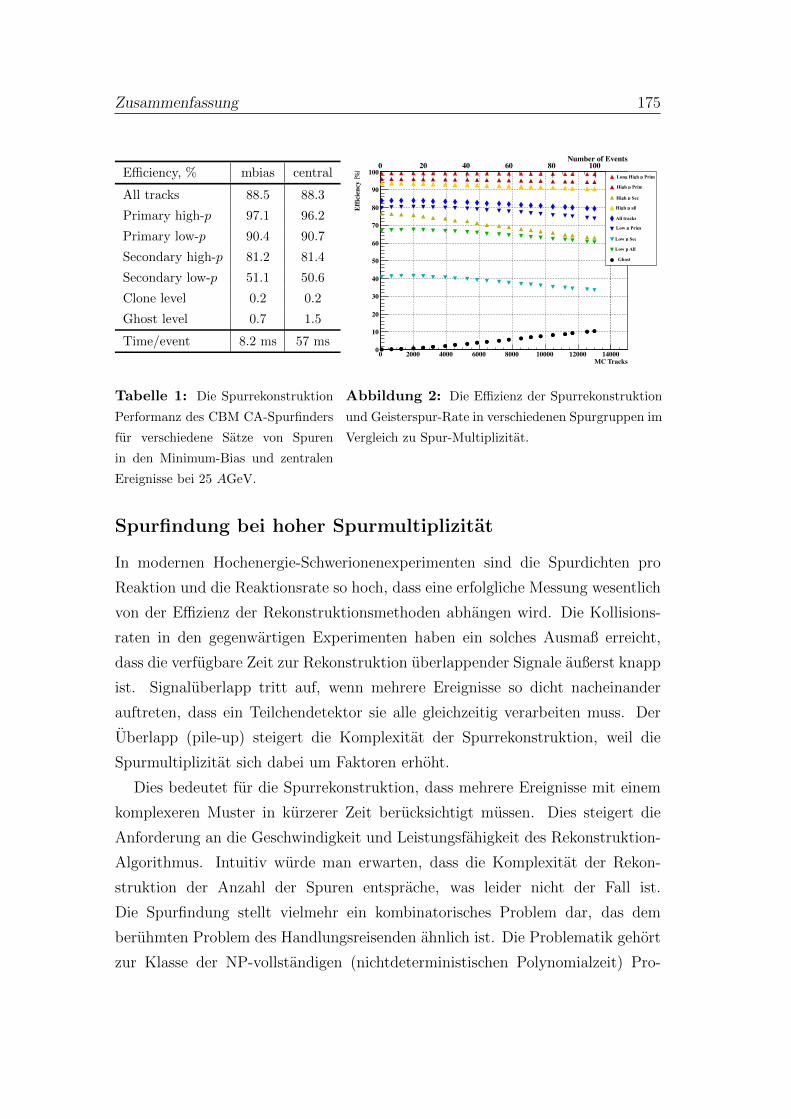
Zusammenfassung 175
Efficiency, % mbias central
All tracks 88.5 88.3
Primary high-p 97.1 96.2
Primary low-p 90.4 90.7
Secondary high-p 81.2 81.4
Secondary low-p 51.1 50.6
Clone level 0.2 0.2
Ghost level 0.7 1.5
Time/event 8.2 ms 57 ms
MC Tracks0 2000 4000 6000 8000 10000 12000 14000
Effic
ienc
y, %
0
10
20
30
40
50
60
70
80
90
100
Number of Events0 20 40 60 80 100
LongRefPrim
RefPrim
RefSec
RefSet
AllSet
ExtraPrim
ExtraSec
ExtraSet
Ghost
Long High p Prim
High p Prim
High p Sec
High p all
All tracks
Low p Prim
Low p Sec
Low p All
Ghost
Tabelle 1: Die Spurrekonstruktion
Performanz des CBM CA-Spurfinders
fur verschiedene Satze von Spuren
in den Minimum-Bias und zentralen
Ereignisse bei 25 AGeV.
Abbildung 2: Die Effizienz der Spurrekonstruktion
und Geisterspur-Rate in verschiedenen Spurgruppen im
Vergleich zu Spur-Multiplizitat.
Spurfindung bei hoher Spurmultiplizitat
In modernen Hochenergie-Schwerionenexperimenten sind die Spurdichten pro
Reaktion und die Reaktionsrate so hoch, dass eine erfolgliche Messung wesentlich
von der Effizienz der Rekonstruktionsmethoden abhangen wird. Die Kollisions-
raten in den gegenwartigen Experimenten haben ein solches Ausmaß erreicht,
dass die verfugbare Zeit zur Rekonstruktion uberlappender Signale außerst knapp
ist. Signaluberlapp tritt auf, wenn mehrere Ereignisse so dicht nacheinander
auftreten, dass ein Teilchendetektor sie alle gleichzeitig verarbeiten muss. Der
Uberlapp (pile-up) steigert die Komplexitat der Spurrekonstruktion, weil die
Spurmultiplizitat sich dabei um Faktoren erhoht.
Dies bedeutet fur die Spurrekonstruktion, dass mehrere Ereignisse mit einem
komplexeren Muster in kurzerer Zeit berucksichtigt mussen. Dies steigert die
Anforderung an die Geschwindigkeit und Leistungsfahigkeit des Rekonstruktion-
Algorithmus. Intuitiv wurde man erwarten, dass die Komplexitat der Rekon-
struktion der Anzahl der Spuren entsprache, was leider nicht der Fall ist.
Die Spurfindung stellt vielmehr ein kombinatorisches Problem dar, das dem
beruhmten Problem des Handlungsreisenden ahnlich ist. Die Problematik gehort
zur Klasse der NP-vollstandigen (nichtdeterministischen Polynomialzeit) Pro-
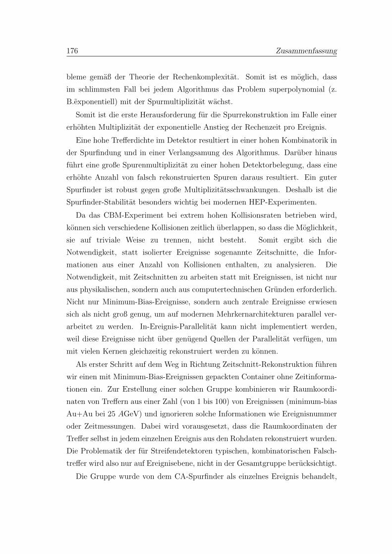
176 Zusammenfassung
bleme gemaß der Theorie der Rechenkomplexitat. Somit ist es moglich, dass
im schlimmsten Fall bei jedem Algorithmus das Problem superpolynomial (z.
B.exponentiell) mit der Spurmultiplizitat wachst.
Somit ist die erste Herausforderung fur die Spurrekonstruktion im Falle einer
erhohten Multiplizitat der exponentielle Anstieg der Rechenzeit pro Ereignis.
Eine hohe Trefferdichte im Detektor resultiert in einer hohen Kombinatorik in
der Spurfindung und in einer Verlangsamung des Algorithmus. Daruber hinaus
fuhrt eine große Spurenmultiplizitat zu einer hohen Detektorbelegung, dass eine
erhohte Anzahl von falsch rekonstruierten Spuren daraus resultiert. Ein guter
Spurfinder ist robust gegen große Multiplizitatsschwankungen. Deshalb ist die
Spurfinder-Stabilitat besonders wichtig bei modernen HEP-Experimenten.
Da das CBM-Experiment bei extrem hohen Kollisionsraten betrieben wird,
konnen sich verschiedene Kollisionen zeitlich uberlappen, so dass die Moglichkeit,
sie auf triviale Weise zu trennen, nicht besteht. Somit ergibt sich die
Notwendigkeit, statt isolierter Ereignisse sogenannte Zeitschnitte, die Infor-
mationen aus einer Anzahl von Kollisionen enthalten, zu analysieren. Die
Notwendigkeit, mit Zeitschnitten zu arbeiten statt mit Ereignissen, ist nicht nur
aus physikalischen, sondern auch aus computertechnischen Grunden erforderlich.
Nicht nur Minimum-Bias-Ereignisse, sondern auch zentrale Ereignisse erwiesen
sich als nicht groß genug, um auf modernen Mehrkernarchitekturen parallel ver-
arbeitet zu werden. In-Ereignis-Parallelitat kann nicht implementiert werden,
weil diese Ereignisse nicht uber genugend Quellen der Parallelitat verfugen, um
mit vielen Kernen gleichzeitig rekonstruiert werden zu konnen.
Als erster Schritt auf dem Weg in Richtung Zeitschnitt-Rekonstruktion fuhren
wir einen mit Minimum-Bias-Ereignissen gepackten Container ohne Zeitinforma-
tionen ein. Zur Erstellung einer solchen Gruppe kombinieren wir Raumkoordi-
naten von Treffern aus einer Zahl (von 1 bis 100) von Ereignissen (minimum-bias
Au+Au bei 25 AGeV) und ignorieren solche Informationen wie Ereignisnummer
oder Zeitmessungen. Dabei wird vorausgesetzt, dass die Raumkoordinaten der
Treffer selbst in jedem einzelnen Ereignis aus den Rohdaten rekonstruiert wurden.
Die Problematik der fur Streifendetektoren typischen, kombinatorischen Falsch-
treffer wird also nur auf Ereignisebene, nicht in der Gesamtgruppe berucksichtigt.
Die Gruppe wurde von dem CA-Spurfinder als einzelnes Ereignis behandelt,
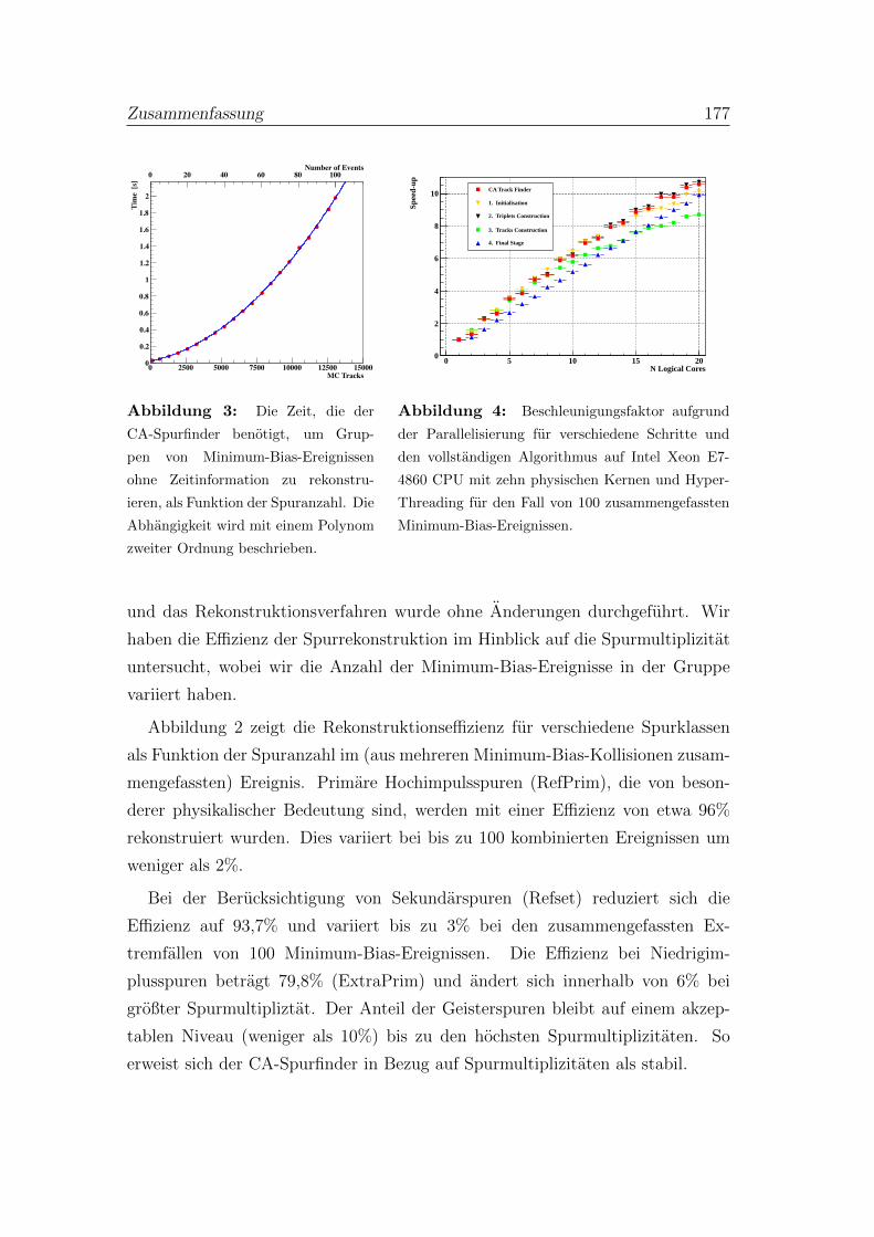
Zusammenfassung 177
MC Tracks0 2500 5000 7500 10000 12500 15000
Tim
e, [s
]
0
0.2
0.4
0.6
0.8
1
1.2
1.4
1.6
1.8
2 / ndf 2χ 0.001229 / 18
p0 0.004993± 0.01834
p1 1.769e-06± 3.463e-05 p2 1.301e-10± 8.856e-09
/ ndf 2χ 0.001229 / 18p0 0.004993± 0.01834
p1 1.769e-06± 3.463e-05 p2 1.301e-10± 8.856e-09
Number of Events0 20 40 60 80 100
N Logical Cores0 5 10 15 20
Spee
d-up
0
2
4
6
8
10CA Track Finder
1. Initialisation
2. Triplets Construction
3. Tracks Construction
4. Final Stage
Abbildung 3: Die Zeit, die der
CA-Spurfinder benotigt, um Grup-
pen von Minimum-Bias-Ereignissen
ohne Zeitinformation zu rekonstru-
ieren, als Funktion der Spuranzahl. Die
Abhangigkeit wird mit einem Polynom
zweiter Ordnung beschrieben.
Abbildung 4: Beschleunigungsfaktor aufgrund
der Parallelisierung fur verschiedene Schritte und
den vollstandigen Algorithmus auf Intel Xeon E7-
4860 CPU mit zehn physischen Kernen und Hyper-
Threading fur den Fall von 100 zusammengefassten
Minimum-Bias-Ereignissen.
und das Rekonstruktionsverfahren wurde ohne Anderungen durchgefuhrt. Wir
haben die Effizienz der Spurrekonstruktion im Hinblick auf die Spurmultiplizitat
untersucht, wobei wir die Anzahl der Minimum-Bias-Ereignisse in der Gruppe
variiert haben.
Abbildung 2 zeigt die Rekonstruktionseffizienz fur verschiedene Spurklassen
als Funktion der Spuranzahl im (aus mehreren Minimum-Bias-Kollisionen zusam-
mengefassten) Ereignis. Primare Hochimpulsspuren (RefPrim), die von beson-
derer physikalischer Bedeutung sind, werden mit einer Effizienz von etwa 96%
rekonstruiert wurden. Dies variiert bei bis zu 100 kombinierten Ereignissen um
weniger als 2%.
Bei der Berucksichtigung von Sekundarspuren (Refset) reduziert sich die
Effizienz auf 93,7% und variiert bis zu 3% bei den zusammengefassten Ex-
tremfallen von 100 Minimum-Bias-Ereignissen. Die Effizienz bei Niedrigim-
plusspuren betragt 79,8% (ExtraPrim) und andert sich innerhalb von 6% bei
großter Spurmultipliztat. Der Anteil der Geisterspuren bleibt auf einem akzep-
tablen Niveau (weniger als 10%) bis zu den hochsten Spurmultiplizitaten. So
erweist sich der CA-Spurfinder in Bezug auf Spurmultiplizitaten als stabil.
178 Zusammenfassung
Jedoch nicht nur die Effizienz, sondern auch eine Geschwindigkeit des
Rekonstruktionsalgorithmus ist fur eine erfolgreiche Durchfuhrung des CBM-
Experiments entscheidend. Die Zeit, die ein CA-Spurfinder benotigt, um ein
Gruppenereignis zu rekonstruieren, wurde als Funktion der Anzahl von Monte-
Carlo-Spuren in einer Gruppe untersucht. Die Ergebnisse zeigen, daß die
Abhangigkeit mit einem Polynom zweiter Ordnung angenahert werden kann (Ab-
bildung 3). Dies ist ein vielversprechendes Ergebnis, insbesondere im Hinblick
auf das exponentielle Wachstum der Kombinatorik bezuglich der Spurmulti-
plizitat. Diese Abhangigkeit kann weiter verbessert und zu einer linearen Funk-
tion gemacht werden, die nach der Einfuhrung der Zeitmessung im Rekonstruk-
tionsalgorithmus der Abhangigkeit der ereignisbasierten Analyse entsprache. So
zeigen sowohl die Geschwindigkeit und Effizienz des CA-Spurfinders stabiles Ver-
halten bei hoher Spurmultiplizitat.
Paralleler CA-Spurfinder
Der CA-Spurfinder-Algorithmus wurde in Bezug auf Parallelitat neu gestaltet
und optimiert. Jeder Schritt des Algorithmus wurde in einem Super-Ereignis
mit OpenMP- und Pthreads-Schnittstellen parallelisiert. In jedem Stadium wer-
den die Quelle der Parallelitat-Elemente gleichzeitig verarbeitet und in einer
neuen Form mit einem hoheren Konsolidierungsumfang gespeichert. Wahrend
der Initialisierungsphase werden alle Eingangstreffer bezuglich ihrer Koordinaten
sortiert und in einem Raumgitter gespeichert. Eine gewisse Anzahl von Treffern
(teilbar durch die Breite des SIMD-Vektor) wird zusammengefasst und aufgeteilt,
um kunftig verarbeitet zu werden. In der Aufbauphase von Triplets werden
Trefferteile verarbeitet ohne Synchronisation zwischen Threads, woraus sich eine
Reihe von Triplets ergibt. In der folgenden Phase der Spurkandidatenerstellung
sind Triplets die Quelle der Parallelitat.
Gleichzeitig stellt der Algorithmus fur jedes Ausgangstriplet den bestmoglichen
Spurkandidaten nach χ2-Wert und Lange auf. In dieser Phase arbeiten die
Threads noch unabhangig. In der vorangegangenen Phase der Spurselektion
mussten die Threads miteinander kommunizieren, um die Treffer zwischen den
Spuren zu verteilen. In der Spurselektionstufe wurde die Synchronisation mit-
Zusammenfassung 179
tels einer Tabelle des gemeinsamen Zugriffs implementiert. In der letzten Phase
werden die verwendeten Treffer fur die nachste Iteration entfernt. Hier reprasen-
tieren die vorliegenden Treffer die Quelle der Parallelitat, wie bei der Initia-
lisierungsphase.
Die sich ergebenden Beschleunigungsfaktoren fur die verschiedenen Phasen
sowie fur den gesamten Algorithmus innerhalb einer CPU (20 Hyper-Threading-
Kerne) sind in Abbildung 4 dargestellt. Einige Schritte haben aufgrund geringer
Thread-Synchronisation eine erhohte Beschleunigung fur eine hohere Anzahl von
Kernen. Der Algorithmus zeigt eine lineare Skalierbarkeit. Aufgrund von Hyper-
Threading kann man auf einer solchen CPU im Idealfall eine Beschleunigung
um einen Faktor 13 erwarten. Der erreichte Beschleunigungsfaktor ist 10.1 fur
den gesamten Algorithmus auf einer CPU mit 10 physischen Kernen mit Hyper-
Threading.
4D paraller CA-Spurfinder
Da die Separierung unterschiedlicher physikalischer Ereignisse im CBM-
Experiment keine triviale Aufgabe ist, musste der CA-Spurfinder so modifiziert
werden, dass er auch Zeitinformationen berucksichtigen konnte. Der Algorith-
mus wurde so angepasst, dass er Eingangszeitschnitte erfasst, die Treffer von
dem Spurdetektor enthalt. Jeder Treffer enthalt zwei Raumkoordinaten x und y
in der Detektorebene z sowie die Zeitmessung t.
Die Zeitinformation wurde in dem CA-Spurfinder verwendet, um die
Geschwindigkeit und die Effizienz des Algorithmus zu verbessern. Da die Triplets
aus drei Treffern zusammengestellt werden sollen, die von ein und demselben
Teilchen erzeugt wurden, sollten diese Treffer nicht nur raumlich sondern auch
zeitlich korreliert sein. Vernachlassigt man die Flugzeit zwischen Detektorsta-
tionen, sollten die Treffer auf derselben Spur in der Zeitmessung innerhalb der
Detektor-Zeitgenauigkeit ubereinstimmen. Treffergruppen, deren Zeitmessun-
gen sich um mehr als die erwartete Flugzeit inklusive Detektor-Zeitgenauigkeit
voneinander unterscheiden, sollten verworfen werden.
Die sich ergebende Performanz und die Geschwindigkeit der ereignisweisen
Analyse sowie fur den 4D CA-Spurfinder fur die Rekonstruktion von Zeitschnit-
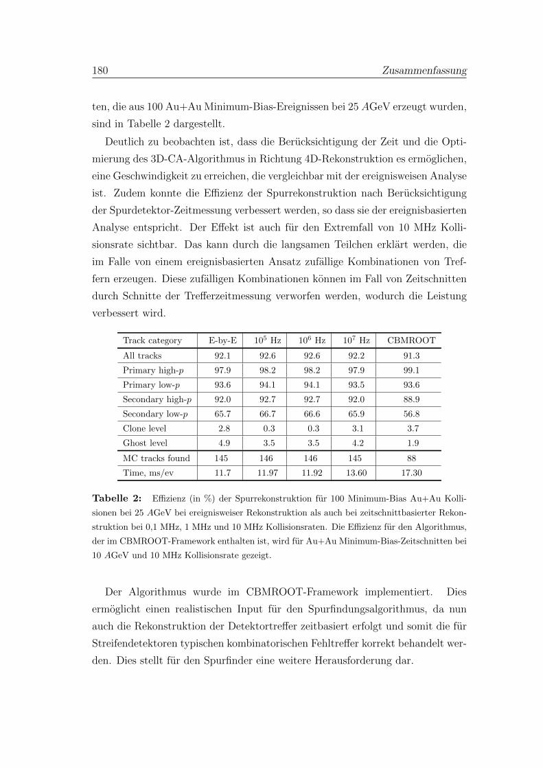
180 Zusammenfassung
ten, die aus 100 Au+Au Minimum-Bias-Ereignissen bei 25 AGeV erzeugt wurden,
sind in Tabelle 2 dargestellt.
Deutlich zu beobachten ist, dass die Berucksichtigung der Zeit und die Opti-
mierung des 3D-CA-Algorithmus in Richtung 4D-Rekonstruktion es ermoglichen,
eine Geschwindigkeit zu erreichen, die vergleichbar mit der ereignisweisen Analyse
ist. Zudem konnte die Effizienz der Spurrekonstruktion nach Berucksichtigung
der Spurdetektor-Zeitmessung verbessert werden, so dass sie der ereignisbasierten
Analyse entspricht. Der Effekt ist auch fur den Extremfall von 10 MHz Kolli-
sionsrate sichtbar. Das kann durch die langsamen Teilchen erklart werden, die
im Falle von einem ereignisbasierten Ansatz zufallige Kombinationen von Tref-
fern erzeugen. Diese zufalligen Kombinationen konnen im Fall von Zeitschnitten
durch Schnitte der Trefferzeitmessung verworfen werden, wodurch die Leistung
verbessert wird.
Track category E-by-E 105 Hz 106 Hz 107 Hz CBMROOT
All tracks 92.1 92.6 92.6 92.2 91.3
Primary high-p 97.9 98.2 98.2 97.9 99.1
Primary low-p 93.6 94.1 94.1 93.5 93.6
Secondary high-p 92.0 92.7 92.7 92.0 88.9
Secondary low-p 65.7 66.7 66.6 65.9 56.8
Clone level 2.8 0.3 0.3 3.1 3.7
Ghost level 4.9 3.5 3.5 4.2 1.9
MC tracks found 145 146 146 145 88
Time, ms/ev 11.7 11.97 11.92 13.60 17.30
Tabelle 2: Effizienz (in %) der Spurrekonstruktion fur 100 Minimum-Bias Au+Au Kolli-
sionen bei 25 AGeV bei ereignisweiser Rekonstruktion als auch bei zeitschnittbasierter Rekon-
struktion bei 0,1 MHz, 1 MHz und 10 MHz Kollisionsraten. Die Effizienz fur den Algorithmus,
der im CBMROOT-Framework enthalten ist, wird fur Au+Au Minimum-Bias-Zeitschnitten bei
10 AGeV und 10 MHz Kollisionsrate gezeigt.
Der Algorithmus wurde im CBMROOT-Framework implementiert. Dies
ermoglicht einen realistischen Input fur den Spurfindungsalgorithmus, da nun
auch die Rekonstruktion der Detektortreffer zeitbasiert erfolgt und somit die fur
Streifendetektoren typischen kombinatorischen Fehltreffer korrekt behandelt wer-
den. Dies stellt fur den Spurfinder eine weitere Herausforderung dar.
Zusammenfassung 181
Die Effizienz des Algorithmus im CBMROOT-Framework im Falle der Rekon-
struktion von Zeitschnitten, die aus Au+Au Minimum-Bias-Ereignissen bei
10 AGeV bestehen, ist in der letzten Spalte der Tabelle 2 dargestellt. Diese Ef-
fizienz ist mit der ereignisbasierten Analyse vergleichbar. Die etwas hohere Klon-
rate konnte durch den Zeitmessungsschnitt erklart werden, der fur diesen Fall zu
streng sein kann und eine weitere Optimierung erforderlich machen konnte.
Fazit
Das First-Level Event Selektion (FLES) Softwarepaket fur das CBM-Experiment
enthalt alle Rekonstruktionsstufen: Spurfindung, Spuranpassung, Suche nach
kurzlebigen Teilchen, Ereignisbildung und Ereignisselektion.
Fur den zeitaufwendigsten Teil des Rekonstruktionsverfahrens wird der Zel-
lulare-Automat-Spurfinder verwendet. Der CA-Spurfinder ist vektorisiert und
zwischen CPU-Kernen parallelisiert. Der ereignisbasierte Algorithmus wurde auf
zeitschnittbasierte Rekonstruktion angepasst, was bei CBM fur die Ereignisbil-
dung erforderlich ist. Der 4D CA-Spurfinder ist in der Lage, eine Performanz und
Geschwindigkeit vergleichbar mit der ereignisbasierten Analyse im Falle extremer
Kollisionsraten von 10 MHz zu erzielen. Der Algorithmus ist im CBMROOT-
Framework implementiert. Somit ist das FLES-Paket betriebsbereit und kann im
CBM-Experiment bei der 4D-Rekonstruktion von Zeitschnitten eingesetzt wer-
den.
Acknowledgements
I would like to thank all the people who contributed to and supported the work
described in this thesis.
First of all I would like to express my deep sense of gratitude to
Prof. Dr. Ivan Kisel, whose expert knowledge in both science and technology
combined with his endless enthusiasm in implementing fresh ideas was a con-
stant source of inspiration to me. I feel very lucky for the opportunity to work
with the supervisor, who always was so much interested in my work.
I express my sincere appreciation to Prof. Dr. Peter Senger for his constant
guidance and particularly for the opportunity to perform my study within the
CBM collaboration. It has been a wonderful experience to work within the col-
laboration. Also I would like to thank Prof. Dr. Victor Ivanov for his constant
support during those years.
I am very grateful to Dr. Iouri Vassiliev for the valuable experience, he shared
with me, and the time, he has devoted to my work. A special thanks goes to
Dr. Irina Rostovtseva for her contribution to porting the developed algorithm
into the CBMROOT framework and to Iaroslava Bezshyiko for her collaboration
in developing the event building algorithm. Also I would like to give a special
thank to Prof. Dr. Peter Senger, Dr. Volker Friese and Kristine Eschedor for
their help in translating the work in German.
Many thanks to my current and former colleagues for their support and the
great and positive work environment, particularly I want to thank Maksym Zyzak,
Igor Kulakov and Olga Derenovskaya.
Finally, I want to thank to my family and friends for all they have been doing
for me during those years.

ValentinaAkishinaCurriculum Vitae
FIAS Frankfurt Institute for Advanced StudiesT +49-6159-711891B [email protected]
Personal InformationDate of BirthPlace of Birth
Citizenship
Education2011–today PhD Student, Johann Wolfgang Goethe University, Frankfurt am Main, Germany.
Subject: Computer ScienceThesis Title: 4D Event Reconstruction in the CBM ExperimentSupervisor: Prof. Dr. Ivan Kisel
2009–2011 Master Student, Lomonosov Moscow State University, Moscow, Russia.Subject: PhysicsSpecialization: Physics and Management in Scientific Research and High TechnologiesThesis Title: Hyperons decay reconstruction in Compressed Baryonic Matterexperiment Supervisors: Prof. Dr. Viktor Ivanov, Prof. Dr. Alexander OlshevskyAverage Grade: 4.9/5
2005–2009 Bachelor Student, Lomonosov Moscow State University, Moscow, Russia.Subject: PhysicsSpecialization: Low Temperature PhysicsThesis Title: Magnetic properties of Ge1−xMnxT e ferromagnetic semiconductors doped withgadolinium.Supervisor: Dr. Elena ZverevaAverage Grade: 4.8/5
1995–2005 Pupil, Secondary school #4, Dubna, Moscow region, Russia.
Employment2015–today Scientist, Frankfurt Institute for Advanced Studies, Frankfurt am Main, Germany.
Software development of reconstruction routines for the CBM experiment.2010–today Software engineer, Joint Institute for Nuclear Research, Dubna, Russia.
Software development of reconstruction routines for the CBM experiment.06.2010–08.2010
Intern, Allied Testing, Moscow, Russia.Creating Quality Assurance proposals.
09.2008–08.2009
Academic Programs Coordinator, Moscow State University Business School, Moscow,Russia.Management of educational process for Master students.

Scientific Schools08.2010–09.2010
GSI International Student Program, GSI Helmholtz Centre for Heavy Ion Research,Darmstadt, Germany.Performed algorithm design and implementation (C++) for short-lived particle reconstruction in theCBM experiment.
08.2013 CERN School of Computing, Nicosia, Cyprus.
Awards2011 The best talk award of the International Symposium on Nuclear Electronics and Computing,
Varna, Bulgaria.
Computer skillsAdvanced C/C++, OpenMP, Vc Library, SIMD, POSIX Library
Intermediate OpenCL, ITBB, Linux OS, LATEX, ROOTBasic Pascal, Delphi
LanguagesNative Russian
Advanced English, German
Teaching experience09.2013–08.2015
Practical Course, Johann Wolfgang Goethe University, Frankfurt am Main, Germany.Title: Architecture of High-Performance ComputersLevel: Bachelor’s and Master’s degree
05.2014,02.2015
Lecture Course, FAIR-Russia Research Centre, Moscow, Russia.Title: Introduction into parallel computations on modern many-core computer architecturesLevel: Bachelor’s, Master’s and Doctorate degree
Selected Publications1. E.A. Zvereva, E.P. Skipetrov, O.A. Savelieva, N.A. Pichugin, A.E. Primenko, V.P. Akishina, E.I. Slyn’ko,
V.E. Slyn’ko Magnetic properties of Ge1−xMnxTe ferromagnetic semiconductors doped with gadolinium,Journal of Physics: Conference Series 400, 062040 (2010).
2. V. Akishina and I. Kisel, J/ψ reconstruction in the di-muon decay channel with the CBM experiment forp+Au collisions at 30 GeV laboratory beam energy, Journal of Physics: Conference Series 426, 012024(2013).
3. V. Akishina and I. Kisel, Online 4-dimensional event building in the CBM experiment, Real Time Conference(RT), 19th IEEE-NPSS (2014).
4. V. Akishina and I. Kisel, Time-based Cellular Automaton track finder for the CBM experiment, Journal ofPhysics: Conference Series 599, 012024 (2015).
5. V. Akishina and I. Kisel, 4-Dimensional Event Building in the First-Level Event Selection of the CBMExperiment, Journal of Physics: Conference Series 664, 072027 (2015).


