Embed Size (px)
Citation preview

FLOW IN OPEN CHANNELS
Third Edition
prelims.indd iprelims.indd i 2/24/2010 3:11:32 PM2/24/2010 3:11:32 PM
About the Author
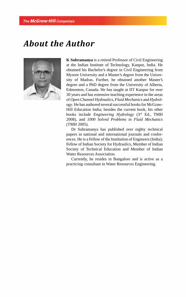
K Subramanya is a retired Professor of Civil Engineering at the Indian Institute of Technology, Kanpur, India. He obtained his Bachelor’s degree in Civil Engineering from Mysore University and a Master’s degree from the Univer-sity of Madras. Further, he obtained another Master’s degree and a PhD degree from the University of Alberta, Edmonton, Canada. He has taught at IIT Kanpur for over 30 years and has extensive teaching experience in the areas of Open Channel Hydraulics, Fluid Mechanics and Hydrol-ogy. He has authored several successful books for McGraw-Hill Education India; besides the current book, his other books include Engineering Hydrology (3rd Ed., TMH 2008), and 1000 Solved Problems in Fluid Mechanics (TMH 2005).
Dr Subramanya has published over eighty technical papers in national and international journals and confer-ences. He is a Fellow of the Institution of Engineers (India); Fellow of Indian Society for Hydraulics, Member of Indian Society of Technical Education and Member of Indian Water Resources Association.
Currently, he resides in Bangalore and is active as a practicing consultant in Water Resources Engineering.
prelims.indd iiprelims.indd ii 2/24/2010 3:11:32 PM2/24/2010 3:11:32 PM

FLOW IN OPEN CHANNELS
Third Edition
K SubramanyaFormer Professor
Department of Civil EngineeringIndian Institute of Technology
Kanpur
Tata McGraw-Hill Publishing Company LimitedNEW DELHI
McGraw-Hill OfficesNew Delhi New York St. Louis San Francisco Auckland Bogotá
Caracas Kuala Lumpur Lisbon London Madrid Mexico City Milan Montreal San Juan Santiago Singapore Sydney Tokyo Toronto
prelims.indd iiiprelims.indd iii 2/24/2010 3:11:33 PM2/24/2010 3:11:33 PM

The McGraw-Hill Companies
Tata McGraw-Hill
Published by the Tata McGraw-Hill Publishing Company Limited,7 West Patel Nagar, New Delhi 110 008.
Copyright © 2009, 1997, 1986 by Tata McGraw-Hill Publishing Company Limited.No part of this publication may be reproduced or distributed in any form or by any means, electronic, mechanical, photocopying, recording, or otherwise or stored in a database or retrieval system without the prior written permission of the publishers. The program listings (if any) may be entered, stored and executed in a computer system, but they may not be reproduced for publication.
This edition can be exported from India only by the publishers,Tata McGraw-Hill Publishing Company Limited
ISBN (13): 978-0-07-008695-1ISBN (10): 0-07-008695-8
Managing Director: Ajay Shukla
General Manager: Publishing—SEM & Tech Ed: Vibha MahajanSponsoring Editor: Shukti MukherjeeJr Editorial Executive: Surabhi ShuklaExecutive—Editorial Services: Sohini MukherjeeSenior Production Manager: P L Pandita
General Manager: Marketing—Higher Education & School: Michael J CruzProduct Manager: SEM & Tech Ed: Biju Ganesan
Controller—Production: Rajender P GhanselaAsst. General Manager—Production: B L Dogra
Typeset at Mukesh Technologies Pvt. Ltd., #10, 100 Feet Road, Ellapillaichavadi, Pondicherry 605 005 and printed at Rashtriya Printers, M-135, Panchsheel Garden, Naveen Shahdara, Delhi 110 032
Cover Printer: Rashtriya Printers
RCXACDDFDRBYA
Information contained in this work has been obtained by Tata McGraw-Hill, from sources believed to be reliable. However, neither Tata McGraw-Hill nor its authors guarantee the accuracy or completeness of any information published herein, and neither Tata McGraw Hill nor its authors shall be responsible for any errors, omissions, or damages arising out of use of this information. This work is published with the understanding that Tata McGraw-Hill and its authors are supplying information but are not attempting to render engineering or other professional services. If such services are required, the assistance of an appropriate professional should be sought.
prelims.indd ivprelims.indd iv 2/24/2010 3:11:33 PM2/24/2010 3:11:33 PM
ToMy Father
Only a well-designed channel performs its functions best.A blind inert force necessitates intelligent control.
MAHABHARATA
prelims.indd vprelims.indd v 2/24/2010 3:11:33 PM2/24/2010 3:11:33 PM

prelims.indd viprelims.indd vi 2/24/2010 3:11:33 PM2/24/2010 3:11:33 PM
Preface xiGuided Tour xv
1. Flow in Open Channels 1 1.1 Introduction 1 1.2 Types of Channels 1 1.3 Classifi cation of Flows 2 1.4 Velocity Distribution 5 1.5 One-Dimensional Method of Flow Analysis 7 1.6 Pressure Distribution 10 1.7 Pressure Distribution in Curvilinear Flows 13 1.8 Flows with Small Water-Surface Curvature 17 1.9 Equation of Continuity 19 1.10 Energy Equation 22 1.11 Momentum Equation 26 References 30 Problems 30 Objective Questions 38
2. Energy–Depth Relationships 42 2.1 Specifi c Energy 42 2.2 Critical Depth 43 2.3 Calculation of the Critical Depth 47 2.4 Section Factor Z 51 2.5 First Hydraulic Exponent M 51 2.6 Computations 54 2.7 Transitions 60 References 73 Problems 73 Objective Questions 78
3. Uniform Flow 85 3.1 Introduction 85 3.2 Chezy Equation 85 3.3 Darcy–Weisbach Friction Factor f 86 3.4 Manning’s Formula 89 3.5 Other Resistance Formulae 91 3.6 Velocity Distribution 91 3.7 Shear Stress Distribution 94 3.8 Resistance Formula for Practical Use 96 3.9 Manning’s Roughness Coeffi cient n 96 3.10 Equivalent Roughness 101 3.11 Uniform Flow Computations 104 3.12 Standard Lined Canal Sections 114 3.13 Maximum Discharge of a Channel of the Second Kind 117 3.14 Hydraulically Effi cient Channel Section 119 3.15 The Second Hydraulic Exponent N 123 3.16 Compound Channels 125 3.17 Critical Slope 131
Contents
prelims.indd viiprelims.indd vii 2/24/2010 3:11:33 PM2/24/2010 3:11:33 PM
3.18 Generalised-Flow Relation 134 3.19 Design of Irrigation Canals 139 References 144 Problems 145 Objective Questions 151
4. Gradually Varied Flow Theory 157 4.1 Introduction 157 4.2 Diff erential Equation of GVF 157 4.3 Classifi cation of Flow Profi les 160 4.4 Some Features of Flow Profi les 166 4.5 Control Sections 169 4.6 Analysis of Flow Profi le 172 4.7 Transitional Depth 180 Problems 183 Objective Questions 185
5. Gradually Varied Flow Computations 189 5.1 Introduction 189 5.2 Direct Integration of GVF Diff erential Equation 190 5.3 Bresse’s Solution 195 5.4 Channels with Considerable Variation in Hydraulic Exponents 199 5.5 Direct Integration for Circular Channels 200 5.6 Simple Numerical Solutions of GVF Problems 203 5.7 Advanced Numerical Methods 221 5.8 Flow Profi les in Divided Channels 223 5.9 Role of End Conditions 225 References 232 Problems 233 Objective Questions 236
6. Rapidly Varied Flow-1—Hydraulic Jump 248 6.1 Introduction 248 6.2 The Momentum Equation Formulation for the Jump 249 6.3 Hydraulic Jump in a Horizontal Rectangular Channel 250 6.4 Jumps in Horizontal Non-Rectangular Channels 265 6.5 Jumps on a Sloping Floor 274 6.6 Use of the Jump as an Energy Dissipator 279 6.7 Location of the Jump 281 References 286 Problems 287 Objective Questions 293
7. Rapidly Varied Flow-2 295 7.1 Introduction 295 7.2 Sharp-Crested Weir 295 7.3 Special Sharp-Crested Weirs 305 7.4 Ogee Spillway 316 7.5 Broad-Crested Weir 326 7.6 Critical-Depth Flumes 332 7.7 End Depth in a Free Overfall 334 7.8 Sluice-Gate Flow 346 7.9 Culvert Hydraulics 352
viii Contents
prelims.indd viiiprelims.indd viii 2/24/2010 3:11:33 PM2/24/2010 3:11:33 PM
References 358 Problems 360 Objective Questions 363
8. Spatially Varied Flow 366 8.1 Introduction 366 8.2 SVF with Increasing Discharge 366 8.3 SVF with Decreasing Discharge 377 8.4 Side Weir 379 8.5 Bottom Racks 388 References 395 Problems 396 Objective Questions 398
9. Supercritical-Flow Transitions 401 9.1 Introduction 401 9.2 Response to a Disturbance 401 9.3 Gradual Change in the Boundary 404 9.4 Flow at a Corner 411 9.5 Wave Interactions and Refl ections 418 9.6 Contractions 421 9.7 Supercritical Expansions 426 9.8 Stability of Supercritical Flows 430 References 432 Problems 432 Objective Questions 435
10. Unsteady Flows 437 10.1 Introduction 437
10.2 Gradually Varied Unsteady Flow (GVUF) 438
10.3 Uniformly Progressive Wave 444
10.4 Numerical Methods 447
10.5 Rapidly Varied Unsteady Flow–Positive Surges 458
10.6 Rapidly Varied Unsteady Flow–Negative Surges 467
References 478
Problems 479
Objective Questions 481
11. Hydraulics of Mobile Bed Channels 483 11.1 Introduction 483 11.2 Initiation of Motion of Sediment 483 11.3 Bed Forms 487 11.4 Sediment Load 494 11.5 Design of Stable Channels Carrying Clear Water
[Critical Tractive Force Approach] 503 11.6 Regime Channels 507 11.7 Scour 511 References 522 Problems 523 Objective Questions 526
Answers to Problems 531Answers to Objective Questions 541Index 543
Contents ix
prelims.indd ixprelims.indd ix 2/24/2010 3:11:33 PM2/24/2010 3:11:33 PM

prelims.indd xprelims.indd x 2/24/2010 3:11:33 PM2/24/2010 3:11:33 PM

Preface
This third edition of Flow in Open Channels marks the silver jubilee of the book which fi rst appeared in a different format of two volumes in 1982. A revised fi rst edi-tion combining the two volumes into a single volume was released in 1986. The second edition of the book which came out in 1997 had substantial improvement of the material from that of the fi rst revised edition and was very well received as refl ected in more than 25 reprints of that edition. This third edition is being brought out by incorporating advances in the subject matter, changes in the technology and related practices. Further, certain topics in the earlier edition that could be considered to be irrelevant or of marginal value due to advancement of knowledge of the subject and technology have been deleted.
In this third edition, the scope of the book is defi ned to provide source material in the form of a textbook that would meet all the requirements of the undergraduate course and most of the requirements of a post-graduate course in open-channel hydraulics as taught in a typical Indian university. Towards this, the following proce-dures have been adopted:
• Careful pruning of the material dealing with obsolete practices from the earlier edition of the book
• Addition of specifi c topics/ recent signifi cant developments in the subject matter of some chapters to bring the chapter contents up to date. This has resulted in inclusion of detailed coverage on
Flow through culverts Discharge estimation in compound channels Scour at bridge constrictions
• Further, many existing sections have been revised through more precise and better presentations. These include substantive improvement to Section 10.6 which deals with negative surges in rapidly varied unsteady fl ow and Section 5.7.4 dealing with backwater curves in natural channels.
• Additional worked examples and additional fi gures at appropriate locations have been provided for easy comprehension of the subject matter.
• Major deletions from the previous edition for reasons of being of marginal value include
Pruning of Tables 2A.2 at the end of Chapter 2, Table 3A-1 at the end of Chapter 3 and Table 5A-1 of Chapter 5
Section 5.3 dealing with a procedure for estimation of N and M for a trape-zoidal channel, and Section 5.9 dealing with graphical methods of GVF computations
Computer Program PROFIL-94 at the end of Chapter 5
The book in the present form contains eleven chapters. Chapters 1 and 2 contain the introduction to the basic principles and energy-depth relationships in open-channel fl ow. Various aspects of critical fl ow, its computation and use in analysis of transitions
prelims.indd xiprelims.indd xi 2/24/2010 3:11:33 PM2/24/2010 3:11:33 PM
are dealt in detail in Chapter 2. Uniform fl ow resistance and computations are dealt in great detail in Chapter 3. This chapter also includes several aspects relating to com-pound channels. Gradually varied fl ow theory and computations of varied fl ow profi les are discussed in ample detail in chapters 4 and 5 with suffi cient coverage of control points and backwater curve computations in natural channels.
Hydraulic jump phenomenon in channels of different shapes is dealt in substantial detail in Chapter 6. Chapter 7 contains thorough treatment of some important rapidly varied fl ow situations which include fl ow-measuring devices, spillways and culverts. Spatially varied fl ow theory with specifi c reference to side channel spillways, side weirs and bottom-rack devices is covered in Chapter 8. A brief description of the tran-sitions in supercritical fl ows is presented in Chapter 9. An introduction to the impor-tant fl ow situation of unsteady fl ow in open channels is provided in Chapter 10. The last chapter provides a brief introduction to the hydraulics of mobile bed channels.
The contents of the book, which cover essentially all the important normally accepted basic areas of open-channel fl ow, are presented in simple, lucid style. A basic knowledge of fl uid mechanics is assumed and the mathematics is kept at the minimal level. Details of advanced numerical methods and their computational pro-cedures are intentionally not included with the belief that the interested reader will source the background and details in appropriate specialized literature on the subject. Each chapter includes a set of worked examples, a list of problems for practice and a set of objective questions for clear comprehension of the subject matter. The Table of problems distribution given at the beginning of problems set in each chapter will be of particular use to teachers to select problems for class work, assignments, quizzes and examinations. The problems are designed to further the student’s capabilities of analysis and application. A total of 314 problems and 240 objective questions, with answers to the above, provided at the end of the book will be of immense use to teach-ers and students alike.
The Online Learning Center of the book can be accessed at http://www.mhhe.com/subramanya/foc3e. It contains the following material:
For Instructors• Solution Manual• Power Point Lecture Slides
For Students• Web links for additional reading• Interactive Objective Questions
A typical undergraduate course in Open-Channel Flow includes major portions of chapters 1 through 6 and selected portions of chapters 7, 10 and 11. In this selection, a few sections, such as Sec.1.8, Sec.3.16, Sec. 3.17, Sec. 5.5, Sec. 5.6, Sec. 5.7.3, and Sec. 5.7.4, Sec. 5.8, Sec. 5.9, Sec. 6.4, Sec. 6.5 and Sec. 6.8 could be excluded to achieve a simple introductory course. A typical post-graduate course would include all the eleven chapters with more emphasis on advanced portions of each chapter and supplemented by additional appropriate reference material.
In addition to students taking formal courses in Open-Channel Flow offered in University engineering colleges, the book is useful to students appearing for AMIE
xii Preface
prelims.indd xiiprelims.indd xii 2/24/2010 3:11:33 PM2/24/2010 3:11:33 PM

Preface xiii
examinations. Candidates taking competitive examinations like Central Engineering Services examinations and Central Civil Services examinations will fi nd this book useful in their preparations related to the topic of water-resources engineering. Prac-ticing engineers in the domain of water-resources engineering will fi nd this book a useful reference source. Further, the book is self-suffi cient to be used in self-study of the subject of open-channel fl ow.
I am grateful to the American Society of Civil Engineers, USA, for permission to reproduce several fi gures and tables from their publications; the Indian Journal of Technology, New Delhi, for permission to reproduce three fi gures; Mr M Bos of the International Institute of Land Reclamation and Improvement, Wageningen, The Netherlands, for photographs of the hydraulic jump and weir fl ow; the US Depart-ment of Interior, Water and Power Resources Service, USA, for the photograph of the side-channel spillway of the Hoover Dam; Dr Chandra Nalluri, of the University of New Castle-upon – Tyne, England, for the tables of Keifer and Chu functions and The Citizen, Gloucester, England, for the photograph of Severn Bore.
I would like express my sincere thanks to all those who have directly and indi-rectly helped me in bringing out this revised edition, especially the reviewers who gave noteworthy suggestions.
They are
Suman Sharma TRUBA College of Engineering and Technology Indore, Madhya Pradesh
Achintya Muzaffarpur Institute of Technology Muzaffarpur, Bihar
Anima Gupta Government Women’s Polytechnic Patna, Bihar
D R Pachpande JT Mahajan College of Engineering Jalgaon, Maharashtra
V Subramania Bharathi Bannari Amman Institute of Technology Anna University, Coimbatore, Tamil Nadu
K V Jaya Kumar National Institute of Technology Warangal, Andhra Pradesh
Comments and suggestions for further improvement of the book would be greatly appreciated. I could be contacted at the following e-mail address: [email protected]
K SUBRAMANYA
prelims.indd xiiiprelims.indd xiii 2/24/2010 3:11:33 PM2/24/2010 3:11:33 PM

prelims.indd xivprelims.indd xiv 2/24/2010 3:11:34 PM2/24/2010 3:11:34 PM
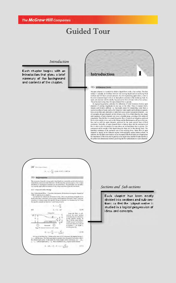
Each chapter begins with an Introduction that gives a brief summary of the background and contents of the chapter.
Each chapter has been neatly divided into sections and sub-sec-tions so that the subject matter is studied in a logical progression of ideas and concepts.
Walk through.indd 1Walk through.indd 1 2/24/2010 3:12:09 PM2/24/2010 3:12:09 PM
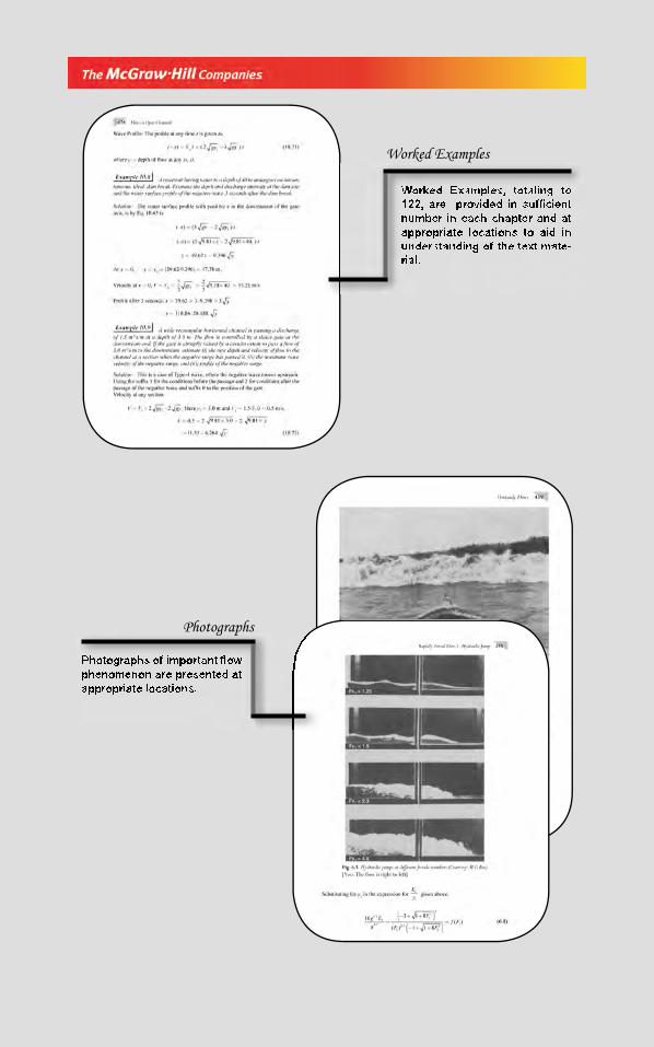
Photographs of important fl ow phenomenon are presented at appropriate locations.
Worked Examples, totaling to 122, are provided in suffi cient number in each chapter and at appropriate locations to aid in understanding of the text mate-rial.
Walk through.indd 2Walk through.indd 2 2/24/2010 3:12:12 PM2/24/2010 3:12:12 PM
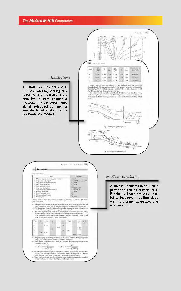
Illustrations are essential tools in books on Engineering sub-jects. Ample illustrations are provided in each chapter to illustrate the concepts, func-tional relationships and to provide defi nition sketches for mathematical models.
A table of Problem Distribution is provided at the top of each set of Problems. These are very help-ful to teachers in setting class work, assignments, quizzes and examinations.
Walk through.indd 3Walk through.indd 3 2/24/2010 3:12:17 PM2/24/2010 3:12:17 PM
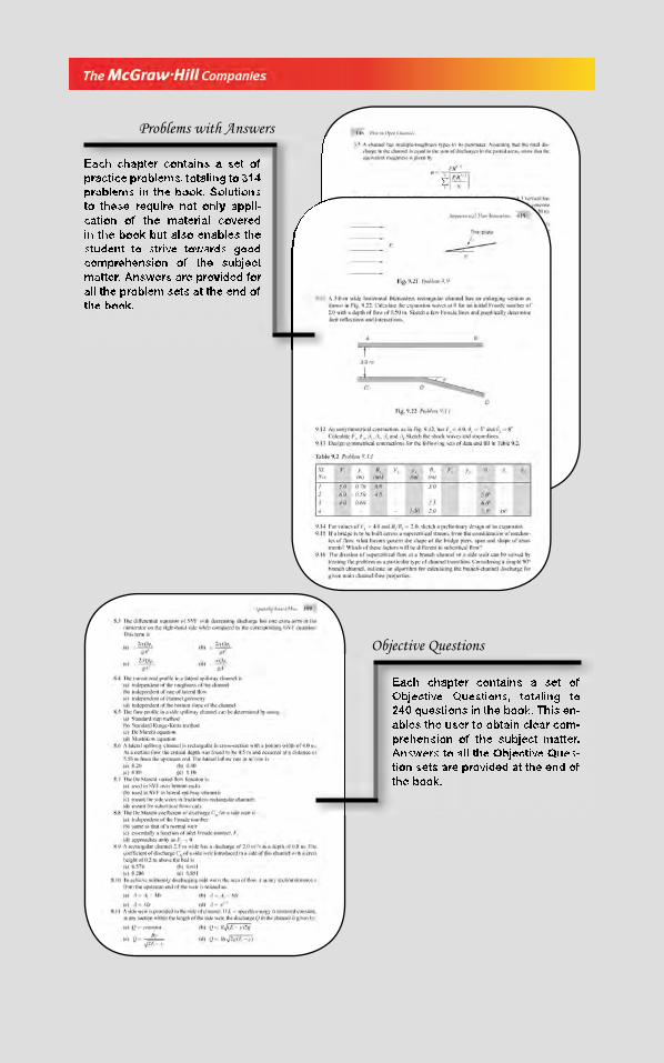
Each chapter contains a set of practice problems, totaling to 314 problems in the book. Solutions to these require not only appli-cation of the material covered in the book but also enables the student to strive towards good comprehension of the subject matter. Answers are provided for all the problem sets at the end of the book.
Each chapter contains a set of Objective Questions, totaling to 240 questions in the book. This en-ables the user to obtain clear com-prehension of the subject matter. Answers to all the Objective Ques-tion sets are provided at the end of the book.
Walk through.indd 4Walk through.indd 4 2/24/2010 3:12:21 PM2/24/2010 3:12:21 PM
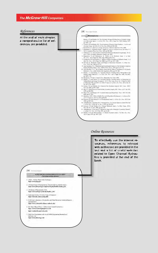
At the end of each chapter, a comprehensive list of ref-erences are provided.
To effectively use the internet re-sources, references to relevant web addresses are provided in the text and a list of useful websites related to Open Channel Hydrau-lics is provided at the end of the book.
Walk through.indd 5Walk through.indd 5 2/24/2010 3:12:26 PM2/24/2010 3:12:26 PM
1.1 INTRODUCTION
An open channel is a conduit in which a liquid fl ows with a free surface. The free surface is actually an interface between the moving liquid and an overlying fl uid medium and will have constant pressure. In civil engineering applications; water is the most common liquid with air at atmospheric pressure as the overlying fl uid. As such, our attention will be chiefl y focused on the fl ow of water with a free surface. The prime motivating force for open channel fl ow is gravity.
In engineering practice, activities for utilization of water resources involve open channels of varying magnitudes in one way or the other. Flows in natural rivers, streams and rivulets; artifi cial, i.e. man-made canals for transmitting water from a source to a place of need, such as for irrigation, water supply and hydropower genera-tion; sewers that carry domestic or industrial waste waters; navigation channels—are all examples of open channels in their diverse roles. It is evident that the size, shape and roughness of open channels vary over a sizeable range, covering a few orders of magnitude. Thus the fl ow in a road side gutter, fl ow of water in an irrigation canal and fl ows in the mighty rivers, such as the Ganga and the Brahmaputra, all have a free sur-face and as such are open channels, governed by the same general laws of fl uid mechanics. Basically, all open channels have a bottom slope and the mechanism of fl ow is akin to the movement of a mass down an inclined plane due to gravity. The component of the weight of the liquid along the slope acts as the driving force. The boundary resistance at the perimeter acts as the resisting force. Water fl ow in open channels is largely in the turbulent regime with negligible surface tention effects. In addition, the fact that water behaves as an incompressible fl uid leads one of appreciate the importance of the force due to gravity as the major force and the Froude number as the prime non-dimensional number governing the fl ow phenomenon in open channels.
1.2 TYPES OF CHANNELS
1.2.1 Prismatic and Non-prismatic Channels
A channel in which the cross-sectional shape and size and also the bottom slope are constant is termed as a prismatic channel. Most of the man-made (artifi cial) chan-nels are prismatic channels over long stretches. The rectangle, trapezoid, triangle
Introduction 1
Chapter 1.indd 1Chapter 1.indd 1 2/24/2010 2:42:16 PM2/24/2010 2:42:16 PM
2 Flow in Open Channels
and circle are some of the commonly used shapes in manmade channels. All natural channels generally have varying cross-sections and consequently are non-prismatic.
1.2.2 Rigid and Mobile Boundary Channels
On the basis of the nature of the boundary open channels can be broadly classifi ed into two types: (i) rigid channels, and (ii) mobile boundary channels.
Rigid channels are those in which the boundary is not deformable in the sense that the shape, planiform and roughness magnitudes are not functions of the fl ow param-eters. Typical examples include lined canals, sewers and non-erodible unlined canals. The fl ow velocity and shear-stress distribution will be such that no major scour, ero-sion or deposition takes place in the channel and the channel geometry and roughness are essentially constant with respect to time. The rigid channels can be considered to have only one degree of freedom; for a given channel geometry the only change that may take place is the depth of fl ow which may vary with space and time depending upon the nature of the fl ow. This book is concerned essentially with the study of rigid boundary channels.
In contrast to the above, we have many unlined channels in alluvium—both man-made channels and natural rivers—in which the boundaries undergo deformation due to the continuous process of erosion and deposition due to the fl ow. The boundary of the channel is mobile in such cases and the fl ow carries considerable amounts of sed-iment through suspension and in contact with the bed. Such channels are classifi ed as mobile-boundary channels. The resistance to fl ow, quantity of sediment transported, channel geometry and planiform, all depend on the interaction of the fl ow with the channel boundaries. A general mobile-boundary channel can be considered to have four degrees of freedom. For a given channel not only the depth of fl ow but also the bed width, longitudinal slope and planiform (or layout) of the channel may undergo changes with space and time depending on the type of fl ow. Mobile-boundary channels, usually treated under the topic of sediment transport or sediment engineer-ing,1,2 attract considerable attention of the hydraulic engineer and their study consti-tutes a major area of multi-disciplinary interest.
Mobile-boundary channels are dealt briefl y in Chapter 11. The discussion in rest of the book is confi ned to rigid-boundary open channels only. Unless specifi cally stated, the term channel is used in this book to mean the rigid–boundary channels.
1.3 CLASSIFICATION OF FLOWS
1.3.1 Steady and Unsteady Flows
A steady fl ow occurs when the fl ow properties, such as the depth or discharge at a section do not change with time. As a corollary, if the depth or discharge changes with time the fl ow is termed unsteady.
In practical applications, due to the turbulent nature of the fl ow and also due to the interaction of various forces, such as wind, surface tension, etc., at the surface there will always be some fl uctuations of the fl ow properties with respect to time. To
Chapter 1.indd 2Chapter 1.indd 2 2/24/2010 2:42:17 PM2/24/2010 2:42:17 PM
Introduction 3
account for these, the defi nition of steady fl ow is somewhat generalised and the clas-sifi cation is done on the basis of gross characteristics of the fl ow. Thus, for example, if there are ripples resulting in small fl uctuations of depth in a canal due to wind blowing over the free surface and if the nature of the water-surface profi le due to the action of an obstruction is to be studied, the fl ow is not termed unsteady. In this case, a time average of depth taken over a suffi ciently long time interval would indicate a constant depth at a section and as such for the study of gross characteristics the fl ow would be taken as steady. However, if the characteristics of the ripples were to be studied, certainly an unsteady wave movement at the surface is warranted. Similarly, a depth or discharge slowly varying with respect to time may be approximated for certain calculations to be steady over short time intervals.
Flood fl ows in rivers and rapidly varying surges in canals are some examples of unsteady fl ows. Unsteady fl ows are considerably more diffi cult to analyse than steady fl ows. Fortunately, a large number of open channel problems encountered in practice can be treated as steady-state situations to obtain meaningful results. A substantial portion of this book deals with steady-state fl ows and only a few relatively simple cases of unsteady fl ow problems are presented in Chapter 10.
1.3.2 Uniform and Non-uniform Flows
If the fl ow properties, say the depth of fl ow, in an open channel remain constant along the length of the channel, the fl ow is said to be uniform. As a corollary of this, a fl ow in which the fl ow properties vary along the channel is termed as non-uniform fl ow or varied fl ow.
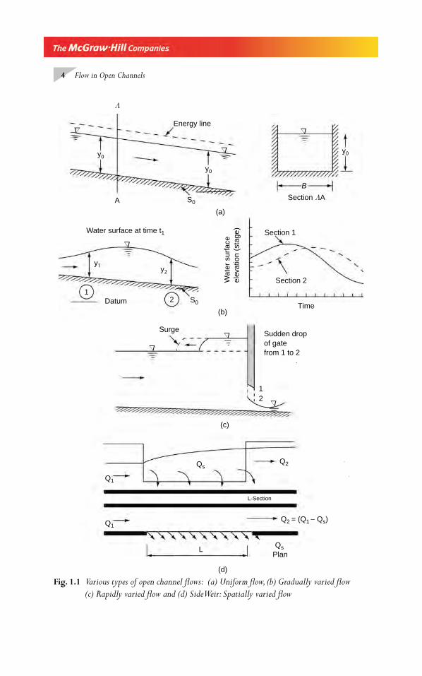
A prismatic channel carrying a certain discharge with a constant velocity is an example of uniform fl ow [Fig. 1.1(a)]. In this case the depth of fl ow will be constant along the channel length and hence the free surface will be parallel to the bed. It is easy to see that an unsteady uniform fl ow is practically impossible, and hence the term uniform fl ow is used for steady uniform fl ow.
Flow in a non-prismatic channel and fl ow with varying velocities in a prismatic channel are examples of varied fl ow. Varied fl ow can be either steady or unsteady.
1.3.3 Gradually Varied and Rapidly Varied Flows
If the change of depth in a varied fl ow is gradual so that the curvature of streamlines is not excessive, such a fl ow is said to be a gradually varied fl ow (GVF). Frictional resistance plays an important role in these fl ows. The backing up of water in a stream due to a dam or drooping of the water surface due to a sudden drop in a canal bed are examples of steady GVF. The passage of a fl ood wave in a river is a case of unsteady GVF [Fig. 1.1(b)].
If the curvature in a varied fl ow is large and the depth changes appreciably over short lengths, such a phenomenon is termed as rapidly varied fl ow (RVF). The fric-tional resistance is relatively insignifi cant in such cases and it is usual to regard RVF as a local phenomenon. A hydraulic jump occurring below a spillway or a sluice gate is an example of steady RVF. A surge moving up a canal [Fig. 1.1(c)] and a bore trav-eling up a river are examples of unsteady RVF.
Chapter 1.indd 3Chapter 1.indd 3 2/24/2010 2:42:17 PM2/24/2010 2:42:17 PM
4 Flow in Open Channels
Fig. 1.1 Various types of open channel fl ows: (a) Uniform fl ow, (b) Gradually varied fl ow
(c) Rapidly varied fl ow and (d) Side Weir: Spatially varied fl ow
y0
y0
y0
Λ
Δ
Δ
Δ
S0
Energy line
A
(a)
B
Section ΛA
21
Datum
y1y2
S0
Water surface at time t1 Section 1
Section 2Wat
er s
urfa
ceel
evat
ion
(sta
ge)
Time(b)
Δ
12
SurgeSudden dropof gatefrom 1 to 2
(c)
Δ
Δ
Δ
L
Q1
Qs Plan
QsQ2
Q2 = (Q1 − Qs) Q1
L-Section
(d)
Chapter 1.indd 4Chapter 1.indd 4 2/24/2010 2:42:17 PM2/24/2010 2:42:17 PM
Introduction 5
1.3.4 Spatially Varied Flow
Varied fl ow classifi ed as GVF and RVF assumes that no fl ow is externally added to or taken out of the canal system. The volume of water in a known time interval is conserved in the channel system. In steady-varied fl ow the discharge is constant at all sections. However, if some fl ow is added to or abstracted from the system the result-ing varied fl ow is known as a spatially varied fl ow (SVF).
SVF can be steady or unsteady. In the steady SVF the discharge while being steady-varies along the channel length. The fl ow over a side weir is an example of steady SVF [Fig. 1.1(d)]. The production of surface runoff due to rainfall, known as overland fl ow, is a typical example of unsteady SVF.
Classifi cation. Thus open channel fl ows are classifi ed for purposes of identifi cation and analysis as follows:
Figure 1.1(a) to (d) shows some typical examples of the above types of fl ows
1.4 VELOCITY DISTRIBUTION
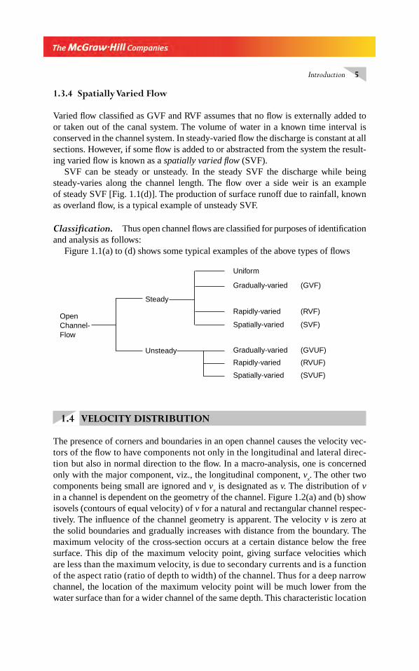
The presence of corners and boundaries in an open channel causes the velocity vec-tors of the fl ow to have components not only in the longitudinal and lateral direc-tion but also in normal direction to the fl ow. In a macro-analysis, one is concerned only with the major component, viz., the longitudinal component, v
x. The other two
components being small are ignored and vx is designated as v. The distribution of v
in a channel is dependent on the geometry of the channel. Figure 1.2(a) and (b) show isovels (contours of equal velocity) of v for a natural and rectangular channel respec-tively. The infl uence of the channel geometry is apparent. The velocity v is zero at the solid boundaries and gradually increases with distance from the boundary. The maximum velocity of the cross-section occurs at a certain distance below the free surface. This dip of the maximum velocity point, giving surface velocities which are less than the maximum velocity, is due to secondary currents and is a function of the aspect ratio (ratio of depth to width) of the channel. Thus for a deep narrow channel, the location of the maximum velocity point will be much lower from the water surface than for a wider channel of the same depth. This characteristic location
OpenChannel-Flow
Steady
Unsteady
Uniform
Gradually-varied
Gradually-varied
Rapidly-varied
Spatially-varied
Rapidly-varied
Spatially-varied
(GVF)
(GVUF)
(RVF)
(RVUF)
(SVF)
(SVUF)
Chapter 1.indd 5Chapter 1.indd 5 2/24/2010 2:42:17 PM2/24/2010 2:42:17 PM
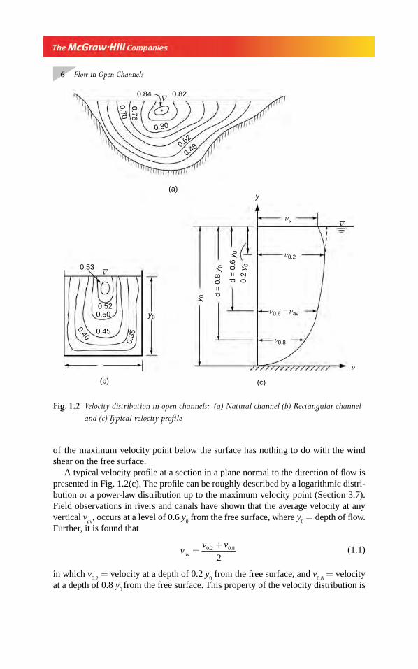
6 Flow in Open Channels
of the maximum velocity point below the surface has nothing to do with the wind shear on the free surface.
A typical velocity profi le at a section in a plane normal to the direction of fl ow is presented in Fig. 1.2(c). The profi le can be roughly described by a logarithmic distri-bution or a power-law distribution up to the maximum velocity point (Section 3.7). Field observations in rivers and canals have shown that the average velocity at any vertical v
av, occurs at a level of 0.6 y
0 from the free surface, where y
0 = depth of fl ow.
Further, it is found that
v
v vav =
+0 2 0 8
2. .
(1.1)
in which v0.2
= velocity at a depth of 0.2 y0 from the free surface, and v
0.8 = velocity
at a depth of 0.8 y0 from the free surface. This property of the velocity distribution is
Fig. 1.2 Velocity distribution in open channels: (a) Natural channel (b) Rectangular channel
and (c) Typical velocity profi le
0.53
0.520.50
0.45
0.35
0.40
y0
(b)
νs
ν0.2
ν0.6 = νav
ν0.8
ν
y 0
d =
0.8
y0
d =
0.6
y0
0.2
y 0
y
(c)
∇
∇
(a)
0.84
0.70
0.82
0.80
0.62
0.48
0.76
∇
Chapter 1.indd 6Chapter 1.indd 6 2/24/2010 2:42:17 PM2/24/2010 2:42:17 PM
Introduction 7
commonly used in stream-gauging practice to determine the discharge using the area-velocity method. The surface velocity v
s is related to the average velocity v
av as
vav
= kvs (1.2)
where, k = a coeffi cient with a value between 0.8 and 0.95. The proper value of k depends on the channel section and has to be determined by fi eld calibrations. Know-ing k, one can estimate the average velocity in an open channel by using fl oats and other surface velocity measuring devices.
1.5 ONE-DIMENSIONAL METHOD OF FLOW ANALYSIS
Flow properties, such as velocity and pressure gradient in a general open channel fl ow situation can be expected to have components in the longitudinal as well as in the normal directions. The analysis of such a three-dimensional problem is very complex. However, for the purpose of obtaining engineering solutions, a majority of open channel fl ow problems are analysed by one-dimensional analysis where only the mean or representative properties of a cross section are considered and their variations in the longitudinal direction is analysed. This method when properly used not only simplifi es the problem but also gives meaningful results.
Regarding velocity, a mean velocity V for the entire cross-section is defi ned on the basis of the longitudinal component of the velocity v as
VA
v dAA
= ∫1
(1.3)
This velocity V is used as a representative velocity at a cross-section. The dis-charge past a section can then be expressed as
Q v dA VA= =∫
(1.4)
The following important features specifi c to one dimensional open channel fl ow are to be noted:
• A single elevation represents the water surface perpendicular to the fl ow.• Velocities in directions other than the direction of the main axis of fl ow are
not considered.
Kinetic Energy The fl ux of the kinetic energy fl owing past a section can also be expressed in terms of V. But in this case, a correction factor α will be needed as the kinetic energy per unit weight V 2/2g will not be the same as v 2/2g averaged over the cross-section area. An expression for α can be obtained as follows:
For an elemental area dA, the fl ux of kinetic energy through it is equal to
mass
time
KE
mass
⎛⎝⎜⎜⎜
⎞⎠⎟⎟⎟⎟⎛⎝⎜⎜⎜
⎞⎠⎟⎟⎟⎟ = ( )ρv dA
v2
2
Chapter 1.indd 7Chapter 1.indd 7 2/24/2010 2:42:18 PM2/24/2010 2:42:18 PM
8 Flow in Open Channels
For the total area, the kinetic energy fl ux
= =∫ρ
αρ
2 23 3
A
v dA V A
(1.5)
from which
α =
∫ v dA
V A
3
3
(1.6)
or for discrete values of v,
α =
Σ Δv A
V A
3
3
(1.7)
α is known as the kinetic energy correction factor and is equal to or greater than unity.
The kinetic energy per unit weight of fl uid can then be written as αV 2
2g.
Momentum Similarly, the fl ux of momentum at a section is also expressed in terms of V and a correction factor β. Considering an elemental area dA, the fl ux of momentum in the longitudinal direction through this elemental area
= ×
⎛⎝⎜⎜⎜
⎞⎠⎟⎟⎟⎟ = ( )( )mass
timevelocity ρv dA v
For the total area, the momentum fl ux
= =∫ ρ βρv dA V A2 2
(1.8)
which gives
β = =
∫ v dA
V A
v A
V AA
2
2
2
2
Σ Δ
(1.9)
β is known as the momentum correction factor and is equal to or greater than unity.
Values of α and β The coeffi cients α and β are both unity in the case of uniform velocity distribution. For any other velocity distribution α > β > 1.0. The higher the non-uniformity of velocity distribution, the greater will be the values of the coef-fi cients. Generally, large and deep channels of regular cross sections and with fairly straight alignments exhibit lower values of the coeffi cients. Conversely, small chan-nels with irregular cross sections contribute to larger values of α and β. A few mea-sured values of α and β are reported by King3. It appears that for straight prismatic channels, α and β are of the order of 1.10 and 1.05 respectively. In compound chan-nels, i.e. channels with one or two fl ood banks, α and β may, in certain cases reach very high values, of the order of 2.0 (see Compound channels in Sec. 5.7.3).
Chapter 1.indd 8Chapter 1.indd 8 2/24/2010 2:42:18 PM2/24/2010 2:42:18 PM
Introduction 9
Generally, one can assume α = β 1.0 when the channels are straight, prismatic and uniform fl ow or GVF takes place. In local phenomenon, it is desirable to include estimated values of these coeffi cients in the analysis. For natural channels, the following values of α and β are suggested for practical use7:
Channels Values of α Values of βRange Average Range Average
Natural channels and torrents 1.15 – 1.50 1.30 1.05 – 1.17 1.10
River valleys, overfl ooded 1.50 – 2.00 1.75 1.17 – 1.33 1.25
It is usual practice to assume α = β = 1.0 when no other specifi c information about the coeffi cients are available.
Example 1.1 The velocity distribution in a rectangular channel of width B and
depth of fl ow y0 was approximated as v k y= 1 in which k
1 = a constant. Calculate
the average velocity for the cross section and correction coeffi cients α and β.
Solution Area of cross section A = By0
Average velocity VBy
v B dyy
= ( )∫1
00
0
= =∫1 2
301 1 0
0
0
yk ydy k y
y
Kinetic energy correction factor
α =( )
=⎛⎝⎜⎜⎜
⎞⎠⎟⎟⎟
=∫ ∫v B dy
V B y
k y B dy
k y B y
y y3
03
0
13 3 2
0
1 0
3
0
0 0
2
3
1 35
/
.
Momentum correction factor
β =( )
=⎛⎝⎜⎜⎜
⎞⎠⎟⎟⎟
=∫ ∫v B dy
V B y
k y B dy
k y B y
y y2
02
0
12
0
1 0
2
0
0 0
2
3
1 125.
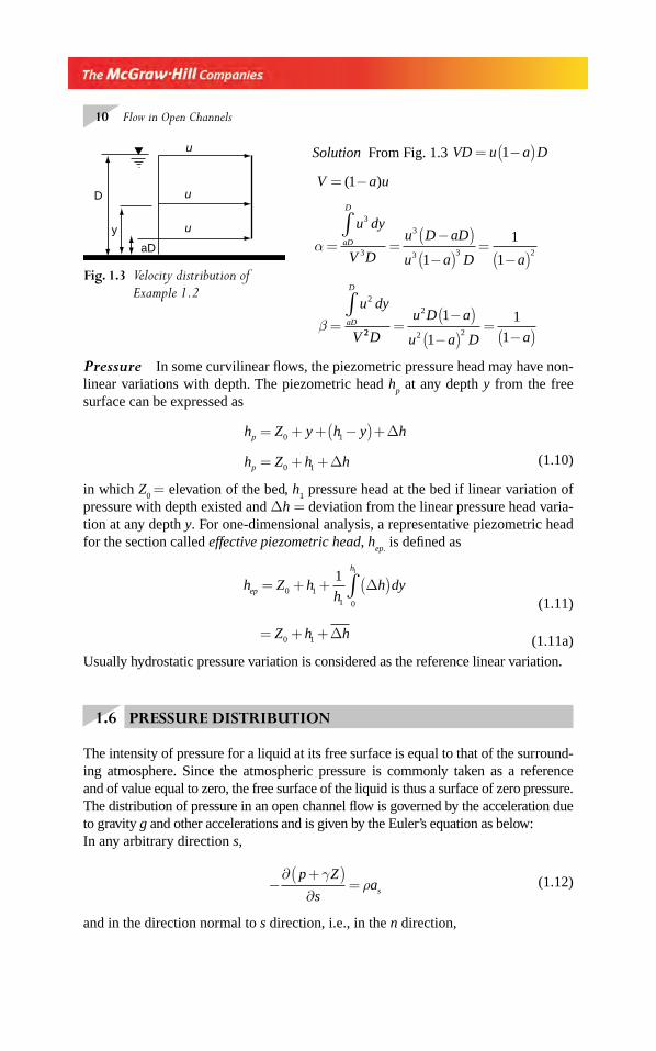
Example 1.2 The velocity distribution in an open channel could be approxi-mated as in Fig. 1.3. Determine the kinetic energy correction factor α and momen-tum correction factor β for this velocity profi le.
Chapter 1.indd 9Chapter 1.indd 9 2/24/2010 2:42:18 PM2/24/2010 2:42:18 PM
10 Flow in Open Channels
Solution From Fig. 1.3 VD u a D= −( )1
V a u= −( )1
u dy
V D
u D aD
u a D aaD
D
= =−( )
−( )=
−( )
∫1
1
1
3
3
3
3 3 2α
u dy
VaD
D
=∫ 2
β22
2
2 2
1
1
1
1D
u D a
u a D a=
−( )−( )
=−( )
Pressure In some curvilinear fl ows, the piezometric pressure head may have non-linear variations with depth. The piezometric head h
p at any depth y from the free
surface can be expressed as
h Z y h y hp = + + −( )+0 1 Δ
h Z h hp = + +0 1 Δ (1.10)
in which Z0 = elevation of the bed, h
1 pressure head at the bed if linear variation of
pressure with depth existed and Δh = deviation from the linear pressure head varia-tion at any depth y. For one-dimensional analysis, a representative piezometric head for the section called effective piezometric head, h
ep. is defi ned as
h Z h
hh dyep
h
= + + ( )∫0 11 0
1 1
Δ (1.11)
Z h h= + +0 1 Δ (1.11a)
Usually hydrostatic pressure variation is considered as the reference linear variation.
1.6 PRESSURE DISTRIBUTION
The intensity of pressure for a liquid at its free surface is equal to that of the surround-ing atmosphere. Since the atmospheric pressure is commonly taken as a reference and of value equal to zero, the free surface of the liquid is thus a surface of zero pressure. The distribution of pressure in an open channel fl ow is governed by the acceleration due to gravity g and other accelerations and is given by the Euler’s equation as below:In any arbitrary direction s,
−
∂ +( )∂
=p Z
sas
γρ
(1.12)
and in the direction normal to s direction, i.e., in the n direction,
D
aD
u
u
uy
Fig. 1.3 Velocity distribution of
Example 1.2
Chapter 1.indd 10Chapter 1.indd 10 2/24/2010 2:42:18 PM2/24/2010 2:42:18 PM
Introduction 11
−
∂∂
+( ) =n
p Z anγ ρ
(1.13)
in which p = pressure, as = acceleration component in the s direction, a
n = accelera-
tion in the n direction and Z = elevation measured above a datum.Consider the s direction along the streamline and the n direction across it. The
direction of the normal towards the centre of curvature is considered as positive. We are interested in studying the pressure distribution in the n-direction. The normal acceleration of any streamline at a section is given by
a
v
rn =2
(1.14)
where v = velocity of fl ow along the streamline of radius of curvature r.Hydrostatic Pressure Distribution The normal acceleration a
n will be zero
(i) if v = 0, i.e., when there is no motion, or(ii) if r → ∞, i.e., when the streamlines are straight lines.
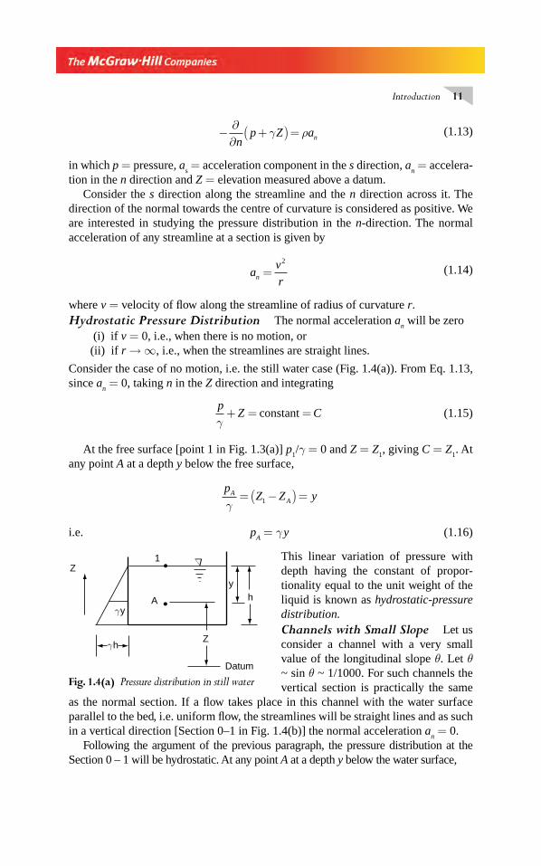
Consider the case of no motion, i.e. the still water case (Fig. 1.4(a)). From Eq. 1.13, since a
n = 0, taking n in the Z direction and integrating
pZ C
γ+ = =constant
(1.15)
At the free surface [point 1 in Fig. 1.3(a)] p1/γ = 0 and Z = Z
1, giving C = Z
1. At
any point A at a depth y below the free surface,
pZ Z yA
Aγ= −( ) =1
i.e. pA = γ y (1.16)
This linear variation of pressure with depth having the constant of propor-tionality equal to the unit weight of the liquid is known as hydrostatic-pressure distribution.Channels with Small Slope Let us consider a channel with a very small value of the longitudinal slope θ. Let θ ~ sin θ ~ 1/1000. For such channels the vertical section is practically the same
as the normal section. If a fl ow takes place in this channel with the water surface parallel to the bed, i.e. uniform fl ow, the streamlines will be straight lines and as such in a vertical direction [Section 0–1 in Fig. 1.4(b)] the normal acceleration a
n = 0.
Following the argument of the previous paragraph, the pressure distribution at the Section 0 – 1 will be hydrostatic. At any point A at a depth y below the water surface,
yh
Z
Z
γh
γyA
1
Datum
Δ
Fig. 1.4(a) Pressure distribution in still water
Chapter 1.indd 11Chapter 1.indd 11 2/24/2010 2:42:19 PM2/24/2010 2:42:19 PM
12 Flow in Open Channels
py
pZ Z
γ γ= + =
=
and
Elevation of water surface
1
Thus the piezometric head at any point in the channel will be equal to the water-surface elevation. The hydraulic grade line will therefore lie essentially on the water surface.
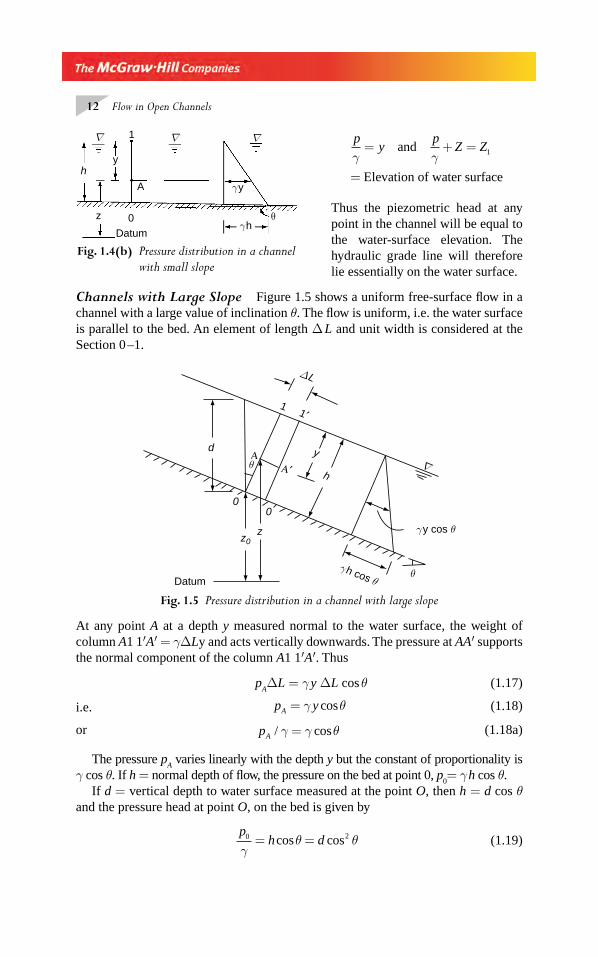
Channels with Large Slope Figure 1.5 shows a uniform free-surface fl ow in a channel with a large value of inclination θ. The fl ow is uniform, i.e. the water surface is parallel to the bed. An element of length Δ L and unit width is considered at the Section 0 –1.
Fig. 1.5 Pressure distribution in a channel with large slope
L
11′
ΑΑ′
y
h
d
00
zz0
Datumθ
θ
γy cos θ
γh cos θ
Δ
∇
At any point A at a depth y measured normal to the water surface, the weight of column A1 1′A′ = γΔLy and acts vertically downwards. The pressure at AA′ supports the normal component of the column A1 1′A′. Thus
pAΔL = γ y ΔL cos θ (1.17)
i.e. p yA = γ θcos (1.18)
or pA / cosγ γ θ= (1.18a)
The pressure pA varies linearly with the depth y but the constant of proportionality is
γ cos θ. If h = normal depth of fl ow, the pressure on the bed at point 0, p0= γ h cos θ.
If d = vertical depth to water surface measured at the point O, then h = d cos θ and the pressure head at point O, on the bed is given by
p
h d0 2
γθ θ= =cos cos (1.19)
yh
z
Datum
0
1
A
∇ ∇ ∇
γy
γhθ
Fig. 1.4(b) Pressure distribution in a channel
with small slope
Chapter 1.indd 12Chapter 1.indd 12 2/24/2010 2:42:19 PM2/24/2010 2:42:19 PM
Introduction 13
The piezometric height at any point A = Z + y cos θ = Z0 + h cos θ. Thus for
channels with large values of the slope, the conventionally defi ned hydraulic gradient line does not lie on the water surface.
Channels of large slopes are encountered rarely in practice except, typically in spillways and chutes. On the other hand, most of the canals, streams and rivers with which a hydraulic engineer is commonly associated will have slopes (sin θ) smaller than 1/100. For such cases cos θ ≈ 1.0. As such, in further sections of this book the term cos θ in the expression for the pressure will be omitted with the knowledge that it has to be used as in Eq. 1.18 if θ is large.
1.7 PRESSURE DISTRIBUTION IN CURVILINEAR FLOWS
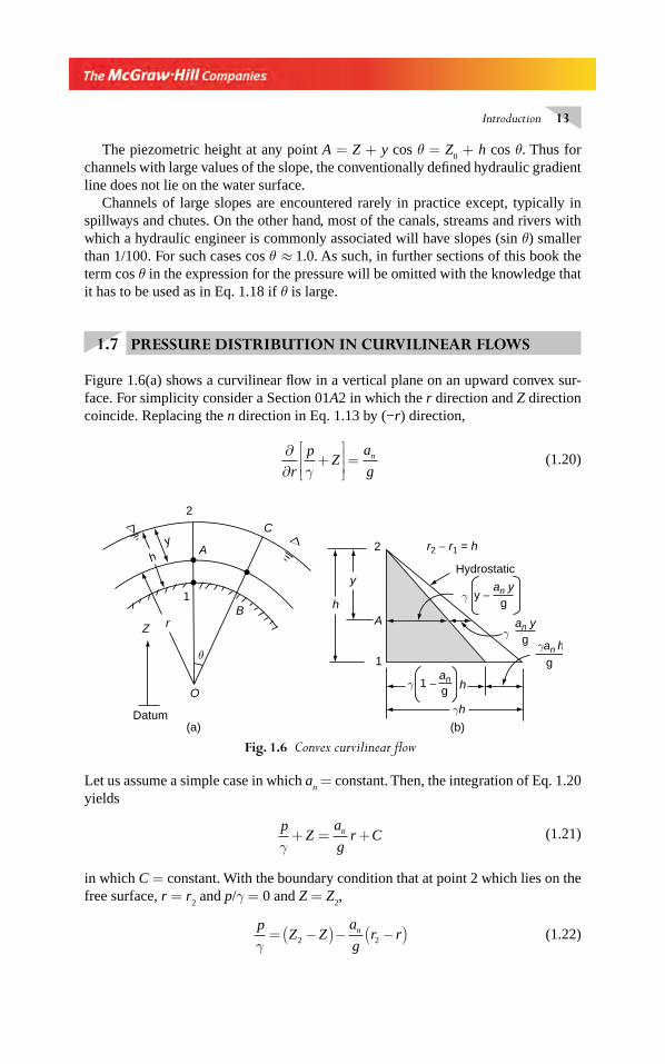
Figure 1.6(a) shows a curvilinear fl ow in a vertical plane on an upward convex sur-face. For simplicity consider a Section 01A2 in which the r direction and Z direction coincide. Replacing the n direction in Eq. 1.13 by (−r) direction,
∂∂
+⎡
⎣⎢⎢
⎤
⎦⎥⎥ =
r
pZ
a
gn
γ (1.20)
2
A
C
B
O
1
hy
Z r
Datum(a)
2
y
hA
1
r2 − r1 = h
Hydrostatic
h1 −ang
y − g
gan y
an y
(b)
γ
γ
g
γh
θ
γ
γan h
ΔΔ
Fig. 1.6 Convex curvilinear fl ow
Let us assume a simple case in which an = constant. Then, the integration of Eq. 1.20
yields
pZ
a
gr Cn
γ+ = + (1.21)
in which C = constant. With the boundary condition that at point 2 which lies on the free surface, r = r
2 and p/γ = 0 and Z = Z
2,
p
Z Za
gr rn
γ= −( )− −( )2 2 (1.22)
Chapter 1.indd 13Chapter 1.indd 13 2/24/2010 2:42:19 PM2/24/2010 2:42:19 PM
14 Flow in Open Channels
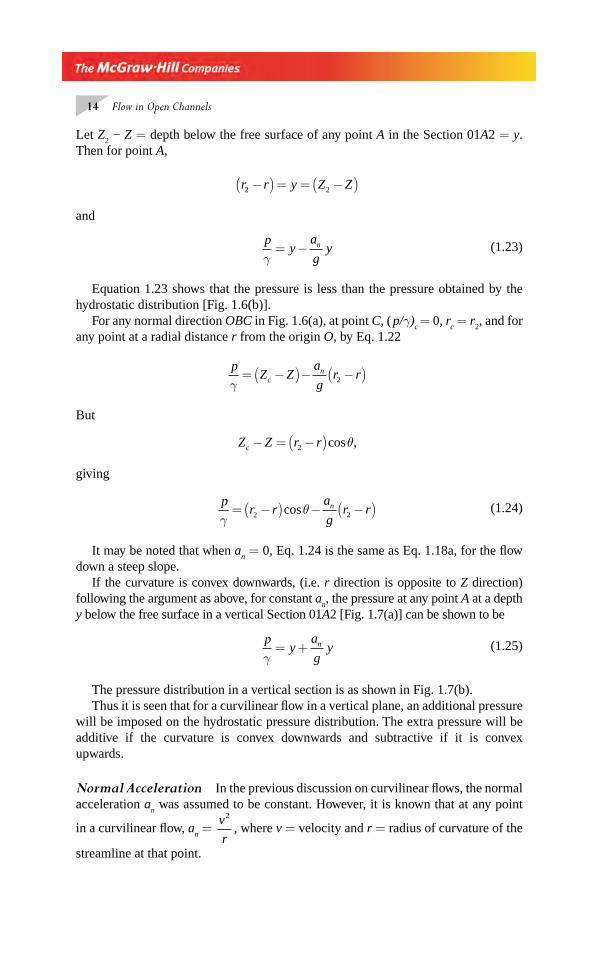
Let Z2 − Z = depth below the free surface of any point A in the Section 01A2 = y.
Then for point A,
r r y Z Z2 2−( ) = = −( )
and
py
a
gyn
γ= − (1.23)
Equation 1.23 shows that the pressure is less than the pressure obtained by the hydrostatic distribution [Fig. 1.6(b)].
For any normal direction OBC in Fig. 1.6(a), at point C, ( p/γ)c = 0, r
c = r
2, and for
any point at a radial distance r from the origin O, by Eq. 1.22
pZ Z
a
gr rc
n
γ= −( )− −( )2
But
Z Z r rc − = −( )2 cos ,θ
giving
pr r
a
gr rn
γθ= −( ) − −( )2 2cos (1.24)
It may be noted that when an = 0, Eq. 1.24 is the same as Eq. 1.18a, for the fl ow
down a steep slope.If the curvature is convex downwards, (i.e. r direction is opposite to Z direction)
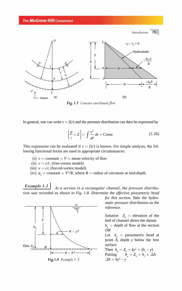
following the argument as above, for constant an, the pressure at any point A at a depth
y below the free surface in a vertical Section 01A2 [Fig. 1.7(a)] can be shown to be
py
a
gyn
γ= + (1.25)
The pressure distribution in a vertical section is as shown in Fig. 1.7(b).Thus it is seen that for a curvilinear fl ow in a vertical plane, an additional pressure
will be imposed on the hydrostatic pressure distribution. The extra pressure will be additive if the curvature is convex downwards and subtractive if it is convex upwards.
Normal Acceleration In the previous discussion on curvilinear fl ows, the normal acceleration a
n was assumed to be constant. However, it is known that at any point
in a curvilinear fl ow, an =
v
r
2
, where v = velocity and r = radius of curvature of the
streamline at that point.
Chapter 1.indd 14Chapter 1.indd 14 2/24/2010 2:42:20 PM2/24/2010 2:42:20 PM
Introduction 15
In general, one can write v = f (r) and the pressure distribution can then be expressed by
pZ
v
grdr
γ+
⎛
⎝⎜⎜⎜⎜
⎞
⎠⎟⎟⎟⎟ = +∫
2
Const (1.26)
This expression can be evaluated if v = f (r) is known. For simple analysis, the fol-lowing functional forms are used in appropriate circumstances:
(i) v = constant = V = mean velocity of fl ow (ii) v = c/r, (free-vortex model)(iii) v = cr, (forced-vortex model) (iv) a
n = constant = V 2/R, where R = radius of curvature at mid-depth.
Example 1.3 At a section in a rectangular channel, the pressure distribu-tion was recorded as shown in Fig. 1.8. Determine the effective piezometric head
for this section. Take the hydro-static pressure distribution as the reference.
Solution Z0 = elevation of the
bed of channel above the datumh
1 = depth of fl ow at the section
OBLet h
p = piezometric head at
point A, depth y below the free surfaceThen h
p = Z
0 + ky2 + (h
1 – y)
Putting hp = Z
0 + h
1 + Δh
Δh = ky2 – y
Fig. 1.7 Concave curvilinear fl ow
1
y
h
A
2
Hydrostatic
g
an y
(b)
anh
gγh
γy
2
A
O
1
hy
Z
r
Datum (a)
r2 – r1 = h
γ
γ
Fig.1.8 Example 1.3
y
h1
B
K γ y2
K γ h2
Elev. Z0
∇
Chapter 1.indd 15Chapter 1.indd 15 2/24/2010 2:42:20 PM2/24/2010 2:42:20 PM
16 Flow in Open Channels
Effective piezometric head, by Eq. 1.11 is
h Z hh
h dy
Z hh
ky y dy
h Zh k
ep
h
h
ep
= + + ( )
= + + −( )
= + +
∫
∫
0 11
0
0 11
2
0
01
1
1
2
1
1
Δ
hh12
2
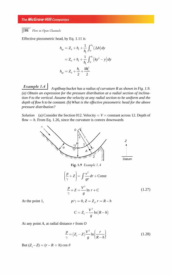
Example 1.4 A spillway bucket has a radius of curvature R as shown in Fig. 1.9. (a) Obtain an expression for the pressure distribution at a radial section of inclina-tion θ to the vertical. Assume the velocity at any radial section to be uniform and the depth of fl ow h to be constant. (b) What is the effective piezometric head for the above pressure distribution?
Solution (a) Consider the Section 012. Velocity = V = constant across 12. Depth of fl ow = h. From Eq. 1.26, since the curvature is convex downwards
Fig. 1.9 Example 1.4
Δ
0
2
1h
A
Zr
R
ν
θ
Datum
pZ
v
grdr
γ+
⎛
⎝⎜⎜⎜⎜
⎞
⎠⎟⎟⎟⎟ = +∫
2
Const
pZ
V
gr C
γ+ = +
2
ln (1.27)
At the point 1, p/γ = 0, Z = Z1, r = R – h
C Z
V
gR h= − −( )1
2
ln
At any point A, at radial distance r from O
p
Z ZV
g
r
R hγ= −( )
−
⎛⎝⎜⎜⎜
⎞⎠⎟⎟⎟⎟1
2
ln (1.28)
But (Z1 – Z) = (r – R + h) cos θ
Chapter 1.indd 16Chapter 1.indd 16 2/24/2010 2:42:20 PM2/24/2010 2:42:20 PM
Introduction 17
p
r R hV
g
r
R hγθ= − +( ) +
−
⎛⎝⎜⎜⎜
⎞⎠⎟⎟⎟⎟cos ln
2
(1.29)
Equation 1.29 represents the pressure distribution at any point (r, θ). At point 2, r = R, p = p
2.
(b) Effective piezometric head, hep
:From Eq. 1.28 the piezometric head h
p at A is
hp
Z ZV
g
r
R hp
A
= +⎛
⎝⎜⎜⎜⎜
⎞
⎠⎟⎟⎟⎟ = +
−
⎛⎝⎜⎜⎜
⎞⎠⎟⎟⎟⎟γ 1
2
ln
Noting that Z1 = Z
2 + h cos θ and expressing h
p in the form of Eq. 1.10
hp = Z
2 + h cos θ + Δh
Where
Δh
V
g
r
R h=
−
2
ln
The effective piezometric head hep.
from Eq. 1.11 is
h Z h
h
V
g
r
R hdrep
R h
R
= + +−−∫2
21cos
coslnθ
θ
on integration,
h Z hV
ghh R
R
R hep = + + − +−
⎡
⎣⎢⎢
⎤
⎦⎥⎥2
2
coscos
θθ
ln
= + +− +
−⎛⎝⎜⎜⎜
⎞⎠⎟⎟⎟
⎛⎝⎜⎜⎜
⎞⎠⎟⎟⎟
Z h
Vh
R h R
gRh
R
2
2 1
1cos
ln/
cos
θθ
(1.30)
It may be noted that when R → ∞ and h /R → 0, hep
→ Z2 + h cos θ
1.8 FLOWS WITH SMALL WATER-SURFACE CURVATURE
Consider a free-surface fl ow with a convex upward water surface over a horizontal bed (Fig. 1.10). For this water surface, d 2h / dx2 is negative. The radius of curvature of the free surface is given by
1
11
2
2
2 3 2
2
2r
d h
dx
dh
dx
d h
dx=
+⎛⎝⎜⎜⎜
⎞⎠⎟⎟⎟
⎡
⎣
⎢⎢⎢
⎤
⎦
⎥⎥⎥
≈ (1.31)
Chapter 1.indd 17Chapter 1.indd 17 2/24/2010 2:42:21 PM2/24/2010 2:42:21 PM
18 Flow in Open Channels
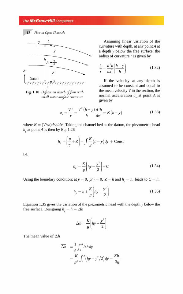
Assuming linear variation of the curvature with depth, at any point A at a depth y below the free surface, the radius of curvature r is given by
1 2
2r
d h
dx
h y
h=
−⎛⎝⎜⎜⎜
⎞⎠⎟⎟⎟⎟
(1.32)
If the velocity at any depth is assumed to be constant and equal to the mean velocity V in the section, the normal acceleration a
n at point A is
given by
aV
r
V h y
h
d h
dxK h yn = =
−( )= −( )
2 2 2
2 (1.33)
where K = (V 2/h)d 2h/dx2. Taking the channel bed as the datum, the piezometric head h
p at point A is then by Eq. 1.26
h
pZ
K
gh y dyp = +
⎛
⎝⎜⎜⎜⎜
⎞
⎠⎟⎟⎟⎟ = −( ) +∫γ
Const
i.e.
hK
ghy
yCp = −
⎛
⎝⎜⎜⎜⎜
⎞
⎠⎟⎟⎟⎟+
2
2 (1.34)
Using the boundary condition; at y = 0, p/γ = 0, Z = h and hp = h, leads to C = h,
h hK
ghy
yp = + −
⎛
⎝⎜⎜⎜⎜
⎞
⎠⎟⎟⎟⎟
2
2 (1.35)
Equation 1.35 gives the variation of the piezometric head with the depth y below the free surface. Designing h
p = h + Δh
Δh
K
ghy
y= −
⎛
⎝⎜⎜⎜⎜
⎞
⎠⎟⎟⎟⎟
2
2
The mean value of Δh
Δ Δhh
hdy
K
ghhy y dy
Kh
g
A
A
=
= −( ) =
∫
∫
1
23
0
22
0
Fig. 1.10 Defi nition sketch of fl ow with
small water-surface curvature
1
Datum
2
y
hA
ZZ
∇
Chapter 1.indd 18Chapter 1.indd 18 2/24/2010 2:42:21 PM2/24/2010 2:42:21 PM
Introduction 19
The effective piezometric head hep
at the section with the channel bed as the datum can now be expressed as
h hKh
gep = +2
3 (1.36)
It may be noted that d 2h / dx2 and hence K is negative for convex upward curvature and positive for concave upward curvature. Substituting for K, Eq. 1.36 reads as
h hV h
g
d h
dxep = +1
3
2 2
2 (1.37)
This equation, attributed to Boussinesq4 fi nds application in solving problems with small departures from the hydrostatic pressure distribution due to the curvature of the water surface.
1.9 EQUATION OF CONTINUITY
The continuity equation is a statement of the law of conservation of matter. In open-channel fl ows, since we deal with incompressible fl uids, this equvation is relatively simple and much more for the cases of steady fl ow.
Steady Flow In a steady fl ow the volumetric rate of fl ow (discharge in m3/s) past various section must be the same. Thus in a varied fl ow, if Q = discharge, V = mean velocity and A = area of cross-section with suffi xes representing the sections to which they refer
Q = VA = V1A
1 = V
2 A
2 = … (1.38)
If the velocity distribution is given, the discharge is obtained by integration as in Eq. 1.4. It should be kept in mind that the area element and the velocity through this area element must be perpendicular to each other.
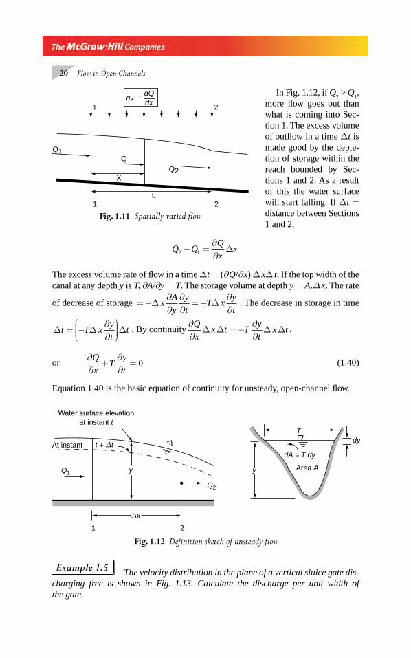
In a steady spatially-varied fl ow, the discharge at various sections will not be the same. A budgeting of infl ows and outfl ows of a reach is necessary. Consider, for example, an SVF with increasing discharge as in Fig. 1.11. The rate of addi-tion of discharge = dQ/dx = q
*. The discharge at any section at a distance x from
Section 1
= = + ∫Q Q q dx
x
10
* (1.39)
If q* = constant, Q = Q
1 + q
*x and Q
2 = Q
1 + q
*L
Unsteady Flow In the unsteady fl ow of incompressible fl uids, if we consider a reach of the channel, the continuity equation states that the net discharge going out of all the boudary surfaces of the reach is equal to the rate of depletion of the storage within it.
Chapter 1.indd 19Chapter 1.indd 19 2/24/2010 2:42:22 PM2/24/2010 2:42:22 PM
20 Flow in Open Channels
In Fig. 1.12, if Q2 > Q
1,
more fl ow goes out than what is coming into Sec-tion 1. The excess volume of outfl ow in a time Δt is made good by the deple-tion of storage within the reach bounded by Sec-tions 1 and 2. As a result of this the water surface will start falling. If Δt = distance between Sections 1 and 2,
Q Q
Q
xx2 1− =
∂∂
Δ
The excess volume rate of fl ow in a time Δt = (∂Q/∂x) Δ xΔ t. If the top width of the canal at any depth y is T, ∂A/∂y = T. The storage volume at depth y = A.Δ x. The rate
of decrease of storage = −∂∂
∂∂
= −∂∂
Δ ΔxA
y
y
tT x
y
t. The decrease in storage in time
Δ Δ Δt T xy
tt= −
∂∂
⎛⎝⎜⎜⎜
⎞⎠⎟⎟⎟⎟ . By continuity
∂∂
= −∂∂
Q
xx t T
y
tx tΔ Δ Δ Δ .
or ∂∂
+∂∂
=Q
xT
y
t0 (1.40)
Equation 1.40 is the basic equation of continuity for unsteady, open-channel fl ow.
Fig. 1.11 Spatially varied fl ow
1 2
1 2
QQ1
Q2
L
X
q = dQdx*
Fig. 1.12 Defi nition sketch of unsteady fl ow
TΔ
Δ
Water surface elevationat instant t
y
Δx
t + Δt
Q1
Q2
At instant
1 2
Area A
dA = T dy
y
dy
Example 1.5 The velocity distribution in the plane of a vertical sluice gate dis-charging free is shown in Fig. 1.13. Calculate the discharge per unit width of the gate.
Chapter 1.indd 20Chapter 1.indd 20 2/24/2010 2:42:22 PM2/24/2010 2:42:22 PM
Introduction 21
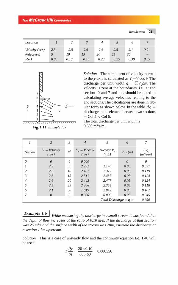
Location 1 2 3 4 5 6 7
Velocity (m/s) 2.3 2.5 2.6 2.6 2.5 2.1 0.0θ(degrees) 5 10 15 20 25 30 –y(m) 0.05 0.10 0.15 0.20 0.25 0.30 0.35
Solution The component of velocity normal to the y-axis is calculated as V
n=V cos θ. The
discharge per unit width q = ∑VnΔy. The
velocity is zero at the boundaries, i.e., at end sections 0 and 7 and this should be noted in calculating average velocities relating to the end sections. The calculations are done in tab-ular form as shown below. In the table Δq = discharge in the element between two sections = Col 5 × Col 6.The total discharge per unit width is0.690 m3/s/m.Fig. 1.13 Example 1.5
y
V
7654321
θ
∇
Example 1.6 While measuring the discharge in a small stream it was found that the depth of fl ow increases at the ratio of 0.10 m/h. If the discharge at that section was 25 m3/s and the surface width of the stream was 20m, estimate the discharge at a section 1 km upstream.
Solution This is a case of unsteady fl ow and the continuity equation Eq. 1.40 will be used.
T
y
t
∂∂
=××
=20 0 10
60 600 000556
..
1 2 3 4 5 6 7
SectionV = Velocity
(m/s)θ 0 V
n = V cos θ
(m/s)Average V
n
(m/s)Δ y (m)
Δ q3
(m3/s/m)
0 0 0 0.000 0 01 2.3 5 2.291 1.146 0.05 0.0572 2.5 10 2.462 2.377 0.05 0.1193 2.6 15 2.511 2.487 0.05 0.1244 2.6 20 2.443 2.477 0.05 0.1245 2.5 25 2.266 2.354 0.05 0.1186 2.1 30 1.819 2.042 0.05 0.1027 0 0 0.000 0.090 0.05 0.045
Total Discharge = q = 0.690
Chapter 1.indd 21Chapter 1.indd 21 2/24/2010 2:42:22 PM2/24/2010 2:42:22 PM
22 Flow in Open Channels
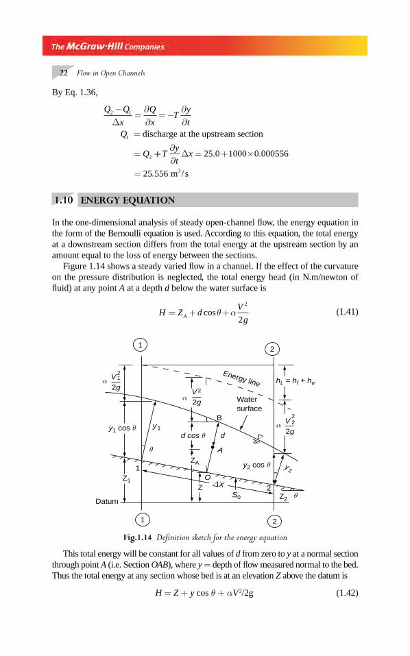
Fig.1.14 Defi nition sketch for the energy equation
Datum
Z1
y1 cos θ
θ
y1d cos θ d
A
ZA
OZ
y2 cos θ1
1
1
2
2
S0
ΔX 2Z2 θ
y2
hL = hf + he
Watersurface
Energy lineV2
2g
V2g
α
α
21
V2g
α22
Δ
B
By Eq. 1.36,
Q Q
x
Q
xT
y
tQ
Q
2 1
1
2
−=
∂∂
= −∂∂
=
=
Δdischarge at the upstream section
++∂∂
= + ×
=
Ty
txΔ 25 0 1000 0 000556
25 556
. .
/ m s3.
1.10 ENERGY EQUATION
In the one-dimensional analysis of steady open-channel fl ow, the energy equation in the form of the Bernoulli equation is used. According to this equation, the total energy at a downstream section differs from the total energy at the upstream section by an amount equal to the loss of energy between the sections.
Figure 1.14 shows a steady varied fl ow in a channel. If the effect of the curvature on the pressure distribution is neglected, the total energy head (in N.m/newton of fl uid) at any point A at a depth d below the water surface is
H Z d
V
gA= + +cosθ α2
2
(1.41)
This total energy will be constant for all values of d from zero to y at a normal section through point A (i.e. Section OAB), where y = depth of fl ow measured normal to the bed. Thus the total energy at any section whose bed is at an elevation Z above the datum is
H = Z + y cos θ + αV 2/2g (1.42)
Chapter 1.indd 22Chapter 1.indd 22 2/24/2010 2:42:23 PM2/24/2010 2:42:23 PM
Introduction 23
In Fig. 1.14, the total energy at a point on the bed is plotted along the vertical through that point. Thus the elevation of energy line on the line 1–1 represents the total energy at any point on the normal section through point 1. The total energies at normal sections through 1 and 2 are therefore
H Z yV
g
H Z yV
g
1 1 1 112
2 2 2 222
2
2
= + +
= + +
cos
cos
θ α
θ α
respectively. The term (Z + y cos θ) = h represents the elevation of the hydraulic grade line above the datum.
If the slope of the channel θ is small, cos θ ≈ 1.0, the normal section is practically the same as the vertical section and the total energy at any section can be written as
H Z yV
g= + +α 2
2 (1.43)
Since most of the channels in practice happen to have small values of θ (θ < 10º), the term cos θ is usually neglected. Thus the energy equation is written as Eq. 1.40 in subsequent sections of this book, with the realisation that the slope term will be included if cos θ is appreciably different from unity.
Due to energy losses between Sections 1 and 2, the energy head H1 will be larger
than H2 and H
1 − H
2 = h
L = head loss. Normally, the head loss (h
L ) can be considered
to be made up of frictional losses (hf ) and eddy or form loss (h
e) such that h
L = h
f +
he. For prismatic channels, h
e = 0. One can observe that for channels of small slope
the piezometric head line essentially coincides with the free surface. The energy line which is a plot of H vs x is a dropping line in the longitudinal (x) direction. The dif-ference of the ordinates between the energy line and free surface represents the velocity head at that section. In general, the bottom profi le, water-surface and energy line will have distinct slopes at a given section. The bed slope is a geometric parame-ter of the channel. The slope of the energy line depends on the resistance characteris-tics of the channel and is discussed in Chapter 3. Discussions on the water-surface profi les are presented in chapter 4 and 5.
In designating the total energy by Eq. 1.41 or 1.42, hydrostatic pressure distribution was assumed. However, if the curvature effects in a vertical plane are appreciable, the pressure distribution at a section may have a non-linear variation with the depth d. In such cases the effective piezometric head h
ep as defi ned in Eq. 1.11 will be used to represent the total
energy at a section as
H hV
gep= +α2
2 (1.44)
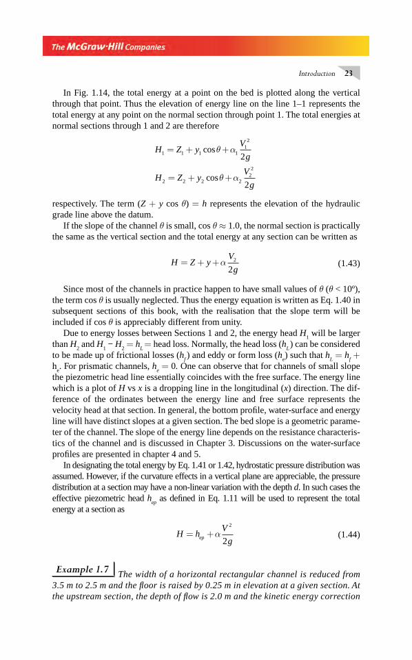
Example 1.7 The width of a horizontal rectangular channel is reduced from 3.5 m to 2.5 m and the fl oor is raised by 0.25 m in elevation at a given section. At the upstream section, the depth of fl ow is 2.0 m and the kinetic energy cor rection
Chapter 1.indd 23Chapter 1.indd 23 2/24/2010 2:42:23 PM2/24/2010 2:42:23 PM
24 Flow in Open Channels
factor α is 1.15. If the drop in the water surface elevation at the contraction is 0.20 m, calculate the discharge if (a) the energy loss is neglected, and (b) the energy loss is one-tenth of the upstream velocity head. [The kin etic energy correction factor at the con-tracted section may be assumed to be unity].
Solution Referring to Fig. 1.15, y
1 = 2.0 m
y2 = 2.0 − 0.25 − 0.20 = 1.55 m
By continuity
B y V B y V
V V V
1 1 1 2 2 2
1 2 2
2 5 1 55
3 5 2 00 5536
=
=××
=. .
. ..
(a) When there is no energy lossBy energy equation applied to Sections 1 and 2,
Z yV
gZ Z y
V
g
V
1 1 112
1 2 222
1 2
22
2 2
1 15 1 0
1 15
+ + = +( )+ +
= =
−
α α
α α
Δ
. .
.
and
VV
gy y Z
12
1 22
( )= − −Δ
V
g22
2
21 1 15 0 5536 2 00 1 55 0 25−( )( )⎡⎣⎢
⎤⎦⎥= − −. . . . .
0 64762 9 81
0 2
2 462
22
2
..
.
.
V
V×
=
= m/s
Discharge Q = × × =2 5 1 55 2 462 9 54. . . . / m s3
(b) When there is an energy loss
HV
g
V
gL =⎡
⎣⎢⎢
⎤
⎦⎥⎥ =0 1
20 115
2112
12
. .α
Fig. 1.15 Example 1.7
B1 = 3.5m B2 = 2.5m
PLAN12
ΔΔ
L-SECTION
y2
0.20m
0.25m
Energy line
y1 = 2.0m
Chapter 1.indd 24Chapter 1.indd 24 2/24/2010 2:42:23 PM2/24/2010 2:42:23 PM
Introduction 25
By energy equation,
Z yV
gZ Z y
V
gH
V
g
V
gH
L
L
1 1 112
1 2 222
222
112
2 2
2 2
+ + = +( )+ + +
− +⎡
⎣⎢⎢
⎤
α α
α α
Δ
⎦⎦⎥⎥ = − −y y Z1 2 Δ
Substituting α2 = 1.0, α
1 = 1.15 and H
V
gL = 0 1152
12
.
V
g
V
g
V
g22
12
12
21 15
20 115
22 00 1 55 0 25− − = − −. . . . .
Since V1 = 0.5536V
2
V
g22
2
21 0 9 1 15 0 5536 0 2−( )( )( )⎡⎣⎢
⎤⎦⎥=. . . .
0 6826
2 9 810 22
2.
..
V
×=
V 2 = 2.397 m/s and discharge Q = × × =2 5 1 55 2 397 9 289. . . . / m s3
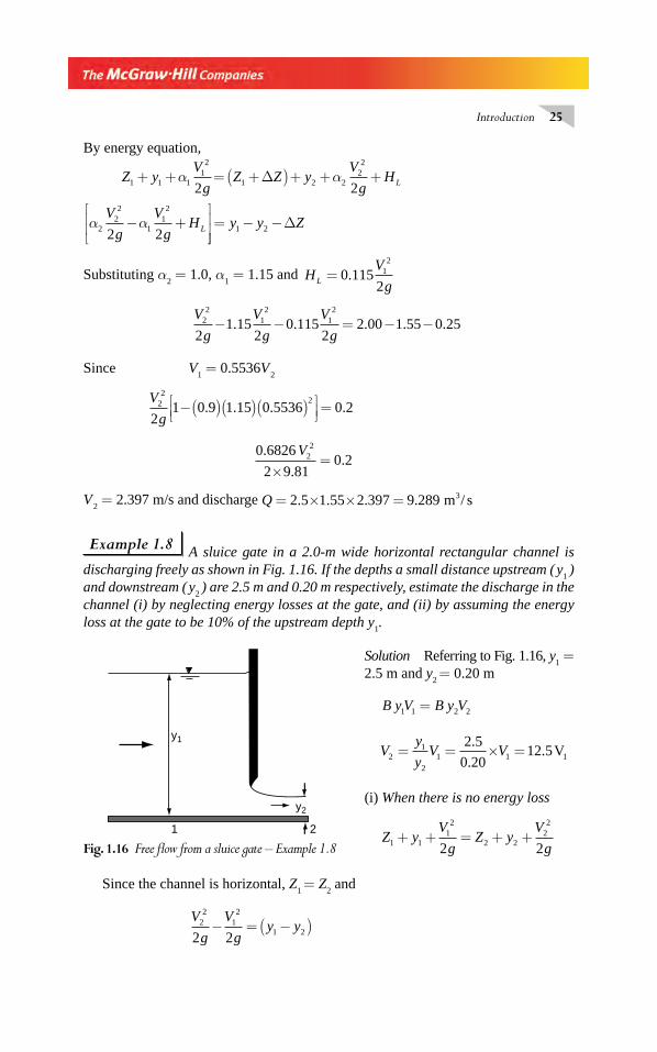
Example 1.8 A sluice gate in a 2.0-m wide horizontal rectangular channel is discharging freely as shown in Fig. 1.16. If the depths a small distance upstream ( y
1 )
and downstream ( y2 ) are 2.5 m and 0.20 m respectively, estimate the discharge in the
channel (i) by neglecting energy losses at the gate, and (ii) by assuming the energy loss at the gate to be 10% of the upstream depth y
1.
Solution Referring to Fig. 1.16, y1 =
2.5 m and y2 = 0.20 m
B y V B y V1 1 2 2=
V
y
yV V2
1
21 1
2 5
0 2012 5= = × =
.
.. V1
(i) When there is no energy loss
Z y
V
gZ y
V
g1 112
2 222
2 2+ + = + +
Since the channel is horizontal, Z1 = Z
2 and
V
g
V
gy y2
212
1 22 2− = −( )
Fig. 1.16 Free fl ow from a sluice gate – Example 1.8
1 2
y2
y1
Chapter 1.indd 25Chapter 1.indd 25 2/24/2010 2:42:24 PM2/24/2010 2:42:24 PM
26 Flow in Open Channels
V
g12
2
212 5 1 2 50 0 20 2 30( . ) . . .−⎡
⎣⎢⎤⎦⎥ = − =
V
gV1
2
12
2 30
155 250 01481 0 539= = =
.
.. .and m/s.
Discharge Q = By1V
1 = 2.0×2.5×0.539 = 2.696 m3/s.
(ii) When there is energy lossH
L = Energy loss = 0.10 y
1 = 0.25 m
yV
gy
V
gHL1
12
222
2 2+ = + +
V
g
V
gy y HL
22
12
1 22 2− = − −( )
V
g12
2
212 5 1 2 50 0 20 0 25 2 05. . . . .( ) −⎡
⎣⎢⎤⎦⎥== − − =
V
gV1
2
12
2 05
155 250 0132 0 509= = =
.
.. . and m/s
Discharge Q By V= = × × =1 1 2 0 2 5 0 509 2 545. . . . / m s.3
1.11 MOMENTUM EQUATION
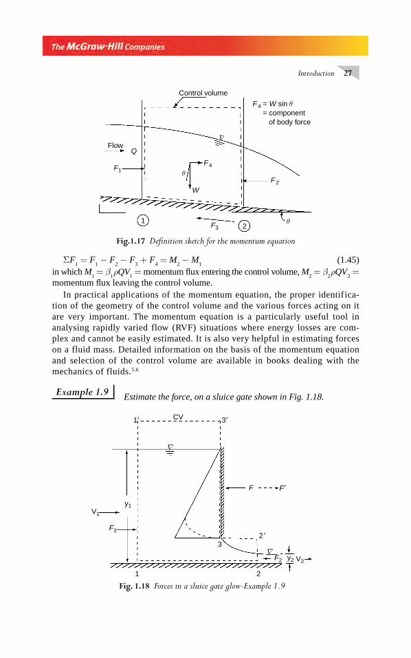
Steady Flow Momentum is a vector quantity. The momentum equation com-monly used in most of the open channel fl ow problems is the linear-momentum equation. This equation states that the algebraic sum of all external forces, acting in a given direction on a fl uid mass equals the time rate of change of linear-momentum of the fl uid mass in the direction. In a steady fl ow the rate of change of momentum in a given direction will be equal to the net fl ux of momentum in that direction.
Figure 1.17 shows a control volume (a volume fi xed in space) bounded by Sec-tions 1 and 2, the boundary and a surface lying above the free surface. The various forces acting on the control volume in the longitudinal direction are as follows:
(i) Pressure forces acting on the control surfaces, F1 and F
2.
(ii) Tangential force on the bed, F3,
(iii) Body force, i.e., the component of the weight of the fl uid in the longitudinal direction, F
4.
By the linear-momentum equation in the longitudinal direction for a steady-fl ow discharge of Q,
Chapter 1.indd 26Chapter 1.indd 26 2/24/2010 2:42:25 PM2/24/2010 2:42:25 PM
Introduction 27
ΣF1 = F
1 − F
2 − F
3 + F
4 = M
2 − M
1 (1.45)
in which M1 = β
1 ρQV1 = momentum fl ux entering the control volume, M
2 = β
2 ρQV
2 =
momentum fl ux leaving the control volume.In practical applications of the momentum equation, the proper identifica-
tion of the geometry of the control volume and the various forces acting on it are very important. The momentum equation is a particularly useful tool in analysing rapidly varied flow (RVF) situations where energy losses are com-plex and cannot be easily estimated. It is also very helpful in estimating forces on a fluid mass. Detailed information on the basis of the momentum equation and selection of the control volume are available in books dealing with the mechanics of fluids.5.6
Example 1.9 Estimate the force, on a sluice gate shown in Fig. 1.18.
Fig.1.17 Defi nition sketch for the momentum equation
Δ
FlowQ
F1F4
W
Control volume
F4 = W sin
= component
of body force
F2
21
θ
θ
θ
F3
Fig. 1.18 Forces in a sluice gate glow-Example 1.9
V2y2F2
2
3
F F′
1′ 3′
2 ′
CV
y1V1
F1
1
Δ
Δ
Chapter 1.indd 27Chapter 1.indd 27 2/24/2010 2:42:25 PM2/24/2010 2:42:25 PM
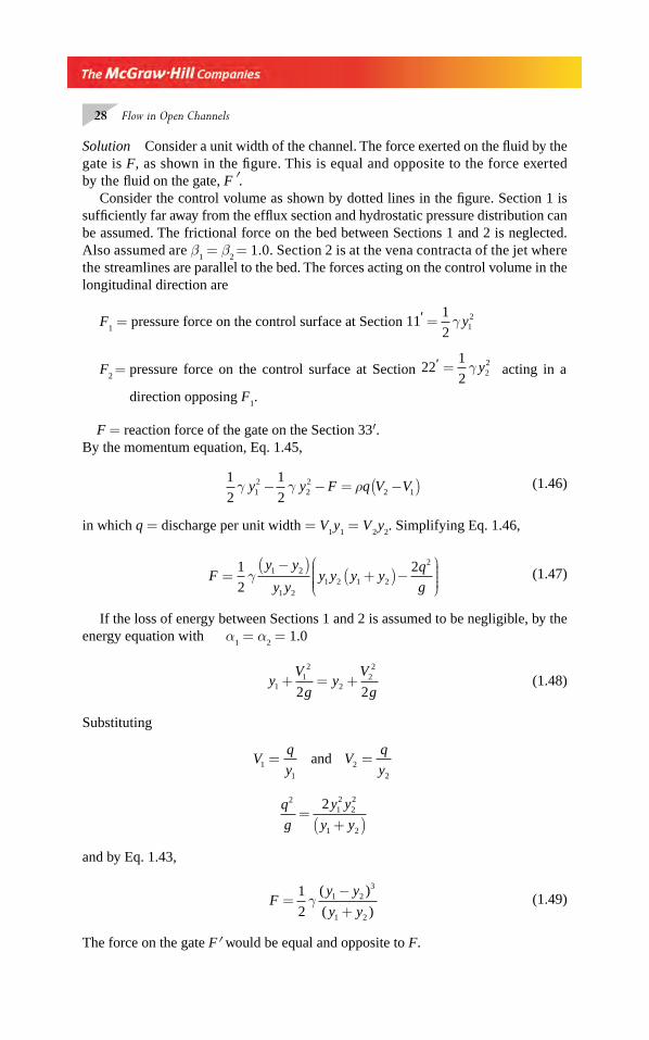
28 Flow in Open Channels
Solution Consider a unit width of the channel. The force exerted on the fl uid by the gate is F, as shown in the fi gure. This is equal and opposite to the force exerted by the fl uid on the gate, F ′.
Consider the control volume as shown by dotted lines in the fi gure. Section 1 is suffi ciently far away from the effl ux section and hydrostatic pressure distribution can be assumed. The frictional force on the bed between Sections 1 and 2 is neglected. Also assumed are β
1 = β
2 = 1.0. Section 2 is at the vena contracta of the jet where
the streamlines are parallel to the bed. The forces acting on the control volume in the longitudinal direction are
F1 = pressure force on the control surface at Section 11
1
2 12' = γ y
F2 = pressure force on the control surface at Section 22
1
2 22= γ y' acting in a
direction opposing F1.
F = reaction force of the gate on the Section 33′.By the momentum equation, Eq. 1.45,
1
2
1
212
22
2 1γ γ ρy y F q V V− − = −( )
(1.46)
in which q = discharge per unit width = V1 y
1 = V
2 y
2. Simplifying Eq. 1.46,
Fy y
y yy y y y
q
gs=
−( )+( )−
⎛
⎝⎜⎜⎜⎜
⎞
⎠⎟⎟⎟⎟
1
2
21 2
1 21 2 1 2
2
γ (1.47)
If the loss of energy between Sections 1 and 2 is assumed to be negligible, by the energy equation with α
1 = α
2 = 1.0
yV
gy
V
g112
222
2 2+ = + (1.48)
Substituting
V
q
yV
q
y11
22
= =and
q
g
y y
y y
212
22
1 2
2=
+( )
and by Eq. 1.43,
Fy y
y y=
−+
1
21 2
3
1 2
γ( )
( ) (1.49)
The force on the gate F′ would be equal and opposite to F.
Chapter 1.indd 28Chapter 1.indd 28 2/24/2010 2:42:25 PM2/24/2010 2:42:25 PM
Introduction 29
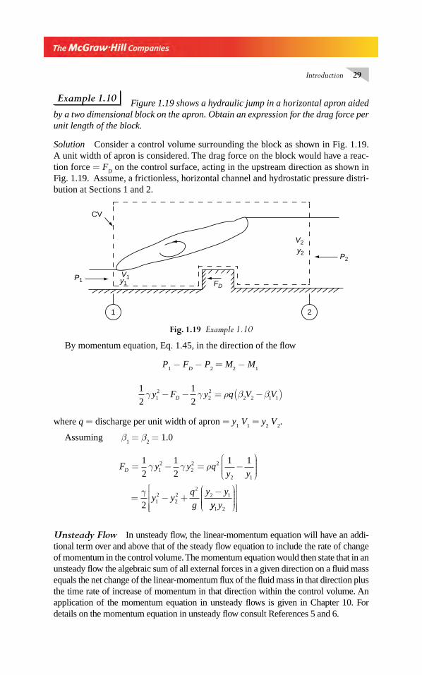
Example 1.10 Figure 1.19 shows a hydraulic jump in a horizontal apron aided by a two dimensional block on the apron. Obtain an expression for the drag force per unit length of the block.
Solution Consider a control volume surrounding the block as shown in Fig. 1.19. A unit width of apron is considered. The drag force on the block would have a reac-tion force = F
D on the control surface, acting in the upstream direction as shown in
Fig. 1.19. Assume, a frictionless, horizontal channel and hydrostatic pressure distri-bution at Sections 1 and 2.
Fig. 1.19 Example 1.10
1 2
CV
P1
P2
V1
V2
y1
y2
FD
By momentum equation, Eq. 1.45, in the direction of the fl ow
P1 − F
D − P
2 = M
2 − M
1
1
2
1
212
22
2 2 1 1γ γ ρ β βy F y q V VD− − = −( )
where q = discharge per unit width of apron = y1 V
1 = y
2 V
2.
Assuming β1 = β
2 = 1.0
F y y qy y
y yq
g
y y
D = − = −⎛
⎝⎜⎜⎜⎜
⎞
⎠⎟⎟⎟⎟
= − +−
1
2
1
2
1 1
2
12
22 2
2 1
12
22
22 1
γ γ ρ
γyy y1 2
⎛
⎝⎜⎜⎜⎜
⎞
⎠⎟⎟⎟⎟
⎡
⎣⎢⎢⎢
⎤
⎦⎥⎥⎥
Unsteady Flow In unsteady fl ow, the linear-momentum equation will have an addi-tional term over and above that of the steady fl ow equation to include the rate of change of momentum in the control volume. The momentum equation would then state that in an unsteady fl ow the algebraic sum of all external forces in a given direction on a fl uid mass equals the net change of the linear-momentum fl ux of the fl uid mass in that direction plus the time rate of increase of momentum in that direction within the control volume. An application of the momentum equation in unsteady fl ows is given in Chapter 10. For details on the momentum equation in unsteady fl ow consult References 5 and 6.
Chapter 1.indd 29Chapter 1.indd 29 2/24/2010 2:42:26 PM2/24/2010 2:42:26 PM
30 Flow in Open Channels
Specifi c Force The steady-state momentum equation (Eq. 1.45) takes a simple form if the tangential force F
3 and body force F
4 are both zero. In that case
F1 − F
2 = M
2 − M
1
or F1 + M
1 = F
2 + M
2
Denoting 1
γF M Ps+( ) =
(Ps)
1 = (P
s)
2 (1.50)
The term Ps is known as the specifi c force and represents the sum of the pressure
force and momentum fl ux per unit weight of the fl uid at a section. Equation (1.50) states that the specifi c force is constant in a horizontal, frictionless channel. This fact can be advantageously used to solve some fl ow situations. An application of the spe-cifi c force relationship to obtain an expression for the depth at the end of a hydraulic jump is given in Section 6.4. In a majority of applications the force F is taken as due
to hydrostatic pressure distribution and hence is given by, F Ay= γ where y is the
depth of the centre of gravity of the fl ow area.
REFERENCES
1. Graf, W H, Hydraulics of Sediment Transport, McGraw-Hill, New York, 1971.2. ASCE, Sedimentation Engineering, American Soc. of Civil Engrs., Manual No. 54, New
York, 1977.3. King, H W, Handbook of Hydraulics, McGraw-Hill, New York, 1954, pp 7–12.4. Jaeger, C, Engineering Fluid Mechanics, Blackie and Son, London, 1957.5. White, F M, Fluid Mechanics, 3rd ed., McGraw-Hill, New York, 1994.6. Daily, J W and Harleman, D R F, Fluid Dynamics, Addison-Wesley, New York, 1966.7. Chow, V T, Open Channel Hydraulics, McGraw-Hill, New York, 1959.
PROBLEMS
Problem Distribution
Topic Problems
Classifi cation 1.1
α and β 1.2 – 1.6
Pressure distribution 1.7 – 1.14
Continuity equation 1.15 – 1.17
Energy equation 1.18 – 1.22
Momentum equation 1.23 – 1.31
1.1 Classify the following open-channel fl ow situations:( a) Flow from a sluice gate(b) Flow in a main irrigation canal( c) A river during fl ood
Chapter 1.indd 30Chapter 1.indd 30 2/24/2010 2:42:26 PM2/24/2010 2:42:26 PM
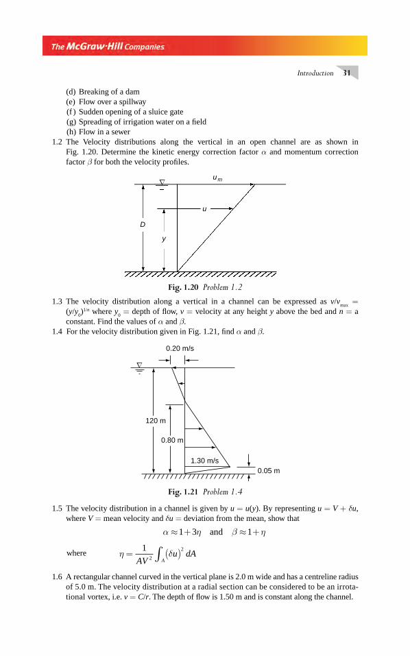
Introduction 31
(d) Breaking of a dam(e) Flow over a spillway(f ) Sudden opening of a sluice gate(g) Spreading of irrigation water on a fi eld(h) Flow in a sewer
1.2 The Velocity distributions along the vertical in an open channel are as shown in Fig. 1.20. Determine the kinetic energy correction factor α and momentum correction factor β for both the velocity profi les.
D
y
u
um∇
Fig. 1.20 Problem 1.2
1.3 The velocity distribution along a vertical in a channel can be expressed as v/vmax
= (y/y
0)1/n where y
0 = depth of fl ow, v = velocity at any height y above the bed and n = a
constant. Find the values of α and β.1.4 For the velocity distribution given in Fig. 1.21, fi nd α and β.
∇
0.20 m/s
120 m
0.80 m
0.05 m1.30 m/s
Fig. 1.21 Problem 1.4
1.5 The velocity distribution in a channel is given by u = u(y). By representing u = V + δu, where V = mean velocity and δu = deviation from the mean, show that
α η β η≈ + ≈ +1 3 1and
where η δ= ( )∫1
2
2
AVu dA
A
1.6 A rectangular channel curved in the vertical plane is 2.0 m wide and has a centreline radius of 5.0 m. The velocity distribution at a radial section can be considered to be an irrota-tional vortex, i.e. v = C/r. The depth of fl ow is 1.50 m and is constant along the channel.
Chapter 1.indd 31Chapter 1.indd 31 2/24/2010 2:42:27 PM2/24/2010 2:42:27 PM
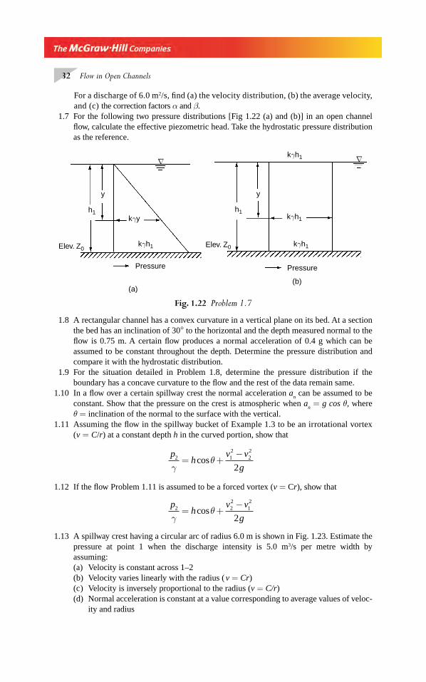
32 Flow in Open Channels
For a discharge of 6.0 m2/s, fi nd (a) the velocity distribution, (b) the average velocity, and (c) the correction factors α and β.
1.7 For the following two pressure distributions [Fig 1.22 (a) and (b)] in an open channel fl ow, calculate the effective piezometric head. Take the hydrostatic pressure distribution as the reference.
Fig. 1.22 Problem 1.7
h1
y
kγy
kγh1Elev. Z0
Pressure
∇
(a)
h1
y
kγh1
kγh1
kγh1Elev. Z0
Pressure
∇
(b)
1.8 A rectangular channel has a convex curvature in a vertical plane on its bed. At a section the bed has an inclination of 30° to the horizontal and the depth measured normal to the fl ow is 0.75 m. A certain fl ow produces a normal acceleration of 0.4 g which can be assumed to be constant throughout the depth. Determine the pressure distribution and compare it with the hydrostatic distribution.
1.9 For the situation detailed in Problem 1.8, determine the pressure distribution if the boundary has a concave curvature to the fl ow and the rest of the data remain same.
1.10 In a fl ow over a certain spillway crest the normal acceleration an can be assumed to be
constant. Show that the pressure on the crest is atmospheric when an = g cos θ, where
θ = inclination of the normal to the surface with the vertical.1.11 Assuming the fl ow in the spillway bucket of Example 1.3 to be an irrotational vortex
(v = C/r) at a constant depth h in the curved portion, show that
ph
v v
g2 1
222
2γθ= +
−cos
1.12 If the fl ow Problem 1.11 is assumed to be a forced vortex (v = Cr), show that
ph
v v
g2 2
212
2γθ= +
−cos
1.13 A spillway crest having a circular arc of radius 6.0 m is shown in Fig. 1.23. Estimate the pressure at point 1 when the discharge intensity is 5.0 m3/s per metre width by assuming:
(a) Velocity is constant across 1–2 (b) Velocity varies linearly with the radius ( v = Cr) (c ) Velocity is inversely proportional to the radius (v = C/r) (d) Normal acceleration is constant at a value corresponding to average values of veloc-
ity and radius
Chapter 1.indd 32Chapter 1.indd 32 2/24/2010 2:42:27 PM2/24/2010 2:42:27 PM
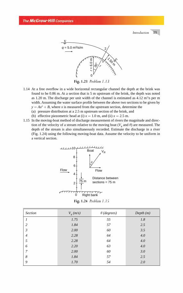
Introduction 33
1.14 At a free overfl ow in a wide horizontal rectangular channel the depth at the brink was found to be 0.86 m. At a section that is 5 m upstream of the brink, the depth was noted as 1.20 m. The discharge per unit width of the channel is estimated as 4.12 m3/s per m width. Assuming the water surface profi le between the above two sections to be given by y = Ax2 + B, where x is measured from the upstream section, determine the
(a) pressure distribution at a 2.5 m upstream section of the brink, and (b) effective piezometric head at (i) x = 1.0 m, and (ii) x = 2.5 m.1.15 In the moving-boat method of discharge measurement of rivers the magnitude and direc-
tion of the velocity of a stream relative to the moving boat (VR and θ) are measured. The
depth of the stream is also simultaneously recorded. Estimate the discharge in a river (Fig. 1.24) using the following moving-boat data. Assume the velocity to be uniform in a vertical section.
Fig. 1.23 Problem 1.13
∇
∇
2
1
0
q = 5.0 m3/s/m
r =
6.0
m30
˚
r
1.50 m
Section VR (m/s) θ (degrees) Depth (m)
1 1.75 55 1.8
2 1.84 57 2.5
3 2.00 60 3.5
4 2.28 64 4.0
5 2.28 64 4.0
6 2.20 63 4.0
7 2.00 60 3.0
8 1.84 57 2.5
9 1.70 54 2.0
Fig. 1.24 Problem 1.15
Flow
10
8
6
4
275 m
θ
Flow
Distance betweensections = 75 m
Boat VR
0 Right bank
Chapter 1.indd 33Chapter 1.indd 33 2/24/2010 2:42:27 PM2/24/2010 2:42:27 PM
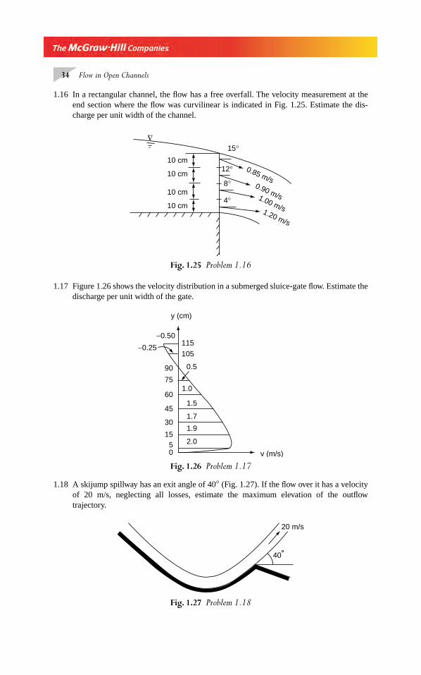
34 Flow in Open Channels
1.16 In a rectangular channel, the fl ow has a free overfall. The velocity measurement at the end section where the fl ow was curvilinear is indicated in Fig. 1.25. Estimate the dis-charge per unit width of the channel.
Fig. 1.25 Problem 1.16
∇15°
12°
8°
4°
10 cm
10 cm
10 cm
10 cm
0.85 m/s0.90 m/s1.00 m/s1.20 m/s
1.17 Figure 1.26 shows the velocity distribution in a submerged sluice-gate fl ow. Estimate the discharge per unit width of the gate.
1.18 A skijump spillway has an exit angle of 40° (Fig. 1.27). If the fl ow over it has a velocity of 20 m/s, neglecting all losses, estimate the maximum elevation of the outfl ow trajectory.
Fig. 1.27 Problem 1.18
20 m/s
40˚
Fig. 1.26 Problem 1.17
y (cm)
−0.50
−0.25115
105
0.5
1.0
1.5
1.7
1.9
2.0
90
75
60
45
30
1550 v (m/s)
Chapter 1.indd 34Chapter 1.indd 34 2/24/2010 2:42:28 PM2/24/2010 2:42:28 PM
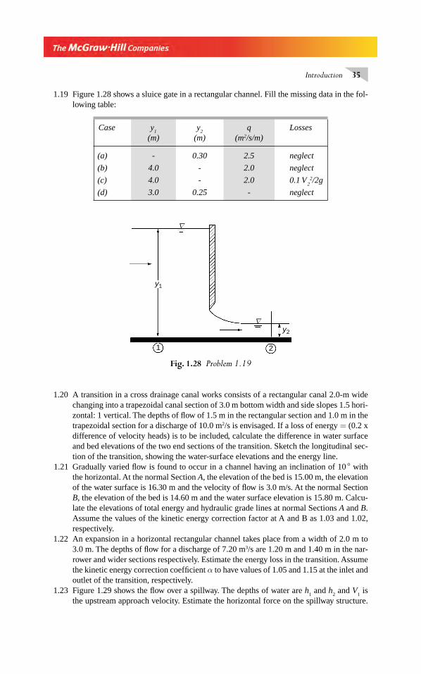
Introduction 35
1.19 Figure 1.28 shows a sluice gate in a rectangular channel. Fill the missing data in the fol-lowing table:
Case y1
(m)y
2
(m)q
(m2/s/m)Losses
(a) - 0.30 2.5 neglect
(b) 4.0 - 2.0 neglect
(c) 4.0 - 2.0 0.1 V 2
2/2g
(d) 3.0 0.25 - neglect
Fig. 1.28 Problem 1.19
y1
y2
∇
∇
1 2
1.20 A transition in a cross drainage canal works consists of a rectangular canal 2.0-m wide changing into a trapezoidal canal section of 3.0 m bottom width and side slopes 1.5 hori-zontal: 1 vertical. The depths of fl ow of 1.5 m in the rectangular section and 1.0 m in the trapezoidal section for a discharge of 10.0 m2/s is envisaged. If a loss of energy = (0.2 x difference of velocity heads) is to be included, calculate the difference in water surface and bed elevations of the two end sections of the transition. Sketch the longitudinal sec-tion of the transition, showing the water-surface elevations and the energy line.
1.21 Gradually varied fl ow is found to occur in a channel having an inclination of 10 ° with the horizontal. At the normal Section A, the elevation of the bed is 15.00 m, the elevation of the water surface is 16.30 m and the velocity of fl ow is 3.0 m/s. At the normal Section B, the elevation of the bed is 14.60 m and the water surface elevation is 15.80 m. Calcu-late the elevations of total energy and hydraulic grade lines at normal Sections A and B. Assume the values of the kinetic energy correction factor at A and B as 1.03 and 1.02, respectively.
1.22 An expansion in a horizontal rectangular channel takes place from a width of 2.0 m to 3.0 m. The depths of fl ow for a discharge of 7.20 m3/s are 1.20 m and 1.40 m in the nar-rower and wider sections respectively. Estimate the energy loss in the transition. Assume the kinetic energy correction coeffi cient α to have values of 1.05 and 1.15 at the inlet and outlet of the transition, respectively.
1.23 Figure 1.29 shows the fl ow over a spillway. The depths of water are h1 and h
2 and V
1 is
the upstream approach velocity. Estimate the horizontal force on the spillway structure.
Chapter 1.indd 35Chapter 1.indd 35 2/24/2010 2:42:28 PM2/24/2010 2:42:28 PM
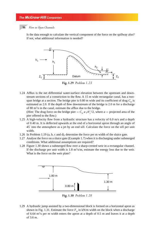
36 Flow in Open Channels
Is the data enough to calculate the vertical component of the force on the spillway also? If not, what additional information is needed?
Fig. 1.29 Problem 1.23
∇
∇
V1 h1
Z1 Z2
h2
Datum
1.24 Affl ux is the net differential water-surface elevation between the upstream and down-stream sections of a constriction to the fl ow. A 15 m wide rectangular canal, has a two-span bridge at a section. The bridge pier is 0.80 m wide and its coeffi cient of drag C
D is
estimated as 2.0. If the depth of fl ow downstream of the bridge is 2.0 m for a discharge of 80 m3/s in the canal, estimate the affl ux due to the bridge.
(Hint: The drag force on the bridge pier = CD a ρV
12/2, where a = projected area of the
pier offered to the fl ow.)1.25 A high-velocity fl ow from a hydraulic structure has a velocity of 6.0 m/s and a depth
of 0.40 m. It is defl ected upwards at the end of a horizontal apron through an angle of 45° into the atmosphere as a jet by an end sill. Calculate the force on the sill per unit width.
1.26 In Problem 1.19 (a, b, c and d), determine the force per m width of the sluice gate.1.27 Analyse the force on a sluice gate (Example 1.7) when it is discharging under submerged
conditions. What additional assumptions are required?1.28 Figure 1.30 shows a submerged fl ow over a sharp-crested weir in a rectangular channel.
If the discharge per unit width is 1.8 m3/s/m, estimate the energy loss due to the weir. What is the force on the weir plate?
Fig. 1.30 Problem 1.28
0.80 m
1.30 m
1.80 m
1.29 A hydraulic jump assisted by a two-dimensional block is formed on a horizontal apron as shown in Fig. 1.31. Estimate the force F
D in kN/m width on the block when a discharge
of 6.64 m3/s per m width enters the apron at a depth of 0.5 m and leaves it at a depth of 3.6 m.
Chapter 1.indd 36Chapter 1.indd 36 2/24/2010 2:42:28 PM2/24/2010 2:42:28 PM
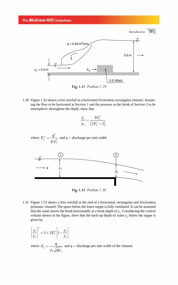
Introduction 37
1.30 Figure 1.32 shows a free overfall in a horizontal frictionless rectangular channel. Assum-ing the fl ow to be horizontal at Section 1 and the pressure at the brink of Section 2 to be atmospheric throughout the depth, show that
y
y
F
Fe
0
02
02
2
2 1=
+( )
where Fq
g y02
2
03
= and q = discharge per unit width.
Fig. 1.31 Problem 1.29
2-D Block
FD
3.6 m
q = 6.64 m3/s/m
y1 = 0.5 m
1.31 Figure 1.33 shows a free overfall at the end of a horizontal, rectangular and frictionless prismatic channel. The space below the lower nappe is fully ventilated. It can be assumed that the water leaves the brink horizontally at a brink depth of y
e. Considering the control
volume shown in the fi gure, show that the back-up depth of water y1 below the nappe is
given by
y
yF
y
ye
1
2
2
22 21 2 1
⎡
⎣⎢⎢
⎤
⎦⎥⎥ = + −
⎡
⎣⎢⎢
⎤
⎦⎥⎥
where Fq
y gy2
2 2
= and q = discharge per unit width of the channel.
Fig. 1.32 Problem 1.30
21
y1ye
q
∇
Chapter 1.indd 37Chapter 1.indd 37 2/24/2010 2:42:29 PM2/24/2010 2:42:29 PM
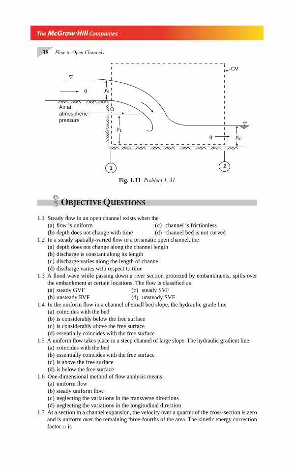
38 Flow in Open Channels
OBJECTIVE QUESTIONS
1.1 Steady fl ow in an open channel exists when the(a) fl ow is uniform ( c) channel is frictionless(b) depth does not change with time (d) channel bed is not curved
1.2 In a steady spatially-varied fl ow in a prismatic open channel, the(a) depth does not change along the channel length(b) discharge is constant along its length(c ) discharge varies along the length of channel(d) discharge varies with respect to time
1.3 A fl ood wave while passing down a river section protected by embankments, spills over the embankment at certain locations. The fl ow is classifi ed as(a) steady GVF (c ) steady SVF(b) unsteady RVF (d) unsteady SVF
1.4 In the uniform fl ow in a channel of small bed slope, the hydraulic grade line(a) coincides with the bed(b) is considerably below the free surface(c ) is considerably above the free surface(d) essentially coincides with the free surface
1.5 A uniform fl ow takes place in a steep channel of large slope. The hydraulic gradient line(a) coincides with the bed(b) essentially coincides with the free surface(c ) is above the free surface(d) is below the free surface
1.6 One-dimensional method of fl ow analysis means(a) uniform fl ow(b) steady uniform fl ow(c ) neglecting the variations in the transverse directions(d) neglecting the variations in the longitudinal direction
1.7 At a section in a channel expansion, the velocity over a quarter of the cross-section is zero and is uniform over the remaining three-fourths of the area. The kinetic energy correction factor α is
21
∇
∇
O
y1
y2
yeq
q
CV
Air atatmosphericpressure
Fig. 1.33 Problem 1.31
Chapter 1.indd 38Chapter 1.indd 38 2/24/2010 2:42:29 PM2/24/2010 2:42:29 PM
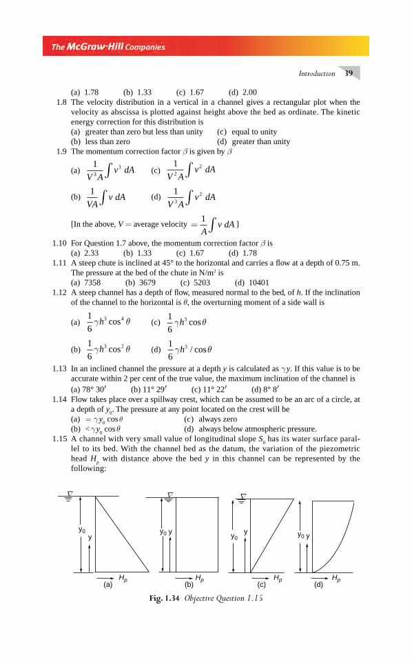
Introduction 39
(a) 1.78 (b) 1.33 (c) 1.67 (d) 2.00 1.8 The velocity distribution in a vertical in a channel gives a rectangular plot when the
velocity as abscissa is plotted against height above the bed as ordinate. The kinetic energy correction for this distribution is
(a) greater than zero but less than unity (c ) equal to unity (b) less than zero (d) greater than unity 1.9 The momentum correction factor β is given by β
(a) 13
3
V Av dA∫ (c)
12
2
V Av dA∫
(b) 1
VAv dA∫ (d)
13
2
V Av dA∫
[In the above, V = average velocity = ∫1
Av dA ]
1.10 For Question 1.7 above, the momentum correction factor β is (a) 2.33 (b) 1.33 (c) 1.67 (d) 1.781.11 A steep chute is inclined at 45° to the horizontal and carries a fl ow at a depth of 0.75 m.
The pressure at the bed of the chute in N/m2 is (a) 7358 (b) 3679 (c) 5203 (d) 104011.12 A steep channel has a depth of fl ow, measured normal to the bed, of h. If the inclination
of the channel to the horizontal is θ, the overturning moment of a side wall is
(a) 1
63 4γ θh cos (c)
1
63γ θh cos
(b) 1
63 2γ θh cos (d)
1
63γ θh / cos
1.13 In an inclined channel the pressure at a depth y is calculated as γ y. If this value is to be accurate within 2 per cent of the true value, the maximum inclination of the channel is
(a) 78° 30′ (b) 11° 29′ (c) 11° 22′ (d) 8° 8′1.14 Flow takes place over a spillway crest, which can be assumed to be an arc of a circle, at
a depth of y0. The pressure at any point located on the crest will be
(a) = γ y0 cos θ (c ) always zero
(b) < γ y0 cos θ (d) always below atmospheric pressure.
1.15 A channel with very small value of longitudinal slope S0 has its water surface paral-
lel to its bed. With the channel bed as the datum, the variation of the piezometric head H
p with distance above the bed y in this channel can be represented by the
following:
Fig. 1.34 Objective Question 1.15
HpHpHp Hp
y0 y0 y0y0y
y y y
∇ ∇ ∇
(a) (b) (c) (d)
Chapter 1.indd 39Chapter 1.indd 39 2/24/2010 2:42:30 PM2/24/2010 2:42:30 PM
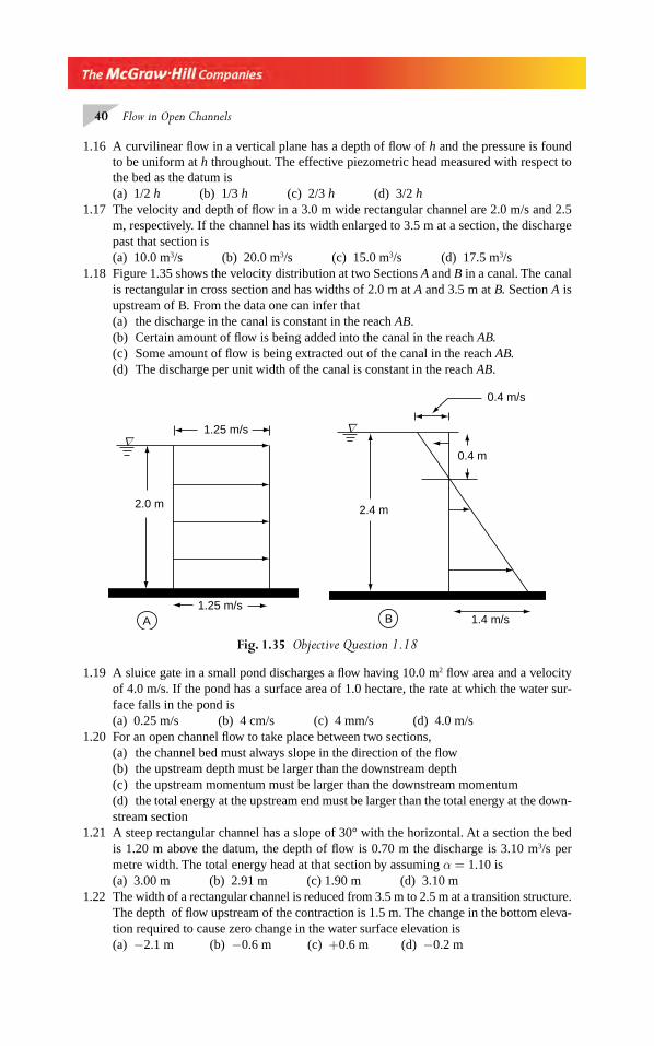
40 Flow in Open Channels
1.16 A curvilinear fl ow in a vertical plane has a depth of fl ow of h and the pressure is found to be uniform at h throughout. The effective piezometric head measured with respect to the bed as the datum is
(a) 1/2 h (b) 1/3 h (c) 2/3 h (d) 3/2 h1.17 The velocity and depth of fl ow in a 3.0 m wide rectangular channel are 2.0 m/s and 2.5
m, respectively. If the channel has its width enlarged to 3.5 m at a section, the discharge past that section is
(a) 10.0 m3/s (b) 20.0 m3/s (c) 15.0 m3/s (d) 17.5 m3/s1.18 Figure 1.35 shows the velocity distribution at two Sections A and B in a canal. The canal
is rectangular in cross section and has widths of 2.0 m at A and 3.5 m at B. Section A is upstream of B. From the data one can infer that
(a) the discharge in the canal is constant in the reach AB. (b) Certain amount of fl ow is being added into the canal in the reach AB. (c ) Some amount of fl ow is being extracted out of the canal in the reach AB. (d) The discharge per unit width of the canal is constant in the reach AB.
Fig. 1.35 Objective Question 1.18
∇∇1.25 m/s
2.0 m
1.25 m/sA B
2.4 m
1.4 m/s
0.4 m
0.4 m/s
1.19 A sluice gate in a small pond discharges a fl ow having 10.0 m2 fl ow area and a velocity of 4.0 m/s. If the pond has a surface area of 1.0 hectare, the rate at which the water sur-face falls in the pond is
(a) 0.25 m/s (b) 4 cm/s (c) 4 mm/s (d) 4.0 m/s1.20 For an open channel fl ow to take place between two sections, (a) the channel bed must always slope in the direction of the fl ow (b) the upstream depth must be larger than the downstream depth (c ) the upstream momentum must be larger than the downstream momentum (d) the total energy at the upstream end must be larger than the total energy at the down-
stream section1.21 A steep rectangular channel has a slope of 30° with the horizontal. At a section the bed
is 1.20 m above the datum, the depth of fl ow is 0.70 m the discharge is 3.10 m3/s per metre width. The total energy head at that section by assuming α = 1.10 is
(a) 3.00 m (b) 2.91 m (c) 1.90 m (d) 3.10 m1.22 The width of a rectangular channel is reduced from 3.5 m to 2.5 m at a transition structure.
The depth of fl ow upstream of the contraction is 1.5 m. The change in the bottom eleva-tion required to cause zero change in the water surface elevation is
(a) −2.1 m (b) −0.6 m (c) +0.6 m (d) −0.2 m
Chapter 1.indd 40Chapter 1.indd 40 2/24/2010 2:42:30 PM2/24/2010 2:42:30 PM

Introduction 41
1.23 The total energy head for an open channel fl ow is written with usual notation as H = z + y + V 2/2g. In this each of the terms represent
(a) energy in kg m/kg mass of fl uid (b) energy in N m/N of fl uid (c ) power in kW/kg mass of fl uid (d) energy in N m/ mass of fl uid1.24 Piezometric head is the sum of (a) pressure head, datum head and velocity head (b) datum head and velocity head (c ) pressure head and velocity head (d) pressure head and datum head1.25 The difference between total head line and piezometric head line represents (a) the velocity head (b) the pressure head (c ) the elevation of the bed of the channel (d) the depth of fl ow1.26 The momentum equation in x-direction as ΣF
x =ρQ
1(V
x 2 – V
x 1) has the assumption that
the fl ow is (a) steady (c ) uniform (b) unsteady (d) frictionless1.27 Normally in a stream the ratio of the surface velocity at a location to the average velocity
in the vertical through that location (a) is greater than 1.0 (b) will be between 0.8 and 0.95 (c ) is less than or greater than unity depending on the type of fl ow (d) is equal to 0.61.28 The specifi c force is constant (a) in all frictionless channels irrespective of the magnitude of the longitudinal slope (b) in horizontal, frictionless channels of any shape (c ) in all horizontal channels of any shape (d) in any open channel
Chapter 1.indd 41Chapter 1.indd 41 2/24/2010 2:42:30 PM2/24/2010 2:42:30 PM
2.1 SPECIFIC ENERGY
The total energy of a channel fl ow referred to a datum is given by Eq.1.39 as
H Z y
V
g= + +cosθ α
2
2
If the datum coincides with the channel bed at the section, the resulting expression is know as specifi c energy and is denoted by E. Thus
E yV
g= +cosθ α
2
2 (2.1)
When cos θ = 1.0 and α = 1.0,
E yV
g= +
2
2 (2.2)
The concept of specifi c energy, introduced by Bakhmeteff, is very useful in defi ning critical depth and in the analysis of fl ow problems. It may be noted that while the total energy in a real fl uid fl ow always decreases in the downstream direction, the specifi c energy is constant for a uniform fl ow and can either decrease or increase in a varied fl ow, since the elevation of the bed of the channel relative to the elevation of the total energy line, determines the specifi c energy. If the fric-tional resistance of the fl ow can be neglected, the total energy in non-uniform fl ow will be constant at all sections while the specifi c energy for such fl ows, however, will be constant only for a horizontal bed channel and in all other cases the specifi c energy will vary.
To simplify the expressions it will be assumed, for use in all further analysis, that the specifi c energy is given by Eq. 2.2, i.e., cos θ = 1.0 and α = 1.0. This is with the knowledge that cos θ and α can be appended to y and (V 2/2g) terms respectively, without diffi culty if warranted.
Energy–Depth
Relationships 2
Chapter 2.indd 42Chapter 2.indd 42 2/24/2010 2:55:49 PM2/24/2010 2:55:49 PM
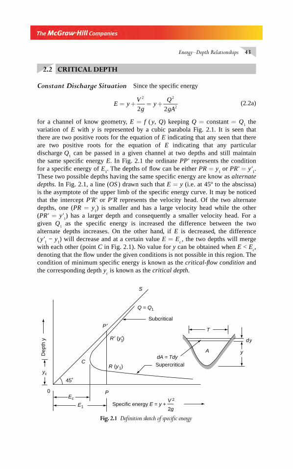
Energy–Depth Relationships 43
2.2 CRITICAL DEPTH
Constant Discharge Situation Since the specifi c energy
E yV
gy
Q
gA= + = +
2 2
22 2 (2.2a)
for a channel of know geometry, E = f ( y, Q) keeping Q = constant = Q1 the
variation of E with y is represented by a cubic parabola Fig. 2.1. It is seen that there are two positive roots for the equation of E indicating that any seen that there are two positive roots for the equation of E indicating that any particular discharge Q
1 can be passed in a given channel at two depths and still maintain
the same specifi c energy E. In Fig. 2.1 the ordinate PP' represents the condition for a specifi c energy of E
1. The depths of fl ow can be either PR = y
1 or PR' = y'
1.
These two possible depths having the same specifi c energy are know as alternate depths. In Fig. 2.1, a line (OS ) drawn such that E = y (i.e. at 45º to the abscissa) is the asymptote of the upper limb of the specifi c energy curve. It may be noticed that the intercept P'R' or P'R represents the velocity head. Of the two alternate depths, one (PR = y
1) is smaller and has a large velocity head while the other
(PR' = y'1) has a larger depth and consequently a smaller velocity head. For a
given Q1 as the specifi c energy is increased the difference between the two
alternate depths increases. On the other hand, if E is decreased, the difference ( y'
1 − y
1) will decrease and at a certain value E = E
c , the two depths will merge
with each other (point C in Fig. 2.1). No value for y can be obtained when E < Ec,
denoting that the fl ow under the given conditions is not possible in this region. The condition of minimum specifi c energy is known as the critical-fl ow condition and the corresponding depth y
c is known as the critical depth.
Fig. 2.1 Defi nition sketch of specifi c energy
1
Dep
th y
yc
0
S
Q = Q1
SubcriticalP ′
P
R (y1)C
45˚
Ec
E1 Specific energy E = y +V 2
2g
T
A
dy
ydA = Tdy
Supercritical
R ′ (y )′
Chapter 2.indd 43Chapter 2.indd 43 2/24/2010 2:55:50 PM2/24/2010 2:55:50 PM
44 Flow in Open Channels
At critical depth, the specifi c energy is minimum. Thus differentiating Eq. 2.2a with respect to y (keeping Q constant) and equating to zero,
dE
dy
Q
gA
dA
dy= − =1 0
2
3 (2.3)
But dA
dyT= = top width, i.e. width of the channel at the water surface.
Designating the critical-fl ow conditions by the suffi x ‘c’,
Q T
gAc
c
2
31= (2.4)
or Q
g
A
Tc
c
2 3
= (2.4a)
If an α value other than unity is to be used, Eq. 2.4 will become
α Q T
gAc
c
2
31 0= . (2.5)
Equation 2.4 or 2.5 is the basic equation governing the critical-fl ow conditions in a channel. It may be noted that the critical-fl ow condition is governed solely by the channel geometry and discharge (and α). Other channel properties such as the bed slope and roughness do not infl uence the critical-fl ow condition for any given Q. If the Froude number of the fl ow is defi ne as
F V gA T= ( )/ (2.6)
it is easy to see that by using F in Eq. 2.4, at the critical fl ow y = yc and F = F
c = 1.0.
We thus get an important result that the critical fl ow corresponds to the minimum specifi c energy and at this condition the Froude number of the fl ow is unity. For a channel with large longitudinal slope θ and having a fl ow with an energy correction factor of α, the Froude number F will be defi ned as
F V gA
T=
⎛
⎝⎜⎜⎜⎜
⎞
⎠⎟⎟⎟⎟⎟
1
αcosθ (2.6a)
Referring to Fig. 2.1, considering any specifi c energy other than Ec, (say ordinate PP'
at E = E1) the Froude number of the fl ow corresponding to both the alternate depths
will be different from unity as y1 or y'
1 ≠ y
c. At the lower limb, CR of the specifi c-
energy curve, the depth y1 < y
c. As such, V'
1 > V
c and F
1 > 1.0. This region is called
the supercritical fl ow region. In the upper limb CR', y'1 > y
c. As such V'
1 < V
c and F'
1
< 1.0. This denotes the subcritical fl ow region. Discharge as a Variable In the above section the critical-fl ow condition was derived by keeping the discharge constant. The specifi c-energy diagram can be plotted
Chapter 2.indd 44Chapter 2.indd 44 2/24/2010 2:55:51 PM2/24/2010 2:55:51 PM
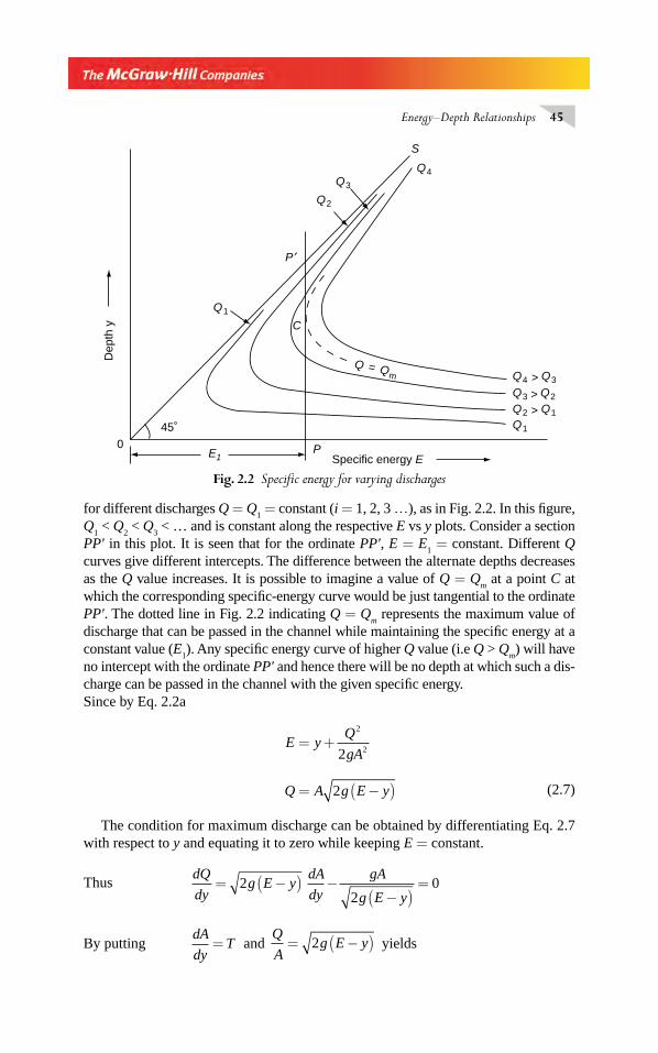
Energy–Depth Relationships 45
for different discharges Q = Q1 = constant (i = 1, 2, 3 …), as in Fig. 2.2. In this fi gure,
Q1 < Q
2 < Q
3 < … and is constant along the respective E vs y plots. Consider a section
PP' in this plot. It is seen that for the ordinate PP', E = E1 = constant. Different Q
curves give different intercepts. The difference between the alternate depths decreases as the Q value increases. It is possible to imagine a value of Q = Q
m at a point C at
which the corresponding specifi c-energy curve would be just tangential to the ordinate PP'. The dotted line in Fig. 2.2 indicating Q = Q
m represents the maximum value of
discharge that can be passed in the channel while maintaining the specifi c energy at a constant value (E
1). Any specifi c energy curve of higher Q value (i.e Q > Q
m) will have
no intercept with the ordinate PP' and hence there will be no depth at which such a dis-charge can be passed in the channel with the given specifi c energy.Since by Eq. 2.2a
E y
Q
gA= +
2
22
Q A g E y= −( )2 (2.7)
The condition for maximum discharge can be obtained by differentiating Eq. 2.7 with respect to y and equating it to zero while keeping E = constant.
Thus dQ
dyg E y
dA
dy
gA
g E y= −( ) −
−( )=2
20
By putting dA
dyT= and
Q
Ag E y= −( )2 yields
Fig. 2.2 Specifi c energy for varying discharges
Dep
th y
045˚
Specific energy E P
P ′
S
C
E1
Q4Q3
Q2
Q1
Q1
Q = Qm Q4 Q3>Q3 Q2>Q2 Q1>
Chapter 2.indd 45Chapter 2.indd 45 2/24/2010 2:55:51 PM2/24/2010 2:55:51 PM
46 Flow in Open Channels
Q T
gA
2
31 0= . (2.8)
This is same as Eq. 2.4 and hence represents the critical-fl ow conditions. Hence, the critical-fl ow condition also corresponds to the condition for maximum discharge in a channel for a fi xed specifi c energy.
Example 2.1 A 2.5-m wide rectangular channel has a specifi c energy of 1.50 m when carrying a discharge of 6.48 m3/s. Calculate the alternate depths and corre-sponding Froude numbers.
Solution From Eq. 2.2a
E y
V
gy
Q
gB y= + = +
2 2
2 22 2
1 5
6 48
2 9 81 2 5
2
2 2.
( . )
. ( . )= +
× ×y
y
= +y
y
0 342432
.
Solving this equation by trial and error, the alternate depths y1 and y
2 are obtained as
y1 = 1.296 m and y
2 = 0.625 m.
Froude number FV
gy y y y= = =
6 48
2 5 9 81
0 827563 2
.
( . ) .
./
,
At y1 = 1.296 m, F
1 = 0.561; and
at y2 = 0.625 m, F
2 = 1.675
The depth y1 = 1.296 m is in the subcritical fl ow region and the depth y = 0.625 m
is in the supercritical fl ow region.
Example 2.2 A fl ow of 5.0 m3/s is passing at a depth of 1.5 m through a rectan-gular channel of 2.5 m width. The kinetic energy correction factor α is found to be 1.20. What is the specifi c energy of the fl ow? What is the value of the depth alternate to the existing depth if α = 1.0 is assumed for the alternate fl ow?
Solution VQ
A11
5 0
2 5 1 51 33= =
( )=
.
. ..
× m/s
α112 2
21 20
1 33
2 9 810 1087
V
g=
( )=.
.
..×
× m
Chapter 2.indd 46Chapter 2.indd 46 2/24/2010 2:55:52 PM2/24/2010 2:55:52 PM
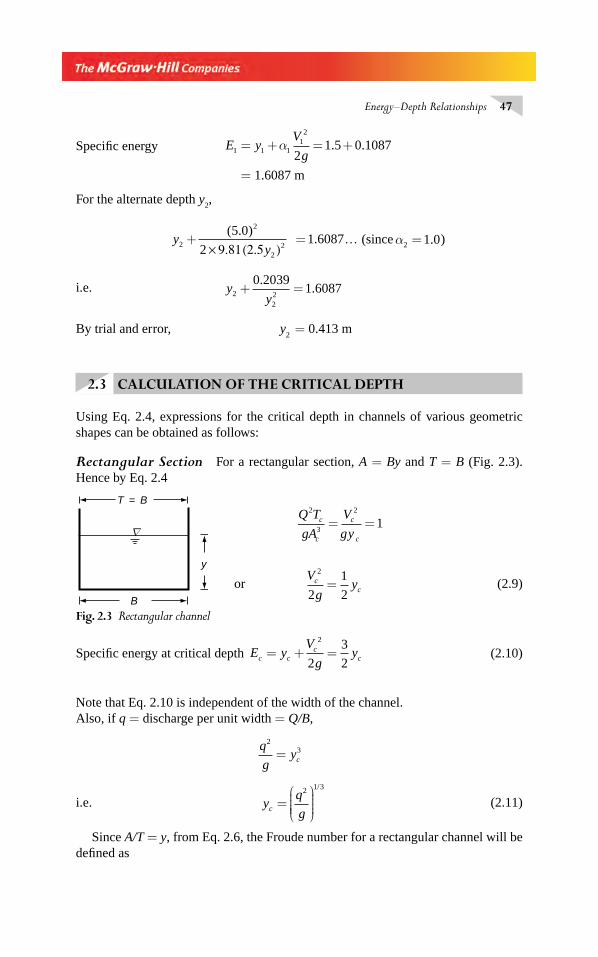
Energy–Depth Relationships 47
Specifi c energy E yV
g1 1 112
21 5 0 1087= + = +α . .
= 1.6087 m
For the alternate depth y2,
yy2
2
22
5 0
21 6087+ =
( . ).
× 9.81 (2.5 )… (since α2 1 0= . )
i.e. yy2
22
0 20391 6087+ =
..
By trial and error, y2 = 0.413 m
2.3 CALCULATION OF THE CRITICAL DEPTH
Using Eq. 2.4, expressions for the critical depth in channels of various geometric shapes can be obtained as follows:
Rectangular Section For a rectangular section, A = By and T = B (Fig. 2.3). Hence by Eq. 2.4
Q T
gA
V
g yc
c
c
c
2
3
2
1= =
or V
gyc
c
2
2
1
2= (2.9)
Specifi c energy at critical depth E yV
gyc c
cc= + =
2
2
3
2 (2.10)
Note that Eq. 2.10 is independent of the width of the channel.Also, if q = discharge per unit width = Q/B,
q
gyc
23=
i.e. yq
gc =⎛
⎝⎜⎜⎜⎜
⎞
⎠⎟⎟⎟⎟
2 1 3/
(2.11)
Since A/T = y, from Eq. 2.6, the Froude number for a rectangular channel will be defi ned as
Fig. 2.3 Rectangular channel
∇
B
y
T = B
Chapter 2.indd 47Chapter 2.indd 47 2/24/2010 2:55:52 PM2/24/2010 2:55:52 PM
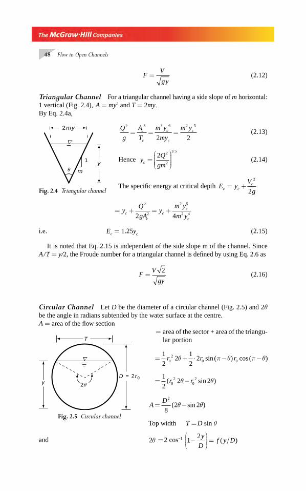
48 Flow in Open Channels
FV
gy= (2.12)
Triangular Channel For a triangular channel having a side slope of m horizontal: 1 vertical (Fig. 2.4), A = my2 and T = 2my.By Eq. 2.4a,
Q
g
A
T
m y
my
m yc
c
c
c
c2 3 3 6 2 5
2 2= = = (2.13)
Hence yQ
gmc =⎛
⎝⎜⎜⎜⎜
⎞
⎠⎟⎟⎟⎟
2 2
2
1 5/
(2.14)
The specifi c energy at critical depth E yV
gc cc= +
2
2
= + = +yQ
gAy
m y
m yc
c
cc
c
2
2
2 5
2 42 4
i.e. Ec = 1.25yc (2.15)
It is noted that Eq. 2.15 is independent of the side slope m of the channel. Since A / T = y/2, the Froude number for a triangular channel is defi ned by using Eq. 2.6 as
FV
gy=
2 (2.16)
Circular Channel Let D be the diameter of a circular channel (Fig. 2.5) and 2θ be the angle in radians subtended by the water surface at the centre.A = area of the fl ow section
= area of the sector + area of the triangu -lar portion
= + ⋅ − −1
22
1
220
20 0r r rθ π θ π θsin ( ) cos( )
= −1
22 20
20
2( sin )r rθ θ
AD
= −2
82 2( sin )θ θ
Top width T = D sin θ
and 2θ = 2 cos−1 12
−⎛⎝⎜⎜⎜
⎞⎠⎟⎟⎟⎟ =
y
Df y D( )
Fig. 2.4 Triangular channel
∇
y
m
2my
θ
1
Fig. 2.5 Circular channel
∇
T
y 2θ
D = 2 r0
Chapter 2.indd 48Chapter 2.indd 48 2/24/2010 2:55:52 PM2/24/2010 2:55:52 PM
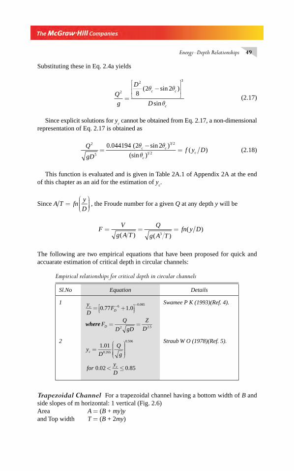
Energy–Depth Relationships 49
Substituting these in Eq. 2.4a yields
Q
g
D
D
c c
c
2
2 3
82 2
=−
⎡
⎣⎢⎢
⎤
⎦⎥⎥( sin )
sin
θ θ
θ (2.17)
Since explicit solutions for yc cannot be obtained from Eq. 2.17, a non-dimensional
representation of Eq. 2.17 is obtained as
Q
gDf y Dc c
c
c
2
5
3 2
1 2
0 044194 2 2=
−=
. ( sin )
(sin )( )
θ θθ
(2.18)
This function is evaluated and is given in Table 2A.1 of Appendix 2A at the endof this chapter as an aid for the estimation of y
c.
Since A T fny
D=
⎛⎝⎜⎜⎜
⎞⎠⎟⎟⎟⎟ , the Froude number for a given Q at any depth y will be
FV
g A T
Q
g A Tfn y D= = =
( ) ( )( )
3
The following are two empirical equations that have been proposed for quick and accuarate estimation of critical depth in circular channels:
Trapezoidal Channel For a trapezoidal channel having a bottom width of B and side slopes of m horizontal: 1 vertical (Fig. 2.6)Area A = (B + my)yand Top width T = (B + 2my)
Sl.No Equation Details
1 y
DF
FQ
D gD
Z
D
cD
D
= +⎡⎣⎢
⎤⎦⎥
= =
− −0 77 1 06 0 085
2 2 5
. ..
.where
Swamee P K (1993)(Ref. 4).
2
yD
Q
g
fory
D
c
c
=⎛
⎝⎜⎜⎜⎜⎜
⎞
⎠
⎟⎟⎟⎟⎟
< ≤
1 01
0 02 0 85
0 265
0 506
.
. .
.
. Straub W O (1978)(Ref. 5).
Empirical relationships for critical depth in circular channels
Chapter 2.indd 49Chapter 2.indd 49 2/24/2010 2:55:53 PM2/24/2010 2:55:53 PM
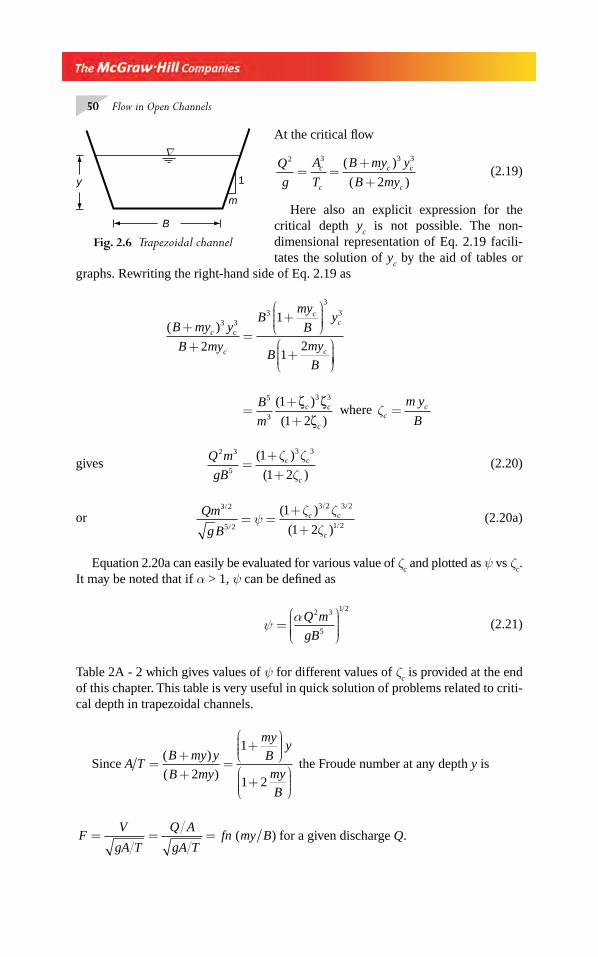
50 Flow in Open Channels
At the critical fl ow
Q
g
A
T
B my y
B myc
c
c c
c
2 3 3 3
2= =
++
( )
( ) (2.19)
Here also an explicit expression for the critical depth y
c is not possible. The non-
dimensional representation of Eq. 2.19 facili-tates the solution of y
c by the aid of tables or
graphs. Rewriting the right-hand side of Eq. 2.19 as
( )B my y
B my
Bmy
By
Bmy
B
c c
c
cc
c
++
=+
⎛
⎝⎜⎜⎜
⎞
⎠⎟⎟⎟⎟
+⎛
⎝⎜⎜⎜
⎞
⎠⎟⎟
3 33
3
3
2
1
12
⎟⎟⎟
=++
B
mc c
c
5
3
3 31
1 2
( )
( )
ζ ζζ
where ζccm y
B=
gives Q m
gBc c
c
2 3
5
3 31
1 2=
++
( )
( )
ζ ζζ
(2.20)
or Qm
gBc c
c
3 2
5 2
3 2 3 2
1 2
1
1 2
/
/
/ /
/
( )
( )= =
++
ψζ ζ
ζ (2.20a)
Equation 2.20a can easily be evaluated for various value of ζc and plotted as ψ vs ζ
c.
It may be noted that if α > 1, ψ can be defi ned as
ψα
=⎛
⎝⎜⎜⎜⎜
⎞
⎠⎟⎟⎟⎟
Q m
gB
2 3
5
1 2
(2.21)
Table 2A - 2 which gives values of ψ for different values of ζc is provided at the end
of this chapter. This table is very useful in quick solution of problems related to criti-cal depth in trapezoidal channels.
Since A TB my y
B my
my
By
my
B
=++
=+
⎛⎝⎜⎜⎜
⎞⎠⎟⎟⎟
+⎛⎝⎜⎜⎜
⎞⎠⎟⎟⎟
( )
( )2
1
1 2
the Froude number at any depth y is
FV
gA T
Q A
gA Tfn my B= = = ( ) for a given discharge Q.
Fig. 2.6 Trapezoidal channel
∇
y
B
m
1
Chapter 2.indd 50Chapter 2.indd 50 2/24/2010 2:55:53 PM2/24/2010 2:55:53 PM
Energy–Depth Relationships 51
Further the specifi c energy at critical depth, Ec is a function of (my
c / B) and it can
be shown that (Problem 2.7)
E
yc
c
c
c
=++
1
2
3 5
1 2
( )
( )
ζζ
where ζ ccmy
B=
2.4 SECTION FACTOR Z
The expression A A T is a function of the depth y for a given channel geometry and is known as the section factor Z.
Thus Z A A T= (2.22)
At the critical-fl ow condition, y = yc and
Z A A T Q gc c c c= = (2.23)
which is a convenient parameter for analysing the role of the critical depth in a fl ow problem.
As a corollary of Eq. 2.23, if Z is the section factor for any depth of fl ow y, then
Q g Zc = (2.24)
where Qc represents the discharge that would make the depth y critical and is known
as the critical discharge.Note that the left-hand side of Eq. 2.18 is a non-dimensional form of the section
factor (as Z/D 2.5) for circular channels.
2.5 FIRST HYDRAULIC EXPONENT M
In many computations involving a wide range of depths in a channel, such as in the GVF computations, it is convenient to express the variation of Z with y in an expo-nential form.The (Z – y) relationship
Z C yM21= (2.25)
is found to be very advantageous. In this equation C1 = a coeffi cient and M = an expo-
nent called the fi rst hydraulic exponent. It is found that generally M is a slowly-varying
Chapter 2.indd 51Chapter 2.indd 51 2/24/2010 2:55:53 PM2/24/2010 2:55:53 PM
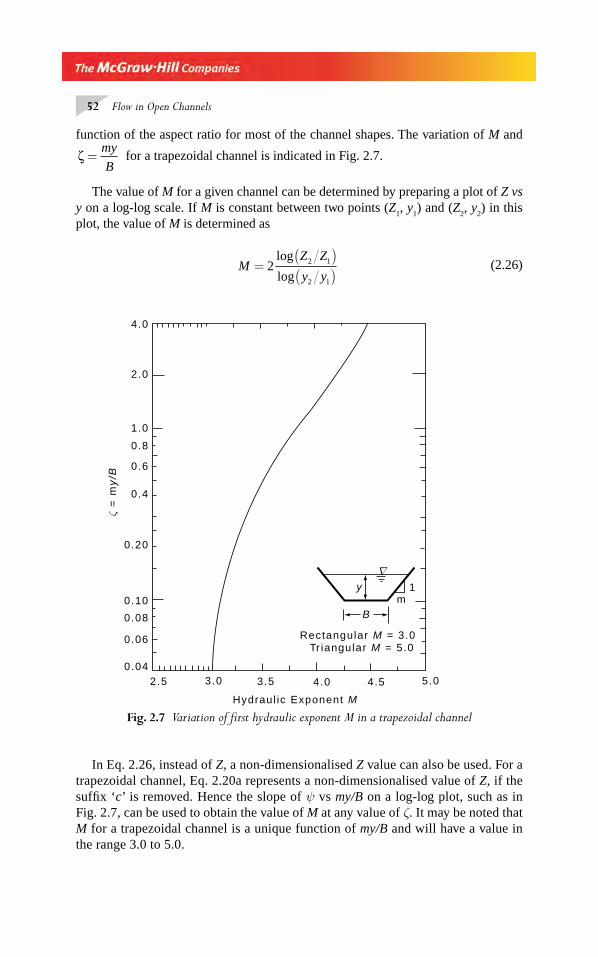
52 Flow in Open Channels
function of the aspect ratio for most of the channel shapes. The variation of M and
ζ =my
B for a trapezoidal channel is indicated in Fig. 2.7.
The value of M for a given channel can be determined by preparing a plot of Z vs y on a log-log scale. If M is constant between two points (Z
1, y
1) and (Z
2, y
2) in this
plot, the value of M is determined as
MZ Z
y y=
( )( )
2 2 1
2 1
log
log (2.26)
Fig. 2.7 Variation of fi rst hydraulic exponent M in a trapezoidal channel
∇
mB
y 1
Rectangular M = 3.0Tr iangular M = 5.0
Hydraul ic Exponent M
2.5 3.0 3.5 4.0 4.5 5.0
4.0
2.0
1.0
0.8
0.6
0.4
0.20
0.10
0.08
0.06
0.04
ζ =
my
/B
In Eq. 2.26, instead of Z, a non-dimensionalised Z value can also be used. For a trapezoidal channel, Eq. 2.20a represents a non-dimensionalised value of Z, if the suffi x ‘c’ is removed. Hence the slope of ψ vs my/B on a log-log plot, such as inFig. 2.7, can be used to obtain the value of M at any value of ζ. It may be noted that M for a trapezoidal channel is a unique function of my/B and will have a value in the range 3.0 to 5.0.
Chapter 2.indd 52Chapter 2.indd 52 2/24/2010 2:55:53 PM2/24/2010 2:55:53 PM
Energy–Depth Relationships 53
An estimate of M can also be obtained by the relation
My
AT
A
T
dT
dy= −
⎛
⎝⎜⎜⎜⎜
⎞
⎠⎟⎟⎟⎟3 (2.27)
Example 2.3 Obtain the value of the fi rst hydraulic exponent M for (a) rectangu-lar channel, and (b) an exponential channel where the area A is given as A = K
1 y a
Solution (a) For a rectangular channel A = By and T = B
By Eq. 2.25, zA
TB y C yM2
22 3
1= = =
By equating the exponents on both sides, M = 3.0[Note: The above value of M can also be obtained directly by using Eq. 2.27]
(b) A K ya= 1
TdA
dyK ay a= = −( )
11
By Eq. 2.27, My
AT
A
T
dT
dy= −( )3
My
K yK ay
K y
K ayK a a y
a
aa
a
a= − −{ }⎡
⎣⎢⎢
⎤
⎦⎥⎥
−( )−
−( )
1
11 1
11 1
23 1( )
( )
= − + = +3 1 2 1a a a
Example 2.4 It is required to have a channel in which the Froude number F remains constant at all depths. If the specifi c energy E is kept constant, show that for
such a channel T
B
E
E y
F
=−
⎡
⎣⎢⎢
⎤
⎦⎥⎥
+⎛
⎝⎜⎜⎜⎜⎜
⎞
⎠
⎟⎟⎟⎟⎟⎟1
2
2
where T and B are the top width and bottom width
of the channel respectively.
Solution E yV
gy
Q
gAy
F A
T= + = + = +
⎛⎝⎜⎜⎜
⎞⎠⎟⎟⎟⎟
2 2
2
2
2 2 2
E yAF
T− =
2
2 (2.28)
Chapter 2.indd 53Chapter 2.indd 53 2/24/2010 2:55:54 PM2/24/2010 2:55:54 PM
54 Flow in Open Channels
Differentiating with respect to y and noting that F is constant,
dE
dx
FT
dA
dyA
dT
dy
T− =
−⎛
⎝⎜⎜⎜⎜
⎞
⎠⎟⎟⎟⎟
⎡
⎣
⎢⎢⎢⎢⎢⎢⎢
⎤
⎦
⎥⎥⎥⎥⎥⎥⎥
12
2
2
Since E is constant,dE
dy = 0. Also
dA
dy = T
Hence, F A
T
dT
dy
2
221 1−
⎛
⎝⎜⎜⎜⎜
⎞
⎠⎟⎟⎟⎟ = −
AF
T T
dT
dy
F2 2
2
11
2= +
⎛
⎝⎜⎜⎜⎜
⎞
⎠⎟⎟⎟⎟
Substituting for AF
T
2
2
⎛
⎝⎜⎜⎜⎜
⎞
⎠⎟⎟⎟⎟
from Eq. 2.28, ( )E yT
dT
dy
F−
⎛
⎝⎜⎜⎜⎜
⎞
⎠⎟⎟⎟⎟ = +
⎛
⎝⎜⎜⎜⎜
⎞
⎠⎟⎟⎟⎟
11
2
2
dT
T
F dy
E y= +
⎛
⎝⎜⎜⎜⎜
⎞
⎠⎟⎟⎟⎟ −( )
12
2
On integration 1n TF
E y C= +⎛
⎝⎜⎜⎜⎜
⎞
⎠⎟⎟⎟⎟
− − +12
12
( ( ) )n
At y = 0, T = B and hence C = 1n BF
+ +⎛
⎝⎜⎜⎜⎜
⎞
⎠⎟⎟⎟⎟
12
2
1n E
∴ 1n T
B
F E
E y= +
⎛
⎝⎜⎜⎜⎜
⎞
⎠⎟⎟⎟⎟ −
⎛
⎝⎜⎜⎜⎜
⎞
⎠⎟⎟⎟⎟1
21
2
n
or T
B
E
E Y
F
=−
⎡
⎣⎢⎢
⎤
⎦⎥⎥
+⎛
⎝⎜⎜⎜⎜⎜
⎞
⎠
⎟⎟⎟⎟⎟⎟1
2
2
2.6 COMPUTATIONS
The problems concerning critical depth involve the following parameters: geom-etry of the channel, Q or E or y
c. For rectangular and triangular channel sections,
most of the problems involve explicit relationships for the variable and a few problems involve trial and error solutions. However, for trapezoidal, circular and most other regular geometrical shapes of channel sections, many of the problems have to be solved by trial and error procedure. Tables 2A.1 and 2A.2 are helpful
Chapter 2.indd 54Chapter 2.indd 54 2/24/2010 2:55:54 PM2/24/2010 2:55:54 PM
Energy–Depth Relationships 55
in problems connected with circular and trapezoidal channels respectively. Examples 2.5 to 2.8 illustrate some of the typical problems and the approach to their solutions. The graphical solutions and monographs which were in use some decades back are obsolete now. With the general availability of computers, a large number of elegant numerical methods are available to solve non-linear algebraic equations and the solutions of critical depth and related critical fl ow problems in channels of all shapes, including natural channels, is no longer diffi cult.
Example 2.5 Calculate the critical depth and the corresponding specifi c energy for a discharge of 5.0 m3/s in the following channels:
(a) Rectangular channel, B = 2.0 m(b) Triangular channel, m = 0.5(c ) Trapezoidal channel, B = 2.0 m, m = 1.5(d) Circular channel, D = 2.0 m
Solution (a) Rectangular Channel
q Q B= = =
5 0
2 02 5 3.
.. m /s/m
y q gc = ( ) =( )⎡
⎣
⎢⎢⎢
⎤
⎦
⎥⎥⎥
=2 1 32 1 3
2 5
9 810 860
.
..
/
m
Since for a rectangular channel E
yc
c
=1 5. , Ec =1 290. m
(b) Triangular Channel
From Eq. 2.14 yQ
gmc =⎛
⎝⎜⎜⎜⎜
⎞
⎠⎟⎟⎟⎟
2 2
2
1 5
=( )( )
⎡
⎣
⎢⎢⎢
⎤
⎦
⎥⎥⎥
=2 5
9 81 0 51 828
2
2
1 5
×
×. .. m
Since for a triangular channel E
yEc
c
c= =1 25 2 284. , . m
(c) Trapezoidal Channel
Ψ = =( )
=Qm
gB
3 2
5 2
3 2
5 2
5 0 1 5
9 81 2 00 51843
. ( . )
. ..
/××
Chapter 2.indd 55Chapter 2.indd 55 2/24/2010 2:55:54 PM2/24/2010 2:55:54 PM
56 Flow in Open Channels
Using Table 2A.2 the corresponding value of
ζccmy
B= = 0 536.
yc = 0 715. m
Ac = +( ) =2 0 1 5 0 715 0 715 2 197 2. . . . .× × m
Vc = =5 0 2 197 2 276. / . . m /s
V gc2 2 0 265= . m
E yV
gc cc= + = + =2
20 715 0 264 0 979. . . m
(d) Circular Channel
ZQ
g
Z
D
c
c
= = =
=( )
=
5 0
9 811 5964
1 5964
2 00 2822
2 5 2 5
.
..
.
..
. .
From Table 2A.1 showing the relationship of Z
D2 5. with y/D, the value of y
c /D
corresponding toZ
Dc2 5.
= 0.2822 is found by suitable linear interpolation as yc /D =
0.537 and hence yc = 1.074 m.
Determination of yc by empirical equations
1. By Swamee’s equation
FQ
D gD
y
DF
D
cD
= =( )
=
= +⎡⎣⎢
⎤⎦⎥
− −
2 2
6 0
5 0
2 0 9 81 2 00 2822
0 77 1 0
.
. . ..
. ..
×0085
6 0 085
2 00 77 0 2822 1 0 0 5363
1 072
y
y
c
c
.. . . .
.
.
= ( ) +⎡⎣⎢
⎤⎦⎥
=
=
− −
m
2. By Straub’s equation
yD
Q
gc =
⎛
⎝
⎜⎜⎜⎜⎜
⎞
⎠
⎟⎟⎟⎟⎟1 01
0 265
0 506
..
.
Chapter 2.indd 56Chapter 2.indd 56 2/24/2010 2:55:54 PM2/24/2010 2:55:54 PM
Energy–Depth Relationships 57
yc =( )
1 01
2 0
5 0
9 810 265
.
.
.
..
⎛⎛
⎝⎜⎜⎜⎜
⎞
⎠⎟⎟⎟⎟ =
0 506
1 065.
. m
Example 2.6 A trapezoidal channel with a bed width of 4.0 m and side slopes of 1.5 H: I V carries a certain discharge. (a) Based on observations, if the critical depth of the fl ow is estimated as 1.70 m, calculate the discharge in the channel. (b) If this discharge is observed to be fl owing at a depth of 2.50 m in a reach, estimate the Froude number of the fl ow in that reach.
Solution (a) At critical depth, area Ac = (B + my
c) y
c
= [4.0 + (1.5 × 1.70)] × 1.70 = 11.135 m2
Top width Tc = (B + 2 m y
c)
= [4.0 + (2 × 1.5 × 1.70)] = 9.10 m
At critical fl ow, by Eq. 2.4a Q
g
A
Tc
c
2 3 311 135
9 10151 715= = =
( . )
..
Discharge Q = 38.579 m3/s
(b) When the depth of fl ow y = 2.50 mArea A = (B + my) y = [4.0 + (1.5 × 2.50)] × 2.50 = 19.375 m2
Top width T = (B + 2 my) = [4.0 + (2 × 1.5 ×2.50)] = 11.5 m A/T = 19.375/11.50 = 1.685 m
VQ
A= = =
38 579
19 3751 991
.
.. m /s
Froude number FV
gA
T
= = =
( )
.
. ..
1 991
9 81 1 6850 490
×
Example 2.7 Calculate the bottom width of a channel required to carry a dis-charge of 15.0 m3/s as a critical fl ow at a depth of 1.2 m, if the channel section is (a) rectangular, and (b) trapezoidal with side slope 1.5 horizontal: 1 vertical.
Solution (a) Rectangular SectionThe solution here is straightforward.
yq
gc =⎛
⎝⎜⎜⎜⎜
⎞
⎠⎟⎟⎟⎟
2 1 3
i.e. q gyc= 3
q = ( ) =9 81 1 2 4 1173
. . . m /s/m3
Chapter 2.indd 57Chapter 2.indd 57 2/24/2010 2:55:54 PM2/24/2010 2:55:54 PM
58 Flow in Open Channels
B = bottom width = 15 0
4 1173 643
.
..= m
(b) Trapezoidal ChannelThe solution in this case is by trial-and-error.
A B B
T B B
Q
g
c
c
= + = +( )= +( ) = +( )
=
( . . ) . . .
.
1 5 1 2 1 2 1 8 1 2
2 3 62
× × ×
×1.5×1.2
AA
T
B
B
B
B
c
c
3
3 3 2
3
1 8 1 2
3 6
15
9 81
1 8
3 613 2
+( ) ( )+( )
=( )
+( )+( )
=
. .
. .
.
..
×
773
By trial-and-error B = 2 535. m
Example 2.8 Find the critical depth for a specifi c energy head of 1.5 m in the following channels:
(a) Rectangular channel, B = 2.0 m(b) Triangular channel, m = 1.5(c) Trapezoidal channel, B = 2.0 m and m = 1.0(d) Circular channel, D = 1.50 m
Solution (a) Rectangular Channel
By Eq. 2.10 E yc c= =3
21 50. m
yc = =1 50 2
31 00
..
×m
(b) Triangular Channel
By Eq. 2.15 E yc c= =1 25 1 50. . m
yc = =1 50
1 251 20
.
.. m
(c) Trapezoidal Channel
E y
V
gy
Q
gAc cc
c
c
= + = +2 2
22 2
Chapter 2.indd 58Chapter 2.indd 58 2/24/2010 2:55:55 PM2/24/2010 2:55:55 PM
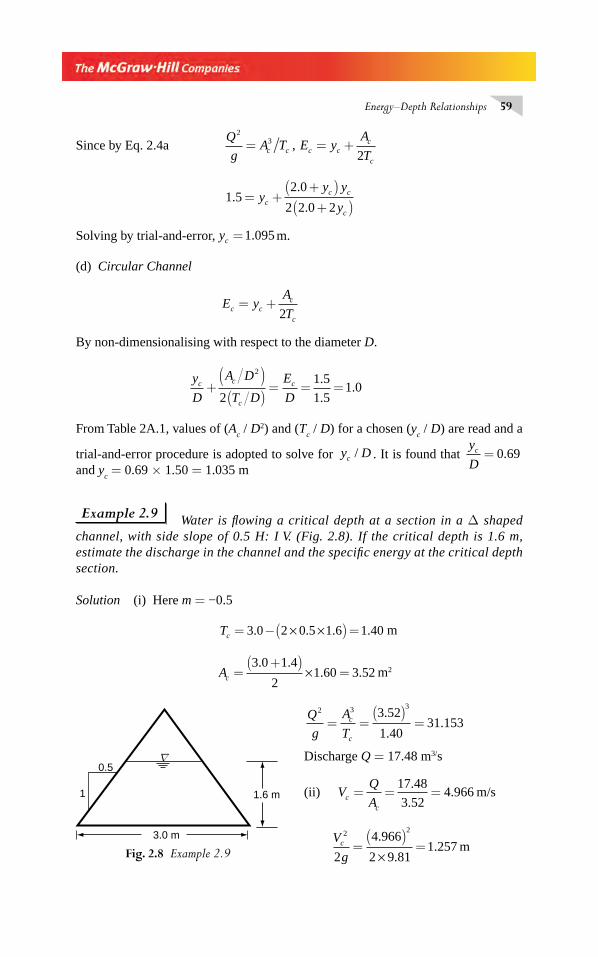
Energy–Depth Relationships 59
Since by Eq. 2.4a Q
gA T E y
A
Tc c c cc
c
23
2= = +,
1 5
2 0
2 2 0 2.
.
.= +
+( )+( )
yy y
ycc c
c
Solving by trial-and-error, yc =1 095. m.
(d) Circular Channel
E yA
Tc cc
c
= +2
By non-dimensionalising with respect to the diameter D.
y
D
A D
T D
E
Dc c
c
c+( )
( )= = =
2
2
1 5
1 51 0
.
..
From Table 2A.1, values of (Ac / D2) and (T
c / D) for a chosen (y
c / D) are read and a
trial-and-error procedure is adopted to solve for y Dc / . It is found that y
Dc = 0 69.
and yc = 0.69 × 1.50 = 1.035 m
Example 2.9 Water is fl owing a critical depth at a section in a Δ shaped channel, with side slope of 0.5 H: I V. (Fig. 2.8). If the critical depth is 1.6 m, estimate the discharge in the channel and the specifi c energy at the critical depth section.
Solution (i) Here m = −0.5
Tc = −( ) =3 0 2 0 5 1 6 1 40. . . .× × m
Ac =+( )
=3 0 1 4
21 60 3 52
. .. .× m2
Q
g
A
Tc
c
2 3 33 52
1 4031 153= =
( )=
.
..
Discharge Q = 17.48 m3/s
(ii) VQ
Ac
c
= = =17 48
3 524 966
.
.. m/s
V
gc2 2
2
4 966
2 9 811 257=
( )=
.
..
×mFig. 2.8 Example 2.9
3.0 m
1
0.5
1.6 m
∇
Chapter 2.indd 59Chapter 2.indd 59 2/24/2010 2:55:55 PM2/24/2010 2:55:55 PM
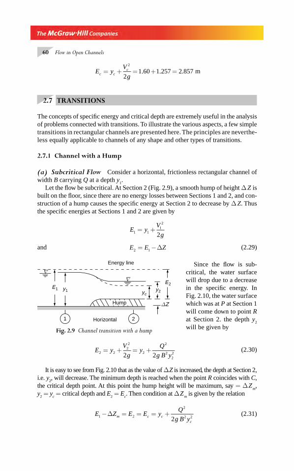
60 Flow in Open Channels
E yV
gc cc= + = + =2
21 60 1 257 2 857. . . m
2.7 TRANSITIONS
The concepts of specifi c energy and critical depth are extremely useful in the analysis of problems connected with transitions. To illustrate the various aspects, a few simple transitions in rectangular channels are presented here. The principles are neverthe-less equally applicable to channels of any shape and other types of transitions.
2.7.1 Channel with a Hump
(a) Subcritical Flow Consider a horizontal, frictionless rectangular channel of width B carrying Q at a depth y
1.
Let the fl ow be subcritical. At Section 2 (Fig. 2.9), a smooth hump of height Δ Z is built on the fl oor, since there are no energy losses between Sections 1 and 2, and con-struction of a hump causes the specifi c energy at Section 2 to decrease by Δ Z. Thus the specifi c energies at Sections 1 and 2 are given by
E yV
g1 112
2= +
and E E Z2 1= −Δ (2.29)
Since the fl ow is sub-critical, the water surface will drop due to a decrease in the specifi c energy. In Fig. 2.10, the water surface which was at P at Section 1 will come down to point R at Section 2. the depth y
2
will be given by
E yV
gy
Q
g B y2 222
2
2
2222 2
= + = + (2.30)
It is easy to see from Fig. 2.10 that as the value of Δ Z is increased, the depth at Section 2, i.e. y
2, will decrease. The minimum depth is reached when the point R coincides with C,
the critical depth point. At this point the hump height will be maximum, say = Δ Z m,
y2 = y
c = critical depth and E
2 = E
c. Then condition at Δ Z
m is given by the relation
E Z E E yQ
g B ym c c
c
1 2
2
2 22− = = = +Δ (2.31)
Fig. 2.9 Channel transition with a hump
1 2
Energy line
Horizontal
Hump
E1
E2y1 y2yc
Chapter 2.indd 60Chapter 2.indd 60 2/24/2010 2:55:55 PM2/24/2010 2:55:55 PM
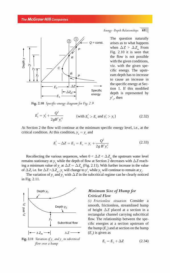
Energy–Depth Relationships 61
The question naturally arises as to what happens when Δ Z > Δ Z
m From
Fig. 2.10 it is seen that the fl ow is not possible with the given condit ions, viz. with the given spe-cifi c energy. The upstr-eam depth has to increase to cause an increase in the specifi c energy at Sec-tion 1. If this modifi ed depth is represented by y′
1 , then
E yQ
gB y1 1
2
21
22'
'= +' {with E E1 1
' > and y y1 1' > } (2.32)
At Section 2 the fl ow will continue at the minimum specifi c energy level, i.e., at the critical condition. At this condition, y
2 = y
c and
E Z E E yQ
g B yc c
c
1 2
2
2 22' − = = = +Δ (2.33)
Recollecting the various sequences, when 0 < Δ Z < Δ Zm the upstream water level
remains stationary at y1 while the depth of fl ow at Section 2 decreases with Δ Z reach-
ing a minimum value of yc at Δ Z = Δ Z
m (Fig. 2.11). With further increase in the value
of Δ Z, i.e. for Δ Z >Δ Zm , y
1 will change to y'
1 while y
2 will continue to remain at y
c.
The variation of y1 and y
2 with Δ Z in the subcritical regime can be clearly noticed
in Fig. 2.11.
Minimum Size of Hump for Critical Flow(i) Frictionless situation Consider a smo oth, frictionless, streamlined hump of height Δ Z placed at a section in a rectangular channel carrying subcritical fl ow. The relationship between the spe-cifi c energies at a section upstream of the hump (E
1) and at section on the hump
(E2) is given as
E E Z1 2= +Δ (2.34)
Fig. 2.10 Specifi c-energy diagram for Fig. 2.9
E2
E1
y2
y1
yc
Dep
th y
Specificenergy
P
R
Q = const.
C
21
Fig. 2.11 Variation of y1 and y
2 in subcritical
fl ow over a hump
Subcritical flow
Depth y2
y 1 a
nd y
2
Depth y1
yc
Δ Zm Δ Z
Chapter 2.indd 61Chapter 2.indd 61 2/24/2010 2:55:55 PM2/24/2010 2:55:55 PM
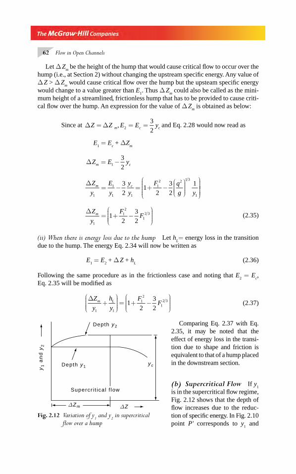
62 Flow in Open Channels
Let Δ Zm be the height of the hump that would cause critical fl ow to occur over the
hump (i.e., at Section 2) without changing the upstream specifi c energy. Any value of Δ Z > Δ Z
m would cause critical fl ow over the hump but the upsteam specifi c energy
would change to a value greater than E1. Thus Δ Z
m could also be called as the mini-
mum height of a streamlined, frictionless hump that has to be provided to cause criti-cal fl ow over the hump. An expression for the value of Δ Z
m is obtained as below:
Since at Δ ΔZ Z E E ym c c= = =, 2
3
2and Eq. 2.28 would now read as
E1 = E
c + ΔZ
m
ΔZ E ym c= −1
3
2
ΔZ
y
E
y
y
y
F q
g ym c
1
1
1 1
12 2 1 3
1
3
21
2
3
2
1= − = + −
⎛
⎝⎜⎜⎜⎜
⎞
⎠⎟⎟⎟⎟
⎛
⎝
⎜⎜⎜⎜⎜
⎞
⎠
⎟⎟⎟⎟⎟⎟⎟
ΔZ
y
FFm
1
12
12 31
2
3
2= + −
⎛
⎝⎜⎜⎜⎜
⎞
⎠⎟⎟⎟⎟ (2.35)
(ii) When there is energy loss due to the hump Let hL= energy loss in the transition
due to the hump. The energy Eq. 2.34 will now be written as
E1 = E
2 + Δ Z + h
L (2.36)
Following the same procedure as in the frictionless case and noting that E2 = E
c,
Eq. 2.35 will be modifi ed as
ΔZ
y
h
y
FFm L
1 1
12
12 31
2
3
2+
⎛
⎝⎜⎜⎜⎜
⎞
⎠⎟⎟⎟⎟
= + −⎛
⎝⎜⎜⎜⎜
⎞
⎠⎟⎟⎟⎟
(2.37)
Comparing Eq. 2.37 with Eq. 2.35, it may be noted that theeffect of energy loss in the transi-tion due to shape and friction is equivalent to that of a hump placed in the downstream section.
(b) Supercritical Flow If y1
is in the supercritical fl ow regime, Fig. 2.12 shows that the depth of fl ow increases due to the reduc-tion of specifi c energy. In Fig. 2.10 point P' corresponds to y
1 and
Fig. 2.12 Variation of y1 and y
2 in supercritical
fl ow over a hump
ycDepth y1
Depth y2
y1 a
nd
y2
Supercr i t ical f low
ΔZΔZm
Chapter 2.indd 62Chapter 2.indd 62 2/24/2010 2:55:56 PM2/24/2010 2:55:56 PM
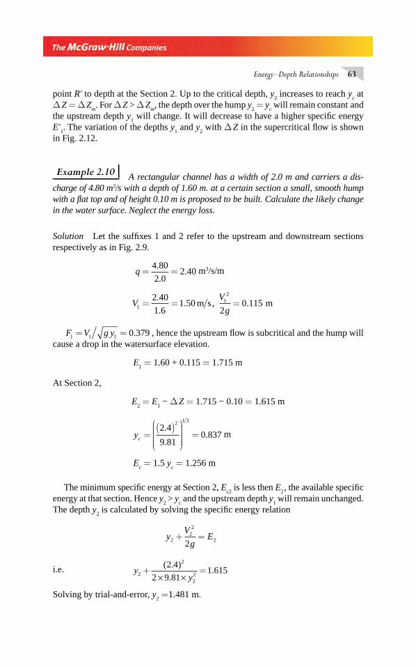
Energy–Depth Relationships 63
point R' to depth at the Section 2. Up to the critical depth, y2 increases to reach y
c at
Δ Z = Δ Zm. For Δ Z > Δ Z
m, the depth over the hump y
2 = y
c will remain constant and
the upstream depth y1 will change. It will decrease to have a higher specifi c energy
E'1. The variation of the depths y
1 and y
2 with Δ Z in the supercritical fl ow is shown
in Fig. 2.12.
Example 2.10 A rectangular channel has a width of 2.0 m and carriers a dis-charge of 4.80 m3/s with a depth of 1.60 m. at a certain section a small, smooth hump with a fl at top and of height 0.10 m is proposed to be built. Calculate the likely change in the water surface. Neglect the energy loss.
Solution Let the suffi xes 1 and 2 refer to the upstream and downstream sections respectively as in Fig. 2.9.
q = =4 80
2 02 40
.
.. m3/s/m
VV
g1122 40
1 61 50
20 115= = =
.
.. , .m s m
F V g y1 1 1 0 379= = . , hence the upstream fl ow is subcritical and the hump will cause a drop in the water surface elevation.
E1 = 1.60 + 0.115 = 1.715 m
At Section 2,
E2 = E
1 − Δ Z = 1.715 − 0.10 = 1.615 m
yc =( )⎛
⎝
⎜⎜⎜⎜⎜
⎞
⎠
⎟⎟⎟⎟⎟⎟=
2 4
9 810 837
2 1 3
.
.. m
Ec = 1.5 y
c = 1.256 m
The minimum specifi c energy at Section 2, Ec2
is less then E2 , the available specifi c
energy at that section. Hence y2 > y
c and the upstream depth y
1 will remain unchanged.
The depth y2 is calculated by solving the specifi c energy relation
yV
gE2
22
22+ =
i.e. yy2
2
22
2 4
2 9 811 615+ =
( . )
..
× ×
Solving by trial-and-error, y2 =1.481 m.
Chapter 2.indd 63Chapter 2.indd 63 2/24/2010 2:55:56 PM2/24/2010 2:55:56 PM
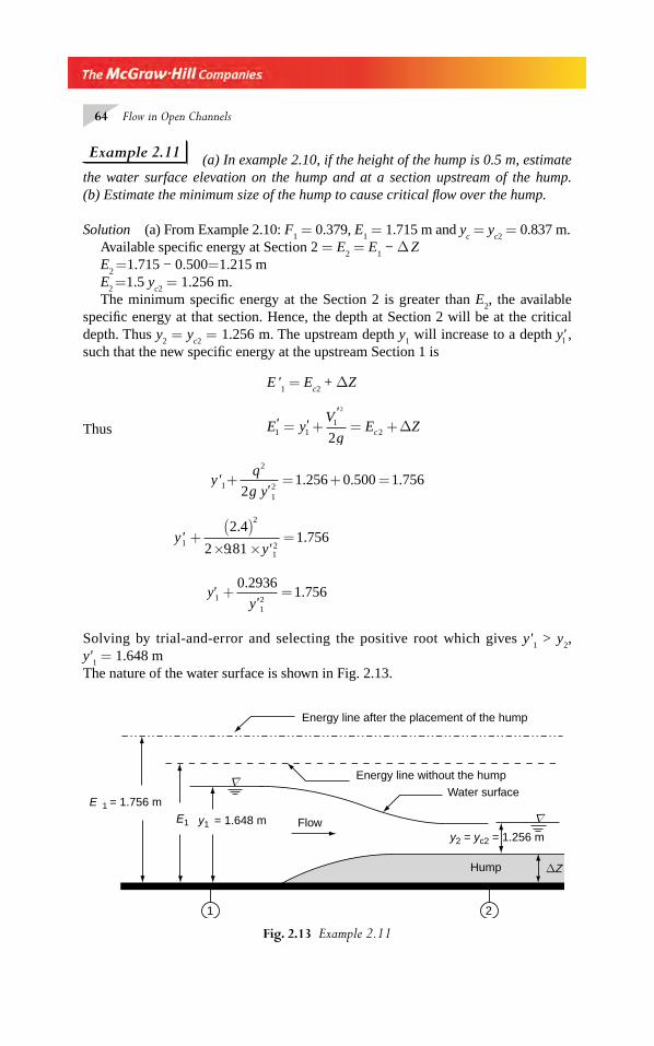
64 Flow in Open Channels
Fig. 2.13 Example 2.11
Energy line after the placement of the hump
Energy line without the hump
Water surface
Flow
Hump
1 2
y2 = yc2 = 1.256 m
E1 y1 = 1.648 m
E 1 = 1.756 m
ΔZ
Δ
Δ
Example 2.11 (a) In example 2.10, if the height of the hump is 0.5 m, estimate the water surface elevation on the hump and at a section upstream of the hump. (b) Estimate the minimum size of the hump to cause critical fl ow over the hump.
Solution (a) From Example 2.10: F1 = 0.379, E
1 = 1.715 m and y
c = y
c2 = 0.837 m.
Available specifi c energy at Section 2 = E2 = E
1 − Δ Z
E2 =1.715 − 0.500=1.215 m
E 2 =1.5 y
c2 = 1.256 m.
The minimum specifi c energy at the Section 2 is greater than E2, the available
specifi c energy at that section. Hence, the depth at Section 2 will be at the critical depth. Thus y
2 = y
c2 = 1.256 m. The upstream depth y
1 will increase to a depth y' ,
such that the new specifi c energy at the upstream Section 1 is
E '1 = E
c2 + ΔZ
Thus E yV
gE Zc1 1
12
2
2'
'= + = +Δ'
yq
g y'
'. . .1
2
122
1 256 0 500 1 756+ = + =
yy
'.
. '.1
2
12
2 4
2 9811 756+
( )× ×
=
yy
'.
'.1
12
0 29361 756+ =
Solving by trial-and-error and selecting the positive root which gives y'1 > y
2,
y'1 = 1.648 m
The nature of the water surface is shown in Fig. 2.13.
1
Chapter 2.indd 64Chapter 2.indd 64 2/24/2010 2:55:56 PM2/24/2010 2:55:56 PM

Energy–Depth Relationships 65
(b) Here, F1 = 0.379 and y
1 = 1.6 m. By use of Eq. 2.35
ΔZ
y
FFm
1
12
12 31
2
3
2= + −
⎛
⎝⎜⎜⎜⎜
⎞
⎠⎟⎟⎟⎟
ΔZm
1 61
0 379
2
3
20 379 0 2866
22 3
.
( . )( . ) .= + −
⎛
⎝⎜⎜⎜⎜
⎞
⎠⎟⎟⎟⎟
=
ΔZm = 0.459 m
Alternatively, ΔZm = E
1 − E
c = 1.715 − 1.256 = 0.459 m
Example 2.12 A 2.5-m wide rectangular channel carries 6.0 m3/s of fl ow at a depth of 0.50 m. Calculate the minimum height of a streamlined, fl at–topped hump required to be placed at a section to cause critical fl ow over the hump. The energy loss over the hump can be taken as 10% of the upstream velocity head.
Solution Discharge intensity q = 6.0/2.5 = 2.40 m3/s/m
V1 = 2.4/0.5 = 4.8 m/s,
V
g12
21 174= . m
Energy loss, hV
gL = × =0 12
0 117412
. .
Froude number, FV
g y1
1
1
4 8
9 81 0 52 167= =
×=
.
. ..
By Eq. (2.37) ( )ΔZ
y
h
y
FFm L
1 1
12
12 31
2
3
2+ = + −
⎛
⎝⎜⎜⎜⎜
⎞
⎠⎟⎟⎟⎟
(.
. )( . )
( . )ΔZm
0 50 1174 1
2 167
2
3
22 167
22 3+ = + −
⎛
⎝⎜⎜⎜⎜
⎞
⎠⎟⎟⎟⎟
ΔZm
0 50 6017
..= and ΔZm = 0.301 m
Alternatively, ΔZm = E
1 − E
c − h
L
E yq
gc c= = ×⎛
⎝⎜⎜⎜⎜
⎞
⎠⎟⎟⎟⎟
1 5 1 52 1 3
. .
= ×⎛
⎝⎜⎜⎜⎜
⎞
⎠⎟⎟⎟⎟
=1 52 4
9 811 256
2 1 3
.( . )
.. m
Chapter 2.indd 65Chapter 2.indd 65 2/24/2010 2:55:57 PM2/24/2010 2:55:57 PM
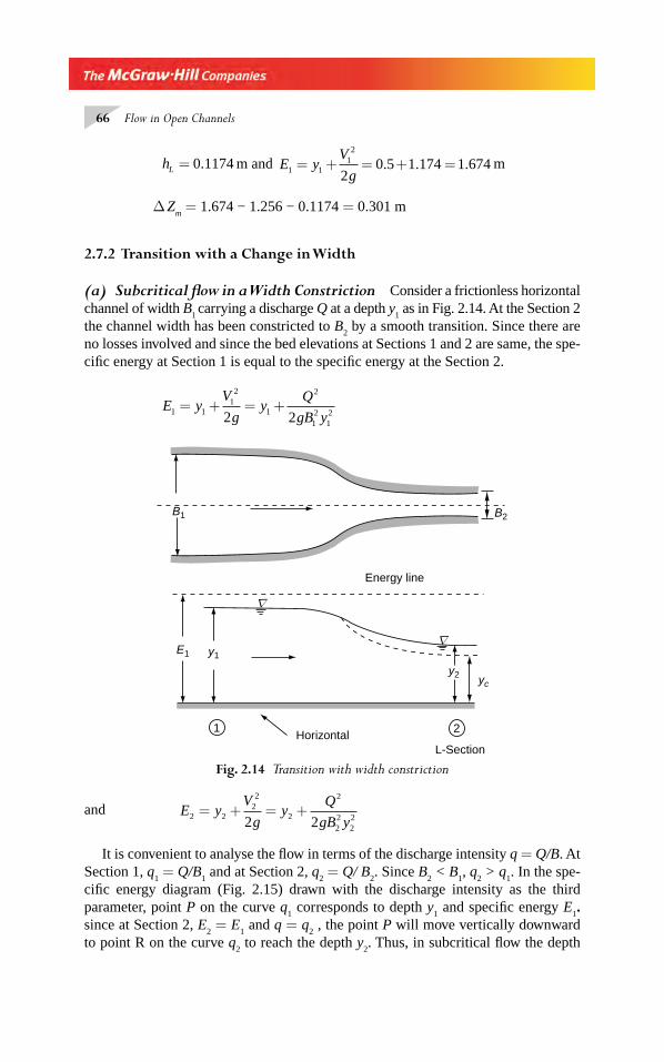
66 Flow in Open Channels
hL = 0 1174. m and E yV
g1 112
20 5 1 174 1 674= + = + =. . . m
Δ Zm = 1.674 − 1.256 − 0.1174 = 0.301 m
2.7.2 Transition with a Change in Width
(a) Subcritical fl ow in a Width Constriction Consider a frictionless horizontal channel of width B
1 carrying a discharge Q at a depth y
1 as in Fig. 2.14. At the Section 2
the channel width has been constricted to B2 by a smooth transition. Since there are
no losses involved and since the bed elevations at Sections 1 and 2 are same, the spe-cifi c energy at Section 1 is equal to the specifi c energy at the Section 2.
E yV
gy
Q
gB y1 112
1
2
12
122 2
= + = +
Fig. 2.14 Transition with width constriction
B1 B2
Energy line
E1 y1
y2 yc
HorizontalL-Section
21
Δ
Δ
and E yV
gy
Q
gB y2 222
2
2
22
222 2
= + = +
It is convenient to analyse the fl ow in terms of the discharge intensity q = Q/B. At Section 1, q
1 = Q/B
1 and at Section 2, q
2 = Q/ B
2. Since B
2 < B
1, q
2 > q
1. In the spe-
cifi c energy diagram (Fig. 2.15) drawn with the discharge intensity as the third parameter, point P on the curve q
1 corresponds to depth y
1 and specifi c energy E
1.
since at Section 2, E2 = E
1 and q = q
2 , the point P will move vertically downward
to point R on the curve q2 to reach the depth y
2. Thus, in subcritical fl ow the depth
Chapter 2.indd 66Chapter 2.indd 66 2/24/2010 2:55:57 PM2/24/2010 2:55:57 PM
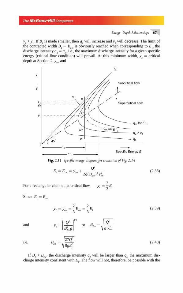
Energy–Depth Relationships 67
y2 < y
1. If B
2 is made smaller, then q
2 will increase and y
2 will decrease. The limit of
the contracted width B2 = B
2 m is obviously reached when corresponding to E
1, the
discharge intensity q2 = q
m, i.e., the maximum discharge intensity for a given specifi c
energy (critical-fl ow condition) will prevail. At this minimum width, y2 = critical
depth at Section 2, ycm
and
Fig. 2.15 Specifi c energy diagram for transition of Fig. 2.14
R
C
P
S
y
P ′
R ′
E ′1
qm for E ′ 1
qm for E ′1
q2 > q1
q1
E1
y1y2
yc
045°
Specific Energy E
Supercritical flow
Subcritical flow
E E yQ
g B ycm cm
m cm
1
2
22 22
= = +( )
(2.38)
For a rectangular channel, at critical fl ow y Ec c=2
3
Since E Ecm1 =
y y E Ecm cm2 1
2
3
2
3= = = (2.39)
and yQ
B gc
m
=⎛
⎝⎜⎜⎜⎜
⎞
⎠⎟⎟⎟⎟
2
22
1 3
or BQ
g ym
cm
2
2
3=
i.e. BQ
gEm2
2
13
27
8= (2.40)
If B2 < B
2m, the discharge intensity q
2 will be larger than q
m the maximum dis-
charge intensity consistent with E1. The fl ow will not, therefore, be possible with the
Chapter 2.indd 67Chapter 2.indd 67 2/24/2010 2:55:57 PM2/24/2010 2:55:57 PM
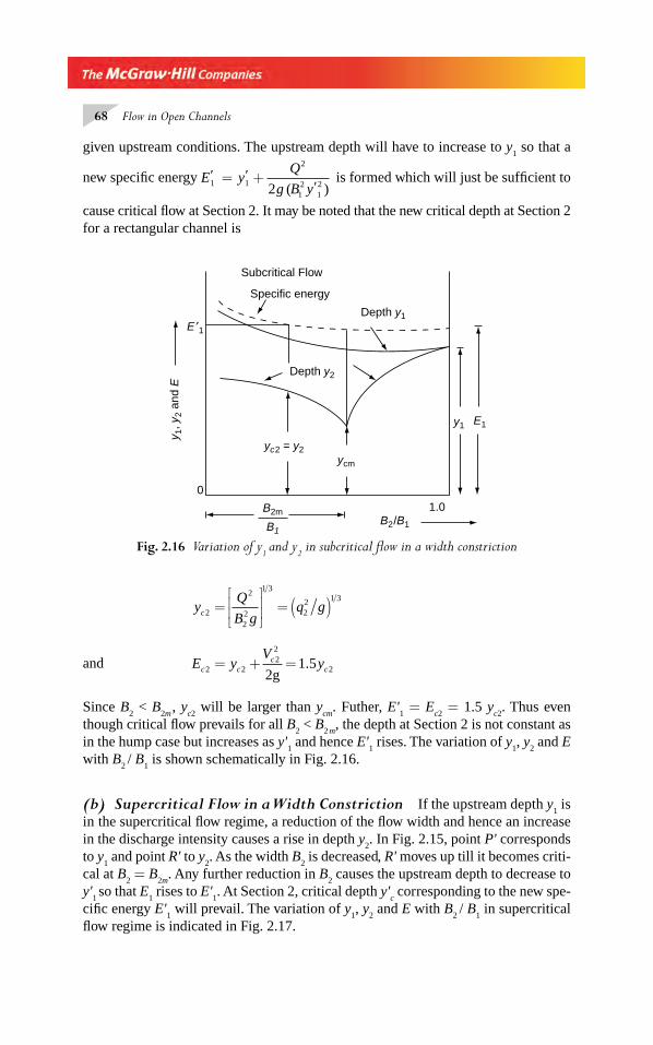
68 Flow in Open Channels
given upstream conditions. The upstream depth will have to increase to y1 so that a
new specifi c energy E yQ
g B y' '
' )1 1
2
12
122
= +(
is formed which will just be suffi cient to
cause critical fl ow at Section 2. It may be noted that the new critical depth at Section 2 for a rectangular channel is
Fig. 2.16 Variation of y1 and y
2 in subcritical fl ow in a width constriction
Subcritical Flow
Specific energy
Depth y1
Depth y2
y1
ycm
yc2 = y2
E1
E ′1
y 1, y
2 an
d E
0
1.0B2/B1
B2m
B1
yQ
B gq gc2
2
22
1 3
22 1 3
=⎡
⎣⎢⎢
⎤
⎦⎥⎥ = ( )
and E yV
yc cc
c2 222
221 5= + =
g.
Since B2 < B
2m , y
c2 will be larger than y
cm. Futher, E'
1 = E
c2 = 1.5 y
c2. Thus even
though critical fl ow prevails for all B2 < B
2 m, the depth at Section 2 is not constant as
in the hump case but increases as y'1 and hence E'
1 rises. The variation of y
1, y
2 and E
with B2 / B
1 is shown schematically in Fig. 2.16.
(b) Supercritical Flow in a Width Constriction If the upstream depth y1 is
in the supercritical fl ow regime, a reduction of the fl ow width and hence an increase in the discharge intensity causes a rise in depth y
2. In Fig. 2.15, point P' corresponds
to y1 and point R' to y
2. As the width B
2 is decreased, R' moves up till it becomes criti-
cal at B2 = B
2m. Any further reduction in B
2 causes the upstream depth to decrease to
y'1 so that E
1 rises to E'
1. At Section 2, critical depth y'
c corresponding to the new spe-
cifi c energy E'1 will prevail. The variation of y
1, y
2 and E with B
2 / B
1 in supercritical
fl ow regime is indicated in Fig. 2.17.
Chapter 2.indd 68Chapter 2.indd 68 2/24/2010 2:55:58 PM2/24/2010 2:55:58 PM
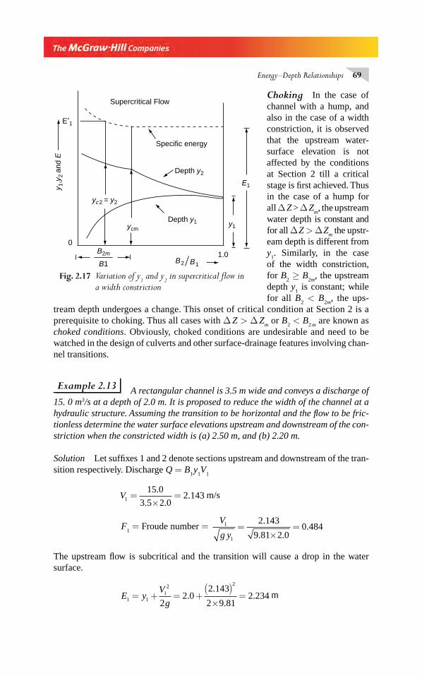
Energy–Depth Relationships 69
Choking In the case of channel with a hump, and also in the case of a width constriction, it is observed that the upstream water-surface ele vation is not affected by the conditions at Section 2 till a critical stage is fi rst ach ieved. Thus in the case of a hump for all Δ Z > Δ Z
m, the upstream
water depth is constant and for all Δ Z > Δ Z
m the upstr-
eam depth is different from y
1. Similarly, in the case
of the width constriction, for B
2 ≥ B
2m, the upstream
depth y1 is constant; while
for all B2 < B
2m, the ups-
tream depth undergoes a change. This onset of critical condition at Section 2 is a prereq uisite to choking. Thus all cases with Δ Z > Δ Z
m or B
2 < B
2 m are known as
choked con ditions. Obviously, choked conditions are undesirable and need to be watched in the design of culverts and other surface-drainage features involving chan-nel transitions.
Example 2.13 A rectangular channel is 3.5 m wide and conveys a discharge of 15. 0 m3/s at a depth of 2.0 m. It is proposed to reduce the width of the channel at a hydraulic structure. Assuming the transition to be horizontal and the fl ow to be fric-tionless determine the water surface elevations upstream and downstream of the con-striction when the constricted width is (a) 2.50 m, and (b) 2.20 m.
Solution Let suffi xes 1 and 2 denote sections upstream and downstream of the tran-sition respectively. Discharge Q = B
1 y
1V
1
V1
15 0
3 5 2 02 143=
×=
.
. .. m/s
F1 = Froude number =
V
g y1
1
2 143
9 81 2 00 484=
×=
.
. ..
The upstream fl ow is subcritical and the transition will cause a drop in the water surface.
E yV
g1 112 2
22 0
2 143
2 9 812 234= + = +
( )×
=..
.. m
Fig. 2.17 Variation of y1 and y
2 in supercritical fl ow in
a width constriction
ycm
yc2 = y2
B2m
B1 B1B21.0
y1
E1
Depth y1
Depth y2
Specific energy
Supercritical Flow
E′1
y 1,y
2 an
d E
0
Chapter 2.indd 69Chapter 2.indd 69 2/24/2010 2:55:58 PM2/24/2010 2:55:58 PM
70 Flow in Open Channels
Let B2m
= minimum width at Section 2 which does not cause choking.
Then E Ecm = =1 2 234. m
y Ecm cm= = × =2
3
2
32 234 1 489. . m
Since yQ
gBcm
m
32
22
=⎡
⎣⎢⎢
⎤
⎦⎥⎥
BQ
g ym
c
2
2
23
1 22
3
1 215 0
9 81 1 4892 636=
⎡
⎣⎢⎢
⎤
⎦⎥⎥ =
×
⎡
⎣⎢⎢
⎤
⎦⎥⎥ =
( . )
. ( . ). m
(a) When B1 = 2.50 m
B2 < B
2m and hence choking conditions prevail. The depth at the Section 2 = y
2 = y
c2.
The upstream depth y1 will increase to y'.
Actually q2
15 0
2 06 0= =
.
.. m3/s/m
yq
gc222 1 3 2 1 3
6 0
9 81=
⎡
⎣⎢⎢
⎤
⎦⎥⎥ =
⎡
⎣⎢⎢
⎤
⎦⎥⎥
( . )
. = 1.542 m
E yc c2 21 5 1 5 1 542 2 3136= = × =. . . . m
At the upstream Section 1:E '
1 = Ec
2 = 2.3136 with new upstream depth of y
1 such that
q1 = y
1 V
1 = 15/3.5 = 4.2857 m3/s/m.
Hence yV
g'
'.1
12
22 3136= =
yy
1
2
12
4 2857
2 9 812 3136'
( . )
. '.+
× ×=
yy1
12
0 93622 3136'
..+ =
'
Solving by the trial and error and selecting a root that gives subcritical fl ow,
y'1 = 2.102 m
(b) When B2 = 2.20 m
As B2 < B
2m choking conditions prevail.
Depth at Section 2 = y2 = y
c2
q2
15 0
2 206 8182= =
.
.. m2/s/m
Chapter 2.indd 70Chapter 2.indd 70 2/24/2010 2:55:58 PM2/24/2010 2:55:58 PM
Energy–Depth Relationships 71
yc2
2 1 36 8182
9 811 6797=
⎡
⎣⎢⎢
⎤
⎦⎥⎥ =
( . )
.. m
E yc c2 21 5 2 5195= =. . m
At upstream Section 1: New upstream depth = y'1 and
E '1 = Ec2 = 2.5195 m
q1 = V '1
y '1 = 15/3.5 = 4.2857 m3/s/m
Hence yV
g y1
12
122 5195'
'
'.= =
y
y1
2
12
4 2857
2 9 812 5195'
( . )
. '.+
× ×=
yy1
12
0 93622 5195' .
.+ ='
Solving by trial and error, the appropriate depth to give subcritical fl ow is
y'1 = 2.350 m
[Note that for the same discharge when B2 < B
2m (i.e., under choking conditions) the
depth at the critical section will be different from ycm
and depends on the value of B2].
2.7.3 General Transition
A transition in its general form may have a change of channel shape, provision of a hump or a depression´ and contraction or expansion of channel width, in any combi-nation. In addition, there may be various degrees of loss of energy at various compo-nents. However, the basic dependence of the depths of fl ow on the channel geometry and specifi c energy of fl ow will remain the same. Many complicated transition situa-tions can be analysed by using the principles of specifi c energy and critical depth.
In subcritical fl ow transitions the emphasis is essentially to provide smooth and gradual changes in the boundary to prevent fl ow separation and consequent energy losses. Details about subcritical fl ow transitions are available in Ref. 1, 2 and 3. The transitions in supercritical fl ow, however, are different and involve suppression of shock waves related disturbances and are explained in Chapter 9.
Example 2.14 A discharge of 16.0 m3/s fl ows with a depth of 2.0 m in a 4.0 m wide rectangular channel. At a downstream section the width is reduced to 3.5 m and the channel bed is raised by Δ Z. Analyse the water-surface elevation in the transi-tions when (a) Δ Z = 0.02 m, and (b) Δ Z = 0.35 m.
Chapter 2.indd 71Chapter 2.indd 71 2/24/2010 2:55:59 PM2/24/2010 2:55:59 PM
72 Flow in Open Channels
Solution Let the suffi xes 1 and 2 refer to the upstream and downstream sections respectively.
At the upstream section, V1
16
4 22 0=
×= . m /s
F1 = Froude number =
V
g y1
1
2 0
9 81 2 00 452=
×=
.
. ..
The upstream fl ow is subcritical and the transition will cause a drop in the water sur-face elevation.
V12/2g = 0.204 m
E1 = 2.0 + 0.204 = 2.204 m
q2 = discharge intensity at the downstream section
= = =Q
B2
16 0
3 54 571
.
.. m3/s/m
yc2
= critical depth corresponding to q2
=⎛
⎝⎜⎜⎜⎜
⎞
⎠⎟⎟⎟⎟
=⎡
⎣⎢⎢
⎤
⎦⎥⎥ =
q
g22 1 3 2 1 3
4 571
9 811 287
( . )
.. m
E yc c2 2
3
21 930= = . m
(a) When ΔZ = 0.20 mE
2 = available specifi c energy at Section 2 = E
1 − ΔZ = 2.204 − 0.20 = 2.004 m > E
c2
Hence the depth y2 > y
c2 and the upstream depth will remain unchanged at y
1.
yV
gZ E2
22
12+ + =Δ
yy2
2
22
4 571
2 9 812 204 0 20+
× ×= −
( . )
.. .
yy2
22
1 0652 004+ =
..
Solving by trial and error, y2 = 1.575 m.
Hence when Δ Z = 0.20 m, y1 = 2.00 m and y
2 = 1.575 m
(b) When Δ Z = 0.35,E
2 = available specifi c energy at Section 2= 2.204 – 0.350 = 1.854 m < E
c2
Chapter 2.indd 72Chapter 2.indd 72 2/24/2010 2:55:59 PM2/24/2010 2:55:59 PM
Energy–Depth Relationships 73
Hence the contraction will be working under choked conditions. The upstream depth must rise to create a higher total head. The depth of fl ow at Section 2 will be critical with y
2 = y
c2 = 1.287 m.
If the new upstream depth is y'1
yQ
gB yE Zc1
2
12
12 22
1 930 0 350' . .+ = + = +Δ
yy
1
2
21
2
16
2 9 81 4 02 28' ( )
. ( . ) '.+
× × ×=
i.e. yy
1
12
0 81552 280' .
'.+ =
By trial-and-error, y1 2 094' .= m.
The upstream depth will therefore rise by 0.094 m due to the choked condition at the constriction. Hence, when Δ Z = 0.35 m
y1 = 2.094 m and y
2 = y
c2= 1.287 m.
REFERENCES
1. Vittal, N and Chiranjeevi, V V ‘Open Channel Transitions : Rational Methods of Design’, J of Hyd. Engg., ASCE, Vol. 109, NO. 1, Jan. 1983, pp 99–115.
2. Vittal, N et. al., ‘Hydraulic Design of Flume Aqueducts’, J. of Hyd. Engg., ASCE, Vol. 119, No. 2, Feb. 1993, pp 284 –289.
3. Swamee, P K and Basak, B C ‘Comphensive Open–Channel Expansion Transition Design’, J. of Irr. & Dri. Engg., ASCE, Vol. 119, No. 1, Jan./Feb., 1993, pp 1–17.
4. Swamee, P K ‘Critical Depth Equations for Irrigation Canals’, J. of Irr. & Dri. Engg.,ASCE, Vol. 119, No. 2, March 1993, pp 400–409.
5. Straub, W Ö ‘A Quick and Easy Way to Calculate Critical and Conjugate Depths in Circu-lar Channels’, Civil Engineering, Dec. 1978, 99.70–71.
PROBLEMS
Problem Distribution
Topics Problems
Specifi c energy and alternate depthsMinimum specifi c energy and critical depthComputations involving critical depthFirst hydraulic exponent, MTransitions
1. with hump/ drop2. with change in width3. General
Miscellaneous concepts
2.1 – 2.72.8 – 2.162.17 – 2.27; 2.292.30 – 2.32
2.33 – 2.352.36 – 2.382.39 – 2.442.28
Chapter 2.indd 73Chapter 2.indd 73 2/24/2010 2:56:00 PM2/24/2010 2:56:00 PM
74 Flow in Open Channels
2.1 In a rectangular channel F1 and F
2 are the Froude numbers corresponding to the alternate
depths of a certain discharge. Show that
F
F
F
F2
1
2 3
22
12
2
2
⎛
⎝⎜⎜⎜⎜
⎞
⎠⎟⎟⎟⎟ =
++
2.2 Show that in a triangular channel, the Froude number corresponding to alternate depths are given by
F
F
F
F1
2
12 5 2
22 5 2
4
4=
++
( )
( )
2.3 A 5.0 m wide rectangular channel carries 20 m3/s of discharge at a depth of 2.0 m.The width beyond a certain section is to be changed to 3.5 m. If it is desired to keep the water-surface elevation unaffected by this change, what modifi cations are needed to the bottom elevation?
2.4 Find the alternate depths corresponding to a specifi c head of 2.0 m and a discharge of 6.0 m3/s in (a) a trapezoidal channel, B = 0.9 m, m = 1.0, (b) triangular channel, m = 1.5, (c) circular channel, D = 2.50 m. (Use the trial and error method. For Part (c) use Table 2A.1)
2.5 If y1 and y
2 are alternate depths in a rectangular channel show that
2 12
22
1 2
3y y
y yyc( )+
=
and hence the specifi c energy, Ey y y y
y y=
+ ++
12
1 2 22
1 2( )
2.6 If y1and y
2 are the alternate depths in a triangular channel show that
4 14
24
12
22
1 2
5y y
y y y yyc+( ) +( )
=
where yc= critical depth. Show further that the specifi c energy E is given by
E
y1
4 3 2
21 1=
+ + ++( ) +( )
η η η ηη η
+1
where η = y2/y
1
2.7 A trapezoidal channel has a bottom width of 6.0 m and side slopes of 1: 1. The depth of fl ow is 1.5 m at a discharge of 15 m3/s. Determine the specifi c energy and alternate depth.
2.8 Show that for a trapezoidal channel the minimum specifi c energy Ec is related to the criti-
cal depth yc as
Ey
cc c
c
=++
⎡
⎣⎢⎢
⎤
⎦⎥⎥2
3 5
1 2
ζζ
where ζccmy
B=
2.9 Prove that the alternate depths in an exponential channel (A = k1ya) are given by
2 12
22
1 2
12
22
2 1ay y y y
y yy
a a
a a ca( )
( )
−−
= +
Chapter 2.indd 74Chapter 2.indd 74 2/24/2010 2:56:00 PM2/24/2010 2:56:00 PM
Energy–Depth Relationships 75
2.10 Show that in an exponential channel (A = k1y a) the minimum specifi c energy E
c and the
critical depth yc are related as
E
y ac
c
= +11
2
2.11 A parabolic channel has its profi le given by x2 = 4ay. Obtain an expression for the rela-tive specifi c energy at the critical fl ow, E
c / y
c for this channel.
2.12 Show that for a horizontal frictionless channel the minimum specifi c force for a specifi ed discharge is obtained at the critical depth.
2.13 A channel in which the area is related to the depth as (A = k1 y a) in which k
1 and a are
constants is called an exponential channel. Show that the critical depth for an exponen-tial channel is given by
yQ
g
a
kc
a
=⎛
⎝⎜⎜⎜⎜
⎞
⎠⎟⎟⎟⎟
+2
12
1 2 1( )
2.14 An exponential channel (A = k1 y a) carries a fl ow with a Froude number F
0 at a depth of
fl ow of y0. Show that the critical depth y
c is given by
y
yFc x
00= where x = 2/(2a+1)
2.15 If it is desired to have a channel in which the fl ow is critical at all stages, show that the cross section of such a channel is given by.
T hQ
g2 2
3
8=
in which T = top width and h = depth of the water surface below the energy line.
2.16 Show that in a parabolic channel x c y=( ) the area can be expressed in terms of the
top width T as
A =2
3Ty
Further, show that the critical depth in such a parabolic channel is given by
yQ
gT
Q
gcc
c
=⎡
⎣⎢⎢
⎤
⎦⎥⎥ =
⎡
⎣⎢⎢
⎤
⎦⎥⎥
27
8
27
32
2
2
1 32
2
1 4
2.17 A channel has a cross section given by the relationship A y= 2 5. . For a critical depth of 0.5 m in this channel, estimate the (i) discharge and (ii) specifi c energy.
2.18 A triangular channel has an apex angle of 60o and carries a fl ow with a velocity of 2.0 m/s and depth of 1.25 m. (a) Is the fl ow subcritical or super-critical? (b) What is the critical depth? (c) What is the specifi c energy? (d) What is the alternate depth pos-sible for this specifi c energy?
2.19 Fill the missing data in the following table connected with critical depth computations in rectangular channels:
Chapter 2.indd 75Chapter 2.indd 75 2/24/2010 2:56:00 PM2/24/2010 2:56:00 PM
76 Flow in Open Channels
Case Q(m3/s)
B(m)
yc
(m)E
c(m)
(a)(b)(c)(d)
–5.607.50
–
3.0–
2.52.0
0.500.80
––
–––
0.60
2.20 Fill in the missing data in the following table connected with critical depth computation in triangular channels:
Case Q(m3/s)
SideSlope = m
yc
(m)E
c
(m)
(i) (ii)(iii)
1.50––
1.251.501.00
–0.30
–
––
0.60
2.21 Fill in the missing data in the following table relating critical depth in trapezoidal channels:
Case m B(m)
yc
(m)Q
(m3/s)E
c(m)
(a)(b)(c)(d)
1.52.01.52.0
3.52.0–
4.0
–0.300.40
–
5.0–
2.641–
–––
1.111
2.22 Calculate the discharges and specifi c energies corresponding to the following cri-tical depths in circular channels: (a) y
c = 0.375 m, D = 1.50 m, and (b) y
c = 0.40 m,
D = 2.0 m.2.23 What is the critical depth corresponding to a discharge of 5.0 m3/s in (a) a trapezoidal
channel of B = 0.80 m and m = 1.5, and (b) a circular channel of D = 1.50 m?2.24 In a circular channel of diameter D = 1.50 m, the critical depth y
c is known to occur at a
specifi c energy of 1.80 m. Estimate the value of yc.
2.25 A circular channel is to carry a discharge of 558 litres/s. Find the diameter of the conduit such that the fl ow is critical when the conduit is running quarter full.
2.26 A circular culvert of 1.20-m diameter is fl owing half full and the fl ow is in critical state. Estimate the discharge and the specifi c energy.
2.27 A brick-lined sewer has a semicircular bottom and vertical side walls 0.60 m apart. If the depth of fl ow at a section where the fl ow is known to be at a critical state is 0.60 m,estimate the discharge in the sewer.
2.28 A rectangular channel section is to have critical fl ow and at the same time the wetted perimeter is to be minimum. Show that for these two conditions to occur simultane-ously, the width of the channel must be equal to 8/9 times the minimum specifi c-energy head.
Chapter 2.indd 76Chapter 2.indd 76 2/24/2010 2:56:01 PM2/24/2010 2:56:01 PM
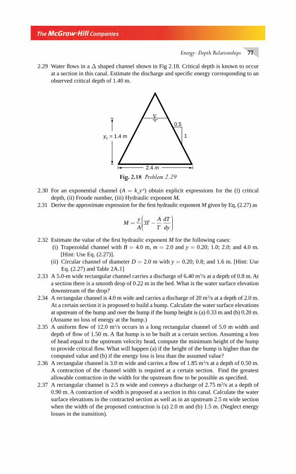
Energy–Depth Relationships 77
2.29 Water fl ows in a Δ shaped channel shown in Fig 2.18. Critical depth is known to occur at a section in this canal. Estimate the discharge and specifi c energy corresponding to an observed critical depth of 1.40 m.
Fig. 2.18 Problem 2.29
∇
2.4 m
0.5
1yc = 1.4 m
2.30 For an exponential channel (A = k1 y a) obtain explicit expressions for the (i) critical
depth, (ii) Froude number, (iii) Hydraulic exponent M.2.31 Derive the approximate expression for the fi rst hydraulic exponent M given by Eq. (2.27) as
My
AT
A
T
dT
dy= −
⎛
⎝⎜⎜⎜⎜
⎞
⎠⎟⎟⎟⎟3
2.32 Estimate the value of the fi rst hydraulic exponent M for the following cases: (i) Trapezoidal channel with B = 4.0 m, m = 2.0 and y = 0.20; 1.0; 2.0; and 4.0 m.
[Hint: Use Eq. (2.27)]. (ii) Circular channel of diameter D = 2.0 m with y = 0.20; 0.8; and 1.6 m. [Hint: Use
Eq. (2.27) and Table 2A.1]2.33 A 5.0-m wide rectangular channel carries a discharge of 6.40 m3/s at a depth of 0.8 m. At
a section there is a smooth drop of 0.22 m in the bed. What is the water surface elevation downstream of the drop?
2.34 A rectangular channel is 4.0 m wide and carries a discharge of 20 m3/s at a depth of 2.0 m. At a certain section it is proposed to build a hump. Calculate the water surface elevations at upstream of the hump and over the hump if the hump height is (a) 0.33 m and (b) 0.20 m. (Assume no loss of energy at the hump.)
2.35 A uniform fl ow of 12.0 m3/s occurs in a long rectangular channel of 5.0 m width and depth of fl ow of 1.50 m. A fl at hump is to be built at a certain section. Assuming a loss of head equal to the upstream velocity head, compute the minimum height of the hump to provide critical fl ow. What will happen (a) if the height of the hump is higher than the computed value and (b) if the energy loss is less than the assumed value?
2.36 A rectangular channel is 3.0 m wide and carries a fl ow of 1.85 m3/s at a depth of 0.50 m. A contraction of the channel width is required at a certain section. Find the greatest allowable contraction in the width for the upstream fl ow to be possible as specifi ed.
2.37 A rectangular channel is 2.5 m wide and conveys a discharge of 2.75 m3/s at a depth of 0.90 m. A contraction of width is proposed at a section in this canal. Calculate the water surface elevations in the contracted section as well as in an upstream 2.5 m wide section when the width of the proposed contraction is (a) 2.0 m and (b) 1.5 m. (Neglect energy losses in the transition).
Chapter 2.indd 77Chapter 2.indd 77 2/24/2010 2:56:01 PM2/24/2010 2:56:01 PM
78 Flow in Open Channels
2.38 A 3.0-m wide horizontal rectangular channel is narrowed to a width of 1.5 m to cause critical fl ow in the contracted section. If the depth in the contracted section is 0.8 m, calculate the discharge in the channel and the possible depths of fl ow and corres-ponding Froude numbers in the 3.0 m wide section. Neglect energy losses in the transition.
2.39 A rectangular channel is 3.0 m wide and carries a discharge of 15.0 m3/s at a depth of 2.0 m. At a certain section of the channel it is proposed to reduce the width to 2.0 m and to alter the bed elevation by Δ Z to obtain critical fl ow at the contracted section without altering the upstream depth. What should be the value of Δ Z ?
2.40 Water fl ows at a velocity of 1.0 m/s and a depth of 2.0 m in an open channel of rectangular cross section and bed-width of 3.0 m. At certain section the width is reduced to 1.80 m and the bed is raised by 0.65 m. Will the upstream depth be affected and if so, to what extent?
2.41 A 3-m wide rectangular channel carries 3 m3/s of water at a depth of 1.0 m. If the width is to be reduced to 2.0 m and bed raised by 10 cm, what would be the depth of fl ow in the contracted section? Neglect the loss of energy in transition. What maximum rise in the bed level of the contracted section is possible without affecting the depth of fl owupstream of the transition?
2.42 Water fl ows in a 3.0-m wide rectangular channel at a velocity of 2.5 m/s and a depth of 1.8 m. If at a section there is a smooth upward step of 0.30 m, what width is needed at that section to enable the critical fl ow to occur on the hump without any change in the upstream depth?
2.43 A 3.0-m wide rectangular channel carries a fl ow at 1.25 m depth. At a certain section the width is reduced to 2.5 m and the channel bed raised by 0.20 m through a streamlined hump. (a) Estimate the discharge in the channel when the water surface drops by 0.15 m over the hump. (b) What change in the bed elevation at the contracted section would make the water surface have the same elevation upstream and downstream of the con-traction? (The energy losses in the contraction can be neglected).
2.44 A 1.5-m wide rectangular channel carries a discharge of 5.0 m3/s at a depth of 1.5 m. At a section the channel undergoes transition to a triangular section of side slopes 2 horizon-tal: 1 vertical. If the fl ow in the triangular section is to be critical without changing the upstream water surface, fi nd the location of the vertex of the triangular section relativeto the bed of the rectangular channel. What is the drop/rise in the water surface at the transition? Assume zero energy loss at the transition.
OBJECTIVE QUESTIONS
2.1 The term alternate depths is used in open channel fl ow to denote the depths (a) having the same kinetic energy for a given discharge(b) having the same specifi c force for a given discharge(c ) having the same specifi c energy for a given discharge(d) having the same total energy for a given discharge
2.2 The two alternate depths in a 4.0 m wide rectangular channel are 3.86 m and 1.0 m respec-tively. The discharge in the channel in m3/s is(a) 15 (b) 1.5 (c) 7.76 (d) 31.0
2.3 In a rectangular channel, the alternate depths are 1.0 m and 2.0 m respectively. The spe-cifi c energy head in m is (a) 3.38 (b) 1.33 (c) 2.33 (d) 3.0
Chapter 2.indd 78Chapter 2.indd 78 2/24/2010 2:56:01 PM2/24/2010 2:56:01 PM
Energy–Depth Relationships 79
2.4 A rectangular channel carries a certain fl ow for which the alternate depths are found to be 3.0 m and 1.0 m. The critical depth in m for this fl ow is(a) 2.65 (b) 1.65 (c) 0.65 (d) 1.33
2.5 The critical fl ow condition in a channel is given by
(a) αQT
gA
2
31= (b)
αQ T
gA
2 2
31=
(c) αQ T
gA
2
31= (d)
αQT
gA31=
2.6 In defi ning a Froude number applicable to open channels of any shape, the length param-eter used is the(a) ratio of area to top width (c) depth of fl ow (b) ratio of area to wetted perimeter (d) square root of the area
2.7 For a triangular channel of side slopes m horizontal : 1 vertical, the Froude number is given by F =
(a) m
g y (b) V
g y2 (c)
V
g y
2 (d) V
g y
2.8 A triangular channel has a vertex angle of 90° and carries a discharge of 1.90 m3/s at a depth of 0.8 m. The Froude number of the fl ow is (a) 0.68 (b) 1.06 (c) 0.75 (d) 1.50
2.9 A triangular channel of apex angle of 120°carries a discharge of 1573 l/s. The critical depth in m is (a) 0.600 (b) 0.700 (c) 0.800 (d) 0.632
2.10 A triangular channel of apex angle of 60° has a critical depth of 0.25 m. The discharge in l/s is(a) 60 (b) 640 (c) 160 (d) 40
2.11 At critical depth(a) the discharge is minimum for a given specifi c energy(b) the discharge is maximum for a given specifi c force(c ) the discharge is maximum for a given specifi c energy (d) the discharge is minimum for a given specifi c force
2.12 For a given open channel carrying a certain discharge the critical depth depends on(a) the geometry of the channel (c) the roughness of the channel (b) the viscosity of water (d) the longitudinal slope of the channel
2.13 In a triangular channel the value of Ec / y
c is
(a) 1.25 (b) 2.5 (c) 3.33 (d) 1.5
2.14 In a parabolic channel x ay2 4=( ) the value of Ec / y
c is
(a) 1.5 (b) 2.0 (c) 3.33 (d) 1.252.15 In an exponential channel (Area A = k y a) the ratio of specifi c energy at critical depth E
c
to the critical depth yc is
(a) 2 1
2
a
a
+⎡
⎣⎢⎢
⎤
⎦⎥⎥ (b) 2a (c)
a
a
+1 (d) 3
2a
2.16 In a rectangular channel carrying uniform fl ow with a specifi c energy E and depth of fl ow = y0
the ratio E / yc is equal to
Chapter 2.indd 79Chapter 2.indd 79 2/24/2010 2:56:01 PM2/24/2010 2:56:01 PM
80 Flow in Open Channels
(a) y
y y yc c
0
2
0
2
1
2
⎛
⎝⎜⎜⎜⎜
⎞
⎠⎟⎟⎟⎟ +
( ) (b)
y
y
y
yc c
0 0
2
2⎛
⎝⎜⎜⎜⎜
⎞
⎠⎟⎟⎟⎟+
⎛
⎝⎜⎜⎜⎜
⎞
⎠⎟⎟⎟⎟
(c) 21
20 0
2
y
y y yc
c
⎛
⎝⎜⎜⎜⎜
⎞
⎠⎟⎟⎟⎟+
( ) (d)
y
y y yc c
0
0
2
1
2
⎛
⎝⎜⎜⎜⎜
⎞
⎠⎟⎟⎟⎟+
( )
2.17 If F0 = Froude number of fl ow in rectangular channel at a depth of fl ow = y
0 then
yc / y
0 =
(a) F0 (b) F02 3 (c) F0
1 3 (d) F03 2
2.18 Supercritical fl ow at Froude number of F0 = 2.0
occurs at a depth of 0.63 m in a rectan-
gular channel. The critical depth in m is(a) 0.857 (b) 0.735 (c) 1.000 (d) 0.500
2.19 The Froude number of a fl ow in a rectangular channel is 0.73. If the depth of fl ow is 1.50 m, the specifi c energy in metres is(a) 1.90 (b) 1.50 (c) 1.73 (d) 0.73
2.20 A trapezoidal channel of bed width of 3.5 m and side slope of 1.5 H: 1 V carries a fl ow of 9.0 m3/s with a depth of 2.0 m. The Froude number of fl ow is(a) 0.156 (b) 0.189 (c) 0.013 (d) 0.506
2.21 For a triangular channel the fi rst hydraulic exponent M is (a) 2.0 (b) 3.0 (c) 5.0 (d) 5.33
2.22 For a trapezoidal canal section with side slope of m horizontal : 1 vertical the value of the fi rst hydraulic exponent M is(a) a constant at all stages(b) a function of S
0 and Manning’s coeffi cient n
(c ) a function my/B(d) a function of y/B only
2.23 In a rectangular channel with subcritical fl ow the height of a hump to be built to cause subcritical fl ow over it was calculated by neglecting energy losses. If, after building the hump, it is found that the energy losses in the transition are appreciable, the effect of this hump on the fl ow will be(a) to make the fl ow over the hump subcritical(b) to make the fl ow over the hump supercritical (c ) to cause the depth of fl ow upstream of the hump to raise(d) to lower the upstream water surface
2.24 For an exponential channel (A = ky a) the fi rst hydraulic exponent M is (a) (a + 1) (b) (2a) (c) (2a + 1) (d) a2
2.25 The fl ow in a rectangular channel is subcritical. If the width is expanded at a certain sec-tion, the water surface(a) at a downstream section will drop(b) at the downstream section will rise(c ) at the upstream section will rise(d) at the upstream section will drop
2.26 A bottom rack in a channel is used to withdraw a part of the discharge fl owing in a canal. If the fl ow is subcritical throughout, this will cause(a) a rise in the water surface on the rack(b) a drop in the water surface over the rack(c ) a jump over the rack(d) a lowering of the water surface upstream of the rack.
Chapter 2.indd 80Chapter 2.indd 80 2/24/2010 2:56:01 PM2/24/2010 2:56:01 PM
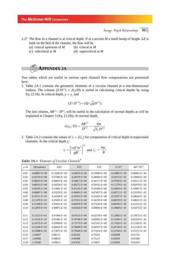
Energy–Depth Relationships 81
2.27 The fl ow in a channel is at critical depth. If at a section M a small hump of height ΔZ is built on the bed of the channel, the fl ow will be (a) critical upstream of M (b) critical at M(c ) subcritical at M (d) supercritical at M
APPENDIX 2A
Two tables which are useful in various open channel fl ow computations are presented here.1. Table 2A.1 contains the geometric elements of a circular channel in a non -dimensional
fashion. The column (Z /D2.5) = f ( y/D) is useful in calculating critical depths by using Eq. (2.18). At critical depth, y = y
c and
( / ) ( / ).. .Z D Q gD2 5 2 5=
The last column, AR2/3 / D8/3, will be useful in the calculation of normal depths as will be explained in Chapter 3 (Eq. (3.29)). At normal depth,
φ( / )y DAR
D
Qn
S D0
2 3
8 3
08 3
= =
2. Table 2A.2 contains the values of ψ = f (ζc) for computation of critical depth in trapezoidal
channels. At the critical depth yc'
ψ =⎛
⎝⎜⎜⎜⎜
⎞
⎠⎟⎟⎟⎟⎟
αQ m
gB
2 3
5
1 2
and ζ c
my
Bc=
Table 2A.1 Elements of Circular Channels*
y / D 2θ(radians) A/D2 P/D T/D Z / D2.5 AR 2/3/D 8/3
0.01 0.40067 E+00 0.13293 E−02 0.20033 E+00 0.19900 E+00 0.10865 E−03 0.46941 E−04
0.02 0.56759 E+00 0.37485 E−02 0.28379 E+00 0.28000 E+00 0.43372 E−03 0.20946 E−03
0.03 0.69633 E+00 0.68655 E−02 0.34817 E+00 0.34117 E+00 0.97392 E−03 0.50111 E−03
0.04 0.80543 E+00 0.10538 E−01 0.40272 E+00 0.39192 E+00 0.17279 E−02 0.92878 E−03
0.05 0.90205 E+00 0.14681 E−01 0.45103 E+00 0.43589 E+00 0.26944 E−02 0.14967 E−02
0.06 0.98987 E+00 0.19239 E−01 0.49493 E+00 0.47497 E+00 0.38721 E−02 0.22078 E−02
0.07 0.10711 E+01 0.24168 E−01 0.53553 E+00 0.51029 E+00 0.52597 E−02 0.30636 E−02
0.08 0.11470 E+01 0.29435 E−01 0.57351 E+00 0.54259 E+00 0.68559 E−02 0.40652 E−02
0.09 0.12188 E+01 0.35012 E−01 0.60939 E+00 0.57236 E+00 0.86594 E−02 0.52131 E−02
0.10 0.12870 E+01 0.40875 E−01 0.64350 E+00 0.60000 E+00 0.10669 E−01 0.65073 E−02
0.11 0.13523 E+01 0.47006 E−01 0.67613 E+00 0.62578 E+00 0.12883 E−01 0.79475 E−02
0.12 0.14150 E+01 0.53385 E−01 0.70748 E+00 0.64992 E+00 0.15300 E−01 0.95329 E−02
0.13 0.14755 E+01 0.59999 E−01 0.73773 E+00 0.67261 E+00 0.17920 E−01 0.11263 E−01
0.14 0.15340 E+01 0.66833 E−01 0.76699 E+00 0.69397 E+00 0.20740 E−01 0.13136 E−01
0.15 0.15908 E+01 0.73875 E−01 0.79540 E+00 0.71414 E+00 0.23760 E−01 0.15151 E−01
0.16 1.64607 0.08111 0.82303 0.73321 0.02698 0.01731
0.17 1.69996 0.08854 0.84998 0.75127 0.03039 0.01960
0.18 1.75260 0.09613 0.87630 0.76837 0.03400 0.02203
Chapter 2.indd 81Chapter 2.indd 81 2/24/2010 2:56:01 PM2/24/2010 2:56:01 PM
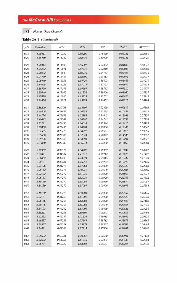
82 Flow in Open Channels
0.19 1.80411 0.10390 0.90205 0.78460 0.03781 0.02460
0.20 1.85459 0.11182 0.92730 0.80000 0.04181 0.02729
0.21 1.90414 0.11990 0.95207 0.81462 0.04600 0.03012
0.22 1.95282 0.12811 0.97641 0.82849 0.05038 0.03308
0.23 2.00072 0.13647 1.00036 0.84167 0.05495 0.03616
0.24 2.04789 0.14494 1.02395 0.85417 0.05971 0.03937
0.25 2.09440 0.15355 1.04720 0.86603 0.06465 0.04270
0.26 2.14028 0.16226 1.07014 0.87727 0.06979 0.04614
0.27 2.18560 0.17109 1.09280 0.88792 0.07510 0.04970
0.28 2.23040 0.18002 1.11520 0.89800 0.08060 0.05337
0.29 2.27470 0.18905 1.13735 0.90752 0.08628 0.05715
0.30 2.31856 0.19817 1.15928 0.91652 0.09215 0.06104
0.31 2.36200 0.20738 1.18100 0.92499 0.09819 0.06503
0.32 2.40506 0.21667 1.20253 0.93295 0.10441 0.06912
0.33 2.44776 0.22603 1.22388 0.94043 0.11081 0.07330
0.34 2.49013 0.23547 1.24507 0.94742 0.11739 0.07758
0.35 2.53221 0.24498 1.26610 0.95394 0.12415 0.08195
0.36 2.57400 0.25455 1.28700 0.96000 0.13108 0.08641
0.37 2.61555 0.26418 1.30777 0.96561 0.13818 0.09095
0.38 2.65686 0.27386 1.32843 0.97077 0.14546 0.09557
0.39 2.69796 0.28359 1.34898 0.97550 0.15291 0.10027
0.40 2.73888 0.29337 1.36944 0.97980 0.16053 0.10503
0.41 2.77962 0.30319 1.38981 0.98367 0.16832 0.10987
0.42 2.82021 0.31304 1.41011 0.98712 0.17629 0.11477
0.43 2.86067 0.32293 1.43033 0.99015 0.18442 0.11973
0.44 2.90101 0.33284 1.45051 0.99277 0.19272 0.12475
0.45 2.94126 0.34278 1.47063 0.99499 0.20120 0.12983
0.46 2.98142 0.35274 1.49071 0.99679 0.20984 0.13495
0.47 3.02152 0.36272 1.51076 0.99820 0.21865 0.14011
0.48 3.06157 0.37270 1.53079 0.99920 0.22763 0.14532
0.49 3.10159 0.38270 1.55080 0.99980 0.23677 0.15057
0.50 3.14159 0.39270 1.57080 1.00000 0.24609 0.15584
0.51 3.18160 0.40270 1.59080 0.99980 0.25557 0.16115
0.52 3.22161 0.41269 1.61081 0.99920 0.26523 0.16648
0.53 3.26166 0.42268 1.63083 0.99820 0.27505 0.17182
0.54 3.30176 0.43266 1.65088 0.99679 0.28504 0.17719
0.55 3.34193 0.44262 1.67096 0.99499 0.29521 0.18256
0.56 3.38217 0.45255 1.69109 0.99277 0.30555 0.18794
0.57 3.42252 0.46247 1.71126 0.99015 0.31606 0.19331
0.58 3.46297 0.47236 1.73149 0.98712 0.32675 0.19869
0.59 3.50357 0.48221 1.75178 0.98367 0.33762 0.20405
0.60 3.54431 0.49203 1.77215 0.97980 0.34867 0.20940
0.61 3.58522 0.50181 1.79261 0.97550 0.35991 0.21473
0.62 3.62632 0.51154 1.81316 0.97077 0.37133 0.22004
0.63 3.66764 0.52122 1.83382 0.96561 0.38294 0.22532
y/D 2θ(radians) A/D2 P/D T/D Z / D2.5 AR2/3/D8/3
Table 2A.1 (Continued)
Chapter 2.indd 82Chapter 2.indd 82 2/24/2010 2:56:01 PM2/24/2010 2:56:01 PM
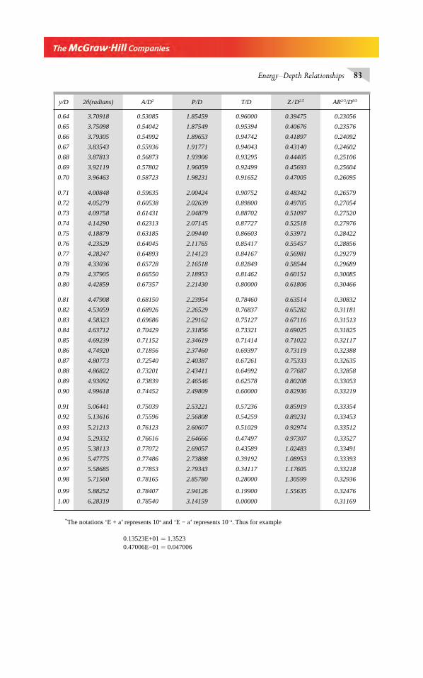
Energy–Depth Relationships 83
0.64 3.70918 0.53085 1.85459 0.96000 0.39475 0.23056
0.65 3.75098 0.54042 1.87549 0.95394 0.40676 0.23576
0.66 3.79305 0.54992 1.89653 0.94742 0.41897 0.24092
0.67 3.83543 0.55936 1.91771 0.94043 0.43140 0.24602
0.68 3.87813 0.56873 1.93906 0.93295 0.44405 0.25106
0.69 3.92119 0.57802 1.96059 0.92499 0.45693 0.25604
0.70 3.96463 0.58723 1.98231 0.91652 0.47005 0.26095
0.71 4.00848 0.59635 2.00424 0.90752 0.48342 0.26579
0.72 4.05279 0.60538 2.02639 0.89800 0.49705 0.27054
0.73 4.09758 0.61431 2.04879 0.88702 0.51097 0.27520
0.74 4.14290 0.62313 2.07145 0.87727 0.52518 0.27976
0.75 4.18879 0.63185 2.09440 0.86603 0.53971 0.28422
0.76 4.23529 0.64045 2.11765 0.85417 0.55457 0.28856
0.77 4.28247 0.64893 2.14123 0.84167 0.56981 0.29279
0.78 4.33036 0.65728 2.16518 0.82849 0.58544 0.29689
0.79 4.37905 0.66550 2.18953 0.81462 0.60151 0.30085
0.80 4.42859 0.67357 2.21430 0.80000 0.61806 0.30466
0.81 4.47908 0.68150 2.23954 0.78460 0.63514 0.30832
0.82 4.53059 0.68926 2.26529 0.76837 0.65282 0.31181
0.83 4.58323 0.69686 2.29162 0.75127 0.67116 0.31513
0.84 4.63712 0.70429 2.31856 0.73321 0.69025 0.31825
0.85 4.69239 0.71152 2.34619 0.71414 0.71022 0.32117
0.86 4.74920 0.71856 2.37460 0.69397 0.73119 0.32388
0.87 4.80773 0.72540 2.40387 0.67261 0.75333 0.32635
0.88 4.86822 0.73201 2.43411 0.64992 0.77687 0.32858
0.89 4.93092 0.73839 2.46546 0.62578 0.80208 0.33053
0.90 4.99618 0.74452 2.49809 0.60000 0.82936 0.33219
0.91 5.06441 0.75039 2.53221 0.57236 0.85919 0.33354
0.92 5.13616 0.75596 2.56808 0.54259 0.89231 0.33453
0.93 5.21213 0.76123 2.60607 0.51029 0.92974 0.33512
0.94 5.29332 0.76616 2.64666 0.47497 0.97307 0.33527
0.95 5.38113 0.77072 2.69057 0.43589 1.02483 0.33491
0.96 5.47775 0.77486 2.73888 0.39192 1.08953 0.33393
0.97 5.58685 0.77853 2.79343 0.34117 1.17605 0.33218
0.98 5.71560 0.78165 2.85780 0.28000 1.30599 0.32936
0.99 5.88252 0.78407 2.94126 0.19900 1.55635 0.32476
1.00 6.28319 0.78540 3.14159 0.00000 0.31169
y/D 2θ(radians) A/D2 P/D T/D Z / D2.5 AR2/3/D8/3
* The notations ‘E + a’ represents 10a and ‘E − a’ represents 10−a. Thus for example
0.13523E+01 = 1.35230.47006E−01 = 0.047006
Chapter 2.indd 83Chapter 2.indd 83 2/24/2010 2:56:02 PM2/24/2010 2:56:02 PM
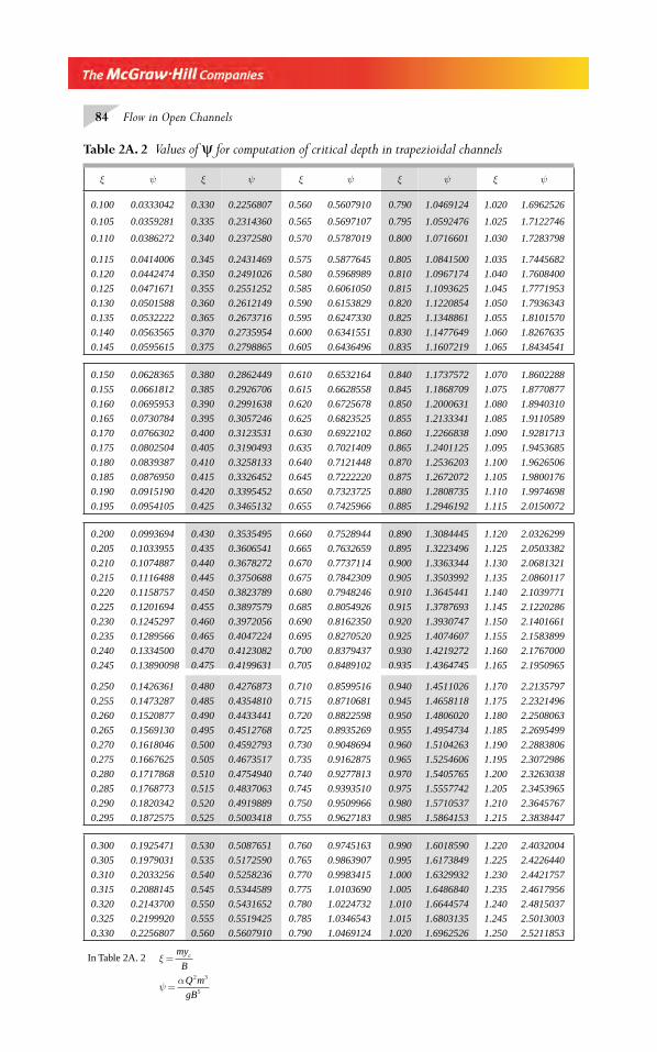
84 Flow in Open Channels
Table 2A. 2 Values of ψ for computation of critical depth in trapezioidal channels
ξ ψ ξ ψ ξ ψ ξ ψ ξ ψ
0.100 0.0333042 0.330 0.2256807 0.560 0.5607910 0.790 1.0469124 1.020 1.6962526
0.105 0.0359281 0.335 0.2314360 0.565 0.5697107 0.795 1.0592476 1.025 1.7122746
0.110 0.0386272 0.340 0.2372580 0.570 0.5787019 0.800 1.0716601 1.030 1.7283798
0.115 0.0414006 0.345 0.2431469 0.575 0.5877645 0.805 1.0841500 1.035 1.7445682
0.120 0.0442474 0.350 0.2491026 0.580 0.5968989 0.810 1.0967174 1.040 1.7608400
0.125 0.0471671 0.355 0.2551252 0.585 0.6061050 0.815 1.1093625 1.045 1.7771953
0.130 0.0501588 0.360 0.2612149 0.590 0.6153829 0.820 1.1220854 1.050 1.7936343
0.135 0.0532222 0.365 0.2673716 0.595 0.6247330 0.825 1.1348861 1.055 1.8101570
0.140 0.0563565 0.370 0.2735954 0.600 0.6341551 0.830 1.1477649 1.060 1.8267635
0.145 0.0595615 0.375 0.2798865 0.605 0.6436496 0.835 1.1607219 1.065 1.8434541
0.150 0.0628365 0.380 0.2862449 0.610 0.6532164 0.840 1.1737572 1.070 1.8602288
0.155 0.0661812 0.385 0.2926706 0.615 0.6628558 0.845 1.1868709 1.075 1.8770877
0.160 0.0695953 0.390 0.2991638 0.620 0.6725678 0.850 1.2000631 1.080 1.8940310
0.165 0.0730784 0.395 0.3057246 0.625 0.6823525 0.855 1.2133341 1.085 1.9110589
0.170 0.0766302 0.400 0.3123531 0.630 0.6922102 0.860 1.2266838 1.090 1.9281713
0.175 0.0802504 0.405 0.3190493 0.635 0.7021409 0.865 1.2401125 1.095 1.9453685
0.180 0.0839387 0.410 0.3258133 0.640 0.7121448 0.870 1.2536203 1.100 1.9626506
0.185 0.0876950 0.415 0.3326452 0.645 0.7222220 0.875 1.2672072 1.105 1.9800176
0.190 0.0915190 0.420 0.3395452 0.650 0.7323725 0.880 1.2808735 1.110 1.9974698
0.195 0.0954105 0.425 0.3465132 0.655 0.7425966 0.885 1.2946192 1.115 2.0150072
0.200 0.0993694 0.430 0.3535495 0.660 0.7528944 0.890 1.3084445 1.120 2.0326299
0.205 0.1033955 0.435 0.3606541 0.665 0.7632659 0.895 1.3223496 1.125 2.0503382
0.210 0.1074887 0.440 0.3678272 0.670 0.7737114 0.900 1.3363344 1.130 2.0681321
0.215 0.1116488 0.445 0.3750688 0.675 0.7842309 0.905 1.3503992 1.135 2.0860117
0.220 0.1158757 0.450 0.3823789 0.680 0.7948246 0.910 1.3645441 1.140 2.1039771
0.225 0.1201694 0.455 0.3897579 0.685 0.8054926 0.915 1.3787693 1.145 2.1220286
0.230 0.1245297 0.460 0.3972056 0.690 0.8162350 0.920 1.3930747 1.150 2.1401661
0.235 0.1289566 0.465 0.4047224 0.695 0.8270520 0.925 1.4074607 1.155 2.1583899
0.240 0.1334500 0.470 0.4123082 0.700 0.8379437 0.930 1.4219272 1.160 2.1767000
0.245 0.13890098 0.475 0.4199631 0.705 0.8489102 0.935 1.4364745 1.165 2.1950965
0.250 0.1426361 0.480 0.4276873 0.710 0.8599516 0.940 1.4511026 1.170 2.2135797
0.255 0.1473287 0.485 0.4354810 0.715 0.8710681 0.945 1.4658118 1.175 2.2321496
0.260 0.1520877 0.490 0.4433441 0.720 0.8822598 0.950 1.4806020 1.180 2.2508063
0.265 0.1569130 0.495 0.4512768 0.725 0.8935269 0.955 1.4954734 1.185 2.2695499
0.270 0.1618046 0.500 0.4592793 0.730 0.9048694 0.960 1.5104263 1.190 2.2883806
0.275 0.1667625 0.505 0.4673517 0.735 0.9162875 0.965 1.5254606 1.195 2.3072986
0.280 0.1717868 0.510 0.4754940 0.740 0.9277813 0.970 1.5405765 1.200 2.3263038
0.285 0.1768773 0.515 0.4837063 0.745 0.9393510 0.975 1.5557742 1.205 2.3453965
0.290 0.1820342 0.520 0.4919889 0.750 0.9509966 0.980 1.5710537 1.210 2.3645767
0.295 0.1872575 0.525 0.5003418 0.755 0.9627183 0.985 1.5864153 1.215 2.3838447
0.300 0.1925471 0.530 0.5087651 0.760 0.9745163 0.990 1.6018590 1.220 2.4032004
0.305 0.1979031 0.535 0.5172590 0.765 0.9863907 0.995 1.6173849 1.225 2.4226440
0.310 0.2033256 0.540 0.5258236 0.770 0.9983415 1.000 1.6329932 1.230 2.4421757
0.315 0.2088145 0.545 0.5344589 0.775 1.0103690 1.005 1.6486840 1.235 2.4617956
0.320 0.2143700 0.550 0.5431652 0.780 1.0224732 1.010 1.6644574 1.240 2.4815037
0.325 0.2199920 0.555 0.5519425 0.785 1.0346543 1.015 1.6803135 1.245 2.5013003
0.330 0.2256807 0.560 0.5607910 0.790 1.0469124 1.020 1.6962526 1.250 2.5211853
In Table 2A. 2 ξ
ψα
=
=
my
B
Q m
gB
c
2 3
5
Chapter 2.indd 84Chapter 2.indd 84 2/24/2010 2:56:02 PM2/24/2010 2:56:02 PM
3.1 INTRODUCTION
A fl ow is said to be uniform if its properties remain constant with respect to distance. As mentioned earlier, the term uniform fl ow in open channels is understood to mean steady uniform fl ow. The depth of fl ow remains constant at all sections in a uniform fl ow (Fig. 3.1). Considering two Sections 1 and 2, the depths
y1 = y
2 = y
0
and hence A1 = A
2 = A
0
Since Q = AV = constant, it follows that in uniform fl ow V1 = V
2 =
V. Thus in
a uniform fl ow, the depth of fl ow, area of cross-section and velocity of fl ow remain con stant along the channel. It is obvious, therefore, that uniform fl ow is possible only in prismatic channels. The trace of the water surface and channel bottom slope are parallel in uniform fl ow (Fig. 3.1). Further, since V = constant, the energy line will be at a constant elevation above the water surface. As such, the slope of the energy line S
f , slope of the water surface S
w and
bottom slope S
0
will all be equal to each other.
3.2 CHEZY EQUATION
By defi nition there is no acceleration in uniform fl ow. By applying the momentum equation to a control volume encompassing Sections 1 and 2, distance L apart, as shown in Fig. 3.1,
P1 − W sin θ − F
f − P
2= M
2 − M
1 (3.1)
where P1 and P
2 are the pressure forces and M
1 and M
2 are the momentum fl uxes at
Sections 1 and 2 respectively W = weight to fl uid in the control volume and Ff =
shear force at the boundary.Since the fl ow is uniform,
P1 = P
2 and M
1 = M
2
Also, W = γ AL and Ff = τ
0 PL
Uniform Flow 3
Chapter 3.indd 85Chapter 3.indd 85 2/24/2010 4:21:50 PM2/24/2010 4:21:50 PM
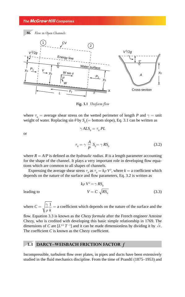
86 Flow in Open Channels
where τ0 = average shear stress on the wetted perimeter of length P and γ = unit
weight of water. Replacing sin θ by S0 (= bottom slope), Eq. 3.1 can be written as
γ ALS0 = τ
0 PL
or
τ0 = γ
A
P S
0= γ RS
0 (3.2)
where R = A/P is defi ned as the hydraulic radius. R is a length parameter accounting for the shape of the channel. It plays a very important role in developing fl ow equa-tions which are common to all shapes of channels.
Expressing the average shear stress τ0 as τ
0 = kρ V 2, where k = a coeffi cient which
depends on the nature of the surface and fl ow parameters, Eq. 3.2 is written as
kρ V 2 = γ RS0
leading to V = C RS0 (3.3)
where C = γρ
1
k= a coeffi cient which depends on the nature of the surface and the
fl ow. Equation 3.3 is known as the Chezy formula after the French engineer Antoine Chezy, who is credited with developing this basic simple relationship in 1769. The dimensions of C are [L1/2 T −1] and it can be made dimensionless by dividing it by g . The coeffi cient C is known as the Chezy coeffi cient.
3.3 DARCY–WEISBACH FRICTION FACTOR f
Incompressible, turbulent fl ow over plates, in pipes and ducts have been extensively studied in the fl uid mechanics discipline. From the time of Prandtl (1875–1953) and
Fig. 3.1 Uniform fl ow
12
CV
Energy line
W sin θ
W
θ
θLFf
Vy0
y0
y0 y0
P1
P2
V 2/2g V 2/2g
X
A
Cross-section
Water surface
ΔΔ
Chapter 3.indd 86Chapter 3.indd 86 2/24/2010 4:21:53 PM2/24/2010 4:21:53 PM
Uniform Flow 87
Von Karman (1881–1963) research by numerous eminent investigators has enabled considerable understanding of turbulent fl ow and associated useful practical applica-tions. The basics of velocity distribution and shear resistance in a turbulent fl ow are available in any good text on fl uid mechanics1,2.
Only relevant information necessary for our study in summed up in this section.
Pipe Flow A surface can be termed hydraulically smooth, rough or in transition depending on the relative thickness of the roughness magnitude to the thickness of the laminar sub-layer. The classifi cation is as follows:
ε ννs ∗ < 4 — hydraulically-smooth wall
4 < ε ν
νs ∗ < 60 — transitional regime
ε ν
νs ∗ < 60 — full rough fl ow
where εs = equivalent sand grain roughness, ν τ ρ* /= 0 = gRS0 = shear veloc-
ity and v = kinematic viscosity.For pipe fl ow, the Darcy–Weisbach equation is
h fL
D
V
gf =2
2 (3.4)
where hf = head loss due to friction in a pipe of diameter D and length L; f = Darcy–
Weisbach friction factor. For smooth pipes, f is found to be a function of the
Reynolds number Re =⎛⎝⎜⎜⎜
⎞⎠⎟⎟⎟⎟
VD
v only. For rough turbulent fl ows, f is a function of the
relative roughness (εs /D ) and type of roughness and is independent of the Reynolds
number. In the transition regime, both the Reynolds number and relative roughness play important roles. The roughness magnitudes for commercial pipes are expressed as equivalent sand-grain roughness εs
. The extensive experimental investigations of pipe fl ow have yielded the following generally accepted relations for the variation of f in various regimes of fl ow:
1. For smooth walls and Re < 105
f = 0 316
1 4
./Re
(Blasius formula) (3.5)
2. For smooth walls and Re > 105
1
f = 2.0 log Re f − 0.8 (Karman–Prandtl equation) (3.6)
Chapter 3.indd 87Chapter 3.indd 87 2/24/2010 4:21:54 PM2/24/2010 4:21:54 PM
88 Flow in Open Channels
3. For rough boundaries and Re > 105
1
f = − 2 log
εs
D + 1.14 (Karman–Prandtl equation) (3.7)
4. For the transition zone
1
f + 2 log
εs
D = 1.14 – 2 log 1 9 35+
⎛
⎝
⎜⎜⎜⎜⎜
⎞
⎠
⎟⎟⎟⎟⎟.
/
D
fsε
Re
(Colebrook–White equation) (3.8)
It is usual to show the variation of f with Re and εs
D by a three-parameter graph
known as the Moody chart.Studies on non-circular conduits, such as rectangular, oval and triangular shapes
have shown that by introducing the hydraulic radius R, the formulae developed for pipes are applicable for non-circular ducts also. Since for a circular shape R = D/4, by replacing D by 4R, Eqs 3.5 to 3.8 can be used for any duct shape provided the conduit areas are close enough to the area of a circumscribing circle or semicircle.
Open Channels For purposes of fl ow resistance which essentially takes place in a thin layer adjacent to the wall, an open channel can be considered to be a conduit cut into two. The hydraulic radius would then be the appropriate length parameter and prediction of friction factor f can be done by using Eqs 3.5 to 3.8. It should be
remembered that Re = 4RV
ν and the relative roughness is (ε
s /4R).
Equation 3.4 can then be written for an open channel fl ow as
h f
L
R
V
gf =4 2
2
which on rearranging gives
Vg
fR h Lf=
8 . / (3.9)
Noting that for uniform fl ow in an open channel hf /L = slope of the energy line =
Sf = S
0 , it may be seen that Eq. 3.9 is the same as Eq. 3.3 (Chezy formula) with
C = 8 g / f (3.10)
For convenience of use, Eq. 3.10 along with Eqs 3.5 to 3.8 can be used to prepare a modifi ed Moody chart showing the variation of C with
Re =⎛⎝⎜⎜⎜
⎞⎠⎟⎟⎟
4RV
v and
4R
εs
⎛⎝⎜⎜⎜
⎞⎠⎟⎟⎟
Chapter 3.indd 88Chapter 3.indd 88 2/24/2010 4:21:54 PM2/24/2010 4:21:54 PM
Uniform Flow 89
If f is to be calculated by using one of the Eqs 3.5 to 3.8, Eqs 3.6 to 3.8 are incon-venient to use as f is involved on both sides of the equations. Simplifi ed empirical forms of Eqs 3.6 and 3.8, which are accurate enough for all practical purposes, are given by Jain3 as follows:
1
f = 1.80 log Re – 1.5146 (in lieu of Eq. (3.6)) (3.6a)
and 1
f = 1.14 – 2.0 log
εs
R4
21 250 9
+ .
.Re
⎛
⎝⎜⎜⎜
⎞
⎠⎟⎟⎟⎟ (in lieu of Eq. (3.8)) (3.8a)
Equation (3.8a) is valid for 5000 ≤ Re ≤ 108 and 10–6 < εs
R4 < 10–2.
These two equations are very useful for obtaining explicit solutions of many fl ow-resistance problems.
Generally, the open channels that are encountered in the fi eld are very large in size and also in the magnitude of roughness elements. Consequently, high Reyn-olds numbers and large relative roughnesses are operative with the result that most of the open channels have rough turbulent-fl ow regimes. Due to paucity of reliable experimental or fi eld data on channels covering a wide range of parameters, values of εs are not available to the same degree of confi dence as for pipe materials. How-ever, Table 3.1 can be used to estimate the values of εs for some common open channel surfaces.
Table 3.1 Values of εs for some Common Channel Surfaces
Sl. No. Surface Equivalent Roughness εs in mm
1 Glass 3 × 10⁻⁴
2 Very smooth concrete surface 0.15–0.303 Glazed sewer pipe 0.604 Gunite (smooth) 0.50–1.55 Rough concrete 3.0–4.56 Earth channels (straight, uniform) 3.07 Rubble masonry 6.08 Untreated gunite 3.0–10.0
3.4 MANNING’S FORMULA
A resistance formula proposed by Robert Manning, an Irish engineer, for uniform fl ow in open channels, is
V =n
1 2 3
0
1 2 R S/ / (3.11)
Chapter 3.indd 89Chapter 3.indd 89 2/24/2010 4:21:55 PM2/24/2010 4:21:55 PM
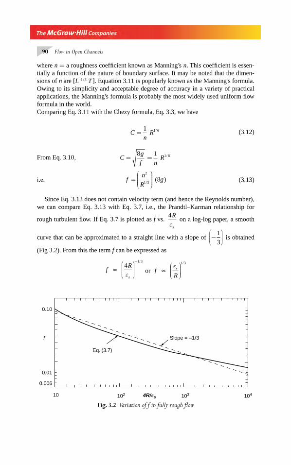
90 Flow in Open Channels
where n = a roughness coeffi cient known as Manning’s n. This coeffi cient is essen-tially a function of the nature of boundary surface. It may be noted that the dimen-sions of n are [L–1 / 3 T ]. Equation 3.11 is popularly known as the Manning’s formula. Owing to its simplicity and acceptable degree of accuracy in a variety of practical applications, the Manning’s formula is probably the most widely used uniform fl ow formula in the world.Comparing Eq. 3.11 with the Chezy formula, Eq. 3.3, we have
Cn
R=1 1 6 / (3.12)
From Eq. 3.10, Cg
f n=
8 1 1 6 = R /
i.e. fn
Rg=
⎛
⎝⎜⎜⎜⎜
⎞
⎠⎟⎟⎟⎟
2
1 3/ (8 ) (3.13)
Since Eq. 3.13 does not contain velocity term (and hence the Reynolds number), we can compare Eq. 3.13 with Eq. 3.7, i.e., the Prandtl–Karman relationship for
rough turbulent fl ow. If Eq. 3.7 is plotted as f vs. 4R
sε on a log-log paper, a smooth
curve that can be approximated to a straight line with a slope of −⎛⎝⎜⎜⎜
⎞⎠⎟⎟⎟⎟
1
3 is obtained
(Fig 3.2). From this the term f can be expressed as
fR
s
∝ 41 3
ε
⎛
⎝⎜⎜⎜⎜
⎞
⎠⎟⎟⎟⎟
− /
or fR
s ∝ε⎛
⎝⎜⎜⎜
⎞
⎠⎟⎟⎟⎟
1 3/
Slope = −1/3
Eq. (3.7)
0.10
0.01
0.006
f
10 102 103 1044R/εs
Fig. 3.2 Variation of f in fully rough fl ow
Chapter 3.indd 90Chapter 3.indd 90 2/24/2010 4:21:55 PM2/24/2010 4:21:55 PM
Uniform Flow 91
Since from Eq. 3.13, fn
R∝
2
1 3/, it follows that n ∝ ε
s1/6. Conversely, if n ∝ ε
s1/6,
the Manning’s formula and Darcy–Weisbach formula both represent rough trubulent
fl ow ε
νsv* >
⎛
⎝⎜⎜⎜⎜
⎞
⎠⎟⎟⎟⎟
60 .
3.5 OTHER RESISTANCE FORMULAE
Several forms of expressions for the Chezy coeffi cient C have been proposed by dif-ferent investigators in the past. Many of these are archaic and are of historic interest only. A few selected ones are listed below:
1. Pavlovski formula
Cn
Rx=1
(3.14)
in which x = 2.5 n − 0.13 − 0.75 R ( n − 0.10) and n = Manning’s coeffi cient.This formula appears to be in use in Russia.
2. Ganguillet and Kutter Formula
Cn S
S
n
R
=+ +
+ +⎡
⎣⎢⎢
⎤
⎦⎥⎥
231 0 00155
1 230 00155
0
0
.
. (3.15)
in which n = Manning’s coeffi cient.
3. Bazin’s formula
CM R
=+
87 0
1
.
/ (3.16)
in which M = a coeffi cient dependent on the surface roughness.
3.6 VELOCITY DISTRIBUTION
(a) Wide Channels
(i) Velocity-defect Law In channels with large aspect ratio B/y0 , as for example
in rivers and very large canals, the fl ow can be considered to be essentially two dimensional. The fully developed velocity distributions are similar to the logarithmic
Chapter 3.indd 91Chapter 3.indd 91 2/24/2010 4:21:55 PM2/24/2010 4:21:55 PM
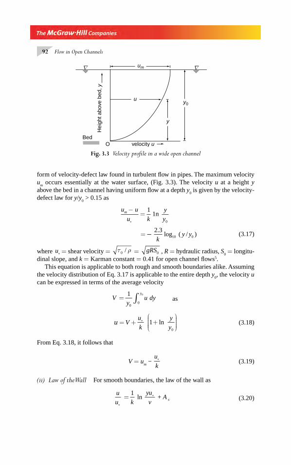
92 Flow in Open Channels
form of velocity-defect law found in turbulent fl ow in pipes. The maximum velocity u
m occurs essentially at the water surface, (Fig. 3.3). The velocity u at a height y
above the bed in a channel having uniform fl ow at a depth y0 is given by the velocity-
defect law for y/y0 > 0.15 as
u u
u k
y
ym −
=∗
1
0
1n
=2 3
10 0 log ( y / y ).
k− (3.17)
where u∗ = shear velocity = τ ρ0 / = gRS0 , R = hydraulic radius, S0 = longitu-
dinal slope, and k = Karman constant = 0.41 for open channel fl ows5.This equation is applicable to both rough and smooth boundaries alike. Assuming
the velocity distribution of Eq. 3.17 is applicable to the entire depth y0, the velocity u
can be expressed in terms of the average velocity
Vy
uy
= dy 1
00
0
∫ as
u = V + u
kln
y
y∗ +
⎛
⎝⎜⎜⎜⎜
⎞
⎠⎟⎟⎟⎟
10
(3.18)
From Eq. 3.18, it follows that
V = um −
u
k∗
(3.19)
(ii) Law of the Wall For smooth boundaries, the law of the wall as
u
u k
yu
v s
∗
∗ = ln + A 1
(3.20)
Fig. 3.3 Velocity profi le in a wide open channel
∇ ∇
BedO velocity u
Hei
ght a
bove
bed
, yu
um
y
y0
Chapter 3.indd 92Chapter 3.indd 92 2/24/2010 4:21:56 PM2/24/2010 4:21:56 PM
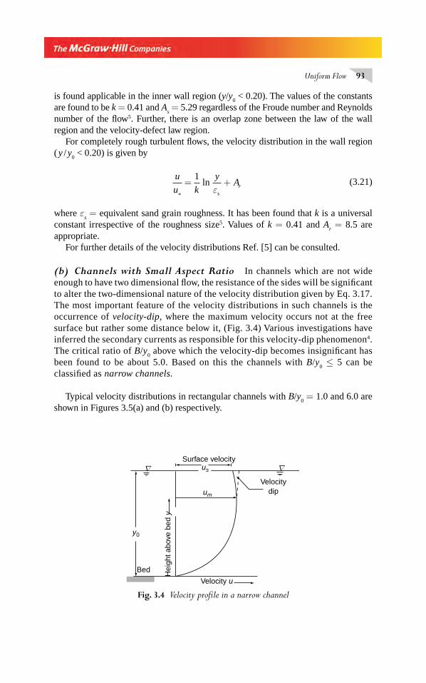
Uniform Flow 93
is found applicable in the inner wall region (y/y0 < 0.20). The values of the constants
are found to be k = 0.41 and As = 5.29 regardless of the Froude number and Reynolds
number of the fl ow5. Further, there is an overlap zone between the law of the wall region and the velocity-defect law region.
For completely rough turbulent fl ows, the velocity distribution in the wall region ( y / y
0 < 0.20) is given by
u
u k
yA
s
r
*
ln= +1
ε (3.21)
where εs = equivalent sand grain roughness. It has been found that k is a universal
constant irrespective of the roughness size5. Values of k = 0.41 and Ar = 8.5 are
appropriate.For further details of the velocity distributions Ref. [5] can be consulted.
(b) Channels with Small Aspect Ratio In channels which are not wide enough to have two dimensional fl ow, the resistance of the sides will be signifi cant to alter the two-dimensional nature of the velocity distribution given by Eq. 3.17. The most important feature of the velocity distributions in such channels is the occurrence of velocity-dip, where the maximum velocity occurs not at the free surface but rather some distance below it, (Fig. 3.4) Various investigations have inferred the secondary currents as responsible for this velocity-dip phenomenon4. The critical ratio of B/y
0 above which the velocity-dip becomes insignifi cant has
been found to be about 5.0. Based on this the channels with B/y0 ≤ 5 can be
classifi ed as narrow channels.
Typical velocity distributions in rectangular channels with B/y0 = 1.0 and 6.0 are
shown in Figures 3.5(a) and (b) respectively.
Fig. 3.4 Velocity profi le in a narrow channel
∇∇Surface velocity
us
um
Velocitydip
Velocity u
y0
Bed Hei
ght a
bove
bed
y
Chapter 3.indd 93Chapter 3.indd 93 2/24/2010 4:21:57 PM2/24/2010 4:21:57 PM
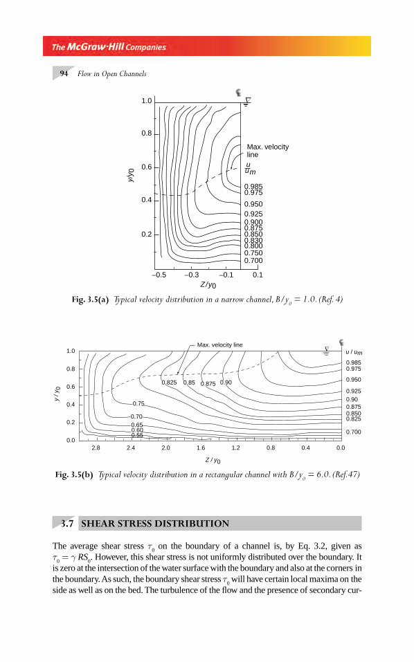
94 Flow in Open Channels
3.7 SHEAR STRESS DISTRIBUTION
The average shear stress τ0 on the boundary of a channel is, by Eq. 3.2, given as
τ0 = γ RS
0. However, this shear stress is not uniformly distributed over the boundary. It
is zero at the intersection of the water surface with the boundary and also at the corners in the boundary. As such, the boundary shear stress τ
0 will have certain local maxima on the
side as well as on the bed. The turbulence of the fl ow and the presence of secondary cur-
Fig. 3.5(a) Typical velocity distribution in a narrow channel, B/y0 = 1.0. (Ref. 4)
∇
Max. velocityline
1.0
0.8
0.6
0.4
0.2
−0.5 −0.3 −0.1 0.1Z/y0
uum
0.9850.975
0.9500.9250.9000.8750.8500.8300.8000.7500.700
y/y 0
Fig. 3.5(b) Typical velocity distribution in a rectangular channel with B/y0 = 6.0. (Ref.47)
2.8 2.4 2.0 1.6 1.2 0.8 0.4 0.00.0
0.2
0.4
0.6
0.8
1.0
0.700
0.8250.8500.8750.900.925
0.950
0.9750.985
u / um
y / y
0
Z / y0
∇
0.550.600.650.70
0.85
0.75
0.900.825 0.875
Max. velocity line
Chapter 3.indd 94Chapter 3.indd 94 2/24/2010 4:21:57 PM2/24/2010 4:21:57 PM
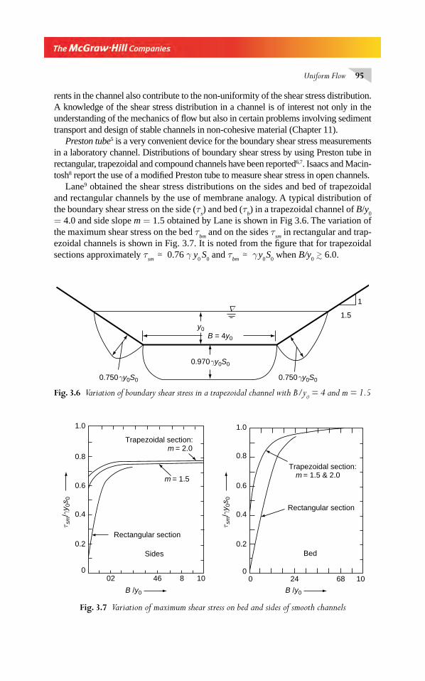
Uniform Flow 95
Fig. 3.7 Variation of maximum shear stress on bed and sides of smooth channels
Trapezoidal section:m = 1.5 & 2.0
Rectangular section
Bed
Trapezoidal section:m = 2.0
m = 1.5
Sides
Rectangular section
τ sm
/γy 0
s 0
τ sm
/γy 0
s 0
002 46 8 10 0
024 68 10
B /y0 B /y0
0.2
0.4
0.6
0.8
1.0
0.2
0.4
0.6
0.8
1.0
1
1.5
0.750γy0S0
0.970γy0S0
0.750γy0S0
y0B = 4y0
∇
Fig. 3.6 Variation of boundary shear stress in a trapezoidal channel with B/y0 = 4 and m = 1.5
rents in the channel also contribute to the non-uniformity of the shear stress distribution. A knowledge of the shear stress distribution in a channel is of interest not only in the understanding of the mechanics of fl ow but also in certain problems involving sediment transport and design of stable channels in non-cohesive material (Chapter 11).
Preston tube5 is a very convenient device for the boundary shear stress measurements in a laboratory channel. Distributions of boundary shear stress by using Preston tube in rectangular, trapezoidal and compound channels have been reported6,7. Isaacs and Macin-tosh8 report the use of a modifi ed Preston tube to measure shear stress in open channels.
Lane9 obtained the shear stress distributions on the sides and bed of trapezoidal and rectangular channels by the use of membrane analogy. A typical distribution of the boundary shear stress on the side (τ
s) and bed (τ
b) in a trapezoidal channel of B/y
0
= 4.0 and side slope m = 1.5 obtained by Lane is shown in Fig 3.6. The variation of the maximum shear stress on the bed τ
bm and on the sides τ
sm in rectangular and trap-
ezoidal channels is shown in Fig. 3.7. It is noted from the fi gure that for trapezoidal sections approximately τ
sm � 0.76 γ y
0 S
0 and τ
bm � γ y
0 S
0 when B/y
0 � 6.0.
Chapter 3.indd 95Chapter 3.indd 95 2/24/2010 4:21:57 PM2/24/2010 4:21:57 PM
96 Flow in Open Channels
3.8 RESISTANCE FORMULA FOR PRACTICAL USE
Since a majority of the open channel fl ow are in the rough turbulent range, the Man-ning’s formula (Eq. 3.11) is the most convenient one for practical use. Since, it is simple in form and is also backed by considerable amount of experience, it is the most preferred choice of hydraulic engineers. However, it has a limitation in that it cannot adequately represent the resistance in situations where the Reynolds number effect is predominant and this must be borne in mind. In the book, the Manning’s formula is used as the resistance equation.
The Darcy–weisbach coeffi cient f used with the Chezy formula is also an equally effec-tive way of representing the resistance in uniform fl ow. However, fi eld engineers generally do not prefer this approach, partly because of the inadequate information to assist in the estimation of ε
s and partly because it is not suffi ciently backed by experimental or fi eld
observational data. It should be realized that for open channel fl ows with hydrodynamically smooth boundaries, it is perhaps the only approach available to estimate the resistance.
3.9 MANNING’S ROUGHNESS COEFFICIENT n
In the Manning’s formula, all the terms except n are capable of direct measurement. The roughness coeffi cient, being a parameter representing the integrated effects of the channel cross-sectional resistance, is to be estimated. The selection of a value for n is subjective, based on one’s own experience and engineering judgement. How-ever, a few aids are available which reduce to a certain extent the subjectiveness in the selection of an appropriate value of n for a given channel. These include:
1. Photographs of selected typical reaches of canals, their description and mea-sured values of n10,11. These act as type values and by comparing the channel under question with a fi gure and description set that resembles it most, one can estimate the value of n fairly well. Movies, stereoscopic colour photographs and video recordings of selected typical reaches are other possible effective aids under the category.
2. A comprehensive list of various types of channels, their descriptions with the associates range of values of n. Some typical values of n for various normally encountered channel surfaces prepared from information gathered from vari-ous sources10,11,12,13 are presented in Table 3.2.
Estimation of correct n-value of natural channels is of utmost importance in practical problems associated with backwater computations, fl ood fl ow estimation, routing and management. The photographs of man-made and natural channels with corre-sponding values of n given by Chow10, Barnes11 and Arcemont and Schnieder14 are very useful in obtaining a fi rst estimate of roughness coeffi cient in such situations.
Cowan15 has developed a procedure to estimate the value of roughness factor n of natural channels in a systematic way by giving weightages to various important fac-tors that affect the roughness coeffi cient. According to Cowan.
n = (nb + n
1 + n
2 +n
3 +n
4) m
Chapter 3.indd 96Chapter 3.indd 96 2/24/2010 4:21:58 PM2/24/2010 4:21:58 PM
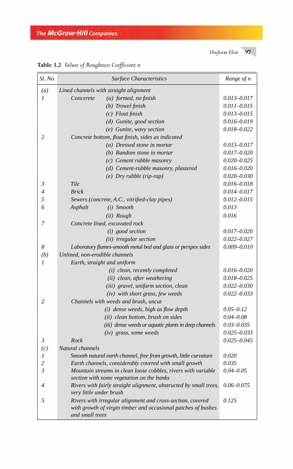
Uniform Flow 97
Table 3.2 Values of Roughness Coeffi cient n
Sl. No. Surface Characteristics Range of n
(a) Lined channels with straight alignment1 Concerete (a) formed, no fi nish 0.013–0.017
(b) Trowel fi nish 0.011–0.015 (c) Float fi nish 0.013–0.015 (d) Gunite, good section 0.016–0.019 (e) Gunite, wavy section 0.018–0.022
2 Concrete bottom, fl oat fi nish, sides as indicated (a) Dressed stone in mortar 0.015–0.017 (b) Random stone in mortar 0.017–0.020 (c) Cement rubble masonry 0.020–0.025 (d) Cement-rubble masonry, plastered 0.016–0.020 (e) Dry rubble (rip-rap) 0.020–0.030
3 Tile 0.016–0.0184 Brick 0.014–0.0175 Sewers (concrete, A.C., vitrifi ed-clay pipes) 0.012–0.0156 Asphalt (i) Smooth 0.013
(ii) Rough 0.0167 Concrete lined, excavated rock
(i) good section 0.017–0.020 (ii) irregular section 0.022–0.027
8 Laboratory fl umes-smooth metal bed and glass or perspex sides 0.009–0.010(b) Unlined, non-erodible channels1 Earth, straight and uniform
(i) clean, recently completed 0.016–0.020 (ii) clean, after weathering 0.018–0.025 (iii) gravel, uniform section, clean 0.022–0.030 (iv) with short grass, few weeds 0.022–0.033
2 Channels with weeds and brush, uncut (i) dense weeds, high as fl ow depth 0.05–0.12 (ii) clean bottom, brush on sides 0.04–0.08 (iii) dense weeds or aquatic plants in deep channels 0.03–0.035 (iv) grass, some weeds 0.025–0.033
3 Rock 0.025–0.045(c) Natural channels1 Smooth natural earth channel, free from growth, little curvature 0.0202 Earth channels, considerably covered with small growth 0.0353 Mountain streams in clean loose cobbles, rivers with variable
section with some vegetation on the banks0.04–0.05
4 Rivers with fairly straight alignment, obstructed by small trees, very little under brush
0.06–0.075
5 Rivers with irregular alignment and cross-section, covered with growth of virgin timber and occasional patches of bushes and small trees
0.125
Chapter 3.indd 97Chapter 3.indd 97 2/24/2010 4:21:58 PM2/24/2010 4:21:58 PM
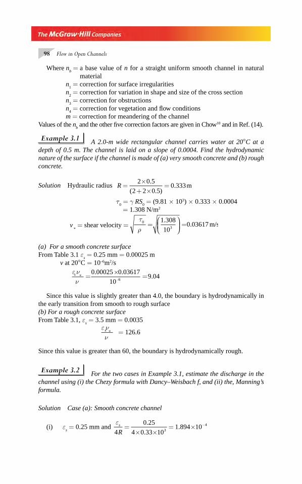
98 Flow in Open Channels
Where nb = a base value of n for a straight uniform smooth channel in natural
material n
1 = correction for surface irregularities
n2 = correction for variation in shape and size of the cross section
n3 = correction for obstructions
n4 = correction for vegetation and fl ow conditions
m = correction for meandering of the channelValues of the n
b and the other fi ve correction factors are given in Chow10 and in Ref. (14).
Example 3.1 A 2.0-m wide rectangular channel carries water at 20°C at a depth of 0.5 m. The channel is laid on a slope of 0.0004. Find the hydrodynamic nature of the surface if the channel is made of (a) very smooth concrete and (b) rough concrete.
Solution Hydraulic radius R =×
+ ×=
2 0 5
2
.
( )2 0.50.333m
τ0 = γ RS
0 = (9.81 × 103) × 0.333 × 0.0004
= 1.308 N/m2
v * = shear velocity =
τρ
0
3
1 308
10= ⎛
⎝⎜⎞⎠⎟
=.
0.03617 m/s
(a) For a smooth concrete surfaceFrom Table 3.1 ε
s = 0.25 mm = 0.00025 m
v at 20°C = 10–6m2/s
ε ννs ∗
−=×
=0 00025
10 6
. 0.036179.04
Since this value is slightly greater than 4.0, the boundary is hydrodynamically in the early transition from smooth to rough surface(b) For a rough concrete surfaceFrom Table 3.1, ε
s = 3.5 mm = 0.0035
ε ννs ∗ = 126.6
Since this value is greater than 60, the boundary is hydrodynamically rough.
Example 3.2 For the two cases in Example 3.1, estimate the discharge in the channel using (i) the Chezy formula with Dancy–Weisbach f, and (ii) the, Manning’s formula.
Solution Case (a): Smooth concrete channel
(i) εs = 0.25 mm and
εs
R4
0 25
4 103
4=× ×
= × −.
0.331.894 10
Chapter 3.indd 98Chapter 3.indd 98 2/24/2010 4:21:58 PM2/24/2010 4:21:58 PM
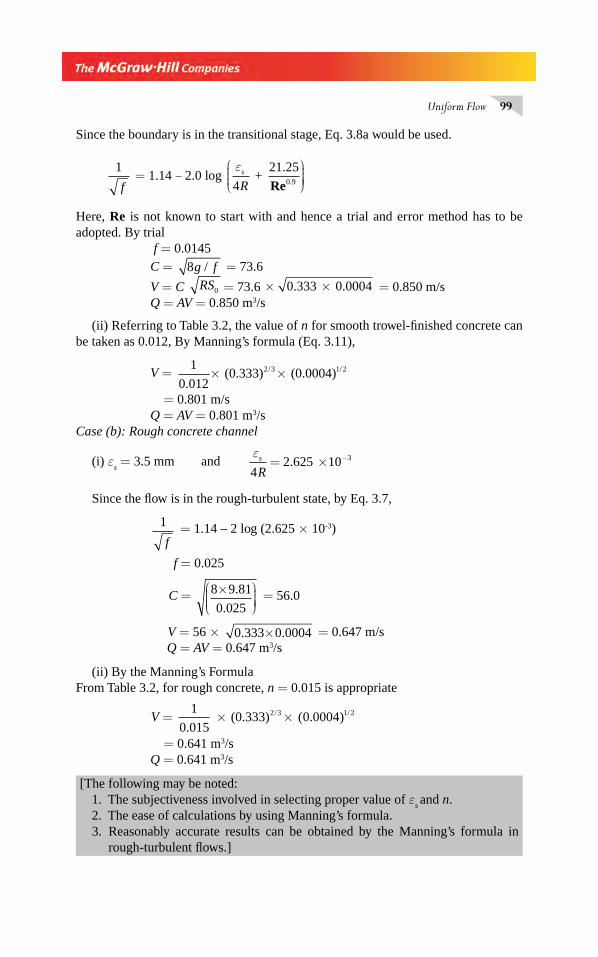
Uniform Flow 99
Since the boundary is in the transitional stage, Eq. 3.8a would be used.
1
4
21 250 9
f Rs = 1.14 2.0 log +
..
εRe
⎛
⎝⎜⎜⎜
⎞
⎠⎟⎟⎟⎟−
Here, Re is not known to start with and hence a trial and error method has to be adopted. By trial
f = 0.0145
C = 8g f/ = 73.6
V = C RS0 = 73.6 × × 0.00040 333. = 0.850 m/sQ = AV = 0.850 m3/s
(ii) Referring to Table 3.2, the value of n for smooth trowel-fi nished concrete can be taken as 0.012, By Manning’s formula (Eq. 3.11),
V = 1
0 0122 3 1 2
./ /× × (0.333) (0.0004)
= 0.801 m/sQ = AV = 0.801 m3/s
Case (b): Rough concrete channel
(i) εs = 3.5 mm and
εs
R42 625 3= × −. 10
Since the fl ow is in the rough-turbulent state, by Eq. 3.7,
1
f = 1.14 – 2 log (2.625 × 10⁻³)
f = 0.025
C = 8 9 81
0 025
×⎛⎝⎜⎜⎜
⎞⎠⎟⎟⎟⎟
.
. = 56.0
V = 56 × 0 333 0 0004. .× = 0.647 m/s Q = AV = 0.647 m3/s
(ii) By the Manning’s FormulaFrom Table 3.2, for rough concrete, n = 0.015 is appropriate
V = 1
0 0150 00042 3 1 2
.( . )/ / (0.333) × ×
= 0.641 m3/sQ = 0.641 m3/s
[The following may be noted:1. The subjectiveness involved in selecting proper value of ε
s and n.
2. The ease of calculations by using Manning’s formula.3. Reasonably accurate results can be obtained by the Manning’s formula in
rough-turbulent fl ows.]
Chapter 3.indd 99Chapter 3.indd 99 2/24/2010 4:21:58 PM2/24/2010 4:21:58 PM

100 Flow in Open Channels
Empirical Formulae for n Many empirical formulae have been presented for estimating Manning’s coeffi cient n in natural streams. These relate n to the bed-particle size. The most popular form under this type is the Strickler formula:
n = d50
1 6
21 1
/
. (3.22)
Where d50
is in metres and represents the particle size in which 50 per cent of the bed material is fi ner. For mixtures of bed materials with considerable coarse-grained sizes, Eq. 3.17 has been modifi ed by Meyer et al. as
nd
= 901 6
26
/
(3.23)
Where d90
= size in metres in which 90 per cent of the particles are fi ner than d90
. This
equation is reported to be useful in predicting n in mountain streams paved with
coarse gravel and cobbles.
Factors Aff ecting n The Manning’s n is essentially a coeffi cient representingthe integrated effect of a large number of factors contributing to the energy loss in a reach. Some important factors are: (a) Surface roughness, (b) vegetation, (c) cross-section irregularity and (d) irregular alignment of channel. The chief among these are the characteristics of the surface. The dependence of the value of n on the surface roughness in indicated in Tables 3.1 and 3.2. Since n is proportional to (ε
s)1/6, a large
variation in the absolute roughness magnitude of a surface causes correspondingly a small change in the value of n. The importance of other factors are indicated in Cowan’s method of estimation of n, as mentioned earlier.
The vegetation on the channel perimeter acts as a fl exible roughness element. At low velocities and small depths vegetations, such as grass and weeds, can act as a rigid roughness element which bends and deforms at higher velocities and depths of fl ow to yield lower resistance. For grass-covered channels, the value of n is known to decrease as the product VR increases. The type of grass and density of coverage also infl uence the value of n. For other types of vegetation, such as brush, trees in fl ood plains, etc. the only recourse is to account for their presence by suitably increasing the values of n given in Table 3.2, which of course ishighly subjective.
Channel irregularities and curvature, especially in natural streams, produce energy losses which are diffi cult to evaluate separately. As such, they are combined with the boundary resistance by suitably increasing the value of n. The procedure is some-times also applied to account for other types of form losses, such as obstructions that may occur in a reach of channel.
An interesting feature of the roughness coeffi cient is observed in some large rivers, where values of n at high stages have been found to be smaller when com-pared to the values of n at low stages. Typically, n can change from a value, such as 0.05 at low stages to 0.02 at high stages. No satisfactory explanation is available for this phenomenon. Another instance of similar, but possibly unrelated, variation of n with the stage is found in the fl ow through circular channels, such as sewers and tile
Chapter 3.indd 100Chapter 3.indd 100 2/24/2010 4:21:59 PM2/24/2010 4:21:59 PM

Uniform Flow 101
drains. In this case the largest value of n is found to occur when the depth of fl ow y
0 = 0.25 D and the least value at y
0 = D, where D = diameter of the channel. The
range of variation of n is about 30 per cent.The resistance to fl ow in alluvial channels is complex owing to the interaction of
the fl ow, fl uid and boundary. Detailed information on this is available in standard treatises on sediment transport (Section 11.3).
3.10 EQUIVALENT ROUGHNESS
In some channels different parts of the channel perimeter may have different rough-nesses. Canals in which only the sides are lined, laboratory fl umes with glass side walls and rough bed, natural rivers with sandy bed and sides with vegetation, fl ood plains with different land uses are some typical examples. For such channels it is necessary to determine an equivalent roughness coeffi cient that can be applied to the entire cross-sectional perimeter for use in Manning’s formula. This equivalent rough-ness, also called the composite roughness, represents a weighted average value for the roughness coeffi cient.
A large number of formulae, proposed by various investigators for calculating equivalent roughness of multi-roughness channel are available in literature. All of them are based on some assumptions and are approximately effective to the same degree. One of the commonly used method due to Horton (1933) and Einstein (1934) is described below. Table 3.3 lists several proposed formulae for equivalent roughness. For calculating subareas the dividing lines can be vertical lines or bisec-tor of angles at the break in the geometry of the roughness element.
3.10.1 Horton’s Method of Equivalent Roughness Estimation:
Consider a channel having its perimeter composed of N types of roughness, P1, P
2, …, P
i,
…, PN are the lengths of these N parts and n
1, n
2, …, n
i …, n
N are the respective roughness
coeffi cients (Fig. 3.8). Let each part Pi be associated with a partial area A
i such that
A A A A A Ai i Ni
N
= + + + + + = ==
∑ 1 21
... ... total area
Δ
PN
Pi
P2 A, P, n
P1
n1
n2
ni
nN
Fig. 3.8 Multi-roughness type perimeter
Chapter 3.indd 101Chapter 3.indd 101 2/24/2010 4:21:59 PM2/24/2010 4:21:59 PM
102 Flow in Open Channels
It is assumed that the mean velocity in each partial area is the mean velocity V for the entire area of fl ow, i.e.,
V1 = V
2= … = V
i = … V
N = V
By the Manning’s formula
SV n
R
V n
R
V n
R
V n
Ri i
i
N N
N
01 2 1 1
12 3
2 2
22 3 2 3 2 3
/
/ / / /= = = = = =... ...
= Vn
R2 3/ (3.24)
Where n = equivalent roughness
From Eq. 3.24 A
A
n P
nPi i i
⎛
⎝⎜⎜⎜
⎞
⎠⎟⎟⎟⎟ =
2 3 2 3
2 3
/ /
/
A An P
n Pii i= 3 2
3 2
/
/ (3.25)
A A A
n P
n Pi
i i= = ∑∑( )/
/
3 2
3 2
i.e. nn P
P
i i=
( )∑ 3 2 2 3
2 3
/ /
/ (3.26)
This equation affords a means of estimating the equivalent roughness of a channel having multiple roughness types in its perimeter. This formula was independently developed by Horton in 1933 and by Einstein in 1934. However, Eq. 3.26 is popu-larly known as Horton’s formula
If the Darcy–Weisbach friction formula is used under the same assumption of (i) Velocity being equal in all the partial areas, and (ii) slope S
0 is common to all par-
tial areas, then
h L S
f V
gR
f V P
gAf / = 0
2 2
8 8 = =
Hence V
gS
A
Pf
A
P fi
i i
2
08= =
Thus Ai /A =
P f
P fi i and on summation A A
P f
Pfii
N i ii
N
/∑∑
= =1
Chapter 3.indd 102Chapter 3.indd 102 2/24/2010 4:21:59 PM2/24/2010 4:21:59 PM
Uniform Flow 103
i.e. P fi i∑ = Pf
or f = P f
Pi i∑
(3.27)
Table 3.3 lists some of the equations proposed for estimation of equivalent roughness. This list is extracted from Ref. 16 which contains a list of 17 equations for composite roughness calculation.
Table 3.3 Equations for Equivalent Roughness Coeffi cient (Ref.10,16)
Sl. No Investigator ne
Concept
1 Horton (1933); Einstein(1934) =
⎡
⎣⎢⎢
⎤
⎦⎥⎥∑1 3 2
2 3
Pn Pi i( )/
/ Mean Velocity is constantin all subareas.
2 Pavlovskii (1931)Muhlhofer (1933)Einstein and Banks (1950)
=⎡
⎣⎢⎢
⎤
⎦⎥⎥∑1 2
1 2
Pn Pi i( )
/ Total resistance force F issum of subarea resistanceforces, Fi∑
3 Lotter (1932)=
∑
PR
PR
ni i
i
5 3
5 3
/
/
Total discharge is sum ofsubarea discharges
4 Felkel (1960)=
∑P
P
ni
i
Total discharge is sum ofsubarea discharges
5 Krishnamurthy and Christensen (1972) =
⎡
⎣
⎢⎢⎢
⎤
⎦
⎥⎥⎥
∑∑
expln/
/
Ph n
Phi i i
i i
3 2
3 2
Logarithmic velocitydistribution over depth hfor wide channel
6 Yen (1991) =
( )n P
P
i i∑ Total shear velocity isweighted sum of subareashear velocity
Example 3.3 An earthen trapezoidal channel (n = 0.025) has a bottom width of 5.0 m, side slopes of 1.5 horizontal: 1 vertical and a uniform fl ow depth of 1.1 m. In an economic study to remedy excessive seepage from the canal two proposals, viz (a) to line the sides only, and (b) to line the bed only are considered. If the lining is of smooth concrete (n = 0.012), determine the equivalent roughness in the above two cases by using (i) Horton’s formula, and by (ii) Pavlovskii formula.
Solution Case (a) Lining of the sides onlyHere for the bed: n
1= 0.025, and P
1 = 5.0 m.
For the sides: n2 = n
3 = 0.012, and P
2 = P
3 = 1.10 × + 1 1 5 2( . ) = 1.983 m
Chapter 3.indd 103Chapter 3.indd 103 2/24/2010 4:22:00 PM2/24/2010 4:22:00 PM
104 Flow in Open Channels
(i) Equivalent roughness ne by Horton’s formula: n
e = 1 3 2
2 3
Pn Pi i( )/
/
∑⎡
⎣⎢⎢
⎤
⎦⎥⎥
ne =
5 0 0 025 1 983 0 012 1 983 0 012
5 0
3 2 3 2 3 2. ( . ) . ( . ) . ( . )
[ .
/ / /× + × + ×⎡⎣⎢
⎤⎦⎥
++ += =
1 983 1 983
0 085448
4 315842 3
2 3
. . ]
.
./
/
0.0198
(ii) Equivalent roughness ne by Pavlovskii formula: n
e =
1 2
1 2
Pn Pi i( )
/
∑⎡
⎣⎢⎢
⎤
⎦⎥⎥
ne =
5 0 0 025 1 983 0 012 1 983 0 012
5 0 1 983
2 2 2. ( . ) . ( . ) . ( . )
[ . .
× + × + ×⎡⎣⎢
⎤⎦⎥
+ ++= =
1 983
0 060796
2 994331 2
1 2
. ]
.
./
/
0.0203
Case (b) Lining of the bed onlyHere for the bed: n
1= 0.012 and P
1= 5.0 m.
For the sides: n2 = n
3 = 0.025, and P
2 = P
3 = 1.10 × = + 1 1 5 2. ) 1.983 m
(i) Equivalent roughness ne by Horton’s formula: n
e =
1 3 2
2 3
Pn Pi i( )/
/
∑⎡
⎣⎢⎢
⎤
⎦⎥⎥
ne=
5 0 0 012 1 983 0 025 1 983 0 025
5 0
3 2 3 2 3 2. ( . ) . ( . ) . ( . )
[ .
/ / /× + × + ×⎡⎣⎢
⎤⎦⎥
++ += =
1 983 1 983
0 079107
4 315842 3
2 3
. . ]
.
./
/
0.01833
(ii) Equivalent roughness ne by Pavlovskii formula: n
e =
1 2
1 2
Pn Pi i( )
/
∑⎡
⎣⎢⎢
⎤
⎦⎥⎥
ne =
5 0 0 012 1 983 0 025 1 983 0 025
5 0 1 983
2 2 2. ( . ) . ( . ) . ( . )
[ . .
× + × + ×⎡⎣⎢
⎤⎦⎥
+ ++= =
1 983
0 05656
2 994331 2
1 2
. ]
.
./
/
0.01889
3.11 UNIFORM FLOW COMPUTATIONS
The Manning’s formula (Eq. 3.11) and the continuity equation, Q = AV form the basic equations for uniform-fl ow computations. The discharge Q is then given by
Q = 1 2 3
01 2
nAR S/ / (3.28)
= K S0 (3.28a)
where, K = 1
n AR2/3 is called the conveyance of the channel and expresses the dis-
charge capacity of the channel per unit longitudinal slope. The term nK = AR2/3 is sometimes called the section factor for uniform-fl ow computations.
Chapter 3.indd 104Chapter 3.indd 104 2/24/2010 4:22:00 PM2/24/2010 4:22:00 PM
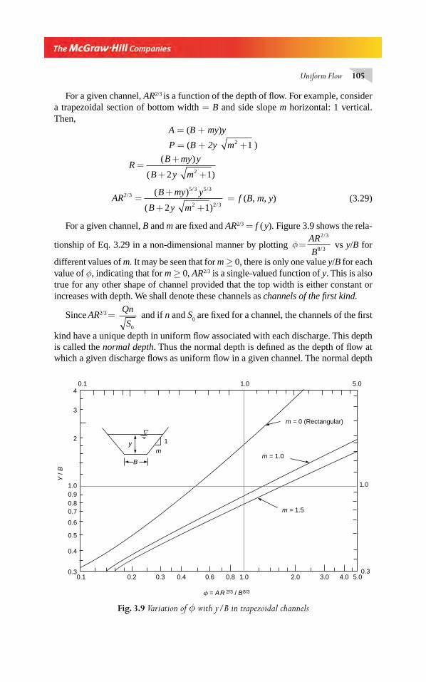
Uniform Flow 105
For a given channel, AR2/3 is a function of the depth of fl ow. For example, consider a trapezoidal section of bottom width = B and side slope m horizontal: 1 vertical. Then,
A = (B + my)y
P = (B + 2y m2 1+ )
RB my y
B y m=
+
+ +
( )
( )2 12
ARB my y
B y m
2 35 3 5 3
2 2 32 1
// /
/
( )
( )=
+
+ + = f (B, m, y) (3.29)
For a given channel, B and m are fi xed and AR2/3 = f ( y). Figure 3.9 shows the rela-
tionship of Eq. 3.29 in a non-dimensional manner by plotting φ=AR
B
2 3
8 3
/
/ vs y/B for
different values of m. It may be seen that for m ≥ 0, there is only one value y/B for each value of φ, indicating that for m ≥ 0, AR2/3 is a single-valued function of y. This is also true for any other shape of channel provided that the top width is either constant or increases with depth. We shall denote these channels as channels of the fi rst kind.
Since AR2/3 = Qn
S0
and if n and S0 are fi xed for a channel, the channels of the fi rst
kind have a unique depth in uniform fl ow associated with each discharge. This depth is called the normal depth. Thus the normal depth is defi ned as the depth of fl ow at which a given discharge fl ows as uniform fl ow in a given channel. The normal depth
40.1
3
2
1.00.90.80.7
0.6
0.5
0.4
0.30.1 0.2 0.3 0.4 0.6 0.8 1.0 2.0 3.0 4.0 5.0
0.3
1.0
5.01.0
Y /
B
1
m
m = 0 (Rectangular)
m = 1.0
m = 1.5
y
B
φ = AR 2/3 / B8/3
Δ
Fig. 3.9 Variation of φ with y/B in trapezoidal channels
Chapter 3.indd 105Chapter 3.indd 105 2/24/2010 4:22:01 PM2/24/2010 4:22:01 PM
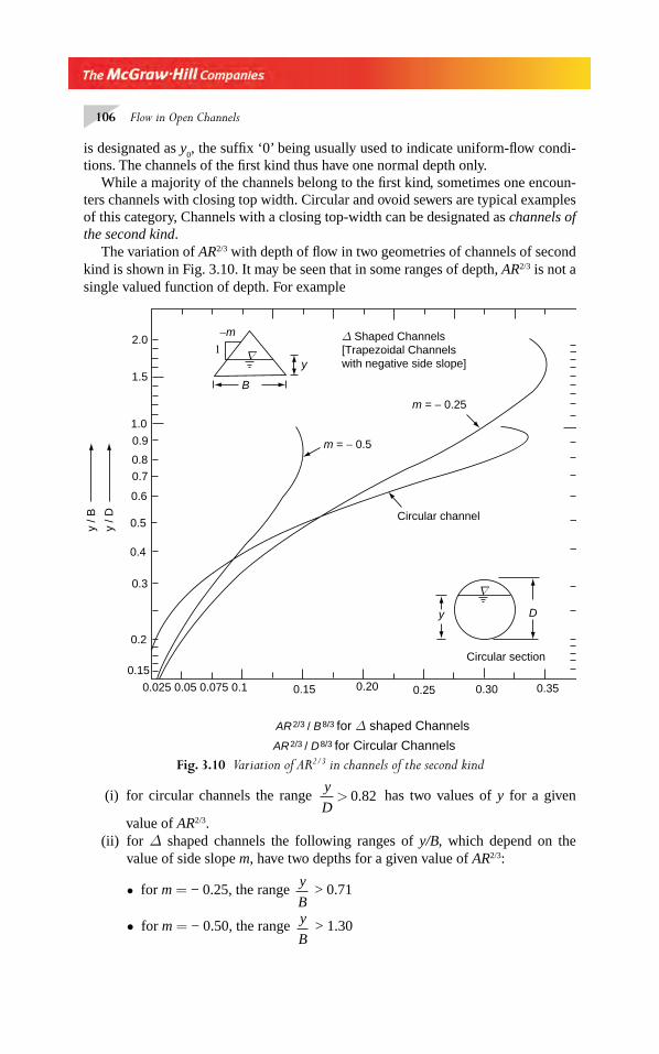
106 Flow in Open Channels
is designated as y0, the suffi x ‘0’ being usually used to indicate uniform-fl ow condi-
tions. The channels of the fi rst kind thus have one normal depth only.While a majority of the channels belong to the fi rst kind, sometimes one encoun-
ters channels with closing top width. Circular and ovoid sewers are typical examples of this category, Channels with a closing top-width can be designated as channels of the second kind.
The variation of AR2/3 with depth of fl ow in two geometries of channels of second kind is shown in Fig. 3.10. It may be seen that in some ranges of depth, AR2/3 is not a single valued function of depth. For example
(i) for circular channels the range y
D> 0 82. has two values of y for a given
value of AR2/3.(ii) for Δ shaped channels the following ranges of y/B, which depend on the
value of side slope m, have two depths for a given value of AR2/3:
• for m = − 0.25, the range y
B > 0.71
• for m = − 0.50, the range y
B > 1.30
Fig. 3.10 Variation of AR2/3 in channels of the second kind
0.025 0.05 0.075 0.1
0.15
0.2
0.3
0.4
0.5
0.6
0.7
0.8
0.9
1.0
1.5
2.0−m
1y
B
m = − 0.25
m = − 0.5
Δ Shaped Channels[Trapezoidal Channelswith negative side slope]
Circular channel
y D
Circular section
0.15 0.20 0.25 0.30 0.35
AR2/3 / B8/3 for Δ shaped Channels
AR2/3 / D8/3 for Circular Channels
Δ
Δ
y / B
y / D
Chapter 3.indd 106Chapter 3.indd 106 2/24/2010 4:22:01 PM2/24/2010 4:22:01 PM
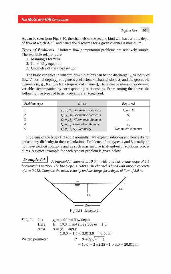
Uniform Flow 107
As can be seen form Fig. 3.10, the channels of the second kind will have a fi nite depth of fl ow at which AR2/3, and hence the discharge for a given channel is maximum.
Types of Problems Uniform fl ow computation problems are relatively simple. The available relations are
1. Manning’s formula 2. Continuity equation3. Geometry of the cross section
The basic variables in uniform fl ow situations can be the discharge Q, velocity of fl ow V, normal depth y
0, roughness coeffi cient n, channel slope S
0 and the geometric
elements (e, g., B and m for a trapezoidal channel), There can be many other derived variables accompanied by corresponding relationships. From among the above, the following fi ve types of basic problems are recognized.
Problem type Given Required
1 y0 , n, S
0 , Geometric elements Q and V
2 Q , y0 , n, Geometric elements S
0
3 Q, y0 , S
0 , Geometric elements n
4 Q, n, S0 , Geometric elements y
0
5 Q, y0 , n, S
0 , Geometry Geometric elements
Problems of the types 1, 2 and 3 normally have explicit solutions and hence do not present any diffi culty in their calculations. Problems of the types 4 and 5 usually do not have explicit solutions and as such may involve trial-and-error solutions proce-dures. A typical example for each type of problem is given below.
Example 3.4 A trapezoidal channel is 10.0 m wide and has a side slope of 1.5 horizontal: 1 vertical. The bed slope is 0.0003. The channel is lined with smooth concrete of n = 0.012. Compute the mean velocity and discharge for a depth of fl ow of 3.0 m.
10 m
1.5
1
y0
Δ
Fig. 3.11 Example 3.4
Solution Let y0 = uniform fl ow depth
Here B = 10.0 m and side slope m = 1.5 Area A = (B + my) y = (10.0 + 1.5 × 3.0) 3.0 = 43.50 m2
Wetted perimeter P = B +2y m2 1+ = 10.0 + 2 2 25 1 3 0 20 817. . .+ × = m
Chapter 3.indd 107Chapter 3.indd 107 2/24/2010 4:22:01 PM2/24/2010 4:22:01 PM
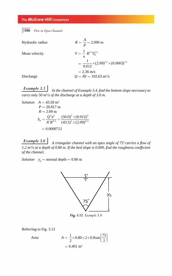
108 Flow in Open Channels
Hydraulic radius R = A
P= 2.090 m
Mean velocity V = 1 2 3
01 2
nR S / /
= 1
0 0122 09 0 00032 3 1 2
.( . ) ( . ). /× ×
= 2.36 m/sDischarge Q = AV = 102.63 m3/s
Example 3.5 In the channel of Example 3.4, fi nd the bottom slope necessary to carry only 50 m3/s of the discharge at a depth of 3.0 m.
Solution A = 43.50 m2
P = 20.817 m R = 2.09 m
S
Q n
A R0
2 2
2 4 3
2 2
2 4 3
50 0 0 012
43 5 2 09= =
××/ /
( . ) ( . )
( . ) ( . )
= 0.0000712
Example 3.6 A triangular channel with an apex angle of 75º carries a fl ow of 1.2 m3/s at a depth of 0.80 m. If the bed slope is 0.009, fi nd the roughness coeffi cient of the channel.
Solution y0 = normal depth = 0.80 m
y0
75°
Δ
Fig. 3.12 Example 3.6
Referring to Fig. 3.12
Area A = 1
20 80 2 0 8
75
2× × ×
⎛⎝⎜⎜⎜
⎞⎠⎟⎟⎟⎟. . tan
= 0.491 m2
Chapter 3.indd 108Chapter 3.indd 108 2/24/2010 4:22:01 PM2/24/2010 4:22:01 PM
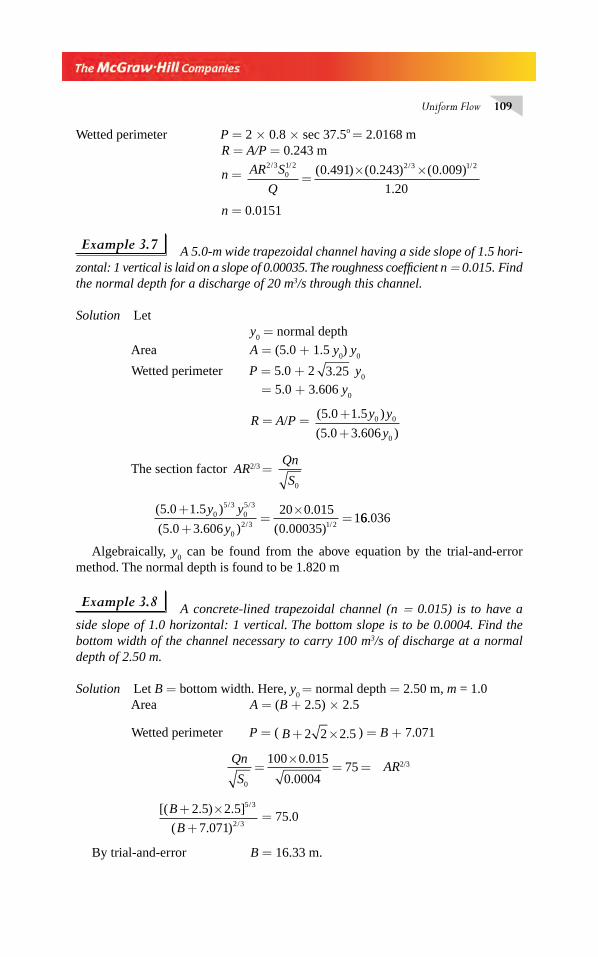
Uniform Flow 109
Wetted perimeter P = 2 × 0.8 × sec 37.5o = 2.0168 m R = A/P = 0.243 m
n = AR S
Q
2 301 2 2 3 1 20 491 0 243 0 009
1 20
/ / / /( . ) ( . ) ( . )
.=
× ×
n = 0.0151
Example 3.7 A 5.0-m wide trapezoidal channel having a side slope of 1.5 hori-zontal: 1 vertical is laid on a slope of 0.00035. The roughness coeffi cient n = 0.015. Find the normal depth for a discharge of 20 m3/s through this channel.
Solution Let y
0 = normal depth
Area A = (5.0 + 1.5 y0) y
0
Wetted perimeter P = 5.0 + 2 3 25. y0
= 5.0 + 3.606 y
0
R = A/P = ( . . )
( . . )
5 0 1 5
5 0 3 6060 0
0
++
y y
y
The section factor AR2/3 = Qn
S0
( . . )
( . . )
.
( . )
/ /
/ /
5 0 1 5
5 0 3 606
20 0 015
0 0003510
5 305 3
02 3 1 2
++
=×
=y y
y66 036.
Algebraically, y0 can be found from the above equation by the trial-and-error
method. The normal depth is found to be 1.820 m
Example 3.8 A concrete-lined trapezoidal channel (n = 0.015) is to have a side slope of 1.0 horizontal: 1 vertical. The bottom slope is to be 0.0004. Find the bottom width of the channel necessary to carry 100 m3/s of discharge at a normal depth of 2.50 m.
Solution Let B = bottom width. Here, y0 = normal depth = 2.50 m, m = 1.0
Area A = (B + 2.5) × 2.5
Wetted perimeter P = ( B + ×2 2 2 5. ) = B + 7.071
Qn
S0
100 0 015
0 0004=
×= =
.
.75 AR2/3
[( . ) . ]
( . )
/
/
B
B
+ ×+2 5 2 5
7 071
5 3
2 3= 75.0
By trial-and-error B = 16.33 m.
Chapter 3.indd 109Chapter 3.indd 109 2/24/2010 4:22:02 PM2/24/2010 4:22:02 PM
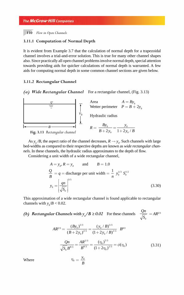
110 Flow in Open Channels
3.11.1 Computation of Normal Depth
It is evident from Example 3.7 that the calculation of normal depth for a trapezoidal channel involves a trial-and-error solution. This is true for many other channel shapes also. Since practically all open channel problems involve normal depth, special attention towards providing aids for quicker calculations of normal depth is warranted. A few aids for computing normal depth in some common channel sections are given below.
3.11.2 Rectangular Channel
(a) Wide Rectangular Channel For a rectangular channel, (Fig. 3.13)
Area A = By0
Wetter perimeter P = B + 2y0
Hydraulic radius
R = By
B y
y
y B0
0
0
02 1 2+=
+ /
As y0 /B, the aspect ratio of the channel decreases, R → y
0. Such channels with large
bed-widths as compared to their respective depths are known as wide rectangular chan-nels. In these channels, the hydraulic radius approximates to the depth of fl ow.
Considering a unit width of a wide rectangular channel,
A = y0, R = y
0 and B = 1.0
Q
B = q = discharge per unit width =
1
ny S0
5 301 2/ /
yqn
S0
0
3 5
=⎡
⎣
⎢⎢⎢
⎤
⎦
⎥⎥⎥
/
(3.30)
This approximation of a wide rectangular channel is found applicable to rectangular channels with y
0/B < 0.02.
(b) Rectangular Channels with y0/B ≥ 0.02 For these channels
Qn
S0
= AR2/3
AR2/3 = ( )
( )
( / )
( / )
/
/
/
/
By
B y
y B
y B0
5 3
02 3
05 3
02 32 1 2+
=+
B8/3
Qn
S B
AR
B0
8 3
2 3
8 30
5 3
02 3 01 2/
/
/
/
/
( )
( )( )= =
+=
ηη
φ η (3.31)
Where η0 = y
B0
B
Y0
Δ
Fig. 3.13 Rectangular channel
Chapter 3.indd 110Chapter 3.indd 110 2/24/2010 4:22:02 PM2/24/2010 4:22:02 PM
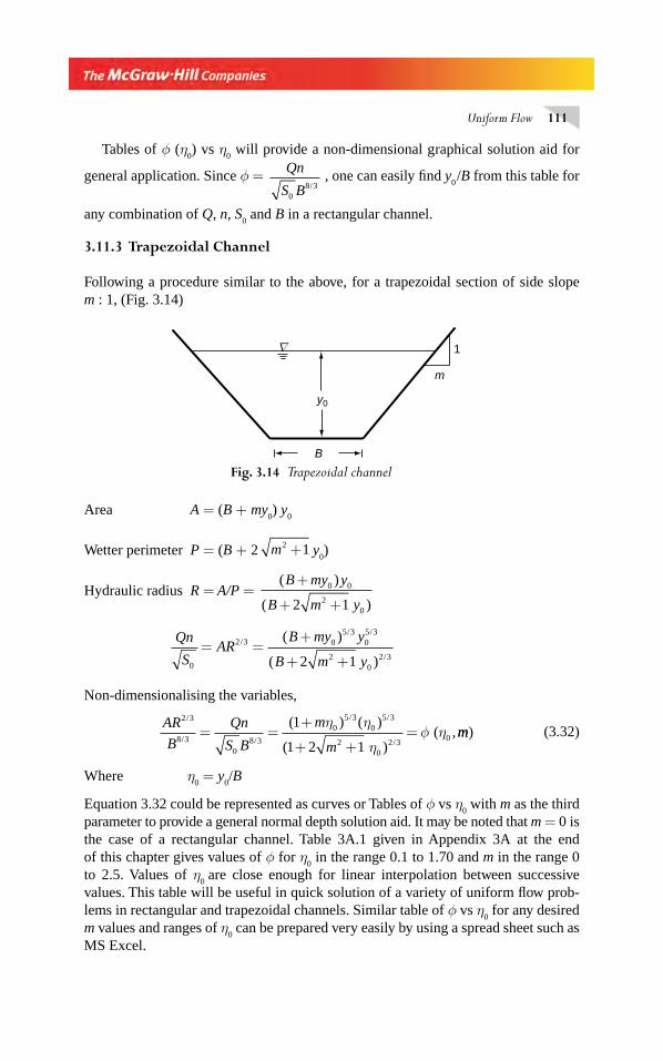
Uniform Flow 111
Tables of φ (η0) vs η
0 will provide a non-dimensional graphical solution aid for
general application. Since φ = Qn
S B08 3/
, one can easily fi nd y0 /B from this table for
any combination of Q, n, S0 and B in a rectangular channel.
3.11.3 Trapezoidal Channel
Following a procedure similar to the above, for a trapezoidal section of side slope m : 1, (Fig. 3.14)
Fig. 3.14 Trapezoidal channel
B
y0
m
1
Δ
Area A = (B + my0) y
0
Wetter perimeter P = (B + 2 m2 1+ y0)
Hydraulic radius R = A/P = ( )
( )
B my y
B m y
+
+ +0 0
202 1
Qn
SAR
B my y
B m y0
2 3 05 3
05 3
20
2 32 1= =
+
+ +/
/ /
/
( )
( )
Non-dimensionalising the variables,
AR
B
Qn
S B
m
m
2 3
8 3
08 3
05 3
05 3
20
2 3 0
1
1 2 1
/
/ /
/ /
/
( ) ( )
( ),= =
+
+ +=
η η
ηφ η
( mm) (3.32)
Where η0 = y
0/B
Equation 3.32 could be represented as curves or Tables of φ vs η0 with m as the third
parameter to provide a general normal depth solution aid. It may be noted that m = 0 is the case of a rectangular channel. Table 3A.1 given in Appendix 3A at the end of this chapter gives values of φ for η
0 in the range 0.1 to 1.70 and m in the range 0
to 2.5. Values of η0
are close enough for linear interpolation between successive values. This table will be useful in quick solution of a variety of uniform fl ow prob-lems in rectangular and trapezoidal channels. Similar table of φ vs η
0 for any desired
m values and ranges of η0 can be prepared very easily by using a spread sheet such as
MS Excel.
Chapter 3.indd 111Chapter 3.indd 111 2/24/2010 4:22:02 PM2/24/2010 4:22:02 PM
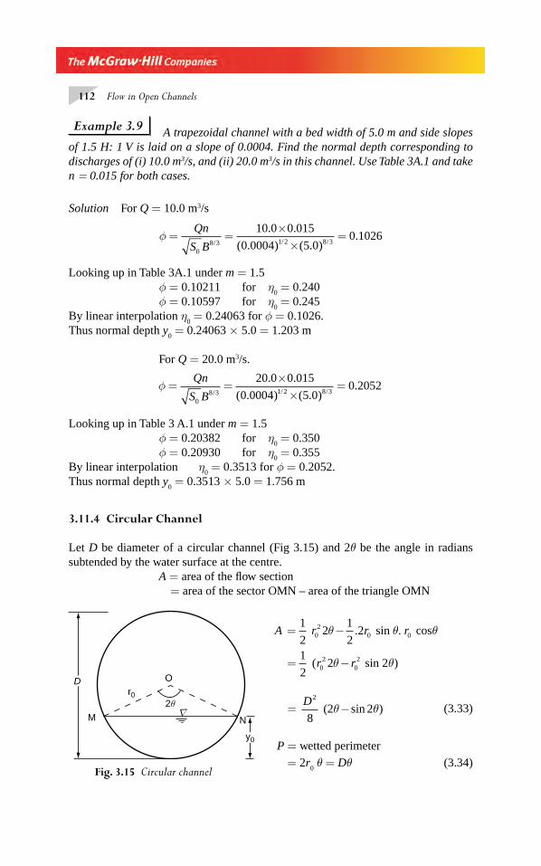
112 Flow in Open Channels
Example 3.9 A trapezoidal channel with a bed width of 5.0 m and side slopes of 1.5 H: 1 V is laid on a slope of 0.0004. Find the normal depth corresponding to discharges of (i) 10.0 m3/s, and (ii) 20.0 m3/s in this channel. Use Table 3A.1 and take n = 0.015 for both cases.
Solution For Q = 10.0 m3/s
φ = =×
×=
Qn
S B08 3 1 2 8 3
10 0 0 015
0 0004 5 00 1026
/ / /
. .
( . ) ( . ).
Looking up in Table 3A.1 under m = 1.5φ = 0.10211 for η
0 = 0.240
φ = 0.10597 for η0 = 0.245
By linear interpolation η0 = 0.24063 for φ = 0.1026.
Thus normal depth y0 = 0.24063 × 5.0 = 1.203 m
For Q = 20.0 m3/s.
0.2052φ = =×
×=
Qn
S B08 3 1 2 8 3
20 0 0 015
0 0004 5 0/ / /
. .
( . ) ( . )
Looking up in Table 3 A.1 under m = 1.5φ = 0.20382 for η
0 = 0.350
φ = 0.20930 for η0 = 0.355
By linear interpolation η0 = 0.3513 for φ = 0.2052.
Thus normal depth y0 = 0.3513 × 5.0 = 1.756 m
3.11.4 Circular Channel
Let D be diameter of a circular channel (Fig 3.15) and 2θ be the angle in radians subtended by the water surface at the centre.
A = area of the fl ow section = area of the sector OMN – area of the triangle OMN
A = −1
22
1
220
20 0 sin cos r r rθ θ θ. .
= −
1
220
202 sin 2( )r rθ θ
= D2
8 (2 2 )θ θ−sin (3.33)
P = wetted perimeter
= 2r0 θ = Dθ (3.34)
Fig. 3.15 Circular channel
Or0
2θ
D
M N
y0
Δ
Chapter 3.indd 112Chapter 3.indd 112 2/24/2010 4:22:03 PM2/24/2010 4:22:03 PM
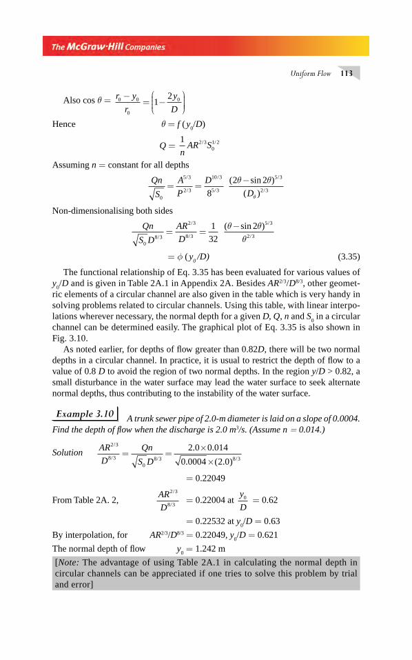
Uniform Flow 113
Also cos θ = r y
r
y
D0 0
0
012−
= −⎛
⎝⎜⎜⎜
⎞
⎠⎟⎟⎟⎟
Hence θ = f ( y0/D)
Q = 1 2 3
01 2
nAR S/ /
Assuming n = constant for all depths
Qn
S
A
P
D
D0
5 3
2 3
10 3
5 3
5 3
2 38
2 2= =
−/
/
/
/
/
/
( sin )
( )
θ θ
θ
Non-dimensionalising both sides
Qn
S D
AR
D0
8 3
2 3
8 3
5 3
2 3
1
32
2/
/
/
/
/
( sin )= =
−
θ θθ
= φ ( y0 /D) (3.35)
The functional relationship of Eq. 3.35 has been evaluated for various values of y
0/D and is given in Table 2A.1 in Appendix 2A. Besides AR2/3/D8/3, other geomet-
ric elements of a circular channel are also given in the table which is very handy in solving problems related to circular channels. Using this table, with linear interpo-lations wherever necessary, the normal depth for a given D, Q, n and S
0 in a circular
channel can be determined easily. The graphical plot of Eq. 3.35 is also shown in Fig. 3.10.
As noted earlier, for depths of fl ow greater than 0.82D, there will be two normal depths in a circular channel. In practice, it is usual to restrict the depth of fl ow to a value of 0.8 D to avoid the region of two normal depths. In the region y/D > 0.82, a small disturbance in the water surface may lead the water surface to seek alternate normal depths, thus contributing to the instability of the water surface.
Example 3.10 A trunk sewer pipe of 2.0-m diameter is laid on a slope of 0.0004. Find the depth of fl ow when the discharge is 2.0 m3/s. (Assume n = 0.014.)
Solution AR
D
Qn
S D
2 3
8 3
08 3 8 3
2 0 0 014
0 0004 2 0
/
/ / /
. .
. ( . )= =
×
×
= 0.22049
From Table 2A. 2, AR
D
2 3
8 3
/
/= 0.22004 at
y
D0 = 0.62
= 0.22532 at y0/D = 0.63
By interpolation, for AR2/3/D8/3 = 0.22049, y0/D = 0.621
The normal depth of fl ow y0 = 1.242 m
[Note: The advantage of using Table 2A.1 in calculating the normal depth in circular channels can be appreciated if one tries to solve this problem by trial and error]
Chapter 3.indd 113Chapter 3.indd 113 2/24/2010 4:22:03 PM2/24/2010 4:22:03 PM
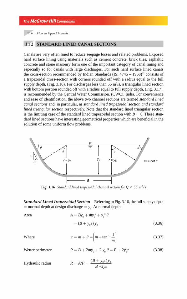
114 Flow in Open Channels
3.12 STANDARD LINED CANAL SECTIONS
Canals are very often lined to reduce seepage losses and related problems. Exposed hard surface lining using materials such as cement concrete, brick tiles, asphaltic concrete and stone masonry form one of the important category of canal lining and especially so for canals with large discharges. For such hard surface lined canals the cross-section recommended by Indian Standards (IS: 4745 – 1968)12 consists of a trapezoidal cross-section with corners rounded off with a radius equal to the full supply depth, (Fig. 3.16). For discharges less than 55 m3/s, a triangular lined section with bottom portion rounded off with a radius equal to full supply depth, (Fig. 3.17), is recommended by the Central Water Commission. (CWC), India. For convenience and ease of identifi cation, the above two channel sections are termed standard lined canal sections and, in particular, as standard lined trapezoidal section and standard lined triangular section respectively. Note that the standard lined triangular section is the limiting case of the standard lined trapezoidal section with B = 0. These stan-dard lined sections have interesting geometrical properties which are benefi cial in the solution of some uniform fl ow problems.
Fig. 3.16 Standard lined trapezoidal channel section for Q > 55 m3/s
r = y0
r r
r = y0 y0
θθθ
θ
θ
m
1
B
m = cot θ
Δ
Standard Lined Trapezoidal Section Referring to Fig. 3.16, the full supply depth = normal depth at design discharge = y
0. At normal depth
Area A = By0 + my
02 + y
02 θ
= (B + y0ε) y
0 (3.36)
Where ε = m + θ = mm
+⎛⎝⎜⎜⎜
⎞⎠⎟⎟⎟⎟
−tan 1 1 (3.37)
Wetter perimeter P = B + 2my0 + 2 y
0 θ = B + 2y
0ε (3.38)
Hydraulic radius R = A/P = ( )B y y
B y
+
+20 0ε
ε
Chapter 3.indd 114Chapter 3.indd 114 2/24/2010 4:22:03 PM2/24/2010 4:22:03 PM
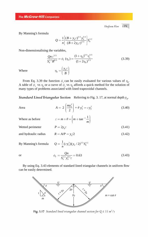
Uniform Flow 115
By Manning’s formula
Qn
B y y
B yS=
++
⎡
⎣⎢⎢
⎤
⎦⎥⎥
1
20
5 305 3
02 3 0
1 2( )
( )
/ /
/
/εε
Non-dimensionalising the variables,
Qn
S B
εφ η
η η
η
5 3
01 2 8 3 1 0
05 3 5 3
02 3
1
1 20
/
/ /
/ /
/
( )
( )= =
+
+ ( ) (3.39)
Where ηε
00=
⎛
⎝⎜⎜⎜
⎞
⎠⎟⎟⎟⎟
y
B
From Eq. 3.39 the function φ1 can be easily evaluated for various values of η
0.
A table of φ1 vs η0 or a curve of φ1 vs η
0 affords a quick method for the solution of
many types of problems associated with lined trapezoidal channels.
Standard Lined Triangular Section Referring to Fig. 3. 17, at normal depth y0,
Area A = 22
02
02
02 +
myy y
⎛
⎝⎜⎜⎜⎜
⎞
⎠⎟⎟⎟⎟
=θ ε (3.40)
Where as before ε θ= + = +⎛⎝⎜⎜⎜
⎞⎠⎟⎟⎟⎟
−m mm
tan 1 1
Wetted perimeter P = 2y0ε (3.41)
and hydraulic radius R = A/P = y0/2 (3.42)
By Manning’s formula Q = 1
202
02 3
01 2
ny S( )( / ) / /εy
or φεT
Qn
S y= =
01 2
08 3
0 63/ /
. (3.43)
By using Eq. 3.43 elements of standard lined triangular channels in uniform fl ow can be easily determined.
Fig. 3.17 Standard lined triangular channel section for Q ≤ 55 m3/s
θ2θ
θ
θ
l
mm = cot θ
r = y 0
r = y0
y0
ΔΔ
Chapter 3.indd 115Chapter 3.indd 115 2/24/2010 4:22:03 PM2/24/2010 4:22:03 PM
116 Flow in Open Channels
Example 3.11 A standard lined trapezoidal canal section is to be designed to convey 100 m3/s of fl ow. The side slopes are to be 1.5 horizontal: 1 vertical and Man-ning’s n = 0.016. The longitudinal slope of the bed is 1 in 5000. If a bed width of 10.0 m is preferred what would be the normal depth?
Solution Referring to Fig. 3.16, m = side slope = 1.5
ε = + = + =− −mm
tan . tan ( / . ) .1 111 5 1 1 5 2 088
Further, here Q = 100.0 m3/s, n = 0.016, S0 = 0.0002, B = 10.0 m
φε
1
5 3
01 2 8 3
5 3
8 3
100 0 016 2 088
0 0002 10 0= =
× ××
=Qn
S B
/
/ /
/
/
. ( . )
( . ) ( . )00.8314
By Eq.(3.39) φη η
η10
5 305 3
02 3
1
1 2=
++
( )
( )
/ /
/= 0.8314
On Simplifying, ( )
( )
/ /
/
1
1 20
5 305 3
02 5
++η η
η= 0.8951
On solving by trial and error ηε
00=
y
B = 0.74
The normal depth y0
0 74 10 0
2 0883 544=
×=
. .
.. m
Example 3.12 Show that for a standard lined trapezoidal canal section with side slopes of m horizontal: 1 vertical, and carrying a discharge of Q with a velocity V
s ,
η0
1
21 1
4
4= − + +
−
⎡
⎣⎢⎢⎢
⎤
⎦⎥⎥⎥M
Where η0 =
y
B0ε
; ε = m + tan−1 1
m; M =
QS
V ns
03 2
4 3
/
ε and n is Manning’s coeffi cient.
Also examine the situation when (i) M → 4 and (ii) M < 4.
Solution For a standard lined trapezoidal canal section (Fig.3.16)Area A = (B+ y
0ε) y
0 = Q/V
s (3.44)
Perimeter P = (B+2 y0ε)
Hydraulic radius R = A/R = Q
V Ps
(3.45)
From Manning’s formula Vs = 1 2 3
01 2
nR S/ /
i.e R2 = V n
Ss3 3
03 2/ (3.46)
Chapter 3.indd 116Chapter 3.indd 116 2/24/2010 4:22:04 PM2/24/2010 4:22:04 PM
Uniform Flow 117
Substituting for R in Eq. 3.45 Q
V P
V n
Ss
s2
2 2
3 3
03 2
=/
Hence P 2 = Q S
V PB
y
Bs
203 2
5 3
2 0
2
12/
= +⎛
⎝⎜⎜⎜
⎞
⎠⎟⎟⎟⎟
ε (3.47)
Putting η0 = y
B0ε
from Eq. 3.44 B2 = εη η
Q
Vs
⎛
⎝⎜⎜⎜⎜
⎞
⎠⎟⎟⎟⎟ +
1
1 0 0( )
Substituting for B2 in Eq. 3.47 ( ) /1 2 0
2
02
0
203 2
5 3
++
=⎡
⎣⎢⎢
⎤
⎦⎥⎥
ηη η ε
Q S
V n
V
Qs
s
= QS
V ns
03 2
4 3
/
= M
Hence 1 + 4 η02 + 4η0 = M η0
2 + Mη0
(M – 4) η02 + (M – 4) η0 – 1 = 0
On solving η0 =1
21 1
4
4−
−
⎡
⎣⎢⎢⎢
⎤
⎦⎥⎥⎥
+ +M
(i) When M → 4, η0 =
y
B0ε
→ ∞ , since y0 and ε are fi nite values this corresponds
to B → 0.Thus M = 4, corresponds to the case of standard lined triangular channel section.
(ii) When M < 4, η0 is imaginary and hence this is not physically realisable
proposition.
[Note: The expression for η0 in terms of M derived as above is very useful in solv-
ing some uniform fl ow problems relating to standard lined trapezoidal sections where V
s is known, (for e.g. Problem 3.28)].
3.13 MAXIMUM DISCHARGE OF A CHANNEL OF THE SECOND KIND
It was shown in Section 3.11 that the channels of the second kind have two nor-mal depths in a certain range and there exists a fi nite depth at which these sec-tions carry maximum discharge. The condition for maximum discharge can be expressed as
dQ
dy= 0 (3.48)
Chapter 3.indd 117Chapter 3.indd 117 2/24/2010 4:22:04 PM2/24/2010 4:22:04 PM
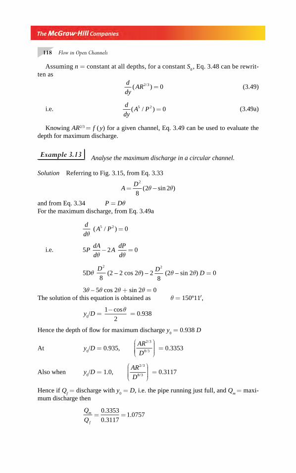
118 Flow in Open Channels
Assuming n = constant at all depths, for a constant S0 , Eq. 3.48 can be rewrit-
ten as
d
dyAR( )/2 3 0= (3.49)
i.e. d
dyA P( / )5 2 0= (3.49a)
Knowing AR2/3 = f ( y) for a given channel, Eq. 3.49 can be used to evaluate the depth for maximum discharge.
Example 3.13 Analyse the maximum discharge in a circular channel.
Solution Referring to Fig. 3.15, from Eq. 3.33
AD
= −2
82 2( sin )θ θ
and from Eq. 3.34 P = DθFor the maximum discharge, from Eq. 3.49a
d
dA P
θ ( / )5 2 0=
i.e. 5 2 0PdA
dA
dP
dθ θ− =
5Dθ D2
8(2 – 2 cos 2θ) – 2
D2
8(2θ – sin 2θ) D = 0
3θ – 5θ cos 2θ + sin 2θ = 0The solution of this equation is obtained as θ = 150º11′,
y0/D =
1
2
−cosθ = 0.938
Hence the depth of fl ow for maximum discharge y0 = 0.938 D
At y0/D = 0.935,
AR
D
2 3
8 3
/
/
⎛
⎝⎜⎜⎜⎜
⎞
⎠⎟⎟⎟⎟ = 0.3353
Also when y0/D = 1.0,
AR
D
2 3
8 3
/
/
⎛
⎝⎜⎜⎜⎜
⎞
⎠⎟⎟⎟⎟
= 0.3117
Hence if Qf = discharge with y
0 = D, i.e. the pipe running just full, and Q
m = maxi-
mum discharge then
Q
Qm
f
= =0 3353
0 31171 0757
.
..
Chapter 3.indd 118Chapter 3.indd 118 2/24/2010 4:22:04 PM2/24/2010 4:22:04 PM
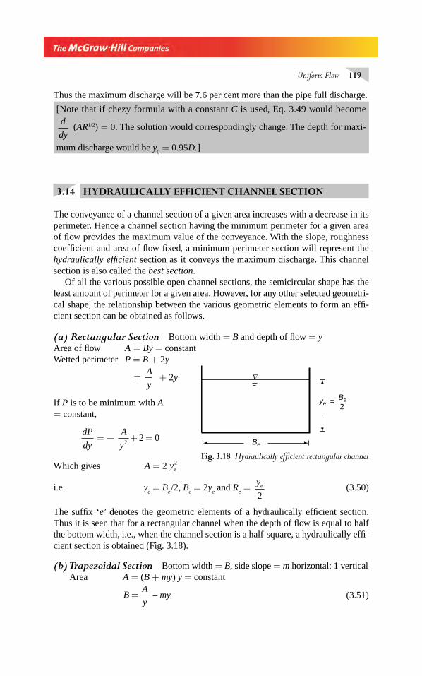
Uniform Flow 119
Thus the maximum discharge will be 7.6 per cent more than the pipe full discharge.
[Note that if chezy formula with a constant C is used, Eq. 3.49 would become d
dy (AR1/2) = 0. The solution would correspondingly change. The depth for maxi-
mum discharge would be y0 = 0.95D.]
3.14 HYDRAULICALLY EFFICIENT CHANNEL SECTION
The conveyance of a channel section of a given area increases with a decrease in its perimeter. Hence a channel section having the minimum perimeter for a given area of fl ow provides the maximum value of the conveyance. With the slope, roughness coeffi cient and area of fl ow fi xed, a minimum perimeter section will represent the hydraulically effi cient section as it conveys the maximum discharge. This channel section is also called the best section.
Of all the various possible open channel sections, the semicircular shape has the least amount of perimeter for a given area. However, for any other selected geometri-cal shape, the relationship between the various geometric elements to form an effi -cient section can be obtained as follows.
(a) Rectangular Section Bottom width = B and depth of fl ow = yArea of fl ow A = By = constantWetted perimeter P = B + 2y
= A
y + 2y
If P is to be minimum with A = constant,
dP
dy
A
y=
22 0+ =−
Which gives A = 2 ye2
i.e. ye = B
e /2, B
e = 2y
e and R
e =
ye
2 (3.50)
The suffi x ‘e’ denotes the geometric elements of a hydraulically effi cient section. Thus it is seen that for a rectangular channel when the depth of fl ow is equal to half the bottom width, i.e., when the channel section is a half-square, a hydraulically effi -cient section is obtained (Fig. 3.18).
(b) Trapezoidal Section Bottom width = B, side slope = m horizontal: 1 verticalArea A = (B + my) y = constant
BA
y= – my (3.51)
Fig. 3.18 Hydraulically effi cient rectangular channel
Be
ye = Be2
Δ
Chapter 3.indd 119Chapter 3.indd 119 2/24/2010 4:22:05 PM2/24/2010 4:22:05 PM
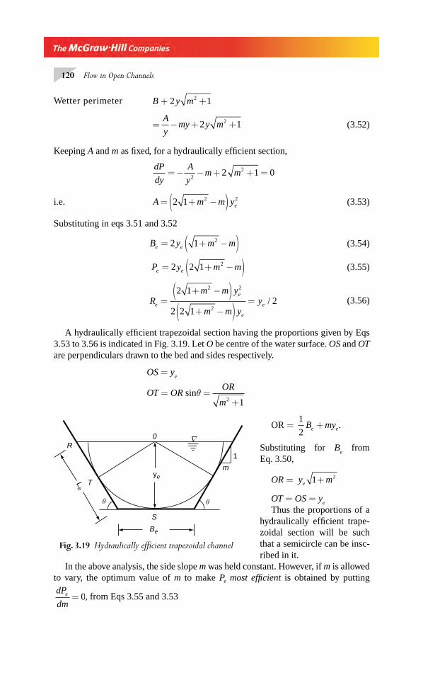
120 Flow in Open Channels
Wetter perimeter B y m+ +2 12
=A
ymy y m− + +2 12 (3.52)
Keeping A and m as fi xed, for a hydraulically effi cient section,
dP
dy
A
ym m= − − + + =
2
22 1 0
i.e. A m m ye= + −( )2 1 2 2 (3.53)
Substituting in eqs 3.51 and 3.52
B y m me e= + −( )2 1 2 (3.54)
P y m me e= + −( )2 2 1 2 (3.55)
Rm m y
m m yye
e
e
e=+ −( )+ −( )
=2 1
2 2 12
2 2
2/ (3.56)
A hydraulically effi cient trapezoidal section having the proportions given by Eqs 3.53 to 3.56 is indicated in Fig. 3.19. Let O be centre of the water surface. OS and OT are perpendiculars drawn to the bed and sides respectively.
OS = ye
OT = OR sinθ =OR
m2 1+
OR = 1
2B mye e+ .
Substituting for Be from
Eq. 3.50,
OR = y me 1 2+
OT = OS = ye
Thus the proportions of a hydraulically effi cient trape-zoidal section will be such that a semicircle can be insc-ribed in it.
In the above analysis, the side slope m was held constant. However, if m is allowed to vary, the optimum value of m to make Pe most effi cient is obtained by putting dP
dme = 0, from Eqs 3.55 and 3.53
Fig. 3.19 Hydraulically effi cient trapezoidal channel
ye
Be
S
Le T
R
θ θ
m
1
0 Δ
Chapter 3.indd 120Chapter 3.indd 120 2/24/2010 4:22:05 PM2/24/2010 4:22:05 PM
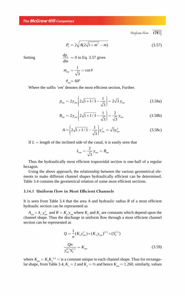
Uniform Flow 121
P A m me = + −2 2 1 2( ) (3.57)
Setting dp
dme = 0 in Eq. 3.57 gives
mem = =
1
3cot θ
θem
= 60º
Where the suffi x ‘em’ denotes the most effi cient section, Further.
p y yem em em= + −⎛
⎝⎜⎜⎜⎜
⎞
⎠⎟⎟⎟⎟ =2 2 1 1 3
1
32 3/ (3.58a)
B y yem em em= + −⎛
⎝⎜⎜⎜⎜
⎞
⎠⎟⎟⎟⎟ =2 2 1 1 3
1
3
2
3/ (3.58b)
A yem em= + −⎛
⎝⎜⎜⎜⎜
⎞
⎠⎟⎟⎟⎟ =2 1 1 3
1
332 2/ y (3.58c)
If L = length of the inclined side of the canal, it is easily seen that
L y Bem em em= =2
3
Thus the hydraulically most effi cient trapezoidal section is one-half of a regular hexagon.
Using the above approach, the relationship between the various geometrical ele-ments to make different channel shapes hydraulically effi cient can be determined. Table 3.4 contains the geometrical relation of some most effi cient sections.
3.14.1 Uniform f low in Most Effi cient Channels
It is seen from Table 3.4 that the area A and hydraulic radius R of a most effi cient hydraulic section can be represented as
Aem
= k1 yem
2 and R = K2 y
em where K
1 and K
2 are constants which depend upon the
channel shape. Thus the discharge in uniform fl ow through a most effi cient channel section can be represented as
Qn
K y K y Sem em= × ×1
12
22 3
01 2( ) ( ) ( )/ /
Qn
y SK
em
em8 301 2/ /
= (3.59)
where Kem
= K1K
22/3 = is a constant unique to each channel shape. Thus for rectangu-
lar shape, from Table 3.4, K1 = 2 and K
2 = ½ and hence K
em = 1.260. simila rly, values
Chapter 3.indd 121Chapter 3.indd 121 2/24/2010 4:22:06 PM2/24/2010 4:22:06 PM
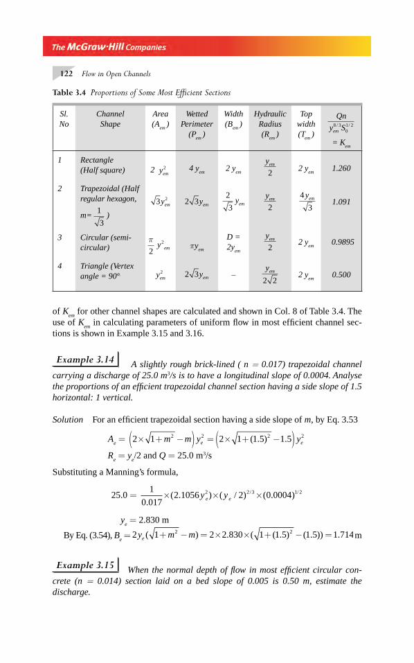
122 Flow in Open Channels
of Kem
for other channel shapes are calculated and shown in Col. 8 of Table 3.4. The use of K
em in calculating parameters of uniform fl ow in most effi cient channel sec-
tions is shown in Example 3.15 and 3.16.
Example 3.14 A slightly rough brick-lined ( n = 0.017) trapezoidal channel carrying a discharge of 25.0 m3/s is to have a longitudinal slope of 0.0004. Analyse the proportions of an effi cient trapezoidal channel section having a side slope of 1.5 horizontal: 1 vertical.
Solution For an effi cient trapezoidal section having a side slope of m, by Eq. 3.53
Ae = 2 1 2 1 1 5 1 52 2 2 2× + −( ) = × + −( )m m y ye e( . ) .
Re = y
e/2 and Q = 25.0 m3/s
Substituting a Manning’s formula,
25.0 = 1
0 0172 1056 2 0 00042 2 3 1 2
.( . ) ( / ) ( . )/ /× × ×y ye e
ye = 2.830 m
By Eq. (3.54), Be = 2 1 2 2 830 1 1 5 1 5 1 7142 2y m me ( ) . ( ( . ) ( . )) .+ − = × × + − = m
Example 3.15 When the normal depth of fl ow in most effi cient circular con-crete (n = 0.014) section laid on a bed slope of 0.005 is 0.50 m, estimate the discharge.
Table 3.4 Proportions of Some Most Effi cient Sections
Sl.No
ChannelShape
Area(A
em )
WettedPerimeter
(Pem
)
Width(B
em )
HydraulicRadius(R
em )
Topwidth(T
em )
Qn
y Sem8 3
01 2/ /
= Kem
1 Rectangle(Half square) 2 yem
2 4 yem
2 yem
yem
22 y
em1.260
2 Trapezoidal (Half regular hexagon,
m=1
3)
3 2yem 2 3yem
2
3yem
yem
2 4
3
yem1.091
3 Circular (semi-circular)
π2
2 y em πyem
D = 2y
em
yem
22 y
em 0.9895
4 Triangle (Vertex angle = 90º. yem
2 2 3yem –yem
2 22 y
em0.500
Chapter 3.indd 122Chapter 3.indd 122 2/24/2010 4:22:06 PM2/24/2010 4:22:06 PM
Uniform Flow 123
Solutions For the most effi cient circular section
From Table 3.4, Qn
y Sem8 3
01 2/ / = 0.9895. In the present case y
em= 0.5 and S
0 = 0.005.
Hence Q =0 9895
0 0140 5 0 005 0 7878 3 1 2.
.( . ) ( . ) ./ /× × = m3/s.
Example 3.16 Determine the normal depth, bed width and sides slopes of a most effi cient trapezoidal channel section to carry a discharge of 25 m3/s. The longi-tudinal slope of the channel is to be 0.0009 and Manning’s n can be taken as 0.015.
Solution For the most effi cient trapezoidal section
From Table 3.4,Qn
y Sem8 3
01 2/ /
= 1.091. In the present case Q = 25.0 m3/s and S0 = 0.0009.
Hence yem− =
××
=8 31 21 091 0 0009
25 0 0 0150 08728/
/. ( . )
. ..
y
em = 2.50 m
Also, from Table 3.4, Bem
= 2
3
2
32 50 2 887yem = × =. . m
Sides slope of most effi cient trapezoidal channel section, m = 1
3= 0.57735
3.15 THE SECOND HYDRAULIC EXPONENT N
The conveyance of a channel is in general a function of the depth of fl ow. In cal-culations involving gradually varied fl ow, for purposes of integration, Bakhmeteff introduced the following assumption
K 2= C2 y N (3.60)
Where C2= a coeffi cient and N = an exponent called here as the second hydraulic
exponent to distinguish it from the fi rst hydraulic exponent M associated with the critical depth. It is found that the second hydraulic exponent N is essentially constant for a channel over a wide range of depths. Alternatively, N is usually a slowly varying function of the aspect ratio of the channel.
To determine N for any channel, a plot of log K vs log y is prepared. If N is con-stant between two points (K
1 , y
1) and (K
2, y
2) in this plot, it is determined as
NK K
y y= 2 1 2
1 2
log ( / )
log ( / )
Chapter 3.indd 123Chapter 3.indd 123 2/24/2010 4:22:07 PM2/24/2010 4:22:07 PM
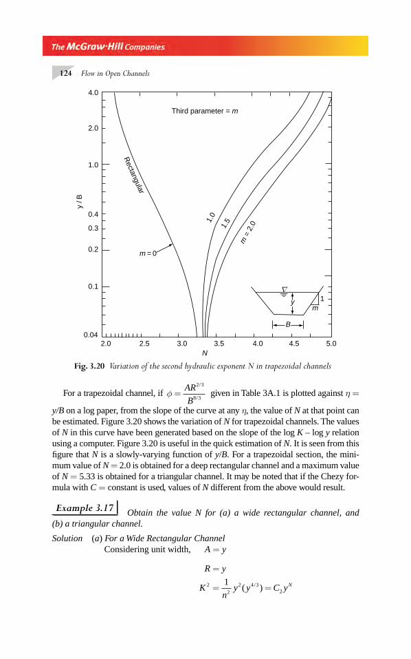
124 Flow in Open Channels
For a trapezoidal channel, if φ =AR
B
2 3
8 3
/
/ given in Table 3A.1 is plotted against η =
y/B on a log paper, from the slope of the curve at any η, the value of N at that point can be estimated. Figure 3.20 shows the variation of N for trapezoidal channels. The values of N in this curve have been generated based on the slope of the log K – log y relation using a computer. Figure 3.20 is useful in the quick estimation of N. It is seen from this fi gure that N is a slowly-varying function of y/B. For a trapezoidal section, the mini-mum value of N = 2.0 is obtained for a deep rectangular channel and a maximum value of N = 5.33 is obtained for a triangular channel. It may be noted that if the Chezy for-mula with C = constant is used, values of N different from the above would result.
Example 3.17 Obtain the value N for (a) a wide rectangular channel, and (b) a triangular channel.
Solution (a) For a Wide Rectangular ChannelConsidering unit width, A = y
R = y
Kn
y y C yN2
2
2 4 32
1= =( )/
Fig. 3.20 Variation of the second hydraulic exponent N in trapezoidal channels
m1
m = 0
Rectangular
Third parameter = m
1.0
1.5
m =
2.0
y
B
4.0
2.0
1.0
y /B
0.4
0.3
0.2
0.1
0.042.0 2.5 3.0 3.5 4.0 4.5 5.0
N
Δ
Chapter 3.indd 124Chapter 3.indd 124 2/24/2010 4:22:07 PM2/24/2010 4:22:07 PM
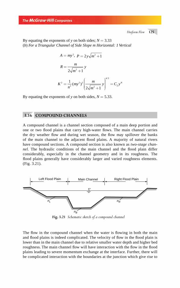
Uniform Flow 125
By equating the exponents of y on both sides; N = 3.33(b) For a Triangular Channel of Side Slope m Horizontal: 1 Vertical
A = my 2, P y m= +2 12
Rm
my=
+2 12
Kn
mym
my C yN2
2
2 2
2
4 3
2
1
2 1=
+
⎛
⎝
⎜⎜⎜⎜⎜
⎞
⎠
⎟⎟⎟⎟⎟=( )
/
By equating the exponents of y on both sides, N = 5.33.
3.16 COMPOUND CHANNELS
A compound channel is a channel section composed of a main deep portion and one or two fl ood plains that carry high-water fl ows. The main channel carries the dry weather fl ow and during wet season, the fl ow may spillover the banksof the main channel to the adjacent fl ood plains. A majority of natural rivershave compound sections. A compound section is also known as two-stage chan-nel. The hydraulic conditions of the main channel and the fl ood plain differconsiderably, especially in the channel geometry and in its roughness. Thefl ood plains generally have considerably larger and varied roughness elements. (Fig. 3.21).
Fig. 3.21 Schematic sketch of a compound channel
Right Flood PlainMain ChannelLeft Flood Plain
nL
nB
nR
Δ
The fl ow in the compound channel when the water is fl owing in both the main and fl ood plains is indeed complicated. The velocity of fl ow in the fl ood plain is lower than in the main channel due to relative smaller water depth and higher bed roughness. The main channel fl ow will have interaction with the fl ow in the fl ood plains leading to severe momentum exchange at the interface. Further, there will be complicated interaction with the boundaries at the junction which give rise to
Chapter 3.indd 125Chapter 3.indd 125 2/24/2010 4:22:07 PM2/24/2010 4:22:07 PM
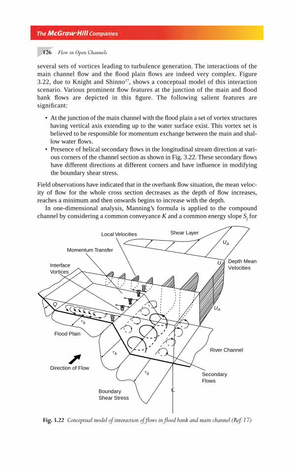
126 Flow in Open Channels
several sets of vortices leading to turbulence generation. The interactions of the main channel fl ow and the fl ood plain fl ows are indeed very complex. Figure 3.22, due to Knight and Shinno17, shows a conceptual model of this interaction scenario. Various prominent fl ow features at the junction of the main and fl ood bank fl ows are depicted in this fi gure. The following salient features are signifi cant:
• At the junction of the main channel with the fl ood plain a set of vortex structures having vertical axis extending up to the water surface exist. This vortex set is believed to be responsible for momentum exchange between the main and shal-low water fl ows.
• Presence of helical secondary fl ows in the longitudinal stream direction at vari-ous corners of the channel section as shown in Fig. 3.22. These secondary fl ows have different directions at different corners and have infl uence in modifying the boundary shear stress.
Field observations have indicated that in the overbank fl ow situation, the mean veloc-ity of fl ow for the whole cross section decreases as the depth of fl ow increases, reaches a minimum and then onwards begins to increase with the depth.
In one-dimensional analysis, Manning’s formula is applied to the compound channel by considering a common conveyance K and a common energy slope S
f for
Fig. 3.22 Conceptual model of interaction of fl ows in fl ood bank and main channel (Ref. 17)
UA
UA
U
Shear LayerLocal Velocities
Momentum Transfer
InterfaceVortices
Flood Plain
Direction of Flow
BoundaryShear Stress
SecondaryFlows
River Channel
Q
τb
τb
τb
Depth MeanVelocities
Chapter 3.indd 126Chapter 3.indd 126 2/24/2010 4:22:07 PM2/24/2010 4:22:07 PM
Uniform Flow 127
the entire section to obtain the discharge as Q = K S f . However, to account for
the different hydraulic conditions of the main and fl ood plain sections, the channel
is considered to be divided into subsections with each subsection having its own conveyance, K
i. The sum of the conveyances will give the total channel convey-
ance (ΣKi = K) for use in discharge computation. Various methods for defi ning the
boundaries of the sub-sections are proposed by different researchers leading to a host of proposed methods. However, the overall method of considering the channel as a composite of sub sections is well accepted and the method is known as Divided Channel method (DCM). Currently DCM is widely used and many well-known software packages, including HEC-RAS (2006), adopt this method in dealing with compound channels.
3.16.1 Divided Channel Method (DCM)
A large number of methods of defi ning the sub-sections in the divided channelmethod are available in literature. These include vertical interface, diagonal inter-face; horizontal interface, curved interface and variable interface to divide the sub-sections. However, the following two methods are popular, been well studied and have been found to give reasonably good results:
1. Vertical Interface Method In this method the fl ood banks are separated from the main channel by means of vertical interface, (as shown in Fig. 3.24). This inter-face is considered as a surface of zero shear where in no transfer of momentum takes place. As such, the length of the vertical interface is not included in the calculation of the wetted perimeter of either the over bank fl ow or the main channel fl ow.
2. Diagonal Interface Method In this method, a diagonal interface (as in Fig. 3.23) is considered from the top of the main channel bank to the centerline of the water surface. This interface is considered to be a surface of zero shear stress and as such the length of the diagonal interfaces are not included in the calculation of the wetted perimeters of the over bank and main channel fl ows. If the over bank portion has signifi cant roughness discontinuities equivalent roughness (as indicated Sec. 3.10) for over bank region can be adopted.
While there is no general agreement to choose a particular method, it is generally believed that the vertical interface method or the diagonal interface method seem to give the best results. HEC-RAS uses vertical interface procedure. In the procedure adopted by HEC-RAS, the fl ow in the over bank areas are subdivided using the n-values break points (locations where n-values change signifi cantly) as the basis.Main channel is not normally subdivided. Conveyance is calculated for each sub division by considering vertical interface. It is known the DCM over estimates the discharge to some extent and due to extreme complexity of the hydraulics of the problem, a high degree of accuracy in the discharge estimation should not be expected in any of the procedures connected with compound channels. Example 3.18 illus-trates the use of these two DCM procedures.
Chapter 3.indd 127Chapter 3.indd 127 2/24/2010 4:22:07 PM2/24/2010 4:22:07 PM
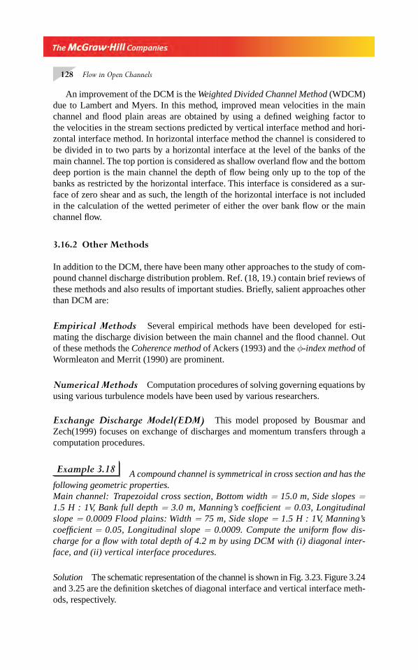
128 Flow in Open Channels
An improvement of the DCM is the Weighted Divided Channel Method (WDCM) due to Lambert and Myers. In this method, improved mean velocities in the main channel and fl ood plain areas are obtained by using a defi ned weighing factor to the velocities in the stream sections predicted by vertical interface method and hori-zontal interface method. In horizontal interface method the channel is considered to be divided in to two parts by a horizontal interface at the level of the banks of the main channel. The top portion is considered as shallow overland fl ow and the bottom deep portion is the main channel the depth of fl ow being only up to the top of the banks as restricted by the horizontal interface. This interface is considered as a sur-face of zero shear and as such, the length of the horizontal interface is not included in the calculation of the wetted perimeter of either the over bank fl ow or the main channel fl ow.
3.16.2 Other Methods
In addition to the DCM, there have been many other approaches to the study of com-pound channel discharge distribution problem. Ref. (18, 19.) contain brief reviews of these methods and also results of important studies. Briefl y, salient approaches other than DCM are:
Empirical Methods Several empirical methods have been developed for esti-mating the discharge division between the main channel and the fl ood channel. Out of these methods the Coherence method of Ackers (1993) and the φ-index method of Wormleaton and Merrit (1990) are prominent.
Numerical Methods Computation procedures of solving governing equations by using various turbulence models have been used by various researchers.
Exchange Discharge Model(EDM) This model proposed by Bousmar and Zech(1999) focuses on exchange of discharges and momentum transfers through a computation procedures.
Example 3.18 A compound channel is symmetrical in cross section and has the following geometric properties.Main channel: Trapezoidal cross section, Bottom width = 15.0 m, Side slopes = 1.5 H : 1V, Bank full depth = 3.0 m, Manning’s coeffi cient = 0.03, Longitudinal slope = 0.0009 Flood plains: Width = 75 m, Side slope = 1.5 H : 1V, Manning’s coeffi cient = 0.05, Longitudinal slope = 0.0009. Compute the uniform fl ow dis-charge for a fl ow with total depth of 4.2 m by using DCM with (i) diagonal inter-face, and (ii) vertical interface procedures.
Solution The schematic representation of the channel is shown in Fig. 3.23. Figure 3.24 and 3.25 are the defi nition sketches of diagonal interface and vertical interface meth-ods, respectively.
Chapter 3.indd 128Chapter 3.indd 128 2/24/2010 4:22:08 PM2/24/2010 4:22:08 PM
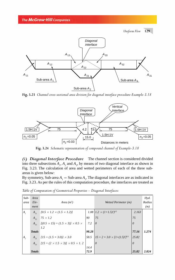
Uniform Flow 129
(i) Diagonal Interface Procedure The channel section is considered divided into three subsections A
1, A
2 and A
3, by means of two diagonal interface as shown in
Fig. 3.23. The calculation of area and wetted perimeters of each of the three sub-areas is given below:By symmetry, Sub-area A
1 = Sub-area A
3. The diagonal interfaces are as indicated in
Fig. 3.23. As per the rules of this computation procedure, the interfaces are treated as
Table of Computation of Geometrical Properties – Diagonal Interfaces:
Sub-
area
Area
Ele-
ment
Area (m2) Wetted Perimeter (m)
Hyd.
Radius
(m)
A1
A11
[0.5 × 1.2 × (1.5 × 1.2)] 1.08 1.2 × (1+1.5)2)0.5 2.163
A12
75 × 1.2 90 75 75
A13
[(0.5 × 15) + (1.5 × 3)] × 0.5 ×
1.2
7.2 0 0
Totals 98.28 77.16 1.274
A2
A21
[15 + (1.5 × 3.0)] × 3.0 58.5 15 + 2 × 3.0 × [1+(1.5)2]0.5 25.82
A22
[15 + (2 × 1.5 × 3)] × 0.5 × 1. 2
14.4
0 0
Totals 72.9 25.82 2.824
Fig. 3.24 Schematic representation of compound channel of Example-3.18
3.0
DiagonalInterface
VerticalInterface
Distances in meters
75 4.2 75
15.0
1.5H:1V1.5H:1V
1.5H:1Vn3 =0.05
n2 =0.03
n1 =0.05
Fig. 3.23 Channel cross-sectional area division for diagonal interface procedure-Example-3.18
Diagonalinterface
A13 A33
A32
A31
A22
A21
A12
A11
Sub-area A1
Sub-area A2
Sub-area A3
Chapter 3.indd 129Chapter 3.indd 129 2/24/2010 4:22:08 PM2/24/2010 4:22:08 PM
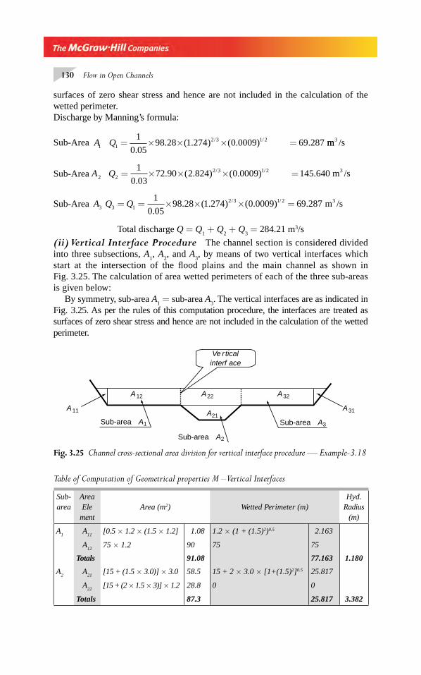
130 Flow in Open Channels
surfaces of zero shear stress and hence are not included in the calculation of the wetted perimeter.Discharge by Manning’s formula:
Sub-Area A Q1 12 3 1 21
0 0598 28 1 274 0 0009 69 287 = × × × =
.. ( . ) ( . ) ./ / mm /s3
Sub-Area A Q2 22 3 1 21
0 0372 90 2 824 0 0009 145.640= × × × =
.. ( . ) ( . )/ / m /s3
Sub-Area m /s3A Q Q3 3 12 3 1 21
0 0598 28 1 274 0 0009 69 287= = × × × =
.. ( . ) ( . ) ./ /
Total discharge Q = Q1 + Q
2 + Q
3 = 284.21 m3/s
(ii) Vertical Interface Procedure The channel section is considered divided into three subsections, A
1, A
2, and A
3, by means of two vertical interfaces which
start at the intersection of the fl ood plains and the main channel as shown in Fig. 3.25. The calculation of area wetted perimeters of each of the three sub-areas is given below:
By symmetry, sub-area A1 = sub-area A
3. The vertical interfaces are as indicated in
Fig. 3.25. As per the rules of this computation procedure, the interfaces are treated as surfaces of zero shear stress and hence are not included in the calculation of the wetted perimeter.
Fig. 3.25 Channel cross-sectional area division for vertical interface procedure — Example-3.18
Ve rticalinterf ace
A32
A31
A22
A21
A12
A11
Sub-area A1
Sub-area A2
Sub-area A3
Sub-area
Area Ele
mentArea (m2) Wetted Perimeter (m)
Hyd. Radius
(m)
A1
A11
[0.5 × 1.2 × (1.5 × 1.2] 1.08 1.2 × (1 + (1.5)2)0.5 2.163
A12
75 × 1.2 90 75 75
Totals 91.08 77.163 1.180
A2
A21
[15 + (1.5 × 3.0)] × 3.0 58.5 15 + 2 × 3.0 × [1+(1.5)2]0.5 25.817
A22
[15 + (2 × 1.5 × 3)] × 1.2 28.8 0 0
Totals 87.3 25.817 3.382
Table of Computation of Geometrical properties M – Vertical Interfaces
Chapter 3.indd 130Chapter 3.indd 130 2/24/2010 4:22:08 PM2/24/2010 4:22:08 PM
Uniform Flow 131
Discharge by Manning’s formula:
Sub-Area A Q1 12 3 1 21
0 0591 08 1 180 0 0009 61 035 = × × × =
.. ( . ) ( . ) ./ / mm /s3
Sub-Area A Q2 22 3 1 21
0 0387 3 3 382 0 0009 196.697 = × × × =
.. ( . ) ( . )/ / mm /s3
Sub-Area m /s3A Q Q3 3 12 3 1 21
0 0591 08 1 180 0 0009 61 035= = × × × =
.. ( . ) ( . ) ./ /
Total discharge Q = Q1 + Q
2 + Q
3 = 318.77 m3/s
3.17 CRITICAL SLOPE
Critical slope is the slope of a specifi ed channel necessary to have uniform fl ow of a given discharge with critical depth as the normal depth. Thus the normal discharge formula
Qn
AR S=1 2 3 1 2/ / would become
Qn
A R Sc c c=1 2 3 1 2/ / (3.61)
Where Ac = area of the channel at critical depth y
c
Rc = hydraulic radius of the channel at critical depth y
c and
Sc = critical slope
From Eq. 3.61 Sc =
n Q
A Rc c
2 2
2 4 3/
⎛
⎝⎜⎜⎜⎜
⎞
⎠⎟⎟⎟⎟ (3.62)
Since the critical depth is a function of the channel geometry and the discharge, the critical slope S
c for a give channel is a function of the discharge. If the critical slope
Sc is larger than the channel slope S
0 the normal depth of fl ow will be larger than the
critical depth and the fl ow is subcritical and the channel is called mild slope channel. Similarly, if the critical slope S
c is smaller than the channel slope S
0 the normal depth
of fl ow will be smaller than the critical depth and the fl ow is supercritical and the channel is called steep slope channel. Further, if the critical slope S
c is equal to
the channel slope S0 the normal depth of fl ow is equal to the critical depth and the
fl ow is critical and the channel is called as Critical slope channel. Further details about the channel classifi cation are given in Chapter 4. Thus the critical slope of a channel is a conceptual slope value which depends on the discharge in the channel. Its relative value with respect to the actual slope of the channel determines the nature of fl ow of the discharge in the channel.
Chapter 3.indd 131Chapter 3.indd 131 2/24/2010 4:22:08 PM2/24/2010 4:22:08 PM
132 Flow in Open Channels
Consider a wide rectangular channel. The expression for the critical slope Sc given in
Eq. 3.62 becomes,
Sn
g yc
c
=2
1 3 / (3.62a)
Substituting the value of critical depth as yc = (q2 / g)1/3,
Sn g
qc =⎛
⎝⎜⎜⎜⎜
⎞
⎠⎟⎟⎟⎟
2 10 9
2 9
/
/ (3.63)
This Eq. 3.63 indicates that Sc decreases with increase in q and asymptotically reaches
a value of zero for q→∞. However for a rectangular channel of fi nite aspect ratio, the behavior is slightly different, the wide rectangular channel being the limiting case.
3.17.1 Critical Depth for Rectangular Channel of Finite Aspect Ratio
Consider a rectangular channel of width B. By Eq. 3.62
Sc =
n Q
A RC c
2 2
2 4 3/
⎛
⎝
⎜⎜⎜⎜⎜
⎞
⎠
⎟⎟⎟⎟⎟
For critical fl ow condition in the channel, Q
g
A
Tc
c
2 3
= . Also RBy
B ycc
c
=+( )2
.
Substituting for Ac and R
c in Eq. 3.62 and after simplifying
Sgn
B
y
By
B
c
c
c
=+
⎛
⎝⎜⎜⎜
⎞
⎠⎟⎟⎟⎟
⎡
⎣
⎢⎢⎢⎢⎢⎢⎢
⎤
⎦
⎥⎥⎥⎥⎥⎥⎥
2
1 3
4 3
12
/
/
SS B
gncc
*
/ /
/
( )= =
+1 3
2
4 3
1 3
1 2ηη
(3.64)
where η = yc/B.
The variation of the non-dimensional term SS B
gncc
*
/
=1 3
2with η is shown in Fig. 3.26.
It is seen that the parameter S*c
and hence Sc has a minimum value at a value of η = η
min
and increase on either side of this ηmin
value. Thus there is a minimum value of critical slope for a rectangular channel. The minimum value of critical slope is known as Limit slope and is designated as S
L. By differentiating Eq. 3.64 with respect to η and equating
the derivative to zero, the minimum value of η = ηmin
= yc/B is found to be 1/6. The
corresponding value of minimum S*c
is 8/3. Hence for a rectangular channel the limit slope is described by
Sgn
BL =⎛
⎝⎜⎜⎜⎜
⎞
⎠⎟⎟⎟⎟
8
3
2
1 3/ (3.65)
and this slope occurs at ηmin
= yc /B = 1/6.
Chapter 3.indd 132Chapter 3.indd 132 2/24/2010 4:22:08 PM2/24/2010 4:22:08 PM
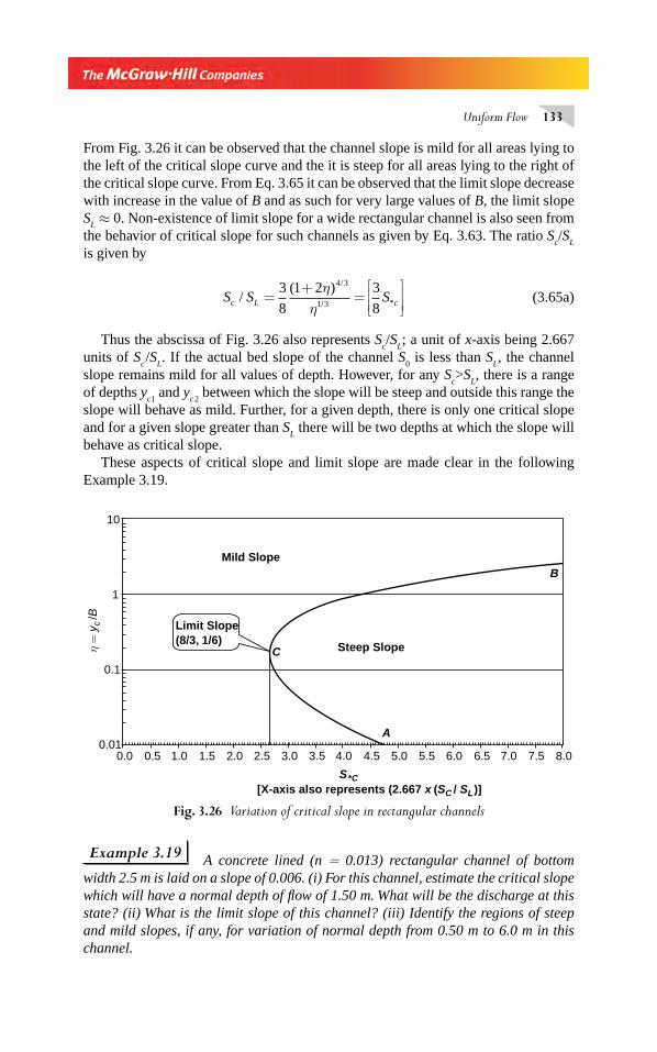
Uniform Flow 133
From Fig. 3.26 it can be observed that the channel slope is mild for all areas lying to the left of the critical slope curve and the it is steep for all areas lying to the right of the critical slope curve. From Eq. 3.65 it can be observed that the limit slope decrease with increase in the value of B and as such for very large values of B, the limit slope S
L ≈ 0. Non-existence of limit slope for a wide rectangular channel is also seen from
the behavior of critical slope for such channels as given by Eq. 3.63. The ratio Sc/S
L
is given by
S S Sc L c/( ) /
/ *=+
=⎡
⎣⎢⎢
⎤
⎦⎥⎥
3
8
1 2 3
8
4 3
1 3
ηη
(3.65a)
Thus the abscissa of Fig. 3.26 also represents Sc/S
L; a unit of x-axis being 2.667
units of Sc /S
L. If the actual bed slope of the channel S
0 is less than S
L, the channel
slope remains mild for all values of depth. However, for any Sc>S
L, there is a range
of depths yc1
and yc 2
between which the slope will be steep and outside this range the slope will behave as mild. Further, for a given depth, there is only one critical slope and for a given slope greater than S
L there will be two depths at which the slope will
behave as critical slope.These aspects of critical slope and limit slope are made clear in the following
Example 3.19.
Fig. 3.26 Variation of critical slope in rectangular channels
Limit Slope(8/3, 1/6)
Steep Slope
Mild Slope
A
B
C
S *C[X-axis also represents (2.667 x (SC / SL)]
0.0 0.5 1.0 1.5 2.0 2.5 3.0 3.5 4.0 4.5 5.0 5.5 6.0 6.5 7.0 7.5 8.00.01
0.1
1
10
η =
yc/B
Example 3.19 A concrete lined (n = 0.013) rectangular channel of bottom width 2.5 m is laid on a slope of 0.006. (i) For this channel, estimate the critical slope which will have a normal depth of fl ow of 1.50 m. What will be the discharge at this state? (ii) What is the limit slope of this channel? (iii) Identify the regions of steep and mild slopes, if any, for variation of normal depth from 0.50 m to 6.0 m in this channel.
Chapter 3.indd 133Chapter 3.indd 133 2/24/2010 4:22:09 PM2/24/2010 4:22:09 PM
134 Flow in Open Channels
Solution (i) η = yc /B = 1.5/2.5 = 0.60
SS B
gncc
*
/ /
/
( )= =
+1 3
2
4 3
1 3
1 2ηη
Sc ××
=+ ×( . )
. ( . )
( . )
( . )
/ /
/
2 5
9 81 0 013
1 2 0 60
0 60
1 3
2
4 3
1 3
818.635 Sc = 3.3924
Sc = 0.004144
Since the normal depth = yc = critical depth,
Discharge Q B gyc= = × × =3 32 5 9 81 1 5 14 385. . ( . ) . m /s3
(ii) Limit slope Sgn
BL =⎛
⎝⎜⎜⎜⎜
⎞
⎠⎟⎟⎟⎟
= ××
=8
3
8
3
9 81 0 013
2 50 003257
2
1 3
2
1 3/ /
. ( . )
( . ). 445
(iii) The actual slope of the channel S0 = 0.006. Since S
0 > S
L , fl ow in both steep and
mild slope categories is possible. From Fig. 3.26 it is seen that there will be two depths y
c1 and y
c2, at which the fl ow will be critical. Further, within the range of y
c1
and yc2
, the channel slope will be steep. Outside the range of these two depths, the
channel slope will be mild. Setting Sc = 0.006,
SS B
gncc
*
/ /. ( . )
. ( . ).= =
××
=11 3
2
3
2
0 006 2 5
9 81 0 0134 9118
And by Eq. (3.60), ( )
./
/
1 24 9118
4 3
1 3
+=
ηη
There are two positive roots of η and the values of these have to be determined by trial and error. Fig. 3.26, which is drawn to scale, affords a fi rst trial. By trial and error, the two values of η are found to be as below:η
1 = y
c1/B = 0.03823 given y
c1 = 2.5 × 0.03823 = 0.9558 m
η1 = y
c2/B = 0.5464 giving y
c2 = 2.5 × 0.5464 = 1.366 m
Hence, for any normal depth y0, the regions with mild and steep slopes are as
follows:
(i) For y0 < 0.9558 m, the channel slope is mild,
(ii) For 1.366 m > y0 > 0.9558 m, the channel slope is steep, and
(iii) For y0 > 1.366 m, the channel slope is mild.
3.18 GENERALISED FLOW RELATION
Since the Froude number of the fl ow in a channel if FV
gA T=
/
Q
g
F A
T
2 2 3
= (3.66)
Chapter 3.indd 134Chapter 3.indd 134 2/24/2010 4:22:09 PM2/24/2010 4:22:09 PM
Uniform Flow 135
If the discharge Q occurs as a uniform fl ow, the slope S0 required to sustain this dis-
charge is, by Manning’s formula,
SQ n
A R0
2 2
2 4 3=
/ (3.67)
Substituting Eq. 3.66 in Eq. 3.67 and simplifying
SF g n P
TA0
2 2 4 3
1 3=
/
/
or S
F gn
P
TAf y0
2 2
4 3
1 3= =
/
/( ) (3.68)
For a trapezoidal channel of side slope m,
S
F gn
B m y
B my B my y0
2 2
24 3
0 01 3
2 1
2=
+ +( )+ +
/
/( )[( ) ] (3.69)
Non-dimensionalising both sides, through multiplication by B1/3,
SS B
F gn
m
m m*
/ /
/
( )
( )( ) (=
⎛
⎝⎜⎜⎜⎜
⎞
⎠⎟⎟⎟⎟
=+ +
+ +0
1 3
2 2
2 4 3
1 3
1 2 1
1 2 1
ηη η ηη) /1 3
(3.70)
in which η = y0/B. Designating
S B
F gnS0
1 3
2 2
/
*
⎛
⎝⎜⎜⎜⎜
⎞
⎠⎟⎟⎟⎟
= = generalized slope
S* = f (m, η) (3.71)
Equation 3.70 represents the relationship between the various elements of uni-form fl ow in a trapezoidal channel in a generalised manner. The functional relation-ship of Eq. 3.70 is plotted in Fig. 3.26. This fi gure can be used to fi nd, for a given trapezoidal channel, (a) the bed slope required to carry a uniform fl ow at a known depth and Froude number and (b) the depth of fl ow necessary for generating a uni-form fl ow of a given Froude number in a channel of known bed slope.For a rectangular channel, m = 0 and hence Eq. (3.70) becomes
S*
/
/
( )=
+1 2 4 3
1 3
ηη
(3.72)
For a triangular channel, B = 0 and hence Eq. (3.70) cannot be used. However, by redefi ning the generalised slope for triangular channels, by Eq. 3.69
S y
F gnS
m
mt0
1 3
2
1 32
2
2 3
21/
*/
/
( )2
= =+⎛
⎝⎜⎜⎜⎜
⎞
⎠⎟⎟⎟⎟
(3.73)
Chapter 3.indd 135Chapter 3.indd 135 2/24/2010 4:22:09 PM2/24/2010 4:22:09 PM
136 Flow in Open Channels
Roots and Limit Values of S. for Trapezoidal Channels Equation 3.70 can be written as
Sm
m m* ( ) ( )3
24
3
1 2 1
1 2 1=
+ +( )+ +
η
η η η (3.74)
This is a fi fth-degree equation in η, except for m = 0 when it reduces to a fourth-degree equation. Out of its fi ve roots it can be shown that (a) at least one root shall be real and positive and (b) two roots are always imaginary. Thus depending upon the value of m and S
*, there may be one, two or three roots. The limiting values of S
* are
obtained by putting, dS
d*
η= 0 , which results in
8 1 1 1 2 1 2 12 2η η η η+ + + − + +m m m m( )( ) ( ) ( )1 10 10 02 2+ + =m mη η (3.75)
Solving Eq. 3.75 the following signifi cant results are obtained.20
1. For rectangular channels (m = 0), a single limiting value with S* = 8/3 and
ηL = 1/6 is obtained.
2. Between m = 0 and m = 0.46635 there are two limiting values.3. At m = 0.46635, the two limit values merge into one at S
* = 2.1545 and
η = 0.7849.4. For m > 0.46635, there are no limiting points.
For rectangular channels, an interesting extension of result (1) noted above is as follows: At the limiting state, for given B, S
0 and η, the Froude number can be consid-
ered as the maximum uniform fl ow Froude number (Fmax
) in the given channel. Thus
S
S B
F gnL*
/
max
= =01 3
2 2
8
3
And by Eq. 3.65 S
SF
L
0 2= max
Thus S F SL02= max (3.76)
Equation 3.76 represents the channel slope required to have uniform fl ow Froude number in the given channel which is equal to or less than the pre assigned F
max, for
all discharges. It is interesting to observe in Fig. 3.27 that for m = 0.46635, S* is
essentially constant at a value of 2.15 over a range of values of η extending from 0.5 to 1.5 and S
* varies very slowly with η in the rest of the plot. Thus a trapezoidal sec-
tion with m = 0.46635 would give a channel in which the Froude number of the fl ow is essentially constant over a suffi ciently large range of depths.
3.18.1 Critical Slope and Limit Slope
The slope of a channel which carries a given discharge as a uniform fl ow at the criti-cal depth is called the critical slope, S
c. The condition governing the critical slope in
any channel can be easily obtained from Eq. 3.70 by putting F = 1.0. For trapezoidal
Chapter 3.indd 136Chapter 3.indd 136 2/24/2010 4:22:09 PM2/24/2010 4:22:09 PM
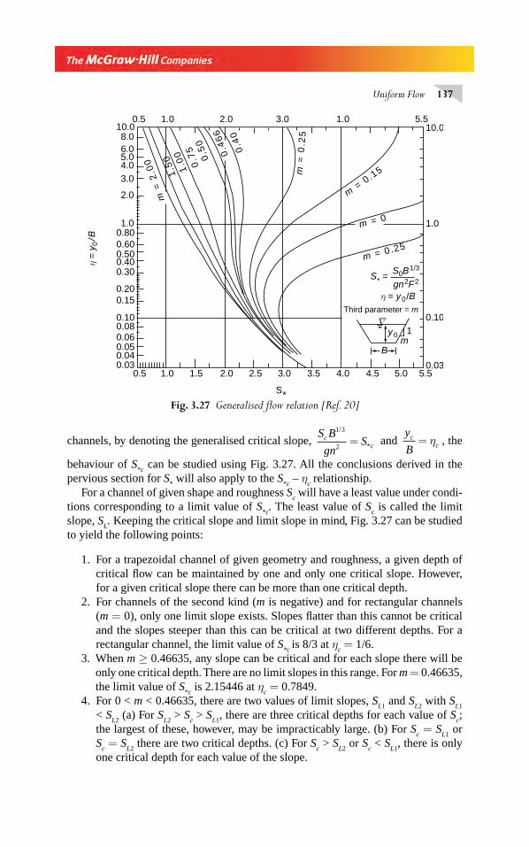
Uniform Flow 137
channels, by denoting the generalised critical slope, S B
gnSc
c
1 3
2
/
*= and y
Bc
c= η , the
behaviour of S*c
can be studied using Fig. 3.27. All the conclusions derived in the pervious section for S
* will also apply to the S
*c – η
c relationship.
For a channel of given shape and roughness Sc will have a least value under condi-
tions corresponding to a limit value of S*c
. The least value of Sc is called the limit
slope, SL. Keeping the critical slope and limit slope in mind, Fig. 3.27 can be studied
to yield the following points:
1. For a trapezoidal channel of given geometry and roughness, a given depth of critical fl ow can be maintained by one and only one critical slope. However,for a given critical slope there can be more than one critical depth.
2. For channels of the second kind (m is negative) and for rectangular channels (m = 0), only one limit slope exists. Slopes fl atter than this cannot be critical and the slopes steeper than this can be critical at two different depths. For a rectangular channel, the limit value of S
*c is 8/3 at η
c = 1/6.
3. When m ≥ 0.46635, any slope can be critical and for each slope there will be only one critical depth. There are no limit slopes in this range. For m = 0.46635, the limit value of S
*c is 2.15446 at η
c = 0.7849.
4. For 0 < m < 0.46635, there are two values of limit slopes, SL1
and SL2
with SL1
< SL2
(a) For SL2
> Sc > S
L1, there are three critical depths for each value of S
c;
the largest of these, however, may be impracticably large. (b) For Sc = S
L1 or
Sc = S
L2 there are two critical depths. (c) For S
c > S
L2 or S
c < S
L1, there is only
one critical depth for each value of the slope.
Fig. 3.27 Generalised fl ow relation [Ref. 20]
∇
S* =S0B1/3
gn2F2
η = y0/B
y0
Bm
1
Third parameter = m
0.035.54.53.52.51.50.5 5.04.03.02.01.0
0.10
1.0
10.05.51.03.02.01.0
10.08.06.05.04.03.0
2.0
1.00.800.600.500.400.30
0.200.15
0.100.080.060.050.040.03
0.5
η =
y0/B
m = 0.25
m =
0.2
5
m =
2.0
0
m = 0
.15
m = 0
0.4
0
0.5
00
.75
1.0
01
.50 0
.46
6
S*
Chapter 3.indd 137Chapter 3.indd 137 2/24/2010 4:22:10 PM2/24/2010 4:22:10 PM
138 Flow in Open Channels
Example 3.20 A rectangular channel is 4.0 m wide and has n = 0.015.
(a) Determine the bed slope required to maintain uniform fl ow in this channel witha fl ow depth of 1.25 m and a uniform fl ow Froude number of (i) 2.0, (ii) 1.0, and (iii) 0.50. Also, fi nd the limit slope and the corresponding critical discharge.
(b) Find the longitudinal slope required to ensure that the uniform fl ow Froude number in this channel is equal to or less than 0.50 for all discharges.
Solution (a) Recalling Eq. 3.72,
SS B
gn F n*
/ /
/
( )= =
+01 3
2 2
4 3
1 3
1 2η
Substituting η = =1 25
4 00 3125
.
.. in the right-hand side of the above equation,
SS
F*
/
.( . )
( . )( . ) ( )= =2 81528
4 0
9 81 0 0150
1 3
2 2
Thus,
(i) For F = 2.0, S0 = 0.015658
(ii) F = 1.0, S0 = S
c = 0.003915
(iii) F = 0.5, S0 = 0.0009787
At the limit slope, F = 1.0, and limit S*c
, = 8/3 and ηc = 1/6
SL =×
=2 667 9 81 0 015
40 003708
2
1 3
. ( . )( . )
( ).
/
y Lc = =4 0
60 667
.. m
(b) Here F = Fmax
= 0.50
By Eq. (3.72) S F SL02= max
and SL = 0.003708 as calculated in part (a) above.
Hence required S0 = (0.50)2 × 0.003708 = 0.000927
Example 3.21 A trapezoidal channel section with m = 0.25, B = 3.0 m, and n = 0.015, has to carry a uniform fl ow with a Froude number of 0.5.(a) If the bed slope of S
0 = 0.001052 is to be used, at what depths would this fl ow be
possible?(b) Within what range of S
0 would the above feature of three possible depths be
feasible?
Solution (a) SS B
gn F*
/ /( . )( . )
( . )( . ) ( . ).= = =0
1 3
2 2
1 3
2 2
0 001052 3 0
9 81 0 015 0 52 75
Chapter 3.indd 138Chapter 3.indd 138 2/24/2010 4:22:10 PM2/24/2010 4:22:10 PM
Uniform Flow 139
From Fig. (3.27), for m = 0.25.η
1 = 0.75 giving y
1 = 2.25 m
η2 = 1.00 giving y
2 = 3.00 m
and from Eq. (3.70) by trial and error, η3 = 18.70 giving y
3 = 56.10 m.
(b) From Fig. (3.27), the limit values of S* are 2.40 and 3.25. As such, the slope S
0
has to lie between 2.40 × gn2/B1/3 and 3.25 × gn2/B1/3, i.e. between S0 = 9.181 × 10⁻¹
and 1.243 × 10⁻³
3.19 DESIGN OF IRRIGATION CANALS
For a uniform fl ow in a canal,
Qn
AR S=1 2 3
01 2/ /
where A and R are in general functions of the geometric elements of the canal. If the canal is of trapezoidal cross-section.
Q f n y S B m= ( , , , , )0 0 (3.77)
Equation 3.77 has six variables out of which one is a dependent variable and the rest fi ve are independent ones. Similarly, for other channel shapes, the number of variables depend upon the channel geometry. In a channel design problem, the inde-pendent variables are known either explicitly or implicitly, or as inequalities, mostly in terms of empirical relationships.
In this section the canal-design practice adopted by the Irrigation Engineering pro-fession in India is given. This practice may have application in other fi elds also. The guidelines given below are meant only for rigid-boundary channels, i.e. for lined and unlined non-erodible channels. The design considerations for unlined alluvial channels follow different principles governed by sediment transport and related aspects. The wide variety of soil and topographical features of the country led different states and agencies, in the past, to adopt their own design practices. Reference 21 indicates the effort of the Central Water Commissions (CWC), India, towards standardisation and general guidelines applicable to the whole country. Relevant Indian standards for irri-gation canal design are found in IS: 4745–1968, IS: 7112–197312,13.
Canal Section Normally, a trapezoidal section is adopted. Rectangular cross-sec-tions are also in use in special situations, such as in rock cuts, steep chutes and in cross-drainage works.
The side slope, expressed as m horizontal: 1 vertical, depends on the type of canal, i.e. lined or unlined, nature and type of soil through which the canal is laid. The slopes are designed to withstand seepage forces under critical conditions, such as (i) a canal running full with banks saturated due to rainfall, and (ii) the sudden draw-down of canal supply. Usually the slopes are steeper in cutting than in fi lling. For lined canals, the slopes roughly correspond to the angle of repose of the natural soil and the values of m range from 1.0 to 1.5 and rarely up to 2.0. The slopes recom-mended by CWC21 for unlined canals in cutting are given in Table 3.5.
Chapter 3.indd 139Chapter 3.indd 139 2/24/2010 4:22:10 PM2/24/2010 4:22:10 PM
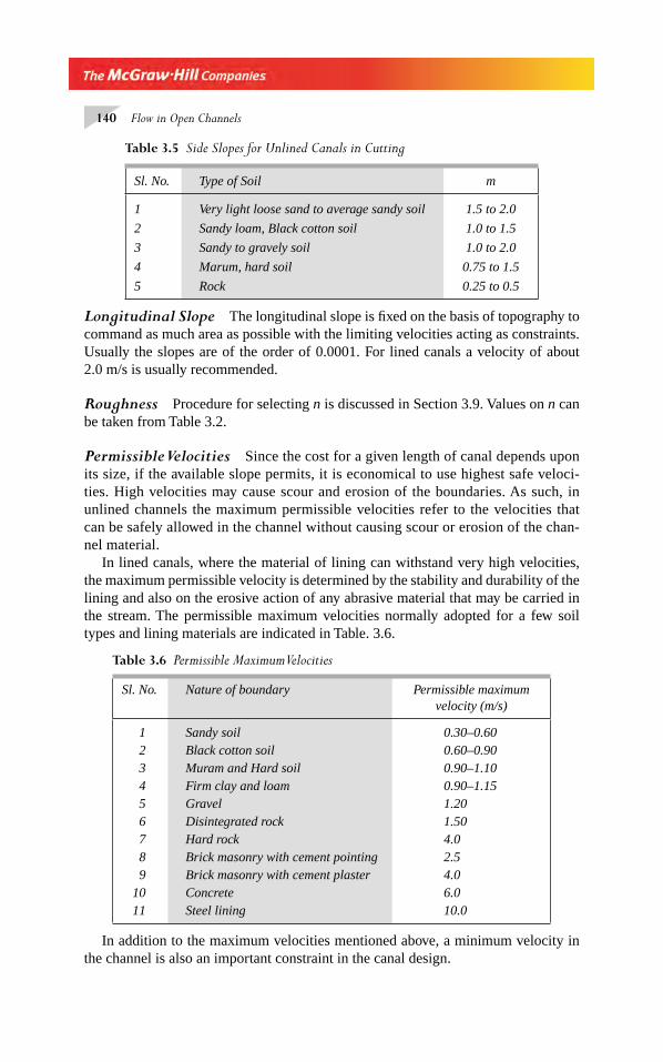
140 Flow in Open Channels
Longitudinal Slope The longitudinal slope is fi xed on the basis of topography to command as much area as possible with the limiting velocities acting as constraints. Usually the slopes are of the order of 0.0001. For lined canals a velocity of about 2.0 m/s is usually recommended.
Roughness Procedure for selecting n is discussed in Section 3.9. Values on n can be taken from Table 3.2.
Permissible Velocities Since the cost for a given length of canal depends upon its size, if the available slope permits, it is economical to use highest safe veloci-ties. High velocities may cause scour and erosion of the boundaries. As such, in unlined channels the maximum permissible velocities refer to the velocities that can be safely allowed in the channel without causing scour or erosion of the chan-nel material.
In lined canals, where the material of lining can withstand very high velocities,the maximum permissible velocity is determined by the stability and durability of the lining and also on the erosive action of any abrasive material that may be carried in the stream. The permissible maximum velocities normally adopted for a few soil types and lining materials are indicated in Table. 3.6.
Table 3.5 Side Slopes for Unlined Canals in Cutting
Sl. No. Type of Soil m
1 Very light loose sand to average sandy soil 1.5 to 2.0
2 Sandy loam, Black cotton soil 1.0 to 1.5
3 Sandy to gravely soil 1.0 to 2.0
4 Marum, hard soil 0.75 to 1.5
5 Rock 0.25 to 0.5
Table 3.6 Permissible Maximum Velocities
Sl. No. Nature of boundary Permissible maximumvelocity (m/s)
1 Sandy soil 0.30–0.602 Black cotton soil 0.60–0.903 Muram and Hard soil 0.90–1.104 Firm clay and loam 0.90–1.155 Gravel 1.206 Disintegrated rock 1.507 Hard rock 4.08 Brick masonry with cement pointing 2.59 Brick masonry with cement plaster 4.0
10 Concrete 6.011 Steel lining 10.0
In addition to the maximum velocities mentioned above, a minimum velocity in the channel is also an important constraint in the canal design.
Chapter 3.indd 140Chapter 3.indd 140 2/24/2010 4:22:10 PM2/24/2010 4:22:10 PM
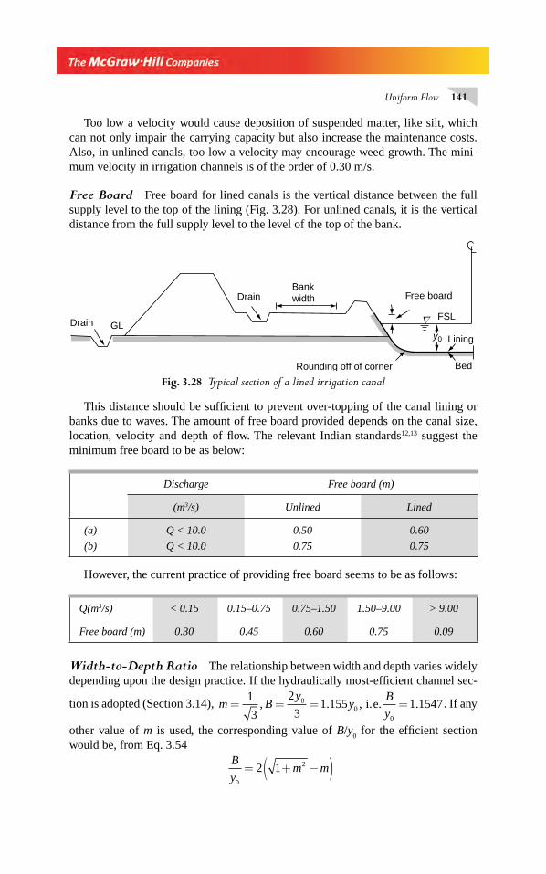
Uniform Flow 141
Too low a velocity would cause deposition of suspended matter, like silt, which can not only impair the carrying capacity but also increase the maintenance costs. Also, in unlined canals, too low a velocity may encourage weed growth. The mini-mum velocity in irrigation channels is of the order of 0.30 m/s.
Free Board Free board for lined canals is the vertical distance between the full supply level to the top of the lining (Fig. 3.28). For unlined canals, it is the vertical distance from the full supply level to the level of the top of the bank.
Fig. 3.28 Typical section of a lined irrigation canal
y0
Bed
Lining
FSL
Free boardBankwidth
Rounding off of corner
Drain
Drain GL
Δ
This distance should be suffi cient to prevent over-topping of the canal lining or banks due to waves. The amount of free board provided depends on the canal size, location, velocity and depth of fl ow. The relevant Indian standards12,13 suggest the minimum free board to be as below:
Discharge Free board (m)
(m3/s) Unlined Lined
(a) Q < 10.0 0.50 0.60
(b) Q < 10.0 0.75 0.75
However, the current practice of providing free board seems to be as follows:
Q(m3/s) < 0.15 0.15–0.75 0.75–1.50 1.50–9.00 > 9.00
Free board (m) 0.30 0.45 0.60 0.75 0.09
Width-to-Depth Ratio The relationship between width and depth varies widely depending upon the design practice. If the hydraulically most-effi cient channel sec-
tion is adopted (Section 3.14), m By
yB
y= = = =
1
3
2
31 155 1 15470
00
, . , . .i.e . If any
other value of m is used, the corresponding value of B/y0 for the effi cient section
would be, from Eq. 3.54B
ym m
0
22 1= + −( )
Chapter 3.indd 141Chapter 3.indd 141 2/24/2010 4:22:10 PM2/24/2010 4:22:10 PM
142 Flow in Open Channels
However, in practice it is usual to adopt a shallower section, i.e. a value of B/y0
larger than that suggested by Eq. 3.54. The CWC recommendation21 for B/y0 as a
function of discharge is as follows:
Q(m3/s) 0.30 3.0 14.0 28.0 140 285
B/y0
2.0 4.0 6.0 7.5 14.0 18.0
In large canals it is necessary to limit the depth to avoid dangers of bank failure. Usually depths higher than about 4.0 m are adopted only when it is absolutely necessary.
For selection of width and depth, the usual procedure is to adopt a recommended
value of B/y0 and to fi nd the corresponding
Qn
S B08 3/
using Table 3A.1. Knowing Q, n
and S0, the values of B and y
0 are found. The bottom width is usually adopted to the
nearest 25 cm or 10 cm and the depth adjusted accordingly. The resulting velocity is then checked to see that permissible velocity constraints are not exceeded. The typi-cal cross-section of a lined irrigation canal is shown in Fig. 3.28.
Super elevation The free board normally provided in design of channels of straight alignment does not account for super elevation of water surface in curved channel ali gnments. Flow around a curve causes water surface to be higher at the outer curved edge than the normal water surface of straight alignment. This would necessitate extra free board and additional lining height to guard against overtopping and erosion respectively. In subcritical fl ow, the following formulae by SCS areuseful in estimating the super elevation requirement.
For rectangular channels: EV B
g r=
3
4
2
(3.78)
For Trapezoidal channels: EV B my
g r mV=
+−
202
2
2 2
( )
( ) (3.79)
where E = Maximum height of water surface above the depth of fl ow y0
y
0 = Normal depth of fl ow for straight alignment at entrance to the curve
B = Bottom widthr = Radius of channel centerlineV = Average velocity of fl ow cross section at entrance to the curve.m = Side slope
Example 3.22 A trapezoidal channel is to carry a discharge of 50 m3/s. The maximum slope that can be used is 0.004. The soil is hard. Design the channel as (a) a lined canal with concrete lining and (b) an unlined non-erod-ible channel.
Chapter 3.indd 142Chapter 3.indd 142 2/24/2010 4:22:11 PM2/24/2010 4:22:11 PM
Uniform Flow 143
Solution (a) Lined CanalAdopt side slope of 1 : 1, i.e., m = 1.0 (from Table 3.4)n for concrete = 0.013 (from Table 3.2)Recommended B/y
0 for Q = 50 m3/s is about 8.0.
For B/y0 = 8.0 (i.e. y
0/B = 0.125), from Table 3A.1
φ = =Qn
S B08 3
0 03108/
.
Substituting Q = 50.0, n = 0.013, S0 = 0.0004 in the above
B = 13.5605 m. Adopt B = 13.50 m. Then actual
φ =×
×=
50 0 013
0 0004 31 50 03145
8 3
.
. ( . ).
/
Corresponding y0/B = 0.12588 giving y
0 = 1.700 m
A = (13.5 + 1.700) x 1.700 = 25.840V = 1.935 m/s
This value is greater than the minimum velocity of 0.3 m/s; is of the order of 2.0 m/s; and further is less than the maximum permissible velocity of 6.0 m/s for concrete. Hence the selection of B and y
0 are all right. The recommended geometric parameters
of the canal are thereforeB = 13.50 m, m = 1.0, S
0 = 0.0004
Adopt a free board of 0.75 m. The normal depth for n = 0.013 will be 1.70 m.
(b) Unlined CanalFrom Table 3.4, a side slope of 1 : 1 is adopted. From Table 3.2, take n for hard
soil surface as 0.020.Recommended B/y
0 for Q = 50 m3/s is about 8.0. From Table 3A.1.
For B
y
Qn
S B0 08 3
8 0 0 03108= = =. , ./
φ
Substituting Q = 50.0, n = 0.020 and S0 = 0.0004 in the above, B = 15.998 m, hence
adopt B = 16.00 m. Actual φ = 0.030760 and the corresponding y0/B = 0.12422.
Then y0 = 0.12422 × 16 = 1.988 m.
A = (16.00 + 1.988) × 1.988 = 35.76 m2
V = 50/35.76 = 1.398 m/sBut this velocity is larger than the permissible velocity of 0.90–1.10 m/s for hard
soil (Table 3.5). In this case, therefore, the maximum permissible velocity will con-trol the channel dimensions.Adopt V = 1.10 m/s
A
my
B
y
BB= = = +
⎛
⎝⎜⎜⎜
⎞
⎠⎟⎟⎟⎟
50 0
1 1045 455 12 0 0 2.
.. m
For B/y0 = 8.0, B = 17.978 m
Adopt B = 18.0 m
Chapter 3.indd 143Chapter 3.indd 143 2/24/2010 4:22:11 PM2/24/2010 4:22:11 PM
144 Flow in Open Channels
From A = (B + my0) y
0, substituting A = 45.455
B = 18.0, m = 1.0, y0 = 2.245 m
P = + + × =18 0 2 1 1 2 245 24 35. . . m
R = A/P = .867 mSubstituting in the general discharge equation
50
1
0 0245 455 1 867 2 3
01 2= × ×
.. ( . ) / /S
S0 = 0.0002106
Hence, the recommended parameters of the canal are B = 18.0 m, m = 1.0 and S
0 = 0.0002106. Adopt a free board of 0.75 m. The normal depth for n = 0.020 will
be 2.245 m.
REFERENCES
1. Daily, J W and Harleman, D R F Fluid Dynamics, Addison – Wesley, New York, 1966. 2. White, F M, Fluid Mechanics, 3/e, McGraw – Hill Book Co., New York, 1994. 3. Jain, A K, ‘An Accurate Explicit Equation for Friction Factor,’ Jour. Of Hyd. Div., Proc.
ASCE, Tech. Note., May 1976, pp 634–677. 4. Nezu, I and Nakagawa, Turbulence in Open Channels, IAHR Monograph, A A Balkhema,
Rotterdam, 1993. 5. Preston, J H, The Determination of Turbulent Skin Friction by means of Pitot tubes, Jour.
of Royal Aero. Soc., London, Vol. 58, 1954, pp. 109–121. 6. Rjaratnam, N and Ahmadi, R. ‘Hydraulics of Channels with Flood Plains’, Jour. of Hyd.
Research, IAHR, Vol. 19, No. 11, 1981. 7. Holden, A P and James, C S ‘Boundary Shear Distribution on Flood Plains’, Jour. of Hyd.
Research, IAHR, Vol. 27, No. 1, 1989. 8. Issacs, L T and Macintosh, J C ‘Boundary Shear Measurements in Open Channels,’ Research
Report No. CE 45, Dept. of Civil Engg., Univ. of Queensland, Australia, Feb. 1985. 9. Lane, E, ‘Design of Stable Channels’, Trans ASCE, Vol. 120, 1955.10. Chow, V T, Open Channel Hydraulics, McGraw – Hill, New York, 1959.11. Barnes, H H, ‘Roughness Characteristics of Natural Channels’, U S Geol. Water Supply
Paper No. 1849, US Govt. Press, Washington, USA, 1967.12. IS: 4745–1968, Code of Practice for the Design of Cross Section of Lined Canals in
Alluvial Soil, Indian Standards Institution, New Delhi, 1968.13. IS: 7112–1973, Code for Design of Cross Section for Unlined Canals, Indian Standards
Institution, New Delhi, 1974.14. Arcement, G J, and Schneider, V R Guide for Selecting Manning’s Roughness Coeffi -
cients for Natural Channels and Flood Plains, Reports No. FHWA-TS-84-204, Federal Highway Administration, US Dept. of Transportation, NTIS, Springfi eld, VA, 1984.[http://www.fhpa.dot.gov/bridge/wsp2339.pdf ].
15. Cowan, W L, Estimating Hydraulic Roughness Coeffi cients, Agricultural Engg., Vol. 37, No. 7, 1956, pp 473–475.
16. Ben Chie Yen, ‘Open Channel Flow Resistance’, Jour. of Hyd. Eng., ASCE, Vol. 128, No. 1, Jan 2002, pp. 20–39.
Chapter 3.indd 144Chapter 3.indd 144 2/24/2010 4:22:11 PM2/24/2010 4:22:11 PM
Uniform Flow 145
17. Knight, D W and Shiono, K, ‘Flood Plain Processes’, Chapter 5 in River Channel and Flood Plain Hydraulics, Ed. Anderson, M G. et al. John Wiley & Sons, Ltd., 1996.
18. Sturm, T W, Open channel Hydraulics McGraw-Hill Higher Education, International ed., Singapore, 2001.
19. Cao, Z., ‘Flow Resistance and Momentum Flux in Compound Open Channels’, Jour. of Hyd. Engg., ASCE, Vol. 132, No. 12, Dec. 2006, PP 1272–1282.
20. Jones, L E and Tripathy, B N ‘Generalized Critical Slope for Trapezoidal Channels’, Jour. of Hyd. Div., Proc. ASCE, Vol. 91, No. Hy1, Jan 1965, pp 85–91.
21. CBIP, ‘Current Practice in Canal Design in India’, Tech. Report No. 3, CBIP (India), New Delhi, June 1968.
PROBLEMS
Problem Distribution
Topic Problems
Darcy–Weisbach friction factor 3.1 – 3.3
Velocity distribution 3.4
Boundary shear stress 3.1, 3.22, 3.24, 3.32
Equivalent roughness 3.5 – 3.8
Uniform fl ow computation 3.9 – 3.33
Computation of normal depth 3.10, 3.12; 3.26 – 3.28; 3.31, 3.32
Standard lined canal sections 3.28 – 3.33, 3.45
Maximum discharge 3.34 – 3.38
Hydraulically effi cient sections 3.39 – 3.50
Second hydraulic exponent, N 3.51 – 3.54
Compound sections 3.55 – 3.57
Generalised fl ow relation 3.58 – 3.60
Critical slope and limit slope 3.61 – 3.69
Design of irrigation canal section 3.70
3.1 A trapezoidal channel has a bottom width of 2.50 m and depth of fl ow of 0.80 m. The side slopes are 1.5 horizontal: 1 vertical. The channel is lined with bricks (ε
s = 3.0 mm). If
the longitudinal slope of the channel is 0.0003, estimate (a) the average shear stress, (b) the hydrodynamic nature of the surface, (c) Chezy C by using f, (d) Manning’s n, (e) the uniform-fl ow discharge for cases (c) and (d).
3.2 The cross-section of a stream could be approximated to a rectangular section of6.0-m bottom width. The stream is in a mountainous region and is formed by cobbles(d
90 = 300 mm). Estimate the discharge if the depth of fl ow is 1.5 m and the bed slope
is 0.001. 3.3 Using Moody diagram fi nd the friction factor f, Manning’s n and Chezy C for a fl ow of
7.0 m3/s in a 3.0-m wide rectangular channel at a depth of 1.75 m. Assume the size of roughness magnitude as 2.0 mm and the temperature of water to be 20°C.
3.4 Assuming the velocity defect law in the logarithmic from to be applicable to the entire depth of fl ow y
0 in a wide channel, show that the average velocity in a vertical occurs at
0.632 y0 below the water surface.
Chapter 3.indd 145Chapter 3.indd 145 2/24/2010 4:22:11 PM2/24/2010 4:22:11 PM
146 Flow in Open Channels
3.5 A channel has multiple-roughness types in its perimeter. Assuming that the total dis-charge in the channel is equal to the sum of discharges in the partial areas, show that the equivalent roughness is given by
nPR
P R
ni i
i
N=
⎛
⎝⎜⎜⎜⎜
⎞
⎠⎟⎟⎟⎟∑
5 3
5 3
1
/
/
3.6 A trapezoidal channel of 4.0-m bed-width and side slopes 1.5 horizontal: I vertical hasa sand bed (n
1 = 0.025). At a certain reach, the sides are lined by smooth concrete
(n2 = 0.012). Calculate the equivalent roughness of this reach if the depth of fl ow is 1.50 m.
(use Horton’s formula). 3.7 A 3.6-m wide rectangular channel had badly damaged surfaces and had a Manning’s
n = 0.030. As a fi rst phase of repair, its bed was lined with concrete (n = 0.015). If the depth of fl ow remains same at 1.2 m before and after the repair, what is the increase of discharge obtained as a result of repair?
3.8 For the channel shown in Fig. 3.24 (Example 3.18) calculate the equivalent roughness by Horton’s formula.
3.9 Find the discharge in the following channels with a bed slope of 0.0006 and n = 0.016:(a ) Rectangular, B = 3.0 m, y
0 = 1.20 m
(b) Trapezoidal, B = 3.0 m, m = 1.5 and y0 = 1.10 m
(c ) Triangular, m = 1.5, y0 = 1.50 m.
3.10 A concrete lined trapezoidal channel (η = 0.015) is 8.0 m wide and has a side slope of 2H: IV. The longitudinal slope is 0.006. Estimate the normal depth in this channel for a discharge of 40 m3/s.
3.11 A trapezoidal channel of 10.0-m bed-width and m = 1.5 carries a discharge of 15.0 m3/s at a depth of 1.30 m. Calculate the bed slope required (a) if the channel is lined with smooth concrete and (b) if the channel is an unlined, clean, earthen channel.
3.12 A circular channel, 2.50 m in diameter, is made of concrete (n = 0.014) and is laid on a slope of 1 in 200.(a) Calculate the discharge if the normal depth is 1.50 m.(b) Calculate the depth of fl ow for a discharge of 15.0 m3/s.
3.13 Calculate the quantity of water that will be discharged at uniform fl ow depth of 0.9 m in a 1.2-m diameter pipe which is laid at a slope of 1 in 1000. Manning’s coeffi cient can be assumed to be 0.015.
3.14 A rectangular channel is to be laid on a slope of 0.0005. The sides will be of smooth con-crete (n = 0.013). What width of channel is necessary to carry a discharge of 9.0 m3/s with a normal depth of 1.60 m?
[Note: A trial-and-error method using Table 3A.1 is recommended.]3.15 An old rectangular canal having a width of 5.0 m and a slope of 0.0001 was gauged to
determine its roughness coeffi cient. If a discharge of 18.0 m3/s was indicated when the depth of uniform fl ow was 2.0 m, estimate the value of Manning’s n.
3.16 What size of concrete pipe (n = 0.015) is required to carry a fl ow of 2.0 m3/s at a depth of 0.9-m diameter, when laid on a slope of 0.0002 ?
3.17 A trapezoidal channel of 3.0-m bed width and side slope of 1.5 horizontal: 1 vertical carries a full supply of 10.0 m3/s at a depth of 1.50 m. What would be the discharge at half of full supply depth (i.e. at 0.75 m)? What would be the depth at half of full supply discharge?
3.18 A trapezoidal channel having a side slope of 1.5 horizontal: 1 vertical carries a discharges of 100 m3/s with a depth of fl ow equal to 0.75 width. If S
0 = 0.0006 and n = 0.015 fi nd
the bed width and depth of fl ow.
Chapter 3.indd 146Chapter 3.indd 146 2/24/2010 4:22:11 PM2/24/2010 4:22:11 PM
Uniform Flow 147
3.19 A rectangular channel (n = 0.020) carries a fl ow of 25.0 m3/s with the depth of fl ow equal to the width of the channel. If S
0 = 0.0004 fi nd the Froude number of the fl ow.
3.20 A concrete storm water drain (n = 0.012) is 0.75 m in diameter and is to discharge 0.10 m3/s. What is the minimum slope that has to be employed if the depth of fl ow should not exceed 0.8-m diameter?
3.21 A triangular channel of apex angle 90° and a rectangular channel of the same material have the same bed slope. If the rectangular channel has the depth of fl ow equal to the width and the fl ow areas in both channels are the same, fi nd the ratio of discharges in the rectangular and triangular channels respectively.
3.22 A circular channel of diameter = 2.5 m carries a uniform fl ow of 1.5 m3/s at a depth of 2.0 m. If Manning’s n = 0.014, estimate the average boundary shear stress per unit length of this channel.
3.23 A fl ow of 10.0 m3/s is to be passed in a rectangular channel with the depth of fl ow equal to one-third the width. The channel is lined with smooth concrete (n = 0.014). Calculate the channel dimensions and its longitudinal slope necessary to carry the above discharge with a mean velocity of 2.5 m/s.
3.24 A 2.6-m wide rectangular channel is lined with rough concrete (n = 0.015). The bed slope of the channel is 0.0004. If the normal depth of fl ow is 1.25 m, calculate the (i) convey-ance of the channel, (ii) discharge, (iii) Froude number of the fl ow, and (iv) the average bed shear stress.
3.25 The specifi c energy in a 2.0-m wide rectangular channel is not to exceed 1.2 m. What maximum discharge can be carried in such a channel? What longitudinal slope is required to sustain such a fl ow? Assume Manning’s n = 0.015.
3.26 A brick-lined (n = 0.017) trapezoidal channel has B = 6.0 m, m = 1.5 and S0 = 0.004. Find
the normal depth of fl ow for a discharge of (a) 10.0 m3/s, (b) 16.0 m3/s, and (c) 25.0 m3/s.3.27 Show that the normal depth in a triangular channel of side slopes m horizontal: 1 vertical,
is given by
yQn
S
m
m0
0
3 82
5
1 8
1 18921
=⎡
⎣
⎢⎢⎢
⎤
⎦
⎥⎥⎥
+⎡
⎣⎢⎢
⎤
⎦⎥⎥.
/ /
3.28 Determine the bottom width and full supply depth of a standard lined trapezoidal section (Fig. 3.29) to carry 180 m3/s of fl ow with a velocity of 2.0 m/s when laid on a slope of 1 in 4500. The side slopes are to be 1.25 horizontal: 1 vertical Manning’s n can be assumed to be 0.014.
Fig. 3.29 Problem 3.28 and 3.29
r = y0 r = y0
θ
θ
θ
θθ
B
1.5
1y0
Δ
3.29 A standard lined trapezoidal section (Fig. 3.29) is to carry a discharge of 100 m3/s at a slope of 1 in 1000. The side slopes are to be 1.5 H : 1V and the Manning’s n can be taken as 0.015. What bottom width in needed to have a full supply depth of 2.00 m?
Chapter 3.indd 147Chapter 3.indd 147 2/24/2010 4:22:12 PM2/24/2010 4:22:12 PM
148 Flow in Open Channels
3.30 Estimate the discharge in a standard lined trapezoidal canal section with B = 35 m, S
0 = 1/5000, Manning’s coeffi cient n = 0.016, normal depth y
0 = 3.5 m. The side slopes
are 1.5 horizontal : 1 vertical.3.31 A standard lined triangular canal section has a side slope of 1.75 H : 1V and is laid on a
longitudinal slope of 0.0004. The Manning’s n is found to be 0.016. If the channel is designed to convey the fully supply discharge at a velocity of 1.5 m/s, estimate (a) thefull supply discharge, and (b) full supply depth.
3.32 A standard lined triangular canal section (Fig. 3.30) is to carry a discharge of 25 m3/s when laid on a slope of 1 in 1000. The side slopes are 1.25 H : 1V. Calculate the depth of fl ow needed. What is the average boundary shear stress in this channel? (Assume n = 0.015)
Fig. 3.30 Problem 3.32
1
1.25
r = y0 r =
y 0
y0
θ
θθ
θ
3.33 A standard lined triangular channel is designed to carry the full supply discharge at a depth of 2.5 m when laid on a slope of 0.0004. The side slope of the channel is 1.25 H : 1V and Manning’s n = 0.015. Determine the full supply discharge in the canal.
3.34 Show that the maximum velocity in a circular channel occurs when y/D = 0.81.3.35 By using the Chezy formula with constant coeffi cient C, show that the condition for
maximum discharge in a circular channel occurs when y/D = 0.95.3.36 A square conduit of side s, placed with its diagonal vertical, acts as an open channel.
Show that the channel carries maximum discharge when y = 1.259 s.3.37 A triangular duct (Fig. 3.31) resting on a side is carrying water with a free surface.
Obtain the condition for maximum discharge when (a) m = 0.5, (b) m = 0.25 and(c) m = 0.10.
Fig. 3.31 Problem 3.37
−m :1
B
y
−m
1Δ
3.38 Water fl ows in a channel of the shape of an isosceles triangle of bed width a and sides making an angle of 45° with the bed. Determine the relation between the depth of fl ow d
Chapter 3.indd 148Chapter 3.indd 148 2/24/2010 4:22:12 PM2/24/2010 4:22:12 PM
Uniform Flow 149
and the bed width a for maximum velocity condition and for maximum discharge condi-tion. Use Manning’s formula and note that d is less than 0.5 a.
3.39 Determine the dimensions of a concrete-lined (n = 0.015) trapezoidal channel of effi -cient proportions to carry a discharge of 7.0 m3/s. The bed slope of the channel is 0.0006 and m = 1.25.
3.40 A trapezoidal channel is 5.0-m wide and has a side slope of 0.5 horizontal: 1 vertical. Find the depth of fl ow which can make the channel an effi cient section. If S
0 = 0.0002
and n = 0.02, fi nd the corresponding discharge.3.41 A rectangular channel is to carry a certain discharge at critical depth. If the section is to
have a minimum perimeter, show that yc = 3B/4.
3.42 A rectangular channel (n = 0.020) is to be 3.0 m wide. If a discharge of 3.00 m3/s is to be passed with the channel having an effi cient section, what longitudinal slope is to be provided?
3.43 Show that a hydraulically effi cient triangular channel section has Ry
ee=
2 2.
3.44 A trapezoidal channel of effi cient section is to have an area of 60.0 m2. The side slope is 1.5 horizontal: 1 vertical. Find the bottom width and depth of fl ow.
3.45 Show that a standard lined triangular canal section is hydraulically effi cient for any real side slope m.
3.46 A trapezoidal channel with one side vertical and the other sloping at 2H : 1V carries a discharge of 28 m3/s. Determine the longitudinal slope and cross-sectional dimensions for best hydraulic effi ciency if Manning’s n 0.014.
3.47 A trapezoidal channel has side slopes of 1H : 1V and is required to discharge 14 m3/s with a bed slope of 1 in 1000. If unlined the value of Chezy C = 45. If lined with con-crete its value is 65. If the cost of excavation per m3 is nine times the cost per m2 of lining, determine whether the lined or unlined channel would be chapter? Assume a free board of 0.75 m in both cases. The section can be assumed to be hydraulically effi cient.
3.48 A lined channel (n = 0.014) is of a trapezoidal section with one side vertical and other side on a slope of 1 H : 1V. If the canal has to deliver 5 m3/s when laid on a slope of 0.0001. Calculate the dimensions of the dimensions of the effi cient section which requires minimum of lining.
3.49 Show that a hydraulically eff icient parabolic section ( )T K y= will have the
fol lowing relationships between the hydraulic radius Re top width T
e and the
depth y P T y Te : /Take = +⎡
⎣⎢⎢
⎤
⎦⎥⎥
8
32
Ry
ee=
2 and T ye e= 8
3.50 Show that a triangular channel should have a vartex angle of 78°77′47′′ to satisfy simul-tancously the conditions of critical state of fl ow and minimum wetted perimeter.
3.51 Show that the second hydraulic exponent N could be calculated approximately as
Ny T
A P
dP
dy= −
⎡
⎣⎢⎢
⎤
⎦⎥⎥
2
35
2
3.52 Show that for a deep, narrow rectangular channel as B/y →0. N → 2.0.
Chapter 3.indd 149Chapter 3.indd 149 2/24/2010 4:22:12 PM2/24/2010 4:22:12 PM
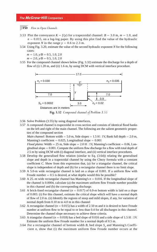
150 Flow in Open Channels
3.53 Plot the conveyance K = f (y) for a trapezoidal channel: B = 3.0 m, m = 1.0, and n = 0.015, on a log-log paper. By using this plot f ind the value of the hydraulic exponent N in the range y = 0.6 to 2.3 m.
3.54 Using Fig. 3.20, estimate the value of the second hydraulic exponent N for the following cases:m = 1.0, y/B = 0.5, 1.0, 2.0m = 2.0, y/B = 0.5, 1.0, 2.0
3.55 For the compound channel shown below (Fig. 3.32) estimate the discharge for a depth of fl ow of (i) 1.20 m, and (ii) 1.6 m, by using DCM with vertical interface procedure.
Fig. 3.32 Compound channel of Problem 3.55
17.0
7.0
0.9
3.0
y
n2 = 0.02
n1 = 0.030 n3 = 0.035
7.0
S0 = 0.0002
Distances are in meters
Δ
3.56 Solve Problem (3.55) by using diagonal interfaces,3.57 A compound channel is trapezoidal in cross section and consists of identical fl ood banks
on the left and right of the main channel. The following are the salient geometric proper-ties of the compound sectionMain channel: Bottom width = 5.0 m, Side slopes = 1.5 H : 1V, Bank full depth = 2.0 m, Manning’s coeffi cient = 0.025, Longitudinal slope = 0.001Flood plains: Width = 25 m, Side slope = 2.0 H : 1V, Manning’s coeffi cient = 0.06, Lon-gitudinal slope = 0.001. Compute the uniform fl ow discharge for a fl ow with total depth of 2.5 m by using DCM with (i) diagonal interface, and (ii) vertical interface procedures.
3.58 Develop the generalised fl ow relation (similar to Eq. (3.64)) relating the generalised slope and depth in a trapezoidal channel by using the Chezy formula with a constant coeffi cient C. Show from this expression that, (a) for a triangular channel, the critical slope is independent of depth and (b) for a rectangular channel there is no limit slope.
3.59 A 5.0-m wide rectangular channel is laid on a slope of 0.001. If a uniform fl ow with Froude number = 0.5 is desired, at what depths would this be possible?
3.60 A 25.-m wide rectangular channel has Manning’s n = 0.016. If the longitudinal slope of the channel is 0.0004, calculate (a) the maximum uniform fl ow Froude number possible in this channel and (b) the corresponding discharge.
3.61 A brick-lined rectangular channel (n = 0.017) of 6.0-m bottom width is laid on a slope of 0.003. (i) For this channel, estimate the critical slope which will have a normal depth of fl ow of 2.0 m. (ii) Identify the regions of steep and mild slopes, if any, for variation of normal depth from 0.10 m to 4.0 m in this channel
3.62 A rectangular channel (n = 0.015) has a width of 2.50 m and it is desired to have Froude number at uniform fl ow to be equal to or less than 0.4 for all discharges in this channel. Determine the channel slope necessary to achieve these criteria.
3.63 A triangular channel (n = 0.018) has a bed slope of 0.016 and a side slope of 1.5 H : 1V. Estimate the uniform fl ow Froude number for a normal depth of 0.5 m.
3.64 For a rectangular channel of bottom width B, bed slope S0 and Manning’s Coeffi-
cient n, show that (i) the maximum uniform flow Froude number occurs at the
Chapter 3.indd 150Chapter 3.indd 150 2/24/2010 4:22:12 PM2/24/2010 4:22:12 PM
Uniform Flow 151
normal depth y0 =B/6, and (ii) the discharge corresponding to the maximum
Froude number is
QB S
n=
8 30
24
/
3.65 For a trapezoidal section B = 3.0 m, m = 1.5 and n = 0.02, fi nd the (a) bed slope required to have a uniform m fl ow at a Froude number of 0.2 and depth of fl ow = 2.5 m, (b) criti-cal slope for the same depth of fl ow of 2.5 m, and (c) depth of fl ow with a bed slope of 0.0009 to cause a uniform fl ow Froude number of 0.5.
3.66 For a triangular channel with apex angle = 90°, determine the critical slope for a critical depth of 1.35 m. If the channel is laid at this slope, what would be the Froude number of the uniform fl ow for a depth of fl ow of 2.0 m? (Assume n= 0.02).
3.67 A 1.2-m wide rectangular channel is lined with smooth concrete (n = 0.013). Determine the limit slope and the corresponding discharge and critical depth.
3.68 Obtain an expression for the critical slope in a circular channel as S*c
= f (ηc) where
SS D
gncc
*
/
=1 3
2 and η
c = y
c/D. Show that the limit slope occurs at y
c/D = 0.316.
3.69 Show that for a parabolic channel T K y= , the limit slope is given by S K
gnLc
2 3
23 36
/
.=
and this limit value occurs at y
Kc =
1
2 2.
Assume P Kyy
K= +
⎡
⎣⎢⎢
⎤
⎦⎥⎥
1 23 28
3/
/
3.70 Design a trapezoidal channel to carry 75 m3/s of fl ow. The maximum permissible slope is 0.0005. It is proposed to adopt a brick-in-cement mortar lining. The soil is classifi ed as average sandy soil.
OBJECTIVE QUESTIONS
3.1 In a non-prismatic channel (a) unsteady fl ow is not possible (c) uniform fl ow is not possible (b) the fl ow is always uniform (d) the fl ow is not possible 3.2 In a uniform open channel fl ow (a) the total energy remains constant along the channel (b) the total energy line either rises or falls along the channel depending on the state of
the fl ow (c) the specifi c energy decreases along the channel (d) the line representing the total energy is parallel to the bed of the channel 3.3 Uniform fl ow in an open channel exists when the fl ow is steady and the channel is (a) prismatic (b) non-prismatic and the depth of the fl ow is constant along the channel (c) prismatic and the depth of the fl ow is constant along the channel (d) fricionless
Chapter 3.indd 151Chapter 3.indd 151 2/24/2010 4:22:12 PM2/24/2010 4:22:12 PM
152 Flow in Open Channels
3.4 In uniform fl ow there is a balance between (a) gravity and frictional forces (b) gravity and inertial forces (c) intertial and frictional forces (d) inertial and viscous forces 3.5 Uniform fl ow is not possible if the (a) friction is large (b) fl uid is an oil (c) S
0 ≤ 0 (d) S
0 > 0
3.6 A rectangular channel of longitudinal slope 0.002 has a width of 0.80 m and carries an oil (rel. density = 0.80) at a depth of 0.40 m in uniform fl ow mode. The average shear stress on the channel boundary in pascals is
(a) 3.14 × 10⁻³ (b) 6.28 × 10⁻³
(c) 3.93 × 10⁻³ (d) 0.01256 3.7 A triangular channel with a side slope of 1.5 horizontal: 1 vertical is laid on slope of
0.005. The shear stress in N/m2 on the boundary for a depth of fl ow of 1.5 m is (a) 3.12 (b) 10.8 (c) 30.6 (d 548 3.8 The dimensions of the Chezy coeffi cient C are (a) L2 T −1 (b) L T −1/2 (c) M 0L 0T 0 (d) L1/2 T −1
3.9 The dimensions of Manning’s n are (a) L1/6 (b) L1/2 T −1
(c) L−1/3 T (d) L−1/3 T −1
3.10 The dimensions of the Darcy–Weisbach coeffi cient f are (a) L1/6 (b) L T −1 (c) L1/2 T −4 (d) M 0L0T 0
3.11 A channel fl ow is found to have a shear Reynolds number u
vs*ε = 25 , where ε
s = sand
grain roughness, u* = shear velocity and v = kinematic viscosity. The channel boundary
can be classifi ed as hydrodynamically (a) rough (b) in transition regime (c) smooth (d) undular3.12 If the bed particle size d
50 of a natural stream is 2.0 mm, then by Strickler formula, the
Manning’s n for the channel is about (a) 0.017 (b) 0.023 (c) 0.013 (d) 0.0443.13 In using the Moody chart for fi nding f for open-channel fl ows, the pipe diameter D is to
be replaced by (a) R (b) D/2 (c) P (d) 4R3.14 The Manning’s n for a smooth, clean, unlined, suffi ciently weathered earthen channel is
about (a) 0.012 (b) 0.20 (c) 0.02 (d) 0.0023.15 The Manning’s n is related to the equivalent sand grain roughness, ε
s as
(a) n s∝ ε−1 6/ (b) n s∝ ε1 6/ (c) n s∝ ε1 3/ (d) nRs=
ε4
3.16 The Darcy–Weisbach f is related to Manning’s n as
(a) fg n
R=
8 2
1 3
/ (b) f
n
R=
8
8
2
1 3
/
(c) fR
g n=
1 3
28
/
(d) f
ng
R=
641 3/
Chapter 3.indd 152Chapter 3.indd 152 2/24/2010 4:22:13 PM2/24/2010 4:22:13 PM
Uniform Flow 153
3.17 The Manning’s n for a straight concrete sewer is about (a) 0.025 (b) 0.014 (c) 0.30 (d) 0.143.18 An open channel carries water with a velocity of 0.605 m/s. If the average bed shear
stress is 1.0 N/m2, the Chezy coeffi cient C is equal to (a) 500 (b) 60 (c) 6.0 (d) 303.19 The conveyance of a triangular channel with side slope of 1 horizontal: 1 vertical is
expressed as K = C y8/3; where C is equal to
(a) 28/3 (b) 1/n (c) 1/2n (d) 2 2 / n3.20 In a wide rectangular channel if the normal depth is increased by 20 per cent, the dis-
charge would increase by (a) 20% (b) 15.5% (c) 35.5% (d) 41.3%3.21 In a uniform fl ow taking place in a wide rectangular channel at a depth of 1.2 m, the
velocity is found to be 1.5 m/s. If a change in the discharge causes a uniform fl ow at a depth of 0.88 m in this channel, the corresponding velocity of fl ow would be
(a) 0.89 m/s (b) 1.22 m/s (c) 1.10 m/s (d) 1.50 m/s3.22 It is expected that due to extreme cold weather the entire top surface of a canal carrying
water will be covered with ice for some days. If the discharge in the canal were to remain unaltered, this would cause
(a) no change in the depth (b) increase in the depth of fl ow (c) decrease in the depth of fl ow (d) an undular surface exhibiting increase and decrease in depths3.23 By using Manning’s formula the depth of fl ow corresponding to the condition of maxi-
mum discharge in a circular channel of diameter D is (a) 0.94 D (b) 0.99 D (c) 0.86 D (d) 0.82 D3.24 In a circular channel the ratio of the maximum discharge to the pipe full discharge is about (a) 1.50 (b) 0.94 (c) 1.08 (d) 1.003.25 For a circular channel of diameter D the maximum depth below which only one normal
depth is assured (a) 0.5 D (b) 0.62 D (c) 0.82 D (d) 0.94 D3.26 A trapezoidal channel had a 10 per cent increase in the roughness coeffi cient over years
of use. This would represent, corresponding to the same stage as at the beginning, a change in discharge of
(a) +10% (b) –10% (c) 11% (d) +9.1 %3.27 For a hydraulically-effi cient rectangular section, B/y
0 is equal to
(a) 1.0 (b) 2.0 (c) 0.5 (d) 1 3/3.28 A triangular section is hydraulically-effi cient when the vertex angle θ is (a) 90° (b) 120° (c) 60° (d) 30°3.29 For a hydraulically effi cient triangular channel with a depth of fl ow y, the hydraulic
radius R is equal to
(a) 2 2y (b) y/2 (c) 2y (d) y / 2 23.30 A hydraulically-effi cient trapezoidal channel has m = 2.0. B/y
0 for this channel is
(a) 1.236 (b) 0.838 (c) 0.472 (d) 2.2363.31 In a hydraulically most effi cient trapezoidal channel section the ratio of the bed width to
depth is (a) 1.155 (b) 0.867 (c) 0.707 (d) 0.503.32 In a hydraulically effi cient circular channel fl ow, the ratio of the hydraulic radius to the
diameter of the pipe is (a) 1.0 (b) 0.5 (c) 2.0 (d) 0.25
Chapter 3.indd 153Chapter 3.indd 153 2/24/2010 4:22:13 PM2/24/2010 4:22:13 PM
154 Flow in Open Channels
3.33 For a wide rectangular channel the value of the fi rst hydraulic exponent N is (a) 3.0 (b) 4.0 (c) 3.33 (d) 5.333.34 If the Chezy formula with C = constant is used, the value of N for a wide rectangular
channel will be (a) 2.0 (b) 3.0 (c) 3.33 (d) 5.33
3.35 For a trapezoidal channel of most-effi cient proportions Qn B S/ ( )/ /8 301 2⎡
⎣⎢⎤⎦⎥ = =φ
(a) 1 3/ (b) 0.7435 (c) 0.8428 (d) 1.4863.36 In a given rectangular channel the maximum value of uniform-fl ow Froude number
occurs when (a) y = B/6 (b) R = y/2 (c) y = B/2 (d) y
0 = y
c
3.37 The limit slope of a rectangular channel 10 m wide and n = 0.015 is (a) 0.000423 (b) 0.00372 (c) 0.00273 (d) 0.07323.38 In a rectangular channel 10 m wide and n = 0.015, the critical depth corresponding to the
limit slope is (a) 1.333 m (b) 0.667 m (c) 2.667 m (d) 1.667 m3.39 A rectangular channel B = 4.0 m, n = 0.015 is to carry a uniform discharge at a depth of
1.0 m and Froude number = 0.5. The required bottom slope is (a) 0.0035 (b) 0.00505 (c) 0.00095 (d) 0.000453.40 A trapezoidal channel with 0 < m < 0.46 will have x number of limit slopes where x is (a) 1 (b) 2 (c) 3 (d) 0
APPENDIX 3A
Table 3A.1 gives the variation of φ = f(η0, m) as represented by Eq. (3.32) and provides a con-
venient aid to determine the normal depth in rectangular and trapezoidal channels. At the normal depth
φ =nQ
S B08 3/
and η00=
y
B.
Note that the column m = 0 corresponds to a rectangular channel
Table 3A-1 Values of φ for Trapezoidal Channels
η0 Value of φ η0
Value of φ
m = 0 m = 1.0 m = 1.5 m = 2.0 m = 2.5 m = 0 m = 1.0 m = 1.5 m = 2.0 m = 2.5
0.100 0.01908 0.02139 0.02215 0.02282 0.02345 0.155 0.03736 0.04463 0.04713 0.04938 0.05151
0.105 0.02058 0.02321 0.02407 0.02484 0.02556 0.160 0.03919 0.04708 0.04982 0.05227 0.05459
0.110 0.02212 0.02509 0.02607 0.02694 0.02776 0.165 0.04104 0.04960 0.05257 0.05523 0.05777
0.115 0.02369 0.02702 0.02814 0.02912 0.03005 0.170 0.04292 0.05217 0.05539 0.05828 0.06104
0.120 0.02529 0.02902 0.03027 0.03138 0.03243 0.175 0.04482 0.05479 0.05828 0.06141 0.06439
0.125 0.02693 0.03108 0.03247 0.03371 0.03489 0.180 0.04675 0.05747 0.06123 0.06462 0.06785
0.130 0.02860 0.03319 0.03475 0.03613 0.03744 0.185 0.04869 0.06021 0.06426 0.06791 0.07139
0.135 0.03029 0.03537 0.03709 0.03862 0.04007 0.190 0.05066 0.06300 0.06735 0.07128 0.07503
0.140 0.03202 0.03760 0.03949 0.04119 0.04280 0.195 0.05265 0.06584 0.07052 0.07474 0.07876
0.145 0.03377 0.03988 0.04197 0.04384 0.04561 0.200 0.05466 0.06874 0.07375 0.07827 0.08259
0.150 0.03555 0.04223 0.04452 0.04657 0.04852
Chapter 3.indd 154Chapter 3.indd 154 2/24/2010 4:22:13 PM2/24/2010 4:22:13 PM
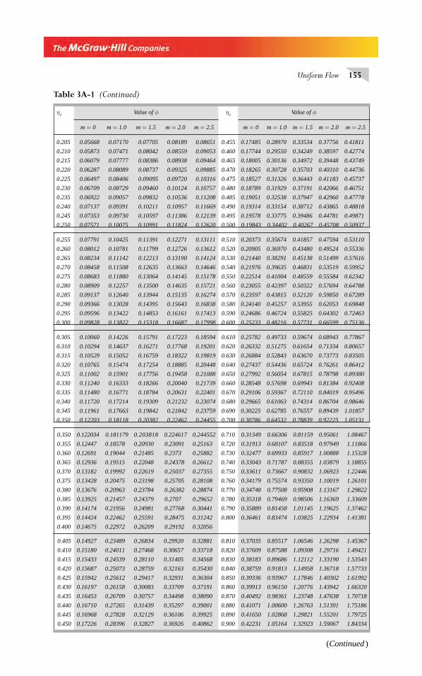
Uniform Flow 155
η0 Value of φ η0 Value of φ
m = 0 m = 1.0 m = 1.5 m = 2.0 m = 2.5 m = 0 m = 1.0 m = 1.5 m = 2.0 m = 2.5
0.205 0.05668 0.07170 0.07705 0.08189 0.08651 0.455 0.17485 0.28970 0.33534 0.37756 0.41811
0.210 0.05873 0.07471 0.08042 0.08559 0.09053 0.460 0.17744 0.29550 0.34249 0.38597 0.42774
0.215 0.06079 0.07777 0.08386 0.08938 0.09464 0.465 0.18005 0.30136 0.34972 0.39448 0.43749
0.220 0.06287 0.08089 0.08737 0.09325 0.09885 0.470 0.18265 0.30728 0.35703 0.40310 0.44736
0.225 0.06497 0.08406 0.09095 0.09720 0.10316 0.475 0.18527 0.31326 0.36443 0.41183 0.45737
0.230 0.06709 0.08729 0.09460 0.10124 0.10757 0.480 0.18789 0.31929 0.37191 0.42066 0.46751
0.235 0.06922 0.09057 0.09832 0.10536 0.11208 0.485 0.19051 0.32538 0.37947 0.42960 0.47778
0.240 0.07137 0.09391 0.10211 0.10957 0.11669 0.490 0.19314 0.33154 0.38712 0.43865 0.48818
0.245 0.07353 0.09730 0.10597 0.11386 0.12139 0.495 0.19578 0.33775 0.39486 0.44781 0.49871
0.250 0.07571 0.10075 0.10991 0.11824 0.12620 0.500 0.19843 0.34402 0.40267 0.45708 0.50937
0.255 0.07791 0.10425 0.11391 0.12271 0.13111 0.510 0.20373 0.35674 0.41857 0.47594 0.53110
0.260 0.08012 0.10781 0.11799 0.12726 0.13612 0.520 0.20905 0.36970 0.43480 0.49524 0.55336
0.265 0.08234 0.11142 0.12213 0.13190 0.14124 0.530 0.21440 0.38291 0.45138 0.51499 0.57616
0.270 0.08458 0.11508 0.12635 0.13663 0.14646 0.540 0.21976 0.39635 0.46831 0.53519 0.59952
0.275 0.08683 0.11880 0.13064 0.14145 0.15178 0.550 0.22514 0.41004 0.48559 0.55584 0.62342
0.280 0.08909 0.12257 0.13500 0.14635 0.15721 0.560 0.23055 0.42397 0.50322 0.57694 0.64788
0.285 0.09137 0.12640 0.13944 0.15135 0.16274 0.570 0.23597 0.43815 0.52120 0.59850 0.67289
0.290 0.09366 0.13028 0.14395 0.15643 0.16838 0.580 0.24140 0.45257 0.53955 0.62053 0.69848
0.295 0.09596 0.13422 0.14853 0.16161 0.17413 0.590 0.24686 0.46724 0.55825 0.64302 0.72463
0.300 0.09828 0.13822 0.15318 0.16687 0.17998 0.600 0.25233 0.48216 0.57731 0.66599 0.75136
0.305 0.10060 0.14226 0.15791 0.17223 0.18594 0.610 0.25782 0.49733 0.59674 0.68943 0.77867
0.310 0.10294 0.14637 0.16271 0.17768 0.19201 0.620 0.26332 0.51275 0.61654 0.71334 0.80657
0.315 0.10529 0.15052 0.16759 0.18322 0.19819 0.630 0.26884 0.52843 0.63670 0.73773 0.83505
0.320 0.10765 0.15474 0.17254 0.18885 0.20448 0.640 0.27437 0.54436 0.65724 0.76261 0.86412
0.325 0.11002 0.15901 0.17756 0.19458 0.21088 0.650 0.27992 0.56054 0.67815 0.78798 0.89380
0.330 0.11240 0.16333 0.18266 0.20040 0.21739 0.660 0.28548 0.57698 0.69943 0.81384 0.92408
0.335 0.11480 0.16771 0.18784 0.20631 0.22401 0.670 0.29106 0.59367 0.72110 0.84019 0.95496
0.340 0.11720 0.17214 0.19309 0.21232 0.23074 0.680 0.29665 0.61063 0.74314 0.86704 0.98646
0.345 0.11961 0.17663 0.19842 0.21842 0.23759 0.690 0.30225 0.62785 0.76557 0.89439 1.01857
0.350 0.12203 0.18118 0.20382 0.22462 0.24455 0.700 0.30786 0.64532 0.78839 0.92225 1.05131
0.350 0.122034 0.181179 0.203818 0.224617 0.244552 0.710 0.31349 0.66306 0.81159 0.95061 1.08467
0.355 0.12447 0.18578 0.20930 0.23091 0.25163 0.720 0.31913 0.68107 0.83518 0.97949 1.11866
0.360 0.12691 0.19044 0.21485 0.2373 0.25882 0.730 0.32477 0.69933 0.85917 1.00888 1.15328
0.365 0.12936 0.19515 0.22048 0.24378 0.26612 0.740 0.33043 0.71787 0.88355 1.03879 1.18855
0.370 0.13182 0.19992 0.22619 0.25037 0.27355 0.750 0.33611 0.73667 0.90832 1.06923 1.22446
0.375 0.13428 0.20475 0.23198 0.25705 0.28108 0.760 0.34179 0.75574 0.93350 1.10019 1.26101
0.380 0.13676 0.20963 0.23784 0.26382 0.28874 0.770 0.34748 0.77508 0.95908 1.13167 1.29822
0.385 0.13925 0.21457 0.24379 0.2707 0.29652 0.780 0.35318 0.79469 0.98506 1.16369 1.33609
0.390 0.14174 0.21956 0.24981 0.27768 0.30441 0.790 0.35889 0.81458 1.01145 1.19625 1.37462
0.395 0.14424 0.22462 0.25591 0.28475 0.31242 0.800 0.36461 0.83474 1.03825 1.22934 1.41381
0.400 0.14675 0.22972 0.26209 0.29192 0.32056
0.405 0.14927 0.23489 0.26834 0.29920 0.32881 0.810 0.37035 0.85517 1.06546 1.26298 1.45367
0.410 0.15180 0.24011 0.27468 0.30657 0.33718 0.820 0.37609 0.87588 1.09308 1.29716 1.49421
0.415 0.15433 0.24539 0.28110 0.31405 0.34568 0.830 0.38183 0.89686 1.12112 1.33190 1.53543
0.420 0.15687 0.25073 0.28759 0.32163 0.35430 0.840 0.38759 0.91813 1.14958 1.36718 1.57733
0.425 0.15942 0.25612 0.29417 0.32931 0.36304 0.850 0.39336 0.93967 1.17846 1.40302 1.61992
0.430 0.16197 0.26158 0.30083 0.33709 0.37191 0.860 0.39913 0.96150 1.20776 1.43942 1.66320
0.435 0.16453 0.26709 0.30757 0.34498 0.38090 0.870 0.40492 0.98361 1.23748 1.47638 1.70718
0.440 0.16710 0.27265 0.31439 0.35297 0.39001 0.880 0.41071 1.00600 1.26763 1.51391 1.75186
0.445 0.16968 0.27828 0.32129 0.36106 0.39925 0.890 0.41650 1.02868 1.29821 1.55201 1.79725
0.450 0.17226 0.28396 0.32827 0.36926 0.40862 0.900 0.42231 1.05164 1.32923 1.59067 1.84334
Table 3A-1 (Continued)
(Continued )
Chapter 3.indd 155Chapter 3.indd 155 2/24/2010 4:22:14 PM2/24/2010 4:22:14 PM
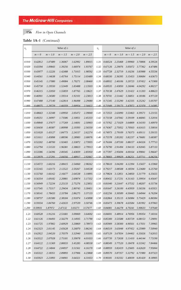
156 Flow in Open Channels
η0 Value of φ η0 Value of φ
m = 0 m = 1.0 m = 1.5 m = 2.0 m = 2.5 m = 0 m = 1.0 m = 1.5 m = 2.0 m = 2.5
0.910 0.42812 1.07489 1.36067 1.62992 1.89015 1.31 0.66524 2.25468 2.99960 3.70806 4.39526
0.920 0.43394 1.09843 1.39256 1.66974 1.93767 1.32 0.67126 2.29076 3.05072 3.77362 4.47486
0.930 0.43977 1.12226 1.42488 1.71015 1.98592 1.33 0.67728 2.32719 3.10236 3.83988 4.55536
0.940 0.44561 1.14638 1.45764 1.75114 2.03489 1.34 0.68330 2.36395 3.15453 3.90684 4.63673
0.950 0.45145 1.17080 1.49084 1.79271 2.08460 1.35 0.68932 2.40106 3.20723 3.97452 4.71900
0.960 0.45730 1.19550 1.52449 1.83488 2.13503 1.36 0.69535 2.43850 3.26046 4.04292 4.80217
0.970 0.46315 1.22050 1.55859 1.87765 2.18621 1.37 0.70138 2.47629 3.31422 4.11203 4.88623
0.980 0.46901 1.24580 1.59314 1.92101 2.23813 1.38 0.70741 2.51442 3.36851 4.18186 4.97120
0.990 0.47488 1.27140 1.62814 1.96498 2.29080 1.39 0.71345 2.55290 3.42335 4.25242 5.05707
1.000 0.48075 1.29729 1.66359 2.00954 2.34422 1.40 0.71949 2.59173 3.47872 4.32370 5.14385
1.010 0.48663 1.32348 1.69950 2.05472 2.39840 1.41 0.72553 2.63090 3.53463 4.39571 5.23155
0.020 0.49251 1.34997 1.73586 2.10051 2.45333 1.42 0.73158 2.67042 3.59109 4.46845 5.32016
1.030 0.49840 1.37677 1.77269 2.14691 2.50903 1.43 0.73762 2.71029 3.64809 4.54193 5.40970
1.040 0.50430 1.40387 1.80998 2.19393 2.56550 1.44 0.74367 2.75052 3.70563 4.61615 5.50016
1.050 0.51020 1.43127 1.84773 2.24157 2.62274 1.45 0.74973 2.79109 3.76373 4.69111 5.59155
1.060 0.51611 1.45898 1.88596 2.28983 2.68076 1.46 0.75578 2.83202 3.82237 4.76681 5.68387
1.070 0.52202 1.48700 1.92465 2.33872 2.73955 1.47 0.76184 2.87330 3.88157 4.84326 5.77713
1.080 0.52794 1.51533 1.96381 2.38823 2.79913 1.48 0.76790 2.91494 3.94133 4.92045 5.87133
1.090 0.53386 1.54396 2.00345 2.43839 2.85950 1.49 0.77397 2.95694 4.00164 4.99841 5.96647
1.100 0.53979 1.57291 2.04356 2.48917 2.92067 1.50 0.78003 2.99929 4.06251 5.07711 6.06256
1.110 0.54572 1.60216 2.08415 2.54060 2.98262 1.51 0.78610 3.04200 4.12394 5.15657 6.15960
1.120 0.55165 1.63173 2.12522 2.59267 3.04538 1.52 0.79217 3.08508 4.18594 5.23680 6.25760
1.130 0.55760 1.66162 2.16677 2.64538 3.10895 1.53 0.79824 3.12851 4.24850 5.31779 6.35655
1.140 0.56354 1.69182 2.20881 2.69874 3.17332 1.54 0.80432 3.17231 4.31163 5.39954 6.45647
1.150 0.56949 1.72234 2.25133 2.75276 3.23851 1.55 0.81040 3.21647 4.37532 5.48207 6.55736
1.160 0.57545 1.75317 2.29434 2.80743 3.30451 1.56 0.81647 3.26100 4.43959 5.56536 6.65921
1.170 0.58141 1.78433 2.33784 2.86275 3.37133 1.57 0.82256 3.30589 4.50443 5.64944 6.76204
1.180 0.58737 1.81580 2.38184 2.91874 3.43898 1.58 0.82864 3.35115 4.56984 5.73429 6.86584
1.190 0.59334 1.84760 2.42633 2.97539 3.50746 1.59 0.83473 3.39678 4.63584 5.81992 6.97063
1.200 0.59931 1.87972 2.47132 3.03271 3.57677 1.60 0.84081 3.44278 4.70241 5.90633 7.07640
1.21 0.60528 1.91216 2.51681 3.09069 3.64692 1.61 0.84691 3.48914 4.76956 5.99354 7.18316
1.22 0.61126 1.94493 2.56279 3.14935 3.71790 1.62 0.85300 3.53588 4.83729 6.08153 7.29091
1.23 0.61725 1.97802 2.60929 3.20869 3.78973 1.63 0.85909 3.58300 4.90561 6.17031 7.39965
1.24 0.62323 2.01145 2.65628 3.26870 3.86241 1.64 0.86519 3.63048 4.97452 6.25989 7.50940
1.25 0.62922 2.04520 2.70379 3.32940 3.93595 1.65 0.87129 3.67834 5.04402 6.35026 7.62015
1.26 0.63522 2.07928 2.75181 3.39078 4.01033 1.66 0.87739 3.72658 5.11410 6.44144 7.73190
1.27 0.64122 2.11369 2.80033 3.45285 4.08558 1.67 0.88349 3.77520 5.18478 6.53342 7.84466
1.28 0.64722 2.14844 2.84937 3.51561 4.16170 1.68 0.88959 3.82419 5.25605 6.62620 7.95844
1.29 0.65322 2.18351 2.89893 3.57906 4.23868 1.69 0.89570 3.87357 5.32792 6.71980 8.07323
1.30 0.65923 2.21893 2.94901 3.64321 4.31653 1.70 0.90181 3.92332 5.40039 6.81420 8.18905
Table 3A-1 (Continued)
Chapter 3.indd 156Chapter 3.indd 156 2/24/2010 4:22:14 PM2/24/2010 4:22:14 PM
4.1 INTRODUCTION
A steady non-uniform fl ow in a prismatic channel with gradual changes in its water surface elevation is termed as gradually varied fl ow (GVF). The backwater produced by a dam or weir across a river and the drawdown produced at a sudden drop in a chan-nel are few typical examples of GVF. In a GVF, the velocity varies along the channel and consequently the bed slope, water surface slope, and energy slope will all differ from each other. Regions of high curvature are excluded in the analysis of this fl ow.
The two basic assumptions involved in the analysis of GVF are the following:
1. The pressure distribution at any section is assumed to be hydrostatic. This follows from the defi nition of the fl ow to have a gradually-varied water sur-face. As gradual changes in the surface curvature give rise to negligible normal accelerations, the departure from the hydrostatic pressure distribution is negli-gible. The exclusion of the region of high curvature from the analysis of GVF, as indicated earlier, is only to meet this requirement.
2. The resistance to fl ow at any depth is assumed to be given by the correspond-ing uniform fl ow equation, such as the Manning’s formula, with the condition that the slope term to be used in the equation is the energy slope and not the bed slope. Thus, if in a GVF the depth of fl ow at any section is y, the energy slope S
f is given by
Sn V
Rf =2 2
4 3/ (4.1)
where R = hydraulic radius of the section at depth y.
4.2 DIFFERENTIAL EQUATION OF GVF
Consider the total energy H of a gradually varied fl ow in a channel of small slope and α = 1.0 as
H Z E Z yV
g= + = + +
2
2 (4.2)
where E = specifi c energy.
Gradually Varied Flow Theory 4
Chapter 4.indd 157Chapter 4.indd 157 2/24/2010 3:42:58 PM2/24/2010 3:42:58 PM
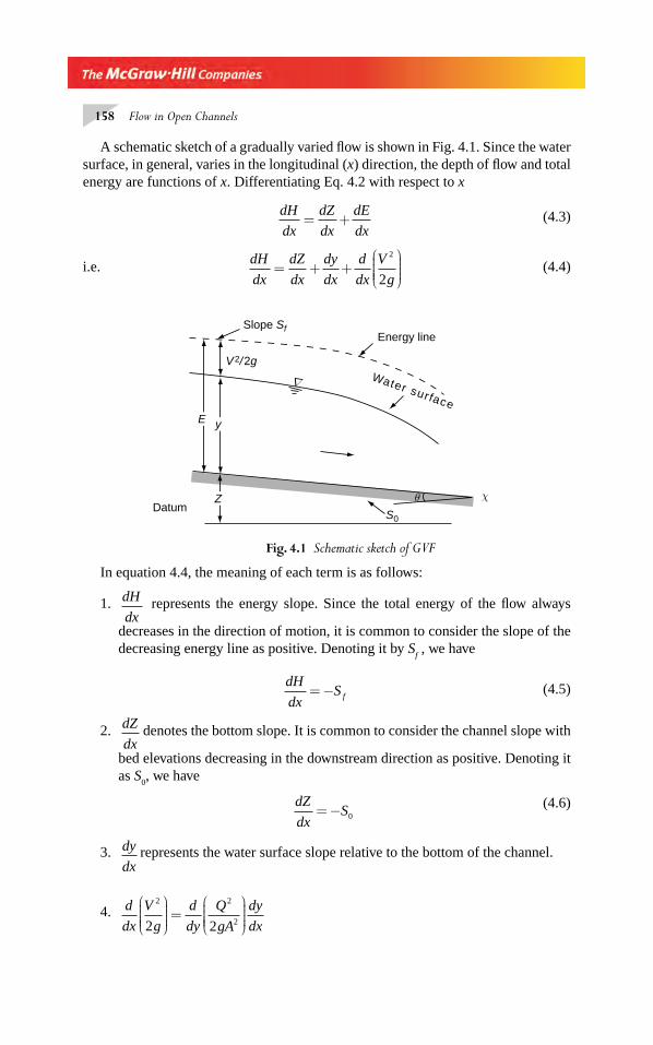
158 Flow in Open Channels
A schematic sketch of a gradually varied fl ow is shown in Fig. 4.1. Since the water surface, in general, varies in the longitudinal (x) direction, the depth of fl ow and total energy are functions of x. Differentiating Eq. 4.2 with respect to x
dH
dx
dZ
dx
dE
dx= + (4.3)
i.e.
dH
dx
dZ
dx
dy
dx
d
dx
V
g= + +
⎛
⎝⎜⎜⎜⎜
⎞
⎠⎟⎟⎟⎟
2
2
(4.4)
∇
Slope Sf
V2/2g
yE
Z
Energy line
DatumS0
χθ
Water surface
Fig. 4.1 Schematic sketch of GVF
In equation 4.4, the meaning of each term is as follows:
1. dH
dx represents the energy slope. Since the total energy of the fl ow always
decreases in the direction of motion, it is common to consider the slope of the decreasing energy line as positive. Denoting it by S
f , we have
dH
dxS f= − (4.5)
2. dZ
dxdenotes the bottom slope. It is common to consider the channel slope with
bed elevations decreasing in the downstream direction as positive. Denoting it as S
0, we have
dZ
dxS= − 0
(4.6)
3. dy
dxrepresents the water surface slope relative to the bottom of the channel.
4. d
dx
V
g
d
dy
Q
gA
dy
dx
2 2
22 2
⎛
⎝⎜⎜⎜⎜
⎞
⎠⎟⎟⎟⎟
=⎛
⎝⎜⎜⎜⎜
⎞
⎠⎟⎟⎟⎟
Chapter 4.indd 158Chapter 4.indd 158 2/24/2010 3:43:00 PM2/24/2010 3:43:00 PM
Gradually Varied Flow Theory 159
= −Q
gA
dA
dy
dy
dx
2
3
Since dA/dy = T,
d
dx
V
g
Q T
gA
dy
dx
2 2
32
⎛
⎝⎜⎜⎜⎜
⎞
⎠⎟⎟⎟⎟
= −
(4.7)
Equation 4.4 can now be rewritten as
− =− + −⎛
⎝⎜⎜⎜⎜
⎞
⎠⎟⎟⎟⎟
S Sdy
dx
Q T
gA
dy
dxf 0
2
3
Re-arranging
dy
dx
S S
Q T
gA
f=−
−
0
2
31
(4.8)
This forms the basic differential equation of GVF and is also known as the dynamic equation of GVF. If a value of the kinetic-energy correction factor α greater than unity is to be used, Eq. 4.8 would then read as
dy
dx
S S
Q T
gA
f=−
−
0
2
31
α
(4.8a)
Other Forms of Eq. 4.8 (a) If K = conveyance at any depth y and K0 = convey-
ance corresponding to the normal depth y0, then
K Q S f=
(By assumption 2 of GVF) (4.9)
and
K Q S0 0= (Uniform fl ow)
S S K Kf 0 0
2 2=
(4.10)
Similarly, if Z = section factor at depth y and Zc = section factor at the critical
depth yc ,
Z A T2 3=
and
Z
A
T
Q
gcc
c
23 2
= =
Chapter 4.indd 159Chapter 4.indd 159 2/24/2010 3:43:00 PM2/24/2010 3:43:00 PM
160 Flow in Open Channels
Hence, Q T
gA
Z
Zc
2
3
2
2= (4.11)
Using Eqs 4.10 and 4.11, Eq. 4.8 can now be written as
dy
dxS
S
S
Q T
g
f
=−
−0
02
3
1
1Α
=−
⎛
⎝⎜⎜⎜
⎞
⎠⎟⎟⎟⎟
−⎛
⎝⎜⎜⎜
⎞
⎠⎟⎟⎟⎟
S
K
K
Z
Zc
0
0
2
2
1
1
(4.12)
This equation is useful in developing direct integration techniques.(b) If Q
n represents the normal discharge at a depth y and Q
c denotes the critical
discharge at the same depth y,
Q K Sn = 0
(4.13)
and Q Z gc =
(4.14)
Using these defi nitions, Eq. 4.8 can be written as
dy
dxS
Q Q
Q Qn
c
=−−0
2
2
1
1
( / )
( / )
(4.15)
(c) Another form of Eq. 4.8 is Eq. 4.3 and can be written as
dE
dxS S f= −0 (4.16)
This equation is called the differential-energy equation of GVF to distinguish it from the GVF differential equations (Eqs (4.8), (4.12) and (4.15)). This energy equation is very useful in developing numerical techniques for the GVF profi le computation.
4.3 CLASSIFICATION OF FLOW PROFILES
In a given channel, y0 and y
c are two fi xed depths if Q, n and S
0 are fi xed. Also,
there are three possible relations between y0 and y
c as (i) y
0 > y
c, (ii) y
0 < y
c and
(iii) y0 = y
c. Further, there are two cases where y
0 does not exist, i.e. when (a) the
channel bed is horizontal, (S0 = 0), (b) when the channel has an adverse slope,
Chapter 4.indd 160Chapter 4.indd 160 2/24/2010 3:43:01 PM2/24/2010 3:43:01 PM
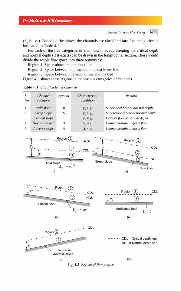
Gradually Varied Flow Theory 161
(S0 is –ve). Based on the above, the channels are classifi ed into fi ve categories as
indicated in Table 4.1.For each of the fi ve categories of channels, lines representing the critical depth
and normal depth (if it exists) can be drawn in the longitudinal section. These would divide the whole fl ow space into three regions as:
Region 1: Space above the top most lineRegion 2: Space between top line and the next lower lineRegion 3: Space between the second line and the bed
Figure 4.2 shows these regions in the various categories of channels.
Table 4. 1 Classifi cation of Channels
Sl. No
Channel category
Symbol Characteristic condition
Remark
1 Mild slope M y0 > y
cSubcritical fl ow at normal depth
2 Steep slope S yc > y
0Supercritical fl ow at normal depth
3 Critical slope C yc = y
0 Critical fl ow at normal depth
4 Horizontal bed H S0 = 0 Cannot sustain uniform fl ow
5 Adverse slope A S0 < 0 Cannot sustain uniform fl ow
Fig. 4.2 Regions of fl ow profi les
1
2
3 NDL
CDL
Region
y0
yc
Steep slope
(ii)S0 = + ve
CDL = Critical depth lineNDL = Normal depth line
(vi)
2
3
CDLRegion
yc
S0 = 0
(iv)
Horizontal bed
1
2
3
NDL
CDL
Mild slopeS0 = + ve
Region
y0
yc
(i)
1
3 NDL
CDL
Region y0 = yc
S0 = + ve
(iii)
Critical slope
2
3
CDLRegion
yc
Adverse slope
(v)
Chapter 4.indd 161Chapter 4.indd 161 2/24/2010 3:43:01 PM2/24/2010 3:43:01 PM
162 Flow in Open Channels
Depending upon the channel category and region of fl ow, the water surface pro-fi les will have characteristic shapes. Whether a given GVF profi le will have an increasing or decreasing water depth in the direction of fl ow will depend upon the term dy/dx in Eq. 4.8 being positive or negative.
It can be seen from Eq. 4.12 that dy
dx is positive
(i) if the numerator > 0 and the denominator > 0or (ii) if the numerator < 0 and the denominator < 0.
i.e. dy
dx is positive if (i) K > K
0 and Z > Z
c or
(ii) K < K0 and Z > Z
c
For channels of the fi rst kind, K is a single-valued function of y, and hence
dy
dx > 0 if (i) y > y
0 and y > y
c or
(ii) y < y0 and y < y
c
Similarly, dy
dx < 0 if (i) y
c > y > y
0 or
(ii) y0 > y > y
c
Further, to assist in the determination of fl ow profi les in various regions, the behaviour of dy/dx at certain key depths is noted by studying Eq. 4.8 as follows:
1. As y ydy
dx→ →0 0, , i.e. the water surface approaches the normal depth line
asymptotically.
2. As y ydy
dxc→ →∞, , i.e. the water surface meets the critical depth line verti-
cally. This information is useful only as indicative of the trend of the profi le. In reality, high curvatures at critical depth zones violate the assumption of gradu-ally-varied nature of the fl ow and as such the GVF computations have to end or commence a short distance away from the critical-depth location.
3. ydy
dxS→ ∞ →, 0 , i.e. the water surface meets a very large depth as a horizon-
tal asymptote.
Based on this information, the various possible gradually varied fl ow profi les are grouped into twelve types (Table 4.2). The characteristic shapes and end conditions of all these profi les are indicated in Fig. 4.3.
Chapter 4.indd 162Chapter 4.indd 162 2/24/2010 3:43:02 PM2/24/2010 3:43:02 PM
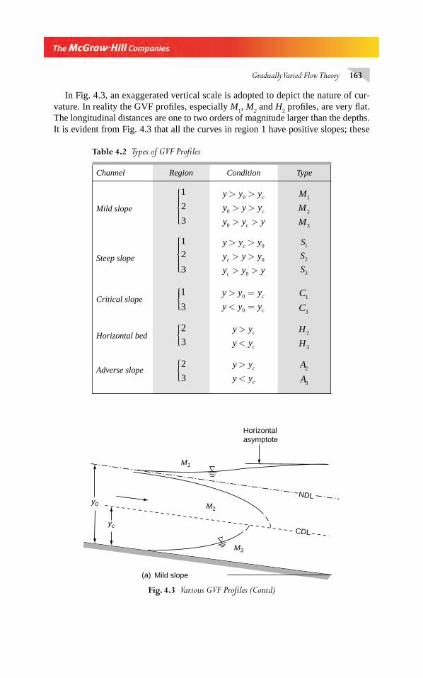
Gradually Varied Flow Theory 163
In Fig. 4.3, an exaggerated vertical scale is adopted to depict the nature of cur-vature. In reality the GVF profi les, especially M
1, M
2 and H
2 profi les, are very fl at.
The longitudinal distances are one to two orders of magnitude larger than the depths. It is evident from Fig. 4.3 that all the curves in region 1 have positive slopes; these
Table 4.2 Types of GVF Profi les
Channel Region Condition Type
Mild slope
1
2
3
⎧
⎨
⎪⎪⎪⎪
⎩⎪⎪⎪
y y y
y y y
y y y
c
c
c
> >> >> >
0
0
0
M
M
M
1
2
3
Steep slope
1
2
3
⎧
⎨⎪⎪⎪⎪
⎩⎪⎪⎪⎪
y y y
y y y
y y y
c
c
c
> >> >> >
0
0
0
S
S
S
1
2
3
Critical slope1
3
⎧⎨⎪⎪⎩⎪
y y y
y y yc
c
> =< =
0
0
C
C1
3
Horizontal bed2
3⎧⎨⎪⎩⎪
y y
y yc
c
><
H
H2
3
Adverse slope2
3
⎧⎨⎪⎩⎪
y y
y yc
c
><
A
A2
3
M2
M1
M3
Mild slope(a)
y0
yc
Horizontalasymptote
CDL
NDL
Fig. 4.3 Various GVF Profi les (Contd)
Chapter 4.indd 163Chapter 4.indd 163 2/24/2010 3:43:02 PM2/24/2010 3:43:02 PM
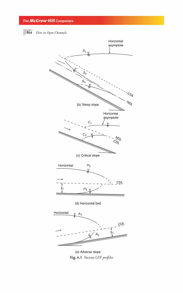
164 Flow in Open Channels
C1
C3NDLCDL
Horizontalasymptote
∇
∇
Critical slope(c)
CDL
∇
∇
H2
H3
Horizontal
yc
(d) Horizontal bed
CDL
∇
∇Horizontal
yc
A2
A3
(e) Adverse slope
∇
∇
∇
Horizontalasymptote
Steep slope(b)
S3
S2
S1
CDL
NDL
Fig. 4.3 Various GVF profi les
Chapter 4.indd 164Chapter 4.indd 164 2/24/2010 3:43:03 PM2/24/2010 3:43:03 PM
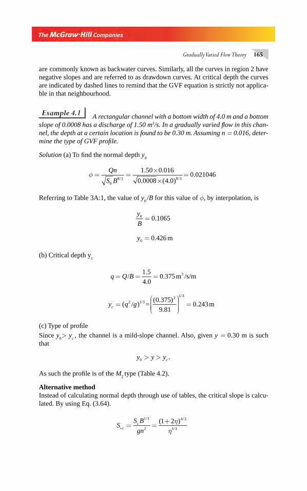
Gradually Varied Flow Theory 165
are commonly known as backwater curves. Similarly, all the curves in region 2 have negative slopes and are referred to as drawdown curves. At critical depth the curves are indicated by dashed lines to remind that the GVF equation is strictly not applica-ble in that neighbourhood.
Example 4.1 A rectangular channel with a bottom width of 4.0 m and a bottom slope of 0.0008 has a discharge of 1.50 m3/s. In a gradually varied fl ow in this chan-nel, the depth at a certain location is found to be 0.30 m. Assuming n = 0.016, deter-mine the type of GVF profi le.
Solution (a) To fi nd the normal depth y0
φ = =×
×=
Qn
S B08 3 8 3
1 50 0 016
0 0008 4 00 021046
/ /
. .
. ( . ).
Referring to Table 3A:1, the value of y0 /B for this value of φ, by interpolation, is
y
B0 0 1065= .
y0 0 426= . m
(b) Critical depth yc
q Q B= = =/ m /s/m31 5
4 00 375
.
..
y q gc =
⎛
⎝⎜⎜⎜⎜
⎞
⎠⎟⎟⎟⎟
=( )( . )
../
/
2 1 32 1 3
0 375
9 810 243/ = m
(c) Type of profi le
Since y0> y
c , the channel is a mild-slope channel. Also, given y = 0.30 m is such
that
y y yc0 > > .
As such the profi le is of the M2 type (Table 4.2).
Alternative methodInstead of calculating normal depth through use of tables, the critical slope is calcu-lated. By using Eq. (3.64).
S
S B
gncc
∗ = =+1 3
2
4 3
1 3
1 2/ /
/
( )ηη
Chapter 4.indd 165Chapter 4.indd 165 2/24/2010 3:43:03 PM2/24/2010 3:43:03 PM
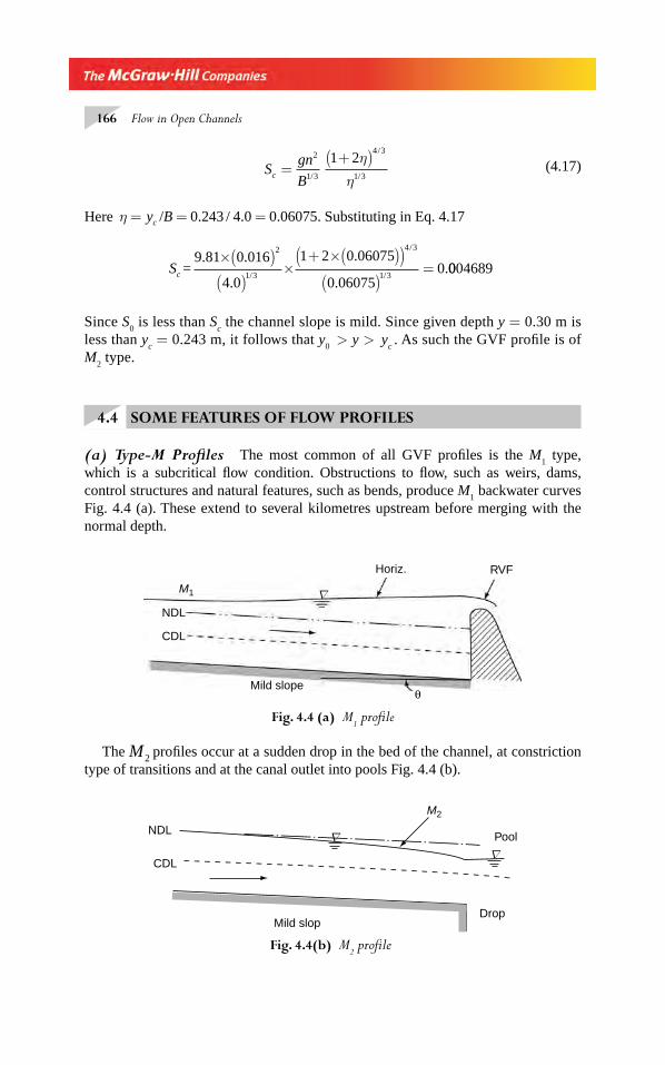
166 Flow in Open Channels
S
gn
Bc =+( )2
1 3
4 3
1 3
1 2/
/
/
η
η
(4.17)
Here η = = =y Bc / 0 243 4 0 0 06075. / . . . Substituting in Eq. 4.17
Sc =9 81 0 016
4 0
1 2 0 06075
0 060750
2
1 3
4 3
1 3
. .
.
.
..
/
/
/
×( )( )
×+ ×( )( )
( )= 0004689
Since S0 is less than S
c the channel slope is mild. Since given depth y = 0.30 m is
less than yc = 0.243 m, it follows that y
0 > y >
y
c . As such the GVF profi le is of
M2 type.
4.4 SOME FEATURES OF FLOW PROFILES
(a) Type-M Profi les The most common of all GVF profi les is the M1 type,
which is a subcritical fl ow condition. Obstructions to fl ow, such as weirs, dams, control structures and natural features, such as bends, produce M
1 backwater curves
Fig. 4.4 (a). These extend to several kilometres upstream before merging with the normal depth.
M2
Pool
Drop
NDL
CDL
Mild slop
∇∇
Fig. 4.4(b) M2 profi le
NDL
CDL
M1
Horiz.
Mild slope
RVF
∇
θ
Fig. 4.4 (a) M1 profi le
The M2 profi les occur at a sudden drop in the bed of the channel, at constriction type of transitions and at the canal outlet into pools Fig. 4.4 (b).
Chapter 4.indd 166Chapter 4.indd 166 2/24/2010 3:43:03 PM2/24/2010 3:43:03 PM
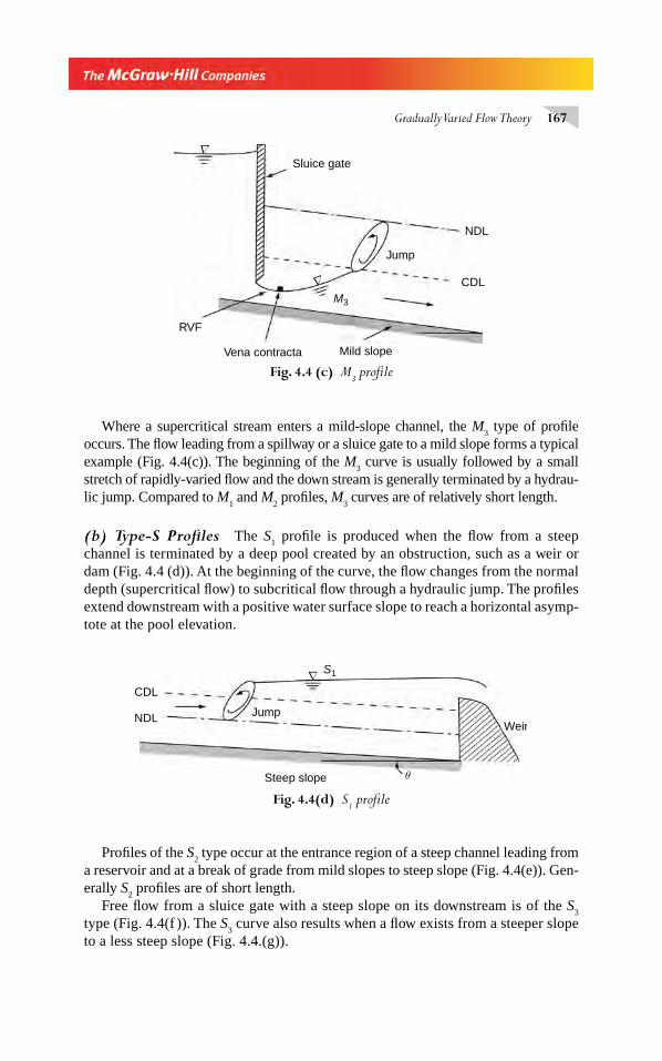
Gradually Varied Flow Theory 167
Where a supercritical stream enters a mild-slope channel, the M3 type of profi le
occurs. The fl ow leading from a spillway or a sluice gate to a mild slope forms a typical example (Fig. 4.4(c)). The beginning of the M
3 curve is usually followed by a small
stretch of rapidly-varied fl ow and the down stream is generally terminated by a hydrau-lic jump. Compared to M
1 and M
2 profi les, M
3 curves are of relatively short length.
(b) Type-S Profi les The S1 profi le is produced when the fl ow from a steep
channel is terminated by a deep pool created by an obstruction, such as a weir or dam (Fig. 4.4 (d)). At the beginning of the curve, the fl ow changes from the normal depth (supercritical fl ow) to subcritical fl ow through a hydraulic jump. The profi les extend downstream with a positive water surface slope to reach a horizontal asymp-tote at the pool elevation.
Sluice gate
Jump
NDL
CDLM3
RVF
Vena contracta Mild slope
∇
∇
Fig. 4.4 (c) M3 profi le
NDL
CDL
Steep slope θ
S1
WeirJump
∇
Fig. 4.4(d) S1 profi le
Profi les of the S2 type occur at the entrance region of a steep channel leading from
a reservoir and at a break of grade from mild slopes to steep slope (Fig. 4.4(e)). Gen-erally S
2 profi les are of short length.
Free fl ow from a sluice gate with a steep slope on its downstream is of the S3
type (Fig. 4.4(f )). The S3 curve also results when a fl ow exists from a steeper slope
to a less steep slope (Fig. 4.4.(g)).
Chapter 4.indd 167Chapter 4.indd 167 2/24/2010 3:43:04 PM2/24/2010 3:43:04 PM
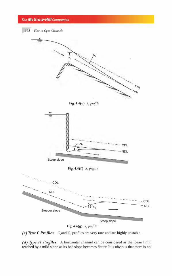
168 Flow in Open Channels
Fig. 4.4(f ) S3 profi le
S3 CDL
NDL
Steep slope
CDL
CDL
NDL
NDL
S3
Steep slope
Steeper slope
Fig. 4.4(g) S4 profi le
yc
S2
CDLNDL
∇
Fig. 4.4(e) S2 profi le
(c) Type C Profi les C1and C
3 profi les are very rare and are highly unstable.
(d) Type H Profi les A horizontal channel can be considered as the lower limit reached by a mild slope as its bed slope becomes fl atter. It is obvious that there is no
Chapter 4.indd 168Chapter 4.indd 168 2/24/2010 3:43:04 PM2/24/2010 3:43:04 PM
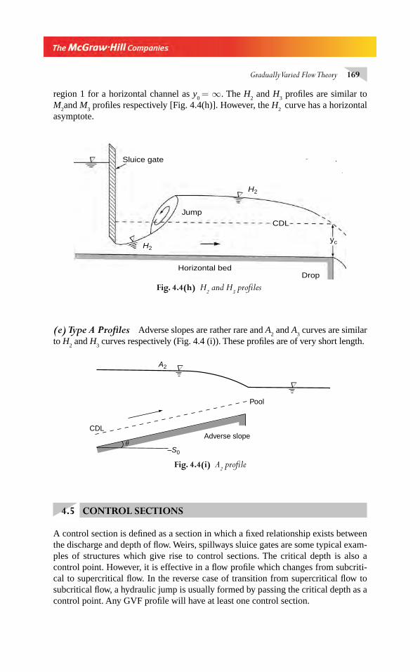
Gradually Varied Flow Theory 169
region 1 for a horizontal channel as y0 = ∞. The H
2 and H
3 profi les are similar to
M2and M
3 profi les respectively [Fig. 4.4(h)]. However, the H
2 curve has a horizontal
asymptote.
yc
Jump
Sluice gate
H2
H2
CDL
DropHorizontal bed
∇
∇
∇
Fig. 4.4(h) H2 and H
3 profi les
(e) Type A Profi les Adverse slopes are rather rare and A2 and A
3 curves are similar
to H2 and H
3 curves respectively (Fig. 4.4 (i)). These profi les are of very short length.
A2
θ
CDL
Pool
Adverse slope
–S0
∇
∇
Fig. 4.4(i) A2 profi le
4.5 CONTROL SECTIONS
A control section is defi ned as a section in which a fi xed relationship exists between the discharge and depth of fl ow. Weirs, spillways sluice gates are some typical exam-ples of structures which give rise to control sections. The critical depth is also a control point. However, it is effective in a fl ow profi le which changes from subcriti-cal to supercritical fl ow. In the reverse case of transition from supercritical fl ow to subcritical fl ow, a hydraulic jump is usually formed by passing the critical depth as a control point. Any GVF profi le will have at least one control section.
Chapter 4.indd 169Chapter 4.indd 169 2/24/2010 3:43:05 PM2/24/2010 3:43:05 PM
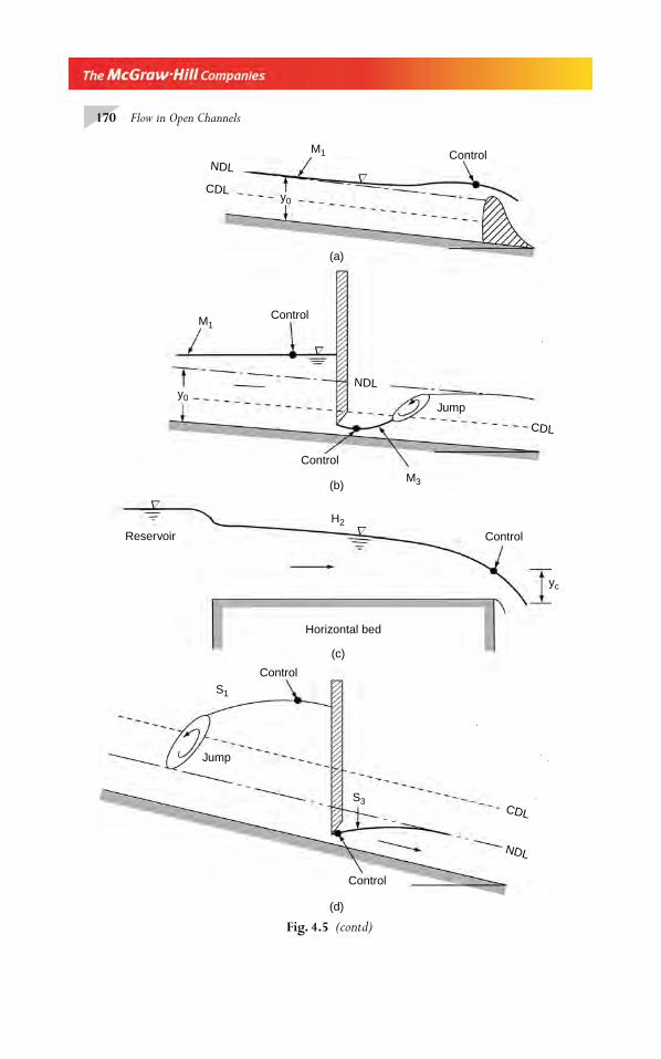
170 Flow in Open Channels
M1Control
Control
M3
CDL
Jump
NDL
(b)
y0
y0
NDL
CDL
Control
(a)
M1
Reservoir
H2
Control
yc
Horizontal bed
(c)
S3
S1
Control
Control
NDL
CDL
Jump
(d)
∇
∇
∇
∇
Fig. 4.5 (contd)
Chapter 4.indd 170Chapter 4.indd 170 2/24/2010 3:43:06 PM2/24/2010 3:43:06 PM
Gradually Varied Flow Theory 171
In the synthesis of GVF profi les occurring in serially connected channel ele-ments, the control sections provide a key to the identifi cation of proper profi le shapes. A few typical control sections are indicated in Fig. 4.5 (a-d). It may be noted that subcritical fl ows have controls in the downstream end while supercrit-ical fl ows are governed by control sections existing at the upstream end of the channel section. In Figs 4.5(a) and (b) for the M
1 profi le, the control section
(indicated by a dark dot in the fi gures) is just upstream of the spillway and sluice gate respectively. In Figs 4.5(b) and (d) for M
3 and S
3 profi les respectively, the
control point is at the vena contracta of the sluice-gate fl ow. In subcritical-fl ow reservoir offtakes Fig. 4.5(c), even though the discharge is governed by the res-ervoir elevation, the channel entry section is not strictly a control section. The water-surface elevation in the channel will be lower than the reservoir elevation by an amount equivalent to (1+K )V 2/2g where K is the entrance-loss coeffi cient. The true control section will be at a downstream location in the channel. For the situation shown in Fig. 4.5(c) the critical depth at the free overfl ow at the
Control
S2
NDL
Reservoir
(e)
= Control
4
2
3
1
B
NDL
Pool
Drop(f)
M1
M2
CDL
∇
∇
∇
∇
∇
∇
∇
Fig. 4.5 Examples of controls in GVF
Chapter 4.indd 171Chapter 4.indd 171 2/24/2010 3:43:06 PM2/24/2010 3:43:06 PM
172 Flow in Open Channels
channel end acts as the downstream control. For a sudden drop (free overfl ow) due to curvature of the streamlines the critical depth actually occurs at distance of about 4.0 y
c upstream of the drop. This distance, being small compared to GVF
lengths, is neglected and it is usual to perform calculations by assuming yc to
occur at the drop.For a supercritical canal intake Fig. 4.5(e)., the reservoir water surface falls to the
critical depth at the head of the canal and then onwards the water surface follows the S
2 curve. The critical depth occurring at the upstream end of the canal is the control
for this fl ow.A mild-slope channel discharging into a pool of variable surface elevation is indi-
cated in Fig. 4.5(f ). Four cases are shown. In case 1, the pool elevation is higher than the elevation of the normal-depth line at B. This gives rise to a drowning of the chan-nel end. A profi le of the M
1 type is produced with the pool level at B as control. The
velocity head of the channel fl ow is lost in turbulence at the exit and there is no recovery in terms of the change in surface elevation. In case 2, the pool elevation is lower than the elevation of the normal-depth line but higher than the critical-depth line at B. The pool elevation acts as a control for the M
2 curve. In case 3, the pool
elevation has dropped down to that of the critical-depth line at B and the control is still at the pool elevation. In case 4, the pool elevation has dropped lower than the elevation of the critical-depth line at B. The water surface cannot pass through a criti-cal depth at any location other than B and hence a sudden drop in the water surface at B is observed. The critical depth at B is the control for this fl ow.
4.6 ANALYSIS OF FLOW PROFILE
The process of identifi cation of possible fl ow profi les as a prelude to quantitative computations is known as analysis of fl ow profi le. It is essentially a synthesis of the information about the GVF profi les and control sections discussed in the previous section.
A channel carrying a gradually varied fl ow can in general contain different pris-moidal-channel sections of varying hydraulic properties. There can be a number of control sections of varying locations. To determine the resulting water-surface profi le in a given case, one should be in a position to analyse the effects of various channel sections and controls connected in series. Simple cases are illustrated to provide information and experience to handle more complex cases.
Break in Grade Simple situations of a series combination of two channel sec-tions with differing bed slopes are considered. In Fig. 4.6(a), a break in grade from a mild channel to a milder channel is s hown. It is necessary to fi rst draw the critical-depth line (CDL) and the normal-depth line (NDL) for both slopes. Since y
c does
not depend upon the slope (as Q = constant), the CDL is at a constant height above the channel bed in both slopes. The normal depth y
01 for the mild slope is lower
than that of the milder slope ( y02
). In this case, y02
acts as a control, similar to the
Chapter 4.indd 172Chapter 4.indd 172 2/24/2010 3:43:06 PM2/24/2010 3:43:06 PM
Gradually Varied Flow Theory 173
weir or spillway case and an M1 backwater curve is produced in the mild-slope
channel.Various combinations of slopes and the resulting GVF profi les are presented in
Fig. 4.6(a-h). It may be noted that in some situations there can be more than one pos-sible profi les. For example, in Fig. 4.6(e), a jump and S
1 profi le or an M
3 profi le and
a jump are possible. The particular curve in this case depends on the channel and its properties.
y02y01
NDL
M1NDL
NDL
NDL
NDL
CDL
CDL
CDL
CDL
CDL
CDL
CDL
Mild
Milder(a)
S2
Steep Steeper(b)
M2
S3
MilderMild
(c)
Steep
Steeper
(d)
CDL
NDL
NDL
NDL
Fig. 4.6 (Contd)
Chapter 4.indd 173Chapter 4.indd 173 2/24/2010 3:43:06 PM2/24/2010 3:43:06 PM
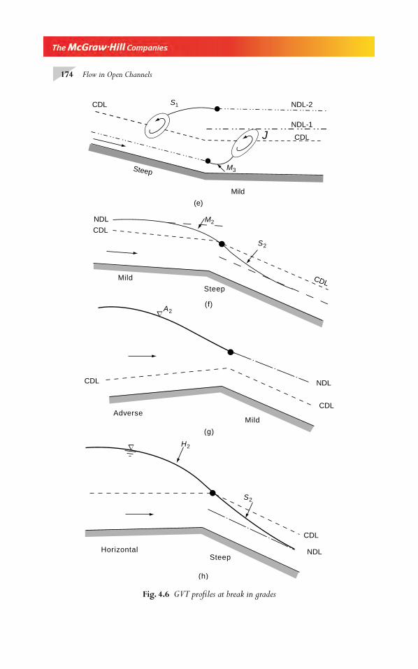
174 Flow in Open Channels
CDL
CDL
S1
M3
NDL-2
NDL-1
(e)
Mild
J
Steep
NDL
CDLM2
S2
Steep
Mild
(f)
(g)
NDLCDL
CDL
CDL
A2
MildAdverse
(h)
NDL
CDL
H2
S2
SteepHorizontal
Fig. 4.6 GVT profi les at break in grades
Chapter 4.indd 174Chapter 4.indd 174 2/24/2010 3:43:06 PM2/24/2010 3:43:06 PM
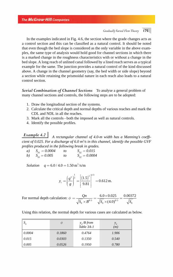
Gradually Varied Flow Theory 175
In the examples indicated in Fig. 4.6, the section where the grade changes acts as a control section and this can be classifi ed as a natural control. It should be noted that even though the bed slope is considered as the only variable in the above exam-ples, the same type of analysis would hold good for channel sections in which there is a marked change in the roughness characteristics with or without a change in the bed slope. A long reach of unlined canal followed by a lined reach serves as a typical example for the same. The junction provides a natural control of the kind discussed above. A change in the channel geometry (say, the bed width or side slope) beyond a section while retaining the prismoidal nature in each reach also leads to a natural control section.
Serial Combination of Channel Sections To analyse a general problem of many channel sections and controls, the following steps are to be adopted:
1. Draw the longitudinal section of the systems.2. Calculate the critical depth and normal depths of various reaches and mark the
CDL and NDL in all the reaches.3. Mark all the controls−both the imposed as well as natural controls.4. Identify the possible profi les.
Example 4.2 A rectangular channel of 4.0-m width has a Manning’s coeffi -cient of 0.025. For a discharge of 6.0 m3/s in this channel, identify the possible GVF profi les produced in the following break in grades.
a) S01
= 0.0004 to S02
= 0.015b) S
01 = 0.005 to S02
= 0.0004
Solution q = =6 0 4 0 1 50 3. / . . m /s/m
yq
gc =⎛
⎝⎜⎜⎜⎜
⎞
⎠⎟⎟⎟⎟
=( )⎡
⎣
⎢⎢⎢
⎤
⎦
⎥⎥⎥
=2
1
32 1 3
1 5
9 810 612
.
.. .
/
m
For normal depth calculation: φ =×
=×
×=
Qn
S B S S08 3
08 3
0
6 0 0 025
4 0
0 00372/ /
. .
( . )
.
Using this relation, the normal depth for various cases are calculated as below.
S0
φ y0 /B from
Table 3A-1y
0
(m)
0.0004 0.1860 0.4764 1.906
0.015 0.0303 0.1350 0.540
0.005 0.0526 0.1950 0.780
Chapter 4.indd 175Chapter 4.indd 175 2/24/2010 3:43:07 PM2/24/2010 3:43:07 PM
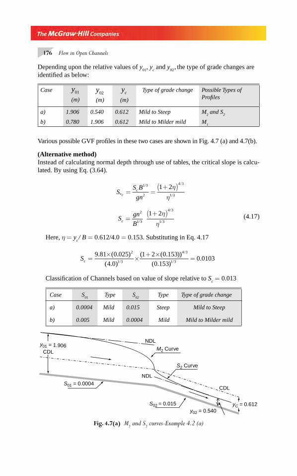
176 Flow in Open Channels
Depending upon the relative values of y01
, yc and y
02 , the type of grade changes are
identifi ed as below:
Case y01
(m)
y02
(m)
yc
(m)
Type of grade change Possible Types of Profi les
a) 1.906 0.540 0.612 Mild to Steep M2 and S
2
b) 0.780 1.906 0.612 Mild to Milder mild M1
Various possible GVF profi les in these two cases are shown in Fig. 4.7 (a) and 4.7(b).
(Alternative method)Instead of calculating normal depth through use of tables, the critical slope is calcu-lated. By using Eq. (3.64).
S
S B
gncc
*
/ /
/= =
+( )1 3
2
4 3
1 3
1 2η
η
S
gn
Bc =+( )2
1 3
4 3
1 3
1 2/
/
/
η
η
(4.17)
Here, η = yc / B = 0.612/4.0 = 0.153. Substituting in Eq. 4.17
Sc =
××
+ ×=
9 81 0 025
4 0
1 2 0 153
0 1530 0103
2
1 3
4 3
1 3
. ( . )
( . )
( ( . ))
( . ).
/
/
/
Classifi cation of Channels based on value of slope relative to Sc = 0.013
Case S01
Type S02
Type Type of grade change
a) 0.0004 Mild 0.015 Steep Mild to Steep
b) 0.005 Mild 0.0004 Mild Mild to Milder mild
y01 = 1.906
S01 = 0.0004
S02 = 0.015
S2 Curve
M2 Curve
NDL
NDL
CDL
y02 = 0.540yC = 0.612
CDL
Fig. 4.7(a) M2 and S
2 curves-Example 4.2 (a)
Chapter 4.indd 176Chapter 4.indd 176 2/24/2010 3:43:07 PM2/24/2010 3:43:07 PM
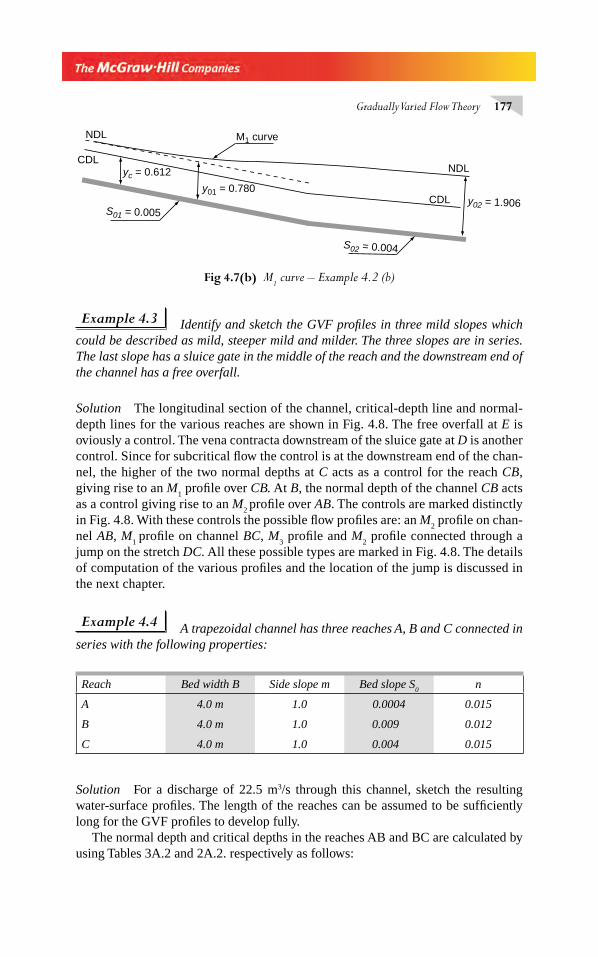
Gradually Varied Flow Theory 177
Example 4.3 Identify and sketch the GVF profi les in three mild slopes which could be described as mild, steeper mild and milder. The three slopes are in series. The last slope has a sluice gate in the middle of the reach and the downstream end of the channel has a free overfall.
Solution The longitudinal section of the channel, critical-depth line and normal-depth lines for the various reaches are shown in Fig. 4.8. The free overfall at E is oviously a control. The vena contracta downstream of the sluice gate at D is another control. Since for subcritical fl ow the control is at the downstream end of the chan-nel, the higher of the two normal depths at C acts as a control for the reach CB, giving rise to an M
1 profi le over CB. At B, the normal depth of the channel CB acts
as a control giving rise to an M2 profi le over AB. The controls are marked distinctly
in Fig. 4.8. With these controls the possible fl ow profi les are: an M2 profi le on chan-
nel AB, M1 profi le on channel BC, M
3 profi le and M
2 profi le connected through a
jump on the stretch DC. All these possible types are marked in Fig. 4.8. The details of computation of the various profi les and the location of the jump is discussed in the next chapter.
Example 4.4 A trapezoidal channel has three reaches A, B and C connected in series with the following properties:
Reach Bed width B Side slope m Bed slope S0
n
A 4.0 m 1.0 0.0004 0.015
B 4.0 m 1.0 0.009 0.012
C 4.0 m 1.0 0.004 0.015
Solution For a discharge of 22.5 m3/s through this channel, sketch the resulting water-surface profi les. The length of the reaches can be assumed to be suffi ciently long for the GVF profi les to develop fully.
The normal depth and critical depths in the reaches AB and BC are calculated by using Tables 3A.2 and 2A.2. respectively as follows:
y01 = 0.780
S01 = 0.005
S02 = 0.004
y02 = 1.906
yc = 0.612
CDL
CDLNDL
NDL M1 curve
Fig 4.7(b) M1 curve – Example 4.2 (b)
Chapter 4.indd 177Chapter 4.indd 177 2/24/2010 3:43:08 PM2/24/2010 3:43:08 PM
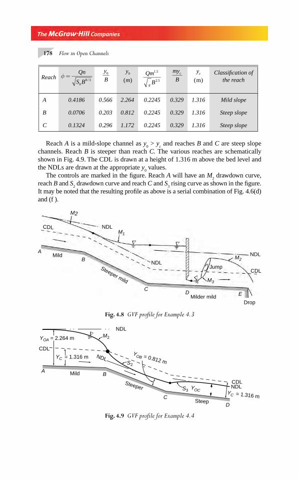
178 Flow in Open Channels
Reach A is a mild-slope channel as y0 > y
c and reaches B and C are steep slope
channels. Reach B is steeper than reach C. The various reaches are schematically shown in Fig. 4.9. The CDL is drawn at a height of 1.316 m above the bed level and the NDLs are drawn at the appropriate y
0 values.
The controls are marked in the fi gure. Reach A will have an M2 drawdown curve,
reach B and S2 drawdown curve and reach C and S
3 rising curve as shown in the fi gure.
It may be noted that the resulting profi le as above is a serial combination of Fig. 4.6(d) and (f ).
M2
NDL
NDL
NDL
CDL
CDL
M2
M1
M3
A
B
CD
Mild
Steeper mild
Milder mild
Jump
Drop
E
∇ ∇
∇
Fig. 4.8 GVF profi le for Example 4.3
YOC
M2
S2
S3
YOA = 2.264 m
YC = 1.316 m
YC = 1.316 m
YOB = 0.812 m
CDL
Mild BA
CD
Steeper
Steep
NDL
NDL
NDLCDL
∇
Fig. 4.9 GVF profi le for Example 4.4
Reach φ =Qn
S B08 3/
y
B0 y
m0
( )Qm
Bg
1 5
2 5
.
.
my
Bc yc
( )mClassifi cation of
the reach
A 0.4186 0.566 2.264 0.2245 0.329 1.316 Mild slope
B 0.0706 0.203 0.812 0.2245 0.329 1.316 Steep slope
C 0.1324 0.296 1.172 0.2245 0.329 1.316 Steep slope
Chapter 4.indd 178Chapter 4.indd 178 2/24/2010 3:43:08 PM2/24/2010 3:43:08 PM
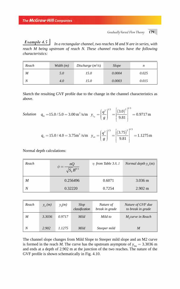
Gradually Varied Flow Theory 179
Example 4.5 In a rectangular channel, two reaches M and N are in series, with reach M being upstream of reach N. These channel reaches have the following characteristics:
Reach Width (m) Discharge (m3/s) Slope n
M 5.0 15.0 0.0004 0.025
N 4.0 15.0 0.0003 0.015
Sketch the resulting GVF profi le due to the change in the channel characteristics as above.
Solution q yq
gm cm= = =
⎛
⎝⎜⎜⎜⎜
⎞
⎠⎟⎟⎟⎟
=( )⎡
⎣
⎢15 0 5 0 3 003 0
9 813
2 1 3 2
. / . ..
.
/
m /s/m ⎢⎢⎢
⎤
⎦
⎥⎥⎥
=
1 3
0 9717
/
. m
q yq
gn cn= = =⎛
⎝⎜⎜⎜⎜
⎞
⎠⎟⎟⎟⎟
=( )⎡
⎣15 0 4 0 3 75
3 75
9 813
2 1 3 2
. / . ..
.
/
m /s/m ⎢⎢⎢⎢
⎤
⎦
⎥⎥⎥
=
1 3
1 1275
/
. m
Normal depth calculations:
Reachφ =
nQ
S B 08 3/
η from Table 3Α.1 Normal depth y0 (m)
M 0.256496 0.6071 3.036 m
N 0.32220 0.7254 2.902 m
Reach y0 (m) y
0(m) Slop
classifi cationNature of
break in gradeNature of GVF due to break in grade
M 3.3036 0.9717 Mild Mild to M2curve in Reach
N 2.902 1.1275 Mild Steeper mild M
The channel slope changes from Mild Slope to Steeper mild slope and an M2 curve is formed in the reach M. The curve has the upstream asymptote of y
0m = 3.3036 m
and ends at a depth of 2.902 m at the junction of the two reaches. The nature of the GVF profi le is shown schematically in Fig. 4.10.
Chapter 4.indd 179Chapter 4.indd 179 2/24/2010 3:43:08 PM2/24/2010 3:43:08 PM
180 Flow in Open Channels
4.7 TRANSITIONAL DEPTH
The transitional depth is defi ned as the depth at which the normal discharge Qn is
equal to the critical discharge Qc and the slope of the gradually varied fl ow profi le is
horizontal. For such a situation,
dy
dxS= 0
(4.18)
Since in a GVF from Eq. (4.15)
dy
dxS
Q Q
Q Q
n
c
=−
−( )0
2
2
1
1
( / )
/
at the transitional depth
Q
Q
Q
Qor
K
K
Z
Zn c
c= =0
(4.19)
i.e
Q S
nAR
Q g
A A T
/ /
//
0
2 31=
or
S
n g
A
T R
P
TA0
2 4 3
4 3
1 3
1= =
/
/
/
(4.20)
Equation 4.20 is the same as the generalized-fl ow relation (Eq. (3.69)) with F = 1.0. For a trapezoidal channel, the non-dimensionalised form of Eq. 4.20 will be
S
S B
n g
m
m mc
t
t t t
∗ = =+ +( )
+ +00
1 3
2
24 3
1 3 1 3
1 2 1
1 2 1
/
/
/ /( )( )
η
η η η
(4.21)
Fig. 4.10 GVF profi le of Example 4.5
NDL
NDL
M2
CDL
CDLycm = 0.9717 m
ycn = 1.1275 my0n = 2.912 m
y0m = 3.3036 m
Channel M
Channel N
Chapter 4.indd 180Chapter 4.indd 180 2/24/2010 3:43:09 PM2/24/2010 3:43:09 PM
Gradually Varied Flow Theory 181
where ηt = y
t = transitional depth. It may be noted that S
*0c is similar to S
*c (Section 3.16)
but with the bed slope S0 being used in place of S
c.
In a given problem, normally S0, B, n are fi xed and the value of η
t is required. It is
important to note that in the gradually-varied fl ow calculations, Qn and Q
c are fi ctitious
discharges and are different from the actual discharge Q. As such, at a transitional depth y
t, the actual fl ow Froude number is not unity (Example 4.4). Since Eq. (4.20) is the
same as Eq. (3.50) of the generalized-fl ow relationship, the behaviour of the transi-tional depth in trapezoidal, rectangular and triangular channels is exactly the same as the behaviour of the critical depth with critical slope (discussed in Section 3.16). The generalised-fl ow diagram (Fig. 3.11) can be used for the solution of Eq. (4.21) to determine the transitional depth.
It may be seen from Eq. (4.20) that the transitional depth depends only on the channel geometry, roughness and slope and is independent of the actual discharge. In general, there can be one, two or three transitional depths depending upon the fl ow and channel geometry. However, situations with more than one transitional depth in a profi le are rare. In gradually varied fl ow computations, the transitional depth is useful to locate sections where the water surface may have a point of infl exion with respect to the horizontal. In spatially-varied fl ows, the transitional depth pro-vides a very effective way of determining the control points.
Example 4.5 A 2.0-m wide rectangular channel (n = 0.015), carries a dis-charge of 4.0 m3/s. The channel is laid on slope of 0.0162. A downstream sluice gate raises the water surface to 7.0 m immediately behind it. Find the transit-ional depth.
Solution From Section 3.17, the limit value of SS B
gncLc
*
/
.= =1 3
22 667
Limit slope SLc = =2 667 9 81 0 015
2 00 004672
2
1 3
. ( . )( . )
( . ).
/
Since the actual slope S0 > S
LC , transitional depth is possible.
The normal depth y0, for given S
0 , n, B and Q is found by using Table 3A.1.
φ =×
×=
4 0 0 015
0 0162 2 00 07424
8 3
. .
. ( . ).
/
y B y0 00 2466 0 493/ . , .= = m
Critical depth yc =×
⎛⎝⎜⎜⎜
⎞⎠⎟⎟⎟⎟ =
16
4 9 810 742
1 3
..
/
m
Chapter 4.indd 181Chapter 4.indd 181 2/24/2010 3:43:09 PM2/24/2010 3:43:09 PM
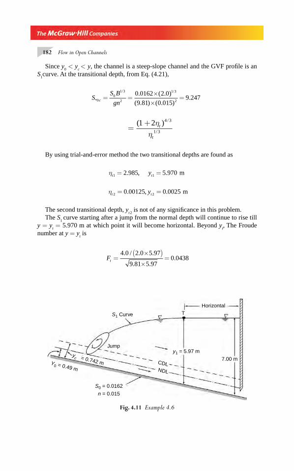
182 Flow in Open Channels
Since y0 < y
c <
y, the channel is a steep-slope channel and the GVF profi le is an
S1curve. At the transitional depth, from Eq. (4.21),
SS B
gnc*
/ /. ( . )
( . ) ( . ).0
01 3
2
1 3
2
0 0162 2 0
9 81 0 0159 247= =
××
=
=+( ) /
/
1 2 4 3
1 3
ηη
t
t
By using trial-and-error method the two transitional depths are found as
ηt ty1 12 985 5 970= =. , . m
ηt ty2 20 00125 0 0025= =. , . m
The second transitional depth, yt 2
is not of any signifi cance in this problem.The S
1 curve starting after a jump from the normal depth will continue to rise till
y = yt = 5.970 m at which point it will become horizontal. Beyond y
t, The Froude
number at y = yt is
Ft =
×( )×
=4 0 2 0 5 97
9 81 5 970 0438
. / . .
. ..
S1 Curve
Jump
S0 = 0.0162
n = 0.015
Y0 = 0.49 m
y = 0.742 m
y1 = 5.97 m
CDL NDL
Horizontal
T
7.00 m
∇ ∇
c
Fig. 4.11 Example 4.6
Chapter 4.indd 182Chapter 4.indd 182 2/24/2010 3:43:09 PM2/24/2010 3:43:09 PM
Gradually Varied Flow Theory 183
PROBLEMS
Problem Distribution
Topic Problems
GVF equation 4.1,4.2
Classifi cation of GVF profi les 4.3, 4.5–4.7
Water surface slope 4.4
GVF profi les at break in grade 4.8, 4.11
Profi le analysis 4.9, 4.10, 4.12 – 4.15
4.1 (i) Show that the differential equation of gradually varied fl ow in a rectangular channel of variable width B can be expressed as
dy
dx
S SQ y
gA
dB
dx
Q B
gA
f
=− +
⎛
⎝⎜⎜⎜⎜
⎞
⎠⎟⎟⎟⎟
−
0
2
3
2
31
(ii) Further, show that for horizontal, frictionless rectangular channel of varying width B, the above relation reduces to
1 02 2−( ) −⎛⎝⎜⎜⎜
⎞⎠⎟⎟⎟⎟ =F
dy
dxF
y
B
dB
dx
where F = Froude number.4.2 Using the basic differential equation of GVF, show that dy/dx is positive for S
1, M
3 and S
3
profi les4.3 Show that for a wide rectangular channel the slope is mild or steep according to S
0 being
less than or greater than
n g
q
2 10 9
2 9
/
/
⎛
⎝⎜⎜⎜⎜
⎞
⎠⎟⎟⎟⎟
4.4 A 3.0-m wide rectangular channel has a longitudinal slope of 150 mm/kmh and Manning’s n = 0.02. When the discharge in the channel is 0.85m3/s, estimate the slope of the water sur-face in the channel (relative to the horizontal) at a point where the depth of fl ow is 0.75 m.
4.5 In a very long, wide rectangular channel the discharge intensity is 3.0 m3/s/metre width. The bed slope of the channel is 0.004 and Manning’s n = 0.015. At a certain section in this channel, the depth of fl ow is observed to be 0.90 m. What type of GVF profi le occurs in the neighbourhood of this section?
4.6 In a 4.0-m wide rectangular channel (n = 0.017) the bed slope is 0.0006. When the channel is conveying 10.0 m3/s of fl ow, estimate the nature of GVF profi les at two far away sections P and R in this channel where the depth of fl ow is measure as 1.6 m and 2.1 m respectively.
Chapter 4.indd 183Chapter 4.indd 183 2/24/2010 3:43:10 PM2/24/2010 3:43:10 PM
184 Flow in Open Channels
4.7 A circular channel having a 2.0-m diameter (n = 0.015) is laid on a slope of 0.005. When a certain discharge is fl owing in this channel at a normal depth of 1.0 m, GVF was found to occur at a certain reach of channel. If a depth of 0.70 m was observed at a section in this GVF reach, what type of GVF profi le was occurring in the neighborhood of this section?
4.8 In a very long trapezoidal channel with bed width B = 3.0 m, side slope m = 1.5, Manning’s n = 0.016, Longitudinal slope S
0 = 0.0004, the normal depth is measured
as 1.20 m. Determine the type of GVF profi le existing at a section X. in this channel when the depth of fl ow at X is (i) 0.5 m, (ii) 0.8 m and (iii) 1.50 m.
4.9 A long and wide rectangular channel (n = 0.016) has a discharge intensity of 4.0 m3/s per metre width. If the bed slope changes from 0.008 to 0.012 at a section, sketch the possi-ble GVF profi les due to this break in grade.
4.10 Analyse the fl ow profi le in a 4.0-m wide rectangular channel (n = 0.015), carrying a dis-charge of 15.0 m3/s. The bed slope of the channel is 0.02 and a 1.5 m high weir (C
d =
0.70) is built on the downstream end of the channel.4.11 At a certain section in a rectangular channel, a constriction of the channel produces a
choking condition. Sketch the GVF profi le produced on the upstream as a result of this, if the channel is on (a) mild slope and (b) steep slope.
4.12 A 4.0-m wide rectangular channel has a Manning’s coeffi cient of 0.025. For a discharge of 6.0 m3/s, identify the possible types of GVF profi les produced in the following break in grades:
( ) .a S01 0 0004= to S02 0 005= .
( ) .b S01 0 015= to S02 0 0004= .
4.13 Sketch the possible GVF profi les in the following serial arrangement of channels and control. The fl ow is from left to right:(a) steep – horizontal – mild slope(b) mild – sluice gate – steep – horizontal – sudden drop(c) steep – steeper–mild – milder slope(d) free intake – steep – sluice gate – mild slope(e) steep – mild – sluice gate – mild – sudden drop(f ) sluice gate – adverse – horizontal – steep slope
4.14 Sketch the GVF profi les produced on the upstream and downstream of a sluice gate introduced in a (a) steep slope, (b) mild slope, and (c) horizontal-bed channel.
4.15 A rectangular channel has two reaches A and B in series with characteristics as below:
Reach Width(m) Discharge(m3/s) Slope n
A 4.80 7.40 0.0005 0.015
B 4.80 5.00 0.0005 0.015
The decrease in discharge at B is due to the withdrawal of some fl ow at the junc-tion and can be considered to be a local phenomenon. Sketch the GVF profi les produced in the channels if (a) the channel is continuous and without any obstruction at the junction, and (b) a sluice gate is provided at the junction.
4.16 In a rectangular channel two reaches A and B in series, with reach A being upstream of Reach B, have the following characteristics:
Chapter 4.indd 184Chapter 4.indd 184 2/24/2010 3:43:10 PM2/24/2010 3:43:10 PM
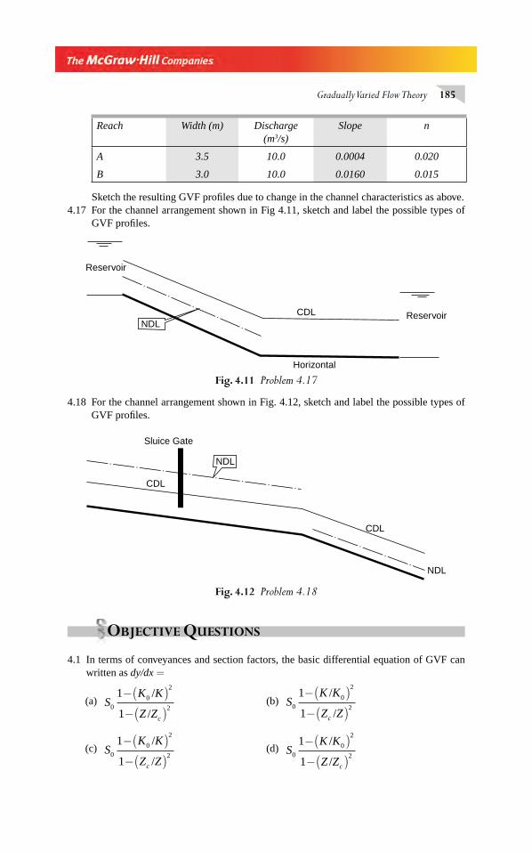
Gradually Varied Flow Theory 185
Reach Width (m) Discharge (m3/s)
Slope n
A 3.5 10.0 0.0004 0.020
B 3.0 10.0 0.0160 0.015
Sketch the resulting GVF profi les due to change in the channel characteristics as above.4.17 For the channel arrangement shown in Fig 4.11, sketch and label the possible types of
GVF profi les.
4.18 For the channel arrangement shown in Fig. 4.12, sketch and label the possible types of GVF profi les.
Fig. 4.11 Problem 4.17
Reservoir
ReservoirNDL
CDL
Horizontal
Fig. 4.12 Problem 4.18
CDL
CDL
NDL
NDL
Sluice Gate
OBJECTIVE QUESTIONS
4.1 In terms of conveyances and section factors, the basic differential equation of GVF can written as dy/dx =
(a) SK K
Z Zc
00
2
2
1
1
−( )−( )
/
/ (b) S
K K
Z Zc
00
2
2
1
1
−( )−( )
/
/
(c) SK K
Z Zc
00
2
2
1
1
−( )−( )
/
/ (d) S
K K
Z Zc
00
2
2
1
1
−( )−( )
/
/
Chapter 4.indd 185Chapter 4.indd 185 2/24/2010 3:43:10 PM2/24/2010 3:43:10 PM
186 Flow in Open Channels
4.2 In GVF profi les as the depth y→ yc ,
(a) dy
dx→ 0 (b) dy
dx→ ∞
(c) dy
dxS→ 0
(d) dy
dx→ a fi nite value
4.3 For a wide rectangular channel, if the Manning’s formula is used, the differential equation of GVF becomes dy/dx =
(a) Sy y
y yc
00
3 33
3 33
1
1
−( )−( )
/
/
.
. (b) S
y y
y yc
00
3 33
3
1
1
−( )−( )
/
/
.
(c) Sy y
y yc
00
3 33
3
1
1
−( )−( )
/
/
.
(d) Sy y
y yc
00
3
0
3 33
1
1
−( )−( )
/
/.
4.4 For a very wide rectangular channel, if Chezy formula is used, the defferential equation of GVF is given by dy/dx =
(a) Sy y
y yc
00
3 33
3 33
1
1
−( )−( )
/
/
.
. (b) S
y y
y yc
00
3
3
1
1
−( )−( )
/
/
(c) Sy y
y yc
00
3
3 33
1
1
−( )−( )
/
/.
(d) Sy y
y yc
00
3 33
3
1
1
−( )−( )
/
/
.
4.5 Uniform fl ow is taking place in a rectangular channel having a longitudinal slope of 0.004 and Manning’s n = 0.013. The discharge per unit width in the channel is measured as 1.2 m3 / s /m. The slope of the channel is classifi ed in GVF analysis as(a) mild (b) critical(c) steep (d) very steep
4.6 In a GVF, dy/dx is positive if
(a) K > K0 and Z > Z
c (b) K > K
0 and Z< Z
c
(c) K0 > K
c and Z
0 > Z
c (d) Z > K and Z
c > K
0
4.7 A 2.0-m wide rectangular channel has normal depth of 1.25 m when the discharge is 8.75 m3/s. The slope of the channel is classifi ed as(a) steep (b) mild(c) critical (d) essentially horizontal
4.8 Identify the incorrect statement:The possible GVF profi les in(a) mild slope channels are M
1, M
2 and M
3
(b) adverse slope channels are A2 and A
3
(c) horizontal channels are H1 and H
3
(d) critical slope channels are C1 and C
3
4.9 The following types of GVF profi les do not exist:(a) C
2, H
2, A
1 (b) A
2, H
1, C
2
(c) H1, A
1, C
2 (d) C
1, A
1, H
1
Chapter 4.indd 186Chapter 4.indd 186 2/24/2010 3:43:11 PM2/24/2010 3:43:11 PM
Gradually Varied Flow Theory 187
4.10 The total number of possible types of GVF profi les are(a) 9 (b) 11(c) 12 (d) 15
4.11 dy/dx is negative in the following GVF profi les:(a) M
1, S
2, A
2 (b) M
2, A
2, S
3
(c) A3, A
2, M
2 (c) M
2, A
2, H
2, A
2
4.12 If in a GVF dy/dx is positive, then dE/dx is:(a) always positive (b) negative for an adverse slope(c) negative if y > y
c (d) positive if y > y
c4.13 In a channel the gradient of the specifi c energy dE/dx is equal to
(a) S0 − S
f (b) S
f − S
0
(c) S0 − S
f
dy
dx− (d) S
0 (1 − F 2
)
4.14 In a wide river the depth of fl ow at a section is 3.0 m, S0 = 1 in 5000 and q = 3.0 m3/s
per metre width. If the Chezy formula with C = 70 is used, the water surface slope rela-tive to the bed at the section is(a) −2.732×10
−4 (b) 1.366×10
−4
(c) 1.211×10⁻⁵
(d) −6.234×10⁻⁴
4.15 The M3 profi le is indicated by the following inequality between the various depths:
(a) y0 > y
c > y (b) y > y
0 > y
c
(c) yc > y
0 > y (d) y > y
c > y
0
4.16 A long prismatic channel ends in an abrupt drop. If the fl ow in the channel far upstream of the drop is subcritical, the resulting GVF profi le(a) starts from the critical depth at the drop and joins the normal depth asymptotically(b) lies wholly below the critical depth line(c) lies wholly above the normal depth line(d) lies partly below and partly above the critical depth line
4.17 When there is a break in grade due to a mild slope A changing into a mider slope B, the GVF profi le produced is(a) M
3 curve on B (b) M
2 curve on B
(c) M1 curve on B (d) M
1 curve on A
4.18 In a channel the bed slope changes from a mild slope to a steep slope. The resulting GVF profi les are(a) (M
1, S
2 ) (b) (M
1, S
3 )
(c) (M2, S
2 ) (d) (M
2, S
1 )
4.19 A rectangular channel has B = 20 m, n = 0.020 and S0 = 0.0004. If the normal depth is
1.0 m, a depth of 0.8m in a GVF in this channel is a part of(a) M
1 (b) M
2
(c) M3 (d) S
2
4.20 A rectangular channel has uniform fl ow at a normal depth of 0.50 m. The discharge intensity in the channel is estimated as 1.40 m3/s/m. If an abrupt drop is provided at the downstream end of this channel, it will cause(a) M
2 type of GVF profi le
(b) S2 type of GVF profi le
(c) No GVF profi le upstream of the drop(d) M
1 type of profi le
4.21 The fl ow will be in the supercritical state in the following types of GVF profi les:(a) All S curves (b) M
2
(c) A3, M
3, S
2 (d) S
2, M
2, S
3
Chapter 4.indd 187Chapter 4.indd 187 2/24/2010 3:43:11 PM2/24/2010 3:43:11 PM
188 Flow in Open Channels
4.22 At the transitional depth
(a) dy
dx= ∞
(b) the slope of the GVF profi le is zero(c) dy/dx = −S
0
(d) the slope of GVF profi le is horizontal
Chapter 4.indd 188Chapter 4.indd 188 2/24/2010 3:43:12 PM2/24/2010 3:43:12 PM
5.1 INTRODUCTION
Almost all major hydraulic-engineering activities in free-surface fl ow involve the computation of GVF profi les. Considerable computational effort is involved in the analysis of problems, such as (a) determination of the effect of a hydraulic struct ure on the fl ow pattern in the channels, (b) inundation of lands due to a dam or weir con-struction, and (c) estimation of the fl ood zone. Because of its practical importance the computation of GVF has been a topic of continued interest to hydraulic engineers for the last 150 years. Dupuit (1848) was perhaps the fi rst to attempt the integration of the differential equation of GVF [Eq. (4.8)]. In the early periods the effort was to integrate [Eq. (4.8)] through the use of a simple resistance equation (such a Chezy equation with constant C ) and through other simplifi cations in the channel geometry (wide rectangular channel, parabolic channel, etc.). Bakhmeteff 1 developed a fairly satis-factory method involving the use of varied-fl ow functions applicable to a wide range of channels. This method has undergone successive refi nements, through various correc-tions, from time to time by subsequent research workers in this fi eld and fi nally in 1955 Chow 2 evolved a fairly comprehensive method using only one varied-fl ow function.
Simultaneously, with the development of direct integration as above, to meet the practical needs, various solution procedures involving graphical and numerical meth-ods were evolved for use by professional engineers. The advent of high-speed com-puters has given rise to general programmes utilizing sophisticated numerical techniques for solving GVF in natural channels. The various available procedures for computing GVF profi les can be classifi ed as:
1. Direct integration2. Numerical method3. Graphical method
Out of these the graphical method is practically obsolete and is seldom used. Fur-ther, the numerical method is the most extensively used technique. In the form of a host of available comprehensive softwares, it is the only method available to solve practical problems in natural channels. The direct integration technique is essentially of academic interest. This chapter describes the theory of GVF computations and a few well established procedures and specifi c methods which have possibilities of wider applications.
Gradually Varied
Flow Computations 5
Chapter 5.indd 189Chapter 5.indd 189 2/24/2010 2:59:14 PM2/24/2010 2:59:14 PM
190 Flow in Open Channels
5.2 DIRECT INTEGRATION OF GVF DIFFERENTIAL EQUATION
The differential equation of GVF for the prismoidal channel, from Eq. 4.12, given by
dy
dxS
K K
Z ZF y
c
=−( )−( )
= ( )0
02 2
2 2
1
1
/
/
is a non-linear, fi rst order, ordinary differential equation. This can be integrated by analytical methods to get closed from solutions only under certain very restricted conditions. A methods due to Chow2, which is based on certain assumptions but applicable with a fair degree of accuracy to a wide range of fi eld conditions, is presented here.
Let it be required to fi nd y = f (x) in the depth range y1 to y
2. The following two
assumptions are made:
1. The conveyance at any depth y is given by
K 2 = C2 y N (5.1)
and at the depth y0 by
K02 = C
2 y
0 N (5.2)
This implies that in the depth range which includes y1, y
2 and y
0, the coeffi cient
C2 and the second hydraulic exponent N are constants.
2. The section factor Z at any depth y is given by
Z2 = C
1 y M (5.3)
and at the critical depth y0 by
Zc2 = C
1 y
cM (5.4)
implying that in the depth range which includes y1, y
2 and y
c , the coeffi cient C
1 and
the fi rst hydraulic exponent M are constants.
Substituting the relationships given by Eqs 5.1 through 5.4 in Eq. 4.12,
dy
dxS
y y
y y
N
c
M=
−( )−( )
001
1
/
/
(5.5)
Putting u = y/y0 , dy = y
0 du and Eq. 5.5 simplifi es to
du
dx
S
y
u
y yu
N
cM M
M
=−
−( )
⎡
⎣
⎢⎢⎢⎢⎢
⎤
⎦
⎥⎥⎥⎥⎥
0
00
1 1
11
Chapter 5.indd 190Chapter 5.indd 190 2/24/2010 2:59:17 PM2/24/2010 2:59:17 PM
Gradually Varied Flow Computations 191
i.e. dxy
S u
y
y
u
udu
Nc
M N M
N= −
−+
⎛
⎝⎜⎜⎜⎜
⎞
⎠⎟⎟⎟⎟ −
⎡
⎣
⎢⎢⎢
⎤
⎦
⎥⎥⎥
−0
0 0
11
1 1
Integrating
xy
Su
du
u
y
y
u
udu
Nc
M N M
N
uu
= −−
+⎛
⎝⎜⎜⎜⎜
⎞
⎠⎟⎟⎟⎟ −
⎡
⎣
⎢⎢⎢
⎤
⎦
⎥⎥⎥
−
∫∫0
0 000 1 1
++ Const. (5.6)
Calling du
uF u N
N
u
10 −= ( )∫ ,
the second integral can be simplifi ed as follows:
Put v uN J= where JN
N M=
− +( )1
to get dvN
Ju du
N
J=−1
= (N – M + 1) uN−M du
∴ u
udu
N M
dv
v
N M
N
u
J
v−
−=
− +( ) −∫ ∫1
1
1 10 0
= ( )J
NF v J, (5.8)
It may be noted that F(v, J) is the same function as F(u, N) with u and N replaced by v and J respectively.Eq. 5.6 can now be written as
x
y
Su F u N
y
y
J
NF v Jc
M
= − ( )+⎛
⎝⎜⎜⎜⎜
⎞
⎠⎟⎟⎟⎟ ( )
⎡
⎣
⎢⎢⎢
⎤
⎦
⎥⎥⎥
0
0 0
, ,
(5.9)
Using Eq. 5.9 between two sections (x1, y
1) and (x
2, y
2) yields
x x
y
Su u F u N F u N2 1
0
02 1 2 1−( ) = −( )⎡
⎣ − ( ){ − ( )}, ,
+⎛
⎝⎜⎜⎜⎜
⎞
⎠⎟⎟⎟⎟ ( )− ( )}{ ⎤
⎦⎥y
y
J
MF v J F v Jc
M
02 1, , (5.10)
The function F(u, N ) is known as the varied-fl ow function. Extensive tables of F(u, N) are readily available1,2,3 and a table showing F(u, N ) for a few values of N is presented in Table 5A.1 in Appendix 5A at the end of this chapter.
A method of obtaining the exact analytical solutions of du
uN
u
10 −∫ for integral
and non-integral values of N is given by Gill4. Numberical integration of du
uN
u
10 −∫
Chapter 5.indd 191Chapter 5.indd 191 2/24/2010 2:59:17 PM2/24/2010 2:59:17 PM
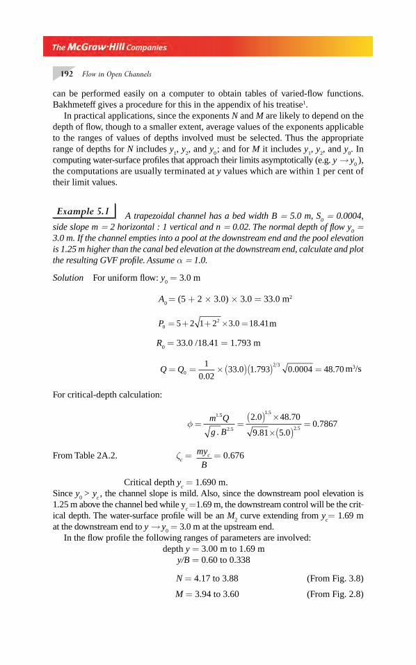
192 Flow in Open Channels
can be performed easily on a computer to obtain tables of varied-fl ow functions. Bakhmeteff gives a procedure for this in the appendix of his treatise1.
In practical applications, since the exponents N and M are likely to depend on the depth of fl ow, though to a smaller extent, average values of the exponents applicable to the ranges of values of depths involved must be selected. Thus the appropriate range of depths for N includes y
1, y
2, and y
0 ; and for M it includes y
1, y
2, and y
0. In
computing water-surface profi les that approach their limits asymptotically (e.g. y → y0 ),
the computations are usually terminated at y values which are within 1 per cent of their limit values.
Example 5.1 A trapezoidal channel has a bed width B = 5.0 m, S0 = 0.0004,
side slope m = 2 horizontal : 1 vertical and n = 0.02. The normal depth of fl ow y0 =
3.0 m. If the channel empties into a pool at the downstream end and the pool elevation is 1.25 m higher than the canal bed elevation at the downstream end, calculate and plot the resulting GVF profi le. Assume α = 1.0.
Solution For uniform fl ow: y0 = 3.0 m
A0 = (5 + 2 × 3.0) × 3.0 = 33.0 m2
P025 2 1 2 3 0 18 41= + + × =. . m
R0 = 33.0 /18.41 = 1.793 m
Q Q= = × ( )( ) =0
2 31
0 0233 0 1 793 0 0004 48 70
.. . . . m3/s
For critical-depth calculation:
φ = =( ) ×
×( )=
m Q
g B
1 5
2 5
1 5
2 5
2 0 48 70
9 81 5 00 7867
.
.
.
..
. .
. ..
From Table 2A.2. ζc = my
Bc = 0.676
Critical depth yc = 1.690 m.
Since y0 > y
c , the channel slope is mild. Also, since the downstream pool elevation is
1.25 m above the channel bed while yc =1.69 m, the downstream control will be the crit_
ical depth. The water-surface profi le will be an M2 curve extending from y
c= 1.69 m
at the downstream end to y → y0 = 3.0 m at the upstream end.
In the fl ow profi le the following ranges of parameters are involved:depth y = 3.00 m to 1.69 m
y/B = 0.60 to 0.338
N = 4.17 to 3.88 (From Fig. 3.8)
M = 3.94 to 3.60 (From Fig. 2.8)
Chapter 5.indd 192Chapter 5.indd 192 2/24/2010 2:59:17 PM2/24/2010 2:59:17 PM
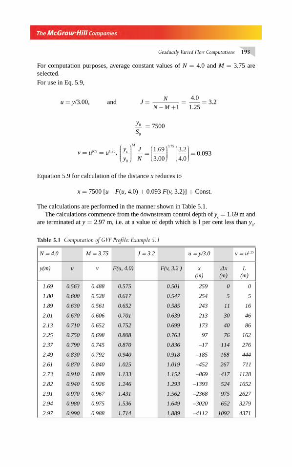
Gradually Varied Flow Computations 193
For computation purposes, average constant values of N = 4.0 and M = 3.75 are selected.
For use in Eq. 5.9,
u = y/3.00, and J = N
N M− +1 =
4 0
1 25
.
. = 3.2
y
S0
0
= 7500
v = uN/J = u1.25, y
yc
M
0
⎛
⎝⎜⎜⎜⎜
⎞
⎠⎟⎟⎟⎟
J
N=
⎛⎝⎜⎜⎜
⎞⎠⎟⎟⎟⎟
⎛⎝⎜⎜⎜
⎞⎠⎟⎟⎟⎟ =
1 69
3 00
3 2
4 00 093
3 75.
.
.
..
.
Equation 5.9 for calculation of the distance x reduces to
x = 7500 [u – F(u, 4.0) + 0.093 F(v, 3.2)] + Const.
The calculations are performed in the manner shown in Table 5.1.The calculations commence from the downstream control depth of y
c = 1.69 m and
are terminated at y = 2.97 m, i.e. at a value of depth which is l per cent less than y0.
N = 4.0 M = 3.75 J = 3.2 u = y/3.0 v = u1.25
y(m) u v F(u, 4.0) F(v, 3.2 ) x(m)
Δx(m)
L(m)
1.69 0.563 0.488 0.575 0.501 259 0 0
1.80 0.600 0.528 0.617 0.547 254 5 5
1.89 0.630 0.561 0.652 0.585 243 11 16
2.01 0.670 0.606 0.701 0.639 213 30 46
2.13 0.710 0.652 0.752 0.699 173 40 86
2.25 0.750 0.698 0.808 0.763 97 76 162
2.37 0.790 0.745 0.870 0.836 –17 114 276
2.49 0.830 0.792 0.940 0.918 –185 168 444
2.61 0.870 0.840 1.025 1.019 –452 267 711
2.73 0.910 0.889 1.133 1.152 –869 417 1128
2.82 0.940 0.926 1.246 1.293 –1393 524 1652
2.91 0.970 0.967 1.431 1.562 –2368 975 2627
2.94 0.980 0.975 1.536 1.649 –3020 652 3279
2.97 0.990 0.988 1.714 1.889 –4112 1092 4371
Table 5.1 Computation of GVF Profi le: Example 5.1
Chapter 5.indd 193Chapter 5.indd 193 2/24/2010 2:59:17 PM2/24/2010 2:59:17 PM
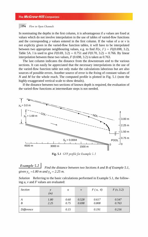
194 Flow in Open Channels
In nominating the depths in the fi rst column, it is advantageous if u values are fi xed at values which do not involve interpolation in the use of tables of varied-fl ow functions and the corresponding y values entered in the fi rst column. If the value of u or v is not explicity given in the varied-fl ow function tables, it will have to be interpolated between two appropriate neighbouring values, e.g. to fi nd F(v, J ) = F((0.698, 3.2),Table 5A. l is used to give F(0.69, 3.2) = 0.751 and F(0.70, 3.2) = 0.766. By linear interpolation between these two values, F (0.698, 3.2) is taken as 0.763.
The last column indicates the distance from the downstream end to the various sections. It can easily be appreciated that the necessary interpolations in the use of the varied-fl ow function table not only make the calculations laborious but are also sources of possible errors. Another source of error is the fi xing of constant values of N and M for the whole reach. The computed profi le is plotted in Fig. 5.1 (note the highly-exaggerated vertical scale to show details).
If the distance between two sections of known depth is required, the evaluation of the varied-fl ow functions at intermediate steps is not needed.
ya = 3.0 m
CDLyb = 1.69 m NDL
POOL0.75 m
1.50 m
0 0
2.25 m
3.00 m
4500 m 3000 m 1500 m
S0 = 0.0004
Δ
Fig. 5.1 GVF profi le for Example 5.1
Section y(m)
u v F ( u, 4) F (v, 3.2)
AB
1.802.25
0.600.75
0.5280.698
0.6170.808
0.5470.763
Difference 0.15 0.191 0.216
Example 5.2 Find the distance between two Sections A and B of Example 5.1,
given yA =1.80 m and y
B = 2.25 m.
Solution Referring to the basic calculations performed in Example 5.1, the follow-ing u, v and F values are evaluated:
Chapter 5.indd 194Chapter 5.indd 194 2/24/2010 2:59:18 PM2/24/2010 2:59:18 PM
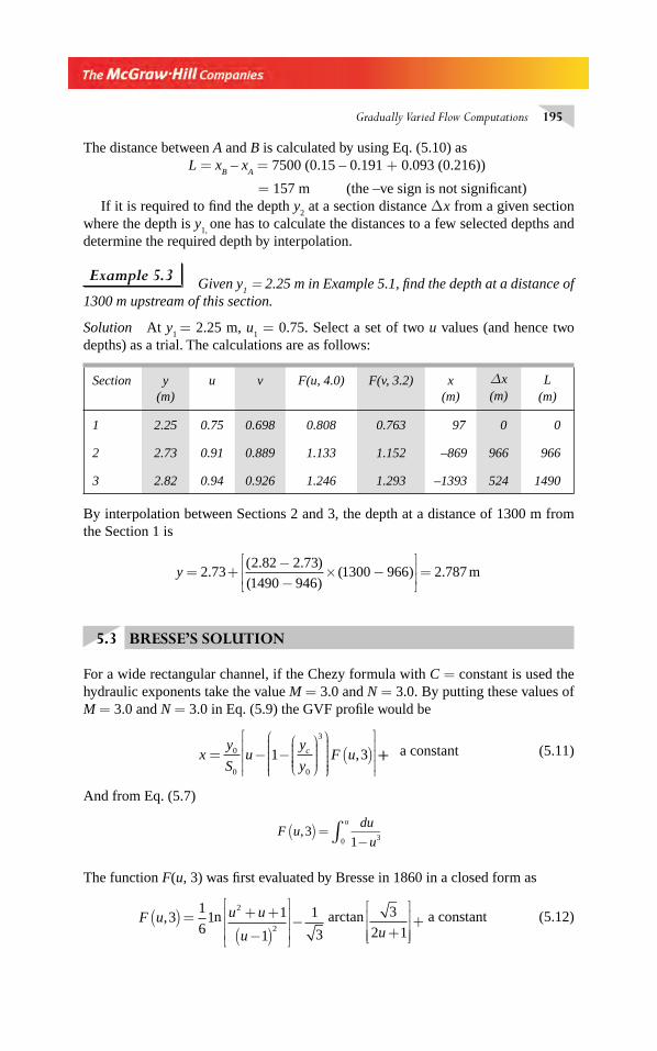
Gradually Varied Flow Computations 195
The distance between A and B is calculated by using Eq. (5.10) asL = x
B – x
A = 7500 (0.15 – 0.191 + 0.093 (0.216))
= 157 m (the –ve sign is not signifi cant)If it is required to fi nd the depth y
2 at a section distance Δ
x from a given section
where the depth is y 1 ,
one has to calculate the distances to a few selected depths and determine the required depth by interpolation.
Example 5.3 Given y
1 = 2.25 m in Example 5.1, fi nd the depth at a distance of
1300 m upstream of this section.
Solution At y1 = 2.25 m, u
1 = 0.75. Select a set of two u values (and hence two
depths) as a trial. The calculations are as follows:
Section y(m)
u v F(u, 4.0) F(v, 3.2) x(m)
Δ x(m)
L(m)
1 2.25 0.75 0.698 0.808 0.763 97 0 0
2 2.73 0.91 0.889 1.133 1.152 –869 966 966
3 2.82 0.94 0.926 1.246 1.293 –1393 524 1490
By interpolation between Sections 2 and 3, the depth at a distance of 1300 m from the Section 1 is
y = +
−−
× −⎡
⎣⎢⎢
⎤
⎦⎥⎥ =2 73
2 82 2 73
1490 9461300 966 2 787.
( . . )
( )( ) . m
5.3 BRESSE’S SOLUTION
For a wide rectangular channel, if the Chezy formula with C = constant is used the hydraulic exponents take the value M = 3.0 and N = 3.0. By putting these values of M = 3.0 and N = 3.0 in Eq. (5.9) the GVF profi le would be
xy
Su
y
yF uc= − −
⎛
⎝⎜⎜⎜⎜
⎞
⎠⎟⎟⎟⎟
⎛
⎝
⎜⎜⎜⎜⎜
⎞
⎠
⎟⎟⎟⎟⎟⎟( )
⎡
⎣
⎢⎢⎢
⎤
⎦
⎥⎥⎥
0
0 0
3
1 3, ++ a constant (5.11)
And from Eq. (5.7)
F u
du
u
u
,31 30
( ) =−∫
The function F(u, 3) was fi rst evaluated by Bresse in 1860 in a closed form as
F u,31
61( ) = n u u
u
2
2
1
1
1
3
+ +
−( )
⎡
⎣
⎢⎢⎢
⎤
⎦
⎥⎥⎥− arctan 3
2 1u +
⎡
⎣⎢⎢⎢
⎤
⎦⎥⎥⎥+ a constant (5.12)
Chapter 5.indd 195Chapter 5.indd 195 2/24/2010 2:59:18 PM2/24/2010 2:59:18 PM
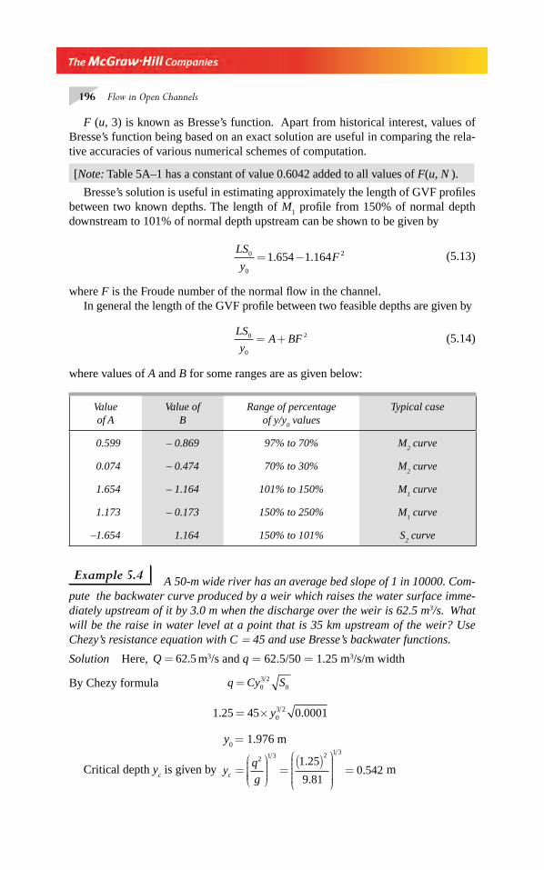
196 Flow in Open Channels
F (u, 3) is known as Bresse’s function. Apart from historical interest, values of Bresse’s function being based on an exact solution are useful in comparing the rela-tive accuracies of various numerical schemes of computation.
[Note: Table 5A–1 has a constant of value 0.6042 added to all values of F(u, N ).
Bresse’s solution is useful in estimating approximately the length of GVF profi les between two known depths. The length of M
1 profi le from 150% of normal depth
downstream to 101% of normal depth upstream can be shown to be given by
LS
yF0
0
21 654 1 164= −. . (5.13)
where F is the Froude number of the normal fl ow in the channel.In general the length of the GVF profi le between two feasible depths are given by
LS
yA BF0
0
2= + (5.14)
where values of A and B for some ranges are as given below:
Valueof A
Value ofB
Range of percentage of y/y
0 values
Typical case
0.599 – 0.869 97% to 70% M2 curve
0.074 – 0.474 70% to 30% M2 curve
1.654 – 1.164 101% to 150% M1 curve
1.173 – 0.173 150% to 250% M1 curve
–1.654 1.164 150% to 101% S2 curve
Example 5.4 A 50-m wide river has an average bed slope of 1 in 10000. Com-pute the backwater curve produced by a weir which raises the water surface imme-diately upstream of it by 3.0 m when the discharge over the weir is 62.5 m3/s. What will be the raise in water level at a point that is 35 km upstream of the weir? Use Chezy’s resistance equation with C = 45 and use Bresse’s backwater functions.
Solution Here, Q = 62 5. m3/s and q = 62.5/50 = 1.25 m3/s/m width
By Chezy formula q Cy S= 03 2
0
1 25 45 0 000103 2. .= × y
y
0 = 1.976 m
Critical depth yc is given by y
q
gc =⎛
⎝⎜⎜⎜⎜
⎞
⎠⎟⎟⎟⎟
=( )⎛
⎝
⎜⎜⎜⎜⎜
⎞
⎠
⎟⎟⎟⎟⎟⎟=
2 1 3 2 1 3
1 25
9 810 542
.
.. m
Chapter 5.indd 196Chapter 5.indd 196 2/24/2010 2:59:18 PM2/24/2010 2:59:18 PM
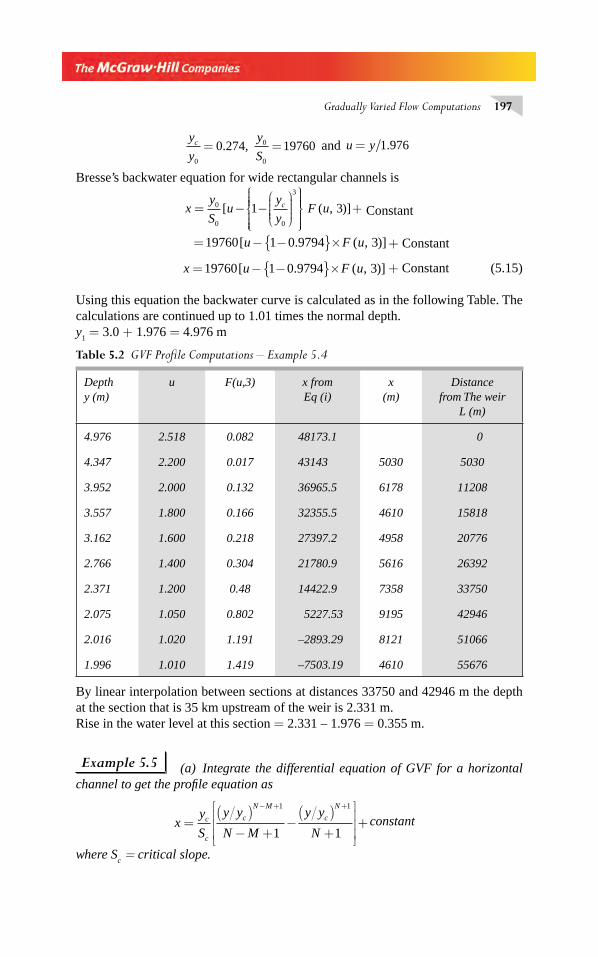
Gradually Varied Flow Computations 197
y
y
y
Sc
0
0
0
0 274 19760= =. , and u y= 1 976.
Bresse’s backwater equation for wide rectangular channels is
xy
Su
y
yF uc= − −
⎛
⎝⎜⎜⎜⎜
⎞
⎠⎟⎟⎟⎟
⎧⎨⎪⎪⎪
⎩⎪⎪⎪
⎫⎬⎪⎪⎪
⎭⎪⎪⎪
+0
0 0
3
1 3[ ( , )] Constant
u F u= − −{ }×19760 1 0 9794 3[ . ( , )] + Constant
x u F u= − −{ }×19760 1 0 9794 3[ . ( , )] + Constant (5.15)
Using this equation the backwater curve is calculated as in the following Table. The calculations are continued up to 1.01 times the normal depth.y
1 = 3.0 + 1.976 = 4.976 m
By linear interpolation between sections at distances 33750 and 42946 m the depth at the section that is 35 km upstream of the weir is 2.331 m.Rise in the water level at this section = 2.331 – 1.976 = 0.355 m.
Example 5.5 (a) Integrate the differential equation of GVF for a horizontal channel to get the profi le equation as
xy
S
y y
N M
y y
Nc
c
c
N M
c
N
=( )
− +−
( )+
⎡
⎣
⎢⎢⎢
⎤
⎦
⎥⎥⎥+
− + +1 1
1 1constant
where Sc = critical slope.
Depthy (m)
u F(u,3) x fromEq (i)
x(m)
Distance from The weir
L (m)
4.976 2.518 0.082 48173.1 0
4.347 2.200 0.017 43143 5030 5030
3.952 2.000 0.132 36965.5 6178 11208
3.557 1.800 0.166 32355.5 4610 15818
3.162 1.600 0.218 27397.2 4958 20776
2.766 1.400 0.304 21780.9 5616 26392
2.371 1.200 0.48 14422.9 7358 33750
2.075 1.050 0.802 5227.53 9195 42946
2.016 1.020 1.191 –2893.29 8121 51066
1.996 1.010 1.419 –7503.19 4610 55676
Table 5.2 GVF Profi le Computations – Example 5.4
Chapter 5.indd 197Chapter 5.indd 197 2/24/2010 2:59:18 PM2/24/2010 2:59:18 PM
198 Flow in Open Channels
(b) Using the result of part (a) above develop an equation for GVF profi le in a wide, rectangular, horizontal channel.
Solution dy
dx
S S
Q T
gA
f=−
−
0
2
31
(5.16)
For a horizontal channel S0 = 0
Also, SQ
K
K S
K
y
ySf
c c c
N
c= = =⎛
⎝⎜⎜⎜⎜
⎞
⎠⎟⎟⎟⎟
2
2
2
2
Further, Q
gZc
22= and
A
TZ
32=
Thus Q T
gA
y
yc
M2
3=
⎛
⎝⎜⎜⎜⎜
⎞
⎠⎟⎟⎟⎟
Equation 5.16 is now written as dy
dx
y
yS
y
y
c
N
c
c
M=
−⎛
⎝⎜⎜⎜⎜
⎞
⎠⎟⎟⎟⎟
−⎛
⎝⎜⎜⎜⎜
⎞
⎠⎟⎟⎟⎟1
− = −( )⎡⎣⎢
⎤⎦⎥ ( )
dx S y yy y
dyc c
M
c
N. 1
1
=⎛
⎝⎜⎜⎜⎜
⎞
⎠⎟⎟⎟⎟
−⎛
⎝⎜⎜⎜⎜
⎞
⎠⎟⎟⎟⎟
⎡
⎣
⎢⎢⎢
⎤
⎦
⎥⎥⎥
−y
y
y
ydy
c
N
c
N M
∴ − =( )
+−
( )− +
⎡
⎣
⎢⎢⎢
⎤
⎦
⎥⎥⎥+
+ − +
S x yy y
N
y y
N Mc cc
N
c
N M1 1
1 1Constant
∴ =( )
− +−
( )+
⎡
⎣
⎢⎢⎢
⎤
⎦
⎥⎥⎥+
− + +
xy
S
y y
N M
y y
Nc
c
c
N M
c
N1 1
1 1Constant
(b) For a wide rectangular channel, by Eq. 3.62 (a) Sn g
yc
c
=2
1 3,
Noting that N = 10/3 and M = 3,Substituting for S
c, N and M in the result of Part (a), viz., that for a horizontal rect-
angular channel,
∴ =( )
− +−
( )+
⎡
⎣
⎢⎢⎢
⎤
⎦
⎥⎥⎥+
− + +
xy
S
y y
N M
y y
Nc
c
c
N M
c
N1 1
1 1Constant,
we get for a wide rectangular, horizontal channel, the GVF profi le as
Chapter 5.indd 198Chapter 5.indd 198 2/24/2010 2:59:19 PM2/24/2010 2:59:19 PM
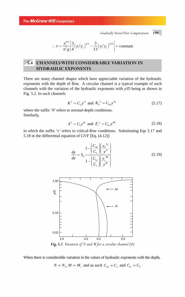
Gradually Varied Flow Computations 199
∴ = ( ) − ( )⎡
⎣⎢⎢
⎤
⎦⎥⎥+x
y
n gy y y yc
c c
4 3
2
4 3 13 33
4
3
13constant
5.4 CHANNELS WITH CONSIDERABLE VARIATION INHYDRAULIC EXPONENTS
There are many channel shapes which have appreciable variation of the hydraulic exponents with the depth of fl ow. A circular channel is a typical example of such channels with the variation of the hydraulic exponents with y/D being as shown in Fig. 5.2. In such channels
K C yN22= and K C yN
02
200= (5.17)
where the suffi x ‘0’ refers to normal-depth conditions.Similarly,
Z C yM21= and Z C yc c
Mc21= (5.18)
in which the suffi x ‘c’ refers to critical-fl ow conditions. Substituting Eqs 5.17 and 5.18 in the differential equation of GVF [Eq. (4.12)]
dy
dxS
C
C
y
y
C
C
N
N
c
=
−⎛
⎝⎜⎜⎜⎜
⎞
⎠⎟⎟⎟⎟
⎛
⎝⎜⎜⎜⎜
⎞
⎠⎟⎟⎟⎟
−⎛
⎝⎜⎜⎜⎜
⎞0
20
2
0
1
1
1
1
0
⎠⎠⎟⎟⎟⎟
⎛
⎝⎜⎜⎜⎜
⎞
⎠⎟⎟⎟⎟
y
yc
Mc
M
(5.19)
M
N
y/D
1.00
0.10
0.02
2.0 3.0 4.0 5.0
Fig. 5.2 Variation of N and M for a circular channel [6]
When there is considerable variation in the values of hydraulic exponents with the depth,
N N M Mc≠ ≠0 , and as such C C20 2≠ and C Cc1 1≠ .
Chapter 5.indd 199Chapter 5.indd 199 2/24/2010 2:59:19 PM2/24/2010 2:59:19 PM
200 Flow in Open Channels
Obviously, Eq. (5.9) cannot be used as a solution of Eq. 5.19Assuming C C20 2= and C Cc1 1= Chow3 has obtained the solution of Eq. 5.19 as
xy
Su F u N
y
y
J
NF v
N Nc
Mc M
N N
M
= − ( )+⎛
⎝⎜⎜⎜⎜
⎞
⎠⎟⎟⎟⎟⎟
⎛⎝⎜⎜⎜
⎞⎠⎟⎟⎟⎟
0
0 0
0
0, , JJ( )
⎡
⎣
⎢⎢⎢
⎤
⎦
⎥⎥⎥ a constant (5.20)
In which u y y N N= 00 . However, it has been shown6 that this assumption is not valid
and Eq. 5.20 may give considerable errors. A generalised procedure for direct integration of Eq. 5.19 using the varied-fl ow function is given by Subramanya and Ramamurthy5.
5.5 DIRECT INTEGRATION FOR CIRCULAR CHANNELS
5.5.1 Keifer and Chu’s method
The direct integration of the differential equation of GVF by Chow’s method is very inconvenient to use in the computation of GVF profi les in circular channels.
A different approach of integration of the differential equation of GVF for circular channels, developed by Keifer and Chu6, simplifi es the calculation procedure considerably.
Let Q be the actual discharge in a circular channel of diameter D and bed slope S0.
Then
Q K S f= (5.21)
and Q K S= 0 0 (5.22)
where K and K0 are the conveyance at depths y and y
0 respectively, y
0 = normal depth,
Sf = energy slope at depth y. Let Q
D = a hypothetical discharge corresponding to
uniform fl ow with the channel fl owing full.Then
Q K SD D= 0 (5.23)
where KD = conveyance at depth D.
i.e. Kn
D DD = ( ) ( )14 42 2 3
π
K
K
K
K
K
KD
D0
2
0
2 2⎛
⎝⎜⎜⎜
⎞
⎠⎟⎟⎟⎟ =
⎛
⎝⎜⎜⎜⎜
⎞
⎠⎟⎟⎟⎟
⎛
⎝⎜⎜⎜
⎞
⎠⎟⎟⎟⎟
But K
K
D D
ARf y DD
⎛
⎝⎜⎜⎜
⎞
⎠⎟⎟⎟⎟ =
( )( )⎡
⎣
⎢⎢⎢⎢
⎤
⎦
⎥⎥⎥⎥=
2 2 2 3
2 3 1
4 4π( )
Chapter 5.indd 200Chapter 5.indd 200 2/24/2010 2:59:19 PM2/24/2010 2:59:19 PM
Gradually Varied Flow Computations 201
and K
K
Q
D D
r0
2 22⎛
⎝⎜⎜⎜⎜
⎞
⎠⎟⎟⎟⎟
=⎛
⎝⎜⎜⎜⎜
⎞
⎠⎟⎟⎟⎟
= ( ) (5.24)
∴ K
KQ f y Dr
0
2
21
⎛
⎝⎜⎜⎜
⎞
⎠⎟⎟⎟⎟ = ( ) (5.25)
The differential equation of GVF, Eq. 4.12, becomes
dy
dxS
Q f y D
Q T gAr=
− ( )−0
21
2 3
1
1
Noting that Q T
gA
Q
g D
T D
A D
Q
gDf y D
2
3
2
5 3 6
2
5 2
1=
( )= ( ) (5.26)
and putting y D = η
d
dx
S
D
Q f
Q
gDf
rη η
η=
− ( )
− ( )
⎡
⎣
⎢⎢⎢⎢⎢⎢
⎤
⎦
⎥⎥⎥⎥⎥⎥
0
21
2
5 2
1
1
dxD
S
d
Q f
Q
gD
f d
Q fr r
=− ( )
−( )
− ( )
⎡
⎣
⎢⎢⎢
⎤
⎦
⎥⎥⎥0
21
2
5
2
211 1
ηη
η η
η
Integrating,
xD
S
d
Q f
Q
gD
f d
Q fr r
=− ( )
−( )
− ( )
⎡
⎣
⎢⎢⎢
⎤
⎦
⎥⎥⎥+∫∫
02
1
2
5
2
21
00 1 1
ηη
η η
η
ηη Const. (5.27)
∴ xD
SI
Q
gDI= −
⎡
⎣⎢⎢
⎤
⎦⎥⎥ +
01
2
5 2 Const. (5.28)
where Id
Q fI Q
r
r1 21
10 1
=− ( )
= ( )∫η
ηη
η,
and If d
Q fI Q
r
r22
21
20 1
=( )
− ( )= ( )∫
η η
ηη
η,
Functions I1 and I
2 are known as Keifer and Chu functions and are available in
slightly different forms in References 3, 6 and 7. The computation of GVF profi les in circular channels is considerably simplifi ed by the use of these functions. Since y D f= = −( ) = ( )η θ θ1 2 1 cos where 2θ = angle subtended by the water surface
at the centre of the section the functions I1 and
I
2 can also be represented as I
1 (Q
r, θ ),
and I2 (Q
r, θ). Tables 5A.2(a) and 5A.2(b) in Appendix 5A show the functions I
1 and
Chapter 5.indd 201Chapter 5.indd 201 2/24/2010 2:59:20 PM2/24/2010 2:59:20 PM
202 Flow in Open Channels
I2 respectively, expressed as functions of Q
r and θ π . Reference 7 gives details of
evaluating the integrals to get I1 and
I
2. Example 5.6 illustrates the use of Keifer and
Chu method [Eq. 5.28] for circular channels.It may be noted that the functions I
1 and
I
2 are applicable to circular channels
only. However, a similar procedure of non-dimensionalising can be adopted to any other channel geometry, e.g. oval and elliptic shapes, and functions similar to I
1 and
I2 can be developed. Applications of the above procedure for use in rectangular chan-
nels is available in literature8.
Example 5.6 A 2.0-m diameter circular concrete drainage pipe (n = 0.015) is laid on a slope of 0.001 and carries a discharge of 3.0 m3/s. If the channel ends in a free overfall, compute the resulting GVF profi le.
Solution Q = 3.0 m3/s
QD = × ×⎛⎝⎜⎜⎜
⎞⎠⎟⎟⎟⎟ ×
⎛⎝⎜⎜⎜
⎞⎠⎟⎟⎟⎟ × =
1
0 015 42
2 0
40 001 4 172
2 3
.
.. .
π m3/s
For normal depth,Qn
S D08 3
0 2241= . , and
from Table 2.A1, y D0 0 628/ .= , giving y0 = 1.256 m, and ( / ) .2 2 0 5820θ π = .
For critical depth, Q
g D
10 1693
2 5..= and
from Table 2A.1, y Dc / .= 0 411, giving yc = 0.822 m, and ( / ) .2 2 0 443θ π c = .
Qr = Q/Q
D = 0.719
Q2/gD5 = 0.0287
Since y0 > y
c , the channel is on a mild slope. The downstream control will be the
critical depth y c = 0.822 m. The GVF profi le is an M
2 curve extending from the criti-
cal depth upwards to the normal depth.The calculations are performed by using the Keifer and Chu method. Equation 5.28
reduces to
x = 2000 [I 1 – 0.0287 I
2] + Const.
Values of (2θ/2π) in the range 0.443 to 0.582 are selected and by referringto Tables 5A.2(a) and 5A.2(b), values of I
1 and I
2 corresponding to a known θ and
Qr = 0.719 are found by interpolation. For a given value of (2θ /2π) the value of
y/D is found by the relation y/D = 1
2 (1 – cos θ). The values of x and Δ x between
Chapter 5.indd 202Chapter 5.indd 202 2/24/2010 2:59:20 PM2/24/2010 2:59:20 PM
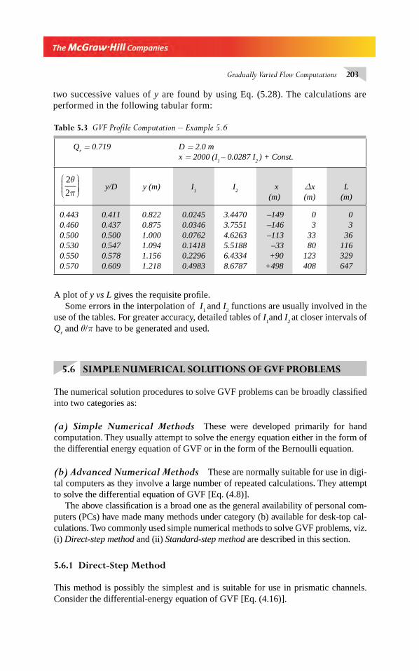
Gradually Varied Flow Computations 203
A plot of y vs L gives the requisite profi le.Some errors in the interpolation of I
1 and I
2 functions are usually involved in the
use of the tables. For greater accuracy, detailed tables of I1and I
2 at closer intervals of
Qr and θ/π have to be generated and used.
5.6 SIMPLE NUMERICAL SOLUTIONS OF GVF PROBLEMS
The numerical solution procedures to solve GVF problems can be broadly classifi ed into two categories as:
(a) Simple Numerical Methods These were developed primarily for hand computation. They usually attempt to solve the energy equation either in the form of the differential energy equation of GVF or in the form of the Bernoulli equation.
(b) Advanced Numerical Methods These are normally suitable for use in digi-tal computers as they involve a large number of repeated calculations. They attempt to solve the differential equation of GVF [Eq. (4.8)].
The above classifi cation is a broad one as the general availability of personal com-puters (PCs) have made many methods under category (b) available for desk-top cal-culations. Two commonly used simple numerical methods to solve GVF problems, viz. (i) Direct-step method and (ii) Standard-step method are described in this section.
5.6.1 Direct-Step Method
This method is possibly the simplest and is suitable for use in prismatic channels. Consider the differential-energy equation of GVF [Eq. (4.16)].
Qr = 0.719 D = 2.0 m
x = 2000 (I1 – 0.0287 I
2 ) + Const.
2
2
θπ
⎛⎝⎜⎜⎜
⎞⎠⎟⎟⎟⎟ y/D y (m) I
1I
2
x(m)
Δx(m)
L(m)
0.4430.4600.5000.5300.5500.570
0.4110.4370.5000.5470.5780.609
0.8220.8751.0001.0941.1561.218
0.02450.03460.07620.14180.22960.4983
3.44703.75514.62635.51886.43348.6787
–149 –146 –113 –33 +90+498
0 3 33 80123408
0 3 36116329647
Table 5.3 GVF Profi le Computation – Example 5.6
two successive values of y are found by using Eq. (5.28). The calculations are performed in the following tabular form:
Chapter 5.indd 203Chapter 5.indd 203 2/24/2010 2:59:20 PM2/24/2010 2:59:20 PM
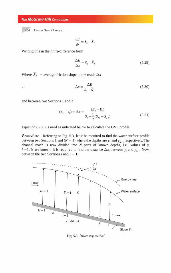
204 Flow in Open Channels
dE
dxS S f= −0
Writing this in the fi nite-difference form
ΔΔ
E
xS S f= −0 (5.29)
Where S f = average-friction slope in the reach Δx
∴ ΔΔ
xE
S S f
=−0
(5.30)
and between two Sections 1 and 2
( )
( )
( )x x x
E E
S S Sf f
2 12 1
0 1 2
1
2
− = =−
− +Δ
(5.31)
Equation (5.30) is used as indicated below to calculate the GVF profi le.
Procedure Referring to Fig. 5.3, let it be required to fi nd the water-surface profi le between two Sections 1 and (N + 1) where the depths are y
1 and y
N+1 respectively. The
channel reach is now divided into N parts of known depths, i.e., values of yi
i =1, N are known. It is required to fi nd the distance Δxi between y
i and y
i+1. Now,
between the two Sections i and i + 1,
Energy line
Water surface
Slope S0
Flow
2 1Δxi
ii + 1
NN + 1
yi
yiyi + 1yN + 1
Vi2
2g
Fig. 5.3 Direct step method
Chapter 5.indd 204Chapter 5.indd 204 2/24/2010 2:59:20 PM2/24/2010 2:59:20 PM
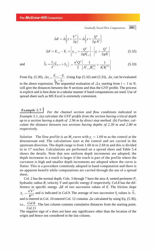
Gradually Varied Flow Computations 205
Δ Δ ΔE yV
gy
Q
g A= +
⎛
⎝⎜⎜⎜⎜
⎞
⎠⎟⎟⎟⎟
= +⎛
⎝⎜⎜⎜⎜
⎞
⎠⎟⎟⎟⎟
2 2
22 2
ΔE E E yQ
gAy
Q
gAi i i
i
i
i
= − = +⎡
⎣⎢⎢⎢
⎤
⎦⎥⎥⎥− +
⎡
⎣⎢⎢
⎤
⎦⎥⎥+ +
+1 1
2
12
2
22 2 (5.32)
and S S Sf fi fi= +( )+1
21 = +
⎡
⎣⎢⎢⎢
⎤
⎦⎥⎥⎥+ +
n Q
A R A Ri i i i
2 2
21 1
4 3 2 4 32
1 1/ /
(5.33)
From Eq. (5.30), Δ xi =
−
−+E E
S Si i
f
1
0
.Using Eqs (5.32) and (5.33), Δxi can be
evaluated
in the above expression. The sequential evaluation of Δ xi starting from i = 1 to N,
will give the distances between the N sections and thus the GVF profi le. The process is explicit and is best done in a tabular manner if hand computations are used. Use of spread sheet such as MS Excel is extremely convenient.
Example 5.7 For the channel section and fl ow conditions indicated in Example 5.1, (a) calculate the GVF profi le from the section having critical depth up to a section having a depth of 2.96 m by direct step method. (b) Further, cal-culate the distance between two sections having depths of 2.30 m and 2.80 m respectively.
Solution The flow profile is an M2 curve with y
c = 1.69 m as the control at the
downstream end. The calculations start at the control and are carried in the upstream direction. The depth range is from 1.60 m to 2.69 m and this is divided in to 17 reaches. Calculations are performed on a spread sheet and Table 5.4 shows the details. Note that non uniform depth increments are adopted; the depth increment in a reach is larger if the reach is part of the profile where the curvature is high and smaller depth increments are adopted where the curve is flatter. This is a procedure commonly adopted in hand computation and there is no apparent benefit while computations are carried through the use of a spread sheet.
Col. 2 has the normal depth. Cols. 3 through 7 have the area A, wetted perimeter P, hydraulic radius R, velocity V and specifi c energy E respectively. Col.8 has the dif-ference in specifi c energy ΔE of two successive values of E. The friction slope
Sn V
Rf =2 2
4 3 and is indicated in Col.9. The average of two successive S
f values is S f
and is entered in Col. 10.entered Col. 12 contains Δx calculated by using Eq. (5.30),
i.e., Col
Col
.
.
8
11. The last column contains cumulative distances from the starting point.
The negative sign of x does not have any signifi cance other than the location of the origin and hence not considered in the last column.
Chapter 5.indd 205Chapter 5.indd 205 2/24/2010 2:59:21 PM2/24/2010 2:59:21 PM
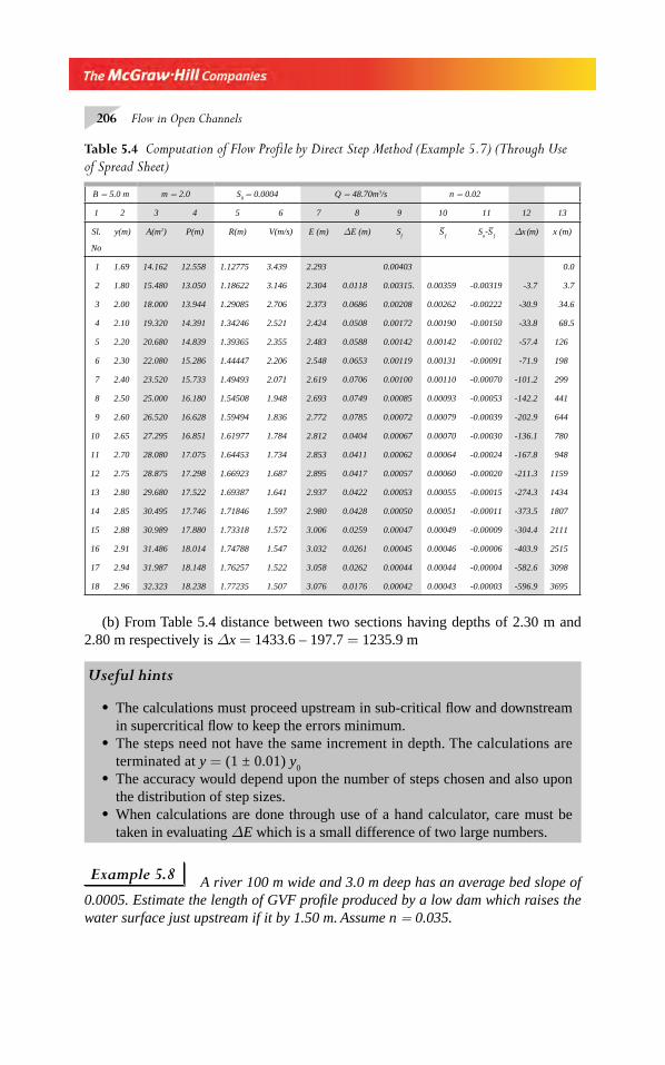
206 Flow in Open Channels
(b) From Table 5.4 distance between two sections having depths of 2.30 m and 2.80 m respectively is Δx = 1433.6 – 197.7 = 1235.9 m
Useful hints
• The calculations must proceed upstream in sub-critical fl ow and downstream in supercritical fl ow to keep the errors minimum.
• The steps need not have the same increment in depth. The calculations are terminated at y = (1 ± 0.01) y
0• The accuracy would depend upon the number of steps chosen and also upon
the distribution of step sizes.• When calculations are done through use of a hand calculator, care must be
taken in evaluating ΔE which is a small difference of two large numbers.
Example 5.8 A river 100 m wide and 3.0 m deep has an average bed slope of 0.0005. Estimate the length of GVF profi le produced by a low dam which raises the water surface just upstream if it by 1.50 m. Assume n = 0.035.
B = 5.0 m m = 2.0 S0 = 0.0004 Q = 48.70m3/s n = 0.02
1 2 3 4 5 6 7 8 9 10 11 12 13
Sl.
No
y(m) A(m2) P(m) R(m) V(m/s) E (m) ΔE (m) Sf
S–
fS
o-S–
fΔx (m) x (m)
1 1.69 14.162 12.558 1.12775 3.439 2.293 0.00403 0.0
2 1.80 15.480 13.050 1.18622 3.146 2.304 0.0118 0.00315. 0.00359 -0.00319 -3.7 3.7
3 2.00 18.000 13.944 1.29085 2.706 2.373 0.0686 0.00208 0.00262 -0.00222 -30.9 34.6
4 2.10 19.320 14.391 1.34246 2.521 2.424 0.0508 0.00172 0.00190 -0.00150 -33.8 68.5
5 2.20 20.680 14.839 1.39365 2.355 2.483 0.0588 0.00142 0.00142 -0.00102 -57.4 126
6 2.30 22.080 15.286 1.44447 2.206 2.548 0.0653 0.00119 0.00131 -0.00091 -71.9 198
7 2.40 23.520 15.733 1.49493 2.071 2.619 0.0706 0.00100 0.00110 -0.00070 -101.2 299
8 2.50 25.000 16.180 1.54508 1.948 2.693 0.0749 0.00085 0.00093 -0.00053 -142.2 441
9 2.60 26.520 16.628 1.59494 1.836 2.772 0.0785 0.00072 0.00079 -0.00039 -202.9 644
10 2.65 27.295 16.851 1.61977 1.784 2.812 0.0404 0.00067 0.00070 -0.00030 -136.1 780
11 2.70 28.080 17.075 1.64453 1.734 2.853 0.0411 0.00062 0.00064 -0.00024 -167.8 948
12 2.75 28.875 17.298 1.66923 1.687 2.895 0.0417 0.00057 0.00060 -0.00020 -211.3 1159
13 2.80 29.680 17.522 1.69387 1.641 2.937 0.0422 0.00053 0.00055 -0.00015 -274.3 1434
14 2.85 30.495 17.746 1.71846 1.597 2.980 0.0428 0.00050 0.00051 -0.00011 -373.5 1807
15 2.88 30.989 17.880 1.73318 1.572 3.006 0.0259 0.00047 0.00049 -0.00009 -304.4 2111
16 2.91 31.486 18.014 1.74788 1.547 3.032 0.0261 0.00045 0.00046 -0.00006 -403.9 2515
17 2.94 31.987 18.148 1.76257 1.522 3.058 0.0262 0.00044 0.00044 -0.00004 -582.6 3098
18 2.96 32.323 18.238 1.77235 1.507 3.076 0.0176 0.00042 0.00043 -0.00003 -596.9 3695
Table 5.4 Computation of Flow Profi le by Direct Step Method (Example 5.7) (Through Use
of Spread Sheet)
Chapter 5.indd 206Chapter 5.indd 206 2/24/2010 2:59:21 PM2/24/2010 2:59:21 PM
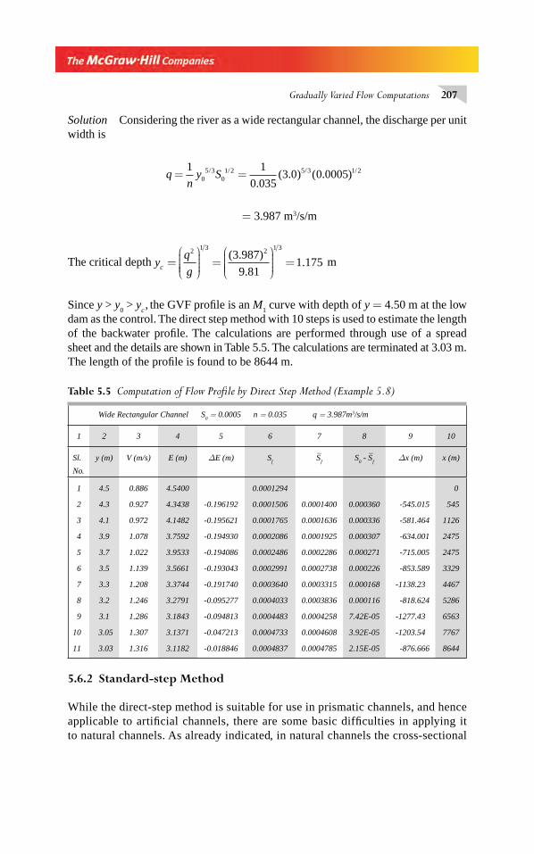
Gradually Varied Flow Computations 207
Wide Rectangular Channel S0 = 0.0005 n = 0.035 q = 3.987m3/s/m
1 2 3 4 5 6 7 8 9 10
Sl.
No.
y (m) V (m/s) E (m) ΔE (m) Sf
S–
fS
0 - S
–f
Δx (m) x (m)
1 4.5 0.886 4.5400 0.0001294 0
2 4.3 0.927 4.3438 -0.196192 0.0001506 0.0001400 0.000360 -545.015 545
3 4.1 0.972 4.1482 -0.195621 0.0001765 0.0001636 0.000336 -581.464 1126
4 3.9 1.078 3.7592 -0.194930 0.0002086 0.0001925 0.000307 -634.001 2475
5 3.7 1.022 3.9533 -0.194086 0.0002486 0.0002286 0.000271 -715.005 2475
6 3.5 1.139 3.5661 -0.193043 0.0002991 0.0002738 0.000226 -853.589 3329
7 3.3 1.208 3.3744 -0.191740 0.0003640 0.0003315 0.000168 -1138.23 4467
8 3.2 1.246 3.2791 -0.095277 0.0004033 0.0003836 0.000116 -818.624 5286
9 3.1 1.286 3.1843 -0.094813 0.0004483 0.0004258 7.42E-05 -1277.43 6563
10 3.05 1.307 3.1371 -0.047213 0.0004733 0.0004608 3.92E-05 -1203.54 7767
11 3.03 1.316 3.1182 -0.018846 0.0004837 0.0004785 2.15E-05 -876.666 8644
Table 5.5 Computation of Flow Profi le by Direct Step Method (Example 5.8)
Solution Considering the river as a wide rectangular channel, the discharge per unit width is
q
ny S= =
1 1
0 0353 0 0 00050
5 301 2 5 3 1 2/ / / /
.( . ) ( . )
= 3.987 m3/s/m
The critical depth yq
gc =⎛
⎝⎜⎜⎜⎜
⎞
⎠⎟⎟⎟⎟
=⎛
⎝⎜⎜⎜⎜
⎞
⎠⎟⎟⎟⎟
=2 1 3 2 1 3
3 987
9 811 175
( . )
.. m
Since y > y0 > y
c , the GVF profi le is an M
1 curve with depth of y = 4.50 m at the low
dam as the control. The direct step method with 10 steps is used to estimate the length of the backwater profi le. The calculations are performed through use of a spread sheet and the details are shown in Table 5.5. The calculations are terminated at 3.03 m. The length of the profi le is found to be 8644 m.
5.6.2 Standard-step Method
While the direct-step method is suitable for use in prismatic channels, and hence applicable to artifi cial channels, there are some basic diffi culties in applying it to natural channels. As already indicated, in natural channels the cross-sectional
Chapter 5.indd 207Chapter 5.indd 207 2/24/2010 2:59:21 PM2/24/2010 2:59:21 PM
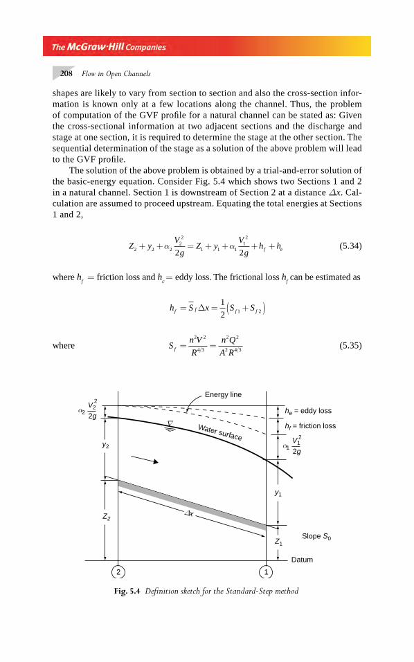
208 Flow in Open Channels
shapes are likely to vary from section to section and also the cross-section infor-mation is known only at a few locations along the channel. Thus, the problem of computation of the GVF profi le for a natural channel can be stated as: Given the cross-sectional information at two adjacent sections and the discharge and stage at one section, it is required to determine the stage at the other section. The sequential determination of the stage as a solution of the above problem will lead to the GVF profi le.
The solution of the above problem is obtained by a trial-and-error solution of the basic-energy equation. Consider Fig. 5.4 which shows two Sections 1 and 2 in a natural channel. Section 1 is downstream of Section 2 at a distance Δx. Cal-culation are assumed to proceed upstream. Equating the total energies at Sections 1 and 2,
Z yV
gZ y
V
gh hf e2 2 2
22
1 1 112
2 2+ + = + + + +α α (5.34)
where hf = friction loss and h
c = eddy loss. The frictional loss h
f can be estimated as
h S x S Sf f f f= = +( )Δ
1
2 1 2
where Sn V
R
n Q
A Rf = =2 2
4 3
2 2
2 4 3 (5.35)
2 1
Energy line
Water surface
he = eddy loss
hf = friction loss
Slope S0
y1
Z1
Datum
Z2
y2
α2V2
2
2g
α1V1
2
2g
Δx
∇
Fig. 5.4 Defi nition sketch for the Standard-Step method
Chapter 5.indd 208Chapter 5.indd 208 2/24/2010 2:59:21 PM2/24/2010 2:59:21 PM
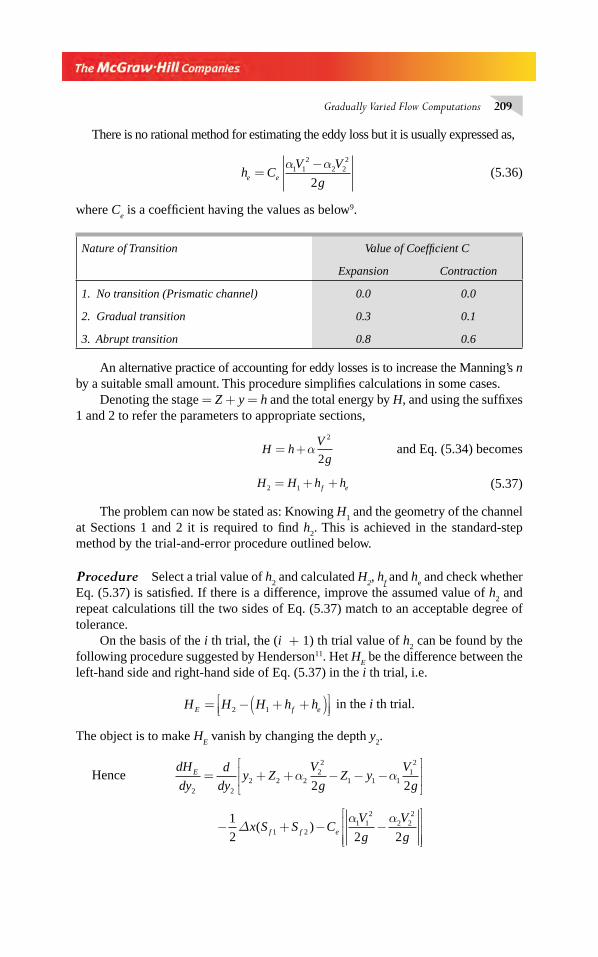
Gradually Varied Flow Computations 209
There is no rational method for estimating the eddy loss but it is usually expressed as,
h CV V
ge e=−α α1 1
22 2
2
2 (5.36)
where Ce is a coeffi cient having the values as below9.
Nature of Transition Value of Coeffi cient C
Expansion Contraction
1. No transition (Prismatic channel) 0.0 0.0
2. Gradual transition 0.3 0.1
3. Abrupt transition 0.8 0.6
An alternative practice of accounting for eddy losses is to increase the Manning’s n by a suitable small amount. This procedure simplifi es calculations in some cases.
Denoting the stage = Z + y = h and the total energy by H, and using the suffi xes 1 and 2 to refer the parameters to appropriate sections,
H hV
g= +α
2
2 and Eq. (5.34) becomes
H H h hf e2 1= + + (5.37)
The problem can now be stated as: Knowing H1 and the geometry of the channel
at Sections 1 and 2 it is required to fi nd h2. This is achieved in the standard-step
method by the trial-and-error procedure outlined below.
Procedure Select a trial value of h2 and calculated H
2, h
f and h
e and check whether
Eq. (5.37) is satisfi ed. If there is a difference, improve the assumed value of h2 and
repeat calculations till the two sides of Eq. (5.37) match to an acceptable degree of tolerance.
On the basis of the i th trial, the (i + 1) th trial value of h2 can be found by the
following procedure suggested by Henderson11. Het HE be the difference between the
left-hand side and right-hand side of Eq. (5.37) in the i th trial, i.e.
H H H h hE f e= − + +( )⎡⎣⎢
⎤⎦⎥2 1 in the i th trial.
The object is to make HE vanish by changing the depth y
2.
Hence dH
dy
d
dyy Z
V
gZ y
V
gE
2 22 2 2
22
1 1 112
2 2= + + − − −
⎡
⎣⎢⎢
⎤
⎦⎥⎥α α
− + − −⎡
⎣⎢⎢⎢
⎤
⎦⎥⎥⎥
1
2 2 21 21 1
22 2
2
Δx S S CV
g
V
gf f e( )α α
Chapter 5.indd 209Chapter 5.indd 209 2/24/2010 2:59:21 PM2/24/2010 2:59:21 PM
210 Flow in Open Channels
Since y1, Z
1, Z
2 and V
1 are constants,
dH
dy
d
dyy C
V
gx SE
e f
2 22
2 22
212
1
2= + + −
⎡
⎣⎢⎢
⎤
⎦⎥⎥( )
αΔ
= − + −1 11
222 2
2
( ) .C F xdS
dye
fΔ (5.38)
Where FQ T
gA22 2
22
23
=α
For a wide rectangular channel,
dS
dy
d
dy
n q
yS yf
f=⎛
⎝⎜⎜⎜⎜
⎞
⎠⎟⎟⎟⎟
=2 2
10 33 33.
Hence dS
dy
S
y
S
Rf f f2
2
2
2
2
2
3 33 3 33� − = −
. . , leading to
dH
dyC F
S x
RE
e
f
222 2
2
1 11 67
= − − +⎡
⎣⎢⎢
⎤
⎦⎥⎥( )
. .Δ
If dH
dy
H
dyE E
2 2
=Δ and Δ y
2 is chosen such that ΔH HE E= ’
ΔΔ
y H C FS x
RE ef
2 22 2
2
1 11 67
= − − + +⎡
⎣⎢⎢
⎤
⎦⎥⎥( )
. (5.39)
The negative sign denotes that Δ y2 is of opposite sign to that of H
E. It may be
noted that if the calculations are performed in the downward direction, as in super-critical fl ow, the third term in the denominator will be negative. The procedure is illustrated in the following example. Spread sheets, such as MS Excel, are extremely convenient to calculate GVF profi le through the use of the standard step method.
Example 5.9 A small stream has a cross section which can be approximated by a trapezoid. The cross-sectional properties at three sections are as follows:
Section Distance up the River (km)
Bed Elevation (m) Bed Width (m) Side Slope
A 100.00 100.000 14.0 1.5 :1
B 102.00 100.800 12.5 1.5 :1
C 103.50 101.400 10.0 1.5 :1
Chapter 5.indd 210Chapter 5.indd 210 2/24/2010 2:59:22 PM2/24/2010 2:59:22 PM
Gradually Varied Flow Computations 211
Section A is the downstream-most section. For a discharge of 100.0 m3/s in the stream, water surface elevation at A was 104.500 m. Estimate the water-surface eleva-tion at the upstream Sections B and C. Assume n = 0.02 and α = 1.0 at all sections.
Solution The calculations are performed in Table 5.6. In thisTotal head H (Column 7) = Column 4 + Column 6h
f (Column 12) = S
f
– × L =(Column 10) × (Column 11)
he = C
v
gCe eΔ
2
20
⎡
⎣⎢⎢
⎤
⎦⎥⎥ =with for expansion.
The first row in the table is based on known information. The second row is based on an assumed stage of 105. 200 m (i.e. a depth of 4.400 m) at Section B. Column 14 is obtained as {(Column 7 of previous section) + (Column 12 + Column 13) of the present section}. It represnts the right-hand side of the Eq. (5.35), while column 7 represents the left-hand side of the same equation. It is seen that the first trial is not successful as Column 7 ≠ Column 14. For this trial, H
E =105.272 – 104.797 =0.475 m. Substituting in Eq. (5.39) with C
e = 0.3,
Fv
gyS xf≈ ≈
×= = × =−2 0 072
4 400 0327 1 3308 10 20002
22
2 24.
.. , . , Δ m, R
2 = 2.963, leads
to Δy2 = – 0.429 m.
The next trial stage is therefore taken as = 105.200 − 0.429 =104.771 m, with a depth of fl ow of 3.971 m.
It may, be seen from the third row in Table 5.6 that in the second trial of the stage B = 104.771 m, Column 7 and Column 14 agree. It is usual to score out the unsuc-cessful trials after a better one has been obtained to avoid confusion.
The procedure is repeated for Section C, by applying the energy equation bet-ween Sections B and C. In the fi rst trial for C, H
E = – 0.293 m. The correction Δy
2 by
Eq. (5.39) is + 0.244 m. It may be seen that two trials are needed in this section to get the correct water-surface elevation.
5.6.3 Standard-step Method for Compound Sections
A majority of natural channels are compound channels (Fig. 5.5). Since the fl ow in fl oodbanks (areas 2 and 3 in Fig. 5.5) is normally at a lower velocity than in the main channel, the energy lines corresponding to various sub-areas will be at different elevations above the water surface. A convenient method of handling this situation is to consider a mean velocity V
– for the entire section and to assume the energy line
to be at a height αV
g
2
2above the water surface. Also, a common friction slope S
f is
assumed.The kinetic-energy correction factor α for the whole section is obtained as
below:
Chapter 5.indd 211Chapter 5.indd 211 2/24/2010 2:59:22 PM2/24/2010 2:59:22 PM
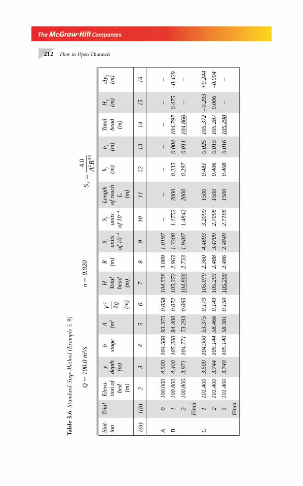
212 Flow in Open Channels
Q =
100
.0 m
3 /s
n =
0.0
20S
AR
f=
40
24
3
.
Stat
-io
nTr
ial
Ele
va-
tion
of
bed
(m
)
yde
pth
(m)
hst
age
A (m2
V
g2
2 (m)
HTo
tal
head
(m)
R (m)
S f
unit
sof
10−
4
S f
unit
sof
10−
4
Len
gth
of r
each
L
. (
m)
h f
(m)
h e
(m)
Tota
lhe
ad(m
)
HE
(m)
Δy 2
(m)
1(a)
1(b)
23
45
67
89
1011
1213
1415
16
A0
100.
000
4.50
010
4.50
093
.375
0.05
810
4.55
83.
089
1.01
97−
−−
−−
−−
B1
100.
800
4.40
010
5.20
084
.400
0.07
210
5.27
22.
963
1.33
08 1
.175
220
000.
235
0.00
410
4.79
70.
475
–0.4
29
210
0.80
03.
971
104.
771
73.2
930.
095
104.
866
2.73
31.
9487
1.4
842
2000
0.29
70.
011
104.
866
−−
Fin
al
C1
101.
400
3.50
010
4.90
053
.375
0.17
910
5.07
92.
360
4.46
93 3
.209
015
000.
481
0.02
510
5.37
2–
0.29
3+
0.24
4
210
1.40
03.
744
105.
144
58.4
660.
149
105.
293
2.48
83.
4709
2.7
098
1500
0.40
60.
015
105.
287
0.00
6–0
.004
310
1.40
03.
740
105.
140
58.3
810.
150
105.
290
2.48
62.
4849
2.7
168
1500
0.40
80.
016
105.
290
−−
Fin
al
Tabl
e 5.
6 St
anda
rd-S
tep-
Met
hod
(Exa
mpl
e 5
.9)
Chapter 5.indd 212Chapter 5.indd 212 2/24/2010 2:59:22 PM2/24/2010 2:59:22 PM
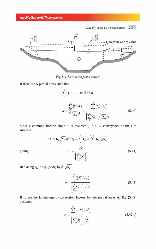
Gradually Varied Flow Computations 213
If there are N partial areas such that
A Ai
N
1∑ = = total area,
α =( )
=( )
⎛
⎝⎜⎜⎜⎜
⎞
⎠⎟⎟⎟⎟ ( )
∑∑
∑
∑ ∑
V A
V A
Q A
Q A
i
N
i
i i
N
i
N
i
13
13
3 2
1
1
32
(5.40)
Since a common friction slope Sf is assumed , if K
i = conveyance of the i th
sub-area
Q K Si i f= and Q Q K Sii
N
ii
N
f= =⎛
⎝⎜⎜⎜⎜
⎞
⎠⎟⎟⎟⎟∑ ∑
giving SQ
K
f
ii
N=
⎛
⎝⎜⎜⎜⎜
⎞
⎠⎟⎟⎟⎟∑
2
2 (5.41)
Replacing Qi in Eq. (5.40) by K Si f ,
α =
( )⎛
⎝⎜⎜⎜⎜
⎞
⎠⎟⎟⎟⎟
∑
∑
K A
K A
i i
N
i
N
3 2
1
1
3
2
(5.42)
If αi are the kinetic-energy correction factors for the partial areas A
i, Eq. (5.42)
becomes
αα
=( )
⎛
⎝⎜⎜⎜⎜
⎞
⎠⎟⎟⎟⎟
∑
∑
i i i
N
i
N
K A
K A
3 2
1
1
3
2
(5.42-a)
α2V2/2g
Common energy l ine
α1V1
2
2
2gα3
V32
2g2gV 2
α
1
32
Δ
Fig. 5.5 Flow in compound sections
Chapter 5.indd 213Chapter 5.indd 213 2/24/2010 2:59:22 PM2/24/2010 2:59:22 PM
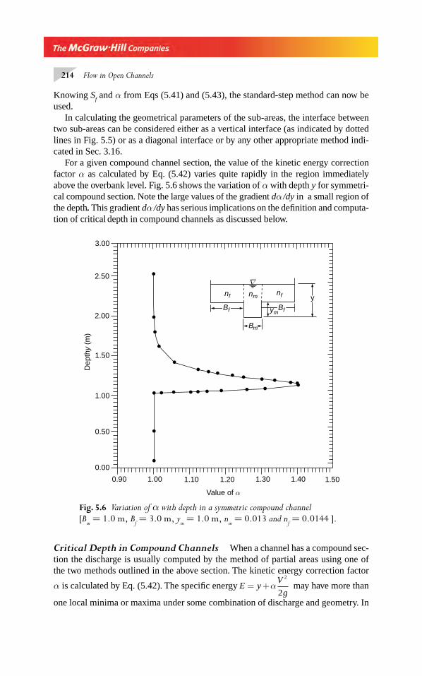
214 Flow in Open Channels
Knowing Sf and α from Eqs (5.41) and (5.43), the standard-step method can now be
used.In calculating the geometrical parameters of the sub-areas, the interface between
two sub-areas can be considered either as a vertical interface (as indicated by dotted lines in Fig. 5.5) or as a diagonal interface or by any other appropriate method indi-cated in Sec. 3.16.
For a given compound channel section, the value of the kinetic energy correction factor α as calculated by Eq. (5.42) varies quite rapidly in the region immediately above the overbank level. Fig. 5.6 shows the variation of α with depth y for symmetri-cal compound section. Note the large values of the gradient dα /dy in a small region of the depth. This gradient dα /dy has serious implications on the defi nition and computa-tion of critical
depth in compound channels as discussed below.
nfnf nm
ymBf
Bm
Bf
y
3.00
2.50
2.00
1.50
1.00
0.50
0.00
0.90 1.00 1.10 1.20 1.30 1.40 1.50
Dep
thy
(m)
Value of α
Δ
Fig. 5.6 Variation of α with depth in a symmetric compound channel
[Bm = 1.0 m, B
f = 3.0 m, y
m = 1.0 m, n
m = 0.013 and n
f = 0.0144 ].
Critical Depth in Compound Channels When a channel has a compound sec-tion the discharge is usually computed by the method of partial areas using one of the two methods outlined in the above section. The kinetic energy correction factor
α is calculated by Eq. (5.42). The specifi c energy E yV
g= +α
2
2 may have more than
one local minima or maxima under some combination of discharge and geometry. In
Chapter 5.indd 214Chapter 5.indd 214 2/24/2010 2:59:23 PM2/24/2010 2:59:23 PM
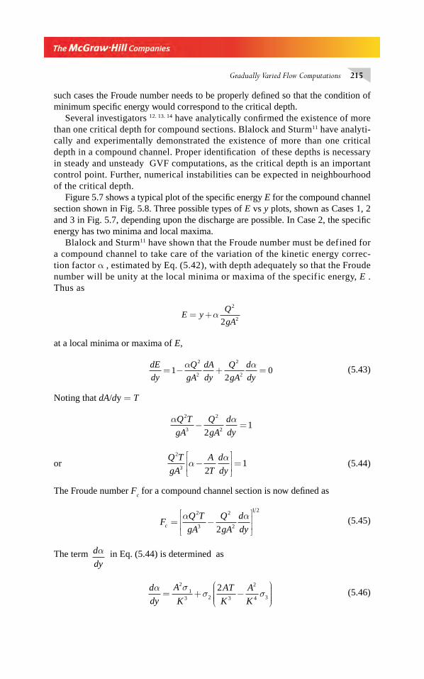
Gradually Varied Flow Computations 215
such cases the Froude number needs to be properly defi ned so that the condition of minimum specifi c energy would correspond to the critical depth.
Several investigators 12. 13. 14 have analytically confi rmed the existence of more than one critical depth for compound sections. Blalock and Sturm11 have analyti-cally and experimentally demonstrated the existence of more than one critical depth in a compound channel. Proper identifi cation of these depths is necessary in steady and unsteady GVF computations, as the critical depth is an important control point. Further, numerical instabilities can be expected in neighbourhood of the critical depth.
Figure 5.7 shows a typical plot of the specifi c energy E for the compound channel section shown in Fig. 5.8. Three possible types of E vs y plots, shown as Cases 1, 2 and 3 in Fig. 5.7, depending upon the discharge are possible. In Case 2, the specifi c energy has two minima and local maxima.
Blalock and Sturm11 have shown that the Froude number must be defined for a compound channel to take care of the variation of the kinetic energy correc-tion factor α , estimated by Eq. (5.42), with depth adequately so that the Froude number will be unity at the local minima or maxima of the specific energy, E . Thus as
E yQ
gA= +α
2
22
at a local minima or maxima of E,
dE
dy
Q
gA
dA
dy
Q
gA
d
dy= − + =1
20
2
2
2
2
α α
(5.43)
Noting that dA/dy = T
α αQ T
gA
Q
gA
d
dy
2
3
2
221− =
or Q T
gA
A
T
d
dy
2
3 21α
α−
⎡
⎣⎢⎢
⎤
⎦⎥⎥ = (5.44)
The Froude number Fc for a compound channel section is now defi ned as
FQ T
gA
Q
gA
d
dyc = −⎡
⎣⎢⎢
⎤
⎦⎥⎥
α α2
3
2
2
1 2
2 (5.45)
The term d
dy
α in Eq. (5.44) is determined as
d
dy
A
K
AT
K
A
K
α σσ σ= + −
⎛
⎝⎜⎜⎜⎜
⎞
⎠⎟⎟⎟⎟
21
3 2 3
2
4 3
2 (5.46)
Chapter 5.indd 215Chapter 5.indd 215 2/24/2010 2:59:23 PM2/24/2010 2:59:23 PM
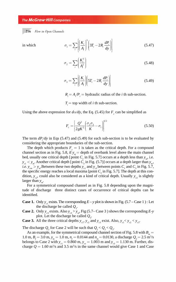
216 Flow in Open Channels
in which σ1
3
3 2=⎛
⎝⎜⎜⎜⎜
⎞
⎠⎟⎟⎟⎟
−⎛
⎝⎜⎜⎜⎜
⎞
⎠⎟⎟⎟⎟
⎡
⎣
⎢⎢⎢
⎤
⎦
⎥⎥⎥
∑K
AT R
dP
dyi
i
i ii
i
(5.47)
σ2
3
2=
⎛
⎝⎜⎜⎜⎜
⎞
⎠⎟⎟⎟⎟∑
K
Ai
ii
(5.48)
σ3 5 2=⎛
⎝⎜⎜⎜⎜
⎞
⎠⎟⎟⎟⎟
−⎛
⎝⎜⎜⎜⎜
⎞
⎠⎟⎟⎟⎟
⎡
⎣⎢⎢⎢
⎤
⎦⎥⎥⎥
∑K
AT R
dP
dyi
i
i ii
i
(5.49)
Ri = A
i /P
i = hydraulic radius of the i th sub-section.
Ti = top width of i th sub-section.
Using the above expression for dα/dy, the Eq. (5.45) for Fc can be simplifi ed as
FQ
gK Kc = −⎛
⎝⎜⎜⎜
⎞
⎠⎟⎟⎟⎟
⎡
⎣⎢⎢
⎤
⎦⎥⎥
2
32 3
1
1 2
2
σ σσ (5.50)
The term dPi /dy in Eqs (5.47) and (5.49) for each sub-section is to be evaluated by
considering the appropriate boundaries of the sub-section. The depth which products F
c = 1 is taken as the critical depth. For a compound
channel section as in Fig. 5.8, if ym
= depth of overbank level above the main channel bed, usually one critical depth [ point C
1 in Fig. 5.7] occurs at a depth less than y
m, i.e.
yc1
< ym. Another critical depth [ point C
3 in Fig. (5.7)] occurs at a depth larger than y
m ,
i.e. ycm
> ym.Between these two depths y
c1 and y
c3 between points C
1 and C
3 in Fig. 5.7,
the specifi c energy reaches a local maxima [point C2 in Fig. 5.7]. The depth at this con-
dition, yc2
, could also be considered as a kind of critical depth. Usually yc2
is slightly larger than y
m.
For a symmetrical compound channel as in Fig. 5.8 depending upon the magni-tude of discharge three distinct cases of occurrence of critical depths can be identifi ed.
Case 1. Only yc1
exists. The corresponding E – y plot is shown in Fig. (5.7 – Case 1 ) : Let the discharge be called Q
1.
Case 2. Only yc3
exists. Also yc3
> ym, Fig (5.7– Case 3 ) shows the corresponding E-y
plot. Let the discharge be called Q3.
Case 3. All the three critical depths yc1
, yc2
and yc3
exist. Also, yc1
< yc2
< yc3
.
The discharge Q2 for Case 2 will be such that Q
1 < Q
2 < Q
3.
As an example, for the symmetrical compound channel section of Fig. 5.8 with Bm =
1.0 m, Bf = 3.0 m, y
m = 1.0 m, n
f = 0.0144 and n
m = 0.0130, a discharge Q
2 = 2.5 m3/s
belongs to Case 2 with yc1
= 0.860 m, ycz = 1.003 m and y
c3 = 1.130 m. Further, dis-
charge Q = 1.60 m3/s and 3.5 m3/s in the same channel would give Case 1 and Case
Chapter 5.indd 216Chapter 5.indd 216 2/24/2010 2:59:23 PM2/24/2010 2:59:23 PM
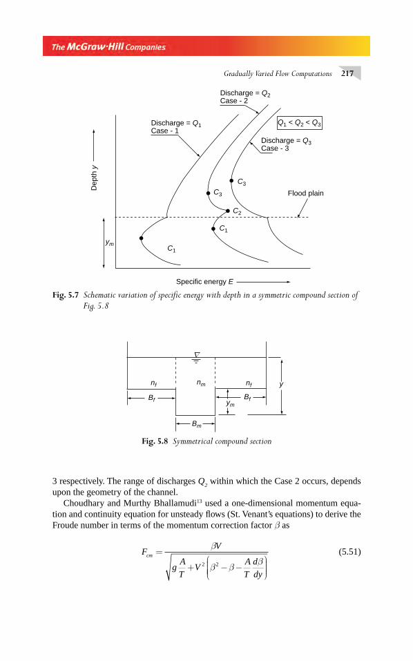
Gradually Varied Flow Computations 217
3 respectively. The range of discharges Q2 within which the Case 2 occurs, depends
upon the geometry of the channel. Choudhary and Murthy Bhallamudi13 used a one-dimensional momentum equa-
tion and continuity equation for unsteady fl ows (St. Venant’s equations) to derive the Froude number in terms of the momentum correction factor β as
FV
gA
TV
A
T
d
dy
cm =
+ − −⎛
⎝⎜⎜⎜⎜
⎞
⎠⎟⎟⎟⎟
β
β ββ2 2
(5.51)
Discharge = Q2Case - 2
Discharge = Q3Case - 3
Discharge = Q1Case - 1
Flood plain
Specific energy E
ym
Dep
th y
Q1 < Q2 < Q3
C1
C1
C2
C3
C3
Fig. 5.7 Schematic variation of specifi c energy with depth in a symmetric compound section of
Fig. 5.8
Fig. 5.8 Symmetrical compound section
y
Bf
nf
ym
nm
Bm
Bf
nf
Δ
Chapter 5.indd 217Chapter 5.indd 217 2/24/2010 2:59:23 PM2/24/2010 2:59:23 PM
218 Flow in Open Channels
The condition at critical fl ow is obtained by putting Fcm
= 1 as
g
Q
T Ad
dy
A2 3=
−⎧
⎨
⎪⎪⎪⎪⎪
⎩
⎪⎪⎪⎪⎪
⎫
⎬
⎪⎪⎪⎪⎪
⎭
⎪⎪⎪⎪⎪
ββ
(5.52)
where β =( )∑ K A
K A
i ii
2
2
/
/ (5.53)
It appears that for GVF fl ows in compound channel sections Eq. 5.50 which uses the specifi c energy criteria and for unsteady fl ows Eq. 5.52 which is based on the momentum criteria are appropriate choices for the defi nition of Froude number and hence in the calculation of the critical depths. Usually, the values of the critical depths calculated by using the two methods do not differ appreciably.
It should be noted that the existence of multiple critical depths would be noticed only when the compound section is considered to be made up of sub-areas and the total discharge is calculated as the sum of the partial area discharges. If the com-pound section is treated as one whole unit for discharge calculation the occurrence of multiple critical depths does not arise.
5.6.4 Backwater Curves in Natural channels
Methodology Computation of Backwater curves due to construction of dams, bar-rages and weirs across natural channels is one of the basic procedures in the planning and design of these structures. The basic issues are to know the extent of fl ooding, areal as well as length of the reach affected by the construction of the structure. For large dams the computations are done for various fl ood frequencies such as 25, 50, 100, 1000 years and for PMF. In addition to computation of the GVF profi le, the sedimentation aspects of the dam and river complex for various time horizons are also computed. The GVF profi les are computed for pre-dam and post dam scenarios. In the post dam situation GVF without siltation and with siltation are estimated.
The basic methodology used is the Standard – Step method. The computations are carried out using well tried out softwares like HEC-RAS and MIKE 21. HEC-RAS has been developed by US Army Corps of Engineers and replaces the widely used HEC-2 of the same organization. HEC-RAS has been developed to perform one dimensional hydraulic analysis for natural as well as man-made channel networks. It is a very versatile program capable of handling very large varieties of water surface computation problems in rigid bed as well as in mobile bed environment. HEC-RAS is available along with user’s manual (http:// www.hec.usace.army.mill/software/ hec-1) for download by individuals free of charge. MIKE-11 is a commercial software of the company DHI and is an industry standard for simulating fl ow and water levels, water quality and sediment transport in rivers, fl ood plains, irrigation canals, reser-voirs and other inland water bodies. Details of MIKE-11 are available in the web site (http://www.dhigroup.com/Software/WaterResources/MIKE11.aspx).
Chapter 5.indd 218Chapter 5.indd 218 2/24/2010 2:59:24 PM2/24/2010 2:59:24 PM
Gradually Varied Flow Computations 219
Basic Assumptions of GVF Computations Before embarking on the compu-tations of GVF profi les of a natural channel, it is advisable to recollect the basic assumptions involved in the computation procedure and to ensure that the fi eld data used in the computations do not violate these constraints: The basic assumptions of the standard step method are:
1. Steady fl ow 2. Gradually varied water surface (Hydrostatic pressure distribution)3. One-dimensional analysis4. Small channel slope5. Rigid boundary6. Constant (averaged) friction slope between adjacent sections
Basic Data requirement
( i ) Complete cross-sectional properties at the cross sections under study includ-ing the stage discharge information at the sections. The number of sections and intervals between the sections depend upon the site conditions and the purpose of the study. Concurrent water surface elevations (and hence dis-charges) at a set of stations at various discharges (preferably at high fl ows) are necessary for calibration and validation of the model.
(ii) Various discharges selected for the study, viz., 5-year fl ood, 25-year fl ood, 100-year fl ood and PMF etc. obtained by appropriate hydrologic studies.
(iii) Channel roughness coeffi cient: These haves to be carefully selected on the basis of fi eld survey, study of the photographs and all other relevant details. It has been found that smaller the value of Manning’s n the longer will be the profi le and vice verse3. Hence the smallest possible n value should be selected when the longest length of backwater curve, as in the case of submergence studies related to construction of reservoirs, is needed.
(iv) (a ) The accuracy of computations, especially in standard-step method, will have to be pre-decided. HEC-RAS adopts an accuracy of 0.003 m for the elevation as default
(b) The termination depth of the computations: Since the GVF profi les approach the normal depth asymptotically, the estimation of the backwater curve will have to be terminated at a fi nite depth to achieve meaningful accuracy. This is usually done up to a depth 1% excess/short of the normal depth, depending upon the nature of the profi le. Thus M
1 curves are
assumed to stop at a depth of 1.01 times normal depth and M2 curves are
assumed to start from a depth of 0.99 times normal depth. In studies related to backwater effect of a dam, the place where the incremental rise in water surface begins to cause damage is defi ned as the end-point of a backwater curve3. For practical purposes, this end point is taken as the termination depth referred above, namely 1.01 times the normal depth.
Procedure
(i) Division of Sub-sections The cross-sectional data has to be analyzed to establish the method of analysis, i.e., whether single channel method or divided channel
Chapter 5.indd 219Chapter 5.indd 219 2/24/2010 2:59:24 PM2/24/2010 2:59:24 PM
220 Flow in Open Channels
method (DCM) of analysis is to be adopted. Compound sections are very common in natural rivers. HEC-RAS adopts the DCM with vertical sections to accommo-date the fl ood plain effect. The composite roughness is calculated by Horton’s method. The following procedure is adopted by HEC-RAS to identify regions for adopting composite roughness and divided channel sections:
(a) Normally, the main channel is not sub divided, except when there is a perceptible change in the roughness coeffi cient along the perimeter of the main channel
(b) If the main channel portion side slopes are steeper than 5H:1V and the main channel has more than one n-value, a composite roughness n
c (calculated by
Horton’s method) is adopted for the main channel. Otherwise, for fl at side slope cases the main channel also has to be sub-divided appropriately
(c) The composite roughness is calculated separately for the left and right fl ood banks.
(ii) Calibration and Validation When all the necessary data for the computation of backwater curves in a natural channel has been assembled, the controls identifi ed and the software to be adopted is selected and other details fi nalised, the next step is to do the calibration of the model.
Model calibration and validation provides an assessment of the model’s ability to accurately reproduce known results. Calibration is performed by running the model at the high fl ow rate with the estimated n-values. A set of stations where con-current water surface elevations (and hence discharges) are known are selected. Water surface elevations at these sections are computed for a given set of data. The computed water surface profi le covering this set of stations is compared to the mea-sured profi le and optimization parameters P and D are determined; where
P E Ei cii N= −( )( )=∑ 2
1
1 2
,
/ (5.54)
and
DE E
Ni ci
i N
=−⎛
⎝⎜⎜⎜⎜
⎞
⎠⎟⎟⎟⎟=
∑( )
,
/2 1 2
1
(5.55)
in which E is the measured water surface elevation, Ec is the computed water
surface elevation at each cross-section i and N is the total number of sections. It may be noted that D represents the root mean square of the deviation of the water surface and provides a measure of the accuracy of the model.
The standard calibration procedure is to adjust the value of roughness factor n such that P and D are minimized. The program is then reproducing the known results to its best capability and can be expected to reproduce the other ranges also to the same degree of accuracy. Before application to the data points of the problem, the calibrated program (with calibrated values of n) is run on another set of data with known concurrent water surface elevations to verify that the program would indeed
Chapter 5.indd 220Chapter 5.indd 220 2/24/2010 2:59:24 PM2/24/2010 2:59:24 PM
Gradually Varied Flow Computations 221
reproduce known results within acceptable degree of error. The data used in the veri-fi cation stage should be different from the data set used in calibration stage.
The model is now ready for the computation of the desired GVF profi les.
5.7 ADVANCED NUMERICAL METHODS
The basic differential equation of GVF [Eq. (4.8)] can be expressed as
dy
dxF y= ( ) (5.56)
in which F yS S
Q T gA
f( ) =−
−( )0
2 31 and is a function of y only for a given S
0, n, Q and
channel geometry. Equation 5.56 is non-linear and a class of methods which is par-ticularly suitable for numerical solution of the above equation is the Runge–Kutta method. There are different types of Runge–Kutta methods and all of them evaluate y at (x + Δ x) given y at x. Using the notation y
i = y(x
i ) and x
i + Δ x = x
i+1 and hence
yi +
1 = y(x
i + 1 ), the various numerical methods for the solution of Eq. 5.56 are as
follows:
(a) Standard Fourth Order Runge–Kutta Methods (SRK)
y y K K K Ki i+ = + + + +1 1 2 3 4
1
62 2( ) (5.57)
where K1 = Δ x F ( y
i )
K x F yK
i21
2= +
⎛
⎝⎜⎜⎜
⎞
⎠⎟⎟⎟⎟Δ
K x F yK
i32
2= +
⎛
⎝⎜⎜⎜
⎞
⎠⎟⎟⎟⎟Δ
K x F y Ki4 3= +( )Δ
(b) Kutta–Merson Method (KM)15
y y K K Ki i+ = + + +1 1 4 5
1
24( ) (5.58)
where K x F yi1
1
3= Δ ( )
K x F y Ki2 1
1
3= +Δ ( )
K x F yK K
i31 21
3 2 2= + +
⎛
⎝⎜⎜⎜
⎞
⎠⎟⎟⎟⎟Δ
Chapter 5.indd 221Chapter 5.indd 221 2/24/2010 2:59:24 PM2/24/2010 2:59:24 PM
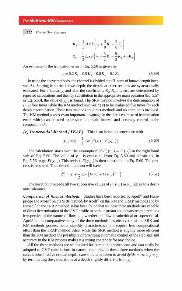
222 Flow in Open Channels
K x F y K Ki4 1 3
1
3
3
8
9
8= + +
⎛⎝⎜⎜⎜
⎞⎠⎟⎟⎟⎟Δ
K x F y K K Ki5 1 3 4
1
3
3
2
9
26= + − +
⎛⎝⎜⎜⎜
⎞⎠⎟⎟⎟⎟Δ
An estimate of the truncation error in Eq. 5.58 is given by
ε = − + −0 2 0 9 0 8 0 11 3 4 5. . . .K K K K (5.59)
In using the above methods, the channel is divided into N parts of known length inter-val Δ x. Starting from the known depth, the depths at other sections are systematically evaluated. For a known y
i and Δ x, the coeffi cients K
1, K
2 , …, etc. are determined by
repeated calculations and then by substitution in the appropriate main equation [Eq. 5.57 or Eq. 5.58], the value of y
i+1 is found. The SRK method involves the determination of
F( y) four times while the KM method involves F( y) to be evaluated fi ve times for each depth determination. These two methods are direct methods and no iteration is involved. The KM method possesses an important advantage in the direct estimate of its truncation error, which can be used to provide automatic interval and accuracy control in the computations17.
(c) Trapezoidal Method (TRAP) This is an iteration procedure with
y y x F y F yi i i i+ += + +{ }1 1
1
2Δ ( ) ( ) (5.60)
The calculation starts with the assumption of F( yi+1
) = F ( yi ) in the right hand
side of Eq. 5.60. The value of yi+1
is evaluated from Eq. 5.60 and substituted in Eq. 5.56 to get F( y
i+1 ). This revised F( y
i+1 ) is then substituted in Eq. 5.60. The pro-
cess is repeated. Thus the r th iteration will have
y y x F y F yir
i i ir
+ +−= + +{ }1 1
11
2( ) ( )( ) ( )Δ (5.61)
The iteration proceeds till two successive values of F( yi+1
) or yi+1
agree to a desir-able tolerance.
Comparison of Various Methods Studies have been reported by Apelt15 and Hum-pridge and Moss16 on the SRK method; by Apelt17 on the KM and TRAP methods and by Prasad17 on the TRAP method. It has been found that all these three methods are capable of direct determination of the GVF profi le in both upstream and downstream directions irrespective of the nature of fl ow, i.e., whether the fl ow is subcritical or supercritical. Apelt17 in his comparative study of the three methods has observed that the SRK and KM methods possess better stability characteristics and require less computational effort than the TRAP method. Also, while the SRK method is slightly more effi cient than the KM method, the possibility of providing automatic control of the step size and accuracy in the KM process makes it a strong contender for any choice.
All the three methods are well-suited for computer applications and can easily be adopted to GVF calculations in natural channels. In these three methods when the calculations involve critical depth, care should be taken to avoid dy/dx = ∞ at y = y
c
by terminating the calculations at a depth slightly different from yc.
Chapter 5.indd 222Chapter 5.indd 222 2/24/2010 2:59:24 PM2/24/2010 2:59:24 PM
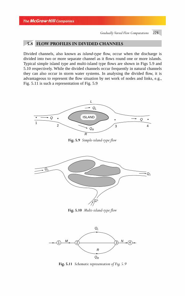
Gradually Varied Flow Computations 223
5.8 FLOW PROFILES IN DIVIDED CHANNELS
Divided channels, also known as island-type fl ow, occur when the discharge is divided into two or more separate channel as it fl ows round one or more islands. Typical simple island type and multi-island type fl ows are shown in Figs 5.9 and 5.10 respectively. While the divided channels occur frequently in natural channels they can also occur in storm water systems. In analysing the divided fl ow, it is advantageous to represent the fl ow situation by net work of nodes and links, e.g., Fig. 5.11 is such a representation of Fig. 5.9
1 2 3 4M N
R
QL
QR
Fig. 5.11 Schematic representation of Fig. 5.9
ISLANDQ
R
QR
QL
L
Q
3 421
Fig. 5.9 Simple-island-type fl ow
Fig. 5.10 Multi-island-type fl ow
Q1
Q 2
Q3
Chapter 5.indd 223Chapter 5.indd 223 2/24/2010 2:59:24 PM2/24/2010 2:59:24 PM
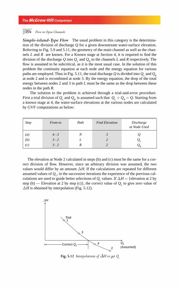
224 Flow in Open Channels
Simple-island-Type Flow The usual problem in this category is the determina-tion of the division of discharge Q for a given downstream water-surface elevation. Referring to Fig. 5.9 and 5.11, the geometry of the main channel as well as the chan-nels L and R are known. For a Known stage at Section 4, it is required to fi nd the division of the discharge Q into Q
L and Q
R in the channels L and R respectively. The
fl ow is assumed to be subcritical, as it is the most usual case. In the solution of this problem the continuity equation at each node and the energy equation for various paths are employed. Thus in Fig. 5.11, the total discharge Q is divided into Q
L and Q
R
at node 2 and is recombined at node 3. By the energy equation, the drop of the total energy between nodes 2 and 3 in path L must be the same as the drop between these nodes in the path R.
The solution to the problem is achieved through a trial-and-error procedure. First a trial division of Q
L and Q
R is assumed such that Q
L + Q
R = Q. Starting from
a known stage at 4, the water-surface elevations at the various nodes are calculated by GVF computations as below:
Step From-to Path Find Elevation Dischargeat Node Used
(a)
(b)
(c)
4−3
3−2
3−2
N
L
R
3
2
2
Q
QL
QR
The elevation at Node 2 calculated in steps (b) and (c) must be the same for a cor-rect division of fl ow. However, since an arbitrary division was assumed, the two values would differ by an amount Δ H. If the calculations are repeated for different assumed values of Q
L, in the successive iterations the experience of the previous cal-
culations are used to guide better selections of QL values. If Δ H = {elevation at 2 by
step (b) — Elevation at 2 by step (c)}, the correct value of QL to give zero value of
Δ H is obtained by interpolation (Fig. 5.12).
Correct QL
1Trial
3
4
2
QL(Assumed)
ΔH
Fig. 5.12 Interpolations of ΔH to get Q
Chapter 5.indd 224Chapter 5.indd 224 2/24/2010 2:59:25 PM2/24/2010 2:59:25 PM
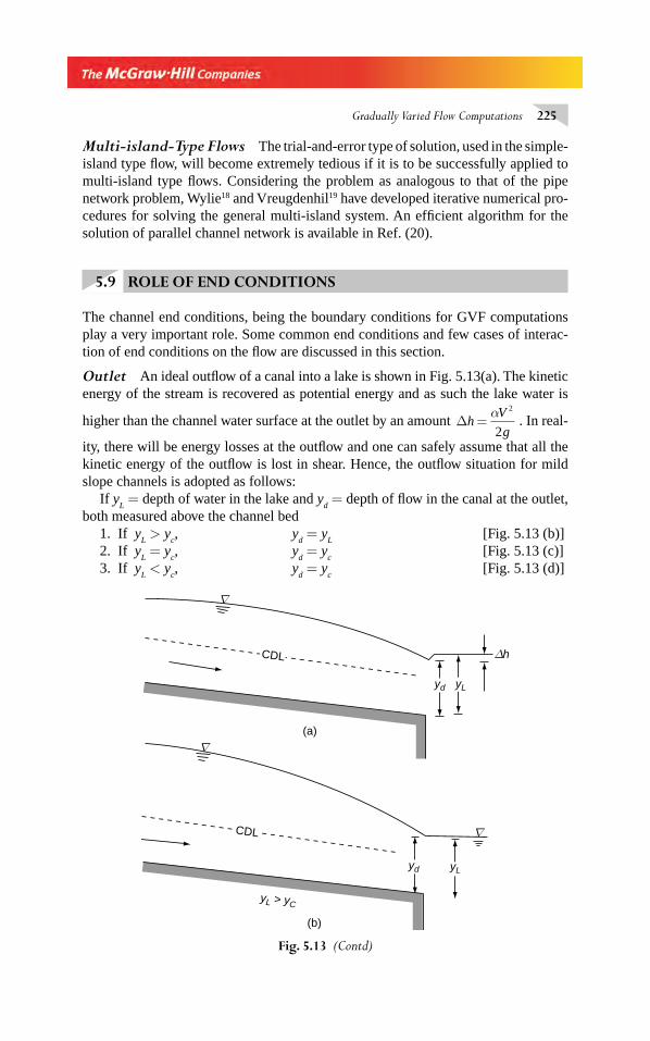
Gradually Varied Flow Computations 225
Multi-island-Type Flows The trial-and-error type of solution, used in the simple-island type fl ow, will become extremely tedious if it is to be successfully applied to multi-island type fl ows. Considering the problem as analogous to that of the pipe network problem, Wylie18 and Vreugdenhil19 have developed iterative numerical pro-cedures for solving the general multi-island system. An effi cient algorithm for the solution of parallel channel network is available in Ref. (20).
5.9 ROLE OF END CONDITIONS
The channel end conditions, being the boundary conditions for GVF computations play a very important role. Some common end conditions and few cases of interac-tion of end conditions on the fl ow are discussed in this section.
Outlet An ideal outfl ow of a canal into a lake is shown in Fig. 5.13(a). The kinetic energy of the stream is recovered as potential energy and as such the lake water is
higher than the channel water surface at the outlet by an amount ΔhV
g=
α 2
2. In real-
ity, there will be energy losses at the outfl ow and one can safely assume that all the kinetic energy of the outfl ow is lost in shear. Hence, the outfl ow situation for mild slope channels is adopted as follows:
If yL = depth of water in the lake and y
d = depth of fl ow in the canal at the outlet,
both measured above the channel bed1. If y
L > y
c, y
d = y
L [Fig. 5.13 (b)]
2. If yL = y
c, y
d = y
c [Fig. 5.13 (c)]
3. If yL < y
c, y
d = y
c [Fig. 5.13 (d)]
Fig. 5.13 (Contd)
CDL
CDL
yLyd
yd
Δh
(a)
(b)
yL
yL > yC
Δ
Δ
Δ
Chapter 5.indd 225Chapter 5.indd 225 2/24/2010 2:59:25 PM2/24/2010 2:59:25 PM
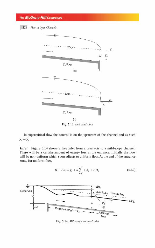
226 Flow in Open Channels
In supercritical fl ow the control is on the upstream of the channel and as such y
d = y
L.
Inlet Figure 5.14 shows a free inlet from a reservoir to a mild-slope channel. There will be a certain amount of energy loss at the entrance. Initially the fl ow will be non-uniform which soon adjusts to uniform fl ow. At the end of the entrance zone, for uniform fl ow,
H Z yV
gh Hf L+ = + + +Δ Δ0
02
2α (5.62)
CDL
yL = yC
yL < yC
(c)
yd yL
yL
(d)
CDL
Δ
Δ
Δ
Δ
Fig. 5.13 End conditions
Fig. 5.14 Mild-slope channel inlet
Uniformflow
Entrance length = Le
ΔZ
H
Reservoir
y0α
V02
2g
ΔHL
hf = S0.Le
NDL
Energy line
Δ
Δ
Chapter 5.indd 226Chapter 5.indd 226 2/24/2010 2:59:25 PM2/24/2010 2:59:25 PM
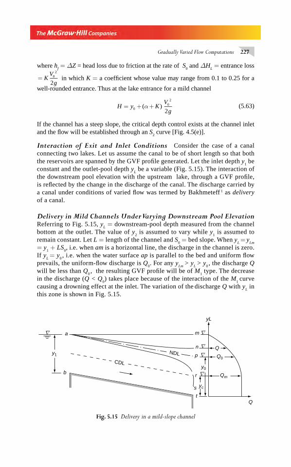
Gradually Varied Flow Computations 227
where hf = ΔZ = head loss due to friction at the rate of S
0 and ΔH
L = entrance loss
= KV
g0
2
2 in which K = a coeffi cient whose value may range from 0.1 to 0.25 for a
well-rounded entrance. Thus at the lake entrance for a mild channel
H y KV
g= + +0
02
2( )α (5.63)
If the channel has a steep slope, the critical depth control exists at the channel inlet and the fl ow will be established through an S
2 curve [Fig. 4.5(e)].
Interaction of Exit and Inlet Conditions Consider the case of a canal connecting two lakes. Let us assume the canal to be of short length so that both the reservoirs are spanned by the GVF profi le generated. Let the inlet depth y
1 be
constant and the outlet-pool depth yL be a variable (Fig. 5.15). The interaction of
the downstream pool elevation with the upstream lake, through a GVF profi le, is refl ected by the change in the discharge of the canal. The discharge carried by a canal under conditions of varied fl ow was termed by Bakhmeteff 1 as delivery of a canal.
Delivery in Mild Channels Under Varying Downstream Pool Elevation Referring to Fig. 5.15, y
L = downstream-pool depth measured from the channel
bottom at the outlet. The value of y2 is assumed to vary while y
1 is assumed to
remain constant. Let L = length of the channel and S0 = bed slope. When y
L =
y
Lm
= y1 + LS
0, i.e. when am is a horizontal line, the discharge in the channel is zero.
If yL
= y0 , i.e. when the water surface ap is parallel to the bed and uniform fl ow
prevails, the uniform-fl ow discharge is Q0. For any y
Lm > y
L > y
0 , the discharge Q
will be less than Q0 , the resulting GVF profi le will be of M
1 type. The decrease
in the discharge (Q < Q0) takes place because of the interaction of the M
1 curve
causing a drowning effect at the inlet. The variation of the discharge Q with y
L in
this zone is shown in Fig. 5.15.
Fig. 5.15 Delivery in a mild-slope channel
CDL
a
b
y1
yL
m
n
p
y0
r
s
t
yc
Qm
Q0
Q
Q
NDL
Δ Δ
Δ
Δ
Δ
Chapter 5.indd 227Chapter 5.indd 227 2/24/2010 2:59:26 PM2/24/2010 2:59:26 PM
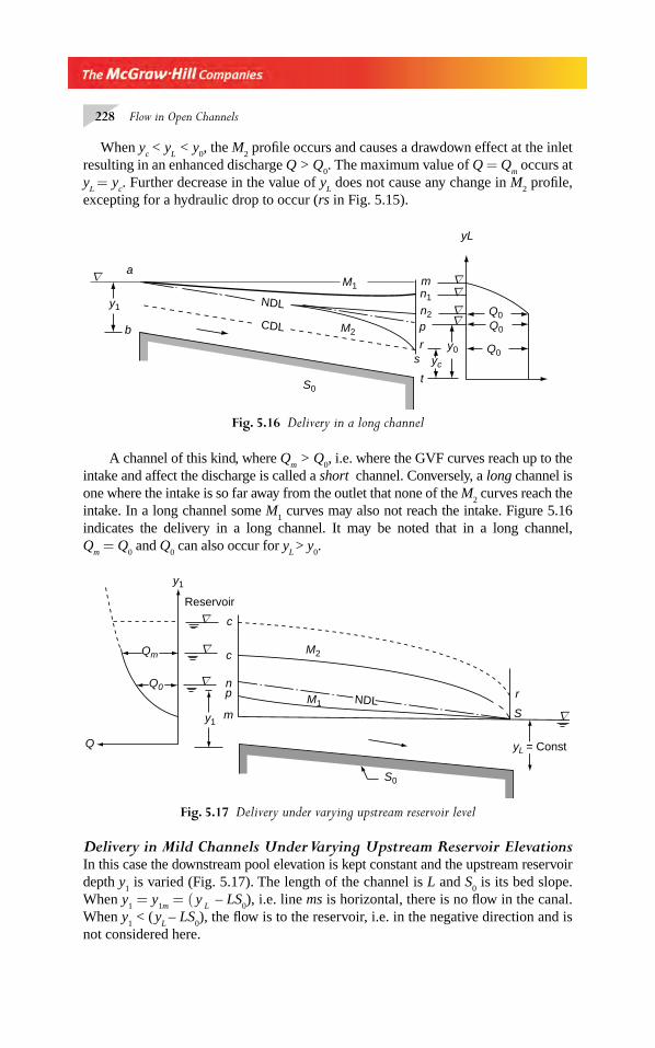
228 Flow in Open Channels
When yc < y
L < y
0, the M
2 profi le occurs and causes a drawdown effect at the inlet
resulting in an enhanced discharge Q > Q0. The maximum value of Q = Q
m occurs at
yL = y
c. Further decrease in the value of y
L does not cause any change in M
2 profi le,
excepting for a hydraulic drop to occur (rs in Fig. 5.15).
Q0Q0
y0
S0
yL
yc
y1n1
M1
M2
n2
Q0
p
rs
t
ma
b CDL
NDL
Δ ΔΔ
ΔΔ
Fig. 5.16 Delivery in a long channel
A channel of this kind, where Qm > Q
0, i.e. where the GVF curves reach up to the
intake and affect the discharge is called a short channel. Conversely, a long channel is one where the intake is so far away from the outlet that none of the M
2 curves reach the
intake. In a long channel some M1 curves may also not reach the intake. Figure 5.16
indicates the delivery in a long channel. It may be noted that in a long channel, Q
m = Q
0 and Q
0 can also occur for y
L > y
0.
Delivery in Mild Channels Under Varying Upstream Reservoir Elevations In this case the downstream pool elevation is kept constant and the upstream reservoir depth y
1 is varied (Fig. 5.17). The length of the channel is L and S
0 is its bed slope.
When y1 = y
1m = ( y
L – LS
0), i.e. line ms is horizontal, there is no fl ow in the canal.
When y1 < ( y
L – LS
0), the fl ow is to the reservoir, i.e. in the negative direction and is
not considered here.
Fig. 5.17 Delivery under varying upstream reservoir level
S0
n
m
p
c
c
y1
y1
Q0
Qm
Reservoir
Q
M2
M1 NDL r
S
yL = Const
Δ
Δ
Δ
Δ
Chapter 5.indd 228Chapter 5.indd 228 2/24/2010 2:59:26 PM2/24/2010 2:59:26 PM
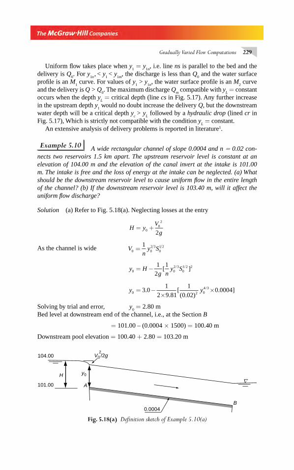
Gradually Varied Flow Computations 229
Uniform fl ow takes place when y1 = y
1n, i.e. line ns is parallel to the bed and the
delivery is Q0. For y
1n , < y
1 < y
1m, the discharge is less than Q
0 and the water surface
profi le is an M1 curve. For values of y
1 > y
1n, the water surface profi le is an M
2 curve
and the delivery is Q > Q0. The maximum discharge Q
m compatible with y
L = constant
occurs when the depth yL = critical depth (line cs in Fig. 5.17). Any further increase
in the upstream depth y1 would no doubt increase the delivery Q, but the downstream
water depth will be a critical depth yc > y
L followed by a hydraulic drop (lined cr in
Fig. 5.17), Which is strictly not compatible with the condition yL = constant.
An extensive analysis of delivery problems is reported in literature1.
Example 5.10 A wide rectangular channel of slope 0.0004 and n = 0.02 con-nects two reservoirs 1.5 km apart. The upstream reservoir level is constant at an elevation of 104.00 m and the elevation of the canal invert at the intake is 101.00 m. The intake is free and the loss of energy at the intake can be neglected. (a) What should be the downstream reservoir level to cause uniform fl ow in the entire length of the channel? (b) If the downstream reservoir level is 103.40 m, will it affect the uniform fl ow discharge?
Solution (a) Refer to Fig. 5.18(a). Neglecting losses at the entry
H yV
g= +0
02
2
As the channel is wide Vn
y S0 02 3
01 21
=
y Hg n
y S0 02 3
01 2 21
2
1= − [ ]/ /
y y0 2 04 33 0
1
2 9 81
1
0 020 0004= −
××.
.[( . )
. ]/
Solving by trial and error, y0 = 2.80 m
Bed level at downstream end of the channel, i.e., at the Section B
= 101.00 – (0.0004 × 1500) = 100.40 m
Downstream pool elevation = 100.40 + 2.80 = 103.20 m
B0.0004
101.00
104.00
H y0
A
V02/2g
Δ
Fig. 5.18(a) Defi nition sketch of Example 5.10(a)
Chapter 5.indd 229Chapter 5.indd 229 2/24/2010 2:59:26 PM2/24/2010 2:59:26 PM
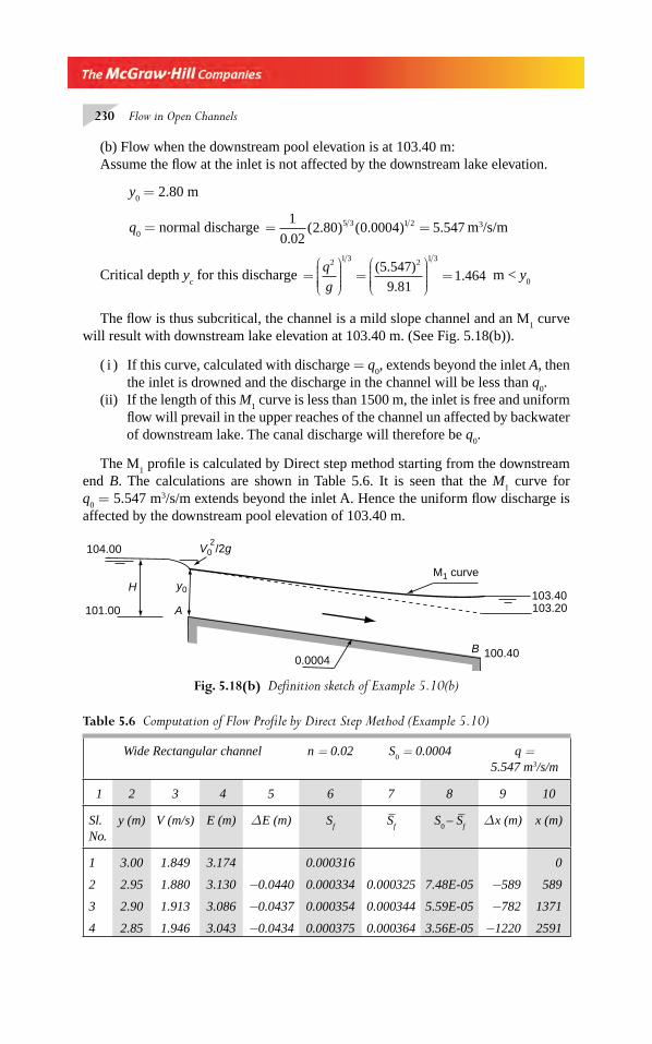
230 Flow in Open Channels
(b) Flow when the downstream pool elevation is at 103.40 m:Assume the fl ow at the inlet is not affected by the downstream lake elevation.
y0 = 2.80 m
q0 = normal discharge = =
1
0 022 80 0 0004 5 5475 3 1 2
.( . ) ( . ) . m3/s/m
Critical depth yc for this discharge =
⎛
⎝⎜⎜⎜⎜
⎞
⎠⎟⎟⎟⎟
=⎛
⎝⎜⎜⎜⎜
⎞
⎠⎟⎟⎟⎟
=q
g
2 1 3 2 1 35 547
9 811 464
( . )
.. m < y
0
The fl ow is thus subcritical, the channel is a mild slope channel and an M1 curve
will result with downstream lake elevation at 103.40 m. (See Fig. 5.18(b)).
( i ) If this curve, calculated with discharge = q0, extends beyond the inlet A, then
the inlet is drowned and the discharge in the channel will be less than q0.
(ii) If the length of this M1 curve is less than 1500 m, the inlet is free and uniform
fl ow will prevail in the upper reaches of the channel un affected by backwater of downstream lake. The canal discharge will therefore be q
0.
The M1 profi le is calculated by Direct step method starting from the downstream
end B. The calculations are shown in Table 5.6. It is seen that the M1 curve for
q0 = 5.547 m3/s/m extends beyond the inlet A. Hence the uniform fl ow discharge is
affected by the downstream pool elevation of 103.40 m.
103.40103.20
M1 curveH
104.00
101.00 A
y0
V02/2g
0.0004B 100.40
Fig. 5.18(b) Defi nition sketch of Example 5.10(b)
Wide Rectangular channel n = 0.02 S0 = 0.0004 q =
5.547 m3/s/m
1 2 3 4 5 6 7 8 9 10
Sl.No.
y (m) V (m/s) E (m) Δ E (m) Sf
Sf
–S
0 – S
f
– Δ x (m) x (m)
1 3.00 1.849 3.174 0.000316 0
2 2.95 1.880 3.130 −0.0440 0.000334 0.000325 7.48E-05 −589 589
3 2.90 1.913 3.086 −0.0437 0.000354 0.000344 5.59E-05 −782 1371
4 2.85 1.946 3.043 −0.0434 0.000375 0.000364 3.56E-05 −1220 2591
Table 5.6 Computation of Flow Profi le by Direct Step Method (Example 5.10)
Chapter 5.indd 230Chapter 5.indd 230 2/24/2010 2:59:27 PM2/24/2010 2:59:27 PM
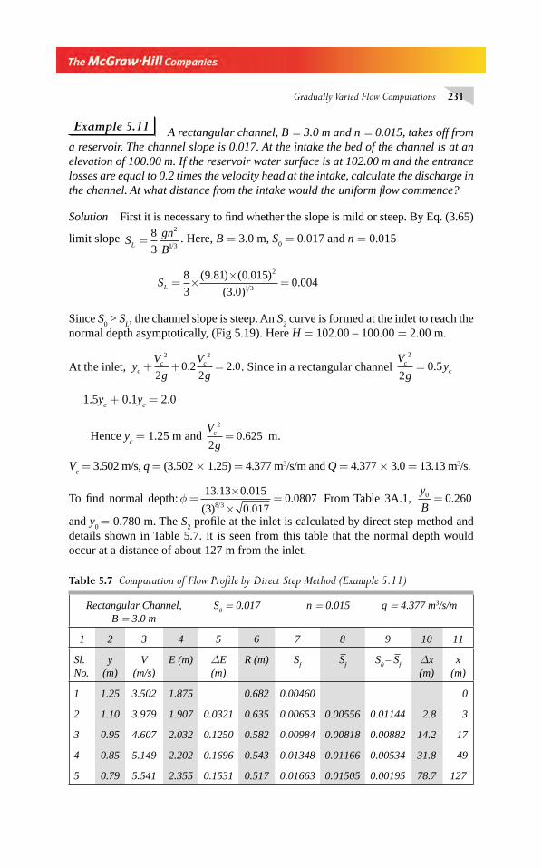
Gradually Varied Flow Computations 231
Example 5.11 A rectangular channel, B = 3.0 m and n = 0.015, takes off from a reservoir. The channel slope is 0.017. At the intake the bed of the channel is at an elevation of 100.00 m. If the reservoir water surface is at 102.00 m and the entrance losses are equal to 0.2 times the velocity head at the intake, calculate the discharge in the channel. At what distance from the intake would the uniform fl ow commence?
Solution First it is necessary to fi nd whether the slope is mild or steep. By Eq. (3.65)
limit slope Sgn
BL =8
3
2
1 3. Here, B = 3.0 m, S
0 = 0.017 and n = 0.015
SL = ××
=8
3
9 81 0 015
3 00 004
2
1 3
( . ) ( . )
( . ).
Since S0 > S
L, the channel slope is steep. An S
2 curve is formed at the inlet to reach the
normal depth asymptotically, (Fig 5.19). Here H = 102.00 – 100.00 = 2.00 m.
At the inlet, yV
g
V
gcc c+ + =
2 2
20 2
22 0. . . Since in a rectangular channel
V
gyc
c
2
20 5= .
1.5yc + 0.1y
c = 2.0
Hence yc = 1.25 m and
V
gc
2
20 625= . m.
Vc = 3.502 m/s, q = (3.502 × 1.25) = 4.377 m3/s/m and Q = 4.377 × 3.0 = 13.13 m3/s.
To fi nd normal depth: φ =×
×=
13 13 0 015
3 0 0170 0807
8 3
. .
( ) .. From Table 3A.1,
y
B0 0 260= .
and y0 = 0.780 m. The S
2 profi le at the inlet is calculated by direct step method and
details shown in Table 5.7. it is seen from this table that the normal depth would occur at a distance of about 127 m from the inlet.
Rectangular Channel,B = 3.0 m
S0 = 0.017 n = 0.015 q = 4.377 m3/s/m
1 2 3 4 5 6 7 8 9 10 11
Sl. No.
y (m)
V (m/s)
E (m) ΔE (m)
R (m) Sf
Sf
–S
0 – S
f
–
Δx (m)
x (m)
1 1.25 3.502 1.875 0.682 0.00460 0
2 1.10 3.979 1.907 0.0321 0.635 0.00653 0.00556 0.01144 2.8 3
3 0.95 4.607 2.032 0.1250 0.582 0.00984 0.00818 0.00882 14.2 17
4 0.85 5.149 2.202 0.1696 0.543 0.01348 0.01166 0.00534 31.8 49
5 0.79 5.541 2.355 0.1531 0.517 0.01663 0.01505 0.00195 78.7 127
Table 5.7 Computation of Flow Profi le by Direct Step Method (Example 5.11)
Chapter 5.indd 231Chapter 5.indd 231 2/24/2010 2:59:27 PM2/24/2010 2:59:27 PM
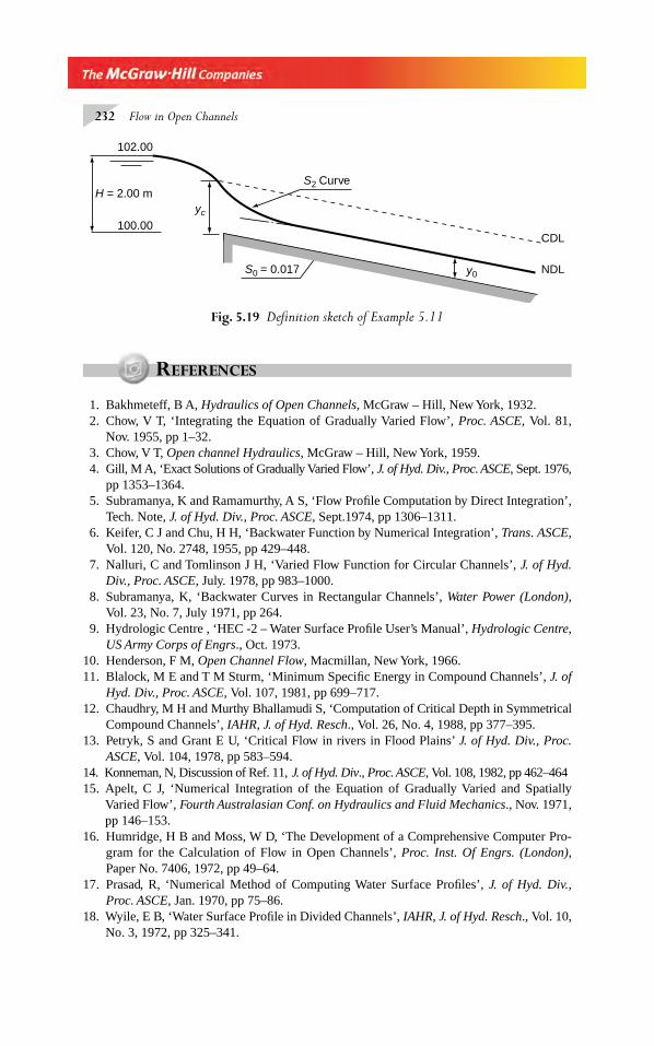
232 Flow in Open Channels
REFERENCES
1. Bakhmeteff, B A, Hydraulics of Open Channels, McGraw – Hill, New York, 1932. 2. Chow, V T, ‘Integrating the Equation of Gradually Varied Flow’, Proc. ASCE, Vol. 81,
Nov. 1955, pp 1–32. 3. Chow, V T, Open channel Hydraulics, McGraw – Hill, New York, 1959. 4. Gill, M A, ‘Exact Solutions of Gradually Varied Flow’, J. of Hyd. Div., Proc. ASCE, Sept. 1976,
pp 1353–1364. 5. Subramanya, K and Ramamurthy, A S, ‘Flow Profi le Computation by Direct Integration’,
Tech. Note, J. of Hyd. Div., Proc. ASCE, Sept.1974, pp 1306–1311. 6. Keifer, C J and Chu, H H, ‘Backwater Function by Numerical Integration’, Trans. ASCE,
Vol. 120, No. 2748, 1955, pp 429–448. 7. Nalluri, C and Tomlinson J H, ‘Varied Flow Function for Circular Channels’, J. of Hyd.
Div., Proc. ASCE, July. 1978, pp 983–1000. 8. Subramanya, K, ‘Backwater Curves in Rectangular Channels’, Water Power (London),
Vol. 23, No. 7, July 1971, pp 264. 9. Hydrologic Centre , ‘HEC -2 – Water Surface Profi le User’s Manual’, Hydrologic Centre,
US Army Corps of Engrs., Oct. 1973.10. Henderson, F M, Open Channel Flow, Macmillan, New York, 1966.11. Blalock, M E and T M Sturm, ‘Minimum Specifi c Energy in Compound Channels’, J. of
Hyd. Div., Proc. ASCE, Vol. 107, 1981, pp 699–717.12. Chaudhry, M H and Murthy Bhallamudi S, ‘Computation of Critical Depth in Symmetrical
Compound Channels’, IAHR, J. of Hyd. Resch., Vol. 26, No. 4, 1988, pp 377–395.13. Petryk, S and Grant E U, ‘Critical Flow in rivers in Flood Plains’ J. of Hyd. Div., Proc.
ASCE, Vol. 104, 1978, pp 583–594.14. Konneman, N, Discussion of Ref. 11, J. of Hyd. Div., Proc. ASCE, Vol. 108, 1982, pp 462–46415. Apelt, C J, ‘Numerical Integration of the Equation of Gradually Varied and Spatially
Varied Flow’, Fourth Australasian Conf. on Hydraulics and Fluid Mechanics., Nov. 1971, pp 146–153.
16. Humridge, H B and Moss, W D, ‘The Development of a Comprehensive Computer Pro-gram for the Calculation of Flow in Open Channels’, Proc. Inst. Of Engrs. (London), Paper No. 7406, 1972, pp 49–64.
17. Prasad, R, ‘Numerical Method of Computing Water Surface Profi les’, J. of Hyd. Div., Proc. ASCE, Jan. 1970, pp 75–86.
18. Wyile, E B, ‘Water Surface Profi le in Divided Channels’, IAHR, J. of Hyd. Resch., Vol. 10, No. 3, 1972, pp 325–341.
H = 2.00 m
100.00
102.00
yc
y0
S2 Curve
S0 = 0.017
CDL
NDL
Fig. 5.19 Defi nition sketch of Example 5.11
Chapter 5.indd 232Chapter 5.indd 232 2/24/2010 2:59:27 PM2/24/2010 2:59:27 PM
Gradually Varied Flow Computations 233
19. Vreugdnhil, C B, ‘Computation Methods for Channel Flow’, Chap. III. Proc. Of Tech. Meeting 26 Hydraulic Research for Water Management, Pub. No. 100, The Delft Hyd. Lab., Delft, 1973, pp 38–77.
20. Chaudhry, M H, Open Channel Flow, Prentice–Hall, Englewood Cliffs, New Jersey, USA, 1993.
PROBLEMS
Problem Distribution
Sl. No.
Topic Problems
1. Direct integration of GVF – Special cases 5.1 to 5.4
2. Computation of GVF
-by Varied Flow Function 5.5
-by Bresse’s function 5.11, 5.12, 5.12
-by Keifer and Chu method 5.15
-Direct step method 5.6, 5.9, 5.13, 5.17, 5.20, 5.22
-Standard step method 5.16
3. Simple island fl ow 5.14
4. Flow at free inlet 5.22 to 5.66
5.1 Prove that the GVF profi le for a horizontal channel can be expressed as
xC
Q Ny
C y
gC N MN
N M
= −+
+− +
⎡
⎣⎢⎢
⎤
⎦⎥⎥
+− +
12
1 21
11 1( ) ( ) + Constant
Where C1 and C
2 are coeffi cients associated with the hydraulic exponents M and N
respectively.5.2 Show that for a horizontal channel, by assuming Chezy C = constant, the GVF profi le is
given by
xC
gy
y
yc
= −⎡
⎣⎢⎢
⎤
⎦⎥⎥
2 4
34+ Constant
5.3 Establish that the GVF profi le in a frictionless rectangular channel is given by
xy
S
y
yc= +
⎛
⎝⎜⎜⎜⎜
⎞
⎠⎟⎟⎟⎟
⎡
⎣
⎢⎢⎢
⎤
⎦
⎥⎥⎥
0
0
3
11
2+ Constant
5.4 Show that in a wide rectangular critical slope channel the gradually varied fl ow profi les calculated by using Chezy formula with C = constant are horizontal lines.
Chapter 5.indd 233Chapter 5.indd 233 2/24/2010 2:59:28 PM2/24/2010 2:59:28 PM
234 Flow in Open Channels
5.5 A trapezoidal channel having B = 6.0 m, side slope m = 2.0, S0 = 0.0016, Manning’s
n = 0.02 carries a discharge of 12.0 m3/s. Compute and plot the backwater produced due to operation of a sluice gate at a downstream section which backs up the water to a depth of 4.0 m immediately behind it. Use Varied fl ow functions.
5.6 Calculate the backwater curve of Problem 5.5 by direct-step method. 5.7 A trapezoidal channel B = 5.0 m and m = 2.0 is laid on a slope of 0.0004. If the normal
depth of fl ow is 3.10 m, compute: (a) the profi le of an M1 curve in this channel lying
between depths of 5.0 m and 3.15 m, and (b) the profi le of an M3 curve lying between
depths of 0.5 m and 1.2 m. Assume Manning’s n = 0.02. 5.8 A rectangular brick-lined channel (n = 0.016) of 4.0-m width is laid on a bottom slope
of 0.0009. It carries a discharge of 15 m3/s and the fl ow is non-uniform. If the depth at a Section A is 2.6 m, calculate the depth at section B, 500 m downstream of A, by using (a) only one step, and (b) two steps.
5.9 A sluice gate discharges a stream of 0.59 m depth with a velocity of 15 m/s in a wide rectangular channel. The channel is laid on an adverse slope of S
0 = – 0.002 and ends
with an abrupt drop at a distance of 100 m from the gate. Assuming n = 0.02, calculate and plot the resulting GVF profi le.
5.10 Figure 5.5 shows the section of a stream with fl ow in the fl ood plain. Idealise the section as shown in the fi gure into three parts with side slopes of 2 : 1 and bottom width and depth for parts 1, 2 and 3 as 15.0 m, 5.0 m; 10.0 m, 1.50 m; 15.0 m and 2.5 m respec-tively. Determine the value of the overall kinetic-energy correction factors α and the friction slope for a discharge of 200 m3/s. The values of the kinetic-energy correction factors for the three subsections can be assumed as α
1 = 1.20, α
2 = 1.05 and α
3 = 1.15.
Assume n = 0.035 for all the boundaries.5.11 A stream which could be considered as a wide rectangular channel has a slope of 0.0003
and Chezy C = 40. Calculate the backwater profi le produced by a weir on the stream which raises the water surface immediately upstream of it by 4.0 m when the discharge over the weir is 3.0 m3/s/m. Use Bresse’s back water functions.
5.12 Derive Equation (5.13) and verify the values of the coeffi cients given in the table accom-panying the equation.
5.13 A 3-m wide rectangular channel laid on a slope of 0.005 carries a fl ow at a normal depth of 1.20 m. A sharp-crested rectangular suppressed weir (C
d = 0.62) is located with its
crest at 2.0 m above the channel bottom at the downstream end of the channel. Compute and plot the water surface profi le. Assume n = 0.02.
Path Width Slope Length N
LeftRight
15.0 m10.0 m
0.00090.0010
2000 m1800 m
0.0250.030
5.14 A small stream is of rectangular cross section. At a certain section it divides itself, encloses an island and then rejoins to form a single channel again. The properties of the two paths past the island are as follows:At a short distance downstream of the confl uence the discharge is found to be 160 m3/s and depth of fl ow of 4.0 m. Find the discharge in each channel and the depth of fl ow at the point of division. Neglect the energy loss at the division and at the confl uence.
5.15 A concrete circular channel (n = 0.015) of diameter = 2.0 m is laid on a slope of 0.05. This channel is used for emptying a pond. The fl ow enters the channel as a free inlet from the pond. Compute and plot the water-surface profi le for a discharge of 8.00 m3/s.
Chapter 5.indd 234Chapter 5.indd 234 2/24/2010 2:59:28 PM2/24/2010 2:59:28 PM
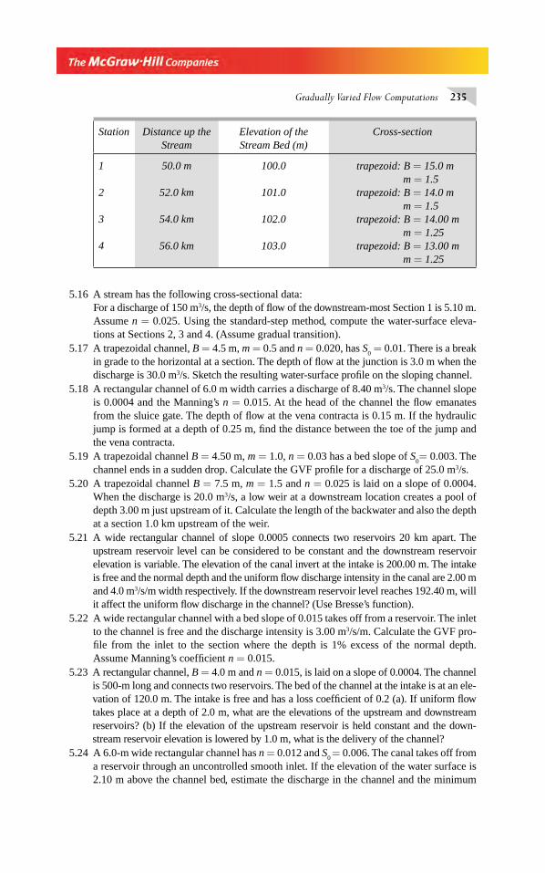
Gradually Varied Flow Computations 235
5.16 A stream has the following cross-sectional data:For a discharge of 150 m3/s, the depth of fl ow of the downstream-most Section 1 is 5.10 m. Assume n = 0.025. Using the standard-step method, compute the water-surface eleva-tions at Sections 2, 3 and 4. (Assume gradual transition).
5.17 A trapezoidal channel, B = 4.5 m, m = 0.5 and n = 0.020, has S0 = 0.01. There is a break
in grade to the horizontal at a section. The depth of fl ow at the junction is 3.0 m when the discharge is 30.0 m3/s. Sketch the resulting water-surface profi le on the sloping channel.
5.18 A rectangular channel of 6.0 m width carries a discharge of 8.40 m3/s. The channel slope is 0.0004 and the Manning’s n = 0.015. At the head of the channel the fl ow emanates from the sluice gate. The depth of fl ow at the vena contracta is 0.15 m. If the hydraulic jump is formed at a depth of 0.25 m, fi nd the distance between the toe of the jump and the vena contracta.
5.19 A trapezoidal channel B = 4.50 m, m = 1.0, n = 0.03 has a bed slope of S0= 0.003. The
channel ends in a sudden drop. Calculate the GVF profi le for a discharge of 25.0 m3/s.5.20 A trapezoidal channel B = 7.5 m, m = 1.5 and n = 0.025 is laid on a slope of 0.0004.
When the discharge is 20.0 m3/s, a low weir at a downstream location creates a pool of depth 3.00 m just upstream of it. Calculate the length of the backwater and also the depth at a section 1.0 km upstream of the weir.
5.21 A wide rectangular channel of slope 0.0005 connects two reservoirs 20 km apart. The upstream reservoir level can be considered to be constant and the downstream reservoir elevation is variable. The elevation of the canal invert at the intake is 200.00 m. The intake is free and the normal depth and the uniform fl ow discharge intensity in the canal are 2.00 m and 4.0 m3/s/m width respectively. If the downstream reservoir level reaches 192.40 m, will it affect the uniform fl ow discharge in the channel? (Use Bresse’s function).
5.22 A wide rectangular channel with a bed slope of 0.015 takes off from a reservoir. The inlet to the channel is free and the discharge intensity is 3.00 m3/s/m. Calculate the GVF pro-fi le from the inlet to the section where the depth is 1% excess of the normal depth. Assume Manning’s coeffi cient n = 0.015.
5.23 A rectangular channel, B = 4.0 m and n = 0.015, is laid on a slope of 0.0004. The channel is 500-m long and connects two reservoirs. The bed of the channel at the intake is at an ele-vation of 120.0 m. The intake is free and has a loss coeffi cient of 0.2 (a). If uniform fl ow takes place at a depth of 2.0 m, what are the elevations of the upstream and downstream reservoirs? (b) If the elevation of the upstream reservoir is held constant and the down-stream reservoir elevation is lowered by 1.0 m, what is the delivery of the channel?
5.24 A 6.0-m wide rectangular channel has n = 0.012 and S0 = 0.006. The canal takes off from
a reservoir through an uncontrolled smooth inlet. If the elevation of the water surface is 2.10 m above the channel bed, estimate the discharge in the channel and the minimum
Station Distance up the Stream
Elevation of the Stream Bed (m)
Cross-section
1
2
3
4
50.0 m
52.0 km
54.0 km
56.0 km
100.0
101.0
102.0
103.0
trapezoid: B = 15.0 m m = 1.5
trapezoid: B = 14.0 m m = 1.5
trapezoid: B = 14.00 m m = 1.25
trapezoid: B = 13.00 m m = 1.25
Chapter 5.indd 235Chapter 5.indd 235 2/24/2010 2:59:28 PM2/24/2010 2:59:28 PM
236 Flow in Open Channels
distance from the inlet at which the fl ow can be considered to be uniform. Neglect energy losses at the entrance to the channel.
5.25 Write an algorithm for computing the discharge in a trapezoidal channel taking off from a reservoir, given S
0, n, B, m and H, where H = reservoir elevation above the channel
invert at the upstream end. The channel-entrance losses can be neglected. 5.26 A trapezoidal channel B = 3.0 m, m = 1.50, n = 0.025 and S
0 = 0.00050 takes off from
a reservoir with free inlet. The reservoir elevation is 7.0 m above the channel bed at the inlet. Calculate the discharge in the channel by neglecting entrance losses.
OBJECTIVE QUESTIONS
5.1 Bresse’s backwater function corresponds to the indicated set of (M, N ) values:
(a) (3,2) (b) 31
33
1
3,
⎛⎝⎜⎜⎜
⎞⎠⎟⎟⎟⎟
(c) 3 31
3,
⎛⎝⎜⎜⎜
⎞⎠⎟⎟⎟⎟ (d) (3,3)
5.2 The solution of the differential equation of GVF by Chow’s method, involves the use of varied fl ow function F (u, N) =
(a) du
uN
u
10
+∫ (b) 10
−( )∫ u duNu
(c) udu
uN
u
10
−∫ (d) du
uN
u
10
−∫5.3 The Keifer and Chu varied-fl ow functions are useful for GVF computations in
(a) all types of channels (b) channels with closing top(c) circular channels only (d) rectangular channels only
5.4 The Kutta-Merson method of solving the GVF differential equation involves (a) evaluation of the function four times for each step(b) evaluation of the function fi ve times for each step(c) three evaluations of the function per step(d) iteration procedure
5.5 The standard-step method aims to solve(a) the differential equation of GVF(b) the differential-energy equation of GVF(c) the Bernoulli equation(d) the momentum equation
5.6 The trapezoidal method (TRAP) of numerical integration of GVF involves(a) direct solution involving evaluation of the function four times (b) iterative procedure (c) Simpson’s rule(d) Graphical procedure
5.7 Bresse’s backwater function is applicable to(a) Circular channels(b) Trapezoidal channels(c) Any shape of channel(d) Wide rectangular channel
5.8 The direct-step method of calculating the GVF profi le uses the relation(a) Δ E = Δ x (S
0 − S
f ) (b) Δ x = Δ E/(S
0 − S
f
– )
(c) Δ x = Δ E (S0 − S
f
– ) (d) Δ y = Δ x (S
0 − S
f ) /(1 − F 2 )
Chapter 5.indd 236Chapter 5.indd 236 2/24/2010 2:59:28 PM2/24/2010 2:59:28 PM

Gradually Varied Flow Computations 237
5.9 In the direct-step method and standard-step methods, the calculations(a) must proceed upstream in subcritical fl ow(b) must end on a control section(c) must always proceed upstream(d) must proceed upstream in supercritical fl ow
5.10 The direct-step method(a) is best-suited for natural channels(b) is accurate for all step sizes(c) is most accurate for calculating supercritical fl ow profi les(d) is none of these
5.11 The standard-step method is (a) an unguided trial-and-error method(b) a rapidly-converging iterative procedure (c) not applicable to natural channels(d) not applicable to artifi cial channels
5.11 In a compound section the slope of the common energy line Sf is
(a) Q
K Ai
2
2 2Σ / (b) Q
Ki
2
2Σ( )
(c) ΣΣ
Q
K Ai
i
2
2 2/ (d)
Σ
Σ
K A
K A
i i
i
3 2
3 2
/
/
( )( )
5.12 The standard Runge-Kutta method for solving GVF profi les is(a) an iterative procedure(b) not rapidly converging (c) dependent on the nature of the profi le(d) independent of the direction of computation
5.14 In a simple island-type divided channel of rectangular cross-section, the discharge division
(a) is judged by common sense (b) is inversely proportional to Manning’s n (c) is to be found by iterative GVF calculations (d) has no fi xed value5.15 For an uncontrolled canal inlet at a reservoir, the discharge drawn (a) is fi xed by the critical depth that occurs at the inlet (b) is determined by a control on the downstream end (c) depends on whether the channel is steep or otherwise (d) is a constant5.16 A mind channel connecting two reservoirs is called a short channel if (a) the discharge varies with the downstream-pool elevation (b) the channel is on a steep slope (c) the channel is frictionless (d) some M
2 curves extend all the way up to the reservoir
5.17 A mild slope channel enters a lake with a sudden drop in its bed. If the depth of water in the lake measured above the channel bed at its outlet y
L is greater than the critical depth,
then the depth of fl ow in the canal at the outlet yd
(a) = y
L (b) = y
c
(c) = normal depth = y0 (d) < y
0
5.18 A compound section as in Fig. 5.19 may have a maximum of (a) one critical depth (c) three critical depths(b) two critical depths (d) four critical depths
Chapter 5.indd 237Chapter 5.indd 237 2/24/2010 2:59:28 PM2/24/2010 2:59:28 PM
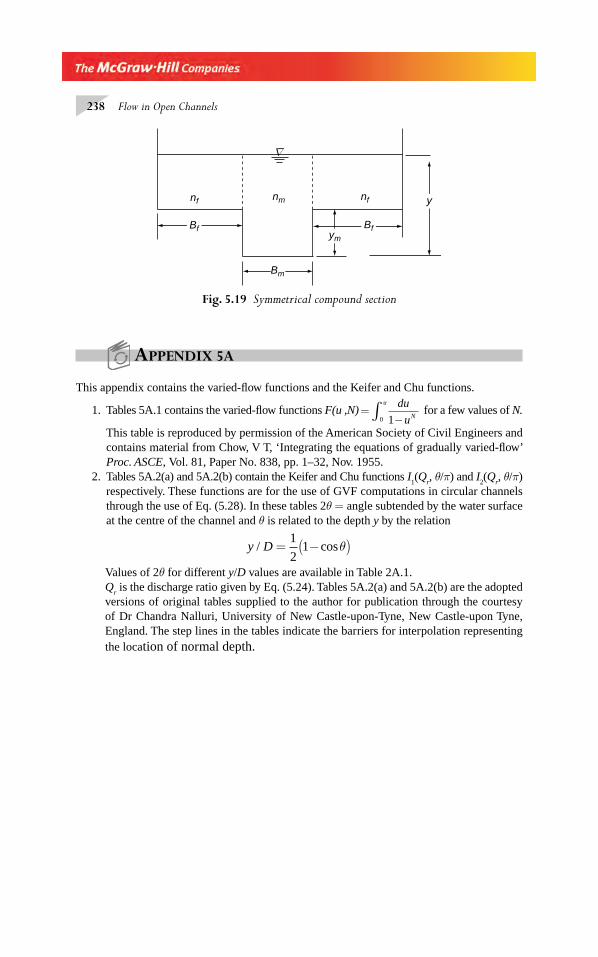
238 Flow in Open Channels
APPENDIX 5A
This appendix contains the varied-fl ow functions and the Keifer and Chu functions.
1. Tables 5A.1 contains the varied-fl ow functions F(u ,N) =−∫du
uN
u
10 for a few values of N.
This table is reproduced by permission of the American Society of Civil Engineers and contains material from Chow, V T, ‘Integrating the equations of gradually varied-fl ow’ Proc. ASCE, Vol. 81, Paper No. 838, pp. 1–32, Nov. 1955.
2. Tables 5A.2(a) and 5A.2(b) contain the Keifer and Chu functions I1(Q
r, θ/π) and I
2(Q
r, θ/π)
respectively. These functions are for the use of GVF computations in circular channels through the use of Eq. (5.28). In these tables 2θ = angle subtended by the water surface at the centre of the channel and θ is related to the depth y by the relation
y D/ cos= −( )1
21 θ
Values of 2θ for different y/D values are available in Table 2A.1.Q
r is the discharge ratio given by Eq. (5.24). Tables 5A.2(a) and 5A.2(b) are the adopted
versions of original tables supplied to the author for publication through the courtesy of Dr Chandra Nalluri, University of New Castle-upon-Tyne, New Castle-upon Tyne, England. The step lines in the tables indicate the barriers for interpolation representing the location of normal depth.
nf nfnm
Bfym
Bm
Bf
y
Δ
Fig. 5.19 Symmetrical compound section
Chapter 5.indd 238Chapter 5.indd 238 2/24/2010 2:59:29 PM2/24/2010 2:59:29 PM
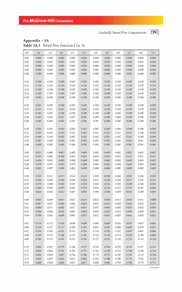
Gradually Varied Flow Computations 239
Appendix – 5ATable 5A.1 Varied Flow Function F (u, N)
u\N 2.6 2.8 3.0 3.2 3.4 3.6 3.8 4.0 4.2 4.6 5.0
0.00 0.000 0.000 0.000 0.000 0.000 0.000 0.000 0.000 0.000 0.000 0.000
0.02 0.020 0.020 0.020 0.020 0.020 0.020 0.020 0.020 0.020 0.020 0.020
0.04 0.040 0.040 0.040 0.040 0.040 0.040 0.040 0.040 0.040 0.040 0.040
0.06 0.060 0.060 0.060 0.060 0.060 0.060 0.060 0.060 0.060 0.060 0.060
0.08 0.080 0.080 0.080 0.080 0.080 0.080 0.080 0.080 0.080 0.080 0.080
0.10 0.100 0.100 0.100 0.100 0.100 0.100 0.100 0.100 0.100 0.100 0.100
0.12 0.120 0.120 0.120 0.120 0.120 0.120 0.120 0.120 0.120 0.120 0.120
0.14 0.140 0.140 0.140 0.140 0.140 0.140 0.140 0.140 0.140 0.140 0.140
0.16 0.160 0.160 0.160 0.160 0.160 0.160 0.160 0.160 0.160 0.160 0.160
0.18 0.181 0.180 0.180 0.180 0.180 0.180 0.180 0.180 0.180 0.180 0.180
0.20 0.201 0.200 0.200 0.201 0.200 0.200 0.200 0.200 0.200 0.200 0.200
0.22 0.221 0.221 0.221 0.220 0.220 0.220 0.220 0.220 0.220 0.220 0.220
0.24 0.242 0.241 0.240 0.240 0.240 0.240 0.240 0.240 0.240 0.240 0.240
0.26 0.262 0.262 0.261 0.261 0.261 0.260 0.260 0.260 0.260 0.260 0.260
0.28 0.283 0.282 0.282 0.281 0.281 0.281 0.280 0.280 0.280 0.280 0.280
0.30 0.304 0.303 0.302 0.302 0.301 0.301 0.300 0.300 0.300 0.300 0.300
0.32 0.325 0.324 0.323 0.322 0.322 0.321 0.321 0.321 0.321 0.320 0.320
0.34 0.346 0.344 0.343 0.343 0.342 0.342 0.341 0.341 0.341 0.340 0.340
0.36 0.367 0.366 0.364 0.363 0.363 0.362 0.362 0.361 0.361 0.361 0.360
0.38 0.389 0.387 0.385 0.384 0.383 0.383 0.382 0.382 0.381 0.381 0.381
0.40 0.411 0.408 0.407 0.405 0.404 0.403 0.403 0.402 0.402 0.401 0.401
0.42 0.433 0.430 0.428 0.426 0.425 0.424 0.423 0.423 0.422 0.421 0.421
0.44 0.456 0.452 0.450 0.448 0.446 0.445 0.444 0.443 0.443 0.442 0.441
0.46 0.479 0.475 0.472 0.470 0.468 0.466 0.465 0.464 0.463 0.462 0.462
0.48 0.502 0.497 0.494 0.492 0.489 0.488 0.486 0.485 0.484 0.483 0.482
0.50 0.525 0.521 0.517 0.514 0.511 0.509 0.508 0.506 0.505 0.504 0.503
0.52 0.550 0.544 0.540 0.536 0.534 0.531 0.529 0.528 0.527 0.525 0.523
0.54 0.574 0.568 0.563 0.559 0.556 0.554 0.551 0.550 0.548 0.546 0.544
0.56 0.599 0.593 0.587 0.583 0.579 0.576 0.574 0.572 0.570 0.567 0.565
0.58 0.626 0.618 0.612 0.607 0.603 0.599 0.596 0.594 0.592 0.589 0.587
0.60 0.653 0.644 0.637 0.631 0.627 0.623 0.620 0.617 0.614 0.611 0.608
0.61 0.667 0.657 0.650 0.644 0.639 0.635 0.631 0.628 0.626 0.622 0.619
0.62 0.680 0.671 0.663 0.657 0.651 0.647 0.643 0.640 0.637 0.633 0.630
0.63 0.694 0.684 0.676 0.669 0.664 0.659 0.655 0.652 0.649 0.644 0.641
0.64 0.709 0.693 0.690 0.683 0.677 0.672 0.667 0.664 0.661 0.656 0.652
0.65 0.724 0.712 0.703 0.696 0.689 0.684 0.680 0.676 0.673 0.667 0.663
0.66 0.738 0.727 0.717 0.709 0.703 0.697 0.692 0.688 0.685 0.679 0.675
0.67 0.754 0.742 0.731 0.723 0.716 0.710 0.705 0.701 0.697 0.691 0.686
0.68 0.769 0.757 0.746 0.737 0.729 0.723 0.718 0.713 0.709 0.703 0.698
0.69 0.785 0.772 0.761 0.751 0.743 0.737 0.731 0.726 0.722 0.715 0.710
0.70 0.802 0.787 0.776 0.766 0.757 0.750 0.744 0.739 0.735 0.727 0.722
0.71 0.819 0.804 0.791 0.781 0.772 0.764 0.758 0.752 0.748 0.740 0.734
0.72 0.836 0.820 0.807 0.796 0.786 0.779 0.772 0.766 0.761 0.752 0.746
0.73 0.854 0.837 0.823 0.811 0.802 0.793 0.786 0.780 0.774 0.765 0.759
0.74 0.868 0.854 0.840 0.827 0.817 0.808 0.800 0.794 0.788 0.779 0.771
(Continued)
Chapter 5.indd 239Chapter 5.indd 239 2/24/2010 2:59:29 PM2/24/2010 2:59:29 PM
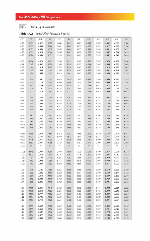
240 Flow in Open Channels
1.03 1.340 1.186 1.060 0.955 0.866 0.790 0.725 0.668 0.618 0.535 0.469
1.04 1.232 1.086 0.967 0.868 0.785 0.714 0.653 0.600 0.554 0.477 0.415
1.05 1.150 1.010 0.896 0.802 0.723 0.656 0.598 0.548 0.504 0.432 0.374
1.06 1.082 0.948 0.838 0.748 0.672 0.608 0.553 0.506 0.464 0.396 0.342
1.07 1.026 0.896 0.790 0.703 0.630 0.569 0.516 0.471 0.431 0.366 0.315
1.08 0.978 0.851 0.749 0.665 0.595 0.535 0.485 0.441 0.403 0.341 0.292
1.09 0.935 0.812 0.713 0.631 0.563 0.506 0.457 0.415 0.379 0.319 0.272
1.10 0.897 0.777 0.681 0.601 0.536 0.480 0.433 0.392 0.357 0.299 0.254
1.11 0.864 0.746 0.652 0.575 0.511 0.457 0.411 0.372 0.338 0.282 0.239
1.12 0.883 0.718 0.626 0.551 0.488 0.436 0.392 0.354 0.321 0.267 0.225
1.13 0.805 0.692 0.602 0.529 0.468 0.417 0.374 0.337 0.305 0.253 0.212
1.14 0.780 0.669 0.581 0.509 0.450 0.400 0.358 0.322 0.291 0.240 0.201
1.15 0.756 0.647 0.561 0.490 0.432 0.384 0.343 0.308 0.278 0.229 0.291
1.16 0.734 0.627 0.542 0.473 0.417 0.369 0.329 0.295 0.266 0.218 0.181
1.17 0.713 0.608 0.525 0.458 0.402 0.356 0.317 0.283 0.255 0.208 0.173
u\N 2.6 2.8 3.0 3.2 3.4 3.6 3.8 4.0 4.2 4.6 5.0
0.75 0.890 0.872 0.857 0.844 0.833 0.823 0.815 0.808 0.802 0.792 0.784
0.76 0.909 0.890 0.874 0.861 0.849 0.839 0.830 0.823 0.817 0.806 0.798
0.77 0.930 0.909 0.892 0.878 0.866 0.855 0.846 0.838 0.831 0.820 0.811
0.78 0.950 0.929 0.911 0.896 0.883 0.872 0.862 0.854 0.847 0.834 0.825
0.79 0.971 0.949 0.930 0.914 0.901 0.889 0.879 0.870 0.862 0.849 0.839
0.80 0.994 0.970 0.950 0.934 0.919 0.907 0.896 0.887 0.878 0.865 0.854
0.81 1.017 0.992 0.971 0.954 0.938 0.925 0.914 0.904 0.895 0.881 0.869
0.82 1.041 1.015 0.993 0.974 0.958 0.945 0.932 0.922 0.913 0.897 0.885
0.83 1.067 1.039 1.016 0.996 0.979 0.965 0.952 0.940 0.931 0.914 0.901
0.84 1.094 1.064 1.040 1.019 1.001 0.985 0.972 0.960 0.949 0.932 0.918
0.85 1.121 1.091 1.065 1.043 1.024 1.007 0.993 0.980 0.969 0.950 0.935
0.86 1.153 1.119 1.092 1.068 1.048 1.031 1.015 1.002 0.990 0.970 0.954
0.87 1.182 1.149 1.120 1.095 1.074 1.055 1.039 1.025 1.012 0.990 0.973
0.88 1.228 1.181 1.151 1.124 1.101 1.081 1.064 1.049 1.035 1.012 0.994
0.89 1.255 1.216 1.183 1.155 1.131 1.110 1.091 1.075 1.060 1.035 1.015
0.90 1.294 1.253 1.218 1.189 1.163 1.140 1.120 1.103 1.087 1.060 1.039
0.91 1.338 1.294 1.257 1.225 1.197 1.173 1.152 1.133 1.116 1.088 1.064
0.92 1.351 1.340 1.300 1.266 1.236 1.210 1.187 1.166 1.148 1.117 1.092
0.93 1.435 1.391 1.348 1.311 1.279 1.251 1.226 1.204 1.184 1.151 1.123
0.94 1.504 1.449 1.403 1.363 1.328 1.297 1.270 1.246 1.225 1.188 1.158
0.950 1.582 1.518 1.467 1.423 1.385 1.352 1.322 1.296 1.272 1.232 1.199
0.960 1.665 1.601 1.545 1.497 1.454 1.417 1.385 1.355 1.329 1.285 1.248
0.970 1.780 1.707 1.644 1.590 1.543 1.501 1.464 1.431 1.402 1.351 1.310
0.975 1.853 1.773 1.707 1.649 1.598 1.554 1.514 1.479 1.447 1.393 1.348
0.980 1.946 1.855 1.783 1.720 1.666 1.617 1.575 1.536 1.502 1.443 1.395
0.985 2.056 1.959 1.880 1.812 1.752 1.699 1.652 1.610 1.573 1.508 1.454
0.990 2.212 2.106 2.017 1.940 1.973 1.814 1.761 1.714 1.671 1.598 1.537
0.995 2.478 2.355 2.250 2.159 2.079 2.008 1.945 1.889 1.838 1.751 1.678
0.999 3.097 2.931 2.788 2.663 2.554 2.457 2.370 2.293 2.223 2.102 2.002
1.000 ∞ ∞ ∞ ∞ ∞ ∞ ∞ ∞ ∞ ∞ ∞
1.001 2.640 2.399 2.184 2.008 1.856 1.725 1.610 1.508 1.417 1.264 1.138
1.005 2.022 1.818 1.649 1.506 1.384 1.279 1.188 1.107 1.036 0.915 0.817
1.010 1.757 1.572 1.419 1.291 1.182 1.089 1.007 0.936 0.873 0.766 0.681
1.015 1.602 1.428 1.286 1.166 1.065 0.978 0.902 0.836 0.778 0.680 0.602
1.020 1.493 1.327 1.191 1.078 0.982 0.900 0.828 0.766 0.711 0.620 0.546
Table 5A.1 Varied Flow Function F (u, N)
Chapter 5.indd 240Chapter 5.indd 240 2/24/2010 2:59:29 PM2/24/2010 2:59:29 PM
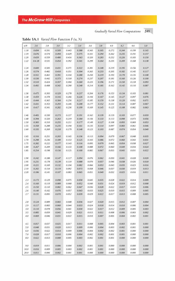
Gradually Varied Flow Computations 241
1.90 0.242 0.188 0.147 0.117 0.094 0.076 0.062 0.050 0.041 0.028 0.020
1.95 0.231 0.178 0.139 0.110 0.088 0.070 0.057 0.046 0.038 0.026 0.018
2.00 0.221 0.169 0.132 0.104 0.082 0.066 0.053 0.043 0.035 0.023 0.016
2.10 0.202 0.154 0.119 0.092 0.073 0.058 0.046 0.037 0.030 0.019 0.013
2.20 0.186 0.141 0.107 0.083 0.065 0.051 0.040 0.032 0.025 0.016 0.011
2.3 0.173 0.129 0.098 0.075 0.058 0.045 0.035 0.028 0.022 0.014 0.009
2.4 0.160 0.119 0.089 0.068 0.052 0.040 0.031 0.024 0.019 0.012 0.008
2.5 0.150 0.110 0.082 0.062 0.047 0.036 0.028 0.022 0.017 0.010 0.006
2.6 0.140 0.102 0.076 0.057 0.043 0.033 0.025 0.019 0.015 0.009 0.005
2.7 0.131 0.095 0.070 0.052 0.039 0.029 0.022 0.017 0.013 0.008 0.005
2.8 0.124 0.089 0.065 0.048 0.036 0.027 0.020 0.015 0.012 0.007 0.004
2.9 0.117 0.083 0.060 0.044 0.033 0.024 0.018 0.014 0.010 0.006 0.004
3.0 0.110 0.078 0.056 0.041 0.030 0.022 0.017 0.012 0.009 0.005 0.003
3.5 0.085 0.059 0.041 0.029 0.021 0.015 0.011 0.008 0.006 0.003 0.002
4.0 0.069 0.046 0.031 0.022 0.015 0.010 0.007 0.005 0.004 0.002 0.001
4.5 0.057 0.037 0.025 0.017 0.011 0.008 0.005 0.004 0.003 0.001 0.001
5.0 0.048 0.031 0.020 0.013 0.009 0.006 0.004 0.003 0.002 0.001 0.000
6.0 0.036 0.022 0.014 0.009 0.006 0.004 0.002 0.002 0.001 0.000 0.000
7.0 0.028 0.017 0.010 0.006 0.004 0.002 0.002 0.001 0.001 0.000 0.000
8.0 0.022 0.013 0.008 0.005 0.003 0.002 0.001 0.001 0.000 0.000 0.000
9.0 0.019 0.011 0.006 0.004 0.002 0.001 0.001 0.000 0.000 0.000 0.000
10.0 0.016 0.009 0.005 0.003 0.002 0.001 0.001 0.000 0.000 0.000 0.000
20.0 0.011 0.006 0.002 0.001 0.001 0.000 0.000 0.000 0.000 0.000 0.000
u\N 2.6 2.8 3.0 3.2 3.4 3.6 3.8 4.0 4.2 4.6 5.0
1.18 0.694 0.591 0.509 0.443 0.388 0.343 0.305 0.272 0.244 0.199 0.165
1.19 0.676 0.574 0.494 0.429 0.375 0.331 0.294 0.262 0.235 0.191 0.157
1.20 0.659 0.559 0.480 0.416 0.363 0.320 0.283 0.252 0.226 0.183 0.150
1.22 0.6 28 0.531 0.454 0.392 0.341 0.299 0.264 0.235 0.209 0.168 0.138
1.24 0.600 0.505 0.431 0.371 0.322 0.281 0.248 0.219 0.195 0.156 0.127
1.26 0.574 0.482 0.410 0.351 0.304 0.265 0.233 0.205 0.182 0.145 0.117
1.28 0.551 0.461 0.391 0.334 0.288 0.250 0.219 0.193 0.170 0.135 0.108
1.30 0.530 0.442 0.373 0.318 0.274 0.237 0.207 0.181 0.160 0.126 0.100
1.32 0.510 0.424 0.357 0.304 0.260 0.225 0.196 0.171 0.150 0.118 0.093
1.34 0.492 0.408 0.342 0.290 0.248 0.214 0.185 0.162 0.142 0.110 0.087
1.36 0.475 0.393 0.329 0.278 0.237 0.204 0.176 0.153 0.134 0.103 0.081
1.38 0.459 0.378 0.316 0.266 0.226 0.194 0.167 0.145 0.127 0.097 0.076
1.40 0.444 0.365 0.304 0.256 0.217 0.185 0.159 0.138 0.120 0.092 0.071
1.42 0.431 0.353 0.293 0.246 0.208 0.177 0.152 0.131 0.114 0.087 0.067
1.44 0.417 0.341 0.282 0.236 0.199 0.169 0.145 0.125 0.108 0.082 0.063
1.46 0.405 0.330 0.273 0.227 0.191 0.162 0.139 0.119 0.103 0.077 0.059
1.48 0.394 0.320 0.263 0.219 0.184 0.156 0.133 0.113 0.098 0.073 0.056
1.50 0.383 0.310 0.255 0.211 0.177 0.149 0.127 0.108 0.093 0.069 0.053
1.55 0.358 0.288 0.235 0.194 0.161 0.135 0.114 0.097 0.083 0.061 0.046
1.60 0.335 0.269 0.218 0.179 0.148 0.123 0.103 0.087 0.074 0.054 0.040
1.65 0.316 0.251 0.203 0.165 0.136 0.113 0.094 0.079 0.067 0.048 0.035
1.70 0.298 0.236 0.189 0.153 0.125 0.103 0.086 0.072 0.060 0.043 0.031
1.75 0.282 0.222 0.177 0.143 0.116 0.095 0.079 0.065 0.054 0.038 0.027
1.80 0.267 0.209 0.166 0.133 0.108 0.088 0.072 0.060 0.049 0.034 0.024
1.85 0.254 0.198 0.156 0.125 0.100 0.082 0.067 0.055 0.045 0.031 0.022
Table 5A.1 Varied Flow Function F (u, N)
Chapter 5.indd 241Chapter 5.indd 241 2/24/2010 2:59:29 PM2/24/2010 2:59:29 PM
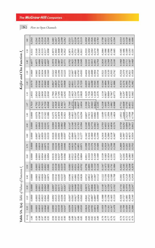
242 Flow in Open Channelsθ/
π\Q
r0.
100.
200.
300.
400.
500.
600.
700.
800.
901.
001.
071.
101.
201.
301.
401.
5016
0
1.00
0.00
000.
0000
0.00
000.
0000
0.00
000.
0000
0.00
000.
0000
0.00
000.
0000
4.76
102.
8555
0.91
700.
5669
0.40
770.
3151
0.25
43
0.99
0.00
030.
0003
0.00
030.
0003
0.00
030.
0004
0.00
040.
0007
0.00
130.
0376
4.75
922.
8543
0.91
640.
5665
0.40
750.
3149
0.25
410.
980.
0010
0.00
100.
0011
0.00
120.
0013
0.00
150.
0019
0.00
270.
0049
0.07
484.
7533
2.85
030.
9146
0.56
540.
4066
0.31
430.
2536
0.97
0.00
220.
0023
0.00
240.
0026
0.00
290.
0034
0.00
420.
0059
0.01
050.
1123
0.74
152.
8430
0.91
140.
5634
0.40
530.
3133
0.25
280.
960.
0040
0.00
410.
0043
0.00
470.
0052
0.00
610.
0075
0.01
030.
0181
0.15
024.
7230
2.83
180.
9069
0.56
060.
4033
0.31
170.
2516
0.95
0.00
620.
0064
0.00
680.
0073
0.00
810.
0094
0.01
160.
0159
0.02
750.
1886
4.69
482.
8160
0.90
060.
5569
0.40
070.
3098
0.25
00
0.94
0.00
900.
0092
0.00
970.
0104
0.01
160.
0135
0.01
660.
0226
0.03
840.
2275
4.65
322.
7945
0.89
270.
5522
0.39
740.
3073
0.24
810.
930.
0122
0.01
250.
0132
0.01
420.
0158
0.01
820.
0224
0.03
030.
0510
0.26
734.
5928
2.76
630.
8829
0.54
640.
3934
0.30
430.
2457
0.92
0.01
590.
0163
0.01
710.
0185
0.02
050.
0237
0.02
900.
0391
0.06
490.
3078
4.50
332.
7295
0.87
100.
5396
0.38
870.
3008
0.24
290.
910.
0200
0.02
060.
0217
0.02
330.
0259
0.02
980.
0364
0.04
890.
0802
0.34
944.
3662
2.68
300.
8570
0.53
160.
3833
0.29
680.
2398
0.90
0.02
470.
0254
0.02
670.
0287
0.03
180.
0366
0.04
460.
0597
0.09
680.
3921
4.14
172.
6245
0.84
080.
5225
0.37
710.
2922
0.23
62
0.89
0.02
990.
0307
0.03
220.
0346
0.03
830.
0441
0.05
360.
0714
0.11
470.
4360
3.71
602.
5518
0.82
210.
5122
0.37
020.
2871
0.23
210.
880.
0354
0.03
650.
0383
0.04
110.
0455
0.05
220.
0633
0.08
400.
1340
0.48
152.
3773
2.46
230.
8011
0.50
070.
3625
0.28
140.
2277
0.87
0.04
150.
0427
0.04
480.
4081
0.05
310.
0610
0.07
380.
0977
0.15
450.
5287
0.00
002.
3547
0.77
770.
4881
0.35
400.
2751
0.22
280.
864.
0480
0.04
940.
0518
0.05
560.
0614
0.07
040.
0851
0.11
220.
1763
0.57
790.
8037
2.22
780.
7519
0.47
430.
3448
0.26
830.
2176
0.85
0.05
500.
0565
0.05
930.
0636
0.07
020.
0804
0.09
710.
1277
0.19
940.
6294
1.60
342.
0828
0.72
390.
4593
0.33
490.
2611
0.21
19
0.84
0.06
240.
0641
0.06
730.
0722
0.07
960.
0911
0.10
980.
1442
0.22
400.
6837
2.31
661.
9229
0.69
390.
4434
0.32
430.
2533
0.20
580.
830.
0703
0.07
220.
0757
0.08
120.
0895
0.10
240.
1234
0.16
160.
2499
0.74
113.
0737
1.75
360.
6621
0.42
650.
3131
0.24
500.
1994
0.82
0.07
850.
0807
0.08
460.
0907
0.10
000.
1143
0.13
760.
1800
0.27
740.
8023
4.04
431.
5820
0.62
880.
4088
0.30
130.
2364
0.19
260.
810.
0872
0.08
970.
0939
0.10
070.
1110
0.12
690.
1526
0.19
940.
3065
0.86
825.
9653
1.41
490.
5945
0.39
040.
2891
0.22
740.
1856
0.80
0.09
640.
0990
0.10
370.
1112
0.12
260.
1400
0.16
840.
2199
0.33
670.
9399
3.52
451.
2576
0.55
960.
3714
0.27
640.
2180
0.17
83
0.79
0.10
590.
1088
0.11
400.
1222
0.13
470.
1539
0.18
500.
2416
0.37
031.
0189
0.23
381.
1134
0.52
440.
3521
0.26
340.
2084
0.17
080.
780.
1158
0.11
900.
1247
0.13
360.
1473
0.16
830.
2024
0.26
440.
4055
1.10
751.
6695
0.98
370.
4894
0.33
260.
2502
0.19
860.
1631
0.77
0.12
610.
1296
0.13
580.
1456
0.16
050.
1834
0.22
070.
2884
0.44
311.
2094
1.32
490.
8684
0.54
490.
3130
0.23
680.
1886
0.15
520.
760.
1367
0.14
050.
1473
0.15
800.
1741
0.19
910.
2398
0.31
380.
4836
1.33
061.
0862
0.76
670.
4212
0.29
350.
2234
0.17
860.
1474
0.75
0.14
780.
1519
0.15
920.
1708
0.18
840.
2155
0.25
980.
3407
0.52
761.
4824
0.90
880.
6773
0.38
860.
2742
0.21
000.
1685
0.13
94
Tabl
e 5A
. 2(a
) Ta
ble
of V
alue
s of
Fun
ctio
n I 1
Kei
fer
and
Chu
Func
tion
I1
0.74
0.15
920.
1636
0.17
160.
1841
0.20
320.
2327
0.28
090.
3693
0.57
581.
6912
0.77
110.
5987
0.35
740.
2554
0.19
680.
1585
0.13
140.
730.
1709
0.17
570.
1843
0.19
780.
2185
0.25
050.
3029
0.39
970.
6292
2.04
490.
6608
0.52
970.
3276
0.23
700.
1838
0.14
860.
1235
0.72
0.18
300.
1881
0.19
740.
2120
0.23
430.
2690
0.32
610.
4323
0.68
942.
6213
0.57
050.
4690
0.29
950.
2192
0.17
110.
1389
0.11
580.
710.
1954
0.20
090.
2109
0.22
660.
2508
0.28
830.
3505
0.46
730.
7587
1.05
980.
4951
0.41
550.
2730
0.20
210.
1587
0.12
930.
1081
0.70
0.20
800.
2140
0.22
470.
2418
0.26
780.
3085
0.37
630.
5054
0.84
130.
7768
0.43
150.
3682
0.24
820.
1858
0.14
680.
1201
0.10
06
Chapter 5.indd 242Chapter 5.indd 242 2/24/2010 2:59:30 PM2/24/2010 2:59:30 PM
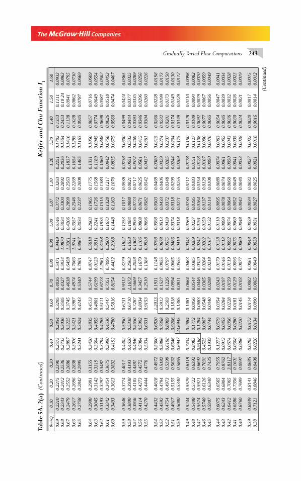
Gradually Varied Flow Computations 243
Tabl
e 5A
. 2(a
) (C
onti
nued
) K
eife
r an
d Ch
u Fu
ncti
on I
1
(Con
tinu
ed)
θ/π\
Qr
0.10
0.20
0.30
0.40
0.50
0.60
0.70
0.80
0.90
1.00
1.07
1.10
1.20
1.30
1.40
1.50
1.60
0.69
0.22
100.
2275
0.23
900.
2573
0.28
540.
3295
0.40
360.
5471
0.94
490.
6146
0.37
720.
3263
0.22
510.
1702
0.13
530.
1111
0.09
330.
680.
2343
0.24
120.
2536
0.27
330.
3036
0.35
050.
4327
0.59
341.
0870
0.50
340.
3304
0.28
920.
2036
0.15
540.
2453
0.10
24
0.08
630.
670.
2479
0.25
520.
2686
0.28
970.
3225
0.37
450.
4638
0.64
581.
3261
0.42
060.
2899
0.25
630.
1837
0.14
160.
1138
0.09
410.
0795
0.66
0.26
170.
2696
0.28
380.
3076
0.34
210.
3987
0.49
740.
7066
1.97
410.
3557
0.25
460.
2269
0.16
540.
1285
0.10
380.
0862
0.07
300.
650.
2758
0.28
420.
2995
0.32
410.
3624
0.42
430.
5340
0.78
010.
6967
0.30
340.
2237
0.20
080.
1485
0.11
630.
0945
0.07
870.
0669
0.64
0.29
000.
2991
0.31
550.
3420
0.38
350.
4513
0.57
440.
8747
0.50
180.
2603
0.19
650.
1775
0.13
310.
1050
0.08
570.
0716
0.06
090.
630.
3045
0.31
420.
3319
0.36
040.
4055
0.48
010.
6199
0.01
230.
3911
0.22
410.
1726
0.15
680.
1189
0.09
450.
0774
0.06
490.
0554
0.62
0.31
930.
3297
0.34
870.
3794
0.42
850.
5111
0.67
231.
2961
0.31
580.
1935
0.15
150.
1383
0.10
600.
0848
0.06
980.
0587
0.05
020.
610.
3342
0.34
540.
3675
0.39
900.
4536
0.54
470.
7351
0.70
960.
2600
0.16
730.
1328
0.12
170.
0942
0.07
580.
0626
0.05
180.
0453
0.60
0.34
930.
3613
0.38
320.
4192
0.47
800.
5816
0.81
540.
4432
0.21
680.
1448
0.11
630.
1070
0.08
350.
0675
0.05
600.
0474
0.04
07
0.59
0.36
460.
3774
0.40
110.
4402
0.50
500.
6231
0.93
120.
3279
0.18
220.
1253
0.10
170.
0938
0.07
380.
0600
0.04
990.
0424
0.03
650.
580.
3800
0.39
380.
4193
0.46
200.
5338
0.67
101.
1673
0.25
630.
1538
0.10
840.
0888
0.08
210.
0651
0.05
320.
0444
0.03
770.
0325
0.57
0.39
560.
4105
0.43
810.
4846
0.56
500.
7287
0.56
690.
2058
0.13
030.
0936
0.07
730.
0717
0.05
720.
0469
0.03
930.
0335
0.02
890.
560.
4114
0.42
730.
4572
0.50
840.
5992
0.80
340.
3457
0.16
790.
1106
0.08
080.
0671
0.06
250.
0501
0.04
120.
0346
0.02
960.
0256
0.55
0.42
700.
4444
0.47
700.
5334
0.66
310.
9153
0.25
100.
1384
0.09
380.
0696
0.05
820.
0542
0.04
370.
0361
0.03
040.
0260
0.02
26
0.54
0.44
320.
4618
0.49
720.
5600
0.6
820
1.20
130.
1931
0.11
480.
0798
0.05
980.
0503
0.04
690.
0380
0.03
150.
0266
0.02
280.
0198
0.53
0.45
920.
4794
0.51
820.
5886
0.7
358
0.39
120.
1527
0.09
550.
0678
0.05
130.
0433
0.04
050.
0329
0.02
740.
0232
0.01
990.
0173
0.52
0.47
540.
4973
0.53
990.
6198
0.8
069
0.25
030.
1226
0.07
970.
0575
0.04
390.
0372
0.03
480.
0285
0.02
370.
0201
0.01
730.
0150
0.51
0.49
170.
5155
0.56
320.
6546
0.9
206
0.18
180.
0994
0.06
650.
0486
0.03
740.
0318
0.02
990.
0244
0.02
040.
0174
0.01
490.
0130
0.50
0.50
800.
5340
0.58
650.
6947
23.6
945
0.13
850.
0811
0.05
550.
0410
0.03
180.
0271
0.02
550.
0209
0.01
750.
0149
0.01
290.
0112
0.49
0.52
440.
5529
0.61
190.
7434
0.2
684
0.10
810.
0664
0.04
630.
0345
0.02
690.
0230
0.02
170.
0178
0.01
500.
0128
0.01
100.
0096
0.48
0.54
080.
5722
0.63
920.
8083
0.1
772
0.08
560.
0544
0.03
850.
0289
0.02
270.
0195
0.01
830.
0151
0.01
270.
0109
0.00
940.
0082
0.47
0.55
740.
5921
0.66
920.
9168
0.1
284
0.06
830.
0446
0.03
200.
0242
0.01
910.
0164
0.01
540.
0128
0.01
080.
0092
0.00
790.
0070
0.46
0.57
400.
6126
0.70
310.
4525
0.0
967
0.05
480.
0365
0.02
640.
0202
0.01
590.
0137
0.01
290.
0107
0.00
900.
0077
0.00
670.
0059
0.45
0.59
070.
6340
0.74
350.
1939
0.0
744
0.04
400.
0298
0.02
180.
0167
0.01
320.
0114
0.01
080.
0090
0.00
760.
0065
0.00
560.
0049
0.44
0.60
750.
6565
0.79
550.
1277
0.0
579
0.03
540.
0243
0.01
790.
0138
0.01
100.
0095
0.00
890.
0074
0.00
630.
0054
0.00
470.
0041
0.43
0.62
430.
6804
0.87
620.
0912
0.0
453
0.02
840.
0197
0.01
460.
0113
0.00
900.
0078
0.00
740.
0061
0.00
520.
0045
0.00
390.
0034
0.42
0.64
120.
7065
3.81
170.
0674
0.0
356
0.02
280.
0159
0.01
190.
0092
0.00
740.
0064
0.00
600.
0050
0.00
430.
0036
0.00
320.
0028
0.41
0.65
860.
7356
0.16
010.
0508
0.0
280
0.01
810.
0129
0.00
960.
0075
0.00
600.
0052
0.00
490.
0041
0.00
350.
0030
0.00
260.
0023
0.40
0.67
600.
7699
0.09
970.
0386
0.0
220
0.01
450.
0103
0.00
770.
0060
0.00
480.
0042
0.00
400.
0033
0.00
280.
0024
0.00
210.
0019
0.39
0.69
390.
8141
0.06
850.
0295
0.0
172
0.01
140.
0082
0.00
610.
0048
0.00
390.
0034
0.00
320.
0027
0.00
220.
0020
0.00
170.
0015
0.38
0.71
210.
8846
0.04
900.
0226
0.0
134
0.00
900.
0065
0.00
490.
0038
0.00
310.
0027
0.00
250.
0021
0.00
180.
0016
0.00
140.
0012
Chapter 5.indd 243Chapter 5.indd 243 2/24/2010 2:59:30 PM2/24/2010 2:59:30 PM
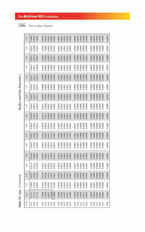
244 Flow in Open Channels
Tabl
e 5A
. 2(a
) (C
onti
nued
) K
eife
r an
d Ch
u Fu
ncti
on I 1
θ/π\
Qr
0.10
0.20
0.30
0.40
0.50
0.60
0.70
0.80
0.90
1.00
1.07
1.10
1.20
1.30
1.40
1.50
1.60
0.37
0.73
110.
2894
0.03
570.
0173
0.0
104
0.00
700.
0051
0.00
390.
0030
0.00
240.
0021
0.00
200.
0017
0.00
140.
0012
0.00
110.
0009
0.36
0.75
100.
1035
0.02
630.
0132
0.0
080
0.00
540.
0039
0.00
300.
0023
0.00
190.
0017
0.00
160.
0013
0.00
110.
0010
0.00
080.
0007
0.35
0.77
250.
0630
0.01
950.
0100
0.0
062
0.00
420.
0030
0.00
230.
0018
0.00
150.
0013
0.00
120.
0010
0.00
090.
0007
0.00
070.
0006
0.34
0.79
640.
0419
0.01
440.
0075
0.0
047
0.00
320.
0023
0.00
180.
0014
0.00
110.
0010
0.00
090.
0008
0.00
070.
0006
0.00
050.
0004
0.33
0.82
460.
0288
0.01
060.
0057
0.0
035
0.00
240.
0018
0.00
140.
0011
0.00
080.
0007
0.00
070.
0006
0.00
050.
0004
0.00
040.
0003
0.32
0.86
250.
0202
0.00
780.
0042
0.0
027
0.00
180.
0013
0.00
100.
0008
0.00
070.
0006
0.00
050.
0004
0.00
040.
0003
0.00
030.
0003
0.31
0.93
780.
0142
0.00
570.
0031
0.0
020
0.00
140.
0010
0.00
070.
0006
0.00
050.
0004
0.00
040.
0003
0.00
030.
0003
0.00
020.
0002
0.30
0.08
950.
0100
0.00
410.
0022
0.0
014
0.00
100.
0007
0.00
050.
0004
0.00
030.
0003
0.00
030.
0003
0.00
020.
0002
0.00
010.
0001
0.29
0.04
460.
0070
0.00
290.
0016
0.00
100.
0007
0.00
050.
0004
0.00
030.
0003
0.00
020.
0002
0.00
020.
0001
0.00
010.
0001
0.00
010.
280.
0265
0.00
490.
0021
0.00
110.
0007
0.00
050.
0004
0.00
030.
0002
0.00
020.
0001
0.00
010.
0001
0.00
010.
0001
0.00
010.
0001
0.27
0.01
670.
0034
0.00
140.
0008
0.00
050.
0003
0.00
030.
0002
0.00
010.
0001
0.00
010.
0001
0.00
010.
0001
0.00
010.
0001
0.00
010.
260.
0107
0.00
230.
0010
0.00
050.
0003
0.00
030.
0002
0.00
010.
0001
0.00
010.
0001
0.00
010.
0001
0.00
010.
0001
0.00
010.
0000
0.25
0.00
690.
0016
0.00
070.
0004
0.00
030.
0002
0.00
010.
0001
0.00
010.
0001
0.00
010.
0001
0.00
010.
0000
0.00
000.
0000
0.00
00
0.24
0.00
450.
0010
0.00
040.
0003
0.00
020.
0001
0.00
010.
0001
0.00
010.
0001
0.00
000.
0000
0.00
000.
0000
0.00
000.
0000
0.00
000.
230.
0028
0.00
070.
0003
0.00
020.
0001
0.00
010.
0001
0.00
010.
0000
0.00
000.
0000
0.00
000.
0000
0.00
000.
0000
0.00
000.
0000
0.22
0.00
180.
0004
0.00
020.
0001
0.00
010.
0001
0.00
000.
0000
0.00
000.
0000
0.00
000.
0000
0.00
000.
0000
0.00
000.
0000
0.00
000.
210.
0011
0.00
030.
0001
0.00
010.
0001
0.00
000.
0000
0.00
000.
0000
0.00
000.
0000
0.00
000.
0000
0.00
000.
0000
0.00
000.
0000
0.20
0.00
070.
0002
0.00
010.
0001
0.00
000.
0000
0.00
000.
0000
0.00
000.
0000
0.00
000.
0000
0.00
000.
0000
0.00
000.
0000
0.00
00
0.19
0.00
040.
0001
0.00
010.
0000
0.00
000.
0000
0.00
000.
0000
0.00
000.
0000
0.00
000.
0000
0.00
000.
0000
0.00
000.
0000
0.00
000.
180.
0002
0.00
010.
0000
0.00
000.
0000
0.00
000.
0000
0.00
000.
0000
0.00
000.
0000
0.00
000.
0000
0.00
000.
0000
0.00
000.
0000
0.17
0.00
010.
0000
0.00
000.
0000
0.00
000.
0000
0.00
000.
0000
0.00
000.
0000
0.00
000.
0000
0.00
000.
0000
0.00
000.
0000
0.00
000.
160.
0001
0.00
000.
0000
0.00
000.
0000
0.00
000.
0000
0.00
000.
0000
0.00
000.
0000
0.00
000.
0000
0.00
000.
0000
0.00
000.
0000
0.15
0.00
000.
0000
0.00
000.
0000
0.00
000.
0000
0.00
000.
0000
0.00
000.
0000
0.00
000.
0000
0.00
000.
0000
0.00
000.
0000
0.00
00
0.00
0.00
000.
0000
0.00
000.
0000
0.00
000.
0000
0.00
000.
0000
0.00
000.
0000
0.00
000.
0000
0.00
000.
0000
0.00
000.
0000
0.00
00
Chapter 5.indd 244Chapter 5.indd 244 2/24/2010 2:59:30 PM2/24/2010 2:59:30 PM
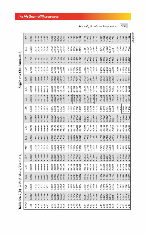
Gradually Varied Flow Computations 245 θ/
π\Q
r0.
100.
200.
300.
400.
500.
600.
700.
800.
901.
001.
071.
101.
201.
301.
401.
501.
60
1.00
0.00
000.
0000
0.00
000.
0000
0.00
000.
0000
0.00
000.
0000
0.00
000.
0000
18.0
736
6.69
443.
6096
2.70
082.
1760
1.81
761.
5488
0.99
0.00
000.
0000
0.00
000.
0000
0.00
000.
0000
0.00
000.
0000
0.00
000.
0000
18.0
736
6.69
443.
6096
2.70
082.
1760
1.81
761.
5488
0.98
0.00
000.
0000
0.00
000.
0000
0.00
000.
0000
0.00
000.
0000
0.00
000.
0000
18.0
736
6.69
443.
6096
2.70
082.
1760
1.81
761.
5488
0.97
0.00
000.
0000
0.00
000.
0000
0.00
000.
0000
0.00
000.
0000
0.00
000.
0128
18.0
736
6.69
443.
6096
2.70
082.
1760
1.81
761.
5488
0.96
0.00
000.
0000
0.00
000.
0000
0.00
000.
0000
0.00
000.
0000
0.00
000.
0256
18.0
736
6.68
163.
6096
2.70
082.
1760
1.81
761.
5488
0.95
0.00
000.
0000
0.00
000.
0000
0.00
000.
0000
0.00
000.
0000
0.00
000.
0256
18.0
608
6.68
163.
6096
2.70
082.
1760
1.81
761.
5488
0.94
0.00
000.
0000
0.00
000.
0000
0.00
000.
0000
0.00
000.
0000
0.01
280.
0384
18.0
480
6.66
883.
6096
2.70
082.
1760
1.80
481.
5360
0.93
0.00
000.
0000
0.00
000.
0000
0.00
000.
0000
0.01
280.
0128
0.01
280.
0640
18.0
224
6.65
603.
5968
2.70
082.
1760
1.80
481.
5360
0.92
0.00
000.
0000
0.00
000.
0000
0.01
280.
0128
0.01
280.
0128
0.02
560.
0768
17.9
712
6.64
323.
5968
2.70
082.
1760
1.80
481.
5360
0.91
0.01
280.
0128
0.01
280.
0128
0.01
280.
0128
0.01
280.
0128
0.02
560.
1024
17.9
072
6.61
763.
5840
2.68
802.
1632
1.80
481.
5360
0.90
0.01
280.
0128
0.01
280.
0128
0.01
280.
0128
0.01
280.
0256
0.03
840.
1280
17.7
664
6.57
923.
5712
2.68
802.
1632
1.80
481.
5360
0.89
0.01
280.
0128
0.01
280.
0128
0.01
280.
0256
0.02
560.
0384
0.05
120.
1664
17.4
720
6.52
803.
5584
2.67
522.
1632
1.80
481.
5360
0.88
0.01
280.
0128
0.02
560.
0256
0.02
560.
0256
0.03
840.
0384
0.06
400.
1920
16.4
480
6.46
403.
5456
2.67
522.
1504
1.79
201.
5232
0.87
0.02
560.
0256
0.02
560.
0256
0.02
560.
0384
0.03
840.
0512
0.08
960.
2304
0.00
006.
3744
3.53
282.
6624
2.15
041.
7920
1.52
320.
860.
0256
0.02
560.
0256
0.03
840.
0384
0.03
840.
0512
0.06
400.
1024
0.28
1655
.974
46.
2592
3.50
722.
6496
2.13
761.
7792
1.52
320.
850.
0384
0.03
840.
0384
0.03
840.
0512
0.05
120.
0640
0.07
680.
1280
0.33
2856
.742
46.
1184
3.48
162.
6368
2.12
481.
7792
1.51
04
0.84
0.03
840.
0384
0.05
120.
0512
0.05
120.
0640
0.07
680.
1024
0.15
360.
3840
57.4
848
5.95
203.
4432
2.61
122.
1120
1.76
641.
5104
0.83
0.05
120.
0512
0.05
120.
0640
0.06
400.
0768
0.08
960.
1152
0.17
920.
4480
58.3
296
5.77
283.
4176
2.59
842.
0992
1.75
361.
4976
0.82
0.06
400.
0640
0.06
400.
0768
0.07
680.
0896
0.10
240.
1408
0.21
730.
5248
59.4
944
5.56
803.
3664
2.57
282.
0864
1.75
361.
4976
0.81
0.07
680.
0768
0.07
680.
0896
0.08
960.
1024
0.12
800.
1664
0.25
600.
6016
61.9
648
5.35
043.
3208
2.56
002.
0736
1.74
081.
4848
0.80
0.08
960.
0896
0.08
960.
1024
0.11
520.
1280
0.15
360.
1920
0.29
440.
7040
8.9
856
5.13
283.
2768
2.53
442.
0608
1.72
801.
4720
0.79
0.10
240.
1024
0.10
240.
1152
0.12
800.
1408
0.17
920.
2304
0.34
560.
8192
7.11
684.
9280
3.22
562.
4960
2.03
521.
7152
1.45
920.
780.
1152
0.11
520.
1280
0.12
800.
1408
0.16
640.
2048
0.25
600.
3968
0.96
006.
2464
4.72
323.
1744
2.47
042.
0224
1.68
961.
4464
0.77
0.12
800.
1408
0.14
080.
1536
0.16
640.
1920
0.23
040.
2944
0.46
081.
1264
5.67
044.
5312
3.12
322.
4320
1.99
681.
6768
1.43
360.
760.
1536
0.15
360.
1664
0.17
920.
1920
0.21
760.
2688
0.34
560.
5248
1.34
405.
2608
4.35
203.
0592
2.40
641.
9712
0.66
400.
4208
0.75
0.16
640.
1792
0.17
920.
1920
0.21
760.
2560
0.30
720.
3968
0.61
441.
6256
4.91
524.
1856
2.99
522.
3680
1.94
561.
6384
1.40
80
0.74
0.19
200.
2048
0.20
480.
2304
0.24
320.
2816
0.34
560.
4480
0.70
402.
0480
4.64
644.
0320
2.93
122.
3296
1.92
001.
6256
1.39
520.
730.
2176
0.23
040.
2432
0.25
600.
2816
0.32
000.
3968
0.51
200.
8192
2.80
324.
4032
3.87
842.
8672
2.29
121.
8944
1.60
001.
3824
0.72
0.24
320.
2560
0.26
880.
2816
0.32
000.
3712
0.44
800.
5888
0.96
009.
8816
4.19
843.
7376
2.80
322.
2528
1.86
881.
5744
1.35
680.
710.
2816
0.28
160.
2944
0.32
000.
3584
0.40
960.
4992
0.67
841.
1264
6.13
124.
0192
3.60
962.
7392
2.20
161.
8304
1.56
161.
3440
0.70
0.30
720.
3200
0.33
280.
3584
0.39
680.
4608
0.57
600.
7808
1.34
405.
4016
3.85
283.
4944
2.67
522.
1632
1.80
481.
5360
1.31
84
Tabl
e 5A
. 2(b
) Ta
ble
of V
alue
s of
Fun
ctio
n I 2
Kei
fer
and
Chu
Func
tion
I2
(Con
tinu
ed)
Chapter 5.indd 245Chapter 5.indd 245 2/24/2010 2:59:31 PM2/24/2010 2:59:31 PM
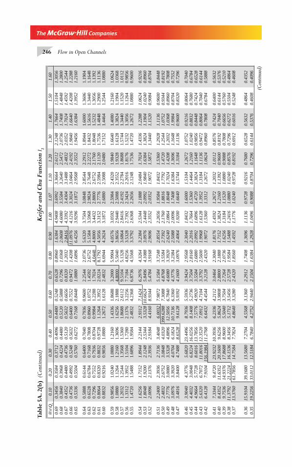
246 Flow in Open Channels
(Con
tinu
ed)
θ/π\
Qr
0.10
0.20
0.30
0.40
0.50
0.60
0.70
0.80
0.90
1.00
1.07
1.10
1.20
1.30
1.40
1.50
1.60
0.69
0.34
560.
3584
0.37
120.
4096
0.44
800.
5248
0.65
280.
8960
1.63
844.
9408
3.69
923.
3664
2.61
122.
1248
1.76
641.
5104
1.30
560.
680.
3840
0.39
680.
4224
0.44
800.
5120
0.58
880.
7296
1.03
682.
0608
4.60
803.
5584
3.26
402.
5472
2.07
361.
7408
1.48
481.
2800
0.67
0.43
520.
4480
0.47
360.
5120
0.56
320.
6656
0.83
201.
2032
2.84
164.
3392
3.43
043.
1488
2.48
322.
0352
1.70
241.
4592
1.25
440.
660.
4736
0.49
920.
5248
0.56
320.
6400
0.75
520.
9472
1.42
0811
.097
64.
1216
3.30
243.
0464
2.41
921.
9840
1.66
401.
4208
1.22
880.
650.
5336
0.55
040.
5760
0.62
720.
7168
0.84
481.
0880
1.68
966.
4256
3.92
963.
1872
2.95
682.
3552
1.94
561.
6384
1.39
521.
2160
0.64
0.58
880.
6144
0.64
000.
7040
0.79
360.
9600
2.25
442.
0736
5.63
203.
7504
3.08
482.
8544
2.29
121.
8944
1.60
001.
3606
1.19
040.
630.
6528
0.67
840.
7168
0.78
080.
8960
1.07
521.
4592
2.67
525.
1584
3.59
682.
9824
2.76
482.
2272
1.84
321.
5616
1.34
401.
1648
0.62
0.72
960.
7552
0.79
360.
8704
0.99
841.
2288
1.70
244.
0448
4.80
003.
4432
2.88
002.
6752
2.17
601.
8048
1.52
321.
3056
1.13
920.
610.
8064
0.83
200.
8832
0.97
281.
1264
1.39
522.
0224
8.17
924.
5056
3.31
522.
7776
2.59
842.
1120
1.75
361.
4848
1.29
001.
1136
0.60
0.88
320.
9216
0.98
561.
0880
1.26
721.
6128
2.48
326.
6944
4.26
243.
1872
2.68
802.
5088
2.04
801.
7152
1.44
641.
2544
1.08
80
0.59
0.98
561.
0240
1.08
801.
2160
1.43
361.
8688
3.20
005.
9904
4.05
763.
0592
2.59
842.
4320
1.98
401.
6640
1.40
801.
2160
1.06
240.
581.
0880
1.12
641.
2160
1.36
961.
6256
2.18
884.
8000
5.50
403.
8656
2.94
402.
5088
2.35
521.
9328
1.61
281.
3824
1.19
041.
0368
0.57
1.20
321.
2544
1.35
681.
5360
1.86
882.
6112
9.51
045.
1328
3.68
642.
8416
2.41
922.
2784
1.86
881.
5744
1.34
401.
1520
1.01
120.
561.
3312
1.39
521.
5104
1.72
802.
1376
3.22
567.
7184
4.82
563.
5328
2.73
922.
3424
2.20
161.
8176
1.52
321.
3056
1.12
640.
9856
0.55
1.47
201.
5488
1.68
961.
9584
2.48
324.
2368
6.87
364.
5568
3.37
922.
6368
2.26
562.
1248
1.75
361.
4720
1.26
721.
0880
0.96
00
0.54
1.62
561.
7152
1.
8944
2.2
144
2
.931
2 7
.142
46.
2976
4.32
643.
2384
2.53
442.
1888
2.04
841.
7024
1.43
361.
2288
1.06
240.
9216
0.53
1.80
481.
9200
2.
1248
2.5
344
3
.532
810
.662
45.
8496
4.10
883.
0976
2.44
482.
0992
1.98
401.
6384
1.38
241.
1904
1.02
400.
8960
0.52
2.00
96 2
.137
6
2.39
36 2
.918
4
4.4
160
8.9
344
5.47
843.
9168
2.96
962.
3552
2.03
521.
9072
1.58
721.
3440
1.15
200.
9084
0.87
04
0.51
2.24
002.
3936
2.
7136
3.4
048
6
.003
2 7
.987
25.
1584
3.72
482.
8554
2.26
561.
9584
1.84
321.
5360
1.29
281.
1136
0.96
000.
8448
0.50
2.48
32 2
.675
2
3.08
48 4
.032
039
9.62
88 7
.308
84.
8768
3.55
842.
7392
2.17
601.
8816
1.77
921.
4720
1.25
441.
0752
0.93
440.
8192
0.49
2.77
76 3
.008
0
3.53
28 4
.889
612
.505
6 6
.784
04.
6080
3.39
202.
6240
2.08
641.
8048
1.70
241.
4208
1.20
321.
0368
0.89
600.
7808
0.48
3.09
76 3
.392
0
4.07
04 6
.182
410
.713
6 6
.336
04.
3776
3.23
842.
5088
2.00
961.
7408
1.63
841.
3696
1.16
481.
9984
0.87
040.
7552
0.47
3.48
16 3
.840
0
4.74
88 8
.652
8
9.6
128
5.9
392
4.16
003.
0976
2.40
641.
9200
1.66
401.
5744
1.31
841.
1136
0.96
000.
8320
0.72
96
0.46
3.90
40 4
.377
6
5.68
2023
.449
6
8.7
936
5.5
936
3.94
242.
9568
2.30
401.
8432
1.60
001.
5104
1.26
721.
0752
0.92
160.
8064
0.70
400.
454.
4032
3.0
048
6.
8224
16.0
256
8
.140
8 5
.273
63.
7504
2.81
602.
2016
1.76
641.
5360
1.44
641.
2160
1.02
400.
8832
0.76
800.
6784
0.44
4.96
64 5
.772
8
8.60
1613
.785
6
7.5
776
4.9
920
3.55
842.
6880
2.09
921.
6896
1.47
201.
3824
1.16
480.
9856
0.84
480.
7424
0.65
280.
435.
6320
6.7
072
11.
8016
12.3
520
7
.091
2 4
.710
43.
3792
2.56
001.
9968
1.61
281.
3952
1.31
841.
1136
0.94
720.
8064
0.70
400.
6144
0.42
6.41
28 7
.910
415
6.19
8411
.276
8
6.6
432
4.4
544
3.21
282.
4320
1.90
721.
5360
1.33
121.
2672
1.06
240.
8960
0.78
080.
6784
0.58
88
0.41
7.33
44 9
.472
0 2
3.92
3210
.393
6
6.2
336
4.2
112
3.04
642.
3040
1.81
761.
4592
1.26
721.
2032
1.01
120.
8576
0.74
240.
6400
0.56
320.
408.
4352
11.6
352
20.
1600
9.6
256
5
.862
4 3
.980
82.
8800
2.18
881.
7152
1.38
241.
2160
1.13
920.
9600
0.81
920.
7040
0.61
440.
5376
0.39
9.75
3614
.937
6 1
7.86
88 8
.960
0
5.5
040
3.7
504
2.72
642.
0736
1.62
561.
3184
1.15
201.
0880
0.90
880.
7808
0.66
560.
5760
0.52
100.
3811
.379
221
.222
4 1
6.15
36 8
.345
6
5.1
712
3.5
456
2.57
281.
9584
1.54
881.
2416
1.08
801.
0240
0.85
760.
7296
0.62
720.
5504
0.48
640.
3713
.376
061
.785
6 1
4.75
84 7
.782
4
4.8
640
3.3
280
2.43
201.
8560
1.45
921.
1776
1.02
400.
9728
0.81
920.
6912
0.60
160.
5248
0.46
08
0.36
15.9
104
39.1
680
13.
5680
7.2
704
4
.556
8 3
.136
02.
2912
1.74
081.
3696
1.11
360.
9728
0.92
160.
7680
0.65
280.
5632
0.48
640.
4352
0.35
19.2
256
33.0
112
12.
5184
6.7
840
4
.275
2 2
.944
02.
1504
1.63
841.
2928
1.04
960.
9088
0.87
040.
7296
0.61
440.
5376
0.46
080.
4096
Tabl
e 5A
. 2(b
) (C
onti
nued
) K
eife
r an
d Ch
u Fu
ncti
on I 2
Chapter 5.indd 246Chapter 5.indd 246 2/24/2010 2:59:31 PM2/24/2010 2:59:31 PM
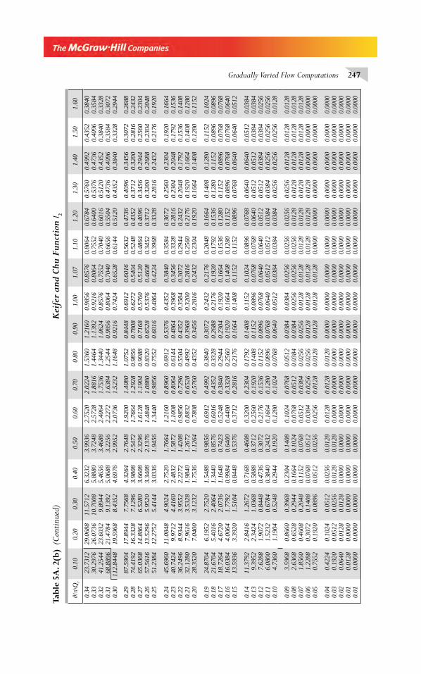
Gradually Varied Flow Computations 247 θ/
π\Q
r0.
100.
200.
300.
400.
500.
600.
700.
800.
901.
001.
071.
101.
201.
301.
401.
501.
60
0.34
23.7
312
29.0
688
11.5
712
6.32
323.
9936
2.75
202.
0224
1.53
601.
2160
0.98
560.
8576
0.80
640.
6784
0.57
600.
4992
0.43
520.
3840
0.33
30.2
976
26.0
736
10.7
008
5.88
803.
7248
2.57
281.
8816
1.44
641.
1392
0.92
160.
8064
0.75
520.
6400
0.53
760.
4736
0.40
960.
3584
0.32
41.2
544
23.6
032
9.8
944
5.46
563.
4688
2.40
641.
7536
1.34
401.
0624
0.85
760.
7552
0.70
400.
6016
0.51
200.
4352
0.38
400.
3328
0.31
68.8
896
21.4
784
9.1
392
5.06
883.
2256
2.22
721.
6384
1.25
440.
9856
0.80
640.
7040
0.66
560.
5504
0.47
360.
4096
0.35
840.
3072
0.30
112.
8448
19.5
968
8.4
352
4.69
762.
9952
2.07
361.
5232
1.16
480.
9216
0.74
240.
6528
0.61
440.
5120
0.43
520.
3840
0.33
280.
2944
0.29
87.5
904
17.8
944
7.7
568
4.32
642.
7648
1.92
001.
4080
1.07
520.
8448
0.69
120.
6016
0.56
320.
4736
0.40
960.
3456
0.30
720.
2688
0.28
74.4
192
16.3
328
7.1
296
3.98
082.
5472
1.76
641.
2928
0.98
560.
7808
0.62
720.
5404
0.52
480.
4352
0.37
120.
3200
0.28
160.
2432
0.27
65.0
368
14.8
864
6.5
280
3.66
082.
3296
1.61
281.
1904
0.90
880.
7168
0.57
600.
5120
0.48
640.
4096
0.34
560.
2944
0.25
600.
2304
0.26
57.5
616
13.5
296
5.9
520
3.34
082.
1376
1.48
481.
0880
0.83
200.
6528
0.53
760.
4608
0.34
520.
3712
0.32
000.
2688
0.23
040.
2048
0.25
51.2
384
12.2
752
5.4
144
3.03
361.
9456
1.34
400.
9856
0.75
520.
6016
0.48
640.
4224
0.39
680.
3328
0.28
160.
2432
0.21
760.
1920
0.24
45.6
960
11.0
848
4.9
024
2.75
201.
7664
1.21
600.
8960
0.69
120.
5376
0.43
520.
3840
0.35
840.
3672
0.25
600.
2304
0.19
200.
1664
0.23
40.7
424
9.9
712
4.4
160
2.48
321.
5872
1.10
080.
8064
0.61
440.
4864
0.39
680.
3456
0.33
280.
2816
0.23
040.
2048
0.17
920.
1536
0.22
36.2
496
8.9
344
3.9
552
2.22
721.
4208
0.98
560.
7296
0.55
040.
4352
0.35
840.
3072
0.29
440.
2432
0.20
480.
1792
0.15
360.
1408
0.21
32.1
280
7.9
616
3.5
328
1.98
401.
2672
0.88
320.
6528
0.49
920.
3968
0.32
000.
2816
0.25
600.
2176
0.19
200.
1664
0.14
080.
1280
0.20
28.3
520
7.0
400
3.1
232
1.75
361.
1264
0.78
080.
5760
0.43
520.
3456
0.28
160.
2432
0.23
040.
1920
0.16
640.
1408
0.12
800.
1152
0.19
24.8
704
6.1
952
2.7
520
1.54
880.
9856
0.69
120.
4992
0.38
400.
3072
0.24
320.
2176
0.20
480.
1664
0.14
080.
1280
0.11
520.
1024
0.18
21.6
704
5.4
016
2.4
064
1.34
400.
8576
0.60
160.
4352
0.33
280.
2688
0.21
760.
1920
0.17
920.
1536
0.12
800.
1152
0.08
960.
0896
0.17
18.7
264
4.6
720
2.0
736
1.16
480.
7423
0.52
480.
3840
0.29
440.
2304
0.19
200.
1664
0.15
360.
1280
0.11
520.
0896
0.07
680.
0768
0.16
16.0
384
4.0
064
1.7
792
0.99
840.
6400
0.44
800.
3328
0.25
600.
1920
0.16
640.
1408
0.12
800.
1152
0.08
960.
0768
0.07
680.
0640
0.15
13.5
936
3.3
920
1.5
104
0.84
480.
5376
0.37
120.
2816
0.21
760.
1664
0.14
080.
1152
0.11
520.
0896
0.07
680.
0640
0.06
400.
0512
0.14
11.3
792
2.8
416
1.2
672
0.71
680.
4608
0.32
000.
2304
0.17
920.
1408
0.11
520.
1024
0.08
960.
0768
0.06
400.
0640
0.05
120.
0384
0.13
9.39
52 2
.342
4 1
.036
80.
5888
0.37
120.
2560
0.19
200.
1408
0.11
520.
0896
0.07
680.
0768
0.06
400.
0512
0.05
120.
0384
0.03
840.
127.
6288
1.9
072
0.8
448
0.47
360.
3072
0.21
760.
1536
0.11
520.
0896
0.07
680.
0640
0.06
400.
0512
0.05
120.
0384
0.03
840.
0256
0.11
6.08
001.
5232
0.67
840.
3840
0.24
320.
1664
0.12
800.
0896
0.07
680.
0640
0.05
120.
0512
0.03
840.
0384
0.02
560.
0256
0.02
560.
104.
7360
1.19
040.
5248
0.29
440.
1920
0.12
800.
1024
0.07
680.
0640
0.05
120.
0384
0.03
840.
0384
0.02
560.
0256
0.02
560.
0128
0.09
3.59
680.
8660
0.39
680.
2304
0.14
080.
1024
0.07
680.
0512
0.03
840.
0384
0.02
560.
0256
0.02
560.
0256
0.01
280.
0128
0.01
280.
082.
6368
0.65
280.
2944
0.16
640.
1024
0.07
680.
0512
0.03
840.
0384
0.02
560.
0256
0.02
560.
0128
0.01
280.
0128
0.01
280.
0128
0.07
1.85
600.
4608
0.20
480.
1152
0.07
680.
0512
0.03
840.
0256
0.02
560.
0128
0.01
280.
0128
0.01
280.
0128
0.01
280.
0128
0.01
280.
061.
2288
0.30
720.
1408
0.07
680.
0512
0.03
840.
0256
0.02
560.
0128
0.01
280.
0128
0.01
280.
0128
0.01
280.
0000
0.00
000.
0000
0.05
0.75
520.
1920
0.08
960.
0512
0.02
560.
0256
0.01
280.
0128
0.01
280.
0128
0.01
280.
0000
0.00
000.
0000
0.00
000.
0000
0.00
00
0.04
0.42
240.
1024
0.05
120.
0256
0.01
280.
0128
0.01
280.
0128
0.00
000.
0000
0.00
000.
0000
0.00
000.
0000
0.00
000.
0000
0.00
000.
030.
1920
0.05
120.
0256
0.01
280.
0128
0.00
000.
0000
0.00
000.
0000
0.00
000.
0000
0.00
000.
0000
0.00
000.
0000
0.00
000.
0000
0.02
0.06
400.
0128
0.01
280.
0000
0.00
000.
0000
0.00
000.
0000
0.00
000.
0000
0.00
000.
0000
0.00
000.
0000
0.00
000.
0000
0.00
000.
010.
0128
0.00
000.
0000
0.00
000.
0000
0.00
000.
0000
0.00
000.
0000
0.00
000.
0000
0.00
000.
0000
0.00
000.
0000
0.00
000.
0000
0.01
0.00
000.
0000
0.00
000.
0000
0.00
000.
0000
0.00
000.
0000
0.00
000.
0000
0.00
000.
0000
0.00
000.
0000
0.00
000.
0000
0.00
00
Tabl
e 5A
. 2(b
) (C
onti
nued
) K
eife
r an
d Ch
u Fu
ncti
on I 2
Chapter 5.indd 247Chapter 5.indd 247 2/24/2010 2:59:31 PM2/24/2010 2:59:31 PM
6.1 INTRODUCTION
Hydraulic jump is one subject which has extensively been studied in the fi eld of hydraulic engineering. It is an intriguing and interesting phenomenon that has caught the imagination of many research workers since its fi rst description by Leonardo da Vinci. The Italian engineer Bidone (1818) is credited with the fi rst experimental investigation of this phenomenon. Since then considerable research effort has gone into the study of this subject. The literature on this topic is vast and ever-expanding. The main reason for such continued interest in this topic is its immense practical utility in hydraulic engineering and allied fi elds. A hydraulic jump primarily serves as an energy dissipator to dissipate the excess energy of fl owing water downstream of hydraulic structures, such as spillways and sluice gates. Some of the other uses are: (a) effi cient operation of fl ow-measurement fl umes, (b) mixing of chemicals, (c) to aid intense mixing and gas transfer in chemical processes, (d) in the desalination of sea water, and (e) in the aeration of streams which are polluted by bio-degradable wastes.
A hydraulic jump occurs when a supercritical stream meets a subcritical stream of suffi cient depth. The supercritical stream jumps up to meet its alternate depth. While doing so it generates considerable disturbances in the form of large-scale eddies and a reverse fl ow roller with the result that the jump falls short of its alternate depth. Figure 6.1 is a schematic sketch of a typical hydraulic jump in a horizontal channel. Section 1, where the incoming supercritical stream undergoes an abrupt rise in the depth forming the commencement of the jump, is called the toe of the jump. The jump proper consists of a steep change in the water-surface elevation with a reverse fl ow roller on the major part. The roller entrains considerable quantity of air and the sur-face has white, frothy and choppy appearance. The jump, while essentially steady, will normally oscillate about a mean position in the longitudinal direction and the surface will be uneven. Section 2, which lies beyond the roller and with an essen-tially level water surface is called the end of the jump and the distance between Sections 1 and 2 is the length of the jump, L
j. The initial depth of the supercritical
stream is y1 and y
2 is the fi nal depth, after the jump, of the subcritical stream. As indi-
cated earlier, y2 will be smaller than the depth alternate to y
1. The two depths y
1. and
y2 at the ends of the jump are called sequent depths. Due to high turbulence and shear
action of the roller, there is considerable loss of energy in the jump between Sections 1 and 2. In view of the high energy loss, the nature of which is diffi cult to estimate,
Rapidly Varied Flow-1
—Hydraulic Jump 6
Chapter 6.indd 248Chapter 6.indd 248 2/24/2010 3:00:02 PM2/24/2010 3:00:02 PM
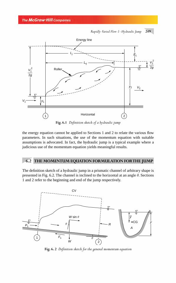
Rapidly-Varied Flow-1–Hydraulic Jump 249
the energy equation cannot be applied to Sections 1 and 2 to relate the various fl ow parameters. In such situations, the use of the momentum equation with suitable assumptions is advocated. In fact, the hydraulic jump is a typical example where a judicious use of the momentum equation yields meaningful results.
6.2 THE MOMENTUM EQUATION FORMULATION FOR THE JUMP
The defi nition sketch of a hydraulic jump in a prismatic channel of arbitrary shape is presented in Fig. 6.2. The channel is inclined to the horizontal at an angle θ. Sections 1 and 2 refer to the beginning and end of the jump respectively.
Fig. 6.1 Defi nition sketch of a hydraulic jump
V2y2
∇
EL
V22
2gV1
2
2g
∇
1 2
Roller
Lj
Lrj
y1V1
Energy line
Horizontal
Fig. 6. 2 Defi nition sketch for the general momentum equation
θ
θFs
W1
2
P1R
∇∇
∇
CV
y
y
CG
A
W sin θ
Chapter 6.indd 249Chapter 6.indd 249 2/24/2010 3:00:05 PM2/24/2010 3:00:05 PM
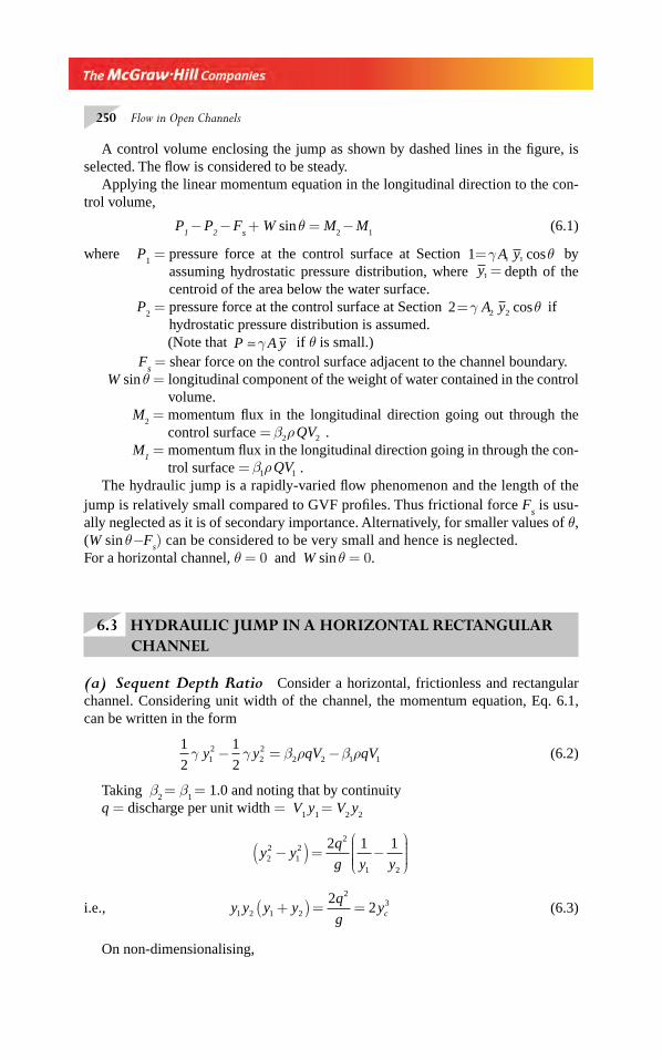
250 Flow in Open Channels
A control volume enclosing the jump as shown by dashed lines in the fi gure, is selected. The fl ow is considered to be steady.
Applying the linear momentum equation in the longitudinal direction to the con-trol volume,
P1 −
P
2 −
F
s + W sin θ = M
2 −
M
1 (6.1)
where P1 = pressure force at the control surface at Section 1 1 1=γ θA y cos by
assuming hydrostatic pressure distribution, where y1 = depth of the centroid of the area below the water surface.
P2 = pressure force at the control surface at Section 2 2 2=γ θA y cos if
hydrostatic pressure distribution is assumed. (Note that P A y� γ if θ is small.) F
s = shear force on the control surface adjacent to the channel boundary.
W sin θ = longitudinal component of the weight of water contained in the control volume.
M2 = momentum fl ux in the longitudinal direction going out through the
control surface = β ρ2 2QV . M
1 = momentum fl ux in the longitudinal direction going in through the con-
trol surface = β ρ1 1QV .The hydraulic jump is a rapidly-varied fl ow phenomenon and the length of the
jump is relatively small compared to GVF profi les. Thus frictional force Fs is usu-
ally neglected as it is of secondary importance. Alternatively, for smaller values of θ, (W sin θ−F
s) can be considered to be very small and hence is neglected.
For a horizontal channel, θ = 0 and W sin θ = 0.
6.3 HYDRAULIC JUMP IN A HORIZONTAL RECTANGULAR CHANNEL
(a) Sequent Depth Ratio Consider a horizontal, frictionless and rectangular channel. Considering unit width of the channel, the momentum equation, Eq. 6.1, can be written in the form
1
2
1
212
22
2 2 1 1γ γ β ρ β ρy y qV qV− = − (6.2)
Taking β2 = β
1 = 1.0 and noting that by continuity
q = discharge per unit width = V1 y
1 = V
2 y
2
y yq
g y y22
12
2
1 2
2 1 1−( ) = −
⎛
⎝⎜⎜⎜⎜
⎞
⎠⎟⎟⎟⎟
i.e., y y y yq
gyc1 2 1 2
232
2+( ) = = (6.3)
On non-dimensionalising,
Chapter 6.indd 250Chapter 6.indd 250 2/24/2010 3:00:06 PM2/24/2010 3:00:06 PM
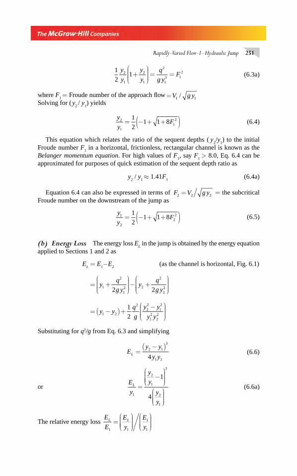
Rapidly-Varied Flow-1–Hydraulic Jump 251
1
212
1
2
1
2
13 1
2y
y
y
y
q
g yF+
⎛
⎝⎜⎜⎜⎜
⎞
⎠⎟⎟⎟⎟
= = (6.3a)
where F1 = Froude number of the approach fl ow =V g y1 1/
Solving for ( y2 / y
1) yields
y
yF2
1121
21 1 8= − + +( ) (6.4)
This equation which relates the ratio of the sequent depths ( y2/y
1) to the initial
Froude number F1 in a horizontal, frictionless, rectangular channel is known as the
Belanger momentum equation. For high values of F1, say F
1 > 8.0, Eq. 6.4 can be
approximated for purposes of quick estimation of the sequent depth ratio as
y2 / y
1 ≈ 1.41F
1 (6.4a)
Equation 6.4 can also be expressed in terms of F V g y2 2 2= = the subcritical Froude number on the downstream of the jump as
y
yF1
2221
21 1 8= − + +( ) (6.5)
(b) Energy Loss The energy loss EL in the jump is obtained by the energy equation
applied to Sections 1 and 2 as
EL = E
1−E
2 (as the channel is horizontal, Fig. 6.1)
= +⎛
⎝⎜⎜⎜⎜
⎞
⎠⎟⎟⎟⎟− +
⎛
⎝⎜⎜⎜⎜
⎞
⎠⎟⎟⎟⎟
yq
g yy
q
g y1
2
12 2
2
222 2
= −( )+
−⎛
⎝⎜⎜⎜⎜
⎞
⎠⎟⎟⎟⎟
y yq
g
y y
y y1 2
222
12
12
22
1
2
Substituting for q2/g from Eq. 6.3 and simplifying
Ey y
y yL =−( )2 1
3
1 24 (6.6)
or E
y
y
y
y
y
L
1
2
1
3
2
1
1
4
=
−⎛
⎝⎜⎜⎜⎜
⎞
⎠⎟⎟⎟⎟
⎛
⎝⎜⎜⎜⎜
⎞
⎠⎟⎟⎟⎟
(6.6a)
The relative energy loss E
E
E
y
E
yL L
1
1=⎛
⎝⎜⎜⎜⎜
⎞
⎠⎟⎟⎟⎟
⎛
⎝⎜⎜⎜⎜
⎞
⎠⎟⎟⎟⎟
1 1
Chapter 6.indd 251Chapter 6.indd 251 2/24/2010 3:00:06 PM2/24/2010 3:00:06 PM
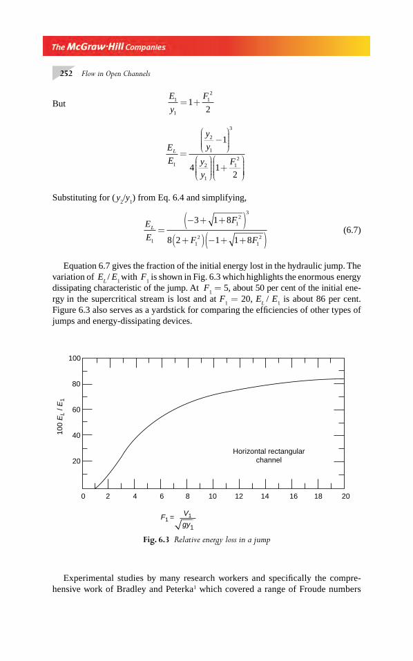
252 Flow in Open Channels
But E
y
F1
1
12
12
= +
E
E
y
y
y
y
FL
1
2
1
3
2
1
12
1
4 12
=
−⎛
⎝⎜⎜⎜⎜
⎞
⎠⎟⎟⎟⎟
⎛
⎝⎜⎜⎜⎜
⎞
⎠⎟⎟⎟⎟
+⎛
⎝⎜⎜⎜⎜
⎞
⎠⎟⎟⎟⎟⎟
Substituting for ( y2/y
1) from Eq. 6.4 and simplifying,
E
E
F
F F
L
1
12
3
12
12
3 1 8
8 2 1 1 8=
− + +( )+( ) − + +( )
(6.7)
Equation 6.7 gives the fraction of the initial energy lost in the hydraulic jump. The variation of E
L / E
1 with F
1 is shown in Fig. 6.3 which highlights the enorm ous energy
dissipating characteristic of the jump. At F1 = 5, about 50 per cent of the initial ene-
rgy in the supercritical stream is lost and at F1 = 20, E
L / E
1 is about 86 per cent.
Figure 6.3 also serves as a yardstick for comparing the effi ciencies of other types of jumps and energy-dissipating devices.
0 2 4 6 8 12 14 1810 16 20
100
80
60
40
20
100
EL
/ E1
Horizontal rectangularchannel
F1 = V1
gy1
Fig. 6.3 Relative energy loss in a jump
Experimental studies by many research workers and specifi cally the compre-hensive work of Bradley and Peterka1 which covered a range of Froude numbers
Chapter 6.indd 252Chapter 6.indd 252 2/24/2010 3:00:07 PM2/24/2010 3:00:07 PM
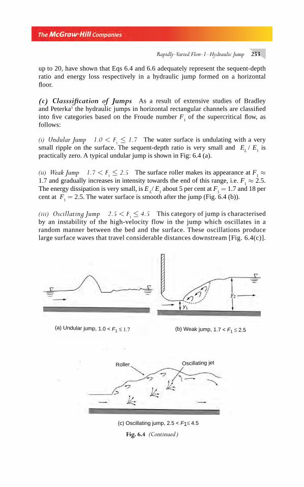
Rapidly-Varied Flow-1–Hydraulic Jump 253
up to 20, have shown that Eqs 6.4 and 6.6 adequately represent the sequent-depth ratio and energy loss respectively in a hydraulic jump formed on a horizontal fl oor.
(c) Classsifi cation of Jumps As a result of extensive studies of Bradley and Peterka1 the hydraulic jumps in horizontal rectangular channels are classifi ed into fi ve categories based on the Froude number F
1 of the supercritical fl ow, as
follows:
(i) Undular Jump 1.0 < F1 ≤ 1.7 The water surface is undulating with a very
small ripple on the surface. The sequent-depth ratio is very small and EL
/ E1 is
practically zero. A typical undular jump is shown in Fig: 6.4 (a).
(ii) Weak Jump 1.7 < F1 ≤ 2.5 The surface roller makes its appearance at F
1 ≈
1.7 and gradually increases in intensity towards the end of this range, i.e. F1 ≈ 2.5.
The energy dissipation is very small, is E L/ E
1 about 5 per cent at F
1 = 1.7 and 18 per
cent at F1 = 2.5. The water surface is smooth after the jump (Fig. 6.4 (b)).
(iii) Oscillating Jump 2.5 < F1 ≤ 4.5 This category of jump is characterised
by an instability of the high-velocity flow in the jump which oscillates in a random manner between the bed and the surface. These oscillations produce large surface waves that travel considerable distances downstream [Fig. 6.4(c)].
Roller
∇ ∇
∇
y2
y1
Oscillating jet
(b) Weak jump, 1.7 < F1 ≤ 2.5(a) Undular jump, 1.0 < F1 ≤ 1.7
(c) Oscillating jump, 2.5 < F1≤ 4.5
Fig. 6.4 (Continued )
Chapter 6.indd 253Chapter 6.indd 253 2/24/2010 3:00:07 PM2/24/2010 3:00:07 PM
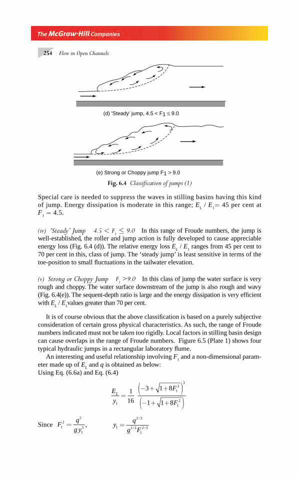
254 Flow in Open Channels
(d) 'Steady' jump, 4.5 < F1 ≤ 9.0
(e) Strong or Choppy jump F1 > 9.0
Fig. 6.4 Classifi cation of jumps (1)
Special care is needed to suppress the waves in stilling basins having this kind of jump. Energy dissipation is moderate in this range; E
L / E
1= 45 per cent at
F1 = 4.5.
(iv) ‘Steady’ Jump 4.5 < F1 ≤ 9.0 In this range of Froude numbers, the jump is
well-established, the roller and jump action is fully developed to cause appreciable energy loss (Fig. 6.4 (d)). The relative energy loss E
L / E
1 ranges from 45 per cent to
70 per cent in this, class of jump. The ‘steady jump’ is least sensitive in terms of the toe-position to small fl uctuations in the tailwater elevation.
(v) Strong or Choppy Jump F1 >9.0 In this class of jump the water surface is very
rough and choppy. The water surface downstream of the jump is also rough and wavy (Fig. 6.4(e)). The sequent-depth ratio is large and the energy dissipation is very effi cient with E
L / E
1values greater than 70 per cent.
It is of course obvious that the above classifi cation is based on a purely subjective consideration of certain gross physical characteristics. As such, the range of Froude numbers indicated must not be taken too rigidly. Local factors in stilling basin design can cause overlaps in the range of Froude numbers. Figure 6.5 (Plate 1) shows four typical hydraulic jumps in a rectangular laboratory fl ume.
An interesting and useful relationship involving F1 and a non-dimensional param-
eter made up of EL and q is obtained as below:
Using Eq. (6.6a) and Eq. (6.4)
E
y
F
F
L
1
12
3
12
1
16
3 1 8
1 1 8=
− + +( )− + +( )
Since Fq
g y12
2
13
= , yq
g F1
2 3
1 312 3
=/
/ /
Chapter 6.indd 254Chapter 6.indd 254 2/24/2010 3:00:07 PM2/24/2010 3:00:07 PM
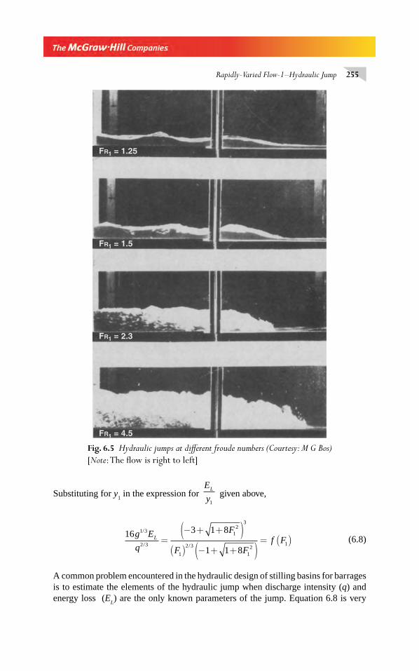
Rapidly-Varied Flow-1–Hydraulic Jump 255
Substituting for y1 in the expression for
E
yL
1
given above,
16 3 1 8
1 1 8
1 3
2 3
12
3
1
2 3
12
1
g E
q
F
F Ff FL
/
/ /=
− + +( )( ) − + +( )
= ( ) (6.8)
A common problem encountered in the hydraulic design of stilling basins for barrages is to estimate the elements of the hydraulic jump when discharge intensity (q) and energy loss (E
L) are the only known parameters of the jump. Equation 6.8 is very
Fig. 6.5 Hydraulic jumps at diff erent froude numbers (Courtesy: M G Bos)
[Note: The fl ow is right to left]
Chapter 6.indd 255Chapter 6.indd 255 2/24/2010 3:00:08 PM2/24/2010 3:00:08 PM
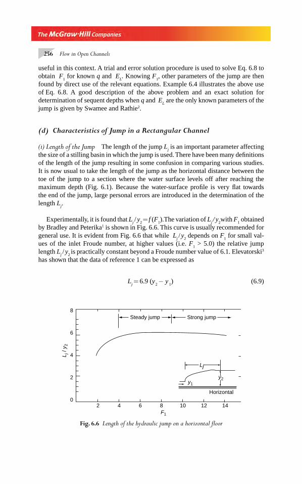
256 Flow in Open Channels
useful in this context. A trial and error solution procedure is used to solve Eq. 6.8 to obtain F
1 for known q and E
L. Knowing F
1, other parameters of the jump are then
found by direct use of the relevant equations. Example 6.4 illustrates the above use of Eq. 6.8. A good description of the above problem and an exact solution for determination of sequent depths when q and E
L are the only known parameters of the
jump is given by Swamee and Rathie2.
(d) Characteristics of Jump in a Rectangular Channel
(i) Length of the Jump The length of the jump Lj is an important parameter affecting
the size of a stilling basin in which the jump is used. There have been many defi nitions of the length of the jump resulting in some confusion in comparing various studies. It is now usual to take the length of the jump as the horizontal distance between the toe of the jump to a section where the water surface levels off after reaching the maximum depth (Fig. 6.1). Because the water-surface profi le is very fl at towards the end of the jump, large personal errors are introduced in the determination of the length L
j.
Experimentally, it is found that Lj / y
2 =
f (F
1).The variation of L
j / y
2with F
1 obtained
by Bradley and Peterika1 is shown in Fig. 6.6. This curve is usually recommended for general use. It is evident from Fig. 6.6 that while L
j / y
2 depends on F
1 for small val-
ues of the inlet Froude number, at higher values (i.e. F1 > 5.0) the relative jump
length Lj / y
2 is practically constant beyond a Froude number value of 6.1. Elevatorski3
has shown that the data of reference 1 can be expressed as
Lj =
6.9 (y
2 − y
1) (6.9)
Fig. 6.6 Length of the hydraulic jump on a horizontal fl oor
0
2
4
6
8
2 4 6 8 10 12 14
Steady jump Strong jump
y2y1
Lj
F1
L j /
y 2
Horizontal
Chapter 6.indd 256Chapter 6.indd 256 2/24/2010 3:00:09 PM2/24/2010 3:00:09 PM
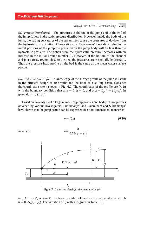
Rapidly-Varied Flow-1–Hydraulic Jump 257
(ii) Pressure Distribution The pressures at the toe of the jump and at the end of the jump follow hydrostatic pressure distribution. However, inside the body of the jump, the strong curvatures of the streamlines cause the pressures to deviate from the hydrostatic distribution. Observations by Rajaratnam4 have shown that in the initial portions of the jump the pressures in the jump body will be less than the hydrostatic pressure. The defi cit from the hydrostatic pressure increases with an increase in the initial Froude number F
1. However, at the bottom of the channel
and in a narrow region close to the bed, the pressures are essentially hydrostatic. Thus the pressure-head profi le on the bed is the same as the mean water-surface profi le.
(iii) Water-Surface Profi le A knowledge of the surface profi le of the jump is useful in the effi cient design of side walls and the fl oor of a stilling basin. Consider the coordinate system shown in Fig. 6.7. The coordinates of the profi le are (x, h) with the boundary condition that at x = 0, h = 0, and at x = L
j, h = ( y
2–y
1). In
general, h = f (x, F1).
Based on an analysis of a large number of jump profi les and bed-pressure profi les obtained by various investigators, Subramanya5 and Rajaratnam and Subramanya6 have shown that the jump profi le can be expressed in a non-dimensional manner as
η = f (λ) (6.10)
in which η =−( )
h
y y0 75 2 1.
Fig. 6.7 Defi nition sketch for the jump profi le (6)
y2
(y2 − y1)
∇
h
h
0.75 (y2 − y1)
Xx x
Lj
y1
and λ = x / X, where X = a length scale def ined as the value of x at which h = 0.75( y
2 − y
1). The variation of η with λ is given in Table 6.1.
Chapter 6.indd 257Chapter 6.indd 257 2/24/2010 3:00:09 PM2/24/2010 3:00:09 PM
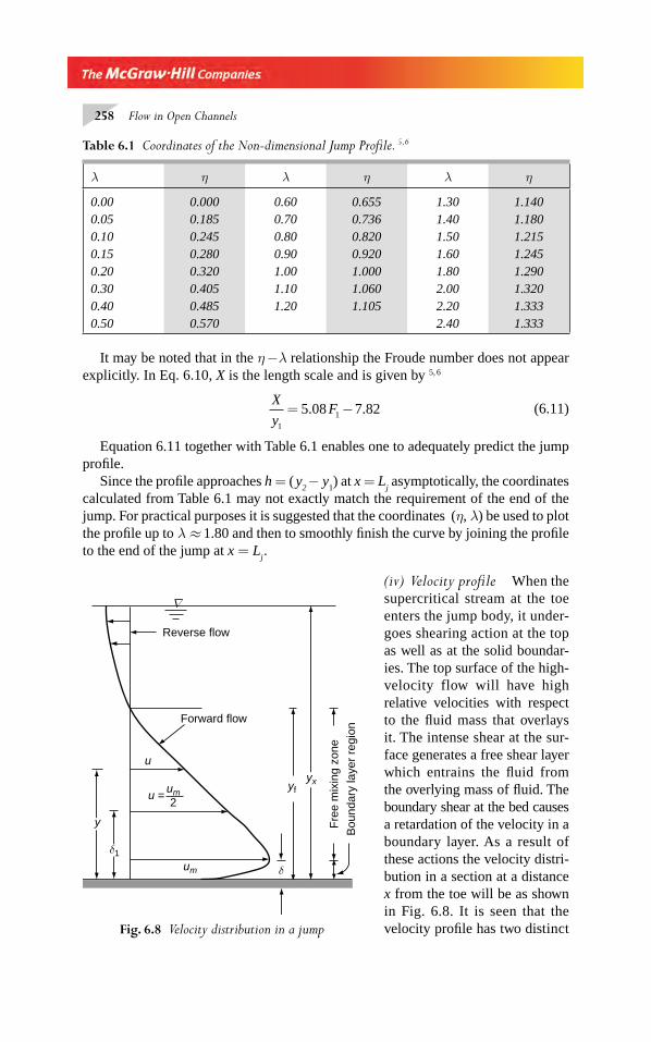
258 Flow in Open Channels
It may be noted that in the η −λ relationship the Froude number does not appear
explicitly. In Eq. 6.10, X is the length scale and is given by 5, 6
X
yF
115 08 7 82= −. . (6.11)
Equation 6.11 together with Table 6.1 enables one to adequately predict the jump profi le.
Since the profi le approaches h = ( y2 − y
1) at x = L
j asymptotically, the coordinates
calculated from Table 6.1 may not exactly match the requirement of the end of the jump. For practical purposes it is suggested that the coordinates (η, λ) be used to plot the profi le up to λ ≈ 1.80 and then to smoothly fi nish the curve by joining the profi le to the end of the jump at x = L
j .
(iv) Velocity profi le When the supercritical stream at the toe enters the jump body, it under-goes shearing action at the top as well as at the solid boundar-ies. The top surface of the high-velocity flow will have high relative velocities with respect to the fl uid mass that overlays it. The intense shear at the sur-face generates a free shear layer which entrains the fl uid from the overlying mass of fl uid. The boundary shear at the bed causes a retardation of the velocity in a boundary layer. As a result of these actions the velocity distri-bution in a section at a distance x from the toe will be as shown in Fig. 6.8. It is seen that the velocity profi le has two distinct
Table 6.1 Coordinates of the Non-dimensional Jump Profi le. 5, 6
λ η λ η λ η
0.00 0.000 0.60 0.655 1.30 1.1400.05 0.185 0.70 0.736 1.40 1.1800.10 0.245 0.80 0.820 1.50 1.2150.15 0.280 0.90 0.920 1.60 1.2450.20 0.320 1.00 1.000 1.80 1.2900.30 0.405 1.10 1.060 2.00 1.3200.40 0.485 1.20 1.105 2.20 1.3330.50 0.570 2.40 1.333
Fig. 6.8 Velocity distribution in a jump
y
δ1
δ
u =um
um
2
u
Forward flow
yfyx
Fre
e m
ixin
g zo
ne
Bou
ndar
y la
yer
regi
on
Reverse flow
∇
Chapter 6.indd 258Chapter 6.indd 258 2/24/2010 3:00:09 PM2/24/2010 3:00:09 PM
Rapidly-Varied Flow-1–Hydraulic Jump 259
portions—a forward fl ow in the lower main body and a negative velocity region at the top. In the forward fl ow, the total volumetric rate of fl ow will be in excess of the discharge Q entering the jump at the toe. This is due to the fl ow entrain-ment at the shear layer. To maintain continuity, i.e. to account for the excess for-ward fl ow, a reverse fl ow exists at the top. This situation results in the formation of the roller.
The forward velocity profi le has zero velocity at the bed, maximum velocity at a distance δ and then gradually decreases to zero at a height y
f above the bed. The
region 0 < y < δ can be called the boundary layer part and the region δ < y < yf the
free-mixing zone. This velocity confi guration indicates that the motion of the forward fl ow is similar to a wall jet except that the pressure gradient is adverse. The velocity profi le and shear stress can be studied by following the methods of analysis similar to those used in the study of wall jets.
The velocity u at a distance y from the bed in the boundary layer portion (0 < y < δ ) can be expressed by a velocity-defect law
u u
uf ym−
=*
( / )δ (6.12)
where u* = =τ ρ0 shear velocity and um = maximum velocity at y = δ. In the free-
mixing zone the velocity profi le is found to be self-similar and can be expressed as3
u
uf y
m
= ( )δ1 fory
δ1
0 16>⎛
⎝⎜⎜⎜⎜
⎞
⎠⎟⎟⎟⎟
. (6.13)
where δ1 = value of y at which u
um=2
. The maximum velocity um occurs at y = δ ≈ 0.16δ
1.
It may be noted that the non-dimensionalised velocity profi le is explicitly indepen-dent of F
1 and x. The scales of the above relationship are u
m and δ
1 which are given
by
u
Vf x ym
11= ( ) (6.14)
and δ1
11y
f x y= ( ) (6.15)
Both Eq. 6.14 and Eq. 6.15 are found 4 to be independent of the initial Froude number F1.
(v) Other Characteristics In addition to characteristics mentioned above, information about shear stress and turbulent characteristics enhance one’s understanding of the jump phenomenon. It has been found that the initial boundary-layer thickness and relative roughness of the bed play a major role in these aspects. Useful information on these topics are available in literature4, 7.
(e) Computations Computations related to hydraulic jumps in rectangular channels are relatively simple. While most of the problem types are amenable to direct solution, a few types require trial and error solution procedure. The available relations are
Chapter 6.indd 259Chapter 6.indd 259 2/24/2010 3:00:10 PM2/24/2010 3:00:10 PM
260 Flow in Open Channels
(i) Continuity equation (ii) Momentum equation for sequent depths and(iii) Energy equation for energy loss in the jump.
The basic variables can be discharge intensity q; sequent depths y1 and y
2; and energy
loss EL. There can be many other derived variables and corresponding relationships.
Based on the above there can be a variety of problem types and a few common ones are illustrated in the following examples.
Example 6.1 In a hydraulic jump occurring in a rectangular channel of 3.0-m, width, the discharge is 7.8 m3/s and the depth before the jump is 0.28 m. Estimate (i) sequent depth, and (ii) the energy loss in the jump.
Solution (i) V1
7 8
3 0 289 286=
×( )=
.
.. /m s
FV
g y1
1
1
9 286
9 81 0 285 603= =
×=
.
. ..
The sequent depth ratio is given by Eq. (6.4) as
y
yF2
112 21
21 1 8
1
21 1 8 5 603 7 424= − + +⎡
⎣⎢⎤⎦⎥= − + + ×⎡
⎣⎢⎤⎦⎥=( . ) .
Sequent depth = y2 0 28 7 424 2 08= × =. . . m(ii) The energy loss E
L is given by Eq. 6.6 as
EL =
( ) ( . . )
. ..
y y
y y2 1
1 2
3 3
4
2 08 0 28
4 0 28 2 082 503
−=
−× ×
= m
Example 6.2 A rectangular channel carrying a supercritical stream is to be
provided with a hydraulic jump type of energy dissipater. It is desired to have an energy loss of 5.0 m in the hydraulic jump when the inlet Froude number is 8.5. What are the sequent depths of this jump?
Solution Given F1 = 8.5 and E
L = 5.0 m
By Eq. 6.4 y
yF2
112 21
21 1 8
1
21 1 8 8 5 11 53= − + +⎡
⎣⎢⎤⎦⎥= − + + ×⎡
⎣⎢⎤⎦⎥=( . ) .
By Eq. 6.7 E
y
y
y
y
y
L
1
2
1
3
2
1
1
4
=
−⎛
⎝⎜⎜⎜⎜
⎞
⎠⎟⎟⎟⎟
⎛
⎝⎜⎜⎜⎜
⎞
⎠⎟⎟⎟⎟
Chapter 6.indd 260Chapter 6.indd 260 2/24/2010 3:00:10 PM2/24/2010 3:00:10 PM
Rapidly-Varied Flow-1–Hydraulic Jump 261
5 0 11 53 1
4 11 5325 32
1
3. ( . )
..
y=
−×
=
y1 = 5.0/25.32 = 0.198 m
and y2 = 0.198 × 11.53 = 2.277 m
Example 6.3 A hydraulic jump takes place in a rectangular channel with sequent depths of 0.25 m and 1.50 m at the beginning and end of the jump respec-tively. Estimate the (i) discharge per unit width of the channel and (ii) energy loss.
Solution (i) By Eq. 6.4 y
yF2
1121
21 1 8= − + +[ ]
1 50
0 25
1
21 1 8 1
2.
.[ ]= − + + F
Thus, F12 = 21 and F
1 = 4.583 m.
V1 4 583 9 81 0 25 7 177= × × =. . . . m/s
Discharge per unit width = q = V1 y
1 = 7.177 × 0.25 = 1.794 m3/s/m width
(ii) The energy loss EL is given by Eq. 6.6 as
Ey y
y yL =−( )
=−( )
× ×=2 1
3
1 2
3
4
1 50 0 25
4 0 25 1 501 302
. .
. .. m
Example 6.4 In a hydraulic jump taking place in a horizontal apron below an Ogee shaped weir the discharge per unit width is 0.25 m3/s/m and the energy loss is 2.75 m. Estimate the depths at the toe and heel of the jump.
Solution This kind of problem needs a trial and error solution procedure. Eq. 6.8 is used for easy trial and error solution.
Here q = 0.25 m3/s/m and EL = 2.75 m.
16 16 9 81 2 75
2 551 135
1 3
2 3
1 3
2 3
g E
qL
/
/
/
/
. .
..=
×( ) ×
( )=
By Eq. 6.8, f FF
F F1
12
3
1
2 3
12
3 1 8
1 1 851 135( ) =
− + +( )( ) − + +( )
=/
. (6.16)
Chapter 6.indd 261Chapter 6.indd 261 2/24/2010 3:00:10 PM2/24/2010 3:00:10 PM
262 Flow in Open Channels
Equation 6.16 is solved for F1 by a trial and error procedure. Table E-6.4 given
below indicates the various trials in a typical solution procedure: Use of Spread sheet (such as MS Excel) greatly facilitates the procedure.
Trial Assumed F
1 Value
Numerator of f(F
1 )
Denominator of f(F
1 )
f(F1 ) Remarks
1 5.0 1396.46 38.53 36.24 Increase the value of F1 in the next
trial2 6.0 2744.00 52.83 51.94 Decrease F
1 by a small amount
3 5.9 2581.31 51.32 50.30 Increase F1 by a very small
amount4 5.95 2661.82 52.07 52.12 Value of F
1 can be accepted
Table E-6.4 Trial and Error Procedure – Example 6.4
Hence, F1=5.95. Using Eq. 6.4
y
yF2
112 21
21 1 8
1
21 1 8 5 95 7 929= − + +( ) = − + + ×( )⎛
⎝⎜⎜⎜
⎞⎠⎟⎟⎟ =. .
By Eq. 6.6a E
y
y
y
y
y
L
1
2
1
3
2
1
31
4
7 929 1
4 7 92=
−⎛
⎝⎜⎜⎜⎜
⎞
⎠⎟⎟⎟⎟
⎛
⎝⎜⎜⎜⎜
⎞
⎠⎟⎟⎟⎟
=−( . )
( . 9910 490
).=
y1 = 2.75/(10.49) = 0.262 m
y2 = 0.262 × 7.929 = 2.079 m
Example 6.5 An overfl ow spillway (Fig. 6.9) is 40.0 m high. At the design energy head of 2.5 m over the spillway fi nd the sequent depths and energy loss in a hydraulic jump formed on a horizontal apron at the toe of the spillway. Neglect energy loss due to fl ow over the spillway face. (Assume C
d = 0.738).
Solution The discharge per meter width of the spillway is
q C g Hd d=
= × × × ×( )
=
2
32
2
30 738 2 9 81 2 5
8 614
3 2
3 2. . .
.
/
m /s/m3
Chapter 6.indd 262Chapter 6.indd 262 2/24/2010 3:00:11 PM2/24/2010 3:00:11 PM
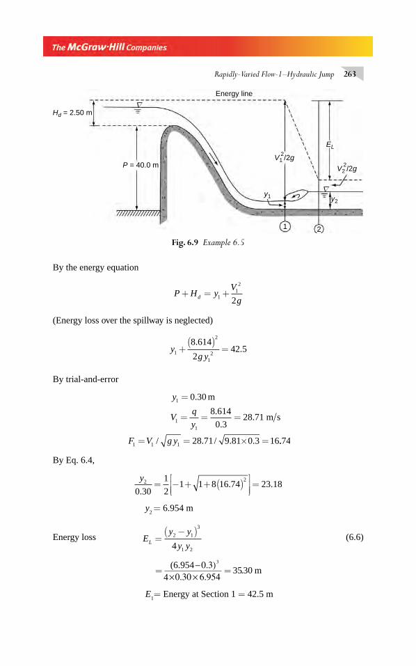
Rapidly-Varied Flow-1–Hydraulic Jump 263
By the energy equation
P H yV
gd+ = +112
2
(Energy loss over the spillway is neglected)
yg y1
2
12
8 614
242 5+
( )=
..
By trial-and-error
y
Vq
y
F V g y
1
11
1 1 1
0 30
8 614
0 328 71
28 71 9 81 0 3 16
=
= = =
= = × =
.
.
..
/ . / . .
m
m s
..74
By Eq. 6.4,
y2 2
0 30
1
21 1 8 16 74 23 18
.. .= − + + ( )⎡
⎣⎢⎢
⎤⎦⎥⎥=
y2 = 6.954 m
Energy loss Ey y
y yL =−( )2 1
3
1 24 (6.6)
= (6.954−0.3)
× 0.30 × 6.954
3
4 m= 3530.
E1= Energy at Section 1 = 42.5 m
Fig. 6.9 Example 6.5
EL
V2 /2g2
1 2
∇
∇
P = 40.0 m
y1 y2
Energy line
Hd = 2.50 m
V1 /2g2
Chapter 6.indd 263Chapter 6.indd 263 2/24/2010 3:00:11 PM2/24/2010 3:00:11 PM
264 Flow in Open Channels
Percentage of initial energy lost = E
EL
1
100 83 0× = . %
Example 6.6 A spillway discharges a fl ood fl ow at a rate of 7.75 m3/s per metre width. At the downstream horizontal apron the depth of fl ow was found to be 0.50 m. What tailwater depth is needed to form a hydraulic jump? If a jump is formed, fi nd its (a) type, (b) length, (c) head loss, (d) energy loss as a percentage of the initial energy, and (e) profi le.
Solution q = 7.75 m3/s/m, and y1 = 0.50 m
V
F
1
1
7 75
0 5015 50
15 50
9 81 0 507 0
= =
=×
=
.
.. /
.
. ..
m s
Sequent-depth By Eq. (6.4)
y
y2
1
21
21 1 8 7 9 41= − + + ×( ) =( ) .
y2 = 4.71 m = required tailwater depth.
( a) Type Since F1 = 7.0, a ‘steady’ jump will be formed
(b) Since F1> 5.0, L
j = 6.1 y
2
Lj = length of the jump = 6.1×4.71 = 28.7 m
( c) EL = head loss =
−= − × ×
=
( )( . . ) /( . . )
.
y y
y y2
3
1 2
31
44 71 0 50 4 0 5 4 71
7 92 m
(d) E yV
g1 112
2= +
2
0 515 50
2 9 8112 75= +
×=.
( . )
.. m
E
EL
1
62 1= . %
( e) Profi le By Eq. (6.11)
X
y
X
y y
1
2 1
5 08 7 0 7 82 27 74
13 87
0 75 3 16
= − =
=− =
. ( . ) . .
.
. ( ) .
m
m
∴ λ =x
13 87. and η =
h
3 16.
Chapter 6.indd 264Chapter 6.indd 264 2/24/2010 3:00:11 PM2/24/2010 3:00:11 PM
Rapidly-Varied Flow-1–Hydraulic Jump 265
Substituting these for the values of λ and η given in Table 6.1 a relation between x and h is obtained. As suggested in Section 6. 4(c), the profi le is calculated up to λ ≈ 1.80, i.e. up to x = 25.0 m and then is joined by a smooth curve to the end of the jump at x = L
j = 28.7 m. The change in the depth in this range would
be 0.0433 × 3.16 = 0.14 m. This being a fl at curve, i.e., a change of 0.14 m in 3.70 m, the procedure as above is adequate.
6.4 JUMPS IN HORIZONTAL NON-RECTANGULAR CHANNELS
If the side walls of a channel are not vertical, e.g. in the case of a trapezoidal chan-nel, the fl ow in a jump will involve lateral expansion of the stream in addition to increase in depth. The cross-sectional areas are not linear functions of the depth of fl ow. This aspect introduces not only computational diffi culties in the calculation of the sequent-depth ratio but also structural changes in the jump. A brief introduc-tion to this wide fi eld of jumps, in non-rectangular channel, is given in this section.
(a) Basic Equations Consider a horizontal frictionless channel of any arbitrary shape, such as in Fig. 6.2. For a hydraulic jump in this channel, the general momentum (Eq. 6.1) with the assumption of β
2 = β
1 = 1.0 reduces to:
P1 − P
2 = M
2 − M
1 (6.17)
i.e. γ γ ρ ρA y A y Q V QV1 1 2 2 2 2 1 1− = −
= −ρ ρQ
A
Q
A22
2
12
1
(6.18)
where A = area of cross-section any y = depth of the centre of gravity of the area from the water surface.
Rearranging Eq. 6.17
P1 + M
1 = P
2 + M
2
i.e. P M AyQ
gA+ = +
⎛
⎝⎜⎜⎜⎜
⎞
⎠⎟⎟⎟⎟
=γ2
Const. (6.19)
i.e. P M
P AyQ
gAs
+= = + =
γ
2
Const. (6.19a)
The term PP M
s =+⎛
⎝⎜⎜⎜⎜
⎞
⎠⎟⎟⎟⎟γ is the specifi c force (Section 1.11 (c)).
Chapter 6.indd 265Chapter 6.indd 265 2/24/2010 3:00:12 PM2/24/2010 3:00:12 PM
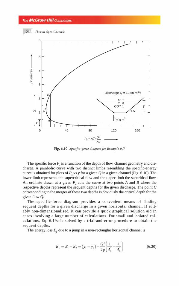
266 Flow in Open Channels
The specifi c force Ps is a function of the depth of fl ow, channel geometry and dis-
charge. A parabolic curve with two distinct limbs resembling the specifi c-energy curve is obtained for plots of P
s vs y for a given Q in a given channel (Fig. 6.10). The
lower limb represents the supercritical fl ow and the upper limb the subcritical fl ow. An ordinate drawn at a given P
s cuts the curve at two points A and B where the
respective depths represent the sequent depths for the given discharge. The point C corresponding to the merger of these two depths is obviously the critical depth for the given fl ow Q.
The specif ic-force diagram provides a convenient means of f inding sequent depths for a given discharge in a given horizontal channel. If suit-ably non-dimensionalised, it can provide a quick graphical solution aid in cases involving a large number of calculations. For small and isolated cal-culations, Eq. 6.19a is solved by a trial- and-error procedure to obtain the sequent depths.
The energy loss EL due to a jump in a non-rectanglar horizontal channel is
E E E y yQ
g A AL = − = −( )+ −⎛
⎝⎜⎜⎜⎜
⎞
⎠⎟⎟⎟⎟1 2 1 2
2
12
222
1 1 (6.20)
Fig. 6.10 Specifi c–force diagram for Example 6.7
1
0 40 80 120 160
2
3
4
5
6
y2
y1
B
A
C
y in
met
res
Ag
Q2Ps = Ay +
2.0 m
CG
1.5
yy
∇
Discharge Q = 13.50 m3/s
Chapter 6.indd 266Chapter 6.indd 266 2/24/2010 3:00:12 PM2/24/2010 3:00:12 PM
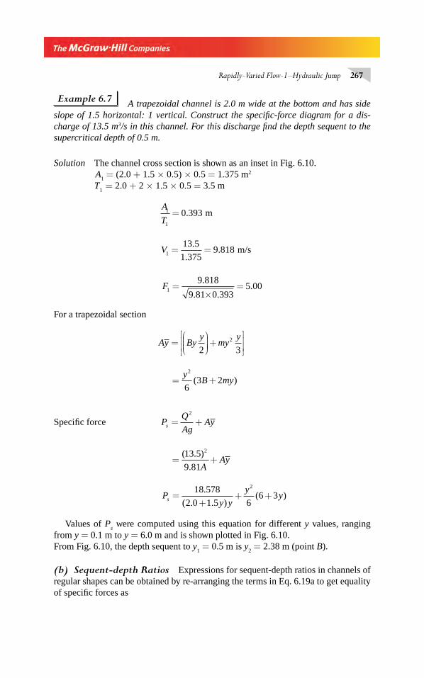
Rapidly-Varied Flow-1–Hydraulic Jump 267
Example 6.7 A trapezoidal channel is 2.0 m wide at the bottom and has side slope of 1.5 horizontal: 1 vertical. Construct the specifi c-force diagram for a dis-charge of 13.5 m3/s in this channel. For this discharge fi nd the depth sequent to the supercritical depth of 0.5 m.
Solution The channel cross section is shown as an inset in Fig. 6.10. A
1 = (2.0 + 1.5 × 0.5) × 0.5 = 1.375 m2
T1 = 2.0 + 2 × 1.5 × 0.5 = 3.5 m
A
T1
1
0 393= . m
V1
13 5
1 3759 818= =
.
.. m/s
F1
9 818
9 81 0 3935 00=
×=
.
. ..
For a trapezoidal section
Ay Byy
myy
=⎛⎝⎜⎜⎜
⎞⎠⎟⎟⎟⎟+
⎡
⎣⎢⎢
⎤
⎦⎥⎥2 3
2
= +y
B my2
63 2( )
Specifi c force PQ
AgAys = +
2
= +( . )
.
13 5
9 81
2
AAy
Py y
yys =
++ +
18 578
2 0 1 5 66 3
2.
( . . )( )
Values of Ps were computed using this equation for different y values, ranging
from y = 0.1 m to y = 6.0 m and is shown plotted in Fig. 6.10.From Fig. 6.10, the depth sequent to y
1 = 0.5 m is y
2 = 2.38 m (point B).
(b) Sequent-depth Ratios Expressions for sequent-depth ratios in channels of regular shapes can be obtained by re-arranging the terms in Eq. 6.19a to get equality of specifi c forces as
Chapter 6.indd 267Chapter 6.indd 267 2/24/2010 3:00:12 PM2/24/2010 3:00:12 PM
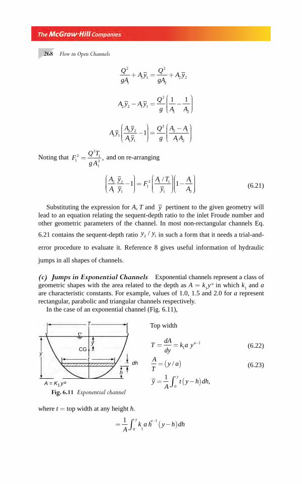
268 Flow in Open Channels
Q
gAA y
Q
gAA y
2
11 1
2
22 2+ = +
A y A yQ
g A A2 2 1 1
2
1 2
1 1− = −
⎛
⎝⎜⎜⎜⎜
⎞
⎠⎟⎟⎟⎟
A yA y
A y
Q
g
A A
A A1 12 2
1 1
22 1
1 2
1−⎛
⎝⎜⎜⎜⎜
⎞
⎠⎟⎟⎟⎟
=−⎛
⎝⎜⎜⎜⎜
⎞
⎠⎟⎟⎟⎟
Noting that FQ T
g A12
21
13
= , and on re-arranging
A
A
y
yF
A T
y
A
A2
1
2
112 1 1
1
1
2
1 1−⎛
⎝⎜⎜⎜⎜
⎞
⎠⎟⎟⎟⎟
=⎛
⎝⎜⎜⎜⎜
⎞
⎠⎟⎟⎟⎟
−⎛
⎝⎜⎜⎜⎜
⎞/
⎠⎠⎟⎟⎟⎟ (6.21)
Substituting the expression for A, T and y pertinent to the given geometry will lead to an equation relating the sequent-depth ratio to the inlet Froude number and other geometric parameters of the channel. In most non-rectangular channels Eq.
6.21 contains the sequent-depth ratio y y2 1/ in such a form that it needs a trial-and-
error procedure to evaluate it. Reference 8 gives useful information of hydraulic
jumps in all shapes of channels.
(c) Jumps in Exponential Channels Exponential channels represent a class of geometric shapes with the area related to the depth as A = k
1 y a in which k
1 and a
are characteristic constants. For example, values of 1.0, 1.5 and 2.0 for a represent rectangular, parabolic and triangular channels respectively.
In the case of an exponential channel (Fig. 6.11),
Top width
TdA
dyk a ya= = −
11
(6.22)
A
Ty a= ( )/ (6.23)
yA
t y h dhy
= −( )∫1
0,
y
h
dh
T
t
yCG
A = K1 ya
∇
∗
Fig. 6.11 Exponential channel
where t = top width at any height h.
= −( )∫
−10 1
1
Ak a h y h dh
y a
Chapter 6.indd 268Chapter 6.indd 268 2/24/2010 3:00:12 PM2/24/2010 3:00:12 PM
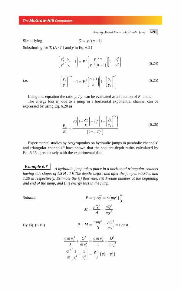
Rapidly-Varied Flow-1–Hydraulic Jump 269
Simplifying y y a= +( )/ 1
Substituting for T, (A / T ) and y in Eq. 6.21
y
y
y
yF
y a
y a
ya
a2
1
2
112 1
1
111
1./
/−
⎛
⎝⎜⎜⎜⎜
⎞
⎠⎟⎟⎟⎟
=+( )
⎛
⎝⎜⎜⎜⎜
⎞
⎠
⎟⎟⎟⎟⎟−
aa
ay2
⎛
⎝⎜⎜⎜⎜
⎞
⎠⎟⎟⎟⎟ (6.24)
i.e. y
yF
a
a
y
y
a
2
1
1
12 1
2
11
1⎛
⎝⎜⎜⎜⎜
⎞
⎠⎟⎟⎟⎟
− =+⎛
⎝⎜⎜⎜
⎞⎠⎟⎟⎟⎟ −
⎛
⎝⎜⎜⎜⎜
⎞
⎠⎟⎟⎟⎟
+ aa⎛
⎝
⎜⎜⎜⎜⎜
⎞
⎠
⎟⎟⎟⎟⎟⎟ (6.25)
Using this equation the ratio y2 / y
1 can be evaluated as a function of F
1 and a.
The energy loss EL due to a jump in a horizontal exponential channel can be
expressed by using Eq. 6.20 as
E
E
ay
yF
y
yL
a
1
2
112 1
2
2
2 1 1
=
−⎛
⎝⎜⎜⎜⎜
⎞
⎠⎟⎟⎟⎟+ −
⎛
⎝⎜⎜⎜⎜
⎞
⎠⎟⎟⎟⎟
⎛
⎝
⎜⎜⎜⎜⎜
⎞
⎠
⎟⎟⎟⎟⎟⎟⎟
+( )2 12a F
(6.26)
Experimental studies by Argyropoulus on hydraulic jumps in parabolic channels9 and triangular channels10 have shown that the sequent-depth ratios calculated by Eq. 6.25 agree closely with the experimental data.
Example 6.8 A hydraulic jump takes place in a horizontal triangular channel having side slopes of 1.5 H : 1 V. The depths before and after the jump are 0.30 m and 1.20 m respectively. Estimate the (i) fl ow rate, (ii) Froude number at the beginning and end of the jump, and (iii) energy loss in the jump.
Solution P Ay myy
MQ
A
Q
my
= = ( )
= =
γ γ
ρ ρ
2
2 2
2
3
By Eq. (6.19) P Mmy Q
my+ = + =
γ ρ3 2
23Const.
g m y Q
m y
g m y Q
my
Q
m y y
g my y
13 2
12
23 2
22
2
12
22 2
313
3 3
1 1
3
+ = +
−⎡
⎣⎢⎢
⎤
⎦⎥⎥ = −(( )
Chapter 6.indd 269Chapter 6.indd 269 2/24/2010 3:00:13 PM2/24/2010 3:00:13 PM
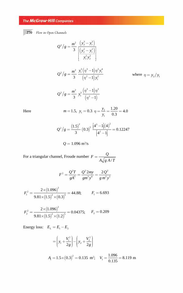
270 Flow in Open Channels
Q gm y y
y y
y y
22
23
13
22
12
12
22
3=
−( )−( )⎡
⎣
⎢⎢⎢
⎤
⎦
⎥⎥⎥
Q gm y y
y2
213 3 2
14
2123
1
1=
−( )−( )
η η
η where η = y y2 1
Q gm
y22
15
3 2
23
1
1=
−( )−( )
η η
η
Here m y= =1 5 0 31. , . , η = = =y
y2
1
1 20
0 34 0
.
..
Q g2
25
3 2
2
1 5
30 3
4 1 4
4 10 12247=
( )( )
−⎡⎣⎢
⎤⎦⎥ ( )
−⎡⎣⎢
⎤⎦⎥
=.
. .
Q = 1.096 m3/s
For a triangular channel, Froude number FQ
A g A T=
/
FQ T
gA
Q my
gm y2
2
3
2
3 6
2= = =
2 2
2 5
Q
g m y
F12
2
2 5
2 1 096
9 81 1 5 0 344 88=
×( )×( ) ×( )
=.
. . .. ; F1 6 693= .
F22
2
2 5
2 1 096
9 81 1 5 1 20 04375=
×( )×( ) ×( )
=.
. . .. ; F2 0 209= .
Energy loss: E E EL = −1 2
= +⎛
⎝⎜⎜⎜⎜
⎞
⎠⎟⎟⎟⎟− +
⎛
⎝⎜⎜⎜⎜
⎞
⎠⎟⎟⎟⎟
yV
gy
V
g112
222
2 2
A1
21 5 0 3 0 135= ×( ) =. . . m2; V1
1 096
0 1358 119= =
.
.. m
Chapter 6.indd 270Chapter 6.indd 270 2/24/2010 3:00:13 PM2/24/2010 3:00:13 PM
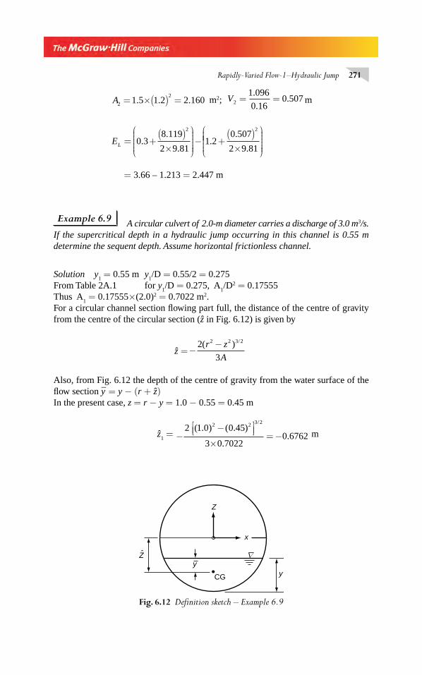
Rapidly-Varied Flow-1–Hydraulic Jump 271
A2
21 5 1 2 2 160= ×( ) =. . . m2; V2 = =
1 096
0 160 507
.
.. m
EL = +( )
×
⎛
⎝
⎜⎜⎜⎜⎜
⎞
⎠
⎟⎟⎟⎟⎟⎟− +
( )×
⎛
⎝
⎜0 3
8 119
2 9 811 2
0 507
2 9 81
2 2
..
..
.
.⎜⎜⎜⎜⎜
⎞
⎠
⎟⎟⎟⎟⎟⎟
= 3.66 – 1.213 = 2.447 m
Example 6.9 A circular culvert of 2.0-m diameter carries a discharge of 3.0 m3/s. If the supercritical depth in a hydraulic jump occurring in this channel is 0.55 m determine the sequent depth. Assume horizontal frictionless channel.
Solution y1 = 0.55 m y
1/D = 0.55/2 = 0.275
From Table 2A.1 for y1/D = 0.275, A
1/D2 = 0.17555
Thus A1 = 0.17555×(2.0)2 = 0.7022 m2.
For a circular channel section fl owing part full, the distance of the centre of gravity from the centre of the circular section (z in Fig. 6.12) is given by
z = ( ) /r z
A−
−2
3
2 2 3 2
Also, from Fig. 6.12 the depth of the centre of gravity from the water surface of the fl ow section y– = y − (r + z)In the present case, z = r − y = 1.0 − 0.55 = 0.45 m
z1 =
( . ) ( . )
..
/2 2 3 22 1 0 0 45
3 0 70220 6762−
−⎡⎣⎢
⎤⎦⎥
×= − m
Fig. 6.12 Defi nition sketch – Example 6.9
x
y
Z
CG
∇y
Z
Chapter 6.indd 271Chapter 6.indd 271 2/24/2010 3:00:14 PM2/24/2010 3:00:14 PM
272 Flow in Open Channels
Trial y2(m) y
2 /D
A2 /D 2
from Table 2A-1
A2(m2) Z
2z
2y2 P
s 2Remarks
1 1.50 0.7500 0.63185 2.52740 0.500 0.1713 0.6713 2.0597 Reduce y2
slightly
2 1.20 0.6000 0.49203 1.96812 0.200 0.3186 0.5186 1.4868 Reduce y2
slightly
3 1.18 0.5900 0.48221 1.92884 0.180 0.3290 0.5090 1.4574 Give very small incre-ment to y
2
4 1.185 0.5925 0.48467 1.93866 0.185 0.3264 0.5114 1.4646 Accept
y1 0 55 1 00 0 6762 0 2262= − + =. . . . m
Specifi c force at Section 1 = = +PQ
gAA ys1
2
11 1
=( )×
+ ×( ) =3 0
9 81 0 70220 7022 0 2262 1 4654
2.
. .. . .
Equating the specifi c forces before and after the jump, Ps1
= P
s2 = 1.4654
Further PQ
gAA ys2
2
22 2 1 4654= + = . (6.27)
The value of y2 satisfying this equation is obtained by trial and error.
Trial and error solution of Eq. 6.27The sequent depth y
2 = 1.185 m
Note: For hydraulic jumps occurring in horizontal, frictionless circular channels several empirical equations are available for facilitating quick calculations. Following are two such equations:
(1) Straub(1978):
(i) For 0 02 0 851 01
0 265
0 506
. . ,.
( ) .
.
< ≤ =⎡
⎣
⎢⎢⎢
⎤
⎦
⎥⎥⎥
y
Dy
D
Q
gc
c (6.28)
(ii) Fy
yc
11
1 93
=⎛
⎝⎜⎜⎜⎜
⎞
⎠⎟⎟⎟⎟
.
(6.29)
Chapter 6.indd 272Chapter 6.indd 272 2/24/2010 3:00:14 PM2/24/2010 3:00:14 PM
Rapidly-Varied Flow-1–Hydraulic Jump 273
(iii) (a) For F1 1 7< . , y
yyc
1
2
2= ( ) (6.30)
(b) For F1 1 7≥ . (in SI Units)
y
yy
y
ycc2
1
0 07
1
1 73
1 087=⎛
⎝⎜⎜⎜⎜
⎞
⎠⎟⎟⎟⎟
. ( ) .
.
(2) K. Subramanya(1996):
y
yF F2
112
10 01 0 8644 0 3354= − + +. . . (6.31)
Alternative Methods to Example 6.9
(1) By using Straub’s Equations
yD
Q
gc =
⎡
⎣
⎢⎢⎢
⎤
⎦
⎥⎥⎥
1 010 265
0 506
.
( ) .
.
yc =⎡
⎣⎢⎢
⎤
⎦⎥⎥ =
1 01
2 0
3 0
9 810 823
0 265
0 506.
( . )
.
..
.
.
m
y Dc / . / . .= =0 823 2 0 0 412
Hence calculation of yc is OK and y
yy
y
ycc2
1
0 07
1
1 73
1 087 2 1534=⎛
⎝⎜⎜⎜⎜
⎞
⎠⎟⎟⎟⎟
=. ( ) ..
.
Sequent depth y2 = 1.1844 m.
(2) Alternative Method-2y
1 = 0.55 m y
1 /D = 0.55 / 2 = 0.275
From Table 2A.1 for y1/D = 0.275, A
1/D2 = 0.17556 and T
1/D =0.89296
Thus A1 = 0.17556×(2.0)2 = 0.7022 m2.
and T1 = 0.89296× 2.0= 1.78596 m
For using Eq. 6.31 VQ
A11
3 0
0 70224 272= = =
.
.. m/s
FV
gA
T
11
1
1
4 272
9 810 7022
1 78596
2 1752= =
×
=.
..
.
.
By Eq. 6.31 y
yF F2
112
10 01 0 8644 0 3354= − + +. . .
y
y2
1
20 01 2 175 0 8644 2 175 0 3354= − ( ) + ( )+. . . . .
= −0.04731 + 1.8803 + 0.3354 = 2.1683
Chapter 6.indd 273Chapter 6.indd 273 2/24/2010 3:00:14 PM2/24/2010 3:00:14 PM
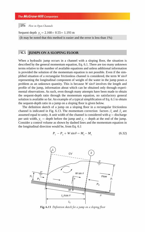
274 Flow in Open Channels
Sequent depth y2 = 2.168× 0.55= 1.193 m
(It may be noted that this method is easier and the error is less than 1%)
6.5 JUMPS ON A SLOPING FLOOR
When a hydraulic jump occurs in a channel with a sloping fl oor, the situation is described by the general momentum equation, Eq. 6.1. There are too many unkn own terms relative to the number of available equations and unless additional information is provided the solution of the momentum equation is not possible. Even if the sim-plifi ed situation of a rectangular frictionless channel is considered, the term W sin θ representing the longitudinal component of weight of the water in the jump poses a problem as an unknown quantity. This is because W sin θ involves the length and profi le of the jump, information about which can be obtained only through experi-mental observations. As such, even though many attempts have been made to obtain the sequent-depth ratio through the momentum equation, no satis factory general solution is available so far. An example of a typical simplifi cation of Eq. 6.1 to obtain the sequent-depth ratio in a jump on a sloping fl oor is given below.
The defi nition sketch of a jump on a sloping fl oor in a rectangular frictionless channel is indicated in Fig. 6.13. The momentum correction factors β
1 and β
2 are
assumed equal to unity. A unit width of the channel is considered with q = discharge per unit width, y
1 = depth before the jump and y
t = depth at the end of the jump.
Consider a control volume as shown by dashed lines and the momentum equation in the longitudinal direction would be, from Eq. 6.1
P1 − P
2 + W sin θ = M
2 − M
1 (6.32)
Fig. 6.13 Defi nition sketch for a jump on a sloping fl oor
12CV
FlowW sin θ
W
Lj /cos θ
Lj
y1ytP1
P2
θ
θ
∇
∇
Chapter 6.indd 274Chapter 6.indd 274 2/24/2010 3:00:15 PM2/24/2010 3:00:15 PM
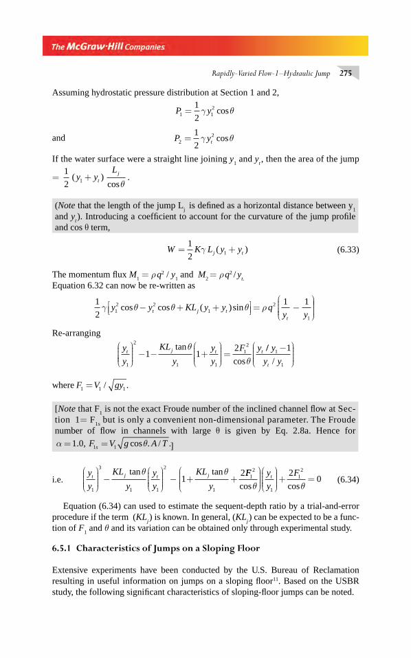
Rapidly-Varied Flow-1–Hydraulic Jump 275
Assuming hydrostatic pressure distribution at Section 1 and 2,
P y1 121
2= γ θcos
and P yt221
2= γ θcos
If the water surface were a straight line joining y1 and y
t , then the area of the jump
= 1
2 1( )cos
y yL
t
j+θ
.
(Note that the length of the jump Lj is defi ned as a horizontal distance between y
1
and yt ). Introducing a coeffi cient to account for the curvature of the jump profi le
and cos θ term,
W K L y yj t= +1
2 1γ ( ) (6.33)
The momentum fl ux M1 = ρ q2 / y
1 and M
2 = ρ q2 /
y
t.
Equation 6.32 can now be re-written as
1
2
1 112 2
12
1
γ θ θ θ ρy y KL y y qy yt j t
t
cos cos ( )sin− + +⎡⎣⎢
⎤⎦⎥ = −
⎛
⎝⎜⎜⎜⎜
⎞
⎠⎟⎟⎟⎟⎟
Re-arranging
y
y
KL
y
y
y
F yt j t t
1
2
1 1
12
1 12⎛
⎝⎜⎜⎜⎜
⎞
⎠⎟⎟⎟⎟
− − +⎛
⎝⎜⎜⎜⎜
⎞
⎠⎟⎟⎟⎟
=tan
cos
θ
θ//
/
y
y yt
1
1
1−⎛
⎝⎜⎜⎜⎜
⎞
⎠⎟⎟⎟⎟
where F V gy1 1 1= / .
[Note that F1 is not the exact Froude number of the inclined channel fl ow at Sec-
tion 1= F1s
but is only a convenient non-dimensional parameter. The Froude number of fl ow in channels with large θ is given by Eq. 2.8a. Hence for
α θ= =1 0 1 1. , cos . / .F V g A Ts ]
i.e. y
y
KL
y
y
y
KL
yt j t j
1
3
1 1
2
1
12⎛
⎝⎜⎜⎜⎜
⎞
⎠⎟⎟⎟⎟
−⎛
⎝⎜⎜⎜⎜
⎞
⎠⎟⎟⎟⎟
− + +tan tanθ θ FF y
y
Ft12
1
122
0cos cosθ θ
⎛
⎝⎜⎜⎜⎜
⎞
⎠⎟⎟⎟⎟⎛
⎝⎜⎜⎜⎜
⎞
⎠⎟⎟⎟⎟+ = (6.34)
Equation (6.34) can used to estimate the sequent-depth ratio by a trial-and-error procedure if the term (KL
j ) is known. In general, (KL
j ) can be expected to be a func-
tion of F1 and θ and its variation can be obtained only through experimental study.
6.5.1 Characteristics of Jumps on a Sloping Floor
Extensive experiments have been conducted by the U.S. Bureau of Reclamation resulting in useful information on jumps on a sloping fl oor11. Based on the USBR study, the following signifi cant characteristics of sloping-fl oor jumps can be noted.
Chapter 6.indd 275Chapter 6.indd 275 2/24/2010 3:00:15 PM2/24/2010 3:00:15 PM
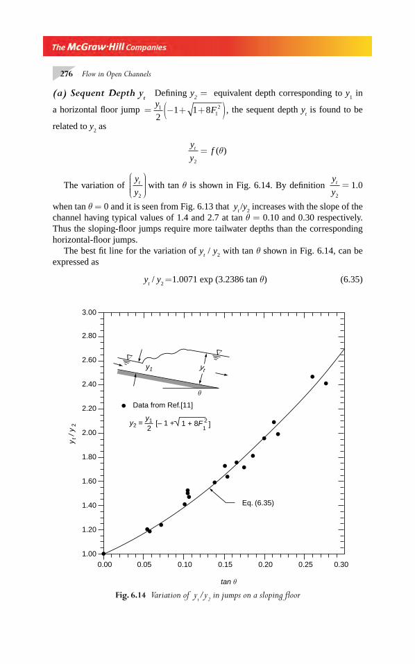
276 Flow in Open Channels
(a) Sequent Depth yt Defi ning y
2 = equivalent depth corresponding to y
1 in
a horizontal fl oor jump = − + +( )yF1
12
21 1 8 , the sequent depth y
t is found to be
related to y2 as
y
yft
2
= ( )θ
The variation of y
yt
2
⎛
⎝⎜⎜⎜⎜
⎞
⎠⎟⎟⎟⎟ with tan θ is shown in Fig. 6.14. By defi nition
y
yt
2
= 1.0
when tan θ = 0 and it is seen from Fig. 6.13 that yt /y
2 increases with the slope of the
channel having typical values of 1.4 and 2.7 at tan θ = 0.10 and 0.30 respectively. Thus the sloping-fl oor jumps require more tailwater depths than the corresponding horizontal-fl oor jumps.
The best fi t line for the variation of yt / y
2 with tan θ shown in Fig. 6.14, can be
expressed as
yt / y
2 =1.0071 exp (3.2386 tan θ) (6.35)
Fig. 6.14 Variation of yt/y
2 in jumps on a sloping fl oor
0.001.00
1.20
1.40
1.60
1.80
2.00
2.20
2.40
2.60
2.80
3.00
0.05 0.10 0.15 0.20 0.25 0.30
Eq. (6.35)
Data from Ref.[11]
y2 =y1
2[– 1 + 1 + 8F
1
∇∇
yt
y t /
y2
y1
θ
tan θ
2]
Chapter 6.indd 276Chapter 6.indd 276 2/24/2010 3:00:15 PM2/24/2010 3:00:15 PM
Rapidly-Varied Flow-1–Hydraulic Jump 277
(b) Length of the Jump Lj The length of the jump L
j was defi ned in the USBR
study as the horizontal distance between the commencement of the jump and a point on the subcritical fl ow region where the streamlines separate from the fl oor or to a point on the level water surface immediately downstream of the roller, whichever is longer.
The length of the jump on a sloping fl oor is longer than the corresponding Lj of a
jump on a horizontal fl oor. The variation of Lj / y
2 with F
1 for any θ is similar to the
variation for θ = 0 case shown in Fig. 6.6. In the range of 4.0 < F1 < 13, L
j / y
2 is
essentially independent of F1 and is a function of θ only. The variation can be approx-
imately expressed as 12
Lj / y
2 = 6.1 + 4.0 tan θ (6.36)
in the range of 4.5 < F1 < 13.0.
Elevatorski’s3 analysis of the USBR data indicates that the jump length can be expressed as
Lj= m
s(y
t–y
1) (6.37)
in which ms = f(θ). The varia-
tion of ms with tan θ is shown in
Fig. 6.15. It may be seen that m
s = 6.9 for tan θ = 0 and
decreases with an increase in the value of the channel slope. Equation 6.37 is based on a wider range of values for F
1
than in Eq. 6.37.
(c) Energy Loss EL Kno wing
the sequent depths yt and y
1 and
the length of the jump, the energy loss E
L can be calculated as
EL = H
1 − H
2
where H = total energy at a section
EL = (E
1 + L
J tan θ)−E
2
= + + − −yV
gL y
V
gt
j1
2
112
2 2cos tan cosθ θ θ (6.38)
where yt = sequent depth in a sloping channel at Section 2. It is found that the
relative energy loss EL/H
1 decreases with an increase in the value of θ, being
highest at tan θ = 0. The absolute value of EL is a function of θ, being least when
θ = 0.
Fig. 6.15 Length of jumps on sloping fl oor
00
2
4
6
8
0.1 0.2 0.3 0.4
Data from (3)Lj = ms (yt – y1)
tan θ
ms
Chapter 6.indd 277Chapter 6.indd 277 2/24/2010 3:00:15 PM2/24/2010 3:00:15 PM
278 Flow in Open Channels
Example 6.10 A rectangular channel is laid on a slope of 1 horizontal : 0.15 vertical. When a discharge of 11.0 m3/s/metre width is passed down the channel at a depth of 0.7 m, a hydraulic jump is known to occur at a section. Calculate the sequent depth, length of the jump and energy loss in the jump. What would be the energy loss if the slope was zero?
Solution q =11.00 m3/s/m
At inlet V1
11 00
0 7015 714= =
.
.. m/s
F1
15 714
9 81 0 76 0=
×=
.
. ..
y2 = equivalent sequent depth in a horizontal fl oor jump
= − + +⎡⎣⎢
⎤⎦⎥= − + + ×( )⎡
⎣⎢⎢
⎤⎦⎥⎥
yF1
12 2
21 1 8
0 70
21 1 8 6
.
= 5.6 mSequent depth From Eq. 6.35 or from Fig. 6.13, corresponding to a value of tan θ = 0.15
y
yt
2
1 63= .
yt = sequent depth in the inclined fl oor jump=1.63 × 5.6 = 9.13 m
Length of the jumpFrom Fig. 6.14, corresponding to tan θ = 0.15, m
s = 3.8
By Eq. 6.37 Lj =
3.8 (9.13 − 0.70) = 32.03 m
By Eq. 6.36 Lj =
5.6(6.1 + 4.0 × 0.15) =37.52 m
An average value of Lj = 34.5 m could be taken as the jump length.
Energy loss
Initial specifi c energy E yV
g1 112
2= +cosθ
cos θ = 0.98893
E1
2
0 7 0 9889315 714
2 9 8113 278= ×( )+
( )×
=. ..
.. m
(Note the small effect of the cos θ term on the energy.)
Lj tanθ = 34.5 × 0.15 = 5.175 m
H1 = total energy at Section 1 with the bed level at 2 as datum
= E1+ L
J tanθ = 13.278 + 5.175 = 18.453 m
Chapter 6.indd 278Chapter 6.indd 278 2/24/2010 3:00:16 PM2/24/2010 3:00:16 PM
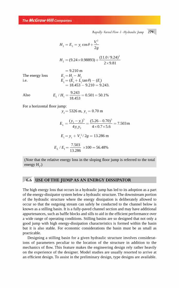
Rapidly-Varied Flow-1–Hydraulic Jump 279
H E yV
gtt
2 2
2
2= = +cosθ
H2
2
9 24 0 9889311 0 9 24
2 9 81= × +
×( . . )
( . / . )
.
= 9.210 mThe energy loss E
1 =
H
1 − H
2
i.e. EL = (E
1 + L
j tan θ) − (E
t)
= 18.453 − 9.210 = 9.243.
Also E HL /.
.. . %1
9 243
18 4530 501 50 1= = =
For a horizontal fl oor jump:y
2 = 5326 m, y
1 = 0.70 m
Ey y
y yL =−
=−
× ×=
( ) ( . . )
. ..2 1
3
1 2
3
4
5 26 0 70
4 0 7 5 67 503m
E1 = y
1 + V
12 / 2g = 13.286 m
E EL /.
.. %1
7 503
13 286100 56 48= × =
(Note that the relative energy loss in the sloping fl oor jump is referred to the total energy H
1.)
6.6 USE OF THE JUMP AS AN ENERGY DISSIPATOR
The high energy loss that occurs in a hydraulic jump has led to its adoption as a part of the energy-dissipator system below a hydraulic structure. The downstream portion of the hydraulic structure where the energy dissipation is deliberately allowed to occur so that the outgoing stream can safely be conducted to the channel below is known as a stilling basin. It is a fully-paved channel section and may have additional appurtenances, such as baffl e blocks and sills to aid in the effi cient performance over a wide range of operating conditions. Stilling basins are so designed that not only a good jump with high energy-dissipation characteristics is formed within the basin but it is also stable. For economic considerations the basin must be as small as practicable.
Designing a stilling basin for a given hydraulic structure involves considerat-ions of parameters peculiar to the location of the structure in addition to the mechanics of fl ow. This feature makes the engineering design rely rather heavily on the experience of the designer. Model studies are usually resorted to arrive at an effi cient design. To assist in the preliminary design, type designs are available.
Chapter 6.indd 279Chapter 6.indd 279 2/24/2010 3:00:16 PM2/24/2010 3:00:16 PM
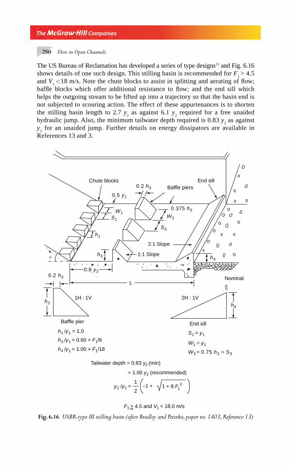
280 Flow in Open Channels
The US Bureau of Reclamation has developed a series of type designs13 and Fig. 6.16 shows details of one such design. This stilling basin is recommended for F
1 > 4.5
and V1 <18 m/s. Note the chute blocks to assist in splitting and aerating of fl ow;
baffl e blocks which offer additional resistance to fl ow; and the end sill which helps the outgoing stream to be lifted up into a trajectory so that the basin end is not subjected to scouring action. The effect of these appurtenances is to shorten the stilling basin length to 2.7 y
2 as against 6.1 y
2 required for a free unaided
hydraulic jump. Also, the minimum tailwater depth required is 0.83 y2 as against
y2 for an unaided jump. Further details on energy dissipators are available in
References 13 and 3.
Fig. 6.16 USBR-type III stilling basin (after Bradley and Peterka, paper no. 1403, Reference 13)
Nominal
2H : 1V1H : 1V
L
h4h3
0.2 h3
h3
h1
h1 /y1 = 1.0
h3 /y1 = 0.60 + F1/6
h4 /y1 = 1.00 + F1/18
S1
S1 = y1
W1 = y1
W3 = 0.75 h3 = S3
S3
W1W3
0.5 y1
0.2 h3
h4
0.375 h3
0.8 y2
θ
2:1 Slope
Baffle pier
Baffle piersChute blocks
End sill
End sill
1:1 Slope
Tailwater depth = 0.83 y2 (min)
= 1.00 y2 (recommended)
y2 /y1 =1
2–1 + 1 + 8 F 2
1
F1 > 4.5 and V1 < 18.0 m/s
Chapter 6.indd 280Chapter 6.indd 280 2/24/2010 3:00:16 PM2/24/2010 3:00:16 PM
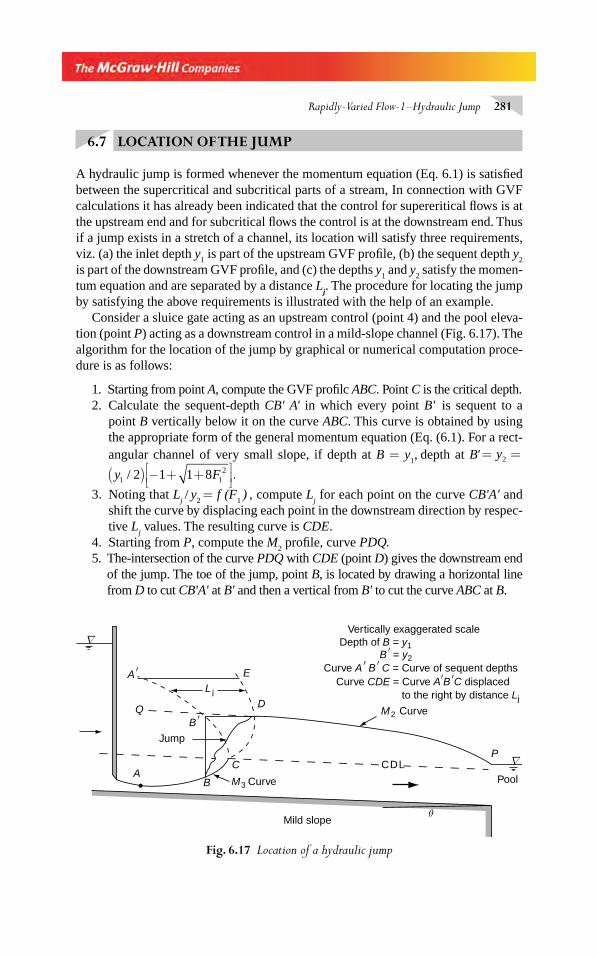
Rapidly-Varied Flow-1–Hydraulic Jump 281
6.7 LOCATION OF THE JUMP
A hydraulic jump is formed whenever the momentum equation (Eq. 6.1) is satisfi ed between the supercritical and subcritical parts of a stream, In connection with GVF calculations it has already been indicated that the control for supereritical fl ows is at the upstream end and for subcritical fl ows the control is at the downstream end. Thus if a jump exists in a stretch of a channel, its location will satisfy three requirements, viz. (a) the inlet depth y
1 is part of the upstream GVF profi le, (b) the sequent depth y
2
is part of the downstream GVF profi le, and (c) the depths y1 and y
2 satisfy the momen-
tum equation and are separated by a distance Lj. The procedure for locating the jump
by satisfying the above requirements is illustrated with the help of an example.Consider a sluice gate acting as an upstream control (point 4) and the pool eleva-
tion (point P) acting as a downstream control in a mild-slope channel (Fig. 6.17). The algorithm for the location of the jump by graphical or numerical computation proce-dure is as follows:
1. Starting from point A, compute the GVF profi lc ABC. Point C is the critical depth.2. Calculate the sequent-depth CB' A' in which every point B' is sequent to a
point B vertically below it on the curve ABC. This curve is obtained by using the appropriate form of the general momentum equation (Eq. (6.1). For a rect-angular channel of very small slope, if depth at B = y
1, depth at B' = =y2
( ) − + +⎡⎣⎢
⎤⎦⎥
y F1 122 1 1 8/ .
3. Noting that Lj / y
2 = f (F
1 )
, compute L
j for each point on the curve CB'A' and
shift the curve by displacing each point in the downstream direction by respec-tive L
j values. The resulting curve is CDE.
4. Starting from P, compute the M2 profi le, curve PDQ.
5. The-intersection of the curve PDQ with CDE (point D) gives the downstream end of the jump. The toe of the jump, point B, is located by drawing a horizontal line from D to cut CB'A' at B' and then a vertical from B' to cut the curve ABC at B.
Fig. 6.17 Location of a hydraulic jump
∇
∇
A ′ E
L j
DQB ′
Jump
C
B M3 Curve
M2 Curve
A
P
Pool
θMild slope
CDL
Vertically exaggerated scaleDepth of B = y1
B ′ = y2Curve A ′ B ′ C = Curve of sequent depths
Curve CDE = Curve A′B ′C displaced to the right by distance Lj
Chapter 6.indd 281Chapter 6.indd 281 2/24/2010 3:00:16 PM2/24/2010 3:00:16 PM
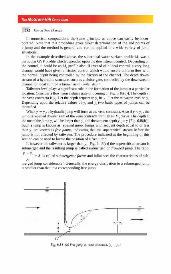
282 Flow in Open Channels
In numerical computations the same principle as above can easily be incor-porated. Note that this procedure gives direct determination of the end points of a jump and the method is general and can be applied in a wide variety of jump situations.
In the example described above, the subcritical water surface profi le M2 was a
particular GVF profi le which depended upon the downstream control. Depending on the control, it could be an M
1 profi le also. If instead of a local control, a very long
channel would have given a friction control which would ensure uniform fl ow with the normal depth being controlled by the friction of the channel. The depth down-stream of a hydraulic structure, such as a sluice gate, controlled by the downstream channel or local control is known as tailwater depth.
Tailwater level plays a signifi cant role in the formation of the jump at a particular location. Consider a fl ow from a sluice gate of opening a [Fig. 6.18(a)]. The depth at the vena contracta is y
a. Let the depth sequent to y
a be y
2. Let the tailwater level be y
t.
Depending upon the relative values of y2 and y
t two basic types of jumps can be
identifi ed.When y
t = y
2, a hydraulic jump will form at the vena contracta. Also if y
t <
y
2 , the
jump is repelled downstream of the vena contracta through an M3 curve. The depth at
the toe of the jump y1 will be larger than y
a and the sequent depth y
12 = y
t [Fig. 6.l8(b)].
Such a jump is known as repelled jump. Jumps with sequent depth equal to or less than y
2 are known as free jumps, indicating that the supercritical stream before the
jump is not affected by tailwater. The procedure indicated at the beginning of this section can be used to locate the position of a free jump.
If however the tailwater is larger than y2 [Fig. 6. l8(c)] the supercritical stream is
submerged and the resulting jump is called submerged or drowned jump. The ratio, y y
ySt −
=2
2
is called submergence factor and infl uences the characteristics of sub-
merged jump considerably3. Generally, the energy dissipation in a submerged jump is smaller than that in a corresponding free jump.
Fig. 6.18 (a) Free jump at vena contracta, (yt = y
2 )
a
A yt = y2
ya
∇
∇
Chapter 6.indd 282Chapter 6.indd 282 2/24/2010 3:00:17 PM2/24/2010 3:00:17 PM
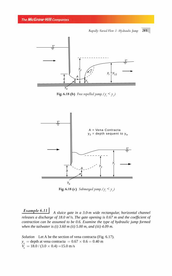
Rapidly-Varied Flow-1–Hydraulic Jump 283
Example 6.11 A sluice gate in a 3.0-m wide rectangular, horizontal channel releases a discharge of 18.0 m3/s. The gate opening is 0.67 m and the coeffi cient of contraction can be assumed to be 0.6. Examine the type of hydraulic jump formed when the tailwater is (i) 3.60 m (ii) 5.00 m, and (iii) 4.09 m.
Solution Let A be the section of vena contracta (Fig. 6.17).y
a = depth at vena contracta = 0.67 × 0.6 = 0.40 m
Va = 18.0 / (3.0 × 0.4) =15.0 m /s
Fig. 6.18 (c) Submerged jump, ( yt < y
2 )
∇
∇
yty
2Aa
ya
A = Vena Contractay2 = depth sequent to ya
Fig. 6.18 (b) Free repelled jump, ( yt < y
2 )
y1
∇
∇
a
y2
yt = y
12A
ya
Chapter 6.indd 283Chapter 6.indd 283 2/24/2010 3:00:17 PM2/24/2010 3:00:17 PM
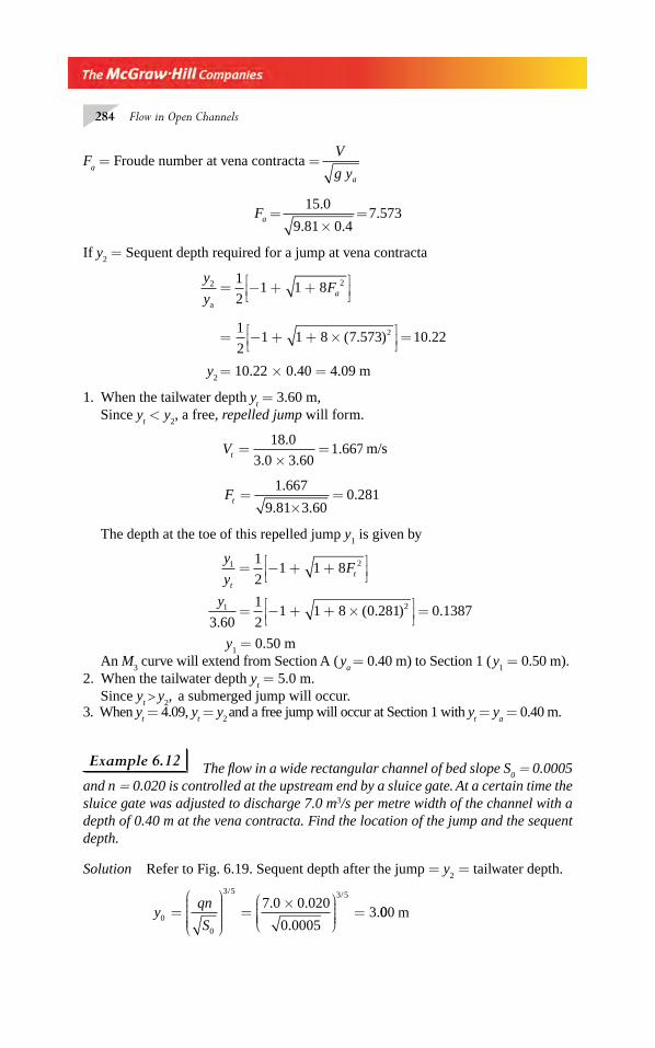
284 Flow in Open Channels
Fa = Froude number at vena contracta =
V
g ya
Fa =×
=15 0
9 81 0 47 573
.
. ..
If y2 = Sequent depth required for a jump at vena contracta
y
yFa
2 21
21 1 8
a
= − + +⎡⎣⎢
⎤⎦⎥
= − + + ×⎡
⎣⎢⎤⎦⎥=
1
21 1 8 7 573 10 222( . ) .
y2 = 10.22 × 0.40 = 4.09 m
1. When the tailwater depth yt = 3.60 m,
Since yt < y
2, a free, repelled jump will form.
Vt =×
=18 0
3 0 3 601 667
.
. .. m/s
Ft =×
=1 667
9 81 3 600 281
.
. ..
The depth at the toe of this repelled jump y1 is given by
y
yF
t
t1 21
21 1 8= − + +⎡
⎣⎢⎤⎦⎥
y1 2
3 60
1
21 1 8 0 281 0 1387
.( . ) .= − + + ×⎡
⎣⎢⎤⎦⎥=
y1 = 0.50 m
An M3 curve will extend from Section A ( y
a = 0.40 m) to Section 1 ( y
1 = 0.50 m).
2. When the tailwater depth yt = 5.0 m.
Since yt >
y2, a submerged jump will occur.
3. When yt = 4.09, y
t = y
2 and a free jump will occur at Section 1 with y
t = y
a = 0.40 m.
Example 6.12 The fl ow in a wide rectangular channel of bed slope S0 = 0.0005
and n = 0.020 is controlled at the upstream end by a sluice gate. At a certain time the sluice gate was adjusted to discharge 7.0 m3/s per metre width of the channel with a depth of 0.40 m at the vena contracta. Find the location of the jump and the sequent depth.
Solution Refer to Fig. 6.19. Sequent depth after the jump = y2
= tailwater depth.
yqn
S0
0
3 5 3 57 0 0 020
0 00053=
⎛
⎝
⎜⎜⎜⎜⎜
⎞
⎠
⎟⎟⎟⎟⎟=
×⎛
⎝⎜⎜⎜⎜
⎞
⎠⎟⎟⎟⎟ =
/ /. .
..000 m
Chapter 6.indd 284Chapter 6.indd 284 2/24/2010 3:00:17 PM2/24/2010 3:00:17 PM
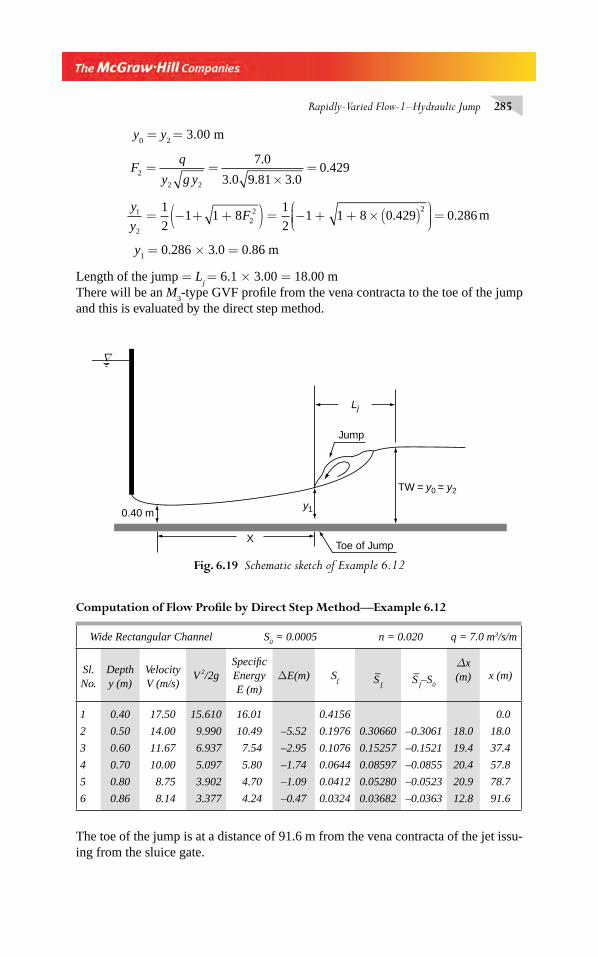
Rapidly-Varied Flow-1–Hydraulic Jump 285
y0 = y
2 = 3.00 m
Fq
y g y2
2 2
7 0
3 0 9 81 3 00 429= =
×=
.
. . ..
y
yF1
222 21
21 1 8
1
21 1 8 0 429 0 286= − + +( ) = − + + × ( )⎛
⎝⎜⎜⎜
⎞⎠⎟⎟⎟ =. . m
y1 = 0.286 × 3.0 = 0.86 m
Length of the jump = Lj = 6.1 × 3.00 = 18.00 m
There will be an M3-type GVF profi le from the vena contracta to the toe of the jump
and this is evaluated by the direct step method.
Fig. 6.19 Schematic sketch of Example 6.12
∇
0.40 m
XToe of Jump
y1
Jump
TW = y0 = y2
Lj
Wide Rectangular Channel S0 = 0.0005 n = 0.020 q = 7.0 m3/s/m
Sl. No.
Depth y (m)
Velocity V (m/s)
V 2/2gSpecifi c Energy E (m)
ΔE(m) Sf S
–f
S–
f–S
0
Δx (m) x (m)
1 0.40 17.50 15.610 16.01 0.4156 0.0
2 0.50 14.00 9.990 10.49 –5.52 0.1976 0.30660 –0.3061 18.0 18.0
3 0.60 11.67 6.937 7.54 –2.95 0.1076 0.15257 –0.1521 19.4 37.4
4 0.70 10.00 5.097 5.80 –1.74 0.0644 0.08597 –0.0855 20.4 57.8
5 0.80 8.75 3.902 4.70 –1.09 0.0412 0.05280 –0.0523 20.9 78.7
6 0.86 8.14 3.377 4.24 –0.47 0.0324 0.03682 –0.0363 12.8 91.6
Computation of Flow Profi le by Direct Step Method—Example 6.12
The toe of the jump is at a distance of 91.6 m from the vena contracta of the jet issu-ing from the sluice gate.
Chapter 6.indd 285Chapter 6.indd 285 2/24/2010 3:00:18 PM2/24/2010 3:00:18 PM
286 Flow in Open Channels
REFERENCES
1. Bradley, J N and Peterka, A J ‘The Hydraulic Design of Stilling Basins, Hydraulic Jumps on a Horizontal Apion’, J. of Hyd. Div., Proc. ASCE, Paper No. 1401, October 1957, pp 1401–l–25.
2. Swamee, P K and Rathie, P N, ‘Exact Solutions of Sequent Depth Problems’, J. of Irr. andDrainage Engg., Vol. 130, No. 6, Nov.-Dec. 2004, pp. 520–522.
3. Elevatorski, E A, Hydraulic Energy Dissipators, McGraw-Hill, New York, 1959. 4. Rajaratnam, N, ‘Hydraulic Jumps’, Chapter in Advances in Hydroscience, ed. Chow, V T
Vol. 4, Academic Press, New York, 1967, pp 198–280. 5. Subramanya, K, ‘Some Studies on Turbulent Wall Jets in Hydraulic Engineering’, Ph. D.
thesis, Univ. of Alberta, Edmonton, Canada, Oct. 1967. 6. Rajaratnam, N and Subramanya, K, ‘Profi le of the Hydraulic Jump’, J. of Hyd.
Div., Proc. ASCE, Paper No. 5931, May 1968, pp 663–673. 7. Leutheusser, H J and Kartha,V C ‘Effects of Infl ow Condition on Hydraulic Jump’, J. of
Hyd. Div., Proc. ASCE, Paper No. 9088, Aug 1972, pp 1367–1385. 8. Silvester, R, ‘Hydraulic Jumps in all Shapes of Horizontal Channels’, J. of Hyd. Div.,
Proc. ASCE, Jan. 1964, pp 23–55. 9. Argyropoulous, P A, ‘Theoretical and Experimental Analysis of the Hydraulic Jump in a
Sloping Parabolic Flume’, Proc. IAHR, Lisbon, Vol. 2, 1957, pp D. 12–1–20.10. Argyropoulous, P A, ‘The Hydraulic Jump and the Effect of Turbulence on Hydraulic
Structures’, Proc. IAHR, Durbrovnik, Yugoslavia, 1961, pp 173–183.11. Bradley, J N and Peterka, A J ‘Hydraulic Design of Stilling Basin: Stilling Basin with
Sloping Apron (Basin,V)’, J. of Hyd. Div, Proc. ASCE, Paper No. 1405, Oct.1957, pp 1405–1–32.
12. Henderson, F M Open Channel Flow, Macmillan, New York, 1966.13. Bradley, J N and Peterka, A J ‘Hydraulic Design of Stilling Basins’ in Symposium on
Stilling Basins and Energy Dissipators’, ASCE, Proc. Symp. Series No. 5, Paper Nos.1401 to 1406, June 1961, pp 1401–1 to 1406–17 (also in J. of Hyd, Div., Proc. ASCE, Vol. 83, No. HY 5, Oct. 1957).
14. Forster, J W and Skrinde, R A ‘Control of the Hydraulic Jump by Sills’, Trans. ASCE, Vol. 115, 1950, pp 973–1022.
15. Hsu, E Y, ‘Discussion on: Control of the Hydraulic Jump by Sills’, Trans. ASCE, Vol. 115, 1950, pp 988–991.
16. Moore, W L, and Morgan, C W ‘Hydraulic Jump at an Abrupt Drop’. Trans. ASCE, Vol. 124, 1959, pp 507–524.
17. Harleman, D R F, ‘Effect of Baffl e Piers on Stilling Basin Performance’, J. of Boston Soc. of Civil Engineers, Vol. 42, 1955, pp 84–89.
18. Koloseus, H J and Ahmad, D ‘Circular Hydraulic Jump’, J. of Hyd. Div., Proc. ASCE, Jan. 1969, pp 409–422.
19. Arbhabhirama, A and Wan, W C ‘Characteristics of a Circular Jump in a Radial Wall Jet’ J. of Hyd. Res., IAHR, Vol. 13, No. 3, 1973, pp 239–262.
20. Lewson, J D and Phillips, B C ‘Circular Hydraulic Jump’, J. of Hyd. Engg., ASCE, Vol. 109, No. 4, April, 1983, pp 505–518.
21. Arbhabhirama, A and Abella, U Hydraulic Jump with a Gradually Expanding Channel’, J. of Hyd. Div., Proc ASCE, Jan. 1971, pp 31–42.
22. Khalifa, A M and McCorquodale, J A ‘Radial Hydraulic Jump’, J. of Hyd. Div., Proc, ASCE, Sept. 1979, pp 1065–1078.
Chapter 6.indd 286Chapter 6.indd 286 2/24/2010 3:00:18 PM2/24/2010 3:00:18 PM
Rapidly-Varied Flow-1–Hydraulic Jump 287
PROBLEMS
Problem Distribution
Topic Problems
1. Elements of jump in a rectangular channel 6.1–6.10 2. Jump below a sluice gate 6.11, 6.23, 6.24, 6.31, 6.32 3. Jump below an overfl ow spillway 6.12–6.14 4. Jump at an abrupt rise 6.15, 6.30 5. Jump at a sudden drop 6.16 6. Jump on a sloping fl oor 6.17, 6.25 , 6.27 7. Jump in non-rectangular channels 6.18–6.22, 6.26 8. Location of the jump 6.23, 6.24 9. Forced hydraulic jump 6.2810. Circular hydraulic jump 6.2911. Repelled jump 6.31, 6.32
(Unless otherwise stated the channel is assumed to be frictionless for purposes of hydraulic jump calculations.)
6.1 A hydraulic jump occurs in a horizontal rectangular channel with sequent depths of 0.70 m and 4.2 m. Calculate the rate of fl ow per unit width, energy loss and the initial Froude number.
6.2 A hydraulic jump occurs in a horizontal rectangular channel at an initial Froude number of 10.0. What percentage of initial energy is lost in this jump?
6.3 The following table gives some of the possible types of problems associated with a hydraulic jump occurring in a rectangular channel. Complete the following table.
(Note that Problem 6.3(c) requires a trial-and-error approach. Assume F1, fi nd y
1, y
2 and
check EL. Repeat till satisfactory values are obtained.)
Prob. No.
V1
(m / s)y
1 (m) q
(m 2/s / m)F
1y
2
(m)V
2(m/s) F
2E
L
(m)E
L/E
1
(%)
a 0.170 1.84b 9.00 2.90c 2.00 1.75d 1.60 0.90e 13.50 0.350f 0.15 8.00
6.4 A hydraulic jump in a rectangular channel has the Froude number at the beginning of the jump F
1 = 5. Find the Froude number F
2 at the end of the jump.
6.5 Show that the Froude numbers F1 and F
2 in a hydraulic jump occurring in a rectangular
channel are related by
(a) FF
F2
2 12
12
3
8
1 1 8=
− + +( ) (b) F
F
F12 2
2
22
3
8
1 1 8=
− + +( )6.6 A rectangular channel carrying a supercritical stream is to be provided with a hydrau-
lic jump type of energy dissipator. If it is desired to have an energy loss of 5 m in the jump when the inlet Froude number is 8.5, determine the sequent depths.
6.7 Show that in a hydraulic jump formed in a horizontal, frictionless, rectangular channel the energy loss E
L relative to the critical depth y
c can be expressed as
Chapter 6.indd 287Chapter 6.indd 287 2/24/2010 3:00:19 PM2/24/2010 3:00:19 PM
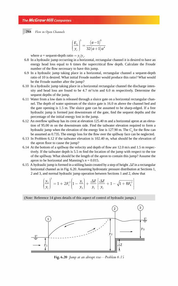
288 Flow in Open Channels
E
y
a
a aL
c
⎛
⎝⎜⎜⎜⎜
⎞
⎠⎟⎟⎟⎟
=−( )+( )
3 9
4
1
32 1
where a = sequent-depth ratio = y2/y
1.
6.8 In a hydraulic jump occurring in a horizontal, rectangular channel it is desired to have an energy head loss equal to 6 times the supercritical fl ow depth. Calculate the Froude number of the fl ow necessary to have this jump.
6.9 In a hydraulic jump taking place in a horizontal, rectangular channel a sequent-depth ratio of 10 is desired. What initial Froude number would produce this ratio? What would be the Froude number after the jump?
6.10 In a hydraulic jump taking place in a horizontal rectangular channel the discharge inten-sity and head loss are found to be 4.7 m3/s/m and 6.0 m respectively. Determine the sequent depths of the jump.
6.11 Water from a low dam is released through a sluice gate on a horizontal rectangular chan-nel. The depth of water upstream of the sluice gate is 16.0 m above the channel bed and the gate opening is 1.5 m. The sluice gate can be assumed to be sharp-edged. If a free hydraulic jump is formed just downstream of the gate, fi nd the sequent depths and the percentage of the initial energy lost in the jump.
6.12 An overfl ow spillway has its crest at elevation 125.40 m and a horizontal apron at an eleva-tion of 95.00 m on the downstream side. Find the tailwater elevation required to form a hydraulic jump when the elevation of the energy line is 127.90 m. The C
d for the fl ow can
be assumed as 0.735. The energy loss for the fl ow over the spillway face can be neglected.6.13 In Problem 6.12 if the tailwater elevation is 102.40 m, what should be the elevation of
the apron fl oor to cause the jump?6.14 At the bottom of a spillway the velocity and depth of fl ow are 12.0 m/s and 1.5 m respec-
tively. If the tailwater depth is 5.5 m fi nd the location of the jump with respect to the toe of the spillway. What should be the length of the apron to contain this jump? Assume the apron to be horizontal and Manning’s n = 0.015.
6.15 A hydraulic jump is formed in a stiliing basin created by a step of height ΔZ in a rec tangular horizontal channel as in Fig. 6.20. Assuming hydrostatic pressure distribution at Sections 1, 2 and 3, and normal hydraulic jump operation between Sections 1 and 2, show that
y
yF
y
y
Z
y
Z
yF3
1
2
12 1
3 1 1
1 2 1 1 1 8⎛
⎝⎜⎜⎜⎜
⎞
⎠⎟⎟⎟⎟
= + −⎛
⎝⎜⎜⎜⎜
⎞
⎠⎟⎟⎟⎟
+Δ Δ
+ − + 112
⎡
⎣⎢⎢
⎤
⎦⎥⎥
(Note: Reference 14 gives details of this aspect of control of hydraulic jumps.)
∇
∇
y3
1
2 3
y1
y2
ΔZ
Fig. 6.20 Jump at an abrupt rise—Problem 6.15
Chapter 6.indd 288Chapter 6.indd 288 2/24/2010 3:00:19 PM2/24/2010 3:00:19 PM
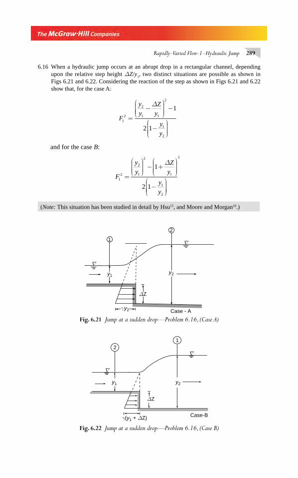
Rapidly-Varied Flow-1–Hydraulic Jump 289
6.16 When a hydraulic jump occurs at an abrupt drop in a rectangular channel, depending upon the relative step height ΔZ/y
1, two distinct situations are possible as shown in
Figs 6.21 and 6.22. Considering the reaction of the step as shown in Figs 6.21 and 6.22 show that, for the case A:
F
y
y
Z
y
y
y
12
2
1 1
2
1
2
1
2 1
=
−Δ⎛
⎝⎜⎜⎜⎜
⎞
⎠⎟⎟⎟⎟
−
−⎛
⎝⎜⎜⎜⎜
⎞
⎠⎟⎟⎟⎟
and for the case B:
F
y
y
Z
y
y
y
12
2
1
2
1
1
2
1
2 1
=
⎛
⎝⎜⎜⎜⎜
⎞
⎠⎟⎟⎟⎟
− +Δ⎛
⎝⎜⎜⎜⎜
⎞
⎠⎟⎟⎟⎟
−⎛
⎝⎜⎜⎜⎜
⎞
⎠⎟⎟⎟⎟⎟
2
(Note: This situation has been studied in detail by Hsu15, and Moore and Morgan16.)
Fig. 6.21 Jump at a sudden drop—Problem 6.16, (Case A)
∇
∇
ΔZ
γy2
y2y1
2
1
Case - A
Fig. 6.22 Jump at a sudden drop—Problem 6.16, (Case B)
∇
∇
ΔZ
y2y1
γ(y1 + ΔZ) Case-B
21
Chapter 6.indd 289Chapter 6.indd 289 2/24/2010 3:00:19 PM2/24/2010 3:00:19 PM
290 Flow in Open Channels
6.17 The Rihand dam in U.P., India, has a sloping apron stilling basin with a slope of 0.077. If the depth for a fl ood fl ow of 64.0 m3/s per metre width is 1.93 m, estimate the sequent depth, length of the jump and energy loss in the hydraulic jump.
6.18 A hydraulic jump occurs in a horizontal 90° triangular channel. If the sequent depths in this jump are 0.60 m and 1.20 m, estimate the fl ow rate and the Froude numbers at the beginning and end of the jump.
6.19 For a hydraulic jump taking place in a horizontal, frictionless, triangular channel show that the sequent depths y
1 and y
2 are related to the pre-jump Froude number F
1 as
F12
2 3
2
2 1
3 1=
−−
η ηη( )
( )
where η = y y2 1/ .6.20 A horizontal trapezoidal channel of 2.0-m bed width and side slopes 2 horizontal : 1 ver-
tical carries a discharge of 6.225 m3/s at a depth of 0.20 m. If a hydraulic jump takes place in this channel, calculate the sequent depth and energy loss.
6.21 A trapezoidal channel of 7.0-m bottom width and side slope 1 horizontal : 1 vertical carries a discharge of 20 m3/s. Prepare the specifi c energy and specifi c-force diagrams for this chan-nel. If the depth after a jump on a horizontal fl oor in this channel for the given discharge is known to be 2.25 m, fi nd the sequent depth and energy loss. What are the limitations of the plots prepared by you? Can you think of a non-dimensional representation of the specifi c-force and specifi c-energy diagrams so that they can be used for jump computations in trape-zoidal channels having a wide range of geometrical parameters and discharges?
6.22 A circular culvert of 1.5-m diameter carries a discharge of 1.0 m3/s. The channel can be assumed to be horizontal and frictionless. If the depth at the beginning of a hydraulic jump occurring in this channel is 0.30 m, determine sequent depth.
6.23 A sluice gate discharges 10.0 m3/s per meter width in to a wide rectangular channel of n = 0.025 and bottom slope S
0 = 0.0002. The depth of fl ow at the vena contracta is 0.40
m. If the channel ends in a sudden drop at a distance of 1300 m downstream of the gate, locate the position of the jump.
6.24 The fl ow in a wide rectangular channel of bed slope S0 = 0.0008 and n = 0.025 is con-
trolled at the upstream end by a sluice gate. The sluice gate is adjusted to discharge 8.0 m3/s per meter width of the channel, with a depth of 0.50m at the vena contracta Find the location of the jump and the sequent depth
6.25 A wide rectangular steep channel (tan θ = 0.20) has a horizontal apron. Find the maxi-mum tailwater depth that will have a jump completely in a horizontal apron when a dis-charge of 2.47 m3/s per metre width passes down the steep channel at a depth of 0.30 m. What tailwater depth will cause the jump to occur completely on the sloping channel?
6.26 Prepare a plot of EL
/ E1 vs F
1 for rectangular, parabolic and triangular horizontal chan-
nels using Eqs (6.23) and (6.24). Observe that the highest relative energy loss occurs in a triangular channel.
6.27 (a) Show that the relative energy loss in a hydraulic jump occurring on a sloping rectan-gular channel is
E
H
y
y
F y
yL
t
t
1
1
12
1
2
12
1
=
−⎛
⎝⎜⎜⎜⎜
⎞
⎠⎟⎟⎟⎟+ −
⎛
⎝⎜⎜⎜⎜
⎞
⎠⎟⎟⎟⎟
⎡
⎣
⎢⎢⎢
⎤
⎦cosθ ⎥⎥
⎥⎥+
⎛
⎝⎜⎜⎜⎜
⎞
⎠⎟⎟⎟⎟
+ +⎛
⎝⎜⎜⎜⎜
⎞
⎠⎟⎟⎟⎟
L
y
y
y
F L
y
y
y
t
t
t
t
1
12
12
tan
cos t
θ
θ aan
( , )
θθ= f F1
Chapter 6.indd 290Chapter 6.indd 290 2/24/2010 3:00:20 PM2/24/2010 3:00:20 PM
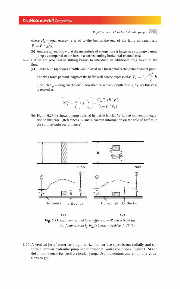
Rapidly-Varied Flow-1–Hydraulic Jump 291
where H1
= total energy referred to the bed at the end of the jump as datum and
F V gy1 1 1= / .
(b) Analyse EL and show that the magnitude of energy loss is larger in a sloping-channel
jump as compared to the loss in a corresponding horizontal-channel case.6.28 Baffl es are provided in stilling basins to introduce an additional drag force on the
fl ow. (a) Figure 6.23 (a) shows a baffl e wall placed in a horizontal rectangular channel jump.
The drag force per unit length of the baffl e wall can be expressed as P CV
hB D=ρ 1
2
2
in which CD = drag coeffi cient. Show that the sequent-depth ratio y
2 / y
1 for this case
is related as
2 111
2 2
1
2
1
12
1
1 2
Fy
y
y
y
C F h y
y yD− +
⎛
⎝⎜⎜⎜⎜
⎞
⎠⎟⎟⎟⎟
⎡
⎣⎢⎢⎢
⎤
⎦⎥⎥⎥=
( )−( )
/
/
(b) Figure 6.23(b) shows a jump assisted by baffl e blocks. Write the momentum equa-tion to this case. (References 17 and 4 contain information on the role of baffl es in the stilling-basin performance).
Fig. 6.23 (a) Jump assisted by a baffl e wall—Problem 6.28 (a)
(b) Jump assisted by baffl e blocks—Problem 6.28 (b)
hy1
y1
1122
h
y2y
2
SW
BB
L-Sect ion Horizontal L- Sect ionHorizontal
Plan Plan
(a) (b)
6.29 A vertical jet of water striking a horizontal surface spreads out radially and can form a circular hydraulic jump under proper tailwater conditions. Figure 6.24 is a definition sketch for such a circular jump. Use momentum and continuity equa-tions to get
Chapter 6.indd 291Chapter 6.indd 291 2/24/2010 3:00:20 PM2/24/2010 3:00:20 PM
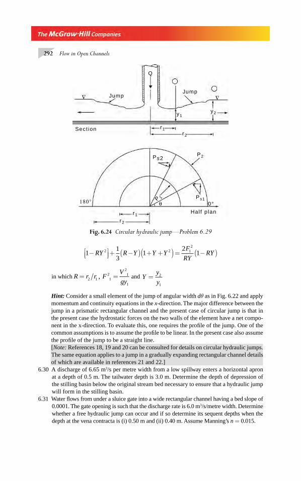
292 Flow in Open Channels
11
31
212 2 1
2
−⎡⎣⎢
⎤⎦⎥ + −( ) + +( ) = −( )RY R Y Y Y
F
RYRY
in which R r r FV
gy= =2 1
21
21
1
, and Yy
y= 2
1
Hint: Consider a small element of the jump of angular width dθ as in Fig. 6.22 and apply momentum and continuity equations in the x-direction. The major difference between the jump in a prismatic rectangular channel and the present case of circular jump is that in the present case the hydrostatic forces on the two walls of the element have a net compo-nent in the x-direction. To evaluate this, one requires the profi le of the jump. One of the common assumptions is to assume the profi le to be linear. In the present case also assume the profi le of the jump to be a straight line.
[Note: References 18, 19 and 20 can be consulted for details on circular hydraulic jumps. The same equation applies to a jump in a gradually expanding rectangular channel details of which are available in references 21 and 22.]
6.30 A discharge of 6.65 m3/s per metre width from a low spillway enters a horizontal apron at a depth of 0.5 m. The tailwater depth is 3.0 m. Determine the depth of depression of the stilling basin below the original stream bed necessary to ensure that a hydraulic jump will form in the stilling basin.
6.31 Water fl ows from under a sluice gate into a wide rectangular channel having a bed slope of 0.0001. The gate opening is such that the discharge rate is 6.0 m3/s/metre width. Determine whether a free hydraulic jump can occur and if so determine its sequent depths when the depth at the vena contracta is (i) 0.50 m and (ii) 0.40 m. Assume Manning’s n = 0.015.
Fig. 6.24 Circular hydraulic jump—Problem 6.29
∇ ∇JumpJump
Q
y1y2
r1r2
Sect ion
P 1
P2
Ps1
Ps2
0°θ180°
r2
r1Hal f p lan
Chapter 6.indd 292Chapter 6.indd 292 2/24/2010 3:00:21 PM2/24/2010 3:00:21 PM
Rapidly-Varied Flow-1–Hydraulic Jump 293
6.32 An opening of a reservoir is controlled by a sluice gate. The gate opening is 1.30 m. Water surface elevation upstream of the gate is 100.00 m. If the elevation of the bed is 85.00 m and the tailwater elevation is 91.00 m.
(a ) What is the discharge per unit width? (b) What kind of jump is formed? What are the sequent depths? (c ) What is the maximum tailwater depth that could be sustained by a free jump? (Assume C
c = 0.75 and C
d = 0.71 for the sluice gate).
OBJECTIVE QUESTIONS
6.1 The hydraulic jump is a phenomenon(a) in which the water surface connects the alternate depths (b) which occurs only in frictionless channels(c ) which occurs only in rectangular channels(d) none of these
6.2 A hydraulic jump occurs when there is a break in grade from a(a) mild slope to steep slope (b) steep slope to mild slope(c) steep slope to steeper slope (d) mild slope to milder slope
6.3 The sequent-depth ratio in a hydraulic jump formed in a horizontal rectangular channel is 16.48. The Froude number of the supercritical stream is(a) 8.0 (b) 4.0 (c) 20 (d) 12.0
6.4 The Froude number of a subcritical stream at the end of a hydraulic jump in a horizontal rectangular channel is 0.22. The sequent-depth ratio of this jump is.(a) 11.25 (b) 15.25 (c) 8.35 (d) 6.50
6.5 If the Froude number of a hydraulic jump is 5.50, it can be classifi ed as (a) an oscillating jump (b) a weak jump(c) a strong jump (d) a steady jump
6.6 The initial depth of a hydraulic jump in a rectangular channel is 0.2 m and the sequent-depth ratio is 10. The length of the jump is about(a) 4 m (b) 6 m (c) 12 m (d) 20 m
6.7 In a hydraulic jump taking place in a horizontal rectangular channel the sequent depths are 0.30 m and 1.50 m respectively. The energy loss in this jump is(a) 1.92 m (b) 1.50 m (c) 0.96 m (d) 1.20 m
6.8 Seventy per cent of the initial energy is lost in a jump taking place in a horizontal rectan-gular channel. The Froude number of the fl ow at the toe is(a) 4.0 (b) 9.0 (c) 20.0 (d) 15.0
6.9 In a hydraulic jump occurring in a horizontal rectangular channel with an initial Froude number of 12, the sequent depth ratio is found to be 13.65. The energy dissipation as a percentage of the initial specifi c energy is about(a) 62% (b) 50% (c) 87% (d) 73%
6.10 The concept of constancy of specifi c force at the beginning and the end of a jump(a) assumes horizontal frictionless channel(b) is valid for jumps in a rectangular sloping fl oor basin(c) is valid for all kinds of channels provided the friction can be assumed to be negligi-
bly small(d) assumes constancy of specifi c energy
Chapter 6.indd 293Chapter 6.indd 293 2/24/2010 3:00:21 PM2/24/2010 3:00:21 PM
294 Flow in Open Channels
6.11 A sluice gate discharges a fl ow with a depth of y1 at the vena contracta. y
2 is the sequent
depth corresponding to y1. If the tailwater depth y
t is larger then y
2 then
(a) a repelled jump occurs (b) a free jump occurs(c) a submerged jump takes place (d) no jump takes place
6.12 If y2 = sequent depth for a rectangular channel obtained by assuming horizontal friction-
less channel in the momentum equation and y2a
= corresponding actual sequent depth measured in a horizontal rectangular channel having high friction, one should expect(a) y
2 > y
2a (b) y
2 = y
2a (c) y
2 < y
2a (c) y
2 ≤ y
2a
6.13 If the length of the jump in a sloping rectangular channel = Ljs and the corresponding
length of the jump in a horizontal rectangular channel having same y1 and F
1 is L
j, then
(a) Lj >
L
js (b) L
js > L
j (c) L
j = L
js (d) L
j /L
js = 0.80
6.14 If ELS
= energy loss in a jump in a sloping rectangular channel and ELH
= energy loss in a corresponding jump on a horizontal rectangular channel having the same y
1 and F
1,
then (a) E
LH = E
LS (b) E
LH > E
LS (c) E
LH < E
LS (d) E
LH /E
LS = 0.80
Chapter 6.indd 294Chapter 6.indd 294 2/24/2010 3:00:21 PM2/24/2010 3:00:21 PM
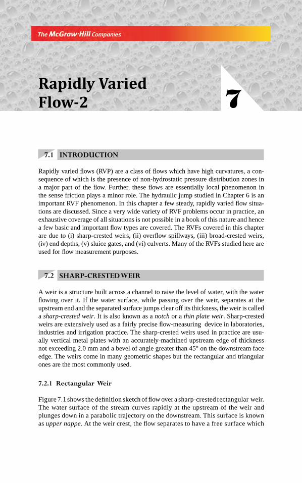
7.1 INTRODUCTION
Rapidly varied fl ows (RVP) are a class of fl ows which have high curvatures, a con-sequence of which is the presence of non-hydrostatic pressure distribution zones in a major part of the fl ow. Further, these fl ows are essentially local phenomenon in the sense friction plays a minor role. The hydraulic jump studied in Chapter 6 is an important RVF phenomenon. In this chapter a few steady, rapidly varied fl ow situa-tions are discussed. Since a very wide variety of RVF problems occur in practice, an exhaustive coverage of all situations is not possible in a book of this nature and hence a few basic and important fl ow types are covered. The RVFs covered in this chapter are due to (i) sharp-crested weirs, (ii) overfl ow spillways, (iii) broad-crested weirs, (iv) end depths, (v) sluice gates, and (vi) culverts. Many of the RVFs studied here are used for fl ow measurement purposes.
7.2 SHARP-CRESTED WEIR
A weir is a structure built across a channel to raise the level of water, with the water fl owing over it. If the water surface, while passing over the weir, separates at the upstream end and the separated surface jumps clear off its thickness, the weir is called a sharp-crested weir. It is also known as a notch or a thin plate weir. Sharp-crested weirs are extensively used as a fairly precise fl ow-measuring device in laboratories, industries and irrigation practice. The sharp-crested weirs used in practice are usu-ally vertical metal plates with an accurately-machined upstream edge of thickness not exceeding 2.0 mm and a bevel of angle greater than 45° on the downstream face edge. The weirs come in many geometric shapes but the rectangular and triangular ones are the most commonly used.
7.2.1 Rectangular Weir
Figure 7.1 shows the defi nition sketch of fl ow over a sharp-crested rectangular weir. The water surface of the stream curves rapidly at the upstream of the weir and plunges down in a parabolic trajectory on the downstream. This surface is known as upper nappe. At the weir crest, the fl ow separates to have a free surface which
Rapidly Varied
Flow-2 7
Chapter 7.indd 295Chapter 7.indd 295 2/24/2010 3:01:25 PM2/24/2010 3:01:25 PM
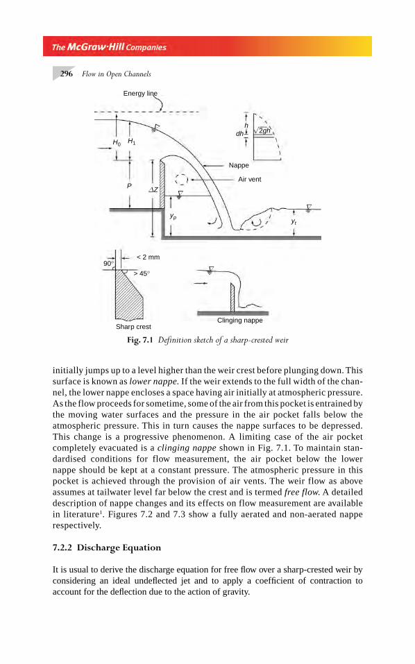
296 Flow in Open Channels
initially jumps up to a level higher than the weir crest before plunging down. This surface is known as lower nappe. If the weir extends to the full width of the chan-nel, the lower nappe encloses a space having air initially at atmospheric pressure. As the flow proceeds for sometime, some of the air from this pocket is entrained by the moving water surfaces and the pressure in the air pocket falls below the atmospheric pressure. This in turn causes the nappe surfaces to be depressed. This change is a progressive phenomenon. A limiting case of the air pocket completely evacuated is a clinging nappe shown in Fig. 7.1. To maintain stan-dardised conditions for flow measurement, the air pocket below the lower nappe should be kept at a constant pressure. The atmospheric pressure in this pocket is achieved through the provision of air vents. The weir flow as above assumes at tailwater level far below the crest and is termed free flow. A detailed description of nappe changes and its effects on flow measurement are available in literature1. Figures 7.2 and 7.3 show a fully aerated and non-aerated nappe respectively.
7.2.2 Discharge Equation
It is usual to derive the discharge equation for free fl ow over a sharp-crested weir by considering an ideal undefl ected jet and to apply a coeffi cient of contraction to account for the defl ection due to the action of gravity.
Energy line
H0H1
P
hdh
Nappe
Air vent
yp yt
ΔZ
< 2 mm
> 45°90°
Sharp crestClinging nappe
∇
∇
∇
∇
√2gh
Fig. 7.1 Defi nition sketch of a sharp-crested weir
Chapter 7.indd 296Chapter 7.indd 296 2/24/2010 3:01:28 PM2/24/2010 3:01:28 PM
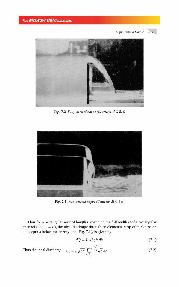
Rapidly Varied Flow-2 297
Thus for a rectangular weir of length L spanning the full width B of a rectangular channel (i.e., L = B), the ideal discharge through an elemental strip of thickness dh at a depth h below the energy line (Fig. 7.1), is given by
dQi = L 2gh dh (7.1)
Thus the ideal discharge Q L g h dhi V
g
HV
g=+
∫202
102
2
2 (7.2)
Fig. 7.2 Fully-aerated nappe (Courtesy: M G Bos)
Fig. 7.3 Non-aerated nappe (Courtesy: M G Bos)
Chapter 7.indd 297Chapter 7.indd 297 2/24/2010 3:01:28 PM2/24/2010 3:01:28 PM
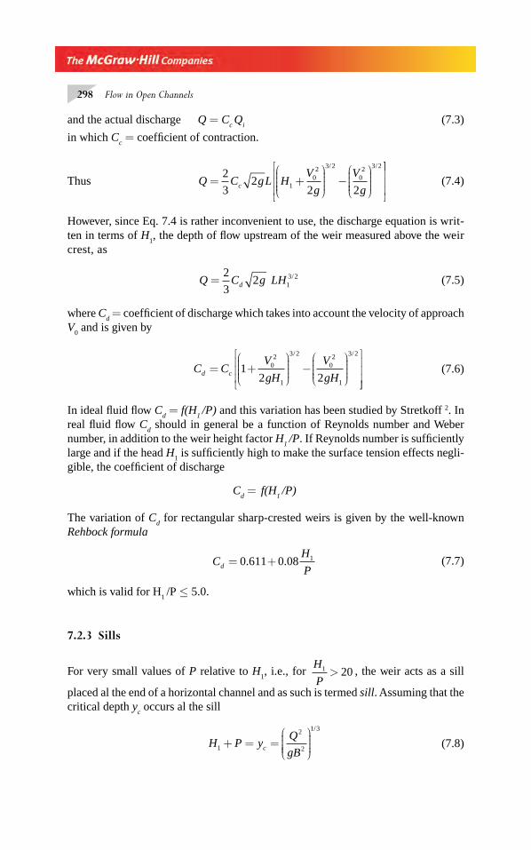
298 Flow in Open Channels
and the actual discharge Q = Cc Q
i (7.3)
in which Cc = coeffi cient of contraction.
Thus Q C gL HV
g
V
gc= +⎛
⎝⎜⎜⎜⎜
⎞
⎠⎟⎟⎟⎟
−⎛
⎝⎜⎜⎜⎜
⎞
⎠⎟⎟⎟⎟
⎡
⎣
⎢⎢⎢
2
32
2 2102 3 2
02 3 2/ / ⎤⎤
⎦
⎥⎥⎥
(7.4)
However, since Eq. 7.4 is rather inconvenient to use, the discharge equation is writ - ten in terms of H
1, the depth of fl ow upstream of the weir measured above the weir
crest, as
Q C g LHd=2
32 1
3 2/ (7.5)
where Cd = coeffi cient of discharge which takes into account the velocity of approach
V0 and is given by
C CV
gH
V
gHd c= +⎛
⎝⎜⎜⎜⎜
⎞
⎠⎟⎟⎟⎟
−⎛
⎝⎜⎜⎜⎜
⎞
⎠⎟⎟⎟⎟
⎡
⎣
⎢⎢⎢
⎤1
2 202
1
3 2
02
1
3 2/ /
⎦⎦
⎥⎥⎥
(7.6)
In ideal fl uid fl ow Cd = f(H
1 /P) and this variation has been studied by Stretkoff 2. In
real fl uid fl ow Cd should in general be a function of Reynolds number and Weber
number, in addition to the weir height factor H1 /P. If Reynolds number is suffi ciently
large and if the head H1 is suffi ciently high to make the surface tension effects negli-
gible, the coeffi cient of discharge
Cd =
f(H
1 /P)
The variation of Cd for rectangular sharp-crested weirs is given by the well-known
Rehbock formula
CH
Pd = +0 611 0 08 1. . (7.7)
which is valid for H1 /P ≤ 5.0.
7.2.3 Sills
For very small values of P relative to H1, i.e., for
H
P1 20> , the weir acts as a sill
placed al the end of a horizontal channel and as such is termed sill. Assuming that the critical depth y
c occurs al the sill
H P yQ
gBc1
2
2
1 3
+ = =⎛
⎝⎜⎜⎜⎜
⎞
⎠⎟⎟⎟⎟
/
(7.8)
Chapter 7.indd 298Chapter 7.indd 298 2/24/2010 3:01:29 PM2/24/2010 3:01:29 PM
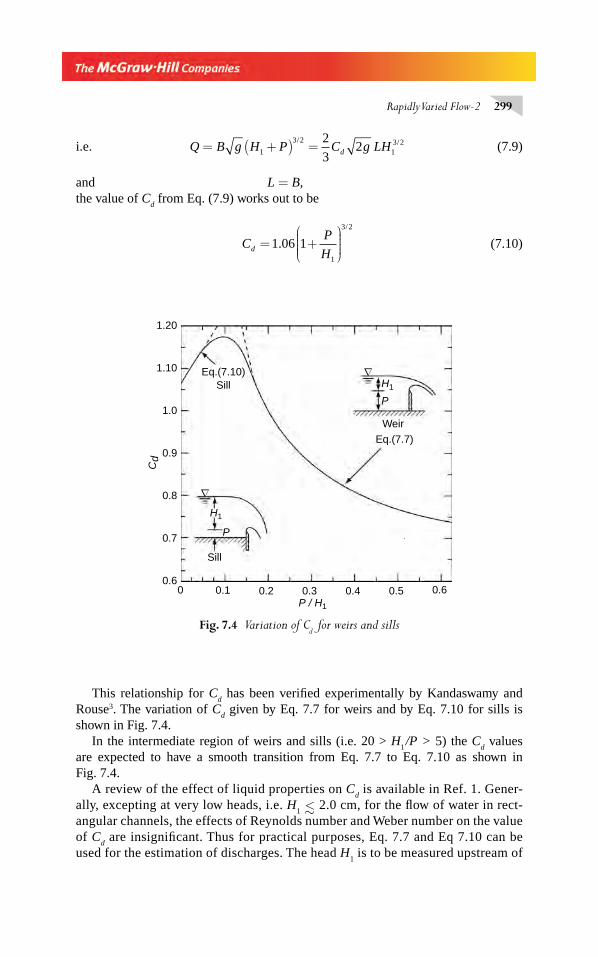
Rapidly Varied Flow-2 299
i.e. Q B g H P C g LHd= +( ) =1
3 2
13 22
32
/ / (7.9)
and L = B,the value of C
d from Eq. (7.9) works out to be
CP
Hd = +⎛
⎝⎜⎜⎜⎜
⎞
⎠⎟⎟⎟⎟
1 06 11
3 2
.
/
(7.10)
0.6
0.7
0.8
0.9
1.0
1.10
1.20
0 0.1 0.2 0.3 0.4 0.5 0.6
Eq.(7.10)Sill
Eq.(7.7)
∇
∇
H1
Cd
P / H1
H1
P
P
Weir
Sill
Fig. 7.4 Variation of Cd for weirs and sills
This relationship for Cd has been verifi ed experimentally by Kandaswamy and
Rouse3. The variation of Cd given by Eq. 7.7 for weirs and by Eq. 7.10 for sills is
shown in Fig. 7.4.In the intermediate region of weirs and sills (i.e. 20 > H
1 /P > 5) the C
d values
are expected to have a smooth transition from Eq. 7.7 to Eq. 7.10 as shown in Fig. 7.4.
A review of the effect of liquid properties on Cd is available in Ref. 1. Gener-
ally, excepting at very low heads, i.e. H1 ∼< 2.0 cm, for the fl ow of water in rect-
angular channels, the effects of Reynolds number and Weber number on the value of C
d are insignifi cant. Thus for practical purposes, Eq. 7.7 and Eq 7.10 can be
used for the estimation of discharges. The head H1 is to be measured upstream of
Chapter 7.indd 299Chapter 7.indd 299 2/24/2010 3:01:29 PM2/24/2010 3:01:29 PM
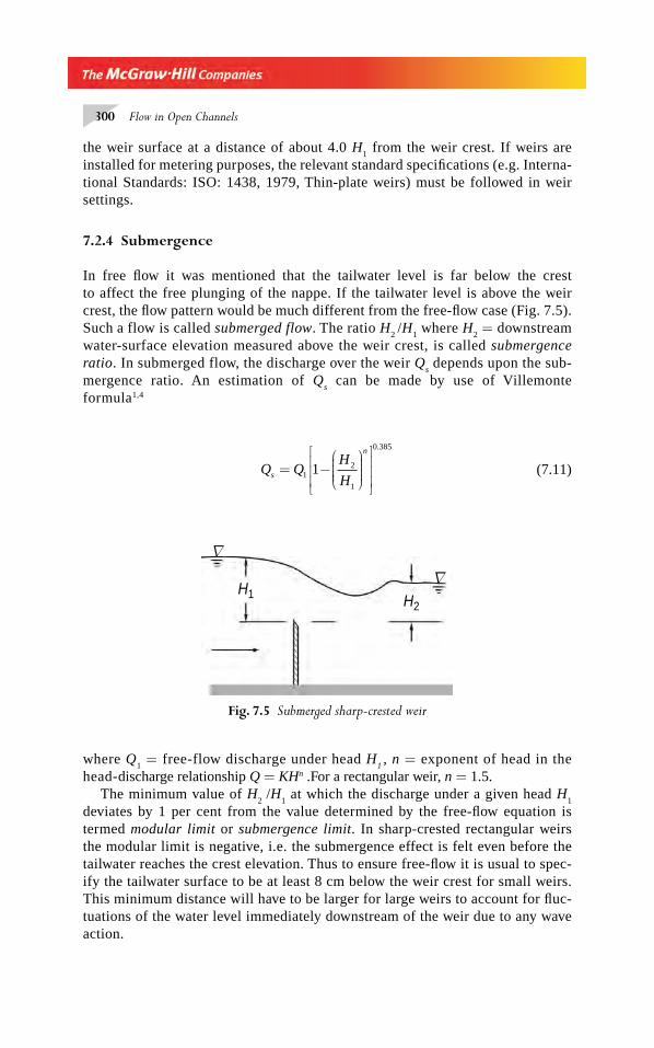
300 Flow in Open Channels
the weir surface at a distance of about 4.0 H1 from the weir crest. If weirs are
installed for metering purposes, the relevant standard specifi cations (e.g. Interna-tional Standards: ISO: 1438, 1979, Thin-plate weirs) must be followed in weir settings.
7.2.4 Submergence
In free fl ow it was mentioned that the tailwater level is far below the crest to affect the free plunging of the nappe. If the tailwater level is above the weir crest, the fl ow pattern would be much different from the free-fl ow case (Fig. 7.5). Such a flow is called submerged flow. The ratio H
2 /H
1 where H
2 = downstream
water-surface elevation measured above the weir crest, is called submergence ratio. In submerged flow, the discharge over the weir Q
s depends upon the sub-
mergence ratio. An estimation of Qs can be made by use of Villemonte
formula1,4
Q QH
Hs
n
= −⎛
⎝⎜⎜⎜⎜
⎞
⎠⎟⎟⎟⎟
⎡
⎣
⎢⎢⎢
⎤
⎦
⎥⎥⎥
12
1
0 385
1
.
(7.11)
H1 H2
∇
∇
Fig. 7.5 Submerged sharp-crested weir
where Q1 = free-flow discharge under head H
1 , n = exponent of head in the
head-discharge relationship Q = KHn .For a rectangular weir, n = 1.5.The minimum value of H
2 /H
1 at which the discharge under a given head H
1
deviates by 1 per cent from the value determined by the free-fl ow equation is termed modular limit or submergence limit. In sharp-crested rectangular weirs the modular limit is negative, i.e. the submergence effect is felt even before the tailwater reaches the crest elevation. Thus to ensure free-fl ow it is usual to spec-ify the tailwater surface to be at least 8 cm below the weir crest for small weirs. This minimum distance will have to be larger for large weirs to account for fl uc-tuations of the water level immediately downstream of the weir due to any wave action.
Chapter 7.indd 300Chapter 7.indd 300 2/24/2010 3:01:30 PM2/24/2010 3:01:30 PM
Rapidly Varied Flow-2 301
7.2.5 Aeration Need of Rectangular Weir
The need for aeration of rectangular weirs spanning the full width of a channel was indicated in Sec. 7.2.1. The rate of air supply (Q
a in m3/s) required to completely
meet the aeration need is given by5
Q
Q y H
a
p
=( )
0 1
1
3 2
.
//
(7.12)
in which Q = water discharge and yp = water-pool depth on the downstream of the
weir plate (Fig. 7.1). If a submerged hydraulic jump takes place, yp can be estimated
by the tailwater depth. On the other hand, for the case of a free jump occurring on the downstream, y
p can be estimated by the following empirical equation5
y ZQ
L g Zp = Δ
Δ( )
⎡
⎣
⎢⎢⎢
⎤
⎦
⎥⎥⎥
2
2 3
0 22.
(7.13)
where ΔZ = difference in elevation between the weir crest and the downstream fl oor (Fig. 7.1).
To cause air fl ow into the air pocket through an air vent, a pressure difference between the ambient atmosphere and the air pocket is needed. Assuming a maximum permissible negative pressure in the pocket (say 2 cm of water column), the size of the air vent can be designed by using the usual Darcy-Weisbach pipe fl ow equation.
Example 7.1 A 2.0-m wide rectangular channel has a discharge of 0.350 m3/s. Find the height of a rectangular weir spanning the full width of the channel that can be used to pass this discharge while maintaining an upstream depth of 0.850 m.
Solution A trial-and-error procedure is required to solve for P. Assuming Cd =
0.640, by Eq. 7.5
H1
3 2 0 3502
30 640 19 62 2 0 0 0926/ . . . . .= × × ×
⎛⎝⎜⎜⎜
⎞⎠⎟⎟⎟ =
H1 0 205= . m and P = 0.850 – 0.205 = 0.645m
H P1 0 318= . m and Cd = 0.611 + (0.08 × 0.318) = 0.636
2nd iteration: Using the above value of Cd
H13 2/ =
0 0926
0 6360 640 0 09318
.
.. .× =
H1 = 0.206 m, P = 0.644 m, H
1 / P = 0.320
and Cd = 0.637
Chapter 7.indd 301Chapter 7.indd 301 2/24/2010 3:01:30 PM2/24/2010 3:01:30 PM
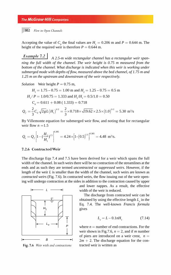
302 Flow in Open Channels
Accepting the value of Cd the fi nal values are H
1 = 0.206 m and P = 0.644 m. The
height of the required weir is therefore P = 0.644 m.
Example 7.2 A 2.5-m wide rectangular channel has a rectangular weir span-ning the full width of the channel. The weir height is 0.75 m measured from the bottom of the channel. What discharge is indicated when this weir is working under submerged mode with depths of fl ow, measured above the bed channel, of 1.75 m and 1.25 m on the upstream and downstream of the weir respectively.
Solution Weir height P = 0.75 m,
H1 = 1.75 – 0.75 = 1.00 m and H
2 = 1.25 – 0.75 = 0.5 m
H1 / P = 1.0/0.75 = 1.333 and H
2 /H
1 = 0.5/1.0 = 0.50
Cd = 0.611 + 0.08 ( 1.333) = 0.718
Q C gL Hf d= ( ) = × × × ×( ) =2
32
2
30 718 19 62 2 5 1 0 5 301
3 2 3 2/ /. . . . . m3/s
By Villemonte equation for submerged weir fl ow, and noting that for rectangular weir fl ow n =1.5
Q QH
Hs f= −⎡
⎣⎢⎢
⎤
⎦⎥⎥ = × ( )⎡
⎣⎢⎤⎦⎥
=1 4 24 1 0 5 42
1
1 5
0 3851 5 0 385
( ) . - ..
.. .
..48 m3/s.
7.2.6 Contracted Weir
The discharge Eqs 7.4 and 7.5 have been derived for a weir which spans the full width of the channel. In such weirs there will be no contraction of the streamlines at the ends and as such they are termed uncontracted or suppressed weirs. However, if the length of the weir L is smaller than the width of the channel, such weirs are known as contracted weirs (Fig. 7.6). In contracted weirs, the fl ow issuing out of the weir open-ing will undergo contraction at the sides in addition to the contraction caused by upper
and lower nappes. As a result, the effective width of the weir is reduced.
The discharge from contracted weir can be obtained by using the effective length L
e in the
Eq. 7.4. The well-known Francis formula gives
Le = L – 0.1nH
1 (7.14)
where n = number of end contractions. For the weir shown in Fig.7.6, n = 2, and if m number of piers are introduced on a weir crest, n = 2m + 2. The discharge equation for the con-tracted weir is written asFig. 7.6 Weir with end contractions
∇
H1
L
B
PLe
Chapter 7.indd 302Chapter 7.indd 302 2/24/2010 3:01:30 PM2/24/2010 3:01:30 PM
Rapidly Varied Flow-2 303
Q C L n H HV
g
V
gc= −( ) +⎛
⎝⎜⎜⎜⎜
⎞
⎠⎟⎟⎟⎟
−⎛
⎝⎜⎜⎜⎜
⎞
⎠⎟⎟⎟⎟
2
30 1
2 21 1
2 3 2 2
2g 0 0.
33 2⎡
⎣
⎢⎢⎢
⎤
⎦
⎥⎥⎥
(7.15)
For L > 3H1 and H P1 1 0/ .< , the value of C
c is taken as C
c = 0.622.
For contracted sharp-crested weirs, Kindsvater and Carter 6 have given a modifi ed version of Eq. 7.15, based on their extensive experimental investigation covering a wide range of variables, as
Q C g L Hdc e e=2
32 1
3 2/ (7.16)
where Cdc
= coeffi cient of discharge for contracted weir, Le = effective length and
Hle = effective head. The effective length and head are obtained as
Le = L + K
L (7.16a)
and H1e
= H1 + K
H (7.16b)
where KH and K
L are additive correction terms to account for several phenomena
attributed to viscosity and surface tension. Values of recommended KH and K
L are
given in Table 7.1. The discharge coeffi cient Cdc
is a function of L
B and H
1/P,
expressed as
C K KH
Pdc = +⎛
⎝⎜⎜⎜
⎞
⎠⎟⎟⎟⎟1 2
1 (7.17)
The variation of K1 and K
2 are also shown in Table 7.1.
Table 7. 1 Value s of Parameters for Use in Eq. (7.16)* 6
LIB KL (m) K
H (m) K
1K
2
1.0 – 0.0009
KH=
0.00
1 m
= C
onst
.
0.602 +0.07500.9 0.0037 0.599 +0.06400.8 0.0043 0.597 +0.04500.7 0.0041 0.595 +0.03000.6 0.0037 0.593 +0.01800.5 0.0030 0.592 +0.01100.4 0.0027 0.591 +0.00580.3 0.0025 0.590 +0.00200.2 0.0024 0.589 −0.00180.1 0.0024 0.588 −0.0021
*Equation (7.16) is subject to the limitations H1 / P < 2.0, H
1 > 0.03 m, L > 0.15 m and P > 0.10 m.
Example 7.3 A 2.0-m wide rectangular channel has a contracted rectangular weir of 1.500-m length and 0.60-m height. What would be the depth of fl ow upstream of the weir when the fl ow through the channel is 0.350 m3/s?
Chapter 7.indd 303Chapter 7.indd 303 2/24/2010 3:01:30 PM2/24/2010 3:01:30 PM
304 Flow in Open Channels
Solution In this case L
B=
1 50
2 00
.
.= 0.75. From Table 7.1,
KL = 0.0042, K
H = 0.001, K
1 = 0.596 and K
2 = 0.0375.
Le = L + K
L = 1.50 + 0.0042 = 1.5042 m
As a trial-and-error procedure is needed to calculate H1, assume C
dc = 0.60 for the
fi rst trial. From Eq. 7.16
H e13 2 0 350
2
30 60 19 62 1 5042 0 13133= × × ×
⎛⎝⎜⎜⎜
⎞⎠⎟⎟⎟ =. . . . .
Hie = 0.2584 m, H
1 = 0.2584 − 0.001 = 0.2574 m
H P1
0 2574
0 60/
.
.= =0.429 and from Eq. 7.17
Cdc
= 0.596 + (0.0375 × 0.429) = 0.612
2nd iteration: Using the above value of Cdc
H e13 2 0 13133
0 6120 600/ .
..= × = 0.128755
H1e
= 0.255 m, H1= 0.254 m, H
1/P= 0.4233 and
Cdc
= 0.612 which is the same as the assumed value.
Hence the fi nal values are H1 = 0.254 m and C
dc = 0.612.
Upstream depth =H1 + P = 0.254 + 0.600 = 0.854 m
The water surface on the upstream will be at a height of 0.854 m above the bed.
7.2.7 Non-Rectangular Weirs
Sharp-crested weirs of various shapes are adopted for meeting specifi c requirements based on their accuracy, range and head-discharge relationships. The general form of head-discharge relationship for a weir can be expressed as Q = KH
1n, where K and n
are coeffi cients. The coeffi cient n depends upon the weir shape and K depends upon the weir shape and its setting. The discharge equations for some commonly used weir shapes are given in Table 7.2.
A variety of sharp-crested weir shapes have been designed to give specifi c head-discharge relationships and are described in literature1. A type of weir for which the discharge varies linearly with head, known as Sutro Weir fi nds use in fl ow measure
Chapter 7.indd 304Chapter 7.indd 304 2/24/2010 3:01:31 PM2/24/2010 3:01:31 PM
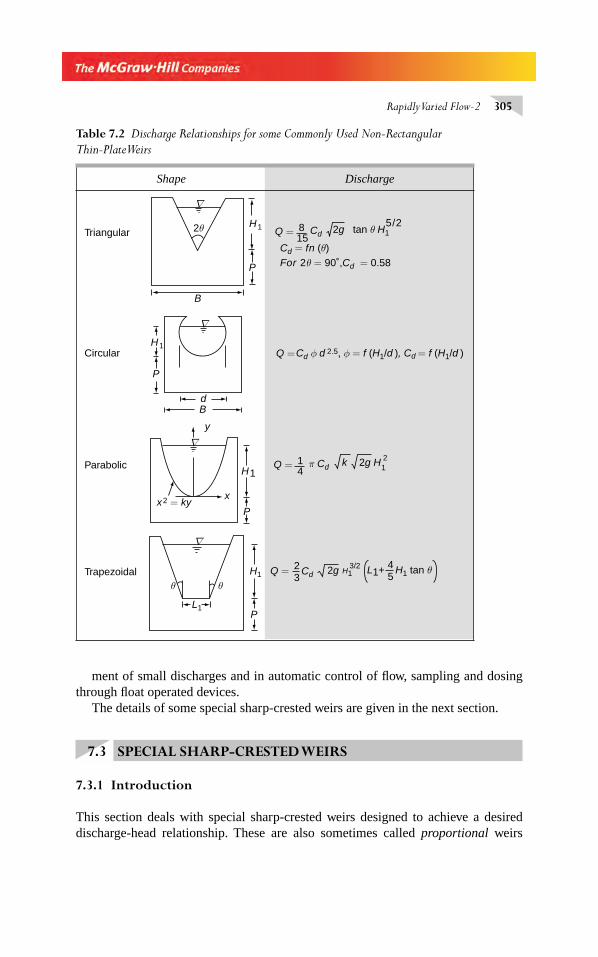
Rapidly Varied Flow-2 305
Table 7.2 Discharge Relationships for some Commonly Used Non-Rectangular
Thin-Plate Weirs
Shape Discharge
x2 = ky
H1
y
B
B
P
H1
H1
d
P
P
x
∇
∇
∇
Parabolic Q =
Q =
1122g H
4π Cd
Cd φ d 2.5, φ = f (H1/d ), Cd = f (H1/d )
k
Cd = fn (θ)
Circular
Triangular 2θ Q = 815
Cd 2g tan θ H15/2
For 2θ = 90˚,Cd = 0.58
L1
H1 H1 H1 tan θ L1+CdQ =
P
∇
θθ
2 2g3
45
3/2Trapezoidal
ment of small discharges and in automatic control of fl ow, sampling and dosing through fl oat operated devices.
The details of some special sharp-crested weirs are given in the next section.
7.3 SPECIAL SHARP-CRESTED WEIRS
7.3.1 Introduction
This section deals with special sharp-crested weirs designed to achieve a desired discharge-head relationship. These are also sometimes called proportional weirs
Chapter 7.indd 305Chapter 7.indd 305 2/24/2010 3:01:31 PM2/24/2010 3:01:31 PM
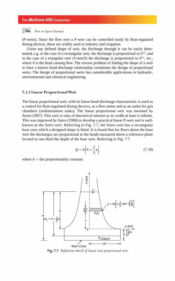
306 Flow in Open Channels
(P-weirs). Since the fl ow over a P-weir can be controlled easily by fl oat-regulated dosing devices, these are widely used in industry and irrigation.
Given any defi ned shape of weir, the discharge through it can be easily deter-mined, e.g. in the case of a rectangular weir, the discharge is proportional to h3/2, and in the case of a triangular weir (V-notch) the discharge is proportional to h5/2, etc., where h is the head causing fl ow. The reverse problem of fi nding the shape of a weir to have a known head-discharge relationship constitutes the design of proportional weirs. The design of proportional weirs has considerable applications in hydraulic, environmental and chemical engineering.
7.3.2 Linear Proportional Weir
The linear proportional weir, with its linear head-discharge characteristic is used as a control for fl oat-regulated dosing devices, as a fl ow meter and as an outlet for grit chambers (sedimentation tanks). The linear proportional weir was invented by Stout (1897). This weir is only of theoretical interest as its width at base is infi nite. This was improved by Sutro (1908) to develop a practical linear P-weir and is well-known as the Sutro weir. Referring to Fig. 7.7, the Sutro weir has a rectangular base over which a designed shape is fi tted. It is found that for fl ows above the base weir the discharges are proportional to the heads measured above a reference plane located at one-third the depth of the base weir. Referring to Fig. 7.7.
Q b h a= +⎛⎝⎜⎜⎜
⎞⎠⎟⎟⎟⎟
2
3 (7.18)
where b = the proportionality constant.
∇
dx
x
f (x)
x-ax
is
y-axis
y = W 1–2π tan–1 xa
a23
a
Datum
23
aHd = h +H
W
h
Weir Crest
0
Fig. 7.7 Defi nition sketch of linear weir proportional weir
Chapter 7.indd 306Chapter 7.indd 306 2/24/2010 3:01:31 PM2/24/2010 3:01:31 PM
Rapidly Varied Flow-2 307
7.3.3 Shape of the Sutro Weirs
Referring to Fig. 7.7, let the weir have the base on a rectangular weir of width 2W and depth a. For convenience, the horizontal and vertical axes at the origin O are chosen as y and x-axes respectively. The weir is assumed to be symmetrical about the x-axis.
The discharge through the rectangular weir when the depth of fl ow is h above the origin is
q WC g h a hd13 2 3 24
32= + −[( ) ]/ / (7.19)
where Cd = coeffi cient of discharge.
The discharge through the upper portion above the origin called the complimentary weir is
q C g h x f x dxd
h
20
2 2= −∫ ( ) (7.19a)
The total discharge through the weir is
Q = q1 + q
2
We wish this discharge to be proportional to the head measured above the refer-
ence plane situated a
3 above the crest of the weir. This reference plane is chosen
arbitrarily by Sutro for mathematical convenience. Thus
Q = q1 + q
2
= + − + −∫4
32 2 23 2 3 2
0WC g h a h C g h x f x dxd d
h
[ ]( ) ( )/ /
= +⎛⎝⎜⎜⎜
⎞⎠⎟⎟⎟⎟ ≥b h
ah
2
30for (7.20)
where b is the proportionality constant.
As there is no fl ow above the base weir when h = 0, we have by substituting h = 0 in Eq. 7.20
b = W K a1/2 (7.21)
where K C gd= 2 2
Substituting this value of b in Eq. 7.20
2
3
2
33 2 3 2 1 2W h a h h x f x dx Wa h
ah
( ) ( )/ / /+ −⎡⎣⎢
⎤⎦⎥ + − = +
⎛⎝⎜⎜⎜
⎞⎠⎟⎟⎟⎟∫0
(7.22)
Re-arranging,
h x f x dx Wa h
aW h a h
h
− = +⎛⎝⎜⎜⎜
⎞⎠⎟⎟⎟⎟− + −⎡
⎣⎢⎤⎦⎥∫0
1 2 3 2 3 22
3
2
3( ) ( )/ / /
Chapter 7.indd 307Chapter 7.indd 307 2/24/2010 3:01:31 PM2/24/2010 3:01:31 PM
308 Flow in Open Channels
= + + − +⎡
⎣⎢⎢
⎤
⎦⎥⎥
W a a h h a h2
3
2
3
2
33 2 1 2 3 2 3 2/ / / /( )
= − + − +⎡
⎣⎢⎢
⎤
⎦⎥⎥
− − −2
3
3
8
1
16
3
1283 2 1 2 2 3 2 3 5 2 4W h a h a h a h/ / / / ... (7.22a)
It is required to fi nd the function f (x) such that Eq. 7.22a is satisfi ed for all positive values of h. This is achieved by expressing f (x) in a series of powers of x and deter-mining their coeffi cients. A general term x m in f (x) results in a term
h x x dx x h h x h x dxm mhh
− = − + −⎛⎝⎜⎜⎜
⎞⎠⎟⎟⎟⎟
− −∫∫ 1 2 1 2 3 2 2
0
1
2
1
8/ / / ...
0
= Const (h)m + (3/2) (7.23)
so that the fi rst term in Eq. 7.22a can be obtained by a constant term in the series for f(x) and the other terms by taking m half an odd integer. Consequently we assume,
f x y A A x A x A x( ) ...= = + + + +1 21 2 3 2
45 2
3 (7.24)
Substituting this in Eq. 7.22a
( )A h x A hx x dxh
1 22
0− + − +∫ …
= + + + +2
3 8 16
5
1281 3 2 2
23
34
4Ah
A h A h A h/ ...π π π
= − +⎡
⎣⎢⎢
⎤
⎦⎥⎥
−2
3
3
83 2 1 2 2W h a h/ / ...
This leads to
A W1 =
A a W21 22
= − −
π/
A a W33 22
3= −
π/
and so on.Substituting these coeffi cients in Eq. 7.24
f x Wx
a
x
a
x
a( ) ...
/
/
/
/
/
/= − − + −
⎧⎨⎪⎪⎩⎪⎪
⎫⎬⎪⎪⎭⎪⎪
⎡
⎣⎢1
2
5
1 2
1 2
3 2
3 2
5 2
5 2π⎢⎢⎢
⎤
⎦⎥⎥⎥
Chapter 7.indd 308Chapter 7.indd 308 2/24/2010 3:01:32 PM2/24/2010 3:01:32 PM
Rapidly Varied Flow-2 309
= −⎡
⎣⎢⎢⎢
⎤
⎦⎥⎥⎥
−Wx
a1
2 1
πtan (7.25)
The discharge equation for the Sutro weir can now be summarised as
Q b h a b Ha
bHd= +⎛⎝⎜⎜⎜
⎞⎠⎟⎟⎟⎟ = −
⎛⎝⎜⎜⎜
⎞⎠⎟⎟⎟⎟=
2
3 3 (7.26)
where b = WKa1/ 2 and K = 2Cd
2g H = depth of fl ow in the channel. (It is usual practice to make the crest of the
base coincide with the bed of the channel) h = head measured from the top of the rectangular base weir H
d = depth of water over the datum.
The sharp edged Sutro weir is found to have an average coeffi cient of discharge of 0.62.
A simple weir geometry, called quadrant plate weir, which has the linear head-discharge relationship is described in Ref. 7. This weir has the advantage of easy fab-rication and installation under fi eld conditions. Linear proportional weirs having non-rectangular base weirs are described in Ref. 8 and 9.
Example 7.4 A Sutro weir has a rectangular base of 30-cm width and 6-cm height. The depth of water in the channel is 12 cm. Assuming the coeffi cient of dis-charge of the weir as 0.62, determine the dischage through the weir. What would be the depth of fl ow in the channel when the discharge is doubled? (Assume the crest of the base weir to coincide with the bed of the channel).
Solution Given a = 0.06 m, W = 0.30/2 = 0.15 m, H = 0.12 m
K C gd= = × × × =2 2 2 0 62 2 9 81 5 4925. . .
b = W K a1/2 = 0.15×5.4925×(0.06)1/2 = 0.2018
From Eq. 7.26 Q b Ha
= −⎛⎝⎜⎜⎜
⎞⎠⎟⎟⎟⎟3
= −
⎛⎝⎜⎜⎜
⎞⎠⎟⎟⎟⎟ =0 2018 0 12
0 06
30 02018. .
.. m /s3
= 20.18 litres/s
When the discharge is doubled, Q = × =2 0 02018 0 04036. . m /s3
Chapter 7.indd 309Chapter 7.indd 309 2/24/2010 3:01:32 PM2/24/2010 3:01:32 PM
310 Flow in Open Channels
From Eq. 7.26, 0 04036 0 20180 06
3. .
.= −
⎛⎝⎜⎜⎜
⎞⎠⎟⎟⎟⎟H
H = 0.2 + 0.02 = 0.22 m
= 22 cm
Example 7.5 Design a Sutro weir for use in a 0.30-m wide rectangular chan-nel to have linear discharge relationship in the discharge range from 0.25 m to 0.60 m3/s. The base of the weir will have to span the full width of the channel.Assume C
d = 0.62.
Solution Here 2 W = 0.30 m. and Cd = 0.62.
K = 2Cd 2 2 0 62 2 9 81g = × × ×. . = 5.49
Q WK amin
/ .= =2
30 253 2
2
30 15 5 49 0 253 2× × × =. . ./a
a = 0.592 m
b WK a= = × ×0 15 5 49 0 592. . . = 0.6337
Q b Hd=
For Q = 0.60 m3/s, HQ
bd = =0 60
0 6337
.
. = 0.9468 m
= − = +Ha
h a3
2
3 (Refer Fig. 7.7)
H = 1.1444 m and h = 0.0552 m.
Using Eq.7.25, the profi le y = f (x) is calculated as
y f xx
= ( ) = −⎡
⎣⎢⎢⎢
⎤
⎦⎥⎥⎥
−0 15 12
0 5921. tan
.π .
7.3.4 General Equation for the Weir
Cowgill8 and Banks9 have shown that the curve describing the weir producing a dis-charge Q = b hm for m ≥ 1/2 is given by
y y xb
C g
m
mx
d
m= = ⋅+
−⋅ −( )
( )
( / )( )( / )
2 2
1
1 23 2
π
ΓΓ
(7.27)
Chapter 7.indd 310Chapter 7.indd 310 2/24/2010 3:01:32 PM2/24/2010 3:01:32 PM
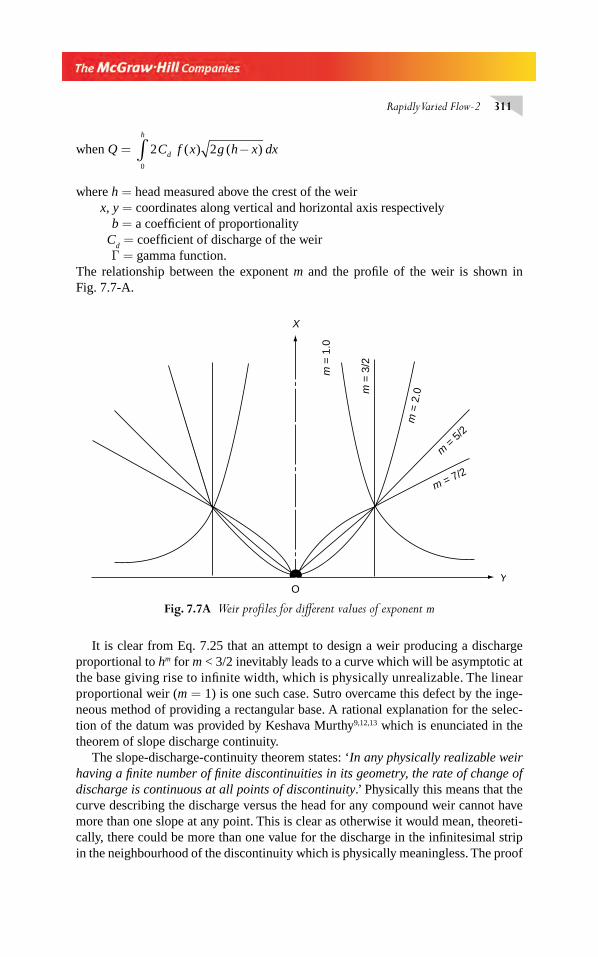
Rapidly Varied Flow-2 311
when Q = 2 20
C f x g h x dxd
h
( ) ( )−∫
where h = head measured above the crest of the weir x, y = coordinates along vertical and horizontal axis respectively b = a coeffi cient of proportionality C
d = coeffi cient of discharge of the weir
Γ = gamma function.The relationship between the exponent m and the profi le of the weir is shown in Fig. 7.7-A.
Xm
= 1
.0
m =
3/2
m =
2.0
m = 5/
2
m = 7/2
YO
Fig. 7.7A Weir profi les for diff erent values of exponent m
It is clear from Eq. 7.25 that an attempt to design a weir producing a discharge proportional to hm for m < 3/2 inevitably leads to a curve which will be asymptotic at the base giving rise to infi nite width, which is physically unrealizable. The linear proportional weir (m = 1) is one such case. Sutro overcame this defect by the inge-neous method of providing a rectangular base. A rational explanation for the selec-tion of the datum was provided by Keshava Murthy9,12,13 which is enunciated in the theorem of slope discharge continuity.
The slope-discharge-continuity theorem states: ‘In any physically realizable weir having a fi nite number of fi nite discontinuities in its geometry, the rate of change of discharge is continuous at all points of discontinuity.’ Physically this means that the curve describing the discharge versus the head for any compound weir cannot have more than one slope at any point. This is clear as otherwise it would mean, theoreti-cally, there could be more than one value for the discharge in the infi nitesimal strip in the neighbourhood of the discontinuity which is physically meaningless. The proof
Chapter 7.indd 311Chapter 7.indd 311 2/24/2010 3:01:33 PM2/24/2010 3:01:33 PM
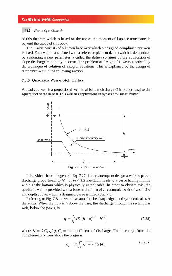
312 Flow in Open Channels
of this theorem which is based on the use of the theorem of Laplace transforms is beyond the scope of this book.
The P-weir consists of a known base over which a designed complimentary weir is fi xed. Each weir is associated with a reference plane or datum which is determined by evaluating a new parameter λ called the datum constant by the application of slope discharge-continuity theorem. The problem of design of P-weirs is solved by the technique of solution of integral equations. This is explained by the design of quadratic weirs in the following section.
7.3.5 Quadratic Weir-notch Orifi ce
A quadratic weir is a proportional weir in which the discharge Q is proportional to the square root of the head h. This weir has applications in bypass fl ow measurement.
W
ao
y = f(x)
y-axis
x-ax
is
∇
h
Base weirComplimentary weir
Fig. 7.8 Defi nition sketch
It is evident from the general Eq. 7.27 that an attempt to design a weir to pass a discharge proportional to hm, for m < 3/2 inevitably leads to a curve having infi nite width at the bottom which is physically unrealizable. In order to obviate this, the quadratic weir is provided with a base in the form of a rectangular weir of width 2W and depth a, over which a designed curve is fi tted (Fig. 7.8).
Referring to Fig. 7.8 the weir is assumed to be sharp-edged and symmetrical over the x-axis. When the fl ow is h above the base, the discharge through the rectangular weir, below the y-axis, is
q WK h a h1
3 2 3 22
3= +( ) −⎡
⎣⎢⎤⎦⎥
/ / (7.28)
where K = 2 2C g Cd d, = the coeffi cient of discharge. The discharge from the complementary weir above the origin is
q K h x f s dxh
20
= −∫ ( ) (7.28a)
Chapter 7.indd 312Chapter 7.indd 312 2/24/2010 3:01:33 PM2/24/2010 3:01:33 PM
Rapidly Varied Flow-2 313
Total discharge Q q q= +1 2
= 2
33 2 3 2
0WK h a h K h x f x dx
h
( ) ( )/ /+ −⎡⎣⎢
⎤⎦⎥ + −∫ (7.29)
We wish to have the discharge Q b h a= +λ , where b is the proportionality constant and λ is the datum constant. In other words, the discharge is proportional to the square root of the head measured above a reference plane. The constants b and λ are to be evaluated. They are determined by the two conditions of continuity of discharge and the requirement of the slope discharge continuity theorem. Rewriting Eq. 7.29
Q WK h a h K h x f x dxh
= + −⎡⎣⎢
⎤⎦⎥ + −∫
2
33 2 3 2
0( ) ( )/ /
= +h h aλ for h ≥ 0 (7.30)
When h = 0, there is no fl ow above the base weir. Hence, substituting h = 0 in Eq. 7.30
2
33 2WKa b a/ = λ (7.31)
Differentiating Eq. 7.30 on both sides by using Leibnitz’s rule for differentiating under the integral sign, and re-arranging
f x
h xdh
b
K h aW h a h h
h ( )−
=+
− +( ) −⎡⎣⎢
⎤⎦⎥= ( )∫ λ
φ21 2 1 2
0
/ /
(7.32)
Applying the slope-discharge-continuity theorem, i.e, putting h = 0 in Eq. 7.32. we have
b
K aWa
λ= 2 1 2/ (7.33)
Solving Equations 7.31 and 7.33
λ =1
3 and b WKa=
2
3 (7.34)
The reference plane for this weir is situated at 2
3
a above the crest of the weir. Equation
7.32 is in the Abel’s form of integral equation whose solution is9:
y f xh
x hdh
h
= ( ) =( )−∫
10π
φ ’
Substituting for φ'( h)
Chapter 7.indd 313Chapter 7.indd 313 2/24/2010 3:01:33 PM2/24/2010 3:01:33 PM
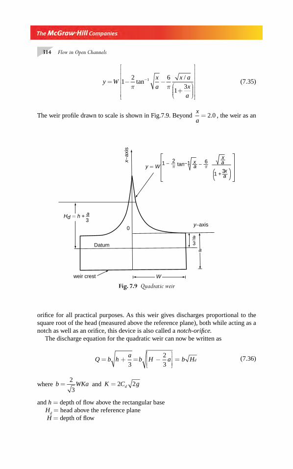
314 Flow in Open Channels
y Wx
a
x a
x
a
= − −+
⎛⎝⎜⎜⎜
⎞⎠⎟⎟⎟
⎡
⎣
⎢⎢⎢⎢⎢⎢
⎤
⎦
⎥⎥⎥⎥⎥⎥
−12 6
13
1
π πtan
/ (7.35)
The weir profi le drawn to scale is shown in Fig.7.9. Beyond x
a= 2 0. , the weir as an
a3
a
y −axis
x −ax
is
a3
Hd = h +
Datum
0
y = W1 − 2
π tan−1a
a− π6
a1 + 3
weir crest W
x
xx
Fig. 7.9 Quadratic weir
orifi ce for all practical purposes. As this weir gives discharges proportional to the square root of the head (measured above the reference plane), both while acting as a notch as well as an orifi ce, this device is also called a notch-orifi ce.
The discharge equation for the quadratic weir can now be written as
Q b ha
b H a b Hd= + = −⎡
⎣⎢⎢
⎤
⎦⎥⎥
=3
2
3 (7.36)
where b WKa=2
3 and K C gd= 2 2
and h = depth of fl ow above the rectangular base H
d = head above the reference plane
H = depth of fl ow
Chapter 7.indd 314Chapter 7.indd 314 2/24/2010 3:01:34 PM2/24/2010 3:01:34 PM
Rapidly Varied Flow-2 315
Quadratic weirs having non-rectangular lower portions (base weirs) are described in detail in Ref. 14.
The quadratic weir has an average coeffi cient of discharge of 0.62. In a quadratic weir the error involved in the discharge calculation for a unit per cent error in head is only 0.5 per cent as against 1.5% in a rectangular weir and 2.5% in a V-notch. Hence this is more sensitive than the rectangular weir and V-notch.
Example 7.6 A quadratic weir is designed for installation in a rectangular channel of 30-cm width. The rectangular base of the weir occupies the full width of the channel and is 6 cm in height. The crest of the base weir coincides with the channel bed. (a) Determine the discharge through the weir when the depth of fl ow in the channel is 15 cm. (b) What would be the depth of fl ow upstream of the weir when the discharge in the channel is 25 litres/s? [Assume C
d =0.62].
Solution Given: a = 0.06 m, W = 0.30/2 = 0.15 m, H = 0.15 m
K = 2 C gd 2 = 2 0 62 2 9 81 5 4925× × × =. . .
b = 2
3
2
30 15 5 4925 0 06W K a = × × ×. . . = 0.05708
From Eq. (7.36), Q b Ha
= −⎛⎝⎜⎜⎜
⎞⎠⎟⎟⎟⎟
2
3
(a) Q = × −×⎛
⎝⎜⎜⎜
⎞⎠⎟⎟⎟⎟
⎡
⎣⎢⎢
⎤
⎦⎥⎥0 05708 0 15
2 0 06
3
1 2
. ..
/
= 0.0189 m3/s = 18.93 litres/s
(b) When the discharge Q = 25 litres/s = 0.025 m3/s
From Eq. (7.36), 0 025 0 057082 0 06
3
1 2
. ..
/
= × −×⎛
⎝⎜⎜⎜
⎞⎠⎟⎟⎟⎟
⎡
⎣⎢⎢
⎤
⎦⎥⎥H
H = 0.1918 + 0.04 = 0.2318 m
= 23.18 cm
7.3.6 Modelling of Flow Velocity using Special Weirs
In many hydraulic engineering situations, it is desirable to maintain a constant aver-age velocity in a channel for a range of fl ows. A typical example of this situation is the grit chamber used in waste water treatment. To obtain such a control of the veloc-ity of fl ow in the channel, proportional weirs can be used at the outlet of the channel. The channel cross-section shape, however, will have to be determined. This, in turn, depends upon the shape of the outlet weir and the relationship between the upstream
Chapter 7.indd 315Chapter 7.indd 315 2/24/2010 3:01:34 PM2/24/2010 3:01:34 PM
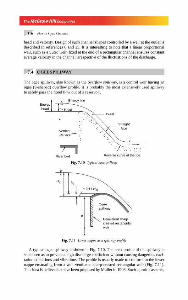
316 Flow in Open Channels
head and velocity. Design of such channel shapes controlled by a weir at the outlet is described in references 8 and 15. It is interesting to note that a linear proportional weir, such as a Sutro weir, fi xed at the end of a rectangular channel ensures constant average velocity in the channel irrespective of the fl uctuations of the discharge.
7.4 OGEE SPILLWAY
The ogee spillway, also known as the overfl ow spillway, is a control weir having an ogee (S-shaped) overfl ow profi le. It is probably the most extensively used spillway to safely pass the fl ood fl ow out of a reservoir.
Fig. 7.10 Typical ogee spillway
Reverse curve at the toe
Straightface
Crest
Energy lineEnergyhead Head
River bed
Verticalu/s face
∇
∇
Fig. 7.11 Lower nappe as a spillway profi le
∇
= 0.11 Hs1
hdHs1
P
Ogeespillway
Equivalent sharpcrested rectangularweir
A typical ogee spillway is shown in Fig. 7.10. The crest profi le of the spillway is so chosen as to provide a high discharge coeffi cient without causing dangerous cavi-tation conditions and vibrations. The profi le is usually made to conform to the lower nappe emanating from a well-ventilated sharp-crested rectangular weir (Fig. 7.11). This idea is believed to have been proposed by Muller in 1908. Such a profi le assures,
Chapter 7.indd 316Chapter 7.indd 316 2/24/2010 3:01:34 PM2/24/2010 3:01:34 PM
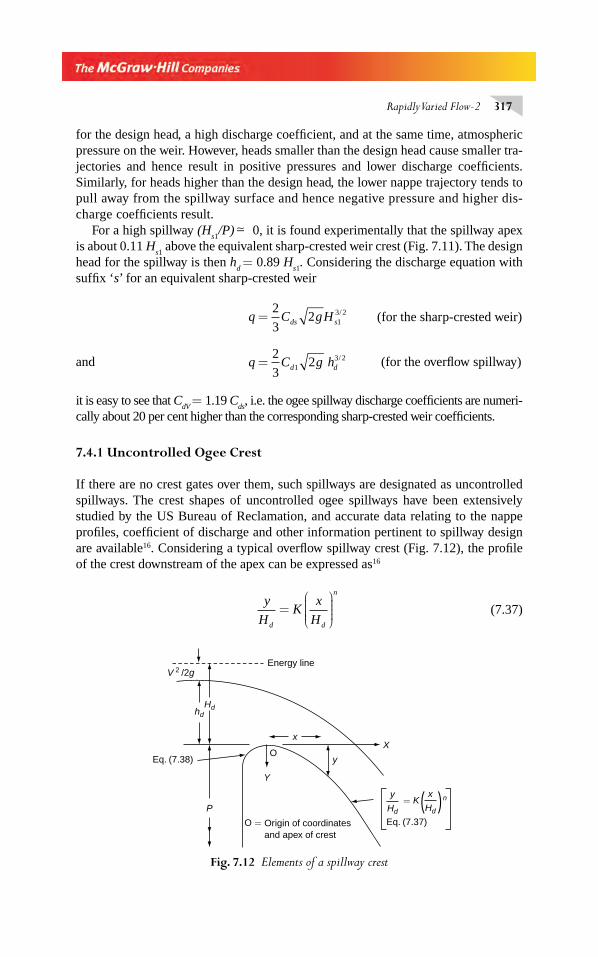
Rapidly Varied Flow-2 317
for the design head, a high discharge coeffi cient, and at the same time, atmospheric pressure on the weir. However, heads smaller than the design head cause smaller tra-jectories and hence result in positive pressures and lower discharge coeffi cients. Similarly, for heads higher than the design head, the lower nappe trajectory tends to pull away from the spillway surface and hence negative pressure and higher dis-charge coeffi cients result.
For a high spillway (Hs1
/P) � 0, it is found experimentally that the spillway apex is about 0.11 H
s1 above the equivalent sharp-crested weir crest (Fig. 7.11). The design
head for the spillway is then hd = 0.89 H
s1. Considering the discharge equation with
suffi x ‘s’ for an equivalent sharp-crested weir
q C gHds s=2
32 1
3 2/ (for the sharp-crested weir)
and q C g hd d=2
321
3 2/ (for the overfl ow spillway)
it is easy to see that CdV
= 1.19 C
ds, i.e. the ogee spillway discharge coeffi cients are numeri-
cally about 20 per cent higher than the corresponding sharp-crested weir coeffi cients.
7.4.1 Uncontrolled Ogee Crest
If there are no crest gates over them, such spillways are designated as uncontrolled spillways. The crest shapes of uncontrolled ogee spillways have been extensively studied by the US Bureau of Reclamation, and accurate data relating to the nappe profi les, coeffi cient of discharge and other information pertinent to spillway design are available16. Considering a typical overfl ow spillway crest (Fig. 7.12), the profi le of the crest downstream of the apex can be expressed as16
y
HK
x
Hd d
n
=⎛
⎝⎜⎜⎜⎜
⎞
⎠⎟⎟⎟⎟ (7.37)
hdHd
P
x
y
Y
O
O =
V 2 /2g
Eq. (7.38)
Origin of coordinatesand apex of crest
Energy line
X
Eq. (7.37)
y
Hd
x
Hd = K
n))
Fig. 7.12 Elements of a spillway crest
Chapter 7.indd 317Chapter 7.indd 317 2/24/2010 3:01:35 PM2/24/2010 3:01:35 PM
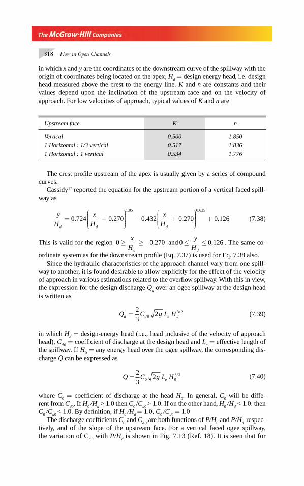
318 Flow in Open Channels
in which x and y are the coordinates of the downstream curve of the spillway with the origin of coordinates being located on the apex, H
d = design energy head, i.e. design
head measured above the crest to the energy line. K and n are constants and their values depend upon the inclination of the upstream face and on the velocity of approach. For low velocities of approach, typical values of K and n are
Upstream face K n
Vertical 0.500 1.850
1 Horizontal : 1/3 vertical 0.517 1.836
1 Horizontal : 1 vertical 0.534 1.776
The crest profi le upstream of the apex is usually given by a series of compound curves.
Cassidy17 reported the equation for the upstream portion of a vertical faced spill-way as
y
H
x
H
x
Hd d d
= +⎛
⎝⎜⎜⎜⎜
⎞
⎠⎟⎟⎟⎟
− +⎛
⎝⎜⎜⎜⎜
⎞
⎠⎟0 724 0 270 0 432 0 270
1 85
. . . .
.
⎟⎟⎟⎟+
0 625
0 126
.
. (7.38)
This is valid for the region 0 0 270≥ ≥ −x
Hd
. and 0 0 126≤ ≤y
Hd
. . The same co-
ordinate system as for the downstream profi le (Eq. 7.37) is used for Eq. 7.38 also.Since the hydraulic characteristics of the approach channel vary from one spill-
way to another, it is found desirable to allow explicitly for the effect of the velocity of approach in various estimations related to the overfl ow spillway. With this in view, the expression for the design discharge Q
d over an ogee spillway at the design head
is written as
Q C g L Hd d e d=2
320
3 2/ (7.39)
in which Hd = design-energy head (i.e., head inclusive of the velocity of approach
head), Cd 0
= coeffi cient of discharge at the design head and Le = effective length of
the spillway. If H0 = any energy head over the ogee spillway, the corresponding dis-
charge Q can be expressed as
Q C g L He=2
320 0
3 2/ (7.40)
where C0 = coeffi cient of discharge at the head H
0. In general, C
0 will be diffe-
rent from Cd0
. If H0 /H
d > 1.0 then C
0 /C
d0 > 1.0. If on the other hand, H
0 /H
d < 1.0. then
C0 /C
d0 < 1.0. By defi nition, if H
0 /H
d = 1.0, C
0 /C
d0 = 1.0
The discharge coeffi cients C0 and C
d 0 are both functions of P/H
0 and P/H
d respec-
tively, and of the slope of the upstream face. For a vertical faced ogee spillway, the variation of C
d 0 with P/H
d is shown in Fig. 7.13 (Ref. 18). It is seen that for
Chapter 7.indd 318Chapter 7.indd 318 2/24/2010 3:01:35 PM2/24/2010 3:01:35 PM
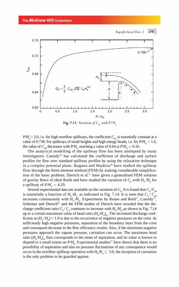
Rapidly Varied Flow-2 319
P/Hd > 2.0, i.e. for high overfl ow spillways, the coeffi cient C
d 0 is essentially constant at a
value of 0.738. For spillways of small heights and high energy heads, i.e. for P/Hd < 1.0,
the value of Cd 0
decreases with P/Hd reaching a value of 0.64 at P/H
d = 0.10.
The analytical modelling of the spillway flow has been attempted by many investigators. Cassidy19 has calculated the coeffi cient of discharge and surface profi les for fl ow over standard spillway profi les by using the relaxation technique in a complex potential plane. Ikegawa and Washizu20 have studied the spillway flow through the fi nite element method (FEM) by making considerable simplifi ca-tion of the basic problem. Diersch et al.21 have given a generalised FEM solution of gravity fl ows of ideal fl uids and have studied the variation of C
0 with H
0 /H
d for
a spillway of P/Hd = 4.29.
Several experimental data are available on the variation of C0. It is found that C
0 /C
dθ is essentially a function of H
0 /H
d as indicated in Fig. 7.14. It is seen that C
0 / C
d0
increases continuously with H0 /H
d. Experiments by Rouse and Reid17, Cassidy17,
Schirmer and Diersch21 and the FEM studies of Diersch have revealed that the dis-charge coeffi cient ratio C
0 / C
d continues to increase with H
0 /H
d ,as shown in Fig. 7.14
up to a certain maximum value of head ratio (H0 /H
d)
m. The increased discharge coef-
fi cient at (H0 / H
d) > 1.0 is due to the occurrence of negative pressures on the crest. At
suffi ciently high negative pressures, separation of the boundary layer from the crest and consequent decrease in the fl ow effi ciency results. Also, if the minimum negative pressures approach the vapour pressure, cavitation can occur. The maximum head ratio (H
0 /H
d)
m thus corresponds to the onset of separation, and its value is known to
depend to a small extent on P/Hd. Experimental studies17 have shown that there is no
possibility of separation and also no pressure fl uctuations of any consequence would occur in the overfl ow spillway operation with H
0/H
d ≤ 3.0, the inception of cavitation
is the only problem to be guarded against.
Fig. 7.13 Variation of Cd0
with P/Hd
∇
Qd =2
3Cd0
Cd
0
LeHd2g3/2
Hd
P / Hd
P
0.76
0.72
0.68
0.64
0.600 0.5 1.0 1.5 2.0 2.5 3.0
0.738
Chapter 7.indd 319Chapter 7.indd 319 2/24/2010 3:01:35 PM2/24/2010 3:01:35 PM
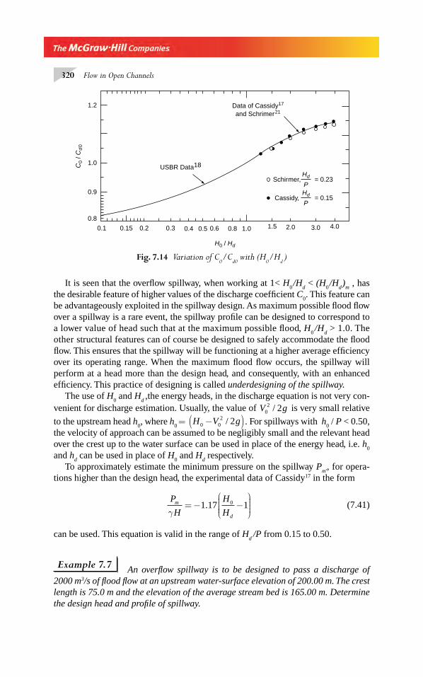
320 Flow in Open Channels
It is seen that the overfl ow spillway, when working at 1< H0 /H
d < (H
0 /H
d )
m , has
the desirable feature of higher values of the discharge coeffi cient C0. This feature can
be advantageously exploited in the spillway design. As maximum possible fl ood fl ow over a spillway is a rare event, the spillway profi le can be designed to correspond to a lower value of head such that at the maximum possible fl ood, H
0 /H
d > 1.0. The
other structural features can of course be designed to safely accommodate the fl ood fl ow. This ensures that the spillway will be functioning at a higher average effi ciency over its operating range. When the maximum fl ood fl ow occurs, the spillway will perform at a head more than the design head, and consequently, with an enhanced effi ciency. This practice of designing is called underdesigning of the spillway.
The use of H0 and H
d ,the energy heads, in the discharge equation is not very con-
venient for discharge estimation. Usually, the value of V g02 2/ is very small relative
to the upstream head h0, where h
0 = H V g0 0
2 2−( )/ . For spillways with h0 / P < 0.50,
the velocity of approach can be assumed to be negligibly small and the relevant head over the crest up to the water surface can be used in place of the energy head, i.e. h
0
and hd can be used in place of H
0 and H
d respectively.
To approximately estimate the minimum pressure on the spillway Pm'
, for opera-tions higher than the design head, the experimental data of Cassidy17 in the form
P
H
H
Hm
dγ= − −
⎛
⎝⎜⎜⎜⎜
⎞
⎠⎟⎟⎟⎟
1 17 10. (7.41)
can be used. This equation is valid in the range of Hd /P from 0.15 to 0.50.
Example 7.7 An overfl ow spillway is to be designed to pass a discharge of 2000 m3/s of fl ood fl ow at an upstream water-surface elevation of 200.00 m. The crest length is 75.0 m and the elevation of the average stream bed is 165.00 m. Determine the design head and profi le of spillway.
Fig. 7.14 Variation of C0/C
d0 with (H
0/H
d )
0.8
0.1 0.2 0.3 0.4 0.5 0.6 0.8 1.0 1.5 2.0 3.0 4.00.15
0.9
1.0
1.2
Schirmer,Hd
P= 0.23
Cassidy,Hd
P= 0.15
H0 / Hd
C0
/ Cd
0
USBR Data18
Data of Cassidy17
and Schrimer21
Chapter 7.indd 320Chapter 7.indd 320 2/24/2010 3:01:36 PM2/24/2010 3:01:36 PM
Rapidly Varied Flow-2 321
Solution A trial-and-error method is adopted to determine the crest elevation.
Discharge per unit width qd = =2000
7526 67. m3/s/m. Assume C
d0 = 0.736.
By Eq. 7.39 q C g Hd d d= ( )2
320
3 2/
26 27
2
30 736 19 62
3 2. . .
/= ( ) ( )Hd
Hd = 5 32. m
Velocity of approach Vq
P ha =+
=−( )0
26 67
200 00 165 00
.
. .
= 0.762 m/s
hV
gaa= = ≈2
20 0296 0 03. . m
Elevation of energy line = 200.03 m
Crest elevation = 200.03 − 5.32 = 195.71m
P = 195.71 − 165.00 = 30.71m
P/Hd =
30 71
5 325 77
.
..=
For this value of P/Hd from Fig. 7.13, C
d 0 = 0.738.
2nd iteration
Hd( ) =( )( )
3 2 26 67
2 3 0 738 19 62
/ .
/ . ., H
d = 5.31m
ha ≈ 0.03. Elevation of energy line = 200.03 m
Crest elevation 200.03 − 5.31 = 194.72 m
P = 194.72 − 165.00 = 29.72 m
P/Hd = 5.60. For this P/H
d , from Fig. 7.13,C
d 0 = 0.738. Hence no more iterations are
required.
Design energy head Hd
= 5.31m
and crest elevation = 194.72 m
The downstream profi le of the crest is calculated by Eq. 7.37, which for the present case is
Chapter 7.indd 321Chapter 7.indd 321 2/24/2010 3:01:36 PM2/24/2010 3:01:36 PM
322 Flow in Open Channels
y x
5 310 50
5 31
1 85
..
.
.
=⎛⎝⎜⎜⎜
⎞⎠⎟⎟⎟⎟
The upstream profi le is calculated by Eq. 7.38 which, for the range 0 1 434≤ − × ≤ . , is given as
y x x
5 310 724
5 310 270 0 432
5 310 270
1 85
..
.. .
..
.
= +⎛⎝⎜⎜⎜
⎞⎠⎟⎟⎟⎟ − +
⎛⎝⎜⎜⎜⎜
⎞⎠⎟⎟⎟⎟ +
0 625
0 126.
.
The apex of the crest at elevation 194.72 m is the origin of coordinates of the above two profi le equations.
Example 7.8 In the spillway of Example 7.7 what would be the discharge if the water-surface elevation reaches 202.00 m? What would be the minimum pressure on the spillway crest under this discharge condition?
Solution h0 = 202.00 –194.72 = 7.28 m
h0 + P = 202.00 – 165.00 = 37.00 m
Assuming the velocity of approach head ha = 0.05 m, the elevation of the energy
line = 202.05 m.
H0 = 202.05 – 194.72 = 7.33 m
H
Hd
0 7 33
5 311 38= =
.
..
From Fig. 7.14, corresponding to H
Hd
0 = 1.38, C
Cd
0
0
1 04= . .
Since Cd 0
= 0.738
C0 = 0.768
q = ( )( ) =2
319 62 0 768 7 33 45 00
3 2. . . .
/ m3 /s/m
Va = =45 00
37 001 216
.
.. m/s, h
V
gaa= ≈2
20 08. m
2nd iteration
Elevation of the energy line = 202.08
H0 = 202.08 – 194.72 = 7.36 m
H
Hd
0 1 386= . C
Cd
0
0
1 04= . from Fig. 7.14,
Chapter 7.indd 322Chapter 7.indd 322 2/24/2010 3:01:36 PM2/24/2010 3:01:36 PM
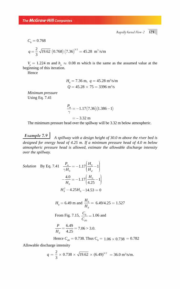
Rapidly Varied Flow-2 323
C0 = 0.768
q = ( ) ( ) =2
319 62 0 768 7 36 45 28
3 2. . . .
/m /s/m3
Va = 1.224 m and h
a ≈ 0.08 m which is the same as the assumed value at the
beginning of this iteration.Hence
H0 = 7.36 m, q = 45.28 m3/s/m
Q = 45.28 × 75 = 3396 m3/s
Minimum pressureUsing Eq. 7.41
Pm
γ= − ( ) −( )1 17 7 36 1 386 1. . .
= – 3.32 mThe minimum pressure head over the spillway will be 3.32 m below atmospheric.
Example 7.9 A spillway with a design height of 30.0 m above the river bed is
designed for energy head of 4.25 m. If a minimum pressure head of 4.0 m below atmospheric pressure head is allowed, estimate the allowable discharge intensity over the spillway.
Solution By Eq. 7.41 P
H
H
Hm
dγ 0
01 17 1= − −⎛
⎝⎜⎜⎜⎜
⎞
⎠⎟⎟⎟⎟
.
− = − −⎛
⎝⎜⎜⎜
⎞
⎠⎟⎟⎟⎟
4 01 17
4 251
0
0..
.H
H
H H02
04 25− . −14.53 = 0
H0 = 6.49 m and
H
Hd
0 = 6.49/4.25 = 1.527
From Fig. 7.15, C
Cd
0
0
= 1.06 and
P
Hd
= =6 49
4 25
.
.7.06 > 3.0.
Hence Cd 0
= 0.738. Thus C0 = 1 06 0 738. .× = 0.782
Allowable discharge intensity
q = × × ×2
30 738 19 62 6 49 3 2. . ( . ) / = 36.0 m3/s/m.
Chapter 7.indd 323Chapter 7.indd 323 2/24/2010 3:01:37 PM2/24/2010 3:01:37 PM
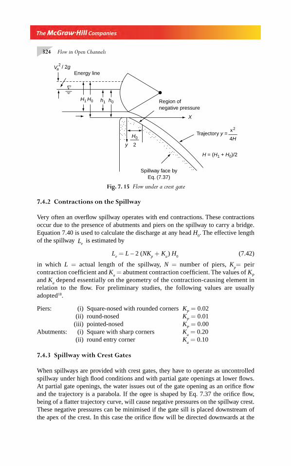
324 Flow in Open Channels
7.4.2 Contractions on the Spillway
Very often an overfl ow spillway operates with end contractions. These contractions occur due to the presence of abutments and piers on the spillway to carry a bridge. Equation 7.40 is used to calculate the discharge at any head H
0. The effective length
of the spillway Le is estimated by
Le = L – 2 (NK
p + K
a ) H
0 (7.42)
in which L = actual length of the spillway, N = number of piers, Kp= peir
contraction coeffi cient and Ka = abutment contraction coeffi cient. The values of K
P
and Ka depend essentially on the geometry of the contraction-causing element in
relation to the fl ow. For preliminary studies, the following values are usually adopted18.
Piers: (i) Square-nosed with rounded corners KP = 0.02
(ii) round-nosed KP = 0.01
(iii) pointed-nosed KP = 0.00
Abutments: (i) Square with sharp corners Ka = 0.20
(ii) round entry corner Ka = 0.10
7.4.3 Spillway with Crest Gates
When spillways are provided with crest gates, they have to operate as uncontrolled spillway under high fl ood conditions and with partial gate openings at lower fl ows. At partial gate openings, the water issues out of the gate opening as an orifi ce fl ow and the trajectory is a parabola. If the ogee is shaped by Eq. 7.37 the orifi ce fl ow, being of a fl atter trajectory curve, will cause negative pressures on the spillway crest. These negative pressures can be minimised if the gate sill is placed downstream of the apex of the crest. In this case the orifi ce fl ow will be directed downwards at the
Fig. 7. 15 Flow under a crest gate
Va2 / 2g
Energy line
H1 H0 h0
y
X
h1
∇
H0
2
Region ofnegative pressure
Spillway face byEq. (7.37)
Trajectory y =4H
x2
H = (H1 + H0)/2
Chapter 7.indd 324Chapter 7.indd 324 2/24/2010 3:01:37 PM2/24/2010 3:01:37 PM
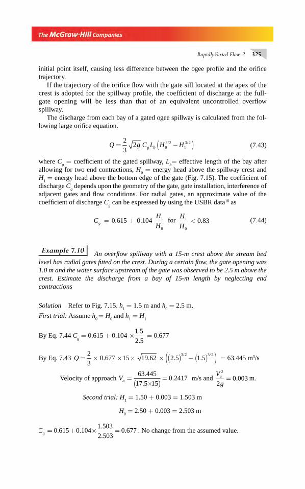
Rapidly Varied Flow-2 325
initial point itself, causing less difference between the ogee profi le and the orifi ce trajectory.
If the trajectory of the orifi ce fl ow with the gate sill located at the apex of the crest is adopted for the spillway profi le, the coeffi cient of discharge at the full-gate opening will be less than that of an equivalent uncontrolled overfl ow spillway.
The discharge from each bay of a gated ogee spillway is calculated from the fol-lowing large orifi ce equation.
Q g C L H Hg b= −( )2
32 0
3 213 2/ / (7.43)
where Cg = coeffi cient of the gated spillway, L
b= effective length of the bay after
allowing for two end contractions, H0 = energy head above the spillway crest and
H1 = energy head above the bottom edge of the gate (Fig. 7.15). The coeffi cient of
discharge Cg depends upon the geometry of the gate, gate installation, interference of
adjacent gates and fl ow conditions. For radial gates, an approximate value of the coeffi cient of discharge C
g can be expressed by using the USBR data18 as
CH
Hg = +0 615 0 104 1
0
. . for H
H1
0
0 83< . (7.44)
Example 7.10 An overfl ow spillway with a 15-m crest above the stream bed level has radial gates fi tted on the crest. During a certain fl ow, the gate opening was 1.0 m and the water surface upstream of the gate was observed to be 2.5 m above the crest. Estimate the discharge from a bay of 15-m length by neglecting end contractions
Solution Refer to Fig. 7.15. h1 = 1.5 m and h
0 = 2.5 m.
First trial: Assume h0 = H
0 and h
1 = H
1
By Eq. 7.44 Cg = 0.615 + 0.104 ×
1 5
2 5
.
. = 0.677
By Eq. 7.43 Q = × × × × ( ) − ( )( )2
30 677 15 19 62 2 5 1 5
3 2 3 2. . . .
/ / = 63.445 m3/s
Velocity of approach Va =×( )
=63 445
17 5 150 2417
.
.. m/s and
V
ga2
20 003= . m.
Second trial: H1 = 1.50 + 0.003 = 1.503 m
H0 = 2.50 + 0.003 = 2.503 m
Cg = + × =0 615 0 1041 503
2 5030 677. .
.
.. . No change from the assumed value.
Chapter 7.indd 325Chapter 7.indd 325 2/24/2010 3:01:37 PM2/24/2010 3:01:37 PM
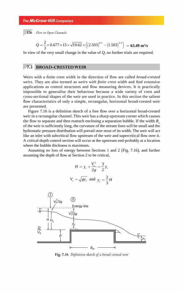
326 Flow in Open Channels
Q = × × × × ( ) −( )( )2
30 677 15 19 62 2 503 1 503
3 2 3 2. . . .
/ /
= 63.49 m3/s
In view of the very small change in the value of Q, no further trials are required.
7.5 BROAD-CRESTED WEIR
Weirs with a fi nite crest width in the direction of fl ow are called broad-crested weirs. They are also termed as weirs with fi nite crest width and fi nd extensive applications as control structures and fl ow measuring devices. It is practically impossible to generalise their behaviour because a wide variety of crest and cross-sectional shapes of the weir are used in practice. In this section the salient fl ow characteristics of only a simple, rectangular, horizontal broad-crested weir are presented.
Figure 7.16 is a defi nition sketch of a free fl ow over a horizontal broad-crested weir in a rectangular channel. This weir has a sharp upstream corner which causes the fl ow to separate and then reattach enclosing a separation bubble. If the width B
w
of the weir is suffi ciently long, the curvature of the stream lines will be small and the hydrostatic pressure distribution will prevail over most of its width. The weir will act like an inlet with subcritical fl ow upstream of the weir and supercritical fl ow over it. A critical-depth control section will occur at the upstream end-probably at a location where the bubble thickness is maximum.
Assuming no loss of energy between Sections 1 and 2 (Fig. 7.16), and further assuming the depth of fl ow at Section 2 to be critical,
H yV
gyc
cc= + =
2
2
3
2
V gyc c= and y Hc =2
3
Fig. 7.16 Defi nition sketch of a broad-crested weir
1
2
Energy line∇
∇
H
P
H1
V0
yc
y1
Bw
V20 /2g
V 2c /2g
Q
Chapter 7.indd 326Chapter 7.indd 326 2/24/2010 3:01:38 PM2/24/2010 3:01:38 PM
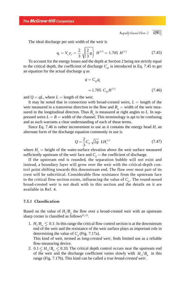
Rapidly Varied Flow-2 327
The ideal discharge per unit width of the weir is
q V y g H Ht c c= =⎛⎝⎜⎜⎜
⎞⎠⎟⎟⎟⎟ =
2
3
2
31 7053 2 3 2/ /. (7.45)
To account for the energy losses and the depth at Section 2 being not strictly equal to the critical depth, the coeffi cient of discharge C
d1 is introduced in Eq. 7.45 to get
an equation for the actual discharge q as
q = Cd1
qt
=1 705 13 2. /C Hd (7.46)
and Q = qL, where L = length of the weir.It may be noted that in connection with broad-crested weirs, L = length of the
weir measured in a transverse direction to the fl ow and Bw = width of the weir mea-
sured in the longitudinal directon. Thus Bw is measured at right angles to L. In sup-
pressed weirs L = B = width of the channel. This terminology is apt to be confusing and as such warrants a clear understanding of each of these terms.
Since Eq. 7.46 is rather inconvenient to use as it contains the energy head H, an alternate form of the discharge equation commonly in use is
Q C g LHd=2
32 1
3 2/ (7.47)
where H1 = height of the water-surface elevation above the weir surface measured
suffi ciently upstream of the weir face and Cd = the coeffi cient of discharge.
If the upstream end is rounded, the separation bubble will not exist and instead, a boundary layer will grow over the weir with the critical-depth con-trol point shifting towards this downstream end. The flow over most part of its crest will be subcritical. Considerable flow resistance from the upstream face to the critical flow section exists, influencing the value of C
d . The round-nosed
broad-crested weir is not dealt with in this section and the details on it are available in Ref. 4.
7.5.1 Classifi cation
Based on the value of H1 /B
w the fl ow over a broad-crested weir with an upstream
sharp corner is classifi ed as follows22, 23.
1. H1 /B
w �< 0.1: In this range the critical fl ow control section is at the downstream
end of the weir and the resistance of the weir surface plays as important role in determining the value of C
d (Fig. 7.17a).
This kind of weir, termed as long-crested weir, fi nds limited use as a reliable fl ow-measuring device.
2. 0 1 0 351. .� �< <H Bw : The critical depth control occurs near the upstream end
of the weir and the discharge coeffi cient varies slowly with H Bw1 in this
range (Fig. 7.17b). This kind can be called a true broad-crested weir.
Chapter 7.indd 327Chapter 7.indd 327 2/24/2010 3:01:38 PM2/24/2010 3:01:38 PM
328 Flow in Open Channels
Fig. 7.17 (a) Long-crested weir ( . )H Bw1 0 1�<
(b) Broad-crested weir ( . . )0 1 0 35� �< <H Bw
(c) Narrow-crested weir ( . . )0 35 1 51� �< <H Bw
(d) Sharp-crested weir ( . )H Bw1 1 5≥
∇∇
Bw Bw
H1
H1
(b)(a)
∇
H1
Bw
(c)
∇
H1
Bw
(d)
b
3. 0 35 1.� �< <H Bw about 1.5: The water-surface profi le will be curvilinear all
over the weir. The control section will be at the upstream end (Fig. 7.17c). The weirs of this kind can be termed as narrow-crested weirs. The upper limit of this range depends upon the value of H P1 .
4. H Bw1 > about 1.5: The fl ow separates at the upstream corner and jumps clear across the weir crest. The fl ow surface is highly curved (Fig. 7.17d), and the weir can be classifi ed as sharp-crested.
7.5.2 Discharge Coeffi cients, Cd and C
d1
From Eqs 7.47 and 7.46 the discharge coeffi cients Cd and C
d1 respectively are given
as
CQ
g LHd =
2
32 1
3 2/
and CQ
LHd1 3 21 705=
. / (7.48)
A formal dimensional analysis of the fl ow situation will reveal that
C C fH
L
H
B
H
PRe W
k
Hd d
w
s( ) , , , , ,or 11 1 1
1
=⎡
⎣⎢⎢
⎤
⎦⎥⎥ (7.49)
Chapter 7.indd 328Chapter 7.indd 328 2/24/2010 3:01:38 PM2/24/2010 3:01:38 PM
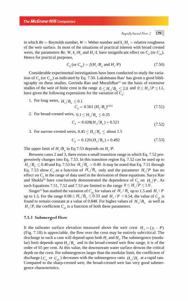
Rapidly Varied Flow-2 329
in which Re = Reynolds number, W = Weber number and ks /H
1 = relative roughness
of the weir surface. In most of the situations of practical interest with broad crested weirs, the parameters Re, W, k
s /H
1 and H
1 /L have insignifi cant effect on C
d (or C
d1).
Hence for practical purposes,
Cd (or C
d1) = f (H
1 /B
w and H
1 /P) (7.50)
Considerable experimental investigations have been conducted to study the varia-tion of C
d (or C
d 1) as indicated by Eq. 7.50. Lakshmana Rao1 has given a good bibli-
ography on these studies. Govinda Rao and Muralidhar22 on the basis of extensive studies of the weir of fi nite crest in the range 0 2 01≤ ≤H Bw . and 0 1 01≤ ≤H P . , have given the following expressions for the variation of C
d:
1. For long weirs, H Bw1 0 1≤ . C
d = 0.561 (H
1 /B
w)0.022 (7.51)
2. For broad-crested weirs, 0 1 0 351. .≤ ≤H Bw
C H Bd w= +0 028 0 5211. ( ) . (7.52)
3. For narrow-crested weirs, 0 45 1.�< <H Bw �
about 1.5
C H Bd w= +0 120 0 4921. ( ) . (7.53)
The upper limit of H1 /B
w in Eq 7.53 depends on H
1 /P.
Between cases 2 and 3, there exists a small transition range in which Eq. 7.52 pro-gressively changes into Eq. 7.53. In this transition region Eq. 7.52 can be used up to H Bw1 0 40≤ . and Eq. 7.53 for H Bw1 0 40> . . It may be noted that Eq. 7.51 through Eq. 7.53 show C
d as a function of H Bw1 only and the parameter H P1 has no
effect on Cd in the range of data used in the derivation of these equations. Surya Rao
and Shukla24 have conclusively demonstrated the dependence of Cd on H P1
. As such Equations 7.51, 7.52 and 7.53 are limited to the range 0 1 01≤ ≤H P . .
Singer23 has studied the variation of Cd1
for values of H Bw1 / up to 1.5 and H P1 / up to 1.5. For the range 0.08≤ ≤H Bw1 0 33. and H P1 / < 0.54, the value of C
d1 is
found to remain constant at a value of 0.848. For higher values of H Bw1 as well as H P1 , the coeffi cient C
d1 is a function of both these parameters.
7.5.3 Submerged Flow
It the tailwater surface elevation measured above the weir crest H y Pt2 = −( ) (Fig. 7.18) is appreciable, the fl ow over the crest may be entirely subcritical. The discharge in such a case will depend upon both H
1 and H
2. The submergence (modu-
lar) limit depends upon H Bw1 and in the broad-crested weir fl ow range, it is of the order of 65 per cent. At this value, the downstream water surface drowns the critical depth on the crest. For submergences larger than the modular limit, the coeffi cient of discharge ( Cd
or Cd1) decreases with the submergence ratio H H2 1
at a rapid rate. Compared to the sharp-crested weir, the broad-crested weir has very good submer-gence characteristics.
Chapter 7.indd 329Chapter 7.indd 329 2/24/2010 3:01:39 PM2/24/2010 3:01:39 PM
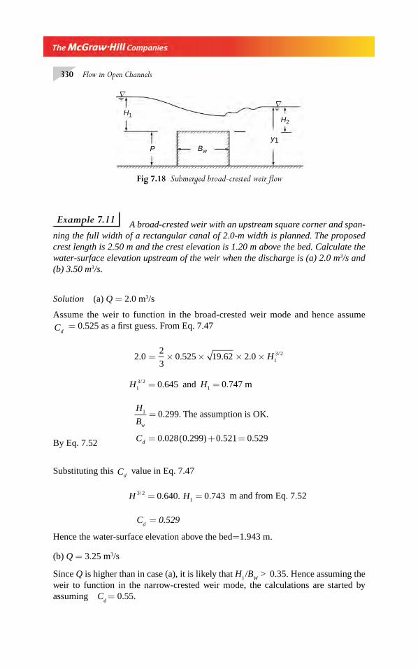
330 Flow in Open Channels
Example 7.11 A broad-crested weir with an upstream square corner and span-ning the full width of a rectangular canal of 2.0-m width is planned. The proposed crest length is 2.50 m and the crest elevation is 1.20 m above the bed. Calculate the water-surface elevation upstream of the weir when the discharge is (a) 2.0 m3/s and (b) 3.50 m3/s.
Solution (a) Q = 2.0 m3/s
Assume the weir to function in the broad-crested weir mode and hence assume
Cd = 0.525 as a fi rst guess. From Eq. 7.47
2 02
30 525 19 62 2 0 1
3 2. . . . /= × × × × H
H13 2 0 645/ .= and H1 0 747= . m
H
Bw
1 0 299= . . The assumption is OK.
By Eq. 7.52 Cd = + =0 028 0 299 0 521 0 529. ( . ) . .
Substituting this Cd value in Eq. 7.47
H H3 210 640 0 743/ . . .= = m and from Eq. 7.52
Cd = 0.529
Hence the water-surface elevation above the bed=1.943 m.
(b) Q = 3.25 m3/s
Since Q is higher than in case (a), it is likely that H1 /B
W >
0.35. Hence assuming the
weir to function in the narrow-crested weir mode, the calculations are started by assuming C
d = 0.55.
Fig 7.18 Submerged broad-crested weir fl ow
∇∇
H1H2
y1BwP
Chapter 7.indd 330Chapter 7.indd 330 2/24/2010 3:01:39 PM2/24/2010 3:01:39 PM
Rapidly Varied Flow-2 331
Ist iteration Cd = 0.55
From Eq. 7.28, 3.50 = 2
30 55 19 62 2 0 1
3 2× × × ×. . . /H
H13 2 1 077/ . ,= H1 1 05= . m,
H
Bw
1 0 42= .
The weir fl ow is in the transition region between the broad-crested and narrow-crested weir modes. Hence, by Eq. 7.53
Cd = 0.120 × (0.42) + 0.492 = 0.534
2nd iteration Using Cd = 0.534 in Eq. 7.47
H13 2 1 109/ . ,= H1 1 071= . m,
H
Bw
1 0 429= .
From Eq. 7.53, Cd = 0 543.
3rd iteration H13/2 = 1.091, H1 1 060= . m,
H
Bw
1 0 424= .
Cd = 0 543.
Hence, H1 = 1.060 and the water-surface elevation above the bed is 2.260 m.
Example 7.12 Show that for a triangular broad crested weir fl owing free the discharge equation can be expressed as
Q Cg
Hd=16
25
2
515 2tan /θ
where H = energy head measured from the vertex of the weir, θ = semi-apex angle and C
d1 = coeffi cient of discharge.
Solution H yV
gyc
cc= + =
2
21 25.
or y Hc =4
5
A my Hc= =2 216
25tanθ where θ = semi vertex angle.
FV
gyc
= =2
1 or Vg
H=2
51 2/
Q C VAd= 1
Q Cg
Hd=16
25
2
515 2tan /θ
Chapter 7.indd 331Chapter 7.indd 331 2/24/2010 3:01:40 PM2/24/2010 3:01:40 PM
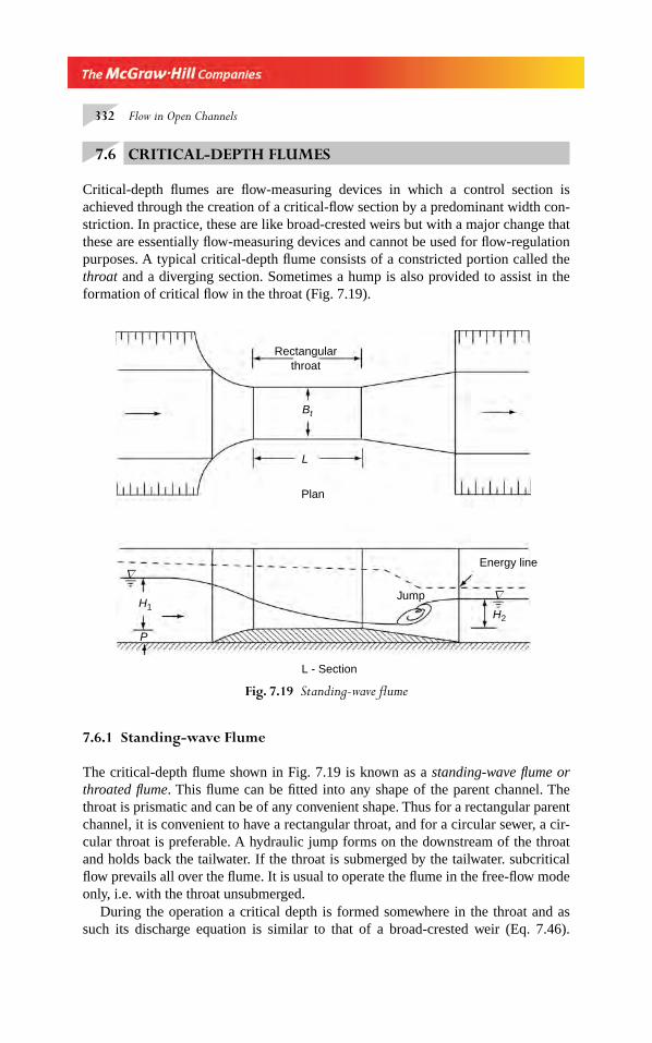
332 Flow in Open Channels
7.6 CRITICAL-DEPTH FLUMES
Critical-depth fl umes are fl ow-measuring devices in which a control section is achieved through the creation of a critical-fl ow section by a predominant width con-striction. In practice, these are like broad-crested weirs but with a major change that these are essentially fl ow-measuring devices and cannot be used for fl ow-regulation purposes. A typical critical-depth fl ume consists of a constricted portion called the throat and a diverging section. Sometimes a hump is also provided to assist in the formation of critical fl ow in the throat (Fig. 7.19).
Fig. 7.19 Standing-wave fl ume
∇
∇
L - Section
Jump
Energy line
H2
H1
Bt
L
P
Plan
Rectangularthroat
7.6.1 Standing-wave Flume
The critical-depth fl ume shown in Fig. 7.19 is known as a standing-wave fl ume or throated fl ume. This fl ume can be fi tted into any shape of the parent channel. The throat is prismatic and can be of any convenient shape. Thus for a rectangular parent channel, it is convenient to have a rectangular throat, and for a circular sewer, a cir-cular throat is preferable. A hydraulic jump forms on the downstream of the throat and holds back the tailwater. If the throat is submerged by the tailwater. subcritical fl ow prevails all over the fl ume. It is usual to operate the fl ume in the free-fl ow mode only, i.e. with the throat unsubmerged.
During the operation a critical depth is formed somewhere in the throat and as such its discharge equation is similar to that of a broad-crested weir (Eq. 7.46).
Chapter 7.indd 332Chapter 7.indd 332 2/24/2010 3:01:41 PM2/24/2010 3:01:41 PM
Rapidly Varied Flow-2 333
However, it is usual to relate the discharge to the upstream depth H1 which can be
typically recorded by an automated fl oat equipment. Thus for a rectangular throat section, the discharge is given by
Q C B Hf t= 13 2/ (7.54)
where Cf = overall discharge coeffi cient of the fl ume = ( )f H L1 / . For a well-
designed fl ume, Cf is of the order of 1.62. It may be noted that in standing-wave
fl umes, H1 is the difference in the water-surface elevation upstream of the inlet and
the elevation of the crest at the throat. If the fl ume is submerged and the subcritical fl ow prevails all over the fl ume, Eq. 7.54 is not valid and two depth measurements are needed to estimate the discharge. Constriction fl umes operating in the subcritical fl ow range are called venturi fl umes.
The modular limit H H2 1/( ) of standing wave fl umes is high, being of the order of 0.90. It is usual to take it as 0.75 to incorporate a small safety factor and to avoid the region of transition from the free to submerged-fl ow mode.
Large varieties of standing-wave fl umes with different types of modifi cations of the basic type described above, resulting in different geometric shapes and corre-sponding fl ow characteristics are in use4,5. However, the basic favourable features of all these throated fl umes can be summarised as (i) low energy loss, (ii) rugged con-struction, (iii) easy passage for fl oating and suspended material load, and (iv) high modular limit. These features are responsible for extensive use of throated fl umes as fl ow-measuring devices in water-treatment plants and in irrigation practice.
Example 7.13 (a) A standing-wave fl ume without a hump is to be provided in a rectangular channel of bottom width = 2.0 m, n = 0.015 and S
0 = 0.0004. A maxi-
mum discharge of 2.50 m3/s is expected to be passed in this fl ume. If the modular limit of the fl ume is 0.75, fi nd the width of the throat. (Assume C
f = 1.62.)
Solution φ = =×( )
( )=
Qn
S B08 3 8 3
2 5 0 015
0 0004 2 00 29529
/ /
. .
. ..
From Table 3A.1, y
B0 (corresponding to m = 0 ) = 0.656 and normal depth
y0 = 1.312 m. This is the tailwater depth H
2.
For a modular limit of 0.75, H1
1 312
0 75= =
.
.1.749 m
By Eq. 7.54, BQ
C Ht
f
= =×( )1
3 2 3 2
2 50
1 62 1 749/ /
.
. .
= 0.667 m
Example 7.14 In the Example 7.12 compare the heading up of water surface (affl ux) due to the fl ume and also due to a suppressed free fl owing sharp-crested weir.
Solution From Example 7.13 heading up (affl ux) due to fl ume
= H1 – H
2 = 1.749 – 1.312 = 0.47 m.
Chapter 7.indd 333Chapter 7.indd 333 2/24/2010 3:01:41 PM2/24/2010 3:01:41 PM
334 Flow in Open Channels
Sharp-crested weirFor free-fl ow operation, the crest of the weir should be at least 0.08 m above the tailwater elevation. Hence P = 1.312 + 0.080 = 1.392 m.1st trial: Assume C
d = 0.650
By Eq. 7.5 Q C g Lhd=2
32 1
3 2/
h1 = head over the crest
h h13 2
1
2 502
30 65 2 0 19 62
0 651 0 751/ .
. . .. , .=
× × ×= = m
h
P1 0 54= . and by Rehbock equation (Eq. 7.7)
Cd = 0.611 + 0.08(0.54) = 0.654
2nd trial Using Cd = 0.654
h13 2/ = 0.651 × 0 650
0 6540 647
.
.. ,= h1 0 748= . m
h P1 0 537/ .= and Cd = 0.654
Hence, h1 = 0.748 m
Affl ux = 0.748 m + 1.392 – 1.312 = 0.828 m
7.6.2 Parshall Flume
The Parshall fl ume is a type of critical-depth fl ume popular in the USA. This fl ume consists of a converging section with a level fl oor, a throat with a downstream slop-ing fl oor and a diverging section with an adverse slope bed (Fig. 7.20). Unlike in the standing-wave fl ume, the head (H
a) is measured at a specifi ed location in the con-
verging section. The discharge in the fl ume in the free fl ow mode is given by
Q KHan= (7.55)
where K and n are constants for a given fl ume. The dimensions of various sizes of Parshall fl umes are standardised and further details are available in references 4, 5, 25 and 26.
7.7 END DEPTH IN A FREE OVERFALL
A free overfall is a situation in which there is a sudden drop in the bed causing the fl ow to separate from the stream bed and move down the step with a free nappe. The situa-tion is analogous to the fl ow over a sharp-crested weir of zero height. A free overfall causes not only a GVF profi le in the subcritical fl ow, but also offers the possibility of being used as a fl ow measuring device in all fl ow regimes.
Chapter 7.indd 334Chapter 7.indd 334 2/24/2010 3:01:41 PM2/24/2010 3:01:41 PM
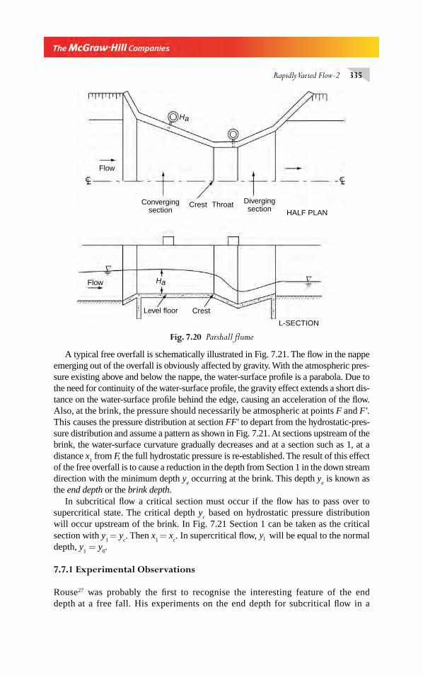
Rapidly Varied Flow-2 335
A typical free overfall is schematically illustrated in Fig. 7.21. The fl ow in the nappe emerging out of the overfall is obviously affected by gravity. With the atmospheric pres-sure existing above and below the nappe, the water-surface profi le is a parabola. Due to the need for continuity of the water-surface profi le, the gravity effect extends a short dis-tance on the water-surface profi le behind the edge, causing an acceleration of the fl ow. Also, at the brink, the pressure should necessarily be atmospheric at points F and F'. This causes the pressure distribution at section FF' to depart from the hydrostatic-pres-sure distribution and assume a pattern as shown in Fig. 7.21. At sections upstream of the brink, the water-surface curvature gradually decreases and at a section such as 1, at a distance x
1 from F, the full hydrostatic pressure is re-established. The result of this effect
of the free overfall is to cause a reduction in the depth from Section 1 in the down stream direction with the minimum depth y
e occurring at the brink. This depth y
e is known as
the end depth or the brink depth.In subcritical fl ow a critical section must occur if the fl ow has to pass over to
supercritical state. The critical depth yc based on hydrostatic pressure distribution
will occur upstream of the brink. In Fig. 7.21 Section 1 can be taken as the critical section with y
1 = y
c. Then x
1 = x
c. In supercritical fl ow, y1 will be equal to the normal
depth, y1 = y
0.
7.7.1 Experimental Observations
Rouse27 was probably the fi rst to recognise the interesting feature of the end depth at a free fall. His experiments on the end depth for subcritical fl ow in a
Fig. 7.20 Parshall fl ume
Flow
Flow
Ha
Ha
L-SECTION
Crest
Crest
Level floor
∇∇
Convergingsection
Throat Divergingsection HALF PLAN
Chapter 7.indd 335Chapter 7.indd 335 2/24/2010 3:01:42 PM2/24/2010 3:01:42 PM
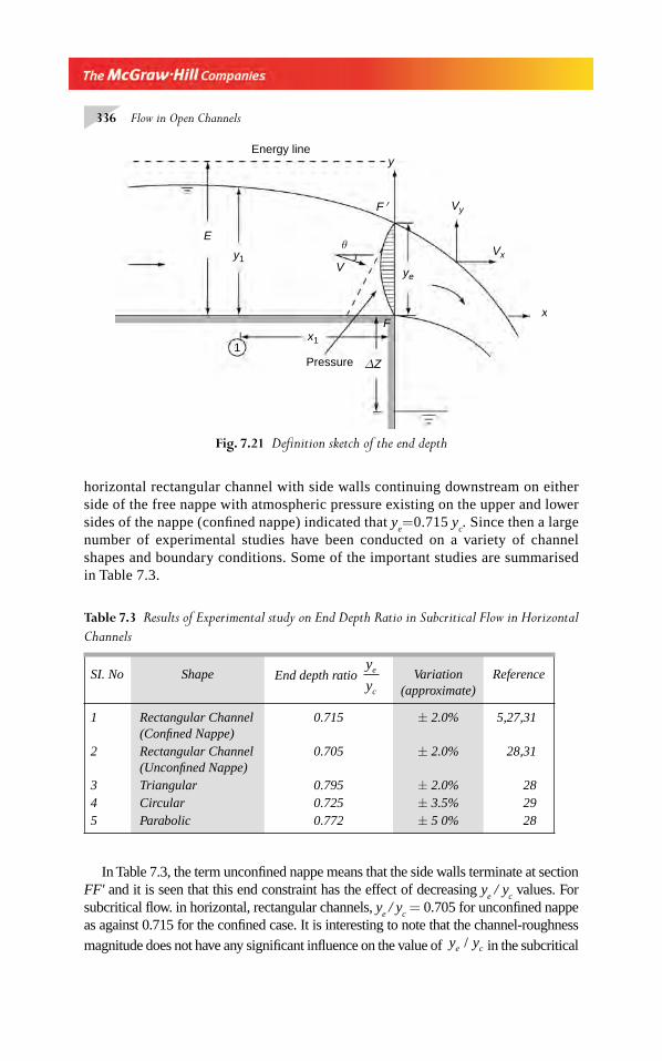
336 Flow in Open Channels
horizontal rectangular channel with side walls continuing downstream on either side of the free nappe with atmospheric pressure existing on the upper and lower sides of the nappe (confi ned nappe) indicated that y
e=0.715 y
c. Since then a large
number of experimental studies have been conducted on a variety of channel shapes and boundary conditions. Some of the important studies are summarised in Table 7.3.
Table 7.3 Results of Experimental study on End Depth Ratio in Subcritical Flow in Horizontal
Channels
SI. No Shape End depth ratio y
ye
c
Variation (approximate)
Reference
1 Rectangular Channel (Confi ned Nappe)
0.715 ± 2.0% 5,27,31
2 Rectangular Channel (Unconfi ned Nappe)
0.705 ± 2.0% 28,31
3 Triangular 0.795 ± 2.0% 284 Circular 0.725 ± 3.5% 295 Parabolic 0.772 ± 5 0% 28
Fig. 7.21 Defi nition sketch of the end depth
Pressure
E
F
Energy liney
Vy
Vx
x
ye
x1
y1V
F ′
ΔZ1
θ
In Table 7.3, the term unconfi ned nappe means that the side walls terminate at section FF' and it is seen that this end constraint has the effect of decreasing y
e / y
c values. For
subcritical fl ow. in horizontal, rectangular channels, ye / y
c = 0.705 for unconfi ned nappe
as against 0.715 for the confi ned case. It is interesting to note that the channel-roughness
magnitude does not have any signifi cant infl uence on the value of y ye c/ in the subcritical
Chapter 7.indd 336Chapter 7.indd 336 2/24/2010 3:01:42 PM2/24/2010 3:01:42 PM
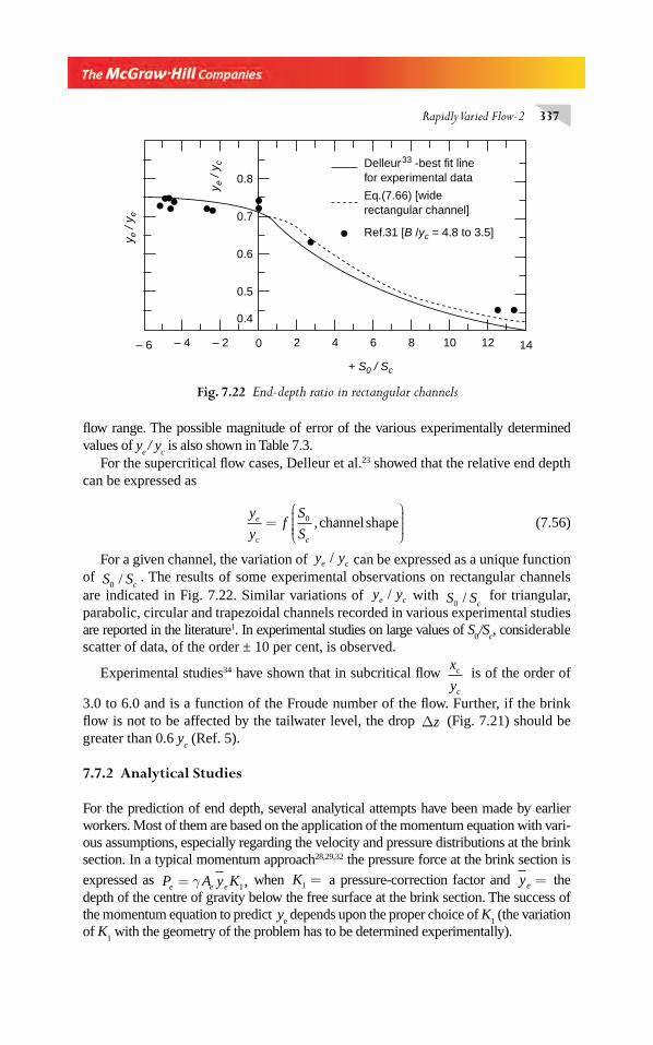
Rapidly Varied Flow-2 337
fl ow range. The possible magnitude of error of the various experimentally determined values of y
e / y
c is also shown in Table 7.3.
For the supercritical fl ow cases, Delleur et al.23 showed that the relative end depth can be expressed as
y
yf
S
Se
c c
=⎛
⎝⎜⎜⎜⎜
⎞
⎠⎟⎟⎟⎟
0 , channelshape (7.56)
For a given channel, the variation of y ye c/ can be expressed as a unique function of S Sc0 / . The results of some experimental observations on rectangular channels are indicated in Fig. 7.22. Similar variations of y ye c/ with S Sc0 / for triangular, parabolic, circular and trapezoidal channels recorded in various experimental studies are reported in the literature1. In experimental studies on large values of S
0 /S
c, considerable
scatter of data, of the order ± 10 per cent, is observed.
Experimental studies34 have shown that in subcritical fl ow x
yc
c
is of the order of
3.0 to 6.0 and is a function of the Froude number of the fl ow. Further, if the brink fl ow is not to be affected by the tailwater level, the drop Δz (Fig. 7.21) should be greater than 0.6 y
c (Ref. 5).
7.7.2 Analytical Studies
For the prediction of end depth, several analytical attempts have been made by earlier workers. Most of them are based on the application of the momentum equation with vari-ous assumptions, especially regarding the velocity and pressure distributions at the brink section. In a typical momentum approach28,29,32 the pressure force at the brink section is
expressed as P A y Ke e e= γ 1, when K1 = a pressure-correction factor and ye = the depth of the centre of gravity below the free surface at the brink section. The success of the momentum equation to predict y
e depends upon the proper choice of K
1 (the variation
of K1 with the geometry of the problem has to be determined experimentally).
Fig. 7.22 End-depth ratio in rectangular channels
– 6 – 4 – 2 0 2 4 6 8 10 12 14
0.4
0.5
0.6
0.7
0.8
y e /
y e
y e /
y c
+ S0 / Sc
Delleur33 -best fit linefor experimental data
Eq.(7.66) [widerectangular channel]
Ref.31 [B /yc = 4.8 to 3.5]
Chapter 7.indd 337Chapter 7.indd 337 2/24/2010 3:01:43 PM2/24/2010 3:01:43 PM
338 Flow in Open Channels
The numerical solution of a two-dimensional ideal fl uid-fl ow at a free overfall has been attempted by some investigators through various fi nite difference schemes. An excellent review of these studies on potential fl ow in a free overfall and a theory describing such a fl ow is presented by Strelkoff et al.35 While it is possible to solve the end-depth problem in a wide rectangular channel through advanced numerical techniques, such as the fi nite-element method, the solution of the problem in chan-nels of different shapes have to be tackled by alternative methods.
An elegant method which differs from the above two approaches has been reported by Anderson34. Based on Anderson’s work, a generalised energy method for the prediction of end-depth in channels of any shape is given by Subramanya36 and is described below. This method is simple, does not need any coeffi cient and can predict the end-depths to a remarkable degree of accuracy in a variety of situations.
7.7.3 Generalised Energy Method for End Depth Prediction36
In a free overfall, the water surface is a continuously falling curve. The water surface profi le starts in the channel somewhere upstream of the edge, passes through the brink and ends up as a trajectory of gravity fall. In deriving the general expression for the end-depth, expressions for the curvature of the water surface are separately derived for the channel fl ow as well as for the free overfall and matched at the brink.
(a) Curvature of the Channel Flow Consider a channel of any shape having a free over fall (Fig. 7.21). The water surface curvature is assumed to be relatively small and is assumed to vary linearly from a fi nite value at the surface to zero value at the channel bottom. The effective piezometric head is then expressed by the Boussinesq equation (Eq. 1–35) The water surface curvature is convex upwards and the specifi c energy E at any section is given by Eq. 1.41 as
E hV
gep= +α2
2
By using Eq. 1.33 for hep
E yV
g
V y
g
d y
dx= + +
⎛
⎝⎜⎜⎜⎜
⎞
⎠⎟⎟⎟⎟
α2 2 2
22
1
3 (7.57)
i.e. E yQ
gA
Q
gAy
d y
dx= + +
⎛
⎝⎜⎜⎜⎜
⎞
⎠⎟⎟⎟⎟
α2
2
2
2
2
22
1
3 (7.58)
Assume the specifi c energy E to be constant in the neighbourhood of the brink and further assume α = 1.0 for simplicity. The conditions at the brink section (denoted by the suffi x e ) is expressed, by non-dimensionalising Eq. 7.58 with respect to the critical depth y
c, as
E
y
y
y
Q
gA y
Q
gA y
y
y
d y y
d x ye
c
e
c e c e c
e
c
c
c
y ye
= + +( )
( )=
2
2
2
2
2
22
1
3 (7.59)
Chapter 7.indd 338Chapter 7.indd 338 2/24/2010 3:01:43 PM2/24/2010 3:01:43 PM
Rapidly Varied Flow-2 339
Denoting the critical conditions by the suffi x c,
y yA
A T yfe c
c
e c c
/ ;= = ( )η η3
2 and E ye c/ = ε
Remembering that Q g A Tc c2 3/ /= Eq. (7.59) can be simplifi ed as
ε η η η η= + ( )+ ( )( )
( )=
1
2
1
3
2
2f f
d y y
d x y
c
c
y ye
/
/ (7.60)
The expression for the curvature of the channel water surface at the brink is from Eq. 7.60,
d y y
d x y ffc
c
y ye
2
2
3 1
2
/
/
( )( )
=( )
− − ( )⎡
⎣⎢⎢
⎤
⎦⎥⎥
=
η ηε η η (7.61)
(b) Overfl ow Trajectory Referring to Fig. 7.21, Vx is x – component of the
velocity in the overfl ow trajectory and is given by
V Vx e= cosθ (7.62)
where Ve = mean velocity at the brink inclined at an angle θ to the horizontal. For a
gravity fall
dV
dtx = 0 and
dV
dtgy = −
where Vy = y – component of the velocity in the trajectory.
Since dy
dx
V
Vy
x
=
d y
dxg V
gA
V A
gA
Q
xe
e e
e
2
2
22
2 2
2
2 2
= − = −( )
= −
/cos
cos
θ
θ (7.63)
Noting that Q
g
A
Tc
c
2 3
= , Eq. 7.63 can be written as
d y
dx
T A
A y fc e
c c
2
2
2
3 2 2
1= − = −
( )cos cosθ η θ
Thus,
d y y
d x y fc
cy ye
2
2 2
1/
/ cos
( )( )
= −( )
=
η θ (7.64)
Chapter 7.indd 339Chapter 7.indd 339 2/24/2010 3:01:43 PM2/24/2010 3:01:43 PM
340 Flow in Open Channels
(c) General Equation for End Depth Ratio For a continuous water surface slope at (x = 0, y = y
e ) Eq. 7.61 and Eq. 7.64 must be identical and as such
−( )
=( )
− − ( )⎡
⎣⎢⎢
⎤
⎦⎥⎥
1 3 1
22f ff
η θ η ηε η η
cos
Simplifying,
6 2 3 1 3 02 2 2ε θ η θ η θcos cos cos− −( )− ( ) =f (7.65)
In the usual cases when θ is small, cos . ,cos .θ θ≈ ≈1 0 1 02 and Eq. 7.65 simplifi es to
6 4 3 0ε η η− − ( ) =f (7.66)
This equation is the general equation relating the end-depth ratio η with the non-dimen-sionalised specifi c energy at the brink and is based on the assumption of constancy of the specifi c energy in the neighbourhood of the brink. To illustrate the use of Eq. 7.66, the prediction of end-depth in exponential channels is presented in the following section.
7.7.4 End Depth in Exponential Channels
An exponential channel is defi ned as the one in which the area A is related to the depth y as A=Ky a, where K and a are constants. It is easily seen that a =1 0 1 5. , . and 2.0 represents rectangular, parabolic and triangular channels respectively.
For exponential channels, TdA
dyKa ya= = −1
and A
T
y
a= (7.67)
fA
A T y ay y
ac
e c c
c e
a
aη
η( ) = = ( ) =
3
2
2
2
1 1 1/ (7.68)
Eq. 7.66 now becomes
6 43 1
02
ε ηη
− − =a a
(7.69)
The solution of Eq. 7.69 is now obtained for subcritical and supercritical channel fl ows separately.
(i) Subcritical Flow If the fl ow upstream of the brink is subcritical, the critical depth must occur before the end-depth. Assuming constant specifi c energy E between the critical section and end section
ε = =E
y
E
ye
c
c
c
Since E yQ
g Ay
A
Tc c
c
cc
c
= + = +2
22 2
Chapter 7.indd 340Chapter 7.indd 340 2/24/2010 3:01:44 PM2/24/2010 3:01:44 PM
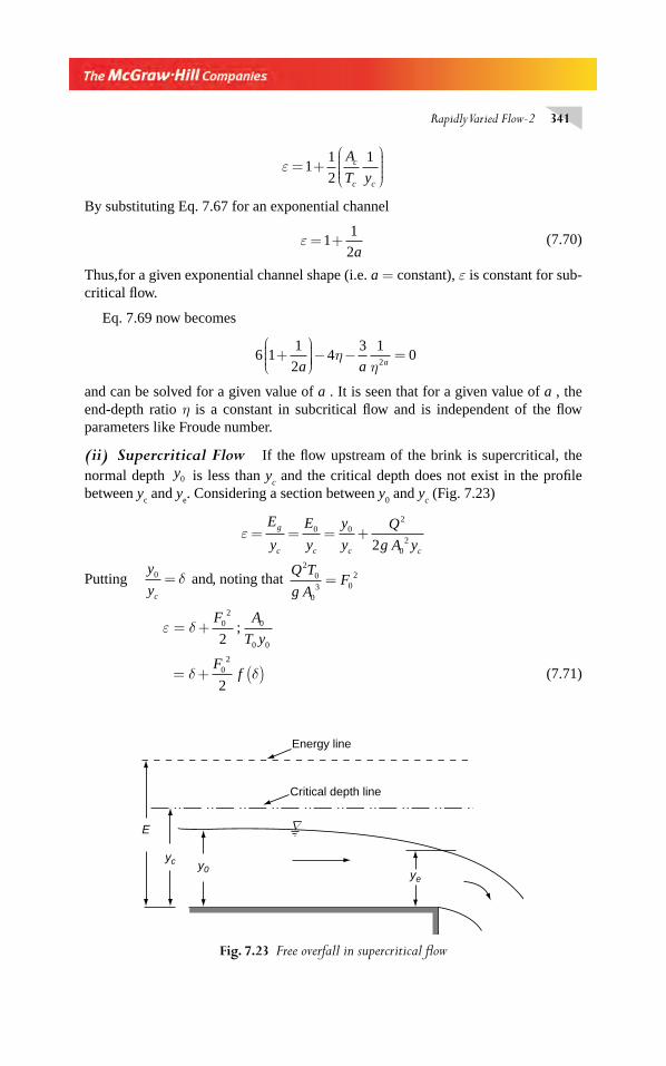
Rapidly Varied Flow-2 341
ε = +⎛
⎝⎜⎜⎜⎜
⎞
⎠⎟⎟⎟⎟
11
2
1A
T yc
c c
By substituting Eq. 7.67 for an exponential channel
ε = +11
2a (7.70)
Thus,for a given exponential channel shape (i.e. a = constant), ε is constant for sub-critical fl ow.
Eq. 7.69 now becomes
6 11
24
3 10
2+
⎛⎝⎜⎜⎜
⎞⎠⎟⎟⎟⎟− − =
a a aη
η
and can be solved for a given value of a . It is seen that for a given value of a , the end-depth ratio η is a constant in subcritical fl ow and is independent of the fl ow parameters like Froude number.
(ii) Supercritical Flow If the fl ow upstream of the brink is supercritical, the
normal depth y0 is less than yc and the critical depth does not exist in the profi le
between yc and y
e. Considering a section between y
0 and y
c (Fig. 7.23)
ε = = = +E
y
E
y
y
y
Q
g A yg
c c c c
0 02
022
Putting y
yc
0 = δ and, noting that Q T
g AF
20
03 0
2=
ε δ
δ δ
= +
= + ( )
F A
T y
Ff
02
0
0 0
02
2
2
;
(7.71)
E
yc y0
Critical depth line
Energy line
ye
∇
Fig. 7.23 Free overfall in supercritical fl ow
Chapter 7.indd 341Chapter 7.indd 341 2/24/2010 3:01:44 PM2/24/2010 3:01:44 PM
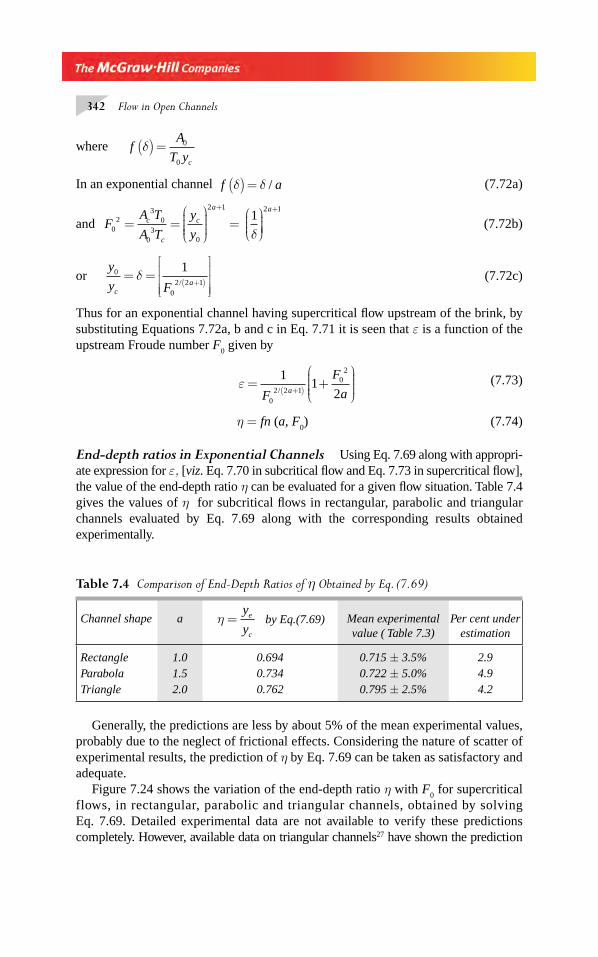
342 Flow in Open Channels
where fA
T yc
δ( ) = 0
0
In an exponential channel f aδ δ( ) = / (7.72a)
and FA T
A T
y
yc
c
c
a a
02
30
03
0
2 1 2 11
= =⎛
⎝⎜⎜⎜⎜
⎞
⎠⎟⎟⎟⎟
=⎛⎝⎜⎜⎜
⎞⎠⎟⎟⎟⎟
+ +
δ (7.72b)
or y
y Fca
0
02 2 1
1= =
⎡
⎣
⎢⎢⎢
⎤
⎦
⎥⎥⎥
+( )δ
/ (7.72c)
Thus for an exponential channel having supercritical fl ow upstream of the brink, by substituting Equations 7.72a, b and c in Eq. 7.71 it is seen that ε is a function of the upstream Froude number F
0 given by
ε = +⎛
⎝⎜⎜⎜⎜
⎞
⎠⎟⎟⎟⎟+( )
11
20
2 2 1
02
F
F
aa/ (7.73)
η = fn (a, F0) (7.74)
End-depth ratios in Exponential Channels Using Eq. 7.69 along with appropri-ate expression for ε, [viz. Eq. 7.70 in subcritical fl ow and Eq. 7.73 in supercritical fl ow], the value of the end-depth ratio η can be evaluated for a given fl ow situation. Table 7.4 gives the values of η for subcritical fl ows in rectangular, parabolic and triangular channels evaluated by Eq. 7.69 along with the corresponding results obtained experimentally.
Table 7.4 Comparison of End-Depth Ratios of η Obtained by Eq. (7.69)
Channel shape a η =y
ye
c
by Eq.(7.69) Mean experimental value ( Table 7.3)
Per cent under estimation
Rectangle 1.0 0.694 0.715 ± 3.5% 2.9Parabola 1.5 0.734 0.722 ± 5.0% 4.9Triangle 2.0 0.762 0.795 ± 2.5% 4.2
Generally, the predictions are less by about 5% of the mean experimental values, probably due to the neglect of frictional effects. Considering the nature of scatter of experimental results, the prediction of η by Eq. 7.69 can be taken as satisfactory and adequate.
Figure 7.24 shows the variation of the end-depth ratio η with F0 for supercritical
flows, in rectangular, parabolic and triangular channels, obtained by solving Eq. 7.69. Detailed experimental data are not available to verify these predictions completely. However, available data on triangular channels27 have shown the prediction
Chapter 7.indd 342Chapter 7.indd 342 2/24/2010 3:01:45 PM2/24/2010 3:01:45 PM
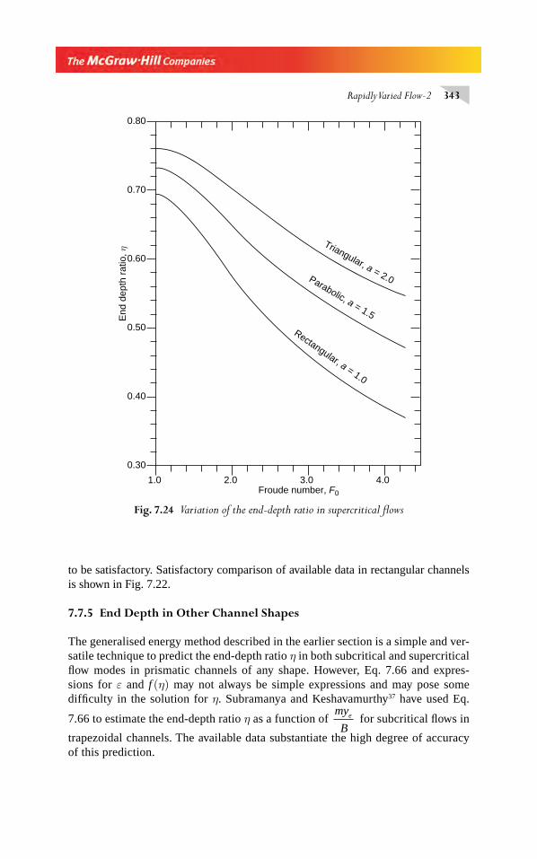
Rapidly Varied Flow-2 343
to be satisfactory. Satisfactory comparison of available data in rectangular channels is shown in Fig. 7.22.
7.7.5 End Depth in Other Channel Shapes
The generalised energy method described in the earlier section is a simple and ver-satile technique to predict the end-depth ratio η in both subcritical and supercritical fl ow modes in prismatic channels of any shape. However, Eq. 7.66 and expres-sions for ε and f (η) may not always be simple expressions and may pose some diffi culty in the solution for η. Subramanya and Keshavamurthy37 have used Eq.
7.66 to estimate the end-depth ratio η as a function of my
Be for subcritical fl ows in
trapezoidal channels. The available data substantiate the high degree of accuracy of this prediction.
0.30
1.0 2.0 3.0 4.0
0.40
0.50
0.60
0.70
0.80
Froude number, F0
End
dep
th r
atio
, η
Rectangular, a = 1.0
Parabolic, a = 1.5
Triangular, a = 2.0
Fig. 7.24 Variation of the end-depth ratio in supercritical fl ows
Chapter 7.indd 343Chapter 7.indd 343 2/24/2010 3:01:45 PM2/24/2010 3:01:45 PM
344 Flow in Open Channels
Subramanya and Niraj Kumar38 have used the generalised energy method (Eq. 7.66) to predict the end-depth in subcritical fl ows in circular channels as η = f ( y
c /D).
It has been shown that η is essentially constant at 0.73 in the entire practical range of y
c /D viz. 0 < y
c /D ≤ 0.8. This compares very well with the value of η = 0.725 ± 3.5%
obtained by Rajaratnam and Muralidhar29. Niraj Kumar39 has reported extensive use of Eq. 7.66 to predict the end-depth ratio η in a variety of channel shapes including elliptical sections, inverted trapezoidal sections and standard lined triangular canal section.
Numerous applications of the generalized energy method to solve end depth ratio in a variety of channel shapes has been reported in literature. Reference 48 gives a review (as of 2002) of the research work on the topic of end depth in open channels and contains an exhaustive bibliography on the topic
Example 7.15 A channel has its area given by A = ky3 where k = a constant. For subcritical fl ow in this channel estimate the ratio of the end-depth to critical depth.
Solution This is an exponential channel with a = 3.0. For subcritical fl ow by Eq. 7.70
ε = + =11
21 167
a.
By Eq. 7.68, fa a
ηη η
( ) = =1 1
3
12 6
The general equation of end depth Eq. 7.66 is
6 4 3 0ε η η− − ( ) =f
Substituting for ε and f η ηη
( ) ×( )− − =, .6 1 167 43
3
10
6
i.e. 1
4 7 06η
η+ − =
Solving by trial and error η = =y ye c/ . .0 80
Example 7.16 A rectangular channel carries a supercritical fl ow with a Froude number of 2.0. Find the end-depth ratio at a free overfall in this channel.
Solution In supercritical fl ow, for an exponential channel, ε = fn (a, F
0)
Here a = 1.0
By Eq. 7.53 ε = +⎛
⎝⎜⎜⎜⎜
⎞
⎠⎟⎟⎟⎟+( )
11
20
2 2 1
02
F
F
aa/
Chapter 7.indd 344Chapter 7.indd 344 2/24/2010 3:01:45 PM2/24/2010 3:01:45 PM
Rapidly Varied Flow-2 345
= +×( )
⎛
⎝⎜⎜⎜⎜
⎞
⎠
⎟⎟⎟⎟⎟=
+( )
1
21
2
2 11 89
2 2 1
2
/ ..
By Eq. 7.68, fa a
ηη η
( )− =1 1
2 2
The general equation of end-depth, Eq. 7.66 is
6 ε – 4η – f(η ) = 0
Substituting for ε and f η ηη
( ) × − −, .6 1 89 43
2
i.e. 4 η3 – 11.34 + 3 = 0
Solving by trial-and-error, η = ye / y
c =
0.577.
7.7.6 End Depth as a Flow-Measuring Device
The unique relationship for ye/y
c for a given channel at a free overfall has given end
depth the status of a fl ow meter. For fl ow-measurement purposes, the end section should be truly level in the lateral direction and must be preceded by a channel of length not less than 15y
c. The overfall must be free and where it is confi ned by side
walls, the nappe well ventilated. The accuracy of measurement is better if the slope is fl at, i.e. as near to being a horizontal bed as possible. The depth should be measured at the end section on the channel centreline by means of a precision point gauge. In subcritical fl ows for a given channel shape a constant value of y
e / y
c as given in
Table 7.3 (or as obtained by using the general equation for end depth, Eq. 7.66) is used to estimate the discharge for a given y
e. The general accuracy of fl ow-measure-
ment by the end depth method is around 3 per cent in subcritical fl ows.International organization for Standards, Geneva, Switzerland has brought out
two standards; ISO 3847 (1977) and ISO 4371 (1984) for end depth method of fl ow measurements in rectangular channels and non-rectangular channels respectively. The website http://www.lmnoeng.com contains details of ISO 3847 and 4371 proce-dures and free softwares for calculation of discharge for a known end depth in rect-angular, triangular and circular channels.
In supercritical fl ows ye/y
c = fn( F
0 ) and as such two depths y
e and y
0 are needed
to estimate the discharge. In view of this, the end-depth method is not advantageous in supercritical fl ows.
Example 7.17 Estimate the discharges corresponding to the following end-depth values in the following horizontal channels. [Assume the fl ows to be sub-critical and use the end depth ratio values given in Table 7.3].
Chapter 7.indd 345Chapter 7.indd 345 2/24/2010 3:01:45 PM2/24/2010 3:01:45 PM
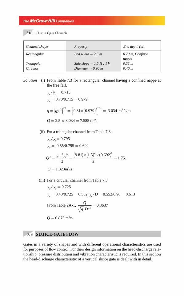
346 Flow in Open Channels
Channel shape Property End depth (m)
Rectangular Bed width = 2.5 m 0.70 m, Confi ned nappe
Triangular Side slope = 1.5 H : 1 V 0.55 mCircular Diameter = 0.90 m 0.40 m
Solution (i) From Table 7.3 for a rectangular channel having a confi ned nappe at the free fall,
ye / y
c = 0.715
yc = 0.70/0.715 = 0.979
q gyc= ⎡⎣⎢
⎤⎦⎥ = ×( )⎡
⎣⎢⎤⎦⎥
=3 1 2 3 1 2
9 81 0 979 3 034/ /
. . . m /s/m3
Q = 2.5 × 3.034 = 7.585 m3/s
(ii) For a triangular channel from Table 7.3,
ye / y
c= 0.795
yc = .0.55/0.795 = 0.692
Qgm yc2
2 5 2 5
2
9 81 1 5 0 692
21 751= =
( )×( ) ×( )=
. . ..
Q = 1.323m3/s
(iii) For a circular channel from Table 7.3,
ye / y
c = 0.725
yc = 0.40/0.725 = 0.552, y
c / D = 0.552/0.90 = 0.613
From Table 2A-1, Q
g D2 50 3637
..=
Q = 0.875 m3/s
7.8 SLUICE-GATE FLOW
Gates in a variety of shapes and with different operational characteristics are used for purposes of fl ow control. For their design information on the head-discharge rela-tionship, pressure distribution and vibration characteristic is required. In this section the head-discharge characteristic of a vertical sluice gate is dealt with in detail.
Chapter 7.indd 346Chapter 7.indd 346 2/24/2010 3:01:46 PM2/24/2010 3:01:46 PM
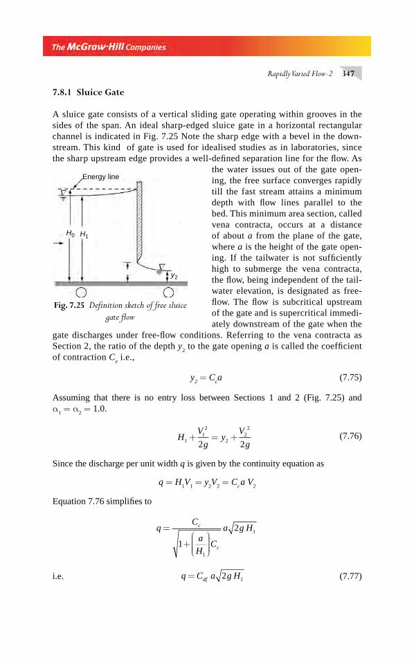
Rapidly Varied Flow-2 347
7.8.1 Sluice Gate
A sluice gate consists of a vertical sliding gate operating within grooves in the sides of the span. An ideal sharp-edged sluice gate in a horizontal rectangular channel is indicated in Fig. 7.25 Note the sharp edge with a bevel in the down-stream. This kind of gate is used for idealised studies as in laboratories, since the sharp upstream edge provides a well-defi ned separation line for the fl ow. As
the water issues out of the gate open-ing, the free surface converges rapidly till the fast stream attains a minimum depth with fl ow lines parallel to the bed. This minimum area section, called vena contracta, occurs at a distance of about a from the plane of the gate, where a is the height of the gate open-ing. If the tailwater is not suffi ciently high to submerge the vena contracta, the fl ow, being independent of the tail-water elevation, is designated as free-fl ow. The fl ow is subcritical upstream of the gate and is supercritical immedi-ately downstream of the gate when the
gate discharges under free-fl ow conditions. Referring to the vena contracta as Section 2, the ratio of the depth y
2 to the gate opening a is called the coeffi cient
of contraction Ce i.e.,
y2 = C
ca (7.75)
Assuming that there is no entry loss between Sections 1 and 2 (Fig. 7.25) and α
1 = α
2 = 1.0.
HV
gy
V
g112
22
2
2 2+ = + (7.76)
Since the discharge per unit width q is given by the continuity equation as
q = H1V
1 = y
2V
2 = C
c a V
2
Equation 7.76 simplifi es to
qC
a
HC
a g Hc
c
=
+⎛
⎝⎜⎜⎜⎜
⎞
⎠⎟⎟⎟⎟
1
2
1
1
i.e. q C a g Hdf= 2 1 (7.77)
y2
H1H0
Energy line
∇
∇
Fig. 7.25 Defi nition sketch of free sluice
gate fl ow
Chapter 7.indd 347Chapter 7.indd 347 2/24/2010 3:01:46 PM2/24/2010 3:01:46 PM
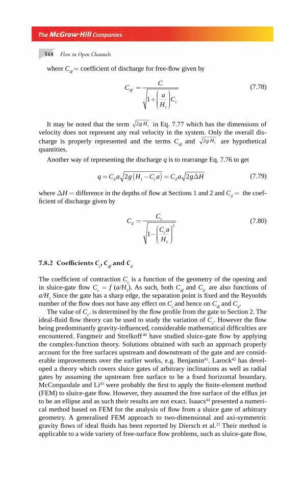
348 Flow in Open Channels
where Cdf
= coeffi cient of discharge for free-fl ow given by
CC
a
HC
df
c
=
+⎛
⎝⎜⎜⎜⎜
⎞
⎠⎟⎟⎟⎟
11
(7.78)
It may be noted that the term 2 1g H in Eq. 7.77 which has the dimensions of velocity does not represent any real velocity in the system. Only the overall dis-charge is properly represented and the terms C
df and 2 1g H are hypothetical
quantities.
Another way of representing the discharge q is to rearrange Eq. 7.76 to get
q C a g H C a C a g Hd c d= −( ) = Δ2 21 (7.79)
where ΔH = difference in the depths of fl ow at Sections 1 and 2 and Cd = the coef-
fi cient of discharge given by
CC
C a
H
dc
c
=
−⎛
⎝⎜⎜⎜⎜
⎞
⎠⎟⎟⎟⎟
11
2
(7.80)
7.8.2 Coeffi cients Cc, C
df and C
d
The coeffi cient of contraction Cc is a function of the geometry of the opening and
in sluice-gate fl ow Cc = f (a/H
1). As such, both C
df and C
d are also functions of
a/H1 Since the gate has a sharp edge, the separation point is fi xed and the Reynolds
number of the fl ow does not have any effect on Cc and hence on C
df and C
d.
The value of Cc. is determined by the fl ow profi le from the gate to Section 2. The
ideal-fl uid fl ow theory can be used to study the variation of Cc. However the fl ow
being predominantly gravity-infl uenced, considerable mathematical diffi culties are encountered. Fangmeir and Strelkoff 40 have studied sluice-gate fl ow by applying the complex-function theory. Solutions obtained with such an approach properly account for the free surfaces upstream and downstream of the gate and are consid-erable improvements over the earlier works, e.g. Benjamin41. Larock42 has devel-oped a theory which covers sluice gates of arbitrary inclinations as well as radial gates by assuming the upstream free surface to be a fi xed horizontal boundary. McCorquodale and Li43 were probably the fi rst to apply the fi nite-element method (FEM) to sluice-gate fl ow. However, they assumed the free surface of the effl ux jet to be an ellipse and as such their results are not exact. Isaacs44 presented a numeri-cal method based on FEM for the analysis of fl ow from a sluice gate of arbitrary geometry. A generalised FEM approach to two-dimensional and axi-symmetric gravity fl ows of ideal fl uids has been reported by Diersch et al.21 Their method is applicable to a wide variety of free-surface fl ow problems, such as sluice-gate fl ow,
Chapter 7.indd 348Chapter 7.indd 348 2/24/2010 3:01:46 PM2/24/2010 3:01:46 PM
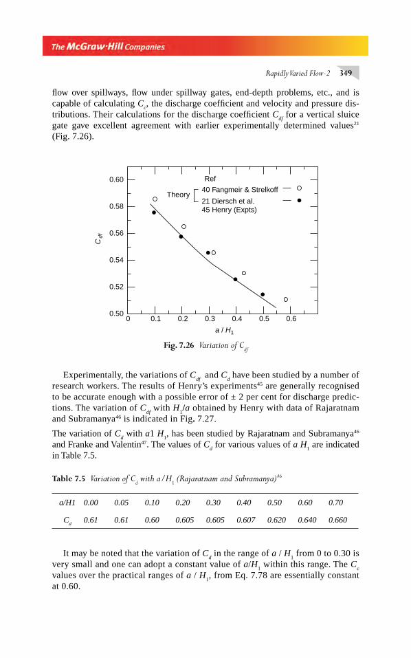
Rapidly Varied Flow-2 349
fl ow over spillways, fl ow under spillway gates, end-depth problems, etc., and is capable of calculating C
c, the discharge coeffi cient and velocity and pressure dis-
tributions. Their calculations for the discharge coeffi cient Cdf for a vertical sluice
gate gave excellent agreement with earlier experimentally determined values21 (Fig. 7.26).
00.50
0.52
0.54
0.56
0.58
0.60
0.1 0.2 0.3 0.4 0.5 0.6
Theory40 Fangmeir & Strelkoff
45 Henry (Expts)21 Diersch et al.
Ref
a / H1
Cdf
Fig. 7.26 Variation of Cdf
Experimentally, the variations of Cdf and C
d have been studied by a number of
research workers. The results of Henry’s experiments45 are generally recognised to be accurate enough with a possible error of ± 2 per cent for discharge predic-tions. The variation of C
df with H
1/a obtained by Henry with data of Rajaratnam
and Subramanya46 is indicated in Fig. 7.27.
The variation of Cd with a1 H
1, has been studied by Rajaratnam and Subramanya46
and Franke and Valentin47. The values of Cd for various values of a H
1 are indicated
in Table 7.5.
Table 7.5 Variation of Cd with a/H
1 (Rajaratnam and Subramanya)46
a/H1 0.00 0.05 0.10 0.20 0.30 0.40 0.50 0.60 0.70
Cd
0.61 0.61 0.60 0.605 0.605 0.607 0.620 0.640 0.660
It may be noted that the variation of Cd in the range of a / H
1 from 0 to 0.30 is
very small and one can adopt a constant value of a/H1 within this range. The C
c
values over the practical ranges of a / H1, from Eq. 7.78 are essentially constant
at 0.60.
Chapter 7.indd 349Chapter 7.indd 349 2/24/2010 3:01:46 PM2/24/2010 3:01:46 PM
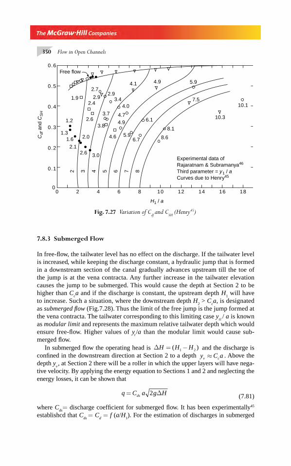
350 Flow in Open Channels
7.8.3 Submerged Flow
In free-fl ow, the tailwater level has no effect on the discharge. If the tailwater level is increased, while keeping the discharge constant, a hydraulic jump that is formed in a downstream section of the canal gradually advances upstream till the toe of the jump is at the vena contracta. Any further increase in the tailwater elevation causes the jump to be submerged. This would cause the depth at Section 2 to be higher than C
ca and if the discharge is constant, the upstream depth H
1 will have
to increase. Such a situation, where the downstream depth H2 > C
ca, is designated
as submerged fl ow (Fig.7.28). Thus the limit of the free jump is the jump formed at the vena contracta. The tailwater corresponding to this limiting case y
tl / a is known
as modular limit and represents the maximum relative tailwater depth which would ensure free-fl ow. Higher values of y
t/a than the modular limit would cause sub-
merged fl ow.In submerged fl ow the operating head is Δ = −H H H( )1 2 and the discharge is
confi ned in the downstream direction at Section 2 to a depth y C av c≈ . Above the depth y
v , at Section 2 there will be a roller in which the upper layers will have nega-
tive velocity. By applying the energy equation to Sections 1 and 2 and neglecting the energy losses, it can be shown that
q C a g Hds= Δ2 (7.81)
where Cds
= discharge coeffi cient for submerged fl ow. It has been experimentally45
establishcd that Cds
= Cd = f (a/H
1). For the estimation of discharges in submerged
00
0.1
0.2
0.3
0.4
0.5
0.6
2 4 6 8 10 12 14 16 18
2 3 4 5 6 7 81.3
1.6
2.12.6 3.0
2.0
1.2
1.92.4
2.9
2.72.9
3.44.0
4.74.9
4.6
3.8
3.72.6
5.96.7
6.1
8.6
8.1
4.94.1
7.5
5.9
10.3
10.1
Experimental data ofRajaratnam & Subramanya46
Third parameter = y1 / aCurves due to Henry45
H1 / a
Cdf
and
CS
H
Free flow
Fig. 7.27 Variation of Cdf
and CSH
(Henry45)
Chapter 7.indd 350Chapter 7.indd 350 2/24/2010 3:01:47 PM2/24/2010 3:01:47 PM
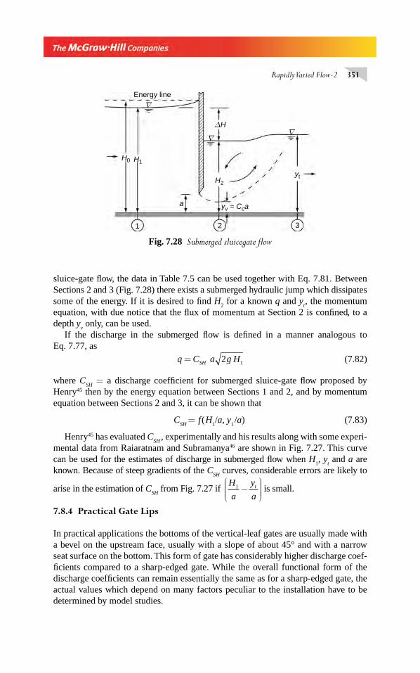
Rapidly Varied Flow-2 351
sluice-gate fl ow, the data in Table 7.5 can be used together with Eq. 7.81. Between Sections 2 and 3 (Fig. 7.28) there exists a submerged hydraulic jump which dissipates some of the energy. If it is desired to fi nd H
2 for a known q and y
t, the momentum
equation, with due notice that the fl ux of momentum at Section 2 is confi ned, to a depth y
v only, can be used.
If the discharge in the submerged fl ow is defi ned in a manner analogous to Eq. 7.77, as
q C a g HSH= 2 1
(7.82)
where CSH
= a discharge coeffi cient for submerged sluice-gate fl ow proposed by Henry45 then by the energy equation between Sections 1 and 2, and by momentum equation between Sections 2 and 3, it can be shown that
CSH
= f(H1/a, y
1 /a) (7.83)
Henry45 has evaluated CSH
, experimentally and his results along with some experi-mental data from Raiaratnam and Subramanya46 are shown in Fig. 7.27. This curve can be used for the estimates of discharge in submerged fl ow when H
1, y
t and a are
known. Because of steep gradients of the CSH
curves, considerable errors are likely to
arise in the estimation of CSH
from Fig. 7.27 if H
a
y
at1 −
⎛
⎝⎜⎜⎜
⎞
⎠⎟⎟⎟⎟ is small.
7.8.4 Practical Gate Lips
In practical applications the bottoms of the vertical-leaf gates are usually made with a bevel on the upstream face, usually with a slope of about 45° and with a narrow seat surface on the bottom. This form of gate has considerably higher discharge coef-fi cients compared to a sharp-edged gate. While the overall functional form of the discharge coeffi cients can remain essentially the same as for a sharp-edged gate, the actual values which depend on many factors peculiar to the installation have to be determined by model studies.
1 2 3
H0 H1
ΔH
a
H2
yt
yv = Cca
∇
∇∇
Energy line
Fig. 7.28 Submerged sluicegate fl ow
Chapter 7.indd 351Chapter 7.indd 351 2/24/2010 3:01:47 PM2/24/2010 3:01:47 PM
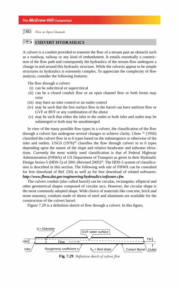
352 Flow in Open Channels
7.9 CULVERT HYDRAULICS
A culvert is a conduit provided to transmit the fl ow of a stream past an obstacle such as a roadway, railway or any kind of embankment. It entails essentially a constric-tion of the fl ow path and consequently the hydraulics of the stream fl ow undergoes a change in and around this hydraulic structure. While the culverts appear to be simple structures its hydraulics is extremely complex. To appreciate the complexity of fl ow analysis, consider the following features:
The fl ow through a culvert (i) can be subcritical or supercritical (ii) can be a closed conduit fl ow or an open channel fl ow or both forms may
exist(iii) may have an inlet control or an outlet control(iv) may be such that the free surface fl ow in the barrel can have uniform fl ow or
GVF or RVF or any combination of the above (v) may be such that either the inlet or the outlet or both inlet and outlet may be
submerged or both may be unsubmerged
In view of the many possible fl ow types in a culvert, the classifi cation of the fl ow through a culvert has undergone several changes to achieve clarity. Chow 26 (1956) classifi ed the culvert fl ow in to 6 types based on the submergence or otherwise of the inlet and outlets. USGS (1976)49 classifi es the fl ow through culvert in to 6 types depending upon the nature of the slope and relative headwater and tailwater eleva-tions. Currently the most widely used classifi cation is that of Federal Highway Administration (FHWA) of US Department of Transport as given in their Hydraulic Design Series-5 (HDS-5) of 2001 (Revised 2005)50. The HDS-5 system of classifi ca-tion is described in this section. The following web site of FHWA can be consulted for free download of Ref. (50) as well as for free download of related softwares: http://www.fhwa.dot.gov/engineering/hydraulics/software.cfm.
The culvert conduit (also called barrel) can be circular, rectangular, elliptical and other geometrical shapes composed of circular arcs. However, the circular shape is the most commonly adopted shape. Wide choice of materials like concrete, brick and stone masonry, conduits made of sheets of steel and aluminum are available for the construction of the culvert barrel.
Figure 7.29 is a defi nition sketch of fl ow through a culvert. In this fi gure,
TW
OutletCulvert BarrelS0 = Bed slope
Flow
Roughness coefficient n
HW
Inlet
d = DiameterGVF water surface
Fig. 7.29 Defi nition sketch of culvert fl ow
Chapter 7.indd 352Chapter 7.indd 352 2/24/2010 3:01:47 PM2/24/2010 3:01:47 PM
Rapidly Varied Flow-2 353
HW = Headwater = head above the invert of the culvert inlet TW = Tailwater = depth of water downstream of the culvert measured from the
outlet invert d = Diameter of the culvert conduit S
0 = Slope of the conduit
n = Manning’s roughness coeffi cient of the conduit
This fi gure shows a type of fl ow in which both the inlet and the outlet of the culvert are unsubmerged. In this case the fl ow in to the culvert is in weir fl ow mode. If the headwater elevation is suffi ciently above the top edge of the inlet the fl ow in to the culvert barrel will be in the orifi ce fl ow mode (with discharge proportional to square root of head ) and the inlet is said to be submerged. The limit of submergence depends
upon the ratio HW
d and the limiting value is found to be in the range of 1.2 to 1.5.
HDS-5 adopts 1.2 as the minimum HW
d ratio marking the onset of submerged fl ow.
Thus for HW
d>1.2 the inlet is considered to be submerged.
The inlet of a culvert has a very important role in reducing energy losses at the entry, especially in closed conduit fl ow conditions. The fl ow entering the culvert barrel undergoes contraction of the fl ow area at the inlet and a properly designed inlet would increase the coeffi cient of contraction leading to higher effi ciency. Some stan-dard types of culvert inlets popularly used in USA are (i) Projecting barrel,(ii) Cast-in – situ concrete headwall and wing walls, (iii) Pre-cast end sections, and (iv) Culvert end mitered in to the slope. Additional factors like structural stability, aesthetics, erosion control and embankment slope control play a role in the fi nal selection.
The outlet is considered to be submerged for all values of tailwater elevation, measured above the invert of the outlet, which are greater than the diameter of the
conduit at the outlet, that is TW
d≥1 0. . Considering the control of fl ow at the inlet
and at the outlet, the fl ow in a culvert is classifi ed by HDS-5 in to four types under inlet control condition and to fi ve types under outlet-control condition. The different types of fl ows are named alphabetically. For clarity sake, prefi xes IC and OC to indi-cate inlet control and OC outlet control respectively are adopted in this book. Thus Type IC-A indicates inlet control, Type–A fl ow and OC-C indicates outlet control Type-C fl ow in the culvert. The details of the classifi cation are given below and also are shown in Figs 7.30 and 7.31.
Inlet Control (IC) In this type the flow control is at the inlet, viz., the upstream end of the culvert and four categories of fl ow are possible as shown in Fig. 7.30 -(i to iv).
Type IC-A (Fig.7.31-(i).) Here both the inlet and the outlet are unsubmerged and channel is steep. The inlet acts like a weir and critical depth is formed just down-stream of the inlet edge. The free surface fl ow will be a GVF of S
2 type in the initial
Chapter 7.indd 353Chapter 7.indd 353 2/24/2010 3:01:47 PM2/24/2010 3:01:47 PM
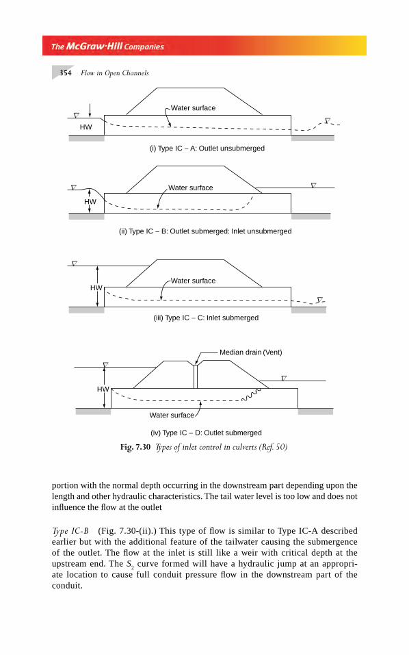
354 Flow in Open Channels
portion with the normal depth occurring in the downstream part depending upon the length and other hydraulic characteristics. The tail water level is too low and does not infl uence the fl ow at the outlet
Type IC-B (Fig. 7.30-(ii).) This type of fl ow is similar to Type IC-A described earlier but with the additional feature of the tailwater causing the submergence of the outlet. The fl ow at the inlet is still like a weir with critical depth at the upstream end. The S
2 curve formed will have a hydraulic jump at an appropri-
ate location to cause full conduit pressure fl ow in the downstream part of the conduit.
Water surface
Water surface
Water surface
Water surface
HW
Median drain (Vent)
HW
(i) Type IC − A: Outlet unsubmerged
HW
(ii) Type IC − B: Outlet submerged: Inlet unsubmerged
HW
(iii) Type IC − C: Inlet submerged
(iv) Type IC − D: Outlet submerged
∇
∇
∇
∇
∇
∇
∇
∇
Fig. 7.30 Types of inlet control in culverts (Ref. 50)
Chapter 7.indd 354Chapter 7.indd 354 2/24/2010 3:01:47 PM2/24/2010 3:01:47 PM
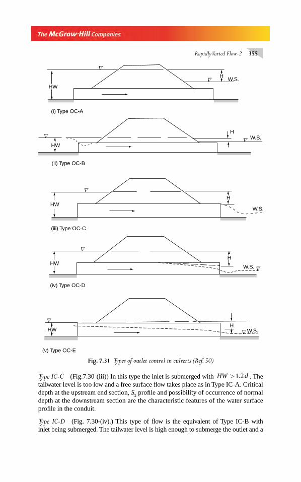
Rapidly Varied Flow-2 355
Type IC-C (Fig.7.30-(iii)) In this type the inlet is submerged with HW d>1 2. . The tailwater level is too low and a free surface fl ow takes place as in Type IC-A. Critical depth at the upstream end section, S
2 profi le and possibility of occurrence of normal
depth at the downstream section are the characteristic features of the water surface profi le in the conduit.
Type IC-D (Fig. 7.30-(iv).) This type of fl ow is the equivalent of Type IC-B with inlet being submerged. The tailwater level is high enough to submerge the outlet and a
Fig. 7.31 Types of outlet control in culverts (Ref. 50)
HW
∇
∇
(i) Type OC-A
∇∇
HW.S.
HW
(ii) Type OC-B
∇H
W.S.
(iii) Type OC-C
∇
∇
∇
∇
W.S.HW
HW
HW
H
(iv) Type OC-D
W.S.H
(v) Type OC-E
HW.S.
Chapter 7.indd 355Chapter 7.indd 355 2/24/2010 3:01:48 PM2/24/2010 3:01:48 PM
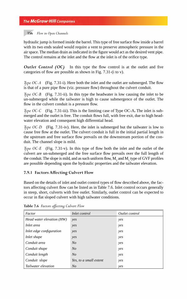
356 Flow in Open Channels
hydraulic jump is formed inside the barrel. This type of free surface fl ow inside a barrel with its two ends sealed would require a vent to preserve atmospheric pressure in the air space. The median drain as indicated in the fi gure would act as the desired vent pipe. The control remains at the inlet and the fl ow at the inlet is of the orifi ce type.
Outlet Control (OC) In this type the fl ow control is at the outlet and fi ve categories of fl ow are possible as shown in Fig. 7.31-(i to v).
Type OC-A (Fig. 7.31-i). Here both the inlet and the outlet are submerged. The fl ow is that of a pure pipe fl ow (viz. pressure fl ow) throughout the culvert conduit.
Type OC-B (Fig. 7.31-ii). In this type the headwater is low causing the inlet to be un-submerged while the tailwater is high to cause submergence of the outlet. The fl ow in the culvert conduit is a pressure fl ow.
Type OC-C (Fig. 7.31-iii). This is the limiting case of Type OC-A. The inlet is sub-merged and the outlet is free. The conduit fl ows full, with free exit, due to high head-water elevation and consequent high differential head.
Type OC-D (Fig. 7.31-iv). Here, the inlet is submerged but the tailwater is low to cause free fl ow at the outlet. The culvert conduit is full in the initial partial length in the upstream and free surface fl ow prevails on the downstream portion of the con-duit. The channel slope is mild.
Type OC-E (Fig. 7.31-v). In this type of fl ow both the inlet and the outlet of the culvert are un-submerged and the free surface fl ow prevails over the full length of the conduit. The slope is mild, and as such uniform fl ow, M
2 and M
1 type of GVF profi les
are possible depending upon the hydraulic properties and the tailwater elevation.
7.9.1 Factors Aff ecting Culvert Flow
Based on the details of inlet and outlet control types of fl ow described above, the fac-tors affecting culvert fl ow can be listed as in Table 7.6. Inlet control occurs generally in steep, short, culverts with free outlet. Similarly, outlet control can be expected to occur in fl at sloped culvert with high tailwater conditions.
Table 7.6 Factors aff ecting Culvert Flow
Factor Inlet control Outlet control
Head water elevation (HW) yes yes
Inlet area yes yes
Inlet edge confi guration yes yes
Inlet shape yes yes
Conduit area No yes
Conduit shape No yes
Conduit length No yes
Conduit slope Yes, to a small extent yes
Tailwater elevation No yes
Chapter 7.indd 356Chapter 7.indd 356 2/24/2010 3:01:48 PM2/24/2010 3:01:48 PM
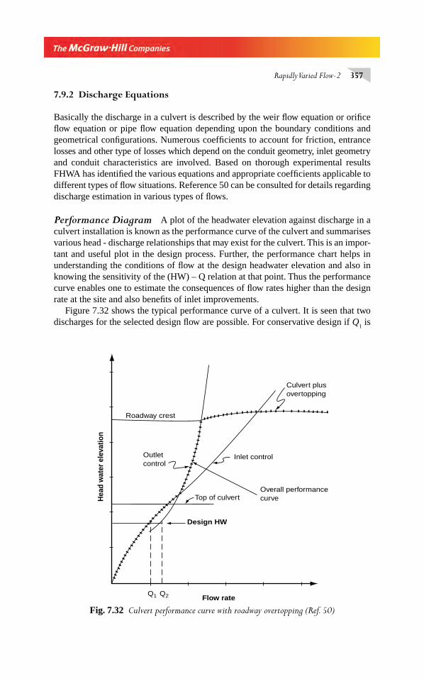
Rapidly Varied Flow-2 357
7.9.2 Discharge Equations
Basically the discharge in a culvert is described by the weir fl ow equation or orifi ce fl ow equation or pipe fl ow equation depending upon the boundary conditions and geometrical confi gurations. Numerous coeffi cients to account for friction, entrance losses and other type of losses which depend on the conduit geometry, inlet geometry and conduit characteristics are involved. Based on thorough experimental results FHWA has identifi ed the various equations and appropriate coeffi cients applicable to different types of fl ow situations. Reference 50 can be consulted for details regarding discharge estimation in various types of fl ows.
Performance Diagram A plot of the headwater elevation against discharge in a culvert installation is known as the performance curve of the culvert and summarises various head - discharge relationships that may exist for the culvert. This is an impor-tant and useful plot in the design process. Further, the performance chart helps in understanding the conditions of fl ow at the design headwater elevation and also in knowing the sensitivity of the (HW) – Q relation at that point. Thus the performance curve enables one to estimate the consequences of fl ow rates higher than the design rate at the site and also benefi ts of inlet improvements.
Figure 7.32 shows the typical performance curve of a culvert. It is seen that two discharges for the selected design fl ow are possible. For conservative design if Q
1 is
Outletcontrol
Roadway crest
Inlet control
Culvert plusovertopping
Design HW
Overall performancecurve
Q1 Q2 Flow rate
Hea
d w
ater
ele
vatio
n
Top of culvert
Fig. 7.32 Culvert performance curve with roadway overtopping (Ref. 50)
Chapter 7.indd 357Chapter 7.indd 357 2/24/2010 3:01:48 PM2/24/2010 3:01:48 PM

358 Flow in Open Channels
selected the culvert barrel capacity is higher than what has been designed and this can be utilized by inlet improvement.
It is normal practice in India to design culverts for free surface fl ow operation. However, in USA the culverts are invariably designed to fl ow full at design dis-charge. Another aspect to be considered in the design of culverts is the velocity of fl ow at the outlet in relation to scour of the bed material of the stream. Generally rip-rap protection is needed at the outlet and in some cases energy dissipaters also have to be provided to prevent serious scours due to high outlet velocities.
7.9.3 Design of Culverts
Reference 50 contains valuable information, worked examples and nomographs for the design of culverts under all types of fl ow conditions. FHWA web site http://www.fhwa.dot.gov/engineering/hydraulics/software.com contains complete information on FHWA Hydraulics Engineering Publications and Software for culvert analysis and related topics. Culvert Analysis Program, HY-8 by FHWA is free public domain software. Web site http://www.imnoeng.com contains free computation/design facility and valuable information on all aspects of culvert fl ow. A program for design of culverts under inlet/outlet control and for preparation of performance chart using HDS-5 methodology is available in this web site. A large number of commercial softwares are available for culvert design and details about these can be obtained through the internet search.
REFERENCES
1. Lakshmana Rao, N S, ‘Theory of Weirs’, a Chapter in Advances in Hydroscience, Vol. 10, 1975, Academic Press, Inc., New York, pp 310–406.
2. Strelkoff, T S, ‘Solutions of Highly Curvilinear Gravity Flows’, J. of Engg. Mech. Div., Proc. ASCE, Vol. 90, June 1964, pp 195–219.
3. Kandaswamy, P K, and Rouse, H, ‘Characteristics of Flow Over Terminal Weirs and Sills’, J. of Hyd. Div., Proc. ASCE, Vol. 83, Paper No. 1345, August l957, pp 1–13.
4. Ackers, P, Weirs and Flumes for Flow Measurement, John Wiley & Sons Ltd., Chichester, U.K., 1978.
5. Bos, M G, (Ed.), Discharge Measurement Structures, Int. Inst. for Land Reclamation and Improvement. Wageningen, The Netherlands, Pub. No. 20, 1976.
6. Kindsvater, C E, and Carter, R W, ‘Discharge Characteristics of Rectangular Thin Plate Weirs’. J. of. Hyd Div,. Proc. ASCE. Vol. 83, Dec. 1957, pp 1–36.
7. Rama Murthy, A S, Subramanya, K and Pani, B, S, Quadrant Plate Weirs, J. of Hyd. Div., ASCE, Vol. 103, No., HY 12 1977. Proc. paper 13395. pp 1431–41.
8. Rao, N S L, ‘Theory of Weirs’. Chap,.in Advances in Hydroscience. Academic Press. New York, USA, Vol. 10, 1975, pp 309-406.
9. Fonck, R M, ‘Datum Line Fixation for Linear Proportional Weirs, J. of App. Mech. Trans ASME, Vol. 45, Brief Notes, pp 441–442, June 1978.
10. Cowgill, P, ‘The Mathematics of Weir Forms’ Quart. Appl. Maths., Vol. 2, No. 2, 1944, p. 142.
11. Banks, R B, ‘A Note on the Generalised Weir Equation,’ North-Western Univ., Paper HP 0654, Nov. 1954.
Chapter 7.indd 358Chapter 7.indd 358 2/24/2010 3:01:48 PM2/24/2010 3:01:48 PM
Rapidly Varied Flow-2 359
12. Keshava Murthy, K, and Seshagiri, N, ‘A generalised mathematical theory and experi-mental verifi cation of proportional notches,’ J. of Franklin Inst., USA. vol 285. No. 5. May 1968. pp 347–363.
13. Keshava Murthy, K, ‘On the Design of the Quadratic Weir.’, J. of Franklin Inst,. USA. Vol. 287, No. 2. 1969, pp 159–174.
14. Keshava Murthy, K, and Pillai, G, ‘Some Aspects of Quadratic Weirs’ J. of Hyd. Div., ASCE, Vol. 103, No. HY 9, Proc. paper 13231, 1977, pp 1059–76.
15. Majcherek, H, ‘Modelling of Flow Velocity Using Weirs’, J. of Hyd. Div., ASCE, Vol. 111, No. HY 1, Proc. paper 19415, 1985, pp 79–92.
16. U.S. Dept. of Interior, Studies of Crests for Overfall Dams, U.S. Bureau of Reclamation, Boulder Canyon Final Reports, Bulletin 3, Part VI, 1948.
17. Cassidy, J. J, ‘Designing Spillway Crests for High-Head Operation’ J. of Hyd. Div., Proc. ASCE, March 1970, pp 745–753.
18. U S Dept. of Interior, Design of Small Dams, USBR, Oxford and IBH Pub. Co., New Delhi, 1974.
19. Cassidy, J. J, ‘Irrotational Flow Over Spillways of Finite Height’, J. of Engg. Mech. Div., Proc. ASCE, Dec. l965, pp 153–173.
20. Ikegawa M, and Washizu, K, ‘Finite Element Method Applied to Analysis of Flow Over a Spillway Crest’, Int. J. for Num. Methods in Engg., Vol. 6, 1973, pp 179–189.
21. Diersch, H J, Schirmer A, and Busch K F, ‘Analysis of Flows with Initially Unknown Discharge’, J. of Hyd. Div., Proc. ASCE, March 1977, pp. 213–232.
22. Govinda Rao, N S, and Muralidhar, D, ‘Discharge Characteristics of Weirs of Finite Crest Width’, La Houille Blanche, August/Sept. No. 5, 1963, pp 537–545.
23. Singer, J. ‘Square-edged Broad-crested Weir as a Flow Measuring Device’, Water and Water Engg., June 1964, Vol. 68, No. 820, pp 229–235.
24. Surya Rao, S and Shukla, M K ‘Characteristics of Flow Over Weirs of Finite Crest Width’, J. of Hyd. Div., Proc. ASCE, Nov. 1971, pp 1807–1816.
25. Skogerboe, G V, Hyat M L, Englund, I D, and Johnson, J R, ‘Design and Calibration of Submerged Open Channel Flow Measurement Structures, Part 2, Parshall Flumes, Utah Water Res. Lab., Utah State Univ., Logan, Utah, Report No. WG 31–3, March 1967.
26. Chow, V T, ‘Open Channel Hydraulics’, McGraw-Hill, Book Co. Inc., New York 1959.27. Rouse, H, ‘Discharge Characteristics of the Free Overfall’, Civil Engineering, ASCE,
April 1936, pp 257–260.28. Rajaratnam, N, and Muralidhar, D. ‘End Depth for Exponential Channels’, J. of Irr. and
Drai. Div., Proc. ASCE, March 1964, pp 17–39.29. Rajaratnam, N, and Muralidhar, D, ‘End Depth for Circular Channels’, J. of Hyd. Div.,
Proc. ASCE, March 1964, pp 99–119.30. Rajaratnam, N, and Muralidhar, D, ‘The Trapezoidal Free Overfall’, J. of Hyd. Res.,
IAHR, Vol. 8. No. 4, 1970, pp 419–447.31. Rajaratnam, N, and Muralidhar, D, ‘Characteristics of Rectangular Free Overfall’ J. of
Hyd. Res., IAHR, Vol. 6, No. 3, 1968, pp 233–258.32. Diskin, M H, ‘The End Depth at a Drop in Trapezoidal Channels’, J. of Hyd. Div,. Proc.
ASCE, July l96l, pp 11–32.33. Delleur, J W, Dooge, J C I, and Gent K W, ‘Infl uence of Slope and Roughness on the Free
Overfall’, J. of Hyd. Div. Proc. ASCE, Aug. 1956, pp 30–35.34. Anderson, M V, ‘Non-uniform fl ow in front of a free overfall’, Acta Polytechnica
Scandinavia, Ci 42, Copenhagen, 1967.35. Strelkoff, T, and Moayeri, M S, ‘Pattern of Potential Flow in a Free Overfall’, J. of Hyd.
Div., Proc, ASCE, April 1970, pp 879–901.
Chapter 7.indd 359Chapter 7.indd 359 2/24/2010 3:01:48 PM2/24/2010 3:01:48 PM
360 Flow in Open Channels
36. Subramanya, K, ‘Measurement of Discharge in an Exponential Channel by the End Depth Method’. Proc. Inst. Conf. on Measuring Techniques, BHRA, London, England, pp 313–324, April 1986.
37. Subramanya, K, and Keshava Murthy, K, ‘End Depth in a Trapezoidal Channel’ J. Inst. Of Engrs. (India), Civil Engg. Div., Vol. 67, Part CI 6, pp. 343–46, May 1987.
38. Subramanya, K and Niraj Kumar, ‘End Depth in Horizontal Circular Channels’, J. of the Insti-tution of Engineers India, Civil Engg. Div., Vol. 73 Part CV 6, pp 185–187, March 1993.
39. Niraj Kumar, “Studies on Some Open Channel Discharge-Measuring Devices”, M. Tech. Thesis, Civil Engg. Dept., I.I.T. Kanpur, Dec.1989.
40. Fangmeir, D D, and Strelkoff, T, ‘Solution for Gravity Flow Under a Sluice Gate’, J. of Engg. Mech, Div., Proc. ASCE. Vol. 94, Feb. 1968, pp 153–176.
41. Benjamin, T B, ‘On the Flow in Channels when Rigid Obstacles are Placed in the Stream’, J. of Fl,. Mech, Vol. 1,1955, pp 227–248.
42. Larock, B, E, ‘Gravity-affected Flows from Planar Sluice Gates’, J. of Hyd. Div., Proc. ASCE, July 1969, pp 1211–1226.
43. McCorquodale, J A, and Li, C Y, Finite Element Analysis of Sluice Gate Flow’, 84th Annual General Meeting, Engg. Inst. of Canada, Ottawa, Canada, Sept. 1970, pp 1–12+4.
44. Isaacs, L T, ‘Numerical Solution for Flow Under Sluice Gates’, J. of Hyd. Div., Proc. ASCE, May 1977, pp 473–482.
45. Henry, H, ‘Discussion on Diffusion of Submerged Jets’, Trans. ASCE, Vol. 155, 1950,pp 687–697.
46. Rajarathnam, N and K Subramanya, ‘Flow Equation for the Sluice Gate’, J. of Irr. and Drai. Div., Proc, ASCE, Sept. 1967, pp 167–186.
47. Franke, P G, and Valentin, F, ‘The Determination of Discharge Below Gates in Case of Variable Tailwater Conditions’, J. of Hyd. Res., IAHR, Vol. 7, No. 4, 1969 pp 433–447.
48. Dey, S, ‘Free Overfall in Open Channels: State of–the art review’, Flow Measurements and Instrumentation. Elsevier, 13, 2002, pp. 247–264.
49. Bodhaine, G L, Measurements of Peak Discharges at Culverts by Indirect Methods, Techniques of Water Resources Investigations, Book 3, Chapter A3, US Geological Survey, 1976.
50. Federal Highway Administration, Hydraulic Design of Culverts, Report FHWA – NH1-01–020, Hydraulic Design Series 5, (HDS-5), US Department of Transportation, Sept. 2001, (Revised 2005).
PROBLEMS
Problem Distribution
SI No Topic Problems
1 Rectangular weir 7.1 to 7.3, 7.6, 7.7, 7.19
2 Weirs of various shapes 7.4,
3 Triangular notch 7.5
4 Sutro weir 7.8, 7.10
5 Quadratic weir 7.9, 7.11
6 Ogee spillway 7.12 to 7.16
7 Broad crested weir 7.17, 7.18, 7. 19
8 Critical depth fl ume 7.20, 7.21
9 End depth 7.22 to 7.27
10 Sluice gate 7.28 to 7.32
Chapter 7.indd 360Chapter 7.indd 360 2/24/2010 3:01:48 PM2/24/2010 3:01:48 PM
Rapidly Varied Flow-2 361
7.1 A rectangular sharp-crested suppressed weir is 2.0 m long and 0.6 m high. Estimate the discharge when the depth of fl ow upstream of the weir is 0.90 m. If the same discharge was to pass over an alternative contracted weir of 1.5 m length and 0.60 m height at the same location, what would be the change in the water-surface elevation?
7.2 A sharp-crested suppressed weir is 1.5 m long. Calculate the height of the weir required to pass a fl ow of 0.75 m3/s while maintaining an upstream depth of fl ow of 1.50 m.
7.3 A rectangular sharp-crested suppressed weir is 3.0 m long and 1.2 m high. During a high fl ow in the channel, the weir was submerged with the depths of fl ow of 1.93 m and 1.35 m at the upstream and downstream of the weir respectively. Estimate the discharge.
7.4 Develop expressions as given in Table 7.2 for the discharge over triangular, circular, par-abolic and trapezoidal sharp-crested weirs.
7.5 A right angled triangular notch discharges under submerged condition. Estimate the discharge if the heights of water surface measured above the vertex of the notch on the upstream and downstream of the notch plate are 0.30 m and 0.15 m respectively (Assume C
d= 0.58).
7.6 A 15-m high sharp-crested weir plate is installed at the end of a 2.0-m wide rectangular channel. The channel side walls are 1.0 m high. What maximum discharge can be passed in the channel if the prescribed minimum free board is 20 cm?
7.7 A sharp-crested weir of 0.80-m height and 2.0-m length was fi tted with a point gauge for recording the head of fl ow. After some use, the point gauge was found to have a zero error; it was reading heads 2 cm too small. Determine the percentage error in the esti-mated discharges corresponding to an observed head of 50 cm.
7.8 Design a Sutro weir for use in a 0.30-m wide rectangular channel to have linear dis-charge relationship in the discharge range from 0.25 m3/s to 0.60 m3/s. The base of the weir will have to span the full width of the channel. Assume C
d = 0.62.
7.9 Design a quadratic weir spanning the full width of a 0.50 m rectangular channel at the base and capable of passing minimum and maximum discharges of 0.10 m3/s and 0.40 m3/s respectively under the desired proportionality relationship. (Assume C
d = 0.61.)
7.10 A Sutro weir with a rectangular base is installed in a rectangular channel of width 60 cm. The base weir spans the full width of the channel, has its crest coinciding with the chan-nel bed; and has a height of 12 cm. (i) Estimate the discharge through the channel when the depth of fl ow in the channel immediately behind the weir is 25 cm. (ii) What dis-charge in the channel is indicated when the depth of fl ow is 33 cm? (iii) What depth of fl ow in the channel can be expected for a discharge of 0.20 m3/s? [Take C
d = 0.61].
7.11 A quadratic weir with rectangular base of 45 cm width and 9 cm height has a depth of fl ow of 15 cm in the channel. Estimate (i) the discharge through the weir and (ii) the depth of fl ow in the channel corresponding to a discharge of 25 litres/s. [Take C
d = 0.61].
7.12 Find the elevation of the water surface and energy line corresponding to a design discharge of 500 m3/s passing over a spillway of crest length 42 m and crest height 20 m above the river bed. What would be the energy head and minimum pressure head when the discharge is 700 m3/s?
7.13 A spillway with a crest height of 25.0 m above the stream bed is designed for an energy head of 3.5 m. If a minimum pressure head of 5.0 m below atmospheric is allowed, what is the allowable discharge intensity over the spillway?
7.14 A spillway has a crest height of 30.0 m above the bed and a design energy head of 3.0 m. The crest length of the spillway is 50 m. As a part of remodelling of the dam, a three-span bridge is proposed over the spillway. The piers will be 1.5 m thick and are round-nosed and the abutment corners will be rounded. What will be the change in the water-surface elevation for the design-fl ood discharge?
7.15 An overfl ow spillway with its crest 10 m above the river bed level has radial gates fi tted on the crest. During a certain fl ow, the water surface upstream of the dam was observed to be 2.5 m above the crest and the gate opening was 1.5 m. Estimate the discharge from a bay of 10.0 m length. (Neglect end contractions.)
Chapter 7.indd 361Chapter 7.indd 361 2/24/2010 3:01:49 PM2/24/2010 3:01:49 PM
362 Flow in Open Channels
7.16 An ogee spillway with a vertical face is designed to pass a fl ood fl ow of 250 m3/s. The dis-tance between the abutments of the spillway is 45.0 m. A three-span bridge is provided over the spillway. The bridge piers are 1.20 m wide and are round nosed. If the crest of the spill-way is 10.0 m above the river bed level, fi nd the elevations of the water surface and energy line. Using this discharge as the design discharge, calculate the spillway crest profi le.
7.17 A 2.5-m wide rectangular channel has a broad-crested weir of height 1.0 m and a crest width of 1.5 m built at a section. The weir spans the full canal width. If the water-surface elevation above the crest is 0.5 m, estimate the discharge passing over the weir. If the same discharge passes over another similar weir, but with a crest width of 2.5 m. what would be the water-surface elevation upstream of this second weir?
7.18 A broad-crested weir of 2.0-m height and 3.0-m width spans the full width of a rectangu-lar channel of width 4.0 m. The channel is used as an outlet for excess water from a tank of surface area 0.5 hectares at the weir crest level. If the water level in the tank at a cer-tain time is 0.90 m above the weir crest, what is the discharge over the weir? Estimate the time taken to lower the water-surface elevation by 60 cm. (Assume that there is no infl ow into the tank and the surface area of the tank is constant in this range.)
7.19 A 2.0-m wide rectangular channel carrying a discharge of 2.5 m3/s is to be fi tted with a weir at its downstream end to provide a means of fl ow measurement as well as to cause heading-up of the water surface. Two choices, viz. (i) a sharp-crested weir plate of 0.80 m height, and (ii) a broad-crested weir block of 0.80–m height and 1.0–m width, both span-ning the full width of the channel, are considered. Which of these weirs causes a higher heading-up and to what extent?
7.20 A standing wave fl ume is used to measure the discharge in a 10.0 m wide rectangular channel. A 5-m wide throat section has a hump of 0.5 m height. What is the discharge indicated when the upstream depth of fl ow in the channel at the fl ume entrance is 2.10 m? Assume an overall coeffi cient of discharge of 1.620 for the fl ume.
7.21 A rectangular throated fl ume is to be used to measure the discharge in a 9.0 m wide chan-nel. It is known that the submergence limit for the fl ume is 0.80 and the overall discharge coeffi cient is 1.535. A throat width of 5.0 m is preferred. What should be the height of the hump if the fl ume is to be capable of measuring a discharge of 20.0 m3/s as a free fl ow with the tailwater depth at 2.30 m?
7.22 Obtain the end-depth ratio η =y
ye
c
for a triangular channel having (a) subcritical fl ow
and (b) supercritical fl ow with a Froude number of 2.5.7.23 Show that for a channel whose area A = k y2.5 the end-depth ratio η for subcritical fl ow
mode is 0.783. Also, determine the variation of η with Froude number F0 for supercritical
fl ow in the channel.7.24 A parabolic channel with a profi le x2 = 4ay, where y axis is in the vertical direction, termi-
nates in a free fall. Show that the end-depth ratio η = ye / y
c for supercritical fl ow is given by
2 η 4 – 4η3 + 1 = 0Determine the relevant root of this equation and compare it with the experimentally obtained value of η.
7.25 Find the end depth at a free overfall in a rectangular channel when the upstream fl ow is at a Froude number of 3.0 with a normal depth of 0.70 m.
7.26 Estimate the discharges corresponding to the following end-depth values in various channels. The channels are horizontal and the fl ow is subcritical in all cases. (i) Rectangular channel, B = 2.0 m, y
c = 0.6 m
(ii) Triangular channels, m = 1.0, yc = 0.5 m
(iii) Circular channel, D = 0.90 m, yc = 0.3 m
[Hint: Use the value of ye/y
c given in Table 7.3.]
Chapter 7.indd 362Chapter 7.indd 362 2/24/2010 3:01:49 PM2/24/2010 3:01:49 PM
Rapidly Varied Flow-2 363
7.27 Write a general mometum equation to the fl ow at the end-depth region in an exponential channel (A = kya). Assuming the channel to be horizontal without any friction and the pressure force at the brink to be P y A Ke e e= γ 1, show that
Ka
ara
ra
ra1 1 2
1 1 1
1= −
+⎛⎝⎜⎜⎜
⎞⎠⎟⎟⎟⎟
−++εε
ε( )
where εr = y
e / y
c.
7.28 A 2.0-m wide rectangular channel has its depth backed-up to a height of 1.2 m by a sharp-edged sluice gate. If the gate opening is 0.30 m and the downstream fl ow is free, estimate the discharge through the gate and the force on the gate.
7.29 A 2.0-m wide rectangular channel has to pass a fl ow of 2.4 m3/s through a sluice gate opening of 0.4 m. If the water depth upstream of the gate is 2.0 m, fi nd the depth of water immediately below the gate.
7.30 Apply the momentum equation to the submerged sluice gate fl ow (Fig. 7.28) by making suitable assumptions and estimate the depth H
2 immediately below the sluice gate in
terms of yt, a, C
c and H
1
7.31 Obtain an expression for the force on the sluice gate in submerged fl ow for the situation in Fig. 7.28.
7.32 Show that the modular limit of the free fl ow in a sluice gate (Fig. 7.28) is given by
y
a
CFt c
c= − + +2
1 1 8 11[ ] where F
C
C
H
aCc
d
c
c12
2
21=
⎛
⎝⎜⎜⎜⎜
⎞
⎠⎟⎟⎟⎟
−⎛
⎝⎜⎜⎜
⎞
⎠⎟⎟⎟⎟ and y
t = tailwater depth.
OBJECTIVE QUESTIONS
7.1 The head over a 3.0-cm sharp-crested sill is 96 cm. The discharge coeffi cient Cd for use in
the weir formula is(a) 0.738 (b) 0.848 (c) 0.611 (d) 1.11
7.2 A suppressed sharp-crested weir is 0.50 m high and carries a fl ow with a head of 2.0 m over the weir crest. The discharge coeffi cient C
d for the weir is
(a) 1.06 (b) 0.931 (c) 0.738 (d) 0.6117.3 The discharge Q in a triangular weir varies as
(a) H 0.5 (b) H 1.5 (c) H 2.0 (d) H 2.5
7.4 In a triangular notch there is a +2% error in the observation of the head. The error in the computed discharge is(a) +2% (b) +5% (c) – 5% (d) +2.5%
7.5 A nominal 90° triangular notch was found to have 2% error in the vertex angle. While dis-charging under a constant head, the error in the estimated discharge is(a) π % (b) π / %4 (c) π / %2 (d) 2%
7.6 In submerged fl ow over sharp-crested rectangular weirs the Villemonte equation relates Q
s / Q
1 as equal to
(a) 1 2
1
0 385
−⎛
⎝⎜⎜⎜⎜
⎞
⎠⎟⎟⎟⎟
⎡
⎣⎢⎢⎢
⎤
⎦⎥⎥⎥
H
H
.
(b) 1 2
1
0 385 1 5
−⎛
⎝⎜⎜⎜⎜
⎞
⎠⎟⎟⎟⎟
⎡
⎣
⎢⎢⎢
⎤
⎦
⎥⎥⎥
H
H
. .
(c) 1 2
1
1 5 0 385
−⎛
⎝⎜⎜⎜⎜
⎞
⎠⎟⎟⎟⎟
⎡
⎣
⎢⎢⎢
⎤
⎦
⎥⎥⎥
H
H
. .
(d) 1 2
1
0 385 1 5
−⎛
⎝⎜⎜⎜⎜
⎞
⎠⎟⎟⎟⎟
⎡
⎣
⎢⎢⎢
⎤
⎦
⎥⎥⎥
H
H
. .
Chapter 7.indd 363Chapter 7.indd 363 2/24/2010 3:01:49 PM2/24/2010 3:01:49 PM
364 Flow in Open Channels
7.7 In a triangular notch the tailwater head is 50% of the upstream head, both measured above the vertex of the notch. If the free fl ow discharge under the same upstream head is 0.5 m3/s, the submerged fl ow, in m3/s, is(a) 0.464 (b) 0.411 (c) 0.500 (d) 0.532
7.8 A parabolic sharp-crested weir has a profi le given by x2 = k y. The discharge in the weir is given by Q = K H n where n is(a) 0.5 (b) 1.5 (c) 2.0 (d) 2.5
7.9 A separate arrangement for aeration of the nappe is necessary in a(a) contracted rectangular weir(b) suppressed rectangular weir(c) submerged contracted rectangular weir(d) triangular weir
7.10 In a linear proportional weir with a rectangular base of height a, the discharges are lin-early proportional to the head h
d measured above a datum. The minimum head at which
the linear head-discharge relation is observed is hd =
(a) a (b) a/2 (c) a/3 (d) 2a/37.11 In a quadratic weir the measured head above the datum was found to have an error of 2%.
This would mean that the discharges estimated from the weir discharge formula will have an error of(a) 0.5% (b) 1% (c) 2% (d) 4%
7.12 Designing of the spillway profi le to conform to the shape of the nappe of a sharp crested weir makes(a) the pressures on the spillway crest always positive(b) the pressures to be positive for H
0 ≥ H
d
(c) the pressures on the spillway always zero(d) the pressure on the crest zero for H
0 = H
d only
7.13 If the head H0 over an overfl ow spillway is less than the design head H
d’(a) the pressure on the spillway crest will be negative(b) the cavitation phenomenon can occur(c) the separation of the streamlines from the surface can occur(d) the coeffi cient of discharge C
0 will be less than the design coeffi cient of discharge C
d 0
7.14 The coeffi cient of discharge C0 at any head H
0 of a spillway is a function of
(a) H
P0
⎛
⎝⎜⎜⎜
⎞
⎠⎟⎟⎟⎟only (b)
H
Hd
0⎛
⎝⎜⎜⎜⎜
⎞
⎠⎟⎟⎟⎟
only
(c) H
P
H
Hd
0 0,⎛
⎝⎜⎜⎜⎜
⎞
⎠⎟⎟⎟⎟only (d)
P
Hd
⎛
⎝⎜⎜⎜⎜
⎞
⎠⎟⎟⎟⎟
only
7.15 A vertical face ogee spillway will have a crest profi le downstream of the apex given by (y / H
d) =
(a) 0.5 (x / Hd)1.50 (b) 0.5 (x / H
d)1.85
(c) 1.85 (x / Hd)0.517 (d) 2.0 (x / H
d)2.0
7.16 A broad-crested weir with H1/B
w = 0.5 and H
1/P = 1.0 and a sharp-crested weir with
H1/P = 1.0, both span the full width of a canal. If the coeffi cient of discharge C
d of the
weir (= Cdw
) and Cd of the broad-crested weir (= C
db ) are compared, it will be found that
(a) Cdw
> Cdb
(b) Cdb
> Cdw
(c) Cdw
= Cdb
(d) Cdw
= Cdb
for small H1 only.
7.17 A fi nite crest width weir with H1/B
w = 0.20 is classifi ed as a
(a) long-crested weir (b) broad crested weir(c) narrow-crested weir (d) sharp-crested weir
Chapter 7.indd 364Chapter 7.indd 364 2/24/2010 3:01:49 PM2/24/2010 3:01:49 PM
Rapidly Varied Flow-2 365
7.18 The modular limit of a sharp-crested weir (Ms ) broad-crested weir (M
b ) and standing
wave fl ume (Mf) are compared under equivalent conditions. It will be found that
(a) MS > M
b > M
f (b) M
s < M
b < M
f
(c) Ms > M
b < M
f (d) M
s < M
b > M
f
7.19 The overall coeffi cient of discharge of a standing wave fl ume Cf = Q / (B
t H
13/2) is of the order of
(a) 0.61 (b) 0.95 (c) 3.30 (d) 1.627.20 The discharge equation of a Parshall fl ume is expressed as Q =
(a) K Ha (b) K Ha (c) K H
a (d) K (H
13/2 – H
a 3/2)
7.21 The end depth ratio ye / y
c in a channel carrying subcritical fl ow is a function of
(a) shape of the channel only (b) Shape and Manning’s coeffi cient(c) Normal depth only (d) Shape and Froude number
7.22 A 2-m wide horizontal rectangular channel carries a discharge 3.0 m3/s. The fl ow is sub-critical. At a free overfall in this channel the end depth in metres is(a) 0.438 (b) 0.612 (c) 0.715 (d) 1.488
7.23 A 2.5-m wide rectangular channel is known to be having subcritical fl ow. If the depth at a free overfall is 0.5 m, the discharge in this channel in, m3/s, is(a) 2.56 (b) 4.40 (c) 1.83 (d) 3.50
7.24 Two horizontal channels A and B of identical widths and depths have roughness such that (K
s)
A = 2(K
s)
B. If the discharges observed by the end-depth method in these two channels
are denoted as QA and Q
B respectively, then it would be found that
(a) QA > Q
B (b) Q QA B=
1
2 (c) Q
A = Q
B (d) Q
A < Q
B
7.25 The effective piezometric head hep
at the brink of a free overfall could be represented as(a) h
ep < y
e (b) h
ep > y
e (c) h
ep = y
e (d) h
ep = y
e
7.26 If a rectangular channel carrying a discharge of 1.85 m3/s/m width shows a brink depth of 0.35 m at a free overal, then(a) the discharge measured is wrong(b) the end depth is wrongly measured(c) the fl ow is subcritical regime(d) the fl ow is in the supercritical regime
7.27 In submerged fl ow through a sluice gate the coeffi cient of discharge Cds
=
(a) fa
H
y
at
1
,⎛
⎝⎜⎜⎜⎜
⎞
⎠⎟⎟⎟⎟
(b) CSH
(c) Cdf (d) C
d
7.28 The coeffi cient of discharge Cd in free sluice gate is related to C
C as
(a) CC
C a Hc
c
c
=+1 1
2( / ) (b) C
C a
H C a Hd
c
c
=−1 1
21 ( / )
(c) CC
C a Hd
c
c
=−1 1
2( / ) (d) C
C
a
HC
dc
c
=
−⎛
⎝⎜⎜⎜⎜
⎞
⎠⎟⎟⎟⎟
11
7.29 The discharge coeffi cient CSH
in submerged sluicegate fl ow is(a) f (a/H
1) (b) f ( y
1 / a) (c) f (a/H
1, y
1/a) (d) = C
d
7.30 Sluice gates used in fi eld applications have(a) a bevel on the upstream face(b) a bevel on the downstream face(c) bevels on both upstream and downstream faces(d) no bevel.
Chapter 7.indd 365Chapter 7.indd 365 2/24/2010 3:01:49 PM2/24/2010 3:01:49 PM
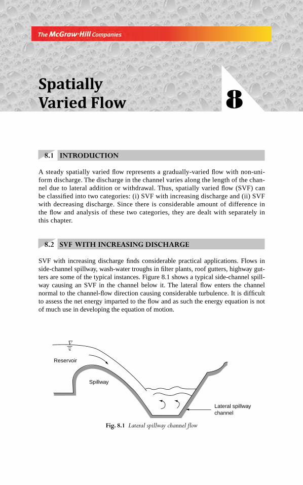
8.1 INTRODUCTION
A steady spatially varied fl ow represents a gradually-varied fl ow with non-uni-form discharge. The discharge in the channel varies along the length of the chan-nel due to lateral addition or withdrawal. Thus, spatially varied fl ow (SVF) can be classifi ed into two categories: (i) SVF with increasing discharge and (ii) SVF with decreasing discharge. Since there is considerable amount of difference in the fl ow and analysis of these two categories, they are dealt with separately in this chapter.
8.2 SVF WITH INCREASING DISCHARGE
SVF with increasing discharge fi nds considerable practical applications. Flows in side-channel spillway, wash-water troughs in fi lter plants, roof gutters, highway gut-ters are some of the typical instances. Figure 8.1 shows a typical side-channel spill-way causing an SVF in the channel below it. The lateral fl ow enters the channel normal to the channel-fl ow direction causing considerable turbulence. It is diffi cult to assess the net energy imparted to the fl ow and as such the energy equation is not of much use in developing the equation of motion.
Spatially
Varied Flow 8
Fig. 8.1 Lateral spillway channel fl ow
∇
Reservoir
Spillway
Lateral spillwaychannel
Chapter 8.indd 366Chapter 8.indd 366 2/24/2010 3:03:20 PM2/24/2010 3:03:20 PM
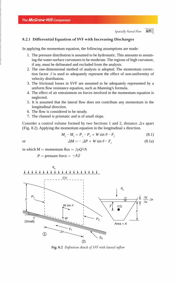
Spatially Varied Flow 367
8.2.1 Diff erential Equation of SVF with Increasing Discharges
In applying the momentum equation, the following assumptions are made:
1. The pressure distribution is assumed to be hydrostatic. This amounts to assum-ing the water-surface curvatures to be moderate. The regions of high curvature, if any, must be delineated and excluded from the analysis.
2. The one-dimensional method of analysis is adopted. The momentum correc-tion factor β is used to adequately represent the effect of non-uniformity of velocity distribution.
3. The frictional losses in SVF are assumed to be adequately represented by a uniform fl ow resistance equation, such as Manning’s formula.
4. The effect of air entrainment on forces involved in the momentum equation is neglected.
5. It is assumed that the lateral fl ow does not contribute any momentum in the longitudinal direction.
6. The fl ow is considered to be steady.7. The channel is prismatic and is of small slope.
Consider a control volume formed by two Sections 1 and 2, distance Δ x apart (Fig. 8.2). Applying the momentum equation in the longitudinal x direction.
M2 − M
1 = P
1 − P
2 + W sin θ − F
f (8.1)
or ΔM = − ΔP + W sin θ − Ff (8.1a)
in which M = momentum fl ux = βρQ2/A
P = pressure force = γ A y
Fig. 8.2 Defi nition sketch of SVF with lateral infl ow
CV
P1y
(Small)θ
FfΔx1
2S0
W sin θ
W P2
y
yCG
q*
q*
∇ ∂y
∂xΔx
Area = A
Chapter 8.indd 367Chapter 8.indd 367 2/24/2010 3:03:23 PM2/24/2010 3:03:23 PM
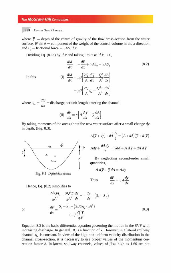
368 Flow in Open Channels
where y = depth of the centre of gravity of the fl ow cross-section from the water surface, W sin θ = component of the weight of the control volume in the x direction and F
f = frictional force = γAS
f Δ x.
Dividing Eq. (8.1a) by Δ x and taking limits as Δ x → 0,
dM
dx
dP
dxAS AS f= − + −γ γ0
(8.2)
In this (i) dM
dx
Q
A
dQ
dx
Q
A
dA
dx= −
⎛
⎝⎜⎜⎜⎜
⎞
⎠⎟⎟⎟⎟
ρβ2 2
2
= −
⎛
⎝⎜⎜⎜⎜
⎞
⎠⎟⎟⎟⎟
ρβ2 2
2
Q
Aq
Q T
A
dA
dx*
where qdQ
dx*= = discharge per unit length entering the channel.
(ii) dP
dxA
d y
dxy
dA
dx= +
⎛⎝⎜⎜⎜
⎞⎠⎟⎟⎟⎟γ
By taking moments of the areas about the new water surface after a small change dy in depth, (Fig. 8.3),
A y dy dAdy
A dA y d y+ + = + +( ) ( )( )2
AdydAdy
ydA A d y dA d y+ = + +2
By neglecting second-order small quantities,
A d y y dA Ady+ =
Thus dP
dxA
dy
dx= γ
Hence, Eq. (8.2) simplifi es to
22
2
3 0
β βQq
gA
Q T
gA
dy
dx
dy
dxS S f
* − = − + −( )
or dy
dx
S S Qq gA
Q T
gA
f=
− −( )−
02
2
3
2
1
β
β
* (8.3)
Equation 8.3 is the basic differential equation governing the motion in the SVF with increasing discharge. In general, q
*is a function of x. However, in a lateral spillway
channel q* is constant. In view of the high non-uniform velocity distribution in the
channel cross-section, it is necessary to use proper values of the momentum cor-rection factor β. In lateral spillway channels, values of β as high as 1.60 are not
Fig. 8.3 Defi nition sketch
∇
y
y
dydA
A
CG
∗
Chapter 8.indd 368Chapter 8.indd 368 2/24/2010 3:03:24 PM2/24/2010 3:03:24 PM
Spatially Varied Flow 369
uncommon. It may be noted that if β = 1.0 and q*
,= 0 Eq. 8.3 will be the same as that of the differential equation of gradually varied fl ow (GVF) (Eq. 4.8)
Equation 8.3 is a non-linear equation and is more complex than the GVF equation. Closed-form solutions are not possible except in highly-simplifi ed cases. A numerical solution of the equation is feasible. Starting from a section where the fl ow properties are known (such as a control section), the water-surface profi le can be computed.
8.2.2 Control Point
If the fl ow is subcritical everywhere in the channel, the control of the profi le will be located at the downstream end of the channel. However, for all fl ow situations other than the above, the determination of the control point is a necessity to start the computations.
In an SVF with increasing discharges, the critical depth line is not a straight line parallel to the bed as in GVF but is a curved line. Depending upon the combination of the bottom slope, channel roughness and channel geometry, the critical depth of spa-tially varied fl ow can occur at a location somewhere between the ends of the channel, giving rise to a profi le which may be subcritical during the fi rst part and supercritical in the subsequent part of the channel. A method of calculation of the critical depth and its location based on the concept of equivalent critical depth channel has been pro-posed by Hinds1. An alternative method based on transitional profi les suggested by Smith2, which has advantages like simplicity and less tedious calculations compared to Hind’s method, is described below:
Consider Eq. 8.3 written as
dy
dxS
S
S
gA S
Q T
gA
f
=− −
−0
02
02
3
12
1
β
β
*
(8.4)
Defi ning Q K S f= = actual discharge
Q K Sn = =0 normal discharge in the channel at a depth y
QgA
Tc = =3
β critical discharge modifi ed by β.
Equation 8.4 reduces to
dy
dxS
K Q
K Q
Q
Q
K q
gA Q
Q Q
n n
c
=
− −⎛
⎝⎜⎜⎜⎜
⎞
⎠⎟⎟⎟⎟
−( )0
2 2
2 2
2
2
2
2
2
12
1
β*
/
=
−⎛
⎝⎜⎜⎜⎜
⎞
⎠⎟⎟⎟⎟
+⎛
⎝⎜⎜⎜⎜
⎞
⎠⎟⎟⎟⎟
−( )S
Q
Q
K
gA
q
Q
Q Q
n
c
0
2 2
2
2
1 12
1
β*
/ (8.5)
Chapter 8.indd 369Chapter 8.indd 369 2/24/2010 3:03:25 PM2/24/2010 3:03:25 PM
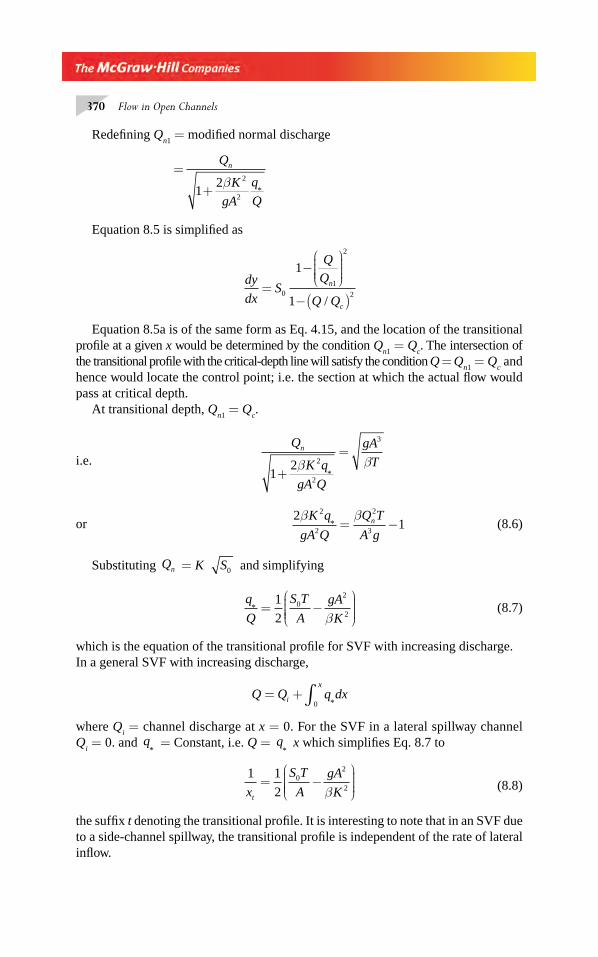
370 Flow in Open Channels
Redefi ning Qn1
= modifi ed normal discharge
=
+
Q
K
gA
q
Q
n
12 2
2
β*
Equation 8.5 is simplifi ed as
dy
dxS
Q
Q
Q Q
n
c
=
−⎛
⎝⎜⎜⎜⎜
⎞
⎠⎟⎟⎟⎟
−( )0
1
2
2
1
1 /
Equation 8.5a is of the same form as Eq. 4.15, and the location of the transitional profi le at a given x would be determined by the condition Q
n1 = Q
c. The intersection of
the transitional profi le with the critical-depth line will satisfy the condition Q = Qn1
= Qc and
hence would locate the control point; i.e. the section at which the actual fl ow would pass at critical depth.
At transitional depth, Qn1
= Qc.
i.e. Q
K q
gA Q
gA
Tn
12 2
2
3
+
=β β
*
or 2
12
2
2
3
β βK q
gA Q
Q T
A gn* = − (8.6)
Substituting Qn = K S0 and simplifying
q
Q
S T
A
gA
K* = −
⎛
⎝⎜⎜⎜⎜
⎞
⎠⎟⎟⎟⎟
1
20
2
2β (8.7)
which is the equation of the transitional profi le for SVF with increasing discharge.In a general SVF with increasing discharge,
Q Q q dxi
x= + ∫ *0
where Qi = channel discharge at x = 0. For the SVF in a lateral spillway channel
Qi = 0. and q
* = Constant, i.e. Q = q
* x which simplifi es Eq. 8.7 to
1 1
20
2
2x
S T
A
gA
Kt
= −⎛
⎝⎜⎜⎜⎜
⎞
⎠⎟⎟⎟⎟β (8.8)
the suffi x t denoting the transitional profi le. It is interesting to note that in an SVF due to a side-channel spillway, the transitional profi le is independent of the rate of lateral infl ow.
Chapter 8.indd 370Chapter 8.indd 370 2/24/2010 3:03:25 PM2/24/2010 3:03:25 PM
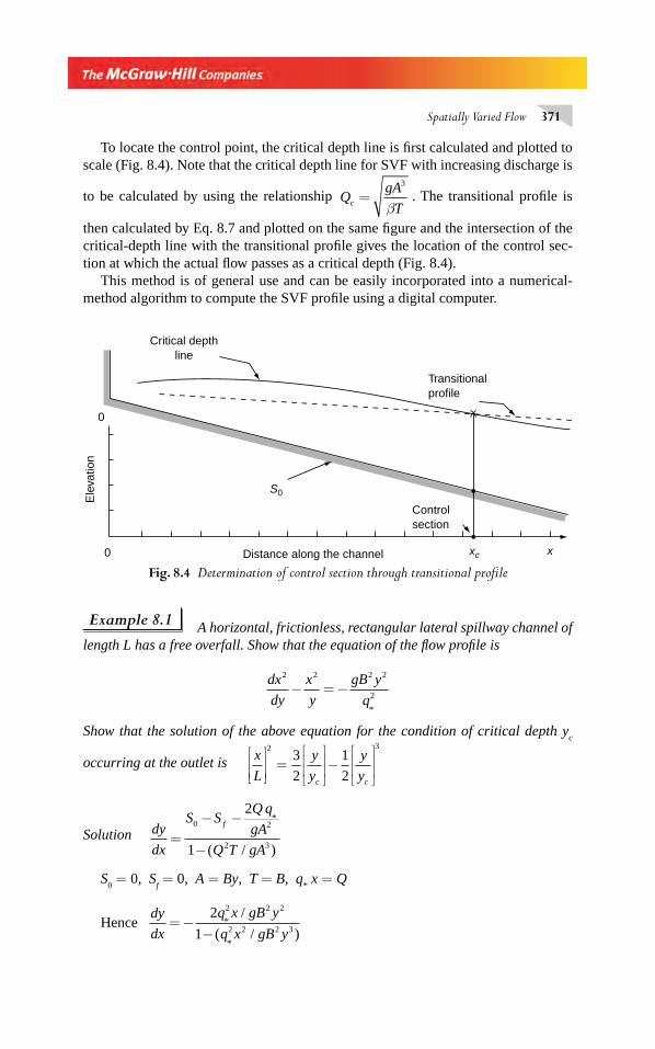
Spatially Varied Flow 371
To locate the control point, the critical depth line is fi rst calculated and plotted to scale (Fig. 8.4). Note that the critical depth line for SVF with increasing discharge is
to be calculated by using the relationship QgA
Tc =3
β. The transitional profi le is
then calculated by Eq. 8.7 and plotted on the same fi gure and the intersection of the critical-depth line with the transitional profi le gives the location of the control sec-tion at which the actual fl ow passes as a critical depth (Fig. 8.4).
This method is of general use and can be easily incorporated into a numerical-method algorithm to compute the SVF profi le using a digital computer.
Example 8.1 A horizontal, frictionless, rectangular lateral spillway channel of length L has a free overfall. Show that the equation of the fl ow profi le is
dx
dy
x
y
gB y
q
2 2 2 2
2− = −
*
Show that the solution of the above equation for the condition of critical depth yc
occurring at the outlet is x
L
y
y
y
yc c
⎡
⎣⎢⎢
⎤
⎦⎥⎥
=⎡
⎣⎢⎢
⎤
⎦⎥⎥ −
⎡
⎣⎢⎢
⎤
⎦⎥⎥
2 33
2
1
2
Solution dy
dx
S SQ q
gA
Q T gA
f
=− −
−
0 2
2 3
2
1
*
( / )
S0 = 0, S
f = 0, A = By, T = B, q
* x = Q
Hence dy
dx
q x gB y
q x gB y= −
−2
1
2 2 2
2 2 2 3*
*
/
( / )
Fig. 8.4 Determination of control section through transitional profi le
Critical depthline
Transitionalprofile
Controlsection
S0
xc x0
0
Ele
vatio
n
Distance along the channel
Chapter 8.indd 371Chapter 8.indd 371 2/24/2010 3:03:25 PM2/24/2010 3:03:25 PM
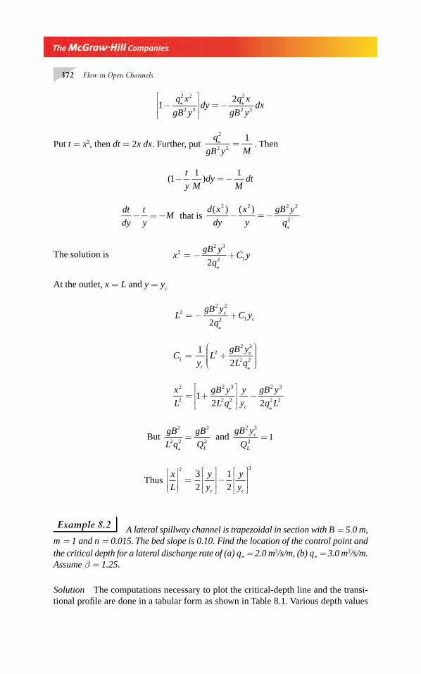
372 Flow in Open Channels
122 2
2 3
2
2 2−
⎡
⎣⎢⎢
⎤
⎦⎥⎥ = −
q x
gB ydy
q x
gB ydx* *
Put t = x2, then dt = 2x dx. Further, put q
gB y M*
2
2 2
1= . Then
( )11 1
− = −t
y Mdy
Mdt
dt
dy
t
yM− = − that is
d x
dy
x
y
gB y
q
( ) ( )
*
2 2 2 2
2− = −
The solution is xgB y
qC y2
2 3
2 12= − +
*
At the outlet, x = L and y = yc
LgB y
qC yc
c2
2 2
2 12= − +
*
Cy
LgB y
L qc
c1
22 3
2 2
1
2= +
⎛
⎝⎜⎜⎜⎜
⎞
⎠⎟⎟⎟⎟
*
x
L
gB y
L q
y
y
gB y
q Lc
2
2
2 3
2 2
2 3
2 21
2 2= +
⎡
⎣⎢⎢
⎤
⎦⎥⎥ −
* *
But gB
L q
gB
QL
2
2 2
2
2
*
= and gB y
Qc
L
2 3
21=
Thus x
L
y
y
y
yc c
⎡
⎣⎢⎢
⎤
⎦⎥⎥
=⎡
⎣⎢⎢
⎤
⎦⎥⎥ −
⎡
⎣⎢⎢
⎤
⎦⎥⎥
2 33
2
1
2
Example 8.2 A lateral spillway channel is trapezoidal in section with B = 5.0 m, m = 1 and n = 0.015. The bed slope is 0.10. Find the location of the control point and the critical depth for a lateral discharge rate of (a) q
* = 2.0 m3/s/m, (b) q
* = 3.0 m3/s/m.
Assume β = 1.25.
Solution The computations necessary to plot the critical-depth line and the transi-tional profi le are done in a tabular form as shown in Table 8.1. Various depth values
Chapter 8.indd 372Chapter 8.indd 372 2/24/2010 3:03:25 PM2/24/2010 3:03:25 PM
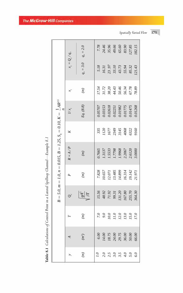
Spatially Varied Flow 373
B =
5.0
, m =
1.0
, n =
0.0
15, B
= 1
.25,
S0 =
0.1
0, K
= 1 n
AR
2/3
y (m)
A (m2 )
T (m)
Qc
gA
T3
β
P (m)
R =
A /
P
(m)
K1/
xt
Eq.
(8.
8)
x t
(m)
x c = Q
c / q
*
q * = 3
.0
q * =
2.0
1.0
6.0
0 7
.0 1
5.56
7.8
280.
7665
335
0.05
707
17.5
4
5.1
8
7.7
8
2.0
14.0
0 9
.0 4
8.92
10.6
571.
3137
1120
0.03
153
31.7
2 1
6.31
24.
46
2.5
18.7
510
.0 7
1.92
12.0
711.
5533
1677
0.02
618
38.2
0 2
3 .9
7 3
5.96
3.0
24.0
011
.0 9
9.31
13.4
851.
7798
2349
0.02
251
44.4
3 3
3.10
49.
66
3.5
29.7
512
.013
1.20
14.8
991.
9968
3145
0.01
982
50.4
6 4
3.73
65.
60
4.0
36.0
013
.016
7.80
16.3
142.
2067
4068
0.01
775
56.3
4 5
5.94
83.
90
5.0
50.0
015
.025
5.70
19.1
422.
6120
6322
0.01
475
67.7
8 8
5.32
127.
85
6.0
66.0
017
.0
364.
3021
.971
3.00
0091
600.
0126
878
.89
121.
4318
2.15
Tabl
e 8.
1 C
alcu
lati
ons
of C
ontr
ol P
oint
in
a La
tera
l Sp
illw
ay C
hann
el—
Exa
mpl
e 8
.1
Chapter 8.indd 373Chapter 8.indd 373 2/24/2010 3:03:26 PM2/24/2010 3:03:26 PM
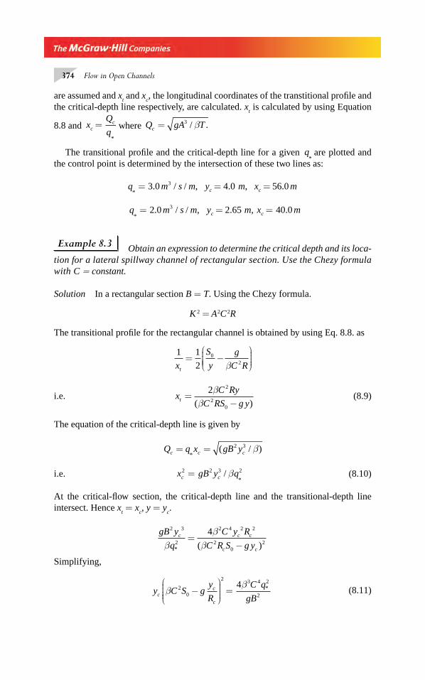
374 Flow in Open Channels
are assumed and xt and x
c, the longitudinal coordinates of the transtitional profi le and
the critical-depth line respectively, are calculated. xt is calculated by using Equation
8.8 and xQ
qcc=*
where Q gA Tc = 3 / .β
The transitional profi le and the critical-depth line for a given q*
are plotted and the control point is determined by the intersection of these two lines as:
q m s m y m x mc c*. / / , . , .= = =3 0 4 0 56 03
q m s m y m x mc c*
. / / , . , .= = =2 0 2 65 40 03
Example 8.3 Obtain an expression to determine the critical depth and its loca-tion for a lateral spillway channel of rectangular section. Use the Chezy formula with C = constant.
Solution In a rectangular section B = T. Using the Chezy formula.
K 2 = A 2C 2R
The transitional profi le for the rectangular channel is obtained by using Eq. 8.8. as
1 1
20
2x
S
y
g
C Rt
= −⎛
⎝⎜⎜⎜⎜
⎞
⎠⎟⎟⎟⎟β
i.e. xC Ry
C RS g yt =−
2 2
20
ββ( )
(8.9)
The equation of the critical-depth line is given by
Q q x gB yc c c= =*
( / )2 3 β
i.e. x gB y qc c2 2 3 2= /
*β (8.10)
At the critical-fl ow section, the critical-depth line and the transitional-depth line intersect. Hence x
t = x
c, y = y
c.
gB y
q
C y R
C R S g yc c c
c c
2 3
2
2 4 2 2
20
2
4
ββ
β* ( )=
−
Simplifying,
y C S gy
R
C q
gBcc
c
ββ2
0
2 3 4 2
2
4−
⎛
⎝⎜⎜⎜⎜
⎞
⎠⎟⎟⎟⎟
= * (8.11)
Chapter 8.indd 374Chapter 8.indd 374 2/24/2010 3:03:26 PM2/24/2010 3:03:26 PM
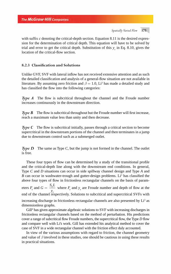
Spatially Varied Flow 375
with suffi x c denoting the critical-depth section. Equation 8.11 is the desired expres-sion for the determination of critical depth. This equation will have to be solved by trial and error to get the critical depth. Substitution of this y
c in Eq. 8.10, gives the
location of the critical-fl ow section.
8.2.3 Classifi cation and Solutions
Unlike GVF, SVF with lateral infl ow has not received extensive attention and as such the detailed classifi cation and analysis of a general-fl ow situation are not available in literature. By assuming zero friction and β = 1.0, Li3 has made a detailed study and has classifi ed the fl ow into the following categories:
Type A The fl ow is subcritical throughout the channel and the Froude number increases continuously in the downstream direction.
Type B The fl ow is subcritical throughout but the Froude number will fi rst increase, reach a maximum value less than unity and then decrease.
Type C The fl ow is subcritical initially, passes through a critical section to become supercritical in the downstream portions of the channel and then terminates in a jump due to downstream control such as a submerged outlet.
Type D The same as Type C, but the jump is not formed in the channel. The outlet is free.
These four types of fl ow can be determined by a study of the transitional profi le and the critical-depth line along with the downstream end conditions. In general, Type C and D situations can occur in side spillway channel design and Type A and B can occur in washwater-trough and gutter-design problems. Li3 has classifi ed the above four types of fl ow in frictionless rectangular channels on the basis of param-
eters Fe and G =
S L
ye
0 where Fe and y
e are Froude number and depth of fl ow at the
end of the channel respectively. Solutions to subcritical and supercritical SVFs with
increasing discharge in frictionless rectangular channels are also presented by Li3 as dimensionless graphs.
Gill4 has given approximate algebraic solutions to SVF with increasing discharges in frictionless rectangular channels based on the method of perturbation. His predictions cover a range of subcritical fl ow Froude numbers, the supercritical fl ow, the Type D fl ow and compare well with Li’s work. Gill has extended his analytical method to cover the case of SVF in a wide rectangular channel with the friction effect duly accounted.
In view of the various assumptions with regard to friction, the channel geometry and value of β involved in these studies, one should be cautious in using these results in practical situations.
Chapter 8.indd 375Chapter 8.indd 375 2/24/2010 3:03:26 PM2/24/2010 3:03:26 PM
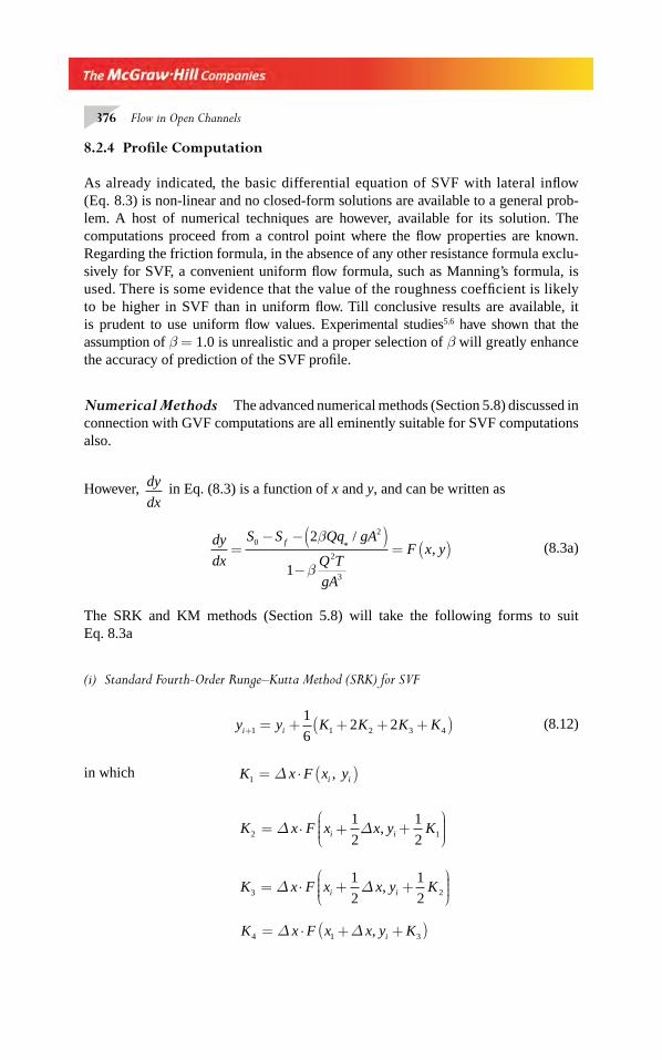
376 Flow in Open Channels
8.2.4 Profi le Computation
As already indicated, the basic differential equation of SVF with lateral infl ow (Eq. 8.3) is non-linear and no closed-form solutions are available to a general prob-lem. A host of numerical techniques are however, available for its solution. The computations proceed from a control point where the fl ow properties are known. Regarding the friction formula, in the absence of any other resistance formula exclu-sively for SVF, a convenient uniform fl ow formula, such as Manning’s formula, is used. There is some evidence that the value of the roughness coeffi cient is likely to be higher in SVF than in uniform fl ow. Till conclusive results are available, it is prudent to use uniform fl ow values. Experimental studies5.6 have shown that the assumption of β = 1.0 is unrealistic and a proper selection of β will greatly enhance the accuracy of prediction of the SVF profi le.
Numerical Methods The advanced numerical methods (Section 5.8) discussed in connection with GVF computations are all eminently suitable for SVF computations also.
However, dy
dx in Eq. (8.3) is a function of x and y, and can be written as
dy
dx
S S Qq gA
Q T
gA
F x yf
=− −( )
−= ( )0
2
2
3
2
1
β
β
*/
, (8.3a)
The SRK and KM methods (Section 5.8) will take the following forms to suit Eq. 8.3a
(i) Standard Fourth-Order Runge–Kutta Method (SRK) for SVF
y y K K K Ki i+ = + + + +( )1 1 2 3 4
1
62 2 (8.12)
in which K x F x yi i1 = Δ ⋅ ( ),
K x F x x y Ki i2
1
2
1
2= Δ ⋅ + Δ +
⎛⎝⎜⎜⎜
⎞⎠⎟⎟⎟, 1
K x F x x y Ki i3
1
2
1
2= Δ ⋅ + Δ +
⎛⎝⎜⎜⎜
⎞⎠⎟⎟⎟, 2
K x F x x y Ki4 1 3= Δ ⋅ +Δ +( ),
Chapter 8.indd 376Chapter 8.indd 376 2/24/2010 3:03:26 PM2/24/2010 3:03:26 PM
Spatially Varied Flow 377
(ii) Kutta–Merson Method (KM) for SVF
y y K K Ki i+ = + + +( )1 1 4 5
1
24 (8.13)
in which K x F x yi i1
1
3= Δ ⋅ ( )'
K x F x x y K
K x F x x y K
i i
i i
2
3
1
3
1
3
1
3
1
3
1
2
1
= Δ ⋅ + Δ +⎛⎝⎜⎜⎜
⎞⎠⎟⎟⎟
= Δ ⋅ + Δ + +
,
,22
1
3
1
2
3
8
9
8
1
3
2
4 3
5
K
K x F x x y K K
K
i i
⎛⎝⎜⎜⎜
⎞⎠⎟⎟⎟
= Δ ⋅ + Δ + +⎛⎝⎜⎜⎜
⎞⎠⎟⎟⎟
=
,
Δ ⋅ + Δ + − +⎛⎝⎜⎜⎜
⎞⎠⎟⎟⎟x F x x y K K Ki i,
3
2
9
261 3 4
1
1
1
(iii) Trapezoidal Method (TRAP) for SVF
y y x F x y F x yi i i i i+ += + Δ ( )+ ( )⎡⎣⎢
⎤⎦1 1
1
2, ,i+1 (8.14)
The details of these methods, their relative accuracy and advantages are the same as discussed in Section 5.8 in connection with the GVF computations.
8.3 SVF WITH DECREASING DISCHARGE
SVF with decreasing discharges occurs in a variety of fi eld situations, typical exam-ples being side weirs, bottom racks and siphon tube irrigation systems. The abstrac-tion of water from a canal by using the above means is normally achieved in such a manner as to cause minimum obstruction and with consequent little energy losses in the parent channel. It is usual to assume that energy loss due to diversion of water is zero and the energy equation is used to derive the basic equation of motion.
8.3.1 Diff erential Equation for SVF with Decreasing Discharge
The following assumptions are made:
1. The pressure distribution is hydrostatic2. The one-dimensional method of analysis is used (the energy-correction factor
α is used to adequately represent the non-uniformity of velocity distribution).3. The friction losses are adequately represented by Manning’s formula.4. Withdrawal of water does not a affect the energy content per unit mass of water
in the channel5. The fl ow is steady6. The channel is prismatic and is of small slope.
Chapter 8.indd 377Chapter 8.indd 377 2/24/2010 3:03:27 PM2/24/2010 3:03:27 PM
378 Flow in Open Channels
Consider the total energy at a Section x,
H = Z + y + α V
g
2
2 (8.15)
Differentiating this with respect to x
dH
dx
dZ
dx
dy
dx
d
dx
V
g= + +
⎛
⎝⎜⎜⎜⎜
⎞
⎠⎟⎟⎟⎟
α2
2 (8.16)
But dH
dxS f= − and
dZ
dxS= − 0
d
dx
V
g
d
dx
Q
gA g
Q
A
dQ
dx
Qα α
α2 2
2 22 2 2
2 2⎛
⎝⎜⎜⎜⎜
⎞
⎠⎟⎟⎟⎟
=⎛
⎝⎜⎜⎜⎜
⎞
⎠⎟⎟⎟⎟
= −22
3A
dA
dy
dy
dx
⎛
⎝⎜⎜⎜⎜
⎞
⎠⎟⎟⎟⎟
dA
dyT= and
dQ
dxq=
*
Equation 8.16 simplifi es to
dy
dx
S SQq
gA
Q T
gA
f
=− −
−
0 2
2
31
α
α
*
(8.17)
Equation 8.17 is the basic differential equation governing the motion of SVF with decreasing discharges. Note the difference between Eq. 8.17 and Eq. 8.3. When q
* = 0,
Eq. 8.17 will be the same as the differential equation of GVF, Eq. 4.8. Unlike the SVF with increasing discharges, in this case q
* is not externally controlled but will
be implicitly governed by the fl ow conditions.
8.3.2 Computations
The determination of the critical-fl ow control point in the SVF with decreasing dis-charges is diffi cult as q
* is not explicitly known. Normally, SVF with lateral out-
fl ow occurs in a relatively small portion of length of canals and the upstream or downstream depth, depending upon the fl ow, is known through the characteristics of the outfl ow structure and main channel. This forms, the starting point for the SVF computations.
It is first necessary to establish a relationship for q* as a function of the rele-
vant flow conditions. The SVF profile is then computed by using a numerical procedure, such as SRK, KM or TRAP method discussed in Section 8.2.4. The method of approach depends upon the understanding of the particular flow phenomenon.
Chapter 8.indd 378Chapter 8.indd 378 2/24/2010 3:03:28 PM2/24/2010 3:03:28 PM
Spatially Varied Flow 379
A few specifi c examples of fl ow situations where SVF with lateral outfl ow occurs, are described below.
8.4 SIDE WEIR
A side weir, also known as a lateral weir, is a free-overfl ow weir set into the side of a channel which allows a part of the liquid to spill over the side when the surface of the fl ow in the channel rises above the weir crest. Side weirs are extensively used as a means of diverting excess storm waters from urban drainage systems and as water-level control devices in fl ood-control works. In irrigation engineering, side weirs of broad crest are used as head regulators of distributaries and escapes.
Figure 8.5 is a defi nition sketch of the fl ow over a side weir. Side weirs are usually short structures with L/B ≤ 3.0. It is obvious from specifi c energy considerations (Section 2.2) that the longitudinal water surface should increase in the downstream direction when the main channel fl ow is subcritical throughout. Similarly, the water-surface profi le would be a decreasing curve for supercritical fl ow in the channel. The possible fl ow profi les can be broadly classifi ed into the following three categories:
Type 1 The channel is on a mild slope and the weir heights s > yc1
where yc1
is the critical depth corresponding to the incoming discharge Q
1 at Section 1, (Fig. 8.6a). At
1 2
B
ys
E
x
L
Q1
V1
Q2
Qs
y0 y1y2
yt
V2
Side weir
L - Section
Energy line
Plan
∇
Fig. 8.5 Defi nition sketch of side weir fl ow
Chapter 8.indd 379Chapter 8.indd 379 2/24/2010 3:03:28 PM2/24/2010 3:03:28 PM
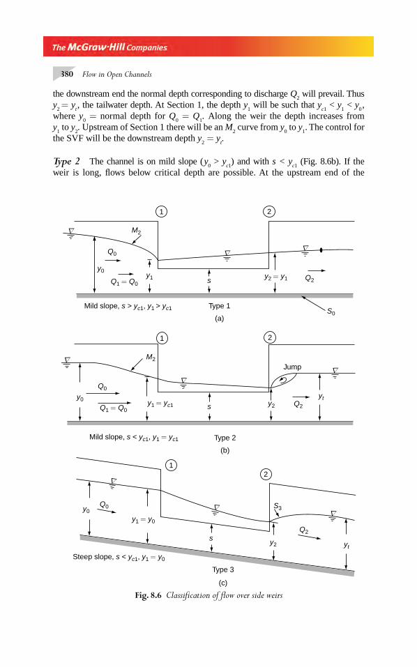
380 Flow in Open Channels
the downstream end the normal depth corresponding to discharge Q2 will prevail. Thus
y2 = y
t , the tailwater depth. At Section 1, the depth y
1 will be such that y
c1 < y
1 < y
0 ,
where y0 = normal depth for Q
0 = Q
1. Along the weir the depth increases from
y1 to y
2. Upstream of Section 1 there will be an M
2 curve from y
0 to y
1. The control for
the SVF will be the downstream depth y2 = y
t.
Type 2 The channel is on mild slope ( y0 > y
c1) and with s < y
c1 (Fig. 8.6b). If the
weir is long, fl ows below critical depth are possible. At the upstream end of the
Fig. 8.6 Classifi cation of fl ow over side weirs
∇
∇
∇∇
∇
∇∇
∇∇
1
1
1
2
2
2
y0
y0
y0y1
Q0
Q0
Q2
Q2
M2
M2
y1 = y0
y2 = y1
Q1 = Q0
Steep slope, s < yc1, y1 = y0
y2
y2
yt
yt
S3
s
s
Type 3
(c)
Mild slope, s < yc1, y1 = yc1 Type 2
(b)
Mild slope, s > yc1, y1 > yc1 Type 1
(a)
Q2s
Q0
Q1 = Q0
y1 = yc1
Jump
S0
Chapter 8.indd 380Chapter 8.indd 380 2/24/2010 3:03:28 PM2/24/2010 3:03:28 PM
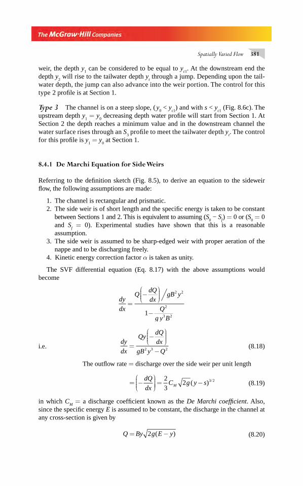
Spatially Varied Flow 381
weir, the depth y1 can be considered to be equal to y
c1. At the downstream end the
depth y2 will rise to the tailwater depth y
t through a jump. Depending upon the tail-
water depth, the jump can also advance into the weir portion. The control for this type 2 profi le is at Section 1.
Type 3 The channel is on a steep slope, ( y0 < y
c1) and with s < y
c1 (Fig. 8.6c). The
upstream depth y1 = y
0 decreasing depth water profi le will start from Section 1. At
Section 2 the depth reaches a minimum value and in the downstream channel the water surface rises through an S
3 profi le to meet the tailwater depth y
t. The control
for this profi le is y1 = y
0 at Section 1.
8.4.1 De Marchi Equation for Side Weirs
Referring to the defi nition sketch (Fig. 8.5), to derive an equation to the sideweir fl ow, the following assumptions are made:
1. The channel is rectangular and prismatic.2. The side weir is of short length and the specifi c energy is taken to be constant
between Sections 1 and 2. This is equivalent to assuming (S0 − S
f ) = 0 or (S
0 = 0
and Sf = 0). Experimental studies have shown that this is a reasonable
assumption.3. The side weir is assumed to be sharp-edged weir with proper aeration of the
nappe and to be discharging freely.4. Kinetic energy correction factor α is taken as unity.
The SVF differential equation (Eq. 8.17) with the above assumptions would become
dy
dx
QdQ
dxgB y
Q
g y B
=−
⎛⎝⎜⎜⎜
⎞⎠⎟⎟⎟
−
2 2
2
3 21
i.e. dy
dx
QydQ
dx
gB y Q=
−⎛⎝⎜⎜⎜
⎞⎠⎟⎟⎟
−2 3 2 (8.18)
The outfl ow rate = discharge over the side weir per unit length
= −⎛⎝⎜⎜⎜
⎞⎠⎟⎟⎟⎟ = −
dQ
dxC g y sM
2
32 3 2( ) / (8.19)
in which CM = a discharge coeffi cient known as the De Marchi coeffi cient. Also,
since the specifi c energy E is assumed to be constant, the discharge in the channel at any cross-section is given by
Q By g E y= −2 ( ) (8.20)
Chapter 8.indd 381Chapter 8.indd 381 2/24/2010 3:03:29 PM2/24/2010 3:03:29 PM
382 Flow in Open Channels
From Eqs 8.18, 8.19 and 8.20
dy
dx
C
B
E y y s
y EM=
−( ) −( )−
4
3 3 2
3
(8.21)
Assuming that CM is independent of x, on integration,
x =3
2
B
CM
M.φ ( y, E, s) + Const. (8.22)
in which
φM ( y, E, s) = 2 3E s
E s
E y
y s
−−
−−
− 3sin–1 E y
E s
−−
Equation 8.22 is known as the De Marchi equation and the function φM ( y, E, s) is known as the De Marchi varied fl ow function. Applying Eq. 8.22 to Sections 2 and 1,
x x LB
CM
2 1
3
2− = = φ φM M2 1−( ) (8.23)
knowing L, s, and (Q and y) at either 2 or 1, the discharge over the side weir Qs can
be computed by Eq. 8.23 and by the continuity equation
Qs = Q
1 – Q
2 (8.24)
De Marchi Coeffi cient CM
Experimental and theoretical studies by Subramanya and Awasthy7 have shown that in subcritical approaching fl ow the major fl ow parameter affecting the De Marchi coeffi cient is the Froude number of the approaching fl ow. The functional relationship of C
M and initial Froude number is shown to be
CF
FM = −
+( )0 611 1
3
212
12
. (8.25)
where FV
g y1
1
1
=
Equation 8.25 can be simplifi ed as
CF
FM =−+
0 8641
212
12
. (8.26)
However, for supercritical approach fl ow the effect of the approach Froude number is insignifi cant and the variation of C
M for F
1 > 2.0 is obtained as
CM
= 0.36 − 0.008F1 (8.27)
Chapter 8.indd 382Chapter 8.indd 382 2/24/2010 3:03:29 PM2/24/2010 3:03:29 PM
Spatially Varied Flow 383
There have been numerous studies on the side weirs in rectangular channels since last three decades. A majority of these studies are on subcritical approach fl ow condi-tion as this is the most common situation in practice. Borghi et al 8 have studied the effect of parameters, s/y
1 and L/B, and propose the following experimentally derived
equation for estimation of the De Marchi coeffi cient CM for subcritical approach
fl ow:
C Fs
y
L
BM = − − +0 7 0 48 0 3 0 0611
. . . . (8.28)
Olivetto et al 9 have studied the side weir fl ow in rectangular and circular channels both through theoretical and experimental means. The studies relate to the case of subcritical fl ow in the approach channel with supercritical fl ow along the side weirs. Ghodsian 10 has experimentally studied the hydraulic characteristics of sharp crested triangular side weirs. For this fl ow situation the De Marchi equation has been expressed as
C A BF Cs
yM = − −11
(8.29)
where s = height of the vertex of the triangular weir above the bed of the channel.The coeffi cients A, B and C are found to be functions of the weir angle θ.
Uyumaz11 has studied the behavior of a rectangular side weir in a triangular chan-nel and has derived the relevant discharge equation. The channel studied had one side vertical and the side weir was located in the vertical side. The coeffi cient of discharge C
M , given by Eq. 8.25 and 8.27 was found to be adequate for this case also. However,
if the weir is set in the inclined side of the channel, the coeffi cient CM can be expected
to be a function of the inclination of the side also.
8.4.2 Computations
The design of a side weir or the calculation of the side-weir discharge can be accom-plished by use of appropriate Eqs 8.23 through 8.27 along with the selection of the proper control depth. In using the De Marchi equation since it is assumed that S
f =
S0 = 0, the controls would be y
1 = y
0 for fl ows of Type 1 and Type 3. However, for
Type 2 fl ows the coeffi cient CM is calculated by taking F
1 = F
0 and for calculations
of discharge and depth profi le the depth at Section 1 is assumed as y1 = y
c1. The
downstream depth y2 would, in all types of fl ows, be determined by the condition of
constancy of specifi c energy, (E = constant).It is apparent that iterative procedures have to be adopted in the calculation of Q
s or L.
Example 8.4 A rectangular channel, B = 2.0 m, n = 0.014, is laid on a slope S
0 = 0.001. A side weir is required at a section such that it comes into operation when
Chapter 8.indd 383Chapter 8.indd 383 2/24/2010 3:03:29 PM2/24/2010 3:03:29 PM
384 Flow in Open Channels
the discharge is 0.6 m3/s and diverts 0.15 m3/s when the canal discharge is 0.9 m3/s. Design the elements of the side weir.
Solution The normal depths at the two discharges are found by referring to Table 3A.1 as:
Q0 φ = nQ S B/ /
08 3 y
0 / B y
0
0.6 0.0418 0.165 0.33 m
0.9 0.0628 0.220 0.44 m
The height of the weir crest s = 0.33 m.
For a discharge of 0.9 m3/s:
Critical depth yc1
2 1 3
0 9
2 09 81=
⎛⎝⎜⎜⎜
⎞⎠⎟⎟⎟
⎛
⎝⎜⎜⎜⎜
⎞
⎠
⎟⎟⎟⎟⎟=
.
..
/
0.274 m
Since s > yc1
, and y0 > y
c1, the fl ow is of Type 1.
In the use of the De Marchi equation y1 = y
0 = 0.44 m.
V1
0 9
1 0 441 023=
×=
.
.. m/s, F1
1 023
9 81 0 440 4924=
×=
.
. ..
Specifi c energy E E1 20 441 023 2
2 9 810 4933= +
( )×
= =..
.. m
Discharge over the side weir QS = 0.15 m3/s
Discharge at the end of the weir Q2 = 0.90 − 0.15 = 0.75 m3/s
At Section 2, E2 = 0.4933 = E
1
yQ
B y gy
y222
2 2
2 2
2
22
2
0 75
4 2 9 81+
( )= +
( )× × ×
.
. = 0.4933
By trial-and-error, y2 = 0.46 m
F
E
y22
2 1 0 38= −⎛
⎝⎜⎜⎜⎜
⎞
⎠⎟⎟⎟⎟
= .
De Marchi varied fl ow function
Chapter 8.indd 384Chapter 8.indd 384 2/24/2010 3:03:30 PM2/24/2010 3:03:30 PM
Spatially Varied Flow 385
φM
E s
E s
E y
y s
E y
E s
E s
E s
=−−
⎛⎝⎜⎜⎜
⎞⎠⎟⎟⎟⎟
−−
−−−
−−
⎛⎝⎜⎜⎜
⎞⎠⎟⎟
−2 33
2 3
1sin
⎟⎟⎟ =×( )− ×( )
−= −
= −( )
2 0 4933 3 0 33
0 4933 0 330 02082
0 020820
1
. .
. ..
.φM
.. .
. .sin
. .
. ..
4933 0 44
0 44 0 333
0 4933 0 44
0 3493 0 331 8401−
−−
−−
= −−
φM 2210 02082
0 0333
0 133
0 0333
0 16331 416= −( ) − = −−.
.
.sin
.
..
From Eq. 8.25,
CM = −×( )+( )
=0 611 13 0 4924
2 0 49240 502
2
2.
.
..
From Eq. 8.23,
LB
CM
M M= −( )
= × − +( )
=
3
2
3
2
2 0
0 5021 416 1 840
2 534
2 1φ φ
.
.. .
. m
Example 8.5 In Example 8.3, if the length of the side weir provided is 4.20 m with s = 0.33 m, fi nd the discharge over the side weir and the depth y
2.
Solution CM = 0.502, E
1 = E
2 = 0.4933
y1 = 0.44 m and φM1 1 840= − .
In Eq. 8.23
4 203
2
2
0 5021 840
1 1372
2
2
..
.
. .
= × +( )
= −
φ
φ
M
M
The value of y2 to satisfy φ
M 2 = − 1.1372 is found by trial-and-error as y
2 = 0.471 m.
Q By g E y2 2 2 2
3
2
2 0 471 2 9 81 0 4933 0 471
0 623
= −( )
= × × × −( )=
. . . .
. m /s
Chapter 8.indd 385Chapter 8.indd 385 2/24/2010 3:03:30 PM2/24/2010 3:03:30 PM
386 Flow in Open Channels
Qs = discharge over the side weir = Q
1 − Q
2
= 0.900 − 0.623 = 0.277 m3/s.
8.4.3 Uniformly Discharging Side Weirs
In many applications of side weirs, such as in irrigation systems and in the disposal of effl uents, it is sometimes necessary to have side weirs in which the discharge rate
−⎛⎝⎜⎜⎜
⎞⎠⎟⎟⎟⎟
dQ
dx is constant along its length. From Eq. 8.19 it follows that if
dQ
dxq= =
* constant,
(y − s) is constant along the weir. If s is kept constant, the water surface elevation will be constant for such weirs. Further, if specifi c energy is assumed to be constant, the water surface will be parallel to the energy line; i.e. the velocity of fl ow will be constant for a uniformly discharging weir. Hence,
V1 = V = V
2
By continuity equation, Q1 − q
* x = Q
i.e Aq x
VA1
1
− =* and q
V
A A
L*
1
1 2=−⎛
⎝⎜⎜⎜
⎞
⎠⎟⎟⎟⎟
AA A
Lx A1
1 2−−⎛
⎝⎜⎜⎜⎜
⎞
⎠⎟⎟⎟⎟
= (8.30)
Thus, the uniformly discharging side weir can be achieved by linear reduction of area of fl ow. This can be achieved in two ways: (i) by contouring the channel side (Fig. 8.7(a)), and (ii) by contouring the channel bed (Fig. 8.7(b)). Further details on uniformly discharging side weirs are available in literature12.
For a uniformly discharging side weir, the lateral outfl ow Qs is therefore,
Q C gL y ss M= −( )2
32
3 2/ (8.31)
where CM = De Marchi coeffi cient given by Eq. 8.25 or Eq. 8.27 depending on the
nature of the approaching fl ow. Further, by continuity,
Q1− Q
2 = Q
s
The computations for Type 1, 2 and 3 fl ows follow the same assumptions as indicated in the previous section.
Example 8.6 A 1.5-m wide rectangular channel conveys a discharge of 1.7 m3/s at a depth of 0.6 m. A uniformly discharging side weir with crest at 0.42 m above the bed
Chapter 8.indd 386Chapter 8.indd 386 2/24/2010 3:03:30 PM2/24/2010 3:03:30 PM
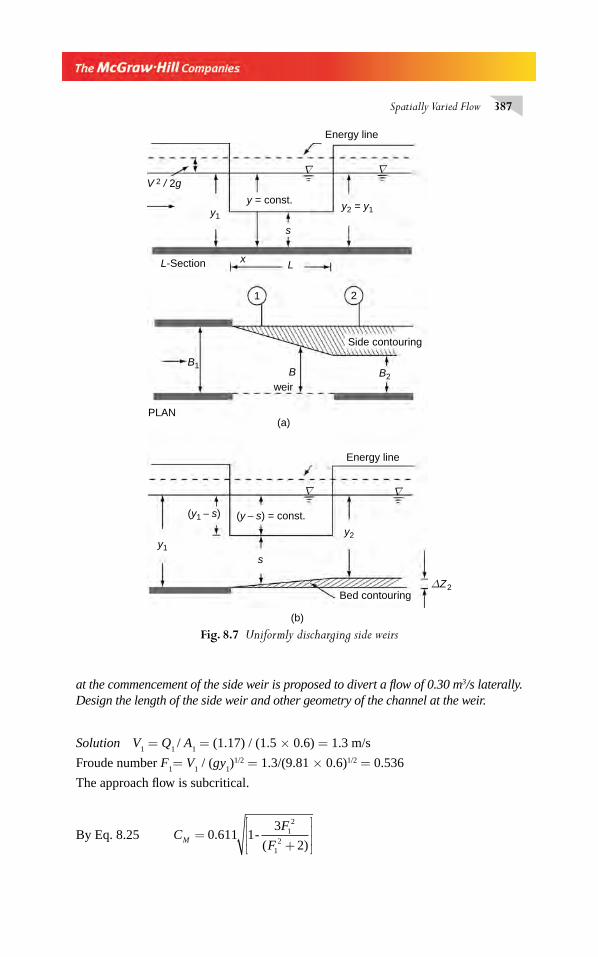
Spatially Varied Flow 387
at the commencement of the side weir is proposed to divert a fl ow of 0.30 m3/s laterally. Design the length of the side weir and other geometry of the channel at the weir.
Solution V1 = Q
1 / A
1 = (1.17) / (1.5 × 0.6) = 1.3 m/s
Froude number F1= V
1 / (gy
1)1/2 = 1.3/(9.81 × 0.6)1/2 = 0.536
The approach fl ow is subcritical.
By Eq. 8.25 CF
FM =+
⎡
⎣⎢⎢
⎤
⎦⎥⎥0 611 1
3
212
12
. -( )
Fig. 8.7 Uniformly discharging side weirs
∇
∇∇
∇
L
y2 = y1y = const.
V 2 / 2g
L-Section
y1
y1
(y1 − s) (y − s) = const.
y2
x
s
s
Energy line
Energy line
1 2
Side contouring
PLAN(a)
(b)
weirB2B
B1
Bed contouringΔZ2
Chapter 8.indd 387Chapter 8.indd 387 2/24/2010 3:03:30 PM2/24/2010 3:03:30 PM
388 Flow in Open Channels
= −×
+{ }⎡
⎣
⎢⎢⎢
⎤
⎦
⎥⎥⎥
0 611 13 0 536
0 536 2
2
2.
( . )
( . )
= 0.482
Critical depth at Section 1 = = =⎡
⎣⎢⎢
⎤
⎦⎥⎥y q gc1
2 1 32 1 3
1 17 1 50
9 81( / )
( . / . )
./
/
= 0.396 m
Height of the weir crest = s = 0.42 m
Since yc1
< s, Type 1 fl ow will prevail and y1 = y
0 = 0.60 m.
Depth of water over the weir = ( y − s) = (0.60 − 0.42) = 0.18 m.
Diverted discharge Q C g L y ss M= −2
32 3 2( ) /
0 30
2
30 482 19 62 0 18 3 2. . . ( . ) /= × × × ×L
= 0.1087 L
Length of the side weir L = 0.30/0.1087 = 2.76 m Q
2 = downstream discharge = 1.17 − 0.30 = 0.87 m3/s
For a uniformly discharging side weir, V1 = V
2 = V.
Hence V2 = 1.3 m/s and A
2 = Q
2/V
2 = 0.87/1.3 = 0.6692 m2.
(i) If side contouring is adopted, y1 = y
2= y
Bed width at Section 2 = B2 = A
2/y
2 = 0.6692 /0.60 = 1.115 m
The bed width varies from 1.50 m at Section 1 to 1.115 m at Section 2, distance 2.76 m downstream of Section 1, linearly.(ii) If bed contouring is adopted, B
1 = B
2 = B
Depth of fl ow at Section 2 = y2 = A
2/B
2 = 0.6692/1.50
= 0.446 m Δ z
2 = change in the elevation of bed at Section 2
= 0.600 − 0.446 = 0.154 m.
The variation of Δ z is linear with a value of zero at Section 1 and 0.154 m at Section 2.
8.5 BOTTOM RACKS
A bottom rack is a device provided at the bottom of a channel for purposes of divert-ing a part of the fl ow. The device consists essentially of an opening in the channel bottom covered with a metal rack to prevent the transport of unwanted solid material
Chapter 8.indd 388Chapter 8.indd 388 2/24/2010 3:03:31 PM2/24/2010 3:03:31 PM
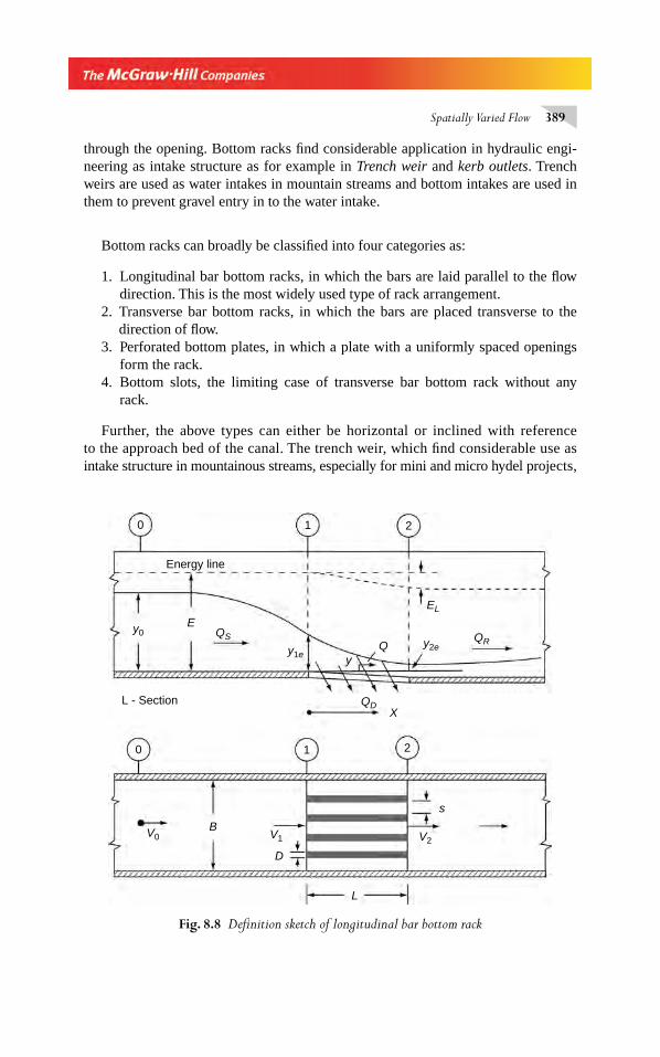
Spatially Varied Flow 389
through the opening. Bottom racks fi nd considerable application in hydraulic engi-neering as intake structure as for example in Trench weir and kerb outlets. Trench weirs are used as water intakes in mountain streams and bottom intakes are used in them to prevent gravel entry in to the water intake.
Bottom racks can broadly be classifi ed into four categories as:
1. Longitudinal bar bottom racks, in which the bars are laid parallel to the fl ow direction. This is the most widely used type of rack arrangement.
2. Transverse bar bottom racks, in which the bars are placed transverse to the direction of fl ow.
3. Perforated bottom plates, in which a plate with a uniformly spaced openings form the rack.
4. Bottom slots, the limiting case of transverse bar bottom rack without any rack.
Further, the above types can either be horizontal or inclined with reference to the approach bed of the canal. The trench weir, which fi nd considerable use as intake structure in mountainous streams, especially for mini and micro hydel projects,
Fig. 8.8 Defi nition sketch of longitudinal bar bottom rack
0 1 2
0 1 2
Energy line
L - Section
EL
QRy2ey1e
y0
V0 V1 V2
y
QD
QSQ
E
B
D
L
s
X
Chapter 8.indd 389Chapter 8.indd 389 2/24/2010 3:03:31 PM2/24/2010 3:03:31 PM
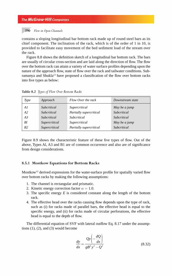
390 Flow in Open Channels
contains a sloping longitudinal bar bottom rack made up of round steel bars as its chief component. The inclination of the rack, which is of the order of 1 in 10, is provided to facilitate easy movement of the bed sediment load of the stream over the rack.
Figure 8.8 shows the defi nition sketch of a longitudinal bar bottom rack. The bars are usually of circular cross-section and are laid along the direction of fl ow. The fl ow over the bottom rack can attain a variety of water surface profi les depending upon the nature of the approach fl ow, state of fl ow over the rack and tailwater conditions. Sub-ramanya and Shukla13 have proposed a classifi cation of the fl ow over bottom racks into fi ve types as below:
Table 8.2 Types of Flow Over Bottom Racks
Type Approach Flow Over the rack Downstream state
A1 Subcritical Supercritical May be a jump
A2 Subcritical Partially supercritical Subcritical
A3 Subcritical Subcritical Subcritical
Bl Supercritical Supercritical May be a jump
B2 Supercritical Partially supercritical Subcritical
Figure 8.9 shows the characteristic feature of these fi ve types of fl ow. Out of the above, Types Al, A3 and B1 are of common occurrence and also are of signifi cance from design considerations.
8.5.1 Mostkow Equations for Bottom Racks
Mostkow12 derived expressions for the water-surface profi le for spatially varied fl ow over bottom racks by making the following assumptions:
1. The channel is rectangular and prismatic.2. Kinetic energy correction factor α = 1.0.3. The specifi c energy E is considered constant along the length of the bottom
rack.4. The effective head over the racks causing fl ow depends upon the type of rack,
such as (i) for racks made of parallel bars, the effective head is equal to the specifi c energy, and (ii) for racks made of circular perforations, the effective head is equal to the depth of fl ow.
The differential equation of SVF with lateral outfl ow Eq. 8.17 under the assump-tions (1), (2), and (3) would become
dy
dx
QydQ
dx
gB y Q=
−⎛⎝⎜⎜⎜
⎞⎠⎟⎟⎟
−2 3 2 (8.32)
Chapter 8.indd 390Chapter 8.indd 390 2/24/2010 3:03:31 PM2/24/2010 3:03:31 PM
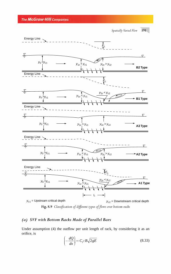
Spatially Varied Flow 391
(a) SVF with Bottom Racks Made of Parallel Bars
Under assumption (4) the outfl ow per unit length of rack, by considering it as an orifi ce, is
−⎛⎝⎜⎜⎜
⎞⎠⎟⎟⎟⎟ =
dQ
dxC B gE1 2ε (8.33)
Fig. 8.9 Classifi cation of diff erent types of fl ows over bottom racks
EL
EL
y1c < yc1
y1c > yc1
y1c < yc1
y1c < yc1
y1c < yc1
y2c > yc2
y2c < yc2
y0 >yc1
y0 >yc1
y0 >yc1
y0 >yc1
y0 >yc1
y2c > yc2
y2c > yc2
y2c < yc2
L
Energy Line
Energy Line
Energy Line
Energy Line
Energy Line
B1 Type
A3 Type
A2 Type
A1 Type
B2 Type
∇
∇
∇
∇
∇
∇
∇
∇
∇
∇
yc1 = Upstream critical depth yc2 = Downstream critical depth
EL
Chapter 8.indd 391Chapter 8.indd 391 2/24/2010 3:03:31 PM2/24/2010 3:03:31 PM
392 Flow in Open Channels
in which C1, = a defi ned coeffi cient of discharge and ε = void ratio = ratio of the
opening area to the total rack area. Since the specifi c energy E = constant, the dis-charge Q at any section is given by:
Q By g E y= −2 ( ) (8.34)
Substituting Eqs 8.33 and 8.34 in Eq. 8.32
dy
dx
C E E y
y E=
−−
2
3 21ε ( )
(8.35)
On integration,
xE
C
y
E
y
E= − − +
ε 1
1 Const. (8.36)
Putting y/E = η and using the boundary condition y = y1 and x = 0, gives
xE
C= − − −
εη η η η
11 11 1( ) (8.37)
which is the equation of the SVF profi le. As in the case of the De Marchi equation (Section 8.3.3), the control depths for use in Eq. 8.37 which are compatible with the assumptions are:
(i) y1
= y0 for A3 and B1 type fl ows and
(ii) y1 = y
C1 for A1 type fl ows.
Note that from Eq. 8.37, dQ
dx
⎛⎝⎜⎜⎜
⎞⎠⎟⎟⎟⎟
is constant along the rack. Hence the total discharge
Qs diverted out is,
Q C BL gEs = 1 2ε (8.38)
(b) SVF Equation for Bottom Racks Made of Perforated Plates
For perforated plate bottom racks the outfl ow discharge per unit length, under assumption (4), is
−⎛⎝⎜⎜⎜
⎞⎠⎟⎟⎟⎟ =
dQ
dxC B g y2 2ε (8.39)
where C2 = discharge coeffi cient for perforated plate fl ow. Substituting Eqs 8.39 and
8.34 in Eq. 8.32, and simplifying
dy
dx
C y E y
y E=
−−
2
3 22ε ( )
(8.40)
Chapter 8.indd 392Chapter 8.indd 392 2/24/2010 3:03:32 PM2/24/2010 3:03:32 PM
Spatially Varied Flow 393
Integrating and using the boundary condition y = yi at x = 0, yields the SVF profi le
for perforated bottom plates as
xE
C= −( )+ −( ) − −( )
⎡
⎣⎢⎢
⎤
⎦⎥⎥
− −
εη η η η η η
2
1 11 1 1
1
2
3
21 1cos cos (8.41)
in which η = y E/ and suffi x 1 refers to Section 1.
8.5.2 Estimation of Discharge Through a Bottom Rack
Longitudinal Bar Bottom Rack For purposes of estimation; the diverted discharge Q
d is expressed in terms of the specifi c energy E
0 at the reference approach
section, in a manner similar to Eq. 8.38 as
Q C B L gEd d= ε 2 0 (8.42)
where Cd = coeffi cient of discharge of the longitudinal bar bottom rack. As a result
of experimental studies, Subramanya15,16 has shown that,
C fn D s Sd L E= [ / , ,η and (type of fl ow)] (8.43)
where D = diameter of the rack bar; s = clear spacing of the bars in the rack,
SL = longitudinal slope of the rack and η
E = a fl ow parameter =
V
gE
F
F02
0
02
022 2
=+
⎛
⎝⎜⎜⎜⎜
⎞
⎠⎟⎟⎟⎟ .
The functional relationship for the variation of Cd in various types of fl ows are as
below:
(a) Inclined Racks
Al Type fl ow : Cd = 0.53 + 0.4 log (D/s) − 0.61 S
L (8.44)
Bl Type fl ow : Cd = 0.39 + 0.27 log (D/s) − 0.8 η
E − 0.5 log S
L (8.45)
(b) Horizontal Racks
Al Type fl ow : Cd = 0.601 + 0.2 log (D/s) − 0.247 ηE (8.46)
A3 Type fl ow : Cd = 0.752 + 0.28 log (D/s) − 0.565 ηE (8.47)
Bl Type fl ow : Cd = 1.115 + 0.36 log (D/s) − 1.084 ηE (8.48)
It has been found15,16 that the energy loss over the rack is signifi cant in Type Al and Type Bl fl ows. However, the energy loss over the rack is not signifi cant in Type A3 fl ows. This implies that Mustkow’s water surface profi le equation (Eq. 8.41)
Chapter 8.indd 393Chapter 8.indd 393 2/24/2010 3:03:32 PM2/24/2010 3:03:32 PM
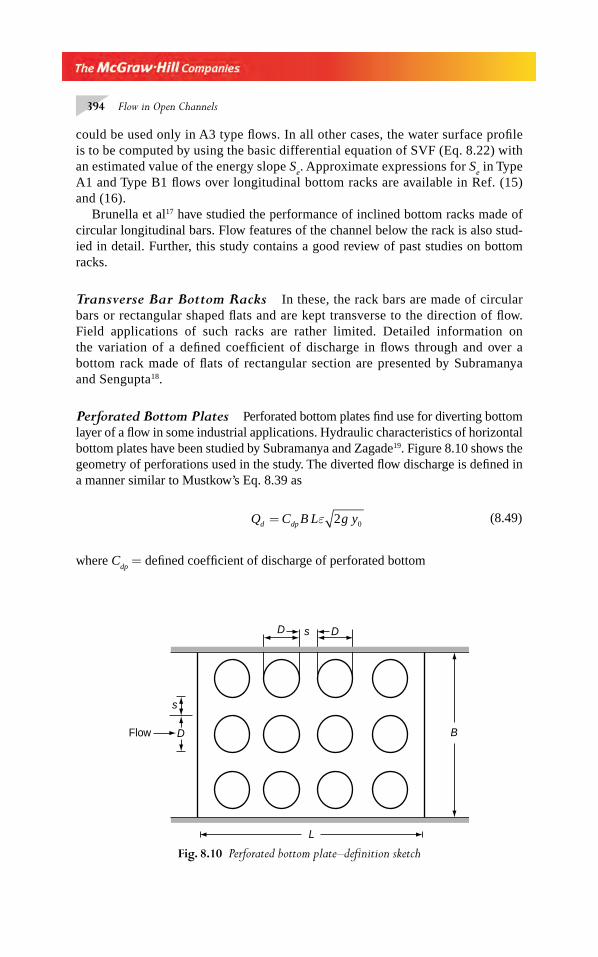
394 Flow in Open Channels
could be used only in A3 type fl ows. In all other cases, the water surface profi le is to be computed by using the basic differential equation of SVF (Eq. 8.22) with an estimated value of the energy slope S
e. Approximate expressions for S
e in Type
A1 and Type B1 fl ows over longitudinal bottom racks are available in Ref. (15) and (16).
Brunella et al17 have studied the performance of inclined bottom racks made of circular longitudinal bars. Flow features of the channel below the rack is also stud-ied in detail. Further, this study contains a good review of past studies on bottom racks.
Transverse Bar Bottom Racks In these, the rack bars are made of circular bars or rectangular shaped fl ats and are kept transverse to the direction of fl ow. Field applications of such racks are rather limited. Detailed information on the variation of a defi ned coeffi cient of discharge in fl ows through and over a bottom rack made of fl ats of rectangular section are presented by Subramanya and Sengupta18.
Perforated Bottom Plates Perforated bottom plates fi nd use for diverting bottom layer of a fl ow in some industrial applications. Hydraulic characteristics of horizontal bottom plates have been studied by Subramanya and Zagade19. Figure 8.10 shows the geometry of perforations used in the study. The diverted fl ow discharge is defi ned in a manner similar to Mustkow’s Eq. 8.39 as
Q C B L g yd dp= ε 2 0 (8.49)
where Cdp
= defi ned coeffi cient of discharge of perforated bottom
D D
B
s
s
D
L
Flow
Fig. 8.10 Perforated bottom plate–defi nition sketch
Chapter 8.indd 394Chapter 8.indd 394 2/24/2010 3:03:32 PM2/24/2010 3:03:32 PM
Spatially Varied Flow 395
plate, y0 = depth of fl ow at reference approach section. The variation of C
dp for vari-
ous types of fl ows are 19
(a) A1 Type fl ow: For B/L ≥ 2.0,
CD
s
D
t
B
Ldp = − + +0 292 0 03 0 0083 0 058. . . . (8.50)
For B/L < 1.78, CDp
is essentially independent of B/L and
C D s D tdp = − +0 41 0 03 0 0083. . ( / ) . ( / ) (8.51)
where t = thickness of the plate, and D = diameter of the perforation.
(b) B1 Type fl ows:
C
Fdp
E
0
0 26 0 28= −. . η (8.52)
where ηE = a fl ow parameter =
V
gE
F
F02
0
02
022 2
=+( )
As in longitudinal bar bottom racks, here also the energy loss has been found to be signifi cant in A1 and B1 Type fl ows and as such Mustkow’s water surface profi le equation (Eq. 8.41) is not valid for these types of fl ows. Approximate expressions for the estimation of the energy slope S
e in fl ows over perforated bottom plates, for use
in the basic differential equation of SVF, are available in Ref. (19).
Bottom Slots Bottom slots are the limiting cases of transverse bar bottom racks and their practical applications are rather limited. The diverted discharge Q
d through
a slot of length L and spanning the full width of the channel can be expressed as
Q C BL gEd ds= ε 2 0 (8.53)
where E0 = specifi c energy of the approach fl ow, and C
ds = coeffi cient of discharge
of the slot.The variation of C
ds has been studied by Nasser et al20 and Ramamurthy et al21.
REFERENCES
1. Hinds, J, ‘Side Channel Spillways’, Trans. ASCE, Vol. 89, 1926, pp 881–927.2. Smith, K V H, ‘Control Point in a Lateral Spillway Channel’, J. of Hyd. Div., Proc. ASCE,
May 1967, pp 27–34.3. Li, W H, ‘Open Channels with Non-uniform Discharge’, Trans. ASCE, Vol. 120, 1955,
pp 255–274.4. Gill, M A, ‘Perturbation Solution of Spatially Varied Flow in Open Channels’, J. of Hyd.
Res., IAHR, Vol.15, No. 4, 1977, pp 337–350.
Chapter 8.indd 395Chapter 8.indd 395 2/24/2010 3:03:33 PM2/24/2010 3:03:33 PM
396 Flow in Open Channels
5. McCool, D K, Gwinn, W R, Ree, W O, and Garton, J E, ‘Spatially Varied Flow in Vege-tated Channel’, Trans. ASCE, Vol. 9, No. 3, 1966, pp 440–444.
6. Farney, H S, and Markus, A ‘Side-channel Spillway Design’, J. of Hyd. Div., Proc. ASCE,May 1962, pp 131–154.
7. Subramanya, K, and Awasthy, S C, ‘Spatially Varied Flow Over Side-Weirs’, J. of Hyd. Div., Proc. ASCE, Jan. 1972, pp 1–10.
8. Borghi, S M, et al, ‘Discharge Coeffi cient for Sharp-crested Side Weirs in Sub-critical Flow’, Journal of Hyd. Engg., ASCE, Vol. 125, No. 10, 1999, pp. 1051–1056.
9. Olivetto, G, et al, ‘Hydraulic Features of Supercritical Flow Along Prismatic Side Weirs’, Journal of Hyd. Research, IAHR, Vol. 39, No. 1, 200l, pp. 73–82.
10. Ghodsian, M, ‘Flow Over Triangular Side Weirs’, Scientia Iranica, Vol. 11, No. 1 & 2, April 2004, pp. 114–120.
11. Uyumaz, A, ‘Side Weir in Triangular Channel’, Journal of Irr. and Drainage Engg., ASCE, Vol. 118, No. 6, 1992, pp. 965–970.
12. Ramamurthy, A, S, Subramanya, K, and Caraballada, L, ‘Uniformly Discharging Lateral Weirs’, Journal of Irr. and Drainage Div., ASCE, Dec. 1978, pp. 399–411.
13. Subramanya, K, and Shukla, S K, ‘Discharge Diversion Characteristics of Trench Weirs’, Journal of Civil Engg. Div., Inst. Of Engrs. (India), Vol. 69, CI 3, Nov. 1988. pp. 163–168.
14. Mustkow, M A, ‘A Theoretical Study of Bottom Type Intakes’, La Houille Blanche, No. 4, Sept. 1957, pp. 570–580.
15. Subramanya, K, ‘Trench Weir Intake for Mini Hydro Projects’, Proc. Hydromech and Water Resources Conf, I.I.Sc., Bangaloe, India, 1990, pp. 33–41.
16. Subramanya, K, ‘Hydraulic Characteristics of Inclined Bottom Intakes’, Proc. National Symp. On Recent Trends in Design of Hydraulic Structures, UOR, Roorkee, India, March 1994, pp. 1–9.
17. Brunella, S, et al, ‘Hydraulics of Bottom Racks’, Journal of Hyd. Engg., Vol. 29, No. 1, Jan. 2003, pp. 2–9.
18. Subramanya, K and Sengupta, D, ‘Flow Through Bottom Racks’, Indian Jour. Tech., CSIR, Vol. 19, No. 2, Feb. 1981, pp. 64–67.
19. Subramanya, K, and Zagade, S B, ‘Flow Over Perforated Bottom Plates’, Proc 17th Nat. Conf. of FM and FP., REC, Warangal, India, 1990, pp. C-51–C-57.
20. Nasser, M S, et al, ‘Flow in Channel with a Slot in a Bed’, Journal of Hyd. Res., IAHR, No. 4, 1980, pp. 359–367.
21. Ramamurthy, A S, and Satish, M S, ‘Discharge Characteristics of Flow Past a Floor Slot’,Journal if Irr. and Drainage Engg., ASCE, Vol. 112, No. 1, 1986, pp. 20–27.
PROBLEMS
SI. No. Topic Problems
1 Lateral spillway channel 8.1 to 8.6
2 Side weir 8.7, 8.8
3 Uniformly discharging side weir 8.9, 8.10
4 Bottom racks 8.11 to 8.13
5 Radial fl ow 8.34
Problem Distribution
Chapter 8.indd 396Chapter 8.indd 396 2/24/2010 3:03:33 PM2/24/2010 3:03:33 PM
Spatially Varied Flow 397
8.1 Show that the following equation is applicable to a control section where critical depth occurs in a frictionless lateral spillway channel:
S gA T
qc c0
2
241
β*
=
8.2 A side channel spillway channel is 100 m long and is rectangular in cross-section with B = 5.0 m, n = 0.020, β = 1.30 and S
0 = 0.15. If the lateral infl ow rate is 1.75 m3/s/m, fi nd the
critical depth and its location.8.3 A lateral spillway channel is trapezoidal in cross-section with B = 10.0 m, side slope
m = 0.5 and Manning’s roughness n = 0.018. The bed slope is 0.08. If the lateral infl ow rate is 2.5 m3/s/m length, fi nd the critical depth and its location. Assume β = 1.20.
8.4 Show that for a wide rectangular channel having SVF with a constant in fl ow rate of q*,
the critical fl ow section is given by
xq
g S g Cc =−8 2
02 3
*( / )
when β = 1.0 is assumed and Chezy formula with C = constant is used. What would be the corresponding value of y
c?
8.5 A lateral spillway channel of length L is rectangular in cross-section. If at the channel exit, y
e = depth of fl ow and F
e = Froude number, show by neglecting friction and assuming β =
1.0, that the critical depth yc is given by
y
yF Gc
e
e= 4 2 2/ and is located at xc, given by
x
y
F
G Sc
e
e=8 2
20
where GS L
ye
= 0
8.6 A wide rectangular channel of length L having a uniform lateral infl ow rate has a discharge of q
e per unit width at the channel exit. If the Darcy–Weisbach friction factor f is used for
representing friction effects, show that
yq
gL S fc
e=−( )
256
8
2
20
2
and xq
gL S fc
e=−( )
4096
8
2
20
3
8.7 A 3.0-m wide rectangular channel can carry a discharge of 3.60 m3/s at a normal depth of 1.2 m. Design a side weir so that it will pass all the fl ow in the canal when the discharge is 2.00 m3/s and will divert 0.6 m3/s when the canal discharge is 3.60 m3/s.
Chapter 8.indd 397Chapter 8.indd 397 2/24/2010 3:03:33 PM2/24/2010 3:03:33 PM
398 Flow in Open Channels
8.8 A rectangular canal of 2.0 m width carries a fl ow with a velocity of 8.75 m/s and depth of 1.25 m. A side weir of height 0.75 m and length 1.20 m is provided in one of its walls. Find the quantity of fl ow diverted by the side weir.
8.9 A rectangular channel is 1.5 m wide and conveys a discharge of 2.0 m3/s at a Froude number of 0.3. A uniformly discharging side weir having contouring on the sides only is set at a height of 0.4 m above the bed with its crest horizontal. If the length of the side weir is 1.8 m, estimate the total fl ow diverted by the side weir.
8.10 A rectangular channel is 2.0 m wide and carries a fl ow of 3.00 m3/s at a depth of 0.9 m. At a certain location in this channel a uniformly discharging side weir is proposed to divert 0.30 m3/s of fl ow laterally. The weir crest is horizontal and is placed at a height of 0.65 m above the bed at the commencement of the side weir. Calculate the length of the side weir and other dimensions of the channel geometry to achieve the objective.
8.11 Show that, by Mustkow’s method of analysis, the minimum length Lm of a parallel bar
bottom rack required to completely divert the initial discharge Q1 in a channel is given by
LQ
C B gE
E
C
y
E
y
Em = = −⎡
⎣⎢⎢⎢
⎤
⎦⎥⎥⎥
1
1 1
1 1
21
ε ε
8.12 A mountainous stream is of rectangular cross section and has a width of 10.0 m, depth of fl ow of 0.25 m and carries a discharge of 6.0 m3/s. A trench weir type intake made up of longitudinal parallel bar rack is proposed at a section to divert the fl ow. The proposed rack has a longitudinal slope of 0.01 and is made of circular bars with diameter to spac-ing ratio of 1.0. Estimate the minimum length of the rack required to completely divert the fl ow. The blockage due to debris can be assumed as 50% of rack opening.
8.13 A 2.0-m wide rectangular channel carries a discharge of 3.5 m3/s at a Froude number of 0.30. A 2.0-m long parallel longitudinal bar bottom rack having a void ratio (ratio of opening to total rack area) of 0.2 is provided at a section. Supercritical fl ow is known to occur over the rack. Estimate the discharge diverted out.
8.14 An axisymmetric radial fl ow emanates from a source on to a horizontal plane. Show that the basic differential equation of SVF with decreasing discharges can be expressed in this case as
dy
dx
V
grS
V
g y
f
=
⎛
⎝⎜⎜⎜⎜
⎞
⎠⎟⎟⎟⎟−
−⎛
⎝⎜⎜⎜⎜
⎞
⎠⎟⎟⎟⎟
2
2
1
OBJECTIVE QUESTIONS
8.1 The basic differential equation of SVF with increasing discharge is based on the(a) continuity equation (c) energy equation(b) momentum equation (d) Manning’s equation
8.2 The basic differential equation of SVF with decreasing discharge is based on the(a) continuity equation (c) energy equation(b) momentum equation (d) Manning’s equation
Chapter 8.indd 398Chapter 8.indd 398 2/24/2010 3:03:33 PM2/24/2010 3:03:33 PM
Spatially Varied Flow 399
8.3 The differential equation of SVF with decreasing discharge has one extra term in the numerator on the right-hand side when compared to the corresponding GVF equation. This term is
(a) − ∗22
αQq
gA (b) + ∗2
2
αQq
gA
(c) − ∗22
β Qq
gA (d) − ∗αQq
gA2
8.4 The transitional profi le in a lateral spillway channel is(a) independent of the roughness of the channel(b) independent of rate of lateral fl ow(c) independent of channel geometry(d) independent of the bottom slope of the channel
8.5 The fl ow profi le in a side spillway channel can be determined by using(a) Standard step method(b) Standard Runge-Kutta method(c) De Marchi equation(d) Mustokow equation
8.6 A lateral spillway channel is rectangular in cross-section with a bottom width of 4.0 m. At a certain fl ow the critical depth was found to be 0.5 m and occurred at a distance of 5.53 m from the upstream end. The lateral infl ow rate in m3/s/m is (a) 0.20 (b) 0.40(c) 0.80 (d) 1.10
8.7 The De Marchi varied-fl ow function is(a) used in SVF over bottom racks(b) used in SVF in lateral spillway channels(c) meant for side weirs in frictionless rectangular channels(d) meant for subcritical fl ows only
8.8 The De Marchi coeffi cient of discharge CM for a side weir is
(a) independent of the Froude number(b) same as that of a normal weir(c) essentially a function of inlet Froude number, F
1
(d) approaches unity as Fl → 0
8.9 A rectangular channel 2.5 m wide has a discharge of 2.0 m3/s at a depth of 0.8 m. The coeffi cient of discharge C
M of a side weir introduced in a side of this channel with a crest
height of 0.2 m above the bed is(a) 0.574 (b) 0.611(c) 0.286 (d) 0.851
8.10 To achieve uniformly discharging side weirs the area of fl ow A at any section distance x from the upstream end of the weir is related as:
(a) A A Mx= −1 (b) A A Mx= −2
(c) A Mx= (d) A x= 3 2/
8.11 A side weir is provided in the side of channel. If E = specifi c energy is assumed constant, at any section within the length of the side weir, the discharge Q in the channel is given by
(a) Q = constant (b) Q B E y g= −( )2
(c) QBy
E y=
−2 (d) Q By g E y= −2 ( )
Chapter 8.indd 399Chapter 8.indd 399 2/24/2010 3:03:34 PM2/24/2010 3:03:34 PM

400 Flow in Open Channels
8.12 In a uniformly discharging side weir provided in the side of a rectangular channel having subcritical fl ow, the longitudinal water surface along the weir(a) increases in the downstream direction(b) remains parallel to the crest(c) decreases in the downstream direction(d) increases linearly in the downstream direction
8.13 In a uniformly discharging side weir in a rectangular channel, if x is the longitudinal dis-tance from the start of the weir(a) the area of the fl ow cross-section in the canal decreases linearly with x(b) the mean velocity of the fl ow varies linearly with x(c) the depth of fl ow above the weir crest varies linearly with x(d) the area of fl ow cross-section in the canal remains constant
8.14 A trench weir type intake has as its main component a(a) side weir (c) transverse, parallel bar bottom rack(b) longitudinal, parallel bar bottom rack (d) perforated bottom plate
Chapter 8.indd 400Chapter 8.indd 400 2/24/2010 3:03:34 PM2/24/2010 3:03:34 PM
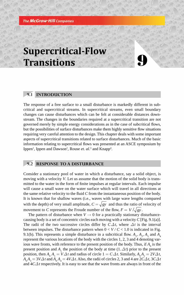
9.1 INTRODUCTION
The response of a free surface to a small disturbance is markedly different in sub-critical and supercritical streams. In supercritical streams, even small boundary changes can cause disturbances which can be felt at considerable distances down-stream. The changes in the boundaries required at a supercritical transition are not governed merely by simple energy considerations as in the case of subcritical fl ows, but the possibilities of surface disturbances make them highly sensitive fl ow situations requiring very careful attention to the design. This chapter deals with some important aspects of supercritical transitions related to surface disturbances. Much of the basic information relating to supercritical fl ows was presented at an ASCE symposium by Ippen1, Ippen and Dawson2, Rouse et. al.3 and Knapp4.
9.2 RESPONSE TO A DISTURBANCE
Consider a stationary pool of water in which a disturbance, say a solid object, is moving with a velocity V. Let us assume that the motion of the solid body is trans-mitted to the water in the form of fi nite impulses at regular intervals. Each impulse will cause a small wave on the water surface which will travel in all directions at the same relative velocity to the fl uid C from the instantaneous position of the body. It is known that for shallow waves (i.e., waves with large wave lengths compared
with the depth) of very small amplitude, C = gy and thus the ratio of velocity of movement to C represents the Froude number of the fl ow, F = V gy/ .
The pattern of disturbance when V → 0 for a practically stationary disturbance-causing body is a set of concentric circles each moving with a velocity C [Fig. 9.1(a)]. The radii of the two successive circles differ by C Δ t, where Δ t is the interval between impulses. The disturbance pattern when 0 < V / C < 1.0 is indicated in Fig. 9.1(b). This represents a simple disturbance in a subcritical fl ow. A
1, A
2, A
3 and A
4
represent the various locations of the body with the circles 1, 2, 3 and 4 denoting var-ious wave fronts, with reference to the present position of the body. Thus, if A
0 is the
present position and A1 the position of the body at time (1. Δ t) prior to the present
position, then A0
A1 = V Δ t and radius of circle 1 = C Δ t. Similarly, A
0 A
2 = 2VΔ t,
A0 A
3 = 3VΔ t and A
0 A
4 = 4VΔ t. Also, the radii of circles 2, 3 and 4 are 2CΔ t, 3CΔ t
and 4CΔ t respectively. It is easy to see that the wave fronts are always in front of the
Supercritical-Flow
Transitions 9
Chapter 9.indd 401Chapter 9.indd 401 2/24/2010 3:06:02 PM2/24/2010 3:06:02 PM
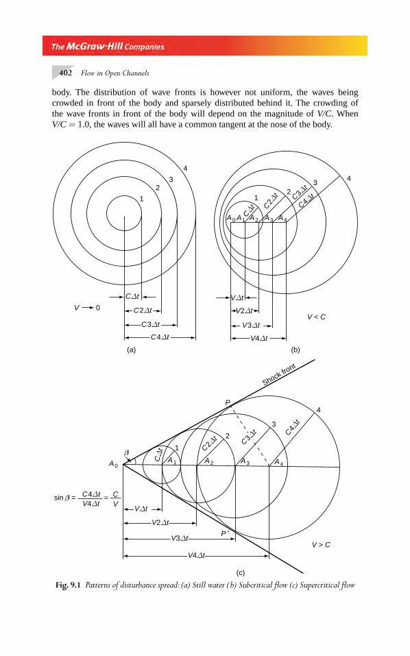
402 Flow in Open Channels
body. The distribution of wave fronts is however not uniform, the waves being crowded in front of the body and sparsely distributed behind it. The crowding of the wave fronts in front of the body will depend on the magnitude of V/C. When V/C = 1.0, the waves will all have a common tangent at the nose of the body.
Fig. 9.1 Patterns of disturbance spread: (a) Still water ( b) Subcritical fl ow (c) Supercritical fl ow
V4ΔtV > C
(c)
1
1 1
2
2 2
3
3 3
4
44
A1
A1
A0
A0
A2
A2
P
P ′
A3
A3
A4
A4
CΔ
t
C4ΔtV4Δt
sin β = = CV
VΔt
VΔtCΔt
CΔt
V2Δt
V2Δt
V3Δt
V3Δt
C3Δt
C2Δt
V4Δt
C4Δ
t
β
V < C
Shock front
(b)(a)
C2Δt
C2Δ
t
C3Δt
C3Δt
C4Δt
C4Δt
V 0
Chapter 9.indd 402Chapter 9.indd 402 2/24/2010 3:06:05 PM2/24/2010 3:06:05 PM
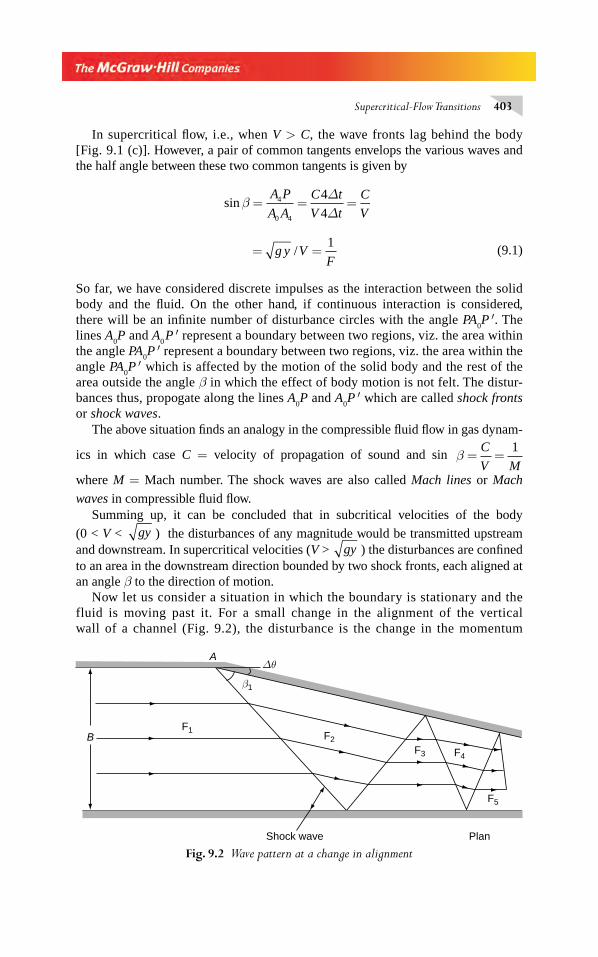
Supercritical-Flow Transitions 403
In supercritical fl ow, i.e., when V > C, the wave fronts lag behind the body [Fig. 9.1 (c)]. However, a pair of common tangents envelops the various waves and the half angle between these two common tangents is given by
sin β = = =A P
A A
C t
V t
C
V4
0 4
4
4
ΔΔ
= =g y VF
/1
(9.1)
So far, we have considered discrete impulses as the interaction between the solid body and the fl uid. On the other hand, if continuous interaction is considered, there will be an infi nite number of disturbance circles with the angle PA
0P ′. The
lines A0P and A
0 P ′ represent a boundary between two regions, viz. the area within
the angle PA0P ′ represent a boundary between two regions, viz. the area within the
angle PA0P ′ which is affected by the motion of the solid body and the rest of the
area outside the angle β in which the effect of body motion is not felt. The distur-bances thus, propogate along the lines A
0P and A
0P ′ which are called shock fronts
or shock waves.The above situation fi nds an analogy in the compressible fl uid fl ow in gas dynam-
ics in which case C = velocity of propagation of sound and sin β = =C
V M
1
where M = Mach number. The shock waves are also called Mach lines or Mach
waves in compressible fl uid fl ow.Summing up, it can be concluded that in subcritical velocities of the body
(0 < V < gy ) the disturbances of any magnitude would be transmitted upstream and downstream. In supercritical velocities (V > gy ) the disturbances are confi ned to an area in the downstream direction bounded by two shock fronts, each aligned at an angle β to the direction of motion.
Now let us consider a situation in which the boundary is stationary and the fluid is moving past it. For a small change in the alignment of the vertical wall of a channel (Fig. 9.2), the disturbance is the change in the momentum
Fig. 9.2 Wave pattern at a change in alignment
BF1
F2
F3 F4
F5
Shock wave Plan
Δθ
β1
A
Chapter 9.indd 403Chapter 9.indd 403 2/24/2010 3:06:05 PM2/24/2010 3:06:05 PM
404 Flow in Open Channels
caused by the deflection on the boundary by Δ θ at A. In subcritical flow past the boundary, the change in momentum will be reflected by a permanent defor-mation of the stream surface, upstream and downstream of the point A. In supercritical flow, however, the boundary change at A cannot affect the flow upstream and hence the effect of the disturbance will be confined to a region, downstream of A, bounded by the shock wave emanating from A and the boundary. The effect of the disturbance will be felt as a change of depth in this area. Since the flow is confined between two side boundaries, the shock wave undergoes multiple reflections at the boundaries resulting in a highly disturbed water sur-face in the downstream.
9.3 GRADUAL CHANGE IN THE BOUNDARY
Consider a supercritical fl ow in a horizontal frictionless rectangular channel (Fig. 9.3) with one of the walls defl ected through a small angle Δ θ. The change in the boundary
Fig. 9.3 Supercritical fl ow past a small change in boundary alignment
y1
V1
V2
y1, V1
y2 , V
2
V1
y2Vn1
Vt1 Vt2Vn1
Vn2
Vn2
(β1 − Δθ) (− Δ Vn)Δθ
Δθβ1
β1
AB
DC
M
M
Shock w
ave
Section MM
∇
∇
Chapter 9.indd 404Chapter 9.indd 404 2/24/2010 3:06:05 PM2/24/2010 3:06:05 PM
Supercritical-Flow Transitions 405
causes a shock wave at an angle β1, to the approaching fl ow. The fl ow upstream of
the shock has a velocity of V1 and depth y
1 and the fl ow after the shock has a velocity
of V2 and depth y
2. From the vector diagram of the velocities,
Vn1
= V1 sin β
1
Vt1 = V
1 cos β
1
Vn2
= V2 sin (β
1 − Δ θ)
Vt2 = V
2 cos (β
1 − Δ θ)
where the suffi xes n and t refer to the normal and tangential directions with respect to the shock front. Considering the unit width of the shock-wave front, the continuity equation can be written as
y V y Vn n1 1 2 2= (9.2)
In a direction normal to the shock wave, the momentum equation is written as
1
2
1
212
22
2 12
2
1
2γ γ ρ ρy y y V y Vn n
− = − (9.3)
From Eqs 9.2 and 9.3
V g yy
y
y
yn1 12
1
2
1
1
21= +
⎛
⎝⎜⎜⎜⎜
⎞
⎠⎟⎟⎟⎟ (9.4)
For very small disturbances, y2 → y
1 and hence,
V V g yn1 1 1= →sin ,β and dropping suffi xes
V V g yn = =sin β or
sin β =g y
V (9.5)
which is the same result as in Eq. 9.1.From the vector triangle ABD,
−Δ( )
Δ=
+ −Δ( )V Vn
sin sinθ β θ1
190
i.e. −Δ =Δ
+ −Δ( )V
Vn
1
190
sin
sin
θβ θ
As Δθ → 0, − =dV
d
Vn
θ βcos (9.6)
Chapter 9.indd 405Chapter 9.indd 405 2/24/2010 3:06:06 PM2/24/2010 3:06:06 PM
406 Flow in Open Channels
The momentum equation, Eq. 9.3 can be written as
P M yg
V yn+ = + =1
22 2γ
γConst.
Differentiating,
γγ γ
y d yg
V y dVg
V d yn n n+ ( )+ ( ) =2 02
i.e. 122
+⎛
⎝⎜⎜⎜⎜
⎞
⎠⎟⎟⎟⎟
= −V
g yy d y
V
gy dVn n
n
For very small angular changes, from Eq. 9.4, V
gyn2
1 0= . and hence,
−⎛
⎝⎜⎜⎜⎜
⎞
⎠⎟⎟⎟⎟
= =dy
dV
V
g
V
gn
n sin β (9.7)
By Eqs 9.6 and 9.7,
−⎛
⎝⎜⎜⎜
⎞
⎠⎟⎟⎟⎟ −⎛
⎝⎜⎜⎜⎜
⎞
⎠⎟⎟⎟⎟
= =dV
d
dy
dV
dy
d
V
g
Vn
nθ θβ
βsin
cos
i.e. dy
d
V
gθβ=
2
tan (9.8)
Assume that there is no energy loss, i.e., the specifi c energy E yV
g= + =
2
2constant. Noting that
E yF
= +⎛
⎝⎜⎜⎜⎜
⎞
⎠⎟⎟⎟⎟
12
2
and sin β =1
F, Eq. 9.8 can be written as
dy
d
E y y
E yθ=
−( )−
2
2 3 (9.9)
The solution of this equation is given as
θ =−
−−
−− −33
2 3
1
3
3
2 31 1
1tan tany
E y
y
E yC (9.10)
in which C1 is a constant.
Other forms of Eq. 9.10 are
θ =−
−−
−− −33
1
1
1
1
2
1
2 1tan tanF F
C (9.11)
or θ =−
− − −− −31
311
21 2
2tan tanF
F C (9.12)
Chapter 9.indd 406Chapter 9.indd 406 2/24/2010 3:06:06 PM2/24/2010 3:06:06 PM
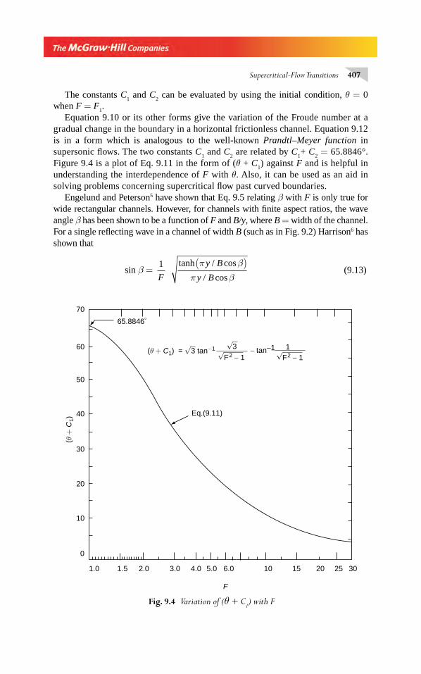
Supercritical-Flow Transitions 407
The constants C1 and C
2 can be evaluated by using the initial condition, θ = 0
when F = F1.
Equation 9.10 or its other forms give the variation of the Froude number at a gradual change in the boundary in a horizontal frictionless channel. Equation 9.12 is in a form which is analogous to the well-known Prandtl–Meyer function in supersonic fl ows. The two constants C
1 and C
2 are related by C
1+ C
2 = 65.8846°.
Figure 9.4 is a plot of Eq. 9.11 in the form of (θ + C1) against F and is helpful in
understanding the interdependence of F with θ. Also, it can be used as an aid in solving problems concerning supercritical fl ow past curved boundaries.
Engelund and Peterson5 have shown that Eq. 9.5 relating β with F is only true for wide rectangular channels. However, for channels with fi nite aspect ratios, the wave angle β has been shown to be a function of F and B/y, where B = width of the channel. For a single refl ecting wave in a channel of width B (such as in Fig. 9.2) Harrison6 has shown that
sin β = 1
F
tanh / cos
/ cos
π β
π β
y B
y B
( ) (9.13)
Fig. 9.4 Variation of (θ + C1) with F
70
60
50
40
30
20
10
10 15 20 25 30
0
1.0 1.5 2.0 3.0 4.0 5.0 6.0
F
Eq.(9.11)
65.8846°
(θ + C1) = 3 tan−1√√
√3
F2 − 1 √F2 − 11− tan−1
(θ +
C1)
Chapter 9.indd 407Chapter 9.indd 407 2/24/2010 3:06:07 PM2/24/2010 3:06:07 PM
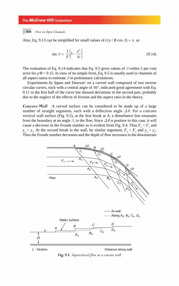
408 Flow in Open Channels
Also, Eq. 9.13 can be simplifi ed for small values of (πy / B cos β) = x as
sin β = 1
16
2
F
x−
⎛
⎝⎜⎜⎜⎜
⎞
⎠⎟⎟⎟⎟ (9.14)
The evaluation of Eq. 9.14 indicates that Eq. 9.5 gives values of β within 5 per cent error for y/B < 0.15. In view of its simple form, Eq. 9.5 is usually used in channels of all aspect ratios to estimate β in preliminary calculations.
Experiments by Ippen and Dawson2 on a curved wall composed of two reverse circular curves, each with a central angle of 16°, indicated good agreement with Eq. 9.11 in the fi rst half of the curve but showed deviations in the second part, probably due to the neglect of the effects of friction and the aspect ratio in the theory.
Concave Wall A curved surface can be considered to be made up of a large number of straight segments, each with a defl ection angle Δ θ. For a concave vertical wall surface (Fig. 9.5), at the fi rst break at A, a disturbance line emanates from the boundary at an angle β
1 to the fl ow. Since Δ θ is positive in this case, it will
cause a decrease in the Froude number as is evident from Fig. 9.4. Thus F2 < F
1 and
y2 > y
1. At the second break in the wall, by similar argument, F
3 < F
2 and y
3 > y
2.
Thus the Froude number decreases and the depth of fl ow increases in the downstream
Fig. 9.5 Supercritical fl ow at a concave wall
At wall
Water surface
L - Section Distance along wall
Along A3 B3 C3 D3
A
A
A3
A3
A2
A1
β1β2
β3
β4
B
B
B3
B3
C
C
C3
C3
D
D
D3
D3
Plan
F1 F2 F3
F4
F5
y1
ΔθΔθ
Δθ
Δθ
∇
Chapter 9.indd 408Chapter 9.indd 408 2/24/2010 3:06:07 PM2/24/2010 3:06:07 PM
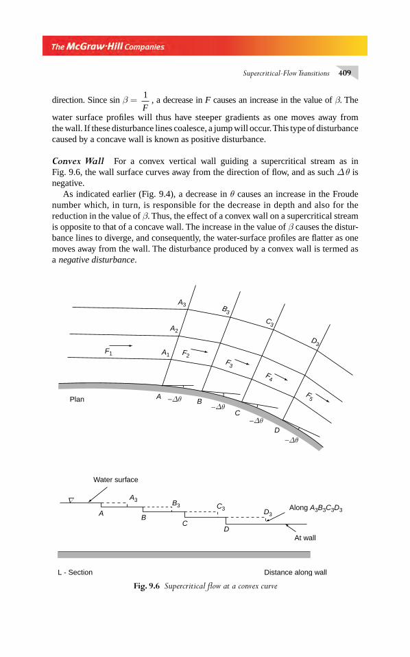
Supercritical-Flow Transitions 409
direction. Since sin β = 1
F, a decrease in F causes an increase in the value of β. The
water surface profi les will thus have steeper gradients as one moves away from the wall. If these disturbance lines coalesce, a jump will occur. This type of disturbance caused by a concave wall is known as positive disturbance.
Convex Wall For a convex vertical wall guiding a supercritical stream as in Fig. 9.6, the wall surface curves away from the direction of fl ow, and as such Δ θ is negative.
As indicated earlier (Fig. 9.4), a decrease in θ causes an increase in the Froude number which, in turn, is responsible for the decrease in depth and also for the reduction in the value of β. Thus, the effect of a convex wall on a supercritical stream is opposite to that of a concave wall. The increase in the value of β causes the distur-bance lines to diverge, and consequently, the water-surface profi les are fl atter as one moves away from the wall. The disturbance produced by a convex wall is termed as a negative disturbance.
Fig. 9.6 Supercritical fl ow at a convex curve
Plan
F1 F2F3
D3
C3
B3
A3
A3 B3 C3 D3
A2
A1
F4
F5
DC
BA
Water surface
At wall
Along A3B3C3D3
−Δθ
−Δθ
−Δθ
L - Section Distance along wall
∇
−Δθ BA
C
D
Chapter 9.indd 409Chapter 9.indd 409 2/24/2010 3:06:07 PM2/24/2010 3:06:07 PM
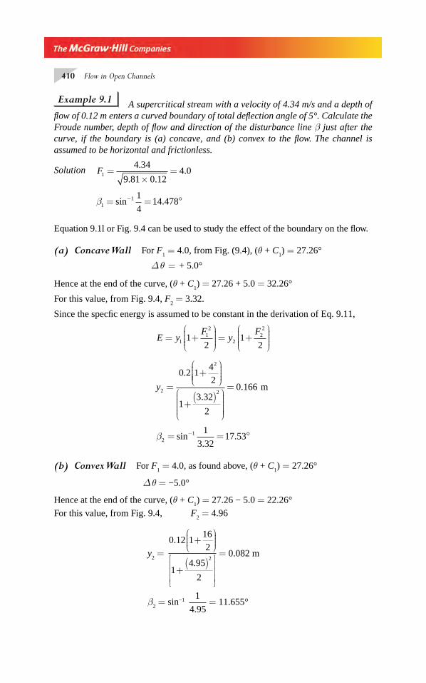
410 Flow in Open Channels
Example 9.1 A supercritical stream with a velocity of 4.34 m/s and a depth of fl ow of 0.12 m enters a curved boundary of total defl ection angle of 5°. Calculate the Froude number, depth of fl ow and direction of the disturbance line β just after the curve, if the boundary is (a) concave, and (b) convex to the fl ow. The channel is assumed to be horizontal and frictionless.
Solution F1
4 34
9 81 0 124 0=
×=
.
. ..
β11 1
414 478= = °−sin .
Equation 9.1l or Fig. 9.4 can be used to study the effect of the boundary on the fl ow.
(a) Concave Wall For F1 = 4.0, from Fig. (9.4), (θ + C
1) = 27.26°
Δ θ = + 5.0°
Hence at the end of the curve, (θ + C1) = 27.26 + 5.0 = 32.26°
For this value, from Fig. 9.4, F2 = 3.32.
Since the specfi c energy is assumed to be constant in the derivation of Eq. 9.11,
E yF
yF
= +⎛
⎝⎜⎜⎜⎜
⎞
⎠⎟⎟⎟⎟
= +⎛
⎝⎜⎜⎜⎜
⎞
⎠⎟⎟⎟⎟1
12
222
12
12
y2
2
2
0 2 14
2
13 32
2
0 166=+
⎛
⎝⎜⎜⎜⎜
⎞
⎠⎟⎟⎟⎟
+( )⎛
⎝
⎜⎜⎜⎜⎜
⎞
⎠
⎟⎟⎟⎟⎟⎟
=.
.. m
β2
1 1
3 3217 53= = °−sin
..
(b) Convex Wall For F1 = 4.0, as found above, (θ + C
1) = 27.26°
Δ θ = −5.0°
Hence at the end of the curve, (θ + C1) = 27.26 − 5.0 = 22.26°
For this value, from Fig. 9.4, F2 = 4.96
y2 =
0 12 116
2
14 95
2
2
.
.
+⎛⎝⎜⎜⎜
⎞⎠⎟⎟⎟
+( )⎡
⎣
⎢⎢⎢
⎤
⎦
⎥⎥⎥
= 0.082 m
β2 = sin−1
1
4 95.= 11.655°
Chapter 9.indd 410Chapter 9.indd 410 2/24/2010 3:06:07 PM2/24/2010 3:06:07 PM
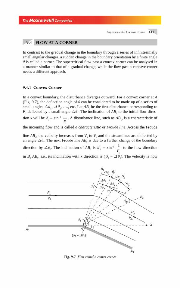
Supercritical-Flow Transitions 411
9.4 FLOW AT A CORNER
In contrast to the gradual change in the boundary through a series of infi nitesimally small angular changes, a sudden change in the boundary orientation by a fi nite angle θ is called a corner. The supercritical fl ow past a convex corner can be analysed in a manner similar to that of a gradual change, while the fl ow past a concave corner needs a different approach.
9.4.1 Convex Corner
In a convex boundary, the disturbance diverges outward. For a convex corner at A (Fig. 9.7), the defl ection angle of θ can be considered to be made up of a series of small angles Δ θ
1 , Δ θ
2, …., etc. Let AB
1 be the fi rst disturbance corresponding to
F1 defl ected by a small angle Δ θ
1. The inclination of AB
1 to the initial fl ow direc-
tion x will be β1= sin−1 1
1F. A disturbance line, such as AB
1, is a characteristic of
the incoming fl ow and is called a characteristic or Froude line. Across the Froude
line AB1, the velocity increases from V
1 to V
2 and the streamlines are defl ected by
an angle Δ θ1. The next Froude line AB
2 is due to a further change of the boundary
direction by Δ θ2. The inclination of AB
2 is β
2 = sin−1
1
2F to the fl ow direction
in B1 AB
2, i.e., its inclination with x direction is ( β
2 − Δ θ
1). The velocity is now
Fig. 9.7 Flow round a convex corner
A0
F1
V1
A
A1
X
Bm
B3
B2
B1
Vm
Fm
Δθ1
Δθ1Δθ2
Δθ3Δθ2β1
β1
(β2 − Δθ1)
β2β3
βm
θ
Chapter 9.indd 411Chapter 9.indd 411 2/24/2010 3:06:08 PM2/24/2010 3:06:08 PM
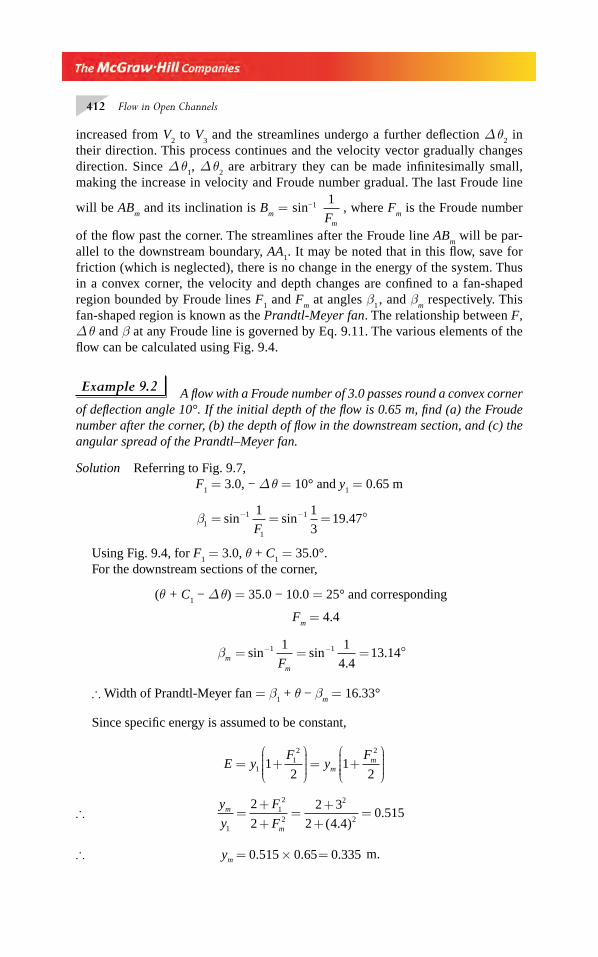
412 Flow in Open Channels
increased from V2 to V
3 and the streamlines undergo a further defl ection Δ θ
2 in
their direction. This process continues and the velocity vector gradually changes direction. Since Δ θ
1, Δ θ
2 are arbitrary they can be made infi nitesimally small,
making the increase in velocity and Froude number gradual. The last Froude line
will be ABm and its inclination is B
m = sin−1
1
Fm
, where Fm is the Froude number
of the fl ow past the corner. The streamlines after the Froude line ABm will be par-
allel to the downstream boundary, AA1. It may be noted that in this fl ow, save for
friction (which is neglected), there is no change in the energy of the system. Thus in a convex corner, the velocity and depth changes are confi ned to a fan-shaped region bounded by Froude lines F
1 and F
m at angles β
1 , and β
m respectively. This
fan-shaped region is known as the Prandtl-Meyer fan. The relationship between F, Δ θ and β at any Froude line is governed by Eq. 9.11. The various elements of the fl ow can be calculated using Fig. 9.4.
Example 9.2 A fl ow with a Froude number of 3.0 passes round a convex corner of defl ection angle 10°. If the initial depth of the fl ow is 0.65 m, fi nd (a) the Froude number after the corner, (b) the depth of fl ow in the downstream section, and (c) the angular spread of the Prandtl–Meyer fan.
Solution Referring to Fig. 9.7,F
1 = 3.0, − Δ θ = 10° and y
1 = 0.65 m
β11
1
11 1
319 47= = = °− −sin sin .
F
Using Fig. 9.4, for F1 = 3.0, θ + C
1 = 35.0°.
For the downstream sections of the corner,
(θ + C1 − Δ θ) = 35.0 − 10.0 = 25° and corresponding
Fm = 4.4
βm
mF= = = °− −sin sin
..1 11 1
4 413 14
∴ Width of Prandtl-Meyer fan = β1 + θ − β
m = 16.33°
Since specifi c energy is assumed to be constant,
E yF
yF
mm= +
⎛
⎝⎜⎜⎜⎜
⎞
⎠⎟⎟⎟⎟
= +⎛
⎝⎜⎜⎜⎜
⎞
⎠⎟⎟⎟⎟1
12 2
12
12
∴ =++
=+
+=
y
y
F
Fm
m1
12
2
2
2
2
2
2 3
2 4 40 515
( . ).
∴ = × =ym 0 515 0 65 0 335. . . m.
Chapter 9.indd 412Chapter 9.indd 412 2/24/2010 3:06:08 PM2/24/2010 3:06:08 PM
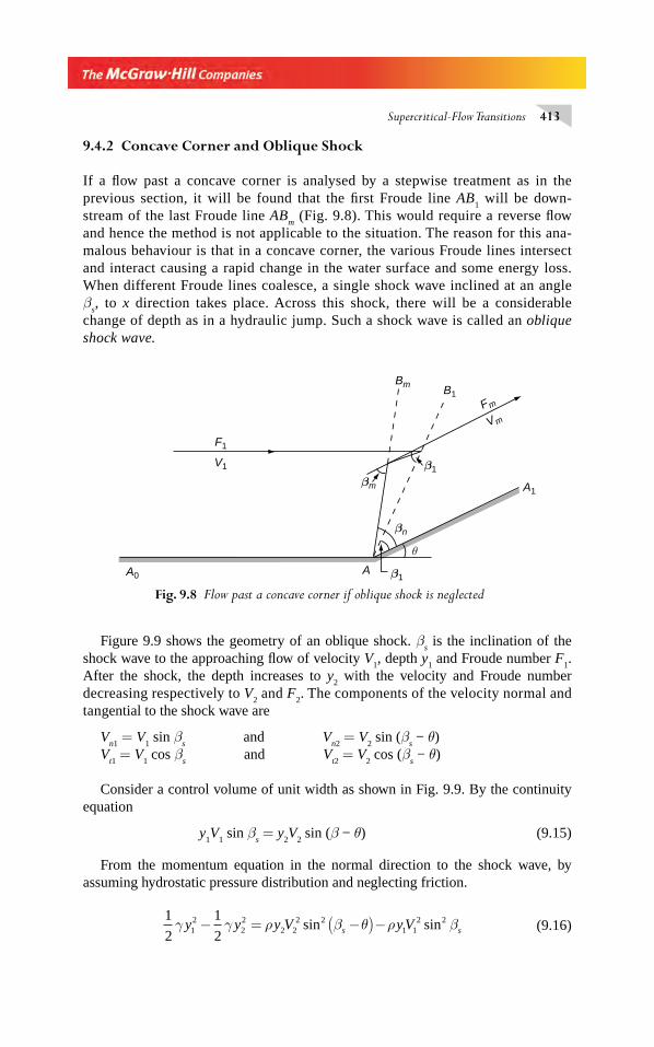
Supercritical-Flow Transitions 413
9.4.2 Concave Corner and Oblique Shock
If a fl ow past a concave corner is analysed by a stepwise treatment as in the previous section, it will be found that the fi rst Froude line AB
1 will be down-
stream of the last Froude line ABm (Fig. 9.8). This would require a reverse fl ow
and hence the method is not applicable to the situation. The reason for this ana-malous behaviour is that in a concave corner, the various Froude lines intersect and interact causing a rapid change in the water surface and some energy loss. When different Froude lines coalesce, a single shock wave inclined at an angle β
s, to x direction takes place. Across this shock, there will be a considerable
change of depth as in a hydraulic jump. Such a shock wave is called an oblique shock wave.
Fig. 9.8 Flow past a concave corner if oblique shock is neglected
AA0
V1
F1
A1
Fm
V m
Bm
βm
β1
β1
B1
θ
βn
Figure 9.9 shows the geometry of an oblique shock. βs is the inclination of the
shock wave to the approaching fl ow of velocity V1, depth y
1 and Froude number F
1.
After the shock, the depth increases to y2 with the velocity and Froude number
decreasing respectively to V2 and F
2. The components of the velocity normal and
tangential to the shock wave are
Vn1
= V1 sin β
s and V
n2 = V
2 sin (β
s − θ)
Vt1 = V
1 cos β
s and V
t2 = V
2 cos (β
s − θ)
Consider a control volume of unit width as shown in Fig. 9.9. By the continuity equation
y1V
1 sin β
s = y
2V
2 sin (β − θ) (9.15)
From the momentum equation in the normal direction to the shock wave, by assuming hydrostatic pressure distribution and neglecting friction.
1
2
1
212
22
2 22 2
1 12 2γ γ ρ β θ ρ βy y y V y Vs s− = −( )−sin sin (9.16)
Chapter 9.indd 413Chapter 9.indd 413 2/24/2010 3:06:08 PM2/24/2010 3:06:08 PM
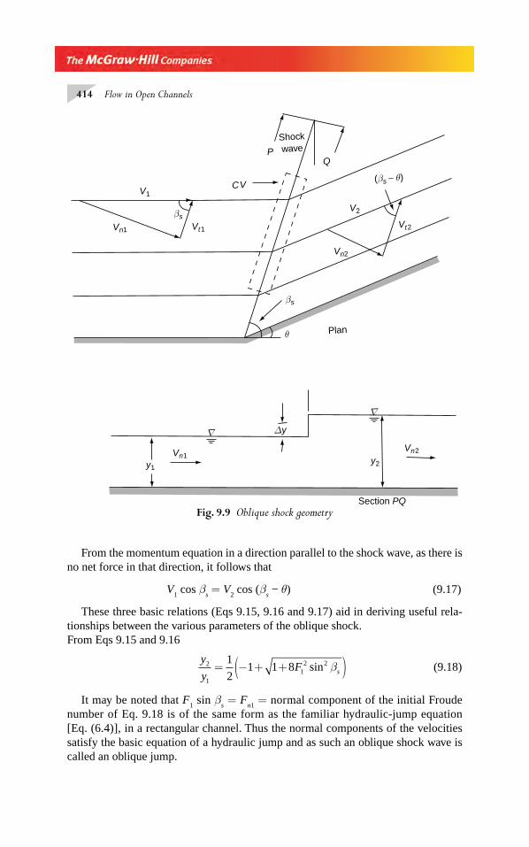
414 Flow in Open Channels
Fig. 9.9 Oblique shock geometry
βs
βs
(βs − θ)
Vn1 Vt1
V1
Vn2
V2
Vt2
QP
CV
θ Plan
Shockwave
∇
∇ Δy
y1y2
Vn1Vn2
Section PQ
From the momentum equation in a direction parallel to the shock wave, as there is no net force in that direction, it follows that
V1 cos β
s = V
2 cos (β
s − θ) (9.17)
These three basic relations (Eqs 9.15, 9.16 and 9.17) aid in deriving useful rela-tionships between the various parameters of the oblique shock.From Eqs 9.15 and 9.16
y
yF s
2
112 21
21 1 8= − + +( )sin β (9.18)
It may be noted that F1 sin β
s = F
n1 = normal component of the initial Froude
number of Eq. 9.18 is of the same form as the familiar hydraulic-jump equation [Eq. (6.4)], in a rectangular channel. Thus the normal components of the velocities satisfy the basic equation of a hydraulic jump and as such an oblique shock wave is called an oblique jump.
Chapter 9.indd 414Chapter 9.indd 414 2/24/2010 3:06:08 PM2/24/2010 3:06:08 PM
Supercritical-Flow Transitions 415
From Eqs 9.15 and 9.17
y
ys
s
2
1
=−
tan
tan ( )
ββ θ
(9.19)
Eliminating y
y2
1
⎛
⎝⎜⎜⎜⎜
⎞
⎠⎟⎟⎟⎟ from Eqs 9.18 and 9.19
tantan sin
tan sinθ
β β
β β=
+ −( )− + +
s s
s s
F
F
1 8 3
2 1 1 8
12 2
212 2
(9.20)
From Eq. 9.18,
F Fy
y
y
yn s1 12
1
2
1
1
21= =
⎛
⎝⎜⎜⎜⎜
⎞
⎠⎟⎟⎟⎟
+⎛
⎝⎜⎜⎜⎜
⎞
⎠⎟⎟⎟⎟
sin β (9.21)
An expression for F2 in terms of F
1 and ( y
2 / y
1) can be obtained as follows:
V V Vn t12
12
12= +
and V V Vn t22
22
22= +
But by Eq. 9.17, Vt1 = V
t2
V V V Vn n22
12
12
22= − +
From Eq. 9.15, V Vy
yn s2 11
2
=⎛
⎝⎜⎜⎜⎜
⎞
⎠⎟⎟⎟⎟
sin β
V Vy
ys22
12 2 1
2
2
1 1= − −⎛
⎝⎜⎜⎜⎜
⎞
⎠⎟⎟⎟⎟
⎡
⎣
⎢⎢⎢
⎤
⎦
⎥⎥⎥
⎧⎨⎪⎪⎪
⎩⎪⎪⎪
⎫⎬⎪⎪⎪sin β⎭⎭⎪⎪⎪
i.e. F Fy
yF
y
y
y
yn22
12 1
2
2 1
2
1
21
1=⎛
⎝⎜⎜⎜⎜
⎞
⎠⎟⎟⎟⎟−
⎛
⎝⎜⎜⎜⎜
⎞
⎠⎟⎟⎟⎟
−⎛
⎝⎜⎜⎜⎜
⎞
⎠⎟⎟⎟⎟⎟
⎡
⎣
⎢⎢⎢
⎤
⎦
⎥⎥⎥
2
Substituting for Fnl from Eq. 9.21 and simplifying
Fy
yF
y
y
y
y22 1
212 1
2
2
2
1
21=
⎛
⎝⎜⎜⎜⎜
⎞
⎠⎟⎟⎟⎟
−⎛
⎝⎜⎜⎜⎜
⎞
⎠⎟⎟⎟⎟
−⎛
⎝⎜⎜⎜⎜
⎞
⎠⎟⎟⎟⎟⎟
+⎛
⎝⎜⎜⎜⎜
⎞
⎠⎟⎟⎟⎟
⎡
⎣
⎢⎢⎢
⎤
⎦
⎥⎥⎥
1 2
1
2y
y (9.22)
Equations 9.15 through 9.22 enable the solution of the various elements of the oblique shock wave. Usually a trial-and-error procedure is required for solving oblique-jump problems. Equation 9.20 when plotted as β
s = f (F
1, θ) (Fig. 9.10), provides a graphi-
cal aid which together with relevant equations greatly simplifi es the determination of oblique-jump elements. Ippen1 has given a four quadrant chart for the graphical solu-tion of oblique-jump equations.
Chapter 9.indd 415Chapter 9.indd 415 2/24/2010 3:06:09 PM2/24/2010 3:06:09 PM
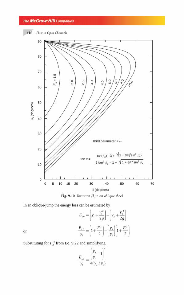
416 Flow in Open Channels
In an oblique-jump the energy loss can be estimated by
E yV
gy
V
gL0 112
222
2 2= +
⎛
⎝⎜⎜⎜⎜
⎞
⎠⎟⎟⎟⎟− +
⎛
⎝⎜⎜⎜⎜
⎞
⎠⎟⎟⎟⎟
or E
y
F y
y
FL0
1
12
2
1
22
12
12
= +⎛
⎝⎜⎜⎜⎜
⎞
⎠⎟⎟⎟⎟−
⎛
⎝⎜⎜⎜⎜
⎞
⎠⎟⎟⎟⎟
+⎛
⎝⎜⎜⎜⎜
⎞
⎠⎟⎟⎟⎟⎟
Substituting for F22 from Eq. 9.22 and simplifying,
E
y
y
y
y yL0
1
2
1
3
2 1
1
4=
−⎛
⎝⎜⎜⎜⎜
⎞
⎠⎟⎟⎟⎟
( / )
Fig. 9.10 Variation βs in an oblique shock
90
80
70
60
50
40
30
20
10
00 5 10 15 20 30 40 50 60 70
Third parameter = F1
θ (degrees)
tan θ =tan βs (− 3 +
2 tan2 βs − 1 + 1 + 8F1 sin2 βs2
1 + 8F1 sin2 βs)2
F1
= 1
.5
2.0
2.5
3.0
4.0 5.0
6.0
8.0
10.0
β s (d
egre
es)
Chapter 9.indd 416Chapter 9.indd 416 2/24/2010 3:06:09 PM2/24/2010 3:06:09 PM
Supercritical-Flow Transitions 417
or Ey y
y yL02 1
3
1 24=
−( )
which is the same as the energy loss in normal hydraulic-jumps (Eq. 8.6). Usually, the value of F
nl is very small and as such the energy loss in an oblique-jump is relatively small.
Estimation of βs For a given value of F
1 and θ, the value of β
s can be estimated
by using Fig. 9.10. However, this will only be a rough estimate, because of the scale of the fi gure and if accurate value is desired the value obtained from Fig. 9.10 can be refi ned by trial and error through use of Eq. 9.23. For quick and fairly accurate estimation of values of β
s the following correlation equation can be used:
βs = (1.4679 − 0.2082 F
1 + 0.0184 F 2) θ + (60.638 F
1−1.044) (9.23)
where βs and θ are in degrees. This equation has been derived from Eq. 9.20 for
values of θ in the range 1.0° to 11.0° and Froude number F1 in the range 2.0 to 7.5.
Equation 9.23 gives results within an error band of ± 2.5%.
Example 9.3 A supercritical stream in a wide rectangular channel has a Froude number of 6.0. One of the vertical walls is turned inward at a section with a defl ection angle of 10°. Calculate the elements of the oblique-jump formed due to this change in direction if the initial depth of fl ow is 0.50 m.
Solution F1 = 6.0, θ = 10.0° and y
1 = 0.50 m
From Fig. 9.10, βs = 18.5
Using Eq. 9.19,
y
ys
s
2
1
18 5
8 52 239=
−=
°°
=tan
tan ( )
tan .
tan ..
ββ θ
y2 0 5 2 239 1 119= ×( )=( . ) . . m
Using Eq. 9.22,
F22 21
2 2396 0
1
2
1
2 2391 239 3 2=
⎛⎝⎜⎜⎜
⎞⎠⎟⎟⎟⎟ −
⎛⎝⎜⎜⎜
⎞⎠⎟⎟⎟⎟.
( . ).
( . ) ( . 339 2)⎡
⎣⎢⎢
= 14.782
F2 = 3.84
Fn 1
= F1 sin β
s = 1.904
Fn 2
= F2 sin (θ
2 − θ) = 0.57
(Note the small values of Froude numbers normal to the shock),
Chapter 9.indd 417Chapter 9.indd 417 2/24/2010 3:06:09 PM2/24/2010 3:06:09 PM
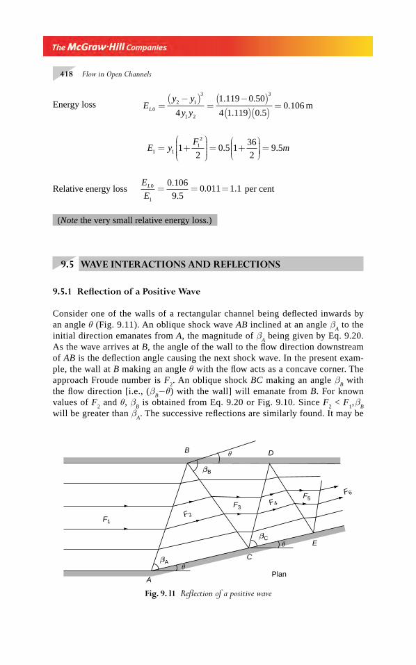
418 Flow in Open Channels
Energy loss Ey y
y yL02 1
3
1 2
3
4
1 119 0 50
4 1 119 0 50 106=
−( )=
−( )( )( )
=. .
. .. m
E yF
m1 112
12
0 5 136
29 5= +
⎛
⎝⎜⎜⎜⎜
⎞
⎠⎟⎟⎟⎟
= +⎛⎝⎜⎜⎜
⎞⎠⎟⎟⎟⎟ =. .
Relative energy loss E
EL0
1
0 106
9 50 011 1 1= = =
.
.. . per cent
(Note the very small relative energy loss.)
9.5 WAVE INTERACTIONS AND REFLECTIONS
9.5.1 Refl ection of a Positive Wave
Consider one of the walls of a rectangular channel being defl ected inwards by an angle θ (Fig. 9.11). An oblique shock wave AB inclined at an angle β
A to the
initial direction emanates from A, the magnitude of βA being given by Eq. 9.20.
As the wave arrives at B, the angle of the wall to the fl ow direction downstream of AB is the defl ection angle causing the next shock wave. In the present exam-ple, the wall at B making an angle θ with the fl ow acts as a concave corner. The approach Froude number is F
2. An oblique shock BC making an angle β
B with
the fl ow direction [i.e., (βB−θ) with the wall] will emanate from B. For known
values of F2 and θ, β
B is obtained from Eq. 9.20 or Fig. 9.10. Since F
2 < F
1, β
B
will be greater than βA. The successive refl ections are similarly found. It may be
Fig. 9. l1 Refl ection of a positive wave
E
A
C
B D
F1F2
F3F4
F5F6
βA
βC
βB
θ
Plan
θ
θ
Chapter 9.indd 418Chapter 9.indd 418 2/24/2010 3:06:09 PM2/24/2010 3:06:09 PM
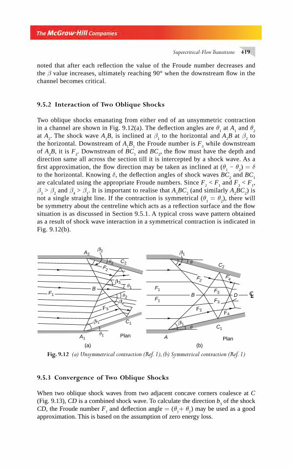
Supercritical-Flow Transitions 419
noted that after each refl ection the value of the Froude number decreases and the β value increases, ultimately reaching 90° when the downstream fl ow in the channel becomes critical.
9.5.2 Interaction of Two Oblique Shocks
Two oblique shocks emanating from either end of an unsymmetric contraction in a channel are shown in Fig. 9.12(a). The defl ection angles are θ
1 at A
1 and θ
2
at A2. The shock wave A
1B, is inclined at β
1 to the horizontal and A
2B at β
2 to
the horizontal. Downstream of A1B
1 the Froude number is F
3 while downstream
of A2B, it is F
2. Downstream of BC
1 and BC
2, the fl ow must have the depth and
direction same all across the section till it is intercepted by a shock wave. As a fi rst approximation, the fl ow direction may be taken as inclined at (θ
1 − θ
2) = δ
to the horizontal. Knowing δ, the defl ection angles of shock waves BC2 and BC
1
are calculated using the appropriate Froude numbers. Since F2 < F
1 and F
3 < F
1,
β3 > β
2 and β
4 > β
1. It is important to realise that A
1BC
2 (and similarly A
2BC
2) is
not a single straight line. If the contraction is symmetrical (θ1 = θ
2), there will
be symmetry about the centreline which acts as a refl ection surface and the fl ow situation is as discussed in Section 9.5.1. A typical cross wave pattern obtained as a result of shock wave interaction in a symmetrical contraction is indicated in Fig. 9.12(b).
Fig. 9.12 (a) Unsymmetrical contraction (Ref. 1), (b) Symmetrical contraction (Ref. 1)
F2
F3
F1B
C2
C1
A1
A2
θ1
β1
β4
β3
β2
θ2
Plan
(a) (b)
F2
F1
C2
C1
F1
A
F2
F4
F3
F3
F4
Plan
B D
β1
β1
θθ1
θ2 θ
9.5.3 Convergence of Two Oblique Shocks
When two oblique shock waves from two adjacent concave corners coalesce at C (Fig. 9.13), CD is a combined shock wave. To calculate the direction b
3 of the shock
CD, the Froude number F1 and defl ection angle = ( θ
1+ θ
2 ) may be used as a good
approximation. This is based on the assumption of zero energy loss.
Chapter 9.indd 419Chapter 9.indd 419 2/24/2010 3:06:10 PM2/24/2010 3:06:10 PM
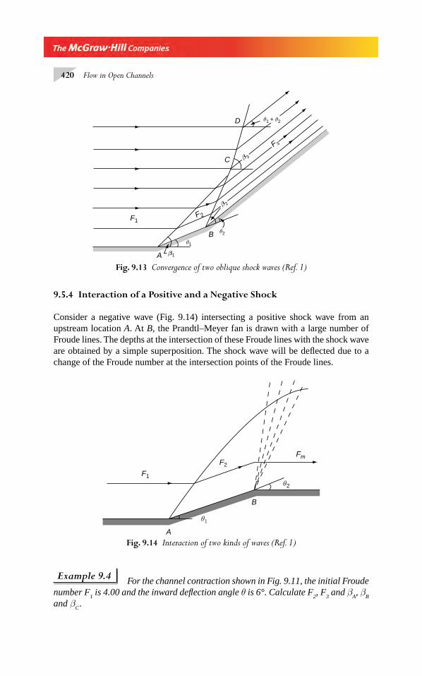
420 Flow in Open Channels
9.5.4 Interaction of a Positive and a Negative Shock
Consider a negative wave (Fig. 9.14) intersecting a positive shock wave from an upstream location A. At B, the Prandtl–Meyer fan is drawn with a large number of Froude lines. The depths at the intersection of these Froude lines with the shock wave are obtained by a simple superposition. The shock wave will be defl ected due to a change of the Froude number at the intersection points of the Froude lines.
Fig. 9.13 Convergence of two oblique shock waves (Ref. 1)
A
B
C
D
F1F2
F 3
β 3
β 2
β1
θ1
θ2
θ1 + θ2
Fig. 9.14 Interaction of two kinds of waves (Ref. 1)A
B
FmF2
F1θ2
θ1
Example 9.4 For the channel contraction shown in Fig. 9.11, the initial Froude number F
1 is 4.00 and the inward defl ection angle θ is 6°. Calculate F
2, F
3 and β
A, β
B
and βC .
Chapter 9.indd 420Chapter 9.indd 420 2/24/2010 3:06:10 PM2/24/2010 3:06:10 PM
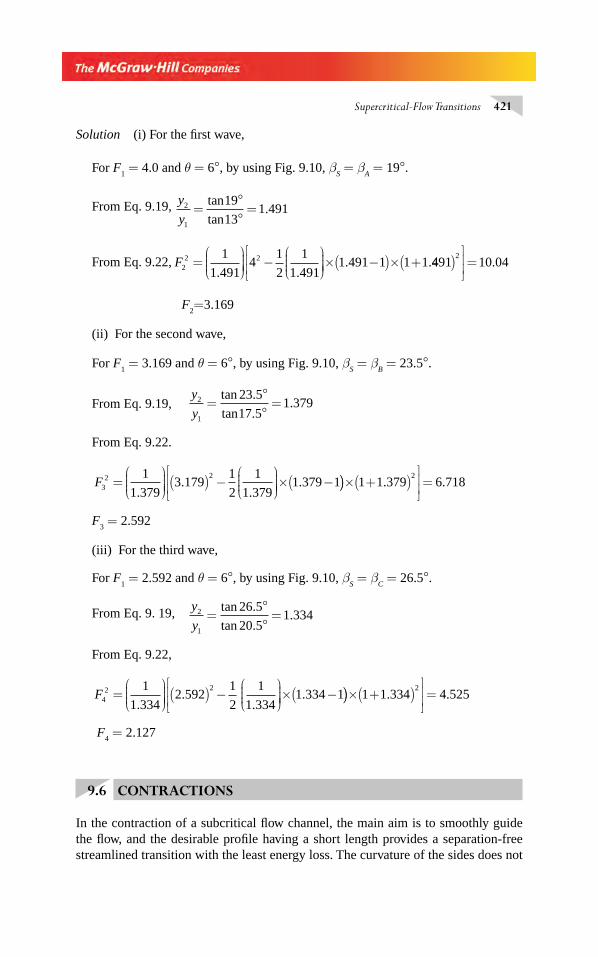
Supercritical-Flow Transitions 421
Solution (i) For the fi rst wave,
For F1 = 4.0 and θ = 6°, by using Fig. 9.10, β
S = β
A = 19°.
From Eq. 9.19, y
y2
1
19
131 491=
°°
=tan
tan.
From Eq. 9.22, F22 21
1 4914
1
2
1
1 4911 491 1 1 1=
⎛⎝⎜⎜⎜
⎞⎠⎟⎟⎟⎟ −
⎛⎝⎜⎜⎜
⎞⎠⎟⎟⎟⎟× −( )× +
. .. .4491 10 04
2( )⎡
⎣⎢⎢
⎤
⎦⎥⎥ = .
F2=3.169
(ii) For the second wave,
For F1 = 3.169 and θ = 6°, by using Fig. 9.10, β
S = β
B = 23.5°.
From Eq. 9.19, y
y2
1
23 5
17 51 379=
°°
=tan .
tan ..
From Eq. 9.22.
F32 21
1 3793 179
1
2
1
1 3791 379 1=
⎛⎝⎜⎜⎜
⎞⎠⎟⎟⎟⎟ ( ) −
⎛⎝⎜⎜⎜
⎞⎠⎟⎟⎟⎟× −(
..
.. ))× +( )
⎡
⎣⎢⎢
⎤
⎦⎥⎥ =1 1 379 6 718
2. .
F3 = 2.592
(iii) For the third wave,
For F1 = 2.592 and θ = 6°, by using Fig. 9.10, β
S = β
C = 26.5°.
From Eq. 9. 19, y
y2
1
26 5
20 51 334=
°°
=tan .
tan ..
From Eq. 9.22,
F42 21
1 3342 592
1
2
1
1 3341 334 1=
⎛⎝⎜⎜⎜
⎞⎠⎟⎟⎟⎟ ( ) −
⎛⎝⎜⎜⎜
⎞⎠⎟⎟⎟⎟× −(
..
.. ))× +( )
⎡
⎣⎢⎢
⎤
⎦⎥⎥ =1 1 334 4 525
2. .
F4 = 2.127
9.6 CONTRACTIONS
In the contraction of a subcritical fl ow channel, the main aim is to smoothly guide the fl ow, and the desirable profi le having a short length provides a separation-free streamlined transition with the least energy loss. The curvature of the sides does not
Chapter 9.indd 421Chapter 9.indd 421 2/24/2010 3:06:10 PM2/24/2010 3:06:10 PM
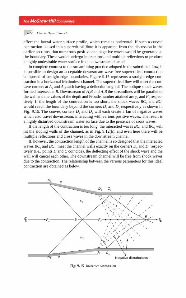
422 Flow in Open Channels
affect the lateral water-surface profi le, which remains horizontal. If such a curved contraction is used in a supercritical fl ow, it is apparent, from the discussion in the earlier sections, that numerous positive and negative waves would be generated at the boundary. These would undergo interactions and multiple refl ections to produce a highly undesirable water surface in the downstream channel.
In complete contrast to the streamlining practice adopted in the subcritical fl ow, it is possible to design an acceptable downstream wave-free supercritical contraction composed of straight-edge boundaries. Figure 9.15 represents a straight-edge con-traction in a horizontal frictionless channel. The supercritical fl ow will meet the con-cave corners at A
1 and A
2 , each having a defl ection angle θ. The oblique shock waves
formed intersect at B. Downstream of A1B and A
2B the streamlines will be parallel to
the wall and the values of the depth and Froude number attained are y2 and F
2 respec-
tively. If the length of the contraction is too short, the shock waves BC2 and BC
1
would reach the boundary beyond the corners D2 and D
1 respectively as shown in
Fig. 9.15. The convex corners D1 and D
2 will each create a fan of negative waves
which also travel downstream, interacting with various positive waves. The result is a highly disturbed downstream water surface due to the presence of cross waves.
If the length of the contraction is too long, the interacted waves BC2 and BC
1 will
hit the sloping walls of the channel, as in Fig. 9.12(b), and even here there will be multiple refl ections and cross waves in the downstream channel.
If, however, the contraction length of the channel is so designed that the interacted waves BC
2 and BC
1, meet the channel walls exactly on the corners D
2 and D
1 respec-
tively (i.e., points D and C coincide), the defl ecting effect of the shock wave and the wall will cancel each other. The downstream channel will be free from shock waves due to the contraction. The relationship between the various parameters for this ideal contraction are obtained as below.
Fig. 9.15 Incorrect contraction
C1
F1
A2
F3
E
F2
D1
D2 C2
F2
B
θ Negative disturbances
θ
A1
Chapter 9.indd 422Chapter 9.indd 422 2/24/2010 3:06:11 PM2/24/2010 3:06:11 PM
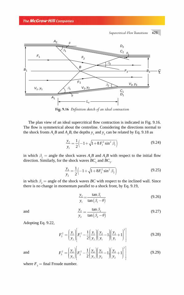
Supercritical-Flow Transitions 423
The plan view of an ideal supercritical fl ow contraction is indicated in Fig. 9.16. The fl ow is symmetrical about the centreline. Considering the directions normal to the shock fronts A
1 B and A
2 B, the depths y
1 and y
2 can be related by Eq. 9.18 as
y
yF2
112 2
1
1
21 1 8= − + +( )sin β (9.24)
in which β1 = angle the shock waves A
1B and A
2B with respect to the initial fl ow
direction. Similarly, for the shock waves BC1 and BC
2’
y
yF3
222 2
2
1
21 1 8= − + +( )sin β
(9.25)
in which β2 = angle of the shock waves BC with respect to the inclined wall. Since
there is no change in momentum parallel to a shock front, by Eq. 9.19,
y
y2
1
1
1
=−( )
tan
tan
ββ θ
(9.26)
and y
y3
2
2
2
=−( )
tan
tan
ββ θ
(9.27)
Adopting Eq. 9.22,
Fy
yF
y
y
y
y22 1
212 1
2
2
1
1
21=
⎛
⎝⎜⎜⎜⎜
⎞
⎠⎟⎟⎟⎟
−⎛
⎝⎜⎜⎜⎜
⎞
⎠⎟⎟⎟⎟
−⎛
⎝⎜⎜⎜⎜
⎞
⎠⎟⎟⎟⎟⎟
+⎛
⎝⎜⎜⎜⎜
⎞
⎠⎟⎟⎟⎟
⎡
⎣
⎢⎢⎢
⎤
⎦
⎥⎥⎥
y
y2
1
2
1 (9.28)
and Fy
yF
y
y
y
y32 2
322 2
3
3
2
1
21=
⎛
⎝⎜⎜⎜⎜
⎞
⎠⎟⎟⎟⎟
−⎛
⎝⎜⎜⎜⎜
⎞
⎠⎟⎟⎟⎟
−⎛
⎝⎜⎜⎜⎜
⎞
⎠⎟⎟⎟⎟⎟
+⎛
⎝⎜⎜⎜⎜
⎞
⎠⎟⎟⎟⎟
⎡
⎣
⎢⎢⎢
⎤
⎦
⎥⎥⎥
y
y3
2
2
1 (9.29)
where F3 = fi nal Froude number.
Fig. 9.16 Defi nition sketch of an ideal contraction
F1
F3
V1, y1 V2, y2
V3, y3
F2
F2
C2
C1D1
D2
A1
B1
A2
B
Lc
θ
B3
β1
β1
β2
β2
θ
θ
Chapter 9.indd 423Chapter 9.indd 423 2/24/2010 3:06:11 PM2/24/2010 3:06:11 PM
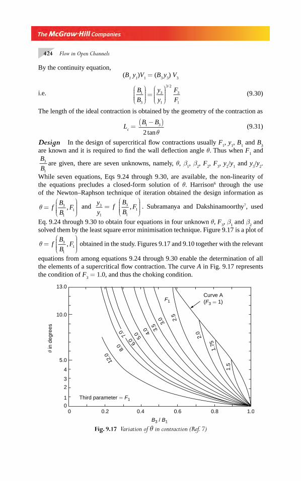
424 Flow in Open Channels
By the continuity equation,(B
1 y
1)V
1 = (B
3 y
3) V
3
i.e. B
B
y
y
F
F1
3
3
1
3 2
3
1
⎛
⎝⎜⎜⎜⎜
⎞
⎠⎟⎟⎟⎟
=⎛
⎝⎜⎜⎜⎜
⎞
⎠⎟⎟⎟⎟
/
(9.30)
The length of the ideal contraction is obtained by the geometry of the contraction as
Lc =
B B1 3
2
−( )tanθ
(9.31)
Design In the design of supercritical fl ow contractions usually F1, y
1, B
1 and B
3
are known and it is required to fi nd the wall defl ection angle θ. Thus when F1 and
B
B3
1
are given, there are seven unknowns, namely, θ, β1, β
2, F
2, F
3, y
2/y
1 and y
3/y
2.
While seven equations, Eqs 9.24 through 9.30, are available, the non-linearity of the equations precludes a closed-form solution of θ. Harrison6 through the use of the Newton–Raphson technique of iteration obtained the design information as
θ =⎛
⎝⎜⎜⎜⎜
⎞
⎠⎟⎟⎟⎟
fB
BF3
11, and
y
y3
1
= f B
BF3
11,
⎛
⎝⎜⎜⎜⎜
⎞
⎠⎟⎟⎟⎟
. Subramanya and Dakshinamoorthy7, used
Eq. 9.24 through 9.30 to obtain four equations in four unknown θ, F3, β
1 and β
2 and
solved them by the least square error minimisation technique. Figure 9.17 is a plot of
θ =⎛
⎝⎜⎜⎜⎜
⎞
⎠⎟⎟⎟⎟
fB
BF3
11, obtained in the study. Figures 9.17 and 9.10 together with the relevant
equations from among equations 9.24 through 9.30 enable the determination of all the elements of a supercritical fl ow contraction. The curve A in Fig. 9.17 represents the condition of F
3 = 1.0, and thus the choking condition.
Fig. 9.17 Variation of θ in contraction (Ref. 7)
Curve A(F3 = 1)F1
Third parameter = F1
θ in
deg
rees
10.0
5.0
13.0
4
3
2
1
00 0.2 0.4 0.6 0.8 1.0
B3 / B1
12.0
8.0
7.0
6.0 5.
0 4.0 3.
5 3.0 2.
5
2.0
1.75
1.5
Chapter 9.indd 424Chapter 9.indd 424 2/24/2010 3:06:11 PM2/24/2010 3:06:11 PM
Supercritical-Flow Transitions 425
References 1, 2, and 6 contain very useful information pertaining to supercritical fl ow contractions. The ideal contraction as above is to be used in preliminary designs only and the fi nal design will have to be based on model studies as the friction and slope of the channel not considered in the ideal design can modify the shock-wave geometry. It should be remembered that the straight-edge supercritical contractions are only valid for the design Froude number. For any off-design values of F
1, the
refl ected waves do not strike at the corners D1 and D
2.
Example 9.4 A rectangular channel carries a fl ow with a Froude number of 6.0 in a 5.0-m wide channel with a depth of 0.75 m. It is required to reduce the width to 2.5 m. Design a contraction and determine all the elements of the transition. Also, determine the energy loss in the transition.
Solution y1 = 0.75 m, F
1 = 6.0 and
B
B3
1
= 0.5
From Fig. 9.17, θ = 4.25°
Referring to Fig. 9.10 or to Eq. 9.23, for θ = 4.25° and F = 6.0,
β1 = 13.0˚
Using Eq. 9.26, y
y2
1
1
1
=−( )
tan
tan
ββ θ
= tan
tan .
13
8 75
°°
=1.50
y2 = 1.12 m
From Eq. 9.28
F22 2 21
1 56 0
1
1 51 50 1 1 5 1=
⎛⎝⎜⎜⎜
⎞⎠⎟⎟⎟⎟ ( ) −
⎛⎝⎜⎜⎜
⎞⎠⎟⎟⎟⎟ −( ) +( )
⎡
..
.. .
⎣⎣⎢⎢
⎤
⎦⎥⎥
= 23.305
F2 = 4.83
For the shock waves BC1 and BC
2, F
2 = 4.83 = initial Froude number and θ = 4.25°.
Using Fig. (9.10) or Eq. 9.23, with θ = 4.25° and F = 4.83,
β2 = 15.5°
From Eq. 9.26,
y
y3
2
2
2
15 5
11 25=
−( )=
°°
tan
tan
tan .
tan .
ββ θ
= 1.394
y
y
y
y
y
y3
1
3
2
2
1
= ⋅ = 1.394 × 1.50 = 2.09
∴ y3 = 2.09 × 0.75 = 1.568 m
Chapter 9.indd 425Chapter 9.indd 425 2/24/2010 3:06:12 PM2/24/2010 3:06:12 PM
426 Flow in Open Channels
From Eq. 9.29
F32 21
1 3944 83
1
2
1
1 3940 394 2 3=
⎛⎝⎜⎜⎜
⎞⎠⎟⎟⎟⎟ ( ) −
⎛⎝⎜⎜⎜
⎞⎠⎟⎟⎟⎟( )
..
.. . 994
2( )⎡
⎣⎢⎢
⎤
⎦⎥⎥
= 16.15
F3 = 4.02
From Eq. 9.31
Lc =
5 0 2 5
2 4 5
. .
tan .
−°
= 15.883 m
Check: By Eq. 9.30, F
F3
1
=B B
y y
1 3
3 1
3 2
/
//( )
F3 =
6 0 2 0
2 093 2
. .
./
×
( ) = 3.97
≈ 4.02 with about 1 per cent error.
In view of the possible errors in the use of various plots, this error is acceptable.Thus the elements of the transition can be summed up as
y1 = 0.75 m θ = 4.25° L
c = 15.883 m
Bl = 5.00 m β
1 = 13.0° y
2 = 1.125 m
F1 = 6.00 β
2 = 15.5° y
3 = 1.568 m
F2 = 4.83 F
3= 4.02
Energy loss:
E1 = y
1 1
212
+⎛
⎝⎜⎜⎜⎜
⎞
⎠⎟⎟⎟⎟
F = 0.75 1
6 0
2
2
+( )⎛
⎝
⎜⎜⎜⎜⎜
⎞
⎠
⎟⎟⎟⎟⎟⎟
.=14.25 m
E3 = y
3 1
232
+⎛
⎝⎜⎜⎜⎜
⎞
⎠⎟⎟⎟⎟
F = 1.568 14 02
2
2
+( )⎛
⎝
⎜⎜⎜⎜⎜
⎞
⎠
⎟⎟⎟⎟⎟⎟
.= 14.238 m
EL = E
1 – E
3 = 14.250 − 14.238 = 0.012 m
9.7 SUPERCRITICAL EXPANSIONS
9.7.1 Introduction
The main aim of a supercritical fl ow expansion design is to have the desired chan-nel-width expansion and to maintain a downstream water surface which is free
Chapter 9.indd 426Chapter 9.indd 426 2/24/2010 3:06:12 PM2/24/2010 3:06:12 PM
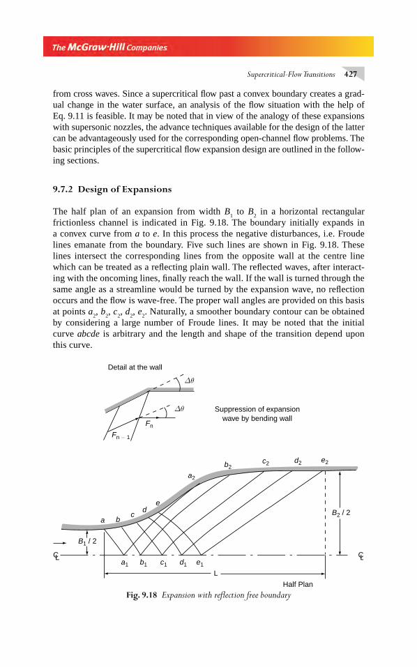
Supercritical-Flow Transitions 427
from cross waves. Since a supercritical fl ow past a convex boundary creates a grad-ual change in the water surface, an analysis of the fl ow situation with the help of Eq. 9.11 is feasible. It may be noted that in view of the analogy of these expansions with supersonic nozzles, the advance techniques available for the design of the latter can be advantageously used for the corresponding open-channel fl ow problems. The basic principles of the supercritical fl ow expansion design are outlined in the follow-ing sections.
9.7.2 Design of Expansions
The half plan of an expansion from width B1 to B
2 in a horizontal rectangular
frictionless channel is indicated in Fig. 9.18. The boundary initially expands in a convex curve from a to e. In this process the negative disturbances, i.e. Froude lines emanate from the boundary. Five such lines are shown in Fig. 9.18. These lines intersect the corresponding lines from the opposite wall at the centre line which can be treated as a refl ecting plain wall. The refl ected waves, after interact-ing with the oncoming lines, fi nally reach the wall. If the wall is turned through the same angle as a streamline would be turned by the expansion wave, no refl ection occurs and the fl ow is wave-free. The proper wall angles are provided on this basis at points a
2, b
2, c
2, d
2, e
2. Naturally, a smoother boundary contour can be obtained
by considering a large number of Froude lines. It may be noted that the initial curve abcde is arbitrary and the length and shape of the transition depend upon this curve.
Fig. 9.18 Expansion with refl ection free boundary
B1 / 2
B2 / 2a
a1
a2
b
b1
b2
c
c1
c2
d
d1
d2
e
e1
e2
Half Plan
L
LC LC
Suppression of expansionwave by bending wall
Detail at the wall
Δθ
Δθ
Fn − 1
Fn
Chapter 9.indd 427Chapter 9.indd 427 2/24/2010 3:06:12 PM2/24/2010 3:06:12 PM
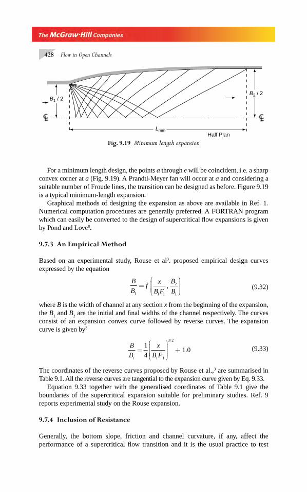
428 Flow in Open Channels
For a minimum length design, the points a through e will be coincident, i.e. a sharp convex corner at a (Fig. 9.19). A Prandtl-Meyer fan will occur at a and considering a suitable number of Froude lines, the transition can be designed as before. Figure 9.19 is a typical minimum-length expansion.
Graphical methods of designing the expansion as above are available in Ref. 1. Numerical computation procedures are generally preferred. A FORTRAN program which can easily be converted to the design of supercritical fl ow expansions is given by Pond and Love8.
9.7.3 An Empirical Method
Based on an experimental study, Rouse et al3. proposed empirical design curves expressed by the equation
B
B1
= f x
B F
B
B1 1
2
1
,⎛
⎝⎜⎜⎜⎜
⎞
⎠⎟⎟⎟⎟ (9.32)
where B is the width of channel at any section x from the beginning of the expansion, the B
1 and B
2 are the initial and fi nal widths of the channel respectively. The curves
consist of an expansion convex curve followed by reverse curves. The expansion curve is given by3
B
B1
=1
4 1 1
3 2
x
B F
⎛
⎝⎜⎜⎜⎜⎜
⎞
⎠
⎟⎟⎟⎟⎟
/
+ 1.0 (9.33)
The coordinates of the reverse curves proposed by Rouse et al.,3 are summarised in Table 9.1. All the reverse curves are tangential to the expansion curve given by Eq. 9.33.
Equation 9.33 together with the generalised coordinates of Table 9.1 give the boundaries of the supercritical expansion suitable for preliminary studies. Ref. 9 reports experimental study on the Rouse expansion.
9.7.4 Inclusion of Resistance
Generally, the bottom slope, friction and channel curvature, if any, affect the performance of a supercritical fl ow transition and it is the usual practice to test
Fig. 9.19 Minimum length expansion
B1 / 2B2 / 2
Half PlanLmm
Chapter 9.indd 428Chapter 9.indd 428 2/24/2010 3:06:13 PM2/24/2010 3:06:13 PM
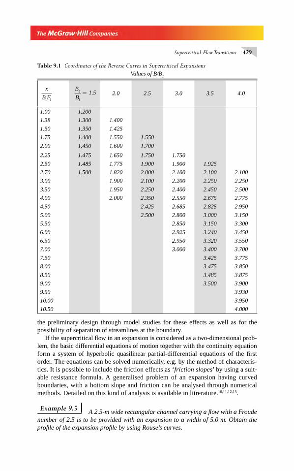
Supercritical-Flow Transitions 429
the preliminary design through model studies for these effects as well as for the possibility of separation of streamlines at the boundary.
If the supercritical fl ow in an expansion is considered as a two-dimensional prob-lem, the basic differential equations of motion together with the continuity equation form a system of hyperbolic quasilinear partial-differential equations of the fi rst order. The equations can be solved numerically, e.g. by the method of characteris-tics. It is possible to include the friction effects as ‘friction slopes’ by using a suit-able resistance formula. A generalised problem of an expansion having curved boundaries, with a bottom slope and friction can be analysed through numerical methods. Detailed on this kind of analysis is available in litrerature.10,11,12,13.
Example 9.5 A 2.5-m wide rectangular channel carrying a fl ow with a Froude number of 2.5 is to be provided with an expansion to a width of 5.0 m. Obtain the profi le of the expansion profi le by using Rouse’s curves.
Values of B/B1
x
B F1 1
B
B2
1
=
1.5 2.0 2.5 3.0 3.5 4.0
1.00 1.200
1.38 1.300 1.400
1.50 1.350 1.425
1.75 1.400 1.550 1.550
2.00 1.450 1.600 1.700
2.25 1.475 1.650 1.750 1.750
2.50 1.485 1.775 1.900 1.900 1.925
2.70 1.500 1.820 2.000 2.100 2.100 2.100
3.00 1.900 2.100 2.200 2.250 2.250
3.50 1.950 2.250 2.400 2.450 2.500
4.00 2.000 2.350 2.550 2.675 2.775
4.50 2.425 2.685 2.825 2.950
5.00 2.500 2.800 3.000 3.150
5.50 2.850 3.150 3.300
6.00 2.925 3.240 3.450
6.50 2.950 3.320 3.550
7.00 3.000 3.400 3.700
7.50 3.425 3.775
8.00 3.475 3.850
8.50 3.485 3.875
9.00 3.500 3.900
9.50 3.930
10.00 3.950
10.50 4.000
Table 9.1 Coordinates of the Reverse Curves in Supercritical Expansions
Chapter 9.indd 429Chapter 9.indd 429 2/24/2010 3:06:13 PM2/24/2010 3:06:13 PM
430 Flow in Open Channels
Solution Rouse’s expansion curve is given by Eq. 9.33 as
B
B
x
B F1 1 1
3 21
41 0=
⎛
⎝⎜⎜⎜⎜
⎞
⎠⎟⎟⎟⎟
+/
.
Here B1 = 2.5 m and F
1 = 2.5.
B x
2 5
1
4 2 5 2 51 0
3 2
. . ..
/
=×
⎛
⎝⎜⎜⎜⎜
⎞
⎠⎟⎟⎟⎟ +
Bx
= +3 2
252 5
/
. (9.34)
Reverse Curve From Table 9.1, for B2 /B
1=2.0, the reverse curve starts at
x
B F1 1
1 38= . ,
i.e., at x = 1.38 × 2.5 × 2.5 = 8.63 m. Also from Table 9.1, for B2/B
1 = 2.0, the length
of transition is given byL
B F1 1
= 4.0. Hence L = 4.0 × 2.5 × 2.5 = 25.0 m. Coordinates
of the reverse curve corresponding to B2/B
1 = 2.0 are obtained from Table 9.1. Thus for
0 < x < 8.6 m, Bx
= +3 2
252 5
/
. and for 8.6 < x < 25.0 m values of B are obtained by
using Table 9.1. A smooth curve is drawn through the reverse curve coordinates to merge with the expansion curve (Eq. 9.34) without kinks.
9.8 STABILITY OF SUPERCRITICAL FLOWS
A fl ow is said to be stable if a small perturbation in the fl ow does not get amplifi ed. From this point of view a subcritical fl ow is inherently stable. However, in supercriti-cal fl ows under certain favorable conditions a perturbation can grow until the origi-nally steady fl ow breaks up in to a train of unsteady surges called roll waves. The transformation of a steady supercritical fl ow in to an unstable unsteady fl ow situation is analogous to the transition from laminar to turbulent fl ow. The roll waves are char-acterized by a series of shock fronts separated by regions of gradually varied fl ow. The wave speed, height and wavelengths of roll waves generally increase as they move downstream. The onset of roll-waves is an important constraint in the designof channels for supercritical fl ow.
The stability analysis14 of the fl ow leads to the criterion for stable fl ows as
− ≤ ≤1 1Ve (9.35)
In which Ve = Vendernikov number = xF R
dP
dA1−
⎛⎝⎜⎜⎜
⎞⎠⎟⎟⎟⎟
Where x = 2/3 if Manning’s formula is used for describing the channel resistance and
x = 0.5 if Chezy formula is used for describing the channel resistance
F = Froude number of the fl ow,
Chapter 9.indd 430Chapter 9.indd 430 2/24/2010 3:06:13 PM2/24/2010 3:06:13 PM
Supercritical-Flow Transitions 431
R = hydraulic radius,
P = wetted perimeter, and
A = area of cross section of the fl ow.
Thus the onset of instability in a channel depends on the channel geometry and the Froude number of the fl ow. Channels having V
e = 0 will be stable for all values of
Froude number and thus constitute channels of absolute stability. Ref. 14 can be con-sulted for further details on stability.
Example 9.6 Derive the conditions for stable supercritical fl ow in (a) rectan-gular, and (b) triangular channels. Consider that Manning’s formula is used to describe the channel resistance to fl ow.
Solution By Eq. 9.35, for stable supercritical fl ow V F RdP
dAe = −⎛⎝⎜⎜⎜
⎞⎠⎟⎟⎟⎟ ≤
2
31 1
(a) Rectangular channel A = By and P = B+2y
dP
dA
dP
dy
dy
dA B= =
2
For stable fl ow, 2
31
2
21F
By
B y B−
+⋅
⎛
⎝⎜⎜⎜⎜
⎞
⎠⎟⎟⎟⎟ ≤
( )
2
3 21F
B
B y+
⎛
⎝⎜⎜⎜⎜
⎞
⎠⎟⎟⎟⎟ ≤
i.e., Fy
B≤ +
⎛⎝⎜⎜⎜
⎞⎠⎟⎟⎟⎟
3
23
(b) For triangular channel A my= 2 P y m= +2 1 2
dP
dA
dP
dy
dy
dA
m
m
m
m= =
+=
+2 1
2
12 2
For stable fl ow 2
31
2 1
12
2
2
Fmy
y m
m
my−
+
⎛
⎝
⎜⎜⎜⎜⎜
⎞
⎠
⎟⎟⎟⎟⎟+⎛
⎝
⎜⎜⎜⎜⎜
⎞
⎠
⎟⎟⎟⎟⎟
⎛
⎝
⎜⎜⎜⎜⎜
⎞
⎠
⎟⎟⎟⎟⎟⎟⎟≤1
i.e., F
31≤ or F ≤ 3
Chapter 9.indd 431Chapter 9.indd 431 2/24/2010 3:06:13 PM2/24/2010 3:06:13 PM
432 Flow in Open Channels
REFERENCES
1. Ippen, A T, ‘Mechanics of Supercritical Flow’, Trans. ASCE, Vol. 116, 1951, p. 268–295.
2. Ippen, A T, and Dawson, J H, ‘Design of Supercritical Contractions’, Trans. ASCE, Vol. 116, 1951, pp 326–346.
3. Rouse, H, Bhoota, B V, and Hsu, E Y, ‘Design of Channel Expansions’, Trans. ASCE, Vol. 116, 1951, pp. 347–363.
4. Knapp, R T, ‘Design of Channel Curve for Supercritical Flow’, Trans, ASCE, Vol. 116, 1951, pp 296–325.
5. Englund, F A, and Munch Peterson, J, ‘Steady Flow in Contracted and Expanded Rectan-gular Channels’, La Houille Blanche, Vol. 8, No. 4, Aug.-Sept. pp 464–474.
6. Harrison, A J M, ‘Design of Channels for Supercritical Flow’, Proc. Inst. of Civil Engrs. (London), Vol. 35, Nov. 1966, pp 475–490.
7. Subramanya, K, and Dakshinamoorthy, S, ‘Design of Supercritical Flow Contractions by Least Square Error Minimisation Technique’, 5th Australasian Conf. on Hydr. and Fl. Mech., Christchurch, New Zealand, Dec. 1974, pp 57–63.
8. Pond, J E, and Love, J, ‘Design of Two-dimensional Sharp-edge-throat Supersonic Nozzle by Digital Computer’, Engg. Expt. Station Series No. 64, Univ. of Missouri, Columbia, USA, 1967.
9. Mazumdar, S K, and Hager, W H, ‘Supercritical Expansion Flow in Rouse Modifi ed and Reverse Transitions’, J. of Hyd. Div., Proc. ASCE, Vol. 119, No. 2, Feb. 1993, pp 201–219.
10. Ligget, J A, and Vasudev, S U, ‘Slope and Friction Effects in Two-dimensional, High –speed Channel Flow’, Proc. 11th Congress of IAHR, Leningrad, 1965, Vol. 1, pp 1–25.
11. Bagge, G, and Herbich, J B, ‘Transitions of Supercritical Open Channel Flow’, J. of Hyd. Div., Proc. ASCE, Vol. 93, Sept. 1967, pp 23–41.
12. Dakshinamoorthy, S, ‘Some Numerical Studies on Supercritical Flow Problems’, Ph. D. Thesis, Indian Institute of Technology, Kanpur, India, Dec. 1973.
13. Choudhry, M H, Open Channel Flow, Prentice-Hall, Englewood Cliffs, New Jersey, 1993.14. Ligget, J, A, ‘Stability’, Chap. 6 in Unsteady Flows in Open Channels, Vol. I, Ed.
by Mahmood, K, and Yevjevich, V, Water Resources Pub., Fort Collins, Colo., USA, pp 259–282
PROBLEMS
Topic Problems
Response to a disturbanceGradual change in the boundaryOblique shockConvex cornerContractionsExpansion Application of shock principleStability
9.1 – 9.29.3 – 9.49.5 – 9.99.7 – 9.99.10 – 9.12 – 9.139.11 – 9.14 – 9.189.15 – 9.179.19
Problem Distribution
Chapter 9.indd 432Chapter 9.indd 432 2/24/2010 3:06:14 PM2/24/2010 3:06:14 PM
Supercritical-Flow Transitions 433
9.1 A rectangular channel has a velocity of 5 m/s and a depth of 0.60 m. If a thin obstruction such as a vertical pole is present in the midst of the stream, estimate the direction of waves produced.
9.2 When a stone was thrown into a pond waves of amplitude 1 cm and velocity 2 m/s were produced. Estimate the depth of water in the pond.
9.3 A wide rectangular channel carries a fl ow with a depth of 0.15 m and a Froude number of 4.5. Calculate and plot the water surface profi le next to a side wall which has (i) a con-cave curve of 8° central angle, and (ii) a convex curve of 8° central angle. The radius of the curved wall is 10 m and the other side wall can be assumed to be too far away to have any interference.
9.4 For a gradual change in the boundary of a supercritical stream, an assumption of constant specifi c energy is made in the derivation of Eq. (9.10). Assuming, instead, a constant velocity, derive an expression for θ as θ = β + sin β cos β + a constant.
9.5 A free surface fl ow with a depth of 0.50 m and initial Froude number of 2.0 approaches a concave corner of defl ection angle 10° in one of the walls. Determine the inclination of the shock wave to the original direction of fl ow and the depth after the shock.
9.6 A supercritical stream of velocity 10.0 m/s and depth 0.24 m is defl ected by a concave corner having a defl ection angle of 20°. Determine the inclination of the shock waves of the original direction of fl ow, the depth after the shock and the energy loss.
9.7 Label the positive and negative shock waves in the cases shown in Fig. 9.20.
Fig. 9.20 Problem 9.7
(c) (d)
(a) (b)
9.8 If the stream in Problem 9.6 is defl ected by a 9° convex corner, determine the down-stream fl ow condition and the angular spread of the Prandtl-Meyer fan.
9.9 Sketch the fl ow past a thin plate kept in a supercritical fl ow as in Fig. 9.21.9.10 For the channel contraction shown in Fig 9.11, if F
l = 3.5 and θ = 5°, calculate F
2, F
3,
βA β
B and β
C.
Chapter 9.indd 433Chapter 9.indd 433 2/24/2010 3:06:14 PM2/24/2010 3:06:14 PM
434 Flow in Open Channels
9.11 A 3.0-m wide horizontal frictionless rectangular channel has an enlarging section as shown in Fig. 9.22. Calculate the expansion waves at 0 for an initial Froude number of 2.0 with a depth of fl ow of 0.50 m. Sketch a few Froude lines and graphically determine their refl ections and interactions.
9.12 An unsymmetrical contraction, as in Fig. 9.12, has F1 = 4.0, θ
1 = 5° and θ
2 = 8°
Calculate F2, F
3, β
1, β
2, β
3 and β
4 Sketch the shock waves and streamlines.
9.13 Design symmetrical contractions for the following sets of data and fi ll in Table 9.2.
Fig. 9.22 Problem 9.11
3.0 m
A B
D
C Oθ°
Fig. 9.21 Problem 9.9
Thin plate
F1
θ°
SI. No.
F1
y1
(m)B
1
(m)F
3y
3
(m)B
3
(m)F
2y
2 θ β1
β2
1 5.0 0.70 6.0 – – 3.0 – – – – –
2 6.0 0.50 4.0 – – – – – 5.0° – –
3 4.0 0.60 – – – 2.5 – – 6.0° – –
4 – – – – 1.30 2.0 – – 7.5° 18° –
Table 9.2 Problem 9.13
9.14 For values of F1 = 4.0 and B
2/B
1 = 2.0, sketch a preliminary design of an expansion.
9.15 If a bridge is to be built across a supercritical stream, from the consideration of mechan-ics of fl ow, what factors govern the shape of the bridge piers, span and shape of abut-ments? Which of these factors will be different in subcritical fl ow?
Chapter 9.indd 434Chapter 9.indd 434 2/24/2010 3:06:14 PM2/24/2010 3:06:14 PM
Supercritical-Flow Transitions 435
9.16 The division of supercritical fl ow at a branch channel or a side weir can be solved by treating the problem as a particular type of channel transition. Considering a simple 90° branch channel, indicate an algorithm for calculating the branch-channel discharge for given main channel fl ow properties.
9.17 Curves are usually used in channels to cause a change in the direction of fl ow. In super-critical fl ow it is possible to create a change in direction with wave-free downstream fl ow by employing sharp corners instead of curves. How can this be achieved and what are the limitations ?
9.18 A 3.0-m wide rectangular channel carrying a supercritical fl ow having a Froude number of 3.0 is to be provided with an expansion to a width of 4.5 m. Obtain the profi le of the expansion by using Rouse’s curves.
9.19 Derive the conditions for stable supercritical fl ow in (i) rectangular channels, and (ii) tri-angular channels, if the resistance in the channels is described by Chezy formula.
OBJECTIVE QUESTIONS
9.1 A thin vertical rod placed vertically in a 0.80 m deep channel creates two small distur-bance waves each making an angle of 30° with the axis of the channel. The velocity of fl ow in m/s is
(a) 5.60 (b) 2.80 (c) 1.40 (d) 0.70
9.2 When a stone was thrown into a pond waves of amplitude 0.80 cm and velocity 2.6 m/s were observed. The depth of water in the pond is about
(a) 6.9 m (b) 0.69 m (c) 0.83 m (d) 3.13 m
9.3 A fl ow with a Froude number of 6.0 in a wide channel undergoes a change in the direc-tion at a curve. The disturbance at the beginning of the curve makes an angle β .
(a) = 9.59° (b) = 6.35° (c) = 16° (d) which depends on whether the curve is convex or concave
9.4 When a supercritical fl ow is guided by a curved convex wall (a) the Froude number decreases (b) the disturbance lines converge (e) the water surface becomes steeper at distances away from the wall (d) the depth decreases along the wall
9.5 A fl ow with F1 = 4.0 and y
1 = 0.9 m moves past a convex corner and attains F
2 = 5.0
downstream of the corner. The depth y2 in metres is
(a) 1.35 (b) 0.90 (c) 0.60 (d) 6.0
9.6 If a stream with F1 = 5.0 fl ows past a convex corner which produces a Prandtl–Meyer fan of angular spread 3° 36’, the Froude number downstream of the corner is
(a) 3.91 (b) 7.24 (c) 9.57 (d) 5.02
9.7 An oblique jump occurs when (a) a subcritical fl ow is turned by a convex corner (b) a supercritical fl ow is turned by a convex corner (c) an obstruction is obliquely placed in a channel (d) when a supercritical fl ow is defl ected by a concave corner
Chapter 9.indd 435Chapter 9.indd 435 2/24/2010 3:06:15 PM2/24/2010 3:06:15 PM

436 Flow in Open Channels
9.8 In an oblique hydraulic jump having a defl ection angle of 15° with the approaching uni-form fl ow of Froude number 6.0, the sequent depth ratio is
(a) 1.75 (b) 17.5 (c) 0.20 (d) 4.0
9.9 An oblique hydraulic jump has a defl ection angle of 18.5° with the approaching uniform fl ow. The depths before and after the jump are 0.4 m and 0.90 m respectively. The energy loss head in the jump is(a) 0.028 m (b) 0.087 m(c) 0.500 m (d) 0.274 m
9.10 A supercritical fl ow past a convex corner produces(a) a positive wave(b) a Froude line(c) a drop in water surface accompanied by considerable energy loss(d) a negative disturbance of fi xed angular width
9.11 In an oblique shock(a) the fl ow after the shock is always subcritical(b) the depth of fl ow downstream of the shock is lower than the upstream depth(c) the fl ow after the shock is always supercritical(d) none of these
9.12 In a supercritical contraction design(a) the length of the transition is constant for all Froude numbers(b) the transition is operative for only one depth(c) the transition is meant to operate at the design Froude number only(d) does not give a unique solution for a given F
1 and B
2/B
1
9.13 A streamlined transition unit was designed for the expansion of a subcritical fl ow in a channel. If this transition unit is introduced in a supercritical fl ow channel(a) it will function effi ciently if used as a contraction(b) it will function effi ciently if used as an expansion(c) fl ow separation occurs if used as a contraction(d) cross waves will be produced if used as an expansion
Chapter 9.indd 436Chapter 9.indd 436 2/24/2010 3:06:15 PM2/24/2010 3:06:15 PM
10.1 INTRODUCTION
For a complete understanding of fl ow in open channels, in addition to the study of steady fl ow which has been dealt with in the previous chapters, unsteady fl ow also deserves attention as it is encountered in one way or other in practice in all open channels. However, the complex nature of unsteady fl ows together with their diversity in form make the subject matter too diffi cult and extensive to be treated in a single chapter. As such, only a brief introduction to unsteady open-chan-nel fl ow problems and the descriptions of a few simple cases are included here. A list of reference for details and for further reading are given at the end of the chapter.
Unsteady fl ows, also called transients, occur in an open channel when the dis-charge or depth or both vary with time at a section. These changes can be due to natural causes, planned action or accidental happenings. Depending upon the curvature of the water surface, the transients can be broadly classifi ed as (i) grad-ually-varied unsteady fl ows (GVUF) and (ii) rapidly-varied unsteady fl ows (RVUF). The chief characteristics of a GVUF are: (i) the small water-surface curvature which enables the pressures to be assumed as hydrostatic and (ii) inclu-sion of friction in the analysis. Flood fl ow in a stream is a typical example of this kind of fl ow. In an RVUF there is appreciable change in the water surface in rela-tively short distances and the friction plays a minor role in determining the fl ow characteristics. The formation and travel of a surge due to the sudden closure of a gate is a good example of an RVUF. Some fi eld situations which give rise to transients can be listed as:
1. Heavy rainfall in a catchment, snow melt, breaking of log or ice-jams, etc., which give rise to fl oods in rivers, streams and surface-drainage systems.
2. Operation of control gates in hydraulic structures and navigation locks; acceptance and rejection of a sudden load by turbines in a hydroelectric installation; sudden starting or tripping of pumps—all leading to the possi-bility of surges.
3. Tides in estuaries and tidal rivers causing a surge, usually called a bore, which is propagated upstream. The bore on the river Severn, near Gloucester, England is a typical example [Fig. 10.1].
Unsteady Flows 10
Chapter 10.indd 437Chapter 10.indd 437 2/24/2010 3:06:58 PM2/24/2010 3:06:58 PM
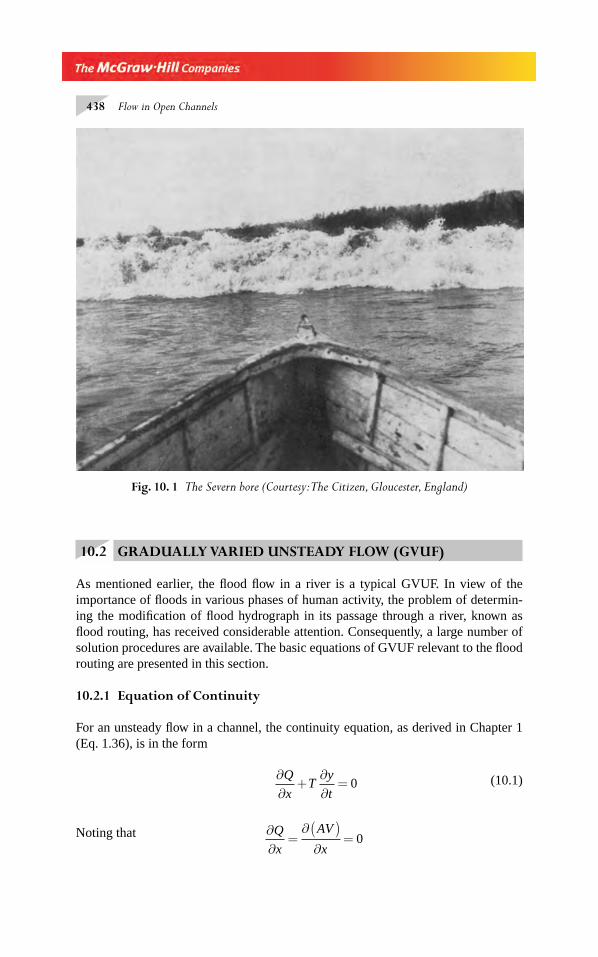
438 Flow in Open Channels
Fig. 10. 1 The Severn bore (Courtesy: The Citizen, Gloucester, England)
10.2 GRADUALLY VARIED UNSTEADY FLOW (GVUF)
As mentioned earlier, the fl ood fl ow in a river is a typical GVUF. In view of the importance of fl oods in various phases of human activity, the problem of determin-ing the modifi cation of fl ood hydrograph in its passage through a river, known as fl ood routing, has received considerable attention. Consequently, a large number of solution procedures are available. The basic equations of GVUF relevant to the fl ood routing are presented in this section.
10.2.1 Equation of Continuity
For an unsteady fl ow in a channel, the continuity equation, as derived in Chapter 1 (Eq. 1.36), is in the form
∂∂
+∂∂
=Q
xT
y
t0 (10.1)
Noting that ∂∂
=∂( )
∂=
Q
x
AV
x0
Chapter 10.indd 438Chapter 10.indd 438 2/24/2010 3:07:02 PM2/24/2010 3:07:02 PM
Unsteady Flows 439
AV
xV
A
xT
y
t
∂∂
+∂∂
+∂∂
= 0 (10.2)
This equation assumes no lateral infl ow or outfl ow. However, if there is a lateral infl ow of q per unit length of channel, Eq. 10.2 will read as
AV
xV
A
xT
y
tq
∂∂
+∂∂
+∂∂
− = 0 (10.3)
The cross-sectional area, in general, can be a function of depth and can also vary from section to section, i.e. A = A(x, y). The x derivative of area at constant time is written as
∂∂
=∂∂
⎛⎝⎜⎜⎜
⎞⎠⎟⎟⎟⎟ +
∂∂
⎛
⎝⎜⎜⎜⎜
⎞
⎠⎟⎟⎟⎟
∂∂
A
x
A
x
A
y
y
xy x
in which the suffi x denotes the variable to be held constant in addition to time
in taking the derivative. Since ∂∂
⎛
⎝⎜⎜⎜⎜
⎞
⎠⎟⎟⎟⎟ =
A
yx
T,
∂∂
=∂∂
⎛⎝⎜⎜⎜
⎞⎠⎟⎟⎟⎟ +
∂∂
A
x
A
xT
y
xy
The fi rst term∂∂
⎛⎝⎜⎜⎜
⎞⎠⎟⎟⎟⎟
A
x y
represents the rate of change of area with the depth held constant
and is the gain in the area due to the width change. The second term Tyx
∂∂
⎛
⎝⎜⎜⎜⎜
⎞
⎠⎟⎟⎟⎟ represents
the gain in the area due to an increase in the depth. The continuity equation in its general form is
AV
xVT
y
x
y
tq V
A
x y
∂∂
+∂∂
+∂∂
− +∂∂
⎛⎝⎜⎜⎜
⎞⎠⎟⎟⎟⎟ = 0 (10.4)
For a prismatic channel,∂∂
⎛⎝⎜⎜⎜
⎞⎠⎟⎟⎟⎟ =
A
x y
0, which simplifi es Eq. 10.4 as
AV
xVT
y
xT
y
tq
∂∂
+∂∂
+∂∂
− = 0 (10.4a)
10.2.2 Equation of Motion
The equation of motion for GVUF in a prismatic channel is derived by the applica-tion of the momentum equation to a control volume encompassing two sections of the fl ow as in Fig. 10.2. Since the fl ow is gradually varied, hydrostatic pressure distribution is assumed. The forces acting on the control volume are:
Chapter 10.indd 439Chapter 10.indd 439 2/24/2010 3:07:03 PM2/24/2010 3:07:03 PM
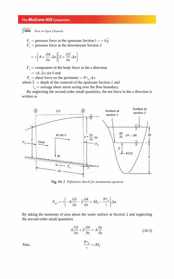
440 Flow in Open Channels
F1 = pressure force at the upstream Section l = γ A y
F2 = pressure force at the downstream Section 2
x yy
= +∂∂
⎛⎝⎜⎜⎜
⎞⎠⎟⎟⎟ +
∂∂
⎛
⎝⎜⎜⎜⎜
⎞
⎠⎟⎟⎟⎟⎟
γ AA
x xxΔ Δ
F3 = component of the body force in the x direction
= γA Δ x sin θ and F
s = shear force on the perimeter = Pτ
0 Δ x
where y = depth of the centroid of the upstream Section 1 and τ
0 = average shear stress acting over the fl ow boundary.
By neglecting the second order small quantities, the net force in the x direction is written as
ΔxFs
F1 F2
W sin θ
W
y
CV1 2
Flow
y +∂y
∂xΔx
xθ
∇
dy
y
y
CG
∂A∂x
Δx = dA
∇
∇
Surface atsection 1
Surface atsection 2
Fig. 10. 2 Defi nition sketch for momentum equation
F Ay
xy
A
xAS
Pxnet = −
∂∂
−∂∂
+ −⎛
⎝⎜⎜⎜⎜
⎞
⎠⎟⎟⎟⎟⎟Δγ
τγ0
0
By taking the moments of area about the water surface at Section 2 and neglecting the second order small quantities
Ay
xy
A
xA
y
x
∂∂
+∂∂
=∂∂ (10.5)
Also, Pτγ
0 = ASf
Chapter 10.indd 440Chapter 10.indd 440 2/24/2010 3:07:03 PM2/24/2010 3:07:03 PM

Unsteady Flows 441
Hence, Fnet
= −∂∂
+ −⎛⎝⎜⎜⎜
⎞⎠⎟⎟⎟γ A
y
xAS AS xf0 Δ
(10.6)
The momentum equation for an unsteady fl ow states that the net external force on the control volume in a given direction is equal to the net rate of the momentum effl ux in that direction plus the time rate of increase of momentum in that direction in the control volume. Assuming β
1 = β
2 = 1.0 and considering the x direction:
1. Momentum infl ux into Section 1 = M1 = ρAV 2
2. Momentum effl ux from Section 2 = M AVx
AV x22 2= + ( )⎡
⎣⎢⎢
⎤
⎦⎥⎥
ρ∂
∂Δ
3. Time rate of increase of x-momentum in the control volume
∂∂
Δ( )t
AV xρMu =
By the momentum equation,
M2 – M
1 + M
u = F
net
i.e. ∂∂
Δ⎛
⎝⎜⎜⎜⎜
⎞
⎠⎟⎟⎟⎟+
∂∂
( )Δ = −∂∂
+ −⎛⎝⎜⎜⎜
⎞⎠⎟⎟⎟t g
AV xg x
AV x Ay
xS S f
γ γγ2
0 Δx
Dividing throughout by γg
xΔ and simplifying,
∂∂
( )+∂∂
( )+∂∂
= −( )t
AVx
AV gAy
xgA S S f
20
i.e.
∂∂
+∂∂
+∂∂
+∂∂
+∂∂
+∂∂
⎛⎝⎜⎜⎜
⎞⎠⎟⎟⎟⎟ = −( )V
tV
V
xg
y
x
V
A
A
tV
A
xA
V
xg S S f0
By Eq. 10.2,
∂∂
+∂∂
+∂∂
=A
tV
A
xA
V
x0
and on re-arranging,
∂∂
+∂∂
+∂∂
y
x
V
g
V
x g
V
t
1= S
0–S
f (10.7)
If there is a lateral infl ow q per unit length into the control volume with negligible initial momentum in the longitudinal x direction, the equation of motion will read as
∂∂
+∂∂
+∂∂
y
x
V
g
V
x g
V
t
1= −( )−S S
qV
Agf0
(10.8)
Chapter 10.indd 441Chapter 10.indd 441 2/24/2010 3:07:04 PM2/24/2010 3:07:04 PM
442 Flow in Open Channels
The continuity equation, Eq. 10.2 and the equation of motion (Eq. 10.7) of unsteady open-channel fl ow are believed to have been fi rst developed by A J C Barré de-Saint Venant in 1871 and are commonly known as Saint Venant equations. These are simul-taneous, quasi-linear, fi rst order, partial differential equations of hyperbolic type and are not amenable to a general analytical solution.
The St Venant equations are expressed in a number of ways by choosing different dependent variables. Some of the common forms are listed below:
(i) With fl ow rate Q (x, t) and depth y(x, t) as dependent variables The velocity V in Eq. 10.7 is replaced by Q/A to get St Venant equations as
Continuity Equation ∂∂
+∂∂
y
t T
Q
x
1= 0 (10.9a)
Momentum Equation∂∂
+∂∂
⎛
⎝⎜⎜⎜⎜
⎞
⎠⎟⎟⎟⎟+
∂∂
+ −( )Q
t x
Q
AgA
y
xgA S S f
2
0 = 0 (10.9b)
From Eq. 10.5 A∂∂
=∂∂
( )y
x xAy . Hence Eq. 10.9(b) can be written as
∂∂
+∂∂
+⎛
⎝⎜⎜⎜⎜
⎞
⎠⎟⎟⎟⎟
= −( )Q
t x
Q
Ag Ay gA S S f
2
0 (10.9c)
This equation is known as momentum equation in conservation form. This form is particularly useful in handling steep fronts and shocks such as in a surge due to a dam break.
(ii) With fl ow rate Q (x, t) and Stage h(x, t) as dependent variable If h = the elevation of the water surface measured above a datum (i.e. stage), then the water depth y = h–h
b, where h
b is the elevation of the bed. Further,
∂∂
=∂∂
y
t
h
t and
∂∂
=∂∂
−∂∂
=∂∂
−y
x
h
x
h
x
h
xSb
0
The St Venant equations are
Continuity Equation ∂∂
+∂∂
=h
t T
Q
x
10 (10.10a)
Momentum Equation ∂∂
+∂∂
⎛
⎝⎜⎜⎜⎜
⎞
⎠⎟⎟⎟⎟+
∂∂
+Q
t x
Q
AgA
h
x
2
gA Sf = 0 (10.10b)
Chapter 10.indd 442Chapter 10.indd 442 2/24/2010 3:07:05 PM2/24/2010 3:07:05 PM
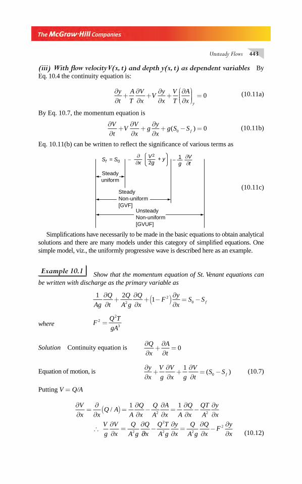
Unsteady Flows 443
(iii) With fl ow velocity V(x, t) and depth y(x, t) as dependent variables By Eq. 10.4 the continuity equation is:
∂∂
+∂∂
+∂∂
+∂∂
⎛⎝⎜⎜⎜
⎞⎠⎟⎟⎟⎟ =
y
t
A
T
V
xV
y
x
V
T
A
x y
0 (10.11a)
By Eq. 10.7, the momentum equation is
∂∂
+∂∂
+∂∂
+ − =V
tV
V
xg
y
xg S S f( )0 0 (10.11b)
Eq. 10.11(b) can be written to refl ect the signifi cance of various terms as
Sf = S0 − ∂V∂t
1g
− ∂∂x
V2
2g+ y
SteadyNon-uniform[GVF]
UnsteadyNon-uniform[GVUF]
Steadyuniform
(10.11c)
Simplifi cations have necessarily to be made in the basic equations to obtain analytical solutions and there are many models under this category of simplifi ed equations. One simple model, viz., the uniformly progressive wave is described here as an example.
Example 10.1 Show that the momentum equation of St. Venant equations can be written with discharge as the primary variable as
1 2
12
20Ag
Q
t
Q
A g
Q
xF
y
xS S f
∂∂
+∂∂
+ −( )∂∂
= −
where FQ T
gA2
2
3=
Solution Continuity equation is ∂∂
+∂∂
=Q
x
A
t0
Equation of motion, is ∂∂
+∂∂
+∂∂
= −y
x
V
g
V
x g
V
tS S f
10( ) (10.7)
Putting V = Q/A
∂∂
=∂∂
( ) =∂∂
−∂∂
=∂∂
−∂∂
∴∂∂
=∂
V
x xQ A
A
Q
x
Q
A
A
x A
Q
x
QT
A
y
x
V
g
V
x
Q
A g
Q
/1 1
2 2
2 ∂∂−
∂∂
=∂∂
−∂∂x
Q T
A g
y
x
Q
A g
Q
xF
y
x
2
2 2
2
(10.12)
Chapter 10.indd 443Chapter 10.indd 443 2/24/2010 3:07:05 PM2/24/2010 3:07:05 PM
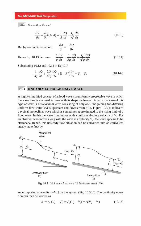
444 Flow in Open Channels
∂∂
=∂∂
( ) =∂∂
−∂∂
V
t tQ A
A
Q
t
Q
A
A
t2
1/
(10.13)
But by continuity equation
∂∂
= −∂∂
A
t
Q
x
Hence Eq. 10.13 becomes 1 1
2g
V
t Ag
Q
t
Q
A g
Q
x
∂∂
=∂∂
+∂∂
(10.14)
Substituting 10.12 and 10.14 in Eq 10.7
1 21
2
20Ag
Q
t
Q
A g
Q
xF
y
xS S f
∂∂
+∂∂
+ −( )∂∂
= −
(10.14a)
10.3 UNIFORMLY PROGRESSIVE WAVE
A highly simplifi ed concept of a fl ood wave is a uniformly progressive wave in which the wave form is assumed to move with its shape unchanged. A particular case of this type of wave is a monoclinal wave consisting of only one limb joining two differing uniform fl ow water levels upstream and downstream of it. Figure 10.3(a) indicates a typical monoclinal wave which is sometimes approximated to the rising limb of a fl ood wave. In this the wave front moves with a uniform absolute velocity of V
w . For
an observer who moves along with the wave at a velocity Vw
, the wave appears to be
stationary. Hence, this unsteady fl ow situation can be converted into an equivalent steady-state fl ow by
Fig. 10.3 (a) A monoclinal wave (b) Equivalent steady fl ow
y2
y1
V2
V1
VW
Monoclinalwave
Unsteady flow(a)
∇
y2
y1
(VW –V2)
(VW –V1)
θ
θ
∇
∇
Steady flow(b)
superimposing a velocity (−Vw ) on the system (Fig. 10.3(b)). The continuity equa-
tion can then be written as
Qr = A
1 (V
w − V
1) = A
2(V
w − V
2) = A(V
w − V ) (10.15)
Chapter 10.indd 444Chapter 10.indd 444 2/24/2010 3:07:06 PM2/24/2010 3:07:06 PM
Unsteady Flows 445
The quantity Qr is termed as overrun. Simplifying,
VAV A V
A A
Q
Aw =−−
=1 1 2 2
1 2
ΔΔ
From this it may be seen that the maximum value of Vw is obtained as
VdQ
dAw m( ) = (10.16)
Since, dA
dyT=
VT
dQ
dyw m( ) =
1 (10.17)
For a wide rectangular channel, the normal discharge per unit width is
qn
y Sn =1 5 3
01 2/ /
or, dq
dy ny S Vn
n= =5
3
1 5
32 3
01 2/ /
where Vn =
q
yn =
normal velocity.
Thus (Vw)
m = k
w V
n (10.18)
where kw = 1.67 for a wide rectangular channel. It can be shown that k
w = 1.44 and
1.33 for wide-parabolic (R ≈ y) and triangular channels respectively. Field observa-tions have indicated that for small rises in the fl ood stage, the absolute-wave veloci-ties can be roughly estimated by Eq. 10.18.
Considering the equivalent steady-state fl ow
d
dtV V
xV V
dx
dt tV Vw w w−( ) =
∂∂
−( ) +∂∂
−( ) = 0
Since Vdx
dtw = = constant, on simplifi cation,
∂∂
= −∂∂
V
tV
V
xw
Also, since
V VQ
Awr= −
∂∂
=∂∂
V
x
QT
A
y
x2
Chapter 10.indd 445Chapter 10.indd 445 2/24/2010 3:07:06 PM2/24/2010 3:07:06 PM
446 Flow in Open Channels
Substituting these in the equation of motion (Eq. 10.7), it can be expressed as
∂∂
+ −∂∂
= −y
x gV V
V
xS Sw f
10( )
i.e.
∂∂
=−
−
y
x
S S
Q T
gA
f
r
0
2
31 (10.19)
This is the differential equation of a monoclinal rising wave. Note the similarity with the differential equation of GVF (Eq. 4.8). The profi le of the wave is obtained by integrating this equation.
Equation 10.19 can be simplifi ed by considering the denominator to be approxi-mately equal to unity for small velocities (i.e. by neglecting the effect of the velocity head) as
∂∂
= −y
xS S f0
= −⎛
⎝⎜⎜⎜⎜
⎞
⎠⎟⎟⎟⎟
= −⎛
⎝⎜⎜⎜⎜
⎞
⎠⎟⎟⎟⎟
SS
SS
Q
Qf
n
00
0
2
21 1
where Q K Sn = 0 = normal discharge at any depth y and Q = actual discharge at that depth. On re-arranging,
Q
Q
y x
Sn
= −∂ ∂
10
/ (10.20)
In a uniformly progressive wave for any point on the wave profi le
dy
dt
y
tV
y
xw=∂∂
+∂∂
= 0
and hence, ∂∂
= −∂ ∂y
x
y t
Vw
/
Substituting in Eq. 10.20 leads to
Q
Q
y t
V Sn w
= +∂ ∂
10
/ (10.21)
This equation indicates that during the rising stages in a fl ood fl ow, the actual dis-charge is larger than the discharge read by the normal stage-discharge relationship. Conversely, during the falling stages in a fl ood fl ow, the actual discharge is lower than that indicated by the normal stage-discharge curve. Equation 10.21 is used in hydrometry to correct the normal discharges read from a stage-discharge curve when
Chapter 10.indd 446Chapter 10.indd 446 2/24/2010 3:07:06 PM2/24/2010 3:07:06 PM
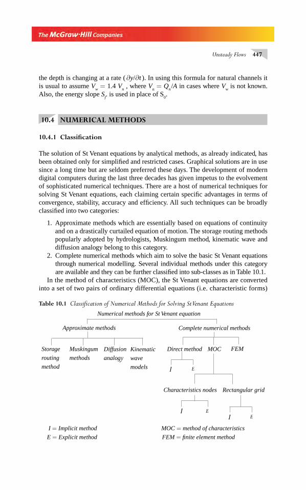
Unsteady Flows 447
the depth is changing at a rate ( ∂y/∂t ). In using this formula for natural channels it is usual to assume V
w = 1.4 V
n , where V
n = Q
n /A in cases where V
w is not known.
Also, the energy slope Sf. is used in place of S
0.
10.4 NUMERICAL METHODS
10.4.1 Classifi cation
The solution of St Venant equations by analytical methods, as already indicated, has been obtained only for simplifi ed and restricted cases. Graphical solutions are in use since a long time but are seldom preferred these days. The development of modern digital computers during the last three decades has given impetus to the evolvement of sophisticated numerical techniques. There are a host of numerical techniques for solving St Venant equations, each claiming certain specifi c advantages in terms of convergence, stability, accuracy and effi ciency. All such techniques can be broadly classifi ed into two categories:
1. Approximate methods which are essentially based on equations of continuity and on a drastically curtailed equation of motion. The storage routing methods popularly adopted by hydrologists, Muskingum method, kinematic wave and diffusion analogy belong to this category.
2. Complete numerical methods which aim to solve the basic St Venant equations through numerical modelling. Several individual methods under this category are available and they can be further classifi ed into sub-classes as in Table 10.1.
In the method of characteristics (MOC), the St Venant equations are converted into a set of two pairs of ordinary differential equations (i.e. characteristic forms)
FEM
Numerical methods for St Venant equation
Approximate methods Complete numerical methods
Storage
routing
method
Muskingum
methods
Kinematic
wave
models
Direct method MOC
Characteristics nodes Rectangular grid
Diffusion
analogy
I E
I = Implicit method MOC = method of characteristics
E = Explicit method FEM = fi nite element method
I EEI
Table 10.1 Classifi cation of Numerical Methods for Solving St Venant Equations
Chapter 10.indd 447Chapter 10.indd 447 2/24/2010 3:07:07 PM2/24/2010 3:07:07 PM
448 Flow in Open Channels
and then solved by fi nite-difference methods. In the direct method, the partial derivatives are replaced by fi nite differences and the resulting algebraic equations are then solved. In the fi nite-element method (FEM) the system is divided into a number of elements and the partial differential equations are integrated at the nodal points of the elements.
The fi nite-difference schemes are further classifi ed into explicit and implicit methods. In the explicit method, the fi nite difference algebraic equations are usu-ally linear and the dependent variables are extracted explicitly at the end of each time step. In the implicit method, the resulting algebraic equations are generally non-linear and the dependent variables occur implicitly. Each of these two methods has different schemes of fi nite differencing.
To start the solution all methods require an initial condition specifying the values of all the unknowns at an initial time for every computational section along the channel. In the usual subcritical fl ow, the upstream boundary condition is a hydrograph of the stage or discharge and the downstream boundary condition is normally a stage-discharge relationship. In the absence of a separate resistance formula for unsteady fl ows, the friction losses are estimated by using a uniform fl ow resistance equation, typically the Manning’s formula is used and in such a case,
Sn V
R
n Q
A R
Q Q
Kf = = =2 2
4 3
2 2
2 4 3 2/ /
where K = conveyance.
10.4.2 Method of Characteristics
Consider a unit width of a wide rectangular channel having a GVUF without lateral
infl ow. Using the celerity of a small wave C = gy ,
∂∂
=∂∂
y
x
C
g
C
x
2 (10.22 a)
and ∂∂
=∂∂
y
t
C
g
C
x
2 (10.22 b)
Substituting these in the equation of continuity (Eq. l0.2) and noting that for a wide rectangular channel T = B = 1.0 and A = y = C2/g
2 2
02CV
g
C
x
C
g
V
x
C
g
C
t
∂∂
+∂∂
+∂∂
= (10.23)
The equation of motion (Eq. 10.7) by a similar substitution becomes,
2 10
C
g
C
x
V
g
V
x g
V
tS S f
∂∂
+∂∂
+∂∂
= −( )
(10.24)
Chapter 10.indd 448Chapter 10.indd 448 2/24/2010 3:07:07 PM2/24/2010 3:07:07 PM
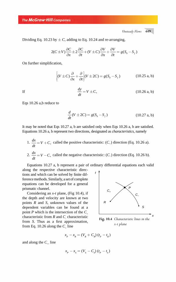
Unsteady Flows 449
Dividing Eq. 10.23 by ± C, adding to Eq. 10.24 and re-arranging,
2 2 0( ) ( ) ( )C V
C
x
C
tV C
V
x
V
tg S S f±
∂∂
±∂∂
+ ±∂∂
+∂∂
= −
On further simplifi cation,
( ) ( ) ( )V C
x tV C g S S f±
∂∂
+∂∂
⎡
⎣⎢⎢
⎤
⎦⎥⎥
± = −2 0
(10.25 a, b)
If dy
dtV C= ± , (10.26 a, b)
Eqs 10.26 a,b reduce to
d
dtV C g S S f( ) ( )± = −2 0 (10.27 a, b)
It may be noted that Eqs 10.27 a, b are satisfi ed only when Eqs 10.26 a, b are satisfi ed. Equations 10.26 a, b represent two directions, designated as characteristics, namely
1. dx
dtV C= + ,
called the positive characteristic: (C+ ) direction (Eq. 10.26 a).
2.
dx
dtV C= − ,
called the negative characteristic: (C_ ) direction (Eq. 10.26 b).
Equations 10.27 a, b represent a pair of ordinary differential equations each valid along the respective characteristic direc-tions and which can be solved by fi nite dif-ference methods. Similarly, a set of complete equations can be developed for a general prismatic channel.
Considering an x-t plane, (Fig 10.4), if the depth and velocity are known at two points R and S, unknown values of the dependent variables can be found at a point P which is the intersection of the C
+
characteristic from R and C- characteristic
from S. Thus as a fi rst approximation, from Eq. 10.26 along the C
+ line
xP − x
R = (V
R + C
R) (t
P − t
R )
and along the C_ line
xP − x
S = (V
S − C
S) (t
P − t
S )
x
t
P
S
R
C+C–
Fig. 10.4 Characteristic lines in the
x-t plane
Chapter 10.indd 449Chapter 10.indd 449 2/24/2010 3:07:07 PM2/24/2010 3:07:07 PM
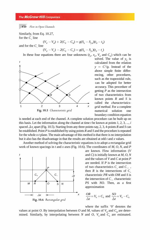
450 Flow in Open Channels
Similarly, from Eq. 10.27,for the C
+ line
(VP − V
R) + 2(C
P − C
R) = g(S
0 − S
f R )(t
P − t
R)
and for the C– line
(VP − V
S ) − 2(C
P − C
S ) = g(S
0 − S
f S )(t
P − t
s )
In these four equations there are four unknowns (tP , x
P , V
P and C
P ) which can be
solved. The value of yP is
calculated from the relation y = C 2/g. Instead of the above simple fi nite differ-encing, other procedures, such as the trapezoidal rule, can be adopted for better accuracy. This procedure of getting P as the intersection of two characteristics from known points R and S is called the characteristics-grid method. For a complete numerical solution one boundary condition equation
is needed at each end of the channel. A complete solution procedure can be built up on this basis. Let the information along the channel at time t be known at points 1, 2, 3, ..., i spaced Δ x
i apart (Fig. 10.5). Starting from any three points-say, 2, 3, 4-points R and S can
be established. Point P is established by using points R and S and the procedure is repeated for the whole x-t plane. The main advantage of this method is that there is no interpolation but it also has the disadvantage in that the results are obtained at odd t and x values.
Another method of solving the characteristic equations is to adopt a rectangular grid work of known spacings in t and x axes (Fig. 10.6). The coordinates of M, O, N, and P
are known. Flow information (V and C) is initially known at M, O, N and the values of V and C at point P are needed. If P is the intersection of two characteristics C
+ and C− ,
then R is the intersections of C+
characteristic PR with OM and S is the intersection of C− characteristic PS with NO. Then, as a fi rst approximation
OR
tV C
Δ= +0 0
and
SO
tV C
Δ= −0 0
where the suffi x ‘0’ denotes the values at point O. By interpolation between O and M, values of V
R and C
R are deter-
mined. Similarly, by interpolating between N and O, VS and C
S are estimated.
1 2 3 4 x
P
SR
t
Fig. 10.5 Characteristic grid
t
x
M R
C+ C–
O
P
NS
Δx
Δt
Fig. 10.6 Rectangular grid
Chapter 10.indd 450Chapter 10.indd 450 2/24/2010 3:07:07 PM2/24/2010 3:07:07 PM
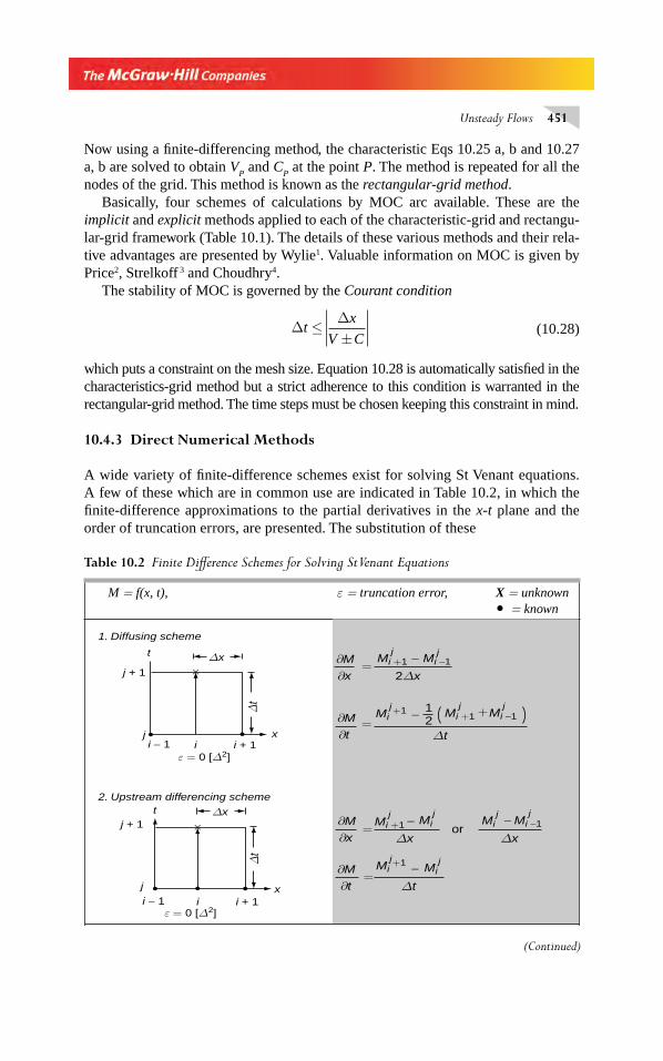
Unsteady Flows 451
Now using a fi nite-differencing method, the characteristic Eqs 10.25 a, b and 10.27 a, b are solved to obtain V
P and C
P at the point P. The method is repeated for all the
nodes of the grid. This method is known as the rectangular-grid method.Basically, four schemes of calculations by MOC arc available. These are the
implicit and explicit methods applied to each of the characteristic-grid and rectangu-lar-grid framework (Table 10.1). The details of these various methods and their rela-tive advantages are presented by Wylie1. Valuable information on MOC is given by Price2, Strelkoff 3 and Choudhry4.
The stability of MOC is governed by the Courant condition
Δ
Δt
x
V C≤
± (10.28)
which puts a constraint on the mesh size. Equation 10.28 is automatically satisfi ed in the characteristics-grid method but a strict adherence to this condition is warranted in the rectangular-grid method. The time steps must be chosen keeping this constraint in mind.
10.4.3 Direct Numerical Methods
A wide variety of fi nite-difference schemes exist for solving St Venant equations. A few of these which are in common use are indicated in Table 10.2, in which the fi nite-difference approximations to the partial derivatives in the x-t plane and the order of truncation errors, are presented. The substitution of these
Table 10.2 Finite Diff erence Schemes for Solving St Venant Equations
M = f(x, t), ε = truncation error, X = unknown
• = known
1. Diffusing scheme
Δx
Δt
t
x
j + 1
i + 1i − 1 ij
∂M
∂t
jMi +1
jMi +1
jMi −1
Mi +1
Mi +1
jMi −1− 2
1 +
Δt
Δx Δx
∂M
∂x
=
∂M
∂x
jMi +1
jMi −1
2Δx
−=
ε = 0 [Δ2]
2. Upstream differencing schemet
x
j + 1
i + 1i − 1 i
j
−Δt
∂M
∂t=
Δt
Δx
ε = 0 [Δ2]
jMi
jMi
jMi
− −= or
×
×
j
j
(Continued)
Chapter 10.indd 451Chapter 10.indd 451 2/24/2010 3:07:08 PM2/24/2010 3:07:08 PM
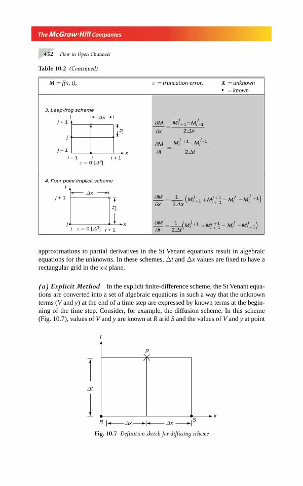
452 Flow in Open Channels
approximations to partial derivatives in the St Venant equations result in algebraic equations for the unknowns. In these schemes, Δt and Δx values are fi xed to have a rectangular grid in the x-t plane.
(a) Explicit Method In the explicit fi nite-difference scheme, the St Venant equa-tions are converted into a set of algebraic equations in such a way that the unknown terms (V and y) at the end of a time step are expressed by known terms at the begin-ning of the time step. Consider, for example, the diffusion scheme. In this scheme (Fig. 10.7), values of V and y are known at R arid S and the values of V and y at point
Fig. 10.7 Defi nition sketch for diff using scheme
R
P
Sx
t
ΔxΔx
Δt
jMi +1
jMi −1
Mi +1 Mi −1
3. Leap-frog scheme
t
x
j + 1
j − 1
i + 1i − 1 i
j
Δt
Δx
ε = 0 [Δ3]
−∂M
∂x=
2Δx
−∂M
∂t=
2Δt
×
j j
jMi +1
jMi +1
Mi +1
Mi +1
i + 1Mj +1
i + 1Mj +1
jMi
jMi
4. Four point implicit schemet
x
j + 1
i + 1ij
− −2Δx1 +∂M
∂x=
− −2Δt1 +∂M
∂t=
Δt
ε = 0 [Δ3]
Δx×
j
j
M = f(x, t), ε = truncation error, X = unknown • = known
Table 10.2 (Continued)
Chapter 10.indd 452Chapter 10.indd 452 2/24/2010 3:07:08 PM2/24/2010 3:07:08 PM
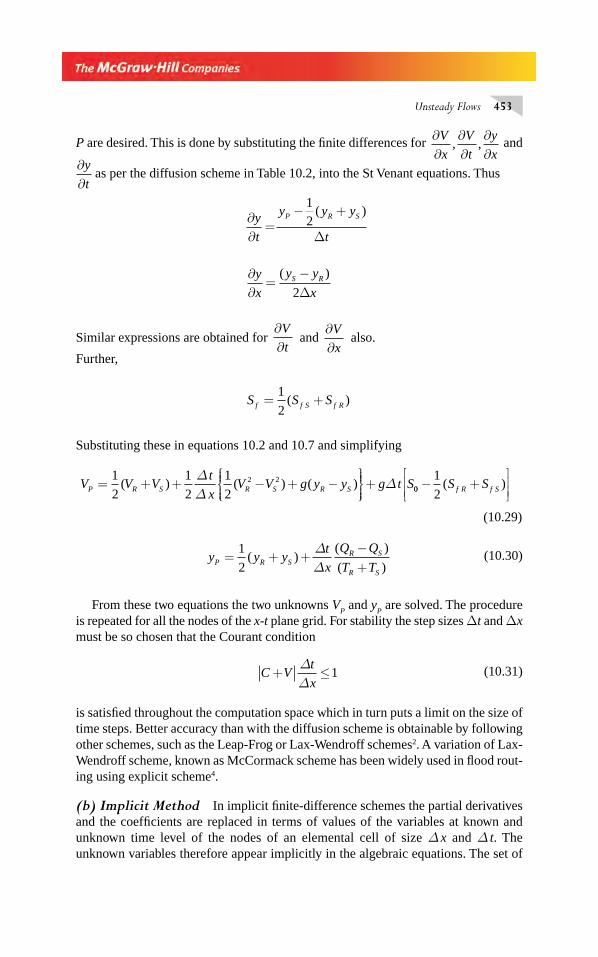
Unsteady Flows 453
P are desired. This is done by substituting the fi nite differences for ∂∂
∂∂
∂∂
V
x
V
t
y
x, , and
∂∂
y
tas per the diffusion scheme in Table 10.2, into the St Venant equations. Thus
∂∂
=− +
Δy
t
y y y
t
P R S
1
2( )
∂∂
=−Δ
y
x
y y
xS R( )
2
Similar expressions are obtained for ∂∂V
t and
∂∂V
x also.
Further,
S S Sf f S f R= +1
2( )
Substituting these in equations 10.2 and 10.7 and simplifying
V V V
t
xV V g y y g t SP R S R S R S= + + − + −
⎧⎨⎪⎪⎩⎪⎪
⎫⎬⎪⎪⎭⎪⎪
+1
2
1
2
1
22 2( ) ( ) ( )
ΔΔ
Δ 00
1
2− +
⎡
⎣⎢⎢
⎤
⎦⎥⎥
( )S Sf R f S
(10.29)
y y y
t
x
Q Q
T TP R SR S
R S
= + +−+
1
2( )
( )
( )
ΔΔ
(10.30)
From these two equations the two unknowns VP and y
P are solved. The procedure
is repeated for all the nodes of the x-t plane grid. For stability the step sizes Δt and Δx must be so chosen that the Courant condition
C V
t
x+ ≤
ΔΔ
1
(10.31)
is satisfi ed throughout the computation space which in turn puts a limit on the size of time steps. Better accuracy than with the diffusion scheme is obtainable by following other schemes, such as the Leap-Frog or Lax-Wendroff schemes2. A variation of Lax-Wendroff scheme, known as McCormack scheme has been widely used in fl ood rout-ing using explicit scheme4.
(b) Implicit Method In implicit fi nite-difference schemes the partial derivatives and the coeffi cients are replaced in terms of values of the variables at known and unknown time level of the nodes of an elemental cell of size Δ x and Δ t. The unknown variables therefore appear implicitly in the algebraic equations. The set of
Chapter 10.indd 453Chapter 10.indd 453 2/24/2010 3:07:08 PM2/24/2010 3:07:08 PM
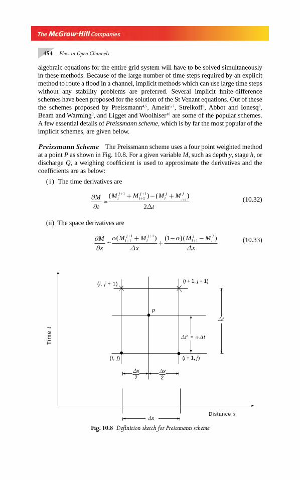
454 Flow in Open Channels
algebraic equations for the entire grid system will have to be solved simultaneously in these methods. Because of the large number of time steps required by an explicit method to route a fl ood in a channel, implicit methods which can use large time steps without any stability problems are preferred. Several implicit fi nite-difference schemes have been proposed for the solution of the St Venant equations. Out of these the schemes proposed by Preissmann4,5, Amein6,7, Strelkoff3, Abbot and Ionesq8, Beam and Warming9, and Ligget and Woolhiser10 are some of the popular schemes. A few essential details of Preissmann scheme, which is by far the most popular of the implicit schemes, are given below.
Preissmann Scheme The Preissmann scheme uses a four point weighted method at a point P as shown in Fig. 10.8. For a given variable M, such as depth y, stage h, or discharge Q, a weighing coeffi cient is used to approximate the derivatives and the coeffi cients are as below:
( i ) The time derivatives are
∂∂
+ − +
Δ
+++
+M
t
M M M M
t
ij
ij
ij j
i�( ) ( )1
11
1
2
(10.32)
(ii) The space derivatives are
∂∂
++
− −++ +
+M
x
M M
x
M M
xij
ij
ij
ij
�α α( ) ( ) ( )1
1 111
Δ Δ
(10.33)
Δx
Δx2
Δx2
(i + 1, j )
(i + 1, j + 1)
Δt
Δt ′ = αΔt
( i, j)
( i, j + 1)
P
Distance x
Tim
e t
Fig. 10.8 Defi nition sketch for Preissmann scheme
Chapter 10.indd 454Chapter 10.indd 454 2/24/2010 3:07:09 PM2/24/2010 3:07:09 PM
Unsteady Flows 455
(iii) The value of M as a coeffi cient is
M M M M Mi
jij
ij
ij�
1
2
1
211
1 11α α+
+ +++( )+ −( ) −( )
The value of α =
Δ ′
Δt
t locates the point P along the time axis in the fi nite differ-
ence grid.The Preissmann scheme is unconditionally stable for 0.50 ≤ α ≤ 1. For typical
applications, a value of α in the range 0.55 to 0.70 is recommended in order to avoid higher order numerical oscillations.
Consider the St. Venant equations in the form of Eqs 10.10a and 10.10b with the discharge Q(x, t) and stage h(x, t) as the dependent variables. With
SQ Q
Kf =| |
2, the St Venant equations are
Continuity
∂∂
+∂∂
=h
t T
Q
x
10
(10.10a)
Momentum
∂∂
+∂∂
⎛
⎝⎜⎜⎜⎜
⎞
⎠⎟⎟⎟⎟+
∂∂
+ =Q
t x
Q
AgA
h
xgA
Q Q
K
2
20
| |
(10.10c)
The application of the Preissmann scheme to the derivatives and the coeffi cients in the Eqs 10.10a and 10.10c results in
∂∂
+( )− +( )Δ
+++
+h
t
h h h h
t
ij
ij
ij
ij
�1
11
1
2
∂∂
+( )− +( )Δ
+++
+Q
t
Q Q Q Q
t
ij
ij
ij
ij
�1
11
1
2
∂∂
−( )Δ
+−( ) −( )
Δ++ +
+Q
x
Q Q
x
Q Q
x
ij
ij
ij
ij
�α α1
1 111
∂∂
⎛
⎝⎜⎜⎜⎜
⎞
⎠⎟⎟⎟⎟ Δ
⎛
⎝⎜⎜⎜⎜
⎞
⎠⎟⎟⎟⎟
−⎛
⎝⎜⎜⎜⎜
⎞
⎠⎟⎟⎟
+
+
x
Q
A x
Q
A
Q
Ai
j2 2
1
1 2
�α
⎟⎟
⎡
⎣
⎢⎢⎢
⎤
⎦
⎥⎥⎥+
−( )Δ
⎡
⎣⎢⎢
⎤
⎦⎥⎥ −
⎛
⎝⎜⎜⎜⎜
⎞
⎠⎟⎟⎟⎟
⎡+
+i
j
i
j
i
j
x
Q
A
Q
A
1 2
1
21 α
⎣⎣
⎢⎢⎢
⎤
⎦
⎥⎥⎥
∂∂
−( )Δ
+−( ) −( )
Δ++ +
+h
x
h h
x
h h
x
ij
ij
ij j
i
�α α1
1 111
Chapter 10.indd 455Chapter 10.indd 455 2/24/2010 3:07:09 PM2/24/2010 3:07:09 PM
456 Flow in Open Channels
The coeffi cients A and T are given by —
A A A A Ai
jij
ij
ij�
1
2
1
211
1 11α α+
+ +++( )+ −( ) +( )
T T T T Ti
ji
ji
ji
j�1
2
1
211
1 11α α+
+ +++( )+ −( ) +( )
Substituting these expressions in Eq. 10.10a and Eq. 10.10c,
1
21
11
1Δ+( )− +( )⎡
⎣⎢⎤⎦⎥
+++
+th h h hi
jij
ij
ij
+Δ
−( )+ −( ) −( )⎡⎣⎢
⎤⎦⎥
+(++ +
+
++ +
2 111
1
11 1x
Q Q Q Q
T T
ij i
ij
ij
ij
ij
ij
α α
α ))+ −( ) +( )=
+10
1α T Tij
ij
(10.34)
1
21
11
1Δ+( )− +( )⎡
⎣⎢⎤⎦⎥
+++
+tQ Q Q Qi
jij
ij
ij
+Δ
⎛
⎝⎜⎜⎜⎜
⎞
⎠⎟⎟⎟⎟
−⎛
⎝⎜⎜⎜⎜
⎞
⎠⎟⎟⎟⎟
+−( )Δ
⎛
⎝+
+ +α α
x
Q
A
Q
A x
Q
Ai
j
i
j2
1
1 2 1 21 ⎜⎜⎜⎜⎜
⎞
⎠⎟⎟⎟⎟
−⎛
⎝⎜⎜⎜⎜
⎞
⎠⎟⎟⎟⎟
⎡
⎣
⎢⎢⎢
⎤
⎦
⎥⎥⎥+i
j
i
jQ
A1
2
+ +( )+
−( )+( )
⎡
⎣⎢⎢⎢
⎤
⎦⎥⎥⎥ Δ
−++ +
+ ++g A A A A
xhi
jij
ij
ij
ijα α α
2
1
211 1
1 11 hhi
j+( )⎡
⎣⎢⎢
⎧⎨⎪⎪⎩⎪⎪
1
+−( )Δ
−( )⎤
⎦⎥⎥⎥+
⎛⎝⎜⎜⎜
⎞⎠⎟⎟⎟⎟ ++
+
+1 1
21 21
1
2
αα
xh h
Q Q
K
Q Q
Kij
ij
i
j| | | |⎛⎛
⎝⎜⎜⎜
⎞⎠⎟⎟⎟⎟
⎡
⎣
⎢⎢⎢
⎤
⎦
⎥⎥⎥+
+
i
j
1
1
+−( ) ⎛
⎝⎜⎜⎜
⎞⎠⎟⎟⎟⎟ +
⎛⎝⎜⎜⎜
⎞⎠⎟⎟⎟⎟
⎡
⎣
⎢⎢⎢
⎤
⎦
⎥⎥⎥+
1
2 21
2
α Q Q
K
Q Q
Ki
j
i
j| | | | ⎫⎫
⎬⎪⎪⎪
⎭⎪⎪⎪
= ≤ ≤0 0 5 1 0for . .α
(10.35)
In these two Eqs 10.34 and 10.35 the terms having superscript j are known. The unknown terms are those having superscript ( j + 1) and can be expressed in terms of
Q Q hij
ij
ij
, , ,+
++ +111 1
and hij++11. As the unknowns are raised to the power other than unity,
these equations are non-linear.
If there are a total of N grid lines at any j value with the upstream boundary as i = 1 and the downstream boundary as i = N, there will be (N – 1) grids at which the above equations are applicable. Thus there are (2N – 2) equations. Further, there are two unknowns at each of N grid points, totaling to 2N unknowns. The two additional equations to form the necessary set of equations are supplied by the boundary condi-tions. In subcritical fl ows, one boundary condition is applied at the upstream end and another at the downstream boundary. In supercritical fl ows, however, both the bound-ary conditions are applied at the upstream end.
Chapter 10.indd 456Chapter 10.indd 456 2/24/2010 3:07:09 PM2/24/2010 3:07:09 PM
Unsteady Flows 457
The upstream boundary condition is usually a known infl ow hydrograph,
Qij+1 = f (t j+1). The downstream boundary condition is usually a known stage-discharge
relationship (i.e. channel rating curve) given as QNj+1 = f hN
j+( )1 .The set of non-linear
algebraic equations are solved by adopting an iterative procedure, such as Newton-Raphson method.
It is generally recognized that while an implicit method is more diffi cult to pro-gramme than an explicit method, it has stability, greater accuracy and has economy in computing time. Details on various numerical techniques can be had from Ref. [4, 5]. Extensive bibliography on unsteady fl ows in open channel fl ows is available in Ref. [11, 12].
The use of FEM to route fl oods in channels and natural streams is presented by Cooley and Moin,13 and King14. Szymkiewicz15 has presented an FEM algorithm to solve St. Venant euations for a channel network. Jie Chen16 has developed an approx-imate formulation of St. Venant equations for natural channels which through the use of FEM can be used effectively to simulate dam break problems and fl ood routing in natural channels.
A large number of software are available, for unsteady fl ow simulation in general and for fl ood fl ow analysis/forecasting and dam break problem in particular. Among these, the HEC-RAS of U.S. Army Corps of Engineers, FLDWAV of U.S. NWS and MKE-11 of DIH, Denmark are very popular (2007). Among these, HEC-RAS is available along with user’s manual (http://www.hec.usaace.army.mill/software/hec-1 ) for download by individuals free of charge. Details of MIKE-11 are available at (http://www.dhigroup.com). BOSSDAMBRK (http://www.bossintl.com ), which is commercial software, is an enhanced version of NWS DAMBRK model.
Example10.2 Determine the time derivative and space derivative of the fl ow rate Q by using Preisman scheme (α =0.65), when the discharges at various (x, t) values are as given below:
x =1000 m x= 1500 m
At t = 3.0h Q= 125.00 m3/s Q=115.00 m3/s
At t = 4.0 h Q= 140.00 m3/s Q= 120.00 m3/s
Solution Here Δt = 1.5 h = 5400 s and Δ x=500 m.
Qij =125 00. m /s3
Qi
j+ =1 115 00. m /s3
Qij+ =1 140 00. m /s3
Qi
j++ =1
1 120 00. m /s3
∂∂
=+( )− +( )
Δ
+++
+Q
t
Q Q Q Q
t
ij
ij
ij
ij1
11
1
2
Chapter 10.indd 457Chapter 10.indd 457 2/24/2010 3:07:10 PM2/24/2010 3:07:10 PM
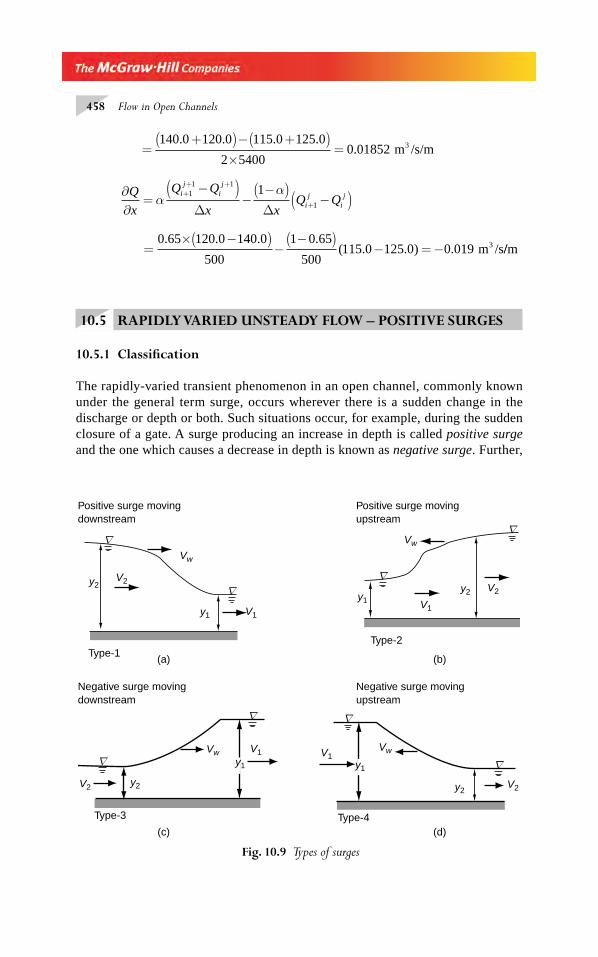
458 Flow in Open Channels
=
+( )− +( )×
=140 0 120 0 115 0 125 0
2 54000 01852
. . . .. m /s/m3
∂∂
=−( )
Δ−
−( )Δ
−( )++ +
+
Q
x
Q Q
x xQ Q
ij
ij
ij
ijα
α11 1
1
1
=
× −( )−
−( )− = −
0 65 120 0 140 0
500
1 0 65
500115 0 125 0 0 019
. . . .( . . ) . m /s3 //m
10.5 RAPIDLY VARIED UNSTEADY FLOW – POSITIVE SURGES
10.5.1 Classifi cation
The rapidly-varied transient phenomenon in an open channel, commonly known under the general term surge, occurs wherever there is a sudden change in the discharge or depth or both. Such situations occur, for example, during the sudden closure of a gate. A surge producing an increase in depth is called positive surge and the one which causes a decrease in depth is known as negative surge. Further,
y2V2
V1Vw
∇
∇y1
(d)Type-4
Negative surge movingupstream
y2V2
V1Vw∇
∇
y1
Type-3
(c)
Negative surge movingdownstream
y2
y1
V2
V1
Vw
∇
∇
Type-1(a)
Positive surge movingdownstream
y2y1
V2
∇
∇Vw
V1
Type-2
(b)
Positive surge movingupstream
Fig. 10.9 Types of surges
Chapter 10.indd 458Chapter 10.indd 458 2/24/2010 3:07:10 PM2/24/2010 3:07:10 PM
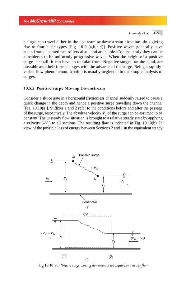
Unsteady Flows 459
a surge can travel either in the upstream or downstream direction, thus giving rise to four basic types [Fig. 10.9 (a,b,c,d)]. Positive waves generally have steep fronts –sometimes rollers also –and are stable. Consequently they can be considered to be uniformly progressive waves. When the height of a positive surge is small, it can have an undular front. Negative surges, on the hand, are unstable and their form changes with the advance of the surge. Being a rapidly-varied flow phenomenon, friction is usually neglected in the simple analysis of surges.
10.5.2 Positive Surge Moving Downstream
Consider a sluice gate in a horizontal frictionless channel suddenly raised to cause a quick change in the depth and hence a positive surge travelling down the channel [Fig. 10.10(a)]. Suffi xes 1 and 2 refer to the conditions before and after the passage of the surge, respectively. The absolute velocity V
w of the surge can be assumed to be
constant. The unsteady fl ow situation is brought to a relative steady state by applying a velocity (–V
w) to all sections. The resulting fl ow is indcated in Fig. 10.10(b). In
view of the possible loss of energy between Sections 2 and 1 in the equivalent steady
Vw
Ny2
y1
V2V1
∇
∇
M
Horizontal
(a)
Positive surge
1 2(b)
∇
∇
(Vw − V2)
(Vw − V1)y2y1
CV
Fig 10.10 (a) Positive surge moving downstream (b) Equivalent steady fl ow
Chapter 10.indd 459Chapter 10.indd 459 2/24/2010 3:07:10 PM2/24/2010 3:07:10 PM
460 Flow in Open Channels
motion, the linear momentum equation is applied to a control volume enclosing the surge to obtain the equation of motion.By the continuity equation,
A2 (V
w−V
2 ) = A
1 (V
w−V
1 ) (10.36)
The momentum equation, through the assumption of hydrostatic pressure at Sections 1 and 2, yields
γ γ
γA y A y
gA V V V V V Vw w w1 1 2 2 1 1 2 1− = −( ) −( )− −( )⎡
⎣⎤⎦
(10.37)
From Eq. 10.36
V
A
AV A A Vw2
1
21 1 21= + −( / )
Substituting this relation in Eq. 10.37,
( )V V gA
A A AA y A yw − =
−( )−( )1
2 2
1 2 12 2 1 1
1
(10.38)
V V g A A A y A y A Aw = + ( ) −( ) −( )1 2 1 2 2 1 1 2 1/ /
(10.38a)
Since the surge is moving downstream, (Vw –V
1) is positive and as such only the
positive sign of the square root is considered practical.For a rectangular channel, considering unit width of the channel. The continuity
Eq. 10.36 is
y1 (V
w−V
1 ) = y
2 (V
w−V
2 ) (10.39)
The momentum equation 10.37 is simplifi ed as
1
2
1
212
22
1 1 1 2γ γγ
y yg
y V V V Vw− = − −( )( ) (10.40)
From Eq. 10.39 Vy
yV
y
yVw2
1
21
1
2
1= + −⎛
⎝⎜⎜⎜⎜
⎞
⎠⎟⎟⎟⎟
Substituting for V2 in Eq. 10.40 and on simplifying,
V V
gy
y
y
y
yw −( )
= +⎛
⎝⎜⎜⎜⎜
⎞
⎠⎟⎟⎟⎟
1
2
1
2
1
2
1
1
21 (10.41)
The equation sets 10.36 and 10.38 and 10.39 and 10.41 contain fi ve variables y1,
y2, V
1, V
2 and V
w. If three of them are known, the other two can be evaluated. In most
of the cases trial and error methods have to be adopted.
Chapter 10.indd 460Chapter 10.indd 460 2/24/2010 3:07:10 PM2/24/2010 3:07:10 PM
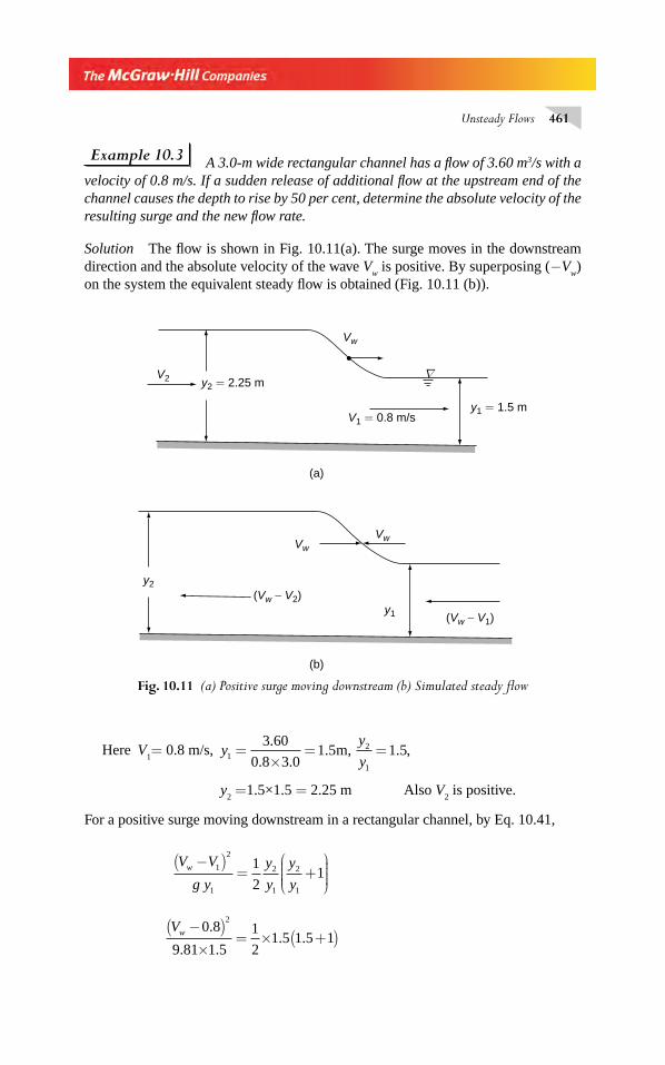
Unsteady Flows 461
Example 10.3 A 3.0-m wide rectangular channel has a fl ow of 3.60 m3/s with a velocity of 0.8 m/s. If a sudden release of additional fl ow at the upstream end of the channel causes the depth to rise by 50 per cent, determine the absolute velocity of the resulting surge and the new fl ow rate.
Solution The fl ow is shown in Fig. 10.11(a). The surge moves in the downstream direction and the absolute velocity of the wave V
w is positive. By superposing (−V
w)
on the system the equivalent steady fl ow is obtained (Fig. 10.11 (b)).
Fig. 10.11 (a) Positive surge moving downstream (b) Simulated steady fl ow
Vw
V1 = 0.8 m/s
V2
y1 = 1.5 m
y2 = 2.25 m∇
(a)
(b)
y1
VwVw
y2(Vw − V2)
(Vw − V1)
Here V1= 0.8 m/s, y
y
y12
1
3 60
0 8 3 01 5 1 5=
×= =
.
. .. . ,m,
y2 =1.5×1.5 = 2.25 m Also V
2 is positive.
For a positive surge moving downstream in a rectangular channel, by Eq. 10.41,
V V
g y
y
y
y
yw −( )
= +⎛
⎝⎜⎜⎜⎜
⎞
⎠⎟⎟⎟⎟
1
2
1
2
1
2
1
1
21
Vw −( )×
= × +( )0 8
9 81 1 5
1
21 5 1 5 1
2.
. .. .
Chapter 10.indd 461Chapter 10.indd 461 2/24/2010 3:07:11 PM2/24/2010 3:07:11 PM
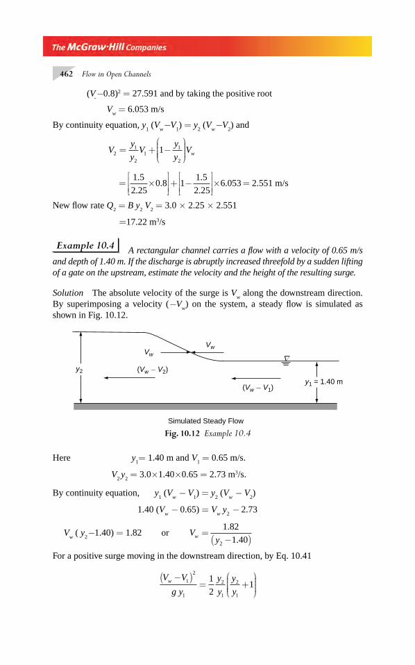
462 Flow in Open Channels
(V-−0.8)2 = 27.591 and by taking the positive root
Vw = 6.053 m/s
By continuity equation, y1 (V
w−V
1) = y
2 (V
w−V
2) and
Vy
yV
y
yVw2
1
21
1
2
1= + −⎛
⎝⎜⎜⎜⎜
⎞
⎠⎟⎟⎟⎟
= ×
⎡
⎣⎢⎢
⎤
⎦⎥⎥+ −
⎡
⎣⎢⎢
⎤
⎦⎥⎥× =
1 5
2 250 8 1
1 5
2 256 053 2 551
.
..
.
.. . m/s
New fl ow rate Q2 = B y
2 V
2 = 3.0 × 2.25 × 2.551
=17.22 m3/s
Example 10.4 A rectangular channel carries a fl ow with a velocity of 0.65 m/s and depth of 1.40 m. If the discharge is abruptly increased threefold by a sudden lifting of a gate on the upstream, estimate the velocity and the height of the resulting surge.
Solution The absolute velocity of the surge is Vw along the downstream direction.
By superimposing a velocity (−Vw) on the system, a steady fl ow is simulated as
shown in Fig. 10.12.
Fig. 10.12 Example 10.4
VwVw
(Vw − V2)
(Vw − V1)
y2
∇
y1 = 1.40 m
Simulated Steady Flow
Here y1= 1.40 m and V
1 = 0.65 m/s.
V2 y
2 = 3.0×1.40×0.65 = 2.73 m3/s.
By continuity equation, y1 (V
w − V
1) = y
2 (V
w − V
2)
1.40 (Vw − 0.65) = V
w y
2 − 2.73
Vw ( y
2−1.40) = 1.82 or V
yw =−( )1 82
1 402
.
.
For a positive surge moving in the downstream direction, by Eq. 10.41
V V
g y
y
y
y
yw −( )
= +⎛
⎝⎜⎜⎜⎜
⎞
⎠⎟⎟⎟⎟
1
2
1
2
1
2
1
1
21
Chapter 10.indd 462Chapter 10.indd 462 2/24/2010 3:07:11 PM2/24/2010 3:07:11 PM
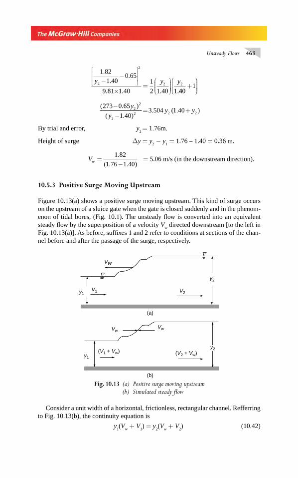
Unsteady Flows 463
1 82
1 400 65
9 81 1 40
1
2 1 40 12
2
2 2
.
..
. . . .
y y y−−
⎡
⎣⎢⎢
⎤
⎦⎥⎥
×=
⎛
⎝⎜⎜⎜
⎞
⎠⎟⎟⎟⎟ 440
1+⎛
⎝⎜⎜⎜
⎞
⎠⎟⎟⎟⎟
( . )
( . ). ( . )
273 0 65
1 403 504 1 402
2
22 2 2
−−
= +y
yy y
By trial and error, y2 = 1.76m.
Height of surge Δy = y2 − y
1 = 1.76 – 1.40 = 0.36 m.
Vw =−
1 82
1 76 1 40
.
( . . ) = 5.06 m/s (in the downstream direction).
10.5.3 Positive Surge Moving Upstream
Figure 10.13(a) shows a positive surge moving upstream. This kind of surge occurs on the upstream of a sluice gate when the gate is closed suddenly and in the phenom-enon of tidal bores, (Fig. 10.1). The unsteady fl ow is converted into an equivalent steady fl ow by the superposition of a velocity V
w directed downstream [to the left in
Fig. 10.13(a)]. As before, suffi xes 1 and 2 refer to conditions at sections of the chan-nel before and after the passage of the surge, respectively.
(V1 + Vw) (V2 + Vw)y1
y2
VwVw
(b)
(a)
∇
∇y2
y1 V2V1
Vw
Fig. 10.13 (a) Positive surge moving upstream
(b) Simulated steady fl ow
Consider a unit width of a horizontal, frictionless, rectangular channel. Refferring to Fig. 10.13(b), the continuity equation is
y1(V
w + V
1) = y
2(V
w + V
2) (10.42)
Chapter 10.indd 463Chapter 10.indd 463 2/24/2010 3:07:11 PM2/24/2010 3:07:11 PM
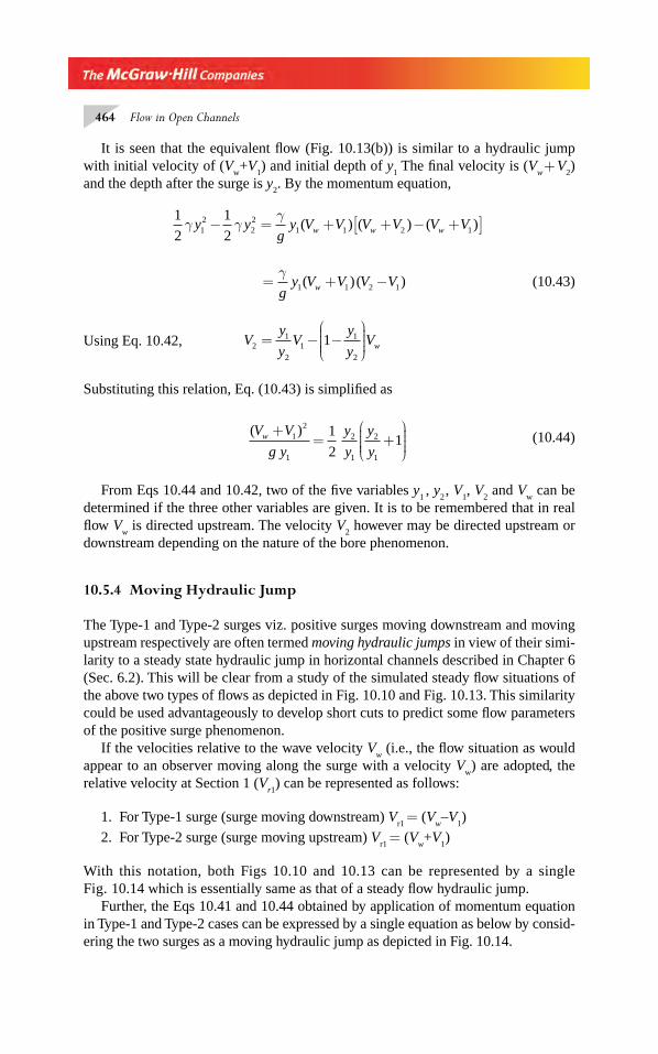
464 Flow in Open Channels
It is seen that the equivalent fl ow (Fig. 10.13(b)) is similar to a hydraulic jump with initial velocity of (V
w+V
1) and initial depth of y
1 The fi nal velocity is (V
w + V
2)
and the depth after the surge is y2. By the momentum equation,
1
2
1
212
22
1 1 2 1γ γγ
y yg
y V V V V V Vw w w− = + + − +[ ]( ) ( ) ( )
= + −γg
y V V V Vw1 1 2 1( ) ( ) (10.43)
Using Eq. 10.42, Vy
yV
y
yVw2
1
21
1
2
1= − −⎛
⎝⎜⎜⎜⎜
⎞
⎠⎟⎟⎟⎟
Substituting this relation, Eq. (10.43) is simplifi ed as
( )V V
g y
y
y
y
yw +
= +⎛
⎝⎜⎜⎜⎜
⎞
⎠⎟⎟⎟⎟
12
1
2
1
2
1
1
21 (10.44)
From Eqs 10.44 and 10.42, two of the fi ve variables y1 , y
2 , V
1, V
2 and V
w can be
determined if the three other variables are given. It is to be remembered that in real fl ow V
w is directed upstream. The velocity V
2 however may be directed upstream or
downstream depending on the nature of the bore phenomenon.
10.5.4 Moving Hydraulic Jump
The Type-1 and Type-2 surges viz. positive surges moving downstream and moving upstream respectively are often termed moving hydraulic jumps in view of their simi-larity to a steady state hydraulic jump in horizontal channels described in Chapter 6 (Sec. 6.2). This will be clear from a study of the simulated steady fl ow situations of the above two types of fl ows as depicted in Fig. 10.10 and Fig. 10.13. This similarity could be used advantageously to develop short cuts to predict some fl ow parameters of the positive surge phenomenon.
If the velocities relative to the wave velocity Vw (i.e., the fl ow situation as would
appear to an observer moving along the surge with a velocity Vw) are adopted, the
relative velocity at Section 1 (Vr1
) can be represented as follows:
1. For Type-1 surge (surge moving downstream) Vr1
= (Vw–V
1)
2. For Type-2 surge (surge moving upstream) Vr1
= (Vw+V
1)
With this notation, both Figs 10.10 and 10.13 can be represented by a single Fig. 10.14 which is essentially same as that of a steady fl ow hydraulic jump.
Further, the Eqs 10.41 and 10.44 obtained by application of momentum equation in Type-1 and Type-2 cases can be expressed by a single equation as below by consid-ering the two surges as a moving hydraulic jump as depicted in Fig. 10.14.
Chapter 10.indd 464Chapter 10.indd 464 2/24/2010 3:07:12 PM2/24/2010 3:07:12 PM
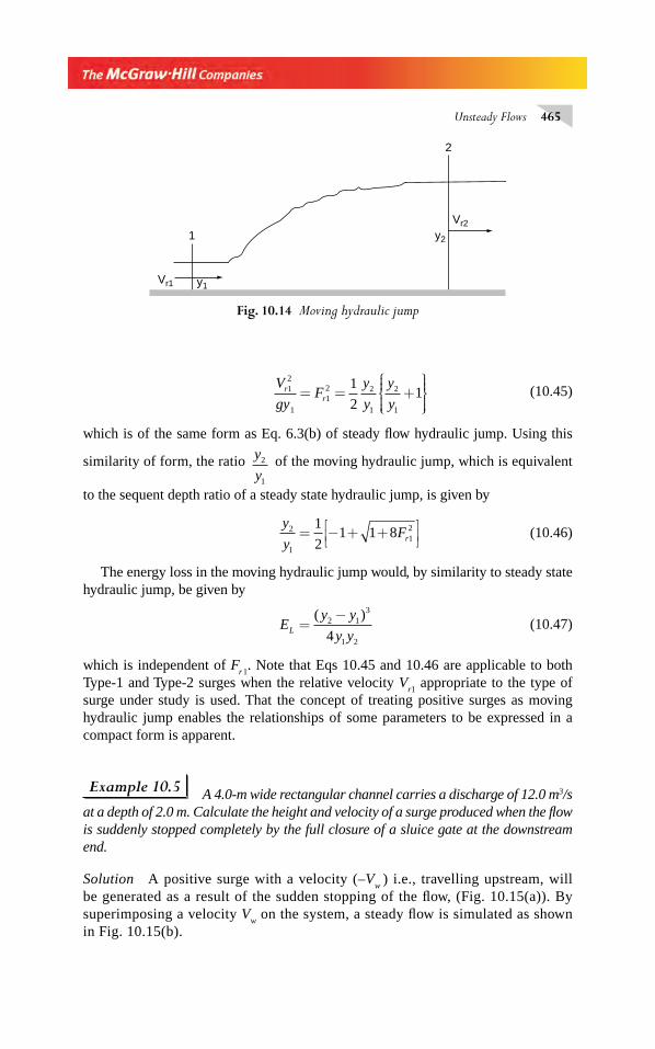
Unsteady Flows 465
V
gyF
y
y
y
yr
r12
112 2
1
2
1
1
21= = +
⎧⎨⎪⎪
⎩⎪⎪
⎫⎬⎪⎪
⎭⎪⎪ (10.45)
which is of the same form as Eq. 6.3(b) of steady fl ow hydraulic jump. Using this
similarity of form, the ratio y
y2
1
of the moving hydraulic jump, which is equivalent
to the sequent depth ratio of a steady state hydraulic jump, is given by
y
yFr
2
1121
21 1 8= − + +⎡
⎣⎢⎤⎦⎥ (10.46)
The energy loss in the moving hydraulic jump would, by similarity to steady state hydraulic jump, be given by
Ey y
y yL =−( )2 1
3
1 24 (10.47)
which is independent of Fr 1
. Note that Eqs 10.45 and 10.46 are applicable to both Type-1 and Type-2 surges when the relative velocity V
r1 appropriate to the type of
surge under study is used. That the concept of treating positive surges as moving hydraulic jump enables the relationships of some parameters to be expressed in a compact form is apparent.
Example 10.5 A 4.0-m wide rectangular channel carries a discharge of 12.0 m3/s at a depth of 2.0 m. Calculate the height and velocity of a surge produced when the fl ow is suddenly stopped completely by the full closure of a sluice gate at the downstream end.
Solution A positive surge with a velocity (–Vw
) i.e., travelling upstream, will be generated as a result of the sudden stopping of the fl ow, (Fig. 10.15(a)). By superimposing a velocity V
w on the system, a steady fl ow is simulated as shown
in Fig. 10.15(b).
Vr1
Vr2
y2
y1
2
1
Fig. 10.14 Moving hydraulic jump
Chapter 10.indd 465Chapter 10.indd 465 2/24/2010 3:07:12 PM2/24/2010 3:07:12 PM
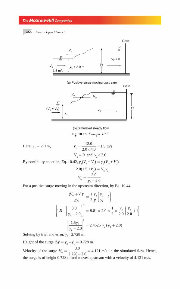
466 Flow in Open Channels
Here, y 1= 2.0 m, V1
12 0
2 0 4 01 5=
×=
.
. .. m/s
V2 = 0 and y
2 > 2.0
By continuity equation, Eq. 10.42, y1(V
w + V
1) = y
2(V
w + V
2)
2.0(1.5 +Vw) = V
w y
2
Vyw =
−3 0
2 02
.
.
For a positive surge moving in the upstream direction, by Eq. 10.44
( )V V
gy
y
y
y
yw +
= +⎛
⎝⎜⎜⎜⎜
⎞
⎠⎟⎟⎟⎟
12
1
2
1
2
1
1
21
1 53 0
2 09 81 2 0
1
2 2 0 22
2
2 2..
.. .
. .+
−
⎛
⎝⎜⎜⎜⎜
⎞
⎠⎟⎟⎟⎟
⎡
⎣⎢⎢⎢
⎤
⎦⎥⎥⎥
= × × ×y
y y
001+
⎛
⎝⎜⎜⎜
⎞
⎠⎟⎟⎟⎟
1 5
2 02 4525 2 02
2
2
2 2
.
.. ( . )
y
yy y
−
⎡
⎣⎢⎢
⎤
⎦⎥⎥ = +
Solving by trial and error, y2=2.728 m.
Height of the surge Δy = y2 – y
1 = 0.728 m.
Velocity of the surge Vw =−
=3 0
2 728 2 04 121
.
. .. m/s in the simulated fl ow. Hence,
the surge is of height 0.728 m and moves upstream with a velocity of 4.121 m/s.
y2
y1
(V1 + Vw)
∇
∇
∇
∇
Vw Vw
Vw
y2y1 = 2.0 m1.5 m/s
V1
V2 = 0
Vw
Gate
Gate(a) Positive surge moving upstream
(b) Simulated steady flow
Fig. 10.15 Example 10.5
Chapter 10.indd 466Chapter 10.indd 466 2/24/2010 3:07:12 PM2/24/2010 3:07:12 PM
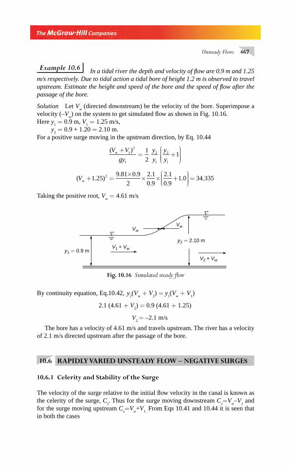
Unsteady Flows 467
Example 10.6 In a tidal river the depth and velocity of fl ow are 0.9 m and 1.25 m/s respectively. Due to tidal action a tidal bore of height 1.2 m is observed to travel upstream. Estimate the height and speed of the bore and the speed of fl ow after the passage of the bore.
Solution Let Vw (directed downstream) be the velocity of the bore. Superimpose a
velocity (–Vw) on the system to get simulated fl ow as shown in Fig. 10.16.
Here y1 = 0.9 m, V
1 = 1.25 m/s,
y2 = 0.9 + 1.20 = 2.10 m.
For a positive surge moving in the upstream direction, by Eq. 10.44
( )V V
gy
y
y
y
yw +
= +⎛
⎝⎜⎜⎜⎜
⎞
⎠⎟⎟⎟⎟
12
1
2
1
2
1
1
21
( . ). . .
.
.
.. .Vw + =
×× × +
⎛⎝⎜⎜⎜
⎞⎠⎟⎟⎟⎟ =1 25
9 81 0 9
2
2 1
0 9
2 1
0 91 0 34 3352
Taking the positive root, Vw = 4.61 m/s
∇
∇
y1 = 0.9 m
y2 = 2.10 mV1 + Vw
V2 + Vw
VwVw
Fig. 10.16 Simulated steady fl ow
By continuity equation, Eq.10.42, y2(V
w + V
2) = y
1(V
w + V
1)
2.1 (4.61 + V2) = 0.9 (4.61 + 1.25)
V2 = –2.1 m/s
The bore has a velocity of 4.61 m/s and travels upstream. The river has a velocity of 2.1 m/s directed upstream after the passage of the bore.
10.6 RAPIDLY VARIED UNSTEADY FLOW – NEGATIVE SURGES
10.6.1 Celerity and Stability of the Surge
The velocity of the surge relative to the initial fl ow velocity in the canal is known as the celerity of the surge, C
s. Thus for the surge moving downstream C
s=V
w–V
1 and
for the surge moving upstream Cs=V
w+V
1. From Eqs 10.41 and 10.44 it is seen that
in both the cases
Chapter 10.indd 467Chapter 10.indd 467 2/24/2010 3:07:12 PM2/24/2010 3:07:12 PM
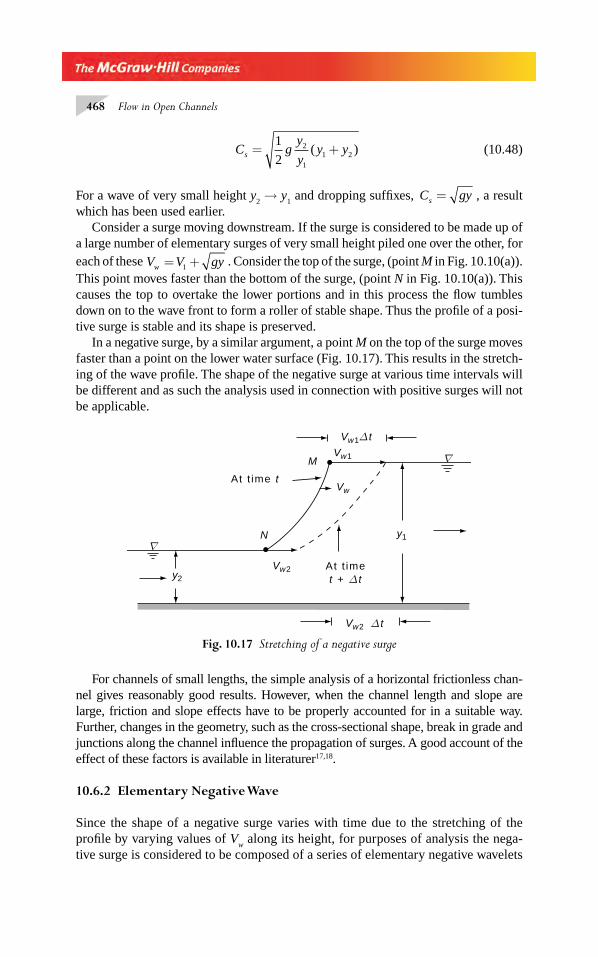
468 Flow in Open Channels
C gy
yy ys = +
1
22
11 2( ) (10.48)
For a wave of very small height y2 → y
1 and dropping suffi xes, C gys = , a result
which has been used earlier.Consider a surge moving downstream. If the surge is considered to be made up of
a large number of elementary surges of very small height piled one over the other, for each of these V V gyw = +1 . Consider the top of the surge, (point M in Fig. 10.10(a)). This point moves faster than the bottom of the surge, (point N in Fig. 10.10(a)). This causes the top to overtake the lower portions and in this process the fl ow tumbles down on to the wave front to form a roller of stable shape. Thus the profi le of a posi-tive surge is stable and its shape is preserved.
In a negative surge, by a similar argument, a point M on the top of the surge moves faster than a point on the lower water surface (Fig. 10.17). This results in the stretch-ing of the wave profi le. The shape of the negative surge at various time intervals will be different and as such the analysis used in connection with positive surges will not be applicable.
∇
∇
y2
y1
Vw1
Vw1Δ t
Vw2
M
N
Vw
Vw2
At t ime t
At t imet + Δ t
Δ t
Fig. 10.17 Stretching of a negative surge
For channels of small lengths, the simple analysis of a horizontal frictionless chan-nel gives reasonably good results. However, when the channel length and slope are large, friction and slope effects have to be properly accounted for in a suitable way. Further, changes in the geometry, such as the cross-sectional shape, break in grade and junctions along the channel infl uence the propagation of surges. A good account of the effect of these factors is available in literaturer17,18.
10.6.2 Elementary Negative Wave
Since the shape of a negative surge varies with time due to the stretching of the profi le by varying values of V
w along its height, for purposes of analysis the nega-
tive surge is considered to be composed of a series of elementary negative wavelets
Chapter 10.indd 468Chapter 10.indd 468 2/24/2010 3:07:13 PM2/24/2010 3:07:13 PM
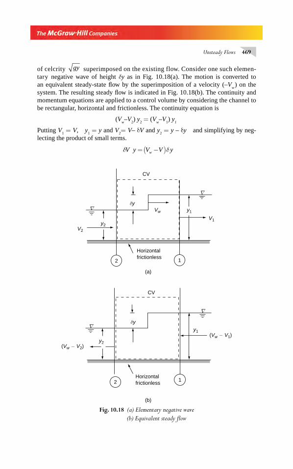
Unsteady Flows 469
of celcrity gy superimposed on the existing flow. Consider one such elemen-tary negative wave of height δy as in Fig. 10.18(a). The motion is converted to an equivalent steady-state fl ow by the superimposition of a velocity (–V
w ) on the
system. The resulting steady fl ow is indicated in Fig. 10.18(b). The continuity and momentum equations are applied to a control volume by considering the channel to be rectangular, horizontal and frictionless. The continuity equation is
(Vw–V
2) y
2 = (V
w–V
1) y
1
Putting V1 = V, y
1 = y and V
2= V– δV and y
2 = y – δy and simplifying by neg-
lecting the product of small terms.
δ δV y V V yw= −( )
Fig. 10.18 (a) Elementary negative wave
(b) Equivalent steady fl ow
∇
∇
∇
∇
Horizontalfrictionless
Horizontalfrictionless
(b)
CV
CV
(a)
2
2
1
1
(Vw − V2)
(Vw − V1)y1
y1
y2
y2
δy
δyVw
V1
V2
Chapter 10.indd 469Chapter 10.indd 469 2/24/2010 3:07:13 PM2/24/2010 3:07:13 PM
470 Flow in Open Channels
or δδV
y
V V
yw=
− (10.49)
By applying the momentum equation to a control volume enclosing the Sections 1 and 2 in the direction of equivalent steady fl ow
γ γ2 21
222
1 1 2 1y y V V y V V V Vw w w−( ) = −( ) −( )− −( )⎡⎣
⎤⎦
Introducing the notation as above and neglecting the product of small quantities the momentum equation simplifi es to
δδV
y
g
V Vw
=−( )
(10.50)
Combining Eqs 10.47 and 10.46
(Vw
– V )2 = C 2 = gy
or C gy= ± (10.51)
in which C = celerity of the elemental at negative wave.Also from Eq. 10.47
δδV
yg y= ± /
As δ y → 0, dV
dyg y= ± / (10.52)
Equation 10.52 is the basic differential equation governing a simple negative wave which on integration with proper boundary conditions enables the determina-tion of the characteristics of a negative wave.
10.6.3 Type 3 Negative Wave Moving Downstream
Consider a sluice gate in a wide rectangular channel passing a flow with a velocity of V
1 and a normal depth of flow of y
1 in the channel downstream of
the gate. Consider the sluice gate to partially close instantaneously. Let the new velocity and depth of flow at the gate be V
0 and y
0 respectively. The closure
action of the gate would cause a negative wave to form on the downstream channel (Type 3 wave) and the wave would move in the downstream direction as shown in Fig. 10.19. The velocity V and depth y at any position x from the gate is obtained by integrating the basic differential equation of a simple nega-tive wave given by Eq. 10.52.
For the negative wave moving downstream, positive sign in Eq. 10.52 is adopted and the resulting basic differential equation is
Chapter 10.indd 470Chapter 10.indd 470 2/24/2010 3:07:13 PM2/24/2010 3:07:13 PM
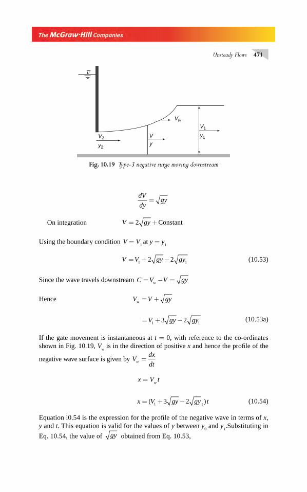
Unsteady Flows 471
dV
dygy=
On integration V gy= +2 Constant
Using the boundary condition V = V1 at y = y
1
V V gy gy= + −1 12 2 (10.53)
Since the wave travels downstream C V V gyw= − =
Hence V V gyw = +
= + −V gy gy1 13 2 (10.53a)
If the gate movement is instantaneous at t = 0, with reference to the co-ordinates shown in Fig. 10.19, V
w is in the direction of positive x and hence the profi le of the
negative wave surface is given by Vdx
dtw =
x = Vw
t
x V gy gy t= + −( )1 13 2 (10.54)
Equation l0.54 is the expression for the profi le of the negative wave in terms of x, y and t. This equation is valid for the values of y between y
0 and y
1.Substituting in
Eq. 10.54, the value of gy obtained from Eq. 10.53,
V2
y2
V1
Vw
y1Vy
∇
Fig. 10.19 Type-3 negative surge moving downstream
Chapter 10.indd 471Chapter 10.indd 471 2/24/2010 3:07:13 PM2/24/2010 3:07:13 PM
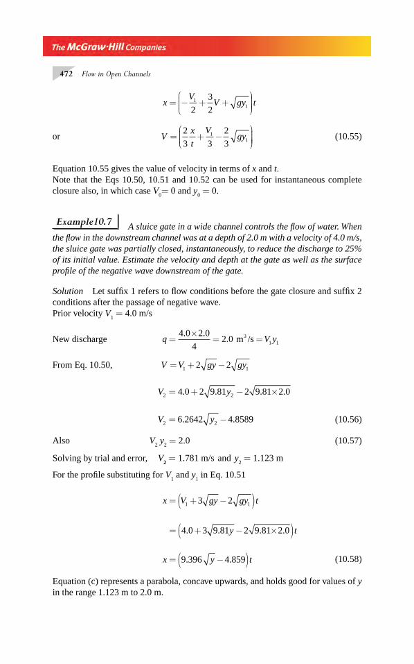
472 Flow in Open Channels
xV
V gy t= − + +⎛
⎝⎜⎜⎜
⎞
⎠⎟⎟⎟⎟
112
3
2
or Vx
t
Vgy= + −
⎛
⎝⎜⎜⎜
⎞
⎠⎟⎟⎟⎟
2
3 3
2
31
1 (10.55)
Equation 10.55 gives the value of velocity in terms of x and t.Note that the Eqs 10.50, 10.51 and 10.52 can be used for instantaneous complete closure also, in which case V
0= 0 and y
0 = 0.
Example10.7 A sluice gate in a wide channel controls the fl ow of water. When the fl ow in the downstream channel was at a depth of 2.0 m with a velocity of 4.0 m/s, the sluice gate was partially closed, instantaneously, to reduce the discharge to 25% of its initial value. Estimate the velocity and depth at the gate as well as the surface profi le of the negative wave downstream of the gate.
Solution Let suffi x 1 refers to fl ow conditions before the gate closure and suffi x 2 conditions after the passage of negative wave.Prior velocity V
1 = 4.0 m/s
New discharge q V y=×
= =4 0 2 0
42 0 1 1
. .. m /s3
From Eq. 10.50, V V gy gy= + −1 12 2
V y2 24 0 2 9 81 2 9 81 2 0= + − ×. . . .
V y2 26 2642 4 8589= −. . (10.56)
Also V2 y
2 = 2.0 (10.57)
Solving by trial and error, V2 = 1.781 m/s and y
2 = 1.123 m
For the profi le substituting for V1 and y
1 in Eq. 10.51
x V gy gy t= + −( )1 13 2
= + − ×( )4 0 3 9 81 2 9 81 2 0. . . .y t
x y t= −( )9 396 4 859. . (10.58)
Equation (c) represents a parabola, concave upwards, and holds good for values of y in the range 1.123 m to 2.0 m.
Chapter 10.indd 472Chapter 10.indd 472 2/24/2010 3:07:14 PM2/24/2010 3:07:14 PM
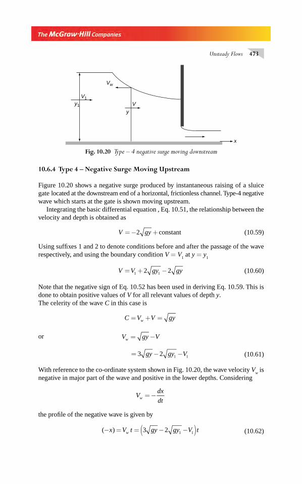
Unsteady Flows 473
10.6.4 Type 4 – Negative Surge Moving Upstream
Figure 10.20 shows a negative surge produced by instantaneous raising of a sluice gate located at the downstream end of a horizontal, frictionless channel. Type-4 negative wave which starts at the gate is shown moving upstream.
Integrating the basic differential equation , Eq. 10.51, the relationship between the velocity and depth is obtained as
V gy= − +2 constant (10.59)
Using suffi xes 1 and 2 to denote conditions before and after the passage of the wave respectively, and using the boundary condition V = V
1 at y = y
1
V V gy gy= + −1 12 2 (10.60)
Note that the negative sign of Eq. 10.52 has been used in deriving Eq. 10.59. This is done to obtain positive values of V for all relevant values of depth y.The celerity of the wave C in this case is
C V V gyw= + =
or V gy Vw = −
= − −3 2 1 1gy gy V (10.61)
With reference to the co-ordinate system shown in Fig. 10.20, the wave velocity Vw is
negative in major part of the wave and positive in the lower depths. Considering
Vdx
dtw = −
the profi le of the negative wave is given by
( )− = = − −( )x V t gy gy V tw 3 2 1 1 (10.62)
y1
Vw
V1 V
x
y
Fig. 10.20 Type – 4 negative surge moving downstream
Chapter 10.indd 473Chapter 10.indd 473 2/24/2010 3:07:14 PM2/24/2010 3:07:14 PM
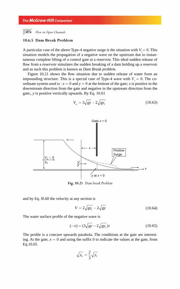
474 Flow in Open Channels
10.6.5 Dam Break Problem
A particular case of the above Type-4 negative surge is the situation with V1= 0. This
situation models the propagation of a negative wave on the upstream due to instan-taneous complete lifting of a control gate at a reservoir. This ideal sudden release of fl ow from a reservoir simulates the sudden breaking of a dam holding up a reservoir and as such this problem is known as Dam Break problem.
Figure 10.21 shows the fl ow situation due to sudden release of water from an impounding structure. This is a special case of Type-4 wave with V
1 = 0. The co-
ordinate system used is : x = 0 and y = 0 at the bottom of the gate; x is positive in the downstream direction from the gate and negative in the upstream direction from the gate;, y is positive vertically upwards. By Eq. 10.61
V gy gyw = −3 2 1 (10.63)
V1 = 0y1
y
y at x = 0
Gate x = 0
x
V
xPositiveSurge
Fig. 10.21 Dam break Problem
and by Eq. l0.60 the velocity at any section is
V gy gy= −2 21 (10.64)
The water surface profi le of the negative wave is
( ) ( )− = −x gy gy t3 2 1 (10.65)
The profi le is a concave upwards parabola. The conditions at the gate are interest-ing. At the gate, x = 0 and using the suffi x 0 to indicate the values at the gate, from Eq.10.65
y y0 1
2
3=
Chapter 10.indd 474Chapter 10.indd 474 2/24/2010 3:07:15 PM2/24/2010 3:07:15 PM
Unsteady Flows 475
i.e., y y0 1
4
9= (10.66)
Note that y0 is independent of time and as such is constant. The salient features of the
wave profi le are as follows:
At y = 0 x t gy= 2 1
At y = y1 x t gy= − 1 and
At x = 0 y y=4
9 1
The velocity at the gate V0 by Eq. 10.64 is
V gy s0 1
2
3= (10.67)
The discharge intensity q V y gy y= =⎛⎝⎜⎜⎜
⎞⎠⎟⎟⎟⎟⎛⎝⎜⎜⎜
⎞⎠⎟⎟⎟⎟0 0 1 1
2
3
4
9
=8
27 13gy (10.68)
which is also independent of time t.Note that the fl ow is being analyzed in a horizontal frictionless channel and as such
the depth y1 with V
1= 0 represents the specifi c energy, E. At the gate axis (x = 0)
y y E0 1
2
3
2
3= = = Critical depth
Also at x = 0, the Froude number of the fl ow FV
gy
gy
g y0
0
0
1
1
2
3
4
9
1 0= =⎛⎝⎜⎜⎜
⎞⎠⎟⎟⎟
= . . Thus
the fl ow at the gate axis is critical and the discharge maximum. Further, it is easy to see that upstream of the gate the fl ow is subcrtical and on the downstream of the gate (for positive values of x) the fl ow is supercritical.
This simple ideal analysis of a sudden release from an impounding structure is found to give satisfactory results for a major part of the profi le. However, in real situ-ation the downstream end is found to have a rounded positive wave instead of the para-bolic profi le with its vertex on the x-axis. In actual dam break the tapered leading edge of the ideal profi le is modifi ed due to action of ground friction to cause a positive surge to move downstream. Details about dam break analysis are found in Refs. 4 ,19 & 20.
10.6.6 Partial lifting of Downstream Gate
A variation of the dam break problem is the case of partial instantaneous lifting of the downstream gate from initial closed position. A simple case of a sluice gate in a rect-angular channel of width B is analyzed as follows.
Chapter 10.indd 475Chapter 10.indd 475 2/24/2010 3:07:15 PM2/24/2010 3:07:15 PM
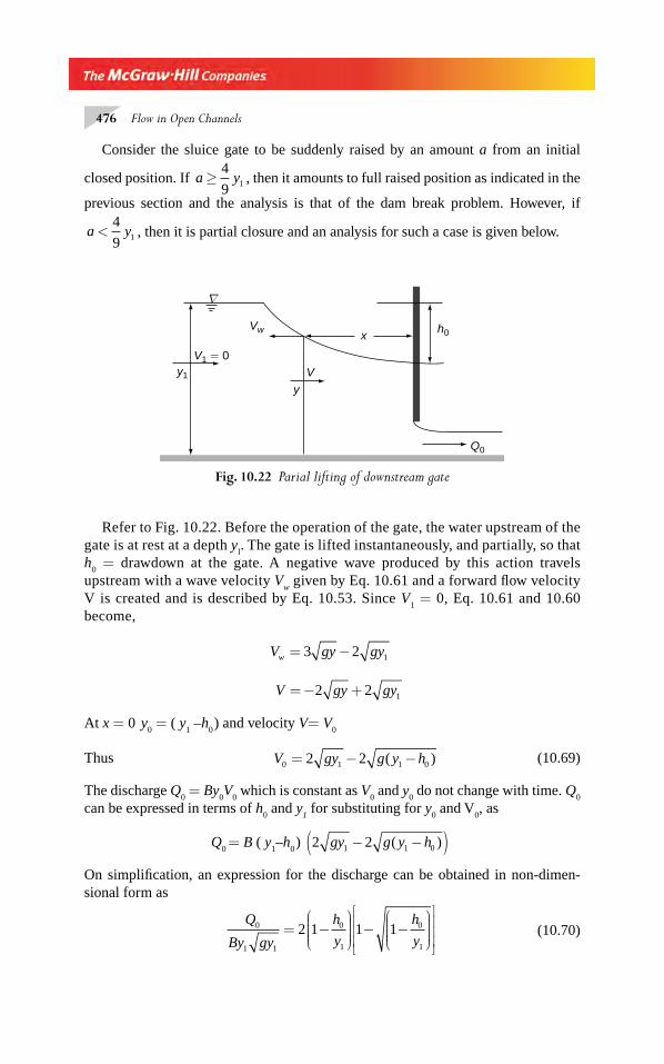
476 Flow in Open Channels
Consider the sluice gate to be suddenly raised by an amount a from an initial
closed position. If a y≥4
9 1 , then it amounts to full raised position as indicated in the
previous section and the analysis is that of the dam break problem. However, if
a y<4
9 1 , then it is partial closure and an analysis for such a case is given below.
Fig. 10.22 Parial lifting of downstream gate
∇
y1
Vw
V1 = 0V
y
xh0
Q0
Refer to Fig. 10.22. Before the operation of the gate, the water upstream of the gate is at rest at a depth y
l. The gate is lifted instantaneously, and partially, so that
h0 = drawdown at the gate. A negative wave produced by this action travels
upstream with a wave velocity Vw given by Eq. 10.61 and a forward fl ow velocity
V is created and is described by Eq. 10.53. Since V1 = 0, Eq. 10.61 and 10.60
become,
V gy gyw = −3 2 1
V gy gy= − +2 2 1
At x = 0 y0 = ( y
1 –h
0 ) and velocity V= V
0
Thus V gy g y h0 1 1 02 2= − −( ) (10.69)
The discharge Q0 = By
0V
0 which is constant as V
0 and y
0 do not change with time. Q
0
can be expressed in terms of h0 and y
1 for substituting for y
0 and V
0, as
Q0 = B ( y
1–h
0 ) 2 21 1 0gy g y h− −( )( )
On simplifi cation, an expression for the discharge can be obtained in non-dimen-sional form as
Q
By gy
h
y
h
y0
1 1
0
1
0
1
2 1 1 1= −⎛
⎝⎜⎜⎜⎜
⎞
⎠⎟⎟⎟⎟
− −⎛
⎝⎜⎜⎜⎜
⎞
⎠⎟⎟⎟⎟
⎡
⎣
⎢⎢⎢
⎤
⎦
⎥⎥⎥ (10.70)
Chapter 10.indd 476Chapter 10.indd 476 2/24/2010 3:07:15 PM2/24/2010 3:07:15 PM
Unsteady Flows 477
Wave Profi le: The profi le of the negative wave at any time t is given as
(− x) = Vw
t = ( 2 gy1−3 gy ) t (10.71)
where y = depth of fl ow at any (x, t).
Example 10.8 A reservoir having water to a depth of 40 m undergoes an instan-taneous, ideal, dam break. Estimate the depth and discharge intensity at the dam site and the water surface profi le of the negative wave 3 seconds after the dam break.
Solution The water surface profi le with positive x in the downstream of the gate axis, is by Eq. 10.65 is
(–x) = 3 2 1gy gy t−( )
(–x) = 3 9 81 2 9 81 401. .× − ×( )y t
x = 39.62 t − 9.396 y
At x = 0, y = y0 = (39.62/9.396) = 17.78 m.
Velocity at x = 0, V = V0 =
2
3 1gy = 2
39 18 40. × = 13.21 m/s
Profi le after 3 seconds: x = 39.62 × 3 – 9.396 × 3 y
: x = 118.86 – 28.188 y
Example 10.9 A wide rectangular horizontal channel is passing a discharge of 1.5 m3/s/m at a depth of 3.0 m. The fl ow is controlled by a sluice gate at the downstream end. If the gate is abruptly raised by a certain extent to pass a fl ow of 3.0 m3/s/m to the downstream, estimate (i) the new depth and velocity of fl ow in the channel at a section when the negative surge has passed it, (ii) the maximum wave velocity of the negative surge, and (iii) profi le of the negative surge.
Solution This is a case of Type-4 wave, where the negative wave moves upstream. Using the suffi x 1 for the conditions before the passage and 2 for conditions after the passage of the negative wave and suffi x 0 to the position of the gate,Velocity at any section
V = V1 + 2 gy1 –2 gy . Here y
1 = 3.0 m and V
1 = 1.5/3. 0 = 0.5 m/s.
V = 0.5 + 2 9 81 3 0. .× − 2 9 81. × y
=11.35 − 6.264 y (10.72)
Chapter 10.indd 477Chapter 10.indd 477 2/24/2010 3:07:16 PM2/24/2010 3:07:16 PM
478 Flow in Open Channels
After the passage of wave, V2 = 3.0/y
2 and from Eq. 10.72 V
2 = 11.35−6.264 y
By trial and error, y2 = 2.66 m and V
2= 1.13 m/s.
Velocity of wave, by Eq. 10.61: Vw = 3 gy − 2 gy1 – V
1
= 3 gy − 2 9 18 3 0. .× − 0.5 = 3 gy −11.35
Vw is maximum at y = y
1 and hence max. V
w = 3 9 81 3 0. .× −11.35 = 4.925 m/s
Wave profi le is given by Eq. l0.62 as (−x) = 3 2 1 1gy gy V t− −( )−x = 3 9 81 2 9 81 3 0 0 5. . . .y t− × −( )
x = 11 35 6 264. .−( )y t
(The profi le is in the negative x direction.)
REFERENCES
1. Wylie, E B, ‘Unsteady Free Surface Flow Computation’, Jour. of Hyd. Div., Proc. ASCE, Nov. 1970, pp 2241–2251.
2. Price, R K, ‘Comparison of Four Numerical Methods for Flood Routing’, Jour. of Hyd. Div., Proc. ASCE, July 1974, pp 879–899.
3. Strelkoff, T, ‘Numerical Solution of St Venant Equations’, Jour. of Hyd. Div., Proc. ASCE, Jan. 1970, pp 223–252.
4. Chaudhry, M H, Open Channel Flow, Prentice-Hall, New Jersey, USA, 1993. 5. Cunge, J A, Holly, F M, and Verwey, A, Practical Aspects of Computational River Hydrau-
lics, Pitman Adv. Pub. Program, Pitman, London, UK, 1980. 6. Amien, M, and Fang, C S, ‘Implicit Food Routing in Natural Channels’, Jour, of Hyd.
Div., Proc. ASCE, Dec. 1970, pp 2481–2500. 7. Amien, M, and Chu, H L, ‘Implicit Numerical Modelling of Unsteady Flows’;, Jour. of
Hyd. Div., Proc. ASCE, Dec. 1970, pp 717–731. 8. Abbot, M B, and Ionesq, F, ‘On the Numerical Computation of Nearly Horizontal Flows’,
Jour of Hyd. Res., IAHR, Vol. 5, No. 2, 1967, pp 96–117. 9. Beam, R M, and Warming, R F, ‘An Implicit Finite Difference Algorithm for Hyperbolic
Systems in Conservation Law Forms’ Jour. of Comp. Physics, Vol. 22, 1976, pp. 87–110.10. Ligget, J A, and Woolhiser, D A, ‘Difference Solutions of the Shallow Water Equation’,
Jour, of Engg. Mech. Div., Proc. ASCE, April 1967, pp 39–71.11. Miller, W A, Jr and Yevjevich, V, (Ed), Unsteady Flow in Open Channels. Vol. III-Bibliography.,
Water Resources Publications, Fort Collins, Colo., USA, 1975.12. Chow, V T, Maidment, D R, and Mays, L W, Applied Hydrology, McGraw-Hill, Singapore,
1988.13. Cooley, R L, and Moin, S A, ‘Finite Element Solution of St. Venant Equations’, Jour. of
Hyd. Div., Proc. ASCE, June 1976, pp 759–775.14. King, I P, ‘Finite element models for unsteady fl ow through irregular channels’, Proc.
First conf. on Finite Elements in Water Resources, Princeton Univ., USA, July 1976; Finite Elements in Water Resources, Pentech Press, 1977, pp 165–184.
Chapter 10.indd 478Chapter 10.indd 478 2/24/2010 3:07:16 PM2/24/2010 3:07:16 PM
Unsteady Flows 479
15. Szymkiewicz, R, ‘Finite element method for the solution of the St Venant equations in an open channel network’, Jour, of Hydrology, 1991, pp 270–287.
16. Jie Chen, et al, “Conservative Formulation for Natural Open Channel and Finite-Element Implementation”, Jour.l of Hyd. Engg., Vol. 133, No. 9, Sept. 2007, pp 1064–1073.
17. Jaeger, C, Engineering Fluid Mechanics, Blackie and Son Ltd., London, UK, 1956.18. Chow, V T, Open Channel Hydraulics, McGraw – Hill, New York, USA, 1959.19. Mahmood, K, and Yevdjevich, V, (Ed), Unsteady Flow in Open Channels, 3 Vols, Water
Resources Publications, Fort Collins, Colo., USA, 1975.20. French, R H, Open Channel Hydraulics, McGraw – Hill Book Co., New York, USA,
1986.
PROBLEMS
Problem Distribution
Topic Problems
1 Equation of motion of GVUF 10.1–10.2
2 Monoclinal wave 10.3
3 Positive surge 10.4–10.13
4 Negative surge 10.14–10.16
10.1 Show that the continuity equation for a GVUF in a non prismatic channel with no lateral in fl ow is
A ∂∂V
x+VT
∂∂
y
x+ εyV
∂∂T
x+ T
∂∂
y
x = 0
where ε = a coeffi cient which depends on the nature of the non-prismaticity of the chan-nel with ε = 0.5 and 1.0 for triangular and rectangular channels respectively.
10.2 Derive the equation of motion for GVUF in a channel having a lateral outfl ow q per unit length as
∂∂
y
x +
V
g
∂∂V
x +
1
g
∂∂V
t = S
0– S
f – D
L
where DL = 0 for bulk lateral outfl ow as over a side spillway, and D
L=
V u
Ag
−⎛
⎝⎜⎜⎜⎜
⎞
⎠⎟⎟⎟⎟ q for lat-
eral infl ow with x component of the infl ow velocity = u;10.3 Show that by using the Chezy formula with C = constant, the ratio (V
w)
m /V
n of a mono-
clinal wave is 1.50 and 1.25 for wide rectangular and triangular channels respectively.10.4 Show that the celerity of a positive surge in a prismoidal channel can be approximated
for small surge heights h relative to the area A as
C ≈ + + +⎛
⎝⎜⎜⎜⎜
⎞
⎠⎟⎟⎟⎟
gA
Th
Th
A
3
2 2
2
≈ + +⎛⎝⎜⎜⎜
⎞⎠⎟⎟⎟⎟g
A
Th
3
2
Chapter 10.indd 479Chapter 10.indd 479 2/24/2010 3:07:16 PM2/24/2010 3:07:16 PM
480 Flow in Open Channels
10.5 For a positive surge travelling in a horizontal rectangular channel, fi ll in the blanks in the following table
Sl. No. y1 (m) V
1 (m/s) y
2 (m) V
2 (m/s) V
H (m/s)
a 2.00 1.50 4.00 − −
b 1.00 1.75 − − +5.50
c 1.75 0.70 − − −5.00
d – 3.00 1.50 − −3.00
e 0.30 − 0.60 − 3.50
10.6 At a point in a shallow lake, a boat moving with a speed of 20 km/h is found to create a wave which rises 35 cm above the undisturbed water surface. Find the approximate depth of the lake at this point.
10.7 A positive surge is often known as a moving hydraulic jump. Obtain an expression in terms of depths y
1 and y
2 for the energy loss in a moving hydraulic jump in a horizontal
rectangular channel. Estimate the energy loss when y1 = 0.9 m and y
2 = 2.10 m.
10.8 A rectangular channel carries a discharge of 1.50 m3/s per metre width at a depth of 0.75 m. If the sudden operation of a sluice gate at an upstream section causes the discharge to increase by 33 per cent, estimate the height and absolute velocity of the positive surge in the channel.
10.9 The depth and velocity of fl ow in a rectangular channel are 0.9 m/s and 1.5 m/s respec-tively. If a gate at the downstream end of the channel is abruptly closed, what will be the height and absolute velocity of the resulting surge?
10.10 A 2.0 m wide rectangular channel, 2 km long carries a steady fl ow of 4.6 m3/s at a depth of 1.15. The sides of the channel are 2.0 m high. If the fl ow is suddenly stopped by the clo-sure of a gate at the downstream end, will the water spill over the sides of the channel ? If there is no spillage, what minimum time interval must elapse before the arrival of the surge at the upstream end?
10.11 A trapezoidal canal with B = 5.0 m and side slope 1H : 1V, carries a discharge of 30.0 m3/s at a depth of 3.0 m. Calculate the speed and height of a positive surge (i) if the fl ow in the canal is suddenly stopped by the operation of a gate at a downstream section, (ii) if the discharge is suddenly increased to 45.0 m3/s(Hint: Use the equation for the celerity given in Problem 10.6 and a trial-and-error procedure).
10.12 A wide tidal river has a low water velocity of 1.5 m/s and a depth of fl ow of 2.5 m. A tide in the sea causes a bore which travels upstream, (a) If the height of the bore is 0.90 m, estimate the speed of the bore and the velocity of fl ow after its passage, (b) If the bore is observed to cover a distance of 2.5 km in 10 minutes determine its height.
10.13 Show that in a positive surge moving down a rectangular channel with absolute velocity V
w , the depths before the passage of the surge y
1 and after the passage are related by a
function of the Froude number of the relative velocity.10.14 A wide rectangular channel carries a discharge of 10 m3/s /m at a depth of 3.0 m. Through
operation of a gate at its upstream end, the discharge is reduced instantaneously to 4.0 m3/s. Estimate the height of the negative wave and the velocity of fl ow in the channel downstream of the gate after the event.
10.15 A small dam stores 9 m of water in the reservoir created by it. If a wide section of the dam collapse instantaneously, using the ideal dam break solution, estimate the dis-charge, depth of fl ow at the axis of the dam and surface profi le 2 s after the dam break.
Chapter 10.indd 480Chapter 10.indd 480 2/24/2010 3:07:17 PM2/24/2010 3:07:17 PM
Unsteady Flows 481
10.16 A negative wave of 0.75-m height is produced in a rectangular channel due to the sudden lifting up of a gate. The initial depth upstream of the gate is 3.0 m. (a) Determine the dis-charge per unit width through the gate and the profi le of the negative wave at 4.0 s after the gate is opened. (b) What will be the discharge if the gate is lifted up by 2.0 m?
OBJECTIVE QUESTIONS
10.1 In a gradually varied unsteady, open-channel fl ow dQ dx/ = 0.10. If the top width of the channel is 10.0 m, ∂ ∂A t is
(a) 0.1 (b) 0.01 (c) –0.1 (d) –0.0110.2 The equation of motion of GVUF differs from the differential equation of GVF by one
essential term. This term is
(a) 1
g
V
t
∂∂
(b) ∂∂V
t (c)
1
g
V
t
∂∂
(d) ∂∂
y
x
10.3 In a uniformly progressive wave the maximum value of the absolute wave velocity Vw is
equal to
(a) ∂∂Q
t (b)
∂∂A
t (c)
∂∂Q
x (d)
∂∂Q
A
10.4 In a fl ood the water surface at a section in a river was found to increase at a rate of 5.6 cm/h. If the slope of the river is known to be 1/3600 and the velocity of the fl ood wave is assumed as 2.0 m/s, the normal discharge for the river stage read from the stage dis-charge curve Q
n is related to the actual discharge Q as Q/ Q
n equal to
(a) 1.014 (b) 0.96 (c) 0.822 (d) 1.40410.5 The stage discharge relation in a river during the passage of a fl ood wave is measured. If
QR= discharge at a stage when the water surface was rising and Q
F= discharge at the
same stage when the water was falling then(a) Q
F = Q
R (b) Q
R > Q
F
(c) QR
< QF (d) Q
R / Q
F= constant for all stages
10.6 In the method of characteristics applied to fl ood routing, the St Venant equations are converted into(a) four differential equations (c) one ordinary differential equation(b) two ordinary differential equations (d) four partial differential equations
10.7 The Courant stability criteria in the method of characteristics requires Δ Δt x/ be
(a) ≤1
V (b) > 1
V C±
(c) ≤ ±V C (d) ≤±1
V C
10.8 In explicit fi nite-difference schemes for solving St Venant equations the Courant condi-tion to be satisfi ed throughout the computational space is
(a) ΔΔ
x
tC V+ ≤1 (b)
ΔΔ
t
xC V+ ≤1
(c) ΔΔ
x
tC V+ ≥1 (c)
ΔΔ
t
xC V+ ≥1
Chapter 10.indd 481Chapter 10.indd 481 2/24/2010 3:07:17 PM2/24/2010 3:07:17 PM
482 Flow in Open Channels
10.9 In fi nite-difference schemes for solving St Venant equations(a) the explicit schemes are unconditionally stable(b) the implicit schemes require Courant conditions to be satisfi ed(c) The implicit schemes are stable for values of the weighing coeffi cient α ≤ 0.5.(d) None of the above statements is correct.
10.10 A positive surge of height 0.50 m was found to occur in a rectangular channel with a depth of 2.0 m. The celerity of the surge is in m/s(a) ± 4.43 (b) ± 2.25 (c) ± 1.25 (d) ± 5.25
10.11 A trapezoidal channel with B = 0.6 m, m = 1.0 and depth of fl ow = 2.0 m has a positive surge of height 0.80 m. The celerity of the surge in m/s(a) ± 4.43 (b) ± 9.5 (c) ± 3.5 (d) none of these
10.12 A stone thrown into a shallow pond produced a wave of amplitude 2 cm and velocity of 1.80 m/s. The depth of the pond in m is(a) 1.80 (b) 0.33 (c) 0.30 (d) 0.02
10.13 A tidal bore is a phenomenon in which(a) a positive surge travels upstream in a tidal river with the incoming tide(b) a positive surge travels downstream in a tidal river with the incoming tide.(c) a positive surge travels downstream in a tidal river with the outgoing tide(d) a negative surge is associated with an incoming tide
10.14 In a negative surge(a) the wave velocity V
w is constant
(b) the celerity is always negative(c) the water surface is a uniformly progressive wave(d) the celerity varies with depth
10.15 A canal has a velocity of 2.5 m/s and a depth of fl ow 1.63 m. A negative wave formed due to a decrease in the discharge at an upstream control moves at this depth with a celerity of(a) + 6.5 m/s (b) – 6.5 m/s (c) + 1.5 m/s (d) – 4.0 m/s
Chapter 10.indd 482Chapter 10.indd 482 2/24/2010 3:07:18 PM2/24/2010 3:07:18 PM
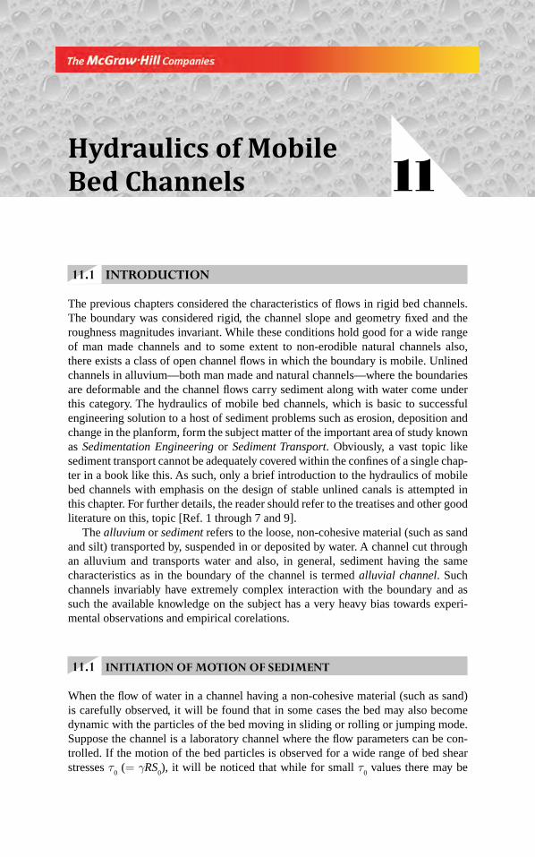
11.1 INTRODUCTION
The previous chapters considered the characteristics of fl ows in rigid bed channels. The boundary was considered rigid, the channel slope and geometry fi xed and the roughness magnitudes invariant. While these conditions hold good for a wide range of man made channels and to some extent to non-erodible natural channels also, there exists a class of open channel fl ows in which the boundary is mobile. Unlined channels in alluvium—both man made and natural channels—where the boundaries are deformable and the channel fl ows carry sediment along with water come under this category. The hydraulics of mobile bed channels, which is basic to successful engineering solution to a host of sediment problems such as erosion, deposition and change in the planform, form the subject matter of the important area of study known as Sedimentation Engineering or Sediment Transport. Obviously, a vast topic like sediment transport cannot be adequately covered within the confi nes of a single chap-ter in a book like this. As such, only a brief introduction to the hydraulics of mobile bed channels with emphasis on the design of stable unlined canals is attempted in this chapter. For further details, the reader should refer to the treatises and other good literature on this, topic [Ref. 1 through 7 and 9].
The alluvium or sediment refers to the loose, non-cohesive material (such as sand and silt) transported by, suspended in or deposited by water. A channel cut through an alluvium and transports water and also, in general, sediment having the same characteristics as in the boundary of the channel is termed alluvial channel. Such channels invariably have extremely complex interaction with the boundary and as such the available knowledge on the subject has a very heavy bias towards experi-mental observations and empirical corelations.
11.1 INITIATION OF MOTION OF SEDIMENT
When the fl ow of water in a channel having a non-cohesive material (such as sand) is carefully observed, it will be found that in some cases the bed may also become dynamic with the particles of the bed moving in sliding or rolling or jumping mode. Suppose the channel is a laboratory channel where the fl ow parameters can be con-trolled. If the motion of the bed particles is observed for a wide range of bed shear stresses τ
0 (= γRS
0), it will be noticed that while for small τ
0 values there may be
Hydraulics of Mobile
Bed Channels 11
Chapter 11.indd 483Chapter 11.indd 483 2/24/2010 3:08:08 PM2/24/2010 3:08:08 PM
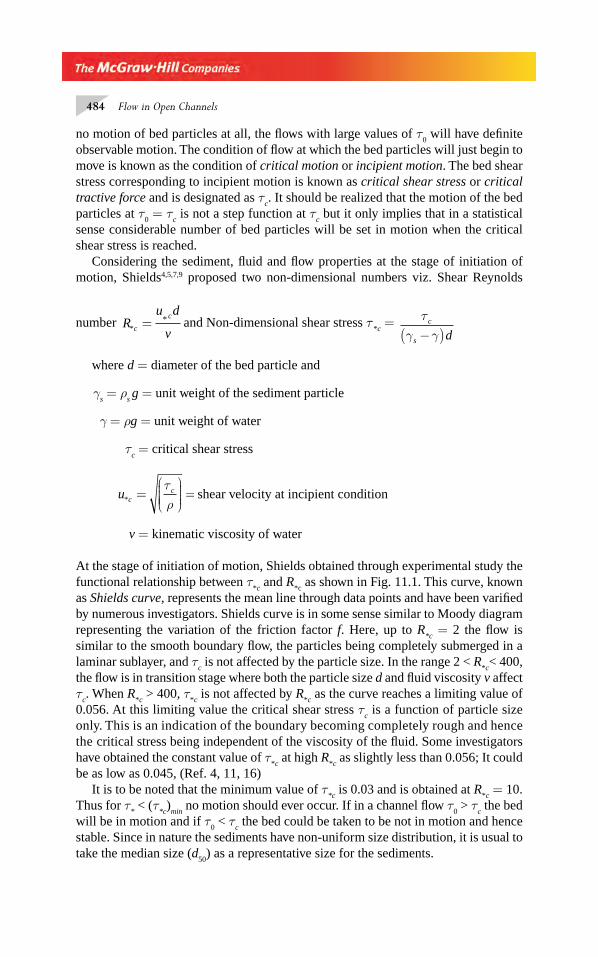
484 Flow in Open Channels
no motion of bed particles at all, the fl ows with large values of τ0 will have defi nite
observable motion. The condition of fl ow at which the bed particles will just begin to move is known as the condition of critical motion or incipient motion. The bed shear stress corresponding to incipient motion is known as critical shear stress or critical tractive force and is designated as τ
c. It should be realized that the motion of the bed
particles at τ0 = τ
c is not a step function at τ
c but it only implies that in a statistical
sense considerable number of bed particles will be set in motion when the critical shear stress is reached.
Considering the sediment, fl uid and fl ow properties at the stage of initiation of motion, Shields4,5,7,9 proposed two non-dimensional numbers viz. Shear Reynolds
number Ru d
vc
c
**= and Non-dimensional shear stress τ
*c = τ
γ γc
s d−( )
where d = diameter of the bed particle and
γs = ρ
s g = unit weight of the sediment particle
γ = ρg = unit weight of water
τc = critical shear stress
u cc
* =⎛
⎝⎜⎜⎜⎜
⎞
⎠⎟⎟⎟⎟ =
τρ
shear velocity at incipient condition
v = kinematic viscosity of water
At the stage of initiation of motion, Shields obtained through experimental study the functional relationship between τ
*c and R
*c as shown in Fig. 11.1. This curve, known
as Shields curve, represents the mean line through data points and have been varifi ed by numerous investigators. Shields curve is in some sense similar to Moody diagram representing the variation of the friction factor f. Here, up to R
*c = 2 the fl ow is
similar to the smooth boundary fl ow, the particles being completely submerged in a laminar sublayer, and τ
c is not affected by the particle size. In the range 2 < R
*c< 400,
the fl ow is in transition stage where both the particle size d and fl uid viscosity v affect τ
c. When R
*c > 400, τ
*c is not affected by R
*c as the curve reaches a limiting value of
0.056. At this limiting value the critical shear stress τc is a function of particle size
only. This is an indication of the boundary becoming completely rough and hence the critical stress being independent of the viscosity of the fl uid. Some investigators have obtained the constant value of τ
*c at high R
*c as slightly less than 0.056; It could
be as low as 0.045, (Ref. 4, 11, 16)It is to be noted that the minimum value of τ
*c is 0.03 and is obtained at R
*c = 10.
Thus for τ* < (τ
*c)
min no motion should ever occur. If in a channel fl ow τ
0 > τ
c the bed
will be in motion and if τ0 < τ
c the bed could be taken to be not in motion and hence
stable. Since in nature the sediments have non-uniform size distribution, it is usual to take the median size (d
50) as a representative size for the sediments.
Chapter 11.indd 484Chapter 11.indd 484 2/24/2010 3:08:10 PM2/24/2010 3:08:10 PM
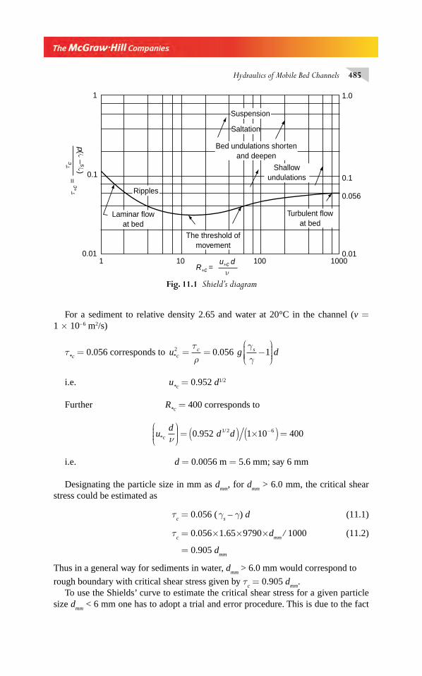
Hydraulics of Mobile Bed Channels 485
For a sediment to relative density 2.65 and water at 20°C in the channel (v = 1 × 10– 6 m2/s)
τ*c
= 0.056 corresponds to u g dcc s
* .2 0 056 1= = −⎛
⎝⎜⎜⎜⎜
⎞
⎠⎟⎟⎟⎟
τρ
γγ
i.e. u*c
= 0.952 d1/2
Further R*c
= 400 corresponds to
ud
ν d dc*
/.⎛⎝⎜⎜⎜
⎞⎠⎟⎟⎟ = ( ) ×( ) =−0 952 1 10 4001 2 6
i.e. d = 0.0056 m = 5.6 mm; say 6 mm
Designating the particle size in mm as dmm
, for dmm
> 6.0 mm, the critical shear stress could be estimated as
τc = 0.056 ( γ
s – γ) d (11.1)
τc = 0.056×1.65×9790×d
mm / 1000 (11.2)
= 0.905 dmm
Thus in a general way for sediments in water, dmm
> 6.0 mm would correspond to
rough boundary with critical shear stress given by τc = 0.905 d
mm.
To use the Shields’ curve to estimate the critical shear stress for a given particle size d
mm < 6 mm one has to adopt a trial and error procedure. This is due to the fact
1
1
10 100 10000.01
0.1
1.0
0.056
νR∗c =
u∗c d
τ ∗c
=τ c
(γs–
γ)d
0.01
0.1
Ripples
Saltation
Suspension
Laminar flowat bed
Shallowundulations
The threshold ofmovement
Bed undulations shortenand deepen
Turbulent flowat bed
Fig. 11.1 Shield’s diagram
Chapter 11.indd 485Chapter 11.indd 485 2/24/2010 3:08:11 PM2/24/2010 3:08:11 PM
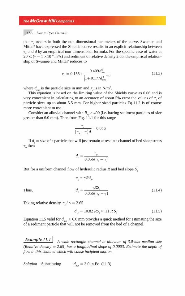
486 Flow in Open Channels
that τc occurs in both the non-dimensional parameters of the curve. Swamee and
Mittal8 have expressed the Shields’ curve results in an explicit relationship between τ
c and d by an empirical non-dimensional formula. For the specifi c case of water at
20°C (v = 1 ×10⁻⁶ m2/s) and sediment of relative density 2.65, the empirical relation-ship of Swamee and Mittal9 reduces to
τcmm
mm
d
d= +
+⎡⎣⎢
⎤⎦⎥
0 1550 409
1 0 177
2
2 1 2.
.
./
(11.3)
where dmm
is the particle size in mm and τc is in N/m2.
This equation is based on the limiting value of the Shields curve as 0.06 and is very convenient in calculating to an accuracy of about 5% error the values of τ
c of
particle sizes up to about 5.5 mm. For higher sized particles Eq.11.2 is of course more convenient to use.
Consider an alluvial channel with R*c
> 400 (i.e. having sediment particles of size greater than 6.0 mm). Then from Fig. 11.1 for this range
τγ γ
c
s d−( )= 0 056.
If dc = size of a particle that will just remain at rest in a channel of bed shear stress
τ0 then
dc
s
=−( )
τγ γ0
0 056.
But for a uniform channel fl ow of hydraulic radius R and bed slope S0
τ0 = γ R S
0
Thus, dRS
c
S
=−( )
γγ γ
0
0 056. (11.4)
Taking relative density γs / γ = 2.65
d c = 10.82 RS
0 ≈ 11 R S
0 (11.5)
Equation 11.5 valid for dmm
≥ 6.0 mm provides a quick method for estimating the size of a sediment particle that will not be removed from the bed of a channel.
Example 11.1 A wide rectangle channel in alluvium of 3.0-mm median size (Relative density = 2.65) has a longitudinal slope of 0.0003. Estimate the depth of fl ow in this channel which will cause incipient motion.
Solution Substituting dmm
= 3.0 in Eq. (11.3)
Chapter 11.indd 486Chapter 11.indd 486 2/24/2010 3:08:11 PM2/24/2010 3:08:11 PM
Hydraulics of Mobile Bed Channels 487
τcmm
mm
d
d= +
+⎡⎣⎢
⎤⎦⎥
0 1550 409
1 0 177
2
2 1 2.
.
./
τc = ++⎡
⎣⎢⎤⎦⎥
=0 1550 409 3
1 0 177 32 44
2
2 1 2.
. ( )
. ( ).
/Pa
For fl ow in a wide rectangular channel at depth D, τ0 = γD S
0 and at incipient
motion τ0 = τ
c.
Hence, 9790 × D × 0.0003 = 2.44 Depth D = 0.831 m.
Example 11.2 Estimate the minimum size of gravel that will not move in the bed of a trapezoidal channel of base width = 3.0 m, side slope = 1.5 H: IV, longitu-dinal slope = 0.004 and having a depth of fl ow of 1.30 m.
Solution R = hydraulic radius
=+ ×( )×
+ × × ( ) +⎡⎣⎢⎢
⎤⎦⎥⎥
3 0 1 5 1 30 1 30
3 0 2 1 30 1 5 12
. . . .
. . .
= 0.837 m
From Eq. (11.5), dc = 11R S
0
= 11×0.837×0.004 = 0.0368 m d
c = 3.7 cm
11.3 BED FORMS
When the shear stress on the bed of an alluvial channel due to fl ow of water is larger than the critical shear stress τ
c the bed will become dynamic and will have a strong
interaction with the fl ow. Depending upon the fl ow, sediment and fl uid characteris-tics, the bed will undergo different levels of deformation and motion. As a result of careful observations the following characteristic bed features are recognized:
1. Plane bed with no sediment motion2. Ripples and dunes3. Transition (a) Plane bed with sediment motion and (b) Standing wave
4. Antidunes
These bed features are called bed forms or bed irregularities. Schematically, these bed forms are shown in Fig. 11.2.
The sequence of formation of these bed forms are best understood by considering a hypothetical laboratory channel with sediment bed where the slope and discharge in the channel can be changed at will. Consider an initial plane bed and a very low
Chapter 11.indd 487Chapter 11.indd 487 2/24/2010 3:08:11 PM2/24/2010 3:08:11 PM
488 Flow in Open Channels
velocity of fl ow being admitted into the channel. The following sequence of bed forms can be expected in the channel.
(1) Plane Bed with no Sediment Motion This situation corresponds to the case when the actual shear stress τ
0 is less than the critical shear stress τ
c. There
will be no motion of the sediment and the bed will remain plane. The friction offered to the fl ow is due to the resistance of the grains only.
(2) Ripples and Dunes
(a) Ripples If the shear stress in the channel is increased (by increasing either dis-charge or slope) so that τ
0 is moderately greater than τ
c, the grains in the bed will
begin to move and very soon the bed will be covered by a saw tooth type of ripple pattern (Fig. 11.2). The height of the ripples will be considerably smaller than their length. The sediment motion will be essentially in the form of rolling and sliding of the particles on the ripple bed. The water surface will remain essentially calm and plane. An interesting feature of the ripples is that they are not formed if the sediment size is greater than about 0.60 mm.
(b) Dunes As the shear stress on the bed is gradually increased in our hypotheti-cal channel, the ripples gradually grow into larger sizes. Then a different bed form known as dunes appear with ripples riding over them. At higher shear stress values the ripples disappear leaving behind only the dunes pattern on the bed.
Dunes are larger in size than the ripples with small height to length ratios. The water surface will be wavy and out of phase with the dunes, (Fig. 11.2). The sediment transport will be larger than in ripples and the dunes advance downstream though with a velocity much smaller than that of the water fl ow. The fl ow will be in subcriti-cal range.
The fl ow in a channel with ripples and dunes in the bed is characterised by separa-tion of the fl ow on the lee side of the bed form. This in turn causes large energy losses and particularly so in duned beds. The shedding of the vortices from the separation region of the dunes cause ruffl ing of the free water surface. In both the ripples and dunes, the bed form gets eroded on the upstream side and some of this material gets deposited on the lee side of the bed form in a continuous manner causing the crest of the bed wave pattern to move downstream.
While the distinction between the ripples and dunes is clear in a general qualita-tive sense, it has not been possible to differentiate between them in terms of specifi c quantifi able parameters. As such, it is usual to consider the ripples and dunes as one class and to distinguish this class of bed form from others.
(3) Transition
(a) Plane bed with sediment motion Further increase of the shear stress after the dune bed pattern phase will lead to a transition phase where the bed undulations get washed away progressively to achieve ultimately an essentially plane bed surface (Fig. 11.2). The sediment transport rate would be considerably larger than in dune
Chapter 11.indd 488Chapter 11.indd 488 2/24/2010 3:08:11 PM2/24/2010 3:08:11 PM
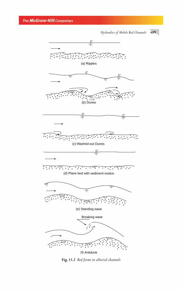
Hydraulics of Mobile Bed Channels 489
(f) Antidune
(e) Standing wave
(d) Plane bed with sediment motion
(c) Washed-out Dunes
(b) Dunes
(a) Ripples
Breaking wave
∇
∇
∇
∇
∇
∇
Fig. 11.2 Bed forms in alluvial channels
Chapter 11.indd 489Chapter 11.indd 489 2/24/2010 3:08:11 PM2/24/2010 3:08:11 PM
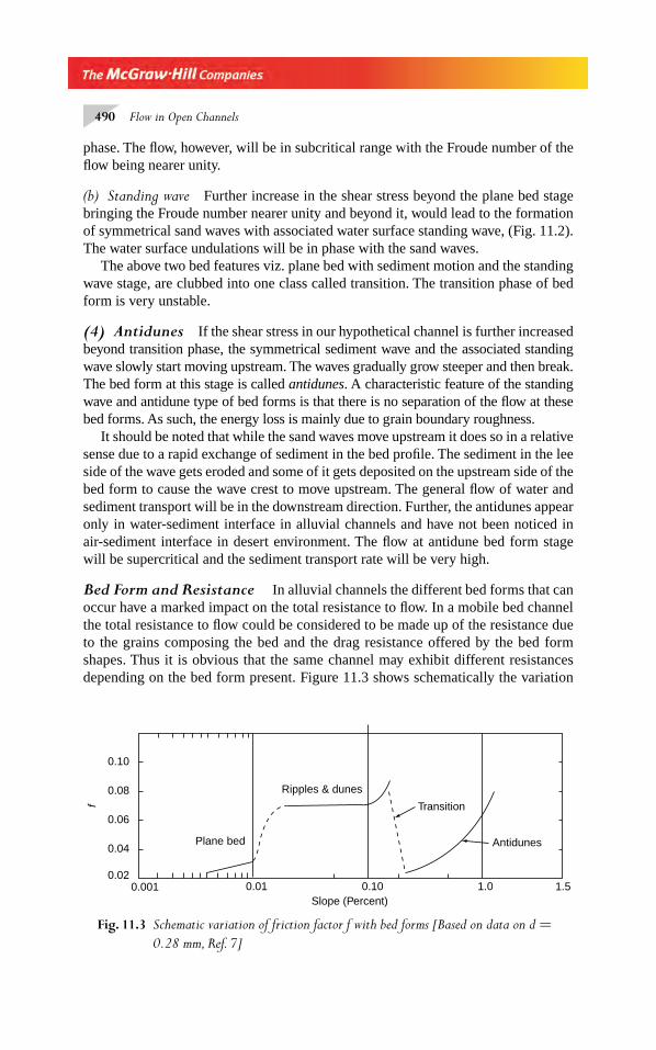
490 Flow in Open Channels
phase. The fl ow, however, will be in subcritical range with the Froude number of the fl ow being nearer unity.
(b) Standing wave Further increase in the shear stress beyond the plane bed stage bringing the Froude number nearer unity and beyond it, would lead to the formation of symmetrical sand waves with associated water surface standing wave, (Fig. 11.2). The water surface undulations will be in phase with the sand waves.
The above two bed features viz. plane bed with sediment motion and the standing wave stage, are clubbed into one class called transition. The transition phase of bed form is very unstable.
(4) Antidunes If the shear stress in our hypothetical channel is further increased beyond transition phase, the symmetrical sediment wave and the associated standing wave slowly start moving upstream. The waves gradually grow steeper and then break. The bed form at this stage is called antidunes. A characteristic feature of the standing wave and antidune type of bed forms is that there is no separation of the fl ow at these bed forms. As such, the energy loss is mainly due to grain boundary roughness.
It should be noted that while the sand waves move upstream it does so in a relative sense due to a rapid exchange of sediment in the bed profi le. The sediment in the lee side of the wave gets eroded and some of it gets deposited on the upstream side of the bed form to cause the wave crest to move upstream. The general fl ow of water and sediment transport will be in the downstream direction. Further, the antidunes appear only in water-sediment interface in alluvial channels and have not been noticed in air-sediment interface in desert environment. The fl ow at antidune bed form stage will be supercritical and the sediment transport rate will be very high.
Bed Form and Resistance In alluvial channels the different bed forms that can occur have a marked impact on the total resistance to fl ow. In a mobile bed channel the total resistance to fl ow could be considered to be made up of the resistance due to the grains composing the bed and the drag resistance offered by the bed form shapes. Thus it is obvious that the same channel may exhibit different resistances depending on the bed form present. Figure 11.3 shows schematically the variation
Plane bed
Ripples & dunes
Transition
Antidunes
0.020.001 0.01 0.10 1.0 1.5
0.04
0.06
0.08
0.10
Slope (Percent)
f
Fig. 11.3 Schematic variation of friction factor f with bed forms [Based on data on d =
0.28 mm, Ref. 7]
Chapter 11.indd 490Chapter 11.indd 490 2/24/2010 3:08:12 PM2/24/2010 3:08:12 PM
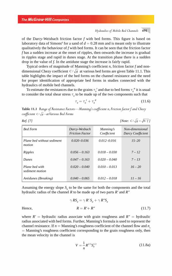
Hydraulics of Mobile Bed Channels 491
of the Darcy-Weisbach friction factor f with bed forms. This fi gure is based on laboratory data of Simons6 for a sand of d = 0.28 mm and is meant only to illustrate qualitatively the behaviour of f with bed forms. It can be seen that the friction factor f has a sudden increase at the onset of ripples, then onwards the increase is gradual in ripples stage and rapid in dunes stage. At the transition phase there is a sudden drop in the value of f. In the antidune stage the increase is fairly rapid.
Typical orders of magnitude of Manning’s coeffi cient n, friction factor f and non-dimensional Chezy coeffi cient C g/ at various bed forms are given Table 11.1. This table highlights the impact of the bed forms on the channel resistance and the need for proper identifi cation of appropriate bed forms in studies connected with the hydraulics of mobile bed channels.
To estimate the resistances due to the grains τ0′ and due to bed forms τ
0″ it is usual
to consider the total shear stress τ0 to be made up of the two components such that
τ0 = τ
0′ + τ
0″ (11.6)
Table 11.1 Range of Resistance Factors—Manning’s coeffi cient n, Friction factor f and Chezy
coeffi cient C g/ –at Various Bed Forms
Ref. [7] [Note: C g f/ /= 8 ]
Bed Form Darcy-Wesbach Friction Factor
Manning’s Coeffi cient
Non-dimensional Darcy Coeffi cient
Plane bed without sediment motion
0.020–0.036 0.012–0.016 15–20
Ripples 0.056 – 0.163 0.018 – 0.030 7 – 12
Dunes 0.047 – 0.163 0.020 – 0.040 7 – 13
Plane bed with sediment motion
0.020 – 0.040 0.010 – 0.013 16 – 20
Antidunes (Breaking) 0.040 – 0.065 0.012 – 0.018 11 – 16
Assuming the energy slope S0 to be the same for both the components and the total
hydraulic radius of the channel R to be made up of two parts R' and R''
γ RS0 = γ R' S
0 + γ R"S
0
Hence, R = R'+ R" (11.7)
where R' = hydraulic radius associate with grain roughness and R" = hydraulic radius associated with bed forms. Further, Manning’s formula is used to represent the channel resistance. If n = Manning’s roughness coeffi cient of the channel fl ow and n
s
= Manning’s roughness coeffi cient corresponding to the grain roughness only, then the mean velocity in the channel is
V
nR S=
1 2 301 2/ /
(11.8a)
Chapter 11.indd 491Chapter 11.indd 491 2/24/2010 3:08:12 PM2/24/2010 3:08:12 PM
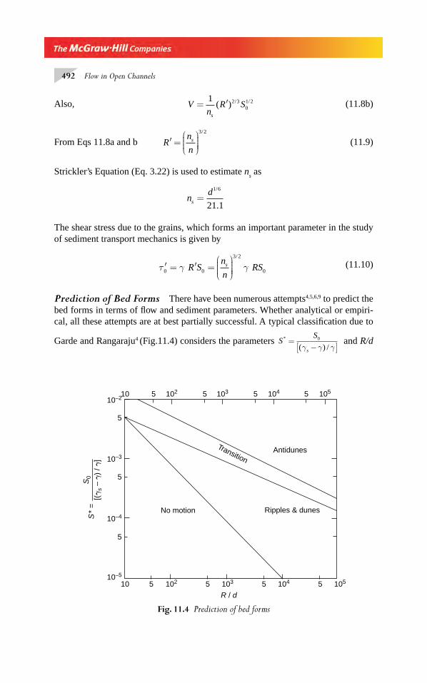
492 Flow in Open Channels
Also,
Vn
R Ss
= ′1 2 301 2( ) / /
(11.8b)
From Eqs 11.8a and b ′ =⎛
⎝⎜⎜⎜
⎞
⎠⎟⎟⎟⎟R
n
ns
3 2/
(11.9)
Strickler’s Equation (Eq. 3.22) is used to estimate ns as
nd
s =1 6
21 1
/
.
The shear stress due to the grains, which forms an important parameter in the study of sediment transport mechanics is given by
′ = ′ =⎛
⎝⎜⎜⎜
⎞
⎠⎟⎟⎟⎟τ γ γ0 0
3 2
0R Sn
nRSs
/
(11.10)
Prediction of Bed Forms There have been numerous attempts4,5,6,9 to predict the bed forms in terms of fl ow and sediment parameters. Whether analytical or empiri-cal, all these attempts are at best partially successful. A typical classifi cation due to
Garde and Rangaraju4 (Fig.11.4) considers the parameters SS
s
*
( ) /=
−[ ]0
γ γ γ and R/d
Fig. 11.4 Prediction of bed forms
No motion
AntidunesTransition
Ripples & dunes
10
10
5
5
5
1025
1025 1035 1045 1055
1035 1045 105510–5
10–4
10–3
10–2
R / d
S*
=S
0
[(γ s
– γ
) / γ
]
Chapter 11.indd 492Chapter 11.indd 492 2/24/2010 3:08:12 PM2/24/2010 3:08:12 PM
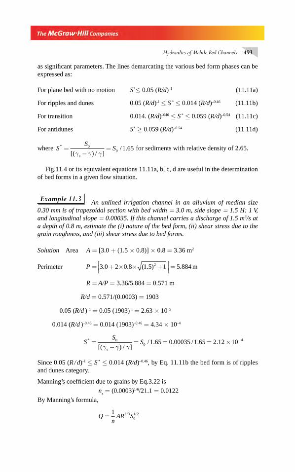
Hydraulics of Mobile Bed Channels 493
as signifi cant parameters. The lines demarcating the various bed form phases can be expressed as:
For plane bed with no motion S *≤ 0.05 (R/d)–1 (11.11a)
For ripples and dunes 0.05 (R/d)–l ≤ S * ≤ 0.014 (R/d)–0.46 (11.11b)
For transition 0.014. (R/d)–046 ≤ S * ≤ 0.059 (R/d)–0.54 (11.11c)
For antidunes S * ≥ 0.059 (R/d)–0.54 (11.11d)
where SS
Ss
*
[( ) / ]/ .=
−=0
0 1 65γ γ γ
for sediments with relative density of 2.65.
Fig.11.4 or its equivalent equations 11.11a, b, c, d are useful in the determination of bed forms in a given fl ow situation.
Example 11.3 An unlined irrigation channel in an alluvium of median size 0.30 mm is of trapezoidal section with bed width = 3.0 m, side slope = 1.5 H: 1 V, and longitudinal slope = 0.00035. If this channel carries a discharge of 1.5 m3/s at a depth of 0.8 m, estimate the (i) nature of the bed form, (ii) shear stress due to the grain roughness, and (iii) shear stress due to bed forms.
Solution Area A = [3.0 + (1.5 × 0.8)] × 0.8 = 3.36 m2
Perimeter
P = + × × +⎡⎣⎢
⎤⎦⎥=3 0 2 0 8 1 5 1 5 8842. . ( . ) . m
R = A/P = 3.36/5.884 = 0.571 m
R/d = 0.571/(0.0003) = 1903
0.05 (R/d )–1 = 0.05 (1903)–l = 2.63 × 10⁻⁵
0.014 (R/d )–0.46 = 0.014 (1903)–0.46 = 4.34 × 10⁻⁴
SS
Ss
*
[( ) / ]/ . . / . .=
−= = = × −0
041 65 0 00035 1 65 2 12 10
γ γ γ
Since 0.05 (R / d)–l ≤ S * ≤ 0.014 (R/d)–0.46, by Eq. 11.11b the bed form is of ripples and dunes category.
Manning’s coeffi cient due to grains by Eq.3.22 is
ns = (0.0003)1/6/21.1 = 0.0122
By Manning’s formula,
Q
nAR S=
1 2 301 2/ /
Chapter 11.indd 493Chapter 11.indd 493 2/24/2010 3:08:12 PM2/24/2010 3:08:12 PM
494 Flow in Open Channels
1 51
3 36 0 571 0 000350 04332 3 1 2. ( . )( . ) ( . )./ /= =
n n
n = Manning’s coeffi cient for the whole channel = 0 0288
By Eq. 11.10, the shear stress due to the grains
′ =⎛
⎝⎜⎜⎜
⎞
⎠⎟⎟⎟⎟ =
⎛⎝⎜⎜⎜
⎞⎠⎟⎟⎟⎟ × ×τ γ0
3 2
0
3 20 0122
0 02889790
n
nRSs
/ /.
.00 571 0 00035. .×
= 0.539 Pa
τ0 = Average bed shear stress due to fl ow. = γ R S
0
= 9790 × 0.571 × 0.00035 = 1.957 Pa
τ0"
= shear stress due to bed forms = τ
0 – τ'
0
= 1.957 – 0.539 = 1.418 Pa
11.4 SEDIMENT LOAD
In an alluvial channel the sediment particles in the bed will start moving when the bed shear stress τ
0 exceeds the critical shear stress τ
c At small values of excess bed
shear stress (τ0 – τ
c) the particles may roll or slide on the bed. Sediment transported
in this manner is called contact load. Sometimes the sediment particles may leave the boundary to execute a small jump (or hop) to come in contact with the bed again. This mode of sediment transport through a large number of small jumps is known as saltation load. The saltation of sediment particles in water fl ow takes place essen-tially in a thin layer, of the order of two grain diameters, next to the bed. In view of this, both the contact load and saltation load are considered under one class as bed load. Thus all the sediment that will be transported in a thin layer of the order of two grain diameters next to the bed is classifi ed as bed load.
At higher shear rates, the fl uid turbulence may pick up the displaced particles and keep them in suspension. The sediment transported in suspension mode is known as suspended load. Whether a particle will travel as bed load or suspended load depends upon the parameter ω/u
* where ω = fall velocity of the particle and u* /= =τ ρ0
shear velocity of the fl ow. The particles of fall velocity ω move in suspension mode when ω/u
0 ≤ 2.0.
The sum of the suspended load and bed load is total load. It should be noted that the total load is made up of material emanating from the boundary of the channel and as such it is also sometimes called as total bed material load. Some-times, the suspended material may contain very fi ne material like clay not found in the boundary of the channel. This material would have come to a stream, and thence to a channel, as a product of erosion during a runoff process. Such sus-pended material which does not form part of the bed material is known as wash
Chapter 11.indd 494Chapter 11.indd 494 2/24/2010 3:08:13 PM2/24/2010 3:08:13 PM
Hydraulics of Mobile Bed Channels 495
load and its transport characteristics are different from that of bed material sus-pended load. Unless otherwise specifi cally mentioned as signifi cant, the wash load is usually ignored in alluvial geometry design. The term suspended load is understood to refer to bed material only.
Bed Load The transport rate of sediments in the bed load (qB) is usually referred
to in units of weight per second per unit width (N/s/m). A very large number of empirical and semi-analytical expressions are available to estimate the bed load q
B in
terms of sediment, fl uid and fl ow parameters. Duboys (1879) was the fi rst to propose an expression for q
B as a function of excess of shear stress τ
0 over the critical shear
stress τ0, viz.
qB = α (τ
0 – τ
c) (11.12)
Since then a very large number of empirical formulae involving the parameter (τ
0 – τ
c ) have–been proposed by various investigators. Probably the most widely
used empirical equation for qB is due to Meyer-Peter and Muller4,5 which relates q
B
in a dimensionless manner as
φB
= 8 (τ'* – 0.047)3/2 (11.13)
where φB = bed load function
= ⋅
−⎡
⎣⎢⎢
⎤
⎦⎥⎥
q
gdB
s sγ γ
γ
( ) / /3 1 2 1 2
1
1
(11.14)
and τ'* = dimensionless grain shear stress
=−( )
=⎡
⎣⎢⎢
⎤
⎦⎥⎥ −( )
γγ γ
γγ γ
R S
d
n
n
RS
ds
s
s
0
3 2
0
/
) (11.15)
in which qB = bed load in N/s/m
d = mean size of sediment
R = hydraulic radius of the channel
γ = unit weight of water
γs= unit weight of sediment particles
n = Manning’s coeffi cient for the whole channel
ns = Manning’s coeffi cient of particle roughness
R' = hydraulic radius corresponding to grain roughness
S0 = longitudinal slope of the channel.
In Eq. 11.13 the term 0.047 corresponds to the asymptotic value in the shields diagram.
Chapter 11.indd 495Chapter 11.indd 495 2/24/2010 3:08:13 PM2/24/2010 3:08:13 PM
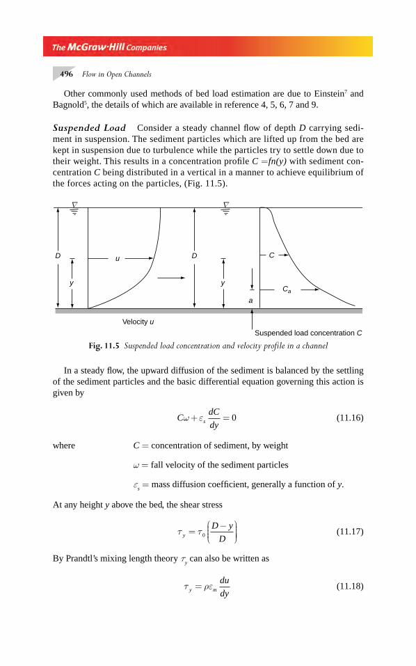
496 Flow in Open Channels
Other commonly used methods of bed load estimation are due to Einstein7 and Bagnold5, the details of which are available in reference 4, 5, 6, 7 and 9.
Suspended Load Consider a steady channel fl ow of depth D carrying sedi-ment in suspension. The sediment particles which are lifted up from the bed are kept in suspension due to turbulence while the particles try to settle down due to their weight. This results in a concentration profi le C =fn(y) with sediment con-centration C being distributed in a vertical in a manner to achieve equilibrium of the forces acting on the particles, (Fig. 11.5).
Fig. 11.5 Suspended load concentration and velocity profi le in a channel
D D
y y
a
Ca
C
Velocity u
u
Suspended load concentration C
∇ ∇
In a steady fl ow, the upward diffusion of the sediment is balanced by the settling of the sediment particles and the basic differential equation governing this action is given by
C
dC
dysω ε+ = 0
(11.16)
where C = concentration of sediment, by weight
ω = fall velocity of the sediment particles
εs = mass diffusion coeffi cient, generally a function of y.
At any height y above the bed, the shear stress
τ τy
D y
D=
−⎛⎝⎜⎜⎜
⎞⎠⎟⎟⎟⎟0
(11.17)
By Prandtl’s mixing length theory τy can also be written as
τ ρεy m
du
dy=
(11.18)
Chapter 11.indd 496Chapter 11.indd 496 2/24/2010 3:08:13 PM2/24/2010 3:08:13 PM
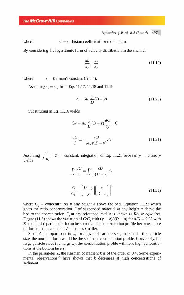
Hydraulics of Mobile Bed Channels 497
where εm
= diffusion coeffi cient for momentum.
By considering the logarithmic form of velocity distribution in the channel.
du
dy
u
ky= *
(11.19)
where k = Karman’s constant (≈ 0.4).
Assuming εs = ε
m, from Eqs 11.17, 11.18 and 11.19
εs kuy
DD y= −* ( )
(11.20)
Substituting in Eq. 11.16 yields
C kuy
DD y
dC
dyω + − =* ( ) 0
dC
C
D
ku y D ydy= −
−ω
* ( )
(11.21)
Assuming ω
k uZ
∗
= = constant, integration of Eq. 11.21 between y = a and y yields
dC
C
ZD
y D ydy
a
y
a
y
∫ ∫=−( )
C
C
D y
y
a
D a
z
=−⎛
⎝⎜⎜⎜⎜
⎞
⎠⎟⎟⎟⎟ −
⎛
⎝⎜⎜⎜
⎞
⎠⎟⎟⎟
⎡
⎣⎢⎢
⎤
⎦⎥⎥
a
(11.22)
where Ca = concentration at any height a above the bed. Equation 11.22 which
gives the ratio concentration C of suspended material at any height y above the bed to the concentration C
a at any reference level a is known as Rouse equation.
Figure (11.6) shows the variation of C/Ca with ( y − a)/ (D − a) for a/D = 0.05 with
Z as the third parameter. It can be seen that the concentration profi le becomes more uniform as the parameter Z becomes smaller.
Since Z is proportional to ω, for a given shear stress τ0, the smaller the particle
size, the more uniform would be the sediment concentration profi le. Conversely, for large particle sizes (i.e. large ω), the concentration profi le will have high concentra-tions at the bottom layers.
In the parameter Z, the Karman coeffi cient k is of the order of 0.4. Some experi-mental observations4,9 have shown that k decreases at high concentrations of sediment.
Chapter 11.indd 497Chapter 11.indd 497 2/24/2010 3:08:13 PM2/24/2010 3:08:13 PM
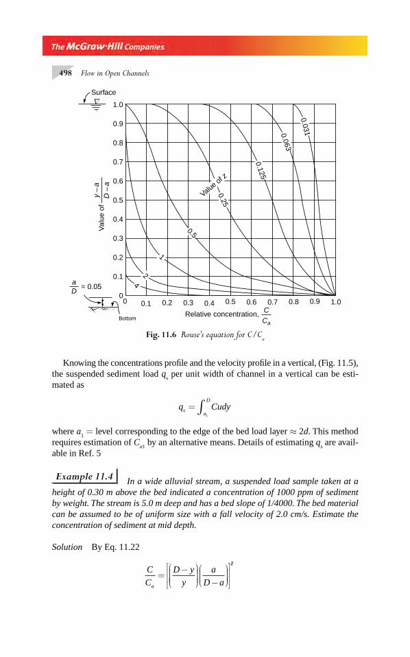
498 Flow in Open Channels
Fig. 11.6 Rouse’s equation for C/Ca
aD
= 0.0500
0.1
0.1
0.2
0.2
0.3
0.3
0.4
0.4
0.5
0.5
0.6
0.6
0.7
0.7
0.8
0.8
0.9
0.9
1.0
1.0
Relative concentration, CCa
Bottom
Val
ue o
fy
–a
D –
a
Surface∇
Value of z
42
1
0.5
0.25
0.125
0.063
0.031
Knowing the concentrations profi le and the velocity profi le in a vertical, (Fig. 11.5), the suspended sediment load q
s per unit width of channel in a vertical can be esti-
mated as
q Cudysa
D
= ∫1
where a1 = level corresponding to the edge of the bed load layer ≈ 2d. This method
requires estimation of Ca1
by an alternative means. Details of estimating qs are avail-
able in Ref. 5
Example 11.4 In a wide alluvial stream, a suspended load sample taken at a height of 0.30 m above the bed indicated a concentration of 1000 ppm of sediment by weight. The stream is 5.0 m deep and has a bed slope of 1/4000. The bed material can be assumed to be of uniform size with a fall velocity of 2.0 cm/s. Estimate the concentration of sediment at mid depth.
Solution By Eq. 11.22
C
C
D y
y
a
D aa
z
=−⎛
⎝⎜⎜⎜⎜
⎞
⎠⎟⎟⎟⎟ −
⎛⎝⎜⎜⎜
⎞⎠⎟⎟⎟⎟
⎡
⎣⎢⎢
⎤
⎦⎥⎥
Chapter 11.indd 498Chapter 11.indd 498 2/24/2010 3:08:14 PM2/24/2010 3:08:14 PM
Hydraulics of Mobile Bed Channels 499
Here a = 0.3 m, D = 5.0 m, y = D/2 = 2.5 m, Ca = 1000, ω = 0.02 m/s.
Z =
ωu k*
Since the channel is wide, R = D and
u gDS Zk gDS
* ,= =0
0
ω
Assuming k = 0.4,
Z =× × ×
=0 02
0 4 9 81 5 1 40000 4515
.
. . /.
By Eq. 11.22
C /
. .
.
.
( . . ).
.
10005 0 2 5
2 5
0 3
5 0 0 30 2887
0 4515
=−( )
×−
⎡
⎣⎢⎢⎢
⎤
⎦⎥⎥⎥
=
C = 2887 ppm by weight.
Total Bed Material Load The sum of the bed load and suspended load form the total bed material load. Using expressions derived for estimation of bed load and suspended load elaborate procedures for estimation of total bed material load are given by Einstein, Colby et al, and Bishop et al, [Ref. 5,7,9]. Numerous empirical equations for the estimation of total bed material load have been proposed. One of these, a commonly used equation due to Englund and Hansen2,4 which expresses the total bed material load per unit width q
T in terms of easily determinable parameters,
is given below:
φT
f = 0.4 τ*5/2 (11.23)
where φT = total load function and
φγ γ
γ
TT
s s
q
gd=
−⎡
⎣⎢⎢
⎤
⎦⎥⎥
( ) / /3 1 2 1 2
1
1
(11.24)
where τ* = non-dimensional shear
=−⎡
⎣⎢⎤⎦⎥
τ
γ γ0
sd
(11.25)
f = Darcy – Weisbach friction factor
=8 0
2
gRS
V (11.26)
qT = total bed material load per unit width of channel in N/s/m
V = mean velocity in the channel and other parameters are same as in Eq. 11.13.
Equation (11.23) is based on data pertaining to a wide range of bed forms and grain sizes and therefore could be relied on to predict the total load fairly adequately.
Chapter 11.indd 499Chapter 11.indd 499 2/24/2010 3:08:14 PM2/24/2010 3:08:14 PM
500 Flow in Open Channels
Example 11.5 A wide alluvial channel has a bed material of median size 0.8 mm. The channel has a longitudinal slope of 5 × 10⁻⁴. The depth and velocity in the channel were measured as 1.6 m and 0.90 m/s respectively. Estimate the (a) bed load, (b) total load, and (c) suspended load per metre width of this channel.
Solution (a) Bed load, qB:
Since the channels is wide R = y0 = 1.60 m.
By Manning’s formula Vn
y S=1
02 3
01 2/ /
0 901
1 6 5 102 3 4 1 2. ( . ) ( )/ /= × −
n
n = 0.034
By Eq. 3.17, n
ds = = =
1 6 1 6
21 1
0 0008
21 10 0144
/ /
.
( . )
..
By Eq. 11.9, shear stress due to gain τ γ0
3 2
0 0′ =
⎛
⎝⎜⎜⎜
⎞
⎠⎟⎟⎟⎟
n
ny Ss
/
τ γ γ0
3 2
0 0 0 0
0 0144
0 03400 2756′ =
⎡
⎣⎢⎢
⎤
⎦⎥⎥
=.
..
/
y S y S
ττ
γ γγ
γ γ00 0 00 2756′ =
−=
−( )
.
( )s sd
y S
d
=× × ×
×=
−0 2756 1 6 5 10
1 65 0 00080 167
4. .
. ..
By Eq. 11.4
φ
γγ γ
γ
BB
ss
q
gd
=−⎡
⎣⎢⎢
⎤
⎦⎥⎥( ) /
/
3 1 2
1 2
φB
Bq=
× ×⎡⎣⎢
⎤⎦⎥
×2 65 9790 9 81 0 0008
1
1 653 1 2 1. . ( . ) ( . )/ /
= 0.4234 qB
By Meyer–Peter formula 11.13
φB = 8 (τ'* − 0.047)3/2
0.4234 qB
= 8(0.167 − 0.047)3/2
qB = 0.785 N/s per metre width.
Chapter 11.indd 500Chapter 11.indd 500 2/24/2010 3:08:14 PM2/24/2010 3:08:14 PM
Hydraulics of Mobile Bed Channels 501
(b) Total load, qT
By Eq. 11.24
φ
γγ γ
γ
TT
ss
q
gd
=−⎡
⎣⎢⎢
⎤
⎦⎥⎥( ) /
/
3 1 2
1 2
φTTq
=× ×⎡
⎣⎢⎤⎦⎥
×2 65 9790 9 81 0 0008
1
1 653 1 2 1 2. . ( . ) ( . )/ /
= 0.4234 qT
The Darcy–Weisbach friction factor f, by Eq. 11.26 is
fgRS
V= =
× × × ×=
−8 8 9 81 1 6 5 10
0 90 07750
2
4
2
. .
( . ).
τγ
γ γ* ( )
.
. ..=
−=
× ××
=−y S
ds
0 041 6 5 10
1 65 0 0080 6061
By Eq. 11.23 φT . f = 0.4 τ
*5/2
0.4234 qT × 0.0775 = 0.4 × (0.6061)5/2
Total load = qT = 3.486 N/s per metre width
(c) Suspended load, qs
qT = q
s+q
B
qs= suspended load = 3.486 − 0.785
= 2.701 N/s per metre width
11.4.1 Measurement and Estimation of Sediment Load
A stream fl owing in a watershed transports not only the runoff that is produced in the catchment but also the erosion products out of the watershed by means of its fl ow. The total sediment load is transported out the catchment by the stream in three com-ponents depending upon their origin as wash load, suspended load and bed load.
In connection with the measurement, the following essential properties of differ-ent types of sediment loads in a stream are worth noting:
• Wash load is generally composed of fi ne grained soils of very small fall velocity.
• The suspended load particles move considerably long distances before settling on the bed and sides and any measurement of suspended load also includes wash load.
Chapter 11.indd 501Chapter 11.indd 501 2/24/2010 3:08:15 PM2/24/2010 3:08:15 PM
502 Flow in Open Channels
• Bed load is the relatively coarse bed material and is moved at the bed surface through sliding, rolling, and saltation. In a general sense, bed load forms a small part of total load (usually < 25%) and wash load forms comparatively very small part of the total load.
Bed load measurement in fi eld is extremely diffi cult. While a large number of devises are available for measuring bed load for experimental / special investiga-tions, no practical devise for routine fi eld measurement of bed load is currently in use. For planning and design purposes the bed load of a stream is usually estimated either by use of a bed load equation such as those due to Meyer–Peter and Muller (Eq. 11.13), Einstein7 and Bagnold5 or is taken as a certain percentage of the meas-ured suspended load.
The suspended load of a stream is measured by taking the samples of sediment laden stream water. The collection of samples is through specially designed sam-plers that do not alter the fl ow confi guration in front of the sampler and get rep-resentative samples of the stream water. A variety of samplers from the simple ones (for example an ordinary bottle) to highly sophisticated ones are available. The sediment from the collected sample of sediment laden water is removed by fi ltering and its dry weight determined. It is usual to express suspended load as parts per million (ppm) on weight basis as
C
Weight of sen ent in sample
weight of se ent water of the ss =+dim
dim( ) aample
⎡
⎣⎢⎢
⎤
⎦⎥⎥×106
Thus the sediment transport rate in a stream of discharge Q m3/s is
Qs = (Q × C
s × 60 × 60 × 24) /106 = 0.086 QC Tonnes/day
Routine observations of suspended load are being done at many stream gauging stations in the country. At these stations in addition to stream fl ow discharge Q the suspended sediment concentration and hence the suspended sediment load Q
s is also
noted. The relation between Qs (tones/day) and stream discharge Q (m3/s) is usually
represented in a log–log plot known as sediment rating curve. The relationship between Q
s and Q can be represented as
Qs = KQ n
where the exponent is usually around 2.0.The sediment rating curve in conjunction with the stream fl ow hydrograph can be
used to estimate the suspended sediment load transport in the stream in a specifi ed time interval. A method of estimating the annual sediment yield of a watershed by using the sediment rating curve in conjunction with fl ow duration curve is described in Ref. 10. For details regarding Sediment problems and relevant measurement tech-niques Ref.6 and 11 can be consulted.
Chapter 11.indd 502Chapter 11.indd 502 2/24/2010 3:08:15 PM2/24/2010 3:08:15 PM
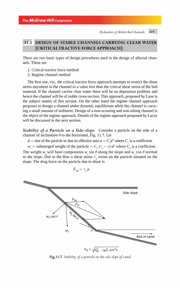
Hydraulics of Mobile Bed Channels 503
11.5 DESIGN OF STABLE CHANNELS CARRYING CLEAR WATER [CRITICAL TRACTIVE FORCE APPROACH]
There are two basic types of design procedures used in the design of alluvial chan-nels. These are
1. Critical tractive force method2. Regime channel method
The fi rst one, viz., the critical tractive force approach attempts to restrict the shear stress anywhere in the channel to a value less than the critical shear stress of the bed material. If the channel carries clear water there will be no deposition problem and hence the channel will be of stable cross-section. This approach, proposed by Lane is the subject matter of this section. On the other hand the regime channel approach proposes to design a channel under dynamic equilibrium while the channel is carry-ing a small amount of sediment. Design of a non-scouring and non-silting channel is the object of the regime approach. Details of the regime approach proposed by Lacey will be discussed in the next section.
Stability of a Particle on a Side-slope Consider a particle on the side of a channel of inclination θ to the horizontal, Fig. 11.7. Let
d = size of the particle so that its effective area a = C1d 2 where C
1 is a coeffi cient.
ws = submerged weight of the particle = C
2 (γ
s – γ) d 3 where C
2 is a coeffi cient.
The weight ws will have components w
s sin θ along the slope and w
s cos θ normal
to the slope. Due to the fl ow a shear stress τw exists on the particle situated on the
slope. The drag force on the particle due to shear is
FDS
= τw
a
Bed of canal
θ
Side slope
FDs
ws
ws cos θ
ws sin θ
FR
FR = F2Ds +w2
s sin2θ
Fig.11.7 Stability of a particle on the side slope of canal
Chapter 11.indd 503Chapter 11.indd 503 2/24/2010 3:08:15 PM2/24/2010 3:08:15 PM
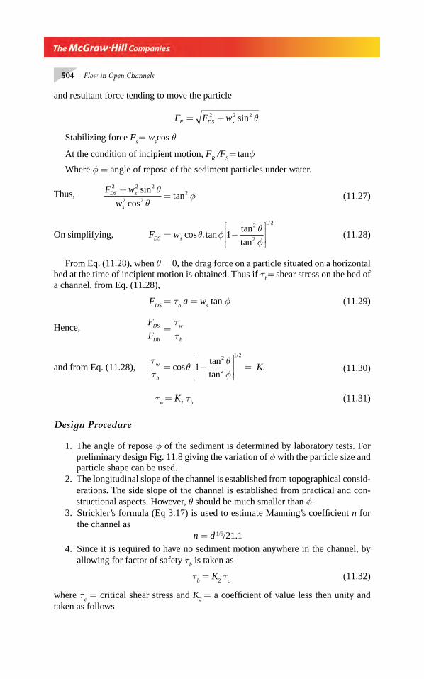
504 Flow in Open Channels
and resultant force tending to move the particle
F F wR DS s= +2 2 2sin θ
Stabilizing force Fs = w
scos θ
At the condition of incipient motion, FR /F
S = tanφ
Where φ = angle of repose of the sediment particles under water.
Thus,
F w
wDS s
s
2 2 2
2 2
2+=
sin
costan
θθ
φ
(11.27)
On simplifying,
F wDS s= −⎡
⎣⎢⎢
⎤
⎦⎥⎥cos . tan
tan
tan
/
θ φθφ
12
2
1 2
(11.28)
From Eq. (11.28), when θ = 0, the drag force on a particle situated on a horizontal bed at the time of incipient motion is obtained. Thus if τ
b= shear stress on the bed of
a channel, from Eq. (11.28),
FDS
= τb a = w
s tan φ (11.29)
Hence, F
FDS
Db
w
b
=ττ
and from Eq. (11.28),
ττ
θθφ
w
b
K= −⎡
⎣⎢⎢
⎤
⎦⎥⎥ =cos
tan
tan
/
12
2
1 2
1 (11.30)
τw
= K1 τ
b (11.31)
Design Procedure
1. The angle of repose φ of the sediment is determined by laboratory tests. For preliminary design Fig. 11.8 giving the variation of φ with the particle size and particle shape can be used.
2. The longitudinal slope of the channel is established from topographical consid-erations. The side slope of the channel is established from practical and con-structional aspects. However, θ should be much smaller than φ.
3. Strickler’s formula (Eq 3.17) is used to estimate Manning’s coeffi cient n for the channel as
n = d 1/6/21.1
4. Since it is required to have no sediment motion anywhere in the channel, by allowing for factor of safety τ
b is taken as
τb = K
2 τ
c (11.32)
where τc = critical shear stress and K
2 = a coeffi cient of value less then unity and
taken as follows
Chapter 11.indd 504Chapter 11.indd 504 2/24/2010 3:08:15 PM2/24/2010 3:08:15 PM
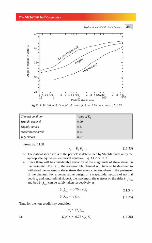
Hydraulics of Mobile Bed Channels 505
Fig.11.8 Variation of the angle of repose φ of particles under water [Ref. 8]
30.3 1 10 100 500
4 5 6789 32 4 56789 32 4 5 32 4 56789
Particle size in mm
Very roundedAngularCrushed le
dge rock`
25
30
35
40
45
Ang
le o
f rep
ose
in w
ater
ϕ
Channel condition Value of K2
Straight channel 0.90
Slightly curved 0.81
Moderately curved 0.67
Very curved 0.54
From Eq. 11.31τ
w = K
1 K
2 τ
c (11.33)
5. The critical shear stress of the particle is determined by Shields curve or by the appropriate equivalent empirical equation, Eq. 11.2 or 11.3.
6. Since there will be considerable variation of the magnitude of shear stress on the perimeter (Fig. 3.6), the non-erodible channel will have to be designed to withstand the maximum shear stress that may occur anywhere in the perimeter of the channel. For a conservative design of a trapezoidal section of normal depth y
0 and longitudinal slope S
0 the maximum shear stress on the sides (τ
w)
max
and bed (τb)
max can be safely taken respectively as
(τw)
max = 0.75 γ y
0S
0 (11.34)
(τb)
max = γ y
0S
0 (11.35)
Thus for the non-erodibility condition,
τw ≤ (τ
w)
max
i.e. K1K
2τ
c ≤ 0.75 γ y
0 S
0 (11.36)
Chapter 11.indd 505Chapter 11.indd 505 2/24/2010 3:08:15 PM2/24/2010 3:08:15 PM
506 Flow in Open Channels
and τb ≤ (τ
b)
max
i.e. K2 τ
c ≤ γ y
0 S
0. (11.37)
The lesser of the two values of y0 obtained from Eqs 11.36 and 11.37 is adopted. The
following example illustrates the design procedure well.
Example 11.6 Design a stable non-erodible channel to carry l0 m3/s of clear water through a 10–mm bed of rounded gravel. A longitudinal slope of 0.0008 and side slope of 2 horizontal: 1 vertical are to be adopted.
Solution From Fig. 11.8 for rounded gravel of d = 10 mm, φ = 32°.
tan φ = 0.6249
Side slope tan θ = 1/2 = 0.5, cos θ = 0.8944
Sine dmm
> 6, by Eq. 11.2, τc = 0.905 × 10 = 9.05 Pa
For the bed: By considering a straight channel K2 = 0.9
τb = K
2 τ
c = 0.9 × 9.05 = 8.145 Pa
By making τb = (τ
b )
max = γ y
0 S
0
y0
8 145
9790 0 00081 04=
×=
.
.. m (11.38)
For the side: By Eq. 11.30, K1
2
2
1 2
1= −⎡
⎣⎢⎢
⎤
⎦⎥⎥cos
tan
tan
/
θθφ
K1
2 1 2
0 8944 10 5000
0 62490 536= −
⎛⎝⎜⎜⎜
⎞⎠⎟⎟⎟⎟
⎡
⎣
⎢⎢⎢
⎤
⎦
⎥⎥⎥
=..
..
/
τw = K
1 τ
b = 0.536 × 8.145 = 4.366 Pa
Making τw = (τ
w )
max = 0.75 g y
0S
0
y0
4 366
0 75 9790 0 00080 743=
× ×=
.
. .. m (11.39)
Adopting the lower of the two values of y0 given by 11.38 and 11.39
y0 = 0.743 = say 0.740 m
To determine the bed width, B:
Area A = (B + 2 × 0.74) × 0.74
= (B + 1.48) × 0.74
Chapter 11.indd 506Chapter 11.indd 506 2/24/2010 3:08:15 PM2/24/2010 3:08:15 PM
Hydraulics of Mobile Bed Channels 507
Perimeter P B B= + × × = +( . ) ( . )2 0 74 5 3 3094
By Eq. 3.22, Manning’s coeffi cient n = (d )1/6 / 21.1
= (0.01)l/6/21.1 = 0.022
By Manning’s formula, Qn
AR S=1 2 3
01 2/ /
Hence QB
B= = ×
+( )+( )
×10 01
0 022
1 48 0 74
3 30940 0008
5 3 5 3
2 3
1 2..
. ( . )
.( . )
/
/
/
(B + 1.48)5/3=12.848 (B + 3.3094)2/3
Solving by trial-and-error, B = 12.4 m.
11.6 REGIME CHANNELS
The term regime is used in connection with alluvial channels to signify a state of dynamic equilibrium. Lacey (1930) defi nes a regime channel as one which carries a constant discharge under uniform fl ow in an unlimited incoherent alluvium having the same characteristics as that transported without changing the bottom slope, shape or size of cross-section over a period of time. Thus in a regime channel, in contrast to the non-erodible channels discussed in the previous section, there will be suspended load, bed load and formation of bed forms. In the initial periods in the life of a chan-nel, there can be changes in the depth, width and longitudinal slope towards attaining the dynamic equilibrium. After the attainment of the regime state, the dimensions of the canal including the longitudinal slope will remain essentially constant over time so long as the discharge and other fl ow characteristics are not disturbed. The regime channel is thus a channel in dynamic state with neither erosion nor deposition.
A rigid bed canal can be said to have one degree of freedom in the sense that for a given channel a change in the
. discharge would cause a change in depth only. For an
alluvial man-made canal, on the other hand, a change in discharge can cause changes in width, depth and bed slope to achieve a new regime. Thus an alluvial channel has three degrees of freedom. In the same way, a natural alluvial river has four degrees of freedom as its planform can also alter. The basic philosophy of regime concept recognizes the degrees of freedom of an alluvial channel and aims at providing initial conditions which are very near the fi nal regime values.
The regime theory of designing stable channels evolved in India during the late 19th century and early periods of twentieth century by the British engineers. Through keen observations of the behaviour of large number of irrigation canals they recognized that in channels that performed satisfactorily the depth and velocity were such that the water and sediment discharges were in equilibrium. In these canals there were no objectionable scour and deposition and maintenance was minimal. These observations have resulted in empirical relations connecting
Chapter 11.indd 507Chapter 11.indd 507 2/24/2010 3:08:16 PM2/24/2010 3:08:16 PM
508 Flow in Open Channels
the geometry and flow properties of regime channels. Most of the data for the development of regime relations have come from irrigation canals in Indo-Gangetic plain which had a low sediment load (< 500 ppm by weight). Since the regime correlations do not include the sediment load explicitly, these equations should be considered applicable only to channels carrying similar concentrations of sediment load.
Further, the regime method is based on the hypothesis that channels adjust their slope, width and depth until they are in equilibrium with the incoming discharge and sediment load. As both discharges and sediment load vary in time in real canals, in using the term regime it is understood that sediment deposition and scour are bal-anced over some suitably long period.
Kennedy Equation Historically, Kennedy (l895) was the fi rst to propose a relation-ship between the velocity V and depth y
0 of a stable channel as
V C ya= 0 (11. 40)
On the basis of observation on Bari-Doab canal system (now in Pakistan) where the channel bed material had a median size of 0.32 mm, Kennedy found the coeffi -cient C = 0.56 and the exponent a = 0.64. Further, he introduced a coeffi cient m (known as critical velocity ratio), to account for the variation of the size of sedi-ments, so that Eq. 11.40 became
V m y= 0 56 00 64. . (11. 41)
In using Eq. 11.41 for designing a stable channel, Manning’s formula is used to describe the channel friction. Tables of recommended values of B/y
0 = fn (discharge)
and recommended values of m = fn (sediment size) are other information needed to estimate the value of y
0 and B of a stable channel to convey a discharge Q, in a chan-
nel of bed slope S0. It is to be noted that Kennedy’s method of stable channel design
assumes the slope to be independent. In view of many defi ciencies, the use of Ken-nedy equation to design stable channels is now obsolete.
Lacey’s Equations Lindley (1919) was the fi rst to recognize the need to have three relationships to account for the three degrees of freedom of an alluvial channel. He advanced the basic philosophy of regime concept in his statement3 “when an artifi cial channel is used to convey silty water, both bed and banks scour or fi ll, changing depth, gradient and width until a balance is attained at which the channel is said to be in regime”.
Lacey, through systematic analysis of the available stable channel data, perfected the regime concept and gave fi nal forms to it through an adequate set of three primary equations. It is these equations, with minor modifi cations, that are in general use in India and many other parts of the world as regime equations. Basically, there are three equations of Lacey to represent the three degrees of freedom of an alluvial channel, viz., depth, width and gradient. The role of the sediment size is expressed, in an approximate way, by a fourth equation. These equations are:
P Q= 4 75. (11.42)
Chapter 11.indd 508Chapter 11.indd 508 2/24/2010 3:08:16 PM2/24/2010 3:08:16 PM
Hydraulics of Mobile Bed Channels 509
R = 0.48 (Q/fs)1/3 (11.43)
S0 = 0.0003 ( f
s )5/3/Q1/6 (11.44)
in which f ds mm=1 76. (11.45)
where P = wetted perimeter in m
R = hydraulic radius in m
Q = discharge in the canal in m3/s
S0 = longitudinal bed slope
dmm
= particle size in mm
fs = silt factor to account for effect of sediment size on
regime dimensions
It is of interest to note that the regime channels have been found to attain a side slope of 0.5 horizontal: 1 vertical at regime due to gradual deposition of fi ne material. This value of 0.5 H: 1 V is attained irrespective of the initial side slope value pro-vided at the time of construction of the canal. Thus in the design of all regime chan-nels, the fi nal side slope value of 0.5 H: 1 V is taken in the calculation of area, perimeter, etc.
There have been many improvements of the Lacey equations to defi ne the behaviour of regime channels, notable amongst them is the work of Blench1 and Simons and Albert-son2. The regime equations of Blench provide for the effect of sediment concentration also on the regime dimension. The Simons and Albertson equations were derived from a larger data set than was available to Lacey and as such are more widely applicable. Refer-ences 1 through 7 and 9 could be consulted for further details on regime channels. Exam-ple 11.7 illustrates use of Lacey equations to design a regime channel.
Based upon these four independent equations of Lacey, (Eq. 11.42 through 11.45) a number of derived relationships between the different parameter have been devel-oped. For example the velocity of fl ow V can be expressed as
V R S=10 8 2 301 3. / / (11.46)
in a manner similar in form to Manning’s formula.
Example 11.7 Design a canal by Lacey’s theory to convey 40 m3/s of water. The canal is to be cut in an alluvial soil of median size 0.6 mm.
Solution Silt factor fs =1 76. dmm
= =1 76 0 6 1 36. . .
Chapter 11.indd 509Chapter 11.indd 509 2/24/2010 3:08:16 PM2/24/2010 3:08:16 PM
510 Flow in Open Channels
Longitudinal slope Sf
Qs
0
5 3
1 6
0 0003=
×. /
/
=× ( )
( )= × −0 0003 1 36
402 72 10
5 3
1 6
4. ..
/
/
Hydraulic radius R = 0.48(Q/fs)1/3
=⎛⎝⎜⎜⎜
⎞⎠⎟⎟⎟⎟ =0 48
40
1 361 482
1 3
..
./
m
Wetted perimeter P Q= 4 75.
= =4 75 40 30 04. . m
Since the fi nal regime channel will have a side slope of 0.5 horizontal: 1 vertical,
P B y= + +( ) =( . ) .2 1 0 5 30 042
0 m (11.47)
P = B + 2.236 y0 = 30.04 m
B = (30.04 – 2.236 y0)
A = (B + 0.5 y0) y
0 = PR = (30.04 × 1.482)
= 44.52 m2
Substituting for B,
(30.04 − 2.236 y0 + 0.5 y
0) y
0 = 44.52
1.736 y02 − 30.04 y
0 + 44.52 = 0
Solving for y0
y0
230 04 30 04 4 44 52 1 736
2 1 736=
± ( ) − × ×
×
( . . . .
.
=±30 04 24 36
3 472
. .
.
=15.66 m and 1.636 m
Chapter 11.indd 510Chapter 11.indd 510 2/24/2010 3:08:16 PM2/24/2010 3:08:16 PM
Hydraulics of Mobile Bed Channels 511
Neglecting the higher value of y0 as impractical,
y0 = 1.636 m
B = 30.04 – (2.236 × 1.636) = 26.38 m
Thus,
B = 26.38 m
y0 = 1.636 m
S0 = 2.72 × 10⁻⁴
Side slope = 0.5 H: 1 V.
Example 11.8 A regime Lacey channel having a full supply discharge of 30 m3/s has a bed material of 0.12-mm median size. What would be the Manning’s roughness coeffi cient n for this channel?
Solution f ds mm= = =1 76 1 76 0 12 0 61. . . .
By Eq. (11.44) Sf
Qs
0
5 3
1 6
5 3
1 6
50 0003 0 0003 0 61
30 07 46 10= =
( )( )
= × −. . .
..
/
/
/
/
By Eq. (11.46) nS
=⎛
⎝⎜⎜⎜⎜
⎞
⎠⎟⎟⎟⎟
=×( )
=−
01 6 5 1 6
10 8
7 46 10
10 80 019
//
.
.
..
11.7 SCOUR
Scour is removal of sediment in a stream due to action of fl owing water. In connec-tion with bridges, scour could be defi ned as the result of erosive action of fl owing water excavating and carrying away sediment from the bed and banks of a streamdue to interference of structures such as abutments and bridge piers on the fl ow-ing water. In an alluvial stream there will be continuous transport of sediment in the stream as a geomorphological process. If however there is additional natural or man induced causes to upset the sediment supply and removal in a reach, such as construction of a barrage or a dam, the stream will have long term changes in the stream bed elevation. If there is progressive build up of stream bed in a reach due to sediment deposition it is called as aggradation. Conversely, if there is a progressive long term lowering of the channel bed due to erosion as a result of defi cit sediment supply to the reach it is called as degradation. In connection with a bridge structure, three types of scour are recognized:
Chapter 11.indd 511Chapter 11.indd 511 2/24/2010 3:08:17 PM2/24/2010 3:08:17 PM

512 Flow in Open Channels
1. Degradation scour This is present in the channel at the bridge site due to stream degradation phenomenon in the reach generating from certain causes upstream of the reach.
2. Contraction scour Due constriction of the width of the stream fl ow at a bridge site, the velocities in the stream would increase and cause erosion resulting in removal of sediment from the bottom and sides of the river. It is also known as general scour.
3. Local scour Due to the presence of bridge piers and abutments the three dimensional fl ow around the obstruction would cause vortices that would scoop the sediment in the immediate neighborhood of the abutment and piers and deposit the same at some other location. This results in a deep scour hole around the foundation of bridge elements and may impair the structural safety of the structure. Further, depending upon the sediment movement in the stream, local scour is classifi ed in to two kinds:
(i) Clear-water scour This refers to the situation where there is no sediment movement in the bed of the stream and hence no sediment is supplied from upstream into the scour zone. Typical clear water scour situation include (i) coarse bed material streams, (ii) fl at gradient streams in low fl ow (iii) armored stream beds, and (iv) vegetated channels
(ii) Live-bed scour This on the other hand, refers to the situation where sediment is continuously being supplied to the scour hole areas. Thus, for example, in a stream where there is dune movement, the scour hole depth will be affected by the movement of a dune in to or out of the scour hole. After a long time there will be some kind equilibrium with the scouring mechanism and bed movement and the equilibrium will be reached asymptotically. The depth of scour will oscillate about a mean position.
Total scour The sum of the three types of scour enumerated above, viz., long term degradation, contraction scour and local scour are known as the total depth of scour at the bridge.
The time development of a scour hole in clear water fl ow and in live bed situation is shown in Fig. 11.9. The main difference between the clear water scour and the live
Fig. 11.9 Time development of scour
Time-averaged equilibriumscour depth in live bed scour
Live bed scour
Time, t
Sco
ur d
epth
ds
Clear water scour
Equilibrium scour depthin clear water scour
Chapter 11.indd 512Chapter 11.indd 512 2/24/2010 3:08:17 PM2/24/2010 3:08:17 PM
Hydraulics of Mobile Bed Channels 513
bed scour is the time taken to reach equilibrium scour; it takes longer in the live bed scour to reach equilibrium. It has been observed in experimental studies that in the live bed scour the equilibrium scour depth is only about 10% smaller than in the cor-responding maximum clear water scour depth. The time development of scour is logarithmic in nature.
11.7.1 Local Scour
Scour at a Bridge Pier Scour caused by fl owing water of a stream past a bridge pier or abutment has been recognized as a major cause of bridge failure. Considerable research attention has been devoted since past several decades to understand the scour phenomenon and to design safe and economical bridge structures. A brief description of the scour at a bridge founded on an alluvial stream is given in the following paragraphs.
Figure l1.10 shows a schematic representation of fl ow around a bridge pier and its scour hole. When the fl ow approaches a bridge pier, there is a stagnation point at the point of intersection of the fl ow with the pier, thus in an ideal case a vertical line of stagnation is obtained. Due to the velocity distribution in the approaching fl ow which is zero at the bed and approaches a maximum at or near the surface, a pressure gradient from top to the bottom is created. Due to this there is a plunging fl ow and its interaction with the separated boundary layer close to the bed and the main fl ow results in a set of vortices wrapping most of the upstream part of the pier as shown in Fig. 11.10. The plan view of this set of vortex is in the form of a horseshoe and as such this vortex structure is known as horseshoe vortex. In addi-tion to the horse shoe vortex, which is known to be the prime agent responsible
Fig. 11.10 Schematic sketch of vortex system at circular bridge pier
Wake vortex
Scour hole
Horseshoe vortexSedimentbed
Down flow
Surfaceroller
Flow
Pier
∇
Chapter 11.indd 513Chapter 11.indd 513 2/24/2010 3:08:17 PM2/24/2010 3:08:17 PM
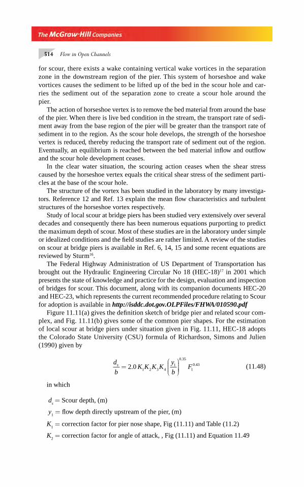
514 Flow in Open Channels
for scour, there exists a wake containing vertical wake vortices in the separation zone in the downstream region of the pier. This system of horseshoe and wake vortices causes the sediment to be lifted up of the bed in the scour hole and car-ries the sediment out of the separation zone to create a scour hole around the pier.
The action of horseshoe vertex is to remove the bed material from around the base of the pier. When there is live bed condition in the stream, the transport rate of sedi-ment away from the base region of the pier will be greater than the transport rate of sediment in to the region. As the scour hole develops, the strength of the horseshoe vertex is reduced, thereby reducing the transport rate of sediment out of the region. Eventually, an equilibrium is reached between the bed material infl ow and outfl ow and the scour hole development ceases.
In the clear water situation, the scouring action ceases when the shear stress caused by the horseshoe vertex equals the critical shear stress of the sediment parti-cles at the base of the scour hole.
The structure of the vortex has been studied in the laboratory by many investiga-tors. Reference 12 and Ref. 13 explain the mean fl ow characteristics and turbulent structures of the horseshoe vortex respectively.
Study of local scour at bridge piers has been studied very extensively over several decades and consequently there has been numerous equations purporting to predict the maximum depth of scour. Most of these studies are in the laboratory under simple or idealized conditions and the fi eld studies are rather limited. A review of the studies on scour at bridge piers is available in Ref. 6, 14, 15 and some recent equations are reviewed by Sturm16.
The Federal Highway Administration of US Department of Transportation has brought out the Hydraulic Engineering Circular No 18 (HEC-18)17 in 2001 which presents the state of knowledge and practice for the design, evaluation and inspection of bridges for scour. This document, along with its companion documents HEC-20 and HEC-23, which represents the current recommended procedure relating to Scour for adoption is available in http://isddc.dot.gov.OLPFiles/FHWA/010590.pdf
Figure 11.11(a) gives the defi nition sketch of bridge pier and related scour com-plex, and Fig. 11.11(b) gives some of the common pier shapes. For the estimation of local scour at bridge piers under situation given in Fig. 11.11, HEC-18 adopts the Colorado State University (CSU) formula of Richardson, Simons and Julien (1990) given by
d
bK K K K
y
bFs =
⎛
⎝⎜⎜⎜
⎞
⎠⎟⎟⎟⎟2 0 1 2 3 4
1
0 35
10 43.
.
. (11.48)
in which
ds = Scour depth, (m)
y1 = fl ow depth directly upstream of the pier, (m)
K1 = correction factor for pier nose shape, Fig (11.11) and Table (11.2)
K2 = correction factor for angle of attack, , Fig (11.11) and Equation 11.49
Chapter 11.indd 514Chapter 11.indd 514 2/24/2010 3:08:17 PM2/24/2010 3:08:17 PM
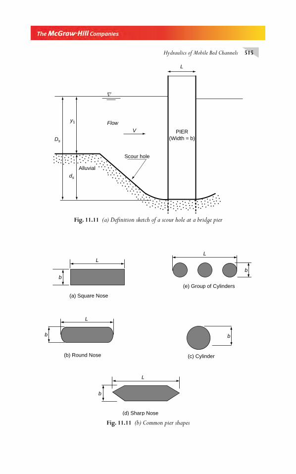
Hydraulics of Mobile Bed Channels 515
Fig. 11.11 (a) Defi nition sketch of a scour hole at a bridge pier
FlowV
L
y1
Ds
ds
Scour hole
PIER(Width = b)
Alluvial
∇
Fig. 11.11 (b) Common pier shapes
b
(c) Cylinder
(e) Group of Cylinders
(a) Square Nose
(d) Sharp Nose
(b) Round Nose
b
b
L
L
L
b
L
b
Chapter 11.indd 515Chapter 11.indd 515 2/24/2010 3:08:18 PM2/24/2010 3:08:18 PM
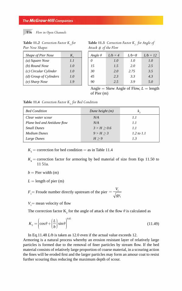
516 Flow in Open Channels
Table 11.2 Correction Factor K1 for
Pier Nose Shapes
Table 11.3 Correction Factor K2 for Angle of
Attack θ of the Flow
Shape of Pier Nose K1
Angle θ L/b = 4 L/b=8 L/b = 12
(a) Square Nose 1.1 0 1.0 1.0 1.0
(b) Round Nose 1.0 15 1.5 2.0 2.5
(c) Circular Cylinder 1.0 30 2.0 2.75 3.5
(d) Group of Cylinders 1.0 45 2.3 3.3 4.3
(e) Sharp Nose 1.9 90 2.5 3.9 5.0
Angle = Skew Angle of Flow, L = length of Pier (m)
Table 11.4 Correction Factor K3 for Bed Condition
Bed Condition Dune height (m) k3
Clear water scour N/A 1.1
Plane bed and Antidune fl ow N/A 1.1
Small Dunes 3 > H ≥ 0.6 1.1
Medium Dunes 9 > H ≥ 3 1.2 to 1.1
Large Dunes H ≥ 9 1.3
K3
= correction for bed condition = as in Table 11.4
K4
= correction factor for armoring by bed material of size from Eqs 11.50 to 11 51a.
b = Pier width (m)
L = length of pier (m)
F1= Froude number directly upstream of the pier =
V
gy1
1
V1= mean velocity of fl ow
The correction factor K2 for the angle of attack of the fl ow θ is calculated as
KL
b2
0 65
= +⎛⎝⎜⎜⎜
⎞⎠⎟⎟⎟⎟
⎛
⎝⎜⎜⎜⎜
⎞
⎠⎟⎟⎟⎟cos sin
.
θ θ (11.49)
In Eq.11.48 L/b is taken as 12.0 even if the actual value exceeds 12.Armoring is a natural process whereby an erosion resistant layer of relatively large particles is formed due to the removal of fi ner particles by stream fl ow. If the bed material consists of relatively large proportion of coarse material, in a scouring action the fi nes will be eroded fi rst and the larger particles may form an amour coat to resist further scouring thus reducing the maximum depth of scour.
Chapter 11.indd 516Chapter 11.indd 516 2/24/2010 3:08:18 PM2/24/2010 3:08:18 PM
Hydraulics of Mobile Bed Channels 517
The correction factor K4 reduces the scour for materials having D
50 ≥ 2.0 mm and
D96
≥ 20 mm. The correction K4 is given as follows:
• K4 = 1.0 for D
50 < 2.0 mm and D
95 < 20.0 mm
• For D50
≥ 2.0 mm and D96
≥ 20 mm, the following relationships are used to calculate K
4:
K4 = 0.4(V
R)0.15 (11.50)
where VV V
V VRicD
cD icD
=−
−>1 50
50 50
0 (11.50a)
VicDx
= approach velocity in m/s required to initiate scour at the pier for the grain size D
x (m).
VD
bVicDx
xcDx=
⎛
⎝⎜⎜⎜
⎞
⎠⎟⎟⎟⎟0 645
0 053
..
(11.51)
VcDx
= critical velocity in m/s for incipient motion for the grain size Dx(m)
V y DcDx x= 6 19 11 6 1 3. / / (11.51a)
In the above y1 = depth of fl ow just upstream of the pier, excluding local scour, (m).
V1= velocity of the approach fl ow just upstream of the pier (m/s)
Dx= grain size for which x percent of the bed material is fi ner (m)
The minimum value of K4 is 0.4.
A study of the above equations reveal the following signifi cant points relating to parameters affecting the scour depth:
(i) The greater the approach velocity greater will be the scour depth. (ii) Similarly, scour depth is directly related to the positive power of the depth
of fl ow. (iii) The scour depth increases with an increase in the width of the pier. (iv) If the approach fl ow is at an angle to the pier the projected length of the pier
will come in to play and the scour increases. (v) Shape of the pier plays an important role on the scour depth. (vi) Size and gradation of the bed material do not have an important role on the
scour depth; the time taken to achieve maximum scour depth depends on the grain size.
(vii) Lodging of debris around a pier can increase the width of pier, change its shape and its projected length with consequent increase in the maximum depth of scour
Chapter 11.indd 517Chapter 11.indd 517 2/24/2010 3:08:18 PM2/24/2010 3:08:18 PM
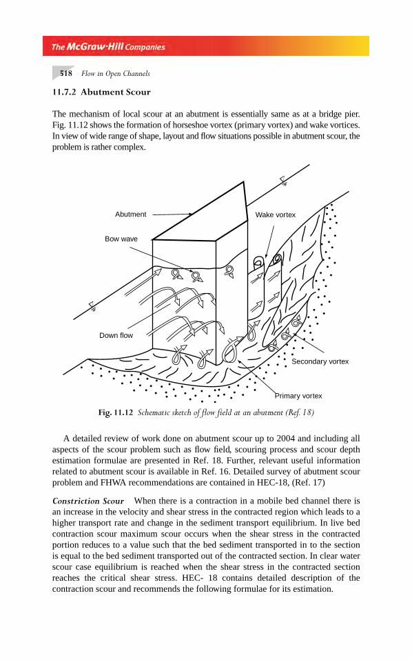
518 Flow in Open Channels
11.7.2 Abutment Scour
The mechanism of local scour at an abutment is essentially same as at a bridge pier. Fig. 11.12 shows the formation of horseshoe vortex (primary vortex) and wake vortices. In view of wide range of shape, layout and fl ow situations possible in abutment scour, the problem is rather complex.
Fig. 11.12 Schematic sketch of fl ow fi eld at an abutment (Ref. 18)
Down flow
Bow wave
Abutment Wake vortex
Secondary vortex
Primary vortex
∇
∇
A detailed review of work done on abutment scour up to 2004 and including all aspects of the scour problem such as fl ow fi eld, scouring process and scour depth estimation formulae are presented in Ref. 18. Further, relevant useful information related to abutment scour is available in Ref. 16. Detailed survey of abutment scour problem and FHWA recommendations are contained in HEC-18, (Ref. 17)
Constriction Scour When there is a contraction in a mobile bed channel there is an increase in the velocity and shear stress in the contracted region which leads to a higher transport rate and change in the sediment transport equilibrium. In live bed contraction scour maximum scour occurs when the shear stress in the contracted portion reduces to a value such that the bed sediment transported in to the section is equal to the bed sediment transported out of the contracted section. In clear water scour case equilibrium is reached when the shear stress in the contracted section reaches the critical shear stress. HEC- 18 contains detailed description of the contraction scour and recommends the following formulae for its estimation.
Chapter 11.indd 518Chapter 11.indd 518 2/24/2010 3:08:18 PM2/24/2010 3:08:18 PM
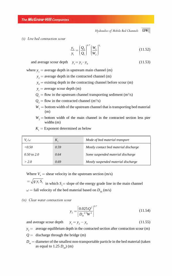
Hydraulics of Mobile Bed Channels 519
(i) Live bed contraction scour
y
y
Q
Q
W
W
k
2
1
2
1
6 7
1
2
1
=⎛
⎝⎜⎜⎜⎜
⎞
⎠⎟⎟⎟⎟
⎛
⎝⎜⎜⎜⎜
⎞
⎠⎟⎟⎟⎟
/
(11.52)
and average scour depth ys = y
2−y
0 (11.53)
where y1 = average depth in upstream main channel (m)
y2 = average depth in the contracted channel (m)
y0 = existing depth in the contracting channel before scour (m)
ys = average scour depth (m)
Q1 = fl ow in the upstream channel transporting sediment (m3/s)
Q2 = fl ow in the contracted channel (m3/s)
W1 = bottom width of the upstream channel that is transporting bed material
(m)
W2 = bottom width of the main channel in the contracted section less pier
widths (m)
K1 = Exponent determined as below
V*/ω K
1Mode of bed material transport
<0.50 0.59 Mostly contact bed material discharge
0.50 to 2.0 0.64 Some suspended material discharge
> 2.0 0.69 Mostly suspended material discharge
Where V* = shear velocity in the upstream section (m/s)
= g y S1 1 in which S1= slope of the energy grade line in the main channel
ω = fall velocity of the bed material based on D50
(m/s)
(ii) Clear water contraction scour
yQ
D Wm
2
2
2 3 2
3 70 025
=⎡
⎣⎢⎢
⎤
⎦⎥⎥
./
/
(11.54)
and average scour depth ys = y
2 − y
0 (11.55)
y2 = average equilibrium depth in the contracted section after contraction scour (m)
Q = discharge through the bridge (m)
Dm = diameter of the smallest non-transportable particle in the bed material (taken
as equal to 1.25 D50
) (m)
Chapter 11.indd 519Chapter 11.indd 519 2/24/2010 3:08:19 PM2/24/2010 3:08:19 PM
520 Flow in Open Channels
y0 = average existing depth in the contracted section (m)
ys = average scour depth (m)
Degradation Scour Long-term degradation of the stream may be the result of some modifi cation of the stream in the upstream regions or in the watershed. The stream may be in equilibrium, or aggrading or degrading at the bridge site. Details of aggradation and degradation phenomenon may be obtained in any treatise on Sediment Transport and is beyond the scope of this book. Details of estimation of degradation of stream at a bridge site are given in HEC-18. Procedures for estimating long-term aggradation and degradation at a bridge site are available in HEC- 20 (Ref. 19).
Total Scour The total scour at a bridge site is the sum of degradation scour, local contraction scour and abutment or pier scour. HEC-18 adopts this procedure to get a conservative estimate of scour.
Example 11.9 A bridge on an alluvial stream has the following features at the design state:
Upstream depth of fl ow = 3.5 m
Discharge intensity = 10.5 m3/s/m
Bed condition = plane bed. Bed material: median size = 1.0 mm
Piers: Round nosed, 12.0 m long and 1.5 m wide.
Estimate the maximum depth of scour at the bridge piers when the angle of attack of fl ow with respect to the pier front end is (a) 20º and (b) zero
Solution By Eq. 11.48
d
bK K K K
y
bFs = 2 0 1 2 3 4
1 0 3510 43. ( ) . .
b = 1.5 m, q = 10.5 m3/s/m and yl = 3.5 m
V1 = 10.5/3.5 = 3.0 m/s
FV
gy1
1
1
3 0
9 81 3 50 512= =
×=
.
. .. m
y1/b = 3.5/1.5 =2.333, L /b = 12.0/1.5= 8.0
K1 = correction factor for pier nose shape from Table (11.2) = 1.0
Chapter 11.indd 520Chapter 11.indd 520 2/24/2010 3:08:19 PM2/24/2010 3:08:19 PM
Hydraulics of Mobile Bed Channels 521
(a) θ = 20°
K2 = correction factor for angle of attack from Eq. 11.49
= (Cos20° + (8.0) Sin 20º )0.65 = 2.33
K3= correction for bed condition from Table 11.4 for plane bed = 1.1
K4 = correction factor for armoring by bed material for D
50 < 2.00 mm = 1.0
d
bs = × × × × × =2 0 1 0 2 33 1 1 1 0 2 333 0 512 5 1720 35 0 65. . . . . ( . ) ( . ) .. . m
ds = 5.172 ×1.5 = 7.76 m below average bed level.
(b) For θ = 0°, K2 = 1.0
d
bs = × × × × × =2 0 1 0 1 0 1 1 1 0 2 333 0 512 2 220 35 0 65. . . . . ( . ) ( . ) .. .
ds = 2.22 × 1.5 = 3.33 m below average bed level.
The Indian Practice The current practice followed in India is based on the Lacey equation. Two Codal provisions are available. Indian Railways Standards (1985) and IRC-5 (1998) and IRC-78 (2000) stipulates that in channels with alluvial beds the design scour depth be two times Lacey depth.The following four Lacey equations are used: The hydraulic radius of Lacey Eq. 11.43 is considered as depth and as such Eq. 11.43 is written as
DQ
fLQ
s
=⎛
⎝⎜⎜⎜⎜
⎞
⎠⎟⎟⎟⎟
0 470
1 3
.
/
(11.56)
P Q= 4 75. (11.42)
f ds mm=1 76. (11.45)
Here, DLQ
= normal scour depth (in meters) below the design fl ood level and is called as Lacey regime depth.
Q = design fl ood discharge (m3/s)
fs = lacey silt factor with d
mm = median diameter of bed particles in mm.
When Lacey ‘s waterway as given by Eq. 11.42 is not available and restricted water-way is used IRC recommends that that instead of Eq. 11.56 the following equation be used to determine the Lacey depth of scour:
Dq
fLq
s
=⎛
⎝⎜⎜⎜⎜
⎞
⎠⎟⎟⎟⎟
1 342 1 3
.
/
(11.57)
Chapter 11.indd 521Chapter 11.indd 521 2/24/2010 3:08:19 PM2/24/2010 3:08:19 PM
522 Flow in Open Channels
where q = intensity of discharge under the bridge = Q/We
where We = effective waterway.
Based on the analysis of fi eld data by Inglis, a multiplying factor of 2.0 is used to obtain design maximum depth of scour below HFL as
Ds = 2.0 D
LQ or D
s = 2.0 D
L q as is appropriate. (11.58)
This method, of estimating design scour depth as above, is sometimes known as Lacey–Inglis method. It is to be noted that in this method there is no separate provi-sion for calculation of degradation scour or contraction scour.
Example 11.10 Estimate the maximum depth of scour for design for the follow-ing data pertaining to a bridge in the Gangetic plain; (Use Lacey – Inglis equations)
Design deischarge = 15,000 m3/s
Effective Water way = 550.0 m
Median size of bed material = dmm
= 0.10 mm
Solution By Eq. 11.42, P Q= = =4 75 4 75 15000 581 8. . . m
Since this is greater than We = 550 m, use Eq. (11.53)
By Eq. 11.44 f ds mm= = =1 76 1 76 0 10 0 556. . . .
q = 15000/550 = 27.27 m3/s/m
By Eq. 11.57 DLq =( )⎛
⎝
⎜⎜⎜⎜⎜
⎞
⎠
⎟⎟⎟⎟⎟⎟=1 34
27 27
0 55614 76
2 1 3
..
..
/
m below HFL
Design scour depth Ds = 2.0 D
Lq = 2 × 14.76 = 29.52 m below HFL
REFERENCES
1. Blench, T, Mobile Bed Fluviology, Univ. of Alberta Press, Edmonton, 1969. 2. Chang, H H, Fluvial Processes in River Engineering, John Wiley and Sons, USA, 1988. 3. Davis, C V, and Sorensen. K E, (Ed), Handbook of Applied Hydraulics, McGraw-Hill
Book Co., New York, 1965. 4. Garde, R J, and Ranga Raju, K G, Mechanics of Sediment Transportation and Alluvial
Stream Problems, Wiley Eastern Ltd., New Delhi, 2nd Ed., 1985. 5. Graf, W H, Hydraulics of Sediment Transport, McGraw-Hill Book Co., New York, 1971. 6. Shen, H W, (Ed), River Mechanics, Vol, I, II, Shen, H W, Fort Collins, Colo., USA, 1971. 7. Simons, D B, and Senturk F, Sediment Transport Technology, Water Resources Publica-
tion, Fort Collins, Colo., USA, 1977.
Chapter 11.indd 522Chapter 11.indd 522 2/24/2010 3:08:19 PM2/24/2010 3:08:19 PM
Hydraulics of Mobile Bed Channels 523
8. Swamee, P K, and Mittal, M K, An Explicit Equation for Critical Shear Stress in Alluvial Streams, J. of Irrigation and Power, CBIP., India, Vol. 33, No. 2, pp. 237–239, April 1976.
9. Vanoni, V A, (Ed.), Sedimentation Engineering, Manual No. 54, A.10. Subramanya, K, Engineering Hydrology, McGraw-Hill Education (India), 3rd Ed, 2008.11. Yang Xiaquing, ‘Manual on Sediment Management and Measurement’, WMO – Opera-
tion Hydrology Report No. 47, Secretariat of WMO, Geneva, Switzerland, 2003.12. Muzzamil, M, and Gangadhariah, T, ‘The Mean Characteristics of a Horseshoe Vortex at
a Cylindrical Pier’, Jour. of Hyd. Research, IAHR, Vol. 41, No.3, 2003, pp. 285–297.13. Dey, S, and Raikar, R V, ‘Characteristics of Horseshoe Vortex in Developing Scour holes
at Piers’, Journal of Hydraulic Engineering, ASCE, Vol. 133, No. 4, 2007, pp. 399–413.14. Breusers, H N C, Nicollet, G, and Shen, H W, ‘Local Scour around Cylindrical Piers’
J. Hyd Res., IAHR, 15(3), 1977, pp. 211–252.15. Dargahi, B, ‘Local Scour at Bridge Piers–A Review of Theory and Practice’, Bull No.
Trita, VBI-114, Hydr. Lab., Royal Institute of Technology, Stockholm, Sweden, 1982.
16. Strum, T W, Open Channel Hydraulics, McGraw-Hill Higher Education, Singapore, 2001.
17. Richardson, E V, and Davis, S R, Evaluating Scour at Bridges, Fourth Ed., Report No. HEC –18, Federal Highway Administration, US Department of Transportation, Washington DC, May 2001.
18. Barbhuiya, A K, and Dey, S, ‘Local Scour at Abutments: A Review’, Sadhana, India, Vol. 29, Part 5, Oct. 2004, pp. 449–476.
19. HEC-20, ‘Stream Stability at Highway Structures’, 3rd ed. Report No. HEC–20, Federal Highway Administration, US Department of Transportation, Washington DC, 2001.
PROBLEMS
Problem Distribution
Topic Problems
Initiation of motion and Critical shear stress 11.1 to 11.5
Bed forms and Resistance 11.6 to 11.10
Bed load 11.11, 11.12, 11.16 and 11.24
Suspended load 11.13 to 11.15
Total load 11.16, 11.18
Non- Erodible channel 11.17, 11.18
Lacey Regime channel 11.19 to 11.24
Bridge Pier Scour 11.25, 11.26
11.1 Estimate the critical shear stress for the following sizes of sediment particles in the bed of a channel:(a) 0.1mm (b) 1.0 mm (c) 10 mm
11.2 A wide stream has a sediment bed of median size 0.35 mm. The slope of the channel is 1.5 × 10⁻⁴.(a) If the depth of fl ow in the channel is 0.25 m, examine whether the bed particles will
be in motion or not.(b) What would be the status of the bed when the depth of fl ow is 0.10 m?
Chapter 11.indd 523Chapter 11.indd 523 2/24/2010 3:08:19 PM2/24/2010 3:08:19 PM
524 Flow in Open Channels
11.3 The median size of bed sediment in a wide gravel bed river is 50 mm. The river bed experiences threshold conditions when the energy slope of fl ow is 0.005. Estimate the depth of fl ow at this stage.
11.4 A wide alluvial channel has a fl ow which causes incipient motion of the bed particles. The temperature of the water is 25° C (v = 0.897 × 10⁻⁶ m2 s). It is expected that the temperature would drop to 5°C (v = 1.519 × 10⁻⁶ m2/s) and all other fl ow parameters would remain unaltered. Examine, with the help of Shields diagram, the status of the channel bed when the initial shear Reynolds number (u
*d/v) is (a) 5, (b) 100, and
(c) 500. [The change in the densities due to temperature change may be neglected]. 11.5 A wide rectangular channel carries clear water at a depth of 1.2 m. The channel bed is
composed of coarse gravel of d50
= 40 mm. Determine the slope of the channel at which incipient conditions exists. What is the discharge per unit width at this slope?
11.6 A wide channel in an alluvium of grain size d50
= 0.30.mm has plane bed with no motion. The depth of fl ow is 0.25 m and the bed slope is measured as 0.0002. Estimate the mean velocity and discharge per metre width in this channel.
11.7 Two wide alluvial channels A and B have the following features:
Channel A Channel A
Depth of fl ow 1.20 m 1.20 m
Slope 1.65 × 10⁻³ 1.65 × 10⁻³
Bed material size 1.3 mm 12 mm
Estimate the nature of the bed form in each of these two channels. 11.8 A wide alluvial channel has a bed slope of 6 × 10⁻⁴ and bed material of median size
0.5 mm. Estimate the maximum depth of fl ow that can be adopted in this channel while maintaining the ripple and dune type of bed form.
11.9 A mobile bed channel with median grain size of 0.8 mm has a longitudinal slope of 2 × 10⁻⁴ and carries a discharge of 10 m3/s at a depth of 1.5 m. The channel is trapezoi-dal in section and has a bed width of 10 m and side slopes of 1.5 horizontal : 1 vertical. Estimate (a) the Manning’s roughness coeffi cient n, (b) the shear stress at the bed due to (i) sediment grains, and (ii) bed forms.
11.10 An irrigation channel is to be excavated on a slope of 0.0001 through a terrain consist-ing of coarse sand having d
50 = 0.8 mm and relative density 2.65. The discharge is to be
1.5 m3/s. If no sediment transport is to be allowed, determine a suitable width for the channel by assuming it to be wide rectangular and the banks are protected.
11.11 Calculate the bed load per unit width in a wide stream having the following data:d
50 =
0.5 mm
S0
= 0.0004
n = Manning’s coeffi cient for the channel = 0.025
q = water discharge per unit width = 3.0 m3/s/m.
11.12 Estimate the bed load for the following canal in coarse alluvium:d
50 =
12 mm
y0 =
depth of fl ow = 5.87 m
B = width = 46.0 m
S0 =
longitudinal slope = 6.5 × 10⁻⁴
n = Manning’s coeffi cient for the channel = 0.025
The channel may be assumed to be a wide rectangular channel, with sides protected.
Chapter 11.indd 524Chapter 11.indd 524 2/24/2010 3:08:20 PM2/24/2010 3:08:20 PM
Hydraulics of Mobile Bed Channels 525
11.13 When a sediment of fall velocity ω is suspended in water where the mass diffusion coeffi cient εs can be assumed constant, show that the concentration C at a height y above the bed is given by
C
C
y a
a s
= −−⎡
⎣⎢⎢
⎤
⎦⎥⎥exp
( )ωε
where Ca = reference concentration at a level a above the bed.
11.14 In a wide channel with a depth of fl ow of 3.0 m suspended load samples at depths of 2.0 m and 2.5 m below the water surface indicated concentrations of 1200 ppm and 1800 ppm respectively. Estimate the concentration at a depth of 0.5 m below the water surface.
11.15 A wide channel has a slope of 1 in 4500 and a depth of fl ow of 2.0 m. Suspended load sampling at a height of 0.4 m above the bed revealed a concentration of 800 ppm by weight, consisting of particles having a fall velocity of 0.05 m/s. Estimate the concen-tration at levels of (a) 0.8 m and (b) 1.2 m above the bed.
11.16 A wide alluvial stream has a bed material of 0.25-mm median size and a longitudi-nal slope of 2.0 × 10⁻⁴. Estimate the bed load and total load per unit width of this stream when the depth of fl ow is 2.0 m and the water discharge is 1.2 m3/s per metre width.
11.17 A channel which will carry a discharge of 60 m3/s is to be cut on a slope of 0.0005 through coarse, well-rounded gravel having a median size of 25 mm and relative den-sity 2.65. Determine the suitable base width and depth of fl ow for a non-erodible chan-nel of trapezoidal cross section with a side slope of 2H: 1V for the canal.
11.18 A trapezoidal channel of side slopes 2.5 H: 1V is cut in angular gravel of 2.0-mm median size. The base width of the channel is 10.0 m. If this channel is to carry clear water determine the maximum possible longitudinal slope to have a stable channel at a full supply depth of 1.5 m. What is the full supply discharge of this channel at this maxi-mum slope?
11.19 Using the primary Lacey equations, show that the velocity of fl ow in a regime channel is given by
V = 10.8 R2/3 S01 2/
11.20 Fill in the following table relating the elements of a Lacey regime channel:
Sl. No. Q m3/s
B m
y0
mS
0V
m/sManning’s Coeffi cient
n
Silt factor
fs
(i) 30.0 – – – – – 0.80
(ii) – – – 3.27 × 10⁻⁴ – – 1.24
(iii) – 30.0 1.50 – – – –
(iv) 15.0 – – 2.0 × 10⁻⁴ – – –
11.21 Design channels by the Lacey theory for the following two cases:(a) Discharge = 50 m3/s, Median size of alluvium = 0.9 mm(b) Discharge = 10m3/s, Median size of alluvium = 0.50 mm
Chapter 11.indd 525Chapter 11.indd 525 2/24/2010 3:08:20 PM2/24/2010 3:08:20 PM
526 Flow in Open Channels
11.22 A regime channel is designed by Lacey theory to carry 20 m3/s of full supply discharge in an alluvium of median size 1.2 mm. What would be the Manning’s roughness coeffi -cient n of this channel?
11.23 Show that the Lacey regime equations would yield the following relationship for the Manning’s roughness coeffi cient n applicable to a Lacey regime channel:
nd
Qmm=
⎧⎨⎪⎪
⎩⎪⎪
⎫⎬⎪⎪
⎭⎪⎪
0 028 5 36
1 36
. /
/
where dmm
= sediment size in mm.11.24 Design a regime channel by Lacey’s equations to convey 15 m3/s of water in an alluvium
of median size 1.2 mm. What bed load and total load can be expected in this channel?11.25 The following data pertain to a bridge on an alluvial stream at the design state:
Upstream depth of fl ow = 4.0 m, Discharge intensity = 12.0 m3/s/mBed condition = Small dunes. Bed material: median size = 1.2 mmPiers: Sharp nosed, 18.0 m long and 1.5 m wide.Estimate the maximum depth of scour at the bridge piers when the angle of attack of fl ow with respect to the pier front end is 5°.
11.26 For the design of a bridge the following data have been collected:Design fl ood discharge = 600 m3/s; Bed material = 0.08 mm.Estimate the design scour for use in the design of the bridge piers.[Use Lacey–Inglis method].
OBJECTIVE QUESTIONS
11.1 For a gravel of median size 11 mm, the critical shear stress is about(a) 3.2 Pa (b) 10 Pa(c) 0.62 Pa (d) 22 Pa
11.2 For water fl ow in coarse alluvium, the minimum size of the particle at which the critical shear stress is independent of the viscosity of water is about(a) 6 mm (b) 6 cm(c) 0.06 mm (d) 3 mm
11.3 Shields diagram is a plot of non-dimensional shear stress τ*c against
(a) Reynolds number of fl ow(b) relative depth of grain size, d/R(c) Shear Reynolds number, u
*c d/v
(d) u* R/v, where R = hydraulic radius.
11.4 In Shields diagram the minimum shear Reynolds number Ru d
vcc
**=
⎡
⎣⎢⎢
⎤
⎦⎥⎥
beyond which
the critical shear stress is independent of R*c
is about(a) 10 (b) 2000(c) 2 (d) 400
11.5 The size dc of a sediment particle that will just remain at rest in the bed of a wide rect-
angular alluvial channel of depth D and slope S0 is given by d
c equal to
(a) 11 D S0 (b) 10.8 D2/3 S
01/3
(c) 11 0RS (d) 1
112 3
01 2R S/ /
Chapter 11.indd 526Chapter 11.indd 526 2/24/2010 3:08:20 PM2/24/2010 3:08:20 PM
Hydraulics of Mobile Bed Channels 527
11.6 If in an alluvial channel the Manning’s n corresponding to plane bed without sediment is 0.016, the same channel with dunes on the bed will have a Manning’s coeffi cient n
d
such that(a) n
d < 0.016 (b) n
d = 0.016
(c) nd > 0.016 (d) n
d = 0.032
11.7 Indicate the incorrect statement in an alluvial channel(a) if the bed form is dunes, then the water surface will be out of phase with the bed
forms(b) if the bed form is antidunes, then the water surface, will be in phase with the bed
form(c) ripples are not formed in sediment of size greater than 0.6 mm(d) if the bed form is dunes, then the Froude number of the fl ow is greater than
unity.
11.8 In an ideal laboratory channel with alluvial bed the channel fl ow is to be observed at various progressively higher shear values. Starting from the plane bed form the follow-ing sequence of bed forms can be expected:(a) Ripples and dunes–Transition–Antidunes(b) Transition–Dunes–Antidunes(c) Ripples and Dunes–Antidunes–Transition(d) Antidunes–Ripples and dunes–Transition.
11.9 The hydraulic radius associated with the grain roughness R′ is related to total hydraulic radius R as
(a) ′ =⎡
⎣⎢⎢
⎤
⎦⎥⎥
Rn
nRs
3 2/
(b) ′ =⎡
⎣⎢⎢
⎤
⎦⎥⎥
Rn
nRs 3 2/
(c) ′ =⎡
⎣⎢⎢
⎤
⎦⎥⎥
Rn
nRs (d) ′ =
⎡
⎣⎢⎢
⎤
⎦⎥⎥
Rn
nRs
2 3/
where ns and n are Manning’s coeffi cient corresponding to grain roughness and total
channel roughness respectively.
11.10 Bed load is a term used to describe(a) the combination of contact load and wash load(b) the combination of contact load and saltation load(c) the combination of contact load and suspended load near the bed(d) the bed material load.
11.11 The term wash load refers to(a) the saltating part of bed material load(b) suspended load during a fl ood(c) part of suspended load comprising of particles not available in the bed material(d) bed load after the fi nes have been washed out.
11.12 An alluvial channel has a bed material of median size 0.9 mm. The Manning’s coeffi -cient n of this bed when it is plane and without motion of particles is(a) 0.0009 (b) 0.0123(c) 0.0273 (d) 0.0147
Chapter 11.indd 527Chapter 11.indd 527 2/24/2010 3:08:20 PM2/24/2010 3:08:20 PM
528 Flow in Open Channels
11.13 An unlined alluvial channel has trapezoidal section with side slopes of 2.5 horizontal: 1 vertical. If the angle of repose of the bed material is 35°, the ratio of critical shear stress of the sediment particle on the side to that on the bed is(a) 0.61 (b) 0.93(c) 0.65 (d) 0.76
11.14 In a trapezoidal channel having a side slope = m horiz : 1 vertical, depth of fl ow = D, longitudinal slope = S
0, the maximum shear stress on the sides is about
(a) γ DS0 (b) 0.99 γ DS
0
(c) 0.76 γ DS0 (d)
10m
DS⎛⎝⎜⎜⎜
⎞⎠⎟⎟⎟⎟γ
11.15 In a regime alluvial channel designed by Lacey’s theory,(a) the bed load is zero(b) the suspended load is zero(c) the bed will have dune type of bed form(d) the bed form will be of plane bed with sediment motion.
11.16 The Lacey’s equations for a regime channel consists of a set of x independent equations relating to the fl ow, where x equal to(a) 1 (b) 3(c) 8 (d) 2
11.17 An alluvium with a median size of 0.32 mm has Lacey’s silt factor f of value(a) 1.76 (b) 1.00(c) 0.57 (d) 0.80
11.18 A regime canal has a discharge of 100 m3/s. It will have a perimeter of(a) 4.8 m (b) 10.0 m(c) 47.5 m (d) 22.0 m
11.19 A regime channel has a width of 22.2 m and depth of fl ow of 1.70 m. The discharge in the channel is about(a) 68 m3/s (b) 3.0 m3/s(c) 30.0 m3/s (d) 7.0 m3/s
11.20 When an alluvial channel attains its regime it will have side slopes(a) of value equal to the angle repose of the alluvium(b) of value equal to the angle of repose of the alluvium under water(c) of value 0.5 vertical : 1 horizontal(d) of value 0.5 horizontal : 1 vertical
11.21 The Lacey regime formulae are in general applicable to alluvial channels with sediment concentration in ppm by weight of less than about(a) 10,000 (b) 1000(c) 500 (d) 5000
11.22 The mean velocity in a Lacey regime channel is proportional to(a) R1/3 (b) R1/2
(c) S01/2 (d) S
01/3
11.23 A regime channel of longitudinal slope S0 will have Manning’s roughness coeffi cient n
given by n is equal to
(a) S0
1 6
10 8
/
.
⎡
⎣⎢⎢
⎤
⎦⎥⎥ (b) [S
01/6]
(c) R1 6
10 8
/
.
⎡
⎣⎢⎢
⎤
⎦⎥⎥ (d)
11 6R /
⎡
⎣⎢⎢
⎤
⎦⎥⎥
Chapter 11.indd 528Chapter 11.indd 528 2/24/2010 3:08:20 PM2/24/2010 3:08:20 PM
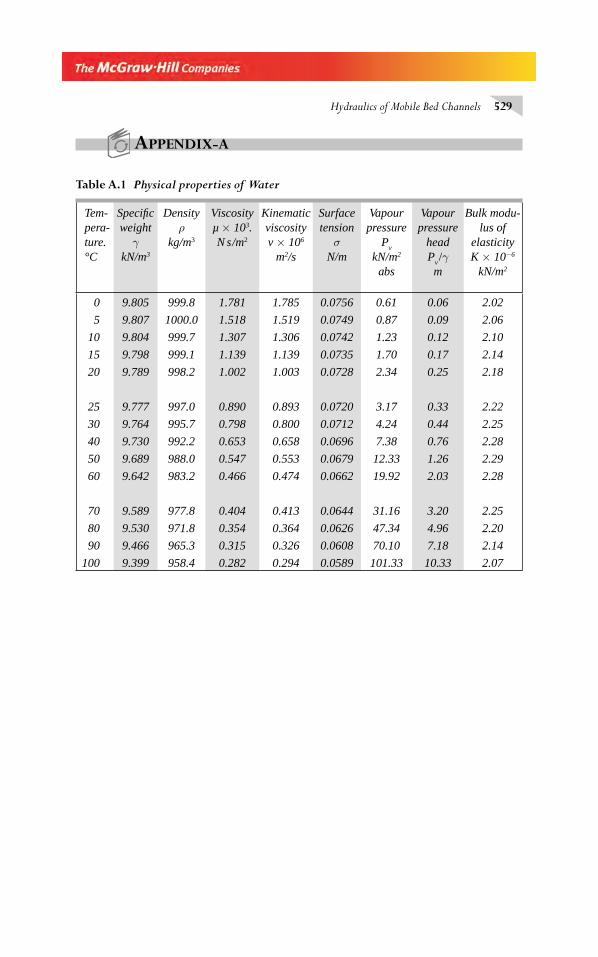
Hydraulics of Mobile Bed Channels 529
APPENDIX-A
Tem-pera-ture. °C
Specifi c weight
γkN/m3
Densityρ
kg/m3
Viscosity µ × 103. N
s
/m2
Kinematic viscosity v × 106
m2/s
Surface tension
σ N/m
Vapour pressure
Pv
kN/m2
abs
Vapour pressure
head P
v /γ
m
Bulk modu-lus of
elasticity K × 10−6
kN/m2
0 9.805 999.8 1.781 1.785 0.0756 0.61 0.06 2.02
5 9.807 1000.0 1.518 1.519 0.0749 0.87 0.09 2.06
10 9.804 999.7 1.307 1.306 0.0742 1.23 0.12 2.10
15 9.798 999.1 1.139 1.139 0.0735 1.70 0.17 2.14
20 9.789 998.2 1.002 1.003 0.0728 2.34 0.25 2.18
25 9.777 997.0 0.890 0.893 0.0720 3.17 0.33 2.22
30 9.764 995.7 0.798 0.800 0.0712 4.24 0.44 2.25
40 9.730 992.2 0.653 0.658 0.0696 7.38 0.76 2.28
50 9.689 988.0 0.547 0.553 0.0679 12.33 1.26 2.29
60 9.642 983.2 0.466 0.474 0.0662 19.92 2.03 2.28
70 9.589 977.8 0.404 0.413 0.0644 31.16 3.20 2.25
80 9.530 971.8 0.354 0.364 0.0626 47.34 4.96 2.20
90 9.466 965.3 0.315 0.326 0.0608 70.10 7.18 2.14
100 9.399 958.4 0.282 0.294 0.0589 101.33 10.33 2.07
Table A.1 Physical properties of Water
Chapter 11.indd 529Chapter 11.indd 529 2/24/2010 3:08:21 PM2/24/2010 3:08:21 PM
530 Flow in Open Channels
SOME USEFUL WEBSITES RELATED TO OPEN CHANNEL HYDRAULICS
1. USGS – Surface Water Field Techniques http://www.usgs,gov
2. US Department of Transportation. Federal Highway Administrationhttp://www.fhwa.dot.gov/engineering/hydraulics/index.cfm
3. US Bureau of Reclamation, USA http://www.usbr.gov/pmts/hydraulics_lab/
4. Hydrologic Centre, US Army Corps of Engineers http://www.hec.usace.army.mil/
5. W M Keck Laboratory of Hydraulics and Water Resources Technical Reports administration. http://www.caltechkhr.library:caltech.edu/
6. Dr. Victor Miguel Ponce – Online Open Channel Hydraulics http ://www.victormiguelponce.com
http://onlinechannel.sdsu.edu/
7. Fluid Flow Calculations web site of LMNO Engineering Research and Software, Ltd. http://www.lmnoeng.com
Chapter 11.indd 530Chapter 11.indd 530 2/24/2010 3:08:21 PM2/24/2010 3:08:21 PM
Hydraulics of Mobile Bed Channels 531
ANSWERS TO PROBLEMS
CHAPTER 1
1.2 (a) α = 2.0, β = 1.33
(b) α =−( )1
12
a, β =
−( )1
1 a
1.3 an
n n=
+( )+( )1
3
3
2 β =
+( )+( )
n
n n
1
2
2
1.4 α = 5.71, β = 2.374
1.6 (a) vr
=9 9245.
(b) V=2.0 m/s
(c) α = 1.023, β = 1.008
1.7 (a) h Zk
hep = ++( )
0 1
1
2 (b) h Z
khep = +
+( )0 1
2 1
2
1.8 p/γ = 0.466 y
1.9 p/γ = 1.266 y
1.13 (a) 1.046 m (b) 1.0473 m (c) 1.0431 m
1.14 (a) At x = 1.0m, hep
= 1.173m (b) At x = 2.5m, hep
= 1.101 m
1.15 Q = 3618 m3/s
1.16 q = 0.3889 m3/s/m
1.17 q = 1.03625 m3/s/m
1.18 hm = 8.424 m
1.19 (a) y1 = 3.818 m, (b) y
2 = 0.232 m
(c) y2 = 0.244 m, (d) q = 1.843 m3/s/m
1.20 Δ z = 0.751 m, ΔWx = 0.251 m
1.21 HA = 16.753 m, h
PA = 16.280 m
HB = 16.331 m, h
PB = 15.782 m
1.22 EL = 0.109 m
Chapter 11.indd 531Chapter 11.indd 531 2/24/2010 3:08:21 PM2/24/2010 3:08:21 PM
532 Flow in Open Channels
1.24 Affl ux = 0.056 m
1.25 Fx = 5000 N/m, F
y = 10182 N/m width
1.26 (a) 51.86 kN/m (b) 61.97 kN/m
(c) 62.79 kN/m (d) 33.51 kN/m width
1.28 F = 6.91 kN/m, EL = 0.453 m
1.29 FD = 13.67 kN/m
CHAPTER 2
2.3 Δz = −0.857 m
2.4 (a) 0.736 m. 1.940 m, (b) 0.936 m, 1.943 m (c) 0.730 m, 1.888 m
2.7 E = 1.5906 m, y2= 0.497 m
2.17 Q = 0.031 m3/s. E = 0.60 m
2.18 (a) Subcritical (b) yc = 1.148 m
(c) E = 1.454 m (d) y3 = 1.08m
2.19 (a) Q = 3.322 m3/s, Ec = 0.75 m
(b) B = 2.5 m, Ec = 1.20 m
(c) yc = 0.972 m, E
c = 1.458 m
(d) Q =1.585 m3/s, yc = 0.40 m
2.20 (i) yc = 0.283 m, E
c = 0.978 m
(ii) Q = 0.164 m3/s, Ec = 0.375 m
(iii) Q = 0.354 m3/s, yc = 0.480 m
2.21 (a) yc = 0.546 m, E
c = 0.775 m
(b) Q = 1.206 m3/s, Ec = 0.422 m
(c) B = 3.0 m, Ec = 0.571 m
(d) yc = 0.80 m, Q = 11.068 m3/s
2.22 (a) Q = 0.558 m3/s, Ec = 0.51 m
(b) Q = 0.741 m3/s, Ec = 0.540 m
2.23 (a) yc = 0.947 m, (b) y
c = 1.1644 m
2.24 yc = 1.185 m
2.25 D = 1.50 m
2.26 Q = 1.216 m3/s, Ec = 0.836 m
2.27 Q = 0.737 m3/s
2.29 Q = 11.50 m3/s
Chapter 11.indd 532Chapter 11.indd 532 2/24/2010 3:08:21 PM2/24/2010 3:08:21 PM
Hydraulics of Mobile Bed Channels 533
2.32 (i) 3.106, 3.500, 3.833 and 4.200 (ii) 3.96, 3.84 and 4.35
2.33 y2 = 1.079 m
2.34 (a) y2 = 1.366 m, y
1, = 2.086 m (b) y
2 = 1.651 m, y
1 = 2.00 m
2.35 Δzm = 0.244 m
2.36 B2 = 2.472 m
2.37 (a) y2 = 0.871 m, y
1 = 0.90 m
(b) y2 = 0.657 m, y
1 = 0.911 m
2.38 Q = 3.362 m3/s, y1 = 1.153 m, F
1 = 0.289
y2 = 0.261 m, F
2 = 2.683
2.39 Δz = −0.366 m
2.40 y1 = 2.171 m
2.41 y2 = 0.744 m, Δz
m = 0.133 m
2.42 B2 = 3.299 m
2.43 Q = 4.825 m3/s, Δz = – 0.25 m
2.44 Δz = 0.440 m, Δy = 0.011 m
CHAPTER 3
3.1 (a) τ0 = 1.6187 N/m2 (b) rough (c) C = 60.9
(d) n = 0.014 (e) Qch
= 2.314 m3/s, QMa
= 2.458 m3/s
3.2 Q = 9.035 m3/s
3.3 f = 0.0178, n = 0.0145, C = 66.5
3.6 n = 0.0181
3.7 38.9%
3.8 n = 0.0474
3.9 (a) 4.206 m3/s, (b) 6.373 m3/s, (c) 3.773 m3/s,
3.10 y0 = 0.944 m
3.11 (a) 1.9446 × 10⁻⁴ (b) 3.46 × 10⁻⁴
3.12 (a) 12.176 m3/s (b) y0 = 1.735 m
3.13 Q = 0.974 m3/s
3.14 B = 3.656 m
3.15 n = 0.0188
3.16 D = 2.00 m
3.17 Q = 2.73 m3/s, y0 = 0.093 m
Chapter 11.indd 533Chapter 11.indd 533 2/24/2010 3:08:22 PM2/24/2010 3:08:22 PM
534 Flow in Open Channels
3.18 B = 4.85 m, y0 = 3.638 m
3.19 F0 = 0.197
3.20 S0 = 7.196 × 10⁻⁴
3.21 0.9615
3.22 τ0 = 0.2674 N/m2
3.23 B = 3.465 m, y0 = 1.155 m, S
0 = 1.998 × 10⁻⁴
3.24 K = 160.5 m3/s, S0 = 3.209 m3/s, F
0 = 0.282, τ
0 = 2.50 N/m2
3.25 Q = 4.48 m3/s, S0 = 5.2 × 10⁻³
3.26 (a) 1.179 m, (b) 1.540 m, (c) 1.957 m
3.28 B = 23.00 m, y0 = 3.105 m
3.29 B = 13.09 m
3.30 Q = 271.3 m3/s
3.31 Q = 23.52 m3/s
3.32 y0 = 2.352 m, τ
0 = 11.537 Pa
3.33 Q = 18.61 m3/s
3.37 (a) y = 0.849 B, (b) y = 1.635 B
3.38 (i) d = 0.3382 a, (ii) d = 0.4378 a
3.39 ye = 1.597 m, B
e = 1.120 m
3.40 ye = 4.045 m, Q = 32.12 m3/s
3.42 S0 = 2.609 × 10⁻⁴
3.44 Be = 3.232 m, y
e = 5.338 m
3.46 Be = 3.57 m, y
e = 2.89 m, S
0 = 2.7 × 10⁻⁴
3.47 Lined canal is 14.7% cheaper.
3.48 ye = 1.934 m, B
e = 2.735 m
3.53 N = 3.51
3.54 m yB = 0.5 1.0 2.0
1.0 N = 3.7 4.0 4.4
1.5 N = 3.9 4.3 4.7
3.55 (i) 2.902 m3/s (ii) 6.568 m3/s
3.56 (i) 2.631 m3/s (ii) 6.010 m3/s
3.57 (i) 41.450 m3/s (ii) 47.99 m3/s
3.59 ye1
= 0.250 m, ye2
= 2.30 m
3.61 Sc = 0.004447, Slope is Mild in the range of depths.
Chapter 11.indd 534Chapter 11.indd 534 2/24/2010 3:08:22 PM2/24/2010 3:08:22 PM
Hydraulics of Mobile Bed Channels 535
3.62 S0 = 0.0006939
3.63 F0 = 0.5
3.64 (a) S0 = 1.6036 × 10⁻⁴ (b) S
c = 4.009 × 10⁻³ (c) y
0 = 3.96 m
3.65 (a) Se = 7.1 × 10⁻³ (b) F = 1.07
3.66 SLc
= 4.166 × 10⁻³ 0= 0.336 m3/s, yc = 0.2 m
3.67 S*Lc
= 2.28
3.68 m = 1.5, n = 0.015, B/y0 = 10.0
B = 18.0 m. y0 = 1.821 m, V = 3.618 m/s
CHAPTER 4
4.4 dy
dxS−
⎛⎝⎜⎜⎜
⎞⎠⎟⎟⎟⎟ = − × −
041 437 10.
4.5 S2 curve
4.6 (i) M2 curve (ii) M
1 curve
4.7 M3 curve
4.8 (i) M3 curve, (ii) M
2 curve, (iii) M
1 curve
4.9 S2 curve on steeper channel
4.10 Jump and S1 curve
4.12 (a) Mild – Steep (b) Mild – Steeper Mild
(c) Steep – Mild (d) Mild – Milder Mild
4.13 (a) [H3–J–H
2] or [J–S
1–H
2]
(b) M1–M
3–J–M
2–S
2–J-S
1–H
2 or
M1–M
3–J–M
2–M
2–S
2–H
3–J–H
2
(c) [S2– J–S
1–M
1 ] or [S
2–M
3–J–M
1 ]
(d) S2–J–S
1–S
3–M
3–J
(e) J–S1–M
1–M
3–J–M
2 or
M3–J–M
1–M
3–J–M
2
(f ) A3–J–A
2–H
2–S
2
4.14 (a) [J– S1] on the upstream and S
1 on the downstream
(b) M1 on the upstream and (M
3 – J – M
2 /M
1 ) on the downstream
(c) Horizontal on the upstream and (H3 –J–H
2 ) on the downstream
4.15 (a) M3 on A (b) M
1 on A and (M
3–.J ) on B
4.16 M2 curve on A and S
2 curve on B
4.17 [S2–H
3– J ] or [S
2–J –S
1]
4.18 M1– M
3–J–M
2–S
2
Chapter 11.indd 535Chapter 11.indd 535 2/24/2010 3:08:22 PM2/24/2010 3:08:22 PM
536 Flow in Open Channels
CHAPTER 5
5.5 M1 curve; L = 2.28 km
5.7 (a) 9.16 km (b)130 m
5.8 (a) 2.87 m (b) 2.873 m
5.9 y0 = 1.074 m
5.10 α =1.195, Sf = 9.795×10⁻⁶
5.11 L = 24,500 m
5.13 M1 profi le, L = 454 m
5.14 Q2 = 105 m3/s, Q
R = 55 m3/s
5.15 S2 curve, L = 70 m
5.16 105.604 m, 106.355 m and 107.313 m.
5.17 S1 curve, 69 m
5.18 22.5 m
5.19 M2 curve, 222 m
5.20 2.69 m, 6.16 km
5.21 Inlet is submerged
5.22 x = 89 m
5.23 (a) 122.109 m and 121.800 m (b) 11.3 m3/s
5.24 Q = 31.13 m3/s, L = 222 m
5.25 Q = 178 m3/s
CHAPTER 6
6.1 q = 8.4 m3/s/m; EL = 3.65 m; F
1 = 4.58
6.2 EL/E
1 = 72.7%
V1
y1
q F1
y2
V2
F2
EL E
EL
1
%
(a) 10.33 0.170 1.756 8.00 1.84 0.954 0.225 3.722 66.4
(b) 8.91 0.100 0.891 9.00 1.224 0.728 0.210 2.900 69.9
(c) 8.00 0.250 2.000 5.10 1.683 1.188 0.292 1.750 50.0
(d) 9.54 0.151 1.440 7.84 1.600 0.900 0.227 3.140 65.5
(e) 13.50 0.350 4.725 7.29 3.435 1.375 0.237 6.105 63.3
(f) 13.64 0.068 0.928 16.70 1.574 0.590 0.150 8.00 83.7
6.4 F2 = 0.296
6.6 y1 = 0.198 m, y
2 = 2.277 m
Chapter 11.indd 536Chapter 11.indd 536 2/24/2010 3:08:22 PM2/24/2010 3:08:22 PM
Hydraulics of Mobile Bed Channels 537
6.8 F1 = 4.82
6.9 F1 = 13.65, F
2 = 0.235
6.10 y1 = 0.348 m, y
2 = 3.40 m
6.11 y1 = 0.90 m, y
2 = 6.94 m; E
L/E
1 = 55%
6.12 101.486 m
6.13 95.973 m
6.14 Repelled jump; y1 = 1.674 m, L
j = 26.4, H
3 curve of length = 81.0 m
6.17 yt = 26.21 m, L
j = 120 m, E
L = 40.77 m
6.18 Q = 1.541 m3/s; F1 = 2.494; F
2 = 0.441
6.20 y2 = 1.875 m, E
L = 6.880 m
6.21 y1 = 0.242 m E
L = 4.695 m
6.22 y2 = 0.796 m
6.23 Jump at 80 m from the gate, y1 = 1.02 m, y
2 = 3.99 m,
6.24 x = 62.0 m, .y1 = 0.96 m, y
2 = 3.23 m
6.25 yth = 1.892 m, y
ts = 3.595 m
6.30 Δz = 0.880 m
6.31 (i) No free jump is possible. Submerged jump occurs
(ii) free repelled jump, y1 = 0.467 m, y
t = 3.737 m
6.32 (a) q = 15.31 m3/s/m
(b) Free – repelled jump, y1 = 1.119 m, y
t = 6.0 m
(c) ytm
= 6.53 m.
CHAPTER 7
7.1 0.074 m rise
7.2 P = 1.088 m
7.3 3.512 m3/s
7.5 Qs = 0.0626 m3/s
7.6 2.965 m3/s
7.7 6.38%
7.8 a = 0.592 m, Hd max
= 1.144 m
7.9 a = 0.231 m, Hd max
= 1.386 m
7.10 (i) 0.118 m3/s, (ii) 0.163 m3/s, (iii) 0.396 m
7.11 (i) 38 lit/s, (ii) 9.91 cm
Chapter 11.indd 537Chapter 11.indd 537 2/24/2010 3:08:22 PM2/24/2010 3:08:22 PM
538 Flow in Open Channels
7.12 23.088 m, 23.102m with river bed as datum, 3.8440 m, −1.069m
7.13 34.243 m3/s/m
7.14 0.150 m
7.15 59.3 m3/s
7.16 11.939 m and 11.950 m above the bed
7.17 0.502 m above the crest
7.18 1240 s
7.19 Broad crested weir; 0.076 m
7.21 16.39 m3/s
7.22 0.785 m
7.23 η = 0.657
7.24 η = 0.7834
7.25 η = 0.733
7.26 0.673 m
7.27 (i) 4.815 m3/s, (ii) 0.695 m3/s, (iii) 0.505 m3/s
7.29 1.624 m3/s; 7580 N
7.30 0.747 m
7.31 0.487 m
CHAPTER 8
8.2 yc = 3.14 m and x
c = 43.7 m
8.3 yc = 3.3 m and x
c = 74.75 m
8.7 L = 1.353 m, s = 0.79 m
8.8 Qs = 0.206 m3/s
8.9 Qs = 0.206 m3/s
8.10 L = 1.729 m, Δz = 0.09 m or B2= 1.80 m
8.12 L = 0.767 m
8.13 Qd = 3.17 m3/s
CHAPTER 9
9.1 β = 29°
9.2 y1 = 0.393 m
9.5 βs = 42°, y
2 = 0.72 m
9.6 βs = 29°, y
2 = 0.84 m, E
L0 = 0.268 m
9.7 (a) Positive (b) Negative (c) Positive (d) Negative
Chapter 11.indd 538Chapter 11.indd 538 2/24/2010 3:08:23 PM2/24/2010 3:08:23 PM
Hydraulics of Mobile Bed Channels 539
9.8 Fm = 13.6, β
m = 4.217 °, Width of fan = 4.606°
9.10 F2 = 2.86, F
3 = 2.384, β
A = 18.3°, β
B = 21.87°, β
c = 25.96°
9.12 F2 = 3.395, F
3 = 3.30, β
1 = 18.5°, β
2 = 21.5°, β
3 = 25.5°, β
4 = 22°.
9.13
Sl. No.
F1
y1
(m)B
1
(m)F
3y
3
(m)B
3
(m)F
2y
2
(m)θ β
1β
2
1 5.0 0.7 6.0 3.317 1.450 3.00 4.02 1.038 5.2º 16.5º 19.2º
2 6.0 0.5 4.0 3.795 1.155 1.802 4.649 0.803 5.0º 13.5º 17.0º
3 4.0 0.6 4.71 2.622 1.213 2.5 3.194 0.885 6.0º 19.5º 4.0º
4 5.2 0.48 5.04 2.939 1.30 2.0 3.807 0.841 7.5º 8.0º 22.5º
CHAPTER 10
10.5 (a) V2 = –2.335 m/s, V
w = – 6.17 m/s
or V2 = 5.335 m/s, V
w = 9.17 m/s
(b) y2 = 1.265 m, V
2 = 2.535 m/s
(c) y2 = 2.640 m,
(d) y1 = 0.385 m, V
2 = – 1.459 m/s
(e) V1 = 0.529 m/s, V
2 = 2.015 m/s
10.6 y1 = 2.60 m
10.7 = 0.2286 m
10.8 y2 = 0.85 m, V
w = 4.95 m/s
10.9 Δy = 0.501 m, Vw = 2.695 m/s
10.10 y2 = 1.915 m, V
w = 3.0 m/s, Time = 11 m 6.6 s
10.11 (i) h = 0.6 m, Vw = 4.248 m (directed upstream)
(ii) h = 0.216 m, Vw = 6.208 m
10.12 (a) Vw = 4.774 m/s, V
2 = – 0.160 m/s
(b) Δy = 0.485 m
10.14 At t = 2.0 s, x y= −37 585 18 792. .
10.15 V2 = 2.778 m/s, y
2 = 1.44 m
10.16 (a) q = 3.27 m3/s/m, (b) qmax
= 15.103 m3/s/m
CHAPTER 11
11.1 (a) 0.159 Pa, (b) 0.532 Pa, (c) 9.05 Pa
11.2 (a) in motion, (b) not in motion
11.3 y0 = 0.925 m
11.4 (a) no motion, (b) motion of bed, (c) incipient conditions
Chapter 11.indd 539Chapter 11.indd 539 2/24/2010 3:08:23 PM2/24/2010 3:08:23 PM
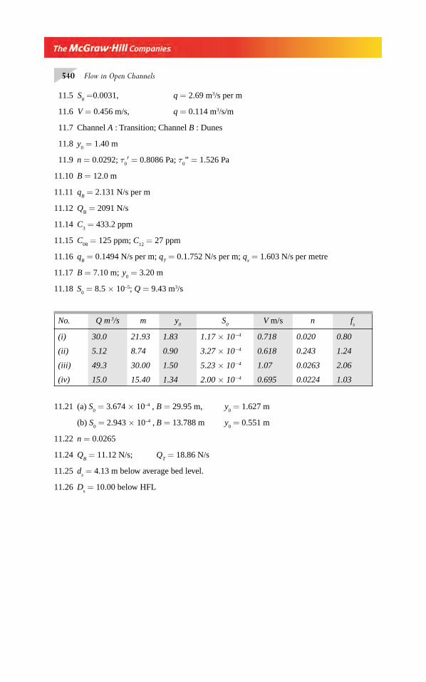
540 Flow in Open Channels
11.5 S0 =0.0031, q = 2.69 m3/s per m
11.6 V = 0.456 m/s, q = 0.114 m3/s/m
11.7 Channel A : Transition; Channel B : Dunes
11.8 y0 = 1.40 m
11.9 n = 0.0292; τ0′ = 0.8086 Pa; τ
0” = 1.526 Pa
11.10 B = 12.0 m
11.11 qB = 2.131 N/s per m
11.12 QB = 2091 N/s
11.14 C3 = 433.2 ppm
11.15 C08
= 125 ppm; C12
= 27 ppm
11.16 qB = 0.1494 N/s per m; q
T = 0.1.752 N/s per m; q
x = 1.603 N/s per metre
11.17 B = 7.10 m; y0 = 3.20 m
11.18 S0 = 8.5 × 10⁻⁵; Q = 9.43 m3/s
No. Q m 3/s m y0
S0
V m/s n fs
(i) 30.0 21.93 1.83 1.17 × 10⁻⁴ 0.718 0.020 0.80
(ii) 5.12 8.74 0.90 3.27 × 10⁻⁴ 0.618 0.243 1.24
(iii) 49.3 30.00 1.50 5.23 × 10⁻⁴ 1.07 0.0263 2.06
(iv) 15.0 15.40 1.34 2.00 × 10⁻⁴ 0.695 0.0224 1.03
11.21 (a) S0 = 3.674 × 10⁻⁴ , B = 29.95 m, y
0 = 1.627 m
(b) S0 = 2.943 × 10⁻⁴ , B = 13.788 m y
0 = 0.551 m
11.22 n = 0.0265
11.24 QB = 11.12 N/s; Q
T = 18.86 N/s
11.25 ds = 4.13 m below average bed level.
11.26 Ds = 10.00 below HFL
Chapter 11.indd 540Chapter 11.indd 540 2/24/2010 3:08:23 PM2/24/2010 3:08:23 PM
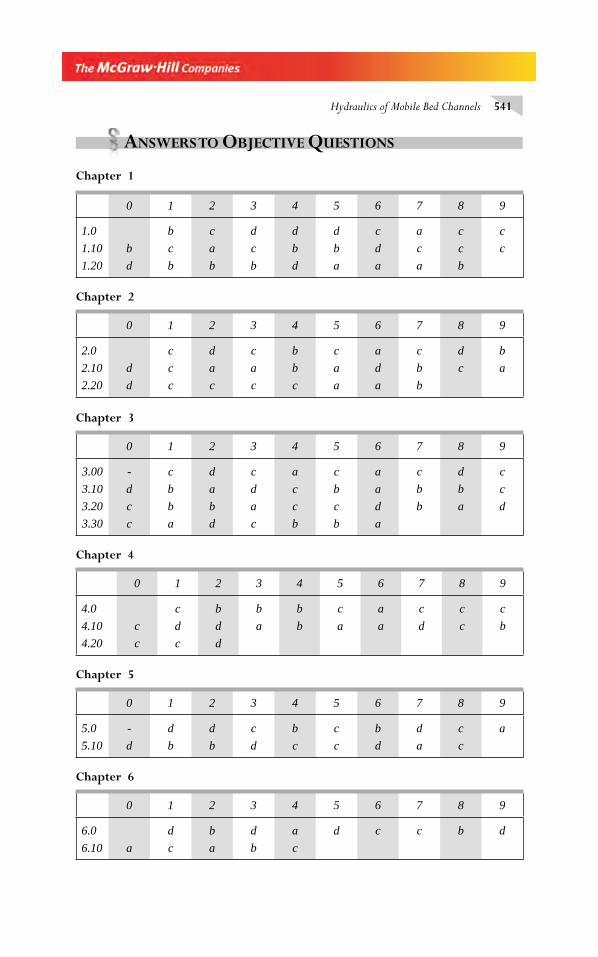
Hydraulics of Mobile Bed Channels 541
ANSWERS TO OBJECTIVE QUESTIONS
Chapter 1
0 1 2 3 4 5 6 7 8 9
1.0 b c d d d c a c c
1.10 b c a c b b d c c c
1.20 d b b b d a a a b
Chapter 2
0 1 2 3 4 5 6 7 8 9
2.0 c d c b c a c d b
2.10 d c a a b a d b c a
2.20 d c c c c a a b
Chapter 3
0 1 2 3 4 5 6 7 8 9
3.00 - c d c a c a c d c
3.10 d b a d c b a b b c
3.20 c b b a c c d b a d
3.30 c a d c b b a
Chapter 4
0 1 2 3 4 5 6 7 8 9
4.0 c b b b c a c c c
4.10 c d d a b a a d c b
4.20 c c d
Chapter 5
0 1 2 3 4 5 6 7 8 9
5.0 - d d c b c b d c a
5.10 d b b d c c d a c
Chapter 6
0 1 2 3 4 5 6 7 8 9
6.0 d b d a d c c b d
6.10 a c a b c
Chapter 11.indd 541Chapter 11.indd 541 2/24/2010 3:08:23 PM2/24/2010 3:08:23 PM
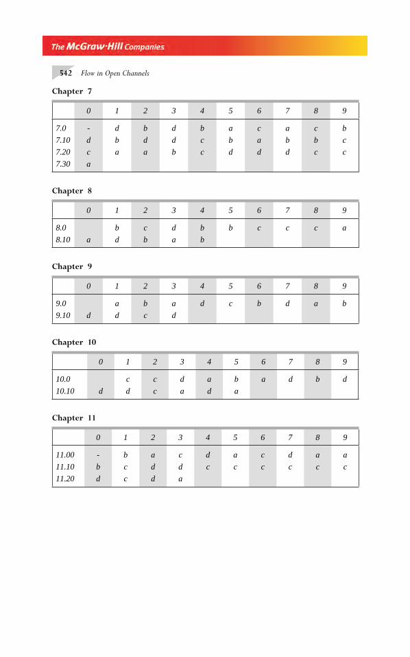
542 Flow in Open Channels
Chapter 7
0 1 2 3 4 5 6 7 8 9
7.0 - d b d b a c a c b
7.10 d b d d c b a b b c
7.20 c a a b c d d d c c
7.30 a
Chapter 8
0 1 2 3 4 5 6 7 8 9
8.0 b c d b b c c c a
8.10 a d b a b
Chapter 9
0 1 2 3 4 5 6 7 8 9
9.0 a b a d c b d a b
9.10 d d c d
Chapter 10
0 1 2 3 4 5 6 7 8 9
10.0 c c d a b a d b d
10.10 d d c a d a
Chapter 11
0 1 2 3 4 5 6 7 8 9
11.00 - b a c d a c d a a
11.10 b c d d c c c c c c
11.20 d c d a
Chapter 11.indd 542Chapter 11.indd 542 2/24/2010 3:08:23 PM2/24/2010 3:08:23 PM
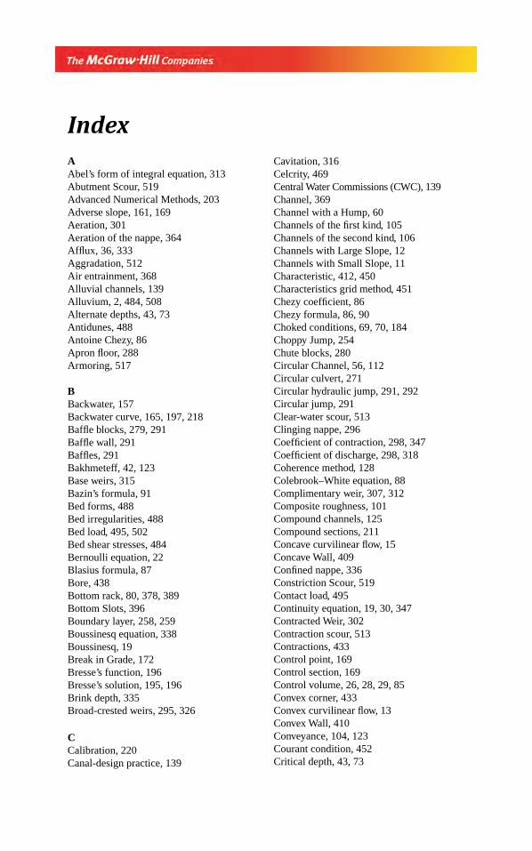
AAbel’s form of integral equation, 313Abutment Scour, 519Advanced Numerical Methods, 203Adverse slope, 161, 169Aeration, 301Aeration of the nappe, 364Affl ux, 36, 333Aggradation, 512Air entrainment, 368Alluvial channels, 139Alluvium, 2, 484, 508Alternate depths, 43, 73Antidunes, 488Antoine Chezy, 86Apron fl oor, 288Armoring, 517
BBackwater, 157Backwater curve, 165, 197, 218Baffl e blocks, 279, 291Baffl e wall, 291Baffl es, 291Bakhmeteff, 42, 123Base weirs, 315Bazin’s formula, 91Bed forms, 488Bed irregularities, 488Bed load, 495, 502Bed shear stresses, 484Bernoulli equation, 22Blasius formula, 87Bore, 438Bottom rack, 80, 378, 389Bottom Slots, 396Boundary layer, 258, 259Boussinesq equation, 338Boussinesq, 19Break in Grade, 172Bresse’s function, 196Bresse’s solution, 195, 196Brink depth, 335Broad-crested weirs, 295, 326
CCalibration, 220Canal-design practice, 139
Cavitation, 316Celcrity, 469Central Water Commissions (CWC), 139Channel, 369Channel with a Hump, 60Channels of the fi rst kind, 105Channels of the second kind, 106Channels with Large Slope, 12Channels with Small Slope, 11Characteristic, 412, 450Characteristics grid method, 451Chezy coeffi cient, 86Chezy formula, 86, 90Choked conditions, 69, 70, 184Choppy Jump, 254Chute blocks, 280Circular Channel, 56, 112Circular culvert, 271Circular hydraulic jump, 291, 292Circular jump, 291Clear-water scour, 513Clinging nappe, 296Coeffi cient of contraction, 298, 347Coeffi cient of discharge, 298, 318Coherence method, 128Colebrook–White equation, 88Complimentary weir, 307, 312Composite roughness, 101Compound channels, 125Compound sections, 211Concave curvilinear fl ow, 15Concave Wall, 409Confi ned nappe, 336Constriction Scour, 519Contact load, 495Continuity equation, 19, 30, 347Contracted Weir, 302Contraction scour, 513Contractions, 433Control point, 169Control section, 169Control volume, 26, 28, 29, 85Convex corner, 433Convex curvilinear fl ow, 13Convex Wall, 410Conveyance, 104, 123Courant condition, 452Critical depth, 43, 73
Index
Index.indd 543Index.indd 543 2/24/2010 3:11:12 PM2/24/2010 3:11:12 PM

544 Index
Critical depth in circular channels, 49Critical discharge, 51Critical motion, 485Critical shear stress, 485Critical slope, 131, 132, 136, 161Critical slope channel, 131Critical tractive force, 485Critical velocity ratio, 509Critical-fl ow condition, 43Cubic parabola, 43Culvert, 295, 352Curvilinear fl ow, 13
DDam break, 443Dam Break problem, 475Darcy–Weisbach equation, 87Darcy–Weisbach friction factor, 87Datum constant, 312, 313De Marchi Coeffi cient CM, 382, 383De Marchi Equation, 382, 383De Marchi varied fl ow function, 383Degradation, 512Degradation scour, 513Delivery of, 227Design head, 317Design-energy head, 318Diagonal Interface Method, 127Differential equation of GVF, 190, 201Diffusing scheme, 453Diffusion coeffi cient, 498Diffusion scheme, 454Direct integration, 189Direct Numerical Methods, 452Direct-Step method, 203Divided channel, 219Divided Channel method (DCM), 127Drowned jump, 282Dunes, 488Dynamic equation of GVF, 159
EEffective length, 318Effective piezometric head, 10, 16, 17, 19Empirical formulae, 100Empirical Methods, 128End contractions, 324End depth, 295, 335End sill, 280Energy Dissipator, 248, 279Energy equation, 22, 30
Energy loss in the jump, 260Equation of continuity, 19Equivalent roughness, 101, 102, 127Equivalent sand-grain roughness, 87Euler’s equation, 10Exchange Discharge Model, 128Expansion, 433Explicit method, 449, 453Exponential channel, 75
FFHWA, 358Finite crest width weir, 364Finite-difference schemes, 449Finite-element method, 449First hydraulic exponent, 51, 73Fluid, 1Flood banks, 150Flood plain, 125Flood routing, 439Flood wave, 38Free Board, 141Free fl ow, 296, 347Free jumps, 282Free overfall, 34, 37, 334Free repelled jump, 283Free surface, 1Free-mixing zone, 259Free-surface fl ow , 189Friction slopes, 430Froude line, 412Froude number, 44, 47, 48, 49Full rough fl ow, 87
GGanguillet and Kutter Formula, 91General scour, 513General Transition, 71Generalised – fl ow relation, 134, 180Generalized slope, 150Gradually varied fl ow, 3, 4, 157Graphical method, 189Grit chamber, 315GVF equation, 183GVF profi le , 194
HHDS-5, 352HEC-18, 20, 23, 515HEC-RAS, 218Helical secondary, 126
Index.indd 544Index.indd 544 2/24/2010 3:11:13 PM2/24/2010 3:11:13 PM

Index 545
Horizontal bed, 161Horseshoe vortex, 514Horton’s formula, 102, 103Hump height, 60HY-8, 358Hydraulic drop , 229Hydraulic exponents, 199Hydraulic jump, 36, 248Hydraulic radius, 86Hydraulically effi cient, 119Hydraulically effi cient
trapezoidal, 120Hydraulically smooth wall, 87Hydrostatic, 157Hydrostatic distribution, 14Hydrostatic pressure, 10Hydrostatic Pressure
Distribution, 11
IIdeal contraction, 424Implicit method, 449, 454Inception of cavitation, 319Incipient motion, 485Incompressible fl uid, 1Indian Practice, 522Initiation of motion, 485Inlet control, 352Interface, 125Irrigation Engineering, 139Island-type fl ow, 223
JJump profi le, 257Jumps on a Sloping Floor, 274, 275
KKarman–Prandtl equation, 87Keifer and Chu’s method, 200Kennedy Equation, 509Kerb outlets, 390Kinetic Energy, 7Kinetic energy correction factor, 8Kutta–Merson Method , 221
LLacey’s Equations, 509Lacey–Inglis method, 523Laminar sublayer, 87, 485Lateral fl ow, 368
Lateral spillway, 369Lateral weir, 380Law of the Wall, 92Lax-Wendroff schemes, 454Leap-Frog, 454Limit slope, 132, 136Linear Proportional Weir, 306Linear-momentum equation, 26Live-bed scour, 513Local phenomenon, 295Local scour, 513Location of the jump, 281Long-crested weir, 327Longitudinal Slope, 140Lower nappe, 296
MManning’s formula, 89, 90, 377Manning’s n, 90Maximum discharge, 117Mechanics, 1Median drain, 356Median size, 485Membrane analogy, 95Method (DCM) , 220Method of characteristics, 430MIKE 21, 218Mild slope, 161Mild slope channel, 131Minimum specifi c energy, 73Mobile bed channels, 484Mobile boundary channels, 2Modular limit, 300, 329, 350Momentum, 8Momentum correction factor, 8Momentum equation, 26, 30Momentum equation in
conservation form, 443Momentum exchange, 125Monoclinal wave, 480Moody chart, 88Moody diagram, 145, 485Most Effi cient Channels, 121Most effi cient section, 121Mostkow Equations, 391Moving Hydraulic Jump, 465Moving-boat method, 33Multi-island-type fl ow, 223, 225Multi-roughness type
perimeter, 101
Index.indd 545Index.indd 545 2/24/2010 3:11:13 PM2/24/2010 3:11:13 PM
546 Index
NNarrow channels, 93Narrow-crested, 328Natural channel, 6, 9, 218Natural streams, 100Negative disturbance, 410Negative surge, 459, 468, 480Negative Wave, 469Non-prismatic channel, 151Non-rectangular channel, 265Non-uniform fl ow, 3Normal Acceleration, 14Normal depth, 81, 105, 110,Notch, 295Notch-orifi ce, 314Numerical Method, 128, 189, 448
OOblique jump, 415Oblique shock, 433Oblique shock wave, 414Ogee Crest, 317Ogee spillway, 316One-dimensional analysis, 7, 126Open channel, 1, 88Orifi ce, 314Oscillating jump, 253, 293Outlet control, 352Overfl ow spillways, 295, 262, 316Overland fl ow, 5Overrun, 446
PParabolic, 305Parshall Flume, 334Pavlovski formula, 91, 103Performance curve, 357Permissible Velocities, 140Piezometric head, 12Plane bed, 488Positive surge, 459, 480Prandtl, 86Prandtl’s mixing length theory, 497Prandtl-Meyer fan, 413, 429Prandtl–Meyer function, 408Preissmann Scheme, 455Pressure, 10Pressure distribution, 10, 30Preston tube, 5, 95Primary vortex, 519Prismatic channels, 1, 85, 207
Profi le analysis, 183Projecting barrel, 353Proportional weir, 305P-weirs, 306
QQuadrant plate weir, 309Quadratic weir, 312, 361
RRapidly varied fl ows, 3, 4, 295Rectangular Section, 47Rectangular Weir, 295Rectangular-grid method, 452Regime channel, 504, 508Rehbock formula, 298Relative roughness, 87Repelled jump, 282, 284Reynolds number, 93, 298Rigid bed channels, 484Rigid channels, 2Ripples, 488Robert Manning, 89Roll waves, 431Roller, 259, 460Rough turbulent-fl ow, 89Roughness, 140Rouse equation, 498Runge–Kutta methods, 221
SSaint Venant equations, 443Saltation load, 495Scales, 259Scour, 512SCS, 142Second hydraulic exponent, 123Secondary currents, 5Section factor, 51Sediment, 484Sediment engineering, 2Sediment load, 495Sediment rating curve, 503Sediment transport, 2, 101, 484Sedimentation Engineering, 484Self-similar, 259Separation, 319Sequent Depth Ratio, 250Sequent depths, 248Shallow waves, 402Sharp-crested weirs, 295
Index.indd 546Index.indd 546 2/24/2010 3:11:13 PM2/24/2010 3:11:13 PM
Index 547
Shear Reynolds number, 485Shear stress, 86Shear velocity, 87, 259, 485Shear-stress distribution, 2Shields curve, 485Shock fronts, 404Shock wave, 71, 404, 406Side weir, 380Side-channel spillway, 367Sill, 279, 298Simple-island-Type Flow, 224Siphon tube irrigation systems, 378Skijump spillway, 34Slope-discharge-continuity theorem, 311Sloping apron, 290Sluice gate, 25, 295, 347Spatially varied fl ow, 5, 20, 38, 367Special Weirs, 315Specifi c energy, 42, 73Specifi c Force, 30Spillway bucket, 16Spillway crest, 32St. Venant’s equations, 217Stability, 431, 433, 468Stability analysis, 431Stable fl ows, 431Stagnation point, 514Standard lined canal sections, 114Standard lined trapezoidal section, 114Standard lined triangular section, 114Standard-step Method, 203, 207, 211Standing wave, 491Standing-wave fl ume, 332Steady fl ow, 2, 19, 26Steady jump, 293Steady uniform fl ow, 3Steep slope, 161Steep slope channel, 131Stilling basin, 279, 280Straub’s Equations, 273Streamlined transition, 422Strickler formula, 100Strickler’s Equation, 493Strong jump, 293Subcritical fl ow, 44, 60Submerged, 282Submerged fl ow, 300, 329, 350Submerged jump, 282, 283Submerged sluice-gate, 34Submergence, 300Submergence factor, 282
Submergence limit, 300Submergence ratio, 300Sudden drop, 172Super elevation, 142Super critical expansions, 427Supercritical Flow, 62Supercritical fl ow region, 44Supercritical streams, 402Supersonic fl ows, 408Supersonic nozzles, 428Suppressed weirs, 302Surface of zero shear, 127, 128Surface of zero shear stress, 127Surface tension, 1, 298, 303Surface velocity, 7Surges, 438, 459Suspended load, 495, 502Sutro Weir, 304, 361SVF with increasing discharge, 367
TTailwater depth, 280, 282Tailwater level, 282The section factor for uniform-fl ow
computations, 104Thin plate weir, 295Throated f ume, 332Tidal bores, 464Top width, 44Torrents, 9Total bed material load, 495, 500Total energy, 42, 151Total load, 495Total scour, 513Transients, 438Transition, 60, 66, 73, 426Transitional depth, 180Transitional profi le, 370, 371, 400Trapezoidal Channel, 49Trapezoidal Method , 222Trench weir, 390True broad-crested weir, 327Turbulent fl ows, 87Turbulent regime, 1Two-stage channel, 125
UUnconfi ned nappe, 336Uncontracted, 302Underdesigning of the spillway, 320Undular jump, 253
Index.indd 547Index.indd 547 2/24/2010 3:11:13 PM2/24/2010 3:11:13 PM


