Embed Size (px)
Citation preview
FINA 4320: Investment ManagementEfficient Diversification
Rajkamal Vasu
University of Houston
C. T. Bauer College of Business
Fall 2018
R. Vasu Efficient Diversification Fall 2018 1 / 36
Two-Security Portfolio: Return
Expected Return:E [rp ] = w1E [r1] + w2E [r2]
Expected Return of portfolio with n securities
E [rp ] =n
∑i=1
wiE [ri ]
n
∑i=1
wi = 1
R. Vasu Efficient Diversification Fall 2018 2 / 36
Portfolio Risk
Risk factors common to the whole economy lead to market risk, alsocalled systematic risk or nondiversifiable risk
Risk that can be eliminated by diversification is called firm-specificrisk, also called unique risk, idiosyncratic risk, residual risk,nonsystematic risk or diversifiable risk
R. Vasu Efficient Diversification Fall 2018 3 / 36
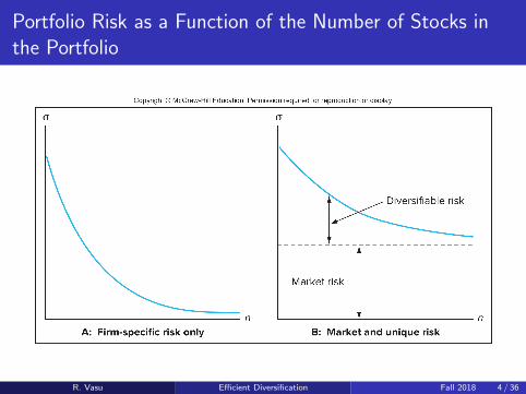
Portfolio Risk as a Function of the Number of Stocks inthe Portfolio
R. Vasu Efficient Diversification Fall 2018 4 / 36
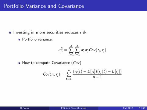
Portfolio Variance and Covariance
Investing in more securities reduces risk:
Portfolio variance:
σ2p =
n
∑i=1
n
∑j=1
wiwjCov(ri , rj )
How to compute Covariance (Cov)
Cov(ri , rj ) =n
∑t=1
(ri (t)− E [ri ])(rj (t)− E [rj ])
n− 1
R. Vasu Efficient Diversification Fall 2018 5 / 36
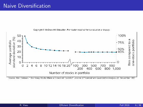
Naive Diversification
R. Vasu Efficient Diversification Fall 2018 6 / 36
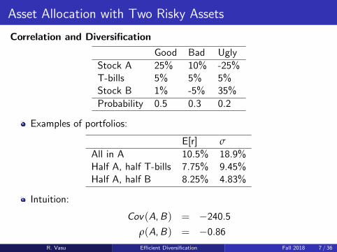
Asset Allocation with Two Risky Assets
Correlation and Diversification
Good Bad Ugly
Stock A 25% 10% -25%T-bills 5% 5% 5%Stock B 1% -5% 35%
Probability 0.5 0.3 0.2
Examples of portfolios:
E[r] σ
All in A 10.5% 18.9%Half A, half T-bills 7.75% 9.45%Half A, half B 8.25% 4.83%
Intuition:
Cov(A,B) = −240.5
ρ(A,B) = −0.86
R. Vasu Efficient Diversification Fall 2018 7 / 36
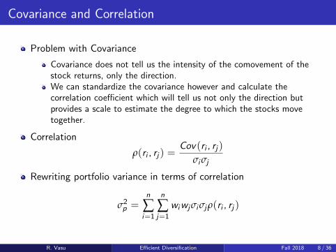
Covariance and Correlation
Problem with Covariance
Covariance does not tell us the intensity of the comovement of thestock returns, only the direction.We can standardize the covariance however and calculate thecorrelation coefficient which will tell us not only the direction butprovides a scale to estimate the degree to which the stocks movetogether.
Correlation
ρ(ri , rj ) =Cov(ri , rj )
σiσj
Rewriting portfolio variance in terms of correlation
σ2p =
n
∑i=1
n
∑j=1
wiwjσiσjρ(ri , rj )
R. Vasu Efficient Diversification Fall 2018 8 / 36
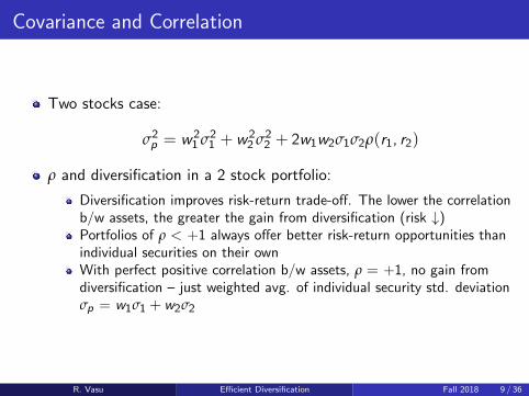
Covariance and Correlation
Two stocks case:
σ2p = w2
1 σ21 + w2
2 σ22 + 2w1w2σ1σ2ρ(r1, r2)
ρ and diversification in a 2 stock portfolio:
Diversification improves risk-return trade-off. The lower the correlationb/w assets, the greater the gain from diversification (risk ↓)Portfolios of ρ < +1 always offer better risk-return opportunities thanindividual securities on their ownWith perfect positive correlation b/w assets, ρ = +1, no gain fromdiversification – just weighted avg. of individual security std. deviationσp = w1σ1 + w2σ2
R. Vasu Efficient Diversification Fall 2018 9 / 36
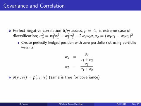
Covariance and Correlation
Perfect negative correlation b/w assets, ρ = -1, is extreme case ofdiversification; σ2
p = w21 σ2
1 + w22 σ2
2 − 2w1w2σ1σ2 = (w1σ1 − w2σ2)2
Create perfectly hedged position with zero portfolio risk using portfolioweights:
w1 =σ2
σ1 + σ2
w2 =σ1
σ1 + σ2
ρ(r1, r2) = ρ(r2, r1) (same is true for covariance)
R. Vasu Efficient Diversification Fall 2018 10 / 36
Summary
Portfolio Risk/Return Two Security Portfolio
Amount of risk reduction depends critically on correlation orcovariances
Adding securities with correlations < 1 will result in risk reduction
If risk is reduced by more than expected return, what happens to thereturn per unit of risk (the Sharpe ratio)?
R. Vasu Efficient Diversification Fall 2018 11 / 36
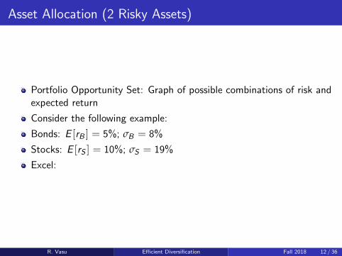
Asset Allocation (2 Risky Assets)
Portfolio Opportunity Set: Graph of possible combinations of risk andexpected return
Consider the following example:
Bonds: E [rB ] = 5%; σB = 8%
Stocks: E [rS ] = 10%; σS = 19%
Excel:
R. Vasu Efficient Diversification Fall 2018 12 / 36
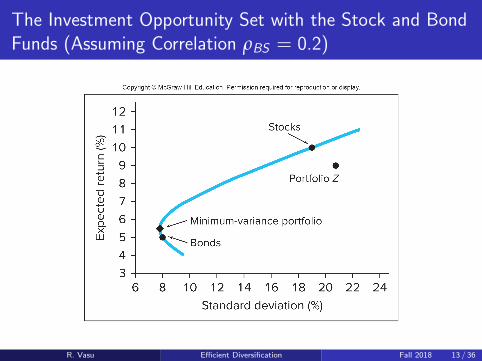
The Investment Opportunity Set with the Stock and BondFunds (Assuming Correlation ρBS = 0.2)
R. Vasu Efficient Diversification Fall 2018 13 / 36
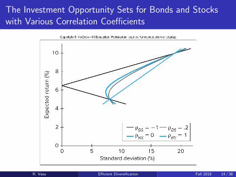
The Investment Opportunity Sets for Bonds and Stockswith Various Correlation Coefficients
R. Vasu Efficient Diversification Fall 2018 14 / 36
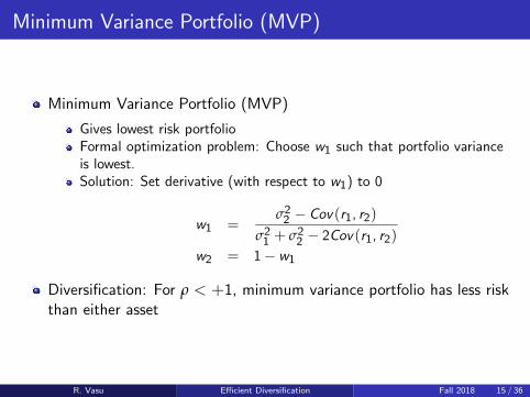
Minimum Variance Portfolio (MVP)
Minimum Variance Portfolio (MVP)
Gives lowest risk portfolioFormal optimization problem: Choose w1 such that portfolio varianceis lowest.Solution: Set derivative (with respect to w1) to 0
w1 =σ2
2 − Cov(r1, r2)
σ21 + σ2
2 − 2Cov(r1, r2)
w2 = 1− w1
Diversification: For ρ < +1, minimum variance portfolio has less riskthan either asset
R. Vasu Efficient Diversification Fall 2018 15 / 36
Efficient and Dominated Portfolios
Portfolios that lie below the minimum-variance portfolio in the figure(on the downward-sloping portion of the curve) are inefficient.
Any such portfolio is dominated by the portfolio that lies directlyabove it on the upward-sloping portion of the curve since thatportfolio has higher expected return and equal standard deviation
Efficient Set: Portfolios that are not dominated
The best choice among the portfolios on the upward-sloping portionof the curve is not as obvious, because in this region higher expectedreturn is accompanied by greater risk
R. Vasu Efficient Diversification Fall 2018 16 / 36
Extending Concepts to All Securities (Many Risky Assets)
Consider all possible combinations of securities, with all possibledifferent weightings and keep track of combinations that provide morereturn for less risk or the least risk for a given level of return andgraph the result
The set of portfolios that provide the optimal trade-offs are describedas the efficient frontier
The efficient frontier portfolios are dominant or the best diversifiedpossible combinations
All investors should want a portfolio on the efficient frontier (... Untilwe add the riskless asset)
R. Vasu Efficient Diversification Fall 2018 17 / 36
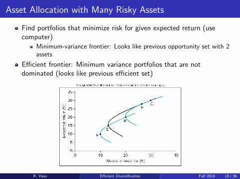
Asset Allocation with Many Risky Assets
Find portfolios that minimize risk for given expected return (usecomputer)
Minimum-variance frontier: Looks like previous opportunity set with 2assets
Efficient frontier: Minimum variance portfolios that are notdominated (looks like previous efficient set)
R. Vasu Efficient Diversification Fall 2018 18 / 36
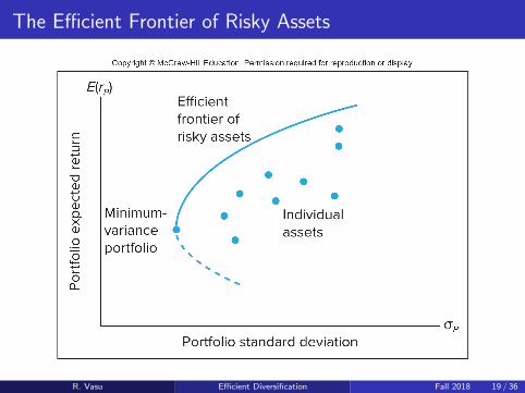
The Efficient Frontier of Risky Assets
R. Vasu Efficient Diversification Fall 2018 19 / 36
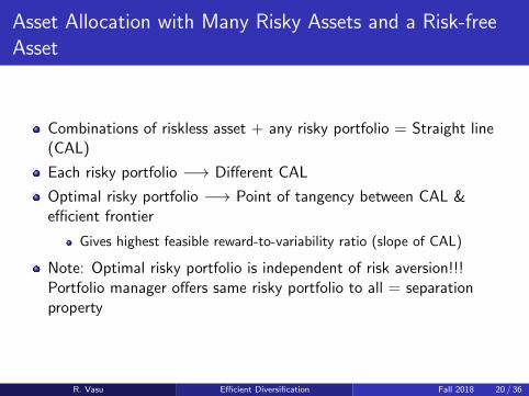
Asset Allocation with Many Risky Assets and a Risk-freeAsset
Combinations of riskless asset + any risky portfolio = Straight line(CAL)
Each risky portfolio −→ Different CAL
Optimal risky portfolio −→ Point of tangency between CAL &efficient frontier
Gives highest feasible reward-to-variability ratio (slope of CAL)
Note: Optimal risky portfolio is independent of risk aversion!!!Portfolio manager offers same risky portfolio to all = separationproperty
R. Vasu Efficient Diversification Fall 2018 20 / 36
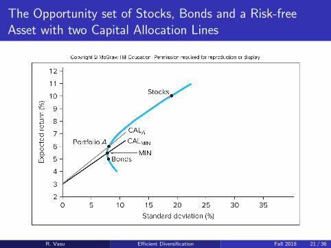
The Opportunity set of Stocks, Bonds and a Risk-freeAsset with two Capital Allocation Lines
R. Vasu Efficient Diversification Fall 2018 21 / 36
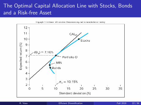
The Optimal Capital Allocation Line with Stocks, Bondsand a Risk-free Asset
R. Vasu Efficient Diversification Fall 2018 22 / 36
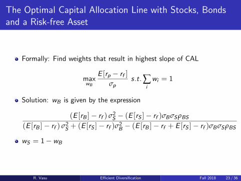
The Optimal Capital Allocation Line with Stocks, Bondsand a Risk-free Asset
Formally: Find weights that result in highest slope of CAL
maxwB
E [rp − rf ]
σps.t. ∑
i
wi = 1
Solution: wB is given by the expression
(E [rB ]− rf ) σ2S − (E [rS ]− rf )σBσSρBS
(E [rB ]− rf ) σ2S + (E [rS ]− rf )σ2
B − (E [rB ]− rf + E [rS ]− rf )σBσSρBS
wS = 1− wB
R. Vasu Efficient Diversification Fall 2018 23 / 36
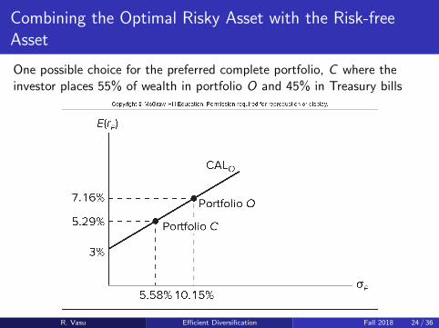
Combining the Optimal Risky Asset with the Risk-freeAsset
One possible choice for the preferred complete portfolio, C where theinvestor places 55% of wealth in portfolio O and 45% in Treasury bills
R. Vasu Efficient Diversification Fall 2018 24 / 36
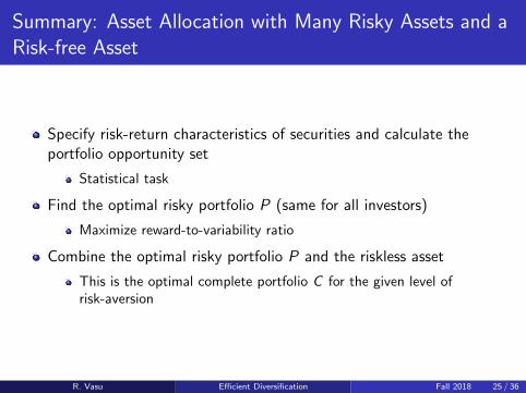
Summary: Asset Allocation with Many Risky Assets and aRisk-free Asset
Specify risk-return characteristics of securities and calculate theportfolio opportunity set
Statistical task
Find the optimal risky portfolio P (same for all investors)
Maximize reward-to-variability ratio
Combine the optimal risky portfolio P and the riskless asset
This is the optimal complete portfolio C for the given level ofrisk-aversion
R. Vasu Efficient Diversification Fall 2018 25 / 36
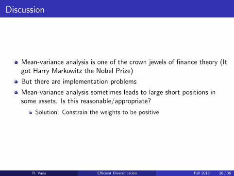
Discussion
Mean-variance analysis is one of the crown jewels of finance theory (Itgot Harry Markowitz the Nobel Prize)
But there are implementation problems
Mean-variance analysis sometimes leads to large short positions insome assets. Is this reasonable/appropriate?
Solution: Constrain the weights to be positive
R. Vasu Efficient Diversification Fall 2018 26 / 36
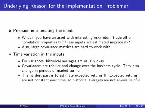
Underlying Reason for the Implementation Problems?
Precision in estimating the inputs
What if you have an asset with interesting risk/return trade-off orcorrelation properties but these inputs are estimated imprecisely?Also, large covariance matrices are hard to work with.
Time variation in the inputs
For variances, historical averages are usually okayCovariances are trickier and change over the business cycle. They alsochange in periods of market turmoil.The hardest part is to estimate expected returns !!! Expected returnsare not constant over time, so historical averages are not always helpful.
R. Vasu Efficient Diversification Fall 2018 27 / 36
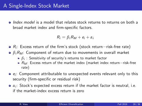
A Single-Index Stock Market
Index model is a model that relates stock returns to returns on both abroad market index and firm-specific factors.
Ri = βiRM + ei + αi
Ri : Excess return of the firm’s stock (stock return−risk-free rate)
βiRM : Component of return due to movements in overall market
βi : Sensitivity of security’s returns to market factorRM : Excess return of the market index (market index return−risk-freerate)
ei : Component attributable to unexpected events relevant only to thissecurity (firm-specific or residual risk)
αi : Stock’s expected excess return if the market factor is neutral, i.e.if the market-index excess return is zero
R. Vasu Efficient Diversification Fall 2018 28 / 36
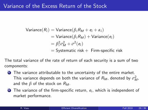
Variance of the Excess Return of the Stock
Variance(Ri ) = Variance(βiRM + ei + αi )
= Variance(βiRM) + Variance(ei )
= β2i σ2
M + σ2(ei )
= Systematic risk + Firm-specific risk
The total variance of the rate of return of each security is a sum of twocomponents:
1 The variance attributable to the uncertainty of the entire market.This variance depends on both the variance of RM , denoted by σ2
M ,and the β of the stock on RM .
2 The variance of the firm-specific return, ei , which is independent ofmarket performance.
R. Vasu Efficient Diversification Fall 2018 29 / 36
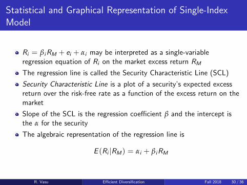
Statistical and Graphical Representation of Single-IndexModel
Ri = βiRM + ei + αi may be interpreted as a single-variableregression equation of Ri on the market excess return RM
The regression line is called the Security Characteristic Line (SCL)
Security Characteristic Line is a plot of a security’s expected excessreturn over the risk-free rate as a function of the excess return on themarket
Slope of the SCL is the regression coefficient β and the intercept isthe α for the security
The algebraic representation of the regression line is
E (Ri |RM) = αi + βiRM
R. Vasu Efficient Diversification Fall 2018 30 / 36
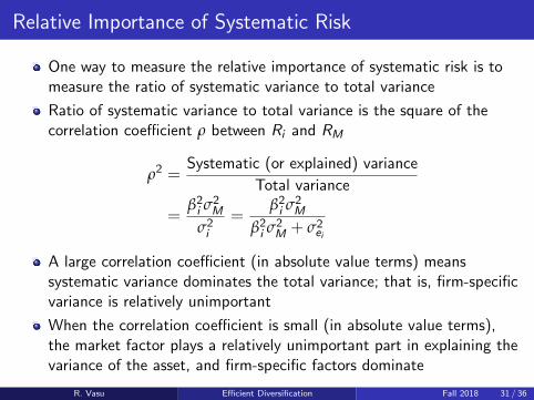
Relative Importance of Systematic Risk
One way to measure the relative importance of systematic risk is tomeasure the ratio of systematic variance to total variance
Ratio of systematic variance to total variance is the square of thecorrelation coefficient ρ between Ri and RM
ρ2 =Systematic (or explained) variance
Total variance
=β2i σ2
M
σ2i
=β2i σ2
M
β2i σ2
M + σ2ei
A large correlation coefficient (in absolute value terms) meanssystematic variance dominates the total variance; that is, firm-specificvariance is relatively unimportant
When the correlation coefficient is small (in absolute value terms),the market factor plays a relatively unimportant part in explaining thevariance of the asset, and firm-specific factors dominate
R. Vasu Efficient Diversification Fall 2018 31 / 36
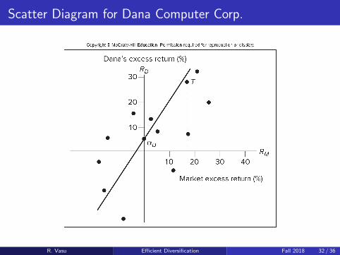
Scatter Diagram for Dana Computer Corp.
R. Vasu Efficient Diversification Fall 2018 32 / 36
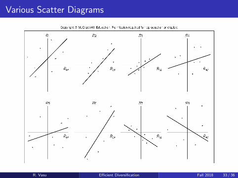
Various Scatter Diagrams
R. Vasu Efficient Diversification Fall 2018 33 / 36
Diversification in a Single-Index Security Market
Imagine a portfolio P that is divided equally among securities whosereturns follow the single-index model
The β of the portfolio is a simple average of the individual security βs
Hence, there are no diversification effects on systematic risk nomatter how many securities are involved
Intuition: The systematic component of each security return, βiRM ,is driven by the market factor and therefore is perfectly correlatedwith the systematic part of any other security’s return
R. Vasu Efficient Diversification Fall 2018 34 / 36
Diversification in a Single-Index Security Market
Consider a portfolio P of n securities with weights wi (n
∑i=1
wi = 1)
Nonsystematic risk of each security is σ2ei
Nonsystematic portion of portfolio P’s return is
eP =n
∑i=1
wiei
Portfolio P’s nonsystematic variance is
σ2eP
=n
∑i=1
w2i σ2
ei
The sum is far less than the average firm-specific variance of thestocks in the portfolio
R. Vasu Efficient Diversification Fall 2018 35 / 36
Diversification in a Single-Index Security Market
The impact of nonsystematic risk becomes negligible as thenumber of securities grows and the portfolio becomes morediversified
The number of securities counts more than the size of theirnonsystematic variance
Sufficient diversification can virtually eliminate firm-specific risk. Onlysystematic risk (market risk) remains.
For diversified investors, the relevant risk measure for a securityis the security’s β, since firms with higher β have greater sensitivityto market risk
The systematic risk, β2σ2M , will be determined by both the market
volatility, σ2M , and the firm’s β
R. Vasu Efficient Diversification Fall 2018 36 / 36