Embed Size (px)
Citation preview
ANDREAS KILIMATOS
FEASIBILITY OF CONCRETE SHELLS USING FLEXIBLE MOULD PREFABRICATED CONCRETE ELEMENTS

Cover photo:Military aircraft hanger by Pier Luigi Nervi-Orvieto, Italy, 1935(Source: concretevinyl)
Feasibility of concrete shells using flexible mouldprefabricated concrete elements
MASTER THESIS
by
Andreas Kilimatos
in partial fulfilling of of the requirement for the degree of
Master of Sciencein Civil Engineering
in Delft University of Technology
To be defended publicly on Monday June 4th, 2018
Student number: 4359909 Supervisor: Dr.ir. H.R.Schipper Thesis committee: Prof.ir. R. Nijsse Ir. P. Egenraam
An electronic version of this thesis is available athttp://repository.tudelft.nl/

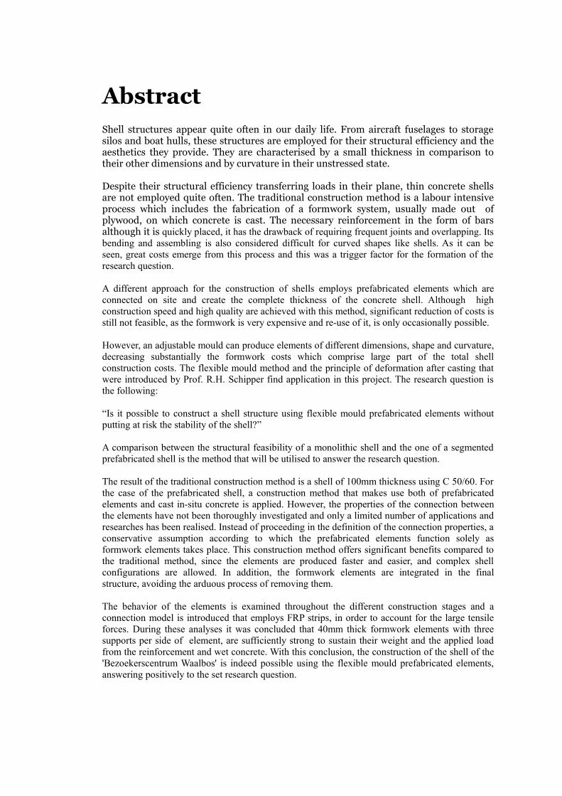
AbstractShell structures appear quite often in our daily life. From aircraft fuselages to storagesilos and boat hulls, these structures are employed for their structural efficiency and theaesthetics they provide. They are characterised by a small thickness in comparison totheir other dimensions and by curvature in their unstressed state.
Despite their structural efficiency transferring loads in their plane, thin concrete shellsare not employed quite often. The traditional construction method is a labour intensiveprocess which includes the fabrication of a formwork system, usually made out ofplywood, on which concrete is cast. The necessary reinforcement in the form of barsalthough it is quickly placed, it has the drawback of requiring frequent joints and overlapping. Itsbending and assembling is also considered difficult for curved shapes like shells. As it can beseen, great costs emerge from this process and this was a trigger factor for the formation of theresearch question.
A different approach for the construction of shells employs prefabricated elements which areconnected on site and create the complete thickness of the concrete shell. Although highconstruction speed and high quality are achieved with this method, significant reduction of costs isstill not feasible, as the formwork is very expensive and re-use of it, is only occasionally possible.
However, an adjustable mould can produce elements of different dimensions, shape and curvature,decreasing substantially the formwork costs which comprise large part of the total shellconstruction costs. The flexible mould method and the principle of deformation after casting thatwere introduced by Prof. R.H. Schipper find application in this project. The research question isthe following:
“Is it possible to construct a shell structure using flexible mould prefabricated elements withoutputting at risk the stability of the shell?”
A comparison between the structural feasibility of a monolithic shell and the one of a segmentedprefabricated shell is the method that will be utilised to answer the research question.
The result of the traditional construction method is a shell of 100mm thickness using C 50/60. Forthe case of the prefabricated shell, a construction method that makes use both of prefabricatedelements and cast in-situ concrete is applied. However, the properties of the connection betweenthe elements have not been thoroughly investigated and only a limited number of applications andresearches has been realised. Instead of proceeding in the definition of the connection properties, aconservative assumption according to which the prefabricated elements function solely asformwork elements takes place. This construction method offers significant benefits compared tothe traditional method, since the elements are produced faster and easier, and complex shellconfigurations are allowed. In addition, the formwork elements are integrated in the finalstructure, avoiding the arduous process of removing them.
The behavior of the elements is examined throughout the different construction stages and aconnection model is introduced that employs FRP strips, in order to account for the large tensileforces. During these analyses it was concluded that 40mm thick formwork elements with threesupports per side of element, are sufficiently strong to sustain their weight and the applied loadfrom the reinforcement and wet concrete. With this conclusion, the construction of the shell of the'Bezoekerscentrum Waalbos' is indeed possible using the flexible mould prefabricated elements,answering positively to the set research question.


Acknowledgments
I would like to take the opportunity to express my gratitude to everyone who contributed tothe completion of this thesis. Initially, I would like to thank my graduation committee fortheir assistance and support throughout the progress of the thesis. Thank you Rob Nijsse,Roel Schipper, Peter Eigenraam for your interest and advice. Special thanks to my friends,fellow engineers, Maria Alexiou, Anna Ioannidou-Kati and Pratik Rao, who sharedgenerously their thoughts, ideas and knowledge with me. Their contribution was priceless.Furthermore, I would like to thank the Fanourakis Foundation for their financial supportduring the first year of my studies. Finally and most importantly, I deeply thank my parents,my brother and my grandmother for believing and supporting me and for offering their loveduring harsh times.
Andreas S. KilimatosDelft, May 2018
Table of Contents
1. 1 SHELL STRUCTURES....................................................................................21.1 SURFACE GEOMETRY.........................................................................................................2
1.2 SHELLS IN FREE-FORM ARCHITECTURE..............................................................................3
1.3 STATE OF AFFAIRS.............................................................................................................4
1.4 PROBLEM DESCRIPTION AND SCOPE....................................................................................6
2. 2 THEORY OF SHELLS......................................................................................82.1 MEMBRANE THEORY OF SHELLS..........................................................................................8
2.2 BENDING THEORY............................................................................................................11
3. 3 FORMWORK TYPES FOR CONCRETE SHELLS...................................143.1 INTRODUCTION................................................................................................................14
3.2 DESCRIPTION OF THE PROBLEM WITH TIMBER FORMWORK..................................................15
3.3 PNEUMATIC INFLATED FORMWORK....................................................................................16
3.4 EARTH MOULDS...............................................................................................................17
3.5 POLYURETHANE FOAM FORMWORK...................................................................................18
3.6 RAISED STEEL SKELETON METHOD....................................................................................19
3.7 3D-PRINTING..................................................................................................................19
3.8 PREFABRICATED CONCRETE ELEMENTS..............................................................................20
3.9 MOULDS FOR PREFABRICATED CONCRETE ELEMENTS-METHODS OF CONSTRUCTION.............213.9.1 Timber moulds......................................................................................................213.9.2 Steel moulds.........................................................................................................22
3.9.2.1 Hoto Fudo...................................................................................................................................223.9.3 Textile formwork...................................................................................................23
3.9.3.1 Palazetto dello Sport...................................................................................................................243.9.3.2 Spencer Dock Bridge..................................................................................................................25
4. 4 ANALYSIS OF APPROXIMATING STRUCTURAL FORMS...................264.1 INTRODUCTION................................................................................................................26
4.2 VERIFICATION PROCESS....................................................................................................27
4.3 LOADS ...........................................................................................................................284.3.1 Permanent loads...................................................................................................284.3.2 Variable loads.......................................................................................................29
4.3.2.1 Snow load...................................................................................................................................294.3.2.2 Wind load....................................................................................................................................30
4.4 FLAT SLAB......................................................................................................................304.4.1 Description of flat slab behaviour........................................................................314.4.2 Load Combinations..............................................................................................324.4.3 Analysis of results-Comparison............................................................................32
4.4.3.1 Theoretical results.......................................................................................................................324.4.3.2 FEA results ................................................................................................................................344.4.3.3 Theoretical results.......................................................................................................................364.4.3.4 FEA results ................................................................................................................................37
4.5 ARCH.............................................................................................................................384.5.1 Load combinations...............................................................................................404.5.2 Analysis of results.................................................................................................41

4.6 CYLINDRICAL SHELL........................................................................................................454.6.1 Load combinations...............................................................................................494.6.2 Theoretical results................................................................................................494.6.3 FEA results..........................................................................................................514.6.4 Comparison..........................................................................................................51
4.7 SPHERICAL SIDE PART......................................................................................................524.7.1 Side part-Dome....................................................................................................52
5. 5 ANALYSIS OF THE CASE STRUCTURE 'BEZOEKERSCENTRUM WAALBOS'............................................................................................................56
5.1 DESCRIPTION OF THE STRUCTURE.....................................................................................56
5.2 VERIFICATION OF THE FINAL MODEL..................................................................................58
5.3 SUPPORTS.......................................................................................................................60
5.4 DISCUSSION ON THE RESULTS OF THE ANALYSIS.................................................................62
5.5 ANALYSIS WITH SERVICE LOADS........................................................................................635.5.1 Permanent Loads..................................................................................................635.5.2 Variable Loads......................................................................................................63
5.5.2.1 Live load ....................................................................................................................................645.5.2.2 Snow Load..................................................................................................................................64
5.5.3 Wind Load............................................................................................................655.5.4 Load combinations...............................................................................................68
5.6 RESULTS OF LINEAR STATIC ANALYSIS ..............................................................................69
5.7 MESH SIZE STUDY...........................................................................................................705.7.1 Process ................................................................................................................70
5.8 INVESTIGATION OF THE THICKNESS OF THE SHELL..............................................................75
5.9 INVESTIGATION OF CONCRETE GRADE................................................................................76
6. 6 ANALYSIS OF THE PREFABRICATED CONCRETE SHELL................786.1 SEGMENTATION OF THE SHELL .........................................................................................78
6.1.1 Boundary -Conforming Grids..............................................................................786.1.2 Structured grids....................................................................................................796.1.3 Block-Structured Grids.........................................................................................796.1.4 Translational grids...............................................................................................806.1.5 Grid generation for dome structures....................................................................81
6.2 SEGMENTATION OF 'BEZOEKERSCENTRUM WAALBOS'.........................................................81
7. 7 ANALYSIS OF THE SEGMENTED STRUCTURE.....................................857.1 CONSTRUCTION METHOD-CONNECTIONS BETWEEN ELEMENTS............................................85
7.2 TYPES OF CONNECTIONS..................................................................................................857.2.1 Wet connection.....................................................................................................857.2.2 Bolted connection/welded connection..................................................................867.2.3 Post-tensioning connection..................................................................................867.2.4 Glued connection..................................................................................................867.2.5 Prefabricated connection.....................................................................................86
7.3 PROPOSED CONSTRUCTION METHOD FOR 'BEZOEKERSCENTRUM WAALBOS'.........................877.3.1 Description of construction method.....................................................................877.3.2 Evaluation of the method......................................................................................88
7.4 SEGMENTED SHELL CHARACTERISTICS AND ANALYSIS.........................................................897.4.1 Introduction..........................................................................................................897.4.2 Dimensions of the elements-Transportation to the building site...........................897.4.3 FRP reinforcement of concrete structures............................................................97
7.5 CONCLUSIONS...............................................................................................................105

8. 8 CONCLUSIONS AND RECOMMENDATIONS........................................1068.1 CONCLUSIONS...............................................................................................................106
8.2 RECOMMENDATIONS......................................................................................................109BIBLIOGRAPHY...........................................................................................113APPENDIX A..................................................................................................117

List of FiguresIllustration 1.1: Types of Gaussian curvature [2]...........................................................2Illustration 1.2: Examples of free-form designs [54], [53].............................................3Illustration 1.3: Concept of deformation after casting [52]............................................6Illustration 2.1: Shell element membrane forces............................................................9Illustration 2.2: Membrane free body...........................................................................10Illustration 3.1: Shapes, formwork and skeleton shuttering[9]....................................15Illustration 3.2: Examples of elaborated timber formwork for concrete shells[9], [25]......................................................................................................................................15Illustration 3.3: The plane concrete plate is produced and the membrane is inflated [10]...............................................................................................................................16Illustration 3.4: Forming soil mould for concrete shell [8]..........................................17Illustration 3.5: Excavation of mould through archways [8]........................................18Illustration 3.6: Double polyurethane foam formwork for concrete shells [23]..........18Illustration 3.7: Central mast and steel rebars [8].........................................................19Illustration 3.8: Jubilee Church, Rome [19].................................................................22Illustration 3.9: Hoto Fudo with Mt. .Fuji in the background [20]..............................23Illustration 3.10: Cross-section of Hoto Fudo shell [22]..............................................23Illustration 3.11: Ribbed roof -Palazzetto dello Sport [26]..........................................25Illustration 3.12: Spencer Dock Bridge-Double-curved parapets [27].........................25Illustration 4.1 Plan view of the structure [28].............................................................26Illustration 4.2: Part of structure considered as a slab..................................................31Illustration 4.3: Slab 1..................................................................................................33Illustration 4.4: Bending moments in a flat slab supported by 2 columns [34]............33Illustration 4.5: Infinitely rigid part of column support [34]........................................34Illustration 4.6: Strips for moment distribution-Original flat slab...............................35Illustration 4.7: Slab 2..................................................................................................36Illustration 4.8: Continuous beam on three supports approximating the behaviour of Slab 2............................................................................................................................37Illustration 4.9: Three-hinged arch...............................................................................40Illustration 4.10: Parabolic arch under uniform load action [35].................................40Illustration 4.11: Free body diagram of a three hinged arch under self-weight............42Illustration 4.12: Normalised moments for a two-hinged arch.....................................45Illustration 4.13: Normalised moments for a three-hinged arch...................................45Illustration 4.14: Parts of the design case structure......................................................45Illustration 4.15: Behaviour of long barrel shell - Beam action [36]...........................46Illustration 4.16: Part of the structure considered as a cylindrical roof........................46Illustration 4.17: Supports in transverse direction for cylindrical roof........................47Illustration 4.18: Cylindrical shell roof-Plan view and cross-section..........................47Illustration 4.19: Free body diagram of shell beam......................................................50Illustration 4.20: Ellipsoid side parts............................................................................53Illustration 4.21: Membrane forces on infinitesimal load element...............................54Illustration 5.1: Model of the structure.........................................................................56Illustration 5.2: Structure with its surroundings...........................................................57Illustration 5.3: Supporting arch at the facade opening................................................57Illustration 5.4: Stresses on a cross section..................................................................59Illustration 5.5: Stresses of the chosen cross-section...................................................59Illustration 5.6: Total stresses-DIANA.........................................................................60Illustration 5.7: Initial deformations of the structure....................................................61
Illustration 5.8: Deformations due to self-weight in the z-axis – arch support............62Illustration 5.9: Hoop stresses-self weight...................................................................62Illustration 5.10: Meridional stresses-self weight........................................................63Illustration 5.11: Snow load shape coefficients for cylindrical roof.............................64Illustration 5.12: Recommended values of Ce for different topographies....................65Illustration 5.13: Exposure factor according to Eurocode............................................66Illustration 5.14: Illustration 5.11: External pressure coefficients cpe,10 for domes with circular base..........................................................................................................67Illustration 5.15: Distribution for vaulted roofs...........................................................67Illustration 5.16: Wind distribution in the circumferential direction............................68Illustration 5.17: Structural failure modes for shells....................................................70Illustration 5.18: Influence length of edge disturbances in a spherical dome..............70Illustration 5.19: Error function of displacement in relation to mesh size...................71Illustration 5.20: Vertical deformation diagram-LC1...................................................72Illustration 5.21: Deflection diagram of two-span beam with uniformly distributed load ..............................................................................................................................72Illustration 5.22: Global stresses in the circumferential direction-LC2.......................73Illustration 5.23: Global stresses in the meridional direction-LC2..............................73Illustration 5.24: Moments in the x-axis (left) and y-axis (right).................................74Illustration 5.25: First buckling mode-LC2..................................................................75Illustration 5.26: Second buckling mode-LC2.............................................................75Illustration 6.1: Boundary conforming quadrangular and triangular grid [3]...............79Illustration 6.2: Types of interface between contiguous blocks: (a) discontinuous, (b and c) non-smooth, (d) smooth [3]...............................................................................80Illustration 6.3: Segmentation of translational surface [3]...........................................80Illustration 6.4: Basic grid patterns [2].........................................................................80Illustration 6.5: Grid configuration for some shapes [3]..............................................81Illustration 6.6: Triangular elements at the sides of the domes....................................83Illustration 6.7: Final segmentation at the sides of the dome.......................................83Illustration 6.8: Segmented shell-top view...................................................................84Illustration 6.9: Segmented shell-front view................................................................84Illustration 7.1: Glued connection [42]........................................................................86Illustration 7.2: Different versions of prefabricated connection [44]...........................87Illustration 7.3: Prefabricated connection model design..............................................88Illustration 7.4: Representation of static and dynamic loads [45]................................90Illustration 7.5: Crane lifting element..........................................................................91/illustration 7.6: Element to be examined under its own weight..................................91Illustration 7.7: Displacements in the vertical axis......................................................92Illustration 7.8: Local stresses y-axis............................................................................92Illustration 7.9: Illustration 7.8: Local stresses x-axis..................................................92Illustration 7.10: Prefabricated elements supported by props......................................94Illustration 7.11: Basic control (critical) perimeter for corner support.........................96Illustration 7.12: Rigid FRP strips [48]........................................................................98Illustration 7.13: Hand layup FRP laminates [48]........................................................98Illustration 7.14: Model of the connection...................................................................99Illustration 7.15: Indicative fibre properties given in JRC2016.................................100Illustration 7.16: Indicative resin properties given in JRC2016.................................100Illustration 7.17: Materials in DIANA model.............................................................102Illustration 7.18: Connection-Deformations z-axis....................................................102Illustration 7.19: Connection-Stresses x-axis.............................................................102Illustration 7.20: Connection-Stresses y-axis.............................................................103
List of Tables Table 4.1: Dead Loads................................................................................................29 Table 4.2: Recommended values of Ce for different topographies............................30 Table 4.3: Geometric dimensions of slab...................................................................31 Table 4.4: Geometrical dimensions of Flat Slab........................................................32 Table 4.5: Position of square columns in Slab1.........................................................33 Table 4.6: Bending moments of Slab1 per meter of strip Theoretical results............33 Table 4.7: Bending moments of Slab1 FEA results....................................................34 Table 4.8: Deviation of FΕΑ results from theoretical results.....................................35 Table 4.9: Position of circular columns in Slab 2.......................................................36 Table 4.10: Bending moments of Slab 2 Theoretical results......................................37 Table 4.11: Bending moments of Slab 2 FEA results.................................................38 Table 4.12: Percentages of deviation in Slab 2...........................................................38 Table 4.13: Resultant horizontal reaction forces of the arch .....................................41 Table 4.14: Resultant horizontal reaction forces of the arch .....................................41 Table 4.15: Angles α and β of check points................................................................42 Table 4.16: Internal forces of the arch for different load cases-FEA results..............43 Table 4.17: Internal forces of the arch for different load cases-theoretical results.....43 Table 4.18: Maximum bending moments in the arch.................................................44 Table 4.19: Geometric dimensions of cylindrical shell roof.......................................49 Table 4.20: Moment at midspan Cylindrical roof.......................................................49 Table 4.21: Maximum tensile force Cylindrical roof theoretical results....................50 Table 4.22: Maximum unit shear at support of cylindrical roof theoretical results....50 Table 4.23: Moment at midspan Cylindrical roof FEA results...................................51 Table 4.24: Maximum tensile force Cylindrical roof FEA results..............................51 Table 4.25: Maximum unit shear force at support Cylindrical roof FEA results.......51 Table 4.26: Bending moment Cylindrical roof FEA results.......................................51 Table 4.27: Deviation between theoretical and FEA results Cylindrical roof............52 Table 4.28: Geometrical dimensions Side part-Dome................................................53 Table 5.1: Deviation of numerical and analytical calculation quantities...................60 Table 5.2: Results of the analysis of the model due to tts self-weight........................61 Table 5.3: Snow load values.......................................................................................65 Table 5.4: External pressure on the shell....................................................................67 Table 5.5: ULS load combinations.............................................................................68 Table 5.6: Applied load cases.....................................................................................69 Table 5.7: Results of applied load cases-Linear static analysis..................................71 Table 5.8: Results of analysis for different shell thickness.........................................76 Table 7.1: Properties of C90/105................................................................................92 Table 7.2: Analysis results multiplied by amplification factor...................................94 Table 7.3: Element on props-Construction loads.......................................................96 Table 7.4: Element on props-Three prop supports per side........................................96 Table 7.5: Properties of FRP laminate......................................................................102

Table 7.6: Properties of the composite material (C90/105 and FRP).......................102 Table 7.7: Properties for "composite material" for the 2mm and 6mm FRP strip....104 Table 7.8: Results of analysis of connected elements of 20mm thickness...............105 Table 7.9: Mechanical properties of epoxy resin matrix HS CFRP .........................105 Table 7.10: Results of analysis of connected elements for element thickness of 40mm....................................................................................................................................106

1
CHAPTER 1
1 Shell structures
1.1 Surface geometry
Shell structures are form-resistant structures that carry the applied loads primarily in
membrane action, which means pure axial and shear action along their middle plane due to
their curvature and continuity. Ideally, they resist loads in pure compression, although
generally tension and shear do occur, accompanied by bending at the boundaries. Concrete
shells are structures that exist quite regularly in our daily life.
From stadium roofs, to cooling towers and water tanks, shells are often employed as they
provide two main advantages: aesthetic provisions of high quality and structural efficiency.
The later comes from the fact that shells are structures that support themselves and external
loads using their geometry and particularly their continuity and curvature [1]. Shells are
structurally continuous in the sense that they can transfer forces in all directions on the
surface of the shell, as required. Moreover they have a different mode of action from
skeletal structures, like trusses and frames, which are able to transfer forces only along their
distinct structural members.
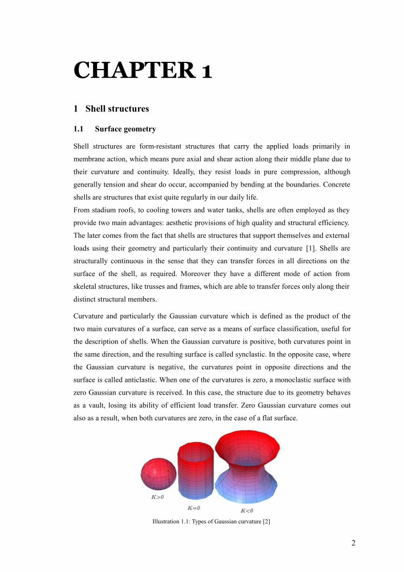
Curvature and particularly the Gaussian curvature which is defined as the product of the
two main curvatures of a surface, can serve as a means of surface classification, useful for
the description of shells. When the Gaussian curvature is positive, both curvatures point in
the same direction, and the resulting surface is called synclastic. In the opposite case, where
the Gaussian curvature is negative, the curvatures point in opposite directions and the
surface is called anticlastic. When one of the curvatures is zero, a monoclastic surface with
zero Gaussian curvature is received. In this case, the structure due to its geometry behaves
as a vault, losing its ability of efficient load transfer. Zero Gaussian curvature comes out
also as a result, when both curvatures are zero, in the case of a flat surface.
2
Illustration 1.1: Types of Gaussian curvature [2]
Surfaces are also classified in a continuous manner according to the way they are developed.
Ruled surfaces are produced by sliding each end of a straight line on their own generating
curve, while retaining the straight line parallel to a prescribed direction or plane. The
generated straight line is not necessarily at right angles to the plane containing the generating
director curves. Translational surfaces are generated by sliding a plane curve along another
plane curve while retaining the orientation of the sliding constant. Finally surfaces of
revolution are pr1oduced by the revolution of a plane curve, the meridional curve, about an
axis, the axis of revolution.
A final distinction of surfaces is done between developable and non-developable surfaces. A
surface is considered developable, when it can be flattened onto a plane without distortion
(i.e. “stretching” or “compressing”). Conversely, they are surfaces that can be generated by
transforming a plane by “folding”, “bending”, “cutting”[4], among other ways, characterized
mathematically by zero curvature. Finally, in three dimensions, all developable surfaces are
ruled surfaces but not vice versa. However, most smooth surfaces are non-developable
surfaces. Non-developable surfaces are referred to as having “double curvature”, “compound
curvature”, or “non-zero Gaussian curvature” Examples of these, are the sphere, the
hyperbolic paraboloid and the hyperboloid.
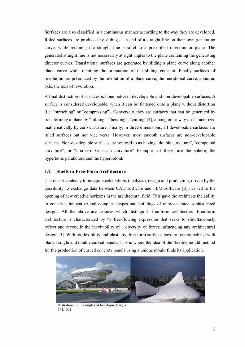
1.2 Shells in Free-Form Architecture
The recent tendency to integrate calculations (analysis), design and production, driven by the
possibility to exchange data between CAD software and FEM software [3] has led to the
opening of new creative horizons in the architectural field. This gave the architects the ability
to construct innovative and complex shapes and buildings of unprecedented sophisticated
designs. All the above are features which distinguish free-form architecture. Free-form
architecture is characterized by “a free-flowing expression that seeks to simultaneously
reflect and reconcile the inevitability of a diversity of forces influencing any architectural
design”[5]. With its flexibility and plasticity, free-form surfaces have to be rationalized with
planar, single and double curved panels. This is where the idea of the flexible mould method
for the production of curved concrete panels using a unique mould finds its application.
3
Illustration 1.2: Examples of free-form designs[54], [53]
A lot of knowledge has been developed to describe the mechanical behavior of
geometrically regular curved surfaces like most shells are formed by, due to the fact that
these surfaces can be described by simple analytical mathematical models [6]. For irregular
curved surfaces however, like the ones that are employed by free-form architecture, very
little analytical mathematical models exist, and the development of formulas is difficult in
order to describe their mechanical behavior. As it was mentioned before, the Finite Element
Analysis software, provide a partial solution to the problem, as they solely provide
quantitative information about the results (like the magnitude of stresses and
displacements),without any qualitative data and graphical and analytical methods have
been developed for the analysis of the shell structural behaviour
1.3 State of Affairs
The emergence of concrete shells dates back to antiquity, with the construction of the still
standing Pantheon in Rome, which was completed about 125 CE [49]. Modern concrete
shells, which began to appear in the 1920s, are made out of thin steel reinforced concrete,
sometimes relying wholly on the shell structure itself [50]. In-plane casting is historically the
most commonly used construction method in shell constructions. Large quantities of timber
formwork supported by a dense wooden or steel scaffolding to keep curvature precise are put
together by high quality carpenters, in a labor intensive procedure [51]. Traditional
construction method of shells makes use of reinforcement bars, which are quickly placed but
has the drawback of needing frequent joints and overlapping. Its bending and assembling is
also considered difficult for curved shapes like shells.
Despite the structural advantage of monolithic shells transferring the loads very efficiently,
and the economical design due to low thickness-to-span ratio, the cost that emerges during
this production method, limits their prevalence in the building environment. The economy is
of great importance, a term that intends to describe the design and construction of the best
building at the least cost. Shells require a minimum of structural materials [15]. The quantity
of concrete and reinforcement are factors that determine the cost. Formworks come next in
importance determining what is possible to build and in certain cases representing up to 60%
of the overall costs of concrete structures.
Different approaches are followed for the construction of modern shell structures. In each
case, certain factors like the economy of the construction, the necessary durability of the shell
and the ease of maintenance of the final structure led to different realization methods and
characteristics of the final structure. Account of these aspects should be thus taken during the
design and the execution of the project. There is no standard procedure and method that is
currently in use. It is also noticed that in large significant projects, where the purpose is the
4
creation of a ‘monument’, economy could not dominate since the production of unique
elements that freeform architecture requires are realized with the use of unique moulds.
Over the years attempts have been made to reduce the construction costs and ease the
construction of shells, mainly on academic level. One of these attempts concerns the
prefabrication of concrete elements. Prefabricating structures is a popular building method,
where manufacturing takes place in a controlled environment, providing at the same time fast
and simple erection on site. Prefabrication for shells means their segmentation in curved
concrete panels, and their subsequent placement and connection at the building site. Benefits
of this type of construction are the higher concrete quality that can be utilized, the higher
building speed and the better logistic organization compared to in-situ cast concrete
structures [42]. Substantial reduction of the costs is, however, not yet achieved for concrete
shells, as the formwork is still very expensive and re-use of the form is only occasionally
possible. Currently prefabricated panels applied for shell structures are produced with
standard fixed formworks. The problem that arises is that for each different element a new
form has to be made, and re-use of this form is almost impossible due to the specific
geometry of each element.
Unless the use of flexible formwork is applied, no financial mitigation is possible. The
original concept for the flexible mould is attributed to the ideas of Renzo Piano. That
involved the placement of a scale model in a machine, where the height of certain points
would be measured. The results would be transferred electronically to a system of vertical
pistons, which will scale up the received measurements, and estimate the exact height.
Subsequently, a mat would be placed on top of the pistons to create a mould Most
developments of the adjustable formwork are based on this idea. The formwork could adapt
its shape, to the required geometry of each single panel comprising the shell. This concept is
based on the principle of deformation of an originally flat sheet of any material into a double
curved surface. More specifically deformation after casting was a concept formed by
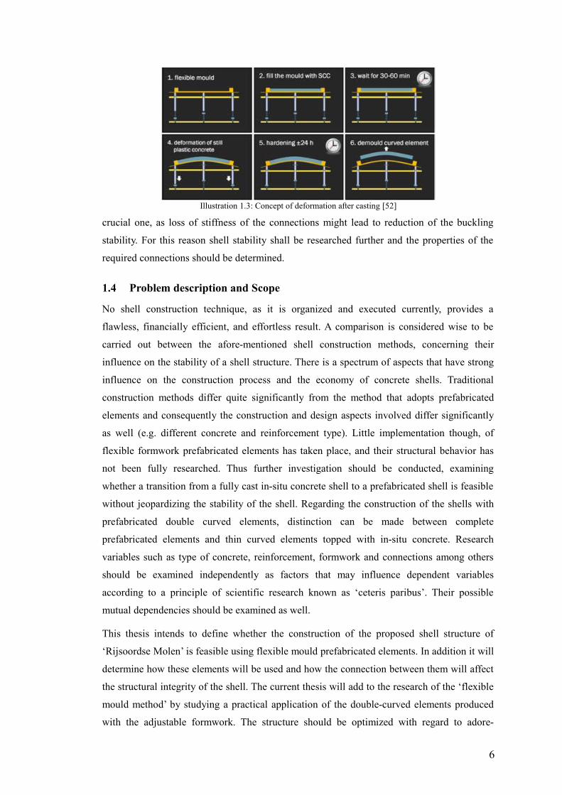
H.R.Schipper(2015) in his PhD study, which includes:
• filling of the flexible mould with self-compacting concrete
• waiting for a period of 30-60 minutes
• deforming the concrete element
• letting the deformed element harden for 24 hours and
• demoulding it.
The flexible mould method proposed by the same author offers a cost-efficient method for the
manufacturing of elements with a reusable mould. Further research is recommended,
addressing different aspects, with the quality and properties of connections being a very
5
crucial one, as loss of stiffness of the connections might lead to reduction of the buckling
stability. For this reason shell stability shall be researched further and the properties of the
required connections should be determined.
1.4 Problem description and Scope
No shell construction technique, as it is organized and executed currently, provides a
flawless, financially efficient, and effortless result. A comparison is considered wise to be
carried out between the afore-mentioned shell construction methods, concerning their
influence on the stability of a shell structure. There is a spectrum of aspects that have strong
influence on the construction process and the economy of concrete shells. Traditional
construction methods differ quite significantly from the method that adopts prefabricated
elements and consequently the construction and design aspects involved differ significantly
as well (e.g. different concrete and reinforcement type). Little implementation though, of
flexible formwork prefabricated elements has taken place, and their structural behavior has
not been fully researched. Thus further investigation should be conducted, examining
whether a transition from a fully cast in-situ concrete shell to a prefabricated shell is feasible
without jeopardizing the stability of the shell. Regarding the construction of the shells with
prefabricated double curved elements, distinction can be made between complete
prefabricated elements and thin curved elements topped with in-situ concrete. Research
variables such as type of concrete, reinforcement, formwork and connections among others
should be examined independently as factors that may influence dependent variables
according to a principle of scientific research known as ‘ceteris paribus’. Their possible
mutual dependencies should be examined as well.
This thesis intends to define whether the construction of the proposed shell structure of
‘Rijsoordse Molen’ is feasible using flexible mould prefabricated elements. In addition it will
determine how these elements will be used and how the connection between them will affect
the structural integrity of the shell. The current thesis will add to the research of the ‘flexible
mould method’ by studying a practical application of the double-curved elements produced
with the adjustable formwork. The structure should be optimized with regard to adore-
6
Illustration 1.3: Concept of deformation after casting [52]

mentioned design and construction aspects, and a solution should be concluded that satisfies
the set criteria, which are the following:
• the structure should satisfy the strength and stiffness requirements for shells.
• the construction and design of the structure should be cost-efficient
• the final design should not diverge greatly from the original design of the architect.
The structural behavior of the shell structure will be analyzed using a finite element analysis
(FEM) program, Diana FEA. One reason for using this software, is that it has already been
used in similar master thesis projects, providing consequently a continuation of the research
and facilitating the comparison of results. It is, furthermore, equipped with powerful solvers
that enable advanced analyses and is utilized by global engineering consultants and research
institutions
7
CHAPTER 2
2 Theory of shells
A lot of theories have been developed for the description of the mechanical behavior of
shells. Among them, a well-known one is the membrane theory, in which it is assumed that
the thickness of the shell is much smaller than the other two dimensions. For this reason its
flexural rigidity is much smaller than its extensional rigidity [3]. Shells are thus structures
that carry the applied loads with membrane action, this is in pure tension and compression
along the middle of the shell thickness. However, bending action is also present, where the
membrane theory does not hold, for example in regions where the extension of shells in
prevented, like the supports. These disturbed zones, where the compatibility moments correct
the thrust line of the structure will be described with the bending theory, which will be also
addressed. It is considered wise to mention the principles of membrane theory,which deals
with the extension of shells and the bending theory which describes the disturbed stress field
of the shells. Initially the membrane theory will be explained, then a simplified method for
deriving the membrane equation will follow for comparison. Finally, the bending theory will
be mentioned.
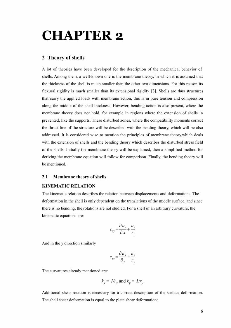
2.1 Membrane theory of shells
KINEMATIC RELATION
The kinematic relation describes the relation between displacements and deformations. The
deformation in the shell is only dependent on the translations of the middle surface, and since
there is no bending, the rotations are not studied. For a shell of an arbitrary curvature, the
kinematic equations are:
ε yy=∂ u x
∂ x+
uz
rx
And in the y direction similarly
ε yy=∂ u y
∂ y
+u z
r y
The curvatures already mentioned are:
kx = 1/rx and ky = 1/ry
Additional shear rotation is necessary for a correct description of the surface deformation.
The shell shear deformation is equal to the plate shear deformation:
8
γ xy=∂ ux
∂y
+∂ u y
∂x
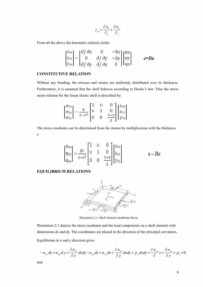
From all the above the kinematic relation yields:
CONSTITUTIVE RELATION
Without any bending, the stresses and strains are uniformly distributed over its thickness.
Furthermore, it is assumed that the shell behaves according to Hooke’s law. Thus the stress
strain relation for the linear elastic shell is described by:
The stress resultants can be determined from the strains by multiplication with the thickness
t:
EQUILIBRIUM RELATIONS
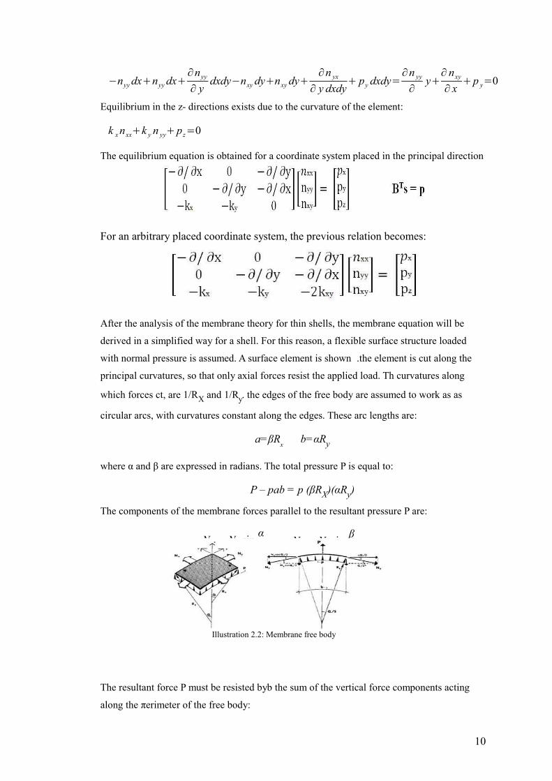
Illustration 2.1 depicts the stress resultants and the load components on a shell element with
dimensions dx and dy. The coordinates are placed in the direction of the principal curvatures.
Equilibrium in x and y direction gives:
−nxx dy+nxx d y+∂ nxx
∂ xdxdy−nxy dx+nxy dx+
∂ nyx
∂ ydxdy+ px dxdy=
∂ nxx
∂x+
∂ nyx
∂ y+ px=0
and
9
Illustration 2.1: Shell element membrane forces
−nyy dx+nyy dx+∂ nyy
∂ ydxdy−nxy dy+nxy dy+
∂ n yx
∂ y dxdy+ py dxdy=
∂ n yy
∂y+
∂ nxy
∂ x+p y=0
Equilibrium in the z- directions exists due to the curvature of the element:
k x nxx+k y n yy+pz=0
The equilibrium equation is obtained for a coordinate system placed in the principal direction
For an arbitrary placed coordinate system, the previous relation becomes:
After the analysis of the membrane theory for thin shells, the membrane equation will be
derived in a simplified way for a shell. For this reason, a flexible surface structure loaded
with normal pressure is assumed. A surface element is shown .the element is cut along the
principal curvatures, so that only axial forces resist the applied load. Th curvatures along
which forces ct, are 1/RX and 1/Ry. the edges of the free body are assumed to work as as
circular arcs, with curvatures constant along the edges. These arc lengths are:
a=βRx b=αRy
where α and β are expressed in radians. The total pressure P is equal to:
P – pab = p (βRX)(αRy)
The components of the membrane forces parallel to the resultant pressure P are:
The resultant force P must be resisted byb the sum of the vertical force components acting
along the πerimeter of the free body:
10
N yv=N y sinα2
N xv=N x sinβ2
Illustration 2.2: Membrane free body
2.2 Bending theory
In regions where the membrane theory does not hold, due to edge disturbances, or for
example in regions of zero Gaussian curvature, bending field components (compatibility
moments) are required to compensate for the limitations of the membrane theory. . This
theory completes the description of the mechanical behavior of shells and will be briefly
explained in the following paragraph. A premise is thus made for the shell in bending, that
its behavior is described with a combination f the shell membrane theory and the bending
theory of plates.
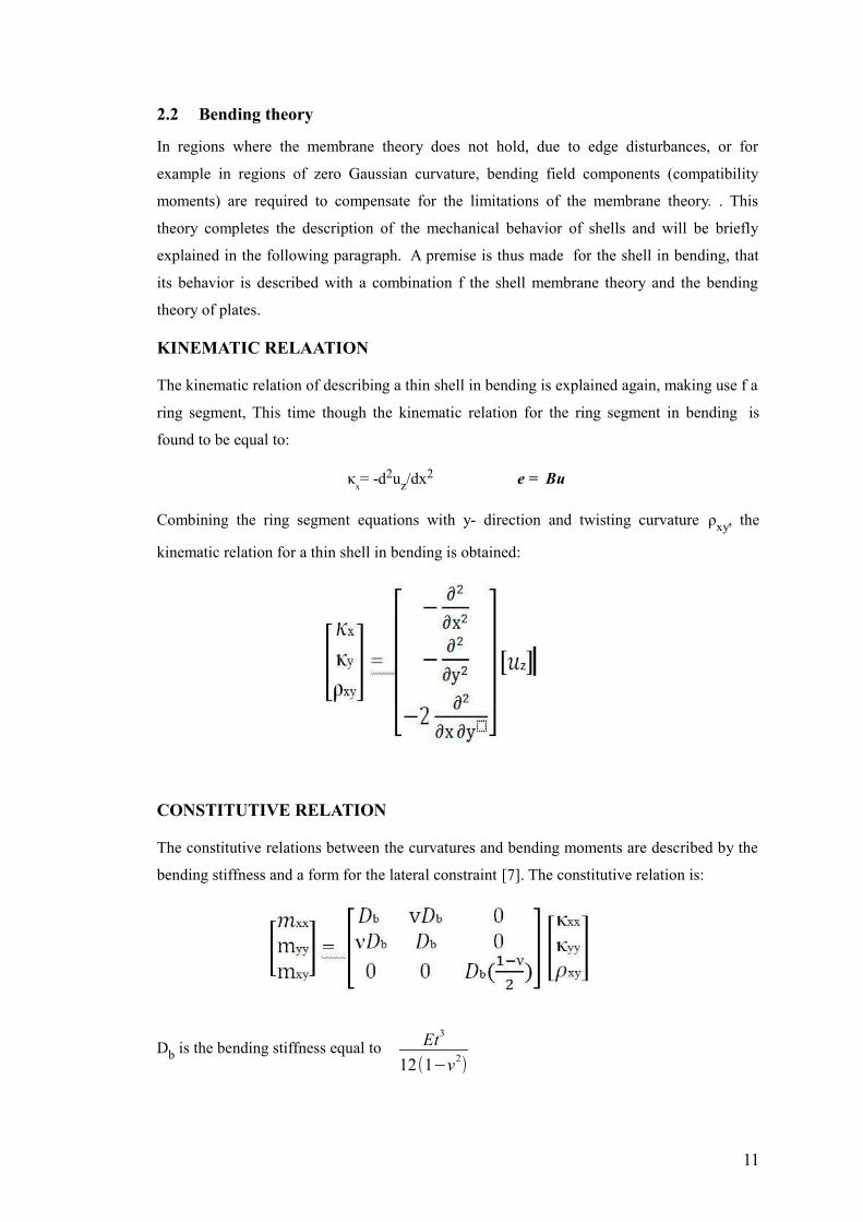
KINEMATIC RELAATION
The kinematic relation of describing a thin shell in bending is explained again, making use f a
ring segment, This time though the kinematic relation for the ring segment in bending is
found to be equal to:
κx= -d2uz/dx2 e = Bu
Combining the ring segment equations with y- direction and twisting curvature ρxy, the
kinematic relation for a thin shell in bending is obtained:
CONSTITUTIVE RELATION
The constitutive relations between the curvatures and bending moments are described by the
bending stiffness and a form for the lateral constraint [7]. The constitutive relation is:
Db is the bending stiffness equal to Et3
12(1−ν2)
11
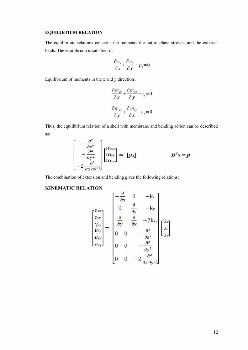
EQUILIBTIUM RELATION
The equilibrium relations concerns the moments the out-of plane stresses and the external
loads. The equilibrium is satisfied if:
∂ υx
∂ x+
∂ υ y
∂ y+ pz=0
Equilibrium of moments in the x and y direction :
∂ mxx
∂ x+
∂ m yx
∂ y−υx=0
∂ m yy
∂ y+
∂ mxy
∂ x−υ y=0
Thus, the equilibrium relation of a shell with membrane and bending action can be described
as:
The combination of extension and bending gives the following relations:
KINEMATIC RELATION
12
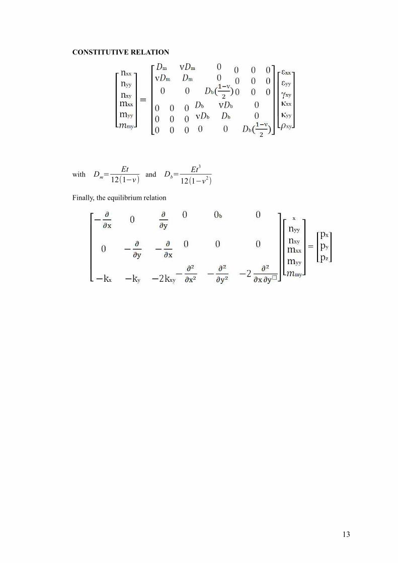
CONSTITUTIVE RELATION
with Dm=Et
12(1−ν )and Db=
Et3
12(1−ν2)
Finally, the equilibrium relation
13
CHAPTER 3
3 Formwork types for concrete shells
3.1 Introduction
In order to realize the reasons for the high costs raised during concrete shell construction, a
description will follow of the current practices and methods. Traditionally the main ways of
constructing concrete shells are:
• Concreting over timber formwork
• Pneumatic formwork
• Ground mounding (Earth mould)
• Polyurethane foam formwork
• Raised steel skeleton method
• 3D-printing (will be included in prefabrication)
• Prefabricated elements, which will be analysed separately
Out of these methods, in-situ casting on timber formwork is applied in most cases and has
been proved to provide high quality structural result, and that is because traditionally timber
formwork have often been associated with concrete structures [8]. This method was
extensively utilized by two famous shell architects of the 20th century, Felix Candela (1910-
1997) and Heinz Isler (1926-2009). By using ruled surfaces, Candela achieved to simplify
formwork, as this meant that his double curved surfaces (hyperbolic paraboloids, conoids,
hyperboloids, cylinders and cones) could be constructed from straight board formwork,
fulfilling moreover the idea of reusability, which otherwise would increase the costs. Isler’s
concrete shells were constructed by casting concrete onto a grid of prepared timber beams,
acting as falsework. The beams were arranged radially or parallel, and should be adjusted to
the right height and position by means of a complicated scaffolding system, which has to
withstand deflections and loads [9].
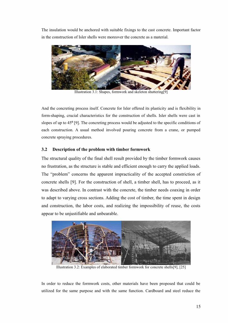
The falsework structure should consequently be lowered in order to allow the removal of the
formwork, which were fixed on it, at centres of approximately 25cm in the form of timber
skeleton boarding. The actual shell membrane would be positioned on the top of the
boarding, concrete would be then laid on the timber membrane, forming the shell itself
(Illustration 3.1). When the weather conditions called for thermal insulation,Isler used
insulation panels as permanent shuttering, in the desired form, which acted as lost formwork.
14
The insulation would be anchored with suitable fixings to the cast concrete. Important factor
in the construction of Isler shells were moreover the concrete as a material.
And the concreting process itself. Concrete for Isler offered its plasticity and is flexibility in
form-shaping, crucial characteristics for the construction of shells. Isler shells were cast in
slopes of up to 45 ⁰ [9]. The concreting process would be adjusted to the specific conditions of
each construction. A usual method involved pouring concrete from a crane, or pumped
concrete spraying procedures.
3.2 Description of the problem with timber formwork
The structural quality of the final shell result provided by the timber formwork causes
no frustration, as the structure is stable and efficient enough to carry the applied loads.
The “problem” concerns the apparent impracticality of the accepted constriction of
concrete shells [9]. For the construction of shell, a timber shell, has to proceed, as it
was described above. In contrast with the concrete, the timber needs coaxing in order
to adapt to varying cross sections. Adding the cost of timber, the time spent in design
and construction, the labor costs, and realizing the impossibility of reuse, the costs
appear to be unjustifiable and unbearable.
In order to reduce the formwork costs, other materials have been proposed that could be
utilized for the same purpose and with the same function. Cardboard and steel reduce the
15
Illustration 3.1: Shapes, formwork and skeleton shuttering[9]
Illustration 3.2: Examples of elaborated timber formwork for concrete shells[9], [25]
formwork costs, and particularly the later offers reusability. Nonetheless, the need to
construct an overpriced framework that does not form a part of the final structure is present.
3.3 Pneumatic inflated formwork
The 1940s saw the developments of pneumatic formwork, as a way of reducing the
construction costs and building speed of concrete shells. In the works of Frei Otto there are
extensive descriptions of the use of pneumatic formwork. Different alternatives exist
concerning their application.
One of them proposes the use of elastic neoprene membranes that when inflated become the
mould on which the casting of concrete will happen. Initially, the membrane is spread flat
across the ground covering the area within the foundation [9]. The reinforcement is
subsequently placed on the membrane, the first layer of concrete is casted, mixed with
hardening retardant substances. Following this, a second membrane is set on top of the
concrete layer. The edges of the membranes are fixed on the footings and the bottom
membrane is inflated. The top membrane keeps the concrete in place. Once the hardening
procedure is completed, the membrane is removed. Waterproofing layer is finally applied.
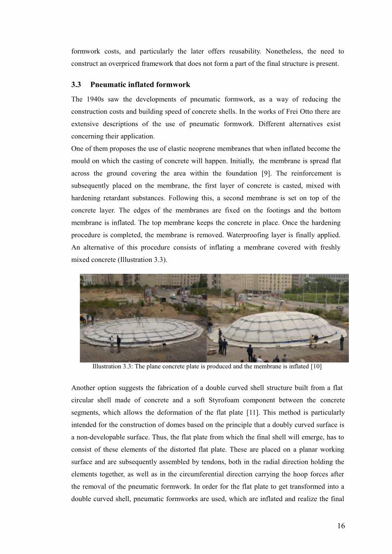
An alternative of this procedure consists of inflating a membrane covered with freshly
mixed concrete (Illustration 3.3).
Another option suggests the fabrication of a double curved shell structure built from a flat
circular shell made of concrete and a soft Styrofoam component between the concrete
segments, which allows the deformation of the flat plate [11]. This method is particularly
intended for the construction of domes based on the principle that a doubly curved surface is
a non-developable surface. Thus, the flat plate from which the final shell will emerge, has to
consist of these elements of the distorted flat plate. These are placed on a planar working
surface and are subsequently assembled by tendons, both in the radial direction holding the
elements together, as well as in the circumferential direction carrying the hoop forces after
the removal of the pneumatic formwork. In order for the flat plate to get transformed into a
double curved shell, pneumatic formworks are used, which are inflated and realize the final
16
Illustration 3.3: The plane concrete plate is produced and the membrane is inflated [10]
shape. The gaps between the elements are grouted and post-tensioned. PVC membrane is
used for the fabrication of the formwork and PVC glue glues parts of this membrane in order
to obtain the required formwork shape. Nowadays, the use of pneumatic formwork is
restricted to the fabrication of synclastic surfaces and particular;y domes. Another issue that
appears with the use of this formwork is the deflections that emerge furring the curing
process and the associated weakening of the concrete.
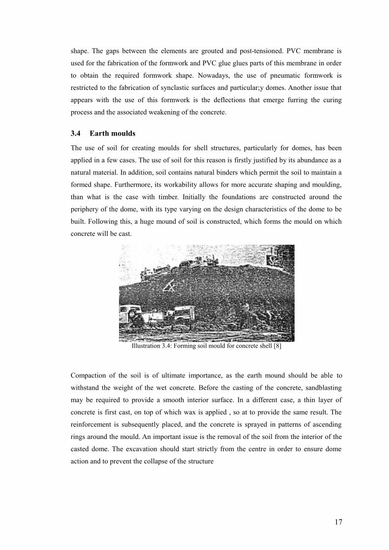
3.4 Earth moulds
The use of soil for creating moulds for shell structures, particularly for domes, has been
applied in a few cases. The use of soil for this reason is firstly justified by its abundance as a
natural material. In addition, soil contains natural binders which permit the soil to maintain a
formed shape. Furthermore, its workability allows for more accurate shaping and moulding,
than what is the case with timber. Initially the foundations are constructed around the
periphery of the dome, with its type varying on the design characteristics of the dome to be
built. Following this, a huge mound of soil is constructed, which forms the mould on which
concrete will be cast.
Compaction of the soil is of ultimate importance, as the earth mound should be able to
withstand the weight of the wet concrete. Before the casting of the concrete, sandblasting
may be required to provide a smooth interior surface. In a different case, a thin layer of
concrete is first cast, on top of which wax is applied , so at to provide the same result. The
reinforcement is subsequently placed, and the concrete is sprayed in patterns of ascending
rings around the mould. An important issue is the removal of the soil from the interior of the
casted dome. The excavation should start strictly from the centre in order to ensure dome
action and to prevent the collapse of the structure
17
Illustration 3.4: Forming soil mould for concrete shell [8]
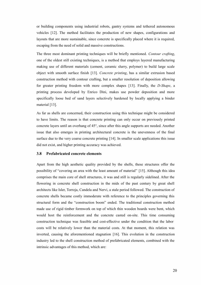
The aforementioned technique can be realized either by constructing the dome around the
mould at its final elevation, or the dome is initially cast on the ground, and then lifted up to
its final elevation in the case of dome roofs [8]. The earth mould should be able to support
the weight of the cast concrete, and for this reason proper soil compaction is essential.
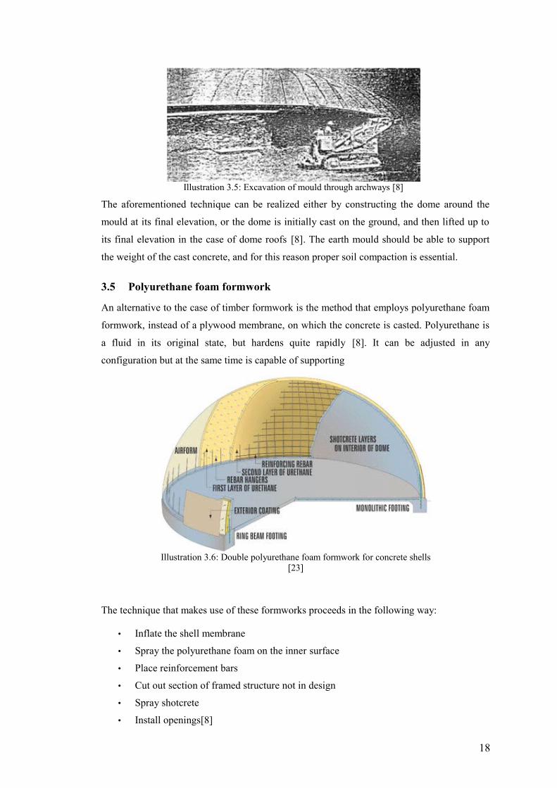
3.5 Polyurethane foam formwork
An alternative to the case of timber formwork is the method that employs polyurethane foam
formwork, instead of a plywood membrane, on which the concrete is casted. Polyurethane is
a fluid in its original state, but hardens quite rapidly [8]. It can be adjusted in any
configuration but at the same time is capable of supporting
The technique that makes use of these formworks proceeds in the following way:
• Inflate the shell membrane
• Spray the polyurethane foam on the inner surface
• Place reinforcement bars
• Cut out section of framed structure not in design
• Spray shotcrete
• Install openings[8]
18
Illustration 3.5: Excavation of mould through archways [8]
Illustration 3.6: Double polyurethane foam formwork for concrete shells[23]
The polyurethane formwork serves this way first as a formwork for the structure, and then t
gets integrated in the construction, functioning as thermal and sound insulation reducing
substantially the construction costs.
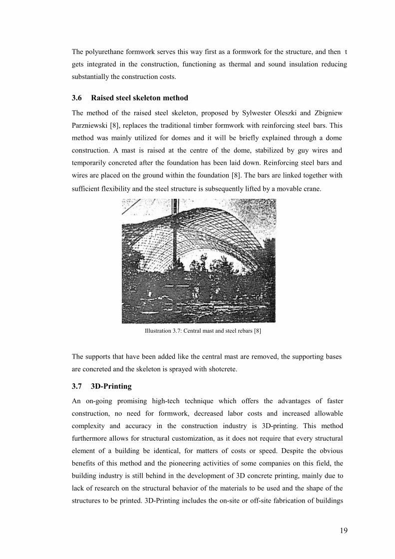
3.6 Raised steel skeleton method
The method of the raised steel skeleton, proposed by Sylwester Oleszki and Zbigniew
Parzniewski [8], replaces the traditional timber formwork with reinforcing steel bars. This
method was mainly utilized for domes and it will be briefly explained through a dome
construction. A mast is raised at the centre of the dome, stabilized by guy wires and
temporarily concreted after the foundation has been laid down. Reinforcing steel bars and
wires are placed on the ground within the foundation [8]. The bars are linked together with
sufficient flexibility and the steel structure is subsequently lifted by a movable crane.
The supports that have been added like the central mast are removed, the supporting bases
are concreted and the skeleton is sprayed with shotcrete.
3.7 3D-Printing
An on-going promising high-tech technique which offers the advantages of faster
construction, no need for formwork, decreased labor costs and increased allowable
complexity and accuracy in the construction industry is 3D-printing. This method
furthermore allows for structural customization, as it does not require that every structural
element of a building be identical, for matters of costs or speed. Despite the obvious
benefits of this method and the pioneering activities of some companies on this field, the
building industry is still behind in the development of 3D concrete printing, mainly due to
lack of research on the structural behavior of the materials to be used and the shape of the
structures to be printed. 3D-Printing includes the on-site or off-site fabrication of buildings
19
Illustration 3.7: Central mast and steel rebars [8]
or building components using industrial robots, gantry systems and tethered autonomous
vehicles [12]. The method facilitates the production of new shapes, configurations and
layouts that are more sustainable, since concrete is specifically placed where it is required,
escaping from the need of solid and massive constructions.
The three most dominant printing techniques will be briefly mentioned. Contour crafting,
one of the oldest still existing techniques, is a method that employs layered manufacturing
making use of different materials (cement, ceramic slurry, polymer) to build large scale
object with smooth surface finish [13]. Concrete printing, has a similar extrusion based
construction method with contour crafting, but a smaller resolution of deposition allowing
for greater printing freedom with more complex shapes [13]. Finally, the D-Shape, a
printing process developed by Enrico Dini, makes use powder deposition and more
specifically loose bed of sand layers selectively hardened by locally applying a binder
material [13].
As far as shells are concerned, their construction using this technique might be considered
to have limits. The reason is that concrete printing can only occur on previously printed
concrete layers until an overhang of 45°, since after this angle supports are needed. Another
issue that also emerges in printing architectural concrete is the unevenness of the final
surface due to the very coarse concrete printing [14]. In smaller scale applications this issue
did not exist, and higher printing accuracy was achieved.
3.8 Prefabricated concrete elements
Apart from the high aesthetic quality provided by the shells, these structures offer the
possibility of “covering an area with the least amount of material” [15]. Although this idea
comprises the main core of shell structures, it was and still is regularly sidelined. After the
flowering in concrete shell construction in the mids of the past century by great shell
architects like Isler, Torroja, Candela and Nervi, a stale period followed. The construction of
concrete shells became costly immoderate with reference to the principles governing this
structural form and the “construction boom” ended. The traditional construction method
made use of rigid timber formwork on top of which thin wooden boards were bent, which
would host the reinforcement and the concrete casted on-site. This time consuming
construction technique was feasible and cost-effective under the condition that the labor
costs will be relatively lower than the material costs. At that moment, this relation was
inverted, causing the aforementioned stagnation [16]. This evolution in the construction
industry led to the shell construction method of prefabricated elements, combined with the
intrinsic advantages of this method, which are:
20
• concrete of better quality is produced, as the manufacturing conditions are under
control in a factory environment
• complex shapes can be realized with high accuracy levels
• the prefabricated structure can be disassembled and the elements be suitably used
elsewhere
• higher construction speed is achieved than cast in-situ concrete
• the labour needed for the construction of the prefabricated elements can easily be
trained
• weather is excluded as an influencing factor on the building process
• particularly for the case of shell structures, the quantity of the required falsework and
scaffolding is substantially reduced
• better logistic organization than cast in-situ concrete
Over the past decade though, extensive progress has been realized in digitizing design and
fabrication processes, enabling the analysis of complex geometries under consideration of
multiple boundary conditions [16]. Developments in computation, storage, handling and
cross-linking of digital information, allow for the integration to one process of activities
starting from planning until the fabrication of the structure, due to the possibility of
exchanging data between CAD-program (Computer Aided Design) and FEM-program (Finite
Element Analysis). Further improvements have also occurred in the sector of material
science, particularly on cementitious materials leading to composite materials with high
tensile and bending tensile strength.
The technological progress mentioned before led architects and followingly engineers to the
design and construction of complex shapes and configurations like the ones employed by
free-form architecture, which behave like shells. This means that their structural behavior
consists mainly of extensional forces and some bending moments due to edge disturbances.
On the other hand, scientists try to rationalise the large-scale intricate surfaces with planar,
single, double- curved panels. The construction of these panels entails the fabrication of
unique moulds, singly used in most cases. The purpose of the adjustable formwork lies
exactly on the point of reducing the mould fabrication, since this is what governs the panel
cost.
3.9 Moulds for prefabricated concrete elements-Methods of construction
3.9.1 Timber moulds
Apart from their use in cast in-situ shell construction, timber formworks are used for the
fabrication of concrete panels. As an example, a case study where implementation of timber
formwork for the construction of prefabricated concrete panels took place, will be mentioned.
21
This case study concerns the construction of the Rolex Learning Centre in Lausanne, where
formwork tables of 2.50 x 5.50 m were constructed in factory by labor [17]. CNC-milling
was also used for the fabrication of timber formwork. Each table consisted of two beams on
which OSB plates were fixed. On top these plates, the final formwork on which the concrete
would be cast were placed, consisting of 10cm wide wooden planks and a laminated
chipboard nailed on these plates[17]. This final surface testified the final curves of the shell.
Reusability of these moulds could be feasible by disassembling the formworks. When proper
surface protection is provided, the moulds are reusable, but their lack of flexibility does not
permit the use for different shapes [14].
3.9.2 Steel moulds
Steel moulds have been quite regularly utilised for the production of ceiling and wall panels
or for entire structural parts like beams and supports, providing high accuracy in complex de-
signs. Their resistance to wear allows for a high degree of repetition, compensating for their
high costs [18]. However for curved elements, steel moulds are much less frequently em-
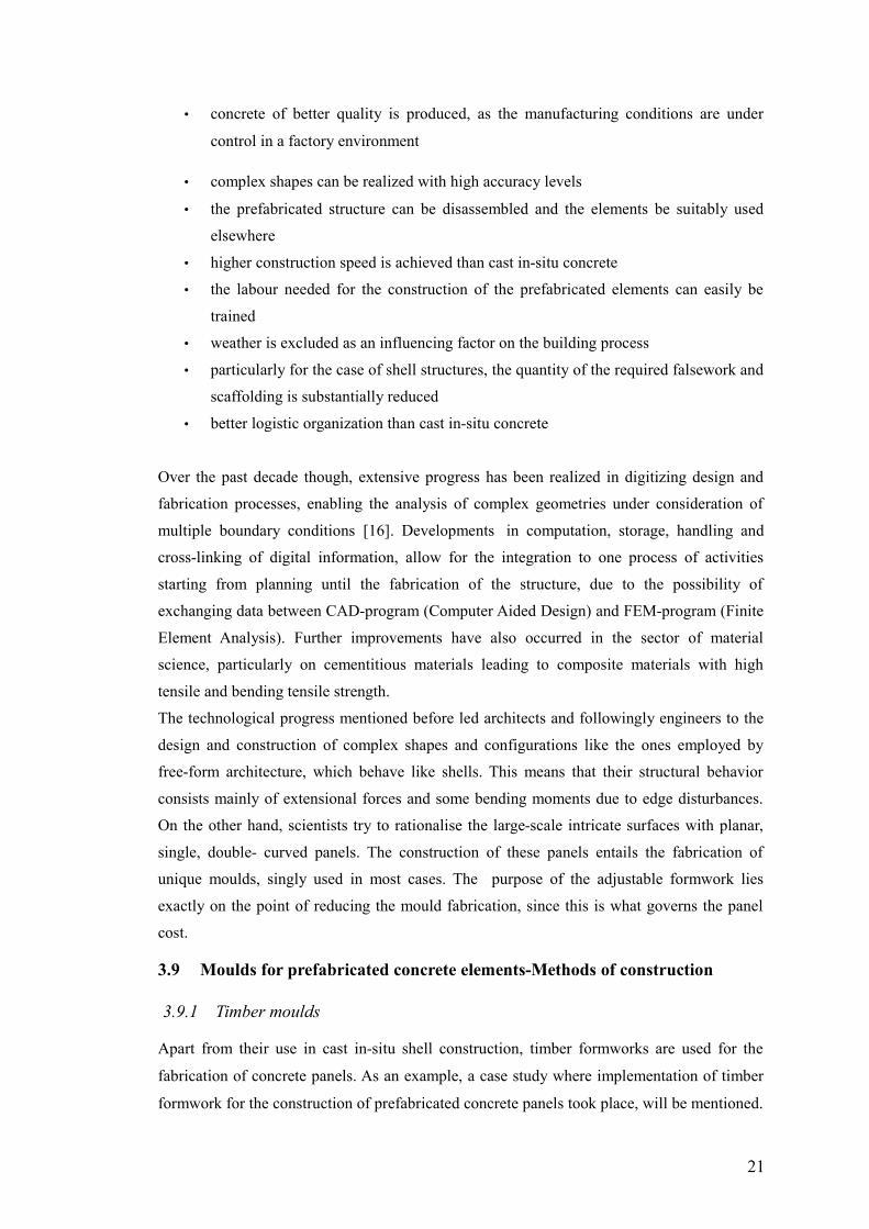
ployed. A prominent example, where fabrication of concrete elements by steel moulds took
place is the Jubilee church in Rome. Known as La Chiesa del Dio Padre Misericordioso in
Italian, this church was a part of pope John Paul II's millennium initiative to rejuvenate parish
life in Italy [19]. It was inaugurated in 2003, and it is American architect's Richard Meier's
first church. The most distinctive feature of the church is the three curved shells walls that
reach a height of 27,5 m above the building, made from prefabricated concrete elements with
a marble;like finish, reinforced with steel and held together by post-tensioned cables
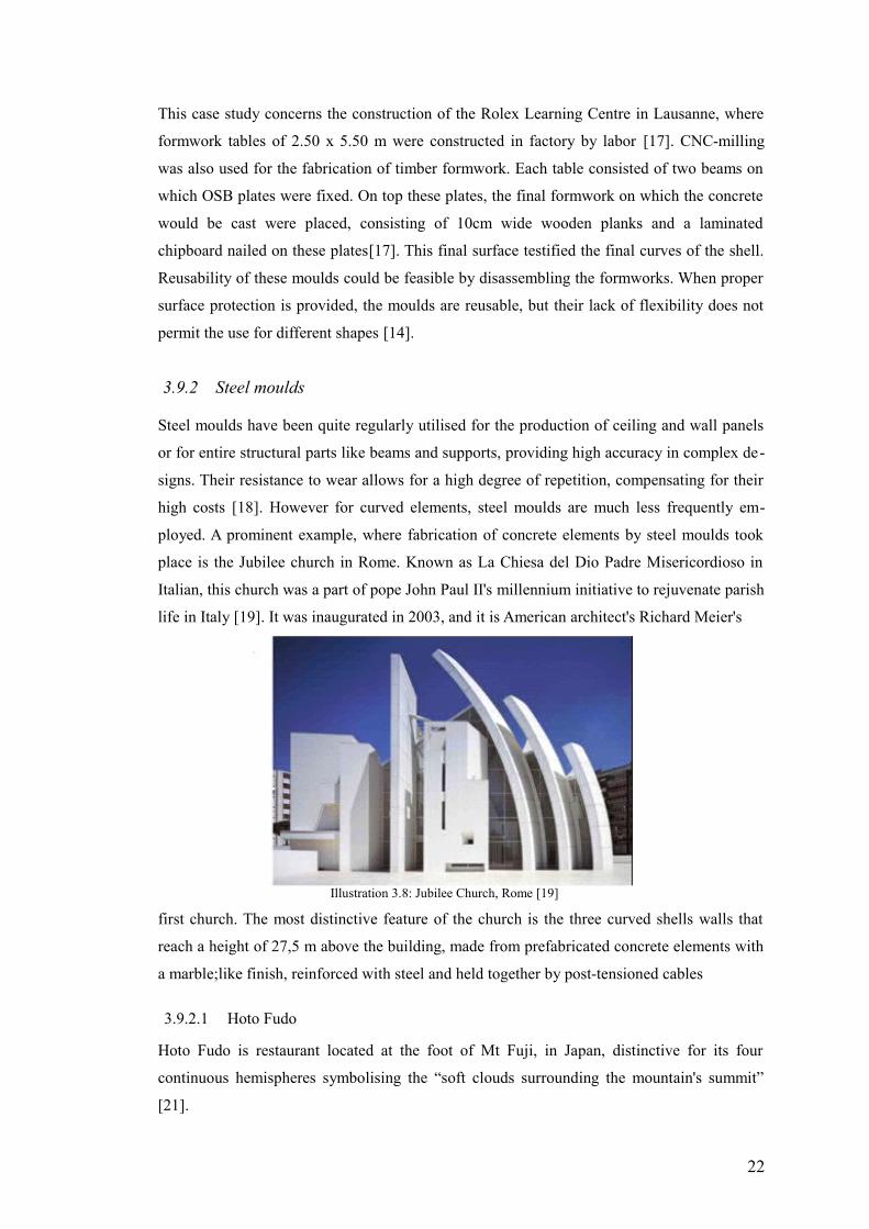
3.9.2.1 Hoto Fudo
Hoto Fudo is restaurant located at the foot of Mt Fuji, in Japan, distinctive for its four
continuous hemispheres symbolising the “soft clouds surrounding the mountain's summit”
[21].
22
Illustration 3.8: Jubilee Church, Rome [19]
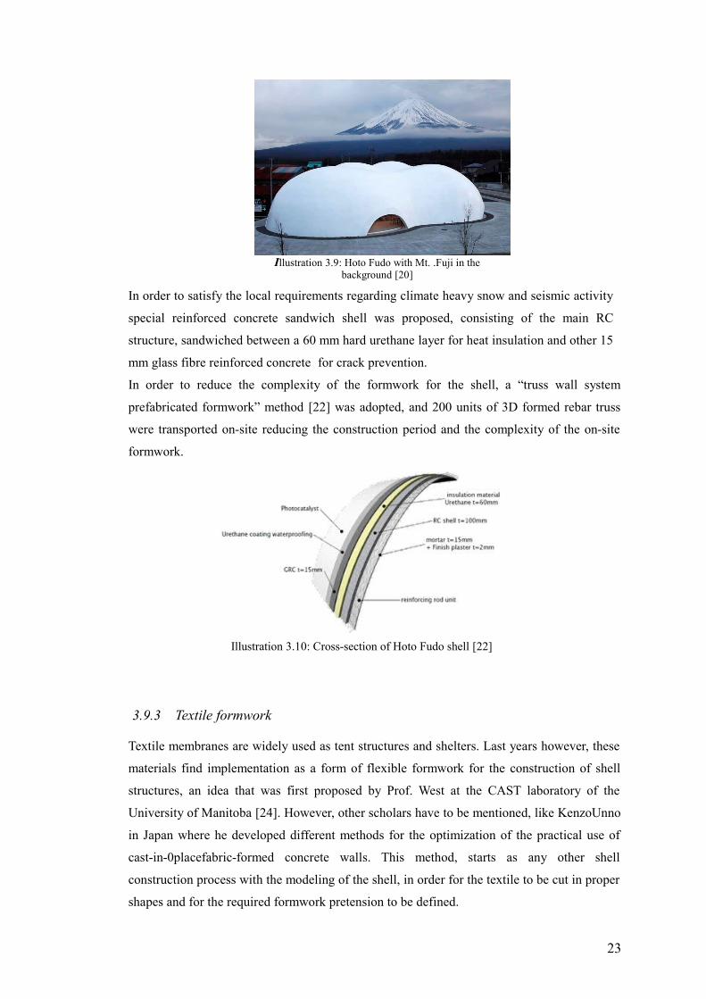
In order to satisfy the local requirements regarding climate heavy snow and seismic activity
special reinforced concrete sandwich shell was proposed, consisting of the main RC
structure, sandwiched between a 60 mm hard urethane layer for heat insulation and other 15
mm glass fibre reinforced concrete for crack prevention.
In order to reduce the complexity of the formwork for the shell, a “truss wall system
prefabricated formwork” method [22] was adopted, and 200 units of 3D formed rebar truss
were transported on-site reducing the construction period and the complexity of the on-site
formwork.
3.9.3 Textile formwork
Textile membranes are widely used as tent structures and shelters. Last years however, these
materials find implementation as a form of flexible formwork for the construction of shell
structures, an idea that was first proposed by Prof. West at the CAST laboratory of the
University of Manitoba [24]. However, other scholars have to be mentioned, like KenzoUnno
in Japan where he developed different methods for the optimization of the practical use of
cast-in-0placefabric-formed concrete walls. This method, starts as any other shell
construction process with the modeling of the shell, in order for the textile to be cut in proper
shapes and for the required formwork pretension to be defined.
23
Illustration 3.9: Hoto Fudo with Mt. .Fuji in thebackground [20]
Illustration 3.10: Cross-section of Hoto Fudo shell [22]
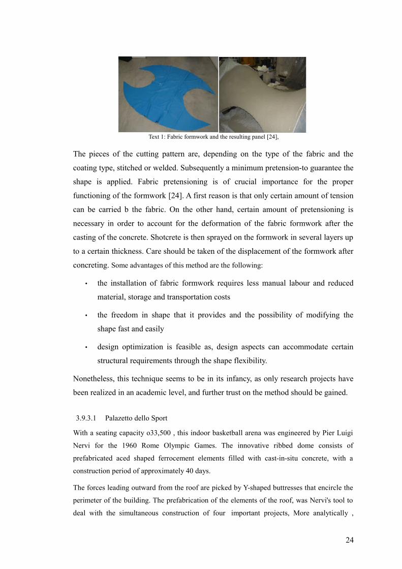
The pieces of the cutting pattern are, depending on the type of the fabric and the
coating type, stitched or welded. Subsequently a minimum pretension-to guarantee the
shape is applied. Fabric pretensioning is of crucial importance for the proper
functioning of the formwork [24]. A first reason is that only certain amount of tension
can be carried b the fabric. On the other hand, certain amount of pretensioning is
necessary in order to account for the deformation of the fabric formwork after the
casting of the concrete. Shotcrete is then sprayed on the formwork in several layers up
to a certain thickness. Care should be taken of the displacement of the formwork after
concreting. Some advantages of this method are the following:
• the installation of fabric formwork requires less manual labour and reduced
material, storage and transportation costs
• the freedom in shape that it provides and the possibility of modifying the
shape fast and easily
• design optimization is feasible as, design aspects can accommodate certain
structural requirements through the shape flexibility.
Nonetheless, this technique seems to be in its infancy, as only research projects have
been realized in an academic level, and further trust on the method should be gained.
3.9.3.1 Palazetto dello Sport
With a seating capacity o33,500 , this indoor basketball arena was engineered by Pier Luigi
Nervi for the 1960 Rome Olympic Games. The innovative ribbed dome consists of
prefabricated aced shaped ferrocement elements filled with cast-in-situ concrete, with a
construction period of approximately 40 days.
The forces leading outward from the roof are picked by Y-shaped buttresses that encircle the
perimeter of the building. The prefabrication of the elements of the roof, was Nervi's tool to
deal with the simultaneous construction of four important projects, More analytically ,
24
Text 1: Fabric formwork and the resulting panel [24],
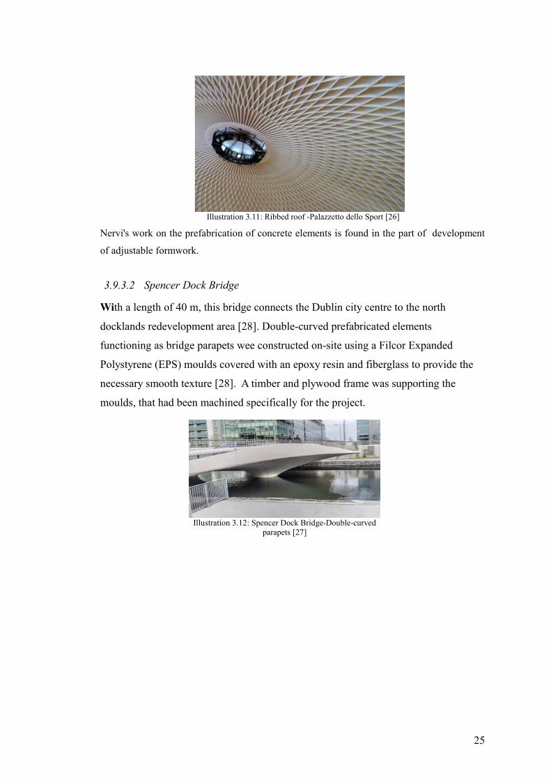
Nervi's work on the prefabrication of concrete elements is found in the part of development
of adjustable formwork.
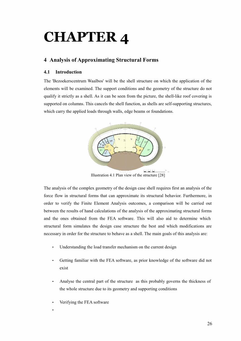
3.9.3.2 Spencer Dock Bridge
With a length of 40 m, this bridge connects the Dublin city centre to the north
docklands redevelopment area [28]. Double-curved prefabricated elements
functioning as bridge parapets wee constructed on-site using a Filcor Expanded
Polystyrene (EPS) moulds covered with an epoxy resin and fiberglass to provide the
necessary smooth texture [28]. A timber and plywood frame was supporting the
moulds, that had been machined specifically for the project.
25
Illustration 3.11: Ribbed roof -Palazzetto dello Sport [26]
Illustration 3.12: Spencer Dock Bridge-Double-curvedparapets [27]
CHAPTER 4
4 Analysis of Approximating Structural Forms
4.1 Introduction
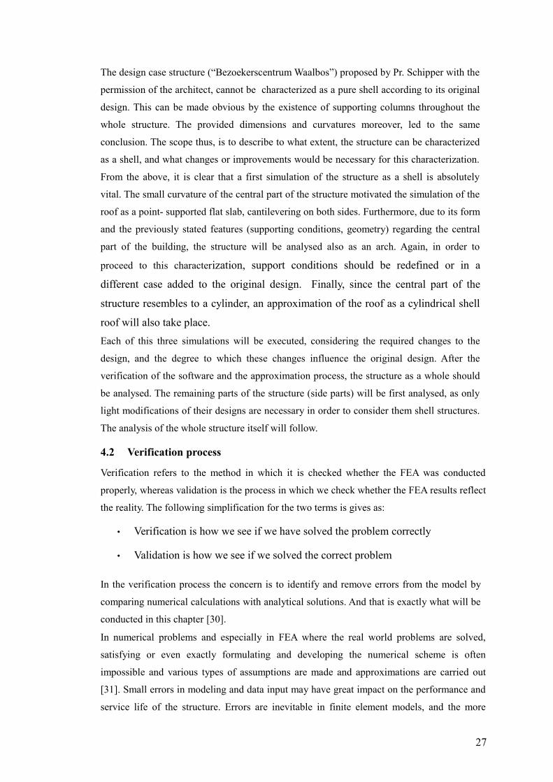
The 'Bezoekerscentrum Waalbos' will be the shell structure on which the application of the
elements will be examined. The support conditions and the geometry of the structure do not
qualify it strictly as a shell. As it can be seen from the picture, the shell-like roof covering is
supported on columns. This cancels the shell function, as shells are self-supporting structures,
which carry the applied loads through walls, edge beams or foundations.
The analysis of the complex geometry of the design case shell requires first an analysis of the
force flow in structural forms that can approximate its structural behavior. Furthermore, in
order to verify the Finite Element Analysis outcomes, a comparison will be carried out
between the results of hand calculations of the analysis of the approximating structural forms
and the ones obtained from the FEA software. This will also aid to determine which
structural form simulates the design case structure the best and which modifications are
necessary in order for the structure to behave as a shell. The main goals of this analysis are:
• Understanding the load transfer mechanism on the current design
• Getting familiar with the FEA software, as prior knowledge of the software did not
exist
• Analyse the central part of the structure as this probably governs the thickness of
the whole structure due to its geometry and supporting conditions
• Verifying the FEA software
•
26
Illustration 4.1 Plan view of the structure [28]
The design case structure (“Bezoekerscentrum Waalbos”) proposed by Pr. Schipper with the
permission of the architect, cannot be characterized as a pure shell according to its original
design. This can be made obvious by the existence of supporting columns throughout the
whole structure. The provided dimensions and curvatures moreover, led to the same
conclusion. The scope thus, is to describe to what extent, the structure can be characterized
as a shell, and what changes or improvements would be necessary for this characterization.
From the above, it is clear that a first simulation of the structure as a shell is absolutely
vital. The small curvature of the central part of the structure motivated the simulation of the
roof as a point- supported flat slab, cantilevering on both sides. Furthermore, due to its form
and the previously stated features (supporting conditions, geometry) regarding the central
part of the building, the structure will be analysed also as an arch. Again, in order to
proceed to this characterization, support conditions should be redefined or in a
different case added to the original design. Finally, since the central part of the
structure resembles to a cylinder, an approximation of the roof as a cylindrical shell
roof will also take place.
Each of this three simulations will be executed, considering the required changes to the
design, and the degree to which these changes influence the original design. After the
verification of the software and the approximation process, the structure as a whole should
be analysed. The remaining parts of the structure (side parts) will be first analysed, as only
light modifications of their designs are necessary in order to consider them shell structures.
The analysis of the whole structure itself will follow.
4.2 Verification process
Verification refers to the method in which it is checked whether the FEA was conducted
properly, whereas validation is the process in which we check whether the FEA results reflect
the reality. The following simplification for the two terms is gives as:
• Verification is how we see if we have solved the problem correctly
• Validation is how we see if we solved the correct problem
In the verification process the concern is to identify and remove errors from the model by
comparing numerical calculations with analytical solutions. And that is exactly what will be
conducted in this chapter [30].
In numerical problems and especially in FEA where the real world problems are solved,
satisfying or even exactly formulating and developing the numerical scheme is often
impossible and various types of assumptions are made and approximations are carried out
[31]. Small errors in modeling and data input may have great impact on the performance and
service life of the structure. Errors are inevitable in finite element models, and the more
27
complex the model, that higher the chance the they will occur. The important thing is to
put a process in place to detect them before any damage occurs. The analysis must
begin with clearly defined goals, accuracy requirements and key assumptions. Some
typical items that this process has to contain are:
• Do key model dimensions agree with actual dimensions?
• Are the material properties correct and are they associated properly to model
elements?
• Are the elements properly connected with interface elements?
• Is the mesh sufficiently refined to provide the required accuracy? Are the element
formulations consistent with the application?
• Are the elements properties correct and are they associated properly to model
elements?
• Does the self-weight produce the expected reaction forces as first indicator?
• Do the reaction forces balance the applied loads in each direction?
• Are the deformations and stresses realistic, and are they compared with hand
calculations?
Most of these questions have been intrinsically set and answered in this chapter in order to
execute the verification process. More analytically, the results are presented in the following
paragraphs.
4.3 Loads
Before proceeding to the analysis of the structure, the acting loads should be determined.
Different load combinations will be examined, as it is not known in advance which load case
will challenge the structure. The applied loads are categorised into groups of permanent,
variable, accidental and time-dependent. Time dependent loads such as creep, shrinkage and
temperature gradients are not considered for simplification reasons, although their effect on
the structure might be severe. The same is valid for the accidental loads, since the purpose of
the analysis of this chapter is restricted to preliminary design.
4.3.1 Permanent loads
The permanent loads for the construction consist of the dead weight of the structure, and
additional weight produced by possible finishing, such as insulation or cladding. However, it
is assumed that the shell does not contain any finishing, thus the extra covering load is not
taken into account. The dead weight is calculated by multiplying the shell thickness with the
28
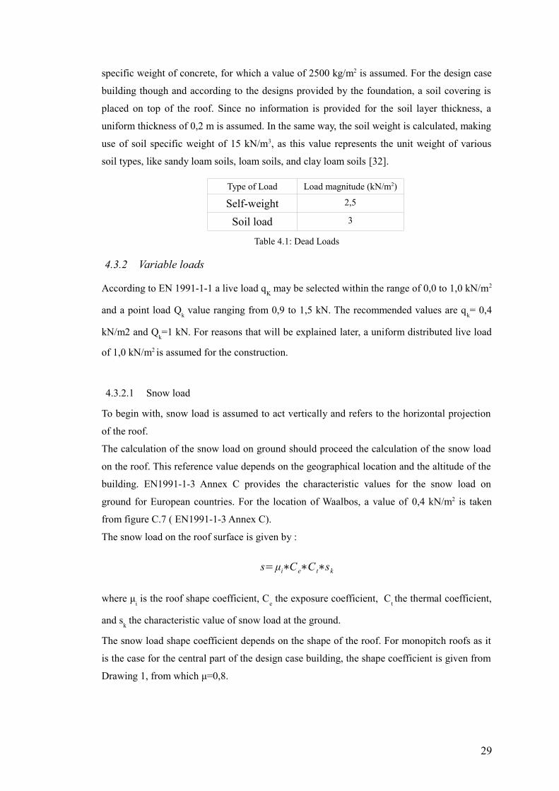
specific weight of concrete, for which a value of 2500 kg/m2 is assumed. For the design case
building though and according to the designs provided by the foundation, a soil covering is
placed on top of the roof. Since no information is provided for the soil layer thickness, a
uniform thickness of 0,2 m is assumed. In the same way, the soil weight is calculated, making
use of soil specific weight of 15 kN/m3, as this value represents the unit weight of various
soil types, like sandy loam soils, loam soils, and clay loam soils [32].
Type of Load Load magnitude (kN/m2)
Self-weight 2,5
Soil load 3
Table 4.1: Dead Loads
4.3.2 Variable loads
According to EN 1991-1-1 a live load qK may be selected within the range of 0,0 to 1,0 kN/m2
and a point load Qk value ranging from 0,9 to 1,5 kN. The recommended values are q
k= 0,4
kN/m2 and Qk=1 kN. For reasons that will be explained later, a uniform distributed live load
of 1,0 kN/m2 is assumed for the construction.
4.3.2.1 Snow load
To begin with, snow load is assumed to act vertically and refers to the horizontal projection
of the roof.
The calculation of the snow load on ground should proceed the calculation of the snow load
on the roof. This reference value depends on the geographical location and the altitude of the
building. EN1991-1-3 Annex C provides the characteristic values for the snow load on
ground for European countries. For the location of Waalbos, a value of 0,4 kN/m2 is taken
from figure C.7 ( EN1991-1-3 Annex C).
The snow load on the roof surface is given by :
s=μi∗C e∗C t∗sk
where μi is the roof shape coefficient, C
e the exposure coefficient, C
t the thermal coefficient,
and sk the characteristic value of snow load at the ground.
The snow load shape coefficient depends on the shape of the roof. For monopitch roofs as it
is the case for the central part of the design case building, the shape coefficient is given from
Drawing 1, from which μ=0,8.
29
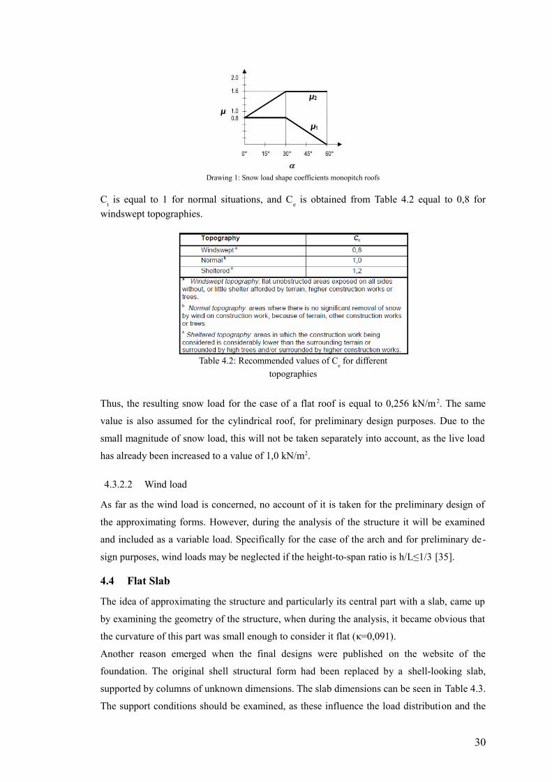
Ct is equal to 1 for normal situations, and C
e is obtained from Table 4.2 equal to 0,8 for
windswept topographies.
Thus, the resulting snow load for the case of a flat roof is equal to 0,256 kN/m 2. The same
value is also assumed for the cylindrical roof, for preliminary design purposes. Due to the
small magnitude of snow load, this will not be taken separately into account, as the live load
has already been increased to a value of 1,0 kN/m2.
4.3.2.2 Wind load
As far as the wind load is concerned, no account of it is taken for the preliminary design of
the approximating forms. However, during the analysis of the structure it will be examined
and included as a variable load. Specifically for the case of the arch and for preliminary de-
sign purposes, wind loads may be neglected if the height-to-span ratio is h/L≤1/3 [35].
4.4 Flat Slab
The idea of approximating the structure and particularly its central part with a slab, came up
by examining the geometry of the structure, when during the analysis, it became obvious that
the curvature of this part was small enough to consider it flat (κ=0,091).
Another reason emerged when the final designs were published on the website of the
foundation. Τhe original shell structural form had been replaced by a shell-looking slab,
supported by columns of unknown dimensions. The slab dimensions can be seen in Table 4.3.
The support conditions should be examined, as these influence the load distribution and the
30
Drawing 1: Snow load shape coefficients monopitch roofs
Table 4.2: Recommended values of Ce for different
topographies
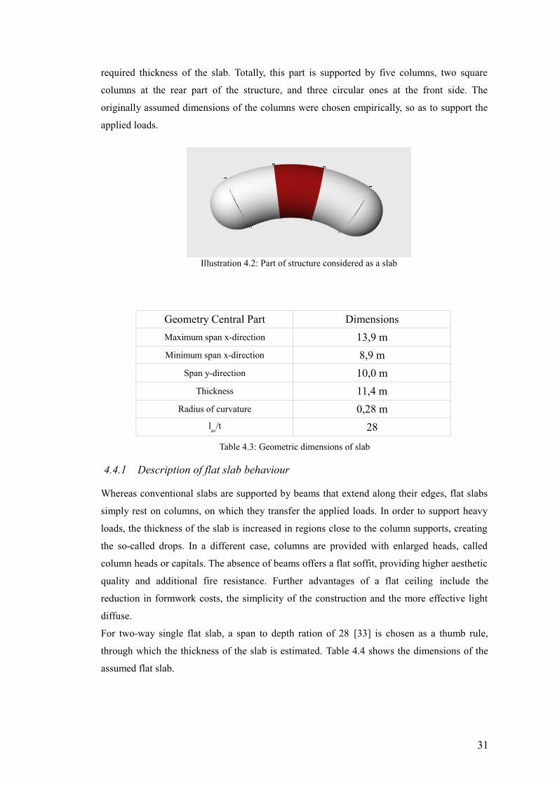
required thickness of the slab. Totally, this part is supported by five columns, two square
columns at the rear part of the structure, and three circular ones at the front side. The
originally assumed dimensions of the columns were chosen empirically, so as to support the
applied loads.
Geometry Central Part Dimensions
Maximum span x-direction 13,9 m
Minimum span x-direction 8,9 m
Span y-direction 10,0 m
Thickness 11,4 m
Radius of curvature 0,28 m
lav
/t 28
Table 4.3: Geometric dimensions of slab
4.4.1 Description of flat slab behaviour
Whereas conventional slabs are supported by beams that extend along their edges, flat slabs
simply rest on columns, on which they transfer the applied loads. In order to support heavy
loads, the thickness of the slab is increased in regions close to the column supports, creating
the so-called drops. In a different case, columns are provided with enlarged heads, called
column heads or capitals. The absence of beams offers a flat soffit, providing higher aesthetic
quality and additional fire resistance. Further advantages of a flat ceiling include the
reduction in formwork costs, the simplicity of the construction and the more effective light
diffuse.
For two-way single flat slab, a span to depth ration of 28 [33] is chosen as a thumb rule,
through which the thickness of the slab is estimated. Table 4.4 shows the dimensions of the
assumed flat slab.
31
Illustration 4.2: Part of structure considered as a slab
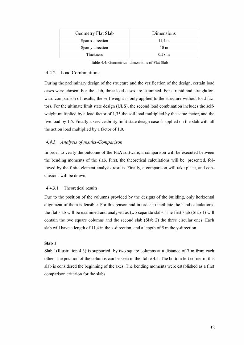
Geometry Flat Slab Dimensions
Span x-direction 11,4 m
Span-y direction 10 m
Thickness 0,28 m
Table 4.4: Geometrical dimensions of Flat Slab
4.4.2 Load Combinations
During the preliminary design of the structure and the verification of the design, certain load
cases were chosen. For the slab, three load cases are examined. For a rapid and straightfor -
ward comparison of results, the self-weight is only applied to the structure without load fac -
tors. For the ultimate limit state design (ULS), the second load combination includes the self-
weight multiplied by a load factor of 1,35 the soil load multiplied by the same factor, and the
live load by 1,5. Finally a serviceability limit state design case is applied on the slab with all
the action load multiplied by a factor of 1,0.
4.4.3 Analysis of results-Comparison
In order to verify the outcome of the FEA software, a comparison will be executed between
the bending moments of the slab. First, the theoretical calculations will be presented, fol -
lowed by the finite element analysis results. Finally, a comparison will take place, and con-
clusions will be drawn.
4.4.3.1 Theoretical results
Due to the position of the columns provided by the designs of the building, only horizontal
alignment of them is feasible. For this reason and in order to facilitate the hand calculations,
the flat slab will be examined and analysed as two separate slabs. The first slab (Slab 1) will
contain the two square columns and the second slab (Slab 2) the three circular ones. Each
slab will have a length of 11,4 in the x-direction, and a length of 5 m the y-direction.
Slab 1
Slab 1(Illustration 4.3) is supported by two square columns at a distance of 7 m from each
other. The position of the columns can be seen in the Table 4.5. The bottom left corner of this
slab is considered the beginning of the axes. The bending moments were established as a first
comparison criterion for the slabs.
32
Column Position x-direction Position y-direction
SQ1 2,05 2,85
SQ2 9,05 2,85
Table 4.5: Position of square columns in Slab1
For a flat slab supported by two columns, formulas are provided for the calculation of bend-
ing moments, shown in Illustration 4.4.
The application of these formulas results in the bending moments at the width of the columns
strip, which in this case is 2l x
4=2
74=3,5m . For this reason, the resulting moments
should be divided by the strip width of 3,5 m, in order to obtain the design moment for 1 m
wide strip of the slab (Table 4.6).
Mxx
(kNm) LC1 LC2 LC3
Left support -30,17 -90,51 -69,4
Middle span 15,08 45,26 34,69
Right support -30,17 -90,51 -69,4
Table 4.6: Bending moments of Slab1 per meter of strip Theoretical results
33
Illustration 4.4: Bending moments in a flat slabsupported by 2 columns [34]
Illustration 4.3: Slab 1
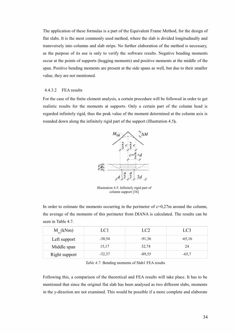
The application of these formulas is a part of the Equivalent Frame Method, for the design of
flat slabs. It is the most commonly used method, where the slab is divided longitudinally and
transversely into columns and slab strips. No further elaboration of the method is necessary,
as the purpose of its use is only to verify the software results. Negative bending moments
occur at the points of supports (hogging moments) and positive moments at the middle of the
span. Positive bending moments are present at the side spans as well, but due to their smaller
value, they are not mentioned.
4.4.3.2 FEA results
For the case of the finite element analysis, a certain procedure will be followed in order to get
realistic results for the moments at supports. Only a certain part of the column head is
regarded infinitely rigid, thus the peak value of the moment determined at the column axis is
rounded down along the infinitely rigid part of the support (Illustration 4.5).
In order to estimate the moments occurring in the perimeter of c=0,27m around the column,
the average of the moments of this perimeter from DIANA is calculated. The results can be
seen in Table 4.7.
Mxx
(kNm) LC1 LC2 LC3
Left support -30,54 -91,36 -65,16
Middle span 15,17 32,74 24
Right support -32,37 -89,55 -65,7
Table 4.7: Bending moments of Slab1 FEA results
Following this, a comparison of the theoretical and FEA results will take place. It has to be
mentioned that since the original flat slab has been analysed as two different slabs, moments
in the y-direction are not examined. This would be possible if a more complete and elaborate
34
Illustration 4.5: Infinitely rigid part ofcolumn support [34]
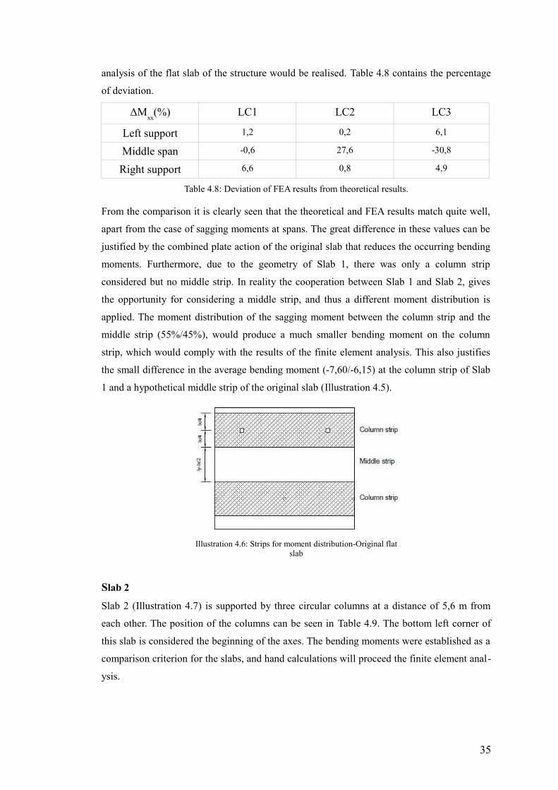
analysis of the flat slab of the structure would be realised. Table 4.8 contains the percentage
of deviation.
ΔMxx
(%) LC1 LC2 LC3
Left support 1,2 0,2 6,1
Middle span -0,6 27,6 -30,8
Right support 6,6 0,8 4,9
Table 4.8: Deviation of FΕΑ results from theoretical results.
From the comparison it is clearly seen that the theoretical and FEA results match quite well,
apart from the case of sagging moments at spans. The great difference in these values can be
justified by the combined plate action of the original slab that reduces the occurring bending
moments. Furthermore, due to the geometry of Slab 1, there was only a column strip
considered but no middle strip. In reality the cooperation between Slab 1 and Slab 2, gives
the opportunity for considering a middle strip, and thus a different moment distribution is
applied. The moment distribution of the sagging moment between the column strip and the
middle strip (55%/45%), would produce a much smaller bending moment on the column
strip, which would comply with the results of the finite element analysis. This also justifies
the small difference in the average bending moment (-7,60/-6,15) at the column strip of Slab
1 and a hypothetical middle strip of the original slab (Illustration 4.5).
Slab 2
Slab 2 (Illustration 4.7) is supported by three circular columns at a distance of 5,6 m from
each other. The position of the columns can be seen in Table 4.9. The bottom left corner of
this slab is considered the beginning of the axes. The bending moments were established as a
comparison criterion for the slabs, and hand calculations will proceed the finite element anal-
ysis.
35
Illustration 4.6: Strips for moment distribution-Original flatslab
Column Position x-direction Position y-direction
CIRC1 0,1 2,5
CIRC2 5,7 2,5
CIRC3 11,3 2,5
Table 4.9: Position of circular columns in Slab 2
In order to calculate the moments of Slab 2, which is supported by 3 columns, coefficients
from Concise Eurocode 2 are used for the calculation. Table 15.3 of Concise Eurocode 2 pro-
vides these coefficients for beams and slabs of three or more spans. However, certain values
for these coefficients are provided at the table comments for two span beams or slabs.
According to this table the design moments at supports are equal to:
coeff * n*span2
For the design moments at spans:
(coeff gk*span*γ
Gg
k+ coeff qk*span*γ
k)*span2
with a requirement of minimum span ≥ 0,85 maximum span.
Furthermore, the same loads and same load combinations are applied to Slab 2 as in Slab .
4.4.3.3 Theoretical results
The condition of minimum span ≥ 0,85 maximum span is satisfied, since the two spans are of
equal length.
The effective span of the slab between the two columns is:
leff
= lx-2d
col+d, where
lx is the span between the columns
dcol
is the diameter of the columns and
d the efficient depth of the slab.
From the above, eff
= 5,6 m.
36
Illustration 4.7: Slab 2
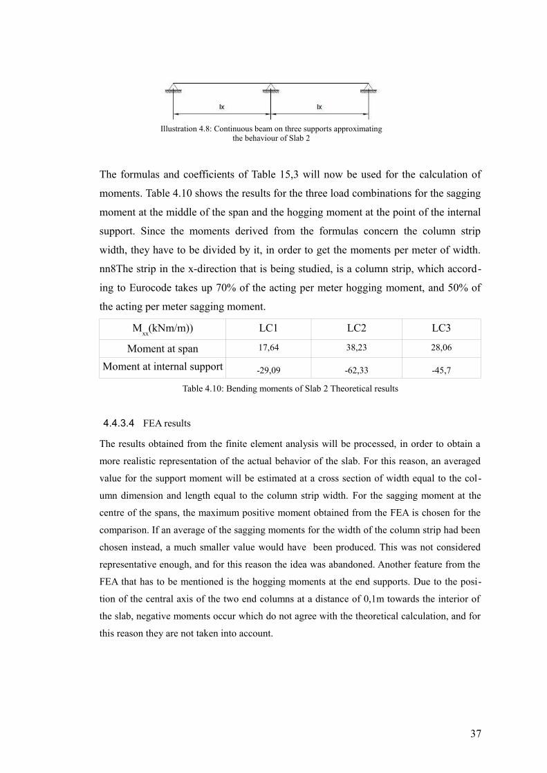
The formulas and coefficients of Table 15,3 will now be used for the calculation of
moments. Table 4.10 shows the results for the three load combinations for the sagging
moment at the middle of the span and the hogging moment at the point of the internal
support. Since the moments derived from the formulas concern the column strip
width, they have to be divided by it, in order to get the moments per meter of width.
nn8The strip in the x-direction that is being studied, is a column strip, which accord-
ing to Eurocode takes up 70% of the acting per meter hogging moment, and 50% of
the acting per meter sagging moment.
Mxx
(kNm/m)) LC1 LC2 LC3
Moment at span 17,64 38,23 28,06
Moment at internal support -29,09 -62,33 -45,7
Table 4.10: Bending moments of Slab 2 Theoretical results
4.4.3.4 FEA results
The results obtained from the finite element analysis will be processed, in order to obtain a
more realistic representation of the actual behavior of the slab. For this reason, an averaged
value for the support moment will be estimated at a cross section of width equal to the col-
umn dimension and length equal to the column strip width. For the sagging moment at the
centre of the spans, the maximum positive moment obtained from the FEA is chosen for the
comparison. If an average of the sagging moments for the width of the column strip had been
chosen instead, a much smaller value would have been produced. This was not considered
representative enough, and for this reason the idea was abandoned. Another feature from the
FEA that has to be mentioned is the hogging moments at the end supports. Due to the posi-
tion of the central axis of the two end columns at a distance of 0,1m towards the interior of
the slab, negative moments occur which do not agree with the theoretical calculation, and for
this reason they are not taken into account.
37
Illustration 4.8: Continuous beam on three supports approximatingthe behaviour of Slab 2
Mxx
(kNm/m)) LC1 LC2 LC3
Moment at span 15,17 32,74 24
Moment at internal support -35,53 -76,67 -56,22
Table 4.11: Bending moments of Slab 2 FEA results
Following the finite element analysis, a comparison of the theoretical and FEA results will
take place. Table 4.8 contains the percentage of deviation of the FEA results from the theoret-
ical ones.
ΔMxx
(%) LC1 LC2 LC3
Moment at span 14 14,4 14,5
Moment at internal support -22 -23,1 -23
Table 4.12: Percentages of deviation in Slab 2
From the comparison of the results, a standard deviation of 14% is observed for the sagging
moment at spans, and of 23% for the hogging moments at supports. For the case of the span
moment this deviation could be considered expected and justified, as the same occurred for
Slab 1, where bigger percentages of deviation were noticed. For the support moments, even
though an averaging procedure was followed, there is still quite a significant percentage of
deviation between theoretical and FEA results. The main reason that justifies the percentages
of deviation, is that most finite element programs work with an elastic moment distribution,
and materials that obey Hooke's law. This may be suitable for e.g. steel plates, but not for
concrete which is an elasto-plastic material, since after it cracks its behavior is not linear.
Consequently, the support moments are overestimated, and the deflection of the slab is
underestimated. These support moments are unlikely to be realised under service loads due to
cracking, and thus the service span moments will be correpondingly increased. In other
words, underestimation of the sagging moments is a result of the FEA as well, for the case of
the flat slabs.
4.5 Arch
When a shell is longitudinally supported by deep beams, walls or foundations, the forces are
carried in the transverse direction to the supports. The shell in this case, works as a series of
parallel arches, the so-called “funicular arches” responding to the applied loads solely in
compression. However, the assumed loads do not remain constant, and that leads to flexure in
the arch, since the rigid arch cannot readjust its shape in contrast to the cables. This means
that the series of parallel arches, respond to forces by bending and axial force action. Their
primary structural response is not membrane type action, and they can be approximated as
arches.
38
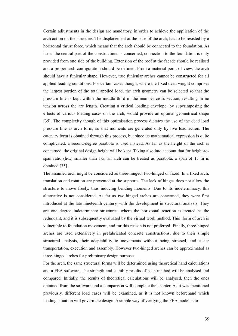
Certain adjustments in the design are mandatory, in order to achieve the application of the
arch action on the structure. The displacement at the base of the arch, has to be resisted by a
horizontal thrust force, which means that the arch should be connected to the foundation. As
far as the central part of the constructions is concerned, connection to the foundation is only
provided from one side of the building. Extension of the roof at the facade should be realised
and a proper arch configuration should be defined. From a material point of view, the arch
should have a funicular shape. However, true funicular arches cannot be constructed for all
applied loading conditions. For certain cases though, where the fixed dead weight comprises
the largest portion of the total applied load, the arch geometry can be selected so that the
pressure line is kept within the middle third of the member cross section, resulting in no
tension across the arc length. Creating a critical loading envelope, by superimposing the
effects of various loading cases on the arch, would provide an optimal geometrical shape
[35]. The complexity though of this optimisation process dictates the use of the dead load
pressure line as arch form, so that moments are generated only by live load action. The
catenary form is obtained through this process, but since its mathematical expression is quite
complicated, a second-degree parabola is used instead. As far as the height of the arch is
concerned, the original design height will be kept. Taking also into account that for height-to-
span ratio (h/L) smaller than 1/5, an arch can be treated as parabola, a span of 15 m is
obtained [35].
The assumed arch might be considered as three-hinged, two-hinged or fixed. In a fixed arch,
translation and rotation are prevented at the supports. The lack of hinges does not allow the
structure to move freely, thus inducing bending moments. Due to its indeterminacy, this
alternative is not considered. As far as two-hinged arches are concerned, they were first
introduced at the late nineteenth century, with the development in structural analysis. They
are one degree indeterminate structures, where the horizontal reaction is treated as the
redundant, and it is subsequently evaluated by the virtual work method. This form of arch is
vulnerable to foundation movement, and for this reason is not preferred. Finally, three-hinged
arches are used extensively in prefabricated concrete constructions, due to their simple
structural analysis, their adaptability to movements without being stressed, and easier
transportation, execution and assembly. However two-hinged arches can be approximated as
three-hinged arches for preliminary design purpose.
For the arch, the same structural forms will be determined using theoretical hand calculations
and a FEA software. The strength and stability results of each method will be analysed and
compared. Initially, the results of theoretical calculations will be analysed, then the ones
obtained from the software and a comparison will complete the chapter. As it was mentioned
previously, different load cases will be examined, as it is not known beforehand which
loading situation will govern the design. A simple way of verifying the FEA model is to
39
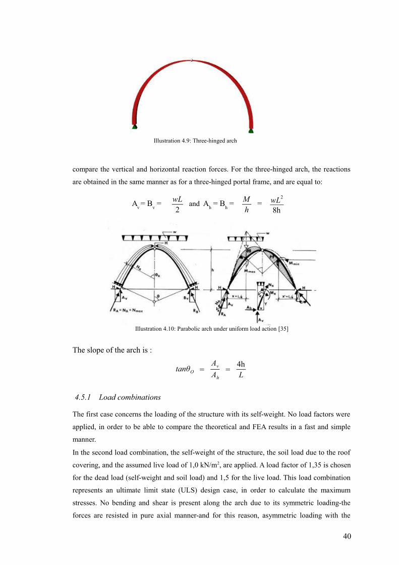
compare the vertical and horizontal reaction forces. For the three-hinged arch, the reactions
are obtained in the same manner as for a three-hinged portal frame, and are equal to:
Av = B
v = wL
2and A
h = B
h = M
h= wL2
8h
The slope of the arch is :
tanθΟ =Αv
Αh
=4hL
4.5.1 Load combinations
The first case concerns the loading of the structure with its self-weight. No load factors were
applied, in order to be able to compare the theoretical and FEA results in a fast and simple
manner.
In the second load combination, the self-weight of the structure, the soil load due to the roof
covering, and the assumed live load of 1,0 kN/m2, are applied. A load factor of 1,35 is chosen
for the dead load (self-weight and soil load) and 1,5 for the live load. This load combination
represents an ultimate limit state (ULS) design case, in order to calculate the maximum
stresses. No bending and shear is present along the arch due to its symmetric loading-the
forces are resisted in pure axial manner-and for this reason, asymmetric loading with the
40
Illustration 4.10: Parabolic arch under uniform load action [35]
Illustration 4.9: Three-hinged arch
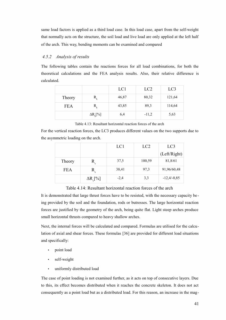
same load factors is applied as a third load case. In this load case, apart from the self-weight
that normally acts on the structure, the soil load and live load are only applied at the left half
of the arch. This way, bending moments can be examined and compared
4.5.2 Analysis of results
The following tables contain the reactions forces for all load combinations, for both the
theoretical calculations and the FEA analysis results. Also, their relative difference is
calculated.
LC1 LC2 LC3
Theory Rh
46,87 80,32 121,64
FEA Rh
43,85 89,3 114,64
ΔRh[%] 6,4 -11,2 5,63
Table 4.13: Resultant horizontal reaction forces of the arch
For the vertical reaction forces, the LC3 produces different values on the two supports due to
the asymmetric loading on the arch.
LC1 LC2 LC3
(Left/Right)
Theory Rv
37,5 100,59 81,8/61
FEA Rv
38,41 97,3 91,96/60,48
ΔRv[%] -2,4 3,3 -12,4/-0,85
Table 4.14: Resultant horizontal reaction forces of the arch
It is demonstrated that large thrust forces have to be resisted, with the necessary capacity be -
ing provided by the soil and the foundation, rods or butresses. The large horizontal reaction
forces are justified by the geometry of the arch, being quite flat. Light steep arches produce
small horizontal thrusts compared to heavy shallow arches.
Next, the internal forces will be calculated and compared. Formulas are utilised for the calcu-
lation of axial and shear forces. These formulas [36] are provided for different load situations
and specifically:
• point load
• self-weight
• uniformly distributed load
The case of point loading is not examined further, as it acts on top of consecutive layers. Due
to this, its effect becomes distributed when it reaches the concrete skeleton. It does not act
consequently as a point load but as a distributed load. For this reason, an increase in the mag-
41
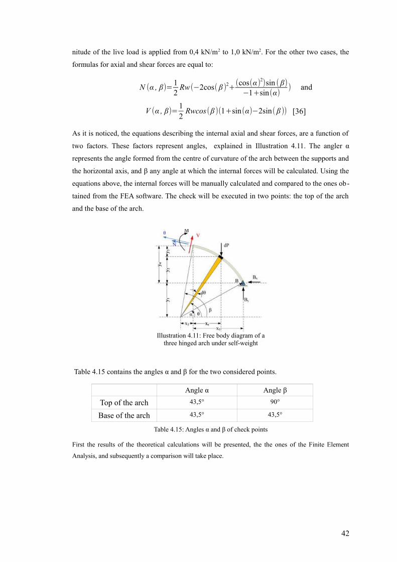
nitude of the live load is applied from 0,4 kN/m2 to 1,0 kN/m2. For the other two cases, the
formulas for axial and shear forces are equal to:
Ν (α , β)=12
Rw(−2cos( β )2+
(cos(α)2)sin ( β)
−1+sin(α)) and
V (α , β)=12
Rwcos(β )(1+sin(α)−2sin( β )) [36]
As it is noticed, the equations describing the internal axial and shear forces, are a function of
two factors. These factors represent angles, explained in Illustration 4.11. The angler α
represents the angle formed from the centre of curvature of the arch between the supports and
the horizontal axis, and β any angle at which the internal forces will be calculated. Using the
equations above, the internal forces will be manually calculated and compared to the ones ob-
tained from the FEA software. The check will be executed in two points: the top of the arch
and the base of the arch.
Table 4.15 contains the angles α and β for the two considered points.
Angle α Angle β
Top of the arch 43,5° 90°
Base of the arch 43,5° 43,5°
Table 4.15: Angles α and β of check points
First the results of the theoretical calculations will be presented, the the ones of the Finite Element
Analysis, and subsequently a comparison will take place.
42
Illustration 4.11: Free body diagram of athree hinged arch under self-weight
LC1 LC2 LC38
Top Bottom Top Bottom Top Bottom
Nx
-43,77 -61,26 -114,49 -160.46 -85,39 -131,42
Qy
0 3,42 0 9,6 -10,7 5,35
Table 4.16: Internal forces of the arch for different load cases-FEA results
From the above, it is demonstrated that the arch responds to uniform distributed load (self-weight or
other load type) with compression, justifying the characterisation of the arch as a “compressive
structural system”. The axial compressive force reaches its highest value at the supports of the arch and
decreases towards the crown. The shear force on the other hand gets a comparatively low value, and it
varies only slightly from the support towards the top, until it reaches zero at the arch crown.
LC1 LC2 LC4
Top Bottom Top Bottom Top Bottom
Nx
-45,86 -60,16 -112,75 -147,96 -87 -114,26
Qy
0 6,1 0 15,12 -10,31 1,36
Table 4.17: Internal forces of the arch for different load cases-theoretical results
This was expected due to the symmetric loading of the arch The results of the hand
calculations were taken using the aforementioned formulas. These formulas though could not
be applied for the case of asymmetric load, as load combinations LC3. The loading of this
combination was analysed in the following forms:
• since the self-weight is applied throughout the structure, the first part of the analysed
loading consists of it. The equations above can properly be implemented.
• asymmetric loading consists of the live load and soil load, acting on the one of the
two symmetrical parts of the arch (left part in DIANA analysis). The value of this
load acting on the left part has been calculated to 5,5 kN/m. Thus, it can be analysed
in a uniformly distributed symmetric load of 5,5/2=2,75 kN/m, and an asymmetric
loading of the same value. For the first case again, use of the equations is allowed.
Due to lack of formulas for the calculation of internal forces for the latter case, these
are calculated assuming the arch as a beam, and estimating the forces
correspondingly. The internal shear force at the support is calculated at ql/4 = Qy=
2,75*15/4 = 10,31 kN.
Moreover, τhe internal moments have to be compared. For this reason, a derived equation is
utilised, which is the product of [36]. The following formula has been derived for a three-
hinged arch, and although the input of DIANA concerns a two-hinged arch, it is decided to be
included, so a comparison of the order of magnitude of the occurring bending moment could
be feasible. The same equation is valid for the self-weight and the external applied loads. The
equation for the calculation of the internal moments is equal to:
43
M (α , β )=12(R2
)w(−1+sin (β ))(−sin (α)+sin (β ))
The assumption of a three-hinged arch results in zero bending moments at the position of the
hinges. Thus, the bending moment is zero at the base of the arch and at its crown, a fact
which is also confirmed by the results of the finite element analysis. These results show that
the bending moment takes values extremely close to zero. For this reason these points cannot
be considered as check points for the comparison between theoretical and FEA results.
Instead, the maximum moment will be located by the result diagram of finite element
analysis, and it will be compared with maximum moment obtained from theoretical
calculations.
To accomplish this, the first derivative of the internal moment function will be calculated,
considering angle β as the only variable of the function (angle α is constant for the arch), and
this will be set equal to 43,5°.
∂M∂ β
=12(R2
)wsin (x)(250sin (x)−211)
125
∂M∂ β
=0 , from where x=90° or x=57,56°.
The first solution cannot be accepted since, at the point of 90° the moment becomes zero.
Substituting the angle β with the value of 57,56°, the maximum bending moment on the arch
is obtained.
LC1 LC2
Theory Mz[kNm] 7,18 21,45
FEA Mz[kNm] 3,3 8,63
Table 4.18: Maximum bending moments in the arch
Large deviation in the results is a result of the different modeling of the arch in each case. The
theoretical calculations assume a three-hinged arch whereas the finite element analysis deals with a two-
hinged arch. The case of asymmetric loading is not taken into account, as no formulas are provided for
the calculations of bending moments. The maximum bending moment from the finite element analysis is
located at the crown of the arch, corresponding to the middle point. This is an expected fact if it is taken
into account that the structural behavior of the arch can be approximated with this of a curved beam.
Concluding, comparing the behavior of the three-hinged and the two-hinged arch, the different moment
distribution is pointed out. In the following pictures the normalised moment diagram for each case is
schematised, in order to obtain a better understanding of he different behavior.
44
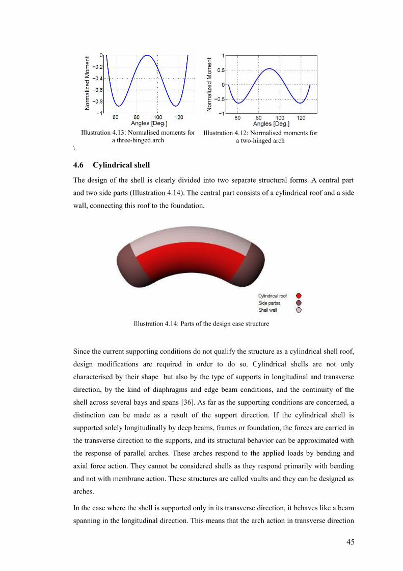
\
4.6 Cylindrical shell
The design of the shell is clearly divided into two separate structural forms. A central part
and two side parts (Illustration 4.14). The central part consists of a cylindrical roof and a side
wall, connecting this roof to the foundation.
Since the current supporting conditions do not qualify the structure as a cylindrical shell roof,
design modifications are required in order to do so. Cylindrical shells are not only
characterised by their shape but also by the type of supports in longitudinal and transverse
direction, by the kind of diaphragms and edge beam conditions, and the continuity of the
shell across several bays and spans [36]. As far as the supporting conditions are concerned, a
distinction can be made as a result of the support direction. If the cylindrical shell is
supported solely longitudinally by deep beams, frames or foundation, the forces are carried in
the transverse direction to the supports, and its structural behavior can be approximated with
the response of parallel arches. These arches respond to the applied loads by bending and
axial force action. They cannot be considered shells as they respond primarily with bending
and not with membrane action. These structures are called vaults and they can be designed as
arches.
In the case where the shell is supported only in its transverse direction, it behaves like a beam
spanning in the longitudinal direction. This means that the arch action in transverse direction
45
Illustration 4.13: Normalised moments fora three-hinged arch
Illustration 4.12: Normalised moments fora two-hinged arch
Illustration 4.14: Parts of the design case structure
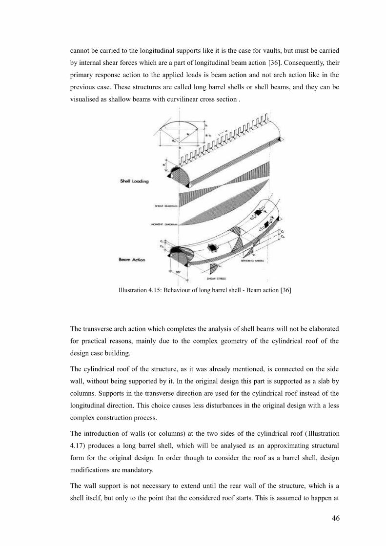
cannot be carried to the longitudinal supports like it is the case for vaults, but must be carried
by internal shear forces which are a part of longitudinal beam action [36]. Consequently, their
primary response action to the applied loads is beam action and not arch action like in the
previous case. These structures are called long barrel shells or shell beams, and they can be
visualised as shallow beams with curvilinear cross section .
The transverse arch action which completes the analysis of shell beams will not be elaborated
for practical reasons, mainly due to the complex geometry of the cylindrical roof of the
design case building.
The cylindrical roof of the structure, as it was already mentioned, is connected on the side
wall, without being supported by it. In the original design this part is supported as a slab by
columns. Supports in the transverse direction are used for the cylindrical roof instead of the
longitudinal direction. This choice causes less disturbances in the original design with a less
complex construction process.
The introduction of walls (or columns) at the two sides of the cylindrical roof ( Illustration
4.17) produces a long barrel shell, which will be analysed as an approximating structural
form for the original design. In order though to consider the roof as a barrel shell, design
modifications are mandatory.
The wall support is not necessary to extend until the rear wall of the structure, which is a
shell itself, but only to the point that the considered roof starts. This is assumed to happen at
46
Illustration 4.16: Part of the structure considered as acylindrical roof
Illustration 4.15: Behaviour of long barrel shell - Beam action [36]
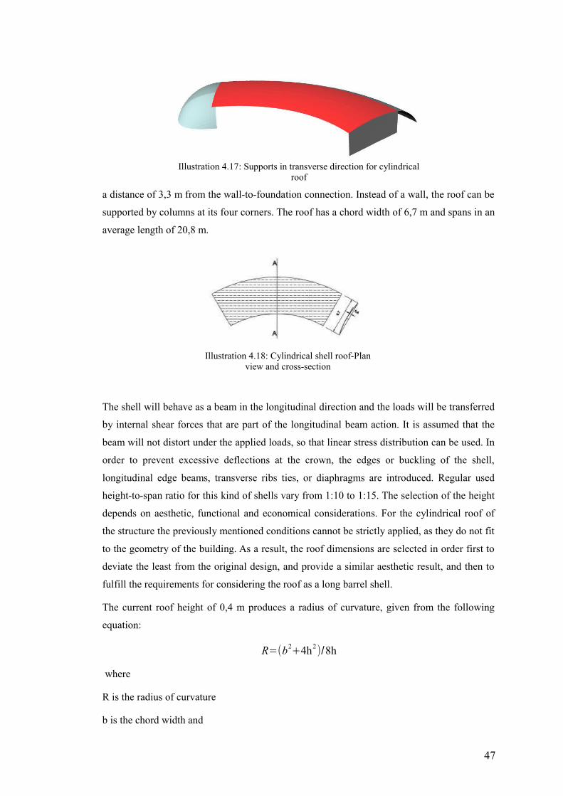
a distance of 3,3 m from the wall-to-foundation connection. Instead of a wall, the roof can be
supported by columns at its four corners. The roof has a chord width of 6,7 m and spans in an
average length of 20,8 m.
The shell will behave as a beam in the longitudinal direction and the loads will be transferred
by internal shear forces that are part of the longitudinal beam action. It is assumed that the
beam will not distort under the applied loads, so that linear stress distribution can be used. In
order to prevent excessive deflections at the crown, the edges or buckling of the shell,
longitudinal edge beams, transverse ribs ties, or diaphragms are introduced. Regular used
height-to-span ratio for this kind of shells vary from 1:10 to 1:15. The selection of the height
depends on aesthetic, functional and economical considerations. For the cylindrical roof of
the structure the previously mentioned conditions cannot be strictly applied, as they do not fit
to the geometry of the building. As a result, the roof dimensions are selected in order first to
deviate the least from the original design, and provide a similar aesthetic result, and then to
fulfill the requirements for considering the roof as a long barrel shell.
The current roof height of 0,4 m produces a radius of curvature, given from the following
equation:
R=(b2+4h2
)/8h
where
R is the radius of curvature
b is the chord width and
47
Illustration 4.17: Supports in transverse direction for cylindricalroof
Illustration 4.18: Cylindrical shell roof-Planview and cross-section
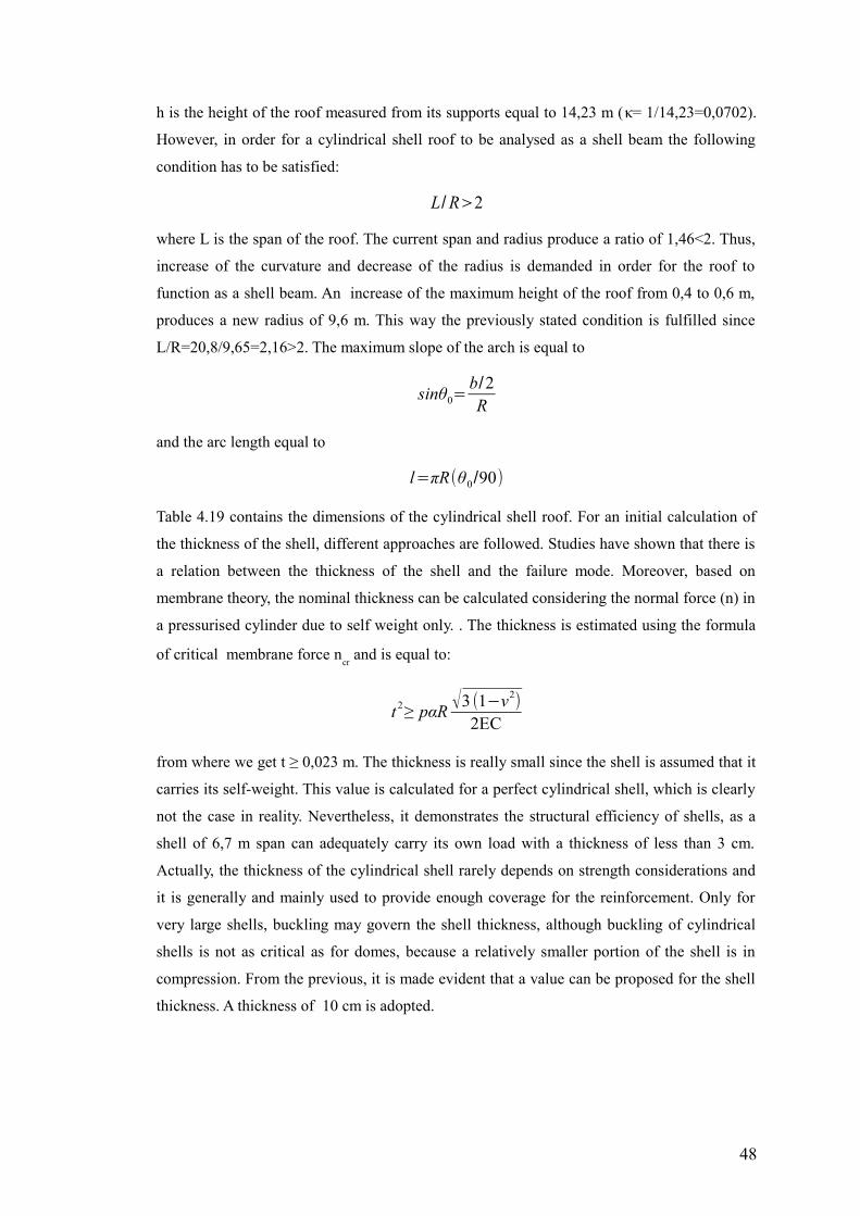
h is the height of the roof measured from its supports equal to 14,23 m (κ= 1/14,23=0,0702).
However, in order for a cylindrical shell roof to be analysed as a shell beam the following
condition has to be satisfied:
L/ R>2
where L is the span of the roof. The current span and radius produce a ratio of 1,46<2. Thus,
increase of the curvature and decrease of the radius is demanded in order for the roof to
function as a shell beam. An increase of the maximum height of the roof from 0,4 to 0,6 m,
produces a new radius of 9,6 m. This way the previously stated condition is fulfilled since
L/R=20,8/9,65=2,16>2. The maximum slope of the arch is equal to
sinθ0=b/2R
and the arc length equal to
l=πR(θ0/90)
Table 4.19 contains the dimensions of the cylindrical shell roof. For an initial calculation of
the thickness of the shell, different approaches are followed. Studies have shown that there is
a relation between the thickness of the shell and the failure mode. Moreover, based on
membrane theory, the nominal thickness can be calculated considering the normal force (n) in
a pressurised cylinder due to self weight only. . The thickness is estimated using the formula
of critical membrane force ncr and is equal to:
t 2≥ pαR √3 (1−ν2)
2EC
from where we get t ≥ 0,023 m. The thickness is really small since the shell is assumed that it
carries its self-weight. This value is calculated for a perfect cylindrical shell, which is clearly
not the case in reality. Nevertheless, it demonstrates the structural efficiency of shells, as a
shell of 6,7 m span can adequately carry its own load with a thickness of less than 3 cm.
Actually, the thickness of the cylindrical shell rarely depends on strength considerations and
it is generally and mainly used to provide enough coverage for the reinforcement. Only for
very large shells, buckling may govern the shell thickness, although buckling of cylindrical
shells is not as critical as for domes, because a relatively smaller portion of the shell is in
compression. From the previous, it is made evident that a value can be proposed for the shell
thickness. A thickness of 10 cm is adopted.
48
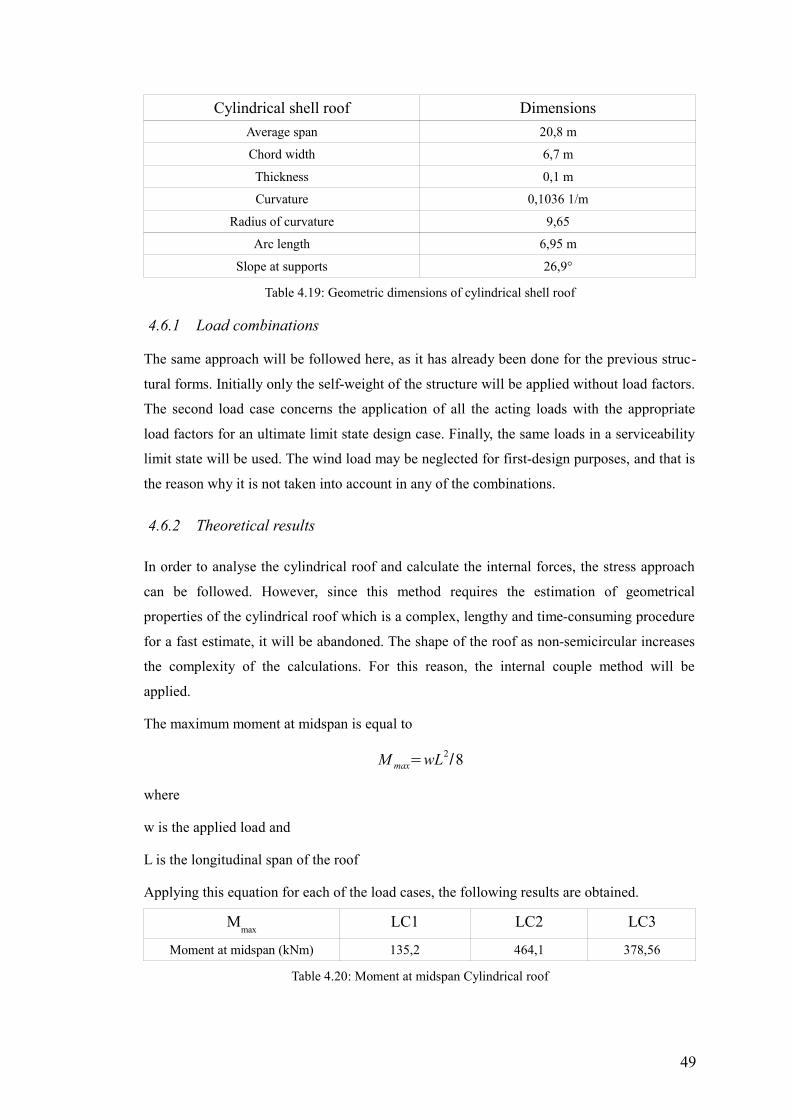
Cylindrical shell roof Dimensions
Average span 20,8 m
Chord width 6,7 m
Thickness 0,1 m
Curvature 0,1036 1/m
Radius of curvature 9,65
Arc length 6,95 m
Slope at supports 26,9°
Table 4.19: Geometric dimensions of cylindrical shell roof
4.6.1 Load combinations
The same approach will be followed here, as it has already been done for the previous struc-
tural forms. Initially only the self-weight of the structure will be applied without load factors.
The second load case concerns the application of all the acting loads with the appropriate
load factors for an ultimate limit state design case. Finally, the same loads in a serviceability
limit state will be used. The wind load may be neglected for first-design purposes, and that is
the reason why it is not taken into account in any of the combinations.
4.6.2 Theoretical results
In order to analyse the cylindrical roof and calculate the internal forces, the stress approach
can be followed. However, since this method requires the estimation of geometrical
properties of the cylindrical roof which is a complex, lengthy and time-consuming procedure
for a fast estimate, it will be abandoned. The shape of the roof as non-semicircular increases
the complexity of the calculations. For this reason, the internal couple method will be
applied.
The maximum moment at midspan is equal to
M max=wL2/8
where
w is the applied load and
L is the longitudinal span of the roof
Applying this equation for each of the load cases, the following results are obtained.
Mmax
LC1 LC2 LC3
Moment at midspan (kNm) 135,2 464,1 378,56
Table 4.20: Moment at midspan Cylindrical roof
49
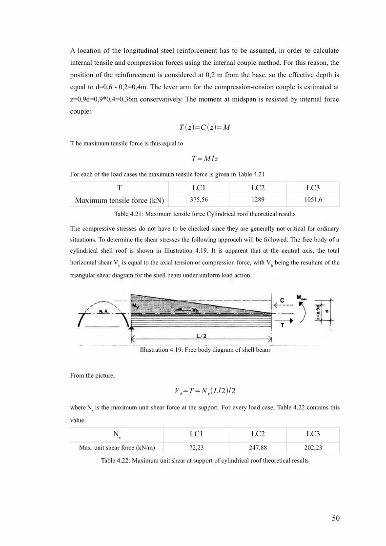
A location of the longitudinal steel reinforcement has to be assumed, in order to calculate
internal tensile and compression forces using the internal couple method. For this reason, the
position of the reinforcement is considered at 0,2 m from the base, so the effective depth is
equal to d=0,6 - 0,2=0,4m. The lever arm for the compression-tension couple is estimated at
z=0,9d=0,9*0,4=0,36m conservatively. The moment at midspan is resisted by internal force
couple:
T (z)=C (z)=M
T he maximum tensile force is thus equal to
T=M /z
For each of the load cases the maximum tensile force is given in Table 4.21
T LC1 LC2 LC3
Maximum tensile force (kN) 375,56 1289 1051,6
Table 4.21: Maximum tensile force Cylindrical roof theoretical results
The compressive stresses do not have to be checked since they are generally not critical for ordinary
situations. To determine the shear stresses the following approach will be followed. The free body of a
cylindrical shell roof is shown in Illustration 4.19. It is apparent that at the neutral axis, the total
horizontal shear Vh is equal to the axial tension or compression force, with V
h being the resultant of the
triangular shear diagram for the shell beam under uniform load action.
From the picture,
V h=T =N v(L/2)/2
where N
v is the maximum unit shear force at the support. For every load case, Table 4.22 contains this
value.
Nv
LC1 LC2 LC3
Max. unit shear force (kN/m) 72,23 247,88 202,23
Table 4.22: Maximum unit shear at support of cylindrical roof theoretical results
50
Illustration 4.19: Free body diagram of shell beam
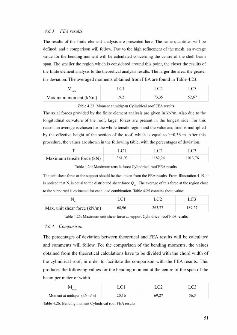
4.6.3 FEA results
The results of the finite element analysis are presented here. The same quantities will be
defined, and a comparison will follow. Due to the high refinement of the mesh, an average
value for the bending moment will be calculated concerning the centre of the shell beam
span. The smaller the region which is considered around this point, the closer the results of
the finite element analysis to the theoretical analysis results. The larger the area, the greater
the deviation. The averaged moments obtained from FEA are found in Table 4.23.
Mmax
LC1 LC2 LC3
Maximum moment (kNm) 19,2 73,35 52,67
Table 4.23: Moment at midspan Cylindrical roof FEA results
The axial forces provided by the finite element analysis are given in kN/m. Also due to the
longitudinal curvature of the roof, larger forces are present in the longest side. For this
reason an average is chosen for the whole tensile region and the value acquired is multiplied
by the effective height of the section of the roof, which is equal to h=0,36 m. After this
procedure, the values are shown in the following table, with the percentages of deviation.
T LC1 LC2 LC3
Maximum tensile force (kN) 361,03 1182,24 1013,76
Table 4.24: Maximum tensile force Cylindrical roof FEA results
The unit shear force at the support should be then taken from the FEA results. From Illustration 4.19, it
is noticed that Nv is equal to the distributed shear force Q
yz.. The average of this force at the region close
to the supported is estimated for each load combination. Table 4.25 contains these values.
Nv
LC1 LC2 LC3
Max. unit shear force (kN/m) 68,96 263,77 189,27
Table 4.25: Maximum unit shear force at support Cylindrical roof FEA results
4.6.4 Comparison
The percentages of deviation between theoretical and FEA results will be calculated
and comments will follow. For the comparison of the bending moments, the values
obtained from the theoretical calculations have to be divided with the chord width of
the cylindrical roof, in order to facilitate the comparison with the FEA results. This
produces the following values for the bending moment at the centre of the span of the
beam per meter of width.
Mmax
LC1 LC2 LC3
Moment at midspan (kNm/m) 20,16 69,27 56,5
Table 4.26: Bending moment Cylindrical roof FEA results
51

LC1 LC2 LC3
Maximum moment ΔMmax
[%] 3,8 -5,9 7,2
Maximum tensile force ΔΤ[%] 3,86 8,3 7
Max. unit shear force ΔNv[%] 4,5 -6,41 6,4
Table 4.27: Deviation between theoretical and FEA results Cylindrical roof
The percentages of the deviation are acceptable, and they are mainly the result of the
simplifications made during the hand calculations. The roof in the theoretical analysis was
modeled as a shell beam without fulfilling strictly the criteria for this consideration. For the
roof to be considered as a shell beam without edge beams or even with edge beams that are
not too deep, the ratio of the longitudinal span to the radius of curvature should have been
greater than 5 or 3 respectively. The resulting height of the roof would not comply with
design criteria and the deviation from the original model would be significant.
Furthermore, shell beams are assumed not to distort under load action so that linear stress
distribution can be used instead of a curvilinear one that is actually the case. However, in the
case of long barrel shells, lateral thrust forces causes large deformations, which make the
application of the beam theory questionable. Another simplification is the arch action in the
transverse direction of the shell, that is neglected in the calculations though it does not affect
the current results(longitudinal direction)
4.7 Spherical Side part
The analysis of the central part will be followed by the analysis of the remaining parts of the
structure, i.e. the spherical side parts. This way the analysis using theoretical calculations will
be completed, in order to proceed to the finite element analysis of the whole structure and its
segmentation.
4.7.1 Side part-Dome
The two side parts on the left and right side of the structure have identical dimensions, and
only one of the them will be representatively analysed. They comprise one quartile of an el-
lipsoid with R1= 5m and R
2= 4m, and they are connected both to the side wall and the roof of
the structure (Illustration 4.20).
For the connection of the side parts to the foundation, hinges are preferred over roll supports,
as in the latter case large horizontal forces will cause great instability at the bottom of the
shell where the rolls are applied. In addition, clamped supports are not selected as large mo-
52
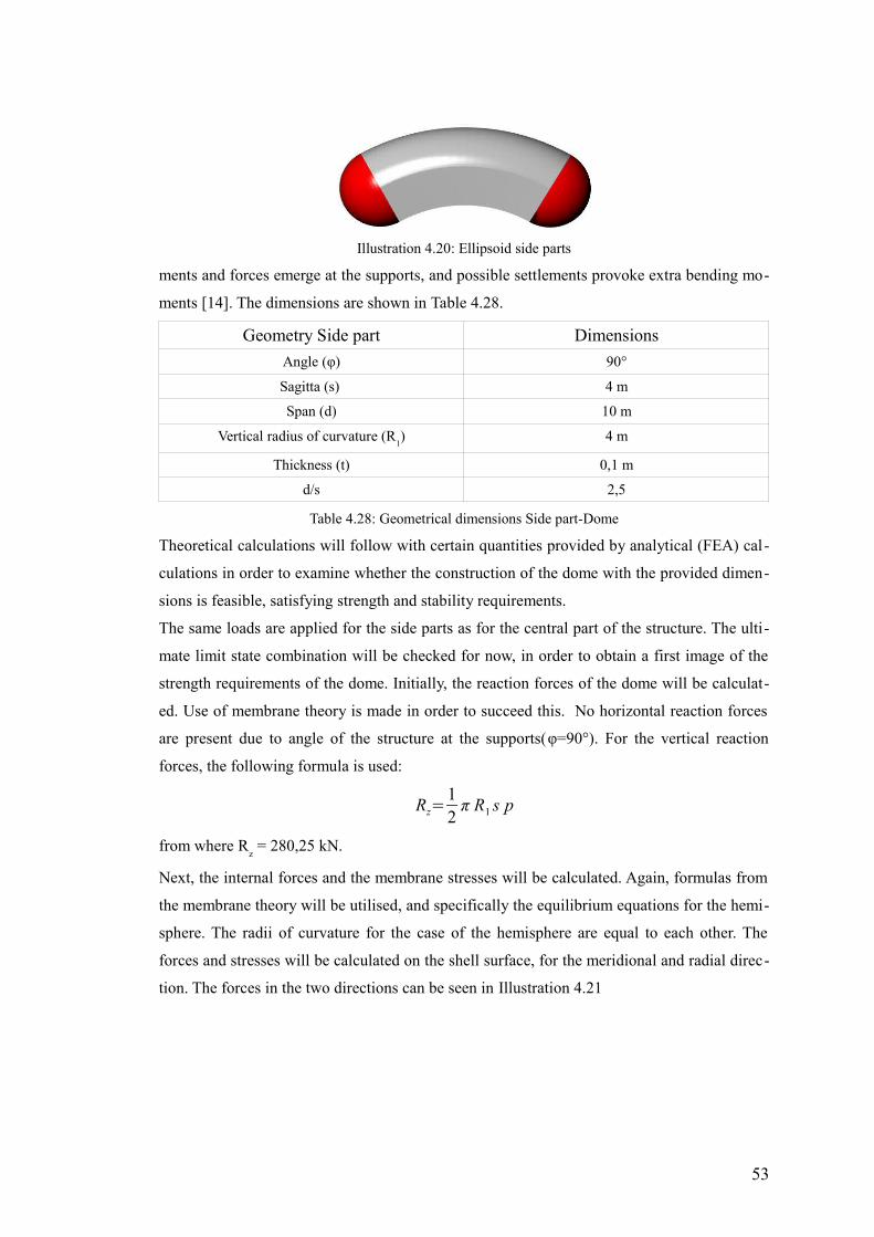
ments and forces emerge at the supports, and possible settlements provoke extra bending mo-
ments [14]. The dimensions are shown in Table 4.28.
Geometry Side part Dimensions
Angle (φ) 90°
Sagitta (s) 4 m
Span (d) 10 m
Vertical radius of curvature (R1) 4 m
Thickness (t) 0,1 m
d/s 2,5
Table 4.28: Geometrical dimensions Side part-Dome
Theoretical calculations will follow with certain quantities provided by analytical (FEA) cal -
culations in order to examine whether the construction of the dome with the provided dimen-
sions is feasible, satisfying strength and stability requirements.
The same loads are applied for the side parts as for the central part of the structure. The ulti-
mate limit state combination will be checked for now, in order to obtain a first image of the
strength requirements of the dome. Initially, the reaction forces of the dome will be calculat-
ed. Use of membrane theory is made in order to succeed this. No horizontal reaction forces
are present due to angle of the structure at the supports(φ=90°). For the vertical reaction
forces, the following formula is used:
Rz=12
π R1 s p
from where Rz = 280,25 kN.
Next, the internal forces and the membrane stresses will be calculated. Again, formulas from
the membrane theory will be utilised, and specifically the equilibrium equations for the hemi-
sphere. The radii of curvature for the case of the hemisphere are equal to each other. The
forces and stresses will be calculated on the shell surface, for the meridional and radial direc-
tion. The forces in the two directions can be seen in Illustration 4.21
53
Illustration 4.20: Ellipsoid side parts
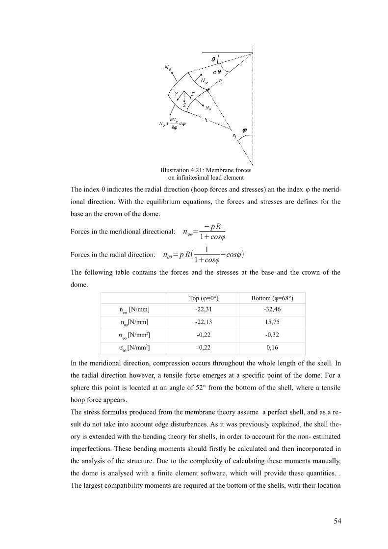
The index θ indicates the radial direction (hoop forces and stresses) an the index φ the merid-
ional direction. With the equilibrium equations, the forces and stresses are defines for the
base an the crown of the dome.
Forces in the meridional directional: nφφ=−p R
1+cosφ
Forces in the radial direction: nθθ=p R(1
1+cosφ−cosφ)
The following table contains the forces and the stresses at the base and the crown of the
dome.
Top (φ=0°) Bottom (φ=68°)
nφφ
[Ν/mm] -22,31 -32,46
nθθ
[Ν/mm] -22,13 15,75
σφφ
[Ν/mm2] -0,22 -0,32
σθθ
[Ν/mm2] -0,22 0,16
In the meridional direction, compression occurs throughout the whole length of the shell. In
the radial direction however, a tensile force emerges at a specific point of the dome. For a
sphere this point is located at an angle of 52° from the bottom of the shell, where a tensile
hoop force appears.
The stress formulas produced from the membrane theory assume a perfect shell, and as a re -
sult do not take into account edge disturbances. As it was previously explained, the shell the-
ory is extended with the bending theory for shells, in order to account for the non- estimated
imperfections. These bending moments should firstly be calculated and then incorporated in
the analysis of the structure. Due to the complexity of calculating these moments manually,
the dome is analysed with a finite element software, which will provide these quantities. .
The largest compatibility moments are required at the bottom of the shells, with their location
54
Illustration 4.21: Membrane forceson infinitesimal load element
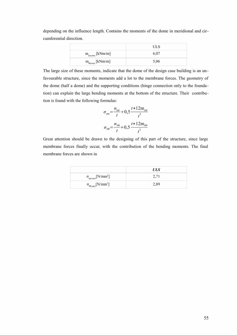
depending on the influence length. Contains the moments of the dome in meridional and cir-
cumferential direction.
ULS
mφφ,max
[kNm/m] 6,07
mθθ,max
[kNm/m] 5,06
The large size of these moments, indicate that the dome of the design case building is an un -
favourable structure, since the moments add a lot to the membrane forces. The geometry of
the dome (half a dome) and the supporting conditions (hinge connection only to the founda-
tion) can explain the large bending moments at the bottom of the structure. Their contribu-
tion is found with the following formulas:
σφφ=nφφ
t+0,5
t∗12mφφ
t3
σθθ=nθθ
t+0,5
t∗12mθθ
t3
Great attention should be drawn to the designing of this part of the structure, since large
membrane forces finally occur, with the contribution of the bending moments. The final
membrane forces are shown in
ULS
σφφ,max
[Ν/mm2] 2,71
σθθ,max
[Ν/mm2] 2,89
55
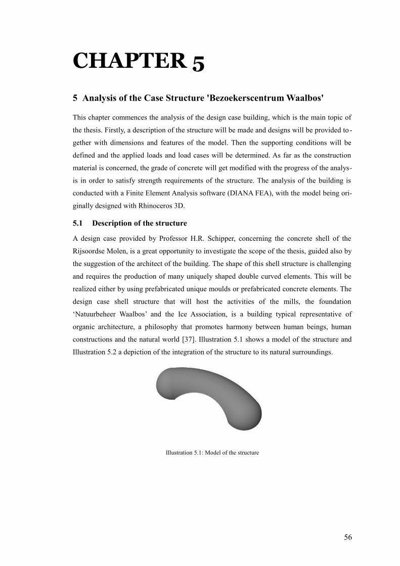
CHAPTER 5
5 Analysis of the Case Structure 'Bezoekerscentrum Waalbos'
This chapter commences the analysis of the design case building, which is the main topic of
the thesis. Firstly, a description of the structure will be made and designs will be provided to -
gether with dimensions and features of the model. Then the supporting conditions will be
defined and the applied loads and load cases will be determined. As far as the construction
material is concerned, the grade of concrete will get modified with the progress of the analys-
is in order to satisfy strength requirements of the structure. The analysis of the building is
conducted with a Finite Element Analysis software (DIANA FEA), with the model being ori-
ginally designed with Rhinoceros 3D.
5.1 Description of the structure
A design case provided by Professor H.R. Schipper, concerning the concrete shell of the
Rijsoordse Molen, is a great opportunity to investigate the scope of the thesis, guided also by
the suggestion of the architect of the building. The shape of this shell structure is challenging
and requires the production of many uniquely shaped double curved elements. This will be
realized either by using prefabricated unique moulds or prefabricated concrete elements. The
design case shell structure that will host the activities of the mills, the foundation
‘Natuurbeheer Waalbos’ and the Ice Association, is a building typical representative of
organic architecture, a philosophy that promotes harmony between human beings, human
constructions and the natural world [37]. Illustration 5.1 shows a model of the structure and
Illustration 5.2 a depiction of the integration of the structure to its natural surroundings.
56
Illustration 5.1: Model of the structure
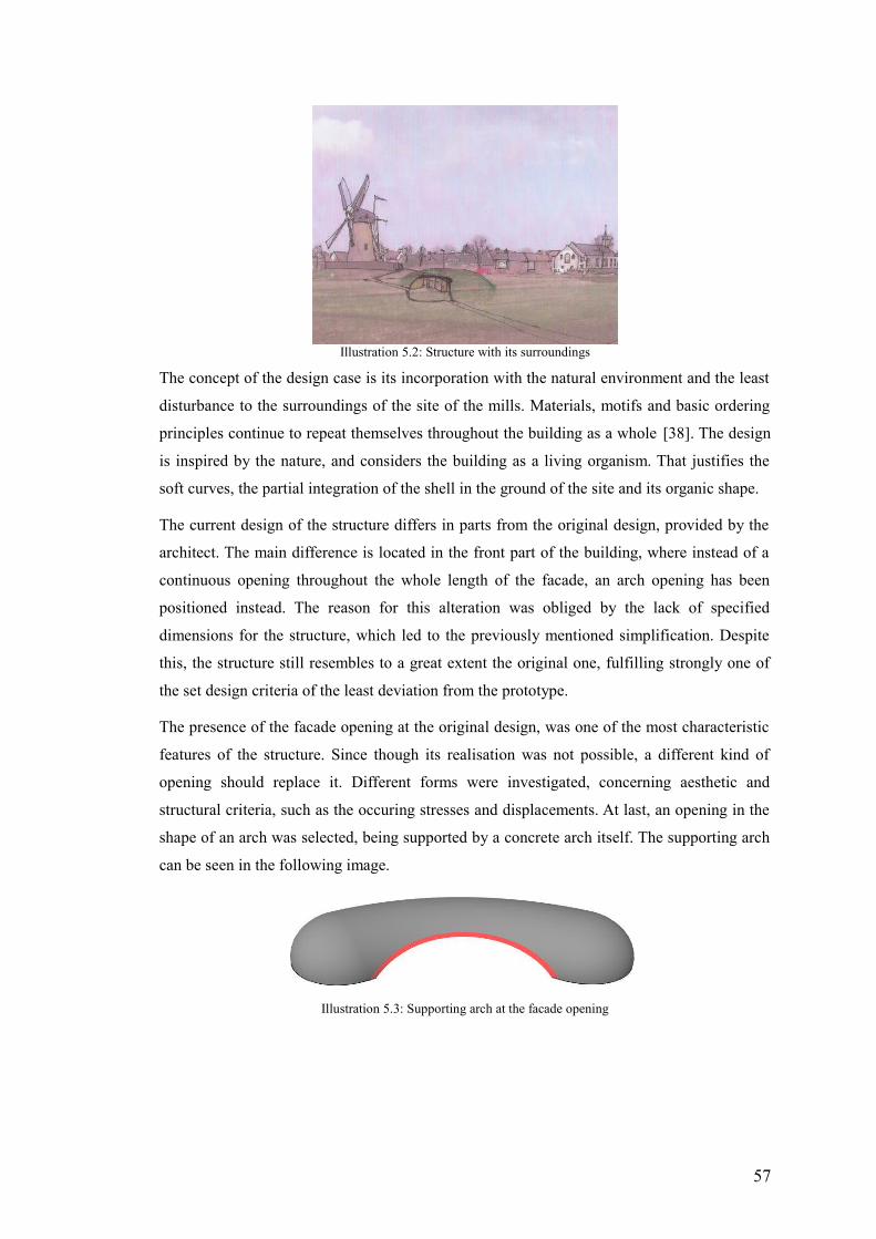
The concept of the design case is its incorporation with the natural environment and the least
disturbance to the surroundings of the site of the mills. Materials, motifs and basic ordering
principles continue to repeat themselves throughout the building as a whole [38]. The design
is inspired by the nature, and considers the building as a living organism. That justifies the
soft curves, the partial integration of the shell in the ground of the site and its organic shape.
The current design of the structure differs in parts from the original design, provided by the
architect. The main difference is located in the front part of the building, where instead of a
continuous opening throughout the whole length of the facade, an arch opening has been
positioned instead. The reason for this alteration was obliged by the lack of specified
dimensions for the structure, which led to the previously mentioned simplification. Despite
this, the structure still resembles to a great extent the original one, fulfilling strongly one of
the set design criteria of the least deviation from the prototype.
The presence of the facade opening at the original design, was one of the most characteristic
features of the structure. Since though its realisation was not possible, a different kind of
opening should replace it. Different forms were investigated, concerning aesthetic and
structural criteria, such as the occuring stresses and displacements. At last, an opening in the
shape of an arch was selected, being supported by a concrete arch itself. The supporting arch
can be seen in the following image.
57
Illustration 5.2: Structure with its surroundings
Illustration 5.3: Supporting arch at the facade opening
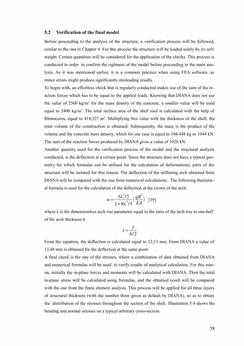
5.2 Verification of the final model
Before proceeding to the analysis of the structure, a verification process will be followed,
similar to the one in Chapter 4. For this process the structure will be loaded solely by its self-
weight. Certain quantities will be considered for the application of the checks. This process is
conducted in order to confirm the rightness of the model before proceeding to the main ana-
lysis. As it was mentioned earlier, it is a common practice when using FEA software, as
minor errors might produce significantly misleading results.
To begin with, an effortless check that is regularly conducted makes use of the sum of the re-
action forces which has to be equal to the applied loads. Knowing that DIANA does not use
the value of 2500 kg/m3 for the mass density of the concrete, a smaller value will be used
equal to 2400 kg/m3. The total surface area of the shell roof is calculated with the help of
Rhinoceros, equal to 418,527 m2. Multiplying this value with the thickness of the shell, the
total volume of the construction is obtained. Subsequently, the mass is the product of the
volume and the concrete mass density, which for our case is equal to 104.448 kg or 1044 kN.
The sum of the reaction forces produced by DIANA gives a value of 1026 kN.
Another quantity used for the verification process of the model and the structural analysis
conducted, is the deflection at a certain point. Since the structure does not have a typical geo-
metry for which formulas can be utilised for the calculation of deformations, parts of the
structure will be isolated for this reason. The deflection of the stiffening arch obtained from
DIANA will be compared with the one from numerical calculations. The following theoretic-
al formula is used for the calculation of the deflection at the crown of the arch:
w=5λ2
/2
1+8λ2/5
(qR2
EA) [39]
where λ is the dimensionless arch rise parameter equal to the ratio of the arch rise to one-half
of the arch thickness h
λ=f
h/2
From the equation, the deflection is calculated equal to 12,13 mm. From DIANA a value of
13,48 mm is obtained for the deflection at the same point.
A final check is the one of the stresses, where a combination of data obtained from DIANA
and numerical formulas will be used to verify results of analytical calculation. For this reas-
on, initially the in-plane forces and moments will be calculated with DIANA. Then the total
in-plane stress will be calculated using formulas, and the obtained result will be compared
with the one from the finite element analysis. This process will be applied for all three layers
of structural thickness (with the number three given as default by DIANA), so as to obtain
the distribution of the stresses throughout the section of the shell. Illustration 5.4 shows the
bending and normal stresses on a typical arbitrary cross-section.
58
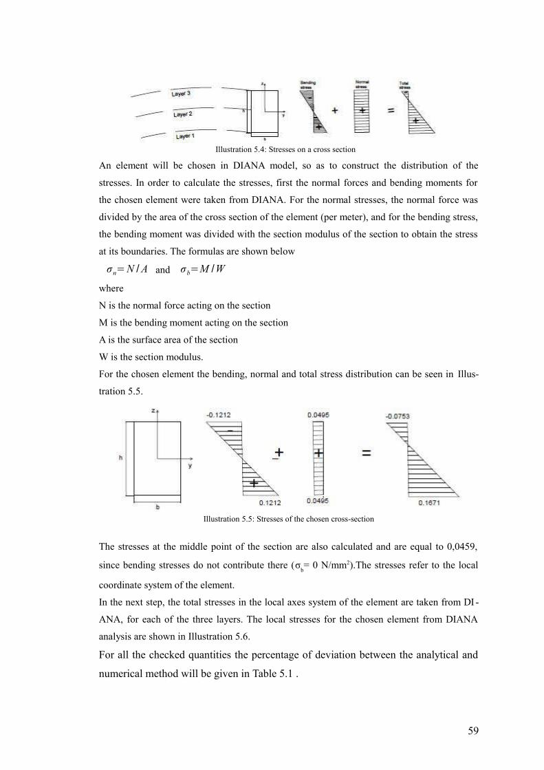
An element will be chosen in DIANA model, so as to construct the distribution of the
stresses. In order to calculate the stresses, first the normal forces and bending moments for
the chosen element were taken from DIANA. For the normal stresses, the normal force was
divided by the area of the cross section of the element (per meter), and for the bending stress,
the bending moment was divided with the section modulus of the section to obtain the stress
at its boundaries. The formulas are shown below
σn=Ν / Α and σb=Μ /W
where
N is the normal force acting on the section
M is the bending moment acting on the section
A is the surface area of the section
W is the section modulus.
For the chosen element the bending, normal and total stress distribution can be seen in Illus-
tration 5.5.
The stresses at the middle point of the section are also calculated and are equal to 0,0459,
since bending stresses do not contribute there (σb= 0 N/mm2).The stresses refer to the local
coordinate system of the element.
In the next step, the total stresses in the local axes system of the element are taken from DI -
ANA, for each of the three layers. The local stresses for the chosen element from DIANA
analysis are shown in Illustration 5.6.
For all the checked quantities the percentage of deviation between the analytical and
numerical method will be given in Table 5.1 .
59
Illustration 5.4: Stresses on a cross section
Illustration 5.5: Stresses of the chosen cross-section
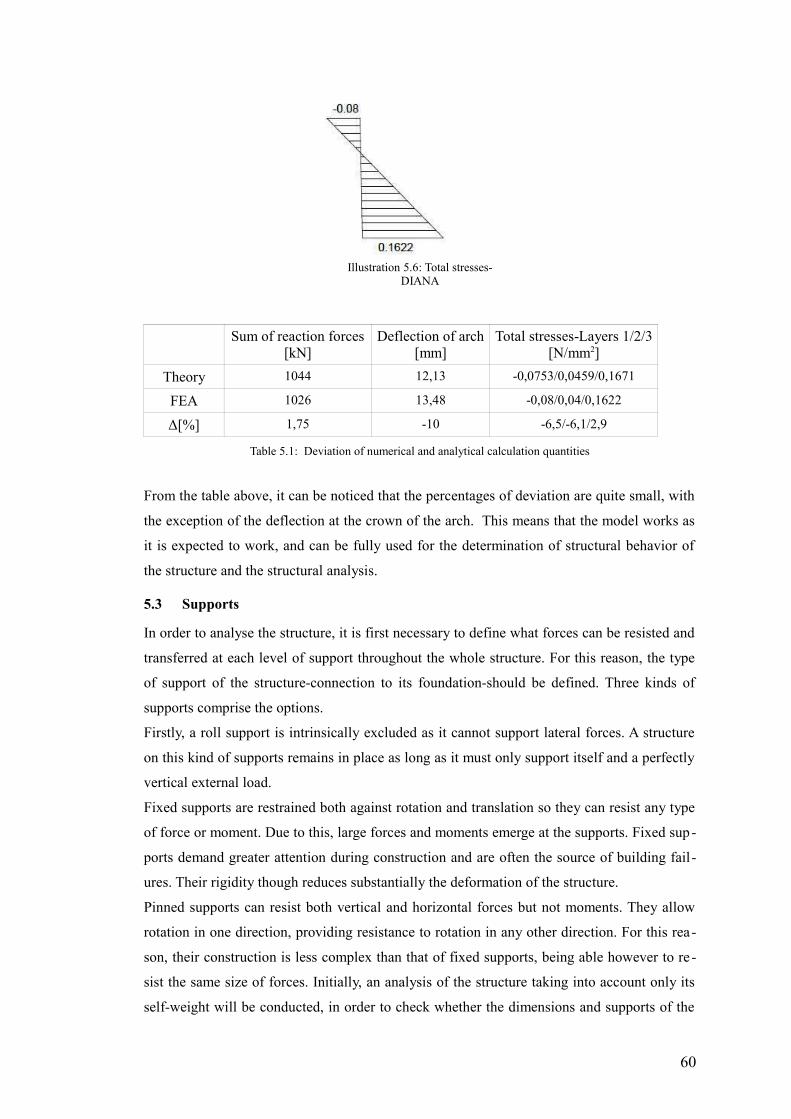
Sum of reaction forces[kN]
Deflection of arch[mm]
Total stresses-Layers 1/2/3[N/mm2]
Theory 1044 12,13 -0,0753/0,0459/0,1671
FEA 1026 13,48 -0,08/0,04/0,1622
Δ[%] 1,75 -10 -6,5/-6,1/2,9
Table 5.1: Deviation of numerical and analytical calculation quantities
From the table above, it can be noticed that the percentages of deviation are quite small, with
the exception of the deflection at the crown of the arch. This means that the model works as
it is expected to work, and can be fully used for the determination of structural behavior of
the structure and the structural analysis.
5.3 Supports
In order to analyse the structure, it is first necessary to define what forces can be resisted and
transferred at each level of support throughout the whole structure. For this reason, the type
of support of the structure-connection to its foundation-should be defined. Three kinds of
supports comprise the options.
Firstly, a roll support is intrinsically excluded as it cannot support lateral forces. A structure
on this kind of supports remains in place as long as it must only support itself and a perfectly
vertical external load.
Fixed supports are restrained both against rotation and translation so they can resist any type
of force or moment. Due to this, large forces and moments emerge at the supports. Fixed sup-
ports demand greater attention during construction and are often the source of building fail-
ures. Their rigidity though reduces substantially the deformation of the structure.
Pinned supports can resist both vertical and horizontal forces but not moments. They allow
rotation in one direction, providing resistance to rotation in any other direction. For this rea-
son, their construction is less complex than that of fixed supports, being able however to re -
sist the same size of forces. Initially, an analysis of the structure taking into account only its
self-weight will be conducted, in order to check whether the dimensions and supports of the
60
Illustration 5.6: Total stresses-DIANA
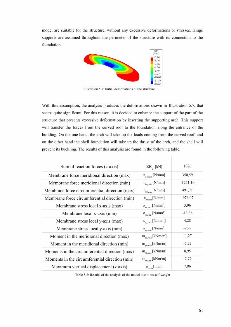
model are suitable for the structure, without any excessive deformations or stresses. Hinge
supports are assumed throughout the perimeter of the structure with its connection to the
foundation.
With this assumption, the analysis produces the deformations shown in Illustration 5.7, that
seems quite significant. For this reason, it is decided to enhance the support of the part of the
structure that presents excessive deformation by inserting the supporting arch. This support
will transfer the forces from the curved roof to the foundation along the entrance of the
building. On the one hand, the arch will take up the loads coming from the curved roof, and
on the other hand the shell foundation will take up the thrust of the arch, and the shell will
prevent its buckling. The results of this analysis are found in the following table.
Sum of reaction forces (z-axis) ΣRz
[kN] 1026
Membrane force meridional direction (max) nφφ,max
[N/mm] 350,59
Membrane force meridional direction (min) nφφ,min
[N/mm] -1251,10
Membrane force circumferential direction (max) nθθ,max
[N/mm] 491,71
Membrane force circumferential direction (min) nθθ,min
[N/mm] -976,07
Membrane stress local x-axis (max) σxx,max
[N/mm2] 3,06
Membrane local x-axis (min) σxx,min
[N/mm2] -13,36
Membrane stress local y-axis (max) σyy,,max
[N/mm2] 4,28
Membrane stress local y-axis (min) σyy,,min
[N/mm2] -9,98
Moment in the meridional direction (max) mφφ,max
[kNm/m] 11,27
Moment in the meridional direction (min) mφφ,min
[kNm/m] -5,22
Moments in the circumferential direction (max) mθθ,max
[kNm/m] 8,95
Moments in the circumferential direction (min) mθθ,min
[kNm/m] -7,72
Maximum vertical displacement (z-axis) uz,max
[ mm] 7,86
Table 5.2: Results of the analysis of the model due to tts self-weight
61
Illustration 5.7: Initial deformations of the structure
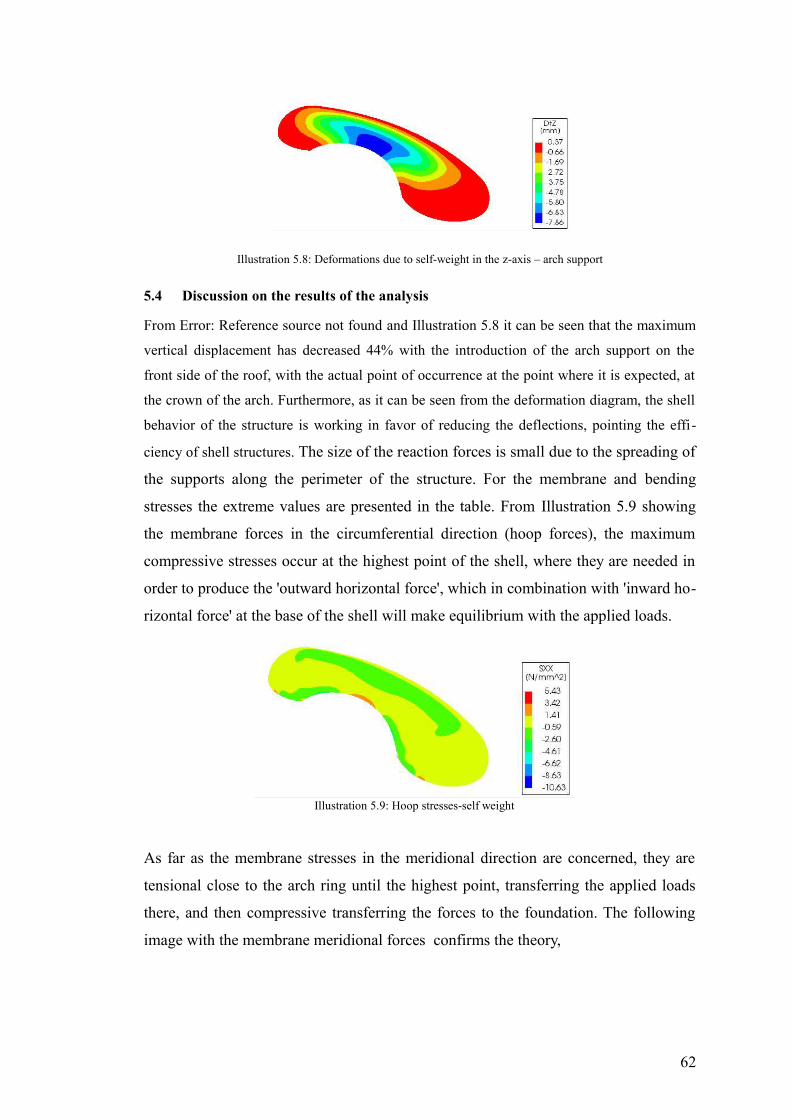
5.4 Discussion on the results of the analysis
From Error: Reference source not found and Illustration 5.8 it can be seen that the maximum
vertical displacement has decreased 44% with the introduction of the arch support on the
front side of the roof, with the actual point of occurrence at the point where it is expected, at
the crown of the arch. Furthermore, as it can be seen from the deformation diagram, the shell
behavior of the structure is working in favor of reducing the deflections, pointing the effi-
ciency of shell structures. The size of the reaction forces is small due to the spreading of
the supports along the perimeter of the structure. For the membrane and bending
stresses the extreme values are presented in the table. From Illustration 5.9 showing
the membrane forces in the circumferential direction (hoop forces), the maximum
compressive stresses occur at the highest point of the shell, where they are needed in
order to produce the 'outward horizontal force', which in combination with 'inward ho-
rizontal force' at the base of the shell will make equilibrium with the applied loads.
As far as the membrane stresses in the meridional direction are concerned, they are
tensional close to the arch ring until the highest point, transferring the applied loads
there, and then compressive transferring the forces to the foundation. The following
image with the membrane meridional forces confirms the theory,
62
Illustration 5.8: Deformations due to self-weight in the z-axis – arch support
Illustration 5.9: Hoop stresses-self weight
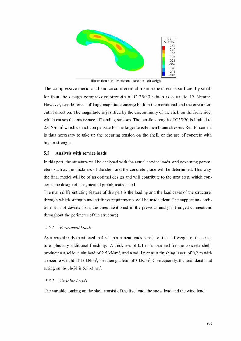
The compressive meridional and circumferential membrane stress is sufficiently smal-
ler than the design compressive strength of C 25/30 which is equal to 17 N/mm2..
However, tensile forces of large magnitude emerge both in the meridional and the circumfer-
ential direction. The magnitude is justified by the discontinuity of the shell on the front side,
which causes the emergence of bending stresses. The tensile strength of C25/30 is limited to
2.6 N/mm2 which cannot compensate for the larger tensile membrane stresses. Reinforcement
is thus necessary to take up the occuring tension on the shell, or the use of concrete with
higher strength.
5.5 Analysis with service loads
In this part, the structure will be analysed with the actual service loads, and governing param-
eters such as the thickness of the shell and the concrete grade will be determined. This way,
the final model will be of an optimal design and will contribute to the next step, which con-
cerns the design of a segmented prefabricated shell.
The main differentiating feature of this part is the loading and the load cases of the structure,
through which strength and stiffness requirements will be made clear. The supporting condi-
tions do not deviate from the ones mentioned in the previous analysis (hinged connections
throughout the perimeter of the structure)
5.5.1 Permanent Loads
As it was already mentioned in 4.3.1, permanent loads consist of the self-weight of the struc-
ture, plus any additional finishing. A thickness of 0,1 m is assumed for the concrete shell,
producing a self-weight load of 2,5 kN/m2, and a soil layer as a finishing layer, of 0,2 m with
a specific weight of 15 kN/m3, producing a load of 3 kN/m2. Consequently, the total dead load
acting on the sheλl is 5,5 kN/m2.
5.5.2 Variable Loads
The variable loading on the shell consist of the live load, the snow load and the wind load.
63
Illustration 5.10: Meridional stresses-self weight
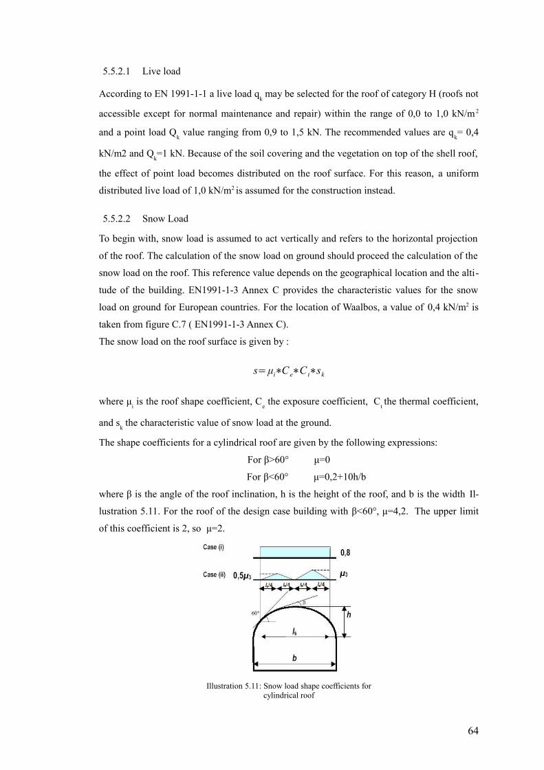
5.5.2.1 Live load
According to EN 1991-1-1 a live load qk may be selected for the roof of category H (roofs not
accessible except for normal maintenance and repair) within the range of 0,0 to 1,0 kN/m 2
and a point load Qk value ranging from 0,9 to 1,5 kN. The recommended values are q
k= 0,4
kN/m2 and Qk=1 kN. Because of the soil covering and the vegetation on top of the shell roof,
the effect of point load becomes distributed on the roof surface. For this reason, a uniform
distributed live load of 1,0 kN/m2 is assumed for the construction instead.
5.5.2.2 Snow Load
To begin with, snow load is assumed to act vertically and refers to the horizontal projection
of the roof. The calculation of the snow load on ground should proceed the calculation of the
snow load on the roof. This reference value depends on the geographical location and the alti-
tude of the building. EN1991-1-3 Annex C provides the characteristic values for the snow
load on ground for European countries. For the location of Waalbos, a value of 0,4 kN/m2 is
taken from figure C.7 ( EN1991-1-3 Annex C).
The snow load on the roof surface is given by :
s=μi∗C e∗C t∗sk
where μi is the roof shape coefficient, C
e the exposure coefficient, C
t the thermal coefficient,
and sk the characteristic value of snow load at the ground.
The shape coefficients for a cylindrical roof are given by the following expressions:
For β>60° μ=0
For β<60° μ=0,2+10h/b
where β is the angle of the roof inclination, h is the height of the roof, and b is the width Il-
lustration 5.11. For the roof of the design case building with β<60°, μ=4,2. The upper limit
of this coefficient is 2, so μ=2.
64
Illustration 5.11: Snow load shape coefficients forcylindrical roof
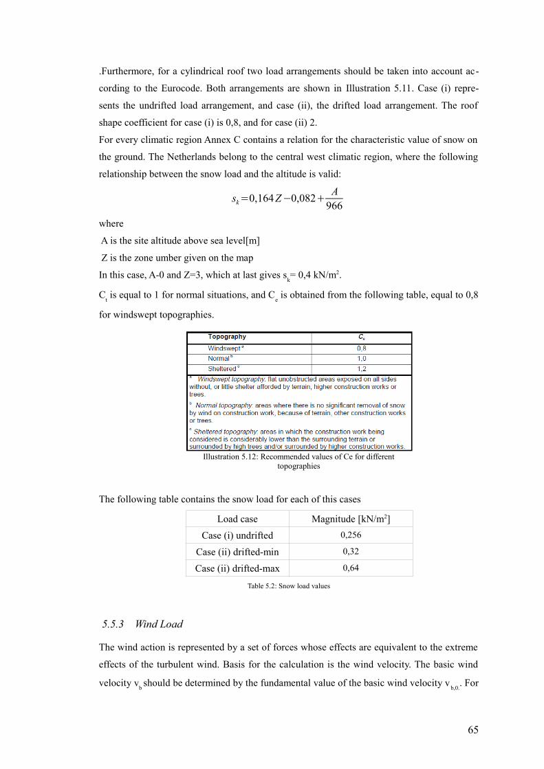
.Furthermore, for a cylindrical roof two load arrangements should be taken into account ac-
cording to the Eurocode. Both arrangements are shown in Illustration 5.11. Case (i) repre-
sents the undrifted load arrangement, and case (ii), the drifted load arrangement. The roof
shape coefficient for case (i) is 0,8, and for case (ii) 2.
For every climatic region Annex C contains a relation for the characteristic value of snow on
the ground. The Netherlands belong to the central west climatic region, where the following
relationship between the snow load and the altitude is valid:
sk=0,164Z−0,082+A
966
where
A is the site altitude above sea level[m]
Z is the zone umber given on the map
In this case, A-0 and Z=3, which at last gives sk= 0,4 kN/m2.
Ct is equal to 1 for normal situations, and C
e is obtained from the following table, equal to 0,8
for windswept topographies.
The following table contains the snow load for each of this cases
Load case Magnitude [kN/m2]
Case (i) undrifted 0,256
Case (ii) drifted-min 0,32
Case (ii) drifted-max 0,64
Table 5.2: Snow load values
5.5.3 Wind Load
The wind action is represented by a set of forces whose effects are equivalent to the extreme
effects of the turbulent wind. Basis for the calculation is the wind velocity. The basic wind
velocity vb should be determined by the fundamental value of the basic wind velocity v
b,0.. For
65
Illustration 5.12: Recommended values of Ce for differenttopographies
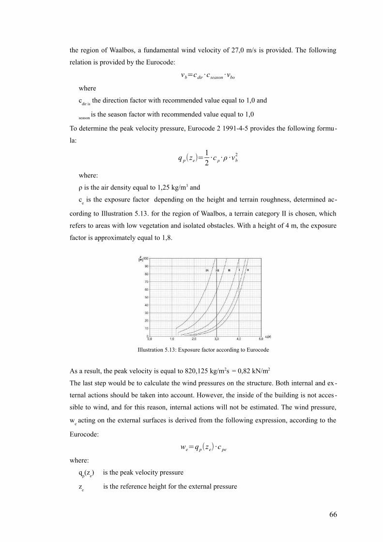
the region of Waalbos, a fundamental wind velocity of 27,0 m/s is provided. The following
relation is provided by the Eurocode:
vb=cdir · cseason · vbo
where
cdir is
the direction factor with recommended value equal to 1,0 and
season is the season factor with recommended value equal to 1,0
To determine the peak velocity pressure, Eurocode 2 1991-4-5 provides the following formu-
la:
q p(ze)=12
· c ρ · ρ · vb2
where:
ρ is the air density equal to 1,25 kg/m3 and
ce is the exposure factor depending on the height and terrain roughness, determined ac-
cording to Illustration 5.13. for the region of Waalbos, a terrain category II is chosen, which
refers to areas with low vegetation and isolated obstacles. With a height of 4 m, the exposure
factor is approximately equal to 1,8.
As a result, the peak velocity is equal to 820,125 kg/m2s = 0,82 kN/m2
The last step would be to calculate the wind pressures on the structure. Both internal and ex-
ternal actions should be taken into account. However, the inside of the building is not acces -
sible to wind, and for this reason, internal actions will not be estimated. The wind pressure,
we acting on the external surfaces is derived from the following expression, according to the
Eurocode:
we=qp(ze) · c pe
where:
qp(z
e) is the peak velocity pressure
ze is the reference height for the external pressure
66
Illustration 5.13: Exposure factor according to Eurocode
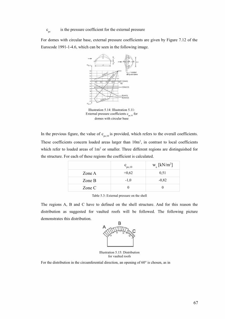
cpe
is the pressure coefficient for the external pressure
For domes with circular base, external pressure coefficients are given by Figure 7.12 of the
Eurocode 1991-1-4.6, which can be seen in the following image.
In the previous figure, the value of cpe,10
is provided, which refers to the overall coefficients.
These coefficients concern loaded areas larger than 10m2, in contrast to local coefficients
which refer to loaded areas of 1m2 or smaller. Three different regions are distinguished for
the structure. For each of these regions the coefficient is calculated.
cpe,10
we [kN/m2]
Zone A +0,62 0,51
Zone B -1,0 -0,82
Zone C 0 0
Table 5.3: External pressure on the shell
The regions A, B and C have to defined on the shell structure. And for this reason the
distribution as suggested for vaulted roofs will be followed. The following picture
demonstrates this distribution.
For the distribution in the circumferential direction, an opening of 60° is chosen, as in
67
Illustration 5.14: Illustration 5.11:External pressure coefficients c
pe,10 for
domes with circular base
Illustration 5.15: Distributionfor vaulted roofs
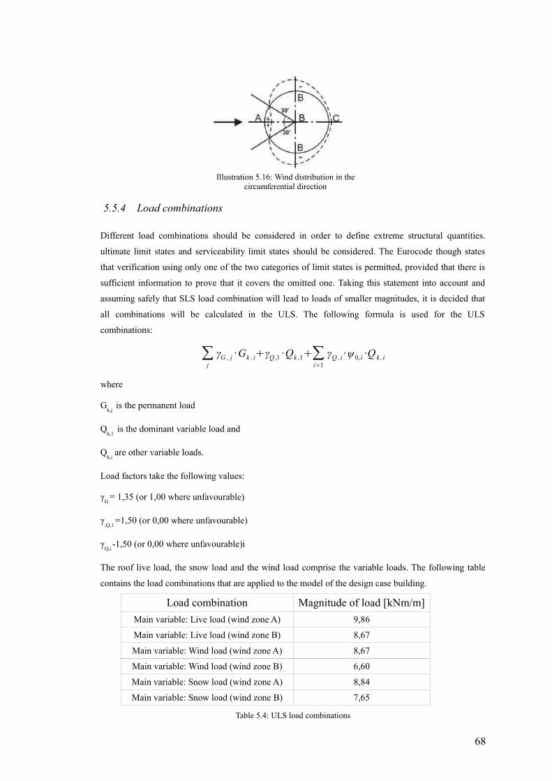
5.5.4 Load combinations
Different load combinations should be considered in order to define extreme structural quantities.
ultimate limit states and serviceability limit states should be considered. The Eurocode though states
that verification using only one of the two categories of limit states is permitted, provided that there is
sufficient information to prove that it covers the omitted one. Taking this statement into account and
assuming safely that SLS load combination will lead to loads of smaller magnitudes, it is decided that
all combinations will be calculated in the ULS. The following formula is used for the ULS
combinations:
∑j
γG , j · Gk ,i+γQ ,1 ·Qk ,1+∑i>1
γQ, i ·ψ0, i ·Q k ,i
where
Gk,j
is the permanent load
Qk,1
is the dominant variable load and
Qk,i
are other variable loads.
Load factors take the following values:
γG
= 1,35 (or 1,00 where unfavourable)
γ;Q,1
=1,50 (or 0,00 where unfavourable)
γQ,i
-1,50 (or 0,00 where unfavourable)i
The roof live load, the snow load and the wind load comprise the variable loads. The following table
contains the load combinations that are applied to the model of the design case building.
Load combination Magnitude of load [kNm/m]
Main variable: Live load (wind zone A) 9,86
Main variable: Live load (wind zone B) 8,67
Main variable: Wind load (wind zone A) 8,67
Main variable: Wind load (wind zone B) 6,60
Main variable: Snow load (wind zone A) 8,84
Main variable: Snow load (wind zone B) 7,65
Table 5.4: ULS load combinations
68
Illustration 5.16: Wind distribution in thecircumferential direction
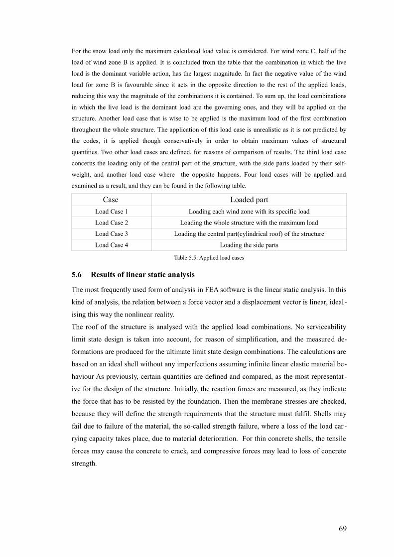
For the snow load only the maximum calculated load value is considered. For wind zone C, half of the
load of wind zone B is applied. It is concluded from the table that the combination in which the live
load is the dominant variable action, has the largest magnitude. In fact the negative value of the wind
load for zone B is favourable since it acts in the opposite direction to the rest of the applied loads,
reducing this way the magnitude of the combinations it is contained. To sum up, the load combinations
in which the live load is the dominant load are the governing ones, and they will be applied on the
structure. Another load case that is wise to be applied is the maximum load of the first combination
throughout the whole structure. The application of this load case is unrealistic as it is not predicted by
the codes, it is applied though conservatively in order to obtain maximum values of structural
quantities. Two other load cases are defined, for reasons of comparison of results. The third load case
concerns the loading only of the central part of the structure, with the side parts loaded by their self-
weight, and another load case where the opposite happens. Four load cases will be applied and
examined as a result, and they can be found in the following table.
Case Loaded part
Load Case 1 Loading each wind zone with its specific load
Load Case 2 Loading the whole structure with the maximum load
Load Case 3 Loading the central part(cylindrical roof) of the structure
Load Case 4 Loading the side parts
Table 5.5: Applied load cases
5.6 Results of linear static analysis
The most frequently used form of analysis in FEA software is the linear static analysis. In this
kind of analysis, the relation between a force vector and a displacement vector is linear, ideal-
ising this way the nonlinear reality.
The roof of the structure is analysed with the applied load combinations. No serviceability
limit state design is taken into account, for reason of simplification, and the measured de-
formations are produced for the ultimate limit state design combinations. The calculations are
based on an ideal shell without any imperfections assuming infinite linear elastic material be-
haviour As previously, certain quantities are defined and compared, as the most representat -
ive for the design of the structure. Initially, the reaction forces are measured, as they indicate
the force that has to be resisted by the foundation. Then the membrane stresses are checked,
because they will define the strength requirements that the structure must fulfil. Shells may
fail due to failure of the material, the so-called strength failure, where a loss of the load car -
rying capacity takes place, due to material deterioration. For thin concrete shells, the tensile
forces may cause the concrete to crack, and compressive forces may lead to loss of concrete
strength.
69
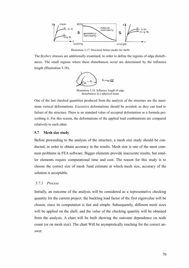
The βενδινγ stresses are additionally examined, in order to define the regions of edge disturb-
ances. The small regions where these disturbances occur are determined by the influence
length (Illustration 5.18).
One of the last checked quantities produced from the analysis of the structure are the maxi-
mum vertical deformations. Excessive deformations should be avoided, as they can lead to
failure of the structure. There is no standard value of accepted deformation or a formula pre-
scribing it. For this reason, the deformations of the applied load combinations are compared
relatively to each other.
5.7 Mesh size study
Before proceeding to the analysis of the structure, a mesh size study should be con-
ducted, in order to obtain accuracy in the results. Mesh size is one of the most com-
mon problems in FEA software. Bigger elements provide inaccurate results, but smal-
ler elements require computational time and cost. The reason for this study is to
choose the correct size of mesh 5and estimate at which mesh size, accuracy of the
solution is acceptable.
5.7.1 Process
Initially, an outcome of the analysis will be considered as a representative checking
quantity for the current project. the buckling load factor of the first eigenvalue will be
chosen, since its computation is fast and simple. Subsequently, different mesh sizes
will be applied on the shell, and the value of the checking quantity will be obtained
from the analysis. A chart will be built showing the outcome dependence on node
count (or on mesh size). The chart Will be asymptotically reaching for the correct an-
swer.
70
Illustration 5.18: Influence length of edgedisturbances in a spherical dome
Illustration 5.17: Structural failure modes for shells
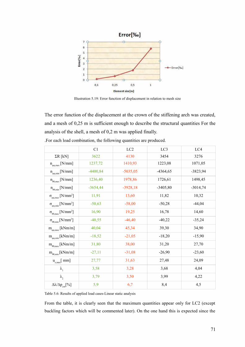
The error function of the displacement at the crown of the stiffening arch was created,
and a mesh of 0,25 m is sufficient enough to describe the structural quantities For the
analysis of the shell, a mesh of 0,2 m was applied finally.
.For each load combination, the following quantities are produced.
C1 LC2 LC3 LC4
ΣR [kΝ] 3622 4130 3454 3276
nφφ,max
[N/mm] 1237,72 1410,93 1223,08 1071,05
nφφ,min
[N/mm] -4400,84 -5035,05 -4364,65 -3823,94
nθθ,max
[N/mm] 1236,40 1978,86 1726,61 1498,45
nθθ,min
[N/mm] -3654,44 -3928,18 -3405,80 -3014,74
σφφ,max
[N/mm2] 11,91 13,60 11,82 10,32
σφφ,min
[N/mm2] -50,63 -58,00 -50,28 -44,04
σθθ,max
[N/mm2] 16,90 19,25 16,78 14,60
σθθ,min
[N/mm2] -40,55 -46,40 -40,22 -35,24
mφφ,max
[kNm/m] 40,04 45,34 39,30 34,90
mφφ,min
[kNm/m] -18,52 -21,05 -18,20 -15,90
mθθ,max
[kNm/m] 31,80 38,00 31,20 27,70
mθθ,min
[kNm/m] -27,11 -31,08 -26,90 -23,60
uz,max
[ mm] 27,77 31,63 27,48 24,09
λ1
3,58 3,28 3,68 4,04
λ2
3,79 3,50 3,99 4,22
Δλ/Δpcrit
[%] 5,9 6,7 8,4 4,5
Table 5.6: Results of applied load cases-Linear static analysis
From the table, it is clearly seen that the maximum quantities appear only for LC2 (except
buckling factors which will be commented later). On the one hand this is expected since the
71
Illustration 5.19: Error function of displacement in relation to mesh size
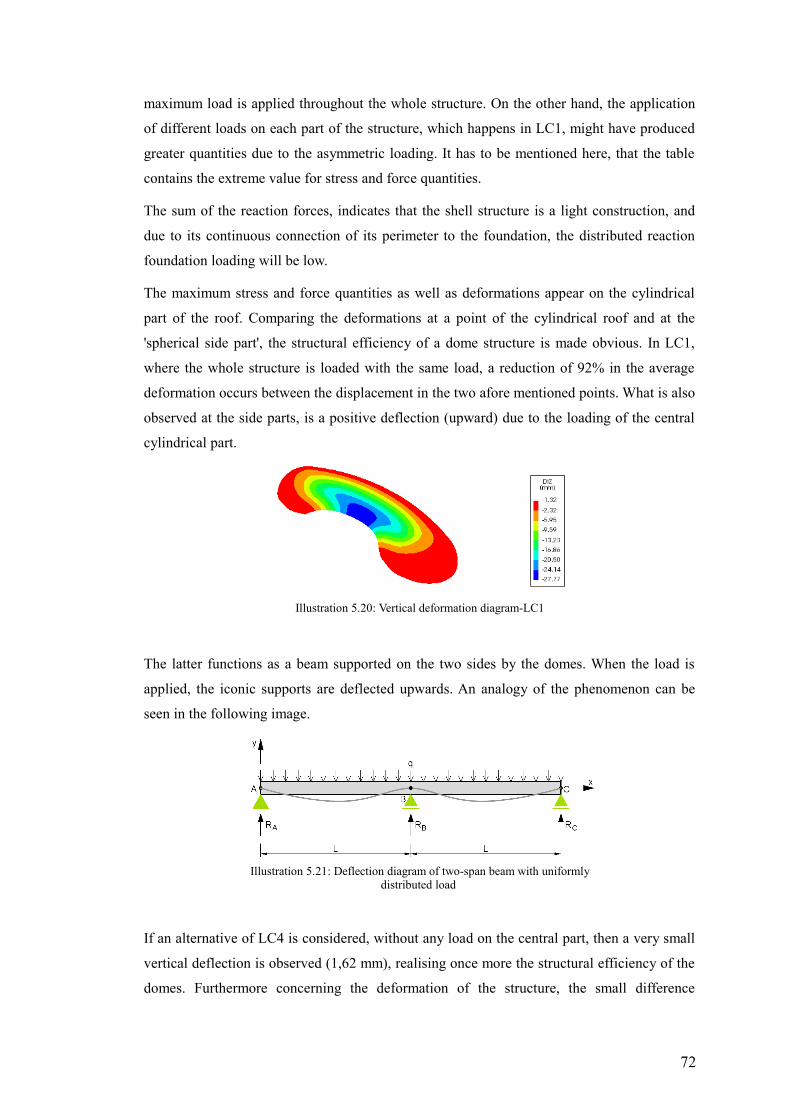
maximum load is applied throughout the whole structure. On the other hand, the application
of different loads on each part of the structure, which happens in LC1, might have produced
greater quantities due to the asymmetric loading. It has to be mentioned here, that the table
contains the extreme value for stress and force quantities.
The sum of the reaction forces, indicates that the shell structure is a light construction, and
due to its continuous connection of its perimeter to the foundation, the distributed reaction
foundation loading will be low.
The maximum stress and force quantities as well as deformations appear on the cylindrical
part of the roof. Comparing the deformations at a point of the cylindrical roof and at the
'spherical side part', the structural efficiency of a dome structure is made obvious. In LC1,
where the whole structure is loaded with the same load, a reduction of 92% in the average
deformation occurs between the displacement in the two afore mentioned points. What is also
observed at the side parts, is a positive deflection (upward) due to the loading of the central
cylindrical part.
The latter functions as a beam supported on the two sides by the domes. When the load is
applied, the iconic supports are deflected upwards. An analogy of the phenomenon can be
seen in the following image.
If an alternative of LC4 is considered, without any load on the central part, then a very small
vertical deflection is observed (1,62 mm), realising once more the structural efficiency of the
domes. Furthermore concerning the deformation of the structure, the small difference
72
Illustration 5.21: Deflection diagram of two-span beam with uniformlydistributed load
Illustration 5.20: Vertical deformation diagram-LC1
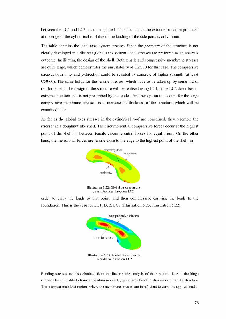
between the LC1 and LC3 has to be spotted. This means that the extra deformation produced
at the edge of the cylindrical roof due to the loading of the side parts is only minor.
The table contains the local axes system stresses. Since the geometry of the structure is not
clearly developed in a discreet global axes system, local stresses are preferred as an analysis
outcome, facilitating the design of the shell. Both tensile and compressive membrane stresses
are quite large, which demonstrates the unsuitability of C25/30 for this case. The compressive
stresses both in x- and y-direction could be resisted by concrete of higher strength (at least
C50/60). The same holds for the tensile stresses, which have to be taken up by some ind of
reinforcement. The design of the structure will be realised using LC1, since LC2 describes an
extreme situation that is not prescribed by the codes. Another option to account for the large
compressive membrane stresses, is to increase the thickness of the structure, which will be
examined later.
As far as the global axes stresses in the cylindrical roof are concerned, they resemble the
stresses in a doughnut like shell. The circumferential compressive forces occur at the highest
point of the shell, in between tensile circumferential forces for equilibrium. On the other
hand, the meridional forces are tensile close to the edge to the highest point of the shell, in
order to carry the loads to that point, and then compressive carrying the loads to the
foundation. This is the case for LC1, LC2, LC3 (Illustration 5.23, Illustration 5.22).
Bending stresses are also obtained from the linear static analysis of the structure. Due to the hinge
supports being unable to transfer bending moments, quite large bending stresses occur at the structure.
These appear mainly at regions where the membrane stresses are insufficient to carry the applied loads.
73
Illustration 5.23: Global stresses in themeridional direction-LC2
Illustration 5.22: Global stresses in thecircumferential direction-LC2
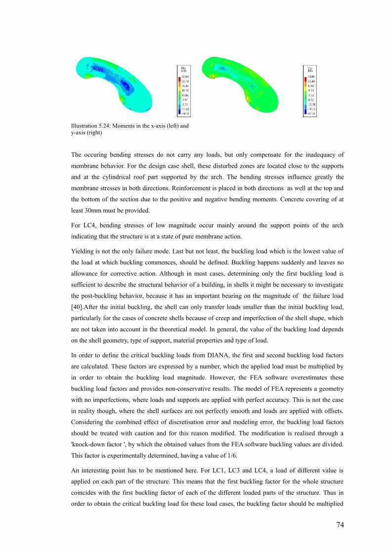
The occuring bending stresses do not carry any loads, but only compensate for the inadequacy of
membrane behavior. For the design case shell, these disturbed zones are located close to the supports
and at the cylindrical roof part supported by the arch. The bending stresses influence greatly the
membrane stresses in both directions. Reinforcement is placed in both directions as well at the top and
the bottom of the section due to the positive and negative bending moments. Concrete covering of at
least 30mm must be provided.
For LC4, bending stresses of low magnitude occur mainly around the support points of the arch
indicating that the structure is at a state of pure membrane action.
Yielding is not the only failure mode. Last but not least, the buckling load which is the lowest value of
the load at which buckling commences, should be defined. Buckling happens suddenly and leaves no
allowance for corrective action. Although in most cases, determining only the first buckling load is
sufficient to describe the structural behavior of a building, in shells it might be necessary to investigate
the post-buckling behavior, because it has an important bearing on the magnitude of the failure load
[40].After the initial buckling, the shell can only transfer loads smaller than the initial buckling load,
particularly for the cases of concrete shells because of creep and imperfection of the shell shape, which
are not taken into account in the theoretical model. In general, the value of the buckling load depends
on the shell geometry, type of support, material properties and type of load.
In order to define the critical buckling loads from DIANA, the first and second buckling load factors
are calculated. These factors are expressed by a number, which the applied load must be multiplied by
in order to obtain the buckling load magnitude. However, the FEA software overestimates these
buckling load factors and provides non-conservative results. The model of FEA represents a geometry
with no imperfections, where loads and supports are applied with perfect accuracy. This is not the case
in reality though, where the shell surfaces are not perfectly smooth and loads are applied with offsets.
Considering the combined effect of discretisation error and modeling error, the buckling load factors
should be treated with caution and for this reason modified. The modification is realised through a
'knock-down factor ', by which the obtained values from the FEA software buckling values are divided.
This factor is experimentally determined, having a value of 1/6.
An interesting point has to be mentioned here. For LC1, LC3 and LC4, a load of different value is
applied on each part of the structure. This means that the first buckling factor for the whole structure
coincides with the first buckling factor of each of the different loaded parts of the structure. Thus in
order to obtain the critical buckling load for these load cases, the buckling factor should be multiplied
74
Illustration 5.24: Moments in the x-axis (left) and y-axis (right)
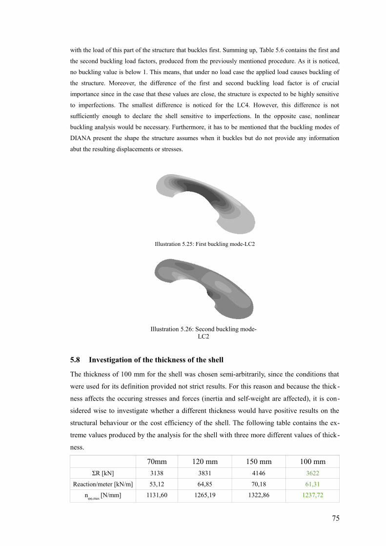
with the load of this part of the structure that buckles first. Summing up, Table 5.6 contains the first and
the second buckling load factors, produced from the previously mentioned procedure. As it is noticed,
no buckling value is below 1. This means, that under no load case the applied load causes buckling of
the structure. Moreover, the difference of the first and second buckling load factor is of crucial
importance since in the case that these values are close, the structure is expected to be highly sensitive
to imperfections. The smallest difference is noticed for the LC4. However, this difference is not
sufficiently enough to declare the shell sensitive to imperfections. In the opposite case, nonlinear
buckling analysis would be necessary. Furthermore, it has to be mentioned that the buckling modes of
DIANA present the shape the structure assumes when it buckles but do not provide any information
abut the resulting displacements or stresses.
5.8 Investigation of the thickness of the shell
The thickness of 100 mm for the shell was chosen semi-arbitrarily, since the conditions that
were used for its definition provided not strict results. For this reason and because the thick -
ness affects the occuring stresses and forces (inertia and self-weight are affected), it is con-
sidered wise to investigate whether a different thickness would have positive results on the
structural behaviour or the cost efficiency of the shell. The following table contains the ex-
treme values produced by the analysis for the shell with three more different values of thick-
ness.
70mm 120 mm 150 mm 100 mm
ΣR [kN] 3138 3831 4146 3622
Reaction/meter [kN/m] 53,12 64,85 70,18 61,31
nφφ,max
[N/mm] 1131,60 1265,19 1322,86 1237,72
75
Illustration 5.26: Second buckling mode-LC2
Illustration 5.25: First buckling mode-LC2
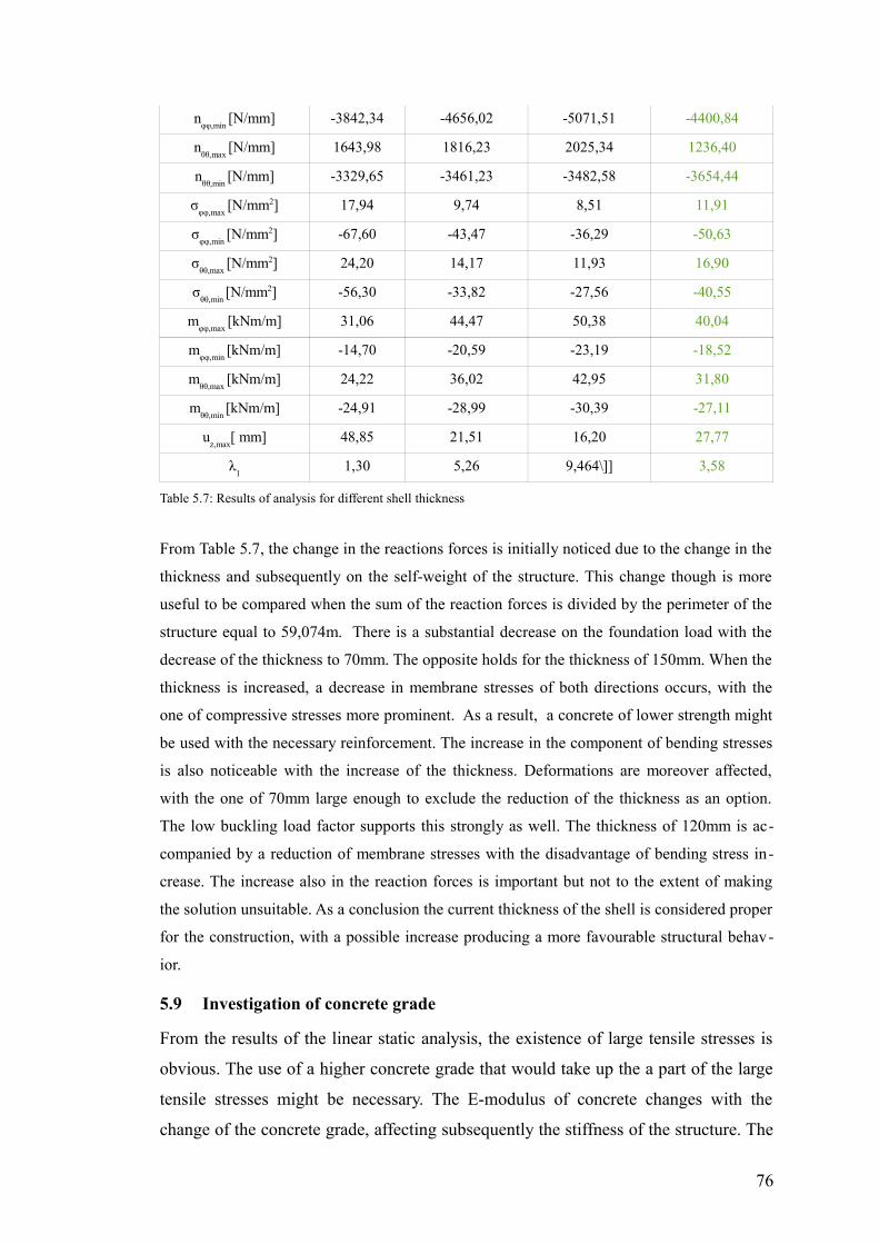
nφφ,min
[N/mm] -3842,34 -4656,02 -5071,51 -4400,84
nθθ,max
[N/mm] 1643,98 1816,23 2025,34 1236,40
nθθ,min
[N/mm] -3329,65 -3461,23 -3482,58 -3654,44
σφφ,max
[N/mm2] 17,94 9,74 8,51 11,91
σφφ,min
[N/mm2] -67,60 -43,47 -36,29 -50,63
σθθ,max
[N/mm2] 24,20 14,17 11,93 16,90
σθθ,min
[N/mm2] -56,30 -33,82 -27,56 -40,55
mφφ,max
[kNm/m] 31,06 44,47 50,38 40,04
mφφ,min
[kNm/m] -14,70 -20,59 -23,19 -18,52
mθθ,max
[kNm/m] 24,22 36,02 42,95 31,80
mθθ,min
[kNm/m] -24,91 -28,99 -30,39 -27,11
uz,max
[ mm] 48,85 21,51 16,20 27,77
λ1
1,30 5,26 9,464\]] 3,58
Table 5.7: Results of analysis for different shell thickness
From Table 5.7, the change in the reactions forces is initially noticed due to the change in the
thickness and subsequently on the self-weight of the structure. This change though is more
useful to be compared when the sum of the reaction forces is divided by the perimeter of the
structure equal to 59,074m. There is a substantial decrease on the foundation load with the
decrease of the thickness to 70mm. The opposite holds for the thickness of 150mm. When the
thickness is increased, a decrease in membrane stresses of both directions occurs, with the
one of compressive stresses more prominent. As a result, a concrete of lower strength might
be used with the necessary reinforcement. The increase in the component of bending stresses
is also noticeable with the increase of the thickness. Deformations are moreover affected,
with the one of 70mm large enough to exclude the reduction of the thickness as an option.
The low buckling load factor supports this strongly as well. The thickness of 120mm is ac-
companied by a reduction of membrane stresses with the disadvantage of bending stress in-
crease. The increase also in the reaction forces is important but not to the extent of making
the solution unsuitable. As a conclusion the current thickness of the shell is considered proper
for the construction, with a possible increase producing a more favourable structural behav-
ior.
5.9 Investigation of concrete grade
From the results of the linear static analysis, the existence of large tensile stresses is
obvious. The use of a higher concrete grade that would take up the a part of the large
tensile stresses might be necessary. The E-modulus of concrete changes with the
change of the concrete grade, affecting subsequently the stiffness of the structure. The
76
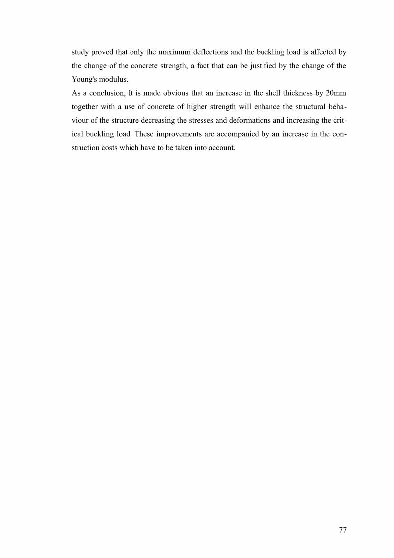
study proved that only the maximum deflections and the buckling load is affected by
the change of the concrete strength, a fact that can be justified by the change of the
Young's modulus.
As a conclusion, It is made obvious that an increase in the shell thickness by 20mm
together with a use of concrete of higher strength will enhance the structural beha-
viour of the structure decreasing the stresses and deformations and increasing the crit-
ical buckling load. These improvements are accompanied by an increase in the con-
struction costs which have to be taken into account.
77
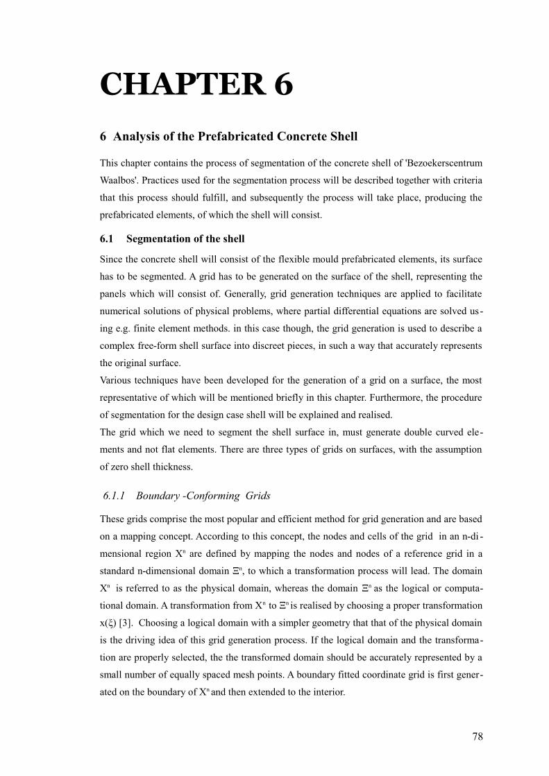
CHAPTER 6
6 Analysis of the Prefabricated Concrete Shell
This chapter contains the process of segmentation of the concrete shell of 'Bezoekerscentrum
Waalbos'. Practices used for the segmentation process will be described together with criteria
that this process should fulfill, and subsequently the process will take place, producing the
prefabricated elements, of which the shell will consist.
6.1 Segmentation of the shell
Since the concrete shell will consist of the flexible mould prefabricated elements, its surface
has to be segmented. A grid has to be generated on the surface of the shell, representing the
panels which will consist of. Generally, grid generation techniques are applied to facilitate
numerical solutions of physical problems, where partial differential equations are solved us-
ing e.g. finite element methods. in this case though, the grid generation is used to describe a
complex free-form shell surface into discreet pieces, in such a way that accurately represents
the original surface.
Various techniques have been developed for the generation of a grid on a surface, the most
representative of which will be mentioned briefly in this chapter. Furthermore, the procedure
of segmentation for the design case shell will be explained and realised.
The grid which we need to segment the shell surface in, must generate double curved ele-
ments and not flat elements. There are three types of grids on surfaces, with the assumption
of zero shell thickness.
6.1.1 Boundary -Conforming Grids
These grids comprise the most popular and efficient method for grid generation and are based
on a mapping concept. According to this concept, the nodes and cells of the grid in an n-di -
mensional region Xn are defined by mapping the nodes and nodes of a reference grid in a
standard n-dimensional domain Ξn, to which a transformation process will lead. The domain
Xn is referred to as the physical domain, whereas the domain Ξn as the logical or computa-
tional domain. A transformation from Xn to Ξn is realised by choosing a proper transformation
x(ξ) [3]. Choosing a logical domain with a simpler geometry that that of the physical domain
is the driving idea of this grid generation process. If the logical domain and the transforma-
tion are properly selected, the the transformed domain should be accurately represented by a
small number of equally spaced mesh points. A boundary fitted coordinate grid is first gener-
ated on the boundary of Xn and then extended to the interior.
78
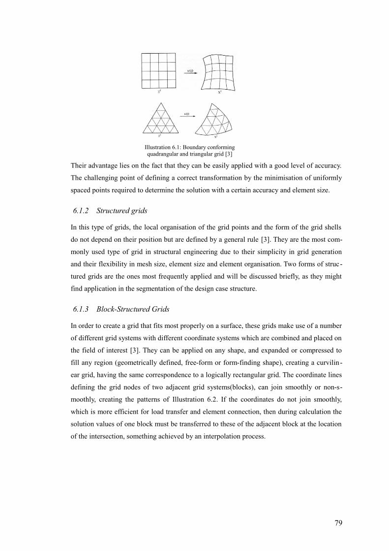
Their advantage lies on the fact that they can be easily applied with a good level of accuracy.
The challenging point of defining a correct transformation by the minimisation of uniformly
spaced points required to determine the solution with a certain accuracy and element size.
6.1.2 Structured grids
In this type of grids, the local organisation of the grid points and the form of the grid shells
do not depend on their position but are defined by a general rule [3]. They are the most com-
monly used type of grid in structural engineering due to their simplicity in grid generation
and their flexibility in mesh size, element size and element organisation. Two forms of struc -
tured grids are the ones most frequently applied and will be discussed briefly, as they might
find application in the segmentation of the design case structure.
6.1.3 Block-Structured Grids
In order to create a grid that fits most properly on a surface, these grids make use of a number
of different grid systems with different coordinate systems which are combined and placed on
the field of interest [3]. They can be applied on any shape, and expanded or compressed to
fill any region (geometrically defined, free-form or form-finding shape), creating a curvilin -
ear grid, having the same correspondence to a logically rectangular grid. The coordinate lines
defining the grid nodes of two adjacent grid systems(blocks), can join smoothly or non-s-
moothly, creating the patterns of Illustration 6.2. If the coordinates do not join smoothly,
which is more efficient for load transfer and element connection, then during calculation the
solution values of one block must be transferred to these of the adjacent block at the location
of the intersection, something achieved by an interpolation process.
79
Illustration 6.1: Boundary conformingquadrangular and triangular grid [3]
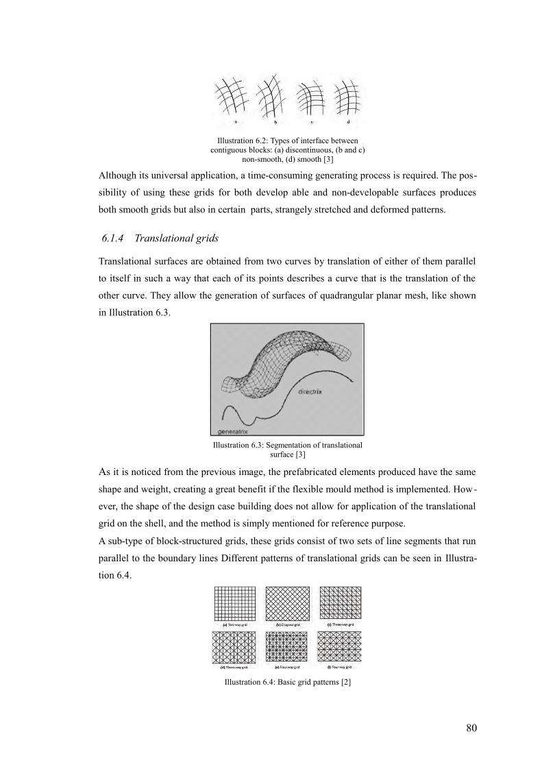
Although its universal application, a time-consuming generating process is required. The pos-
sibility of using these grids for both develop able and non-developable surfaces produces
both smooth grids but also in certain parts, strangely stretched and deformed patterns.
6.1.4 Translational grids
Translational surfaces are obtained from two curves by translation of either of them parallel
to itself in such a way that each of its points describes a curve that is the translation of the
other curve. They allow the generation of surfaces of quadrangular planar mesh, like shown
in Illustration 6.3.
As it is noticed from the previous image, the prefabricated elements produced have the same
shape and weight, creating a great benefit if the flexible mould method is implemented. How-
ever, the shape of the design case building does not allow for application of the translational
grid on the shell, and the method is simply mentioned for reference purpose.
A sub-type of block-structured grids, these grids consist of two sets of line segments that run
parallel to the boundary lines Different patterns of translational grids can be seen in Illustra-
tion 6.4.
80
Illustration 6.2: Types of interface betweencontiguous blocks: (a) discontinuous, (b and c)
non-smooth, (d) smooth [3]
Illustration 6.3: Segmentation of translationalsurface [3]
Illustration 6.4: Basic grid patterns [2]
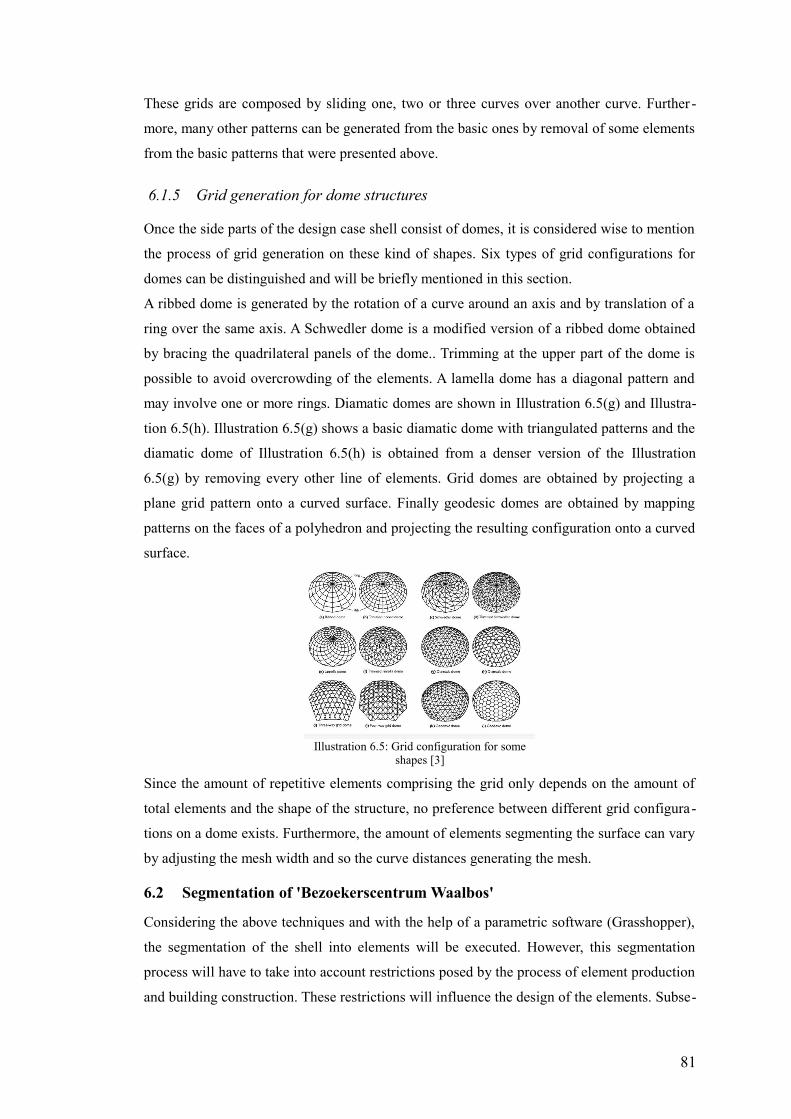
These grids are composed by sliding one, two or three curves over another curve. Further -
more, many other patterns can be generated from the basic ones by removal of some elements
from the basic patterns that were presented above.
6.1.5 Grid generation for dome structures
Once the side parts of the design case shell consist of domes, it is considered wise to mention
the process of grid generation on these kind of shapes. Six types of grid configurations for
domes can be distinguished and will be briefly mentioned in this section.
A ribbed dome is generated by the rotation of a curve around an axis and by translation of a
ring over the same axis. A Schwedler dome is a modified version of a ribbed dome obtained
by bracing the quadrilateral panels of the dome.. Trimming at the upper part of the dome is
possible to avoid overcrowding of the elements. A lamella dome has a diagonal pattern and
may involve one or more rings. Diamatic domes are shown in Illustration 6.5(g) and Illustra-
tion 6.5(h). Illustration 6.5(g) shows a basic diamatic dome with triangulated patterns and the
diamatic dome of Illustration 6.5(h) is obtained from a denser version of the Illustration
6.5(g) by removing every other line of elements. Grid domes are obtained by projecting a
plane grid pattern onto a curved surface. Finally geodesic domes are obtained by mapping
patterns on the faces of a polyhedron and projecting the resulting configuration onto a curved
surface.
Since the amount of repetitive elements comprising the grid only depends on the amount of
total elements and the shape of the structure, no preference between different grid configura-
tions on a dome exists. Furthermore, the amount of elements segmenting the surface can vary
by adjusting the mesh width and so the curve distances generating the mesh.
6.2 Segmentation of 'Bezoekerscentrum Waalbos'
Considering the above techniques and with the help of a parametric software (Grasshopper),
the segmentation of the shell into elements will be executed. However, this segmentation
process will have to take into account restrictions posed by the process of element production
and building construction. These restrictions will influence the design of the elements. Subse-
81
Illustration 6.5: Grid configuration for someshapes [3]
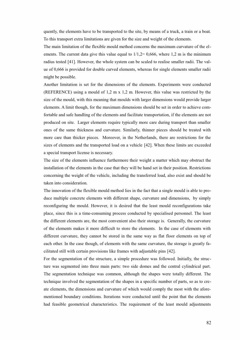
quently, the elements have to be transported to the site, by means of a truck, a train or a boat.
To this transport extra limitations are given for the size and weight of the elements.
The main limitation of the flexible mould method concerns the maximum curvature of the el -
ements. The current data give this value equal to 1/1,2= 0,666, where 1,2 m is the minimum
radius tested [41]. However, the whole system can be scaled to realise smaller radii. The val-
ue of 0,666 is provided for double curved elements, whereas for single elements smaller radii
might be possible.
Another limitation is set for the dimensions of the elements. Experiments were conducted
(REFERENCE) using a mould of 1,2 m x 1,2 m. However, this value was restricted by the
size of the mould, with this meaning that moulds with larger dimensions would provide larger
elements. A limit though, for the maximum dimensions should be set in order to achieve com-
fortable and safe handling of the elements and facilitate transportation, if the elements are not
produced on site. Larger elements require typically more care during transport than smaller
ones of the same thickness and curvature. Similarly, thinner pieces should be treated with
more care than thicker pieces. Moreover, in the Netherlands, there are restrictions for the
sizes of elements and the transported load on a vehicle [42]. When these limits are exceeded
a special transport license is necessary.
The size of the elements influence furthermore their weight a matter which may obstruct the
installation of the elements in the case that they will be hand set in their position. Restrictions
concerning the weight of the vehicle, including the transferred load, also exist and should be
taken into consideration.
The innovation of the flexible mould method lies in the fact that a single mould is able to pro-
duce multiple concrete elements with different shape, curvature and dimensions, by simply
reconfiguring the mould. However, it is desired that the least mould reconfigurations take
place, since this is a time-consuming process conducted by specialised personnel. The least
the different elements are, the most convenient also their storage is. Generally, the curvature
of the elements makes it more difficult to store the elements. In the case of elements with
different curvature, they cannot be stored in the same way as flat floor elements on top of
each other. In the case though, of elements with the same curvature, the storage is greatly fa-
cilitated still with certain provisions like frames with adjustable pins [42].
For the segmentation of the structure, a simple procedure was followed. Initially, the struc-
ture was segmented into three main parts: two side domes and the central cylindrical part.
The segmentation technique was common, although the shapes were totally different. The
technique involved the segmentation of the shapes in a specific number of parts, so as to cre-
ate elements, the dimensions and curvature of which would comply the most with the afore-
mentioned boundary conditions. Iterations were conducted until the point that the elements
had feasible geometrical characteristics. The requirement of the least mould adjustments
82
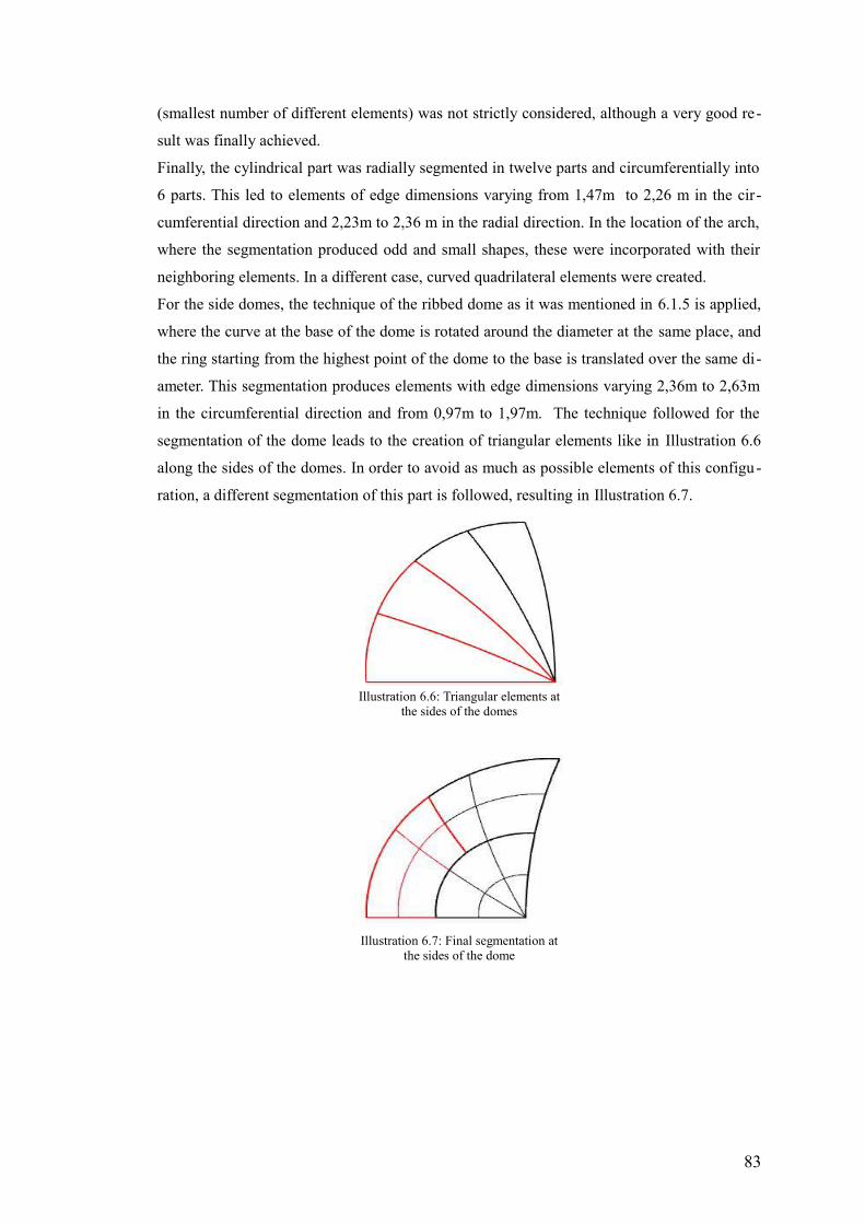
(smallest number of different elements) was not strictly considered, although a very good re-
sult was finally achieved.
Finally, the cylindrical part was radially segmented in twelve parts and circumferentially into
6 parts. This led to elements of edge dimensions varying from 1,47m to 2,26 m in the cir-
cumferential direction and 2,23m to 2,36 m in the radial direction. In the location of the arch,
where the segmentation produced odd and small shapes, these were incorporated with their
neighboring elements. In a different case, curved quadrilateral elements were created.
For the side domes, the technique of the ribbed dome as it was mentioned in 6.1.5 is applied,
where the curve at the base of the dome is rotated around the diameter at the same place, and
the ring starting from the highest point of the dome to the base is translated over the same di-
ameter. This segmentation produces elements with edge dimensions varying 2,36m to 2,63m
in the circumferential direction and from 0,97m to 1,97m. The technique followed for the
segmentation of the dome leads to the creation of triangular elements like in Illustration 6.6
along the sides of the domes. In order to avoid as much as possible elements of this configu-
ration, a different segmentation of this part is followed, resulting in Illustration 6.7.
83
Illustration 6.6: Triangular elements atthe sides of the domes
Illustration 6.7: Final segmentation atthe sides of the dome
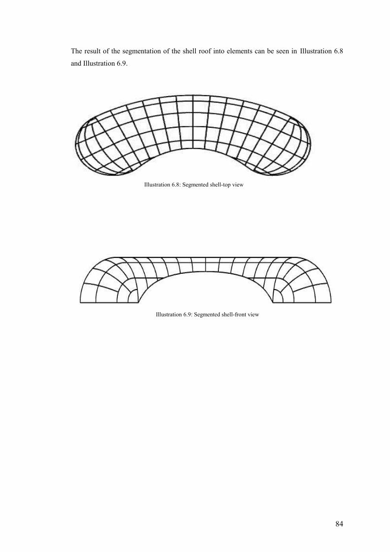
The result of the segmentation of the shell roof into elements can be seen in Illustration 6.8
and Illustration 6.9.
84
Illustration 6.8: Segmented shell-top view
Illustration 6.9: Segmented shell-front view
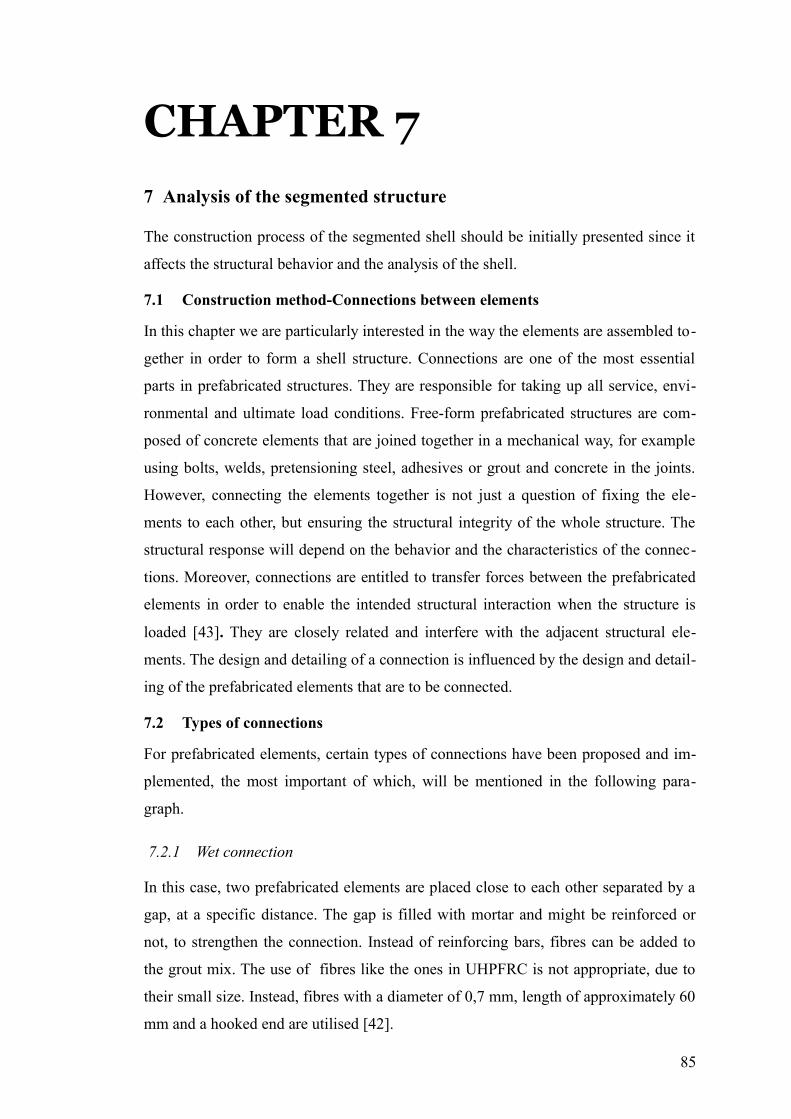
CHAPTER 7
7 Analysis of the segmented structure
The construction process of the segmented shell should be initially presented since it
affects the structural behavior and the analysis of the shell.
7.1 Construction method-Connections between elements
In this chapter we are particularly interested in the way the elements are assembled to-
gether in order to form a shell structure. Connections are one of the most essential
parts in prefabricated structures. They are responsible for taking up all service, envi-
ronmental and ultimate load conditions. Free-form prefabricated structures are com-
posed of concrete elements that are joined together in a mechanical way, for example
using bolts, welds, pretensioning steel, adhesives or grout and concrete in the joints.
However, connecting the elements together is not just a question of fixing the ele-
ments to each other, but ensuring the structural integrity of the whole structure. The
structural response will depend on the behavior and the characteristics of the connec-
tions. Moreover, connections are entitled to transfer forces between the prefabricated
elements in order to enable the intended structural interaction when the structure is
loaded [43]. They are closely related and interfere with the adjacent structural ele-
ments. The design and detailing of a connection is influenced by the design and detail-
ing of the prefabricated elements that are to be connected.
7.2 Types of connections
For prefabricated elements, certain types of connections have been proposed and im-
plemented, the most important of which, will be mentioned in the following para-
graph.
7.2.1 Wet connection
In this case, two prefabricated elements are placed close to each other separated by a
gap, at a specific distance. The gap is filled with mortar and might be reinforced or
not, to strengthen the connection. Instead of reinforcing bars, fibres can be added to
the grout mix. The use of fibres like the ones in UHPFRC is not appropriate, due to
their small size. Instead, fibres with a diameter of 0,7 mm, length of approximately 60
mm and a hooked end are utilised [42].
85
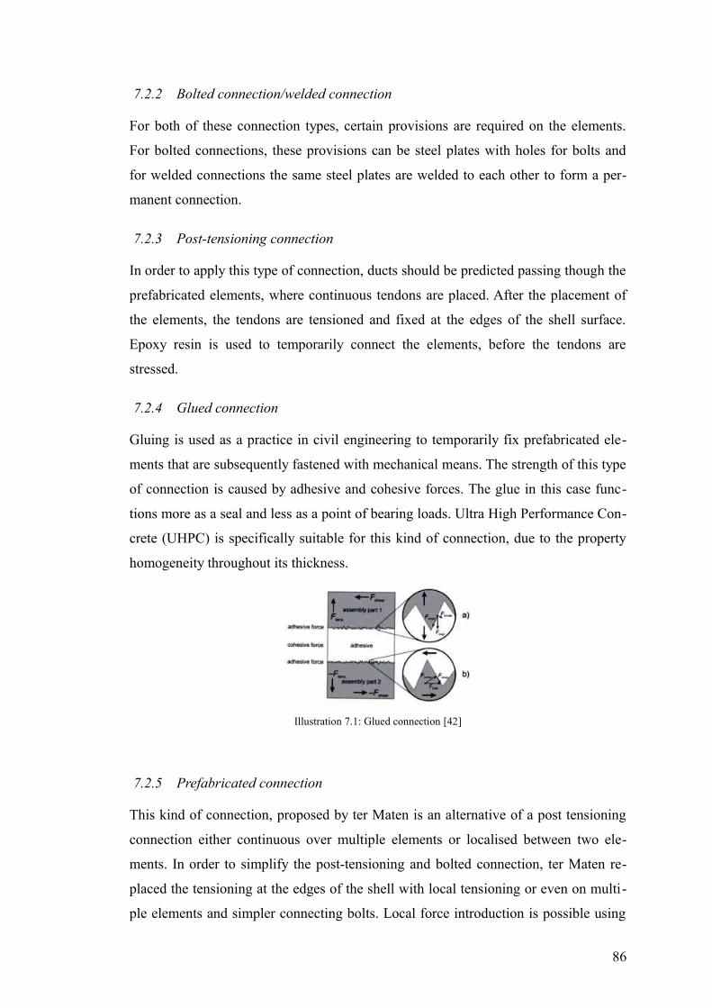
7.2.2 Bolted connection/welded connection
For both of these connection types, certain provisions are required on the elements.
For bolted connections, these provisions can be steel plates with holes for bolts and
for welded connections the same steel plates are welded to each other to form a per-
manent connection.
7.2.3 Post-tensioning connection
In order to apply this type of connection, ducts should be predicted passing though the
prefabricated elements, where continuous tendons are placed. After the placement of
the elements, the tendons are tensioned and fixed at the edges of the shell surface.
Epoxy resin is used to temporarily connect the elements, before the tendons are
stressed.
7.2.4 Glued connection
Gluing is used as a practice in civil engineering to temporarily fix prefabricated ele-
ments that are subsequently fastened with mechanical means. The strength of this type
of connection is caused by adhesive and cohesive forces. The glue in this case func-
tions more as a seal and less as a point of bearing loads. Ultra High Performance Con-
crete (UHPC) is specifically suitable for this kind of connection, due to the property
homogeneity throughout its thickness.
7.2.5 Prefabricated connection
This kind of connection, proposed by ter Maten is an alternative of a post tensioning
connection either continuous over multiple elements or localised between two ele-
ments. In order to simplify the post-tensioning and bolted connection, ter Maten re-
placed the tensioning at the edges of the shell with local tensioning or even on multi-
ple elements and simpler connecting bolts. Local force introduction is possible using
86
Illustration 7.1: Glued connection [42]
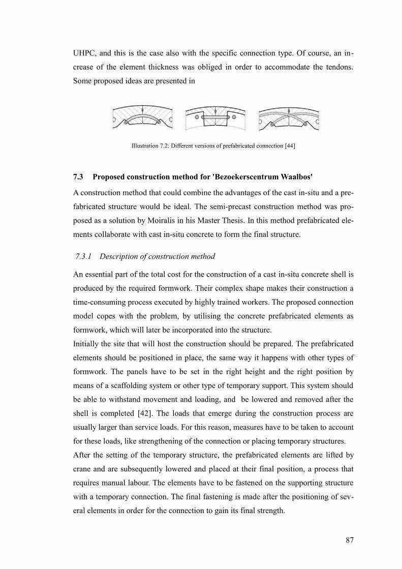
UHPC, and this is the case also with the specific connection type. Of course, an in-
crease of the element thickness was obliged in order to accommodate the tendons.
Some proposed ideas are presented in
7.3 Proposed construction method for 'Bezoekerscentrum Waalbos'
A construction method that could combine the advantages of the cast in-situ and a pre-
fabricated structure would be ideal. The semi-precast construction method was pro-
posed as a solution by Moiralis in his Master Thesis. In this method prefabricated ele-
ments collaborate with cast in-situ concrete to form the final structure.
7.3.1 Description of construction method
An essential part of the total cost for the construction of a cast in-situ concrete shell is
produced by the required formwork. Their complex shape makes their construction a
time-consuming process executed by highly trained workers. The proposed connection
model copes with the problem, by utilising the concrete prefabricated elements as
formwork, which will later be incorporated into the structure.
Initially the site that will host the construction should be prepared. The prefabricated
elements should be positioned in place, the same way it happens with other types of
formwork. The panels have to be set in the right height and the right position by
means of a scaffolding system or other type of temporary support. This system should
be able to withstand movement and loading, and be lowered and removed after the
shell is completed [42]. The loads that emerge during the construction process are
usually larger than service loads. For this reason, measures have to be taken to account
for these loads, like strengthening of the connection or placing temporary structures.
After the setting of the temporary structure, the prefabricated elements are lifted by
crane and are subsequently lowered and placed at their final position, a process that
requires manual labour. The elements have to be fastened on the supporting structure
with a temporary connection. The final fastening is made after the positioning of sev-
eral elements in order for the connection to gain its final strength.
87
Illustration 7.2: Different versions of prefabricated connection [44]
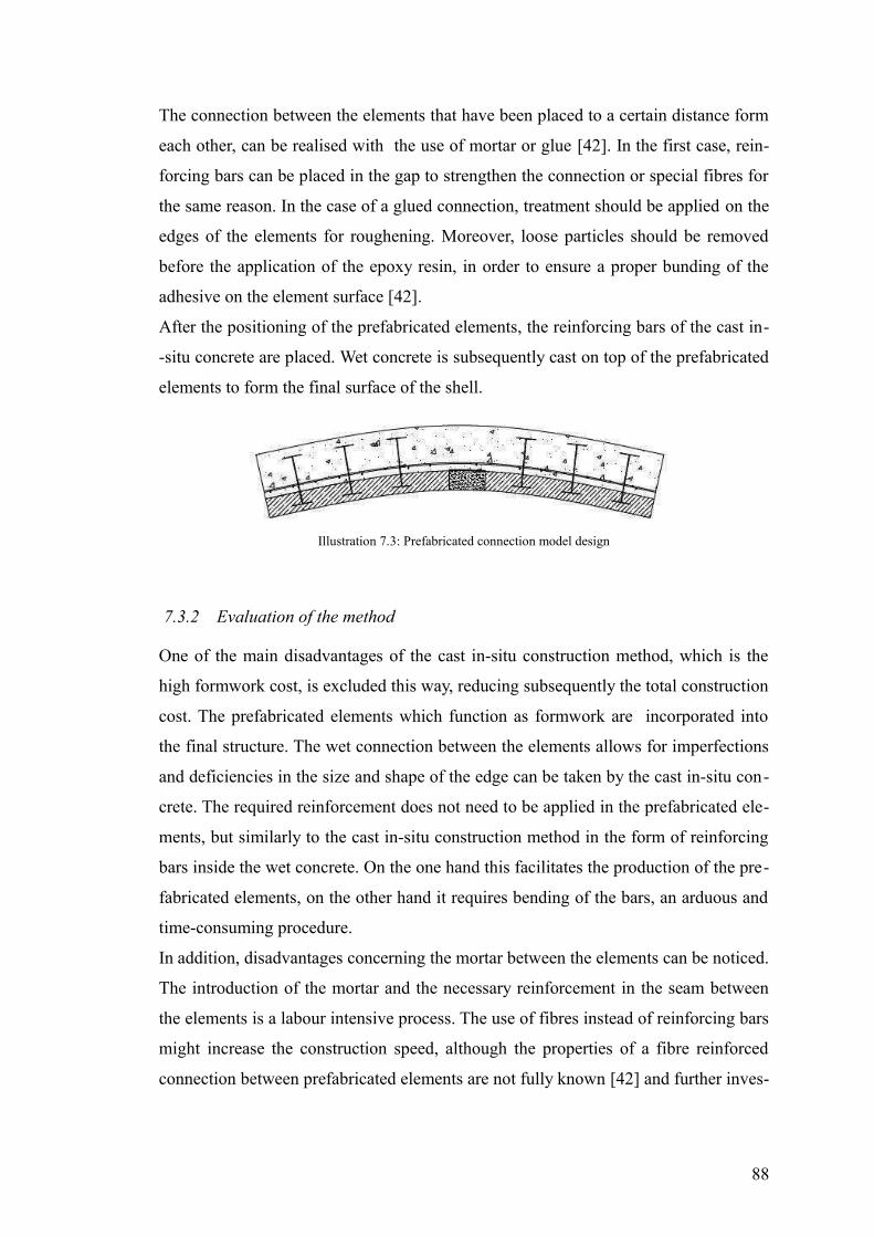
The connection between the elements that have been placed to a certain distance form
each other, can be realised with the use of mortar or glue [42]. In the first case, rein-
forcing bars can be placed in the gap to strengthen the connection or special fibres for
the same reason. In the case of a glued connection, treatment should be applied on the
edges of the elements for roughening. Moreover, loose particles should be removed
before the application of the epoxy resin, in order to ensure a proper bunding of the
adhesive on the element surface [42].
After the positioning of the prefabricated elements, the reinforcing bars of the cast in-
-situ concrete are placed. Wet concrete is subsequently cast on top of the prefabricated
elements to form the final surface of the shell.
7.3.2 Evaluation of the method
One of the main disadvantages of the cast in-situ construction method, which is the
high formwork cost, is excluded this way, reducing subsequently the total construction
cost. The prefabricated elements which function as formwork are incorporated into
the final structure. The wet connection between the elements allows for imperfections
and deficiencies in the size and shape of the edge can be taken by the cast in-situ con-
crete. The required reinforcement does not need to be applied in the prefabricated ele-
ments, but similarly to the cast in-situ construction method in the form of reinforcing
bars inside the wet concrete. On the one hand this facilitates the production of the pre-
fabricated elements, on the other hand it requires bending of the bars, an arduous and
time-consuming procedure.
In addition, disadvantages concerning the mortar between the elements can be noticed.
The introduction of the mortar and the necessary reinforcement in the seam between
the elements is a labour intensive process. The use of fibres instead of reinforcing bars
might increase the construction speed, although the properties of a fibre reinforced
connection between prefabricated elements are not fully known [42] and further inves-
88
Illustration 7.3: Prefabricated connection model design
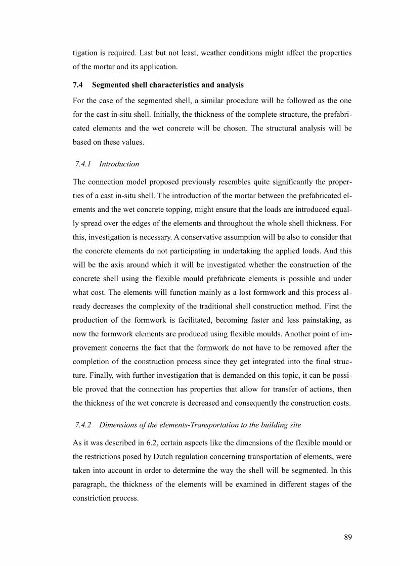
tigation is required. Last but not least, weather conditions might affect the properties
of the mortar and its application.
7.4 Segmented shell characteristics and analysis
For the case of the segmented shell, a similar procedure will be followed as the one
for the cast in-situ shell. Initially, the thickness of the complete structure, the prefabri-
cated elements and the wet concrete will be chosen. The structural analysis will be
based on these values.
7.4.1 Introduction
The connection model proposed previously resembles quite significantly the proper-
ties of a cast in-situ shell. The introduction of the mortar between the prefabricated el-
ements and the wet concrete topping, might ensure that the loads are introduced equal-
ly spread over the edges of the elements and throughout the whole shell thickness. For
this, investigation is necessary. A conservative assumption will be also to consider that
the concrete elements do not participating in undertaking the applied loads. And this
will be the axis around which it will be investigated whether the construction of the
concrete shell using the flexible mould prefabricate elements is possible and under
what cost. The elements will function mainly as a lost formwork and this process al-
ready decreases the complexity of the traditional shell construction method. First the
production of the formwork is facilitated, becoming faster and less painstaking, as
now the formwork elements are produced using flexible moulds. Another point of im-
provement concerns the fact that the formwork do not have to be removed after the
completion of the construction process since they get integrated into the final struc-
ture. Finally, with further investigation that is demanded on this topic, it can be possi-
ble proved that the connection has properties that allow for transfer of actions, then
the thickness of the wet concrete is decreased and consequently the construction costs.
7.4.2 Dimensions of the elements-Transportation to the building site
As it was described in 6.2, certain aspects like the dimensions of the flexible mould or
the restrictions posed by Dutch regulation concerning transportation of elements, were
taken into account in order to determine the way the shell will be segmented. In this
paragraph, the thickness of the elements will be examined in different stages of the
constriction process.
89
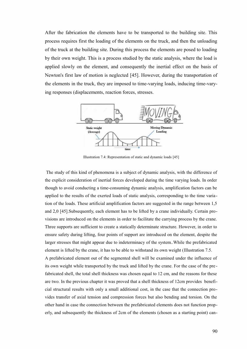
After the fabrication the elements have to be transported to the building site. This
process requires first the loading of the elements on the truck, and then the unloading
of the truck at the building site. During this process the elements are posed to loading
by their own weight. This is a process studied by the static analysis, where the load is
applied slowly on the element, and consequently the inertial effect on the basis of
Newton's first law of motion is neglected [45]. However, during the transportation of
the elements in the truck, they are imposed to time-varying loads, inducing time-vary-
ing responses (displacements, reaction forces, stresses.
The study of this kind of phenomena is a subject of dynamic analysis, with the difference of
the explicit consideration of inertial forces developed during the time varying loads. In order
though to avoid conducting a time-consuming dynamic analysis, amplification factors can be
applied to the results of the exerted loads of static analysis, corresponding to the time varia -
tion of the loads. These artificial amplification factors are suggested in the range between 1,5
and 2,0 [45].Subsequently, each element has to be lifted by a crane individually. Certain pro-
visions are introduced on the elements in order to facilitate the carrying process by the crane.
Three supports are sufficient to create a statically determinate structure. However, in order to
ensure safety during lifting, four points of support are introduced on the element, despite the
larger stresses that might appear due to indeterminacy of the system..While the prefabricated
element is lifted by the crane, it has to be able to withstand its own weight (Illustration 7.5.
A prefabricated element out of the segmented shell will be examined under the influence of
its own weight while transported by the truck and lifted by the crane. For the case of the pre -
fabricated shell, the total shell thickness was chosen equal to 12 cm, and the reasons for these
are two. In the previous chapter it was proved that a shell thickness of 12cm provides benefi-
cial structural results with only a small additional cost, in the case that the connection pro-
vides transfer of axial tension and compression forces but also bending and torsion. On the
other hand in case the connection between the prefabricated elements does not function prop-
erly, and subsequently the thickness of 2cm of the elements (chosen as a starting point) can-
90
Illustration 7.4: Representation of static and dynamic loads [45]
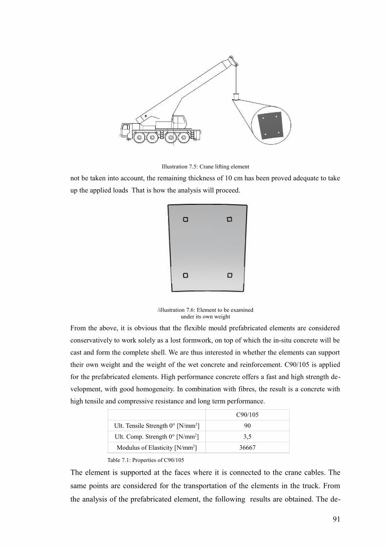
not be taken into account, the remaining thickness of 10 cm has been proved adequate to take
up the applied loads That is how the analysis will proceed.
From the above, it is obvious that the flexible mould prefabricated elements are considered
conservatively to work solely as a lost formwork, on top of which the in-situ concrete will be
cast and form the complete shell. We are thus interested in whether the elements can support
their own weight and the weight of the wet concrete and reinforcement. C90/105 is applied
for the prefabricated elements. High performance concrete offers a fast and high strength de-
velopment, with good homogeneity. In combination with fibres, the result is a concrete with
high tensile and compressive resistance and long term performance.
C90/105
Ult. Tensile Strength 0° [N/mm2] 90
Ult. Comp. Strength 0° [N/mm2] 3,5
Modulus of Elasticity [N/mm2] 36667
Table 7.1: Properties of C90/105
The element is supported at the faces where it is connected to the crane cables. The
same points are considered for the transportation of the elements in the truck. From
the analysis of the prefabricated element, the following results are obtained. The de-
91
Illustration 7.5: Crane lifting element
/illustration 7.6: Element to be examinedunder its own weight
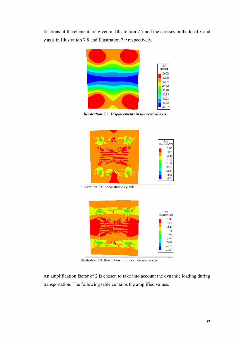
flections of the element are given in Illustration 7.7 and the stresses in the local x and
y axis in Illustration 7.8 and Illustration 7.9 respectively.
An amplification factor of 2 is chosen to take into account the dynamic loading during
transportation. The following table contains the amplified values.
92
Illustration 7.8: Local stresses y-axis
Illustration 7.9: Illustration 7.8: Local stresses x-axis
Illustration 7.7: Displacements in the vertical axis
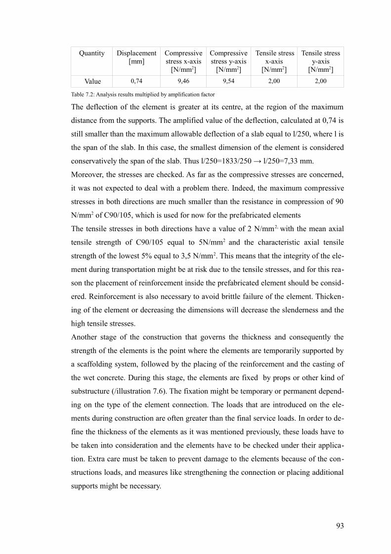
Quantity Displacement[mm]
Compressivestress x-axis
[N/mm2]
Compressivestress y-axis
[N/mm2]
Tensile stressx-axis
[N/mm2]
Tensile stressy-axis
[N/mm2]
Value 0,74 9,46 9,54 2,00 2,00
Table 7.2: Analysis results multiplied by amplification factor
The deflection of the element is greater at its centre, at the region of the maximum
distance from the supports. The amplified value of the deflection, calculated at 0,74 is
still smaller than the maximum allowable deflection of a slab equal to l/250, where l is
the span of the slab. In this case, the smallest dimension of the element is considered
conservatively the span of the slab. Thus l/250=1833/250 → l/250=7,33 mm.
Moreover, the stresses are checked. As far as the compressive stresses are concerned,
it was not expected to deal with a problem there. Indeed, the maximum compressive
stresses in both directions are much smaller than the resistance in compression of 90
N/mm2 of C90/105, which is used for now for the prefabricated elements
The tensile stresses in both directions have a value of 2 N/mm2, with the mean axial
tensile strength of C90/105 equal to 5N/mm2 and the characteristic axial tensile
strength of the lowest 5% equal to 3,5 N/mm2. This means that the integrity of the ele-
ment during transportation might be at risk due to the tensile stresses, and for this rea-
son the placement of reinforcement inside the prefabricated element should be consid-
ered. Reinforcement is also necessary to avoid brittle failure of the element. Thicken-
ing of the element or decreasing the dimensions will decrease the slenderness and the
high tensile stresses.
Another stage of the construction that governs the thickness and consequently the
strength of the elements is the point where the elements are temporarily supported by
a scaffolding system, followed by the placing of the reinforcement and the casting of
the wet concrete. During this stage, the elements are fixed by props or other kind of
substructure (/illustration 7.6). The fixation might be temporary or permanent depend-
ing on the type of the element connection. The loads that are introduced on the ele-
ments during construction are often greater than the final service loads. In order to de-
fine the thickness of the elements as it was mentioned previously, these loads have to
be taken into consideration and the elements have to be checked under their applica-
tion. Extra care must be taken to prevent damage to the elements because of the con-
structions loads, and measures like strengthening the connection or placing additional
supports might be necessary.
93
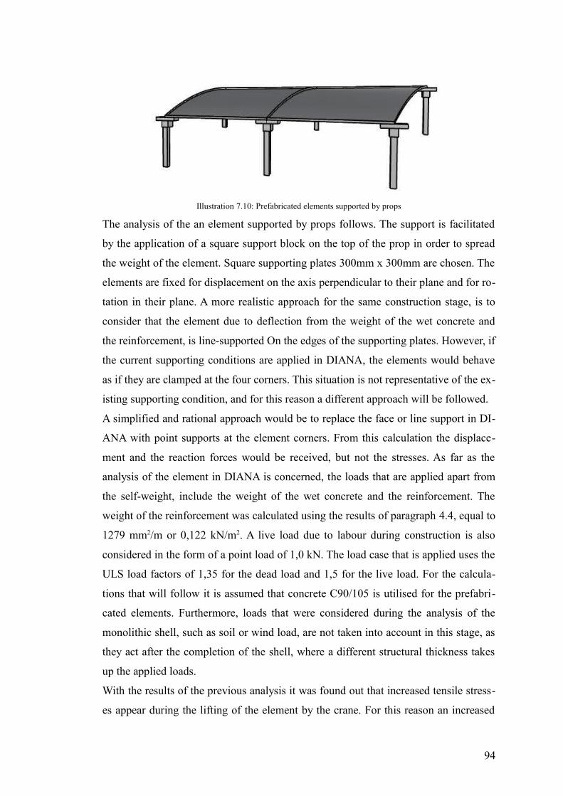
The analysis of the an element supported by props follows. The support is facilitated
by the application of a square support block on the top of the prop in order to spread
the weight of the element. Square supporting plates 300mm x 300mm are chosen. The
elements are fixed for displacement on the axis perpendicular to their plane and for ro-
tation in their plane. A more realistic approach for the same construction stage, is to
consider that the element due to deflection from the weight of the wet concrete and
the reinforcement, is line-supported On the edges of the supporting plates. However, if
the current supporting conditions are applied in DIANA, the elements would behave
as if they are clamped at the four corners. This situation is not representative of the ex-
isting supporting condition, and for this reason a different approach will be followed.
A simplified and rational approach would be to replace the face or line support in DI-
ANA with point supports at the element corners. From this calculation the displace-
ment and the reaction forces would be received, but not the stresses. As far as the
analysis of the element in DIANA is concerned, the loads that are applied apart from
the self-weight, include the weight of the wet concrete and the reinforcement. The
weight of the reinforcement was calculated using the results of paragraph 4.4, equal to
1279 mm2/m or 0,122 kN/m2. A live load due to labour during construction is also
considered in the form of a point load of 1,0 kN. The load case that is applied uses the
ULS load factors of 1,35 for the dead load and 1,5 for the live load. For the calcula-
tions that will follow it is assumed that concrete C90/105 is utilised for the prefabri-
cated elements. Furthermore, loads that were considered during the analysis of the
monolithic shell, such as soil or wind load, are not taken into account in this stage, as
they act after the completion of the shell, where a different structural thickness takes
up the applied loads.
With the results of the previous analysis it was found out that increased tensile stress-
es appear during the lifting of the element by the crane. For this reason an increased
94
Illustration 7.10: Prefabricated elements supported by props
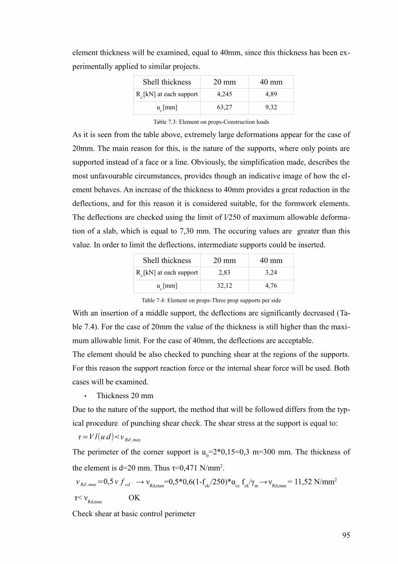
element thickness will be examined, equal to 40mm, since this thickness has been ex-
perimentally applied to similar projects.
Shell thickness 20 mm 40 mm
Rz [kN] at each support 4,245 4,89
uz [mm] 63,27 9,32
Table 7.3: Element on props-Construction loads
As it is seen from the table above, extremely large deformations appear for the case of
20mm. The main reason for this, is the nature of the supports, where only points are
supported instead of a face or a line. Obviously, the simplification made, describes the
most unfavourable circumstances, provides though an indicative image of how the el-
ement behaves. An increase of the thickness to 40mm provides a great reduction in the
deflections, and for this reason it is considered suitable, for the formwork elements.
The deflections are checked using the limit of l/250 of maximum allowable deforma-
tion of a slab, which is equal to 7,30 mm. The occuring values are greater than this
value. In order to limit the deflections, intermediate supports could be inserted.
Shell thickness 20 mm 40 mm
Rz [kN] at each support 2,83 3,24
uz [mm] 32,12 4,76
Table 7.4: Element on props-Three prop supports per side
With an insertion of a middle support, the deflections are significantly decreased (Ta-
ble 7.4). For the case of 20mm the value of the thickness is still higher than the maxi-
mum allowable limit. For the case of 40mm, the deflections are acceptable.
The element should be also checked to punching shear at the regions of the supports.
For this reason the support reaction force or the internal shear force will be used. Both
cases will be examined.
• Thickness 20 mm
Due to the nature of the support, the method that will be followed differs from the typ-
ical procedure of punching shear check. The shear stress at the support is equal to:
τ=V /(u d )<v Rd ,max
The perimeter of the corner support is u0=2*0,15=0,3 m=300 mm. The thickness of
the element is d=20 mm. Thus τ=0,471 N/mm2.
→ νRd,max
=0,5*0,6(1-fck/
/250)*αcc
fck
/γm
→ ν
Rd,max = 11,52 N/mm2
τ< νRd,max
OK
Check shear at basic control perimeter
95
v Rd ,max=0,5ν f cd
τu1=V Εd /(u1d )<vRd , c
The basic control perimeter u1 for a corner support can be seen in Illustration 7.11.
For the support of 150 mm, this perimeter is equal to 362,8 mm. Thus ved
= 0,39
N/mm2.
v Rd ,c=0,12k (100ρl f ck)(1 /3) For ρ
l which is the ratio of the reinforcement area
over the cross section area, the lowest allowable value of 0,0025 is assumed for both
directions. vRd,c
=0,68 N/mm2. The check vEd
<vRd,c
is valid, which means that punching
does not occur.
The same checks are conducted for the thickness of 30mm.
• Thickness 0 mm
At the perimeter of the support
τ=0,34 N/mm2<νRd,max
= 8 N/mm2 OK
At the basic control perimeter
τ=0,31 N/mm2 < vRd,c
=0,56 N/mm2 OK
Although the occuring displacements exceed the maximum allowable limit due to the
assumed supporting conditions, the punching shear check is satisfied, meaning that
the slab of both thicknesses does not suffer from punching shear. If this was not the
case, then an increase of the element thickness would have been a solution. Moreover,
a beneficial way to deal with punching shear would be the increase of the supporting
plate width in order to achieve more favourable distribution of the load at the sup-
ports. For safety reasons, the plate width is increased to 450 mm for the analyses that
will follow.
In a final stage, the connection between the elements should be examined. It was pre-
viously mentioned that wet concrete will be placed between the elements with a cer-
tain type of reinforcement. The main problem of the connection between the prefabri-
cated elements is not the compression forces, since these can be taken up by a high
96
Illustration 7.11: Basic control(critical) perimeter for corner support
strength mortar, but the tensional forces. The first thought that comes to mind in order
to account for the tension at the connection is the introduction of reinforcing bars. At a
first glance, this might sound simple but there are issues that have not been studied or
researched which influence the tensional resistance of the connection. The placement
of the rebars entails the existence of sockets in which the bars will be placed, get con-
creted and cooperate with the elements.
The use of fibres instead of rebars have been proposed and researched. Fibres used as
concrete reinforcement are not appropriate for use in the connection, due to their small
dimension [42]. Instead fibres of larger length and diameter with a hooked end have
been used. Tests have been conducted [46] which indicate that fibres can work, how-
ever further investigation is required to gain confidence in the properties of the con-
nection.
7.4.3 FRP reinforcement of concrete structures
The idea of using Fibre Reinforced Polymers (FRP) as a means of reinforcement for
the connection between the prefabricated elements came up during a discussion with
Pr. Schipper. FRP reinforcement is one of the most promising new developments for
concrete structures. FRP laminates have been used to strengthen, repair or add ductili-
ty to existing and new structures. The practice of strengthening concrete structures
with externally bonded FRP system had been widely investigated and applied. FRP
laminate bonding involves adhering thin flexible fibre plies on the concrete surface
using an epoxy resin. The method known as manual lay-up increases the shear and
flexural resistance of concrete beams and slabs and offers the benefits of fast and easy
construction with a durable, high performance and light-weight connection.
No application has been found though using FRP laminates for a connection between
prefabricated double-curved concrete elements. However an attempt will be made in
order to examine whether the application of the FRP laminates can be proved benefi-
cial for this connection. Assumptions and simplifications will be made in order to ar-
rive to results, and thus further extensive investigation is necessary, as only a proposal
is made in this chapter.
The idea of FRP reinforcement for the connection uses the same principles with the
application of strips of FRP laminates on concrete slabs, as mentioned previously.
FRP systems restore the structural capacity both in reinforced and unreinforced con-
crete slabs. For the latter case, a substantial increase of the structural capacity is also
97
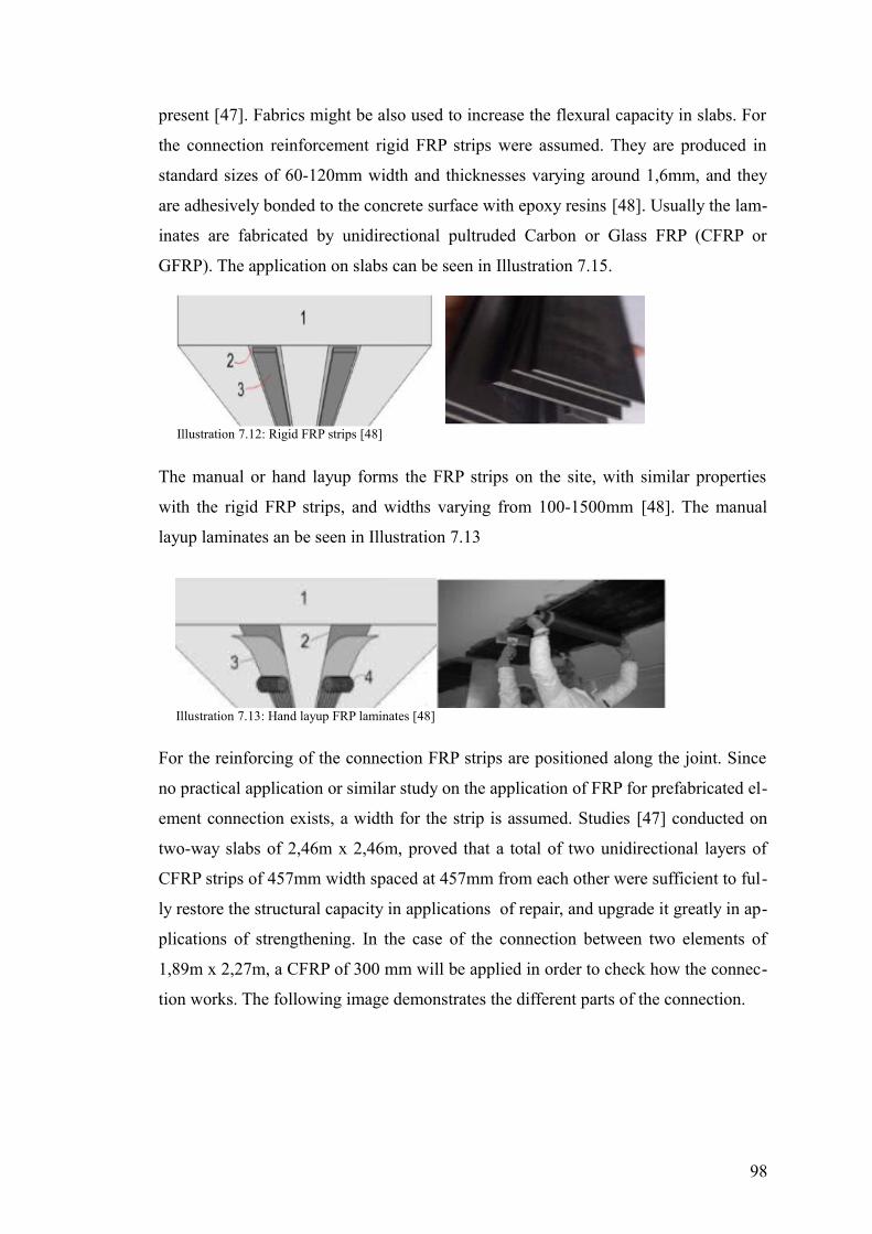
present [47]. Fabrics might be also used to increase the flexural capacity in slabs. For
the connection reinforcement rigid FRP strips were assumed. They are produced in
standard sizes of 60-120mm width and thicknesses varying around 1,6mm, and they
are adhesively bonded to the concrete surface with epoxy resins [48]. Usually the lam-
inates are fabricated by unidirectional pultruded Carbon or Glass FRP (CFRP or
GFRP). The application on slabs can be seen in Illustration 7.15.
The manual or hand layup forms the FRP strips on the site, with similar properties
with the rigid FRP strips, and widths varying from 100-1500mm [48]. The manual
layup laminates an be seen in Illustration 7.13
For the reinforcing of the connection FRP strips are positioned along the joint. Since
no practical application or similar study on the application of FRP for prefabricated el-
ement connection exists, a width for the strip is assumed. Studies [47] conducted on
two-way slabs of 2,46m x 2,46m, proved that a total of two unidirectional layers of
CFRP strips of 457mm width spaced at 457mm from each other were sufficient to ful-
ly restore the structural capacity in applications of repair, and upgrade it greatly in ap-
plications of strengthening. In the case of the connection between two elements of
1,89m x 2,27m, a CFRP of 300 mm will be applied in order to check how the connec-
tion works. The following image demonstrates the different parts of the connection.
98
Illustration 7.13: Hand layup FRP laminates [48]
Illustration 7.12: Rigid FRP strips [48]
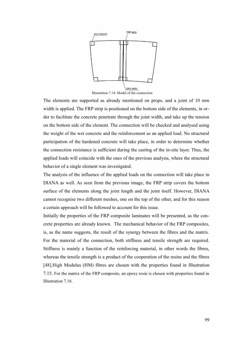
The elements are supported as already mentioned on props, and a joint of 10 mm
width is applied. The FRP strip is positioned on the bottom side of the elements, in or-
der to facilitate the concrete penetrate through the joint width, and take up the tension
on the bottom side of the element. The connection will be checked and analysed using
the weight of the wet concrete and the reinforcement as an applied load. No structural
participation of the hardened concrete will take place, in order to determine whether
the connection resistance is sufficient during the casting of the in-situ layer. Thus, the
applied loads will coincide with the ones of the previous analysis, where the structural
behavior of a single element was investigated.
The analysis of the influence of the applied loads on the connection will take place in
DIANA as well. As seen from the previous image, the FRP strip covers the bottom
surface of the elements along the joint length and the joint itself. However, DIANA
cannot recognise two different meshes, one on the top of the other, and for this reason
a certain approach will be followed to account for this issue.
Initially the properties of the FRP composite laminates will be presented, as the con-
crete properties are already known. The mechanical behavior of the FRP composites,
is, as the name suggests, the result of the synergy between the fibres and the matrix.
For the material of the connection, both stiffness and tensile strength are required.
Stiffness is mainly a function of the reinforcing material, in other words the fibres,
whereas the tensile strength is a product of the cooperation of the resins and the fibres
[48].High Modulus (HM) fibres are chosen with the properties found in Illustration
7.15. For the matrix of the FRP composite, an epoxy resin is chosen with properties found in
Illustration 7.16.
99
Illustration 7.14: Model of the connection
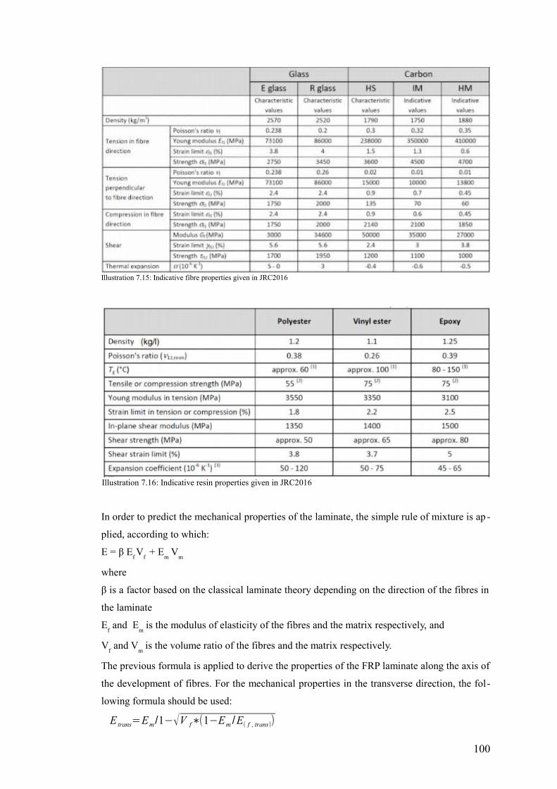
In order to predict the mechanical properties of the laminate, the simple rule of mixture is ap -
plied, according to which:
E = β Εf V
f + E
m V
m
where
β is a factor based on the classical laminate theory depending on the direction of the fibres in
the laminate
Εf and E
m is the modulus of elasticity of the fibres and the matrix respectively, and
Vf and V
m is the volume ratio of the fibres and the matrix respectively.
The previous formula is applied to derive the properties of the FRP laminate along the axis of
the development of fibres. For the mechanical properties in the transverse direction, the fol-
lowing formula should be used:
E trans=Em/1−√V f∗(1−Em /E( f , trans))
100
Illustration 7.15: Indicative fibre properties given in JRC2016
Illustration 7.16: Indicative resin properties given in JRC2016
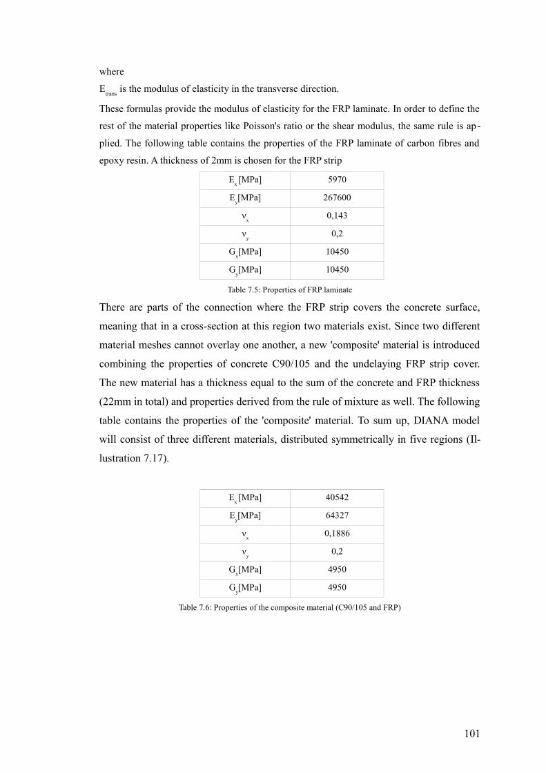
where
Etrans
is the modulus of elasticity in the transverse direction.
These formulas provide the modulus of elasticity for the FRP laminate. In order to define the
rest of the material properties like Poisson's ratio or the shear modulus, the same rule is ap-
plied. The following table contains the properties of the FRP laminate of carbon fibres and
epoxy resin. A thickness of 2mm is chosen for the FRP strip
Εx [MPa] 5970
Εy[MPa] 267600
νx
0,143
νy
0,2
Gx[MPa] 10450
Gy[MPa] 10450
Table 7.5: Properties of FRP laminate
There are parts of the connection where the FRP strip covers the concrete surface,
meaning that in a cross-section at this region two materials exist. Since two different
material meshes cannot overlay one another, a new 'composite' material is introduced
combining the properties of concrete C90/105 and the undelaying FRP strip cover.
The new material has a thickness equal to the sum of the concrete and FRP thickness
(22mm in total) and properties derived from the rule of mixture as well. The following
table contains the properties of the 'composite' material. To sum up, DIANA model
will consist of three different materials, distributed symmetrically in five regions (Il-
lustration 7.17).
Εx [MPa] 40542
Εy[MPa] 64327
νx
0,1886
νy
0,2
Gx[MPa] 4950
Gy[MPa] 4950
Table 7.6: Properties of the composite material (C90/105 and FRP)
101
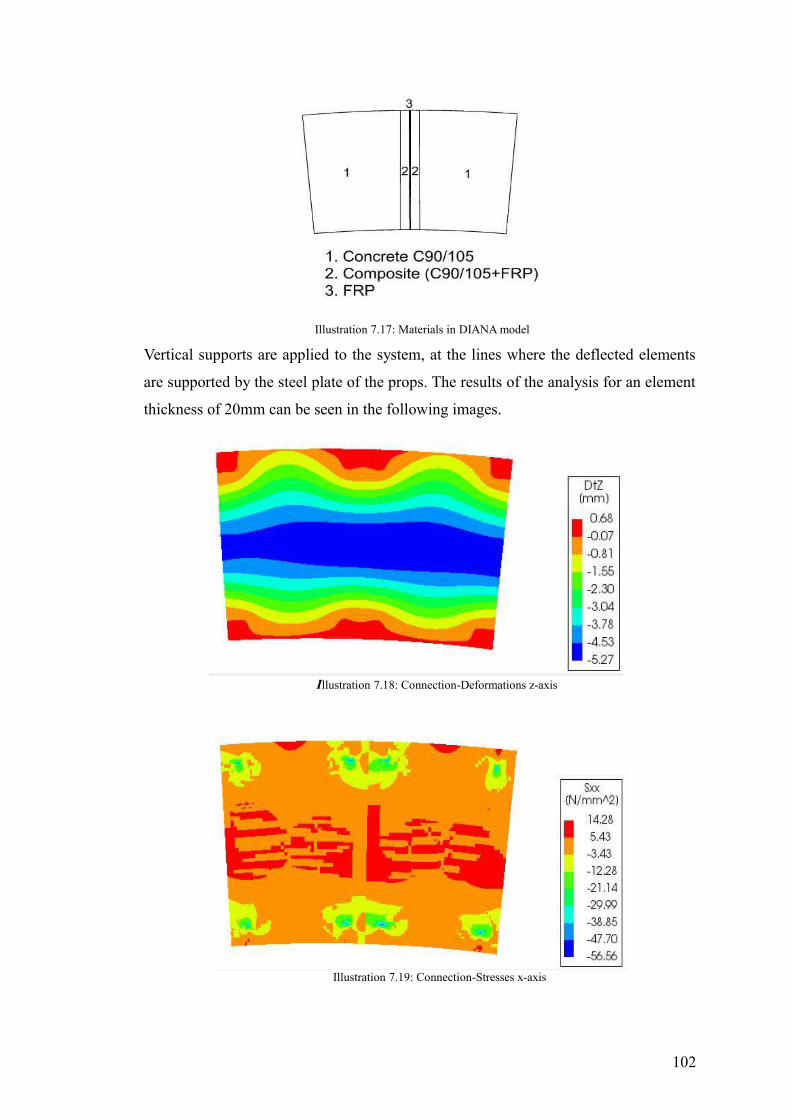
Vertical supports are applied to the system, at the lines where the deflected elements
are supported by the steel plate of the props. The results of the analysis for an element
thickness of 20mm can be seen in the following images.
102
Illustration 7.17: Materials in DIANA model
Illustration 7.18: Connection-Deformations z-axis
Illustration 7.19: Connection-Stresses x-axis
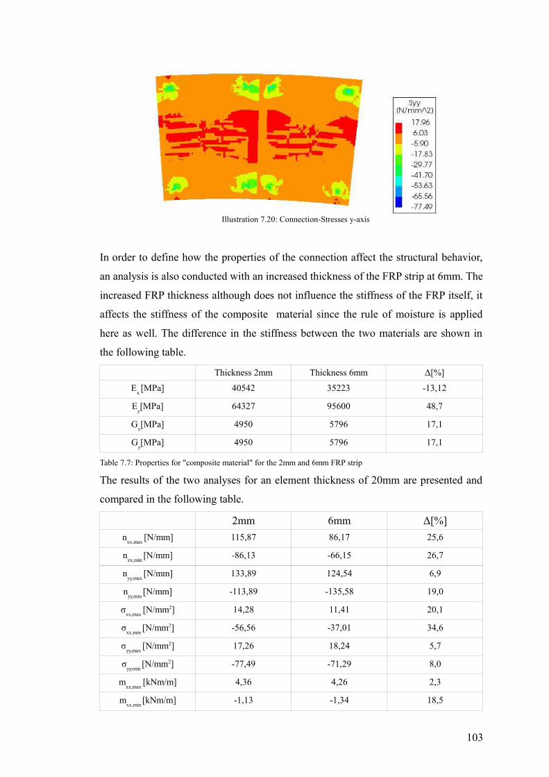
In order to define how the properties of the connection affect the structural behavior,
an analysis is also conducted with an increased thickness of the FRP strip at 6mm. The
increased FRP thickness although does not influence the stiffness of the FRP itself, it
affects the stiffness of the composite material since the rule of moisture is applied
here as well. The difference in the stiffness between the two materials are shown in
the following table.
Thickness 2mm Thickness 6mm Δ[%]
Εx [MPa] 40542 35223 -13,12
Εy[MPa] 64327 95600 48,7
Gx[MPa] 4950 5796 17,1
Gy[MPa] 4950 5796 17,1
Table 7.7: Properties for "composite material" for the 2mm and 6mm FRP strip
The results of the two analyses for an element thickness of 20mm are presented and
compared in the following table.
2mm 6mm Δ[%]
nxx,max
[N/mm] 115,87 86,17 25,6
nxx,min
[N/mm] -86,13 -66,15 26,7
nyy,max
[N/mm] 133,89 124,54 6,9
nyy,min
[N/mm] -113,89 -135,58 19,0
σxx,max
[N/mm2] 14,28 11,41 20,1
σxx,min
[N/mm2] -56,56 -37,01 34,6
σyy,max
[N/mm2] 17,26 18,24 5,7
σyy,min
[N/mm2] -77,49 -71,29 8,0
mxx,max
[kNm/m] 4,36 4,26 2,3
mxx,min
[kNm/m] -1,13 -1,34 18,5
103
Illustration 7.20: Connection-Stresses y-axis
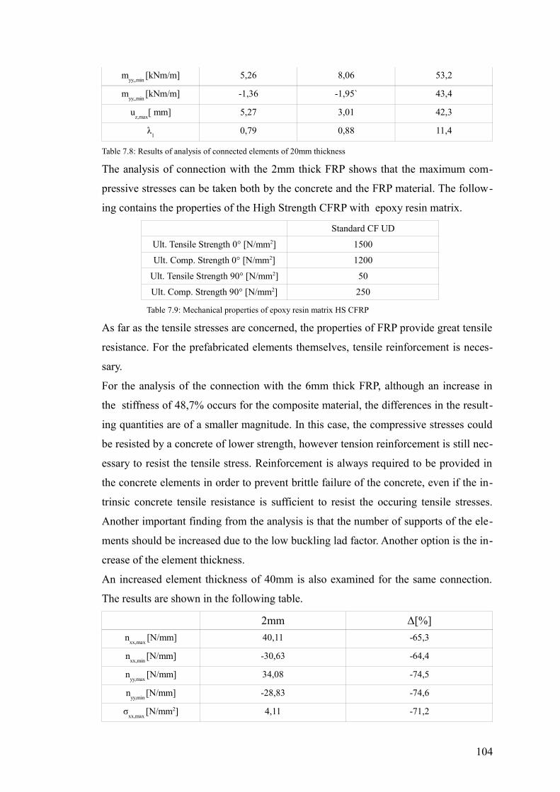
myy,,min
[kNm/m] 5,26 8,06 53,2
myy,,min
[kNm/m] -1,36 -1,95` 43,4
uz,max
[ mm] 5,27 3,01 42,3
λ1
0,79 0,88 11,4
Table 7.8: Results of analysis of connected elements of 20mm thickness
The analysis of connection with the 2mm thick FRP shows that the maximum com-
pressive stresses can be taken both by the concrete and the FRP material. The follow-
ing contains the properties of the High Strength CFRP with epoxy resin matrix.
Standard CF UD
Ult. Tensile Strength 0° [N/mm2] 1500
Ult. Comp. Strength 0° [N/mm2] 1200
Ult. Tensile Strength 90° [N/mm2] 50
Ult. Comp. Strength 90° [N/mm2] 250
Table 7.9: Mechanical properties of epoxy resin matrix HS CFRP
As far as the tensile stresses are concerned, the properties of FRP provide great tensile
resistance. For the prefabricated elements themselves, tensile reinforcement is neces-
sary.
For the analysis of the connection with the 6mm thick FRP, although an increase in
the stiffness of 48,7% occurs for the composite material, the differences in the result-
ing quantities are of a smaller magnitude. In this case, the compressive stresses could
be resisted by a concrete of lower strength, however tension reinforcement is still nec-
essary to resist the tensile stress. Reinforcement is always required to be provided in
the concrete elements in order to prevent brittle failure of the concrete, even if the in-
trinsic concrete tensile resistance is sufficient to resist the occuring tensile stresses.
Another important finding from the analysis is that the number of supports of the ele-
ments should be increased due to the low buckling lad factor. Another option is the in-
crease of the element thickness.
An increased element thickness of 40mm is also examined for the same connection.
The results are shown in the following table.
2mm Δ[%]
nxx,max
[N/mm] 40,11 -65,3
nxx,min
[N/mm] -30,63 -64,4
nyy,max
[N/mm] 34,08 -74,5
nyy,min
[N/mm] -28,83 -74,6
σxx,max
[N/mm2] 4,11 -71,2
104
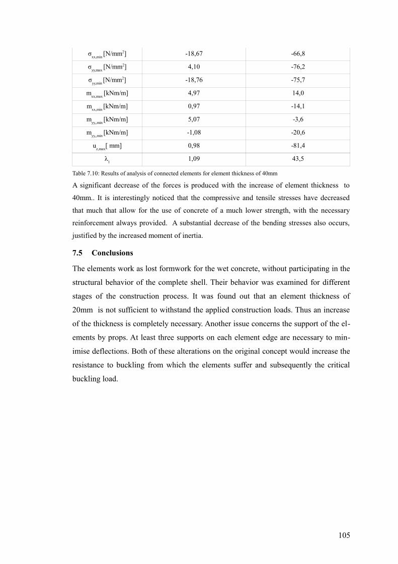
σxx,min
[N/mm2] -18,67 -66,8
σyy,max
[N/mm2] 4,10 -76,2
σyy,min
[N/mm2] -18,76 -75,7
mxx,max
[kNm/m] 4,97 14,0
mxx,min
[kNm/m] 0,97 -14,1
myy,,min
[kNm/m] 5,07 -3,6
myy,,min
[kNm/m] -1,08 -20,6
uz,max
[ mm] 0,98 -81,4
λ1
1,09 43,5
Table 7.10: Results of analysis of connected elements for element thickness of 40mm
A significant decrease of the forces is produced with the increase of element thickness to
40mm.. It is interestingly noticed that the compressive and tensile stresses have decreased
that much that allow for the use of concrete of a much lower strength, with the necessary
reinforcement always provided. A substantial decrease of the bending stresses also occurs,
justified by the increased moment of inertia.
7.5 Conclusions
The elements work as lost formwork for the wet concrete, without participating in the
structural behavior of the complete shell. Their behavior was examined for different
stages of the construction process. It was found out that an element thickness of
20mm is not sufficient to withstand the applied construction loads. Thus an increase
of the thickness is completely necessary. Another issue concerns the support of the el-
ements by props. At least three supports on each element edge are necessary to min-
imise deflections. Both of these alterations on the original concept would increase the
resistance to buckling from which the elements suffer and subsequently the critical
buckling load.
105
CHAPTER 8
8 Conclusions and Recommendations
8.1 Conclusions
The aim of this master thesis was to examine whether the construction of a concrete
shell was feasible using flexible mould prefabricated concrete elements. In order to
accomplice this, a design case building was chosen, which had to be analysed both as
a monolithic structure and as a prefabricated structure. The shell of the 'Bezoekerscen-
trum Waalbos' has not been constructed yet, thus apart from its constructability it was
wise also to check design parameters, such as its dimensions and its geometrical char-
acteristics.
Accompanying the research question, there are set design criteria which have to be
satisfied throughout the progress of the thesis. These are the following:
• the structure should satisfy the strength and stiffness requirements for shells.
• the construction and design of the structure should be cost-efficient
• the final design should not diverge greatly from the original design of the architect.
Subsequently, since the structural feasibility of the shell had not been checked, it was
examined if this is possible and what modifications in the design were necessary. A
limitation to this was the criterion of the least deviation from the original design. The
analysis of the structure in a FEA software required first its validation. After a design
had been produced, it was necessary to verify the finite element model. The structure
was then analysed considering it as a monolithic shell. The structure was then seg-
mented in elements, and a connection model was proposed, in which a cooperation of
prefabricated elements and cast in-situ concrete took place.
From the analysis of the approximating structures, it was concluded, that the structural
behavior of the central part of the structure could approach the behavior of a flat slab
supported on columns or a long barrel shell (shell beam) supported on walls in its
transverse direction. Moreover, an effort was made to relate the shell with a catenary
arch, however it was proved unsuccessful for two reasons. First the resulting design
was differentiating substantially from the original design. Second, the research for the
arch geometry did not follow an optimisation process where a critical loading enve-
106
lope should be constructed by superimposing the effects of various load cases on the
arch. The dead weight was chosen instead, and as a result the rest of the applied loads
which had significant magnitude would produce tension across the arch length. Final-
ly, the analysis of the side parts, showed that they behave quite similarly to dome
structures. With the analysis of the approximating structure, the validation of the FEA
software was also completed.
The architect's designs only included rough dimensions for the building layout, with-
out defining essential features of the shell like its curvature and the design of the fa-
cade. A lot of ideas for the shape of the facade were tested with structural and aesthet-
ic criteria. The design was altered, with the main difference located at the front part of
the structure, where instead of a continuous opening throughout the whole length of
the facade, an arch opening was positioned.
The new model was verified using three checks: sum of reaction forces, deformations
at the crown of the arch, stresses. Only small percentages of deviation between theo-
retical and analytical calculations were present, proving that the structure works as ex-
pected. The analysis of the model loaded only by its self-weight produced excessive
deformations at the top of the arch opening, which made necessary the introduction of
a stiffening arch across the opening. The resulting deformations were decreased by
44%. Before the analysis of the structure with the service loads, a mesh study was per-
formed, where a mesh size of 0,25 m was proved sufficiently small to produce repre-
sentative results.
The model was then analysed with service loads, and the combinations where the live
load is the dominant variable action were the governing ones. LC2 produced the maxi-
mum structural quantities but it was not used for the design, as its application is not
predicted by Eurocode. LC1 was used instead. The sum of the reaction forces shows
that the structure is relatively light. Structural efficiency of the side domes is proved
due to much lower deformations at this part. Tensile (16,90N/mm2) and compressive
(50,63N/mm2) stresses are quite large for LC1, indicating that C25/30, assumed in the
beginning, was not suitable for the construction of the building. Global axis stresses
showed that the behavior of the central part of the shell resembles the behavior of a
doughnut like axisymmtric shell dome, where compressive hoop forces appear at the
highest point surrounded by tensile forces. Bending stresses occur where the mem-
brane stresses are insufficient to carry the applied loads, at regions close to the con-
nections with foundation and at the arch support. The first and second buckling load
107
factors were determined after they have been multiplied with a 'knock-down' factor.
There is no load case for which the buckling factor is below 1. The difference between
the first and second buckling load factor is big enough to conclude that the shell is not
sensitive to imperfections.
Since the thickness of 100 mm for the shell was chosen arbitrarily, a thickness study
was also conducted, proving that although the initial thickness is sufficient to with-
stand the applied loads and provide the necessary stability to the structure, an increase
to 120mm, causes a reduction in the tensile and compressive stresses (14,17N/mm2
43,47N/mm2 respectively) and deflections (21,51mm) allowing for use of concrete of
lower strength, accompanied by a minor increase in the reaction forces.
After the analysis of the monolithic shell, the segmentation of the shell took place. For
this process, certain boundary conditions were taken into account, like the dimensions
and the curvature of the elements and the number of reconfigurations of the flexible
mould. Finally, the cylindrical part was segmented in 72 (6x12) elements of 1,47m-
2,26m x 2,23m-2,36 m. Elements with odd and small shapes were incorporated with
the neighboring ones. For the spherical side part, the technique of the ribbed dome
was applied producing elements of 0,97m-1,97m x 2,36m-2,63m. For the sides of the
domes, a segmentation in quadrilaterals was followed instead of the ribbed dome tech-
nique, which would lead in triangular elements.
Following this, a model had to be defined for the connection between the prefabricat-
ed elements. First a construction method was applied that makes use of both prefabri-
cated elements and cast in-situ concrete. The properties of the connection between the
elements need further investigation in order to ensure that load transfer is realised and
for this reason it was decided to consider that the prefabricated elements function
solely as a lost formwork, on which the wet concrete will be cast. This method is an
enhancement to the traditional shell construction method. The reasons are:
• faster and less arduous production of formwork elements
• it allows for complex shell configuration using the flexible mould
• it skips the process of lowering and removing the formwork, as they are inte-
grated in the final structure
Since the elements function as formwork, it was wise to examine their structural be-
havior throughout the different stages of the construction process. Initially, a curved
element part of the prefabricated shell was checked during its transportation to the
building site. Dynamic loading effects were considered with the use of amplification
108
factors for the static loading. During its lifting by the crane, the element with a thick-
ness of 20mm, using C90/105 is not put at risk since deflections equal to 0,74mm
were within the acceptable limits of l/250=7,33mm and compressive and tensile
forces could be resisted by the concrete. However, reinforcement of the elements is
considered advantageous in order to avoid brittle failure of the elements. In a later
stage, the elements should be examined when they are placed on top of props, and
loaded with the weight of the wet concrete and reinforcement. Considering that the el-
ement is point-supported at its four corners, quite large deflections occur for the case
of 20mm, equal to 63,27mm. With an increased element thickness at 40mm, the de-
flections (9,32mm) are greatly decreased, still not satisfying the maximum allowable
limits of 7,33mm. An insertion of a third support on each edge of the element decreas-
es the deformations to 32,12mm and 4,76mm for the case of 20mm and 40mm thick-
ness respectively. The reason for the large magnitude of deflections is mainly due to
the type of the assumed supports. Punching shear check was performed and finally
satisfied on the element for the thickness of 20mm and 40mm assuming a support
steel plate of 300mm. For safety reasons, the plate width is increased from 300mm to
400mm.
A connection model was defined at the last part. The main problem of the connection
is the transfer of tensile stresses. FRP strips were used for this reason, placed on the
bottom side of the elements. The analysis of two connected elements showed that the
transfer of tensile forces is facilitated with the use of the FRP strip, however reinforce-
ment is necessary for the prefabricated elements as well. The deformations were with-
in the acceptable limit of 7,33mmfor this stage of construction,but buckling occurred
for the case of 20mm thick elements.. As a conclusion the construction of the shell us-
ing flexible mould prefabricated elements as formwork is feasible with a minimum el-
ement thickness at 40mm and at least three supports on each element side.
8.2 Recommendations
This project concerned the feasibility of the shell of the 'Bazoekerscentrum Waalbos'
as a monolithic and prefabricated shell. Since the structure has not been built yet, op-
timisation procedures could take place throughout the whole project, from its design
to its construction. Unfortunately, these optimisation steps could not all be addressed
in this thesis, due to the lack of time. This chapter includes the extra steps that could
enhance the quality of the final result.
109
To begin with, as it was made clear in the thesis report, no finalised dimensions or
geometrical characteristics were given, and consequently a certain form was selected
and examined based on structural and aesthetic criteria. For this reason, different
designs should be examined with various dimension and curvature combinations d in
order to obtain a more advantageous structural behaviour of the shell. Numerous con-
cepts for the facade opening were tested, without this excluding the possibility of a
different design with higher aesthetic quality.
Moreover, specific types of loads were not considered in order to decrease the com-
plexity of the analysis. The use of time-dependent and accidental loads is thus recom-
mended The wind load was examined in the axis of the development of the building.
Applying the wind load in the perpendicular axis is recommended to check whether
governing results are produced. Serviceability limit state load combinations were not
considered in order to speed up the process. Instead the deformations were determined
using the ULS load combinations. A more economic design would have been pro-
duced in the opposite case and for this reason, the use of SLS load combinations is re-
commended
it is also proposed to combine the optimisation steps of shell thickness and concrete
strength and specify regions on the structure where each combination would produce
beneficial results
A linear static analysis simulates reality only when the deflections are infinitesimally
small and stresses and strains induced by loads are within the elastic range. The occur-
ing stresses exceed the elastic range and for this reason non-linear analysis is con-
sidered wise. A non-linear analysis could be performed to examine the stability prob-
lems, taking into account material and geometrical non-linearities, a step that would
produce higher buckling factors than the ones obtained from the conservative linear
static analysis with the 'knock down' factors.
Proceeding to the segmentation of the shell in prefabricated elements, the main criter-
ia concerned the number of different elements and their dimensions. In addition to
this, more parameters could be introduced to Grasshopper such as the curvature and
weight of the elements or limits for the occuring stresses, that could enhance even
more the quality of the segmented design. Specialised segmentation tools could be
also used.
The analysis of the prefabricated shell started with the definition of the construction
process, where an in-situ and a prefabricated part would cooperate. In this thesis since
110
no previous investigation on that model existed, it was conservatively assumed that no
cooperation between the cast in-situ and prefabricated part took place. Initially it is
recommended to research the constructional feasibility of this model. If this assump-
tion and approach will be followed, an exact thickness for the elements used as lost
formwork should be defined, that would satisfy the stability and strength requirements
Moreover, further investigation on the number of props combined with the thickness
study can produce more cost-efficient results.
The connection model that uses FRP strips was selected due to its simplicity in design
and analysis. However, the model, as it was previously mentioned, has never been
studied or applied before and investigation is absolutely necessary. The effects of the
connection on the structure should be checked. In this thesis since no structural co-
operation between the cast in-situ and prefabricated part was assumed, this was not
necessary. Furthermore, different connection types can be applied and the properties
of the connection they provide should be determined. Subsequently, the properties of
the connection should be applied to the prefabricated shell, in order to proceed to its
analysis. The structural response of the prefabricated shell should be compared to the
one of the monolithic shell in order to check the feasibility of the method.
This approach is recommended since a different one was followed in the thesis. The
assumption of no cooperation between the cast in-sit and the prefabricated shell
should be checked.
From the last paragraphs it ca be seen that the connection model that employs FRP
strips is only a proposal, studied in this thesis with assumptions and simplifications.
However, it comprises an interesting research topic that would be complemented by
the construction of a physical scale model which would verify its behaviour and its ef-
fects on the structural response of the shells.
111

112
BIBLIOGRAPHY
[1] www.slideshare.net/IanToisa/shell-structure-basic-concept
[2] anhngq.wordpress.com/2009/12/10/r-g-curvature/
[3] CIE 5251-09 Reader
[4] en.wikipedia.org/wiki/Developable_surface
[5] Joseph Francis Wong, The text of free-form architecture: qualitative study of the discourse of fourarchitects, 2010
[6] Flugge W., Theory of Plares and Shells, 1960
[7] Peerdeman B., Analysis of Thin Concrete Shells Revisited:Opportunities due to Innovations in Materials and Analysis Methods, 2008
[8] Moore R.E., Construction Techniques for Thin Shell Concrete Domes, 1980
[9] Bösiger H., The Building of Isler Shells, 2011
[10] www.globalconstructionreview.com/
[11] Dallinger S., Johann Kollegger, Pneumatic Formwork for Concrete and Ice Shells
[12] https://en.wikipedia.org/wiki/Construction_3D_printing
[13] Wolfs R.J.M., 3D Printing of Concrete Structures
[14] Witterholt S., The application of double-curved precast concrete elements for the Project Green Planet, 2016
[15] www.ketchum.org, Construction of Concrete Shells
[16] Eisenbach P., Processing of Slener Concrete Shells -Fabricationand Installation, 2017
[17] Weilandt A., Grohmann M., Bollinger K., Wagner M. ROLEX LEARNING CENTER in Lausanne: From conceptual design to execution, 2009
[18] Schipper H.R., Double-curved precast concrete elements-Research into technical viability of the flexiblemould method, 2015
[19] www.richardmeier.com/?projects=jubilee-church-2
[20] www.archdaily.com/127679/hoto-fudo-takeshi-hosaka-architects, Takeshi Hosaka Architects-Hoto Fudo
[21] www.arup.com/projects/hoto-fudo, A unique restaurant at the foot of Mt Fuji
113

[22] https://www.arthitectural.com/takeshi-hosaka-architects-hoto-fudo/, The Monolithic Dome
[23] www.monolithic.org/domes, The Monolithic Dome
[24] Cauberg N., Parmentier B., Vanneste M., Mollaert M., Fabric Formwork for Flexible Architectural Concrete, 2009
[25] fponsolle.wordpress.com/2016/02/17/carton-a-dessin-feuille70, SUN TRAP – BLOG D'ARCHITECTURE
[26] stadiafile.com/category/articles/features/, THE GREAT ARENA ROOF: Part III (Nervi's Palazzetto dello Sport)
[27] http://mapio.net/s/31923292/, Spencer Dock,
[28] Cordek, Spencer Dock Beidge Case Study, 2016
[29] nl-nl.facebook.com/Project-Bezoekerscentrum-Waalbos-603174846539508/, Project BezoekerscentrumWaalbos
[30] Abbey T., Verification VSs. Validation in Relation to FEA, 2015
[31] https://www.researchgate.net/post/In_finite_element_analysis_verification_and_validation_with_field_tests_universally_what_is_the_expected_percentage_FEA_should_meet
[32] elibrary.asabe.org, Typical properties of soil
[33] Cement and Concrete Association of Australia, Guide to Long-Span Concrete Floors, 2003
[34] https://www.slideshare.net/Tarunkumar689/flat-slab, Flat slab
[35] Shueler W., The Design of Building Structures, 1995
[36] Snavane T., Analysis of Arches, 2006
[37] en.wikipedia.org/wiki/Organic_architecture, Organic Architecture
[38] Nielsen K., Organic architecture, 2016
[39] Clive L. Dym, F.ASCE: and Harry E. Williams, Stress and Displacements for Arches, 2011
[40] Mekjavić I., BUCKLING ANALYSIS OF CONCRETE SPHERICAL SHELLS, 2011
[41] Schiper R., Janssen B., Manufacturing Double-Curved Elements in Precast Concrete using a fFlexible Mould-First Experimental Results,2011
[42] den Hartog E., Prefabrication of concrete shells, 2008
[43] The International Federation for Structural Concrete-Task Group 6,2, FIB 43 - Structural Connections for Precast Concrete Buildings, 2008
[44] ter Maten R.N., Ultra High Performance Concrete in Large Span Shell Structures, 2011
114
[45] Shandliya Dattakumar Sushanth, Ganeshan Vivek, Converting dynamic impact events to equivalent static loadsin vehicle chassis, 2017
[46] Ruhle H., Raumliche Dachtragwerke Construction und Ausfuhrung, Band 1, 1969
[47] Ayman S. Mosallam , Khalid M. Mosalam, Strengthening of two-way concrete slabs with FRP composite laminates, 2003
[48] Pavlovic M., CIE5128, Lecture 12 Retrofitting by FRP, 2016
[49] en.wikipedia.org/wiki/Pantheon,_Rome
[50] Krivoshepko, Hyeng, & Mamieva, Chronology of Erection of the Earliest Reinforced Concrete Shells,2014
[51] Luitse Simon Jan Johannes, Deconstruction: A new construction method for prefab shell structures, 2016
[52] Schipper, H.R., Eigenraam P., Mapping double-curved surfaces for production of precast concrete shell elements, 2016
[53] www.e-architect.co.uk/azerbaijan/heydar-aliyev-centre-baku , Heydar Aliyev Centre Baku
[54] www.cladglobal.com/CLADnews/architecture-design/Coop-Himmelb(l)au-House-of-Bread-Asten-architecture-design-Austria-Backaldrin/322478?source=news, Coop Himmelb(l)au design House of Bread museum in Austria
115

116
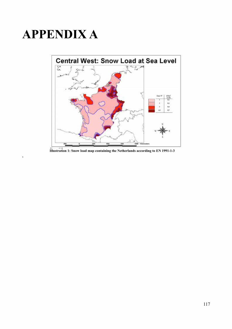
APPENDIX A
,
117
Illustration 1: Snow load map containing the Netherlands according to EN 1991-1-3

118

119


![Mollusks [sic] and other shells - pdf version](https://img.dokumen.tips/doc/110x75/631cdc3ea906b217b90728f3/mollusks-sic-and-other-shells-pdf-version.jpg)


