EXTRACTION OF VITAL SIGNS USING REAL TIME VIDEO

University of Texas at TylerScholar Works at UT Tyler

Electrical Engineering Theses Electrical Engineering

Fall 12-10-2018

EXTRACTION OF VITAL SIGNS USINGREAL TIME VIDEO ANALYSIS FORNEONATAL MONITORINGBHUSHAN LOHANIThe University of Texas at Tyler

Follow this and additional works at: https://scholarworks.uttyler.edu/ee_grad

Part of the Biomedical Commons, and the Signal Processing Commons

This Thesis is brought to you for free and open access by the ElectricalEngineering at Scholar Works at UT Tyler. It has been accepted forinclusion in Electrical Engineering Theses by an authorized administratorof Scholar Works at UT Tyler. For more information, please [email protected].

Recommended CitationLOHANI, BHUSHAN, "EXTRACTION OF VITAL SIGNS USING REAL TIME VIDEO ANALYSIS FOR NEONATALMONITORING" (2018). Electrical Engineering Theses. Paper 40.http://hdl.handle.net/10950/1212

http://www.uttyler.edu/graduate/?utm_source=scholarworks.uttyler.edu%2Fee_grad%2F40&utm_medium=PDF&utm_campaign=PDFCoverPages

http://www.uttyler.edu/graduate/?utm_source=scholarworks.uttyler.edu%2Fee_grad%2F40&utm_medium=PDF&utm_campaign=PDFCoverPages

https://scholarworks.uttyler.edu?utm_source=scholarworks.uttyler.edu%2Fee_grad%2F40&utm_medium=PDF&utm_campaign=PDFCoverPages

https://scholarworks.uttyler.edu/ee_grad?utm_source=scholarworks.uttyler.edu%2Fee_grad%2F40&utm_medium=PDF&utm_campaign=PDFCoverPages

https://scholarworks.uttyler.edu/ee?utm_source=scholarworks.uttyler.edu%2Fee_grad%2F40&utm_medium=PDF&utm_campaign=PDFCoverPages

https://scholarworks.uttyler.edu/ee_grad?utm_source=scholarworks.uttyler.edu%2Fee_grad%2F40&utm_medium=PDF&utm_campaign=PDFCoverPages

http://network.bepress.com/hgg/discipline/267?utm_source=scholarworks.uttyler.edu%2Fee_grad%2F40&utm_medium=PDF&utm_campaign=PDFCoverPages

http://network.bepress.com/hgg/discipline/275?utm_source=scholarworks.uttyler.edu%2Fee_grad%2F40&utm_medium=PDF&utm_campaign=PDFCoverPages

http://hdl.handle.net/10950/1212?utm_source=scholarworks.uttyler.edu%2Fee_grad%2F40&utm_medium=PDF&utm_campaign=PDFCoverPages

mailto:[email protected]

EXTRACTION OF VITAL SIGNS USING REAL TIME

VIDEO ANALYSIS FOR NEONATAL MONITORING

by

BHUSHAN LOHANI

A thesis submitted in partial fulfillment

of the requirements of the degree of

Master of Science in Electrical Engineering

Mukul V. Shirvaikar, Ph.D., Committee Chair

College of Engineering

The University of Texas at Tyler

December 2018

Acknowledgements

First, I would like to express my gratitude to my parents and my siblings. With their love, care and

support always upon me, I am confident on passing any obstacles in my life.

I would like to thank Dr. Mukul V. Shirvaikar for being such a wonderful thesis advisor to me.

His guidelines paved my paths and without his advice it would not have been possible to even start

this research. His door was always open for me whenever I had difficulties understanding some of

the core concepts. I do not have enough words to thank him.

I would also like to thank Dr. Indic who always acted as my second advisor and was ready to help

me out when needed. Thank you for being such a wonderful teacher. I would also like to thank Dr.

Pieper who always had confidence on me and for all those nice words of advice.

I express my profound gratitude to the Office of Graduate School and Dr. Alecia Wolf for

providing me with this opportunity. Dr. Wolf has always been my teacher, friend, advisor and

guardian.

I would like to thank the members of the Department of Electrical Engineering family for making

this place my second home. I would also like to remember and thank my flatmates Ashab and

Sambhu who always supported me and extended their valuable suggestions and help when

required.

At last I would like to thank my loving wife for always boosting up my confidence whenever I

was down. Her valuable suggestions regarding the medical aspect of this research helped a lot.

Thank you for always being there for me.

Bhushan Lohani

i

Table of Contents

List of Tables ................................................................................................................................. iii

List of Figures ................................................................................................................................ iv

Abstract ........................................................................................................................................... v

Chapter 1 ......................................................................................................................................... 1

Introduction ..................................................................................................................................... 1

1.1 Introduction to video data. ................................................................................................... 1

1.2 Heartbeats and pulse. ........................................................................................................... 2

1.3 Pulse rate from video. .......................................................................................................... 3

1.3.1 Pulse rate from monochrome video. ............................................................................... 3

1.3.2 Pulse rate from colored video ......................................................................................... 4

1.4 Thesis coverage ..................................................................................................................... 4

Chapter 2 ......................................................................................................................................... 5

Literature Survey ............................................................................................................................ 5

Chapter 3 ......................................................................................................................................... 9

Theoretical Background .................................................................................................................. 9

3.1 Video acquisition and frame extraction. .............................................................................. 10

3.1.1 Frame Extraction for monochrome video processing ................................................... 11

3.1.2 Frame extraction for HSI/color video processing ......................................................... 11

3.2 Region of interest (ROI) selection from each frame. .......................................................... 12

3.2.1 Global Thresholding ..................................................................................................... 12

3.3 Gaussian Smoothing ............................................................................................................ 13

3.4 Signal extraction .................................................................................................................. 15

3.5 Wavelet-based denoising. .................................................................................................... 16

3.6 Bandpass Filtering ............................................................................................................... 17

3.7 Power spectral Density Approximation. ............................................................................. 17

Chapter 4 ....................................................................................................................................... 19

Experimental Results .................................................................................................................... 19

ii

4.1 Results for monochrome extraction. ................................................................................... 19

4.2 Results from color video ..................................................................................................... 20

4.3 Results comparison. ............................................................................................................. 22

Chapter 5 ....................................................................................................................................... 23

Discussion and Conclusions ......................................................................................................... 23

References ..................................................................................................................................... 24

Appendix ....................................................................................................................................... 27

Appendix A: MATLAB code .................................................................................................... 27

Appendix B: More results ......................................................................................................... 35

iii

List of Tables

Table 1. Experimental data for monochrome and color video processing. .................................. 22

iv

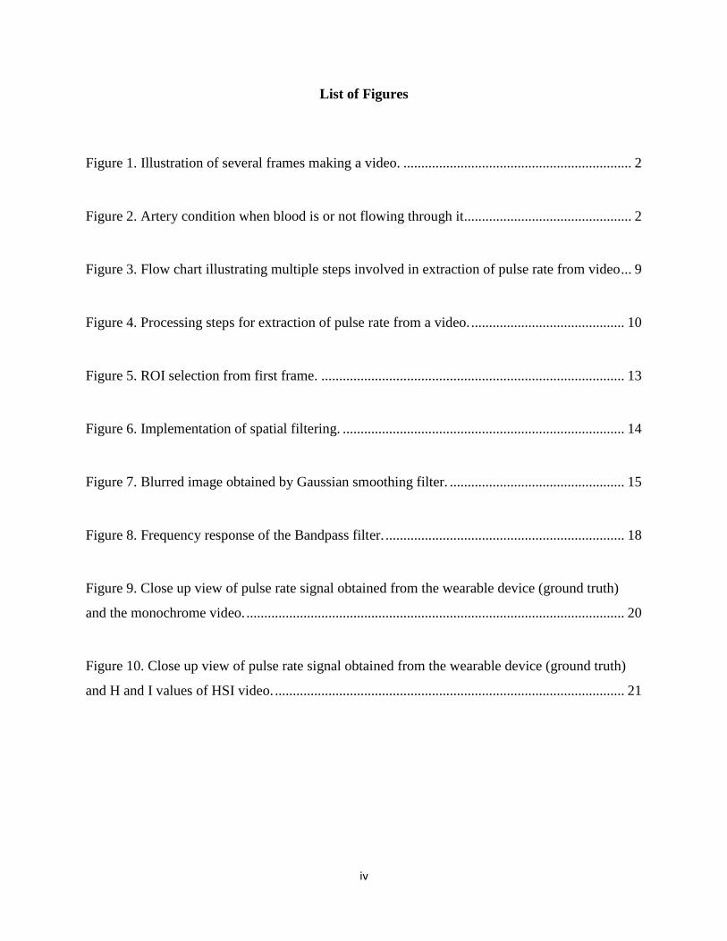
List of Figures

Figure 1. Illustration of several frames making a video. ................................................................ 2

Figure 2. Artery condition when blood is or not flowing through it............................................... 2

Figure 3. Flow chart illustrating multiple steps involved in extraction of pulse rate from video ... 9

Figure 4. Processing steps for extraction of pulse rate from a video. ........................................... 10

Figure 5. ROI selection from first frame. ..................................................................................... 13

Figure 6. Implementation of spatial filtering. ............................................................................... 14

Figure 7. Blurred image obtained by Gaussian smoothing filter. ................................................. 15

Figure 8. Frequency response of the Bandpass filter. ................................................................... 18

Figure 9. Close up view of pulse rate signal obtained from the wearable device (ground truth)

and the monochrome video. .......................................................................................................... 20

Figure 10. Close up view of pulse rate signal obtained from the wearable device (ground truth)

and H and I values of HSI video. .................................................................................................. 21

v

Abstract

Extraction of vital signs using video analysis for

neonatal monitoring

Bhushan Lohani

Thesis Chair: Mukul V. Shirvaikar, Ph.D.

The University of Texas at Tyler

December 2018

Video data is now commonly used for analysis in surveillance, security, medical and many other

fields. The development of low cost but high-quality portable cameras has contributed significantly

to this trend. One such trend includes non-invasive vital statistics monitoring of infants in Neonatal

Intensive Care Units (NICU). National Center for Health Statistics Publications has reported a

high infant death rate (23,215 in 2014). This statistic has drawn the interest of health system

professionals. Due to occurrence of conditions like bradycardia, apnea and hypoxia, these preterm

infants are kept in an NICU for constant monitoring. One of the problems faced at the NICU is the

use of traditional sensors for vital statistics monitoring which might cause damage to the already

fragile skin of these infants. A contact-less approach to record such vital signs can now be

employed using a live video feed. Recent literature shows that it is possible to extract features from

videos that are invisible to the human eye, employing various image and signal processing

techniques. One of the algorithms demonstrated recently is the extraction of medical vital signs

based on wavelet filtering of monochrome video data.

The pumping of blood to various parts of body from the heart in rhythmic fashion causes subtle

changes in the skin tone of humans. These changes are periodic in nature as the pumping action

itself is periodic corresponding to the heart beat. Typical heartbeat of a human ranges from 50-200

beats per minutes (bpm) implying the range to be 0.83-3.33 Hz. Similarly, a video is a sequence

vi

of frames with frame rate ranging from 15-30 frames per seconds (fps). This creates the possibility

of using videos to detect heart rates as the Nyquist Criterion is met with ease. The subtle changes

in skin tones can be further processed and magnified. The mean gray level signal obtained from

such a process has been found to be resembling the pulse rate waveform obtained from

photoplethysmograph(PPG) sensor to measure pulse rate. The other approach is to use color

channel domain like HSI (Hue, Saturation and Intensity).

With the above concept, a video processing algorithm was designed in MATLAB. Short videos of

several subjects with different skin tone were recorded for the analysis. In order to compare to the

ground truth, pulse data were recorded at the same time using the photoplethysmographsensor of

a wearable watch. Upon implementing the algorithm designed, on the videos, it was possible to

extract waveforms from the videos that resembled the pulse waveform recorded from the ground

truth measuring device. The percentage error was in the range of 0.2 to 1.4%. This led to the

conclusion that video data can be analyzed to extract heart rate and with further study can be used

for real time monitoring of cardiac activity of infants at an NICU.

1

Chapter 1

Introduction

As per the report published by the National Center for Health Statistics Publications, US health

system has been facing higher death rates (23,215 in 2014) [1]. This condition of infant mortality

has advocated for constant monitoring of infants at an NICU. Infants and especially preterm infants

need uninterrupted monitoring of vital statistics like respiration rates and heart rates to access their

health conditions and to detect the occurrence of life-threatening conditions like apnea,

bradycardia and hypoxia. At present conventional sensors are employed for such measurements.

However, irritability of infant skin and the chances of detachment due to movements is possible

with mechanically attached sensors. Efforts are being directed towards use of non-contact

measures. A non-invasive vital statistics monitoring system is a present need and it can be attained

using live video data [2].

1.1 Introduction to video data.

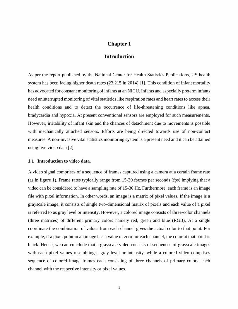
A video signal comprises of a sequence of frames captured using a camera at a certain frame rate

(as in figure 1). Frame rates typically range from 15-30 frames per seconds (fps) implying that a

video can be considered to have a sampling rate of 15-30 Hz. Furthermore, each frame is an image

file with pixel information. In other words, an image is a matrix of pixel values. If the image is a

grayscale image, it consists of single two-dimensional matrix of pixels and each value of a pixel

is referred to as gray level or intensity. However, a colored image consists of three-color channels

(three matrices) of different primary colors namely red, green and blue (RGB). At a single

coordinate the combination of values from each channel gives the actual color to that point. For

example, if a pixel point in an image has a value of zero for each channel, the color at that point is

black. Hence, we can conclude that a grayscale video consists of sequences of grayscale images

with each pixel values resembling a gray level or intensity, while a colored video comprises

sequence of colored image frames each consisting of three channels of primary colors, each

channel with the respective intensity or pixel values.

2

Figure 1. Illustration of several frames (left) making a video (right).

1.2 Heartbeats and pulse.

Heart is the main part of the circulatory system. The main function of the heart to collect

deoxygenated blood from various body parts transport it to lungs for purification and supply

oxygenated blood to the different body parts.

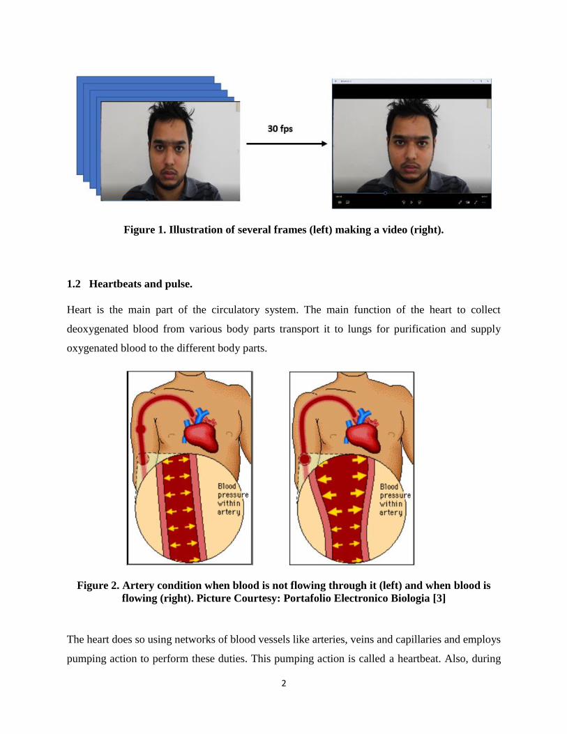
Figure 2. Artery condition when blood is not flowing through it (left) and when blood is

flowing (right). Picture Courtesy: Portafolio Electronico Biologia [3]

The heart does so using networks of blood vessels like arteries, veins and capillaries and employs

pumping action to perform these duties. This pumping action is called a heartbeat. Also, during

3

the supply of oxygenated blood to various body parts, the arteries are in action. As the heart pumps

the blood into the arteries, the pressure caused due to pumping transmits to the wall of arteries as

shown in figure 2. This periodic pressure applied to the arteries walls resembling heart beat is

called pulse. The rate at which the heart pumps or beats is called heart rate and the same rate

derived from the artery walls is called pulse rate. In general, the range of human heartbeat is 50-

200 bpm. When converted it lies in the region of 0.83-3.33 Hz.

1.3 Pulse rate from video.

The pumping or flow of blood to different body parts in a rhythmic fashion causes subtle change

in the skin tone of humans. As, the heart beat is periodic, these subtle changes are periodic as well.

However, these changes are very small in magnitude and are almost invisible to human eyes. If a

video of a part of body is captured for certain interval of time and if this variation in skin tone is

studied at pixel levels and magnified, it is possible to extract a pulse waveform from the video.

As previously stated, the frame rate or sampling rate of a video lies in the range of 15-30 Hz. Also,

the human pulse rate ranges from 0.83-3.33 Hz. This condition allows the satisfaction of the

Nyquist Criterion and the possibility of derivation of heart rate or pulse rate from video. For this,

an algorithm can be developed, and the pulse rate can be extracted. We have investigated two

methods to derive the pulse rate, as described below.

1.3.1 Pulse rate from monochrome video.

In this method the three-color channels of the video are combined to form a single gray scale

channel of intensity. This method is based on the fact that there are changes in the intensity value

of a point of a body part due to pumping action of blood on arteries. The average intensity of the

region of interest (ROI) is calculated for each frame, processed through various signal conditioning

steps like bandpass filtering and wavelet based denoising to obtain a signal resembling the pulse

waveform. From this waveform the pulse rate can be derived using frequency transforms.

4

1.3.2 Pulse rate from colored video

For the implementation of this method, each RGB frames obtained from the video is first

transformed to HSI (Hue, Saturation and Intensity) domain and the intensity and hue channels can

be used for pulse rate derivation. The average pixel values of ROI for each frame from these two

channels are calculated, processed using bandpass filtering and pulse waveform can be obtained.

The pulse rate can be derived as in the first method.

1.4 Thesis coverage

This thesis report is divided into five chapters. Chapter 2 provides the literature survey related to

the problems incorporating similar past work. Chapter 3 delivers the theoretical methodologies

used for the research work with detailed descriptions. The experimental results for different

subjects are presented in chapter 4. The appendix contains the code and functions written on

MATLAB used for the research.

5

Chapter 2

Literature Survey

The application of heart rate extraction on mobile devices was studied by Kwon et al using a single

green channel from the video data [4]. They extracted frames from video and ultimately the signals

for RGB channels. Based on the strong plethysmographic nature of the green channel, the group

selected it as their principal signal of interest. They used video recorded from an iPhone 4 and

employed face detection algorithm from Open Computer Vision (OpenCV) library as their region

of interest (ROI) selection tool. RGB channels from each frame were separated and corresponding

signals were extracted from the whole video. The final implementation using Fast Fourier

Transform resulted in the extraction of heart rate from the video. An iPhone application named

FaceBEAT was developed using the same algorithm by the group that could record 20 seconds of

video of a subject and extract the heart rate.

HSV model was used by Cho et al to devise a non-contact heart rate measuring algorithm [5]. They

combined matrix-based IIR (mIIR) filter and HSV (Hue, Saturation and Value) processing to

formulate a new algorithm named HSV+mIIR algorithm. They first designed an mIIR filter

converting general IIR filter to matrix- based so that it can be applied to each pixel simultaneously.

The algorithm was applied to the RGB data and Short Time Fourier Transform (STFT) was applied

to it. It was revealed that; green channel represents the hemodynamics of the human skin. The

RGB domain was then converted to HSV domain and only the V value of HSV domain, that

corresponds to intensity value, was processed using HSV+mIIR algorithm. The result was

compared to other algorithms like green trace (signal obtained by averaging pixels in R of RGB

domain), Independent Component Analysis (ICA) and mIIR on G channel of RGB domain. The

results displayed by HSV+mIIR was the clearest one as per Cho et al.

Various works have been done in the past in the field of vital statistics extraction from video.

Cattani et al used motion analysis to monitor infants [6]. They placed multiple video sensors

around the patient and extracted relevant motion signals. With the application of Maximum

Likelihood (ML) criterion to these extracted signals, their periodicity was estimated. The first step

was to extract temporal motion signal. This was performed by first converting each frame of the

6

video to gray scale, then applying a simple Finite Impulse Response (FIR) filtering. The FIR

filtering was based on the difference between consecutive frames. The resulting frames were then

converted to binary image using morphological operation of erosion. Derivation of spatial average

luminance signal was the final step on motion extraction. The spatial average luminance signal

represents the movement pattern of the body part of interest.

After the extraction of motion signal, a decision-making approach named Maximum-likelihood

approach was used to detect the presence or absence of motion of the concerned body part. With

this they were able to detect colonic seizures on the basis of presence of absence of periodic

motion. The addition of Eulerian Video Magnification (EVM) as a pre-processing step to the video

helped detect sleep apnea as well.

Sharma et al proposed a method to detect respiratory motion and its absence by motion

magnification and filtering [7]. A close shot view of the subject was taken and a manual ROI

around babies’ abdomen and chest was marked. Subtle chest movement detection was performed

using EVM technique. The EVM technique consists of three steps. The first step is the spatial

decomposition. In this step the input video sequence is decomposed into different frequency bands.

These bands are magnified differently as they might exhibit different signal-to-noise ratios (SNR).

In other words, the magnifications are based on the requirement of magnifying the motion signal

of concern only. They decomposed the video using n levels of Laplacian pyramid obtained by

subtracting consecutive levels of Gaussian pyramids.

The next step involved the temporal filtering and magnification. A temporal bandpass filter was

employed to each level of a Laplacian pyramid. A bandpass filter of lower cut off frequency of

0.4Hz and higher cut off frequency of 3Hz was applied to each level. The motion thus obtained

was magnified by a factor of 10 in order to magnify the respiratory signal and at the same time

control the magnification of noise and other artifacts. The sum of intensity values from each frame

is calculated which will display the presence or absence of motion due to respiration.

EVM and 2-Gaussian curve modelling were incorporated by He et al to measure wrist pulse [8].

EVM was applied to frame level to reveal invisible wrist pulse signal in the video. The procedure

involved similar steps as performed by Sharma et al [7]. Application of full Laplacian pyramid for

spatial decomposition into several bands, temporal filtering of each band to emphasize motion and

finally magnification of the motion signal were performed by the group to reveal wrist pulse from

7

the video. The features of wrist pulse were observed on one cycle of the signal obtained from

EVM. For this 2-Gaussian curve modeling method was employed. The initial coefficient values of

the Gaussian curve were set, and the fitted model was determined by nonlinear least squares

algorithm and “Trust-Region” fitting algorithm. With this they were able to compare the wrist

signal obtained from the video with the ground truth.

Similar work was done by Balakrishna et al but used Newtonian motion signal of head due to

cardiac cycle [9]. The group exploited subtle head oscillations due to cardiac activity to extract

cardiac activity from the video. The periodic flow of blood from heart to the head via the abdominal

aorta and the carotid arteries causes head to move following the law of Newtonian action and

reaction. The paper presented an approach to track the motion and extract the cardiac statistics

from the same. Videos of front view and back view of heads of subjects were taken. For front face

visible videos, Viola Jones face detector from OpenCV was employed. The eyes were removed

from the ROI so that they would not add up their blinking artifacts. For videos with back facing

head, manual ROI was selected. The motion of the head was extracted using OpenCV Lucas Kande

tracker for each frame. The motion signal was then passed to a temporal filter to remove unwanted

frequencies. A 5th order Butterworth bandpass filter of range 0.75-5 Hz was used for the purpose.

The obtained signal was the mixture of pulse signal as well as other signals like respiratory,

vestibular and facial signals. To isolate the cardiac signal from the mixture, Balakrishna et al

decomposed the signal and use principal component analysis (PCA). The final signal obtained

resembled the cardiac signal.

Zadeh et al used Doppler radar to detect mechanical vibration of heart and was successful in

proposing a non-invasive heart rate measuring system [10]. Contactless heart monitoring (CHM)

uses a microwave Doppler radar sensor (operating range: 2.45GHz). A beam of radio frequency

signal is directed towards the body of the subject and the reflected wave is studied. The heart rate

can be determined according to the Doppler theory which states that a constant frequency signal

reflected off an object with a periodically varying displacement will result in a reflected signal at

the same frequency but with a time varying phase.

A non-contact system was also proposed using thermal imaging system by studying the thermal

signal emitted by superficial blood vessels [11]. The periodic motion of blood to superficial blood

vessels modulates tissue temperature due to heat exchange via convection and conduction. This

8

change in temperature can be studied and linked to the pulsating nature of blood flow in the vessel

which ultimately resembles the cardiac activity. These methods employ expensive modalities like

radar and thermal imaging.

Heart rate and rhythm was estimated using 3D motion tracking in depth video [12]. Yang et al

proposed a non- invasive heart rate detection procedure incorporating joint bit-depth enhancement

and PCA.

In past work we have investigated the possibility of heart rate detection from monochrome video

[2]. Frames were extracted from color video and each frame was processed successively. A region

of interest was selected manually which was supposed to be same for the entire video as stationary

subjects were considered. Then the frames were converted to monochrome images. Each frame

was first smoothened to remove noise using Gaussian filters. Average gray-level values from each

frame was determined as a 1D signal from all the frames in the video. This 1D signal was further

denoised using wavelet based denoising and passed to the bandpass filter. The final operation

produced a signal which was similar to pulse rate waveform. Hence, it was possible to extract heart

rate or pulse rate from a color video first converting it to a monochrome one and following various

steps discussed above. The thesis is based on the same work with addition of color video

processing as well.

9

Chapter 3

Theoretical Background

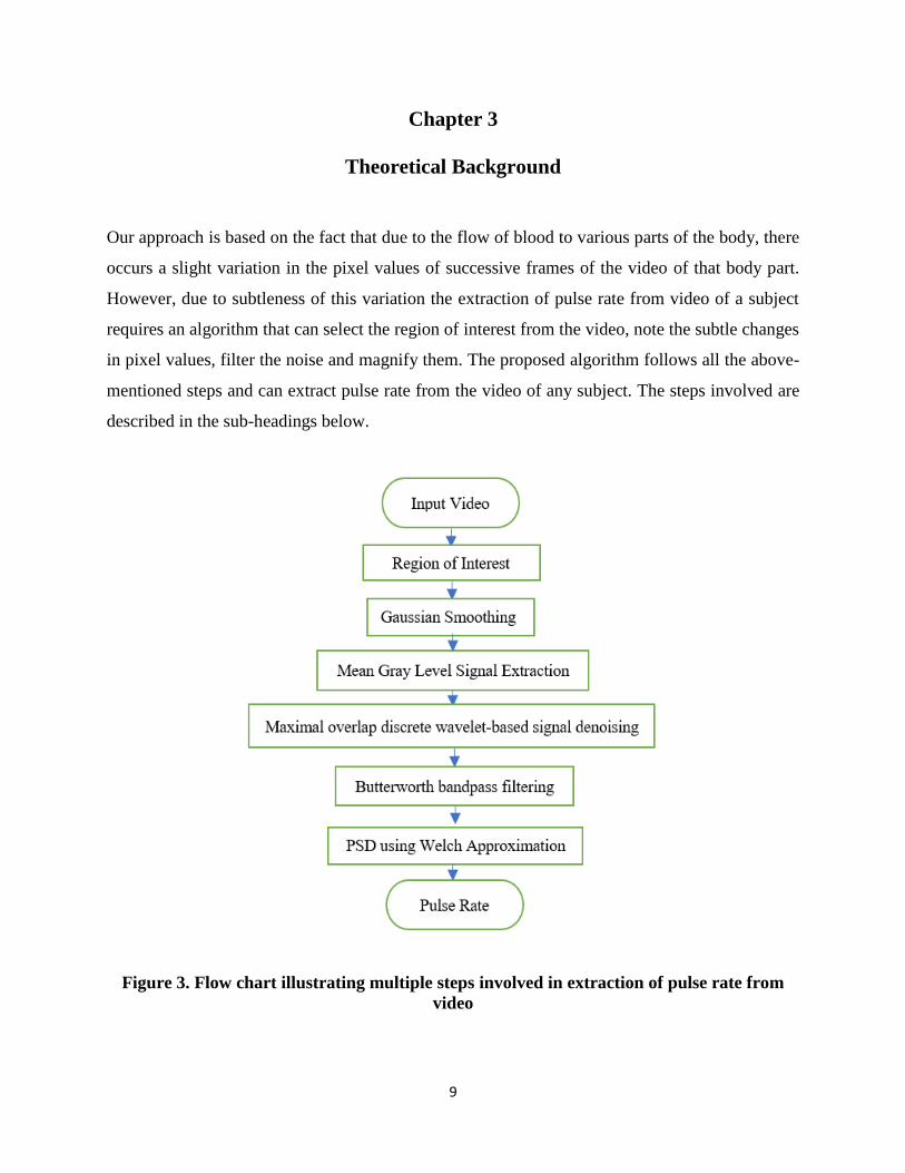
Our approach is based on the fact that due to the flow of blood to various parts of the body, there

occurs a slight variation in the pixel values of successive frames of the video of that body part.

However, due to subtleness of this variation the extraction of pulse rate from video of a subject

requires an algorithm that can select the region of interest from the video, note the subtle changes

in pixel values, filter the noise and magnify them. The proposed algorithm follows all the above-

mentioned steps and can extract pulse rate from the video of any subject. The steps involved are

described in the sub-headings below.

Figure 3. Flow chart illustrating multiple steps involved in extraction of pulse rate from

video

10

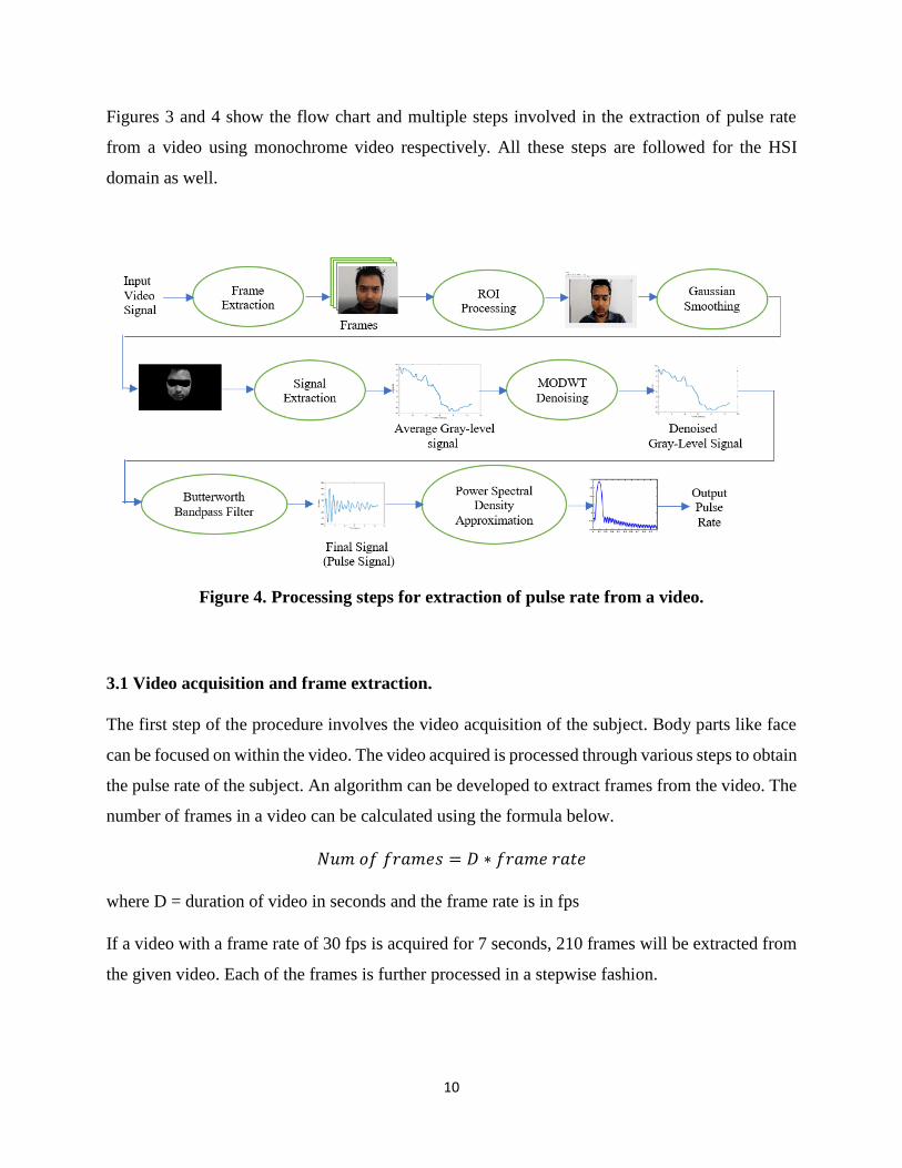
Figures 3 and 4 show the flow chart and multiple steps involved in the extraction of pulse rate

from a video using monochrome video respectively. All these steps are followed for the HSI

domain as well.

Figure 4. Processing steps for extraction of pulse rate from a video.

3.1 Video acquisition and frame extraction.

The first step of the procedure involves the video acquisition of the subject. Body parts like face

can be focused on within the video. The video acquired is processed through various steps to obtain

the pulse rate of the subject. An algorithm can be developed to extract frames from the video. The

number of frames in a video can be calculated using the formula below.

𝑁𝑢𝑚 𝑜𝑓 𝑓𝑟𝑎𝑚ⅇ𝑠 = 𝐷 ∗ 𝑓𝑟𝑎𝑚ⅇ 𝑟𝑎𝑡ⅇ

where D = duration of video in seconds and the frame rate is in fps

If a video with a frame rate of 30 fps is acquired for 7 seconds, 210 frames will be extracted from

the given video. Each of the frames is further processed in a stepwise fashion.

11

3.1.1 Frame Extraction for monochrome video processing

The first video processing algorithm designed to extract heart rate from video involves simple

monochrome processing. In this method, each extracted RGB frame obtained from the video is

first converted to a monochrome frame. A frame at any discrete time is an array of matrices of

pixels, containing red, green and blue (RGB) values. This corresponds to a gray scale value Y(t)

at any discrete time given by the weighed sum of RGB values [13]:

𝑌(𝑡) = 0.299𝑅(𝑡) + 0.587𝐺(𝑡) + 0.114𝐵(𝑡)

The above equation can be used to compute the gray level for each pixel of each frame.

3.1.2 Frame extraction for HSI/color video processing

Another similar approach is the use of color domain for heart rate extraction. This method focuses

on the use of HSI domain to create frames and heart rate signals for further processing. In this

method, the RGB frames obtained from the video are first converted to HSI domains. Like a 3

channel RGB image HSI domain too has three channels namely Hue (H), Saturation (S) and

Intensity (I). These three channels can be derived from RGB domain by the relations below [14].

𝐻 = {𝜃 ⅈ𝑓 𝐵 ≤ 𝐺360 − 𝜃 ⅈ𝑓 𝐵 > 𝐺

Where

𝜃 = 𝑐𝑜𝑠−1 {1

2⁄ [(𝑅 − 𝐺) + (𝑅 − 𝐵)]

[(𝑅 − 𝐺)2 + (𝑅 − 𝐵)(𝐺 − 𝐵)]1

2⁄}

Similarly,

𝑆 = 1 −3

(𝑅 + 𝐺 + 𝐵)[𝑚ⅈ𝑛(𝑅, 𝐺, 𝐵)]

And,

𝐼 =1

3(𝑅 + 𝐺 + 𝐵)

12

From the equations above, three channels of HSI domain are obtained. Each channel can be

separately processed along the line of processes as monochrome channel and waveform from each

channel can be derived. Experimental results showed that only Hue and Intensity channels display

the nature of heart waveform, hence, the saturation channel is not further processed.

3.2 Region of interest (ROI) selection from each frame.

The parts of body like the face excluding the eye area can be considered to be the ROI for the

experiment. The eyes are excluded to avoid noise due to eye ball movements. The ROI is assumed

to be the same for the entire processing of the still video of the subject. A mask can be created

using a global thresholding algorithm.

3.2.1 Global Thresholding

The simple implementation and speed of computation makes thresholding one of the most used

segmentation methods available. The scheme is based on the principal of segregating the pixel

values into groups. One such procedure involves global thresholding. In this process we convert a

given frame to grayscale image, select a random threshold value, divide all the pixel values into

groups based on the threshold value. The means of each pixel values from each group are

calculated and a new value of threshold (T) is updated as follows

𝑇 = 𝑟𝑎𝑛𝑑𝑜𝑚 𝑣𝑎𝑙𝑢ⅇ … … … … … … … . 𝑓ⅈ𝑟𝑠𝑡 ⅈ𝑛ⅈ𝑡𝑎𝑙ⅈ𝑧𝑎𝑡ⅈ𝑜𝑛

Step1: 𝑚1 = 𝑚ⅇ𝑎𝑛 𝑜𝑓 ⅈ𝑛𝑡ⅇ𝑛𝑠ⅈ𝑡ⅈⅇ𝑠 𝑜𝑓 ⅈ𝑚𝑎𝑔ⅇ 𝑏ⅇ𝑙𝑜𝑤 𝑇

Step2: 𝑚2 = 𝑚ⅇ𝑎𝑛 𝑜𝑓 ⅈ𝑛𝑡ⅇ𝑛𝑠ⅈ𝑡ⅈⅇ𝑠 𝑜𝑓 ⅈ𝑚𝑎𝑔ⅇ 𝑎𝑏𝑜𝑣ⅇ 𝑇

Step 3: 𝑇 =(𝑚1+𝑚2)

2… … … … … … … … … . . 𝑛ⅇ𝑤 𝑣𝑎𝑙𝑢ⅇ 𝑜𝑓 𝑇

The steps (1), (2) and (3) are repeated until the difference between T values in successive iteration

becomes less than the predefined value [14]. The image is then segmented between the new-found

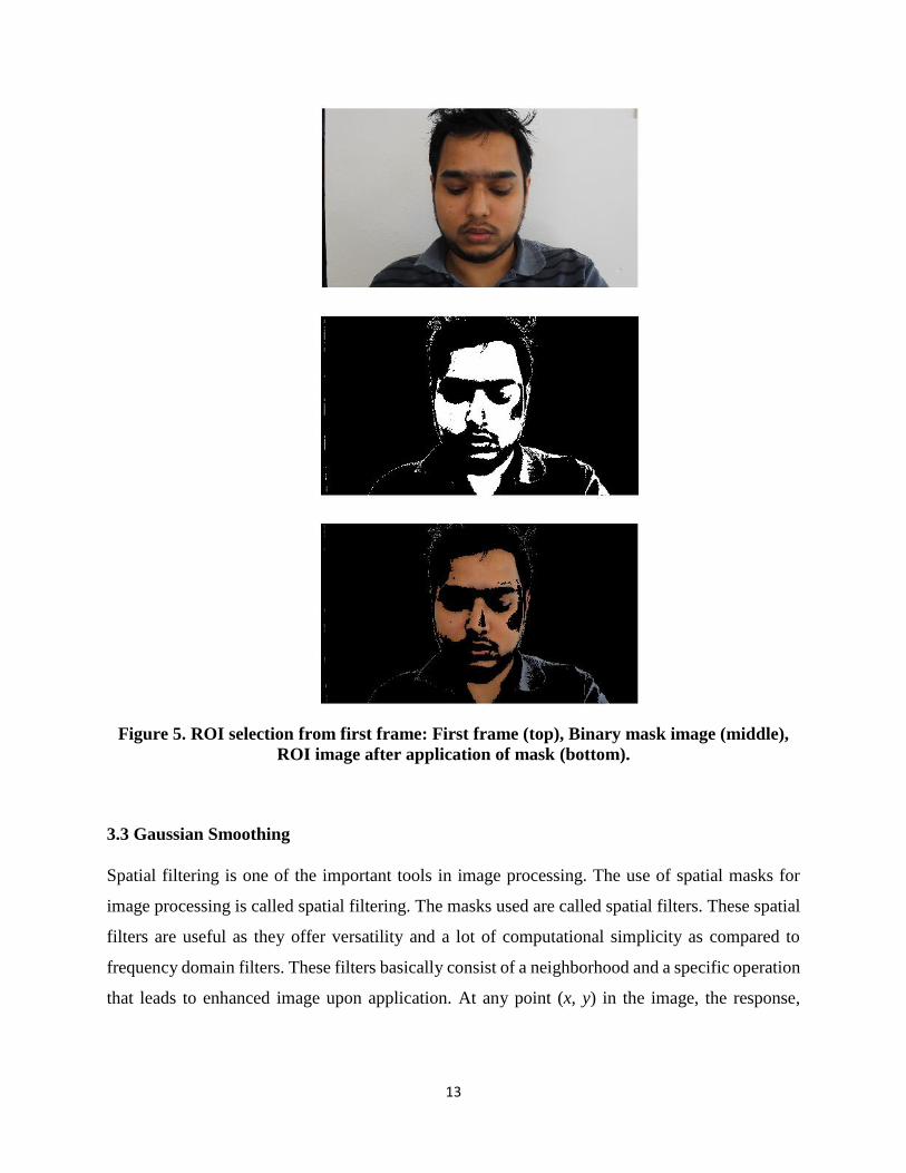
threshold value. Figure 5 shows the derivation of ROI from first frame of one of the experiments.

As the present research considers still videos of subjects, the ROI can be set the same for the whole

video. Besides, as the experimental videos are of 7 seconds in length, constant ROI makes sense.

Further work involves updating of ROI after certain time intervals.

13

Figure 5. ROI selection from first frame: First frame (top), Binary mask image (middle),

ROI image after application of mask (bottom).

3.3 Gaussian Smoothing

Spatial filtering is one of the important tools in image processing. The use of spatial masks for

image processing is called spatial filtering. The masks used are called spatial filters. These spatial

filters are useful as they offer versatility and a lot of computational simplicity as compared to

frequency domain filters. These filters basically consist of a neighborhood and a specific operation

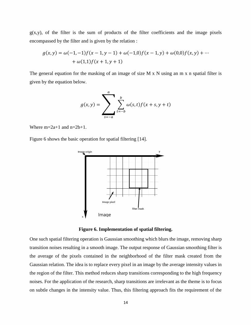
that leads to enhanced image upon application. At any point (x, y) in the image, the response,

14

g(x,y), of the filter is the sum of products of the filter coefficients and the image pixels

encompassed by the filter and is given by the relation :

𝑔(𝑥, 𝑦) = 𝜔(−1, −1)𝑓(𝑥 − 1, 𝑦 − 1) + 𝜔(−1,0)𝑓(𝑥 − 1, 𝑦) + 𝜔(0,0)𝑓(𝑥, 𝑦) + ⋯

+ 𝜔(1,1)𝑓(𝑥 + 1, 𝑦 + 1)

The general equation for the masking of an image of size M x N using an m x n spatial filter is

given by the equation below.

𝑔(𝑥, 𝑦) = ∑ ∑ 𝜔(𝑠, 𝑡)𝑓(𝑥 + 𝑠, 𝑦 + 𝑡)

𝑏

𝑡=−𝑏

𝑎

𝑠=−𝑎

Where m=2a+1 and n=2b+1.

Figure 6 shows the basic operation for spatial filtering [14].

Figure 6. Implementation of spatial filtering.

One such spatial filtering operation is Gaussian smoothing which blurs the image, removing sharp

transition noises resulting in a smooth image. The output response of Gaussian smoothing filter is

the average of the pixels contained in the neighborhood of the filter mask created from the

Gaussian relation. The idea is to replace every pixel in an image by the average intensity values in

the region of the filter. This method reduces sharp transitions corresponding to the high frequency

noises. For the application of the research, sharp transitions are irrelevant as the theme is to focus

on subtle changes in the intensity value. Thus, this filtering approach fits the requirement of the

Image

15

experiments. The mask is created using the relation below where h(x,y) is the mask and σ is the

standard deviation

ℎ(𝑥, 𝑦) = ⅇ−(𝑥2+𝑦2)

2𝜎2

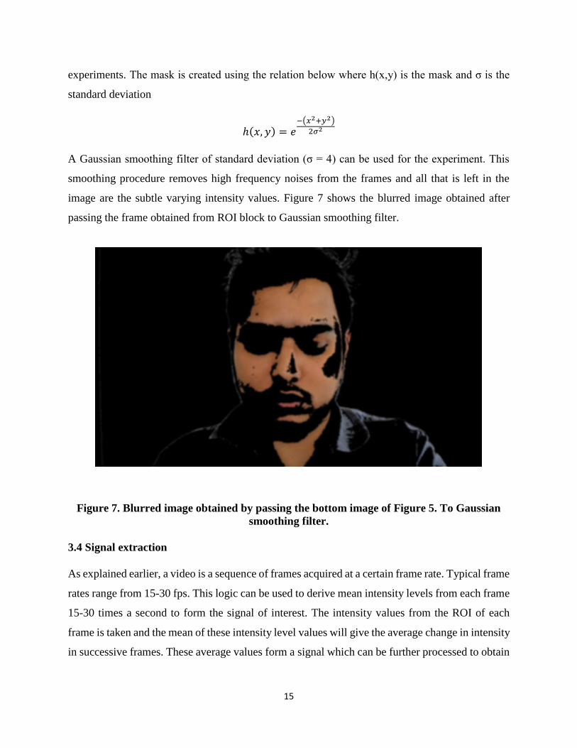
A Gaussian smoothing filter of standard deviation (σ = 4) can be used for the experiment. This

smoothing procedure removes high frequency noises from the frames and all that is left in the

image are the subtle varying intensity values. Figure 7 shows the blurred image obtained after

passing the frame obtained from ROI block to Gaussian smoothing filter.

Figure 7. Blurred image obtained by passing the bottom image of Figure 5. To Gaussian

smoothing filter.

3.4 Signal extraction

As explained earlier, a video is a sequence of frames acquired at a certain frame rate. Typical frame

rates range from 15-30 fps. This logic can be used to derive mean intensity levels from each frame

15-30 times a second to form the signal of interest. The intensity values from the ROI of each

frame is taken and the mean of these intensity level values will give the average change in intensity

in successive frames. These average values form a signal which can be further processed to obtain

16

the pulse waveform from the video. The first step towards processing is the removal of DC value

from the video waveform in order to analyze the signal further.

For the monochrome processing, as a single channel is used, we can obtain single waveform from

a video. For HSI domain, two waveforms are obtained for each Hue and Intensity channels. These

signals are processed further in later steps to obtain the pulse waveforms.

3.5 Wavelet-based denoising.

The raw signal thus obtained comprises of features and noise. From elementary frequency domain

analysis, it became apparent that the signal consisted of the desired Pulse waveform entangled with

other noise in a close frequency range. Removal of such noise in the proximity requires segregation

of the desired periodic signal from other signals of less significance. A signal denoising technique

called Maximal Overlap Discrete Wavelet Transform (MODWT) has been employed as an

appropriate transform for this purpose [12]. Maximal Overlap Discrete Wavelet Transform

(MODWT) automatically computes coefficients for the data using Donoho and Johnstone’s

universal threshold and level-dependent thresholding

If L is the length of the filter ℎ̃𝑙 and �̃�𝑙 be the rescaling filters, then the MODWT pyramid algorithm

generates the wavelet coefficient {𝑑𝑗,𝑛(𝑀)

} and the scaling coefficient {𝑐𝑗,𝑛(𝑀)

} given by [15]:

𝑑𝑗,𝑛(𝑀)

= ∑ ℎ̃𝑙𝑐𝑗−1,(𝑛−2𝑗−𝑙) mod 𝑁

(𝑀)

𝐿−1

𝑙=0

𝑐𝑗,𝑛(𝑀)

= ∑ �̃�𝑙𝑐𝑗−1,(𝑛−2𝑗−𝑙) mod 𝑁

(𝑀)

𝐿−1

𝑙=0

Application of the MODWT should provide a signal that is more amenable for further analysis. In

this analysis the choice of MODWT is based on its features which preserve the smooth time-

varying structure that is otherwise lost during the application of the normal Discrete Wavelet

Transform (DWT). The pulse wave signals of concern correspond to minor variation in the

intensity levels. Also, the signal length is a concern as MODWT is statistically appropriate for the

17

processing of arbitrary signals while DWT of level J0 can only be applied to signals whose length

is a multiple of 2𝐽0 [16]. In other words, the smooth and detail coefficients of MODWT best fits

the application in this research based on the literature [17].

3.6 Bandpass Filtering

A filter is a class of linear time invariant system that passes certain frequency component and

attenuates other frequencies. The filter design process involves specification, approximation and

realization of the filter system. For the application of the research, a Butterworth bandpass filter is

used after denoising filter.

The normal heart rate lies in the region of [50, 200] beats/minutes for infants [18]. This is

equivalent to [0.83, 3.33] Hz. This frequency range also helps to ignore certain low frequency

features like respiration that introduces noise in the process. A 5th order filter is used to maximize

output reliability and the output of the filtering procedure was a smooth signal that represented

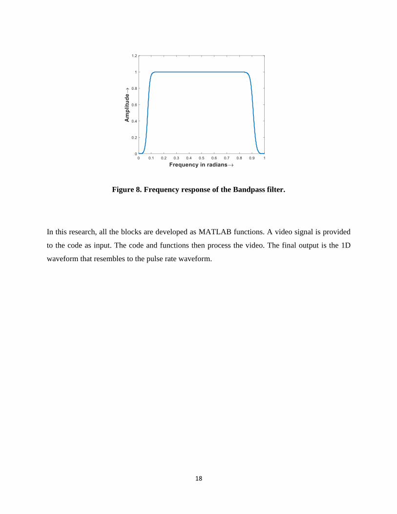
pulse rate. Figure 8 shows the frequency response of the filter used.

3.7 Power Spectral Density Approximation.

Power spectral density was estimated for the signal obtained after filtering via Welch’s method

[15]. This estimation method divides the signal into longest possible sections. It then computes

modified periodogram for each segment using Hamming window. The periodograms are averaged

to compute the final spectral estimate. This estimate gives the power per unit frequency. The

frequency value with the maximum PSD is considered to be the pulse rate frequency (fPR). The

pulse rate per minute is given by:

𝑃𝑅 = 60 ∗ 𝑓𝑃𝑅 𝑏ⅇ𝑎𝑡𝑠 𝑝ⅇ𝑟 𝑚ⅈ𝑛𝑢𝑡ⅇ𝑠

All the above steps if followed stepwise, will give heart rate as the output. It is possible to develop

an algorithm with video as an input signal. The algorithm will have blocks for extracting frames,

reading individual frames and selecting the ROI, smoothening each of the frames, extracting a 1D

signal from the frames, denoising the extracted signal, filtering it with a bandpass filter and finally

analyzing power spectral density of the signal to render heart rate.

18

Figure 8. Frequency response of the Bandpass filter.

In this research, all the blocks are developed as MATLAB functions. A video signal is provided

to the code as input. The code and functions then process the video. The final output is the 1D

waveform that resembles to the pulse rate waveform.

19

Chapter 4

Experimental Results

The entire research used ‘Canon EOS REBEL T6’, a digital single-lens reflex (DSLR) camera by

Canon (video resolution of 1920 x 1088 and 29.97 fps), as the video acquisition tool. Similar

results were obtained using iPhone 4S inbuilt camera (video resolution of 1920 x 1080 and 29.97

fps) during testing phase. Videos of body parts like face of the subject can be acquired using a

standard camera. These videos can be processed using the multi-steps algorithms discussed above

to obtain a 1-D signal corresponding to pulse rate waveform. These signals are tested for accuracy

using data simultaneously taken from ground truth device taken at the time of video recording. For

ground truth measurement, the subject had an ‘Empatica E4 wristband’ worn during video

recording. This wristband consists of inbuilt photoplethysmograph(PPG) sensor that can measure

Blood Volume Pulse (BVP), from which heart rate measurement can be derived. The

experimental procedure incorporated the recording of a short (7 Seconds) video segments focusing

the face area.

The experiments were repeated on five subjects 2-3 times each. A total of 16 readings were taken

and were compared to the pulse signal extracted from the corresponding videos. The delay in signal

acquired from the video and data from wristband were calculated and incorporated by determining

the cross-correlation between the pair of signals at all possible lags. Table 1 shows the results,

including the error rate which ranges from (0.2-1.4%).

4.1 Results for monochrome extraction.

Figure 9 shows the close-up view of pulse waveform extracted from a trial subject. This trial was

performed on monochrome video. The RGB video obtained from the camera was first converted

to a monochrome one for this processing. The average gray level signal obtained from each frame

after removal of DC component was obtained from the video. The signal was further processed to

obtain a waveform and was compared to the ground truth. In figure 9, the ground truth signal and

the one obtained from the video are displayed together for comparison. The text below the figure

shows the data calculated from the waveforms. It is clear from the figure and the text that the

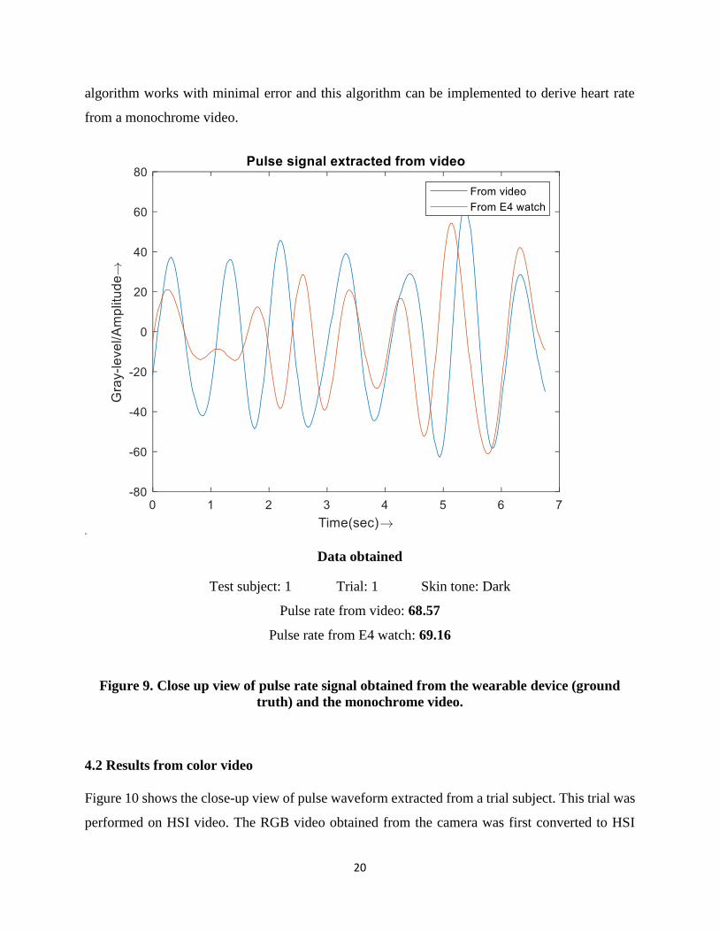
20

algorithm works with minimal error and this algorithm can be implemented to derive heart rate

from a monochrome video.

Data obtained

Test subject: 1 Trial: 1 Skin tone: Dark

Pulse rate from video: 68.57

Pulse rate from E4 watch: 69.16

Figure 9. Close up view of pulse rate signal obtained from the wearable device (ground

truth) and the monochrome video.

4.2 Results from color video

Figure 10 shows the close-up view of pulse waveform extracted from a trial subject. This trial was

performed on HSI video. The RGB video obtained from the camera was first converted to HSI

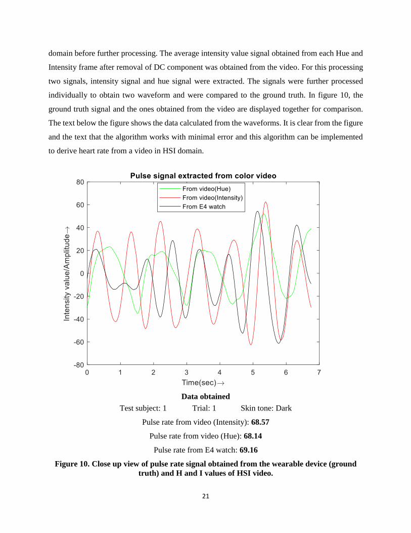
21

domain before further processing. The average intensity value signal obtained from each Hue and

Intensity frame after removal of DC component was obtained from the video. For this processing

two signals, intensity signal and hue signal were extracted. The signals were further processed

individually to obtain two waveform and were compared to the ground truth. In figure 10, the

ground truth signal and the ones obtained from the video are displayed together for comparison.

The text below the figure shows the data calculated from the waveforms. It is clear from the figure

and the text that the algorithm works with minimal error and this algorithm can be implemented

to derive heart rate from a video in HSI domain.

Data obtained


Pulse rate from video (Intensity): 68.57

Pulse rate from video (Hue): 68.14


Figure 10. Close up view of pulse rate signal obtained from the wearable device (ground

truth) and H and I values of HSI video.

22

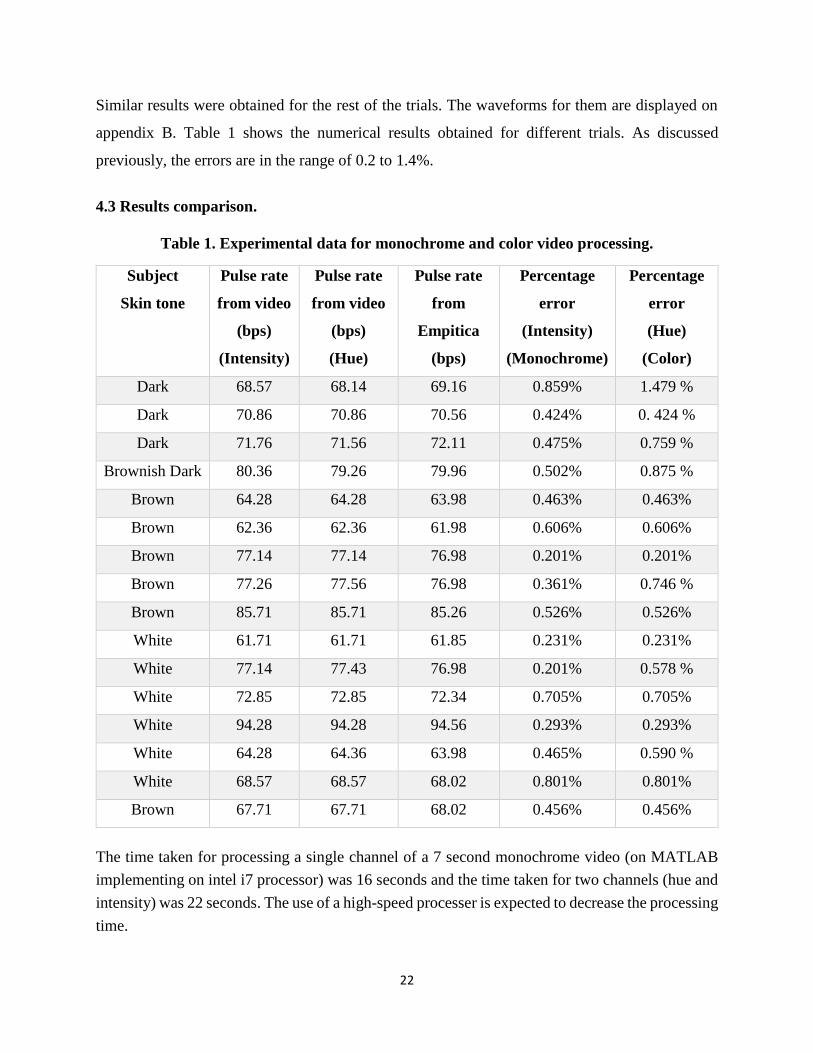
Similar results were obtained for the rest of the trials. The waveforms for them are displayed on

appendix B. Table 1 shows the numerical results obtained for different trials. As discussed

previously, the errors are in the range of 0.2 to 1.4%.

4.3 Results comparison.

Table 1. Experimental data for monochrome and color video processing.

Subject

Skin tone

Pulse rate

from video

(bps)

(Intensity)

Pulse rate

from video

(bps)

(Hue)

Pulse rate

from

Empitica

(bps)

Percentage

error

(Intensity)

(Monochrome)

Percentage

error

(Hue)

(Color)

Dark 68.57 68.14 69.16 0.859% 1.479 %

Dark 70.86 70.86 70.56 0.424% 0. 424 %

Dark 71.76 71.56 72.11 0.475% 0.759 %

Brownish Dark 80.36 79.26 79.96 0.502% 0.875 %

Brown 64.28 64.28 63.98 0.463% 0.463%

Brown 62.36 62.36 61.98 0.606% 0.606%

Brown 77.14 77.14 76.98 0.201% 0.201%

Brown 77.26 77.56 76.98 0.361% 0.746 %

Brown 85.71 85.71 85.26 0.526% 0.526%

White 61.71 61.71 61.85 0.231% 0.231%

White 77.14 77.43 76.98 0.201% 0.578 %

White 72.85 72.85 72.34 0.705% 0.705%

White 94.28 94.28 94.56 0.293% 0.293%

White 64.28 64.36 63.98 0.465% 0.590 %

White 68.57 68.57 68.02 0.801% 0.801%

Brown 67.71 67.71 68.02 0.456% 0.456%

The time taken for processing a single channel of a 7 second monochrome video (on MATLAB

implementing on intel i7 processor) was 16 seconds and the time taken for two channels (hue and

intensity) was 22 seconds. The use of a high-speed processer is expected to decrease the processing

time.

23

Chapter 5

Discussion and Conclusions

From the experiments it can be inferred that, with proper design of video processing algorithm, it

is possible to extract heart rate from a video of a subject. The stepwise process of extracting frames,

removing noises from them, recording changes in intensity values in all of them produced a

waveform resembling the pulse waveform. This was validated from the data obtained from a PPG

device. It was possible to extract pulse waveform from a monochrome video or a color video with

a high degree of accuracy. The percentage error ranged to a highest of 1.4% which makes this

algorithm a promising replacement of conventional invasive vital statistics measuring devices.

From Table 1 it becomes clear that the use of either grey level values from a monochrome video

or Hue as well as Intensity values of a color video can be used for this analysis.

This algorithm was primarily designed to propose a real-time non-invasive vital statistic measuring

procedure to be implemented at an NICU to continuously monitor infants for life threatening

conditions. During development of the algorithm, many other applications of it were visualized.

Development of mobile application to record the vital statistics of user can be one of the

applications. The development of cellular phones hardware, especially the inbuilt cameras and

their portability make them one of the best devices to make use of the algorithm designed. Users

can take out their personal phone device, open an application and record the video of their face

and in turn be informed about their vital statistics in no time.

Another similar example is to use this algorithm to track the vital statistics of commercial drivers.

The detection of the health condition of commercial drivers including checks for drowsiness and

fatigue is extremely important and mandated by law in some countries. However, the use of

conventional sensors attached to bands or hats might irk the drivers. A non-contact option

developed in this research can be used to have a continuous monitoring of drivers in commercial

transport industries which will certainly reduce a lot of accidents due to drowsiness of the drivers.

24

References

[1] National Center for Health Statistics Publications, National Vital Statistics Reports, Volume

65, Number 4, 2014

[2] B. Lohani, P. Indic and M. Shirvaikar, "Extraction of vital signs using real time video

analysis for neonatal monitoring," Proc. SPIE 10670, Real-Time Image and Video

Processing 2018, 1067005 (14 May 2018)

[3] "Laboratory 10: Circulatory Physiology," Electronic Portfolio Biology, Google Sites,

https://sites.google.com/site/portafolioelectronicobiologia/laboratorio-5/laboratorio-10.

[4] S. Kwon, H. Kim and K. S. Park, "Validation of heart rate extraction using video imaging on

a built-in camera system of a smartphone," 2012 Annual International Conference of the

IEEE Engineering in Medicine and Biology Society, San Diego, CA, 2012, pp. 2174-2177.

[5] D. Cho and B. Lee, "Non-contact robust heart rate estimation using HSV color model and

matrix-based IIR filter in the face video imaging," 2016 38th Annual International

Conference of the IEEE Engineering in Medicine and Biology Society (EMBC), Orlando, FL,

2016, pp. 3847-3850.

[6] L. Cattani, D. Alinovi, G. Ferrari, R. Raheli, E. Pavalidis, C. Spagnoli and F. Pisani,

"Monitoring infants by automatic video processing: A unified approach to motion analysis,"

Computers in biology and Medicine 80 (2017) pp. 158-165.

[7] S. Sharma, S. Bhattacharyya, J. Mukherjee, P. K. Purkait, A. Biswas and A. K. Deb,

"Automated detection of newborn sleep apnea using video monitoring system," 2015 Eighth

International Conference on Advances in Pattern Recognition (ICAPR), Kolkata, 2015, pp.

1-6.

[8] X. He, R. A. Goubran and X. P. Liu, "Wrist pulse measurement and analysis using Eulerian

video magnification," 2016 IEEE-EMBS International Conference on Biomedical and

Health Informatics (BHI), Las Vegas, NV, 2016, pp. 41-44.

[9] G. Balakrishnan, F. Durand and J. Guttag, "Detecting Pulse from Head Motions in

Video," 2013 IEEE Conference on Computer Vision and Pattern Recognition, Portland, OR,

2013, pp. 3430-3437.

25

[10] F. Mohammad-Zadeh, F. Taghibakhsh and B. Kaminska, "Contactless Heart Monitoring

(CHM)," 2007 Canadian Conference on Electrical and Computer Engineering, Vancouver,

BC, 2007, pp. 583-585.

[11] M. Garbey, N. Sun, A. Merla and I. Pavlidis, "Contact-Free Measurement of Cardiac Pulse

Based on the Analysis of Thermal Imagery," in IEEE Transactions on Biomedical

Engineering, vol. 54, no. 8, pp. 1418-1426, Aug. 2007.

[12] C. Yang, G. Cheung and V. Stankovic, "Estimating Heart Rate and Rhythm via 3D Motion

Tracking in Depth Video," 2017 IEEE Transactions on Multimedia, vol. 19, pp. 1625-

1636.

[13] G. M. K. Ntonfo, G. Ferrari, R. Raheli and F. Pisani, "Low-Complexity Image Processing

for Real-Time Detection of Neonatal Clonic Seizures, " 2012 IEEE Transactions on

Information Technology in Biomedicine, vol. 16, pp. 375-382.

[14] R. C. Gonzalez and R. E. Woods, "Digital Image Processing, " 3rd ed. Upper Saddle River,

New Jersey: Pearson Education, Inc. 2008.

[15] Chang Chiann and Pedro A. Moretin, "A Wavelet Analysis for Time Series, Nonparametric

Statistics," 10 (1998), 1-46.

[16] Abdoullah Ahmed Dghais, Amel & Ismail and Mohd Tahir. (2013). "A Comparative Study

between Discrete Wavelet Transform and Maximal Overlap Discrete Wavelet Transform for

Testing Stationarity," International Journal of Mathematical Science and Engineering. 7.

471-475.

[17] Zhang, Zitong et al.,"Choosing Wavelet Methods, Filters, and Lengths for Functional Brain

Network Construction," Ed. Satoru Hayasaka. PLoS ONE 11.6 (2016): e0157243. PMC.

Web. 7 Mar. 2018.

[18] J. Hart, "Normal Resting Pulse Rate," 2015 Journal of Nursing Education and Practice,

Spartanburg, 2014, vol. 5, no. 8.

[19] Donoho, D.L. (1993), "Progress in wavelet analysis and WVD: a ten minute tour,"

in Progress in wavelet analysis and applications, Y. Meyer, S. Roques, pp. 109–128.

Frontières Ed.

[20] I. Zuzarte, C. Temple, P. Indic and D. Paydarfar, "Transforming artifact to signal: A wavelet-

based algorithm for quantifying neonatal movement," 2014 36th Annual International

http://ieeexplore.ieee.org.ezproxy.uttyler.edu:2048/search/searchresult.jsp?searchWithin=%22Authors%22:.QT.Cheng%20Yang.QT.&newsearch=true

http://ieeexplore.ieee.org.ezproxy.uttyler.edu:2048/search/searchresult.jsp?searchWithin=%22Authors%22:.QT.Gene%20Cheung.QT.&newsearch=true

http://ieeexplore.ieee.org.ezproxy.uttyler.edu:2048/search/searchresult.jsp?searchWithin=%22Authors%22:.QT.Vladimir%20Stankovic.QT.&newsearch=true

26

Conference of the IEEE Engineering in Medicine and Biology Society, Chicago, IL, 2014,

pp. 5466-5469.

[21] A. Sikdar, S. K. Behera, D. P. Dogra and H. Bhaskar, "Contactless vision-based pulse rate

detection of Infants Under Neurological Examinations," 2015 37th Annual International

Conference of the IEEE Engineering in Medicine and Biology Society (EMBC), Milan, 2015,

pp. 650-653.

[22] M. Villarroel, A. Guazzi, J. Jorge, S. Davis, P. Watkinson, G. Green, A. Shenvi, K.

McCormick and L. Tarassenko. "Continuous non-contact vital sign monitoring in neonatal

intensive care unit," in Healthcare Technology Letters, vol. 1, no. 3, pp. 87-91, 09 2014.

[23] A. Alzahrani and A. Whitehead, "Preprocessing Realistic Video for Contactless Heart Rate

Monitoring Using Video Magnification," 2015 12th Conference on Computer and Robot

Vision, Halifax, NS, 2015, pp. 261-268.

[24] B. Mandal, L. Li, G. S. Wang and J. Lin, "Towards Detection of Bus Driver Fatigue Based

on Robust Visual Analysis of Eye State," in IEEE Transactions on Intelligent Transportation

Systems, vol. 18, no3, pp.545-557, March2017. doi: 10.1109/TITS.2016.2582900

[25] S. Jung, H. Shin and W. Chung, "Driver fatigue and drowsiness monitoring system with

embedded electrocardiogram sensor on steering wheel," in IET Intelligent Transport

Systems, vol. 8, no. 1, pp. 43-50, Feb.2014. doi: 10.1049/iet-its.2012.0032

27

Appendix

Appendix A: MATLAB code

The following MATLAB codes were implemented to design the algorithm.

Main code

%Starting the program

vidfile=VideoReader('trial1a.MOV');%Reading video file

Array1=csvread('C:\Users\BhuZane\Desktop\Results\trial3\c\BVP.cs

v'); % Reading Empatica data

fsampl=Array1(2); % Sampling frequency of Empatica data

Array=Array1(3:end);

Num_of_points=length(Array);

t_data=(1:Num_of_points)/fsampl;%Using sampling frequency from

data

D = vidfile.Duration;%Duration of the video

fr=vidfile.FrameRate;

fs=fr;

Ts=1/fs;

N=vidfile.NumberofFrames;

t=(0:N-1)*Ts;

[Imean,Hmean,Smean,gauss_image]=extract_frames(vidfile);

% Calling frame extracting function

Mean_Value=mean(Imean);

Mean_Value_H=mean(Hmean);

Mean_Value_S=mean(Smean);

Imean=(Imean-mean(Imean));

Hmean=(Hmean-mean(Hmean));

Smean=(Hmean-mean(Smean));

28

Appendix A (continued)

Gmean2=Imean;

Hmean2=Hmean;

fprintf('Extracting Graylevels\n');

noisy_Gmean=Imean;

noisy_Hmean=Hmean;

Gmean=denoising_filter(noisy_Gmean); %Calling denoising filter

Hmean=denoising_filter(noisy_Hmean);

Gmean3=Gmean;

Hmean3=Hmean;

fprintf('Time taken to extract signal from the video frames=\n')

fprintf('Denoising');

out_I=bandpass_filter(Imean); % Calling bandpass filter

out_H=bandpass_filter(Hmean);

out_S=bandpass_filter(Smean);

fprintf('Filtering\n');

fprintf('Time taken for filering=\n')

out=denoising_filter(out);

out_H=denoising_filter(out_H);

fprintf('Time taken for denoising=\n')

fprintf('Rendering Output\n');

[h,w]=pwelch(out); % PSD approximation

[h_H,w_H]=pwelch(out_H);

figure

29


plot(w/pi,10*log10(h),'b');

figure

plot(w_H/pi,10*log10(h_H),'b');

xlabel('Normalized frequency\rightarrow');

ylabel('Magnitude\rightarrow');

title('PSD using Welch Approximation of Pulse signal')

Pulse_rate=measurement(h,w,fs); % Calling pulse rate measuring

function

Pulse_rate_H=measurement(h_H,w_H,fs);

fprintf('Time taken to render output=\n')

%To print all the results together

t_video=(1:N)/fr; %Using frame rate for video

plot(t_video,out_I,'g')

xlabel('Time(sec)\rightarrow');

ylabel('Gray-level/Amplitude\rightarrow');

title('Pulse signal extracted from video as gray level signal')

hold on;

plot(t_video,out_S,'r')

plot(t_video,out_H,'c');

plot(t_data,Array)

hold off;

legend('Hue','Saturation','Intensity','Ground truth');

Frame extracting function

function [Gmean,Hmean,Smean,gauss_image]=extract_frames(vidfile)

Gmean=[]; % Empty cell for gray-level storage

Hmean=[];

30


Smean=[];

firstFrame = read(vidfile,1); %Deducing mask from the first

frame

mask=ROIfinal(firstFrame); % Calling ROI function

fprintf('Masking');

for img=1:vidfile.NumberofFrames

frameext=read(vidfile,img);

frameext=rgb2hsv(frameext);

frameext_H=frameext(:,:,1);

frameext_V=frameext(:,:,3);

frameext_S=frameext(:,:,2);

frame_masked=bsxfun(@times, frameext,

cast(mask,class(frameext)));%masked image

frame_masked_H=bsxfun(@times, frameext_H,

cast(mask,class(frameext_H)));%masked image

frame_masked_V=bsxfun(@times, frameext_V,

cast(mask,class(frameext_V)));%masked image

frame_masked_S=bsxfun(@times, frameext_S,

cast(mask,class(frameext_S)));

frame_new=0.299*frame_masked(:,:,1)+0.587*frame_masked(:,:,2)+0.

114*frame_masked(:,:,3);

frame_new_H = imgaussfilt(frame_masked_H, 4); % Gaussian

Smoothing

frame_new_V = imgaussfilt(frame_masked_V, 4);

frame_new_S=imgaussfilt(frame_masked_S, 4);

gauss_image=frame_new_H;

31


% gauss_image=double(gauss_image);

frame_new_H( ~any(frame_new_H,2), : ) = []; %rows

frame_new_H( :, ~any(frame_new_H,1) ) = []; %columns

frame_new_V( ~any(frame_new_V,2), : ) = []; %rows

frame_new_V( :, ~any(frame_new_V,1) ) = []; %columns

frame_new_S( ~any(frame_new_S,2), : ) = []; %rows

frame_new_S( :, ~any(frame_new_S,1) ) = [];

Hmean=[Hmean,mean2(frame_new_H(:))];

Gmean=[Gmean,mean2(frame_new_V(:))];

Smean=[Smean,mean2(frame_new_S(:))];

end

end

ROI function

function mask_final=ROIfinal(inpimage)

gray_image=0.299*inpimage(:,:,1)+0.587*inpimage(:,:,2)+0.114*inp

image(:,:,3);

T=rand;

global_threshold=0;

f=double(gray_image);

[h,w]=size(f);

while (global_threshold~=T)

m1=0;

m2=0;

global_threshold=T;

32


for i=1:h

for j=1:w

if(f(i,j)>=global_threshold)

m1=m1+f(i,j); % Finding first mean

else

m2=m2+f(i,j); % Finding second mean

end

end

end

[a,b]=size(find(f>=global_threshold));

m1_len=a;

[a1,b1]=size(find(f<global_threshold));

m2_len=b1;

T=(m1+m2)/(2*h*w); % average

end

g=f>T; %Thresholded image

mask_final=g;

end

Filters

Denoising filter

function out1=denoising_filter(out)

%Denoising using wavelets

out1 = wden(out,'modwtsqtwolog','s','mln',3,'sym4');

end

33


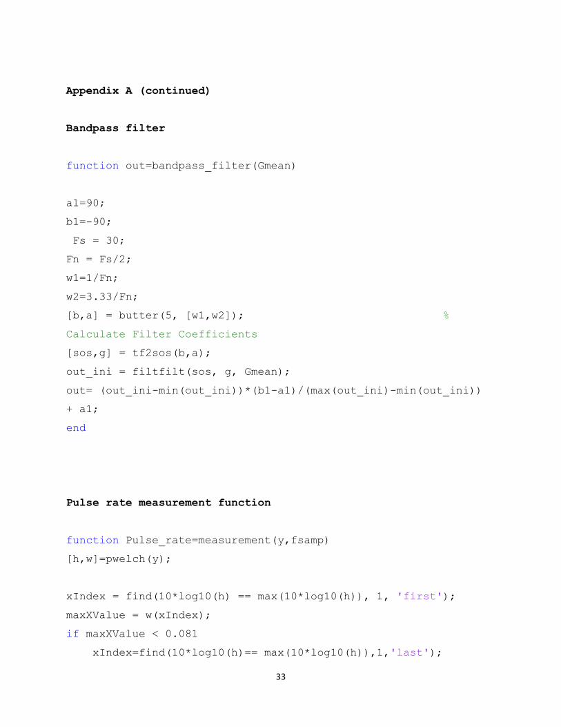
Bandpass filter

function out=bandpass_filter(Gmean)

a1=90;

b1=-90;

Fs = 30;

Fn = Fs/2;

w1=1/Fn;

w2=3.33/Fn;

[b,a] = butter(5, [w1,w2]); %

Calculate Filter Coefficients

[sos,g] = tf2sos(b,a);

out_ini = filtfilt(sos, g, Gmean);

out= (out_ini-min(out_ini))*(b1-a1)/(max(out_ini)-min(out_ini))

+ a1;

end

Pulse rate measurement function

function Pulse_rate=measurement(y,fsamp)

[h,w]=pwelch(y);

xIndex = find(10*log10(h) == max(10*log10(h)), 1, 'first');

maxXValue = w(xIndex);

if maxXValue < 0.081

xIndex=find(10*log10(h)== max(10*log10(h)),1,'last');

34


end

maxXValue = h(xIndex);

x_normalized=maxXValue /pi;

Pulse_rate=60*x_normalized*fsamp/2;

end

35

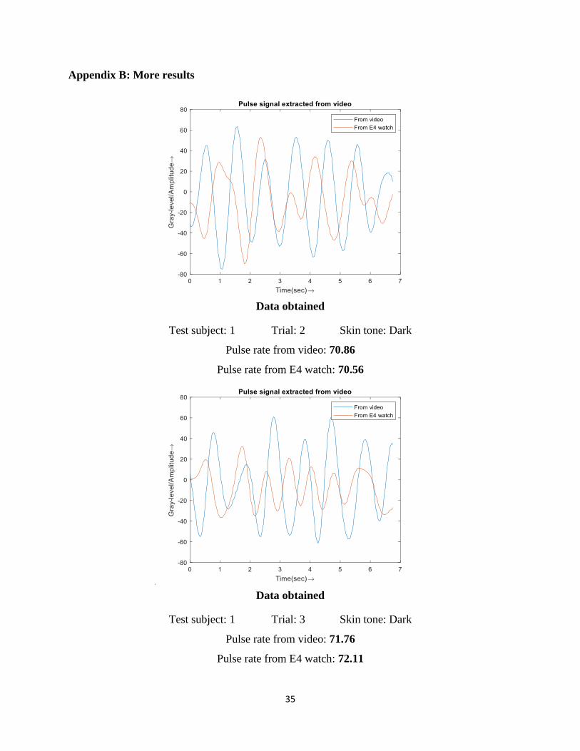
Appendix B: More results

Data obtained




Data obtained




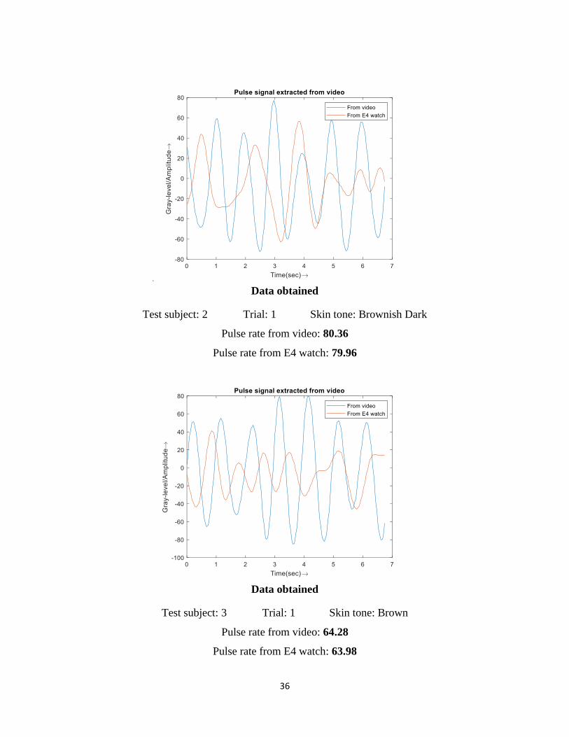
36

Data obtained

Test subject: 2 Trial: 1 Skin tone: Brownish Dark



Data obtained

Test subject: 3 Trial: 1 Skin tone: Brown



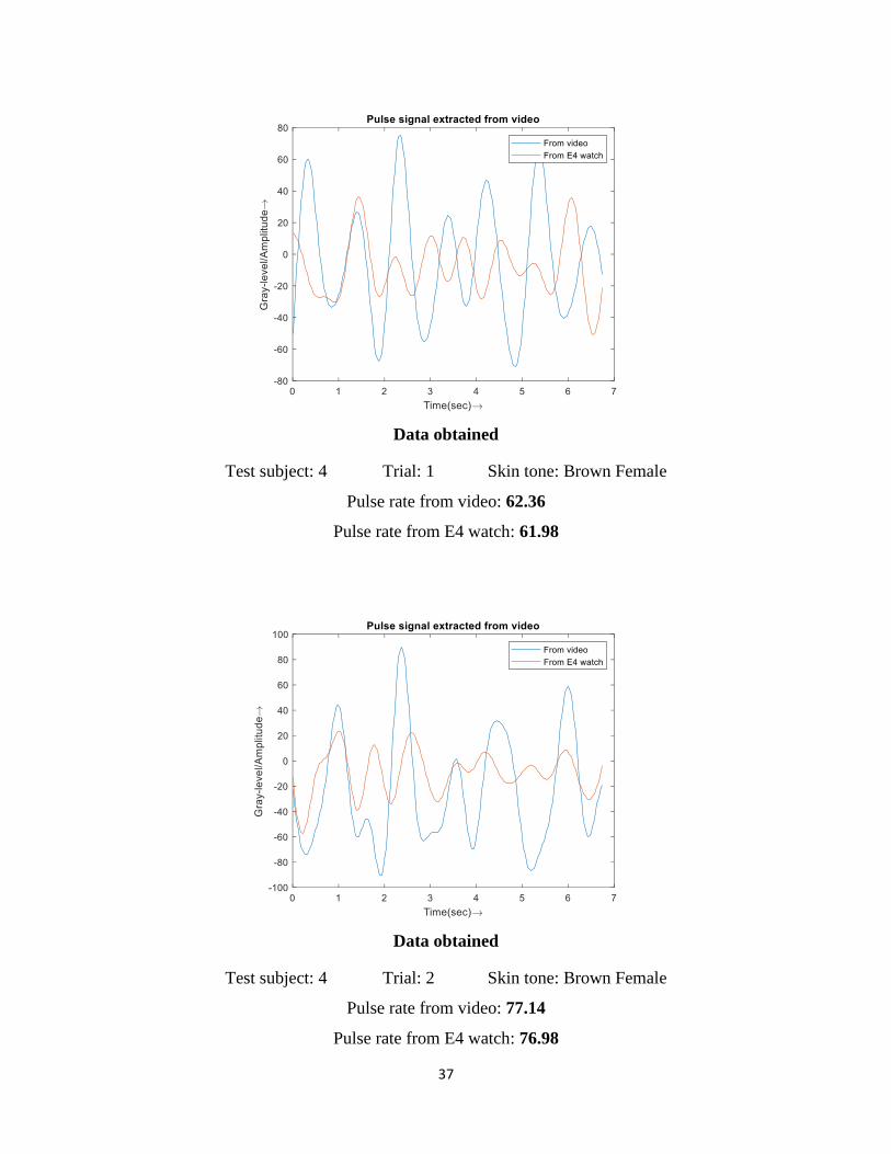
37

Data obtained

Test subject: 4 Trial: 1 Skin tone: Brown Female



Data obtained




38

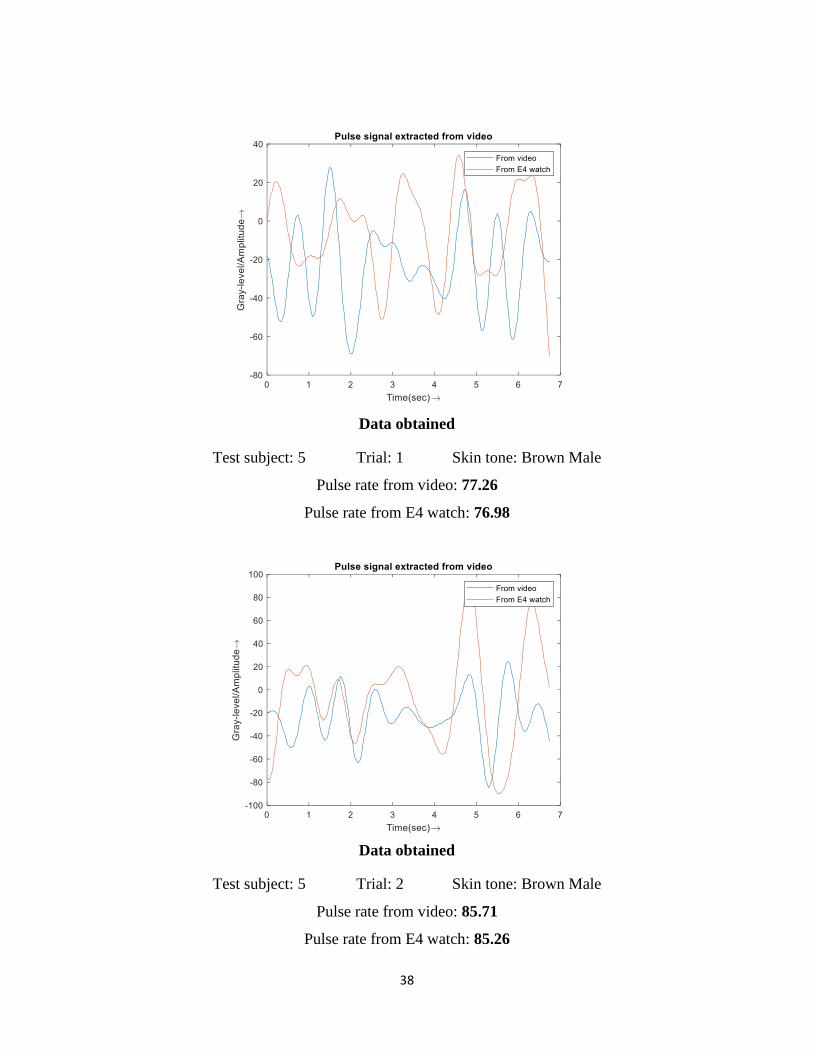
Data obtained

Test subject: 5 Trial: 1 Skin tone: Brown Male



Data obtained




39

Data obtained

Test subject: 6 Trial: 1 Skin tone: White Female



Data obtained




40

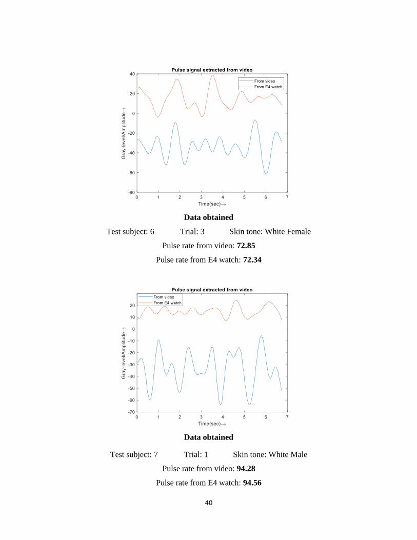
Data obtained




Data obtained

Test subject: 7 Trial: 1 Skin tone: White Male



41

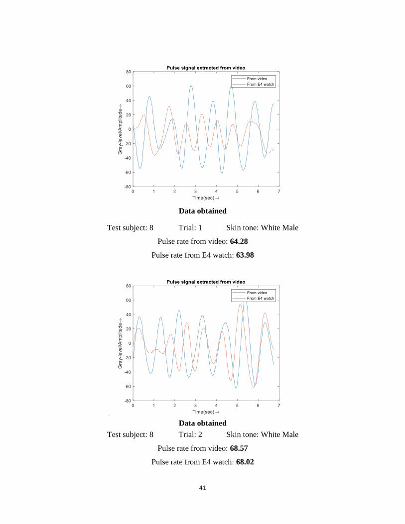
Data obtained




Data obtained




42

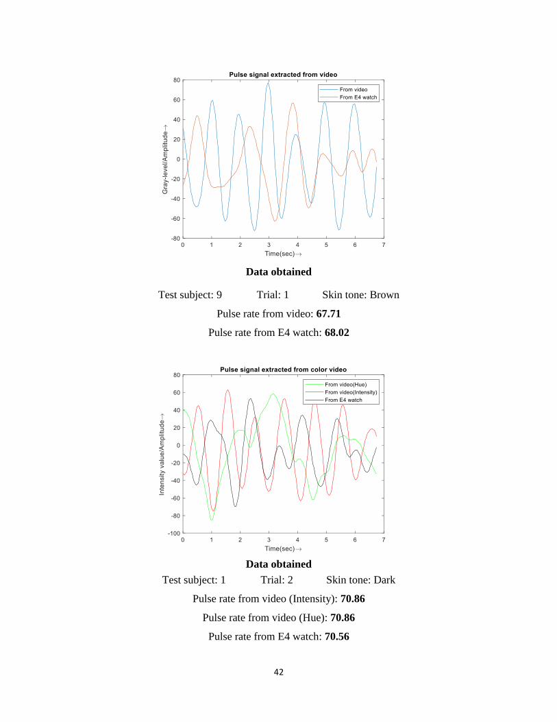
Data obtained




Data obtained


Pulse rate from video (Intensity): 70.86



43

Data obtained





Data obtained

Test subject: 2 Trial: 1 Skin tone: Brownish Dark




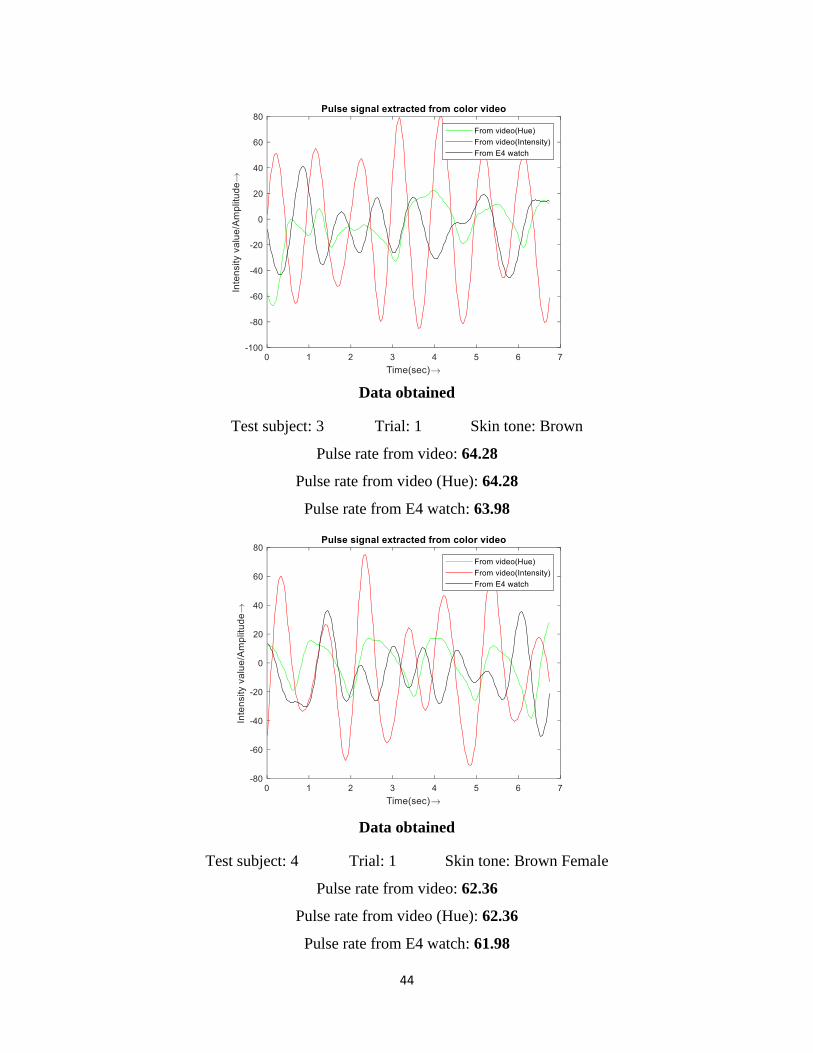
44

Data obtained





Data obtained





45

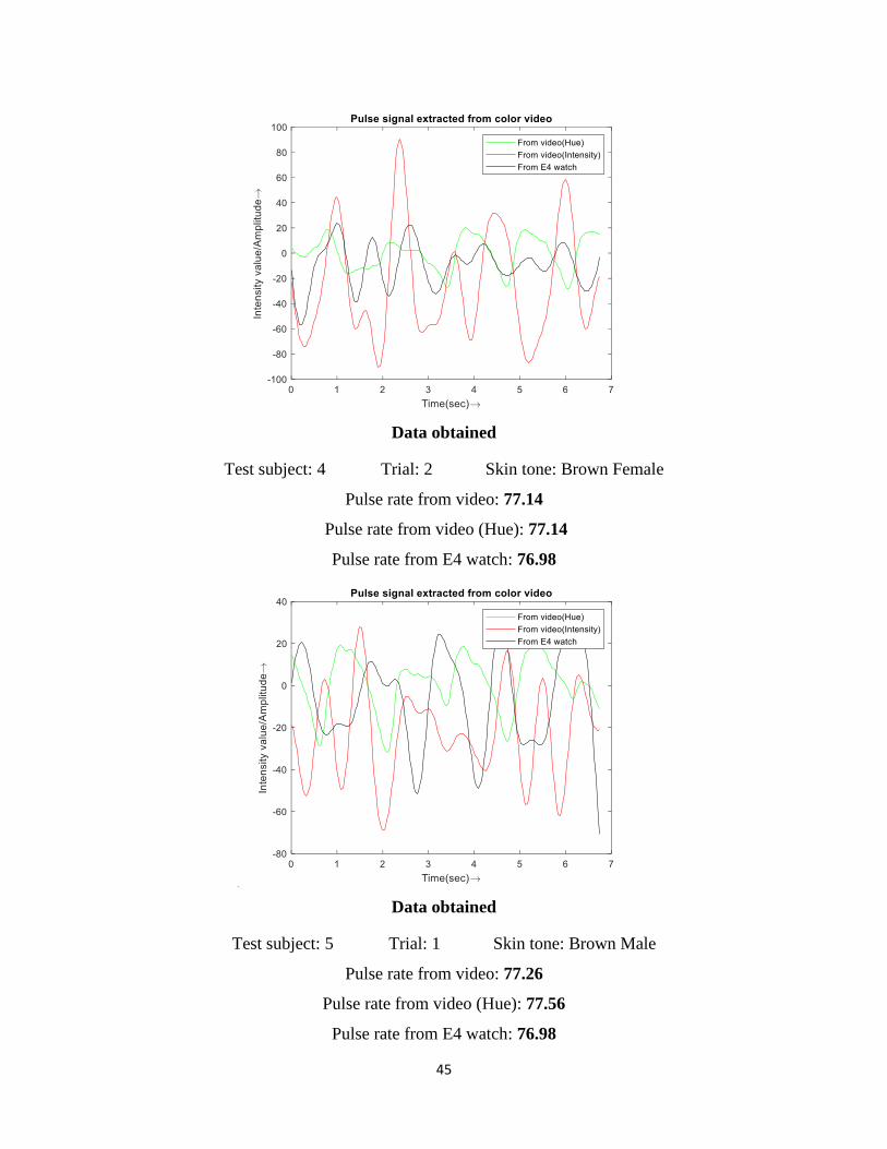
Data obtained





Data obtained





46

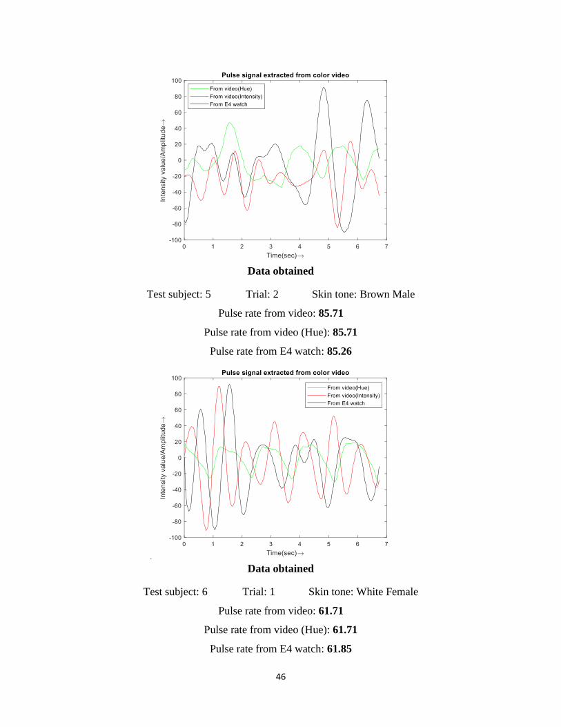
Data obtained





Data obtained





47

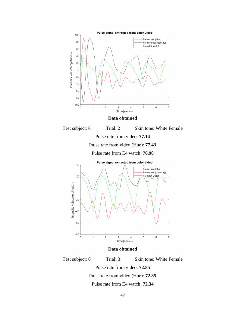
Data obtained





Data obtained





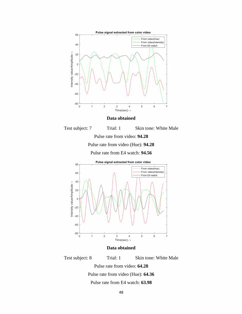
48

Data obtained





Data obtained





49

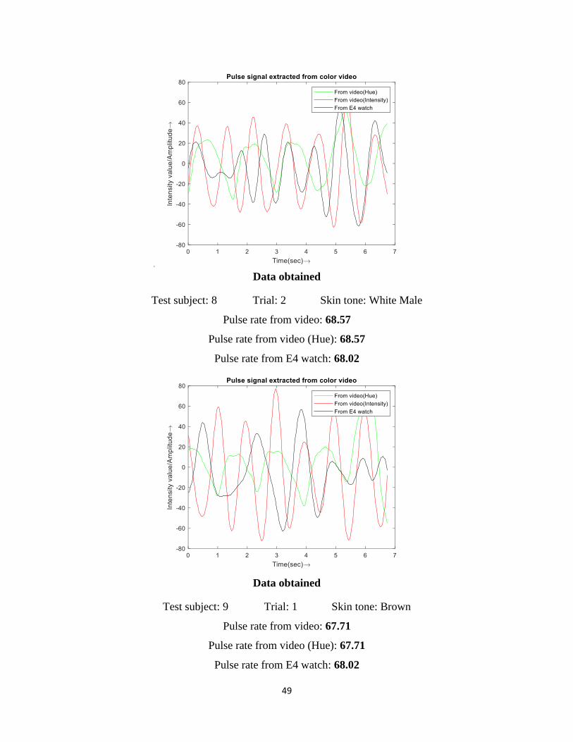
Data obtained





Data obtained





Documents

EXTRACTION OF VITAL SIGNS USING REAL TIME VIDEO