Exact, Heuristic and Metaheuristic Methods for Confidentiality Protection by Controlled Tabular Adjustment

International Journal of Operations Research Vol. 5, No. 2, 117−128 (2008)

Exact, Heuristic and Metaheuristic Methods for Confidentiality Protection by Controlled Tabular Adjustment

Fred Glover1, ∗, Lawrence H. Cox2, James P. Kelly3, and Rahul Patil1

1Leeds School of Business, University of Colorado, Campus Box 419, Boulder, CO 80309

2National Center for Health Statistics, Centers for Disease Control and Prevention, 3311 Toledo Road, Room 3211, Hyattsville, MD 20782

3OptTek Systems, Inc., 1919 7th St., Boulder, CO 80302

Received September 2005; Revised August 2007; Accepted November 2007

AbstractGovernment agencies and commercial organizations that report data face the task of representing the data meaningfully while simultaneously protecting the confidentiality of critical data components. The challenge is to organize and disseminate data in a form that prevents these components from being unmasked by corporate espionage, or falling prey to efforts to penetrate the security of the information underlying the data. Unscrupulous data investigators could use unprotected data sources to infer sensitive, personal data about individuals. Besides harming individuals, these types of disclosures can drastically affect the willingness of future respondents to provide valuable data. Controlled tabular adjustment is a recently developed approach for protecting sensitive information by imposing a special form of statistical disclosure limitation on tabular data. The underlying model gives rise to a mixed integer linear programming problem involving both continuous and discrete (zero-one) variables. In this paper we develop new hybrid heuristics and a new meta-heuristic learning approach for solving this model, and compare their performance to previous heuristics and to an exact algorithm in the ILOG-CPLEX software. Our new approaches are based on partitioning the problem into its discrete and continuous components, and first creating a hybrid that reduces the number of binary variables through a grouping procedure that combines an exact mathematical programming model with constructive heuristics. Finally, we introduce a new metaheuristic learning method that significantly improves the quality of solutions obtained. KeywordsConfidentiality, Mixed integer, Optimization, Metaheuristics, Adaptive learning, Mathematical programming, Evolutionary computation

∗ Corresponding author’s email: [email protected]

1. INTRODUCTION

Data confidentiality is an essential component of statistical surveys, for three reasons. The first reason applies primarily to surveys conducted by government and can be described as regulatory. In particular, laws and government regulations pertaining to a particular survey or to the agency collecting the data require that responses provided to the survey be held confidential by the agency.

The second reason is that confidentiality protection is regarded as ethical statistical practice and appears specifically in the Codes of Ethical Conduct of the International Statistical Institute, the American Statistical Association, and other statistical organizations.

The third reason is practical. Respondents would not respond, or at least not as completely and truthfully as they might otherwise, if they did not have faith in the intent and ability of the data collector to preserve confidentiality.

The need to safeguard the confidentiality of statistical data presents a monumental task, and government agencies such as the U.S. Bureau of the Census and the U.S.

National Center for Health Statistics that regularly report data must wrestle with this problem on a continuing basis. Inadvertent disclosure of sensitive corporate information could cost a large commercial enterprise financially and in other ways. At the same time government reporting agencies are duty-bound to provide figures that convey meaningful, accurate information about the state of our national economy and its component industries and sectors. Consequently, the confidentiality problem looms as a major challenge with far-reaching consequences.

The purpose of this paper is to propose a new method for solving controlled tabular adjustment problems computationally. To understand the nature and impact of our contribution, some background terminology is necessary. In tabular data, a cell is considered sensitive if the publication of the true cell value is likely to disclose a contributor’s data to the public or a competitor. For example, in an economic survey, if a cell contains data from one respondent, then publication of the cell value would disclose confidential data pertaining to a single respondent. As identities of companies in individual cells

International Journal of Operations Research

1813-713X Copyright © 2008 ORSTW

Glover, Cox, Kelly, and Patil: Exact, Heuristic and Metaheuristic Methods for Confidentiality Protection by Controlled Tabular Adjustment IJOR Vol. 5, No. 2, 117−128 (2008)

118

are publicly available, this would breach the pledge of confidentiality made to the company by the statistical office collecting the data. Similarly, if the cell contains data from two respondents, or if the cell total is dominated by the contributions of two respondents, then either respondent could subtract its own contribution from the cell value to obtain a narrow estimate of the other’s contribution.

Confidentiality protection for tabular data is based on assuring that all released tabular cells satisfy an appropriate disclosure rule (see JSPI (1981), Doyle et al. (2001), Willenborg and de Waal (1996), Willenborg and de Waal (2001)). Cells failing to satisfy the rule (sensitive cells) are assigned protection ranges defined by lower and upper bounds on the true cell value computed from the disclosure rule. Published or derived estimates of the original values of sensitive cells that lie within the protection range are considered unacceptable.

Different procedures have been used by statistical offices to protect confidentiality of sensitive cells in tabular data. The most often used method is complementary cell suppression (see Cox (1980), Kelly et al. (1992), Fischetti and Salazar (1999), Fischetti and Salazar, (2000)). The complementary cell suppression method suppresses both primary (sensitive) and secondary (nonsensitive) cells to protect the confidentiality of the sensitive cells. Although suppression is widely used, it has serious limitations. Complementary cell suppression is an NP hard problem (Kelly et al., 1992), typically involving extremely large numbers of binary variables. An even more significant limitation of this commonly used approach is that it produces tables that are generally difficult to analyze by standard methods and even, in some cases, by advanced methods.

To overcome the limitations of complementary cell suppression we propose new methods that are designed to exploit the model called Controlled Tabular Adjustment (CTA) which affords an opportunity to overcome many of the problems associated with traditional cell suppression and perturbation methods. CTA introduces controlled perturbations (adjustments) into tabular data that satisfy the protection ranges and tabular constraints (additivity) while minimizing data loss as measured by one of several linear measures of overall data distortion, such as the sum of the absolute values of the individual cell value adjustments. CTA replaces each sensitive cell by either of the two endpoints of its protection range. These values are the minimally safe values. Selected nonsensitive cell values are then adjusted from their true values by small amounts to restore additivity. Additionally, nonsensitive cell perturbations are constrained to be small or insignificant, such as limiting them to be within sampling variability, and cell values for which adjustment is deemed undesirable can be held fixed. Cox (ASA, 2000) provides a mixed integer programming formulation for CTA; Danderkar and Cox (2002) consider elementary heuristics.

The empirical evaluations of methods for CTA conducted in this paper begin by comparing heuristic procedures proposed by Danderkar and Cox (2002) to the

commercial CPLEX solver. These analyses disclose both useful features and significant limitations of these approaches (including severe limitations to CPLEX as problem size increases to dimensions often encountered in practice). This leads to our development and analysis of two new alternative methods embodying strategies of grouping and evolutionary scatter search, which prove more powerful than the previous heuristic approaches. Scatter search offers particular advantages by running far more efficiently than CPLEX, and significantly extending the size of problems that can be addressed, yet still encounters limitations shared with its predecessors in generating solutions of high quality. Finally, we develop a new metaheuristic learning method that performs far more effectively than all of the other methods and provides a reliable and efficient approach for producing high quality solutions for problems of practical size.

Our development is organized as follows. Section 2 presents the mixed integer/continuous optimization model for CTA. Section 3 describes numerical tests using the heuristic approaches suggested by Danderkar and Cox (2002), including an examination of multiple objective functions and an evaluation of their impact on the CTA process. Section 4 describes a new hybrid heuristic, based on reducing the number of binary variables through grouping and combining the exact CPLEX solution approach with principles embodied in the heuristics.

Section 5 introduces the metaheuristic learning algorithm that produces additional improvement by dramatically enhancing the quality of solutions obtained. Section 6 summarizes our findings. 2. MATHEMATICAL FORMULATION FOR

OPTIMAL CONTROLLED TABULAR ADJUSTMENT

The objective of synthetic tabular data is to closely mimic the original data, subject to obscuring sensitive cell values to a sufficient extent. By setting sensitive values to minimally safe values and constraining adjustments both locally (individual cells) and globally (overall measure of distortion), controlled tabular adjustment is aimed at replacing original data by data that are comparable from a data analysis perspective. Cox and Danderkar (2004) provide approaches for preserving data accuracy and ease of use. Extensions that address statistical data analytic issues directly are presented in Cox and Kelly (2004) and Cox et al. (2004).

The underlying concept of CTA is simple: The value of each sensitive cell is replaced by an adjusted value selected to be at a safe distance from the original value. Danderkar and Cox (2002) suggest minimal adjustment, viz., to either the sensitive cell’s lower or upper protection limit. Some or all nonsensitive cell values are then adjusted from their true values by small amounts to restore additivity to totals within the tabular system.

Within this framework, adjustments to nonsensitive cell values can be controlled in various ways. Selected nonsensitive cells, e.g., certain zero cells or totals, can be


119

exempt from change through imposition of capacity constraints. Capacities are also used to confine nonsensitive adjustments to within meaningful limits such as sampling variability or total measurement error. One of several linear objective functions can be used to measure and assure minimum deviation. Some approaches, not discussed here, do not strictly adhere to the use of minimally safe values, replacing sensitive values by “safer” values (Cox and Kelly (2004)) or by “less safe” values based on enhanced protective capabilities of CTA (Cox and Danderkar (2004)).

Tabular data systems can be represented by their system of linear equations in matrix form: Ax = 0. Column vector x represents the tabulation cells of the system; x* represents the original data. Matrix A is the aggregation matrix representing the tabular structure among the cells. The entries of A are −1, 0 or +1; each row of A corresponds to one aggregation (tabular equation) in which “+1” denotes a contributing internal cell and “−1” a total (marginal) cell. Hence, there is precisely one “−1” per row. The mathematical structure of optimal synthetic tabular data is specified below by a mixed integer linear programming (MILP) formulation, containing binary and continuous variables, analogous to that introduced in ASA (2000).

Notation: i = 1, ..., p: denotes the p sensitive cells; i = p + 1, ..., n: denotes the n−p nonsensitive cells; bi = a binary (zero/one) variable denoting selection of the lower/upper limit for sensitive cell i = 1, ..., p; li = lower deviation required to protect sensitive cell i = 1, ..., p; ui = upper deviation required to protect sensitive cell i = 1, ..., p; +

iy = a nonnegative continuous variable identifying a “positive adjustment” for the gap to cell value i; −

iy = a nonnegative continuous variable identifying a “negative adjustment” for the gap to cell value i; UBi, LBi = upper/lower cell bounds on change to cell i; ci = cost per unit change in cell i.

MILP for Optimal Controlled Tabular Adjustment

1

( )n

i i ii

Min c y y+ −

=

+∑ (1)

Subject to: For i = 1, ..., n:

( ) 0A y y+ −− = (2) 0 i iy UB+≤ ≤ (3) 0 i iy LB−≤ ≤ (4) For i = 1, ..., p:

i i iy u b+ = (5) (1 )i i iy l b− = − (6)

After solving the MILP, the synthetic tabular data t = (ti)

is: ∗ + −= + − .i i i it x y y Eq. (1) is the objective function, which minimizes the cost due to cell deviations. Two linear cost functions are commonly used, usually defined over deviation variables + −+ .i iy y The first involves coefficients

ci = 1 corresponding to minimizing the distortion measure “total absolute adjustment,” and the other ∗= 1/ ,i ic x corresponding to minimizing total percent absolute adjustment. CTA perturbs the sensitive cells until they are safe, i.e. sensitive cell values are sufficiently far from their original values. This creates inconsistency in the tabular system, as sums are no longer maintained. Eq. (2) maintains tabular consistency. Eqs. (3) and (4) are used to constrain the non-sensitive cell deviations. Usually, the upper bounds are computed using the estimated measurement errors for non-sensitive cells. Eqs. (5) and (6) ensure that the sensitive cells are set at their safe values. This is achieved by setting these cells at either their lower or upper protection limits. The protection limits for the cell include the minimum amount, which must be added or subtracted from the true value to make the sensitive cells “safe”. Cox (1980) (and in Doyle et al. (2001)) discusses protection limits theory in detail. It can be noted that CTA offers increased protection from disclosure attack because in CTA the sensitive cells are not highlighted and are replaced with a value. More importantly, sensitive cells are set at either their lower or upper limits. The intruder has no idea about the direction of perturbation.

It is possible that the CTA gives rise to an infeasible problem if the number of sensitive cells in a particular row or column is large. The sensitive cell constraints in the model can be relaxed in the following manner to virtually eliminate these types of problems.

i i iy u b+ ≥ (7) _ (1 )i i iy l b≥ − (8)

Consider the following example, which illustrates how

the mathematical programming formulation can be used to protect the sensitive cells in a 2-dimensional table as shown in Table 1. Cells (3, 1), (1, 2), and (3, 2) shown in bold have been identified as sensitive cells and the associated protection limits are shown in the brackets. The upper and lower bounds for the non-sensitive cells are set at 20% of the original cell value. Table 2 shows the tabular data after solving the mathematical program. Cells with ∗ indicate that they have been adjusted.

The foregoing MILP formulation can only be solved to optimality for very small problems. As we show, the CPLEX solver for MILP problems requires an excessive amount of time to solve a problem of size no larger than 10 × 10 × 20.

Table 1. Tabular data before CTA 74 17[0, 37] 85 176 71 51 30 152

1[0, 21] 9[0, 29] 36 46 146 77 151 374


120

Table 2. Tabular data after CTA 75* 0* 85 160* 71 51 30 152 0* 29* 36 65*

146 80* 151 377* 3. EARLIER PROPOSED HEURISTICS AND

PRELIMINARY NUMERICAL TESTING

We first examine the simple heuristic methods proposed earlier for the CTA problem and evaluate their effectiveness relative to a set of 2- and 3-dimensional test tables. The test problems include tables with varying attributes. Forty-four 2-dimensional and six 3-dimensional tables are randomly generated using the following specifications:

2-dimensional tables range in size from 4 × 4 to 25 × 25. 3-dimensional tables range in size from 5 × 5 × 2 to 5 × 5 × 7. Data values for internal tabular entries range from 0 to 1000 and are selected from a uniform distribution. 10% of the internal entries are selected randomly (uniformly distributed) and are assigned a value of 0. For the 2-dimensional tables, two sets of tables are generated. The first set has 10% of the internal entries defined as sensitive. The second set has 30% of the internal entries defined as sensitive. The sensitive cells are distributed randomly (uniform) throughout the table. Marginal or sum cells are not defined as sensitive. For the 3-dimensional tables, 30% of the internal entries are defined as sensitive. The sensitive cells are distributed randomly (uniform) throughout the table. Marginal cells are not defined as sensitive. Sensitive entries must be assigned a value 20% greater than the original value or 20% smaller than the original value. All nonsensitive cells modified to values within 20% of their original values.

For 2-dimensional tables, the coefficient matrix is

unimodular when the sensitive entries are integer and consequently nonsensitive entries are automatically assigned to integer values. Solutions for 3-dimensional and other tables can exhibit fractional entries in nonsensitive cells. Integer values are often preferred for cosmetic purposes, and a typical and simple way to deal with this is to round fractional internal entries to their nearest integer and recompute totals.

For each method tested, an objective function that minimizes the sum of the absolute changes is used. The methods are summarized below:

l The ILOG CPLEX 8.1 Optimizing (Exact) Solver l Random Heuristic: Sensitive entries are set to either their

low value or high value with 0.5 probability. The nonsensitive entries are computed using a linear programming formulation. The simulation is run 100 times and the results are analyzed for worst, mean (average), and best case performance. In practice, the Best Random case is selected.

l Ordered Heuristic: Sensitive entries are ordered from smallest to largest value. Adjusted sensitive data values are assigned by alternating between the low value and the high value of the sensitive cell while moving through the ordered list. The one exception is when a cell value equals one or more of its corresponding totals, in which case both are assigned the same direction. The nonsensitive entries are computed using a linear programming formulation to evaluate the nonsensitive cells.

To evaluate the performance of the Random and

Ordered heuristics, the results are compared to the optimal solutions found using the Branch & Bound procedure. Percent Error equals: 100% × (Heuristic Objective − Optimal Objective)/Optimal Objective

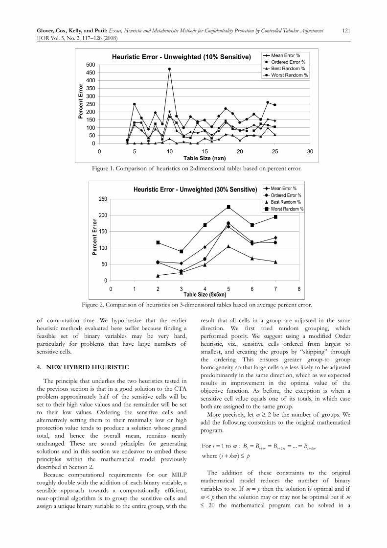
Figure 1 displays the results obtained for 2-dimensional tables that contain 10% sensitive entries. The figure shows results for tables ranging in size from 4 × 4 to 25 × 25. There is a single curve for the Ordered heuristic and three curves for the Random heuristic. The curves for the Random heuristic provide mean, worst, and best solutions found during the 100 simulations.

Figure 1 shows that Best Random performed best among the heuristics, but produces solutions that are far from optimal. It is interesting to note that the Ordered heuristic method produces solutions of similar quality to the mean Random result. Finally, it appears that error increases slightly with table size.

Next, 2-dimensional tables with 30% sensitive entries were processed. Except for the errors being larger, the results are analogous to those found for the tables with 10% sensitive entries. The relative changes for the 30% sensitive cell tables are also very similar to those found for the 10% sensitive cell tables, and thus are not included.

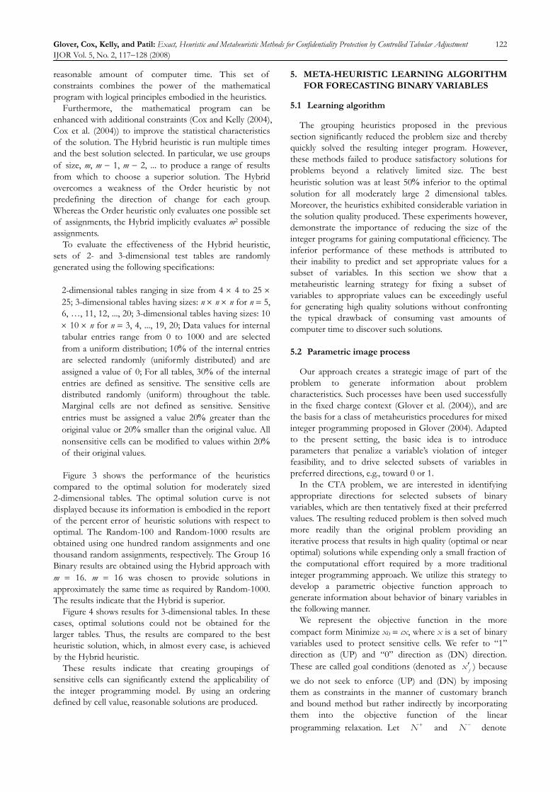
Figure 2 shows results for 3-dimensional tables ranging in size from 5 × 5 × 2 to 5 × 5 × 7 and containing 30% sensitive entries. The results that are obtained are very similar to the results obtained for 2-dimensional tables.

The results of evaluating previously proposed heuristics for controlled tabular adjustment support the following observations:

l The Best Random solution obtained over 100

Random executions was shown to be superior to the best solution from the Ordered Heuristic in most cases;

l When objective function values were considered, the performance of all of the heuristics was poor, having errors in excess of 50%;

l As would be expected, for these problems of significantly limited size, the CPLEX solver produces optimal solutions in reasonable amounts of time.

These results confirm that the exact solution approach

works better than the heuristic approaches for small problems, but unfortunately CPLEX cannot be used to solve large problems due to consuming excessive amounts


121

Heuristic Error - Unweighted (10% Sensitive)

050

100150200250300350400450500

0 5 10 15 20 25 30Table Size (nxn)

Perc

ent E

rror

Mean Error %Ordered Error %Best Random %Worst Random %

Figure 1. Comparison of heuristics on 2-dimensional tables based on percent error.

Heuristic Error - Unweighted (30% Sensitive)

0

50

100

150

200

250

0 1 2 3 4 5 6 7 8Table Size (5x5xn)

Perc

ent E

rror

Mean Error %Ordered Error %Best Random %Worst Random %

Figure 2. Comparison of heuristics on 3-dimensional tables based on average percent error.

of computation time. We hypothesize that the earlier heuristic methods evaluated here suffer because finding a feasible set of binary variables may be very hard, particularly for problems that have large numbers of sensitive cells. 4. NEW HYBRID HEURISTIC

The principle that underlies the two heuristics tested in the previous section is that in a good solution to the CTA problem approximately half of the sensitive cells will be set to their high value values and the remainder will be set to their low values. Ordering the sensitive cells and alternatively setting them to their minimally low or high protection value tends to produce a solution whose grand total, and hence the overall mean, remains nearly unchanged. These are sound principles for generating solutions and in this section we endeavor to embed these principles within the mathematical model previously described in Section 2.

Because computational requirements for our MILP roughly double with the addition of each binary variable, a sensible approach towards a computationally efficient, near-optimal algorithm is to group the sensitive cells and assign a unique binary variable to the entire group, with the

result that all cells in a group are adjusted in the same direction. We first tried random grouping, which performed poorly. We suggest using a modified Order heuristic, viz., sensitive cells ordered from largest to smallest, and creating the groups by “skipping” through the ordering. This ensures greater group-to group homogeneity so that large cells are less likely to be adjusted predominantly in the same direction, which as we expected results in improvement in the optimal value of the objective function. As before, the exception is when a sensitive cell value equals one of its totals, in which case both are assigned to the same group.

More precisely, let m ≥ 2 be the number of groups. We add the following constraints to the original mathematical program.

2For 1 to : ...where ( )

i i m i m i kmi m B B B Bi km p

+ + += = = = =+ ≤

The addition of these constraints to the original

mathematical model reduces the number of binary variables to m. If m = p then the solution is optimal and if m < p then the solution may or may not be optimal but if m ≤ 20 the mathematical program can be solved in a


122

reasonable amount of computer time. This set of constraints combines the power of the mathematical program with logical principles embodied in the heuristics.

Furthermore, the mathematical program can be enhanced with additional constraints (Cox and Kelly (2004), Cox et al. (2004)) to improve the statistical characteristics of the solution. The Hybrid heuristic is run multiple times and the best solution selected. In particular, we use groups of size, m, m − 1, m − 2, ... to produce a range of results from which to choose a superior solution. The Hybrid overcomes a weakness of the Order heuristic by not predefining the direction of change for each group. Whereas the Order heuristic only evaluates one possible set of assignments, the Hybrid implicitly evaluates m2 possible assignments.

To evaluate the effectiveness of the Hybrid heuristic, sets of 2- and 3-dimensional test tables are randomly generated using the following specifications:

2-dimensional tables ranging in size from 4 × 4 to 25 × 25; 3-dimensional tables having sizes: n × n × n for n = 5, 6, …, 11, 12, ..., 20; 3-dimensional tables having sizes: 10 × 10 × n for n = 3, 4, ..., 19, 20; Data values for internal tabular entries range from 0 to 1000 and are selected from a uniform distribution; 10% of the internal entries are selected randomly (uniformly distributed) and are assigned a value of 0; For all tables, 30% of the internal entries are defined as sensitive. The sensitive cells are distributed randomly (uniform) throughout the table. Marginal cells are not defined as sensitive. Sensitive entries must be assigned a value 20% greater than the original value or 20% smaller than the original value. All nonsensitive cells can be modified to values within 20% of their original values. Figure 3 shows the performance of the heuristics

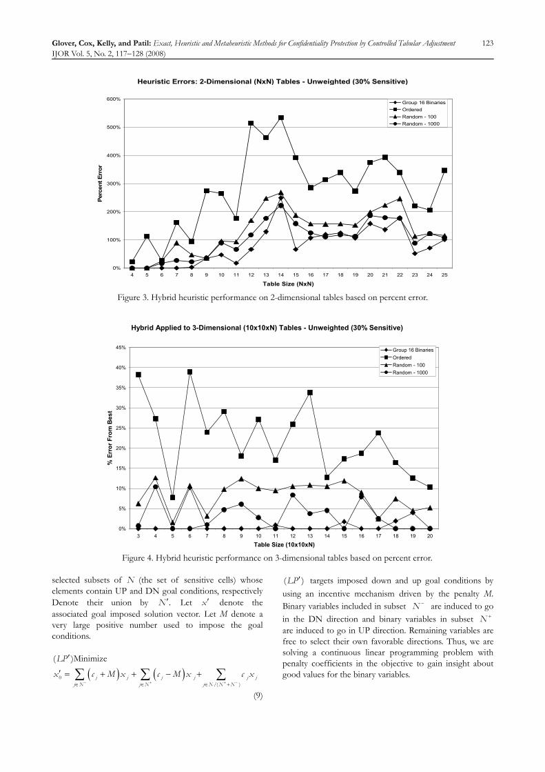
compared to the optimal solution for moderately sized 2-dimensional tables. The optimal solution curve is not displayed because its information is embodied in the report of the percent error of heuristic solutions with respect to optimal. The Random-100 and Random-1000 results are obtained using one hundred random assignments and one thousand random assignments, respectively. The Group 16 Binary results are obtained using the Hybrid approach with m = 16. m = 16 was chosen to provide solutions in approximately the same time as required by Random-1000. The results indicate that the Hybrid is superior.

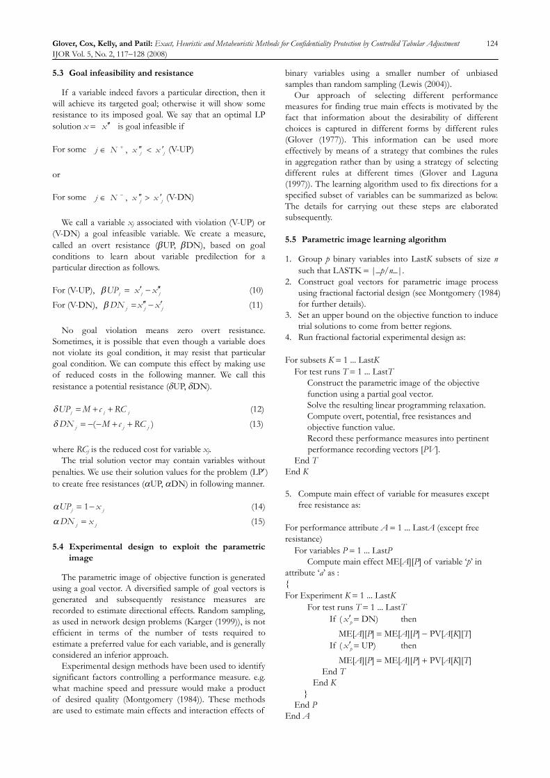
Figure 4 shows results for 3-dimensional tables. In these cases, optimal solutions could not be obtained for the larger tables. Thus, the results are compared to the best heuristic solution, which, in almost every case, is achieved by the Hybrid heuristic.

These results indicate that creating groupings of sensitive cells can significantly extend the applicability of the integer programming model. By using an ordering defined by cell value, reasonable solutions are produced.

5. META-HEURISTIC LEARNING ALGORITHM FOR FORECASTING BINARY VARIABLES

5.1 Learning algorithm

The grouping heuristics proposed in the previous section significantly reduced the problem size and thereby quickly solved the resulting integer program. However, these methods failed to produce satisfactory solutions for problems beyond a relatively limited size. The best heuristic solution was at least 50% inferior to the optimal solution for all moderately large 2 dimensional tables. Moreover, the heuristics exhibited considerable variation in the solution quality produced. These experiments however, demonstrate the importance of reducing the size of the integer programs for gaining computational efficiency. The inferior performance of these methods is attributed to their inability to predict and set appropriate values for a subset of variables. In this section we show that a metaheuristic learning strategy for fixing a subset of variables to appropriate values can be exceedingly useful for generating high quality solutions without confronting the typical drawback of consuming vast amounts of computer time to discover such solutions. 5.2 Parametric image process

Our approach creates a strategic image of part of the problem to generate information about problem characteristics. Such processes have been used successfully in the fixed charge context (Glover et al. (2004)), and are the basis for a class of metaheuristics procedures for mixed integer programming proposed in Glover (2004). Adapted to the present setting, the basic idea is to introduce parameters that penalize a variable’s violation of integer feasibility, and to drive selected subsets of variables in preferred directions, e.g., toward 0 or 1.

In the CTA problem, we are interested in identifying appropriate directions for selected subsets of binary variables, which are then tentatively fixed at their preferred values. The resulting reduced problem is then solved much more readily than the original problem providing an iterative process that results in high quality (optimal or near optimal) solutions while expending only a small fraction of the computational effort required by a more traditional integer programming approach. We utilize this strategy to develop a parametric objective function approach to generate information about behavior of binary variables in the following manner.

We represent the objective function in the more compact form Minimize x0 = cx, where x is a set of binary variables used to protect sensitive cells. We refer to “1” direction as (UP) and “0” direction as (DN) direction. These are called goal conditions (denoted as jx ′ ) because we do not seek to enforce (UP) and (DN) by imposing them as constraints in the manner of customary branch and bound method but rather indirectly by incorporating them into the objective function of the linear programming relaxation. Let +N and −N denote


123

Heuristic Errors: 2-Dimensional (NxN) Tables - Unweighted (30% Sensitive)

0%

100%

200%

300%

400%

500%

600%

4 5 6 7 8 9 10 11 12 13 14 15 16 17 18 19 20 21 22 23 24 25

Table Size (NxN)

Perc

ent E

rror

Group 16 BinariesOrderedRandom - 100Random - 1000

Figure 3. Hybrid heuristic performance on 2-dimensional tables based on percent error.

0%

5%

10%

15%

20%

25%

30%

35%

40%

45%

3 4 5 6 7 8 9 10 11 12 13 14 15 16 17 18 19 20

Table Size (10x10xN)

% E

rror

Fro

m B

est

Group 16 BinariesOrderedRandom - 100Random - 1000

Hybrid Applied to 3-Dimensional (10x10xN) Tables - Unweighted (30% Sensitive)

Figure 4. Hybrid heuristic performance on 3-dimensional tables based on percent error.

selected subsets of N (the set of sensitive cells) whose elements contain UP and DN goal conditions, respectively Denote their union by ′.N Let ′x denote the associated goal imposed solution vector. Let M denote a very large positive number used to impose the goal conditions.

′( )MinimizeLP

( ) ( )0/( )

j j j j j jj N j N j N N N

x c M x c M x c x− + + −∈ ∈ ∈ +

′ = + + − +∑ ∑ ∑

(9)

′( )LP targets imposed down and up goal conditions by using an incentive mechanism driven by the penalty M. Binary variables included in subset −N are induced to go in the DN direction and binary variables in subset +N are induced to go in UP direction. Remaining variables are free to select their own favorable directions. Thus, we are solving a continuous linear programming problem with penalty coefficients in the objective to gain insight about good values for the binary variables.


124

5.3 Goal infeasibility and resistance

If a variable indeed favors a particular direction, then it will achieve its targeted goal; otherwise it will show some resistance to its imposed goal. We say that an optimal LP solution x = ′′x is goal infeasible if For some , j jj N x x+ ′′ ′∈ < (V-UP) or For some , j jj N x x− ′′ ′∈ > (V-DN)

We call a variable xj associated with violation (V-UP) or (V-DN) a goal infeasible variable. We create a measure, called an overt resistance (βUP, βDN), based on goal conditions to learn about variable predilection for a particular direction as follows. For (V-UP), β ′ ′′= −j j jUP x x (10) For (V-DN), β ′′ ′= −j j jDN x x (11)

No goal violation means zero overt resistance.

Sometimes, it is possible that even though a variable does not violate its goal condition, it may resist that particular goal condition. We can compute this effect by making use of reduced costs in the following manner. We call this resistance a potential resistance (δUP, δDN).

j j jUP M c RCδ = + + (12)

( )j j jDN M c RCδ = − − + + (13) where RCj is the reduced cost for variable xj.

The trial solution vector may contain variables without penalties. We use their solution values for the problem (LP′) to create free resistances (αUP, αDN) in following manner.

1j jUP xα = − (14)

j jDN xα = (15) 5.4 Experimental design to exploit the parametric

image

The parametric image of objective function is generated using a goal vector. A diversified sample of goal vectors is generated and subsequently resistance measures are recorded to estimate directional effects. Random sampling, as used in network design problems (Karger (1999)), is not efficient in terms of the number of tests required to estimate a preferred value for each variable, and is generally considered an inferior approach.

Experimental design methods have been used to identify significant factors controlling a performance measure. e.g. what machine speed and pressure would make a product of desired quality (Montgomery (1984)). These methods are used to estimate main effects and interaction effects of

binary variables using a smaller number of unbiased samples than random sampling (Lewis (2004)).

Our approach of selecting different performance measures for finding true main effects is motivated by the fact that information about the desirability of different choices is captured in different forms by different rules (Glover (1977)). This information can be used more effectively by means of a strategy that combines the rules in aggregation rather than by using a strategy of selecting different rules at different times (Glover and Laguna (1997)). The learning algorithm used to fix directions for a specified subset of variables can be summarized as below. The details for carrying out these steps are elaborated subsequently. 5.5 Parametric image learning algorithm

1. Group p binary variables into LastK subsets of size n such that LASTK = |_p/n_|.

2. Construct goal vectors for parametric image process using fractional factorial design (see Montgomery (1984) for further details).

3. Set an upper bound on the objective function to induce trial solutions to come from better regions.

4. Run fractional factorial experimental design as: For subsets K = 1 ... LastK

For test runs T = 1 ... LastT Construct the parametric image of the objective function using a partial goal vector. Solve the resulting linear programming relaxation. Compute overt, potential, free resistances and objective function value. Record these performance measures into pertinent performance recording vectors [PV].

End T End K 5. Compute main effect of variable for measures except

free resistance as: For performance attribute A = 1 ... LastA (except free resistance)

For variables P = 1 ... LastP Compute main effect ME[A][P] of variable ‘p’ in

attribute ‘a’ as : { For Experiment K = 1 ... LastK

For test runs T = 1 ... LastT If ( ′px = DN) then

ME[A][P] = ME[A][P] − PV[A[K][T] If ( ′px = UP) then

ME[A][P] = ME[A][P] + PV[A[K][T] End T

End K }

End P End A


125

6. Compute main effect of variable for Free Resistance as: For variables P = 1 ... LastP

Compute main effect ME[A][P] as {

For Experiment K = 1 ... LastK For test runs T = 1 ... LastT

If ( px < 0.5 ) then ME[A][P] = ME[A][P] + 1

If ( px > 0.5 ) then ME[A][P] = ME[A][P] − 1

End T End K

} End P 7. Compute final score for each variable using persistent

voting principle as: For variables P = 1 ... LastP

Final Score [P] = 0 For A = 1 ... LastA (includes free resistance measure)

If (ME[A][P] > 0) then Final Score [P] = Final Score [P] + 1

If (ME[A][P] < 0) then Final Score [P] = Final Score [P] − 1

End A End P 8. Rank variables P = 1 ... LastP in descending order of

the absolute values of final scores. 9. Set cutoff ‘c’ to fix direction for the variables. 10. Fix directions for binary variables as: For variables P = 1 ... c

If (Final Score [P] > 0) then xp = 0

If (Final Score [P] < 0) then xp = 1

End P 11. Solve the resulting mixed integer programming

problem. 5.6 Discussion and elaboration of the method

Variables are grouped into K subsets in step 1 in a random manner. The rationale for using a random assignment is to avoid generating an interaction effect. By contrast, a process of grouping variables from a particular row or column together can produce significant interaction effects because of tabular additivity. The Fractional Factorial design we employ confounds interaction effects with the aim of reducing the number of test runs. Selecting sensitive cells in a random fashion encourages them to exhibit minor interaction effects due to weak tabular connectivity.

The logic of an ordering heuristic, which assigns up and down directions for ordered cells in an alternating fashion, is consistent with this finding. Thus, an ordering heuristic tries to capitalize on a positive two-factor interaction effect. There is one subtle possible disadvantage, which might undermine efficiency of this heuristic. Sometimes, this heuristic might assign either plus or minus directions to all cells in a row or a column thereby increasing the absolute adjustment. For example consider the 4 × 4 table in which cells (1, 1), (2, 4), (3, 1), and (4, 4) are sensitive with protection limits of 40, 35, 30, 25 respectively. The ordering heuristic would cause very large adjustments to nonsensitive cells in this case. This might be the reason why an ordering heuristic did not perform well in our experiments.

A parametric image of the objective function is generated as follows. A typical test run contains target directions for a subset of variables and free directions for remaining variables. We can use these targeted directions to generate a parametric image of the objective function as:

( ) ( )0/( )

j j j j j jj N j N j N N N

x c M x c M x c x− + + −∈ ∈ ∈ +

′ = + + − +∑ ∑ ∑

(16)

The new model has an effect of motivating variables with a DN goal condition to receive a value of 0 and variables with an UP goal condition to receive a value of 1 while allowing remaining variables to take their optimal directions according to the situation.

Steps 5 and 6 compute the average effect of a variable for a given measure. This basically computes the average change in the performance measure when a binary variable is changed from zero to one. This method is widely used in experimental design to compute average effects (Montgomery, 1984) because it groups observations into two sets and then checks on average whether there is any difference in performance between the two sets. For example, if the DN direction sum is higher than the UP direction sum, this signals a negative effect, implying that a performance measure would decrease if a binary variable were set to 1 instead of 0.

Performance measures are recorded in three- dimensional vectors for each variable, where the row dimension refers to the performance measure, the column dimension refers to the experiment and the page dimension refers to the test run from the experiment. As shown in steps 5 and 6, to calculate the main effect for a measure, we sum over performance values computed with respect to all test runs from all experiments for that measure. We subsequently record the main effects of variables in a 2 dimensional vector in which the row dimension refers to the performance measure and the column dimension refers to a binary variable.

We rank binary variables in descending order according to the absolute values of their final scores and select a subset of these variables to fix directions. The cutoff level was decided using experimental evaluation. We found 45 % and 70% as cutoff levels for “small” and “big” tables


126

Squares (NxN)

0%

20%

40%

60%

80%

100%

120%

140%

160%

180%

200%

4 5 6 7 8 9 10 11 12 13 14 15 16 17 18 19 20 21 22 23 24 25

N

GA

P

Group 16 BinariesGroup 16 - Min CommonExperimentlearning method(optimal)learning method(lower bound)

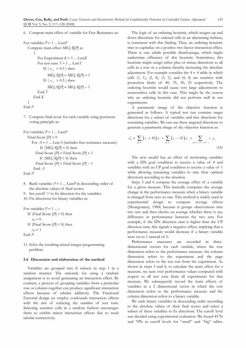
Figure 5. Performance of proposed learning method on optimality gaps.

respectively, in the sense that these levels generated high quality solutions in a reasonable amount of time. The results section shows in detail how the percent of fixed variables affected solution quality and time. Use of 0 as threshold in the final step is mainly conceptual in nature as it means that variables with positive final scores prefer the DN direction and those with negative final scores prefers the UP direction. The chosen cutoff level ensures that variables chosen to be fixed will be those that have sufficiently high absolute final scores, thereby offering adequate support for the chosen directions. 5.7 Performance of the learning algorithm for

2-dimensional tables

We implemented the learning algorithm using C++, ILOG- Concert Technology 1.2, and ILOG-CPLEX 8.1. Figure 5 shows the performance of our proposed learning method compared to other variable fixing heuristics. It was extremely time consuming to run larger problem instances to optimality using the default version of CPLEX. For example, we ran the 25 × 25 problem using the default CPLEX method on a 2GB RAM and 3.2GHz workstation for 24 hours. Unfortunately, the best solution found by CPLEX (after 19 hours and 35 minutes) still exhibited an optimality gap of 9.6%. Real world applications require the generation of hundreds to thousands of such solutions, and require these solutions to have better lower bounds and hence smaller optimality gaps. Reliance on CPLEX as a solution approach is therefore clearly unsuitable.

Consequently, we needed a computationally efficient alternative to compute a better lower bound, which is essential for measuring the optimality gap. Cox et al. (2005) proposed a set partitioning relaxation for generating a tighter lower bound on the objective in the CTA context.

We used the lower bound as a proxy for an optimum value for computing the optimality gap for larger instances. Lower bounds were reliable in the sense that they were consistently very close to the optimal values for those problems where an optimal solution could be verified (by running CPLEX for a period of time that does not exceed practical feasibility). In particular, for these problems involving 2-dimensional tables, restricted in size to no more than 18 rows and columns to permit them to be solved by CPLEX, the optimality gap was verified to be approximately 1%. For example, for the 18 × 18 problem, the computed lower bound was 9736 compared to the optimum value of 9850, representing a gap of 1.15 %. In Figure 5, the “Learning Method (optimal)” curve identifies the optimality gap with respect to the known optimal value, and the “Learning Method (lower bound)” curve identifies the optimality gap for the heuristic with respect to the lower bound.

Our learning method yielded significant improvements in reducing the optimality gap across the entire 2 dimensional test set as demonstrated by Figure 5. Optimality gap values obtained by the methods described in preceding sections degraded considerably for the larger problem instances. For example, using these earlier methods, the mean gap for the 25 × 25 table was 117.6% compared to the overall mean gap of 70% for smaller problems. In either case, the results were disappointing in relation to what might be hoped for. By contrast, the learning method performed dramatically better, consistently generating high quality solutions irrespective of the problem size, giving an overall mean gap of 6% and a gap of 5.72% for the 25 × 25 problem.

We define prediction accuracy to be the percentage of variables that are correctly assigned their optimal values,


127

from a selected set of the “top” (highest scoring) variables identified .The prediction accuracy of our method for a 14 × 14 problem which contains 69 variables, was 85.5% for the top 10% of the problem variables (6 correct decisions out of 7 fixed variables). In order to analyze the tradeoff between solution quality and time, we fixed only the top 15% of the variables for the 17 × 17 problem. We found a better solution (objective value = 9206) than our reported solution (objective value = 9460) although, at the expense of computational speed efficiency. For this particular experiment, the result of fixing fewer variables caused the number of nodes processed to increase from 2400 to 72600 and the solution time to increase from 16.38 sec to 520 sec. We believe this increase in the computation time does not warrant reducing the number of fixed variables in order to achieve a modest gain in solution quality. 6. CONCLUSIONS AND REMARKS

This study has undertaken an extensive set of comparative computational tests and analyses to evaluate the relative performance of alternative methods for the controlled tabular adjustment (CTA) model. Our preliminary tests compared previously proposed heuristics to the exact CPLEX method. The outcomes showed that the exact procedure yields solutions superior to those of earlier heuristic approaches, but is unable to solve problems of modest size within a reasonable amount of time.

To overcome these limitations of previous approaches, we introduced a hybrid heuristic that combines the exact mathematical programming approach with constructive heuristics suggested by Danderkar and Cox (2002). Numeric simulations indicate that the hybrid has the ability to produce better solutions than previous heuristics in reasonable time, and in addition finds reasonable solutions to highly constrained problems, but is limited to problems of modest dimension.

Finally, we demonstrate that a special metaheuristic learning method based on parametric image processes leads to significant additional improvements by generating solutions of greatly improved quality. In particular, the learning method succeeds in reducing the optimality gap for the problems tested from an overall average of 70% to an average of 6%. The true distance from a theoretical optimum is likely to be somewhat smaller still, since the gap is based on an imprecise bound. REFERENCES

1. Cox, L.H. (2000). Discussion (on Session 49: Statistical Disclosure Control for Establishment Data). Proceedings of the ICES II: The Second International Conference on Establishment Surveys−Survey Methods for Businesses, Farms and Institutions, Alexandria, VA, American Statistical Association, Invited Papers, pp. 904-907.

2. Cox, L.H. (1980). Suppression methodology and statistical disclosure control. Journal of the American

Statistical Association, 75: 377-385. 3. Cox, L.H. and Danderkar, R.A. (2004). A disclosure

limitation method for tabular data that preserves accuracy and ease-of-use. Proceedings of the 2002 FCSM Statistical Policy Conference, Office of Management and Budget, Washington, DC, pp. 15-30.

4. Cox, L.H. and Kelly, J.P. (2004). Balancing data quality and confidentiality for tabular data. Proceedings of the UNECE/EUROSTAT Work Session on Statistical Data Confidentiality, Monographs of Official Statistics, Eurostat., Luxembourg, pp. 11-23.

5. Cox, L.H., Kelly, J.P., and Patil, R.J. (2004). Preserving quality and confidentiality for multivariate tabular data. Proceedings of Privacy in Statistical Databases 2004 (PSD’ 2004), Barcelona, pp. 9-11, Lecture Notes in Computer Science 3050, Springer Verlag, New York, pp. 87-98.

6. Cox, L.H., Kelly, J.P., and Patil, R.J. (2005). Computational aspects of controlled tabular adjustment: Algorithm and analysis. In: B. Golden, S. Raghavan, and E. Wasil (Eds.), The Next Wave in Computer, Optimization and Decision Technologies, Kluwer, Boston, pp. 45-59.

7. Danderkar, R.A. and Cox, L.H. (2002). Synthetic tabular data-an alternative to complementary cell suppression, manuscript.

8. Doyle, P., Lane, J.I., Theeuwes, J.J.M., and Zayatz, L.V. (Eds.) (2001). Chapter 8: Disclosure risk for tabular economic data. Proceedings of Confidentiality, Disclosure and Data Access: Theory and Practical Applications for Statistical Agencies, North-Holland, Amsterdam, pp. 167-184.

9. Fischetti, M. and Salazar, J.J. (1999). Models and algorithms for the 2-dimensional cell suppression problem in statistical disclosure control. Mathematical Programming, 84: 283-312.

10. Fischetti, M. and Salazar, J.J. (2000). Solving the cell suppression problem on tabular data with linear constraints. Management Science, 47: 1008-1026.

11. Glover, F. (1977). Heuristics for integer programming using surrogate constraints. Decision Sciences, 8: 156-166.

12. Glover, F. (2004). Parametric tabu search methods for mixed integer programming. Leeds School of Business, University of Colorado, Boulder.

13. Glover, F., Amini, M., and Kochenberger, G. (2004). Parametric ghost image processes for fixed-charge problems: A study of transportation networks. Journal of Heuristics, 11(4): 307-336.

14. Glover, F. and Laguna, M. (1997). Tabu Search, Kluwer Academic Publishers, Boston.

15. JSPI (1981). Linear sensitivity measures in statistical disclosure control. Journal of Statistical Planning and Inference, 5: 153-164.

16. Karger, D.R. (1999). Random sampling in cut, flow, and network design problems. Mathematics of Operations Research, 24(2): 383-413.

17. Kelly, J., Golden, B., and Assad, A. (1992). Cell suppression: Disclosure protection for sensitive tabular data. Networks, 22: 397-417.

18. Lewis, M.W. (2004). Solving fixed charge


128

multi-commodity network design problems using guided design search. Hearin Center Technical Report, University of Mississippi, HCES-01-04.

19. Montgomery, D.C. (1984). Design and Analysis of Experiments, John Wiley and Sons, New York, N.Y.

20. Willenborg, L. and de Waal, T.D. (Eds.) (1996). Statistical Disclosure Control in Practice, Lecture Notes in Statistics, 111, Springer, New York.

21. Willenborg, L. and de Waal, T.D. (Eds.) (2001). Elements of Statistical Disclosure Control, Lecture Notes in Statistics, 155, Springer, New York.

Documents

Exact, Heuristic and Metaheuristic Methods for Confidentiality Protection by Controlled Tabular Adjustment