Evolution analysis of airline network concentration using spatially-normalized indexes

- application to Brazil

Alessandro V. M. Oliveira* Guilherme Lohmann** William Bendinelli * Tiago G. Costa*

* Aeronautics Institute of Technology, Brazil ** Southern Cross University, Australia

This version: February 26, 2014

Research question

• Brazil: recent decrease in airline network spatial concentration

– causes? consequences?

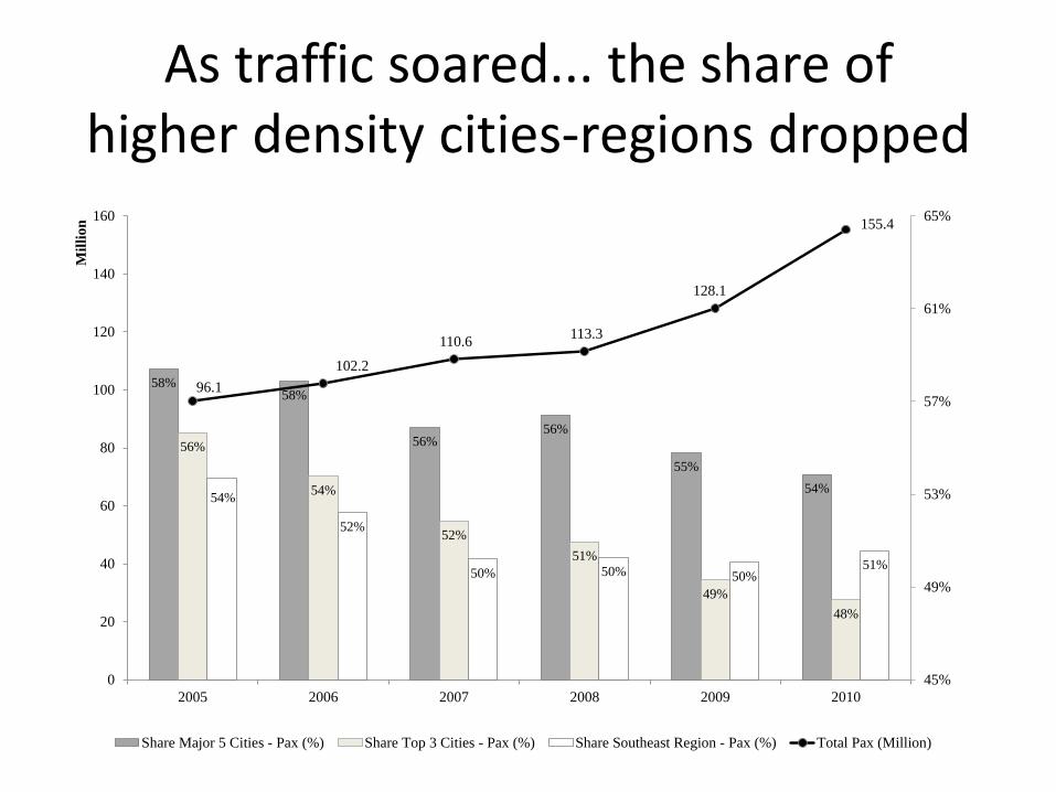
As traffic soared... the share of higher density cities-regions dropped

58%58%

56%56%

55%

54%

56%

54%

52%

51%

49%

48%

54%

52%

50% 50% 50%51%

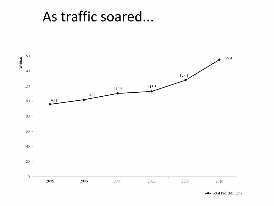
96.1

102.2

110.6 113.3

128.1

155.4

45%

49%

53%

57%

61%

65%

0

20

40

60

80

100

120

140

160

2005 2006 2007 2008 2009 2010

Mil

lion

Share Major 5 Cities - Pax (%) Share Top 3 Cities - Pax (%) Share Southeast Region - Pax (%) Total Pax (Million)

As traffic soared... the share of higher density cities-regions dropped

58%58%

56%56%

55%

54%

56%

54%

52%

51%

49%

48%

54%

52%

50% 50% 50%51%

96.1

102.2

110.6 113.3

128.1

155.4

45%

49%

53%

57%

61%

65%

0

20

40

60

80

100

120

140

160

2005 2006 2007 2008 2009 2010

Mil

lion

Share Major 5 Cities - Pax (%) Share Top 3 Cities - Pax (%) Share Southeast Region - Pax (%) Total Pax (Million)

Cities(1)

2005

(2)

2010

(2) - (1)Regions

(1)

2005

(2)

2010

(2) - (1)

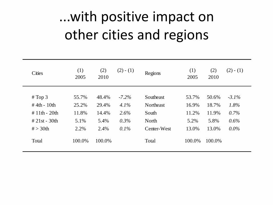
# Top 3 55.7% 48.4% -7.2% Southeast 53.7% 50.6% -3.1%

# 4th - 10th 25.2% 29.4% 4.1% Northeast 16.9% 18.7% 1.8%

# 11th - 20th 11.8% 14.4% 2.6% South 11.2% 11.9% 0.7%

# 21st - 30th 5.1% 5.4% 0.3% North 5.2% 5.8% 0.6%

# > 30th 2.2% 2.4% 0.1% Center-West 13.0% 13.0% 0.0%

Total 100.0% 100.0% Total 100.0% 100.0%

...with positive impact on other cities and regions

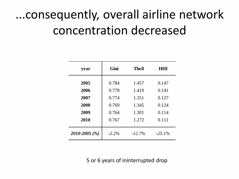
...consequently, overall airline network concentration decreased

year Gini Theil HHI

2005 0.784 1.457 0.147

2006 0.778 1.419 0.141

2007 0.774 1.351 0.127

2008 0.769 1.345 0.124

2009 0.764 1.301 0.114

2010 0.767 1.272 0.111

2010-2005 (%) -2.2% -12.7% -25.1%

5 or 6 years of ininterrupted drop

Our study

• Analysis of airline network concentration in Brazil

• drivers of its spatial evolution

– demand?

– costs?

– competition?

Contributions

• Study of determinants of network concentration

– use of econometric analysis

• Analysis of an emerging country of the BRICS

– a unique dataset from Brazil

• Use of spatially-normalized concentration measures

– network concentration relative to geographic concentration

Main findings

• Drop in spatial concentration of late 2000s:

– caused by the high increase in domestic demand and traffic spill from major aiports

– but a long run trend of increase in concentration

• Crises, cost shocks (jet fuel) and enhanced flow of international tourists tend to increase concentration

• Recent LCC entry decreased concentration

Application

Most knwon concentration indexes

• Gini, Theil, HHI

• Use for spatial concentration assessment

• Literature: use of normalized measures for airline network concentration

– Reynolds-Geighan (1998, 2001)

– Burghouwt, Hakfoort and van Eck (2003)

– Martín, J. C. and Voltes-Dorta, A. (2009)

This paper

• Airline network concentration indexes should account for changes in geographic concentration

• Our proposal:

Spatially-normalized concentration indexes

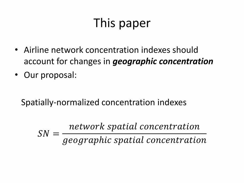
This paper

• Airline network concentration indexes should account for changes in geographic concentration

• Our proposal:

Spatially-normalized concentration indexes

𝑆𝑁 =𝑛𝑒𝑡𝑤𝑜𝑟𝑘 𝑠𝑝𝑎𝑡𝑖𝑎𝑙 𝑐𝑜𝑛𝑐𝑒𝑛𝑡𝑟𝑎𝑡𝑖𝑜𝑛

𝑔𝑒𝑜𝑔𝑟𝑎𝑝ℎ𝑖𝑐 𝑠𝑝𝑎𝑡𝑖𝑎𝑙 𝑐𝑜𝑛𝑐𝑒𝑛𝑡𝑟𝑎𝑡𝑖𝑜𝑛

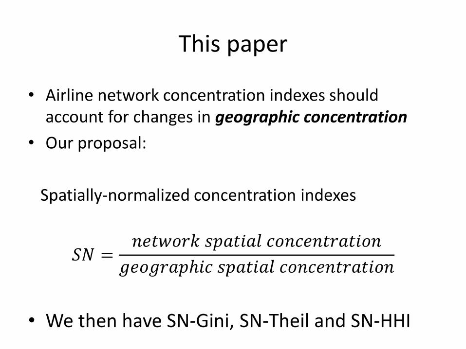
This paper

• Airline network concentration indexes should account for changes in geographic concentration

• Our proposal:

Spatially-normalized concentration indexes

𝑆𝑁 =𝑛𝑒𝑡𝑤𝑜𝑟𝑘 𝑠𝑝𝑎𝑡𝑖𝑎𝑙 𝑐𝑜𝑛𝑐𝑒𝑛𝑡𝑟𝑎𝑡𝑖𝑜𝑛

𝑔𝑒𝑜𝑔𝑟𝑎𝑝ℎ𝑖𝑐 𝑠𝑝𝑎𝑡𝑖𝑎𝑙 𝑐𝑜𝑛𝑐𝑒𝑛𝑡𝑟𝑎𝑡𝑖𝑜𝑛

• We then have SN-Gini, SN-Theil and SN-HHI

Application

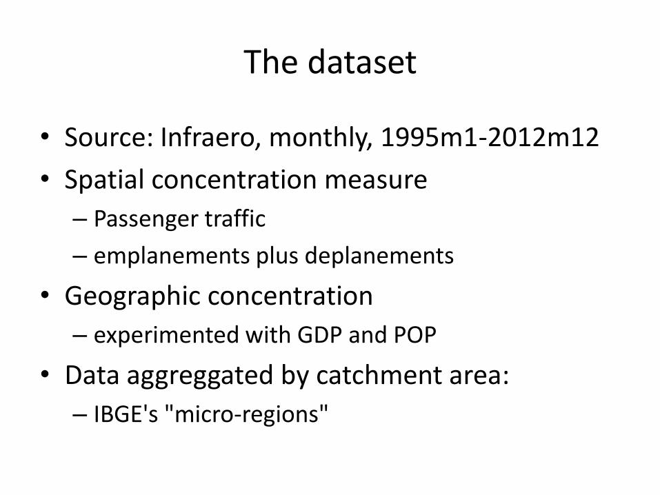
The dataset

• Source: Infraero, monthly, 1995m1-2012m12

• Spatial concentration measure

– Passenger traffic

– emplanements plus deplanements

• Geographic concentration

– experimented with GDP and POP

• Data aggreggated by catchment area:

– IBGE's "micro-regions"

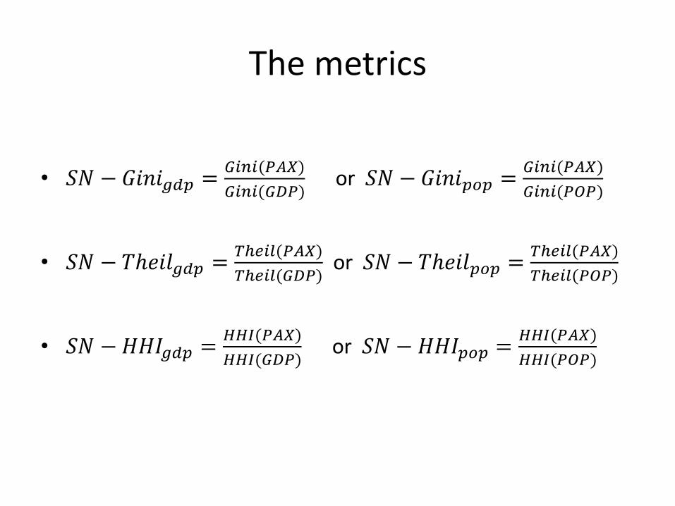
The metrics

• 𝑆𝑁 − 𝐺𝑖𝑛𝑖𝑔𝑑𝑝 =𝐺𝑖𝑛𝑖(𝑃𝐴𝑋)

𝐺𝑖𝑛𝑖(𝐺𝐷𝑃) or 𝑆𝑁 − 𝐺𝑖𝑛𝑖𝑝𝑜𝑝 =

𝐺𝑖𝑛𝑖(𝑃𝐴𝑋)

𝐺𝑖𝑛𝑖(𝑃𝑂𝑃)

• 𝑆𝑁 − 𝑇ℎ𝑒𝑖𝑙𝑔𝑑𝑝 =𝑇ℎ𝑒𝑖𝑙(𝑃𝐴𝑋)

𝑇ℎ𝑒𝑖𝑙(𝐺𝐷𝑃) or 𝑆𝑁 − 𝑇ℎ𝑒𝑖𝑙𝑝𝑜𝑝 =

𝑇ℎ𝑒𝑖𝑙(𝑃𝐴𝑋)

𝑇ℎ𝑒𝑖𝑙(𝑃𝑂𝑃)

• 𝑆𝑁 − 𝐻𝐻𝐼𝑔𝑑𝑝 =𝐻𝐻𝐼(𝑃𝐴𝑋)

𝐻𝐻𝐼(𝐺𝐷𝑃) or 𝑆𝑁 − 𝐻𝐻𝐼𝑝𝑜𝑝 =

𝐻𝐻𝐼(𝑃𝐴𝑋)

𝐻𝐻𝐼(𝑃𝑂𝑃)

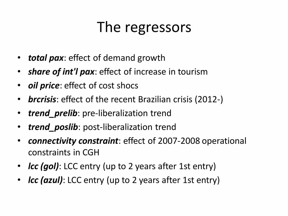
The regressors

• total pax: effect of demand growth

• share of int'l pax: effect of increase in tourism

• oil price: effect of cost shocs

• brcrisis: effect of the recent Brazilian crisis (2012-)

• trend_prelib: pre-liberalization trend

• trend_poslib: post-liberalization trend

• connectivity constraint: effect of 2007-2008 operational constraints in CGH

• lcc (gol): LCC entry (up to 2 years after 1st entry)

• lcc (azul): LCC entry (up to 2 years after 1st entry)

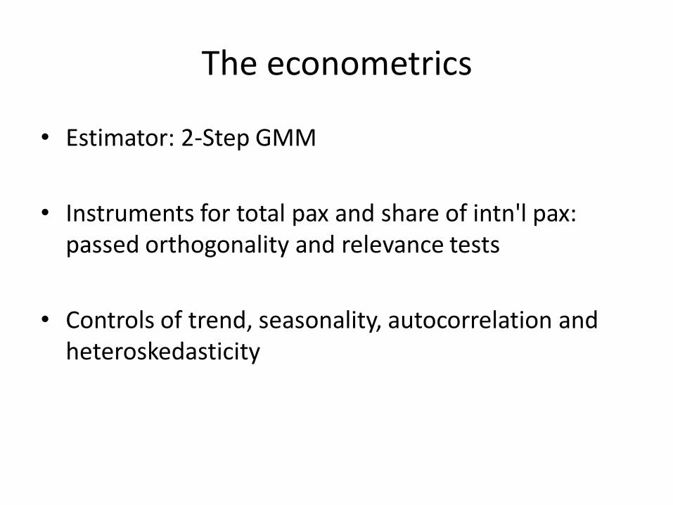
The econometrics

• Estimator: 2-Step GMM

• Instruments for total pax and share of intn'l pax: passed orthogonality and relevance tests

• Controls of trend, seasonality, autocorrelation and heteroskedasticity

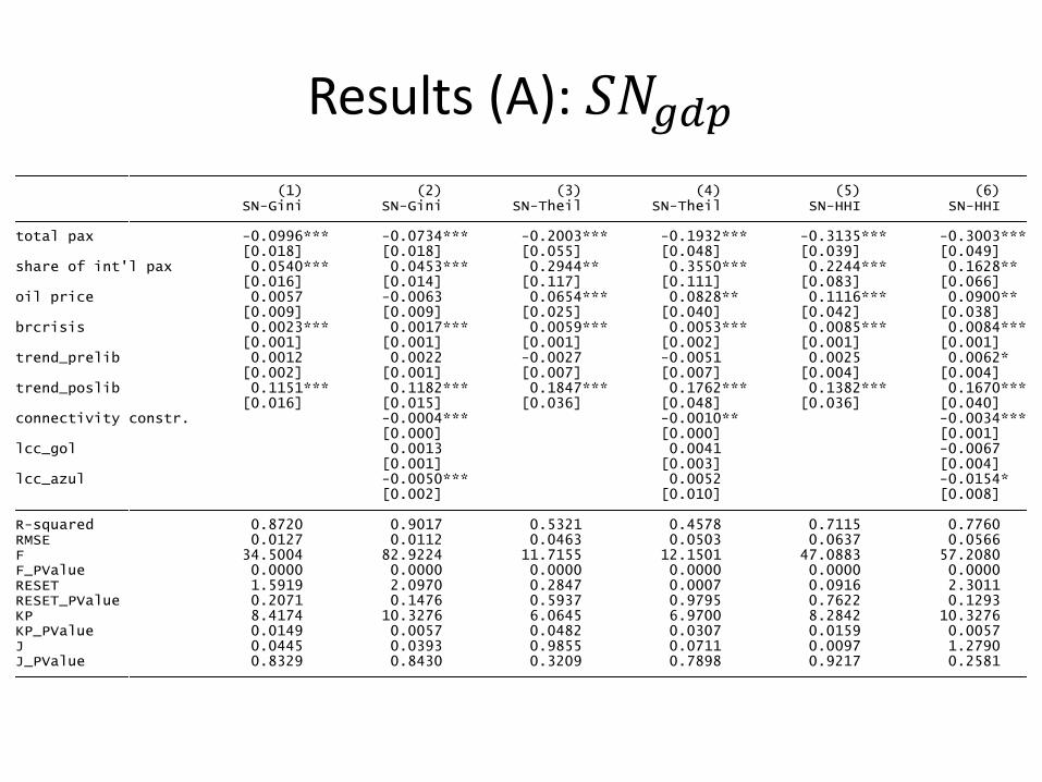
Results (A): 𝑆𝑁𝑔𝑑𝑝

J_PValue 0.8329 0.8430 0.3209 0.7898 0.9217 0.2581 J 0.0445 0.0393 0.9855 0.0711 0.0097 1.2790 KP_PValue 0.0149 0.0057 0.0482 0.0307 0.0159 0.0057 KP 8.4174 10.3276 6.0645 6.9700 8.2842 10.3276 RESET_PValue 0.2071 0.1476 0.5937 0.9795 0.7622 0.1293 RESET 1.5919 2.0970 0.2847 0.0007 0.0916 2.3011 F_PValue 0.0000 0.0000 0.0000 0.0000 0.0000 0.0000 F 34.5004 82.9224 11.7155 12.1501 47.0883 57.2080 RMSE 0.0127 0.0112 0.0463 0.0503 0.0637 0.0566 R-squared 0.8720 0.9017 0.5321 0.4578 0.7115 0.7760 [0.002] [0.010] [0.008] lcc_azul -0.0050*** 0.0052 -0.0154* [0.001] [0.003] [0.004] lcc_gol 0.0013 0.0041 -0.0067 [0.000] [0.000] [0.001] connectivity constr. -0.0004*** -0.0010** -0.0034*** [0.016] [0.015] [0.036] [0.048] [0.036] [0.040] trend_poslib 0.1151*** 0.1182*** 0.1847*** 0.1762*** 0.1382*** 0.1670*** [0.002] [0.001] [0.007] [0.007] [0.004] [0.004] trend_prelib 0.0012 0.0022 -0.0027 -0.0051 0.0025 0.0062* [0.001] [0.001] [0.001] [0.002] [0.001] [0.001] brcrisis 0.0023*** 0.0017*** 0.0059*** 0.0053*** 0.0085*** 0.0084*** [0.009] [0.009] [0.025] [0.040] [0.042] [0.038] oil price 0.0057 -0.0063 0.0654*** 0.0828** 0.1116*** 0.0900** [0.016] [0.014] [0.117] [0.111] [0.083] [0.066] share of int'l pax 0.0540*** 0.0453*** 0.2944** 0.3550*** 0.2244*** 0.1628** [0.018] [0.018] [0.055] [0.048] [0.039] [0.049] total pax -0.0996*** -0.0734*** -0.2003*** -0.1932*** -0.3135*** -0.3003*** SN-Gini SN-Gini SN-Theil SN-Theil SN-HHI SN-HHI (1) (2) (3) (4) (5) (6)

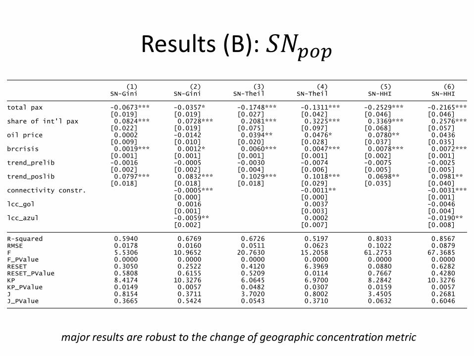
Results (B): 𝑆𝑁𝑝𝑜𝑝

J_PValue 0.3665 0.5424 0.0543 0.3710 0.0632 0.6046 J 0.8154 0.3711 3.7020 0.8002 3.4505 0.2681 KP_PValue 0.0149 0.0057 0.0482 0.0307 0.0159 0.0057 KP 8.4174 10.3276 6.0645 6.9700 8.2842 10.3276 RESET_PValue 0.5808 0.6155 0.5209 0.0114 0.7667 0.4280 RESET 0.3050 0.2522 0.4120 6.3969 0.0880 0.6282 F_PValue 0.0000 0.0000 0.0000 0.0000 0.0000 0.0000 F 5.5306 10.9652 20.7630 15.2058 61.2753 67.3685 RMSE 0.0178 0.0160 0.0511 0.0623 0.1022 0.0879 R-squared 0.5940 0.6769 0.6726 0.5197 0.8033 0.8567 [0.002] [0.007] [0.008] lcc_azul -0.0059** 0.0002 -0.0190** [0.001] [0.003] [0.004] lcc_gol 0.0016 0.0037 -0.0046 [0.000] [0.000] [0.001] connectivity constr. -0.0005*** -0.0011** -0.0031*** [0.018] [0.018] [0.018] [0.029] [0.035] [0.040] trend_poslib 0.0797*** 0.0832*** 0.1029*** 0.1018*** 0.0698** 0.0981** [0.002] [0.002] [0.004] [0.006] [0.005] [0.005] trend_prelib -0.0016 -0.0005 -0.0030 -0.0074 -0.0075 -0.0025 [0.001] [0.001] [0.001] [0.001] [0.002] [0.001] brcrisis 0.0019*** 0.0012* 0.0060*** 0.0047*** 0.0078*** 0.0072*** [0.009] [0.010] [0.020] [0.028] [0.037] [0.035] oil price 0.0002 -0.0142 0.0394** 0.0476* 0.0780** 0.0436 [0.022] [0.019] [0.075] [0.097] [0.068] [0.057] share of int'l pax 0.0824*** 0.0728*** 0.2081*** 0.3225*** 0.3369*** 0.2576*** [0.019] [0.019] [0.027] [0.042] [0.046] [0.046] total pax -0.0673*** -0.0357* -0.1748*** -0.1311*** -0.2529*** -0.2165*** SN-Gini SN-Gini SN-Theil SN-Theil SN-HHI SN-HHI (1) (2) (3) (4) (5) (6)

major results are robust to the change of geographic concentration metric

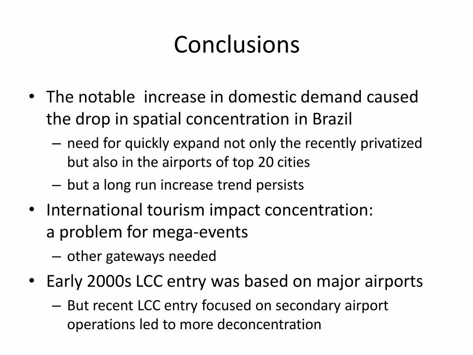
Conclusions

• The notable increase in domestic demand caused the drop in spatial concentration in Brazil

– need for quickly expand not only the recently privatized but also in the airports of top 20 cities

– but a long run increase trend persists

• International tourism impact concentration: a problem for mega-events

– other gateways needed

• Early 2000s LCC entry was based on major airports

– But recent LCC entry focused on secondary airport operations led to more deconcentration