WP/06/181

The Difference Between Hedonic Imputation Indexes and Time Dummy Hedonic Indexes

Mick Silver and Saeed Heravi

© 2006 International Monetary Fund WP/06/181

IMF Working Paper

IMF Statistics Department

The Difference Between Hedonic Imputation Indexes and Time Dummy Hedonic Indexes

Prepared by Mick Silver and Saeed Heravi1

Authorized for distribution by Adriaan M. Bloem

July 2006

Abstract

This Working Paper should not be reported as representing the views of the IMF. The views expressed in this Working Paper are those of the author(s) and do not necessarily represent those of the IMF or IMF policy. Working Papers describe research in progress by the author(s) and are published to elicit comments and to further debate.

Statistical offices try to match item models when measuring inflation between two periods. For product areas with a high turnover of differentiated models, however, the use of hedonic indexes is more appropriate since they include the prices and quantities of unmatched new and old models. The two main approaches to hedonic indexes are hedonic imputation (HI) indexes and dummy time hedonic (DTH) indexes. This study provides a formal analysis of the difference between the two approaches for alternative implementations of the Törnqvist “superlative” index. It shows why the results may differ and discusses the issue of choice between these approaches. JEL Classification Numbers: C43, C82, E31 Keywords: Hedonic regressions; consumer price indexes; superlative indexes Author(s) E-Mail Address: msilver@imf.org

1 Cardiff University. We acknowledge useful comments from Paul Armknecht (IMF), Ernst Berndt (MIT), Erwin Diewert (University of British Columbia), Kevin Fox (UNSW), Jan de Haan (Statistics Netherlands), and two anonymous referees for the Journal of Business and Economic Statistics.

- 2 -

Contents Page

I. Introduction ............................................................................................................................3

II. Hedonic Indexes....................................................................................................................4 A. Hedonic Imputation (HI) Indexes .............................................................................4 B. Dummy Time Hedonic (DTH) Indexes ....................................................................6

III. Why Hedonic Imputation and Dummy Time Hedonic Indexes Differ................................8 A. Algebraic Differences: A Reformulation of the Hedonic Indexes............................8 B. How Does a Törnqvist HI Index Differ from a Törnqvist DTH Index? ...................9 C. Interpretation of ( )tz Törn11 −

∗λ ..................................................................................10 D. Treatment of Unmatched Observations ..................................................................12 E. Observations with Undue Influence ........................................................................12 F. Chaining...................................................................................................................12

IV. Choice Between Hedonic Indexes and Time Dummy Hedonic Indexes...........................13

V. Conclusions.........................................................................................................................14 Figure 1. Illustration of Hedonic Indices ……………………………………………………15 Appendix. Hedonic Imputation Index Estimate at a Törnqvist Mean ….…...........................16 References................................................................................................................................17

- 3 -

I. INTRODUCTION

This paper outlines and compares the two main and quite distinct approaches to the measurement of hedonic price indexes: dummy time hedonic indexes and hedonic imputation indexes (also referred to as “characteristic price index numbers,” Triplett, 2004). Both approaches not only correct price changes for changes in the quality of items purchased, but also allow the indexes to incorporate matched and unmatched models. They provide a means by which price changes can be measured in product markets where there is a rapid turnover of differentiated models. However, they can yield quite different results. This paper provides a formal exposition of the factors underlying such differences and the implications for choice of method. This is undertaken for the Törnqvist index, a superlative formula. As will be explained below, superlative index number formulas, which include the Fisher index, have desirable properties and provides results similar to each other.

The standard way price changes are measured by national statistical offices is through the use of the matched models method. In this method the details and prices of a representative selection of items are collected in a base reference period and their matched prices collected in successive periods so that the prices of “like” are compared with “like.” If, however, there is a rapid turnover of available models, then the sample of product prices used to measure price changes becomes unrepresentative of the category as a whole. This is as a result of both new unmatched models being introduced (but not included in the sample), and older unmatched models being retired (and thus dropping out of the sample). Hedonic indexes use matched and unmatched models and in doing so put an end to the matched models sample selection bias (see Cole, et al., 1986; Silver and Heravi, 2003 and 2005; and Pakes, 2003). The need for hedonic indexes can be seen in the context of the need to reduce bias in the measurement of the U.S. consumer price index (CPI), which has been the subject of three major reports—the Stigler Committee (1961), Boskin Commission (1996), and the Committee on National Statistics (2002) called the Schultze panel. Each found the inability to properly remove the effect on price changes of changes in quality to be a major source of bias. Hedonic regressions were considered to be the most promising approach to control for such quality changes, although the Schultze panel cautioned for the need for further research on methodology:

Hedonic techniques currently offer the most promising approach for explicitly adjusting observed prices to account for changing product quality. But our analysis suggests that there are still substantial unresolved econometric, data, and other measurement issues that need further attention. (Committee on National Statistics, 2002, p. 6).

At first sight, the two approaches to hedonic indexes appear quite similar. Both rely on hedonic regression equations to remove the effects on price of quality changes. They can also incorporate a range of weighting systems, can be formulated as a geometric, harmonic, or arithmetic aggregator function, and as chained or direct, fixed-base comparisons. Yet they can give quite different results, even when using comparable weights, functional forms, and the same periodic comparison. This is because they work on different principles. The dummy variable method constrains hedonic regression parameters to be the same over time. A hedonic imputation index paradoxically relies on parameter change as the essence of the measure.

- 4 -

There has been some valuable research on the two approaches (see Berndt and Rappaport 2001; Diewert, 2002; Silver and Heravi, 2003; Pakes, 2003); Haan, 2004; and Triplett, 2004), although no formal analysis, to the author’s knowledge, of the factors governing the differences between the approaches. Berndt and Rappaport (2001) and Pakes (2003) have highlighted the fact that the two approaches can give different results, and both advise the use of hedonic imputation indexes when parameters are unstable, a proposal considered in section 5.

This paper first examines the alternative formulations of the two main methods, in Section II, and then, in Section III, develops an expression for their differences. Section IV discusses the practical issue of choice between the approaches in light of the findings, and Section V concludes.

II. HEDONIC INDEXES

A hedonic regression equation of the prices of i = 1,...,N models of a product, pi, on their quality characteristics zki , where zk = 1,….,K price-determining characteristics, is given in a log-linear form by:

i

K

kkiki zp εβγ ++= ∑

=10ln . (1)

The βk are estimates of the marginal valuations the data ascribes to each characteristic (Rosen, 1974; Griliches, 1988; and Triplett, 1987; see also Diewert, 2003; and Pakes, 2003). Statistical offices use hedonic regressions for CPI measurement when a model is no longer sold and a price adjustment for the quality difference is needed. This adjustment is in order that the price of the original model can be compared with that of a non-comparable replacement model. Silver and Heravi (2001) refer to this as “patching.” However, it is only when a model is missing that a new replacement is found, and this is on a one-to-one basis. In dynamic markets, such as personal computers (PCs), old models regularly leave the market and new ones are regularly introduced, not necessarily on a one-to-one basis. There is a need to incorporate the prices of all unmatched models of differing quality and hedonic indexes provide the required measures.

A. Hedonic Imputation (HI) Indexes

Hedonic imputation (hereafter—HI) indexes take a number of forms: (i) as either equally-weighted or weighted indexes; (ii) depending on the functional form of the aggregator, say a geometric aggregator as against an arithmetic one; (iii) with regard to which period’s characteristic set is held constant; and (iv) as direct binary comparisons between periods 0 and t, or as chained indexes. For chained indexes the individual links are calculated between periods 0 and 1, 1 and 2,…, t – 1 and t, and the results combined by successive multiplication. We consider in this section, as equations (2) and (3) respectively, hedonic Laspeyres and Paasche indexes—weighted, arithmetic, constant base (Laspeyres), and current period (Paasche), aggregators for binary comparisons—and then focus on a generalized hedonic Törnqvist index, given by equation (4). The Törnqvist index is a weighted, geometric

- 5 -

aggregator which makes symmetric use of base and current information in binary comparisons. It is a superlative index and, thus, has highly desirable properties. An index number is defined as exact when it equals the true cost of living index for a consumer whose preferences are represented by a particular functional form. A superlative index is defined as an index that is exact for a flexible functional form that can provide a second-order approximation to other twice-differentiable functions around the same point. Superlative indexes are generally symmetrical with respect to their use of information from the two time periods (see Diewert, 2004). Fisher and Walsh index formulas are also superlative indexes and closely approximate the Törnqvist index. The Fisher index is the preferred target index in the international CPI Manual (Diewert, 2004, chapters 15–18). We start by outlining the hedonic formulations of the well-known Laspeyres and Paasche indexes. Consider the hedonic function ( )000ˆ ii zhp = from the semi-logarithmic form of (1),

estimated in period 0 with a vector of K quality characteristics 001

0iKii z,......,zz = and 0N

observations and similarly for period 1. Let quantities sold in periods 0 and 1 be 0iq and 1

iq , respectively. A hedonic Laspeyres index for matched and unmatched period 0 models is given by:

( )

0

0

1 0 0

1

0 0 0

1

( )N

i ii

HLas N

i ii

h z qP

h z q

=

=

=∑

∑ (2)

and a hedonic Paasche index for matched and unmatched period 1 models by:

( )

( ) 1

1

10

1

1

11

i

N

ii

i

N

ii

HPas

qzh

qzhP t

t

∑

∑

=

== . (3)

It is apparent from equations (2) and (3) that a hedonic Laspeyres index holds characteristics constant in the base period and a hedonic Paasche index holds the characteristics constant in the current period. Thus the differences between the hedonic valuations in Laspeyres and Paasche are dictated by the extent to which the characteristics change over time; that is, ( )01

ii zz − . The farther the iz values differ over time, say due to greater technological change, the less justifiable is the use of an individual estimate and the less faith there is in a compromise geometric mean of the two indexes—a Fisher index. Note that new (unmatched) models available in period 1, but not in period 0, are excluded from equation (2) and old (unmatched) models available in period 0, but not in period 1, are excluded from equation (3). Laspeyres and Paasche HI indices suffer from a sample selectivity bias. Let tSi∈ (t = 0,1) be the set of models available in period t. Let 10 SSSi M ∩≡∈ be the set of matched models with common characteristics 10

iimi zzz == in both periods 0 and 1.

- 6 -

Unmatched new models present in period 1, but not in period 0 are given by ( )011 ¬∈ Si ; and unmatched old models present in period 0, but not in period 1, by ( )100 ¬∈ Si . Let the number of models in these respective sets be denoted by MN , ( )100 ¬N and ( )011 ¬N . A hedonic Törnqvist index, for matched models only, is given by the first term on the right-hand-side of equation (4). The hedonic Törnqvist index is generalized to include disappearing and new models by the respective inclusion of the second and third terms on the right-hand-side of equation (4). An alternative and equivalent formulation to equation (4) would be to include only these last two terms, but with the products taken over 0i S∈ and

1i S∈ respectively. However, we use equation (4) as it provides a more detailed, and analytically useful, decomposition of the price changes of the different sets of models.

A generalized hedonic Törnqvist index is given by:

( )

( )

( )( )

( )( )

( )( )

( )( )

0 1

0 1

0 1

2 21 0 1 11

0 1 1 0Törnqvist

0 0 0 0 1

0 1 1 0

i imi

M

M

s ss

mi ii

i S i Si SH

mi i i

i S i S i S

h z h zh zP

h z h z h z

∈ ¬ ∈ ¬∈

∈ ∈ ¬ ∈ ¬

⎡ ⎤ ⎡ ⎤⎡ ⎤⎢ ⎥ ⎢ ⎥⎢ ⎥⎢ ⎥ ⎢ ⎥⎢ ⎥= × ×⎢ ⎥ ⎢ ⎥⎢ ⎥⎢ ⎥ ⎢ ⎥⎢ ⎥⎣ ⎦ ⎣ ⎦ ⎣ ⎦

∏ ∏∏

∏ ∏ ∏

%

(4)

where relative expenditure shares for model i in period t are given by /t t t t ti i i j jj

s p q p q= ∑ for

t=0,1 and expenditure shares for matched models m are an average of those in periods 0 and 1, that is, 2/)(~ 10

iim

i sss += for MSi∈ . Note that mis% (for MSi∈ ) plus 0 / 2is (for ( )100 ¬∈ Si )

plus 1 / 2is (for ( )011 ¬∈ Si ) sum to unity. For illustration, if the expenditure shares of matched models were 0.6 and 0.7 in periods 0 and 1, respectively; of unmatched old models in period 0, 0.4; and unmatched new models in period 1, 0.3; then 0.65m

iis =∑ % ,

0 / 2 0.2iis =∑ , and 1 / 2 0.15.ii

s =∑ Of note is that estimated prices are used for matched models; a good case can be made for using actual prices for matched models when available (Haan, 2004, p.2). Equation (4) is a (superlative) Törnqvist HI index generalized to include new and disappearing models. In Section II.B. a dummy time hedonic index will be identified as an alternative approach to estimating a generalized Törnqvist hedonic index. The issue addressed by the paper is to identify an expression for the differences between the hedonic imputation and dummy time hedonic approaches. As will be seen, an econometric device is useful in this respect which requires we work with predicted, rather than actual, prices for matched models, although this paper is not alone in this (Pakes, 2003).

B. Dummy Time Hedonic (DTH) Indexes

Dummy time hedonic (hereafter—DTH) indexes are a second approach to estimating price changes that use hedonic regressions to control for the different quality mix of new and disappearing models. As with HI indexes, DTH indexes do not require a matched sample. In

- 7 -

this section we show how the generalized Törnqvist hedonic index in (4) can be estimated as a DTH index. The DTH formulation is similar to equation (1) except that a single regression is estimated on the data in the two time periods, 0 and 1 compared, tSi∈ for 1,0=t . The prices, t

ip , for each model i, are regressed on a dummy variable tiD0 which is equal to 1 in

period 1 and zero otherwise, and tkiz =1,….,K price-determining characteristics in a

regression with well-behaved residuals tiε :

0 1 01

ln K

t t t ti i k ki i

k

p D zδ δ β ε=

= + + +∑ for ti S∈ and 1,0=t . (5)

The exponent of the estimated coefficient *1δ is an estimate of the quality-adjusted price

change between period 0 and period 1 regardless of the reference quality vector. Consider for simplicity the case of only matched models where there is no need for the quality

characteristics tkiz in (5). Then ( )∑ =

−=n

i ii p lnp lnn1

01*1 /1δ and ( )*

1exp δ is the geometric

mean of 01 / ii pp —with an adjustment, as detailed in van Garderen and Shah (2002). Also note that for unmatched models, since kkk βββ == 10 in (5), the value of *

1δ is invariant to the level of t

kiz —the lines of the functions of tip ln on t

kiz for periods t=0,1 are parallel and the shift intercept constant. It may at first be although that weighted indexes such as the target Törnqvist index cannot be compared with DTH indexes, as in (5), since the latter are unweighted (equally weighted). However, Diewert (2002 and 2005) shows that if a weighted least squares (WLS) estimator is applied to (5), the resulting estimate of price change will correspond to a weighted index number formula. More particularly, the formulation of the weights for the WLS estimator dictates which index number formula the DTH estimate corresponds to. A WLS estimator is equivalent to an OLS estimator applied to data which have been repeated in line with their weight, akin to repeated sampling. A DTH price change estimate based on a WLS estimator, with weights 2/)(~ 10

iim

i sss += for matched models and 0is /2 or 1

is /2 for the unmatched old and new models respectively, corresponds to a generalized Törnqvist index (Diewert, 2005). In section 3.1 use is made of this weighting structure to derive and compare generalized DTH and HI Törnqvist index estimates. The regression equation (5) constrains each of the βk coefficients to be the same across the two periods compared. In restricting the slopes to be the same, the (log of the) price change between periods 0 and 1 can be measured at any value of z, as illustrated by the difference between the dashed lines in Figure 1. For convenience it is first evaluated at the origin as *

1δ . Bear in mind that the HI indexes outlined above estimate the differences between price surfaces with different slopes. As such, the estimates have to be conditioned on particular values of z, which gives rise to the two estimates (whose arithmetic equivalents are) considered in (2) and (3): the base HI using z0 and the current period HI using z1

, as shown in Figure 1. The very core of the DTH method is to constrain the slope coefficients to be the same, so there is no need to condition on particular values of z. The DTH estimates implicitly and usefully make symmetric use of base and current period data. As with hedonic

- 8 -

imputation indexes, DTH indexes can take fixed and chained base forms, although they can also take a fully constrained form whereby a single constrained regression is estimated for say January to December with dummy variables for each month, although this is impractical in real time since it requires data on future observations.

III. WHY HEDONIC IMPUTATION AND DUMMY TIME HEDONIC INDEXES DIFFER

A. Algebraic Differences: A Reformulation of the Hedonic Indexes

There has been little analytical work undertaken on the factors governing differences between the two approaches. To compare the HI approach to the DTH approach we first need to reformulate the HI indexes. We note that the HI approach relies on two estimated hedonic equations, ( )11

izh and ( )00izh for periods 0 and 1 respectively:

∑=

++=K

kikiki z p

1

11110

1ln εβγ (6)

∑=

++=K

kikiki zp

1

00000

0ln εβγ (7)

We assume that the errors in each equation are similarly distributed, then phrase the two equations as a single hedonic regression equation with dummy time intercept and slope variables:

0 00 1 0

1 1

ln K K

t t t t ti i k ki k ki i

k k

p D z Dγ γ β β ε= =

= + + + +∑ ∑ for ti S∈ and 1,0=t (8)

where 10 =tiD if observations are in period 1 and 0 otherwise, )( 0

0101 γγγ −= ,

1ki

tki zD = if observations are in period 1 and 0 otherwise, and )( 01

kkk βββ −= . The estimated *1γ is an estimate of the change in the intercepts of the two hedonic price equations and is

thus an HI index evaluated at a particular value of tkiz , tSi∈ and 1,0=t ; let this value be

denoted by tkz~ which is equal to zero at the intercept. An HI index evaluated at 0~ =t

kz has no economic meaning. For our phrasing of a HI index in (10) to correspond to the generalized hedonic Törnqvist index in (4) two things are required. First, a weighted least squares (WLS) estimator should be used to estimate 1γ from equation (8) with weights 2/)(~ 10

iim

i sss += for matched models and 0

is /2 or 1is /2 for unmatched old and new models respectively (Diewert, 2002 and 2005).

Second, the estimate of 1γ in (8) is at the intercept, while the generalized HI Törnqvist index (4) requires it be evaluated at the mean value of t

kiz implicit in the generalized Törnqvist HI index of (4):

( ) ( )( )

( )( )

0 1

0

0 12 2ö

0 1 1 0

ki kiki

M t

s sst t mk kT rn ki ki ki

i S i S i S

z z z z z∈ ∈ ¬ ∈ ¬

= = × ×∏ ∏ ∏%

% . (9)

- 9 -

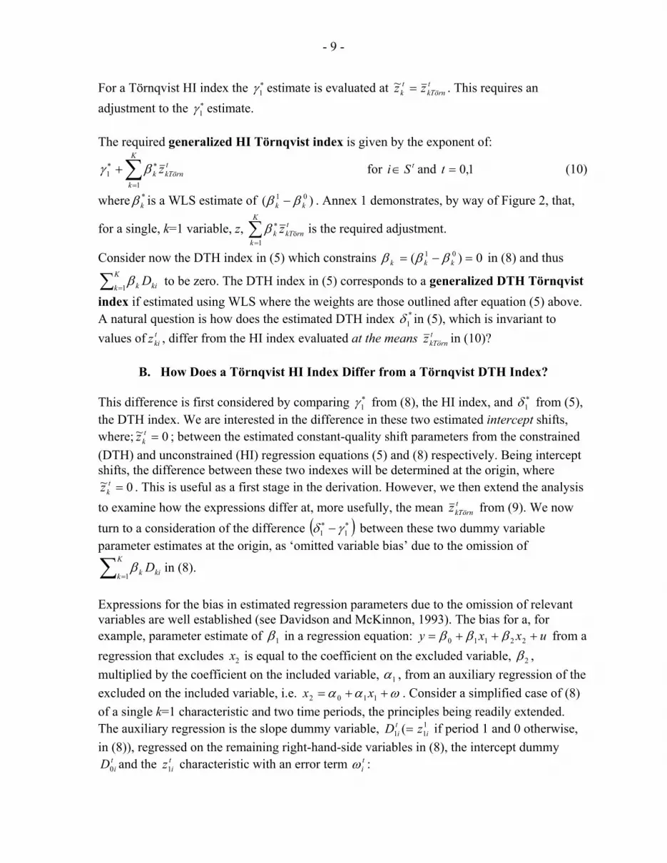
For a Törnqvist HI index the 1γ∗ estimate is evaluated at t

rnökTtk zz =~ . This requires an

adjustment to the 1γ∗ estimate.

The required generalized HI Törnqvist index is given by the exponent of:

∑=

∗∗ +K

k

trnökTk z

11 βγ for ti S∈ and 1,0=t (10)

where *kβ is a WLS estimate of )( 01

kk ββ − . Annex 1 demonstrates, by way of Figure 2, that,

for a single, k=1 variable, z, ∑=

∗K

k

trnkTk z

1öβ is the required adjustment.

Consider now the DTH index in (5) which constrains 0)( 01 =−= kkk βββ in (8) and thus

∑ =

K

k kik D1β to be zero. The DTH index in (5) corresponds to a generalized DTH Törnqvist

index if estimated using WLS where the weights are those outlined after equation (5) above. A natural question is how does the estimated DTH index *

1δ in (5), which is invariant to values of t

kiz , differ from the HI index evaluated at the means trnokTz && in (10)?

B. How Does a Törnqvist HI Index Differ from a Törnqvist DTH Index?

This difference is first considered by comparing ∗1γ from (8), the HI index, and ∗

1δ from (5), the DTH index. We are interested in the difference in these two estimated intercept shifts, where; 0~ =t

kz ; between the estimated constant-quality shift parameters from the constrained (DTH) and unconstrained (HI) regression equations (5) and (8) respectively. Being intercept shifts, the difference between these two indexes will be determined at the origin, where

0~ =tkz . This is useful as a first stage in the derivation. However, we then extend the analysis

to examine how the expressions differ at, more usefully, the mean trnökTz from (9). We now

turn to a consideration of the difference ( )∗∗ − 11 γδ between these two dummy variable parameter estimates at the origin, as ‘omitted variable bias’ due to the omission of

∑ =

K

k kik D1β in (8).

Expressions for the bias in estimated regression parameters due to the omission of relevant variables are well established (see Davidson and McKinnon, 1993). The bias for a, for example, parameter estimate of 1β in a regression equation: uxxy +++= 22110 βββ from a regression that excludes 2x is equal to the coefficient on the excluded variable, 2β , multiplied by the coefficient on the included variable, 1α , from an auxiliary regression of the excluded on the included variable, i.e. ωαα ++= 1102 xx . Consider a simplified case of (8) of a single k=1 characteristic and two time periods, the principles being readily extended. The auxiliary regression is the slope dummy variable, 1

11 ( iti zD = if period 1 and 0 otherwise,

in (8)), regressed on the remaining right-hand-side variables in (8), the intercept dummy tiD0 and the t

iz1 characteristic with an error term tiω :

- 10 -

ti

ti

ti

ti zDD ωλλλ +++= 1

0201

001 . (11)

Omitted variable bias is the product of the estimated coefficient on the omitted variable, *1β (for k=1 in (8)), and the estimated coefficient *

1λ from the above regression (11)—Davidson and McKinnon (1993). Thus the difference (before taking exponents) DTH minus HI, at the intercept is ( ) ∗∗∗∗ ×=− 1111 λβγδ . Our next concern is to derive this difference at t

Törnz1 rather than at 0~ =tkz . Since the DTH

method holds the parameter estimates constant through any value of tkz , the (log of the) DTH

index is thus given by ∗∗∗∗ +×= 1111 γλβδ . However, the (log of the) Törnqvist HI index at t

Törnz1 from (8) for one variable is estimated as:

tTörnz1

*1

*1 βγ + . (12)

Thus the ratio of the DTH and HI indexes at the intercept is ( ) ( ) ( )∗∗∗∗ ×= 1111 λβγδ expexp/exp and the DTH index is thus given

by ( ) ( ) ( )∗∗∗∗ ××= 1111 γλβδ expexpexp . The Törnqvist HI index at tTörnz1 from (8) for one variable

is estimated as: ( )tTörnz1

*1

*1exp βγ + . Thus the ratio of the Törnqvist DTH index to the

Törnqvist HI index at tTörnz1 is:

( )[ ]t

z

zt

Törn110

11

1 )(exp index HITörnqvist

index DTHTörnqvist

Törn1

−−=⎟⎟⎠

⎞⎜⎜⎝

⎛ ∗∗∗ λββM

(13)

where 11∗β and 0

1∗β are WLS estimates.

If either of the two terms making up the product on the right–hand-side is close to zero then there will be little difference between the indexes. Neither parameter instability nor a change in the mean characteristic is sufficient in itself to lead to a difference between the formulas. The )( 01

1∗∗∗ −= kk βββ from (5) is the estimated marginal valuation of the

characteristic between periods 0 and 1, which can be positive or negative, but may be more generally althought to be negative to represent diminishing marginal utility/cost of the characteristic.

C. Interpretation of ( )tz Törn11 −∗λ

Equation (13) shows us that the change in the coefficients is one factor determining difference between the two methods. The second expression, ( )tz Törn11 −

∗λ , is more difficult to interpret and we consider it here. Bear in mind that the left-hand-side of the regression in equation (11), t

iD1 , is 0 in period 0 and 11iz in period 1 and that t

iD0 on the right-hand-side is 1 in period 1 and zero in period 0. If we assume quality characteristics are positive, 1λ will always be positive as the change from 0 in period 0 to their values in period 1. Consider the

- 11 -

weighted (Törnqvist) mean 01Tornz for MSi∈ and ( )tSi ¬∈ 00 (matched period 0 and

unmatched old period 0) and 11Törnz for MSi∈ and ( )01¬∈ tSi (matched period 1 and

unmatched new models in period 1). If we assume for simplicity that 1

1Törn0

1Törn zz = , then * 11 1Törnzλ ≈ since *

1λ is an estimate of the change in t

iD1 in (11) arising from changing from period 0 to period 1, where it is 11Törnz and

has an expectation of 11Törnz . The *

1λ estimate is conditioned in (11) on tz Törn1 , the change from 0Törn1z to 1

1Törnz , but since we assume these two have not changed, our estimate of 11Törn

*1 z≈λ

holds true. Thus the second part of the difference expression in (13), ( )tTörnz1

*1 −λ , is simply

( )tzz Törn111Törn − which, given our assumption of 1

1Törn0Törn1 zz = , is equal to 0. It follows from

the right-hand side of (13), that for samples with negligible change in the mean values of the characteristics, the DTH and HI will be similar irrespective of any parameter instability. Diewert (2002) and Aizcorbe (2003) have shown that the DTH and HI indexes will be the same for matched models and this analysis gives support to their finding. However, we find first, that it is not matching per se that dictates the relationship; for unmatched models all that is required is that tzz Törn1

11Törn = which may occur without matching—it simply requires the

means of the characteristics not to change. Second, that even when the means change the two approaches will be equal if 00*1* =− kk ββ , i.e. there is parameter stability. Finally, it follows that if either of the two right-hand side expressions in (13) are large, the differences between the indexes will be compounded. But what if 1

1Törn0

1 zz Törn ≠ ? Since the estimated coefficient on 1x of a regression of y on 1x and

2x is given by: ( )

21 2 2 1 2

22 21 2 1 2

yx x yx x x

x x x x

−

−∑ ∑ ∑ ∑∑ ∑ ∑

, the estimated coefficient *1λ from (11) is given

by:

121

11

211

1111

2111*

1 )()())(,cov()(

NzzNNzzzDNNNz

tz

tti

tiz

−−−−−−

=σ

σλ (14)

for an unweighted regression where 1N and N are the respective number of observations in period 1 and both periods 0 and 1, 2

zσ is the variance of z and

( ) zzNzzD tti

ti

11211 ),cov( ∑ −= is the covariance of t

iD1 and tiz1 from (11). Readers are

reminded that from (13):

( )[ ]1Törn11

01

11 )(exp

index HITörnqvist index DTHTörnqvist

Törn1

ztz

−−=⎟⎟⎠

⎞⎜⎜⎝

⎛ ∗∗∗ λββM

. (15)

First, as noted, if there is either negligible parameter instability or a negligible change in the mean of the characteristic, then there will be little difference between the formulas. However, as parameter instability increases and the change in the mean characteristic increases, the multiplicative effect on the difference between the indexes is compounded. The likely

- 12 -

direction and magnitude of any difference is not immediately obvious. Assume diminishing marginal valuations of characteristics, so that 0)( 0*

11*

1 ⟨− ββ . Second, even assuming a positive technological advance, 0)( 1

11 ⟩− tzz , and given )( 1NN − , ),cov( 11

ti

ti zD , 1

1z and 2zσ

are positive, it remains difficult to establish from (14) the effect on *1λ of changes in its

constituent parts. However, third, as 1N becomes an increasing share of N , and at the limit if 1N takes up all of N (i.e. 0)( 1 →− NN ), then 2

11 ),cov( zti

ti zD σ→ and importantly,

tzz 111 → and the difference between the formulas tends to zero. Note that (14) is based on an

OLS estimator and for a WLS Törnqvist estimator similar principles apply, although the determining factor for a DTH index to exceed a HI index is for the weights of new models to be increasing, a much more reasonable scenario. Thus the nature and extent of any differences between the two indexes will, aside from the parameter change, also depend on (i) changes in the mean quality of models )( 1

11

tzz − , (ii) the relative number of models in each period, )( 1NN − , (iii) the dispersion in z, 2

zσ , (iv) the mean of the characteristics in period 1, 1

1z , (v) the ),cov( 11ti

ti zD which as 0)( 1 →− NN , i.e. 1N takes up all of N , then

211 ),cov( zti

ti zD σ→ and 1

11 zz = and 0*

1 =λ .

D. Treatment of Unmatched Observations

Diewert (2002) and Aizcorbe (2003) show that while the DTH and HI indexes will be the same for matched models, they differ in their treatment of unmatched data. Consider hedonic functions ( )11

ii zh and ( )00ii zh for periods 1 and 0 respectively, as in (2) and (3), and a

(constrained) time dummy regression equation (5). Consider further an unmatched observation only available in period 1. A base period HI index such as (2) would exclude it, while a current period HI index, such as (3), would include it, and a geometric mean of the two would give it half the weight in the calculation of that of a matched observation. A Törnqvist hedonic index, (4), would also give an unmatched model half the weight of a matched one. For a DTH index, such as (5), an unmatched period 1 model would appear only once in period 1, in the estimation of constrained parameters, as opposed to twice for matched data. We would therefore expect superlative HI indexes, such as (4), to be closer to DTH indexes than their constituent elements, (2) and (3), because they make symmetric use of the data.

E. Observations With Undue Influence

HI indexes, such as (2) and (3), explicitly incorporate weights. Silver (2002) has shown that weights are implicitly incorporated in DTH indexes by means of the OLS or WLS estimator used. Silver (2002) has further shown, for DTH indexes, that the manner in which the estimator incorporates the weights may not fully represent the weights, due to adverse influence and leverage effects generated by observations with unusual characteristics and above average residuals.

F. Chaining

Chained base HI indexes are preferred to fixed base ones, especially when matched samples degrade rapidly. In such a case, their use reduces the spread between Laspeyres and Paasche

- 13 -

indexes. However, caution is advised in the use of chained monthly series when prices may oscillate around a trend (i.e. ‘bounce’) and as a result, chained indexes can ‘drift’ (Forsyth and Fowler, 1981 and Szulc, 1983).

IV. CHOICE BETWEEN HEDONIC INDEXES AND DUMMY TIME HEDONIC INDEXES

The main concern with the DTH index approach as given by equation (5) is that by construction, it constrains the parameters on the characteristic variables to be the same. The HI indexes have no such constraint. Berndt and Rappaport (2001) found, for example, from 1987 to 1999 for desktop PCs, the null hypothesis of adjacent-year equality to be rejected in all but one case. For mobile PCs the null hypothesis of parameter stability was rejected in eight of the 12 adjacent-year comparisons. Berndt and Rappaport (2001) preferred the use of HI indexes if there was evidence of parameter instability. Pakes (2003), using quarterly data for hedonic regressions for desktop PCs over the period 1995 to 1999, rejected just about any hypothesis on the constancy of the coefficients. He also advocated HI indexes on the grounds that “....since hedonic coefficients vary across periods it [the DTH index approach] has no theoretical justification.” Pakes (2003: 1593). The concern over parameter instability for DTH methods is warranted. Consider constraining the estimated coefficients in a DTH index to either 1*

1β or 01*β , the index is likely to give

quite different results, and this difference is a form of “spread.” A DTH index constrains the parameters to be the same, an average of the two. There is a sense in which we have more confidence in an index based on constraining similar parameters, than one based on constraining two disparate parameters. Equation (15) showed that )( 0

11

1∗∗ − ββ was a

determining factor in the nature and magnitude of any difference between the HI and DTH indexes. However, equation (15) also showed how the ratio of DTH and HI indexes was not solely dependent on parameter instability. It depended on the exponent of the product of two components: the change over time in the (WLS estimated) hedonic coefficients and the difference in (statistics that relate to) the (weighted) mean values of the characteristic. Even if parameters were unstable, the difference between the indexes may be compounded or mitigated by the change in the other component. Note that base and current period HI indexes, (2) and (3), can differ as a result of using a constant 1

iz as against a constant 0iz . Diewert (2002) has argued that HI indexes have the

disadvantage that two distinct estimates will be generated and it is somewhat arbitrary how these two estimates are to be averaged to form a single estimate of price change. Of course Diewert (2003) also resolves this very problem by considering superlative hedonic indexes, that is by not using just the base or just the current period characteristic configurations, but a symmetric average such as (4). Yet there is a sense that in constraining the coefficients to be the same, the DTH index performs a similar averaging function, but with the parameter estimates. Rather than using a base or current period coefficient set, it constrains them to form an average. There is then the

- 14 -

question of which form of constraint is preferred: averaging the characteristic set (HI) or the coefficients (DTH)? There is much in the theory of superlative index numbers that argues for taking a symmetric mean of the characteristic quantities or value shares. The result is that HI indexes fall more neatly into existing index number theory. At least in this sense they are to be preferred, although (15) provides useful insights into their differences.

V. CONCLUSIONS

It is recognized that extensive product differentiation with a high model turnover is an increasing feature of product markets (Triplett, 1999). The motivation of this paper lay in the failure of the matched models method to adequately deal with price measurement in this context and the need for hedonic indexes as the most promising alternative (Schultze and Mackie, 2002). The paper first, developed in Section II a Törnqvist, generalized, hedonic index, that is a Törnqvist index number formula which was generalized to deal with matched and unmatched models and used hedonic regressions to control for quality changes. The paper second, considered HI and DTH indexes as the two main approaches to estimating a Törnqvist hedonic index. That the two approaches can yield quite different results is of concern. In Section III the paper provided a formal exposition of the factors underlying the difference between the two approaches. It was shown that differences between the two approaches may arise from both parameter instability and changes in the characteristics and such differences are compounded when both occur. It further showed that similarities between the two approaches resulted if there was little difference in either component. Consideration of the issue of choice between the two approaches was based in Section IV on minimizing parameter instability as a concept of spread. The analysis led to the advice that (i) either the DTH or HI index approaches are acceptable if either the parameters are relatively stable or the values of the characteristic set do not change much over time; otherwise, (ii) HI indexes are preferred when there is evidence of parameter instability. Superlative formulations, such as the Törnqvist HI index, are well grounded in index number theory and more intuitively acceptable than a DTH index, which constrains the parameters to be the same, for which there is less obvious justification.

- 15 -

- 16 - APPENDIX

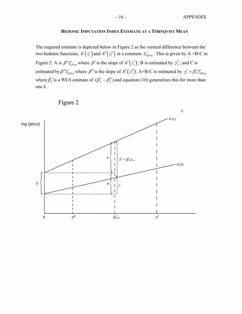
HEDONIC IMPUTATION INDEX ESTIMATE AT A TÖRNQVIST MEAN

The required estimate is depicted below in Figure 2 as the vertical difference between the two hedonic functions, ( )1 1

ih z and ( )0 0ih z at a common t

rnokTz && . This is given by A +B-C in

Figure 2. A is 1 tkTornzβ && where 1β is the slope of ( )1 1

ih z ; B is estimated by ∗1γ ; and C is

estimated by 0 tkTornzβ && where 0β is the slope of ( )0 0

ih z . A+B-C is estimated by 1 öt

k kT rnzγ β∗ ∗+

where *kβ is a WLS estimate of )( 01

kk ββ − and equation (10) generalizes this for more than one k.

- 17 -

References Aizcorbe, A., 2003, “The Stability of Dummy Variable Price Measures Obtained from

Hedonic Regressions” (Unpublished; Washington: Federal Reserve Board).

Berndt, E.R. and N.J. Rappaport, 2001, “Price and Quality of Desktop and Mobile Personal Computers: A Quarter-Century Historical Overview,” American Economic Review, Vol. 91, No. 2, pp. 268–73.

Boskin, M.S. (Chair) Advisory Commission to Study the Consumer Price Index 1996, Towards a More Accurate Measure of the Cost of living, Interim Report to the Senate Finance Committee, Washington D.C.

Cole, R., Y.C. Chen, J.A. Barquin-Stolleman, E. Dulberger, N. Helvacian, and J.H. Hodge, 1986, “Quality-Adjusted Price Indexes for Computer Processors and Selected Peripheral Equipment,” Survey of Current Businesses, Vol. 66, No. 1, January, pp. 41–50.

Committee on National Statistics, 2002, At What Price? Conceptualising and Measuring Cost-of-Living and Price Indexes, Panel on Conceptual, Measurement and Other Statistical Issues in Developing Cost-of-Living Indexes, ed. by Charles Schultze and Chris Mackie (Washington: Committee on National Statistics, National Academy Press).

Davidson, J.R. and J.G. Mackinnon, 1993, Estimation and Inference in Econometrics, (Oxford: Oxford University Press).

Diewert W. E., 2002, “Hedonic Regressions: A Review of Some Unresolved Issues” (Unpublished; Vancouver: Department of Economics, University of British Columbia).

__________, 2003, “Hedonic Regressions: A Consumer Theory Approach,” in Scanner Data

and Price Indexes, ed. by Mathew Shapiro and Rob Feenstra, National Bureau of Economic Research, Studies in Income and Wealth, Vol. 61 (Chicago: University of Chicago Press) pp.317–48.

__________, 2004, Chapters 15-20 in Consumer Price Index Manual: Theory and Practice, (Geneva: International Labour Office). Available via the Internet at www.ilo.org/public/english/bureau/stat/guides/cpi/index.htm.

__________, 2005, “Weighted Country Product Dummy Variable Regressions and Index Number Formulas,” Review of Income and Wealth, Vol. 51, No. 4, December, pp. 561–70.

Forsyth, F.G., and R.F. Fowler, 1981, “The Theory and Practice of Chain Price Index Numbers,” Journal of the Royal Statistical Society, Series A, Vol. 144, No. 2, pp. 224–47.

Griliches, Z., 1988, “Postscript on Hedonics,” in Technology, Education, and Productivity, ed. by Z. Griliches, New York: Basil Blackwell, Inc., 119–122.

Haan, J. de, 2003, “Time Dummy Approaches to Hedonic Price Measurement,” Paper presented at the Seventh Meeting of the International Working Group on Price Indices, May, 27–29 (Paris: INSEE). Available via the Internet at http://www.ottawagroup.org/meet.shtml.

- 18 -

__________, 2004, “Hedonic Regressions: The Time Dummy Index as a Special Case of the Törnqvist Index, Time Dummy Approaches to Hedonic Price Measurement,” Paper presented at the Eighth Meeting of the International Working Group on Price Indices, August, 23–25 (Helsinki: Statistics Finland). Available via the Internet at http://www.ottawagroup.org/meet.shtml.

Pakes A., 2003, “A Reconsideration of Hedonic Price Indexes with an Application to PCs,” The American Economic Review, Vol. 93, No. 5, December, pp.1576–93.

Rosen, S, 1974, “Hedonic Prices and Implicit Markets: Product Differentiation and Pure Competition,” Journal of Political Economy, Vol. 82, pp.34–49.

Schultze,C. and C. Mackie, 2002, (editors), see Committee on National Statistics, 2002, op. cit.

Silver, M., 2002, “The Use of Weights in Hedonic Regressions: the Measurement of Quality-Adjusted Price Changes” (Unpublished; Cardiff: Cardiff Business School, Cardiff University).

Silver, M. and S. Heravi, 2001, “Scanner Data and the Measurement of Inflation,” The Economic Journal, Vol. 11, June, pp.384–405.

__________, 2003, “The Measurement of Quality-Adjusted Price Changes,” in Scanner Data and Price Indexes, ed. by M. Shapiro and R. Feenstra, National Bureau of Economic Research, Studies in Income and Wealth, Vol. 61 (Chicago: University of Chicago Press) pp. 277–317.

__________, 2005, “Why the CPI Matched Models Method May Fail Us: Results from an Hedonic and Matched Experiment Using Scanner Data,” Journal of Business and Economic Statistics, Vol. 23, No. 3, pp. 269-81.

Stigler, G., 1961, “The Price Statistics of the Federal Government,” Report to the Office of Statistical Standards, Bureau of the Budget (New York: NBER).

Szulc, B. J., 1983, “Linking Price Index Numbers,” in Price Level Measurement, pp. 537–66, (Ottawa: Statistics Canada).

__________, 1987, “Hedonic Functions and Hedonic Indexes,” in The New Palgrave: A Dictionary of Economics, ed. by J. Eatwell, M. Milgate, and P. Newman (New York: Stockton Press) pp. 630–634.

__________, 1999, “The Solow Productivity Paradox: What do Computers do to Productivity?,” Canadian Journal of Economics, Vol. 32, No. 2, April, pp.309–34.

__________, 2004, Handbook on Hedonic Indexes and Quality Adjustments in Price Indexes, Directorate for Science, Technology and Industry (Paris: Organisation for Economic Cooperation and Development).

van Garderen K.R. and C. Shah, 2002, “Exact Interpretation of Dummy Variables in Semi-Logarithmic Equations,” Econometric Journal, Vol. 5, No. 1, pp.149–59.