IEEE TRANSACTIONS ON RELIABILITY, VOL. 37, NO. 1,1988 APRIL 57

Performance Indexes of a Telecommunication Network

Ali M. Rushdi, Senior Member IEEE King Abdul Aziz University, Jeddah

Key Words - Positive and complementary indexes, Mean normalized capacity, Pseudo-switching function, Map method, Reduction rule, Generalized Max-Flow Min-Cut Theorem

Rcodrr Aids - Purpose: Tutorial Special math needed for explanations: Probability Special math needed to use results: Same Results useful to: Reliability and telecommunication analysts

Abstract - Two recently proposed performance indexes for telecommunication networks are shown to be the s-t and overall versions of the same measure, vlz, the mean normalized network capacity. The network capacity is a pseudo-switching function of the branch successes, and hence its mean value is readily ob- tainable from its sum-of-products expression. Three manual techniques of conventional reliability analysis are adapted for the computation of the new performance indexes, viz, a map pro- cedure, reduction rules, and a generalized cutset procedure. Four tutorial examples illustrate these techniques and demonstrate their computational advantages over the stateenumeration technique.

I. INTRODUCTION

A telecommunication network is usually modeled by a stochastic graph G = (V , E ) (where Vand E are the sets of vertices (nodes) and edges (branches) of G) on which a set K E V is distinguished [l]. A standard index of network performance is that of network reliability which is simply a measure of probabilistic connectivity since it equals the probability that certain connections (directed or un- directed) exist in G among the nodes in K [l-51. Two im- portant special cases are those of: i) source-to-terminal (s-t) reliability for which IK( = 2 and one of the nodes in K is designated as a source, and 2) overall reliability (all- terminal reliability) for which K = V. A second standard index of network performance is that of network s-t capacity which equals the maximum flow that can be passed from a source node to a terminal node so that no branch capacity is violated, and under the assumption that all branches are working [6-91. Traditionally, each of the performance indexes of reliability and capacity is used in- dependently of the other one; whenever one is considered the other is disregarded. Recently, Aggarwal [lo] and Trstensk9 & Bowron [l 11 have proposed two new perfor- mance indexes for telecommunication networks that in- tegrate the reliability and capacity criteria. These two per- formance indexes have been computed through computa- tionally uneconomical stateenumeration procedures.

. This paper interprets the two new performance indexes in terms of certain mean capacities in the network. The Ag- garwal index [lo] is the mean normalized s-t capacity of the network, while the Trstensk9-Bowron index [ll] is simply an overall counterpart, viz, it is the mean normalized overall capacity of the network. Both are positive (direct) indexes, but other complementary (inverse) indexes can be defined. The algebraic properties of the capacity function are in- vestigated, and it is observed that once the capacity function is put in a sum-of-products (s-o-p) form, it becomes readily convertible to its mean value. Based on this observation, some of the manual techniques used in conventional reliability analysis are adapted here for the computation of the new performance indexes. This approach stresses both the similarities and differences between the two applica- tions. The first of these techniques is a map procedure that results in simple symbolic expressions for the performance indexes. However, this technique can only be applied manually to small or moderate networks. A second tech- nique applies network transformations or reduction rules in such a way that the network capacity function is preserved. These rules are straightforward to apply in the case of series- parallel subnetworks. The case of bridging branches is, however, more difficult and is handled by a function expan- sion or network decomposition. A third technique generalizes the “Max-Flow Min-Cut Theorem” [6-91 for network states X other than the ideal state (X = 1). This technique is very fast when the network minimal cutsets [12], and possibly its minimal paths [12] are known. None of the aforementioned techniques has been computerized. Nevertheless, they offer computational advantages for manual use, and the concepts of the last two techniques lay the foundations for the development of computerized algorithms that can handle complex networks.

11. ASSUMPTIONS, NOTATION, & NOMENCLATURE

Assumptions

1 . The telecommunication network is modeled by a linear graph whose nodes (vertices) are perfectly reliable and of unlimited capacities.

2. Each network branch (edge or link) can have only two states, good or failed. The branch failures are statistically independent.

3. Each network branch is assigned specific values for its reliability and capacity. The branch capacity is the up- per bound on the branch flow in either direction.

Notation

n number of branches (links) in the logic diagram of the network.

00 18-9529/88/O4OO-OO57$01 .00 0 1988 IEEE

indicator variables for successful and unsuccessful operation of branch i. These are switching random variables that take only values belonging to the bivalent discrete domain Bz = (0, l};Xi = 1 and X i = Oifiisgood,andXi = OandXi = I i f i i s failed. indicator variables for successful and unsuccessful operation of the network. Successful operation can be equivalent to connectivity, or to the satisfaction of a certain flow requirement [lo, 12, 131. reliability and unreliability of branch i: pi = Pr{Xi = l}; qi = Pr{Xi = l } = 1 -pi. Bothpi and qi take real values on the closed interval [0, 11. network reliability and unreliability; R = Pr{S =

capacity or number of channels of branch i; ci 0. n-dimensional vectors of branch successes, reliabilities and capacities: X = (XJZ ... X , f ; p

a superscript, implies transpose. state k of the network, denoted by a particular value of the n-dimensional vector X, k = 0, 1 , 2, ..., 2" - 1. capacity (effectiveness) of interconnection from node i to node j in state X. This is the maximum flow from i to j that does not violate branch capacities; Cij(X) 2 0. Since X is a binary random vector, C,(X) is a discrete random variable of a probability mass function of no more than 2" distinct values. maximum capacity (effectiveness) of interconnec- tion from node i to node j: Cum- = Cij(l) = capacity of interconnection from i to j in the ideal case when all branches are good. This maximum capacity can sometimes be achieved at certain states xk other than 1. source, terminal node. positive and complementary performance indexes of the network; L = 1 - M, 0 d L, M < 1 . The subscripts st and o may be added to either Mor L. In the high performance limit (M - 1, L - 0), L is more useful than M when expressed in the same floating-point number system. normalized s-t capacity (effectiveness) of the net- work in state X; Wst(X) = Cst(X)/Cst(l). normalized overall capacity (effectiveness) of the network in state X; *(X) = aij Wij(X); aij =

l } = E { S } , F = 1 - R , O < R , F d l .

= @1pz ... pn)T; c = (CICZ ... C?JT.

i*j

Cij(l)/ c Cij(1). i#j

CiJ@ 1 13 , CiJ@ IO,) the function Cij(X) when X, is set to 1 or 0. Meanings of Cij(X I l,, l,,,), ..., etc. follow similarly.

Nomenclature

Switching (Boolean) function S(X): A mapping B; - Bz where Bz = (0, l}, ie, S(X) is any one particular

IEEE TRANSACTIONS ON RELIABILITY, VOL. 37, NO. 1,1988 APRIL

assignment of the two functional values (0 or 1) for all possible 2" values of X [14, p 581.

Pseudo-switching (-Boolean) function C(X): A mapping B; - R where R is the field of real numbers, ie C(X) is an assignment of a real number for each of the possible 2" values of X [15, p 211.

multiaffine function: A function of several variables which is a first-degree polynomial in each of its variables. Examples of multiaffine functions in- clude:

1. Certain algebraic functions such as system reliability/unreliability as a function of compo- nent reliability/ unreliability [ 12, 161, system availability/unavailability as a function of compo- nent availability/unavailability [ 16, 171, and the mean capacity as a function of branch reliabilities.

2. Pseudo-switching functions [15, pp 21-22] such as network s-t or overall capacity as a func- tion of branch successes.

111. PERFORMANCE INDEXES

Aggarwal [lo] has proposed an s-t performance index which can be expressed in the present notation as:

The sum in (1) is taken over values of k that correspond to success states. It can as well be taken over all values of k since Ws&) = 0 for failure states. Then the states {X = xk} are exhaustive and disjoint, and hence (1) can be re- written in the form:

which means that s-t performance is measured by the mean normalized s-t capacity, ie, by the mean value of the s-t capacity normalized by its maximum.

On the other hand, Trstensky & Bowron [l 11 have in- troduced an overall performance index, which can be ex- pressed in the present notation as:

= c Cij(X)/ c Cij(1). i # j +j

(4)

Substituting (4) into (3), then interchanging the orders of the summation and expectation operators results in the following alternative expression for M,

= C aijMij. i#j

RUSHDI: PERFORMANCE INDEXES OF A TELECOMMUNICATION NETWORK

~

59

Equation ( 5 ) means that overall performance is measured by the mean normalized overall capacity, ie, it is measured by the sum of the mean values of s-t capacities when summed over all node pairs divided by the corresponding summation of their maximum values. As a result, the overall performance index Mo is simply a particular weighted average of the s-t performance indexes Mij.

Both the indexes M,, and Mo are positive or direct in- dexes; the higher M, the better the performance. The definition of Mis analogous to that of traditional direct in- dexes such as reliability and availability. Complementary indexes L whose definition parallels that of unreliability or unavailability can also be defined, such that if L is lower, the performance is better, namely:

Lst = 1 - Mst = E{ 1 - Wst(X>},

Lo = 1 - Mo = E{l - *(X)}.

(6)

(7)

Trstensk9 & Bowron [l 11 have characterised the scat- ter of q(X) around Mo by the variance:

var{*(X)} = c k ( * ( X k ) - Mo)’ Pr{X = x k }

= E{P(X)} - Mb. (8)

Eq. (8) is a correction of (4) in [ll]. The scatter of (1 - q(X)) around Lo is characterised by Var{ 1 - q(X)} which is given also by (8). Similarly, the scatter of W,,(X) around M,, is:

vu{ wst(X)} = c k ( W s t ( X k ) - Mst)’ Pr{X = x k }

= E{ W%W} - M;t, (9)

while the scatter of (1 - W,,(X)) around L,, is character- ised by Var{ 1 - Wst(X)} = Var{ Wst(X)}.

IV. CAPACITY AND ITS MEAN The source-to-terminal capacity as a function of com-

ponent successes Cij(X) is a real-valued function of binary arguments, and hence it is a pseudo-switching function that obeys the algebraic decomposition formula:

Cij(X) = Cij(X 103 + [Cij(X 113

- Ci,QlIOl)]X,, P = 1,2, ..., n. (10)

Eq. (10) can be easily proved by perfect induction over all possible values of X, namely, { X IOr} and {X 1 If}. It means that Cij(X) is a multiaffine function. Hence C,@) can always be written in a sum-of-products (s-o-p) form. Furthermore, Cij(X) is completely specified by the 2” coef- ficients Ci&) corresponding to the 2“ values X k that its argument X takes. Consequently, C,@) can be conve- niently expressed in the form of a truth table or a Kar- naugh map of real entries.

If the random function Cij(X) is written in s-o-p form, then its mean value

can be &rived from it directly by replacing the arguments X , and X , by their means pr and qr respectively, viz,

Cij(X) (s-o-p) {*, 9 x r } .-. {pr2 qr} +E{ C,} (p) (s-o-p).

Eq. (1 1) results immediately from the fact that the mean of a sum is the sum of means, and the assumption that the X;s are statistically independent.

Not only the capacity Cij(X) but also the capacity squared C$(X) is a pseudo-switching function. Therefore, C$(X) can also be put in s-o-p form, so that it becomes readily convertible into its mean:

C$(X) (s-0-p) ~ {*r 3 z r }

-

(1 1)

{Po qr), E{ C:.} @) (s-0-p)

(12) On account of (11) and (12), the problem of finding

the mean of the capacity and its variance reduces to that of expressing the capacity itself and its square in s-o-p forms.

V. A MAP PROCEDURE

The pseudo-switching function Cij(X) can be specified by a modified Karnaugh map. The map variables are the elements of X and the map entries are the real numbers c,&) which represent the s-t capacity for states x k , and hence are not necessarily 1’s and 0’s. These numbers can be obtained individually or collectively via any of the pro- cedures in sections VI and VII. To express Cij(X) in an almost minimal s-o-p form, it is necessary to cover the nonzero entries of the map by the smallest possible number of map loops. Each of these loops should be the largest that combines 2’ {i = 0, 1 , 2, ..., n} adjacent cells of the map containing as a minimum a certain (so far uncovered) value. The contribution of such a loop to the s-o-p expres- sion of C,(X) equals its covered value multiplied by the usual loop term. To allow for the choice of larger loops, a cell entry may be partitioned into several values to be covered by several loops. Such a partition is usually possi- ble for integer-valued entries in maps describing small-size networks. Once a portion of an entry is covered, that entry is replaced by its uncovered portion. In particular, if an en- try is totally covered, then it is replaced by a zero. The pro- cedure terminates when all entries in the map become 0’s.

The above map procedure results in capacity expres- sions that are simpler than those obtained by the direct stateenumeration method in [lo]. It is particularly useful when the map entries belong to a small set of integral values, which is usually the case when the branch capacities are integer valued. Though the map procedure suffers the limitation that it is capable of handling only small net- works (of six branches or less), it can be extended to handle moderate networks through the use of variable-entered Karnaugh maps (VEKMs) [ 181.

Example I

This example applies the map procedure to the net- work discussed in [lo]. This network is shown in Figure 1 and its branch capacities are:

IEEE TRANSACTIONS ON RELIABILITY, VOL. 37, NO. 1,1988 APRIL 60

c = [lo 4 5 3 4IT.

"1

"3

"4

-xj - \ x 3 x I x 6 -x, -

Fig. 3. A 2-Step Map Procedure to Cover the Pseudo-Switching Function c14P).

The pseudo-switching function c14@) can be converted in- to the switching function of success &4@) by suppressing all non-unity numerals and replacing the arithmetic operators { +, *} by their logic counterparts, viz,

Fig. 1. A 5-Branch Bridge Network. s14@) = X5(X2 u X12&3)

u X4(Xl u x lX&35>. (15)

If all branches have the same reliability p and unreliability q, then

E{C14}@) = 4P2(1 + qp) I i' + 3p2(1 + q2p) =p2(7 + qp(4 + 3q)).

Forp = 0.9 and q = 0.1 t- x 4 4

Fig. 2. Modified Karnaugh Map Representing the Pseudo- Switching Function CI4(X).

Figure 2 shows the modified Karnaugh map representing the s-t capacity C14@). The map has 25 = 32 cells each of which represents a particular state of the network. The

s-t capacity for the corresponding state. C14 is a nondecreasing function of X. Figure 3 illustrates a 2-step map procedure to cover the nonzero map entries. In step 1, the map entry 4 is covered for all the map cells in which either 4 or 7 appears, and these cells are left with entries of 0 or 3, respectively. Hence, the only nonzero entry in the map is 3 and this is covered in step 2. The final sa-p ex- pressions for CI4(X) and its mean are

The numerical value of M14 agrees exactly with the cor- responding value in [lo], while (14) and (16) are much simpler than their equivalents [lo; (6) & (7)l.

A minimal s-o-p expression for c:,<x) is readily ob- tained either by the map procedure to a map

figure 2 or by squaring (13) and noting that X? = Xi and X X i = 0. This expression for C?4@) and the correspond- ing one for its mean are

e , @ ) = 16X5(X2 + Xlx&3) + 9x4(x1 + ~ 1 ~ & ~ 5 )

number entered in a particular cell equals the value of the whose entries are the squares for those of the map in

+ NXlXfi5(X2 + x&3), (17)

E{C14}@) = 4p5Cpz + ~ 1 4 2 ~ 3 ) + 3p4@1 + q1p2p3q5). (14) If the branch reliabilities are all 0.9, then -

RUSHDI: PERFORMANCE INDEXES OF A TELECOMMUNICATION NETWORK 61

+ 24p2(1 + 4)) = 38.80305,

VU{ W14(X)) = 0.0612483 = (0.247484)2.

VI. REDUCTION RULES

Simple networks can be analyzed by combining branches in series and/or in parallel using both capacity and connectivity criteria. If a single branch P is character- ized by a capacity function Cgf (&), then the capacity function of n series branches is:

CiAX) = m;t"{Gj,CXt)}, (19)

while the capacity function of n parallel branches is:

n

Ci.(X) = c Cf)(Xf). f=1

Combining parallel branches is easier than combining series branches for the present general case in which in- dividual branches are described in terms of their capacity functions only. Such a case arises frequently, eg, whenever the individual branches are themselves equivalent branches resulting from previous parallel-series reductions . However, sometimes the capacity function of an individual branch can be split into a product of the numerical value c, of its capacity and the switching variable Xf of its success, ie

In this latter case, the reduction rules for series and parallel connections simplify, respectively, to

Relation (22) means that a series connection of branches described each by the ordered pair of a capacity c, and a success X, can be replaced by a single equivalent branch of a binary capacity function with capacity (min cf) and suc-

cess (fi Xe). No similar interpretation c L be given to

relation (23) for the parallel connection case, since the capacity function becomes nonbinary. Evaluation of the min function is much easier in (22) than in (19) since, in the former relation, it involves comparison of numerals while, in the latter equation, it requires the comparison of pseudo-switching functions. Eq. (19) can, however, be simplified through successive application of (10).

"4

"1 Fig. 4. A CBranch Series-Parallel Network.

A1 "2

Example 2

The reduction rules are now applied to the series- parallelnetwork discussed in [ll]. This network is given by figure 4 and its branch reliabilities and capacities are:

p = [ 0.94 0.92 0.96 0.9]',

c = [12 36 36 24 1'

= 12[ 1 3 3 2 1'.

Several s-t capacities are obtained immediately via (22) and (231, eg,

C13(X) = 12(3X2 + min{3,2}Xa4) = 12(3X2 + X&),

while others are obtained through the additional use of the decomposition rule (10):

C23(X) = 12 min{X1, 3X2 + min(3, 2 } X a 4 }

= 12 min{X1, 3X2 + =a4}

= 12 (X2 min{Xl, 3 + 2 X a 4 }

Therefore, the sum of the s-t capacities is:

62 IEEE TRANSACTIONS ON RELIABILITY, VOL. 37, NO. 1,1988 APRIL

and the maximum value for this sum is:

C Cij(1) = 24(18). i + j

Then, by (9, (8), (24), (25), the numerical values of M, and the standard deviation for q(x) are 0.9040 and 0.1733 respectively. The corresponding values in [ 1 11 are 0.8 1 and 0.17. The M value in [ l l ] might have lacked accuracy due to accumulated roundoff errors.

The previous reduction rules are restricted to series- parallel networks. They are still useful for general complex networks if bridging branches in these networks can be eliminated. Such an elimination is achievable as follows.

According to the decomposition formula (lo), the s-t capacity function Cij(x) of a certain network can be calculated in terms of the conditional capacity functions Cij(x I If) and Cij@ IOt). The function Cij@ (0,) can be viewed as the capacity function for a subnetwork derived from the original network by opening a keystone branch P. The function C,(X ( lf), however, cannot be viewed similarly as the capacity function for a subnetwork derived from the original network by “shorting” the keystone branch P. In fact, if the keystone branch is perfect, it can- not always be “shorted” since it retains its limited capaci- ty. A similar difficulty has been observed in the application of Bayes decomposition to oriented networks [19], since a perfect oriented branch cannot be “shorted” because it re- tains its orientation.

The foregoing discussion does not rule out the utility of network decomposition for capacity computations, but should serve as a cautionary remark against the indiscrimi- nant “shorting” of branches whenever this decomposition is used. If certain branches are assumed perfect in some subnetwork, then the capacity function for the subnetwork should be found first, while these branches are present, and later this function can be simplified by setting to 1 the indicator variables for the perfect branches.

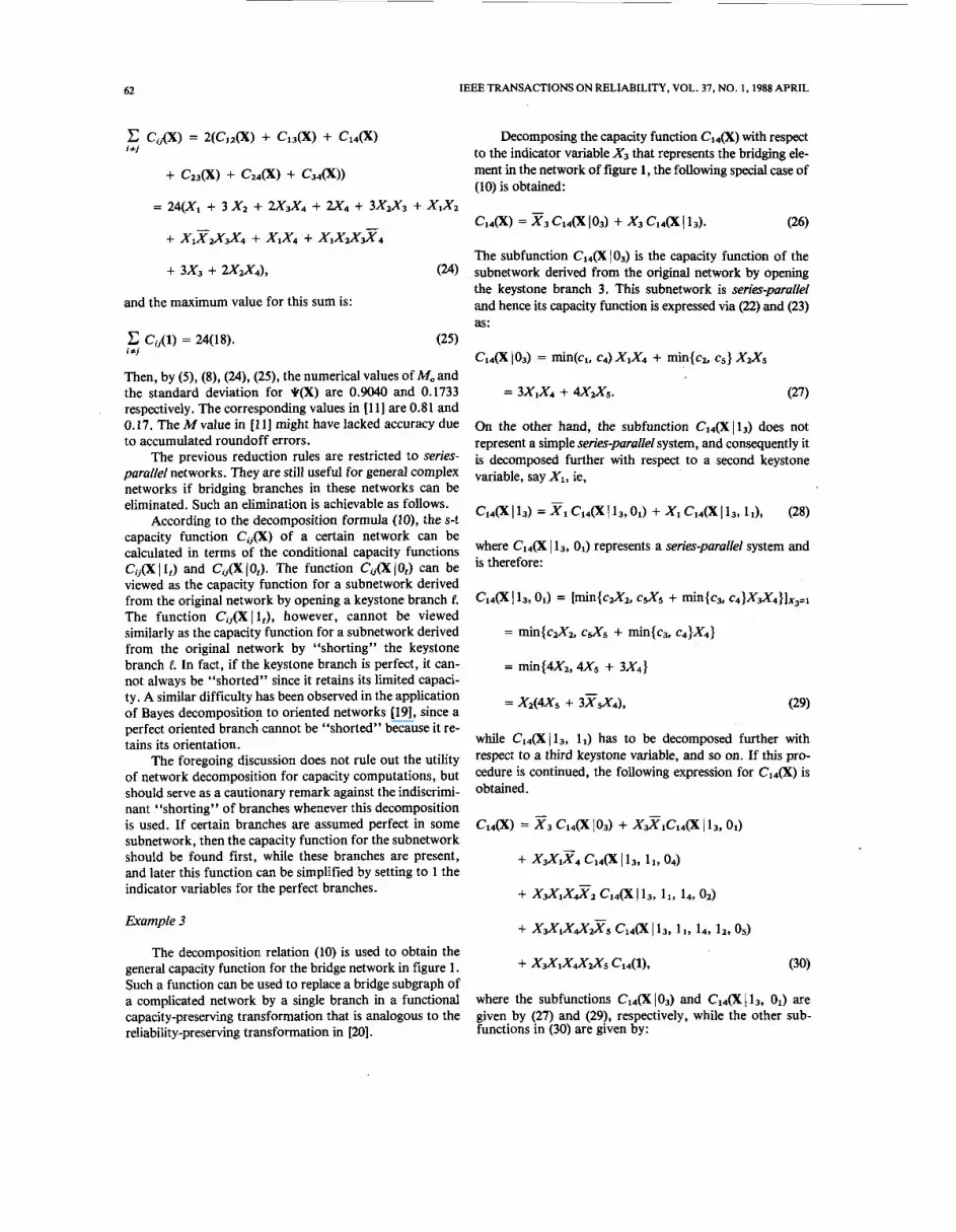
Decomposing the capacity function &(x) with respect to the indicator variable X3 that represents the bridging ele- ment in the network of figure 1, the following special case of (10) is obtained:

The subfunction c14@ 10,) is the capacity function of the subnetwork derived from the original network by opening the keystone branch 3. This subnetwork is series-parallel and hence its capacity function is expressed via (22) and (23) as:

On the other hand, the subfunction c 1 4 ( x I 13) does not represent a simple series-parallel system, and consequently it is decomposed further with respect to a second keystone variable, say Xl, ie,

where c14(x I 13, 01) represents a series-parallel system and is therefore:

= rnin{cat c& + min{cs c4}X4}

= min{4X2, 4X5 + 3X4}

while c14(x I 13, 11) has to be decomposed further with respect to a third keystone variable, and so on. If this pro- cedure is continued, the following expression for c14(x) is obtained.

The decomposition relation (10) is used to obtain the

Such a function can be used to replace a bridge subgraph of a complicated network by a single branch in a functional capacity-preserving transformation that is analogous to the reliability-preserving transformation in [20].

general capacity function for the bridge network in figure 1 . + xalxZ&5 c14(1), (30)

where the subfunctions c14(x103) and c14(xl13, 01) are given by (27) and (29), respectively, while the other sub- functions in (30) are given by:

RUSHDI: PERFORMANCE INDEXES OF A TELECOMMUNICATION NETWORK

= min(4X5,4X2 + 5 ) = 4X5, (31)

= min(l0, 3 + min(5, 4)X5)

= 3 + 4x5, (32)

= min(3,lO + min(4,5)) = 3,

(33)

c14(1) = min{cl + cz, c4 + c5, c1 + c3 + c5, cz + c3 + c4)

= min{ 14,7, 19, 12) = 7. (34)

The subfunctions in (30) correspond to the set of disjoint and exhaustive keystog terms x , Xxl, Xzlx4, X S l X 3 , xd1x&&5 and X&,X&&. Therefore, they can conveniently be used to yield the entries of the map cells in Figure 2. All of these subfunctions represent simple subnetworks, and are therefore obtained through series-parallel reduction rules, with the only exception of C14(1) which is obtained via the “Max-Flow Min-Cut Theorem” [6-91.

V. A GENERALIZED CUTSET PROCEDURE

One of the important problems in flow or capacitated networks is the problem of maximum flow, which is simply the problem of finding the maximum number of flow units from the source node to the terminal node so that no branch capacity is violated. An implicit assumption in that problem is that all network branches are good, ie, the net- work state is X = 1 and the maximum flow is actually equal to C,,(l). An elegant approach for solving the max- imum flow problem is the maximum flow algorithm of Ford & Fulkerson [a-91. A corollary of this approach is the “Max-Flow Min-Cut Theorem”, which can be generalized for all network states as follows

(35)

where Mi is the set of branches constituting the minimal s-t cutset number i for the network [12]. Eq. (35) includes the series and parallel reduction rules of the previous section as special cases.

To facilitate the computation of C,,(X) via (39, it is noted that C,,(X) = 0 if state X is an s-t cutset (ie, if there is no s-t connection) and C,,(X) # 0 if state X is an s-t path (ie, if there is some s-t connection). Therefore, if (Pi) is a (preferrably minimal) set of exhaustive and disjoint s-t paths, ie, if -

n

s,, = u Pj, j = 1

~

63

Pj f l Pk = 0, for a l l j f k, (37)

where S,, is the indicator variable of s-t success (s-t connec- tivity) [12, 181, then Cs,(X) is:

n-

Eq. (38) can be proved by the repeated application of the decomposition rule of (10). The subfunctions Cst(X /Pi = 1) in (38) are to be obtained by substituting (X /Pi = 1) for X in (35).

Example 4

The problem of example 3 is now reworked by the generalized cutset procedure. The network of figure 1 has 4 minimal cutsets, namely

Ml = (1,211 Mz = (4,513 M3 = (1 ,3 ,5)

m d M 4 = (2, 3, 4).

Therefore, (35) takes the form -

= min(lOX1 + 4X2, 3X4 + 4X5, loxl + SX3

which can be successively simplified by decomposition about various keystone variables in accordance with (10). Otherwise, (38) can be used. A set of exhaustive and dis- joint s-t paths for the network is -

(PI = x1X4~ P z = xlXfi5, P3 = xlxZz&5,

P4 = XlX2XX&5, P S = X1xaz4m. Therefore, the subfunctions in (38) are obtained via (39) as-

= min(l0 + 4Xz, 3 + 4X5, 10 + 5X3 + 4X5,4X2

+ 5x3 + 3)

= 3 + X5 min(7 + 4Xz, 4, 11 + 5X3, 4x2 + 5x3)

64

c14m

c14G

These I Ss, = 0) = 0, be used to fill in the map entries in

Figure 2. They can also be substituted into (38) to yield the relation

which can be shown to be equivalent to the more compact form in (13).

ACKNOWLEDGMENT

I thank the referees and the Editor, Dr. Richard Kowalski, for their helpful comments.

REFERENCES

T. Politof, A. Satyanarayana, “Efficient algorithms for reliability analysis of planar networks-A survey”, IEEE Trans. Reliability, vol

C. L. Hwang, F. A. Tillman, M. H. Lee, “System reliability evalua- tion techniques for complexflarge systems: A review”, IEEE Trans. Reliability, vol R-30, 1981 Dec, pp 416-422. V. Agrawal, R. E. Barlow, “A survey of network reliability and domination theory”, Operations Research, vol 32, 1984 May-Jun, pp 478-492. M. 0. Locks, “Recent developments in computing of system reliability”, IEEE Trans. Reliability, vol R-34, 1985 Dec, pp 425-436. B. N. Clark, E. M. Neufeld, C. J. Colbourn, “Maximizing the mean number of communicating vertex pairs in series-parallel networks”, ZEEE Trans. Reliability, vol R-35, 1986 Aug, pp 247-251.

R-35, 1986 Aug, pp 252-259.

IEEE TRANSACTIONS ON RELIABILITY, VOL. 37, NO. 1,1988 APRIL

[6] L. R. Ford and D. R. Fulkerson, Flows in Networks, Princeton

[7] E. Minieka, Optimization Algorithms for Networks and Graphs,

[8] A. S . Tanenbaum, Computer Networks, Prentice-Hall, 1981. [9] A. Tucker, Applied Combinatorics, 2nd ed, John Wiley & Sons,

1984. [lo] K. K. Aggarwal, “Integration of reliability and capacity in perfor-

mance measure of a telecommunication network”, IEEE Truns. Reliability, vol R-34, 1985 Jun, pp 184-186.

[ l l ] D. Trstenskq, P. Bowron, “An alternative index for the reliability of telecommunication networks”, IEEE Trans. Reliability, vol

[12] A. M. Rushdi, “How to handcheck a symbolic reliability expres- sion”, IEEE Trans. Reliability, vol R-32, 1983 Dec, pp 402408.

[13] S. H. Lee, “Reliability evaluation of a flow network”, IEEE Trans. Reliability, vol R-29, 1980 Apr, pp 24-26.

[14] F. J. Hill, G. R. Peterson, Introduction to Switching Theory and Logical Design, 3rd ed, John Wiley & Sons, 1981.

[IS] P. L. Hammer (Ivhescu), S . Rudeanu, Boolean Methods in Opera- tions Research and Related Areas, Springer-Verlag, 1968.

[16] A. M. Rushdi, “Uncertainty analysis of fault-tree outputs”, IEEE Trans. Reliability, vol R-34, 1985 Dec, pp 458462.

[17] E. J. Henley, H. Kumamoto, Reliability Engineering and Risk Assessment, Prentice-Hall, 1981.

[18] A. M. Rushdi, “Symbolic reliability analysis with the aid of variableentered Karnaugh maps”, IEEE Trans. Reliability# vol R-32, 1983 Jun, pp 134-139.

[19] H. Nakazawa, “Bayesian decomposition method for computing the reliability of an oriented network”, IEEE Trans. Reliability, vol R-25, 1976 Jun, pp 77-80.

(201 R. Johnson, “The Wheatstone bridge reduction in network reliabili- ty computations”, IEEE Trans. Reliability, vol R-32, 1983 Oct, pp

University Press, 1962.

Marcel Dekker, 1978.

R-33, 1984 Oct, pp 343-345.

374-378.

AUTHOR

Dr. Ali M. Rushdi; Department of Electrical and Computer Engineering; King Abdul Aziz University; POBOX 9027; Jeddah 21413; Kingdom of SAUDI ARABIA.

Au M. Rushdi (S’73, M’81, SM’84): For biography, see IEEE Trans. Reliability, vol R-34. 1985 Dec, p 462.

Manuscript TR86-001 received 1986 January 9; revised 1987 February 9.

IEEE Log Number 17959 4 T R B

“A Maximum Utility Stopping Rule for Reliability Growth Testing of One-Shot Systems.” A. Fries, E. A. Seglie 0 Inst. for Defense Analyses 0 Alexandria, Virgina 0 USA. (TR88-015)

“Non-Parametric Bayes Estimation of a Distribution Function Based on Nomination Sampling,” R. Tiwari 0 University of North Carolina 0 Charlotte, North Carolina 0 USA. (TR88-016)

“Bayes Reliability Estimation Under a Random Environment Governed by a Dirichlet Prior,” S. Kumar, and R. Tiwari 0 University of North Carolina 0 Charlotte, North Carolina 0 USA. (TR88-017)

Some Tests for Comparing Reliability Growth/Deterioration Rates of Repairable Systems,” T . Aven 0 Rogaland University Center 0 Stavanger 0 NORWAY. (TR88-018)

“Availability Formulae for Standby Systems of Identical Units Which are Subject to Preventive Maintenance,” T . Aven 0 Rogaland University Center 0 Stavanger 0 NORWAY. (TR88-019)

“A Closed-Loop Computer Program for Generating Power System Load- Point Minimal Paths Useful for Deducing Minimal Cut-Set Orders,” C. 0. A. Awosope, T . Akinbulire 0 University of Lagos 0 NIGERIA.

,

(TR88-020)

4 TR b