Equity Analysis and Valuation of Texas Roadhouse

Taylor Edwards taylor.w.edwards@ttu.edu

Slade Solcher slade.solcher@ttu.edu

Kason Wood kason.w.wood@ttu.edu

Blake Rasmussen blake.rasmussen@ttu.edu

2

Table of Contents

EXECUTIVE SUMMARY 6

INDUSTRY ANALYSIS 7 ACCOUNTING ANALYSIS 10 FINANCIAL ANALYSIS 11 VALUATION ANALYSIS 14

COMPANY OVERVIEW 16

INDUSTRY OVERVIEW 17

FIVE FORCES MODEL 21

RIVALRY AMONG EXISTING FIRMS 22 INDUSTRY GROWTH RATE 22 CONCENTRATION 25 DIFFERENTIATION 27 SWITCHING COSTS 27 LEARNING AND SCALE ECONOMIES 28 FIXED – VARIABLE COSTS 30 EXCESS CAPACITY 31 EXIT BARRIERS 33 CONCLUSION 33 THREAT OF NEW ENTRANTS 34 ECONOMIES OF SCALE 34 FIRST MOVER ADVANTAGE 35 ACCESS TO CHANNELS OF DISTRIBUTION AND RELATIONSHIPS 38 LEGAL BARRIERS 38 CONCLUSION 39 THREAT OF SUBSTITUTES 40 RELATIVE PRICE PERFORMANCE 41 BARGAINING POWER OF CUSTOMERS 41 DIFFERENTIATION 41 PRICE SENSITIVITY 42 NUMBER OF CUSTOMERS 43 CONCLUSION 44 BARGAINING POWER OF SUPPLIERS 44 SWITCHING COSTS 45 DIFFERENTIATION 45 IMPORTANCE OF PRODUCT FOR COSTS AND QUALITY 46 NUMBER OF SUPPLIERS 46 CONCLUSION 47 COST LEADERSHIP 48 ECONOMIES OF SCALE 48 EFFICIENT PRODUCTION 49 RESEARCH AND DEVELOPMENT AND BRAND ADVERTISING 50 DIFFERENTIATION 51 SUPERIOR PRODUCT QUALITY 51 SUPERIOR PRODUCT VARIETY 52

3

INVESTMENT IN BRAND IMAGE 53 CONCLUSION 54

COMPETITIVE ADVANTAGE ANALYSIS 55

COST LEADERSHIP 55 PRODUCT DIFFERENTIATION 56

INTRODUCTION TO ACCOUNTING ANALYSIS 57

KEY ACCOUNTING POLICIES 57

TYPE ONE ACCOUNTING POLICIES 58 ECONOMIES OF SCALE 58 PRODUCT QUALITY 60 BRAND IMAGE 61 TYPE TWO ACCOUNTING POLICIES 61 OPERATING LEASES 62 GOODWILL 62

ASSESS DEGREE OF POTENTIAL ACCOUNTING FLEXIBILITY 63

OPERATING/CAPITAL LEASES 64 GOODWILL 64 CONCLUSION 65

EVALUATION OF ACTUAL ACCOUNTING STRATEGY 66

PENSION PLAN 66 RESEARCH AND DEVELOPMENT 66 GOODWILL 66 OPERATING AND CAPITAL LEASING 68 CONCLUSION 69

QUALITY OF DISCLOSURE 70

QUALITATIVE MEASURES OF ACCOUNTING QUALITY 70 ECONOMIES OF SCALE 70 GOODWILL 71 OPERATING AND CAPITAL LEASING 71 QUANTITATIVE MEASURES OF ACCOUNTING QUALITY 72

IDENTIFYING POTENTIAL RED FLAGS 72

GOODWILL 72 OPERATING LEASES 72 GOODWILL 77 FINANCIAL STATEMENTS 78 BALANCE SHEET 79 INCOME STATEMENT 84 CONCLUSION 87

INTRODUCTION TO FINANCIAL ANALYSIS 88

4

RATIO ANALYSIS 88

LIQUIDITY RATIOS 88 CURRENT RATIO 89 QUICK RATIO 90 INVENTORY TURNOVER 91 ACCOUNTS RECEIVABLE TURNOVER 92 ACCOUNTS RECEIVABLE DAYS 93 CASH TO CASH CYCLE 94 WORKING CAPITAL TURNOVER 95 CONCLUSION 96 PROFITABILITY RATIOS 96 SALES GROWTH 97 GROSS PROFIT MARGIN 98 OPERATING PROFIT MARGIN 99 NET PROFIT MARGIN 100 RETURN ON ASSET 102 RETURN ON EQUITY 103 CONCLUSION 104

CAPITAL STRUCTURE RATIOS 104

DEBT TO EQUITY 105 TIMES INTEREST EARNED 106 ALTMAN’S Z-SCORE 107 INTERNAL GROWTH RATE 108 SUSTAINABLE GROWTH RATE 109 CONCLUSION 110

FINANCIAL FORECASTING 110

INCOME STATEMENT 110 DIVIDENDS FORECASTING 114 BALANCE SHEET 114 STATEMENT OF CASH FLOWS 118

COST OF CAPITAL ESTIMATION 120

COST OF DEBT 120 COST OF EQUITY 121 BACKDOOR COST OF EQUITY 124 WEIGHTED AVERAGE COST OF CAPITAL (WACC) 124

METHOD OF COMPARABLES 127

TRAILING P/E RATIO 128 FORWARD P/E RATIO 129 PRICE TO BOOK RATIO 130 DIVIDENDS TO PRICE RATIO 131 PRICE EARNINGS GROWTH RATIO 132 PRICE TO EBITDA 133 ENTERPRISE VALUE TO EBITDA 134 CONCLUSION 135

5

INTRINSIC VALUATION MODEL 135

DISCOUNTED DIVIDENDS MODEL 136 DISCOUNTED FREE CASH FLOWS MODEL 137 AS STATED RESIDUAL INCOME MODEL 140 LONG RUN RESIDUAL INCOME MODEL 142 AS STATED LONG-RUN RESIDUAL INCOME MODELS 143 RESTATED LONG-RUN RESIDUAL INCOME MODELS 145

SOURCES 147

APPENDIX 148

CAPITAL STRUCTURES RATIOS 148 PROFITABILITY RATIOS 149 LIQUIDITY RATIOS 151 METHOD OF COMPARABLES 154 COST OF DEBT AND EQUITY MODELS 157 GROWTH RATE GRAPHS 158 REGRESSIONS 159 1 YEAR REGRESSIONS 161 7 YEAR REGRESSIONS 164 INTRINSIC VALUATION MODELS 169

6

Executive Summary

Analyst Recommendation: SELL (OVERVALUED)

TXRH - NYSE (6/1/2014) Altman Z-Scores

52 Week Range $22.87 - $29.07 2009 2010 2011 2012 2013

Revenue 1.59 Billion Initial Scores 23.18 33.9 53.01 47.06 53.57

Market Capitalization 1.83 Billion Revised Scores 4.35 5.68 6.27 9.79 11.12

Shares Outstanding 69.17 Million

Financial Based Valuations

As Stated Restated As Stated Restated

Book Value Per Share 0.001 Trailing P/E 22.05 25.76

Return on Equity 15.60% 17.40% Forward P/E 23.31 26.68

Return on Assets 10.53% 10.1% Dividends to Price 30.17 30.17

PEG Ratio 15.45 22.46

Cost of Capital Price to Book 53.51 54.52

Estimated Adj. R^2 Beta Size Adj Ke Price to EBITDA 21.28 24.08

3 month 5.11% 0.42 7.68% EV/EBITDA 28.23 30.13

1 Year 5.11% 0.42 7.68%

2 Year 5.12% 0.42 7.69% Intrinsic Valuations

7 Year 5.18% 0.42 7.70% As Stated Restated

10 Year 5.14% 0.42 7.69% Discounted Dividends $20.18 N/A

Free Cash Flows $10.51 N/A

As Stated Restated Residual Income $17.16 $18.18

Backdoor Ke 10.4% Long Run Residual Income $12.99 $13.91

WACC(BT) 8.80% 9.73%

Published Beta 0.88

Lower Bound

Center Value Upper Bound

Ke 0.92% 5.90% 10.88%

Size Adjusted Ke 2.72% 7.70% 12.68%

WACC(BT) 8.31% 9.73% 11.15%

7

TXRH Historical Stock Prices

TXRH, BJRI, RT, RUTH Historical Prices

Industry Analysis

Texas Roadhouse is an upscale casual dining restaurant that operates in

the United States and 3 foreign countries. They compete with other restaurants

such as Ruby Tuesday, BJ’s Brewhouse, and Ruth’s Hospitality Group. Because

these companies have similar strategies and corporate structures, we have

chosen to use them as a sample of the restaurant industry Texas Roadhouse

competes in. Overall, the restaurant industry is growing, with sales expected to

8

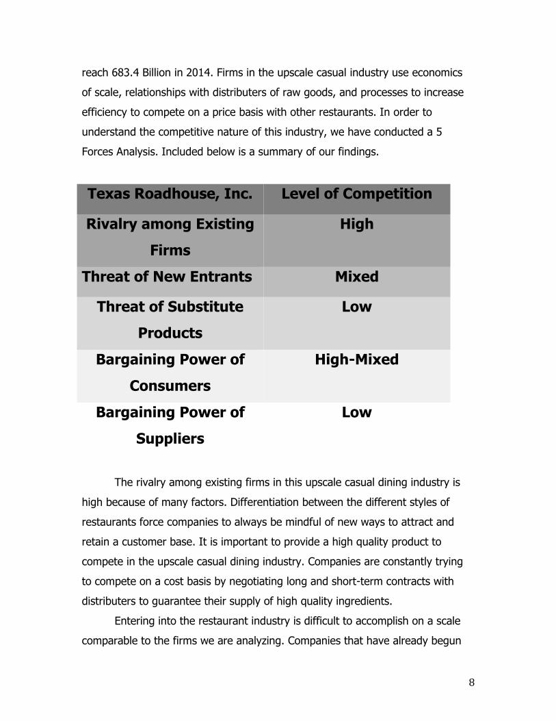
reach 683.4 Billion in 2014. Firms in the upscale casual industry use economics

of scale, relationships with distributers of raw goods, and processes to increase

efficiency to compete on a price basis with other restaurants. In order to

understand the competitive nature of this industry, we have conducted a 5

Forces Analysis. Included below is a summary of our findings.

Texas Roadhouse, Inc. Level of Competition

Rivalry among Existing

Firms

High

Threat of New Entrants Mixed

Threat of Substitute

Products

Low

Bargaining Power of

Consumers

High-Mixed

Bargaining Power of

Suppliers

Low

The rivalry among existing firms in this upscale casual dining industry is

high because of many factors. Differentiation between the different styles of

restaurants force companies to always be mindful of new ways to attract and

retain a customer base. It is important to provide a high quality product to

compete in the upscale casual dining industry. Companies are constantly trying

to compete on a cost basis by negotiating long and short-term contracts with

distributers to guarantee their supply of high quality ingredients.

Entering into the restaurant industry is difficult to accomplish on a scale

comparable to the firms we are analyzing. Companies that have already begun

9

operations at the level of these firms have a distinct cost advantage because of

economies of scale. This allows companies that are buying ingredients in huge

quantities to demand prices from suppliers that smaller businesses cannot

obtain. Also, new entrants are faced with the difficult process of negotiating

channels of distribution, while existing firms have these contracts in place. In

addition to this cost disadvantage, new entrants generally do not have the

opportunity to obtain a “first mover advantage” because of the sheer size of the

industry they are trying to enter. This is due to the small amount of room for

innovation in the restaurant industry. Finally, new entrants must be ready to deal

with the heavy regulation of the industry. Food safety, alcohol regulations, and

employee regulations can be costly to these start-ups.

The threat of substitute products in the restaurant industry is low. While it

may be more cost efficient for households to eat at home, many will simply

choose the ease of dining out over preparing meals at home.

The consumer base for the restaurant industry has significant bargaining

power over the companies we are analyzing. Customers have many options and

will choose to take their business elsewhere if a company is not meeting high

standards in quality at a bargain price.

Companies in this industry have bargaining power over their suppliers.

The companies we are analyzing all have a core group of suppliers that provide a

majority of their raw goods, but they also have a secondary network of suppliers

in place in the event of a shortage. The wide range of options to supply goods

allows firms in the restaurant industry to demand low prices from their suppliers.

Overall the restaurant industry is very competitive. By researching

disclosures by the firms in our sample industry, we have determined several Key

Success Factors for these companies. These KSFs are efficiency (cost

leadership), differentiation from other companies through superior quality and

variety, and brand image.

10

Accounting Analysis

In addition to looking at the nature of the restaurant industry, we have

also analyzed the accounting practices of Texas Roadhouse. This is necessary

because the degree of flexibility allowed in reporting by GAAP can lead a

company’s financial statements to be misleading. Firms that do not have a

credible amount of disclosure can be difficult to value because investors are

unable to see where value is being created. By evaluating their disclosure

regarding Type 1 (related to the KSFs identified above) and Type 2 (potentially

distortive) accounting policies, we have determined which areas of Texas

Roadhouses corporate structure could be misleading.

Type 1 policies, for Texas Roadhouse, cover disclosures regarding

economies of scale, product quality, and brand image. We have analyzed Texas

Roadhouse’s disclosures about their KSFs and found that they disclose

information at or above the level of the other companies in our sample industry.

Texas Roadhouse’s Type 2 accounting policies include disclosure about

their operating/capital lease structure, and goodwill. These items in their

financials are accounted for with a high degree of flexibility and were identified

as potential red flags.

Texas Roadhouse categorizes a majority of their leases as operating

leases. Because the off the book nature of these leases changes the structure of

Texas Roadhouse’s financials, we have capitalized them and provided restated

financial statements later in this report, allowing for a more accurate view of the

financial standing of the company.

Goodwill is an asset that is usually improperly impaired, causing

companies to overstate their assets and understate their expenses. We have

determined that Texas Roadhouse has not properly impaired their goodwill, so

we have also restated this on the restated financial statements provided.

Through our analysis, we have determined that Texas Roadhouse’s

disclosure in not extensive enough to provide accurate information for a

11

valuation. Because of this, we will restate the financials for this company to

account for the potential red flags we have identified.

Financial Analysis

After conducting the analysis of Texas Roadhouse’s accounting policies,

we began our financial analysis. The first step in the process was to use ratio

analysis to gain a better understanding of Texas Roadhouse’s liquidity, capital

structure, and profitability. The liquidity ratios we used are the current ratio,

quick ratio, inventory turnover, accounts receivable turnover, accounts receivable

days, cash to cash cycle, and working capital turnover. These ratios show a

firm’s ability to pay their short-term obligations, so a higher level of liquidity is

considered to show a better short-term financial standing. Below, Texas

Roadhouse is compared relative to the ratios for the other firms in our sample

industry.

12

After the liquidity ratios, we analyzed Texas Roadhouse’s profitability by

looking at sales growth, gross profit margin, operating profit margin, net profit

margin, asset turnover, return on assets, and return on equity. These ratios

show the ability of Texas Roadhouse to transform sales revenue to profit. In the

ratio analysis section of this report, we show Texas Roadhouse relative to the

other sample firms we selected. After looking at the profitability ratios, we can

conclude that Texas Roadhouse is performing at or above the level of the other

firms in our sample industry.

Analyzing the capital structure ratios for Texas Roadhouse allows us to

see how Texas Roadhouse finances their operating and investing activities. The

ratios we used are debt to equity, times interest earned, and Altman’s Z-score.

Banks and investors use Altman’s Z-score to determine a company’s likelihood of

declaring bankruptcy. Compared to the other benchmark companies, Texas

Roadhouse shows no real concerns in their capital structure ratios. Even after

financial re-statements, this company still competes on a number basis fairly well

against the competition.

13

After conducting the ratio analysis, we were able to forecast Texas

Roadhouse’s financial statements for the next 10 years. Although no forecast can

be perfect, we believe that our forecast is reasonably accurate. After determining

the forward trend of the sales growth rate by looking at the trend for Texas

Roadhouse and considering the different factors influencing the industry, we

forecasted the rest of the income statement using ratio analysis and taking past

performance into consideration. For balance sheet purposes, we used the asset

turnover ratio to calculate asset values relative to sales. Because we are valuing

the equity of Texas Roadhouse, little weight was given to the liabilities and the

remainder of our focus for the balance sheet was spent on accurately forecasting

equity. We also forecasted the statement of cash flows, but this is a very volatile

and hard to predict financial statement. Therefore, this forecast can be expected

to be less accurate than the income statement and balance sheet. All of our

forecasts took into account the restatement of Texas Roadhouse’s goodwill and

operating leases.

The final step of our financial analysis was to calculate Texas Roadhouse’s

cost of capital. Through regression analysis, we were able to estimate a beta for

Texas Roadhouse at different points on the yield curve and at different points in

time. We chose the beta with the highest R2 statistic (a measure of statistical

relevance), which was the 7 year, 36 month regression. Using a beta of .417, we

14

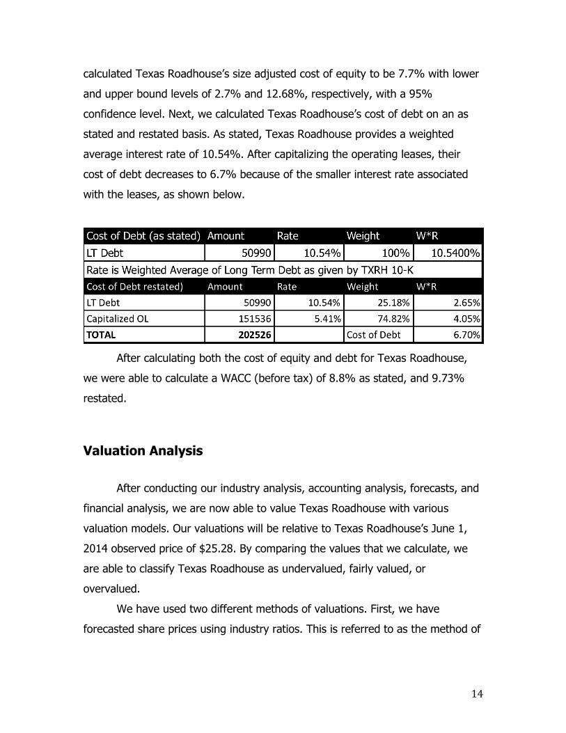
calculated Texas Roadhouse’s size adjusted cost of equity to be 7.7% with lower

and upper bound levels of 2.7% and 12.68%, respectively, with a 95%

confidence level. Next, we calculated Texas Roadhouse’s cost of debt on an as

stated and restated basis. As stated, Texas Roadhouse provides a weighted

average interest rate of 10.54%. After capitalizing the operating leases, their

cost of debt decreases to 6.7% because of the smaller interest rate associated

with the leases, as shown below.

After calculating both the cost of equity and debt for Texas Roadhouse,

we were able to calculate a WACC (before tax) of 8.8% as stated, and 9.73%

restated.

Valuation Analysis

After conducting our industry analysis, accounting analysis, forecasts, and

financial analysis, we are now able to value Texas Roadhouse with various

valuation models. Our valuations will be relative to Texas Roadhouse’s June 1,

2014 observed price of $25.28. By comparing the values that we calculate, we

are able to classify Texas Roadhouse as undervalued, fairly valued, or

overvalued.

We have used two different methods of valuations. First, we have

forecasted share prices using industry ratios. This is referred to as the method of

15

comparables. Because of the simple nature of ratio analysis as a valuation tool,

this method does not carry as much weight as our intrinsic valuation method.

The intrinsic value methods used to value Texas Roadhouse use the

forecasted financials we have calculated and provide a value of the company

based on internal information, rather than industry standards. The models we

have used to value Texas Roadhouse are the discounted dividend model, free

cash flow model, residual income model, and the long run residual income

model. Compared to the industry ratio analysis valuation method, intrinsic value

models are significantly more reliable. Our valuation places the most weight on

discounted dividend model, residual income model, and long run residual income

model because of the unreliable nature of forecasted cash flows. By using these

models and allowing a 10% cushion of fair value, we are able to come to the

conclusion that Texas Roadhouse is overvalued.

16

Company Overview

Opening in Clarksville, Indiana in 1993, Texas Roadhouse is designed to

offer a casual dinning experience to “hometown consumers seeking high quality,

affordable meals served with friendly, attentive service”(2). The company

currently operates in 48 states and 3 foreign countries with 346 Corporately

owned restaurants with an additional 74 franchises (2). Texas Roadhouse is a full

service restaurant known for its specialty seasoned and aged steaks, which are

hand-cut daily on site and cooked to order on an open gas-fired grill.

Additionally, TXRH offers guests a selection of ribs, fish, seafood, chicken, pork

chops, pulled pork ad vegetable plates, hamburgers, salads, and sandwiches (2).

A kids menu is available for children 12 & under. Lastly, guests are offered an

unlimited supply of roasted in-shell peanuts and yeast rolls which are made from

scratch (2). This variety of a menu is a critical asset to TXRH because consumers

have a variety of choices, which appeases big groups and families, as well as the

female demographic.

Entrée’s range from $8.99 - $24.99, with at least 15 meals priced under

$10.00 (2). Main items include the specialty and seasoned steaks including

6,8,11, and 16 oz. Sirloins; 10, 12, and 16 oz. Rib-eyes; 6 and 8 oz. Filets; New

York Strip; Prime Rib; and our Porterhouse T-Bone (2). These items are TXRH

showcase items in which the restaurant regularly pushes to sale. TXRH has

maintained a consistent menu over time with about 60 entrees and 90 total

menu items. Extensive studies on operational and economic implications are

conducted and considered in feedback when selecting new, and removing old,

items from the menu.

Most of TXRH restaurants feature a full bar with an extensive selection of

draft and bottle beer, major liquor brands, and specialty margaritas. Managing

partners are encouraged to stock local brewery’s and distillers in their inventory.

TXRH doesn’t push the bar atmosphere but instead a family friendly

17

environment, and consequently, alcohol sales accounted for only 11% of sales in

2013(2).

Site Selection is a volatile characteristic in which TXRH spends significant

time and resources in the evaluation process of selecting sites for future

restaurants. Evaluation key points include market demographics, population

density, household income levels, as well as site specific traits such as visibility,

accessibility, traffic generators, proximity to other retail activities, traffic counts,

and parking (2). By spending significant resources towards the selection of sites

for potential TXRH sites, the company sets the restaurant up for success by

placing locations in high traffic areas of towns where visibility, accessibility, and

customer volume is high.

To succeed in the highly competitive restaurant industry against

competitors such as BJ’s, Ruby Tuesdays, and Ruth’s Steakhouse, TXRH strives

to provide an exceptional quality product with a casual, but attentive, dining

experience.

Industry Overview

TXRH is in the fast growing, but highly competitive restaurant industry,

which is expected to reach 683.4 Billion in industry sales in 2014. This 3.6%

growth since last year is only expected to continue throughout the foreseeable

future. With over 990,000 restaurant locations in the United States, the

restaurant industry employs over 13.5 Million workers, which is about 10% of the

entire workforce in the U.S.. Specifically, Texas ranks number 2 in fastest

restaurant job growth rate projections for the next decade at 15.3%. (9) This

industry has almost tripled since 1990, and will continue to be a dominant source

of employment and GDP in the future.

18

Below is a graph of the restaurant industry sales over the past 4 decades,

a performance index from 04/2013 – 04/2014, and a growth analysis for 2014

19

20

The Restaurant Performance Index is a monthly index that tracks the

health and the overall outlook for the U.S. restaurant industry. The RPI consists

of 2 different components including the Current Situation Index and the

Expectations Index. The Current Situation Index measures the current trends in

4 industry indicators (same-store sales, traffic, labor and capital market

expenditures). The Expectation Index Measures restaurant operators’ six-month

outlook in 4 industry indicators (same-store sales, employees, capital

expenditures, and business conditions)

The companies that we have chosen to represent the overall market are

Ruby Tuesday’s, BJ’s Restaurant and Brewhouse, and Ruth’s hospitality group.

21

Five Forces Model

The five forces model is a tool for estimating profitability of a firm by

using “five forces” to interpret the intensity of competition (1). This model is a

step towards valuing a firm’s worth and determining if that firm’s stock prices are

set at the right price. The five forces that drive this model are rivalry among

existing firms, Threat of new entrants, threat of substitute products, bargaining

power of consumers, and bargaining power of suppliers. These five elements will

allow us to gather a strong understanding of the industry’s weaknesses and

strengths, while also explaining the industry’s profitability as a whole. There are

three levels of competition that can exist in an industry: high competition, low

competition, or mixed competition. All parts of the five forces model is

categorized into high, low, or mixed competition in order to understand whether

your industry is a cost leadership or differentiated industry.

Texas Roadhouse, Inc. Level of Competition

Rivalry among Existing

Firms

High

Threat of New Entrants Mixed

Threat of Substitute

Products

Low

Bargaining Power of

Consumers

High-Mixed

Bargaining Power of

Supplies

Low

22

Rivalry among Existing Firms

Rivalry among firms in the restaurant industry exists because of changes

of demand and supply in the market. When demand is high, firms in the

restaurant industry avoid competing against each other, but when demand is low

competition over customers occurs and consequently the firms must adapt their

promotions, deals, and lowering their overall prices on goods.

The companies that we decided to use to represent the overall market are

Ruby Tuesday’s, BJ’s Restaurant and Brewhouse, and Ruth’s Hospitality Group,

along with the company we are valuing, Texas Roadhouse. We chose these

companies to represent the overall market mainly because of their common

ground in market share, niche type, profit margin, and growth rate. The

important components that we will analyze to gain an understanding of the

rivalry in the restaurant industry are growth rate, concentration, differentiation,

switching costs, scale of economy/learning curve, fixed-variable costs, excess

capacity, and exit barriers.

Industry Growth Rate Industry growth rate is something that averages the growth of all the

companies in a certain industry, like the restaurant industry for example. To

maintain growth in the restaurant industry many companies have adapted their

menus, prices, overall demeanor, etc. to the consumer demand. For example,

Texas Roadhouse spends extreme amounts of time training their managers and

partners to be able to run their franchises and restaurants in a way that

increases Texas Roadhouse’s competitive advantage and ability to grow as a

company. Another example of attempt to maintain growth by companies in the

restaurant industry is Ruby Tuesday’s initiative to increase their brand value by

changing menu items to reach a larger segment of customers while also

23

attempting to reduce the debt on their balance sheet by refinancing and

extending some of their contracts on property.

Depending on whether industry growth rate is high or low market share

becomes a very important component as well, causing competitors to either steal

share from other competing companies or grow internally. The companies in the

restaurant industry steal market share from each other consistently over time by

obtaining ideal business locations, which are difficult to find. All of the companies

we chose to represent the restaurant industry are franchising companies, which

allow them to sell their branding to an individual or group, for fees, royalties, and

increased growth.

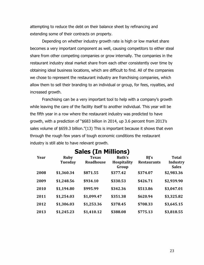
Franchising can be a very important tool to help with a company’s growth

while leaving the care of the facility itself to another individual. This year will be

the fifth year in a row where the restaurant industry was predicted to have

growth, with a prediction of “$683 billion in 2014, up 3.6 percent from 2013’s

sales volume of $659.3 billion.”(13) This is important because it shows that even

through the rough few years of tough economic conditions the restaurant

industry is still able to have relevant growth.

Sales (In Millions) Year Ruby

Tuesday Texas

Roadhouse Ruth’s

Hospitality Group

BJ’s Restaurants

Total Industry

Sales

2008 $1,360.34 $871.55 $377.42 $374.07 $2,983.36

2009 $1,248.56 $934.10 $330.53 $426.71 $2,939.90

2010 $1,194.80 $995.99 $342.36 $513.86 $3,047.01

2011 $1,254.03 $1,099.47 $351.38 $620.94 $3,325.82

2012 $1,306.03 $1,253.36 $378.45 $708.33 $3,645.15

2013 $1,245.23 $1,410.12 $388.08 $775.13 $3,818.55

24

Annual Percent Change in Sales

When comparing the sample firms, the graph shows which firms have

higher potential for continued growth, like Texas Roadhouse, and which

companies are hitting a mature stage in their time line where growth is at a

plateau, like Ruby Tuesday. Even though there is continued growth throughout

-15.00%

-10.00%

-5.00%

0.00%

5.00%

10.00%

15.00%

20.00%

25.00%

2008 2009 2010 2011 2012 2013

Ruby Tuesday

Texas Roadhouse, Inc.

Ruth's Hospitality Group, Inc.

Bj's Restaurants, Inc.

Ruby Tuesday Texas Roadhouse, Inc. Ruth's Hospitality Group, Inc. Bj's Restaurants, Inc. Total Industry Sales

2009 -8.21% 7.18% -12.42% 14.07% -1.46%

2010 -4.31% 6.63% 3.58% 20.42% 3.64%

2011 4.96% 10.39% 2.63% 20.84% 9.15%

2012 4.15% 13.91% 7.70% 14.07% 9.60%

2013 -4.66% 12.60% 2.55% 9.43% 4.76%

25

the years for the sample as a whole, the growth rate seems to have decreased

over the past two year. We believe Texas Roadhouse’s increased revenue has

been attributed to by the constant increase in number of stores, which has been

around an average of 25 each year, and the additional sales from existing

franchise owners. (2) Ruby Tuesday’s stunted growth is caused by the difficulty

of continuing to put up more restaurants to maintain a continuing stream of

growth in sales and the extinguishing of already owned properties over the past

couple of years.

The lack of growth from Ruby Tuesday and Ruth’s compared to BJ’s and

Texas Roadhouse is also because of the difference of casual dining market

compared to upper scale casual dining market. The difference in sales between

casual and upper scale casual restaurants has increased over the past years

because of the consumer idea of finding a better bargain.

Concentration The restaurant industry is a very competitive and intense setting for most

businesses, where new competition is always a strong possibility and battles over

possible new business sites and customers is constant. The restaurant industry

itself has some very large players such as Ruby Tuesday, who have over 700

restaurants active throughout the world. (3) These large players cause many

attempts by new firms to enter the restaurant industry to fall short and fail, so

even though it is somewhat easy to enter the industry itself the large players in

the industry tend to create a high failure rate of new restaurant companies.

Keeping new competitors out of the industry requires the willingness to

undercut on prices even when not undercutting on any quality of product, so

price competition is still pretty stiff even though the industry is run by big players

for the most part. Even with the big players controlling most of the market,

smaller companies every once in a while establish themselves in an effective

manner allowing them to maintain themselves in the industry. These new firms

26

can pose a threat to the existing firm’s market share and give customers another

choice when it comes to the already very competitive restaurant industry. Below

is a graph of the market share of each firm in the sample used to represent the

industry.

Market Share (Sales)

In terms of market share of the sample Ruby Tuesday and Texas

Roadhouse contain most of the market share, where Ruby Tuesday is losing

share and Texas Roadhouse is gaining share. The main reason for both Ruby

Tuesday and Texas Roadhouse having more market share than Bj’s and Ruth’s is

because of their larger number of restaurants.

As the years progress Texas Roadhouse’s gains of market share are

contributed to by the increase of restaurants being opened yearly, while the

discontinuing of restaurants contributes to the loss of market share by Ruby

Tuesday. Ruth’s, being an intensely more upscale causal restaurant, has a harder

time gathering market share because they put so much more money into the

preparation of their restaurants. BJ’s, being like Texas Roadhouse, has a steady

growth rate from putting up new restaurants at an average rate of 14

restaurants per year. (5) As demonstrated by the recent information, market

0.00%

5.00%

10.00%

15.00%

20.00%

25.00%

30.00%

35.00%

40.00%

45.00%

50.00%

2009 2010 2011 2012 2013

Ruby Tuesday

Texas Roadhouse, Inc.

Ruth's Hospitality Group, Inc.

Bj's Restaurants, Inc.

27

share is strongly influenced by the increase of new locations for the acting firm.

A firm intending to increase their concentration is completely influenced by

increasing locations and market share.

Differentiation In an industry, product differentiation can become a key part of expansion

and competitive advantage. Product differentiation is the ability of a firm to

differentiate their good and services from the rest of the firms in the same

market as them, in most cases, either based on price, quality, atmosphere, or

services. When a firm has little product difference the consumers it targets have

an option to go other firms with like products instead. Firms like Ruth’s

Hospitality Group depend on their more upscale food choices, whereas BJ’s

Brewhouse instead spends most of its resources giving its’ customers an

enjoyable service experience while still providing a relaxing and casual social

environment. (5, 4) Another example of differentiation is the way Texas

Roadhouse has its menu reviewed each year and adjusts it to customer opinions,

but also still only maintaining 60 menu items. (2) The intensity of the

competition in the restaurant industry causes product differentiation to be

important for a firm to attain leverage over their competitors, and a lack of it can

be detrimental to their success.

Switching Costs

Switching costs represent the cost of a company to go from one industry

to another industry. In the restaurant industry, if a company wants to switch

from one specific industry to a completely different industry they would have to

sell off almost all of their assets and have them completely replaced. All of the

cooking machinery, kitchens, dining areas, and other industry machinery cannot,

in most cases, be used for any other industry, so switching costs for the

28

restaurant industry can be very costly. It would be much cheaper for a company

to switch to another area in the same industry. An example would be, if a

company in the restaurant industry makes a switch to another section of the

restaurant industry such as a switch from serving in a casual setting to serving in

an upper casual setting. Since it is so expensive to switch out of the industry, the

industry itself becomes more competitive because no one can easily leave the

industry in a cost-worthy manner. The biggest risks for companies in this specific

industry is the dilution of available customers over the increasing number of

competitors and the ability of competitors to be able to switch into specific

industry niche markets in a cost conservative manner.

Learning and Scale Economies Learning and scale economies play an important part to almost every

industry because of the ability these two economies have in lowering production

costs over all. The learning economy boosts this competitive advantage inside

the restaurant industry by utilizing methods that allow for reduced waste with

resources, empowering employees, and overall increasing productivity to lower

costs. Meanwhile, when there are economies of scale, increasing the size of the

operation decreases the minimum average cost (8). In other words, the larger

the size of the production, the lower the average cost per unit will be.

Our benchmark companies utilize mainly intensive training for

management and team members as a means to increase the learning economies

in this industry. Training times can range anywhere from 7-17 weeks (2)(4)and

most of the firms have either third party training or specialized programs their

personnel can go through. Just from Ruby Tuesday’s most recent 10-K, we can

see they have at least three major training centers located around their HQ

because they believe “[their] emphasis on training and retaining high quality

restaurant managers is critical to [their] long-term success.” (2)Texas

29

RoadHouse is also willing to pay 550k on the average store on pre-opening

costs, which is consisted of mainly training and recruiting costs.

Because this industry does not revolve around low-skilled jobs that the

fast food industry needs, it makes sense that firm’s would need to invest time

and money in increasing the learning economy from training employees. Each

staff member is now an important asset that adds value, so we can conclude

that competition will arise in firms competing for quality workers.

In this industry, scale economies come into play by the amount of

restaurants each firm has opened and the total assets they have. The following

graph shows the assets of our selected key companies along with the industry

total.

We see here that the industry is growing slowly over the years, so this

means the individual firms are getting larger on average. Because the industry is

growing larger, the companies are able to open more stores which allow them to

grow even larger, provided they keep profits per store up. Below is another

graph that shows the number of stores each firm in the industry own for the past

five years.

$0

$500,000

$1,000,000

$1,500,000

$2,000,000

$2,500,000

$3,000,000

2007 2008 2009 2010 2011 2012 2013

Total Assets

Texas RoadHouse

Ruth's Hospitality Group

BJ's Restaurants

RubyTuesday

Industry Assets

30

Looking at the above graph, all but Ruby Tuesday did well as far as

opening up new restaurants. Ruby Tuesday had to close a few stores due to

losing a lot of consumer base after the financial crises of 2008 and have been

trying to find new methods to get them back. In 2013, BJ’s sales increased over

$16 million, and they attribute that increase primarily due to the opening of 17

new restaurants during the year. They also stated that if [they] do not

successfully expand [their] restaurant operations, [their] growth rate and results

of operations would be adversely affected. So expanding all operations in this

industry is key to increasing sales.

Fixed – Variable Costs

Fixed to variable costs can show how volatile a firm might be. If a firm

has a high fixed to variable cost ratio, then that means that an increase in sales

would allow the firm to be able to have far more profit in that period as opposed

to having a lower ratio due to a greater reduction in cost per unit. However, a

decrease in sales with a high fixed-variable cost ratio would mean that the cost

per unit shoots up and the firm will struggle with covering the losses if it isn’t

able to cut fixed costs.

331 345 366 392 420

152 154 153 159 161 82 93 103 130 147

901 879 846 793 783

0

250

500

750

1000

2009 2010 2011 2012 2013

Number of Stores

Texas RoadHouse

Ruth's Hospitality Group

BJ's Restaurants

RubyTuesday

31

In this industry, the firms all have a high fixed-variable cost ratio as

shown below.

The firms here show almost a 3:1 ratio of fixed costs to variable costs

which would indicate that a slight increase to sales would allow this industry to

have incredible profits; however, this would also cause the firms to increase

competition because if too many mistakes were made, profits would plummet.

Selling, general, and administrative expenses, net increased $18.4 million

(15.3%) from the prior year for Ruby Tuesday (3) which contributed to higher

fixed costs and then sales also decreased 4.6% that period, causing the fixed-

variable ratio to increase and Ruby Tuesday took a 39 million dollar loss last

year.

We can easily see that this ratio could either make or break a firm for the

year, so our conclusion is that because there is so much risk in having a higher

fixed-variable cost, this will cause price wars amongst the industry. Firms that

are able to either sell more or cut down on fixed costs will come out on top, but

there is intense competition.

Excess Capacity

Excess capacity refers to the extra space in something that hasn’t yet

been filled. In the business world this can be a very dangerous thing, because if

there is something not being used, it’s costing the firm money. Companies might

cut costs to fill that excess capacity if the customer demand in the industry isn’t

as large as what could be produced. (1)

Fixed/Variable Ratio 2009 2010 2011 2012 2013

Texas RoadHouse 1.77 1.82 1.76 1.72 1.65

Ruth's Hospitality 2.47 2.26 2.15 2.08 2.08

BJ's Restaurants 2.82 2.84 2.79 2.80 2.92

Ruby Tuesday 2.60 2.25 2.27 2.45 2.65

32

In the restaurant industry where firms don’t make a lot of mass products

to fill orders whenever they want, excess capacity comes in other forms.

Whenever there is a lull in customer traffic into a restaurant, there is a lot of

potential production that isn’t being taken advantage of because there simply

aren’t enough customers, especially if the location doesn’t have many people

living around it. For this reason, the industry won’t order more food than it

absolutely needs because there is a good chance it will have too much than the

general population demands. In order to maximize operating efficiencies

between purchase and usage, each restaurant’s Executive Kitchen Manager

determines daily usage requirements for food ingredients, products and supplies

for their restaurant. (5)

A good measurement of the excess capacity we used is the sales per

square foot ratio, and compared this to the same measurement from previous

years. This describes how efficient the area of the entire restaurant floor for all

of the industry is. The more dollars there is per square foot, the less excess

capacity. Below is our table showing the ratio from each of our benchmark firms.

Sales/Square Foot 2009 2010 2011 2012 2013

Texas RoadHouse $397.47 $406.61 $423.10 $449.97 $472.88

Ruth's Hospitality $228.90 $234.01 $241.75 $250.54 $253.73

BJ's Restaurants $626.96 $665.71 $726.33 $656.46 $635.30

Ruby Tuesday $275.05 $269.83 $296.46 $329.39 $318.07

We see there is positive growth inside this industry as the years progress

in regards to getting rid of excess capacity. Each firm is able to utilize more and

more of their space, which lowers the competition just a little bit. However, the

rate of increase isn’t very high and is comparable to the current inflation rate of

2% (14). So in actuality, there hasn’t been much growth at all and competition

for more customers will stay high as the industry fights to rid its excess capacity.

33

Exit Barriers

Exit barriers keep firms from getting out of an industry due to the high

costs that might be required to leave. Exit barriers are high when the assets are

specialized or if there are regulations which make exit costly. (1) In some cases

in an industry, it might be hard to essentially liquidate to get out because of

highly specialized equipment or material. Most companies won’t find a use for

these kinds of things unless the industry is highly competitive. If a firm can’t get

out, its only option is to compete with others more to stay alive.

In the restaurant industry, however, the overall cost to exit would be low.

This overall is a highly competitive environment to where selling off the few

specialized assets wouldn’t pose too much of a problem, and the property itself

could be easily gutted and remodeled for any other business that wants to move

in. Therefore, we conclude that because of the low cost for the exit barriers, this

would not add too much more competition to the mix since it wouldn’t be too

hard to leave the industry.

Conclusion

For the rivalry among existing firms, we conclude that competition is

extremely high. Differentiation, switching cost, the fixed-variable cost ratio,

concentration, learning and scale economies, and excess capacity all add to the

intensity of the competition. Because of the high competition, there is little room

for mistakes as just a few could cause the firms to lose a lot of competitive

advantage and go under.

34

Threat of New Entrants

The threat of new entrants into the industry analyzes the potential

barriers to entry for firms seeking to begin operations on the scale of other firms

in the industry. Many factors play into the threat of new entrants including

economies of scale, first mover advantage, relationships with channels of

distribution, and legal barriers(1). Existing firms in the industry must keep these

potential new entrants in mind when making business decisions regarding their

ability to compete. If firms find that there are few barriers to enter a market,

they must work to maintain their market share and prevent a loss of profitability

to new firms.

Economies of Scale

An economy of scale occurs when a proportionate savings in cost is

generated by an increase in production. Economies of scale can apply to both

fixed and variable costs can be affected by the size of a firm entering the

industry(1). Firms looking to enter an industry must be able to begin operations

at the same level as their competition. As seen in the charts that follow, the

firms selected as a representative of the restaurant industry have between 147

and 783 stores currently open. In addition to this, the trend with the restaurants

(with the exception of Ruby Tuesday) is to continue opening stores and

extending the scale of their business.(2,3,4,5) New entrants to the industry will

be subject to a distinct cost advantage, at least at start up in comparison to the

large firms they hope to compete with. To effectively compete at the level of the

firms in our sample industry, new entrants must be able to effectively match the

scale of their competitors while also matching the quality of food and service

their customers desire.

35

In our sample of the restaurant industry, Texas Roadhouse is the second

largest firm in terms of stores in business at 420 company and franchise stores,

behind Ruby Tuesday at 783 company and franchise stores.(2,3) Ruth’s

Hospitality and BJ’s Restaurants Inc. are approximately the same size, but BJ’s

does not have any franchisee stores at this time.(5,4)

Because these firms operate on such a large scale, they have a cost

advantage achieved by their ability to buy in large quantities and establish long

and short-term relationships with their suppliers.

Restaurant Additions 2009 2010 2011 2012 2013

Texas RoadHouse 17 14 21 26 28

Ruth's Hospitality Group 15 2 -1 6 2

BJ's Restaurants 12 11 10 27 17

RubyTuesday -44 -22 -33 -53 -10

First Mover Advantage

The first movers in an industry have the advantage of being able to set

trends for the entire industry, have a cost advantage while other firms adjust to

the new trends, and even potentially create barriers to enter into the new area of

the market.(1)

A first mover advantage can be attained in the restaurant industry by site

selection. Below is the location breakdown for Texas Roadhouse. Texas

36

Roadhouse plans to continue expansion domestically and has franchising

contracts in place to develop restaurants in the Middle East.(2) Currently, Ruby

Tuesday is the only other firm in our sample industry conducting international

operations with 44 international franchises.(3) By having an international

presence, Ruby Tuesday and Texas Roadhouse have achieved a first mover

advantage and have the ability to set the trends for the restaurant industries in

those areas.

Similarly, new entrants have the ability to gain a first mover advantage by

following these strategies or by moving into new areas domestically.

37

38

Access to Channels of Distribution and Relationships

New entrants into an industry can be deterred by the difficulty and cost of

distribution. Existing competitors usually have contracts in place with distributors,

which can limit the options for a new entrant.(1)

In our sample industry, Texas Roadhouse, Ruby Tuesday and Ruth’s

Hospitality Group rely on two to three core suppliers to meet their needs

company wide.(2,3,4) BJ’s has an agreement with “a large consortium of large,

regional food distributors” in lieu of the type of agreements in place with the

other three firms.(5) Texas Roadhouse also has local agreements to purchase

products such as dairy and select produce in the interest of freshness.(2) Texas

Roadhouse and Ruth’s Hospitality Group also have a chain of secondary suppliers

in the event there is a shortage or failure to deliver with their primary

suppliers.(2,4)

Restaurants such as those included in our sample industry use their size

to negotiate better prices from their suppliers. They also have to take into

account the quality, freshness, and large-scale availability of the products to

insure their products consistently meet the standards set by the firms and their

customers. By negotiating long and short-term deals with suppliers, restaurants

in this industry work to maintain positive relationships with distribution sources.

These relationships ease the future negation process and are beneficial for firms,

distribution sources, and consumers.

Because of the difficulty of locating and negotiating distribution channels, new

entrants to the industry may be unable to begin business on a scale large

enough to compete with the firms in our sample industry and those like them.

Legal Barriers

Legal barriers to entry are regulations or legal ramifications that could

prevent potential new entrants to the industry.(1) The restaurant industry is

39

heavily regulated by federal, state, and local agencies. Restaurants are required

to obtain permits and licensing to cover food safety, alcohol service, regulations

such as OSHA, minimum wage requirements and alcohol service, which is the

most directly related to profits.(2,3,4,5)

Both Ruby Tuesday and Texas Roadhouse attribute approximately 11% of

yearly sales to alcoholic beverages (2,3), BJ’s attributes 22%(5), and Ruth’s

Hospitality Group does not disclose their alcoholic sales, although they do state

that wine makes up 61% of their beverage sales.(4) The regulation of alcohol

sales is stringent and approval to sell such beverages can be costly (Texas

Roadhouse accounts for up to $75,000 in alcohol permitting fees when opening a

new restaurant.)(2) Such an expense could pose serious limitations to firms

seeking to enter the market.

Even more regulated than alcohol sales, food safety is a top priority for

most regulations regarding the restaurant industry. While these are not as costly

pertaining to fees involved, properly training management and workers on how

to properly abide by the regulations can pose a significant cost as well.

Entrants to the industry wishing to compete at the same level as the firms

included in our sample industry as well as those like it will face significant

regulatory barriers to begin business operations. The cost of these regulations

and the level of difficulty involved in overcoming them may prove to be too much

for many potential entrants.

Conclusion

New entrants will find that in order to begin business operations at the

level of firms such as Texas Roadhouse, Ruby Tuesday, BJ’s, and Ruth’s

Hospitality Group, there are many barriers to entry. Existing competition has a

significant cost advantage because of the sheer size of their operations. Without

the benefits of lower cost, quality ingredients, new entrants may find it difficult

to compete with these firms.

40

Another difficulty facing new entrants to this industry is that there is

limited first mover advantage, leaving room for this advantage only in new

markets. In most cases, existing firms in an area have already been established

and have a reliable customer base, leaving little room for innovation and price

setting. In some cases, the attraction of a new business may help offset this

issue, but new entrants will find that their advantage as movers will not be

significant.

Distribution among existing firms is large scale and can cause limitations

for potential entrants. New entrants will have to negotiate contracts and try to

obtain cost advantages similar to those held firms already in business within the

industry because of their existing relationships. This will be the least difficult task

for new entrants, as there are many options for suppliers in the food service

industry.

The restaurant industry is heavily regulated. These regulations can be

difficult to adhere to, as well as expensive to undertake. If new entrants cannot

properly manage the heavily regulated aspects of the business, it will be very

difficult to become a major firm in this industry.

Overall, it is very difficult to grow to the size and market share of the

firms included in our sample of the industry and those like them. Many new

entrants would be more suited to being operations on a much smaller scale.

Firms that already have an established market share and customer base have a

significant advantage over new firms trying to enter the industry.

Threat of Substitutes

Threat of Substitutes is a risk the industry faces in its products or services.

Substitutes are not necessarily the same form as existing products, but

essentially perform the same function (1). Substitutes can come from a variety

of reasons including the utilization of technology that allow consumers to use

either less, or go completely without existing products (1).

41

Relative Price Performance

In the casual dining industry they’re 2 threats of substitutes, eating in,

and quick service restaurants. Both of these substitutions are of a completely

different, and lower price point in comparison to casual dining. Fast food

customers generally pay a price of $5 to $7 a meal, while cooking in cost people

on average $1.50 to $3.00 (16).

We believe this price differentiation is a low risk to casual dining

restaurants, in that, we believe that the experience in which is being offered by

the casual dining restaurants will overcome the price differentiation. We believe

that the ease of going out will outweigh the complications faced by eating in,

and that the experience of service and attentiveness will outweigh the cost

benefit of fast food.

Bargaining Power of Customers

The bargaining power of customers refers to the power that the consumer

has relative to price and options within the market. These pressures by the

consumer force restaurants to offer a unique experience at a great value. By

having a variety of choices and low switching cost, restaurants are at the mercy

of the consumer.

Differentiation

Differentiation refers to how close one product is to its competitors. For

example, in the television industry, there is little product differentiation between

the major competitors in the market. Each product, essentially, provides the

exact same service and function.

42

The casual dining industry is the complete opposite. Within the industry

there are unlimited different options to consumers not only in terms of types of

food, but also in preferential atmosphere. Sometimes, consumers can even walk

across the street and receive the exact same type of food, but with a different

Atmosphere.

Price Sensitivity

Consumers are always looking for a valuable experience at a great price.

Price sensitivity relates to how the consumer will act when prices are lowered or

raised. In the competitive restaurant industry, since there are very few switching

costs for consumers, restaurants must remain price competitive in order to keep

market share.

From High-end all the way down to a fast food drive through, the

consumer considers a variety of factors when deciding where to eat, rather than

just personal preference. Time and dress appropriateness are non-price sensitive

factors in deciding on the level of prestige that consumers care to entice in.

Consumers with a time constraint will move towards the casual to drive through

spectrum of eating out, while consumers with no time constraints and

appropriate attire will move towards the high-end to upper casual.

In order to compete with the extremely competitive casual dining

experience, along with the excessive amounts of steakhouse competition, TXRH

has competitively set prices against major competitors in the acceptable range in

terms of quality compared to price. TXRH offers a variety of price ranges for

entrees, which start at under $10 all the way up to $24.99(2), while Ruby

Tuesdays offers entrees from $7.49 to 19.49(4). BJ’s is also competitive in this

price range, with an average check of $11 to $17(5).

43

Number of Customers

One of the most critical parts of the restaurant industry is the number of

customers the restaurant serves. With an almost 100% customer base of people

who are willing to eat out, the competition to get these customers through the

door is immense. As the price of the meal goes down, the more customer base

the restaurant is going to have. Therefore, it is imperative to capture as much of

the market share as possible within the vast scale of casual dining restaurants

available to consumers.

Since the drop in traffic since 2008, the restaurant industry has slowly

started to grow back to its original normality. Traffic has increased by 8 percent

from 2012, but overall checks totals have only increased by 1 percent (11).

Economists predict this growth will maintain stable as the markets continue to

grow. Below is a graph of the change in customer traffic at Fast Casual and

Quick Service restaurants from 2009.

44

(8)

Conclusion Although the industry as a whole is growing, the power still remains with

the consumer. This price taking market must constantly offer consumers with a

valuable price or risk being easily replaced. The high competition in the industry

is the key factor, in that consumers can easily switch restaurants if it’s deemed

that the value being offered to them is more at a competitor.

Bargaining Power of Suppliers

The bargaining power of suppliers represents the ability of suppliers to

control the price and conditions of their contracts with firms that need materials

to do business. Suppliers tend to be powerful in this regard when there are few

companies in an industry and few substitute products for customers to choose

from. (9) In the restaurant industry there tends to be a lot of give and take when

45

it comes to suppliers, some restaurants have the ability to maintain the power in

their relationships with their suppliers, while others don’t have as much freedom

and maintain one or a few specific suppliers.

Switching Costs Switching costs, when applied between firm and supplier, is the cost of a

firm to switch from one supplier to another. Depending on the amount of

suppliers in an industry, the switching costs can be quite different. In the

restaurant industry there are a good amount of suppliers, but there are some

very big ones that maintain most of the market share in the restaurant supplying

industry, like Crisco. In most cases restaurants will make contracts with multiple

suppliers for different foods and materials in an attempt to gain the best deal.

Texas Roadhouse, Inc. gathers most of their meats from five different suppliers

under contracts, while most of its other materials are gathered locally to insure

freshness. (2) Ruby Tuesday has opt-out contracts with multiple suppliers and

secondary suppliers to insure their good are to the level that they designate at all

times. (3)

Differentiation

Product differentiation, when it comes to food material, is not much

different from supplier to supplier. Most suppliers have to compete with each

other on delivery time, price, and quality of service, which causes the restaurant

industry to have some power in their negotiations with the suppliers. This also

causes suppliers to maintain quality goods to be able to compete for business.

Restaurants like Texas Roadhouse, Ruby Tuesday, and Ruth’s all maintain

contracts with multiple suppliers for meats, dairy product, etc. in order to

maintain the quality of their products and keep the supplier prices at a

46

reasonable level. (3,1,4) Since restaurants have such a high expectation of

supplied goods even small differentiation is important.

Importance of Product for Costs and Quality

In the restaurant industry product cost and quality is very important for a

competing firm. For a firm to not have a product that is up to par with the given

standards can be very detrimental to their business and in some cases illegal.

This can be a problem for suppliers because of the consumer’s standards, “If any

major supplier or distributor is unable to meet our supply needs, we would

negotiate and enter into agreements with alternative providers to supply or

distribute products to our restaurants”, so suppliers have no room for error when

it comes to their goods quality and cost. (5) Restaurants have to attempt to get

quality products for the cheapest price possible, which can’t always happen in

most cases because of certain circumstances beyond anybody’s control. For

example, if a flood hit a farm in Texas and killed most of the crops prices would

raise from lack of supply in most cases. To avoid these problems most

restaurants join into short-term contracts with specific suppliers in order to lock

in specific prices.

Number of Suppliers There are many suppliers for the restaurant industry in the United States,

which causes a lot of competition for contracts between suppliers and firms.

Since there isn’t much difference from each supplier’s raw materials, most

suppliers have to compete with price and other competitive values like service.

The number of suppliers compared to the number of firms in the restaurant

industry is somewhat smaller than in other industries mainly because there are

large amounts of suppliers while at the same time there are also large amounts

of restaurant firms. Since switching costs are so low, restaurants are able to

47

look around when it comes to picking relevant suppliers to purchase materials

from. This causes suppliers to have a major disadvantage when it comes to

negotiating with the firms.

Conclusion By examining all of these factors, assessments can be made that the

bargaining power of suppliers in the restaurant industry is relatively weak as a

whole. Switching costs for firms is relatively low because of the large number of

suppliers for the restaurant industry. The differentiation of products from

supplier to supplier is largely similar, so price and service tends to determine

which supplier gets the business from the restaurant industry firms. The volume

of firms to suppliers is relatively even, which causes competition for reasonably

scarce consumers.

Classification of Industry

Based on our findings from the five forces model, we concluded that this

industry utilizes a mixed model of cost leadership and differentiation. However,

this industry is mainly focused on the cost leadership strategies rather than

differentiation, but does pick and choose a few differentiation techniques.

Analysis of Key Success Factors

Firms within any industry will either try to become a costing leader by

lowering costs whenever they can to beat out competitors prices, or by becoming

differentiated to the point where customers are easily able to see a clear

difference between the firms and attract people that way. We will see that in the

restaurant industry, firms use a mix of cost leadership strategies and

differentiation to try to maximize their sales each year.

48

Cost Leadership

Firms that achieve cost leadership focus on tight cost controls. (1) This

means that the firms that utilize a cost leadership strategy will try to cut down on

costs wherever they can. The restaurant industry is no exception to this idea.

They will compete with each other for this almost invaluable competitive

advantage by trying to minimize expenses across the board.

Economies of Scale Economies of scale we defined earlier is when a firm increases the size of

the operation, this ends up decreasing the minimum average cost (8) For an

industry focused on cost leadership, having a lower cost is extremely important,

and the economies of scale play an important part in aiding this.

In the restaurant industry, this comes into play once again by the amount

of stores the firm has open. The idea is that the bigger the firm, the more power

it will have to open up more stores, which in turn makes the firm bigger. Below

is a table that shows the number of new restaurants opened (closed) for the past

five years.

Restaurant Additions 2009 2010 2011 2012 2013

Texas RoadHouse 17 14 21 26 28

Ruth's Hospitality

Group 15 2 (1) 6 2

BJ's Restaurants 12 11 10 27 17

RubyTuesday (44) (22) (33) (53) (10)

49

Besides Ruby Tuesday, these firms opened quite a few new restaurants,

which significantly increased the size of them overall. The increase in size gives

them a huge competitive advantage over smaller companies, which allows them

to be able to expand even further, as long as the customer base is able to

support the firms.

Efficient Production

A firm that is able to have an efficient production is able to cut costs by

not having a very high waste, or by utilizing all the resources available to it,

whether that be time, money, or materials.

Firms in the restaurant industry have to be incredibly efficient because

food supplies can either be scarce, or go bad because some items are perishable.

Service can either take a lot of time per customer, or the lack of customers will

cause an overabundance of time due to a high excess capacity. There also have

to be wise investments that will ultimately create value to the firms, which goes

across the board for all industries, and is no exception here.

Because food is generally perishable unlike metals or plastics that other

industries might produce, wastes here can be very devastating and unintentional.

Because of the relatively short storage life of inventories, a minimum amount of

inventory is maintained at our restaurants. (3) Food also loses a lot of its weight

when it is washed, pruned of all defects, and cut into shape for consumption, so

firms have to hire highly qualified chefs and food handlers to not have as much

excess scraps. BJ’s has a theoretical food cost system and automated food prep

system to measure the amount of waste and their product yields, while

increasing kitchen efficiency. (5).

Time, depending on the amount of customers, can either be in extreme

excess or extreme shortage. When a restaurant is busy, customers will take

50

longer to serve because the waiting time is increased. Either there aren’t enough

seats available, or the staff is just overwhelmed and can’t serve everybody. Food

takes a long time to cook correctly, but if the customer is kept waiting too long,

they will clearly be unsatisfied and might get impatient, which will cause them to

down value everything else in the restaurant. Texas RoadHouse implements

some sort of process to reduce customer waiting times to combat this. (2)

Overall, an inefficient firm in this industry would not last very long. Firms

can’t afford to have much waste of anything because of the high fixed costs they

have to overcome each period. So if a firm can’t invest in itself to become more

efficient, it’s not worth investing in period.

Research and Development and Brand Advertising Having little to no research and development is key to a cost leadership

focused industry. R&D can be incredibly expensive, especially because non

specialized products are generally bought up. There isn’t too much benefit in

changing something that will sell anyways. As for brand advertising, firms

generally rely on their relationship of the public alone to promote themselves.

In this industry, most of the firms do not engage in research and

development, but instead conduct inexpensive studies. Ruby Tuesday for

example, [does] not engage in any material research and development activities.

However, [they] do engage in ongoing studies to assist with food and menu

development. (3) These types of activities help the firms to control costs and

lower overall expenses.

Brand advertising is something that all our benchmark companies engage

in, but expenses are generally very low (1-3% of total revenue) for each firm.

Most of the firms use other methods as a means to attract customers. Texas

RoadHouse utilizes public relations to generate "earned media" story placement

in local, regional and national media. (2) This means that most of Texas

RoadHouse’s advertising is done by the media for free.

51

With little to no research and development and very inexpensive

advertising campaigns, this segment shows us this industry is definitely using the

cost leadership idea here. This saves the restaurants millions of dollars each

year, and allows them to put money where they think would be a better

investment.

Differentiation

A firm that is trying to have a differentiation strategy must find ways to

become unique and stand out from their competitors. For differentiation to be

successful, a firm has to accomplish three things: First, it needs to identify one

or more attributes of a product or service that customer’s value. Second, it has

to position itself to meet the chosen customer need in a unique manner. Finally,

the firm has to achieve differentiation at a cost that is lower than the price the

customer is willing to pay for the differentiated product or service. (1)

Superior Product Quality Superior product quality is very important to any differentiating company.

Having a better product than the competitors adds a competitive advantage to

where customers would want what is better for the same price they could get

elsewhere. This comes at an extra cost as opposed to a cost leadership strategy,

but might be worth it to some industries.

In the restaurant industry, where customers go to sit down to enjoy a

meal, having a high quality product is very important. As opposed to fast food,

where customers expect to pay for something cheap just to sate their hunger,

people go to restaurants expecting so much better for a higher price because of

the environment a sit down restaurant has. For this reason, firms invest a lot in

creating the best product they can. Product quality is added by the quality of the

52

actual product itself, the service that comes with it, and how the entire thing is

presented.

Texas RoadHouse for example, hand-cuts all but one of [their] assortment

of steaks and make [their] sides from scratch. In other food industries, food is

shipped in frozen, then nuked in an microwave, oven, or fryer and is basically

served immediately straight from the package. Texas RoadHouse also has a

management level employee to inspect every entrée before it leaves the kitchen

to confirm it matches the guest's order and meets [their] standards for quality,

appearance and presentation. (2) Ruth’s Chris restaurants oversees a line check

system of quality control and must complete a quality assurance checklist

verifying the flavor, presentation and proper temperature of the food and

beverages. (4) BJ’s Executive Kitchen Manager is responsible for managing food

quality and preparation. These lead to the idea that every product must be

uniform, meaning that every meal must be the same so that customers receive

the same quality every time they order.

In this industry, having high quality food is essential to making sales. If

customers don’t feel like they are receiving the best quality for their money, then

they will simply go elsewhere. Therefore, it is wise to be willing to spend the

extra money on creating something superior to ultimately add value by having

yet another benefit to competitive advantage.

Superior Product Variety Most of the time in industries, creating more than one different types of

products can be incredibly expensive; however, in some industries, having more

variety will allow customers to feel like they are being treated more personally

and will be willing to pay a little bit more for some customization of their own.

Fortunately for the restaurant industry, adding more products to menus is

relatively inexpensive compared to adding entire new product lines in major

manufacturing industries. The excess costs come from training the employees

53

how to handle each and every product available to the customer, and the special

licensing costs that might be associated with the product itself like alcohol. Firms

like Ruth’s sells over 50 different items on their menus, and offer over 200

different selections of wine and even more selections of other alcoholic drinks.(4)

Texas RoadHouse also has well over 50 different customizable options on their

menu not including alcohol, and all four restaurants have an ever changing

menu. (2)

Although an expensive investment, BJ’s even has created its own brewery

that allows it to craft a wide variety of beer that you can’t buy anywhere else.

This has allowed BJ’s to add a 9% increase in sales for 2013 from their own

brewed beer alone. So because of this, we concluded that having a superior

product variety is incredibly value adding to this industry.

Investment in Brand Image Brand image is how the customers see the company and its product. This

is essentially the firm’s reputation in society and is aided by having uniformity

between stores. For the restaurant industry, this created by having the same

theme and atmosphere across all the stores in a firm. This adds value by

allowing the customer to feel a sense of the same quality and service they will

receive at any of the locations.

Substantially all Texas Roadhouse restaurants are of [their] prototype

design, reflecting a rustic southwestern lodge atmosphere, featuring an exterior

of rough-hewn cedar siding and corrugated metal. (2) Along with this, they have

jukeboxes and host line dancing inside their restaurants, and customers can

either wait in the lounge or go to the southwestern styled bar. (2) Restaurants

typically try to look and feel the same way wherever the customer might go.

They are willing to invest to try to achieve this idea of uniformity across the

board. According to a 2003 New York Times article, Ruby Tuesday budgets

$25,000 to $50,000 for up to 1,000 refurbished antiques it will use in a

54

restaurant, because when people go out, they want more than food; they want

visual stimulation. ''It is part of the entertainment of eating out,'' said Rick

Johnson. (15)

From this, we can conclude that restaurants value having a certain

ambiance about them, that the customers can relate to and associate themselves

with the brand image of the firm. This creates a certain immeasurable value that

causes the customer to want to return at a later date, increasing sales at each

store. If each restaurant can achieve uniformity with one another, then overall

sales will increase much more as customers travel and recognize something they

are already used to.

Conclusion In general, restaurants in this industry commonly use a mix between cost

leadership strategies, and differentiation strategies. Typically, these companies

will lean towards mainly the cost leadership side of business, but will have a little

influence from differentiation techniques.

Firms save a lot of money from the cost leadership side, mainly through

their efficient production to where wastes are kept at a minimum, and the entire

lack of significant investment towards research and development or brand

advertising. They then use these savings to invest in a few differentiation ideas

like having superior product qualities, superior product varieties, and in brand

imaging. Even still, they don’t invest too much in these differentiating areas as

opposed to other companies, and so employ cost leadership strategies inside

their own differentiating strategies. Overall, we believe these key factors are

invaluable to this industry as far as making a profit goes.

55

Competitive Advantage Analysis

In order to gain a competitive advantage, firms must find sources of cost

leadership or product differentiation. In a cost leadership competitive advantage,

firms use economies of scale, efficiency, and other methods of cost-advantage to

position themselves as price takers in the industry. Product differentiation

focuses on the customer experience. Firms will provide a superior product

through quality of variety, service, or atmosphere. Firms looking to gain an

advantage through differentiation will, overall, have more focus on their brand

image and constantly improving the customer experience.

Texas Roadhouse has found a mix of these two concepts through their

Key Success Factors. Because of the high level of competition in the restaurant

industry, it is necessary for Texas Roadhouse to focus on the price setting

aspects of their competitive strategy without sacrificing the quality of product

and service they desire to provide for their customer base.

Cost Leadership

Texas Roadhouse is able to take advantage of economies of scale because

of the large scale of their businesses. With 420 company and franchise store

currently operating, they have the ability to negotiate long and short-term

contracts with suppliers that give them a cost advantage over firms that operate

on a smaller scale.

Texas Roadhouse is also able to compete on a cost leadership basis

because of their focus on efficiency. They keep little inventory on site at their

restaurants and keep highly trained butchers and chefs on staff to reduce waste

as much as possible. Texas Roadhouse also has a system in place to reduce

customer wait times when the restaurant is at capacity.

Texas Roadhouse uses these success factors to create a cost advantage

over their competitors. By combining these business strategies to position

56

themselves as price takers, Texas Roadhouse increases their profit margins and

manages their market share and competitive positioning.

Product Differentiation

Based on our research, we believe Texas Roadhouse’s main focus on

product differentiation is through the quality of their product. They hand-cut all

but one of their assortment of steaks and make their sides from scratch, as

opposed to many of their competitors who choose to cut corners by using

premade or frozen foods. Texas Roadhouse also makes sure their products meet

their production standards by having every entre leaving the kitchen inspected

by a management level employee.

In addition to product quality, Texas Roadhouse also offers a wide variety

of menu items to their customers. They have well over 50 different customizable

options on their menu not including alcohol, and feature an ever-changing menu.

Texas Roadhouse places a large emphasis on the development of their

brand image and the atmosphere that their customers experience. Substantially

all Texas Roadhouse restaurants are of [their] prototype design, reflecting a

rustic southwestern lodge atmosphere, featuring an exterior of rough-hewn

cedar siding and corrugated metal. (2) Along with this, they have jukeboxes and

host line dancing inside their restaurants, and customers can either wait in the

lounge or go to the southwestern styled bar. (2)

57

Introduction to Accounting Analysis

After examination of the industry overview based off of the five forces

model, we will continue on to the accounting analysis. In the accounting analysis

we will take a look at key accounting policies, assess the degree of potential

accounting flexibility, evaluate actual accounting strategy, and Identify potential

red flags of Texas Roadhouse. When looking into the accounting policies of the

company we will attempt to find key accounting policies and connect them to key

success factors described in the industry analysis. After identifying key

accounting policies we will assess the degree of potential accounting flexibility,

which represents the industry’s ability to choose accounting policies such as

estimates and requirements for disclosure and placement of specific items on

financial statements. Once we have assessed the degree of potential accounting

flexibility we will evaluate actual accounting strategy, which involves how they

present their financials based on the flexibility of their accounting policies and we

will then identify potential red flags in the financial statements. Using the

information we gather from the accounting analysis of Texas Roadhouse we will

then undo any accounting material that is materially distortive to the financial

statements.

Key Accounting Policies

Analyzing a firm’s key accounting policies provides insight into the

business and industry that can be obscured by financial statements. Because the

accrual accounting system records net income based on expected, rather than

actual transactions, a firm’s financial information can be distorted. (1)

There are two types of key accounting policies. Type One covers the

presentation and disclosure of information about the Key Success Factors we

discussed earlier and look at the industry as a whole. Type Two covers

58

potentially distortive items on an individual firm’s balance sheet such as

intangible assets and leases. By analyzing these accounting policies, we will have

a better understanding of the financial standing of Texas Roadhouse and the

other firms in our sample industry.

Type One Accounting Policies

Type One accounting policies will look into the disclosure of the firms in

the sample industry regarding the Key Success Factors. In the case of Texas

Roadhouse, those factors are economies of scale, product quality, and brand

image among others. These factors also apply to the other firms in our

representative sample of the industry.

Economies of Scale

Texas Roadhouse and the other firms in our sample industry are able to

utilize economies of scale to achieve a cost advantage over smaller firms because

of the large scale of their operations. Shown below is the number of stores each

firm is operating along with their increases over time. Operating on this scale

allows the firms to achieve a cost advantage as discussed in the Key Success

Factors section. Texas Roadhouse, Bj’s, and Ruth Chris all show steady growth

while Ruby Tuesday has been closing stores in bulk.

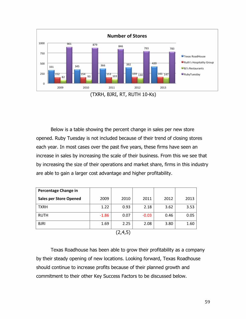
59

(TXRH, BJRI, RT, RUTH 10-Ks)

Below is a table showing the percent change in sales per new store

opened. Ruby Tuesday is not included because of their trend of closing stores

each year. In most cases over the past five years, these firms have seen an

increase in sales by increasing the scale of their business. From this we see that

by increasing the size of their operations and market share, firms in this industry

are able to gain a larger cost advantage and higher profitability.

Percentage Change in

Sales per Store Opened 2009 2010 2011 2012 2013

TXRH 1.22 0.93 2.18 3.62 3.53

RUTH -1.86 0.07 -0.03 0.46 0.05

BJRI 1.69 2.25 2.08 3.80 1.60

(2,4,5)

Texas Roadhouse has been able to grow their profitability as a company

by their steady opening of new locations. Looking forward, Texas Roadhouse

should continue to increase profits because of their planned growth and

commitment to their other Key Success Factors to be discussed below.

60

Product Quality

In this industry, having high quality food is essential to making sales. If

customers don’t feel like they are receiving the best quality for their money, then

they will simply go elsewhere. Texas Roadhouse divulges their techniques to

ensure quality in their annual report. They “hand-cut all but one of [their]

assortment of steaks and make[s their] sides from scratch.” In addition to this,

Texas Roadhouse “also has a management level employee to inspect every

entrée before it leaves the kitchen to confirm it matches the guest's order and

meets [their] standards for quality.” (2)

In addition to in-store efforts to ensure quality, Texas Roadhouse and

their competitors maintain relationships with distributers who supply them with

the high quality food necessary to have a superior quality. In addition to their

relationships with nationwide vendors, these firms also have contracts with local

suppliers to purchase products such as dairy and select produce in the interest of

freshness. (2,3,4)

Texas Roadhouse also shows a commitment to training their management

and key employees to ensure everything runs smoothly in their restaurants.

“Managing and market partners are generally required to have significant

experience in the full-service restaurant industry and are generally hired at a

minimum of nine to 12 months before their placement in a new or existing

restaurant to allow time to fully train in all aspects of restaurant operations. All

managing partners, kitchen and service managers and other management team

members are required to complete a comprehensive training program of up to 17

weeks, which includes training for every position in the restaurant. Trainees are

validated at predetermined points during their training by either the market

partner, product coach or a training manager or service coach.” (2) BJ’s focuses

on ”recruiting and training qualified managers and hourly employees to

correctly operate [their] new restaurants,” and Ruby Tuesday sends key

employees to the Ruby Tuesday Center for Leadership Excellence to ensure their

61

restaurants are in good hands. (3,5)

By working to maintain superior product quality, the firms in our sample

industry add value to their business. Adding value in this way allows them to

charge a premium on their goods and increase their profitability.

Brand Image

Texas Roadhouse and the other companies in the casual dining industry

have a large focus on the atmosphere customers experience in their restaurants.

For example, “The atmosphere of Texas Roadhouse restaurants is intended to

appeal to broad segments of the population, children, families, couples, adults

and business persons. Substantially all Texas Roadhouse restaurants are of our

prototype design, reflecting a rustic southwestern lodge atmosphere, featuring

an exterior of rough-hewn cedar siding and corrugated metal. The interiors

feature pine floors and stained concrete and are decorated with hand-painted

murals, neon signs, southwestern prints, rugs and artifacts.” (2) As a value

added activity, the disclosure of these parts of the business relies on Goodwill,

which is addressed in the next section.

Type Two Accounting Policies

Potentially distortive items on a company’s financial statements can lead

to large over or understatements of economic performance. These items,

including goodwill, leases, benefit plans, and R&D, have a high degree of

flexibility in how they are recorded. Because of the flexible accounting standards

for these items, managers can potentially use them to distort a firm’s financial

statements. Texas Roadhouse and the other competitors have goodwill and

operating leases as significant items in their financial statement, so these

accounts will be discussed below.

62

Operating Leases

Under GAAP, firms are able to record lease liabilities in two ways.

Operating leases have the potential to lead to an understatement of their lease

liabilities on their financial statements because of their off-book nature. Capital

leases, on the other hand, are presented as a capitalized asset and depreciated

over the life of the lease. When a firm classifies a lease as an operating lease, it

is not recorded as an asset, but as an expense such as rent.

All of the companies in our sample industry utilize operating leases to

record a majority of their lease obligations. These leases will be restated later in

this report, reflecting the distortion in earnings caused by understating both

assets and liabilities.

Goodwill

Goodwill is a reflection of the premium a firm would have to pay to

acquire a firm based on competitive advantage or another intangible asset.

(Goodwill = Purchase Price – Fair Market Value) The main issue with having

goodwill on the books as an asset is that firms fail to properly impair it over time.

Most companies hold goodwill as an asset for much longer than a competitive

advantage would reasonably last in an industry.

The chart below shows the impairments that should have been recorded

from 2008-2013 for Texas Roadhouse as well as the restated balance of goodwill

assumong a life of four years. This shows that goodwill has been largely

overstated, resulting in an overstatement of earning because of the lack of

impairment of goodwill.

63

Assess Degree of Potential Accounting Flexibility

The degree of accounting flexibility varies from industry to industry, and

not all firms have equal flexibility in choosing their accounting policies and

estimates (1). If managers have little flexibility in the accounting policies and

estimates related to the company’s key success factors, accounting data is likely

to be less useful in understanding the firms economics. However, if managers

have more flexibility in choosing their policies and estimates, accounting data has

the potential to be informative and useful towards understanding the business as

a whole. This flexibility is not always proactive, in that it can lead to companies

misleadingly producing financial statements.

Companies within the restaurant industry have flexibility in terms of how

they report their Operating/Capital leases, defined pension plans, goodwill, and

research and development. However, for Texas Roadhouse, only

Operating/Capital leases and goodwill will be subjected to financial flexibility for

64

the purpose of this analysis. This is because research and development is not a

critical factor in the industry, while goodwill and leases play a prominent role in

the restaurants financial statements.

Operating/Capital Leases

Operating and Capital leases are one of the most flexible accounting items

that companies can misrepresent. For the capitalization of lease agreements,

companies will recognize the present value of the minimum lease payments, and

then record it again as an asset on the books (7). However, if a company

chooses to sign operating leases, the company simply records the lease

transaction as an operating expense, which is a decrease in the cash flow from

operations (7).

Texas Roadhouse has both Operating and capital leases in its operations.

For 2013, TXRH paid $24,539,400 in operating leases and $117,000 in capital

leases. The importance of these numbers and how they relate to our accounting

analysis will be discussed later in this segment.

Goodwill

Goodwill is an intangible asset that arises from the merging or acquisition

of another company. This intangible asset is recorded at the value of the excess

of the purchase price over the fair market value of the equity gained minus the

assets and liabilities gained. In other words, it is the premium that a company

paid on the acquisition of another. Goodwill is used to measure a competitive

advantage gained on the acquisition of another company.

Because this asset is intangible and subjective, company’s can overstate

the actual value of this account by choosing not to impair it. By doing this, a

65

company is overstating its assets, understating its expenses, and overstating

their net income. Goodwill should be impaired on a basis of fair market value, in

that it should be reported on the balance sheet as it is economically worth.

For 2013, Texas Roadhouse reported over 116 Million worth of goodwill,

which is 13.3% of its total assets. Below is a graph illustrating the value of

goodwill TXRH has reported from 2007.

Conclusion

There are many different ways in which a company can distort their

financial statements and report earnings that may be misleading. However, as a

casual dining company, there is little amount of flexibility in how managers

choose to report certain items.

66

Evaluation of Actual Accounting Strategy

Companies will either use an aggressive or a conservative accounting

strategy in the books based on the incentives management might have at that

time. An overall aggressive strategy shows a higher income to its investors by

overstating assets and retained earnings, while a conservative approach

overstates liabilities which lower its earnings. Firms that are more aggressive

aren’t doing as well as they say they are while the conservative ones should be

doing better than what they claim. Both, however, add a clear distortion to the

actual value of the firm.

Pension Plan

Texas RoadHouse does not offer its employees a pension plan and is

therefore not relevant to the accounting strategy.

Research and Development

Research and Development does not account for more than 20% of

operating income and is therefore not relevant to the accounting strategy.

Goodwill

Goodwill is measured as the excess of the cost of the purchase over the

fair value of the identifiable net assets (assets less liabilities) purchased. (7) This

is an intangible asset that if not impaired properly, will cause an overstatement

of assets.

Due to the fact that this is not a tangible asset, firms can choose whether

or not to impair goodwill for that term. Firms that use an aggressive accounting

strategy will choose not to write off goodwill and instead delay the process

because impairment is inherently subjective. (2) This allows the firm to show a

higher earnings for the period since a write off would take away from the

67

operating income, giving firms an incentive to delay impairment until an

opportune time. To measure if goodwill is being used aggressively, we took the

goodwill for each of our benchmark firm’s years over their total property, plant

and equipment. Below is a graph that expresses this.

We believe that companies with over 20% of goodwill compared to

property, plant, and equipment most likely have an aggressive accounting

strategy as opposed to the ones that do not. Both Texas Roadhouse and Ruth’s

Hospitality Group has well over 20% a few of the years on the graph, whereas

BJ’s and Ruby Tuesday are extremely low instead. Ruby Tuesday impaired all of

its goodwill in 2013, which shows a very conservative approach, (3) while BJ’s

didn’t have much goodwill to begin because they must also impair it relatively

fast.

68

Below is a graph that shows Texas Roadhouse’s goodwill that should have

been written off over that corresponding year’s operating income.

2008 2009 2010 2011 2012 2013

% of Operating

Income 41.1% 36.0% 29.8% 29.3% 2.7% 0.6%

This percentage that results in the table above is actually the amount of

loss for that year in a percent of operating income had the goodwill been written

off; but because the numbers in the first four years are quite significant, Texas

RoadHouse chose not to impair goodwill very much. Instead they claim the

goodwill is still valuable to the firm because they did not want to take such a hit

to their net income. This tells us that they have an aggressive policy towards

goodwill and will not impair it unless management sees it fit.

Operating and Capital Leasing

Operating and capital leases refer to the land the firm uses for its

locations; however, they differ from how they are recorded on the books. Capital

leasing allows the firm to assume some of the risk of ownership immediately and

therefore it becomes a liability recorded on the balance sheet. Operating leases

don’t allow the firm to assume any ownership risk, therefore can be expensed off

as just rent and won’t be recorded on the balance sheets. (1)

An aggressive firm is going to show it has mainly operating leases

whereas a conservative firm is more likely going to have more capital leases.

Because of this, an aggressive firm with high operating leases is able to have

less leverage because of the lower liabilities, and ultimately will show higher net

income. Below is the industry’s percent of operating leases of the total amount of

leases.

69

BJ’s classifies all of its leases as operating leases for all six years. (5)

Because they have nothing but operating leases, they have a very aggressive

strategy as compared to the rest of the benchmark firms. Texas Roadhouse is

somewhat in the middle area, but the data proves that the firm is becoming

more aggressive over the years, getting rid of its capital leases in exchange for

operating leases.

Conclusion

From our evaluation of Texas RoadHouse’s accounting strategy, we

conclude that they employ an aggressive accounting strategy. This means that

their assets and retained earnings are overvalued, and must be dealt with

accordingly to find the true value for this firm.

70

Quality of Disclosure

While accounting rules require a certain amount of minimum disclosure,

managers have considerable choice in the matter. (1) Managers who choose not

to reveal information not required by the GAAP standards lower the quality of the

firm’s disclosure. Although not always true, this could mean that they might be

hiding information to keep investors happy by not disclosing bad news that

would inherently lower the firms rating. We evaluated the firm on their quality on

both a qualitative measure and a quantitative measure below.

Qualitative Measures of Accounting Quality

To measure the qualitative measures of accounting quality, we addressed

how well the firm disclosed information on their strategies as a whole, rather

than the specifics that we discuss later underneath the quantitative section. This

section is important because we point out if Texas Roadhouse hides behind walls

of text to hide vital information, or details information elaborately. Or whether or

not Texas Roadhouse intentionally misleads investors with bad information or

gives good solid disclosures.

Economies of Scale

When a firm becomes larger, it increases its economies of scale. So a high

disclosure of information about their properties tells us that the firm is confident

in successfully expanding. When Texas Roadhouse talks about their restaurants

which relates to the economies of scale directly, they disclose a lot of information

on the properties.

For example: Texas Roadhouse lists under every state the amount of

restaurants they have, and how many of those are actually leased or owned;

how much square feet they lease in total (70k sq.ft2) with the average per store

(7,100 sq.ft2); how much capital it costs to start one restaurant (4.1m), and how

much time each one takes to get up and running efficiently. They also show they

71

have plans to start construction on 25-30 new restaurants next year, and the

costs they spend on construction in total. (2) These are just a few examples.

Overall, Texas RoadHouse displays a very high disclosure of information

regarding their properties.

Goodwill

Texas RoadHouse disclosed a lot of details on their 10-K on goodwill. At

December 31, 2013, [they] had 66 reporting units, primarily at the restaurant

level, with allocated goodwill of $116.5 million (2), and the average amount of

goodwill associated with each reporting unit is $1.8 million with six reporting

units having goodwill in excess of $4.0 million. (2) Texas RoadHouse also

explains in detail impairment of good will costs, unlike Ruth’s, who just gives out

the total amount of goodwill. (4) Texas RoadHouse has a very high level of

disclosure compared to Ruth’s but is about the same as Ruby Tuesday. (3)

Operating and Capital Leasing

For the most part, Texas RoadHouse discloses a lot of information on their

leases and the leasing policies. Especially compared to Ruth’s 10-K, who make no

mention of capital leases, and instead refer to them as ‘certain leases’. (4)

However, after calculating our own discount rate based on the information they

gave us for the capital leases which was 10.54% for 2013, we can see there is a

lot of distortion in how they came up with that number. The rate we found turns

out to be 5.4%, which is a huge cause for concern. Therefore, we have no

choice but to conclude that the quality of disclosure for the leases is low.

72

Quantitative Measures of Accounting Quality

The quantitative measures of accounting quality are important because it

shows potential red flags that are raised from the numbers rather than the

words. Any suspicious accounting activity is caught in this section.

Identifying Potential Red Flags

Red flags are items in a company’s financials that present a cause for

concern or a potentially distortive item that warrant a deeper look. (1) Red flags

do not necessarily mean there was intentional wrongdoing, but they do show

potential areas of concern for investors. For Texas Roadhouse, the red flags we

will be looking further into are goodwill, operating leases, and net sales as

compared to changes in inventory.

Goodwill

Goodwill, which is a potentially distortive item, represents a significant

part of Texas Roadhouse’s operations. Because goodwill is an intangible asset,

firms can choose whether or not to impair it for a certain period. If goodwill is

more than 20% of a firm’s PP&E, they generally have not assumed a fair life

span for the goodwill and thus, have not impaired it properly. We have assumed

that because of their aggressive method of accounting, we have identified

goodwill as a red flag and are restating it for Texas Roadhouse later in this

report.

Operating Leases

Because Texas Roadhouse records almost all of their lease obligations as

operating leases, their liabilities are being largely understated according to their

financial statements. This is a uniform trend throughout our sample industry,

leading us to look into this matter further. Later in this valuation, we will restate

73

the financial statements for Texas Roadhouse to show a more fair assessment of

their lease obligations. (2,3,4,5)

Undoing Accounting Distortions Undoing accounting policies involves taking accounts that could possibly

make a difference in a person’s opinion on the value of a company and restating

them in a way that reflects the true value of the company. Doing this allows

potential investors to come to a conclusion on whether or not to invest in a

company based off of a more reliable valuation of a company’s financial

statements. Through further investigation of Texas Roadhouse’s financial

statements there were a few accounts that needed restating in order to value

the company correctly, which were the operating leases and goodwill. We

restated the operating leases for Texas Roadhouse because they have not been

capitalized and represent a large part of the company’s liabilities that happen to

stay off the books, while also not showing up as an expense to reduce income.

We also restated goodwill since it was over 20% of the net assets on the balance

sheet and Texas Roadhouse has only impaired small portions of their goodwill

over the six year period being used to value the company.

Operating Leases

Operating leases are an item on many company’s 10ks that don’t show up

on the balance sheet or the income statement since it is considered a temporary

asset. For Texas Roadhouse the amount of operating leases is material enough

to be considered an important restatement on the financial statements.

Operating leases are not required to be capitalized under GAAP so Texas

Roadhouse has used this to their advantage allowing them understate their

liabilities and overstate their retained earnings. In order to show a more

complete picture of the company’s financial statements we have capitalized the

operating leases in the most accurate way possible with the information we are

74

given on the Texas Roadhouse 10k. Texas Roadhouse gave us a large amount of

information on their 10k, allowing for a relatively simple restatement of the

financials. Below are the graphs for the capitalization of the operating leases that

Texas Roadhouse would have on their financials if they had capitalized them.

2013 (in Thousands of Dollars) - Interest Rate: 5.4%

2012 (in Thousands of Dollars) – Interest Rate: 7.55%

75

2011 (In Thousands of Dollars) – Interest Rate: 8.2%

2010 (In Thousands of Dollars) – Interest Rate: 8.7%

76

2009 (in Thousands of Dollars) – Interest Rate: 9.6%

2008 (in Thousands of Dollars) – Interest Rate: 10.2%

77

To restate the balance sheet, in lieu of the operating leases, the assets

and liabilities must be increased by the present value of the operating leases,

while also making adjustments to the retained earnings based on the effect of

the operating leases on the income statement. Interest and depreciation are

used to increase expenses on the following year’s income statement, while the

payment amount is removed from rent expense as if the operating leases had

been capitalized from the beginning of 2008. The graphs show a trend of a

reduced interest rate each year, which can represent a reduced riskiness of

Texas Roadhouse as a firm. There is also an increase in the present value of the

operating leases over each year because of the increase in property that Texas

Roadhouse has invested in.

Goodwill

Goodwill is an asset that sits on the books of companies that acquire other

companies for a greater amount than what the acquired company’s equity is

worth. Goodwill is usually categorized as a competitive advantage gained from

the acquisition of another company and takes the form of an intangible asset on

the balance sheet. Since impairment of goodwill is somewhat of a gray area,

goodwill tends to be misrepresented on the financial statements of companies.

Texas Roadhouse has goodwill that is greater than 20% of the company’s net

PPE so we have restated goodwill in order to show the Texas Roadhouse

financials fairly.

78

In order to provide somewhat reasonable information we made an

assumption that a competitive advantage in the restaurant industry would only

last for up to 4 years, so we divided goodwill starting from 2007 over four years.

We also divided out any new goodwill over four years in order to maintain the

assumption. These changes to the financials cause assets to decrease from the

increase in impairments of their goodwill, representing Texas Roadhouse’s

competitive advantage. The changes to goodwill also increase expenses in the

form of goodwill impairment expense, which causes retained earnings to

decrease.

Financial Statements

A company’s financial statements represent the overall performance of the

company as a whole. Even though GAAP regulates what most companies can

and can’t do with their public financial statements, there are still some items that

are considered gray area and can misstate a company’s financials. In order to

provide the true value of Texas Roadhouse as of June 30, 2014 we have

revalued the company’s balance sheet and income statement for the years of

Year New GW Impair 2008 2009 2010 2011 2012 2013 2014 2015 2016 2017

2007 101856 25464 25464 25464 25464

2008 12951 3237.75 3237.75 3237.75 3237.75

2009 52 1394 13 13 13 13

2010 0 1680 0 0 0 0

2011 0 839 0 0 0 0

2012 2741 252 685.25 685.25 685.25 685.25

2013 3033 758.25 758.25 758.25 758.25

Total 120633 4165 25464 28701.8 28714.8 28714.8 3250.75 698.25 1443.5 1443.5 1443.5 758.25

79

2008 to 2013. The adjustments made between the original statements and the

restatements are for impairing goodwill and amortizing of operating leases using

the assumptions stated above. Research and development (R&D) is usually

something that can also cause a company’s financials to be misstated, but for

Texas Roadhouse R&D does not represent a large portion of the expenses they

have on the income statement, so we decided to leave R&D alone.

Balance Sheet The balance sheet is a financial record of the values of permanent

accounts such as asset, liability, and stockholder’s equity accounts. The records

of these accounts show the financial position of a company during a certain time

period. We have restated the balance sheets below to represent a more

reasonable value of Texas Roadhouse by restating operating leases and goodwill

over 2008 to 2013.

80

Assets As Stated Re-Stated As Stated Re-Stated

Current assets 2013 Debit Credit 2013 2012 Debit Credit 2012Cash and cash equivalents 94874 94874 81746 81746Notes and accounts receivable-trade (net of allowances) 25391 25391 16416 16416Prepaid Income Taxes 421 421 3374 3374Inventories 11954 11954 10909 10909Deferred taxes 2853 2853 2836 2836Prepaid expenses and other current assets 10250 10250 7191 7191

Total current assets 145743 145743 122472 122472

Non-Current assets

Property, plant and equipment 0 0Less: Accumulated depreciation 0 0

Property, plant and equipment-net 586192 586192 531654 531654Cap OL Rights (net of Amortization) 164180.2 635.15 163545.1 137150.1 624.76 136525.3Goodwill 116,468 698.25 115,770 113435 2998.75 110,436Intangible assets-net 8625 8,625 9264 9,264Other Assets 20616 20,616 14429 14,429

Total non-current assets 731901 894747.8 668782 802308.6

Total assets 877644 1040491 791254 924780.6

Liabilities and equity

Current liabilities

Accrued Taxes 17434 17434 13253 13253Short-term debt 243 243 338 338Accounts payable 38404 38404 32374 32374Dividends payable 0 13,135 13135Accrued Wages 28994 28994 25030 25030Deferred income 62723 62723 53041 53041Other accrued expenses and liabilities 27382 27382 21491 21491

Total current liabilities 175180 175180 158662 158662

Non-Current liabilities

Long-term debt 50990 50990 51264 51264Cap OL Liabilities 12644.17 164180.2 151536 10374.83 137150.1 126775.3Deferred Rent 23742 23742 20168 20168Defferent Tax Liability 5774 5774 6102 6102Stock option and other deposits 5311 5311 4718 4718Deferred income 0 0Fair value of derivative financial instruments 2696 2696 4016 4016Other liabilities 20091 20091 15587 15587

Total non-current liabilities 108604 260140 101855 228630.3

Total liabilities 283784 435320 260517 387292.3

Equity

TXRH stockholders' equity

Common stock, par value $.001 per share, and additional paid-in capital70 70 69 69Additional Paid in Capital 215051 215051 199967 199967Retained earnings 374190 11,311 385500.8 327509 6,751 334260.3

Treasury stock, at cost

Accumulated other comprehensive income/(loss) -1652 -1652 -2461 -2461

Total IBM stockholders' equity

Noncontrolling interests 6201 6201 5653 5653

Total equity 593860 605170.8 530737 537488.3

Total liabilities and equity 877644 1040491 791254 924780.6

81

Assets As Stated Re-Stated As Stated Re-Stated

Current assets 2011 Debit Credit 2011 2010 Debit Credit 2010

Cash and cash equivalents 73731 73731 82215 82215Notes and accounts receivable-trade (net of allowances) 16526 16526 12563 12563Prepaid Income Taxes 575 575 375 375Inventories 10730 10730 9197 9197Deferred taxes 3367 3367 2368 2368Prepaid expenses and other current assets 7045 7045 7204 7204

Total current assets 111974 111974 113922 113922

Non-Current assets

Property, plant and equipment 0 0Less: Accumulated depreciation 0 0

Property, plant and equipment-net 497217 497217 458983 458983Cap OL Rights (net of Amortization) 130601.2 667.69 129933.5 132183.2 499.03 131684.2Goodwill 110946 27875.75 83,070 111,785 27034.75 84750.25Intangible assets-net 9042 9,042 10118 10118Other Assets 11491 11,491 7993 7993

Total non-current assets 628696 730753.8 588879 693528.4

Total assets 740670 842727.8 702801 807450.4

Liabilities and equity

Current liabilities

Accrued Taxes 12381 12381 12318 12318Short-term debt 304 304 274 274Accounts payable 32744 32744 26864 26864Dividends payable 5535 5535 0Accrued Wages 23701 23701 21050 21050Deferred income 44058 44058 39165 39165Other accrued expenses and liabilities 17649 17649 12387 12387

Total current liabilities 136372 136372 112058 112058

Non-Current liabilities

Long-term debt 61601 61601 51906 51906Cap OL Liabilities 8577.62 130601.2 122023.6 7061.35 132183.2 125121.9Deferred Rent 17133 17133 14457 14457Defferent Tax Liability 8715 8715 8444 8444Stock option and other deposits 4546 4546 4052 4052Deferred income 0 2178 2178Fair value of derivative financial instruments 4247 4247 10324 10324Other liabilities 12234 12234 91361 216482.9

Total non-current liabilities 108476 230499.6 203419 328540.9

Total liabilities 244848 366871.6 0

Equity

TXRH stockholders' equity 72 72Common stock, par value $.001 per share, and additional paid-in capital69 69 0Additional Paid in Capital 206019 206019 250874 250874Retained earnings 288425 19,966 268459.2 247008 20472.43 226535.6

0

Treasury stock, at cost 0Accumulated other comprehensive income/(loss) -2609 -2609 -1338 -1338

Total IBM stockholders' equity 0Noncontrolling interests 3918 3918 2766 2766

Total equity 495822 475856.2 499382 478909.6

Total liabilities and equity 740670 842727.8 702801 807450.4

82

Assets As Stated Re-Stated As Stated Re-Stated

Current assets 2009 Debit Credit 2009 2008 Debit Credit 2008Cash and cash equivalents 46858 46858 5258 5258Notes and accounts receivable-trade (net of allowances) 12312 12312 9922 9922Prepaid Income Taxes 0 0 3429 3429Inventories 8004 8004 8140 8140Deferred taxes 1531 1531 1962 1962Prepaid expenses and other current assets 5611 5611 6097 6097

Total current assets 74316 74316 34808 34808

Non-Current assets

Property, plant and equipment 0 0Less: Accumulated depreciation 0 0

Property, plant and equipment-net 456281 456281 456132 456132Cap OL Rights (net of Amortization) 122545.52 471.13 122074.4 119250.70 119250.7Prepaid pension assets 31 31 0Goodwill 113465 27307.75 86157.25 114807 25464 89343Intangible assets-net 11194 11194 12807 12807Other Assets 6786 6786 4109 4109

Total non-current assets 587757 682523.6 587855 681641.7

Total assets 662073 756839.6 622663 716449.7

Liabilities and equity

Current liabilities

Accrued Taxes 8579 8579 8544 8544Short-term debt 247 247 228 228Accounts payable 27882 27882 32175 32175Income Taxes Payable 6194 6194 0Accrued Wages 20186 20186 15500 15500Deferred income 34443 34443 32265 32265Other accrued expenses and liabilities 10672 10672 10931 10931

Total current liabilities 108203 108203 99643 99643

Non-Current liabilities

Long-term debt 101,179 101179 132482 132482Cap OL Liabilities 6691.80 122545.52 115853.7 119250.7 119250.7Deferred Rent 12089 12089 9920 9920Defferent Tax Liability 6660 6660 6205 6205Stock option and other deposits 3653 3653 3784 3784Fair value of derivative financial instruments 0 2704 2704Other liabilities 7339 7339 5128 5128

Total non-current liabilities 130,920 246773.7 160223 279473.7

Total liabilities 239,123 354976.7 259866 379116.7

Minority interest in consolidated subsidiaries 0 2807 2807

Equity

TXRH stockholders' equity

Common stock, par value $.001 per share, and additional paid-in capital70 70 64 64Class B Common Stock $.001 per share 0 5 5Additional Paid in Capital 231564 231564 220385 220385Retained earnings 188719 21087.08 167631.9 141240 25464 115776

0 0

Treasury stock, at cost 0 0Accumulated other comprehensive income/(loss) 19 19 -1704 -1704

Total TXRH stockholders' equity 0 0Noncontrolling interests 2578 2578 0

Total equity 422950 401862.9 359990 334526

Total liabilities and equity 662,073 756839.6 622663 716449.7

83

The as stated and restated balance sheets above represent the changes in

the company’s assets, liabilities, stockholder’s equity because of the capitalizing

of operating leases and the impairment of goodwill. The capitalizing of operating

leases increase assets and liabilities greatly and because of the way the expenses

work out on the income statement the retained earnings ended up being reduced

for every year except for the last two years when goodwill starts to balance back

out. The goodwill impairment starts off reducing the assets of the company in

large amounts starting off mainly because of the assumption that they started

impairing goodwill over four years starting 2008. All other changes after 2008 are

increases in total goodwill that are given the same assumption of a four year

useful life. We think that the company is overstated mainly because the changes

we made change the relationship of debt/equity by a material amount, making

the firm a riskier choice in general. The debt/equity ratio decreases from 2008 to

2013 on the as stated and restated balance sheets showing a decrease of

interest rates. At the same time, on the restated balance sheet the debt/equity

ratios for each year jump up by an average .27 to compensate for the operating

leases showing less progress than previously thought.

Debt/Equity

Year 2013 2012 2011 2010 2009 2008

as stated 0.477 0.490 0.493 0.407 0.565 0.721

re stated 0.719 0.720 0.770 0.686 0.883 1.133

increase 0.241 0.229 0.277 0.278 0.317 0.411

84

Income Statement The income statement is a record of all the temporary accounts in the

accounting process that allow companies to keep track of the past years

expenses and revenues. These accounts also allow companies to recalculate

retained earnings by closing out all of the revenues and expenses. Closing these

accounts out allow the value of that year to be maintained in a permanent

account, while resetting the temporary accounts for a new year. To fully

understand the value of the firm as it changes from year to year, it is necessary

to understand how the changes to the financial statements, such as the

operating leases and goodwill, affect the income statement and how its relevant

to the change in the balance sheet for the same and upcoming year. Below are

the income statements as stated and restated balances for 2008-2013.

85

Income Statement for TXRH (as stated) 2008 2009 2010 2011 2012 2013

Franchise Fees and Royalties $8,905 $8,231 $9,005 $10,973 $10,973 $12,467

Sales $871,556 $934,100 $995,988 $1,252,358 $1,252,358 $1,410,118

Total Revenue $880,461 $942,331 $1,004,993 $1,263,331 $1,263,331 $1,422,585

Cost of Sales $308,123 $312,800 $324,267 $423,615 $423,615 $492,306

Gross Profit $572,338 $629,531 $680,726 $839,716 $839,716 $930,279

Labor $253,132 $276,626 $293,022 $367,763 $367,763 $411,394

Rent $15,879 $20,018 $21,361 $4,707 $25,797 $28,978

Other Operating Costs $146,019 $158,961 $172,893 $204,318 $204,318 $224,882

Pre-Opening Costs $11,604 $5,813 $7,051 $12,399 $12,399 $17,891

Depreciation and Amortization $37,694 $41,822 $41,283 $47,342 $46,717 $51,562

Goodwill Impairment Charge Adjustment $2,999 Impairment and Closure

$2,175 $3,000 $2,005 $1,624 $1,624 $399 Selling, General and Administrative

$43,808 $47,430 $52,494 $70,640 $70,640 $77,258 Total Operating Cost

$510,311 $553,670 $590,109 $711,792 $729,258 $812,364 Operating Income

$62,027 $75,861 $90,617 $127,924 $110,458 $117,915

Intellectual Property and Custom Development Income $215 $221 $428 -$428 -$428 -$713 Gain on Sale

$0 $0 $0 $0 $0 -$1,800 Interest Expense

$3,844 $3,273 $2,673 $13,062 $2,347 $2,201 Total Expense and Other Income Expenses $3,629 $3,052 $2,245 $12,634 -$1,919 $312 Income before Income Taxes

$58,398 $72,809 $88,372 $115,290 $108,539 $118,227

Provision for Income Taxes $19,389 $23,491 $27,683 $34,738 $34,738 $34,140

Net income $39,009 $49,318 $60,689 $80,552 $73,801 $84,087

Net Income Contributed to Noncontrolling Interest $841 $1,839 $2,400 $2,631 $2,631 $3,664 Net Income Contributed to TXRH

$38,168 $47,479 $58,289 $77,921 $71,170 $80,423

86

Income Statement for TXRH (re-stated)

2008 2009 2010 2011 2012 2013

Franchise Fees and Royalties $8,905 $8,231 $9,005 $9,751 $10,973 $12,467

Sales $871,556 $934,100 $995,988 $1,099,475 $1,252,358 $1,410,118

Total Revenue $880,461 $942,331 $1,004,993 $1,109,226 $1,263,331 $1,422,585

Cost of Sales $308,123 $312,800 $324,267 $367,385 $423,615 $492,306

Gross Profit $572,338 $629,531 $680,726 $741,841 $839,716 $930,279

Labor $253,132 $276,626 $293,022 $326,233 $367,763 $411,394

Rent $15,879 $1,225 $2,568 $3,161 $4,707 $5,979

Other Operating Costs $146,019 $158,961 $172,893 $184,073 $204,318 $224,882

Pre-Opening Costs $11,604 $5,813 $7,051 $11,534 $12,399 $17,891

Depreciation and Amortization $37,694 $42,293 $41,782 $43,377 $47,342 $52,197

Goodwill Impairment Charge Adjustment

$25,464 $27,308 $27,035 $27,876 $2,999 $698

Impairment and Closure $2,175 $3,000 $2,005 $1,201 $1,624 $399

Selling, General and Administrative $43,808 $47,430 $52,494 $57,702 $70,640 $77,258

Total Operating Cost $535,775 $562,656 $598,850 $655,156 $711,792 $790,698

Operating Income $36,563 $66,875 $81,876 $86,685 $127,924 $139,581

Intellectual Property and Custom Development Income

$215 $221 $428 -$366 -$428 -$713

Gain on Sale $0 $0 $0 $0 $0 -$1,800

Interest Expense $3,844 $15,374 $14,405 $13,824 $13,062 $12,556

Total Expense and Other Income Expenses

$3,629 $15,153 $13,977 $13,458 $12,634 $10,043

Income before Income Taxes $32,934 $51,722 $67,900 $73,226 $115,290 $129,538

Provision for Income Taxes $19,389 $23,491 $27,683 $26,765 $34,738 $34,140

Net income $13,545 $28,231 $40,217 $46,461 $80,552 $95,398

Net Income Contributed to Noncontrolling Interest

$841 $1,839 $2,400 $2,463 $2,631 $3,664

Net Income Contributed to TXRH $12,704 $26,392 $37,817 $43,998 $77,921 $91,734

87

As shown by the income statements, the impairment of goodwill and the

capitalization of the operating leases cause the net income from 2008-2011 drop,

but in 2012 and 2013 the income statement balances out and net income end up

increasing. The reason for the change is because of the assumption that goodwill

has a useful life of four years, causing the large part of goodwill to be fully

depreciated at the end of 2011. The capitalization of the operating leases

actually takes away some of the expenses from operating expenses in the form

of rent expense, which in some way kind of counteracts the extra expense from

interest and depreciation. These changes show that the income statement was

overstated for the first few years, but then eventually became understated

during 2012 and 2013.

Conclusion

The differences in the statements between as stated and restated are

differences in the accounting choices made in the gray areas of accounting that

Texas Roadhouse has in their statements. Texas Roadhouse decided to use

operating leases instead of capital leases because it leaves a potential liability off

the books permanently and leaves out certain expenses out of the income

statement. They also don’t impair their goodwill because it shows as a few bad

years on the income statement due to increased expenses.

88

Introduction to Financial Analysis

In order to determine the value of a firm, it is necessary to perform a

prospective analysis. In this section, we will use ratio analysis, forecast Texas

Roadhouse’s restated financials, and estimate the weighted average cost of

capital (WACC) by calculating the cost of equity and debt for this company. Ratio

analysis will be used to determine Texas Roadhouse’s ability to pay their short-

term obligations, their ability to convert pure revenue into profit, and how they

finance their operating and investing activities. Using information derived from

the ratio analysis, we will the forecast future financial statements to be used in

our valuation models. These forecasted financials will also be used in calculating

Texas Roadhouse’s cost of debt, cost of equity, and WACC.

Ratio Analysis

Liquidity Ratios

Liquidity is the measure of how easily an asset can be converted into cash

without a reduction in value of the asset itself. Assets with high liquidity are

highly traded and are easily bought and sold, while assets with low liquidity are

more time consuming to buy and sell. High liquidity assets are safer investments

because it is easier for the investor to receive their money out of the investment

at any given time. Types of liquid assets for a company include money market

securities, accounts receivable, and most stocks. In this section we will look at

the current and quick ratios, inventory turnover, inventory days, accounts

receivable turnover, accounts receivable days, cash to cash cycle, and working

capital turnover with respect to how the company’s compare against each other.

89

Current Ratio The current ratio is calculated by dividing the company’s current assets by

its current liabilities. It is a measure of the company’s ability to pay short-term

obligations. Analysts view a current ratio of more than one to be an indication

that the firm can cover its current liabilities from the cash realized from its

current assets. However, the firm can face a short term liquidity problem even

with a current ratio exceeding one when some of its current assets are not easy

to liquidate(2).

TXRH’s current ratio is in the median along with RT, while BJRI is on the

upper end of the ratio and RUTH is on the lower end.

2009 2010 2011 2012 2013 Average

Texas RoadHouse 0.69 1.02 0.82 0.77 0.83 0.83

Ruby Tuesday 0.82 0.66 0.70 0.97 1.15 0.86

Ruth's 0.37 0.42 0.41 0.43 0.48 0.42

BJ's 1.33 1.29 1.17 0.91 0.77 1.10

Industry Average 0.80 0.85 0.78 0.77 0.81 0.80

-

0.20

0.40

0.60

0.80

1.00

1.20

1.40

1.60

Current Ratio

90

Quick Ratio The quick ratio measures essentially the same thing as the current ratio,

however, inventories are excluded from current assets. This ratio is a better

measure of immediate liquidity because inventory is the least liquid of current

assets. By only using the most liquid of assets, this ratio eliminates the possibility

of distortion caused by high inventory levels that may be obsolescent.

TXRH is above the industry average in this respect, which is attributed to

the low inventory on hand that TXRH keeps.

2009 2010 2011 2012 2013 Average

Texas RoadHouse 0.55 0.85 0.66 0.62 0.69 0.67

Ruby Tuesday 0.16 0.17 0.14 0.40 0.55 0.28

Ruth's 0.20 0.26 0.25 0.26 0.30 0.25

BJ's 1.04 0.99 0.81 0.63 0.47 0.79

Industry Average 0.49 0.56 0.47 0.48 0.50 0.50

0.00

0.20

0.40

0.60

0.80

1.00

1.20

Quick Asset Ratio

91

Inventory Turnover Inventory Turnover is calculated by dividing cost of goods sold by

inventory. Inventory Turnover represents the number of times a company’s

inventory on hand is sold during a certain period. The higher the inventory

turnover, the better the company turns its inventory into sales. Inventory

turnover in the casual dining industry is high, because companies must move

their inventory much faster because of the factor of food perishing if it is not

sold.

2009 2010 2011 2012 2013 Average

Texas RoadHouse 39.08 35.26 34.24 38.83 41.18 37.72

Ruby Tuesday 27.21 16.29 14.21 18.86 15.68 18.45

Ruth's 44.86 43.50 46.64 46.69 47.02 45.74

BJ's 64.05 70.44 61.61 69.42 62.63 65.63

Industry Average 43.80 41.37 39.17 43.45 41.63 41.88

-

20.00

40.00

60.00

80.00Inventory Turnover

92

Accounts Receivable Turnover Accounts Receivable Turnover is calculated by dividing the total sales by

the accounts receivable. This metric measures how many times a company

collects its accounts receivable within the year. The higher the A/R turnover the

better because a company wants to collect its accounts receivable as quickly as

possible. As you can see from the graph, RT does a substantially better job in

comparison to TXRH and the industry average.

2009 2010 2011 2012 2013 Average

Texas RoadHouse 75.87 79.28 66.53 76.29 55.54 70.70

Ruby Tuesday 154.24 122.59 167.46 279.10 258.89 196.46

Ruth's 32.33 28.20 27.64 33.51 28.94 30.12

BJ's 32.35 51.18 42.71 37.42 60.65 44.86

Industry Average 73.70 70.31 76.08 106.58 101.01 85.54

- 50.00

100.00 150.00 200.00 250.00 300.00

Accounts Receivable Turnover

93

Accounts Receivable Days

This ratio shows how many days it takes to collect the accounts

receivables. The lower the number, the quicker a company is able to collect

those accounts. In the restaurant industry, the majority of customers will use

either cash or credit, which will be paid back in less than a month anyways. This

causes a very low industry average of about 5.4 days each year. Texas

Roadhouse has a very low accounts receivable, placing second just behind Ruby

Tuesday, and so is very efficient at collecting its accounts. There was not a need

to show Texas Roadhouse restated due to no accounts related being affected.

Below is a graph and table that shows each firm’s accounts receivables days.

2008 2009 2010 2011 2012 2013 Average

Texas RoadHouse 4.2 4.8 4.6 5.5 4.8 6.6 5.2

Ruby Tuesday 2.8 2.4 3.0 2.2 1.3 1.4 2.2

Ruth's 13.1 11.3 12.9 13.2 10.9 12.6 12.3

BJ's 9.8 11.3 7.1 8.5 9.8 6.0 8.5

Industry Average 5.4 5.4 5.3 5.6 5.1 5.4 5.4

0.0

2.0

4.0

6.0

8.0

10.0

12.0

14.0

Accounts Receivables Days

94

Cash to Cash Cycle The cash to cash cycle ratio is a measure of how fast cash is converted

within a firm. It is calculated by adding the accounts receivables days, plus the

inventory turnover days, minus the accounts payable days. A lower number, and

sometimes even a potentially negative number, shows how fast cash is being

converted from a non-cash account. We subtracted accounts payable days

because that ratio shows how long cash is being held by the firm before it has to

pay anything out. The subtraction from inventory and accounts receivables days

just allows us to better compare each firm’s handling of money. In this industry,

Texas Roadhouse and Bj’s both have a very low number compared to the rest of

the firms. Texas Roadhouse improved its ratio a lot between 2010 and 2011 so

they must have adopted a better management system. This ratio did not need a

restated version of Texas Roadhouse because the accounts affected weren’t

related.

2008 2009 2010 2011 2012 2013 Average

Texas RoadHouse 13.7 14.1 14.9 3.9 4.7 5.5 8.8

Ruby Tesday 16.6 17.9 26.5 28.1 19.8 30.0 25.4

Ruth's 39.3 31.8 30.9 29.5 22.3 22.5 29.2

BJ's 11.4 14.7 6.0 8.8 9.1 5.3 8.7

Industry Average 17.6 17.4 19.5 15.6 12.5 14.4 16.0

0.0

5.0

10.0

15.0

20.0

25.0

30.0

35.0

40.0

45.0

Cash to Cash Cycle

95

Working Capital Turnover

The working capital turnover shows how well a firm is able to pay off its

current liabilities with its current assets. The higher the ratio, the better the

company is able to finance its short term debt for that year. It is calculated by

taking the sales divided by the working capital. Below is a comparison of each

company’s ratio.

Every company in this industry has a negative working capital turnover

because of the way that they run their business. Each company has very little

accounts receivables because in the restaurant industry, customers pay almost

immediately, or within the month if they use a debit or credit card. This causes

all the companies to experience abnormal negative ratios. Therefore this ratio is

not very useful.

2008 2009 2010 2011 2012 2013 Average

Texas RoadHouse -13.44 -27.57 534.33 -45.06 -34.61 -47.90 -35.12

Ruby Tuesday -131.46 -58.93 -30.88 -34.87 -330.14 80.17 -80.52

Ruth's -10.29 -8.56 -8.80 -8.95 -8.87 -9.33 -9.12

BJ's -19.07 56.47 27.57 48.39 -99.50 -36.39 -379.39

Industry Average -22.66 -34.26 -53.89 -38.33 -40.54 -49.71 -37.48

-400.00

-200.00

0.00

200.00

400.00

600.00

Working Capital Turnover

96

Conclusion In conclusion, TXRH lies within the industry average of liquidity in the

metrics measured. BJRI and RT are usually in the upper to median range in the

metrics while RUTH is usually lower than the industry average in terms of

liquidity.

Profitability Ratios

These ratios measure the degree of success or failure of a given company

for a given period of time. (7) More specifically, these ratios measure how

efficient a company is, how productive the assets the company owns are, and

the rates of return on its assets and equity.

97

Sales Growth Sales growth simply measures how much sales have increased from the

previous year as a percentage. Higher numbers mean that the company

increased sales by that much. There is positive sales growth for the industry on

average, with BJ’s leading the early years by a good 10% average of the first

three years. Texas RoadHouse was able to steadily improve sales growth over all

the years and by 2013 they have the highest percentage. We did not list a

restated version of Texas RoadHouse because there were no relevant accounts

that had been changed.

2009 2010 2011 2012 2013 Average

Texas RoadHouse 7.2% 6.6% 10.4% 13.9% 12.6% 10.1%

Ruby Tuesday -8.0% -4.1% 5.6% 4.1% -4.7% -1.4%

Ruth's -12.3% 3.7% 4.0% 7.7% 2.5% 1.1%

BJ's 14.1% 20.4% 20.8% 14.1% 9.4% 15.8%

Industry Average -1.3% 3.8% 9.6% 9.6% 4.8% 5.3%

-15.0%

-10.0%

-5.0%

0.0%

5.0%

10.0%

15.0%

20.0%

25.0%

Sales Growth

98

Gross Profit Margin The gross profit margin is calculated by taking total revenues minus cost

of goods sold over sales. This ratio shows what percent of revenues is left over

after the cost from all the sales has been taken out. Higher percentages mean

the company has more of their sales to pay for other expenses like labor costs,

SG&A, and other operating costs. Below is Texas Roadhouse compared to the

benchmark companies in the industry in a graph and table.

For the most part, each firm was able to keep a very steady percentage

between each year. There is a little bit of segmentation between each company,

which might be caused by different standards of the same products each

restaurant sells, or from a different management structure. Texas Roadhouse

has the lowest gross profit margins out of all of the benchmark companies, but is

just behind the industry average by 2-5%. There was also not a reason to list a

restated version of Texas Roadhouse because no changed accounts were

relevant to this section.

2008 2009 2010 2011 2012 2013 Average

Texas RoadHouse 65.7% 67.4% 68.3% 67.5% 67.1% 66.0% 67.0%

Ruby Tuesday 72.5% 71.8% 71.0% 71.5% 71.7% 73.1% 71.9%

Ruth's 69.0% 71.9% 71.5% 70.4% 69.6% 70.3% 70.4%

BJ's 74.8% 75.0% 75.5% 75.4% 75.2% 75.2% 75.2%

Industry Average 70.3% 70.9% 70.9% 70.8% 70.6% 70.6% 70.7%

64.0%

66.0%

68.0%

70.0%

72.0%

74.0%

76.0%

Gross Profit Margin

99

Operating Profit Margin The operating profit margin, like the gross profit margin, measures what

percentage of sales is kept after all the operating expenses are taken out. If a

company is negative by this point, then its net income will definitely suffer a loss

later on. Texas Roadhouse has the highest percentage of income compared to all

the other benchmark companies. Even after we restated their financials, they still

have around a 3% increases from their nearest competitor after 2008. Texas

Roadhouse is able to manage its operating expenses better than the competition,

especially since they had the lowest gross profit margins displayed in the last

section.

2008 2009 2010 2011 2012 2013 Average

Texas RoadHouse 7.1% 8.1% 9.1% 11.6% 8.8% 8.4% 8.9%

Ruby Tuesday 4.1% -0.7% 6.2% 5.6% 1.1% 0.4% 2.8%

Ruth's -15.5% 2.8% 7.3% 6.6% 6.6% 8.5% 2.7%

BJ's 2.9% 4.6% 5.9% 6.8% 5.8% 3.1% 4.9%

Industry Average 2.3% 3.3% 7.2% 7.9% 5.2% 4.7% 5.2%

Texas RoadHouse (re-stated) 4.2% 7.2% 8.2% 7.9% 10.2% 9.9% 8.2%

-16.0%

-12.0%

-8.0%

-4.0%

0.0%

4.0%

8.0%

12.0%

Operating Profit Margin

100

Net Profit Margin

Taking the net income from a company and dividing it by net sales

calculates net Profit margin. This represents the amount of profits maintained

compared to the amount of sales produced. The results from using this formula

becomes useful when comparing it to past years of the company, allowing them

to record the changes in their ability to maintain profit growth or added value by

their sales. The Net profit margin for Texas Roadhouse has had slight growth

over the past few years and has been higher than the industry average on an as

stated basis. The restated statements of Texas Roadhouse has maintained above

the industry average also for the most part except in 2010 and 2011, where their

net profit margin was less than the industry by an average of .75%. The average

of the industry is heading toward a decline going into 2014 mainly because Ruby

Tuesday is struggling having its profit margin get into the negatives in three of

its sampled years.

Net Profit Margin 2008 2009 2010 2011 2012 2013

Texas Roadhouse 4.34% 5.04% 5.80% 5.77% 5.63% 5.65%

Ruth's Hospitality Group (13.69)% 0.70% 4.46% 5.32% 4.14% 5.53%

Ruby Tuesdays 1.94% (1.44)% 3.80% 3.74% (0.01)% (3.17)%

BJ's Restaurants 2.76% 3.06% 4.51% 5.08% 4.43% 2.71%

Texas Roadhouse Restated 1.44% 2.80% 3.76% 3.97% 6.17% 6.45%

Industry Average (0.64)% 2.03% 4.47% 4.78% 4.07% 3.44%

-15.00%

-10.00%

-5.00%

0.00%

5.00%

10.00%

2008 2009 2010 2011 2012 2013

Texas Roadhouse

Ruth's Hospitality Group

Ruby Tuesday

BJ's Restaurants

Texas RoadhouseRestated

101

Asset Turnover

The asset turnover ratio represents how many dollars of revenue is

produced by each dollar of assets on your balance sheet the year before. Having

a higher asset turnover ratio is important for a company since having the assets

produce a higher amount of sales means they are running more efficiently. All of

the companies that we used to represent the industry maintained an asset

turnover higher than 1 in all years except for Ruby Tuesdays in 2009, which

means that each dollar of assets at the beginning of the year produced at least

one dollar of revenues. Texas Roadhouse maintains the highest asset turnover

ratio of the four companies, but after Texas Roadhouse’s restatement Ruth’s

ends up having the highest turnover ratio, with Texas Roadhouse having a lower

turnover than the industry average in 2010 and 2011. As shown by the graph

and chart, Ruby Tuesday seems to be struggling with keeping its asset turnover

ratio above 1, which is caused mainly by the closing of its locations as well as the

lack of growth going on in the company.

Asset Turnover Ratio 2009 2010 2011 2012 2013

Texas Roadhouse 1.51 1.51 1.57 1.70 1.79

Ruth's Hospitality Group 1.17 1.40 1.47 1.66 1.77

Ruby Tuesday 0.98 1.06 1.18 1.10 1.06

BJ's Restaurants 1.27 1.34 1.44 1.41 1.38

Texas Roadhouse Restated 1.31 1.32 1.37 1.49 1.53

Industry Average 1.25 1.33 1.41 1.47 1.51

102

Return on Asset

Return on Asset is how much net income is generated by a company’s

total assets at the beginning of the year. The calculation for this ratio is net

income divided by total assets at the beginning of the year, or the total assets at

the end of the last year. The change in return on assets is an important statistic

for a company because it allows them to make sure increasing growth is also

increasing net income and not just revenues, so having a higher ROA is more

advantageous. Texas Roadhouse had the highest ROA before restatement and

Ruth’s came in as a close second. After the Texas Roadhouse restatement they

still had the highest ROA in 2009, 2012, and 2013 but Ruth’s Hospitality Group

had a higher ROA in 2010 and 2011. Ruby Tuesday again has the lowest ROA

where its ROA reaches negative percentages for three of the past five years. BJ’s

restaurants had increasing ROA up until after 2011, where its ROA starts to

decrease quickly from 7.34% down to 3.76% in 2013.

Return on Asset 2009 2010 2011 2012 2013

Texas Roadhouse 7.63% 8.80% 9.10% 9.61% 10.16%

Ruth's Hospitality Group 0.82% 6.27% 7.85% 6.87% 9.79%

Ruby Tuesday (1.41)% 4.03% 4.44% (0.02)% (3.38)%

BJ's Tuesday 3.89% 6.08% 7.34% 6.26% 3.76%

Texas Roadhouse Restated 3.68% 5.00% 5.45% 9.25% 9.92%

Industry Average 2.92% 6.04% 6.84% 6.39% 6.05%

103

Return on Equity

Return on Equity ratio represents the amount of net income produced by

last year’s ending stockholder’s equity. This ratio is calculated by taking net

income and dividing it by the year’s beginning stockholder’s equity. The return

on equity is relevant when compared to the industry’s return on equity and

comparing it to the company’s overall required rate of return. This ratio can

represent the efficient use of a company’s equity to produce value adding

revenues. The return on equity over the past few years has been pretty volatile

for most of the restaurant industry companies. Ruth’s Hospitality Group has had

the greatest ROE over the past five years ranging from 39.78% all the way down

to 6.51%. Texas Roadhouse again had higher ROE percentages in as stated form

compared to the industry average, but with Texas Roadhouse’s financial

statements restated it had a lower ROE than the industry in 2010 and 2011.

Texas Roadhouse has been maintaining its ROE by using a repurchase program

which says that the company will repurchase up to $100 million worth of its

shares starting in 2008 and having no expiration date. Ruby Tuesday and BJ’s

Restaurants both have decreasing ROE from the end of 2011 to 2013, brining

Ruby Tuesday’s ROE into the negative figures.

Return On Equity 2009 2010 2011 2012 2013

Texas Roadhouse 13.19% 13.78% 12.81% 14.35% 15.15%

Ruth's Hospitality Group 6.51% 39.78% 24.84% 16.72% 27.86%

Ruby Tuesday (4.15)% 10.89% 8.71% (0.03)% (6.84)%

BJ's Restaurants 5.61% 9.16% 10.97% 9.45% 5.65%

Texas Roadhouse Restated 7.89% 9.41% 9.19% 16.37% 17.07%

Industry Average 5.81% 16.60% 13.30% 11.37% 11.78%

104

Return on Equity (In Percent)

Conclusion

TXRH, in relation to its competitors, spends more money on cost of goods

sold. However, TXRH well above the average in operating profit margin and net

operating profit margin. This is due to TXRH low operating expenses compared

to the industry average. Consequently, TXRH has higher profitability ratios in

comparison to the industry competitors.

Capital Structure Ratios Capital structure refers to the way a company finances its assets using a

combination of debt and equity. The capital structure ratios show how a firm

finances the purchase of its assets. (financial management book)

-10.00%

0.00%

10.00%

20.00%

30.00%

40.00%

50.00%

2009 2010 2011 2012 2013

Texas Roadhouse

Ruth's Hospitality Group

Ruby Tuesday

BJ's Restaurants

Texas Roadhouse Restated

Industry Average

105

Debt to Equity

The ratio of debt to equity measures a firm’s financial leverage. The

higher the financial leverage, the higher the firm’s potential ROE can be. Below is

the industry’s debt to equity ratio with their averages.

Ruth’s had extremely low stockholder’s equity for 2008 and 2009, but

increased their equity significantly for the last years. The industry is just slightly

segmented, with averages of around a 1:1 ratio in total. Texas RoadHouse had a

low ratio, and therefore are not very financially leveraged because they show

around a 1:2 average ratio. Texas RoadHouse re-stated has a little better

numbers due to the capitalization of operating leases, but not substantially so.

2008 2009 2010 2011 2012 2013 Average

Texas RoadHouse 0.72 0.57 0.41 0.49 0.49 0.48 0.53

Ruby Tuesday 1.95 1.70 0.98 1.01 1.04 1.02 1.28

Ruth's 6.90 5.09 0.21 0.16 1.85 1.27 2.58

BJ's 0.44 0.51 0.49 0.51 0.50 0.52 0.50

Industry Average 1.52 1.26 0.57 0.59 0.84 0.80 0.93

Texas RoadHouse(re-stated) 1.13 0.88 0.69 0.77 0.72 0.72 0.82

0.00

1.00

2.00

3.00

4.00

5.00

6.00

7.00

Debt to Equity

106

Times Interest Earned

The times interest earned ratio measures the company’s ability to pay its

interest expense from the firm’s operating income. A higher ratio indicates that

the company’s ability to pay its interest in a timely manner is greater. (Finance

management) Below is Texas RoadHouse’s times interest earned compared to its

benchmark competitors and the industry average.

BJRI has an incredibly low ratio because they actually gained money from

interest instead of spending money on it. We did not include BJ’s in the industry

average for this reason. Texas RoadHouse has the highest ratio out of the

selected benchmark competitors because they do not have a very high interest

expense. Even after we restated their financials, Texas RoadHouse still has the

highest ratio in the industry.

2008 2009 2010 2011 2012 2013 Average

Texas RoadHouse 16.14 23.18 33.90 53.01 47.06 53.57 37.81

Ruby Tuesday 1.76 -0.26 4.53 5.23 0.63 0.19 2.01

Ruth's -5.83 1.21 6.08 8.37 11.10 21.09 7.00

BJ's -6.18 -92.07 -886.88 -476.26 -184.08 -179.40 -304.14

Industry Average 1.21 1.77 6.89 8.19 5.77 5.12 4.82

Texas RoadHouse(re-stated) 9.51 4.35 5.68 6.27 9.79 11.12 7.79

-6.004.00

14.0024.0034.0044.0054.00

Times Interest Earned

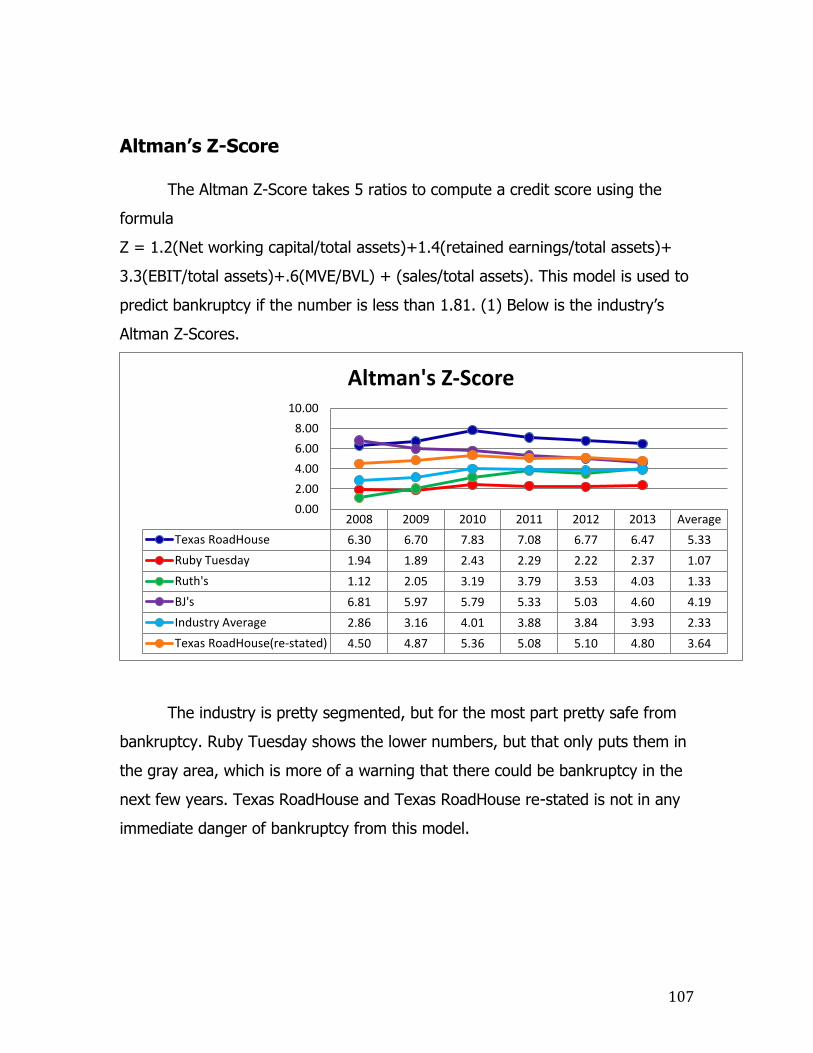
107

Altman’s Z-Score

The Altman Z-Score takes 5 ratios to compute a credit score using the

formula

Z = 1.2(Net working capital/total assets)+1.4(retained earnings/total assets)+

3.3(EBIT/total assets)+.6(MVE/BVL) + (sales/total assets). This model is used to

predict bankruptcy if the number is less than 1.81. (1) Below is the industry’s

Altman Z-Scores.

The industry is pretty segmented, but for the most part pretty safe from

bankruptcy. Ruby Tuesday shows the lower numbers, but that only puts them in

the gray area, which is more of a warning that there could be bankruptcy in the

next few years. Texas RoadHouse and Texas RoadHouse re-stated is not in any

immediate danger of bankruptcy from this model.

2008 2009 2010 2011 2012 2013 Average

Texas RoadHouse 6.30 6.70 7.83 7.08 6.77 6.47 5.33

Ruby Tuesday 1.94 1.89 2.43 2.29 2.22 2.37 1.07

Ruth's 1.12 2.05 3.19 3.79 3.53 4.03 1.33

BJ's 6.81 5.97 5.79 5.33 5.03 4.60 4.19

Industry Average 2.86 3.16 4.01 3.88 3.84 3.93 2.33

Texas RoadHouse(re-stated) 4.50 4.87 5.36 5.08 5.10 4.80 3.64

0.00

2.00

4.00

6.00

8.00

10.00

Altman's Z-Score

108

Internal Growth Rate

The Internal Growth Rate is the highest growth rate a company can grow

by using only the company’s earnings and no outside investment in debt or

equity.

IGR = ROA * (1- Dividend Payout Ratio)

Calculated above, IGR multiplies the retention of net income that is not

paid in dividends by the Return on Assets. This means that the fewer dividends a

company pays, and reinvests in the company, the higher the IGR will be.

By restating the financials for TXRH, we can see that IGR has risen. This is

due to the goodwill impairment, and consequently, the now higher ROA.

2009 2010 2011 2012 2013 Average

Texas RoadHouse 5.8% 7.0% 8.1% 6.2% 5.6% 6.5%

Ruby Tuesday 2.4% -1.7% 4.0% 4.2% 0.0% 1.8%

Ruth's 1.0% 6.1% 7.6% 7.1% 8.7% 6.1%

BJ's 3.5% 5.7% 6.7% 5.9% 3.6% 5.1%

Industry Average 3.2% 4.3% 6.6% 5.9% 4.5% 4.9%

Texas RoadHouse(re-stated) 4.1% 5.6% 6.1% 13.1% 14.9% 8.8%

-4.0%-2.0%0.0%2.0%4.0%6.0%8.0%

10.0%12.0%14.0%16.0%

Internal Growth Rate

109

Sustainable Growth Rate

The Sustainable Growth rate is the highest rate at which a company can

grow without increasing its financial leverage. This means that the company can

accrue no more outstanding debt or issuance of stock for capital.

SGR = ROE * (1-Div Payout Ratio) * (1+(Total Liabilities/Book Value of Equity))

As calculated above, the sustainable growth rate is calculated by

multiplying the Return on Equity by the plowback ratio then multiplying by the

debt to equity ratio.

As shown in the graph above, the SGR of Texas Roadhouse dropped, then

grew after the financial restatement. This is due to the decrease in the Return on

Equity from 2009 – 2001 then increase in 2012 and 2013.

2009 2010 2011 2012 2013 Average

Texas RoadHouse 10.8% 11.7% 12.2% 10.0% 9.3% 10.8%

Ruby Tuesday 6.3% -3.3% 7.7% 8.1% 0.0% 3.8%

Ruth's 5.8% 13.8% 13.8% 18.9% 18.1% 14.1%

BJ's 5.2% 8.0% 9.5% 8.4% 5.2% 7.3%

Industry Average 7.0% 7.5% 10.8% 11.4% 8.1% 9.0%

Texas RoadHouse(re-stated) 8.4% 10.0% 9.7% 20.5% 22.3% 14.2%

-5.0%

0.0%

5.0%

10.0%

15.0%

20.0%

25.0%

Sustainable Growth Rate

110

Conclusion

Compared to all the other benchmark companies, Texas Roadhouse shows

no real concerns in their capital structure ratios. Even after financial re-

statements, this company still competes well against the competition.

Financial Forecasting Financial forecasting uses trends, ratios, and assumptions to calculate

possible future balance sheet, income statement, and statement of cash flows

balances. This information matters because it is an important piece of

understanding the intrinsic value of a firm. The short term forecasts are the more

important pieces of information so most of the time doing the forecasts was

spent improving the accuracy of the first few years, while the long-term forecasts

just follow the trend of the first few forecasted years. By taking the information

from Texas Roadhouse’s balance sheet, income statement, and statement of

cash flows we forecasted out their financial statements out 10 years past the

most recent year, 2013.

Income Statement

When preparing to work out the forecast, we decided that it was

important to start with the income statement. Using logical assumptions based

off the trends from the past six years we forecasted out the net income, gross

profit, sales, cost of goods sold, and other expense and sales figures we thought

were important to Texas Roadhouse. To get things started we determined the

sales growth over the past few years and found that there was an upward trend

up till 2012 where we assumed that 2012 would be the spike and that the sales

growth would start dropping from 12% down to 9% over the next 10 years. This

111

assumption was based off the idea that Texas Roadhouse would slowly decrease

the number of restaurants it opens by one or two each year.

After projecting the sales growth over the next ten years we created a common

sized income statement, which is just taking each part of the income statement

and dividing it by the total sales for that year. By doing this it becomes easier to

see trends of growth for specific sections such as operating expenses and gross

profit. We determined that the cost of goods sold would increase over the next

10 years based off the growing trend that the common sized income statement

showed us. This growth in cost of goods sold is caused by the increased number

of restaurants being put up each year, which in turn creates more goods to be

purchased and created. We decided the growth would grow from 34% in 2014 to

38% in 2018, where it would flatten out like the sales growth. There was also a

decreasing trend of growth in operating costs over the past few years caused by

the reduced number of stores opened each year. Using this information we

predicted the operating costs to go from around 57% at 2013 down to 55%

around 2018, where it flattens out and from 55% at 2013 down to 53% in 2018

where it flattens out. The difference between restated and as stated is caused by

the change in the operating leases, where we don’t have to charge a rent

expense since they have been capitalized. The provisions for taxes growth will

decrease also in both restated and as stated because of the decrease in

operating income growth. The changes in the income statement causes net

income growth to decrease from 6.6% in 2013 down to 5.5% over the next 10

years for the restated financials and from 5.8% down to 5.2% for the as stated.

Using the projections from the income statement we can now begin to forecast

the balance sheet and the statement of cash flows as well as predicting

dividends.

112

113

114

Dividends Forecasting

Texas Roadhouse has been paying dividends since 2011 and their

dividend payout is roughly .60 cents per share annually and is paid out quarterly.

We assumed that their shares would not increase over the next ten years, and

their dividends will increase by $.12 per share each year, as it did from 2012 to

2013. The trend takes the dividends paid for each year from $.60 per share in

2013 up to $1.8 per share in 2023.

Balance Sheet

After forecasting the income statement, we used the net income,

forecasted dividends, and some important financial ratios created from past

financial statements to forecast out the balance sheet. In order to begin

forecasting the balance sheet, we had to find a trend in the asset turnover ratio

and forecast that out for the next 10 years. We forecasted that the asset

turnover ratio would follow the current trend and increase from 1.54 at 2013 up

to 1.57 in 2018, where it would top out there. Using the forecasted asset

turnover ratios and the growth percentages of current and noncurrent assets we

forecasted out total assets, noncurrent assets, and current assets. Current assets

were forecasted to have an increasing growth percent caused by an increasing

growth in cash and accounts/notes receivables. Non-current assets were

forecasted to have a decreasing growth percent based of the decreasing

forecasted growth of total noncurrent assets, PPE, and Goodwill. We forecasted

out accounts receivables based off past accounts receivable turnover ratios,

where the trend looked as though it was decreasing over time so we took the

ratio from 2013 and decreased it over the 10 years from 56% down to 49% in

115

2020, where it would start to maintain. We also used the inventory turnover ratio

to forecast out the inventory for the Texas Roadhouse balance sheet. The

inventory turnover had a growing trend over the past few years, so we

forecasted it to grow from 43.71 in 2014 to 61.68 in 2023. Growing the inventory

turnover ratio caused the inventory growth on the balance sheet to decrease

from 1.35% of assets in 2014 to 1.3% in 2019, where it maintained from then

afterward.

After forecasting the assets for the balance sheet, we started to forecast

the stockholder’s equity of Texas Roadhouse. When forecasting the stockholder’s

equity, we made the assumption that no new shares were to be sold and no

shares were going to be bought up by the company for the 10 year forecasting

period. Since we made these assumptions, the only thing that would change in

the forecast for stockholder’s equity would be the retained earnings. The

retained earnings for our forecast were forecasted by adding net income and

subtracting dividends paid from the existing retained earnings each year up until

2023. Based on the assumptions given in the stockholder’s equity section

liabilities were used as a plug, where current liabilities and noncurrent liabilities

were given as a percent of total liabilities and total liabilities were forecasted as a

balancing tool to make liabilities and stockholder’s equity equal assets. After

forecasting out the balance sheet we moved on to the statement of cash flows,

where we estimated dividends and capital expenditures.

116

117

118

Statement of Cash Flows

The last part of the financial statement forecasting is the statement of

cash flows, where we forecasted operating activities and investment activities. In

order to estimate the trend in the operating cash flows we took Cash flows from

operations (CFFO) and divided it by the sales, operating income, and net income

of that same year. After taking the CFFO and dividing it by the sales we

discovered a trend that CFFO was around 12% of sales each year so we took

that trend and maintained it throughout the next 10 years by taking the sales

from each year and multiplying it by 12%, which gave us the CFFO for that year.

To estimate the cash flow from investing activities we took Sales from the

balance sheet and divided it by the PPE(net) from the year before in order to get

a PPE turnover ratio. Once we got the PPE turnover ratio we discovered that

there was a trend of increasing PPE turnover, so we continued that trend by

taking the PPE turnover at 2014 of 2.65 and increasing it each year till 2020

where it reached 3.8 and maintained at that amount till 2023, this change

increased capital expenditures each year.

119

120

Cost of Capital Estimation

In this section, we will estimate Texas Roadhouse’s cost of capital by

calculating their weighted average cost of capital (WACC). WACC is a firm's cost

of capital in which each category of capital is proportionately weighted. All else

remaining constant, the WACC of a firm increases as the beta and rate of return

on equity increases, as an increase in WACC notes a decrease in valuation and a

higher risk.

Cost of Debt

The cost of debt is shown as a weighted average of interest rates on debt

owed by a company. In Texas Roadhouse’s case, interest rates have been

consolidated in their 10-K into a single WAIR of 10.54% for their long term

liabilities. Shown below are the cost of debt calculations for Texas Roadhouse’s

financial statements as stated and restated. To obtain the rate stated for the

capitalized operating leases, the interest rate given for capital leases was used.

(2)

121

For the restated amounts, a weight was assigned to both Long Term Debt

and Capitalized Operating Leases relative to the total size of Texas Roadhouse’s

long-term obligations. From there, the weights were multiplied by their

respective interest rates and added together to get the weighted average cost of

debt for Texas Roadhouse. As a result, the WACD of the restated financials is

6.7%, significantly less than the as stated WACD of 10.54%.

Cost of Equity

A company’s cost of equity is calculated using the Capital Asset Pricing

Model or CAPM. This formula uses the risk free rate (Rf), systematic risk (beta),

the market risk premium MRP, and adds a Size Premium (SP).

Ke = Rf + B(MRP) + SP

To find the risk free rate, we found the yields for 3-month, 1-year, 2-year,

7-year, and 10-year treasury bonds via the St. Louis Federal Reserve website.

However, because these yields are provided in an annual basis, we had to

convert this annual rate to a monthly rate. For this analysis, the most recent 10-

year treasury rate was used, and was found to be 2.71%.

To find our plug for the risk free rate, we used yields for 3-month, 1-year,

2-year, 7 year, and 10- year treasury bonds from the Federal Reserve Bank of St.

Louis website. After converting the annual rates given to monthly rates, the May

2014 10-year Treasury bond yield was used. This rate is 2.13%.

The plugs used for the market risk premium and size premium were

obtained from the Business Valuation Text. Because the market risk premium is

understated due to government influence of interest rate, an 8% rate was

substituted for MRP. The size premium is determined by the market value of a

firm. The table below shows that Texas Roadhouse is in the 6th decile and has a

size premium of 1.8%

122

Beta is a measure of the systematic risk, or market risk, affecting a

company. To calculate the beta for Texas Roadhouse, we used regression

analysis to determine the relationship between the holding period return for

Texas Roadhouse and the return on the overall market. The historic returns for

the S&P 500 were used as the rates for return on market. By using data for 24,

36,48, 60 and 72 month times periods for each of the risk free treasury bonds,

we were able to calculate 25 betas ranging from -.07 to .42. After calculating the

initial cost of equity (Ke), we added the Size Premium to determine the 2-factor

cost of equity. Also included in the charts are the upper and lower 95% limits of

the 2-factor cost of equity, calculated by using the upper and lower limits of the

beta from the regression analysis.

123

Months Beta Beta LB Beta UB R^2 MRP Rf Ke SP 2 factor KeKe LB Ke UB

72 0.10 -0.34 0.54 0.31% 8% 2.56% 3.380% 1.8% 5.180% 1.66% 8.70%

60 -0.07 -0.53 0.39 0.16% 8% 2.56% 2.002% 1.8% 3.802% 0.15% 7.46%

48 0.12 -0.42 0.65 0.42% 8% 2.56% 3.487% 1.8% 5.287% 1.04% 9.54%

36 0.42 -0.21 1.04 5.11% 8% 2.56% 5.883% 1.8% 7.683% 2.69% 12.68%

24 0.40 -0.72 1.52 2.43% 8% 2.56% 5.757% 1.8% 7.557% -1.40% 16.51%

Months Beta Beta LB Beta UB R^2 MRP Rf Ke SP 2 factor KeKe LB Ke UB

72 0.10 -0.34 0.54 0.31% 8% 2.56% 3.387% 1.8% 5.187% 1.67% 8.70%

60 -0.07 -0.53 0.39 0.16% 8% 2.56% 2.004% 1.8% 3.804% 0.15% 7.46%

48 0.12 -0.41 0.65 0.42% 8% 2.56% 3.490% 1.8% 5.290% 1.04% 9.54%

36 0.42 -0.21 1.04 5.11% 8% 2.56% 5.884% 1.8% 7.684% 2.69% 12.68%24 0.40 -0.72 1.52 2.44% 8% 2.56% 5.761% 1.8% 7.561% -1.40% 16.52%

Months Beta Beta LB Beta UB R^2 MRP Rf Ke SP 2 factor KeKe LB Ke UB

72 0.10 -0.34 0.54 0.31% 8% 2.56% 3.386% 1.8% 5.186% 1.67% 8.70%

60 -0.07 -0.53 0.39 0.16% 8% 2.56% 2.009% 1.8% 3.809% 0.15% 7.46%

48 0.12 -0.41 0.65 0.43% 8% 2.56% 3.497% 1.8% 5.297% 1.05% 9.55%

36 0.42 -0.21 1.04 5.12% 8% 2.56% 5.887% 1.8% 7.687% 2.70% 12.68%

24 0.40 -0.72 1.52 2.45% 8% 2.56% 5.773% 1.8% 7.573% -1.39% 16.53%

Months Beta Beta LB Beta UB R^2 MRP Rf Ke SP 2 factor KeKe LB Ke UB

72 0.10 -0.33 0.54 0.32% 8% 2.56% 3.396% 1.8% 5.196% 1.68% 8.71%

60 -0.07 -0.52 0.39 0.15% 8% 2.56% 2.023% 1.8% 3.823% 0.17% 7.47%

48 0.12 -0.41 0.65 0.45% 8% 2.56% 3.523% 1.8% 5.323% 1.08% 9.57%

36 0.42 -0.20 1.04 5.18% 8% 2.56% 5.901% 1.8% 7.701% 2.72% 12.68%

24 0.41 -0.71 1.53 2.52% 8% 2.56% 5.819% 1.8% 7.619% -1.34% 16.57%

Months Beta Beta LB Beta UB R^2 MRP Rf Ke SP 2 factor KeKe LB Ke UB

72 0.10 -0.34 0.55 0.32% 8% 2.56% 3.391% 1.8% 5.191% 1.65% 8.73%60 -0.07 -0.53 0.39 0.16% 8% 2.56% 2.014% 1.8% 3.814% 0.13% 7.50%

48 0.12 -0.42 0.66 0.44% 8% 2.56% 3.513% 1.8% 5.313% 1.02% 9.60%36 0.42 -0.22 1.05 5.14% 8% 2.56% 5.886% 1.8% 7.686% 2.63% 12.74%24 0.40 -0.78 1.58 2.49% 8% 2.56% 5.794% 1.8% 7.594% -1.85% 17.04%

3 Month Regression

1 Year Regression

2 Year Regression

7 Year Regression

10 Year Regression

From this regression, we get a beta of .42 with upper and lower limits of -

.2 and 1.04, respectively, with a confidence level of 95%. We have chosen this

regression because it has the highest R2 statistic, showing that 5.18% of Texas

Roadhouse’s risk can be associated with market risk. According to Yahoo

Finance, Texas Roadhouse has a beta of .88, which is within our confidence

interval. Because their beta is less than 1, Texas Roadhouse is not affected by

systematic rest at as high of a degree as the rest of the firms in the market.

By using CAPM, the regression data gives us a cost of equity (Ke) of 7.7%

after adjusting for the size premium for Texas Roadhouse. The cost of equity can

also be seen as the required rate of return that investors in Texas Roadhouse

expect to earn. With the upper and lower bound intervals for cost of equity show

124

that Texas Roadhouse can expect its cost of equity to lie between 2.72% and

12.68% with a confidence of 95%.

Backdoor Cost of Equity

The backdoor cost of equity is a measure that uses key ratios and information

from a firm’s financials to determine their cost of equity rather than historical

prices and data. By using ratios for return on equity, price to book ratio, and

growth within the firm, we will be able to estimate the cost of equity. The

formula for backdoor cost of equity is:

Price = 1 + (ROE + Ke)

Book (Ke – g)

For this formula, Price/book value is the measure of Market Price to Book

value of the company. ROE is representative of the forecasted long run return on

equity and g is the forecasted growth rate for the firm.

The price to book ratio used in this calculation is 2.97, the ROE is 16%,

and the growth rate is 2%. From this calculation, we get a 10.4% cost of equity,

which is within our confidence interval.

Weighted Average Cost of Capital (WACC)

A company’s WACC is calculated by multiplying the company’s

proportionate debt or equity by its respective cost. By combining these figures,

we are able to calculate the overall cost of capital for a company. The formula

for WACC is

WACC= WeightDebt*CostDebt + WeightEquity*CostEquity

WACCAfter Taxes= WeightDebt*CostDebt + WeightEquity*CostEquity (1- Tax Rate)

125

The weight of equity is determined by the market value of equity at

valuation. For our valuation date of 6/1/2014, Texas Roadhouse had

322,200,000 shares outstanding at a stock price of $25.13, giving a market value

of $8,993,990. According to Texas Roadhouse’s 2014 10-K, the market value of

their debt bearing liabilities is $50,990,000. After being restated to reflect the

capitalized operating leases, the market value of their liabilities is now

$202,526,000. As stated, the weight and interest rates for liabilities and equity

are 38.63%/10.54% and 61.37%/5.35%, respectively. After the restatement,

the weights of liabilities and equity change to 71.43% and 28.57% respectively.

The cost of debt also changes because of the difference in interest rate caused

by the capitalization of operating leases. These weights show that as-stated,

Texas Roadhouse holds in value mostly in equity, but after restatement, we can

see that liabilities hold much more weight.

Texas Roadhouse’s WACC(restated) is 9.73% but because of the costs

incurred because of taxes, the effective WACC is 7.55%. This is calculated by

using Texas Roadhouse’s effective tax rate as given by their 2014 10-K.

The WACC can be interpreted as the rate at which Texas

Roadhouse can finance their operations through debt and equity. Also, because

126

of the significant change in WACC caused by the restatements made in this

valuation, we can determine that operating leases are a significant part of Texas

Roadhouse’s operations. Because the WACC can be unreliable due to outside

circumstances, we have also calculated the WACC according to the upper and

lower boundaries determined by the regression analysis.

From this data we can assume that Texas Roadhouse’s cost of capital will be between 8.31% and 11.15% after restatements with a 95% level of confidence.

127

Method of Comparables

The methods of comparables section uses several different ratios to put

Texas RoadHouse’s stock price against their other competition and benchmarks’

stock prices. Under each ratio, we took the average of each ratio, without

including Texas RoadHouse or any outliers or negative numbers, and adjusted

our evaluated company to that number. For each ratio, we have our benchmark

companies of Ruby Tuesday, Ruth’s, and Bj’s, but we also included Darden and

Brinker because they were the closest publically available competition in this

industry, and we needed more numbers to come out with a better industry

average.

For Texas RoadHouse’s observed price, we used the closing date for May

30th, which is $25.28 per share. With a 20% swing (10% in each direction,) we

set the lower limit of this price to be $22.75 per share and the upper limit to be

$27.81 per share. Anything below this limit means Texas RoadHouse is

overvalued; anything above means they are undervalued.

128

Trailing P/E Ratio

This number tells you how many years’ worth of profits you’re paying for

a stock. All things equal, the lower the P/E the better (18.) We calculated this

ratio by taking the closing share price at May 30Th and divided that number by

the company’s earnings per share for the past year for each company. After

getting the ratio for each firm, we took an average of the companies in the

industry without Texas RoadHouse and any negative numbers. Using this

average, we then recalculated Texas RoadHouse’s share price and compared it

with the rest of the companies. Below is our table that compares each firm.

We set Texas RoadHouse’s lower and upper limits to be $22.75 and

$27.81 respectively. After readjusting both the as-stated and re-stated financials

for the company, Texas RoadHouse is shown to be overvalued by 70 cents as-

stated, but is right in the middle for their re-stated financials. Due to the lower

limit strictly being $22.75, Texas RoadHouse definitely overstates themselves,

but this ratio is not enough for us to entirely conclude that.

Company Trailing EPS Trailing PPS P/E Adjusted PPS

Texas RH 1.13 25.28 22.37 22.05

Ruby Tuesday -1.55 7.87 -

Ruth's 0.66 12.25 18.56

BJ's 0.60 31.59 52.65

Darden 2.51 50.12 19.97

Brinker 2.48 49.65 20.02

Texas RH (restated) 1.32 25.28 19.15 25.76

Industry Average - - 19.52

Trailing P/E Ratio

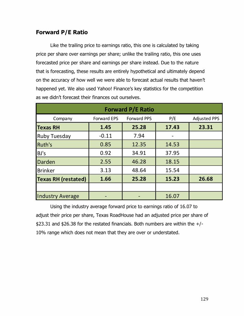
129

Forward P/E Ratio

Like the trailing price to earnings ratio, this one is calculated by taking

price per share over earnings per share; unlike the trailing ratio, this one uses

forecasted price per share and earnings per share instead. Due to the nature

that is forecasting, these results are entirely hypothetical and ultimately depend

on the accuracy of how well we were able to forecast actual results that haven’t

happened yet. We also used Yahoo! Finance’s key statistics for the competition

as we didn’t forecast their finances out ourselves.

Using the industry average forward price to earnings ratio of 16.07 to

adjust their price per share, Texas RoadHouse had an adjusted price per share of

$23.31 and $26.38 for the restated financials. Both numbers are within the +/-

10% range which does not mean that they are over or understated.

Company Forward EPS Forward PPS P/E Adjusted PPS

Texas RH 1.45 25.28 17.43 23.31

Ruby Tuesday -0.11 7.94 -

Ruth's 0.85 12.35 14.53

BJ's 0.92 34.91 37.95

Darden 2.55 46.28 18.15

Brinker 3.13 48.64 15.54

Texas RH (restated) 1.66 25.28 15.23 26.68

Industry Average - - 16.07

Forward P/E Ratio

130

Price to Book Ratio

The price to book ratio is the calculation of price per share over book

value per share. Book value per share is the total owner’s equity minus preferred

stock value, all over the outstanding common stock shares. A low P/B can offer

investors an excellent opportunity to capitalize on an undervalued stock. The

formula is a great indicator, but should not be used alone. A low Price to Book

can sometimes indicate an underlying problem with the company. (17)

Texas RoadHouse shows a below average P/B ratio of about 3 in both

their as-stated and re-stated financials. We did not include Darden in the

industry average due to it being so much larger than all the rest, but we used

the industry average to adjust Texas RoadHouse’s price per share which caused

it to be severely undervalued. At a price of $53.53 and $54.52, this number

seems unreasonably large compared to the other ratio’s adjusted prices. This

formula tells us that Texas RoadHouse is undervalued by over $25 dollars, but

we do not believe it to be undervalued by that much.

Company PPS BPS P/B Adjusted PPS

Texas RH 25.28 8.52 2.97 53.51

Ruby Tuesday 7.87 0.99 7.95

Ruth's 12.25 4.19 2.92

BJ's 31.59 2.45 12.89

Darden 50.12 2.86 17.52

Brinker 49.65 36.58 1.36

Texas RH (restated) 25.28 8.68 2.91 54.52

Industry Average - - 6.28

Price/Book Ratio

131

Dividends to Price Ratio

This ratio is calculated by taking a company’s dividends per share over

their price per share from May 30th. Because both Bj’s and Ruby Tuesday do not

issue dividends, our industry average is severely flawed due to the lack of inputs,

which causes our adjusted price per share for Texas RoadHouse to be off.

We used the exact same numbers for the as-stated and re-stated Texas

RoadHouse financials because there was no change from those numbers are

adjusting the financials. Texas RoadHouse’s adjusted price per share came out to

be undervalued by a little over two dollars per share, but once again, due to the

lack of inputs for the industry average, this number is not very accurate.

Company DPS PPS D/P Adjusted PPS

Texas RH 0.6 25.28 0.0237 30.17

Ruby Tuesday - 7.87 -

Ruth's 0.2 12.25 0.0163

BJ's - 31.59 -

Darden 2.2 50.12 0.0439

Brinker 0.96 49.65 0.0193

Texas RH (restated) 0.6 25.28 0.0237 30.17

Industry Average - - 0.0199

Dividends/Price Ratio

132

Price Earnings Growth Ratio

The PEG ratio attempts to measure the degree of a discount or premium

you’re paying for growth. The calculation is to divide the P/E ratio by the long-

term annualized percentage growth rate of earnings. A result of less than 1.0

implies that the market is not fully valuing the prospects for future growth. (18)

Below is Texas RoadHouse compared to the industry and restated price per

share by the industry average.

For Texas RoadHouse’s earnings per share growth rate, we took our

forecasted earnings per share and calculate the change between each year. The

percentage came out to be 9% as-stated and 11.2% restated for the company.

After calculating the average of the industry minus the company and Ruby

Tuesday, we adjusted Texas RoadHouse’s trailing price to earnings ratio. With

these new numbers, we then calculated out the company’s adjusted price per

share. On both an as-stated and re-stated basis, Texas RoadHouse has an

overvalued stock price.

Company Trailing P/E %EPS Growth P.E.G. Adjusted PPS

Texas RH 22.37 9.00% 2.49 15.45

Ruby Tuesday - - -

Ruth's 18.56 15.70% 1.18

BJ's 52.65 29.60% 1.78

Darden 19.97 12% 1.71

Brinker 20.02 14.20% 1.41

Texas RH (restated) 19.15 11.20% 1.71 22.46

Industry Average 1.52

Price Earnings Growth Ratio

133

Price to EBITDA

The price to EBITDA ratio is a measure of the market value of equity over

the earnings before interest, tax, depreciation, and amortization. To calculate the

market value of equity, we took the outstanding shares of each company,

multiplied by the price per share as of May 30th. For each of the company’s

ratios, we got the numbers off of their respective 10-K and crunched them out

ourselves. Below is Texas RoadHouse’s ratio compared to the rest of the

industry.

For 2013, Texas RoadHouse was overstated on an as-stated basis for their

price per share, but was within our 10% range on the re-stated one. To get this

number, we took the industry average of the other companies and got an

adjusted market cap. With this new market value of equity, we divided it by the

number of shares outstanding to get the adjusted price per share. Texas

RoadHouse would probably not be considered overvalued if interest and taxes

were not taken out of the earnings because the higher amount of earnings would

lower the ratio, ultimately increasing the adjusted price per share.

Company Market Cap EBITDA P/EBITDA Adjusted PPS

Texas RH $1,762,228 $169,477 10.40 21.28

Ruby Tuesday $483,550 $64,305 7.52

Ruth's $441,326 $47,647 9.26

BJ's $898,848 $72,867 12.34

Darden $6,612,320 $1,043,100 6.34

Brinker $3,224,843 $388,256 8.31

Texas RH (restated) $1,762,228 $191,778 9.19 24.08

Industry Average 8.75

Price/EBITDA

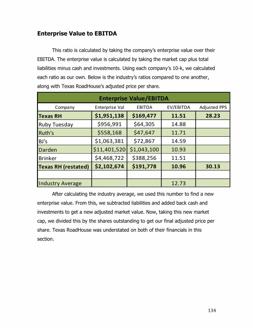
134

Enterprise Value to EBITDA

This ratio is calculated by taking the company’s enterprise value over their

EBITDA. The enterprise value is calculated by taking the market cap plus total

liabilities minus cash and investments. Using each company’s 10-k, we calculated

each ratio as our own. Below is the industry’s ratios compared to one another,

along with Texas RoadHouse’s adjusted price per share.

After calculating the industry average, we used this number to find a new

enterprise value. From this, we subtracted liabilities and added back cash and

investments to get a new adjusted market value. Now, taking this new market

cap, we divided this by the shares outstanding to get our final adjusted price per

share. Texas RoadHouse was understated on both of their financials in this

section.

Company Enterprise Val EBITDA EV/EBITDA Adjusted PPS

Texas RH $1,951,138 $169,477 11.51 28.23

Ruby Tuesday $956,991 $64,305 14.88

Ruth's $558,168 $47,647 11.71

BJ's $1,063,381 $72,867 14.59

Darden $11,401,520 $1,043,100 10.93

Brinker $4,468,722 $388,256 11.51

Texas RH (restated) $2,102,674 $191,778 10.96 30.13

Industry Average 12.73

Enterprise Value/EBITDA

135

Conclusion

We did not include the dividends to price ratio in the concluded overview

because of the severe lack of inputs from our major benchmark companies in

that section. Overall Texas RoadHouse over valued themselves on an as-stated

basis, but after re-stating their financials, they were considered undervalued only

because they increased the amounts of their fairly valued prices, not because

they increased the amounts of undervalued prices. In the end, we conclude that

ultimately Texas RoadHouse has over valued itself from the results in this

section.

Intrinsic Valuation Model The intrinsic valuation models are an accurate measure of the value of a

firm and are based off of forecasts produced by stock valuations. There are four

intrinsic valuation models that we will use to value Texas Roadhouse: the

discounted dividends model, the discounted free cash flows model, the residual

income model, and the long-run residual income model. We will use the

information provided by our forecasts to determine the value of the firm based

Ratios As-Stated Re-Stated

Trailing P/E Over Valued Fairly Valued

Forward P/E Fairly Valued Fairly Valued

P/B Under Valued Under Valued

D/P Under Valued* Under Valued*

P.E.G. Over Valued Over Valued

P/EBITDA Over Valued Fairly Valued

EV/EBITDA Under Valued Under Valued

Conclusion Over Valued Under Valued

Method of Comparables

*Not included in conclusion

136

off of these four models. We will use the dividend forecasts in the discounted

dividends model to value the firm based off only Texas Roadhouse’s payout of

dividends per share. The free cash flows model will use the operating and

investing activities from the statement of cash flows to ascertain the value of the

price of the stock at 6/1/14. In order to do the residual income model, we will

have to use the forecasted net income, forecasted dividends paid, and the

stockholder’s equity from 2013 to value the firm’s stock at 6/1/14. Using these

four intrinsic valuation models we will create a basis to decide on whether or not

Texas Roadhouse is fairly value.

Discounted Dividends Model

The discounted dividends model is used to value the firm based solely on

the payment of dividends each year. This method in some cases can be

somewhat accurate, but since it only derives value of the firm based off of the

dividends, it can’t derive the full value of the stock price unless the company

focuses a majority of its earnings into dividends. When running this model we

discovered that a reasonable amount the value of Texas Roadhouse’s stock can

be depicted by the dividends model.

This model uses the predicted dividends to be paid over the next 10

years, so we forecasted out 10 years of dividends in order to meet the criteria for

this model. In the past years Texas Roadhouse has increased its dividends to be

paid by $.01 per share each year from 2011 through 2012 and by $.03 per share

from 2013 till present. In order to forecast the dividends somewhat accurately

we carried the growth by $.03 per share each year for the next 10 years. Since

we assumed that there would be no shares sold or bought, the only changes in

the dividends past 2013 were the growth from the forecast.

For the discounted dividend model to work we used the cost of equity that

we estimated in the financial analysis and an array of different possible growth

rates in order to come to a reasonable resulting model. Using an upper bound

rate (12.68%), lower bound rate (2.72%), and an estimated cost of equity

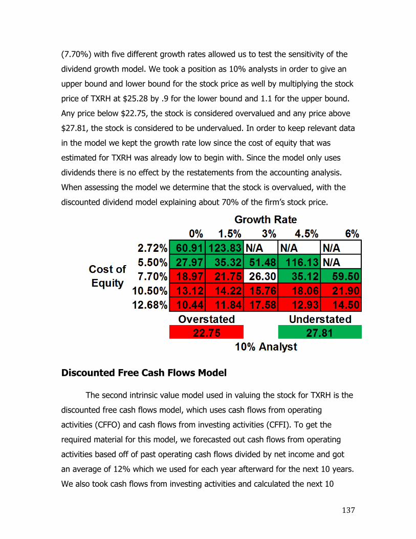
137

(7.70%) with five different growth rates allowed us to test the sensitivity of the

dividend growth model. We took a position as 10% analysts in order to give an

upper bound and lower bound for the stock price as well by multiplying the stock

price of TXRH at $25.28 by .9 for the lower bound and 1.1 for the upper bound.

Any price below $22.75, the stock is considered overvalued and any price above

$27.81, the stock is considered to be undervalued. In order to keep relevant data

in the model we kept the growth rate low since the cost of equity that was

estimated for TXRH was already low to begin with. Since the model only uses

dividends there is no effect by the restatements from the accounting analysis.

When assessing the model we determine that the stock is overvalued, with the

discounted dividend model explaining about 70% of the firm’s stock price.

Discounted Free Cash Flows Model

The second intrinsic value model used in valuing the stock for TXRH is the

discounted free cash flows model, which uses cash flows from operating

activities (CFFO) and cash flows from investing activities (CFFI). To get the

required material for this model, we forecasted out cash flows from operating

activities based off of past operating cash flows divided by net income and got

an average of 12% which we used for each year afterward for the next 10 years.

We also took cash flows from investing activities and calculated the next 10

138

years based off of a PPE turnover ratio, which was derived by taking Sales and

dividing it by PPE (net).

After calculating the forecasted amounts for CFFO and CFFI we then

calculated free cash flows from assets by subtracting CFFI from CFFO. By taking

the present value of the free cash flows from assets we were then able to

calculate the market value of the assets for the company, where we subtracted

the book value of debt in order to derive the market value of equity for the

company. After finding the MV of equity for the firm we then divided that

amount by the number of shares and multiplied that number by a time

consistency factor in order to come to an estimated amount for the stock price of

the firm. We used a before tax WACC in order to discount the cash flows while

avoiding double taxation, since cash flows are an after tax figure, to get a more

accurate measure of the stock price of the firm.

For the free cash flow model to work we used the WACC (before tax) that

we estimated in the financial analysis and an array of different possible growth

rates in order to come to a reasonable resulting model. Using an upper bound

rate (11.15%), lower bound rate (8.31%), and an estimated WACC (before tax)

(9.71%) with five different growth rates allowed us to test the sensitivity of the

free cash flow model. We took a position as 10% analysts in order to give an

upper bound and lower bound for the stock price as well by multiplying the stock

price of TXRH at $25.28 by .9 for the lower bound and 1.1 for the upper bound.

Any price below $22.75 the stock is considered overvalued and any price above

$27.81 the stock is considered to be undervalued. This model did not value the

company very efficiently, mainly because of the change in the last free cash flow

can determine whether the firms estimated value could be high or low. The

sensitivity of this model is very high also, which doesn’t work well with possible

estimation errors on growth rates and discount rates. From the information in

the graph, Texas Roadhouse is considered to have an overvalued stock price at

139

6/1/14.

Residual Income Model

The residual income model is the third intrinsic valuation model and has

the highest explanatory power of the three models. This model has a higher

explanatory power than the other models mainly because of the fact that it is

less sensitive to estimation errors with discount rates and growth rates, which

becomes important when all the information you use is estimations based off of

forecasted numbers. The required inputs for this model are net income

forecasted out for 10 years, dividends forecasted out for 10 years, and

stockholder’s equity in 2013. We forecasted out net income by forecasting out

the sales growth over the next 10 years based off of trends from the past six

years and then making adjustments to cost of goods sold and operating

expenses based off of their trends also. The model connects the balance sheet,

income statement, and statement of cash flows since it has net income,

dividends paid, and stockholder’s equity, all together giving this model a very

strong explanatory power.

To start this model we gather the required values: net income, dividends,

and stockholder’s equity at year 0, which we use to estimate stockholder’s equity

0 1.50% 3.00% 4.50% 6%

8.31% $11.52 12.70 13.93 16.14 21.21

9.00% $11.11 11.73 12.66 14.22 17.33

9.73% $10.36 10.85 11.56 12.68 14.70

10.50% $9.66 10.05 10.60 11.41 12.78

11.15% $9.13 9.45 9.89 10.54 11.55

WACC

(Before

Tax)

10% Analyst

Growth Rate

$22.75

Overstated

$27.81

Understated

140

outward based on only net income and dividend changes. After adding in net

income and subtracting dividends from the year before stockholder’s equity, we

took that value and multiply it by the cost of equity to get the annual normal

income or the benchmark income. Once you get the benchmark income we took

the net income and subtract the benchmark income from it to get your residual

income, which represents value added by the firm. Now that we have the

residual income we just have to discount each year by the cost of equity and add

them up with the terminal value and the book value of equity at year 0 in order

to find the market value of the equity. The terminal value is used to represent

gains in the future past 10 years for an undetermined amount of time. All that’s

left to do after getting the market value of equity is to divide it by the number of

shares outstanding at the end of the year 0 or 2013 for our uses and then

multiply that number by the time consistency factor in order to get the stock

value at 6/1/14.

As Stated Residual Income Model

For the residual income model to be able to work we used the cost of

equity that we estimated in the financial analysis and an array of different

possible growth rates in order to come to a reasonable resulting model. Using an

upper bound rate (12.68%), lower bound rate (2.72%), and an estimated cost of

-10% -20% -30% -40% -50%

2.72% $36.57 29.64 26.95 25.51 24.62

5.00% $26.98 23.31 21.74 20.87 20.31

7.70% $19.71 17.98 17.16 16.69 16.38

10.50% $14.84 14.08 13.7 13.46 13.31

12.68% $12.20 11.83 11.63 11.51 11.43

10% Analyst

Growth Rates

Cost of

Equity

Overstated Understated

$27.81$22.75

141

equity (7.70%) with five different growth rates allowed us to test the sensitivity

of the free cash flow model. We took a position as 10% analysts in order to give

an upper bound and lower bound for the stock price as well by multiplying the

stock price of TXRH at $25.28 by .9 for the lower bound and 1.1 for the upper

bound. Any price below $22.75, the stock is considered overvalued and any price

above $27.81, the stock is considered to be undervalued. From the information

in the model, we have discovered that the residual income model shows Texas

Roadhouse as an overvalued stock price at 6/1/14. Since this model has more

explanatory power than any of the other models, we will take the results from

this model as a heavier weight than any of the other models in our decision

making process. There is also a change in this model from as stated to restated

since we have net income involved, so we also did a restated residual income

model.

Restated Residual Income Model

There is a small difference between the as stated and restated models,

but not a big enough difference to really change the outward results of the

model. Texas Roadhouse’s stock price is still considered to be overvalued as of

6/1/14, based off of the residual income model.

-10% -20% -30% -40% -50%

2.72% $38.79 31.54 28.72 27.22 26.29

5.00% $28.51 24.72 23.10 22.20 21.62

7.70% $20.74 18.99 18.18 17.70 17.39

10.50% $15.56 14.82 14.45 14.22 14.07

12.68% $12.75 12.41 12.24 12.13 12.05

10% Analyst

Growth Rates

Cost of

Equity

Overstated Understated

$22.75 $27.81

142

Long Run Residual Income Model

The long run residual income model calculates the value of the firm by

using return on equity, cost of equity, and varying growth rates. This model,

compared to the other three models, is a little less accurate than the residual

income model, but has more explanatory power than the free cash flows model.

In order to for the model to work the forecasts from the financial analysis of the

company’s income statement and balance sheet are required. For the models

information to be represented in a relevant manor we will hold either the return

on equity, cost of equity, or the growth rates constant in three separate models

for an as stated basis and a restated basis.

All of the figures have been created by the forecasts from the financial

analysis and represent predictions of the possible trends and direction that the

firm is converging to. The return on equity used in this model is represented by

the net income of the current year divided by the stockholder’s equity of the year

before and the cost of equity has been estimated based off of the capital asset

pricing model and multiple regressions based off of past interest rates. In this

model the growth rates will be negative just like the residual income model in

order to maintain the idea that the firm would not outperform its cost of equity.

Using multiple growth rates, costs of equity, and returns on equity allows us to

provide a sensitivity analysis for this model, while showing possible outcomes for

errors in estimations. The model is started off by taking the amount of the

stockholder’s equity at year 0, or 2013 for our purposes, and using a growth

formula that compares the cost of equity, return on equity, and growth to figure

out the market value of the firm’s equity. The equation looks like this:

MVE= BVE [ 1 + ((ROE – Ke)/(Ke – g)) ]

In order to continue the model the shares outstanding are gathered and

used to calculate the model price at the end of year 0 by taking the market value

of equity and dividing it by the shares outstanding. Since we are valuing the

company at 6/1/14 a time consistent factor is required in order to bring the price

143

up to the correct date. As stated earlier, there will be three separate sensitivity

models since there are three different variables used in computing the share

price for the firm.

As Stated Long-Run Residual Income Models

14% 16% 18% 20% 22%

2.72% $16.38 $17.75 $19.11 $20.48 $21.84

5% $14.02 $15.19 $16.36 $17.52 $18.69

7.70% $12.01 $13.01 $14.01 $15.01 $16.01

10.50% $10.48 $11.35 $12.22 $13.10 $13.97

12.68% $9.55 $10.34 $11.14 $11.94 $12.73

Overstated

$22.75

Understated

$27.81

Holding Growth Constant at -10%

Return on Equity

Cost

of

Equity

(Ke)

10% Analyst

-10% -20% -30% -40% -50%

2.72% $21.84 $16.05 $13.80 $12.60 $11.86

5% $18.69 $14.72 $13.02 $12.07 $11.47

7.70% $16.01 $13.43 $12.21 $11.51 $11.05

10.50% $13.97 $12.32 $11.49 $10.99 $10.65

12.68% $12.73 $11.60 $10.99 $10.62 $10.37

Cost

of

Equity

(Ke)

Overstated Understated

$22.75 $27.81

10% Analyst

Holding ROE constant at 22%

Growth

144

For the three values of the hold variables we chose the values that would

cause the prices to be the highest to show that with this range of cost of equity

rates, return on equity rates, and growth rates Texas Roadhouse’s stock will

come out to be overvalued in all instances. For the as stated and restated

models we used an upper bound rate (12.68%), lower bound rate (2.72%),

estimated cost of equity (7.70%), and two other averaged rates for the cost of

equity. For the as stated models and restated models we held the growth rate at

-10% for the first one, held return on equity at 22% for as stated and at 24% for

restated for the second one, and held cost of equity at 2.72% for both as stated

and restated for the third one. The first model will compare return on equity to

cost of equity, the second model will compare growth to cost of equity, and the

third model will compare growth to return on equity for both as stated and

restated. As shown by the results of this model, the stock for Texas Roadhouse

is overvalued and is very similar to the original residual income model in the

section before this one, with one difference being that the long run residual

income model has lower values than the residual income model. Since net

income and stockholder’s equity is involved in the model, we have to do a

restated version of the model as well as the as stated model.

-10% -20% -30% -40% -50%

14.00% $16.38 $12.99 $11.68 $10.97 $10.54

16% $17.75 $13.76 $12.21 $11.38 $10.87

18.00% $19.11 $14.52 $12.74 $11.79 $11.20

20.00% $20.48 $15.29 $13.27 $12.19 $11.53

22.00% $21.84 $16.05 $13.80 $12.60 $11.86

Return

on

Equity

(ROE)

Overstated Understated

$22.75 $27.81

Hold Ke constant at 2.72%

10% Analyst

Growth

145

Restated Long-Run Residual Income Models

16% 18% 20% 22% 24%

2.72% $18.08 $19.48 $20.87 $22.26 $23.65

5% $15.48 $16.67 $17.86 $19.05 $20.24

7.70% $13.26 $14.27 $15.29 $16.31 $17.33

10.50% $11.57 $12.46 $13.35 $14.24 $15.13

12.68% $10.54 $11.35 $12.16 $12.97 $13.78

Holding Growth Constant at -10%

Return on Equity (ROE)

Cost

of

Equity

(Ke)

Overstated Understated

$22.75 $27.81

10% Analyst

-10% -20% -30% -40% -50%

2.72% $23.65 $17.13 $14.60 $13.25 $12.42

5% $20.24 $15.71 $13.78 $12.70 $12.01

7.70% $17.33 $14.33 $12.93 $12.11 $11.57

10.50% $15.13 $13.16 $12.16 $11.56 $11.16

12.68% $13.78 $12.38 $11.63 $11.17 $10.86

Growth

Cost

of

Equity

(Ke)

Overstated Understated

$22.75 $27.81

10% Analyst

Holding ROE constant at 24%

146

Comparing the as stated models to the restated models, there isn’t a huge

difference between the two of them except for the change in the estimated

return on equity that was gathered from the forecasting estimates. Since most of

the changes from the restatements affected the past six years only, the

forecasted years only had a small effect of increasing the net income and

stockholder’s equity leading to increased return on equity and a small change in

the results of these models. The model still concludes that Texas Roadhouse’s

stock is overvalued and the only extra conclusion we can draw from the change

in the restated version is that it isn’t as overvalued as it seems in the as stated

long-run residual income model.

-10% -20% -30% -40% -50%

16.00% $18.08 $14.02 $12.44 $11.60 $11.08

18% $19.48 $14.80 $12.98 $12.01 $11.41

20.00% $20.87 $15.58 $13.52 $12.43 $11.75

22.00% $22.26 $16.36 $14.06 $12.84 $12.08

24.00% $23.65 $17.13 $14.60 $13.25 $12.45

Growth

Retur

n on

Equity

(ROE)

10% Analyst

Overstated Understated

$22.75 $27.81

Holding Ke constant at 2.72

147

Sources

1) Business Analyzation and Valuation 5th Edition: Palepu,Healy

2) TXRH 10-K

3) RT 10-K

4) RUTH 10-K

5) BJRI 10-K

6) Financial Management - Principles and Applications 2nd Edition:

Titman, Keown, Martin

7) Intermediate Accounting 14th Edition: Kieso, Weygandt, Warfield

8) Managerial Economics and Business Strategy 8th Edition: Baye, Prince

http://www.restaurant.org/News-Research/Research/Facts-at-a-Glance

9) http://www.restaurant.org/News-Research/Research/RPI

10) http://nrn.com/consumer-trends/npd-forecasts-traffic-spending-

growth-2014

11) http://www.huffingtonpost.com/burgerbusiness/fast-casual-thrives-fast_b_4731097.html

12) www.eturbonews.com

13) www.usinflation.org/us-inflation-rate

14) http://www.nytimes.com/2003/07/13/business/business-sifting-

through-junk-in-search-of-dining-ambience.html

15) http://www.dailyfinance.com/2013/05/13/did-you-know-fast-food-isnt-

cheaper-savings-experiment/

16) http://www.forbes.com/sites/benzingainsights/2011/05/02/bargain-

hunting-ten-stocks-with-low-price-to-book-ratios-near-52-week-lows/

17) http://www.forbes.com/sites/johndobosz/2013/09/25/10-ratios-to-

make-you-money-in-stocks/

148

Appendix

Capital Structures Ratios

149

Profitability Ratios

150

Asset Turnover Ratio 2009 2010 2011 2012 2013

Texas Roadhouse 1.51 1.51 1.57 1.7 1.79

Ruth's Hospitality Group 1.17 1.4 1.47 1.66 1.77

Ruby Tuesday 0.98 1.06 1.18 1.1 1.06

BJ's Restaurants 1.27 1.34 1.44 1.41 1.38

Texas Roadhouse Restated 1.31 1.32 1.37 1.49 1.53

Industry Average 1.25 1.33 1.41 1.47 1.51

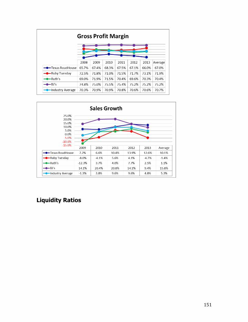
151

Liquidity Ratios

152

153

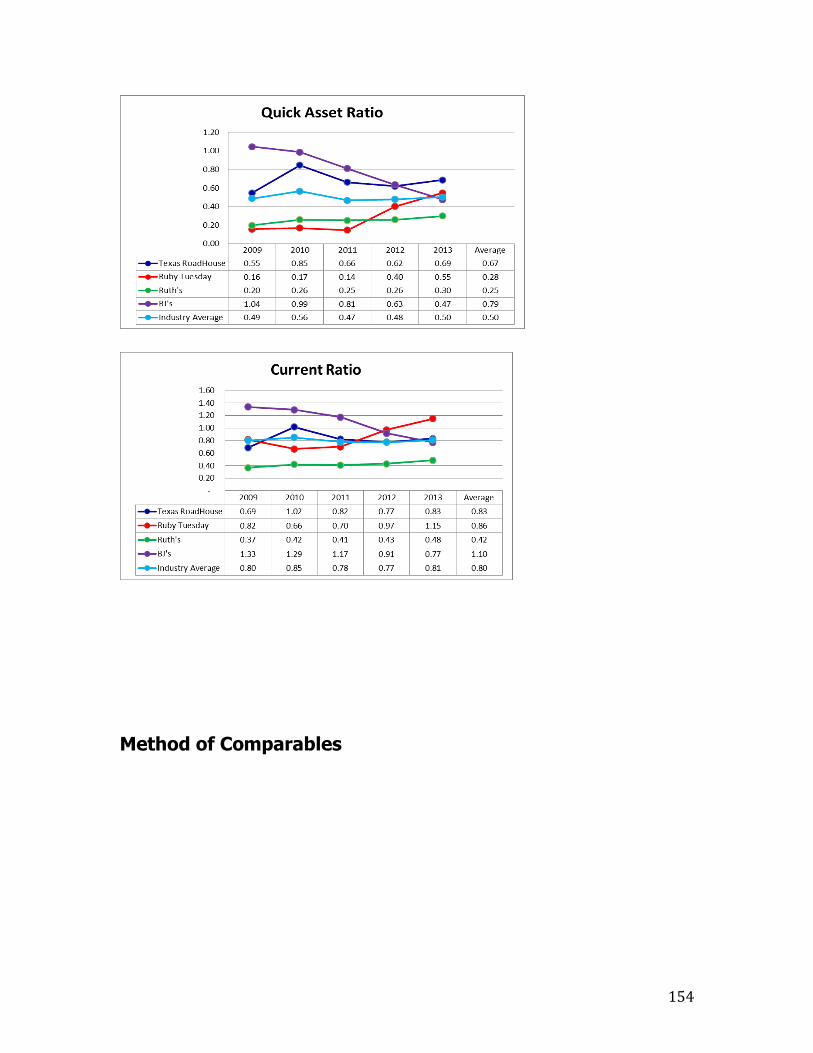
154

Method of Comparables

155

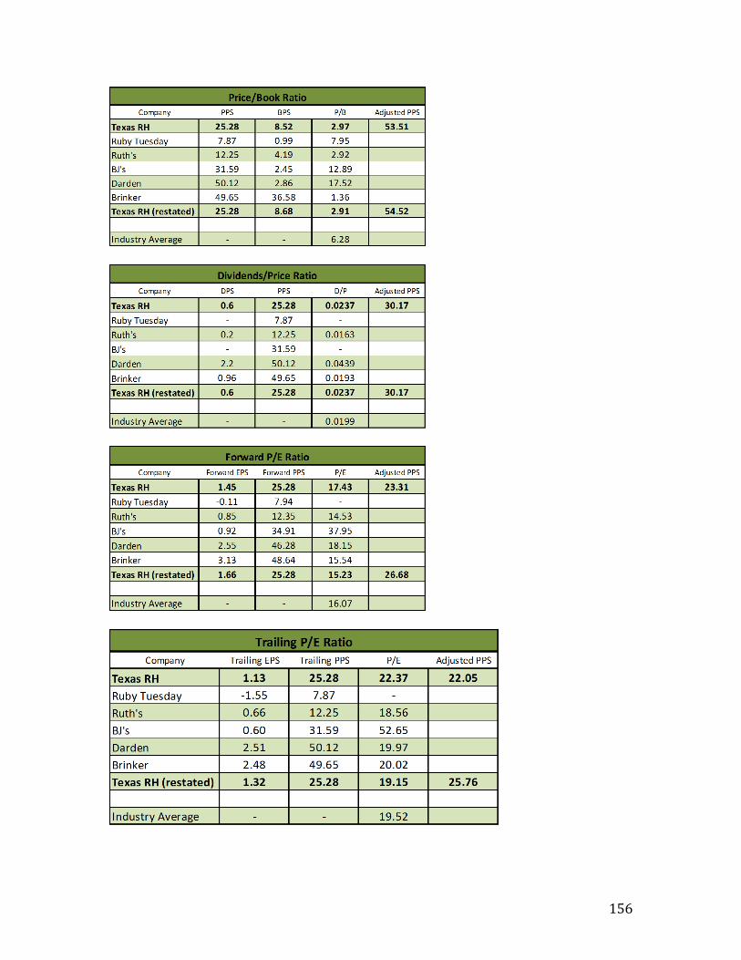
156

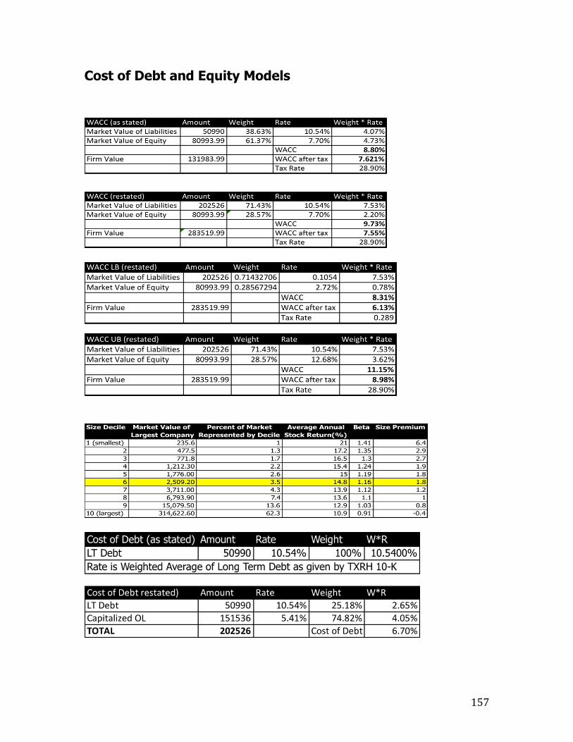
157

Cost of Debt and Equity Models

158

Growth Rate Graphs

2009 2010 2011 2012 2013 Average

Texas RoadHouse 5.8% 7.0% 8.1% 6.2% 5.6% 6.5%

Ruby Tuesday 2.4% -1.7% 4.0% 4.2% 0.0% 1.8%

Ruth's 1.0% 6.1% 7.6% 7.1% 8.7% 6.1%

BJ's 3.5% 5.7% 6.7% 5.9% 3.6% 5.1%

Industry Average 3.2% 4.3% 6.6% 5.9% 4.5% 4.9%

Texas RoadHouse(re-stated) 4.1% 5.6% 6.1% 13.1% 14.9% 8.8%

-4.0%-2.0%0.0%2.0%4.0%6.0%8.0%

10.0%12.0%14.0%16.0%

Internal Growth Rate

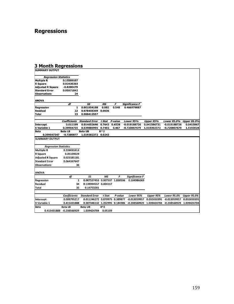
159

Regressions

3 Month Regressions

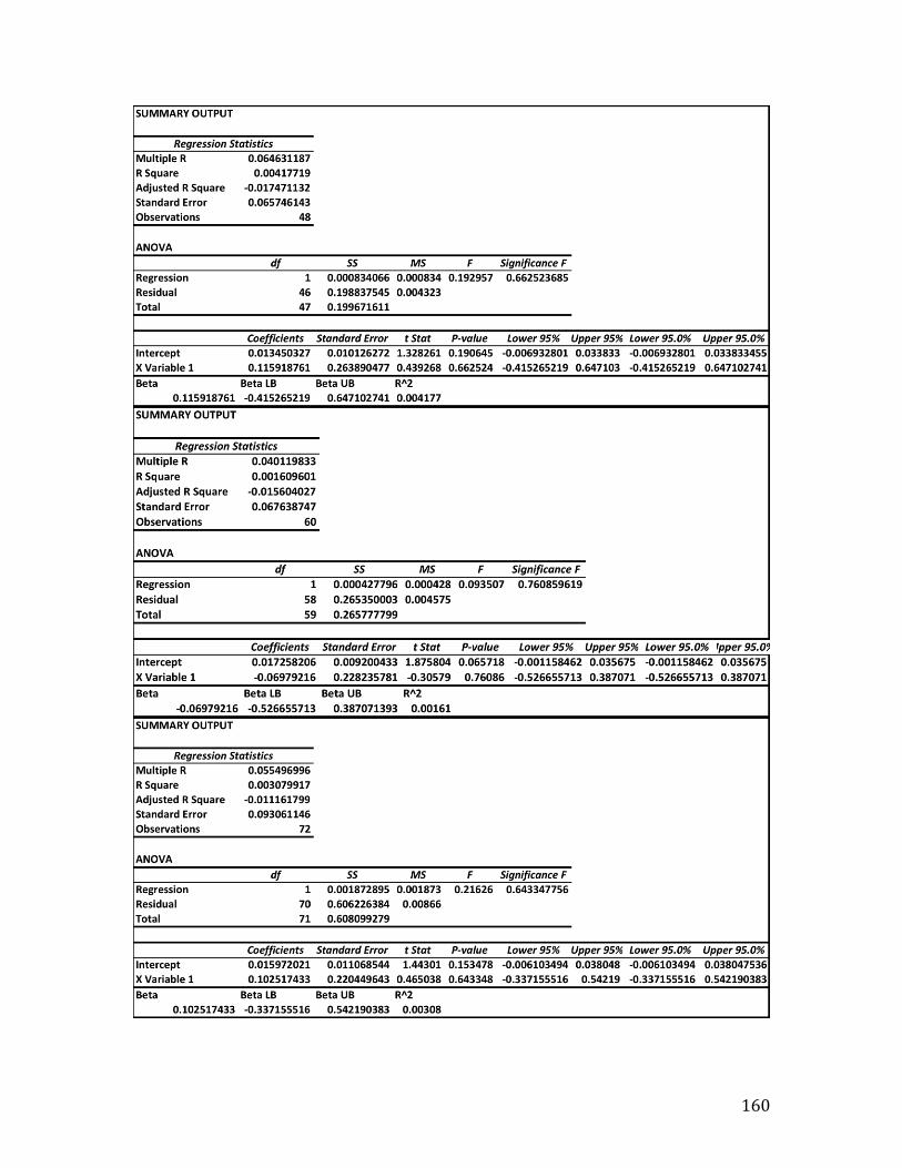
160

161

1 Year Regressions

162

2 Year Regressions

163

164

7 Year Regressions

165

166

10-Year Regressions

167

168

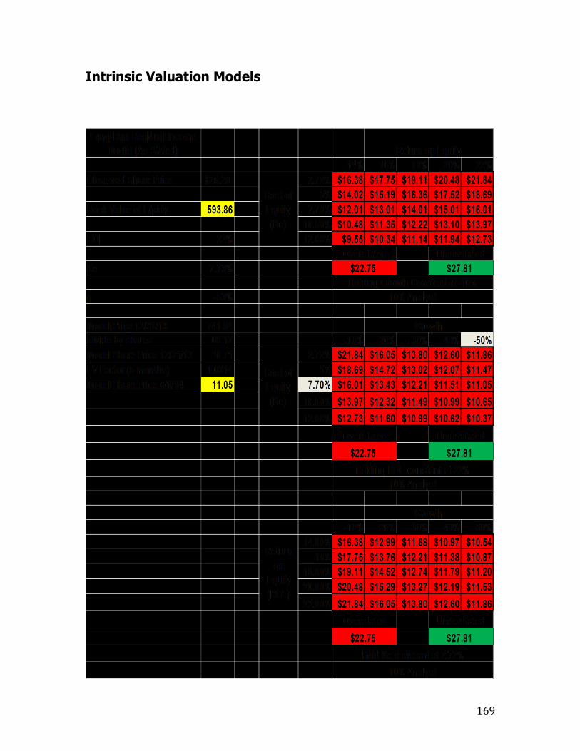
169

Intrinsic Valuation Models

170

171

172

173

174