Business Valuation OIVjournal - ICAEW

BusinessValuationOIV journal

3. Presentation

5. Implied cost of capital: how to calculate it and how to use it Mauro Bini

33. Solvency II framework in insurance equity valuation: some critical issues Stefano Giuliani, Giulia Raffo, Niccolò Dalla Palma

53. Bank valuation using multiples in US and Europe: an historical perspective Mario Massari, Christopher Difonzo, Gianfranco Gianfrate, Laura Zanetti

Volume 0Issue 0Fall 2018

Copyright 2018 Wolters Kluwer Italia S.r.l.Via dei Missaglia n. 97 - Edificio B3 - 20142 - Milano

The rights of translation, electronic storage, reproduction and total or partial adaptation, by any means (including microfilm and photostatic copies), are reserved for all countries.

The elaboration of texts, even if treated with scrupulous attention, cannot lead to specific responsibilities for any unintentional mistake or inaccuracy.

Presentation of the Journal

Business Valuation OIV Journal has been created by OIV- Organismo Italiano di Valutazione –the Italian Valuation Standard Setter – to provide a forum for discussion and to foster culturalprogress in the field of business valuation.

OIV is a non-profit Foundation established by the main Italian professional organizations andinstitutions engaged in valuation1 and its activities include the advancement of a valuationculture, including through international debate. The Journal can be downloaded free of chargefrom the OIV (www.fondazioneoiv.it) and the IVSC-International Valuation Standard Coun-cil (www.ivsc.org) websites.

Business valuation should not be regarded as the mechanical application of valuation modelsbut as a procedure adopted by an expert capable of using appropriate valuation models in a givencontext - in light of specific facts and circumstances – and for the stated purpose. Accordingly,valuation is not a routine-based exercise but a process rooted in subjective, professional judg-ment. To ensure that it does not turn into mere discretionality, subjectivity needs to beanchored to a solid framework of standards and best practices. As such, diligent attention tothe development of standards and best practices is first and foremost an ethical duty, more thana professional obligation, of the business valuer.

While business valuation is global in scope, there is a very limited number of platforms whereexperts from different countries can debate advanced professional issues and the profession isstill highly fragmented. Due to language and jurisdiction barriers, many manuals, documents andvaluation practices remain confined to their countries of origin. Accordingly, it transpires thatmany good practices developed in a country may not be known abroad and their applicationoutside that country is met with suspicion, even when common valuation standards are adopted.The different cultural references in terms of standards, concepts and methodologies engenderextreme prudence in the adoption of foreign solutions and experiences, with the result thatsignificant professional growth opportunities may be lost. Business Valuation OIV Journal wantsto be a bridge among national communities of business valuers, with the objective of facilitatingthe exchange of experiences and competencies, overcoming national barriers in terms of falseprejudice and preconceived notions regarding experiences developed in different contexts.

Obviously, geography in business valuation matters, as the characteristics of each country doaffect the environment in which valuation experts are called upon to perform their estimations.As an example, one might consider the average size and the prevailing governance of compa-nies; the degree of development of equity markets and private equity; the stability of macro-economic and financial conditions; tax regulations and, lastly, a law that may require valuationsfor different purposes, assuming bases of value that may vary significantly from one another.These are aspects that affect the activities of valuation experts and the solutions that theydevelop. On the other hand, many of these aspects are common to different countries andoccur in similar forms across many geographies. For example, most European countries have incommon the limited relevance of financial and equity markets compared to banking as a sourceof finance; a preference for group structures instead of a divisional organizational structure;similar legal protection for minorities, etc. All these elements are reflected in such significant

1 OIV’s founding entities are AIAF- Associazione Italiana di Analisti Finanziari, ANDAF – Associazione Italiana dei Direttori Ammnistrativi eFinanziari, ASSIREVI- Associazione Italiana Revisori Contabili, Borsa Italiana, CNDCEC- Consiglio nazionale dei Dottori Commercialisti e degliEsperti Contabili, Universita L. Bocconi.

assumptions by the business valuer as estimated cost of capital, estimated liquidity discount andcontrol premium, estimated diversification and holding discounts, the valuation of cross-hold-ings, the impact of tax loss carryforwards, the measurement of transferable goodwill, to mentionbut a few. Other aspects that cut across geographies concern listed companies and the growingrole of liquidity in explaining equity prices and their volatility as well as the progressivelydiminishing role of fundamental analysis and value investing.

Business Valuation OIV Journal intends to foster the extension of domestic experiences andsolutions to advanced valuation problems common to different geographical areas and broadersectors by publishing high-quality, practitioner-relevant articles. The journal’s objective is tostimulate the exchange of the best practice, practical solutions, evidence and, more generally,experiences developed in academia and international professional practice for the cultural andprofessional advancement of the Business Valuer community.

Valuing means measuring and measurement requires the exercise of three different capabilities:good thinking, good application and good balance between costs and benefits 2. The articles thatthe Journal intends to publish concern all three capabilities. Thus, these articles will not onlyreport empirical evidence but also comparative analyses, conceptual frameworks and innovativesolutions, with the greatest variety of approaches and methods. Articles will be screened inrelation to their ability to offer new elements to the reader community. With that in mind,articles might be intended, without limitation, to:

• fill the gap between theory and practice in business valuation;• identify theoretically sound solutions to new valuation problems;• propose solutions commonly accepted at the national level but unknown to the internationalcommunity;• produce meaningful evidence for business valuation purposes;• encourage debate on significant issues at the international level;• raise criticism to long-held professional consensus views;• identify areas where a consensus view is missing;• explore issues related to value measurement in contexts other than those assumed by businessvaluation theory;• provide solutions to test the reasonableness of prospective information.

2 Mention S. H. Penman, Financial statement analysis and security valuation McGraw Hill, 4th ed., page 21.

Implied Cost of Capital: How to Calculate Itand How to Use ItMauro Bini*

The article discusses the importance of implied cost of capital as a tool capable of guiding choices in

valuations based on the income approach and the market approach. In particular, the article suggests the

use of implied cost of capital for two main purposes: a) as a test of reasonableness of the cost of capital

estimated on the basis of the CAPM and the WACC (MM formula); b) as a test of valuations using

multiples. The article consists of three parts: part one highlights the criticalities in the application of the

CAPM and the MM formula in the current market context (low risk-free interest rates, unstable beta

coefficients, volatile ERPs, risky debt); part two outlines the ways in which implied cost of capital is

estimated while part three illustrates the use of implied cost of capital by reference to a listed multi-

national company (for which it is hard to determine in advance whether the expected return depends on

local or global factors, i.e. risk-free rate, ERP and beta) and a listed company operating in the luxury goods

sector (to test the reasonableness of the estimate that would be obtained by using multiples).

1. Introduction

Business valuation is founded often on assumptionsthat tend to become conventional wisdom, also whenthe context would require critical thinking in theirapplication. In an essay on the role of fundamentalanalysis in investment activities 1, Lee and So write:‘‘Assumptions matter. They confine the flexibility that webelieve is available to us as researchers and they define thetopics we deem worthy of study. Perhaps more insidiously,once we’ve lived with them long enough, they can disappearentirely from our consciousness’’.Estimation of the cost of capital is the area where the

presence of these limitations is clearer. In fact, theestimation of such cost involves two types of choice:a) identification of the model;b) selection of the input factors necessary to feed

such model.Regarding the model, the main criterion adopted by

professional practice is usually ease of use. This ex-plains why the CAPM is still the most popular modelin estimating the cost of equity, despite the extensivecriticism levied against it by the academic literature(the beta coefficient is not a good estimator of theexpected risk premium). The simplicity of the modelovershadows its imprecision as it typically returns rea-sonable estimates. It might be said that the CAPM isconventionally considered the model of reference toestimate the cost of equity by the business valuer com-munity.As to the selection of inputs, the benefit of the

CAPM is that it only requires three factors: the risk-free interest rate, the Equity Risk Premium (ERP) andthe beta coefficient. Even though the factors are inter-related, in practice they are considered as independentof one another. For example, the risk-free interest ratemay be assumed to be equal to that prevailing on thevaluation date, the ERP might be set as equal to thelong-term historical average while the beta coefficientmight be calculated on a more recent historical period.If the risk-free rate is inversely related to the ERP andthe beta coefficient is a function of the (prospective)ERP, when the estimation of the three factors (risk-free rate, ERP and beta coefficient) fails to take intoaccount their mutual relationships, the estimation er-ror is inevitable. Under normal market conditions, theerror is small and the CAPM still returns reasonableestimates of the cost of equity. However, under unu-sual market conditions, such as those we are experien-cing now – with risk-free rates particularly low and amarked instability of the beta coefficients – to obtainreasonable results it is necessary in many cases to nor-malize the input factors of the CAPM.Normalization requires always subjective judgment,

with considerable scope for discretion. The adoptionof a model to estimate the cost of equity (CAPM)whose main benefit is simplicity, followed by discre-tional and subjective adjustments, not only casts doubton the result but ends up being a nonsense. For exam-ple, when as a result of normalization use is made ofinput factors substantially different from those cur-

* Bocconi University.1 Charles M. C. Lee, Eric C. So, Alphanomics: the informational

underpinnings of market efficiency, Foundations and Trends in Account-ing, Vol. 9, Nos 2-3, 2014, 59-258.

Business Valuation OIV Journal Fall 2018 5

Implied Cost of Capital: How to Calculate It and How to Use It n Volume 0 - Issue 0

rently prevailing in the market (suffice to think of theuse of long-term average risk-free rates when the cur-rent rates are low) one risks violating two of the re-quirements typical of every valuation that shouldnever be violated, even in the presence of specific factsand circumstances, considering that ‘‘value is deter-mined at a specific point in time2’’ and must reflect:a) current conditions at the valuation date;b) current expectations of market participants.Hence the need to have methodologies alternative

to the CAPM that might produce estimates that couldbe used as comparable measures or to supplement andsupport the results obtained with the CAPM, eventhough this might be a little hard to do.In fact, even though the academic literature has had

for many years models capable of overcoming certainimportant limitations of the CAPM (including theFama French three-factor, and eventually five-factor,model, capable of explaining anomalies that theCAPM does not capture) and professional practicehas introduced modifications to the CAPM (includingthe CAPM build-up approach), such new models arestill founded on historical returns that, under unusualmarket conditions, still require the normalization ofinput data. This normalization is even harder to applycompared to that required by the CAPM, if nothingelse for the greater number of variables to be estimated.As early as August 2010, in the Presidential Address ofthe American Finance Association entitled ‘‘DiscountRates’’, John Cochrane said 3: ‘‘In the beginning, therewas chaos. Practitioners thought that one only needed to beclever to earn high returns. Then came the CAPM. Everyclever strategy to deliver high average returns ended updelivering high market betas as well. Then anomalieserupted, and there was chaos again’’ and concluded bystressing the limitations typical of statistic models toestimate the cost of equity: ‘‘Discount rates vary a lotmore than we thought. Most of the puzzles and anomaliesthat we face amount to discount-rate variation we do notunderstand. Our theoretical controversies are about howdiscount rates are formed. We need to recognize and in-corporate discount-rate variation in applied procedures. Weare really only beginning these tasks. The facts about dis-count-rate variation need at least a dramatic consolidation.Theories are in their infancy. And most applications stillimplicitly assume i.i.d. [independent and identicallydistributed, editor’s note] returns and the CAPM, andtherefore that price changes only reveal cashflow news.Throughout, I see hints that discount-rate variation maylead us to refocus analysis on prices and long-run payoffstreams rather than one-period returns’’.

Hence the growing interest for models to estimatethe cost of equity based on expected returns. This is astrand of the academic literature devoted to the im-plied cost of capital, derived from accounting-basedvaluation models and developed more than 15 yearsago, which only recently has gained currency amongpractitioners.The idea underlying this strand of analysis is very

simple: assuming that the market is efficient (prices= fundamental values) and that the consensus forecastsof equity analysts (sell side) reflect market (investors’)expectations, the expected return (= cost of equity) ofa share is equal to the internal rate of return thatequates the present value of expected (consensus) cashflows to the current market value of the share. Thus,the estimation of the implied cost of capital uses cur-rent prices and consensus expectations, making it pos-sible – for listed companies with adequate analyst cov-erage – to derive the cost of equity just by reverseengineering valuation formulas, thereby dispensingwith the use of historical data (and the resulting needto normalize).The literature in question has followed two parallel

paths centred on the estimation of expected returns forsingle companies or for company portfolios, with themain difference that, in the former, to calculate theimplied cost of capital it is necessary to make assump-tions on earnings growth rates beyond the explicitforecast period covered by analysts (long-term growthrate) while, in the latter, no assumption is required asthe long-term growth rate and the implied cost ofcapital (though related to a company portfolio) canbe estimated simultaneously through a cross-sectionalanalysis.The simplicity of the calculation models and the

prospective nature of the implied cost of capital seemto represent the ideal features for its adoption on alarge scale. However, the concept is based on twoheroic assumptions, in that to express the cost of equi-ty it is necessary that financial markets be fundamen-tally efficient (prices = intrinsic values) and that ana-lysts’ forecasts be not distorted by excessive bullishness(i.e. express stock market expectations). The academicliterature has shown that both assumptions do not passmuster. As such, the implied cost of capital is nothingmore than the internal rate of return (IRR) of thosewho base their investment decisions on analysts’ fore-casts and the current price of a share. For this reason,more than an alternative to CAPM, implied cost ofcapital is a comparative measure, which is all the morenecessary the more current market conditions are unu-

2 ‘‘Value is determined at a specific point in time. It is a function offacts known and expectations made only at that point in time’’ HowardE. Johnson, Business Valuation, Veracap Corporate Finance Limited,

2012, pag. 34.3 John H. Cochrane, Discount rates, The Journal of Finance, Vol.

LXVI, n. 4, August 2011, pag. 1047-1108.

6 Business Valuation OIV Journal Fall 2018

Volume 0 - Issue 0 n Implied Cost of Capital: How to Calculate It and How to Use It

sual, as there is no doubt that it provides useful evi-dence in the formation of an opinion on the reason-ableness of the estimated cost of capital obtained withthe CAPM.Yet the benefits of implied cost of capital go beyond

the mere support to the results obtained with theCAPM. In fact, the CAPM is typically used to esti-mate the cost of equity but, since in most cases (non-financial) business valuations are performed by adopt-ing the enterprise value perspective, the cost of capitalconsidered is the WACC (Weighted Average Cost ofCapital), of which the cost of equity is only a part. Theestimation of WACC assumes that the leverage ratio,based on market values, is known and introduces acircularity in the estimation of the cost of capital (tofind the market value of the company, and to calculateits leverage ratio, it is necessary to know its cost ofcapital but the cost of capital can be estimated onlyif the level of debt is known). To overcome this cir-cularity, typically reference is made to the averageleverage ratio for the industry (derived from compar-able listed companies) and to the Modigliani Miller(MM) model to estimate the weighted average costof capital. However, both solutions have significantlimitations:a) the financial structure of the company to be va-

lued might be significantly and persistently differentfrom the industry average;b) estimation of the WACC based on the MM mod-

el postulates zero bankruptcy costs (a circumstancepredicated upon the existence of risk-free debt, or thatthe debt beta is zero) while evidence suggests that evencompanies rated BBB (investment grade) have debtbeta coefficients persistently greater than zero.Despite these limitations, the MM model constitutes

the second main approach related to the estimation ofthe cost of capital (after the CAPM) for the businessvaluers community4.The possibility to calculate the WACC implied in

the current measure of enterprise value makes it pos-sible to overcome both the circularity of the estimationof the cost of capital and the limitations of the averagetarget financial structure for the industry and the lackof bankruptcy costs.Another important benefit of the implied cost of

capital concerns multinational companies. Typically,to estimate the cost of capital with the CAPM, the

risk-free rate is estimated on the basis of the yields onlong-term government bonds of the country where thecompany is headquartered. In the case of multinationalenterprises, this solution is not practicable. Two com-panies that compete in the same markets on a globalbasis, which are exposed to the same risks and use thesame functional currency (e.g. the euro), should alwaysbe valued on the basis of the same cost of capital,regardless of the country where they are headquartered(e.g. Germany or Greece), even though the yieldspreads between their respective government bondsof the two countries are wide.Lastly, the implied cost of capital can be used to

check the consistency between the estimates derivedfrom both the market approach and the income ap-proach. Valuations based on multiples of comparablecompanies rest on a careful selection of peers. Inparticular, the company undergoing valuation shouldexhibit risk profiles and growth prospects similar tothose of the selected comparable companies. The im-plied cost of capital can provide an indication of thequality of this selection. In fact, if the selection is doneproperly, the implied cost of capital in the value esti-mated through multiples (that is by applying to thecompany undergoing valuation the multiple consideredappropriate, as derived from the comparable companies)and in the income streams utilized in the income ap-proach should be aligned with the cost of capital used inthe income approach (CAPM and WACE).The main practical limitation of the implied cost of

capital is that it can be calculated only for listed com-panies with adequate analyst coverage. However, thislimitation is not more stringent than that of theCAPM, where in any case it is necessary to identifylisted companies comparable to the subject of the va-luation from which an estimation of the beta coeffi-cient can be derived.This article discusses the ways in which the implied

cost of capital can be estimated and analyses its pos-sible different uses. The article is structured in 3 chap-ters. Chapter 2 illustrates briefly the limitations of theCAPM in the current market conditions. Chapter 3outlines the main methods of estimation of the im-plied cost of capital (which valuation model, whichmarket price, enterprise value or equity value perspec-tive etc.). Finally, chapter 4 describes two different

4 In fact, paragraph 50.30 of International Valuation Standard (IVS)105 ‘‘Valuation approaches and methods’’ states:

‘‘50.30. Valuers may use any reasonable method for developing a discountrate. While there are many methods for developing or determining the reason-ableness of a discount rate, a non-exhaustive list of common methods in-cludes:

(a) the capital asset pricing model (CAPM),(b) the weighted average cost of capital (WACC),

(c) the observed or inferred rates/yields,(d) the internal rate of return (IRR),(e) the weighted average return on assets (WARA), and(f) the build-up method (generally used only in the absence of market

inputs)’’.CAPM and WACC (MM model) rank first and second, respec-

tively, on the list but the third approach on the list is that based onobserved or inferred rates/yields, i.e. implied cost of capital.



practical estimations of the implied cost of capital oftwo different listed companies.

2. Practical limitations of the CAPM and the MMformula in the current market conditions

A few facts and figures will suffice to grasp the maindifficulties in applying the CAPM in the current mar-ket context.The first difficulty is the estimation of the risk-free

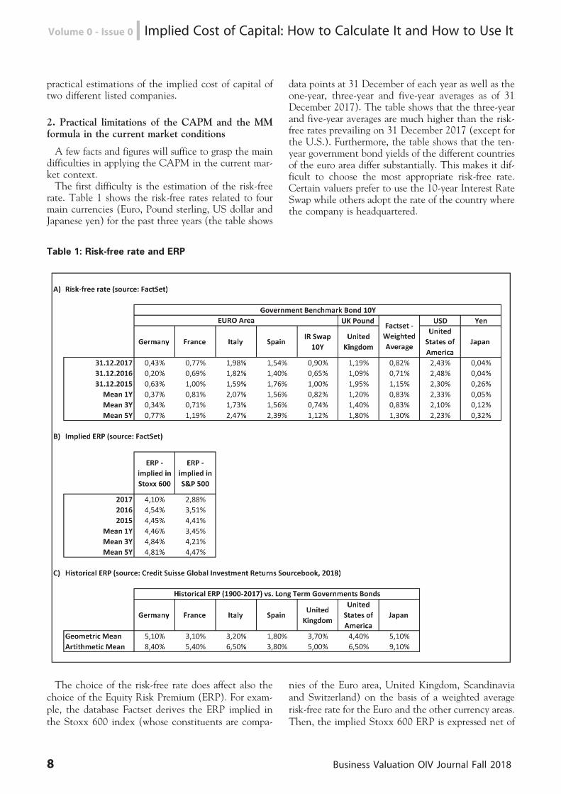
rate. Table 1 shows the risk-free rates related to fourmain currencies (Euro, Pound sterling, US dollar andJapanese yen) for the past three years (the table shows

data points at 31 December of each year as well as theone-year, three-year and five-year averages as of 31December 2017). The table shows that the three-yearand five-year averages are much higher than the risk-free rates prevailing on 31 December 2017 (except forthe U.S.). Furthermore, the table shows that the ten-year government bond yields of the different countriesof the euro area differ substantially. This makes it dif-ficult to choose the most appropriate risk-free rate.Certain valuers prefer to use the 10-year Interest RateSwap while others adopt the rate of the country wherethe company is headquartered.

Table 1: Risk-free rate and ERP

The choice of the risk-free rate does affect also thechoice of the Equity Risk Premium (ERP). For exam-ple, the database Factset derives the ERP implied inthe Stoxx 600 index (whose constituents are compa-

nies of the Euro area, United Kingdom, Scandinaviaand Switzerland) on the basis of a weighted averagerisk-free rate for the Euro and the other currency areas.Then, the implied Stoxx 600 ERP is expressed net of



the average country risk of the two currency areas(Euro and Pound sterling) taken as a whole. On theother hand, if use is made of historical ERP measures,it would be necessary to consider that such measuresare calculated as the arithmetic or geometric mean ofthe differences between equity returns in each countryand long-term government bond yields for the samecountry (thus inclusive of the specific country risk). Inthis case, the ERPs are already net of the specificcountry risk.The Equity Risk Premium and the risk-free rate com-

bine to determine the overall stock market return(Rm). The composition of the stock market return,however, is not neutral. Given the same market return(Rm), a higher ERP entails a greater cost of equity.Table 1 shows the ERPs implied in the Stoxx 600 andin the S&P 500 indices as well as the historical long-term ERPs for the same countries for which the risk-free rate is indicated. The table reveals, for example,that the calculation of stock market returns as the sumof government bond yields prevailing on 31 December2017 and the arithmetic mean of historical ERP wouldreturn unreasonable results. To see that, it is enough tocompare the data related to Germany and Italy, twocountries of the Euro area. In fact:i. Germany’s stock market return (Rm) would be

8.83% (= 0.43% + 8.40%), which is higher than theItalian stock market return calculated with the samemethodology (8.48% = 1.98% + 6.50%), while onemight be forgiven for doubting that an investor wouldrequire a return on an investment in Italian equitieslower than that for an investment in German equities,when the same investor does require a premium of 145bps (= 1.98% – 0.43%) on Italian government bonds;ii. the difference between expected returns on ag-

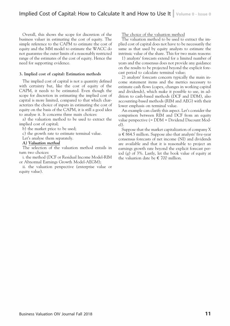
gressive shares (beta>1) would be even greater. AnItalian share with a beta of 1.5 should provide a returnof at least 11.73% whereas a German share with thesame beta should return 13.03% (delta = 130 bps.).Table 2 shows as an example three different options

to estimate Italian market returns (considering onlythe data points at 31 December 2017) and the result-ing estimated returns of two hypothetical shares (Ri),with a respective beta of 1.5 and 0.5 (limits of thenormal distribution range of the beta coefficients).The table shows that the estimated market returnscould range between 5.18% and 8.48%, the returnson the aggressive share (beta = 1.5) between 6.78%and 11.73% while the returns on the defensive sharebetween 3.58% and 5.23%. It is clear that these differ-ences are too broad and unreasonable.

Table 2: Different options for estimating the expected return of the market and of aggressive stock anddefensive stock

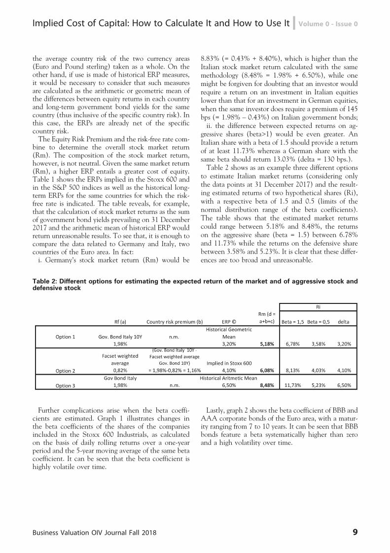
Further complications arise when the beta coeffi-cients are estimated. Graph 1 illustrates changes inthe beta coefficients of the shares of the companiesincluded in the Stoxx 600 Industrials, as calculatedon the basis of daily rolling returns over a one-yearperiod and the 5-year moving average of the same betacoefficient. It can be seen that the beta coefficient ishighly volatile over time.

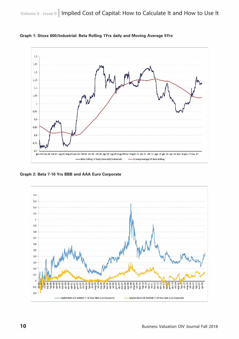
Lastly, graph 2 shows the beta coefficient of BBB andAAA corporate bonds of the Euro area, with a matur-ity ranging from 7 to 10 years. It can be seen that BBBbonds feature a beta systematically higher than zeroand a high volatility over time.



Graph 1: Stoxx 600/Industrial: Beta Rolling 1Yrs daily and Moving Average 5Yrs

Graph 2: Beta 7-10 Yrs BBB and AAA Euro Corporate



Overall, this shows the scope for discretion of thebusiness valuer in estimating the cost of equity. Thesimple reference to the CAPM to estimate the cost ofequity and the MM model to estimate the WACC donot guarantee the outer limits of a reasonably restrictedrange of the estimates of the cost of equity. Hence theneed for supporting evidence.

3. Implied cost of capital: Estimation methods

The implied cost of capital is not a quantity definedwith certainty but, like the cost of equity of theCAPM, it needs to be estimated. Even though thescope for discretion in estimating the implied cost ofcapital is more limited, compared to that which char-acterizes the choice of inputs in estimating the cost ofequity on the basis of the CAPM, it is still a good ideato analyse it. It concerns three main choices:a) the valuation method to be used to extract the

implied cost of capital;b) the market price to be used;c) the growth rate to estimate terminal value.Let’s analyse them separately.A) Valuation methodThe selection of the valuation method entails in

turn two choices:i. the method (DCF or Residual Income Model-RIM

or Abnormal Earnings Growth Model-AEGM);ii. the valuation perspective (enterprise value or

equity value).

The choice of the valuation methodThe valuation method to be used to extract the im-

plied cost of capital does not have to be necessarily thesame as that used by equity analysts to estimate theintrinsic value of the share. This for two main reasons:1) analysts’ forecasts extend for a limited number of

years and the consensus does not provide any guidanceon the results to be projected beyond the explicit fore-cast period to calculate terminal value;2) analysts’ forecasts concern typically the main in-

come statement items and the metrics necessary toestimate cash flows (capex, changes in working capitaland dividends), which make it possible to use, in ad-dition to cash-based methods (DCF and DDM), alsoaccounting-based methods (RIM and AEG) with theirlower emphasis on terminal value.An example can clarify this aspect. Let’s consider the

comparison between RIM and DCF from an equityvalue perspective (= DDM = Dividend Discount Mod-el).Suppose that the market capitalization of company X

is E 864.5 million. Suppose also that analysts’ five-yearconsensus forecasts of net income (NI) and dividendsare available and that it is reasonable to project anearnings growth rate beyond the explicit forecast per-iod (g) of 3%. Lastly, let the book value of equity atthe valuation date be E 700 million.



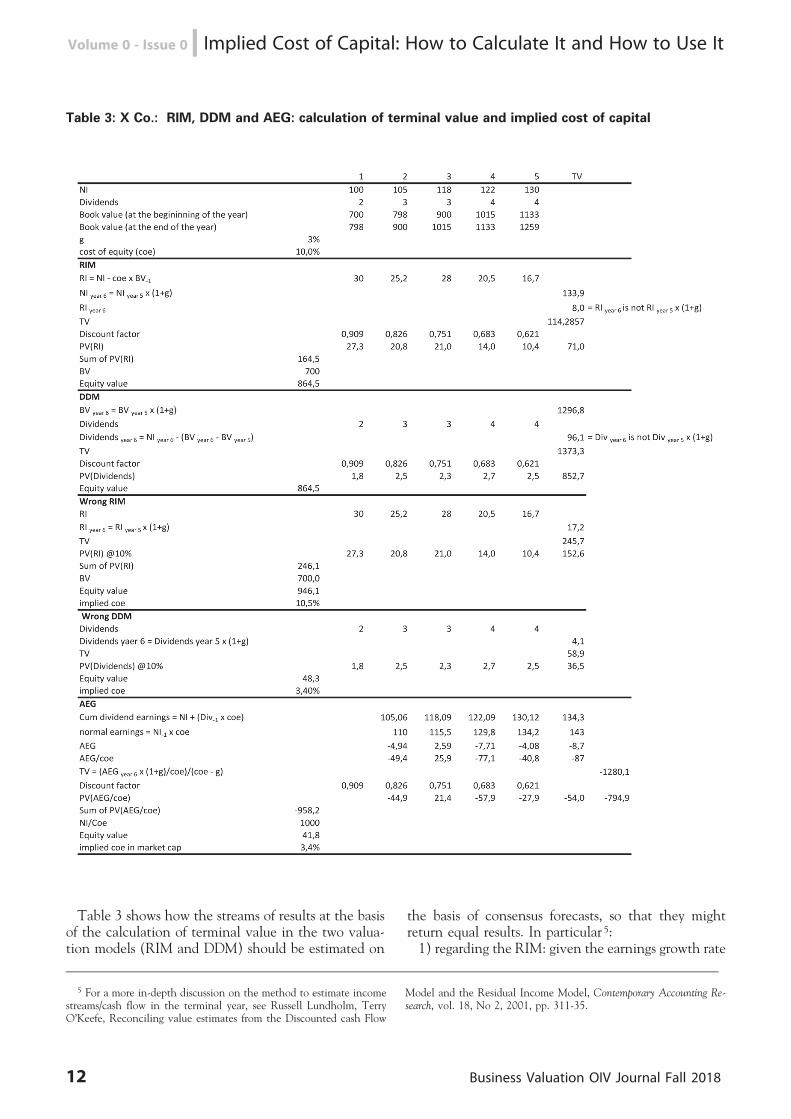
Table 3: X Co.: RIM, DDM and AEG: calculation of terminal value and implied cost of capital

Table 3 shows how the streams of results at the basisof the calculation of terminal value in the two valua-tion models (RIM and DDM) should be estimated on

the basis of consensus forecasts, so that they mightreturn equal results. In particular 5:1) regarding the RIM: given the earnings growth rate

5 For a more in-depth discussion on the method to estimate incomestreams/cash flow in the terminal year, see Russell Lundholm, TerryO’Keefe, Reconciling value estimates from the Discounted cash Flow

Model and the Residual Income Model, Contemporary Accounting Re-search, vol. 18, No 2, 2001, pp. 311-35.



beyond the explicit consensus forecast horizon (g), theResidual Income to estimate terminal value (year 6) isas follows:Residual Income year 6 = Net Income year 6 – cost of

equity 6 Book Valueat the end year 5

where:Net Income year 6 = Net Income year 5 6 (1 + g),thus:Residual Income year 6 ≠ Residual Income year 5 6 (1

+ g)2) regarding the DDM: the dividend to estimate

terminal value (year 6) is as follows:Dividends year 6 = Net Income year 6 – (Book Value at

the end year 6 – Book Valueat the end year 5)where:Book Value year 6 = Book Value year 5 6 (1 + g),thus:Dividends year 6 ≠ Dividends year 5 6 (1 + g)The adoption of these residual-income and dividend

values to estimate terminal value results in the sameequity value with both valuation models, so that bysetting equity value as equal to market capitalizationand tracing our way back through the valuation, thesame implied cost of capital is obtained (in the exam-ple it is 10%).However, if to estimate terminal value use had been

made of the values obtained on the basis of the follow-ing (wrong) relationships, which are still used fre-quently:Residual Income year 6 = Residual Income year 5 6 (1

+ g)Dividends year 6 = Dividends year 5 6 (1 + g)the result would have been distorted estimates of

implied cost of capital and the distortion would havebeen significantly greater if the DDM had been ap-plied.Table 3 shows also the calculation based on the

wrong estimates of terminal value. The table showsfirst how, by making use of wrong streams of resultsto be projected beyond the explicit forecast period, theequity value that would be derived from the two mod-els (RIM and DDM) by adopting a cost of capital of10% would be greater than current enterprise value ofcompany X’s (946.1 vs. 864.5), in the case of RIM,and significantly lower (48.4 vs. 864.5), in the case ofDDM.By the same token, by tracing our way back through

the two models, after setting the equity value equal tomarket capitalization, the implied cost of capital would

be significantly different from each other and differentfrom the effective implied cost of capital (which in theexample is equal to 10%). In fact:– in the case of RIM, the implied cost of capital

would be higher than 10% (and equal to 10.5%, withan error of + 0.5%);– in the case of DDM, the implied cost of capital

would be lower than 10% (and equal to 3.4%, with anerror of – 6.6%).The example in table 3 casts light on four significant

aspects 6:a) even with a complete set of consensus informa-

tion (earnings and dividend forecast and growth ratebeyond the explicit forecast horizon), a wrong esti-mate of implied cost of capital is still a possibility,due to the wrong estimate of last year’s stream ofresults to be projected in perpetuity;b) the size of the error is typically greater in the

DDM than in the RIM, simply because the DDM putsgreater weight on terminal value, while in the RIMmodel terminal value acts as an adjustment factor ofthe book value of the initial equity;c) the size of the DDM’s error is inversely related to

the pay-out ratio (the lower the pay-out, the greaterthe error in estimating the terminal stream of resultsobtained by applying the growth rate g to the dividendof the last year of the explicit forecast) 7;d) the proper application of the DDM requires the

same information as the RIM (in particular, it is ne-cessary to have earnings and equity growth forecasts)and, as such, it is not, in practical terms, a model thatuses fewer data inputs but only a model more exposedto possible estimate errors.These elements explain why ample preference is gi-

ven to the RIM in the literature, compared to theDDM, in estimating the implied cost of capital, eventhough the RIM is used much less frequently than theDDM by analysts 8 (the RIM is normally applied tocompanies in regulated sectors to estimate enterprisevalue – given that their invested capital is equal toRAB _ Regulatory Asset Base – and to financial com-panies, to estimate equity value, given that equity isrepresented by regulatory capital).However, even the RIM has a noticeable limitation.

In fact, it is based on the clean surplus assumption,whereby any change in equity between two years isequal to retained earnings, as per the following formu-la:

6 The considerations made for DDM and RIM, from the equity valueperspective, apply also to DCF and RIM but from the enterprise valueperspective.

7 If anything, for dividends equal to zero, for any growth rate g, thedividend stream to be utilized to estimate terminal value is always equalto zero.

8 Richardson S., Tuna I. and Wysocki P., ‘Accounting anomaliesand fundamental analysis: A review of recent research advances’, Jour-nal of Accounting and Economics, 2010, vol. 50, issue 2-3, 410-454:‘‘Table 1 Q6: Over the last 12 months how often have you used the followingvaluation techniques in your work? Practitioner: RIM Infrequently (46%);Academic Frequently (71%’’).



BV at the end of the year = BV at the beginning of the ye (NI– Dividends)In this case the assumption is that net income is the

same as comprehensive income and that the companydid not carry out any equity-related transactions (issueof new shares or buyback of own shares) 9.To overcome the limitation of the RIM, use has

been made in the literature of the AEG model. Thetheoretical benefit of the AEG is that it is not foundedon the clean surplus assumption. On the other hand,the AEG has a significant practical limitation, in thatoften it is not compatible with earnings growth fore-casts beyond the explicit forecast period utilized byanalysts. This is the case also of company X. Table 4illustrates the application of the AEG to company Xon the basis of the same earnings, dividend and growthforecasts beyond the explicit forecast period shownpreviously. The earnings growth rate beyond the ex-plicit forecast period (g = 3%) significantly lower thanthe product of the retention ratio in year 5 (b = 96%)by the cost of equity (coe = 10%) is indicative ofnegative abnormal earnings which, projected in perpe-tuity at a growth rate g, give a highly negative terminalvalue that lowers the estimated equity value. Conse-quently, the implied cost of capital that would be de-rived from the use of the AEG model would be 3.4%(the same that would be obtained by applying thewrong formula to estimate terminal value in the caseof the DDM) and the error in the estimation withrespect to the correct implied cost of capital (=10%) would be equal to 6.6% (= 10% – 3.4%)Thus, the AEG model has the same significant prac-

tical limitations as the DDM. As such, the RIM is themost suitable model to extract the implied cost ofcapital. Typically, the RIM is applied:a) on a per share basis, that is by considering the

price per share (instead of market capitalization) andearnings per share (so as to offset the effects of capitalincreases or share buybacks);b) in the absence of non-neutral equity-related trans-

actions which, with their dilutive effects or theirabove-market prices, distort the results of valuations;c) on the assumption that expected comprehensive

income is the same as the net income expected byequity analysts.The valuation perspective (enterprise value or equity

value)The choice of the valuation perspective is a function

of the type of implied cost of capital sought. To thisend, there are three types of implied cost of capital:

– cost of equity (coe): this is obtained by using themarket value of equity and net income. In this case,the cost of capital is a function of the level of indebt-edness of the specific company whose market capitali-zation is used to extract the implied cost of capital;– weighted average cost of capital (WACC): this is

obtained by using enterprise value (which reflects thesum of the market value of equity and the book valueof net debt) and net operating income after taxes. Inthis case, assuming that the debt’s market value isequal to its book value, WACC is computed withoutthe need to estimate the cost of debt or the targetfinancial structure;– unlevered cost of capital: this is obtained by using

enterprise value net of the tax benefits on debt esti-mated on the basis of the Modigliani Miller model andnet operating income after taxes (Nopat). In this case– assuming that the debt’s market value is equal to itsbook value and that there are no bankruptcy costs, sothat the Modigliani Miller relationship:EV unlevered = EV levered – Tax shields on Debt ap-

plies,where:Tax shields on debt = Debt 6 Tc with Tc = corpo-

rate tax ratean estimate of the cost of capital can be derived to be

adapted to the particular financial structure of thecompany to be valued on the basis of the well-knownModigliani Miller relationship whereby:WACC = unlevered cost of capital 6 (1 – Tc B/

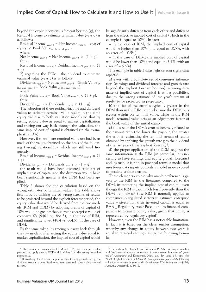
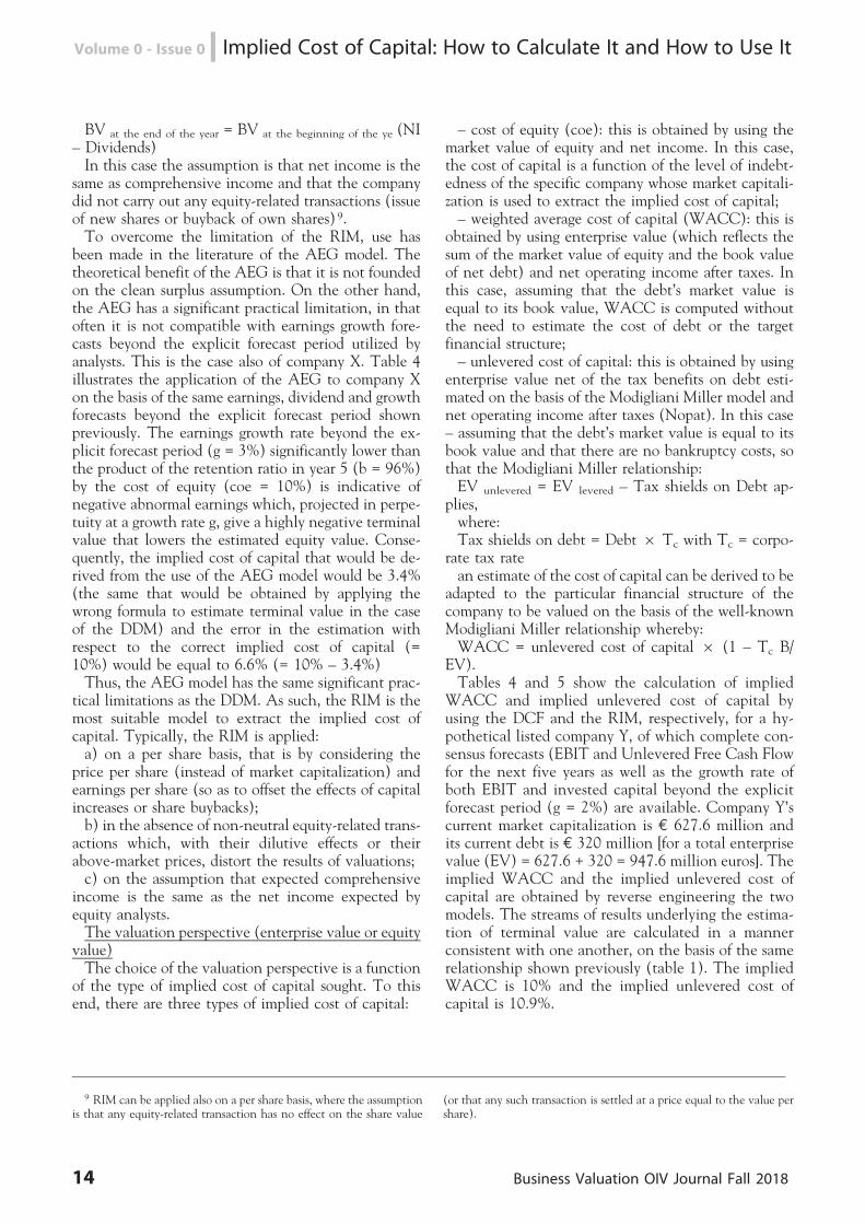
EV).Tables 4 and 5 show the calculation of implied

WACC and implied unlevered cost of capital byusing the DCF and the RIM, respectively, for a hy-pothetical listed company Y, of which complete con-sensus forecasts (EBIT and Unlevered Free Cash Flowfor the next five years as well as the growth rate ofboth EBIT and invested capital beyond the explicitforecast period (g = 2%) are available. Company Y’scurrent market capitalization is E 627.6 million andits current debt is E 320 million [for a total enterprisevalue (EV) = 627.6 + 320 = 947.6 million euros]. Theimplied WACC and the implied unlevered cost ofcapital are obtained by reverse engineering the twomodels. The streams of results underlying the estima-tion of terminal value are calculated in a mannerconsistent with one another, on the basis of the samerelationship shown previously (table 1). The impliedWACC is 10% and the implied unlevered cost ofcapital is 10.9%.

9 RIM can be applied also on a per share basis, where the assumptionis that any equity-related transaction has no effect on the share value

(or that any such transaction is settled at a price equal to the value pershare).



Table 4: Y Co.: RIM asset side and implied cost of capital (wacc and unlevered coc)

Table 5: Y Co.: DCF asset side and implied cost of capital (wacc and unlevered coc)

Table 6 illustrates the calculation of the implied costof equity of company Y from the equity value perspec-tive (in this case also the interest expense and net debtforecasts are available) by using not only the RIM and

the DDM but also the AEG. The streams of resultsreflect the funds available only to the shareholders andthe implied cost of equity is obtained as the internalrate of return of an investment that assumes market



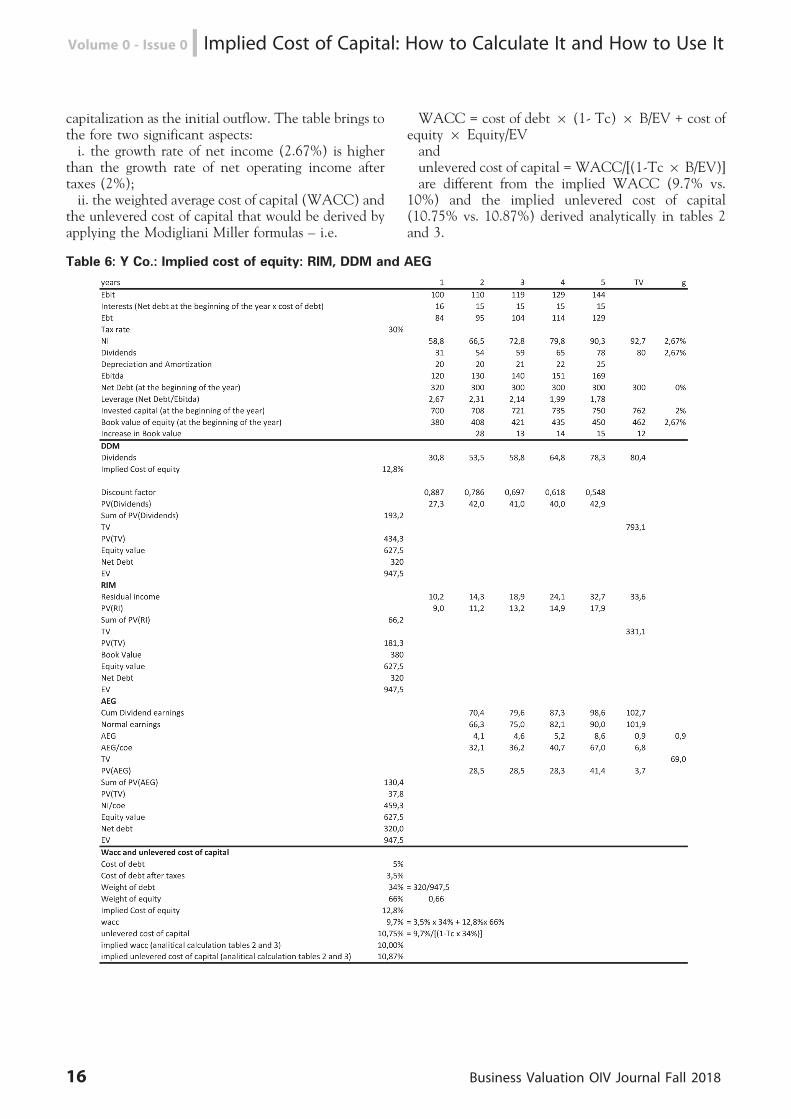
capitalization as the initial outflow. The table brings tothe fore two significant aspects:i. the growth rate of net income (2.67%) is higher

than the growth rate of net operating income aftertaxes (2%);ii. the weighted average cost of capital (WACC) and

the unlevered cost of capital that would be derived byapplying the Modigliani Miller formulas – i.e.

WACC = cost of debt 6 (1- Tc) 6 B/EV + cost ofequity 6 Equity/EVandunlevered cost of capital = WACC/[(1-Tc6 B/EV)]are different from the implied WACC (9.7% vs.

10%) and the implied unlevered cost of capital(10.75% vs. 10.87%) derived analytically in tables 2and 3.

Table 6: Y Co.: Implied cost of equity: RIM, DDM and AEG



The effects under both i) and ii) are due to the factthat company Y’s leverage is not constant. In fact, theexample considers stable interest expense and netdebt, in the presence of growing unlevered streams.A constant leverage (thus net income streams growingat the same rate as unlevered net income streams) isbased on the principle that interest expense on debtincreases at the same rate as unlevered net income(and, given the same cost of debt, this means that debtincreases at the same rate). Thus, if debt is constant:i. the growth rate of net income is necessarily higher

than the growth rate of unlevered net income;ii. implied WACC and implied cost of capital can-

not be equal to the corresponding metrics calculatedwith the MM formulas, as such formulas assume aconstant leverage. If the leverage ratio falls in relativeterms (constant debt and growing unlevered net in-come) the MM formulas end up making an error.B) The price to be usedEstimation of the implied cost of capital assumes

consistent price and analysts’ forecasts. To that end,the choices concern:a) the use of either an average market price or an

actual price;b) the use of either market prices or target prices;

c) the use of ‘‘asymmetrical’’ analyst forecasts.Use of either an average price or an actual priceTo express the internal rate of return, the implied

cost of capital must be calculated by avoiding a mis-alignment between prices and forecasts. This might bedifficult, as prices are more volatile than forecasts andforecasts are updated slowly 10. Consequently, anyprice variation not met by a variation in the analysts’consensus entails a change in the implied cost of ca-pital in the opposite direction and to an extent pro-portionate to the duration of the share.Table 7 compares the error in the estimation of im-

plied cost of capital of two hypothetical listed compa-nies: company Y (the same as in table 4) and companyZ, each with its own equity duration. Both companieshave the same market capitalization but company Zhas higher expected dividends in the explicit forecastperiod (shorter equity duration). The table shows thatfor a 15% decrease of market capitalization, not ac-companied by a revision of earnings and dividendsby analysts, company Y’s implied cost of equity risesfrom 12.8% to 14.4% (= 14.4%/12.8% – 1 = +12.5%), while company Z’s implied cost of capital in-creases at a lower rate, from 12.8% to 14% (= 14%/12.8% – 1 = 9.4%).

10 In the literature this is called sluggishness. Guay W. S. Kothariand S. Shu Properties of implied cost of capital using analysts’ forecasts,

Working paper, University of Pennsylvania, Pennsylvania, WhartonSchool, 2005.



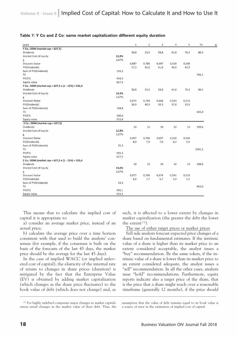
Table 7: Y Co and Z Co: same market capitalization different equity duration

This means that to calculate the implied cost ofcapital it is appropriate to:a) consider an average market price, instead of an

actual price;b) calculate the average price over a time horizon

consistent with that used to build the analysts’ con-sensus (for example, if the consensus is built on thebasis of the forecasts of the last 45 days, the marketprice should be the average for the last 45 days).In the case of implied WACC (or implied unlev-

ered cost of capital), the elasticity of the internal rateof return to changes in share prices (duration) ismitigated by the fact that the Enterprise Value(EV) is obtained by adding market capitalization(which changes as the share price fluctuates) to thebook value of debt (which does not change) and, as

such, it is affected to a lower extent by changes inmarket capitalization (the greater the debt the lowerthe extent 11).The use of either target prices or market pricesSell side analysts forecast expected price changes of a

share based on fundamental estimates. If the intrinsicvalue of a share is higher than its market price to anextent considered acceptable, the analyst issues a‘‘buy’’ recommendation. By the same token, if the in-trinsic value of a share is lower than its market price toan extent considered adequate, the analyst issues a‘‘sell’’ recommendation. In all the other cases, analystsissue ‘‘hold’’ recommendations. Furthermore, equityreports indicate also a target price of the share, thatis the price that a share might reach over a reasonabletimeframe (generally 12 months), if the price should

11 For highly indebted companies major changes in market capitali-zation entail changes in the market value of their debt. Thus, the

assumption that the value of debt remains equal to its book value isa source of error in the estimation of implied cost of capital.



realign with intrinsic value. This is why equity reportsindicate both the current share price (which varies byanalyst as reports are drafted at different dates) and thetarget price (12-month forward).In principle, if the share’s current price were aligned

with its intrinsic (or fundamental) value, the targetprice (which reflects a forward equilibrium price)could be derived from the following equation:Target price = Current price 6 (1+ coe) – Divi-

dends.Accordingly, price and target price should return the

same implied cost of capital.On the other hand, when the share’s current price is

lower than its intrinsic (fundamental) value, the rela-tionship is as follows:Target price = Intrinsic value 6 (1 + coe) – Divi-

dendswhere:if ‘‘Intrinsic value > Current price’’, the share is

undervalued and, consequently, ‘‘Target Price > Cur-rent price 6 (1 + coe) – Dividends’’; whileif ‘‘Intrinsic value < Current price’’ the share is over-

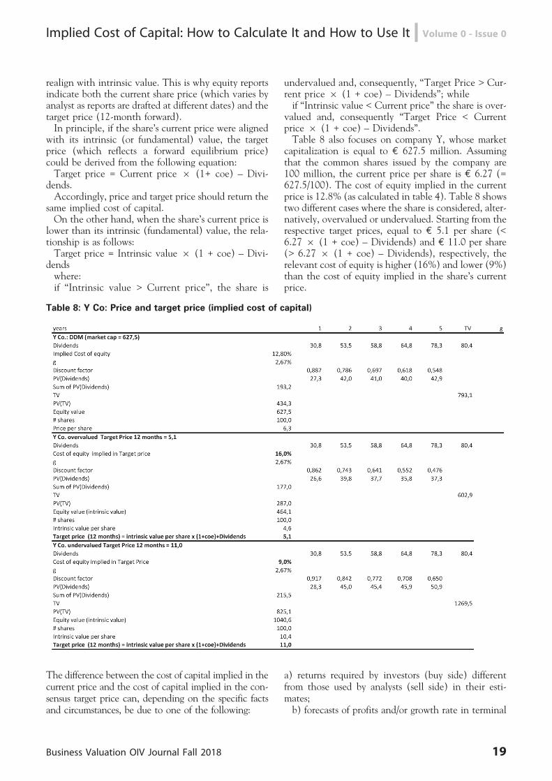
valued and, consequently ‘‘Target Price < Currentprice 6 (1 + coe) – Dividends’’.Table 8 also focuses on company Y, whose market

capitalization is equal to E 627.5 million. Assumingthat the common shares issued by the company are100 million, the current price per share is E 6.27 (=627.5/100). The cost of equity implied in the currentprice is 12.8% (as calculated in table 4). Table 8 showstwo different cases where the share is considered, alter-natively, overvalued or undervalued. Starting from therespective target prices, equal to E 5.1 per share (<6.27 6 (1 + coe) – Dividends) and E 11.0 per share(> 6.27 6 (1 + coe) – Dividends), respectively, therelevant cost of equity is higher (16%) and lower (9%)than the cost of equity implied in the share’s currentprice.

Table 8: Y Co: Price and target price (implied cost of capital)

The difference between the cost of capital implied in thecurrent price and the cost of capital implied in the con-sensus target price can, depending on the specific factsand circumstances, be due to one of the following:

a) returns required by investors (buy side) differentfrom those used by analysts (sell side) in their esti-mates;b) forecasts of profits and/or growth rate in terminal



value by equity analysts different from those of inves-tors (buy side);c) the presence of premiums over and/or discounts to

the share’s intrinsic value based on the prevailing mar-ket sentiment (determined by non-fundamental rea-sons).The asymmetry of analysts’ forecastsEmpirical evidence point to excessively bullish ana-

lysts’ (sell side) forecasts 12. This might be due to manydifferent reasons. The main reason however is thatanalysts’ forecasts might be based on expected resultsassociated with the most likely scenario (which do notnecessarily reflects expected average streams of results).Certain brokerage houses (e.g. Morgan Stanley) re-quire analysts to provide, in addition to the target priceof the base scenario (built on the most likely scenario),also price forecasts related to two alternative scenarios(bull and bear). Bull and bear prices are constructed byconsidering risk factors that are not necessarily char-acterized by a normal distribution, such as: success orfailure in the launch of a new product; new regula-tions; technological disruptions; growing competitionetc. Bull and bear prices are built on conditional fore-casts, that is forecasts assuming the materialization ofcertain events. The most likely scenario (used for thetarget price) typically corresponds to the average ex-pected scenario (expected value forecast). Joos, Pio-troski and Srinivasan show that the target price ofMorgan Stanley’s analysts (which is based on the basescenario) features (moderate) optimism, settling typi-cally above the average between the bull price and thebear price.If analysts’ scenarios suffer from optimism bias, and

the market is fundamentally efficient, the implied costof capital calculated by reference to the current marketprice is systematically distorted upwardly, as the mar-ket price does not reflect the analysts’ results 13 but theaverage expected results (which are not observableyet). The distortion of the implied cost of capital doesnot necessarily reduce its signalling capabilities. Infact, the implied cost of capital ends up capturing boththe return required by the market and the premium forthe specific risk (alpha) that the market implicitly

applies to analysts’ forecasts to translate them intomarket prices.As there is evidence in the literature that optimism

in consensus forecasts is more pronounced in the caseof smaller companies and with more limited analystcoverage, it might be presumed that the smaller thesize of the listed company concerned the greater thedifference between implied cost of capital and cost ofcapital calculated on the basis of the CAPM or othermodels (also considering the size effect 14). The differ-ence between the two can be taken as the currentmeasure of the alpha coefficient.C) The growth rate beyond the explicit forecast

periodSo far analysts’ consensus forecasts of the growth rate

beyond the explicit forecast period have been assumedto be available. Typically this rate is indicated in thereports of equity analysts who estimate the intrinsicvalue of shares on the basis of expected results 15 butis not available in the traditional databases used byvaluers. When the number of comparable companiesis high, the manual search of the growth rate goingthrough the single reports on each company can becomplex or otherwise impracticable in terms of timeand cost. However, the growth rate in terminal value isa very significant variable in the estimation of theimplied cost of capital.Table 9 shows the effects of a different growth rate in

the estimation of terminal value on company Y’s im-plied cost of capital (see table 6). A one percentagepoint decrease (from 2.67% to 1.67%) or increase(from 2.67% to 3.67%) in the growth rate determinesa 60 bps. change in the implied cost of capital in thesame direction.Thus, the higher the growth rate used in the estima-

tion of terminal value the greater the implied cost ofcapital and vice versa. Hence, the need to draw atten-tion to two significant aspects:a) the growth rate is a function of the valuation

model adopted;b) the growth rate is a function of the explicit fore-

cast horizon.

12 ‘‘Brown (1997) provides evidence that analysts’ forecast errors aresmaller for (1) S&P 500 firms;(2) firms with large market capitalization,large absolute value of earnings forecasts, and large analyst following; and(3) firms in certain industries’’ in Peter Easton, Estimating the cost ofcapital implied by market prices and accounting data, Foundation andtrends in accounting Vol. 2, No. 4, 2007 pp. 241-364 (2009).

13 Easton e Sommers (2007) show that excessive optimism in ana-lysts’ forecasts translates into an average increase of 2.84% of the im-plied cost of capital for the market portfolio, a significant value con-sidering the daily ERP generally measured through the implied cost ofcapital at the level of securities portfolios. Easton P. and Sommers,

Effects of analysts’ optimism on estimates of the expected rate of returnimplied by earnings forecasts’’ Journal of Accounting Research, 45 (De-cember 2007) pp. 983-1015.

14 The Fama French models considers specifically the size factor,while with respect to the CAPM the size factor is captured implicitlythrough the use of sum betas.

15 It should be noted that:a) not every analysts use valuation models founded on the discount

to present value of expected streams of results, as many analysts onlyuse multiples;

b) not all analysts report the input data used in their valuation.



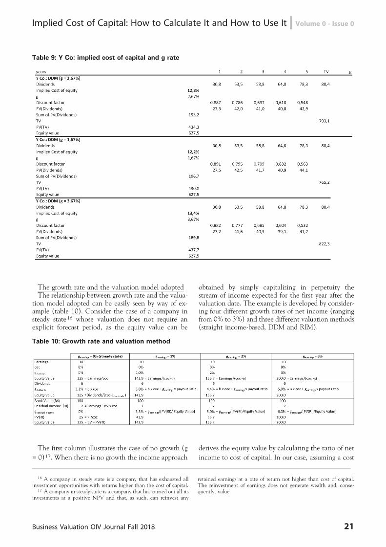
Table 9: Y Co: implied cost of capital and g rate

The growth rate and the valuation model adoptedThe relationship between growth rate and the valua-

tion model adopted can be easily seen by way of ex-ample (table 10). Consider the case of a company insteady state 16 whose valuation does not require anexplicit forecast period, as the equity value can be

obtained by simply capitalizing in perpetuity thestream of income expected for the first year after thevaluation date. The example is developed by consider-ing four different growth rates of net income (rangingfrom 0% to 3%) and three different valuation methods(straight income-based, DDM and RIM).

Table 10: Growth rate and valuation method

The first column illustrates the case of no growth (g

= 0)17. When there is no growth the income approach

derives the equity value by calculating the ratio of net

income to cost of capital. In our case, assuming a cost

16 A company in steady state is a company that has exhausted allinvestment opportunities with returns higher than the cost of capital.

17 A company in steady state is a company that has carried out all itsinvestments at a positive NPV and that, as such, can reinvest any

retained earnings at a rate of return not higher than cost of capital.The reinvestment of earnings does not generate wealth and, conse-quently, value.



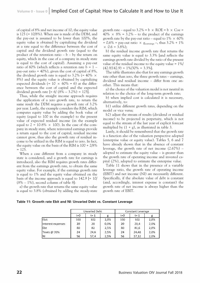
of capital of 8% and net income of 10, the equity valueis 125 (= 10/8%). When use is made of the DDM, andthe pay-out is assumed to be lower than 100%, theequity value is obtained by capitalizing the dividendat a rate equal to the difference between the cost ofcapital and the dividend growth rate (equal to theproduct of the retention ratio – b – by the return onequity, which in the case of a company in steady stateis equal to the cost of capital). Assuming a pay-outratio of 60% (which reflects a retention rate b = 1 –pay-out ratio = 40%), given the cost of capital of 8%,the dividend growth rate is equal to 3.2% (= 40% 68%) and the equity value is obtained by capitalizingexpected dividends (= 10 6 60% = 6) at the differ-ence between the cost of capital and the expecteddividend growth rate [= 6/ (8% – 3.2%) = 125].Thus, while the straight income approach requires

the application of a zero growth rate, to return thesame result the DDM requires a growth rate of 3.2%per year. Lastly, the example considers the RIM, whichcomputes equity value by adding the book value ofequity (equal to 100 in the example) to the presentvalue of expected residual income (in the exampleequal to 2 = 10-8% 6 100). In the case of the com-pany in steady state, where reinvested earnings providea return equal to the cost of capital, residual incomecannot grow, thus also the growth rate of residual in-come to be utilized in the RIM is equal to zero. In fact,the equity value on the basis of the RIM is 100 + 2/8%= 125.When a case different from a company in steady

state is considered, and a growth rate for earnings isintroduced, also the RIM requires growth rates differ-ent from the earnings growth rate, to obtain the sameequity value. For example, if the earnings growth rateis equal to 1% and the equity value obtained on thebasis of the income approach is equal to 142.9 [= 10/(8% – 1%), second column of table 8]:a) the growth rate that returns the same equity value

is equal to 3.8% (obtained by adding the steady-state

growth rate – equal to 3.2% = b 6 ROE = b 6 Coe =40% 6 8% = 3.2% – to the product of the earningsgrowth rate by the pay-out ratio – equal to 1% 6 60%= 0,6% = pay-out ratio 6 gearnings –, thus 3.2% + 1%6 0.6 = 3.8%);b) the residual income growth rate that returns the

same equity value is equal to 3.3% [and reflects theearnings growth rate divided by the ratio of the presentvalue of the residual income to the equity value = 1%/(42.9/142.9) = 1%/30% = 3.3%].The table illustrates also that for any earnings growth

rate other than zero, the three growth rates – earnings,dividend and residual income – differ from one an-other. This means that:a) the choice of the valuation model is not neutral in

relation to the choice of the long-term growth rate;b) when implied cost is calculated it is necessary,

alternatively, to:b1) utilize different growth rates, depending on the

model or vice versa;b2) adjust the stream of results (dividend or residual

income) to be projected in perpetuity, which is notequal to the stream of the last year of explicit forecastmultiplied by (1 + g), as illustrated in table 3.Lastly, it should be remembered that the growth rate

is a function also of the valuation perspective adopted(enterprise value or equity value). Tables 5, 6 and 7have already shown that in the absence of constantleverage, the growth rate of net income (2.67%) –adopted to estimate the equity value – is greater thanthe growth rate of operating income and invested ca-pital (2%), adopted to estimate the enterprise value.Table 11 shows that in the presence of a variable

leverage ratio, the growth rate of operating income(EBIT) and net income (NI) are necessarily different.Specifically, if the absolute value of debt is constant(and, accordingly, interest expense is constant) thegrowth rate of net income is always higher than thegrowth rate of EBIT.

Table 11: Growth rate Ebit and NI: Unvaried Debt vs. Constant Leverage



The growth rate and the explicit forecast horizonWhen a sufficiently long explicit forecast horizon is

adopted, the growth rate used to estimate terminalvalue should only reflect the industry’s or the econo-my’s long-term expectations and should not differ sub-stantially among comparable companies 18. This meansthat, to estimate the implied cost of capital, valuerscould use the same long-term growth rate that theyconsider appropriate for the specific company to bevalued. Actually, also in the literature the implied costof capital is estimated by using proxies of industry orGDP growth rates or just long-term inflation rates 19.However, in practical terms, it should be noted that

equity analysts’ forecasts:a) never go beyond a five-year horizon;b) can be relied on typically only for the first three

years (as just few analysts make forecasts for the fourthand fifth year).The consequence is that, for all fast-growing compa-

nies for which the excess earnings growth20 is ex-pected to continue beyond the analysts’ forecast hor-izon, application of the consensus growth rate to theearnings of the last year of the forecast would result inan underestimated implied cost of capital, with theparadox that the greater the excess earnings growthbeyond the explicit forecast period the lower the im-plied cost of capital and, consequently, the greater therisk associated with this growth. This is why, in com-panies with particularly high growth prospects, it isnecessary to adopt multi-stage growth models. To thatend, it is necessary to identify growth rates to be ap-plied to the streams of results generated after the ana-lysts’ forecast horizon whose intensity and durationreflect directly on the cost of equity. More often, theexcess earnings growth rate is estimated on the basis ofthe progressive convergence of the return on equity ofthe specific company towards the average ROE for theindustry. The constant erosion of abnormal returnsover time and the convergence toward normal industry

returns are the two most common assumptions under-lying the estimation of the excess earnings growth rate.It is important to point out that any earnings and

cash-flow growth forecasts need to be consistent withthe investments necessary to support the growth ofresults. The typical decline of growth rates goes handin hand also with rising investments to support growth,owing to the natural decrease of the marginal effi-ciency of capital. As a reminder, given that the growthrate g is equal to the product of the retention rate (b)by the return on equity, if g falls while b rises, thereturn on equity can only decrease faster than g.In other words, beyond a given point in the future,

high though as the growth rate g might still be, growthshould not affect the enterprise value (and the impliedcost of capital), as the reinvestment of earnings shouldbe such as to realign the return on investment with thecost of equity.Table 12A illustrates the case of listed company W,

which has a P/E1 of 35x. Such a high multiple is in-dicative of very high earnings growth prospects. Theanalysts’ consensus projects a 40% earnings growthrate for year 2 and a 38% earnings growth rate for year3, with a pay-out ratio of 80%. The valuation modelused is the DDM. Assuming a 2% GDP growth rate tocalculate W’s terminal value and limiting the analysisto the first three years, the implied cost of capitalwould be 7%. The table shows two other valuationsfounded both on the explicit forecast period and onsuccessive fading periods (each of 6 and 9 years) wherethe excess earnings growth rates converge progressivelytoward the GDP growth rate. In the fading growthperiod, the pay-out is equal to that of the consensusfor the first three years (80%). The table shows howthe implied cost of capital increases as the fadinggrowth period extends. In particular, by adopting afading period of 6 years the implied cost of capital is10.7% while for a fading period of 9 years the impliedcost of capital rises to 13%.

18 The earnings growth rate beyond the explicit forecast horizon canbe calculated, for example, on the basis of a medium/long-term averageretention rate and the average ROE for the industry.

19 For a review of the literature, see Easton P., ‘Estimating the cost ofcapital implied by market prices and accounting data’, Foundations and

Trends in Accounting, Vol. 2, No. 4, 2007, p. 282.20 Excess earnings growth refers to a growth rate for the specific

company that exceeds that of the industry in which it operates orthe economy.



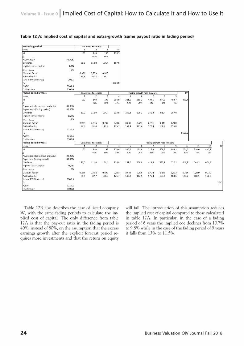
Table 12 A: Implied cost of capital and extra-growth (same payout ratio in fading period)

Table 12B also describes the case of listed companyW, with the same fading periods to calculate the im-plied cost of capital. The only difference from table12A is that the pay-out ratio in the fading period is40%, instead of 80%, on the assumption that the excessearnings growth after the explicit forecast period re-quires more investments and that the return on equity

will fall. The introduction of this assumption reducesthe implied cost of capital compared to those calculatedin table 12A. In particular, in the case of a fadingperiod of 6 years the implied coe declines from 10.7%to 9.8% while in the case of the fading period of 9 yearsit falls from 13% to 11.5%.



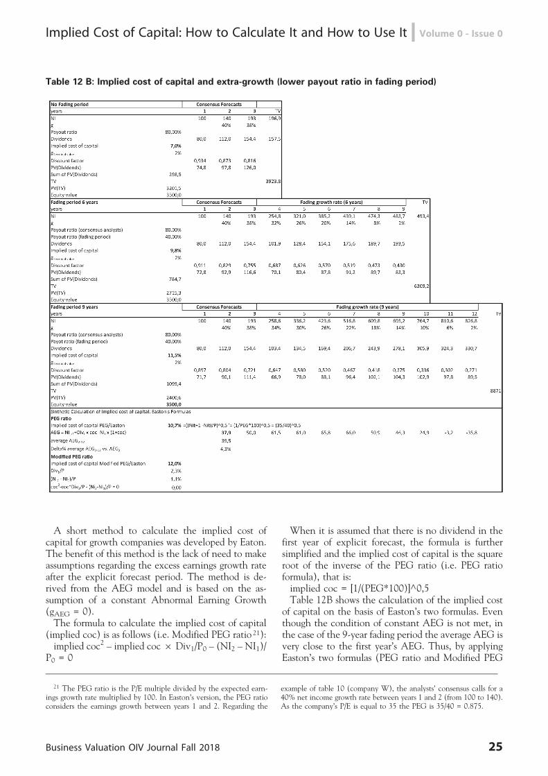
Table 12 B: Implied cost of capital and extra-growth (lower payout ratio in fading period)

A short method to calculate the implied cost ofcapital for growth companies was developed by Eaton.The benefit of this method is the lack of need to makeassumptions regarding the excess earnings growth rateafter the explicit forecast period. The method is de-rived from the AEG model and is based on the as-sumption of a constant Abnormal Earning Growth(gAEG = 0).The formula to calculate the implied cost of capital

(implied coc) is as follows (i.e. Modified PEG ratio 21):implied coc2 – implied coc6 Div1/P0 – (NI2 – NI1)/

P0 = 0

When it is assumed that there is no dividend in thefirst year of explicit forecast, the formula is furthersimplified and the implied cost of capital is the squareroot of the inverse of the PEG ratio (i.e. PEG ratioformula), that is:implied coc = [1/(PEG*100)]^0,5Table 12B shows the calculation of the implied cost

of capital on the basis of Easton’s two formulas. Eventhough the condition of constant AEG is not met, inthe case of the 9-year fading period the average AEG isvery close to the first year’s AEG. Thus, by applyingEaston’s two formulas (PEG ratio and Modified PEG

21 The PEG ratio is the P/E multiple divided by the expected earn-ings growth rate multiplied by 100. In Easton’s version, the PEG ratioconsiders the earnings growth between years 1 and 2. Regarding the

example of table 10 (company W), the analysts’ consensus calls for a40% net income growth rate between years 1 and 2 (from 100 to 140).As the company’s P/E is equal to 35 the PEG is 35/40 = 0.875.



ratio) the result should be an implied cost of capitalvery close to that calculated analytically over a 9-yearfading period. In fact, the table shows that the PEGformula returns an implied cost of capital of 10.7%while the Modified PEG formula an implied cost ofcapital of 12%, vis-a-vis an implied cost of capitalcalculated analytically of 11.5%.

4. Two practical applications of the implied cost ofcapital

This section intends to show two different applica-tions of the implied cost of capital to two listed com-panies. Both companies are listed on the Italian stockexchange.One is a multinational company (Pirelli) while the

second is a medium-size company engaged in the luxurygoods industry (Tod’s). In Pirelli’s case the implied costof capital is used to clarify the uncertainty related to theCAPM factors to be used to estimate the cost of equity(considering that it is a company listed in Italy butoperating on a global scale). In Tod’s case, the impliedcost of capital is utilized instead to compare the reason-

ableness of the estimate that would be obtained by usingthe multiples of comparable companies.The implied cost of capital for a multinational com-

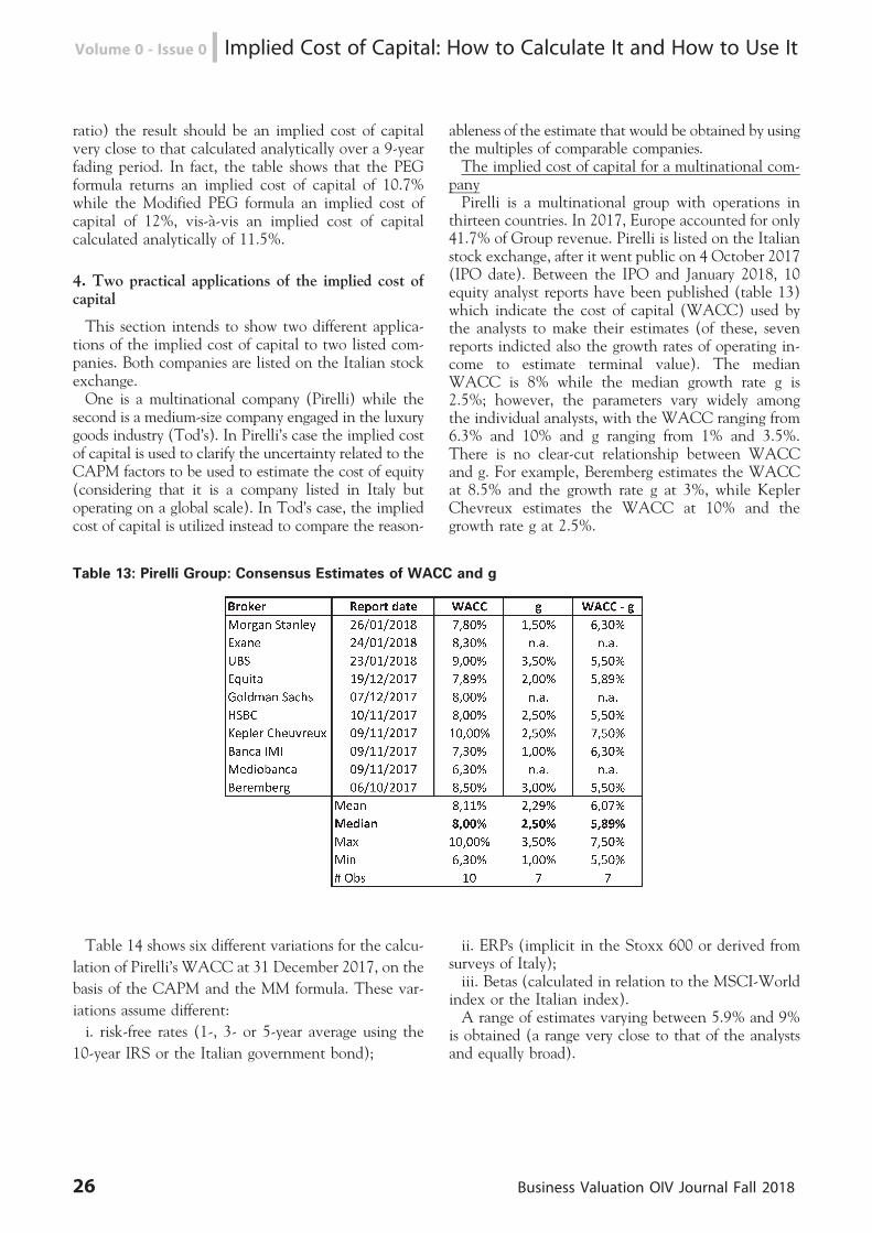
panyPirelli is a multinational group with operations in

thirteen countries. In 2017, Europe accounted for only41.7% of Group revenue. Pirelli is listed on the Italianstock exchange, after it went public on 4 October 2017(IPO date). Between the IPO and January 2018, 10equity analyst reports have been published (table 13)which indicate the cost of capital (WACC) used bythe analysts to make their estimates (of these, sevenreports indicted also the growth rates of operating in-come to estimate terminal value). The medianWACC is 8% while the median growth rate g is2.5%; however, the parameters vary widely amongthe individual analysts, with the WACC ranging from6.3% and 10% and g ranging from 1% and 3.5%.There is no clear-cut relationship between WACCand g. For example, Beremberg estimates the WACCat 8.5% and the growth rate g at 3%, while KeplerChevreux estimates the WACC at 10% and thegrowth rate g at 2.5%.

Table 13: Pirelli Group: Consensus Estimates of WACC and g

Table 14 shows six different variations for the calcu-

lation of Pirelli’s WACC at 31 December 2017, on the

basis of the CAPM and the MM formula. These var-

iations assume different:

i. risk-free rates (1-, 3- or 5-year average using the

10-year IRS or the Italian government bond);

ii. ERPs (implicit in the Stoxx 600 or derived fromsurveys of Italy);iii. Betas (calculated in relation to the MSCI-World

index or the Italian index).A range of estimates varying between 5.9% and 9%

is obtained (a range very close to that of the analystsand equally broad).



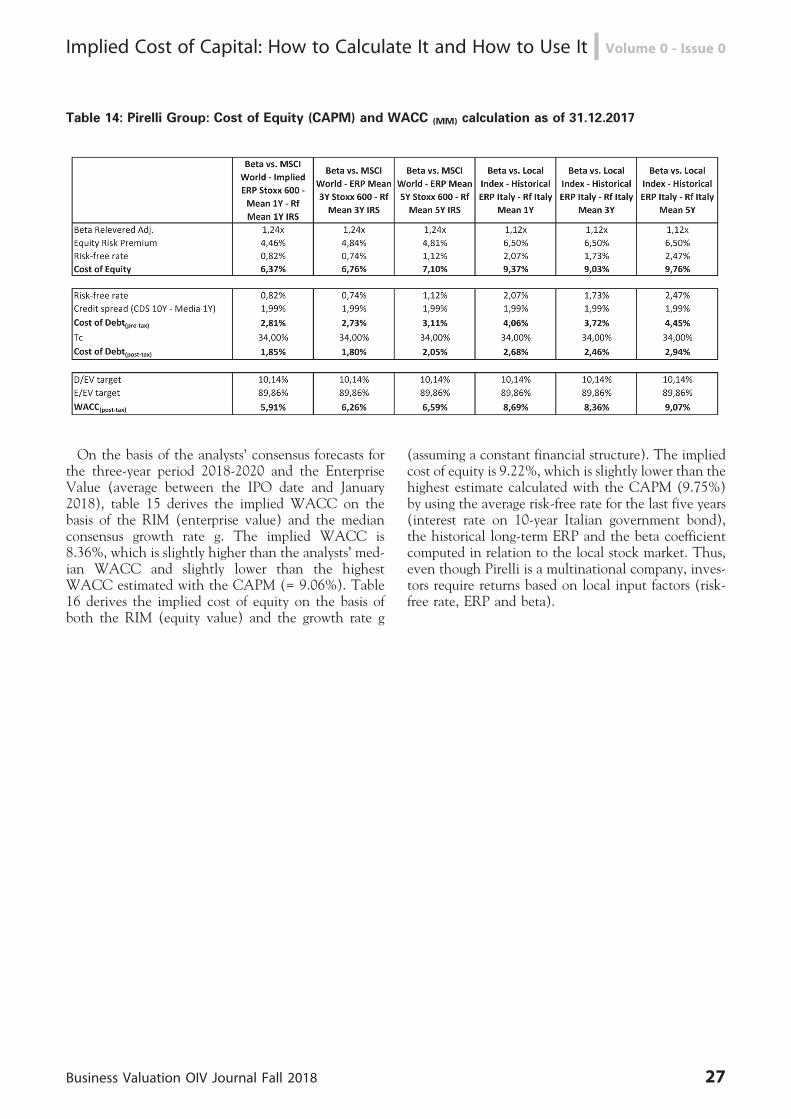
Table 14: Pirelli Group: Cost of Equity (CAPM) and WACC (MM) calculation as of 31.12.2017

On the basis of the analysts’ consensus forecasts forthe three-year period 2018-2020 and the EnterpriseValue (average between the IPO date and January2018), table 15 derives the implied WACC on thebasis of the RIM (enterprise value) and the medianconsensus growth rate g. The implied WACC is8.36%, which is slightly higher than the analysts’ med-ian WACC and slightly lower than the highestWACC estimated with the CAPM (= 9.06%). Table16 derives the implied cost of equity on the basis ofboth the RIM (equity value) and the growth rate g

(assuming a constant financial structure). The impliedcost of equity is 9.22%, which is slightly lower than thehighest estimate calculated with the CAPM (9.75%)by using the average risk-free rate for the last five years(interest rate on 10-year Italian government bond),the historical long-term ERP and the beta coefficientcomputed in relation to the local stock market. Thus,even though Pirelli is a multinational company, inves-tors require returns based on local input factors (risk-free rate, ERP and beta).



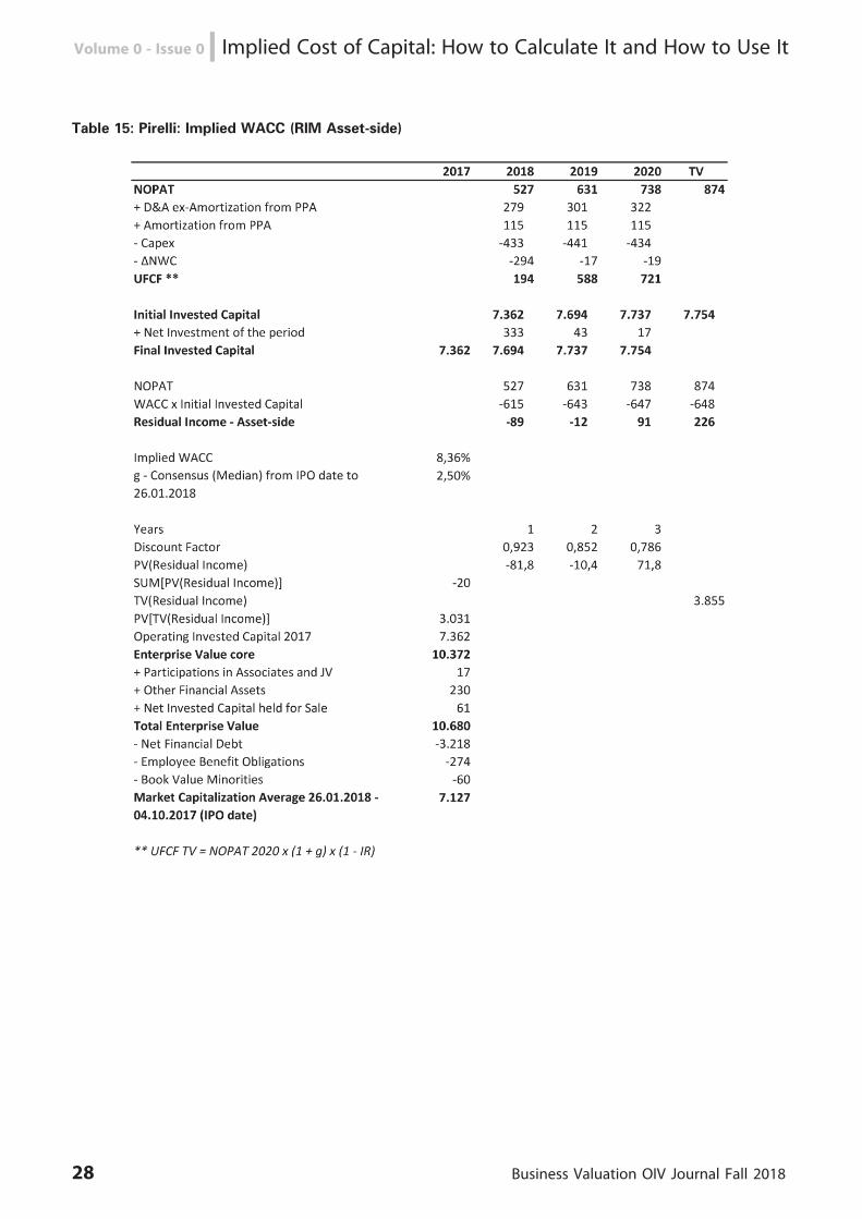
Table 15: Pirelli: Implied WACC (RIM Asset-side)



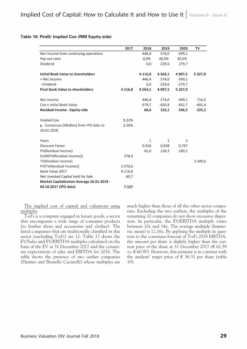
Table 16: Pirelli: Implied Coe (RIM Equity-side)

The implied cost of capital and valuations usingmultiplesTod’s is a company engaged in luxury goods, a sector

that encompasses a wide range of consumer products(to leather shoes and accessories and clothes). Thelisted companies that are traditionally classified in thissector (excluding Tod’s) are 12. Table 17 shows theEV/Sales and EV/EBITDA multiples calculated on thebasis of the EV at 31 December 2017 and the consen-sus expectations of sales and EBITDA for 2018. Thetable shows the presence of two outlier companies(Hermes and Brunello Cucinelli) whose multiples are

much higher than those of all the other sector compa-nies. Excluding the two outliers, the multiples of theremaining 10 companies do not show excessive disper-sion. In particular, the EV/EBITDA multiple variesbetween 10x and 14x. The average multiple (harmo-nic mean) is 12.16x. By applying the multiple in ques-tion to the consensus forecast of Tod’s 2018 EBITDA,the amount per share is slightly higher than the cur-rent price of the share at 31 December 2017 (E 62.59vs. E 60.90). However, this estimate is in contrast withthe analysts’ target price of E 56.31 per share (table18).



Table 17: Multiple for Luxury Sector (Tod’s excluded)

Source: FactSet as of 31.12.2017

Table 18: TOD’S ’s Multiple Valuation as of 31.12.2017 - Data in mln of Euro

Source: FactSet as of 31.12.2017

Table 19 shows the estimated WACC implied in thevaluation based on the average multiple of the com-parable companies (E 62,59 per share) on the basis ofthe DCF (enterprise value), the analysts’ consensusforecast for the 2018-2020 three-year period and a

growth rate of the unlevered free cash flow (UFCF)beyond the explicit forecast period of 2.5% (analysts’consensus). The implied WACC is equal to 6.4%.This is too low, taking into account that in its 2017annual report Tod’s itself indicated that it had used a



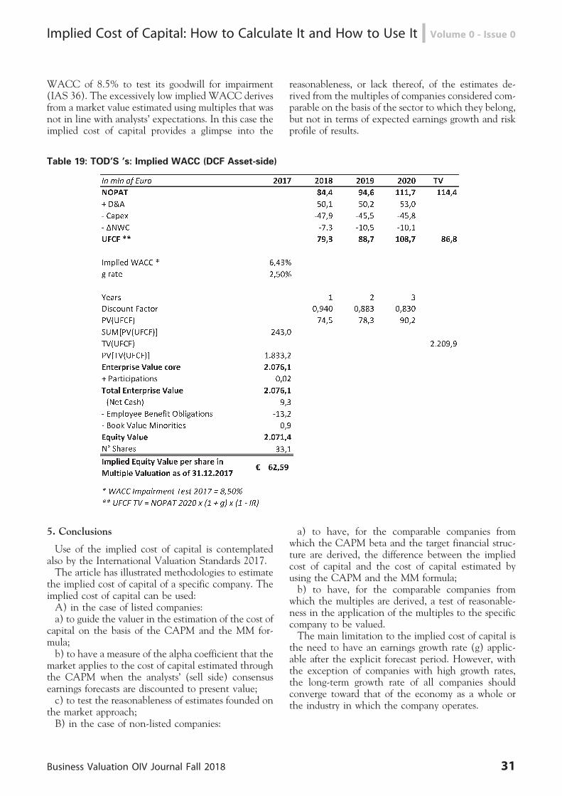
WACC of 8.5% to test its goodwill for impairment(IAS 36). The excessively low implied WACC derivesfrom a market value estimated using multiples that wasnot in line with analysts’ expectations. In this case theimplied cost of capital provides a glimpse into the

reasonableness, or lack thereof, of the estimates de-rived from the multiples of companies considered com-parable on the basis of the sector to which they belong,but not in terms of expected earnings growth and riskprofile of results.

Table 19: TOD’S ’s: Implied WACC (DCF Asset-side)

5. Conclusions

Use of the implied cost of capital is contemplatedalso by the International Valuation Standards 2017.The article has illustrated methodologies to estimate

the implied cost of capital of a specific company. Theimplied cost of capital can be used:A) in the case of listed companies:a) to guide the valuer in the estimation of the cost of

capital on the basis of the CAPM and the MM for-mula;b) to have a measure of the alpha coefficient that the

market applies to the cost of capital estimated throughthe CAPM when the analysts’ (sell side) consensusearnings forecasts are discounted to present value;c) to test the reasonableness of estimates founded on

the market approach;B) in the case of non-listed companies:

a) to have, for the comparable companies fromwhich the CAPM beta and the target financial struc-ture are derived, the difference between the impliedcost of capital and the cost of capital estimated byusing the CAPM and the MM formula;b) to have, for the comparable companies from

which the multiples are derived, a test of reasonable-ness in the application of the multiples to the specificcompany to be valued.The main limitation to the implied cost of capital is

the need to have an earnings growth rate (g) applic-able after the explicit forecast period. However, withthe exception of companies with high growth rates,the long-term growth rate of all companies shouldconverge toward that of the economy as a whole orthe industry in which the company operates.



Bibliography

Cochrane J.H., ‘Presidential Address: Discountrates’, The Journal of Finance, Vol. LXVI, No. 4, Au-gust 2011, pp. 1047-1108.Easton P., Taylor G., Shroff P., Sougiannis T.,

‘Using forecasts of earnings to simultaneously estimategrowth and the rate of return on equity investment’,Journal of Accounting Research, Vol. 40, no. 3, 2002,pp. 657-76.Easton P., Monahan S.J., ‘Review of recent research

on improving earnings forecasts and evaluating account-ing-based estimates of the expected rate of return onequity capital’, Abacus, Vol. 52, No. 1, 2016 pp. 35-58.Easton P., ‘Estimating the cost of capital implied by

market prices and accounting data’, Foundations andTrends in Accounting, Vol. 2, No. 4, 2007, pp. 241-364 (2009).Easton P., Monahan S.J., ‘An evaluation of account-

ing-based measures of expected returns’, The Account-ing Review, vol. 80, No. 2, 2005, pp. 501-38.Easton P., Sommers G., ‘Effects of analysts optimism

on estimates of the expected rate of return implied byearnings forecasts’, Journal of Accounting Research, 45,2007, pp. 983-1015.Ecker F., ‘Review of recent research on improving

earnings forecasts and evaluating accounting-based es-timates of the expected rate of return on equity capital.Discussion of Easton and Monahan’, Abacus, Vol. 52,No. 1, 2016, pp. 59-69.Fama E.F., French K.R., ‘A five factor asset pricing

model’, Journal of financial Economics, Vol. 116, 2015,pp. 1-22.Fitzgerald T., Gray S., Hall J., ‘Unconstrained esti-

mates of the equity risk premium’, Review of AccountingStudies, 2013, 18, pp. 560-639.Garvey G.T., ‘Discussion of ‘‘on the relation be-

tween predictable market returns and predictable ana-lyst forecast errors’’’, Review of Accounting Studies,2008, 13, pp. 292-294.Gebhardt W.R., Lee C.M.C., Swaminathan B., ‘To-

ward an implied cost of capital’, Journal of AccountingResearch, Vol. 39, No. 1, 2001, pp. 135-176.Guay W., Kothari S., Shu S., ‘Properties of implied

cost of capital using analysts’ forecasts’, Working pa-per, University of Pennsylvania, Pennsylvania, Whar-ton School, 2005.Hughes J., Jing L., Su W., ‘On the relation between

predictable market returns and predictable analystforecast errors’, Review of Accounting Studies, 13,2008, pp. 266-291.Johannesson E., Ohlson J.A., Explaining returns

through valuation, Columbia Business School ResearchPaper, No. 17-38, June 13, 2018, pp. 56.Johnson H.E., Business Valuation, Veracap Corporate

Finance Limited, 2012.Joos P., Piotroski J.D., Srinivasan S., ‘Can Analysts

assess fundamental risk and valuation uncertainty? Anempirical analysis of scenario-based value estimates’,Journal of Financial Economics, 2016, 121, pp. 645-663.Lambert R.A., ‘Discussion of ‘‘on the relation be-

tween expected returns and implied cost of capital’’’,Review of Accounting Studies, 2009, 14, pp. 260-268.Larocque S., ‘Analysts’ earnings forecast errors and

cost of equity capital estimates’, Review of AccountingStudies, 2013, 18, pp. 135-166.Lee C.M.C., So E.C., ‘Alphanomics: the informa-

tional underpinnings of market efficiency’, Foundationsand Trends in Accounting, Vol. 9, Nos. 2-3, 2014, pp.59-258.Lewellen J., ‘Predicting returns with financial ratios’,

Journal of Financial Economics, 74, 2004, pp. 209-235.Lundholm R., O’Keefe T., ‘Reconciling value esti-

mates from the discounted cash flow model and theresidual income model’, Contemporary Accounting Re-search, vol. 18, No. 2, 2001, pp. 311-35.Lundholm R., O’Keefe T., ‘On comparing residual

income and discounted cash flow models of equityvaluation: a response to Penman 2001’, ContemporaryAccounting Research, Vol. 18, No. 4, 2001, pp. 693-96.Lyle M.R., ‘Valuation: accounting for risk and the

expected return. Discussion of Penman’, Abacus, Vol.52, No. 1, 2016, pp. 131-39.Mohanram P., Gode D., ‘Removing predictable ana-

lyst forecast errors to improve implied cost of equityestimates’, Review of Accounting Studies, 2013, 18, pp.443-78.Ohlson, J.A., ‘Valuation and Growth’ (June 8,

2017). Available at SSRN: https://ssrn.com/ab-stract=2983031.Penman S.H., Zhu L., ‘Accounting-Based Estimates

of the Cost of Capital: A Third Way’ (September 1,2016). Available at SSRN: https://ssrn.com/ab-stract=2842269.Penman S.H., ‘On comparing cash flow and accrual

accounting models for use in equity valuation: a re-sponse to Lundholm and O’Keefe’, Contemporary Ac-counting Research, Vol. 18, No. 4, 2001, pp. 681-92.Penman S.H., ‘Valuation: accounting for risk and

the expected return’, Abacus, vol. 52, No. 1, 2016,pp. 106-30.Richardson S., Tuna I., Wysocki P., ‘Accounting

anomalies and fundamental analysis: A review of re-cent research advances’, Journal of Accounting and Eco-nomics, 2010, vol. 50, issue 2-3, 410-454.Richardson G., Tinaikar S., ‘Accounting based va-

luation models: what have we learned?’, Accountingand Finance, Vol. 44, 2004, pp. 223-55.Vuolteenaho T., ‘What drives firm-level stock re-

turns ?’, The Journal of Finance, vol. 57, No. 1, 2002,pp. 233-64.Weber M., ‘Cash flow duration and the term struc-

ture of equity returns’, Journal of Financial Economics,128, 2018, pp. 486-503.



Solvency II Framework in Insurance EquityValuation: Some Critical IssuesStefano Giuliani* - Giulia Raffo** - Niccolo Dalla Palma***

A new regulatory framework – Solvency 2 – has been in place for over two years in the European

insurance industry. Given that an increased number of market participants are availing of Solvency 2 data

in assessing insurance equity valuations, this paper aims to highlight some critical issues and shortcom-

ings associated with that practise.

1. Introduction

For all regulated European insurance entities a newsolvency regime called Solvency 2 (S2 from now on-wards) became effective since 1st January 2016. Underthe new framework, insurance companies determinetheir level of available capital resources (EOF or Eli-gible Own Funds) and relate that to their stochasti-cally calculated level of required capital (SCR or sol-vency capital required) thus deriving a certain Sol-vency Ratio (EOF over SCR). The aim of the regula-tor (EIOPA) was to move away from the old determi-nistic and not risk-based Solvency 1 regime towards amore market-consistent and risk-based approach tomeasure available capital.During the course of the last two and a half years,

an increasing number of equity market participantsstarted to use S2 data in order to assess the equityfair value of listed insurance groups. Moving fromthe actual Solvency Ratio components (EOF/SCR),analysts and investors started to focus on price-to-equity capital ratios (namely unrestricted Tier 1)while the information on capital generation has beenused to estimate free cash flows available to share-holders in order to calculate the equity fundamentalvalue.In this work, we would like to highlight some critical

issues in using the S2 framework to build a coherentand informed valuation to compare to the currentmarket price.The study will proceed as follows: we start to briefly

summarise the main drivers of the S2 framework,showing the elements constituting the SCR, theEOF and the Capital Generation. Then we remindthe main valuation methods that in the last 20 yearshave been used in the European equity markets for theInsurance Industry (P/E, Dividend Yield, EV/MCEV,FCF). After that, we show what the actual approachusing S2 is based-on and how it is currently used.Finally, we underlie some critical issues and incoher-ence of the approach to determine a proper economicequity value.We conclude that S2 data are valuable and provide

insights but shouldn’t be used, in our view, as a uniqueapproach for equity valuation. We think investorsshould go through a much more comprehensive setof data to build a more stable and coherent frameworkin order to determine a fundamental economic valueof equity capital.

2. Solvency II Regime: aims and structure

The introduction of the new prudential supervisoryregime had different objectives 1:– Adopting a risk-based economic capital to better

calculate and undertake all the different risks involved(technical, market, operating etc.);– Creating a level playing field within the European

Union;– Increasing Policyholders’ protection;– Improving capital allocation within firms and

groups.

* Caxton Europe LLP, London. ‘‘The views expressed in the paperare those of Stefano Giuliani and do not represent the views of CaxtonAssociates LP. This paper is intended for information purposes onlyand is not, and should not be considered as, an offer to invest in, or tobuy or sell, any interests or shares in any funds, or to participate in anyinvestment or trading strategy.’’

** Boussard and Gavaudan Partners Ltd, London. ‘‘The views ex-pressed in the paper are those of Giulia Raffo and do not represent theviews of Boussard and Gavaudan Ltd. This paper is intended for in-formation purposes only and is not, and should not be considered as, an

offer to invest in, or to buy or sell, any interests or shares in any funds,or to participate in any investment or trading strategy.’’

*** Exane BNP Paribas, Paris. ‘‘The views expressed in the paper byNiccolo Dalla Palma do not represent Investment Research as definedby the MiFID regulation. This paper is not, and should not be con-sidered as, an offer to invest in, or to buy or sell, any interests or sharesin any funds, or to participate in any investment or trading strategy.’’

1 Andenas M., Avesani R.G., Manes P., Vella F., Wood P.R., Sol-vency II: A Dynamic Challenge for the Insurance Market, Il Mulino,Bologna, 2017.


Solvency II Framework in Insurance Equity Valuation n Volume 0 - Issue 0

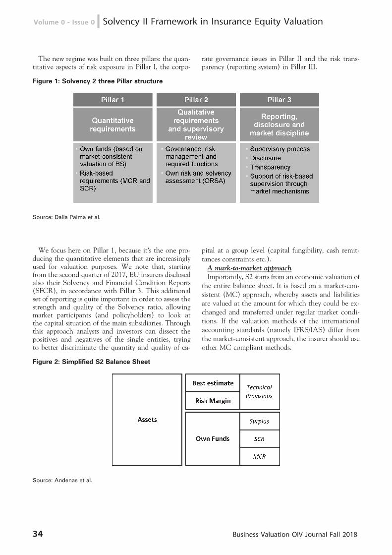
The new regime was built on three pillars: the quan-titative aspects of risk exposure in Pillar I, the corpo-

rate governance issues in Pillar II and the risk trans-parency (reporting system) in Pillar III.

Figure 1: Solvency 2 three Pillar structure

Source: Dalla Palma et al.

We focus here on Pillar 1, because it’s the one pro-ducing the quantitative elements that are increasinglyused for valuation purposes. We note that, startingfrom the second quarter of 2017, EU insurers disclosedalso their Solvency and Financial Condition Reports(SFCR), in accordance with Pillar 3. This additionalset of reporting is quite important in order to assess thestrength and quality of the Solvency ratio, allowingmarket participants (and policyholders) to look atthe capital situation of the main subsidiaries. Throughthis approach analysts and investors can dissect thepositives and negatives of the single entities, tryingto better discriminate the quantity and quality of ca-

pital at a group level (capital fungibility, cash remit-tances constraints etc.).A mark-to-market approachImportantly, S2 starts from an economic valuation of

the entire balance sheet. It is based on a market-con-sistent (MC) approach, whereby assets and liabilitiesare valued at the amount for which they could be ex-changed and transferred under regular market condi-tions. If the valuation methods of the internationalaccounting standards (namely IFRS/IAS) differ fromthe market-consistent approach, the insurer should useother MC compliant methods.

Figure 2: Simplified S2 Balance Sheet

Source: Andenas et al.


Volume 0 - Issue 0 n Solvency II Framework in Insurance Equity Valuation

As far as the valuation of Liabilities is concerned, thevalue of technical provisions has to be equal to thesum of best estimate and risk margin, where the formeris defined as the probability weighted average of futurecash-flows, taking into account the time value of

money using the relevant risk-free interest rate termstructure, while the latter is equivalent to the cost ofcapital the insurer is required to hold to take over andmeet the insurance obligations throughout their dura-tion.

Figure 3: Simplified comparison between IAS/IFRS and S2 accounts

Source: Andenas et al.

Defining capital requirementsThe Solvency Capital Requirement (SCR) is calcu-

lated as the amount of capital that insurance compa-nies should hold to be able, with a probability of99.5%, to meet their obligations to policyholders overthe next year, thereby ensuring that a ‘ruin’ event willnot occur more than once in 200 years.

In practice the calculation that the insurance under-taking performs is structured in six main modules andfurther into sub-modules. In addition to the classifica-tion proposed by the legislation, other risks taken un-der consideration are liquidity and ALM risk, sover-eign risk, strategic and emerging risks, reputational riskand risks connected with group membership.



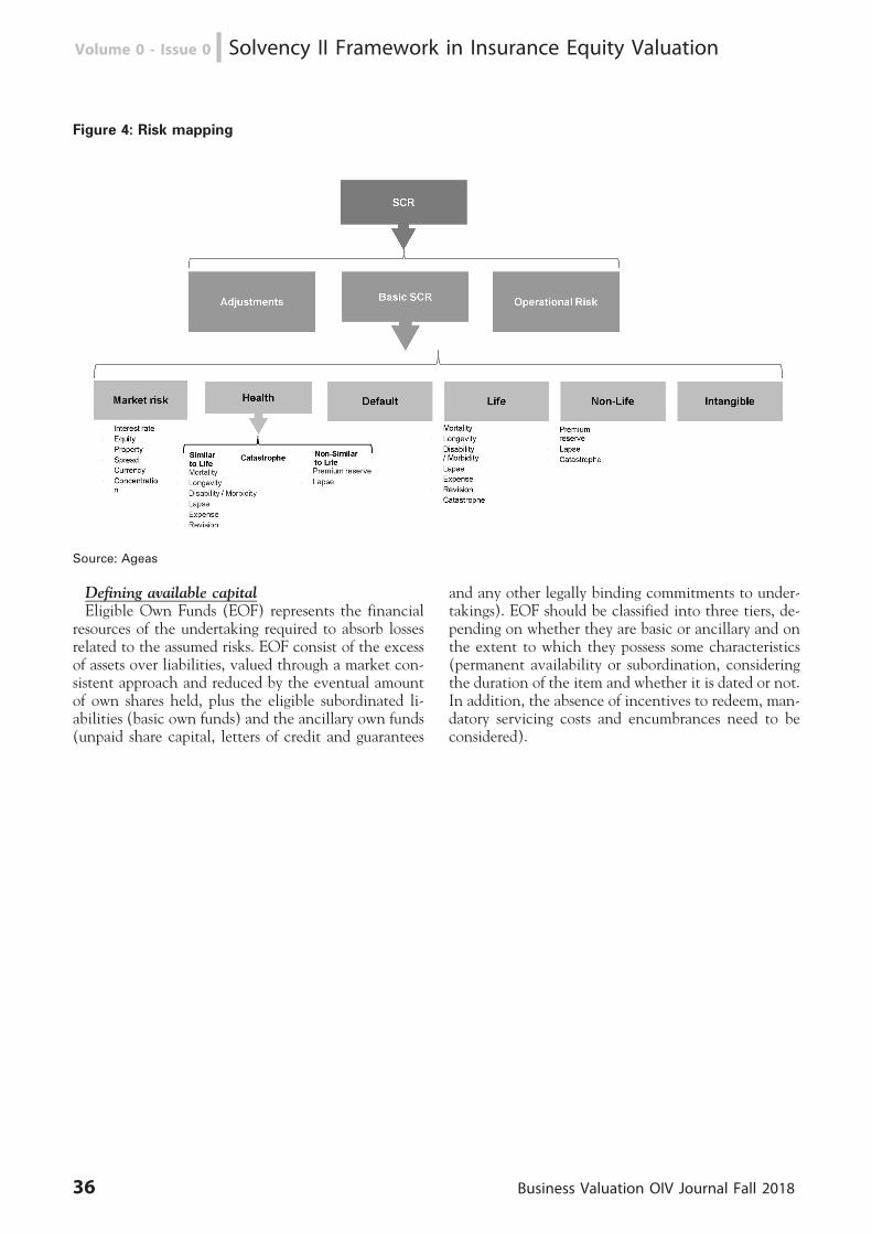
Figure 4: Risk mapping

Source: Ageas

Defining available capitalEligible Own Funds (EOF) represents the financial

resources of the undertaking required to absorb lossesrelated to the assumed risks. EOF consist of the excessof assets over liabilities, valued through a market con-sistent approach and reduced by the eventual amountof own shares held, plus the eligible subordinated li-abilities (basic own funds) and the ancillary own funds(unpaid share capital, letters of credit and guarantees

and any other legally binding commitments to under-takings). EOF should be classified into three tiers, de-pending on whether they are basic or ancillary and onthe extent to which they possess some characteristics(permanent availability or subordination, consideringthe duration of the item and whether it is dated or not.In addition, the absence of incentives to redeem, man-datory servicing costs and encumbrances need to beconsidered).



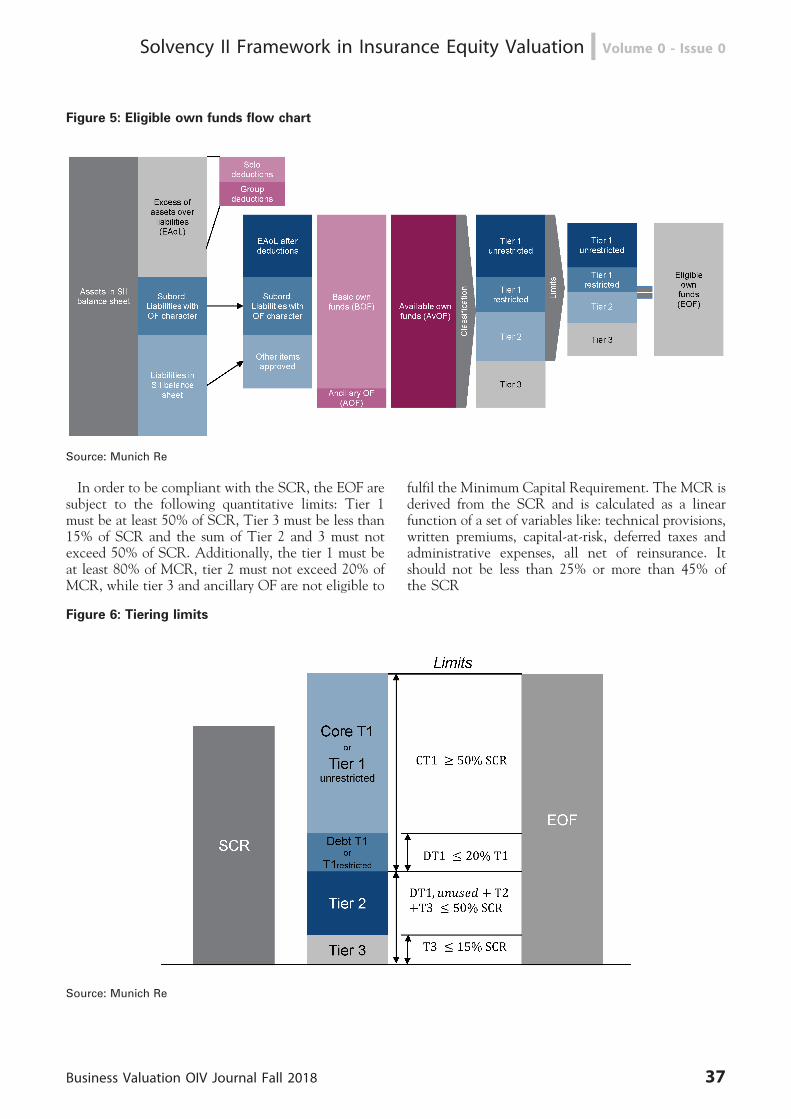
Figure 5: Eligible own funds flow chart

Source: Munich Re

In order to be compliant with the SCR, the EOF aresubject to the following quantitative limits: Tier 1must be at least 50% of SCR, Tier 3 must be less than15% of SCR and the sum of Tier 2 and 3 must notexceed 50% of SCR. Additionally, the tier 1 must beat least 80% of MCR, tier 2 must not exceed 20% ofMCR, while tier 3 and ancillary OF are not eligible to

fulfil the Minimum Capital Requirement. The MCR isderived from the SCR and is calculated as a linearfunction of a set of variables like: technical provisions,written premiums, capital-at-risk, deferred taxes andadministrative expenses, all net of reinsurance. Itshould not be less than 25% or more than 45% ofthe SCR

Figure 6: Tiering limits

Source: Munich Re



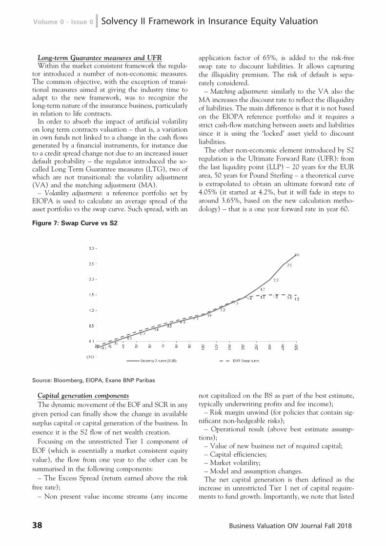
Long-term Guarantee measures and UFRWithin the market consistent framework the regula-

tor introduced a number of non-economic measures.The common objective, with the exception of transi-tional measures aimed at giving the industry time toadapt to the new framework, was to recognize thelong-term nature of the insurance business, particularlyin relation to life contracts.In order to absorb the impact of artificial volatility

on long term contracts valuation – that is, a variationin own funds not linked to a change in the cash flowsgenerated by a financial instruments, for instance dueto a credit spread change not due to an increased issuerdefault probability – the regulator introduced the so-called Long Term Guarantee measures (LTG), two ofwhich are not transitional: the volatility adjustment(VA) and the matching adjustment (MA).– Volatility adjustment: a reference portfolio set by

EIOPA is used to calculate an average spread of theasset portfolio vs the swap curve. Such spread, with an

application factor of 65%, is added to the risk-freeswap rate to discount liabilities. It allows capturingthe illiquidity premium. The risk of default is sepa-rately considered.– Matching adjustment: similarly to the VA also the

MA increases the discount rate to reflect the illiquidityof liabilities. The main difference is that it is not basedon the EIOPA reference portfolio and it requires astrict cash-flow matching between assets and liabilitiessince it is using the ‘locked’ asset yield to discountliabilities.The other non-economic element introduced by S2

regulation is the Ultimate Forward Rate (UFR): fromthe last liquidity point (LLP) – 20 years for the EURarea, 50 years for Pound Sterling – a theoretical curveis extrapolated to obtain an ultimate forward rate of4.05% (it started at 4.2%, but it will fade in steps toaround 3.65%, based on the new calculation metho-dology) – that is a one year forward rate in year 60.

Figure 7: Swap Curve vs S2

Source: Bloomberg, EIOPA, Exane BNP Paribas

Capital generation components

The dynamic movement of the EOF and SCR in any

given period can finally show the change in available

surplus capital or capital generation of the business. In

essence it is the S2 flow of net wealth creation.

Focusing on the unrestricted Tier 1 component of

EOF (which is essentially a market consistent equity

value), the flow from one year to the other can be

summarised in the following components:

– The Excess Spread (return earned above the risk

free rate);

– Non present value income streams (any income

not capitalized on the BS as part of the best estimate,typically underwriting profits and fee income);– Risk margin unwind (for policies that contain sig-

nificant non-hedgeable risks);– Operational result (above best estimate assump-

tions);– Value of new business net of required capital;– Capital efficiencies;– Market volatility;– Model and assumption changes.The net capital generation is then defined as the

increase in unrestricted Tier 1 net of capital require-ments to fund growth. Importantly, we note that listed



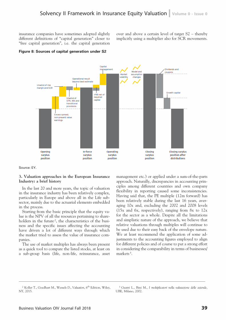
insurance companies have sometimes adopted slightlydifferent definitions of ‘‘capital generation’’ closer to‘‘free capital generation’’, i.e. the capital generation

over and above a certain level of target S2 – therebyimplicitly using a multiplier also for SCR movements.

Figure 8: Sources of capital generation under S2

Source: EY.

3. Valuation approaches in the European InsuranceIndustry: a brief history

In the last 20 and more years, the topic of valuationin the insurance industry has been relatively complex,particularly in Europe and above all in the Life sub-sector, mainly due to the actuarial elements embeddedin the process.Starting from the basic principle that the equity va-

lue is the NPV of all the resources pertaining to share-holders in the future 2, the characteristics of the busi-ness and the specific issues affecting the accountinghave driven a lot of different ways through whichthe market tried to assess the value of insurance com-panies.The use of market multiples has always been present

as a quick tool to compare the listed stocks, at least ona sub-group basis (life, non-life, reinsurance, asset

management etc.) or applied under a sum-of-the-partsapproach. Naturally, discrepancies in accounting prin-ciples among different countries and own companyflexibility in reporting caused some inconsistencies.Having said that, the PE multiple (12m forward) hasbeen relatively stable during the last 16 years, aver-aging 10x and, excluding the 2002 and 2008 levels(15x and 6x, respectively), ranging from 8x to 12xfor the sector as a whole. Despite all the limitationsand simplistic nature of the approach, we believe thatrelative valuations through multiples will continue tobe used due to their easy back of the envelope nature.We at least recommend the application of some ad-justments to the accounting figures employed to alignfor different policies and of course to put a strong effortin considering the comparability in terms of businesses/markets 3.

2 Koller T., Goedhart M., Wessels D., Valuation, 6th Edition, Wiley,NY, 2015.

3 Guatri L., Bini M., I moltiplicatori nella valutazione delle aziende,UBE, Milano, 2002.



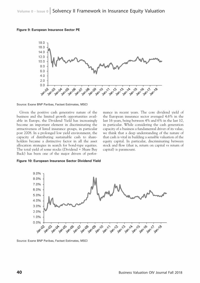
Figure 9: European Insurance Sector PE

Source: Exane BNP Paribas, Factset Estimates, MSCI

Given the positive cash generative nature of thebusiness and the limited growth opportunities avail-able in Europe, the Dividend Yield has increasinglybecome an important element in discriminating theattractiveness of listed insurance groups, in particularpost 2008. In a prolonged low yield environment, thecapacity of distributing sustainable cash to share-holders became a distinctive factor in all the assetallocation strategies in search for bond-type equities.The total yield of some stocks (Dividend + Share BuyBack) has been one of the major drivers of perfor-

mance in recent years. The core dividend yield ofthe European insurance sector averaged 4.6% in thelast 16 years, being between 4% and 6% in the last 10,in particular. While considering the cash generationcapacity of a business a fundamental driver of its value,we think that a deep understanding of the nature ofthat cash is vital in building a sensible valuation of theequity capital. In particular, discriminating betweenstock and flow (that is, return on capital vs return ofcapital) is paramount.

Figure 10: European Insurance Sector Dividend Yield

Source: Exane BNP Paribas, Factset Estimates, MSCI



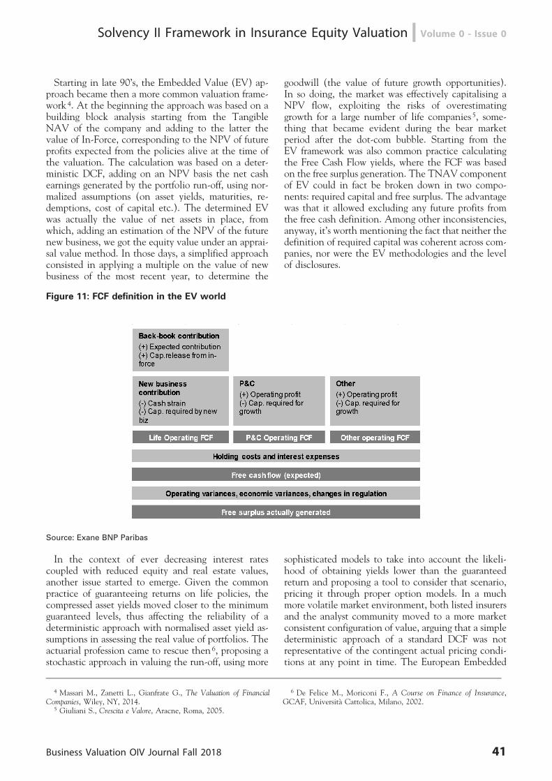
Starting in late 90’s, the Embedded Value (EV) ap-proach became then a more common valuation frame-work4. At the beginning the approach was based on abuilding block analysis starting from the TangibleNAV of the company and adding to the latter thevalue of In-Force, corresponding to the NPV of futureprofits expected from the policies alive at the time ofthe valuation. The calculation was based on a deter-ministic DCF, adding on an NPV basis the net cashearnings generated by the portfolio run-off, using nor-malized assumptions (on asset yields, maturities, re-demptions, cost of capital etc.). The determined EVwas actually the value of net assets in place, fromwhich, adding an estimation of the NPV of the futurenew business, we got the equity value under an apprai-sal value method. In those days, a simplified approachconsisted in applying a multiple on the value of newbusiness of the most recent year, to determine the

goodwill (the value of future growth opportunities).In so doing, the market was effectively capitalising aNPV flow, exploiting the risks of overestimatinggrowth for a large number of life companies 5, some-thing that became evident during the bear marketperiod after the dot-com bubble. Starting from theEV framework was also common practice calculatingthe Free Cash Flow yields, where the FCF was basedon the free surplus generation. The TNAV componentof EV could in fact be broken down in two compo-nents: required capital and free surplus. The advantagewas that it allowed excluding any future profits fromthe free cash definition. Among other inconsistencies,anyway, it’s worth mentioning the fact that neither thedefinition of required capital was coherent across com-panies, nor were the EV methodologies and the levelof disclosures.

Figure 11: FCF definition in the EV world

Source: Exane BNP Paribas

In the context of ever decreasing interest ratescoupled with reduced equity and real estate values,another issue started to emerge. Given the commonpractice of guaranteeing returns on life policies, thecompressed asset yields moved closer to the minimumguaranteed levels, thus affecting the reliability of adeterministic approach with normalised asset yield as-sumptions in assessing the real value of portfolios. Theactuarial profession came to rescue then6, proposing astochastic approach in valuing the run-off, using more

sophisticated models to take into account the likeli-hood of obtaining yields lower than the guaranteedreturn and proposing a tool to consider that scenario,pricing it through proper option models. In a muchmore volatile market environment, both listed insurersand the analyst community moved to a more marketconsistent configuration of value, arguing that a simpledeterministic approach of a standard DCF was notrepresentative of the contingent actual pricing condi-tions at any point in time. The European Embedded

4 Massari M., Zanetti L., Gianfrate G., The Valuation of FinancialCompanies, Wiley, NY, 2014.

5 Giuliani S., Crescita e Valore, Aracne, Roma, 2005.

6 De Felice M., Moriconi F., A Course on Finance of Insurance,GCAF, Universita Cattolica, Milano, 2002.



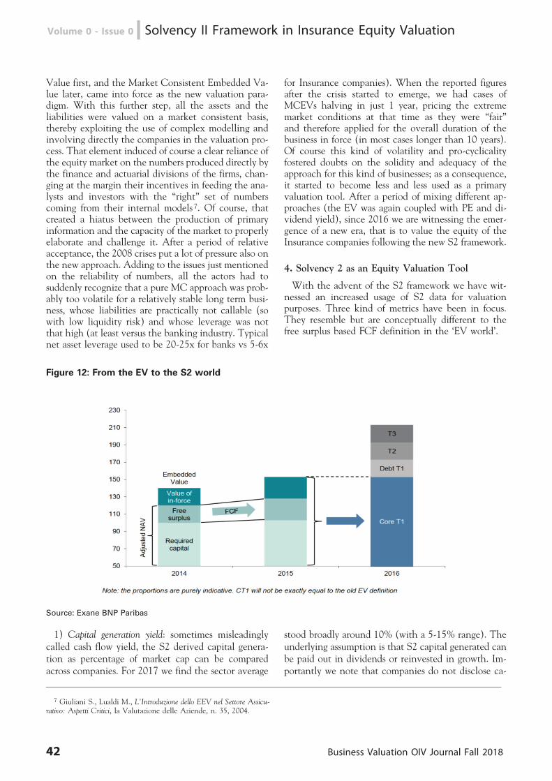
Value first, and the Market Consistent Embedded Va-lue later, came into force as the new valuation para-digm. With this further step, all the assets and theliabilities were valued on a market consistent basis,thereby exploiting the use of complex modelling andinvolving directly the companies in the valuation pro-cess. That element induced of course a clear reliance ofthe equity market on the numbers produced directly bythe finance and actuarial divisions of the firms, chan-ging at the margin their incentives in feeding the ana-lysts and investors with the ‘‘right’’ set of numberscoming from their internal models 7. Of course, thatcreated a hiatus between the production of primaryinformation and the capacity of the market to properlyelaborate and challenge it. After a period of relativeacceptance, the 2008 crises put a lot of pressure also onthe new approach. Adding to the issues just mentionedon the reliability of numbers, all the actors had tosuddenly recognize that a pure MC approach was prob-ably too volatile for a relatively stable long term busi-ness, whose liabilities are practically not callable (sowith low liquidity risk) and whose leverage was notthat high (at least versus the banking industry. Typicalnet asset leverage used to be 20-25x for banks vs 5-6x

for Insurance companies). When the reported figuresafter the crisis started to emerge, we had cases ofMCEVs halving in just 1 year, pricing the extrememarket conditions at that time as they were ‘‘fair’’and therefore applied for the overall duration of thebusiness in force (in most cases longer than 10 years).Of course this kind of volatility and pro-cyclicalityfostered doubts on the solidity and adequacy of theapproach for this kind of businesses; as a consequence,it started to become less and less used as a primaryvaluation tool. After a period of mixing different ap-proaches (the EV was again coupled with PE and di-vidend yield), since 2016 we are witnessing the emer-gence of a new era, that is to value the equity of theInsurance companies following the new S2 framework.

4. Solvency 2 as an Equity Valuation Tool

With the advent of the S2 framework we have wit-nessed an increased usage of S2 data for valuationpurposes. Three kind of metrics have been in focus.They resemble but are conceptually different to thefree surplus based FCF definition in the ‘EV world’.

Figure 12: From the EV to the S2 world

Source: Exane BNP Paribas

1) Capital generation yield: sometimes misleadinglycalled cash flow yield, the S2 derived capital genera-tion as percentage of market cap can be comparedacross companies. For 2017 we find the sector average

stood broadly around 10% (with a 5-15% range). Theunderlying assumption is that S2 capital generated canbe paid out in dividends or reinvested in growth. Im-portantly we note that companies do not disclose ca-

7 Giuliani S., Lualdi M., L’Introduzione dello EEV nel Settore Assicu-rativo: Aspetti Critici, la Valutazione delle Aziende, n. 35, 2004.



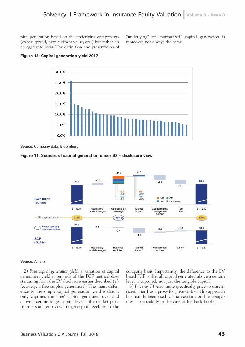
pital generation based on the underlying components(excess spread, new business value, etc.) but rather onan aggregate basis. The definition and presentation of

‘‘underlying’’ or ‘‘normalized’’ capital generation ismoreover not always the same.

Figure 13: Capital generation yield 2017

Source: Company data, Bloomberg

Figure 14: Sources of capital generation under S2 – disclosure view

Source: Allianz

2) Free capital generation yield: a variation of capitalgeneration yield it reminds of the FCF methodologystemming from the EV disclosure earlier described (ef-fectively, a free surplus generation). The main differ-ence to the simple capital generation yield is that itonly captures the ‘free’ capital generated over andabove a certain target capital level – the market prac-titioner shall set his own target capital level, or use the

company basis. Importantly, the difference to the EVbased FCF is that all capital generated above a certainlevel is captured, not just the tangible capital.3) Price-to-T1 ratio: more specifically price-to-unrest-

ricted Tier 1 as a proxy for price-to-EV. This approachhas mainly been used for transactions on life compa-nies – particularly in the case of life back books.



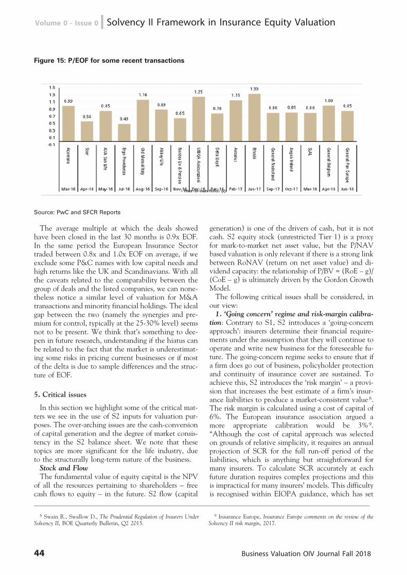
Figure 15: P/EOF for some recent transactions

Source: PwC and SFCR Reports

The average multiple at which the deals showedhave been closed in the last 30 months is 0.9x EOF.In the same period the European Insurance Sectortraded between 0.8x and 1.0x EOF on average, if weexclude some P&C names with low capital needs andhigh returns like the UK and Scandinavians. With allthe caveats related to the comparability between thegroup of deals and the listed companies, we can none-theless notice a similar level of valuation for M&Atransactions and minority financial holdings. The idealgap between the two (namely the synergies and pre-mium for control, typically at the 25-30% level) seemsnot to be present. We think that’s something to dee-pen in future research, understanding if the hiatus canbe related to the fact that the market is underestimat-ing some risks in pricing current businesses or if mostof the delta is due to sample differences and the struc-ture of EOF.

5. Critical issues

In this section we highlight some of the critical mat-ters we see in the use of S2 inputs for valuation pur-poses. The over-arching issues are the cash-conversionof capital generation and the degree of market consis-tency in the S2 balance sheet. We note that thesetopics are more significant for the life industry, dueto the structurally long-term nature of the business.Stock and FlowThe fundamental value of equity capital is the NPV

of all the resources pertaining to shareholders – freecash flows to equity – in the future. S2 flow (capital

generation) is one of the drivers of cash, but it is notcash. S2 equity stock (unrestricted Tier 1) is a proxyfor mark-to-market net asset value, but the P/NAVbased valuation is only relevant if there is a strong linkbetween RoNAV (return on net asset value) and di-vidend capacity: the relationship of P/BV = (RoE – g)/(CoE – g) is ultimately driven by the Gordon GrowthModel.The following critical issues shall be considered, in

our view:1. ‘Going concern’ regime and risk-margin calibra-

tion: Contrary to S1, S2 introduces a ‘going-concernapproach’: insurers determine their financial require-ments under the assumption that they will continue tooperate and write new business for the foreseeable fu-ture. The going-concern regime seeks to ensure that ifa firm does go out of business, policyholder protectionand continuity of insurance cover are sustained. Toachieve this, S2 introduces the ‘risk margin’ – a provi-sion that increases the best estimate of a firm’s insur-ance liabilities to produce a market-consistent value8.The risk margin is calculated using a cost of capital of6%. The European insurance association argued amore appropriate calibration would be 3%9.‘‘Although the cost of capital approach was selectedon grounds of relative simplicity, it requires an annualprojection of SCR for the full run-off period of theliabilities, which is anything but straightforward formany insurers. To calculate SCR accurately at eachfuture duration requires complex projections and thisis impractical for many insurers’ models. This difficultyis recognised within EIOPA guidance, which has set

8 Swain R., Swallow D., The Prudential Regulation of Insurers UnderSolvency II, BOE Quarterly Bulletin, Q2 2015.

9 Insurance Europe, Insurance Europe comments on the review of theSolvency II risk margin, 2017.



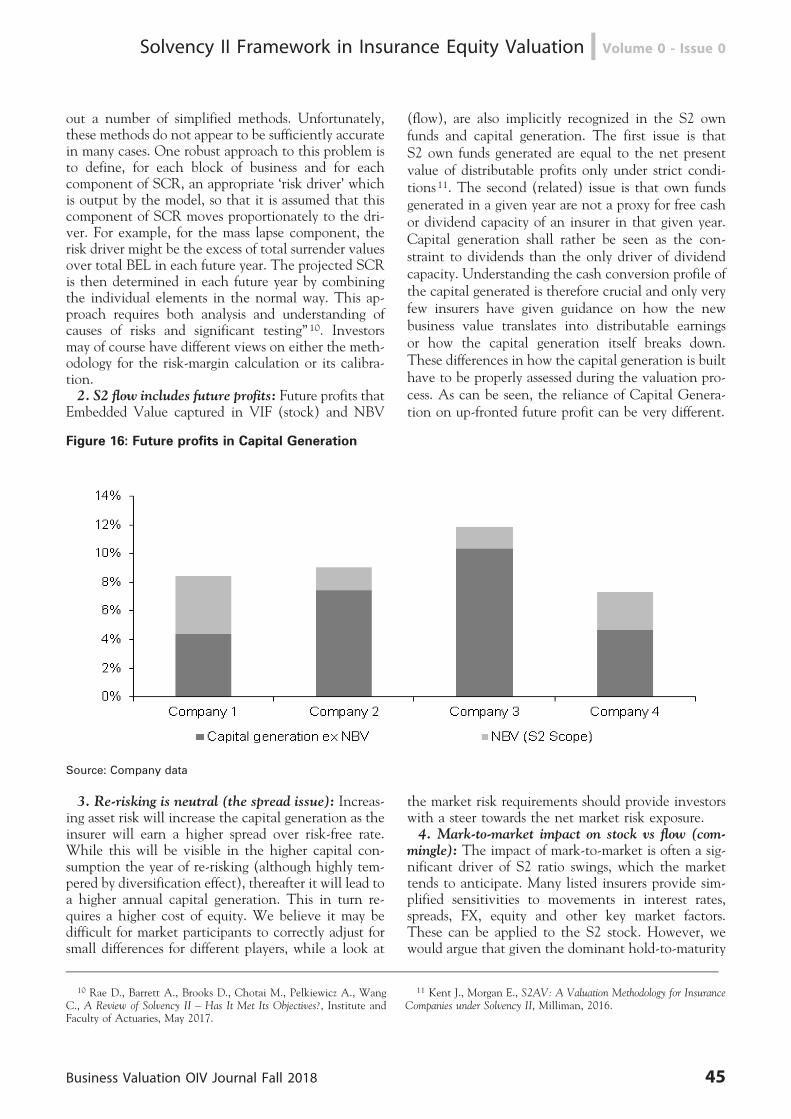
out a number of simplified methods. Unfortunately,these methods do not appear to be sufficiently accuratein many cases. One robust approach to this problem isto define, for each block of business and for eachcomponent of SCR, an appropriate ‘risk driver’ whichis output by the model, so that it is assumed that thiscomponent of SCR moves proportionately to the dri-ver. For example, for the mass lapse component, therisk driver might be the excess of total surrender valuesover total BEL in each future year. The projected SCRis then determined in each future year by combiningthe individual elements in the normal way. This ap-proach requires both analysis and understanding ofcauses of risks and significant testing’’ 10. Investorsmay of course have different views on either the meth-odology for the risk-margin calculation or its calibra-tion.2. S2 flow includes future profits: Future profits that

Embedded Value captured in VIF (stock) and NBV

(flow), are also implicitly recognized in the S2 ownfunds and capital generation. The first issue is thatS2 own funds generated are equal to the net presentvalue of distributable profits only under strict condi-tions 11. The second (related) issue is that own fundsgenerated in a given year are not a proxy for free cashor dividend capacity of an insurer in that given year.Capital generation shall rather be seen as the con-straint to dividends than the only driver of dividendcapacity. Understanding the cash conversion profile ofthe capital generated is therefore crucial and only veryfew insurers have given guidance on how the newbusiness value translates into distributable earningsor how the capital generation itself breaks down.These differences in how the capital generation is builthave to be properly assessed during the valuation pro-cess. As can be seen, the reliance of Capital Genera-tion on up-fronted future profit can be very different.

Figure 16: Future profits in Capital Generation

Source: Company data

3. Re-risking is neutral (the spread issue): Increas-ing asset risk will increase the capital generation as theinsurer will earn a higher spread over risk-free rate.While this will be visible in the higher capital con-sumption the year of re-risking (although highly tem-pered by diversification effect), thereafter it will lead toa higher annual capital generation. This in turn re-quires a higher cost of equity. We believe it may bedifficult for market participants to correctly adjust forsmall differences for different players, while a look at

the market risk requirements should provide investorswith a steer towards the net market risk exposure.4. Mark-to-market impact on stock vs flow (com-

mingle): The impact of mark-to-market is often a sig-nificant driver of S2 ratio swings, which the markettends to anticipate. Many listed insurers provide sim-plified sensitivities to movements in interest rates,spreads, FX, equity and other key market factors.These can be applied to the S2 stock. However, wewould argue that given the dominant hold-to-maturity

10 Rae D., Barrett A., Brooks D., Chotai M., Pelkiewicz A., WangC., A Review of Solvency II – Has It Met Its Objectives?, Institute andFaculty of Actuaries, May 2017.

11 Kent J., Morgan E., S2AV: A Valuation Methodology for InsuranceCompanies under Solvency II, Milliman, 2016.



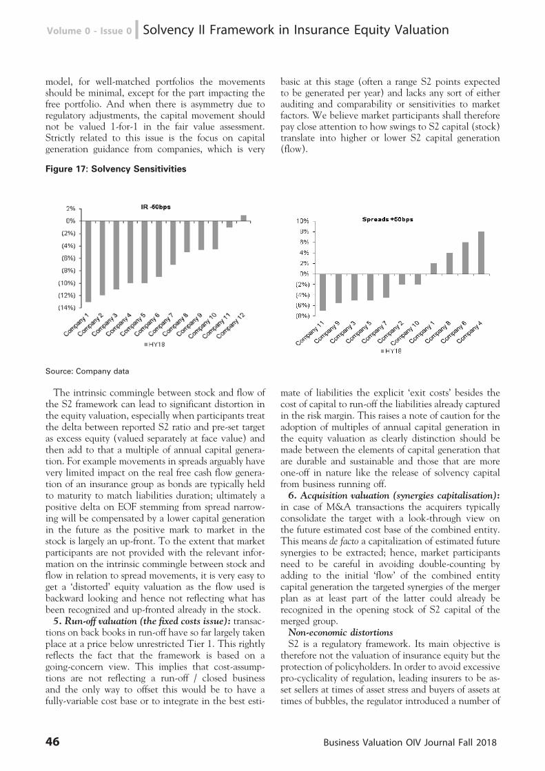
model, for well-matched portfolios the movementsshould be minimal, except for the part impacting thefree portfolio. And when there is asymmetry due toregulatory adjustments, the capital movement shouldnot be valued 1-for-1 in the fair value assessment.Strictly related to this issue is the focus on capitalgeneration guidance from companies, which is very

basic at this stage (often a range S2 points expectedto be generated per year) and lacks any sort of eitherauditing and comparability or sensitivities to marketfactors. We believe market participants shall thereforepay close attention to how swings to S2 capital (stock)translate into higher or lower S2 capital generation(flow).

Figure 17: Solvency Sensitivities


The intrinsic commingle between stock and flow ofthe S2 framework can lead to significant distortion inthe equity valuation, especially when participants treatthe delta between reported S2 ratio and pre-set targetas excess equity (valued separately at face value) andthen add to that a multiple of annual capital genera-tion. For example movements in spreads arguably havevery limited impact on the real free cash flow genera-tion of an insurance group as bonds are typically heldto maturity to match liabilities duration; ultimately apositive delta on EOF stemming from spread narrow-ing will be compensated by a lower capital generationin the future as the positive mark to market in thestock is largely an up-front. To the extent that marketparticipants are not provided with the relevant infor-mation on the intrinsic commingle between stock andflow in relation to spread movements, it is very easy toget a ‘distorted’ equity valuation as the flow used isbackward looking and hence not reflecting what hasbeen recognized and up-fronted already in the stock.5. Run-off valuation (the fixed costs issue): transac-

tions on back books in run-off have so far largely takenplace at a price below unrestricted Tier 1. This rightlyreflects the fact that the framework is based on agoing-concern view. This implies that cost-assump-tions are not reflecting a run-off / closed businessand the only way to offset this would be to have afully-variable cost base or to integrate in the best esti-

mate of liabilities the explicit ‘exit costs’ besides thecost of capital to run-off the liabilities already capturedin the risk margin. This raises a note of caution for theadoption of multiples of annual capital generation inthe equity valuation as clearly distinction should bemade between the elements of capital generation thatare durable and sustainable and those that are moreone-off in nature like the release of solvency capitalfrom business running off.6. Acquisition valuation (synergies capitalisation):

in case of M&A transactions the acquirers typicallyconsolidate the target with a look-through view onthe future estimated cost base of the combined entity.This means de facto a capitalization of estimated futuresynergies to be extracted; hence, market participantsneed to be careful in avoiding double-counting byadding to the initial ‘flow’ of the combined entitycapital generation the targeted synergies of the mergerplan as at least part of the latter could already berecognized in the opening stock of S2 capital of themerged group.Non-economic distortionsS2 is a regulatory framework. Its main objective is

therefore not the valuation of insurance equity but theprotection of policyholders. In order to avoid excessivepro-cyclicality of regulation, leading insurers to be as-set sellers at times of asset stress and buyers of assets attimes of bubbles, the regulator introduced a number of



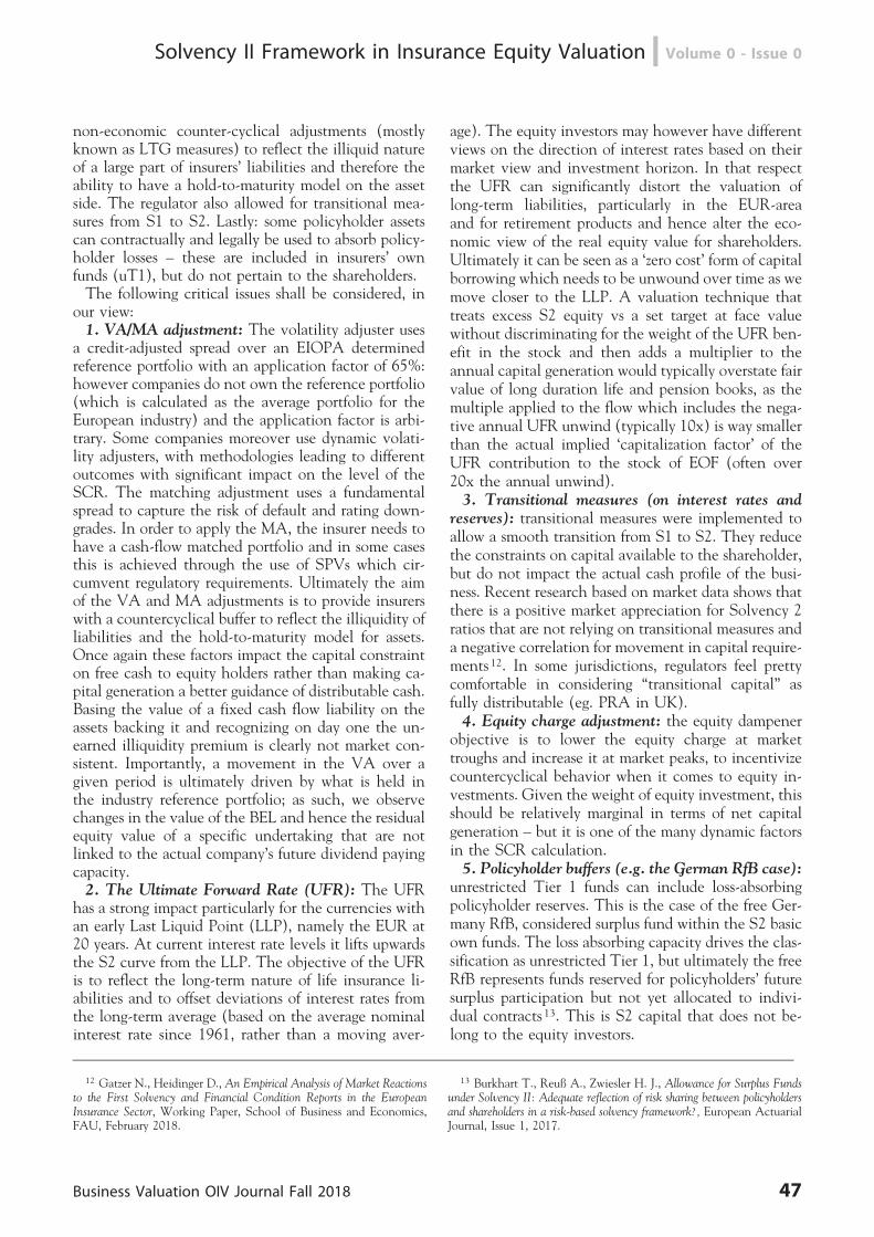
non-economic counter-cyclical adjustments (mostlyknown as LTG measures) to reflect the illiquid natureof a large part of insurers’ liabilities and therefore theability to have a hold-to-maturity model on the assetside. The regulator also allowed for transitional mea-sures from S1 to S2. Lastly: some policyholder assetscan contractually and legally be used to absorb policy-holder losses – these are included in insurers’ ownfunds (uT1), but do not pertain to the shareholders.The following critical issues shall be considered, in

our view:1. VA/MA adjustment: The volatility adjuster uses

a credit-adjusted spread over an EIOPA determinedreference portfolio with an application factor of 65%:however companies do not own the reference portfolio(which is calculated as the average portfolio for theEuropean industry) and the application factor is arbi-trary. Some companies moreover use dynamic volati-lity adjusters, with methodologies leading to differentoutcomes with significant impact on the level of theSCR. The matching adjustment uses a fundamentalspread to capture the risk of default and rating down-grades. In order to apply the MA, the insurer needs tohave a cash-flow matched portfolio and in some casesthis is achieved through the use of SPVs which cir-cumvent regulatory requirements. Ultimately the aimof the VA and MA adjustments is to provide insurerswith a countercyclical buffer to reflect the illiquidity ofliabilities and the hold-to-maturity model for assets.Once again these factors impact the capital constrainton free cash to equity holders rather than making ca-pital generation a better guidance of distributable cash.Basing the value of a fixed cash flow liability on theassets backing it and recognizing on day one the un-earned illiquidity premium is clearly not market con-sistent. Importantly, a movement in the VA over agiven period is ultimately driven by what is held inthe industry reference portfolio; as such, we observechanges in the value of the BEL and hence the residualequity value of a specific undertaking that are notlinked to the actual company’s future dividend payingcapacity.2. The Ultimate Forward Rate (UFR): The UFR

has a strong impact particularly for the currencies withan early Last Liquid Point (LLP), namely the EUR at20 years. At current interest rate levels it lifts upwardsthe S2 curve from the LLP. The objective of the UFRis to reflect the long-term nature of life insurance li-abilities and to offset deviations of interest rates fromthe long-term average (based on the average nominalinterest rate since 1961, rather than a moving aver-

age). The equity investors may however have differentviews on the direction of interest rates based on theirmarket view and investment horizon. In that respectthe UFR can significantly distort the valuation oflong-term liabilities, particularly in the EUR-areaand for retirement products and hence alter the eco-nomic view of the real equity value for shareholders.Ultimately it can be seen as a ‘zero cost’ form of capitalborrowing which needs to be unwound over time as wemove closer to the LLP. A valuation technique thattreats excess S2 equity vs a set target at face valuewithout discriminating for the weight of the UFR ben-efit in the stock and then adds a multiplier to theannual capital generation would typically overstate fairvalue of long duration life and pension books, as themultiple applied to the flow which includes the nega-tive annual UFR unwind (typically 10x) is way smallerthan the actual implied ‘capitalization factor’ of theUFR contribution to the stock of EOF (often over20x the annual unwind).3. Transitional measures (on interest rates and

reserves): transitional measures were implemented toallow a smooth transition from S1 to S2. They reducethe constraints on capital available to the shareholder,but do not impact the actual cash profile of the busi-ness. Recent research based on market data shows thatthere is a positive market appreciation for Solvency 2ratios that are not relying on transitional measures anda negative correlation for movement in capital require-ments 12. In some jurisdictions, regulators feel prettycomfortable in considering ‘‘transitional capital’’ asfully distributable (eg. PRA in UK).4. Equity charge adjustment: the equity dampener

objective is to lower the equity charge at markettroughs and increase it at market peaks, to incentivizecountercyclical behavior when it comes to equity in-vestments. Given the weight of equity investment, thisshould be relatively marginal in terms of net capitalgeneration – but it is one of the many dynamic factorsin the SCR calculation.5. Policyholder buffers (e.g. the German RfB case):

unrestricted Tier 1 funds can include loss-absorbingpolicyholder reserves. This is the case of the free Ger-many RfB, considered surplus fund within the S2 basicown funds. The loss absorbing capacity drives the clas-sification as unrestricted Tier 1, but ultimately the freeRfB represents funds reserved for policyholders’ futuresurplus participation but not yet allocated to indivi-dual contracts 13. This is S2 capital that does not be-long to the equity investors.

12 Gatzer N., Heidinger D., An Empirical Analysis of Market Reactionsto the First Solvency and Financial Condition Reports in the EuropeanInsurance Sector, Working Paper, School of Business and Economics,FAU, February 2018.

13 Burkhart T., Reuß A., Zwiesler H. J., Allowance for Surplus Fundsunder Solvency II: Adequate reflection of risk sharing between policyholdersand shareholders in a risk-based solvency framework?, European ActuarialJournal, Issue 1, 2017.



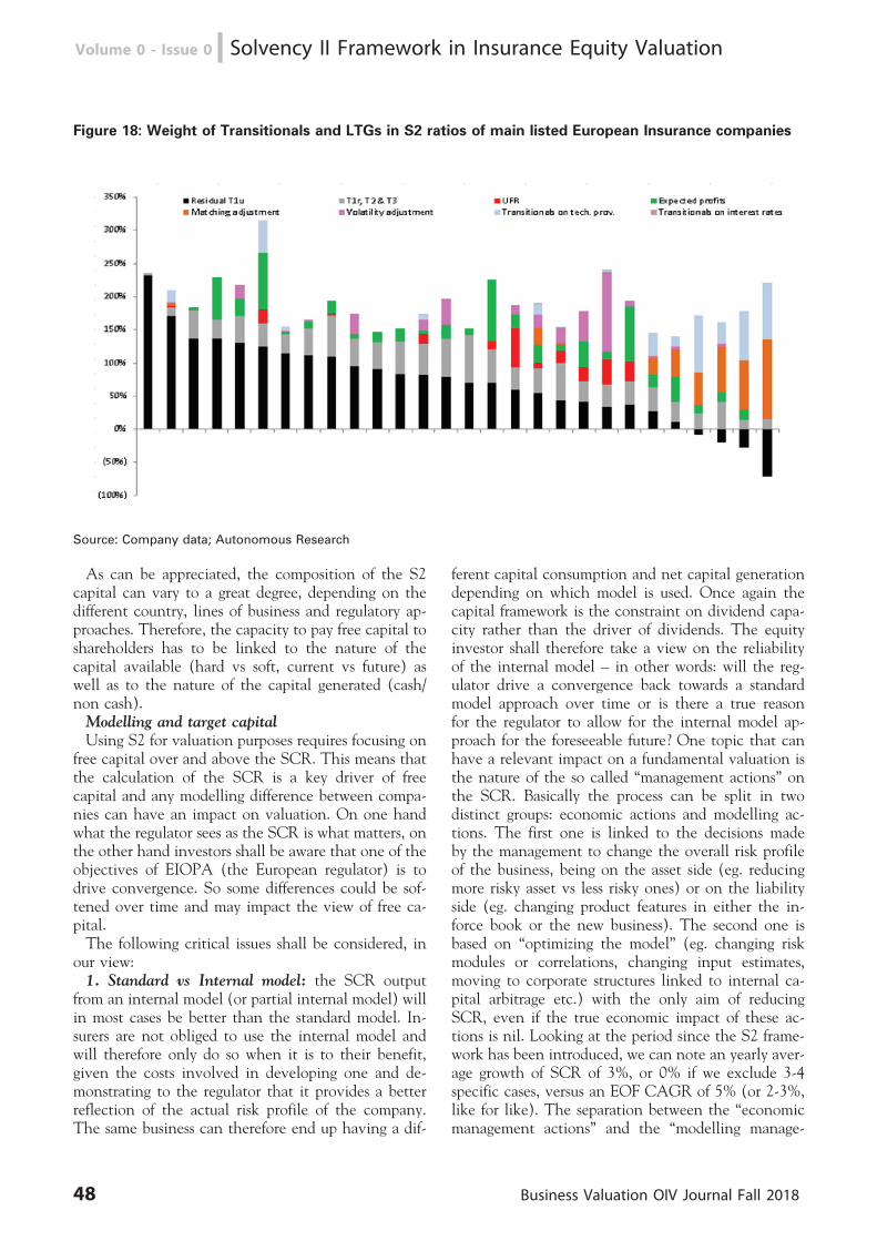
Figure 18: Weight of Transitionals and LTGs in S2 ratios of main listed European Insurance companies

Source: Company data; Autonomous Research

As can be appreciated, the composition of the S2capital can vary to a great degree, depending on thedifferent country, lines of business and regulatory ap-proaches. Therefore, the capacity to pay free capital toshareholders has to be linked to the nature of thecapital available (hard vs soft, current vs future) aswell as to the nature of the capital generated (cash/non cash).Modelling and target capitalUsing S2 for valuation purposes requires focusing on

free capital over and above the SCR. This means thatthe calculation of the SCR is a key driver of freecapital and any modelling difference between compa-nies can have an impact on valuation. On one handwhat the regulator sees as the SCR is what matters, onthe other hand investors shall be aware that one of theobjectives of EIOPA (the European regulator) is todrive convergence. So some differences could be sof-tened over time and may impact the view of free ca-pital.The following critical issues shall be considered, in

our view:1. Standard vs Internal model: the SCR output

from an internal model (or partial internal model) willin most cases be better than the standard model. In-surers are not obliged to use the internal model andwill therefore only do so when it is to their benefit,given the costs involved in developing one and de-monstrating to the regulator that it provides a betterreflection of the actual risk profile of the company.The same business can therefore end up having a dif-

ferent capital consumption and net capital generationdepending on which model is used. Once again thecapital framework is the constraint on dividend capa-city rather than the driver of dividends. The equityinvestor shall therefore take a view on the reliabilityof the internal model – in other words: will the reg-ulator drive a convergence back towards a standardmodel approach over time or is there a true reasonfor the regulator to allow for the internal model ap-proach for the foreseeable future? One topic that canhave a relevant impact on a fundamental valuation isthe nature of the so called ‘‘management actions’’ onthe SCR. Basically the process can be split in twodistinct groups: economic actions and modelling ac-tions. The first one is linked to the decisions madeby the management to change the overall risk profileof the business, being on the asset side (eg. reducingmore risky asset vs less risky ones) or on the liabilityside (eg. changing product features in either the in-force book or the new business). The second one isbased on ‘‘optimizing the model’’ (eg. changing riskmodules or correlations, changing input estimates,moving to corporate structures linked to internal ca-pital arbitrage etc.) with the only aim of reducingSCR, even if the true economic impact of these ac-tions is nil. Looking at the period since the S2 frame-work has been introduced, we can note an yearly aver-age growth of SCR of 3%, or 0% if we exclude 3-4specific cases, versus an EOF CAGR of 5% (or 2-3%,like for like). The separation between the ‘‘economicmanagement actions’’ and the ‘‘modelling manage-



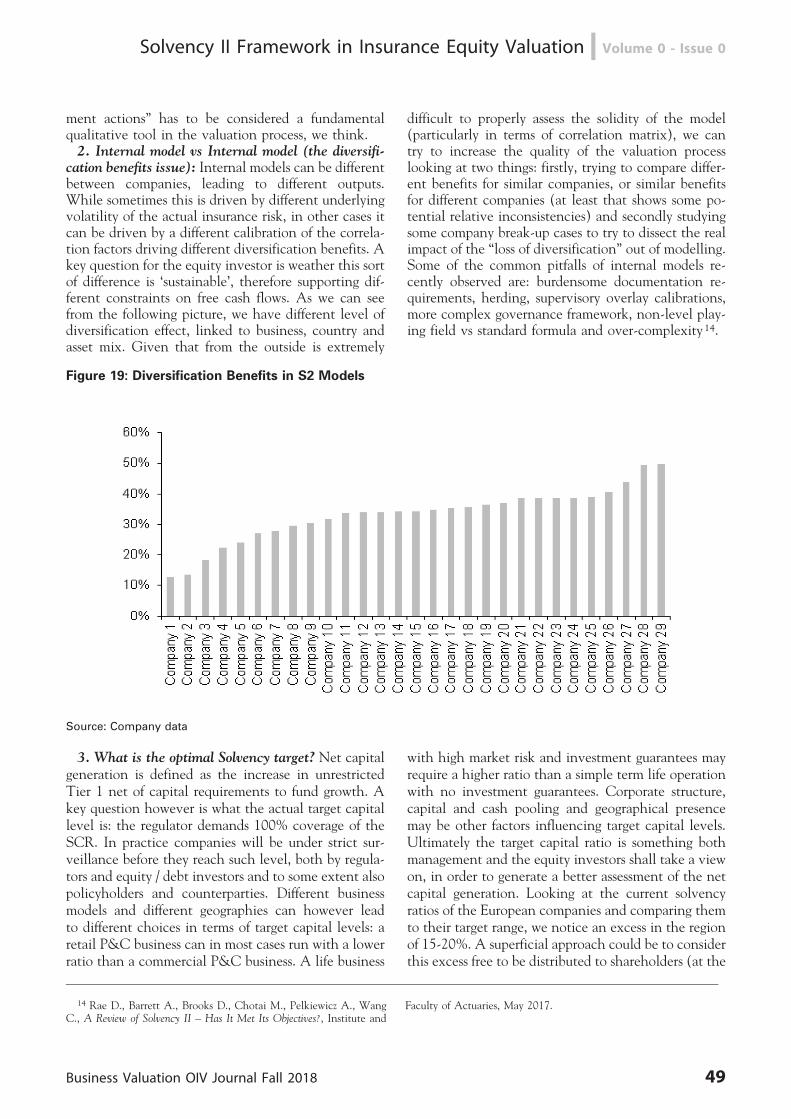
ment actions’’ has to be considered a fundamentalqualitative tool in the valuation process, we think.2. Internal model vs Internal model (the diversifi-

cation benefits issue): Internal models can be differentbetween companies, leading to different outputs.While sometimes this is driven by different underlyingvolatility of the actual insurance risk, in other cases itcan be driven by a different calibration of the correla-tion factors driving different diversification benefits. Akey question for the equity investor is weather this sortof difference is ‘sustainable’, therefore supporting dif-ferent constraints on free cash flows. As we can seefrom the following picture, we have different level ofdiversification effect, linked to business, country andasset mix. Given that from the outside is extremely

difficult to properly assess the solidity of the model(particularly in terms of correlation matrix), we cantry to increase the quality of the valuation processlooking at two things: firstly, trying to compare differ-ent benefits for similar companies, or similar benefitsfor different companies (at least that shows some po-tential relative inconsistencies) and secondly studyingsome company break-up cases to try to dissect the realimpact of the ‘‘loss of diversification’’ out of modelling.Some of the common pitfalls of internal models re-cently observed are: burdensome documentation re-quirements, herding, supervisory overlay calibrations,more complex governance framework, non-level play-ing field vs standard formula and over-complexity 14.

Figure 19: Diversification Benefits in S2 Models


3. What is the optimal Solvency target? Net capitalgeneration is defined as the increase in unrestrictedTier 1 net of capital requirements to fund growth. Akey question however is what the actual target capitallevel is: the regulator demands 100% coverage of theSCR. In practice companies will be under strict sur-veillance before they reach such level, both by regula-tors and equity / debt investors and to some extent alsopolicyholders and counterparties. Different businessmodels and different geographies can however leadto different choices in terms of target capital levels: aretail P&C business can in most cases run with a lowerratio than a commercial P&C business. A life business

with high market risk and investment guarantees mayrequire a higher ratio than a simple term life operationwith no investment guarantees. Corporate structure,capital and cash pooling and geographical presencemay be other factors influencing target capital levels.Ultimately the target capital ratio is something bothmanagement and the equity investors shall take a viewon, in order to generate a better assessment of the netcapital generation. Looking at the current solvencyratios of the European companies and comparing themto their target range, we notice an excess in the regionof 15-20%. A superficial approach could be to considerthis excess free to be distributed to shareholders (at the

14 Rae D., Barrett A., Brooks D., Chotai M., Pelkiewicz A., WangC., A Review of Solvency II – Has It Met Its Objectives?, Institute and

Faculty of Actuaries, May 2017.



end of the day, that’s the level above the company’starget, and it should take into account all the systemicand idiosyncratic risks involved). In reality part of theS2 movements can be predicated on non-economicfactors and not always an economic change in sol-

vency is related to actual cash. In order to discriminatebetween a distributable free excess capital situationand a weaker one, we need to go through all the ana-lysis we are trying to underlie.

Figure 20: Solvency ratios: actual vs targets


Disclosure & comparabilityS2 has significantly increased the level of disclosure.

The Solvency Financial Condition Reports (SFCR)are mandatory and publicly available for all groupsand for each subsidiary. Quantity of disclosure is how-ever not a guarantee of full comparability across thesector: for example, so far many companies have givena view on ‘‘normalized’’ capital generation, albeit defi-nition varies by company.The following critical issues shall be considered in

our view:1. ‘‘Underlying’’ or ‘‘normalized’’ capital genera-

tion: in order to better understand the underlying dri-vers of capital generation, some companies have givena view on ‘‘underlying’’ or ‘‘normalized’’ capital genera-tion. Such information is indeed useful, with somecaveats: comparability between companies is limitedby the different definitions – the ‘‘normalized’’ marketreturn assumptions can differ, model changes are trea-ted differently and so are management actions. On theSCR side the target capital ratio used as a multiplierfor the SCR is also not always consistent (although

generally set at 100%). The issue is not dissimilar tothe comparison of ‘‘operating’’ or ‘‘adjusted’’ earnings.To be more specific, we neither have the disclosurearound the ‘normalized’ asset yield assumptions drivingthe excess spread nor around the operating and actuar-ial assumptions behind new business profits and oper-ating return vs. current experience.2. Group vs subsidiary view: group capital and ca-

pital generation are most scrutinized. While they re-present the constraint on free cash flows for the group,they are not always informative of the subsidiary viewand the potential bottlenecks that can be found at alocal subsidiary level and that therefore constrain cashremittances back to group. One example is the diver-sification benefit on which the groups rely on – butsuch benefit is not always ‘‘payable’’ to shareholders ifthe risk is taken in different legal entities.3. Aggregate view vs LoB: capital generation disclo-

sure, where available, remains very high level and canhardly be broken down in detail by line of business(LoB) for multi-line companies.4. Non-S2 operations: for operations included in



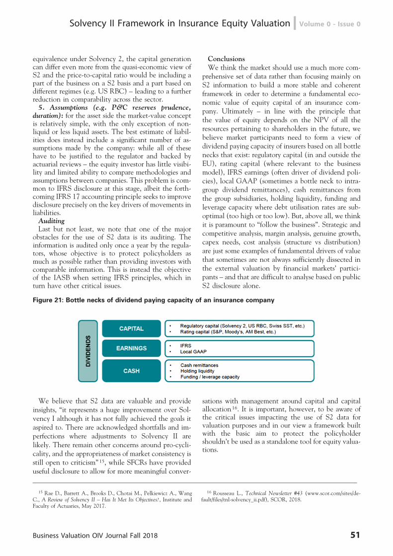
equivalence under Solvency 2, the capital generationcan differ even more from the quasi-economic view ofS2 and the price-to-capital ratio would be including apart of the business on a S2 basis and a part based ondifferent regimes (e.g. US RBC) – leading to a furtherreduction in comparability across the sector.5. Assumptions (e.g. P&C reserves prudence,

duration): for the asset side the market-value conceptis relatively simple, with the only exception of non-liquid or less liquid assets. The best estimate of liabil-ities does instead include a significant number of as-sumptions made by the company: while all of thesehave to be justified to the regulator and backed byactuarial reviews – the equity investor has little visibi-lity and limited ability to compare methodologies andassumptions between companies. This problem is com-mon to IFRS disclosure at this stage, albeit the forth-coming IFRS 17 accounting principle seeks to improvedisclosure precisely on the key drivers of movements inliabilities.AuditingLast but not least, we note that one of the major

obstacles for the use of S2 data is its auditing. Theinformation is audited only once a year by the regula-tors, whose objective is to protect policyholders asmuch as possible rather than providing investors withcomparable information. This is instead the objectiveof the IASB when setting IFRS principles, which inturn have other critical issues.

ConclusionsWe think the market should use a much more com-

prehensive set of data rather than focusing mainly onS2 information to build a more stable and coherentframework in order to determine a fundamental eco-nomic value of equity capital of an insurance com-pany. Ultimately – in line with the principle thatthe value of equity depends on the NPV of all theresources pertaining to shareholders in the future, webelieve market participants need to form a view ofdividend paying capacity of insurers based on all bottlenecks that exist: regulatory capital (in and outside theEU), rating capital (where relevant to the businessmodel), IFRS earnings (often driver of dividend poli-cies), local GAAP (sometimes a bottle neck to intra-group dividend remittances), cash remittances fromthe group subsidiaries, holding liquidity, funding andleverage capacity where debt utilisation rates are sub-optimal (too high or too low). But, above all, we thinkit is paramount to ‘‘follow the business’’. Strategic andcompetitive analysis, margin analysis, genuine growth,capex needs, cost analysis (structure vs distribution)are just some examples of fundamental drivers of valuethat sometimes are not always sufficiently dissected inthe external valuation by financial markets’ partici-pants – and that are difficult to analyse based on publicS2 disclosure alone.

Figure 21: Bottle necks of dividend paying capacity of an insurance company

We believe that S2 data are valuable and provideinsights, ‘‘it represents a huge improvement over Sol-vency I although it has not fully achieved the goals itaspired to. There are acknowledged shortfalls and im-perfections where adjustments to Solvency II arelikely. There remain other concerns around pro-cycli-cality, and the appropriateness of market consistency isstill open to criticism’’ 15, while SFCRs have provideduseful disclosure to allow for more meaningful conver-

sations with management around capital and capitalallocation16. It is important, however, to be aware ofthe critical issues impacting the use of S2 data forvaluation purposes and in our view a framework builtwith the basic aim to protect the policyholdershouldn’t be used as a standalone tool for equity valua-tions.

15 Rae D., Barrett A., Brooks D., Chotai M., Pelkiewicz A., WangC., A Review of Solvency II – Has It Met Its Objectives?, Institute andFaculty of Actuaries, May 2017.

16 Rousseau L., Technical Newsletter #43 (www.scor.com/sites/de-fault/files/tnl-solvency_ii.pdf), SCOR, 2018.



References

Andenas M., Avesani R.G., Manes P., Vella F.,Wood P.R., Solvency II: A Dynamic Challenge for theInsurance Market, Il Mulino, Bologna, 2017.Burkhart T., Reuß A., Zwiesler H. J., Allowance for

Surplus Funds under Solvency II: Adequate reflection ofrisk sharing between policyholders and shareholders in arisk-based solvency framework?, European ActuarialJournal, Issue 1, 2017.Dalla Palma N., Horvath G., Jacquet T., Preston M.,

It’s not another Solvency 2 primer, Exane BNP Paribas,2016.De Felice M., Moriconi F., A Course on Finance of

Insurance, GCAF, Universita Cattolica, Milano, 2002.EY, Cash, Capital and Dividends. How Solvency II is

Challenging the Insurance Investor Story, March 2016.Gatzer N., Heidinger D., An Empirical Analysis of

Market Reactions to the First Solvency and Financial Con-dition Reports in the European Insurance Sector, WorkingPaper, School of Business and Economics, FAU, Feb-ruary 2018.Giuliani S. Crescita e Valore, Aracne, Roma, 2005.Giuliani S., Lualdi M., L’Introduzione dello EEV nel

Settore Assicurativo: Aspetti Critici, la Valutazione delleAziende, n. 35, 2004.

Guatri L., Bini M., I Moltiplicatori nella Valutazionedelle Aziende, UBE, Milano, 2002.Insurance Europe, Insurance Europe comments on the

review of the Solvency II risk margin, 2017.Massari M., Zanetti L., Gianfrate G., The Valuation

of Financial Companies, Wiley, NY, 2014.Nissim D., Analysis and Valuation of Insurance Com-

panies, CE/ASA, Columbia University, NY, 2010.Kent J., Morgan E., S2AV: A Valuation Methodology

for Insurance Companies under Solvency II, MillimanResearch Report, 2016.Koller T., Goedhart M., Wessels D., Valuation, 6th

Edition, Wiley, NY, 2015.Rae D., Barrett A., Brooks D., Chotai M., Pelkiewicz

A., Wang C., A Review of Solvency II – Has It Met ItsObjectives?, Institute and Faculty of Actuaries, May2017.Rousseau L., Technical Newsletter #43 (www.scor.-

com/sites/default/files/tnl-solvency_ii.pdf), SCOR,2018.Swain R., Swallow D., The Prudential Regulation of

Insurers Under Solvency II, BOE Quarterly Bulletin, Q22015.Wilson T.C., Value and Capital Management, Wiley,

NY, 2015.



Bank Valuation Using Multiples in USand Europe: An Historical PerspectiveMario Massari* - Christopher Difonzo** - Gianfranco Gianfrate*** - Laura Zanetti****

We investigate the performance of relative valuation for US and European banks over the period 1990-

2017. While the literature on the use of multiples is well developed, the relative valuation of financial

institutions has received scant attention. We study the distribution and the main properties of each

multiple’s valuation errors, assessing which multiples work best and should be preferred when valuing

banks. Our results show that on average high levels of accuracy are achieved by two years forward P/E.

Moreover, diluted earnings not including extraordinary items should be preferred when computing trailing

earnings multiples and, interestingly, P/BV consistently outperforms P/TBV. Dividends’ multiples are not

among the best performers, anyway, it is preferable to consider only common dividends when computing

them. Most of the times P/Deposits and P/Revenues deliver poor performances, therefore it is advisable

not to use them as main valuation approach.

1. Introduction

The performance of multiples with respect to equityvaluation of non-financial companies has been exten-sively debated in financial and accounting literature(Liu et al., 2002; Liu et al., 2007; Nissim, 2013). How-ever, research and evidence are limited concerning theequity valuation of banks. In fact, the relative valua-tion approach (also referred to as ‘‘market approach’’)may represent the simplest way to value a bank: theapproach specifies the value of the bank as a functionof selected fundamentals and the average price of peerbanks (Forte et al., 2018; Nissim, 2013).This work analyzes the accuracy of the market ap-

proach for US and European bank valuation. We firstmeasure the performance 08 multiples based on valuedrivers such as the book value of equity, the tangiblebook value of equity, revenue, trailing earnings, for-ward earnings, common dividends, total dividends,bank deposits, and customer deposits. Following Liuet al. (2002), we measure the accuracy of multiplesby comparing the ‘‘theoretical’’ valuation of banks ob-tained using multiples to the actual prices: multiplesthat produce the lowest errors – meaning the differ-ence between theoretical prices and actual prices – areconsidered to be most accurate.The results of our analysis show that the accuracy of

multiples for US entities is significantly higher whenEuropean metrics are used, whereas small retail and in-vestment banks present more of a valuation challengethan large retail banks. Forward Price/Equity (P/E) mul-tiples outperform historical multiples, and multiples

based on two-year-ahead forecasts (not just one-year-ahead) are more accurate. Despite the usual practitionerassumptions, Price/Tangible Book Value (P/TBV) is notfound to be more meaningful and precise than Price/Book Value (P/BV). The P/BV is preferred. This studyalso reveals the weak relationship between value and theamount of preferred dividends: P/Common Dividends isa more precise tool than P/Total Dividends. Finally, P/Bank Deposits appears to be an accurate value driverwhen valuing investment banks, whereas P/CustomerDeposits is preferred when addressing commercial banks.The structure of this paper is as follows. A description

of relative valuation (introducing all of the multiplesanalyzed) is presented in Section 2, while Section 3summarizes the major contributions published in litera-ture. Section 4 describes the data and the methodologyadopted to assess the performance and accuracy of mul-tiples and presents all of the results for each analysissubsample. The impact of the financial crisis and theintroduction of the Euro on relative valuation precisionare studied. Additionally, regression and correlationanalyses investigate whether significant positive andnegative errors, corresponding to undervalued and over-valued banks, reflect subsequent price reactions.

2. Relative valuation

The use of multiples to perform company valuationhas been showing an increasingly positive trend, fol-lowing the development of financial markets and cor-porate finance deals during the last decades. Moreover,

* Bocconi University.** Credit Suisse.

*** EDHEC Business School.**** Bocconi University.


Bank Valuation Using Multiples in US and Europe n Volume 0 - Issue 0

great supporters of complex valuation techniques fre-quently recall the use of multiples when estimatingterminal values or checking for plausibility of theirresults (Bhojraj & Lee, 2002).The logic behind relative valuation is grounded on

the assumption that market prices are largely efficient,that, on average, fundamentals are correctly priced in,and that the law of one price holds. The basic princi-ple governing relative valuation (i.e., similar assets,and so similar firms, should trade at similar levels) fullyrelies on this set of assumptions. Market prices thusneed to be close to the true intrinsic value of firms.The following list of multiples is the collection of the

ones selected to run this empirical analysis, whichcorrespond to the ones mostly used and consideredby analysts and practitioners when running valuationfor banks.Price/Book Value of Equity (P/BV)The ratio between the market capitalization of the

firm and the book value of equity is widely used forcapital-intensive businesses, whereas it is less appropri-ate for sectors where the main driver of price perfor-mances is future growth (e.g., technology). It is con-sidered one of the most suitable multiples for financialinstitutions since it captures the regulatory attentionon solvency, capital requirements and equity mainte-nance.Price/Tangible Book Value of Equity (P/TBV)This multiple is a variation of the previous one and

deducts the value of all the intangible assets from theequity. Many practitioners prefer to use this multipleover the simple P/BV in order to obtain a more con-servative figure, which uses a liquid representation ofbook value eliminating the potential bias derivingfrom the accounting of illiquid intangible assets. Theintuition is that, in case of default, the value of intan-gible assets may easily collapse to zero, so it is advisableto use a multiple that eliminates their interferences.Moreover, it recalls the regulatory capital compositionof the CET1 Capital according to Basel III, whichindeed deducts goodwill and other intangibles.Price/Revenues (P/Revenues)Market capitalization divided by revenues is one of

the less used and most criticized multiple. Firstly, be-cause revenues should be compared with an asset-sidemeasure (e.g., enterprise value). Secondly, comparingbanks using only this multiple may lead to misjudge-ments because the cost structure and the riskiness ofthe underlying assets, which generated those revenues,are not considered.Price/Deposits (P/Deposits)Market capitalization is divided by the deposits,

which is the core driver for the vast majority of com-mercial banks. This multiple used to be popular in thepast but nowadays banks are more diversified and theirrevenues and profitability depend more and more on

fees-generating activities rather than on the sole inter-est income. This explains why this multiple is now lessused, but it is still helpful. In fact, given that depositsshould be rather uniform among retail banks, they area good candidate as explicative operating multiple.When considering deposits, these could be measured

in two different ways: the first one considers customerdeposits only (i.e., demand, savings and time depositsheld on account for individuals and corporations), theother one includes also bank deposits (i.e., the depositsheld on account for other banks). The latter thus con-siders not only collections from customers, but also theinvolvement in the interbank market. This broad mea-sure is the one used in this work.Price/Dividends (P/Dividends)Share price is divided by dividends per share, or,

alternatively, market capitalization is divided by theentire amount of dividends. This is another operatingmultiple typically used for banks because of the impor-tance of dividends for these institutions. In fact, divi-dends are the unique meaningful cash flow in thebanking sector, as also highlighted when discussingabout intrinsic valuation. However, this multiplecould be applied to firms operating in any sector, butit would be meaningless in many circumstances.Many companies, differently from banks, do not dis-

tribute dividends so frequently because they prefer toimplement alternative shareholders’ remunerationpractices (e.g., shares buy-back programs) or they sim-ply prefer to retain earnings to finance investmentopportunities using internal sources.When computing dividends multiples, it is impor-

tant to consider that dividends distributions may occurmore than once in a year and so all the relevant flowshave to be summed up to obtain a yearly value. More-over, this multiple can be built in two different ways,depending on the choice made for dividends. Consid-ering that total dividends is the sum of common divi-dends, paid on common shares, and preferred divi-dends, paid on preferred shares, the multiple can becomputed using total dividends (P/Total Dividends) orcommon dividends only (P/Common Dividends) asthe denominator. The distinction wants to catch po-tential connections between preferred stocks and va-lue. The use of common dividends only is generallypreferred because they should better reflect value withrespect to preferred dividends, which are more stableand less dependent on the actual level of profitabilityachieved in a given year. However, for the sake of thisempirical study, both will be computed.The last important consideration is related to out-

liers, which in this case can strongly affect the multi-ple. If dividends are particularly low because of a lackof financial resources or as a result of a strategic choice,the average multiple may reach extremely high values,


Volume 0 - Issue 0 n Bank Valuation Using Multiples in US and Europe

negatively affecting the quality of the valuation per-formed.Price/Earnings (P/E)The last multiple analysed is considered ‘‘the king’’ of

relative valuation, in particular for banks. It is com-puted as the ratio between the share price and earningsper share (EPS) or alternatively as market capitaliza-tion over total earnings. The multiple can be built indifferent ways, depending on the methodology used toselect earnings.Firstly, the choice can be made distinguishing be-

tween trailing and forward earnings. If historical va-lues, i.e., the earnings of the last twelve months (LTMearnings) are used, it is classified as a trailing – orLTM. Alternatively, if analysts’ forecasts for earningsare used, it is classified as a forward multiple. Forecastscan be computed on a one year, two years or moreyears basis, but best practices generally use one ortwo years forecasts, to avoid a strong dependence onestimates based on unobservable and unpredictablefigures. Nevertheless, Yee (2004) demonstrated thatfrom a theoretical standpoint the use of more forwardearnings represents an effective and important attri-bute in order to obtain more accurate results whenperforming valuation (i.e., the more forward, the moreaccurate).The second element affecting EPS calculation is di-

lution. The resulting multiples are the Basic P/E, ifEPS are computed considering only outstanding com-mon shares or instead the Diluted P/E if diluted com-mon shares are considered. Diluted common sharesinclude the effects generated by the hypothetical ex-ercise of all the outstanding convertible securities (e.g.,convertible bonds, stock options, warrants), whichcauses an increase in the number of outstanding shares.This assumed increase pushes EPS down (diluted EPSare lower than basic EPS, if there are convertible se-curity outstanding) and, consequently, the resultingmultiple is higher.The last point about earnings calculation is whether

to include non-recurring items. The rationale behindthe exclusion of these items is that unusual and extra-ordinary gains or losses should not affect valuation,since these will not constantly take place in the future.In this way, earnings excluding extraordinary itemscommunicate better the actual profitability of a com-pany without suffering from any interference directedby one-offs.The combination of all these aspects and considera-

tions gives rise to the identification of six different P/Emultiples, which will be inspected in this work. Theyare:

– P / 1 Year Forward Earnings– P / 2 Years Forward Earnings– P / LTM Diluted Earnings, considering extraordin-

ary items– P / LTM Diluted Earnings, excluding extraordinary

items– P / LTM Basic Earnings, considering extraordinary

items– P / LTM Basic Earnings, excluding extraordinary

itemsNonetheless, P/E has an important drawback that

can limit its applicability. In case of negative earnings,the multiple becomes completely meaningless becauseof its negative value. In order to avoid any issue, theset of comparables must be built accordingly. More-over, the presence of outliers should be accuratelymonitored in case of very low earnings that can gen-erate an abnormal increase in the multiple. In parti-cular, Dermine (2010) outlines that the use of the P/Eis biased when banks report large provisions for creditlosses (a problem that, recently, has been affecting thebanking system of many countries, such as Italy) im-plying lower earnings. This causes large volatility inthe multiple and drives bias.

3. Literature review

While the extensive use of multiples among bothpractitioners and academicians has progressivelygrown, theory and empirical research have also de-monstrated some advancements, but still limited gui-dance is available to assess relative valuation metricsperformance.Essentially, some practitioners consider the use of

multiples as an art form1 rather than a science. There-fore, they suggest that the practice should be left onlyto industry professionals. Notwithstanding, the impor-tance of multiples in valuation methods and their effi-cacy in supporting investment decisions have attractedmany researchers to this field. Both standard literatureand empirical studies on multiples have experiencednotable advances over the past decades, becoming adebated topic among academicians.Methodologies and findings from Nissim (2002 &

2011) and Cooper (2008) are particularly relevantfor the development of this empirical study. Addition-ally, contributions to the literature coming from otherauthors provided an important theoretical support andmany relevant intuitions.Nissim (2011) analysed the accuracy of relative va-

luation for U.S. insurance companies. From March1990 to January 2011, he monthly analysed a sample

1 Bhojraj (2003) noted that the level of subjectivity required in theapplication of multiples, is inconsistent with a scientific standpoint. In

particular, the selection process of comparable firms tends to relystrongly on individual analyst’s expertise.



of 372 different firms, demonstrating that valuationperforms better when using earnings forecasts (i.e., for-ward multiples) rather than reported earnings (i.e.,trailing multiples). The same result will come fromthe analysis here performed. His study also proved thatbook value multiples perform robustly, in particular ifthe price-to-book ratio is conditioned to ROE. More-over, Nissim observed other two relevant aspects,which are less marked in the results from the analysishere performed, but still evident. He compared theperformance of Basic P/E and Diluted P/E, observingthat the latter has higher predictive properties. He alsoshowed that valuation accuracy substantially improveswhen using income before special items instead of re-ported income.In a previous work Liu, Nissim & Thomas (2002)

carried out a comprehensive analysis of multiples’ pre-cision in the U.S. between 1982 and 1999, drawing upa ranking of the better performing multiples, whichholds true for almost every sector analysed. Multipleswere ranked as follows: forward earnings measures asthe best ones, then historical earnings measures as avalid second best option, cash flows measures and bookvalue measures perform equally ranking as third, salesmeasures as the worst ones. These results are in linewith the ones here obtained.Cooper (2008) aimed at finding the optimal number

of comparable firms to use when computing out-of-sample multiples. The results of his analysis high-lighted that the use of about five comparables is opti-mal when some requirements are met (i.e., compar-ables operate in the same industry, their expectedgrowth rates are close to the one of the target firmand their average growth rate stays within 1% of thetarget firm’s growth rate). Cooper’s work is extremelyuseful here for the statistical tools implemented, whichwill be introduced later in the empirical section, morethan for the results achieved.Cheng & McNamara (2000) inspected valuation

accuracy when using historical P/E multiples, P/BVmultiples and a combination of the two using equalweights. The analysis was performed for the U.S. equi-ty market, firstly considered as an aggregate and thensplit depending on SIC codes 2. They found that theequally weighted combination of P/E and P/BV per-formed better than both multiples alone, underlyingthat both earnings and book values are significant va-lue drivers.Alford (1992) tested the effects of the choice of

comparable firms on the precision of valuation esti-mates when using earnings multiples. In particular,

he focused on the use of industry membership andproxies for growth and risk for the selection of compar-ables. Results showed that valuation accuracy increaseswhen the level of detail for the industry definition usedto identify comparables is not too specific (i.e., three-digit SIC codes). Differently, Bhojraj & Lee (2002)implemented a matching mechanism to identify com-parable firms based on the use of economic variables,rather than industry membership. The analysis hereperformed combines the different intuitions comingfrom these two studies: only banks will be considered,but the sample will be then subdivided depending onbalance sheet figures determining size (large or small)and business model (commercial or investment bank).Minjina (2009) implemented the same analysis done

by Nissim, but he did not focus on the same marketand on a unique sector. Indeed, his analysis embracedall the companies listed in the Bucharest Stock Ex-change from January 2003 to June 2008, but excludedthe financial sector. Results underlined that Price/Cash Flows (P/CF) and Enterprise Value/EBITDA(EV/EBITDA) are the first and second best multiplesto use when valuing Romanian companies, whereasPrice/Sales appeared to be the least reliable. As alreadymentioned, these multiples are not significant andsomehow meaningless for banks, which also explainswhy the financial sector was excluded to perform thisanalysis. Another relevant outcome of Minjina’s studywas the observation of a lower performance accuracyfor Romanian listed companies, if compared with com-panies from more developed countries. The lower effi-ciency of Romanian capital markets and the smallersize of Romanian companies are considered the maindeterminants of this finding. The same difference inaccuracy will be evident later, when comparing resultsfor multiples’ accuracy between American and Eur-opean banks.Forte et al. (2018) investigates the role of relative

valuation in the banking industry by evaluating theaccuracy of a group of industry specific multiples.The results highlight that stock market multiples arebest suited for US institutions, and that a two-year-forward P/E is the most precise metric. Contrary topractitioner beliefs, P/Tangible Book Value is lessmeaningful than P/BV. Multiples accuracy declinesin case of small commercial banks relative to largecommercial banks and investment bank relative to re-tail banks pointing out that for small retail bank andinvestment bank equity valuation using multiples be-comes a more challenging exercise. Additionally, errordistributions are exploited to assess whether large po-

2 The Standard Industrial Classification (SIC) is a system for classi-fying industries by a four-digit code. SIC codes can be grouped intoprogressively broader industry classifications: industry group (the first

three digits), major group (the first two digits) and division (encom-passing a range of SIC codes).



sitive errors lead to systematic one-year positive priceperformances and whether negative errors lead to ne-gative price changes.

4. Performance and accuracy of multiples

This section discusses about the main findings of theempirical research conducted to analyse the effective-ness of multiples and to understand if there is one multi-ple outperforming the others, which should be thereforeconsidered the most reliable to perform banks valua-tion. Detailed analyses on valuation accuracy and onthe distribution of valuation errors are presented.Furthermore, the effects on the performance of relativevaluation driven by the introduction of the Euro and ofthe 2007/2008 financial turmoil are analysed. In the lastpart, a summary ranking of the best multiples to be usedin each subgroup of banks is proposed.

4.1. Data

The timespan considered in our empirical analysisstarts in January 1990 and terminates in April 2018.The dataset comprises all the banks currently listed,but also banks that have been listed during the periodanalysed. Delisting mostly derives from M&A activityor bankruptcy, more rarely it represents a strategicchoice taken by the management. The final datasetis composed of 1,118 banks, of which 181 located inthe Eurozone, while 937 are American. When buildinga database for comparables, there is always a ‘‘biasversus variability’’ trade-off to consider. In this case,variability is minimized, but the bias deriving from bigdifferences among comparables may be relevant. Thedifferent techniques, which have been adopted to limitthis effect and increase homogeneity, are showed later.The analysis required a wide range of financial data,

which have been collected from different data provi-ders and then merged into a unique dataset. The list ofthese data providers and the corresponding data col-lected follows.– Wharton Research Data Services – CompustatThis database provides all the historical Balance

Sheet and Income Statement figures, along with otheraccounting measures (e.g., the number of shares out-standing). Data from 1990 until 2017 have been col-lected, using two different queries. The ‘‘Bank – Daily’’query provides data for North America banks only, sodata for banks in the United States were easily col-lected filtering only for the country. To collect data forthe Eurozone, the ‘‘Compustat Global – FundamentalAnnual’’ query was used. However, this dataset coversall the industries globally. Data were therefore filtered

according to the GICS3 codes, including only the en-tire Industry Group 4010 (Banks) and the Industry402030 (Capital Markets), and according to the coun-try, including only the ones within the Eurozone (Ta-ble 1). Furthermore, it is important to underline thatthese two queries do not provide the same informa-tion. In particular, the one used for the Eurozone doesnot provide data on diluted earnings, so that two mul-tiples (i.e., P/LTM Diluted Earnings, considering ex-traordinary items and excluding extraordinary items)cannot be computed for these banks.– Institutional Brokers’ Estimate System (I/B/E/S)This database, accessed via Thomson Reuters Data-

stream, provides all the analysts’ forecasts, which arefundamental to compute forward multiples. Moreover,the measure of volatility of forecasts (i.e., the standarddeviation of two years forward earnings) and the num-ber of analysts covering each bank were collected fromI/B/E/S.– BloombergWeekly prices have been collected from Bloomberg

and then a monthly value has been obtained comput-ing the median of the corresponding weekly observa-tions. However, to compute multiples, only one pricefor each year is required and the April one has beenselected. This choice is consistent with practice andfollows the procedure implemented from Nissim in hisstudy on relative valuation performance for the insur-ance sector. Market prices are selected four monthsafter the fiscal year end to ensure that all year-endinformation are publicly available and reflected inprices (Schreiner, 2007). Moreover, in April, I/B/E/Supdates and publishes summary forecasts, maximisingalso consistency between prices and future estimates.Once that all data have been collected, in order to

increase comparability and to reduce bias, banks havebeen divided in subgroups, maintaining the Americanand the European sample separated.The first differentiation is related to the business

model, distinguishing between Investment and Com-mercial Banks. Following the example of Beltratti andStulz (2009), a summary ratio is computed for eachbank as the median of the available ratios of CustomerLoans over Total Assets, between 1990 and 2017. Athreshold is set at 40%. Banks with a summary ratioexceeding the threshold are labelled as CommercialBanks, since the ratio signals that the business modelis particularly focused on lending money to clients,more than on offering advisory services. Loans tobanks are not included when computing the ratio toeliminate the effects of banks participating to the in-

3 The Global Industry Classification Standard (CIGS) is an industrytaxonomy developed by MSCI and Standard & Poor’s used to categor-

ise all major public companies. It consists of 11 sectors, 24 industrygroups, 68 industries and 157 sub-industries.



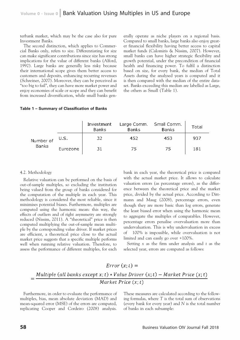
terbank market, which may be the case also for pureInvestment Banks.The second distinction, which applies to Commer-

cial Banks only, refers to size. Differentiating for sizecan make significant contributions since size has strongimplications for the value of different banks (Alford,1992). Large banks are generally less risky becausetheir international scope gives them better access tocustomers and deposits, enhancing recurring revenues(Schreiner, 2007). Moreover, they can be perceived as‘‘too big to fail’’, they can have more market power andenjoy economies of scale or scope and they can benefitfrom increased diversification, while small banks gen-

erally operate as niche players on a regional basis.Compared to small banks, large banks also enjoy great-er financial flexibility having better access to capitalmarket funds (Calomiris & Nissim, 2007). However,small banks can have higher strategic flexibility andgrowth potential, under the precondition of financialhealth and financing power. To fulfil a distinctionbased on size, for every bank, the median of TotalAssets during the analysed years is computed and itis then compared with the median of the entire data-set. Banks exceeding this median are labelled as Large,the others as Small (Table 1).

Table 1 – Summary of Classification of Banks

4.2. Methodology

Relative valuation can be performed on the basis ofout-of-sample multiples, so excluding the institutionbeing valued from the group of banks considered forthe computation of the multiple in each year. Thismethodology is considered the most reliable, since itminimises potential biases. Furthermore, multiples arecomputed using the harmonic mean: this way, theeffects of outliers and of right asymmetry are stronglyreduced (Nissim, 2011). A ‘‘theoretical’’ price is thencomputed multiplying the out-of-sample mean multi-ple by the corresponding value driver. If market pricesare efficient, a theoretical price close to the actualmarket price suggests that a specific multiple performswell when running relative valuation. Therefore, toassess the performance of different multiples, for each

bank in each year, the theoretical price is compared

with the actual market price. It allows to calculate

valuation errors (as percentage errors), as the differ-

ence between the theoretical price and the market

price, divided by the actual price. According to Ditt-

mann and Maug (2008), percentage errors, even

though they are more basic than log errors, generate

the least biased error when using the harmonic mean

to aggregate the multiples of comparables. However,

percentage errors penalise overvaluation more than

undervaluation. This is why undervaluation in excess

of �100% is impossible, while overvaluation is not

limited and can easily go over +100%.

Setting x as the firm under analysis and t as the

selected year, errors are computed as follows:

Furthermore, in order to evaluate the performance ofmultiples, bias, mean absolute deviation (MAD) andmean-squared error (MSE) of the errors are computed,replicating Cooper and Cordeiro (2008) analysis.

These measures are calculated according to the follow-ing formulas, where T is the total sum of observations(every bank for every year) and N is the total numberof banks in each subsample:



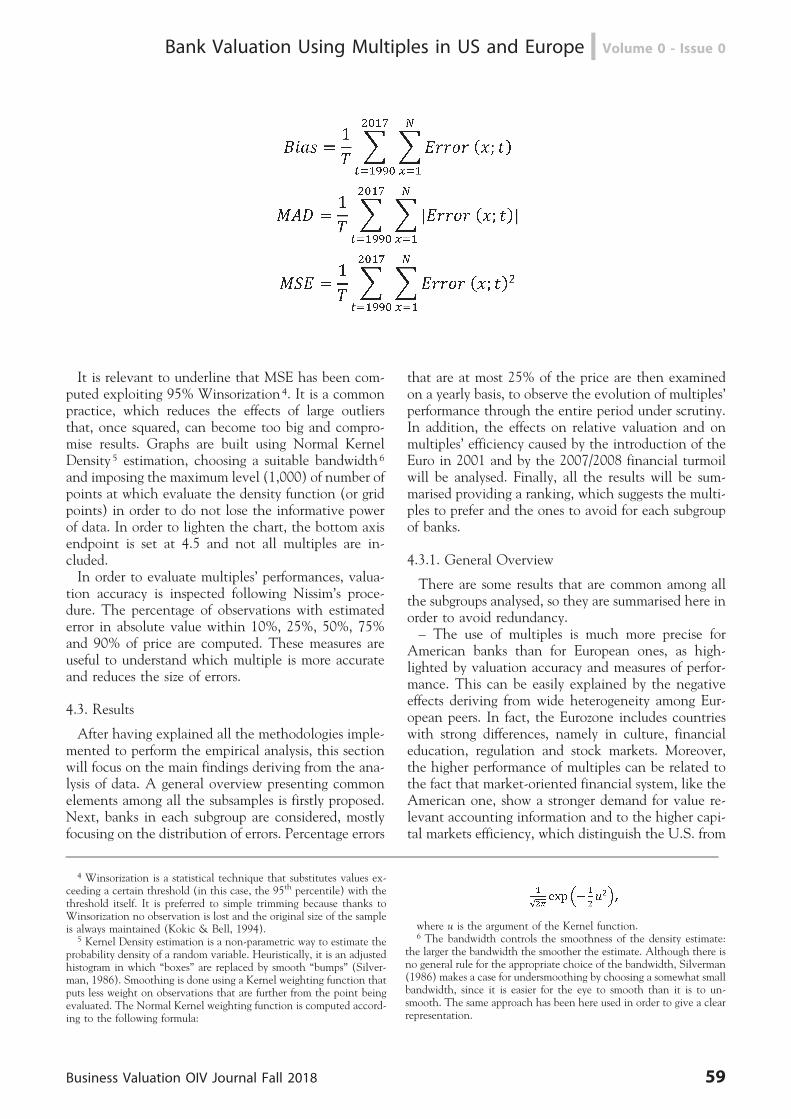
It is relevant to underline that MSE has been com-puted exploiting 95% Winsorization4. It is a commonpractice, which reduces the effects of large outliersthat, once squared, can become too big and compro-mise results. Graphs are built using Normal KernelDensity 5 estimation, choosing a suitable bandwidth6

and imposing the maximum level (1,000) of number ofpoints at which evaluate the density function (or gridpoints) in order to do not lose the informative powerof data. In order to lighten the chart, the bottom axisendpoint is set at 4.5 and not all multiples are in-cluded.In order to evaluate multiples’ performances, valua-

tion accuracy is inspected following Nissim’s proce-dure. The percentage of observations with estimatederror in absolute value within 10%, 25%, 50%, 75%and 90% of price are computed. These measures areuseful to understand which multiple is more accurateand reduces the size of errors.

4.3. Results

After having explained all the methodologies imple-mented to perform the empirical analysis, this sectionwill focus on the main findings deriving from the ana-lysis of data. A general overview presenting commonelements among all the subsamples is firstly proposed.Next, banks in each subgroup are considered, mostlyfocusing on the distribution of errors. Percentage errors

that are at most 25% of the price are then examinedon a yearly basis, to observe the evolution of multiples’performance through the entire period under scrutiny.In addition, the effects on relative valuation and onmultiples’ efficiency caused by the introduction of theEuro in 2001 and by the 2007/2008 financial turmoilwill be analysed. Finally, all the results will be sum-marised providing a ranking, which suggests the multi-ples to prefer and the ones to avoid for each subgroupof banks.

4.3.1. General Overview

There are some results that are common among allthe subgroups analysed, so they are summarised here inorder to avoid redundancy.– The use of multiples is much more precise for

American banks than for European ones, as high-lighted by valuation accuracy and measures of perfor-mance. This can be easily explained by the negativeeffects deriving from wide heterogeneity among Eur-opean peers. In fact, the Eurozone includes countrieswith strong differences, namely in culture, financialeducation, regulation and stock markets. Moreover,the higher performance of multiples can be related tothe fact that market-oriented financial system, like theAmerican one, show a stronger demand for value re-levant accounting information and to the higher capi-tal markets efficiency, which distinguish the U.S. from

4 Winsorization is a statistical technique that substitutes values ex-ceeding a certain threshold (in this case, the 95th percentile) with thethreshold itself. It is preferred to simple trimming because thanks toWinsorization no observation is lost and the original size of the sampleis always maintained (Kokic & Bell, 1994).

5 Kernel Density estimation is a non-parametric way to estimate theprobability density of a random variable. Heuristically, it is an adjustedhistogram in which ‘‘boxes’’ are replaced by smooth ‘‘bumps’’ (Silver-man, 1986). Smoothing is done using a Kernel weighting function thatputs less weight on observations that are further from the point beingevaluated. The Normal Kernel weighting function is computed accord-ing to the following formula:

where u is the argument of the Kernel function.6 The bandwidth controls the smoothness of the density estimate:

the larger the bandwidth the smoother the estimate. Although there isno general rule for the appropriate choice of the bandwidth, Silverman(1986) makes a case for undersmoothing by choosing a somewhat smallbandwidth, since it is easier for the eye to smooth than it is to un-smooth. The same approach has been here used in order to give a clearrepresentation.



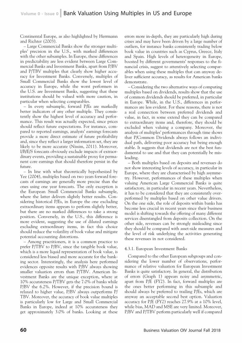
Continental Europe, as also highlighted by Herrmannand Richter (2003).– Large Commercial Banks show the stronger multi-

ples’ precision in the U.S., with marked differenceswith the other subsamples. In Europe, these differencesin predictability are less evident between Large Com-mercial Banks and Investment Banks, apart from P/BVand P/TBV multiples that clearly show higher accu-racy for Investment Banks. Conversely, multiples ofSmall Commercial Banks show the lowest level ofaccuracy in Europe, while the worst performers inthe U.S. are Investment Banks, suggesting that theseinstitutions should be valued with more caution, inparticular when selecting comparables.– In every subsample, forward P/Es are markedly

better indicators of any other multiple. They consis-tently show the highest level of accuracy and perfor-mance. This result was actually expected, since pricesshould reflect future expectations. For instance, com-pared to reported earnings, analysts’ earnings forecastsprovide a more direct estimate of future profitabilityand, since they reflect a larger information set, they arelikely to be more accurate (Nissim, 2011). Moreover,I/B/E/S forecasts obviously exclude impacts of extraor-dinary events, providing a sustainable proxy for perma-nent core earnings that should therefore persist in thefuture.– In line with what theoretically hypothesized by

Yee (2004), multiples based on two years forward fore-casts of earnings are generally more precise than theones using one year forecasts. The only exception isthe European Small Commercial Banks subsample,where the latter delivers slightly better results. Con-sidering historical P/Es, in Europe the one excludingextraordinary items appears to perform slightly better,but there are no marked differences to take a strongposition. Conversely, in the U.S., this difference ismore evident, suggesting the use of diluted earningsexcluding extraordinary items, in fact this choiceshould reduce the volatility of book value and mitigatepotential accounting distortions.– Among practitioners, it is a common practice to

prefer P/TBV to P/BV, since the tangible book value,which is a more liquid representation of book value, isconsidered less biased and more accurate for the bank-ing sector. Interestingly, the analysis here performedevidences opposite results with P/BV always showingsmaller valuation errors than P/TBV. American In-vestment Banks are the unique exception, where at10% accurateness P/TBV gets the 7.0% of banks whileP/BV the 6.2%. However, if the precision bound isrelaxed to higher value, P/BV always outperforms P/TBV. Moreover, the accuracy of book value multiplesis particularly low for Large and Small CommercialBanks in Europe, indeed at 10% accurateness theyget approximately 3.0% of banks. Looking at these

errors more in-depth, they are particularly high duringcrises and may have been driven by a large number ofoutliers, for instance banks consistently trading belowbook value in countries such as Cyprus, Greece, Italyand Spain. High levels of heterogeneity in Europe,boosted by different governments’ responses to the fi-nancial crisis, suggest to attentively selecting compar-ables when using these multiples that can anyway de-liver sufficient accuracy, as results for American banksdemonstrate.– Considering the two alternative ways of computing

multiples based on dividends, results show that the useof common dividends should be preferred, in particularin Europe. While, in the U.S., differences in perfor-mances are less evident. For these reasons, there is nota real connection between preferred dividends andvalue, in fact, in some extend they can be comparedto extraordinary items and, therefore, they should beexcluded when valuing a company. Moreover, theanalysis of multiples’ performances through time showsthat P/Common Dividends always follows an indivi-dual path, delivering poor accuracy but being enoughstable. It suggests that dividends are not the best fun-damental to use and that they can potentially be mis-leading.– Both multiples based on deposits and revenues do

not show interesting levels of accuracy, in particular inEurope, where they are characterised by high asymme-try. However, performances of these multiples whenvaluing American Large Commercial Banks is quitesatisfactory, in particular in recent years. Nevertheless,it has to be considered that they are consistently over-performed by multiples based on other value drivers.On the one side, the role of deposits within banks hasbecome less crucial in recent years since their businessmodel is shifting towards the offering of many differentservices disentangled from deposits collection. On theother side, revenues can be strongly misleading sincethey should be compared with asset-side measures andthe level of risk underlying the activities generatingthese revenues in not considered.

4.3.1. European Investment Banks

Compared to the other European subgroups and con-sidering the lower number of observations, perfor-mance of relative valuation for European InvestmentBanks is quite satisfactory. In general, the distributionof errors (Graph 1) appears noisy and asymmetric,apart from P/E (FY2). In fact, forward multiples arethe ones better performing in this subsample andshould always be preferred to trailing P/Es, which areanyway an acceptable second best option. Valuationaccuracy for P/E (FY2) reaches 27.9% at a 10% level,while bias, MAD and MSE are very limited. Moreover,P/BV and P/TBV perform particularly well if compared



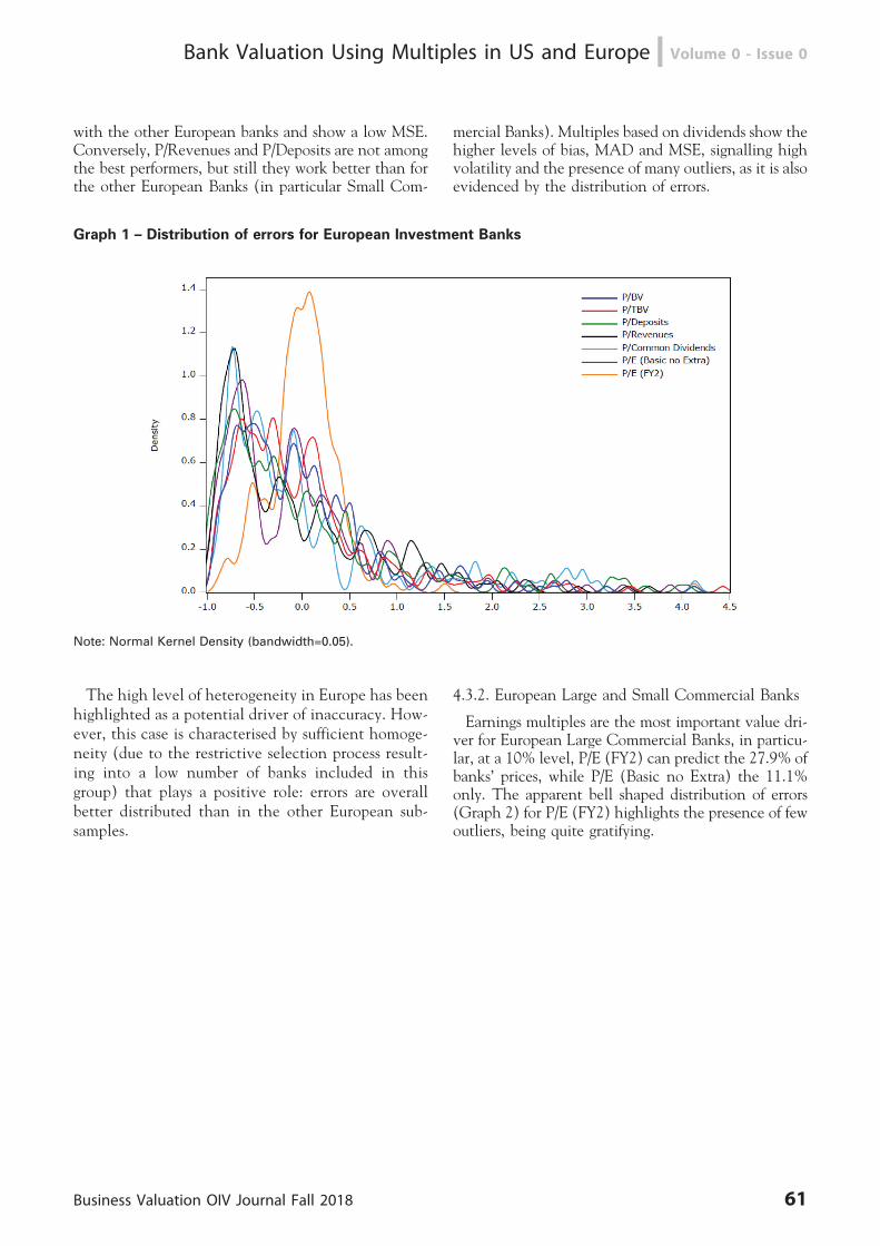
with the other European banks and show a low MSE.Conversely, P/Revenues and P/Deposits are not amongthe best performers, but still they work better than forthe other European Banks (in particular Small Com-

mercial Banks). Multiples based on dividends show thehigher levels of bias, MAD and MSE, signalling highvolatility and the presence of many outliers, as it is alsoevidenced by the distribution of errors.

Graph 1 – Distribution of errors for European Investment Banks

Note: Normal Kernel Density (bandwidth=0.05).

The high level of heterogeneity in Europe has beenhighlighted as a potential driver of inaccuracy. How-ever, this case is characterised by sufficient homoge-neity (due to the restrictive selection process result-ing into a low number of banks included in thisgroup) that plays a positive role: errors are overallbetter distributed than in the other European sub-samples.

4.3.2. European Large and Small Commercial Banks

Earnings multiples are the most important value dri-ver for European Large Commercial Banks, in particu-lar, at a 10% level, P/E (FY2) can predict the 27.9% ofbanks’ prices, while P/E (Basic no Extra) the 11.1%only. The apparent bell shaped distribution of errors(Graph 2) for P/E (FY2) highlights the presence of fewoutliers, being quite gratifying.



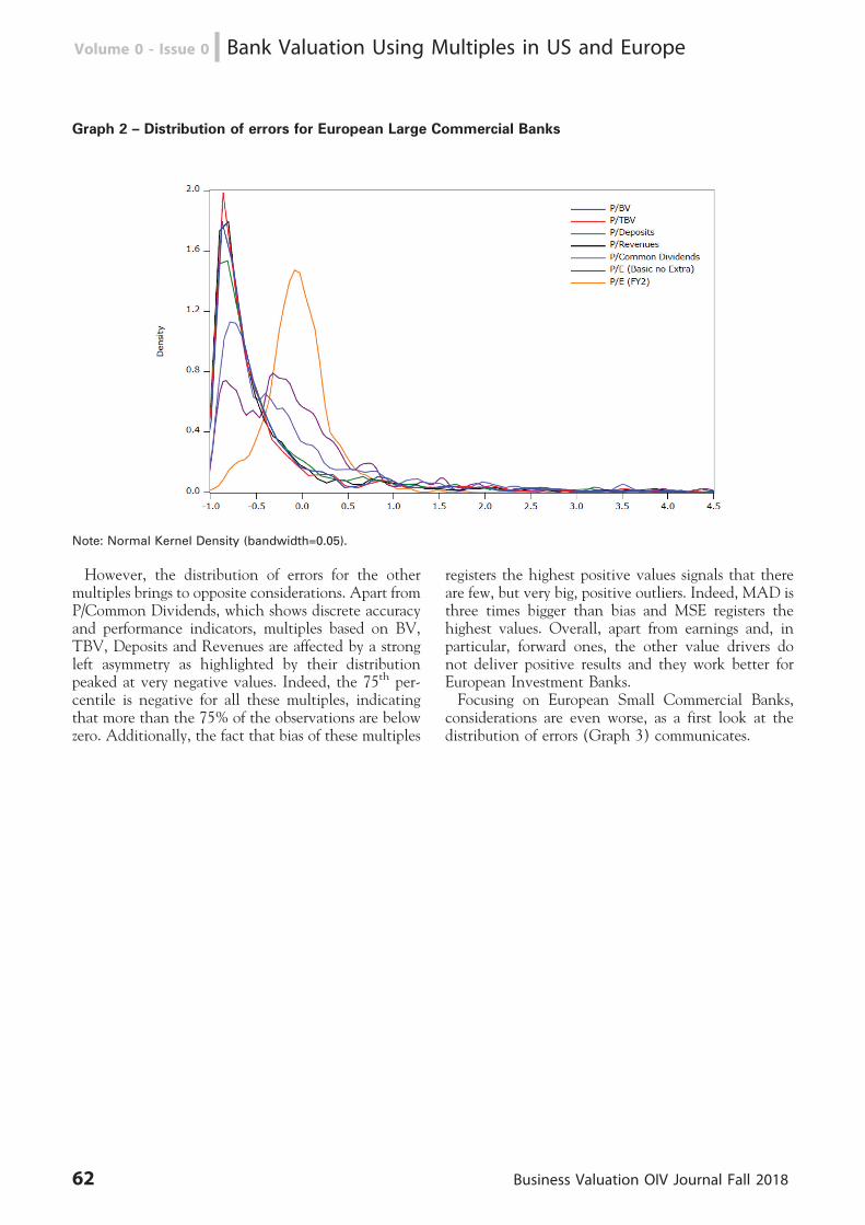
Graph 2 – Distribution of errors for European Large Commercial Banks


However, the distribution of errors for the othermultiples brings to opposite considerations. Apart fromP/Common Dividends, which shows discrete accuracyand performance indicators, multiples based on BV,TBV, Deposits and Revenues are affected by a strongleft asymmetry as highlighted by their distributionpeaked at very negative values. Indeed, the 75th per-centile is negative for all these multiples, indicatingthat more than the 75% of the observations are belowzero. Additionally, the fact that bias of these multiples

registers the highest positive values signals that thereare few, but very big, positive outliers. Indeed, MAD isthree times bigger than bias and MSE registers thehighest values. Overall, apart from earnings and, inparticular, forward ones, the other value drivers donot deliver positive results and they work better forEuropean Investment Banks.Focusing on European Small Commercial Banks,

considerations are even worse, as a first look at thedistribution of errors (Graph 3) communicates.



Graph 3 – Distribution of errors for European Small Commercial Banks


This is the unique subsample where P/E (FY1) deli-vers the highest accuracy: at a 10% level it predicts20.2% of prices against 17.1% of P/E (FY2), but look-ing at bias, MAD and MSE, values are lower for thelatter. The distribution of errors for both forward earn-ings multiples is quite similar. The one of P/E (FY1),on the one side, seems to show higher density forvalues closer to zero, on the other side, big negativeerrors appear more frequent. Furthermore, the less re-liable multiples are the ones based on BV and TBV,registering the highest MSE and very bad accuracy,which is lower than 3.0% at a 10% level. Moreover,the median multiples stand respectively at 0.67x and0.70x, suggesting high risk of undervaluation. In fact,left asymmetry is extremely evident: the distribution oferrors is peaked at very negative values. However, itappears to be lower than the case for large banks, infact the 75th percentile takes on positive values be-cause of the presence of a higher number of positiveobservations. Moreover, also large outliers are morefrequent, as confirmed by the bumps in the right tails.Errors of P/Common Dividends are better distributed,but still performance and accuracy are quite low.Overall, these results suggest that multiples should

be used more as a confirmatory tool than as primary

valuation methodology for European CommercialBanks. Unique exception is the use of forward earningsmultiples for Large Commercial Banks. While resultsfor Investment Banks are quite acceptable. However, itis important to recall that the selection of comparablescan have significant impacts in this case and can po-tentially deliver stronger results.To sum up, it is advisable to prefer forward P/E mul-

tiples since they deliver more precise values than anyother multiple. However, trailing multiples could beconsidered a second best option when forecasts are notavailable.

4.3.3. American Investment Banks

Accuracy of forward P/Es is quite satisfactory forAmerican Investment Banks, showing substantially si-milar results when using FY1 and FY2 earnings (at a10% level, both predict 23.2% of prices), while MADand MSE are lower for the latter measure. Apart fromP/TBV, which shows low performances and a strongleft asymmetry, with high values for MAD, MSE andmedian (in absolute value), the other multiples arecharacterised by a relative homogeneous distributionof errors (Graph 4) and similar performances.



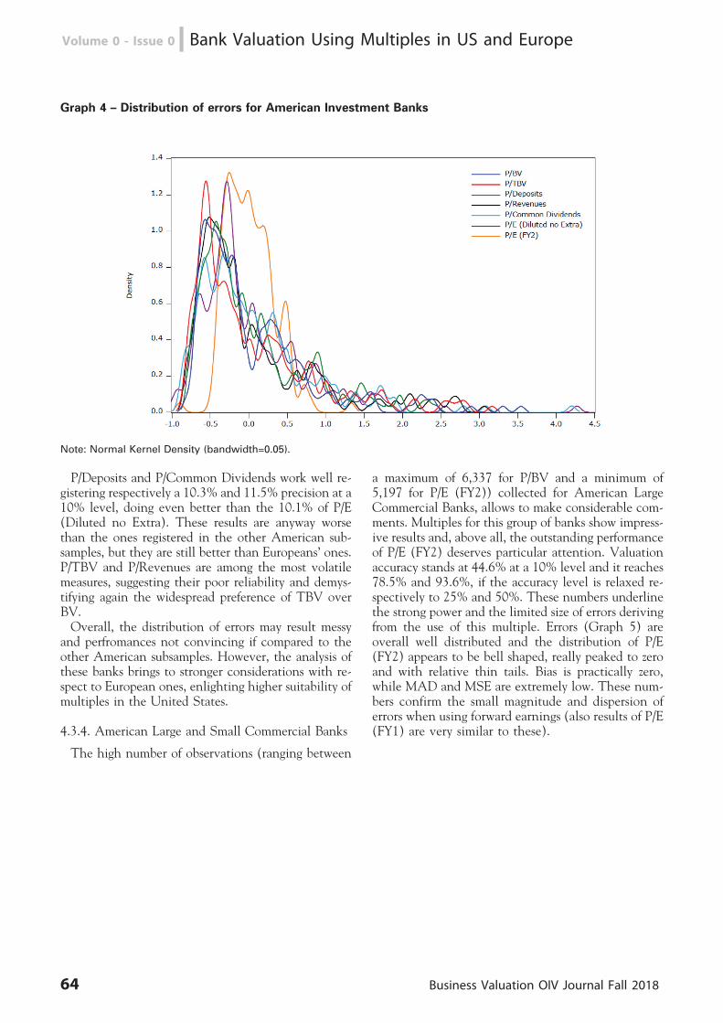
Graph 4 – Distribution of errors for American Investment Banks


P/Deposits and P/Common Dividends work well re-gistering respectively a 10.3% and 11.5% precision at a10% level, doing even better than the 10.1% of P/E(Diluted no Extra). These results are anyway worsethan the ones registered in the other American sub-samples, but they are still better than Europeans’ ones.P/TBV and P/Revenues are among the most volatilemeasures, suggesting their poor reliability and demys-tifying again the widespread preference of TBV overBV.Overall, the distribution of errors may result messy

and perfromances not convincing if compared to theother American subsamples. However, the analysis ofthese banks brings to stronger considerations with re-spect to European ones, enlighting higher suitability ofmultiples in the United States.

4.3.4. American Large and Small Commercial Banks

The high number of observations (ranging between

a maximum of 6,337 for P/BV and a minimum of5,197 for P/E (FY2)) collected for American LargeCommercial Banks, allows to make considerable com-ments. Multiples for this group of banks show impress-ive results and, above all, the outstanding performanceof P/E (FY2) deserves particular attention. Valuationaccuracy stands at 44.6% at a 10% level and it reaches78.5% and 93.6%, if the accuracy level is relaxed re-spectively to 25% and 50%. These numbers underlinethe strong power and the limited size of errors derivingfrom the use of this multiple. Errors (Graph 5) areoverall well distributed and the distribution of P/E(FY2) appears to be bell shaped, really peaked to zeroand with relative thin tails. Bias is practically zero,while MAD and MSE are extremely low. These num-bers confirm the small magnitude and dispersion oferrors when using forward earnings (also results of P/E(FY1) are very similar to these).



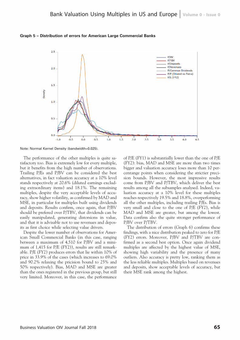
Graph 5 – Distribution of errors for American Large Commercial Banks


The performance of the other multiples is quite sa-tisfactory too. Bias is extremely low for every multiple,but it benefits from the high number of observations.Trailing P/Es and P/BV can be considered the bestalternatives, in fact valuation accuracy at a 10% levelstands respectively at 20.6% (diluted earnings exclud-ing extraordinary items) and 18.1%. The remainingmultiples, despite the very acceptable levels of accu-racy, show higher volatility, as confirmed by MAD andMSE, in particular for multiples built using dividendsand deposits. Results confirm, once again, that P/BVshould be prefered over P/TBV, that dividends can beeasily manipulated, generating distorsions in value,and that it is advisable not to use revenues and depos-its as first choice while selecting value drivers.Despite the lower number of observations for Amer-

ican Small Commercial Banks (in this case, rangingbetween a maximum of 4,510 for P/BV and a mini-mum of 1,415 for P/E (FY2)), results are still remark-able. P/E (FY2) produces errors that lie within 10% ofprice in 33.9% of the cases (which increases to 69.0%and 90.2% relaxing the pricision bound to 25% and50% respectively). Bias, MAD and MSE are greaterthan the ones registered in the previous group, but stillvery limited. Moreover, in this case, the performance

of P/E (FY1) is substantially lower than the one of P/E(FY2): bias, MAD and MSE are more than two timesbigger and valuation accuracy loses more than 10 per-centange points when considering the strictier preci-sion bounds. However, the most impressive resultscome from P/BV and P/TBV, which deliver the bestresults among all the subsamples analysed. Indeed, va-luation accuracy at a 10% level for these multiplesreaches respectively 19.5% and 18.8%, overperformingall the other multiples, including trailing P/Es. Bias isvery small and close to the one of P/E (FY2), whileMAD and MSE are greater, but among the lowest.Data confirm also the quite stronger performance ofP/BV over P/TBV.The distribution of errors (Graph 6) confirms these

findings, with a nice distribution peaked to zero for P/E(FY2) errors. Moreover, P/BV and P/TBV are con-firmed as a second best option. Once again dividendmultiples are affected by the highest value of MSE,showing high variability and the presence of manyoutliers. Also accuracy is pretty low, ranking them asthe less reliable multiples. Multiples based on revenuesand deposits, show acceptable levels of accuracy, buttheir MSE rank among the highest.



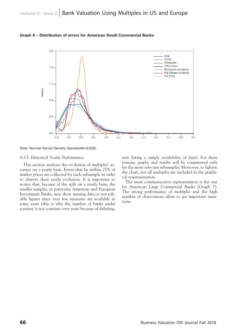
Graph 6 – Distribution of errors for American Small Commercial Banks


4.3.5. Historical Yearly Performance

This section analyses the evolution of multiples’ ac-curacy on a yearly basis. Errors that lie within 25% ofmarket prices are collected for each subsample in orderto observe their yearly evolution. It is important tonotice that, because of the split on a yearly basis, thesmaller samples, in particular American and EuropeanInvestment Banks, may show missing data or not reli-able figures since very few measures are available insome years (this is why the number of banks underscrutiny is not constant over years because of delisting,

new listing o simply availability of data). For thesereasons, graphs and results will be commented onlyfor the more relevant subsamples. Moreover, to lightenthe chart, not all multiples are included in the graphi-cal respresentation.The most communicative representation is the one

for American Large Commercial Banks (Graph 7).The strong performance of multiples and the highnumber of observations allow to get important intui-tions.



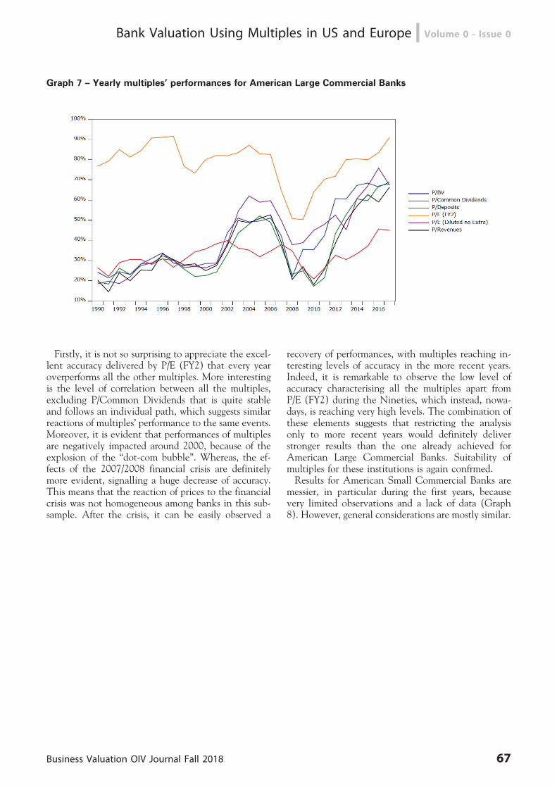
Graph 7 – Yearly multiples’ performances for American Large Commercial Banks

Firstly, it is not so surprising to appreciate the excel-lent accuracy delivered by P/E (FY2) that every yearoverperforms all the other multiples. More interestingis the level of correlation between all the multiples,excluding P/Common Dividends that is quite stableand follows an individual path, which suggests similarreactions of multiples’ performance to the same events.Moreover, it is evident that performances of multiplesare negatively impacted around 2000, because of theexplosion of the ‘‘dot-com bubble’’. Whereas, the ef-fects of the 2007/2008 financial crisis are definitelymore evident, signalling a huge decrease of accuracy.This means that the reaction of prices to the financialcrisis was not homogeneous among banks in this sub-sample. After the crisis, it can be easily observed a

recovery of performances, with multiples reaching in-teresting levels of accuracy in the more recent years.Indeed, it is remarkable to observe the low level ofaccuracy characterising all the multiples apart fromP/E (FY2) during the Nineties, which instead, nowa-days, is reaching very high levels. The combination ofthese elements suggests that restricting the analysisonly to more recent years would definitely deliverstronger results than the one already achieved forAmerican Large Commercial Banks. Suitability ofmultiples for these institutions is again confrmed.Results for American Small Commercial Banks are

messier, in particular during the first years, becausevery limited observations and a lack of data (Graph8). However, general considerations are mostly similar.



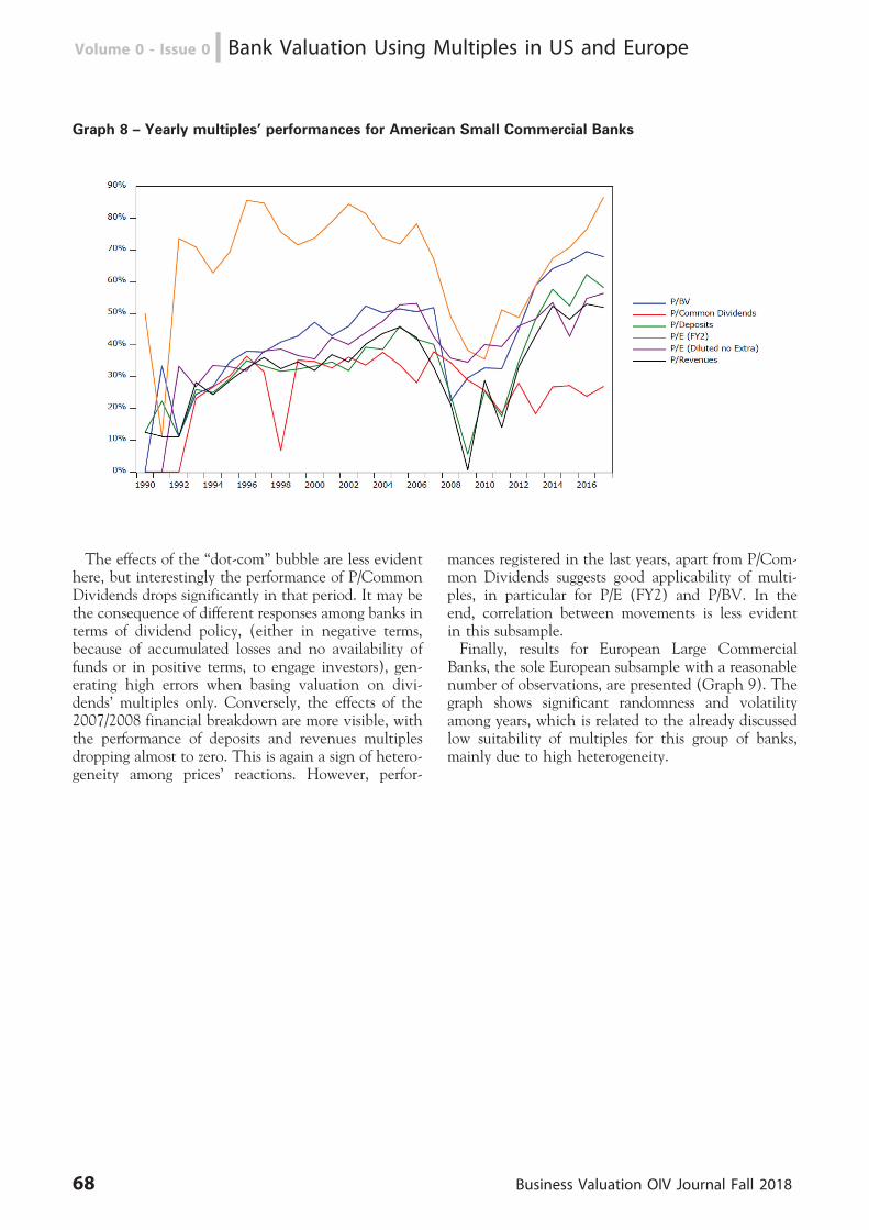
Graph 8 – Yearly multiples’ performances for American Small Commercial Banks

The effects of the ‘‘dot-com’’ bubble are less evidenthere, but interestingly the performance of P/CommonDividends drops significantly in that period. It may bethe consequence of different responses among banks interms of dividend policy, (either in negative terms,because of accumulated losses and no availability offunds or in positive terms, to engage investors), gen-erating high errors when basing valuation on divi-dends’ multiples only. Conversely, the effects of the2007/2008 financial breakdown are more visible, withthe performance of deposits and revenues multiplesdropping almost to zero. This is again a sign of hetero-geneity among prices’ reactions. However, perfor-

mances registered in the last years, apart from P/Com-mon Dividends suggests good applicability of multi-ples, in particular for P/E (FY2) and P/BV. In theend, correlation between movements is less evidentin this subsample.Finally, results for European Large Commercial

Banks, the sole European subsample with a reasonablenumber of observations, are presented (Graph 9). Thegraph shows significant randomness and volatilityamong years, which is related to the already discussedlow suitability of multiples for this group of banks,mainly due to high heterogeneity.



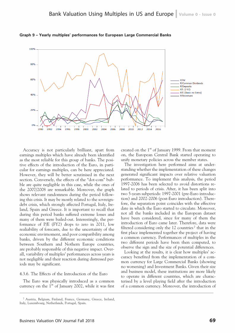
Graph 9 – Yearly multiples’ performances for European Large Commercial Banks

Accuracy is not particularly brilliant, apart fromearnings multiples which have already been identifiedas the most reliable for this group of banks. The posi-tive effects of the introduction of the Euro, in parti-cular for earnings multiples, can be here appreciated.However, they will be better scrutinised in the nextsection. Conversely, the effects of the ‘‘dot-com’’ bub-ble are quite negligible in this case, while the ones ofthe 2007/2008 are remarkable. Moreover, the graphshows relevant randomness during the period follow-ing this crisis. It may be mostly related to the sovreign-debt crisis, which strongly affected Portugal, Italy, Ire-land, Spain and Greece. It is important to recall thatduring this period banks suffered extreme losses andmany of them were bailed-out. Interestingly, the per-formance of P/E (FY2) drops to zero in 2011, lowrealiability of forecasts, due to the uncertainty of theeconomic envirnoment, and poor comparibility amongbanks, driven by the different economic conditionsbetween Southern and Nothern Europe countries,are probably responsible of this negative impact. Over-all, variability of multiples’ performances across years isnot negligible and their reaction during distressed per-iods may be significant.

4.3.6. The Effects of the Introduction of the Euro

The Euro was physically introduced as a commoncurrency on the 1st of January 2002, while it was first

created on the 1st of January 1999. From that momenton, the European Central Bank started operating tounify monetary policies across the member states.The investigation here performed aims at under-

standing whether the implementation of these changesgenerated significant impacts over relative valuationperformance. To implement this analysis, the period1997-2006 has been selected to avoid distortions re-lated to periods of crisis. After, it has been split intotwo 5-years subperiods: 1997-2001 (pre-Euro introduc-tion) and 2002-2006 (post-Euro introduction). There-fore, the separation point coincides with the effectivedate in which the Euro started to circulate. Moreover,not all the banks included in the European datasethave been considered, since for many of them theintroduction of Euro came later. Therefore, data werefiltered considering only the 12 countries 7 that in thefirst place implemented together the project of havinga common currency. Performances of multiples in thetwo different periods have been then computed, toobserve the sign and the size of potential differences.Looking at the results, it is clear how multiples’ ac-

curacy benefited from the implementation of a com-mon currency for Large Commercial Banks (showingno worsening) and Investment Banks. Given their sizeand business model, these institutions are more likelyto operate in different countries, which are charac-terised by a level playing field after the introductionof a common currency. Moreover, the introduction of

7 Austria, Belgium, Finland, France, Germany, Greece, Ireland,Italy, Luxembourg, Netherlands, Portugal, Spain.



a common currency limited currency risks for banks,making also cheaper the access to capital markets. Inaddition, a unique monetary policy, setting a stableinflation target, drove interest rates down and in-creased their stability. Being value inversely propor-tional to the level of interest rates, these effects madevalue estimation easier and less discretionary, increas-ing multiples’ performances. The overall level ofhomogeneity among comparables therefore increased,and this was particularly true for Large CommercialBanks and Investment Banks, which generally donot compete at a national level, being more geogra-phically diversified. Finally, it is important to under-line that the rank among multiples for these institu-tions does not show significant changes between thetwo periods analysed, apart from P/BV, which was theworst performer for Investment Banks before 2002.While forward P/E multiples are always the best per-formers and, interestingly, are the ones showing betterimprovements.Conversely, the effects on Small Commercial Banks

are less clear. This can be explained considering thatthese institutions are generally more focused on regio-nal markets and compete on a national level. P/BV,P/TBV and dividends multiples show a decrease inaccuracy, while earnings multiples register an increase.

4.3.7. The Effects of the 2007/2008 Financial Crisis

The worldwide effects of the 2007/2008 crisis wereimpressive: many banks went bankrupt and govern-emnt bail-outs were often necessary forcing them torun budget deficits, stock prices plummeted and un-employment surged, affecting every industry. It was thebeginning of a global economic recession and of a longlasting sovreign-debt crisis in Europe: nowadays someSouthern Europe countries still have to fully recoverfrom the crisis. Taking Italy as an example: GDPgrowth still shows weak positive signs and the imple-mentation of policies to boost growth and reduce gov-ernment debt appears difficult to be achieved as longas political instability remains there.This section focuses on the analysis of the effects of

the financial crisis on valuation accuracy. The period2003-2012 has been selected and it has been split intotwo 5-years subperiods: 2003-2007 (pre-financial cri-sis) and 2008-2012 (post-financial crisis). Therefore,the separation point coincides with Lehman Brothers’collapse. Performances of multiples in the two differentperiods are then computed to observe the sign and thesize of potential differences.The financial crisis had different effects on European

Small Commercial Banks, depending on their level ofinternational exposure and on their dependence onmortgages. In general, accuracy was badly hit, apartfrom trailing multiples that did slightly better. This

can be related to market operators relying more onrealized results than on expected results, which weresurrounded by huge uncertainty.European Large Commercial Banks, show a strong

decrease in forward earnings multiples’ accuracy, los-ing more than 20 and 45 percentage points at a 10%and 25% level respectively. Notwithstanding thesemultiples are still the best performers. Trailing multi-ples show a slightly better accuracy, but only at a10% level. Interestingly, solvency-based multiples(P/BV and P/TBV) show greater accuracy, underly-ing analysts’ attention on the level of capitalizationof banks during the crisis. Indeed, large banks werelargely affected by deteriorated and non-performingexposures, forcing them to account for massive write-downs. In addition, P/Common Dividends per-formed slightly better during the crisis, highlightinga focus on the capability of distributing dividendsmore than on the uncertain earnings achievable inthe future.Results for European Investment Banks, which, by

definition, are strongly dependent on financial marketsperformances, show mostly a worsening of multiples’accuracy. P/E (FY2) is the multiple suffering the mostin performances: it registers a decrease in accuracy at a10% level higher than 40 percentage points. Smallimprovements are achieved when using P/CommonDividends and P/TBV and can be justified by marketoperators shifting their focus on cash flows and levelsof capitalization.Moving to American Commercial Banks, results

show a strong worsening in multiples accuracy, high-lighting how impressive the magnitude of the sub-prime market was in the United States. Both largeand small commercial banks show negative perfor-mances for all the multiples, with the ones basedon forward earnings suffering the most. Also Amer-ican Investment Banks were affected by a decrease ofthe performance of almost every multiple and, inparticular, of the ones based on earnings. Conversely,P/Revenues and P/Deposits show interestingly higherlevels of accuracy during the crisis. An increase in therelevance of revenues may be related to analystsbeing more focused on the capabilities of these insti-tutions in generating fees from a frozen M&A marketand gains from extremely volatile stock markets.While the performance of P/Deposits is quite unex-pected, since deposits are not a relevant measure forinvestment banks. This may imply that investmentbanks’ business model was shifting to the one of retailbanks. As a matter of fact, few days after the collapseof Lehman Brothers, the two major pure AmericanInvestment Banks, i.e., Goldman Sachs and MorganStanley, confirmed to become traditional bank hold-ing companies, bringing an end to the era of pureinvestment banking on Wall Street.



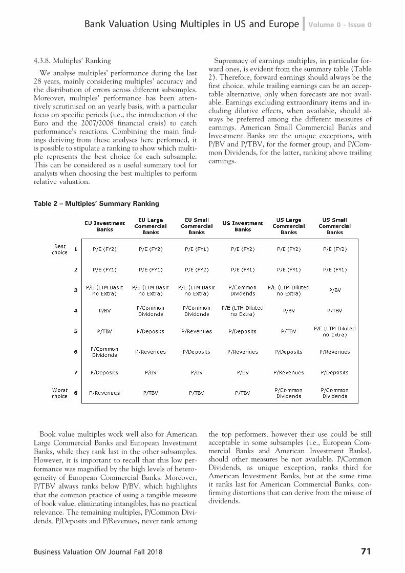
4.3.8. Multiples’ Ranking

We analyse multiples’ performance during the last28 years, mainly considering multiples’ accuracy andthe distribution of errors across different subsamples.Moreover, multiples’ performance has been atten-tively scrutinised on an yearly basis, with a particularfocus on specific periods (i.e., the introduction of theEuro and the 2007/2008 financial crisis) to catchperformance’s reactions. Combining the main find-ings deriving from these analyses here performed, itis possible to stipulate a ranking to show which multi-ple represents the best choice for each subsample.This can be considered as a useful summary tool foranalysts when choosing the best multiples to performrelative valuation.

Supremacy of earnings multiples, in particular for-ward ones, is evident from the summary table (Table2). Therefore, forward earnings should always be thefirst choice, while trailing earnings can be an accep-table alternative, only when forecasts are not avail-able. Earnings excluding extraordinary items and in-cluding dilutive effects, when available, should al-ways be preferred among the different measures ofearnings. American Small Commercial Banks andInvestment Banks are the unique exceptions, withP/BV and P/TBV, for the former group, and P/Com-mon Dividends, for the latter, ranking above trailingearnings.

Table 2 – Multiples’ Summary Ranking

Book value multiples work well also for AmericanLarge Commercial Banks and European InvestmentBanks, while they rank last in the other subsamples.However, it is important to recall that this low per-formance was magnified by the high levels of hetero-geneity of European Commercial Banks. Moreover,P/TBV always ranks below P/BV, which highlightsthat the common practice of using a tangible measureof book value, eliminating intangibles, has no practicalrelevance. The remaining multiples, P/Common Divi-dends, P/Deposits and P/Revenues, never rank among

the top performers, however their use could be stillacceptable in some subsamples (i.e., European Com-mercial Banks and American Investment Banks),should other measures be not available. P/CommonDividends, as unique exception, ranks third forAmerican Investment Banks, but at the same timeit ranks last for American Commercial Banks, con-firming distortions that can derive from the misuse ofdividends.



5. Conclusions

We study the relative valuation accuracy of 1,118listed and delisted banks across the United States andthe Eurozone from 1990 to 2017. Multiples deliverstrong valuation accuracy in the U.S. (in particularfor Large Commercial Banks), while in Europe resultsare less univocal. Multiples based on forward earningsare the best performers and the one based on twoyears forecasts are the most accurate. However, theuse of trailing earnings is quite often a valid secondbest option and diluted earnings not including extra-ordinary items should always be preferred amongearnings measures. Despite practitioners consider P/TBV more reliable than P/BV, results show the op-posite with the latter consistently overperforming theformer. Moreover, the performance of these solvency-based multiples is very low in Europe, while theywork quite well for American Commercial Banks. Avery weak relationship between value and the

amount of preferred dividends is also revealed withP/Common Dividends being a more precise tool thanP/Total Dividends. Multiples based on Revenues andDeposits do not show particularly interesting perfor-mances.We also investigate the historical performance of

multiples. The effects of the financial crisis appearstrongly negative in every subsample, while perfor-mances registered in recent years are at the highestlevels. On the one hand, American Large CommercialBanks confirm the strong accuracy of P/E (FY2) thatevery year overperformed the other multiples. On theother hand, they register an increasing performance inthe last 5 years for the multiples based on book value,trailing earnings, deposits and revenues. Finally, preci-sion of different multiples appears to move in a corre-late way, while P/Common Dividends tends to follow aproper path.



APPENDIX A – The 2007/08 Financial Crisis: Perfomance Statistics





Bibliography

Alford, A. W. (1992). The effect of the set of com-parable firms on the accuracy of the price-earningsvaluation method. Journal of Accounting Research30(1): 94-108.Allayannis, G., Rountree, B. & Weston, J. P.

(2005). Earnings volatility, cash flow volatility andfirm value. Working Paper, SSRN.Barker, R. G. (1999). Survey and market-based evi-

dence of industry-dependence in analysts’ preferencesbetween the dividend yield and price-earnings ratiovaluation models. Journal of Business and Accounting26(3): 393-418.Baker, M. & Ruback, R. (1999). Estimating industry

multiples. Working Paper, Harvard University, USA.Beltratti, A & Stulz, R. M. (2009). Why did some

banks perform better during the credit crisis? A cross-coun-try study of the impact of governance and regulation.Working Paper 254, ECGI.Bhojraj, S. & Lee, C. M. C. (2002). Who is my peer?

A valuation based approach to the selection of com-parable firms. Journal of Accounting Research 40(2):407-439.Brennan, M. & Hughes, P. (1991). Stock Prices and

the Supply of Information. Journal of Finance 46: 1665-1691.Brooks, C. (2014). Introductory Econometrics for Fi-

nance. 3rd ed. Cambridge University Press.Calomiris, C. & Nissim, D. (2007). Activity-based

valuation for bank holding companies. Working Paper12918, NBER.Cheng, C. S. A. & McNamara, R. (2000). The va-

luation accuracy of the price-earnings and price-bookbenchmark valuation methods. Review of QuantitativeFinance and Accounting 15(4): 349-370.Cooper, I. & Cordeiro, L. (2008). Optimal equity

valuation using multiples: The number of comparablefirms. Working Paper, SSRN.Damodaran, A. (2002). Investment Valuation. Tools

and Techniques for Determining the Value of Any Asset.2nd ed. John Wiley & Sons.Damodaran, A. (2006). Damodaran on Valuation.

Security Analysis for Investment and Corporate Finance.2nd ed. John Wiley & Sons.Deev, O. (2011). Methods of bank valuation: A

critical overview. Financial Assets and Investing2011(3): 33-44.Dermine, J. (2010). Bank valuation: With an applica-

tion to the implicit duration of non-maturing deposits.Working Paper, INSEAD Business School, France.Dittmann, I & Maug, E. G. (2008). Biases and error

measures: How to compare valuation methods. WorkingPaper, SSRN.Guatri, L. & Bini, M. (2002). I moltiplicatori nella

valutazione delle aziende. Volume 1: Principi e linee guida

professionali, Volume 2: Metodi e Strumenti. UniversitaBocconi Editore.Forte, G., Gianfrate, G., & Rossi, E. (2018). Does

relative valuation work for banks? Global Finance Jour-nal, forthcoming.Forte, G. & Rossi, E. (2016). Assessing Relative Va-

luation in Equity Markets: Bridging Research and Practice.Palgrave Macmillan.Herrmann, V. & Richter, F. (2003). Pricing with

performance-controlled multiples. Schmalenbach Busi-ness Review, 55: 194-219.Kokic, P. N. & Bell, P. A. (1994). Optimal winsor-

izing cutoffs for a stratified finite population estimator.Journal of Official Statistics, 10(4): 419-435.Koller, T.; Goedhart, M. & Wessels, D. (2005). Va-

luation, Measuring and Managing the Value of Compa-nies. 4th ed. John Wiley & Sons.Lie, E. & Lie, H. (2002). Multiple used to estimate

corporate value. Financial Analysts Journal, 58(2): 44-54.Lin, C. (2017). Impact of International Cross-Listing

and Delisting on Return Volatility. Universal Journal ofAccounting and Finance 5(3): 60-71.Liu, J.; Nissim, D. & Thomas, J. (2002). Equity va-

luation using multiples. Journal of Accounting Research,40(1): 135-172.Lokey, O. K.; Braun, R. S. & Cefali, S. L. (1990).

Business Valuation. Litigation Services Handbook: TheRole of Accountant as Expert Witness.Massari, M.; Gianfrate, G. & Zanetti, L. (2014). The

Valuation of Financial Companies. John Wiley & Sons.Minjina, D. I. (2009). Relative performance of va-

luation using multiples. Empirical evidence on Buchar-est Stock Exchange. The Review of Finance and Bank-ing, 1(1): 35-53.Nissim, D. & Penman, S. (2001). Ratio analysis and

equity valuation: from research to practice. Review ofAccounting Studies, 6(1): 109-154.Nissim, D. (2010). Analysis and valuation of insurance

companies. Industry Study #2, Center for Excellence inAccounting and Security Analysis, Columbia BusinessSchool, USA.Nissim, D. (2011). Relative valuation of U.S. insur-

ance companies. Review of Accounting Studies, 18(2):324-359.Ou, J. A. & Penan, S. H. (1995). Financial statement

analysis and the evaluation of market-to-book ratios.Working Paper, University of California at Berkeley,USA.Park, Y. S. & Lee, J. (2003). An empirical study on

the relevance of applying relative valuation models toinvestment strategies in the Japanese stock market.Japan and the World Economy, 15(3): 331-339.Pratt, S. P. (1989). Valuing a Business: The Analysis

and Appraisal of Closely-Held Companies. New York:Dow Jones-Irwin.



Resti, A. & Sironi, A. (2007). Risk Management andShareholders’ Value in Banking. John Wiley & Sons.Schipper, K. (1991). Commentary on Analysts’

Forecasts, Accounting Horizons 5, 105-121.Schreiner, A. (2007). Equity valuation using multiples:

an empirical investigation. Academic Network, RolandBerger Strategy Consultants, Wiesbaden: DUV GablerEdition Wissenschaft.Siems, M. (2009). The foundations of securities law.

European Business Law Review, 20: 141-171.Stockenstrand, A. & Nilsson, F. (2017). Bank Reg-

ulation. Effects on Strategy, Financial Accounting andManagement Control. Routledge.Tasker, S. C. (1998). Industry-preferred multiples in

acquisition valuation. Working Paper, Cornell Univer-sity, USA.Yee, K. K. (2004). Forward versus trailing earnings

in equity valuation. Review of Accounting Studies 9(2):301-329.Wu, Y. (2017). What’s Behind the Smooth Dividends?

Evidence from Structural Estimation. Working Paper,University of Illinois at Urbana-Champaign, USA.



0023

9732

Documents

Business Valuation OIVjournal - ICAEW