Embed Size (px)
Citation preview


VALUATIONTECHNIQUES
ffirs 12 September 2012; 17:36:29

CFA Institute Investment Perspectives Series is a thematically organized compilation ofhigh-quality content developed to address the needs of serious investment professionals. Thecontent builds on issues accepted by the profession in the CFA Institute Global Body ofInvestment Knowledge and explores less established concepts on the frontiers of investmentknowledge. These books tap into a vast store of knowledge of prominent thought leaders whohave focused their energies on solving complex problems facing the financial community.
CFA Institute is a global community of investment professionals dedicated to driving industry-wide adoption of the highest ethical and analytical standards. Through our programs,conferences, credentialing, and publications, CFA Institute leads industry thinking, helpingmembers of the investment community deepen their expertise. We believe that fair and effectivefinancial markets led by competent and ethically-centered professionals stimulate economicgrowth. Together—with our 110,000 members from around the world, including 100,000CFA charterholders—we are shaping an investment industry that serves the greater good.
www.cfainstitute.org
Research Foundation of CFA Institute is a not-for-profit organization established topromote the development and dissemination of relevant research for investment practitionersworldwide. Since 1965, the Research Foundation has emphasized research of practical value toinvestment professionals, while exploring new and challenging topics that provide a uniqueperspective in the rapidly evolving profession of investment management. To carry out itswork, the Research Foundation funds and publishes new research, supports the creation ofliterature reviews, sponsors workshops and seminars, and delivers online multimedia content.Recent efforts from the Research Foundation have addressed a wide array of topics, rangingfrom risk management to the equity risk premium.
www.cfainstitute.org/foundation
ffirs 12 September 2012; 17:36:29
VALUATIONTECHNIQUES
Discounted Cash Flow, Earnings Quality,Measures of Value Added, and Real Options
David T. Larrabee, CFAJason A. Voss, CFA
John Wiley & Sons, Inc.
ffirs 12 September 2012; 17:36:29
Cover Design: Loretta LeivaCover Photograph: ª Simon Belcher / Alamy
Copyright ª 2013 by CFA Institute. All rights reserved.
Published by John Wiley & Sons, Inc., Hoboken, New Jersey.Published simultaneously in Canada.
No part of this publication may be reproduced, stored in a retrieval system, or transmitted in any form orby any means, electronic, mechanical, photocopying, recording, scanning, or otherwise, except aspermitted under Section 107 or 108 of the 1976 United States Copyright Act, without either the priorwritten permission of the Publisher, or authorization through payment of the appropriate per-copy fee tothe Copyright Clearance Center, Inc., 222 Rosewood Drive, Danvers, MA 01923, (978) 750-8400,fax (978) 646-8600, or on the Web at www.copyright.com. Requests to the Publisher for permissionshould be addressed to the Permissions Department, John Wiley & Sons, Inc., 111 River Street,Hoboken, NJ 07030, (201) 748-6011, fax (201) 748-6008, or online at http://www.wiley.com/go/permissions.
Limit of Liability/Disclaimer of Warranty: While the publisher and author have used their best efforts inpreparing this book, they make no representations or warranties with respect to the accuracy orcompleteness of the contents of this book and specifically disclaim any implied warranties ofmerchantability or fitness for a particular purpose. No warranty may be created or extended by salesrepresentatives or written sales materials. The advice and strategies contained herein may not be suitablefor your situation. You should consult with a professional where appropriate. Neither the publisher norauthor shall be liable for any loss of profit or any other commercial damages, including but not limited tospecial, incidental, consequential, or other damages.
For general information on our other products and services or for technical support, please contact ourCustomer Care Department within the United States at (800) 762-2974, outside the United States at(317) 572-3993 or fax (317) 572-4002.
Wiley publishes in a variety of print and electronic formats and by print-on-demand. Some materialincluded with standard print versions of this book may not be included in e-books or in print-on-demand. If this book refers to media such as a CD or DVD that is not included in the version youpurchased, you may download this material at http://booksupport.wiley.com. For more informationabout Wiley products, visit www.wiley.com.
Library of Congress Cataloging-in-Publication Data:
Larrabee, David T.Valuation techniques : discounted cash flow, earnings quality, measures of value added, and
real options / David T. Larrabee and Jason A. Voss.p. cm. — (CFA Institute investment perspectives series)
Includes index.ISBN 978-1-118-39743-5 (cloth); ISBN 978-1-118-41760-7 (ebk);ISBN 978-1-118-42179-6 (ebk); ISBN 978-1-118-45017-8 (ebk)1. Corporations—Valuation. 2. Investment analysis. I. Voss, Jason Apollo. II. Title.
HG4028.V3L346 2013332.63 0221—dc23
2012022595
Printed in the United States of America
10 9 8 7 6 5 4 3 2 1
ffirs 12 September 2012; 17:36:29
CONTENTS
Foreword ix
Introduction 1
PART I: VALUATION PERSPECTIVES:THEN AND NOW 3
CHAPTER 1Two Illustrative Approaches to Formula Valuationsof Common Stocks 5Benjamin GrahamReprinted from the Financial Analysts Journal (November 1957):11�15.
CHAPTER 2Seeking a Margin of Safety and Valuation 17Matthew B. McLennan, CFAReprinted from CFA Institute Conference Proceedings Quarterly (June 2011):27�34.
PART II: VALUATION METHODOLOGIES 29
CHAPTER 3Company Performance and Measures of Value Added 31Pamela P. Peterson, CFA, and David R. PetersonReprinted from the Research Foundation of CFA Institute (December 1996).
CHAPTER 4The Affordable Dividend Approach to Equity Valuation 93Alfred RappaportReprinted from the Financial Analysts Journal (July/August 1986):52�58.
CHAPTER 5Discounted-Cash-Flow Approach to Valuation 105Gregory A. Gilbert, CFAReprinted from ICFA Continuing Education Series (1990):23�30.
ftoc 12 September 2012; 13:6:20
v
CHAPTER 6Equity Securities Analysis Case Study: Merck & Company 115Randall S. Billingsley, CFAReprinted from AIMR Conference Proceedings: Equity Securities Analysisand Evaluation (December 1993):63�95.
CHAPTER 7Traditional Equity Valuation Methods 155Thomas A. Martin, Jr., CFAReprinted from AIMR Conference Proceedings (May 1998):21�35.
CHAPTER 8A Simple Valuation Model and Growth Expectations 177Morris G. DanielsonReprinted from the Financial Analysts Journal (May/June 1998):50�57.
CHAPTER 9Franchise Valuation under Q-Type Competition 189Martin L. LeibowitzReprinted from the Financial Analysts Journal (November/December 1998):62�74.
CHAPTER 10Value Enhancement and Cash-Driven Valuation Models 209Aswath DamodaranReprinted from AIMR Conference Proceedings: Practical Issues in Equity Analysis(February 2000):4�17.
CHAPTER 11FEVA: A Financial and Economic Approach to Valuation 229Xavier Adsera and Pere VinolasReprinted from the Financial Analysts Journal (March/April 2003):80�87.
CHAPTER 12Choosing the Right Valuation Approach 243Charles M.C. LeeReprinted from AIMR Conference Proceedings: Equity Valuation in a GlobalContext (April 2003):4�14.
CHAPTER 13Choosing the Right Valuation Approach 259Robert Parrino, CFAReprinted from CFA Institute Conference Proceedings: Analyzing, Researching,and Valuing Equity Investments (June 2005):15�28.
CHAPTER 14Valuing Illiquid Common Stock 279Edward A. Dyl and George J. JiangReprinted from the Financial Analysts Journal (July/August 2008):40�47.
ftoc 12 September 2012; 13:6:21
vi Contents
PART III: EARNINGS ANDCASH FLOW ANALYSIS 291
CHAPTER 15Earnings: Measurement, Disclosure, and the Impacton Equity Valuation 293D. Eric Hirst and Patrick E. HopkinsReprinted from the Research Foundation of CFA Institute (August 2000).
CHAPTER 16Cash Flow Analysis and Equity Valuation 349James A. OhlsonReprinted from AIMR Conference Proceedings: Equity Research and ValuationTechniques (May 1998):36�43.
CHAPTER 17Accounting Valuation: Is Earnings Quality an Issue? 361Bradford Cornell and Wayne R. LandsmanReprinted from the Financial Analysts Journal (November/December 2003):20�28.
CHAPTER 18Earnings Quality Analysis and Equity Valuation 375Richard G. SloanReprinted from CFA Institute Conference Proceedings Quarterly (September 2006):52�60.
CHAPTER 19Is Cash Flow King in Valuations? 389Jing Liu, Doron Nissim, and Jacob ThomasReprinted from the Financial Analysts Journal (March/April 2007):56�68.
PART IV: OPTION VALUATION 407
CHAPTER 20Employee Stock Options and Equity Valuation 409Mark LangReprinted from the Research Foundation of CFA Institute (July 2004).
CHAPTER 21Employee Stock Option Valuation with an EarlyExercise Boundary 465Neil Brisley and Chris K. AndersonReprinted from the Financial Analysts Journal (September/October 2008):88�100.
ftoc 12 September 2012; 13:6:21
Contents vii

PART V: REAL OPTIONS VALUATION 483
CHAPTER 22Real Options and Investment Valuation 485Don M. Chance, CFA, and Pamela P. Peterson, CFAReprinted from the Research Foundation of CFA Institute (July 2002).
CHAPTER 23Real-Options Valuation for a Biotechnology Company 573David Kellogg and John M. CharnesReprinted from the Financial Analysts Journal (May/June 2000):76�84.
About the Contributors 587
Index 589
ftoc 12 September 2012; 13:6:21
viii Contents
FOREWORD
From peak to trough, Enron’s share price declined 99.98%, or from around $90 per share tojust $0.02, in only 12 months. Near its pinnacle valuation, rallying cries could be heard fromthe company’s management that Enron’s already inflated stock price was sure to go evenhigher. Unfortunately, most investors and analysts followed the tune of the Enron piper,paying no heed to the company’s true state when close scrutiny might have revealed hiddencracks in its foundation. Too few analysts questioned Enron’s valuation, and those who didwere often met with derision from employers, peers, and even Enron’s management.Groupthink pervaded Enron’s valuation, and investors and employees paid dearly.
How was Enron’s fraud eventually uncovered? Daniel Scotto, an analyst at BNP Paribas,was one of the first investment professionals to sound the alarm bells. After conducting athorough analysis of Enron that included an estimation of its value, Scotto said Enronsecurities “should be sold at all costs and sold now” in a 2001 research report. As has been thecase so often in the capital markets, valuation proved to be an essential investment tool topoint toward fraud.
Reporting shortly after the Enron scandal broke, Rebecca Smith, in her article headlined“Ex-Analyst at BNP Paribas Warned His Clients in August about Enron” in the 29 January2002 edition of the Wall Street Journal, stated:
Mr. Scotto’s experience highlights one of the oldest pressure points on Wall Streetinvolving financial analysts, who traditionally act as a filter between investors and thefinancial markets. During the past decade, Wall Street securities firms increasinglyhave pushed their research analysts to actively trumpet stocks and bonds, notimpartially analyze them.
When conducting financial analysis, the challenge is always to discern the truth about afirm or a security. Analysts have tools at their disposal for detecting reality and unearthingpotential misrepresentations. Among these tools are financial statement analysis, assessmentof management, and measures of absolute and relative value. By using these tools carefullyand objectively, the analyst can point to gaps in disclosure, inconsistencies, and mispricingopportunities. From time to time, the careful analyst can even identify possible mis-representations that can signal serious management failings.
Detailed, objective valuation serves as a powerful tool for establishing a case for the meritsof an investment. A holistic approach to valuation serves not just as a check on the economicworth of a prospective investment but also as an examination of the sustainability of thatprice. The ongoing application of these tools is just as important as the initial decision toinvest. Too many investors expend all their energy on the “buy” decision and do not reserveany for the consideration of the evolution of value over a holding period.
flast 12 September 2012; 13:9:16
ix

The publication of this book coincides with the 50th anniversary of the CFA Program. Italso comes at a time when trust in the financial industry and investment professionals isprofoundly challenged. As we take steps to rebuild trust, the tens of thousands of diligent andethical investment professionals who do their own analyses deserve thanks for upholding highstandards of practice.
Trust is built on reliability, transparency, and stewardship. Without public trust, theinvestment profession will stagnate and wither. At CFA Institute, we call on investment pro-fessionals to act to restore trust. We have broadened our mission—to lead the investmentprofession globally by promoting the highest standards of ethics, education, and professionalexcellence—to recognize our responsibility to serve society as a whole. Our mission guides us tolead and educate in the broad sense. This book on investment valuation is an expression of theCFA Institute mission. I hope its breadth, rigor, and relevance will educate and inspire readers.
JOHN ROGERS, CFAPresident and CEOCFA Institute
flast 12 September 2012; 13:9:16
x Foreword

VALUATIONTECHNIQUES
flast 12 September 2012; 13:9:16

flast 12 September 2012; 13:9:16
INTRODUCTION
Valuation is the cornerstone for the edifice we call “security analysis.” The pioneering work indeveloping a rigorous theory for valuation was published in 1938 as The Theory of InvestmentValue by John Burr Williams. For reasons that I have never been able to understand, it wasnot until 1959, when Myron J. Gordon published his paper “Dividends, Earnings, and StockPrices” in the Review of Economics and Statistics (where the now well-known Gordon modelwas put forth), that attention was finally directed to the seminal work of Williams’s 1938piece. Perhaps it was the highly quantitative nature (for its time) of the original Williamswork that deterred earlier interest; after all, in the early days finance and investments werelargely descriptive fields of endeavor and devoid of quantitative analysis other than that relatedto accounting statements. Benjamin Graham and David Dodd published their first edition ofSecurity Analysis in 1934, and the valuation work in that text was accounting based and didnot contain the necessary theoretical underpinnings that Williams and then Gordon laterdeveloped. Security Analysis (ultimately six editions have been published) was considered thedefinitive work for investors until the late 1960s, when attention began to turn to moreadvanced methodologies that were consistent with an understanding of the theory of valua-tion. Graham himself was somewhat skeptical of Williams’s valuation theory, saying in his1939 review (Journal of Political Economy, April 1939) that if investors can be persuaded totake a saner attitude toward stocks by Williams’s “higher algebra,” then he (Graham) wouldvote for it despite the hit-or-miss character embedded in the model’s assumptions.
Perhaps indirectly related, but of decided importance, to the development of valuationmethodologies for security analysis were two papers that concentrated on portfolio analysis.Harry Markowitz published his now famous article “Portfolio Selection” (Journal of Finance,March 1952) that focused attention on the proper understanding of stock price variability anddiversification. Bill Sharpe published his own path-breaking article, “A Simplified Model forPortfolio Analysis” (Management Science, January 1963), which built upon the earlier work ofMarkowitz and extended the understanding of equilibrium in security pricing. Both of thesepapers, although slow to be accepted in the practitioner’s toolkit until the 1970s, make a largecontribution to our understanding of “risk premiums” for valuation models. Similarly,Martin Leibowitz, in his 1972 book with Sidney Homer titled Inside the Yield Book, broughtvaluation techniques into clear perspective for fixed-income investors and also provided freshinsight into the importance of discount rates used in common stock valuation models.
This compendium of valuation methodologies put together by Jason Voss, CFA, andDavid Larrabee, CFA, draws from publications sponsored by CFA Institute and its pre-decessors over many years and provides a robust review of the important literature that hasevolved in the valuation field. Each of the pieces offers structure and insight into the
cintro 12 September 2012; 14:37:6
1
complexities of valuation modeling and, in its own way, points to the joint importance ofmodel design and input to the model’s variables. Models in and of themselves are critical inproviding us with a framework for thought as it pertains to security pricing. They anchor us tothe appropriate variables, their interaction with each other, and the resulting pricing sensi-tivities. But in the quest for making the models practical and useful to investors, the modelsthemselves have become a necessary yet insufficient condition for success. Model inputs viathe defined variables are the deciding factor, and it is here that the investor can distinguishhimself or herself from the crowd. Unlike Graham and Dodd with their emphasis on his-torical accounting data, today’s successful investor needs to understand the uncertainties ofthe future and how the input variables will develop ex ante rather than simply taking theex post observations. This can be a daunting task.
The economist Frank Knight in his book Risk, Uncertainty and Profit (1921) made afamous distinction that many in the investment profession seem to have forgotten but wouldbe well served to remember. Knight pointed out that risk is a condition in which the out-comes are unknown but the probabilities are known with certainty. Throwing dice is an easyexample of this risk case. Uncertainty, as Knight points out, is different from risk because theprobabilities are not known with exactness and the outcomes are similarly not known. Thisnotion of uncertainty is what we in the investment world are constantly grappling with in ourmodels. We need to always remind ourselves that our probabilities are subjective, notobjective, and flow from our analysis in establishing the ex ante input variables. Investors livein a world of uncertainty, not risk as defined by Knight, which is why the task is so daunting.
Valuation methodologies will continue to evolve with the passage of time and, correctlyapplied, will enable investors to cope more successfully with the inevitable uncertaintiesembedded in financial markets. The articles contained in this book should serve as aninvaluable resource for understanding the contributions made by CFA Institute to this field.
GARY P. BRINSON, CFA
cintro 12 September 2012; 14:37:6
2 Introduction
PART IVALUATION
PERSPECTIVES:THEN AND NOW
Chapter 1 Two Illustrative Approaches to Formula Valuations of Common Stocks 5
Chapter 2 Seeking a Margin of Safety and Valuation 17
c01 12 September 2012; 13:13:34
3

c01 12 September 2012; 13:13:34
CHAPTER 1TWO ILLUSTRATIVE
APPROACHESTO FORMULA VALUATIONS
OF COMMON STOCKS
Benjamin Graham
Two common-stock valuation approaches are examined in detail. The first approachconsiders company profitability, earnings growth and stability, and dividend payout.It derives an independent value of a stock that is then compared with the market price.In contrast, the second approach starts with the market price of a stock and calculatesthe rate of future growth implied by the market. From the expected growth rate, futureearnings can be derived, as well as the implicit earnings multiplier in the currentmarket price. Both approaches demonstrate that the market often has future growthexpectations that cannot be derived from companies’ past performance.
Of the various basic approaches to common-stock valuation, the most widely accepted is thatwhich estimates the average earnings and dividends for a period of years in the future andcapitalizes these elements at an appropriate rate. This statement is reasonably definite in form,but its application permits of the widest range of techniques and assumptions, including plainguesswork. The analyst has first a broad choice as to the future period he will consider; thenthe earnings and dividends for the period must be estimated, and finally a capitalization rateselected in accordance with his judgment or his prejudices. We may observe here that sincethere is no a priori rule governing the number of years to which the valuer should lookforward in the future, it is almost inevitable that in bull markets investors and analysts willtend to see far and hopefully ahead, whereas at other times they will not be so disposed to
Reprinted from the Financial Analysts Journal (November 1957):11�15. When this article was origi-nally published, Benjamin Graham was a visiting professor of finance at the University of SouthernCalifornia, Los Angeles.
c01 12 September 2012; 13:13:34
5
“heed the rumble of a distant drum.” Hence arises a high degree of built-in instability in themarket valuation of growth stocks, so much so that one might assert with some justice thatthe more dynamic the company the more inherently speculative and fluctuating may be themarket history of its shares.1
When it comes to estimating future earnings few analysts are willing to venture forth,Columbus-like, on completely uncharted seas. They prefer to start with known quantities—e.g., current or past earnings—and process these in some fashion to reach an estimate forthe future. As a consequence, in security analysis the past is always being thrown out of thewindow of theory and coming in again through the back door of practice. It would be a sorryjoke on our profession if all the elaborate data on past operations, so industriously collectedand so minutely analyzed, should prove in the end to be quite unrelated to the real deter-minants of the value—the earnings and dividends of the future.
Undoubtedly there are situations, not few perhaps, where this proves to be the rueful fact.But in most cases the relationship between past and future proves significant enough to justifythe analyst’s preoccupation with the statistical record. In fact the daily work of our practi-tioner consists largely of an effort to construct a plausible picture of a company’s future fromhis study of its past performance, the latter phrase inevitably suggesting similar intensivestudies carried on by devotees of a very different discipline. The better the analyst he is, theless he confines himself to the published figures and the more he adds to these from his specialstudy of the company’s management, its policies, and its possibilities.
The student of security analysis, in the classroom or at home, tends to have a specialpreoccupation with the past record as distinct from an independent judgment of the com-pany’s future. He can be taught and can learn to analyze the former, but he lacks a suitableequipment to attempt the latter. What he seeks, typically, is some persuasive method bywhich a company’s earnings record—including such aspects as the average, the trend orgrowth, stability, etc.—plus some examination of the current balance sheet, can be trans-muted first into a projection of future earnings and dividends, and secondly into a valuationbased on such projection.
A closer look at this desired process will reveal immediately that the future earnings anddividends need not be computed separately to produce the final value. Take the simplestpresentation:
1. Past earnings times X equal future earnings.2. Future earnings times Y equal Present Value.
This operation immediately foreshortens to:
3. Past Earnings times XY equal Present Value.
It is the XY factor, or multiplier of past earnings, that my students would dearly love tolearn about and to calculate. When I tell them that there is no dependable method of findingthis multiplier they tend to be incredulous or to ask, “What good is security analysis then?”They feel that if the right weight is given to all the relevant factors in the past record, at least areasonably good present valuation of a common stock can be produced, one that will takeprobable future earnings into account and can be used as a guide to determine the attrac-tiveness or the reverse of the issue at its current market price.
In this article I propose to explain two approaches of this kind which have been developedin a Seminar on Common-Stock Valuation. I believe the first will illustrate reasonably well howformula operations of this kind may be worked out and applied. Ours is an endeavor toestablish a comparative value in 1957 for each of the 30 stocks in the Dow-Jones Industrial
c01 12 September 2012; 13:13:35
6 Part I: Valuation Perspectives: Then and Now
Average, related to a base valuation of 400 and 500, respectively, for the composite or group.(The 400 figure represented the approximate “Central Value” of the Dow-Jones Average, asfound separately by a whole series of formula methods derived from historical relationships. The500 figure represented about the average market level for the preceding twelve months.)
As will be seen, the valuations of each component issue take into account the four“quality elements” of profitability, growth, stability and dividend pay-out, applying them asmultipliers to the average earnings for 1947�1956. In addition, and entirely separately, aweight of 20% is given to the net asset value.
The second approach is essentially the reverse of that just described. Whereas the firstmethod attempts to derive an independent value to be compared with the market price, thesecond starts with the market price and calculates therefrom the rate of future growthexpected by the market. From that figure we readily derive the earnings expected for thefuture period, in our case 1957�1966, and hence the multiplier for such future earningsimplicit in the current market price.
The place for detailed comment on these calculations is after they have been developedand presented. But it may be well to express the gist of my conclusions at this point, viz.:
1. Our own “formula valuations” for the individual stocks, and probably any others of thesame general type, have little if any utility in themselves. It would be silly to assert thatStock A is “worth” only half its market price, or Stock B twice its market price, becausethese figures result from our valuation formula.
2. On the other hand, they may be suggestive and useful as composite reflections of the pastrecord, taken by itself. They may even be said to represent what the value would be,assuming that the future were merely a continuation of past performances.
3. The analyst is thus presented with a “discrepancy” of definite magnitude, between for-mula “value” and the price, which it becomes his task to deal with in terms of his superiorknowledge and judgment. The actual size of these discrepancies, and the attitude that maypossibly be taken respecting them, are discussed below.
Similarly, the approach which starts from the market price, and derives an implied“growth factor” and an implied multiplier therefrom, may have utility in concentratingthe analyst’s attention on just what the market seems to be expecting from each stock in thefuture, in comparison or contrast with what it actually accomplished in the past. Here againhis knowledge and judgment are called upon either to accept or reject the apparentassumptions of the marketplace.
Method 1. A Formula Valuation Based Solely on Past Performance in Relation to theDow-Jones Industrial Average as a Group.
The assumptions underlying this method are the following:
1. Each component issue of the Dow-Jones Industrial Average may be valued in relation to abase value of the average as a whole by a comparison of the statistical records.
2. The data to be considered are the following:a. Profitability—as measured by the rate of return on invested capital. (For convenience
this was computed only for the year 1956.)b. Growth of per-share earnings—as shown by two measurements: 1947�56 earnings vs.
1947 earnings, and 1956 earnings vs. 1947�56 earnings.
c01 12 September 2012; 13:13:35
Chapter 1 Two Illustrative Approaches to Formula Valuations of Common Stocks 7
(It would have been more logical to have used the 1954�56 average instead of thesingle year 1956, but the change would have little effect on the final valuations.)
c. Stability—as measured by the greatest shrinkage of profits in the periods 1937�1938and 1947�1956.(The calculation is based on the percentage of earnings retained in the period ofmaximum shrinkage.)
d. Pay-out—as measured by the ratio of 1956 dividends to 1956 earnings. In the fewcases where the 1956 earnings were below the 1947�56 average we substituted thelatter for the former, to get a more realistic figure of current pay-out.
These criteria demonstrate the quality of the company’s earnings (and dividend policy)and thus may control the multiplier to be applied to the earnings. The figure found undereach heading is divided by the corresponding figure for the Dow-Jones group as a whole, togive the company’s relative performance. The four relatives were then combined on the basisof equal weights to give a final “quality index” of the company as against the overall quality ofthe group.
The rate of earnings on invested capital is perhaps the most logical measure of the successand quality of an enterprise. It tells how productive are the dollars invested in the business. Instudies made in the relatively “normal” market of 1953 I found a surprisingly good corre-lation between the profitability rate and the price-earnings ratio, after introducing a majoradjustment for the dividend payout and a minor (moderating) adjustment for net asset value.
It is not necessary to emphasize the importance of the growth factor to stock-marketpeople. They are likely to ask rather why we have not taken it as the major determinant ofquality and multipliers. There is little doubt that the expected future growth is in fact themajor influence upon current price-earnings ratios, and this truth is fully recognized in oursecond approach, which deals with growth expectations as reflected in market prices. But thecorrelation between market multipliers and past growth is by no means close.
Some interesting figures worked out by Ralph A. Bing show this clearly.2 Dow Chemical,with per-share earnings growth of 31% (1955 vs. 1948) had in August 1956 a price-earningsratio of 47.3 times 1955 earnings. Bethlehem Steel, with corresponding growth of 93%, had amultiplier of only 9.1. The spread between the two relationships is thus as wide as fourteen toone. Other ratios in Mr. Bing’s table show similar wide disparities between past growth andcurrent multipliers.
It is here that the stability factor asserts its importance. The companies with highmultipliers may not have had the best growth in 1948�55, but most of them had greater thanaverage stability of earnings over the past two decades.
These considerations led us to adopt the simple arithmetical course of assigning equalweight to past growth, past stability, and current profitability in working out the qualitycoefficient for each company. The dividend payout is not strictly a measure of quality ofearning power, though in the typical case investors probably regard it in some such fashion.Its importance in most instances is undeniable, and it is both convenient and plausible to giveit equal weight and similar treatment with each of the other factors just discussed.
Finally we depart from the usual Wall Street attitude and assign a weight of 20% in thefinal valuation to the net assets per share. It is true that in the typical case the asset value hasno perceptible influence on current market price. But it may have some long-run effect onfuture market price, and thus it has a claim to be considered seriously in any independentvaluation of a company. As is well known, asset values invariably play some part, sometimes a
c01 12 September 2012; 13:13:35
8 Part I: Valuation Perspectives: Then and Now
fairly important one, in the many varieties of legal valuations of common stocks, which growout of tax cases, merger litigation, and the like. The basic justification for considering assetvalue in this process, even though it may be ignored in the current market price, lies in thepossibility of its showing its weight later, through competitive developments, changes inmanagement or its policies, merger or sale eventuality, etc.
The above discussion will explain, perhaps not very satisfactorily, why the four factorsentering into the quality rating and the fifth factor of asset value were finally assigned equalweight of 20% each.
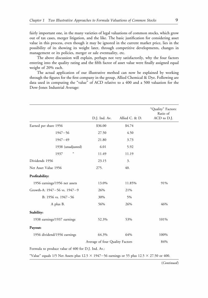
The actual application of our illustrative method can now be explained by workingthrough the figures for the first company in the group, Allied Chemical & Dye. Following aredata used in computing the “value” of ACD relative to a 400 and a 500 valuation for theDow-Jones Industrial Average:
D.J. Ind. Av. Allied C. & D.
“Quality” Factors:Ratio of
ACD to D.J.
Earned per share 1956 $36.00 $4.74
1947�56 27.50 4.50
1947�49 21.80 3.73
1938 (unadjusted) 6.01 5.92
1937 “ 11.49 11.19
Dividends 1956 23.15 3.
Net Asset Value 1956 275. 40.
Profitability:
1956 earnings/1956 net assets 13.0% 11.85% 91%
Growth-A: 1947�56 vs. 1947�9 26% 21%
B: 1956 vs. 1947�56 30% 5%
A plus B. 56% 26% 46%
Stability:
1938 earnings/1937 earnings 52.3% 53% 101%
Payout:
1956 dividend/1956 earnings 64.3% 64% 100%
Average of four Quality Factors 84%
Formula to produce value of 400 for D.J. Ind. Av.:
“Value” equals 1/5 Net Assets plus 12.5 3 1947�56 earnings or 55 plus 12.5 3 27.50 or 400.
(Continued)
c01 12 September 2012; 13:13:35
Chapter 1 Two Illustrative Approaches to Formula Valuations of Common Stocks 9
Corresponding “Valuation” of Allied Chem. & Dye, (including Quality Factor of 84%):
Value equals 1/5 3 40 plus .84 3 12.5 3 4.50 or 55.
Formula to produce value of 500 for D.J. Ind. Av.:
Value equals 1/5 Net Assets plus 16.2 3 1947�56 earnings or 500.
Corresponding “Valuation” of Allied Chem. & Dye:
Value equals 1/5 3 40 plus .84 3 16.2 3 4.50 or 69.
In Table 1.1 we supply the “valuation” reached by this method for each of the 30 stocksin the Dow Jones Industrial Average. Our table includes the various quality factors, theaverage earnings, and the asset values used to arrive at our final figures.
In about half the cases these “valuations” differ quite widely from the prices ruling onAugust 5 last, on which date the D. J. Average actually sold at 500. Seven issues were selling at20% or more above their formula value, and an equal number at 20% or more below suchvalue. At the extremes we find Westinghouse selling at a 100% “premium,” and UnitedAircraft at about a 50% “discount.” The extent of these disparities naturally suggests that ourmethod is technically a poor one, and that more plausible valuations could be reached—i.e.,ones more congruous with market prices—if a better choice were made of the factors andweights entering into the method.
A number of tests were applied to our results to see if they could be “improved” by someplausible changes in the technique. To give these in any detail would prolong this reportunnecessarily. Suffice it to say that they were unproductive. If the asset-value factor had beenexcluded, a very slight change would have resulted in favor of the issues which were selling atthe highest premium over their formula value. On the other hand, if major emphasis had beenplaced on the factor of past growth, some of our apparently undervalued issues would havebeen given still larger formula values; for Table 1.1 shows that more of the spectacular growthpercentages occur in this group than in the other—e.g., United Aircraft, International Nickel,and Goodyear.
It is quite evident from Table 1.1 that the stock market fixes its valuation of a givencommon stock on the basis not of its past statistical performance but rather of its expected futureperformance, which may differ significantly from its past behavior. The market is, of course,fully justified in seeking to make this independent appraisal of the future, and for that reasonany automatic rejection of themarket’s verdict because it differs from a formula valuation wouldbe the height of folly. We cannot avoid the observation, however, that the independentappraisals made in the stock market are themselves far from infallible, as is shown in part by therapid changes to which they are subject. It is possible, in fact, that they may be on the whole a nomore dependable guide to what the future will produce than the “values” reached by ourmechanical processing of past data, with all the latter’s obvious shortcomings.
Let us turn now to our second mathematical approach, which concerns itself with futuregrowth, or future earnings, as they appear to be predicted by the market price itself. We startwith the theory that the market price of a representative stock, such as any one in the Dow-Jones group, reflects the earnings to be expected in a future period, times a multiplier which isin turn based on the percentage of future growth. Thus an issue for which more than averagegrowth is expected will have this fact shown to a double degree, or “squared,” in its marketprice—first in the higher figure taken for future earnings, and second in the higher multiplierapplied to those higher earnings.
c01 12 September 2012; 13:13:35
10 Part I: Valuation Perspectives: Then and Now
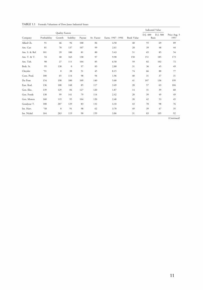
TABLE 1.1 Formula Valuations of Dow-Jones Industrial Issues
Indicated ValueQuality Factors
D.J. 400 D.J. 500 Price Aug. 5Company Profitability Growth Stability Payout Av. Factor Earns. 1947�1956 Book Value Basis 1957
Allied Ch. 91 46 94 100 84 4.50 40 55 69 89
Am. Can 81 70 137 107 99 2.61 28 39 48 44
Am. S. & Ref. 101 39 100 81 80 5.43 51 65 85 54
Am. T. & T. 54 40 163 130 97 9.90 150 151 185 173
Am. Tob. 98 27 111 104 85 6.58 59 82 102 72
Beth. St. 95 138 0 97 83 2.88 31 36 45 49
Chrysler �91 0 38 51 45 8.15 74 66 80 77
Corn. Prod. 100 65 114 98 94 1.96 40 31 37 31
Du Pont 154 198 100 109 140 5.60 41 107 136 199
East. Kod. 136 100 148 85 117 3.49 28 57 63 104
Gen. Elec. 139 129 84 127 120 1.87 14 31 39 68
Gen. Foods 138 99 141 79 114 2.42 20 39 49 49
Gen. Motors 160 119 95 104 120 2.48 20 42 53 45
Goodyear T. 108 207 129 83 132 4.18 43 78 98 76
Int. Harv. �58 0 91 98 62 3.70 49 39 47 35
Int. Nickel 164 263 119 90 159 3.86 31 83 105 92
(Continued)
c01 12 September 2012; 13:13:36
11
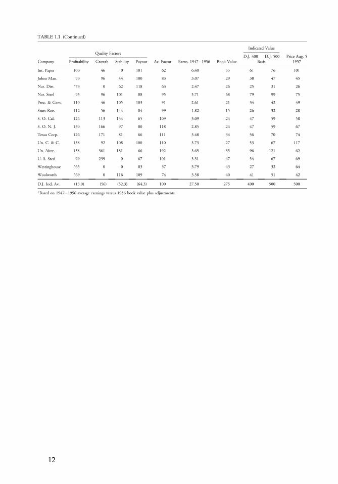
TABLE 1.1 (Continued)
Indicated ValueQuality Factors
D.J. 400 D.J. 500 Price Aug. 5Company Profitability Growth Stability Payout Av. Factor Earns. 1947�1956 Book Value Basis 1957
Int. Paper 100 46 0 101 62 6.40 55 61 76 101
Johns Man. 93 96 44 100 83 3.07 29 38 47 45
Nat. Dist. �73 0 62 118 63 2.47 26 25 31 26
Nat. Steel 95 96 101 88 95 5.71 68 79 99 75
Proc. & Gam. 110 46 105 103 91 2.61 21 34 42 49
Sears Roe. 112 56 144 84 99 1.82 15 26 32 28
S. O. Cal. 124 113 134 65 109 3.09 24 47 59 58
S. O. N. J. 130 166 97 80 118 2.85 24 47 59 67
Texas Corp. 126 171 81 66 111 3.48 34 56 70 74
Un. C. & C. 138 92 108 100 110 3.73 27 53 67 117
Un. Aircr. 158 361 181 66 192 3.65 35 96 121 62
U. S. Steel 99 239 0 67 101 3.51 47 54 67 69
Westinghouse �65 0 0 83 37 3.79 43 27 32 64
Woolworth �69 0 116 109 74 3.58 40 41 51 42
D.J. Ind. Av. (13.0) (56) (52.3) (64.3) 100 27.50 275 400 500 500
�Based on 1947�1956 average earnings versus 1956 book value plus adjustments.
c01 12 September 2012; 13:13:36
12
We shall measure growth by comparing the expected 1957�66 earnings with the actualfigures for 1947�56. Our basic formula says, somewhat arbitrarily, that where no growth isexpected the current price will be 8 times both 1947�56 earnings and the expected 1957�66earnings. If growth G is expected, expressed as the ratio of 1957�66 to 1947�56 earnings,then the price reflects such next decade earnings multiplied by 8 times G.
From these assumptions we obtain the simple formula:
Price equals ðE3GÞ3 ð83GÞ, or 8G2 3E,
where E is the per-share earnings for 1947�56:
To find G, the expected rate of future growth, we have only to divide the current price by8 times 1947�56 earnings, and take the square root.
When this is done for the Dow-Jones Average as a whole, using its August 5, 1957, priceof 500, we get a value of 1.5 for G—indicating an expected growth of 50% for 1957�66earnings vs. the 1947�56 actuality. This anticipates an average of $41 in the next decade, asagainst $27.50 for the previous 10 years and about $36 in 1956. This estimate appearsreasonable to the writer in relation to the 500 level. (In fact, he started with this estimate andworked back from it to get the basic multiplier of 8 to be applied to issues with no expectedgrowth.) The price of 500 for the D. J. Average would represent in turn a multiplier of 8 31.5, or 12, to be applied to the expected future earnings of $41. (Incidentally, on theseassumptions the average current formula value of about 400 for the Dow-Jones Averagewould reflect expectations of a decade-to-decade growth of 35%, average earnings of $37.1 for1957�66, and a current multiplier of 10.8 for such future earnings.)
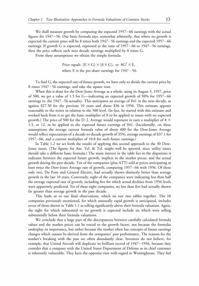
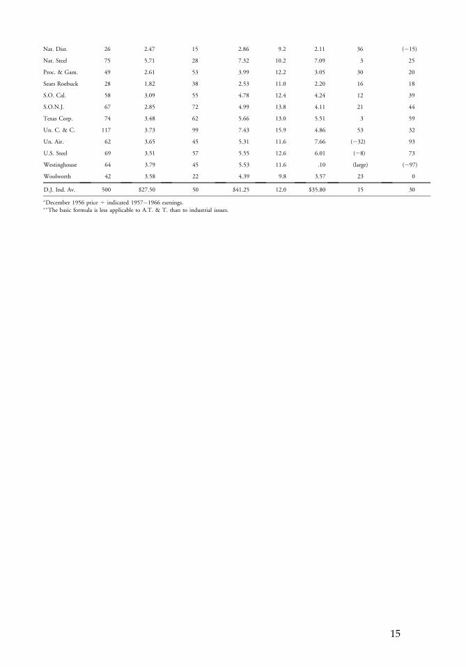
In Table 1.2 we set forth the results of applying this second approach to the 30 Dow-Jones issues. (The figures for Am. Tel. & Tel. might well be ignored, since utility issuesshould take a different basic formula.) The main interest in the table lies in the disparities itindicates between the expected future growth, implicit in the market prices, and the actualgrowth during the past decade. Ten of the companies (plus ATT) sold at prices anticipating atleast twice the Dow-Jones Average rate of growth, comparing 1957�66 with 1956. Of theseonly two, Du Pont and General Electric, had actually shown distinctly better than averagegrowth in the last 10 years. Conversely, eight of the companies were indicating less than halfthe average expected rate of growth, including five for which actual declines from 1956 levelswere apparently predicted. Yet of these eight companies, no less than five had actually shownfar greater than average growth in the past decade.
This leads us to our final observations, which tie our two tables together. The 10companies previously mentioned, for which unusually rapid growth is anticipated, includesseven of those shown in Table 1.1 as selling significantly above their formula valuation. Again,the eight for which subnormal or no growth is expected include six which were sellingsubstantially below their formula valuations.
We conclude that a large part of the discrepancies between carefully calculated formulavalues and the market prices can be traced to the growth factor, not because the formulasunderplay its importance, but rather because the market often has concepts of future earningschanges which cannot be derived from the companies’ past performance. The reasons for themarket’s breaking with the past are often abundantly clear. Investors do not believe, forexample, that United Aircraft will duplicate its brilliant record of 1947�1956, because theyconsider that a company with the United States Department of Defense as its chief customeris inherently vulnerable. They have the opposite view with regard to Westinghouse. They feel
c01 12 September 2012; 13:13:37
Chapter 1 Two Illustrative Approaches to Formula Valuations of Common Stocks 13
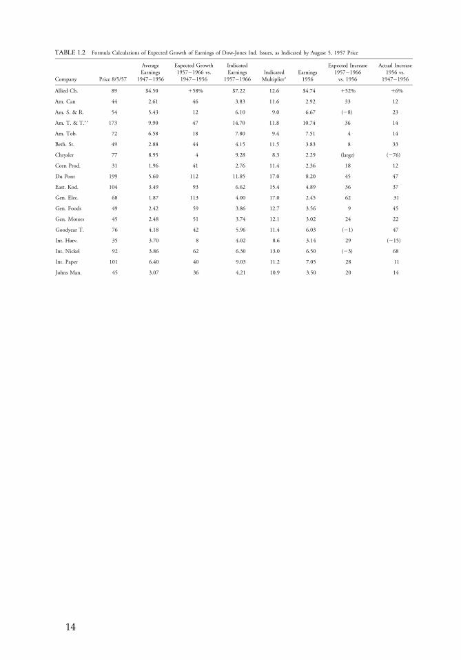
TABLE 1.2 Formula Calculations of Expected Growth of Earnings of Dow-Jones Ind. Issues, as Indicated by August 5, 1957 Price
Company Price 8/5/57
AverageEarnings
1947�1956
Expected Growth1957�1966 vs.1947�1956
IndicatedEarnings
1957�1966IndicatedMultiplier�
Earnings1956
Expected Increase1957�1966vs. 1956
Actual Increase1956 vs.
1947�1956
Allied Ch. 89 $4.50 158% $7.22 12.6 $4.74 152% 16%
Am. Can 44 2.61 46 3.83 11.6 2.92 33 12
Am. S. & R. 54 5.43 12 6.10 9.0 6.67 (28) 23
Am. T. & T.�� 173 9.90 47 14.70 11.8 10.74 36 14
Am. Tob. 72 6.58 18 7.80 9.4 7.51 4 14
Beth. St. 49 2.88 44 4.15 11.5 3.83 8 33
Chrysler 77 8.95 4 9.28 8.3 2.29 (large) (276)
Corn Prod. 31 1.96 41 2.76 11.4 2.36 18 12
Du Pont 199 5.60 112 11.85 17.0 8.20 45 47
East. Kod. 104 3.49 93 6.62 15.4 4.89 36 37
Gen. Elec. 68 1.87 113 4.00 17.0 2.45 62 31
Gen. Foods 49 2.42 59 3.86 12.7 3.56 9 45
Gen. Motors 45 2.48 51 3.74 12.1 3.02 24 22
Goodyear T. 76 4.18 42 5.96 11.4 6.03 (21) 47
Int. Harv. 35 3.70 8 4.02 8.6 3.14 29 (215)
Int. Nickel 92 3.86 62 6.30 13.0 6.50 (23) 68
Int. Paper 101 6.40 40 9.03 11.2 7.05 28 11
Johns Man. 45 3.07 36 4.21 10.9 3.50 20 14
c01 12 September 2012; 13:13:37
14
Nat. Dist. 26 2.47 15 2.86 9.2 2.11 36 (215)
Nat. Steel 75 5.71 28 7.32 10.2 7.09 3 25
Proc. & Gam. 49 2.61 53 3.99 12.2 3.05 30 20
Sears Roebuck 28 1.82 38 2.53 11.0 2.20 16 18
S.O. Cal. 58 3.09 55 4.78 12.4 4.24 12 39
S.O.N.J. 67 2.85 72 4.99 13.8 4.11 21 44
Texas Corp. 74 3.48 62 5.66 13.0 5.51 3 59
Un. C. & C. 117 3.73 99 7.43 15.9 4.86 53 32
Un. Air. 62 3.65 45 5.31 11.6 7.66 (232) 93
U.S. Steel 69 3.51 57 5.55 12.6 6.01 (28) 73
Westinghouse 64 3.79 45 5.53 11.6 .10 (large) (297)
Woolworth 42 3.58 22 4.39 9.8 3.57 23 0
D.J. Ind. Av. 500 $27.50 50 $41.25 12.0 $35.80 15 30
�December 1956 price 4 indicated 1957�1966 earnings.��The basic formula is less applicable to A.T. & T. than to industrial issues.
c01 12 September 2012; 13:13:37
15
its relatively mediocre showing in recent years was the result of temporary factors, and that theelectric manufacturing industry is inherently so growth-assured that a major supplier such asWestinghouse is bound to prosper in the future.
These cases are clear cut enough, but other divergencies shown in our table are not soeasy to understand or to accept. There is a difference between these two verbs. The marketmay be right in its general feeling about a company’s future, but the price tag it sets on thatfuture may be quite unreasonable in either direction.
It is here that many analysts will find their challenge. They may not be satisfied merely tofind out what the market is doing and thinking, and then to explain it to everyone’s satis-faction. They may prefer to exercise an independent judgment—one not controlled by thedaily verdict of the marketplace, but ready at times to take definite issue with it. For this kindof activity one or more valuation processes, of the general type we have been illustrating, mayserve a useful purpose. They give a concrete and elaborated picture of the past record, whichthe analyst may use as a point of departure for his individual exploration and discoveries inthe field of investment values.
NOTES
1. On this point the philosophically inclined are referred to the recent article of DavidDurand on “Growth Stocks and the Petersburg Paradox,” in the September 1957 issue ofthe Journal of Finance. His conclusion is “that the growth-stock problem offers no greathope of a satisfactory solution.”
2. “Can We Improve Methods of Appraising Growth Stocks?” by R. A. Bing, Commercialand Financial Chronicle, Sept. 13, 1956; table on p. 24.
c01 12 September 2012; 13:13:37
16 Part I: Valuation Perspectives: Then and Now
CHAPTER 2SEEKING A MARGIN OF
SAFETY AND VALUATION
Matthew B. McLennan, CFA
The foremost goal of investing is to avoid the permanent impairment of capital,which we believe can be done primarily by investing in companies that provide amargin of safety. Cash and gold also play unique but significant roles in ourportfolios that are designed to preserve real wealth.
Nearly two decades ago, my wife and I visited a Buddhist temple on the west coast of Japan.As we walked into the monastery, we were approached by a monk with a piece of paper in hishand. My Western mind-set assumed that he was handing me a nondisclosure agreement or arelease of liability, but instead he was holding a sign, written in Japanese, that said if we wereto go into the temple, we had to do so with an open mind.
An open mind is also an essential element in the concept of margin of safety. A margin ofsafety is more about mind-set than it is about any specific algorithm, model, or set of preciseinputs. It is about temperament. In my presentation, I describe the mind-set that we haveembraced at First Eagle for defining and applying the concept of a margin of safety to helppreserve value over time for our clients.
TWO BASIC INVESTMENT GOALS
The most important element in adopting the right mind-set is to have a clear and sensible goal.But a lot of confusion exists in today’s investment industry about what an investor’s goals shouldactually be. The popular focus is on relative returns, tracking error, and similar measures, but
Reprinted from CFA Institute Conference Proceedings Quarterly (June 2011):27�34. This presentationcomes from the CFA Institute Security Analysis and the Search for Value conference held in Chicago on17�18 November 2010 in partnership with the CFA Society of Chicago. When this article was orig-inally published, Matthew B. McLennan, CFA, was a portfolio manager at First Eagle InvestmentManagement, LLC.
c02 12 September 2012; 13:19:18
17
such a focus obfuscates one simple truth—the first and most important goal of investing is toavoid the permanent impairment of capital. If people give an investment manager their hard-earned savings, the manager should first seek to not erode the real value of those savings. Themanager should also want to grow the purchasing power of those savings over time.
THE PRICE OF MONEY IS FAKE
Democracy and deflation are like oil and water. Virtually no popular appetite exists fordeflation. The consequence is that policymakers are doing “whatever it takes” to stabilize theprice outlook after the deflationary pulse of the global financial crisis, and the result is thatthe price of money today is actually fake. What do we mean by the term fake?
Short-term real interest rates are negative and meaningfully so. Fiscal deficits aimed atsustaining or smoothing aggregate demand are creating a burgeoning supply of governmentbonds. Governments are intervening directly in the long end of the bond market throughquantitative easing and long-dated sovereign liquidity facilities. Even bank debt during thecrisis was guaranteed. Central banks are adhering to exchange pegs, despite the fact thatfundamentals do not warrant the exchange pegs and are thus producing vast amounts ofreserve accumulation or the need for complicated bailout facilities to ease the required realadjustments.
In some ways, nature’s currency, gold, is an alternative store of value to the paper cur-rency conundrum because it cannot be printed, it is scarce, and its supply is not subject to apolitical process. But the challenge investors face is that gold has been symmetrically re-ratedupward in value as the quality of man-made money has deteriorated. There is no free lunch.
The primary goal of avoiding permanent impairment of capital is difficult to achieve inthe current environment because no risk-free instrument exists to help preserve capital in realterms with low credit or valuation risk. Thus, in a reflexive response, investors have begun toinvest heavily in longer-term fixed income for some incremental yield, despite low absoluteyields. Return envy has also led them to think about owning real assets that have growthpotential. Such thematic thinking has driven many investors to invest in the fully valuedemerging markets because they believe it is a sector that offers the real return and growth theyseek to compensate them for low yields in their fixed-income holdings. The problem is thatthis approach may not necessarily be the right way to find a margin of safety and to preservecapital. Both thematic decisions ignore individual security risks and the full valuation of bothlong-duration fixed income and emerging market equities, both of which require substantialfaith to be placed in policymakers, who have recently made mistakes.
THE FUTURE IS UNCERTAIN
At First Eagle, the core of our mind-set is not only a clear goal to preserve capital but also arecognition that it is necessary to have the humility to accept uncertainty, as well as to notplace excessive faith in the prescience of policymakers. We do not try to predict the next hugethematic growth trend. Let me illustrate why we internalize this philosophy by using theexample of a period in history that shares some parallels with today and in which emergingmarket bond investing was immensely popular, as it is today, because people had excessive
c02 12 September 2012; 13:19:19
18 Part I: Valuation Perspectives: Then and Now
confidence in the global financial architecture. The period I am referring to was, similar totoday, preceded by two decades of unprecedented global growth. As a result of this growth,it was a period of changing relativities in terms of the geopolitical backdrop—one super-power was peaking, another was in decline, and a third was on the rise. Inflation was low andstable and was believed to have been conquered. Global monetary orthodoxy reigned. Onlya year before the beginning of this period, the stock market had also lost 40 percent of itsvalue in a liquidity-induced panic caused by investment trust companies investing long andborrowing short. These are some interesting parallels.
The period I am describing is 1908�1911. An investor who had been investing for acouple of decades prior to that time would have experienced, before 1908, a fairly stable worldin which asset values did not appear to be out of balance. That investor may also have had avery precise sense of how to deploy capital in that world, but clearly that sense would soon beproven wrong.
A further warning that not all was certain after the 1907 market panic occurred when theTitanic, the unsinkable ship, sunk on its 1912 maiden voyage. Man cannot control nature.In 1914, an unfortunate assassination in the Balkans led to a domino-like chain reactionamong a complex set of geopolitical alliances that precipitated World War I. Man cannoteven guarantee rational behavior. Once the war broke out, the New York Stock Exchange,despite being on the other side of the Atlantic Ocean, closed for more than four months. Afterthe war, between 1918 and 1920, the Spanish flu pandemic wiped out nearly 5 percent of theworld’s population. The hyperinflation of the Weimar Republic, which broke the fabric of theGerman political economy and ultimately led to the rise of Hitler and World War II,materialized in 1921�1922, and was followed by a severe depression. One can only wonderwhat the economic and market prognosticators were predicting with seeming precision in1913. The lesson this historical comparison teaches is that the future is intrinsically uncertain.The crystal ball is foggy at best. The first step to becoming a sound investor is being honestwith oneself. The experience of one generation may be very different from the experience ofthe generations that both precede it and follow it.
But acknowledging that the future is murky is a very difficult thing for investors to do.Investors and managers alike tend to want to preserve their sense of ego. The sense of actuallybeing able to predict the future is an ego preservation device. At First Eagle, however, webelieve that in order to implement a margin of safety approach, it is fundamental toacknowledge that the future cannot be predicted with certainty. Only then does one demand amargin of safety at all times.
DEALING WITH MACRO RISK
Investors have several ways to attempt to control the macro risk in their portfolios: eschew thewrong systemic framework, hold liquid cash and gold, or hedge with options. Ironically, inmodern capital theory, the taught response to an assertion that the future is uncertain is forinvestors to be “fully invested” in the “market portfolio.” But if the goal is to preserve capitalin real terms, then investors should be willing to not own certain parts of the market port-folio—for example, those parts where property rights may not be respected, or where thegovernment is the leading shareholder with a primary goal to maximize employment and notcash flow, or where valuations are excessive, or where imprudent management behavior iscreating impairment risks.
c02 12 September 2012; 13:19:19
Chapter 2 Seeking a Margin of Safety and Valuation 19
Being fully invested at all times is also not a precondition for success. Some investorsargue that if cash has a low real return, a portfolio should never hold any cash because itcreates a drag on performance. Cash can be a residual of our investment approach. Becauseour goal is absolute—to find great businesses with good prices or good businesses with greatprices—if the markets become ebullient, as they were in 1999 and 2007, and we cannot findsufficient opportunities, then we wait. The cash builds in the portfolios. It is not a market-timing call. It is about having the flexibility and patience to commit to an absolute set ofstandards for underwriting across time. The return on the cash is not only its stated return butalso the option to deploy it in times of distress when liquidity is not otherwise available.
We like to commit capital when an absence of market liquidity exists. Consequently,some of our lowest cash levels ever occurred in March 2009. The reason was not because wewere calling the market bottom but because, as structural business buyers, we committedcapital when a wider margin of safety opened. Having a time-varying level of cash in aportfolio is actually an important part of dealing with uncertainty and enables equanimity inunderwriting standards.
We also hold gold in our portfolios. We view the value of gold as being inversely relatedto systemic confidence and positively related to political efforts to inflate the money supply.The reason for this relationship is that the supply of gold is exogenously determined bynature, not politics. All the gold ever mined remains in existence; the supply is thus not afunction of any one year of mining output but rather the cumulative stock of all of the goldever mined. The supply of gold barely moves by more than 1 percent based on the miningoutput in any given year. Historically, the relative stability of gold’s supply has meant thatgold’s value has varied inversely with confidence in a man-made economic system becausethe supply of man-made money usually becomes less predictable in economic distress. In theUnited States during the late 1920s, late 1960s, and late 1990s, when people believed thatthe economic system was strong, markets boomed, confidence was high, and gold wasinexpensive relative to the price of equities and personal incomes. But when the economicsystem frayed in the 1930s, 1980s, and most recently in 2008�2009, gold re-rated upwardsubstantially versus the price of equities and personal incomes.
Hence, gold is used at First Eagle as a source of ballast in our portfolios and has typicallybeen about 10 percent of the overall portfolio. We believe that if the allocation were 15percent or higher, it would start to become a directional view on gold, which is a situation wewant to avoid, given that we know we cannot predict future systemic confidence with pre-cision and we recognize that gold can suffer a generation of poor returns when, and if, sys-temic faith is restored. Yet, we also would not typically want it below 5 percent of the overallportfolio because it would not provide material ballast.
Another strategy for coping with macro risk is hedging with options. Hedging a portfoliowith options, however, requires paying very close attention to the cost of the potential hedgebecause it is time-definite. Investors often adopt tail-hedging strategies when implied volatilityis high and when asset values are cheap, such as after a major market correction. But ifinvestors use a fundamental approach to value options, we believe it becomes possible toidentify periods of time when options are expensive or cheap in fundamental terms. The timeto buy tail insurance is when asset values are high and implied volatility is low. Yet, mostpeople seem to do the opposite, which is an example of the rear-vision investing that webelieve is going on in the world today. Finally, the purchase of options often involves anassessment of counterparty risk. To the extent that an investor is trying to hedge for a tailevent, what matters is what the counterparty risk will be in the tail state of the world ratherthan in the current state of the world.
c02 12 September 2012; 13:19:19
20 Part I: Valuation Perspectives: Then and Now
OWNING AN ENTERPRISE PRESERVESPURCHASING POWER
To preserve purchasing power, investors need to not only avoid permanent impairment ofcapital but also to keep pace with the continual growth of human potential. Investing ina business enterprise allows investors to participate in humanity’s capacity to continueimproving.
The growth in human potential can be measured by numerous improvements over time:the mechanics of trade over roads, rails, and ports; the faster diffusion of ideas, from the speedof a horse to the speed of microprocessors and routers; the potential for greater energyproductivity harnessing solar, wind, and nuclear power versus burning timber, coal, and oil;the increased life expectancy through biotechnology and public health initiatives; and thebroadening of property rights.
Preserving purchasing power in real terms is not only about participating in the marchof man but also about keeping pace with a monetary stock that is growing steadily. In aworld of inflation-targeting orthodoxy, modest deflation is not deemed an acceptable out-come. The central banks of advanced economies are practicing some unconventional mon-etary “therapy” to try to sustain a rising monetary stock. For example, the U.S. FederalReserve is trying to put a floor under U.S. inflation, a policy that is producing commensu-rately greater inflationary pressures in the emerging markets, which are U.S. dollar reservecurrency accumulators. As a result, Brazil, Russia, India, and China (the BRIC) have arguablybecome the monetary epicenters of the world. The annual growth rate for M2 (the amount ofmoney in circulation) in most of these economies has been averaging more than 15 percent,which eclipses the credit growth rate in the United States during the last decade by nearlythreefold.
Owning a business is akin to owning the source of productivity. If investors own busi-nesses that generate real cash flow, then that cash flow over time will also scale with the level ofnominal activity and capital may be preserved. The result is that investors will come full circleto the first goal of investing: preserving capital, albeit paradoxically through the “risky”ownership of an enterprise.
SEEK A MARGIN OF SAFETY
The strategic need to be an owner of an enterprise while fundamentally accepting that theworld is an uncertain place means investors must demand a margin of safety on eachinvestment that they make. The best way to create a margin of safety is from the bottom up,by analyzing risk security by security.
Karl Popper, who was a leading figure in the field of scientific methodology, said in hisbook Objective Knowledge that “the main difference between Einstein and an amoeba is thatEinstein consciously seeks for error elimination.”1 It sounds trite, but it is a very profoundrealization. Many investors are simply trying to identify the next great wave of new-erainvestment, such as BRIC recently or technology in the late 1990s, and they try to catch thatparticular wave only to get dumped. We believe a better approach to investing is to attempt tomake the least number of bad choices at the individual security level. To invest with themind-set of Einstein is not to try and call the market’s “ups and downs” but rather toavoid errors.
c02 12 September 2012; 13:19:19
Chapter 2 Seeking a Margin of Safety and Valuation 21
From a bottom-up standpoint, investors should try to avoid the four following paths topermanent destruction of capital: overpayment for a business, business model substitutionrisk, vulnerability from the wrong capital structure, and management dilution. A lot of valuemanagers were wrong in 2008 because they had a unidimensional sense of a margin of safetythat was centered solely on price. Price is an important component of a margin of safety, but amultifaceted approach that incorporates the business model, capital structure, and manage-ment integrity is preferable.
Valuation
Businesses can be parsed into two broad categories: commodity businesses and franchisebusinesses.
A commodity business does not have a competitive advantage. Its intrinsic value isbasically its sustainable earnings power divided by its cost of capital. In growing its capital stock,it does not create value because it is only earning its cost of capital. If its capital stock shrinks,however, it will produce more free cash flow than earnings because it will release surplus capitaland not need as much to invest in the future. In the absence of product substitution ormanagement stupidity, the valuation exercise for a commodity business is relatively straight-forward; it is essentially about identifying the sustainable earnings power and the nominalcost of capital.
A franchise business has some competitive advantage that enables it to generate very highincremental returns on capital. It is like a royalty on a slice of the global economy. On the onehand, however, its growth requires limited capital and thereby creates substantial value. Onthe other hand, if it loses relevance and shrinks, no meaningful capital is released and valueerodes, and there is no shield against this fade. Valuing a franchise business, therefore, requiresthe discriminating investor to disentangle the concepts of an objective margin of safety and asubjective margin of safety because, counterintuitively, the range of intrinsic value outcomes isbroader for a franchise business than a commodity business. The subjective margin of safetyis based on the investor’s view of the franchise relevance and prospects for the future. Theobjective margin of safety is based on entry price. The value of a franchise business, for thosewithout a biased sense of how the company will evolve in relevance, should conservativelyassume no real growth but allow for pricing power to pass through the effects of inflation. Thenuance here relative to valuing a commodity business is that for a commodity business,inflation produces lower free cash flow than earnings because the maintenance capitalexpenditures will exceed historical book depreciation. In fact, the capital stock will have togrow by the amount of the inflation, thereby offsetting all the benefits of that growth. Thus,for a commodity business that is growing, use a nominal discount rate to discount earnings.In the case of a franchise business, however, take the business’s earnings power divided by thereal cost of capital to estimate intrinsic value. We use “real,” not “nominal,” cost of capitalbecause inflation passes through a franchise’s earnings stream without much capital drag—earnings are basically free cash flow irrespective of the level of inflation. In a normal cost ofcapital environment, the average commodity business is worth a low double-digit multipleof earnings (in the low teens) and the great franchise business, assuming no real growth, is wortha higher multiple of earnings (in the high teens). Assuming an unleveraged capital structure, thisvalue translates to high single-digit earnings before interest and taxes (EBIT) multiples forcommodity businesses and lower- to mid-teens EBIT multiples for franchise businesses.
Because of the wide range of outcomes, franchise investing requires not only an objectivemargin in price but also a subjective margin of safety in the analysis of franchise fade. We only
c02 12 September 2012; 13:19:19
22 Part I: Valuation Perspectives: Then and Now
buy franchise businesses that are priced for fade—that is, trading at a multiple lower than theinverse of their real cost of capital—and we try, while acknowledging the limits of our crystalball, to focus on those that have the potential to endure or grow in relevance.
In simple terms, whether buying a commodity business at a discount to intrinsic value ora franchise priced for fade, typically we are buying businesses at single-digit multiples ofEBIT. Investing in equities that are priced for fade creates an error-tolerant system. If abusiness does not produce the expected results, a margin of safety exists in the price. Takingthe concept one step further, if investors have already selected from the lower part of theequity universe that is priced for fade, it is possible to reduce the percentage of companies thatwill actually fade by focusing on the subjective margin of safety. The objective price is bal-anced against the subjective fade. Unfortunately, fade cannot be completely eliminated.
The ironclad rule of the universe—entropy—makes it self-evident that nothing willreplicate itself into perpetuity and that all forms of order are local and transient. The same lineof thinking exists in evolutionary theory. The concepts of fade and entropy mean investorsneed to think carefully about business model erosion.
Business Model Erosion
Investors are taught to think of businesses as perpetuities, and the typical dividend discountmodel projects 3�4 percent growth into perpetuity. Instead, investors should assumethat every business is on a path to some form of irrelevance. The only unknown is howlong the current earnings power can be sustained or increased in a transient fashion. Ratherthan assume perpetuity, investors should ponder the intrinsic duration of an earningspower stream.
For a commodity business, the basis of earnings power duration is asset life, assetreplacement value, and the cost-curve positioning of the business relative to competitors. Theearnings power in a commodity business is shielded by the replacement value of its long-livedassets. For a franchise business, the basis of earnings power duration is a specific and sus-tainable competitive advantage. The focus of our analysis is on identifying local scaleadvantages and the degree of customer captivity.
So, investors should begin their investment selection process within the universe ofequities that are priced for fade and then identify the subset of businesses they want to invest inthat are less likely to experience fade. If the business is commodity-like in nature, it must havelong-life asset value protection. If the business is franchise-like in nature, it must have intan-gible asset protection through the strength of its local market position and customer captivity.
Focus on Assets, Not on Residual Equity
Another area to consider, in keeping with the concept of a margin of safety, is seeking amaterial discount to the intrinsic value of a company’s assets. Equity should be viewed asa residual claim on a business. Equity has value only after debtholders, pension claimants,contingent litigants, and minority interests are satisfied. At First Eagle, we prefer to buy assetsat 70 cents on the dollar based on capitalizing EBIT, not post-tax earnings. On the basis ofthat asset value, we decide what price we are willing to pay for the equity, taking into accountthe company’s capital structure and other sources of contingent leakage.
A good example of the importance of distinguishing asset value from equity value is howan investor would obtain a margin of safety on a wholesale-funded bank that does not have alot of non-balance-sheet income. A bank typically has about 10 percent of its assets in equity
c02 12 September 2012; 13:19:19
Chapter 2 Seeking a Margin of Safety and Valuation 23
with the remainder in deposit- and debtholder liabilities. If the bank does not have a retaildeposit franchise, then most of the 90 percent nonequity liabilities will be some form of debtissued at market prices. Thus, no matter what investors pay for a wholesale bank’s equity, theyare paying at least 90 cents on the dollar for its assets. The equity sliver exists only after theother claimants are paid. It is thus hard to obtain a margin of safety on the assets deemed to beacceptable unless there is some form of below-market deposit funding that creates incrementalvalue or some other source of material intrinsic value based on fee-earning businesses inde-pendent of the balance sheet lending activity.
The margin of safety does not have to exist in the price paid for a company’s stock but inthe price paid for its assets. For equityholders, the asset value may be there in the long term,but this does not help them if the assets transition to the hands of the senior secured debt-holders in a short-term funding crisis. There is no point in owning assets that have somematerial probability of being taken away. Consequently, investors need to pay a lot ofattention to the quality of the capital structure.
Management
The management of an enterprise is also very important. For a typical equity that trades at 10times gross cash flow (i.e., earnings plus depreciation), the management team will redeployapproximately 10 percent of the face value of an investor’s investment every year. The realityis even more dramatic when mergers and acquisitions (M&A) via new security issuance areincluded. Over a long holding period, such as more than five years, the management teamcould easily redeploy 50 percent of the gross cash flow in market capitalization in mainte-nance capital expenditures, discretionary capital investments, security repurchases, and M&Aactivities. It is important to thus determine what amount of gross cash flow an investor willreceive back as dividends and whether management’s retained capital deployment is accretiveor dilutive in nature.
Investors should demand a larger valuation margin of safety in companies with thefollowing management mistakes: (1) implementing poor pricing strategies, such as gougingthe customer on price for short-term earnings power or engaging in destructive pricing warsdespite an oligopolistic market structure; (2) engaging in fad-driven business migration, suchas diversifying away from an advantaged local position or stretching to engage in “globali-zation” or product diversification; (3) showing financial imprudence, such as adding largeamounts of leverage or putting balance sheet growth ahead of secular market trends; and(4) practicing myopia, or “milking” the business.
Perhaps one of the best indicators of management prudence is free cash flow generation.Management teams that are focused on generating free cash flow relative to earnings typically aremaking conservative accounting choices, growing within the speed limit of their business, andmaking reasoned business decisions. Seek managers who are prudent owners/entrepreneursfocused on sustaining culture and thoughtfully distributing or retiring capital, and avoidexpeditionary management teams that are aggressive, new-era thinkers willing to bet the ranchon dilutive terms to feed their ambition.
FLEXIBILITY TO LOOK DIFFERENT
Combining all elements of the margin of safety is more important than believing you have acrystal ball. The successful turning points in First Eagle’s investment track record have oftenbeen acts of omission: being out of Japan in the late 1980s, being largely out of technology in
c02 12 September 2012; 13:19:19
24 Part I: Valuation Perspectives: Then and Now
the late 1990s, and being largely out of financials in 2007 and 2008. As I said earlier, we donot have a crystal ball; we simply could not find enough businesses during those times in thosemarket environments that embodied the valuation margin of safety and had the sustainableearnings power, conservative management behavior, and conservative balance sheet evolutionthat we demand. Our peripheral vision for macro capital preservation was the sum total of aset of prudent micro acts of omission.
Almost by definition, a passive approach to investing (i.e., mimicking an index) leads tooverweighting the sectors that experience the bubbles because it is in those sectors that thegreatest expectations for complacency exist in the system. Most managers seek a low trackingerror against a benchmark. The whole notion of minimizing risk by minimizing tracking erroris a logical non sequitur. The goal of avoiding permanent impairment of capital means thatsometimes investors need to stay away from sectors that embody the wrong set of expecta-tions, even if they are the biggest sectors of the market. Most investment managers are notstructured to flexibly implement such an approach.
At First Eagle, we view the market as if it were a piece of marble. The goal of errorminimization in structuring a portfolio is similar to chipping away the unwanted pieces ofmarble to let the statue emerge from within. We do not own the whole block of marblejust for the sake of owning it. The point of a margin of safety approach is not to ask, Dowe overweight Japan versus the United States? Do we own one sector versus another?Rather, the point is to find clusters of investments that we believe make sense from amargin of safety perspective and thus help in attaining the goal of preserving capital inreal terms.
Three clusters of equity securities are typically found in the portfolios we build at FirstEagle. The first cluster is what we call “eclectic royalties.” These equities are similar tofranchise businesses; they dominate a slice of the world economy and may help preserve thepurchasing power of our clients’ capital. These companies typically have an initial objectivemargin of safety in being priced for fade and a longer-term margin of safety in subjectiverelevance. They have dominance in their product or service market, they have balance sheetstrength, and they have cultural duration.
The second cluster is “scarce real assets” because owning real assets at the right pricehelps preserve real wealth. In addition to owning gold directly as a potential source ofportfolio ballast, we have owned such real assets as timberlands and quarries throughlisted equities. We bought these assets at a discount to the liquidation value of the reservesacross time when their equities were depressed, and thus the equity market was essentiallypaying us for storage. A timberland with a 50-year harvest life or a quarry with 60 years ofreserves will produce cash flows of substantial duration. In times of cyclically depressedprices, the market often underestimates the power of this cash flow duration. Scarce realassets often have local market monopolies and, therefore, real pricing power over thelong haul.
The third cluster is composed of businesses that have discounted cash flows typicallythrough an accounting distortion. It can be very beneficial for investors when anaccounting convention obscures the true economic value of a business because an investorcan obtain a very wide margin of safety. We have been long-term investors in investmentand insurance holding companies, which have been fertile territories for these kinds ofopportunities. Another area of distortion is when a company is in fade and generating alot more cash flow than GAAP earnings (because GAAP assumes a company reinvestsdepreciation to sustain the capital stock) or selling assets at market values well in excess ofhistoric book value.
c02 12 September 2012; 13:19:19
Chapter 2 Seeking a Margin of Safety and Valuation 25
CONCLUSION
A margin of safety in investing requires an initial goal to avoid permanent impairment ofcapital, a mind-set that accepts uncertainty, and a multifaceted approach centered on errorelimination. The result of requiring a margin of safety in each investment is often a portfoliothat looks very different from the underlying market and that may have material ballast incash and gold. In a world where the price of man-made money is fake, an investor needs tobe primarily an owner of an enterprise in order to preserve capital. Trying to predict thefuture with scientific precision is a losing game, but trying to find securities one at atime across the globe that embody a margin of safety in price can help investors endure theinevitable vicissitudes of the business cycle and geopolitical turbulence. It requires patience.The margin of safety approach is applicable in all markets. At First Eagle, we have done it fordecades, and it has been the mainstay of how we approach investing.
� � �
Past performance is no guarantee of future results. All investments involve the risk of loss of capital.Investment in gold and gold-related investments present certain risks, and returns on gold and gold-related investments have traditionally been more volatile than investments in broader equitymarkets or debt markets. Performance of First Eagle for periods prior to 2000 occurred when thethen portfolio manager was affiliated with another manager.
QUESTION AND ANSWER SESSION
Question: How do you tell when gold is overvalued?McLennan:We own gold as a potential source of ballast and do not take a directional view, so
the under- or overvaluation of gold is not our primary concern. For us, the value of goldis essentially on a continuum that is inversely related to confidence in the system.Investors can calibrate the value of gold by looking at it in an opportunity cost context.
If gold is a potential hedge against monetary calamity, then people should bewilling to pay for that hedge over time based on their per capita income levels and thevalue of their assets. They will pay a certain amount for that hedge depending on whatthey perceive to be the need for a hedge. We have observed that when real interest ratesare low and/or the creditworthiness and credibility of a government is low, the value ofgold tends to be higher than average.
Question: What is the current economy saying about the value of gold?McLennan: The self-healingmechanism of the economymay already be in place at this point in
2010. Corporations are generating free cash flow, which has typically led to betteremployment and confidence trends and, in turn, to a self-sustaining recovery. If thathappens, real interest rates andbudget deficits will normalize at somepoint and the price ofgold could go down. In fact, that would be the preferred scenario because equities thatembody a margin of safety in price could do just fine in that better state of the world.
Another state of the world could materialize, however, in which the path tonormalization has an unanticipated discontinuity and the debt burden at the govern-ment level causes the markets to lose confidence in the current financial architecture. Inthat state of the world, the price of gold could increase dramatically. We hope that doesnot happen, but were it so, we would value the potential hedge.
c02 12 September 2012; 13:19:20
26 Part I: Valuation Perspectives: Then and Now
Question: Do you own large amounts of gold and large amounts of cash at the same time, orare they mutually exclusive?
McLennan: Cash and gold each have a unique role in the portfolios. Cash can be viewed as aresidual of the investment approach that builds and declines throughout the market,business, and liquidity cycles. Gold can be viewed as a systemic and longer-termstructural potential hedge.
Question: Could you give an example of a market in which private property rights are notrespected?
McLennan: Some jurisdictions of the world have more “flexible” property rights than others.Russia is an example of a market in which property rights have not always beenrespected, and we have been wary of investing there. An investor does not have to beinvested everywhere.
Good investing is about finding some asymmetry between price and prospects.Despite the enthusiasm for emerging market investing, today we see more asymmetrybetween price and prospects in the developed world than in the emerging markets.
In fact, we have a lot of investments in Japan, which is a country that someinvestors have written off. We own several good businesses that we believe are cheapafter a two-decade bear market; many of these businesses are benefiting from the growthin emerging markets.
NOTE
1. Karl Popper, Objective Knowledge (Oxford, U.K.: Oxford University Press, 1972).
c02 12 September 2012; 13:19:20
Chapter 2 Seeking a Margin of Safety and Valuation 27

c02 12 September 2012; 13:19:20
PART IIVALUATION
METHODOLOGIES
Chapter 3 Company Performance and Measures of Value Added 31
Chapter 4 The Affordable Dividend Approach to Equity Valuation 93
Chapter 5 Discounted-Cash-Flow Approach to Valuation 105
Chapter 6 Equity Securities Analysis Case Study: Merck & Company 115
Chapter 7 Traditional Equity Valuation Methods 155
Chapter 8 A Simple Valuation Model and Growth Expectations 177
Chapter 9 Franchise Valuation under Q-Type Competition 189
Chapter 10 Value Enhancement and Cash-Driven Valuation Models 209
Chapter 11 FEVA: A Financial and Economic Approach to Valuation 229
Chapter 12 Choosing the Right Valuation Approach 243
Chapter 13 Choosing the Right Valuation Approach 259
Chapter 14 Valuing Illiquid Common Stock 279
c03 12 September 2012; 11:2:44
29

c03 12 September 2012; 11:2:44
CHAPTER 3COMPANY PERFORMANCE
AND MEASURESOF VALUE ADDED
Pamela P. Peterson, CFA, and David R. Peterson
This chapter compares the advantages and disadvantages of such traditional measuresof firm performance as return on investment with those of more recent performancemeasures—economic value added, market value added, and cash flow return oninvestment. The authors use 1993 financial data from Hershey Foods Corporation,and they conclude that the usefulness of a method depends on the analyst’s purpose.
FOREWORD
Few skills are more essential to a security analyst than the ability to evaluate a company’sperformance in a concise and compelling manner. Given the importance that firm valuationplays in financial markets, the wealth of research literature on the topic (including con-tributions from such giants in the investment management profession as Gordon, Graham,Dodd, Modigliani, Miller, and Tobin) is not surprising. In spite of all the intellectual fire-power that has been aimed at the issue, however, performance evaluation can hardly beconsidered a permanently solved puzzle. Indeed, recent years have witnessed the ascent of asometimes confusing array of terms—EVAs, MVAt, CFROI—representing state-of-the-artstatistical measures intended to take the place in analysts’ hearts and minds of the traditionalmarket-based metrics, such as return on assets (ROA) and return on equity (ROE).1 Althoughit is widely acknowledged that these new methods are often useful, it is not clearly understoodwhere they fit in the analyst’s toolkit.
Copyright ª 1996 The Research Foundation of CFA Institute. Reprinted with permission. When thisarticle was originally published, Pamela P. Peterson, CFA, was professor of finance at Florida StateUniversity and David R. Peterson was professor of finance at Florida State University.
c03 12 September 2012; 11:2:44
31
In this chapter, Pamela Peterson and David Peterson help make sense of these con-temporary developments and provide a context in which to compare the new with the old.The authors also do a great job of dispelling some current myths about the latest generation ofevaluation techniques. For example, one interesting aspect of these new performance tools isthat they are not all that new. Economic value added has its origins in the notion of economicprofit, first advanced a century ago; cash flow return on investment is an adaptation of thewell-established internal rate of return. The authors’ impartial insights prove particularlyvaluable to the reader in that much of what is presently known about EVA and CFROI comesfrom the consulting firms that promote these statistics.
Peterson and Peterson begin their analysis with a summary of conventional measures ofcompany performance, such as the myriad return ratios (e.g., earnings power, ROA, ROE),book-to-market value, and Tobin’s q. Against this backdrop, they then develop the intuitionfor the so-called value-added measures, including the aforementioned EVA—along with itscompanion measure, market value added—and CFROI. These explanations are at once userfriendly and illuminating; in fact, the careful pedagogy contained in this section is arguablythe most valuable part of the chapter. Taking the case of Hershey Foods Corporation, theauthors show how these measures can be constructed from publicly available accounting datausing each of several different methods. Along the way, they highlight the many assumptionsthat the analyst must make to apply these approaches in practice. I suspect that this sectionwill serve both industry and academia as a “how to” manual in this area for years to come.
The authors conclude their study with an empirical analysis of how closely the value-addedmeasures are linked to stock returns, which they suggest is the ultimate test of a company’sperformance. In particular, they calculate the extent to which both the market-based and value-added metrics correlate with various return calculations. Peterson and Peterson start from theposition that because “value-added measures are theoretically more closely related to firm valuethan the simpler traditional measures,” they should also be more closely related empirically. Inthis regard, their results are somewhat surprising. Although stock returns are, in fact, highlycorrelated with both the conventional and value-added statistics, the advantage that the latterholds over the former is slight. Furthermore, the authors document some important biases of theEVA and MVA measures involving the market capitalizations of the firms in their sample.
Although the authors express disappointment in these empirical findings, the reader certainlyshould not be disappointed. To the contrary, this research performs two important services. First,and quite possibly foremost, it provides a thoughtful primer on how to translate “value-added”theory into practice. Second, it offers an unbiased and critical examination of the advantage ofthese tools. Although the authors’ analysis supports the usefulness of the modern measures, theypoint out the fact that nontrivial costs are involved in the application. Thematerial in this chapteris at the heart of what a security analyst needs to know to perform his or her job in today’s market,and the Research Foundation is pleased to have been part of its development.
Keith C. Brown, CFAResearch Director
The Research Foundation of theInstitute of Chartered Financial Analysts
ACKNOWLEDGMENTS
We would like to thank Keith Brown, CFA, for helpful direction and comments; Sam Eddinsand Bartley Madden of HOLT Value Associates, Rawley Thomas of BCG/HOLT, and
c03 12 September 2012; 11:2:44
32 Part II: Valuation Methodologies
Lee Glasner for answering questions and supplying information concerning CFROI; andAl Ehrbar of Stern, Stewart & Company for answering questions regarding the economic-value-added approach. We would also like to thank the Research Foundation of the Instituteof Chartered Financial Analysts, AIMR, and Florida State University for their support.
Pamela P. Peterson, CFADavid R. Peterson
INTRODUCTION
A business that operates in such a way as to maximize its owners’ wealth allocates its ownresources efficiently, which results in an efficient allocation of resources for society as a whole.Owners, employees, customers, and anyone else who has a stake in the business enterprise are allbetter off when its managers make decisions that maximize the value of the firm. Therefore,evaluating a firm’s management on the basis of whether it maximizes the owners’ wealth is areasonable approach.
Evaluating a firm’s performance seems to be a rather straightforward issue, but it is not.By focusing on the maximization of a stock’s price, one might conclude that the higher thestock’s price, the better the performance of the firm’s management. But should managementbe penalized if the market declines? Should management be praised simply because theeconomy has recovered? Should management be rewarded for taking on excessive risks?
Evaluating a firm’s performance is much more challenging than looking at its stock price,and evaluating the performance of specific managers is even more challenging. Regulators andshareholder activists have long complained about the way firms pay executives, especiallywhen pay is not linked to performance. Even when executive pay is linked to performance, theissue of how to measure performance remains. If pay is linked to accounting earnings,the possibility exists that these accounting earnings can be manipulated to produce high payfor the executives at the expense of shareholders.2 In recent years, executive compensation hasbeen overhauled to improve the link between pay and performance by shifting pay packagesto include stock options. Yet in many companies, such a link does not exist, and in others, thelink is imperfect.3
Because of the need for better methods of evaluating performance, several consultingfirms have been advocating performance evaluation methods that look at a firm’s performanceas a whole and the performance of specific managers. These methods are, in some cases,supplanting traditional methods of measuring performance, such as return on assets.
The purpose of this chapter is to examine traditional and recently developed methods ofevaluating firm performance. Our focus is on the performance of the firm as a whole, and wedo not address the application of these measures to specific managers or products. But whatwe learn from applying these methods to firms as a whole may affect the application of thesemethods to specific managers.
How Value Is Created
A firm’s management creates value when it makes decisions that provide benefits exceedingcosts. These benefits may be received in the near or distant future, and the costs include thedirect cost of the investment and a less obvious cost, the cost of capital.
This benefit�cost analysis is the heart of the traditional capital-budgeting analysis. Onecommon technique for analyzing these benefits and costs is the net present value method,
c03 12 September 2012; 11:2:44
Chapter 3 Company Performance and Measures of Value Added 33
which discounts uncertain future cash flows at some rate that reflects the cost of capital usedin the investment. This cost of capital reflects the marginal cost of raising additional capital.The cost also reflects the risk inherent in the project; the greater the investment’s risk, thegreater its cost of capital.4 The difference between the present value of these uncertain cashflows and the cost of the project (i.e., the investment outlay) is referred to as the project’s netpresent value.
The net present value is expressed in terms of dollars of value. If the net present valueis positive, the investment is expected to add value to the firm; if the net present value isnegative, the investment is expected to reduce the value of the firm. Hence, the net presentvalue is a measure of value added (if positive) or value subtracted (if negative).
Another often-used technique is the internal rate of return (IRR). In this approach toevaluating investment projects, the discount rate is determined (through iteration) so that itequates the future cash flows with the investment’s explicit costs (i.e., the investment outlay).Stated equivalently, the IRR is the discount rate that equates the net present value to zero.
Use of the IRR requires first calculating the IRR (the project’s “internal rate”) and thencomparing this rate with a rate that reflects the cost of capital. Once again, this cost of capitalreflects the costs of the various sources of funds and the uncertainty associated withthe investment. If the project’s IRR exceeds this cost of capital (sometimes referred to as the“hurdle rate”), the project is value enhancing. If, on the other hand, the project’s IRR is lessthan the cost of capital, the project is value reducing.
No matter the particular capital-budgeting technique used, the principles are thesame: A firm should invest only in projects that enhance the value of the firm. So, where dothese value-enhancing projects come from? In a competitive market in which many firmscompete for available investment opportunities, value-enhancing projects should not exist. Inother words, the cost of a project should be bid upward through competition so that no netbenefit results from investing in the project. This explanation is rather gloomy and ignoresthe true source of value-enhancing projects—a firm’s comparative or competitive advantage.Only through some advantage vis-a-vis its competitors can a firm invest in projects thatenhance value.
A comparative advantage is the advantage one firm has over others in terms of the cost ofproducing or distributing goods or services. Wal-Mart Stores developed a comparativeadvantage over its competitors (such as Kmart Corporation) through its network of ware-houses and its distribution system. Wal-Mart invested in a system of regional warehouses andin its own trucking system. By using the regional warehouse system instead of a nationalwarehouse system or no warehouse system at all, Wal-Mart reduces its need for inventory.Furthermore, by having its own truck fleet, Wal-Mart is able to replenish store inventoriesmore frequently than its competitors. Combined with bulk purchases and a unique customerapproach (such as its “greeters”), Wal-Mart’s comparative advantage in its warehousing anddistribution systems has helped it grow to be a major, and very profitable, retailer in a shortspan of time.
A competitive advantage is the advantage one firm has over another because of the structureof the markets (input and output markets) in which they both operate. For example, one firmmay have a competitive advantage because of barriers that prevent other firms from entering thesame market. Barriers to entering a market arise in the case of governmental regulations thatlimit the number of firms in amarket, as with banks, or in the case of monopolies granted by thegovernment, as in the past with local cable companies. A firm itself may create barriers to entry(with the help of the government) with patents and trademarks.
c03 12 September 2012; 11:2:44
34 Part II: Valuation Methodologies
In cases in which no impediments to investment exist (that is, the market forinvestments is competitive), only through having some type of advantage can a firm makean investment and get more than the present value of the initial outlay back in return. Thesame basic principles applied here to individual projects can be applied when looking atthe entire firm. If the firm’s investments provide future benefits greater than theircosts, the investments enhance the value of the firm. If the firm’s investments providefuture benefits that are less than their costs, this situation is detrimental to the value ofthe firm.
The idea of producing current value from future investment opportunities is reflected inthe concept of franchise value, which is discussed by Kogelman and Leibowitz (1995) in theirdecomposition of the price-to-earnings ratio (P/E) into a franchise P/E and a base P/E.5
In their analysis, future investment opportunities in excess of market returns are reflected inabove-market P/Es.
From the perspective of analysts, the focus of performance evaluation is on the firm as awhole, not on individual investment decisions within the firm. The key to evaluating a firm’sperformance is, therefore, determining whether the firm’s investment decisions as a whole areproducing value for the shareholders. But no obvious technique exists for determiningwhether a firm’s decisions produce value for shareholders because (1) no one has the ability toperfectly forecast future cash flows from investments, (2) no one has accurate measures of therisks of each investment, and (3) no one knows the precise cost of capital. Therefore, proxiesmust be used (however imperfect) to assess a firm’s performance.
Relating New Performance Methods to Capital-Budgeting Techniques
The most prominent value-added techniques recently developed for evaluating a firm’s per-formance are economic value added and market value added.6,7 EVA and MVA measureshave links to the fundamental valuation techniques and are based on the same valuationprinciples as the net present value capital-budgeting technique.
The net present value for a specific investment project is the estimate of change in thevalue of equity if the firm invests in the project. The value-added measures also produce anestimate of the change in the value of the firm, but they relate to the firm as a whole ratherthan a specific project. Furthermore, although net present value is forward looking (assistingmanagement in making decisions dealing with the use of capital in the future), measuring afirm’s performance using value-added techniques to help gauge how well management per-formed focuses on the decisions that have been made during a period and the cost of capitalthat supported those investment decisions.
Economic value added is another name for the firm’s economic profit. To estimateeconomic profit, the following key elements are necessary:
� Calculation of the firm’s operating profit from financial statement data, making adjust-ments to accounting profit to reflect a firm’s results for a certain period.
� Calculation of the cost of capital.� Comparison of operating profit with the cost of capital.
The difference between the operating profit and the cost of capital is the estimate of the firm’seconomic profit, or economic value added.
c03 12 September 2012; 11:2:44
Chapter 3 Company Performance and Measures of Value Added 35
A related measure, market value added, focuses on the market value of capital, ascompared with the cost of capital. The following are key elements of market value added:
� Calculation of the market value of capital.� Calculation of the capital invested.� Comparison of the market value of capital with the capital invested.
The difference between the market value of capital and the amount of capital invested is themarket value added. The primary distinction between economic value added and marketvalue added is that the latter incorporates market data in the calculation.
An important part of performance evaluation is considering the controllable versusuncontrollable aspects of an investment. Consider the example of a good manager and a badscenario. A manager of a firm may decide to invest in a risky project that is expected to producecash flows sufficient to make up for the expected cost of capital. Some risk exists that the projectmay not be profitable, although this scenario is unlikely (i.e., a small chance exists that theproject will be unprofitable), but no matter how slight this unprofitable scenario, this project isrisky. After investing in the project, the unlikely scenario may in fact materialize and cause theinvestment decision to be value decreasing when, in fact, it was anticipated to be a profitabledecision—assuming for the sake of this example that the manager made the correct investmentdecision (he or she was not omniscient). How should this manager’s performance be evaluated?In a capital-budgeting sense, the manager made the correct decision. The tough part is figuringout how to evaluate the decision maker because an evaluation after the fact should hold thedecision maker accountable for only those factors over which he or she has control.
What makes a good evaluation technique? Ideally, a measure of a firm’s performanceshould consider several factors. First, the measure should not be sensitive to the choice ofaccounting methods. Second, the measure should evaluate the firm’s current decisions in lightof the expected future results. Third, the measure should consider the risk associated withthe decisions made by the firm. Fourth, the measure should neither penalize nor reward thefirm’s management for factors outside its control, such as market movements and unantici-pated changes in the economy. We will look at these criteria when discussing the particulars ofthe measures in the next two sections.
Summary
The purpose of this chapter is to examine traditional and recently developed measures ofperformance and to compare these measures with the market’s assessment of company per-formance. We examine several traditional measures of company performance in “TraditionalMeasures of Performance” and more recently devised measures in “Measures of Value Added.”We compare these measures empirically with market performance measures in “Comparison ofAlternative Performance Measures” and offer concluding remarks in the “Conclusions” section.
A disclaimer that we should reveal up front is that these recently devised methods,although steeped in traditional corporate theory, are proprietary methods. Therefore, wecannot replicate the precise details of application. Furthermore, each of these methods is usedin application not only to judge firm performance as a whole but to provide assessment ofdivisional or product line management. We do not purport to replicate these methods pre-cisely or demonstrate how these methods are applied within a corporation to evaluatemanagement performance, but rather, we give a general descriptive overview and an empirical
c03 12 September 2012; 11:2:44
36 Part II: Valuation Methodologies
approximation. We hope that by providing the tools to critique performance measures, theanalyst will be able to evaluate methods in a particular application.
TRADITIONAL MEASURES OF PERFORMANCE
A number of financial ratios are traditionally used to evaluate a firm’s performance. These mea-sures include return-on-investment and market-to-book (expressed by Tobin’s q) ratios. In thissection we take a brief look at each of these ratios and how they are used to evaluate performance.
Return-on-Investment Ratios
Return-on-investment ratios compare the benefit from decisions (represented in the numerator)with the resources affecting that benefit (represented in the denominator). To evaluate how wellthe firm uses its assets in its operations, the basic earning power ratio, the ratio of earnings beforeinterest and taxes (i.e., operating earnings) to total assets, can be used:
Basic earning power ratio ¼ Earnings before interest and taxes
Total assets: ð3:1Þ
For example, a basic earning power ratio of 25 percent means that for every dollar invested inassets, the firm generates 25 cents of operating profit. Because this measure deals with earningsfrom operations, it does not consider how these operations are financed; that is, the earningsbefore interest and taxes are available to pay both creditors and owners.
Another return-on-investment ratio, return on assets, uses net income (i.e., operatingearnings less interest and taxes) in comparison with total assets:
Return on assets ¼ Net income
Total assets: ð3:2Þ
This ratio shows the return available to owners from the investment of capital from bothcreditors and owners. A return on assets of 20 percent indicates that for every dollar of capital,a profit of 20 cents is generated for the firm’s owners.
An investor may not be interested in the return the firm gets from its total investment(that is, the funds provided by both creditors and owners), but rather, he or she may beinterested in the return the firm earns on the equity investment. For example, commonshareholders are interested in the return the firm can generate on their investment. Return onequity is the ratio of the net income shareholders receive to their equity in the stock:
Return on equity ¼ Net income
Book value of equity: ð3:3Þ
A return on equity of 10 percent indicates that for every dollar invested by owners (as reflected inbook-value terms), they earn 10 cents.
Generally, higher return ratios are associated with better performance. Return ratios aretypically used in two ways. First, return ratios are often compared over time for a given firm ifit is the trend, rather than the actual return for a particular period, that indicates performance.Second, return ratios are often compared among firms or compared with a benchmark, suchas an industry average return or a return for the industry leaders.
c03 12 September 2012; 11:2:44
Chapter 3 Company Performance and Measures of Value Added 37
An advantage of using return ratios in evaluating a firm’s performance is the ease ofcalculation. All information necessary for the calculation is readily available, either fromfinancial statements or from market data. And because the return is expressed as a percentageof the investment, its interpretation is straightforward.
An attractive feature of return ratios is that they can be decomposed to reveal the sources ofchanges in returns. For example, a low return on assets may be attributable to low activity, lowmargins, or both. When evaluating past operating performance to investigate different aspects ofthemanagement of the firm or to predict future performance, knowing the source of these returnsis valuable information. DuPont analysis is used to look at return ratios by breaking the returnratios into their activity and profit components.8 This technique allows for further evaluating thesource of the return changes from year to year and for evaluating differences among firms.
Return-on-investment measures are not good measures of performance for a number ofreasons. First, the return-on-investment ratios are formed using financial statement data in thenumerator and/or the denominator; therefore, these ratios are sensitive to the choice ofaccounting methods. This sensitivity to accounting methods makes comparing return ratiosamong firms and over time difficult, thereby requiring an adjustment of the accounting datato place return ratios on the same accounting basis.
Second, these ratios use financial data that are an accumulation of monetary values fromdifferent time periods. For example, the gross plant account includes the cost of assets pur-chased at different points in time. If significant inflation takes place in some periods, an“apples and oranges” addition problem results for most accounts, which affects total assetsand equity and distorts the calculated return on investment.
Third, return-on-investment ratios are backward looking, not forward looking. Althoughthe immediate effects of current investments influence the return ratios, the expected futurebenefits from current-period decisions are generally not incorporated in the return ratios.
A fourth deficiency of return-on-investment ratios is that they fail to consider risk. Theseratios simply use historical financial statement data that in no way reflect the uncertainty thefirm faces.
Finally, the return-on-investment ratios do not adjust for controllable versus non-controllable factors. Ideally, the performance of the firm should be isolated from factors thatare outside the control of management. Yet, the return-on-investment ratios reflect thebottom line alone and do not consider any other factors.
Tobin’s q
Tobin’s q is often used as a measure of the real value created by a firm’s management.9 The higherthe q, the more value is added. The attractiveness of q is that it provides an estimate of the firm’sintangible assets, which include market power, goodwill, quality management, and futureinvestment opportunities; the greater the value of these intangibles, the greater the value of q.Therefore, ranking firms on the basis of their q-values amounts to ranking firms on the basis ofanticipated future cash flow generation. Furthermore, looking at changes in q-values from year toyear gives an analyst an idea of how the firm’s opportunities have changed.
The q-value is the ratio of the market value of a firm’s assets to the replacement value ofits assets:
q ¼ Market value of assets
Replacement cost of assets: ð3:4Þ
c03 12 September 2012; 11:2:45
38 Part II: Valuation Methodologies
The greater the real return on investment (that is, the return after the effects of inflation), thegreater the value of q.
The estimation of the replacement cost of assets is fairly difficult. One approximation wasproposed by Lindenberg and Ross (1981). In this approximation, the numerator is the sum ofthe book value of debt (adjusted for age), market value of common equity, and book valueof preferred stock, less net short-term assets. The denominator is total assets plus anadjustment for inflation on the firm’s equity capital. These calculations can be quite complexwith respect to the debt adjustment and the inflation adjustment.
An alternative proxy for Tobin’s q is a ratio whose numerator comprises both marketvalue (common stock) and book value (preferred stock and debt):
Proxy for q ¼Book valueof debt
þ Liquidating valueof preferred stock
þ Market value ofcommon stock
Total assets: ð3:5Þ
This proxy has been shown to be empirically close to the more complex Lindenberg and Rossproxy (Chung and Pruitt 1994; Perfect and Wiles 1994). For example, Perfect and Wilescompare five different proxies, ranging from the very complex to the simplest, and find thatthese proxies differ somewhat when comparing q-values for firms but are not substantiallydifferent when looking at changes in q-values.
This q-proxy resembles the market-to-book ratio except that the book value of debt and theliquidating value of preferred stock are included in both the numerator and the denominator.The close relation between the proxy for the q-ratio (which has theoretical underpinnings) andthe book-to-market equity ratio may explain why the latter has been shown to explain securityreturns.
Many researchers observe that the ratio of the book value of equity to the market value ofequity (BV/MV) is related to security returns: High BV/MVs are associated with high futurereturns.10,11 For example, Fama and French (1992) find that BV/MV and firm size (i.e.,equity capitalization) explain cross-sectional security returns. Furthermore, they find that BV/MV explains security returns better than both beta and size: High-BV/MV firms have highreturns.
Why the book-to-market equity ratio explains security returns is not known because littletheoretical justification exists for this ratio to influence returns. Several explanations for therole of BV/MV exist. One explanation is that BV/MV is a proxy for risk: The greaterthe firm’s BV/MV, the greater the risk of that firm’s security. This explanation is consistentwith the efficient market theory and Fama and French’s evidence if BV/MV is considered arisk factor and is, therefore, priced accordingly.
Another explanation for the book-to-market ratio’s relation to security returns is that itproxies for future growth: The greater the BV/MV, the lower the firm’s expected future growthprospects. This explanation is supported by Harris and Marston (1994).12 Given this explana-tion, the ratio is a measure of the value added by the firm’s management: The lower the value ofthis ratio, the better the firm is managing its assets to generate future value for the firm.
Related to this explanation is the hypothesis offered by Haugen (1995): The marketconsistently overestimates the persistence of above-average future growth, which explains whylow-BV/MV firms underperform high-BV/MV firms. This argument is supported byLakonishok, Shleifer, and Vishny (1994), who observe that the earnings growth rates tend toconverge for high-BV/MV and low-BV/MV securities and that the market tends to over-extrapolate earnings growth.
c03 12 September 2012; 11:2:45
Chapter 3 Company Performance and Measures of Value Added 39
The relation among BV/MV, Tobin’s q, and security returns is straightforward:
Statement 1: Firms that currently have high BV-MV ratios tend to have higher future returnsthan firms with low BV-MV ratios. Hence, selecting firms on the basis of BV/MV mayproduce superior returns.
Statement 2: Firms with current high values of q (hence, low BV/MV) tend to be those firmsthat have performed well in terms of past stock returns, because the greater stock value isreflected in q’s numerator (Equation 3.5).
Are these statements in conflict? Not necessarily. Firms with high q-values (low BV/MVs)have added value relative to book capital. The higher the q, the better the firm’s past performance,which does not mean that these firms will necessarily produce superior returns in the future. Infact, if Haugen’s explanation of mean-reverting growth is true, high-q firms may have performedwell in the past but may not necessarily perform well in the future, which points out a problemwith Tobin’s q and other traditional measures: Performance in the past does not necessarilyindicate performance in the future. Therefore, these measures may not be useful in portfolioselection, even though they may be useful to gauge current and past performance.
Summary
The traditional measures of firm performance are based largely on accounting data; therefore,any use of these measures must consider the potential distortions arising from the chosenaccounting methods. In addition, these traditional measures use, for the most part, historicaldata to measure current performance. Ideally, one would like to measure how current deci-sions will affect the firm’s future performance.
However one may criticize the traditional measures of performance, the key to their use iswhether they are sufficient measures of performance. We take an empirical look at these tradi-tional measures in the section “Comparison of Alternative Performance Measures” and examinehowwell several of themeasures relate firm performance to stock returnmeasures of performance.
MEASURES OF VALUE ADDED
Measuring whether a firm’s management has increased or decreased a firm’s value during aperiod is difficult because a firm’s value may be affected by many factors. Currently advocatedperformance measurement techniques, such as Stern, Stewart & Company’s EVA and MVAapproaches, are based on valuation principles, but an important distinction exists betweenvaluation and performance measurement: Valuation relies on forecasts, and performancemeasurement relies on actual results. In this section we take a close look at value-addedmeasures of performance and discuss an alternative measure of performance, the cash flowreturn on investment (CFROI).
Economic Profit
Many U.S. corporations, including The Coca-Cola Company, Briggs & Stratton Corpora-tion, CSX Corporation, and AT&T Corporation, are embracing a relatively new method ofevaluating and rewarding management performance that is based on the idea of compensatingmanagement for economic profit rather than for accounting profit.13 What is economic
c03 12 September 2012; 11:2:45
40 Part II: Valuation Methodologies
profit? It is basically the difference between revenues and costs, where the costs include notonly expenses but also the cost of capital. And although the application of economic profit isrelatively new in the measurement of performance, the concept of economic profit has beenaround since the late 19th century (Marshall 1890). What this recent emphasis on economicprofit has done is focus attention away from accounting profit and toward the cost of capital.14
The cost of capital is the rate of return that is required by the suppliers of a firm’s capital.For a business that finances its operations or investments using both debt and equity, the costof capital includes the explicit interest on the debt and the implicit minimum return thatowners require. This minimum return to owners is necessary so that owners will keep theirinvestment capital in the firm.
Economic Profit versus Accounting Profit
Two important distinctions must be made between accounting profit and economic profit. Thefirst distinction deals with the cost of capital. Accounting profit is the difference between revenuesand costs, based on the representation of these items according to accounting principles. Eco-nomic profit is also the difference between revenues and costs, but unlike in the determination ofaccounting profit, in economic profit, the cost of capital is included in the costs.
The second distinction between accounting and economic profit deals with the principlesof recognition of revenues and costs. Accounting profits, for the most part, are representedusing the accrual method, whereas economic profits reflect cash-basis accounting. But becausethe data reported in financial statements are only in terms of accrual accounting, analystscalculating economic profits must first start with accounting profits and then make adjust-ments to place the data on a cash basis. Further adjustments must be made to accountingprofits to compensate for distortions that may arise from the choice of particular accountingmethods. For example, goodwill is amortized over 40 years in the United States, but goodwilldoes not represent a cost; goodwill amortization must thus be added back into reported netincome in calculating economic profit.
Unlike accounting profit, economic profit (if measured accurately) cannot be manipulatedby management through the choice of accounting methods. Furthermore, basing compensationon economic profit, rather than accounting profit, encourages longer-sighted decision making.Therefore, management compensation based on economic profit is an attractive idea.
In addition to the use of economic profit for compensating managers, financial analystsare incorporating the basic principles of economic profit into their assessments of corporatesuccess. Performance measures based on economic profit are known by several names,including MVA and EVA approaches and excess shareholder value.
Economic Profit and Net Present Value
The estimation of economic profit is analogous to the net present value method of evaluatinginvestments. Although the concept is attractive in principle, many pitfalls are associated withhow economic profit applies the net present value capital-budgeting technique to actual firms.These pitfalls involve (1) the use of accounting data to determine economic profit and (2) theestimation of the cost of capital.15
Just as the net present value of a project produces results that are sensitive to the cost ofcapital, so does the economic profit approach. For example, if the cost of capital for Anheuser-Busch Companies is estimated at 11.3 percent, the economic value added for 1992 is $235million (Tully 1993). On the other hand, if the cost of capital is estimated at, say, 12 percent,
c03 12 September 2012; 11:2:45
Chapter 3 Company Performance and Measures of Value Added 41
the economic value added for the same year is $179 million. The slight difference in the cost-of-capital estimate changes the estimated value added by $56million. The variation in the cost-of-capital estimate may also change the resulting compensation for Anheuser-Busch’s management.
Economic profit is an idea that has been around for a long time and is based on the conceptsof valuation advocated for many years in academia. In most introductory textbooks on finance,the net present valuemethod that is used to evaluate capital projects is presented in detail.16 In thecase of a capital project, the net present value is the present value of future expected cash flowsfrom a particular investment in which these cash flows are discounted at the cost of capital. Thenet present value, hence, represents the incremental value that the project adds to the firm.Whencompared with alternative methods of evaluating capital projects, the net present value method isfound to be superior to the other commonly used techniques: the internal rate of return (IRR) andpayback period methods.
The net present value method as applied in the context of evaluating performance offirms and management was brought to prominence by G. Bennett Stewart III in his bookentitled The Quest for Value, which was published in 1991, and through the consulting workof Stern Stewart & Company.
Calculation of Economic Profit
Economic profit, referred to as economic value added, is the difference between operatingprofits and the cost of capital, where the cost of capital is expressed in dollar terms. Theapplication of this technique to an entire firm involves, essentially, calculating the net presentvalue of all investment projects, both those involving existing assets (i.e., past investmentdecisions) and projected investments. Economic profit can, according to Stewart (1991,p. 136), be written as
Economic profit ¼ Net operating profit after taxes � ðCost of capital3CapitalÞ ð3:6Þ
or, equivalently, using the spread between the rate of return and the percentage cost of capital,
Economic profit ¼ ðReturn on capital� Cost of capitalÞ3Capital, ð3:7Þ
where the return on capital is the ratio of net operating profit after taxes (NOPAT) to capital.17
Applying this formula produces an estimate of the economic profit for a single period. Inevaluating a firm’s performance for a given period, economic profit reflects whether value isadded (a positive economic profit) or reduced (a negative economic profit). Following is adetailed discussion of each element contained in this formula.
NOPAT Two elements are important in the calculation of NOPAT: operating profit afterdepreciation and cash operating taxes. Cash operating taxes are taxes on operating income,placed on a cash basis.
Operating income after depreciation is used rather than the traditional operating incomebefore depreciation because depreciation is considered an economic expense: Depreciation is ameasure of how much of an asset is used up in the period, which indicates how much must beexpended to maintain operations at the existing level. In addition to cash operating taxes, severaladjustments that are intended to alter accounting profit to better reflect economic profit need tobe made, but because these adjustments involve modifying accounting profit to arrive at eco-nomic profit, they must be tailored to the firm’s specific accounting practices and situation.Adjustments noted by Stewart (1991) to arrive atNOPAT are detailed in Table 3.1. As shown in
c03 12 September 2012; 11:2:45
42 Part II: Valuation Methodologies

this table, whether starting with operating profit after depreciation (the “bottom-up” approach)or beginning with sales (the “top-down” approach), one arrives at adjusted operating profitbefore taxes. Subtracting cash operating taxes from the adjusted profit produces NOPAT.
To show how adjustments are made to actual company data, we will calculate NOPAT forHershey Foods Corporation for 1993. Using the basic income statement data as presented in
TABLE 3.1 Calculation of NOPAT from Financial Statement Data
A. Bottom-up approach
Begin:
Operating profit after depreciation and amortization
Add:
Implied interest expense on operating leases
Increase in LIFO reserve
Goodwill amortization
Increase in bad-debt reserve
Increase in net capitalized research and development
Equals:
Adjusted operating profit before taxes
Subtract:
Cash operating taxes
Equals:
NOPAT
B. Top-down approach
Begin:
Sales
Add:
Increase in LIFO reserve
Implied interest expense on operating leases
Other income
Subtract:
Cost of goods sold
Selling, general, and administrative expenses
Depreciation
Equals:
Adjusted operating profit before taxes
Subtract:
Cash operating taxes
Equals:
NOPAT
Note: Table based on information in Stewart (1991).
c03 12 September 2012; 11:2:45
Chapter 3 Company Performance and Measures of Value Added 43
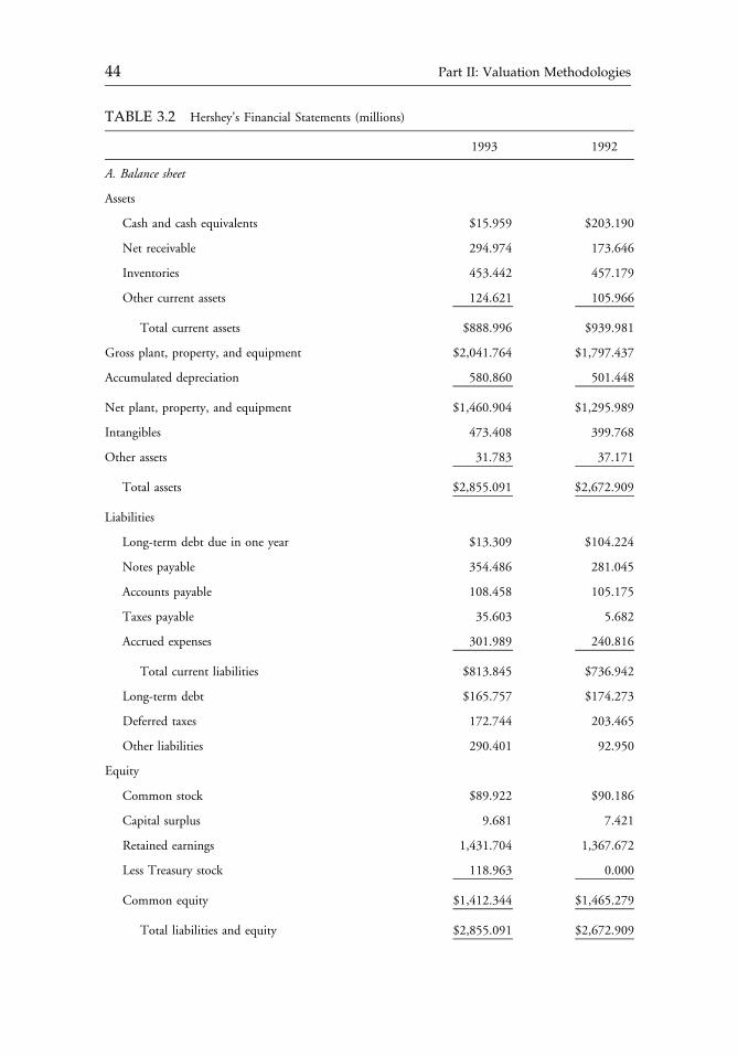
TABLE 3.2 Hershey’s Financial Statements (millions)
1993 1992
A. Balance sheet
Assets
Cash and cash equivalents $15.959 $203.190
Net receivable 294.974 173.646
Inventories 453.442 457.179
Other current assets 124.621 105.966
Total current assets $888.996 $939.981
Gross plant, property, and equipment $2,041.764 $1,797.437
Accumulated depreciation 580.860 501.448
Net plant, property, and equipment $1,460.904 $1,295.989
Intangibles 473.408 399.768
Other assets 31.783 37.171
Total assets $2,855.091 $2,672.909
Liabilities
Long-term debt due in one year $13.309 $104.224
Notes payable 354.486 281.045
Accounts payable 108.458 105.175
Taxes payable 35.603 5.682
Accrued expenses 301.989 240.816
Total current liabilities $813.845 $736.942
Long-term debt $165.757 $174.273
Deferred taxes 172.744 203.465
Other liabilities 290.401 92.950
Equity
Common stock $89.922 $90.186
Capital surplus 9.681 7.421
Retained earnings 1,431.704 1,367.672
Less Treasury stock 118.963 0.000
Common equity $1,412.344 $1,465.279
Total liabilities and equity $2,855.091 $2,672.909
c03 12 September 2012; 11:2:46
44 Part II: Valuation Methodologies
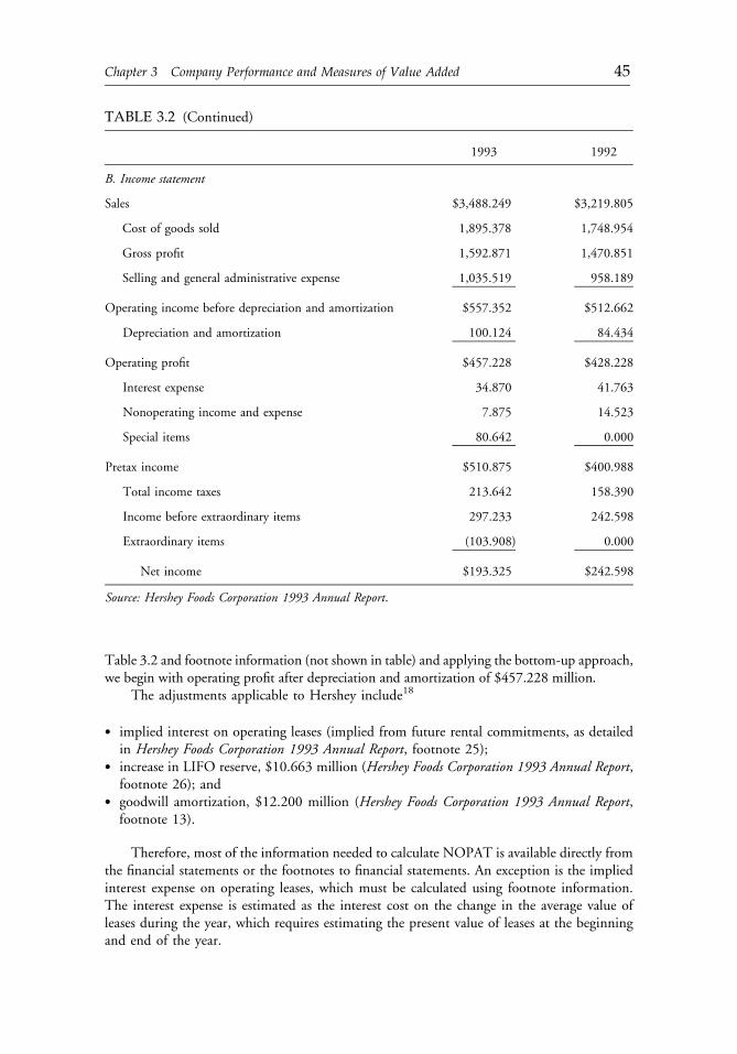
Table 3.2 and footnote information (not shown in table) and applying the bottom-up approach,we begin with operating profit after depreciation and amortization of $457.228 million.
The adjustments applicable to Hershey include18
� implied interest on operating leases (implied from future rental commitments, as detailedin Hershey Foods Corporation 1993 Annual Report, footnote 25);
� increase in LIFO reserve, $10.663 million (Hershey Foods Corporation 1993 Annual Report,footnote 26); and
� goodwill amortization, $12.200 million (Hershey Foods Corporation 1993 Annual Report,footnote 13).
Therefore, most of the information needed to calculate NOPAT is available directly fromthe financial statements or the footnotes to financial statements. An exception is the impliedinterest expense on operating leases, which must be calculated using footnote information.The interest expense is estimated as the interest cost on the change in the average value ofleases during the year, which requires estimating the present value of leases at the beginningand end of the year.
TABLE 3.2 (Continued)
1993 1992
B. Income statement
Sales $3,488.249 $3,219.805
Cost of goods sold 1,895.378 1,748.954
Gross profit 1,592.871 1,470.851
Selling and general administrative expense 1,035.519 958.189
Operating income before depreciation and amortization $557.352 $512.662
Depreciation and amortization 100.124 84.434
Operating profit $457.228 $428.228
Interest expense 34.870 41.763
Nonoperating income and expense 7.875 14.523
Special items 80.642 0.000
Pretax income $510.875 $400.988
Total income taxes 213.642 158.390
Income before extraordinary items 297.233 242.598
Extraordinary items (103.908) 0.000
Net income $193.325 $242.598
Source: Hershey Foods Corporation 1993 Annual Report.
c03 12 September 2012; 11:2:46
Chapter 3 Company Performance and Measures of Value Added 45
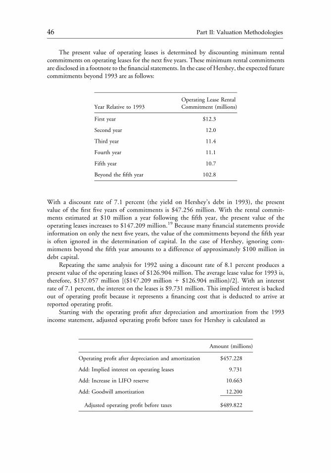
The present value of operating leases is determined by discounting minimum rentalcommitments on operating leases for the next five years. These minimum rental commitmentsare disclosed in a footnote to the financial statements. In the case of Hershey, the expected futurecommitments beyond 1993 are as follows:
Year Relative to 1993Operating Lease RentalCommitment (millions)
First year $12.3
Second year 12.0
Third year 11.4
Fourth year 11.1
Fifth year 10.7
Beyond the fifth year 102.8
With a discount rate of 7.1 percent (the yield on Hershey’s debt in 1993), the presentvalue of the first five years of commitments is $47.256 million. With the rental commit-ments estimated at $10 million a year following the fifth year, the present value of theoperating leases increases to $147.209 million.19 Because many financial statements provideinformation on only the next five years, the value of the commitments beyond the fifth yearis often ignored in the determination of capital. In the case of Hershey, ignoring com-mitments beyond the fifth year amounts to a difference of approximately $100 million indebt capital.
Repeating the same analysis for 1992 using a discount rate of 8.1 percent produces apresent value of the operating leases of $126.904 million. The average lease value for 1993 is,therefore, $137.057 million [($147.209 million 1 $126.904 million)/2]. With an interestrate of 7.1 percent, the interest on the leases is $9.731 million. This implied interest is backedout of operating profit because it represents a financing cost that is deducted to arrive atreported operating profit.
Starting with the operating profit after depreciation and amortization from the 1993income statement, adjusted operating profit before taxes for Hershey is calculated as
Amount (millions)
Operating profit after depreciation and amortization $457.228
Add: Implied interest on operating leases 9.731
Add: Increase in LIFO reserve 10.663
Add: Goodwill amortization 12.200
Adjusted operating profit before taxes $489.822
c03 12 September 2012; 11:2:46
46 Part II: Valuation Methodologies
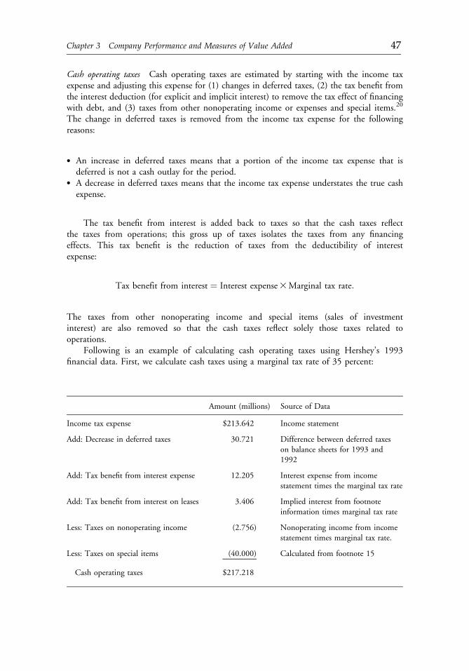
Cash operating taxes Cash operating taxes are estimated by starting with the income taxexpense and adjusting this expense for (1) changes in deferred taxes, (2) the tax benefit fromthe interest deduction (for explicit and implicit interest) to remove the tax effect of financingwith debt, and (3) taxes from other nonoperating income or expenses and special items.20
The change in deferred taxes is removed from the income tax expense for the followingreasons:
� An increase in deferred taxes means that a portion of the income tax expense that isdeferred is not a cash outlay for the period.
� A decrease in deferred taxes means that the income tax expense understates the true cashexpense.
The tax benefit from interest is added back to taxes so that the cash taxes reflectthe taxes from operations; this gross up of taxes isolates the taxes from any financingeffects. This tax benefit is the reduction of taxes from the deductibility of interestexpense:
Tax benefit from interest ¼ Interest expense3Marginal tax rate:
The taxes from other nonoperating income and special items (sales of investmentinterest) are also removed so that the cash taxes reflect solely those taxes related tooperations.
Following is an example of calculating cash operating taxes using Hershey’s 1993financial data. First, we calculate cash taxes using a marginal tax rate of 35 percent:
Amount (millions) Source of Data
Income tax expense $213.642 Income statement
Add: Decrease in deferred taxes 30.721 Difference between deferred taxeson balance sheets for 1993 and1992
Add: Tax benefit from interest expense 12.205 Interest expense from incomestatement times the marginal tax rate
Add: Tax benefit from interest on leases 3.406 Implied interest from footnoteinformation times marginal tax rate
Less: Taxes on nonoperating income (2.756) Nonoperating income from incomestatement times marginal tax rate.
Less: Taxes on special items (40.000) Calculated from footnote 15
Cash operating taxes $217.218
c03 12 September 2012; 11:2:46
Chapter 3 Company Performance and Measures of Value Added 47
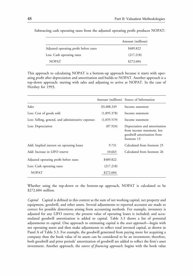
Subtracting cash operating taxes from the adjusted operating profit produces NOPAT:
Amount (millions)
Adjusted operating profit before taxes $489.822
Less: Cash operating taxes (217.218)
NOPAT $272.604
This approach to calculating NOPAT is a bottom-up approach because it starts with oper-ating profit after depreciation and amortization and builds to NOPAT. Another approach is atop-down approach: starting with sales and adjusting to arrive at NOPAT. In the case ofHershey for 1993,
Amount (millions) Source of Information
Sales $3,488.249 Income statement
Less: Cost of goods sold (1,895.378) Income statement
Less: Selling, general, and administrative expenses (1,035.519) Income statement
Less: Depreciation (87.924) Depreciation and amortizationfrom income statement, lessgoodwill amortization fromfootnote 13
Add: Implied interest on operating leases 9.731 Calculated from footnote 25
Add: Increase in LIFO reserve 10.663 Calculated from footnote 26
Adjusted operating profit before taxes $489.822
Less: Cash operating taxes (217.218)
NOPAT $272.604
Whether using the top-down or the bottom-up approach, NOPAT is calculated to be$272.604 million.
Capital Capital is defined in this context as the sum of net working capital, net property andequipment, goodwill, and other assets. Several adjustments to reported accounts are made tocorrect for possible distortions arising from accounting methods. For example, inventory isadjusted for any LIFO reserve; the present value of operating leases is included; and accu-mulated goodwill amortization is added to capital. Table 3.3 shows a list of potentialadjustments to capital. One approach to estimating capital is the asset approach—begin withnet operating assets and then make adjustments to reflect total invested capital, as shown inPanel A of Table 3.3. For example, the goodwill generated from paying more for acquiring acompany than the book value of its assets can be considered to be an investment; therefore,both goodwill and prior periods’ amortization of goodwill are added to reflect the firm’s assetinvestment. Another approach, the source of financing approach, begins with the book value
c03 12 September 2012; 11:2:46
48 Part II: Valuation Methodologies
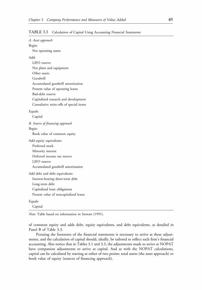
of common equity and adds debt, equity equivalents, and debt equivalents, as detailed inPanel B of Table 3.3.
Perusing the footnotes of the financial statements is necessary to arrive at these adjust-ments, and the calculation of capital should, ideally, be tailored to reflect each firm’s financialaccounting. Also notice that in Tables 3.1 and 3.3, the adjustments made to arrive at NOPAThave companion adjustments to arrive at capital. And as with the NOPAT calculations,capital can be calculated by starting at either of two points: total assets (the asset approach) orbook value of equity (sources of financing approach).
TABLE 3.3 Calculation of Capital Using Accounting Financial Statements
A. Asset approach
Begin:
Net operating assets
Add:
LIFO reserve
Net plant and equipment
Other assets
Goodwill
Accumulated goodwill amortization
Present value of operating leases
Bad-debt reserve
Capitalized research and development
Cumulative write-offs of special items
Equals:
Capital
B. Source of financing approach
Begin:
Book value of common equity
Add equity equivalents:
Preferred stock
Minority interest
Deferred income tax reserve
LIFO reserve
Accumulated goodwill amortization
Add debt and debt equivalents:
Interest-bearing short-term debt
Long-term debt
Capitalized lease obligations
Present value of noncapitalized leases
Equals:
Capital
Note: Table based on information in Stewart (1991).
c03 12 September 2012; 11:2:46
Chapter 3 Company Performance and Measures of Value Added 49
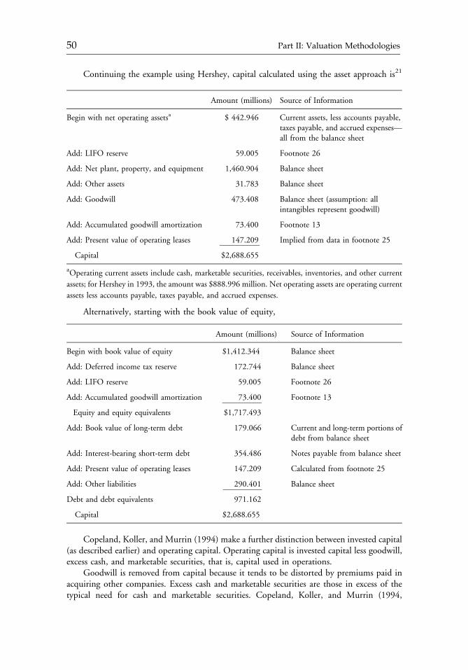
Continuing the example using Hershey, capital calculated using the asset approach is21
Amount (millions) Source of Information
Begin with net operating assetsa $ 442.946 Current assets, less accounts payable,taxes payable, and accrued expenses—all from the balance sheet
Add: LIFO reserve 59.005 Footnote 26
Add: Net plant, property, and equipment 1,460.904 Balance sheet
Add: Other assets 31.783 Balance sheet
Add: Goodwill 473.408 Balance sheet (assumption: allintangibles represent goodwill)
Add: Accumulated goodwill amortization 73.400 Footnote 13
Add: Present value of operating leases 147.209 Implied from data in footnote 25
Capital $2,688.655
aOperating current assets include cash, marketable securities, receivables, inventories, and other current
assets; for Hershey in 1993, the amount was $888.996 million. Net operating assets are operating current
assets less accounts payable, taxes payable, and accrued expenses.
Alternatively, starting with the book value of equity,
Amount (millions) Source of Information
Begin with book value of equity $1,412.344 Balance sheet
Add: Deferred income tax reserve 172.744 Balance sheet
Add: LIFO reserve 59.005 Footnote 26
Add: Accumulated goodwill amortization 73.400 Footnote 13
Equity and equity equivalents $1,717.493
Add: Book value of long-term debt 179.066 Current and long-term portions ofdebt from balance sheet
Add: Interest-bearing short-term debt 354.486 Notes payable from balance sheet
Add: Present value of operating leases 147.209 Calculated from footnote 25
Add: Other liabilities 290.401 Balance sheet
Debt and debt equivalents 971.162
Capital $2,688.655
Copeland, Koller, and Murrin (1994) make a further distinction between invested capital(as described earlier) and operating capital. Operating capital is invested capital less goodwill,excess cash, and marketable securities, that is, capital used in operations.
Goodwill is removed from capital because it tends to be distorted by premiums paid inacquiring other companies. Excess cash and marketable securities are those in excess of thetypical need for cash and marketable securities. Copeland, Koller, and Murrin (1994,
c03 12 September 2012; 11:2:47
50 Part II: Valuation Methodologies
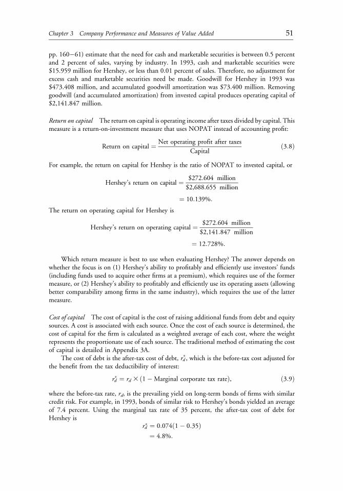
pp. 160�61) estimate that the need for cash and marketable securities is between 0.5 percentand 2 percent of sales, varying by industry. In 1993, cash and marketable securities were$15.959 million for Hershey, or less than 0.01 percent of sales. Therefore, no adjustment forexcess cash and marketable securities need be made. Goodwill for Hershey in 1993 was$473.408 million, and accumulated goodwill amortization was $73.400 million. Removinggoodwill (and accumulated amortization) from invested capital produces operating capital of$2,141.847 million.
Return on capital The return on capital is operating income after taxes divided by capital. Thismeasure is a return-on-investment measure that uses NOPAT instead of accounting profit:
Return on capital ¼ Net operating profit after taxes
Capitalð3:8Þ
For example, the return on capital for Hershey is the ratio of NOPAT to invested capital, or
Hershey’s return on capital ¼ $272:604 million
$2,688:655 million
¼ 10:139%:
The return on operating capital for Hershey is
Hershey’s return on operating capital ¼ $272:604 million
$2,141:847 million
¼ 12:728%:
Which return measure is best to use when evaluating Hershey? The answer depends onwhether the focus is on (1) Hershey’s ability to profitably and efficiently use investors’ funds(including funds used to acquire other firms at a premium), which requires use of the formermeasure, or (2) Hershey’s ability to profitably and efficiently use its operating assets (allowingbetter comparability among firms in the same industry), which requires the use of the lattermeasure.
Cost of capital The cost of capital is the cost of raising additional funds from debt and equitysources. A cost is associated with each source. Once the cost of each source is determined, thecost of capital for the firm is calculated as a weighted average of each cost, where the weightrepresents the proportionate use of each source. The traditional method of estimating the costof capital is detailed in Appendix 3A.
The cost of debt is the after-tax cost of debt, rd�, which is the before-tax cost adjusted for
the benefit from the tax deductibility of interest:
rd� ¼ rd 3 ð1�Marginal corporate tax rateÞ, ð3:9Þwhere the before-tax rate, rd, is the prevailing yield on long-term bonds of firms with similarcredit risk. For example, in 1993, bonds of similar risk to Hershey’s bonds yielded an averageof 7.4 percent. Using the marginal tax rate of 35 percent, the after-tax cost of debt forHershey is
rd� ¼ 0:074ð1� 0:35Þ¼ 4:8%:
c03 12 September 2012; 11:2:47
Chapter 3 Company Performance and Measures of Value Added 51
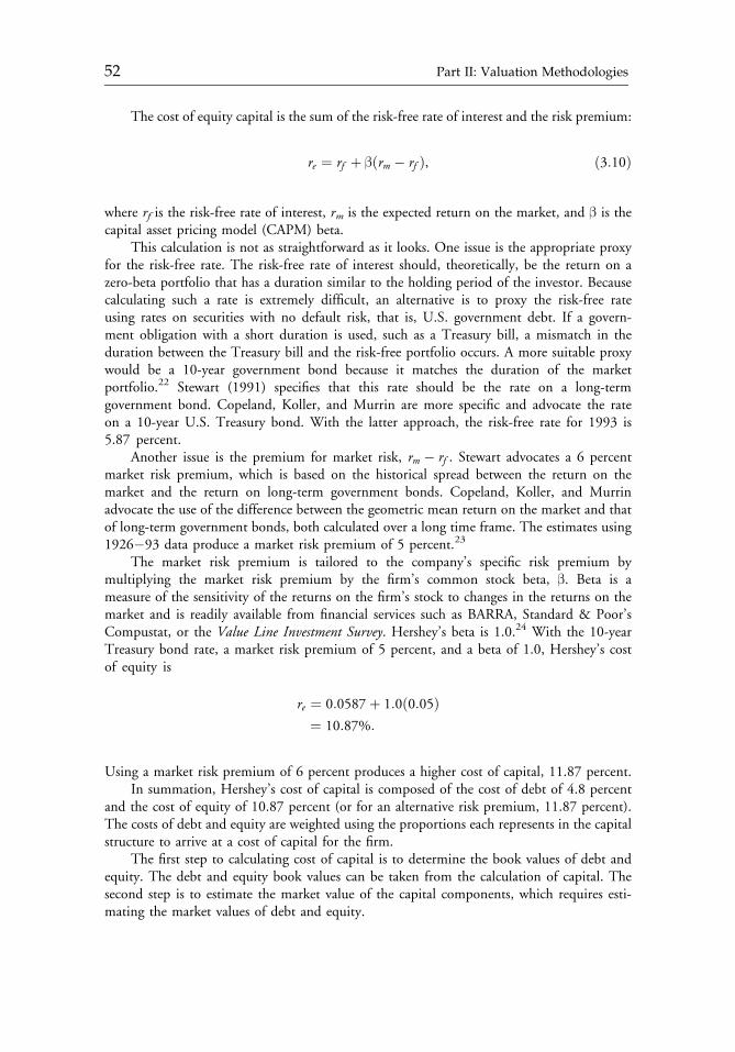
The cost of equity capital is the sum of the risk-free rate of interest and the risk premium:
re ¼ rf þ βðrm � rf Þ, ð3:10Þ
where rf is the risk-free rate of interest, rm is the expected return on the market, and β is thecapital asset pricing model (CAPM) beta.
This calculation is not as straightforward as it looks. One issue is the appropriate proxyfor the risk-free rate. The risk-free rate of interest should, theoretically, be the return on azero-beta portfolio that has a duration similar to the holding period of the investor. Becausecalculating such a rate is extremely difficult, an alternative is to proxy the risk-free rateusing rates on securities with no default risk, that is, U.S. government debt. If a govern-ment obligation with a short duration is used, such as a Treasury bill, a mismatch in theduration between the Treasury bill and the risk-free portfolio occurs. A more suitable proxywould be a 10-year government bond because it matches the duration of the marketportfolio.22 Stewart (1991) specifies that this rate should be the rate on a long-termgovernment bond. Copeland, Koller, and Murrin are more specific and advocate the rateon a 10-year U.S. Treasury bond. With the latter approach, the risk-free rate for 1993 is5.87 percent.
Another issue is the premium for market risk, rm � rf . Stewart advocates a 6 percentmarket risk premium, which is based on the historical spread between the return on themarket and the return on long-term government bonds. Copeland, Koller, and Murrinadvocate the use of the difference between the geometric mean return on the market and thatof long-term government bonds, both calculated over a long time frame. The estimates using1926�93 data produce a market risk premium of 5 percent.23
The market risk premium is tailored to the company’s specific risk premium bymultiplying the market risk premium by the firm’s common stock beta, β. Beta is ameasure of the sensitivity of the returns on the firm’s stock to changes in the returns on themarket and is readily available from financial services such as BARRA, Standard & Poor’sCompustat, or the Value Line Investment Survey. Hershey’s beta is 1.0.24 With the 10-yearTreasury bond rate, a market risk premium of 5 percent, and a beta of 1.0, Hershey’s costof equity is
re ¼ 0:0587þ 1:0ð0:05Þ¼ 10:87%:
Using a market risk premium of 6 percent produces a higher cost of capital, 11.87 percent.In summation, Hershey’s cost of capital is composed of the cost of debt of 4.8 percent
and the cost of equity of 10.87 percent (or for an alternative risk premium, 11.87 percent).The costs of debt and equity are weighted using the proportions each represents in the capitalstructure to arrive at a cost of capital for the firm.
The first step to calculating cost of capital is to determine the book values of debt andequity. The debt and equity book values can be taken from the calculation of capital. Thesecond step is to estimate the market value of the capital components, which requires esti-mating the market values of debt and equity.
c03 12 September 2012; 11:2:47
52 Part II: Valuation Methodologies
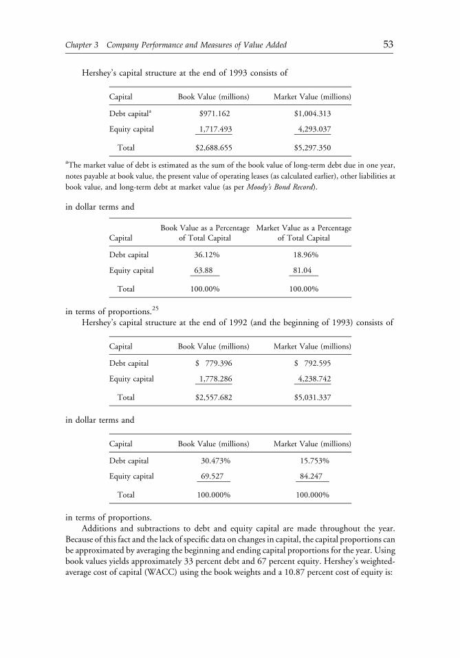
Hershey’s capital structure at the end of 1993 consists of
Capital Book Value (millions) Market Value (millions)
Debt capitala $971.162 $1,004.313
Equity capital 1,717.493 4,293.037
Total $2,688.655 $5,297.350
aThe market value of debt is estimated as the sum of the book value of long-term debt due in one year,
notes payable at book value, the present value of operating leases (as calculated earlier), other liabilities at
book value, and long-term debt at market value (as per Moody’s Bond Record).
in dollar terms and
CapitalBook Value as a Percentage
of Total CapitalMarket Value as a Percentage
of Total Capital
Debt capital 36.12% 18.96%
Equity capital 63.88 81.04
Total 100.00% 100.00%
in terms of proportions.25
Hershey’s capital structure at the end of 1992 (and the beginning of 1993) consists of
Capital Book Value (millions) Market Value (millions)
Debt capital $ 779.396 $ 792.595
Equity capital 1,778.286 4,238.742
Total $2,557.682 $5,031.337
in dollar terms and
Capital Book Value (millions) Market Value (millions)
Debt capital 30.473% 15.753%
Equity capital 69.527 84.247
Total 100.000% 100.000%
in terms of proportions.Additions and subtractions to debt and equity capital are made throughout the year.
Because of this fact and the lack of specific data on changes in capital, the capital proportions canbe approximated by averaging the beginning and ending capital proportions for the year. Usingbook values yields approximately 33 percent debt and 67 percent equity. Hershey’s weighted-average cost of capital (WACC) using the book weights and a 10.87 percent cost of equity is:
c03 12 September 2012; 11:2:47
Chapter 3 Company Performance and Measures of Value Added 53
Hershey’s WACC using book-value weights ¼ ½0:33ð0:048Þ� þ ½0:67ð0:1087Þ�¼ 0:0886 or 8:86%:
Using market-value weights, the cost of capital is greater because approximately 83 percent ofHershey’s capital is equity:
Hershey’s WACC using market-value weights ¼ ½0:17ð0:048Þ� þ ½0:83ð0:1087Þ�¼ 0:0984 or 9:84%:
Which value should be used, 8.86 percent or 9.84 percent? For most applications, oneshould choose the method that better reflects the marginal cost of funds. If the firm raises anadditional dollar of capital, in what proportion does it raise these funds? This question isusually thought of in terms of the market-value proportions—the 9.84 percent cost of capital.But in this particular application, the cost of capital is being applied against the investedcapital, which is most often stated in terms of book values. Mixing a market-value-determinedcost of capital with book value of invested capital results in distortions.26 Therefore, the book-value-weighted cost of capital is used here to determine economic profit.
Economic profit and performance Economic profit is the profit generated during the period inexcess of what is required by investors for the level of risk associated with the firm’s invest-ments. Economic profit is analogous to the net present value of capital budgeting andrepresents the value added by the firm’s management during the period.
Using the two equivalent economic profit calculations shows that Hershey’s managementgenerated an economic profit in 1993:
Hershey’s economic profit ¼ NOPAT � ðCost of capital3CapitalÞ¼ $272:604 million� ð0:08863 $2,688:655 millionÞ¼ $272:604 million� $238:215 million
¼ $34:389 million
or
Hershey’s economic profit ¼ ðRate of return� Cost of capitalÞ3Capital
¼ ð0:10139� 0:0886Þ3 $2; 688:655 million
¼ $34:389 million:
Hershey earned an economic profit of $34.389 million in 1993. In other words, Hershey’smanagement added value during 1993.
Although it seems that Hershey added value during the period, as represented by theestimate of economic profit, we should note that the estimate of economic profit is sensitive tothe estimate of the cost of capital. The cost of capital is something that is difficult to measure,as noted in Appendix 3A. Looking at a range of cost of capital, plus and minus 100 basispoints, gives an idea of this sensitivity:
Hershey’s economic profit if the cost of capital is 9:86%
¼ $272:604 million� $265:101 million
¼ $7:503 million:
c03 12 September 2012; 11:2:47
54 Part II: Valuation Methodologies
Hershey’s economic profit if the cost of capital is 7:86%
¼ $272:604 million� $211:328 million
¼ $61:276 million:
Consequently, drawing a conclusion regarding the degree of profitability depends, in largepart, on the estimated cost of capital.
Market Value Added
A measure closely related to economic profit is market value added. Market value added is thedifference between the firm’s market value and its capital. Essentially, market value added is ameasure of what the firm’s management has been able to do with a given level of resources(the invested capital):
Market value added ¼ Market value of the firm � Capital: ð3:11Þ
Like economic profit, market value added is expressed in terms of dollars, making thegoal of the firm to increase added value. Performance is evaluated by looking at the change inmarket value added over a period. The change in the market value added is a measure of howeffectively the firm’s management uses capital to enhance its value for all suppliers of capital,not simply common shareholders.27 The change in market value added is the change in themarket value of capital (debt and equity) less the change in the book value of capital.
Looking once again at Hershey, the following can be seen for 1992 and 1993:
Capital 1993 (millions) 1992 (millions)Change from 1992to 1993 (millions)
Market value of equity plus marketvalue of debt
$5,297.350 $5,031.337 $266.013
Less: Invested capital 2,688.655 2,557.682 130.973
Market value added $2,608.695 $2,473.655 $135.040
This analysis indicates that Hershey’s management has increased market value added in 1993by adding $135.040 million more in market value in excess of invested capital.28
In practice, the book value of debt and the book value of preferred stock are often used toestimate the market value of capital and the book value of capital.29 Therefore, the change inmarket value added from one year to the next amounts to the change in the market value ofcommon equity plus the change in the book value of debt and preferred stock.
Reconciling Economic Value Added with Market Value Added
Two approaches are used to measure value added: economic value added (economic profit)and market value added. Economic value added is based on adjusted operating earnings (aftertaxes), invested capital, and the firm’s WACC. Market value added is based on a comparisonof invested capital with the market value of capital. The two measures are both designed tohelp evaluate the performance of a firm.
c03 12 September 2012; 11:2:48
Chapter 3 Company Performance and Measures of Value Added 55
Moreover, a logical link exists between market value added and economic profit. Marketvalue added should be equal to the present value of future periods’ economic profit dis-counted at the cost of capital. Assuming that the firm will generate, in perpetuity, future-period economic profit equivalent to the current period’s economic profit, the relationbetween market value and economic profit is thus a simple one:
Market value added ¼ Economic profit
Cost of capital: ð3:12Þ
The perpetuity assumption is not valid for most firms, however, because of a very basic notion:Economic profits are generated only when a firm has some comparative or competitiveadvantage. Most firms cannot maintain these advantages for long periods of time; for example,government regulations change, patents are not perpetual, and demographics change—all ofwhich can erode a firm’s advantage and, hence, its economic profit. Therefore, the assumptionof a perpetual stream of the current period’s economic profit is not reasonable in most cases.
Another reason why the relation in Equation 3.12 does not hold in practice is that themethods of determining economic profit and market value added are quite different. Eco-nomic value added is a single-period measure that is estimated using accounting data and anestimated cost of capital. Market value added uses market values, which are more forward-looking estimates of performance than economic profit.
A final reason why Equation 3.12 does not hold true is that the estimates of economic profitare just that—estimates. Economic profit is estimatedby startingwith accounting data andmakingadjustments to better reflect economic reality. No matter how careful an analyst is in adjustingthe accounting data, the estimated economic profit cannot precisely reflect true economic profit.
Economic profit and market value added may result in conflicting evaluations of per-formance. For example, in 1993, General Electric Company ranked fourth among 1,000firms selected by Stern Stewart based on its market value added ($42 billion), which indicatesthat General Electric was one of the best firms in terms of providing value to its shareholders.But General Electric had a negative economic profit of $304 million, which implies that thefirm’s management was losing value.30 This apparent contradiction between economic profitand market value added may be because of the fact that economic profit, although theoret-ically forward looking, is based on historical, single-period accounting data and market valueadded is based on forward-looking stock prices.31 Therefore, Equation 3.12 is nonsensical inthe case in which there is an economic loss and a positive market value added.
Challenges in Applying Value-Added Measures
Even advocates of economic profit do not prescribe a particular formula for its calculation. Eachfirm is an individual case; the adjustments to arrive at operating profits after taxes are different foreach firm. Therefore, from the perspective of the financial analyst who must rely on financialstatements and other publicly available information to determine economic profit, applying EVAmeasures is difficult. Although a formula could be developed to deal with the most commonadjustments, exceptions to the general rules, which must be dealt with, will always exist.
Economic profit has ambiguous elements, most notably adjustments to operating incomeand cost of capital.32 These ambiguous elements result in several major problems whenapplying economic profit. First, two analysts may apply different formulas and draw differentconclusions regarding a firm’s relative performance.33 Second, when applied internally toreward management, economic profit is subject to potential manipulation. Unfortunately,
c03 12 September 2012; 11:2:48
56 Part II: Valuation Methodologies
manipulation is the problem that economic profit was developed to solve—avoiding mis-leading accounting measurements.34
Another problem with economic profit is how the cost of capital is calculated:
� The use of the CAPM. Most applications of economic profit use a CAPM-based cost ofequity. The CAPM has been challenged, however, as inadequately capturing the risk-returnrelationship.35
� The estimate of the market risk premium. In the applications prescribed by Stewart (1991), arisk premium of 6 percent is used, which contrasts with the lower risk premium of 5percent used by Copeland, Koller, and Murrin (1994). Does it matter? Using the 6 percentrisk premium produces a cost of capital for Hershey of 9.53 percent (instead of 8.86percent) and a lower economic profit.36
� The use of historical data. Some methods of calculating the WACC use historical-based datafor the cost of capital instead of the marginal cost. Using historical data is reflected in threeaspects of the cost-of-capital calculation: the use of a historical beta, the use of averages ofhistorical capital structure proportions, and the use of current yields on long-term debt (asopposed to expected yields). The estimated cost of capital is sensitive to the choice of data.
Whether these issues affect the assessment of performance and relative performance is, ofcourse, an empirical issue.
Holt’s Cfroi
To evaluate firm performance, an alternative to economic profit is a return-on- investmentmeasure known as theHOLTmethod.37 This measure, referred to as CFROI, is an IRRmeasurebut not in the traditional sense. The key difference between CFROI and the IRR typically seenin capital budgeting is that cash flows and investments are stated in constant monetary units inCFROI, which overcomes a deficiency of the traditional return-on-investment measures.
CFROI and other cash-focused measures are a promising approach to performancemeasurement.38 CFROI is, in essence, a rate of return. But as with other rate-of-returnmeasures, high CFROIs are neither good nor bad because the return on an investment, to beattractive, should compensate the investor for the investment’s risk. Therefore, when using areturn measure such as CFROI, a benchmark is also needed that reflects the amount of risk—the firm’s cost of capital.
CFROI Calculations
Basically six steps are involved in calculating a firm’s CFROI:
Step 1: Calculate the life of the assets.Step 2: Calculate gross cash flow.Step 3: Calculate gross cash investment.Step 4: Calculate the sum of nondepreciating assets.Step 5: Solve for the rate of return (CFROI).Step 6: Compare CFROI with the benchmark.
CFROI is the return on investment expected over the average life of the firm’s existing assets.The basic idea is that the firm has made current and past investment decisions that are expected togenerate future cash flows, andCFROI is a measure of the return on those investments. The grosscash flow (Step 2) is the estimate of the cash flow expected each year over the life of the assets.
c03 12 September 2012; 11:2:48
Chapter 3 Company Performance and Measures of Value Added 57
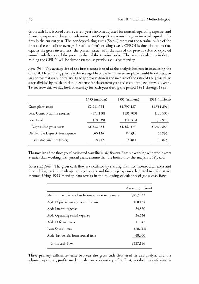
Gross cash flow is based on the current year’s income adjusted for noncash operating expenses andfinancing expenses. The gross cash investment (Step 3) represents the gross invested capital in thefirm in the current year. The nondepreciating assets (Step 4) represent the terminal value of thefirm at the end of the average life of the firm’s existing assets. CFROI is thus the return thatequates the gross investment (the present value) with the sum of the present value of expectedannual cash flows and the present value of the terminal value. The basic calculations in deter-mining the CFROI will be demonstrated, as previously, using Hershey.
Asset life The average life of the firm’s assets is used as the analysis horizon in calculating theCFROI. Determining precisely the average life of the firm’s assets-in-place would be difficult, soan approximation is necessary. One approximation is the median of the ratio of the gross plantassets divided by the depreciation expense for the current year and each of the two previous years.To see how this works, look at Hershey for each year during the period 1991 through 1993:
1993 (millions) 1992 (millions) 1991 (millions)
Gross plant assets $2,041.764 $1,797.437 $1,581.296
Less: Construction in progress (171.100) (196.900) (170.500)
Less: Land (48.239) (40.163) (37.911)
Depreciable gross assets $1,822.425 $1,560.374 $1,372.885
Divided by: Depreciation expense 100.124 84.434 72.735
Estimated asset life (years) 18.202 18.480 18.875
Themedian of the three years’ estimated asset life is 18.48 years. Becauseworkingwithwhole yearsis easier than working with partial years, assume that the horizon for the analysis is 18 years.
Gross cash flow The gross cash flow is calculated by starting with net income after taxes andthen adding back noncash operating expenses and financing expenses deducted to arrive at netincome. Using 1993 Hershey data results in the following calculation of gross cash flow:
Amount (millions)
Net income after tax but before extraordinary items $297.233
Add: Depreciation and amortization 100.124
Add: Interest expense 34.870
Add: Operating rental expense 24.524
Add: Deferred taxes 11.047
Less: Special item (80.642)
Add: Tax benefit from special item 40.000
Gross cash flow $427.156
Three primary differences exist between the gross cash flow used in this analysis and theadjusted operating profits used to calculate economic profits. First, goodwill amortization is
c03 12 September 2012; 11:2:48
58 Part II: Valuation Methodologies
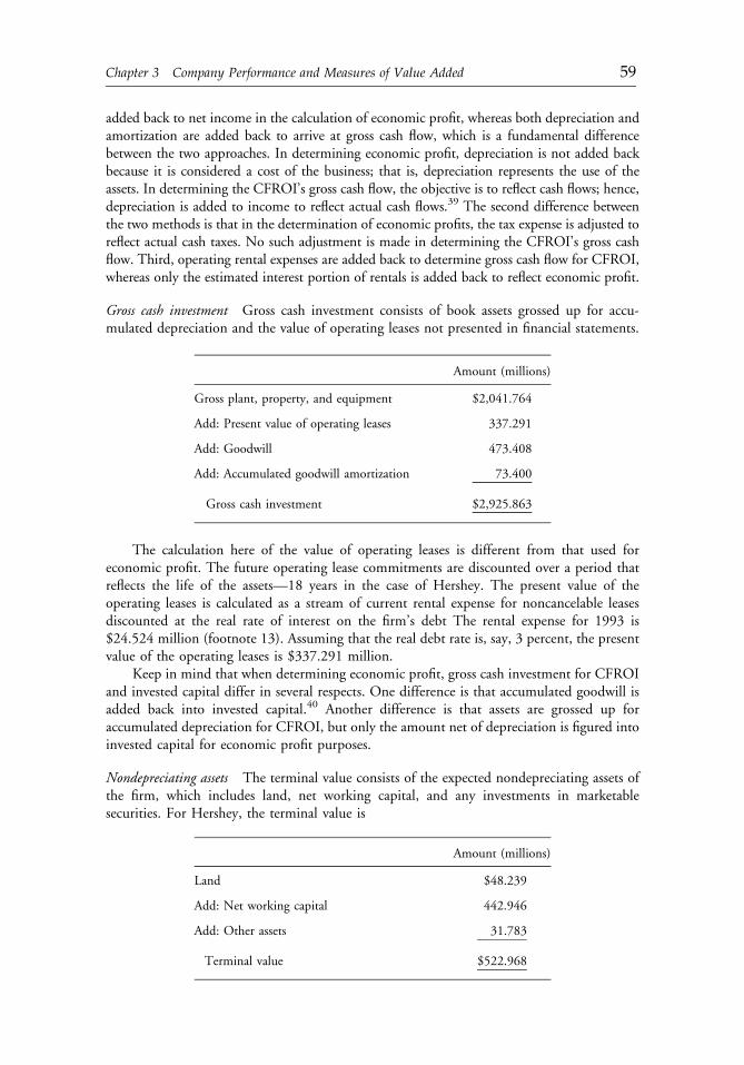
added back to net income in the calculation of economic profit, whereas both depreciation andamortization are added back to arrive at gross cash flow, which is a fundamental differencebetween the two approaches. In determining economic profit, depreciation is not added backbecause it is considered a cost of the business; that is, depreciation represents the use of theassets. In determining the CFROI’s gross cash flow, the objective is to reflect cash flows; hence,depreciation is added to income to reflect actual cash flows.39 The second difference betweenthe two methods is that in the determination of economic profits, the tax expense is adjusted toreflect actual cash taxes. No such adjustment is made in determining the CFROI’s gross cashflow. Third, operating rental expenses are added back to determine gross cash flow for CFROI,whereas only the estimated interest portion of rentals is added back to reflect economic profit.
Gross cash investment Gross cash investment consists of book assets grossed up for accu-mulated depreciation and the value of operating leases not presented in financial statements.
Amount (millions)
Gross plant, property, and equipment $2,041.764
Add: Present value of operating leases 337.291
Add: Goodwill 473.408
Add: Accumulated goodwill amortization 73.400
Gross cash investment $2,925.863
The calculation here of the value of operating leases is different from that used foreconomic profit. The future operating lease commitments are discounted over a period thatreflects the life of the assets—18 years in the case of Hershey. The present value of theoperating leases is calculated as a stream of current rental expense for noncancelable leasesdiscounted at the real rate of interest on the firm’s debt The rental expense for 1993 is$24.524 million (footnote 13). Assuming that the real debt rate is, say, 3 percent, the presentvalue of the operating leases is $337.291 million.
Keep in mind that when determining economic profit, gross cash investment for CFROIand invested capital differ in several respects. One difference is that accumulated goodwill isadded back into invested capital.40 Another difference is that assets are grossed up foraccumulated depreciation for CFROI, but only the amount net of depreciation is figured intoinvested capital for economic profit purposes.
Nondepreciating assets The terminal value consists of the expected nondepreciating assets ofthe firm, which includes land, net working capital, and any investments in marketablesecurities. For Hershey, the terminal value is
Amount (millions)
Land $48.239
Add: Net working capital 442.946
Add: Other assets 31.783
Terminal value $522.968
c03 12 September 2012; 11:2:48
Chapter 3 Company Performance and Measures of Value Added 59
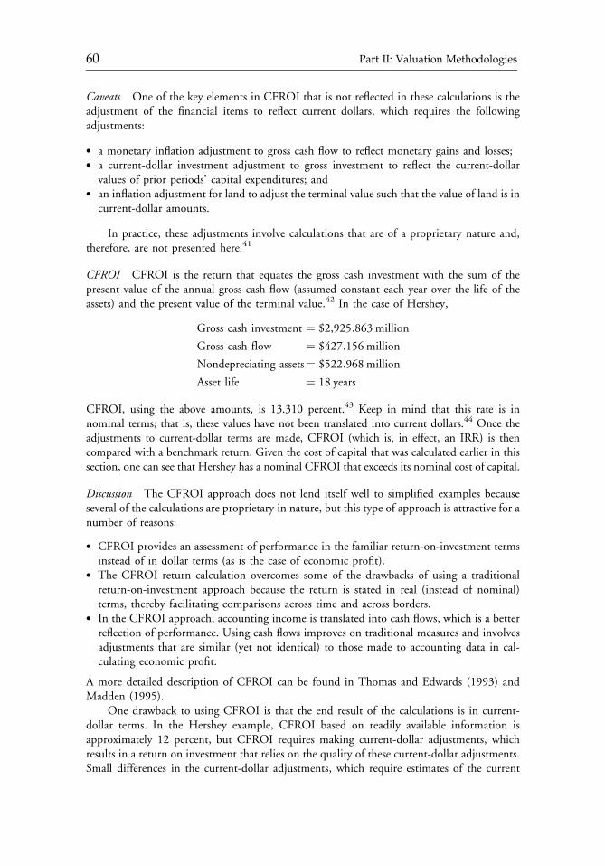
Caveats One of the key elements in CFROI that is not reflected in these calculations is theadjustment of the financial items to reflect current dollars, which requires the followingadjustments:
� a monetary inflation adjustment to gross cash flow to reflect monetary gains and losses;� a current-dollar investment adjustment to gross investment to reflect the current-dollar
values of prior periods’ capital expenditures; and� an inflation adjustment for land to adjust the terminal value such that the value of land is in
current-dollar amounts.
In practice, these adjustments involve calculations that are of a proprietary nature and,therefore, are not presented here.41
CFROI CFROI is the return that equates the gross cash investment with the sum of thepresent value of the annual gross cash flow (assumed constant each year over the life of theassets) and the present value of the terminal value.42 In the case of Hershey,
Gross cash investment ¼ $2,925:863 million
Gross cash flow ¼ $427:156 million
Nondepreciating assets¼ $522:968 million
Asset life ¼ 18 years
CFROI, using the above amounts, is 13.310 percent.43 Keep in mind that this rate is innominal terms; that is, these values have not been translated into current dollars.44 Once theadjustments to current-dollar terms are made, CFROI (which is, in effect, an IRR) is thencompared with a benchmark return. Given the cost of capital that was calculated earlier in thissection, one can see that Hershey has a nominal CFROI that exceeds its nominal cost of capital.
Discussion The CFROI approach does not lend itself well to simplified examples becauseseveral of the calculations are proprietary in nature, but this type of approach is attractive for anumber of reasons:
� CFROI provides an assessment of performance in the familiar return-on-investment termsinstead of in dollar terms (as is the case of economic profit).
� The CFROI return calculation overcomes some of the drawbacks of using a traditionalreturn-on-investment approach because the return is stated in real (instead of nominal)terms, thereby facilitating comparisons across time and across borders.
� In the CFROI approach, accounting income is translated into cash flows, which is a betterreflection of performance. Using cash flows improves on traditional measures and involvesadjustments that are similar (yet not identical) to those made to accounting data in cal-culating economic profit.
A more detailed description of CFROI can be found in Thomas and Edwards (1993) andMadden (1995).
One drawback to using CFROI is that the end result of the calculations is in current-dollar terms. In the Hershey example, CFROI based on readily available information isapproximately 12 percent, but CFROI requires making current-dollar adjustments, whichresults in a return on investment that relies on the quality of these current-dollar adjustments.Small differences in the current-dollar adjustments, which require estimates of the current
c03 12 September 2012; 11:2:49
60 Part II: Valuation Methodologies
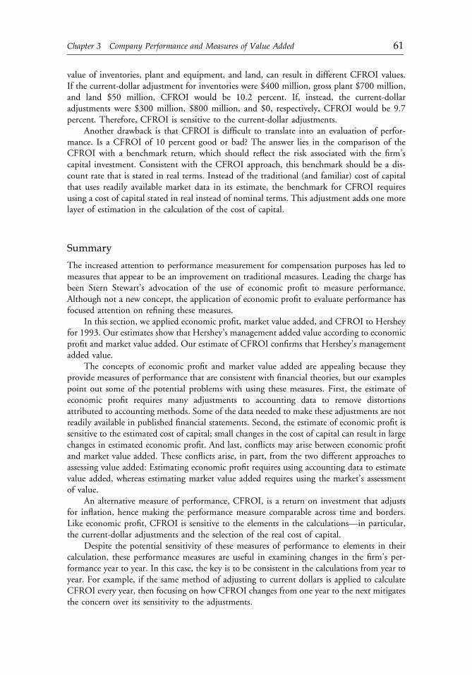
value of inventories, plant and equipment, and land, can result in different CFROI values.If the current-dollar adjustment for inventories were $400 million, gross plant $700 million,and land $50 million, CFROI would be 10.2 percent. If, instead, the current-dollaradjustments were $300 million, $800 million, and $0, respectively, CFROI would be 9.7percent. Therefore, CFROI is sensitive to the current-dollar adjustments.
Another drawback is that CFROI is difficult to translate into an evaluation of perfor-mance. Is a CFROI of 10 percent good or bad? The answer lies in the comparison of theCFROI with a benchmark return, which should reflect the risk associated with the firm’scapital investment. Consistent with the CFROI approach, this benchmark should be a dis-count rate that is stated in real terms. Instead of the traditional (and familiar) cost of capitalthat uses readily available market data in its estimate, the benchmark for CFROI requiresusing a cost of capital stated in real instead of nominal terms. This adjustment adds one morelayer of estimation in the calculation of the cost of capital.
Summary
The increased attention to performance measurement for compensation purposes has led tomeasures that appear to be an improvement on traditional measures. Leading the charge hasbeen Stern Stewart’s advocation of the use of economic profit to measure performance.Although not a new concept, the application of economic profit to evaluate performance hasfocused attention on refining these measures.
In this section, we applied economic profit, market value added, and CFROI to Hersheyfor 1993. Our estimates show that Hershey’s management added value according to economicprofit and market value added. Our estimate of CFROI confirms that Hershey’s managementadded value.
The concepts of economic profit and market value added are appealing because theyprovide measures of performance that are consistent with financial theories, but our examplespoint out some of the potential problems with using these measures. First, the estimate ofeconomic profit requires many adjustments to accounting data to remove distortionsattributed to accounting methods. Some of the data needed to make these adjustments are notreadily available in published financial statements. Second, the estimate of economic profit issensitive to the estimated cost of capital; small changes in the cost of capital can result in largechanges in estimated economic profit. And last, conflicts may arise between economic profitand market value added. These conflicts arise, in part, from the two different approaches toassessing value added: Estimating economic profit requires using accounting data to estimatevalue added, whereas estimating market value added requires using the market’s assessmentof value.
An alternative measure of performance, CFROI, is a return on investment that adjustsfor inflation, hence making the performance measure comparable across time and borders.Like economic profit, CFROI is sensitive to the elements in the calculations—in particular,the current-dollar adjustments and the selection of the real cost of capital.
Despite the potential sensitivity of these measures of performance to elements in theircalculation, these performance measures are useful in examining changes in the firm’s per-formance year to year. In this case, the key is to be consistent in the calculations from year toyear. For example, if the same method of adjusting to current dollars is applied to calculateCFROI every year, then focusing on how CFROI changes from one year to the next mitigatesthe concern over its sensitivity to the adjustments.
c03 12 September 2012; 11:2:49
Chapter 3 Company Performance and Measures of Value Added 61

Perhaps the greatest benefit from the value added and CFROI measures is their ability toshift the focus away from accounting profits and toward measures that more closely representtrue economic performance. The measures’ developers face challenges in devising methodsthat both remove accounting distortions from reported financial data and capture the truecosts of capital, but the discussion and debate surrounding these measures will help refinethem to better represent a firm’s performance.
COMPARISON OF ALTERNATIVE PERFORMANCE MEASURES
The ultimate test of a measure of performance for a publicly traded firm is its stock price—themarket’s collective judgment of the value of the company’s ownership interests. Therefore,our evaluation uses market performance measures as a benchmark.45 We believe that the goalof a firm’s management should be to maximize shareholder wealth. To that end, the per-formance of any firm should be judged using some type of share price performance measures.In this section, we compare both the traditional and recently developed value-added measureswith share price performance to gauge how well these measures reflect the market’s assessmentof performance.46 We cannot directly test how well these measures assess the performance of aparticular division, product line, or manager, but we can examine how these measures assessthe performance of a firm compared with market measures of performance, thus providinginformation on their usefulness.
The Sample
The empirical comparisons require stock price and financial statement data. Financialstatement data are taken from Standard & Poor’s Compustat, and stock price data are takenfrom the University of Chicago’s Center for Research in Security Prices (CRSP) databases.Several sample years are selected to examine the robustness of these measures for differentmarket and economic environments. We chose five sample years, 1988 through 1992.
The sample contains companies that satisfy the following criteria:
1. The company’s common stock traded on the New York Stock Exchange during thesample years.
2. The company is not in a financial or public utility line of business, based on StandardIndustrial Classification codes.
3. Monthly stock price data for the company are available in CRSP’s databases for thesample years.
4. Financial statement information is available for the company from Compustat’s annualindustrial and research databases for the sample years.47
5. The company’s fiscal year end is in December.
The first criterion allows for the comparison of our findings with published examples, thusproviding confidence in our results. The second criterion is necessary because several of themeasures are not applicable to financial or utility companies.48 The third criterion allows forthe calculation of the share price benchmarks. The fourth criterion allows for the calculationof the traditional and recently developed performance measures. Because several of the perfor-mance measures require detailed financial statement data, we perform the analysis for a differentnumber of firms each year based on availability of data. The last criterion permits comparisons of
c03 12 September 2012; 11:2:49
62 Part II: Valuation Methodologies
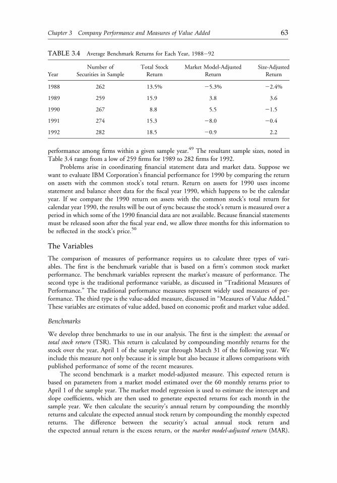
performance among firms within a given sample year.49 The resultant sample sizes, noted inTable 3.4 range from a low of 259 firms for 1989 to 282 firms for 1992.
Problems arise in coordinating financial statement data and market data. Suppose wewant to evaluate IBM Corporation’s financial performance for 1990 by comparing the returnon assets with the common stock’s total return. Return on assets for 1990 uses incomestatement and balance sheet data for the fiscal year 1990, which happens to be the calendaryear. If we compare the 1990 return on assets with the common stock’s total return forcalendar year 1990, the results will be out of sync because the stock’s return is measured over aperiod in which some of the 1990 financial data are not available. Because financial statementsmust be released soon after the fiscal year end, we allow three months for this information tobe reflected in the stock’s price.50
The Variables
The comparison of measures of performance requires us to calculate three types of vari-ables. The first is the benchmark variable that is based on a firm’s common stock marketperformance. The benchmark variables represent the market’s measure of performance. Thesecond type is the traditional performance variable, as discussed in “Traditional Measures ofPerformance.” The traditional performance measures represent widely used measures of per-formance. The third type is the value-added measure, discussed in “Measures of Value Added.”These variables are estimates of value added, based on economic profit and market value added.
Benchmarks
We develop three benchmarks to use in our analysis. The first is the simplest: the annual ortotal stock return (TSR). This return is calculated by compounding monthly returns for thestock over the year, April 1 of the sample year through March 31 of the following year. Weinclude this measure not only because it is simple but also because it allows comparisons withpublished performance of some of the recent measures.
The second benchmark is a market model-adjusted measure. This expected return isbased on parameters from a market model estimated over the 60 monthly returns prior toApril 1 of the sample year. The market model regression is used to estimate the intercept andslope coefficients, which are then used to generate expected returns for each month in thesample year. We then calculate the security’s annual return by compounding the monthlyreturns and calculate the expected annual stock return by compounding the monthly expectedreturns. The difference between the security’s actual annual stock return andthe expected annual return is the excess return, or the market model-adjusted return (MAR).
TABLE 3.4 Average Benchmark Returns for Each Year, 1988�92
YearNumber of
Securities in SampleTotal StockReturn
Market Model-AdjustedReturn
Size-AdjustedReturn
1988 262 13.5% 25.3% 22.4%
1989 259 15.9 3.8 3.6
1990 267 8.8 5.5 21.5
1991 274 15.3 28.0 20.4
1992 282 18.5 20.9 2.2
c03 12 September 2012; 11:2:49
Chapter 3 Company Performance and Measures of Value Added 63
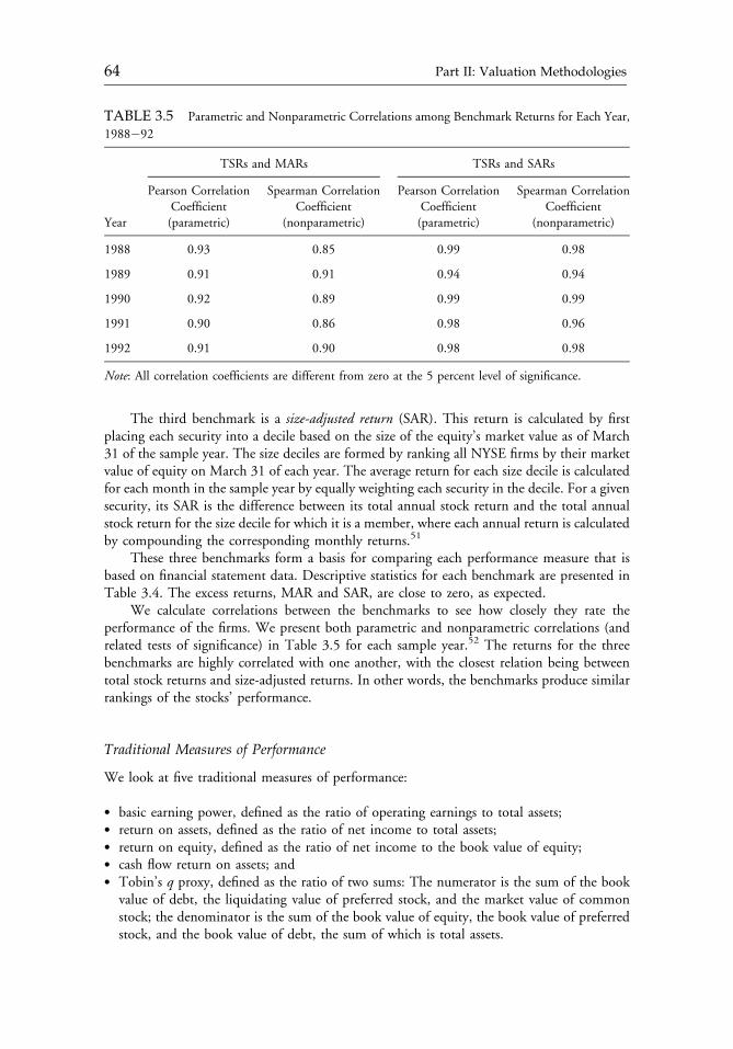
The third benchmark is a size-adjusted return (SAR). This return is calculated by firstplacing each security into a decile based on the size of the equity’s market value as of March31 of the sample year. The size deciles are formed by ranking all NYSE firms by their marketvalue of equity on March 31 of each year. The average return for each size decile is calculatedfor each month in the sample year by equally weighting each security in the decile. For a givensecurity, its SAR is the difference between its total annual stock return and the total annualstock return for the size decile for which it is a member, where each annual return is calculatedby compounding the corresponding monthly returns.51
These three benchmarks form a basis for comparing each performance measure that isbased on financial statement data. Descriptive statistics for each benchmark are presented inTable 3.4. The excess returns, MAR and SAR, are close to zero, as expected.
We calculate correlations between the benchmarks to see how closely they rate theperformance of the firms. We present both parametric and nonparametric correlations (andrelated tests of significance) in Table 3.5 for each sample year.52 The returns for the threebenchmarks are highly correlated with one another, with the closest relation being betweentotal stock returns and size-adjusted returns. In other words, the benchmarks produce similarrankings of the stocks’ performance.
Traditional Measures of Performance
We look at five traditional measures of performance:
� basic earning power, defined as the ratio of operating earnings to total assets;� return on assets, defined as the ratio of net income to total assets;� return on equity, defined as the ratio of net income to the book value of equity;� cash flow return on assets; and� Tobin’s q proxy, defined as the ratio of two sums: The numerator is the sum of the book
value of debt, the liquidating value of preferred stock, and the market value of commonstock; the denominator is the sum of the book value of equity, the book value of preferredstock, and the book value of debt, the sum of which is total assets.
TABLE 3.5 Parametric and Nonparametric Correlations among Benchmark Returns for Each Year,
1988�92
TSRs and MARs TSRs and SARs
Year
Pearson CorrelationCoefficient(parametric)
Spearman CorrelationCoefficient
(nonparametric)
Pearson CorrelationCoefficient(parametric)
Spearman CorrelationCoefficient
(nonparametric)
1988 0.93 0.85 0.99 0.98
1989 0.91 0.91 0.94 0.94
1990 0.92 0.89 0.99 0.99
1991 0.90 0.86 0.98 0.96
1992 0.91 0.90 0.98 0.98
Note: All correlation coefficients are different from zero at the 5 percent level of significance.
c03 12 September 2012; 11:2:49
64 Part II: Valuation Methodologies
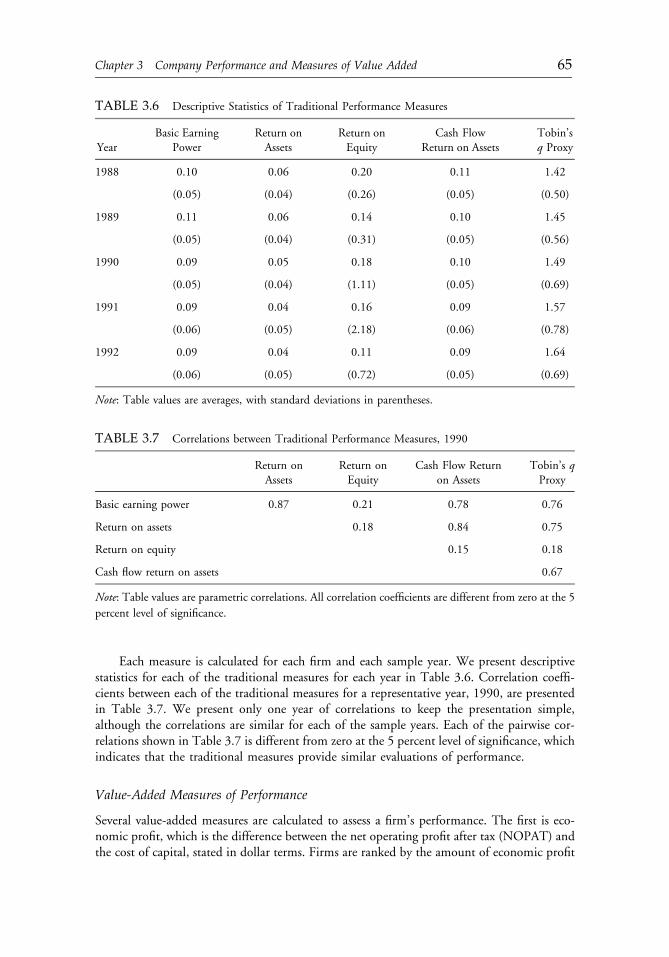
Each measure is calculated for each firm and each sample year. We present descriptivestatistics for each of the traditional measures for each year in Table 3.6. Correlation coeffi-cients between each of the traditional measures for a representative year, 1990, are presentedin Table 3.7. We present only one year of correlations to keep the presentation simple,although the correlations are similar for each of the sample years. Each of the pairwise cor-relations shown in Table 3.7 is different from zero at the 5 percent level of significance, whichindicates that the traditional measures provide similar evaluations of performance.
Value-Added Measures of Performance
Several value-added measures are calculated to assess a firm’s performance. The first is eco-nomic profit, which is the difference between the net operating profit after tax (NOPAT) andthe cost of capital, stated in dollar terms. Firms are ranked by the amount of economic profit
TABLE 3.6 Descriptive Statistics of Traditional Performance Measures
YearBasic Earning
PowerReturn onAssets
Return onEquity
Cash FlowReturn on Assets
Tobin’sq Proxy
1988 0.10 0.06 0.20 0.11 1.42
(0.05) (0.04) (0.26) (0.05) (0.50)
1989 0.11 0.06 0.14 0.10 1.45
(0.05) (0.04) (0.31) (0.05) (0.56)
1990 0.09 0.05 0.18 0.10 1.49
(0.05) (0.04) (1.11) (0.05) (0.69)
1991 0.09 0.04 0.16 0.09 1.57
(0.06) (0.05) (2.18) (0.06) (0.78)
1992 0.09 0.04 0.11 0.09 1.64
(0.06) (0.05) (0.72) (0.05) (0.69)
Note: Table values are averages, with standard deviations in parentheses.
TABLE 3.7 Correlations between Traditional Performance Measures, 1990
Return onAssets
Return onEquity
Cash Flow Returnon Assets
Tobin’s qProxy
Basic earning power 0.87 0.21 0.78 0.76
Return on assets 0.18 0.84 0.75
Return on equity 0.15 0.18
Cash flow return on assets 0.67
Note: Table values are parametric correlations. All correlation coefficients are different from zero at the 5
percent level of significance.
c03 12 September 2012; 11:2:50
Chapter 3 Company Performance and Measures of Value Added 65
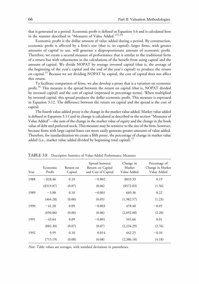
that is generated in a period. Economic profit is defined in Equation 3.6 and is calculated herein the manner described in “Measures of Value Added.”53,54
Economic profit is the dollar amount of value added during a period. By construction,economic profit is affected by a firm’s size (that is, its capital); larger firms, with greateramounts of capital to use, will generate a disproportionate amount of economic profit.Therefore, we create a second measure of performance that is similar to the traditional formof a return but with refinements in the calculations of the benefit from using capital and theamount of capital. We divide NOPAT by average invested capital (that is, the average ofthe beginning of the year’s capital and the end of the year’s capital) to produce the returnon capital.55 Because we are dividing NOPAT by capital, the cost of capital does not affectthis return.
To facilitate comparison of firms, we also develop a proxy that is a variation on economicprofit.56 This measure is the spread between the return on capital (that is, NOPAT dividedby invested capital) and the cost of capital (expressed in percentage terms). When multipliedby invested capital, this spread produces the dollar economic profit. This measure is expressedin Equation 3.12. The difference between the return on capital and the spread is the cost ofcapital.
The fourth value-added proxy is the change in the market value added.Market value addedis defined in Equation 3.11 and its change is calculated as described in the section “Measures ofValue Added”—the sum of the change in the market value of equity and the change in the bookvalue of debt and preferred stock. This measure may be sensitive to the size of the firm, however,because firms with large capital bases can more easily generate greater amounts of value added.Therefore, for standardization we create a fifth proxy, the percentage of change in market valueadded (i.e., market value added divided by beginning total capital).57
TABLE 3.8 Descriptive Statistics of Value-Added Performance Measures
YearEconomicProfit
Return onCapital
Spread betweenReturn on Capitaland Cost of Capital
Change inMarket
Value Added
Percentage ofChange in Market
Value Added
1988 2$28.46 0.10 20.002 $833.33 0.19
($319.87) (0.07) (0.06) ($572.03) (1.56)
1989 23.88 0.10 20.001 669.36 0.22
(464.28) (0.06) (0.05) (1,982.57) (1.23)
1990 241.28 0.09 20.003 478.40 20.05
(650.06) (0.06) (0.06) (2,692.00) (2.20)
1991 243.64 0.09 20.001 545.66 0.01
(882.30) (0.07) (0.07) (2,234.29) (2.76)
1992 9.95 0.10 0.014 442.25 20.10
(715.19) (0.08) (0.08) (2,386.18) (4.18)
Note: Table values are averages, with standard deviations in parentheses.
c03 12 September 2012; 11:2:50
66 Part II: Valuation Methodologies
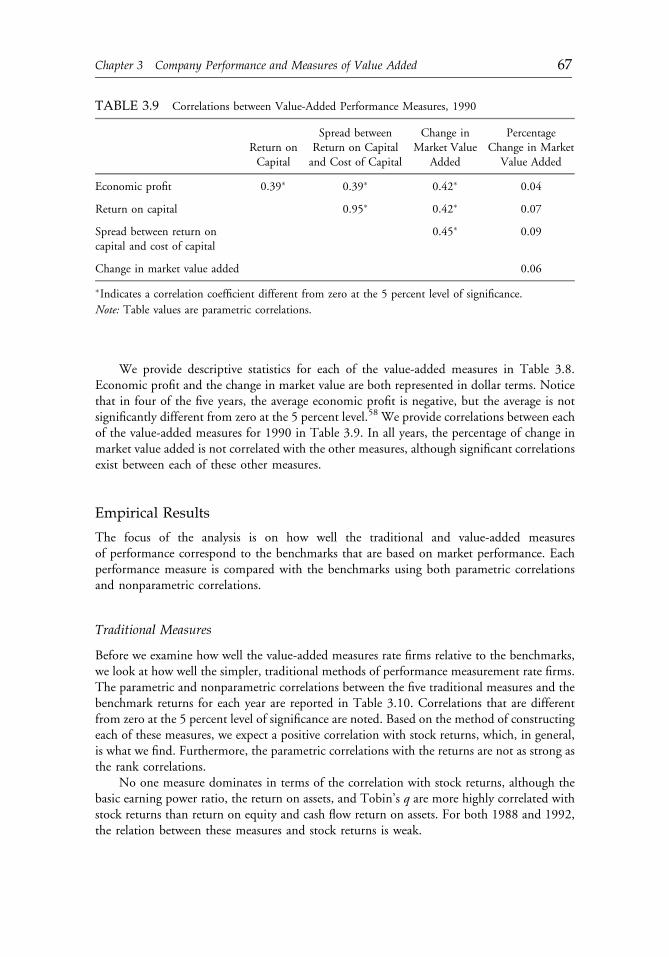
We provide descriptive statistics for each of the value-added measures in Table 3.8.Economic profit and the change in market value are both represented in dollar terms. Noticethat in four of the five years, the average economic profit is negative, but the average is notsignificantly different from zero at the 5 percent level.58 We provide correlations between eachof the value-added measures for 1990 in Table 3.9. In all years, the percentage of change inmarket value added is not correlated with the other measures, although significant correlationsexist between each of these other measures.
Empirical Results
The focus of the analysis is on how well the traditional and value-added measuresof performance correspond to the benchmarks that are based on market performance. Eachperformance measure is compared with the benchmarks using both parametric correlationsand nonparametric correlations.
Traditional Measures
Before we examine how well the value-added measures rate firms relative to the benchmarks,we look at how well the simpler, traditional methods of performance measurement rate firms.The parametric and nonparametric correlations between the five traditional measures and thebenchmark returns for each year are reported in Table 3.10. Correlations that are differentfrom zero at the 5 percent level of significance are noted. Based on the method of constructingeach of these measures, we expect a positive correlation with stock returns, which, in general,is what we find. Furthermore, the parametric correlations with the returns are not as strong asthe rank correlations.
No one measure dominates in terms of the correlation with stock returns, although thebasic earning power ratio, the return on assets, and Tobin’s q are more highly correlated withstock returns than return on equity and cash flow return on assets. For both 1988 and 1992,the relation between these measures and stock returns is weak.
TABLE 3.9 Correlations between Value-Added Performance Measures, 1990
Return onCapital
Spread betweenReturn on Capitaland Cost of Capital
Change inMarket Value
Added
PercentageChange in Market
Value Added
Economic profit 0.39� 0.39� 0.42� 0.04
Return on capital 0.95� 0.42� 0.07
Spread between return oncapital and cost of capital
0.45� 0.09
Change in market value added 0.06
�Indicates a correlation coefficient different from zero at the 5 percent level of significance.
Note: Table values are parametric correlations.
c03 12 September 2012; 11:2:50
Chapter 3 Company Performance and Measures of Value Added 67
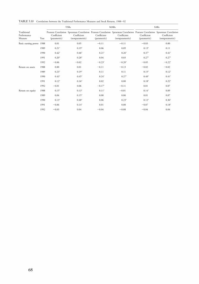
TABLE 3.10 Correlations between the Traditional Performance Measures and Stock Returns, 1988�92
TSRs MARs SARs
TraditionalPerformanceMeasure Year
Pearson CorrelationCoefficient(parametric)
Spearman CorrelationCoefficient
(nonparametric)
Pearson CorrelationCoefficient(parametric)
Spearman CorrelationCoefficient
(nonparametric)
Pearson CorrelationCoefficient(parametric)
Spearman CorrelationCoefficient
(nonparametric)
Basic earning power 1988 0.01 0.05 20.11 20.11 20.03 0.00
1989 0.21� 0.19� 0.06 0.09 0.13� 0.11
1990 0.42� 0.46� 0.21� 0.26� 0.37� 0.41�
1991 0.20� 0.20� 0.04 0.03 0.27� 0.27�
1992 20.06 20.02 20.23� 20.20� 20.05 20.22�
Return on assets 1988 0.00 0.01 20.11 20.13 20.02 20.02
1989 0.23� 0.19� 0.11 0.11 0.15� 0.12�
1990 0.43� 0.45� 0.24� 0.27� 0.40� 0.41�
1991 0.12� 0.16� 0.02 0.00 0.18� 0.22�
1992 20.01 0.06 20.17� 20.11 0.01 0.07
Return on equity 1988 0.15� 0.13� 0.11� 20.01 0.14� 0.09
1989 0.04 0.15� 0.00 0.06 0.01 0.07
1990 0.13� 0.40� 0.06 0.23� 0.12� 0.36�
1991 20.06 0.14� 0.01 0.00 20.07 0.18�
1992 20.03 0.04 20.04 20.08 20.04 0.04
c03 12 September 2012; 11:2:51
68

Cash flow returnon assets 1988 0.04 0.06 20.04 20.05 0.02 0.02
1989 0.09 0.18� 0.19� 0.13� 0.10 0.09
1990 0.31� 0.30� 0.15� 0.16� 0.27� 0.25�
1991 0.08 0.09 20.02 20.09 0.14� 0.16�
1992 0.04 0.06 20.11 20.09 0.06 0.08
Tobin’s q proxy 1988 0.13� 0.10 0.01 20.02 0.10 0.07
1989 0.27� 0.31� 0.12 0.18� 0.16� 0.20�
1990 0.45� 0.40� 0.29� 0.24� 0.41� 0.36�
1991 0.16� 0.16� 20.06 20.10 0.23� 0.24�
1992 0.00 0.05 20.20� 20.15� 0.00 0.04
�Indicates that the correlation coefficient is different from zero at the 5 percent level of significance.
c03 12 September 2012; 11:2:51
69
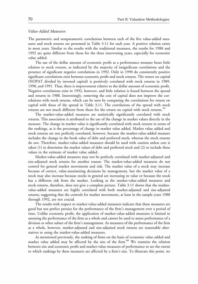
Value-Added Measures
The parametric and nonparametric correlations between each of the five value-added mea-sures and stock returns are presented in Table 3.11 for each year. A positive relation existsin most years. Similar to the results with the traditional measures, the results for 1988 and1992 are quite different from those for the three intervening years, especially for economicvalue added.
The use of the dollar amount of economic profit as a performance measure bears littlerelation to stock returns, as indicated by the majority of insignificant correlations and thepresence of significant negative correlations in 1992. Only in 1990 do consistently positivesignificant correlations exist between economic profit and stock returns. The return on capital(NOPAT divided by invested capital) is positively correlated with stock returns in 1989,1990, and 1991. Thus, there is improvement relative to the dollar amount of economic profit.Negative correlations exist in 1992, however, and little relation is found between the spreadand returns in 1988. Interestingly, removing the cost of capital does not improve the cor-relations with stock returns, which can be seen by comparing the correlations for return oncapital with those of the spread in Table 3.11. The correlations of the spread with stockreturns are not much different from those for the return on capital with stock returns.59
The market-value-added measures are statistically significantly correlated with stockreturns. This association is attributed to the use of the change in market values directly in themeasure. The change in market value is significantly correlated with stock returns in terms ofthe rankings, as is the percentage of change in market value added. Market value added andstock returns are not perfectly correlated, however, because the market-value-added measureincludes the change in the book value of debt and preferred stock, whereas the stock returnsdo not. Therefore, market-value-added measures should be used with caution unless care istaken (1) to determine the market values of debt and preferred stock and (2) to include thesevalues in the estimate of market value added.
Market-value-added measures may not be perfectly correlated with market-adjusted andsize-adjusted stock returns for another reason: The market-value-added measures do notcontrol for general market movements and risk. The market value of a stock may increasebecause of correct, value-maximizing decisions by management, but the market value of astock may also increase because stocks in general are increasing in value or because the stockhas a different risk from the market. Looking at the market-value-added measures andstock returns, therefore, does not give a complete picture. Table 3.11 shows that the market-value-added measures are highly correlated with both market-adjusted and size-adjustedreturns, suggesting that the controls for market movements, at least in the sample years 1988through 1992, are not crucial.
The results with respect to market-value-added measures indicate that these measures aregood but not perfect proxies for the performance of the firm’s management over a period oftime. Unlike economic profit, the application of market-value-added measures is limited toassessing the performance of the firm as a whole and cannot be used to assess performance of adivision or other subset of the firm’s management. As measures of the performance of the firmas a whole, however, market-adjusted and size-adjusted stock returns are reasonable alter-natives to using the market-value-added measures.
As mentioned previously, the ranking of firms on the basis of economic value added andmarket value added may be affected by the size of the firm.60 We examine the relationbetween size and economic profit and market-value measures of performance to see the extentto which rankings by these measures are affected by a firm’s size. To illustrate this point, we
c03 12 September 2012; 11:2:51
70 Part II: Valuation Methodologies
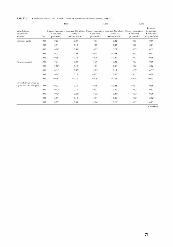
TABLE 3.11 Correlations between Value-Added Measures of Performance and Stock Returns, 1988�92
TSRs MARs SARs
Valued-AddedPerformanceMeasure Year
Pearson CorrelationCoefficient(parametric)
Spearman CorrelationCoefficient
(nonparametric)
Pearson CorrelationCoefficient(parametric)
Spearman CorrelationCoefficient
(nonparametric)
Pearson CorrelationCoefficient(parametric)
SpearmanCorrelationCoefficient
(nonparametric)
Economic profit 1988 0.02 0.07 20.03 20.04 0.02 0.05
1989 0.11 0.10 0.07 0.00 0.08 0.05
1990 0.26� 0.40� 0.23� 0.25� 0.27� 0.39
1991 0.02 0.08 20.03 20.04 0.03 0.12�
1992 20.15 20.12� 20.20� 20.21� 0.02 20.10
Return on capital 1988 0.01 0.08 20.09 20.04 20.03 0.05
1989 0.16� 0.15� 0.03 0.06 0.06 0.06
1990 0.41� 0.37� 0.24� 0.18 0.37� 0.33�
1991 0.14� 0.16� 20.01 0.00 0.21� 0.24�
1992 20.16� 20.11 20.29� 20.26� 20.14� 20.11
Spread between return oncapital and cost of capital 1988 20.02 0.10 20.08 20.04 20.01 0.06
1989 0.17� 0.19� 20.01 0.06 0.07 0.07
1990 0.42� 0.40� 0.23� 0.21� 0.37� 0.35�
1991 0.09 0.10 20.03 20.01 0.16� 0.16�
1992 20.15� 20.09 20.26� 20.21� 20.13� 20.09
(Continued)
c03 12 September 2012; 11:2:51
71
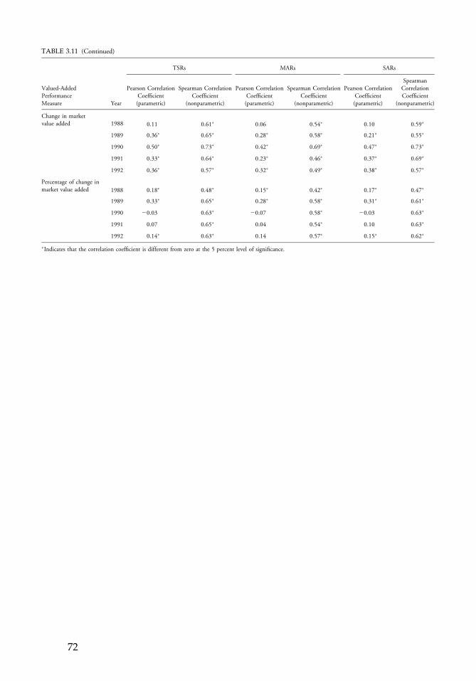
TABLE 3.11 (Continued)
TSRs MARs SARs
Valued-AddedPerformanceMeasure Year
Pearson CorrelationCoefficient(parametric)
Spearman CorrelationCoefficient
(nonparametric)
Pearson CorrelationCoefficient(parametric)
Spearman CorrelationCoefficient
(nonparametric)
Pearson CorrelationCoefficient(parametric)
SpearmanCorrelationCoefficient
(nonparametric)
Change in marketvalue added 1988 0.11 0.61� 0.06 0.54� 0.10 0.59�
1989 0.36� 0.65� 0.28� 0.58� 0.21� 0.55�
1990 0.50� 0.73� 0.42� 0.69� 0.47� 0.73�
1991 0.33� 0.64� 0.23� 0.46� 0.37� 0.69�
1992 0.36� 0.57� 0.32� 0.49� 0.38� 0.57�
Percentage of change inmarket value added 1988 0.18� 0.48� 0.15� 0.42� 0.17� 0.47�
1989 0.33� 0.65� 0.28� 0.58� 0.31� 0.61�
1990 20.03 0.63� 20.07 0.58� 20.03 0.63�
1991 0.07 0.65� 0.04 0.54� 0.10 0.63�
1992 0.14� 0.63� 0.14 0.57� 0.15� 0.62�
�Indicates that the correlation coefficient is different from zero at the 5 percent level of significance.
c03 12 September 2012; 11:2:52
72
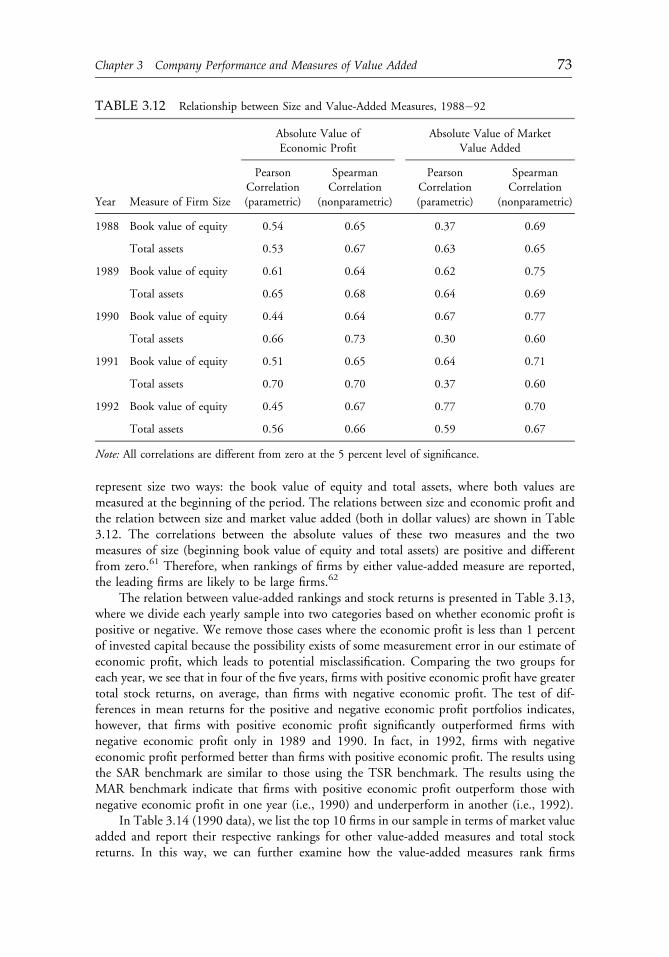
represent size two ways: the book value of equity and total assets, where both values aremeasured at the beginning of the period. The relations between size and economic profit andthe relation between size and market value added (both in dollar values) are shown in Table3.12. The correlations between the absolute values of these two measures and the twomeasures of size (beginning book value of equity and total assets) are positive and differentfrom zero.61 Therefore, when rankings of firms by either value-added measure are reported,the leading firms are likely to be large firms.62
The relation between value-added rankings and stock returns is presented in Table 3.13,where we divide each yearly sample into two categories based on whether economic profit ispositive or negative. We remove those cases where the economic profit is less than 1 percentof invested capital because the possibility exists of some measurement error in our estimate ofeconomic profit, which leads to potential misclassification. Comparing the two groups foreach year, we see that in four of the five years, firms with positive economic profit have greatertotal stock returns, on average, than firms with negative economic profit. The test of dif-ferences in mean returns for the positive and negative economic profit portfolios indicates,however, that firms with positive economic profit significantly outperformed firms withnegative economic profit only in 1989 and 1990. In fact, in 1992, firms with negativeeconomic profit performed better than firms with positive economic profit. The results usingthe SAR benchmark are similar to those using the TSR benchmark. The results using theMAR benchmark indicate that firms with positive economic profit outperform those withnegative economic profit in one year (i.e., 1990) and underperform in another (i.e., 1992).
In Table 3.14 (1990 data), we list the top 10 firms in our sample in terms of market valueadded and report their respective rankings for other value-added measures and total stockreturns. In this way, we can further examine how the value-added measures rank firms
TABLE 3.12 Relationship between Size and Value-Added Measures, 1988�92
Absolute Value ofEconomic Profit
Absolute Value of MarketValue Added
Year Measure of Firm Size
PearsonCorrelation(parametric)
SpearmanCorrelation
(nonparametric)
PearsonCorrelation(parametric)
SpearmanCorrelation
(nonparametric)
1988 Book value of equity 0.54 0.65 0.37 0.69
Total assets 0.53 0.67 0.63 0.65
1989 Book value of equity 0.61 0.64 0.62 0.75
Total assets 0.65 0.68 0.64 0.69
1990 Book value of equity 0.44 0.64 0.67 0.77
Total assets 0.66 0.73 0.30 0.60
1991 Book value of equity 0.51 0.65 0.64 0.71
Total assets 0.70 0.70 0.37 0.60
1992 Book value of equity 0.45 0.67 0.77 0.70
Total assets 0.56 0.66 0.59 0.67
Note: All correlations are different from zero at the 5 percent level of significance.
c03 12 September 2012; 11:2:52
Chapter 3 Company Performance and Measures of Value Added 73
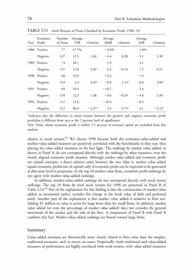
relative to stock returns.63 We choose 1990 because both the economic-value-added andmarket-value-added measures are positively correlated with the benchmarks in that year, thusplacing the value-added measures in the best light. The rankings by market value added, asshown in Panel A, do not correspond directly with the rankings by other measures, even theclosely aligned economic profit measure. Although market value added and economic profitare related concepts, a direct relation exists between the two (that is, market value addedequals economic profit/cost of capital) only if economic profit can be expected to be generatedat that same level in perpetuity. In the top 10 market-value firms, economic profit rankings donot agree with market-value-added rankings.
In addition, market-value-added rankings do not correspond directly with stock returnrankings. The top 10 firms by total stock returns for 1990 are presented in Panel B ofTable 3.14.64 Part of the explanation for this finding is that the construction of market valueadded, as mentioned earlier, includes the change in the book value of debt and preferredstock. Another part of the explanation is that market value added is sensitive to firm size:Adding $1 million in value is easier for large firms than for small firms. In addition, marketvalue added (or even the percentage of market value added) does not consider the generalmovement of the market and the risk of the firm. A comparison of Panel B with Panel Aconfirms this fact: Market-value-added rankings are biased toward large firms.
Summary
Value-added measures are theoretically more closely related to firm value than the simpler,traditional measures, such as return on assets. Empirically, both traditional and value-addedmeasures of performance are highly correlated with stock returns, with value-added measures
TABLE 3.13 Stock Returns of Firms Classified by Economic Profit, 1988�92
YearEconomicProfit
Numberof Firms
AverageTSR t-Statistic
AverageMAR t-Statistic
AverageSAR t-Statistic
1988 Positive 77 17.7% 23.4% 1.0%
Negative 147 12.5 1.64 24.4 0.28 23.1 1.30
1989 Positive 73 18.1 1.9 3.1
Negative 131 12.0 2.01� 2.4 20.14 1.5 0.51
1990 Positive 68 19.3 20.2 7.4
Negative 153 3.4 4.43� 28.0 2.15� 26.0 3.83�
1991 Positive 84 16.9 210.7 3.4
Negative 134 12.3 1.38 29.6 20.29 24.6 2.44�
1992 Positive 111 13.0 210.4 26.3
Negative 112 20.4 22.27� 3.5 23.75� 4.1 22.12�
�Indicates that the difference in mean returns between the positive and negative economic profit
portfolios is different from zero at the 5 percent level of significance.
Note: Firms whose economic profit is within 61 percent of invested capital are excluded from this
analysis.
c03 12 September 2012; 11:2:52
74 Part II: Valuation Methodologies
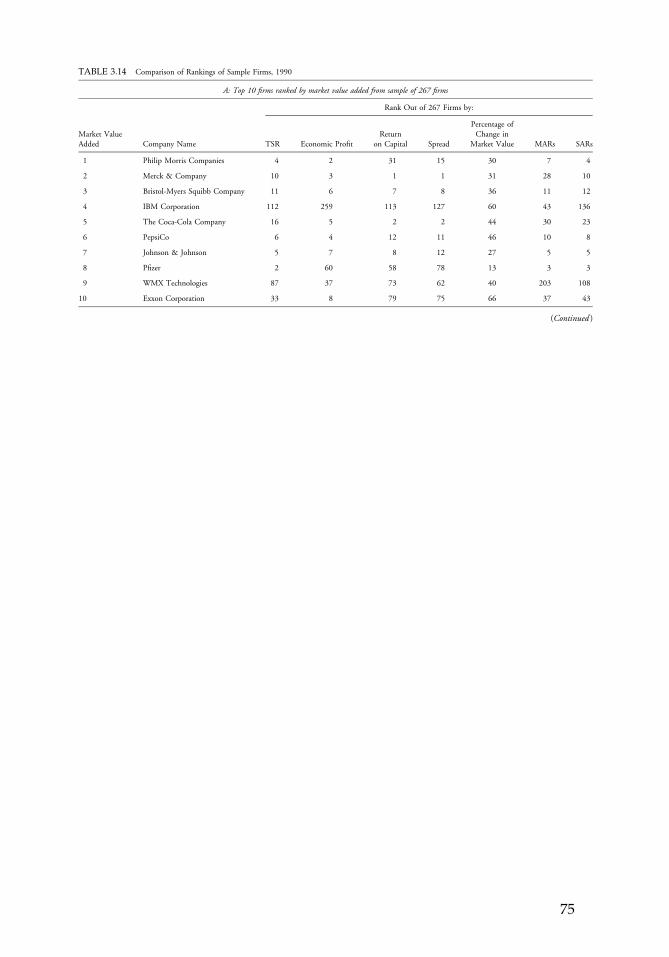
TABLE 3.14 Comparison of Rankings of Sample Firms, 1990
A: Top 10 firms ranked by market value added from sample of 267 firms
Rank Out of 267 Firms by:
Market ValueAdded Company Name TSR Economic Profit
Returnon Capital Spread
Percentage ofChange in
Market Value MARs SARs
1 Philip Morris Companies 4 2 31 15 30 7 4
2 Merck & Company 10 3 1 1 31 28 10
3 Bristol-Myers Squibb Company 11 6 7 8 36 11 12
4 IBM Corporation 112 259 113 127 60 43 136
5 The Coca-Cola Company 16 5 2 2 44 30 23
6 PepsiCo 6 4 12 11 46 10 8
7 Johnson & Johnson 5 7 8 12 27 5 5
8 Pfizer 2 60 58 78 13 3 3
9 WMX Technologies 87 37 73 62 40 203 108
10 Exxon Corporation 33 8 79 75 66 37 43
(Continued )
c03 12 September 2012; 11:2:52
75

TABLE 3.14 (Continued)
B: Top 10 firms ranked by TSRs from sample of 267 firms
Rank Out of 267 Firms by:
TSR Company Name Market Value Added Economic ProfitReturn
on Capital Spread
Percentage ofChange in
Market Value MARs SARs
1 Wendy’s International 75 154 154 221 5 1 1
2 Pfizer 8 60 58 783 13 3 3
3 Southwest Airlines Company 62 185 220 222 267 2 2
4 Philip Morris 1 2 31 15 30 7 4
5 Johnson & Johnson 7 7 8 12 27 5 5
6 PepsiCo 6 4 12 11 46 10 8
7 Safety-Kleen Corporation 48 87 61 84 17 6 6
8 Service Corporation International 52 108 151 113 11 4 7
9 Kellogg Company 18 27 24 21 38 15 9
10 Merck 2 3 1 1 31 28 10
c03 12 September 2012; 11:2:53
76
having a slight edge over the traditional measures. The commonly used value-added measures,economic profit and market value added, which have gained much attention in the financialpress, are only slightly more correlated with stock returns than the traditional measures andthus may not be better gauges of performance than traditional measures.
Enhancements to the value-added measures to reduce the effects of a size bias, such asusing the return on capital or the percentage of change in market value added, improvesomewhat the value-added measures and make them more attractive for performance eval-uation than the traditional measures. But because we stacked the deck against the traditionalmeasures in the empirical analysis by using the most naive form of these measures, making noadjustments in the reported accounting profit amounts and using end-of-period values fortotal assets and the book value of equity, it is disappointing that the more recently developedmeasures do not dominate the traditional measures.65
CONCLUSIONS
The aim of this analysis is to see whether the value-added measures when applied to the firmas a whole align with market measures of performance. If they do, confidence is gained inusing such measures to evaluate aspects of the firm’s management, such as a division or aproduct line. In particular, those measures that do not rely on market values (which wouldnot be available for such aspects as a division) are of particular interest. Return on capital,using the refinements in adjusting accounting data to better reflect economic reality, appearspromising. This measure correlates significantly with stock price performance and does notrely on market values in its construction, but we do not find that this measure is empiricallymore closely related to stock returns than the traditional measures. This finding suggests thatthe parsimonious, but less theoretically pleasing, traditional measures should not be elimi-nated from consideration in performance evaluation.
From the perspective of an analyst, do value-added measures add value? The change inmarket value added is correlated with stock returns. Should the analyst thus use market-value-added measures to evaluate the performance of a firm? Not necessarily. Market-value-addedmeasures may not be superior to stock returns for several reasons:
� Market-value-added measures, as strictly applied, suffer from a size bias. Even whenadjustments are made to reduce this bias, market-value-added measures do not adjust forevents outside the control of management, such as general market movements. On theother hand, simple adjustments can be made for market movements and security risk toimprove stock returns as a measure of performance.
� Stock returns are readily available measures of firm performance that do not depend onaccounting book values of capital. Stock returns can be calculated for any interval of timeand do not rely on the use of accounting values, which are made available at specificintervals of time (e.g., quarterly).
� Market value added, if computed using market values of all sources of capital (not simplythe market value of equity), reflects the performance of the firm in using all of its capitaland is, therefore, sensitive to changes in yields. Focusing instead on the market value ofequity, and hence on stock returns, does not avoid this problem completely because stockprices are also affected by market yields.
If the objective of the management of a firm is to maximize the value of equity, then stockreturns, adjusted for market movements and risk, are superior to market-value- added measures
c03 12 September 2012; 11:2:53
Chapter 3 Company Performance and Measures of Value Added 77
in evaluating a firm’s overall performance. From an analyst’s perspective, market-value-addedmeasures do not provide any information above that offered by stock returns, which is not tosay that the recently developed measures of economic profit and market value added are notworthwhile. Quite the contrary. The resurgence of attention on economic profit and away fromaccounting profit allows managers to focus on value creation rather than on short-sightedaccounting numbers.66 This shift in focus should ultimately enhance the value of the firm.
APPENDIX 3A THE FIRM’S COST OF CAPITAL
The cost of capital is the rate of return that a firm must earn to satisfy its suppliers of capital—debtholders and shareholders. The term “cost of capital” is a source of confusion, however, forseveral reasons. First is the issue of whether what is being referred to is the firm’s overall costof capital—that is, the cost of capital for all of the firm’s projects (past and present)—or thecost of capital for a specific project. The former is used in performance evaluation techniques,and the latter is used in capital budgeting applications for individual projects. In the lattercase, a project’s cost of capital is generally determined by first starting with the firm’s overallcost of capital and then tailoring this value to reflect the project’s relative riskiness.
Another source of confusion is whether what is being referred to is the marginal cost ofcapital or the embedded cost of capital. The marginal cost of capital is the cost of capital forraising the next dollar of capital. The marginal cost of capital is used in capital budgetingsituations when evaluating whether the project’s future cash flows outweigh the cost of thefunds to support those cash flows. The embedded cost of capital is the cost of funds alreadyraised—that is, what it costs the firm for the funds already supplied. In performance evalu-ation, an embedded rate is used because a specific period is being examined to see whether thefirm created value during that period. Whether the marginal cost of capital or the embeddedcost of capital is being calculated, however, the principles are the same; only the particularcosts of the sources of funds are slightly different.
Cost of Debt
The cost-of-debt capital is the after-tax cost of raising additional debt. Let rd represent the costof debt per year before considering the tax deductibility of interest, r�d represent the cost ofdebt after considering the tax deductibility of interest, and t be the marginal tax rate. Theeffective cost of debt is
rd� ¼ rd ð1� tÞ: ð3A:1Þ
The before-tax cost of debt is estimated as the current yield on debt with similarcredit risk, but a number of complications exist in estimating the current cost of debt. Thesecomplications include
� the yield on convertible debt;� debt with variable interest rates that contain rate caps and floors;� the yield on debt denominated in a foreign currency;� leases for which no current yield is defined; and� debt that is not rated.
c03 12 September 2012; 11:2:53
78 Part II: Valuation Methodologies
Cost of Preferred Stock
The cost of preferred stock is based on the valuation of a perpetuity. Let Pp indicate thepresent value of the preferred stock, Dp indicate the perpetual dividend per share per period,and rp indicate the discount rate. Then,
Pp ¼ DP
rp: ð3A:2Þ
Equation 3A.2 can be turned around to solve for rp, the cost of preferred stock, given Pp (thecurrent price) and Dp:
rp ¼Dp
Pp: ð3A:3Þ
The cost of preferred stock can be proxied by, for example, discounting the currentpreferred dividend by the current market price of the stock or by using yields on similarlyrated preferred stock.
The Cost of Common Equity
The cost of common stock is the cost of raising one more dollar of common equity capital,either internally from earnings retained in the firm or externally by issuing new shares ofcommon stock. Costs are associated with both internally and externally generated capital.How can internally generated capital (i.e., retained earnings) have a cost? As a firm generatesinternal funds, some portion is used to pay off creditors and preferred shareholders. Theremainder are funds owned by the common shareholders. The firm may either retain thesefunds (investing in assets) or pay them out to the shareholders in the form of cash dividends.
Shareholders require the firm to use retained earnings to generate a return that is at leastas large as the return they could have generated for themselves if they had received as divi-dends the amount of funds represented in the retained earnings. Therefore, retained funds arenot a free source of capital. The cost of internal equity funds is the opportunity cost of fundsof the firm’s shareholders. This opportunity cost is what shareholders could earn on thesefunds for the same level of risk.
The only difference between the cost of internally and externally generated funds isthe cost of issuing new common stock. The cost of internally generated funds is theopportunity cost of those funds—what shareholders could have earned on those funds. Butthe cost of externally generated funds (that is, funds from selling new shares of stock) includesthe sum of the opportunity cost and the cost of issuing the new stock (i.e., flotation costs). Fornow, ignore flotation costs.
The cost of issuing common stock is difficult to estimate because of the nature of the cashflow streams to common shareholders. Common shareholders receive their returns in theform of dividends and change in the price of the shares. The dividend stream is not fixed, as inthe case of preferred stock. How often and how much is paid as dividends is at the discretionof the board of directors. Therefore, this stream is unknown, so determining its value isdifficult. The change in the price of shares is also difficult to estimate; the price of the stock atany future point in time is influenced by investors’ expectations of cash flows beyond thatfuture point.
Nevertheless, two methods are commonly used to estimate the cost of common stock:The dividend valuation model (DVM) and the capital asset pricing model (CAPM). Each
c03 12 September 2012; 11:2:53
Chapter 3 Company Performance and Measures of Value Added 79
method relies on different assumptions regarding the cost of equity; each produces differentestimates of the cost of common equity.
The DVM states that the price of a share of stock, P, is the present value of all its futurecash dividends, where the future dividends are discounted at the required rate of return onequity, re:
67
P ¼ Dividends in first period
ð1þ reÞ1þDividends in second period
ð1þ reÞ2þ �? ð3A:4Þ
If these dividends are constant forever, the cost of common stock (the required return onequity, re) is derived from the value of a perpetuity. But common stock dividends do notusually remain constant. Dividends typically grow. Let D0 indicate this period’s dividend. Ifdividends grow at a constant rate, g, forever, the present value of the common stock is thepresent value of all future dividends:
P ¼ D0ð1þ gÞ1ð1þ reÞ1
þ D0ð1þ gÞ2ð1þ reÞ2
þ?þ D0ð1þ gÞNð1þ reÞN : ð3A:5Þ
Representing the next period’s dividend as D1 = D0 (1 1 g), this equation can besimplified to the familiar constant growth dividend model (or the Gordon model):68
P ¼ D01þ gre � g
¼ D1
re � g:
ð3A:6Þ
Rearranging this equation to solve for re produces
re ¼ D1
Pþ g ,
which shows that the cost of common stock is the sum of the next period’s dividend yield,D1/P, plus the growth rate of dividends.
An alternative way to estimate the cost of equity is to take a slightly different approach toanalyzing investors’ required rate of return: Assuming that what investors require is com-pensation for both the time value of money and for risk, the CAPM can be used to helpdetermine the cost of common equity.
Before figuring out how much investors should be compensated for risk, the type of riskmust be understood. The CAPM assumes an investor holds a diversified portfolio. The resultis that the only risk left in the portfolio as a whole is the risk related to movements in themarket as a whole; that is, the only relevant risk is market risk. The importance of thisassumption is that because investors bear only market risk, they need only be compensated formarket risk.
Assuming all shareholders hold diversified portfolios, the risk that is relevant in valuing afirm’s equity is its market risk. The greater the market risk, the greater the compensation (i.e.,higher yield) for bearing this risk.
c03 12 September 2012; 11:2:53
80 Part II: Valuation Methodologies
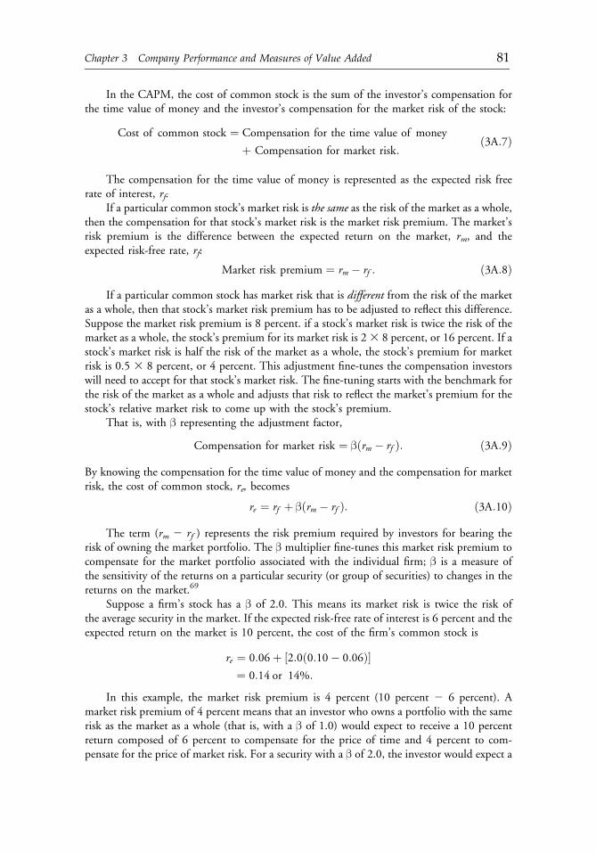
In the CAPM, the cost of common stock is the sum of the investor’s compensation forthe time value of money and the investor’s compensation for the market risk of the stock:
Cost of common stock ¼ Compensation for the time value of money
þ Compensation for market risk:ð3A:7Þ
The compensation for the time value of money is represented as the expected risk freerate of interest, rf.
If a particular common stock’s market risk is the same as the risk of the market as a whole,then the compensation for that stock’s market risk is the market risk premium. The market’srisk premium is the difference between the expected return on the market, rm, and theexpected risk-free rate, rf:
Market risk premium ¼ rm � rf : ð3A:8ÞIf a particular common stock has market risk that is different from the risk of the market
as a whole, then that stock’s market risk premium has to be adjusted to reflect this difference.Suppose the market risk premium is 8 percent. if a stock’s market risk is twice the risk of themarket as a whole, the stock’s premium for its market risk is 23 8 percent, or 16 percent. If astock’s market risk is half the risk of the market as a whole, the stock’s premium for marketrisk is 0.5 3 8 percent, or 4 percent. This adjustment fine-tunes the compensation investorswill need to accept for that stock’s market risk. The fine-tuning starts with the benchmark forthe risk of the market as a whole and adjusts that risk to reflect the market’s premium for thestock’s relative market risk to come up with the stock’s premium.
That is, with β representing the adjustment factor,
Compensation for market risk ¼ βðrm � rf Þ: ð3A:9Þ
By knowing the compensation for the time value of money and the compensation for marketrisk, the cost of common stock, re, becomes
re ¼ rf þ βðrm � rf Þ: ð3A:10Þ
The term (rm 2 rf ) represents the risk premium required by investors for bearing therisk of owning the market portfolio. The β multiplier fine-tunes this market risk premium tocompensate for the market portfolio associated with the individual firm; β is a measure ofthe sensitivity of the returns on a particular security (or group of securities) to changes in thereturns on the market.69
Suppose a firm’s stock has a β of 2.0. This means its market risk is twice the risk ofthe average security in the market. If the expected risk-free rate of interest is 6 percent and theexpected return on the market is 10 percent, the cost of the firm’s common stock is
re ¼ 0:06þ ½2:0ð0:10� 0:06Þ�¼ 0:14 or 14%:
In this example, the market risk premium is 4 percent (10 percent 2 6 percent). Amarket risk premium of 4 percent means that an investor who owns a portfolio with the samerisk as the market as a whole (that is, with a β of 1.0) would expect to receive a 10 percentreturn composed of 6 percent to compensate for the price of time and 4 percent to com-pensate for the price of market risk. For a security with a β of 2.0, the investor would expect a
c03 12 September 2012; 11:2:53
Chapter 3 Company Performance and Measures of Value Added 81
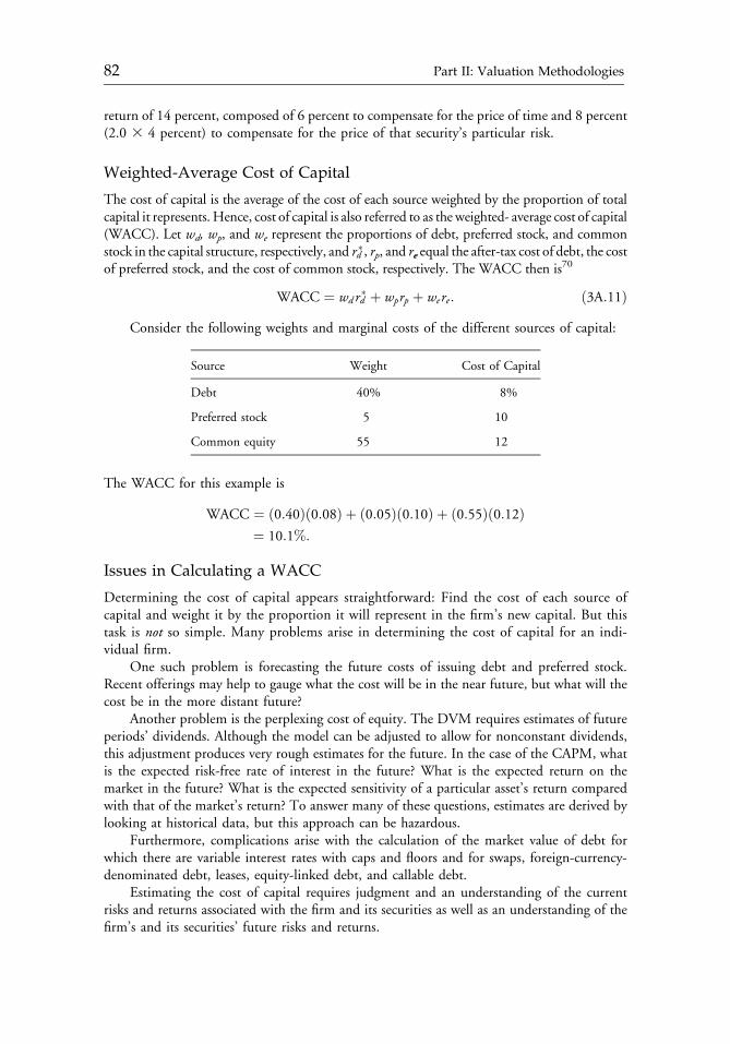
return of 14 percent, composed of 6 percent to compensate for the price of time and 8 percent(2.0 3 4 percent) to compensate for the price of that security’s particular risk.
Weighted-Average Cost of Capital
The cost of capital is the average of the cost of each source weighted by the proportion of totalcapital it represents.Hence, cost of capital is also referred to as the weighted- average cost of capital(WACC). Let wd, wp, and we represent the proportions of debt, preferred stock, and commonstock in the capital structure, respectively, and rd�, rp, and re equal the after-tax cost of debt, the costof preferred stock, and the cost of common stock, respectively. The WACC then is70
WACC ¼ wd rd� þ wprp þ were: ð3A:11ÞConsider the following weights and marginal costs of the different sources of capital:
Source Weight Cost of Capital
Debt 40% 8%
Preferred stock 5 10
Common equity 55 12
The WACC for this example is
WACC ¼ ð0:40Þð0:08Þ þ ð0:05Þð0:10Þ þ ð0:55Þð0:12Þ¼ 10:1%:
Issues in Calculating a WACC
Determining the cost of capital appears straightforward: Find the cost of each source ofcapital and weight it by the proportion it will represent in the firm’s new capital. But thistask is not so simple. Many problems arise in determining the cost of capital for an indi-vidual firm.
One such problem is forecasting the future costs of issuing debt and preferred stock.Recent offerings may help to gauge what the cost will be in the near future, but what will thecost be in the more distant future?
Another problem is the perplexing cost of equity. The DVM requires estimates of futureperiods’ dividends. Although the model can be adjusted to allow for nonconstant dividends,this adjustment produces very rough estimates for the future. In the case of the CAPM, whatis the expected risk-free rate of interest in the future? What is the expected return on themarket in the future? What is the expected sensitivity of a particular asset’s return comparedwith that of the market’s return? To answer many of these questions, estimates are derived bylooking at historical data, but this approach can be hazardous.
Furthermore, complications arise with the calculation of the market value of debt forwhich there are variable interest rates with caps and floors and for swaps, foreign-currency-denominated debt, leases, equity-linked debt, and callable debt.
Estimating the cost of capital requires judgment and an understanding of the currentrisks and returns associated with the firm and its securities as well as an understanding of thefirm’s and its securities’ future risks and returns.
c03 12 September 2012; 11:2:54
82 Part II: Valuation Methodologies
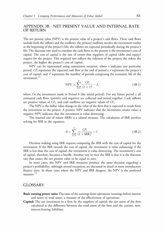
APPENDIX 3B NET PRESENT VALUE AND INTERNAL RATEOF RETURN
The net present value (NPV) is the present value of a project’s cash flows. These cash flowsinclude both the inflows and the outflows; the primary outflows involve the investment outlayat the beginning of the project’s life; the inflows are expected periodically during the project’slife. The discount rate used to translate the cash flows to the present is the investment’s cost ofcapital. The cost of capital is the rate of return that suppliers of capital (debt and equity)require for the project. This required rate reflects the riskiness of the project; the riskier theproject, the higher the project’s cost of capital.
NPV can be represented using summation notation, where t indicates any particularperiod, CFt represents the expected cash flow at the end of period t, r represents the project’scost of capital, and T represents the number of periods composing the economic life of theinvestment:71
NPV ¼XTt¼1
CFtð1þ rÞt � I , ð3B:1Þ
where I is the investment made in Period 0 (the initial period). For any future period t, allestimated cash flows (positive and negative) are collected and netted together. Cash inflowsare positive values of CFt, and cash outflows are negative values of CFt.
The NPV is the dollar value change in the value of the firm that is expected to result fromthe investment in the project. A positive NPV indicates that the investment creates value; anegative NPV indicates that the investment is value destroying.
The internal rate of return (IRR) is a related measure. The calculation of IRR involvessolving for IRR in the equation:
0 ¼XTt¼1
CFtð1þ IRRÞt � I : ð3B:2Þ
Decision making using IRR requires comparing the IRR with the cost of capital for theinvestment: If the IRR exceeds the cost of capital, the investment is value enhancing; if theIRR is less than the cost of capital, the investment is value destroying. The investment’s costof capital, therefore, becomes a hurdle. Another way to view the IRR is that it is the discountrate that causes the net present value to be equal to zero.
In most cases, the NPV and IRR measures produce the same decision regarding aproject’s profitability, although several exceptions are discussed in detail in most introductoryfinance texts. In those cases where the NPV and IRR disagree, the NPV is the preferredmeasure.72
GLOSSARY
Basic earning power ratio: The ratio of the earnings from operations (earnings before interestand taxes) to total assets; a measure of the effectiveness of operations.
Capital: The net investment in a firm by the suppliers of capital; the net assets of the firmcalculated as the difference between the total assets of the firm and the current, non-interest-bearing liabilities.
c03 12 September 2012; 11:2:54
Chapter 3 Company Performance and Measures of Value Added 83
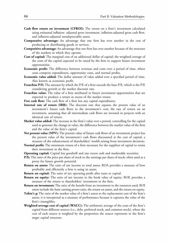
Cash flow return on investment (CFROI): The return on a firm’s investment calculatedusing estimated inflation- adjusted gross investment, inflation-adjusted gross cash flow,and inflation-adjusted nondepreciable assets.
Comparative advantage: An advantage that one firm has over another in the cost ofproducing or distributing goods or services.
Competitive advantage: An advantage that one firm has over another because of the structureof the markets in which they operate.
Cost of capital: The marginal cost of an additional dollar of capital; the weighted average ofthe costs of the capital expected to be raised by the firm to support future investmentopportunities.
Economic profit: The difference between revenues and costs over a period of time, wherecosts comprise expenditures, opportunity costs, and normal profits.
Economic value added: The dollar amount of value added over a specified period of time.Also known as economic profit.
Franchise P/E: The amount by which the P/E of a firm exceeds the base P/E, which is the P/Econsidering growth at the market discount rate.
Franchise value: The value of a firm attributed to future investment opportunities that areexpected to produce a return in excess of the market return.
Free cash flow: The cash flow of a firm less any capital expenditures.Internal rate of return (IRR): The discount rate that equates the present value of an
investment’s future cash flows to the investment’s cost; the rate of return on aninvestment, assuming that all intermediate cash flows are invested in projects with anidentical rate of return.
Market value added: The increase in the firm’s value over a period, controlling for the capitalused to generate the change in value; the difference between the market value of the firmand the value of the firm’s capital.
Net present value (NPV): The present value of future cash flows of an investment project lessthe present value of the investment’s cash flows discounted at the cost of capital; ameasure of the enhancement of shareholders’ wealth arising from investment decisions.
Normal profit: The minimum return of a firm necessary for the suppliers of capital to retaintheir investment in the firm.
Operating capital: Capital less goodwill and any excess cash and marketable securities.P/E: The ratio of the price per share of stock to the earnings per share of stock; often used as a
proxy for future growth potential.Return on assets: The ratio of net income to total assets; ROA provides a measure of how
profitably and efficiently a firm is using its assets.Return on capital: The ratio of net operating profit after taxes to capital.Return on equity: The ratio of net income to the book value of equity; ROE provides a
measure of the return to shareholders’ investment in the firm.Return on investment: The ratio of the benefit from an investment to the resources used; ROI
ratios include the basic earning power ratio, the return on assets, and the return on equity.Tobin’s q: The ratio of the market value of a firm’s assets to the replacement cost of the firm’s
assets; it is interpreted as a measure of performance because it captures the value of thefirm’s intangibles.
Weighted-average cost of capital (WACC): The arithmetic average of the costs of the firm’scapital from different sources (i.e., debt, preferred stock, and common stock), where thecost of each source is weighted by the proportion the source represents in the firm’starget capital structure.
c03 12 September 2012; 11:2:54
84 Part II: Valuation Methodologies
NOTES
1. EVA and MVA are trademarks of Stern, Stewart & Company.2. See, for example, the evidence produced in Healy (1985) and Holthausen, Larcker, and
Sloan (1995).3. The link between pay and performance is highlighted in the BusinessWeek special report
by Byrne and Bongiomo (1995).4. The key elements of the cost of capital concept in capital budgeting are that (1) the cost
is a marginal cost (the cost on the next dollar of capital) and (2) the cost reflects the riskof the individual project. For a more detailed presentation of the cost of capital, seeAppendix 3A.
5. This article is a continuation of their work in Leibowitz and Kogelman (1990); see alsoLeibowitz and Kogelman (1994).
6. A detailed description of the value-added methods can be found in Stewart (1991).7. Another prominent valuation approach is the discounted-cash-flow approach advocated
by McKinsey & Company and discussed by Copeland, Koller, and Murrin (1994,p. 116). This approach involves forecasting future periods’ free cash flows, forecasting afirm’s continuing value at the end of the forecast period, and discounting the future freecash flows and the continuing value at the firm’s weighted-average cost of capital.Because this approach involves valuation based on forecasts, it is not a suitable device forevaluating performance, although it is useful in setting performance targets.
8. The decomposition of return ratios in terms of profit margin and turnover ratios iscredited to E.I. duPont de Nemours & Company, whose management developed a systemof breaking down return ratios into their components (American Management Associa-tion 1960).
9. Tobin’s q is named for its originator, James Tobin (Tobin 1969).10. See, for example, Rosenberg, Reid, and Lanstein (1985); Chan, Hamao, and Lakonishok
(1990); Fama and French (1992, 1995); and Harris and Marston (1994).11. The relation between the market value of equity and the book value of equity is used by
some in the form of MV/BV and by others in the form of the inverse, BV/MV. We usethe form MV/BV to simplify the interpretation of the analysis and comparison withother performance measures: Higher is better. This statement does not mean that high-MV/BV firms will outperform low-MV/BV firms in the future. Evidence indicates thathigh-MV/BV firms (“growth” firms) will underperform low-MV/BV firms (“value”firms) in the future.
12. Still another explanation is that high-BV/MV securities are underpriced; hence, subse-quent returns are higher for high-BV/MV stocks. This explanation, however, is sufficientonly if the market is inefficient. This explanation is not supported by Harris andMarston (1994), among others.
13. One of the first people to advocate: using economic profit in compensating managementwas Stewart (1991).
14. For a discussion of the benefits from this shift in focus, see, for example, Rutledge(1993); Stern (1993a, 1993b, 1994); Sheehan (1994); Jones (1995); and Saint (1995).
15. The cost of capital is an opportunity cost of funds, measured as the weighted average ofthe marginal costs of debt and equity capital.
16. See, for example, Peterson (1994, Chapter 9) and Brigham (1995, Chapter 9).17. The cost of capital times capital is the cost of capital in dollar terms. The return on
capital minus the cost of capital is the spread.
c03 12 September 2012; 11:2:54
Chapter 3 Company Performance and Measures of Value Added 85
18. Information on change in the bad-debt reserve and capitalized research and developmentis not available in Hershey’s financial statement. Therefore, these adjustments are notmade, which points to a potential problem in calculating economic profit: The infor-mation needed may not be available in published financial reports.
19. The present value of the perpetuity of $10 million each year forever is $140.845 million.Discounting this value to 1993 prices at 7.1 percent adds $99.953 million to the presentvalue of the leases.
20. The adjustment for the taxes on other nonoperating income is suggested by Copeland,Koller, and Murrin (1994), although the amount is typically small.
21. Information on bad-debt reserve, capitalized research and development, and cumulativewrite-offs was not available in the financial statements. The extent to which these omissionsaffect the resultant measure of economic value added is unknown, but these items are alsoomitted in published examples of economic value added because of unavailability of thedata (see, for example, the explanations accompanying the Wal-Mart example in Stewart[1991, p. 99]).
22. See Copeland, Koller, and Murrin (1994, Chapter 8) for a discussion of the compa-rability of durations.
23. See Copeland, Koller, and Murrin (1994, pp. 260�61).24. The 1.0 beta taken from Value Line agrees with the beta reported by Compustat.25. In addition to estimating the firm’s most recent market value capital components,
looking at the capital structure of other firms in the industry and considering the trendsin the firm’s capital structure over time are useful because the capital structure of a firmat a point in time may not reflect the firm’s target capital structure.
26. The extent of the distortion depends on the relation between the market value of capitaland the book value of capital—in other words, the market-to-book value ratio discussedearlier.
27. A related issue is whether the firm’s management should be striving to maximize thevalue of the firm or to maximize the value of common equity. The market-value-addedmeasure focuses on the former, whereas more common measures, such as stock returns,focus on the latter. In general, maximizing the value of the firm will result in maximizingshareholder wealth.
28. In the case of Hershey, a small portion of the value added is from the increase in themarket value of existing debt that resulted from a change in bond yields. The change inbond yields, which is in general outside the control of Hershey’s management, thusaffects the estimate of market value added (and, for that matter, economic profit,through the cost of capital). This sensitivity to changes in yields is, therefore, a weaknessof economic profit and market value added; factors outside the control of the firm’smanagement affect the performance measure.
29. See, for example, Stewart (1991, pp. 153�54).30. See Walbert (1993, p. 65). Other conflicts in the top 10 MVA firms for 1992 include
AT&T (MVA rank of 7), Exxon Corporation (MVA rank of 11), and Pfizer (MVA rankof 17)—all of which had negative EVA values.
31. As previously shown, slight differences in the estimated cost of capital can result in quitedifferent conclusions regarding economic profit and, hence, performance.
32. These ambiguous elements are not the fault of economic profit, per se, but the startingpoint of the calculations: reported financial statements prepared according to generallyaccepted accounting principles.
c03 12 September 2012; 11:2:54
86 Part II: Valuation Methodologies
33. Stewart (1994) discusses the customization of EVA calculations for particular companiesand applications.
34. See Brossy and Balkcom (1994) and “Stern Stewart EVA Roundtable” (1994, p. 66).35. See for example, Fama and French (1992) and Haugen (1995) for a discussion of the
challenges to the CAPM.36. Ranking firms according to economic profit should not be affected significantly by the
choice of the risk premium as long as the firms’ betas are close to 1. But in those caseswith betas much different from 1, the choice of the risk premium begins to affect firms’relative rankings.
37. Two firms use the HOLT method in their consulting practice: HOLT Value Associates,LP (dealing primarily with portfolio management) and BCG/HOLT (dealing primarilywith corporate management). Slight differences arise in the calculation of CFROIs bythese two firms.
38. See Reimann (1988) and Birchard (1994) for a discussion of the benefits from thesemeasures.
39. Another rationale for adding back depreciation is that the depreciation expense reflectsan element that can be easily manipulated by the judicious choice of depreciationmethods. Adding back the depreciation expense results in more comparable returnsamong firms.
40. In some applications, accumulated goodwill is added back into the CFROI’s investedcapital.
41. Bartley Madden, a partner of HOLT Value Associates, kindly provided rough estimatesof these adjustments for Hershey’s 1993 calculations. The estimate of the current-dollaradjustments to nondepreciating assets is $74 million, and the estimate of the current-dollar adjustments to gross cash investments is $624 million.
42. In time-value-of-money vernacular, the present value is the gross cash investment, theperiodic cash flow (the payment) is the gross cash flow, the future value is the terminalvalue, and the asset life is the number of periods.
43. The calculation of CFROI is straightforward when it is the rate that equates the grosscash investment to the future gross cash flow stream and the nondepreciating assets (theterminal value). Therefore, using time-value-of-money terms, future value 5 $522.968million, present value 5 $2,925.863 million, payment 5 $427.156 million, andnumber of periods 5 18.
44. Using the estimates of the current-dollar adjustments provided by HOLT ValueAssociates, CFROI for Hershey is 10.254 percent, which still exceeds Hershey’s cost ofcapital. This value for CFROI has not, by the way, been translated into real terms. Itshould be noted, however, that HOLT Value Associates calculates an inflation-adjustedbenchmark discount rate by using methods that differ from the traditional cost-of-capitalcalculations.
45. Because the market-value-added measure includes the change in market value, weexpect to find that market value added is closely related to the market performancebenchmarks.
46. The CFROI measure is not examined in this empirical study because the key adjust-ments for current-dollar translations are proprietary.
47. We include firms that are listed in the Compustat Research database and firms in theAnnual Industrial database to avoid a survivorship bias. For a discussion of the potentialproblems with survivorship bias, see Hagin (1988) and Ross (1994).
c03 12 September 2012; 11:2:55
Chapter 3 Company Performance and Measures of Value Added 87
48. The value-added measures are not applicable to financial service firms because thedefinition of capital is quite different for these firms. The value-added measures are notapplicable to public utility because these firms are regulated in such a way as to produce aspecific return on capital.
49. Some of the published rankings of firms based on return and value added (see, forexample, Tully [1993]) do not distinguish among firms based on fiscal year end, whichcauses a mismatch of the data among firms and with any market return data.
50. This approach is similar to that used by Fama and French (1992) and others in studies thatuse both financial statement data and market data. The purpose of this strategy is to avoidlook-ahead bias. Therefore, when we report stock performance for the sample year 1990, forexample, we are reporting performance for April 1, 1990, throughMarch 31, 1991, a periodthat we assume captures the financial information released for the fiscal year 1990.
51. We follow a methodology similar to that used in Lakonishok, Shleifer, and Vishny (1994).52. The nonparametric correlations are similar to the more familiar parametric correlations.
The nonparametric, or Spearman, correlations involve first ranking the sample cases byeach of two variables (in this case, two of the return benchmarks) and then testingwhether the rankings are similar.
53. One difference, however, between economic profit in the empirical study and thatdescribed in “Measures of Value Added” is that rentals beyond the fifth year are notavailable for most firms, so this element is left out in the empirical study; in other words,the present value of operating leases is the present value of the reported next five years’rentals.
54. In estimating the cost of capital for each firm, we use the following assumptions andproxies: (1) The risk-free rate is proxied by the U.S. Treasury 10-year bond rate; (2) thelong-term debt interest rate is assumed to be the prevailing yield on similar-rated debt;(3) the preferred shock yield is proxied by the average yield on seasoned preferred stockissues; (4) the common stock beta is calculated using the monthly returns for the 60months prior to March 31 of the sample year; and (5) the risk premium for the market is5 percent. All debt and preferred stock yields are from Moody’s Investors Service’sIndustrial Manual, 1989 to 1993. The average cost of capital ranges from a low of 8.12percent in 1992 to a high of 10.12 percent in 1988.
55. We use the average of the beginning-of-the-year and end-of-the-year capital in ourcalculations of economic profit and market value added. This technique differs fromStewart’s approach (1991, p. 173); he uses beginning-of-the-year capital to estimateeconomic profit and end-of-the-year capital to estimate market value added.
56. The need to standardize among firms is recognized by Stewart (1991, p. 167). Ifcomparisons are made among years, further standardization is needed.
57. The need to standardize the change in market value added is recognized by Stewart(1991, p. 173), with further standardization required if comparisons are made over time.Despite the recognized need to standardize, many published rankings of firms do not usestandardization.
58. We examined firms with extreme negative values of economic profit. These firms were,in general, fairly large and were experiencing flat or declining earnings. For example, in1989, the five largest negative values of economic profit were for Ford Motor Company,Chevron Corporation, Occidental Petroleum, Xerox Corporation, and McDonnellDouglas Corporation.
59. We also calculated economic profit, return on capital, and the spread based on endingcapital with nearly identical results.
c03 12 September 2012; 11:2:55
88 Part II: Valuation Methodologies
60. Consider the following example. Suppose Firm A has total assets of $10 million andproduces an economic value added of $1 million and Firm B has total assets of $100million and produces an economic value added of $1 million. Which firm has the betterperformance? A ranking by economic value added indicates that the firms are identicalin performance. In fact, however, Firm A has been able to generate the same amount ofvalue added as Firm B but with far fewer assets. Although this issue may seem to be atrivial matter, firms have been ranked by the dollar amount of economic value added andmarket value added (see, for example, the rankings produced by Fortune in Tully [1993,1994]).
61. We use the absolute value of economic profit and market value added because the greaterthe capital to begin with, the greater the economic profit or market value added, whetherpositive or negative in sign. In addition, end-of-period book value of equity and totalassets also correlate with economic profit and market value of equity, and the correlationsare similar to those reported in Table 3.12.
62. See, for example, the rankings by Fortune in Tully (1993, 1994).63. This table allows comparison with published rankings based on market value added.64. In Table 3.11, we showed that a statistically significant correlation exists between the
market-value-added measures and stock returns. Although that information is correct,the correlation is not perfect. For example, the correlation of 0.50 between the change inmarket-value added and stock returns means that only 25 percent of the variation in thestock returns is explained by the market-value-added measure’s variation (that is, becauseR50.50, R250.25). Although statistically significant, this result leaves 75 percentunexplained. The imperfect correlation explains the apparent lack of relation betweenrankings shown in Table 3.14.
65. One can assume that analysts make some adjustments using the traditional measures,such as placing comparable firms on the same accounting basis. The traditional measuresare used in this empirical work in their simplest form.
66. The calculation of economic profit for a firm, division, or product is quite detailed,however, and should be done with expertise and caution. Furthermore, the use ofeconomic profit measures in performance evaluation should be undertaken with theunderstanding of the sensitivity of these measures to the methods of calculation andassumptions.
67. The DVM is attributed to Gordon (1959, 1962).68. Pulling today’s dividend, D0, from each term produces,
P ¼ D0ð1þ gÞ1ð1þ reÞ1
þ ð1þ gÞ2ð1þ reÞ2
þ?þ ð1þ gÞNð1þ reÞN
!:
Expressing this equation in summation notation yields
P ¼ D0
XNt¼1
ð1þ gÞtð1þ reÞt :
The termXNt¼1
ð1þ gÞtð1þ reÞt is approximately equal to
1þ gre � g
.
69. A common stock with a β greater than 1.0 has more risk than the average security in themarket. A common stock with a β less than 1.0 has less risk than the average security inthe market.
c03 12 September 2012; 11:2:55
Chapter 3 Company Performance and Measures of Value Added 89
70. WACC is a weighted average of the different costs of capital, but each of these costs is amarginal cost—the cost of raising additional capital using that source. Therefore,WACC is a marginal cost—what it costs to raise additional capital—averaged across thedifferent sources of capital.
71. We use the notation r to represent the firm’s cost of capital for the investment project,which is the marginal cost of one dollar of additional capital for this project. Theweighted-average cost of capital, as calculated in Appendix 3A, is a method of estimatingr for the firm as a whole. In practice, WACC is used as a starting point for estimating rfor a given project. For example, if the project is a new product that is riskier than thefirm’s typical project, an estimate of r may be WACC plus, say, 5 percent.
72. A source of conflict exists between the NPV and the IRR in making decisions because ofthe different reinvestment assumptions of the two methods. The NPV mathematicsassume that all intermediate cash flows are reinvested in projects that yield the cost ofcapital. The IRR mathematics assume that all intermediate cash flows are reinvested inprojects that yield the IRR. The latter is generally a more aggressive assumption to makein actual capital budgeting situations.
REFERENCES
American Management Association. 1960. “Executive Committee Control Charts.” AMA ManagementBulletin, no. 6:22.
Birchard, B. 1994. “Mastering the New Metrics.” CFO, vol. 10, no. 10 (October):30�38.Brigham, E.F. 1995. Fundamentals of Financial Management, 7th ed. Fort Worth, TX: The Dryden Press.Brossy, R., and J.E. Balkcom. 1994. “Getting Executives to Create Value.” Journal of Business Strategy,
vol. 15, no. 1 (January�February):18�21.Byrne, J.A., and L. Bongiorno. 1995. “CEO Pay: Ready for Takeoff.” Business Week, no. 3421 (April 24):
88�119.Chan, L.K., Y. Hamao, and J. Lakonishok. 1990. “Fundamentals and Stock Returns in Japan.” Journal
of Finance, vol. 46, no. 5 (December):1739�64.Chung, K.H., and S.W. Pruitt. 1994. “A Simple Approximation of Tobin’s q.” Financial Management,
vol. 23, no. 3 (Autumn):70�74.Copeland, T., T. Koller, and J. Murrin. 1994. Valuation: Measuring and Managing the Value of
Companies, 2nd ed. New York: John Wiley & Sons.Fama, E.F., and K.R. French. 1992. “The Cross-Section of Expected Stock Returns.” Journal of Finance,
vol. 47, no. 2 (June):427�65.———. 1995. “Size and Book-to-Market Factors in Earnings and Returns.” Journal of Finance, vol. 50,
no. 1 (March):131�55.Gordon, M. 1959. “Dividends, Earnings and Stock Prices.” Review of Economics and Statistics, vol. 41,
no. 2 (May):99�105.———. 1962. The Investment Financing and Valuation of the Corporation. Homewood, IL: R.D. Irwin.Hagin, R.L. 1988. “Engineered Investment Strategies: Problems and Solutions.” In Equity Markets and
Valuation Methods. Edited by Katrina F. Sherrerd. Charlottesville, VA: Institute of CharteredFinancial Analysts.
Harris, R.S., and F.C. Marston. 1994. “Value versus Growth Stocks: Book-to-Market, Growth, andBeta.” Financial Analysts Journal, vol. 50, no. 5 (September/October):18�24.
Haugen, R.A. 1995. The New Finance: The Case Against Efficient Markets. Englewood Cliffs, NJ:Prentice-Hall.
Healy, P. 1985. “The Effect of Bonus Schemes on Accounting Decisions.” Journal of Accounting &Economics, vol. 7, nos. 1�3 (April):85�113.
c03 12 September 2012; 11:2:55
90 Part II: Valuation Methodologies
Holthausen, R.W., D.F. Larcker, and R.G. Sloan. 1995. “Annual Bonus Schemes and the Manipulationof Earnings.” Journal of Accounting & Economics, vol. 19, no. 1 (February):29�74.
Jones, T.P. 1995. “The Economic Value-Added Approach to Corporate Investment.” In CorporateFinancial Decision Making and Equity Analysis. Edited by Randall S. Billingsley. Charlottesville,VA: AIMR.
Kogelman, S., and M.L. Leibowitz. 1995. “The Franchise Factor Valuation Approach: Capturing theFirm’s Investment Opportunities.” In Corporate Financial Decision Making and Equity Analysis.Edited by Randall S. Billingsley. Charlottesville, VA: AIMR.
Lakonishok, J., A. Shleifer, and R.W. Vishny. 1994. “Contrarian Investment, Extrapolation, and Risk.”Journal of Finance, vol. 49, no. 5 (December):11541�1578.
Leibowitz, M.L., and S. Kogelman. 1990. “Inside the P/E Ratio: The Franchise Factor.” FinancialAnalysts Journal, vol. 46, no. 6 (November/December):17�35.
———. 1994. Franchise Value and the Price/Earnings Ratio. Charlottesville, VA: The Research Foun-dation of the Institute of Chartered Financial Analysts.
Lindenberg, E.B., and S.A. Ross. 1981. “Tobin’s q Ratio and Industrial Organization.” Journal ofBusiness, vol. 54, no. 1 (January):1�32.
Madden, B.J. 1995. “The Case for Cash Flow ROI in Linking Company Performance with MarketValuation.” Valuation Issues, vol. 1, no. 3 (November):4�7.
Marshall, A. 1890. Principles of Economics. New York: Macmillan, vol. 1:142.Myers, S. 1984. “Finance Theory and Financial Strategy.” Interfaces, vol. 14, no. 1 (January�February):
126�37.Perfect, S.B., and K.W. Wiles. 1994. “Alternative Construction of Tobin’s q: An Empirical Compar-
ison.” Journal of Empirical Finance, vol. 1, no. 3/4 (July):313�41.Peterson, P. 1994. Financial Management and Analysis. New York: McGraw-Hill.Reimann, B.C. 1988. “Decision Support Software for Value-Based Planning.” Planning Review, vol. 16,
no. 2 (March/April):22�32.Rosenberg, B., K. Reid, and R. Lanstein. 1985. “Persuasive Evidence of Market Inefficiency.” Journal of
Portfolio Management, vol. 11, no. 3 (Spring):9�16.Ross, S. 1994. “Survivorship Bias in Performance Studies.” In Blending Quantitative and Traditional
Equity Analysis. Edited by H. Russell Fogler. Charlottesville, VA: AIMR.Rutledge, I. 1993. “De-jargoning EVA.” Forbes, vol. 152, no. 10 (October 25):148.Saint, D.K. 1995. “Why Economic Value Is a Yardstick for Numbers, Not People.” Financial Executive,
vol. 11, no. 2 (March/April):9�11.Sheehan, T.J. 1994. “To EVA or Not to EVA: Is That the Question?” Journal of Applied Corporate
Finance, vol. 7, no. 2 (Summer):84�87.Stern, J. 1993a. “Value and People Management,” Corporate Finance, no. 104 (July 1993):35�37.———. “EVA: Share Options that Maximize Value.” Corporate Finance, no. 105 (August):31�32.———. “No Incentive for Bad Management.” Corporate Finance (March):43�44.“Stern Stewart EVA Roundtable.” 1994. Journal of Applied Corporate Finance, vol. 7, no. 2 (Summer):
46�70.Stewart, G.B. III. 1991. The Quest for Value. New York: Harper Collins.———. 1994. “EVA: Fact and Fantasy.” Journal of Applied Corporate Finance, vol. 7, no. 2
(Summer):71�84.Thomas, R, and L. Edwards. 1993. “For Good Decisions, Determine Business Values More Accu-
rately.” Corporate CashFlow, vol. 14, no. 9 (September):37�40.Tobin, J. 1969. “A General Equilibrium Approach to Monetary Theory.” Journal of Money, Credit, and
Banking, vol. 1, no. 1 (February):15�29.Tully, S. 1993. “The Real Key to Creating Wealth.” Fortune, vol. 128, no. 6 (September 20):38�50.———. 1994. “America’s Best Wealth Creators.” Fortune, vol. 130, no. 11 (November 28):143�62.Walbert, L. 1993. “America’s Best Wealth Creators.” Fortune, vol. 128, no. 16 (December 27):64�76.
c03 12 September 2012; 11:2:56
Chapter 3 Company Performance and Measures of Value Added 91

c03 12 September 2012; 11:2:56
CHAPTER 4THE AFFORDABLE DIVIDEND
APPROACH TO EQUITYVALUATION
Alfred Rappaport
Dividend discount models rely on dividend projections derived from analysts’ forecastsof earnings and dividend payout rates. Substantial valuation errors can result if thepayout rate does not take into account the cash consequences of expected operating,investment, and financing decisions on a company’s dividend-paying ability.
A standard dividend discount model, assuming transition from a supernormal toa normal growth period for a company, will usually understate the dividend a com-pany can afford to pay in the first year of its normal growth period, because it does notexplicitly recognize that a slowdown in sales growth also precipitates a slowdown ininvestment requirements. An affordable dividend approach, which explicitly incor-porates the cash consequences of any discontinuities in growth, corrects for this error,and generally results in a larger dividend (and higher expected return). Valuationdifferences between the two models are potentially largest when large changes in salesgrowth rates are forecast and when the company is relatively investment-intensive.
Discounting the future stream of cash flows to shareholders is the most widely acceptedmethod of stock valuation. The cash flows consist of dividends plus the proceeds from saleof the stock. The selling price, however, reflects the next buyer’s expectations about futuredividends. Thus the value of a share reflects projected dividends to current and allfuture shareholders. Dividend discount models (DDM) based on this valuation theory havebecome standard fare for equity research groups operating in leading brokerage houses,commercial banks, money management firms and institutional investment settings.1
Reprinted from the Financial Analysts Journal (July/August 1986):52�58. When this article was orig-inally published, Alfred Rappaport was Leonard Spacek Professor of Accounting and InformationSystems at Northwestern University and chairman at The Alcar Group Inc.
c04 12 September 2012; 13:22:6
93
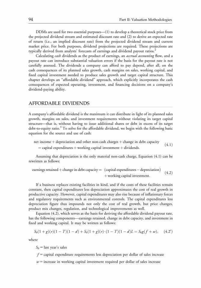
DDMs are used for two essential purposes—(1) to develop a theoretical stock price fromthe projected dividend stream and estimated discount rate and (2) to derive an expected rateof return (i.e., an implied discount rate) from the projected dividend stream and currentmarket price. For both purposes, dividend projections are required. These projections aretypically derived from analysts’ forecasts of earnings and dividend payout ratios.2
Calculating cash dividends as the product of earnings, an accrual accounting flow, and apayout rate can introduce substantial valuation errors if the basis for the payout rate is notcarefully assessed. The dividends a company can afford to pay depend, after all, on thecash consequences of its planned sales growth, cash margins on sales, working capital, andfixed capital investment needed to produce sales growth and target capital structure. Thischapter develops an “affordable dividend” approach, which explicitly incorporates the cashconsequences of expected operating, investment, and financing decisions on a company’sdividend-paying ability.
AFFORDABLE DIVIDENDS
A company’s affordable dividend is the maximum it can distribute in light of its planned salesgrowth, margins on sales, and investment requirements without violating its target capitalstructure—that is, without having to issue additional shares or debt in excess of its targetdebt-to-equity ratio.3 To solve for the affordable dividend, we begin with the following basicequation for the source and use of cash:
net incomeþ depreciation and other non-cash chargesþ change in debt capacity
¼ capital expendituresþworking capital investmentþ dividends:ð4:1Þ
Assuming that depreciation is the only material non-cash charge, Equation (4.1) can berewritten as follows:
earnings retainedþ change in debt capacity¼ ðcapital expenditures�depreciationÞþworking capital investment:
ð4:2Þ
If a business replaces existing facilities in kind, and if the costs of these facilities remainconstant, then capital expenditures less depreciation approximates the cost of real growth inproductive capacity. However, capital expenditures may also rise because of inflationary forcesand regulatory requirements such as environmental controls. The capital expenditures lessdepreciation figure thus impounds not only the cost of real growth, but price changes,product mix changes, regulation, and technological improvements as well.
Equation (4.2), which serves as the basis for deriving the affordable dividend payout rate,has the following components—earnings retained, change in debt capacity, and investment infixed and working capital. It may be written as follows:
S0ð1þ gÞðrÞð1� T Þð1� dÞ þ S0ð1þ gÞðrÞUð1� T Þð1� dÞL ¼ S0gð f þ wÞ; ð4:20Þwhere
S05 last year’s sales
f 5 capital expenditure requirements less depreciation per dollar of sales increase
w5 increase in working capital investment required per dollar of sales increase
c04 12 September 2012; 13:22:6
94 Part II: Valuation Methodologies
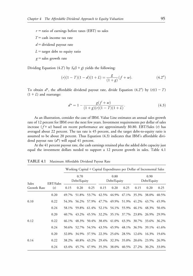
r 5 ratio of earnings before taxes (EBT) to sales
T5 cash income tax rate
d5 dividend payout rate
L5 target debt to equity ratio
g5 sales growth rate
Dividing Equation (4.20) by S0(l1 g) yields the following:
ðrÞð1� T Þð1� d Þð1þ LÞ ¼ gð1þ gÞ ð f þ wÞ: ð4:200Þ
To obtain d*, the affordable dividend payout rate, divide Equation (4.200) by (r)(12T )(11 L) and rearrange:
d* ¼ 1� gð f þ wÞð1þ gÞðrÞð1� T Þð1þ LÞ : ð4:3Þ
As an illustration, consider the case of IBM. Value Line estimates an annual sales growthrate of 12 percent for IBM over the next few years. Investment requirements per dollar of salesincrease ( f1w) based on recent performance are approximately $0.80. EBT/Sales (r) hasaveraged about 22 percent. The tax rate is 45 percent, and the target debt-to-equity ratio isassumed to be about 20 percent. Thus Equation (4.3) indicates that IBM’s affordable divi-dend payout rate (d*) will equal 41 percent.
At the 41 percent payout rate, the cash earnings retained plus the added debt capacity justequal the investment dollars needed to support a 12 percent growth in sales. Table 4.1
TABLE 4.1 Maximum Affordable Dividend Payout Rate
Working Capital1Capital Expenditures per Dollar of Incremental Sales
0.70 0.80 0.90
Sales EBT/SalesDebt/Equity Debt/Equity Debt/Equity
Growth Rate (r) 0.15 0.20 0.25 0.15 0.20 0.25 0.15 0.20 0.25
0.20 49.7% 51.8% 53.7% 42.5% 44.9% 47.1% 35.3% 38.0% 40.5%
0.10 0.22 54.3% 56.2% 57.9% 47.7% 49.9% 51.9% 41.2% 43.7% 45.9%
0.24 58.1% 59.8% 61.4% 52.1% 54.1% 55.9% 46.1% 48.3% 50.4%
0.20 40.7% 43.2% 45.5% 32.2% 35.1% 37.7% 23.8% 26.9% 29.9%
0.12 0.22 46.1% 48.3% 50.4% 38.4% 41.0% 43.3% 30.7% 33.6% 36.2%
0.24 50.6% 52.7% 54.5% 43.5% 45.9% 48.1% 36.5% 39.1% 41.6%
0.20 32.0% 34.9% 37.5% 22.3% 25.6% 28.5% 12.6% 16.3% 19.6%
0.14 0.22 38.2% 40.8% 43.2% 29.4% 32.3% 35.0% 20.6% 23.9% 26.9%
0.24 43.4% 45.7% 47.9% 35.3% 38.0% 40.5% 27.2% 30.2% 33.0%
c04 12 September 2012; 13:22:6
Chapter 4 The Affordable Dividend Approach to Equity Valuation 95
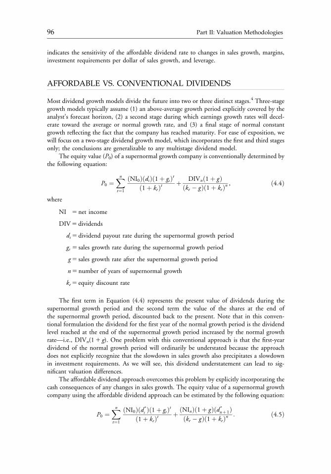
indicates the sensitivity of the affordable dividend rate to changes in sales growth, margins,investment requirements per dollar of sales growth, and leverage.
AFFORDABLE VS. CONVENTIONAL DIVIDENDS
Most dividend growth models divide the future into two or three distinct stages.4 Three-stagegrowth models typically assume (1) an above-average growth period explicitly covered by theanalyst’s forecast horizon, (2) a second stage during which earnings growth rates will decel-erate toward the average or normal growth rate, and (3) a final stage of normal constantgrowth reflecting the fact that the company has reached maturity. For ease of exposition, wewill focus on a two-stage dividend growth model, which incorporates the first and third stagesonly; the conclusions are generalizable to any multistage dividend model.
The equity value (P0) of a supernormal growth company is conventionally determined bythe following equation:
P0 ¼Xnt¼1
ðNI0ÞðdsÞð1þ gsÞtð1þ keÞt þ DIVnð1þ gÞ
ðke � gÞð1þ keÞn , ð4:4Þ
where
NI 5 net income
DIV5 dividends
ds5 dividend payout rate during the supernormal growth period
gs 5 sales growth rate during the supernormal growth period
g5 sales growth rate after the supernormal growth period
n5 number of years of supernormal growth
ke5 equity discount rate
The first term in Equation (4.4) represents the present value of dividends during thesupernormal growth period and the second term the value of the shares at the end ofthe supernormal growth period, discounted back to the present. Note that in this conven-tional formulation the dividend for the first year of the normal growth period is the dividendlevel reached at the end of the supernormal growth period increased by the normal growthrate—i.e., DIVn(11 g). One problem with this conventional approach is that the first-yeardividend of the normal growth period will ordinarily be understated because the approachdoes not explicitly recognize that the slowdown in sales growth also precipitates a slowdownin investment requirements. As we will see, this dividend understatement can lead to sig-nificant valuation differences.
The affordable dividend approach overcomes this problem by explicitly incorporating thecash consequences of any changes in sales growth. The equity value of a supernormal growthcompany using the affordable dividend approach can be estimated by the following equation:
P0 ¼Xnt¼1
ðNI0Þðd *s Þð1þ gsÞt
ð1þ keÞt þ ðNInÞð1þ gÞðd *nþ 1Þ
ðke � gÞð1þ keÞn : ð4:5Þ
c04 12 September 2012; 13:22:7
96 Part II: Valuation Methodologies
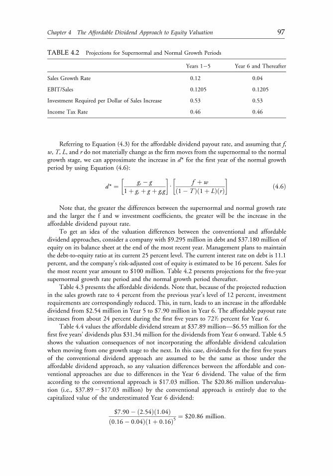
Referring to Equation (4.3) for the affordable dividend payout rate, and assuming that f,w, T, L, and r do not materially change as the firm moves from the supernormal to the normalgrowth stage, we can approximate the increase in d* for the first year of the normal growthperiod by using Equation (4.6):
d* ¼ gs � g1þ gs þ g þ gsg
� �U
f þ wð1� T Þð1þ LÞðrÞ� �
ð4:6Þ
Note that, the greater the differences between the supernormal and normal growth rateand the larger the f and w investment coefficients, the greater will be the increase in theaffordable dividend payout rate.
To get an idea of the valuation differences between the conventional and affordabledividend approaches, consider a company with $9.295 million in debt and $37.180 million ofequity on its balance sheet at the end of the most recent year. Management plans to maintainthe debt-to-equity ratio at its current 25 percent level. The current interest rate on debt is 11.1percent, and the company’s risk-adjusted cost of equity is estimated to be 16 percent. Sales forthe most recent year amount to $100 million. Table 4.2 presents projections for the five-yearsupernormal growth rate period and the normal growth period thereafter.
Table 4.3 presents the affordable dividends. Note that, because of the projected reductionin the sales growth rate to 4 percent from the previous year’s level of 12 percent, investmentrequirements are correspondingly reduced. This, in turn, leads to an increase in the affordabledividend from $2.54 million in Year 5 to $7.90 million in Year 6. The affordable payout rateincreases from about 24 percent during the first five years to 721/2 percent for Year 6.
Table 4.4 values the affordable dividend stream at $37.89 million—$6.55 million for thefirst five years’ dividends plus $31.34 million for the dividends from Year 6 onward. Table 4.5shows the valuation consequences of not incorporating the affordable dividend calculationwhen moving from one growth stage to the next. In this case, dividends for the first five yearsof the conventional dividend approach are assumed to be the same as those under theaffordable dividend approach, so any valuation differences between the affordable and con-ventional approaches are due to differences in the Year 6 dividend. The value of the firmaccording to the conventional approach is $17.03 million. The $20.86 million undervalua-tion (i.e., $37.892 $17.03 million) by the conventional approach is entirely due to thecapitalized value of the underestimated Year 6 dividend:
$7:90� ð2:54Þð1:04Þð0:16� 0:04Þð1þ 0:16Þ5 ¼ $20:86 million:
TABLE 4.2 Projections for Supernormal and Normal Growth Periods
Years 1�5 Year 6 and Thereafter
Sales Growth Rate 0.12 0.04
EBIT/Sales 0.1205 0.1205
Investment Required per Dollar of Sales Increase 0.53 0.53
Income Tax Rate 0.46 0.46
c04 12 September 2012; 13:22:7
Chapter 4 The Affordable Dividend Approach to Equity Valuation 97
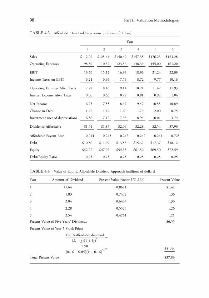
TABLE 4.3 Affordable Dividend Projections (millions of dollars)
Year
1 2 3 4 5 6
Sales $112.00 $125.44 $140.49 $157.35 $176.23 $183.28
Operating Expenses 98.50 110.32 123.56 138.39 155.00 161.20
EBIT 13.50 15.12 16.93 18.96 21.24 22.09
Income Taxes on EBIT 6.21 6.95 7.79 8.72 9.77 10.16
Operating Earnings After Taxes 7.29 8.16 9.14 10.24 11.47 11.93
Interest Expense After Taxes 0.56 0.63 0.72 0.81 0.92 1.04
Net Income 6.73 7.53 8.42 9.42 10.55 10.89
Change in Debt 1.27 1.42 1.60 1.79 2.00 0.75
Investment (net of depreciation) 6.36 7.12 7.98 8.94 10.01 3.74
Dividends-Affordable $1.64 $1.83 $2.04 $2.28 $2.54 $7.90
Affordable Payout Rate 0.244 0.243 0.242 0.242 0.241 0.725
Debt $10.56 $11.99 $13.58 $15.37 $17.37 $18.12
Equity $42.27 $47.97 $54.35 $61.50 $69.50 $72.49
Debt/Equity Ratio 0.25 0.25 0.25 0.25 0.25 0.25
TABLE 4.4 Value of Equity, Affordable Dividend Approach (millions of dollars)
Year Amount of Dividend Present Value Factor 1/(1.16)t Present Value
1 $1.64 0.8621 $1.42
2 1.83 0.7432 1.36
3 2.04 0.6407 1.30
4 2.28 0.5523 1.26
5 2.54 0.4761 1.21
Present Value of Five Years’ Dividends $6.55
Present Value of Year 5 Stock Price:
Year 6 affordable dividend
ðke � gÞð1þ keÞ5¼
7:90
ð0:16� 0:04Þð1þ 0:16Þ5 ¼ $31.34
Total Present Value $37.89
c04 12 September 2012; 13:22:7
98 Part II: Valuation Methodologies
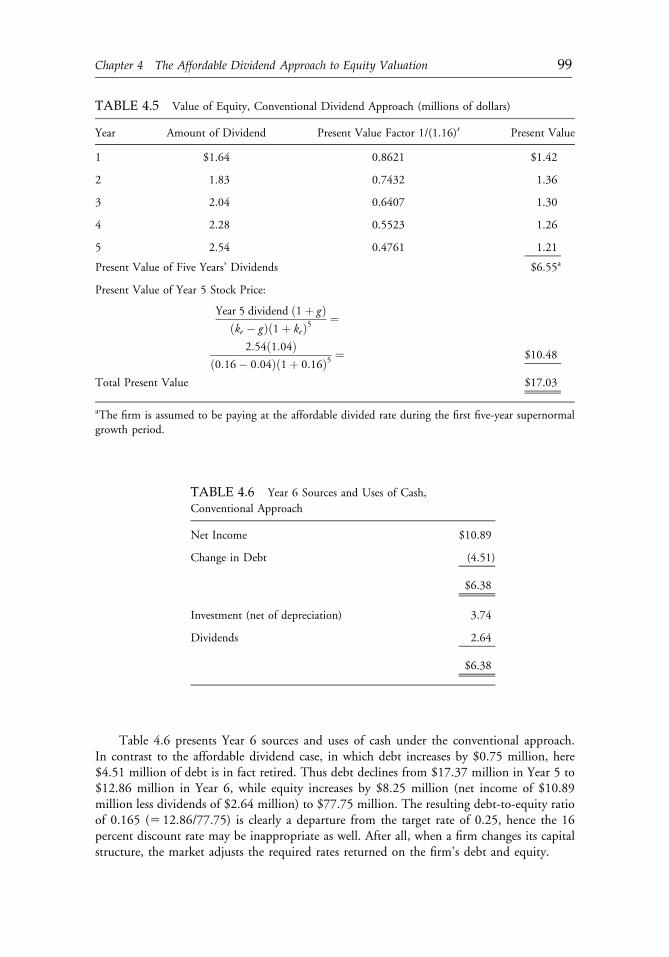
Table 4.6 presents Year 6 sources and uses of cash under the conventional approach.In contrast to the affordable dividend case, in which debt increases by $0.75 million, here$4.51 million of debt is in fact retired. Thus debt declines from $17.37 million in Year 5 to$12.86 million in Year 6, while equity increases by $8.25 million (net income of $10.89million less dividends of $2.64 million) to $77.75 million. The resulting debt-to-equity ratioof 0.165 (5 12.86/77.75) is clearly a departure from the target rate of 0.25, hence the 16percent discount rate may be inappropriate as well. After all, when a firm changes its capitalstructure, the market adjusts the required rates returned on the firm’s debt and equity.
TABLE 4.5 Value of Equity, Conventional Dividend Approach (millions of dollars)
Year Amount of Dividend Present Value Factor 1/(1.16)t Present Value
1 $1.64 0.8621 $1.42
2 1.83 0.7432 1.36
3 2.04 0.6407 1.30
4 2.28 0.5523 1.26
5 2.54 0.4761 1.21
Present Value of Five Years’ Dividends $6.55a
Present Value of Year 5 Stock Price:
Year 5 dividend ð1þ gÞðke � gÞð1þ keÞ5
¼
2:54ð1:04Þð0:16� 0:04Þð1þ 0:16Þ5 ¼ $10.48
Total Present Value $17.03
aThe firm is assumed to be paying at the affordable divided rate during the first five-year supernormalgrowth period.
TABLE 4.6 Year 6 Sources and Uses of Cash,
Conventional Approach
Net Income $10.89
Change in Debt (4.51)
$6.38
Investment (net of depreciation) 3.74
Dividends 2.64
$6.38
c04 12 September 2012; 13:22:7
Chapter 4 The Affordable Dividend Approach to Equity Valuation 99
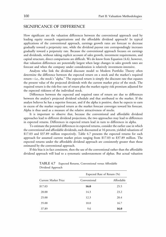
SIGNIFICANCE OF DIFFERENCE
How significant are the valuation differences between the conventional approach used byleading equity research organizations and the affordable dividend approach? In typicalapplications of the conventional approach, earnings growth rates are forecast to decreasegradually toward a perpetuity rate, while the dividend payout rate correspondingly increasesgradually toward a perpetuity rate. Because the conventional approach focuses on earningsand dividends, without taking explicit account of sales growth, investment requirements, andcapital structure, direct comparisons are difficult. We do know from Equation (4.6), however,that valuation differences are potentially largest when large changes in sales growth rates areforecast and when the company under consideration is relatively investment-intensive.
Analysts who link the dividend discount model to Modern Portfolio Theory oftendetermine the difference between the expected return on a stock and the market’s requiredreturn—i.e., the stock’s “alpha.” The expected return is simply the discount rate that equatesthe present value of the projected dividends with the current market price of the stock. Therequired return is the risk-free rate of return plus the market equity risk premium adjusted forthe expected riskiness of the individual stock.
Differences between the expected and required rates of return are due to differencesbetween the analyst’s projected dividend schedule and that attributed to the market. If theanalyst believes he has a superior forecast, and if the alpha is positive, then he expects to earnin excess of the market required return as the market forecast converges toward his forecast.Alpha is thus used as a measure of the relative attractiveness of stocks.
It is important to observe that, because the conventional and affordable dividendapproaches lead to different dividend projections, the two approaches may lead to differencesin expected returns. Differences in expected return lead in turn to differences in alpha.
To estimate the potential differences in expected returns, consider the earlier case in whichthe conventional and affordable dividends, each discounted at 16 percent, yielded valuations of$17.03 and $37.89 million respectively. Table 4.7 presents the expected returns for eachapproach for assumed current market prices ranging from $17.03 to $37.89 million. Theexpected returns under the affordable dividend approach are consistently greater than thoseestimated by the conventional approach.
If this bias is in fact consistent, then the use of the conventional rather than the affordabledividend approach will lead to a systematic understatement of alphas. But actual valuation
TABLE 4.7 Expected Returns, Conventional versus Affordable
Dividend Approach
Expected Rate of Return (%)
Current Market Price Conventional Affordable
$17.03 16.0 25.5
20.00 14.3 23.2
25.00 12.3 20.4
35.00 10.0 16.7
37.89 9.6 16.0
c04 12 September 2012; 13:22:7
100 Part II: Valuation Methodologies
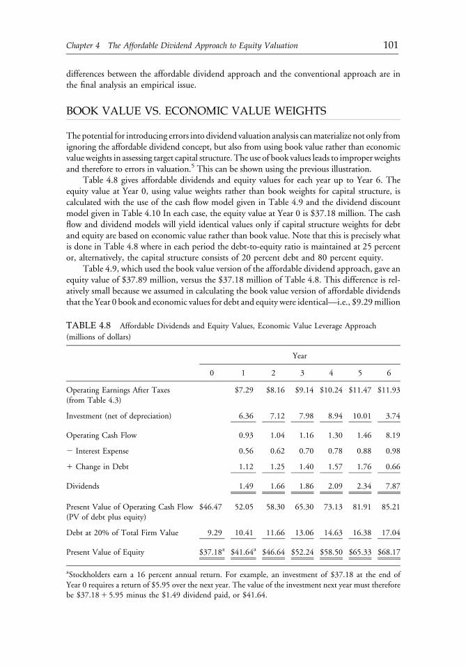
differences between the affordable dividend approach and the conventional approach are inthe final analysis an empirical issue.
BOOK VALUE VS. ECONOMIC VALUE WEIGHTS
The potential for introducing errors into dividend valuation analysis canmaterialize not only fromignoring the affordable dividend concept, but also from using book value rather than economicvalueweights in assessing target capital structure. The use of book values leads to improperweightsand therefore to errors in valuation.5 This can be shown using the previous illustration.
Table 4.8 gives affordable dividends and equity values for each year up to Year 6. Theequity value at Year 0, using value weights rather than book weights for capital structure, iscalculated with the use of the cash flow model given in Table 4.9 and the dividend discountmodel given in Table 4.10 In each case, the equity value at Year 0 is $37.18 million. The cashflow and dividend models will yield identical values only if capital structure weights for debtand equity are based on economic value rather than book value. Note that this is precisely whatis done in Table 4.8 where in each period the debt-to-equity ratio is maintained at 25 percentor, alternatively, the capital structure consists of 20 percent debt and 80 percent equity.
Table 4.9, which used the book value version of the affordable dividend approach, gave anequity value of $37.89 million, versus the $37.18 million of Table 4.8. This difference is rel-atively small because we assumed in calculating the book value version of affordable dividendsthat the Year 0 book and economic values for debt and equity were identical—i.e., $9.29million
TABLE 4.8 Affordable Dividends and Equity Values, Economic Value Leverage Approach
(millions of dollars)
Year
0 1 2 3 4 5 6
Operating Earnings After Taxes(from Table 4.3)
$7.29 $8.16 $9.14 $10.24 $11.47 $11.93
Investment (net of depreciation) 6.36 7.12 7.98 8.94 10.01 3.74
Operating Cash Flow 0.93 1.04 1.16 1.30 1.46 8.19
2 Interest Expense 0.56 0.62 0.70 0.78 0.88 0.98
1 Change in Debt 1.12 1.25 1.40 1.57 1.76 0.66
Dividends 1.49 1.66 1.86 2.09 2.34 7.87
Present Value of Operating Cash Flow(PV of debt plus equity)
$46.47 52.05 58.30 65.30 73.13 81.91 85.21
Debt at 20% of Total Firm Value 9.29 10.41 11.66 13.06 14.63 16.38 17.04
Present Value of Equity $37.18a $41.64a $46.64 $52.24 $58.50 $65.33 $68.17
aStockholders earn a 16 percent annual return. For example, an investment of $37.18 at the end ofYear 0 requires a return of $5.95 over the next year. The value of the investment next year must thereforebe $37.181 5.95 minus the $1.49 dividend paid, or $41.64.
c04 12 September 2012; 13:22:8
Chapter 4 The Affordable Dividend Approach to Equity Valuation 101
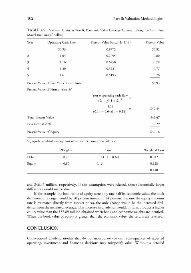
and $46.47 million, respectively. If this assumption were relaxed, then substantially largerdifferences would materialize.
If, for example, the book value of equity were only one-half its economic value, the bookdebt-to-equity target would be 50 percent instead of 24 percent. Because the equity discountrate is estimated directly from market prices, the only change would be the increased divi-dends from the increased leverage. This increase in dividends would, in turn, produce a higherequity value than the $37.89 million obtained when book and economic weights are identical.When the book value of equity is greater than the economic value, the results are reversed.
CONCLUSION
Conventional dividend models that do not incorporate the cash consequences of expectedoperating, investment, and financing decisions may misspecify value. Without a detailed
TABLE 4.9 Value of Equity at Year 0, Economic Value Leverage Approach Using the Cash Flow
Model (millions of dollars)
Year Operating Cash Flow Present Value Factor 1/(1.14)t Present Value
1 $0.93 0.8772 $0.82
2 1.04 0.7695 0.80
3 1.16 0.6750 0.78
4 1.30 0.5921 0.77
5 1.6 0.5193 0.76
Present Value of Five Years’ Cash Flows $3.93
Present Value of Firm at Year 5:a
Year 6 operating cash flow
ðka � gÞð1þ kaÞ5¼
8:19
ð0:14� 0:04Þð1þ 0:14Þ5 ¼ $42.54
Total Present Value $46.47
Less Debt at 20% 9.29
Present Value of Equity $37.18
aka equals weighted average cost of capital, determined as follows:
Weights Cost Weighted Cost
Debt 0.20 0.111 (12 0.46) 0.012
Equity 0.80 0.16 0.128
0.140
c04 12 September 2012; 13:22:8
102 Part II: Valuation Methodologies
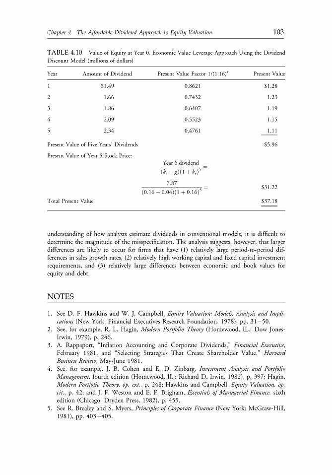
understanding of how analysts estimate dividends in conventional models, it is difficult todetermine the magnitude of the misspecification. The analysis suggests, however, that largerdifferences are likely to occur for firms that have (1) relatively large period-to-period dif-ferences in sales growth rates, (2) relatively high working capital and fixed capital investmentrequirements, and (3) relatively large differences between economic and book values forequity and debt.
NOTES
1. See D. F. Hawkins and W. J. Campbell, Equity Valuation: Models, Analysis and Impli-cations (New York: Financial Executives Research Foundation, 1978), pp. 31�50.
2. See, for example, R. L. Hagin, Modern Portfolio Theory (Homewood, IL.: Dow Jones-Irwin, 1979), p. 246.
3. A. Rappaport, “Inflation Accounting and Corporate Dividends,” Financial Executive,February 1981, and “Selecting Strategies That Create Shareholder Value,” HarvardBusiness Review, May-June 1981.
4. See, for example, J. B. Cohen and E. D. Zinbarg, Investment Analysis and PortfolioManagement, fourth edition (Homewood, IL.: Richard D. Irwin, 1982), p. 397; Hagin,Modern Portfolio Theory, op. ext., p. 248; Hawkins and Campbell, Equity Valuation, op.cit., p. 42; and J. F. Weston and E. F. Brigham, Essentials of Managerial Finance, sixthedition (Chicago: Dryden Press, 1982), p. 455.
5. See R. Brealey and S. Myers, Principles of Corporate Finance (New York: McGraw-Hill,1981), pp. 403�405.
TABLE 4.10 Value of Equity at Year 0, Economic Value Leverage Approach Using the Dividend
Discount Model (millions of dollars)
Year Amount of Dividend Present Value Factor 1/(1.16)t Present Value
1 $1.49 0.8621 $1.28
2 1.66 0.7432 1.23
3 1.86 0.6407 1.19
4 2.09 0.5523 1.15
5 2.34 0.4761 1.11
Present Value of Five Years’ Dividends $5.96
Present Value of Year 5 Stock Price:Year 6 dividend
ðke � gÞð1þ keÞ5¼
7:87
ð0:16� 0:04Þð1þ 0:16Þ5 ¼ $31.22
Total Present Value $37.18
c04 12 September 2012; 13:22:8
Chapter 4 The Affordable Dividend Approach to Equity Valuation 103

c04 12 September 2012; 13:22:8
CHAPTER 5DISCOUNTED-CASH-FLOWAPPROACH TO VALUATION
Gregory A. Gilbert, CFA
Financial theory states that the fair market value of an ongoing business is thepresent value of its expected cash flows. This conceptual framework is known as thediscounted-cash-flow (DCF) valuation approach. Although the DCF approach isdeceptively simple in theoretical execution, in practice it is quite complex and verysubjective. It requires that the analyst use great care in the estimation of cash flows,discount rates, and terminal values. Fortunately, there are ways to overcome thesubjectivity and make the valuation process more rational and objective.
According to finance texts, the fair market value of an ongoing business is the present worth ofits expected cash flows. This simple conceptual framework is known as the discounted-cash-flow (DCF) valuation approach. The calculations necessary in a DCF approach are equallysimple: Add the present values of the individual cash-flow estimates for each year from one toinfinity. Although the DCF approach is the technically correct way to value a company, andalthough it is deceptively simple in theoretical execution, in practice it is quite complexand very subjective. In this chapter, I will discuss ways to try to overcome that subjectivity andmake the valuation process more rational and objective.
THE DCF FORMULA
The formula for the DCF approach is shown in equation (1) of Figure 5.1. The cash flow(CF) for each time period (n) is reduced to its present value using the compound-interest term[(1+i )n]. The value of the company equals the sum of the present values for all periods, one to
Copyright ª 1990 Gregory A. Gilbert, CFA. Reprinted with permission from ICFA ContinuingEducation Series (1990):23�30. This chapter comes from the Valuation of Closely Held Companies andInactively Traded Securities conference held in Chicago on December 5, 1989. When this article wasoriginally published, Gregory A. Gilbert, CFA, was president of Corporate Valuations, Inc.
c05 12 September 2012; 17:43:8
105
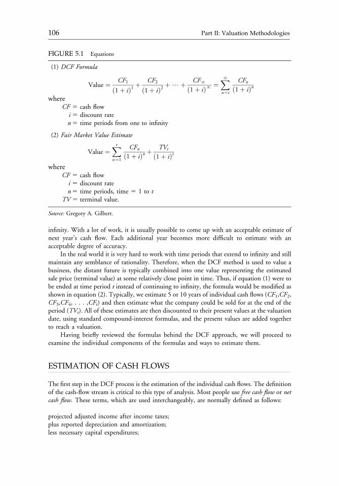
infinity. With a lot of work, it is usually possible to come up with an acceptable estimate ofnext year’s cash flow. Each additional year becomes more difficult to estimate with anacceptable degree of accuracy.
In the real world it is very hard to work with time periods that extend to infinity and stillmaintain any semblance of rationality. Therefore, when the DCF method is used to value abusiness, the distant future is typically combined into one value representing the estimatedsale price (terminal value) at some relatively close point in time. Thus, if equation (1) were tobe ended at time period t instead of continuing to infinity, the formula would be modified asshown in equation (2). Typically, we estimate 5 or 10 years of individual cash flows (CF1,CF2,CF3,CF4, . . . ,CFt) and then estimate what the company could be sold for at the end of theperiod (TVt). All of these estimates are then discounted to their present values at the valuationdate, using standard compound-interest formulas, and the present values are added togetherto reach a valuation.
Having briefly reviewed the formulas behind the DCF approach, we will proceed toexamine the individual components of the formulas and ways to estimate them.
ESTIMATION OF CASH FLOWS
The first step in the DCF process is the estimation of the individual cash flows. The definitionof the cash-flow stream is critical to this type of analysis. Most people use free cash flow or netcash flow. These terms, which are used interchangeably, are normally defined as follows:
projected adjusted income after income taxes;plus reported depreciation and amortization;less necessary capital expenditures;
FIGURE 5.1 Equations
(1) DCF Formula
Value ¼ CF1ð1þ iÞ1 þ
CF2ð1þ iÞ2 þ?þ CFN
ð1þ iÞN ¼XNn¼i
CFnð1þ iÞn
whereCF 5 cash flowi5 discount raten5 time periods from one to infinity
(2) Fair Market Value Estimate
Value ¼Xtn¼1
CFnð1þ iÞn þ
TVt
ð1þ iÞtwhere
CF 5 cash flowi 5 discount raten5 time periods, time 5 1 to t
TV 5 terminal value.
Source: Gregory A. Gilbert.
c05 12 September 2012; 17:43:8
106 Part II: Valuation Methodologies
less necessary working capital increases; andless debt principal repayments, sometimes alsoadjusted for the issuance of new debt.
Stated in simplified form, free cash flow is the sum of the sources of cash, less the capitalexpenditures necessary to stay in business and continue to grow at the expected rate. Theseexpenses must be included because a company cannot remain in business if its capitalmachinery gets old and outdated, nor can it grow without increases in working capital. Thegoal is to estimate recurring operating earnings and all cash-flow items associated with thoseearnings, including necessary capital expenditures. These estimates are the first area of sub-jectivity in the DCF valuation approach.
One way to estimate the annual cash flows is to use the company’s financial history as thebase for projections. There are many ways to use historical data. One of the best is to build afinancial model of the company. The model may be very simple, for example a mathematicalrelation between sales and employees (either in dollar terms or unit terms), or it may be quitecomplex, incorporating non-linear relationships between the many variables. The process ofestimating cash flows is similar to developing a 5-year or 10-year business plan. It shouldaddress all key items in the income statement.
In addition to estimation of net earnings, it should also involve an analysis of requiredcapital equipment, cash to finance working capital, and any additional debt.
As well as making detailed estimates of the future, an appraiser must often makeadjustments to accounting income to get the true economic income—that is, the cash flowsgenerated by the operation of the business.
Perhaps the most common adjustment is to determine whether the owner’s compensationis correct—in an economic sense. The appraiser must also look at the other employees andtheir compensation. Is the owner’s grandmother really needed on the payroll? She might bevery important if the product is Grandma’s Cookies, and she is the only one who has therecipe. Otherwise, she might not be necessary to the company.
Contracts with related parties comprise the second area of adjustments. Leases are the mostcommon type of contract in this category. Often, the business owner personally holds the landand building, and leases them to the business. There have been many attempts to make thelease rate close to a fair market value rate. In some instances, however, the lease rate is toohigh; in still other cases, too low. The arrangement often depends on the owner’s personal taxsituation. Appraisers have the responsibility to adjust the accounting income for differencesbetween the actual lease rate and the economic lease rate. The theory is that a new buyer couldchange the leases (or other types of contracts) to economic rates and more accurately calculatethe income from the operation of the company.
The third type of adjustment is to remove from the income statement the income andexpense related to nonoperating assets; for example, an airplane that is not used for businesspurposes but is owned and maintained by the company. The cost of maintaining andoperating this asset must be removed from the income statement to avoid distortion ofthe appraiser’s estimate of the company’s operating income. Other types of assets might haveincome that must be removed from the income statement; still others may have both incomeand expense.
The fourth group of adjustments are those that must be made for nonrecurring incomeand expense. For example, if the firm incurred $200,000 in legal fees because of a lawsuit, andthese costs are not likely to recur over the 5- to 10-year time horizon, they should beeliminated.
c05 12 September 2012; 17:43:8
Chapter 5 Discounted-Cash-Flow Approach to Valuation 107
The fifth type of adjustment an appraiser may have to make is for capital deficiency (orsurplus). The appraiser must determine whether the firm’s operations will need more (or less)capital and how the addition (or removal) of that capital would impact the income statement.
Finally, adjustments must often be made to reconcile different accounting methods. Notonly are these adjustments part of the process of deriving the true economic income, or cashflow, figures, but they are also necessary to make the company’s cash flow estimates conformwith the data used to calculate the discount rate. Unfortunately, it is not always possible toreconcile different accounting methods when the companies are publicly owned. Thus,sometimes there is a conflict between these two reasons. In these cases, no adjustments shouldbe made. The appraiser must make sure the company’s cash flows conform as closely aspossible to those of the publicly traded companies used in the derivation of the discount rate.In fact, an appraiser must sometimes construct two sets of estimated cash-flow statements: oneadjusted statement that makes the closely held company look as much like a publicly tradedcompany as possible, and another that attempts to show the economic reality.
DISCOUNT RATE
The second step in the DCF process is the determination of the discount rate.
Definition
A discount rate is defined as the rate of return an investor would require to be induced toinvest in the cash-flow stream being discounted. There are six important aspects of discountrates. Discount rates
� are affected by the market;� vary with time;� depend on what is being discounted;� must be risk adjusted;� are based on yields available on alternative investments; and� are inflation adjusted.
External Factors
Three basic external factors affect discount rates: (1) general economic conditions; (2) yieldsavailable on alternative investments; and (3) industry conditions and outlook. The process ofanalyzing the external factors provides the appraiser with a sense of what might affect thediscount rate. The answers to a few basic questions may provide a wealth of information. Forexample, is the industry going to grow at 5 percent? At 10 percent? Is it stable? Is it shrinking?How will the industry’s growth affect the expectations for cash flow? If management says thatthe subject company is going to grow at 10 percent a year for the next 10 years, but theindustry is stable or declining, that projection may not make sense.
Internal Factors
There are three internal factors that affect discount rates: (1) financial risk, (2) operating risk,and (3) the risk associated with the estimation of the cash-flow stream.
c05 12 September 2012; 17:43:9
108 Part II: Valuation Methodologies
1. Financial risk has five basic inputs: leverage, coverage, turnover, return, and liquidity. Theadjustments to the discount rate are fairly obvious; higher risk in the financial measuresmust lead to higher discount rates.
2. Operating risk has the following basic inputs: management, accounting methods, stabilityof markets, customer base, and competitive position. The appraiser must incorporate intothe discount rate his assessment of the capability of management, whether the accountingmethods are conservative or aggressive, and so forth. For example, if aggressive accountingtreatments that increase risk are left in the cashflow projections, a higher discount rateshould be used. On the other hand, a very stable customer base might lead one to reducethe discount rate. Similarly, if there is a lot of competition, the rate should be higher; ifthere is very little competition, the rate should be lower.
3. Risk associated with the estimation of the cash-flow stream. If there is considerable uncertaintysurrounding the 10-year sales and earnings forecast, as would be true with a start-upcompany, the discount rate must be higher to account for this risk. On the other hand, ifthe company has a stable operating history and established relationships, the greatercertainty of the forecast should be reflected in a lower discount rate.
Components
The discount rate is a function of three components: (1) a risk-free rate, (2) a generalrisk premium covering both equity risk and industry risk, and (3) a factor for company-specific risk.
1. The risk-free rate is the easiest factor to identify objectively. It is generally recognized thatthere are three measures of the risk-free rate: long-term government bonds, intermediate-term Treasury notes, and short-term Treasury bills. The appropriate risk-free instrumentto use in the construction of a discount rate is the one that matches the investmenthorizon. For an equity investment with a long time horizon, a 30-year bond might beappropriate. Often a typical financial horizon is five to seven years; in that case,intermediate-term notes would be appropriate. Finally, if an appraiser is valuing somethinglike a patent that only has a few years left before expiration, short-term Treasury billsmight be the appropriate measure of the risk-free rate. The analyst must determine whatmakes sense.
2. It is harder for the appraiser to identify the appropriate general risk premium. There arefour basic methods that appraisers use to estimate this premium.� One of the four commonly used methods is direct comparison. This method involvesdeveloping a discount rate from actual transactions. Unfortunately, it is often hard tofind the necessary data.
� The second of the four methods is the inverse of a price/cash-flow ratio plus growth. Thismethod involves five steps. The first step is to find a list of publicly traded companiesthat are enough like the company being appraised to be considered similar or com-parative, or if you are really lucky, comparable. The second step is to calculate price/cash-flow ratios for the similar publicly traded companies. The third step is to invert theprice/cash-flow ratio to get a cash-flow/price ratio. A cash-flow/price ratio is really acapitalization rate. (Note that price 5 cash-flow/cap rate, or cap rate 5 cash-flow/price.) The difference between a capitalization rate and a discount rate is growth. Therelationship is: cap rate plus growth equals discount rate. The fourth step is to estimate
c05 12 September 2012; 17:43:9
Chapter 5 Discounted-Cash-Flow Approach to Valuation 109
the growth rate from the similar publicly traded companies. Note that the growth ratereferenced here is the expected (not observed), long-term growth rate. The final step inthe derivation of the discount rate is to add the growth rate to the cash-flow/price ratio.
� The third approach to developing a general risk premium is to use historical stock marketreturn data. The Ibbotson-Sinquefield studies are the normal source of historicalreturns.1 The differential between returns on stocks and a risk-free rate is believed to bea measure of the extra reward accruing to investors for assuming equity risk. Forappraisal purposes the general equity risk premium is normally estimated as the dif-ference between the arithmetic mean return for small-capitalization stocks and the samereturn for government bonds.
� The fourth method for estimating the general risk-premium portion of a discount rate isthe capital asset pricing model (CAPM). This is perhaps the most common method usedby appraisers. The formula for the CAPM is as follows:
Re ¼ Rf þ ðRm � Rf ÞBwhere
Re 5 expected return
Rf 5 expected risk-free rate
Rm 5 expected return on the market
B 5 expected systematic risk (commonly called beta).
The needed inputs to CAPM are obtained from several sources. The return on themarket (Rm) is usually derived from historical stock market returns (Ibbotson andSinquefield 1989). Betas are only published for publicly traded companies, so a betaapplicable to an individual company must be estimated, usually using the betas ofsimilar publicly traded companies. The selection of beta is critical to the accuratecalculation of a discount rate, yet the appraiser has little to guide the selection process.Further, CAPM theory is based on estimates of expected returns (Rf and Rm) andexpected betas. In actual practice we can only use historical returns and historical betas.Unfortunately, both returns and betas vary over time, which casts suspicion on usinghistorical measures.
In the theoretical framework of the CAPM, the specific return (alpha) is assumedto be diversified away for efficient portfolios. It is probably still relevant for individualstocks, however.
I remain skeptical about using the CAPM to derive the discount rate because thekey inputs are so subjective. The reason for using a model like the CAPM to estimatethe discount rate is to increase the objectivity of the process. Ironically, the subjectivedecisions necessary in the CAPM process may increase the subjectivity of the finaldiscount rate instead of the objectivity.
3. The hardest part of the determination of a discount rate is to estimate the company-specific risk premium. Unfortunately, there are no objective data to help reach anappropriate company-specific risk premium (or alpha, in CAPM parlance). Experience isvery valuable. Each company’s situation must be evaluated separately, and all risk factorsmust be recognized and incorporated into the company-specific premium. Just as thestock market determines a different beta for each publicly traded company, the appraisermust determine a different beta (or industry beta plus individual alpha) for each subjectcompany.
c05 12 September 2012; 17:43:9
110 Part II: Valuation Methodologies
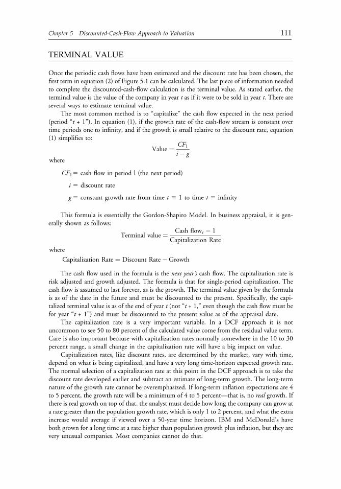
TERMINAL VALUE
Once the periodic cash flows have been estimated and the discount rate has been chosen, thefirst term in equation (2) of Figure 5.1 can be calculated. The last piece of information neededto complete the discounted-cash-flow calculation is the terminal value. As stated earlier, theterminal value is the value of the company in year t as if it were to be sold in year t. There areseveral ways to estimate terminal value.
The most common method is to “capitalize” the cash flow expected in the next period(period “t + 1”). In equation (1), if the growth rate of the cash-flow stream is constant overtime periods one to infinity, and if the growth is small relative to the discount rate, equation(1) simplifies to:
Value ¼ CF1i � g
where
CF15 cash flow in period l (the next period)
i 5 discount rate
g5 constant growth rate from time t 5 1 to time t 5 infinity
This formula is essentially the Gordon-Shapiro Model. In business appraisal, it is gen-erally shown as follows:
Terminal value ¼ Cash flowt � 1
Capitalization Rate
where
Capitalization Rate ¼ Discount Rate� Growth
The cash flow used in the formula is the next year’s cash flow. The capitalization rate isrisk adjusted and growth adjusted. The formula is that for single-period capitalization. Thecash flow is assumed to last forever, as is the growth. The terminal value given by the formulais as of the date in the future and must be discounted to the present. Specifically, the capi-talized terminal value is as of the end of year t (not “t + 1,” even though the cash flow must befor year “t + 1”) and must be discounted to the present value as of the appraisal date.
The capitalization rate is a very important variable. In a DCF approach it is notuncommon to see 50 to 80 percent of the calculated value come from the residual value term.Care is also important because with capitalization rates normally somewhere in the 10 to 30percent range, a small change in the capitalization rate will have a big impact on value.
Capitalization rates, like discount rates, are determined by the market, vary with time,depend on what is being capitalized, and have a very long time-horizon expected growth rate.The normal selection of a capitalization rate at this point in the DCF approach is to take thediscount rate developed earlier and subtract an estimate of long-term growth. The long-termnature of the growth rate cannot be overemphasized. If long-term inflation expectations are 4to 5 percent, the growth rate will be a minimum of 4 to 5 percent—that is, no real growth. Ifthere is real growth on top of that, the analyst must decide how long the company can grow ata rate greater than the population growth rate, which is only 1 to 2 percent, and what the extraincrease would average if viewed over a 50-year time horizon. IBM and McDonald’s haveboth grown for a long time at a rate higher than population growth plus inflation, but they arevery unusual companies. Most companies cannot do that.
c05 12 September 2012; 17:43:9
Chapter 5 Discounted-Cash-Flow Approach to Valuation 111
As an alternative to the capitalization process for estimation of terminal value, one mayassume that the company will be worth its book value at the end of time t. If a company isever going to be worth book value, time t is probably as good a time as any; at least it is severalyears away. (Nonetheless, it will be worthwhile to check the expected return on equity in timeperiod t to see if book value is a reasonable estimate of value. Do not use a book value as aterminal value if you are expecting a return on equity 10 years from now that is double today’sindustry rate of return.) The future book value must be discounted back to its present value asof the valuation date.
Another method for calculating terminal value is to use an industry rule of thumb. If youuse a rule of thumb, be sure it makes sense, or at least does not offend common sense.
CONCLUSION
The DCF valuation approach is theoretically the most “correct” valuation approach. It isnecessary for the appraiser to use great care in the estimation of cash flows, discount rates, andterminal values. The expected cash flows must be rigorously developed and supported with allavailable data.
The CAPM may help the appraiser, but it must be applied with wisdom and the benefitof experience in recognizing and quantifying investment risk. Company-specific risk must notbe forgotten. Likewise, other methods may be used to help develop discount rates, or tocorroborate rates reached through use of the CAPM.
The estimation of terminal value is perhaps the most crucial part of the DCF approach,because normally over half of the ultimate appraised value comes from the terminal value.The capitalization rate and its growth component are critical in the development of anaccurate terminal value.
QUESTION AND ANSWER SECTION
Question: What range of discount rates should be used in a DCF analysis?Gilbert: The answer depends on the company. When you are dealing with start-up companies,
you look to rates expected by venture capitalists—perhaps rates as high as 100 percent peryear, or even more. The fact that these are very high rates implies—among other things—that you do not have a lot of faith in the cash-flow stream being discounted. Forcompanies that are not start-ups, the rate normally falls in the 10- to 30-percent range.
Question: Should the discount rate be pre-tax or post-tax?Gilbert: The answer depends on whether the cash flows are net of taxes. Most appraisers use
free cash-flow and post-tax discount rates.Question: Is it appropriate to use a higher discount rate for the terminal value to account for a
higher risk so far into the future?Gilbert: It makes a lot of sense conceptually to use a higher discount rate, but you almost
never see it done.Question: Is the value derived in the DCF analysis a minority-interest value or a controlling-
interest value?
c05 12 September 2012; 17:43:9
112 Part II: Valuation Methodologies
Gilbert: The value depends on whether you use a control discount rate or a minority-interestdiscount rate. For example, if you adjust for owner’s compensation and add back a hugeincrement because the owner is taking excessive compensation, then you have probablycaptured a good portion of the control premium in the cash-flow stream (numerator).Similarly, if you are valuing a minority interest and you do not adjust for excessiveowner’s compensation (on the theory that the minority owners do not have the right torequire the controlling person to take a lower salary), a lot of the minority-interestdiscount is in the numerator.
Question: If, instead of using net free cash flow as the numerator in your cash-flow projectionyou use operating cash flow or net income, what is the proper discount rate?
Gilbert: Normally, I simply add 5 percentage points. It is an entirely empirical approach;there is no theoretical basis for 5 points, it just seems to work out right most ofthe time.
Question: What is wrong with the CAPM?Gilbert: I would start with the efficient markets theory. I do not believe the efficient markets
theory holds in either its strong form or semi-strong form. I also have problems withother underlying CAPM assumptions. I do not like the fact that we have to usehistorical data when the theory requires expectational data. Nor do I like the assumptionthat anyone may borrow at the risk-free rate; that is not a realistic assumption. Further, Iam not convinced that it is valid to use CAPM on a portfolio of just common stocks.After all, the theory was developed for portfolios made up of every asset, not justfinancial assets that are easily measured. To then use CAPM on a single companypresses the theory one step further.
Then, there are problems with betas. First, they are not stationary. Second, I amnot sure that we are measuring beta correctly. Is price volatility the right measure of risk?Maybe earnings volatility or dividend volatility would be better. The list of problemsgoes on.
Question: Is the arbitrage pricing theory (APT) any better?Gilbert: I think you wind up with similar problems using APT as you do with the CAPM.Question: Would you still use 20- or 30-year government bonds for the risk-free rate on a
long-term horizon if the yield curve is inverted?Gilbert: Yes—although I do not like to deal with an inverted yield curve in valuing a
long-term equity.Question: You stated that the DCF valuation approach is very subjective. Isn’t the market
approach, with the judgment required in selecting comparables and adjusting theirstatements, also subjective? Given the level of subjectivity in so many areas of DCFanalysis—that is, revenue and margin projections, discount rates, estimation of terminalvalue, and so forth—can DCF analysis be accurate enough to be used as anything morethan a smell test for other valuation measures?
Gilbert: Subjectivity is important. Without subjectivity, my computer would do everything,and everyone in this room would be out of a job. There is a lot of subjectivity in everyappraisal approach. The market approach has a lot of subjectivity when it comes topicking the correct multiple. A good set of data will narrow the choices to a reasonableset, but that last step—from the narrowed range to “the” number—depends onsubjectivity.
Question: Is it appropriate to make adjustments to income for a minority valuation?
c05 12 September 2012; 17:43:9
Chapter 5 Discounted-Cash-Flow Approach to Valuation 113

Gilbert: If you make adjustments, some of the control premium may be contained in theadjustments. So if you are doing a minority appraisal, you have to consider a minoritydiscount. If you do not make the adjustments to income for a minority valuation, mostof the minority discount will probably be captured in the cash flows; therefore, you donot need to make as large a minority discount.
Question: Are necessary capital expenditures a part of the numerator in the standard DCFequation? If so, do you use Generally Accepted Accounting Principles (GAAP) capitalexpenditures or economic capital expenditures? For example, how do you recommendtreating capital expenditures financed by operating leases such as aircraft or a truck fleet?
Gilbert: Assuming the leases are good, fair-market-value, third-party leases, they shouldalready be included in the cash-flow stream. I prefer to use economic capitalexpenditures rather than GAAP because GAAP accounting is not very relevant inappraisal terms.
Question: If optimistic cash flows are used, should the discount rate be higher than the rateused for more conservative cash flows?
Gilbert: Yes. Absolutely.Question: Do you use probability trees as an alternative to adjusting your discount rate to
reflect errors in estimation?Gilbert: It depends on the audience: Never use a probability tree on a judge. On the other
hand, if you have a very sophisticated corporate CFO who might understand aprobability tree, use it.
Question: What is the best way to value a contingent liability?Gilbert: The best way to handle a contingent liability, like a lawsuit that will bankrupt the
company, is to value the company before the contingent liability and then adjust thatfor the value of the contingent liability. A probability tree is superb for this kind ofthing. Of course, the biggest problem is assigning the probabilities.
NOTE
1. See Ibbotson and Sinquefield (1989); data is updated annually by Ibbotson Assoicates.
c05 12 September 2012; 17:43:9
114 Part II: Valuation Methodologies
CHAPTER 6EQUITY SECURITIES
ANALYSIS CASE STUDY:MERCK & COMPANY
Randall S. Billingsley, CFA
It is one thing to know what all the tools of oil painting are and quite another to usethose tools to create a finished oil painting. The same is true in valuation. It is one thingto know what the components of a thorough valuation analysis are and quite anotherto apply that knowledge to calculate the value of an asset. This thorough case studycontains important information about how to apply valuation knowledge (valuation asscience) to a real-world company, Merck, to create a valuation conclusion (valuationas art).
Bill Kurious, a junior analyst with Grand Concepts Investment Management and a CFAcandidate, has been assigned the task of valuing the common stock of Merck & Company.Merck, the world’s largest ethical drug manufacturer, discovers, develops, produces, andmarkets human and animal health products and specialty chemicals. The company has beenconsistently ranked among the top companies in return on assets and return on sales inFortune magazine’s analysis of the 500 largest companies in the United States. It also isconsidered one of the “most admired” companies in the United States.
Kurious wishes to impress his supervisor, Amy Randall, but is mindful of the highexpectations for his performance and the fact that this is his first “real” valuation report.Randall requested that the analysis consider a variety of valuation approaches and thatall assumptions be identified explicitly and critically evaluated through sensitivity analysis.Further, Randall directed Kurious to discuss the relative strengths and weaknesses of
Reprinted from AIMR Conference Proceedings: Equity Securities Analysis and Evaluation (December1993):63�95. This presentation comes from the Equity Securities Analysis and Evaluation conferenceheld in Tokyo on March 1�3, 1993. When this article was originally published, Randall S. Billingsley,CFA, was vice president at the Association for Investment Management and Research (AIMR).
c06 12 September 2012; 17:41:24
115
the valuation methods used in forming his opinion and the associated investmentrecommendation.
The impending presidential inauguration of Governor Clinton later in the month hasgreatly complicated Kurious’s valuation efforts. The president elect is known to favor moreaffordable health care for a broader group of people and advocates a dramatic overhaul of theU.S. health care system. Many analysts believe the new administration will be tougher onpharmaceutical pricing and that, as a result, the inherent riskiness of the pharmaceuticalindustry has increased dramatically. Indeed, many investors and analysts believe that theriskiness of the industry cannot be confidently assessed because of the marked politicaluncertainty surrounding its future.
Notwithstanding these complications, Kurious intends to apply to his assignment theCFA curriculum material on valuation. He decides to pose a series of questions to himself thatwill guide the valuation process in a methodical fashion. In coming up with these questions,he develops the following notes and observations on Merck, the pharmaceutical industry, andalternative equity valuation methods.
RECENT ANNUAL REPORTS
As of January 1993, Merck had about 38,000 employees and 91,000 stockholders.Sales by non-U.S. subsidiaries were 47 percent of sales in 1989 and 1990 and 46 percent ofsales in 1991. The company’s most important product names include Vasotec and Prinivil(inhibitor agents for high blood pressure and angina), Mevacor and Zocor (cholesterol-lowering agents), Primaxin and Mefoxin (antibiotics), Pepcid (anti-ulcer agent), RecombivaxHB (hepatitis B vaccine), and Prilosec (gastrointestinal). Financial data for Merck are pre-sented in Appendix 6A.
Strategic Objectives
The main thrust of Merck’s strategic objectives has been to develop, manufacture, and sellproducts that reflect progress in science and therapy. Year-to-year objectives include stayingamong the leaders in the industry in sales growth, earnings per share, and (cash) return onassets. Operationally, Merck pursues these objectives under the assumption that research anddevelopment (R&D) is the key to its long-term growth. Indeed, in 1991, the company spentnearly $1 billion on R&D, which was about 10 percent of all U.S. pharmaceutical R&Dspending and about 5 percent of all such spending in the world. According to Merck’s 1991annual report, it planned to increase its R&D spending by about 16 percent in 1992.
Structural Reorganization
Merck realizes that the pharmaceutical industry is becoming increasingly global in research,manufacturing, and marketing. Consistent with that observation, the company decided toreorganize on a global basis in order to increase productivity and to bring into focus itsstrategic alliances. This reorganization affected its worldwide marketing, vaccines, andmanufacturing efforts.
Specifically, Merck created a Human Health Division with the responsibility to marketprescription drugs on a global basis. The company’s U.S. and international marketing
c06 12 September 2012; 17:41:24
116 Part II: Valuation Methodologies
operations were consolidated in this division. The rationale for this shift was that changes inthe U.S. health care delivery system are making traditional marketing techniques obsolete.Buyers such as managed health care groups, or health maintenance organizations (HMOs),and hospitals are becoming a growing portion of Merck’s customer base. The VaccineDivision was created to seek growth opportunities through internal research and throughworldwide strategic alliances. The Manufacturing Division united 31 chemical and phar-maceutical manufacturing plants into a global organization.
Merck’s major strategic alliances in 1991 included ventures with AB Astra, DuPont, andJohnson & Johnson. AB Astra/Merck produces Prilosec (anti-ulcer) and Plendil (hyperten-sion). The DuPont/Merck Pharmaceutical Company produces Cardolite (cardiac-imagingagent), Coumadin (anticlotting agent), and IV Persantine (heart stress testing) and conductsjoint research on drugs for Alzheimer’s disease. The Johnson & Johnson/Merck ConsumerPharmaceutical Company’s primary strategy is to develop over-the-counter versions of certainMerck prescription medicines. One of the first candidates was Merck’s Pepcid.
Position on Health Care Reform
Merck has observed that the desire to deliver health care to everyone in the United States atcosts that society can afford is a major challenge. The annual U.S. health care bill in 1991 wasapproaching $750 billion, double what it had been seven years earlier. Nevertheless, about34 million Americans had inadequate or no access to health care in 1991.
Merck argues that pharmaceuticals are the most cost-effective part of the health caresystem because they often prevent the need for more expensive forms of care. During the past20 years, the cost of pharmaceuticals as a percentage of the total health care bill has declinedconsistently.
The company’s general position is that everyone should have access to necessary health careservices and products. Its stated commitments are to work with public and private organizationsto solve problems and to preserve an environment that fosters innovation and risk taking.
Outlook for the Future
Merck is forecasting that competition from generic drugs and from non-U.S. firms willincrease. Further, the company expects that health care delivery will continue to shift awayfrom its traditional mode and more toward managed care providers. It believes this trend willslow the escalation of costs in both the private and the government-funded markets. Merck isexpecting to acquire new products through licensing, research collaboration, and otherstrategic alliances. The company is planning to adapt to the economic integration of theEuropean Community market and is encouraging member countries to adopt uniformpolicies regarding the regulatory review of new products, drug pricing, reimbursement sys-tems, product liability, and patent restoration laws.
FUNDAMENTALS OF THE U.S.PHARMACEUTICAL INDUSTRY
After reviewing the particulars of the company itself, Kurious turns his attention to those ofthe industry in which Merck operates. Data on the major pharmaceutical companies can befound in Appendix 6B.
c06 12 September 2012; 17:41:24
Chapter 6 Equity Securities Analysis Case Study: Merck & Company 117
Pricing and the Demand for Pharmaceuticals
The demand for pharmaceuticals is relatively inelastic. U.S. consumers are not particularlyprice sensitive because third-party payers (e.g., the government, insurance companies, andlarge corporate employers) account for the vast majority of health care spending. Theimplication of demand inelasticity is that the industry is viewed as recession resistant.
The demand for pharmaceuticals is sensitive to significant demographic shifts. The over-65 segment of the U.S. population is increasing. The so-called “greying of America” impliesan increase in the demand for pharmaceuticals. Third-party coverage of pharmaceutical costs,however, is neither uniform nor complete throughout the elderly population. Thus, theirdemand may be somewhat more price elastic than that of the general population.
Consolidation and Joint Ventures
The U.S. pharmaceutical industry has historically been of below-average concentration. It hasbeen composed of numerous medium-sized companies. In recent years, however, the trendtoward mergers has reduced the number and increased the size of pharmaceutical companies.Examples of major recent mergers and acquisitions are the merger of SmithKline Beckmanwith the Beecham Group in a $16 billion deal, the purchase of Squibb by Bristol Myers for$11.5 billion, the purchase of a 60 percent share in Genentech by Hoffman-La Roche for$2.1 billion, the combination of Marion Labs with Merrell Dow, and the acquisition of A.H.Robbins by American Home Products for about $3 billion.
This consolidation trend is expected to slow, replaced by increasing use of joint ventures.Examples include Merck’s joint venture with Repligen Corporation to develop an AIDSvaccine, Johnson & Johnson’s joint venture with Merck to market over-the-counter products,and Merck’s venture with DuPont to develop and market medicines for heart disease and highblood pressure.
Marketing Trends
The Waxman�Hatch Act of 1984 simplified the regulatory approval process for generics.The act has made it easier for firms to bring generic drugs to the marketplace. Major growth isexpected in the U.S. generic market because of the Medicare Catastrophic Coverage Act of1988. Further, patent protection on at least a dozen key drugs will expire in the next fewyears. The push toward health care reform should increase demand for less expensive generics.Large pharmaceutical companies are moving to gain generic drug production capacity to easethe profit pressure resulting from increased use of generics.
HMOs have been growing and establishing drug utilization programs with broaddecision-making ability and large buying power. Further, surveys indicate that patients arechanging from passive recipients to active participants in the drug-selection process. Thus,pharmaceutical firms must consider appealing not only to physicians but also to patients.
International Competition
U.S. companies produce about 40 percent of the pharmaceuticals marketed in the world.Although most other countries impose price and/or profit controls that limit the prices ofpharmaceuticals, the United States currently has no such controls. For example, pharma-ceuticals’ prices in European countries in the past 20 years have increased by about half of the
c06 12 September 2012; 17:41:24
118 Part II: Valuation Methodologies
general inflation rate. In contrast, the prices of pharmaceuticals in the United States haveincreased by more than three times the general rate of inflation during the same time period.Such pricing disparities create significant opportunities for non-U.S. firms. The markets forU.S. pharmaceuticals have also been eroded by an alarming increase in the illegal circum-vention of U.S. patents and by export restrictions.
The significant dependence of U.S. companies on international sales implies thatindustry profits are influenced by variations in the value of the U.S. dollar relative to othercurrencies. A stronger dollar hurts the industry by making U.S. exports less competitive,because non-U.S. products become relatively less expensive.
The U.S. Political/Regulatory Environment
Balancing the concern that the Clinton administration will be tougher on pharmaceuticalpricing issues is the possibility that Clinton’s emphasis on more comprehensive health carewill lead to higher medicine sales volumes. Value Line stated that those companies relyingmore on volume increases than on price increases should prosper under the Clintonadministration (Value Line Investment Survey, Ratings & Reports, November 6, 1992,p. 1257).
The income earned by U.S. pharmaceutical firms’ Puerto Rican operations is currentlyexempt from U.S. federal income taxes. Some legislators argue that this tax break is at leastpartially responsible for the alleged excessive profitability in the pharmaceutical industry.President-elect Clinton is known to support a plan that would reduce special tax breaks forthe industry.
In April 1992, the Food and Drug Administration (FDA) announced a new program togain faster access to new drugs and to improve the entire drug review process. The revision inthe FDA’s procedures is expected to reduce from 10 years to 6 years the average time requiredto test and win approval for new drugs.
TASKS TO BE COMPLETED
Armed with this information about Merck and the industry, Kurious proceeds to organize thereport he will present to Randall. Because of the uncertainty surrounding the health careindustry, he plans to look at three scenarios—most likely, most pessimistic, and most opti-mistic—and various growth assumptions. The plan for his analysis includes the followingtasks:
1. Briefly describe the current issues involved in marketing pharmaceuticals.2. Applying Porter’s framework for the analysis of competitive strategy, describe the
competitive structure of the U.S. pharmaceutical industry. Porter’s approach is sum-marized in the schematic presented in Figure 6.1. (For a summary of the Porterframework, see Appendix 6C.)
3. Discuss the extent to which Merck depends on each of the three competitive strategiesconsidered in Porter’s model for evaluating the competitive structure of an industry.
4. Evaluate Merck’s recent ROE performance using the DuPont ROE decompositionapproach presented in Table 6.1. (For a review of the DuPont method, see Appendix6D.) To supplement the ROE analysis, consider the comparative financial ratios pro-vided in the data in Table 6.2.
c06 12 September 2012; 17:41:24
Chapter 6 Equity Securities Analysis Case Study: Merck & Company 119
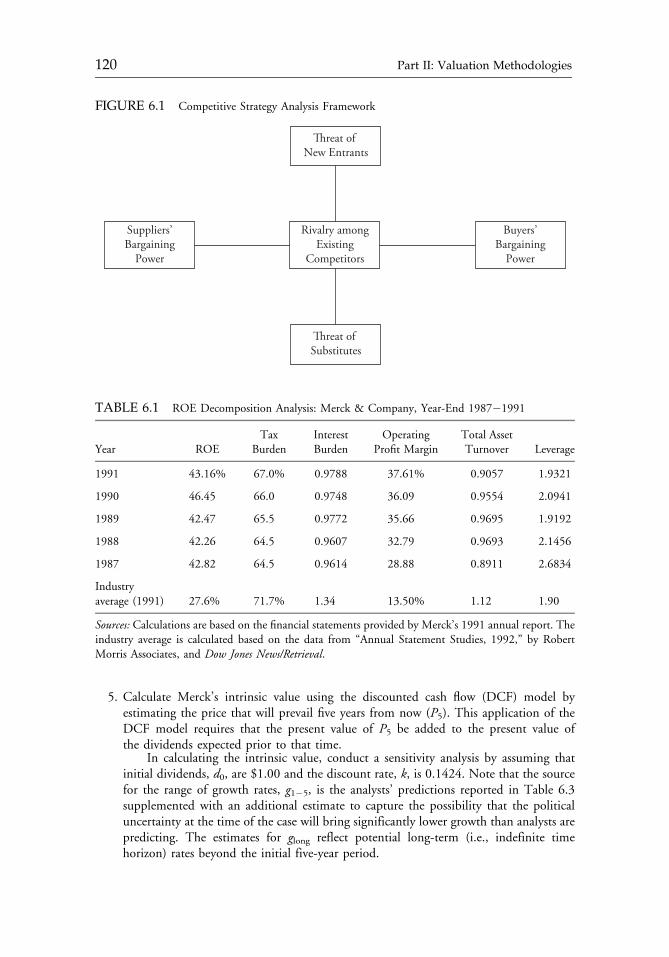
5. Calculate Merck’s intrinsic value using the discounted cash flow (DCF) model byestimating the price that will prevail five years from now (P5). This application of theDCF model requires that the present value of P5 be added to the present value ofthe dividends expected prior to that time.
In calculating the intrinsic value, conduct a sensitivity analysis by assuming thatinitial dividends, d0, are $1.00 and the discount rate, k, is 0.1424. Note that the sourcefor the range of growth rates, g1�5, is the analysts’ predictions reported in Table 6.3supplemented with an additional estimate to capture the possibility that the politicaluncertainty at the time of the case will bring significantly lower growth than analysts arepredicting. The estimates for glong reflect potential long-term (i.e., indefinite timehorizon) rates beyond the initial five-year period.
TABLE 6.1 ROE Decomposition Analysis: Merck & Company, Year-End 1987�1991
Year ROETax
BurdenInterestBurden
OperatingProfit Margin
Total AssetTurnover Leverage
1991 43.16% 67.0% 0.9788 37.61% 0.9057 1.9321
1990 46.45 66.0 0.9748 36.09 0.9554 2.0941
1989 42.47 65.5 0.9772 35.66 0.9695 1.9192
1988 42.26 64.5 0.9607 32.79 0.9693 2.1456
1987 42.82 64.5 0.9614 28.88 0.8911 2.6834
Industryaverage (1991) 27.6% 71.7% 1.34 13.50% 1.12 1.90
Sources: Calculations are based on the financial statements provided by Merck’s 1991 annual report. Theindustry average is calculated based on the data from “Annual Statement Studies, 1992,” by RobertMorris Associates, and Dow Jones News/Retrieval.
FIGURE 6.1 Competitive Strategy Analysis Framework
Threat of New Entrants
Threat of Substitutes
Suppliers’Bargaining
Power
Rivalry amongExisting
Competitors
Buyers’Bargaining
Power
c06 12 September 2012; 17:41:24
120 Part II: Valuation Methodologies
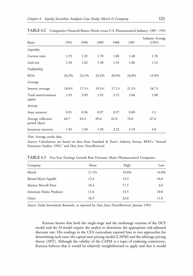
Kurious knows that both the single-stage and the multistage versions of the DCFmodel and the H-model require the analyst to determine the appropriate risk-adjusteddiscount rate. His readings in the CFA curriculum exposed him to two approaches fordetermining such rates: the capital asset pricing model (CAPM) and the arbitrage pricingtheory (APT). Although the validity of the CAPM is a topic of enduring controversy,Kurious believes that it would be relatively straightforward to apply and that it would
TABLE 6.2 Comparative Financial Ratios: Merck versus U.S. Pharmaceutical Industry, 1987�1991
Industry AverageRatio 1991 1990 1989 1988 1987 (1991)
Liquidity
Current ratio 1.53 1.33 1.78 1.80 1.40 1.70
Acid test 1.18 1.02 1.38 1.43 1.06 1.14
Profitability
ROA 24.2% 24.1% 23.2% 20.4% 16.8% 13.9%
Leverage
Interest coverage 18.03 17.53 19.33 17.23 21.33 18.73
Total assets/commonequity
1.93 2.09 1.92 2.15 2.68 1.90
Activity
Asset turnover 0.91 0.96 0.97 0.97 0.89 1.5
Average collectionperiod (days)
64.7 63.2 69.6 62.0 76.6 67.6
Inventory turnover 1.95 1.99 1.99 2.32 2.19 3.8
Note: Average yearly data.
Sources: Calculations are based on data from Standard & Poor’s Industry Surveys, RMA’s “AnnualStatement Studies, 1992,” and Dow Jones News/Retrieval.
TABLE 6.3 Five-Year Earnings Growth Rate Forecasts: Major Pharmaceutical Companies
Company Mean High Low
Merck 17.1% 19.0% 14.0%
Bristol-Myers Squibb 13.4 19.2 10.0
Marion Merrell Dow 10.4 17.5 3.0
American Home Products 11.6 13.5 10.0
Glaxo 16.5 22.0 11.0
Source: Zacks Investment Research, as reported by Dow Jones News/Retrieval, January 1993.
c06 12 September 2012; 17:41:25
Chapter 6 Equity Securities Analysis Case Study: Merck & Company 121
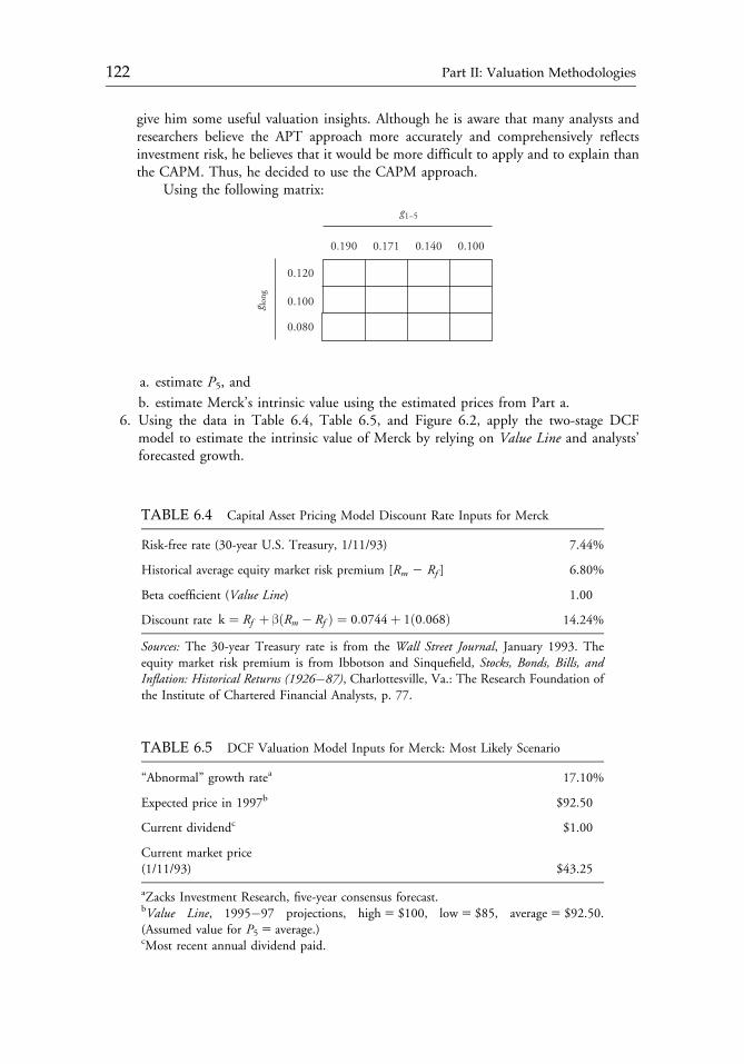
give him some useful valuation insights. Although he is aware that many analysts andresearchers believe the APT approach more accurately and comprehensively reflectsinvestment risk, he believes that it would be more difficult to apply and to explain thanthe CAPM. Thus, he decided to use the CAPM approach.
Using the following matrix:
0.190
0.120
0.100g long
0.080
0.171
g1–5
0.140 0.100
a. estimate P5, and
b. estimate Merck’s intrinsic value using the estimated prices from Part a.6. Using the data in Table 6.4, Table 6.5, and Figure 6.2, apply the two-stage DCF
model to estimate the intrinsic value of Merck by relying on Value Line and analysts’forecasted growth.
TABLE 6.5 DCF Valuation Model Inputs for Merck: Most Likely Scenario
“Abnormal” growth ratea 17.10%
Expected price in 1997b $92.50
Current dividendc $1.00
Current market price(1/11/93) $43.25
aZacks Investment Research, five-year consensus forecast.bValue Line, 1995�97 projections, high5 $100, low5 $85, average5 $92.50.(Assumed value for P55 average.)cMost recent annual dividend paid.
TABLE 6.4 Capital Asset Pricing Model Discount Rate Inputs for Merck
Risk-free rate (30-year U.S. Treasury, 1/11/93) 7.44%
Historical average equity market risk premium [Rm 2 Rf ] 6.80%
Beta coefficient (Value Line) 1.00
Discount rate k ¼ Rf þ βðRm � Rf Þ ¼ 0:0744þ 1ð0:068Þ 14.24%
Sources: The 30-year Treasury rate is from the Wall Street Journal, January 1993. Theequity market risk premium is from Ibbotson and Sinquefield, Stocks, Bonds, Bills, andInflation: Historical Returns (1926�87), Charlottesville, Va.: The Research Foundation ofthe Institute of Chartered Financial Analysts, p. 77.
c06 12 September 2012; 17:41:25
122 Part II: Valuation Methodologies

FIGURE 6.2 Value Line on Merck, November 6, 1992
c06 12 September 2012; 17:41:25
Chapter 6 Equity Securities Analysis Case Study: Merck & Company 123
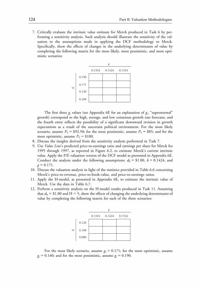
7. Critically evaluate the intrinsic value estimate for Merck produced in Task 6 by per-forming a sensitivity analysis. Such analysis should illustrate the sensitivity of the val-uation to the assumptions made in applying the DCF methodology to Merck.Specifically, show the effects of changes in the underlying determinants of value bycompleting the following matrix for the most likely, most pessimistic, and most opti-mistic scenarios:
0.190
0.1324 0.1424 0.1524
0.171
g s
0.140
0.100
k
The first three gs values (see Appendix 6E for an explanation of gs, “supernormal”growth) correspond to the high, average, and low consensus growth rate forecasts, andthe fourth entry reflects the possibility of a significant downward revision in growthexpectations as a result of the uncertain political environment. For the most likelyscenario, assume P55 $92.50; for the most pessimistic, assume P55 $85; and for themost optimistic, assume P55 $100.
8. Discuss the insights derived from the sensitivity analysis performed in Task 7.9. Use Value Line’s predicted price-to-earnings ratio and earnings per share for Merck for
1995 through 1997, as reported in Figure 6.2, to estimate Merck’s current intrinsicvalue. Apply the P/E valuation version of the DCF model as presented in Appendix 6E.Conduct the analysis under the following assumptions: d05 $1.00, k5 0.1424, andg5 0.171.
10. Discuss the valuation analysis in light of the statistics provided in Table 6.6 concerningMerck’s price-to-revenue, price-to-book-value, and price-to-earnings ratios.
11. Apply the H-model, as presented in Appendix 6E, to estimate the intrinsic value ofMerck. Use the data in Table 6.7.
12. Perform a sensitivity analysis on the H-model results produced in Task 11. Assumingthat d05 $1.00 and H5 5, show the effects of changing the underlying determinants ofvalue by completing the following matrix for each of the three scenarios:
0.120
0.1324 0.1424 0.1524
0.100g s
0.080
k
For the most likely scenario, assume gs5 0.171; for the most optimistic, assumegs5 0.140; and for the most pessimistic, assume gs5 0.190.
c06 12 September 2012; 17:41:26
124 Part II: Valuation Methodologies
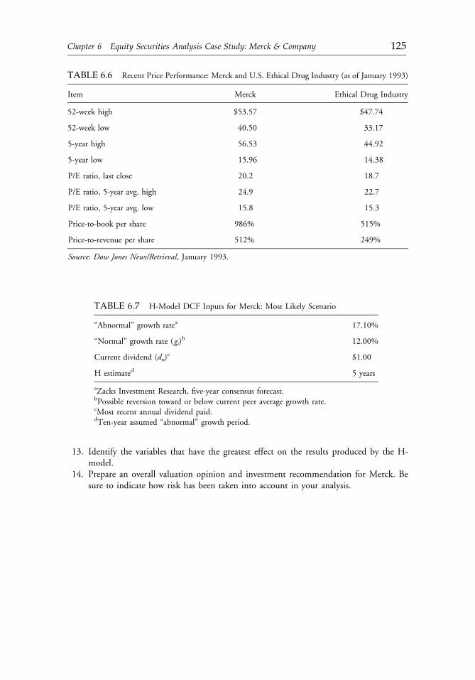
13. Identify the variables that have the greatest effect on the results produced by the H-model.
14. Prepare an overall valuation opinion and investment recommendation for Merck. Besure to indicate how risk has been taken into account in your analysis.
TABLE 6.6 Recent Price Performance: Merck and U.S. Ethical Drug Industry (as of January 1993)
Item Merck Ethical Drug Industry
52-week high $53.57 $47.74
52-week low 40.50 33.17
5-year high 56.53 44.92
5-year low 15.96 14.38
P/E ratio, last close 20.2 18.7
P/E ratio, 5-year avg. high 24.9 22.7
P/E ratio, 5-year avg. low 15.8 15.3
Price-to-book per share 986% 515%
Price-to-revenue per share 512% 249%
Source: Dow Jones News/Retrieval, January 1993.
TABLE 6.7 H-Model DCF Inputs for Merck: Most Likely Scenario
“Abnormal” growth ratea 17.10%
“Normal” growth rate (gs)b 12.00%
Current dividend (dn)c $1.00
H estimated 5 years
aZacks Investment Research, five-year consensus forecast.bPossible reversion toward or below current peer average growth rate.cMost recent annual dividend paid.dTen-year assumed “abnormal” growth period.
c06 12 September 2012; 17:41:26
Chapter 6 Equity Securities Analysis Case Study: Merck & Company 125
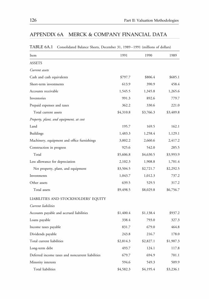
APPENDIX 6A MERCK & COMPANY FINANCIAL DATA
TABLE 6A.1 Consolidated Balance Sheets, December 31, 1989�1991 (millions of dollars)
Item 1991 1990 1989
ASSETS
Current assets
Cash and cash equivalents $797.7 $806.4 $685.1
Short-term investments 613.9 390.9 458.4
Accounts receivable 1,545.5 1,345.8 1,265.6
Inventories 991.3 892.6 779.7
Prepaid expenses and taxes 362.2 330.6 221.0
Total current assets $4,310.8 $3,766.3 $3,409.8
Property, plant, and equipment, at cost
Land 195.7 169.5 162.1
Buildings 1,483.3 1,258.4 1,129.1
Machinery, equipment and office furnishings 3,002.2 2,660.6 2,417.2
Construction in progress 925.6 542.0 285.5
Total $5,606.8 $4,630.5 $3,993.9
Less allowance for depreciation 2,102.3 1,908.8 1,701.4
Net property, plant, and equipment $3,504.5 $2,721.7 $2,292.5
Investments 1,043.7 1,012.3 737.2
Other assets 639.5 529.5 317.2
Total assets $9,498.5 $8,029.8 $6,756.7
LIABILITIES AND STOCKHOLDERS’ EQUITY
Current liabilities
Accounts payable and accrued liabilities $1,400.4 $1,138.4 $937.2
Loans payable 338.4 793.0 327.3
Income taxes payable 831.7 679.0 464.8
Dividends payable 243.8 216.7 178.0
Total current liabilities $2,814.3 $2,827.1 $1,907.3
Long-term debt 493.7 124.1 117.8
Deferred income taxes and noncurrent liabilities 679.7 694.9 701.1
Minority interests 594.6 549.3 509.9
Total liabilities $4,582.3 $4,195.4 $3,236.1
c06 12 September 2012; 17:41:27
126 Part II: Valuation Methodologies
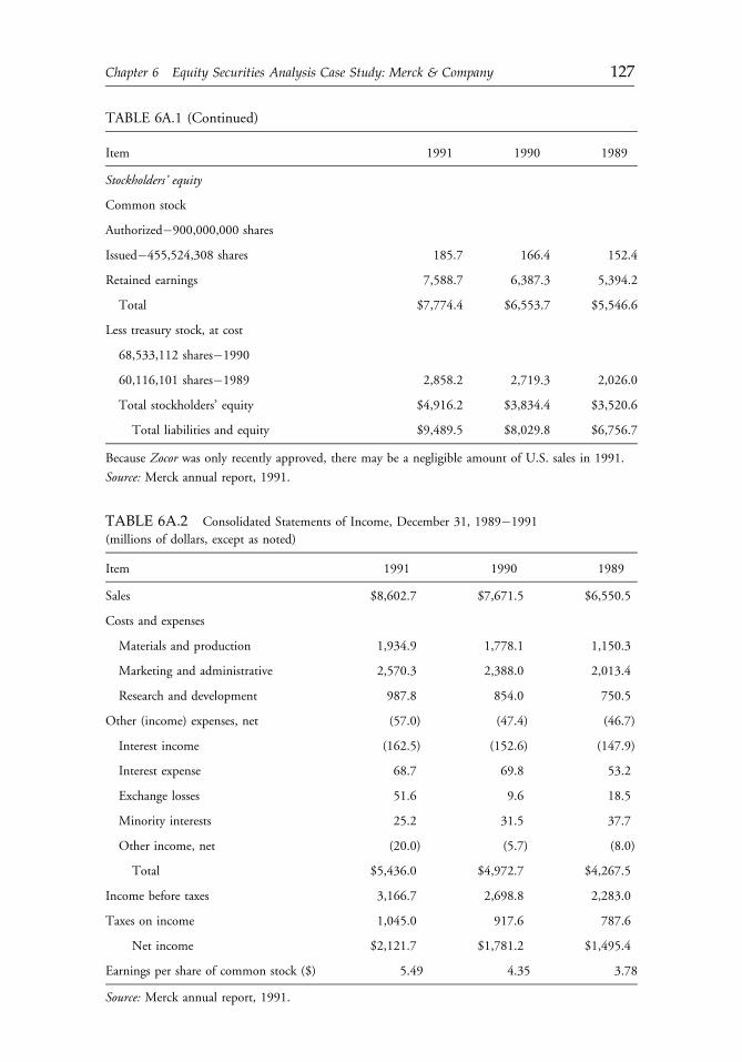
TABLE 6A.1 (Continued)
Item 1991 1990 1989
Stockholders’ equity
Common stock
Authorized�900,000,000 shares
Issued�455,524,308 shares 185.7 166.4 152.4
Retained earnings 7,588.7 6,387.3 5,394.2
Total $7,774.4 $6,553.7 $5,546.6
Less treasury stock, at cost
68,533,112 shares�1990
60,116,101 shares�1989 2,858.2 2,719.3 2,026.0
Total stockholders’ equity $4,916.2 $3,834.4 $3,520.6
Total liabilities and equity $9,489.5 $8,029.8 $6,756.7
Because Zocor was only recently approved, there may be a negligible amount of U.S. sales in 1991.
Source: Merck annual report, 1991.
TABLE 6A.2 Consolidated Statements of Income, December 31, 1989�1991
(millions of dollars, except as noted)
Item 1991 1990 1989
Sales $8,602.7 $7,671.5 $6,550.5
Costs and expenses
Materials and production 1,934.9 1,778.1 1,150.3
Marketing and administrative 2,570.3 2,388.0 2,013.4
Research and development 987.8 854.0 750.5
Other (income) expenses, net (57.0) (47.4) (46.7)
Interest income (162.5) (152.6) (147.9)
Interest expense 68.7 69.8 53.2
Exchange losses 51.6 9.6 18.5
Minority interests 25.2 31.5 37.7
Other income, net (20.0) (5.7) (8.0)
Total $5,436.0 $4,972.7 $4,267.5
Income before taxes 3,166.7 2,698.8 2,283.0
Taxes on income 1,045.0 917.6 787.6
Net income $2,121.7 $1,781.2 $1,495.4
Earnings per share of common stock ($) 5.49 4.35 3.78
Source: Merck annual report, 1991.
c06 12 September 2012; 17:41:27
Chapter 6 Equity Securities Analysis Case Study: Merck & Company 127
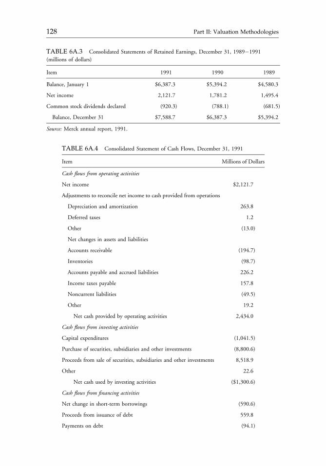
TABLE 6A.4 Consolidated Statement of Cash Flows, December 31, 1991
Item Millions of Dollars
Cash flows from operating activities
Net income $2,121.7
Adjustments to reconcile net income to cash provided from operations
Depreciation and amortization 263.8
Deferred taxes 1.2
Other (13.0)
Net changes in assets and liabilities
Accounts receivable (194.7)
Inventories (98.7)
Accounts payable and accrued liabilities 226.2
Income taxes payable 157.8
Noncurrent liabilities (49.5)
Other 19.2
Net cash provided by operating activities 2,434.0
Cash flows from investing activities
Capital expenditures (1,041.5)
Purchase of securities, subsidiaries and other investments (8,800.6)
Proceeds from sale of securities, subsidiaries and other investments 8,518.9
Other 22.6
Net cash used by investing activities ($1,300.6)
Cash flows from financing activities
Net change in short-term borrowings (590.6)
Proceeds from issuance of debt 559.8
Payments on debt (94.1)
TABLE 6A.3 Consolidated Statements of Retained Earnings, December 31, 1989�1991
(millions of dollars)
Item 1991 1990 1989
Balance, January 1 $6,387.3 $5,394.2 $4,580.3
Net income 2,121.7 1,781.2 1,495.4
Common stock dividends declared (920.3) (788.1) (681.5)
Balance, December 31 $7,588.7 $6,387.3 $5,394.2
Source: Merck annual report, 1991.
c06 12 September 2012; 17:41:27
128 Part II: Valuation Methodologies
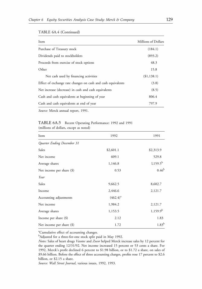
TABLE 6A.5 Recent Operating Performance: 1992 and 1991
(millions of dollars, except as noted)
Item 1992 1991
Quarter Ending December 31
Sales $2,601.1 $2,313.9
Net income 609.1 529.8
Average shares 1,146.8 l,159.5b
Net income per share ($) 0.53 0.46b
Year
Sales 9,662.5 8,602.7
Income 2,446.6 2,121.7
Accounting adjustments (462.4)a
Net income 1,984.2 2,121.7
Average shares 1,153.5 1,159.9b
Income per share ($) 2.12 1.83
Net income per share ($) 1.72 1.83b
aCumulative effect of accounting changes.bAdjusted for a three-for-one stock split paid in May 1992.Notes: Sales of heart drugs Vasotec and Zocor helped Merck increase sales by 12 percent forthe quarter ending 12/31/92. Net income increased 15 percent or 53 cents a share. For1992, Merck’s profit declined 6 percent to $1.98 billion, or to $1.72 a share, on sales of$9.66 billion. Before the effect of three accounting charges, profits rose 17 percent to $2.6billion, or $2.15 a share.Source: Wall Street Journal, various issues, 1992, 1993.
TABLE 6A.4 (Continued)
Item Millions of Dollars
Purchase of Treasury stock (184.1)
Dividends paid to stockholders (893.2)
Proceeds from exercise of stock options 48.3
Other 15.8
Net cash used by financing activities ($1,138.1)
Effect of exchange rate changes on cash and cash equivalents (3.8)
Net increase (decrease) in cash and cash equivalents (8.5)
Cash and cash equivalents at beginning of year 806.4
Cash and cash equivalents at end of year 797.9
Source: Merck annual report, 1991.
c06 12 September 2012; 17:41:27
Chapter 6 Equity Securities Analysis Case Study: Merck & Company 129
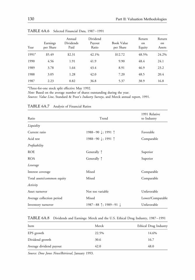
TABLE 6A.7 Analysis of Financial Ratios
Ratio Trend1991 Relativeto Industry
Liquidity
Current ratio 1988�90 k; 1991 m Favorable
Acid test 1988�90 k; 1991 m Comparable
Profitability
ROE Generally m Superior
ROA Generally m Superior
Leverage
Interest coverage Mixed Comparable
Total assets/common equity Mixed Comparable
Activity
Asset turnover Not too variable Unfavorable
Average collection period Mixed Lower/Comparable
Inventory turnover 1987�88 m; 1989�91 k Unfavorable
TABLE 6A.6 Selected Financial Data, 1987�1991
YearEarningsper Share
AnnualDividends
Paid
DividendPayoutRatio
Book Valueper Share
Returnon
Equity
Returnon
Assets
1991a $5.49 $2.31 42.1% $12.72 48.5% 24.2%
1990 4.56 1.91 41.9 9.90 48.4 24.1
1989 3.78 1.64 43.4 8.91 46.9 23.2
1988 3.05 1.28 42.0 7.20 48.5 20.4
1987 2.23 0.82 36.8 5.37 38.9 16.8
aThree-for-one stock split effective May 1992.Note: Based on the average number of shares outstanding during the year.Sources: Value Line, Standard & Poor’s Industry Surveys, and Merck annual report, 1991.
TABLE 6A.8 Dividends and Earnings: Merck and the U.S. Ethical Drug Industry, 1987�1991
Item Merck Ethical Drug Industry
EPS growth 22.5% 14.6%
Dividend growth 30.6 16.7
Average dividend payout 42.0 48.0
Source: Dow Jones News/Retrieval, January 1993.
c06 12 September 2012; 17:41:28
130 Part II: Valuation Methodologies
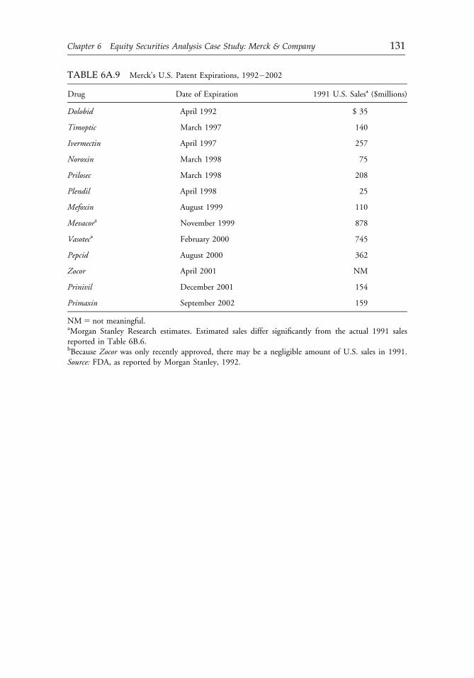
TABLE 6A.9 Merck’s U.S. Patent Expirations, 1992�2002
Drug Date of Expiration 1991 U.S. Salesa ($millions)
Dolobid April 1992 $ 35
Timoptic March 1997 140
Ivermectin April 1997 257
Noroxin March 1998 75
Prilosec March 1998 208
Plendil April 1998 25
Mefoxin August 1999 110
Mevacora November 1999 878
Vasoteca February 2000 745
Pepcid August 2000 362
Zocor April 2001 NM
Prinivil December 2001 154
Primaxin September 2002 159
NM5 not meaningful.aMorgan Stanley Research estimates. Estimated sales differ significantly from the actual 1991 salesreported in Table 6B.6.bBecause Zocor was only recently approved, there may be a negligible amount of U.S. sales in 1991.Source: FDA, as reported by Morgan Stanley, 1992.
c06 12 September 2012; 17:41:28
Chapter 6 Equity Securities Analysis Case Study: Merck & Company 131
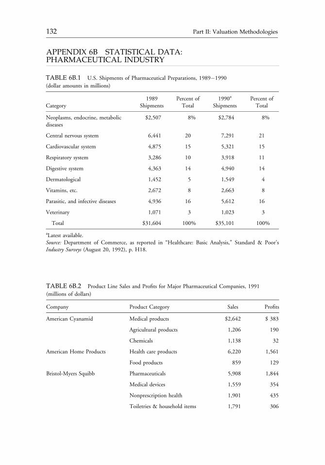
APPENDIX 6B STATISTICAL DATA:PHARMACEUTICAL INDUSTRY
TABLE 6B.1 U.S. Shipments of Pharmaceutical Preparations, 1989�1990
(dollar amounts in millions)
Category1989
ShipmentsPercent ofTotal
1990a
ShipmentsPercent ofTotal
Neoplasms, endocrine, metabolicdiseases
$2,507 8% $2,784 8%
Central nervous system 6,441 20 7,291 21
Cardiovascular system 4,875 15 5,321 15
Respiratory system 3,286 10 3,918 11
Digestive system 4,363 14 4,940 14
Dermatological 1,452 5 1,549 4
Vitamins, etc. 2,672 8 2,663 8
Parasitic, and infective diseases 4,936 16 5,612 16
Veterinary 1,071 3 1,023 3
Total $31,604 100% $35,101 100%
aLatest available.Source: Department of Commerce, as reported in “Healthcare: Basic Analysis,” Standard & Poor’sIndustry Surveys (August 20, 1992), p. H18.
TABLE 6B.2 Product Line Sales and Profits for Major Pharmaceutical Companies, 1991
(millions of dollars)
Company Product Category Sales Profits
American Cyanamid Medical products $2,642 $ 383
Agricultural products 1,206 190
Chemicals 1,138 32
American Home Products Health care products 6,220 1,561
Food products 859 129
Bristol-Myers Squibb Pharmaceuticals 5,908 1,844
Medical devices 1,559 354
Nonprescription health 1,901 435
Toiletries & household items 1,791 306
c06 12 September 2012; 17:41:28
132 Part II: Valuation Methodologies
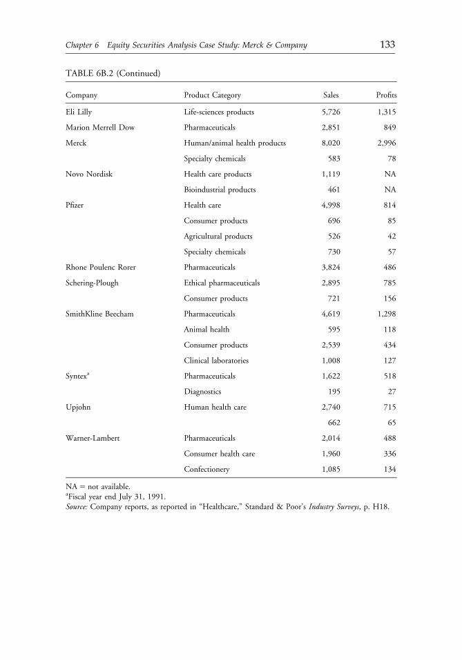
TABLE 6B.2 (Continued)
Company Product Category Sales Profits
Eli Lilly Life-sciences products 5,726 1,315
Marion Merrell Dow Pharmaceuticals 2,851 849
Merck Human/animal health products 8,020 2,996
Specialty chemicals 583 78
Novo Nordisk Health care products 1,119 NA
Bioindustrial products 461 NA
Pfizer Health care 4,998 814
Consumer products 696 85
Agricultural products 526 42
Specialty chemicals 730 57
Rhone Poulenc Rorer Pharmaceuticals 3,824 486
Schering-Plough Ethical pharmaceuticals 2,895 785
Consumer products 721 156
SmithKline Beecham Pharmaceuticals 4,619 1,298
Animal health 595 118
Consumer products 2,539 434
Clinical laboratories 1,008 127
Syntexa Pharmaceuticals 1,622 518
Diagnostics 195 27
Upjohn Human health care 2,740 715
662 65
Warner-Lambert Pharmaceuticals 2,014 488
Consumer health care 1,960 336
Confectionery 1,085 134
NA5 not available.aFiscal year end July 31, 1991.Source: Company reports, as reported in “Healthcare,” Standard & Poor’s Industry Surveys, p. H18.
c06 12 September 2012; 17:41:29
Chapter 6 Equity Securities Analysis Case Study: Merck & Company 133
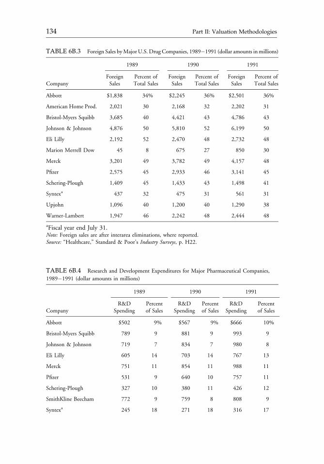
TABLE 6B.3 Foreign Sales byMajorU.S. Drug Companies, 1989�1991 (dollar amounts inmillions)
1989 1990 1991
CompanyForeignSales
Percent ofTotal Sales
ForeignSales
Percent ofTotal Sales
ForeignSales
Percent ofTotal Sales
Abbott $1,838 34% $2,245 36% $2,501 36%
American Home Prod. 2,021 30 2,168 32 2,202 31
Bristol-Myers Squibb 3,685 40 4,421 43 4,786 43
Johnson & Johnson 4,876 50 5,810 52 6,199 50
Eli Lilly 2,192 52 2,470 48 2,732 48
Marion Merrell Dow 45 8 675 27 850 30
Merck 3,201 49 3,782 49 4,157 48
Pfizer 2,575 45 2,933 46 3,141 45
Schering-Plough 1,409 45 1,433 43 1,498 41
Syntexa 437 32 475 31 561 31
Upjohn 1,096 40 1,200 40 1,290 38
Warner-Lambert 1,947 46 2,242 48 2,444 48
aFiscal year end July 31.Note: Foreign sales are after interarea eliminations, where reported.Source: “Healthcare,” Standard & Poor’s Industry Surveys, p. H22.
TABLE 6B.4 Research and Development Expenditures for Major Pharmaceutical Companies,
1989�1991 (dollar amounts in millions)
1989 1990 1991
CompanyR&D
SpendingPercentof Sales
R&DSpending
Percentof Sales
R&DSpending
Percentof Sales
Abbott $502 9% $567 9% $666 10%
Bristol-Myers Squibb 789 9 881 9 993 9
Johnson & Johnson 719 7 834 7 980 8
Eli Lilly 605 14 703 14 767 13
Merck 751 11 854 11 988 11
Pfizer 531 9 640 10 757 11
Schering-Plough 327 10 380 11 426 12
SmithKline Beecham 772 9 759 8 808 9
Syntexa 245 18 271 18 316 17
c06 12 September 2012; 17:41:29
134 Part II: Valuation Methodologies
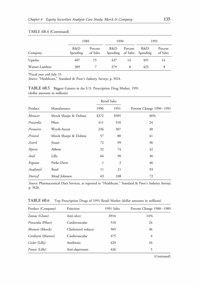
TABLE 6B.5 Biggest Gainers in the U.S. Prescription Drug Market, 1991
(dollar amounts in millions)
Retail Sales
Product Manufacturer 1990 1991 Percent Change 1990�1991
Mevacor Merck Sharpe & Dohme $372 $505 36%
Procardia Pfizer 411 510 24
Premarin Wyeth-Ayerst 236 307 30
Prinivil Merck Sharpe & Dohme 57 80 41
Zestril Stuart 72 99 36
Hytrin Abbott 52 74 42
Axid Lilly 66 90 36
Ergostat Parke-Davis 1 2 46
Anafranil Basel 11 21 93
Duricef Mead Johnson 63 108 72
Source: Pharmaceutical Data Services, as reported in “Healthcare,” Standard & Poor’s Industry Surveys,p. H26.
TABLE 6B.6 Top Prescription Drugs of 1991 Retail Market (dollar amounts in millions)
Product (Company) Function 1991 Sales Percent Change 1988�1989
Zantac (Glaxo) Anti-ulcer $916 14%
Procardia (Pfizer) Cardiovascular 510 24
Mevacor (Merck) Cholesterol reducer 505 36
Cardizem (Marion) Cardiovascular 475 4
Ceclor (Lilly) Antibiotic 429 16
Prozac (Lilly) Anti-depressant 426 5
(Continued)
TABLE 6B.4 (Continued)
1989 1990 1991
CompanyR&D
SpendingPercentof Sales
R&DSpending
Percentof Sales
R&DSpending
Percentof Sales
Upjohn 407 15 427 14 491 14
Warner-Lambert 309 7 379 8 423 8
aFiscal year end July 31.Source: “Healthcare,” Standard & Poor’s Industry Surveys, p. H24.
c06 12 September 2012; 17:41:29
Chapter 6 Equity Securities Analysis Case Study: Merck & Company 135
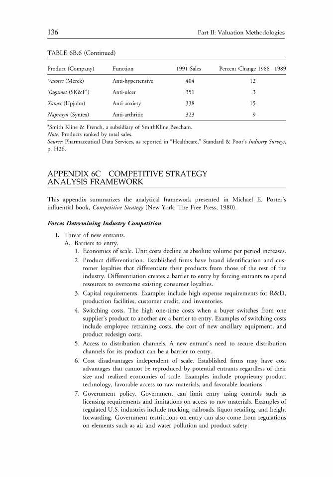
APPENDIX 6C COMPETITIVE STRATEGYANALYSIS FRAMEWORK
This appendix summarizes the analytical framework presented in Michael E. Porter’sinfluential book, Competitive Strategy (New York: The Free Press, 1980).
Forces Determining Industry Competition
I. Threat of new entrants.A. Barriers to entry.
1. Economies of scale. Unit costs decline as absolute volume per period increases.
2. Product differentiation. Established firms have brand identification and cus-tomer loyalties that differentiate their products from those of the rest of theindustry. Differentiation creates a barrier to entry by forcing entrants to spendresources to overcome existing consumer loyalties.
3. Capital requirements. Examples include high expense requirements for R&D,production facilities, customer credit, and inventories.
4. Switching costs. The high one-time costs when a buyer switches from onesupplier’s product to another are a barrier to entry. Examples of switching costsinclude employee retraining costs, the cost of new ancillary equipment, andproduct redesign costs.
5. Access to distribution channels. A new entrant’s need to secure distributionchannels for its product can be a barrier to entry.
6. Cost disadvantages independent of scale. Established firms may have costadvantages that cannot be reproduced by potential entrants regardless of theirsize and realized economies of scale. Examples include proprietary producttechnology, favorable access to raw materials, and favorable locations.
7. Government policy. Government can limit entry using controls such aslicensing requirements and limitations on access to raw materials. Examples ofregulated U.S. industries include trucking, railroads, liquor retailing, and freightforwarding. Government restrictions on entry can also come from regulationson elements such as air and water pollution and product safety.
TABLE 6B.6 (Continued)
Product (Company) Function 1991 Sales Percent Change 1988�1989
Vasotec (Merck) Anti-hypertensive 404 12
Tagamet (SK&Fa) Anti-ulcer 351 3
Xanax (Upjohn) Anti-anxiety 338 15
Naprosyn (Syntex) Anti-arthritic 323 9
aSmith Kline & French, a subsidiary of SmithKline Beecham.Note: Products ranked by total sales.Source: Pharmaceutical Data Services, as reported in “Healthcare,” Standard & Poor’s Industry Surveys,p. H26.
c06 12 September 2012; 17:41:30
136 Part II: Valuation Methodologies
B. Expected reaction of existing competition. The threat of entry is influenced bythe potential entrant’s expectations about the reaction of existing competitors to anew entrant.
II. Conditions associated with intense rivalry among existing competitors.A. Numerous or equally balanced competitors.B. Slow industry growth.C. High fixed or storage costs.D. Lack of differentiation or switching costs.E. Capacity augmented in large increments (dictated by extent of economies of scale).F. Diverse competitors. Companies that are diverse in strategies, origins, personalities
can run into each other in their operations.G. High strategic stakes. Rivalry becomes more volatile as the number of firms with
high stakes in achieving success increases.H. High exit barriers. Examples include specialized assets, fixed costs of exit, strategic
interrelationships, and government restrictions.III. Pressure from substitute products. Substitutes constrain potential returns in an industry
by putting a ceiling on prices. The impact of substitutes can be measured by theindustry’s overall elasticity of demand.
IV. Conditions associated with powerful buyers.A. Buyer purchases large volumes relative to seller sales.B. Product purchased represents a significant fraction of buyer’s costs or purchases.C. Product purchased is standard or undifferentiated.D. Buyer faces few switching costs.E. Buyers earn low profits.F. Buyers pose a credible threat of backward integration.G. Industry’s product is unimportant to the quality of the buyer’s products or
services.H. Buyer has full information.
V. Conditions associated with powerful supplier groups.A. Suppliers are dominated by a few companies and are more concentrated than the
purchasing industry.B. Suppliers need not contend with substitute products for sale to the industry.C. Industry is not an important customer of the supplier group.D. The suppliers’ product is an important input to the buyer’s business.E. The supplier group’s product is differentiated, or there are significant
switching costs.F. The supplier group poses a credible threat of forward integration.
Generic Competitive Strategies
I. Overall cost leadership strategy.A. Description: Cost leadership requires the construction of efficient-scale facilities,
the pursuit of cost reductions from experience, tight cost and overhead control, andcost minimization in such areas as R&D, sales, and advertising.
B. Observations.1. A low-cost position can yield above-average returns despite strong competitive
forces.
c06 12 September 2012; 17:41:30
Chapter 6 Equity Securities Analysis Case Study: Merck & Company 137
2. A low-cost position often requires a high relative market share or otheradvantages.
3. The strategy can revolutionize an industry in which the nature of competitionhas been otherwise historically and competitors are unprepared to pursue costminimization.
II. Differentiation strategy.A. Description: Differentiation requires the creation of a product or service that is
perceived industrywide as unique.B. Approaches to differentiation.
1. Design or brand image.
2. Technological superiority.
3. Superior customer service.
C. Differentiation and market share. Differentiation may preclude gaining highmarket share.
III. Focus strategy.A. Description: Focusing on a particular buyer group, segments of the product line, or
geographic market. The premise of this strategy is that the firm is able to serve itsstrategic target more effectively or efficiently than competitors that are competingmore broadly.
B. Forms of the focus strategy.1. Differentiation within target area.
2. Cost leadership within target area.
Pursuit of More Than One Generic Strategy
I. It is usually necessary to make a choice among the generic strategies or become “stuckin the middle.” The pursuit of more than one strategy is more feasible if the units arestrictly separated.
II. Achieving cost leadership and differentiation is usually inconsistent unless:A. Competitors are “stuck in the middle.”B. Cost is strongly affected by share or interrelationships.C. A firm pioneers a major innovation.
Sustainability and Above-Average Performance
A generic strategy will not bring above-average performance unless it is sustainable vis-a-vis afirm’s competitors. Competitive advantage must resist erosion by competitor behavior orindustry evolution.
c06 12 September 2012; 17:41:30
138 Part II: Valuation Methodologies
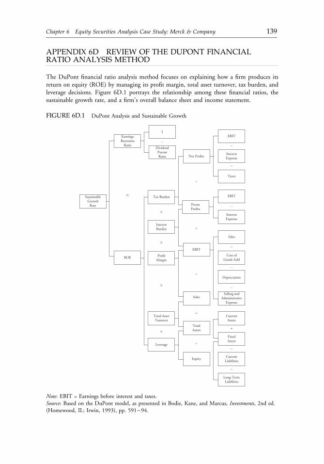
APPENDIX 6D REVIEW OF THE DUPONT FINANCIALRATIO ANALYSIS METHOD
The DuPont financial ratio analysis method focuses on explaining how a firm produces itsreturn on equity (ROE) by managing its profit margin, total asset turnover, tax burden, andleverage decisions. Figure 6D.1 portrays the relationship among these financial ratios, thesustainable growth rate, and a firm’s overall balance sheet and income statement.
FIGURE 6D.1 DuPont Analysis and Sustainable Growth
1EarningsRetention
Ratio
ROE
DividendPayoutRatio
–�
�
Net ProfitsInterestExpense
Taxes
EBIT
EBIT
EBIT
�
InterestExpense
Sales
�
Cost ofGoods Sold
�
Depreciation
�
Selling andAdministrative
Expense
CurrentAssets
�
FixedAssets
�
CurrentLiabilities
�
Long-TermLiabilities
PretaxProfits
�
�
�
�
�
�
�
�
Sales
�
TotalAssets
�
Total AssetTurnover
Leverage
ProfitMargin
InterestBurden
Tax BurdenSustainableGrowth
Rate
Equity
Note: EBIT = Earnings before interest and taxes.Source: Based on the DuPont model, as presented in Bodie, Kane, and Marcus, Investments, 2nd ed.(Homewood, IL: Irwin, 1993), pp. 591�94.
c06 12 September 2012; 17:41:30
Chapter 6 Equity Securities Analysis Case Study: Merck & Company 139
APPENDIX 6E SELECTED VALUATION METHODS
This appendix reviews six widely used methods: the single-stage constant-growth discountedcash flow (DCF) model, the multistage DCF model, the so-called H-model, the price-to-earnings ratio (P/E) approach, the price-to-sales ratio (P/S) approach, and the price-to-book-value (P/B) approach.
Single-Stage Constant-Growth DCF Model
The single-stage constant-growth DCF model values a stock by taking the present value of thecash flows the investment is expected to generate. In practice, this approach implies that aninvestor or analyst must estimate the company’s future earnings per share, project the pro-portion of earnings that will be paid out as dividends in the future, and calculate the presentvalue of the expected stream of cash flows at the appropriate risk-adjusted discount rate. Thesingle-stage approach assumes that the expected rate of growth will persist indefinitely andthat the appropriate discount rate exceeds that growth rate (i.e., growth is “normal”). Thebasic form of the model is:
P0 ¼XNt¼1
dtð1þ kÞt
¼ d1ð1þ kÞ1 þ
d2ð1þ kÞ2 þ?þ dN
ð1þ kÞN
¼ d0ð1þ gÞ1ð1þ kÞ1 þ d0ð1þ gÞ2
ð1þ kÞ2 þ?þ d0ð1þ gÞNð1þ kÞN
¼XNt¼1
d0ð1þ gÞtð1þ kÞt
where P0 is the current appropriate or intrinsic value of the stock, dt is the dividend expectedin period t, k is the appropriate risk-adjusted discount rate, d0 is the initial dividend, and g isthe expected constant rate of dividend growth.
An equivalent form of the model, restated to facilitate making the necessary calcu-lations, is:
P0 ¼ d0ð1þ gÞk � g
:
This form of the single-stage DCF model is valid only under the assumption that kexceeds g. Further, this and the subsequent forms of the DCF model discussed are notadjusted for the quarterly payment of dividends.
Multistage DCF Model
Many analysts believe it is more realistic to assume that firms pass through various stagesof growth that are manifested by different rates of dividend growth. This belief has the
c06 12 September 2012; 17:41:30
140 Part II: Valuation Methodologies
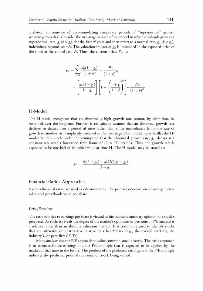
analytical convenience of accommodating temporary periods of “supernormal” growthwherein g exceeds k. Consider the two-stage version of the model in which dividends grow at asupernormal rate, gs (k, gs), for the first N years and then revert to a normal rate, gn (k. gn),indefinitely beyond year N. The valuation impact of gn is imbedded in the expected price ofthe stock at the end of year N. Thus, the current price, P0, is:
P0 ¼XNt¼1
d0ð1þ gsÞtð1þ kÞt þ PN
ð1þ kÞN
¼ d0ð1þ gsÞk � gs
24
35 1� 1þ gs
1þ k
0@
1AN2
435þ PN
ð1þ kÞN :
H-Model
The H-model recognizes that an abnormally high growth rate cannot, by definition, besustained over the long run. Further, it realistically assumes that an abnormal growth ratedeclines or decays over a period of time rather than shifts immediately from one rate ofgrowth to another, as is implicitly assumed in the two-stage DCF model. Specifically, the H-model values a stock under the assumption that the abnormal growth rate, gs,, decays at aconstant rate over a forecasted time frame of (2 3 H) periods. Thus, the growth rate isexpected to be one-half of its initial value at time H. The H-model may be stated as:
P0 ¼ d0ð1þ gnÞ þ d0ðHÞðgs � gnÞk � gn
:
Financial Ratios Approaches
Various financial ratios are used as valuation tools. The primary ones are price/earnings, price/sales, and price/book value per share.
Price/Earnings
The ratio of price to earnings per share is viewed as the market’s summary opinion of a stock’sprospects. As such, it reveals the degree of the market’s optimism or pessimism. P/E analysis isa relative rather than an absolute valuation method. It is commonly used to identify stocksthat are attractive or unattractive relative to a benchmark (e.g., the overall market’s, theindustry’s, or peer firms’ P/Es).
Many analysts use the P/E approach to value common stock directly. The basic approachis to estimate future earnings and the P/E multiple that is expected to be applied by themarket at that time in the future. The product of the predicted earnings and the P/E multipleindicates the predicted price of the common stock being valued.
c06 12 September 2012; 17:41:31
Chapter 6 Equity Securities Analysis Case Study: Merck & Company 141
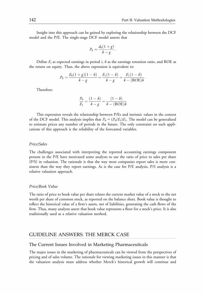
Insight into this approach can be gained by exploring the relationship between the DCFmodel and the P/E. The single-stage DCF model asserts that
P0 ¼ d0ð1þ gÞk � g
:
Define Ei as expected earnings in period i, b as the earnings retention ratio, and ROE asthe return on equity. Thus, the above expression is equivalent to:
P0 ¼ E0ð1þ gÞð1� bÞk � g
¼ E1ð1� bÞk � g
¼ E1ð1� bÞk � ðROEÞb :
Therefore:
P0E1
¼ ð1� bÞk � g
¼ ð1� bÞk � ðROEÞb
This expression reveals the relationship between P/Es and intrinsic values in the contextof the DCF model. This analysis implies that P05 (P0/E1)E1. The model can be generalizedto estimate prices any number of periods in the future. The only constraint on such appli-cations of this approach is the reliability of the forecasted variables.
Price/Sales
The challenges associated with interpreting the reported accounting earnings componentpresent in the P/E have motivated some analysts to use the ratio of price to sales per share(P/S) in valuation. The rationale is that the way most companies report sales is more con-sistent than the way they report earnings. As is the case for P/E analysis, P/S analysis is arelative valuation approach.
Price/Book Value
The ratio of price to book value per share relates the current market value of a stock to the networth per share of common stock, as reported on the balance sheet. Book value is thought toreflect the historical value of a firm’s assets, net of liabilities, generating the cash flows of thefirm. Thus, many analysts assert that book value represents a floor for a stock’s price. It is alsotraditionally used as a relative valuation method.
GUIDELINE ANSWERS: THE MERCK CASE
The Current Issues Involved in Marketing Pharmaceuticals
The major issues in the marketing of pharmaceuticals can be viewed from the perspectives ofpricing and of sales volume. The rationale for viewing marketing issues in this manner is thatthe valuation analysis must address whether Merck’s historical growth will continue and
c06 12 September 2012; 17:41:31
142 Part II: Valuation Methodologies

where its future growth is likely to come from. The case observes that the demand forpharmaceuticals is relatively price inelastic because most payments are made by third parties.Another observation is that pharmaceutical prices in recent years have increased at roughlythree times the U.S. rate of inflation. Thus, the discussion of marketing issues is organizedaround the question of whether Merck’s future growth will come predominantly from priceincreases or from sales volume increases.
Pricing and volume issues can be evaluated by discussing the implications of four recentdevelopments: the growth of managed health care programs, the aging U.S. population,changes in the role of the consumer/patient, and changes in the U.S. political environment.
Growth of Managed Health Care Programs
Health management organizations are growing in number and are establishing drug utiliza-tion programs that have broad decision-making power. Merck’s strategic response to thistrend was the creation of a Managed Health Care Affairs Department to develop relationshipswith major HMOs. The widespread presence of such groups could put downward pressure onpharmaceutical prices.
Aging U.S. Population
The so-called “greying of America” implies an increase in the demand for pharmaceuticals.Thus, the aging U.S. population indicates projected growth in sales volume.
Changes in the Role of the Consumer/Patient
Patients are changing from passive recipients to active participants in the drug-selectionprocess. Merck’s strategic response has been to increase its initiatives to involve consumers. Anexample is the increased use of patient-oriented packaging and advertising. This role changecould affect price elasticity adversely from Merck’s perspective.
Changes in the U.S. Political Environment
In January 1993, the investment community was assessing the implications of President-electClinton’s stated positions on the pharmaceutical industry. The predominant opinion was thatthe new administration would be tough on pharmaceutical pricing. The emphasis on morecomprehensive, inclusive health care could boost sales volume. Indeed, this policy goal couldmake the U.S. federal government the largest purchaser of Merck’s products in the future.Government product-substitution requirements could greatly increase generic drugs’ marketshare. Greater government involvement could also bring reimbursement policies that includecost-containment goals, which would constrain pharmaceutical prices.
The consensus opinion at this time is that Merck’s future growth will most likely comepredominantly from growth in sales volume and not from price increases, as was the case inthe past.
The Competitive Structure of the U.S. Pharmaceutical Industry
A schematic analysis of Merck’s competitive position, using the Porter approach, is shown inFigure 6E.1.
c06 12 September 2012; 17:41:31
Chapter 6 Equity Securities Analysis Case Study: Merck & Company 143
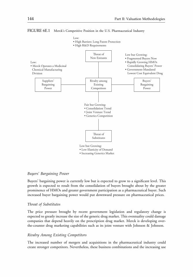
Buyers’ Bargaining Power
Buyers’ bargaining power is currently low but is expected to grow to a significant level. Thisgrowth is expected to result from the consolidation of buyers brought about by the greaterprominence of HMOs and greater government participation as a pharmaceutical buyer. Suchincreased buyer bargaining power would put downward pressure on pharmaceutical prices.
Threat of Substitutes
The price pressure brought by recent government legislation and regulatory change isexpected to greatly increase the size of the generic drug market. This eventuality could damagecompanies that depend heavily on the prescription drug market. Merck is developing over-the-counter drug marketing capabilities such as its joint venture with Johnson & Johnson.
Rivalry Among Existing Competitors
The increased number of mergers and acquisitions in the pharmaceutical industry couldcreate stronger competitors. Nevertheless, these business combinations and the increasing use
FIGURE 6E.1 Merck’s Competitive Position in the U.S. Pharmaceutical Industry
Threat ofNew Entrants
Low:• High Barriers: Long Patent Protection• High R&D Requirements
Low:• Merck Operates a Medicinal Chemical Manufacturing Division
Low but Growing:• Low Elasticity of Demand• Increasing Generics Market
Low but Growing:• Fragmented Buyers Now• Rapidly Growing HMOs Consolidating Buyers’ Power• Government-Mandated Lowest Cost Equivalent Drug
Threat ofSubstitutes
Rivalry amongExisting
Competitors
Suppliers’Bargaining
Power
Buyers’Bargaining
Power
Fair but Growing:• Consolidation Trend• Joint Venture Trend• Generics Competition
c06 12 September 2012; 17:41:31
144 Part II: Valuation Methodologies
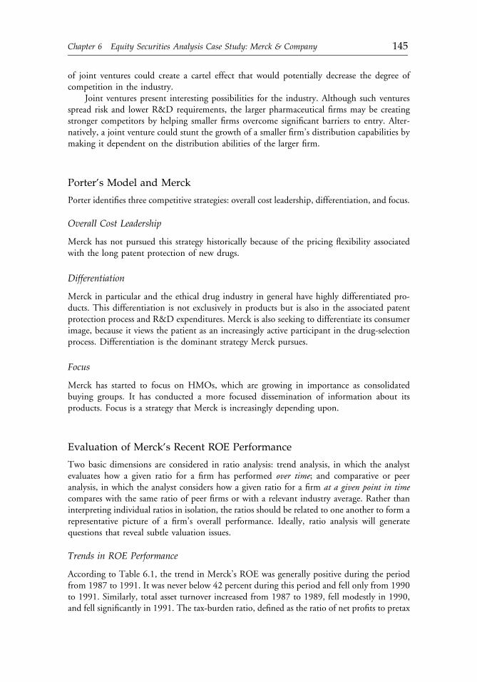
of joint ventures could create a cartel effect that would potentially decrease the degree ofcompetition in the industry.
Joint ventures present interesting possibilities for the industry. Although such venturesspread risk and lower R&D requirements, the larger pharmaceutical firms may be creatingstronger competitors by helping smaller firms overcome significant barriers to entry. Alter-natively, a joint venture could stunt the growth of a smaller firm’s distribution capabilities bymaking it dependent on the distribution abilities of the larger firm.
Porter’s Model and Merck
Porter identifies three competitive strategies: overall cost leadership, differentiation, and focus.
Overall Cost Leadership
Merck has not pursued this strategy historically because of the pricing flexibility associatedwith the long patent protection of new drugs.
Differentiation
Merck in particular and the ethical drug industry in general have highly differentiated pro-ducts. This differentiation is not exclusively in products but is also in the associated patentprotection process and R&D expenditures. Merck is also seeking to differentiate its consumerimage, because it views the patient as an increasingly active participant in the drug-selectionprocess. Differentiation is the dominant strategy Merck pursues.
Focus
Merck has started to focus on HMOs, which are growing in importance as consolidatedbuying groups. It has conducted a more focused dissemination of information about itsproducts. Focus is a strategy that Merck is increasingly depending upon.
Evaluation of Merck’s Recent ROE Performance
Two basic dimensions are considered in ratio analysis: trend analysis, in which the analystevaluates how a given ratio for a firm has performed over time; and comparative or peeranalysis, in which the analyst considers how a given ratio for a firm at a given point in timecompares with the same ratio of peer firms or with a relevant industry average. Rather thaninterpreting individual ratios in isolation, the ratios should be related to one another to form arepresentative picture of a firm’s overall performance. Ideally, ratio analysis will generatequestions that reveal subtle valuation issues.
Trends in ROE Performance
According to Table 6.1, the trend in Merck’s ROE was generally positive during the periodfrom 1987 to 1991. It was never below 42 percent during this period and fell only from 1990to 1991. Similarly, total asset turnover increased from 1987 to 1989, fell modestly in 1990,and fell significantly in 1991. The tax-burden ratio, defined as the ratio of net profits to pretax
c06 12 September 2012; 17:41:31
Chapter 6 Equity Securities Analysis Case Study: Merck & Company 145

profits, increased consistently during the 1987�91 period. The interest burden rose onlymodestly during this time period. This result indicates that Merck consistently reduced its taxliability. The operating profit margin improved consistently. Leverage was the most volatile ofthe DuPont variables. It decreased significantly from 1987 to 1989 and then drifted upwardin 1990, only to fall back to its prior level in 1991.
Comparative, or Peer, Analysis of ROE Performance
Merck compared favorably with the industry averages for ROE and operating profit margin in1991 (see Table 6.1). Its leverage was roughly comparable; its interest burden, tax burden, andtotal asset turnover ratio were all lower than the respective industry averages.
The comparative financial ratios portrayed in Table 6.2 are largely consistent withthe patterns revealed by the DuPont ROE analysis. The lower-than-average total asset turnoverratio in 1991 was accompanied by lower-than-average liquidity as measured by thecurrent ratio. The lower-than-average interest coverage ratio was comparable to the industry’s,as was the leverage ratio. Merck’s average collection period was shorter than the industryaverage in 1991.
Overall Interpretation of the Ratio Analysis
The primary source of Merck’s exemplary ROE performance was its ability to increasesteadily the already dramatic levels of its operating profit margin from 1987 to 1991. Merck’saccomplishment reflects its product mix. Merck is more a pure ethical drug company thanmost of the other firms in the industry. Ethical drugs have a higher margin than otherproducts. For example, some of the companies in the industry have consumer productbusinesses that have thin margins. Other companies sell medical supplies, which also tend tohave lower margins, as part of their product mixes. Thus, comparisons between Merck’s loftyoperating profit margins and the industry average must be made cautiously because of thedifferences between Merck’s product mix and those of other firms.
Caution must also be exercised in interpreting the significance of the decline and lowerlevel of Merck’s total asset turnover ratio. When turnover ratios fall, a firm is typically per-ceived to be having a problem maintaining efficiency. For example, a marked decline or lowcomparative level in inventory turnover is generally interpreted as negative. Total assetturnover is not so easily interpreted, however. This ratio can fall because a firm is investingheavily in assets to enhance its future efficiency. Thus, in the short run, asset turnover andROE can suffer but will actually benefit from such investment over the long term.
The potential implications of Merck’s enviably high ROE are important in light of theextremely uncertain political environment facing the U.S. pharmaceutical industry in 1993.Since 1988, Merck’s ROE has never been lower than 42 percent. Such a high return could beviewed as a tempting target for regulators, who might wonder why any firm would need suchhigh earnings. The uncertain political environment also has potential implications for Merck’sability to continue increasing its operating profit margin.
The company’s expected future growth is presumably heavily reliant on increasing profitmargins, the primary source of its growth in the recent past. Yet, in 1993, the press waspublishing stories about high pharmaceutical prices and the need for cost containment. Thus,
c06 12 September 2012; 17:41:32
146 Part II: Valuation Methodologies

Merck’s ability to depend on aggressive product pricing and, by implication, high margins toenhance its future growth is in question.
Calculate Merck’s Intrinsic Value
The technique for estimating intrinsic value that is indicated by the form of the data is:
P0 ¼X5t¼1
d0ð1þ g1�5Þtð1þ kÞt þ P5
ð1þ kÞ5
¼ d0ð1þ g1�5Þk � g1�5
þ 1� 1þ g1�5
ð1þ kÞ
0@
1A52
435þ P5
ð1þ kÞ5 :
This technique requires an estimate of P5, which can be done using the followingformula:
P5 ¼ d6k � g
¼ ½d0ð1þ g1�5Þ5�ð1þ glongÞ
ðk � glongÞ
The expected P5 values under the DCF model sensitivity analysis are as follows:
0.120
0.190 0.171 0.140 0.100
0.100g long
g1–5
0.080
$119.32
$61.91
$41.30
$110.09
$57.12
$38.11
$96.27
$49.95
$33.32
$80.52
$41.78
$27.87
Using these estimated prices, the intrinsic value sensitivity analysis for Merck is asfollows:
0.120
0.190 0.171 0.140 0.100
0.100g long
g1–5
0.080
$66.98
$37.48
$26.89
$61.97
$34.74
$24.97
$54.45
$30.64
$22.09
$45.85
$25.94
$18.79
c06 12 September 2012; 17:41:32
Chapter 6 Equity Securities Analysis Case Study: Merck & Company 147
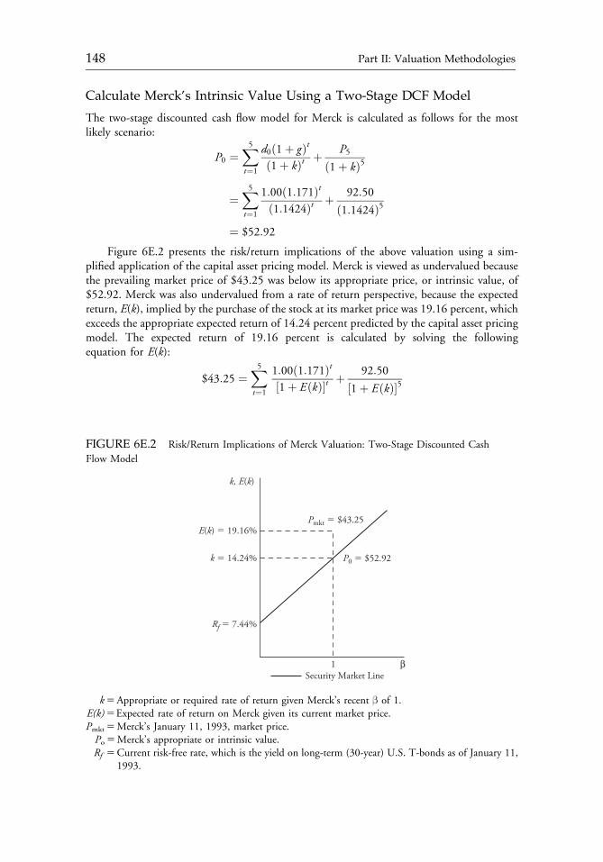
Calculate Merck’s Intrinsic Value Using a Two-Stage DCF Model
The two-stage discounted cash flow model for Merck is calculated as follows for the mostlikely scenario:
P0 ¼X5t¼1
d0ð1þ gÞtð1þ kÞt þ P5
ð1þ kÞ5
¼X5t¼1
1:00ð1:171Þtð1:1424Þt þ 92:50
ð1:1424Þ5
¼ $52:92
Figure 6E.2 presents the risk/return implications of the above valuation using a sim-plified application of the capital asset pricing model. Merck is viewed as undervalued becausethe prevailing market price of $43.25 was below its appropriate price, or intrinsic value, of$52.92. Merck was also undervalued from a rate of return perspective, because the expectedreturn, E(k), implied by the purchase of the stock at its market price was 19.16 percent, whichexceeds the appropriate expected return of 14.24 percent predicted by the capital asset pricingmodel. The expected return of 19.16 percent is calculated by solving the followingequation for E(k):
$43:25 ¼X5t¼1
1:00ð1:171Þt½1þ EðkÞ�t þ 92:50
½1þ EðkÞ�5
FIGURE 6E.2 Risk/Return Implications of Merck Valuation: Two-Stage Discounted Cash
Flow Model
Security Market Line1 β
k, E(k)
P0 � $52.92
Pmkt � $43.25
Rf � 7.44%
k � 14.24%
E(k) � 19.16%
k5Appropriate or required rate of return given Merck’s recent β of 1.E(k)5Expected rate of return on Merck given its current market price.Pmkt5Merck’s January 11, 1993, market price.Po5Merck’s appropriate or intrinsic value.Rf 5Current risk-free rate, which is the yield on long-term (30-year) U.S. T-bonds as of January 11,
1993.
c06 12 September 2012; 17:41:32
148 Part II: Valuation Methodologies
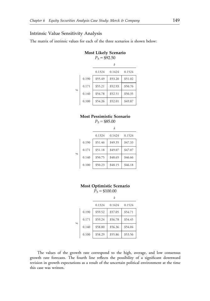
Intrinsic Value Sensitivity Analysis
The matrix of intrinsic values for each of the three scenarios is shown below:
Most Likely ScenarioP55 $92.50
0.190
0.1324 0.1424 0.1524
0.171
g
k
0.140
$55.49
$55.21
$54.78
$53.20
$52.93
$52.51
$51.02
$50.76
$50.35
0.100 $54.26 $52.01 $49.87
Most Pessimistic ScenarioP55 $85.00
0.190
0.1324 0.1424 0.1524
0.171
g
k
0.140
$51.46
$51.18
$50.75
$49.35
$49.07
$48.65
$47.33
$47.07
$46.66
0.100 $50.23 $48.15 $46.18
Most Optimistic ScenarioP55 $100.00
0.190
0.1324 0.1424 0.1524
0.171
g
k
0.140
$59.52
$59.24
$58.80
$57.05
$56.78
$56.36
$54.71
$54.45
$54.04
0.100 $58.29 $55.86 $53.56
The values of the growth rate correspond to the high, average, and low consensusgrowth rate forecasts. The fourth line reflects the possibility of a significant downwardrevision in growth expectations as a result of the uncertain political environment at the timethis case was written.
c06 12 September 2012; 17:41:32
Chapter 6 Equity Securities Analysis Case Study: Merck & Company 149
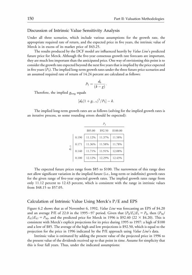
Discussion of Intrinsic Value Sensitivity Analysis
Under all three scenarios, which include various assumptions for the growth rate, theappropriate required rate of return, and the expected price in five years, the intrinsic value ofMerck is in excess of its market price of $43.25.
The results produced by the DCF model are influenced heavily by Value Line’s predictedfuture price for Merck. Although the five-year consensus growth rate forecasts are important,they are much less important than the anticipated price. One way of envisioning this point is toconsider the growth rate expected beyond the next five years that is implied by the price expectedin five years (P5). The implied long-term growth rates under the three future price scenarios andan assumed required rate of return of 14.24 percent are calculated as follows:
P5 ¼ d6ðk � gÞ :
Therefore, the implied glong equals
½d0ð1þ g1�5Þ5=P5� � k:
The implied long-term growth rates are as follows (solving for the implied growth rates isan iterative process, so some rounding errors should be expected):
0.190
$85.00 $92.50 $100.00
0.171
g 1–5
0.140
0.100
11.12%
11.36%
11.71%
11.37%
11.58%
11.91%
11.58%
11.78%
12.08%
P5
12.12% 12.29% 12.43%
The expected future prices range from $85 to $100. The narrowness of this range doesnot allow significant variation in the implied future (i.e., long-term or indefinite) growth ratesfor the given range of five-year expected growth rates. The implied growth rates range fromonly 11.12 percent to 12.43 percent, which is consistent with the range in intrinsic valuesfrom $48.15 to $57.05.
Calculation of Intrinsic Value Using Merck’s P/E and EPS
Figure 6.2 shows that as of November 6, 1992, Value Line was forecasting an EPS of $4.20and an average P/E of 22.0 in the 1995�97 period. Given that (P0/E1)E15 P0, then (P96/E97)E975 P96, and the predicted price for Merck in 1996 is $92.40 (22 3 $4.20). This isconsistent with Merck’s explicit projections for its price during 1995 to 1997: a high of $100and a low of $85. The average of the high and low projections is $92.50, which is equal to theprojection for the price in 1996 indicated by the P/E approach using Value Line’s data.
Intrinsic value is estimated by adding the present value of the projected price in 1996 tothe present value of the dividends received up to that point in time. Assume for simplicity thatthis is four full years. Thus, under the indicated assumptions:
c06 12 September 2012; 17:41:32
150 Part II: Valuation Methodologies

P0 ¼X4t¼1
d0ð1þ gÞtð1þ kÞt þ P96
ð1þ kÞ4
¼ d0ð1þ gÞk � g
1��1þ g1þ k
�N24
35þ P96
ð1þ kÞ4
¼ 1:00ð1:171Þ0:1424� 0:171
1��
1:171
1:1424
�424
35þ 92:40
ð1:1424Þ4 ¼ $58:51:
Discussion of the Valuation Analysis
Table 6.6 shows that Merck’s price-to-revenue ratio (P/R) is about 2.06 times greater than theindustry average, its P/B is about 1.91 times greater than the industry average, and its P/E isonly 1.08 times greater than the industry average. Apparently, investors are paying more forasset-based sources of growth, as measured by the P/R and P/B, than for Merck’s earnings, asmeasured by its P/E. The P/E analysis performed for the preceding task provides no insightsbeyond those yielded by the DCF model analyses.
Calculation of Intrinsic Value Using the H-Model
The following H-model valuation shows that the intrinsic value of Merck is $61.38. Notethat the long-term growth rate is assumed to be 12 percent under the rationale that Merck’sexpected long-term growth rate could fall because of the implications of the uncertainpolitical environment:
P0 ¼ d0ð1þ gnÞ þ d0ðH Þðgs � gnÞðk � gnÞ
¼ 1:00ð1:1200Þ þ 1:00ð5Þð0:1710� 0:1200Þ0:1424� 0:1200
¼ $61:38:
Sensitivity Analysis of the H-Model
The effects of changing the underlying determinants of value are as follows:
Most Likely Scenariogs5 17.10%
0.12
0.1324 0.1424 0.1524
0.10g n
0.08
$110.89
$44.91
$29.29
$61.38
$34.32
$24.60
$42.44
$27.77
$21.20
k
c06 12 September 2012; 17:41:33
Chapter 6 Equity Securities Analysis Case Study: Merck & Company 151
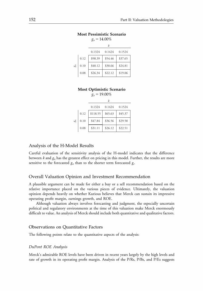
Most Pessimistic Scenariogs5 14.00%
0.12
0.1324 0.1424 0.1524
0.10g n0.08
$98.39
$40.12
$26.34
$54.46
$30.66
$22.12
$37.65
$24.81
$19.06
k
Most Optimistic Scenariogs5 19.00%
0.12
0.1324 0.1424 0.1524
0.10g n
0.08
$118.55
$47.84
$31.11
$65.63
$36.56
$26.12
$45.37
$29.58
$22.51
k
Analysis of the H-Model Results
Careful evaluation of the sensitivity analysis of the H-model indicates that the differencebetween k and gn has the greatest effect on pricing in this model. Further, the results are moresensitive to the forecasted gn than to the shorter term forecasted gs.
Overall Valuation Opinion and Investment Recommendation
A plausible argument can be made for either a buy or a sell recommendation based on therelative importance placed on the various pieces of evidence. Ultimately, the valuationopinion depends heavily on whether Kurious believes that Merck can sustain its impressiveoperating profit margin, earnings growth, and ROE.
Although valuation always involves forecasting and judgment, the especially uncertainpolitical and regulatory environments at the time of this valuation make Merck enormouslydifficult to value. An analysis of Merck should include both quantitative and qualitative factors.
Observations on Quantitative Factors
The following points relate to the quantitative aspects of the analysis:
DuPont ROE Analysis
Merck’s admirable ROE levels have been driven in recent years largely by the high levels andrate of growth in its operating profit margin. Analysis of the P/Rs, P/Bs, and P/Es suggests
c06 12 September 2012; 17:41:33
152 Part II: Valuation Methodologies
that Merck’s market price is affected more by asset-based factors than by earnings-basedfactors. Interestingly, however, consensus five-year forecasted earnings growth rates werein the range of 14 to 17 percent at this time. Similarly, Value Line was predicting that Merck’sprice would be between $85 and $100 in the period from 1995 to 1997. Valuation modelscan provide insight into the implications of such high forecasted growth rates andfuture prices.
Valuation Model Results
The initial DCF model sensitivity analysis, which focuses on the expected price of Merck infive years (P5), produced intrinsic values in excess of Merck’s current price for all expectedshort-term growth rates (g1�5) only under the assumption that the long-term growth rate(glong) was 0.12 or higher. Under glong assumptions of 0.10 and 0.08, Merck was overvaluedfor all assumed values of g1�5. The two-stage DCF model under various assumptions pro-duced intrinsic values that were all in excess of Merck’s prevailing market price of $43.25.The H-model under various assumptions produced more mixed results than the two-stageDCF model.
Depending on which normal growth rate, abnormal growth rate, and discount rateKurious has the most confidence in, Merck could be viewed as either over- or undervalued.Although the evidence provided by the two-stage DCF model generally indicated that Merckis undervalued, the evidence provided by the initial DCF model and H-model was mixed andgenerally less supportive of that valuation opinion.
Pitfalls in Quantitative Analysis
The quantitative analysis of Merck is only as good as the assumptions made concerning theunderlying determinants of value. The primary way to take risk into account in quantitativeanalysis is through the assumed discount rate. Thus, Kurious must judge the reasonableness ofthe forecasted growth rates and the discount rate used in his analysis. The discount ratesassumed in this case can be criticized on the grounds that they were estimated using only asimplified application of the CAPM. Even if that model is accepted as the best approach,analysts differ in their approaches to estimating the required parameters. For instance, somewould take issue with the chosen proxy for the risk-free rate and with the value of the riskpremium, especially in light of the observation that risk premiums widen during periods oflower interest rates. Further, one might argue that another approach, such as the APT, mightbe a more useful way to estimate the discount rate.
Observations on Qualitative Factors
The valuation of Merck dramatically illustrates the potential dangers of extrapolatingfrom historical data. Merck has been one of the most admired companies in the world andhas produced dramatic investment results. An analyst, however, must always ask howapplicable the past is to the future. This question can only be answered by determininghow Merck generated its growth in the past and by evaluating how sustainable that growthwill be in the future.
As noted above, the primary source of Merck’s growth in the recent past was its operatingprofit margin. In light of the significant uncertainty concerning the implications of the new
c06 12 September 2012; 17:41:33
Chapter 6 Equity Securities Analysis Case Study: Merck & Company 153

administration’s evolving health care policy reforms, Merck appears unlikely to sustain itsgrowth by relying on significant pharmaceutical price increases. Thus, Merck’s future growthappears to be more dependent on volume increases. Merck’s historical product-mix strategycould dampen such growth somewhat. Further, potential adverse legislative developmentssuch as the removal of the Puerto Rican tax shelter for U.S. pharmaceutical companies couldalso restrain Merck’s growth by increasing its future tax liability. A convincing argument cantherefore be made that Merck will not be able to sustain its dramatic growth record in thefuture. Depending on how much Kurious believes that future growth will decline, Merckcould be viewed as either over- or undervalued.
c06 12 September 2012; 17:41:33
154 Part II: Valuation Methodologies
CHAPTER 7TRADITIONAL EQUITYVALUATION METHODS
Thomas A. Martin, Jr., CFA
Traditional equity valuation methods are simply ways of exercising the criticaljudgment needed to determine value between the extremes of “cheap” and “expen-sive.” Whether used for screening purposes or for fundamental analysis, such methodsallow investors to make rational and consistent assessments of potential changes inkey valuation inputs.
Valuation is all about judgment. At the extremes of cheap or expensive, value is obvious, butbetween those extremes, analysis and judgment are crucial for determining value. Traditionalequity valuation methods are simply ways of performing analysis and exercising judgment.None of these methods consistently works particularly better than any of the others, and to acertain degree, they tend to give similar buy/sell signals for specific stocks. Still, these tra-ditional methods are useful for thinking about stocks and what should drive buying andselling decisions.
Although the traditional valuationmethods are relatively simple, their compelling advantageis that analysts understandwhat thesemethods are indicating.Most of the timewhen an analyst ora portfolio manager talks about valuation, stock selection, or the investment process, the decisionultimately comes down to picking cheap stocks. Stocks are considered cheap on some basis.Whenthat basis is not something complex and sophisticated—such as franchise value or firm value oreconomic value added or some measure of cash flow that is “not distorted by accountingmeasures”—the traditionalmethods, which are, in turn, based on accountingmeasures, are prettymuch all that is left. Even some of the newer approaches fall back ultimately on traditionalmeasures. Thus, traditional valuation measures should be well understood by all analysts.
Copyright ª 1998 Thomas A. Martin, Jr., CFA. Reprinted with permission from AIMR ConferenceProceedings (May 1998):21�35. This presentation comes from the Equity Research and ValuationTechniques conference held in Philadelphia on December 9, 1997. When this article was originallypublished, Thomas A. Martin, Jr., CFA, was an equity portfolio manager at INVESCO CapitalManagement Incorporated.
c07 12 September 2012; 13:28:8
155
The goal of this chapter is to remind equity analysts of the nature of these traditionalmethods—how they work, their effective use, and their limitations. The chapter begins byconsidering the purpose of valuation. It then goes on to define traditional valuation methods andlooks at how they are used for screening and in fundamental equity analysis and valuation.
PURPOSE
Analysts all want to buy stocks that will go up and sell stocks that will go down. A stock goesup or down from its current level because of some fundamental reevaluation of the companyand its prospects or of the environment in which the company operates. This fundamentalreevaluation comes about either because something has changed or is perceived to havechanged in the world. Probably no model can predict actual or perceived changes in a directand explicit way, but the models that seem to work the best do so because, for whateverreason, they capture those changes. Traditional equity valuation methods, and fundamentalanalysis in general, try to get at the nature of those changes.
Various factors affect a firm’s value. Certainly, environmental influences—such asinflation, taxes, and available rates of return on a variety of assets—affect all companies and allvaluations. Those influences are valuation inputs because they affect companies at the macrolevel. Company-specific influences, such as the current earnings and the future growth ofthose earnings, also affect valuation. In fact, at its simplest, value is the consistent piling upof profits. In addition, the level and trend of a company’s risk, as well as that of the envi-ronment, affects the company’s valuation; assessing risk is probably the most difficult andleast effectively accomplished of all the equity analyst’s tasks.
Therefore, the process of seeking buy opportunities involves identifying those companiesfor which the current expectations built into the current price are likely to be less than what willactually happen. Thus, the analyst needs models that will help identify (1) companies for whichconsensus future expected earnings are less than what “true” earnings will be or (2) companiesfor which the consensus expected risk is higher than what the “true” risk will be.
SHORTCUTS
How are analysts to solve the daunting problem of determining which companies and stockshave value? So much data and information are available. The world is very complicated, andshortcuts are not only helpful but also nearly mandatory. These shortcuts can be categorizedinto two groups: expectational models and valuation models.
Expectational Models
The focus in expectational models is typically the so-called momentum measures: earningssurprise, earnings revisions, or other technical measures. These models assume that the trendthat is in place will stay in place. In the case of earnings surprise, for instance, it is not theexistence of the last earnings surprise that will provide outperformance. Rather, it is the factthat the last earnings surprise is a good predictor that another earnings surprise will occur.By definition, nobody expects that next earning surprise because the market efficiently adjustsits expectations. But much of the time, expectations are not adjusted enough. So, in anexpectational model, a company keeps reporting positive earnings surprises, and the analystskeep raising earnings estimates until the company hits the wall and announces significantly
c07 12 September 2012; 13:28:8
156 Part II: Valuation Methodologies
disappointing news. Then, all the expectation-oriented investors sell the stock, and the stock’sprice goes down some large percentage in one day.
Valuation Models
Valuation models are typically based on mean-reversion, or contrarian, approaches. Theyassume that the trend that is in place will reverse and revert to some mean value. For example,suppose a company reports a big disappointment in earnings because of a sales shortfall andmargin contraction. The sales shortfall and margin contraction result from some combinationof short- and long-term factors. Earnings estimates are cut, and the stock price is hammered.The price may go down so much that the stock becomes cheap relative to traditionalbenchmarks. Mean reversion suggests that the stock price has overreacted, earnings expec-tations are now too low, and in the longer-term, the company will recover.
TRADITIONAL VALUATION METHODS
Despite their differences, both expectational and valuation models are ultimately trying to dothe same thing: Identify those companies for which the current expectations built into today’sstock price are wrong. Traditional equity valuation models and methods are simply systematicways of trying to make that identification.
The four primary traditional methods for equity valuation use the price-to-book ratio(P/B), price-to-sales ratio (P/S), price-to-earnings ratio (P/E), and the dividend discountmodel (DDM).
P/B
Book value is a static historicalmeasure that does not take into account the going-concern value ofa firm. Book value is calculated in relation to assets, not to the ability to generate profits. The P/Bdoes not explicitly or even implicitly account for growth or risk of a company, and it is subject to asubstantial amount of accounting measurement error because book value accumulates on thebalance sheet. Management can make accounting choices in terms of timing, inventories,depreciation, write-offs, write-downs, capitalization versus expensing, and how many shares thecompany repurchases and at what price. Then there are intangibles. If intangibles—brands,patents, relationships, employees, technology, know-how, and so on—make up a substantialportion of a company’s assets, the company will show a low book value relative to “reality.”
If book value presents problems in its use, one might question the logic of using it. P/B isuseful, however, for valuing (1) asset-rich companies, (2) non-going-concern situations, and(3) mature or cyclical companies with essentially zero or negative earnings. In the case of thelatter, P/B, along with historical and expected return on equity (ROE), can help to estimatenormalized peak earnings and normalized earnings ranges. In other words, using P/B canprovide guidance when a company does not have any earnings or when earnings do not seemto be the immediate value driver. P/B can also be used to help differentiate among companieswithin a homogenous industry.
P/S
Like P/B, P/S does not explicitly account for the growth or risk of a company. SometimesP/S is viewed favorably because it is the least subject to accounting manipulations of all the
c07 12 September 2012; 13:28:8
Chapter 7 Traditional Equity Valuation Methods 157
traditional valuation measures. At the same time, P/S is also the number with the leastamount of embedded information: It is a long way from the sales line on the incomestatement to the EPS line, and certainly, a lot of value is made or lost as we go from oneto the other. P/S may not be subject to manipulation, but a lot of crucial information isleft out.
P/S can be used in the same ways as P/B. For a mature or cyclical company withessentially zero or negative earnings, P/S in conjunction with margin assumptions can identifynormalized levels for the next peak earnings or normalized earnings. P/S can be helpful forevaluating companies with large recurring revenue bases or companies with high levelsof intangibles. As with P/B, P/S can be used to help differentiate among companies in ahomogenous industry.
P/E
The problem with P/E, like P/S and P/B, is that it does not explicitly account for growthor risk. In addition, P/E is difficult to put into perspective when EPS is declining ornegative because of cyclically or distress or when the company is in the early stages of itslife cycle. But P/E is probably the most commonly used valuation measure, and analysts allknow what it means to say that a company is cheap on a P/E basis. P/E is most effectivelyused to evaluate and compare stable companies in the late growth and maturity stages oftheir life cycles.
DDM
The DDM is intellectually and ideally the best model for valuing companies. The generalizedformula is next year’s dividend divided by some discount rate that is appropriate for that year,plus the second year’s dividend divided by some discount rate that is appropriate for thatyear, and so on. The generalized model requires the analyst to estimate a dividend for everyyear from now to eternity as well as the appropriate discount rate, which may be differentfrom year to year because inflation, the expected return on alternative investments, and therisk of the company and of the market itself may all be different from year to year. Forthe constant-growth version, the DDM states that a company’s stock price is equal to the nextyear’s dividend divided by the difference between k, the required rate of return, and g,the expected dividend growth rate in perpetuity. The DDM also comes in multistage models,which can vary from 2-stage models to 102-stage models. Multistage DDMs usually have asupernormal period in which earnings growth or dividend growth is higher than the long-term average for a mature company. Then they have a normalization period, during which thedividend growth rate reverts to some long-term sustainable level, and finally, a mature period,in which the dividend growth rate is constant.
An advantage of any DDM approach is that all of the input assumptions can be asexplicit, complicated, and specific as the analyst desires. Building such a model forces theanalyst to ask important questions: What does this company do? What products does it make?What stage of its industry, company, and product life cycle is the company in, in terms of itssales, profitability, and returns? The DDM makes the analyst think about these factors andput them in the model explicitly, whereas the other traditional models do not. The drawbackis that the analyst has to make many assumptions, and there are a lot of places to go wrong.Small changes in key assumptions, especially in the growth rate and the discount rate, canhave a big effect on the valuation estimate generated by the model.
c07 12 September 2012; 13:28:9
158 Part II: Valuation Methodologies
SCREENING
The first potential use for these traditional valuation methods is to look for ways of narrowingthe overwhelmingly large universe of investable companies down to some number of rea-sonable candidates that are more likely to have the desired value characteristics. This process iscalled screening.
Numerous studies have been done on all of the traditional valuation models, witha variety of results. Researchers contend that if portfolio managers would only follow aparticular valuation model, such as low P/E, P/S, or P/B, they would be rewarded withoutperformance. In fact, studies have shown that applying any one of these methods blindlyand faithfully will generate outperformance over time; however, many practical reasons can befound for not applying these methods blindly and faithfully. Perhaps the most important isthat such quantitatively generated portfolios typically exhibit other characteristics that maynot be prudent for most investors. So, although screening is useful for identifying potentialinvestment candidates, analysts must take care to understand the implications of the screeningfactor for portfolio construction.
To illustrate the biases of the traditional valuation methods, I put about 1,000 of thelargest companies in the United States through five valuation screens: P/B, P/S, P/E, P/E togrowth (a form of P/E valuation), and the DDM. I created five model portfolios, eachconsisting of the 50 cheapest stocks as defined by the particular valuation method. These fiveportfolios could then be compared with regard to sector composition, valuation, ROEcomposition, growth, and finally, risk, expectations, and performance.
Sector Composition
The sector compositions of the model portfolios are shown in Table 7.1. The S&P 500 Index,provided for reference, is a well- diversified portfolio. It represents a reasonable capitalization-weighted cross-section of the U.S. economy, and it is the benchmark against which most equitymanagers are compared.
In contrast, the portfolio containing the 50 cheapest stocks on the basis of the P/E-to-growth ratio is 30 percent in consumer cyclicals, 26 percent in technology, and 10 percent orless in all other sectors—not a particularly well-diversified portfolio. The P/B portfolio is54 percent in utilities, 20 percent in cyclicals, and underweighted in everything else. Staplesare cheap in the P/S strategy, as indicated by their overweighting, but they are not cheap byany other measure. The P/E and P/B portfolios turn out to be very similar: both overweightedin utilities and consumer cyclicals. The P/E portfolio is the only one that shows financials tobe cheap. The P/E-to-growth portfolio is a reasonably well-diversified portfolio but containsno utilities. The DDM portfolio is one of the best diversified of all the model portfolios, but itdoes have some overweights that seem to allow the manager to buy stocks with good growthcharacteristics, such as technology and health care.
The point is that most managers would not be comfortable with any of these individualportfolios, and they would have difficulty adhering to the discipline of using just one strategyno matter what type of portfolio was indicated. As an alternative, a manager might considerpicking the cheapest stocks in each sector and then using the S&P 500 weights, but then thatmanager has diverged from the path of using a pure quantitative valuation strategy to that ofusing some degree of judgment. How many more good judgments will that manager have tomake when the quantitative indications are not to his or her liking? The important issue,
c07 12 September 2012; 13:28:9
Chapter 7 Traditional Equity Valuation Methods 159
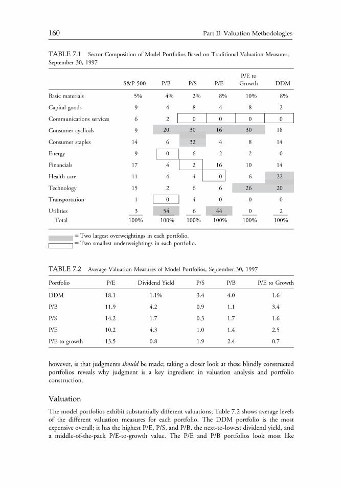
however, is that judgments should be made; taking a closer look at these blindly constructedportfolios reveals why judgment is a key ingredient in valuation analysis and portfolioconstruction.
Valuation
The model portfolios exhibit substantially different valuations; Table 7.2 shows average levelsof the different valuation measures for each portfolio. The DDM portfolio is the mostexpensive overall; it has the highest P/E, P/S, and P/B, the next-to-lowest dividend yield, anda middle-of-the-pack P/E-to-growth value. The P/E and P/B portfolios look most like
TABLE 7.1 Sector Composition of Model Portfolios Based on Traditional Valuation Measures,
September 30, 1997
P/E toS&P 500 P/B P/S P/E Growth DDM
Basic materials 5% 4% 2% 8% 10% 8%
Capital goods 9 4 8 4 8 2
Communications services 6 2 0 0 0 0
Consumer cyclicals 9 20 30 16 30 18
Consumer staples 14 6 32 4 8 14
Energy 9 0 6 2 2 0
Financials 17 4 2 16 10 14
Health care 11 4 4 0 6 22
Technology 15 2 6 6 26 20
Transportation 1 0 4 0 0 0
Utilities 3 54 6 44 0 2
Total 100% 100% 100% 100% 100% 100%
5Two largest overweightings in each portfolio.5Two smallest underweightings in each portfolio.
TABLE 7.2 Average Valuation Measures of Model Portfolios, September 30, 1997
Portfolio P/E Dividend Yield P/S P/B P/E to Growth
DDM 18.1 1.1% 3.4 4.0 1.6
P/B 11.9 4.2 0.9 1.1 3.4
P/S 14.2 1.7 0.3 1.7 1.6
P/E 10.2 4.3 1.0 1.4 2.5
P/E to growth 13.5 0.8 1.9 2.4 0.7
c07 12 September 2012; 13:28:9
160 Part II: Valuation Methodologies
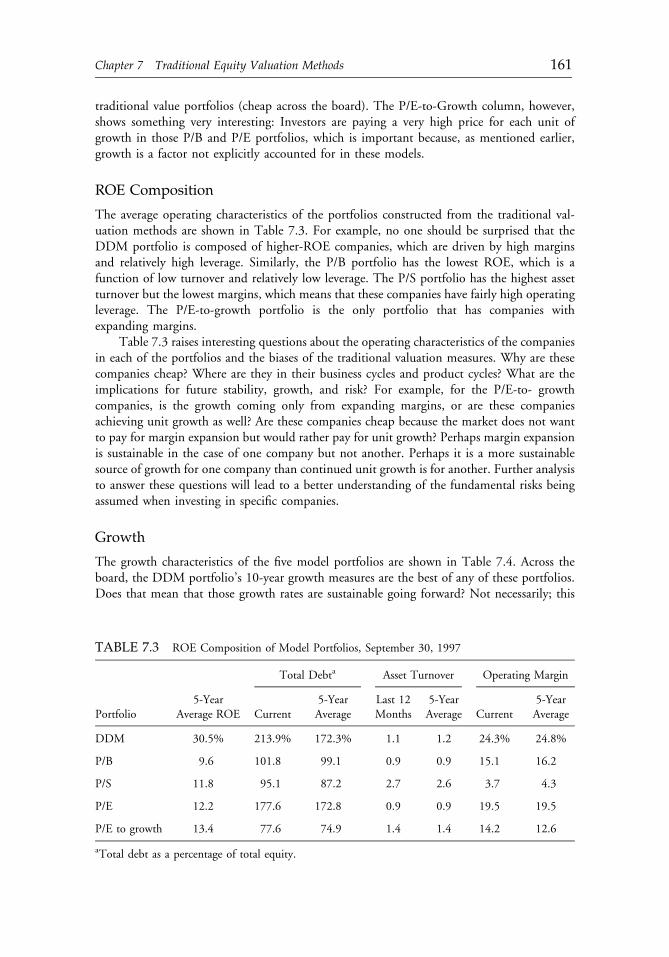
traditional value portfolios (cheap across the board). The P/E-to-Growth column, however,shows something very interesting: Investors are paying a very high price for each unit ofgrowth in those P/B and P/E portfolios, which is important because, as mentioned earlier,growth is a factor not explicitly accounted for in these models.
ROE Composition
The average operating characteristics of the portfolios constructed from the traditional val-uation methods are shown in Table 7.3. For example, no one should be surprised that theDDM portfolio is composed of higher-ROE companies, which are driven by high marginsand relatively high leverage. Similarly, the P/B portfolio has the lowest ROE, which is afunction of low turnover and relatively low leverage. The P/S portfolio has the highest assetturnover but the lowest margins, which means that these companies have fairly high operatingleverage. The P/E-to-growth portfolio is the only portfolio that has companies withexpanding margins.
Table 7.3 raises interesting questions about the operating characteristics of the companiesin each of the portfolios and the biases of the traditional valuation measures. Why are thesecompanies cheap? Where are they in their business cycles and product cycles? What are theimplications for future stability, growth, and risk? For example, for the P/E-to- growthcompanies, is the growth coming only from expanding margins, or are these companiesachieving unit growth as well? Are these companies cheap because the market does not wantto pay for margin expansion but would rather pay for unit growth? Perhaps margin expansionis sustainable in the case of one company but not another. Perhaps it is a more sustainablesource of growth for one company than continued unit growth is for another. Further analysisto answer these questions will lead to a better understanding of the fundamental risks beingassumed when investing in specific companies.
Growth
The growth characteristics of the five model portfolios are shown in Table 7.4. Across theboard, the DDM portfolio’s 10-year growth measures are the best of any of these portfolios.Does that mean that those growth rates are sustainable going forward? Not necessarily; this
TABLE 7.3 ROE Composition of Model Portfolios, September 30, 1997
Total Debta Asset Turnover Operating Margin
Portfolio5-Year
Average ROE Current5-YearAverage
Last 12Months
5-YearAverage Current
5-YearAverage
DDM 30.5% 213.9% 172.3% 1.1 1.2 24.3% 24.8%
P/B 9.6 101.8 99.1 0.9 0.9 15.1 16.2
P/S 11.8 95.1 87.2 2.7 2.6 3.7 4.3
P/E 12.2 177.6 172.8 0.9 0.9 19.5 19.5
P/E to growth 13.4 77.6 74.9 1.4 1.4 14.2 12.6
aTotal debt as a percentage of total equity.
c07 12 September 2012; 13:28:9
Chapter 7 Traditional Equity Valuation Methods 161

TABLE 7.4 Growth Characteristics of Model Portfolios, September 30, 1997 (percents)
I/B/E/S Estimated EPS
Primary EPS GrowthFY1�Actual FY2�FY1 Next 5 Years
Sustainable Growth Sales per Share GrowthBook Value per Share
Growth
Portfolio 5 Years 10 Years Percent Change Percent Change Forecast Growth 1 Year 5 Years 10 Years 1 Year 5 Years 10 Years 1 Year 5 Years 10 Years
DDM 20.1 21.2 13.4 14.0 15.7 19.8 20.4 22.2 14.3 17.2 17.8 10.9 19.4 20.8
P/B 6.0 1.2 176.4 20.5 7.2 3.6 21.7 0.0 7.4 4.1 4.7 24.7 5.4 6.2
P/S 6.3 4.6 15.9 29.2 12.9 7.0 6.2 6.6 17.0 10.8 10.4 15.7 8.6 9.3
P/E 12.3 3.1 2.6 14.6 8.1 4.8 0.1 1.3 6.6 3.6 5.0 21.3 5.8 5.1
P/E togrowth
33.5 13.9 23.9 33.2 21.2 14.5 11.0 11.2 14.5 12.3 12.5 11.6 15.5 13.5
FY = fiscal year.
c07 12 September 2012; 13:28:10
162
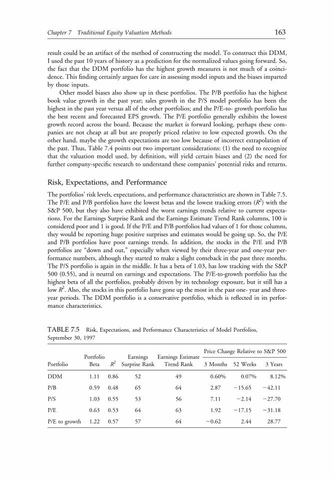
result could be an artifact of the method of constructing the model. To construct this DDM,I used the past 10 years of history as a prediction for the normalized values going forward. So,the fact that the DDM portfolio has the highest growth measures is not much of a coinci-dence. This finding certainly argues for care in assessing model inputs and the biases impartedby those inputs.
Other model biases also show up in these portfolios. The P/B portfolio has the highestbook value growth in the past year; sales growth in the P/S model portfolio has been thehighest in the past year versus all of the other portfolios; and the P/E-to- growth portfolio hasthe best recent and forecasted EPS growth. The P/E portfolio generally exhibits the lowestgrowth record across the board. Because the market is forward looking, perhaps these com-panies are not cheap at all but are properly priced relative to low expected growth. On theother hand, maybe the growth expectations are too low because of incorrect extrapolation ofthe past. Thus, Table 7.4 points out two important considerations: (1) the need to recognizethat the valuation model used, by definition, will yield certain biases and (2) the need forfurther company-specific research to understand these companies’ potential risks and returns.
Risk, Expectations, and Performance
The portfolios’ risk levels, expectations, and performance characteristics are shown in Table 7.5.The P/E and P/B portfolios have the lowest betas and the lowest tracking errors (R2) with theS&P 500, but they also have exhibited the worst earnings trends relative to current expecta-tions. For the Earnings Surprise Rank and the Earnings Estimate Trend Rank columns, 100 isconsidered poor and 1 is good. If the P/E and P/B portfolios had values of 1 for those columns,they would be reporting huge positive surprises and estimates would be going up. So, the P/Eand P/B portfolios have poor earnings trends. In addition, the stocks in the P/E and P/Bportfolios are “down and out,” especially when viewed by their three-year and one-year per-formance numbers, although they started to make a slight comeback in the past three months.The P/S portfolio is again in the middle. It has a beta of 1.03, has low tracking with the S&P500 (0.55), and is neutral on earnings and expectations. The P/E-to-growth portfolio has thehighest beta of all the portfolios, probably driven by its technology exposure, but it still has alow R2. Also, the stocks in this portfolio have gone up the most in the past one- year and three-year periods. The DDM portfolio is a conservative portfolio, which is reflected in its perfor-mance characteristics.
TABLE 7.5 Risk, Expectations, and Performance Characteristics of Model Portfolios,
September 30, 1997
Price Change Relative to S&P 500
PortfolioPortfolioBeta R2
EarningsSurprise Rank
Earnings EstimateTrend Rank 3 Months 52 Weeks 3 Years
DDM 1.11 0.86 52 49 0.60% 0.07% 8.12%
P/B 0.59 0.48 65 64 2.87 215.65 242.11
P/S 1.03 0.55 53 56 7.11 22.14 227.70
P/E 0.63 0.53 64 63 1.92 217.15 231.18
P/E to growth 1.22 0.57 57 64 20.62 2.44 28.77
c07 12 September 2012; 13:28:10
Chapter 7 Traditional Equity Valuation Methods 163
Tables 7.1 through 7.5 illustrate a crucial point: Each of the traditional valuationmeasures biases stock selection in many different ways—from growth history and prospects tooperating characteristics, to recently reported results and stock performance, to degree ofdiversification. Analysts and portfolio managers must recognize these biases, understand theirimplications, and use the information as a guide for further research and insight into specificcompany risks and returns.
FUNDAMENTAL ANALYSIS
In addition to screening the universe of stocks into a more manageable set, traditional val-uation methods can be used to look for insights into how a company is priced in the marketrelative to its factual, historical record and relative to any predictions about its future eco-nomic performance. This process is typically called fundamental analysis, and the DDM is anoften-used application in this context.
Growth and Discount Rates
A two-stage DDM can be used to isolate the valuation impact of growth and discount rates.For simplicity, assume that the first stage runs for 10 years and that the company has growthin excess of the mature growth rate for that 10-year period. The second stage is the maturestage; assume that the company will grow at the average long-term historical earnings growthrate of the S&P 500 from Year 11 through eternity. This framework allows an analyst to posesome interesting questions regarding the growth and discount rates that are embedded in anobserved stock price.
Suppose, for instance, that the two-stage DDM is applied to the stock of MicrosoftCorporation and International Paper (IP). On September 30, 1997, as shown in Table 7.6,Microsoft’s stock price was $132.31 and IP’s stock price was $55.00.With second-stage growthconstant at 6.50 percent annually (which is the S&P 400 Industrials long-term growth rate) forboth companies and first-stage annual growth estimates generated by Wall Street of 23.80percent for Microsoft and 16.20 percent for IP, the respective prices would be $132.58 and$33.90. With a constant discount rate for each company, the DDM framework allows ananalyst to solve for the first-stage growth rate implied by any stock price. For example,Microsoft’s September 30, 1997, stock price implies a first-stage growth rate of 23.78 percent,only 2 basis points (bps) off the Wall Street estimate. By contrast, IP’s September 30, 1997,stock price implies a first- stage growth rate of 22.67 percent, contrasted to the Street’s 16.20percent growth estimate. Is IP overpriced? Will it be able to grow for the next 10 years at a ratenearly 650 bps higher than analysts are expecting? At this point, judgment about the modelcomes in.What would it take to cut the stock price in half?What growth rate would be implied?If Microsoft grew at only 15.5 percent, the stock should fall by about half. If IP grew at only13 percent on average for 10 years, the stock price would be cut in half. Could the two stockprices double? Holding everything else constant, both companies would have to grow at a ratehigher than 32 percent for the next 10 years for the two prices to double. Finally, this analysisshows that none of Microsoft’s value is explicitly derived from first-stage growth because of theassumption that Microsoft does not pay a dividend at all in the first stage; however, roughly20�30 percent of IP’s value is first-stage based, depending on which measure is examined.
Table 7.7 shows exactly the same analysis with only one change: The first-stagegrowth rates are held constant at the levels estimated by Wall Street, and the second-stage
c07 12 September 2012; 13:28:10
164 Part II: Valuation Methodologies
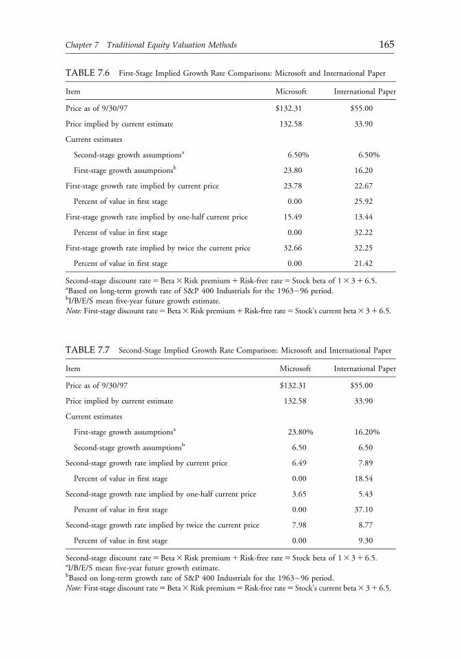
TABLE 7.6 First-Stage Implied Growth Rate Comparisons: Microsoft and International Paper
Item Microsoft International Paper
Price as of 9/30/97 $132.31 $55.00
Price implied by current estimate 132.58 33.90
Current estimates
Second-stage growth assumptionsa 6.50% 6.50%
First-stage growth assumptionsb 23.80 16.20
First-stage growth rate implied by current price 23.78 22.67
Percent of value in first stage 0.00 25.92
First-stage growth rate implied by one-half current price 15.49 13.44
Percent of value in first stage 0.00 32.22
First-stage growth rate implied by twice the current price 32.66 32.25
Percent of value in first stage 0.00 21.42
Second-stage discount rate5Beta3Risk premium1Risk-free rate5 Stock beta of 13 31 6.5.aBased on long-term growth rate of S&P 400 Industrials for the 1963�96 period.bI/B/E/S mean five-year future growth estimate.Note: First-stage discount rate5Beta3Risk premium1Risk-free rate5 Stock’s current beta3 31 6.5.
TABLE 7.7 Second-Stage Implied Growth Rate Comparison: Microsoft and International Paper
Item Microsoft International Paper
Price as of 9/30/97 $132.31 $55.00
Price implied by current estimate 132.58 33.90
Current estimates
First-stage growth assumptionsa 23.80% 16.20%
Second-stage growth assumptionsb 6.50 6.50
Second-stage growth rate implied by current price 6.49 7.89
Percent of value in first stage 0.00 18.54
Second-stage growth rate implied by one-half current price 3.65 5.43
Percent of value in first stage 0.00 37.10
Second-stage growth rate implied by twice the current price 7.98 8.77
Percent of value in first stage 0.00 9.30
Second-stage discount rate5Beta3Risk premium1Risk-free rate5 Stock beta of 13 31 6.5.aI/B/E/S mean five-year future growth estimate.bBased on long-term growth rate of S&P 400 Industrials for the 1963�96 period.Note: First-stage discount rate5Beta3Risk premium5Risk-free rate5 Stock’s current beta3 31 6.5.
c07 12 September 2012; 13:28:10
Chapter 7 Traditional Equity Valuation Methods 165
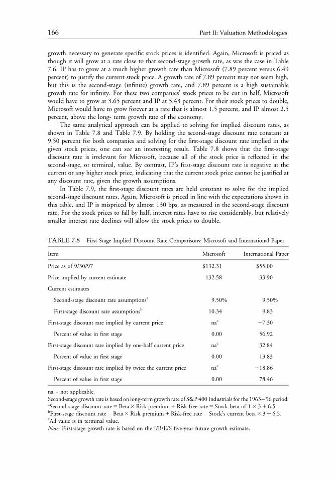
growth necessary to generate specific stock prices is identified. Again, Microsoft is priced asthough it will grow at a rate close to that second-stage growth rate, as was the case in Table7.6. IP has to grow at a much higher growth rate than Microsoft (7.89 percent versus 6.49percent) to justify the current stock price. A growth rate of 7.89 percent may not seem high,but this is the second-stage (infinite) growth rate, and 7.89 percent is a high sustainablegrowth rate for infinity. For these two companies’ stock prices to be cut in half, Microsoftwould have to grow at 3.65 percent and IP at 5.43 percent. For their stock prices to double,Microsoft would have to grow forever at a rate that is almost 1.5 percent, and IP almost 2.5percent, above the long- term growth rate of the economy.
The same analytical approach can be applied to solving for implied discount rates, asshown in Table 7.8 and Table 7.9. By holding the second-stage discount rate constant at9.50 percent for both companies and solving for the first-stage discount rate implied in thegiven stock prices, one can see an interesting result. Table 7.8 shows that the first-stagediscount rate is irrelevant for Microsoft, because all of the stock price is reflected in thesecond-stage, or terminal, value. By contrast, IP’s first-stage discount rate is negative at thecurrent or any higher stock price, indicating that the current stock price cannot be justified atany discount rate, given the growth assumptions.
In Table 7.9, the first-stage discount rates are held constant to solve for the impliedsecond-stage discount rates. Again, Microsoft is priced in line with the expectations shown inthis table, and IP is mispriced by almost 130 bps, as measured in the second-stage discountrate. For the stock prices to fall by half, interest rates have to rise considerably, but relativelysmaller interest rate declines will allow the stock prices to double.
TABLE 7.8 First-Stage Implied Discount Rate Comparisons: Microsoft and International Paper
Item Microsoft International Paper
Price as of 9/30/97 $132.31 $55.00
Price implied by current estimate 132.58 33.90
Current estimates
Second-stage discount rate assumptionsa 9.50% 9.50%
First-stage discount rate assumptionsb 10.34 9.83
First-stage discount rate implied by current price nac 27.30
Percent of value in first stage 0.00 56.92
First-stage discount rate implied by one-half current price nac 32.84
Percent of value in first stage 0.00 13.83
First-stage discount rate implied by twice the current price nac 218.86
Percent of value in first stage 0.00 78.46
na = not applicable.Second-stage growth rate is based on long-term growth rate of S&P 400 Industrials for the 1963�96 period.aSecond-stage discount rate5Beta3Risk premium1Risk-free rate5 Stock beta of 13 31 6.5.bFirst-stage discount rate5Beta3Risk premium1Risk-free rate5 Stock’s current beta3 31 6.5.cAll value is in terminal value.Note: First-stage growth rate is based on the I/B/E/S five-year future growth estimate.
c07 12 September 2012; 13:28:10
166 Part II: Valuation Methodologies
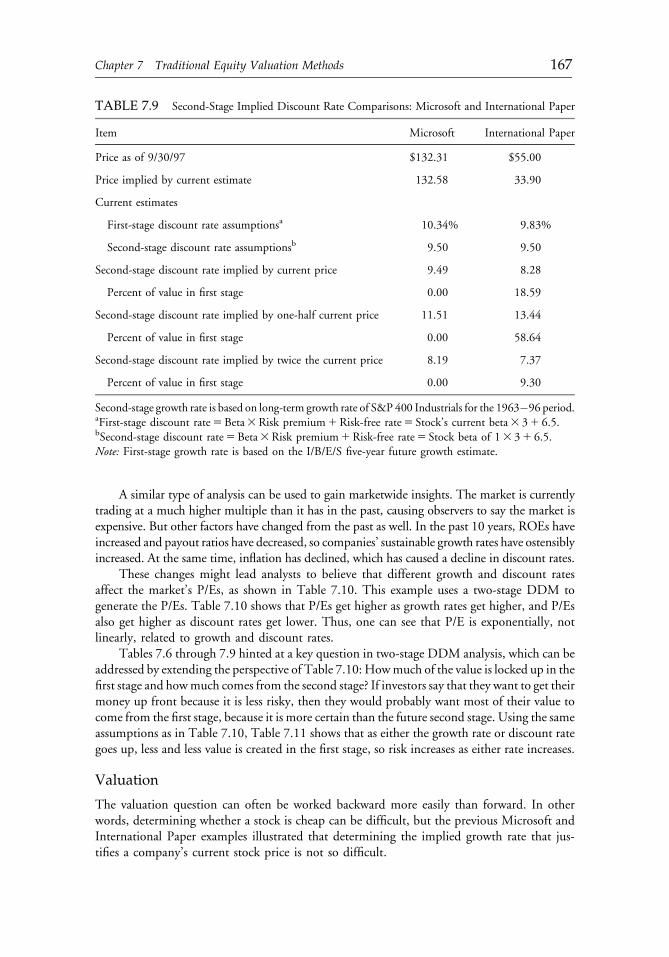
A similar type of analysis can be used to gain marketwide insights. The market is currentlytrading at a much higher multiple than it has in the past, causing observers to say the market isexpensive. But other factors have changed from the past as well. In the past 10 years, ROEs haveincreased and payout ratios have decreased, so companies’ sustainable growth rates have ostensiblyincreased. At the same time, inflation has declined, which has caused a decline in discount rates.
These changes might lead analysts to believe that different growth and discount ratesaffect the market’s P/Es, as shown in Table 7.10. This example uses a two-stage DDM togenerate the P/Es. Table 7.10 shows that P/Es get higher as growth rates get higher, and P/Esalso get higher as discount rates get lower. Thus, one can see that P/E is exponentially, notlinearly, related to growth and discount rates.
Tables 7.6 through 7.9 hinted at a key question in two-stage DDM analysis, which can beaddressed by extending the perspective of Table 7.10: Howmuch of the value is locked up in thefirst stage and howmuch comes from the second stage? If investors say that they want to get theirmoney up front because it is less risky, then they would probably want most of their value tocome from the first stage, because it is more certain than the future second stage. Using the sameassumptions as in Table 7.10, Table 7.11 shows that as either the growth rate or discount rategoes up, less and less value is created in the first stage, so risk increases as either rate increases.
Valuation
The valuation question can often be worked backward more easily than forward. In otherwords, determining whether a stock is cheap can be difficult, but the previous Microsoft andInternational Paper examples illustrated that determining the implied growth rate that jus-tifies a company’s current stock price is not so difficult.
TABLE 7.9 Second-Stage Implied Discount Rate Comparisons: Microsoft and International Paper
Item Microsoft International Paper
Price as of 9/30/97 $132.31 $55.00
Price implied by current estimate 132.58 33.90
Current estimates
First-stage discount rate assumptionsa 10.34% 9.83%
Second-stage discount rate assumptionsb 9.50 9.50
Second-stage discount rate implied by current price 9.49 8.28
Percent of value in first stage 0.00 18.59
Second-stage discount rate implied by one-half current price 11.51 13.44
Percent of value in first stage 0.00 58.64
Second-stage discount rate implied by twice the current price 8.19 7.37
Percent of value in first stage 0.00 9.30
Second-stage growth rate is based on long-term growth rate of S&P 400 Industrials for the 1963�96 period.aFirst-stage discount rate5Beta3Risk premium1Risk-free rate5 Stock’s current beta3 31 6.5.bSecond-stage discount rate5Beta3Risk premium1Risk-free rate5 Stock beta of 13 31 6.5.Note: First-stage growth rate is based on the I/B/E/S five-year future growth estimate.
c07 12 September 2012; 13:28:11
Chapter 7 Traditional Equity Valuation Methods 167
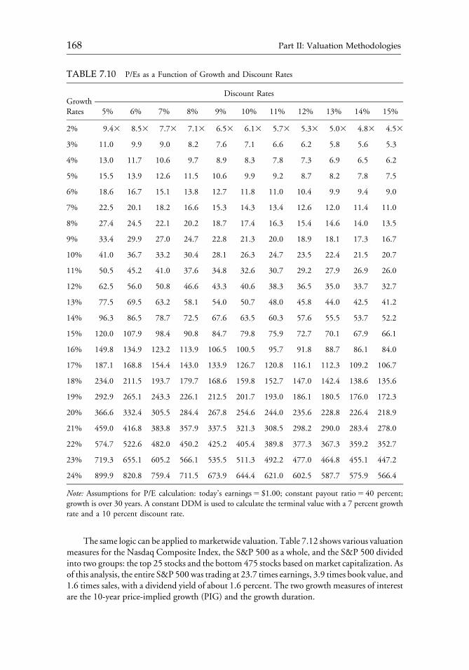
The same logic can be applied tomarketwide valuation. Table 7.12 shows various valuationmeasures for the Nasdaq Composite Index, the S&P 500 as a whole, and the S&P 500 dividedinto two groups: the top 25 stocks and the bottom 475 stocks based onmarket capitalization. Asof this analysis, the entire S&P 500was trading at 23.7 times earnings, 3.9 times book value, and1.6 times sales, with a dividend yield of about 1.6 percent. The two growth measures of interestare the 10-year price-implied growth (PIG) and the growth duration.
TABLE 7.10 P/Es as a Function of Growth and Discount Rates
Discount RatesGrowthRates 5% 6% 7% 8% 9% 10% 11% 12% 13% 14% 15%
2% 9.43 8.53 7.73 7.13 6.53 6.13 5.73 5.33 5.03 4.83 4.53
3% 11.0 9.9 9.0 8.2 7.6 7.1 6.6 6.2 5.8 5.6 5.3
4% 13.0 11.7 10.6 9.7 8.9 8.3 7.8 7.3 6.9 6.5 6.2
5% 15.5 13.9 12.6 11.5 10.6 9.9 9.2 8.7 8.2 7.8 7.5
6% 18.6 16.7 15.1 13.8 12.7 11.8 11.0 10.4 9.9 9.4 9.0
7% 22.5 20.1 18.2 16.6 15.3 14.3 13.4 12.6 12.0 11.4 11.0
8% 27.4 24.5 22.1 20.2 18.7 17.4 16.3 15.4 14.6 14.0 13.5
9% 33.4 29.9 27.0 24.7 22.8 21.3 20.0 18.9 18.1 17.3 16.7
10% 41.0 36.7 33.2 30.4 28.1 26.3 24.7 23.5 22.4 21.5 20.7
11% 50.5 45.2 41.0 37.6 34.8 32.6 30.7 29.2 27.9 26.9 26.0
12% 62.5 56.0 50.8 46.6 43.3 40.6 38.3 36.5 35.0 33.7 32.7
13% 77.5 69.5 63.2 58.1 54.0 50.7 48.0 45.8 44.0 42.5 41.2
14% 96.3 86.5 78.7 72.5 67.6 63.5 60.3 57.6 55.5 53.7 52.2
15% 120.0 107.9 98.4 90.8 84.7 79.8 75.9 72.7 70.1 67.9 66.1
16% 149.8 134.9 123.2 113.9 106.5 100.5 95.7 91.8 88.7 86.1 84.0
17% 187.1 168.8 154.4 143.0 133.9 126.7 120.8 116.1 112.3 109.2 106.7
18% 234.0 211.5 193.7 179.7 168.6 159.8 152.7 147.0 142.4 138.6 135.6
19% 292.9 265.1 243.3 226.1 212.5 201.7 193.0 186.1 180.5 176.0 172.3
20% 366.6 332.4 305.5 284.4 267.8 254.6 244.0 235.6 228.8 226.4 218.9
21% 459.0 416.8 383.8 357.9 337.5 321.3 308.5 298.2 290.0 283.4 278.0
22% 574.7 522.6 482.0 450.2 425.2 405.4 389.8 377.3 367.3 359.2 352.7
23% 719.3 655.1 605.2 566.1 535.5 511.3 492.2 477.0 464.8 455.1 447.2
24% 899.9 820.8 759.4 711.5 673.9 644.4 621.0 602.5 587.7 575.9 566.4
Note: Assumptions for P/E calculation: today’s earnings5 $1.00; constant payout ratio5 40 percent;growth is over 30 years. A constant DDM is used to calculate the terminal value with a 7 percent growthrate and a 10 percent discount rate.
c07 12 September 2012; 13:28:12
168 Part II: Valuation Methodologies
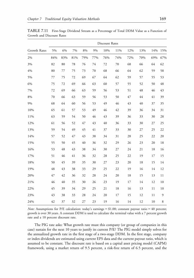
The PIG rate asks: What growth rate must this company (or group of companies in thiscase) sustain for the next 10 years to justify its current P/E? The PIG model simply solves forthe annualized growth rate in the first stage of a two-stage DDM. In the first stage, companyor index dividends are estimated using current EPS data and the current payout ratio, which isassumed to be constant. The discount rate is based on a capital asset pricing model (CAPM)framework, using a market return of 9.5 percent, a risk-free return of 6.5 percent, and the
TABLE 7.11 First-Stage Dividend Stream as a Percentage of Total DDM Value as a Function of
Growth and Discount Rates
Discount Rates
Growth Rates 5% 6% 7% 8% 9% 10% 11% 12% 13% 14% 15%
2% 84% 83% 81% 79% 77% 76% 74% 72% 70% 69% 67%
3% 82 80 78 76 74 72 70 68 66 64 62
4% 80 77 75 73 70 68 66 64 62 59 58
5% 77 75 72 69 67 64 62 59 57 55 53
6% 75 72 69 66 63 60 57 55 52 50 48
7% 72 69 66 63 59 56 53 51 48 46 43
8% 70 66 63 59 56 53 50 47 44 41 39
9% 68 64 60 56 53 49 46 43 40 37 35
10% 65 61 57 53 49 46 42 39 36 34 31
11% 63 59 54 50 46 43 39 36 33 30 28
12% 61 56 52 47 43 40 36 33 30 27 25
13% 59 54 49 45 41 37 33 30 27 25 22
14% 57 52 47 43 38 34 31 28 25 22 20
15% 55 50 45 40 36 32 29 26 23 20 18
16% 53 48 43 38 34 30 27 24 21 18 16
17% 51 46 41 36 32 28 25 22 19 17 15
18% 50 45 39 35 30 27 23 20 18 15 14
19% 48 43 38 33 29 25 22 19 16 14 12
20% 47 42 36 32 28 24 20 18 15 13 11
21% 46 40 35 30 26 23 19 17 14 12 10
22% 45 39 34 29 25 21 18 16 13 11 10
23% 43 38 33 28 24 20 17 15 12 11 9
24% 42 37 32 27 23 19 16 14 12 10 8
Note: Assumptions for P/E calculation: today’s earnings5 $1.00; constant payout ratio5 40 percent;growth is over 30 years. A constant DDM is used to calculate the terminal value with a 7 percent growthrate and a 10 percent discount rate.
c07 12 September 2012; 13:28:12
Chapter 7 Traditional Equity Valuation Methods 169

TABLE 7.12 Traditional Valuation Measures for Various Indexes, September 30, 1997
Historical Annualized Growth Rates
IndexTrailing 12-Month
Earnings P/E P/B P/SDividendYield
5-Year ExpectedGrowth Rate 10-Year PIG 5 Years 10 Years 20 Years 30 Years
Years to Justify P/E versusS&P 500 (Growth Duration)
Nasdaq 74.7 3.7 1.6 0.5% 21.5% 29.2% 729.8% 21.0% 17.7% 9.2% 22.7
S&P 500
Total index 23.7 3.9 1.6 1.6 13.8 15.8 18.8 12.3 9.1 9.0 —
Top 25a 25.4 5.8 2.3 1.5 13.9 14.3 17.0 14.9 11.2 10.2 Never
Bottom 475a 23.0 3.3 1.4 1.7 13.8 12.9 20.1 10.6 7.6 8.1 2118.7
aRank based on market capitalization.
c07 12 September 2012; 13:28:13
170
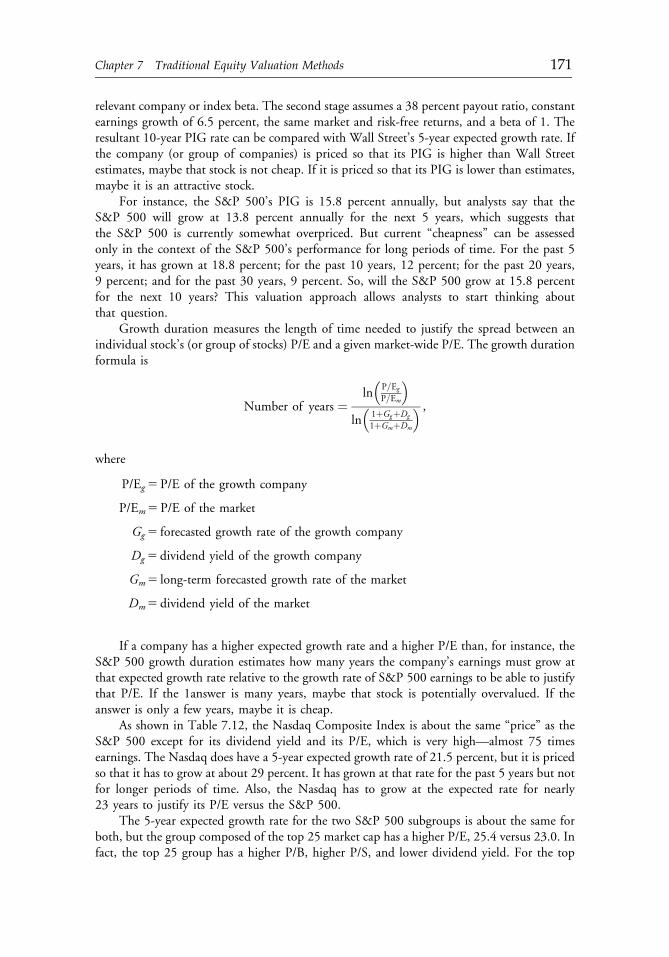
relevant company or index beta. The second stage assumes a 38 percent payout ratio, constantearnings growth of 6.5 percent, the same market and risk-free returns, and a beta of 1. Theresultant 10-year PIG rate can be compared with Wall Street’s 5-year expected growth rate. Ifthe company (or group of companies) is priced so that its PIG is higher than Wall Streetestimates, maybe that stock is not cheap. If it is priced so that its PIG is lower than estimates,maybe it is an attractive stock.
For instance, the S&P 500’s PIG is 15.8 percent annually, but analysts say that theS&P 500 will grow at 13.8 percent annually for the next 5 years, which suggests thatthe S&P 500 is currently somewhat overpriced. But current “cheapness” can be assessedonly in the context of the S&P 500’s performance for long periods of time. For the past 5years, it has grown at 18.8 percent; for the past 10 years, 12 percent; for the past 20 years,9 percent; and for the past 30 years, 9 percent. So, will the S&P 500 grow at 15.8 percentfor the next 10 years? This valuation approach allows analysts to start thinking aboutthat question.
Growth duration measures the length of time needed to justify the spread between anindividual stock’s (or group of stocks) P/E and a given market-wide P/E. The growth durationformula is
Number of years ¼ln
P=Eg
P=Em
� �ln
1þGgþDg
1þGmþDm
� � ,
where
P/Eg5 P/E of the growth company
P/Em5 P/E of the market
Gg5 forecasted growth rate of the growth company
Dg5 dividend yield of the growth company
Gm5 long-term forecasted growth rate of the market
Dm5 dividend yield of the market
If a company has a higher expected growth rate and a higher P/E than, for instance, theS&P 500 growth duration estimates how many years the company’s earnings must grow atthat expected growth rate relative to the growth rate of S&P 500 earnings to be able to justifythat P/E. If the 1answer is many years, maybe that stock is potentially overvalued. If theanswer is only a few years, maybe it is cheap.
As shown in Table 7.12, the Nasdaq Composite Index is about the same “price” as theS&P 500 except for its dividend yield and its P/E, which is very high—almost 75 timesearnings. The Nasdaq does have a 5-year expected growth rate of 21.5 percent, but it is pricedso that it has to grow at about 29 percent. It has grown at that rate for the past 5 years but notfor longer periods of time. Also, the Nasdaq has to grow at the expected rate for nearly23 years to justify its P/E versus the S&P 500.
The 5-year expected growth rate for the two S&P 500 subgroups is about the same forboth, but the group composed of the top 25 market cap has a higher P/E, 25.4 versus 23.0. Infact, the top 25 group has a higher P/B, higher P/S, and lower dividend yield. For the top
c07 12 September 2012; 13:28:13
Chapter 7 Traditional Equity Valuation Methods 171
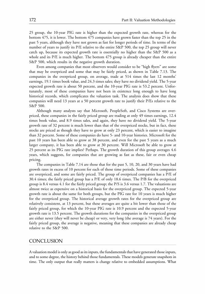
25 group, the 10-year PIG rate is higher than the expected growth rate, whereas for thebottom 475, it is lower. The bottom 475 companies have grown faster than the top 25 in thepast 5 years, although they have not grown as fast for longer periods of time. In terms of thenumber of years to justify its P/E relative to the entire S&P 500, the top 25 group will nevercatch up, because its expected growth rate is essentially no higher than the S&P 500 as awhole and its P/E is much higher. The bottom 475 group is already cheaper than the entireS&P 500, which results in the negative growth duration.
Even among companies that most observers would consider to be “high flyers” are somethat may be overpriced and some that may be fairly priced, as shown in Table 7.13. Thecompanies in the overpriced group, on average, trade at 514 times the last 12 months’earnings, 19.1 times book value, and 24.3 times sales; they have no dividend yield. The 5-yearexpected growth rate is about 50 percent, and the 10-year PIG rate is 53.2 percent. Unfor-tunately, most of these companies have not been in existence long enough to have longhistorical records, which complicates the valuation task. The analysis does show that thesecompanies will need 13 years at a 50 percent growth rate to justify their P/Es relative to theS&P 500.
Although many analysts say that Microsoft, PeopleSoft, and Cisco Systems are over-priced, these companies in the fairly priced group are trading at only 49 times earnings, 12.4times book value, and 8.9 times sales, and again, they have no dividend yield. The 5-yeargrowth rate of 32 percent is much lower than that of the overpriced stocks, but in fact, thesestocks are priced as though they have to grow at only 23 percent, which is easier to imaginethan 32 percent. Some of these companies do have 5- and 10-year histories. Microsoft for thepast 10 years has been able to grow at 38 percent, and even for the past 5 years as a muchlarger company, it has been able to grow at 30 percent. Will Microsoft be able to grow at25 percent as its PIG rate implies? Perhaps. The growth duration of this group averages 4.6years, which suggests, for companies that are growing as fast as these, fair or even cheappricing.
The companies in Table 7.14 are those that for the past 5, 10, 20, and 30 years have hadgrowth rates in excess of 10 percent for each of those time periods. Some of these companiesare overpriced, and some are fairly priced. The group of overpriced companies has a P/E of30.4 times; the fairly priced group has a P/E of only 18.6 times. The P/B for the overpricedgroup is 8.4 versus 4.1 for the fairly priced group; the P/S is 3.6 versus 1.7. The valuations arealmost twice as expensive on a historical basis for the overpriced group. The expected 5-yeargrowth rate is about the same for both groups, but the PIG rate for 10 years is much higherfor the overpriced group. The historical average growth rates for the overpriced group arerelatively consistent, at 13 percent, but these averages are quite a bit lower than those of thefairly priced group, for which the 10-year PIG rate is 10.9 percent and the expected 5-yeargrowth rate is 13.5 percent. The growth durations for the companies in the overpriced groupare either never (they will never be cheap) or very, very long (the average is 74 years). For thefairly priced group, the average is negative, meaning that these companies are already cheaprelative to the S&P 500.
CONCLUSION
A valuationmodel is only as good as its inputs, the fundamentals that have generated those inputs,and to some degree, the history behind those fundamentals. These models generate snapshots intime. The only output that really matters is change relative to embedded assumptions. What
c07 12 September 2012; 13:28:13
172 Part II: Valuation Methodologies
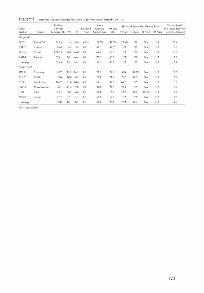
TABLE 7.13 Traditional Valuation Measures for Various High-Flyer Stocks, September 30, 1997
TickerTrailing12-Month Dividend
5-YearExpected 10-Year
Historical Annualized Growth Rates Years to JustifyP/E versus S&P 500
Symbol Name Earnings P/E P/B P/S Yield Growth Rate PIG 5 Years 10 Years 20 Years 30 Years (Growth Duration)
Overpriced
PCTL PictureTel 345.8 1.4 0.8 0.0% 28.3% 51.5% 37.8% NA NA NA 25.4
ABMD Abiomed 90.8 4.4 5.9 0.0 35.0 32.5 NA NA NA NA 8.6
YHOO Yahoo! 1,002.5 20.5 44.0 0.0 64.2 68.5 NA NA NA NA 10.6
RMBS Rambus 618.1 50.1 46.4 0.0 75.0 60.5 NA NA NA NA 7.8
Average 514.3 19.1 24.3 0.0 50.6 53.2 NA NA NA NA 13.1
Fairly Priced
MSFT Microsoft 49.7 15.2 14.3 0.0 23.8 24.8 30.4 38.5% NA NA 10.6
TLAB Tellabs 39.0 10.6 8.5 0.0 27.4 21.8 76.7 42.5 NA NA 5.0
PSFT PeopleSoft 106.7 21.0 10.6 0.0 45.5 34.7 64.7 NA NA NA 6.5
CSCO Cisco Systems 48.1 11.4 7.8 0.0 33.1 24.3 71.9 NA NA NA 5.0
INTC Intel 23.3 8.7 6.6 0.1 21.4 15.5 42.7 35.9 28.8% NA 0.0
ASND Ascend 27.2 7.3 5.3 0.0 40.3 17.5 NA NA NA NA 0.7
Average 49.0 12.4 8.9 0.0 31.9 23.1 57.3 39.0 NA NA 4.6
NA = not available.
c07 12 September 2012; 13:28:13
173
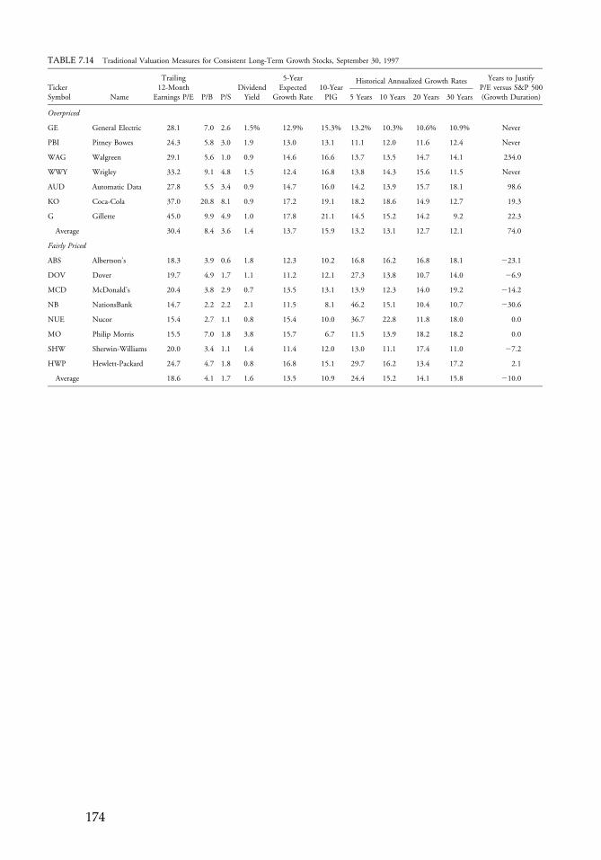
TABLE 7.14 Traditional Valuation Measures for Consistent Long-Term Growth Stocks, September 30, 1997
TickerTrailing12-Month Dividend
5-YearExpected 10-Year
Historical Annualized Growth Rates Years to JustifyP/E versus S&P 500
Symbol Name Earnings P/E P/B P/S Yield Growth Rate PIG 5 Years 10 Years 20 Years 30 Years (Growth Duration)
Overpriced
GE General Electric 28.1 7.0 2.6 1.5% 12.9% 15.3% 13.2% 10.3% 10.6% 10.9% Never
PBI Pitney Bowes 24.3 5.8 3.0 1.9 13.0 13.1 11.1 12.0 11.6 12.4 Never
WAG Walgreen 29.1 5.6 1.0 0.9 14.6 16.6 13.7 13.5 14.7 14.1 234.0
WWY Wrigley 33.2 9.1 4.8 1.5 12.4 16.8 13.8 14.3 15.6 11.5 Never
AUD Automatic Data 27.8 5.5 3.4 0.9 14.7 16.0 14.2 13.9 15.7 18.1 98.6
KO Coca-Cola 37.0 20.8 8.1 0.9 17.2 19.1 18.2 18.6 14.9 12.7 19.3
G Gillette 45.0 9.9 4.9 1.0 17.8 21.1 14.5 15.2 14.2 9.2 22.3
Average 30.4 8.4 3.6 1.4 13.7 15.9 13.2 13.1 12.7 12.1 74.0
Fairly Priced
ABS Albertson’s 18.3 3.9 0.6 1.8 12.3 10.2 16.8 16.2 16.8 18.1 223.1
DOV Dover 19.7 4.9 1.7 1.1 11.2 12.1 27.3 13.8 10.7 14.0 26.9
MCD McDonald’s 20.4 3.8 2.9 0.7 13.5 13.1 13.9 12.3 14.0 19.2 214.2
NB NationsBank 14.7 2.2 2.2 2.1 11.5 8.1 46.2 15.1 10.4 10.7 230.6
NUE Nucor 15.4 2.7 1.1 0.8 15.4 10.0 36.7 22.8 11.8 18.0 0.0
MO Philip Morris 15.5 7.0 1.8 3.8 15.7 6.7 11.5 13.9 18.2 18.2 0.0
SHW Sherwin-Williams 20.0 3.4 1.1 1.4 11.4 12.0 13.0 11.1 17.4 11.0 27.2
HWP Hewlett-Packard 24.7 4.7 1.8 0.8 16.8 15.1 29.7 16.2 13.4 17.2 2.1
Average 18.6 4.1 1.7 1.6 13.5 10.9 24.4 15.2 14.1 15.8 210.0
c07 12 September 2012; 13:28:14
174
needs to be done, then, is to use tools that reflect the underlying fundamentals and the embeddedassumptions, thus allowing investors to make rational and consistent judgments about the likelydirection and magnitude of change and, ultimately, to buy and sell stocks accordingly. Tradi-tional valuation methods offer investors such a tool—one that, like all tools, has limitations, butone that is also widely applicable and relatively straightforward.
QUESTION AND ANSWER SESSION
Question: How does the DDM work if a company pays no dividend?Martin: For a company with no cash dividends, such as Microsoft, we have to assume that
during the first-stage period of supernormal growth, the company will reinvest all of itsearnings back into the company at a high ROE. Then in the second-stage normalizationprocess, or maturity process, we must make assumptions about the point at which thecompany will be mature enough that it decides to start paying out some dividends, whatthat rate will be, and how fast the rate of payout will increase to reach some normalpayout level. Again, the model makes us explicitly think about where such a company isin its life cycle and what is likely to happen to its products and its profitability over time.
Question: What is the role of beta in these traditional models?Martin: Beta has no role in the traditional valuation models, with the notable exception of the
DDM because the DDM requires the explicit estimation of a discount rate. A discountrate can be derived in a number of ways, one of which is a CAPM approach. If we aregoing to use CAPM, we also have to use a company beta for each stock being considered.
Beta also can be calculated in several ways. Beta is supposed to be the amount ofvolatility in the stock price over some period of time relative to some benchmark, buthistorical betas that are calculated based on price typically are not good predictors offuture betas. We all want to know what the relationship will be going forward. So, manyanalysts have started using fundamental betas, which are similar to multifactor modelsbased on a company’s characteristics, such as debt to equity, sales growth, and margins.Therefore, if we are going to use a CAPM approach, using a fundamental beta tocalculate the discount rate probably makes sense.
Question: Do you use normalized earnings in your models?Martin: A normalized earnings number is a good starting point in using a DDM approach.
How we get at that normalized number probably is the key, and it would differ forcyclical companies, for stable companies, and for companies that are currently indistress. One good approach is to have the analysts who follow these companies analyzethe fundamentals and try to come up with a normalized number. Another approach isto look at what the company has actually done over some period of time, such as a fullbusiness, economic, or profitability cycle, and see if there is some sort of reasonable basisfor making our own judgment. Large, stable companies may lend themselves to usingpast results as a good indicator of the future results because this approach is less subjectto analyst forecasting error, but the younger the company or the more fluid thesituation, the more our judgment will have to come to bear.
Question: What range of discount rates do you use and how do you apply them to differentcompanies?
c07 12 September 2012; 13:28:14
Chapter 7 Traditional Equity Valuation Methods 175
Martin:Most users of the DDM solve for the internal rate of return of the company instead ofputting a discount rate into the model and solving for a dollar intrinsic value. The needto estimate the discount rate, which can be a source of potentially large errors, is therebyeliminated.
Question: What is your opinion of price to cash flow and enterprise value to EBITDA(earnings before interest, taxes, depreciation, and amortization) as valuation measures?
Martin: I do not have any real biases for or against any of the valuation models. I think thatusing a number such as EBITDA is probably better than using a net earnings number,because what we really want to get at is the ongoing capability of a company to generateoperating earnings. So, we want to take out as many “nonrecurring” and “management/accounting discretion” items as possible. But even EBITDA is not immune tomanipulation. The trouble is that these companies, especially in the S&P 500, changetheir businesses on an ongoing basis. I saw one study where a substantial portion of theS&P 500’s book value had been written off over the past 10 years, and that was onecontributor to why ROEs are so much higher and profitability is so much better than inthe past. Essentially, managements made a lot of mistakes, and instead of depreciatingor amortizing them, they simply wrote them off all at once and hoped that the Streetwould forget about them. By writing off these expenses, managements figured that theyhad a better chance of making their earnings estimates and showing good growth ratesgoing forward.
c07 12 September 2012; 13:28:14
176 Part II: Valuation Methodologies
CHAPTER 8A SIMPLE VALUATIONMODEL AND GROWTH
EXPECTATIONS
Morris G. Danielson
A simple valuation model is presented in which a firm can invest in projects withpositive net present values for a limited number of years. Although prior models havemade this assumption, this model can be simplified to a concise, easy-to-use form.The model can facilitate a broad understanding of the expectations implied by afirm’s stock price—for example, growth patterns consistent with a firm’s P/E—whichcan guide in-depth analysis of prices.
The valuation model presented here provides a simple, concise method for analyzing stockprices. The model is similar to the finite-horizon model described by Gordon and Gordon(1997), in that both models assume a firm can invest in projects with positive net presentvalues (NPVs) for a limited number of years.1 The two models differ, however, in theirtreatment of earnings in excess of the amount invested in positive-NPV projects. In the Gordonand Gordon model, the firm pays these amounts as dividends. In the new model, the firminvests these amounts in projects with NPVs equal to zero. Although the two models predictsimilar stock prices, the new model can be simplified to a more tractable form. The resultingmodel combines the computational ease of the perpetual-growth model with the more realisticfinite-growth assumption.
Gordon and Gordon used the finite-growth model to estimate expected stock returns in atest of the capital asset pricing model (CAPM). Using the estimates of expected returns,Gordon and Gordon found evidence in support of the CAPM.
Reprinted from the Financial Analysts Journal (May/June 1998):50–57. When this article was originallypublished, Morris G. Danielson was an assistant professor of finance at the Temple University School ofBusiness and Management.
c08 12 September 2012; 17:44:47
177
This chapter presents a different application of the finite-growth model. The model isused to explore how a firm’s P/E relates to four value drivers: the risk-adjusted discount rate,the reinvestment rate, the return on new investments, and the length of a period of com-petitive advantage. The period of competitive advantage is the number of years the firm isexpected to be able to invest in positive-NPV projects.
Because forecasting each of these variables into the distant future is difficult, the modeldoes not yield a precise estimate of the “correct” stock price or P/E, but it can promote abroad understanding of the expectations implied by a firm’s P/E. For example, an analyst canuse the model to identify future growth patterns consistent with a firm’s observed P/E. Themodel states that a non-dividend-paying stock will justify a P/E of 30 if the firm’s returnon new investments exceeds the firm’s cost of capital by 4.8 percent each year for the next20 years, by 9.9 percent each year for the next 10 years, or by 20.7 percent each year for thenext 5 years.2
Similarly, an analyst can use the model to illustrate the trade-offs between (1) thereinvestment rate and required return on new investments and (2) the discount rate andrequired return on new investments.
The information the model provides raises questions that can guide a more in-depthanalysis of a stock price. For example, does the firm have a competitive advantage that willallow it to earn a return on new investments that exceeds its cost of capital by 9.9 percent?Will the company be able to earn this return on new investments in each of the next 10 years?In particular, do sufficient new markets exist for the firm’s products to allow the predictedgrowth, and can the firm protect these markets from competition for a 10-year period? In thisrespect, the model shows how stock valuation concepts can be combined with concepts aboutindustry structure and competitive advantage (see Porter 1980, 1985).
After outlining the finite-growth model from Gordon and Gordon, this chapter willdevelop the new model for two cases. In the first case, the firm does not pay a dividend andreinvests 100 percent of its earnings in (new) positive-NPV projects. In the second case, thereinvestment rate can be either higher than or lower than 100 percent of the firm’s currentearnings. The chapter concludes with a discussion of how the model can be used to evaluate afirm’s P/E. An appendix compares the new model with the Gordon and Gordon model.
THE GORDON AND GORDON MODEL
The finite-growth model from Gordon and Gordon can be written as
Pt¼0 ¼Xτt¼1
Et¼1ð1� ρÞð1þ ρRN Þt�1
ð1þ kÞt þ Et¼1ð1þ ρRN Þτkð1þ kÞτ ð8:1Þ
Equation 8.1 uses the following definitions:
� The firm’s current stock price is Pt¼0. To interpret Pt¼0 as the stock price for a levered firm,one must assume that all new investments by the firm are financed with the same pro-portion of debt as the existing assets.
� The firm’s assets in place will produce a perpetual (after-tax) per share equity cash flowstream, called earnings, in the amount Et¼1. The first cash flow will be received in one year,at t5 1.
c08 12 September 2012; 17:44:47
178 Part II: Valuation Methodologies
� Each year, the firm can reinvest a percentage ρ of its earnings in new projects. In each of thenext τ years, the new investments will earn a return on equity of RN that exceeds the firm’srisk-adjusted required return on equity, k. In all subsequent years, new investments willearn a return on equity equal to the required return k. The remainder of the firm’s earningseach year will be paid as dividends. For example, the dividend to be paid at t5 1 is Dt¼1,which can be calculated as ð1� ρÞEt¼1. With these assumptions, earnings and dividends willgrow at the annual rate ρRN over the time period τ and at the annual rate ρk in subsequentyears. The entire dividend stream is discounted at the risk-adjusted rate k. This discount rateremains constant throughout time and is not affected by new investment.
Equation 8.1 shows that the finite-growth model can be reduced to a fairly simple form.Even so, Equation 8.1 does not offer the same degree of clarity as the perpetual-growthmodel. The model developed in the next section shows that, with a few minor changes, thefinite-growth model can be reduced to an even simpler, easier-to-use form.
A SIMPLE FINITE-GROWTH MODEL
The new model is developed here for two cases—a firm that does not pay a dividend andreinvests all of its earnings in new positive-NPV projects and a firm using a reinvestment ratethat is either higher or lower than 100 percent of its earnings.
Case 1: All Earnings Reinvested in Positive-NPV Projects
Assume that a firm does not currently pay a dividend and will not pay a dividend untilt ¼ τþ 1. The firm’s existing assets will produce a perpetual (after-tax) cash flow stream pershare in the amount Et¼1. The first cash flow will be received in one year, at t5 1. This cashflow is calculated as follows: Accounting earnings are increased by the amount of any noncashcharges, such as depreciation. At the same time, accounting earnings are reduced by theinvestment necessary to maintain the level of cash flow. Accounting earnings may need tobe further adjusted if the estimated earnings for t5 1 are unusually high or low because ofthe cyclical nature of the business or because of nonrecurring accounting adjustments.
The firm has a competitive advantage that will allow it to invest its entire earnings inpositive-NPV projects during each of the next τ years. These projects offer a return on equity,RN, that is greater than the risk-adjusted required return on equity, k. Each dollar of equityinvestment will generate a perpetual annual cash flow in the amount RN starting at the end ofthe year following the investment. The model assumes that the inflation rate is zero; therefore,earnings growth comes only from the new investment and k does not include an inflationpremium. Using these assumptions, earnings for the year t ¼ τþ 1 will be
Et¼τþ1 ¼ Et¼1ð1þ RN Þτ: ð8:2Þ
Investments in the year t ¼ τþ 1, and in all subsequent years, will earn the requiredreturn k. Because RN ¼ k in each of these years, the present value of the cash flows generatedby the firm during these years will be the same regardless of the investment policy of the firmduring these years. So, the model will use the assumption that simplifies the calculations,namely, 100 percent dividend payout. With this assumption, the stock price at t5 τ can be
c08 12 September 2012; 17:44:47
Chapter 8 A Simple Valuation Model and Growth Expectations 179
calculated as the present value of a perpetual annuity in the amount of the t ¼ τþ 1 earnings,with the discount rate k:
Pt¼τ ¼ Et¼τþ1
k: ð8:3Þ
The stock price at t5 0 is the present value of the t5 τ stock price calculated using thediscount rate k after substituting Equation 8.2 into Equation 8.3:
Pt¼0 ¼ Et¼1
kθτ, ð8:4Þ
where
θ ¼ 1þ RN
1þ k: ð8:5Þ
Equation 8.1 can be simplified to Equation 8.4 when the reinvestment rate is equal to 1.So, the two models are equivalent in this case.
Case 2: Partial Reinvestment of Earnings in Positive-NPV Projects
In this case, a firm’s reinvestment rate ρ can be any number greater than zero. If ρ fallsbetween zero and 1, the firm will reinvest a portion of its earnings in new projects. Theremainder of its earnings can be paid as dividends. If ρ exceeds 1, the firm will reinvest anamount greater than its earnings in new projects.
During a period of competitive advantage, the next τ years, the firm can invest anamount equal to ρEt in positive-NPV projects. The return on each dollar invested in theseprojects is RN. The model assumes that earnings in excess of the ρE amount are not paid asdividends. Instead, the excess earnings will be invested in projects with expected returns equalto the discount rate k. This assumption distinguishes the model from the Gordon andGordon model, in which the excess earnings are paid as dividends, and allows the model to bereduced to a much simpler form. Using this assumption, a firm’s earnings at t5 2 are thedollar amount Et¼2, defined by Equation 8.6, and the firm’s earnings for the year t ¼ τþ 1are the dollar amount Et¼τþ1, defined by Equation 8.7:
Et¼2 ¼ ½ρEt¼1ð1þ RN Þ� þ ½ð1� ρÞEt¼1ð1þ kÞ�¼ Et¼1½1þ k þ ρðRN � kÞ�;
ð8:6Þ
Et¼τþ1 ¼ Et¼1½1þ k þ ρðRN � kÞ�τ: ð8:7Þ
In each year of competitive advantage, τ, the amount ρET is invested in positive-NPVprojects. Compared with the Gordon and Gordon model, in the new model, a slightly higherdollar amount is reinvested in positive-NPV projects in each of these years for the givenreinvestment rate ρ. The higher investment in positive-NPV projects occurs becausethe reinvestment of ð1� ρÞE in projects earning the return k causes the hypothetical earningsto grow and a portion of this earnings growth is invested in positive-NPV projects. Theappendix discusses how this assumption causes the implications of the two models to differ.
c08 12 September 2012; 17:44:47
180 Part II: Valuation Methodologies
Any new investment in the year t ¼ τþ 1 and in all subsequent years will earn therequired return k. Because RN ¼ k in each of these years, the value of the cash flows generatedby the firm during these years will be the same regardless of the investment policies of thefirm during these years. So, the model will use the assumption that simplifies the calculations:100 percent dividend payout. Using this assumption, and following the same steps used forEquations 8.2�8.5, produces the t5 0 stock price as
Pt¼0 ¼ Et¼1
kθτ, ð8:8Þ
where
θ ¼ 1þ k þ ρðRN � kÞ1þ k
: ð8:9Þ
Equation 8.9 collapses to Equation 8.5 when ρ is equal to 1, so the model for a non-dividend-paying firm is a special case of this model.
THE MODEL AND MARKET EXPECTATIONS
The new model can be used to quantify growth patterns consistent with a firm’s stock price.This section addresses how the implied growth responds to changes in three of the variables:the P/E (P0/E1), the reinvestment rate, and the discount rate. The calculations use Equation8.10, which rearranges Equation 8.8 (or Equation 8.4) to show how τ can be calculated givenspecific values of pt¼0, Et¼1,and k:
τ ¼ ln½ðPt¼0=Et¼1Þk�lnðθÞ : ð8:10Þ
Figure 8.1 uses Equation 8.10 to plot growth patterns consistent with three P/Es—P/E5 15, 20, and 30—assuming that the firm does not pay dividends. The growth patternsare defined by (1) length of the period of competitive advantage, τ, and (2) the excessinvestment return, RN � k. Because Figure 8.1 considers a non-dividend-paying stock, θ wasdefined by Equation 8.5. In each case, k was assumed to be 8 percent. As noted previously,the model ignores earnings growth caused by inflation and does not include an inflationpremium in the discount rate. This assumption implies that the value effect of any earningsgrowth caused by inflation will exactly offset the value effect of an inflation premium in thediscount rate.3
Figure 8.1 shows that each P/E is associated with (an infinite number of) uniquecombinations of τ and RN � k. For example, consider a stock with a P/E of 20. If the firmcan earn a return on new investments of 16 percent (RN�k ¼ 8 percent) for 6.58 years (PointA) or a return on new investments of 12 percent RN � k ¼ 4 percent) for 12.92 years (PointB), an investor who purchases the firm’s stock today will earn a return of 8 percent. The curvedefined by each P/E separates all possible combinations of τ and RN � k into two areas. Thearea to the northeast of a specific P/E curve can be interpreted in two ways. First, if the actualperformance of a firm falls into this area, the return earned by an investor will exceed k.
c08 12 September 2012; 17:44:48
Chapter 8 A Simple Valuation Model and Growth Expectations 181
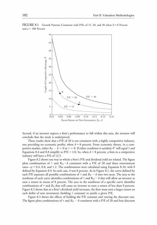
Second, if an investor expects a firm’s performance to fall within this area, the investor willconclude that the stock is underpriced.
These results show that a P/E of 20 is not consistent with a highly competitive industry,one providing no economic profits, when k5 8 percent. From economic theory, in a com-petitive market, either RN � k ¼ 0 or τ ¼ 0. If either condition is satisfied, θτ will equal 1 andEquations 8.4 and 8.8 simplify to P/E5 1/k. So, when k5 8 percent, a firm in a competitiveindustry will have a P/E of 12.5.
Figure 8.2 shows one way in which a firm’s P/E and dividend yield are related. The figureplots combinations of τ and RN2k consistent with a P/E of 20 and three reinvestmentrates—ρ5 0.4, 0.8, and 1.2. The combinations were calculated using Equation 8.10, with θdefined by Equation 8.9. In each case, k was 8 percent. As in Figure 8.1, the curve defined byeach P/E separates all possible combinations of τ and RN � k into two areas. The area to thenortheast of each curve identifies combinations of τ and RN2 k that will allow an investor toearn a return in excess of 8 percent. The area to the southwest of a specific curve identifiescombinations of τ and RN that will cause an investor to earn a return of less than 8 percent.Figure 8.2 shows that as a firm’s dividend yield increases, the firm must earn a larger return oneach dollar of new investment (holding τ constant) to justify a given P/E.
Figure 8.3 shows the effects of holding the P/E constant and varying the discount rate.The figure plots combinations of τ and RN � k consistent with a P/E of 20 and four discount
FIGURE 8.1 Growth Patterns Consistent with P/Es of 15, 20, and 30 when k5 8 Percent
and ρ5 100 Percent
50
45
40
35
30
25
20
15
10
5
0.02 0.04 0.06 0.08 0.10 0.12 0.14 0.160
Leng
th o
f Com
petit
ive
Adv
anta
ge, τ
Excess Return on New Investments, RN –k
P/E � 30P/E � 20
P/E � 15
B
A
c08 12 September 2012; 17:44:48
182 Part II: Valuation Methodologies
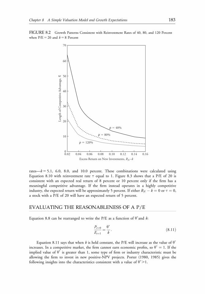
rates—k5 5.1, 6.0, 8.0, and 10.0 percent. These combinations were calculated usingEquation 8.10 with reinvestment rate τ equal to 1. Figure 8.3 shows that a P/E of 20 isconsistent with an expected real return of 8 percent or 10 percent only if the firm has ameaningful competitive advantage. If the firm instead operates in a highly competitiveindustry, the expected return will be approximately 5 percent. If either RN � k ¼ 0 or τ ¼ 0,a stock with a P/E of 20 will have an expected return of 5 percent.
EVALUATING THE REASONABLENESS OF A P/E
Equation 8.8 can be rearranged to write the P/E as a function of θτand k:
Pt¼0
Et¼1¼ θτ
k: ð8:11Þ
Equation 8.11 says that when k is held constant, the P/E will increase as the value of θτ
increases. In a competitive market, the firm cannot earn economic profits, so θτ ¼ 1. If theimplied value of θτ is greater than 1, some type of firm or industry characteristic must beallowing the firm to invest in new positive-NPV projects. Porter (1980, 1985) gives thefollowing insights into the characteristics consistent with a value of θτ.1.
FIGURE 8.2 Growth Patterns Consistent with Reinvestment Rates of 40, 80, and 120 Percent
when P/E5 20 and k5 8 Percent
0.02 0.04 0.06 0.08 0.10 0.12 0.14 0.16
70
60
50
40
30
20
10
0
Leng
th o
f Com
petit
ive
Adv
anta
ge, τ
Excess Return on New Investments, RN –k
ρ � 40%
ρ � 80%
ρ � 120%
c08 12 September 2012; 17:44:48
Chapter 8 A Simple Valuation Model and Growth Expectations 183
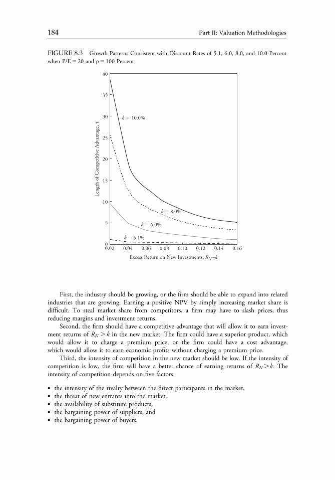
First, the industry should be growing, or the firm should be able to expand into relatedindustries that are growing. Earning a positive NPV by simply increasing market share isdifficult. To steal market share from competitors, a firm may have to slash prices, thusreducing margins and investment returns.
Second, the firm should have a competitive advantage that will allow it to earn invest-ment returns of RN . k in the new market. The firm could have a superior product, whichwould allow it to charge a premium price, or the firm could have a cost advantage,which would allow it to earn economic profits without charging a premium price.
Third, the intensity of competition in the new market should be low. If the intensity ofcompetition is low, the firm will have a better chance of earning returns of RN .k: Theintensity of competition depends on five factors:
� the intensity of the rivalry between the direct participants in the market,� the threat of new entrants into the market,� the availability of substitute products,� the bargaining power of suppliers, and� the bargaining power of buyers.
FIGURE 8.3 Growth Patterns Consistent with Discount Rates of 5.1, 6.0, 8.0, and 10.0 Percent
when P/E5 20 and ρ5 100 Percent
40
35
30
25
20
15
10
5
0
k � 8.0%
k � 10.0%
k � 6.0%
k � 5.1%
Leng
th o
f Com
petit
ive
Adv
anta
ge, τ
0.02 0.04 0.06 0.08 0.10 0.12 0.14 0.16
Excess Return on New Investments, RN –k
c08 12 September 2012; 17:44:48
184 Part II: Valuation Methodologies
To evaluate the implied value of θτ, an analyst can estimate values of RN and τ: His-torical information can be a useful starting point when estimating the return on newinvestments, but analysts should keep in mind that the firm’s competitive position in itscurrent and new markets may not be the same. For example, a firm that was a cost leader inthe past may or may not be the cost leader in a new market. A firm with a comparativeadvantage in the past may face different direct and indirect competition in a new market,which will affect its ability to charge premium prices. Such changes can cause future returns todiffer from past returns. The length of the period of competitive advantage, τ, depends on atleast three factors: (1) the size of the new market, (2) the costs of entry into the new market,and (3) the intensity of existing competition in the new market. In addition, the threat of newtechnologies or government regulations can limit the value of τ.
A high value of θτ is consistent with a unique competitive situation. The firm mustcompete in a growing market in which economic profits can be earned from new investmentsfor a number of years. This type of market will tend to attract the most competition, however,and as new firms enter the market, both RN � k ¼ 0 and τ will decrease.
This discussion points out two potential dangers of investing in high-P/E stocks. Ifthe competitive situation of a firm with a high P/E is consistent with a low value of θτ, theexpected return will be low. If the required return, k, is high, the implied value of θτ could behigher than the firm can reasonably be expected to achieve. If so, an investor’s actual returnmay be lower than the required return.
OVERPRICING OF HIGH-P/E STOCKS
The poor returns from high-P/E stocks could be caused in part by the failure of high-P/Efirms to meet growth expectations. Fama and French (1992) and Jaffe, Keim, and Westerfield(1989), among others, reported a negative relationship between stock market returns and P/Es(or, more precisely, a positive relationship between returns and earnings-to-price ratios).4
Recent evidence suggests that the earnings of high-P/E firms may not grow at a rate fastenough to justify their current prices. Lakonishok, Shleifer, and Vishny (1994) and Fuller,Huberts, and Levinson (1993) found that firms with high P/Es do have higher future earningsgrowth rates than low-P/E firms but that superior growth tends to last for a fairly short periodof time—eight years or less.
Is eight years of superior earnings growth long enough to justify a high P/E? Fuller,Huberts, and Levinson concluded that the superior earnings growth of high-P/E stocks isconsistent with the correct pricing of stocks across P/E groups. Haugen (1994) looked at thesame data and concluded that high-P/E stocks may be systematically overpriced. Without anobjective benchmark, this conflict cannot be resolved. The model presented here is a first steptoward identifying such a benchmark.
CONCLUSION
One way an analyst can quantify the expectations implied by a stock price is to consider fivefactors a stock price depends on: expected earnings (cash flows), reinvestment rate, returnon new investments, risk-adjusted discount rate, and length of the period of competitive
c08 12 September 2012; 17:44:48
Chapter 8 A Simple Valuation Model and Growth Expectations 185
advantage. The model described here allows an analyst to quickly identify combinations ofthese variables consistent with a stock price. The analyst can then use this information todetermine if the stock price is reasonable. To do this, an analyst must be able to answer thefollowing questions: First, does the firm have a competitive advantage that will allow it toinvest in (new) positive-NPV projects? Second, how profitable will the new projects be? Inparticular, what is the size of RN � k? Finally, how long will the firm be able to investin projects offering this return? Or, stated another way, how long will it take competition toreduce the economic profit on new investments toward zero?
The basic idea behind the model presented here is not new. Several existing modelsuse the assumption that a firm can invest in positive-NPV projects for a limited numberof years. In addition to the Gordon and Gordon model, finite-growth models havebeen developed by Miller and Modigliani (1961), Holt (1962), and Mao (1966). The modeldescribed here can be simplified, however, to a more concise, easier-to-use form than previousmodels. Therefore, the new model is better suited to the “first-cut” analysis outlined inthis chapter.
APPENDIX 8A COMPARISON OF NEW MODELWITH GORDON AND GORDON MODEL
The model presented here differs slightly from the Gordon and Gordon model in how thetwo models treat earnings in excess of the amount invested in positive-NPV projects. Inthe Gordon and Gordon model, the firm pays these amounts as dividends. In the newmodel, the firm invests these amounts in projects with NPVs equal to zero. Because of thisdifference, the models predict slightly different stock prices for a given set of inputs. Table 8A.1compares the predicted prices from the two models for several sets of inputs. It compares theestimated stock price from Equation 8.8 with the estimated stock price from the Gordonand Gordon model, Equation 8.1. In each case, the required return, k, is equal to 8 percent andthe expected earnings next year are $1 per share; therefore, the estimated price is also theestimated P/E.
Panel A of Table 8.A1 shows that the two models predict similar prices when the period ofcompetitive advantage, τ, is less than 10. For firms facing competition, this range is probably themost realistic. In addition, the evidence in Gordon and Gordon suggests that analysts do notforecast abnormal performance beyond seven years.
Panel B of Table 8A.1 shows that the two models predict similar prices when the returnon the new investments, RN, is relatively close to k. Again, competition will make this rangethe most realistic for many firms.
Panel C of Table 8A.1 shows that the difference between the prices predicted by the modelsincreases as the reinvestment rate, ρ, moves from zero to 1. Equations 8.1, 8.8, and 8.9 indicatethat the two models predict the same price when ρ is equal to zero—that is, when there is nogrowth from new investment. For the assumptions in Panel C, the maximum difference isreached at ρ ¼ 0:498. The difference between the prices then decreases as ρ approaches 1. Asnoted previously, Equation 8.1 simplifies to Equations 8.4 and 8.5 when ρ ¼ 1.
Although the differences in Table 8A.1 can be significant, they do not mean that onemodel is better than the other. After all, the assumptions of either model are not likely toportray the investment policies of all (or any) firms exactly. Therefore, the price estimate fromeither model is only a rough estimate of the appropriate price.
c08 12 September 2012; 17:44:48
186 Part II: Valuation Methodologies
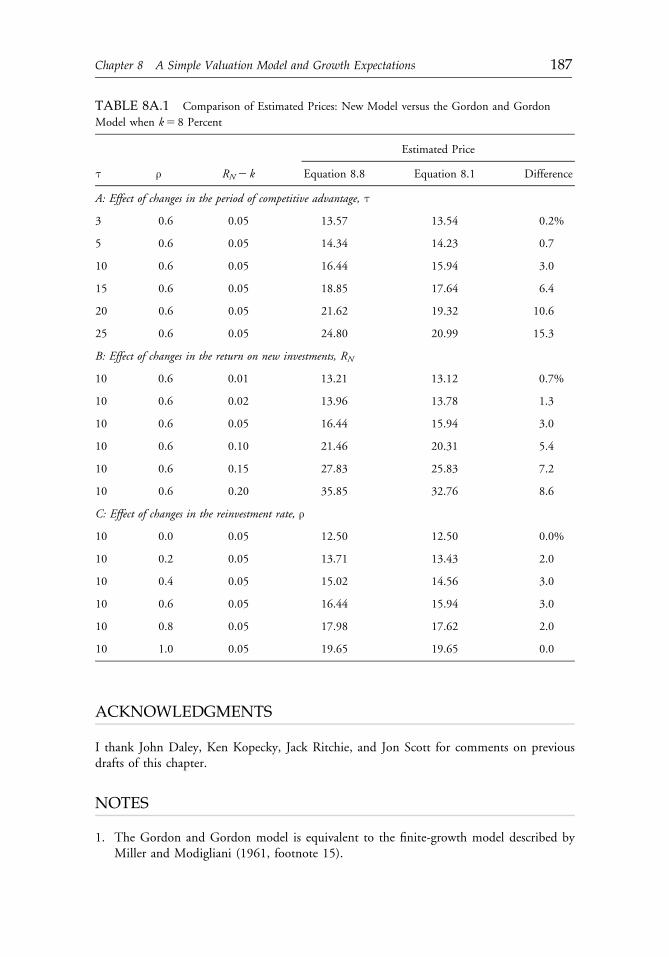
ACKNOWLEDGMENTS
I thank John Daley, Ken Kopecky, Jack Ritchie, and Jon Scott for comments on previousdrafts of this chapter.
NOTES
1. The Gordon and Gordon model is equivalent to the finite-growth model described byMiller and Modigliani (1961, footnote 15).
TABLE 8A.1 Comparison of Estimated Prices: New Model versus the Gordon and Gordon
Model when k5 8 Percent
Estimated Price
τ ρ RN2 k Equation 8.8 Equation 8.1 Difference
A: Effect of changes in the period of competitive advantage, τ
3 0.6 0.05 13.57 13.54 0.2%
5 0.6 0.05 14.34 14.23 0.7
10 0.6 0.05 16.44 15.94 3.0
15 0.6 0.05 18.85 17.64 6.4
20 0.6 0.05 21.62 19.32 10.6
25 0.6 0.05 24.80 20.99 15.3
B: Effect of changes in the return on new investments, RN
10 0.6 0.01 13.21 13.12 0.7%
10 0.6 0.02 13.96 13.78 1.3
10 0.6 0.05 16.44 15.94 3.0
10 0.6 0.10 21.46 20.31 5.4
10 0.6 0.15 27.83 25.83 7.2
10 0.6 0.20 35.85 32.76 8.6
C: Effect of changes in the reinvestment rate, ρ
10 0.0 0.05 12.50 12.50 0.0%
10 0.2 0.05 13.71 13.43 2.0
10 0.4 0.05 15.02 14.56 3.0
10 0.6 0.05 16.44 15.94 3.0
10 0.8 0.05 17.98 17.62 2.0
10 1.0 0.05 19.65 19.65 0.0
c08 12 September 2012; 17:44:49
Chapter 8 A Simple Valuation Model and Growth Expectations 187
2. The numbers in this paragraph come from simulations described in the section titled “TheModel and Market Expectations.” These numbers can be recalculated using Equation8.10 with a required return of 8 percent.
3. A discount rate of 8 percent can be thought of as a real (risk-free) interest rate of 2 percentplus an equity risk premium of 6 percent.
4. Not all studies have found that high-P/E firms underperform. Siegel (1995), for example,found that price appreciation and dividends over a 25-year period ultimately justified thehigh P/Es of a group of 50 stocks.
REFERENCES
Fama, E., and K. French. 1992. “The Cross-Section of Expected Stock Returns.” Journal of Finance, vol.47, no. 2 (June):427�65.
Fuller, R., L. Huberts, and M. Levinson. 1993. “Returns to E/P Strategies, Higgledy-Piggledy Growth,Analysts’ Forecast Errors, and Omitted Risk Factors.” Journal of Portfolio Management, vol. 19,no. 2 (Winter):13�24.
Gordon, J., and M. Gordon. 1997. “The Finite Horizon Expected Return Model.” Financial AnalystsJournal, vol. 53, no. 3 (May/June):52�61.
Gordon, M. 1962. The Investment, Financing, and Valuation of the Corporation. Homewood, IL:Richard D. Irwin.
Haugen, R. 1994. The New Finance: The Case against Efficient Markets. Englewood Cliffs, NJ: Prentice-Hall.
Holt, C. 1962. “The Influence of Growth Duration on Share Prices.” Journal of Finance, vol. 17, no. 3(July):465�75.
Jaffe, J., D. Keim, and R. Westerfield. 1989. “Earnings Yields, Market Values, and Stock Returns.”Journal of Finance, vol. 44, no. 1 (March):135�48.
Lakonishok, J., A. Shleifer, and R. Vishny. 1994. “Contrarian Investment, Extrapolation, and Risk.”Journal of Finance, vol. 49, no. 5 (December):1541�78.
Mao, J. 1966. “The Valuation of Growth Stocks: The Investment Opportunities Approach.” Journal ofFinance, vol. 21, no. 1 (March):95�102.
Miller, M., and F. Modigliani. 1961. “Dividend Policy, Growth, and the Valuation of Shares.” Journalof Business, vol. 34, no. 4 (October):411�33.
Porter, M. 1980. Competitive Strategy: Techniques for Analyzing Industries and Competitors. New York:The Free Press.
_____. 1985. Competitive Advantage: Creating and Sustaining Superior Performance. New York: The FreePress.
Siegel, J. 1995. “The Nifty-Fifty Revisited: Do Growth Stocks Ultimately Justify Their Price?” Journal ofPortfolio Management, vol. 21, no. 4 (Summer):8�20.
c08 12 September 2012; 17:44:49
188 Part II: Valuation Methodologies
CHAPTER 9FRANCHISE
VALUATION UNDERQ-TYPE COMPETITION
Martin L. Leibowitz
When considering a company’s prospects, analysts often segment the earnings pro-gression, either formally or intuitively, into a series of growth phases followed by arelatively stable terminal phase. This study focuses on the role of competition in theterminal phase. In the simplified two-phase model of a single-product company,the first-phase earnings growth drives the company’s overall return on equity towardthe (generally higher) incremental ROE on new investments. The company thenenters the terminal phase with a high ROE that attracts the attention of a potentialcompetitor that can replicate the company’s production/distribution capacity at somemultiple Q of the original capital cost. This “Q-type competition” can lead tomargin erosion and a reduction in earnings as the ROE slides to more competitivelevels. The implication is that, unless a company has either the diversity of product/service cycles or other special ways to deflect competitive pressures, the analyst shouldaddress the potential impact of Q-type competition on the sustainability of thecompany’s franchise and the company’s valuation.
Most valuation models view a company as going through various phases of differentiatedgrowth before ultimately entering a terminal phase of “competitive equilibrium.” Relativelylittle attention has been given to the nature of this terminal phase, however, or to the materialimpact that various characterizations of this phase can have on the valuation of the company.
In developing a valuation model for a company, analysts face an almost irresistibletemptation to focus on the early, more exciting growth phases of the earnings progression.
Reprinted from the Financial Analysts Journal (November/December 1998):62�74.When this article wasoriginally published, Martin L. Leibowitz was vice chair and chief investment officer at TIAA-CREF.
c09 12 September 2012; 17:48:43
189
Indeed, the typical practitioner treatment of the terminal phase has been to assume thatearnings either stabilize or regress to some general market growth rate. In the theoreticalliterature, a number of early writers have been concerned with the issue of how to model agrowth company’s transition into an equilibrium state.1 This chapter demonstrates howuseful insights into the complex structure of this terminal phase can be obtained from recentwork on a sales-driven franchise approach to valuation (Leibowitz 1997a, 1997b).
In a sales-driven context, the terminal phase can be construed as the period when salesgrowth finally stabilizes but in which the company’s earnings may continue to change as thepricing margin moves toward some competitive equilibrium. This margin-equilibratingprocess can be usefully described in terms of the ratio of asset replacement cost to thecompany’s book value, a parameter that is related to Tobin’s q (Tobin 1969; Lindenberg andRoss 1981). Generally, lower replacement costs in the company’s industry lead to adversefranchise changes, “franchise slides.” In other cases, significantly higher replacement costs canlead, even after all sales growth has come to an end, to further earnings growth, or “franchiserides.” The potential for such earnings variability in the terminal phase appears to havereceived insufficient recognition in most of the literature on valuation models, including theprevious work of this author.
Of course, the valuation impact of this terminal-phase effect will depend totally on thenature of the company’s business and its long-term competitive posture. For example,companies that might stand to gain from postgrowth margin expansion include companiesthat are able to achieve a sustainable market dominance, perhaps because growth itself builds arelatively unassailable efficiency of scale; companies whose organizational, distributional, ortechnological assets far exceed a more readily replicable capital base; companies with sufficientpatent protection and/or extraordinary brand acceptance to assure franchise-level margins foryears to come; and companies whose products (leading-edge products, for example) canthemselves act as germinators for subsequent generations of even more-advanced products.For such fortunate companies, the investor can look forward to a future period of sustainedhigh sales when the margins can be enhanced, or at least maintained, and when a high payoutratio can at last be applied. It is in this halcyon period that the patient investor will finally berewarded with the significant cash returns that formed the foundation for the value ascribed tothe company at the outset.
For less-fortunate growth companies, alas, barriers to entry do indeed become porousover time, high franchise margins are vulnerable to erosion, and extraordinary earnings levelsare subject to the gravitational pull of commoditization. The analysis of such companies mustconsider the P/E reduction that arises from a franchise slide.
For the practical analyst, the basic message does not lie in the specific numerical results orthe quantitative models developed in this paper. Rather, the key finding is the surprisingimportance of exactly how a growth franchise plays out over time. This finding suggests thatthe analyst should go beyond estimation of a firm’s growth rate and the duration of its growthphase. Serious consideration—even if only qualitative—should be given to the period whenthe firm’s capital needs have abated and it can begin directing a more significant portionof the attained earnings back to the investor. Apart from any numerical assessments that maybe difficult or impossible to achieve, the analyst may be able to provide some insight into thedurability of the firm’s franchise in the face of the inevitable competition always present inany truly global market. Any such insights will provide a helpful new dimension in enablinginvestors to ascertain whether a particular firm, in that distant but critically important period,could be expected to enjoy an enhanced franchise ride, to face a costly franchise slide, or tofind itself on the more intermediary path of a “franchise glide.”
c09 12 September 2012; 17:48:44
190 Part II: Valuation Methodologies
SINGLE-PHASE NO-GROWTH MODEL
The simplest valuation model deals with a company that has a stable level of current earningsbut a total absence of any investment prospects that could generate returns in excess of thecost of capital. In this simplest of all cases, the well-known result is
P ¼ Ek,
where P is the firm’s intrinsic value, E is the fixed level of earnings, and k is the cost of capital.In this “no-growth” example, all earnings are being paid out as dividends.2 Clearly, the verynotion of a constant earnings stream is artificial. Nonetheless, this simple case serves handilyas a convenient starting point for the analysis of more-complex multiphase growth models. Inparticular, the constant-earnings assumption forms the basis for the treatment of the terminalphase in many valuation models.
To deal with the question of the earnings progression under a specific form of com-petitive equilibrium and the ultimate impact that such a state would have on the company’svaluation, the first step is to recast the problem in sales-driven terms. In the terminologyof sales-driven franchise value (Leibowitz 1997a), the constant-earnings model can berewritten as
P ¼ Ek
¼ mSk
,
where S is (constant) annual unit sales and m is net margin. (For simplicity, assume a regimewithout taxation.) The earnings and sales flows can be related to the company’s asset value, B,through the relationship
E ¼ rB
¼ ðmT ÞB,
where r is return on equity (ROE) for the (unlevered) company and T is “sales turnover” (i.e.,annual sales per dollar of book value).
The company enjoys a “franchise return” as long as its ROE is greater than its cost ofcapital (i.e., r2 k. 0).
Alternatively, in sales terms, a franchise margin factor, fm, can be defined as the earningson each sales dollar in excess of the return required to cover the annual capital cost. Now, itcan be shown that
fm ¼ m� kT:
It readily follows that fm will be positive when the company enjoys an ROE franchise. Thus,the company will enjoy a franchise ride to the extent that it can sustain sufficient pricingpower (or production cost advantage) to achieve margins in excess of k/T.
This rationale motivated the use of the franchise margin as a gauge of the company’spricing power (i.e., its ability to extract a margin above and beyond that needed to cover thecost of capital).
c09 12 September 2012; 17:48:44
Chapter 9 Franchise Valuation under Q-Type Competition 191
Q-TYPE COMPETITIVE EQUILIBRIUM
For purposes of clarity, the discussion in this chapter focuses on the dour case of the franchiseslide: the situation in which the company undergoes a margin erosion once the growth phasehas been completed.
In a modern competitive environment, technological obsolescence progresses rapidly,product cycles contract, capital is broadly available for valid projects, and globalizationreduces the advantage of low-cost production sites. In such an environment, sustaining along franchise ride is a great challenge. Large, technologically proficient, well-capitalizedcompetitors lurk in the shadows of even the brightest franchise. Theoretically, when thebarriers to entry have eroded, these competitors will be happy to replicate the company’sproducts and/or services for a margin that just covers their cost of capital. In otherwords, in this environment, competition (or even the threat of competition) should driveprices down to a level at which the franchise margin essentially vanishes (where fm - 0or m - k/T).
Other authors and I have described some aspects of such competition (Leibowitz1997a, 1997b; Rappaport 1986, 1998), but I did not recognize that this margin erosionwould be exacerbated by a form of the Tobin q effect. In my earlier work, the tacit assumptionwas that a new competitor would incur the same capital costs to achieve the comparablesales capacity. But what if the competitor’s new facilities, for one reason or another (theopportunity to use the latest technology, more-precise market targeting, or simply pricingshifts in the market for capital goods), could be developed with a lower capital expenditure;in other words, what if the replacement cost was below the original company’s bookvalue? This ratio of a competitor’s replacement costs to the company’s book value can bedesignated Q.3
With this terminology, Q-type competitive equilibrium is defined as a situation in whichone or more competitors could replace the original company’s production and distributioncapability through the capital expenditure of only QB where Q # 1.4
Now consider the earnings differential between the original company and the hypo-thetical competitor. The original company’s earnings are E5 rB, but the competitor cangenerate the same level of unit sales by the capital expenditure of only QB. The competitorcompany would thus be tempted to move into the fray if it could achieve a level of earningskQB that would cover its capital costs. Thus, in a fully competitive environment, the originalcompany’s earnings would also have to descend to kQB. And because the original company’sassets represent funds that have already been spent, the company would have to respond tothis competition whether the resulting margin did or did not cover the sunk cost of its capital.The original company’s intrinsic value would then have to decline by a factor equal to theratio of these two earnings levels:
kQBE
¼ kQBrB
¼ kQr:
The same point can be made by noting that the ratio of the original company’s earningsto the replacement cost could be interpreted as a kind of “excessive ROE,” E/QB5 rB/QB,
c09 12 September 2012; 17:48:44
192 Part II: Valuation Methodologies
that must ultimately descend to the market rate k. Here again, the company’s pricingwould be reduced by the ratio of the competitive ROE k to this currently “excessive ROE.”That is,
kðrB=QBÞ ¼
kQr,
so the same factor, kQ/r, results.Note that this analysis holds regardless of how one accounts for the company’s capital
base, B—whether by book accounting, liquidation value, earnings capitalization, or so on.The key is not the original company’s capital base, which is simply a sunk cost (and one thatmay even be artificially measured), but the actual capital expenditure required for newentrants to field a comparable sales capacity and just cover their cost of capital—that is, QB.5
Although Q may be defined in terms of the original company’s book value accounting for B,the multiple QB represents the competitor’s literal capital expenditure required to produce thecurrent sales level. Similarly, r basically relates the “hard” variable of earnings to the bookvalue in whatever way B is defined. Thus, because Q and r are both defined in relation to theoriginal company’s book value, the choice of the accounting for B drops out of the Q/r ratiothat determines the pricing reduction. If potential competitors need only achieve their capitalcosts, the original company’s earnings will ultimately be reduced by the factor kQ/r, regardlessof how the book value of assets is measured and regardless of what value is ascribed to thosebook assets.
The valuation impact of this earnings decline will clearly depend on the rapidity of thefranchise slide. The worst case would be an immediate “cliff” drop-off in earnings, whichwould result in a price value of
P ¼ kQBk
¼ QB:
In other words, the company would be worth no more than the new capital expenditurerequired to replace its sales capacity.6
Before leaving this simplest of all cases, consider how the franchise slide affectsthe company’s P/E. On the assumption that the denominator of this ratio is the preslideearnings,
P=E ¼�kQBk
��1
rB
�
¼�1
k
��kQr
�
¼ 1
k
�rQr
�,
where rQ5 (EQ/B)5 kQ is the ROE for the postslide company.7
c09 12 September 2012; 17:48:44
Chapter 9 Franchise Valuation under Q-Type Competition 193
A GENERAL DECAY MODEL
The preceding discussion was based on the special case of an immediate franchise plunge in aharshly competitive environment from an excess-return franchise to no franchise whatsoever. Amore realistic (and more general) situation would be for the franchise to erode at some fixedpace in the course of time. The simplest approach to modeling such a situation would use afixed annual decay rate, d, that takes the company’s earnings from its original level down to theultimate fully competitive level, EQ. Thus, the earnings in the tth year would be expressed as
EðtÞ ¼ Eð1� dÞt t , D
EQ t $ D,
(
where D is the time required for the decay to reach the EQ level, EQ5E(12 d )D, so
D ¼ logðEQ=EÞlogð1� dÞ
¼ logðkQ=rÞlogð1� d Þ for 0 , d , 1:
In the happy case in which Q is sufficiently large, this “decay orientation” would have to beexpanded to include a margin that can grow at some annual rate until competitive equilibriumis attained.
At this point, a numerical example would probably be helpful: Suppose
k ¼ 12 percent;
B ¼ 100,
E ¼ 15 ðimplying an initial ROE of15 percentÞ,Q ¼ 0:75:
Because all earnings are paid out in this single-phase model, there is no reinvestment, andthe book value remains constant.
Under competition, the earnings are assumed to fall to the point at which the ROEequals
Qk ¼ 0:753 12 percent ¼ 9 percent
and the earnings are EQ5 9.If the selected decay rate is 5 percent a year, the 40 percent earnings decline from 15 to 9
will occur gradually over a span of 10 years. The time path of this earnings decline is shown asthe lower curve in Figure 9.1.
The general relationship between the annual decay rate and the time required to reachequilibrium is shown in Figure 9.2. The lower-curve values for the no-growth model show thatraising the decay rate from 1 percent to 5 percent significantly shortens the decay time—from50 years to 10. In between, a 2.5 percent decay rate results in a span of 20 years, which mightbe considered unrealistically long for many cases. The upper curve will be discussed later.
c09 12 September 2012; 17:48:44
194 Part II: Valuation Methodologies
Now, the intrinsic price, P(Q, d ), in this “(Q, d ) decay process” can be determined in areasonably straightforward way:
PðQ , d Þ ¼XNt¼1
Et
ð1þ kÞt
¼XDt¼1
ð1� dÞt Eð1þ kÞt þ
XNt¼Dþ1
EQð1þ kÞt
FIGURE 9.1 Earnings Patterns in Two Competitive Decay Scenarios: No-Growth Model
17
16
15
14
13
12
11
10
9
8
7
6
5
4
Earn
ings
0 10 15 205
Time (years)
3025
d � 0
Q � 1, d � 5%
Q � 0.75, d � 5%
FIGURE 9.2 Decay Times to Reach Q-Type Competitive Equilibrium for No-Growth and Growth
Models: Q5 0.75
80
70
60
50
40
30
20
10
0
Dec
ay T
ime
(yea
rs)
1
Decay Rate (%)
2 3 54
g � 0
g � 22%
c09 12 September 2012; 17:48:45
Chapter 9 Franchise Valuation under Q-Type Competition 195
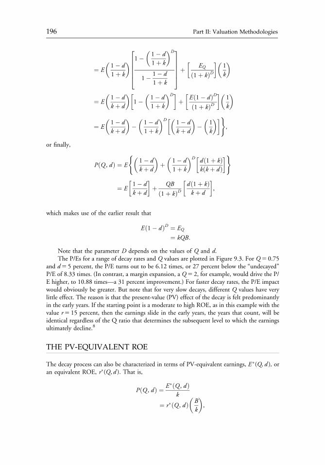
¼ E�1� d1þ k
� 1��1� d1þ k
�D
1� 1� d1þ k
266664
377775þ
�EQ
ð1þ kÞD��
1
k
�
¼ E�1� dk þ d
��1�
�1� d1þ k
�D�þ�Eð1� dÞDð1þ kÞD
��1
k
�
¼ E�1� dk þ d
���1� d1þ k
�D�� 1� dk þ d
���1
k
��),
or finally,
PðQ , dÞ ¼ E
(�1� dk þ d
�þ�1� d1þ k
�D� dð1þ kÞkðk þ dÞ
�)
¼ E�1� dk þ d
�þ QB
ð1þ kÞD�d ð1þ kÞk þ d
�,
which makes use of the earlier result that
Eð1� dÞD ¼ EQ
¼ kQB:
Note that the parameter D depends on the values of Q and d.The P/Es for a range of decay rates and Q values are plotted in Figure 9.3. For Q5 0.75
and d5 5 percent, the P/E turns out to be 6.12 times, or 27 percent below the “undecayed”P/E of 8.33 times. (In contrast, a margin expansion, a Q5 2, for example, would drive the P/E higher, to 10.88 times—a 31 percent improvement.) For faster decay rates, the P/E impactwould obviously be greater. But note that for very slow decays, different Q values have verylittle effect. The reason is that the present-value (PV) effect of the decay is felt predominantlyin the early years. If the starting point is a moderate to high ROE, as in this example with thevalue r5 15 percent, then the earnings slide in the early years, the years that count, will beidentical regardless of the Q ratio that determines the subsequent level to which the earningsultimately decline.8
THE PV-EQUIVALENT ROE
The decay process can also be characterized in terms of PV-equivalent earnings, E �(Q, d ), oran equivalent ROE, r�(Q, d ). That is,
PðQ , dÞ ¼ E�ðQ , dÞk
¼ r�ðQ , d Þ�Bk
�,
c09 12 September 2012; 17:48:45
196 Part II: Valuation Methodologies
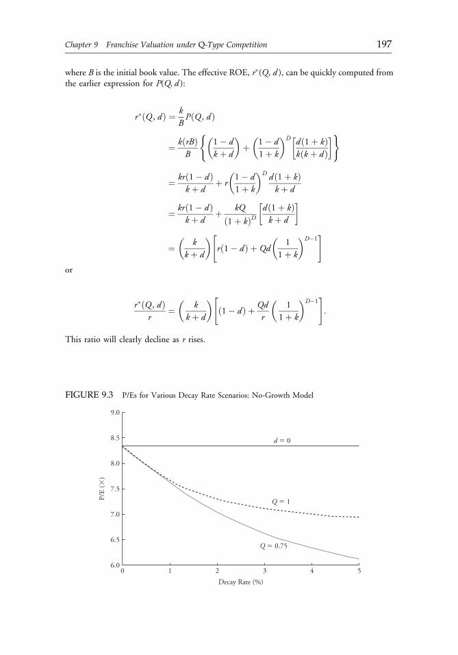
where B is the initial book value. The effective ROE, r�(Q, d ), can be quickly computed fromthe earlier expression for P(Q, d ):
r�ðQ , dÞ ¼ kBPðQ , d Þ
¼ kðrBÞB
1� dk þ d
� �þ 1� d
1þ k
� �D dð1þ kÞkðk þ dÞ� �( )
¼ krð1� dÞk þ d
þ r1� d1þ k
� �D d ð1þ kÞk þ d
¼ krð1� d Þk þ d
þ kQ
ð1þ kÞDd ð1þ kÞk þ d
� �
¼ kk þ d
� �rð1� dÞ þ Qd
1
1þ k
� �D�1" #
or
r�ðQ , d Þr
¼�
kk þ d
�ð1� dÞ þ Qd
r
�1
1þ k
�D�1" #
:
This ratio will clearly decline as r rises.
FIGURE 9.3 P/Es for Various Decay Rate Scenarios: No-Growth Model
d � 0
Q � 1
Q � 0.75
9.0
8.5
8.0
7.5
7.0
6.5
Decay Rate (%)
6.0
P/E
(�)
0 1 2 3 4 5
c09 12 September 2012; 17:48:45
Chapter 9 Franchise Valuation under Q-Type Competition 197
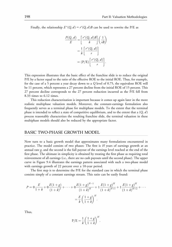
Finally, the relationship E �(Q, d )5 r�(Q, d )B can be used to rewrite the P/E as
PðQ , d ÞE
¼�r�ðQ , d ÞB
k
��1
rB
�
¼ 1
k
�r�ðQ , dÞ
r
�
¼ ðP=EÞ�r�ðQ , d Þ
r
�:
This expression illustrates that the basic effect of the franchise slide is to reduce the originalP/E by a factor equal to the ratio of the effective ROE to the initial ROE. Thus, for example,for the case of a 5 percent a year decay down to a Q level of 0.75, the equivalent ROE willbe 11 percent, which represents a 27 percent decline from the initial ROE of 15 percent. This27 percent decline corresponds to the 27 percent reduction incurred as the P/E fell from8.33 times to 6.12 times.
This reduction characterization is important because it comes up again later in the morerealistic multiphase valuation models. Moreover, the constant-earnings formulation alsofrequently serves as a terminal phase for multiphase models. To the extent that the terminalphase is intended to reflect a state of competitive equilibrium, and to the extent that a (Q, d )process reasonably characterizes the resulting franchise slide, the terminal valuation in thesemultiphase models should also be reduced by the appropriate factor.
BASIC TWO-PHASE GROWTH MODEL
Now turn to a basic growth model that approximates many formulations encountered inpractice. The model consists of two phases: The first is H years of earnings growth at anannual rate g, and the second is the full payout of the earnings level reached at the end of thefirst phase. The ultimate in simplicity is obtained by treating the first phase as requiring totalreinvestment of all earnings (i.e., there are no cash payouts until the second phase). The uppercurve in Figure 9.4 illustrates the earnings pattern associated with such a two-phase modelwith earnings growth of 22 percent over a 10-year period.
The first step is to determine the P/E for the standard case in which the terminal phaseconsists simply of a constant earnings stream. This ratio can be easily found:
P ¼ 0E
1þ kþ 0
Eð1þ gÞð1þ kÞ2 þ � � � þ 0
Eð1þ gÞH�1
ð1þ kÞH þ 1Eð1þ gÞHð1þ kÞHþ1 þ 1
Eð1þ gÞHð1þ kÞHþ2 þ � � �
¼ Ek
�1þ g1þ k
�H
:
Thus,
P=E ¼ 1
k
�1þ g1þ k
�H
:
c09 12 September 2012; 17:48:46
198 Part II: Valuation Methodologies
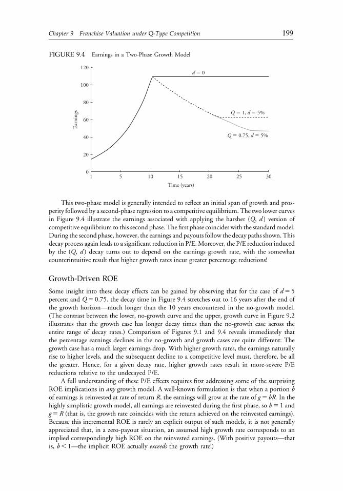
This two-phase model is generally intended to reflect an initial span of growth and pros-perity followed by a second-phase regression to a competitive equilibrium. The two lower curvesin Figure 9.4 illustrate the earnings associated with applying the harsher (Q, d ) version ofcompetitive equilibrium to this second phase. The first phase coincides with the standardmodel.During the second phase, however, the earnings and payouts follow the decay paths shown. Thisdecay process again leads to a significant reduction in P/E.Moreover, the P/E reduction inducedby the (Q, d ) decay turns out to depend on the earnings growth rate, with the somewhatcounterintuitive result that higher growth rates incur greater percentage reductions!
Growth-Driven ROE
Some insight into these decay effects can be gained by observing that for the case of d5 5percent and Q5 0.75, the decay time in Figure 9.4 stretches out to 16 years after the end ofthe growth horizon—much longer than the 10 years encountered in the no-growth model.(The contrast between the lower, no-growth curve and the upper, growth curve in Figure 9.2illustrates that the growth case has longer decay times than the no-growth case across theentire range of decay rates.) Comparison of Figures 9.1 and 9.4 reveals immediately thatthe percentage earnings declines in the no-growth and growth cases are quite different: Thegrowth case has a much larger earnings drop. With higher growth rates, the earnings naturallyrise to higher levels, and the subsequent decline to a competitive level must, therefore, be allthe greater. Hence, for a given decay rate, higher growth rates result in more-severe P/Ereductions relative to the undecayed P/E.
A full understanding of these P/E effects requires first addressing some of the surprisingROE implications in any growth model. A well-known formulation is that when a portion bof earnings is reinvested at rate of return R, the earnings will grow at the rate of g5 bR. In thehighly simplistic growth model, all earnings are reinvested during the first phase, so b5 1 andg5 R (that is, the growth rate coincides with the return achieved on the reinvested earnings).Because this incremental ROE is rarely an explicit output of such models, it is not generallyappreciated that, in a zero-payout situation, an assumed high growth rate corresponds to animplied correspondingly high ROE on the reinvested earnings. (With positive payouts—thatis, b, 1—the implicit ROE actually exceeds the growth rate!)
FIGURE 9.4 Earnings in a Two-Phase Growth Model
d � 0120
100
80
60
40
20
0
Earn
ings
1
Time (years)
5 201510 25 30
Q � 1, d � 5%
Q � 0.75, d � 5%
c09 12 September 2012; 17:48:46
Chapter 9 Franchise Valuation under Q-Type Competition 199
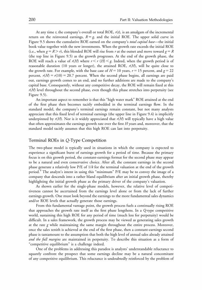
At any time t, the company’s overall or total ROE, r(t), is an amalgam of the incrementalreturn on the reinvested earnings, R5 g, and the initial ROE. The upper solid curve inFigure 9.5 shows the cumulative ROE earned on the company’s total capital base—the initialbook value together with the new investments. When the growth rate exceeds the initial ROE(i.e., when g5R. r), this blended ROE will rise from r at the outset and move toward g5 R(the top line in Figure 9.5) as the growth progresses. At the end of the growth phase, theROE will reach a value of r(H) where r, r (H), g. Indeed, when the growth period is ofreasonable duration (10 years or longer), the attained ROE, r(H), will be quite close tothe growth rate. For example, with the base case of H5 10 years, r5 15 percent, and g5 22percent, r(H)5 r(10)5 20.7 percent. When the second phase begins, all earnings are paidout, earnings growth comes to an end, and no further additions are made to the company’scapital base. Consequently, without any competitive decay, the ROE will remain fixed at thisr(H) level throughout the second phase, even though this phase stretches into perpetuity (seeFigure 9.5).
An important aspect to remember is that this “high water mark” ROE attained at the endof the first phase then becomes tacitly embedded in the terminal earnings flow. In thestandard model, the company’s terminal earnings remain constant, but not many analystsappreciate that this fixed level of terminal earnings (the upper line in Figure 9.4) is implicitlyunderpinned by r(H). Nor is it widely appreciated that r(H) will typically have a high valuethat often approximates the earnings growth rate over the first H years and, moreover, that thestandard model tacitly assumes that this high ROE can last into perpetuity.
Terminal ROEs in Q-Type Competition
The two-phase model is typically used in situations in which the company is expected toexperience a significant burst of earnings growth for a period of time. Because the primaryfocus is on this growth period, the constant-earnings format for the second phase may appearto be a natural and even conservative choice. After all, the constant earnings in the secondphase generate a relatively low P/E of 1/k for the terminal valuation at the end of the growthperiod.9 The analyst’s intent in using this “minimum” P/E may be to convey the image of acompany that descends into a rather bland equilibrium after an initial growth phase, therebyhighlighting the initial growth phase as the primary driver of the company’s valuation.
As shown earlier for the single-phase models, however, the relative level of competi-tiveness cannot be ascertained from the earnings level alone or from the lack of furtherearnings growth. One must look beyond the earnings to the more fundamental sales dynamicsand/or ROE levels that actually generate those earnings.
From this fundamental vantage point, the growth process fuels a continually rising ROEthat approaches the growth rate itself as the first phase lengthens. In a Q-type competitiveworld, sustaining this high ROE for any period of time (much less for perpetuity) would bedifficult. In a sales framework, the growth process may be viewed as generating sales growthat the rate g while maintaining the same margin throughout the entire process. Moreover,once the sales zenith is achieved at the end of the first phase, then a constant-earnings secondphase is tantamount to the assumption that both the high level of annual sales already attainedand the full margins are maintained in perpetuity. To describe this situation as a form of“competitive equilibrium” is a challenge indeed.
One of the problems in addressing this paradox is analysts’ understandable reluctance tosquarely confront the prospect that some earnings decline may be a natural concomitantof any competitive equilibrium. This reluctance is undoubtedly reinforced by the problem of
c09 12 September 2012; 17:48:46
200 Part II: Valuation Methodologies
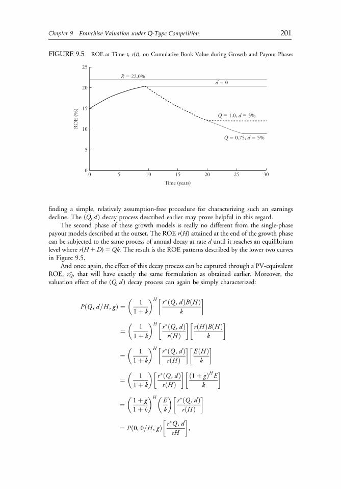
finding a simple, relatively assumption-free procedure for characterizing such an earningsdecline. The (Q, d ) decay process described earlier may prove helpful in this regard.
The second phase of these growth models is really no different from the single-phasepayout models described at the outset. The ROE r(H) attained at the end of the growth phasecan be subjected to the same process of annual decay at rate d until it reaches an equilibriumlevel where r(H1D)5Qk. The result is the ROE patterns described by the lower two curvesin Figure 9.5.
And once again, the effect of this decay process can be captured through a PV-equivalentROE, rQ�, that will have exactly the same formulation as obtained earlier. Moreover, thevaluation effect of the (Q, d ) decay process can again be simply characterized:
PðQ , d=H , gÞ ¼�
1
1þ k
�H� r�ðQ , d ÞBðH Þk
�
¼�
1
1þ k
�H� r�ðQ , dÞrðHÞ
��rðH ÞBðHÞ
k
�
¼�
1
1þ k
�H� r�ðQ , d ÞrðH Þ
��EðH Þk
�
¼�
1
1þ k
��r�ðQ , dÞrðH Þ
�� ð1þ gÞHEk
�
¼�1þ g1þ k
�H�Ek
��r�ðQ , dÞrðH Þ
�
¼ Pð0, 0=H , gÞ�r�Q , drH
�,
FIGURE 9.5 ROE at Time t, r(t), on Cumulative Book Value during Growth and Payout Phases
25
20
15
10
5
0
RO
E (%
)
0
Time (years)
5 25201510 30
Q � 1.0, d � 5%
Q � 0.75, d � 5%
R � 22.0%d � 0
c09 12 September 2012; 17:48:46
Chapter 9 Franchise Valuation under Q-Type Competition 201
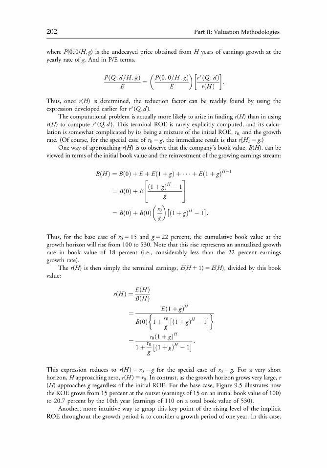
where P(0, 0/H, g) is the undecayed price obtained from H years of earnings growth at theyearly rate of g. And in P/E terms,
PðQ , d=H , gÞE
¼�Pð0, 0=H , gÞ
E
�r�ðQ , dÞrðH Þ
� �:
Thus, once r(H) is determined, the reduction factor can be readily found by using theexpression developed earlier for r�(Q, d ).
The computational problem is actually more likely to arise in finding r(H) than in usingr(H) to compute r�(Q, d ). This terminal ROE is rarely explicitly computed, and its calcu-lation is somewhat complicated by its being a mixture of the initial ROE, r0, and the growthrate. (Of course, for the special case of r05 g, the immediate result is that r[H]5 g.)
One way of approaching r(H) is to observe that the company’s book value, B(H), can beviewed in terms of the initial book value and the reinvestment of the growing earnings stream:
BðHÞ ¼ Bð0Þ þ E þ Eð1þ gÞ þ � � � þ Eð1þ gÞH�1
¼ B 0ð Þ þ Eð1þ gÞH � 1
g
24
35
¼ B 0ð Þ þ B 0ð Þ�r0g
��ð1þ gÞH � 1:
Thus, for the base case of r05 15 and g5 22 percent, the cumulative book value at thegrowth horizon will rise from 100 to 530. Note that this rise represents an annualized growthrate in book value of 18 percent (i.e., considerably less than the 22 percent earningsgrowth rate).
The r(H) is then simply the terminal earnings, E(H1 1)5E(H), divided by this bookvalue:
rðH Þ ¼ EðH ÞBðHÞ
¼ Eð1þ gÞH
Bð0Þ 1þ r0g
�ð1þ gÞH � 1 �
¼ r0ð1þ gÞH1þ r0
g
�ð1þ gÞH � 1 :
This expression reduces to r(H )5 r05 g for the special case of r05 g. For a very shorthorizon, H approaching zero, r(H )5 r0. In contrast, as the growth horizon grows very large, r(H) approaches g regardless of the initial ROE. For the base case, Figure 9.5 illustrates howthe ROE grows from 15 percent at the outset (earnings of 15 on an initial book value of 100)to 20.7 percent by the 10th year (earnings of 110 on a total book value of 530).
Another, more intuitive way to grasp this key point of the rising level of the implicitROE throughout the growth period is to consider a growth period of one year. In this case,
c09 12 September 2012; 17:48:47
202 Part II: Valuation Methodologies
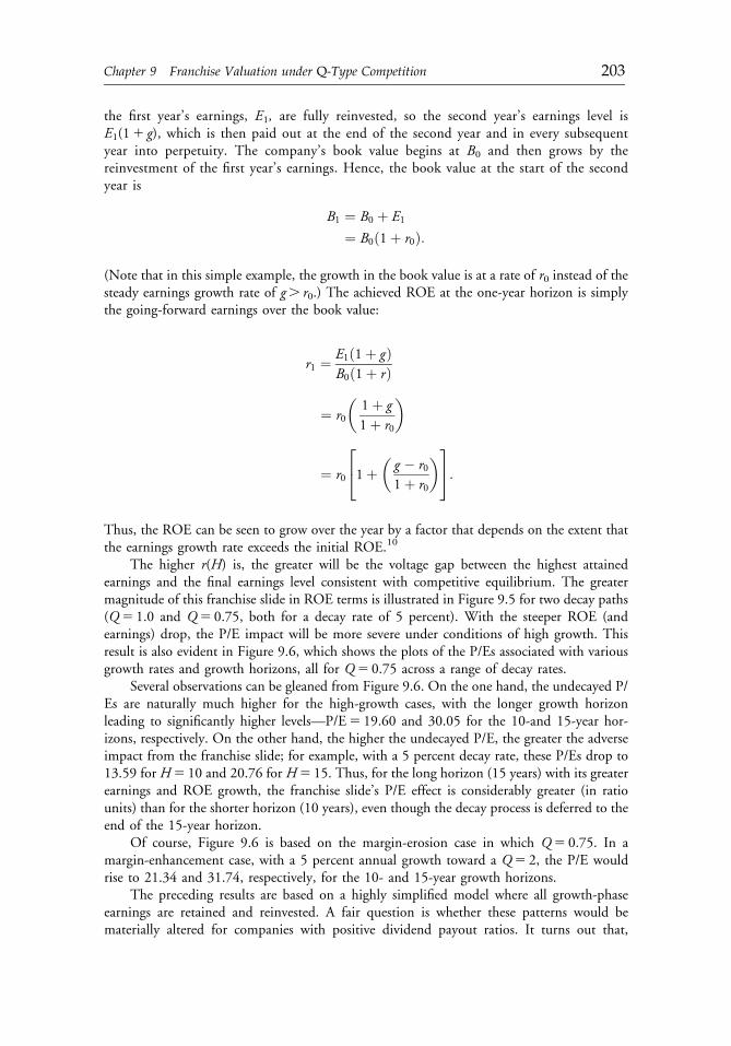
the first year’s earnings, E1, are fully reinvested, so the second year’s earnings level isE1(11 g), which is then paid out at the end of the second year and in every subsequentyear into perpetuity. The company’s book value begins at B0 and then grows by thereinvestment of the first year’s earnings. Hence, the book value at the start of the secondyear is
B1 ¼ B0 þ E1
¼ B0ð1þ r0Þ:
(Note that in this simple example, the growth in the book value is at a rate of r0 instead of thesteady earnings growth rate of g. r0.) The achieved ROE at the one-year horizon is simplythe going-forward earnings over the book value:
r1 ¼ E1ð1þ gÞB0ð1þ rÞ
¼ r0
�1þ g1þ r0
�
¼ r0 1þ�g � r01þ r0
�24
35:
Thus, the ROE can be seen to grow over the year by a factor that depends on the extent thatthe earnings growth rate exceeds the initial ROE.10
The higher r(H) is, the greater will be the voltage gap between the highest attainedearnings and the final earnings level consistent with competitive equilibrium. The greatermagnitude of this franchise slide in ROE terms is illustrated in Figure 9.5 for two decay paths(Q5 1.0 and Q5 0.75, both for a decay rate of 5 percent). With the steeper ROE (andearnings) drop, the P/E impact will be more severe under conditions of high growth. Thisresult is also evident in Figure 9.6, which shows the plots of the P/Es associated with variousgrowth rates and growth horizons, all for Q5 0.75 across a range of decay rates.
Several observations can be gleaned from Figure 9.6. On the one hand, the undecayed P/Es are naturally much higher for the high-growth cases, with the longer growth horizonleading to significantly higher levels—P/E5 19.60 and 30.05 for the 10-and 15-year hor-izons, respectively. On the other hand, the higher the undecayed P/E, the greater the adverseimpact from the franchise slide; for example, with a 5 percent decay rate, these P/Es drop to13.59 for H5 10 and 20.76 for H5 15. Thus, for the long horizon (15 years) with its greaterearnings and ROE growth, the franchise slide’s P/E effect is considerably greater (in ratiounits) than for the shorter horizon (10 years), even though the decay process is deferred to theend of the 15-year horizon.
Of course, Figure 9.6 is based on the margin-erosion case in which Q5 0.75. In amargin-enhancement case, with a 5 percent annual growth toward a Q5 2, the P/E wouldrise to 21.34 and 31.74, respectively, for the 10- and 15-year growth horizons.
The preceding results are based on a highly simplified model where all growth-phaseearnings are retained and reinvested. A fair question is whether these patterns would bematerially altered for companies with positive dividend payout ratios. It turns out that,
c09 12 September 2012; 17:48:47
Chapter 9 Franchise Valuation under Q-Type Competition 203
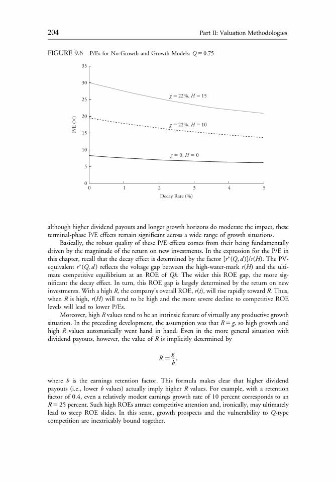
although higher dividend payouts and longer growth horizons do moderate the impact, theseterminal-phase P/E effects remain significant across a wide range of growth situations.
Basically, the robust quality of these P/E effects comes from their being fundamentallydriven by the magnitude of the return on new investments. In the expression for the P/E inthis chapter, recall that the decay effect is determined by the factor [r�(Q, d )]/r(H). The PV-equivalent r�(Q, d ) reflects the voltage gap between the high-water-mark r(H) and the ulti-mate competitive equilibrium at an ROE of Qk. The wider this ROE gap, the more sig-nificant the decay effect. In turn, this ROE gap is largely determined by the return on newinvestments. With a high R, the company’s overall ROE, r(t), will rise rapidly toward R. Thus,when R is high, r(H) will tend to be high and the more severe decline to competitive ROElevels will lead to lower P/Es.
Moreover, high R values tend to be an intrinsic feature of virtually any productive growthsituation. In the preceding development, the assumption was that R5 g, so high growth andhigh R values automatically went hand in hand. Even in the more general situation withdividend payouts, however, the value of R is implicitly determined by
R ¼ gb,
where b is the earnings retention factor. This formula makes clear that higher dividendpayouts (i.e., lower b values) actually imply higher R values. For example, with a retentionfactor of 0.4, even a relatively modest earnings growth rate of 10 percent corresponds to anR5 25 percent. Such high ROEs attract competitive attention and, ironically, may ultimatelylead to steep ROE slides. In this sense, growth prospects and the vulnerability to Q-typecompetition are inextricably bound together.
FIGURE 9.6 P/Es for No-Growth and Growth Models: Q5 0.75
P/E
(�)
35
30
25
20
15
10
5
00 5
Decay Rate (%)
2 3 41
g � 22%, H � 15
g � 22%, H � 10
g � 0, H � 0
c09 12 September 2012; 17:48:48
204 Part II: Valuation Methodologies
CONCLUSION
The results discussed here raise interesting questions about both the valuation process forhigh-growth stocks and the subtle implications of standard growth models. As one delvesdeeply into patterns of company growth, one finds that even simple earnings growth isimplicitly associated with considerably more-complex processes than are assumed in standardgrowth models. At the beginning, the typical high reinvestment rates that fuel earningsgrowth also add to the company’s capital base and enhance its production and distributioncapacity. The increased sales and earnings generated by these capacity enhancements aresources of high margin flows, which is fine because they provide substantial profits.
The problem arises when these high-margin earnings move toward competitive equi-librium. With a Q-type definition of such an equilibrium, the high-margin flows mustdescend toward margin levels that would just satisfy new competitors. To the extent that aninvestor would begin to receive a substantial payout only in the postgrowth period, such amargin shift could materially affect the company’s valuation. In essence, reinvestment-drivengrowth represents a leveraging of competitively vulnerable earnings. It is tantamount to arepeated doubling-up of the stakes in the face of escalating risks. If the franchise ride canbe extended, however, with new or existing products, these terminal-phase effects may bemuted.11
This chapter focused on the one- and two-phase valuation models, but the general thrustof the argument applies to any multiphase model that uses a constant-earnings assumption inthe terminal phase. Insufficient attention has been given to this problem of how the highROEs that are typically embedded in the terminal phase might fare in the face of seriousglobal competition. By recognizing the importance of such effects, the analyst should be ableto generate more-realistic characterizations of a firm’s long-term earnings and, in turn, be ableto develop better estimates for its valuation.
� � �
This chapter represents a purely analytical study by the author using hypothetical examples forillustrative purposes only. It is not intended to be descriptive of any individual companies or anyspecific class of equities. I would like to express gratitude for the many helpful suggestions from PeterBernstein, Paul Davis, Benson Durham, Hans Erickson, Scott Evans, Robert Ferguson, EricFisher, James Fleischmann, William Gray, Brett Hammond, Leo Kamp, Stanley Kogelman, andRichard Michaud. However, I accept full responsibility for the final form of the study. In par-ticular, this work does not represent any official organizational position of TIAA-CREF.
NOTES
1. See Bodie and Merton (1998); Damodaran (1994); Danielson (1998); Elton and Gruber(1991); Fruhan (1979); Gordon and Gordon (1997); Gordon (1962); Miller andModigliani (1961); Peterson and Peterson (1996); Rappaport (1998); Sorensen, andWilliamson (1985); Treynor (1972); and Williams (1938).
2. Although valuation models can be cast in terms of various flow variables—dividends,earnings, cash flow, etc.—I adhere in this chapter to more standard “earnings anddividends” terminology. The basic thrust of my argument can be readily extended tomodels based on other measures.
c09 12 September 2012; 17:48:48
Chapter 9 Franchise Valuation under Q-Type Competition 205
3. The choice of the capital Q reflects an intentional deference to Tobin’s q measure, eventhough his concept was much broader in scope. Moreover, because of the narrow focuson the competitive challenge, I have found it helpful to have the replacement costs serveas the numerator in our Q ratio rather than the denominator as in Tobin’s classic qmeasure.
4. In the more general case, strong franchise barriers could also lead to situations in whichthe would-be competitor’s capital expenditure would have to go far beyond simplyreplicating the original company’s goods-producing capacity. Such high-replacement-cost situations could lead to Q values that greatly exceed 1.
5. Q may also incorporate any general pricing divergences in the market for old versus newcapital assets.
6. Even these harsh conditions would not necessarily doom the company to operationalfailure: The sales margin can still be positive even when the franchise margin is negative.
7. The P/E in this case can obviously be reduced to simply P/E5Q/r, but I use the longerexpression for P/E, (1/k)(rQ/r), because it will prove useful later in the chapter. For thepositive case with a sufficiently higher Q,Q. 1, a better mental model might be to viewthe company as being able to expand its margin up to the point where competitionmight just consider entering the field. Apart from this somewhat different view of thecompany’s motivation, the mathematical development remains the same.
8. This simple example ignores any probable interaction between d and Q (i.e., the pos-sibility that a more dramatic “voltage gap” between a high initial ROE and a low Q valuemight be accompanied by a more accelerated decay process).
9. This same postgrowth P/E of 1/k is obtained even under a growth scenario as long as theretained earnings can be invested at an ROE that only matches the cost of capital.
10. Moreover, it is comforting to see that this formulation agrees with the general expressionwhen the horizon H is set equal to 1.
11. For example, Q-type competition would have a less dramatic impact on multiproductcompanies, especially those with asynchronous product cycles, than on single-productcompanies.
REFERENCES
Bodie, Zvi, and Robert C. Merton. 1998. Finance. Englewood Cliffs, NJ: Prentice Hall.Damodaran, Aswath. 1994. Damodaran on Valuation. New York: John Wiley & Sons.Danielson, Morris G. 1998. “A Simple Valuation Model and Growth Expectations.” Financial Analysts
Journal, vol. 54, no. 3 (May/June):50�56.Elton, Edwin J., and Martin J. Gruber. 1991. Modern Portfolio Theory and Investment Analysis. New
York: John Wiley & Sons.Fruhan, William E. 1979. Financial Strategy: Studies in the Creation, Transfer, and Destruction of
Shareholder Value. Homewood, IL: Richard D. Irwin.Gordon, J., and M. Gordon. 1997. “The Finite Horizon Expected Return Model.” Financial Analysts
Journal, vol. 53, no. 3 (May/June):52�61.Gordon, Myron J. 1962. The Investment Financing and Valuation of the Corporation. Homewood, IL:
Richard D. Irwin.Leibowitz, Martin L., and Stanley Kogelman. 1994. Franchise Value and the Price/Earnings Ratio.
Charlottesville, VA: Research Foundation of the Institute of Chartered Financial Analysts.Leibowitz, Martin L. 1997a. “Sales-Driven Franchise Value.” Charlottesville, VA: Research Foundation
of the Institute of Chartered Financial Analysts.
c09 12 September 2012; 17:48:49
206 Part II: Valuation Methodologies
______. 1997b. “Franchise Margins and the Sales-Driven Franchise Value.” Financial Analysts Journal,vol. 53, no. 6 (November/December):43�53.
Lindenberg, Eric, and Stephen Ross. 1981. “Tobin’s q Ratio and Industrial Organization.” Journal ofBusiness, vol. 54, no. 1 (January):1�33.
Miller, Merton H., and Franco Modigliani. 1961. “Dividend Policy, Growth, and the Valuation ofShares.” Journal of Business, vol. 34, no. 4 (October):411�33.
Peterson, Pamela P., and David R. Peterson. 1996. Company Performance and Measures of Value Added.Charlottesville, VA: Research Foundation of the Institute of Chartered Financial Analysts.
Rappaport, Alfred. 1998. Creating Shareholder Value. New York: The Free Press (first published in1986).
Sorensen, Eric H., and David A. Williamson. 1985. “Some Evidence on the Value of Dividend Dis-count Models.” Financial Analysts Journal, vol. 41, no. 6 (November/December):3�12.
Tobin, James. 1969. “A General Equilibrium Approach to Monetary Theory.” Journal of Money, Credit,and Banking, vol. 1, no. 1 (February):15�29.
Treynor, Jack L. 1972. “The Trouble with Earnings.” Financial Analysts Journal, vol. 28, no. 5 (Sep-tember/October):41�43.
Williams, John B. 1938. The Theory of Investment Value. Amsterdam: North-Holland Publishing.
c09 12 September 2012; 17:48:49
Chapter 9 Franchise Valuation under Q-Type Competition 207

c09 12 September 2012; 17:48:49
CHAPTER 10VALUE ENHANCEMENT
AND CASH-DRIVENVALUATION MODELS
Aswath Damodaran
Because the “new” value enhancement tools, such as EVA, are simply derivatives ofthe traditional discounted cash flow model, they offer no truly new advances. Whenused for valuation, these value enhancement methods also present the same corechallenges of estimation as DCF analysis, such as cash flows, growth rates, and riskpremiums. The key to effective valuation remains unchanged: choosing the rightmethods for estimating critical variables and understanding the real nature of valuecreation.
In the past 10 years, value enhancement has become the mantra of consultants and investmentbanks, who recognize that this concept is a cash cow. As a result, various new measures forvalue enhancement, such as economic value added (EVA), have come into existence.
This chapter attempts to put the concept of value enhancement in perspective by pro-viding an appreciation of the underlying principles of cash-driven valuation models. The firstsection examines the basic aspects of the discounted cash flow (DCF) model and reconsiderssome of the fundamental estimation issues that typically cause problems in this type ofanalysis. The second section analyzes the limited number of ways in which companies cantruly create value and explains how investors can distinguish between value-neutral actionsand value-enhancing actions. The third section directly evaluates the most prominent valueenhancement concept, EVA, and compares it with DCF analysis.
Reprinted from AIMR Conference Proceedings: Practical Issues in Equity Analysis (February 2000):4�17.When this article was originally published, Aswath Damodaran was associate professor of finance at theNew York University Stern School of Business.
c10 12 September 2012; 13:36:58
209

DISCOUNTED CASH FLOW AND ESTIMATES
The value of an asset, in a DCF approach, is the present value of the expected cash flows fromthat asset. The cornerstone equation of DCF analysis is
ValueXt¼n
t¼1
CFtð1þ rÞt ,
where
n 5 life of the asset
CFt 5 cash flow in period t
r 5 discount rate reflecting the riskiness of the estimated cash flows
We can debate whether anyone can estimate these cash flows correctly or get the discount rateright, but we should not be debating whether, in fact, this equation is correct. The equation isnot a hypothesis; it is always true.
To perform DCF valuation, we start with the after-tax operating income and subtractreinvestment needs. The result is the cash flow before debt payments but after reinvestments,called the free cash flow to the company. Next, we make a projection that cash flows will growat some rate. Fundamentally, this growth rate has to be a function of two things—how muchis reinvested and how well it is reinvested. The reinvestment rate times the return on capital(or the return on invested capital) provides the expected growth rate.
The problem in valuing a company, unlike valuing a finite-life asset, is that companiestheoretically have infinite life, but cash flows cannot be projected forever. To get closure, weassume that at some point in the future the company’s cash flows will grow at a constant rate;this growth rate has to be less than or equal to the growth rate of the economy in which thecompany operates. This assumption allows us to estimate the terminal value at that point.Using exit multiples to get the terminal value is not a part of DCF valuation; it converts theanalysis to a relative valuation.
Estimating when the growth rate in cash flows will be less than or equal to the growth rateof cash flows and earnings in the entire economy is a challenge faced in every DCF valuation,and investors should give more thought to this issue. The length of the high-growth period hasto be a direct function of how strong a company’s competitive advantages are; the stronger theseadvantages, other things remaining equal, the longer a company can sustain high growth.
The discount rate when discounting cash flows to the company is always the cost ofcapital, which is the weighted average of cost of equity and cost of debt, using market valueweights. Discounting the cash flows at the cost of capital provides the value of a company’soperating assets. To this number, we add the value of cash and nonoperating assets and netout the value of the debt to get the value of the equity. Many companies have non-common-stock equity, such as warrants and management options. To come up with the value per share,we subtract non-common-stock equity from the value of the equity before dividing by thenumber of shares.
In the end, the value of a company can be written in terms of four inputs: the current freecash flows to the company, the length of the high-growth period, the growth rate during theperiod, and the cost of capital.
c10 12 September 2012; 13:36:58
210 Part II: Valuation Methodologies
ESTIMATION ISSUES
The real challenges in valuation are questions of estimation, not problems with theexisting model. Investors need to revisit the fundamental aspects of the estimates requiredfor DCF analysis. In the process, they may develop a better framework for looking atvaluation.
Nominal versus Real Valuation
One of the first decisions in DCF analysis, especially for valuations of companies outside theUnited States, is the basic decision of whether to do valuations in nominal or in real terms. Intheory, using nominal cash flows and nominal discount rates will produce the same value, butwhen inflation rises above 10 percent, DCF valuations start falling apart in nominal termsbecause they become extraordinarily sensitive to small changes in assumptions. The solution isto use real valuation or perform the valuation in a different currency.
In real valuations, we look at cash flows prior to considering inflation, and we discountthem at real discount rates, which are also before inflation. Discounting real cash flows at thereal discount rate yields the value of the company. The two biggest problems with thisapproach are that taxes are still computed based on nominal, not real, income and thatestimating real risk-free rates and risk premiums is far more difficult.
An alternative is to do the valuation in a more stable currency. In Brazil, for example,DCF valuation is typically done in U.S. dollar terms. Analysts might think that using thisapproach means they do not have to worry about expected inflation in the Brazilian cur-rency. Unfortunately, that is not true. For example, for Brahma, a major beverage companyin Brazil, projecting the cash flows in dollars means first projecting in Brazilian reais andthen converting the cash flows into dollars. Converting the cash flows into dollars requiresexpected exchange rates. Of course, simply using current exchange rates will not suffice.Because changes in exchange rates are driven by differences in inflation between the localcurrency and the U.S. dollar, doing this conversion requires analysts to project inflationrates.
The issue of consistency is not emphasized enough in valuation. We have to make surethat cash flows and discount rates are consistently estimated and that currency terms, whethernominal or real, are matched up correctly.
Cost of Equity
Consider the simplest approach of estimating cost of equity, which is a fundamental input inevery valuation:
Cost of equity ¼ Rf þ Equity beta3 ½EðRmÞ � Rf �,
where Rf is the risk-free rate and E(Rm) is the expected return on the market index (diversifiedportfolio).
Estimating cost of equity requires three inputs: the risk-free rate, the risk premium, andbeta. For the risk-free rate, the common practice is to use short-term government securityrates. For setting a risk premium, the standard practice is to use a historical risk premium. Forbeta, the most common approach is to regress stock returns against market returns. Unfor-tunately, all three of these practices can provide misleading answers.
c10 12 September 2012; 13:36:58
Chapter 10 Value Enhancement and Cash-Driven Valuation Models 211
Short-Term Government Security Rates
For an investment to be risk free, the exact return over the life of the investment must beknown. A six-month U.S. T-bill is not risk free for the purpose of considering an eight-yearcash flow. It is not risk free because the investor has to reinvest it at the end of each six-monthperiod—at a currently unknown rate. In this case, the appropriate risk-free rate is an eight-year zero-coupon government bond rate.
This requirement suggests that every single cash flow in a valuation will actually have adifferent risk-free rate, depending on when it comes due. As a practical matter, analysts couldprobably use some variant of duration matching. In the United States, the best solution is touse the long-term government bond as the risk-free rate.
U.S. investors assume that U.S. government securities are default free, and they use agovernment security rate as the risk-free rate. Outside the United States, however, thisassumption is violated more often than not. The Brazilian government is not viewed as adefault-free entity. So, one of the first problems is that the government itself might not be riskfree. In such cases, coming up with the risk-free rate is a challenge. Thus, one of the challengesof applying valuation models outside the United States is coming up with risk-free rates in thefirst place.
Historical Premiums
Many people who use the capital asset pricing model (CAPM) to come up with the cost ofequity prefer to use historical premiums. They use historical data on stock and bond returnsover a past period, determine the average return made on stocks and on a riskless asset overthe period, and take the difference, which is the historical risk premium. Often, the numbertakes on a life of its own and we stop thinking about what the risk premium really means.
Whenever investors use the historical risk premium in valuation, they are implicitlyassuming two things. The first assumption is that the risk aversion of investors has not changedin a systematic way over time. That is, the risk aversion of investors over a certain period(frequently, the period between 1926 and the present) is, on average, equal to the risk aversionof investors looking forward from this point in time. The second assumption is that theaverage-risk investment on which the premium is computed is, in fact, consistent over time.
What is also disturbing is that, although investors use the same historical data, they donot generally agree on a risk premium. Different investment banks and different valuationauthorities use different numbers—5.0 percent, 5.5 percent, 6.0 percent. Risk premiums ashigh as 12.5 percent and as low as 3.0 percent have been in use at the same time.
How the historical risk premium is computed matters. The result depends on severalfactors: what historical period is used, what type of investment is defined as the risk-free rate,and whether the arithmetic average or the geometric average is used. For example, as shown inTable 10.1, if the arithmetic average premium for stocks over T-bills is used for the 1926�96period, the risk premium is 8.76 percent, versus 5.91 percent for the geometric average overT-bonds.
Arguably, the best basis is to use geometric premiums over the T-bond rate, and thereason is simple. If the goal is long-term returns over, say, a 10-year horizon, the focus is thecompounded return over the 10 years, not the arithmetic average return. The statisticalrationale for using the arithmetic average premium does not hold up. In addition, if thechoice for the risk-free rate is a T-bond rate, use a T-bond rate for the risk premium to beconsistent. Mixing up the risk-free rate with a risk premium measured against a differentdefinition of a risk-free rate is absurd.
c10 12 September 2012; 13:36:58
212 Part II: Valuation Methodologies
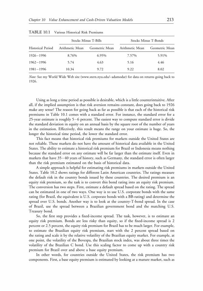
Using as long a time period as possible is desirable, which is a little counterintuitive. Afterall, if the implied assumption is that risk aversion remains constant, does going back to 1926make any sense? The reason for going back as far as possible is that each of the historical riskpremiums in Table 10.1 comes with a standard error. For instance, the standard error for a25-year estimate is roughly 5�6 percent. The easiest way to compute standard error is dividethe standard deviation in equity on an annual basis by the square root of the number of yearsin the estimation. Effectively, this result means the range on your estimate is huge. So, thelonger the historical time period, the lower the standard error.
This fact means that historical risk premiums for markets outside the United States arenot reliable. These markets do not have the amount of historical data available in the UnitedStates. The ability to estimate a historical risk premium for Brazil or Indonesia means nothingbecause the standard error on any estimate will be far larger than the estimate itself. Even inmarkets that have 35�40 years of history, such as Germany, the standard error is often largerthan the risk premium estimated on the basis of historical data.
A simple approach is helpful for estimating risk premiums in markets outside the UnitedStates. Table 10.2 shows ratings for different Latin American countries. The ratings measurethe default risk in the country bonds issued by these countries. The desired premium is anequity risk premium, so the task is to convert this bond rating into an equity risk premium.The conversion has two steps. First, estimate a default spread based on the rating. The spreadcan be estimated in one of two ways. One way is to use U.S. corporate bonds with the samerating (for Brazil, the equivalent is U.S. corporate bonds with a BB-rating) and determine thespread over U.S. bonds. Another way is to look at the country-T-bond spread. In the caseof Brazil, use the spread between a Brazilian government bond and the matching U.S.Treasury bond.
So, the first step provides a fixed-income spread. The task, however, is to estimate anequity risk premium. Bonds are less risky than equity, so if the fixed-income spread is 2percent or 2.5 percent, the equity risk premium for Brazil has to be much larger. For example,to estimate the Brazilian equity risk premium, start with the 2 percent spread based onthe rating and scale it by the relative volatility of the Brazilian equity market. For example, atone point, the volatility of the Bovespa, the Brazilian stock index, was about three times thevolatility of the Brazilian C bond. Use this scaling factor to come up with a country riskpremium for Brazil over and above a base equity premium.
In other words, for countries outside the United States, the risk premium has twocomponents. First, a base equity premium is estimated by looking at a mature market, such as
TABLE 10.1 Various Historical Risk Premiums
Stocks Minus T-Bills Stocks Minus T-Bonds
Historical Period Arithmetic Mean Geometric Mean Arithmetic Mean Geometric Mean
1926�1996 8.76% 6.95% 7.57% 5.91%
1962�1996 5.74 4.63 5.16 4.46
1981�1996 10.34 9.72 9.22 8.02
Note: See my World Wide Web site (www.stern.nyu.edu/~adamodar) for data on returns going back to1926.
c10 12 September 2012; 13:36:58
Chapter 10 Value Enhancement and Cash-Driven Valuation Models 213
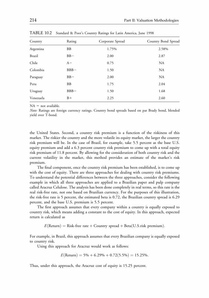
the United States. Second, a country risk premium is a function of the riskiness of thismarket. The riskier the country and the more volatile its equity market, the larger the countryrisk premium will be. In the case of Brazil, for example, take 5.5 percent as the base U.S.equity premium and add a 6.3 percent country risk premium to come up with a total equityrisk premium of 11.8 percent. By allowing for the consideration of both country risk and thecurrent volatility in the market, this method provides an estimate of the market’s riskpremium.
The final component, once the country risk premium has been established, is to come upwith the cost of equity. There are three approaches for dealing with country risk premiums.To understand the potential differences between the three approaches, consider the followingexample in which all three approaches are applied to a Brazilian paper and pulp companycalled Aracruz Celulose. The analysis has been done completely in real terms, so this rate is thereal risk-free rate, not one based on Brazilian currency. For the purposes of this illustration,the risk-free rate is 5 percent, the estimated beta is 0.72, the Brazilian country spread is 6.29percent, and the base U.S. premium is 5.5 percent.
The first approach assumes that every company within a country is equally exposed tocountry risk, which means adding a constant to the cost of equity. In this approach, expectedreturn is calculated as
EðReturnÞ ¼ Risk-free rateþ Country spreadþ BetaðU:S:risk premiumÞ:
For example, in Brazil, this approach assumes that every Brazilian company is equally exposedto country risk.
Using this approach for Aracruz would work as follows:
EðReturnÞ ¼ 5%þ 6:29%þ 0:72ð5:5%Þ ¼ 15:25%:
Thus, under this approach, the Aracruz cost of equity is 15.25 percent.
TABLE 10.2 Standard & Poor’s Country Ratings for Latin America, June 1998
Country Rating Corporate Spread Country Bond Spread
Argentina BB 1.75% 2.58%
Brazil BB2 2.00 2.87
Chile A2 0.75 NA
Colombia BBB2 1.50 NA
Paraguay BB2 2.00 NA
Peru BB 1.75 2.04
Uruguay BBB2 1.50 1.68
Venezuela B1 2.25 2.60
NA 5 not available.Note: Ratings are foreign currency ratings. Country bond spreads based on par Brady bond, blendedyield over T-bond.
c10 12 September 2012; 13:36:59
214 Part II: Valuation Methodologies
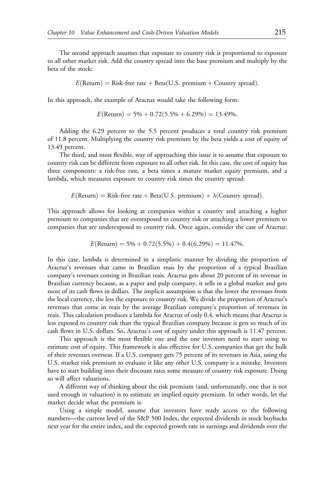
The second approach assumes that exposure to country risk is proportional to exposureto all other market risk. Add the country spread into the base premium and multiply by thebeta of the stock:
EðReturnÞ ¼ Risk-free rateþ BetaðU:S: premium þ Country spreadÞ:
In this approach, the example of Aracruz would take the following form:
EðReturnÞ ¼ 5%þ 0:72ð5:5%þ 6:29%Þ ¼ 13:49%:
Adding the 6.29 percent to the 5.5 percent produces a total country risk premiumof 11.8 percent. Multiplying the country risk premium by the beta yields a cost of equity of13.49 percent.
The third, and most flexible, way of approaching this issue is to assume that exposure tocountry risk can be different from exposure to all other risk. In this case, the cost of equity hasthree components: a risk-free rate, a beta times a mature market equity premium, and alambda, which measures exposure to country risk times the country spread:
EðReturnÞ ¼ Risk-free rateþ BetaðU:S: premiumÞ þ λðCountry spreadÞ:
This approach allows for looking at companies within a country and attaching a higherpremium to companies that are overexposed to country risk or attaching a lower premium tocompanies that are underexposed to country risk. Once again, consider the case of Aracruz:
EðReturnÞ ¼ 5%þ 0:72ð5:5%Þ þ 0:4ð6:29%Þ ¼ 11:47%:
In this case, lambda is determined in a simplistic manner by dividing the proportion ofAracruz’s revenues that came in Brazilian reais by the proportion of a typical Braziliancompany’s revenues coming in Brazilian reais. Aracruz gets about 20 percent of its revenue inBrazilian currency because, as a paper and pulp company, it sells in a global market and getsmost of its cash flows in dollars. The implicit assumption is that the lower the revenues fromthe local currency, the less the exposure to country risk. We divide the proportion of Aracruz’srevenues that come in reais by the average Brazilian company’s proportion of revenues inreais. This calculation produces a lambda for Aracruz of only 0.4, which means that Aracruz isless exposed to country risk than the typical Brazilian company because it gets so much of itscash flows in U.S. dollars. So, Aracruz’s cost of equity under this approach is 11.47 percent.
This approach is the most flexible one and the one investors need to start using toestimate cost of equity. This framework is also effective for U.S. companies that get the bulkof their revenues overseas. If a U.S. company gets 75 percent of its revenues in Asia, using theU.S. market risk premium to evaluate it like any other U.S. company is a mistake. Investorshave to start building into their discount rates some measure of country risk exposure. Doingso will affect valuations.
A different way of thinking about the risk premium (and, unfortunately, one that is notused enough in valuation) is to estimate an implied equity premium. In other words, let themarket decide what the premium is.
Using a simple model, assume that investors have ready access to the followingnumbers—the current level of the S&P 500 Index, the expected dividends in stock buybacksnext year for the entire index, and the expected growth rate in earnings and dividends over the
c10 12 September 2012; 13:36:59
Chapter 10 Value Enhancement and Cash-Driven Valuation Models 215
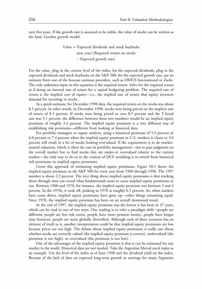
next five years. If the growth rate is assumed to be stable, the value of stocks can be written asthe basic Gordon growth model:
Value ¼ Expected dividends and stock buybacks
next year=ðRequired return on stocks
� Expected growth rateÞ
For the value, plug in the current level of the index; for the expected dividends, plug in theexpected dividends and stock buybacks on the S&P 500; for the expected growth rate, use anestimate from one of the forecast estimate providers, such as I/B/E/S International or Zacks.The only unknown input in this equation is the required return. Solve for the required returnas if doing an internal rate of return for a capital budgeting problem. The required rate ofreturn is the implied cost of equity—i.e., the implied rate of return that equity investorsdemand for investing in stocks.
As a quick estimate, for December 1998 data, the required return on the stocks was about8.5 percent. In other words, in December 1998, stocks were being priced on the implicit rateof return of 8.5 percent. If stocks were being priced to earn 8.5 percent and the T-bondrate was 5.1 percent, the difference between these two numbers would be an implied equitypremium of roughly 3.4 percent. The implied equity premium is a very different way ofestablishing risk premiums—different from looking at historical data.
For portfolio managers or equity analysts, using a historical premium of 5.5 percent or6.0 percent or 7.4 percent when the implied equity premium in U.S. markets is closer to 3.0percent will result in a lot of stocks looking overvalued. If the requirement is to do market-neutral valuation, which is often the case in portfolio management—not to pass judgment onthe overall market but to find stocks that are under-or overvalued relative to the currentmarket—the only way to do so in the context of DCF modeling is to switch from historicalrisk premiums to implied equity premiums.
Given this approach of estimating implied equity premiums, Figure 10.1 shows theimplied equity premium in the S&P 500 for every year from 1960 through 1996. The 1997number is about 2.3 percent. The nice thing about implied equity premiums is that trackingthem through time can reveal what fundamentals seem to cause implied equity premiums torise. Between 1960 and 1970, for instance, the implied equity premium was between 3 and 4percent. In the 1970s, it took off, peaking in 1978 at roughly 6.5 percent. So, when marketshave come down, implied equity premiums have gone up—other things remaining equal.Since 1978, the implied equity premium has been on an overall downward trend.
At the end of 1997, the implied equity premium was the lowest it has been in 37 years,which can be read in one of two ways. One reading is to infer a paradigm shift—people aredifferent, people are less risk averse, people have more pension money, people have longertime horizons, people are more globally diversified. Although each of these scenarios has anelement of truth to it, another interpretation could be that implied equity premiums are lowbecause prices are too high. The debate about implied equity premiums is really one aboutwhether stocks are correctly valued (the implied equity premium is correct), undervalued (thepremium is too high), or overvalued (the premium is too low).
One of the advantages of the implied equity premium is that it can be estimated for anymarket in the world. Historical data are not needed. Take the Argentine Merval stock index asan example. Use the level of the index as of June 1998 and the dividend yield on the index.Because of the lack of data on expected long-term growth in earnings for many Argentine
c10 12 September 2012; 13:36:59
216 Part II: Valuation Methodologies
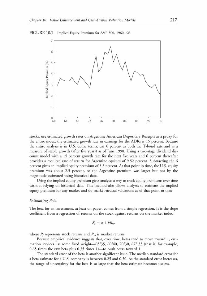
stocks, use estimated growth rates on Argentine American Depositary Receipts as a proxy forthe entire index; the estimated growth rate in earnings for the ADRs is 15 percent. Becausethe entire analysis is in U.S. dollar terms, use 6 percent as both the T-bond rate and as ameasure of stable growth (after five years) as of June 1998. Using a two-stage dividend dis-count model with a 15 percent growth rate for the next five years and 6 percent thereafterprovides a required rate of return for Argentine equities of 9.52 percent. Subtracting the 6percent gives an implied equity premium of 3.5 percent. At that point in time, the U.S. equitypremium was about 2.3 percent, so the Argentine premium was larger but not by themagnitude estimated using historical data.
Using the implied equity premium gives analysts a way to track equity premiums over timewithout relying on historical data. This method also allows analysts to estimate the impliedequity premium for any market and do market-neutral valuations as of that point in time.
Estimating Beta
The beta for an investment, at least on paper, comes from a simple regression. It is the slopecoefficient from a regression of returns on the stock against returns on the market index:
Rj ¼ a þ bRm,
where Rj represents stock returns and Rm is market returns.Because empirical evidence suggests that, over time, betas tend to move toward 1, esti-
mation services use some fixed weight—65/35, 60/40, 70/30, 67/ 33 (that is, for example,0.65 times the raw beta plus 0.35 times 1)—to push betas toward 1.
The standard error of the beta is another significant issue. The median standard error fora beta estimate for a U.S. company is between 0.25 and 0.30. As the standard error increases,the range of uncertainty for the beta is so large that the beta estimate becomes useless.
FIGURE 10.1 Implied Equity Premium for S&P 500, 1960�96
Impl
ied
Equi
ty P
rem
ium
(%)
60 96
7
6
5
4
3
2
1
064 68 72 76 80 84 88 92
c10 12 September 2012; 13:36:59
Chapter 10 Value Enhancement and Cash-Driven Valuation Models 217
Another phenomenon involving beta is common in most emerging markets, in which thetop three or four companies may compose 60�70 percent of the index. For example, theBrazilian company Telebras (Telecomunicacoes Brasileiras) appears to have a very preciseestimate of beta when regressed against the Bovespa stock index, with an R2 of 70 percent and astandard deviation of 0.07. Telebras, however, accounts for 50 percent of the Bovespa, which isa trade-weighted index. Because Telebras is half of the trading volume in real terms at any pointin time, the beta for Telebras would be little more than a regression of Telebras against itself.
Even for developed markets, this problem exists, although to a smaller degree. Forexample, in Germany, Allianz and DaimlerChrysler are each roughly 10 percent of the DAX,which is the local index used to estimate betas for German companies.
A key point is that beta measures the risk relative to a diversified portfolio. In order forTelebras to have a beta of 1.11 (which is the beta estimated against the Bovespa), thediversified portfolio to which the stock is added must consist of only Brazilian stocks held inproportion to their trading value. Because most services estimate betas for emerging marketcompanies using the local index, these betas mean absolutely nothing if the stocks are forinclusion in a portfolio that includes nonlocal stocks. To be meaningful, the beta of everycompany ought to be estimated not against a local index but against a global index.
An even more troubling problem with beta is that the betas for emerging markets arecompletely counterintuitive. The largest and the safest companies look riskiest; the smallestand riskiest companies look safest. This phenomenon is caused by index domination. Theweighted-average beta, for all stocks, is 1. Because Telebras has a beta greater than 1, all 177other stocks in the index could conceivably have betas of less than 1 and still produce aweighted average of 1. The possibility is more than theoretical. Recently, only nine stocks inthe Brazilian index had betas above 1, whereas 169 had betas below 1.
Three solutions to the regression beta problem exist. First, investors can modify theregression beta. One modification is to choose a different index. For example, one couldestimate Telebras’s beta by using its ADR and working with the S&P 500. A lot of U.S.investors use this approach, but it works only if a company has an ADR.
A second solution to the regression beta problem is to estimate the beta for a companywithout using the regression. A measure called the “relative standard deviation” is a usefulproxy for relative risk and does not require running a regression of stock prices against theindex. Instead of a regression, this method uses the standard deviation of stock prices.Dividing each company’s individual standard deviation by the market average produces anumber for relative volatility that looks very much like a beta. It will be scaled around 1;a number above 1 is above-average risk and below 1 is below-average risk. Not only does thisrelative volatility look like beta but it can be used exactly like beta. Wherever beta is used inthe CAPM, plug in the relative volatility. The implicit assumption is that total risk andmarket risk are perfectly correlated, but given how much trouble arises in estimating marketrisk, relative volatility is a useful approximation for the risk of a company.
A third solution is to estimate the beta from the bottom up. Bottom-up beta arguablyprovides a far better estimate of a company’s beta than top-down beta, which is whatregression beta is. Knowing what a company’s business is permits the estimation of its betawithout ever running a company-specific regression. Begin by getting the unlevered betas forthe company’s core businesses by looking up the unlevered betas for other companies in thosebusinesses, taking out the financial leverage because the company might have no debt ormight have a lot of debt. Take a weighted average of these unlevered betas (weighted by theproportion of operating income that comes from each type of business). Next, lever up usingthe company’s debt-to-equity ratio.
c10 12 September 2012; 13:36:59
218 Part II: Valuation Methodologies
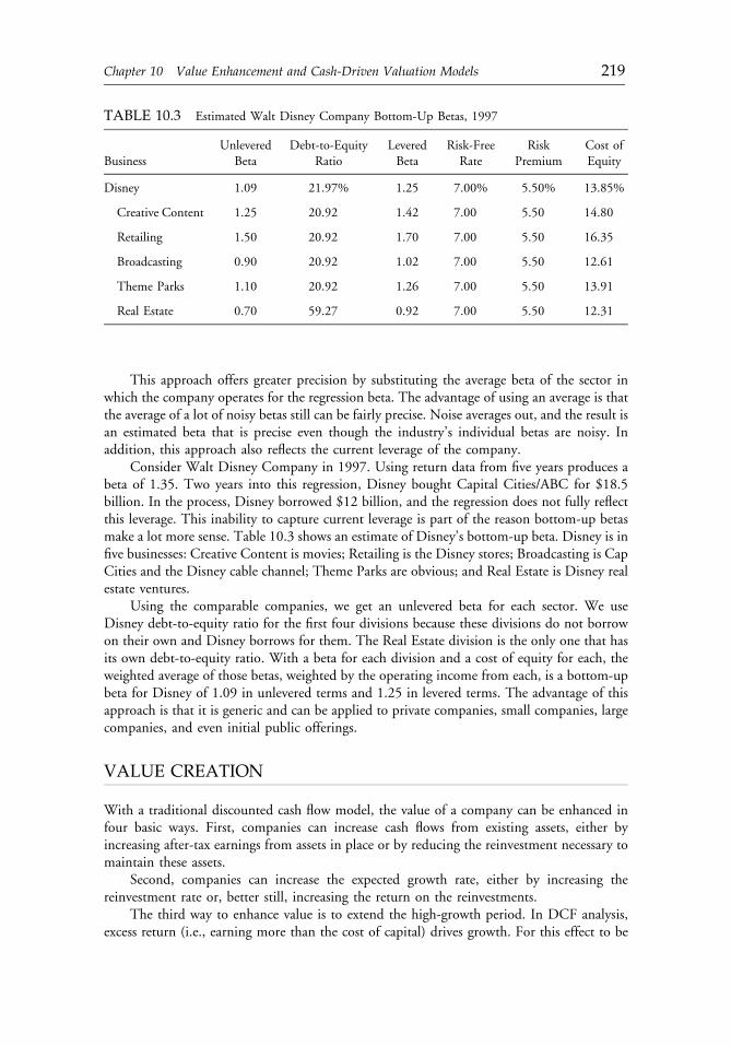
This approach offers greater precision by substituting the average beta of the sector inwhich the company operates for the regression beta. The advantage of using an average is thatthe average of a lot of noisy betas still can be fairly precise. Noise averages out, and the result isan estimated beta that is precise even though the industry’s individual betas are noisy. Inaddition, this approach also reflects the current leverage of the company.
Consider Walt Disney Company in 1997. Using return data from five years produces abeta of 1.35. Two years into this regression, Disney bought Capital Cities/ABC for $18.5billion. In the process, Disney borrowed $12 billion, and the regression does not fully reflectthis leverage. This inability to capture current leverage is part of the reason bottom-up betasmake a lot more sense. Table 10.3 shows an estimate of Disney’s bottom-up beta. Disney is infive businesses: Creative Content is movies; Retailing is the Disney stores; Broadcasting is CapCities and the Disney cable channel; Theme Parks are obvious; and Real Estate is Disney realestate ventures.
Using the comparable companies, we get an unlevered beta for each sector. We useDisney debt-to-equity ratio for the first four divisions because these divisions do not borrowon their own and Disney borrows for them. The Real Estate division is the only one that hasits own debt-to-equity ratio. With a beta for each division and a cost of equity for each, theweighted average of those betas, weighted by the operating income from each, is a bottom-upbeta for Disney of 1.09 in unlevered terms and 1.25 in levered terms. The advantage of thisapproach is that it is generic and can be applied to private companies, small companies, largecompanies, and even initial public offerings.
VALUE CREATION
With a traditional discounted cash flow model, the value of a company can be enhanced infour basic ways. First, companies can increase cash flows from existing assets, either byincreasing after-tax earnings from assets in place or by reducing the reinvestment necessary tomaintain these assets.
Second, companies can increase the expected growth rate, either by increasing thereinvestment rate or, better still, increasing the return on the reinvestments.
The third way to enhance value is to extend the high-growth period. In DCF analysis,excess return (i.e., earning more than the cost of capital) drives growth. For this effect to be
TABLE 10.3 Estimated Walt Disney Company Bottom-Up Betas, 1997
BusinessUnlevered
BetaDebt-to-Equity
RatioLeveredBeta
Risk-FreeRate
RiskPremium
Cost ofEquity
Disney 1.09 21.97% 1.25 7.00% 5.50% 13.85%
Creative Content 1.25 20.92 1.42 7.00 5.50 14.80
Retailing 1.50 20.92 1.70 7.00 5.50 16.35
Broadcasting 0.90 20.92 1.02 7.00 5.50 12.61
Theme Parks 1.10 20.92 1.26 7.00 5.50 13.91
Real Estate 0.70 59.27 0.92 7.00 5.50 12.31
c10 12 September 2012; 13:36:59
Chapter 10 Value Enhancement and Cash-Driven Valuation Models 219
true, the company must have some barrier to entry, because in a competitive marketplace,excess return acts as a magnet. So, lengthening the high-growth period requires figuring out away to increase the barriers to entry.
Fourth, reducing the cost of capital will enhance value. Companies can diminish cost ofcapital by reducing the operating risk in investments and assets, changing the financial mix, orchanging the financing composition.
Ultimately, these four actions are the only ways to create value. The converse of thisproposition is that, by definition, an action that does not affect cash flows, the growth rate,the length of the growth period, or the cost of capital cannot affect value.
Value-Neutral Actions
Arguably, 80 percent of what companies do is value neutral. Such activity may generatepublicity, but it has no effect on value. For example, a number of accounting decisions affectreported earnings but not cash flows, including
� changing inventory methods from FIFO to LIFO or vice versa in financial reports but notfor tax purposes,
� changing the depreciation method used in financial reports (but not the tax books) fromaccelerated to straight-line depreciation, and
� taking major noncash restructuring charges that reduce reported earnings but are not taxdeductible.
These actions are value neutral because they do not affect cash flows, the growth rate, thelength of the growth period, or the cost of capital.
A good example of value-neutral activity is what happens in acquisitions. Many acqui-sitions are rejected because the acquiring company cannot use a pooling accounting treatmentto do the acquisition. The distinction between purchase accounting and pooling accounting isthat in pooling, the book values are added up—with no amortization of goodwill and thus noeffect on earnings. In purchase accounting, the difference between the price paid and the bookvalue shows up as goodwill, which then is amortized over time.
Amortization of goodwill does not affect cash flows because it is not a tax-deductibleexpense and thus does not affect taxes. It also does not affect the expected growth rate becausemarginal investments stay the same whether purchase or pooling is used. Amortization ofgoodwill does not affect the length of the high-growth period because it cannot increase thebarriers to entry for competition. Finally, it does affect cost of capital. Although the decisionto use purchase or pooling is value neutral, companies spend great amounts of time, energy,and resources trying to get a pooling treatment rather than a purchase treatment for theiracquisitions.
Value-Enhancing Actions
Companies can create value in only a limited number of ways. Understanding the true pathsto value creation is vital to investors’ ability to cut through financial noise and focus on thecritical areas of performance.
Table 10.4 shows the value enhancement chain. On one dimension are the four cate-gories that value enhancement affects—cash flows from assets in place, the expected growthrate, the length of the high-growth period, and the cost of financing. The other dimensionconsists of possible ways to create value within the four categories. The first column represents
c10 12 September 2012; 13:36:59
220 Part II: Valuation Methodologies
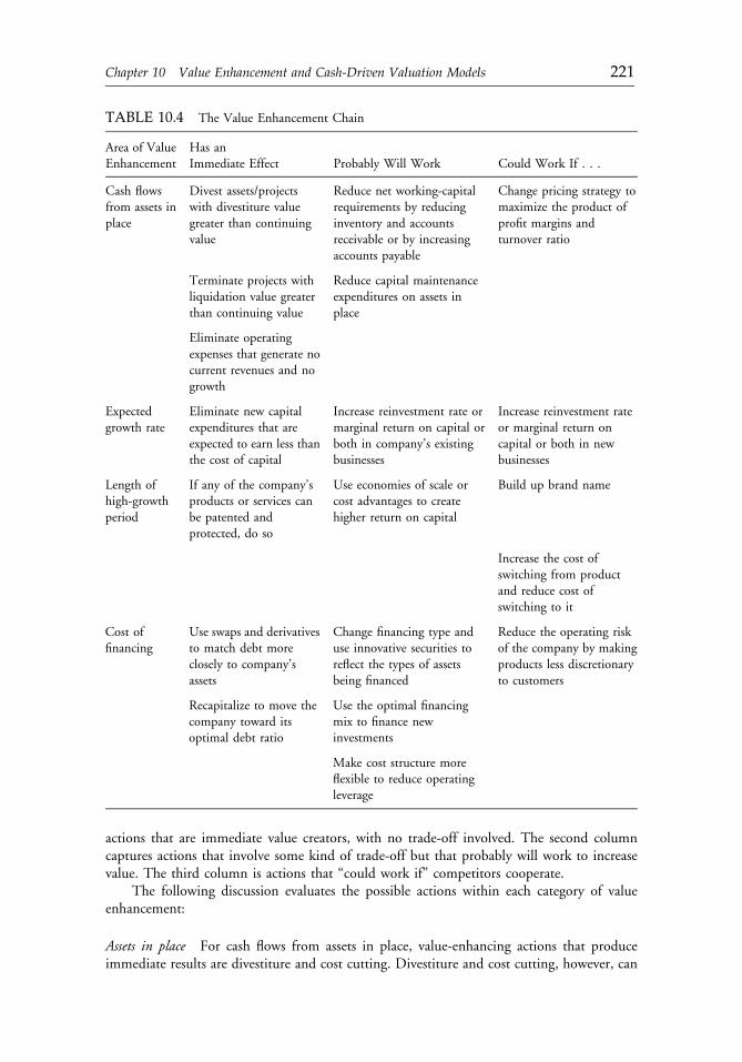
actions that are immediate value creators, with no trade-off involved. The second columncaptures actions that involve some kind of trade-off but that probably will work to increasevalue. The third column is actions that “could work if” competitors cooperate.
The following discussion evaluates the possible actions within each category of valueenhancement:
Assets in place For cash flows from assets in place, value-enhancing actions that produceimmediate results are divestiture and cost cutting. Divestiture and cost cutting, however, can
TABLE 10.4 The Value Enhancement Chain
Area of ValueEnhancement
Has anImmediate Effect Probably Will Work Could Work If . . .
Cash flowsfrom assets inplace
Divest assets/projectswith divestiture valuegreater than continuingvalue
Reduce net working-capitalrequirements by reducinginventory and accountsreceivable or by increasingaccounts payable
Change pricing strategy tomaximize the product ofprofit margins andturnover ratio
Terminate projects withliquidation value greaterthan continuing value
Reduce capital maintenanceexpenditures on assets inplace
Eliminate operatingexpenses that generate nocurrent revenues and nogrowth
Expectedgrowth rate
Eliminate new capitalexpenditures that areexpected to earn less thanthe cost of capital
Increase reinvestment rate ormarginal return on capital orboth in company’s existingbusinesses
Increase reinvestment rateor marginal return oncapital or both in newbusinesses
Length ofhigh-growthperiod
If any of the company’sproducts or services canbe patented andprotected, do so
Use economies of scale orcost advantages to createhigher return on capital
Build up brand name
Increase the cost ofswitching from productand reduce cost ofswitching to it
Cost offinancing
Use swaps and derivativesto match debt moreclosely to company’sassets
Change financing type anduse innovative securities toreflect the types of assetsbeing financed
Reduce the operating riskof the company by makingproducts less discretionaryto customers
Recapitalize to move thecompany toward itsoptimal debt ratio
Use the optimal financingmix to finance newinvestments
Make cost structure moreflexible to reduce operatingleverage
c10 12 September 2012; 13:37:0
Chapter 10 Value Enhancement and Cash-Driven Valuation Models 221
backfire. For example, a divestiture strategy’s results may be immediate, but the right targetsfor elimination or reduction are not always obvious. A common mistake is to think that avalue-enhancing strategy is simply to get rid of poor projects or divisions that are not earningtheir required rate of return. This view is mistaken because what matters is not how much isinvested in the divisions but how much they are worth if divested.
If the divestiture value of the division is greater than the value of the division continuingin the company, divestiture makes sense. The challenge is to divest or liquidate only thoseprojects for which the divestiture or liquidation value actually exceeds the continuing valueand to eliminate only those operating expenses that truly do not create revenues.
In terms of actions that probably will get results, companies can increase the cash flowsfrom assets in place by reducing the net working-capital requirements. This change does affectcash flows. Reducing inventories to 3 percent of revenues from 7 percent of revenues willmake a large impact on value.
Another action that will probably enhance value is reducing capital maintenanceexpenditures. Think of capital expenditures coming from two sources—maintaining existingassets and creating future growth. Reducing capital maintenance expenditures on assets inplace will increase the cash flows from assets in place and thus increase value.
Expected growth The immediate action for improving expected growth is to eliminate newcapital expenditures for which the return on capital is less than the cost of capital. Suchexpenditures are obviously value destroying.
An action that probably will work is increasing the reinvestment rate or the marginalreturn on capital—or preferably both—for the company’s existing businesses, therebyincreasing the growth rate.
An action with much less certainty of success is to increase the reinvestment rate and/orincrease the marginal return on capital for the company’s new businesses.
Length of high-growth period Actions for lengthening the high-growth period all boil downto increasing barriers to entry. The only immediate action in this area is to make sure that alleligible products are patented and protected. Actions that probably will work are improvingeconomies of scale and enhancing cost advantages.
The most uncertain actions involve building up brand names or increasing the cost ofswitching away from the product and reducing the cost of switching to it. Brand advantages are atremendous barrier to entry in some markets and allow companies to maintain high returns oncapital and high value. In high-tech industries, the biggest barrier to entry is the cost ofswitching. For example, in the software industry, a company might come up with a betterspreadsheet program than Microsoft Excel, but getting existing customers to switch to the newprogram would be tough because the cost of switching is so large, especially for large businesses.
Cost of financing Immediate enhancement of value through cost of financing is possible intwo ways. First, the cash flows on financing should have the same characteristics as the cashflows of the assets being financed. In other words, long-term assets should get long-termfinancing, dollar assets should have dollar financing; and so forth. Making the financingreflect the asset structure reduces the company’s risk; reducing the company’s risk reduces itscost of capital; and reducing its cost of capital increases its value.
c10 12 September 2012; 13:37:0
222 Part II: Valuation Methodologies
The second immediate action that will increase value is moving toward the optimaldebt ratio.
Three actions probably will work to enhance value through cost of financing. The firstapproach is to change the financing type and use innovative securities to reflect the types ofassets being financed, and the second approach is to use the optimal financing mix to financenew investments.
The third action that is likely to work is to make the cost structure more flexible. Overthe past 5�10 years, U.S. companies talked about flexibility but, in fact, they were simplytrying to make their cost structure a function of their revenue levels. So, if a company canmake wages much more of a function of how well the company is doing (e.g., in negotiationwith the unions), it can increase the proportion of its costs that are variable. One of thepayoffs to this approach is that the company’s beta goes down: The lower the proportion ofcosts that are fixed costs, the lower the beta will be. Having a lot of fixed costs exaggerates risk.Having a lot of variable costs reduces risk by making the cost structure more flexible—reducethe risk, reduce the cost of capital.
A long-term, “could work if . . .” way of reducing the cost of financing is to try to reducethe operating risk of the company.
Effectively, the approaches described in this section summarize all the different ways ofthinking about enhancing value. Actions that enhance value must affect one of four areas: cashflows from assets in place, expected growth, length of growth period, or cost of capital.Enhancing value through any other means is impossible. The other important consideration isthe probability of a particular action succeeding. Even in a traditional valuation model,showing the effect of value-enhancing actions is straightforward.
Alternative Approaches to Enhancing Value
Alternative ways of enhancing value, which claim the advantage of simplicity, do exist. Thealternative methods seek to maximize a variable that is correlated with the company’s value.Possible targets are (and historically have been) accounting variables, such as earnings orreturn on investment; marketing variables, such as market share; and surplus value measures,such as EVA.
The danger of focusing on these variables is that the underlying assumption that thesevariables are correlated with value might be wrong. In the 1970s and 1980s, Japanesecompanies concentrated on increasing market share. They assumed that increasing theirmarket share increased their value, but many of these companies subsequently learnedthat this assumption is not necessarily true. The advantage of such alternative approachesis that they have fewer variables than DCF valuation. The disadvantage is that this simplicitycomes with a cost.
ECONOMIC VALUE ADDED
Economic value added is a measure of surplus value created by an investment. This approachdefines the return on capital as the “true” cash flow return on capital earned on an investment.It also defines the cost of capital as the weighted average of the costs of the different financing
c10 12 September 2012; 13:37:0
Chapter 10 Value Enhancement and Cash-Driven Valuation Models 223
instruments used to finance the investment. EVA has three basic inputs—invested capital,return on capital, and cost of capital:
EVA ¼ ðReturn on capital� Cost of capitalÞ3 ðCapital invested in projectÞ
“Capital invested in project” is designed to capture how much capital is invested in assetsin place, projects that are already active. How is invested capital measured? Some peoplemight think market value is a potential measure. One of the problems of market value ofcompanies is that market value includes expected future growth (in addition to assets inplace). So, market value is out of the question as a potential measure. The next choice is bookvalue. Is the accounting measure of book value really a measure of the market value of assets inplace? Not always and not generally. To get from book value to capital investments, fouradjustments are typically used: One adjustment is operating leases. For example, the balancesheet of The Gap has only equity—no debt. The problem is that The Gap leases all of itsstores and qualifies the leases as operating leases. In accounting terms, operating leases areoperating expenses and do not show up on the balance sheet. The Gap has operating leases ofhalf a billion dollars a year, the equivalent of almost $42$5 billion in debt. So, to get TheGap’s total invested capital, use the book equity plus the present value of operating leases.This approach is a more accurate measure of invested capital than simply taking the bookvalue of capital found in the balance sheet.
The second adjustment for invested capital involves research and development expenses.Computing the EVA for high-tech companies, such as Intel Corporation or Microsoft, willproduce an absurdly small book value of capital. The reason is simple: The accountingconvention, at least in the United States, is that R&D expenses must be expensed and cannotbe capitalized. As a consequence, although a company may have $22$3 billion in R&Dexpenses and may be creating very valuable assets from these expenses, the R&D expensesnever show up on the balance sheet. So, the adjustment is to capitalize R&D expenses. Simplyadd up the R&D expenses over time and treat them like any other asset.
The third adjustment is for one-time charges that reduce invested capital. Goodwillamortization is a classic example of such a one-time charge. Writing off goodwill reducesthe invested capital. In computing the capital invested in assets in place, add back all of thevariables that make invested capital look smaller than is the case.
The fourth type of adjustment, which tends to be small, involves accounting adjustments.The task is to account for the kind of game playing—switching from FIFO to LIFO orLIFO to FIFO, and so forth—that occurs at the margin to change operating earnings, whichaffects capital.
External analysts’ EVA estimates will always be inferior to the EVA estimate made bysomeone working for the company. For example, a few years ago, one publishing companycame up with a huge return on invested capital for their publishing division, something like1,787 percent. The reason for the high number was that the assets of the publishing divisionwere all copyrights and trademarks, which effectively had been amortized almost down tozero. So, when computing return on capital, the company was dividing the operating incomeby an unusually small number.
Of course, equity research analysts or portfolio managers working outside the companywould not have a listing of every copyright and trademark the company owns and thus wouldbe limited in what they could evaluate. Instead, they must work with book capital and make
c10 12 September 2012; 13:37:0
224 Part II: Valuation Methodologies
rough adjustments. The older the company, the less accuracy book capital can have as ameasure of invested capital.
The other two components of EVA, “return on capital” and “cost of capital,” also havelimitations. The return on capital that analysts would like to measure is the return on invest-ments already in place. The cost of capital should be a market value of cost of capital. Somepeople compute EVA using book value weights for debt and equity, to maintain consistencywith the use of book value in measuring capital invested. This practice is not appropriate, andthe cost of capital used in EVA calculations has to be exactly the same cost of capital as is used forDCF valuation, which is a market-value-weighted cost of capital. Using book cost of capital willsystematically overstate the EVA of every company in the United States.
EVA Caveats
When companies adopt EVA, they are judging their managers based on this year’s EVA versusan expected number. In other words, as long as managers deliver an EVA next year that is higherthan some benchmark, they will be rewarded, usually with no upper limit on compensation.
A company can deliver a higher EVA than expected—while making stockholders worseoff—in three ways. The first option is the “capital invested game.” Bringing down thecompany’s invested capital will make EVA look much better, even if the effect is purelycosmetic—especially if it is purely cosmetic. Increasing stock buybacks or taking largerestructuring charges will generally lower capital and increase EVA.
The second possibility is the “growth game.” In other words, the company tries to makenext year’s EVA look better by stealing from future growth. Thus, cutting back on R&D orexpenses designed to generate future growthmay improve EVA in the short termwhile reducingvalue in the long term. The CEOmay end up with a bonus, but the stockholders get lower value.
The third option is “the risk game.” The value of the company is the present value ofEVA. So, if the company delivers a higher EVA but at a much higher cost of capital becausethe company has become riskier, stockholders are worse off because the company has exposedthem to more risk.
Investors also face caveats for EVA. Portfolio managers who invest in the companies withthe highest EVA or the highest increase in EVA, in the hope of earning excess returns, willfail. The reason is that market prices are driven not by the magnitude of the actual EVA butby the actual EVA versus expectations. The companies with the highest EVA may not nec-essarily make a great portfolio. More desirable are the companies for which the EVAs will bemuch higher than expected—because expectation is what determines stock prices.
Richard Bernstein, with Merrill Lynch & Company, did two studies (Bernstein 1997 andBernstein 1998) on the effectiveness of using EVA for investing. First, he looked at 12-monthreturns by buying the top 10 percent of companies in terms of EVA. This portfolio returnedabout 1 percent less than the S&P 500 during the period studied. Next, he looked atcompanies that had the highest increase in EVA over the previous year. A portfolio of 50companies drawn from the 10 percent of companies with the highest increase in EVA over theprevious year would have done even worse.
Comparing EVA and DCF Valuation
In addition to value enhancement, EVA can also be used as a traditional valuation tool. Infact, analysts can write the value of a company as a sum of three components—the investmentin existing assets plus the net present value (NPV) of the existing assets in place plus the NPV
c10 12 September 2012; 13:37:0
Chapter 10 Value Enhancement and Cash-Driven Valuation Models 225
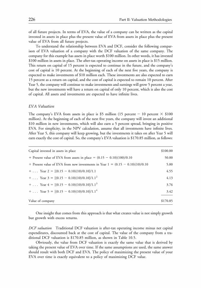
of all future projects. In terms of EVA, the value of a company can be written as the capitalinvested in assets in place plus the present value of EVA from assets in place plus the presentvalue of EVA from all future projects.
To understand the relationship between EVA and DCF, consider the following compar-ison of EVA valuation of a company with the DCF valuation of the same company. Thecompany for this example has assets in place worth $100 million. In other words, it has invested$100 million in assets in place. The after-tax operating income on assets in place is $15 million.This return on capital of 15 percent is expected to continue in the future, and the company’scost of capital is 10 percent. At the beginning of each of the next five years, the company isexpected to make investments of $10 million each. These investments are also expected to earn15 percent as a return on capital, and the cost of capital is expected to remain 10 percent. AfterYear 5, the company will continue to make investments and earnings will grow 5 percent a year,but the new investments will have a return on capital of only 10 percent, which is also the costof capital. All assets and investments are expected to have infinite lives.
EVA Valuation
The company’s EVA from assets in place is $5 million (15 percent 2 10 percent 3 $100million). At the beginning of each of the next five years, the company will invest an additional$10 million in new investments, which will also earn a 5 percent spread, bringing in positiveEVA. For simplicity, in the NPV calculation, assume that all investments have infinite lives.After Year 5, this company will keep growing, but the investments it takes on after Year 5 willearn exactly the cost of capital. So, the company’s EVA valuation is $170.85 million, as follows:
Capital invested in assets in place $100.00
1 Present value of EVA from assets in place 5 (0.15 2 0.10)(100)/0.10 50.00
1 Present value of EVA from new investments in Year 1 5 (0.15 2 0.10)(10)/0.10 5.00
1 . . . Year 2 5 [(0.15 2 0.10)(10)/0.10]/1.1 4.55
1 . . . Year 3 5 [(0.15 2 0.10)(10)/0.10]/1.12 4.13
1 . . . Year 4 5 [(0.15 2 0.10)(10)/0.10]/1.13 3.76
1 . . . Year 5 5 [(0.15 2 0.10)(10)/0.10]/1.14 3.42
Value of company $170.85
One insight that comes from this approach is that what creates value is not simply growthbut growth with excess returns.
DCF valuation Traditional DCF valuation is after-tax operating income minus net capitalexpenditures, discounted back at the cost of capital. The value of the company from a tra-ditional DCF valuation is $170.85 million, as shown in Table 10.5.
Obviously, the value from DCF valuation is exactly the same value that is derived bytaking the present value of EVA over time. If the same assumptions are used, the same answershould result with both DCF and EVA. The policy of maximizing the present value of yourEVA over time is exactly equivalent to a policy of maximizing DCF value.
c10 12 September 2012; 13:37:0
226 Part II: Valuation Methodologies
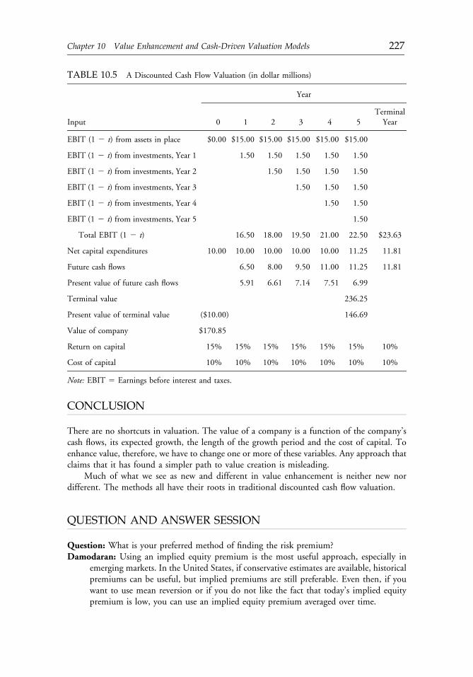
CONCLUSION
There are no shortcuts in valuation. The value of a company is a function of the company’scash flows, its expected growth, the length of the growth period and the cost of capital. Toenhance value, therefore, we have to change one or more of these variables. Any approach thatclaims that it has found a simpler path to value creation is misleading.
Much of what we see as new and different in value enhancement is neither new nordifferent. The methods all have their roots in traditional discounted cash flow valuation.
QUESTION AND ANSWER SESSION
Question: What is your preferred method of finding the risk premium?Damodaran: Using an implied equity premium is the most useful approach, especially in
emerging markets. In the United States, if conservative estimates are available, historicalpremiums can be useful, but implied premiums are still preferable. Even then, if youwant to use mean reversion or if you do not like the fact that today’s implied equitypremium is low, you can use an implied equity premium averaged over time.
TABLE 10.5 A Discounted Cash Flow Valuation (in dollar millions)
Year
Input 0 1 2 3 4 5TerminalYear
EBIT (1 2 t) from assets in place $0.00 $15.00 $15.00 $15.00 $15.00 $15.00
EBIT (1 2 t) from investments, Year 1 1.50 1.50 1.50 1.50 1.50
EBIT (1 2 t) from investments, Year 2 1.50 1.50 1.50 1.50
EBIT (1 2 t) from investments, Year 3 1.50 1.50 1.50
EBIT (1 2 t) from investments, Year 4 1.50 1.50
EBIT (1 2 t) from investments, Year 5 1.50
Total EBIT (1 2 t) 16.50 18.00 19.50 21.00 22.50 $23.63
Net capital expenditures 10.00 10.00 10.00 10.00 10.00 11.25 11.81
Future cash flows 6.50 8.00 9.50 11.00 11.25 11.81
Present value of future cash flows 5.91 6.61 7.14 7.51 6.99
Terminal value 236.25
Present value of terminal value ($10.00) 146.69
Value of company $170.85
Return on capital 15% 15% 15% 15% 15% 15% 10%
Cost of capital 10% 10% 10% 10% 10% 10% 10%
Note: EBIT 5 Earnings before interest and taxes.
c10 12 September 2012; 13:37:1
Chapter 10 Value Enhancement and Cash-Driven Valuation Models 227
Question: If a high-P/E company acquires a low-P/E company and thus has instant earnings,how do you view the cost of capital for the acquisition?
Damodaran: If a high-P/E company acquires a low-P/E company, use the same test as forvalue. The acquisition does not increase cash flows collectively for the company. It doesnot increase the growth rate on a weighted-average basis. It has no effect on the length ofthe growth period. As for cost of capital, if a composite cost of capital is used, it will be aweighted average. Companies can create value only by taking actions that affect one ofthose four components. Essentially, the net present value of the acquisition is whatdrives value.
Question: With so many companies adopting EVA, are they learning that leveraging thebalance sheet to buy back stock is a way to achieve the EVA?
Damodaran: These companies are learning that the easiest way to increase EVA is to bringdown invested capital. Companies tried initially to increase earnings, which takes toomuch work. Instead, they found a much easier way to increase EVA. Companies thathave adopted EVA have exhibited a progressive depletion in book capital, whetherthrough stock buybacks or through something else. These companies know they look alot better if they have less invested capital at play.
c10 12 September 2012; 13:37:1
228 Part II: Valuation Methodologies
CHAPTER 11FEVA: A FINANCIAL
AND ECONOMIC APPROACHTO VALUATION
Xavier Adsera and Pere Vinolas
Traditional valuation methods (economic value added, discounted cash flow, andModigliani and Miller models) are mathematically equivalent and thus shouldprovide the same result when the same inputs are used. They do not. Because thesemethods focus on different value drivers, we suggest an alternative valuation methodthat provides the adjustment necessary to produce consistent results. We also proposea new corporate valuation method (“financial and economic value added,” orFEVA) that integrates the EVA, DCF, and MM approaches and allows a detailedanalysis of financial and economic corporate value drivers.
Financial analysts face a fundamental problem: When different valuation models are applied tothe same company, they yield significantly different results. Because the three main families ofcorporate valuation models—economic value added (EVA), discounted cash flow (DCF), andModigliani and Miller (MM)—share the same underlying assumptions, the principle of onevalue states that when the same inputs are used, such models should yield exactly the same result.
In this chapter, we show that all traditional valuation methods, when properly applied, aremathematically equivalent; thus, the principle of one value should apply to the last decimal. Inaddition, we demonstrate the adjustments required to produce consistent valuation results. Ourresults raise an important question: If the traditional valuation models are mathematicallyequivalent, could their different value drivers be reconciled into one method? We offer anapproach (which we call “financial and economic value added,” or FEVA) that splits corporate
Reprinted from the Financial Analysts Journal (March/April 2003):80�87. When this article wasoriginally published, Xavier Adsera was a partner and general manager of Riva y Garcıa Financial Groupand professor of finance at ESADE, Barcelona, Spain, and Pere Vinolas was a partner and generalmanager of Riva y Garcıa Financial Group and professor of finance at ESADE, Barcelona, Spain.
c11 12 September 2012; 17:56:13
229
valuation into eight value drivers drawn from the MM and EVA approaches and identifies theexact contribution of each driver. Thus, the principle of one value is maintained in the newformula because it is mathematically consistent with previous methodologies.
PRINCIPLE OF ONE VALUE
To consider how the principle of one value applies in practical terms, we will examine fouralternative valuation formulas. Each is well known, and each is used to estimate the perpetuity(terminal value) in a detailed cash flow analysis. The formulas as presented here, however, addone important assumption: The growth rate of operating profits is held constant in eachprojection. So, in effect, we are working with multiples.
The first two formulas are typical DCF models.1 They are based on the net present value,with a discount rate based on the capital asset pricing model (CAPM):
E ¼ FCFeke � g
ð11:1Þ
and
E ¼ FCFk � g
� D; ð11:2Þ
where
E 5 market value of equity
FCFe 5 free cash flow to shareholders2
ke 5 cost of equity 5 Rf 1 βe(RM 2 Rf ), where Rf is the risk-free rate, βe is thelevered beta, and RM 2 Rf defines the market equity risk premium
FCF 5 operating free cash flow3
k 5 weighted-average cost of capital
g 5 growth rate
D 5 debt.
Note that
k ¼ keEV
þ kdDV, ð11:3Þ
where kd 5 i (1 2 t), with i the expected yield on corporate debt.In recent years, EVA-based methods have become analysts’ preferred approach to cor-
porate valuation.4 In spite of its current popularity, EVA is not a new approach because itsbasic message was established some decades ago (e.g., Modigliani and Miller 1961; Solomon1963; Walter 1956). The basic principle of EVA analysis is that the key driver of firm value isthe spread between the return on existing investments and the average cost of capital of thoseinvestments. So, this approach focuses on the left-hand side of the balance sheet. EVA divides
c11 12 September 2012; 17:56:13
230 Part II: Valuation Methodologies
corporate value into two parts. The first part is the base value of a company excluding newinvestments and growth opportunities (in the case of a new company, the base value may beequal to the capital invested). The second part is the value derived from new investments ingrowth opportunities; the key factor is the spread between the return on new investments andthe opportunity cost of capital.
The basic EVA formula is as follows:
E ¼ EATke
þ EATre � kereke
� �g
ke � g
� �, ð11:4Þ
where EAT is earnings after taxes and re is (leveraged) return on new investment; that is,
re ¼ gðEAT ÞI � Dg
,
where I is net investment (excluding depreciation).The fourth formula is an example of the MM approach (see, for example, Modigliani
and Miller 1958). In the 1950s, Modigliani and Miller argued that corporate value can bederived from the value of an unleveraged firm, the value of the tax shield from the existingdebt (derived from the fact that interest expenses are deductible from income taxes), andbankruptcy costs (derived from the fact that a high level of debt has certain costs for acompany). The model is as follows:
E ¼ EBIT ð1� tÞku
þ tD, ð11:5Þ
where
EBIT 5 earnings before interest and taxes
tD 5 tax shield from existing debt
ku 5 unleveraged cost of equity 5 Rf 1 βu(RM 2 RF), in which βu is the unleveredbeta that measures the operating risk of a company or an asset
Why should these methods fail to yield the same result? In our view, three problemstypically account for the inconsistency:
� First, the cost of equity, ke, is usually not properly leveraged, and according to the CAPM,risk depends on leverage. The uncertainty of the return depends on the operating risk andthe debt-to-equity ratio of the firm. The most commonly used equation for equity risk is
βe ¼ βu 1þ DEð1� tÞ
� �, ð11:6Þ
but a more complete picture would be to consider the case in which the risk of debt, βd, isdifferent from zero.5 Practitioners usually forget to take financial risk into consideration.
� Second, when analysts define the free cash flow generated by the company, their growthassumptions are often not consistent with the investment policy being considered.
� Third, all the formulas need the market value of equity, E, as an input, but this value is alsothe expected outcome of all the formulas.
c11 12 September 2012; 17:56:14
Chapter 11 FEVA: A Financial and Economic Approach to Valuation 231
The first two problems do not arise if the valuationmethods are properly applied. The thirdproblem is one of circularity. For example, in Equation 11.1, ke depends on E. One way to avoidthis circularity would be to find an expression that does not depend on equity market value.
SOLVING THE CIRCULARITY PROBLEM
Modigliani and Miller (1963) established that the value of a company depends on three elements:the unleveraged value of the company, the value of the tax shields resulting from the existing debt,and the negative value created by the potential bankruptcy costs. Surprisingly, with some minoradjustments, one can move a typical DCF valuation formula close to the MM approach bymaking corporate value dependent on the net present value of the unleveraged free cash flow plusthe value of tax shields minus potential bankruptcy costs. In short, from a simple DCF expression,we can derive the following formula (see Appendix 11A for the derivation of this formula):
E ¼ EBIT ð1� tÞ � Iku � g
þ tDkuku � g
�Dð1� tÞði � Rf Þku � g
� D, ð11:7Þ
where
I 5 net investments (excluding depreciation)6
i 5 expected yield on debt
Rf 5 risk-free rate
This approach has two advantages. First, it provides new insight into the MM approachto corporate valuation by splitting corporate value into three parts. The first part is clearly theunleveraged firm value:
EBIT ð1� tÞ � Iku � g
:
The second part is close to a formula for tax shields because the present value of the taxshield is calculated as
PVtax shields ¼ tDkuku � g
: ð11:8Þ
This part of Equation 11.7 shows that, in addition to the tax advantage of theexisting debt, tD, a tax shield is created because growth opportunities generate greater debtcapacity.7 It also shows that tax shields should not be considered risk free and should beassumed to include an unleveraged risk premium.
The third part of Equation 11.7 is a good approximation of bankruptcy costs, bc. It isbased on the spread between the expected yield (not the promised yield) on debt, i, and therisk-free rate, Rf :
8,9
PVbc ¼Dð1� tÞði � Rf Þ
ku � g: ð11:9Þ
c11 12 September 2012; 17:56:14
232 Part II: Valuation Methodologies
Thus, from a simple DCF valuation formula, we can derive the complete MM approach.The second advantage of the adjusted approach stems from its mathematical grounding.
Equity value does not depend on any leveraged input (such as the cost of equity or the cost ofcapital) that would generate the circularity problem. Also, because this approach is mathemat-ically equivalent to DCF methods, it satisfies the principle of one value when comparing manydifferent corporate valuation formulas. This approach also makes possible mathematical equiv-alence between the MM approach and an EVA approach, such as the franchise factor model.
Consider a practical demonstration of Equations 11.1, 11.2, 11.4, and 11.7. Table 11.1provides the data for an imaginary company. At first, the basic MM approach (Equation 11.5)appears to be too simple to be consistent with the rest of the corporate valuation methodsto value this hypothetical company. From the data in Table 11.1, we can use the CAPM toderive ku 5 9.5 percent [5 percent 1 0.9 3 (10 percent 2 5 percent)]. Thus, we may applyEquation 11.7 as follows:
E ¼ EBIT ð1� tÞ � Iku � g
þ tDkuku � g
� Dð1� tÞði � Rf Þku � g
� D
¼ 4003 ð1� 0:4Þ � 100
9:5%� 5%þ 0:43 1,0003 9:5%
9:5%� 5%
� 1,0003 ð1� 0:4Þ3 ð10%� 5%Þ9:5%� 5%
� 1,000
¼ 2,288:89:
TABLE 11.1 Company Data for an Example Valuation
Variable Value (currency omitted)
EBITDA 600
Depreciation 2200
EBIT 400
Interest 2100
EBT 300
Taxes 2120
EAT 180
Capital initially invested, CI 3,000
I (gross investment) 300
t 5 40% Rf 5 5%
Interest rate i 5 10% RM 5 10%
βu 5 0.9 g 5 5%
D 5 1.000
c11 12 September 2012; 17:56:14
Chapter 11 FEVA: A Financial and Economic Approach to Valuation 233
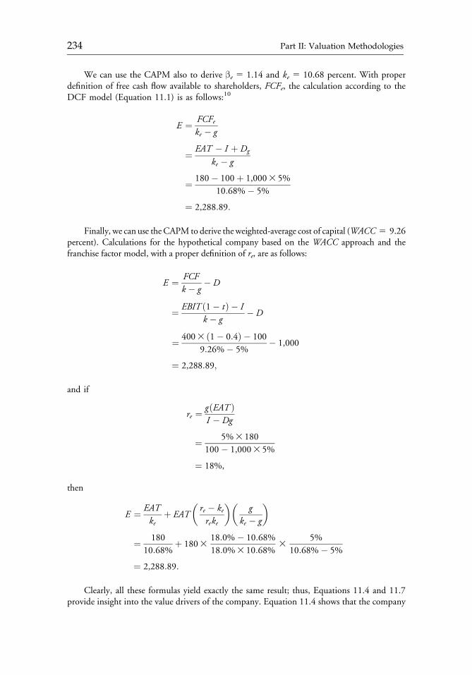
We can use the CAPM also to derive βe 5 1.14 and ke 5 10.68 percent. With properdefinition of free cash flow available to shareholders, FCFe, the calculation according to theDCF model (Equation 11.1) is as follows:10
E ¼ FCFeke � g
¼ EAT � I þ Dg
ke � g
¼ 180� 100þ 1,0003 5%
10:68%� 5%
¼ 2,288:89:
Finally, we can use theCAPM to derive theweighted-average cost of capital (WACC 5 9.26percent). Calculations for the hypothetical company based on the WACC approach and thefranchise factor model, with a proper definition of re, are as follows:
E ¼ FCFk � g
� D
¼ EBIT ð1� tÞ � Ik � g
� D
¼ 4003 ð1� 0:4Þ � 100
9:26%� 5%� 1,000
¼ 2,288:89;
and if
re ¼ gðEAT ÞI � Dg
¼ 5%3 180
100� 1,0003 5%
¼ 18%,
then
E ¼ EATke
þ EAT�re � kereke
��g
ke � g
�
¼ 180
10:68%þ 1803
18:0%� 10:68%
18:0%3 10:68%3
5%
10:68%� 5%
¼ 2,288:89:
Clearly, all these formulas yield exactly the same result; thus, Equations 11.4 and 11.7provide insight into the value drivers of the company. Equation 11.4 shows that the company
c11 12 September 2012; 17:56:14
234 Part II: Valuation Methodologies
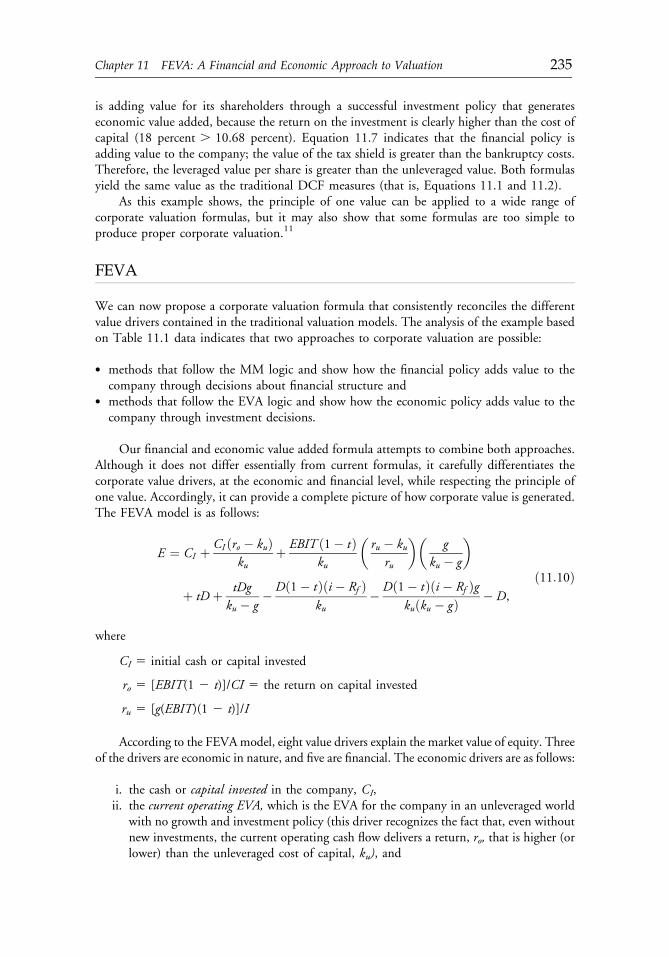
is adding value for its shareholders through a successful investment policy that generateseconomic value added, because the return on the investment is clearly higher than the cost ofcapital (18 percent . 10.68 percent). Equation 11.7 indicates that the financial policy isadding value to the company; the value of the tax shield is greater than the bankruptcy costs.Therefore, the leveraged value per share is greater than the unleveraged value. Both formulasyield the same value as the traditional DCF measures (that is, Equations 11.1 and 11.2).
As this example shows, the principle of one value can be applied to a wide range ofcorporate valuation formulas, but it may also show that some formulas are too simple toproduce proper corporate valuation.11
FEVA
We can now propose a corporate valuation formula that consistently reconciles the differentvalue drivers contained in the traditional valuation models. The analysis of the example basedon Table 11.1 data indicates that two approaches to corporate valuation are possible:
� methods that follow the MM logic and show how the financial policy adds value to thecompany through decisions about financial structure and
� methods that follow the EVA logic and show how the economic policy adds value to thecompany through investment decisions.
Our financial and economic value added formula attempts to combine both approaches.Although it does not differ essentially from current formulas, it carefully differentiates thecorporate value drivers, at the economic and financial level, while respecting the principle ofone value. Accordingly, it can provide a complete picture of how corporate value is generated.The FEVA model is as follows:
E ¼ CI þ CI ðro � kuÞku
þ EBIT ð1� tÞku
�ru � ku
ru
��g
ku � g
�
þ tD þ tDgku � g
� Dð1� tÞði � Rf Þku
� Dð1� tÞði � Rf Þgkuðku � gÞ � D,
ð11:10Þ
where
CI 5 initial cash or capital invested
ro 5 [EBIT(1 2 t)]/CI 5 the return on capital invested
ru 5 [g(EBIT)(1 2 t)]/I
According to the FEVAmodel, eight value drivers explain the market value of equity. Threeof the drivers are economic in nature, and five are financial. The economic drivers are as follows:
i. the cash or capital invested in the company, CI,ii. the current operating EVA, which is the EVA for the company in an unleveraged world
with no growth and investment policy (this driver recognizes the fact that, even withoutnew investments, the current operating cash flow delivers a return, ro, that is higher (orlower) than the unleveraged cost of capital, ku), and
c11 12 September 2012; 17:56:15
Chapter 11 FEVA: A Financial and Economic Approach to Valuation 235
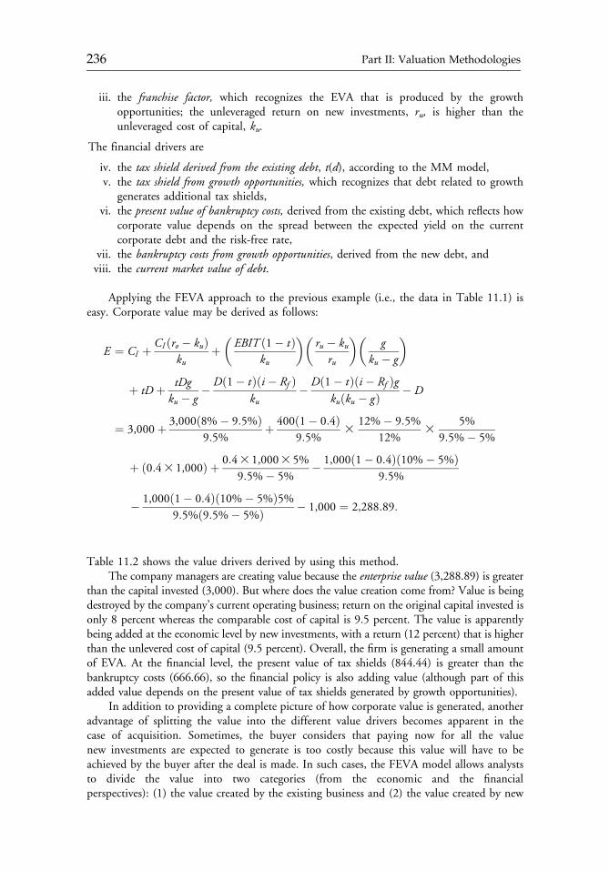
iii. the franchise factor, which recognizes the EVA that is produced by the growthopportunities; the unleveraged return on new investments, ru, is higher than theunleveraged cost of capital, ku.
The financial drivers are
iv. the tax shield derived from the existing debt, t(d), according to the MM model,v. the tax shield from growth opportunities, which recognizes that debt related to growth
generates additional tax shields,vi. the present value of bankruptcy costs, derived from the existing debt, which reflects how
corporate value depends on the spread between the expected yield on the currentcorporate debt and the risk-free rate,
vii. the bankruptcy costs from growth opportunities, derived from the new debt, andviii. the current market value of debt.
Applying the FEVA approach to the previous example (i.e., the data in Table 11.1) iseasy. Corporate value may be derived as follows:
E ¼ CI þ CI ðro � kuÞku
þ�EBIT ð1� tÞ
ku
��ru � ku
ru
��g
ku � g
�
þ tD þ tDgku � g
� Dð1� tÞði � Rf Þku
� Dð1� tÞði � Rf Þgkuðku � gÞ � D
¼ 3,000þ 3,000ð8%� 9:5%Þ9:5%
þ 400ð1� 0:4Þ9:5%
312%� 9:5%
12%3
5%
9:5%� 5%
þ ð0:43 1,000Þ þ 0:43 1,0003 5%
9:5%� 5%� 1,000ð1� 0:4Þð10%� 5%Þ
9:5%
� 1,000ð1� 0:4Þð10%� 5%Þ5%9:5%ð9:5%� 5%Þ � 1,000 ¼ 2,288:89:
Table 11.2 shows the value drivers derived by using this method.The company managers are creating value because the enterprise value (3,288.89) is greater
than the capital invested (3,000). But where does the value creation come from? Value is beingdestroyed by the company’s current operating business; return on the original capital invested isonly 8 percent whereas the comparable cost of capital is 9.5 percent. The value is apparentlybeing added at the economic level by new investments, with a return (12 percent) that is higherthan the unlevered cost of capital (9.5 percent). Overall, the firm is generating a small amountof EVA. At the financial level, the present value of tax shields (844.44) is greater than thebankruptcy costs (666.66), so the financial policy is also adding value (although part of thisadded value depends on the present value of tax shields generated by growth opportunities).
In addition to providing a complete picture of how corporate value is generated, anotheradvantage of splitting the value into the different value drivers becomes apparent in thecase of acquisition. Sometimes, the buyer considers that paying now for all the valuenew investments are expected to generate is too costly because this value will have to beachieved by the buyer after the deal is made. In such cases, the FEVA model allows analyststo divide the value into two categories (from the economic and the financialperspectives): (1) the value created by the existing business and (2) the value created by new
c11 12 September 2012; 17:56:15
236 Part II: Valuation Methodologies
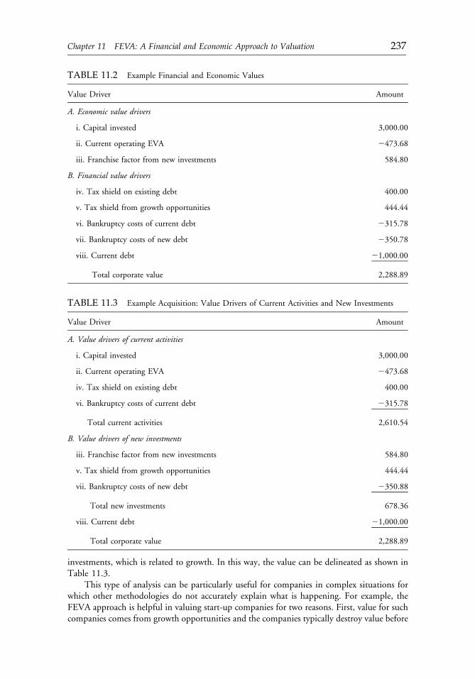
investments, which is related to growth. In this way, the value can be delineated as shown inTable 11.3.
This type of analysis can be particularly useful for companies in complex situations forwhich other methodologies do not accurately explain what is happening. For example, theFEVA approach is helpful in valuing start-up companies for two reasons. First, value for suchcompanies comes from growth opportunities and the companies typically destroy value before
TABLE 11.3 Example Acquisition: Value Drivers of Current Activities and New Investments
Value Driver Amount
A. Value drivers of current activities
i. Capital invested 3,000.00
ii. Current operating EVA 2473.68
iv. Tax shield on existing debt 400.00
vi. Bankruptcy costs of current debt 2315.78
Total current activities 2,610.54
B. Value drivers of new investments
iii. Franchise factor from new investments 584.80
v. Tax shield from growth opportunities 444.44
vii. Bankruptcy costs of new debt 2350.88
Total new investments 678.36
viii. Current debt 21,000.00
Total corporate value 2,288.89
TABLE 11.2 Example Financial and Economic Values
Value Driver Amount
A. Economic value drivers
i. Capital invested 3,000.00
ii. Current operating EVA 2473.68
iii. Franchise factor from new investments 584.80
B. Financial value drivers
iv. Tax shield on existing debt 400.00
v. Tax shield from growth opportunities 444.44
vi. Bankruptcy costs of current debt 2315.78
vii. Bankruptcy costs of new debt 2350.78
viii. Current debt 21,000.00
Total corporate value 2,288.89
c11 12 September 2012; 17:56:15
Chapter 11 FEVA: A Financial and Economic Approach to Valuation 237
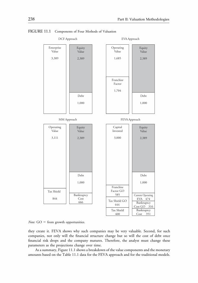
they create it. FEVA shows why such companies may be very valuable. Second, for suchcompanies, not only will the financial structure change but so will the cost of debt oncefinancial risk drops and the company matures. Therefore, the analyst must change theseparameters as the projections change over time.
As a summary, Figure 11.1 shows a breakdown of the value components and the monetaryamounts based on the Table 11.1 data for the FEVA approach and for the traditional models.
FIGURE 11.1 Components of Four Methods of Valuation
DCF Approach
EnterpriseValue
3,389
Debt
1,000
EquityValue
2,389
EVA Approach
OperatingValue
1,685
FranchiseFactor
1,704
Debt
1,000
EquityValue
2,389
MM Approach
OperatingValue
3,111
Debt
1,000
BankruptcyCost666
Tax Shield
844
EquityValue
2,389
FEVA Approach
CapitalInvested
3,000
FranchiseFactor GO
585
Tax Shield GO444
Tax Shield400
BankruptcyCost 351
BankruptcyCost GO 316
Current OperatingEVA 474
Debt
1,000
EquityValue
2,389
Note: GO 5 from growth opportunities.
c11 12 September 2012; 17:56:15
238 Part II: Valuation Methodologies
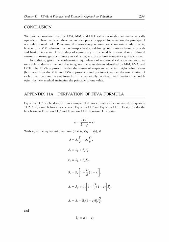
CONCLUSION
We have demonstrated that the EVA, MM, and DCF valuation models are mathematicallyequivalent. Therefore, when these methods are properly applied for valuation, the principle ofone value should hold. Preserving this consistency requires some important adjustments,however, for MM valuation methods—specifically, redefining contributions from tax shieldsand bankruptcy costs. This finding of equivalency in the models is more than a technicalcuriosity allowing greater accuracy in valuation; it explains how companies generate value.
In addition, given the mathematical equivalency of traditional valuation methods, wewere able to devise a method that integrates the value drivers identified by MM, EVA, andDCF. The FEVA approach divides the source of corporate value into eight value drivers(borrowed from the MM and EVA approaches) and precisely identifies the contribution ofeach driver. Because the new formula is mathematically consistent with previous methodol-ogies, the new method maintains the principle of one value.
APPENDIX 11A DERIVATION OF FEVA FORMULA
Equation 11.7 can be derived from a simple DCF model, such as the one stated in Equation11.2. Also, a simple link exists between Equation 11.7 and Equation 11.10. First, consider thelink between Equation 11.7 and Equation 11.2. Equation 11.2 states
E ¼ FCFk � g
� D:
With Ep as the equity risk premium (that is, RM 2 Rf ), if
k ¼ keEV
þ kdDV,
ke ¼ Rf þ βeEp,
ku ¼ Rf þ βuEp,
βe ¼ βu
�1þ D
Eð1� tÞ
�,
ke ¼ Rf þ βu
�1þ D
Eð1� tÞ
�Ep,
ke ¼ ku þ βuð1� tÞEpDE,
and
kd ¼ ið1� tÞ
c11 12 September 2012; 17:56:15
Chapter 11 FEVA: A Financial and Economic Approach to Valuation 239
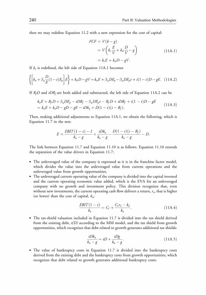
then we may redefine Equation 11.2 with a new expression for the cost of capital:
FCF ¼ V ðk � gÞ¼ V
�ke
EV
þ kdDV
� g�
¼ keE þ kdD � gV :
ð11A:1Þ
If ke is redefined, the left side of Equation 11A.1 becomes
ku þ βuDEð1� tÞEp
� �E
�þ kdD�gV ¼kuE þ βuDEp� βuDEpt þ ið1� tÞD� gE : ð11A:2Þ
If RfD and tDRf are both added and substracted, the left side of Equation 11A.2 can be
kuE þ Rf D þ βuDEp � tDRf � βuDEpt � Rf D þ tDRf þ ið1� tÞD � gE
¼ kuE þ kuD � gD � gE � tDku þ Dð1� tÞði � Rf Þ: ð11A:3Þ
Then, making additional adjustments to Equation 11A.1, we obtain the following, which isEquation 11.7 in the text:
E ¼ EBIT ð1� tÞ � Iku � g
þ tDkuku � g
� Dð1� tÞði � Rf Þku � g
� D:
The link between Equation 11.7 and Equation 11.10 is as follows. Equation 11.10 extendsthe separation of the value drivers in Equation 11.7:
� The unleveraged value of the company is expressed as it is in the franchise factor model,which divides the value into the unleveraged value from current operations and theunleveraged value from growth opportunities.
� The unleveraged current operating value of the company is divided into the capital investedand the current operating economic value added, which is the EVA for an unleveragedcompany with no growth and investment policy. This division recognizes that, evenwithout new investments, the current operating cash flow delivers a return, ro, that is higher(or lower) than the cost of capital, ku:
EBIT ð1� tÞku
¼ CI þ CI ro � kuku
: ð11A:4Þ
� The tax-shield valuation included in Equation 11.7 is divided into the tax shield derivedfrom the existing debt, t(D) according to the MM model, and the tax shield from growthopportunities, which recognizes that debt related to growth generates additional tax shields:
tDkuku � g
¼ tD þ tDgku � g
: ð11A:5Þ
� The value of bankruptcy costs in Equation 11.7 is divided into the bankruptcy costsderived from the existing debt and the bankruptcy costs from growth opportunities, whichrecognizes that debt related to growth generates additional bankruptcy costs:
c11 12 September 2012; 17:56:16
240 Part II: Valuation Methodologies
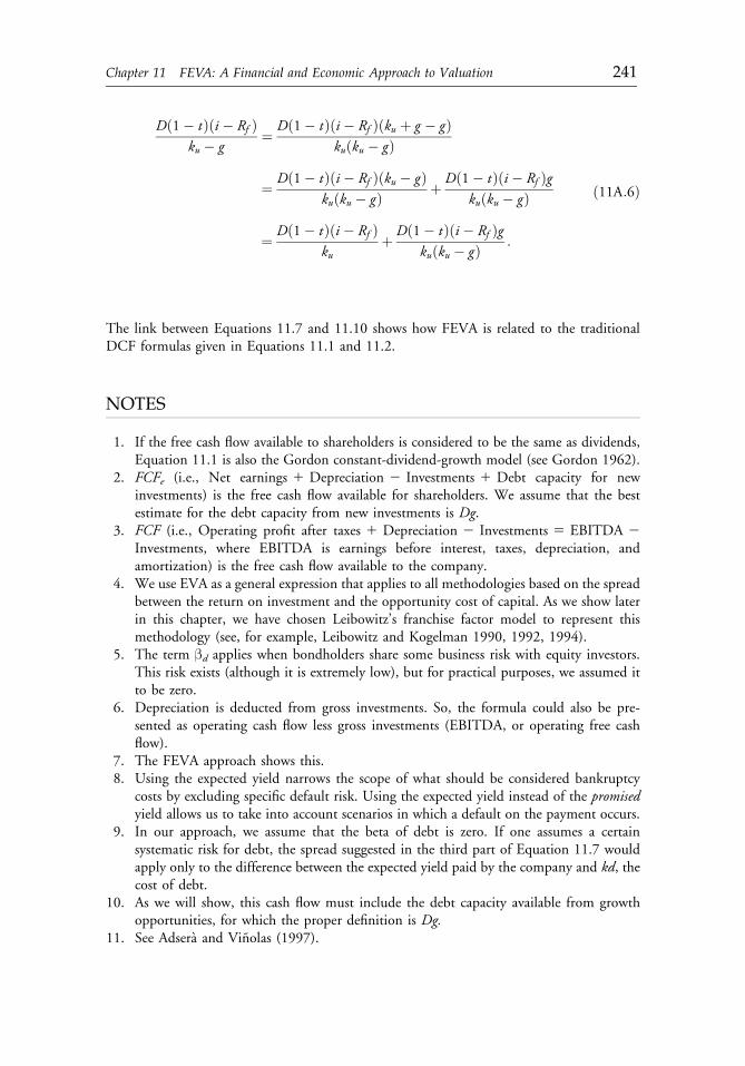
Dð1� tÞði � Rf Þku � g
¼ Dð1� tÞði � Rf Þðku þ g � gÞkuðku � gÞ
¼ Dð1� tÞði � Rf Þðku � gÞkuðku � gÞ þ Dð1� tÞði � Rf Þg
kuðku � gÞ
¼ Dð1� tÞði � Rf Þku
þ Dð1� tÞði � Rf Þgkuðku � gÞ :
ð11A:6Þ
The link between Equations 11.7 and 11.10 shows how FEVA is related to the traditionalDCF formulas given in Equations 11.1 and 11.2.
NOTES
1. If the free cash flow available to shareholders is considered to be the same as dividends,Equation 11.1 is also the Gordon constant-dividend-growth model (see Gordon 1962).
2. FCFe (i.e., Net earnings 1 Depreciation 2 Investments 1 Debt capacity for newinvestments) is the free cash flow available for shareholders. We assume that the bestestimate for the debt capacity from new investments is Dg.
3. FCF (i.e., Operating profit after taxes 1 Depreciation 2 Investments 5 EBITDA 2Investments, where EBITDA is earnings before interest, taxes, depreciation, andamortization) is the free cash flow available to the company.
4. We use EVA as a general expression that applies to all methodologies based on the spreadbetween the return on investment and the opportunity cost of capital. As we show laterin this chapter, we have chosen Leibowitz’s franchise factor model to represent thismethodology (see, for example, Leibowitz and Kogelman 1990, 1992, 1994).
5. The term βd applies when bondholders share some business risk with equity investors.This risk exists (although it is extremely low), but for practical purposes, we assumed itto be zero.
6. Depreciation is deducted from gross investments. So, the formula could also be pre-sented as operating cash flow less gross investments (EBITDA, or operating free cashflow).
7. The FEVA approach shows this.8. Using the expected yield narrows the scope of what should be considered bankruptcy
costs by excluding specific default risk. Using the expected yield instead of the promisedyield allows us to take into account scenarios in which a default on the payment occurs.
9. In our approach, we assume that the beta of debt is zero. If one assumes a certainsystematic risk for debt, the spread suggested in the third part of Equation 11.7 wouldapply only to the difference between the expected yield paid by the company and kd, thecost of debt.
10. As we will show, this cash flow must include the debt capacity available from growthopportunities, for which the proper definition is Dg.
11. See Adsera and Vinolas (1997).
c11 12 September 2012; 17:56:16
Chapter 11 FEVA: A Financial and Economic Approach to Valuation 241

REFERENCES
Adsera, X., and P. Vinolas. 1997. Principios de Valoraci�on de Empresas. Barcelona: Deusto.Copeland, Tom, Tim Koller, and Jack Murrin. 1990. Valuation: Measuring and Managing the Value of
Companies. New York: John Wiley & Sons.Damodaran, A. 1994. Damodaran on Valuation. New York: John Wiley & Sons.Gordon, M. 1959. “Dividends, Earnings, and Stock Prices.” Review of Economics and Statistics, vol. 41,
no. 2 (May):99�105.———. 1962. “The Savings, Investment and Valuation of a Corporation.” Review of Economics and
Statistics, vol. 44, no. 1 (February):37�49.Hamada, R.S. 1969. “Portfolio Analysis, Market Equilibrium, and Corporation Finance.” Journal of
Finance, vol. 24, no. 1 (March):13�31.Leibowitz, M.L., and S. Kogelman. 1990. “Inside the P/E Ratio: The Franchise Factor.” Financial
Analysts Journal, vol. 46, no. 6 (November/December):17�35.———. 1992. “Franchise Value and the Growth Process.” Financial Analysts Journal, vol. 48, no. 1
(January/February):53�62.———. 1994. Franchise Value and the Price/Earnings Ratio. Charlottesville, VA: Research Foundation
of the Institute of Chartered Financial Analysts.Modigliani, F., and M. Miller. 1958. “The Cost of Capital, Corporate Finance and the Theory of
Investment.” American Economic Review, vol. 48, no. 3 (June):261�297.———. 1961. “Dividend Policy, Growth, and the Valuation of Shares.” Journal of Business, vol. 34, no.
4 (October):411�433.———. 1963. “Corporate Income Taxes and the Cost of Capital: A Correction.” American Economic
Review, vol. 53 (June):433�443.———. 1969. “Reply to Heins and Sprenkle.” American Economic Review, vol. 59 (September):592�595.Myers, S.C. 1974. “Interactions of Corporate Financing and Investment Decisions—Implications for
Capital Budgeting.” Journal of Finance, vol. 29, no. 1 (March):1�25.Solomon, E. 1963. The Theory of Financial Management. New York: Columbia University Press.Stewart, G.B. 1991. The Quest for Value. New York: Harper Business.Walter, James. 1956. “Dividend Policies and Common Stock Prices.” Journal of Finance, vol. 11, no. 1
(March):29�41.
c11 12 September 2012; 17:56:16
242 Part II: Valuation Methodologies
CHAPTER 12CHOOSING THE RIGHTVALUATION APPROACH
Charles M.C. Lee
In picking a comparable company for use in multiple-based valuation, the choicedepends on the multiple being used. Much better results can be obtained by using awarranted-multiple approach to select peer companies. One advantage of thisapproach is that it allows the integration of relative and direct valuation techniques.
This chapter has two objectives. First, I will explain how valuation models are related andprovide a brief overview of the different valuation approaches for equity. In particular, I willfocus on multiple-based and discounted cash flow (DCF) approaches and show how they areessentially two pieces of the same puzzle. Second, I will discuss a new valuation tool for equitythat has emerged from academic research, focusing on recent research that uses a valuation-based approach to select comparable companies for multiple-based valuation.1
EQUITY VALUATION IN PERSPECTIVE
Unlike rare art, stocks are presumed to have an intrinsic value. The intrinsic value of a VanGogh painting is ill defined; basically, it is the amount that someone is willing to pay for it.But when equity analysts think of valuation, we think of intrinsic value. We have in mind amonetary sum that corresponds to the present value (PV) of expected future payoffs toshareholders. Equity valuation methods differ in technique, but they share the same objec-tive—to estimate the PV of these payoffs to shareholders.
An obvious observation that follows directly from this definition is that equity valuationinvolves forecasting. Estimates of future cash flows, discount rates, and option values all
Reprinted from AIMR Conference Proceedings: Equity Valuation in a Global Context (April 2003):4–14.When this article was originally published, Charles M.C. Lee was Henrietta Johnson Louis Professor ofManagement, professor of accounting and finance, and director of the Parker Center for InvestmentResearch at the Johnson Graduate School of Management at Cornell University.
c12 12 September 2012; 13:50:29
243
involve forecasting what could happen to a company in the future. Some techniques, such asmultiple-based approaches, may not appear to involve forecasting. In using these types oftechniques, however, the analyst is taking a shortcut with the ultimate goal of forecasting acompany’s future prospects. In fact, it is probably useful for us to acknowledge from theoutset that equity valuation is an imprecise science. It involves an educated guess, wherebyanalysts peer into an uncertain future and attempt to predict what a company might be worth.
No More New Economy
What about the “new economy”? We do not hear the term used much anymore. Only a fewyears ago, many were ready to discard traditional valuation models because the models failedto rationalize the successively larger market prices. The term “new economy” was coined todescribe this new valuation environment. But exactly what has changed and what has notchanged in the market and in valuation?
What has not changed is fundamental valuation theory; analysts are still trying to value astream of uncertain future cash flows. What is different is the pace of change, which isextremely rapid. We live in a world in which the barriers to entry that have taken years to buildcan fall in just a few months. Forecasting is difficult in this type of environment, particularly forgrowth companies that will not see net positive cash flows until some distant point in thefuture. In this fast-paced world, the means by which we estimate the key inputs to our valuationmodels (e.g., cash flows, cost of capital, and the value of intangible assets) are also changing.
Survey of Valuation Techniques
I will begin with a general overview. The arsenal of techniques available to analysts is dividedinto relative valuation methods and direct valuation methods. Relative valuation methods arethose in which market multiples of “comparable” companies are used to value the targetcompany. These include price to book (P/B), price to sales (P/S), price to earnings (P/E), andenterprise value to earnings before interest, taxes, depreciation, and amortization (EV/EBITDA). Direct valuation methods include a balance sheet approach, a contingency claimsapproach, and forecast-cash-flow approaches. The balance sheet approach values a companyby valuing the individual assets and liabilities on the company’s balance sheet; the contin-gency claims approach values a company as a basket of real options; and the forecast-cash-flowapproaches value a company on the basis of the PV of the company’s projected cash flows toshareholders. Each method has its advantages and disadvantages.
Of the three direct valuation methods, two are contextual in nature and are thus of lessinterest in general valuation. The balance sheet approach is often used in making lendingdecisions and in liquidation or distressed-company analysis. Its primary shortcoming is that itignores the value of intangibles and assets in use (the fact that individual assets create valuethrough synergy). In other words, most companies are worth more alive than dead. Thecontingency claims approach, although conceptually appealing, encompasses many practicalproblems related to parameter estimation. Because of these problems, I will focus my dis-cussion on the remaining two approaches—forecast cash flows and market multiples.
Forecast Cash Flows
A forecast-cash-flow approach encompasses various derivatives of the dividend discountmodel (DDM), such as the DCF model, the Edwards-Bell-Ohlson (EBO) model, the eco-nomic value added (EVA) model, and the residual income model (RIM). All of these models
c12 12 September 2012; 13:50:30
244 Part II: Valuation Methodologies
are essentially the same; like different brands of camera, they work the same way. A photog-rapher might prefer a Minolta to a Nikon, but all cameras incorporate the same variables—the amount of light entering the shutter is determined by the duration of the light exposureand the shutter speed. Likewise, all forecast-cash-flow models function according to thesame principles.
These models also feature similar advantages and limitations. The main advantage isthat they are conceptually sound and can be applied to most companies. The disadvantageis that they require explicit forecasting of future cash flows and discount rates. Some headway isbeing made on most of these limitations. For example, we now have a better understanding ofthe terminal-value problem—that most of the value comes in the later years of the forecast—and thus we are able to improve the estimation of terminal value. We are also making someprogress in estimating the cost of capital. Finally, techniques are being developed to deal withthe intangibles problem—the fact that new “knowledge-based” assets and other intangibles mayhave option values that are not reflected in short-term cash flow forecasts. But ultimately, theanalyst’s job in valuation is to forecast future earnings, cash flows, or dividends. The ability tomake that educated guess gives life to a valuation model and is largely (and, perhaps, thank-fully) still in the hands of human beings who can add value to this process.
Terminal-Value Problem
We can think of a company’s value, or its expected cash flow, as having two separate com-ponents: The first is the PV of future cash flows during an explicit forecast period, and thesecond is the PV of future cash flows beyond the explicit forecast period. This second piece iscalled the company’s terminal, or continuing, value.
The relative importance that the terminal value assumes in a company’s total value islargely determined by the company’s industry or production technology. For example, in aneight-year forecast period for a typical company in the tobacco industry, the continuing valuetypically represents 56 percent of the total value of the company; for sporting goods com-panies, the continuing value represents 81 percent; for companies specializing in skin careproducts, 100 percent.2 For a typical high-technology company, continuing value typicallyrepresents 125 percent of total value, which means that the PV of the free cash flows for thefirst eight years of the company’s life will be negative. In fact, all of the value of the companywill derive from the expected cash flow beyond the first eight years. The terminal-valueestimate truly is the tail that wags the dog when it comes to DCF valuations.
Figure 12.1 illustrates the way in which different valuation models deal with the terminal-value problem. On the left side of this diagram are the product and input markets of a company,and on the right side are the capital markets that provide the financing for a company. Inside thecompany are two types of assets—operating assets and financing assets. Net operating assets (NOA)are the wealth-creating engine of the company. Net financing assets (NFA) are assets and liabilitiesin which cash is “parked” until needed. The NOA of a company will increase as operating revenue(OR) increases and will decrease as NOA are used to pay operating expenses (OE).
A key measure shown on the diagram is free cash flow, or cash flow from operationsminus cash flow from investments (C 2 I), which is the net cash flow between NOA andNFA. The cash flow to shareholders is represented by net dividends (d), or the dividends acompany pays net of new equity financing, and is the net cash flow between a company andits shareholders. Cash flow to debtholders (F) is the net cash flow between a company and itsdebtholders. So, Figure 12.1 succinctly summarizes how cash moves in, within, and out of acompany.
c12 12 September 2012; 13:50:30
Chapter 12 Choosing the Right Valuation Approach 245
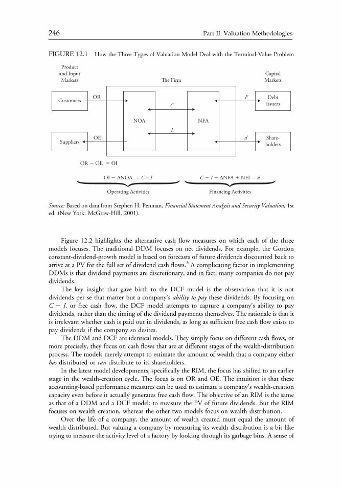
Figure 12.2 highlights the alternative cash flow measures on which each of the threemodels focuses. The traditional DDM focuses on net dividends. For example, the Gordonconstant-dividend-growth model is based on forecasts of future dividends discounted back toarrive at a PV for the full set of dividend cash flows.3 A complicating factor in implementingDDMs is that dividend payments are discretionary, and in fact, many companies do not paydividends.
The key insight that gave birth to the DCF model is the observation that it is notdividends per se that matter but a company’s ability to pay these dividends. By focusing onC 2 I, or free cash flow, the DCF model attempts to capture a company’s ability to paydividends, rather than the timing of the dividend payments themselves. The rationale is that itis irrelevant whether cash is paid out in dividends, as long as sufficient free cash flow exists topay dividends if the company so desires.
The DDM and DCF are identical models. They simply focus on different cash flows, ormore precisely, they focus on cash flows that are at different stages of the wealth-distributionprocess. The models merely attempt to estimate the amount of wealth that a company eitherhas distributed or can distribute to its shareholders.
In the latest model developments, specifically the RIM, the focus has shifted to an earlierstage in the wealth-creation cycle. The focus is on OR and OE. The intuition is that theseaccounting-based performance measures can be used to estimate a company’s wealth-creationcapacity even before it actually generates free cash flow. The objective of an RIM is the sameas that of a DDM and a DCF model: to measure the PV of future dividends. But the RIMfocuses on wealth creation, whereas the other two models focus on wealth distribution.
Over the life of a company, the amount of wealth created must equal the amount ofwealth distributed. But valuing a company by measuring its wealth distribution is a bit liketrying to measure the activity level of a factory by looking through its garbage bins. A sense of
FIGURE 12.1 How the Three Types of Valuation Model Deal with the Terminal-Value Problem
The Firm
C
I
CapitalMarkets
Productand InputMarkets
NOA
Suppliers
Customers
Share-holders
DebtIssuers
NFA
d
F
OE
OR
Financing ActivitiesOperating Activities
OI � ΔNOA � C − I C � I � ΔNFA � NFI � d
OR � OE � ΟΙ
Source: Based on data from Stephen H. Penman, Financial Statement Analysis and Security Valuation, 1sted. (New York: McGraw-Hill, 2001).
c12 12 September 2012; 13:50:30
246 Part II: Valuation Methodologies
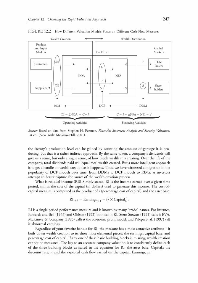
the factory’s production level can be gained by counting the amount of garbage it is pro-ducing, but that is a rather indirect approach. By the same token, a company’s dividends willgive us a sense, but only a vague sense, of how much wealth it is creating. Over the life of thecompany, total dividends paid will equal total wealth created. But a more intelligent approachis to get a handle on wealth creation as it happens. Thus, we have witnessed a migration in thepopularity of DCF models over time, from DDMs to DCF models to RIMs, as investorsattempt to better capture the source of the wealth-creation process.
What is residual income (RI)? Simply stated, RI is the income earned over a given timeperiod, minus the cost of the capital (in dollars) used to generate this income. The cost-of-capital measure is computed as the product of r (percentage cost of capital) and the asset base:
RItþ1 ¼ Earningstþ1 � ðr3CapitaltÞ:
RI is a single-period performance measure and is known by many “trade” names. For instance,Edwards and Bell (1963) and Ohlson (1992) both call it RI, Stern Stewart (1991) calls it EVA,McKinsey & Company (1995) calls it the economic profit model, and Palepu et al. (1997) callit abnormal earnings.
Regardless of your favorite handle for RI, the measure has a most attractive attribute—itboils down wealth creation to its three most elemental pieces: the earnings, capital base, andpercentage cost of capital. If any one of these basic building blocks is missing, wealth creationcannot be measured. The key to an accurate company valuation is to consistently define eachof the three building blocks as stated in the equation for RI: the asset base, Capitalt; thediscount rate, r; and the expected cash flow earned on the capital, Earningst1i.
FIGURE 12.2 How Different Valuation Models Focus on Different Cash Flow Measures
The Firm
Wealth Creation Wealth Distribution
C
I
CapitalMarkets
Productand InputMarkets
NOA
Suppliers
Customers
Share-holders
DebtIssuers
NFA
d
F
OE
OR
Financing ActivitiesOperating Activities
OI � ΔNOA � C − I C � I � ΔNFA � NFI � d
RIM DDMDCF
Source: Based on data from Stephen H. Penman, Financial Statement Analysis and Security Valuation,1st ed. (New York: McGraw-Hill, 2001).
c12 12 September 2012; 13:50:30
Chapter 12 Choosing the Right Valuation Approach 247
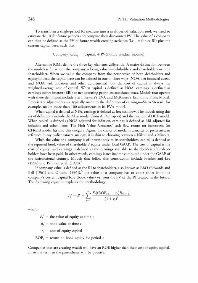
To transform a single-period RI measure into a multiperiod valuation tool, we need toestimate the RI for future periods and compute their discounted PV. The value of a companycan then be defined as the PV of future wealth-creating activities (i.e., its future RI) plus thecurrent capital base, such that
Company valuet ¼ Capitalt þ PVðFuture residual incomeÞ:
Alternative RIMs define the three key elements differently. A major distinction betweenthe models is for whom the company is being valued—debtholders and shareholders or onlyshareholders. When we value the company from the perspective of both debtholders andequityholders, the capital base can be defined in one of three ways (NOA, net financial assets,and NOA with inflation and other adjustments), but the cost of capital is always theweighted-average cost of capital. When capital is defined as NOA, earnings is defined asearnings before interest (EBI) or net operating profit less associated taxes. Models that operatewith these definitions include Stern Stewart’s EVA and McKinsey’s Economic Profit Model.Proprietary adjustments are typically made to the definition of earnings—Stern Stewart, forexample, makes more than 100 adjustments in its EVA model.
When capital is defined as NFA, earnings is defined as free cash flow. The models using thisset of definitions include the Alcar model (from Al Rappaport) and the traditional DCF model.When capital is defined as NOA adjusted for inflation, earnings is defined as EBI adjusted forinflation and other items. The Holt Value Associates’ cash flow return on investment (orCFROI) model fits into this category. Again, the choice of model is a matter of preference; inreference to my earlier camera analogy, it is akin to choosing between a Nikon and a Minolta.
When the value of a company is of interest only to its shareholders, capital is defined asthe reported book value of shareholders’ equity under local GAAP. The cost of capital is thecost of equity, and earnings is defined as the earnings available to shareholders after debt-holders have been paid. In other words, earnings is net income computed under the GAAP ofthe jurisdictional country. Models that follow this construction include Frankel and Lee(1998) and Penman et al. (1998).4
If company value is defined as the RI to shareholders, also known as EBO (Edwards andBell [1961] and Ohlson [1995]),5 the value of a company has to come either from thecompany’s current capital base (book value) or from the PV of the RI created in the future.The following equation explains the methodology:
Pt* ¼ Bt þXNi¼1
Et ½ðROEtþi � reÞBtþi�1�ð1þ reÞi
where
Pt* 5 the value of equity at time t
Bt 5 book value at time t
re 5 cost of equity capital
ROEt 5 return on book equity for period t.
Companies that are creating wealth will have an ROE higher than their cost of equity capital,re, so the term in the parentheses will be positive.
c12 12 September 2012; 13:50:30
248 Part II: Valuation Methodologies
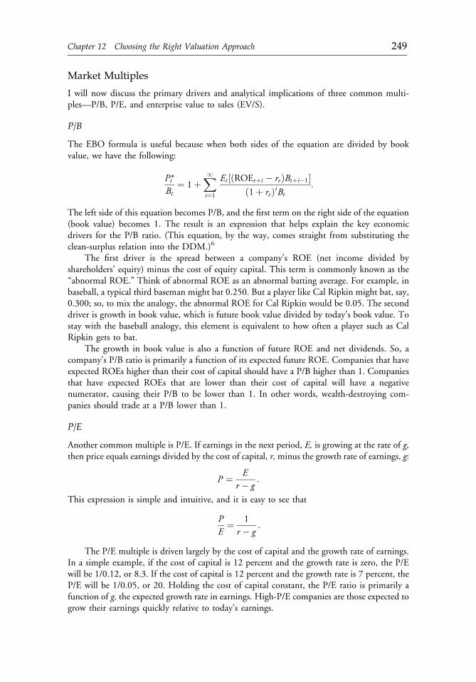
Market Multiples
I will now discuss the primary drivers and analytical implications of three common multi-ples—P/B, P/E, and enterprise value to sales (EV/S).
P/B
The EBO formula is useful because when both sides of the equation are divided by bookvalue, we have the following:
Pt*Bt
¼ 1þXNi¼1
Et ½ðROEtþi � reÞBtþi�1�ð1þ reÞiBt
:
The left side of this equation becomes P/B, and the first term on the right side of the equation(book value) becomes 1. The result is an expression that helps explain the key economicdrivers for the P/B ratio. (This equation, by the way, comes straight from substituting theclean-surplus relation into the DDM.)6
The first driver is the spread between a company’s ROE (net income divided byshareholders’ equity) minus the cost of equity capital. This term is commonly known as the“abnormal ROE.” Think of abnormal ROE as an abnormal batting average. For example, inbaseball, a typical third baseman might bat 0.250. But a player like Cal Ripkin might bat, say,0.300; so, to mix the analogy, the abnormal ROE for Cal Ripkin would be 0.05. The seconddriver is growth in book value, which is future book value divided by today’s book value. Tostay with the baseball analogy, this element is equivalent to how often a player such as CalRipkin gets to bat.
The growth in book value is also a function of future ROE and net dividends. So, acompany’s P/B ratio is primarily a function of its expected future ROE. Companies that haveexpected ROEs higher than their cost of capital should have a P/B higher than 1. Companiesthat have expected ROEs that are lower than their cost of capital will have a negativenumerator, causing their P/B to be lower than 1. In other words, wealth-destroying com-panies should trade at a P/B lower than 1.
P/E
Another common multiple is P/E. If earnings in the next period, E, is growing at the rate of g,then price equals earnings divided by the cost of capital, r,minus the growth rate of earnings, g:
P ¼ Er � g
:
This expression is simple and intuitive, and it is easy to see that
PE¼ 1
r � g:
The P/E multiple is driven largely by the cost of capital and the growth rate of earnings.In a simple example, if the cost of capital is 12 percent and the growth rate is zero, the P/Ewill be 1/0.12, or 8.3. If the cost of capital is 12 percent and the growth rate is 7 percent, theP/E will be 1/0.05, or 20. Holding the cost of capital constant, the P/E ratio is primarily afunction of g, the expected growth rate in earnings. High-P/E companies are those expected togrow their earnings quickly relative to today’s earnings.
c12 12 September 2012; 13:50:30
Chapter 12 Choosing the Right Valuation Approach 249
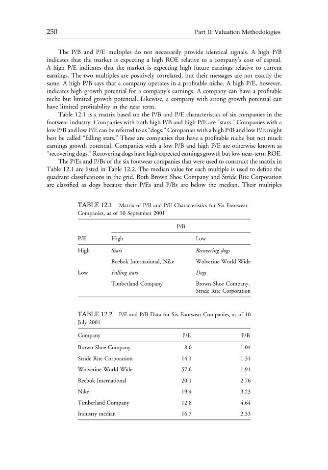
The P/B and P/E multiples do not necessarily provide identical signals. A high P/Bindicates that the market is expecting a high ROE relative to a company’s cost of capital.A high P/E indicates that the market is expecting high future earnings relative to currentearnings. The two multiples are positively correlated, but their messages are not exactly thesame. A high P/B says that a company operates in a profitable niche. A high P/E, however,indicates high growth potential for a company’s earnings. A company can have a profitableniche but limited growth potential. Likewise, a company with strong growth potential canhave limited profitability in the near term.
Table 12.1 is a matrix based on the P/B and P/E characteristics of six companies in thefootwear industry. Companies with both high P/B and high P/E are “stars.” Companies with alow P/B and low P/E can be referred to as “dogs.” Companies with a high P/B and low P/Emightbest be called “falling stars.” These are companies that have a profitable niche but not muchearnings growth potential. Companies with a low P/B and high P/E are otherwise known as“recovering dogs.” Recovering dogs have high expected earnings growth but low near-term ROE.
The P/Es and P/Bs of the six footwear companies that were used to construct the matrix inTable 12.1 are listed in Table 12.2. The median value for each multiple is used to define thequadrant classifications in the grid. Both Brown Shoe Company and Stride Rite Corporationare classified as dogs because their P/Es and P/Bs are below the median. Their multiples
TABLE 12.1 Matrix of P/B and P/E Characteristics for Six Footwear
Companies, as of 10 September 2001
P/B
P/E High Low
High Stars Recovering dogs
Reebok International, Nike Wolverine World Wide
Low Falling stars Dogs
Timberland Company Brown Shoe Company,Stride Rite Corporation
TABLE 12.2 P/E and P/B Data for Six Footwear Companies, as of 10
July 2001
Company P/E P/B
Brown Shoe Company 8.0 1.04
Stride Rite Corporation 14.1 1.31
Wolverine World Wide 57.6 1.91
Reebok International 20.1 2.76
Nike 19.4 3.23
Timberland Company 12.8 4.64
Industry median 16.7 2.33
c12 12 September 2012; 13:50:31
250 Part II: Valuation Methodologies
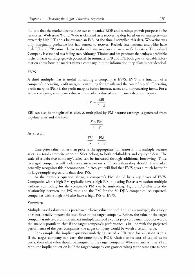
indicate that the market deems these two companies’ ROE and earnings growth prospects to belackluster. Wolverine World Wide is classified as a recovering dog based on its multiples—anextremely high P/E and a below-median P/B. At the time I compiled this data, Wolverine wasonly marginally profitable but had started to recover. Reebok International and Nike havehigh P/E and P/B ratios relative to the industry median and are classified as stars. TimberlandCompany is classified as a falling star. Although Timberland has products that enjoy a profitableniche, it lacks earnings growth potential. In summary, P/B and P/E both give us valuable infor-mation about how the market views a company, but the information they relate is not identical.
EV/S
A third multiple that is useful in valuing a company is EV/S. EV/S is a function of acompany’s operating profit margin, controlling for growth and the cost of capital. Operatingprofit margins (PM) is the profit margins before interest, taxes, and nonrecurring items. For astable company, enterprise value is the market value of a company’s debt and equity:
EV ¼ EBI
r � g:
EBI can also be thought of as sales, S, multiplied by PM because earnings is generated fromtop-line sales and the PM:
S3 PM
r � g:
As a result,EV
S¼ PM
r � g:
Enterprise value, rather than price, is the appropriate numerator in this multiple becausesales is a total enterprise concept. Sales belong to both debtholders and equityholders. Thescale of a debt-free company’s sales can be increased through additional borrowing. Thus,leveraged companies will look more attractive on a P/S basis than they should. The marketgenerally recognizes this phenomenon. In fact, you will find that EV/S gives a much better fitin large-sample regressions than does P/S.
As the previous equation shows, a company’s PM should be a key driver of EV/S.Companies with a high PM typically have a high P/S, but using P/S as a valuation multiplewithout controlling for the company’s PM can be misleading. Figure 12.3 illustrates therelationship between the P/S ratio and the PM for the 30 DJIA companies. As expected,companies with a high PM also have a high P/S or EV/S.
Summary
Multiple-based valuation is a peer-based relative valuation tool. In using a multiple, the analystdoes not literally forecast the cash flows of the target company. Rather, the value of the targetcompany is inferred from the market multiple ascribed to other peer companies. In other words,the analysis postulates that if the target company’s performance is in line with the projectedperformance of the peer companies, the target company would be worth a certain value.
For example, the implicit question underlying use of a P/B ratio for valuation is this:If the target company can earn the same future ROE relative to its cost of capital as itspeers, then what value should be assigned to the target company? When an analyst uses a P/Eratio, the implicit question is: If the target company can grow earnings at the same rate as peer
c12 12 September 2012; 13:50:31
Chapter 12 Choosing the Right Valuation Approach 251
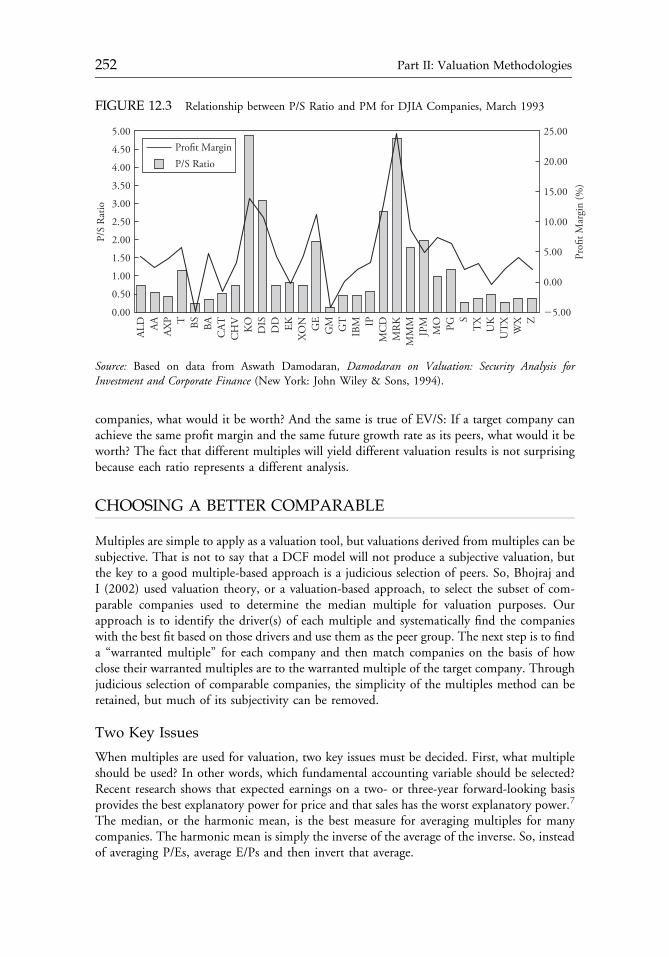
companies, what would it be worth? And the same is true of EV/S: If a target company canachieve the same profit margin and the same future growth rate as its peers, what would it beworth? The fact that different multiples will yield different valuation results is not surprisingbecause each ratio represents a different analysis.
CHOOSING A BETTER COMPARABLE
Multiples are simple to apply as a valuation tool, but valuations derived from multiples can besubjective. That is not to say that a DCF model will not produce a subjective valuation, butthe key to a good multiple-based approach is a judicious selection of peers. So, Bhojraj andI (2002) used valuation theory, or a valuation-based approach, to select the subset of com-parable companies used to determine the median multiple for valuation purposes. Ourapproach is to identify the driver(s) of each multiple and systematically find the companieswith the best fit based on those drivers and use them as the peer group. The next step is to finda “warranted multiple” for each company and then match companies on the basis of howclose their warranted multiples are to the warranted multiple of the target company. Throughjudicious selection of comparable companies, the simplicity of the multiples method can beretained, but much of its subjectivity can be removed.
Two Key Issues
When multiples are used for valuation, two key issues must be decided. First, what multipleshould be used? In other words, which fundamental accounting variable should be selected?Recent research shows that expected earnings on a two- or three-year forward-looking basisprovides the best explanatory power for price and that sales has the worst explanatory power.7
The median, or the harmonic mean, is the best measure for averaging multiples for manycompanies. The harmonic mean is simply the inverse of the average of the inverse. So, insteadof averaging P/Es, average E/Ps and then invert that average.
FIGURE 12.3 Relationship between P/S Ratio and PM for DJIA Companies, March 1993
5.00
4.50
4.00
3.50
3.00
2.50
2.00
1.50
1.00
0.50
0.00
25.00
20.00
15.00
10.00
5.00
0.00
�5.00
ALD A
AA
XP T BS
BA
CA
TC
HV
KO
DIS
DD EK
XO
N GE
GM GT
IBM IP
MC
DM
RK
MM
MJP
MM
O PGS
TX
UK
UT
XW
X Z
P/S
Rat
io
Profi
t Mar
gin
(%)
Profit Margin
P/S Ratio
Source: Based on data from Aswath Damodaran, Damodaran on Valuation: Security Analysis forInvestment and Corporate Finance (New York: John Wiley & Sons, 1994).
c12 12 September 2012; 13:50:31
252 Part II: Valuation Methodologies
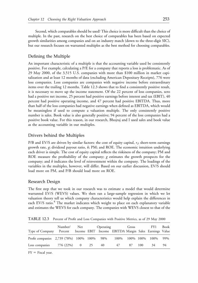
Second, which comparables should be used? This choice is more difficult than the choice ofmultiple. In the past, research on the best choice of comparables has been based on expectedgrowth similarities among companies and on an industry match (down to the three-digit SIC),but our research focuses on warranted multiples as the best method for choosing comparables.
Defining the Multiple
An important characteristic of a multiple is that the accounting variable used be consistentlypositive. For example, calculating a P/E for a company that reports a loss is problematic. As of29 May 2000, of the 3,515 U.S. companies with more than $100 million in market capi-talization and at least 12 months of data (excluding American Depositary Receipts), 776 wereloss companies. Loss companies are companies with negative income before extraordinaryitems over the trailing 12 months. Table 12.3 shows that to find a consistently positive result,it is necessary to move up the income statement. Of the 22 percent of loss companies, zerohad a positive net income, 25 percent had positive earnings before interest and tax (EBIT), 40percent had positive operating income, and 47 percent had positive EBITDA. Thus, morethan half of the loss companies had negative earnings when defined as EBITDA, which wouldbe meaningless if used to compute a valuation multiple. The only consistently positivenumber is sales. Book value is also generally positive; 94 percent of the loss companies had apositive book value. For this reason, in our research, Bhojraj and I used sales and book valueas the accounting variable in our multiples.
Drivers behind the Multiples
P/B and EV/S are driven by similar factors: the cost of equity capital, re; short-term earningsgrowth rate, g; dividend payout ratio, k; PM; and ROE. The economic intuition underlyingeach driver is simple. The cost of equity capital reflects the riskiness of the company; PM andROE measure the profitability of the company; g estimates the growth prospects for thecompany; and k indicates the level of reinvestment within the company. The loadings of thevariables in the multiples, however, will differ. Based on our earlier discussion, EV/S shouldload more on PM, and P/B should load more on ROE.
Research Design
The first step that we took in our research was to estimate a model that would determinewarranted EV/S (WEVS) values. We then ran a large-sample regression in which we letvaluation theory tell us which company characteristics would help explain the differences ineach EV/S ratio.8 The market indicates which weight to place on each explanatory variableand estimates the WEVS for each company. The companies with WEVS closest to that of the
TABLE 12.3 Percent of Profit and Loss Companies with Positive Metrics, as of 29 May 2000
Type of CompanyNumber/Percent
NetIncome EBIT
OperatingIncome EBITDA
GrossMargin Sales
FY1Earnings
BookValue
Profit companies 2,739 (78%) 100% 100% 98% 100% 100% 100% 100% 99%
Loss companies 776 (22%) 0 25 40 47 87 100 34 94
FY 5 Fiscal year.
c12 12 September 2012; 13:50:31
Chapter 12 Choosing the Right Valuation Approach 253
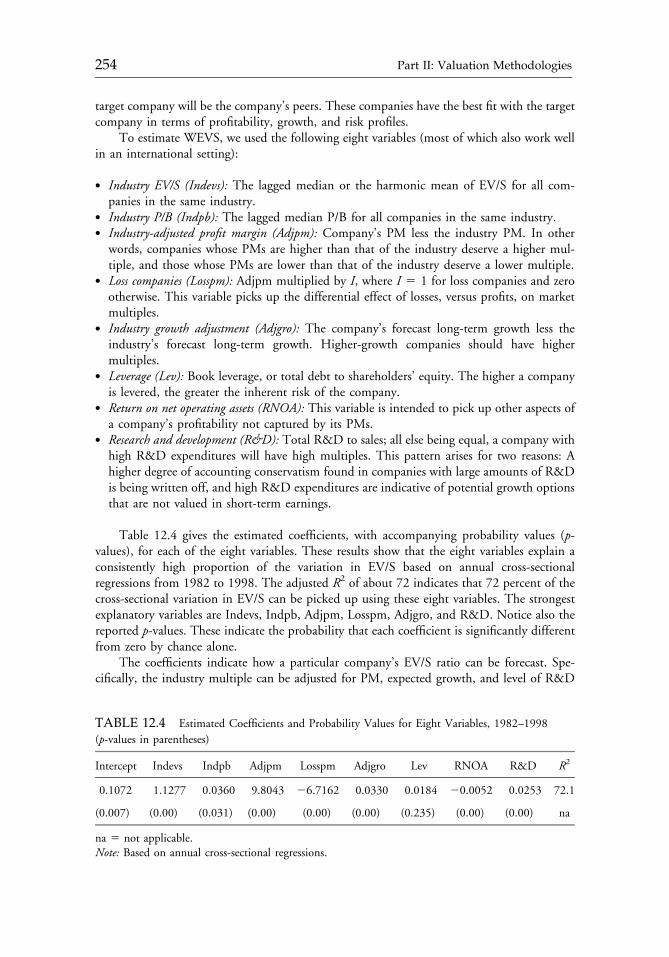
target company will be the company’s peers. These companies have the best fit with the targetcompany in terms of profitability, growth, and risk profiles.
To estimate WEVS, we used the following eight variables (most of which also work wellin an international setting):
� Industry EV/S (Indevs): The lagged median or the harmonic mean of EV/S for all com-panies in the same industry.
� Industry P/B (Indpb): The lagged median P/B for all companies in the same industry.� Industry-adjusted profit margin (Adjpm): Company’s PM less the industry PM. In other
words, companies whose PMs are higher than that of the industry deserve a higher mul-tiple, and those whose PMs are lower than that of the industry deserve a lower multiple.
� Loss companies (Losspm): Adjpm multiplied by I, where I 5 1 for loss companies and zerootherwise. This variable picks up the differential effect of losses, versus profits, on marketmultiples.
� Industry growth adjustment (Adjgro): The company’s forecast long-term growth less theindustry’s forecast long-term growth. Higher-growth companies should have highermultiples.
� Leverage (Lev): Book leverage, or total debt to shareholders’ equity. The higher a companyis levered, the greater the inherent risk of the company.
� Return on net operating assets (RNOA): This variable is intended to pick up other aspects ofa company’s profitability not captured by its PMs.
� Research and development (R&D): Total R&D to sales; all else being equal, a company withhigh R&D expenditures will have high multiples. This pattern arises for two reasons: Ahigher degree of accounting conservatism found in companies with large amounts of R&Dis being written off, and high R&D expenditures are indicative of potential growth optionsthat are not valued in short-term earnings.
Table 12.4 gives the estimated coefficients, with accompanying probability values (p-values), for each of the eight variables. These results show that the eight variables explain aconsistently high proportion of the variation in EV/S based on annual cross-sectionalregressions from 1982 to 1998. The adjusted R2 of about 72 indicates that 72 percent of thecross-sectional variation in EV/S can be picked up using these eight variables. The strongestexplanatory variables are Indevs, Indpb, Adjpm, Losspm, Adjgro, and R&D. Notice also thereported p-values. These indicate the probability that each coefficient is significantly differentfrom zero by chance alone.
The coefficients indicate how a particular company’s EV/S ratio can be forecast. Spe-cifically, the industry multiple can be adjusted for PM, expected growth, and level of R&D
TABLE 12.4 Estimated Coefficients and Probability Values for Eight Variables, 1982–1998
(p-values in parentheses)
Intercept Indevs Indpb Adjpm Losspm Adjgro Lev RNOA R&D R2
0.1072 1.1277 0.0360 9.8043 26.7162 0.0330 0.0184 20.0052 0.0253 72.1
(0.007) (0.00) (0.031) (0.00) (0.00) (0.00) (0.235) (0.00) (0.00) na
na 5 not applicable.Note: Based on annual cross-sectional regressions.
c12 12 September 2012; 13:50:31
254 Part II: Valuation Methodologies
(because more profitable, higher-growth companies and companies with higher levels ofR&D are worth more). The coefficients from this regression indicate how much weight to puton each of these company characteristics.
The preceding model estimation is used to identify peer companies by one of fourmethods. The first two methods are basically a simple industry and size match and the secondtwo are based on WEVS:
� IEVS: The harmonic mean of actual EV/S for all companies with the same two-digit SICcode.
� ISEVS: The harmonic mean of actual EV/S for the four companies in the same industrywith the closest market capitalization.
� COMP: The harmonic mean of actual EV/S for the four closest comparable companiesbased on their current WEVS.
� ICOMP: The harmonic mean of actual EV/S for the four closest comparable companiesbased on WEVS, in which the companies are constrained to the same industry.
Research Results
We find that the latter two methods produce much better EV/S forecasting results. The firsttwo methods, simple industry mean and size-adjusted mean, explain only about 22–24percent of current cross-sectional EV/S, with the adjusted R2 ranging from 22.94 to 23.46.But as soon as other variables—PMs and earnings growth and so forth—are introduced, amuch larger portion of EV/S can be explained. In fact, the latter two methods, COMP andICOMP, explain approximately 60 percent of current-year EV/S.
One way to test the value of the estimation variables is their ability to forecast future EV/Sor P/S. Industry- and size-matched peers explain only about 18 percent of two-year-forwardEV/S. In contrast, COMP and ICOMP are able to explain about 50 percent of the EV/S ofthese companies, and three years ahead, from 45 to 50 percent. In short, a big improvement inforecasting ability is achievable by choosing the comparables used in multiple-based valuation.
This methodology for choosing peers also works for so-called new-economy stocks—biotechnology, technology, and telecommunication stocks. In that subset of companies, manyare loss companies. Our approach of moving up the income statement and using sales asthe multiple’s denominator is particularly effective for this group of companies. In fact, theannual predictive power of our approach ranges from 58 to 84 percent. The coefficients usedin the model estimation differ from those used for “old economy” stocks. R&D has a greaterloading for this subset of companies, compared with the heavier loadings of the old-economystocks on PMs and ROE. The heavier loading on R&D for tech companies makes sense, andthe fit is good, even for the loss companies.
SUMMARY
This chapter offers five lessons. First, in picking a comparable company for use in multiple-based valuation, the choice is dependent to a large extent on the choice of multiple. Forexample, the choice of a comparable for a valuation based on P/B should depend on ROE,and the comparable for a valuation based on P/S should depend on PM.
Second, much better results can be obtained if we use a warranted-multiple approach toselect peer companies. In this approach, we start with the industry mean and adjust for PM,
c12 12 September 2012; 13:50:32
Chapter 12 Choosing the Right Valuation Approach 255
expected growth, and R&D. Because this approach is based on a DCF valuation model, weare able to find matching companies that have the closest overall match to the target companyfor valuation purposes.
Third, the warranted-multiple approach is applicable in cross-border situations. We arenow taking the same approach to valuation using a pool of companies from the G–7 countries.Our preliminary findings suggest this technique works well in an international setting.
Fourth, an integration of relative and direct valuation techniques is possible when peersare chosen based on warranted multiples. The line between the two techniques has beenblurred through the use of “smart” multiples. The “smart” comes from using DCF conceptsto pick peers.
Fifth, RIMs and DCF models are similar in spirit. Their goal is the same, and withspecific international applications, they allow for cross-border comparables.
QUESTION AND ANSWER SESSION
Question: Does the formula work if the ROE declines with a higher book value?Lee: Yes, the math works. But the key question is whether you can forecast ROE well. The
task is more difficult for growth companies because the bulk of their free cash flow isgenerated further in the future.
Question:How long does the specific forecast period have to be to get the best result from thevaluation model?
Lee: I can tell you what we do, but that doesn’t mean our way is in any way optimal. I aim fora period of explicit forecasts that is long enough that I will not have to add anothergrowth rate to the terminal value. Typically, a fixed period of about 10 years will do thejob. If the explicit forecast period is long enough, I can simply assume a growth rateequal to the nominal GDP rate for the terminal value.
Question: Regarding the terminal-value problem, what is the discount rate used in calculatingthe PV of the cash flow during the explicit period and the PV of the cash flow beyondthe explicit forecast period?
Lee:We use the same discount rate for both cash flow periods. We sometimes make an adjustmentto growth for the cash flows in the terminal-value period that isn’t made for cash flows in theexplicit forecast period, so it may appear to be a different discount rate, but it is still r 2 g.
Question: The RIM requires the clean-surplus relation, which requires estimated dividends,so why not use the DDM? In other words, what is the advantage of the RIM versus theDDM?
Lee: That is a good question: If you’re going to forecast dividends, why not simply use theDDM? In reality, a pure DDM is never used. Generally, in implementing a DDM, youstill have to begin by forecasting earnings because dividends are paid from earnings. Andin the terminal period of a DDM, you still have to assume 100 percent payout ofearnings. The RIM is gaining in popularity over the DDM because a long-term forecastis easier to do when forecasting accounting numbers. The time-series behavior ofaccounting rates of return (such as ROA and ROE) is easier to predict than trying tocome up with a long-term growth rate, g, in order to use a DDM.
Question: So, RI allows for better-quality forecasting?
c12 12 September 2012; 13:50:32
256 Part II: Valuation Methodologies
Lee: That is generally true. Consider, for instance, a traditional DCF approach in which youdo a detailed line-by-line forecast for 10 years. How do you know that you have made asensible cash flow forecast 10 years from now? How do you know you’ve not madesome inconsistent assumptions? The textbooks tell you to analyze the resulting financialratios—asset turnover, PM, ROA, and ROE of the company 10 years from now. Whenyou use a DCF model, you are still forecasting accounting numbers. You compute thecash flows and then check accounting ratios again 10 years later to see whether you’vemade reasonable assumptions.
In an RIM, you are explicitly forecasting the financial ratios. With consistent assump-tions, the two methods should generate identical answers. But in selecting the right approach,consider focusing your forecast on the parameter for which you have the highest confidence.What do you want to forecast? Do you want to forecast earnings with a g rate or futureaccounting rates of return (ROA or ROE) with a fade rate? Forecast the number for whichyou have the tightest confidence band and let the valuation model convert that forecast into acompany value estimate.
NOTES
1. Sanjeev Bhojraj and Charles M.C. Lee, “Who Is My Peer? A Valuation-Based Approachto the Selection of Comparable Firms,” Journal of Accounting Research (May 2002):407–439.
2. Based on data from Tom Copeland, Tim Koller, and Jack Murrin, Valuation: Measuringand Managing the Value of Companies, 2nd ed. (New York: John Wiley & Sons, 1996).
3. For further information on the Gordon constant-dividend-growth model, see Myron J.Gordon, “The Savings, Investment and Valuation of a Corporation,” Review of Economicsand Statistics (February 1962):37–49.
4. Richard Frankel and Charles M.C. Lee, “Accounting Valuation, Market Expectation, andCross-Sectional Stock Returns,” Journal of Accounting and Economics (June 1998):283–319; Stephen H. Penman and Theodore Sougiannis, “A Comparison of Dividend, CashFlow, and Earnings Approaches to Equity Valuation,” Contemporary Accounting Research(Fall 1998):343–383.
5. Edgar O. Edwards and Philip W. Bell, The Theory and Measurement of Business Income(Berkeley, CA: University of California Press, 1961); James A. Ohlson, “Earnings, BookValues, and Dividends in Security Valuation,” Contemporary Accounting Research (Spring1995):661–687.
6. The clean-surplus relation is the assumption that changes in book value are completelycaptured by earnings or net dividends. In other words, Bt11 5 Bt 1 NIt11 2 DIVt11.
7. Jing Liu, Doron Nissim, and Jacob Thomas, “Equity Valuation Using Multiples,”Working Paper, UCLA and Columbia University, December 1999.
8. The regression can be done across countries. We are undertaking research of this characternow. See Sanjeev Bhojraj, Charles M.C. Lee, and David Tat-Chee Ng, “InternationalValuation Using Smart Multiples,” Working Paper, Cornell University, 2003.
c12 12 September 2012; 13:50:32
Chapter 12 Choosing the Right Valuation Approach 257

c12 12 September 2012; 13:50:32
CHAPTER 13CHOOSING THE RIGHTVALUATION APPROACH
Robert Parrino, CFA
Before beginning any analysis, the analyst should define the claim and level of value,the valuation date, and the purpose/definition of value. In essence, those “defini-tions” help the analyst choose among the many valuation methodologies available.But even with the wide range of tools that are available, the quality of any valueestimate ultimately depends on how well the analyst understands the firm and itsstrategy, its competitive position, and its future prospects.
In this chapter, I will focus on business valuation techniques. In the course of this discussion,I will present the concepts underlying a number of valuation methods. Although many peopleare familiar with these methods, it is still worthwhile to systematically examine and discuss theconcepts that underlie these approaches, their proper applications, and the pros and consassociated with each. Ultimately, I hope to provide a better sense of how these different methodsfit together and the circumstances under which one method might be preferable to another.
DEFINING THE VALUATION PROBLEM
When trying to decide what valuation approach to use in a particular situation, it is importantto begin by defining the objective of the analysis. In other words, it is important to accuratelydefine the valuation problem. Three things are particularly important to consider in thiscontext: the claim and level of value, the valuation date, and the purpose/definition of value.This process of defining the valuation problem often leads the analyst to the appropriatemethodology.
Reprinted from CFA Institute Conference Proceedings: Analyzing, Researching, and Valuing EquityInvestments (June 2005):15�28. When this article was originally published, Robert Parrino, CFA, wasdirector of the Hicks, Muse, Tate & Furst Center for Private Equity Finance in the McCombs School ofBusiness at the University of Texas at Austin.
c13 12 September 2012; 13:53:10
259
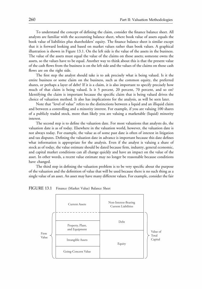
To understand the concept of defining the claim, consider the finance balance sheet. Allanalysts are familiar with the accounting balance sheet, where book value of assets equals thebook value of liabilities plus shareholders’ equity. The finance balance sheet is similar exceptthat it is forward looking and based on market values rather than book values. A graphicalillustration is shown in Figure 13.1. On the left side is the value of the assets in the business.The value of the assets must equal the value of the claims on those assets; someone owns theassets, so the values have to be equal. Another way to think about this is that the present valueof the cash flows from the business is on the left side and the values of the claims on those cashflows are on the right side.
The first step the analyst should take is to ask precisely what is being valued. Is it theentire business or some claim on the business, such as the common equity, the preferredshares, or perhaps a layer of debt? If it is a claim, it is also important to specify precisely howmuch of that claim is being valued. Is it 5 percent, 20 percent, 70 percent, and so on?Identifying the claim is important because the specific claim that is being valued drives thechoice of valuation method. It also has implications for the analysis, as will be seen later.
Note that “level of value” refers to the distinctions between a liquid and an illiquid claimand between a controlling and a minority interest. For example, if you are valuing 100 sharesof a publicly traded stock, more than likely you are valuing a marketable (liquid) minorityinterest.
The second step is to define the valuation date. For most valuations that analysts do, thevaluation date is as of today. Elsewhere in the valuation world, however, the valuation date isnot always today. For example, the value as of some past date is often of interest in litigationand tax disputes. Defining the valuation date in advance is important because this date defineswhat information is appropriate for the analysis. Even if the analyst is valuing a share ofstock as of today, the value estimate should be dated because firm, industry, general economic,and capital market conditions can all change quickly and have an impact on the value of theasset. In other words, a recent value estimate may no longer be reasonable because conditionshave changed.
The third step in defining the valuation problem is to be very specific about the purposeof the valuation and the definition of value that will be used because there is no such thing as asingle value of an asset. An asset may have many different values. For example, consider the fair
FIGURE 13.1 Finance (Market Value) Balance Sheet
Current Assets
FirmValue
Value ofTotalCapital
Property, Plant,and Equipment
Intangible Assets
Going-Concern Value
Non-Interest-BearingCurrent Liabilities
Debt
Equity
c13 12 September 2012; 13:53:10
260 Part II: Valuation Methodologies
market value concept (i.e., definition of value). The fair market value of any asset is defined asthe cash price at which the asset would change hands between a willing buyer and a willingseller if the asset were offered for sale on the open market for a reasonable period of time withboth the buyer and seller being apprised of the relevant facts and neither being under anycompulsion to act. Basically, it is a freely traded value where cash is being exchanged and noone is being forced to act. When an analyst values a share of stock in a public company with aview toward making a buy, hold, or sell recommendation, the analyst is estimating the fairmarket value of that share. There is no specific buyer or seller in mind. What the analyst islooking for in this case is an estimate of the value of that share to a typical buyer.
Contrast the fair market value concept with investment value. The investment value of anasset is the value of that asset to a specific buyer. If known, the identity of the prospectivebuyer affects the valuation. For example, the investment value of a share of stock to some-one who already owns 49.9999 percent of the outstanding shares can be much different fromthe investment value of that share to a typical buyer.
If an analyst is valuing an entire company, the same analogy applies. For example,suppose that XYZ Corporation announces that it is going to sell one of its divisions. One wayto think about the price it might obtain for the sale of that division is to do a fair market valueanalysis on a controlling basis. In this situation, the analyst estimates what someone who isknowledgeable about that business and competent in managing that type of business wouldpay. What is the present value of the cash flows to someone like that? Answering that questioninvolves valuing the firm under the assumptions that operating and financial policies aretypical of those in that industry.
That situation is much different from the sale by XYZ Corporation of a division to aprivate investment firm that will likely roll the business up with some other businesses. In thiscase, a lot of leverage will probably be applied to the transaction and the operating policies ofthe business will be different. This will have different implications for the value of the businessand the sale price that will ultimately be agreed upon.
The bottom line is that defining the valuation problem up front is importantbecause it has implications for the choice of valuation method as well as for the informationthat is used, the assumptions that are made, and the way the selected valuation methodsare applied.
Although a wide range of valuation methodologies exists, the majority fall within threecategories: asset/cost approaches, market approaches, and income approaches. To see how thesecategories differ, think of commercial real estate. The asset/cost approach might be used forinsurance purposes, such as determining what it would cost to replace a structure. The marketapproach, in contrast, is the evaluation of what comparable buildings sold for on a squarefootage basis, with adjustments for specific features of the asset being valued. The incomeapproach involves discounting the present value of the rental stream net of any expenses andinvestment requirements.
The same three categories of approaches are used in business valuation. They are genericto the valuation of any asset. So, what I will do is frame this discussion in the context of asset/cost, market, and income approaches. I will describe methodologies that use each of the threeapproaches, the cases in which each approach is useful, the ways in which each approach isused, and the pros and cons of each approach. Although it is not one of the three majorcategories I just mentioned—asset/cost, market, and income—a fourth approach I will brieflydiscuss is the contingent claims approach. Contingent claims methods are used to value claimson underlying assets. In that sense, I will distinguish these methods from the other approaches,which value the underlying assets themselves.
c13 12 September 2012; 13:53:10
Chapter 13 Choosing the Right Valuation Approach 261
Option-pricing methodologies are examples of the contingent claims approach. Thecontingent claims approach is useful in business valuation for cases in which someone doesnot have a 100 percent claim on the cash flows of an asset. In those instances, those claimslook a lot like derivatives. In fact, as will be seen, they can look a lot like options.
I will thus discuss how to value equity using contingent claims methods because thesemethods can be very useful. How many analysts have ever done a discounted cash flow (DCF)analysis of a financially distressed company and arrived at a negative equity value? This, ofcourse, means the equity is worth zero because equity cannot have a negative value. If theshares in this example are trading with a positive price, then they are effectively trading ontheir option value.
ASSET/COST APPROACHES
This section reviews two basic asset/cost methods: the adjusted book value approach and thereplacement cost approach.
Adjusted Book Value Approach
The adjusted book value approach is conceptually simple. The adjusted book value of a firmequals the sum of the market value of each of the firm’s identifiable assets. The value of theequity equals this value less the market value of all liability claims on the business.
This method is commonly used for valuing mutual funds. If an analyst is valuing anoperating company with separate autonomous units, he or she can value each of the businessunits separately and then add those values together to estimate the value of the total enterprise.
Although straightforward, this method is not very useful for valuing a typical operatingbusiness because the value of a typical operating business is greater than the sum of the valuesof the individual identifiable assets. The reason for this is that a typical operating business hassomething called “going-concern value.” The going-concern value is value that is attributableto the way a business is organized and managed. For example, suppose you are starting adecorative brick manufacturing business and you have a national franchise to sell your bricks.Would you locate in California or Kansas? Given that transportation costs would presumablybe significant for transporting bricks around the country, you would opt for a locationin Kansas over California. If you located on the West Coast, you might kill your opportu-nities in the eastern half of the country. The choice of location thus has value implicationsbecause it affects the number of potential customers (sales); costs; and to the extent thatregional economies differ, risks. But when using the adjusted book value approach, you mightcome up with the same value for both locations even though the going-concern value isquite different. Operating policies, the quality of management, the organizational structure,and a lot of other factors contribute to going-concern value. These factors are not all properlyaccounted for with the adjusted book value method.
The situations where this approach can be very useful are ones where the analyst isvaluing a business with separate autonomous assets and where there are no synergies betweenthose assets. It can also be very useful in estimating the liquidation value of a business, which,incidentally, is often done when the going-concern value is negative.
Finally, this approach can be useful as a “sanity check” for other valuation methods, suchas the DCF methods discussed later. The reason adjusted book value can be useful as a sanitycheck is that it provides an estimate of the floor value for a business. So, if a DCF analysis
c13 12 September 2012; 13:53:10
262 Part II: Valuation Methodologies
yields a value estimate that is lower than adjusted book value, a problem more than likelyexists with the DCF analysis. Perhaps the analyst misestimated revenue growth, margins, orthe appropriate discount rate. If there is no problem with the DCF analysis and the DCFvalue is less than the adjusted book value, then the business should be shut down because it isdestroying, rather than creating, value.
Replacement Cost Approach
The second asset/cost approach is the replacement cost approach. The replacement costsimply reflects the cost of duplicating assets in their present form at a particular point in time.It thus reflects the asset type and condition.
Although this approach is generally more useful for insurance than for any other purpose,in business valuation, a replacement cost analysis can be helpful in conducting a buy-versus-build analysis. Think about some of the prices people were paying for domain names in 1999and 2000. It was not unusual to hear of prices in the billions of dollars. Hopefully, they paidthat much only after asking themselves the obvious question: Can we create the consumerawareness that is associated with that particular domain name in a reasonable period for lessmoney? Or, put another way, what is the opportunity cost for not making the investment?
Likewise, if a company announces that it is going to acquire another business at aspecified price, the first thing an analyst should do is think about whether the company isoverpaying. Is this something the company could do on its own for less? Certainly, getting tothe market more quickly has some value, and it may be risky to try to play catch-up witha competitor at this particular point in time. Those factors will serve to complicate theanalysis. Nevertheless, analysts should be conducting this type of analysis whenever they heara company say it is considering purchasing a business.
MARKET APPROACHES
In this section, I will discuss two market approaches: guideline multiples analysis andguideline transactions analysis. In both of these approaches, the term “guideline” is simplyanother way to say “comparable.”
Guideline Multiples
Multiples analysis is commonly used by investment analysts. It involves identifying publiclytraded companies engaged in similar business activities and that have risk�return characteristicsthat are similar to those of the company being analyzed. The analyst then uses the prices atwhich shares of those publicly traded companies are trading to infer something about thecompany of interest, such as whether the company’s shares are over- or undervalued. Similarly,if an analyst is valuing a closely held business, guideline multiples analysis might help theanalyst estimate the fair market value of its securities.
Commonly used multiples for assessing equity value are price/earnings, price/dividends,price/revenue, and market value/book value. Other ratios divide enterprise value by a proxyfor cash flow, such as enterprise value/revenue or enterprise value/free cash flow.1 Theseenterprise multiples are used to derive a value estimate for the total business.
Applying the guideline multiples approach is conceptually straightforward, but inpractice, applying the approach correctly can be very difficult. For instance, often a business
c13 12 September 2012; 13:53:10
Chapter 13 Choosing the Right Valuation Approach 263
has no true comparables, or what are often called “pure plays.” This can be very frustratingbecause in such cases a guideline multiples analysis can yield a wide range of value estimatesthat are difficult to reconcile. The ideal comparable has to match on many dimensions. Forexample, the ideal comparable is a company that sells the same products, competes in thesame markets, is of similar size, has similar revenue growth prospects, has similar profitmargins, and has similar management quality. In addition, if the analyst is using an equityratio (such as price/earnings or price/dividends) the comparable should have a similarcapital structure because, all else being equal, capital structure can have a dramatic impact onthose ratios.
The importance of identifying guideline companies that are similar to the companybeing analyzed can be illustrated by considering the characteristics that determine a com-pany’s P/E:
P0 ¼ DIV1
kE � g¼ EPS1b
kE � g.
P0EPS1
¼ bkE � g
,
where
DIV15 dividends in Period 1
EPS15 earnings per share in Period 1
b5 payout ratio
kE5 cost of equity
g5 dividends/earnings growth rate
This equation is a simple constant growth model. I will talk about this model in more detaillater, but for now, it is useful to recognize the fact that it can be rearranged to represent theP/E multiple as essentially the payout ratio over kE minus g. It can be further simplified bysetting b to 1 if some assumptions are made about the net present value of projects that thecompany invests its retained earnings in.
By focusing on the variables that drive the P/E multiple, even in this admittedly simplecontext, one can see the importance of identifying a good comparable. What drives kE, thecost of equity? In a capital asset pricing model (CAPM) world, the cost of equity is the risk-free rate plus beta times the market risk premium. What drives beta? Beta is the riskiness ofthe overall business plus the financial risk (i.e., asset risk plus financial risk). The financial riskis a function of leverage. So, if the leverage of the comparable company is different from theleverage of the company being analyzed, the two betas will be different even if the underlyingbusinesses are identical. Think about what drives the business risk of a company: products,markets, margins, growth rates, and so on. They will affect the underlying asset risk of thecompany, which will affect the asset beta, which, in turn, will affect the cost of equity. Whatdrives the growth rate? The same things I just described. So, if the analyst is not matchingthe comparable company and the company being analyzed on a lot of these dimensions, theanalyst has to be somewhat careful using a ratio such as P/E.
Another important point is that analysts should use contemporaneous data with themultiples approach. Remember that earlier I said analysts should define the valuation date inadvance because any value estimate is specific to a particular date. That thought certainly
c13 12 September 2012; 13:53:10
264 Part II: Valuation Methodologies
applies here. For multiples analysis, analysts have to be sure that the multiples they are usingare obtained for the point in time for which they are doing the valuation.
Finally, analysts have to make sure that they are being consistent with the numerator andthe denominator in all these ratios. In other words, they have to be sure that the value in thenumerator is consistent with the flow measure in the denominator. If equity price is inthe numerator, some proxy for cash flow to equity must be in the denominator. If enterprisevalue is in the numerator, a proxy for total cash flows from the entire business must be in thedenominator.
The exception to this rule is the price-to-revenue ratio. I would not normally recommendusing this ratio, but it can be helpful in certain situations, such as cases where the analyst isevaluating a relatively young company that is not yet generating profits. For example,companies in high-tech industries often trade based on multiples of their revenue. Implicit inthose multiples are expectations about future margins, as well as growth in revenue. By usingprice to revenue, the analyst is effectively assuming that the company being analyzed has profitmargins similar to those that are anticipated by the market in pricing the publicly tradedcomparable(s).
Guideline Transactions
The guideline transactions approach is another useful valuation tool. In transactions analysis,the analyst looks at what was paid for similar companies in mergers and acquisitions. Severaldatabases report transactions data. The problem is that transactions data are not typically asreliable as the data available for multiples analysis, especially when the guideline transactionsinvolve private companies. The databases may report revenues of the private company but notdata on profitability. They might report the net income but not enough information toestimate cash flows. Consequently, it can be difficult to compute some of the key ratios.
Additionally, the terms of the transactions can be difficult to assess. The P/E multiplefor a publicly traded company is an indicator of fair market value; for all intents and purposes,it is an indicator of what might be obtained in a cash transaction. Frequently, however,guideline transactions involve some combination of cash, debt, or equity payments. A wholepackage of such securities and promises, which are difficult to value, could be included in thereported transaction price, and this may not be apparent to the analyst. The value estimatesfor those securities and claims can be distorted for various reasons, and analysts have to bevery sensitive to these problems when using this approach.
A guideline transactions analysis yields a value estimate on a controlling basis, whereasa multiples analysis provides an estimate on a minority basis. With a transactions analysis,the analyst knows howmuch someone paid for a business. It was worth at least that much to thebuyer, and this provides at least some idea of the value of control. Of course, it also includessynergies to that specific buyer, which may or may not be relevant in this valuation case.
Summary
Market approaches reflect prices that have actually been paid. Thus, the analyst sees whatpeople are actually willing to pay for a similar asset. It may not be obvious what drove thesepeople to pay that price, but that information is helpful and is a big benefit from using thisapproach. Guideline multiples and transactions analyses can provide useful valuationbenchmarks for valuations based on other methodologies, such as the income approaches thatI will discuss next.
c13 12 September 2012; 13:53:10
Chapter 13 Choosing the Right Valuation Approach 265
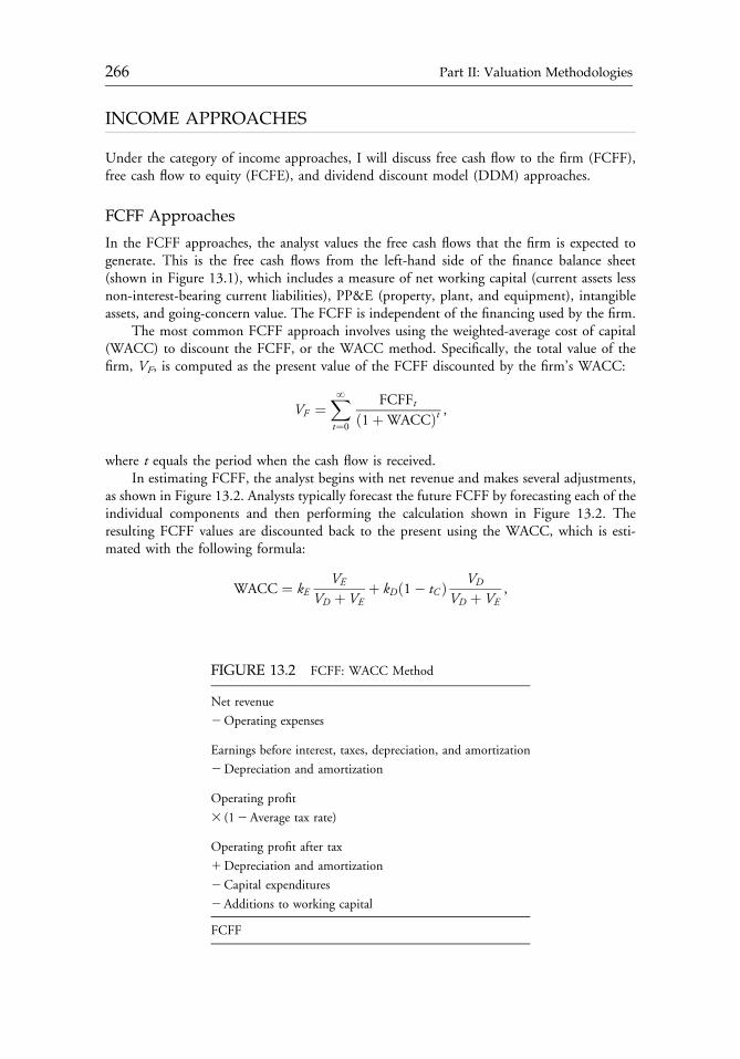
INCOME APPROACHES
Under the category of income approaches, I will discuss free cash flow to the firm (FCFF),free cash flow to equity (FCFE), and dividend discount model (DDM) approaches.
FCFF Approaches
In the FCFF approaches, the analyst values the free cash flows that the firm is expected togenerate. This is the free cash flows from the left-hand side of the finance balance sheet(shown in Figure 13.1), which includes a measure of net working capital (current assets lessnon-interest-bearing current liabilities), PP&E (property, plant, and equipment), intangibleassets, and going-concern value. The FCFF is independent of the financing used by the firm.
The most common FCFF approach involves using the weighted-average cost of capital(WACC) to discount the FCFF, or the WACC method. Specifically, the total value of thefirm, VF, is computed as the present value of the FCFF discounted by the firm’s WACC:
VF ¼XNt¼0
FCFFtð1þWACCÞt ,
where t equals the period when the cash flow is received.In estimating FCFF, the analyst begins with net revenue and makes several adjustments,
as shown in Figure 13.2. Analysts typically forecast the future FCFF by forecasting each of theindividual components and then performing the calculation shown in Figure 13.2. Theresulting FCFF values are discounted back to the present using the WACC, which is esti-mated with the following formula:
WACC ¼ kEVE
VD þ VEþ kDð1� tC Þ VD
VD þ VE,
FIGURE 13.2 FCFF: WACC Method
Net revenue
2Operating expenses
Earnings before interest, taxes, depreciation, and amortization
2Depreciation and amortization
Operating profit
3 (12Average tax rate)
Operating profit after tax
1Depreciation and amortization
2Capital expenditures
2Additions to working capital
FCFF
c13 12 September 2012; 13:53:10
266 Part II: Valuation Methodologies
where
kE5 cost of equity (often estimated using the CAPM)
kD5 cost of debt (should be consistent with the firm’s financial policy)
tC5 corporate tax rate
VE /(VD1VE)5market value of equity to market value of total capital (i.e., proportionof the firm’s capital represented by equity)
VD /(VD1VE)5market value of debt to market value of total capital (i.e., proportion ofthe firm’s capital represented by debt)
The WACC is simply a weighted average of the various layers of financing used by thebusiness. The first term represents the proportionate cost of equity (in practice, there isactually a separate term like this for each class of equity), and the second term represents theproportionate cost of debt. When analysts use this method, the key assumption concerns howthe firm’s operations will be financed in the future. For example, the financing might be80 percent equity and 20 percent debt. Or it might be 30 percent equity and 70 percent debt.
The WACC method is typically used to value a mature firm under the assumption thatover the long run, the firm will manage its capital structure toward some target level of debt.With that assumption, the analyst can just plug in the percentages and does not have toactually estimate VD or VE.
If it is not reasonable to assume that the firm’s capital structure will be stable in the future(for example, if the firm is currently highly leveraged and its leverage is expected to decline),then the WACC method is problematic. Assuming a constant capital structure when valuingsuch a business can yield misleading results. Some of the other methods I will discuss can beused to work around that problem, but the WACC method is the most common and simplestincome approach that uses FCFF. It is adequate for most analyses of large, publicly tradedfirms that are relatively stable. These types of firms manage their capital structure within anadmittedly broad range sometimes, but they typically target a particular structure if for noother reason than to maintain a specific debt credit rating.
In cases where it is not reasonable to assume that the firm is managing its financial policytoward some specific capital structure, an analyst can use another approach called the adjustedpresent value (APV) method. This method involves first valuing the business under theassumption that it is financed entirely with equity and then adding the present value ofthe effects of the firm’s financing decisions to this unlevered firm value.
The APV method is a lot easier to use than the WACC method when the debt-to-total-capital ratio for a firm is changing over time. The APV method also uses the FCFF—exactlythe same cash flow definition used with the WACC method. With the APV method, how-ever, FCFF is discounted using the unlevered WACC to obtain the unlevered value of thefirm, VUF.
VUF ¼Xnt¼0
FCFFtð1þUnlevered WACCÞt :
The unlevered WACC is literally the cost of equity when the firm has no debt. If theCAPM is used to estimate the cost of equity, the unlevered WACC is simply the risk-free rateplus the asset beta (or unlevered beta) times the market risk premium. Thus,
c13 12 September 2012; 13:53:11
Chapter 13 Choosing the Right Valuation Approach 267
Unlevered WACC5 kF1 βA 3 Market risk premium
where
kF 5 risk-free rate
βA5 asset beta
Market risk premium5 expected market return less the risk-free rate
Once the analyst has estimated the unlevered value of the firm, the effects of the firm’sfinancing decisions on the value of the firm are computed and added to the unlevered value toobtain the APV. The APV method is usually applied in this way:
APV ¼ VUF þXnt¼0
Tax ratet 3 Interesttð1þ kDÞt :
The second term in this equation is the present value of the interest tax shields that the firm isexpected to realize from its debt financing. This is simply the present value of the tax ratetimes the interest payment in each year discounted using the cost of debt, kD. The cost of debtis often used in this calculation under the assumption that the tax shields will be realized whenthe firm is able to make its debt payments; therefore, the tax shields are about as risky as thedebt. By that reasoning, the cost of debt is an appropriate discount rate for the tax shields.
When using the APV method, analysts should be aware of one issue in particular: Withthe way this method is typically applied, something is missing. If the APV were plotted as afunction of debt (i.e., APV on the vertical axis and debt level on the horizontal axis), the resultwould be an upward-sloping line that never turns downward. Of course, this implies thatmore debt is always better. The problem is that bankruptcy costs are missing from thecalculation. Typically, as a firm levers up, the probability that it will get into financial dif-ficulty increases. There is thus an increase in the expected costs associated with financialdistress, which should cause the line in my example to start curving down at some point.Consequently, when the APV method is applied, analysts should be sure to include not onlythe benefits of debt (such as the value of the tax shield) but also the costs (such as bankruptcycosts and possibly debt issuance costs).
The APV method is easier to use in instances when a firm has a changing capital structurebecause it involves forecasting the dollar interest payments rather than the debt-to-value ratio,which is inherently difficult to estimate in an exercise where the goal is to estimate the value ofthe firm or its securities in the first place.
For example, the APVmethod would be particularly useful for a leveraged buyout analysis.Suppose a company is acquiring another business and levering it up to 65 percent debt.Furthermore, suppose that over the next five or six years, the company is going to pay downthe debt to some normal level and then maintain a more typical capital structure thereafter. Insuch a case, the financing is set up front and the analyst has a good idea of what the interestpayments will be. The cost of each of the layers of debt and the repayment schedules are known,so the analyst can estimate the cost of debt and the present value of the tax shields year by year.In a case like this, the APV method is easier to apply than the WACC method.
The bottom line with the FCFF approaches is that the WACC method is relativelystraightforward to use with a mature firm where the analyst can assume that the firm willtarget a constant capital structure going forward. In cases where the capital structure maychange substantially over time, the APV method can be much easier to use.
c13 12 September 2012; 13:53:11
268 Part II: Valuation Methodologies
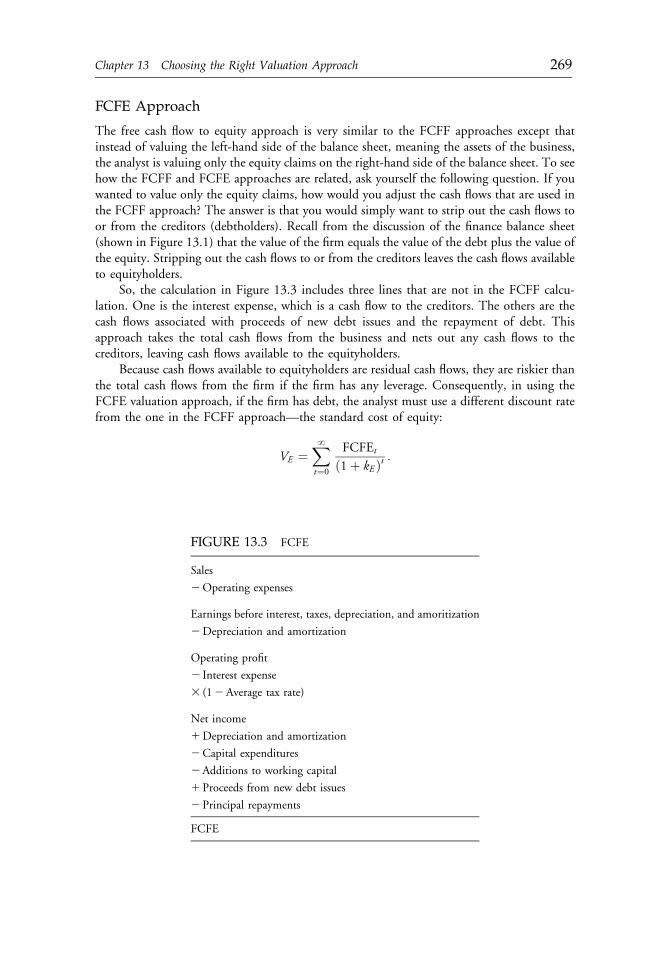
FCFE Approach
The free cash flow to equity approach is very similar to the FCFF approaches except thatinstead of valuing the left-hand side of the balance sheet, meaning the assets of the business,the analyst is valuing only the equity claims on the right-hand side of the balance sheet. To seehow the FCFF and FCFE approaches are related, ask yourself the following question. If youwanted to value only the equity claims, how would you adjust the cash flows that are used inthe FCFF approach? The answer is that you would simply want to strip out the cash flows toor from the creditors (debtholders). Recall from the discussion of the finance balance sheet(shown in Figure 13.1) that the value of the firm equals the value of the debt plus the value ofthe equity. Stripping out the cash flows to or from the creditors leaves the cash flows availableto equityholders.
So, the calculation in Figure 13.3 includes three lines that are not in the FCFF calcu-lation. One is the interest expense, which is a cash flow to the creditors. The others are thecash flows associated with proceeds of new debt issues and the repayment of debt. Thisapproach takes the total cash flows from the business and nets out any cash flows to thecreditors, leaving cash flows available to the equityholders.
Because cash flows available to equityholders are residual cash flows, they are riskier thanthe total cash flows from the firm if the firm has any leverage. Consequently, in using theFCFE valuation approach, if the firm has debt, the analyst must use a different discount ratefrom the one in the FCFF approach—the standard cost of equity:
VE ¼XNt¼0
FCFEt
ð1þ kE Þt :
FIGURE 13.3 FCFE
Sales
2Operating expenses
Earnings before interest, taxes, depreciation, and amoritization
2Depreciation and amortization
Operating profit
2 Interest expense
3 (12Average tax rate)
Net income
1Depreciation and amortization
2Capital expenditures
2Additions to working capital
1Proceeds from new debt issues
2Principal repayments
FCFE
c13 12 September 2012; 13:53:11
Chapter 13 Choosing the Right Valuation Approach 269
Unfortunately, this approach can be very difficult to apply in practice, especially for amature firm, because it has the worst of both worlds from the examples I have discussed. Inorder to forecast these cash flows, an analyst must forecast the actual dollar interest expenseincurred to finance the firm in each year. In order to estimate the discount rate, the analystalso has to forecast the debt-to-total-capital ratio, on a market value basis, for each year.Remember that the cost of equity is a function of the levered beta. Going forward, as thedollar value of outstanding debt changes (or even if it does not change), the debt-to-total-capital ratio is likely to be moving around as the value of the firm also changes. For thediscount rate to be consistent with the cash flow forecasts (which include forecasts of thedollar interest expense), the analyst must estimate future debt-to-equity ratios that are con-sistent with the dollar interest numbers he or she is putting in the cash flow forecasts. So, thisapproach can be very difficult and may require several iterations through the computations toobtain a reasonable result. It is a lot easier to use the WACC or the APV method to value theentire firm and then to just subtract the value of the debt if the analyst wants to estimatethe value of the equity.
DDM Approach
The dividend discount model approach is the third income approach I will discuss in thischapter. In the purest form, the DDM approach values the stream of cash flows thatshareholders expect to receive. In contrast, the FCFF and FCFE approaches use cash flowsavailable for distribution to shareholders. The firm may or may not be expected to distributeall available cash flows.
DDMs are easy to use because they are simple models. But I will argue that they arelikewise easy to abuse. They can be used to develop ballpark estimates for some shares, but inmany cases, they are not very useful if the objective is to determine the intrinsic value of abusiness.
Another thing to keep in mind is that the application of DDMs became more difficult asdividend payments declined from the late 1980s through the end of the 1990s. Marketvaluations and the values implied by traditional DDMs diverged during this period. Althoughdividend payments have risen somewhat since 2000, dividend yields remain low by historicalstandards.
That said, the modeling technologies used by DDMs are still quite useful becausethey can be used elsewhere, such as with the FCFF or FCFE approaches. In the FCFF orFCFE approaches, analysts typically forecast cash flows year by year for several years andthen estimate a terminal value as of the last year that is forecasted individually. Instead,they could simply compute the present values of all future cash flows using one of theDDM models.
When analysts use the constant growth DDM, which I will discuss in detail shortly, theyare simply assuming that the growth rate in dividends will be constant in perpetuity. With atwo-stage model, an analyst assumes one rate over some period of time and then a differentgrowth rate thereafter. These are really just modeling techniques that can be applied to anycash flow stream, including FCFF and FCFE, depending on how the analyst sees the cashflows evolving over time. So, DDMs can be useful in some circumstances as a distinct val-uation method, but even where analysts do not feel comfortable forecasting the dividends, orif they believe the dividends do not reflect the intrinsic value of the business, DDM methodscan be applied in other cash flow valuation approaches.
c13 12 September 2012; 13:53:11
270 Part II: Valuation Methodologies
Constant Growth Model
The constant growth DDM is familiar to most analysts:
P0 ¼ DIV0ð1þ gÞkE � g
¼ DIV1
kE � g,
where
P05 current price of stock
DIV05 dividend payment today
DIV15 dividend payment next period
g5 dividend growth rate
kE5 cost of equity
Keep in mind that a lot of assumptions are implicit in this model; for example, one assumptionis that the cost of equity is greater than the growth rate of dividends. If the dividend growthrate is greater than the cost of equity, the model yields a negative share price. Of course, thiscannot happen because equity is an option on the underlying assets of the firm andoptions cannot have negative values. So, this model cannot work if the dividend growth rate isgreater than the cost of equity, which is one reason why it makes sense to use this model onlywhen the growth rate has slowed to some long-run sustainable rate. (Another reason is that ifone assumes a growth rate that is greater than the expected rate of inflation plus the real growthrate in the economy, then one is essentially assuming that the firm will become larger than theeconomy. Remember that this model assumes a growth rate in perpetuity.)
In addition to assuming an infinite time horizon, the model assumes a constant return onreinvested equity. Many do not realize they are making this assumption when they use thismodel. The model assumes that every year, as the business grows and the firm reinvests aconstant percentage of its earnings (the dividend payout rate is assumed to be constant), thefirm will earn the same rate of return on reinvested capital. The dollar amount is increasingannually while the rate of return is remaining constant. Thus, some fairly strict assumptionsunderlie the constant growth model.
Alternative Form of Constant Growth DDM
An alternative form of the constant growth model is a little more complicated but providessome interesting insights:
P0 ¼ EPS1bkE
þ EPS1ð1� bÞðROE=kEÞkE
,
where
EPS15 earnings per share in the next period
b5 the dividend payout ratio (dividend per share/earnings per share)
ROE5 return on equity
This model is just like the traditional constant growth model except it makes a differentassumption regarding reinvestment: Instead of assuming that a constant proportion of earnings
c13 12 September 2012; 13:53:11
Chapter 13 Choosing the Right Valuation Approach 271
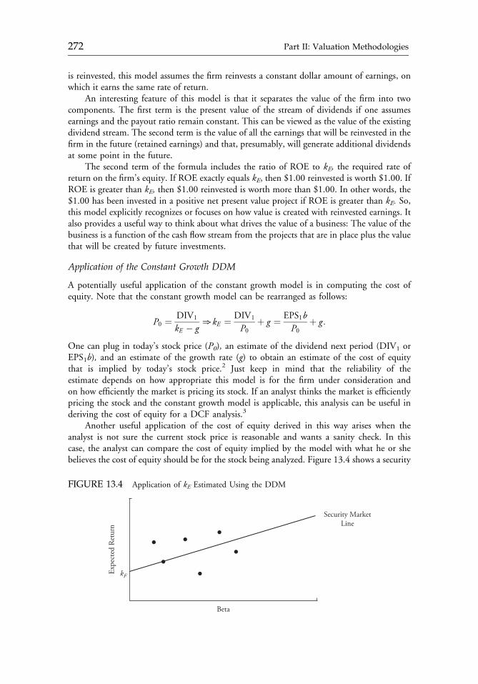
is reinvested, this model assumes the firm reinvests a constant dollar amount of earnings, onwhich it earns the same rate of return.
An interesting feature of this model is that it separates the value of the firm into twocomponents. The first term is the present value of the stream of dividends if one assumesearnings and the payout ratio remain constant. This can be viewed as the value of the existingdividend stream. The second term is the value of all the earnings that will be reinvested in thefirm in the future (retained earnings) and that, presumably, will generate additional dividendsat some point in the future.
The second term of the formula includes the ratio of ROE to kE, the required rate ofreturn on the firm’s equity. If ROE exactly equals kE, then $1.00 reinvested is worth $1.00. IfROE is greater than kE, then $1.00 reinvested is worth more than $1.00. In other words, the$1.00 has been invested in a positive net present value project if ROE is greater than kE. So,this model explicitly recognizes or focuses on how value is created with reinvested earnings. Italso provides a useful way to think about what drives the value of a business: The value of thebusiness is a function of the cash flow stream from the projects that are in place plus the valuethat will be created by future investments.
Application of the Constant Growth DDM
A potentially useful application of the constant growth model is in computing the cost ofequity. Note that the constant growth model can be rearranged as follows:
P0 ¼ DIV1
kE � g.kE ¼ DIV1
P0þ g ¼ EPS1b
P0þ g :
One can plug in today’s stock price (P0), an estimate of the dividend next period (DIV1 orEPS1b), and an estimate of the growth rate (g) to obtain an estimate of the cost of equitythat is implied by today’s stock price.2 Just keep in mind that the reliability of theestimate depends on how appropriate this model is for the firm under consideration andon how efficiently the market is pricing its stock. If an analyst thinks the market is efficientlypricing the stock and the constant growth model is applicable, this analysis can be useful inderiving the cost of equity for a DCF analysis.3
Another useful application of the cost of equity derived in this way arises when theanalyst is not sure the current stock price is reasonable and wants a sanity check. In thiscase, the analyst can compare the cost of equity implied by the model with what he or shebelieves the cost of equity should be for the stock being analyzed. Figure 13.4 shows a security
FIGURE 13.4 Application of kE Estimated Using the DDM
Expe
cted
Ret
urn
Security MarketLine
kF
Beta
c13 12 September 2012; 13:53:11
272 Part II: Valuation Methodologies
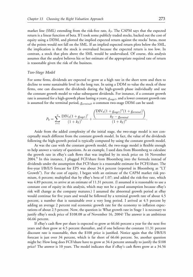
market line (SML) extending from the risk-free rate, kF. The CAPM says that the expectedreturn is a linear function of beta. If I took some publicly traded stocks, backed out the cost ofequity using a DDM, and plotted the implied expected return against the stocks’ betas, mostof the points would not fall on the SML. If an implied expected return plots below the SML,the implication is that the stock is overvalued because the expected return is too low. Incontrast, a stock that plots above the SML would be undervalued. Of course, this analysisassumes that the analyst believes his or her estimate of the appropriate required rate of returnis reasonable given the risk of the business.
Two-Stage Model
For some firms, dividends are expected to grow at a high rate in the short term and then todecline to some sustainable level in the long run. In using a DDM to value the stock of thesefirms, one can discount the dividends during the high-growth phase individually and usethe constant growth model to value subsequent dividends. For instance, if a constant growthrate is assumed for a high-growth phase lasting n years, gstage1, and a lower constant growth rateis assumed for the terminal period, gterminal, a common two-stage DDM can be used:
P0 ¼Xnt¼1
DIV0ð1þ gstage1Þtð1þ kEÞt þ
DIV0ð1þ gstage1Þnð1þ gterminal ÞkE � gterminal
� �ð1þ kE Þn :
Aside from the added complexity of the initial stage, the two-stage model is not con-ceptually much different from the constant growth model. In fact, the value of the dividendsfollowing the high-growth period is typically computed by using the constant growth model.
As was the case with the constant growth model, the two-stage model is flexible enoughto help answer a variety of questions. As an example, I used data from Bloomberg to calculatethe growth rate in eBay’s cash flows that was implied by its stock price on 16 November2004.4 In this instance, I plugged FCF/share from Bloomberg into the formula instead ofdividends under the assumption that FCF/share is a reasonable estimate for FCFE/share. Thefive-year I/B/E/S forecast for EPS was about 34.4 percent (reported in Bloomberg as “LTGrowth”). For the cost of equity, I began with an estimate of the CAPM market risk pre-mium, 6 percent; multiplied that by eBay’s beta of 1.07; and added the risk-free rate, whichwas 4.89 percent, to arrive at an estimate of 11.31 percent. (I assumed it is reasonable to use aconstant cost of equity in this analysis, which may not be a good assumption because eBay’srisk will change as the company matures.) I assumed the abnormal growth period at eBaywould continue for five years and would be followed by a terminal growth rate of about 4.5percent, a number that is sustainable over a very long period. I arrived at 4.5 percent byadding an average 2 percent real economic growth rate for the economy to inflation expec-tations of about 2.5 percent. Now, the question is: What growth rate in Stage 1 is necessary tojustify eBay’s stock price of $108.08 as of November 16, 2004? The answer is an ambitious66.66 percent.
If eBay’s cash flow per share is expected to grow at 66.66 percent a year for the next fiveyears and then grow at 4.5 percent thereafter, and if one believes the constant 11.31 percentdiscount rate is reasonable, then the $108 price is justified. Notice again that the I/B/E/Sforecast is just over 34 percent, which is far short of 66.66 percent. So, another questionmight be: How long does FCF/share have to grow at 34.4 percent annually to justify the $108price? The answer is 10 years. The model indicates that if eBay’s cash flows grow at a 34.56
c13 12 September 2012; 13:53:12
Chapter 13 Choosing the Right Valuation Approach 273
percent annual rate for 10 years and then grow at 4.5 percent a year thereafter, this price isjustified.
This and other DDM models are thus useful in helping analysts think about whatassumptions are implicit in the price observed in the market. In other words, these models canbe used as a sanity check in support of other valuation approaches as well as an independentapproach for estimating the intrinsic value of a stock directly.
CONTINGENT CLAIMS APPROACH:OPTION VALUATION METHOD
The last of the valuation approaches I will discuss are those that use option valuation methods.To see why option valuation concepts are relevant to the valuation of equity, consider a firmwith a single $5million face value, zero-coupon debt issue outstanding that matures in one year.Furthermore, assume that VF
� is the value of the assets of the firm when the debt matures a yearfrom now.
Figure 13.5 shows the payoffs to the debtholders and to the equityholders when the debtin this example matures. If the firm is worth more than $5 million, the debtholders will bepaid off in full and the shareholders will get any residual value above the $5 million face valueof the debt, F. If the value of the firm is below $5 million, the debtholders, at least in theory,get the firm. In other words, the shareholders have an option to default. The shareholders’downside is limited to what they have already invested in the firm, and the debtholders receivethe residual value of the firm if that option is exercised.
Another way of thinking about this idea is to realize that the shareholders essentially havea call option on the underlying assets of the firm. When the debt matures, the shareholdershave the option to pay off the debt or walk away. If, on the one hand, the value of the firm isgreater than $5 million, the shareholders can pay the $5 million and realize the difference invalue even if they do not want to continue to hold the firm; they can always sell it and pocketthe difference. If, on the other hand, the firm’s assets are worth less than $5 million, theshareholders will let their option expire and will walk away, leaving the debtholders to receivewhatever is left.
The debtholders, in turn, have a payoff function similar to that of someone who is short aput option. The debtholders have effectively sold the shareholders a put option on the firm. Theshareholders have the right to put the firm back to the debtholders, forcing the debtholders tobear the loss if the value of the firm is less than the $5 million the debtholders are owed.
FIGURE 13.5 Option Characteristics of Debt and Equity Claims
F
VF∗ VF
∗
VF∗�F
VD∗ VE
∗
F � $5 million
A. Payoff to Debtholders at Maturity B. Payoff to Shareholders at Maturity
F � $5 million
c13 12 September 2012; 13:53:12
274 Part II: Valuation Methodologies
Therefore, debt and equity are essentially options on the underlying assets of the firm.Whenever there are multiple claims on an underlying asset that have different priorities, analystsshould be aware that they may be dealing with option claims. Recognizing this, one can see therationale, under certain circumstances, of valuing equity by using option-pricing methods. Forexample, the following is a variation of the Black�Scholes model that includes dividends:
C ¼ VF e�δTNlnðVF=F Þ þ ðrf � δþ σ2=2ÞT
σffiffiffiffiT
p24
35
� Fe�rf TNlnðVF=F Þ þ ðrf � δþ σ2=2ÞT
σffiffiffiffiT
p24
35,
where
VF5 value of the firm
F5 face value of the debt in this corporate valuation context
T5 length of time until the debt matures
rf 5 risk-free rate
σ5 volatility of the rate of return on the underlying asset, the firm
δ5 dividend yield
Note that the above six variables drive the value of this option.It is quite possible to find real-world companies for which aDCF valuation analysis yields a
negative equity value, which I already pointed out is unreasonable. It is also common to seestocks in this situation trading at a positive, albeit relatively small, price. Just because a DCFanalysis yields a negative number, implying a value of zero, does not mean the equity isworthless. Things change. For example, general economic conditions change, industry condi-tions change, firm conditions change, quotas and tariffs change, and capital market conditionschange. Some possibility virtually always exists with an operating company that between nowand the time when the firm’s debt matures, the value of the firm will exceed the face value of thedebt, the firm will pay off the debt, and the shareholders will receive some residual value.
Valuing those possibilities is very difficult in the context of a DCF analysis because thefirm’s risk, and therefore its discount rate, is changing over time as the underlying char-acteristics of the business change. One way to get around this problem is to use an option-pricing approach.
The option I have just discussed is the option to liquidate the firm where the shareholdershave the option to absolve themselves of the firm’s obligations by filing for bankruptcy.Option-pricing models can also be used to value an option to delay an investment. Optionslike this are commonly valued in the oil and gas industry in the process of valuing oil and gasfields. For example, a landowner might have the option to tap into undeveloped reserves. Invaluing such an option, the analyst would take into account the length of the option (i.e., howlong the landowner has to develop the reserves), the volatility of the expected cash flows, thepresent value of the cash flows that are expected to be generated (which will be tied to oilprices), and how much it will cost the landowner to develop the reserves. So, the strike price,or the exercise price, in this case is how much it costs to develop the field. The value of thefield is the present value of all the cash inflows once the landowner has developed it.
c13 12 September 2012; 13:53:12
Chapter 13 Choosing the Right Valuation Approach 275
CONCLUSION
This chapter discusses various valuation tools and methods and the circumstances underwhich they are used. It is important for an analyst to understand these concepts. It is alsoimportant to recognize that, ultimately, the quality of any value estimate depends on how wellthe analyst understands the firm and its competitive position, its operating strategy, and whatcould happen in the future. Those expectations about the future drive the cash flow forecastsand ultimately determine how well the analyst estimates the value of the business. In essence,the quality of any value estimate depends on the quality of the information that is availableand how well that information is used.
QUESTION AND ANSWER SESSION
Question: Can you elaborate on valuing a controlling interest versus a minority interest?Parrino: In valuing a controlling interest, you must account for the incremental value of
control. The magnitude of the adjustment depends on the situation. It reflects the factthat control of a firm affords the controlling shareholder the right to set the strategicdirection of the firm, hire and fire managers, buy or sell assets, set financial policies, andso on. A noncontrolling shareholder does not have the ability to do these things. Theincremental value of control is specific to the party gaining control and varies with howthe business is run and how it is financed. Keep in mind that the price actually paidwhen one business buys a controlling interest in another business reflects some generalbenefits of control as well as benefits and synergies that are expected to be realized fromthe pairing of the two specific businesses involved in the transaction. It is not always easyto isolate the effect of the control premium on the value of a business from the effects ofother factors, such as synergies.
If you are valuing a controlling interest, your cash flow forecast and discount ratemay be very different from the case where you are valuing a minority interest.Additionally, there will be implications for how you can use, for example, a guidelinecomparables analysis.
Question: In a free cash flow analysis, should you adjust for off-balance-sheet items—especially, for example, for companies with a lot of operating leases?
Parrino: Yes, off-balance-sheet items should be reflected. You are trying to get at the trueeconomic substance of the business, and off-balance-sheet items are certainly importantin this regard. In the particular case of operating leases, the relevant impact of thoseleases is generally already reflected in the operating expenses of the business and,therefore, in the earnings or cash flows.
A situation where you would have to be careful with operating leases is where thelease payments differ from market and are likely to be adjusted. In such a case, youwould have to reflect any expected adjustments in your cash flow forecasts.
In general, you have to be especially careful to account for off-balance-sheet itemslike liabilities that are not normally reflected in the operating cash flows—for instance,off-balance-sheet debt. On the flip side, you should also account for off-balance-sheetassets in your analysis.
Question: To get a valuation that makes any sense, doesn’t it imply using a target debt-to-capital ratio that is significantly higher than reality?
c13 12 September 2012; 13:53:12
276 Part II: Valuation Methodologies
Parrino: If a company’s stock trades at a price that implies higher leverage, then that mightsuggest that the market expects a change in financial policies at some point in the future.Alternatively (and this suggests that a contingent claims analysis might be more appro-priate than the DCF analysis I believe the questioner is thinking about), the incrementalvalue could be associated with some option value, perhaps even option value that is derivedin part from a low degree of leverage.
For example, many high-tech companies carry a lot of cash on their balance sheets.Even those that don’t have a lot of cash do not tend to carry much debt. One explanationfor these conservative financial policies is that these companies are operating comparativelyrisky businesses and the cost of levering up would be high.
Another reason formaintaining lower leverage is that low leverage provides companieswith more financial flexibility. This allows them to take advantage of attractiveopportunities as they arise, such as acquisitions or capital investment opportunities.Low leverage also provides companies with the ability to counter strategic moves by theircompetitors, such as when competitors change their pricing policies. These benefits mightbe reflected in the stock price but will be hard to capture in a DCF analysis because youdon’t know what options these companies are likely to have in the future. So, it can bereally tough to value companies in situations like that.
Question: In calculating free cash flow, should there be a distinction between maintenancecapital expenditures and growth capital expenditures?
Parrino: Yes, absolutely. From a forecasting standpoint, it is usually important to separate thetwo. In many industries, maintenance capital expenditures (CAPEX) are relativelystable as a fraction of operating characteristics that reflect the size of the business, such asrevenues. That makes maintenance CAPEX pretty easy to forecast.
Growth capital expenditures are typically more complicated to forecast. Oneof the things I am always very concerned about in a DCF analysis is making surethat my projections are internally consistent. If a firm is operating at 99 percentcapacity and I am forecasting unit sales to double, I had better make sure that myprojections include enough growth in CAPEX to accommodate the increase in unitsales. By separating maintenance from growth CAPEX, I am forcing myself toconsciously think about when capacity should be added and how much that capacitywill cost the company.
Question: Should there be an adjustment made for companies that are using stock to fundCAPEX?
Parrino: If the question being asked is whether it matters if the firm’s stock is over- orundervalued and stock is used instead of cash, the answer is most likely no. Forexample, in capital budgeting, if a firm sells overvalued stock to fund CAPEX and ifthe firm could have realized the same value if it sold the stock to finance somethingelse, such as a dividend, there is an opportunity cost associated with using theproceeds from the sale of the stock to fund CAPEX. This opportunity cost equals thevalue realized from the sale of the stock and should be accounted for in the capitalbudgeting analysis.
The same general idea applies in business valuation. An adjustment for usingstock instead of cash should be made only if using stock effectively changes the costof the investment.
Question: In a two-stage DDM, isn’t the terminal value assumption even more importantthan that for the initial growth stage?
c13 12 September 2012; 13:53:12
Chapter 13 Choosing the Right Valuation Approach 277
Parrino: It certainly can be. It depends on the nature of the business. In a lot of businesses, ahigh proportion of the value is derived in years beyond the initial stage. But that isn’t tosay that the initial stage isn’t also important. For example, if the initial stage is five yearsin length, then the number used in the numerator when you calculate the cash flow forYear 6 will be very sensitive to your assumption about the growth rate in the initialstage. Changing the annual growth rate by just 1 percentage point over the first fiveyears can have a huge impact on the dollar value of the terminal value.
So, I would argue that they’re both very important. But I will concede that whenyou are computing the terminal value, especially of a business with high-growthoptions, where most of the value is further out, you have to pay special attention to theassumptions you are making when computing the terminal value.
Question: What do you think about using EPS for an estimate of cash flow per share?Parrino: EPS can probably provide a good approximation, at least to the extent that (1)
noncash charges and investment expenditures are relatively small numbers or largelycancel each other out and (2) the company is running a cash business where earnings area good reflection of actual cash flows from operations. Of course, the applicability ofany valuation approach or assumption to a specific industry or company depends on thecharacteristics of that industry or company. In some cases, a shortcut like using EPS asan estimate of cash flow per share is reasonable. In other cases, it is not.
NOTES
1. Enterprise value is typically defined as being equal to market value of common stock plusmarket value of preferred stock plus market value of debt minus excess cash and cashequivalents.
2. To estimate the growth rate for an exercise such as this, one might use I/B/E/S or con-sensus forecasts.
3. Other, more complicated models can be used to accomplish this same task, but the mathis somewhat more complex.
4. All data were as of November 16, 2004.
c13 12 September 2012; 13:53:12
278 Part II: Valuation Methodologies
CHAPTER 14VALUING ILLIQUIDCOMMON STOCK
Edward A. Dyl and George J. Jiang
Illiquid common stock is worth less than stock that can be readily sold because theinvestor incurs an opportunity cost by being locked into the investment. Quantifyingthe amount of this illiquidity discount is an important issue in valuing certaincommon stock, especially for estate valuations. We examine whether a previouslydeveloped analytical model for valuing the lost “option to sell” when a stock isilliquid is a useful, practical tool for valuing illiquid common stock.
Some common stock cannot be easily liquidated. The stock of companies that are not publiclytraded is an obvious example. Restricted stock in publicly traded companies may also beilliquid when the restrictions prohibit its sale. A formal contractual agreement when the stockis issued (e.g., letter stock) may limit liquidity, or the shares may be illiquid because they arenot registered with the U.S. SEC. Unregistered stock in publicly traded companies is subjectto selling limitations under Rule 144, which mandates a minimum holding period of one yearfor unregistered stock and also limits how much stock can subsequently be sold by anindividual in any three-month period.1 Finally, a large holding of a particular common stockis essentially illiquid if the underlying public market for the stock is thin relative to the size ofthe block. For example, blocks of stock in secondary distributions generally sell at a pricelower than the current market price of the stock because the underlying market is not elasticenough to absorb the additional shares at the current price (Mikkelson and Partch 1985).
The value of an illiquid asset is generally lower than the value of a similar asset that isreadily marketable. Investors value liquidity because the absence of liquidity limits the owner’soption to convert an asset to cash, which increases opportunity costs. That is, investors arelocked into their holding of that particular asset and, therefore, locked into the vagaries of
Reprinted from the Financial Analysts Journal (July/August 2008):40�47. When this article wasoriginally published, Edward A. Dyl was Sheafe/Neill/Estes Professor of Finance at the University ofArizona, Tucson, and George J. Jiang was associate professor of finance at the University of Arizona,Tucson.
c14 12 September 2012; 13:59:54
279
fluctuating values of the asset. And asset values, particularly values of common stocks, canfluctuate widely.
Valuing illiquid common stock is a contentious issue and frequently involves largeamounts of money. The valuations are required, however, for estate valuations for tax pur-poses, merger and acquisition transactions, divorce settlements and other forms of partnershipdissolutions, and other situations in which the valuation has financial consequences forthe parties involved. Valuing illiquid common stock may result in one party gaining at theexpense of the other; thus, the valuations often take place in litigious environments.
The state of the art in valuing illiquid common stock belies the importance of the topic.The dominant approach is to compute the mean or median percentage discount observed forsales of restricted common stock in the past and apply this discount to the stock being valued.The validity of this approach is doubtful. Also, the assumption that the marketability discountfor a stock is constant over time is questionable. Discounts on restricted common stock varywidely from company to company, and none of the studies of restricted stock that weexamined provides a credible basis for estimating the value of marketability for a specificcompany’s stock at a particular time. Moreover, most of the existing studies are out of date.The most recent study, that of Bajaj, Denis, Ferris, and Sarin (2001), examined discounts onprivate placements of restricted common stock for 1990�1995.2
In this chapter, we examine the usefulness of an options-based framework developed byLongstaff in 1995 for estimating the value of the marketability (i.e., liquidity) for a particularcommon stock for a particular investor at a particular time.
VALUE OF LIQUIDITY
Longstaff’s fundamental insight is that liquidity is properly construed as the option to sell anasset at the time of one’s choosing (i.e., liquidity is a put option). Thus, the value of liquiditycan be estimated by using techniques from option-pricing theory. Longstaff’s analysis assumesa hypothetical world where a perfectly liquid asset is continuously traded in a frictionlessmarket with a constant riskless interest rate and where an investor with perfect market timingsells the asset and invests the proceeds in the riskless asset to maximize the value of theinvestor’s portfolio. If the investor is restricted from selling the asset for a period of time equalto T, the investor cannot trade assets optimally to maximize the value of the portfolio.
Longstaff derived a model that measures the loss in value resulting from the opportunitycost imposed by the period of time during which the asset is not liquid. This model is asfollows:
Maximum discount ¼ 2þ σ2T2
� �½N ðd Þ� þ
ffiffiffiffiffiffiffiffiffiσ2T2π
rexp � σ2T
8
� �� 1, ð14:1Þ
where
σ5 standard deviation of the company’s daily stock returns (annualized)
T 5 length of time that the shares are illiquid
N(d )5 probability that a standardized, normally distributed, random variable is greateror less than d, where d ¼
ffiffiffiffiffiffiffiffiffiσ2T
p=2
c14 12 September 2012; 13:59:54
280 Part II: Valuation Methodologies
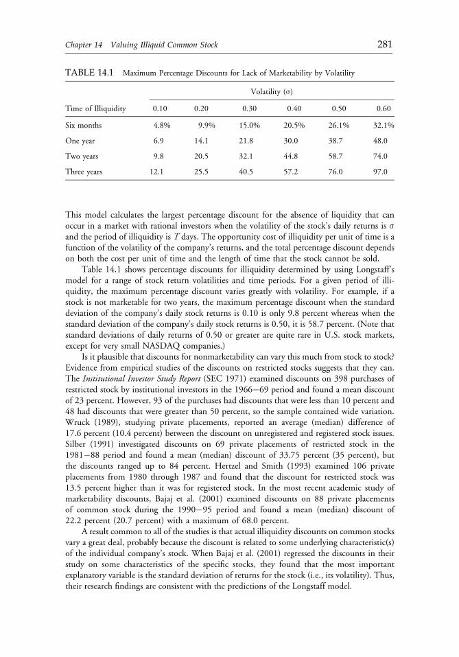
This model calculates the largest percentage discount for the absence of liquidity that canoccur in a market with rational investors when the volatility of the stock’s daily returns is σand the period of illiquidity is T days. The opportunity cost of illiquidity per unit of time is afunction of the volatility of the company’s returns, and the total percentage discount dependson both the cost per unit of time and the length of time that the stock cannot be sold.
Table 14.1 shows percentage discounts for illiquidity determined by using Longstaff’smodel for a range of stock return volatilities and time periods. For a given period of illi-quidity, the maximum percentage discount varies greatly with volatility. For example, if astock is not marketable for two years, the maximum percentage discount when the standarddeviation of the company’s daily stock returns is 0.10 is only 9.8 percent whereas when thestandard deviation of the company’s daily stock returns is 0.50, it is 58.7 percent. (Note thatstandard deviations of daily returns of 0.50 or greater are quite rare in U.S. stock markets,except for very small NASDAQ companies.)
Is it plausible that discounts for nonmarketability can vary this much from stock to stock?Evidence from empirical studies of the discounts on restricted stocks suggests that they can.The Institutional Investor Study Report (SEC 1971) examined discounts on 398 purchases ofrestricted stock by institutional investors in the 1966�69 period and found a mean discountof 23 percent. However, 93 of the purchases had discounts that were less than 10 percent and48 had discounts that were greater than 50 percent, so the sample contained wide variation.Wruck (1989), studying private placements, reported an average (median) difference of17.6 percent (10.4 percent) between the discount on unregistered and registered stock issues.Silber (1991) investigated discounts on 69 private placements of restricted stock in the1981�88 period and found a mean (median) discount of 33.75 percent (35 percent), butthe discounts ranged up to 84 percent. Hertzel and Smith (1993) examined 106 privateplacements from 1980 through 1987 and found that the discount for restricted stock was13.5 percent higher than it was for registered stock. In the most recent academic study ofmarketability discounts, Bajaj et al. (2001) examined discounts on 88 private placementsof common stock during the 1990�95 period and found a mean (median) discount of22.2 percent (20.7 percent) with a maximum of 68.0 percent.
A result common to all of the studies is that actual illiquidity discounts on common stocksvary a great deal, probably because the discount is related to some underlying characteristic(s)of the individual company’s stock. When Bajaj et al. (2001) regressed the discounts in theirstudy on some characteristics of the specific stocks, they found that the most importantexplanatory variable is the standard deviation of returns for the stock (i.e., its volatility). Thus,their research findings are consistent with the predictions of the Longstaff model.
TABLE 14.1 Maximum Percentage Discounts for Lack of Marketability by Volatility
Volatility (σ)
Time of Illiquidity 0.10 0.20 0.30 0.40 0.50 0.60
Six months 4.8% 9.9% 15.0% 20.5% 26.1% 32.1%
One year 6.9 14.1 21.8 30.0 38.7 48.0
Two years 9.8 20.5 32.1 44.8 58.7 74.0
Three years 12.1 25.5 40.5 57.2 76.0 97.0
c14 12 September 2012; 13:59:54
Chapter 14 Valuing Illiquid Common Stock 281
In summary, the model developed by Longstaff indicates that the primary determinantof the value of liquidity for common stocks is the volatility of the stock’s returns. Themagnitudes of the discounts implied by the model, reported in Table 14.1, are plausible, inthat they are similar to the discounts observed in empirical studies of illiquidity discounts forrestricted stock and other similarly illiquid common stock.
STOCK RETURN VOLATILITY
When considering the premium or discount of stock returns, several questions arise: (1) Whatis the best measure of the volatility of stock returns to use when applying the Longstaff model?(2) What actual return volatilities do we observe for NYSE and NASDAQ stocks? (3) Isvolatility persistent?
Measuring Volatility
The application of Longstaff’s model requires a measure of stock return volatility. Usinghistorical volatility as an estimate of future volatility is the most common approach. Forexample, the Financial Accounting Standards Board, in Statement of Financial AccountingStandards No. 123 (revised), Share-Based Payment, requires U.S. companies to considerhistorical volatility as a key factor in forecasting volatility for the purpose of valuing andexpensing stock options. But analysts have several alternatives to using historical volatilities.For instance, if option contracts on the stock are traded, the implied volatility from theseoptions can be used as the volatility estimate in Longstaff’s model. In addition, variousvolatility models can be used to forecast future volatility (see Figlewski 1997). Nevertheless,the strong persistence in volatility that researchers have found suggests that the historicalvolatility of a stock’s returns is a reliable forecast of its future volatility.
We used daily returns to calculate historical stock return volatilities.3 This procedureprovides a relevant measure of fluctuations in stock prices for several reasons. First, publiclytraded common stock can be sold on any trading day, so daily changes in stock prices arerelevant for estimating the opportunity cost (and the discount) of an illiquid stock. Second,using daily prices is consistent with the underlying behavioral basis of Longstaff’s model. Mostinvestors are unlikely to monitor prices hourly, but they are likely to do so more often thanmonthly. Furthermore, because closing stock prices are reported in daily newspapers andelsewhere, investors can easily monitor these prices. Third, reliable daily closing prices arereadily available in a form that can be used in volatility calculations.4 Fourth, the use of dailystock returns mitigates concerns that readers may have about measurement issues. Althoughtrading can occur throughout the day, intraday stock returns are often noisy because of intervalswhen no trading occurs and because of bid�ask bounce. Finally, and most importantly, dailydata offer a reasonably large number of return observations for volatility calculations over arelatively short time period. On average, there are 63 trading days in each quarter, so returnvolatilities calculated over a three-month (six-month) period use 63 (126) daily return obser-vations. These relatively large sample sizes make the volatility estimates efficient and reliable.
All the volatility estimates in this chapter are based on daily stock returns and werecalculated by using the following formula:
σ ¼ffiffiffiffiffiffiffiffiffiffiffiffiffiffiffiffiffiffiffiffiffiffiffiffiffiffiffiffiffiffiffiffiffiffiffiffiffiffiffiffiffiffiffiffiffiffiffiffiffiffiffiffiffiffiXM
t¼1
hðrt � r Þ2=ðM � 1Þ
ir, ð14:2Þ
c14 12 September 2012; 13:59:54
282 Part II: Valuation Methodologies
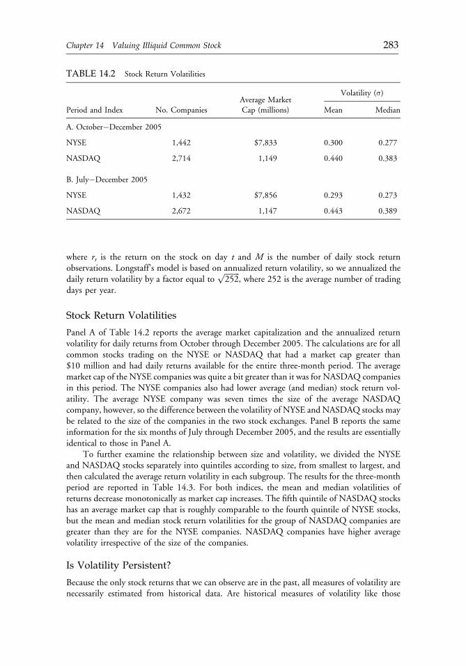
where rt is the return on the stock on day t and M is the number of daily stock returnobservations. Longstaff’s model is based on annualized return volatility, so we annualized thedaily return volatility by a factor equal to
ffiffiffiffiffiffiffiffi252
p, where 252 is the average number of trading
days per year.
Stock Return Volatilities
Panel A of Table 14.2 reports the average market capitalization and the annualized returnvolatility for daily returns from October through December 2005. The calculations are for allcommon stocks trading on the NYSE or NASDAQ that had a market cap greater than$10 million and had daily returns available for the entire three-month period. The averagemarket cap of the NYSE companies was quite a bit greater than it was for NASDAQ companiesin this period. The NYSE companies also had lower average (and median) stock return vol-atility. The average NYSE company was seven times the size of the average NASDAQcompany, however, so the difference between the volatility of NYSE and NASDAQ stocks maybe related to the size of the companies in the two stock exchanges. Panel B reports the sameinformation for the six months of July through December 2005, and the results are essentiallyidentical to those in Panel A.
To further examine the relationship between size and volatility, we divided the NYSEand NASDAQ stocks separately into quintiles according to size, from smallest to largest, andthen calculated the average return volatility in each subgroup. The results for the three-monthperiod are reported in Table 14.3. For both indices, the mean and median volatilities ofreturns decrease monotonically as market cap increases. The fifth quintile of NASDAQ stockshas an average market cap that is roughly comparable to the fourth quintile of NYSE stocks,but the mean and median stock return volatilities for the group of NASDAQ companies aregreater than they are for the NYSE companies. NASDAQ companies have higher averagevolatility irrespective of the size of the companies.
Is Volatility Persistent?
Because the only stock returns that we can observe are in the past, all measures of volatility arenecessarily estimated from historical data. Are historical measures of volatility like those
TABLE 14.2 Stock Return Volatilities
Average MarketVolatility (σ)
Period and Index No. Companies Cap (millions) Mean Median
A. October�December 2005
NYSE 1,442 $7,833 0.300 0.277
NASDAQ 2,714 1,149 0.440 0.383
B. July�December 2005
NYSE 1,432 $7,856 0.293 0.273
NASDAQ 2,672 1,147 0.443 0.389
c14 12 September 2012; 13:59:54
Chapter 14 Valuing Illiquid Common Stock 283
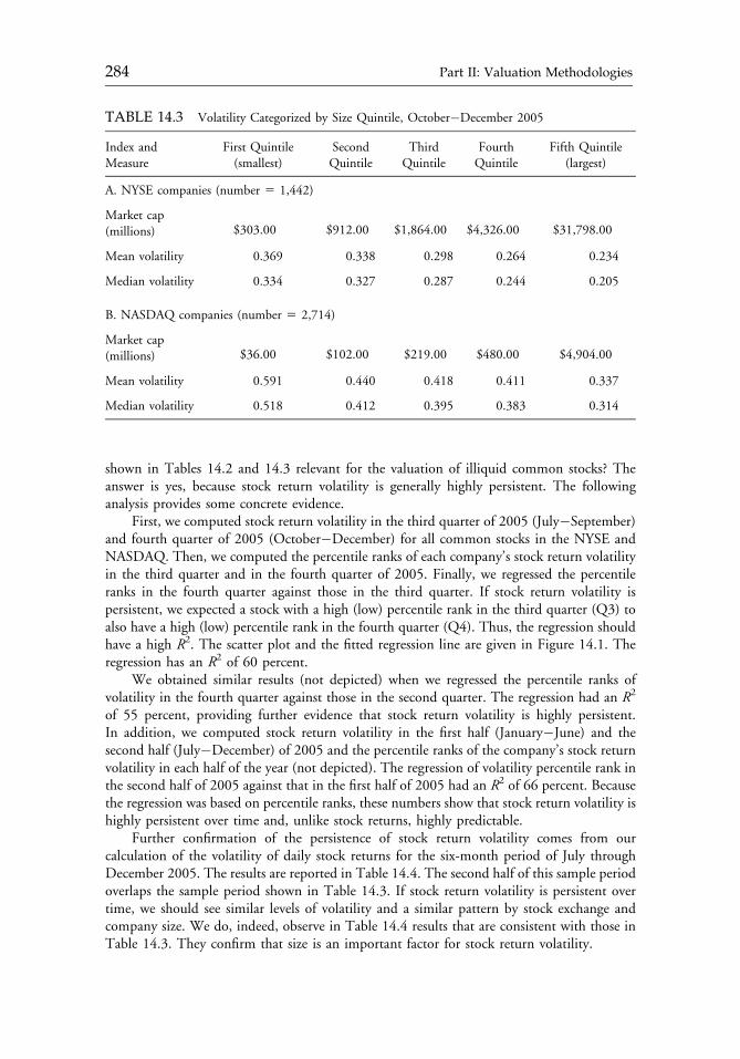
shown in Tables 14.2 and 14.3 relevant for the valuation of illiquid common stocks? Theanswer is yes, because stock return volatility is generally highly persistent. The followinganalysis provides some concrete evidence.
First, we computed stock return volatility in the third quarter of 2005 (July�September)and fourth quarter of 2005 (October�December) for all common stocks in the NYSE andNASDAQ. Then, we computed the percentile ranks of each company’s stock return volatilityin the third quarter and in the fourth quarter of 2005. Finally, we regressed the percentileranks in the fourth quarter against those in the third quarter. If stock return volatility ispersistent, we expected a stock with a high (low) percentile rank in the third quarter (Q3) toalso have a high (low) percentile rank in the fourth quarter (Q4). Thus, the regression shouldhave a high R2. The scatter plot and the fitted regression line are given in Figure 14.1. Theregression has an R2 of 60 percent.
We obtained similar results (not depicted) when we regressed the percentile ranks ofvolatility in the fourth quarter against those in the second quarter. The regression had an R2
of 55 percent, providing further evidence that stock return volatility is highly persistent.In addition, we computed stock return volatility in the first half (January�June) and thesecond half (July�December) of 2005 and the percentile ranks of the company’s stock returnvolatility in each half of the year (not depicted). The regression of volatility percentile rank inthe second half of 2005 against that in the first half of 2005 had an R2 of 66 percent. Becausethe regression was based on percentile ranks, these numbers show that stock return volatility ishighly persistent over time and, unlike stock returns, highly predictable.
Further confirmation of the persistence of stock return volatility comes from ourcalculation of the volatility of daily stock returns for the six-month period of July throughDecember 2005. The results are reported in Table 14.4. The second half of this sample periodoverlaps the sample period shown in Table 14.3. If stock return volatility is persistent overtime, we should see similar levels of volatility and a similar pattern by stock exchange andcompany size. We do, indeed, observe in Table 14.4 results that are consistent with those inTable 14.3. They confirm that size is an important factor for stock return volatility.
TABLE 14.3 Volatility Categorized by Size Quintile, October�December 2005
Index andMeasure
First Quintile(smallest)
SecondQuintile
ThirdQuintile
FourthQuintile
Fifth Quintile(largest)
A. NYSE companies (number 5 1,442)
Market cap(millions) $303.00 $912.00 $1,864.00 $4,326.00 $31,798.00
Mean volatility 0.369 0.338 0.298 0.264 0.234
Median volatility 0.334 0.327 0.287 0.244 0.205
B. NASDAQ companies (number 5 2,714)
Market cap(millions) $36.00 $102.00 $219.00 $480.00 $4,904.00
Mean volatility 0.591 0.440 0.418 0.411 0.337
Median volatility 0.518 0.412 0.395 0.383 0.314
c14 12 September 2012; 13:59:55
284 Part II: Valuation Methodologies
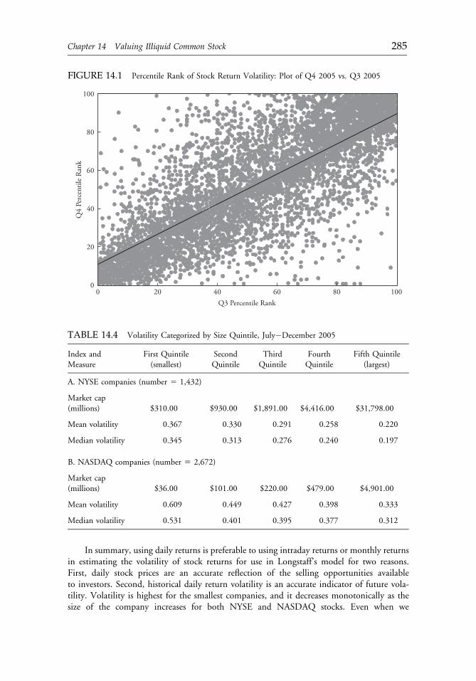
In summary, using daily returns is preferable to using intraday returns or monthly returnsin estimating the volatility of stock returns for use in Longstaff’s model for two reasons.First, daily stock prices are an accurate reflection of the selling opportunities availableto investors. Second, historical daily return volatility is an accurate indicator of future vola-tility. Volatility is highest for the smallest companies, and it decreases monotonically as thesize of the company increases for both NYSE and NASDAQ stocks. Even when we
FIGURE 14.1 Percentile Rank of Stock Return Volatility: Plot of Q4 2005 vs. Q3 2005Q
4 Pe
rcen
tile
Ran
k
Q3 Percentile Rank0 10020 40 60 80
100
80
60
40
20
0
TABLE 14.4 Volatility Categorized by Size Quintile, July�December 2005
Index andMeasure
First Quintile(smallest)
SecondQuintile
ThirdQuintile
FourthQuintile
Fifth Quintile(largest)
A. NYSE companies (number 5 1,432)
Market cap(millions) $310.00 $930.00 $1,891.00 $4,416.00 $31,798.00
Mean volatility 0.367 0.330 0.291 0.258 0.220
Median volatility 0.345 0.313 0.276 0.240 0.197
B. NASDAQ companies (number 5 2,672)
Market cap(millions) $36.00 $101.00 $220.00 $479.00 $4,901.00
Mean volatility 0.609 0.449 0.427 0.398 0.333
Median volatility 0.531 0.401 0.395 0.377 0.312
c14 12 September 2012; 13:59:55
Chapter 14 Valuing Illiquid Common Stock 285
controlled for the size of the company, NASDAQ stocks were shown to be more volatile thanNYSE stocks.
CASE STUDY
We describe here an actual study that we carried out to use the Longstaff model for valuingilliquid common stock.5 The case is about estimating the value of shares of Elite FinancialCorporation for estate tax purposes. The shares were part of the estate of Mary Hellmann,who died on September 27, 1998. The estate owned 396,000 shares of Elite Financialcommon stock. The market cap of Elite Financial in September 1998 was approximately$52 million. The shares were traded on the NASDAQ. The closing price on Friday,September 25, was $15.1875, which was also the opening price on Monday, September 28.The total value of the shares at this price was slightly more than $6 million. The median andmean daily reported trading volumes were, respectively, 1,900 shares and 4,113 shares,however, so a block of 396,000 shares was not readily marketable at the then currentprice.6 Moreover, the shares were unregistered and, therefore, subject to selling limits underSEC Rule 144 (see Note 1). A realistic estimate of the value of the shares at the time ofMs. Hellmann’s death must recognize that the stock was illiquid.
Maximum Discount for Illiquidity
The number of shares that could be sold in any three-month period was limited to the greaterof either 1 percent of the 3.6 million shares outstanding—36,000 shares—or the averageweekly trading volume preceding the week of the sale. The average weekly trading volume inElite Financial from January 1 through September 25, 1998, was 20,555 shares, so 36,000shares is a reasonable estimate of the maximum number of shares that could be sold eachquarter.
With sales of Elite Financial limited to 36,000 shares per three-month period,11 quarters—or 2.75 years—would be needed to liquidate the entire holding of 396,000shares. If we assume sales of 36,000 shares each three months, the average share could not besold for 1.375 years, or 346 trading days. That is, 346 trading days is the length of time forwhich the average share was completely illiquid. For simplicity, we express our estimates ofthe length of time Elite Financial’s stock was illiquid and the resulting discount for illiquidityin terms of the average share in the portfolio.
The other input required for the model is the volatility of the stock’s daily returns,measured as the annualized standard deviation of daily returns. We computed this measurefor the six months preceding September 1998. The volatility of the daily returns on EliteFinancial stock from April to September 1998 was σ 5 0.605. Although the volatility ofElite Financial’s returns is high compared with average volatilities observed for all stocksduring 2005, it is not inordinately high for a NASDAQ company with a small market cap(see Tables 14.3 and 14.4).
We now have the two inputs needed to use the Longstaff model to estimate the upperbound for the illiquidity discount that should be applied in valuing the shares ofElite Financial common stock in the estate of Mary Hellmann: The annualized standarddeviation of Elite Financial’s daily stock returns is 0.605, and the length of time before
c14 12 September 2012; 13:59:55
286 Part II: Valuation Methodologies
the average share can be liquidated, T, is 346 trading days. Substituting these values intoEquation 14.1, we find that the maximum illiquidity discount for Elite Financial shares in1998 is 59 percent.
The advantages of calculating this number as part of the valuation process are, first, thatit is based on an objective computation—that is, it applies specifically to Elite Financial stockin 1998—and, second, that the procedures we used are available for all to see. The model isderived from a rigorous theoretical analysis of the value of the option to sell an asset.Moreover, it provides an estimate that is based on specific characteristics (volatility and lengthof time before the average share can be liquidated) of a particular common stock (in this case,a stock in Ms. Hellmann’s portfolio in 1998) rather than being based on dated studies ofrestricted stock.
The figure of 59 percent is only the upper limit, however, for the discount for illiquidity.Other factors must be considered to obtain an appropriate discount to use in valuing the EliteFinancial holding.
Determining the Final Discount
A good starting point for determining the final discount would be to observe the discount thatgenerally occurs in practice when the Longstaff model indicates an upper limit of 59 percent.Unfortunately, such data would require an empirical study calibrating Longstaff’s model, andto our knowledge, no such study has been carried out.
Bajaj et al. (2001), however, estimated the parameters of a regression equation of pricediscounts for 88 private placements during 1990�1995, and this regression did include thestandard deviation of returns as one of four variables. Unfortunately, it did not includethe length of time that the stock was illiquid. Nonetheless, this regression, together withthe Bajaj et al. assumptions, allows us to make a crude estimate of the discount associatedwith a stock that has an annualized standard deviation of daily returns of 0.605.7 Based on theparameters of the Bajaj et al. regression model, our rough estimate of the appropriate discountfor the value of the illiquid Elite Financial shares is approximately 23 percent. The priceof Elite Financial shares on September 27, 1998, was $15.1875, so the market value ofthe estate’s 396,000 shares of stock in Elite Financial would have been $6,014,250.00 if theshares were completely liquid. After the 23 percent discount for illiquidity, the value is$4,630,972.50, a reduction of $1,383,277.50.
The marginal tax rate on estates greater than $3 million in 1998 was 55 percent, soapplying the 23 percent discount to the valuation of the shares saved the estate more than$760,000 in taxes (see Johnson and Mikow 2002). Of course, this valuation would also haveto be either accepted by the U.S. Internal Revenue Service or upheld in tax court. As apractical matter, however, the finance expert’s valuation frequently serves as a starting pointfor negotiations with the IRS.
In specific cases, circumstances might dictate a higher or lower discount than generallyobserved for a comparable stock. For example, if the large block of Elite Financial shares hadenabled the heirs to the estate to continue to control the company and to enjoy substantialbenefits as a result of these rights (e.g., lucrative employment with the company), the optionto sell the shares in the open market might have had little value to those particular investors.In that case, either no discount or only a small discount might be indicated.
The situation would be dramatically different if the Elite Financial shares were the bulkof the Hellmann estate and the beneficiary of the estate was a trust fund for Mary Hellmann’s
c14 12 September 2012; 13:59:55
Chapter 14 Valuing Illiquid Common Stock 287

minor children. The trustee is a fiduciary who is obligated to act prudently and to diversifythe trust’s assets to minimize the risk of large losses.8 In this case, the value of the 396,000shares of Elite Financial stock is far less than its $6 million nominal value and probably alsoless than the discounted value of $4.6 million that we calculated earlier. Recall that EliteFinancial is a very risky company and that the Longstaff model indicates a 59 percent dis-count as an upper bound on the value of being able to sell this stock. Would it be prudent forthe trustee to accept, for example, $3 million in cash in lieu of the risky and illiquid EliteFinancial stock? Possibly! If so, a discount of 50 percent or higher might be reasonable invaluing the stock as part of the estate.
CONCLUSION
We have provided a tutorial on applying the Longstaff model to the valuation of illiquidcommon stock. Although the model does not produce an exact discount for the valuation ofilliquid stocks, it provides an upper bound that is a useful starting point for valuing illiquidstock. The model is also parsimonious, has a closed form, and requires only two inputs—namely, the volatility of the stock return and the length of time the stock is illiquid.
Using volatility as an input provides a more analytical approach to determining discountsthan is provided by current practices because it explicitly takes into account the put optioninherent in a liquid asset. Previous studies examined the relationship between the discount tothe value of restricted stock and such variables as size and leverage, but these analyses are adhoc. Illiquid stock has a lower value than liquid stock because of the opportunity cost of beinglocked into holding an illiquid asset. This cost arises as a result of stock price fluctuations, andstock return volatility is a good measure of stock price fluctuation.
Finally, we want to point out that the basic framework of Longstaff’s model is also usefulfor understanding the relationships among illiquidity, risk, and returns for other types ofassets, such as hedge funds and private equity limited partnerships. For example, Liang andPark (2007) documented that many hedge funds impose various liquidity restrictions oninvestors, such as lockups and redemption fees. The average lockup period for hedge funds ofall types is about six months. In other words, hedge funds tend to offer less liquidity toinvestors than do mutual funds. This situation is very similar to the case of restricted stocks, inwhich investors are locked into their holdings and subject to the vagaries of changing assetvalues. Thus, one could reasonably expect investors to value hedge fund shares at a discount tomutual fund investments or, equivalently, require higher expected returns from hedge fundinvestments. Indeed, recent studies by Aragon (2007) and Liang and Park (2007) docu-mented that hedge funds with stringent liquidity restrictions on their shares do provideinvestors with higher returns. The authors presented evidence that, freed from the need toprovide liquidity, hedge funds are more likely than mutual funds to invest in the less liquidassets that promise higher returns.9
A remaining question is whether hedge funds provide adequate compensation toinvestors in the form of an illiquidity premium. To answer this question, the illiquiditydiscount associated with various liquidity restrictions has to be quantified. The Longstaffmodel may add to our understanding of this issue by providing a quantitative measure of theilliquidity discount based on daily fund return volatility or share price fluctuation. We leavethe application of Longstaff’s model to the question of a hedge fund illiquidity discount tofuture research.10
c14 12 September 2012; 13:59:55
288 Part II: Valuation Methodologies
NOTES
1. The number of restricted shares that can be sold by an individual during any three-month window is limited to the greater of either 1 percent of the shares outstanding orthe average weekly trading volume in the security calculated over the four calendar weekspreceding the week the notice of sale is filed.
2. Earlier studies include Hertzel and Smith (1993), Silber (1991), and Wruck (1989).3. We used historical volatilities calculated from daily returns largely for convenience
(because daily returns are readily available).4. For instance, in the CRSP database, the closing prices or the bid�ask averages at the
close are reported for all publicly traded stocks.5. The names have been changed to maintain confidentiality, but the facts of the case are
largely unchanged.6. In addition, reported trading volume for NASDAQ stocks was overstated at this time
because of dealer participation on one side of most trades, so Elite Financial stock wasactually even more thinly traded than these volumes indicate. See Anderson and Dyl(2005, 2007).
7. The other variables in the Bajaj et al. (2001) study are percentage of shares issued, thecompany’s Z-score (a measure of the financial health of the company), and an indicatorvariable equal to 1.0 if the shares are registered. To apply the regression to the EliteFinancial shares, we used the average values for the sample for the first two variables. Weassumed that the shares were unregistered, we rescaled the coefficient on the standarddeviation of returns so that it would apply to the annualized standard deviation of dailyreturns, and we used the value computed for Elite Financial (σ 5 0.605) as the standarddeviation.
8. Under the so-called prudent man rule, the standard for the fiduciary’s decisions, thefiduciary is required to act “with the care, skill, prudence, and diligence underthe circumstances then prevailing that a prudent man acting in a like capacity andfamiliar with such matters would use in the conduct of an enterprise of a like characterand with like aims” [ERISA, sec. 404(a)1(B)].
9. See Lerner and Schoar (2004) for a discussion of illiquidity and private equityinvestments.
10. Unfortunately, observations of daily returns for hedge funds are generally unavailableand return volatility cannot be readily calculated.
REFERENCES
Anderson, A.M., and E.A. Dyl. 2005. “Market Structure and Trading Volume.” Journal of FinancialResearch, vol. 28, no. 1 (March):115�231.
Anderson, A.M., and E.A. Dyl. 2007. “Trading Volume: NASDAQ and the NYSE.” Financial AnalystsJournal, vol. 63, no. 3 (May/June):79�86.
Aragon, G.O. 2007. “Share Restrictions and Asset Pricing: Evidence from the Hedge Fund Industry.”Journal of Financial Economics, vol. 83, no. 1 (January):33�58.
Bajaj, M., D.J. Denis, S.P. Ferris, and A. Sarin. 2001. “Firm Value and Marketability Discounts.”Journal of Corporation Law, vol. 27, no. 1 (Fall):89�115.
Figlewski, S. 1997. “Forecasting Volatility.” Financial Markets, Institutions & Instruments, vol. 6,no. 1:1�88.
c14 12 September 2012; 13:59:55
Chapter 14 Valuing Illiquid Common Stock 289
Hertzel, M., and R.L. Smith. 1993. “Market Discounts and Shareholder Gains from Placing EquityPrivately.” Journal of Finance, vol. 48, no. 2 (June):459�485.
Johnson, B.W., and J.M. Mikow. 2002. “Federal Estate Tax Returns, 1998�2000.” Statistics of IncomeBulletin, vol. 21, no. 4 (Spring):133�186.
Lerner, J., and A. Schoar. 2004. “The Illiquidity Puzzle Theory and Evidence from Private Equity.”Journal of Financial Economics, vol. 72, no. 1 (April):3�40.
Liang, B., and H. Park. 2007. “Share Restrictions, Liquidity Premiums, and Offshore Hedge Funds.”Working paper, University of Massachusetts.
Longstaff, F.A. 1995. “How Much Can Marketability Affect Security Values?” Journal of Finance,vol. 50, no. 5 (December):1767�1774.
Mikkelson, W.H., and M.M. Partch. 1985. “Stock Price Effects and Costs of Secondary Distributions.”Journal of Financial Economics, vol. 14, no. 2 (June):165�194.
SEC. 1971. “Discounts Involved in Purchases of Common Stock.” In Institutional Investor Study Reportof the Securities and Exchange Commission. Securities and Exchange Commission, H.R. Doc.No. 64, Part 5, 92nd Congress:2444�2456 (see revision at www.nber.org/chapters/c3534.pdf).
Silber, W.L. 1991. “Discounts on Restricted Stock: The Impact of Illiquidity on Stock Prices.” FinancialAnalysts Journal, vol. 47, no. 4 (July/August):60�64.
Wruck, K.H. 1989. “Equity Ownership Concentration and Firm Value: Evidence from Private EquityFinancings.” Journal of Financial Economics, vol. 23, no. 1 (June):3�28.
c14 12 September 2012; 13:59:56
290 Part II: Valuation Methodologies
PART IIIEARNINGS AND CASH
FLOW ANALYSIS
Chapter 15 Earnings: Measurement, Disclosure, and theImpact on Equity Valuation 293
Chapter 16 Cash Flow Analysis and Equity Valuation 349
Chapter 17 Accounting Valuation: Is Earnings Quality an Issue? 361
Chapter 18 Earnings Quality Analysis and Equity Valuation 375
Chapter 19 Is Cash Flow King in Valuations? 389
c15 12 September 2012; 18:0:8
291

c15 12 September 2012; 18:0:8
CHAPTER 15EARNINGS: MEASUREMENT,
DISCLOSURE, AND THEIMPACT ON EQUITY
VALUATION
D. Eric Hirst and Patrick E. Hopkins
Although a large body of research documents the significance of the relationshipbetween accounting information—especially reported earnings—and security prices,most of this research examines the connection between accounting information andmarket-level phenomena. Little research exists, however, to help practicing equityanalysts who are trying to use earnings data to produce accurate valuations forparticular stocks. In this chapter, the authors provide an extensive primer onearnings classifications that is intended to improve analysts’ ability to determine thequality and persistence of earnings. Moreover, they present the results of two originalexperiments designed to determine how analysts actually use earnings information inreaching stock�price judgments, and they report findings that hold valuable lessonsabout the ability of analysts to identify opportunistic earnings management.
FOREWORD
It has long been accepted that the central function of security analysis is to forecast futureaccounting earnings for the purpose of valuation. Recent valuations, however, especially in thetechnology sector, have raised doubts in the minds of many investors as to the relevance of
Copyright ª 2000 The Research Foundation of CFA Institute. Reprinted with permission. When thisarticle was originally published, D. Eric Hirst was associate professor of accounting at the McCombsSchool of Business at the University of Texas at Austin and Patrick E. Hopkins was assistant professorand the OLIVE LLP Faculty Fellow at the Kelley School of Business at Indiana University.
c15 12 September 2012; 18:0:8
293
accounting earnings. Some analysts advocate the use of free cash flows in lieu of earnings.D. Eric Hirst and Patrick E. Hopkins tackle this crucial issue and provide persuasive evidenceof the continued relevance of accounting earnings for the determination of investment value.
In addition to documenting the critical relationship between accounting earnings andsecurity prices, Hirst and Hopkins offer a comprehensive compendium of earnings classifi-cations to help analysts distinguish between transitory earnings and those earnings that aremore likely to persist and thus affect future valuations. Hirst and Hopkins use a variety ofreal-world examples to illustrate these earnings classifications and to show analysts how tointerpret them for the purpose of fundamental analysis.
Hirst and Hopkins next present the results of two original, controlled experiments toevaluate the use of accounting earnings by buy-side analysts. The first experiment reveals thatanalysts are often misled by opportunistic earnings management and, therefore, should focusgreater attention on the sources and quality of earnings. The follow-up experiment shows thatmore comprehensive disclosure of the components of earnings helps to mitigate the problemof opportunistic earnings management and thus improves analysts’ assessments of investmentvalue. This latter finding strongly suggests that our profession should encourage policymakersto require greater transparency with respect to reported earnings.
This chapter is essential for anyone engaged in security analysis, whether a seasonedexpert or a novice. Moreover, all investment professionals who seek a clear and thoroughexplication of accounting earnings and their relationship to valuation will benefit fromthe work of Hirst and Hopkins. The Research Foundation is pleased to present Earnings:Measurement, Disclosure, and the Impact on Equity Valuation.
Mark Kritzman, CFAResearch Director
The Research Foundation of theAssociation for Investment Management and Research
ACKNOWLEDGMENTS
We thank the Research Foundation of AIMR for the opportunity to write this chapter andKeith Brown for his support of the project. We also received helpful feedback from our col-leagues at the University of Texas at Austin and Indiana University—especially Daniel Beneish,Michael Clement, Roger Martin, Bob Parrino, Curt Rogers, and Jim Wahlen. We receivedcomments on various parts of the project from workshop participants at Cornell University, theUniversity of Florida, the University of Illinois, Indiana University, Ohio State University,the University of Utah, and Virginia Tech. The participants at the IU-NDU-PU SummerResearch Conference, the Eighth Annual Conference on Financial Economics and Accounting,the University of Texas Summer Brownbag Workshop, the Financial Accounting StandardsBoard Professional Development Session, the 1998 Midwest AAA meeting, the 1998Behavioral Decision Research in Management Conference, the 1998 American AccountingAssociation Annual Meeting, and the 1998 Journal of Accounting Research Conference alsoprovided valuable comments. Lynette Wood provided research assistance.
We owe special thanks to Jeff Lucado, Walter Koon, Thomas Pence, and Gary Strattenfor their efforts in helping us develop and administer the experiment reported in the section“How Buy-Side Equity Analysts Use Earnings in Valuation.” In addition, we are indebted to
c15 12 September 2012; 18:0:8
294 Part III: Earnings and Cash Flow Analysis
the professional analysts and portfolio managers who unselfishly and anonymously donatedtheir time to complete the case materials.
The usual caveats apply. Foremost among them is that we are solely responsible for anyerrors or omissions.
DEDICATION
The fact that you are holding a copy of this chapter is testament to the support andencouragement we have received from our families. We dedicate this chapter to them.
To
Patty, Kevin, and MatthewLaura, Maggie, and William
Thanks!
INTRODUCTION
Many textbook explanations of equity security valuation provide students and analysts withclear and concise explanations that give a false impression of the practical complexity of thevaluation exercise. Part art and part science, part dissecting the past and part predictingthe future—valuation is simultaneously a rewarding and frustrating process. On the one hand,gathering relevant information from a variety of sources and distilling it into a range ofreasonable equity values is rewarding. It is the cornerstone of many individual and institu-tional investors’ decisions to buy, sell, or hold securities. On the other hand, valuation isfrustrating because it is fraught with uncertainty. First is the uncertainty associated with theexercise itself (for example, what is the right valuation model to use? Is the price too high?When will the market share my beliefs about the future and correct the price?). In addition,analysts find themselves playing cat-and-mouse games with the preparers of corporatefinancial statements. That analysts cannot simply take information reported in financialstatements at face value is an aspect of equity valuation that significantly increases thecomplexity of an already difficult activity.
The rules that guide the preparation of financial statements in the United States (gen-erally accepted accounting principles, or GAAP) allow company managers sufficient latitudeto effectively communicate the financial position and results of the company operations. Thatsame flexibility, however, also provides managers with the opportunity to conceal informationfrom competitors, analysts, and other readers of the financial statements. In theory, whenmanagers make financial reporting decisions, they trade off the potential benefits (e.g.,reducing the cost of capital because disclosure reduces uncertainty) against potential costs(e.g., revealing proprietary information to existing and potential competitors). In addition,managers recognize that financial statements and their components affect contracts, includingcompensation contracts. Thus, managers may have significant incentives to paint a self-serving picture of the company. Prudent analysts, wary of the claims made in the financialstatements, consider the source and context of the claims.
The goal of this chapter is simple: We want to increase analysts’ understanding of howincome statements and other disclosures can be used to assess the underlying quality and
c15 12 September 2012; 18:0:8
Chapter 15 Earnings: Measurement, Disclosure, and the Impact on Equity Valuation 295
persistence of companies’ economic activities. We believe the recent rush to “cash earnings”valuation models is caused by the need to justify sky-high prices for so-called new-economystocks and is an overreaction to perceived weaknesses in the measurement of GAAP earnings.In the long run, however, cash earnings are unlikely to be the panacea that some claim theyare.1 Accounting data provide a rich source of insights into the intrinsic value of a firm.Harnessing the power of such information requires an understanding of its strengths andweaknesses. We hope that with the right tools and a thorough understanding of the inputsrequired to use them, security analysts will be able to generate accurate and insightfulvaluations of equity securities.
The chapter is organized as follows. In the first section, “Evidence on the Relevance ofEarnings to Valuation,” we provide a brief review of the large body of research that exploresthe relationship between financial accounting information and security valuation. Althoughwe deal only with selected research highlights, a clear picture emerges: Accounting data—inparticular, reported earnings—are strongly related to security prices. We suggest that thosewho criticize financial accounting data as irrelevant are standing on shaky ground. We alsoreview the claims that “cash is king” and accounting earnings are “a fiction,” and we show thatempirical results strongly support the relevance of accrual-basis accounting information.
In the second section, “The Reporting of Earnings and Equity Valuation,” we examinethe question: What are earnings? We start with an overview of a powerful accounting-basedvaluation model. We also describe how accountants classify earnings into recurring andnonrecurring components. Then, we illustrate those classifications with actual disclosuresand discuss how managers’ judgments can lead to self-serving reporting. Armed with a goodunderstanding of a company’s accounting and its underlying strengths and weaknesses, thediligent analyst is in a good position to assess past performance. This understanding shouldlead to improved forecasts of future results.
The third section, “How Buy-Side Equity Analysts Use Earnings in Valuation,” providesthe results of two new empirical studies in which more than 100 members of the professionalanalyst community participated. The purpose of this discussion is to illustrate the difficultyunderlying fundamental analysis and equity valuation. Our findings reveal that, in contrast topopular belief, the manner in which accounting data are reported predictably affects analysts’valuation judgments.
The Conclusion closes the chapter with a brief summary of our argument.
EVIDENCE ON THE RELEVANCE OF EARNINGSTO VALUATION
In this section, we consider the empirical evidence for three aspects of the relevance ofaccounting earnings to valuation: the relationship between earnings data and stock prices, theinformation content of earnings data relative to the information content of cash flow data,and the use analysts make of earnings data in valuation.
In truth, a formal study of the role of accounting earnings in the capital markets is notneeded to gauge the importance of reported income in the work of managers, analysts, andinvestors. Articles in the business press clearly focus significant attention on companies’quarterly and annual earnings announcements. Furthermore, corporate managers go to greatlengths to explain the factors that influence reported income numbers and, increasingly, try tomanage analysts’ earnings expectations. For example, in recent years, the incidence of man-agers “talking down” investors’ earnings expectations in the weeks leading up to an earnings
c15 12 September 2012; 18:0:9
296 Part III: Earnings and Cash Flow Analysis
announcement has increased. Their methods include initiating “whisper forecasts” and“preannouncing” earnings. In addition, the business press regularly provides comprehensiveanalyses of corporate valuations in terms of earnings-based multiples (e.g., the price-to-earnings ratio). Even articles announcing quarterly results for Internet companies includenumerous adjustments and qualifications intended to guide the investing public to someestimate of (distant) future earnings.
The anecdotal evidence on the relevance of accounting earnings in security valuation maybe interesting, but explicit conclusions about the relevance of earnings versus cash flows invaluation are best determined by observing the relationship between these metrics and stockprices. Fortunately, scholars in accounting and finance have conducted many studies of therelevance of accounting information for explaining the price levels and price changes ofequity securities.
The following discussion briefly describes some of the classic research studies thatdemonstrate the relevance of accounting earnings for the purpose of equity security valua-tion.2 Then, we consider studies that directly compare the relative usefulness of earnings andcash flows in valuation activities, although much of this discussion is at the level of market-determined stock prices. We conclude the section by describing results from the limitednumber of studies that have investigated how financial analysts actually use earnings-relatedinformation in valuation activities. This discussion provides the context for the experiment,described in the section “How Buy-Side Equity Analysts Use Earnings in Valuation,” thatinvestigates the effect of earnings on buy-side analysts’ stock-price judgments.
Earnings Information and Equity Prices
For more than three decades, accounting and finance researchers have been rigorouslyinvestigating the relationship between accounting earnings and security prices. The relevanceof this research lies not in allowing students or practitioners to pick winners before the factbut in its ability to explain variations in past stock prices. The fundamental questionaddressed in this research is whether, and to what extent, historical earnings are correlatedwith stock returns and/or stock prices. If historical earnings information is shown to be rel-evant in explaining current stock prices, then a valuation model that explicitly incorporatesexpectations of future earnings, such as the model we provide in the next section, “TheReporting of Earnings and Equity Valuation,” should be seriously considered by anyonepracticing fundamental analysis.
Unexpected Earnings and Stock-Price Changes
A study by Ball and Brown (1968) provided the initial evidence that accounting earnings conveyrelevant information about the underlying value of securities. Their study laid the groundworkfor much of the earnings-related academic research in accounting and finance that followed.Ball and Brown addressed the specific question of whether positive unexpected earningsare associated with positive changes in stock prices and whether negative unexpected earnings areassociated with negative changes in stock prices. Although information from many sources isimpounded in security prices, Ball and Brown isolated the effect of earnings on prices by lookingat cross-sectional changes in earnings and the corresponding changes in prices. This designreduced the possibility that some factor other than the information aggregated in earnings wasexplaining stock-price changes.
c15 12 September 2012; 18:0:9
Chapter 15 Earnings: Measurement, Disclosure, and the Impact on Equity Valuation 297
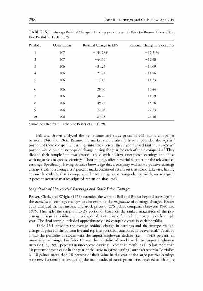
Ball and Brown analyzed the net income and stock prices of 261 public companiesbetween 1946 and 1966. Because the market should already have impounded the expectedportion of these companies’ earnings into stock prices, they hypothesized that the unexpectedportion would predict stock-price change during the year for each of these companies.3 Theydivided their sample into two groups—those with positive unexpected earnings and thosewith negative unexpected earnings. Their findings offer powerful support for the relevance ofearnings. Specifically, having advance knowledge that a company will have a positive earningschange yields, on average, a 7 percent market-adjusted return on that stock. Likewise, havingadvance knowledge that a company will have a negative earnings change yields, on average, a9 percent negative market-adjusted return on that stock.
Magnitude of Unexpected Earnings and Stock-Price Changes
Beaver, Clark, and Wright (1979) extended the work of Ball and Brown beyond investigatingthe direction of earnings changes to also examine the magnitude of earnings changes. Beaveret al. analyzed the net income and stock prices of 276 public companies between 1960 and1975. They split the sample into 25 portfolios based on the ranked magnitude of the per-centage change in residual (i.e., unexpected) net income for each company in each sampleyear. The final sample included approximately 106 company-years in each portfolio.
Table 15.1 provides the average residual change in earnings and the average residualchange in price for the bottom five and top five portfolios composed in Beaver et al.4 Portfolio1 was the portfolio of stocks with the largest single-year decline (i.e., 2154.8 percent) inunexpected earnings; Portfolio 10 was the portfolio of stocks with the largest single-yearincrease (i.e., 185.1 percent) in unexpected earnings. Note that Portfolios 1�5 lost more than10 percent of their value in the year of the large negative earnings surprises whereas Portfolios6�10 gained more than 10 percent of their value in the year of the large positive earningssurprises. Furthermore, evaluating the magnitudes of earnings surprises revealed much more
TABLE 15.1 Average Residual Change in Earnings per Share and in Price for Bottom Five and Top
Five Portfolios, 1960�1975
Portfolio Observations Residual Change in EPS Residual Change in Stock Price
1 107 2154.78% 217.51%
2 107 244.69 212.40
3 106 231.23 214.69
4 106 222.92 211.76
5 106 217.47 211.33
6 106 28.70 10.44
7 106 36.28 11.79
8 106 49.72 15.76
9 106 72.06 22.23
10 106 185.08 29.16
Source: Adapted from Table 3 of Beaver et al. (1979).
c15 12 September 2012; 18:0:9
298 Part III: Earnings and Cash Flow Analysis
pronounced return patterns than those observed in Ball and Brown. That is, the largestnegative stock return was 217.5 percent (compared with 29.0 percent in Ball and Brown),and the highest positive stock return was 29.2 percent (compared with 7.0 percent in Ball andBrown).
The asymmetric reaction to positive (29.2 percent) and negative (217.5 percent)earnings surprises documented in Beaver et al. raises the possibility that the magnitude of astock-price reaction may not be uniform for all levels or sources of earnings. These asym-metric results are not surprising in the context of our discussion in the section “The Reportingof Earnings and Equity Valuation” about the varying sources and persistence of items thatcontribute to net income. Indeed, given companies’ incentives to write off future expenses in ayear that is already experiencing a net loss (i.e., to “take a bath”), the Beaver et al. relativestock-price return results for the highest and lowest portfolios of unexpected earnings arequite intuitive.
Determinants of Price Reaction
Although the pattern of results reported in Beaver et al. is consistent with intuition, these authorsdid not address the important issue of exactly what determines the magnitude of the stock-pricereaction to a given level of unexpected historical earnings. This reaction, often referred to as the“earnings response coefficient” (ERC), is basically the slope coefficient between unexpectedearnings and unexpected stock returns. For example, if a company was expected to report netincome of $2 per share but actually reported net income of $3 per share, the unexpected earningswould equal $1. If the company’s stock price increased by $5 per share based on this earningsannouncement, the ERC would be 5. If all unexpected earnings were created equal, consistentERCs would be observed, at least at the company level. But intuition suggests that some unex-pected earnings are recurring and others are one-time events.
Kormendi and Lipe (1987) were the first to investigate whether ERCs can be explainedby the extent to which one period’s unexpected earnings become expected in the future.5 Thatis, they believed the magnitude of companies’ ERCs are (at least partly) explained by theportion of the earnings surprise that is expected to become part of normal earnings inthe future. They found that, indeed, higher ERCs are associated with higher levels of futureearnings persistence. In other words, stock prices respond the most to earnings changes that areindicative of future earnings performance.
Although a number of factors have been identified that affect the relationship betweenunexpected earnings and stock returns, the findings of Kormendi and Lipe and subsequentresearchers indicate that this relationship depends in part on the extent to which earnings areexpected to persist in the future. These results suggest that analysts should carefully considerthe source and expected duration of earnings components when they include earnings in avaluation model.
Long-Term Relationships
Although Ball and Brown and Beaver et al. provided evidence that accounting earnings arerelevant in pricing equity securities, the findings correlating earnings with stock prices or stockreturns have suffered from low explanatory power. Models that correlate unexpected returnswith unexpected earnings (aggregated over periods up to a year) rarely obtain R2s in excess of10 percent.6 The implication is that the majority of stock returns over short time intervals areexplained by factors other than one year’s earnings. Easton, Harris, and Ohlson (1992)
c15 12 September 2012; 18:0:9
Chapter 15 Earnings: Measurement, Disclosure, and the Impact on Equity Valuation 299
addressed this problem by analyzing the relationship between earnings and returns over alonger time period.
Easton et al. made two important contributions to the understanding of the earnings-stock returns relationship. First, they noted that the explanatory power of earnings shouldincrease over longer return intervals because earnings aggregate over time and, therefore, thenoise induced by possible income shifting and the noncomparability caused by the use ofalternative accounting methods should diminish over time. That is, over a long period, thevarious alternatives allowed by accrual accounting generally result in the same overall levels ofaggregate accounting earnings. Second, they found that a long window allows investigationof the relationship between stock returns and the aggregate amount of earnings during theperiod. Most earnings research (for example, Ball and Brown; Beaver et al.) has generallyinvestigated the correlation between unexpected earnings (or changes in earnings) and stockreturns over short time frames.
Easton et al. analyzed the correlation between returns and earnings for 20 years of datafrom the 1987 Compustat data file.7 They found that models correlating stock returns andthe aggregate level of earnings over a 10-year period result in R2s higher than 60 percent—asignificant improvement in explanatory power over studies using short windows. In addition,their results pointed to the long-run relevance of accounting earnings in explaining the returnson common stock. The value relevance of long windows of aggregated historical earningssuggests that forecasting expected long-term future earnings should be useful for valuationpurposes and even points to the potential usefulness in valuation of forecasting a company’snet book value.8
Has the Value Relevance of Earnings Declined in Recent Years?
Although Easton et al. suggested that long-window earnings explain a large proportion ofstock returns, many academics and analysts complain that quarterly and annual accountingearnings have become increasingly less relevant in explaining common stock returns. Forexample, many complain that the recurring reporting by companies of supposedly one-timeitems has recently increased. Elliott and Hanna (1996) confirm that reports of large, one-time items increased during the 20 years ending in 1994, and in particular, reports of largenegative write-offs increased dramatically.9 For example, in 1975, less than 5 percent ofcompanies reported a large negative write-off, compared with 21 percent of companies in1994. Elliott and Hanna also showed that the companies most likely to record these write-offsare companies that previously reported a similar write-off. The authors demonstrated thatanalysts’ sarcasm about “recurring nonrecurring items” in quarterly and annual reports isjustified. Their results point to a potential decline in usefulness of periodically reportedbottom-line net income in the valuation of companies.
Collins, Maydew, and Weiss (1997) noted that factors leading to the decline in use-fulness of single-period income measures might also lead to the increased relevance of netbook value in valuing companies. To test this proposition, they analyzed the incrementalexplanatory power of net book value and earnings for stock prices for each of 40 years through1993. They used a discounted abnormal earnings (DAE) valuation framework to investigatethe relative importance of net book value and earnings. Briefly explained, DAE modelssuggest that the total equity value of a company can be expressed in terms of its futureabnormal earnings and its current reported net book value.10 From a valuation perspective,the important contribution of this framework lies in its ability to explain and predict stock
c15 12 September 2012; 18:0:9
300 Part III: Earnings and Cash Flow Analysis
values (i.e., prices) instead of changes in value (i.e., returns), which was investigated by muchprior accounting research.
Collins et al. found that the average annual R2s ranged between 0.5 and 0.75 when bothearnings and book values were included in the valuation model. That is, together, earningsand net book value explained between 50 and 75 percent of the overall variation in stockprices—a substantial portion. In addition, consistent with the views of those who maintainthat earnings have become increasingly less relevant, they found that the incrementalexplanatory power of bottom-line net income has indeed declined in the past 40 years. Thisfinding reinforces the importance of evaluating the components of earnings rather thanfocusing on a single summary measure of profit. Collins et al. also found, however, that theincremental explanatory power of net book value has increased over the same period. To thesurprise of those who argue that accounting has become less relevant to valuation, the totalexplanatory power of net income and net book value taken together has significantly increasedin the past 40 years. In short, the Collins et al. findings are an important indicator of therelevance of accrual accounting information in explaining the levels of stock prices.
Taken together, these studies provide strong evidence that accrual-basis earningsinformation can be used to explain stock prices. Indeed, the results of these studies are socompelling that analysts would be wise to include an earnings-based model in their valuationrepertoire.
The Information Content of Earnings versus Cash Flows
Chapter 3: Cash is King—Copeland, Koller, and Murrin (1996)
Common sense tells us that accounting information is relevant for valuing stocks.—Brennan (1995)
These quotations, each from eminent authors in finance, illustrate the perspectives in thefinance community about the role of accrual accounting in equity valuation. The first per-spective is based on the observation that the value of an asset is equal to the present value of itsfuture cash flows. To determine a fair or intrinsic value for the bundles of cash flowsembodied in an equity security, why not directly estimate those flows? From this perspective,an analyst logically begins the valuation process by evaluating currentperiod cash flows andthen forecasting how they will change (or persist) in the future.
The perspective illustrated by the Brennan quotation is rooted in the observation that thefinancial reporting function is designed to provide information (i.e., earnings data) thatsummarizes the present and future net cash effects of the activities in which a company isengaged during a given period. From this perspective, one can rely on the accounting processto estimate and report the most likely cash flow implications of operations during the period.Furthermore, analysts can focus on the economic factors that influenced the company’s coreoperating activities during the period and estimate the extent to which those factors willchange or persist in the future. Indeed, as we note in the section “The Reporting of Earningsand Equity Valuation,” accountants classify income statements to aid in this endeavor.
In the previous subsection, our discussion of the relevance of earnings in valuation didlittle to address the concerns of analysts, portfolio managers, and academics who believe thata company’s cash flows, not earnings, are the only true indicator of a company’s value.
c15 12 September 2012; 18:0:9
Chapter 15 Earnings: Measurement, Disclosure, and the Impact on Equity Valuation 301
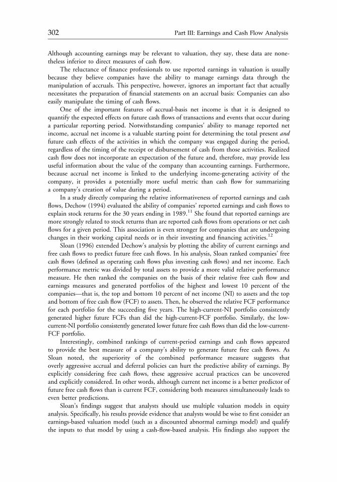
Although accounting earnings may be relevant to valuation, they say, these data are none-theless inferior to direct measures of cash flow.
The reluctance of finance professionals to use reported earnings in valuation is usuallybecause they believe companies have the ability to manage earnings data through themanipulation of accruals. This perspective, however, ignores an important fact that actuallynecessitates the preparation of financial statements on an accrual basis: Companies can alsoeasily manipulate the timing of cash flows.
One of the important features of accrual-basis net income is that it is designed toquantify the expected effects on future cash flows of transactions and events that occur duringa particular reporting period. Notwithstanding companies’ ability to manage reported netincome, accrual net income is a valuable starting point for determining the total present andfuture cash effects of the activities in which the company was engaged during the period,regardless of the timing of the receipt or disbursement of cash from those activities. Realizedcash flow does not incorporate an expectation of the future and, therefore, may provide lessuseful information about the value of the company than accounting earnings. Furthermore,because accrual net income is linked to the underlying income-generating activity of thecompany, it provides a potentially more useful metric than cash flow for summarizinga company’s creation of value during a period.
In a study directly comparing the relative informativeness of reported earnings and cashflows, Dechow (1994) evaluated the ability of companies’ reported earnings and cash flows toexplain stock returns for the 30 years ending in 1989.11 She found that reported earnings aremore strongly related to stock returns than are reported cash flows from operations or net cashflows for a given period. This association is even stronger for companies that are undergoingchanges in their working capital needs or in their investing and financing activities.12
Sloan (1996) extended Dechow’s analysis by plotting the ability of current earnings andfree cash flows to predict future free cash flows. In his analysis, Sloan ranked companies’ freecash flows (defined as operating cash flows plus investing cash flows) and net income. Eachperformance metric was divided by total assets to provide a more valid relative performancemeasure. He then ranked the companies on the basis of their relative free cash flow andearnings measures and generated portfolios of the highest and lowest 10 percent of thecompanies—that is, the top and bottom 10 percent of net income (NI) to assets and the topand bottom of free cash flow (FCF) to assets. Then, he observed the relative FCF performancefor each portfolio for the succeeding five years. The high-current-NI portfolio consistentlygenerated higher future FCFs than did the high-current-FCF portfolio. Similarly, the low-current-NI portfolio consistently generated lower future free cash flows than did the low-current-FCF portfolio.
Interestingly, combined rankings of current-period earnings and cash flows appearedto provide the best measure of a company’s ability to generate future free cash flows. AsSloan noted, the superiority of the combined performance measure suggests thatoverly aggressive accrual and deferral policies can hurt the predictive ability of earnings. Byexplicitly considering free cash flows, these aggressive accrual practices can be uncoveredand explicitly considered. In other words, although current net income is a better predictor offuture free cash flows than is current FCF, considering both measures simultaneously leads toeven better predictions.
Sloan’s findings suggest that analysts should use multiple valuation models in equityanalysis. Specifically, his results provide evidence that analysts would be wise to first consider anearnings-based valuation model (such as a discounted abnormal earnings model) and qualifythe inputs to that model by using a cash-flow-based analysis. His findings also support the
c15 12 September 2012; 18:0:9
302 Part III: Earnings and Cash Flow Analysis
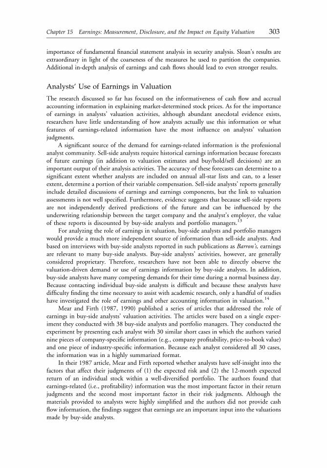
importance of fundamental financial statement analysis in security analysis. Sloan’s results areextraordinary in light of the coarseness of the measures he used to partition the companies.Additional in-depth analysis of earnings and cash flows should lead to even stronger results.
Analysts’ Use of Earnings in Valuation
The research discussed so far has focused on the informativeness of cash flow and accrualaccounting information in explaining market-determined stock prices. As for the importanceof earnings in analysts’ valuation activities, although abundant anecdotal evidence exists,researchers have little understanding of how analysts actually use this information or whatfeatures of earnings-related information have the most influence on analysts’ valuationjudgments.
A significant source of the demand for earnings-related information is the professionalanalyst community. Sell-side analysts require historical earnings information because forecastsof future earnings (in addition to valuation estimates and buy/hold/sell decisions) are animportant output of their analysis activities. The accuracy of these forecasts can determine to asignificant extent whether analysts are included on annual all-star lists and can, to a lesserextent, determine a portion of their variable compensation. Sell-side analysts’ reports generallyinclude detailed discussions of earnings and earnings components, but the link to valuationassessments is not well specified. Furthermore, evidence suggests that because sell-side reportsare not independently derived predictions of the future and can be influenced by theunderwriting relationship between the target company and the analyst’s employer, the valueof these reports is discounted by buy-side analysts and portfolio managers.13
For analyzing the role of earnings in valuation, buy-side analysts and portfolio managerswould provide a much more independent source of information than sell-side analysts. Andbased on interviews with buy-side analysts reported in such publications as Barron’s, earningsare relevant to many buy-side analysts. Buy-side analysts’ activities, however, are generallyconsidered proprietary. Therefore, researchers have not been able to directly observe thevaluation-driven demand or use of earnings information by buy-side analysts. In addition,buy-side analysts have many competing demands for their time during a normal business day.Because contacting individual buy-side analysts is difficult and because these analysts havedifficulty finding the time necessary to assist with academic research, only a handful of studieshave investigated the role of earnings and other accounting information in valuation.14
Mear and Firth (1987, 1990) published a series of articles that addressed the role ofearnings in buy-side analysts’ valuation activities. The articles were based on a single exper-iment they conducted with 38 buy-side analysts and portfolio managers. They conducted theexperiment by presenting each analyst with 30 similar short cases in which the authors variednine pieces of company-specific information (e.g., company profitability, price-to-book value)and one piece of industry-specific information. Because each analyst considered all 30 cases,the information was in a highly summarized format.
In their 1987 article, Mear and Firth reported whether analysts have self-insight into thefactors that affect their judgments of (1) the expected risk and (2) the 12-month expectedreturn of an individual stock within a well-diversified portfolio. The authors found thatearnings-related (i.e., profitability) information was the most important factor in their returnjudgments and the second most important factor in their risk judgments. Although thematerials provided to analysts were highly simplified and the authors did not provide cashflow information, the findings suggest that earnings are an important input into the valuationsmade by buy-side analysts.
c15 12 September 2012; 18:0:9
Chapter 15 Earnings: Measurement, Disclosure, and the Impact on Equity Valuation 303
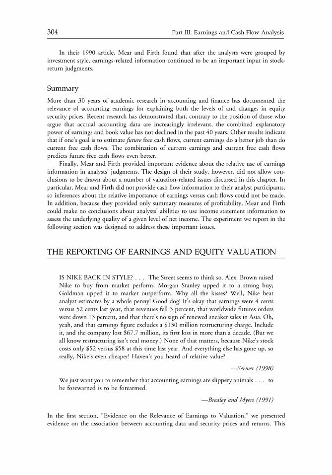
In their 1990 article, Mear and Firth found that after the analysts were grouped byinvestment style, earnings-related information continued to be an important input in stock-return judgments.
Summary
More than 30 years of academic research in accounting and finance has documented therelevance of accounting earnings for explaining both the levels of and changes in equitysecurity prices. Recent research has demonstrated that, contrary to the position of those whoargue that accrual accounting data are increasingly irrelevant, the combined explanatorypower of earnings and book value has not declined in the past 40 years. Other results indicatethat if one’s goal is to estimate future free cash flows, current earnings do a better job than docurrent free cash flows. The combination of current earnings and current free cash flowspredicts future free cash flows even better.
Finally, Mear and Firth provided important evidence about the relative use of earningsinformation in analysts’ judgments. The design of their study, however, did not allow con-clusions to be drawn about a number of valuation-related issues discussed in this chapter. Inparticular, Mear and Firth did not provide cash flow information to their analyst participants,so inferences about the relative importance of earnings versus cash flows could not be made.In addition, because they provided only summary measures of profitability, Mear and Firthcould make no conclusions about analysts’ abilities to use income statement information toassess the underlying quality of a given level of net income. The experiment we report in thefollowing section was designed to address these important issues.
THE REPORTING OF EARNINGS AND EQUITY VALUATION
IS NIKE BACK IN STYLE? . . . The Street seems to think so. Alex. Brown raisedNike to buy from market perform; Morgan Stanley upped it to a strong buy;Goldman upped it to market outperform. Why all the kisses? Well, Nike beatanalyst estimates by a whole penny! Good dog! It’s okay that earnings were 4 centsversus 52 cents last year, that revenues fell 3 percent, that worldwide futures orderswere down 13 percent, and that there’s no sign of renewed sneaker sales in Asia. Oh,yeah, and that earnings figure excludes a $130 million restructuring charge. Includeit, and the company lost $67.7 million, its first loss in more than a decade. (But weall know restructuring isn’t real money.) None of that matters, because Nike’s stockcosts only $52 versus $58 at this time last year. And everything else has gone up, soreally, Nike’s even cheaper! Haven’t you heard of relative value?
—Serwer (1998)
We just want you to remember that accounting earnings are slippery animals . . . tobe forewarned is to be forearmed.
—Brealey and Myers (1991)
In the first section, “Evidence on the Relevance of Earnings to Valuation,” we presentedevidence on the association between accounting data and security prices and returns. This
c15 12 September 2012; 18:0:10
304 Part III: Earnings and Cash Flow Analysis
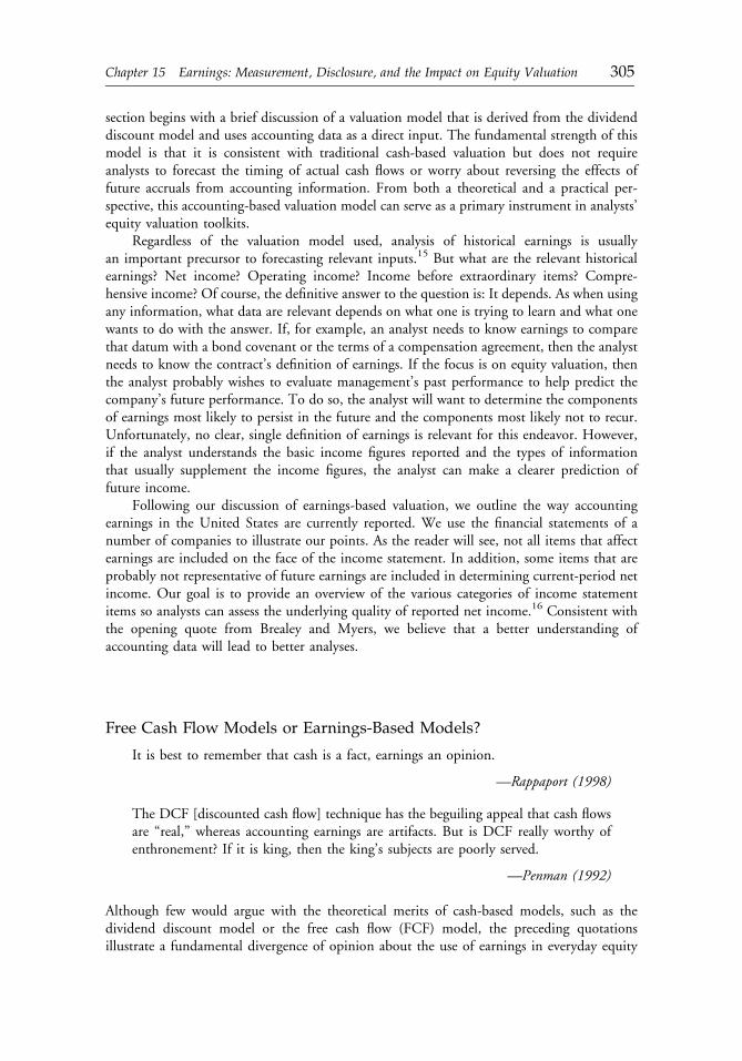
section begins with a brief discussion of a valuation model that is derived from the dividenddiscount model and uses accounting data as a direct input. The fundamental strength of thismodel is that it is consistent with traditional cash-based valuation but does not requireanalysts to forecast the timing of actual cash flows or worry about reversing the effects offuture accruals from accounting information. From both a theoretical and a practical per-spective, this accounting-based valuation model can serve as a primary instrument in analysts’equity valuation toolkits.
Regardless of the valuation model used, analysis of historical earnings is usuallyan important precursor to forecasting relevant inputs.15 But what are the relevant historicalearnings? Net income? Operating income? Income before extraordinary items? Compre-hensive income? Of course, the definitive answer to the question is: It depends. As when usingany information, what data are relevant depends on what one is trying to learn and what onewants to do with the answer. If, for example, an analyst needs to know earnings to comparethat datum with a bond covenant or the terms of a compensation agreement, then the analystneeds to know the contract’s definition of earnings. If the focus is on equity valuation, thenthe analyst probably wishes to evaluate management’s past performance to help predict thecompany’s future performance. To do so, the analyst will want to determine the componentsof earnings most likely to persist in the future and the components most likely not to recur.Unfortunately, no clear, single definition of earnings is relevant for this endeavor. However,if the analyst understands the basic income figures reported and the types of informationthat usually supplement the income figures, the analyst can make a clearer prediction offuture income.
Following our discussion of earnings-based valuation, we outline the way accountingearnings in the United States are currently reported. We use the financial statements of anumber of companies to illustrate our points. As the reader will see, not all items that affectearnings are included on the face of the income statement. In addition, some items that areprobably not representative of future earnings are included in determining current-period netincome. Our goal is to provide an overview of the various categories of income statementitems so analysts can assess the underlying quality of reported net income.16 Consistent withthe opening quote from Brealey and Myers, we believe that a better understanding ofaccounting data will lead to better analyses.
Free Cash Flow Models or Earnings-Based Models?
It is best to remember that cash is a fact, earnings an opinion.
—Rappaport (1998)
The DCF [discounted cash flow] technique has the beguiling appeal that cash flowsare “real,” whereas accounting earnings are artifacts. But is DCF really worthy ofenthronement? If it is king, then the king’s subjects are poorly served.
—Penman (1992)
Although few would argue with the theoretical merits of cash-based models, such as thedividend discount model or the free cash flow (FCF) model, the preceding quotationsillustrate a fundamental divergence of opinion about the use of earnings in everyday equity
c15 12 September 2012; 18:0:10
Chapter 15 Earnings: Measurement, Disclosure, and the Impact on Equity Valuation 305
valuation. Our view, supported by a growing body of empirical research, is that earnings-based models, properly applied, are particularly useful tools for security analysts. Suchmodels, derived directly from the dividend discount model, can be used to value securities. Anearnings-based model’s key strengths are the ease with which intuitive economic notions areincorporated into its inputs, its integration into models for comprehensive financial statementanalysis (such as the DuPont model of return on equity), and the manner in which it reducesthe “terminal value problem” associated with FCF models.
Some argue that FCF models are superior to earnings-based models because FCFmodels use the “true” flows that matter to shareholders—cash flows.17 Accounting earnings,they argue, are subject to manipulation by management, suffer from a conservative bias inaccounting standards, and sometimes omit important elements of economic income.Although most observers recognize that corporate managers time payments (and, to somedegree, receipts) of cash to manage cash flows, the perception is that cash flows are real andaccounting earnings are not.18 For example, Copeland, Koller and Murrin (1996) claimedthat, just as one cannot buy groceries with earnings (only with cash), analysts should useDCF methods, rather than earnings, to value a company. This argument hinges on theassumption that current cash flow (versus current earnings) is a better measure of future cashflow. Of course, this issue is an empirical one, and the research evidence reported in“Evidence on the Relevance of Earnings to Valuation” suggests that the assumption issuspect. Indeed, research evidence points to current earnings as a superior predictor of futurecash flows.
Given the potential benefits of an earnings-based valuation approach, the primary hurdlebecomes identifying a rigorous and descriptively valid model. Fortunately, recent theoreticaladvances in accounting provide a valuation model that uses accounting data as a directinput.19 Derivation of this model, called the discounted abnormal earnings (DAE) model,begins with two fundamental relationships. First,
Bt ¼ Bt�1 þ Et � Dt , ð15:1Þ
where
Bt 5 ending book value of equity
Bt21 5 beginning book value of equity
Et 5 current-period earnings
Dt 5 current-period dividends
Equation 15.1 is known as the “clean surplus relation.” It says that ending book value ofequity equals beginning book value plus current-period earnings less current-perioddividends.20
The second fundamental relationship is
Et ¼ ROEt 3Bt�1: ð15:2Þ
That is, current-period earnings can be expressed as the current-period return on equity(ROEt) times the beginning book value of equity.
c15 12 September 2012; 18:0:10
306 Part III: Earnings and Cash Flow Analysis
These relationships are not controversial. They simply draw on the fundamentalaccounting equation and basic notions of returns. A relationship between accounting data andequity valuation develops when the clean surplus relation is rearranged (solving for dividends)and substituted into the dividend discount model:
P0 ¼XNt¼1
Dt
ð1þ rÞ , ð15:3Þ
where
P0 5 intrinsic value of the company’s equity at time 0
Dt 5 expected dividends at time t
r 5 cost of equity capital
Equation 15.3 leads to
P0 ¼XNt¼1
Et � ðBt � Bt�1Þð1þ rÞt : ð15:4Þ
This reformulation of the dividend discount model can be further rearranged to yield21
P0 ¼ B0 þXNt¼1
Et � rBt�1
ð1þ rÞt
¼ B0 þXNt¼1
ROEt � rBt�1
ð1þ rÞt :
ð15:5Þ
That is, the intrinsic value of a company’s equity at time 0 equals the accounting bookvalue of equity plus the sum of discounted future abnormal earnings, or earnings above therequired rate of return on opening book value (i.e., [ROEt2r] 3 Bt21).
22 Because the modelfocuses on returns to common equityholders, the appropriate discount rate is the cost ofequity capital.
An important benefit of the DAE valuation technique is one of framing the valuationquestion. As is clear from Equation 15.5, the required inputs are not future dividends (i.e.,value distribution) but rather the relationship between future earnings and future book value(i.e., value creation).
Another key feature of the model is the relationship between future abnormal earningsand the notion of competitive equilibrium. When competitive equilibrium is reached—and itis hard to imagine most companies not reaching that level in a relatively short time23—thecompany’s abnormal earnings become zero (i.e., ROE 2 r) and are irrelevant to valuation.Thus, the forecasted terminal value term in the pragmatic versions of the dividend discountmodel and the FCF model is absent. The DAE model replaces it with a currently observablemeasure, namely, opening book value. Indeed, the terminal-value problem is completely
c15 12 September 2012; 18:0:10
Chapter 15 Earnings: Measurement, Disclosure, and the Impact on Equity Valuation 307

eliminated if financial statement forecasts are made for the period in which the company isexpected to reach competitive equilibrium.
To be sure, some companies will not reach competitive equilibrium in which abnormalearnings equal zero or will earn accounting-based ROE greater than the cost of equity capital.In the former scenario, the company may have established barriers to entry or competitiveadvantages that are indefinitely sustainable. In the latter case, conservative accounting may,in effect, overstate ROE. For example, U.S. pharmaceutical companies are requiredto immediately expense their research and development costs. When the R&D is expected togenerate future profits, this requirement leads to an understatement of current equity. Whenthose future profits arise, they will then be compared with an understated Bt21, and theresulting ROEt may appear to exceed the cost of equity capital. These “abnormal earnings”are more a function of accounting measurement error than of true economic excess profits.Note that if the book value of equity equaled the market value of equity, then in competitiveequilibrium ROE would likely equal the cost of equity capital. Regardless of the bookvalue�market value relationship, the DAE model generally reduces the magnitude of theterminal value problem and enhances the interpretation of the term.
Finally, the DAE model is explicit in the emphasis placed on ROE. In fact, forecastingabnormal future earnings hinges on the analyst’s ability to forecast future ROE. Well-knownROE decompositions, such as DuPont analysis, allow the analyst to focus on why ROE willachieve a certain level and why its growth will (or will not) persist.24 Thus, the valuation taskis closely tied to the analyst’s views of company operating profitability and efficiency, leverage,tax rates, and so on. This characteristic allows careful business analysis to be explicitly inte-grated into the valuation exercise.
How does a model that ignores cash flows in favor of accounting figures capture value?Accrual-based accounting earnings are designed to measure value creation. But everyone knowsthat some companiesmanage earnings and that accounting numbersmaydistort economic reality.Indeed, in applying economic value added (EVA)—a specific version ofDAE—to value securities,Goldman, Sachs &Company (1997) indicates that some 160 adjustments to accounting data arerequired (although Goldman Sachs applies a much smaller subset). How does the DAE modelcapture these distortions? The answer lies in the complementary relationship between book valueand abnormal earnings. Figure 15.1 illustrates this relationship and provides a specific example ofwhy different revenue-recognition methods do not affect overall DAE valuation.
An important constraint on this analysis is that analysts must consider the rules underwhich accounting data are generated. For example, if a company is recognizing revenue andearnings on an aggressive basis, Figure 15.1 illustrates that the DAE valuation will beunaffected only if the analyst properly estimates the drop in future abnormal earnings resultingfrom the early recognition of earnings. More generally, the method requires that analystsexplicitly consider “accounting quality” and determine how the numbers reported in the pastare likely to affect the figures reported in the future. If aggressive reporting leads the analyst tooverestimate the amount of overall future abnormal earnings, the DAE model will notmagically self-correct the valuation.25
Accounting systems are simply sets of rules that relate economic events—some observ-able, some not—and financial statements. Although imperfect, accounting reports aredesigned to provide analysts with information useful for predicting future earnings and cashflows. Indeed, the accounting classifications we describe next have that purpose. Under-standing what has been recorded in book value or in earnings (and why) helps analysts predictfuture patterns of earnings and book values—that is, the inputs to DAE valuation.
c15 12 September 2012; 18:0:10
308 Part III: Earnings and Cash Flow Analysis
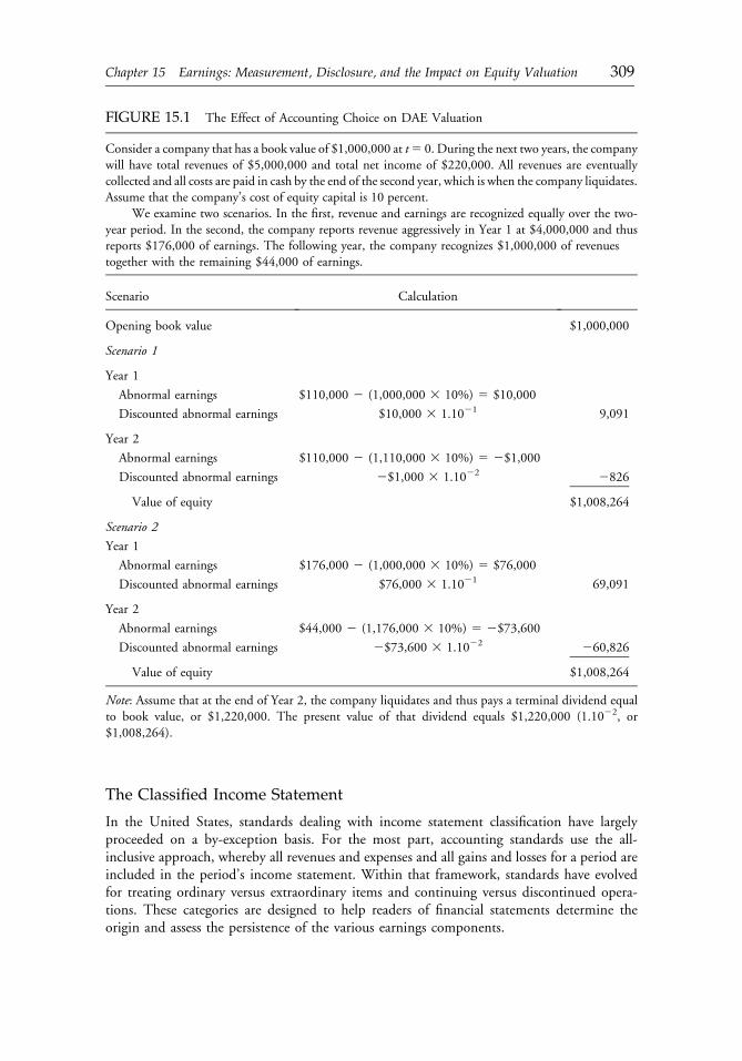
The Classified Income Statement
In the United States, standards dealing with income statement classification have largelyproceeded on a by-exception basis. For the most part, accounting standards use the all-inclusive approach, whereby all revenues and expenses and all gains and losses for a period areincluded in the period’s income statement. Within that framework, standards have evolvedfor treating ordinary versus extraordinary items and continuing versus discontinued opera-tions. These categories are designed to help readers of financial statements determine theorigin and assess the persistence of the various earnings components.
FIGURE 15.1 The Effect of Accounting Choice on DAE Valuation
Consider a company that has a book value of $1,000,000 at t5 0. During the next two years, the companywill have total revenues of $5,000,000 and total net income of $220,000. All revenues are eventuallycollected and all costs are paid in cash by the end of the second year, which is when the company liquidates.Assume that the company’s cost of equity capital is 10 percent.
We examine two scenarios. In the first, revenue and earnings are recognized equally over the two-year period. In the second, the company reports revenue aggressively in Year 1 at $4,000,000 and thusreports $176,000 of earnings. The following year, the company recognizes $1,000,000 of revenuestogether with the remaining $44,000 of earnings.
Scenario Calculation
Opening book value $1,000,000
Scenario 1
Year 1
Abnormal earnings $110,000 2 (1,000,000 3 10%) 5 $10,000
Discounted abnormal earnings $10,000 3 1.1021 9,091
Year 2
Abnormal earnings $110,000 2 (1,110,000 3 10%) 5 2$1,000
Discounted abnormal earnings 2$1,000 3 1.1022 2826
Value of equity $1,008,264
Scenario 2
Year 1
Abnormal earnings $176,000 2 (1,000,000 3 10%) 5 $76,000
Discounted abnormal earnings $76,000 3 1.1021 69,091
Year 2
Abnormal earnings $44,000 2 (1,176,000 3 10%) 5 2$73,600
Discounted abnormal earnings 2$73,600 3 1.1022 260,826
Value of equity $1,008,264
Note: Assume that at the end of Year 2, the company liquidates and thus pays a terminal dividend equalto book value, or $1,220,000. The present value of that dividend equals $1,220,000 (1.1022, or$1,008,264).
c15 12 September 2012; 18:0:10
Chapter 15 Earnings: Measurement, Disclosure, and the Impact on Equity Valuation 309
Income statements generally include the following broad categories or line items:
Sales
Cost of goods soldGross profit
Other operating revenues and expenses including bothrecurring and nonrecurring itemsOperating income
Financing and other costsPretax income from continuing operations
Income tax on continuing operationsIncome from continuing operations
Discontinued operations, net of tax (separated into resultsof operations and gain or loss on disposal)
Extraordinary items, net of taxCumulative effects of accounting changes, net of taxNet income
Harnischfeger Industries’ 1995 income statement provides a detailed example of thesecategories, as shown in Table 15.2.
Under a pure all-inclusive approach to reporting income, net income captures all changesin owners’ equity except those involving transactions with owners. That is, net income anddividends are the items that reconcile opening and ending retained earnings as follows:
Assets� Liabilities ¼ Owners’ equity ði:e:; Contributed capitalþ Retained earningsÞ:
Thus,
ΔA �ΔL ¼ ΔContributed capitalþΔRetained earnings¼ ΔContributed capitalþNet income�Dividends:
In recent years, however, accounting standards have allowed a number of items to bypassthe income statement, resulting in changes made directly to owners’ equity (i.e., “dirty sur-plus”). Currently, the major items treated this way are certain foreign-currency-related items(under Statement of Financial Accounting Standards No. 52), certain financial-instrument-related items (under SFAS No. 80), certain pension-liability-related items (under SFASNo. 87), certain marketable-security-related items (under SFAS No. 115), and certainderivatives-related activities (under SFAS No. 133).
Since 1998, SFAS No. 130, Reporting Comprehensive Income, has required companies toreport an income figure that incorporates net income and changes in these dirty surplus items.Because these additional items typically have low levels of persistence, they should not directlyaffect analysts’ forecasts of future abnormal earnings. Comprehensive income can, however,include additional information relevant to valuations and should be considered part of dili-gent fundamental analysis. Thus, we begin our discussion of accounting analysis with the
c15 12 September 2012; 18:0:11
310 Part III: Earnings and Cash Flow Analysis
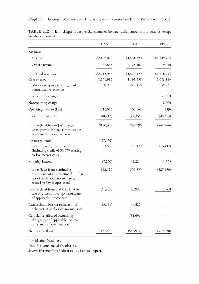
TABLE 15.2 Harnischfeger Industries Statements of Income (dollar amounts in thousands, except
per-share amounts)
1995 1994 1993
Revenues
Net sales $2,152,079 $1,551,728 $1,409,204
Other income 61,865 23,301 9,040
Total revenues $2,213,944 $1,575,029 $1,418,244
Cost of sales 1,671,932 1,195,851 1,083,846
Product development, selling, andadministrative expenses
330,990 279,016 259,831
Restructuring charges — — 67,000
Nonrecurring charge — — 8,000
Operating income (loss) 211,022 100,162 (433)
Interest expense, net (40,713) (47,366) (48,313)
Income (loss) before Joya mergercosts, provision (credit) for incometaxes, and minority interest
$170,309 $52,796 ($48,746)
Joy merger costs (17,459) — —
Provision (credit) for income taxes(including credit of $6,075 relatingto Joy merger costs)
53,500 13,979 (16,497)
Minority interest (7,230) (2,224) 4,799
Income (loss) from continuingoperations (after deducting $11,384,net of applicable income taxes,related to Joy merger costs)
$92,120 $36,593 ($27,450)
Income (loss) from and (net loss) onsale of discontinued operations, netof applicable income taxes
(31,235) (3,982) 7,760
Extraordinary loss on retirement ofdebt, net of applicable income taxes
(3,481) (4,827) —
Cumulative effect of accountingchange, net of applicable incometaxes and minority interest
— (81,696) —
Net income (loss) $57,404 ($53,912) ($19,690)
aJoy Mining Machinery.
Note: For years ended October 31.
Source: Harnischfeger Industries 1995 annual report.
c15 12 September 2012; 18:0:11
Chapter 15 Earnings: Measurement, Disclosure, and the Impact on Equity Valuation 311
most important value-relevant data—income from continuing operations—and discusscomprehensive income in detail at the end of the section.
Income from Continuing Operations
Income from continuing operations, as the name implies, is the profit reported in the currentperiod from the operations that management purportedly expects to continue in the future. Itshould not be interpreted as permanent or recurring earnings because companies systemati-cally include items in it that reasonably can be expected to occur only once. Sometimes,the reason is restrictive accounting rules; sometimes, it results from “strategic reporting”on the part of the company managers. For example, a common belief is that managers aremore likely to highlight one-time losses than one-time gains in communications withshareholders and in the business press.26 So, analysts should always study the notes and othersources to develop an unbiased assessment of the company’s recurring earnings stream. Someof the more common nonrecurring items are unusual items and restructuring charges.
Unusual and Nonrecurring Items
To be fair, IBM’s policy of taking nonrecurring charges on a recurring basis doesmake estimates [of earnings] rather chancy and, indeed, gives a wonderfully surrealquality to its earnings, since the charges not only reconfigure the past but con-ceivably prefigure, by anticipating expenses, the future.
—Abelson (1996)
Terms such as “discontinued operations” and “extraordinary items” are income statementclassifications specifically defined in accounting standards, but the term “unusual items” is acatchall phrase referring to items that do not meet more specific definitions. Because “unusualitems” do not have a restrictive definition, managers often describe an income statement itemas “unusual” to draw readers’ attention to it. In practice, these items are explicitly labeled“unusual” on the face of the income statement, or they are more fully described as such in thenotes or in the management discussion and analysis.
For example, in the 1993�95 income statements of Harnischfeger Industries shown inTable 15.2, the company reported a restructuring charge of $67 million in 1993 and an $8million item labeled “nonrecurring charge.” (Restructuring charges are discussed in the nextsection.) In 1995, the company reported a separate line item for costs associated with a recentmerger (together with associated tax costs). An analyst wishing to examine the trend in acompany’s income from continuing operations must decide how to treat these items.
The easiest alternative (aside from completely ignoring them) is to remove them (withtheir associated tax effects) from the analysis. In this approach, the analyst is relying onmanagement’s classification of the items as one-time or nonrecurring items.
Experience says, however, that a deeper analysis is usually worth conducting. The pur-pose is to determine what these charges represent, whether they are truly nonrecurring, andwhether the charges relate solely to the past or include costs more properly associated with thefuture. Additionally, analysts will benefit from determining whether the income statementcontains “buried” items—items that might properly be considered unusual or nonrecurringbut to which management has not explicitly drawn attention.
c15 12 September 2012; 18:0:11
312 Part III: Earnings and Cash Flow Analysis
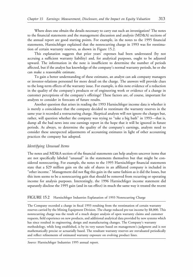
Where does one obtain the details necessary to carry out such an investigation? The notesto the financial statements and the management discussion and analysis (MD&A) sections ofthe annual report are good starting points. For example, in the notes to the 1995 financialstatements, Harnischfeger explained that the nonrecurring charge in 1993 was for reestima-tion of certain warranty reserves, as shown in Figure 15.2.
This explanation suggests that prior years’ expenses had been understated (by notaccruing a sufficient warranty liability) and, for analytical purposes, ought to be adjustedupward. The information in the note is insufficient to determine the number of periodsaffected, but if the analyst has knowledge of the company’s normal warranty periods, he or shecan make a reasonable estimate.
To gain a better understanding of these estimates, an analyst can ask company managersor investor-relations personnel for more detail on the charge. The answers will provide cluesto the long-term effects of the warranty issue. For example, is this note evidence of a reductionin the quality of the company’s products or of engineering work or evidence of a change incustomer perceptions of the company’s offerings? These factors are, of course, important foranalysts to consider in forecasts of future results.
Another question that arises in reading the 1993 Harnischfeger income data is whether itis merely a coincidence that the company decided to reestimate the warranty reserves in thesame year it recorded a restructuring charge. Skeptical analysts will not ignore the charges but,rather, will question whether the company was trying to “take a big bath” in 1993—that is,dump all the bad news into one earnings report in the hope that it will be ignored in futureperiods. As always, to determine the quality of the company’s earnings, analysts need toconsider these unexpected adjustments of accounting estimates in light of other accountingpractices the company has adopted.
Identifying Unusual Items
The notes and MD&A section of the financial statements can help analysts uncover items thatare not specifically labeled “unusual” in the statements themselves but that might be con-sidered nonrecurring. For example, the notes to the 1995 Harnischfeger financial statementsstate that a $29 million gain on the sale of shares in an affiliated company is included in“other income.” Management did not flag this gain in the same fashion as it did the losses, butthis item seems to be a nonrecurring gain that should be removed from recurring or operatingincome for analysis purposes. Interestingly, the 1996 Harnischfeger income statement didseparately disclose the 1995 gain (and its tax effect) in much the same way it treated the recent
FIGURE 15.2 Harnischfeger Industries Explanation of 1993 Nonrecurring Charge
The Company recorded a charge in fiscal 1993 resulting from the reestimation of certain warrantyreserves carried by the Mining Equipment Division. The charge reduced pre-tax income by $8,000. Thisnonrecurring charge was the result of a much deeper analysis of open warranty claims and customerrequests, field experience on new products, and additional analytical data provided by new systems whichhas since resulted in engineering, design and manufacturing changes. The Company’s warrantymethodology, while long established, is by its very nature based on management’s judgment and is notmathematically precise or actuarially based. The resultant warranty reserves are reevaluated periodicallyand reflect refinements of estimated warranty exposure on evolving product lines.
Source: Harnischfeger Industries 1995 annual report.
c15 12 September 2012; 18:0:11
Chapter 15 Earnings: Measurement, Disclosure, and the Impact on Equity Valuation 313
merger costs. This step made it easier for readers to assess the persistence of reported earn-ings—and coincidentally lowered the “expected” level of earnings against which 1996 resultsmight reasonably be compared.
Another example of disclosure of an unusual item makes clear the value of going beyondthe income statement alone. In the 1994�1996 financial statements of Total Petroleum(North America) Ltd., a number of potentially nonrecurring items are buried in higher-levelcategories in the income statement and are outlined only in the notes. In 1994 and 1995, thecompany did not—on the face of the income statement—refer specifically to unusual itemsthat amounted to more than 10 percent of the respective period’s net income or loss. Clearly,analysts who ignore the notes do so at their own peril.
As these examples demonstrate, a common unusual item is the restructuring charge, towhich we now turn our attention.
Restructurings
But, some investors and other critics argue that AT&T’s fourth major restructuringin the past decade—following big one-time moves in 1986, 1988, and 1991—hasleft them dazed and confused about how much money the telecommunications gianthas actually been making.
—Smith and Lipin (1996)
In recent years, restructuring charges have been prominent on the income statements of manycompanies.27 For example, recall from Table 15.2 that Harnischfeger reported a restructuringcharge of $67 million in fiscal 1993—enough to put operating income into the loss columnthat year. These charges are typically associated with a decision to “do things differently in thefuture” and they generally involve layoffs, plant closings, and asset write-downs. The difficultyin dealing with restructuring charges is not trying to discover them; normally, they are clearlylabeled on the income statement. The trick is to get a handle on what they represent and whatthey suggest about the future. Indeed, the Emerging Issues Task Force (EITF) of the FinancialAccounting Standards Board (FASB) deliberated on this matter because the members believedthat many companies were including inappropriate items in their restructuring charges. As aresult, since 1994, stricter guidance exists for what can and cannot be included in restruc-turing charges, when they are accrued, and how they are disclosed.28
Determining when to accrue for restructuring and what to include in the charge is dif-ficult and fraught with uncertainty. Managers who believe that investors and analysts discountthe impact of restructuring charges have an incentive to increase the charge (“it’s already$1 billion, why not make it $1.2 billion?”). That way, in future years, costs can be chargedagainst the restructuring liability instead of earnings. If the restructuring charge has beenoveraccrued in one year, it can be brought back into income in a future year, perhaps with theintent to raise or smooth those earnings.
EITF No. 94-3 (together with the guidance of the U.S. Securities and ExchangeCommission’s Staff Accounting Bulletin [SAB] No. 100) attempts to add a degree of uni-formity to the types of costs included in restructuring charges—in particular, to stop com-panies from including the restructuring charge costs that more properly relate to futureyears.29 For example, the cost of layoffs can be accrued as a liability and charged as part of therestructuring expense only when all the following conditions exist:
c15 12 September 2012; 18:0:11
314 Part III: Earnings and Cash Flow Analysis
� Prior to the date of the financial statements, management, having the appropriate level ofauthority to impose involuntary termination on employees, approves and commits theenterprise to the plan of termination and establishes the benefits that current employees willreceive upon termination.
� Prior to the date of the financial statements, the benefit arrangement is communicated indetail to employees.
� The plan of termination specifically identifies the number of employees to be terminated,their job classifications or functions, and their locations.
� The period of time to complete the plan of termination indicates that significant changes tothe plan of termination are not likely.
Similar criteria need to be met to accrue other sorts of restructuring charges.Contrary to most accounting standards, which promote conservatism that results in
income understatement, this guidance effectively delays the recognition of expenses. Themain reason for this position in the standards is that some companies had been accruing avariety of future costs (such as marketing campaigns for the company’s “new image,” updatedinformation systems installed to enhance productivity in the restructured company, and soon) with their restructuring charges in the hope that the entire charge would be discounted byanalysts as a one-time event. The resulting early recognition of expenses would lead to futureearnings being higher than otherwise.
From an accounting perspective, restructurings are neither extraordinary items nor dis-continued operations. As we will see, those items are reported on a net-of-tax basis, and per-share data for the items are also reported. Standard setters expressed concern that companieswould try to blur the distinction between restructuring and these other items. Because, inprinciple, restructurings are conceptually distinct from discontinued operations (i.e.,restructurings represent a new way of engaging in a continuing line of business, and a dis-continued operation is a line of business that will no longer be engaged in) and are notunusual and infrequent (the accountant’s definition of extraordinary), their disclosure oughtnot lead to confusion among the categories. As such, standard setters concluded that forrestructuring costs, the following conditions should apply:
� The income statement effect of recognizing a liability at the commitment date should bereported in income from continuing operations and should not be reported on the face ofthe income statement net of income taxes.
� The effect on earnings per share should not be disclosed on the face of the incomestatement.
� Revenue and related costs and expenses of activities that will not be continued should notbe combined and reported as a separate component of income.
In addition, the following information, when material, must be disclosed:
� A description of the major actions composing the exit plan, activities that will not becontinued, including the method of disposition and the anticipated date of completion.
� A description of the type and amount of exit costs recognized as liabilities and the clas-sification of those costs in the income statement.
� A description of the type and amount of exit costs paid and charged against the liability.� The amount of any adjustment(s) to the liability.
c15 12 September 2012; 18:0:11
Chapter 15 Earnings: Measurement, Disclosure, and the Impact on Equity Valuation 315
� For all periods presented, the revenue and net operating income or losses from activitiesthat will not be continued, if those activities have separately identifiable operations.
The key to dealing with restructuring charges is to understand what they are for, whythey are needed, and what will be different in the future. Reaching such understanding can bea nontrivial and time-consuming task. In assessing possible future changes, analysts need toask whether they have seen the last of the charges or whether the company is one of many thatrecognizes “recurring nonrecurring charges.” This judgment should be a function of priorexperience with the company and the disclosures made by the company. Analysts shouldadminister a healthy dose of skepticism to disclosures and descriptions provided by companiesthat have a history of recurring nonrecurring items.
A two-step approach to the analysis of restructuring costs is useful. The first step is todetermine which charges relate to the past and which to the future so that appropriateadjustments to historical trends can be made. In reading the financial press, company pressreleases, and analysts’ research reports, one sometimes gets the feeling that the best thing to dowith restructuring charges is to ignore them. Analysts should resist this temptation becausethese charges often reflect the cumulative effect of items that should have been charged off inthe past. For example, when the charges represent the cost of closing a factory or disposing ofequipment, it suggests that prior-period depreciation expense was too low and that the level ofprior earnings thus was too high. A simple way to deal with the charge is to allocate it to, say,the past five years and restate prior results for analysis purposes. Although somewhat arbitrary,this method seems better than ignoring the costs altogether. Lowenstein (1997) suggests thatanalysts should add up the restructuring charges of the past five years, average them, penalizeeach prior quarter by the same amount, and in the future, deduct the same charge fromexpected earnings. His logic is that businesses almost always make mistakes, and althoughsuch errors do not happen every 90 days, they are nonetheless to be expected. The second stepin the analysis of restructuring charges is to monitor the reserves and their uses from prioryears to assess the veracity of prior disclosures, the likelihood that prior restructurings are ontrack, and whether the planned savings are materializing.
A critical item to look for is the reversal of old restructuring charges into current-periodearnings. Companies that have carefully called attention to their so-called nonrecurringrestructurings in prior periods have been known to be less forthcoming when the charges arereversed in later years.30 Prudent analysts will be on the lookout for reversals buried in cost ofsales or selling and administrative expenses.
In some ways, restructuring charges are similar in spirit to discontinuing certainoperations of the company. From an accounting perspective, the major difference betweenrestructuring and discontinuing operations is one of intent and scope. Restructurings rear-range the way business is done and sometimes that means incurring exit costs related tofacility closures and downsizing. Nonetheless, the company does not exit the businesses it isengaged in. Discontinued operations involve leaving entire lines of business, and we turn tothis topic in the next section.
Discontinued Operations
MacMillan Bloedel said it agreed to sell its paper-making unit for $850 millionCanadian dollars to a group of investors. . . . MacMillan said the sale will result ina charge of C$35 to C$45 million, to be recorded in discontinued operations in thesecond quarter.
—Chipello (1998)
c15 12 September 2012; 18:0:12
316 Part III: Earnings and Cash Flow Analysis

Analysts should be on the lookout for restructurings that are classified as discontinuedoperations. Restructurings are admissions on the part of management that the way business wasdone in the past needs to change in order to be effective in the future. Often, such a changemeans that prior-period results were misstated. (For example, assets may have been depreciatedover estimated useful lives that turned out to have been too long.) Consequently, restructuringsinclude costs that might otherwise be considered recurring but are simply aggregated into asingle year. In addition, because they typically involve significant accounting estimates, anychanges in the estimates are dealt with prospectively and prior-period results are not restated.Diligent analysts, however, will carefully consider the effects of any changes in estimates.
Discontinued operations are different from restructurings and involve changes inoperations for which the past truly may not be representative of the future. Accountantsrestate prior results and accord special treatment to gains and losses on disposal of theseoperations. Management, in turn, has incentives to treat charges that might be classified asrestructuring costs as costs of discontinued operations to obtain this accounting treatment.Thus, the careful analyst will be on the lookout for the gray areas and will carefully examinethe nature of the charges involved in discontinued operations disclosures. Accounting guid-ance for these activities is found in APB (Accounting Principles Board) Opinion 30, Reportingthe Results of Operations—Reporting the Effects of Disposal of a Segment of a Business, andExtraordinary, Unusual and Infrequently Occurring Events and Transactions.
Companies add and drop product lines as part of the normal course of business. Rev-enues and expenses related to the disposal of part of a business, the shifting of production ormarketing activities from one line or location to another, the phasing out of a productor service, and changes driven by technological improvements are not considered dis-continued operations. These are considered normal costs of continuing operations. Forcompanies in today’s business environment, avoiding such costs while remaining competitiveis difficult to imagine. In contrast, companies may decide to fundamentally change the mix ofeconomic activity for their overall organization and dispose of an entire business segment.
Special accounting is required if a disposal qualifies as a business segment. APB Opinion30 defines a “segment of a business” as a component of an entity whose activities represent aseparate major line of business or class of customer. Opinion 30 provides the followingexamples of disposals that should be classified as disposals of a segment of a business:
� A diversified company sells a major division that represents the company’s only activities inthe electronics industry.
� A meatpacking company sells a 25 percent interest in a professional football team that hasbeen accounted for under the equity method. All other activities of the company are in themeatpacking business.
� A communications company sells all its radio stations. The company’s remaining activitiesare three television stations and a publishing company. The assets and results of operationsof the radio stations are clearly distinguishable physically, operationally, and for financialreporting purposes.
� A food distributor disposes of one of its two divisions. One division sells food wholesale,primarily to supermarket chains, and the other division sells food through its chain of fast-food restaurants, some of which are franchised and some of which are company owned. Bothdivisions are in the business of food distribution, but the nature of selling food through fast-food outlets is vastly different from that of wholesaling food to supermarket chains. Byhaving two major classes of customers, the company has two segments of its business.
Furthermore, the following disposals are not classified as disposals of a segment of a business.
c15 12 September 2012; 18:0:12
Chapter 15 Earnings: Measurement, Disclosure, and the Impact on Equity Valuation 317
� A mining company sells a foreign subsidiary engaged in silver mining that represents all ofthe controlling company’s activities in a particular country. The fact that the companycontinues to engage in silver mining activities in other countries indicates that the salerepresents only a part of a line of business.
� A petrochemical company sells a 25 percent interest in a petrochemical plant. Because theremaining activities of the company are in the same line of business as the 25 percentinterest that has been sold, the transaction is a sale not of a major line of business but ofonly part of a line of business.
� A diversified company sells a subsidiary that manufactures furniture. The company hasretained its other furniture-manufacturing subsidiary. The disposal of the subsidiary,therefore, is not a disposal of a segment of the business but rather a disposal of part of a lineof business. Such disposals are incidental to the evolution of the entity’s business.
� The sale of all the assets related to the manufacture of men’s woolen suits by an apparelmanufacturer in order to concentrate activities in the manufacture of men’s suits fromsynthetic products. This transaction would represent a disposal of a product line, as dis-tinguished from the disposal of a major line of business.
Disclosures about discontinued operations involve two relevant dates. The measurementdate is the date at which the decision to discontinue an operation is made. The disposal date isthe date at which the operation is sold or abandoned. Sometimes these dates coincide, butmore often, they do not. The period between the two is known as the phase-out period. In thereporting period that includes the measurement date, the results of discontinued operationsprior to the measurement date are disclosed separately from continuing operations and net oftax. Prior-period data are restated as well. This approach allows the analyst to see more clearlythe trend in continuing operations.
In addition, a gain or loss on the disposal is recorded in the same period as the mea-surement date. The calculation of the gain or loss depends on whether the disposal andmeasurement dates coincide, whether the disposal and measurement dates are in the sameperiod, and whether a net gain or loss is expected. When the measurement and disposal datescoincide, the gain or loss is separately disclosed, net of tax. When the measurement anddisposal dates are different but occur in the same period, results of the discontinued opera-tions between the measurement date and the disposal date are netted with the gain or loss onthe sale of the net assets to arrive at the net gain or loss on disposal (reported net of tax).Details of each component are provided.
When the two dates fall in different periods, management needs to estimate the resultsof operations up to the (possibly unknown) disposal date and the gain or loss on the netasset sale. When the (expected) combined results of the discontinued operations subsequentto the measurement date and the gain or loss on the disposal of the net assets sum to a netloss, the entire amount is accrued in the same period as the measurement date. Thus, as longas the sum of the expected operating profits or losses and expected gain or loss on net assetsale is a net loss, the net amount is conservatively reported, even though the amountsmay occur in later periods. When net gains are expected, the gains are recorded onlywhen realized.
From the perspective of an equity analyst valuing a company, the discontinued opera-tions disclosures offer an opportunity to break earnings into persistent and transitory com-ponents. In most cases, the disposals take place over a relatively short period. When thediscontinued operations spill over into future periods and the amounts are material, analysts
c15 12 September 2012; 18:0:12
318 Part III: Earnings and Cash Flow Analysis
should separately value the continuing and discontinued operations. The accounting dis-closures of net assets of discontinued operations and separate disclosure of operating resultsare particularly amenable to analysis by using the DAE model.
As if the confusion in determining what is unusual and what is discontinued were notenough, accountants have another category of items that appears on the income statement:extraordinary items. According to APB Opinion 30, an event or transaction should beclassified as extraordinary if it is both unusual and infrequent.31 “Unusual” implies thatthe event or transaction is highly abnormal and not related to, or incidentally related to, theordinary activities of the enterprise. “Infrequent” implies that the event or transaction is notexpected to recur in the foreseeable future.
Extraordinary Items
Assessing whether an item is unusual and infrequent requires consideration of the context inwhich it arose. For example, one might consider the Exxon Valdez oil spill to be unusual andinfrequent on the basis of its magnitude. Further thought, however, leads one to realize thatmajor oil companies likely spill some oil daily. Indeed, oil companies undoubtedly devote partof their risk-management activities to ensuring an effective cost-benefit trade-off for spills. Inthis light, it is not surprising that Exxon Corporation did not report the related costs of thespill as extraordinary. Rather, as shown in Table 15.3, the company reported the item on aseparate line of the income statement (i.e., as an unusual item).
APB Opinion 30 indicates that certain items are not considered extraordinary, including
� write-down or write-off of receivables, inventories, equipment leased to others, deferredresearch and development costs, and other intangible assets;
� gains and losses from exchange or translation of foreign currencies, including those relatedto major devaluations or revaluations;
� gains and losses on the disposal of a segment of a business;� other gains and losses from sale of abandonment of property, plant, or equipment used in
the business;� effects of a strike, including those against competitors and major suppliers;� adjustment of accruals on long-term contracts.
In general, most events and transactions will not meet the definition of extraordinary.32
When extraordinary items are reported, they are shown as net of income taxes in aseparate section of the income statement. In addition, the per-share effect of the items isreported. Note that disclosure is normally provided to enhance the reader’s understanding ofthe event or transaction. For example, refer again to the Harnischfeger income statementreproduced in Table 15.2 and the excerpt from the related note to the financial statements inFigure 15.3. In both fiscal 1994 and 1995, the company retired some of its debt early, butbecause the cost of doing so exceeded the book value of the debt, a loss was incurred. Analystsreviewing the financial statements and coming across an extraordinary loss should ask why thecompany has chosen to refinance, how the refinancing was accomplished, and how futureresults may be affected. For example, has the company been able to restructure the debt withcheaper debt or with less restrictive debt? Is the company timing the retirement to achievesome sort of income smoothing? Was the debt refinanced because of (or to avoid) the vio-lation of a covenant?33
c15 12 September 2012; 18:0:12
Chapter 15 Earnings: Measurement, Disclosure, and the Impact on Equity Valuation 319
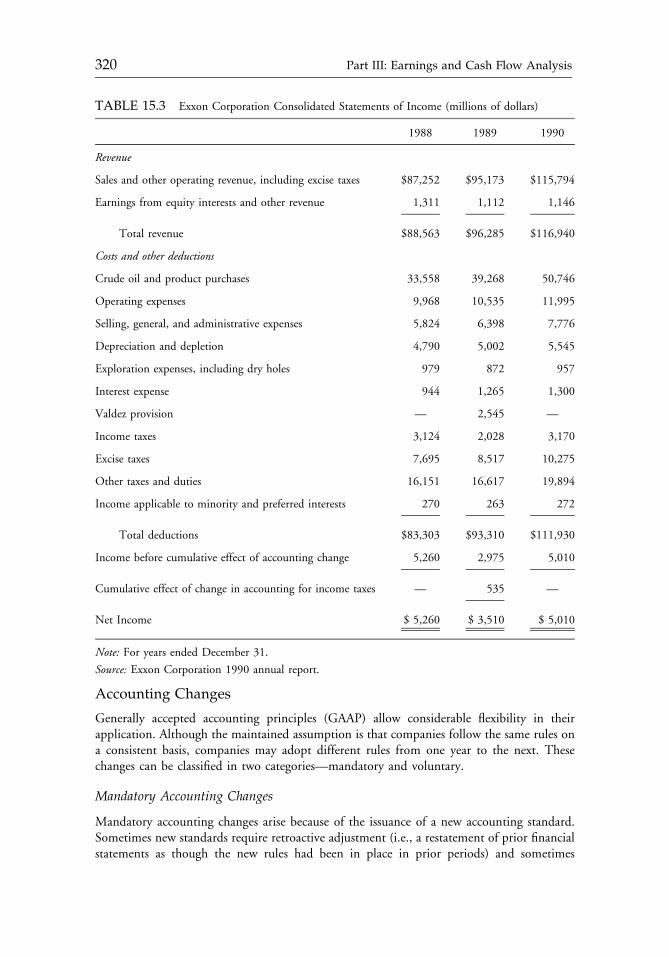
Accounting Changes
Generally accepted accounting principles (GAAP) allow considerable flexibility in theirapplication. Although the maintained assumption is that companies follow the same rules ona consistent basis, companies may adopt different rules from one year to the next. Thesechanges can be classified in two categories—mandatory and voluntary.
Mandatory Accounting Changes
Mandatory accounting changes arise because of the issuance of a new accounting standard.Sometimes new standards require retroactive adjustment (i.e., a restatement of prior financialstatements as though the new rules had been in place in prior periods) and sometimes
TABLE 15.3 Exxon Corporation Consolidated Statements of Income (millions of dollars)
1988 1989 1990
Revenue
Sales and other operating revenue, including excise taxes $87,252 $95,173 $115,794
Earnings from equity interests and other revenue 1,311 1,112 1,146
Total revenue $88,563 $96,285 $116,940
Costs and other deductions
Crude oil and product purchases 33,558 39,268 50,746
Operating expenses 9,968 10,535 11,995
Selling, general, and administrative expenses 5,824 6,398 7,776
Depreciation and depletion 4,790 5,002 5,545
Exploration expenses, including dry holes 979 872 957
Interest expense 944 1,265 1,300
Valdez provision — 2,545 —
Income taxes 3,124 2,028 3,170
Excise taxes 7,695 8,517 10,275
Other taxes and duties 16,151 16,617 19,894
Income applicable to minority and preferred interests 270 263 272
Total deductions $83,303 $93,310 $111,930
Income before cumulative effect of accounting change 5,260 2,975 5,010
Cumulative effect of change in accounting for income taxes — 535 —
Net Income $ 5,260 $ 3,510 $ 5,010
Note: For years ended December 31.
Source: Exxon Corporation 1990 annual report.
c15 12 September 2012; 18:0:12
320 Part III: Earnings and Cash Flow Analysis
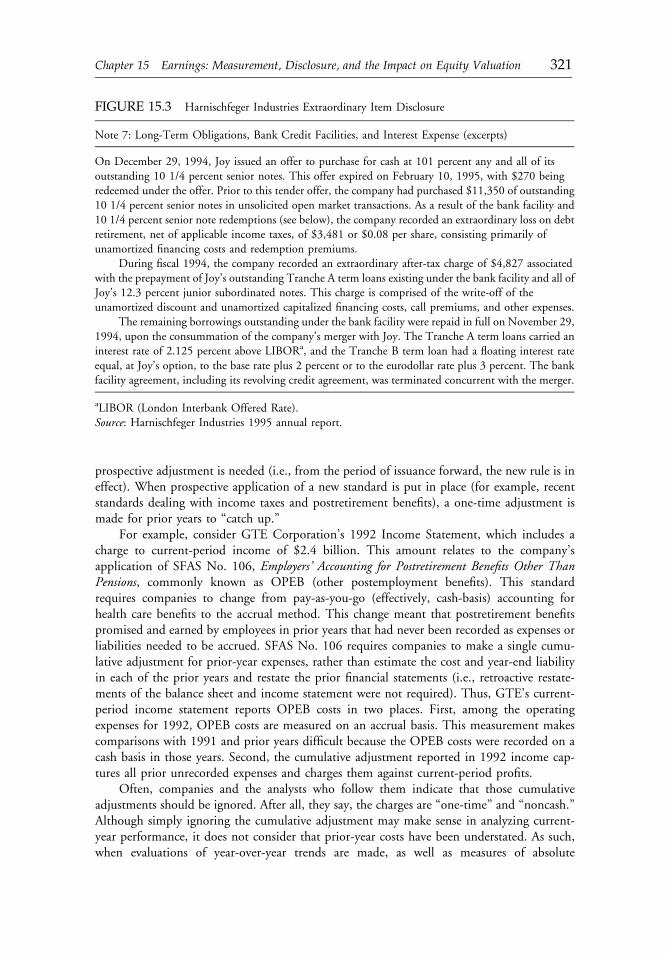
prospective adjustment is needed (i.e., from the period of issuance forward, the new rule is ineffect). When prospective application of a new standard is put in place (for example, recentstandards dealing with income taxes and postretirement benefits), a one-time adjustment ismade for prior years to “catch up.”
For example, consider GTE Corporation’s 1992 Income Statement, which includes acharge to current-period income of $2.4 billion. This amount relates to the company’sapplication of SFAS No. 106, Employers’ Accounting for Postretirement Benefits Other ThanPensions, commonly known as OPEB (other postemployment benefits). This standardrequires companies to change from pay-as-you-go (effectively, cash-basis) accounting forhealth care benefits to the accrual method. This change meant that postretirement benefitspromised and earned by employees in prior years that had never been recorded as expenses orliabilities needed to be accrued. SFAS No. 106 requires companies to make a single cumu-lative adjustment for prior-year expenses, rather than estimate the cost and year-end liabilityin each of the prior years and restate the prior financial statements (i.e., retroactive restate-ments of the balance sheet and income statement were not required). Thus, GTE’s current-period income statement reports OPEB costs in two places. First, among the operatingexpenses for 1992, OPEB costs are measured on an accrual basis. This measurement makescomparisons with 1991 and prior years difficult because the OPEB costs were recorded on acash basis in those years. Second, the cumulative adjustment reported in 1992 income cap-tures all prior unrecorded expenses and charges them against current-period profits.
Often, companies and the analysts who follow them indicate that those cumulativeadjustments should be ignored. After all, they say, the charges are “one-time” and “noncash.”Although simply ignoring the cumulative adjustment may make sense in analyzing current-year performance, it does not consider that prior-year costs have been understated. As such,when evaluations of year-over-year trends are made, as well as measures of absolute
FIGURE 15.3 Harnischfeger Industries Extraordinary Item Disclosure
Note 7: Long-Term Obligations, Bank Credit Facilities, and Interest Expense (excerpts)
On December 29, 1994, Joy issued an offer to purchase for cash at 101 percent any and all of itsoutstanding 10 1/4 percent senior notes. This offer expired on February 10, 1995, with $270 beingredeemed under the offer. Prior to this tender offer, the company had purchased $11,350 of outstanding10 1/4 percent senior notes in unsolicited open market transactions. As a result of the bank facility and10 1/4 percent senior note redemptions (see below), the company recorded an extraordinary loss on debtretirement, net of applicable income taxes, of $3,481 or $0.08 per share, consisting primarily ofunamortized financing costs and redemption premiums.
During fiscal 1994, the company recorded an extraordinary after-tax charge of $4,827 associatedwith the prepayment of Joy’s outstanding Tranche A term loans existing under the bank facility and all ofJoy’s 12.3 percent junior subordinated notes. This charge is comprised of the write-off of theunamortized discount and unamortized capitalized financing costs, call premiums, and other expenses.
The remaining borrowings outstanding under the bank facility were repaid in full on November 29,1994, upon the consummation of the company’s merger with Joy. The Tranche A term loans carried aninterest rate of 2.125 percent above LIBORa, and the Tranche B term loan had a floating interest rateequal, at Joy’s option, to the base rate plus 2 percent or to the eurodollar rate plus 3 percent. The bankfacility agreement, including its revolving credit agreement, was terminated concurrent with the merger.
aLIBOR (London Interbank Offered Rate).Source: Harnischfeger Industries 1995 annual report.
c15 12 September 2012; 18:0:12
Chapter 15 Earnings: Measurement, Disclosure, and the Impact on Equity Valuation 321
performance levels, analysts need to consider how the financial statements would have lookedif retroactive adjustment had been made. Companies rarely provide precise figures to allowsuch adjustments. Nonetheless, one can start by applying the current-year effect, if provided,to the prior years’ financial statements (perhaps with an adjustment for inflation or, in the caseof OPEB, workforce levels). This strategy is similar to the one we suggested for dealing withrestructuring costs and other so-called one-time events that, in fact, suggest that prior-periodresults may have been overstated (see Lowenstein 1997).34
Voluntary Accounting Changes and Changes in Accounting Estimates
Voluntary accounting changes need to be treated with caution. Analysts need to determinewhy a company is changing its accounting policies. Reasonable explanations include changingto use policies generally used by competitors and rationalizing different policies that mightarise as acquisitions take place. Although these reasons may be valid, analysts should alwaysquestion the timing of the changes and evaluate them in light of any other issues related toquality of earnings. For example, in fiscal 1996, B/E Aerospace changed its method ofaccounting for engineering costs. Rather than capitalize and amortize the costs, the companybegan to expense them immediately, consistent with its competitors. The skeptical analyst willquestion the timing of such a change. In this case, the company was otherwise having a verypoor year. Was it dumping all its bad news into one announcement? Did the new methodenhance the usefulness of the firm’s reporting?
Voluntary accounting changes normally involve restating prior results, although somecompanies argue that the differences are not material. Voluntary changes in accountingmethod can be distinguished from changes in accounting estimates. Changing the inventory-cost allocation method from FIFO (first in, first out) to LIFO (last in, first out) or thedepreciation method from accelerated to straight line is a change in method. Changingthe estimate of obsolete inventory or the estimated useful life of equipment is a change inestimate. Changes in estimate are accounted for prospectively (that is, prior results are notrestated). Sometimes, pro forma figures are provided. As with voluntary accounting changes,the important thing for the analyst to consider is the reason for the change in estimates andwhether the change is intended to improve the quality of the disclosures or to mislead ana-lysts. The change in estimates could be timed to record a “big bath,” thereby alleviating theneed for the company to amortize the costs in future years.
Comprehensive Income and Its Components
For fiscal years beginning after December 15, 1997, companies are required to report areconciliation of net income to comprehensive income in the primary financial statements. InSFAS No. 130, comprehensive income is defined as:
the change in equity [net assets] of a business enterprise during a period fromtransactions and other events and circumstances from nonowner sources. It includesall changes in equity during a period, except those resulting from investments byowners and distributions to owners.35
If all such nonowner transactions ran through the income statement, comprehensive incomewould be identical to net income.
The required explicit reconciliation of comprehensive income to net income is partly inresponse to concerns that an increasing number of earnings-related items were being reported
c15 12 September 2012; 18:0:13
322 Part III: Earnings and Cash Flow Analysis
in varying locations throughout the financial statements. The SFAS No. 130 reportingrequirements are designed to reduce the effort required to find and analyze these otherperformance-related items. The FASB did not specify the format and financial statementlocation of the comprehensive income reconciliation, so companies can include the infor-mation as an extension of the income statement, a stand-alone statement of performance, oras part of the statement of changes in equity. Most companies have elected to report it as partof the statement of changes in equity.
The most common cause of direct changes to equity is recording assets and liabilities atmarket value (or some modified market value) on the balance sheet. For example, whenavailable-for-sale marketable securities are recorded at market value, unrealized gains andlosses are included on the balance sheet as part of “accumulated other comprehensive income”and in the reconciliation of net and comprehensive income as “other comprehensive income.”When the securities are sold, the realized gain or loss is recorded on the income statement. Toavoid double counting the gain in both this period’s net income and a prior period’s com-prehensive income, “other comprehensive income” includes a reclassification adjustment inthe period of the realized gain.
Other items included in other comprehensive income are adjustments for foreign cur-rency exchange rate changes, minimum pension liability adjustments, and derivatives-relatedhedging activities. Most of the items included in the reconciliation are outside of manage-ment’s control (i.e., the company may manage foreign currency risk, but it is unlikely to beable to affect the exchange rates themselves). One exception is the net unrealized gain onavailable-for-sale marketable securities. That is, although a company may not be able toinfluence security prices, it can strategically time the sale of securities with previously unre-alized gains or losses (a practice known as “cherry picking”). The strategically timed sales willnot affect comprehensive income, because a reclassification adjustment is made so that thegains are not counted in comprehensive income twice (once as other comprehensive incomeand once as net income). For example, Table 15.4 shows the 1997 adjustments First IndianaCorporation made in its report of comprehensive income.36
Nonetheless, current-period net income can be managed via the strategic timing of salesof available-for-sale marketable securities.37 Consequently, the clear reporting of marketablesecurities activity (one of the components of other comprehensive income) can help analystsassess the quality of a company’s reported net income.
Summary
Determining the quality and persistence of earnings is tricky. It requires not only in-depthknowledge of a company’s competitive strategy and its relationship to its industry andcompetitors but also knowledge of the accounting rules used to generate earnings reports.Prudent analysts are aware that management has both the incentive and the discretion topractice opportunistic earnings management in both the classification and the timing ofcertain elements of earnings. Analysis of the notes to the financial statements, a careful readingof management’s discussion and analysis, and a healthy dose of skepticism go a long waytoward generating an understanding of past earnings trends and the questions for manage-ment to aid in the development of forecasted future results.
We believe that accounting classifications are especially useful starting points forunderstanding the nature or persistence of earnings. Nonetheless, it is important for analyststo look beyond the classifications to get at the underlying events. In this section, we outlined
c15 12 September 2012; 18:0:13
Chapter 15 Earnings: Measurement, Disclosure, and the Impact on Equity Valuation 323
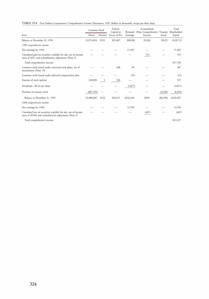
TABLE 15.4 First Indiana Corporation’s Comprehensive Income Disclosures, 1997 (dollars in thousands, except per-share data)
Common Stock Paid-InCapital in
Excess of ParRetainedEarnings
AccumulatedOther Comprehensive
IncomeTreasuryStock
TotalShareholders’
EquityItem Shares Amount
Balance at December 31, 1994 12,974,854 $131 $31,867 $88,981 ($120) ($147) $120,712
1995 comprehensive income
Net earnings for 1995 — — — 17,267 — — 17,267
Unrealized gain on securities available for sale, net of incometaxes of $351 and reclassification adjustment (Note 2)
— — — — 515 — 515
Total comprehensive income $17,782
Common stock issued under restricted stock plans, net ofamortization (Note 13)
— — 268 99 — — 367
Common stock issued under deferred compensation plan — — — (21) — — (21)
Exercise of stock options 120,830 1 536 — — — 537
Dividends—$0.32 per share — — — (3,877) — — (3,877)
Purchase of treasury stock (687,199) — — — — (6,203) (6,203)
Balance at December 31, 1995 12,408,485 $132 $32,671 $102,449 $395 ($6,350) $129,297
1996 comprehensive income
Net earnings for 1996 — — — 13,704 — — 13,704
Unrealized loss on securities available for sale, net of incometaxes of ($320) and reclassification adjustment (Note 2)
— — — — (467) — (467)
Total comprehensive income $13,237
c15 12 September 2012; 18:0:13
324
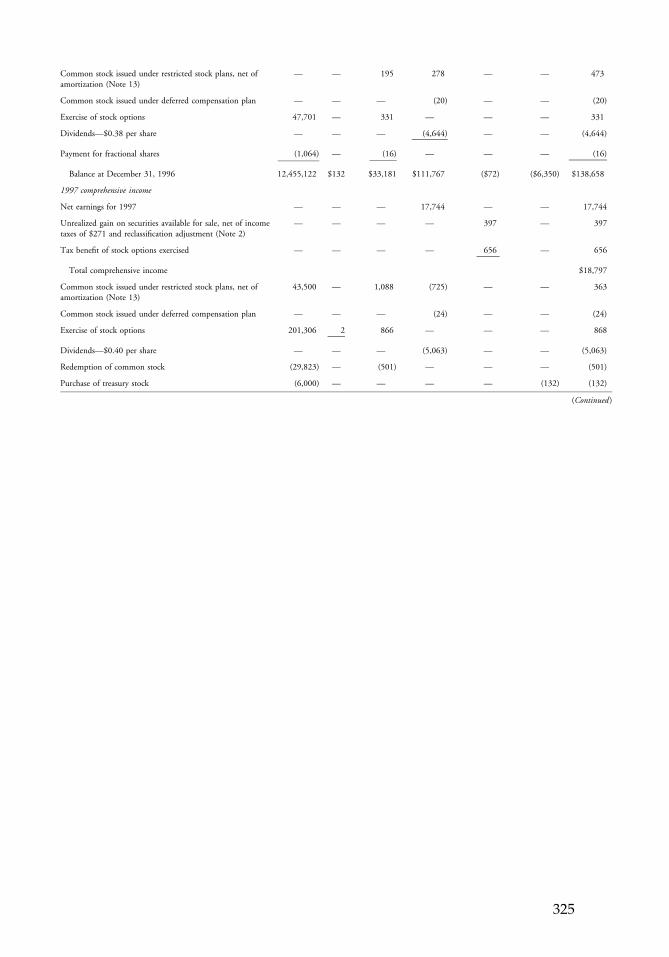
Common stock issued under restricted stock plans, net ofamortization (Note 13)
— — 195 278 — — 473
Common stock issued under deferred compensation plan — — — (20) — — (20)
Exercise of stock options 47,701 — 331 — — — 331
Dividends—$0.38 per share — — — (4,644) — — (4,644)
Payment for fractional shares (1,064) — (16) — — — (16)
Balance at December 31, 1996 12,455,122 $132 $33,181 $111,767 ($72) ($6,350) $138,658
1997 comprehensive income
Net earnings for 1997 — — — 17,744 — — 17,744
Unrealized gain on securities available for sale, net of incometaxes of $271 and reclassification adjustment (Note 2)
— — — — 397 — 397
Tax benefit of stock options exercised — — — — 656 — 656
Total comprehensive income $18,797
Common stock issued under restricted stock plans, net ofamortization (Note 13)
43,500 — 1,088 (725) — — 363
Common stock issued under deferred compensation plan — — — (24) — — (24)
Exercise of stock options 201,306 2 866 — — — 868
Dividends—$0.40 per share — — — (5,063) — — (5,063)
Redemption of common stock (29,823) — (501) — — — (501)
Purchase of treasury stock (6,000) — — — — (132) (132)
(Continued)
c15 12 September 2012; 18:0:13
325

Table 15.4 (Continued)
Common Stock Paid-InCapital in
Excess of ParRetainedEarnings
AccumulatedOther Comprehensive
IncomeTreasuryStock
TotalShareholders’
EquityItem Shares Amount
Reissuance of treasury stock 4,591 — 40 — — 42 82
Payment for fractional shares (505) — (12) — — — (12)
Balance at December 31, 1997 12,668,191 $134 $34,662 $123,699 $981 ($6,440) ($153,036)
The following table was included in Note 2 to the financial statements:
December 31
1997 1996 1995
Unrealized holding gains (losses) arising during the period $614 ($186) $568
Reclassification adjustment for gains included in net earnings (217) (281) (53)
Net unrealized gain (loss) on securities available for sale $397 ($467) $515
Note: Consolidated statements of shareholders’ equity.
Source: First Indiana Corporation and subsidiaries 1997 annual report.
c15 12 September 2012; 18:0:13
326
the categories of income typically found in U.S. GAAP earnings reports. We described theclassification rules and provided guidance to analysts with respect to interpreting the data andrestating them for fundamental analysis purposes. The key to analysis of recurringand nonrecurring items is the determination of their effect on future earnings and cash flows,and thus, the value of the company.
HOW BUY-SIDE EQUITY ANALYSTS USE EARNINGSIN VALUATION
In this section, we report the results of an experiment in which we provided buy-side equityanalysts with financial information and asked them to value the common stock of a hypo-thetical company. Most valuation-related research in finance and accounting is based on theanalysis of complex mathematical models (i.e., analytical research) or involves the study ofhistorical databases, such as stock prices and published accounting information (i.e., archivalresearch). Although less frequently conducted, controlled experiments (i.e., experimentalresearch) can provide powerful and complementary evidence about cause-and-effect rela-tionships in valuation. In the experiment described in this section, we provided differentsubgroups of analysts with subtly different income information for the hypothetical companyand kept constant all other financial information (e.g., balance sheet and cash flows). Thisapproach not only allows inferences about the general role of earnings in valuation but alsomakes it possible to isolate the incremental importance of reported income and its compo-nents in equity analysts’ valuation activities.38
Although experiments cannot capture all elements of the naturally occurring settings towhich one wants to generalize, the method allows precise manipulation of the variables ofinterest and control of variables that are not of interest. This ability provides an importantadvantage over methods that rely on analysis of archival databases. For example, in theexperiment we report, we designed a set of case materials in which the company to be valuedwas the same in all versions, except that we seeded a type of earnings management into asubset of the versions. This approach allowed us to investigate the use of accounting earningsand its components while significantly reducing the possibility that “real” economic differ-ences in the companies caused differences in analysts’ stock-price judgments. Experiments alsoallow investigation of economic phenomena when archival data are sparse or not yet available.In this study, we are able to investigate the role of various types of financial information in thevaluation judgments of buy-side analysts, despite the fact that the valuation activities of theseanalysts typically are not publicly disclosed.
Finally, although archival research can show the “real world” effect of information oninvestor decisions through stock returns (i.e., executed buy and sell decisions determine price),traditional research methods cannot as readily provide evidence on the judgment process thatprecedes those decisions. In our experiment, we are able to examine the effect of earnings andother financial information on the stock-price judgments of practicing analysts. For buy-sideanalysts, the trade data generated after institutional buy or sell orders have been executedconstitute the only evidence about these judgments that is available to archival researchers.
Analysts are important consumers of accounting information. Understanding whatearnings-related information analysts use and how that information is actually incorporatedinto their valuation activities can help analysts recognize and avoid common pitfalls in theinterpretation and use of financial accounting information. In addition, a clearer under-standing of how analysts use information in their valuation activities can help the Financial
c15 12 September 2012; 18:0:14
Chapter 15 Earnings: Measurement, Disclosure, and the Impact on Equity Valuation 327
Accounting Standards Board (FASB) and the U.S. Securities and Exchange Commission(SEC) in evaluating new and existing financial reporting rules.
Objectives and Procedures
For most fundamental analysts, a logical starting point for predicting the future earnings of acompany is the most recent historical earnings of the company. To estimate future earnings,an analyst must assess the various components of the company’s historical earnings and decidewhether these components will recur and, if so, for how long. Excessive attention to acompany’s bottom line—without evaluating the individual items that contribute to netincome—could lead to an overly optimistic or pessimistic estimate of the future earningspotential of a company. One of the objectives of our experiment, therefore, is to investigatethe extent to which analysts recognize the varying persistence of earnings components andtake into account significant nonrecurring income items.
An important assumption underlying this section is that buy-side analysts actually usereported earnings to value a company. Although the majority of equity analysts likely do notrely solely on earnings-based valuation approaches, the innumerable references to earnings andprice-to-earnings ratios (P/Es) in sell-side analyst reports and in the financial press suggest thatreported income is a nontrivial input of the valuation process. Because little direct evidenceexists about the use and relative importance of reported earnings in the activities of individualanalysts, another objective of the experiment is to assess the relative importance of earningsinformation and other potentially useful types of financial statement information.
Financial statement analysis can be a difficult and onerous task. Beyond the inherentuncertainty involved in trying to map financial fundamentals into equity security value, theprocess is made more difficult by the possibility that a company’s reported financial infor-mation is not representative of its “true” current economic state or future economic potential.Consistent with this possibility, numerous articles in the financial press and academic researchjournals indicate that companies manage their earnings in an attempt to influence investors’impressions of the company.39 If analysts do not detect opportunistic earnings management ina company’s reporting of past earnings, their predictions of the company’s future earningsmay be overly optimistic or pessimistic. If historical earnings, or biased estimates of futureearnings, are used in valuation models, analysts’ assessments of value also may be overlyoptimistic or pessimistic.
To investigate buy-side analysts’ use of earnings information in valuation, we designed anexperiment in which we systematically varied certain earnings data and asked analysts to valuea security. In particular, we varied the level of opportunistic earnings management in the casematerials to determine the potential effect of such a reporting strategy on analysts’ valuationjudgments. Although many methods of earnings management exist, our investigation islimited to the effect of realized marketable securities gains on analysts’ valuation judgments.
Most industrial companies in the United States hold the majority of their marketableequity securities in an “available-for-sale” portfolio. Under current accounting practice,available-for-sale marketable equity securities are included on the balance sheet at fair value.A problem inherent in any type of fair value asset accounting is the treatment of holding gainsor losses caused by changes in the assets’ fair values.40 Under Statement of FinancialAccounting Standards (SFAS) No. 115, Accounting for Certain Investments in Debt and EquitySecurities, the holding gains on these securities temporarily bypass the income statement andare recorded as a direct increase in owners’ equity. Only when these securities are sold cana company report the previously accumulated gains as part of its net income.41 Thus,
c15 12 September 2012; 18:0:14
328 Part III: Earnings and Cash Flow Analysis
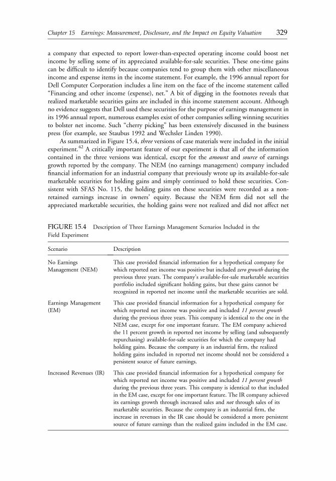
a company that expected to report lower-than-expected operating income could boost netincome by selling some of its appreciated available-for-sale securities. These one-time gainscan be difficult to identify because companies tend to group them with other miscellaneousincome and expense items in the income statement. For example, the 1996 annual report forDell Computer Corporation includes a line item on the face of the income statement called“Financing and other income (expense), net.” A bit of digging in the footnotes reveals thatrealized marketable securities gains are included in this income statement account. Althoughno evidence suggests that Dell used these securities for the purpose of earnings management inits 1996 annual report, numerous examples exist of other companies selling winning securitiesto bolster net income. Such “cherry picking” has been extensively discussed in the businesspress (for example, see Staubus 1992 and Wechsler Linden 1990).
As summarized in Figure 15.4, three versions of case materials were included in the initialexperiment.42 A critically important feature of our experiment is that all of the informationcontained in the three versions was identical, except for the amount and source of earningsgrowth reported by the company. The NEM (no earnings management) company includedfinancial information for an industrial company that previously wrote up its available-for-salemarketable securities for holding gains and simply continued to hold these securities. Con-sistent with SFAS No. 115, the holding gains on these securities were recorded as a non-retained earnings increase in owners’ equity. Because the NEM firm did not sell theappreciated marketable securities, the holding gains were not realized and did not affect net
FIGURE 15.4 Description of Three Earnings Management Scenarios Included in the
Field Experiment
Scenario Description
No EarningsManagement (NEM)
This case provided financial information for a hypothetical company forwhich reported net income was positive but included zero growth during theprevious three years. The company’s available-for-sale marketable securitiesportfolio included significant holding gains, but these gains cannot berecognized in reported net income until the marketable securities are sold.
Earnings Management(EM)
This case provided financial information for a hypothetical company forwhich reported net income was positive and included 11 percent growthduring the previous three years. This company is identical to the one in theNEM case, except for one important feature. The EM company achievedthe 11 percent growth in reported net income by selling (and subsequentlyrepurchasing) available-for-sale securities for which the company hadholding gains. Because the company is an industrial firm, the realizedholding gains included in reported net income should not be considered apersistent source of future earnings.
Increased Revenues (IR) This case provided financial information for a hypothetical company forwhich reported net income was positive and included 11 percent growthduring the previous three years. This company is identical to that includedin the EM case, except for one important feature. The IR company achievedits earnings growth through increased sales and not through sales of itsmarketable securities. Because the company is an industrial firm, theincrease in revenues in the IR case should be considered a more persistentsource of future earnings than the realized gains included in the EM case.
c15 12 September 2012; 18:0:14
Chapter 15 Earnings: Measurement, Disclosure, and the Impact on Equity Valuation 329
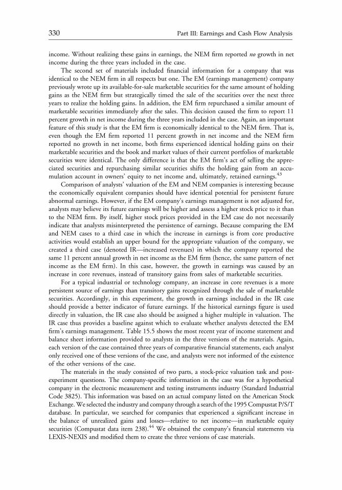
income. Without realizing these gains in earnings, the NEM firm reported no growth in netincome during the three years included in the case.
The second set of materials included financial information for a company that wasidentical to the NEM firm in all respects but one. The EM (earnings management) companypreviously wrote up its available-for-sale marketable securities for the same amount of holdinggains as the NEM firm but strategically timed the sale of the securities over the next threeyears to realize the holding gains. In addition, the EM firm repurchased a similar amount ofmarketable securities immediately after the sales. This decision caused the firm to report 11percent growth in net income during the three years included in the case. Again, an importantfeature of this study is that the EM firm is economically identical to the NEM firm. That is,even though the EM firm reported 11 percent growth in net income and the NEM firmreported no growth in net income, both firms experienced identical holding gains on theirmarketable securities and the book and market values of their current portfolios of marketablesecurities were identical. The only difference is that the EM firm’s act of selling the appre-ciated securities and repurchasing similar securities shifts the holding gain from an accu-mulation account in owners’ equity to net income and, ultimately, retained earnings.43
Comparison of analysts’ valuation of the EM and NEM companies is interesting becausethe economically equivalent companies should have identical potential for persistent futureabnormal earnings. However, if the EM company’s earnings management is not adjusted for,analysts may believe its future earnings will be higher and assess a higher stock price to it thanto the NEM firm. By itself, higher stock prices provided in the EM case do not necessarilyindicate that analysts misinterpreted the persistence of earnings. Because comparing the EMand NEM cases to a third case in which the increase in earnings is from core productiveactivities would establish an upper bound for the appropriate valuation of the company, wecreated a third case (denoted IR—increased revenues) in which the company reported thesame 11 percent annual growth in net income as the EM firm (hence, the same pattern of netincome as the EM firm). In this case, however, the growth in earnings was caused by anincrease in core revenues, instead of transitory gains from sales of marketable securities.
For a typical industrial or technology company, an increase in core revenues is a morepersistent source of earnings than transitory gains recognized through the sale of marketablesecurities. Accordingly, in this experiment, the growth in earnings included in the IR caseshould provide a better indicator of future earnings. If the historical earnings figure is useddirectly in valuation, the IR case also should be assigned a higher multiple in valuation. TheIR case thus provides a baseline against which to evaluate whether analysts detected the EMfirm’s earnings management. Table 15.5 shows the most recent year of income statement andbalance sheet information provided to analysts in the three versions of the materials. Again,each version of the case contained three years of comparative financial statements, each analystonly received one of these versions of the case, and analysts were not informed of the existenceof the other versions of the case.
The materials in the study consisted of two parts, a stock-price valuation task and post-experiment questions. The company-specific information in the case was for a hypotheticalcompany in the electronic measurement and testing instruments industry (Standard IndustrialCode 3825). This information was based on an actual company listed on the American StockExchange.We selected the industry and company through a search of the 1995Compustat P/S/Tdatabase. In particular, we searched for companies that experienced a significant increase inthe balance of unrealized gains and losses—relative to net income—in marketable equitysecurities (Compustat data item 238).44 We obtained the company’s financial statements viaLEXIS-NEXIS and modified them to create the three versions of case materials.
c15 12 September 2012; 18:0:14
330 Part III: Earnings and Cash Flow Analysis
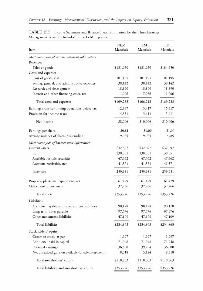
TABLE 15.5 Income Statement and Balance Sheet Information for the Three Earnings
Management Scenarios Included in the Field Experiment
ItemNEM
MaterialsEM
MaterialsIR
Materials
Most recent year of income statement information
Revenues
Sales of goods $181,630 $181,630 $184,650
Costs and expenses
Cost of goods sold 101,195 101,195 101,195
Selling, general, and administrative expenses 38,142 38,142 38,142
Research and development 18,890 18,890 18,890
Interest and other financing costs, net 11,006 7,986 11,006
Total costs and expenses $169,233 $166,213 $169,233
Earnings from continuing operations before tax 12,397 15,417 15,417
Provision for income taxes 4,351 5,411 5,411
Net income $8,046 $10,006 $10,006
Earnings per share $0.81 $1.00 $1.00
Average number of shares outstanding 9,985 9,985 9,985
Most recent year of balance sheet information
Current assets $32,697 $32,697 $32,697
Cash 138,551 138,551 138,551
Available-for-sale securities 47,362 47,362 47,362
Accounts receivable, net 41,371 41,371 41,371
Inventory 259,981 259,981 259,981
Property, plant, and equipment, net 61,479 61,479 61,479
Other noncurrent assets 32,266 32,266 32,266
Total assets $353,726 $353,726 $353,726
Liabilities
Accounts payable and other current liabilities 90,178 90,178 90,178
Long-term notes payable 97,576 97,576 97,576
Other noncurrent liabilities 47,109 47,109 47,109
Total liabilities $234,863 $234,863 $234,863
Stockholders’ equity
Common stock, at par 1,997 1,997 1,997
Additional paid-in capital 71,948 71,948 71,948
Retained earnings 36,600 39,794 36,600
Net unrealized gains on available-for-sale investments 8,318 5,124 8,318
Total stockholders’ equity $118,863 $118,863 $118,863
Total liabilities and stockholders’ equity $353,726 $353,726 $353,726
c15 12 September 2012; 18:0:14
Chapter 15 Earnings: Measurement, Disclosure, and the Impact on Equity Valuation 331
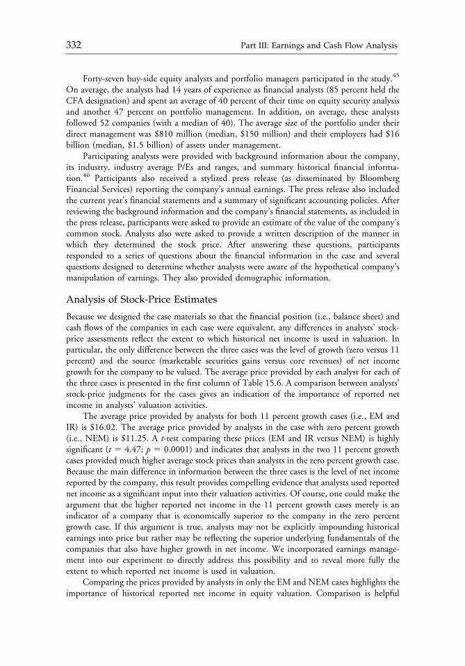
Forty-seven buy-side equity analysts and portfolio managers participated in the study.45
On average, the analysts had 14 years of experience as financial analysts (85 percent held theCFA designation) and spent an average of 40 percent of their time on equity security analysisand another 47 percent on portfolio management. In addition, on average, these analystsfollowed 52 companies (with a median of 40). The average size of the portfolio under theirdirect management was $810 million (median, $150 million) and their employers had $16billion (median, $1.5 billion) of assets under management.
Participating analysts were provided with background information about the company,its industry, industry average P/Es and ranges, and summary historical financial informa-tion.46 Participants also received a stylized press release (as disseminated by BloombergFinancial Services) reporting the company’s annual earnings. The press release also includedthe current year’s financial statements and a summary of significant accounting policies. Afterreviewing the background information and the company’s financial statements, as included inthe press release, participants were asked to provide an estimate of the value of the company’scommon stock. Analysts also were asked to provide a written description of the manner inwhich they determined the stock price. After answering these questions, participantsresponded to a series of questions about the financial information in the case and severalquestions designed to determine whether analysts were aware of the hypothetical company’smanipulation of earnings. They also provided demographic information.
Analysis of Stock-Price Estimates
Because we designed the case materials so that the financial position (i.e., balance sheet) andcash flows of the companies in each case were equivalent, any differences in analysts’ stock-price assessments reflect the extent to which historical net income is used in valuation. Inparticular, the only difference between the three cases was the level of growth (zero versus 11percent) and the source (marketable securities gains versus core revenues) of net incomegrowth for the company to be valued. The average price provided by each analyst for each ofthe three cases is presented in the first column of Table 15.6. A comparison between analysts’stock-price judgments for the cases gives an indication of the importance of reported netincome in analysts’ valuation activities.
The average price provided by analysts for both 11 percent growth cases (i.e., EM andIR) is $16.02. The average price provided by analysts in the case with zero percent growth(i.e., NEM) is $11.25. A t-test comparing these prices (EM and IR versus NEM) is highlysignificant (t 5 4.47; p 5 0.0001) and indicates that analysts in the two 11 percent growthcases provided much higher average stock prices than analysts in the zero percent growth case.Because the main difference in information between the three cases is the level of net incomereported by the company, this result provides compelling evidence that analysts used reportednet income as a significant input into their valuation activities. Of course, one could make theargument that the higher reported net income in the 11 percent growth cases merely is anindicator of a company that is economically superior to the company in the zero percentgrowth case. If this argument is true, analysts may not be explicitly impounding historicalearnings into price but rather may be reflecting the superior underlying fundamentals of thecompanies that also have higher growth in net income. We incorporated earnings manage-ment into our experiment to directly address this possibility and to reveal more fully theextent to which reported net income is used in valuation.
Comparing the prices provided by analysts in only the EM and NEM cases highlights theimportance of historical reported net income in equity valuation. Comparison is helpful
c15 12 September 2012; 18:0:14
332 Part III: Earnings and Cash Flow Analysis
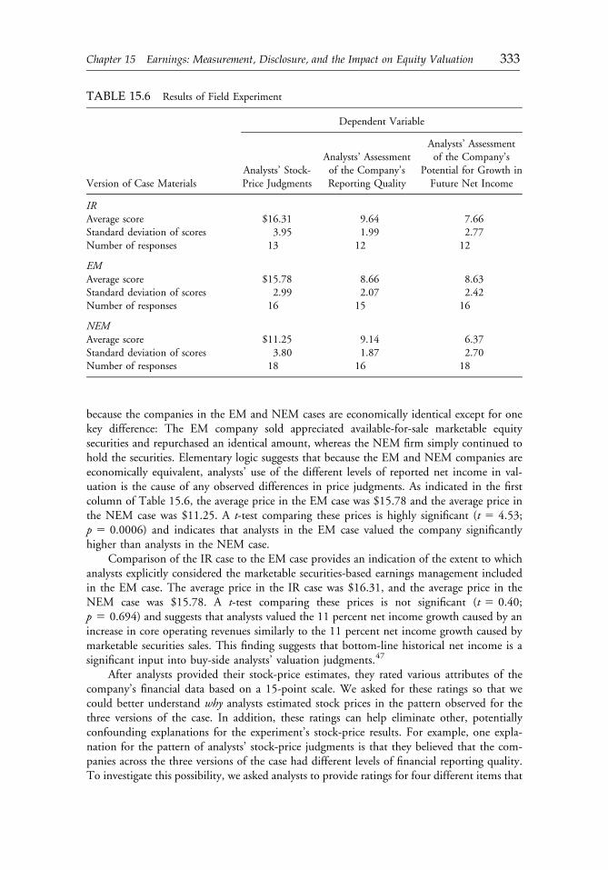
because the companies in the EM and NEM cases are economically identical except for onekey difference: The EM company sold appreciated available-for-sale marketable equitysecurities and repurchased an identical amount, whereas the NEM firm simply continued tohold the securities. Elementary logic suggests that because the EM and NEM companies areeconomically equivalent, analysts’ use of the different levels of reported net income in val-uation is the cause of any observed differences in price judgments. As indicated in the firstcolumn of Table 15.6, the average price in the EM case was $15.78 and the average price inthe NEM case was $11.25. A t-test comparing these prices is highly significant (t 5 4.53;p 5 0.0006) and indicates that analysts in the EM case valued the company significantlyhigher than analysts in the NEM case.
Comparison of the IR case to the EM case provides an indication of the extent to whichanalysts explicitly considered the marketable securities-based earnings management includedin the EM case. The average price in the IR case was $16.31, and the average price in theNEM case was $15.78. A t-test comparing these prices is not significant (t 5 0.40;p 5 0.694) and suggests that analysts valued the 11 percent net income growth caused by anincrease in core operating revenues similarly to the 11 percent net income growth caused bymarketable securities sales. This finding suggests that bottom-line historical net income is asignificant input into buy-side analysts’ valuation judgments.47
After analysts provided their stock-price estimates, they rated various attributes of thecompany’s financial data based on a 15-point scale. We asked for these ratings so that wecould better understand why analysts estimated stock prices in the pattern observed for thethree versions of the case. In addition, these ratings can help eliminate other, potentiallyconfounding explanations for the experiment’s stock-price results. For example, one expla-nation for the pattern of analysts’ stock-price judgments is that they believed that the com-panies across the three versions of the case had different levels of financial reporting quality.To investigate this possibility, we asked analysts to provide ratings for four different items that
TABLE 15.6 Results of Field Experiment
Dependent Variable
Version of Case MaterialsAnalysts’ Stock-Price Judgments
Analysts’ Assessmentof the Company’sReporting Quality
Analysts’ Assessmentof the Company’s
Potential for Growth inFuture Net Income
IRAverage score $16.31 9.64 7.66Standard deviation of scores 3.95 1.99 2.77Number of responses 13 12 12
EMAverage score $15.78 8.66 8.63Standard deviation of scores 2.99 2.07 2.42Number of responses 16 15 16
NEMAverage score $11.25 9.14 6.37Standard deviation of scores 3.80 1.87 2.70Number of responses 18 16 18
c15 12 September 2012; 18:0:14
Chapter 15 Earnings: Measurement, Disclosure, and the Impact on Equity Valuation 333

were designed to provide an indication of the company’s financial reporting quality. Spe-cifically, analysts rated the quality of the company’s reported net income (from very low tovery high), the clarity of the company’s financial statements (from not at all clear tovery clear), the reliability of the company’s financial statements (from very unreliable to veryreliable) and the manner in which the financial statements portrayed the company’s overalllong-term financial performance (from very misleading to very truthful).
Because these questions were designed to measure the same underlying characteristic ofthe company, we constructed a composite measure of perceived reporting quality by taking asimple average of the four measures.48 As reported in the second column of Table 15.6, theaverage perceived reporting quality rating was 9.64 in the IR condition, 8.66 in the EMcondition, and 9.14 in the NEM condition. An F-test conducted on these means indicatesthat the perceived reporting quality did not differ between the three versions of the case(F , 0.5). This result suggests that analysts perceived financial reporting quality to be similarfor all three cases and that the observed differences in stock-price judgments were caused bythe variation in the levels of reported net income and not differences in analysts’ perceptionsof the company’s reporting quality.
Another factor that could have contributed to the differences between analysts’ commonstock-price judgments is variation in the perceived growth potential for the company.49 Togather information on this factor, we asked analysts to rate, on a 15-point scale (from very lowto very high), the company’s potential for future earnings growth. As summarized in the thirdcolumn of Table 15.6, analysts who completed the EM case provided a mean rating for thecompany of 8.63 and believed the company had significantly better prospects for futureearnings growth than analysts who completed the NEM case, with a mean rating of 6.37(t 5 2.51; p 5 0.016). In contrast, analysts perceived no statistically significant difference(t , 1) between the IR case, with a mean rating of 7.66, and the EM case, with a mean ratingof 8.63. These results suggest that management’s opportunistic earnings management in theEM case was successful in making analysts believe the company’s future prospects for earningsgrowth were better than for the NEM firm, even though the EM and NEM companies wereeconomically identical. In addition, the opportunistic management of earnings in the EMcase caused analysts to perceive the company’s future prospects for earnings growth to be thesame as that observed for the company that created the earnings growth through an increase inoperating revenues (i.e., the IR company).
Insights from the Experiment
The results of this experiment suggest that buy-side financial analysts rely extensively onreported net income in performing equity security valuation. In particular, analysis of analysts’stock-price judgments and written explanations for those judgments suggest that buy-sideanalysts do not derive primary estimates of value from cash flow or balance sheet information.
The apparent importance of earnings in valuation presents both good news and cause forconcern. First, the good news: Analysts’ use of reported net income in valuation suggests thatthey appear to be comfortable with using earnings in valuation and may benefit from morecareful consideration of issues related to earnings quality. As we argued in the section “TheReporting of Earnings and Equity Valuation,” rigorous earnings-based models (such as thediscounted abnormal earnings model) present an opportunity for analysts to focus on acompany’s productive activities and competitive environment without becoming distracted byspecific forecasts of cash flows. Although forecasted earnings are a critical input for pragmaticapplications of the free cash flow model, the importance of this forecast often gets
c15 12 September 2012; 18:0:15
334 Part III: Earnings and Cash Flow Analysis
overshadowed by other items that affect the implementation of the model, such as concernsover which noncash items to back out of forecasted earnings to arrive at forecasted free cashflow and whether free cash flows are being reinvested in zero-NPV (net present value) pro-jects. By remaining focused on estimating the persistent earnings of the company, analysts caneliminate layers of complexity that add little value to valuation activities.
Of course, to appropriately apply a discounted abnormal earnings (DAE) model—or anyvaluation model for that matter—analysts must carefully consider the model’s inputs. Inparticular, analysts should pay special attention to the underlying quality of historical reportedearnings, if this number is being used to forecast future earnings. The need to forecast futureearnings in the DAE model leads to a potentially troubling result for this experiment:Companies may be able to engage in opportunistic earnings management and may be able todo so without being detected by many analysts.50
How might analysts avoid the valuation pitfalls presented by firms that opportunisticallymanage their earnings? This question is not easy to answer because financial statement analysisis a difficult and time-consuming task that rarely leads to a single, clear, all-encompassingconclusion about a company. In addition, as reported earlier, analysts who participated in ourexperiment follow, on average, 52 companies and split their time between analysis andportfolio management. Given the demands on their time, the many ways in which companiescan manage their earnings, and the complexity of financial information, analysts cannotrealistically be expected to detect every instance of opportunistic earnings management.Analysts might be more likely to detect the sort of earnings management engaged in by theEM firm if they are provided with clearer disclosure of activity in marketable securities. Wetested this possibility in a follow-up study.
Follow-Up Study
In the section “The Reporting of Earnings and Equity Valuation,” we noted that the FASBrecently adopted a reporting standard for comprehensive income reporting. SFAS No. 130was issued to facilitate the item-by-item assessment of companies’ earnings performance. Inparticular, some proponents of the standard suggested that all performance-related changes inowners’ equity should be presented in a single statement so that analysts could determine thevalue relevance of each of the performance-related line items. Indeed, in the context of ourexperiment, explicit reconciliation of marketable securities gains and losses in a performancestatement might have helped analysts detect the opportunistic earnings management in theEM case. Accordingly, we performed a follow-up study to investigate the possibility thatthe new reporting standard for comprehensive income increases the likelihood that analystswill detect opportunistic earnings management through examination of the marketablesecurities portfolio and adjust their valuation judgments accordingly.
An interesting feature of SFAS No. 130 is that it does not require a specific format orlocation for the reporting of comprehensive income. Indeed, the only hard and fastrequirement of the new standard is that companies disclose comprehensive income infor-mation in one of the primary financial statements. Although the FASB expressed a preferencefor reporting comprehensive income in a separate performance statement (consistent withtheir original exposure draft of the standard), most companies report comprehensive incomein the statement of changes in equity (SCE). Because analysts currently regard the SCE as oneof the least useful sources of financial information (Brown 1997), it is possible that SCEreporting of comprehensive income and its components will be less useful than reporting thesame information in a separate performance report.
c15 12 September 2012; 18:0:15
Chapter 15 Earnings: Measurement, Disclosure, and the Impact on Equity Valuation 335

To address the potential benefit of the new comprehensive income information, weinvestigated whether a separate performance statement format and the SCE format, which ismore likely to be used by most companies, are equally likely to correct the bias in analysts’stock-price judgments in the EM case.51 We generated four additional experimental conditions(that is, in addition to the original EM and NEM conditions reported in Table 15.6, in whichcomprehensive income was not disclosed but could be derived from the financial statements).For each firm, we created two conditions in which a reconciliation of net income and com-prehensive income was provided, as shown in Table 15.7. In one condition, the reconciliationwas provided in a separate statement of performance immediately after the income statement.In the other condition, the reconciliation was included in the statement of changes in equity. Intotal, we analyzed six conditions: earnings management with no reconciliation of net incomeand comprehensive income (EM-No-CI); no earnings management with no reconciliationof net income and comprehensive income (NEM-No-CI); earnings management with thereconciliation included in SCE (EM-CI-SCE); no earnings management with reconciliationincluded in SCE (NEM-CI-SCE); earnings management with reconciliation provided in aseparate statement immediately after the income statement (EM-CI-IS); and no earningsmanagement with reconciliation provided in a separate statement immediately after the incomestatement (NEM-CI-IS). In total, 96 buy-side analysts participated in the study—34 from theinitial No-CI conditions and 62 additional analysts for the CI-SCE and CI-IS conditions.
We predicted that the clear disclosure of elements of other comprehensive income in theEM-CI-IS condition would lead analysts to detect the earnings management and to reach
TABLE 15.7 Reconciliation of Net Income and Comprehensive Income in the CI-IS Conditions of
Follow-Up Study
Comprehensive Income DisclosureEM-CI-ISCondition
NEM-CI-ISCondition
Net income $10,006 $8,046
Other comprehensive income
Unrealized gains on available-for-sale securities arising this period
Gross unrealized gain 1,379 1,379
Income tax (484) (484)
Net unrealized gain 895 895
Reclassification adjustment for realized gains on available-for-salesecurities included in net income
Gross realized gain (3,020) 0
Income tax 1,060 0
Net realized gain (1,960) 0
Total other comprehensive income ($1,065) $895
Comprehensive income $8,941 $8,941
Note: Data from Hirst and Hopkins (1998).
c15 12 September 2012; 18:0:15
336 Part III: Earnings and Cash Flow Analysis
the same valuation for both the EM and NEM companies. Given that the disclosure ofelements of other comprehensive income in the EM-CI-SCE condition is not as clear as inthe EM-CI-IS condition but is clearer than in the EM-No-CI condition, we did not make aspecific prediction about whether that disclosure format would be effective in allowinganalysts to detect earnings management and reach an appropriate valuation for the company.
As expected, within the study, clear reporting of comprehensive income and its compo-nents in a separate performance statement (i.e., the CI-IS conditions) helped analysts recognizethe opportunistic earnings management in the EM case and led them to reach approximatelythe same judgment about stock price as did analysts completing the NEM case. Analystsprovided amean stock price for the EM-CI-IS condition of $13.40 versus $12.57 for the NEM-CI-IS condition. The difference between the average prices is not statistically significant, with at-statistic of 0.66. This finding suggests that when analysts recognized that opportunisticearnings management was causing the smooth earnings growth of 11 percent (in the EM case),they adjusted their valuation judgments to reflect it. Interestingly, reporting comprehensiveincome and its components in the SCE did not mitigate the difference in stock-price judgmentsbetween the EM and NEM cases. Analysts provided a mean stock price of $14.81 for the EM-CI-SCE condition versus $12.49 for the NEM-CI-SCE condition (t 5 1.85; p 5 0.034).
The finding that comprehensive income disclosures have more impact when disclosed ina separate statement of performance than in the SCE is consistent with the survey datareported in Brown (1997). In particular, Brown reports that analysts regard the SCE as one ofthe least useful reports provided by companies. In our study, analysts apparently disregardedthe potentially important value-relevant information in the SCE. One reason that analystsmight ignore the SCE is that prior to the issuance of the reporting standard for comprehensiveincome, although the major transactions reported in the SCE and not in other statements(i.e., stock issuances and buybacks, dividends) were highly significant, analysts were likely tohave known such information before the release of the financial statements. With usefuldisclosures becoming more likely to appear in the SCE, analysts may begin to pay moreattention to that statement. The findings of the follow-up study suggest that ignoring the SCEmay allow certain forms of earnings management to go undetected.
Summary
We conducted two studies to evaluate how buy-side analysts use earnings information in theirvaluation process. The findings of the initial study, which indicated that analysts have troubledetecting opportunistic earnings management, suggest that analysts need to pay more attentionto the sources of earnings and not simply focus on the amount. The separate follow-up studytested whether different ways of reporting comprehensive income and its components mightmitigate analysts’ inability to detect opportunistic earnings management. The findings of thisexperiment support the view that clear disclosure of all performance-related items would allowanalysts to more easily incorporate value relevant information into their valuations.
CONCLUSION
This research project began with the goal of providing analysts with the answer to thequestion “What are earnings?” One might think that answering this question would be fairlystraightforward for two accounting professors. As we considered ways to formulate ouranswer, however, we quickly realized how big this question actually is. In the United States,
c15 12 September 2012; 18:0:15
Chapter 15 Earnings: Measurement, Disclosure, and the Impact on Equity Valuation 337
academic accounting scholars have spent the better part of the 20th century trying to answerthis question, and this quest has generated some wonderful insights about the definition andmeasurement of “true” economic earnings—from the academic’s philosophical perspective.Little of this research, however, could directly benefit a practicing equity analyst in answeringour initial question. Because equity analysts are, first and foremost, concerned with valuation,our primary goal in writing this chapter was to demystify reported earnings and to explainhow they can best be incorporated into valuation activities.
In the section “Evidence on the Relevance of Earnings to Valuation,” we providedselected highlights from the large body of academic research that demonstrate the relevanceof accounting information to security prices. This body of research documents theimportance not only of the bottom-line net income figure but also of components ofearnings. If the goal is to forecast future free cash flows, current accounting earnings actuallyare more helpful than current-period cash flows. The bulk of prior research, however,addresses the relation between accounting data and aggregate, market-level data, such asstock prices and returns, and little research has investigated the valuation judgments anddecision making of individual analysts.
As with any other model, the output of an earnings-based valuation model will only be asgood as its inputs. To help improve the quality of accounting inputs in the valuation process,the section “The Reporting of Earnings and Equity Valuation” outlined the way accountantsclassify components of earnings and provided examples of how these classifications helpanalysts determine the quality and persistence of historical earnings. To help analysts seethrough the potential biases inherent in financial data provided by management, weemphasized the importance of understanding the discretion involved in making accountingclassifications. Being armed with better knowledge about how accounting data are generatedputs analysts in a better position to use the information effectively.
The section “How Buy-Side Analysts Use Earnings in Valuation” describes two studiesthat investigate the valuation judgments of individual buy-side equity analysts. The initialstudy provides direct evidence that the level of a firm’s accounting earnings influences pro-fessional buy-side analysts’ valuation judgments. A troubling finding, however, is that theanalysts did not appear to distinguish between firms that were and were not managing theirearnings through the strategic timing of sales and repurchases of marketable securities.
We hypothesized that this result may have been a function of the way the accountingdata were presented to the analysts. Although the efficient market hypothesis maintainsthat data presentation ought not affect security prices, we argued that given the nature ofsecurity analysts’ jobs (i.e., the number of firms they follow and the other demands on theirtime), analysts may require clearer disclosure of such transactions if they are to incorporatesuch data into stock price judgments. In a follow-up study (Hirst and Hopkins 1998), weinvestigated this hypothesis and found that comprehensive income disclosures do indeedhelp analysts uncover earnings management. We provided evidence of the benefits toanalysts of lobbying the Financial Accounting Standards Board for improvements inaccounting standards and evidence to the FASB of the implications of their new compre-hensive income standard.
Our hope is that analysts will benefit from better knowledge of what earnings are andhow they can be incorporated into equity valuation. In addition, we hope that readers havegained an appreciation for the value of examining the judgments and decision making ofindividual analysts. In our view, continued research in this area can lead to insights about howanalysts do their job, how expert and novice analysts differ, how to improve the education andtraining of analysts, and most important, how to improve the practice of equity analysis.
c15 12 September 2012; 18:0:15
338 Part III: Earnings and Cash Flow Analysis
NOTES
1. The adage that “you manage what you measure” applies to cash earnings and cash flowsas much as it does to accounting net income. Managing cash flow is as simple as delayingthe payment of a supplier or running an advertising campaign a week earlier or later.
2. Although finance and accounting researchers have performed innumerable studies modelingand testing the relationship between earnings and stock returns and between earnings andstock values, the discussion in this section focuses on themost important lessons to be learnedfrom a handful of the studies. For a more complete synthesis of research investigating thevalue relevance of earnings and other types of accounting information, see Bernard (1989),Lev (1989), Lev and Ohlson (1982), and Bauman (1996).
3. Ball and Brown used three proxies for unexpected earnings, with similar results for each.We limit our discussion to the random walk change in earnings or, more simply, thechange in earnings from one year to the next. Ball and Brown also analyzed the abnormalreturns on each company’s stock. “Abnormal return” was defined as a company’scommon stock return for a month adjusted for the expected return as predicted by thecapital asset pricing model (CAPM).
4. The residual change in earnings measure used in Beaver et al. was a proxy for companies’unexpected earnings, and the residual change in price represents companies’ commonstock return for a month adjusted for the expected return as suggested by the CAPM.
5. The publication of this paper by Kormendi and Lipe spawned intensive investigation ofERCs by accounting researchers. An extensive review of ERC research can be found inCho and Jung (1991).
6. Loosely speaking, R2 is the portion of variation in one variable that can be explained bythe variation in another variable. Two variables that are perfectly correlated will have anR2 of 1.0 (or 100 percent), and two variables that are randomly associated will have an R2
of 0.7. Their sample 20 years of data allowed the formation of ten 10-consecutive-year earnings
samples. Each 10-year sample contained, on average, 1,045 companies.8. Net book value is equal to a company’s assets minus its liabilities (i.e., it is equal to total
owners’ equity). Except when owners are investing or withdrawing capital, the net bookvalue of a company changes as a result of earnings. Therefore, net book value is a metricthat includes the historical aggregation of earnings of a company. Brennan (1995) notedthat “the accretion to book value caused by the retention of earnings is eventuallyreflected in the stock price. Far from being close to useless, as some have claimed,accounting earnings are seen to be highly informative about stock returns over long timeintervals” (p. 51).
9. Elliott and Hanna defined large write-offs as those exceeding 1 percent of total assets.10. The section “The Reporting of Earnings and Equity Valuation,” contains a discussion of
the DAE model.11. For a more in-depth explanation of the relative informativeness of earnings and cash
flows, see Sloan (1996).12. On the other hand, one would expect cash flows to be more value relevant than
accounting earnings in circumstances in which current earnings are not representative offuture earnings. A study by Cheng, Liu, and Schaefer (1996) showed that cash flowsexplain more of stock returns when earnings are highly transitory (i.e., not permanent),which underscores the need to evaluate the components of earnings.
c15 12 September 2012; 18:0:15
Chapter 15 Earnings: Measurement, Disclosure, and the Impact on Equity Valuation 339
13. A number of studies analyzed sell-side analysts’ reports. For example, in a sample of 479sell-side analysts’ reports, Previts, Bricker, Robinson, and Young (1994) noted thatearnings-related information is the factor most cited by sell-side analysts. In a follow-upstudy, Bricker, Previts, Robinson, and Young (1995) investigated the factors thatdetermine whether sell-side analysts believe companies have “high-quality” earnings.
14. A number of studies conducted during the 1980s (e.g., Anderson 1988) analyzed thepattern of information use by small samples of analysts. These studies provided evidenceon the styles of information searches conducted by professional analysts, but they gen-erally did not address the relevance of specific pieces of accounting information (e.g.,earnings) in analysts’ valuation activities.
15. For example, in a common application of the free cash flow model, a company’s currentperiod earnings are used to forecast future years’ earnings. Then, after forecasted futureearnings are estimated, the analyst removes forecasted future noncash items fromearnings to arrive at forecasted cash flows.
16. We use the term “quality” to refer to the extent to which the current-period earnings areuseful in predicting future earnings.
17. We believe that the “cash is king” perspective is an extremist view, especially whenconsidering the typical application of cash-flow models (including FCF models) inpractice. In typical real-world applications, expected future FCF is generally derived byfirst forecasting future income statements and balance sheets. Furthermore, historicalfinancial statements are the most common starting point for forecasting future financialstatements. Reflecting on the sequence of steps in this estimation process quickly revealsthat analysts apply FCF models by forecasting and analyzing the very data the models aredesigned to avoid—accrual accounting data. So, although forecasted accruals areunwound in the models to arrive at the free cash flows, the models are highly dependenton accounting-based measures of performance.
18. Just as accounting-based earnings can be manipulated, so can cash flows—and theaggressive timing of cash flows is not likely to spark problems with the auditors! Con-sider a simple way to increase cash flow in the current period: Pay suppliers on the firstday of the following period. Although it might be clear that the company is trying tomake the current period’s ending cash position look strong, no auditor would force thecompany to record the cash payment (from next period) in the current period. If theaccount payable arose because a service was consumed this year (and was likely to beconsumed again next year), the auditor would surely require the company to include therelated expense in determining the current period’s earnings. Indeed, accrual accountingrequires that the cost of currently consumed goods and services be included in deter-mining a company’s profitability.
19. See, for example, Ohlson (1995), Feltham and Ohlson (1995), and Edwards and Bell(1961). Empirical support for the model as a predictor of value is available in, amongothers, Bernard (1995), Francis, Olsson, and Oswald (2000), and Penman and Sou-giannis (1998).
20. Two important points need to be clarified. First, earnings in Equation 15.1 are definedas clean surplus earnings. Technically, therefore, “comprehensive income” (not “netincome”) is the correct performance measure. (Comprehensive income is discussed inmore detail later in this section.) Second, dividends are defined as dividends in thenormal use of the term plus share repurchases less share issuances.
21. White, Sondhi, and Fried (1998) used the relationships in Equations 15.1 and 15.2,together with the fact that Bt/(1 1 r) 5 Bt 2 rBt/(1 1 r), to derive Equation 15.5. The
c15 12 September 2012; 18:0:15
340 Part III: Earnings and Cash Flow Analysis
process involves expanding Equation 15.4 for t 5 1 and 2 and substituting the afore-mentioned relationship for Bt/(1 1 r). After reducing the resulting equation for termsthat cancel out and expanding from t 5 3 to t 5N, Equation 15.5 results.
22. Note that economic value added (EVA) and DAE are both models of “residual income.”That is, they both attempt to capture the value created by a company after providingreturns to all providers of capital. Accounting earnings, through interest expense, con-sider the return to debtholders, but because accounting earnings do not include a chargefor the cost of equity capital, they overstate residual income. By explicitly considering theequity capital invested to generate the returns, EVA and DAE capture measures ofresidual income. Using residual income to value entities can be traced to work byPreinreich (1938).
23. Figure 3.1 in Palepu, Bernard, and Healy (1996) shows that most U.S. industrialcompanies earn 10�14 percent ROE and that abnormally high or low ROEs in a givenyear tend to revert to the 10�14 percent range within three years.
24. Although DuPont analysis comes in a variety of forms, one useful form breaks downROE into NI/CSE 5 NI/EBT 3 EBT/EBIT 3 EBIT/Sales 3 Sales/Assets 3 Assets/CSE, where NI is net income, CSE is common shareholders’ equity, EBT is earningsbefore taxes, and EBIT is earnings before interest and taxes. The first term in thebreakdown of ROE measures the proportion of earnings retained after paying taxes (i.e.,1 2 Average tax rate). The second term represents the proportion of earnings beforeinterest and taxes that belongs to the equityholders. The third term is operating returnon sales. The fourth term is total asset turnover, and the final term is a measure ofleverage (i.e., Liabilities/CSE 1 1). The model can be easily extended to incorporatecomprehensive income (CI) into ROE by substituting CI for NI in return on equity andadding an additional term into the decomposition (CI/NI) that captures the after-taxeffect on ROE for items of other comprehensive income.
25. Consider the case of Sunbeam Corporation as described by Laing (1998). The companywas accused of manufacturing its 1997 earnings through various aggressive accountingchoices and by “preselling” products ahead of normal schedules. Preselling can come inmany forms, including offering deep discounts to distributors at the end of a givenquarter, offering very liberal return policies, and billing for goods that have not beenshipped. Sunbeam is alleged to have paid some distributors a monthly fee to hold gasgrills at the distributors’ warehouses. In addition, particularly loose return policiesapplied to the goods. Barron’s compared these sales to consignment sales (which nor-mally would not be recorded as revenue). The DAE model would accommodate thisaccounting as long as the analyst recognized that past earnings may not be representativeof future results. Aggressive year-end discounting and accounting lead to high currentabnormal earnings, but via their effect on increased book value, the threshold level ofearnings required to record future abnormal earnings is raised. Because the aggressiverevenue recognition in prior periods means that those revenues will not be reported inlater periods, the chance of high future abnormal earnings is lowered.
26. Schrand and Walther (2000) find that managers are more likely to remind investorsabout prior-period gains than losses. They argue that this practice is strategic in nature;that is, companies are attempting to manage perceptions of what a reasonable perfor-mance benchmark is. They find that in quarterly earnings announcements, managerstend to highlight prior gains on property, plant, and equipment dispositions to reducethe potential benchmark against which current earnings are evaluated. Managers do nothighlight prior-period losses on disposal of the same items, which leads to an emphasis
c15 12 September 2012; 18:0:16
Chapter 15 Earnings: Measurement, Disclosure, and the Impact on Equity Valuation 341
on the greatest possible improvement in quarter-over-quarter earnings. Remindinginvestors about prior gains serves to reduce the benchmark, and ignoring prior lossesserves to keep the benchmark low.
27. An exit cost, or restructuring cost, according to the Financial Accounting StandardsBoard [Emerging Issues Task Force No. 94-3, “Liability Recognition for CertainEmployee Termination Benefits and Other Costs to Exit an Activity (including CertainCosts Incurred in a Restructuring)”], is a cost resulting from a plan to exit an activity thathas no future economic benefit. All three following conditions need to be met to record arestructuring cost:1. The cost is not associated with or does not benefit activities that will be continued.2. The cost is not associated with or is not incurred to generate revenues after the exit
plan’s commitment date.3. The cost meets one of the following criteria:
a. The cost is incremental to other costs incurred by the enterprise in the conduct ofits activities prior to the commitment date and will be incurred as a direct result ofthe exit plan (e.g., the additional cost of subcontracting warranty work over thecost that would be incurred had the company continued to provide the serviceitself or the costs of employees and other costs to be incurred to close a plant afterit ceases operations).
b. The cost represents amounts to be incurred by the enterprise under a contractualobligation that existed prior to the commitment date and will either continue afterthe exit plan is completed with no economic benefit to the enterprise or be apenalty to cancel the contractual obligation (e.g., a lease cancellation penalty orthe cost of leased space that will remain unused for the duration of a lease once theexit plan is completed).
28. The guidance is included in EITF No. 94-3 (see previous note). Other guidance isprovided in, among others, EITF No. 96-9, “Classification of Inventory Markdowns andOther Costs Associated with a Restructuring”; No. 95-23, “The Treatment of CertainSite Restoration/Environmental Exit Costs When Testing a Long-Lived Asset forImpairment”; and No. 95-3, “Recognition of Liabilities in Connection with a PurchaseBusiness Combination.” In the U.S. Securities and Exchange Commission’s StaffAccounting Bulletin (SAB) No. 100, the SEC reiterated that restructuring charges needto be charged only when rigorously developed and thoroughly supported plans to exit anactivity exist. In SAB No. 100, the SEC is cracking down on the practice of accruinglarge charges in poor periods with the hope that such expenses will be ignored in futureanalyses. Formal documentation and approval by upper-level managers of the specifics ofthe restructuring are required before an accrual can be recorded. Furthermore, enhanceddisclosure in the footnotes and MD&A of the status of the accruals (and their reversals)needs to be presented in future interim and annual financial statements.
29. Despite the EITF’s attempt to tighten the rules, skeptical analysts and the business pressoften uncover suspicious items related to restructurings. For example, Laing (1998)questioned components of Sunbeam’s 1996 restructuring charge. He noted largeincreases in litigation reserves and the allowance for doubtful accounts. This Barron’sarticle is widely credited with the firing of CEO Al Dunlap and the initiation of aSecurities and Exchange Commission inquiry into the company’s accounting methods.
30. These reversals take place whenever the estimated cost of the restructuring turns out tobe too large. The exit plan is completed, but a portion of the initial accrued liability
c15 12 September 2012; 18:0:16
342 Part III: Earnings and Cash Flow Analysis
remains. Reversing the liability leads to “negative” expenses being recorded. Most ana-lysts would not consider them recurring benefits.
31. This definition is subtly different from the one used in International AccountingStandard No. 8, which defines extraordinary items as “income or expenses that arisefrom events or transactions that are clearly distinct from the ordinary activities of theenterprise and, therefore, are not expected to recur frequently or regularly.” The dif-ference in definitions underscores our contention that the labeling of income statementitems is largely irrelevant, except for contracting purposes. What is important is that theanalyst consider the underlying economics of the events in question and comes to areasoned conclusion about their effect on the profitability of the enterprise.
32. Some items are explicitly defined as extraordinary. Interestingly, (as we will see in ourHarnischfeger example) the gain or loss that arises on the early retirement of debt is, bydefinition, treated as an extraordinary item (in accordance with SFAS No. 4, ReportingGains and Losses from Extinguishment of Debt).
33. Research by Hand (1989) suggests that companies used debt�equity swaps to smooth anunexpected and transitory decrease in earnings per share. These findings may generalizeto other debt-related activity. Skeptical analysts will consider management’s motives forearly debt retirement in order to assess whether the transactions were undertaken foreconomic or accounting purposes.
34. Furthermore, to the extent that the new accounting standard provides management withnew information, they may make different operating decisions. It is widely believedthat the adoption of new OPEB measurement requirements led many companies tochange the way they managed their OPEB costs.
35. Brackets are in the original text.36. In 1997, First Indiana’s net income was $17,744 and its comprehensive income was
$18,797 (figures in thousands). The difference is attributable to two items. First, thecompany received a tax benefit when certain stock options were exercised. These trans-actions did not affect earnings, but the tax benefit positively affected shareholders. Second,the company recorded a net unrealized holding gain on its available-for-sale marketablesecurities portfolio of $614 (net of tax). This unrealized gain appears in equity but bypassesthe income statement. When the securities are sold, the realized gain will appear in netincome and thus flow through to retained earnings. To avoid double-counting the gains(i.e., once as unrealized gains and once as realized ones), when the securities are sold,previously recorded unrealized gains that were included in equity as accumulated othercomprehensive income are reversed. At First Indiana, the 1997 reversals out of accumulatedother comprehensive income (and included in net income) were $217 (net of tax).
37. Of course, we are not implying that all sales of marketable securities are strategic and aremade to manage earnings. Clearly, however, some analysts do look for such activity.Referring to a series of one-time gains that allowed Citicorp to report a 12 percentincrease in 1997 fourth-quarter earnings as “hamburger helper,” an analyst quoted in theWall Street Journal’s “Heard on the Street” column singled out securities gains as onereason why Citicorp’s earnings for the period were considered of poor quality (see Frankand Browning 1998). More recently, Microsoft Corporation’s earnings quality has comeunder scrutiny as the level of marketable security activity has increased (see Bank 2000).
38. We did not analyze sell-side analysts’ reports because, in addition to valuing andrecommending stocks, they usually make explicit forecasts for future-period earnings.Thus, even if sell-side analysts completely ignore earnings in their valuation activities
c15 12 September 2012; 18:0:16
Chapter 15 Earnings: Measurement, Disclosure, and the Impact on Equity Valuation 343
(e.g., by using a pure dividend discount model or free cash flow approach), one wouldexpect many references to a company’s past earnings performance in support of thereport’s forecast of future-period earnings.
39. In an article on General Electric Company’s earnings management practices, Smith,Lipin, and Naj (1994) provide the following definition of earnings management: “Theorchestrated timing of gains and losses to smooth out bumps and, especially, avoid adecline.” In the spirit of this definition, we focus our discussion on opportunistic earningsmanagement by companies.
40. To simplify exposition for the rest of the section, we will limit our discussion to fairvalue write-ups for holding gains. Our discussion implicitly includes consideration ofholding losses associated with fair value write-downs.
41. Prior to the issuance of new comprehensive income disclosure requirements, analyzingthe changes in unrealized holding gains and losses involved considerable detective work.A recent analysis conducted by Smith and Reither (1996) suggests that the fair valueadjustment account balance was difficult to find in annual reports because companiesoften net it with other equity accounts. SFAS No. 130 requires explicit disclosure ofactivities in this arena.
42. Although three versions of the case materials are described in this section, it is important tonote that the analysts who participated in our study saw only one version of the materials.This type of experimental design—called “between subjects”—allows strong inferencesabout the cause of any observed differences between analysts’ stock-price predictions.
43. Both firms recorded deferred taxes in the period the holding gain was experienced.Although a “real” tax payable is accrued in the period that the securities are actually sold,the amount of deferred taxes at the NEM firm and the sum of the remaining deferredtaxes and the taxes payable at the EM firm are identical.
44. A significant increase in this item number suggests a high level of available-for-salemarketable securities holding gains relative to net income.
45. All analysts were individually recruited from the 1996 Membership Directory (AIMR1997) on the basis of their self-reported job descriptions. After securing their agreementto participate, we distributed the materials via overnight mail to 65 analysts, yielding a72 percent response rate. Sixty-two additional equity analysts and portfolio managersparticipated in a follow-up study on the usefulness of the FASB’s new comprehensiveincome reporting requirement (see Hirst and Hopkins 1998). We discuss the follow-upstudy in the summary at the end of this section.
46. The P/E data were provided to indicate a reasonable range within which the company’sstock price might fall. An actual stock price was not provided in the materials because, asdiscussed in the section “Evidence on the Relevance of Earnings to Valuation,” theresults of Ball and Brown (1968) suggest that most information in net income isimpounded into a company’s stock price by the earnings release date.
47. Nonetheless, some readers will be disturbed by the analysts’ failure to distinguishbetween earnings based on growth in sales versus earnings based on strategic securitysales. We return to that issue in our discussion of a follow-up study later in the section.
48. A Cronbach coefficient alpha score of 0.78 provides evidence that analysts’ responses tothese items are highly correlated and suggests that the four questions are measuring thesame underlying characteristic.
49. After providing their stock-price judgments, analysts were asked to provide a briefexplanation of how they arrived at their price. Analysis of these explanations suggests thatmany analysts used an earnings-based multiple (e.g., P/E). Of course, an important
c15 12 September 2012; 18:0:16
344 Part III: Earnings and Cash Flow Analysis
determinant of the relationship between price and earnings is analysts’ assessment of acompany’s prospects for earnings growth.
50. Skeptics might argue that our findings would not hold in “real life” because participatinganalysts did not have the proper incentives to take the task seriously. We contend thatthis argument is incorrect for three reasons. First, participants were individually con-tacted and agreed to participate in the study. They were aware that the researchers couldidentify their responses and, therefore, likely felt a high degree of accountability. Second,the models they said they used to arrive at the valuations were the same ones they saidthey use on an everyday basis. Finally, the time they devoted to the task is not unrep-resentative of the average time they would have to devote to an individual holding intheir portfolios. These facts suggest that the data are reliable and likely to hold in naturalsettings.
51. This research was originally published in Hirst and Hopkins (1998).
REFERENCES
Abelson, A. 1996. “Big Blue Sky.” Barron’s (January 22):3.Anderson, M. 1988. “A Comparative Analysis of Information Search and Evaluation of Professional and
Non-Professional Financial Analysts.” Accounting, Organizations and Society, vol. 13, no. 5(September):431�446.
Association for Investment Management and Research. 1993. Financial Reporting in the 1990s andBeyond. Charlottesville, VA: AIMR.
Association for Investment Management and Research. 1997. 1996 Membership Directory. Charlottes-ville, VA: AIMR.
Ball, R., and P. Brown. 1968. “An Empirical Evaluation of Accounting Income Numbers.” Journal ofAccounting Research, vol. 6, no. 2 (Autumn):159�178.
Bank, D. 2000. “Microsoft Net Tops Estimates, Boosted by Portfolio Gains.” Wall Street JournalInteractive Edition (January 19).
Bauman, M.P. 1996. “A Review of Fundamental Analysis Research in Accounting.” Journal ofAccounting Literature, vol. 15:1�33.
Beaver, W., R. Clarke, and W. Wright. 1979. “The Association between Unsystematic SecuritiesReturns and the Magnitude of Earnings Forecast Errors.” Journal of Accounting Research, vol. 17,no. 2 (Autumn):316�340.
Bernard, V.L. 1989. “Capital Markets Research in Accounting During the 1980s: A Critical Review.” InThe State of Accounting Research as We Enter the 1990s. Edited by T.J. Frecka. Urbana-Champaign,IL: University of Illinois.
———. 1995. “The Feltham-Ohlson Framework: Implications for Empiricists.” ContemporaryAccounting Research, vol. 11, no. 2 (Spring):733�748.
Brealey, R.A., and S.C. Myers. 1991. Principles of Corporate Finance. 4th ed. New York: McGraw-Hill,Inc.
Brennan, M.J. 1995. “A Perspective on Accounting and Stock Prices.” Journal of Applied CorporateFinance, vol. 8, no. 1 (Spring):43�50.
Bricker, R., G. Previts, T. Robinson, and S. Young. 1995. “Financial Analyst Assessment of CompanyEarnings Quality.” Journal of Accounting, Auditing and Finance, vol. 10, no. 3 (Summer):541�554.
Brown, P.R. 1997. “Financial Data and Decision Making by Sell-Side Analysts.” Journal of FinancialStatement Analysis, vol. 2, no. 3 (Spring):43�49.
Cheng, C.S.A., C.S. Liu, and T.F. Schaefer. 1996. “Earnings Permanence and the Incremental Infor-mation Content of Cash Flows from Operations.” Journal of Accounting Research, vol. 34, no. 1(Spring):173�181.
c15 12 September 2012; 18:0:16
Chapter 15 Earnings: Measurement, Disclosure, and the Impact on Equity Valuation 345

Chipello, C.J. 1998. “MacMillan Bloedel to Sell Paper Unit for $593.6 Million.” Wall Street Journal(April 24):A6.
Cho, Y.J., and K. Jung. 1991. “Earnings Response Coefficients: A Synthesis of Theory and EmpiricalEvidence.” Journal of Accounting Literature, vol. 10:85�116.
Collins, D.W., E.L. Maydew, and I.S. Weiss. 1997. “Changes in the Value-Relevance of Earnings andBook Values over the Past Forty Years.” Journal of Accounting and Economics, vol. 24, no. 1(December):39�67.
Copeland, T., T. Koller, and J. Murrin. 1996. Valuation: Measuring and Managing the Value ofCompanies. 2nd ed. New York: John Wiley & Sons, Inc.
Dechow, P.M. 1994. “Accounting Earnings and Cash Flows as Measures of Firm Performance: TheRole of Accounting Accruals.” Journal of Accounting and Economics, vol. 18, no. 1 (July):3�42.
Easton, P.D., T.S. Harris, and J.A. Ohlson. 1992. “Aggregate Accounting Earnings Can Explain Mostof Security Returns.” Journal of Accounting and Economics, vol. 15, no. 2/3 (June/September):119�142.
Edwards, E.O., and P.W. Bell. 1961. The Theory and Measurement of Business Income. Berkeley, CA:University of California Press.
Elliott, J.A., and J.D. Hanna. 1996. “Repeated Accounting Write-Offs and the Information Content ofEarnings.” Journal of Accounting Research, vol. 34 (Supplement):135�156.
Feltham, G.A., and J.A. Ohlson. 1995. “Valuation and Clean Surplus Accounting for Operating andFinancial Activities.” Contemporary Accounting Research, vol. 11, no. 2 (Spring):689�731.
Francis, J., P. Olsson, and D.R. Oswald. 2000. “Comparing the Accuracy and Explainability of Div-idend, Free Cash Flow and Abnormal Earnings Equity Value Estimates.” Journal of AccountingResearch, vol. 38, no. 1 (Spring):135�156.
Frank, S.E., and E.S. Browning. 1998. “Assortment of One-Time Gains Help Boost Citicorp’s Earn-ings.” Wall Street Journal (January 28):C1.
Goldman, Sachs & Company. 1997. EVA: A Primer. (September 10).Hand, J.R.M. 1989. “Did Firms Undertake Debt-Equity Swaps for an Accounting Paper Profit or True
Financial Gain?” Accounting Review, vol. 64, no. 4 (October):587�623.Hirst, D.E., and P.E. Hopkins. 1998. “Comprehensive Income Reporting and Analysts’ Valuation
Judgments.” Journal of Accounting Research, vol. 36 (Supplement):47�75.Kormendi, R., and R. Lipe. 1987. “Earnings Innovations, Earnings Persistence, and Stock Returns.”
Journal of Business, vol. 60, no. 3 (July):323�346.Laing, J.R. 1998. “Dangerous Games.” Barron’s Online (June 8).Lev, B. 1989. “On the Usefulness of Earnings and Earnings Research: Lessons and Directions from Two
Decades of Empirical Research.” Journal of Accounting Research, vol. 27 (Supplement):153�192.Lev, B., and J.A. Ohlson. 1982. “Market-Based Empirical Research in Accounting: A Review, Inter-
pretation, and Extension.” Journal of Accounting Research, vol. 20 (Supplement):249�322.Lowenstein, R. 1997. “Stocks Worth Writing Off.” Smart Money, vol. 6, no. 12 (December): 67�70.Mear, R., and M. Firth. 1987. “Cue Usage and Self-Insight of Financial Analysts.” Accounting Review,
vol. 62, no. 1 (January):176�182.———. 1990. “A Parsimonious Description of Individual Differences in Financial Analyst Judgment.”
Journal of Accounting, Auditing and Finance, vol. 5, no. 4 (Fall):501�526.Ohlson, J.A. 1995. “Earnings, Book Values, and Dividends in Equity Valuation.” Contemporary
Accounting Research, vol. 11, no. 2 (Spring):661�687.Palepu, K.G., V.L. Bernard, and P.M. Healy. 1996. Business Analysis & Valuation Using Financial
Statements. Cincinnati, OH: South-Western College Publishing.Penman, S.H. 1992. “Return to Fundamentals.” Journal of Accounting, Auditing and Finance, vol. 7, no.
4 (Fall):465�483.Penman, S.H., and T. Sougiannis. 1998. “A Comparison of Dividend, Cash Flow, and Earnings
Approaches to Equity Valuation.” Contemporary Accounting Research, vol. 15, no. 3(Fall):343�383.
c15 12 September 2012; 18:0:17
346 Part III: Earnings and Cash Flow Analysis
Preinreich, G.A.D. 1938. “Annual Survey of Economic Theory: The Theory of Depreciation.” Econ-ometrica, vol. 6, no. 3 (July):219�241.
Previts, G.J., R.J. Bricker, T.R. Robinson, and S.J. Young. 1994. “A Content Analysis of Sell-SideFinancial Analyst Company Reports.” Accounting Horizons, vol. 8, no. 2 (June):55�70.
Rappaport, A. 1998. “Three Ways Stock-Market Investors Can Stack the Odds in Their Favor.” WallStreet Journal (February 26):R6.
Schrand, C.M., and B.R. Walther. 2000. “Strategic Benchmarks in Earnings Announcements: TheSelective Disclosure of Prior-Period Earnings Components.” Accounting Review, vol. 75, no. 2(April):151�177.
Serwer, A. 1998. “Street Life.” Fortune.com (July 1).Sloan, R.G. 1996. “Using Earnings and Free Cash Flow to Evaluate Corporate Performance.” Bank of
America Journal of Applied Corporate Finance, vol. 9, no. 1 (Spring):70�78.Smith, P.A., and C.L. Reither. 1996. “Comprehensive Income and the Effect of Reporting It.” Financial
Analysts Journal, vol. 52, no. 6 (November/December):14�19.Smith, R., and S. Lipin. 1996. “Odd Numbers: Are Companies Using Restructuring Costs To Fudge
the Figures?” Wall Street Journal (January 30):A1.Smith, R., S. Lipin, and A.K. Naj. 1994. “Managing Profits: How General Electric Damps Fluctuations
in Its Annual Earnings.” Wall Street Journal (November 3):A1.Staubus, G.J. 1992. “Cherry Pickers’ Friend.” Barron’s (December 7):16�17.Wechsler Linden, D. 1990. “If Life Is Volatile, Account For It.” Forbes (November 12):114.White, G.I., A.C. Sondhi, and D. Fried. 1998. The Analysis and Use of Financial Statements. 2nd ed.
New York: John Wiley & Sons, Inc.
c15 12 September 2012; 18:0:17
Chapter 15 Earnings: Measurement, Disclosure, and the Impact on Equity Valuation 347

c15 12 September 2012; 18:0:17
CHAPTER 16CASH FLOW ANALYSIS
AND EQUITY VALUATION
James A. Ohlson
Cash flow analysis is not the right approach to all valuation exercises, but a focus oncash flow does sharpen many aspects of equity valuation. Using cash flow avoidsmeasurement problems encountered in using an earnings-based valuation approach,and the process of valuing a stock can readily be structured around the concept of freecash flow.
Cash flow analysis may be generally viewed as an extension of the dividend discount modelframework with cash flow measures substituted for dividend measures. In truth, cash flowanalysis has probably been oversold and is not the one right approach to all valuation exercises.The focus on cash flow analysis, however, does sharpen many aspects of equity valuation, andinvestors and analysts should have a basic understanding of the insights provided by anemphasis on cash flows.
This chapter sets forth a general approach to free cash flow (FCF) analysis, including thejustification for using cash flow analysis and some of the practical issues and limitationsconcerning its application. The chapter also discusses the problems involved in using anearnings-based valuation approach and provides an explanation and example of how to useFCF analysis for stock valuation.
FCF APPROACH
The basic idea behind any valuation approach is to estimate the intrinsic value of a company. Thefirst step is to split the company into operating and financial activities. So, the value of
Reprinted from AIMR Conference Proceedings: Equity Research and Valuation Techniques (May1998):36�43. This presentation comes from the Equity Research and Valuation Techniques conferenceheld in Philadelphia on December 9, 1997. When this article was originally published, James A. Ohlsonwas George O. May Professor of Accounting at Columbia University, Graduate School of Business.
c16 12 September 2012; 11:55:23
349
the company’s equity is the present value (PV) of expected FCFsminus the financial obligations,including any passive financial assets. Passive financial assets are those assets that are unnecessaryto operate the business, which makes them conceptually similar to financial obligations:
Value ¼ PV of expected FCFs �Net financial obligations;
where
Value 5 intrinsic value of equity
FCFs 5 cash generated by the business, net of capital expenditures
Net financial obligations 5 financial obligations (debt) obligations minus financial assets
In this approach, the PV is determined by a discount factor set equal to the company’sweighted-average cost of capital (WACC), which in turn, is a function of the company’s costof equity and after-tax borrowing cost. The cost of equity is typically inferred from the capitalasset pricing model or arbitrage pricing theory, which estimate beta, the risk premium, andthe risk-free rate. Also, the PV of FCFs usually has two components: the PV of annual FCFsfor some specified time horizon, say 7 years or 10 years, plus the PV of the company’s“continuing” or “terminal” value as of the end of the time horizon.
Practical issues of implementation arise with this approach; establishing the length of thehorizon, for instance, necessarily means that growth issues must be addressed, and estimatingcontinuing value is difficult. Nevertheless, the overall perspective is fairly straightforward: Thefinancial policy is fundamentally irrelevant. The focus is on the business and its ability togenerate cash. Debts should be deducted from and financial assets should be added to theestimated intrinsic value of the business. The intrinsic value of the business equates the PV ofFCFs so that offsetting the debts and assets yields the value of the equity. Dividend policy,stock buybacks, change in leverage—these elements simply change the risk factor, not cashgeneration. FCF is the bottom-line cash generated by the business. That cash is thendistributed to the creditors and the equityholders in some fashion that depends on thecompany’s financial policy.
Justification for the FCF Approach
Under the assumption that financial policy is irrelevant, the FCF approach is entirelyconsistent with the dividend discount model, with the economic value added framework, andin fact, with nearly any other valuation approach. FCF has the advantage of being easy toconceptualize, and it allows the investor to focus on what is ultimately important about acompany’s performance.
Some researchers contend that no alternative to this approach exists; however, alternativesdo exist that are conceptually the same, although they may differ at the implementation stage.Researchers also like to point out that by focusing on FCF, accounting problems, especiallyarbitrary measurements and even manipulations, can be avoided.
The overarching justification for FCF analysis is the notion “cash is king.” Theproblem is that when most people think about that phrase, they think it means that,ultimately, cash is the only component that counts. The correct perspective is that cash isthe only component researchers can get a handle on that does not have the potential formeasurement error. Although other property rights are equally important, they are muchmore difficult to value. Therefore, the cash-is-king belief for FCF analysis implies that by
c16 12 September 2012; 11:55:23
350 Part III: Earnings and Cash Flow Analysis
focusing on cash, measurement error should not be a factor, in the sense that the numbersshould not be sensitive to accounting issues; thus, cash is the only company attribute oflong-term relevance.
Practical Questions
The FCF approach, despite its obvious advantages, does engender a number of questions.Practical investment work must always deal with the following specific issues:
� How is FCF defined?� How is WACC measured?� How is the horizon determined?� How is continuing value estimated?
Implicit in these questions are three key issues. First, forecasting FCFs is a tricky business.Running the numbers and generating current FCFs are easy tasks, but adding value is difficultwhen one engages in forecasting FCFs, which is what concerns people: “I am asked toforecast, but I do not have a comparative advantage, so why am I doing it? Can my forecastsbe meaningful in any analytical sense?” If analysts have a good understanding of a businessand its management strategy, then forecasting might be a good idea. But the problem is, ifanalysts simply have the company’s financial reports and some understanding from variousresearch reports, they may not be able to add much value by forecasting.
The second issue is that, in general, most of the company’s value resides in the con-tinuing value, which can make FCF analysis a somewhat disappointing approach. Attempts toestimate continuing value, in turn, usually take one of two forms. One approach is to look atthe projected FCFs at the horizon date and then extrapolate the FCF trend using theanticipated growth rate. The second approach, probably used by most analysts, is to assignmultiples to the projected net operating profit after taxes (NOPAT) at the horizon year.Typically, the value estimates generated by these two approaches are not that different, butboth approaches clearly add uncertainty on top of uncertainty to the analysis—growth in theformer case, the multiples in the latter. So, an analyst can engage in detailed forecasting forthe next five years and then calculate the PV of FCFs only to find that the PV is dominated bycontinuing value, which is itself subject to additional uncertainty. All these elaborate forecastsfor the next few years might not do much good because their impact on the estimated value ismarginal. In other words, the detailed forecasts for the next year or two have virtually nomaterial impact on the bottom line in terms of the estimated intrinsic value.
The third and final issue concerning FCF analysis is that the valuation conclusions aresensitive to the choice of a discount factor. In fact, an analyst’s buy or sell conclusion dependssubstantially on his or her choice of a discount factor as compared with the market’s discountfactor. In today’s market, for example, if an analyst tries to value IBM Corporation using adiscount factor in excess of 10 percent, it goes almost without saying that the recommen-dation will be “sell.” The analyst’s perception of IBM’s economic performance may beoptimistic or pessimistic, but this perception is unlikely to be relevant given a discount factorof 10 percent or more.
Implementation Problems
Frankly, and perhaps surprisingly, most people’s overall experience in actually using the FCFapproach is disappointing. Typically, two reasonable analysts—equally educated, both with a
c16 12 September 2012; 11:55:23
Chapter 16 Cash Flow Analysis and Equity Valuation 351
good understanding of the business—can apply the approach and end up with radicallydifferent conclusions. They can make FCF forecasts, estimate WACC, specify a horizon,develop continuing values, generate a value, and perform sensitivity analyses. But how was theconclusion reached? Why is the market’s conclusion different from that of the FCF analysis?The biggest problem is that once a conclusion is made based on FCF analysis—the stock ischeap or the stock is expensive—analysts have a difficult time trying to disentangle how theyarrived at their conclusions compared with the market. Is it because they are more optimisticor less optimistic? Is it because of their discount factor? Is it because of their choice of horizon?Is it their assumption about the continuing value? What about the definition of FCF? In otherwords, nailing down where the conclusion came from is very difficult.
As a result of these problems, after analysts try the FCF approach for a couple of years, theytypically switch to a focus on forecasting earnings. The basic approach is to try to buy earningscheaply. This approach is straightforward in terms of its various applications. The advantage isthat by focusing on earnings, investors can tell what they are doing differently from the rest ofthe market. Checking anticipated earnings against the market’s anticipated earnings is easy,whereas comparing anticipated FCFs with the market’s anticipated FCFs is hard indeed.
PROBLEMS WITH EARNINGS FOCUS
Have analysts or investors solved their problems by moving from FCFs to earnings? Certainlynot. In general, earnings realizations depend substantially on generally accepted accountingprinciples (GAAP), and companies have discretion and can manage their earnings by usingtheir choice of accounting principles. Perhaps more importantly, they can also managetransactions within the context of GAAP. Investors might suspect, then, that accountingnumbers generally, and earnings numbers specifically, are not really indicative of the company’sperformance. Ultimately, investors are left with the quality of earnings issue, which com-mingles two tricky factors: (1) the company’s real economic activities and the creation of valueand (2) the company’s application of accounting principles and management of transactions.
The general idea is to determine whether the current earnings are a good indicator ofearnings in the future. The company does not even have to be acting mischievously to causedistortions; circumstances may simply create a high quality of earnings or a low quality ofearnings. Even under fairly ideal circumstances, determining whether current earnings are, infact, closely aligned with future earnings is difficult. To the extent that EPS mirrors economicreality, this similarity is often more by chance than by construction. Some telling examples ofthe difficulties of earnings assessment can be seen in a variety of accounting principleapplications that materially affect a company’s EPS.
Depreciation and Amortization
The problems with depreciation and amortization are fairly well known. Depreciationschedules are fundamentally arbitrary. The establishment of expected useful lives is enor-mously flexible, which means that when rapidly growing companies use conservativeaccounting, they may have heavy depreciation expenses early in the assets’ lives. Othercompanies may find the opposite is true. The result may be a different kind of depreciationexpense relative to the standard definition of economic depreciation. For example, if ananalyst picked companies at random and looked at their capital expenditures compared withtheir depreciation expenditures, in several cases, a company’s depreciation expenses might well
c16 12 September 2012; 11:55:23
352 Part III: Earnings and Cash Flow Analysis
be 30 percent or more of its capital expenditures, even though the company is not growingparticularly rapidly. Thus, that company’s current capital expenditures would show up asfuture depreciation expenses 5 or 10 years down the line. The point is that depreciationexpenses may not reflect in any way the capital expenditures necessary to maintain acompany’s productivity or capacity or size. Depreciation expenses are a matter of accountingconvention, and because companies can determine useful lives according to their ownconventions, an enormous amount of discretion exists with depreciation and amortizationexpenses.
Restructuring Charges
Restructuring charges are the current accounting curse. Companies like to show earningsgrowth, and they can do so by simply taking huge write-offs and converting nonrecurringexpenses into future recurring profits. If this move does not work to improve earnings, thecompany can simply do it a second time, as Kimberly-Clark Corporation did recently.Readers of financial statements often think that they do not need to worry about nonrecurringrestructuring charges on an income statement because they are nonrecurring. In fact, whenincurring huge restructuring charges, companies will show a significant improvement in theprofit margin.
Gains and Losses
Gains and losses are essentially the management of transactions and, as such, are very arbi-trary. Gains and losses in themselves are nonrecurring, but they do have an impact on thefuture recurring profit margins. Gains and losses can be either phased in or accelerated,depending on how the company structures its transactions. A company that structures a dealproperly can accelerate the gain or loss relative to that transaction.
Research and Development (R&D) Expenditures
R&D expenditures are becoming more and more important in the U.S. economy. Theseitems are expensed, so growing companies that have R&D expenditures will have consistentlyunderstated earnings and apparently high market-to-book ratios.
Postemployment Expenses
Postemployment expenses present specific accounting problems. The postemploymentexpenses (pensions and postretirement benefits) are quite arbitrary. If a company wants todecrease or increase expenses by 50 percent, in general, that change can be readily accom-plished. Fortunately, these items can be found in the footnotes of the financial statements.
This litany of potential earnings distortions, by no means exhaustive, serves to show thatearnings do not provide a trouble-free alternative to FCF analysis. Accounting earnings are, infact, sensitive not only to the application of accounting principles but also to what may becalled the management of transactions.
So, how can analysts and investors move past these problems to assess the quality of acompany’s earnings? The number and variety of suggested approaches to quality-of-earningsanalysis is probably limitless, but certain fundamental issues should be kept in mind. Ana-lytical techniques can be used to generate quality-of-earnings ratios, one of the most useful
c16 12 September 2012; 11:55:23
Chapter 16 Cash Flow Analysis and Equity Valuation 353
categories being turnover ratios. If a company wants to overstate earnings, then it does so byincreasing the profit margin, but the penalty imposed, so to speak, will show up in theturnover ratios, which can be validated analytically or empirically. If a company shows adecrease in asset-turnover ratios, in general, that decrease is an indicator that subsequent profitmargins will be lower than current margins.
The footnotes of the financial statements can also help get at quality-of-earnings issues,particularly as those notes detail subtleties in the implementation of accounting principles.
Finally, many, if not most, quality-of-earnings analyses circle back to FCF analysis; outof frustration, analysts and investors decide to focus on cash flows, after having determinedthat only cash flows are reasonably hard numbers, reasonably free of distortion, andreasonably suitable as a starting point in valuation analysis.
FCF ANALYSIS FOR STOCK VALUATION
So, having come full circle from FCF analysis and its difficulties through earnings analysis andits distortions, the idea is that FCF analysis can be used to get at a company’s value and thusits stock value. This approach should not be used to replace traditional equity valuationtechniques but, rather, as a supplement: a good starting point for trying to understand acompany’s current market value and possibly whether its stock is overvalued or undervalued.A simple but fairly comprehensive FCF analysis can be conducted in five discrete steps.
Estimate Current FCF
The first step is to estimate the current FCF. Many analysts think that if they want to estimatea company’s FCF, they need to look at the cash flow statements; however, the cash flowstatements are not needed. The best answer to the problem of how to estimate the currentFCF is to define FCF as NOPAT minus the change in the book value of invested capital:
FCF ¼ NOPAT �Δ Invested capital:
NOPAT uses a bottom-up, rather than top-down, approach that starts with net income.Then, any adjustments for foreign currency translation need to be made to get comprehensiveincome. Next, any interest incurred on debt, net of interest earned on cash and marketablesecurities, is added; as a practical matter, this net interest can be imputed on the basis of anestimated average after-tax cost. Trying to find the net interest after taxes in the line items israrely worth the effort, and using a figure such as 4 percent after taxes introduces error thatis absolutely minimal.
Invested capital is the book value of equity plus preferred stock plus current and long-term debt minus cash and marketable securities. This calculation can be extended to includeaccounts receivable and accounts payable to get even more-comprehensive results. If thechange in invested capital were not included in the definition, FCF would be simplyoperating earnings after taxes.
The important insight in this step is that when the current FCF calculation is completed,the resulting number is not sensitive to accounting principles. The company may use FIFO orLIFO inventory valuation, straight-line or accelerated depreciation, or other accountingapproaches. The choice fundamentally has no impact on the derivation of the current FCF.On the other hand, the FCF result depends heavily on both the company’s intrinsic profit-ability and its intrinsic economic growth.
c16 12 September 2012; 11:55:24
354 Part III: Earnings and Cash Flow Analysis
Estimate Anticipated Growth in FCF
The second step is to estimate the anticipated growth in FCFs. The focus must be on sales andthe growth in sales; determining the changes in profit and profit margin is too difficult anaccounting calculation, one that relies on complicated aspects of a company’s business.Focusing on sales is based on the idea that a company’s long-term FCFs are anchored in long-term sales trends that extend from current and recent sales experience. Furthermore, thegrowth in invested capital should not be materially different from the current growth in sales.If it is, then some adjustments may be appropriate, because growth in invested capital oftenserves as a leading indicator of future growth in sales. A reasonable, albeit subjective, measureof anticipated growth in FCF puts a one-third weight on recent growth in invested capital anda two-thirds weight on recent growth in sales.
Infer Expected Return on the “Unlevered Firm”
After estimating the current FCFs and the anticipated growth in FCFs, the present value ofthe FCFs can be calculated as
PV of FCF ¼ 1þGrowth
r � GrowthðCurrent FCFÞ,
where r is the expected return or discount factor. This equation is essentially the constant-growth dividend discount model with FCF substituted for dividends.
The discount factor cannot be assumed but, rather, needs to be inferred: What is theanticipated return given the current FCFs and the anticipated growth rate? The properprocedure is to look at current FCFs, visualize future growth, and try to infer the impliedreturn on that kind of investment as follows. The value of the firm is equal to the marketcapitalization of equity plus net debt, which in turn, should be equal to the PV of the FCFs:
Value of the firm ¼ Market capitalization of equity þNet debt
¼ PV of FCFs:
Realizing that the value of the firm equals the PV of FCFs allows the anticipated discountfactor, r, to be inferred:
Value of the firm ¼ 1þ Growth
r �GrowthðCurrent FCFÞ;
and
r ¼ Growthþ ð1þ GrowthÞ Current FCF
Value of the firm
¼ Growthþ Current FCF
Value of the firm
þ GrowthCurrent FCF
Value of the firm
0@
1A:
c16 12 September 2012; 11:55:24
Chapter 16 Cash Flow Analysis and Equity Valuation 355
Thus, the anticipated return is a function of the anticipated growth, the current FCF, and thevalue of the firm (unlevered). In this calculation, however, the value of
GrowthCurrent FCF
Value of the firm
� �is virtually always immaterial, so the anticipated return is equal to the anticipated sales growthplus the cash yield of the company, or
r ¼ Growthþ Current FCF
Value of the firm:
Therefore, by picking a growth rate and looking at the current FCFs relative to capitalization,the expected future return, r, can be determined, given that the current market price isconsidered valid. It follows that r can be used as part of a buy/sell decision: A relatively high rsuggests a buy signal, and a relatively low r suggests a sell signal.
Calculate Levered r
The fourth step is a further refinement of the general procedure: calculating the r value for thelevered rather than the unlevered firm. The expected return on equity relates to the previouslyderived r, but adjustments are required to reflect the existence of leverage.
Equity-r ¼ r þ Leverage3 ½r � BCðATÞ�,
where
Equity-r 5 expected return after adjustment for leverage (i.e., expected equity return)
r 5 expected return on (unlevered) firm
Leverage 5 Net debt/Market value of equity
BC(AT)5 after-tax interest (or borrowing) cost (4 percent)
These calculations are routine. If a company has leverage, then the implied return on an equityinvestment will be higher, depending on the borrowing cost and the extent of the leverage.
Relate Equity-r to Risk
The fifth step is a final refinement to make some kind of implicit risk adjustment. Oneapproach is to run regression models that use beta to explain the inferred equity value. Theresiduals can then be examined as indications that a stock is overvalued or undervalued. As analternative procedure, an analyst may simply compare Equity-r with some direct assessment ofthe appropriate benchmark for a company’s equity risk. For example, if an analyst is com-fortable that a reasonable risk-adjusted discount factor should not exceed 8 percent for acompany and the implied Equity-r equals 10 percent, then the analyst should also be com-fortable with a buy decision. Regardless of approach, the message is that somewhere in theoverall process, a risk adjustment needs to be made, and adjusting for risk is probably the laststep, given that it is very difficult and exceedingly subjective.
c16 12 September 2012; 11:55:24
356 Part III: Earnings and Cash Flow Analysis
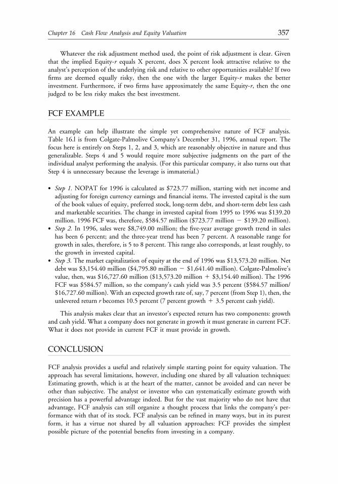
Whatever the risk adjustment method used, the point of risk adjustment is clear. Giventhat the implied Equity-r equals X percent, does X percent look attractive relative to theanalyst’s perception of the underlying risk and relative to other opportunities available? If twofirms are deemed equally risky, then the one with the larger Equity-r makes the betterinvestment. Furthermore, if two firms have approximately the same Equity-r, then the onejudged to be less risky makes the best investment.
FCF EXAMPLE
An example can help illustrate the simple yet comprehensive nature of FCF analysis.Table 16.l is from Colgate-Palmolive Company’s December 31, 1996, annual report. Thefocus here is entirely on Steps 1, 2, and 3, which are reasonably objective in nature and thusgeneralizable. Steps 4 and 5 would require more subjective judgments on the part of theindividual analyst performing the analysis. (For this particular company, it also turns out thatStep 4 is unnecessary because the leverage is immaterial.)
� Step 1. NOPAT for 1996 is calculated as $723.77 million, starting with net income andadjusting for foreign currency earnings and financial items. The invested capital is the sumof the book values of equity, preferred stock, long-term debt, and short-term debt less cashand marketable securities. The change in invested capital from 1995 to 1996 was $139.20million. 1996 FCF was, therefore, $584.57 million ($723.77 million 2 $139.20 million).
� Step 2. In 1996, sales were $8,749.00 million; the five-year average growth trend in saleshas been 6 percent; and the three-year trend has been 7 percent. A reasonable range forgrowth in sales, therefore, is 5 to 8 percent. This range also corresponds, at least roughly, tothe growth in invested capital.
� Step 3. The market capitalization of equity at the end of 1996 was $13,573.20 million. Netdebt was $3,154.40 million ($4,795.80 million 2 $1,641.40 million). Colgate-Palmolive’svalue, then, was $16,727.60 million ($13,573.20 million 1 $3,154.40 million). The 1996FCF was $584.57 million, so the company’s cash yield was 3.5 percent ($584.57 million/$16,727.60 million). With an expected growth rate of, say, 7 percent (from Step 1), then, theunlevered return r becomes 10.5 percent (7 percent growth 1 3.5 percent cash yield).
This analysis makes clear that an investor’s expected return has two components: growthand cash yield. What a company does not generate in growth it must generate in current FCF.What it does not provide in current FCF it must provide in growth.
CONCLUSION
FCF analysis provides a useful and relatively simple starting point for equity valuation. Theapproach has several limitations, however, including one shared by all valuation techniques:Estimating growth, which is at the heart of the matter, cannot be avoided and can never beother than subjective. The analyst or investor who can systematically estimate growth withprecision has a powerful advantage indeed. But for the vast majority who do not have thatadvantage, FCF analysis can still organize a thought process that links the company’s per-formance with that of its stock. FCF analysis can be refined in many ways, but in its purestform, it has a virtue not shared by all valuation approaches: FCF provides the simplestpossible picture of the potential benefits from investing in a company.
c16 12 September 2012; 11:55:24
Chapter 16 Cash Flow Analysis and Equity Valuation 357
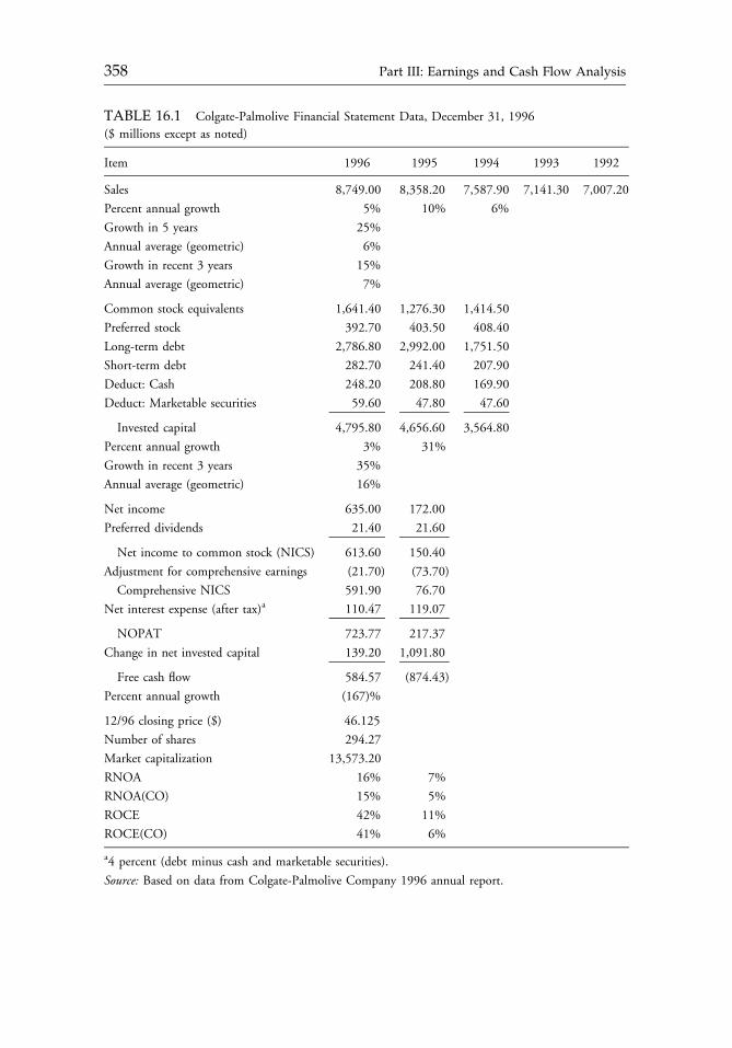
TABLE 16.1 Colgate-Palmolive Financial Statement Data, December 31, 1996
($ millions except as noted)
Item 1996 1995 1994 1993 1992
Sales 8,749.00 8,358.20 7,587.90 7,141.30 7,007.20
Percent annual growth 5% 10% 6%
Growth in 5 years 25%
Annual average (geometric) 6%
Growth in recent 3 years 15%
Annual average (geometric) 7%
Common stock equivalents 1,641.40 1,276.30 1,414.50
Preferred stock 392.70 403.50 408.40
Long-term debt 2,786.80 2,992.00 1,751.50
Short-term debt 282.70 241.40 207.90
Deduct: Cash 248.20 208.80 169.90
Deduct: Marketable securities 59.60 47.80 47.60
Invested capital 4,795.80 4,656.60 3,564.80
Percent annual growth 3% 31%
Growth in recent 3 years 35%
Annual average (geometric) 16%
Net income 635.00 172.00
Preferred dividends 21.40 21.60
Net income to common stock (NICS) 613.60 150.40
Adjustment for comprehensive earnings (21.70) (73.70)
Comprehensive NICS 591.90 76.70
Net interest expense (after tax)a 110.47 119.07
NOPAT 723.77 217.37
Change in net invested capital 139.20 1,091.80
Free cash flow 584.57 (874.43)
Percent annual growth (167)%
12/96 closing price ($) 46.125
Number of shares 294.27
Market capitalization 13,573.20
RNOA 16% 7%
RNOA(CO) 15% 5%
ROCE 42% 11%
ROCE(CO) 41% 6%
a4 percent (debt minus cash and marketable securities).
Source: Based on data from Colgate-Palmolive Company 1996 annual report.
c16 12 September 2012; 11:55:25
358 Part III: Earnings and Cash Flow Analysis
QUESTION AND ANSWER SESSION
Question: Why do you exclude changes in working capital from your calculation?Ohlson: It is not excluded! Remember that I am working backward, so to speak, from the
entire balance sheet. Remember also that debits equal credits; thus, the change ininvested capital from a financial perspective must, by construction, equal the changein invested capital from an operating perspective. One can use either approach, ofcourse. The number will always be the same as long as we are comprehensive andmutually exclusive in the treatment of the line items in the balance sheet.
Question: How can the FCF approach be applied to a rapidly growing small company that isgenerating negative cash or to a company that is acquisition driven?
Ohlson: It cannot be applied very well in the case of rapid growth and negative cash.Whenever we try to value a company that has a growth factor in excess of the discountfactor, we will have very difficult problems, because no growth rate can exceed thediscount factor forever. Somewhere along the line, we have to make a call as to whenthat growth rate is going to level off, decline, and ultimately go below the discountfactor. Even this approach to the growth problem does not completely solve theproblem of how to value a currently negative cash generator. This kind of case alwaysposes daunting valuation problems.
An acquisition-driven company poses similar problems: If I believe that acquisi-tions are going to change a company’s intrinsic economic profitability, then I amsaying that the current financial statements are not going to help me anticipate andunderstand the future financial statements. To the extent that the current statementscannot give me a sense of the future statements, I have no or little basis for the FCFapproach. That limitation, I would argue, applies to any valuation approach.
Question: How do you justify using these methods, which are long-term oriented, when WallStreet is so short-term oriented?
Ohlson: The way I think about all of these valuation techniques is that they are neitherengineering approaches nor the right or best approach. They are just different schemesto organize our thinking. I think it is dangerous to look for the Holy Grail of valuation.That level of certainty is not there, and it is never going to be there. Some of the keyparameters that we have to put into any of these models are too close to figments of theimagination to take the models that seriously.
Question: Is cash flow truly independent of the accounting method used?Ohlson: Yes. If you calculate FCF the way I outlined, it does not depend on the depreciation
expense. Why? Because, on the one hand, depreciation expense has an impact onNOPAT and, on the other hand, depreciation expense has an impact on the changein invested capital. The two impacts are precisely offsetting, as are the effects of otheraccruals, such as pension expense. There are exceptions, of course, such as executivecompensation options, but in general, accounting problems do not arise when wecalculate FCF. The exceptions refer to transactions in which capital contributions anddeductions are improperly measured. Options are one example, and the accounting foremployee stock ownership plans is another. It is rarely worth the effort to try tostraighten out these items, although it can generally be done.
c16 12 September 2012; 11:55:25
Chapter 16 Cash Flow Analysis and Equity Valuation 359

c16 12 September 2012; 11:55:25
CHAPTER 17ACCOUNTING VALUATION:
IS EARNINGS QUALITYAN ISSUE?
Bradford Cornell and Wayne R. Landsman
Debate has raged for decades about which valuation methodology is the best forvaluing a business interest. In practice, companies often prefer to present pro formameasures of value instead of the results from using measures established byaccounting authorities and regulators. In this article, the authors argue that there isessentially no difference between various valuation methodologies if they are accu-rately and consistently applied. However, this is true only as long as those who usepro forma earnings numbers provide transparency about how pro forma numbersdiffer from traditional accounting earnings numbers and as long as they apply thesediffering methods consistently. Essentially, the argument is that the best earningsmethod is the one that makes the most sense to the analyst’s view of the businessunder study, which can be considered license to apply careful judgment, rather thanblind methodology, in valuing a business interest.
Two forces have combined to focus increasing attention on the issue of the quality of reportedcorporate earnings. On the one hand, a growing number of companies are including proforma earnings as well as net income figures in their earnings releases. The explanation is thatpro forma numbers reflect the company’s true earning power more accurately than does netincome.1 Analysts have echoed the company support for these “Street” estimates of earnings.The numbers tracked by such clearinghouses for analyst estimates as Thomson First CallI/B/E/S and Zacks Investment Research are primarily Street estimates. On the other hand,
Reprinted from the Financial Analysts Journal (November/December 2003):20�28. When this articlewas originally published, Bradford Cornell was Bank of America Professor of Finance at the AndersonGraduate School of Management, University of California at Los Angeles, and Wayne R. Landsman wasKPMG Professor of Accounting at Kenan-Flagler Business School, University of North Carolina.
c17 12 September 2012; 14:7:52
361
regulators are concerned about the potentially misleading qualities of non-GAAP (generallyaccepted accounting principles) earnings measures. For instance, the U.S. SEC’s formerchief accountant, Lynn Turner (2000), has argued with respect to pro forma releases, “Oftenthey appear to be trying to lead investors away from the real number, from real net income.”
In response to this and other concerns about pro forma earnings, the FinancialAccounting Standards Board proposed in August 2001 a new agenda project called“Reporting Information about the Financial Performance of Business Enterprises.” In thatproposal, the FASB cited three concerns. (1) There are no common definitions of theelements of financial performance, and there are inconsistent practices in their presentation.For example, none of the pro forma earnings measures released by companies is specificallydefined. Depending on what items are added to or excluded from GAAP earnings, pro formaincome may mean one thing to one company and another thing to another company. In fact,the National Investor Relations Institute announced in a January 17, 2002, press release(see NIRI 2002) that in a sample of 133 companies that released pro forma earnings numbers,19 definitions of pro forma income were used. (2) Not only are companies increasingly relyingon pro forma performance measures in earnings releases and other investor-related commu-nications, but analysts and other financial statement users are increasingly accepting thesemeasures in assessing company performance. (3) There is no consensus about whichperformance measures should be in the financial statements.
The concern over which measure of income is the most meaningful for valuation hasproduced a host of empirical studies that use regression techniques to estimate the “quality”of competing earnings measures based on the valuation information they contain.2
The specific results are mixed and depend on the earnings measures being compared, the timeperiod, the sample of companies chosen, and the metric used. The overall result, however,is that the differences in information conveyed by the competing definitions of earnings—which include GAAP earnings, EBITDA (earnings before interest, taxes, depreciation, andamortization), operating income, and pro forma income—are not large. The empirical studiessuffer, however, from the problem that non-GAAP earnings are not unambiguously definedand that different companies compute pro forma income differently. As a result, studies thatcompare GAAP earnings with pro forma income may not be comparing the same twomeasures for all companies.
Our thesis is that from a valuation perspective, the entire debate regarding earningsquality is theoretically unresolvable. Consequently, attempts to resolve it by using empiricaltechniques will be misleading. Put simply, no consistently meaningful way exists to condenseall the historical financial data relevant for forecasting future performance into one measure(or a time series of one measure). Furthermore, attempts by regulatory bodies (e.g., the SEC)or accounting standard setting bodies (e.g., the FASB and International Accounting StandardsBoard) to determine an appropriate definition of pro forma income distracts attention fromfar more critical problems involving omissions and ambiguities in the constituent items thatmake up any measure of earnings.
The debate about the quality of earnings is based on a more fundamental issue. Theultimate issue of concern to regulators and standard setters is an efficient allocation of capitalin a properly functioning capital market. A prerequisite for efficient allocation is that marketvalues, on which the allocation of capital is based, reflect true economic values to the greatestextent possible. This prerequisite requires that the forecasts on which investor valuations arebased be as accurate as possible. One thing it does not depend on is precisely which measureof income investors are forecasting. As the insightful work of Ohlson (1995) and Feltham andOhlson (1995) makes clear, valuation models can be based on free cash flow, operating
c17 12 September 2012; 14:7:52
362 Part III: Earnings and Cash Flow Analysis
income, or accounting earnings.3 As long as a method of clean surplus accounting(i.e., income, however measured, equals change in equity book value plus net dividends) isused, the differences between the different measures of income cancel out in the present value(PV) relationship. Therefore, all the measures of income are of equal “quality” in a forward-looking sense, as long as they satisfy the clean surplus condition and the PV model is used.Viewed in this context, the quality of different historical measures of earnings must be relatedto the information that the competing earnings measures provide as inputs to the forecaststhat go into the PV relationship.4
In that regard, we make two arguments. First, none of the measures of earnings,including GAAP, satisfactorily condenses financial statement information for forecastingpurposes. Forecasting future cash flow (or earnings or operating income) requires anunderstanding of the earning power of a company on a component-by-component basis.Basic questions that must be answered are: How have revenues grown over time and why?What has been the cost of producing those revenues in terms of both marginal outlays andcapital expenditures? To what extent have past expenditures provided the company withgrowth options for the future? The historical financial information necessary to answer thesequestions generally cannot be condensed into a time series of any earnings measure.
Second, no meaningful criterion exists for determining whether one earnings measure isbetter than another, even for a specific company, other than going through the forecastingexercise and then determining which historical time series is more closely related to theforecasts. Such an exercise is redundant, however, because once the forecasts have beendeveloped, selection of the best historical earnings measure is irrelevant.5 In addition, the bestmeasure will be both company specific and time specific. Depending on the circumstances inwhich a company finds itself, different historical measures of earnings will have differentrelationships to future forecasts. Consequently, to speak of the “best” measure as if it could bedetermined for all companies and over all time is misleading.
EARNINGS MEASURES AND VALUATION
The dispute about earnings quality arises because of two conflicting interpretations of themotives underlying company releases of their own pro forma income numbers in additionto U.S. GAAP numbers. The first view, expressed succinctly by various spokespersons foronline supermarket Amazon. com, is that appropriate pro forma results give better insight intothe fundamental operations of a business than does the bottom line. Thus, according toAmazon, pro forma numbers provide investors with more accurate guidance as to the com-pany’s future earnings and cash flow. The second view, voiced by various past and currentSEC officials, including Turner (2000), is that the presentation of differing earnings measuresis an effort to present a company’s financials in an artificially favorable light. In fact, Turnerhas cynically referred to many pro forma releases as “EBS accounting,” in that they include“everything but bad stuff.”
This dispute is highlighted by Amazon’s own chosen pro forma measure. As Bradshawand Sloan (2002) pointed out, Amazon chooses to report pro forma earnings that excludeamortization of goodwill and other intangibles, equity in losses of companies not consoli-dated, stock-based compensation costs, merger and acquisition costs, investment-related costs,and interest expense on long-term debt. But despite excluding equity-method losses, Amazonincludes revenue associated with noncash transactions in which the company received equitysecurities for advertising and promotional services. Given that every one of these decisions
c17 12 September 2012; 14:7:52
Chapter 17 Accounting Valuation: Is Earnings Quality an Issue? 363
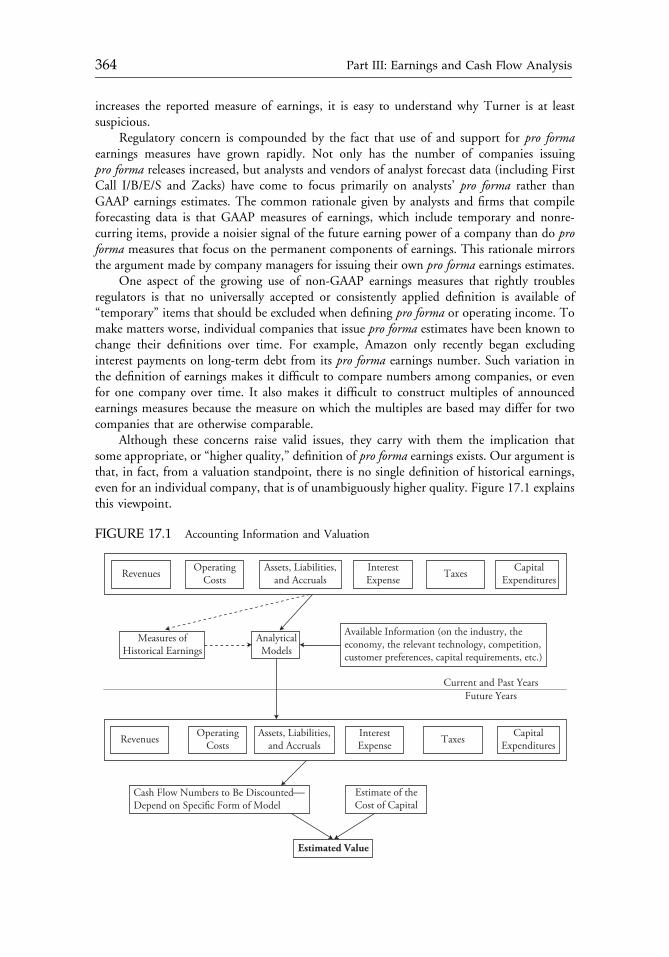
increases the reported measure of earnings, it is easy to understand why Turner is at leastsuspicious.
Regulatory concern is compounded by the fact that use of and support for pro formaearnings measures have grown rapidly. Not only has the number of companies issuingpro forma releases increased, but analysts and vendors of analyst forecast data (including FirstCall I/B/E/S and Zacks) have come to focus primarily on analysts’ pro forma rather thanGAAP earnings estimates. The common rationale given by analysts and firms that compileforecasting data is that GAAP measures of earnings, which include temporary and nonre-curring items, provide a noisier signal of the future earning power of a company than do proforma measures that focus on the permanent components of earnings. This rationale mirrorsthe argument made by company managers for issuing their own pro forma earnings estimates.
One aspect of the growing use of non-GAAP earnings measures that rightly troublesregulators is that no universally accepted or consistently applied definition is available of“temporary” items that should be excluded when defining pro forma or operating income. Tomake matters worse, individual companies that issue pro forma estimates have been known tochange their definitions over time. For example, Amazon only recently began excludinginterest payments on long-term debt from its pro forma earnings number. Such variation inthe definition of earnings makes it difficult to compare numbers among companies, or evenfor one company over time. It also makes it difficult to construct multiples of announcedearnings measures because the measure on which the multiples are based may differ for twocompanies that are otherwise comparable.
Although these concerns raise valid issues, they carry with them the implication thatsome appropriate, or “higher quality,” definition of pro forma earnings exists. Our argument isthat, in fact, from a valuation standpoint, there is no single definition of historical earnings,even for an individual company, that is of unambiguously higher quality. Figure 17.1 explainsthis viewpoint.
FIGURE 17.1 Accounting Information and Valuation
Revenues Taxes
Current and Past YearsFuture Years
OperatingCosts
InterestExpense
CapitalExpenditures
Assets, Liabilities,and Accruals
Revenues TaxesOperatingCosts
InterestExpense
CapitalExpenditures
Assets, Liabilities,and Accruals
Measures ofHistorical Earnings
Estimate of theCost of Capital
Estimated Value
AnalyticalModels
Available Information (on the industry, theeconomy, the relevant technology, competition,customer preferences, capital requirements, etc.)
Cash Flow Numbers to Be Discounted⎯Depend on Specific Form of Model
c17 12 September 2012; 14:7:52
364 Part III: Earnings and Cash Flow Analysis
Figure 17.1 is a generic illustration of the discounted cash flow valuation process.The specific application depends on the form of the valuation equation used. As noted, thePV equation can be expressed in terms of dividends (Gordon 1962), free cash flows (Cornell1993), capital cash flows (Ruback 2000), or accounting earnings (Ohlson 1995). As long asclean surplus accounting and the appropriate discount rate are used, these models areequivalent. Furthermore, they all follow the same basic process illustrated in Figure 17.1: Thevaluation analysis depends on projections of the constituent items of future incomestatements and balance sheets and selection of the discount rate. The projections, in turn,depend on analysis of the past financial performance of the company in conjunction withconsideration of such factors as forecasts of economic growth, industry developments,technological innovations, changes in customer preferences, and reactions of competitors,each of which can affect the relationship between past results and future performance. Theseprojections are fed into whatever analytical model the analyst determines is appropriate toproduce forecasts of the component items of future balance sheets and income statements.From those future financial statements, calculating the cash flow measure to be discounted isan arithmetic exercise.
The fundamental question is: What advantages are provided by aggregating the historicalinformation into a measure of “earnings” as part of the valuation process depicted inFigure 17.1? Such aggregation is potentially useful for two (related) reasons.
First, it reduces the vast amount of component financial data to a single time series. Thisreduction makes analysis of a large number of companies computationally feasible. Whetherthis computational aid is beneficial is unclear; however, because the critical issue is not havinga measure of earnings but understanding how that measure is related to future cash flow.6
As Figure 17.1 makes clear, that understanding cannot be based on analysis of any singleearnings measure alone.
Second, earnings measures provide a metric for comparing valuations among companies.As described in Cornell (1993), multiple valuation analysis based on comparables is one of themost common techniques used by investment bankers and other finance practitioners toappraise companies. The multiple analyses are almost invariably based on some earningsaggregate.
For an earnings measure to be useful in comparing valuations, however, the measureshould capture as effectively as possible the persistent components of earnings. One-timecharges will produce idiosyncratic variations in earnings among otherwise comparable com-panies that are not reflected in relative valuations. The result will be idiosyncratic variations inthe multiples, which will produce unnecessary errors in the analysis. This aspect suggests thatmultiple analyses should always be based on some measure of pro forma earnings instead ofGAAP. But there are some complications. Most importantly, the concept of the persistentcomponents of earnings extends well beyond accounting. Although (as pro forma advocatesargue) GAAP earnings may misstate the persistent element of earnings because of one-timecharges or write-offs associated with such events as merger or restructuring, reported earningsalso may differ from persistent earnings for a host of nonaccounting economic reasons. Forinstance, a company may cut prices or offer special financing to spur sales. Such eventsare likely to have a nonpersistent impact on earnings. In addition, the impact of such eventsis likely to be hidden if the analyst focuses on earnings and does not drill down to studyrevenues and costs. Similarly, current earnings may be temporarily affected by internal events,such as executive turnover. Adjusting forecasts to take into account these economic sources oftemporary perturbations is every bit as important as adjusting for one-time accounting
c17 12 September 2012; 14:7:52
Chapter 17 Accounting Valuation: Is Earnings Quality an Issue? 365
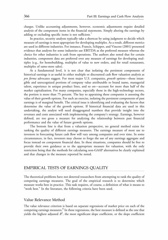
charges. Unlike accounting adjustments, however, economic adjustments require detailedanalysis of the component items in the financial statements. Simply altering the earnings byadding or excluding specific items is not sufficient.7
In practice, security analysts typically take a shortcut by using judgment to decide whichmeasure of earnings is most appropriate for developing multiples. As a result, different metricsare used in different industries. For instance, Francis, Schipper, and Vincent (2001) presentedevidence that analysts for some industries use EBITDA as the preferred measure whereas thechoice for other industries is cash from operations. The authors also noted that for certainindustries, component data are preferred over any measure of earnings for developing mul-tiples (e.g., for homebuilding, multiples of value to new orders, and for retail restaurants,multiples of same-store sales).
At a fundamental level, it is not clear that isolating the persistent components ofhistorical earnings is as useful in either multiple or discounted cash flow valuation analysis aspro forma advocates suggest. For most major U.S. companies, growth options—those intan-gible and unrecognized portions of company value attributable to brand name, managerialtalent, experience in unique product lines, and so on—account for more than half of themarket capitalization. For many companies, especially those in the high-technology sectors,the portion is more than 75 percent. The key to appraising these companies is assessing thevalue of their growth options. For such an exercise, isolating the persistent components of pastearnings is of marginal benefit. The critical issue is identifying and evaluating the factors thatdetermine the value of the growth options. If historical financial data are used in thisundertaking, the analyst will need disaggregated numbers that provide insight into therevenues and costs associated with implementing the company’s strategy. Earnings, howeverdefined, are too gross a measure for analyzing the relationship between past financialperformance and the value of future growth options.
The bottom line is that from a valuation perspective, no general method exists forranking the quality of different earnings measures. The earnings measure of most use toinvestors in forecasting future cash flow will vary among companies and over time. In somecircumstances, in fact, investors may choose to forgo the use of any earnings aggregate andfocus instead on component financial data. In these situations, companies should be free toprovide their own guidance as to the appropriate measure for valuation, with the onlyrestriction being that the methods for calculating non-GAAP alternatives be clearly explainedand that changes in the measure reported be noted.
EMPIRICAL TESTS OF EARNINGS QUALITY
The theoretical problems have not deterred researchers from attempting to rank the quality ofcompeting earnings measures. The goal of the empirical research is to determine whichmeasure works best in practice. This task requires, of course, a definition of what it means to“work best.” In the literature, the following criteria have been used.
Value Relevance Method
The value relevance criterion is based on separate regressions of market price on each of thecompeting earnings measures.8 In these regressions, the best measure is defined as the one thatyields the highest adjusted R2, the most significant slope coefficient, or the slope coefficient
c17 12 September 2012; 14:7:52
366 Part III: Earnings and Cash Flow Analysis
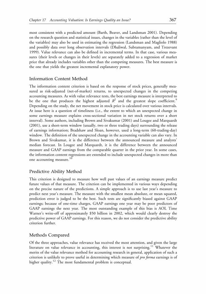
most consistent with a predicted amount (Barth, Beaver, and Landsman 2001). Dependingon the research question and statistical issues, changes in the variables (rather than the level ofthe variables) may also be used in estimating the regression (Landsman and Magliolo 1988)and possibly data over long observation intervals (Dhaliwal, Subramanyam, and Trezevant1999). Value relevance can also be defined in incremental terms. In that case, various mea-sures (their levels or changes in their levels) are separately added to a regression of marketprice that already includes variables other than the competing measures. The best measure isthe one that yields the greatest incremental explanatory power.
Information Content Method
The information content criterion is based on the response of stock prices, generally mea-sured as risk-adjusted (net-of-market) returns, to unexpected changes in the competingaccounting measures. As with value relevance tests, the best earnings measure is interpreted tobe the one that produces the highest adjusted R2 and the greatest slope coefficient.9
Depending on the study, the net movement in stock price is calculated over various intervals.At issue here is a question of timeliness (i.e., the extent to which an unexpected change insome earnings measure explains cross-sectional variation in net stock returns over a shortinterval). Some authors, including Brown and Sivakumar (2001) and Lougee and Marquardt(2001), use a short-term window (usually, two or three trading days) surrounding the releaseof earnings information; Bradshaw and Sloan, however, used a long-term (60-trading-day)window. The definition of the unexpected change in the accounting variable can also vary. InBrown and Sivakumar, it is the difference between the announced measure and analysts’median forecast. In Lougee and Marquardt, it is the difference between the announcedmeasure and GAAP earnings from the comparable quarter in the prior year. In some cases,the information content regressions are extended to include unexpected changes in more thanone accounting measure.10
Predictive Ability Method
This criterion is designed to measure how well past values of an earnings measure predictfuture values of that measure. The criterion can be implemented in various ways dependingon the precise nature of the predictions. A simple approach is to use last year’s measure topredict next year’s measure. The measure with the smallest mean absolute, or mean squared,prediction error is judged to be the best. Such tests are significantly biased against GAAPearnings; because of one-time charges, GAAP earnings one year may be poor predictors ofGAAP earnings the next year. The most outstanding example of this bias is AOL TimeWarner’s write-off of approximately $50 billion in 2002, which would clearly destroy thepredictive power of GAAP earnings. For this reason, we do not consider the predictive abilitycriterion further.
Methods Compared
Of the three approaches, value relevance has received the most attention, and given the largeliterature on value relevance in accounting, this interest is not surprising.11 Whatever themerits of the value relevance method for accounting research in general, application of such acriterion is unlikely to prove useful in determining which measure of pro forma earnings is ofhigher quality.12 The most fundamental problem is conceptual.
c17 12 September 2012; 14:7:52
Chapter 17 Accounting Valuation: Is Earnings Quality an Issue? 367
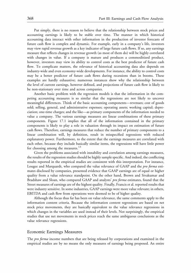
Put simply, there is no reason to believe that the relationship between stock prices andaccounting earnings is likely to be stable over time. The manner in which historicalaccounting data interact with other information in the production of investor forecasts offuture cash flow is complex and dynamic. For example, early in a company’s life, investorsmay view rapid revenue growth as a key indicator of large future cash flows. If so, any earningsmeasure that reflects changes in revenue growth (as most of them do) will be highly correlatedwith changes in value. If a company is mature and produces a commoditized product,however, investors may view its ability to control costs as the best predictor of future cashflow. To complicate matters, the relevance of historical accounting data also depends onindustry-wide and even economy-wide developments. For instance, the ability to control costsmay be a better predictor of future cash flows during recessions than in booms. Theseexamples are hardly exhaustive; numerous instances show why the relationship betweenthe level of current earnings, however defined, and projections of future cash flow is likely tobe non-stationary over time and across companies.
Another basic problem with the regression models is that the information in the com-peting accounting measures is so similar that the regressions are not likely to uncovermeaningful differences. Think of the basic accounting components—revenues; cost of goodssold; selling, general, and administrative expenses; operating assets; working capital; depre-ciation; one-time charges; and the like—as primary components of the information needed tovalue a company. The various earnings measures are linear combinations of these primarycomponents. Figure 17.1 implies that all of the information contained in the primarycomponents is likely to play a role in valuation through its impact on estimation of futurecash flows. Therefore, earnings measures that reduce the number of primary components to alinear combination will, by definition, result in misspecified regressions with reducedexplanatory power. Furthermore, to the extent that the earnings measures are correlated witheach other, because they include basically similar items, the regressions will have little powerfor choosing among the measures.13
Given the problems associated with instability and correlation among earnings measures,the results of the regression studies should be highly sample specific. And indeed, the conflictingresults reported in the empirical studies are consistent with this interpretation. For instance,Lougee and Marquardt, who compared the value relevance of GAAP and the pro forma esti-mates disclosed by companies, presented evidence that GAAP earnings are of equal or higherquality from a value relevance standpoint. On the other hand, Brown and Sivakumar andBradshaw and Sloan, who compared GAAP and analysts’ pro forma estimates, found that theStreet measures of earnings are of the highest quality. Finally, Francis et al. reported results thatwere industry sensitive. In some industries, GAAP earnings were more value relevant; in others,EBITDA and cash flow from operations were deemed to be of higher quality.
Although the focus thus far has been on value relevance, the same comments apply to theinformation content criteria. Because the information content regressions are based on netstock price movements, they are basically equivalent to the value relevance regressions inwhich changes in the variables are used instead of their levels. Not surprisingly, the empiricalstudies that use net movements in stock prices reach the same ambiguous conclusions as thevalue relevance regressions.
Economic Earnings Measures
The pro forma income numbers that are being released by corporations and examined in theempirical studies are by no means the only measures of earnings being proposed. An entire
c17 12 September 2012; 14:7:52
368 Part III: Earnings and Cash Flow Analysis
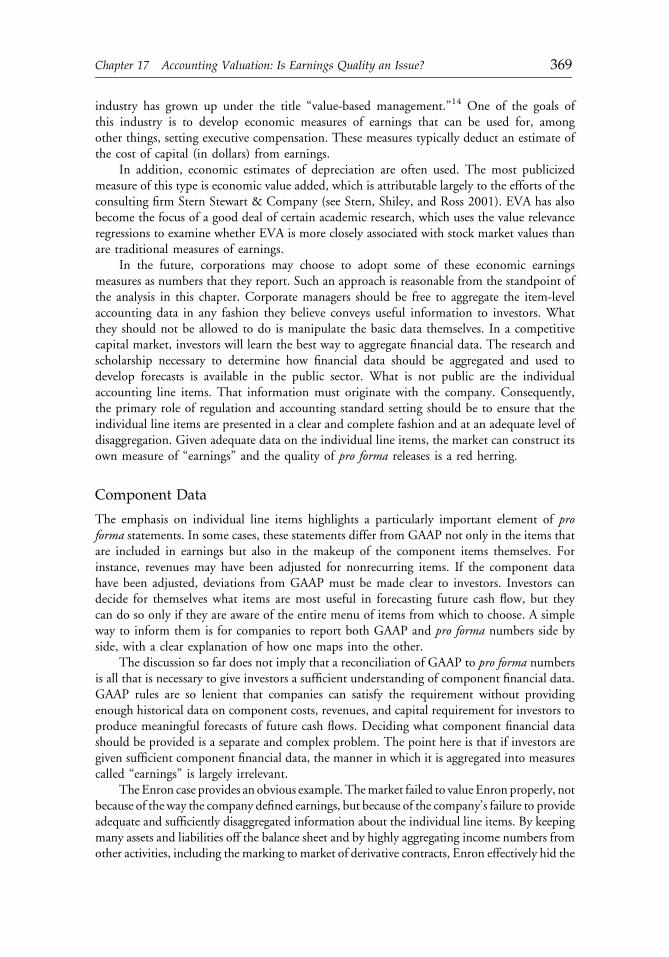
industry has grown up under the title “value-based management.”14 One of the goals ofthis industry is to develop economic measures of earnings that can be used for, amongother things, setting executive compensation. These measures typically deduct an estimate ofthe cost of capital (in dollars) from earnings.
In addition, economic estimates of depreciation are often used. The most publicizedmeasure of this type is economic value added, which is attributable largely to the efforts of theconsulting firm Stern Stewart & Company (see Stern, Shiley, and Ross 2001). EVA has alsobecome the focus of a good deal of certain academic research, which uses the value relevanceregressions to examine whether EVA is more closely associated with stock market values thanare traditional measures of earnings.
In the future, corporations may choose to adopt some of these economic earningsmeasures as numbers that they report. Such an approach is reasonable from the standpoint ofthe analysis in this chapter. Corporate managers should be free to aggregate the item-levelaccounting data in any fashion they believe conveys useful information to investors. Whatthey should not be allowed to do is manipulate the basic data themselves. In a competitivecapital market, investors will learn the best way to aggregate financial data. The research andscholarship necessary to determine how financial data should be aggregated and used todevelop forecasts is available in the public sector. What is not public are the individualaccounting line items. That information must originate with the company. Consequently,the primary role of regulation and accounting standard setting should be to ensure that theindividual line items are presented in a clear and complete fashion and at an adequate level ofdisaggregation. Given adequate data on the individual line items, the market can construct itsown measure of “earnings” and the quality of pro forma releases is a red herring.
Component Data
The emphasis on individual line items highlights a particularly important element of proforma statements. In some cases, these statements differ from GAAP not only in the items thatare included in earnings but also in the makeup of the component items themselves. Forinstance, revenues may have been adjusted for nonrecurring items. If the component datahave been adjusted, deviations from GAAP must be made clear to investors. Investors candecide for themselves what items are most useful in forecasting future cash flow, but theycan do so only if they are aware of the entire menu of items from which to choose. A simpleway to inform them is for companies to report both GAAP and pro forma numbers side byside, with a clear explanation of how one maps into the other.
The discussion so far does not imply that a reconciliation of GAAP to pro forma numbersis all that is necessary to give investors a sufficient understanding of component financial data.GAAP rules are so lenient that companies can satisfy the requirement without providingenough historical data on component costs, revenues, and capital requirement for investors toproduce meaningful forecasts of future cash flows. Deciding what component financial datashould be provided is a separate and complex problem. The point here is that if investors aregiven sufficient component financial data, the manner in which it is aggregated into measurescalled “earnings” is largely irrelevant.
The Enron case provides an obvious example. Themarket failed to value Enron properly, notbecause of the way the company defined earnings, but because of the company’s failure to provideadequate and sufficiently disaggregated information about the individual line items. By keepingmany assets and liabilities off the balance sheet and by highly aggregating income numbers fromother activities, including the marking to market of derivative contracts, Enron effectively hid the
c17 12 September 2012; 14:7:52
Chapter 17 Accounting Valuation: Is Earnings Quality an Issue? 369
component financial data from the market. Thus, investors could not construct their ownmeaningful earnings measures or produce reliable forecasts of future cash flow.
POLICY IMPLICATIONS
Two policy implications emerge from this analysis. The principal conclusion is that efforts todetermine which measure of earnings is appropriate for a company to disseminate are mis-guided. There is no clear theoretical or empirical basis for consistently preferring one measureover another. As inputs to investor valuation analyses, “earnings” definitions will vary over timeand among companies. In some situations, investors will find working with basic line items,such as revenues, costs, and capital used, more appropriate than computing any measure ofearnings. In such circumstances, companies should be free to aggregate the component financialdata in any fashion they believe provides the most useful information to investors.
What is critical is that the basic elements that make up any measure of earnings bepresented with sufficient clarity and at a sufficient level of disaggregation that investors cananswer such fundamental questions as: What were the revenues generated by operations?What were the costs associated with generating those revenues? And how much capital wasrequired to generate those revenues? If sufficient information is available to answer suchquestions, investors can aggregate the information into an earnings measure they believe ismost appropriate for forecasting future cash flows. In its proposal Reporting Information aboutthe Financial Performance of Business Enterprises, the FASB (2001) suggested that it wouldconsider requiring financial statements to display separately the items underlying the variousperformance metrics, including depreciation, interest, taxes, research and developmentexpenses, losses on asset impairment, and gains/losses for holdings of financial instruments.We agree with this proposed requirement but urge the FASB to expand the scope of requireddisclosures to include all information necessary for understanding the fundamental questionswe have identified.
The second policy implication to emerge from this analysis is that, althoughcompanies should be free to provide any aggregate measure of earnings they considerappropriate, they should follow some basic guidelines. Because none of the alternatives toGAAP earnings is precisely defined or consistently applied, companies that release non-GAAP numbers should explain how the numbers differ from GAAP. No ambiguity shouldsurround what types of items are being excluded from or added to the GAAP measure ofearnings. Similarly, companies should not be allowed to change the measure they are usingwithout clarifying that the definition has changed and stating what the impact of thatchange is on current and past earnings reports. Clearly, confusion will reign if a company’sdefinition of “pro forma earnings” differs from quarter to quarter, particularly if it does so ina fashion designed to disguise operational problems.
Although we limited our discussion here to the debate surrounding pro forma earnings,our line of reasoning applies to other policy issues currently under consideration by the SECand the FASB. A prominent example, related to Enron, is “consolidation accounting.” A keyproblem in the Enron case was that analysts and investors did not have sufficient informationabout the company to value it properly. The specific issue was that by failing to consolidatespecial-purpose entities (SPEs), Enron prevented investors from discovering the company’strue financial position, particularly its profitability and extent of debt financing. The FASBrecently issued an exposure draft tightening the rules for consolidating SPEs, “QualifyingSpecial-Purpose Entities and Isolation of Transferred Assets,”15 but determining when entities
c17 12 September 2012; 14:7:53
370 Part III: Earnings and Cash Flow Analysis
should be consolidated is the broader question and remains a key policy issue. To valuecompanies correctly, investors must have adequate disclosure of the underlying businessrelationships among affiliated companies.
� � �
We thank the Bank of America and the Center for Financial and Accounting Research at theUniversity of North Carolina for their generous financial support.
NOTES
1. See “Varied Profit Reports by Firms Create Confusion” (1999).2. Brown and Sivakumar (2001); Bradshaw and Sloan (2002); Francis, Schipper, and
Vincent (2001); Lougee and Marquardt (2001).3. See also Bernard (1995).4. Although some authors, including Bernard and Frankel and Lee (1999), have interpreted
the Ohlson model as an empirical model, it is more appropriately interpreted as atransformation of the dividend discount model. So, in empirical implementations, thereare two explanations for a less-than-perfect fit of model values to market prices. One isthat approximations to the market discount rate and the market’s cash flow expectationsused by researchers contain measurement error. The second is that market prices maynot be rational, so the PV relationship, in any form, fails to describe the manner inwhich stocks are valued. For this chapter, we have assumed that the market is rational.Thus, we interpret the PV relationship, given the expectations and the discount rate thatit incorporates, as an identity.
5. Beaver (1998) made a similar point about earnings and market value in completemarkets. That is, earnings measurement is redundant once market values are known.
6. Moreover, computational feasibility is unlikely to be a compelling issue for analysts withstate-of-the-art computers and real-time access to financial statement information for theuniverse of publicly traded companies.
7. We do not mean to say that accounting adjustments are divorced from economicadjustments. For example, GAAP provides several examples of the economic effects ofcurrent and future events being reflected in current accounting adjustments, includingaccounting for asset impairments, asset retirement obligations, and anticipated trans-actions with derivative hedging relationships.
8. In principle, valuation regressions can include a variety of financial statement datain addition to earnings—balance sheet information, unrecognized assets and liabilities (e.g.,pension assets and liabilities), and other nonaccounting information. The research contextgenerally dictates the regressors to be included in the estimating equation. For reasons ofparsimony, we assume that earnings, however measured, are the only explanatory variable.
9. Specifically, the net movement in stock price is measured by the cumulative averageresidual over the observation interval.
10. Brown, Hagerman, Griffin, and Zmijewski (1987) showed that when multiple proxiesfor the same underlying earnings variable are significant in the regression, it may indicatethat each variable contains significant measurement error.
11. See Barth, Beaver, and Landsman and Holthausen and Watts (2001) for reviews of thevalue relevance literature.
c17 12 September 2012; 14:7:53
Chapter 17 Accounting Valuation: Is Earnings Quality an Issue? 371
12. One reason is that a variety of statistical problems can arise when estimating regressionsof stock prices on measures of accounting earnings (see Barth, Beaver, and Landsman,Section 4.2.1, for a summary). These problems can be solved, in principle, at least, so wedo not discuss them here.
13. Two findings related to this discussion are illustrated in Barth, Beaver, Hand, andLandsman (1999, 2002), who analyzed how earnings components, includingcash flow and accrual components, relate to equity values. They showed, first, thatdisaggregated earnings explain the cross-sectional variation in share prices better than doaggregate earnings. Second, they showed that the way in which particular accruals relateto share prices is quite industry specific and is affected by the way in which accrualsrelate informationally to other accruals as well as by their degree of permanence inforecasting future earnings.
14. See, for instance, Eccles, Herz, Keegan, and Phillips (2001).15. Available at www.fasb.org/draft/ed_gspe.pdf.
REFERENCES
Barth, Mary E., William H. Beaver, and Wayne R. Landsman. 2001. “The Relevance of the ValueRelevance Literature for Financial Accounting Standard Setting: Another View.” Journal ofAccounting and Economics, vol. 31, nos. 1�3 (January):77�104.
Barth, Mary E., William H. Beaver, John R.M. Hand, and Wayne R. Landsman. 1999.“Accruals, Cash Flows, and Equity Values.” Review of Accounting Studies, vol. 4, nos. 3�4(December):205�229.
———. 2002. “Accrual Components, Earnings Forecasting, and Equity Values.” Working paper,University of North Carolina and Stanford University.
Beaver, William H. 1998. Financial Reporting: An Accounting Revolution. Upper Saddle River, NJ:Prentice-Hall.
Beaver, William H., Richard A. Lambert, and Dale Morse. 1980. “The Information Content of SecurityPrices.” Journal of Accounting and Economics, vol. 2, no. 1 (March):3�28.
Beaver, William H., Richard A. Lambert, and Stephen G. Ryan. 1987. “The Information Content ofSecurity Prices: A Second Look.” Journal of Accounting and Economics, vol. 9, no. 2(July):139�157.
Bernard, Victor L. 1995. “The Feltham-Ohlson Framework: Implications for Empiricists.” Contem-porary Accounting Research, vol. 11, no. 2 (Spring):733�747.
Bradshaw, Mark T., and Richard G. Sloan. 2002. “GAAP versus the Street: An Empirical Assessment ofTwo Alternative Definitions of Earnings.” Journal of Accounting Research, vol. 40, no. 1(March):41�66.
Brown, Lawrence D., and Kumar Sivakumar. 2001. “Comparing the Quality of Three EarningsMeasures.” Unpublished working paper, Georgia State University.
Brown, Lawrence D., Robert L. Hagerman, Paul A. Griffin, and Mark E. Zmijewski. 1987. “AnEvaluation of Alternative Proxies for the Market’s Assessment of Unexpected Earnings.” Journal ofAccounting and Economics, vol. 9, no. 2 (July):159�193.
Cornell, Bradford. 1993. Corporate Valuation. New York: Business One Irwin.———. 2001. “Is the Response of Analysts to Information Consistent with Fundamental Valuation?
The Case of Intel.” Financial Management, vol. 30, no. 1 (Spring):113�136.Dhaliwal, D., K.R. Subramanyam, and R. Trezevant. 1999. “Is Comprehensive Income Superior to Net
Income as a Measure of Firm Performance?” Journal of Accounting and Economics, vol. 26, nos. 1�3(January):43�67.
Eccles, Robert G., Robert H. Herz, E. Mary Keegan, and David M.H. Phillips. 2001. The ValueReporting Revolution: Moving beyond the Earnings Game. New York: John Wiley & Sons.
c17 12 September 2012; 14:7:53
372 Part III: Earnings and Cash Flow Analysis
FASB. 2001. Reporting Information about the Financial Performance of Business Enterprises: Focusing on theForm and Content of Financial Statements. Norwalk, CT: Financial Accounting Standards Board.
Feltham, Gerald A., and James A. Ohlson. 1995. “Valuation and Clean Surplus Accounting for Operatingand Financial Activities.” Contemporary Accounting Research, vol. 11, no. 2 (Spring):689�731.
Francis, Jennifer, Katherine Schipper, and Linda Vincent. 2001. “The Relative and IncrementalInformation in Alternative (to Earnings) Performance Measures.” Unpublished working paper,Duke University.
Frankel, R., and Charles M.C. Lee. 1999. “Accounting Diversity and International Valuation.”Unpublished working paper, University of Michigan.
Gordon, Myron J. 1962. The Investment, Financing, and Valuation of the Corporation. Homewood, IL:Irwin.
Holthausen, Robert W., and Ross L. Watts. 2001. “The Relevance of the Value Relevance Literature forFinancial Accounting Standard Setting.” Journal of Accounting and Economics, vol. 31, nos. 1�3(September):3�75.
Landsman, Wayne, and Joseph Magliolo. 1988. “Cross-Sectional Capital Market Research and ModelSpecification.” Accounting Review, vol. 63, no. 4 (October):586�604.
Lougee, Barbara A., and Carol A. Marquardt. 2001. “Earnings Quality and Strategic Disclosure: AnEmpirical Examination of ‘Pro Forma’ Net Income.” Unpublished working paper, University ofCalifornia at Irvine.
NIRI. 2002. “NIRI Releases Survey: An Analysis of Corporate Use of Pro Forma Reporting.”Pres release, National Investor Relations Institute (17 January 2002): www.fei.org/download/NIRI_Survey_Pro_Forma_Earnings_Use.pdf.
Ohlson, James A. 1995. “Earnings, Book Value, and Dividends in Security Valuation.” ContemporaryAccounting Research, vol. 11, no. 2 (Spring):661�687.
———. 1999. “On Transitory Earnings.” Review of Accounting Studies, vol. 4, nos. 3/4(December):145�162.
Ruback, Richard. 2000. “Capital Cash Flows: A Simple Approach to Valuing Risky Cash Flows.”Unpublished working paper, Harvard Business School.
Stern, Joel M., John S. Shiley, and Irwin Ross. 2001. The EVA Challenge: Implementing Value-AddedChange in an Organization. New York: John Wiley & Sons.
Turner, Lynn E. 2000. Remarks to the 39th Annual Corporate Counsel Institute presentedby Northwestern University School of Law (12 October 2000): www.sec.gov/news/speech/spch418.htm.
“Varied Profit Reports by Firms Create Confusion.” 1999. Wall Street Journal (24 August):C1.
c17 12 September 2012; 14:7:53
Chapter 17 Accounting Valuation: Is Earnings Quality an Issue? 373

c17 12 September 2012; 14:7:53
CHAPTER 18EARNINGS QUALITY
ANALYSIS AND EQUITYVALUATION
Richard G. Sloan
For years, a widely held belief was that markets are efficient and that fundamentalanalysis is futile. But after the discovery of several market anomalies, the stage wasset for exploring the use of fundamentally based techniques. A simple quantitativetrading strategy based on the quality of earnings analysis has worked remarkablywell. And although this particular opportunity will inevitably be arbitraged away,it does support the concept that fundamental analysis works.
I have long been interested in fundamental analysis, but I was originally told that markets areefficient and thus it is futile to engage in fundamental analysis. Then, academics started todiscover what seemed to be violations of market efficiency, such as the size effect and theJanuary effect. These violations struck me as being fairly technical and mechanical. Thus,the door had been opened to investigate whether fundamentally based techniques might work.
I began by looking at a simple quantitative screen based on the quality of earningsanalysis (discussed more fully later). When I first back tested this screen against U.S. equitydata, I thought I must have made a mistake. I obtained what could be described only as hedgefund returns. Returns averaged about 10 percent a year above the market over the 30 yearstested; in only 2 of the years were the returns less than the market. Predictable returns of thatmagnitude just had not been documented before; returns from strategies based on the sizeeffect and the January effect were a lot smaller. Interestingly, in the 10 years that have passed
Reprinted from CFA Institute Conference Proceedings Quarterly (September 2006):52�60. This presen-tation comes from the Equity Research and Valuation Techniques conference held in Boston onDecember 1�2, 2005. When this article was originally published, Richard G. Sloan was Victor L. BernardPricewaterhouseCoopers Collegiate Professor of Accounting, professor of finance, and director of theTozzi Electronic Finance Center at the University of Michigan Ross School of Business.
c18 12 September 2012; 12:11:50
375

since I did the original research, this screen has continued to work well. In fact, this techniquehas been refined to obtain even bigger returns. Needless to say, it has generated a great deal ofinterest in the quantitative investment community.
To me, this technique demonstrates the viability of the concept that simple fundamentalanalysis combined with mechanical trading rules based on quality of earnings analysis works.Moreover, I believe that this is just the tip of the iceberg in terms of what good fundamentalanalysis can do. Although over time simple quantitative trading rules will get arbitraged away, theimportant point is that gains may always be found by digging deeper—by understandingthe accounting and the company’s business model and how they fit together.
WHY ANALYZE EARNINGS QUALITY?
A natural question to ask is why earnings quality should be analyzed. Certainly, everyone isaware that earnings numbers can be manipulated. Thus, some practitioners have taken theposition that they will focus only on the cash flows and perform their intrinsic value analysisbased on those numbers. Earnings, and the underlying subjective assumptions, are irrelevant.I think earnings quality analysis works so well because, despite the shortcomings of earnings,the bulk of the market is looking at earnings. If you had a crystal ball that allowed you to lookat the value of one variable (other than stock price) one year or one quarter from now, yourbest pick would be earnings. By comparing that value with the current consensus expectationsof earnings, you could generate a powerful trading strategy. Even if your crystal ball toldyou the true intrinsic value of a stock, knowing that number would not necessarily help yougenerate trading strategies in the short run because it could take many years, if ever, for thestock price to revert to that intrinsic value. Knowing future earnings is better than knowingintrinsic value for those interested in forecasting stock returns over the next 3�12 months.
Targeting earnings quality is also important because it forces the investor to focus onwhat I call the “continuous evolution” of business operations and accounting assumptions.The right accounting for a company depends critically on the business it is engaged in, theway it is conducting its business, and the things it is doing relative to its competitors. Forexample, consider Krispy Kreme Doughnuts, whose stock has taken significant losses in thepast few years. Krispy Kreme invested heavily in doughnut-making equipment and usedthe straight-line method to depreciate this equipment over a 10�15 year useful life. ForKrispy Kreme, this was the wrong way to depreciate. I do not have any qualms with the usefullife in terms of how long the machines will physically make doughnuts. But to me, thisproduct seemed like a fad. Remember that when Krispy Kreme first opened new stores,people would form lines outside to purchase the doughnuts. Krispy Kreme would broadcastthis phenomenon in press releases, and in the early days, the stock price would go higher. Butclearly, it was going to wear off fairly quickly. Certainly, people would not be forming linesoutside two or three years after a store opened, which is what happened. Krispy Kreme wouldnever have booked a profit had it used an accounting policy that frontloaded the depreciationand matched it to the cash flows that the doughnut machines generated.
Following is another example. Netflix, which rents DVDs through the mail, seems to bedoing quite well. It is giving Blockbuster tough competition. But most of its profits overthe past 18 months have come from extending the depreciation period from one year to threeyears for its DVD library, what Netflix calls its “back catalog”—the DVDs that are not newreleases. Netflix has done so because it thinks these DVDs will physically last a long time andwill be in demand three years from now. This practice looks similar to what AOL did with its
c18 12 September 2012; 12:11:50
376 Part III: Earnings and Cash Flow Analysis

subscriber acquisition costs in the late 1990s, which it eventually had to write down. Onecould make the argument that Netflix faces a similar situation. Three years from now, if videoon demand and Internet downloading of movies do indeed become available, little demandwill exist for Netflix’s mail-order service. Thus, getting the accounting right involvesunderstanding the business, which is why no quantitative analyst will ever be able to come upwith a mechanical formula to screen stocks. A fundamental analyst will always be needed tounderstand the business and look at the accounting.
IMPACT OF EARNINGS SURPRISES
As is widely known, stock prices do indeed respond to earnings surprises, as shown inFigure 18.1. Quarterly abnormal returns are plotted on the vertical axis as a function ofquarterly forecast error (realized earnings versus the I/B/E/S consensus forecast adjusted by thestock price) for a large sample of companies. The result is an S-shaped nonlinear curve. Forhigh-growth stocks, a 1 percent earnings surprise as a percentage of price triggers a 12 percentincrease on the upside and a 15 percent decrease on the downside. If one could perfectlyforecast these earnings surprises, one could generate a 27 percent quarterly hedge portfolioreturn. Earnings quality analysis is powerful because it is very good at forecasting theseearnings surprises.
I would like to emphasize the asymmetric nature of this graph for high-growth stocks.Earnings quality analysis is most useful in picking “earnings torpedoes” in growth stocks(i.e., growth stocks that are trading at high valuations but are doing it through the use ofaggressive accounting). These valuations get addictive to the managers of these companies.They are great when managers are raising capital. They are also great when managers havestock options in the company, so they tend to be the ones where management pushes theenvelope with respect to the accounting assumptions. When the company is finally forced totake a write-down, the price crashes, even if the company just misses the consensus by a smallamount. Thus, analyzing growth stocks is one area where these techniques are particularlyhelpful.
FIGURE 18.1 Earnings Surprise Response Functions for High-Growth and Low-Growth Stocks:
Quarterly Abnormal Returns vs. Quarterly Forecast Error
0
Abn
orm
al R
etur
n
High Growth
Low Growth
0.20
0.15
0.10
0
�0.10
�0.15
0.05
�0.05
�0.20�0.07 0.07�0.05 �0.01�0.03 0.01 0.03 0.05
Forecast Error
c18 12 September 2012; 12:11:50
Chapter 18 Earnings Quality Analysis and Equity Valuation 377
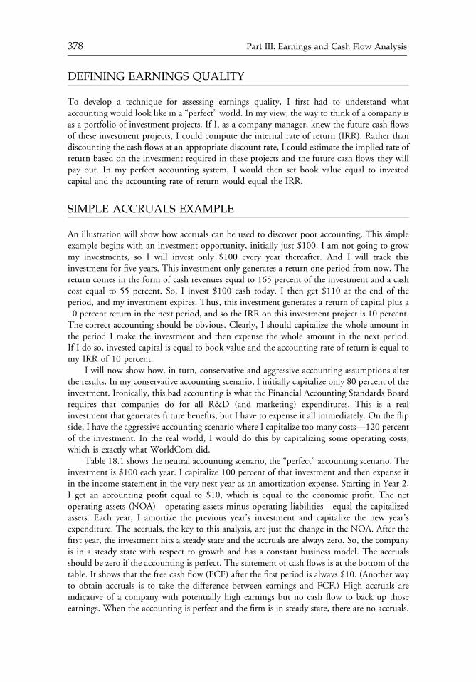
DEFINING EARNINGS QUALITY
To develop a technique for assessing earnings quality, I first had to understand whataccounting would look like in a “perfect” world. In my view, the way to think of a company isas a portfolio of investment projects. If I, as a company manager, knew the future cash flowsof these investment projects, I could compute the internal rate of return (IRR). Rather thandiscounting the cash flows at an appropriate discount rate, I could estimate the implied rate ofreturn based on the investment required in these projects and the future cash flows they willpay out. In my perfect accounting system, I would then set book value equal to investedcapital and the accounting rate of return would equal the IRR.
SIMPLE ACCRUALS EXAMPLE
An illustration will show how accruals can be used to discover poor accounting. This simpleexample begins with an investment opportunity, initially just $100. I am not going to growmy investments, so I will invest only $100 every year thereafter. And I will track thisinvestment for five years. This investment only generates a return one period from now. Thereturn comes in the form of cash revenues equal to 165 percent of the investment and a cashcost equal to 55 percent. So, I invest $100 cash today. I then get $110 at the end of theperiod, and my investment expires. Thus, this investment generates a return of capital plus a10 percent return in the next period, and so the IRR on this investment project is 10 percent.The correct accounting should be obvious. Clearly, I should capitalize the whole amount inthe period I make the investment and then expense the whole amount in the next period.If I do so, invested capital is equal to book value and the accounting rate of return is equal tomy IRR of 10 percent.
I will now show how, in turn, conservative and aggressive accounting assumptions alterthe results. In my conservative accounting scenario, I initially capitalize only 80 percent of theinvestment. Ironically, this bad accounting is what the Financial Accounting Standards Boardrequires that companies do for all R&D (and marketing) expenditures. This is a realinvestment that generates future benefits, but I have to expense it all immediately. On the flipside, I have the aggressive accounting scenario where I capitalize too many costs—120 percentof the investment. In the real world, I would do this by capitalizing some operating costs,which is exactly what WorldCom did.
Table 18.1 shows the neutral accounting scenario, the “perfect” accounting scenario. Theinvestment is $100 each year. I capitalize 100 percent of that investment and then expense itin the income statement in the very next year as an amortization expense. Starting in Year 2,I get an accounting profit equal to $10, which is equal to the economic profit. The netoperating assets (NOA)—operating assets minus operating liabilities—equal the capitalizedassets. Each year, I amortize the previous year’s investment and capitalize the new year’sexpenditure. The accruals, the key to this analysis, are just the change in the NOA. After thefirst year, the investment hits a steady state and the accruals are always zero. So, the companyis in a steady state with respect to growth and has a constant business model. The accrualsshould be zero if the accounting is perfect. The statement of cash flows is at the bottom of thetable. It shows that the free cash flow (FCF) after the first period is always $10. (Another wayto obtain accruals is to take the difference between earnings and FCF.) High accruals areindicative of a company with potentially high earnings but no cash flow to back up thoseearnings. When the accounting is perfect and the firm is in steady state, there are no accruals.
c18 12 September 2012; 12:11:50
378 Part III: Earnings and Cash Flow Analysis
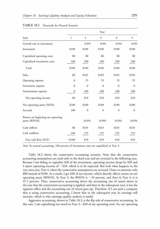
Table 18.2 shows the conservative accounting scenario. Note that the conservativeaccounting assumptions are used only in the third year and are reversed in the following year.Because I am failing to capitalize $20 of the investment, operating income drops by $20 andI report operating income of 2$10, which is to be expected. But look what happens in thevery next year, Year 4, when the conservative assumptions are reversed. I have to amortize only$80 instead of $100. As a result, I get $30 of net income, which directly affects return on netoperating assets (RNOA). In Year 3, the RNOA is 210 percent, and then in Year 4, it is37.5 percent. Thus, conservative accounting drives the accounting rate of return down inthe year that the conservative accounting is applied, and then in the subsequent year, it has theopposite effect and the accounting rate of return goes up. Therefore, if I can pick a companythat is using conservative accounting, I know that in the subsequent year its earnings willincrease, which is why earnings quality analysis is useful.
Aggressive accounting, shown in Table 18.3, is the flip side of conservative accounting. Inthis case, I am capitalizing too much in Year 3—$20 of my operating costs. So, my operating
TABLE 18.1 Financials for Neutral Scenario
Year
Item 1 2 3 4 5
Growth rate in investment 0.0% 0.0% 0.0% 0.0%
Investment $100 $100 $100 $100 $100
Capitalized operating costs $0 $0 $0 $0 $0
Capitalized investment costs 100 100 100 100 100
Total $100 $100 $100 $100 $100
Sales $0 $165 $165 $165 $165
Operating expense 0 55 55 55 55
Investment expense 0 0 0 0 0
Amortization expense 0 100 100 100 100
Net operating income $0 $10 $10 $10 $10
Net operating assets (NOA) $100 $100 $100 $100 $100
Accruals 100 0 0 0 0
Return on beginning net operatingassets (RNOA) 10.0% 10.0% 10.0% 10.0%
Cash inflows $0 $165 $165 $165 $165
Cash outflows 100 155 155 155 155
Free cash flow (FCF) 2$100 $10 $10 $10 $10
Note: In neutral accounting, 100 percent of investment costs are capitalized in Year 3.
c18 12 September 2012; 12:11:50
Chapter 18 Earnings Quality Analysis and Equity Valuation 379
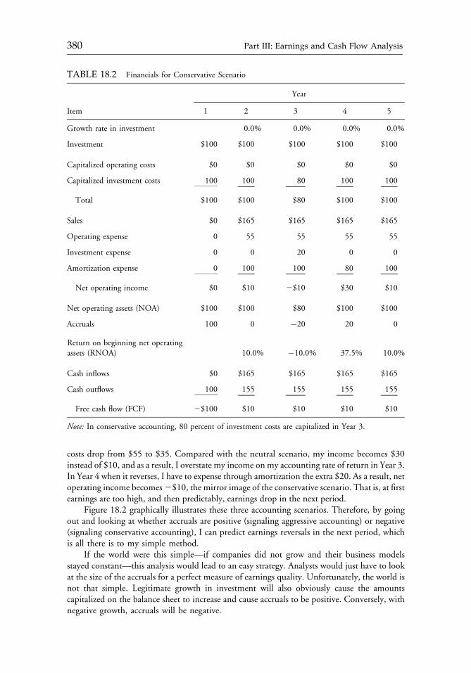
costs drop from $55 to $35. Compared with the neutral scenario, my income becomes $30instead of $10, and as a result, I overstate my income on my accounting rate of return in Year 3.In Year 4 when it reverses, I have to expense through amortization the extra $20. As a result, netoperating income becomes2$10, the mirror image of the conservative scenario. That is, at firstearnings are too high, and then predictably, earnings drop in the next period.
Figure 18.2 graphically illustrates these three accounting scenarios. Therefore, by goingout and looking at whether accruals are positive (signaling aggressive accounting) or negative(signaling conservative accounting), I can predict earnings reversals in the next period, whichis all there is to my simple method.
If the world were this simple—if companies did not grow and their business modelsstayed constant—this analysis would lead to an easy strategy. Analysts would just have to lookat the size of the accruals for a perfect measure of earnings quality. Unfortunately, the world isnot that simple. Legitimate growth in investment will also obviously cause the amountscapitalized on the balance sheet to increase and cause accruals to be positive. Conversely, withnegative growth, accruals will be negative.
TABLE 18.2 Financials for Conservative Scenario
Year
Item 1 2 3 4 5
Growth rate in investment 0.0% 0.0% 0.0% 0.0%
Investment $100 $100 $100 $100 $100
Capitalized operating costs $0 $0 $0 $0 $0
Capitalized investment costs 100 100 80 100 100
Total $100 $100 $80 $100 $100
Sales $0 $165 $165 $165 $165
Operating expense 0 55 55 55 55
Investment expense 0 0 20 0 0
Amortization expense 0 100 100 80 100
Net operating income $0 $10 2$10 $30 $10
Net operating assets (NOA) $100 $100 $80 $100 $100
Accruals 100 0 �20 20 0
Return on beginning net operatingassets (RNOA) 10.0% �10.0% 37.5% 10.0%
Cash inflows $0 $165 $165 $165 $165
Cash outflows 100 155 155 155 155
Free cash flow (FCF) 2$100 $10 $10 $10 $10
Note: In conservative accounting, 80 percent of investment costs are capitalized in Year 3.
c18 12 September 2012; 12:11:51
380 Part III: Earnings and Cash Flow Analysis
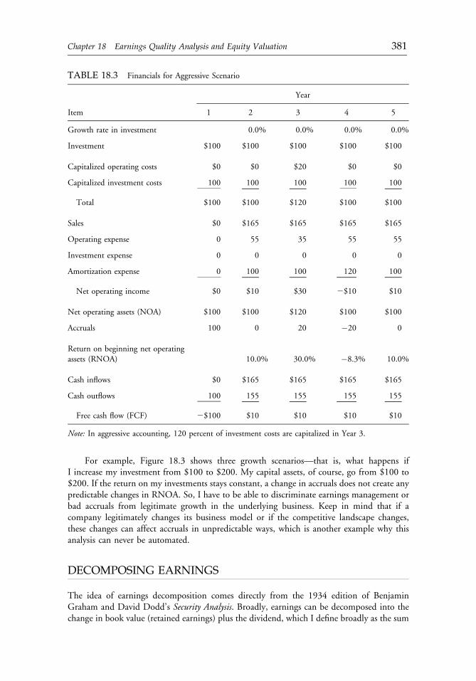
For example, Figure 18.3 shows three growth scenarios—that is, what happens ifI increase my investment from $100 to $200. My capital assets, of course, go from $100 to$200. If the return on my investments stays constant, a change in accruals does not create anypredictable changes in RNOA. So, I have to be able to discriminate earnings management orbad accruals from legitimate growth in the underlying business. Keep in mind that if acompany legitimately changes its business model or if the competitive landscape changes,these changes can affect accruals in unpredictable ways, which is another example why thisanalysis can never be automated.
DECOMPOSING EARNINGS
The idea of earnings decomposition comes directly from the 1934 edition of BenjaminGraham and David Dodd’s Security Analysis. Broadly, earnings can be decomposed into thechange in book value (retained earnings) plus the dividend, which I define broadly as the sum
TABLE 18.3 Financials for Aggressive Scenario
Year
Item 1 2 3 4 5
Growth rate in investment 0.0% 0.0% 0.0% 0.0%
Investment $100 $100 $100 $100 $100
Capitalized operating costs $0 $0 $20 $0 $0
Capitalized investment costs 100 100 100 100 100
Total $100 $100 $120 $100 $100
Sales $0 $165 $165 $165 $165
Operating expense 0 55 35 55 55
Investment expense 0 0 0 0 0
Amortization expense 0 100 100 120 100
Net operating income $0 $10 $30 2$10 $10
Net operating assets (NOA) $100 $100 $120 $100 $100
Accruals 100 0 20 �20 0
Return on beginning net operatingassets (RNOA) 10.0% 30.0% �8.3% 10.0%
Cash inflows $0 $165 $165 $165 $165
Cash outflows 100 155 155 155 155
Free cash flow (FCF) 2$100 $10 $10 $10 $10
Note: In aggressive accounting, 120 percent of investment costs are capitalized in Year 3.
c18 12 September 2012; 12:11:52
Chapter 18 Earnings Quality Analysis and Equity Valuation 381
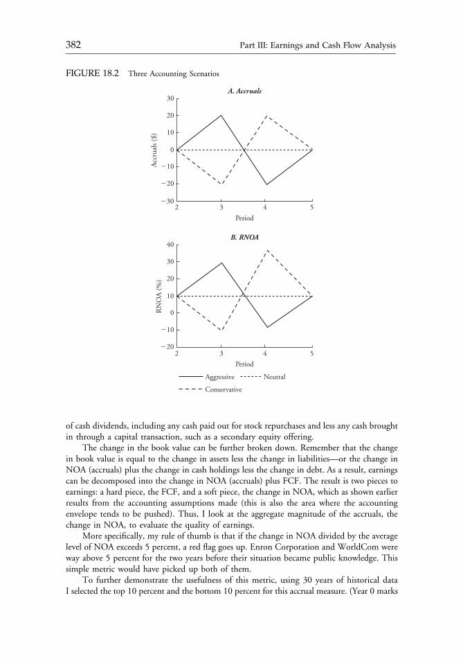
of cash dividends, including any cash paid out for stock repurchases and less any cash broughtin through a capital transaction, such as a secondary equity offering.
The change in the book value can be further broken down. Remember that the changein book value is equal to the change in assets less the change in liabilities—or the change inNOA (accruals) plus the change in cash holdings less the change in debt. As a result, earningscan be decomposed into the change in NOA (accruals) plus FCF. The result is two pieces toearnings: a hard piece, the FCF, and a soft piece, the change in NOA, which as shown earlierresults from the accounting assumptions made (this is also the area where the accountingenvelope tends to be pushed). Thus, I look at the aggregate magnitude of the accruals, thechange in NOA, to evaluate the quality of earnings.
More specifically, my rule of thumb is that if the change in NOA divided by the averagelevel of NOA exceeds 5 percent, a red flag goes up. Enron Corporation and WorldCom wereway above 5 percent for the two years before their situation became public knowledge. Thissimple metric would have picked up both of them.
To further demonstrate the usefulness of this metric, using 30 years of historical dataI selected the top 10 percent and the bottom 10 percent for this accrual measure. (Year 0 marks
FIGURE 18.2 Three Accounting Scenarios
Acc
rual
s ($)
A. Accruals30
20
10
0
�10
�20
�302 53 4
Period
Aggressive Neutral
Conservative
RN
OA
(%)
B. RNOA40
30
20
10
0
�10
�202 53 4
Period
c18 12 September 2012; 12:11:52
382 Part III: Earnings and Cash Flow Analysis
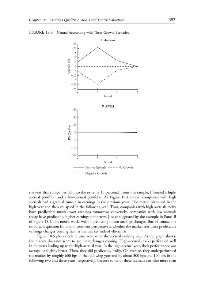
the year that companies fall into the extreme 10 percent.) From this sample, I formed a high-accrual portfolio and a low-accrual portfolio. As Figure 18.4 shows, companies with highaccruals had a gradual run-up in earnings in the previous years. The metric plateaued in thehigh year and then collapsed in the following year. Thus, companies with high accruals todayhave predictably much lower earnings tomorrow; conversely, companies with low accrualstoday have predictably higher earnings tomorrow. Just as suggested by the example in Panel Bof Figure 18.2, this metric works well in predicting future earnings changes. But, of course, theimportant question from an investment perspective is whether the market sees these predictableearnings changes coming (i.e., is the market indeed efficient)?
Figure 18.5 plots stock returns relative to the accrual ranking year. As the graph shows,the market does not seem to see these changes coming. High-accrual stocks performed wellin the years leading up to the high-accrual year. In the high-accrual year, their performance wasaverage or slightly better. Then, they did predictably badly. On average, they underperformedthe market by roughly 600 bps in the following year and by about 300 bps and 100 bps in thefollowing two and three years, respectively, because some of these accruals can take more than
FIGURE 18.3 Neutral Accounting with Three Growth Scenarios
Acc
rual
s ($)
A. Accruals2520
105
15
0
�10�5
�15�20�25
2 53 4Period
Positive Growth No Growth
Negative Growth
RN
OA
(%)
B. RNOA40
30
20
10
0
�10
�202 53 4
Period
c18 12 September 2012; 12:11:52
Chapter 18 Earnings Quality Analysis and Equity Valuation 383
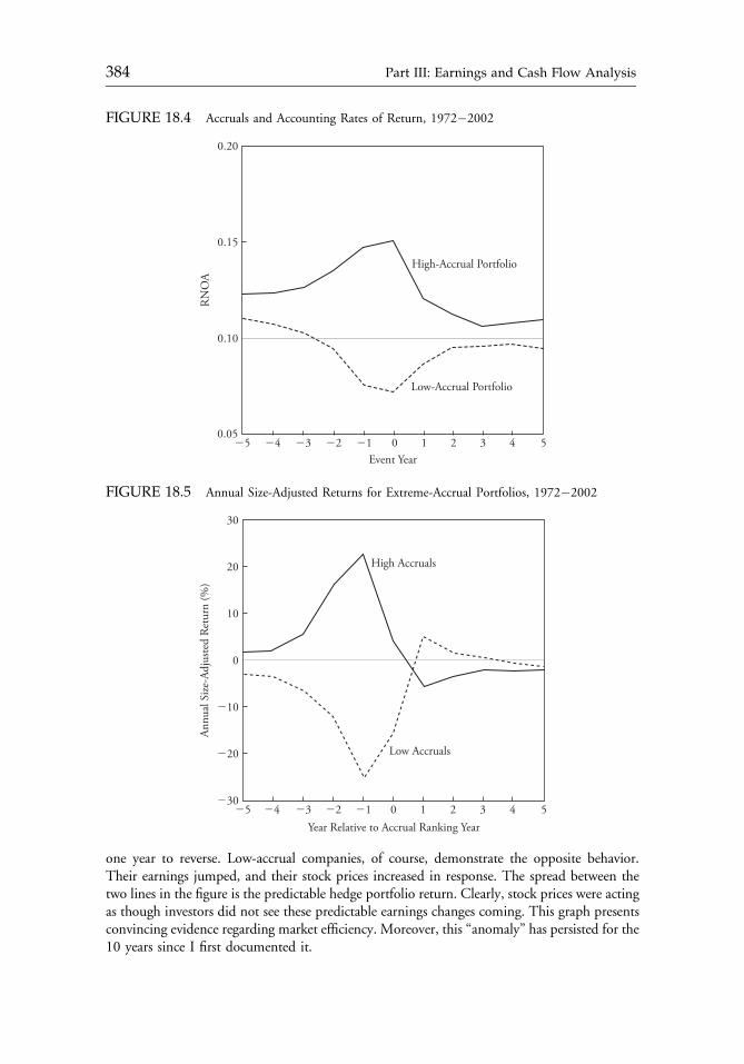
one year to reverse. Low-accrual companies, of course, demonstrate the opposite behavior.Their earnings jumped, and their stock prices increased in response. The spread between thetwo lines in the figure is the predictable hedge portfolio return. Clearly, stock prices were actingas though investors did not see these predictable earnings changes coming. This graph presentsconvincing evidence regarding market efficiency. Moreover, this “anomaly” has persisted for the10 years since I first documented it.
FIGURE 18.4 Accruals and Accounting Rates of Return, 1972�2002
RN
OA
High-Accrual Portfolio
Low-Accrual Portfolio
0.20
0.10
0.15
0.05�5 5�2 1 4�3 0 3�4 �1 2
Event Year
FIGURE 18.5 Annual Size-Adjusted Returns for Extreme-Accrual Portfolios, 1972�2002
Ann
ual S
ize-
Adj
uste
d R
etur
n (%
)
High Accruals
Low Accruals
30
0
10
�10
�20
20
�30�5 5�2 1 4�3 0 3�4 �1 2
Year Relative to Accrual Ranking Year
c18 12 September 2012; 12:11:52
384 Part III: Earnings and Cash Flow Analysis

As a check on this metric, I gathered a sample of about 100 companies that had beentargeted by the U.S. SEC for manipulating earnings upward. Year 0 is the year that the SECalleged that these earnings abuses occurred, not the year that the SEC announced theenforcement action, which typically did not occur until several years after the abuses becamecommon knowledge. Figure 18.6 shows that the accruals peaked in Year 0 and then plum-meted in the following year. The thin solid line in this figure mirrors the solid line in Panel Aof Figure 18.2 for aggressive accounting almost perfectly. Thus, an accruals analysis picks upincidences of aggressive accounting.
I want to emphasize that rising accruals can do no more than raise a red flag. Forexample, if a company’s inventory is rising, that could be a bad sign of obsolete inventory or itcould be a good sign because the company is growing. Perhaps the clearest way to helpdisentangle these two possibilities is to analyze accounts payable. If inventory is rising to meetincreasing sales, then accounts payable should be rising accordingly. When inventories arerising but payables are not increasing at the same rate, an earnings quality problem caused byobsolete inventory is most likely occurring. In this way, the liability side of the balance sheetcan be used to help judge the quality of the asset side of the balance sheet, where most of theearnings quality problems arise.
CONCLUSION
The simple technique of earnings quality analysis shown here would have done wonderfullyover the past half century in terms of generating superior stock returns. Although thisquantitative method has worked well, it will probably get arbitraged away. Still, I believe thatusing good fundamental analysis to detect accounting distortions by understanding theaccounting and the company’s strategy and how they fit together will always be an incrediblyimportant source of value added for the investment management community.
FIGURE 18.6 Accruals and SEC Enforcement Actions, 1987�2002
Acc
rual
s
Mean
Median Average for AllOther Companies
0.40
0
0.15
�0.05
0.30
0.35
0.25
0.20
0.10
0.05
�0.10�5 5�2 1 4�3 0 3�4 �1 2
Year Relative to the SEC Enforcement Action
Note: Accruals are measured by the annual change in NOA divided by the beginning level of NOA.
c18 12 September 2012; 12:11:52
Chapter 18 Earnings Quality Analysis and Equity Valuation 385
QUESTION AND ANSWER SESSION
Question: In the world of insurance companies and banks, half their books are accruals. Canthis type of analysis be used there?
Sloan: They do have assets and liabilities, but it is more difficult to distinguish what I call“proprietary assets” and “proprietary liabilities” from the marketable securities and debtthat represent a standard source of financing, such as bonds or commercial paper issuedby a bank. What you must do is identify the proprietary assets and liabilities and focuson them.
For insurance companies, you must focus on the spread between the reinsurancereceivables and the reinsurance payables and also the liability for claims reserves; theseare the proprietary assets and liabilities. One of the important areas we’re focusing onlately concerns companies in the financial sector that are issuing loans, particularlyresidential loans and consumer loans, and then securitizing and selling them whileholding a residual interest in these loans.
These residual interests hold most of the risk because they are the first not to bepaid in the event of a default. They are a small chunk of the balance sheets of thesecompanies because the residual interests are small in dollar magnitude, but the risk isenormous. So, you could take $1 billion of receivables, hold a residual interest in $20million, and basically have the risk of $1 billion of loans concentrated in $20 million ofreceivables.
If we see a downturn in the housing market and people defaulting on loans, theseresidual interests will evaporate fairly quickly. You can perform the same analysis withbanks and insurance companies. It just becomes a little more important to do thedetailed financial analysis and fundamental analysis to discriminate between the high-risk assets and liabilities, where the judgment exists, and the low-risk ones, which arejust the marketable securities and the plain vanilla debt.
Question: Do mergers and acquisitions lend themselves to greater accrual subjectivity?Sloan: We’ve tested for this by going to the statement of cash flows where we can exclude
stock deals and strip out the acquisitions as a separate line item. By purging mergers andacquisitions (M&A) activity, we can get a cleaner measure of earnings quality. It turnsout that the measure actually works slightly worse. I think the reason for this is thatmost of these stock acquisitions engage in a stock-for-stock acquisition when thecompany’s stock is the most overvalued. Hence, the goodwill on the balance sheetassociated with that acquisition tends to be extremely subjective and often overstatesassets. On the face of it, it might seem like something you want to strip out, but forpractical purposes, we find that leaving the M&A activity in actually helps the measure.
Question: Which areas should we watch the most for accruals in the future?Sloan: This is why a fundamental analyst has such a competitive advantage over a quantitative
analyst because new business comes along, accounting rules change, and it’s just a case oflooking at things differently.
One ofmy favorite examples when I first got interested in this was BostonChicken andits receivables. Inmany cases, receivables are not a problem. In this particular case, however,receivables were over half of Boston Chicken’s total balance sheet—over half of its assets.The franchisees were making huge losses, and the only reason they were surviving wasbecause Boston Chicken was lending themmoney and they were paying it back in the formof a royalty fee.
c18 12 September 2012; 12:11:52
386 Part III: Earnings and Cash Flow Analysis

Normally, when I analyze a company, I look at the company and see which is itsbiggest asset. If it is a proprietary asset that involves subjective judgment, then that iswhere I do my homework. In the case of Enron, its equity investments and its nonequityinvestments were huge numbers because much of the action was taking place on theseoff-balance-sheet entities. If they showed up at all, they showed up on an equity one-lineconsolidation-type entry. So, that is one situation I would not normally have focusedon, but in Enron’s case, that was the one that flagged the company’s problems.
c18 12 September 2012; 12:11:52
Chapter 18 Earnings Quality Analysis and Equity Valuation 387

c18 12 September 2012; 12:11:52
CHAPTER 19IS CASH FLOW KINGIN VALUATIONS?
Jing Liu, Doron Nissim, and Jacob Thomas
Contrary to the common perception that operating cash flows are better thanaccounting earnings at explaining equity valuations, recent studies suggest thatvaluations derived from industry multiples based on reported earnings are closer totraded prices than those based on reported operating cash flows. The questionaddressed in the article is whether the balance tilts in favor of cash flows when thefollowing are considered: (1) forecasts rather than reported numbers, (2) dividendsrather than operating cash flows, (3) individual industries rather than all industriescombined, and (4) companies in non-U.S. markets. In all cases studied, earningsdominated operating cash flows and dividends.
Industry multiples are used often in practice, both to provide stand-alone “quick and dirty”valuations and to anchor more complex discounted cash flow valuations. To obtain a com-pany valuation, one simply multiplies a value driver (such as earnings) for the company by thecorresponding multiple, which is based on the ratio of stock price to that value driver for agroup of comparable companies. Choices for value drivers include various measures of cashflow, book value, earnings, and revenues, but earnings and cash flows are by far the mostcommonly used. In the study reported here, we compare the valuation performance ofearnings multiples with the performance of multiples based on two measures of cash flow—operating cash flow and dividends—for a large sample of companies drawn from 10 nationalmarkets.
“Valuation performance” in our study does not refer to picking mispriced stocks.1 Wefocus on how close the valuations based on industry multiples are to traded prices. Our
Reprinted from the Financial Analysts Journal (March/April 2007):56�68. When this article wasoriginally published, Jing Liu was associate professor of accounting at the University of California atLos Angeles, Doron Nissim was associate professor of accounting at Columbia University, and JacobThomas was the Williams Brothers Professor of Accounting and Finance at Yale University.
c19 12 September 2012; 14:13:41
389
objective is to provide a comprehensive investigation of whether earnings or cash flows bestrepresent a summary measure of value.
At a conceptual level, earnings should be the more representative value driver becauseearnings reflect value changes regardless of when the cash flows occur. For example, thepromise to deliver health benefits later, when employees retire, is a compensation cost, similarto cash wages. Current cash flows remain unaffected by this promise, but earnings are reducedby an expense equal to the present value of that deferred compensation. Conversely, thepurchase of inventory for cash reduces operating cash flow, but earnings remain unaffectedbecause this purchase does not alter value. Still, many practitioners, arguing that accrualsinvolve discretion and are often used to manipulate earnings, prefer to use cash flow multiples.They also point out that expenses such as depreciation and amortization deviate substantiallyfrom actual declines in value because they are based on ad hoc estimates that are, in turn,derived from potentially meaningless historical costs.
In Liu, Nissim, and Thomas (2002), we found that multiples based on reported earningsoutperform multiples based on a variety of reported operating cash flow measures. Thesefindings were based on reported values of earnings and cash flows, however, and on arestricted sample (U.S. companies that satisfied extensive data requirements). In this study, weextended the analysis to determine whether cash flows outperform earnings when we consider(1) forecasts rather than reported numbers, (2) dividends as well as operating cash flows,(3) individual industries rather than all industries combined, and (4) companies in marketsbeyond the United States.
We undertook the first extension because reported operating cash flows often reflectnonrecurring payments or receipts, which blur the relationship between current cash flowsand value. For example, a company may engage in a large securitization transaction, therebyincreasing operating cash flows above their normal, recurring level. If such transitory effectsare excluded from cash flow forecasts (because analysts may not attempt to, or may not be ableto, forecast such transactions), we should see a commensurate performance improvement aswe change from using reported cash flows to using cash flow forecasts.
We undertook the second extension because stock price is related more directly toexpected dividends than to expected operating cash flows (Williams 1938). Moreover,managers might choose to signal long-term prospects via dividends. Although many com-panies do not pay dividends (only 30 percent of publicly traded U.S. companies paiddividends in 2003), dividends may outperform operating cash flows as a measure of valuewithin the subset of companies paying dividends.
The third extension allowed us to investigate whether the performance of earnings andcash flow multiples varies among industries (hereafter, “cash flow” includes both operatingcash flows and dividends). Numerous arguments have been offered in the practitioner liter-ature for why cash flows should perform well in some but not other industries.
Our final extension, to non-U.S. markets, was driven by the greater availability of cashflow forecasts for non-U.S. companies, but it also allowed us to document across-marketpatterns in the performance of earnings, operating cash flows, and dividends.
MULTIPLES-BASED VALUATION
Valuation based on industry multiples boils down a complex function of discount rates andfuture cash flows into a simple proportional relationship: Predicted value equals the level ofthe value driver for that company times the corresponding industry multiple. Because the
c19 12 September 2012; 14:13:42
390 Part III: Earnings and Cash Flow Analysis
industry multiple is an “average” ratio of stock price to value driver for the remainingcompanies in the industry, predicted values based on multiples will be close to traded stockprices if companies in the industry are relatively similar in terms of the price-to-value-driverratio. That is, our research question can be viewed intuitively as follows: Are companieswithin an industry more homogeneous in terms of P/Es or price-to-cash-flow ratios (P/CFs)?Stated differently, if we plotted histograms of the P/Es and P/CFs in an industry, the valuedriver with the tighter distribution should result in better valuations because a tighter dis-tribution indicates that companies’ ratios are closer to each other and, therefore, closer to theindustry average. However, although comparing the tightness of such distributions wouldallow us to rank earnings versus cash flows in each industry, it would not quantify the extentto which valuations from earnings and valuations from cash flow multiples deviate fromtraded stock prices. The methodology that allows us to do that is described next.
For each value driver, we first calculated an industry multiple for each company based onthe prices and value drivers for all remaining companies in that country-industry-monthcombination. (Deleting the target company from the industry before calculating the industrymultiple was necessary to avoid the target’s valuation being contaminated by its own price.)To obtain an industry multiple, analysts often use the average or median value of the ratio ofprice to value driver for the industry. Based on findings of academic research, we used theharmonic mean instead, where the harmonic mean was calculated by first finding the averagevalue driver to price for the industry and then inverting that average.2
For an illustration, assume there are five companies in the steel industry in Australia inMay 1989, indexed by i 5 1, 2, . . ., 5, with earnings per share of $1.50, $3.00, $2.50,$0.50, and $2.00 and share prices of $20, $35, $45, $25, and $30, respectively. Assume thatwe wish to calculate the industry multiple that is relevant for company i 5 3. If we use theaverage ratio of price to EPS of the remaining four companies, the industry multiple will be
Average P=E ¼ 1
43
20
1:50þ 35
3:00þ 25
0:50þ 30
2:00
� �¼ 22:5:
But if we use the harmonic mean P/E, the industry multiple for company i 5 3 is the inverseof the mean earnings-to-price multiples for the remaining four companies:
Harmonic mean P=E ¼ 1
ð1=4Þ3 ½ð1:50=20Þ þ ð3:00=35Þ þ ð0:50=25Þ þ ð2:00=30Þ�¼ 16:17:
The large difference between the two multiples (22.5 versus 16.17) is primarily caused bycompany i 5 4, which has a P/E of 50 (5 25/0.50). Without this company, the averagemultiple would be 13.33 and the harmonic mean multiple would be 13.19, which are closerto each other. When some high P/E values are caused by temporarily low values of earningsper share, the average multiple is skewed upward by those companies. The harmonic meanprovides a way to mitigate the effect of such companies by first inverting the P/E beforefinding the average; moving low values of EPS from the denominator to the numeratorreduces their impact on the industry multiple.
After obtaining an industry multiple for the target company, we calculated the predictedvalue by multiplying the harmonic mean industry multiple by the EPS for that company. Thepredicted value for company i 5 3 is $40.43 (5 16.17 3 $2.50). Finally, we calculated a
c19 12 September 2012; 14:13:42
Chapter 19 Is Cash Flow King in Valuations? 391
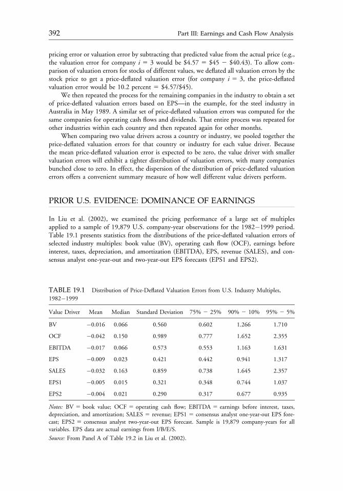
pricing error or valuation error by subtracting that predicted value from the actual price (e.g.,the valuation error for company i 5 3 would be $4.57 5 $45 2 $40.43). To allow com-parison of valuation errors for stocks of different values, we deflated all valuation errors by thestock price to get a price-deflated valuation error (for company i 5 3, the price-deflatedvaluation error would be 10.2 percent 5 $4.57/$45).
We then repeated the process for the remaining companies in the industry to obtain a setof price-deflated valuation errors based on EPS—in the example, for the steel industry inAustralia in May 1989. A similar set of price-deflated valuation errors was computed for thesame companies for operating cash flows and dividends. That entire process was repeated forother industries within each country and then repeated again for other months.
When comparing two value drivers across a country or industry, we pooled together theprice-deflated valuation errors for that country or industry for each value driver. Becausethe mean price-deflated valuation error is expected to be zero, the value driver with smallervaluation errors will exhibit a tighter distribution of valuation errors, with many companiesbunched close to zero. In effect, the dispersion of the distribution of price-deflated valuationerrors offers a convenient summary measure of how well different value drivers perform.
PRIOR U.S. EVIDENCE: DOMINANCE OF EARNINGS
In Liu et al. (2002), we examined the pricing performance of a large set of multiplesapplied to a sample of 19,879 U.S. company-year observations for the 1982�1999 period.Table 19.1 presents statistics from the distributions of the price-deflated valuation errors ofselected industry multiples: book value (BV), operating cash flow (OCF), earnings beforeinterest, taxes, depreciation, and amortization (EBITDA), EPS, revenue (SALES), and con-sensus analyst one-year-out and two-year-out EPS forecasts (EPS1 and EPS2).
TABLE 19.1 Distribution of Price-Deflated Valuation Errors from U.S. Industry Multiples,
1982�1999
Value Driver Mean Median Standard Deviation 75% 2 25% 90% 2 10% 95% 2 5%
BV �0.016 0.066 0.560 0.602 1.266 1.710
OCF �0.042 0.150 0.989 0.777 1.652 2.355
EBITDA �0.017 0.066 0.573 0.553 1.163 1.631
EPS �0.009 0.023 0.421 0.442 0.941 1.317
SALES �0.032 0.163 0.859 0.738 1.645 2.357
EPS1 �0.005 0.015 0.321 0.348 0.744 1.037
EPS2 �0.004 0.021 0.290 0.317 0.677 0.935
Notes: BV 5 book value; OCF 5 operating cash flow; EBITDA 5 earnings before interest, taxes,depreciation, and amortization; SALES 5 revenue; EPS1 5 consensus analyst one-year-out EPS fore-cast; EPS2 5 consensus analyst two-year-out EPS forecast. Sample is 19,879 company-years for allvariables. EPS data are actual earnings from I/B/E/S.
Source: From Panel A of Table 19.2 in Liu et al. (2002).
c19 12 September 2012; 14:13:42
392 Part III: Earnings and Cash Flow Analysis
Examination of the standard deviation and three nonparametric dispersion measures(interquartile range, or 75th percentile less 25th percentile, 90th percentile less 10th per-centile, and 95th percentile less 5th percentile) suggests the following ranking of multiples.Forecast earnings perform best; they exhibit the lowest dispersion of pricing errors. This resultis intuitively appealing because earnings forecasts should reflect future profitability better thanhistorical measures do. Consistent with this reasoning, performance improves with forecasthorizon: The dispersion measures for two-year-out forward earnings (EPS2) are lower thanthose for one-year-out earnings (EPS1). Among historical or reported value drivers, earningsdata dominate all other value drivers, SALES and OCF are the worst performers, andEBITDA and book value lie in the middle. These results are generally consistent with the viewthat accrual accounting enhances the link between earnings and value; earnings outperformrevenues because earnings incorporate relevant expenses, and earnings outperform cash flowsbecause earnings ignore current-period cash flows that are not value relevant and incorporatevalue-relevant cash flows that occur in other periods.
INTERNATIONAL SAMPLE
We obtained forecast data from the I/B/E/S International Summary files and reported (oractual) data from the I/B/E/S International Actual files. These files provide consensus analystforecasts and reported numbers for various value drivers at a monthly frequency. The actualmeasures are from the most recently published annual report, and the forecast measures weused are the consensus (mean) estimates during the month for the next full fiscal period. Forexample, the actual EPS for a U.S. calendar-year company in May of 1990 would refer to theEPS reported for 1989 (announced sometime early in 1990), and the forecast EPS would referto the consensus EPS forecast for 1991, based on forecasts available as of the third Friday inMay 1990.3 We also obtained per share prices as of that date from I/B/E/S. Even though werefer to the prior year’s EPS as actual or reported EPS, I/B/E/S often adjusts these data toremove some one-time items that analysts did not forecast. Because operating cash flownumbers are derived from earnings, actual operating cash flows reported by I/B/E/S may havealso been adjusted to remove some one-time items. I/B/E/S makes no adjustments to actualdividends.
I/B/E/S currently collects forecasts for 63 countries, but the number of observations isrelatively small for many countries. We identified the following 10 countries as having themost data available for earnings forecasts: Australia, Canada, France, Germany, Hong Kong,Japan, South Africa, Taiwan, the United Kingdom, and the United States. We analyzed theperformance of EPS valuations for each of these countries, but for comparing earnings andcash flow multiples, we used subsets of these countries in which selection biases were leastlikely to affect the results.
The potential for selection bias exists because forecasts for operating cash flows anddividends are not as frequent as earnings forecasts, especially for certain country and sectorcombinations.4 Whereas earnings forecasts are almost always provided for companies followedby analysts, forecasts for operating cash flows and dividends appear to be provided on anoptional basis. In particular, cash flow forecasts are more likely to be provided in sectors whereearnings forecasts are less informative and cash flow forecasts are more informative relative toother sectors (see, for example, the evidence in DeFond and Hung 2003 regarding U.S.companies providing operating cash flow forecasts). Thus, to mitigate selection biases
c19 12 September 2012; 14:13:42
Chapter 19 Is Cash Flow King in Valuations? 393
resulting from the nonrandomness of the availability of cash flow forecasts, we required twoconditions for a country to be included in the operating cash flow/dividend samples: (1) Thecountry should have a sufficiently large fraction of companies with operating cash flow/dividend forecasts, and (2) the across-sector distributions of these forecasts should resemblethe corresponding distributions for earnings forecasts. For the first condition, we required that30 percent of observations with earnings forecasts also have forecasts for cash flows (divi-dends). For the second condition, we calculated the absolute value of the difference betweenthe percentages of sample companies in each sector with earnings forecasts and the corre-sponding percentage for operating cash flows (dividends); we required that the averageabsolute difference across all sectors for that country be less than 2 percent. We also examinedthe country-year distributions for the three value drivers to confirm that the forecasts were notconcentrated in a few years.
The countries with sufficient and representative forecasts for operating cash flow wereAustralia, France, Hong Kong, Taiwan, and the United Kingdom. The correspondingcountries for dividend forecasts were Australia, France, Germany, Hong Kong, Japan, SouthAfrica, and the United Kingdom. We used these subsets of countries in the comparisons ofearnings with, respectively, cash flow from operations and dividends.
Comparison of company-years that had forecasts of both earnings and operating cashflow with the remaining company-years in our sample suggested that the subgroup with bothcontained companies with larger market capitalizations on average; the P/Es, however, werecomparable. Similarly, company-years that had both earnings and dividend forecasts hadlarger market caps than the remaining company-years, although the difference was not as largeas for the cash flow sample; again, the P/Es for both subgroups were comparable.
Appendix 19A presents how I/B/E/S normally calculates EPS, OCF per share (OCPS),and dividends per share (DPS) and summarizes in a table how those variables are calculated invarious countries and how they differ from the norm described for I/B/E/S. Calculations ofdividends are comparable across the sample, OCF is generally defined similarly (equalapproximately to operating cash flows from the cash flow statement), and EPS are measureddifferently to the extent that accounting rules vary across countries and over time. ForGermany, analysts follow their own conventions when calculating earnings rather than thelocal accounting rules.5 If the company was followed on a diluted basis, we used the I/B/E/Sdilution factor to convert per share variables to a primary basis.
To construct our sample, we merged the summary and actual files, and then we selectedall observations for which price, outstanding shares, and the actual and forecast values of thevalue driver were available (I/B/E/S reports separate observations for each value driver).6 Next,defining six variables corresponding to the actual and forecast values of EPS, OCPS, andDPS, we created one observation from each set of company-month observations. To maintainthe largest possible sample size for each value driver, we retained a company-month obser-vation as long as at least one of the six variables was positive.7 The initial sample included1,559,421 observations for 25,843 companies, and the sample period extended from January1987 through September 2004. To mitigate the effect of influential observations, values ofvariables that when deflated by price lay outside the 1st to 99th percentiles of the pooleddistribution were recorded as missing values.
Our data requirements when making pairwise comparisons were as follows: (1) Bothvalue drivers had positive values and (2) at least six observations satisfied the first requirementfrom the same country-industry-month combination (so a minimum of five companies wereavailable for calculating industry multiples for both value drivers). We used the intermediateindustry classification from the sector/industry/group classification by I/B/E/S because visual
c19 12 September 2012; 14:13:42
394 Part III: Earnings and Cash Flow Analysis
examination of companies included in the same sector suggested the sector classification wastoo broad to allow selection of homogeneous companies and because tabulation of thenumber of companies in different groups suggested that group classification was too narrowto allow the inclusion of enough comparable companies. Using pairwise comparisons left uswith substantially larger samples than if we had required nonmissing data for all variables,which in turn, increases the extent to which our results can be generalized.
INTERNATIONAL RESULTS
We began by comparing earnings with operating cash flows for the five countries in thatsample and then repeated the process for earnings and dividends for the seven countries in thedividend sample. Our final set of results describes the performance of multiple valuationsbased on earnings forecasts for all 10 countries.
We used the interquartile (IQ) range of the dispersion of price-deflated valuation errorsas a measure of the performance of various value drivers. We did so because the IQ range isless sensitive to outliers than are other dispersion measures, such as standard deviation or rootmean squared errors. When using alternative ranges (10�90 percent and 5�95 percent),however, we obtained results that are qualitatively similar to those reported here. We alsoconfirmed that these IQ ranges for the different pricing-error distributions straddle a medianthat is approximately zero. When comparing two value drivers—say, 1 and 2—we report theinterquartile range for the distributions of pricing errors for both variables (IQ1 and IQ2). Wemeasured the relative improvement (%IMP) in performance of variable 2 over variable 1 bycalculating the percentage decrease in the interquartile range [%IMP 5 100 percent 3(IQ1 2 IQ2)/IQ1]. We also computed a t-statistic for %IMP, derived from a bootstrapapproach (see Liu et al. 2002 for details).
Operating Cash Flows vs. Earnings
Columns 1�4 in Table 19.2 contain the results of comparing earnings forecasts withoperating cash flow forecasts. Columns 1 and 2 contain the IQ ranges of percentage pricingerrors, Column 3 reports the improvement in performance shown in Column 2 overColumn 1 (negative values indicate lower IQ ranges or higher performance for the valuedriver in the first column), and Column 4 provides the sample size for each country. Themean and median IQ ranges for the distribution of percentage pricing errors for earningsforecasts reported in the bottom two rows of Column 1 (0.524 and 0.548) are substantiallylower than the Column 2 mean and median IQ ranges for operating cash flow forecasts.The large negative values of %IMP in Column 3 for all five countries, between a high ofalmost 26 percent for the United Kingdom and a low of almost 18 percent for Taiwan,indicate the extent to which earnings forecasts outperformed operating cash flow forecastsfor this period (all differences are statistically significant at the 1 percent level unless oth-erwise stated).8
Columns 5�8 repeat the comparison in terms of actual operating cash flows versus cashflow forecasts. The degree to which the IQ ranges for forecasts (Column 6) are lower thanthose for actuals (Column 5) is clear from the %IMP values reported in Column 7.
The next four columns (9�12) repeat the comparison in terms of actual earnings versusearnings forecasts. As with operating cash flows, we found the IQ ranges for forecasts
c19 12 September 2012; 14:13:42
Chapter 19 Is Cash Flow King in Valuations? 395

TABLE 19.2 Price-Deflated Valuation Errors by Country for Industry Multiples Based on OCPS and EPS, January 1987�September 2004
OCPS Forecast vs. EPS Forecast OCPS Forecast vs. OCPS Actual EPS Forecast vs. EPS Actual OCPS Actual vs. EPS Actual
IQ Ranges for IQ Ranges for IQ Ranges for IQ Ranges for
EPS OCPS %IMP N Actual Forecast %IMP N Actual Forecast %IMP N EPS OCPS %IMP NCountry 1 2 3 4 5 6 7 8 9 10 11 12 13 14 15 16
Australia 0.467 0.564 220.86% 20,885 0.698 0.537 23.14% 18,069 0.538 0.400 25.65% 36,534 0.526 0.672 227.79% 16,637
France 0.548 0.665 221.21 20,595 0.791 0.666 15.81 20,139 0.624 0.481 22.95 43,449 0.659 0.759 215.24 16,754
Hong Kong 0.572 0.713 224.71 5,926 0.794 0.707 10.90 4,886 0.606 0.518 14.60 17,878 0.655 0.766 216.86 4,198
Taiwan 0.578 0.681 217.75 8,663 0.781 0.679 12.97 7,929 0.733 0.581 20.72 22,965 0.734 0.754 22.80a 7,257
United Kingdom 0.453 0.570 225.84 53,320 0.690 0.560 18.86 52,685 0.541 0.411 24.02 159,747 0.540 0.680 �25.88 48,653
Mean 0.524 0.639 222.07 21,878 0.751 0.630 16.34 20,742 0.608 0.478 21.59 56,115 0.623 0.726 217.71 18,700
Median 0.548 0.665 221.21 20,595 0.781 0.666 15.81 18,069 0.606 0.481 22.95 36,534 0.655 0.754 �16.86 16,637
aNot significant.
c19 12 September 2012; 14:13:43
396
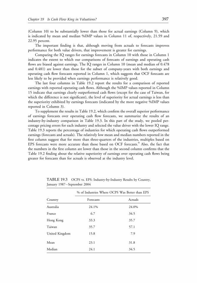
(Column 10) to be substantially lower than those for actual earnings (Column 9), whichis indicated by mean and median %IMP values in Column 11 of, respectively, 21.59 and22.95 percent.
The important finding is that, although moving from actuals to forecasts improvesperformance for both value drivers, that improvement is greater for earnings.
Comparing the IQ ranges for earnings forecasts in Column 10 with those in Column 1indicates the extent to which our comparisons of forecasts of earnings and operating cashflows are biased against earnings. The IQ ranges in Column 10 (mean and median of 0.478and 0.481) are lower than those for the subset of company-years with both earnings andoperating cash flow forecasts reported in Column 1, which suggests that OCF forecasts areless likely to be provided when earnings performance is relatively good.
The last four columns in Table 19.2 report the results for a comparison of reportedearnings with reported operating cash flows. Although the %IMP values reported in Column15 indicate that earnings clearly outperformed cash flows (except for the case of Taiwan, forwhich the difference is not significant), the level of superiority for actual earnings is less thanthe superiority exhibited by earnings forecasts (indicated by the more negative %IMP valuesreported in Column 3).
To supplement the results in Table 19.2, which confirm the overall superior performanceof earnings forecasts over operating cash flow forecasts, we summarize the results of anindustry-by-industry comparison in Table 19.3. In this part of the study, we pooled per-centage pricing errors for each industry and selected the value driver with the lower IQ range.Table 19.3 reports the percentage of industries for which operating cash flows outperformedearnings (forecasts and actuals). The relatively low mean and median numbers reported in thefirst column suggest that for more than three-quarters of the industries, multiples based onEPS forecasts were more accurate than those based on OCF forecasts.9 Also, the fact thatthe numbers in the first column are lower than those in the second column confirms that theTable 19.2 finding about the relative superiority of earnings over operating cash flows beinggreater for forecasts than for actuals is observed at the industry level.
TABLE 19.3 OCPS vs. EPS: Industry-by-Industry Results by Country,
January 1987�September 2004
% of Industries Where OCPS Was Better than EPS
Country Forecasts Actuals
Australia 24.1% 24.0%
France 6.7 34.5
Hong Kong 33.3 35.7
Taiwan 35.7 57.1
United Kingdom 15.8 7.9
Mean 23.1 31.8
Median 24.1 34.5
c19 12 September 2012; 14:13:43
Chapter 19 Is Cash Flow King in Valuations? 397
Dividends versus Earnings
The EPS-to-DPS comparison reported in Table 19.4 is analogous to the EPS-to-OCPScomparison reported in Table 19.2. Columns 1 and 2 contain the IQ ranges of percentagepricing errors for, respectively, earnings and dividend forecasts. Column 3 reports theimprovement in performance of Column 1 over Column 2, and Column 4 providesthe sample size for each country. The mean and median IQ ranges for the distribution ofpercentage pricing errors for earnings forecasts are substantially lower than the correspondingmean and median IQ ranges for dividend forecasts. Although the mean and median values of%IMP are quite large and negative, the distribution across countries appears to be bimodal.Four of the seven countries have relatively large negative values of %IMP, whereas threecountries (Hong Kong, Japan, and South Africa) have smaller values. All the differences,however, are significant at the 1 percent level.
The analysis of actual versus forecast dividends reported in Columns 5�8 confirms thatmoving from actuals to forecasts improves performance for industry multiples based ondividends. The relatively low values of %IMP reported in Column 7 for most countriessuggest that dividends are “sticky” (vary little over time) and multiples based on forecasts ofdividends are not substantially better than multiples based on reported dividends. The rel-atively large %IMP values for Australia (23.1 percent) and Hong Kong (21.5 percent),however, suggest that the value relevance of dividends in these two countries differs in someimportant way from its role in the other countries. (Additional analysis of that difference isreported later.)
The results of comparing actual earnings with forecasts, reported in Columns 9�12, aresimilar to the corresponding columns reported in Table 19.2. As with the results for operatingcash flows, the important finding is that, although moving from actuals to forecasts improvesperformance for both DPS and EPS, that improvement is greater for EPS. Also as with theTable 19.2 findings, the lower IQ ranges in Column 10 for earnings forecasts for the largersample of companies (relative to those in Column 1 for the subset of companies that also haddividend forecasts) suggest that dividend forecasts are less frequent when earnings forecastsperform relatively well, and the comparisons in Columns 1�4 are biased against earningsforecasts exhibiting superior performance.
The last four columns in Table 19.4 report the results of a comparison of reportedearnings and reported dividends. Similar to the bimodal distribution observed for %IMPvalues in Column 3, the %IMP values reported in Column 15 indicate that reported earningsclearly outperformed dividends for Australia, France, Germany, and the United Kingdom,but the margin of superiority is lower for Hong Kong and South Africa, and the relativeranking is reversed in the case of Japan (indicated by a positive and significant %IMP value of12.8 percent).10 As with operating cash flows, the lower values in Column 15 (relative tothose in Column 3) suggest that the level of superiority for actual earnings over actualdividends is less than that exhibited by earnings forecasts over dividend forecasts.
In the industry-by-industry comparison reported in Table 19.5, the relatively low meanand median numbers reported in the first column suggest, again, that for more than three-quarters of the industries, multiples based on earnings forecasts are more accurate than thosebased on dividend forecasts.11 Also, the fact that the numbers in the first column are lowerthan those in the second column confirms that the overall conclusion about the relativesuperiority of earnings over dividends being greater for forecasts than for actuals is alsoobservable at the industry level.
c19 12 September 2012; 14:13:43
398 Part III: Earnings and Cash Flow Analysis
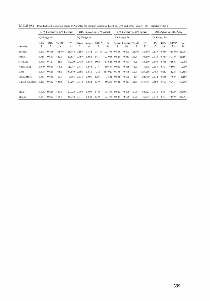
TABLE 19.4 Price-Deflated Valuation Errors by Country for Industry Multiples Based on DPS and EPS, January 1987�September 2004
DPS Forecast vs. EPS Forecast DPS Forecast vs. DPS Actual EPS Forecast vs. EPS Actual DPS Actual vs. EPS Actual
IQ Ranges for IQ Ranges for IQ Ranges for IQ Ranges for
EPS DPS %IMP N Actual Forecast %IMP N Actual Forecast %IMP N EPS DPS %IMP NCountry 1 2 3 4 5 6 7 8 9 10 11 12 13 14 15 16
Australia 0.408 0.485 �18.9% 25,748 0.565 0.434 23.1% 22,193 0.538 0.400 25.7% 36,534 0.479 0.555 215.9% 21,051
France 0.518 0.684 232.0 26,537 0.769 0.661 14.1 23,083 0.624 0.481 22.9 43,449 0.618 0.753 221.9 21,191
Germany 0.568 0.727 �28.1 14,920 0.730 0.656 10.2 11,628 0.685 0.561 18.2 35,219 0.640 0.746 216.6 10,904
Hong Kong 0.570 0.606 26.3 11,947 0.711 0.558 21.5 10,504 0.606 0.518 14.6 17,878 0.633 0.701 210.8 9,609
Japan 0.598 0.646 28.0 104,340 0.668 0.646 3.2 134,920 0.755 0.598 20.9 127,036 0.753 0.657 12.8 89,388
South Africa 0.557 0.615 �10.4 9,465 0.675 0.590 12.6 7,881 0.601 0.506 15.7 22,700 0.612 0.649 26.0 8,166
United Kingdom 0.463 0.632 236.5 87,201 0.713 0.621 13.0 89,284 0.541 0.411 24.0 159,747 0.560 0.703 225.7 80,456
Mean 0.526 0.628 220.0 40,023 0.690 0.595 14.0 42,785 0.622 0.496 20.3 63,223 0.613 0.681 212.0 34,395
Median 0.557 0.632 218.9 25,748 0.711 0.621 13.0 22,193 0.606 0.506 20.9 36,534 0.618 0.701 215.9 21,051
c19 12 September 2012; 14:13:44
399
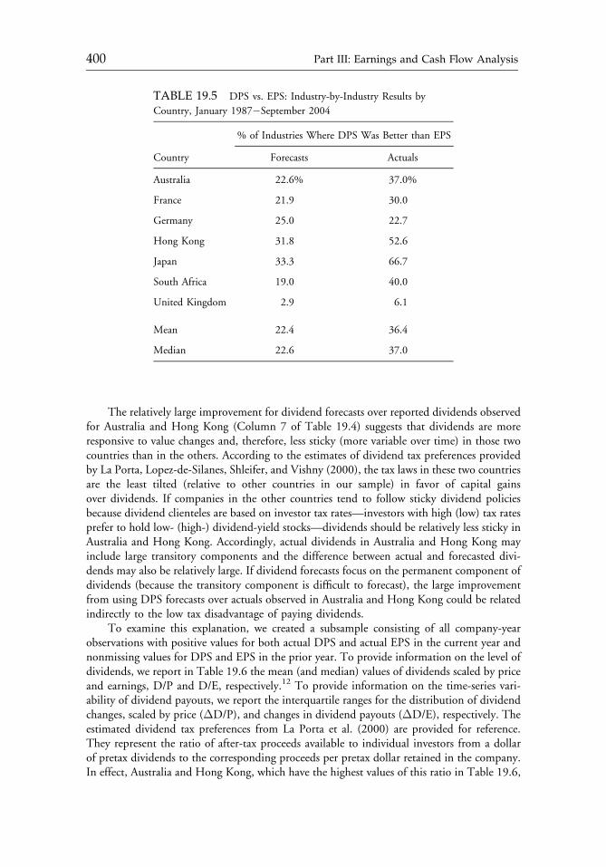
The relatively large improvement for dividend forecasts over reported dividends observedfor Australia and Hong Kong (Column 7 of Table 19.4) suggests that dividends are moreresponsive to value changes and, therefore, less sticky (more variable over time) in those twocountries than in the others. According to the estimates of dividend tax preferences providedby La Porta, Lopez-de-Silanes, Shleifer, and Vishny (2000), the tax laws in these two countriesare the least tilted (relative to other countries in our sample) in favor of capital gainsover dividends. If companies in the other countries tend to follow sticky dividend policiesbecause dividend clienteles are based on investor tax rates—investors with high (low) tax ratesprefer to hold low- (high-) dividend-yield stocks—dividends should be relatively less sticky inAustralia and Hong Kong. Accordingly, actual dividends in Australia and Hong Kong mayinclude large transitory components and the difference between actual and forecasted divi-dends may also be relatively large. If dividend forecasts focus on the permanent component ofdividends (because the transitory component is difficult to forecast), the large improvementfrom using DPS forecasts over actuals observed in Australia and Hong Kong could be relatedindirectly to the low tax disadvantage of paying dividends.
To examine this explanation, we created a subsample consisting of all company-yearobservations with positive values for both actual DPS and actual EPS in the current year andnonmissing values for DPS and EPS in the prior year. To provide information on the level ofdividends, we report in Table 19.6 the mean (and median) values of dividends scaled by priceand earnings, D/P and D/E, respectively.12 To provide information on the time-series vari-ability of dividend payouts, we report the interquartile ranges for the distribution of dividendchanges, scaled by price (ΔD/P), and changes in dividend payouts (ΔD/E), respectively. Theestimated dividend tax preferences from La Porta et al. (2000) are provided for reference.They represent the ratio of after-tax proceeds available to individual investors from a dollarof pretax dividends to the corresponding proceeds per pretax dollar retained in the company.In effect, Australia and Hong Kong, which have the highest values of this ratio in Table 19.6,
TABLE 19.5 DPS vs. EPS: Industry-by-Industry Results by
Country, January 1987�September 2004
% of Industries Where DPS Was Better than EPS
Country Forecasts Actuals
Australia 22.6% 37.0%
France 21.9 30.0
Germany 25.0 22.7
Hong Kong 31.8 52.6
Japan 33.3 66.7
South Africa 19.0 40.0
United Kingdom 2.9 6.1
Mean 22.4 36.4
Median 22.6 37.0
c19 12 September 2012; 14:13:44
400 Part III: Earnings and Cash Flow Analysis
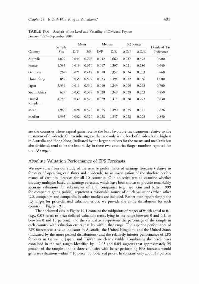
are the countries where capital gains receive the least favorable tax treatment relative to thetreatment of dividends. Our results suggest that not only is the level of dividends the highestin Australia and Hong Kong (indicated by the larger numbers for the means and medians) butalso dividends tend to be the least sticky in these two countries (larger numbers reported forthe IQ range).
Absolute Valuation Performance of EPS Forecasts
We now turn from our study of the relative performance of earnings forecasts (relative toforecasts of operating cash flows and dividends) to an investigation of the absolute perfor-mance of earnings forecasts for all 10 countries. Our objective was to examine whetherindustry multiples based on earnings forecasts, which have been shown to provide remarkablyaccurate valuations for subsamples of U.S. companies (e.g., see Kim and Ritter 1999for companies going public), represent a reasonable source of quick valuations when otherU.S. companies and companies in other markets are included. Rather than report simply theIQ ranges for price-deflated valuation errors, we provide the entire distribution for eachcountry in Figure 19.1.
The horizontal axis in Figure 19.1 contains the midpoints of ranges of width equal to 0.1(e.g., 0.05 refers to price-deflated valuation errors lying in the range between 0 and 0.1, orbetween 0 and 10 percent), and the vertical axis represents the percentage of the sample ineach country with valuation errors that lay within that range. The superior performance ofEPS forecasts as a value indicator in Australia, the United Kingdom, and the United States(indicated by the more peaked distributions) and the relatively inferior performance of EPSforecasts in Germany, Japan, and Taiwan are clearly visible. Combining the percentagescontained in the two ranges identified by 20.05 and 0.05 suggests that approximately 25percent of the sample for the three countries with better-performing EPS forecasts wouldgenerate valuations within 610 percent of observed prices. In contrast, only about 17 percent
TABLE 19.6 Analysis of the Level and Volatility of Dividend Payouts,
January 1987�September 2004
SampleSize
Mean Median IQ RangeDividend TaxPreferenceCountry D/P D/E D/P D/E ΔD/P ΔD/E
Australia 1,829 0.044 0.796 0.042 0.660 0.037 0.492 0.900
France 1,595 0.019 0.370 0.017 0.307 0.021 0.280 0.640
Germany 762 0.021 0.417 0.018 0.357 0.024 0.353 0.860
Hong Kong 852 0.035 0.592 0.033 0.394 0.032 0.336 1.000
Japan 3,339 0.011 0.549 0.010 0.249 0.009 0.263 0.700
South Africa 627 0.032 0.398 0.028 0.349 0.028 0.233 0.850
UnitedKingdom
4,758 0.032 0.520 0.029 0.414 0.028 0.293 0.830
Mean 1,966 0.028 0.520 0.025 0.390 0.025 0.321 0.826
Median 1,595 0.032 0.520 0.028 0.357 0.028 0.293 0.850
c19 12 September 2012; 14:13:44
Chapter 19 Is Cash Flow King in Valuations? 401
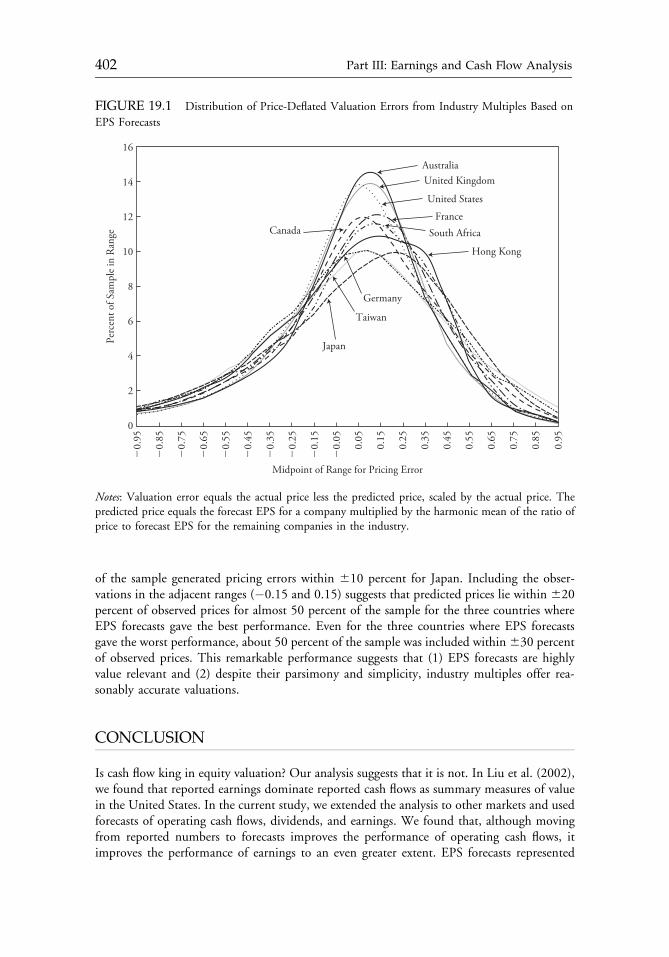
of the sample generated pricing errors within 610 percent for Japan. Including the obser-vations in the adjacent ranges (�0.15 and 0.15) suggests that predicted prices lie within 620percent of observed prices for almost 50 percent of the sample for the three countries whereEPS forecasts gave the best performance. Even for the three countries where EPS forecastsgave the worst performance, about 50 percent of the sample was included within630 percentof observed prices. This remarkable performance suggests that (1) EPS forecasts are highlyvalue relevant and (2) despite their parsimony and simplicity, industry multiples offer rea-sonably accurate valuations.
CONCLUSION
Is cash flow king in equity valuation? Our analysis suggests that it is not. In Liu et al. (2002),we found that reported earnings dominate reported cash flows as summary measures of valuein the United States. In the current study, we extended the analysis to other markets and usedforecasts of operating cash flows, dividends, and earnings. We found that, although movingfrom reported numbers to forecasts improves the performance of operating cash flows, itimproves the performance of earnings to an even greater extent. EPS forecasts represented
FIGURE 19.1 Distribution of Price-Deflated Valuation Errors from Industry Multiples Based on
EPS ForecastsPe
rcen
t of S
ampl
e in
Ran
ge
16
14
12
10
8
6
4
2
0
�0.
95
�0.
55
�0.
75
�0.
85
�0.
35
0.05
�0.
15
0.65
0.85
0.95
0.45
0.25
�0.
45
�0.
65
�0.
25
0.15
�0.
05
0.75
0.55
0.35
Midpoint of Range for Pricing Error
Australia
United States
United Kingdom
CanadaFrance
South Africa
Hong Kong
Germany
Taiwan
Japan
Notes: Valuation error equals the actual price less the predicted price, scaled by the actual price. Thepredicted price equals the forecast EPS for a company multiplied by the harmonic mean of the ratio ofprice to forecast EPS for the remaining companies in the industry.
c19 12 September 2012; 14:13:44
402 Part III: Earnings and Cash Flow Analysis
substantially better summary measures of value than did OCF forecasts in all five countriesexamined, and this relative superiority was observed in most industries.
When we compared dividends rather than operating cash flows with earnings for asample derived from seven countries where dividend forecasts are common, we found, again,that earnings forecasts were a better summary measure of value than dividend forecasts in allcountries and most industries. And we found that moving from reported numbers to forecastsimproved performance more for earnings than for dividends.
Overall, our results suggest that proponents of cash flow multiples should consider usingearnings multiples instead because valuations based on earnings forecasts are remarkablyaccurate for a substantial majority of companies. The increased availability of earningsforecasts should be an impetus to use earnings multiples.
We conclude with three caveats. First, because valuations based on multiples can becalculated only when the value driver is positive, we excluded companies with nonpositivevalues for the multiples examined (earnings, cash from operations, or dividends). Ourinferences, therefore, cannot be generalized to situations where value drivers are not positive.Nevertheless, although this requirement eliminates many companies for most value drivers,earnings forecasts are positive in a substantial majority of cases, which supports our callthat earnings forecasts be used for multiples. Second, nonearnings forecasts are more likely tobe provided in sectors where nonearnings forecasts are more informative than earningsforecasts (see DeFond and Hung 2003). Although we focused on countries where cashflow forecasts are relatively widespread, some selection bias probably remained in our samples.However, this bias worked against our findings; that is, we used observations where cash flowforecasts were likely to perform better than average but we still found that earnings dominatecash flows. The final caveat relates to our use of market price as a proxy for intrinsic (“true”)value. To the extent that market inefficiencies are correlated with earnings or cash flowinformation, differences between the pricing accuracy of earnings multiples and cashflow multiples may arise partly from market inefficiencies rather than the multiple’s ability tomeasure value. Prior research suggests, however, that, although market inefficiencies mayinduce substantial bias in stock return tests, the magnitude of the bias in price-level analyses islikely to be negligible because cross-sectional variation in mispricing is likely to be smallerthan cross-sectional variation in intrinsic values (Aboody, Hughes, and Liu 2002).
APPENDIX 19A VARIABLE DEFINITIONS
The following definitions are those of I/B/E/S. Table 19A.1 provides the definitions ofearnings and operating cash flows used by each of the 10 countries in the study.
Earnings Per Share (EPS)
A corporation’s net income from continuing operations (i.e., income after backing out dis-continued operations, extraordinary charges, and other nonoperating items) divided by theweighted average number of shares outstanding for the year.
Operating Cash Flow Per Share (OCPS)
Net income plus depreciation and amortization plus net working capital divided by theweighted average number of common shares outstanding for the year.
c19 12 September 2012; 14:13:44
Chapter 19 Is Cash Flow King in Valuations? 403
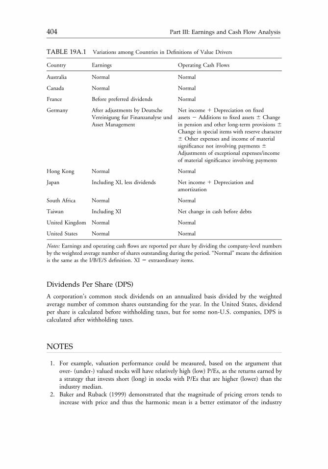
Dividends Per Share (DPS)
A corporation’s common stock dividends on an annualized basis divided by the weightedaverage number of common shares outstanding for the year. In the United States, dividendper share is calculated before withholding taxes, but for some non-U.S. companies, DPS iscalculated after withholding taxes.
NOTES
1. For example, valuation performance could be measured, based on the argument thatover- (under-) valued stocks will have relatively high (low) P/Es, as the returns earned bya strategy that invests short (long) in stocks with P/Es that are higher (lower) than theindustry median.
2. Baker and Ruback (1999) demonstrated that the magnitude of pricing errors tends toincrease with price and thus the harmonic mean is a better estimator of the industry
TABLE 19A.1 Variations among Countries in Definitions of Value Drivers
Country Earnings Operating Cash Flows
Australia Normal Normal
Canada Normal Normal
France Before preferred dividends Normal
Germany After adjustments by DeutscheVereinigung fur Finanzanalyse undAsset Management
Net income 1 Depreciation on fixedassets 2 Additions to fixed assets 6 Changein pension and other long-term provisions 6Change in special items with reserve character6 Other expenses and income of materialsignificance not involving payments 6Adjustments of exceptional expenses/incomeof material significance involving payments
Hong Kong Normal Normal
Japan Including XI, less dividends Net income 1 Depreciation andamortization
South Africa Normal Normal
Taiwan Including XI Net change in cash before debts
United Kingdom Normal Normal
United States Normal Normal
Notes: Earnings and operating cash flows are reported per share by dividing the company-level numbersby the weighted average number of shares outstanding during the period. “Normal” means the definitionis the same as the I/B/E/S definition. XI 5 extraordinary items.
c19 12 September 2012; 14:13:44
404 Part III: Earnings and Cash Flow Analysis
multiple than such estimators as the arithmetic mean or median. As demonstrated in theexample in the text, the harmonic mean gives less weight to companies with relativelyhigh price-to-value-driver ratios, which is consistent with the larger absolute valuationerrors that typify these companies. Indeed, several studies (e.g., Beatty, Riffe, andThompson 1999; Liu et al. 2002) confirmed that the harmonic mean performs well interms of minimizing price-deflated pricing errors.
3. Although analysts also provide one-year-out (for 1990) forecasts, we elected not to usethem because they represent a mixture of actuals for interim periods already reported andforecasts for the remaining interim periods.
4. I/B/E/S uses a proprietary classification scheme to categorize companies into homoge-neous groups according to business lines. In the United States, a scheme similar to theS&P 500 Index industry groupings is followed. For non-U.S. companies, a system basedloosely on the Morgan Stanley Capital International industry classifications is used. TheI/B/E/S classification system segregates companies at three levels (sector, industry, andgroup). Sectors are subdivided into industries, which are, in turn, subdivided intogroups.
5. The German financial analyst society, Deutsche Vereinigung fur Finanzanalyse undAsset Management (DVFA), has developed a system used by analysts (and often bycompanies) to adjust reported earnings data to provide a measure that is close to per-manent or core earnings. The adjustment process uses both reported financial infor-mation and companies’ internal records.
6. To prevent duplication, we deleted all observations with a “secondary” flag (for theactual or forecast). Also, to ensure consistency when merging, we deleted observations forwhich the fiscal year-end for the actual was not exactly 24 months before the fiscal year-end of the forecast.
7. Because prices are positive, the multiples approach requires that both comparable andtarget companies have positive value drivers. The proportion of observations withnegative values of actual (forecast) EPS and OCPS is 15 percent (5 percent) and 8percent (1 percent); no negative values were observed for actual or forecast DPS. Therewere few cases in which the value driver was zero except for the case of dividends (16percent for actual dividends and 10 percent for forecast dividends) and, occasionally, foractual OCPS observations (1 percent).
8. See Figure 19.1 and the related discussion for a graphical approach to illustrate per-formance differences.
9. Because the sample sizes were very small for some industries, especially in countries withfew forecasts, some of these comparisons are probably associated with error.
10. This contrary result observed in Japan is primarily a result of the relatively poor per-formance of reported earnings rather than the superior performance of dividends; the IQrange for reported dividends in Japan is close to the mean for other countries, but theIQ range for reported earnings in Japan is considerably higher than the mean for othercountries. See Charitou, Clubb, and Andreou (2000) for a potential explanation of thelower value relevance observed for reported earnings in Japan.
11. Because the sample sizes are very small for some industries, especially in countries withfewer forecasts, some of these comparisons are probably associated with error.
12. The resulting sample sizes are smaller than those in previous tables, primarily because acompany-year appears only once in Table 19.6.
c19 12 September 2012; 14:13:45
Chapter 19 Is Cash Flow King in Valuations? 405
REFERENCES
Aboody, D., J. Hughes, and J. Liu. 2002. “Measuring Value Relevance in a (Possibly) InefficientMarket.” Journal of Accounting Research, vol. 40, no. 4 (September):965�986.
Baker, M., and R. Ruback. 1999. “Estimating Industry Multiples.” Working paper, Harvard University.Beatty, R.P., S.M. Riffe, and R. Thompson. 1999. “The Method of Comparables and Tax Court
Valuations of Private Firms: An Empirical Investigation.” Accounting Horizons, vol. 13, no. 3(September):177�199.
Charitou, A., C. Clubb, and A. Andreou. 2000. “The Value Relevance of Earnings and Cash Flows:Empirical Evidence for Japan.” Journal of International Financial Management and Accounting, vol.11, no. 1 (Spring):1�22.
DeFond, M., and M. Hung. 2003. “An Empirical Analysis of Analysts’ Cash Flow Forecasts.” Journal ofAccounting and Economics, vol. 35, no. 1 (April):73�100.
Kim, M., and J.R. Ritter. 1999. “Valuing IPOs.” Journal of Financial Economics, vol. 53, no. 3(September):409�437.
La Porta, R., F. Lopez-de-Silanes, A. Shleifer, and R. Vishny. 2000. “Agency Problems and DividendPolicies around the World.” Journal of Finance, vol. 55, no. 1 (February):1�33.
Liu, J., D. Nissim, and J. Thomas. 2002. “Equity Valuation Using Multiples.” Journal of AccountingResearch, vol. 40, no. 1 (March):135�172.
Williams, J.B. 1938. The Theory of Investment Value. Cambridge, MA: Harvard University Press.
c19 12 September 2012; 14:13:45
406 Part III: Earnings and Cash Flow Analysis

PART IVOPTION VALUATION
Chapter 20 Employee Stock Options and Equity Valuation 409
Chapter 21 Employee Stock Option Valuation with an Early Exercise Boundary 465
c20 12 September 2012; 14:17:55
407

c20 12 September 2012; 14:17:55
CHAPTER 20EMPLOYEE STOCK OPTIONSAND EQUITY VALUATION
Mark Lang
Increasingly, companies are turning to employee stock options to meet the challenge ofaligning the interests of employees and shareholders. These stock options, however,create some difficult issues: Stock options represent a significant claim againstcompanies that should be reflected in their valuations, but valuing employee stockoptions is very complex. Fortunately, in this chapter, Mark Lang presents anexcellent framework for valuing these claims by balancing the obligation of thecompany to fund outstanding options and future grants with the benefits arisingfrom the incentive effects of options.
FOREWORD
One of the great challenges of corporate management is to align the interests of employeesand shareholders, and increasingly, companies are resorting to employee stock options to meetthis challenge. Stock options grant employees a direct stake in the fortunes of the company;hence, employees are motivated to engage in value-enhancing behavior, which benefitsshareholders. This apparent simplicity in logic, however, belies a considerable amount ofcomplexity in the implementation and valuation of employee stock options.
Mark Lang addresses the key issues of employee stock options primarily from theperspective of an analyst charged with valuing a company, although he views these issuesfrom the perspective of employees as well. He begins with a description of a typical employeestock option and measures the claim it poses against shareholders. Lang then discussesthe accounting issues surrounding employee stock options. He leaves no doubt as to theimportance of these claims, noting that in 2000, tax deductions for options exceeded net
Copyright ª 2004 The Research Foundation of CFA Institute. Reprinted with permission. When thisarticle was originally published (July 2004), Mark Lang was Thomas W. Hudson, Jr./Deloitte and ToucheL.L.P. Distinguished Professor at the Kenan-Flagler Business School at the University of North Carolina.
c20 12 September 2012; 14:17:55
409
income for 8 of the largest 100 companies in the S&P 100 Index and, on average, for allcompanies in the NASDAQ 100 Index.
Lang then reviews the features of employee stock options that differentiate them fromtraded options. Because employees are typically prohibited from hedging these options byselling stock against them, early exercise is common, which means it is important todetermine patterns of exercise in order to value them properly. Lang reviews the empiricalliterature, much of which he contributed to, about exercise patterns. He notes that as the ratioof the market price to the strike price rises, early exercise increases. But as the optionsapproach their expiration dates, employees will exercise at lower ratios. Employees also tendto exercise as volatility rises (because they are risk averse) and soon after vesting (becausedemand for liquidity builds up during the prevesting date). One of Lang’s most interestingobservations is that subsequent company returns are inversely correlated with the incidence ofexercise, suggesting that company insiders have privileged information about the prospects forthe company.
Lang discusses the prevalent methods for valuing employee stock options. Manycompanies modify the Black�Scholes valuation model by assuming that exercise occurshalfway to expiration. This assumption, however, usually overvalues options compared with amore realistic assumption that exercise occurs throughout the term to expiration. A moresignificant bias occurs if companies ignore how the propensity to exercise is conditioned onthe ratio of market price to exercise price. Finally, some companies introduce biases byselecting particular assumptions about expected exercise and volatility in order to lowertheir expenses.
Lang leaves no doubt that employee stock options present a significant claim againstcompanies, which should be reflected in their valuations. And he leaves no doubt thatvaluation of employee stock options is very complex. Fortunately, he presents an excellentframework for valuing these claims by balancing the obligation of the company to fundoutstanding options and future grants with the benefits arising from the incentive effects ofoptions. The Research Foundation is especially pleased to present Employee Stock Options andEquity Valuation.
Mark Kritzman, CFAResearch Director
The Research Foundation ofCFA Institute
PREFACE
One of the most striking developments in compensation has been the growth in importanceof employee stock option plans. Stock option plans are pervasive among U.S. companies andof increasing importance internationally. Because options exact a significant cost from theexisting shareholders and potentially affect managerial decisions, understanding the effects ofoptions is important to understanding and valuing companies. Furthermore, optionaccounting has proved very controversial. As the incidence of and controversy associated withoptions has increased, so has the research literature investigating many of the concerns.
The origins of employee stock options reflect the effort to tie compensation to employeeperformance. Holmstrom (1979) formalized the notion that companies face a fundamentaltrade-off in compensating risk-averse employees. On the one hand, incentives can be
c20 12 September 2012; 14:17:55
410 Part IV: Option Valuation
improved by tying compensation to performance and hence aligning employees’ incentiveswith shareholders’. On the other hand, if employees are risk averse and performance-basedcompensation places risk on them, the employer will have to provide additional expectedcompensation for taking on the additional risk.
Option granting began as an executive compensation device because the incentive effectsare most clear for individuals who have the ability to significantly affect share price. Anincreased emphasis on incentive-based compensation along with favorable accounting treat-ment and other factors have resulted in increased option use over time. Today, optionsrepresent a significant component of compensation and a significant cost of doing business formany companies.
As a result, understanding stock option compensation and its implications is importantto understanding the company and its value. My goal in this chapter is to provide a generaloverview on options using evidence from the empirical research literature and financials fromDell Computer Corporation to illustrate various points. Although one could take a number ofapproaches to evaluating the literature, I structure my discussion around the implicationsof options for the value of existing shares. And rather than attempting a thorough review ofall of the research literature on options, I focus on implications of research for evaluating thelikely effect of options on equity valuation.1
EMPLOYEE STOCK OPTION BASICS
To frame the discussion of options and equity valuation, it is useful to consider typicalfeatures of employee stock options and a basic approach for incorporating options invaluation. In this section, I develop a simple option example to highlight the economicimplications of options for existing equityholders. Then, I apply the implications from theexample to a standard discounted cash flow model to highlight the effect employee optionscan have on equity valuation. In later sections, I use the insights from the option example andequity valuation equation to emphasize the importance of the research findings for equityvaluation.
A Typical Employee Option
Although the length of term varies across companies, a typical option has a 10-year life.Furthermore, the typical option is granted at the money, meaning that the strike price atwhich the option can be exercised is equal to the stock price at the time of the grant.Therefore, if the stock remains below the price at grant date throughout its life, the optionwill expire valueless and the employee will have gained nothing. If the stock increases in value,however, the employee has the right to exercise the option and receive the shares at the strikeprice specified in the option agreement. Typically, an option also carries a vesting period andschedule, such as 25 percent per year at the end of each of the first four years of the option’slife, limiting exercise until vesting has occurred. As do option lives, vesting schedules varyacross companies.
When employees exercise their options, they receive shares in exchange for paying thestrike price. They can then retain the shares or sell them on the market for the current shareprice, having retained the spread between the market and strike prices (often referred to asthe “intrinsic value” of the option). Because employees often exercise for liquidity or to reducerisk, they do not typically choose to hold the stock. Rather, an employee can engage in a
c20 12 September 2012; 14:17:55
Chapter 20 Employee Stock Options and Equity Valuation 411
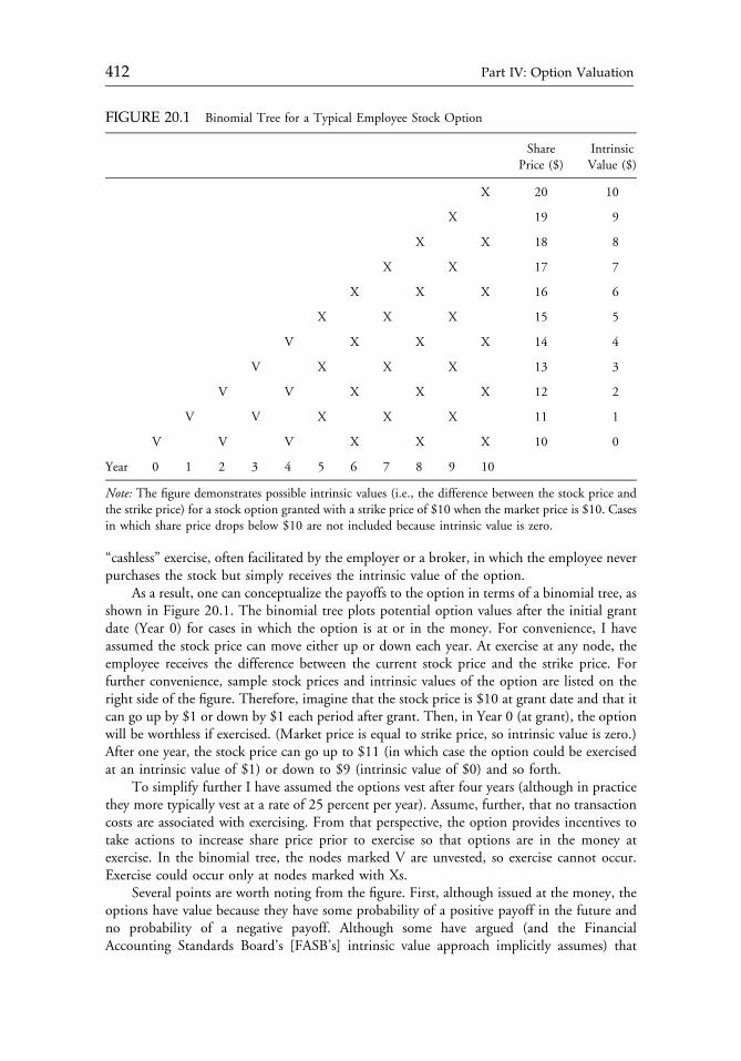
“cashless” exercise, often facilitated by the employer or a broker, in which the employee neverpurchases the stock but simply receives the intrinsic value of the option.
As a result, one can conceptualize the payoffs to the option in terms of a binomial tree, asshown in Figure 20.1. The binomial tree plots potential option values after the initial grantdate (Year 0) for cases in which the option is at or in the money. For convenience, I haveassumed the stock price can move either up or down each year. At exercise at any node, theemployee receives the difference between the current stock price and the strike price. Forfurther convenience, sample stock prices and intrinsic values of the option are listed on theright side of the figure. Therefore, imagine that the stock price is $10 at grant date and that itcan go up by $1 or down by $1 each period after grant. Then, in Year 0 (at grant), the optionwill be worthless if exercised. (Market price is equal to strike price, so intrinsic value is zero.)After one year, the stock price can go up to $11 (in which case the option could be exercisedat an intrinsic value of $1) or down to $9 (intrinsic value of $0) and so forth.
To simplify further I have assumed the options vest after four years (although in practicethey more typically vest at a rate of 25 percent per year). Assume, further, that no transactioncosts are associated with exercising. From that perspective, the option provides incentives totake actions to increase share price prior to exercise so that options are in the money atexercise. In the binomial tree, the nodes marked V are unvested, so exercise cannot occur.Exercise could occur only at nodes marked with Xs.
Several points are worth noting from the figure. First, although issued at the money, theoptions have value because they have some probability of a positive payoff in the future andno probability of a negative payoff. Although some have argued (and the FinancialAccounting Standards Board’s [FASB’s] intrinsic value approach implicitly assumes) that
FIGURE 20.1 Binomial Tree for a Typical Employee Stock Option
Share IntrinsicPrice ($) Value ($)
X 20 10
X 19 9
X X 18 8
X X 17 7
X X X 16 6
X X X 15 5
V X X X 14 4
V X X X 13 3
V V X X X 12 2
V V X X X 11 1
V V V X X X 10 0
Year 0 1 2 3 4 5 6 7 8 9 10
Note: The figure demonstrates possible intrinsic values (i.e., the difference between the stock price andthe strike price) for a stock option granted with a strike price of $10 when the market price is $10. Casesin which share price drops below $10 are not included because intrinsic value is zero.
c20 12 September 2012; 14:17:56
412 Part IV: Option Valuation
at-the-money options do not have value at the grant date because they would not have value ifexercised at that time, they clearly do have value in expectation because they have upsidepotential and no downside potential.
Second, and more importantly, the expected benefit to the employee from holding theoption comes at the expense of existing shareholders. This point bears elaboration becausesome have suggested that options are noncash and, therefore, do not represent a true cost toshareholders under a discounted cash flow approach. For example, if the employee is ableto exercise the option at a strike of $10 when the share price is $15, the employee receives abenefit of $5 at the expense of the shareholders, which is clearest with cashless exercise.Suppose the employee exercises the option and immediately sells the share, pocketing the $5.As a result, the employee ends up with $5 of compensation while the company ends up with$10 of additional paid-in capital and one more share of stock outstanding. If taxes andtransaction costs are set aside, all parties are in exactly the same position that they would behad the company sold the shares on the open market for $15 and paid the employee $5.
At that point, the company can either allow the additional share to remain outstandingor repurchase it on the open market. The effect of options on equity valuation is easiest to see,however, if one assumes that the company chooses to avoid dilution by repurchasing the stockfor $15. The underlying economic outcome would be the same had the employee been paid$5 in salary (even down to the likely tax effect). The company would have paid out a netamount of $5, the employee would have received a net amount of $5, and the number ofshares outstanding would be unchanged.
Whether or not the company opts to repurchase shares, however, the cost of optionsaccrues to the shareholders. If the company repurchases its shares to satisfy option exercise, itavoids dilution but sacrifices cash. If the company chooses not to repurchase and instead issuesmore shares, it retains cash but dilutes ownership. Assuming markets are efficient and the cashused for share repurchases would otherwise be invested in zero-net-present-value projects,existing shareholders are indifferent between the two alternatives. But the problem issimplified (without changing the conclusion) if I assume that the company pays the employeethe difference between the market and strike prices when the employee exercises an option.
Options in Equity Valuation
This example provides the framework for thinking about the consequences of options forequity valuation. First, options create a claim against the existing shareholders. Furthermore,one can consider the magnitude of that obligation in terms of the discounted expected cashflows based on the intrinsic value of the option at exercise.
Second, options create potential benefits to the company’s shareholders. Most directly,option compensation is likely to substitute for other forms of compensation that employeeswould otherwise require. More generally, option compensation changes incentives, whichmay also change the expected cash flows to the company.
Probably the easiest way to consider options when valuing the equity of a company isto take a cash flow perspective and assume that the company repurchases shares to issue toemployees who are exercising options. Then, the cash flow implications of options are mostclear without mixing in the effect of dilution.
Similarly, the easiest way to structure the problem is to divide the company into assets,liabilities, and equity:
Assets ¼ Liabilitiesþ Equity: ð20:1Þ
c20 12 September 2012; 14:17:56
Chapter 20 Employee Stock Options and Equity Valuation 413
Following Soffer (2000) and if one assumes no nonoperating assets, the value of theexisting equity can be expressed as the value of the net operating assets (net of operatingliabilities) less existing interest-bearing (nonoperating) debt.
If the company provides all compensation in the form of salary or bonus and a standarddiscounted cash flow approach is followed, the value of the existing equity of the company canbe expressed as:
Value of common equity ¼ PVðExpected operating free cash flowsÞ� Existing debt,
ð20:2Þ
where PV(Expected operating free cash flows) is the present value of the expected operatingfree cash flows and Existing debt is existing interest-bearing debt, including preferred stock.
The next step is to incorporate options. In thinking about the equity valuation effects ofoptions, it is important to be consistent in considering both the likely costs, such as dilution,and the likely benefits, such as improved incentives. If, for example, the cash flow benefits ofcurrent and future option grants are to be included in estimating future operating cash flows,the associated cost of those options should also be considered. Initially, I will assume thatoption grants remain a fixed proportion of compensation; later, I will relax that assumption.2
Loosely speaking, options could affect Equation 20.2 in at least three ways. First, andmost directly, existing options represent an obligation of the company that is not naturallyreflected in operating free cash flows and must be explicitly incorporated. From the per-spective of the statement of cash flows, for example, options are reflected as a cash outflowfrom financing (to the extent that shares are repurchased to satisfy option grants) and a cashinflow from financing (for the strike price received when options are exercised). But from anequity valuation perspective, the cost of outstanding options should be taken into account.Although this obligation does not satisfy the accounting definition of a liability, it represents apotentially significant claim against the equity of the company that is conceptually verysimilar to a liability. In particular, it represents a claim for which the benefits have, at leastpartially, already been received. Furthermore, if the company were to cease issuing options,the outstanding options would still represent an unavoidable claim against the company.They are contingent obligations because they will need to be satisfied only under certain stockprice scenarios. Like a typical liability, outstanding options can be valued based on the presentvalue of the expected option payouts.
Second, the cost of likely future option grants should be considered. As discussedearlier, the issue here is one of consistency. To the extent that the forecasted cash inflowsincorporate the anticipated benefits of options, the valuation must also include their costs.Although it may initially seem odd to consider option compensation separately from othercompensation, the fact remains that options are different from other forms of compensationbecause they are not reflected typically on the income statement. As a result, net income isoverstated because a major cost of doing business is ignored, but options do conceptuallyrepresent an expense and should be taken into account either in expected operating free cashflows or separately. I will take options into account separately under the assumption that thestarting point for equity valuation is expected free cash flows based on reported net income,thus ignoring options.
Third, considering the effects of options on expected future operating cash flows isimportant. That adjustment may be taken into account more naturally because it will directlyaffect the operating free cash flows of the company. For example, if the company has beenrelatively consistent in granting options, past experience in generating operating cash flows
c20 12 September 2012; 14:17:56
414 Part IV: Option Valuation
may be representative in the future. Similarly, the benefits of options will be reflected in netincome, so earnings forecasts will incorporate the incentive effects of options. If, on the otherhand, the company has recently changed its compensation policy, explicitly taking optionincentives into account may be more important. The potential adjustment takes two forms.First, options substitute for other compensation, so if the company has been increasing optioncompensation over time, its growth in reported profitability will be artificially inflated becauseof the resulting reduction in other forms of compensation that are included as part ofcompensation expense on the income statement. Second, options have incentive effects thatmay influence the future cash flow trajectory and risk.
To summarize, therefore, when a company grants options, the equity valuation equationcan be supplemented by adding terms to reflect both the expected cost of existing and futureoptions and the expected benefits from the options:
Value of common equity ¼ PVðExpected pre-option operating free cash flowsÞ� Existing debt� PVðExpected cost of existing optionsÞ� PVðExpected cost of future optionsÞþ PVðExpected incremental cash inflows from optionsÞ:
ð20:3Þ
EXPECTED COST OF OPTIONS
Conceptually, one way to incorporate existing options when valuing the equity of a companyis to include their implications in the forecasted operating cash flow stream. For example, ineach future period, the pre-option operating cash flows can be estimated and the cost ofsatisfying options exercised can be incorporated as part of the cash flow stream.
In practice, however, valuing the option component separately from the other operatingcash flows is probably easier because option exercise is difficult to forecast and incorporatingoption value separately allows one to use existing option-pricing models. In particular,given information on the inputs to an option-pricing model, one can assign a value to theoutstanding options and, hence, estimate the magnitude of the obligation.
Before proceeding, however, I will review the accounting and disclosure for stockoptions, which underpin both the discussion of equity valuation and the review of theresearch literature.
Accounting for Stock Options
The primary goal of financial accounting is to provide investors with information they can useto value a company’s equity. The challenge for stock option accounting is determining howbest to provide the information that investors need to incorporate options properly intoequity valuation.
From early on, the Financial Accounting Standards Board (FASB) and its predecessor,the Accounting Principles Board (APB), recognized that options were important to assessingcompany value. As the use of options grew in importance as a compensation device, so did theneed to determine the best way to represent options in the financial statements.
Throughout the extensive discussions of option accounting, two facts have seemed clear.First, an option has expected value (and expected cost to existing shareholders) even if the
c20 12 September 2012; 14:17:56
Chapter 20 Employee Stock Options and Equity Valuation 415
option is not currently in the money. If the share price increases, the option pays off; if not,the employee receives nothing. But the employee can never lose, so the expected value ispositive. Analogously, outstanding options represent an obligation of the company.
Second, options are granted as part of compensation. The employee will find theinclusion of options in the employment contract attractive and may be willing to sacrificeother compensation in exchange for options. In fact, employment contracts often specify anestimated value for options as part of total compensation. Clearly, the value of optionsrepresents part of the cost of doing business.
Based on the notion that options represent value given to the employee as compensationfor effort, the FASB has concluded that options should represent part of compensationexpense on a company’s income statement. The more difficult issue, however, is determiningthe best method for measuring the value of that compensation.
Measuring and Recording Option Expense
One of the first questions to address has to do with timing: When should the expense bemeasured and recorded? Conceptually, at least two potential measurement dates exist. Onepossibility is to wait until the option is exercised, typically years after the grant date, andmeasure an expense as the value of the option at the point of exercise. This approach is theone taken for tax purposes on nonqualified stock options (NQOs), which will be discussedlater. Unfortunately, when using this approach as a basis for stock option accounting in thefinancial statements, two problems arise. First, in terms of the income statement, it does notmatch the benefit of options to the cost. The incentive benefits of options are typicallyreceived in periods prior to the exercise period. Second, it does not accurately reflect theeconomics of the transaction. To be analogous with the treatment of other forms ofcompensation, options should be reflected as a charge against income as they are earned sothat two companies granting compensation packages with the same total value are representedon a consistent basis regardless of mix.
The other approach is to measure the value of the option at the date of grant (grant-dateaccounting) based on an estimate of its value. The APB, and more recently the FASB andthe International Accounting Standards Board (IASB), opted for grant-date accountingunder the argument that the fair value of the option is established at the granting date. Theoption value is then expensed over the service period during which the options are earnedthrough vesting, the notion being that options should be recognized as employees gain therights to them.
The major disadvantage of grant-date accounting is that the value of the option must beestimated at the time of grant, which leads to the most difficult problem in optionaccounting—how to value an employee stock option. The primary consideration facing mostproponents of expensing stock options has been the issue of the appropriate option-valuationapproach, and the difficulty of determining the appropriate approach is what, in the past,caused options not to be recognized as an expense. The issue persists even today, with theFASB indicating support for expensing stock options but still discussing the appropriateoption-valuation approach.
In that regard, it is instructive to consider the traditional accounting for options in APBNo. 25, which was completed in 1973 around the time such articles as Black and Scholes(1973) and Merton (1973) were published. The issue facing the APB is clear from thebinomial tree in Figure 20.1. Although the general approach to thinking about option val-uation seems clear (discounting future expected option values), the practical application is
c20 12 September 2012; 14:17:56
416 Part IV: Option Valuation
more difficult. For instance, in Figure 20.1, a very limited number of future stock pricepossibilities exist. In practice, however, with share prices changing constantly and by verysmall amounts, an almost infinite number of possible future stock price outcomes must beconsidered, thus complicating the computation. Similarly, the issue of an appropriate dis-count rate is complex. All these factors make it difficult to comply with the underlying notionof many accounting standards—that resulting amounts must be reasonably and objectivelyestimable to merit inclusion in the financial statements.
At the time of APB No. 25, the APB argued that options had value and should berecognized as an expense but concluded that the option-valuation approaches were not suf-ficiently developed to justify applying an option-pricing model. It settled on an approachbased on intrinsic value in which options with fixed terms were valued at the grant date basedon the difference between market and strike prices (intrinsic value), at least until there was amore generally accepted approach for option valuation. As a result, options issued at themoney required no expense recognition, primarily in response to the lack of an acceptableoption-valuation approach.
Arguments against Expensing Options
With the general acceptance of the Black�Scholes model and other option-pricing models forpublicly traded options and the increasing use of options in practice, the issue of optionmeasurement became more pressing. Many commentators noted the inconsistency inaccounting between stock options and other forms of compensation. In fact, even with stockoptions, grants to nonemployees (such as for goods or services) were required to be recognizedas an expense based on option-pricing models, with only option grants to employees accordedspecial treatment. Companies issuing substantial nonoption compensation argued that theywere unfairly disadvantaged by the special treatment accorded options. As a result, the FASBagreed to reconsider the option issue.
Although many arguments were raised against the expensing of options, the mostcompelling were (1) that there were economic consequences to option expensing and (2) thatthe value of options could not be accurately estimated.3
Regarding the economic consequences, some critics asserted that even if the currentaccounting were incorrect, the cost of changing it (in terms of harming the competitivenessand capital-raising ability of high-technology companies) would be too high. But the FASBhas indicated on a variety of issues (such as expensing research and development andaccounting for post-retirement benefits) that economic consequences are not a major con-sideration in its deliberations and that accounting is intended to be neutral (that is, accountingshould report on economic reality without affecting it). The FASB views the currentaccounting for options as nonneutral because companies appear to change the structure ofoption contracts (such as issuing options at the money) to avoid expense recognition.
Option-Valuation Concerns
The concerns over option valuation are more substantive. As many commentators have noted,existing option-pricing models are based on assumptions that are generally not designed foremployee stock options. Furthermore, although option-pricing models work well for publiclytraded options, they may not be as effective for employee stock options.
Under pressure from a variety of sources, the FASB opted in SFAS No. 123, Accountingfor Stock-Based Compensation, to encourage companies to expense the fair value of options butoffered the alternative of disclosure.4 More importantly from an equity valuation perspective,
c20 12 September 2012; 14:17:57
Chapter 20 Employee Stock Options and Equity Valuation 417
the FASB established a set of required disclosures to inform valuation so that even if thecompany chose not to expense options, sufficient detail was available for investors to estimatethe value of existing options and likely future options. The resulting disclosures include thefair value of the options earned by employees during the period as well as information aboutthe characteristics of options currently outstanding.
To understand the disclosures, it is useful to explicitly consider the inputs into a modelsuch as the Black�Scholes option-pricing model because the disclosures are designed to helpinvestors who are using such a model to arrive at their own estimates.
The basic Black�Scholes model for a non-dividend-paying stock expresses option valueas follows:
C ¼ SN ðD1Þ � Ke�rtN ðD2Þ, ð20:4Þ
where
C 5 the value of the option
S 5 the current market price of the stock
K 5 the strike price to be paid when the option is exercised
t 5 the time remaining before the option expires
N(�)5 the cumulative standard normal density function
r 5 the risk-free interest rate
σ 5 the standard deviation of the return on the stock
D1 � logðS=K Þ þ ðr þ σ2=2Þtσffiffit
p ð20:5Þ
D2 � logðS=K Þ þ ðr � σ2=2Þtσffiffit
p : ð20:6Þ
The first term of the equation can be thought of as the present value of receiving thestock at exercise conditional on the option being in the money. The second term capturesthe present value of having to pay the exercise price conditional on the option being in themoney. The difference is the value of the option.
If the company is expected to pay dividends, the Black�Scholes model can be supple-mented with an adjustment for dividends. In particular, because options are not typicallydividend protected and because dividends substitute for capital gains, the value of an optionon a stock that pays dividends is reduced relative to the value of an option on the same stock ifit paid no dividends. The adjustment basically represents the present value of the dividendsthat would be sacrificed by holding the option rather than the underlying stock. If oneassumes that the stock pays dividends continuously at a constant dividend yield and thatoptions are held to maturity, the option-pricing model can be adjusted by substitutingSDividend for S in the Black�Scholes model, where
SDividend ¼ Se�δt ,
c20 12 September 2012; 14:17:57
418 Part IV: Option Valuation
and where δ is the annual dividend yield as a percentage of the current market price ofthe stock.5
The Black�Scholes model is well suited for estimating the value of the option obligationbecause it provides an estimate of the present value of the future payoffs to the option. As aconsequence, it does not require that the potential values of the options be forecasted thendiscounted back but instead permits the value to be inferred from inputs—such as the currentmarket price, option strike price, risk-free interest rate, expected share price volatility, divi-dend payout, and expected time to exercise—to calculate the value of an option.
Dell Example
To understand how such an approach might be implemented in practice, I will apply it toDell Computer Corporation. The Appendix presents financial statements and selected dis-closure from Dell’s fiscal 2002 annual report, including the option footnote.
Footnote Disclosure
Note that the option footnote presents five basic sets of information. First, it providesinformation on the terms of the options. For example, it notes that there are two optionplans—one for executives and one for nonexecutive employees (the broad-based plan). Interms of the tax treatment of the options, the broad-based plan is limited to nonqualifiedoptions; the executive plan includes both nonqualified options and incentive stock options.Dell’s options typically have a 10-year maturity and vest over 5 years. That information willbe useful in estimating the value of the options.
Second, it provides information on the option granting, exercise, and cancellationbehavior in previous years. For example, it shows that 344 million options were outstandingat the beginning of 2002, 126 million more were granted, 63 million were exercised, and57 million were canceled, leaving 350 million outstanding at year-end.6 Given 2,602 milliontotal shares outstanding at year-end, optioned shares represent 13.5 percent of shares out-standing. In addition, it shows the average exercise prices of each group of options. Forexample, it shows that the options granted during 2002 were at an average strike of $23.24and those that were exercised were at a strike of $3.11, indicating that the share priceincreased about 647 percent on average since those options were granted. In addition, optionscanceled had an exercise price of $32.86, indicating that most were out of the moneywhen the employee left the company. Such information is useful in forecasting option activitygoing forward.
Third, the disclosure provides a summary of the terms of the options that were stilloutstanding at the time of the statement. In particular, the outstanding options are catego-rized by exercise price range, and Dell also discloses weighted-average exercise price andremaining contractual life. Options are divided into those that are exercisable and those thatare not (typically because they have not vested). That information provides useful inputs intothe option-valuation model.
Fourth, the footnote presents information on fair value estimates and the assumptionsunderlying those estimates. In particular, the footnote indicates that Dell estimates that theaverage fair value of an option granted in fiscal 2002 was $13.04, down from $20.98 and$22.64 in 2001 and 2000, respectively, primarily because of lower share prices. Furthermore,the footnote provides estimates of the reduction in income had options been expensed, onboth a pretax and after-tax basis, as well as on a per-share basis. In 2002, expensing options
c20 12 September 2012; 14:17:57
Chapter 20 Employee Stock Options and Equity Valuation 419
would have reduced pretax income by $964 million, $694 million after tax. Given a reportedpretax income of $1,731 million, expensing options would have represented a reduction of56 percent. In terms of an equity valuation framework, this information is useful in thinkingabout current option intensity (and profitability) as a means of assessing the likely cost ofoptions in the future. In that sense, options are like other forms of compensation on theincome statement, and the footnotes provide information on current profitability after takingoptions into account as a means for estimating future profitability.
Finally, regarding the assumptions underlying the fair value estimates, the footnote showsthat expected life on new option grants is 5 years (relative to a contractual life of 10 years), therisk-free rate is 4.63 percent, the share price volatility is 61.18 percent, and no dividendsare anticipated.
Value of Outstanding Options
With the information provided by Dell, estimates of the inputs listed below can be developed,which can then be used to estimate the value of outstanding options using Equation 20.4:
S 5 the current market price of the stockK 5 the strike price to be paid when the option is exercisedt 5 the time remaining before the option expiresr 5 the risk-free rate of returnσ5 the standard deviation of the return on the stockδ5 the annual dividend yield
The footnote discloses, as mentioned previously, the following option assumptions as ofyear-end 2002:
� Risk-free rate (r in the Black�Scholes model) is 4.63 percent.� Standard deviation of returns (σ in the model) is 61.18 percent.� Expected dividend yield (δ in the model) is zero.
The footnote also discloses information on the terms of various subsets of options. Forexample, the set of 30 million options outstanding has an average remaining contractuallife of 3.49 years and a strike price (K in the Black�Scholes model) of $0.96. The strike pricecan be compared with Dell’s share price at fiscal year-end 2002 (S in the Black�Scholesmodel) of $26.80.
The only missing input for calculating the option value as of year-end 2002 is theexpected remaining life; yet even for expected remaining life, some information is available.First, Dell’s disclosure shows that the expected term at time of grant for the typical option isfive years. Second, it shows that the options in this group are, on average, already more thanfive years from grant and have a remaining contractual life of only 3.49 years. As a result, theremaining life for this particular group of options cannot exceed 3.49 years. AlthoughI discuss approaches for developing more sophisticated estimates of option exercise later inthis chapter, at this point I will assume that exercise takes place at half of the remaining life(in 1.745 years for this group of options).
Using this available information and applying the Black�Scholes pricing model, thevalue of each option is about $25.91. The option value is very close to the intrinsic value ofthe options (market price of $26.80 2 strike price of $0.96 5 $25.84) because the options
c20 12 September 2012; 14:17:57
420 Part IV: Option Valuation
are deep in the money and close to the end of their lives and, hence, are very likely to beexercised. Multiplied by 30 million, that group of options is worth about $777 million.
Analogous calculations can be made for the other option subsets as well, and by con-tinuing, for convenience, to assume that options are exercised halfway through theirremaining lives, the total value of outstanding options is found to be $5,257 million. Because,as discussed in more detail later, option exercise typically creates tax deductions, the impli-cations for cash flows are not as extreme as the magnitude of that liability would imply. Butassuming a tax rate of 28 percent, the after-tax liability is about $3,785 million.
At year-end 2002, Dell had total liabilities of $8,841 million; therefore, options wouldincrease the liabilities by 43 percent. Given a market capitalization of $69,734 million as ofyear-end 2002, the after-tax value of outstanding options is 5.4 percent of the market valueof Dell’s outstanding equity. If treated as a liability, the option obligation would representone of the largest claims against the company.
Future Option Grants
If one assumes that the operating cash flow estimates do not explicitly incorporate theeffects of options, future option grants need to be taken into account. Based on the footnotedisclosure, stock options could have a substantial impact on Dell’s reported profitability. Inparticular, the pro forma disclosure indicates that diluted earnings per share in 2002 wouldhave been reduced by $0.27 per share—from $0.46 to $0.19. In other words, based on thevaluation approach used by Dell, options constituted a substantial cost of doing business.Coupled with the valuation approach just demonstrated, one could use this information(and information on the prior years’ options) to assess the quantity of options necessary tosupport past accounting profitability and get a sense of the intensity of options likely neededfor the future.
Dell’s statements show that pro forma option expense totaled $964 million in 2002, butthat figure includes a mixture of effects. First, it includes a portion of the options granted ineach of the last five years (because Dell has a five-year vesting plan and option expense isspread out over the vesting period). As a result, the $964 million reflects options granted as farback as 1997, which also explains part of the reason that pro forma option expense increasedsubstantially over recent years. In SFAS No. 123, the FASB established a transition in whichthe footnote expense was based only on grants going forward, so the first year includedonly that year’s option grants. As time passed, additional layers of option grants were addeduntil the calculation reached steady state at the end of the vesting period for options granted inthe first year of the standard (five years in Dell’s case). As a result, the trend in historical data onpro forma option expense is not necessarily representative going forward. Second, under SFASNo. 123, option values are adjusted for estimated forfeitures. The company estimates the valueper option and the likely forfeitures during the vesting period. The remaining amount isamortized over the vesting period, with an adjustment each period for the amounts by whichthe forfeiture rate differs from expectations. As a result, the $964 million is affected by theoption grants over the previous five years and the experience with forfeitures.
In 2002, the total value of Dell’s options could be computed as $1,643 million (126million options granted 3 an option value per share of $13.04). In 2001, the total was$3,231 million ($20.98 3 154 million), and in 2001, it was $1,132 million ($22.64 350 million). The volatility of option grants makes them difficult to forecast in this context,and knowledge of the company’s plans with respect to options is important for forecastingoptions. But as a starting point, the value of options granted from 2000 to 2002 averaged
c20 12 September 2012; 14:17:57
Chapter 20 Employee Stock Options and Equity Valuation 421
$2,002 million. During those same three years, cancellations on Dell’s options averaged33 percent. Although that average probably overstates the effect of cancellations because itincludes out-of-the-money options that were canceled but would otherwise have expired outof the money, it provides at least a benchmark for thinking about options going forward.Assuming that 33 percent of the options are ultimately canceled and applying Dell’s statedeffective tax rate of 28 percent, one can see that the pretax option amount is $1,341 millionand the after-tax amount is $966 million.
The notion that Dell incurred about $966 million of after-tax option costs in 2002provides at least a starting point for thinking about future option costs. If option intensitywere to remain relatively constant, the cost of option-based compensation might be expectedto grow at approximately the growth rate of sales. Starting with a baseline expense of $966million and assuming a growth rate of, say, 3 percent in perpetuity and an 8 percent discountrate, the estimated obligation created by future option grants would total about $19,315million. Coupled with the estimated obligations for existing options discussed earlier, thetotal obligation for current and future options would total $23,100 million. Comparing thatamount with Dell’s year-end market capitalization of $69,734 million, the cost of options isclearly substantial.
Of course, the preceding is based on fairly ad hoc assumptions and, in practice, would needto be adjusted for expectations about future events, especially with regard to future optiongrants. For example, many companies, including Dell, have announced intentions to reduceoption intensity going forward. But even if that is the case, companies such as Dell will likelyhave to substitute other types of compensation for the portion of compensation currently inoptions. As a result, the effects of an overestimate of option compensation will be mitigatedpotentially by an underestimation of other compensation. In the extreme, if other compen-sation replaces option compensation dollar for dollar, an inaccurate estimate of options goingforward does not necessarily create an inaccurate estimate of value. As discussed later, however,the trade-off need not be dollar for dollar because of such factors as risk aversion.
Tax Issues
From an equity valuation perspective, incorporating the tax effects of employee options can bequite important because the tax deduction can significantly reduce the cost of options. Whenexamining the tax issues, one must consider the two major classes of stock options—incentivestock options (ISOs) and nonqualified stock options (NQOs)—although ISOs have declinedin importance.
Incentive stock options are restricted because they must meet certain IRS criteria,including requirements that the underlying stock not be sold for two years after the option isgranted and for one year after the option is exercised. ISOs provide no tax deduction to theissuing company and no taxable income to the employee at exercise. But when the underlyingstock is sold, the employee must pay tax on the difference between the selling price and thepurchase price (the option strike price), usually at the capital gains rate.
Nonqualified stock options do not carry the same restrictions and require the employeeto pay taxes at the ordinary income tax rate on the difference between the market price andstrike price when the options are exercised. In addition, the company receives a tax deductionin the same amount at that time. Prior to the Tax Reform Act of 1996, many options wereISOs because the ordinary income tax rate for individuals was quite high relative to the capitalgains rate and the corporate tax rate. But the Tax Reform Act of 1996 reduced the attrac-tiveness of ISOs from a tax perspective.
c20 12 September 2012; 14:17:57
422 Part IV: Option Valuation
Although some companies still have some ISOs, the majority of outstanding options arenow NQOs. Furthermore, those companies that continue to hold ISOs do not typicallyseparate them from NQOs. For example, Dell notes that its broad-based option plan containsonly NQOs. The executive plan, in contrast, contains a combination of ISOs and NQOs, butthe split is not stated. In addition, Dell’s proxy statement indicates that the options granted toexecutives represent only about 10 percent of options granted to all employees, so I willassume that all options are NQOs.
The tax implications of stock options are not conceptually different from those of otherforms of compensation because such other forms also typically provide a tax deduction whenthe value is received by the employee. But two important factors set NQOs apart. First, thetax treatment of NQOs is based on exercise-date accounting, whereas the financial accountingtreatment is based on grant-date accounting. As a result, at the time options are granted toemployees, their value is represented as an expense or (more commonly) in the footnotes atthe modified Black�Scholes value of the option based on expected payoff. For tax purposes,however, the deduction is based on the intrinsic value at the time of exercise. Therefore, evenif options are expensed for financial accounting purposes, the tax and accounting treatmentscan differ drastically in terms of timing and amount. Second, the amounts of optiondeductions can be extremely large for a company if it has experienced a substantial stock pricerun-up. Not only will the deduction per share exercised be large, but option exercise will alsobe more prevalent.
For a comfortably profitable company with a relatively modest stock option plan,treating the tax effects of stock options is fairly straightforward. Because the stock option isvalued based on the expected intrinsic value at exercise, which also represents the expected taxdeduction, the after-tax option value can be approximated by subtracting the likely tax benefitresulting from the option exercise (expected corporate tax rate times the expected intrinsicvalue) from the pretax value. This is the approach used earlier to determine the basic equityvaluation for Dell.
The situation becomes more complex if the company is likely to experience a tax lossduring the period when the option is exercised. Although such a tax loss should be a concernfor any tax deduction, it is particularly pronounced for stock options because of the possibilitythat an otherwise profitable company can realize so much in stock option deductions that itreports a tax loss.
The effect of options on taxes can be substantial even for large companies. Sullivan(2002), for example, estimated that the tax deductions for options exceeded net income for8 of the 40 largest U.S. companies in 2000—Microsoft Corporation, America Online, CiscoSystems, Amgen, Dell, Sun Microsystems, Qualcomm, and Lucent Technologies. Graham,Lang, and Shackelford (forthcoming 2004) estimated that option deductions totaled10 percent of pretax income for S&P 100 Index companies during 2000. Even morestriking, aggregate option deductions exceeded aggregate pretax income for the NASDAQ100 Index companies in 2000 (although some did pay taxes because the deductions did notexceed pretax income for some individual companies). Therefore, one cannot assume thatoption-intensive companies that are profitable on an accounting basis also have positivetaxable income.
Option Tax Effects on Cash Flows
Current accounting and disclosure create a challenge for understanding the past effect ofoptions on taxes because if the underlying options are not treated as an expense for financial
c20 12 September 2012; 14:17:58
Chapter 20 Employee Stock Options and Equity Valuation 423
accounting purposes, then they also do not reduce income tax expense. The reason for theparallel treatment is fairly clear. If options reduced income tax expense but not pretax income,the net effect of issuing options would be to increase income (reduce tax expense but notpretax income). In addition, effective tax rates would appear to be unreasonably low becausetax expense would be reduced by the effects of options but pretax income would not bereduced.
Instead, stock option tax benefits do not directly affect tax expense on the incomestatement, either when the options are granted or when they are exercised. Furthermore,because they never affect tax expense, deferred tax is not typically created. As a result, the tax/book difference for options never reverses, so a company could have significant tax expense onthe income statement without ever paying taxes. Further still, the changes in the deferred taxaccounts are not informative about the tax effects of options because deferred-tax accountingis generally not required.
A similar issue exists with respect to pretax income. Because options are not deducted asan expense when issued, they never directly affect pretax income. Finally, because the taxbenefits from options flow through the operating section of the statement of cash flows, acompany can report high profits and even higher operating cash flows.
In some cases, it is possible to get a sense of the likely size of the tax effect of options fromthe statement of cash flows or the statement of shareholders’ equity. In particular, whenoptions are exercised, the typical accounting for the tax effect is as follows:
Taxes payable
Additional paid-in capital
In theory, one should be able to infer the amount of the tax benefit from the statement ofshareholders’ equity. But many companies combine different effects of options on the sameline. For example, by reading Dell’s financial statement, investors would know that Dell had“Stock issuances under employee plans, including tax benefits” of $853 million in 2002, butinvestors would not know how much the option exercise itself was (which would also haveaffected additional paid-in capital) nor how much the tax benefit was.
Similarly, the statement of cash flows disclosure is inconsistent, and the effects of optionsare often not separated, especially for smaller magnitudes. For example, Hanlon and Shevlin(2002) found that only 63 of the NASDAQ 100 companies separate out the tax benefits ofstock options, even though they are likely to be especially option intensive. Furthermore,interpreting information on option tax benefits is complex in cases of net operating losscarryforwards and tax valuation allowances. As a result, Hanlon and Shevlin advocated usingthe tax footnote information to estimate the tax effect of options.
It is clear from Dell’s stock option footnote that the effect of options on taxes can besignificant. For example, one can estimate the size of the option tax deduction by taking intoaccount the number of shares exercised in each year and then estimating the degree to whichthe underlying options are in the money. The footnote provides information on the weighted-average strike price but not on the market price. An estimate of the market price at exercise,however, can be based on the weighted-average strike price on options granted during the yearif the company typically issues at the money, or it can be based on the actual stock price pathduring the year.
Using the information from the footnote, Dell’s option deductions for 2002 can beestimated as $1,268 million [63 million shares 3 ($23.24 2 $3.11)], which compares withpretax income on the income statement of $1,731 million. Dell, therefore, appeared
c20 12 September 2012; 14:17:58
424 Part IV: Option Valuation
substantially more profitable for financial accounting purposes than it did on its tax return.Similar calculations estimate that Dell had $3,279 million of deductions relative to $3,194million of pretax income in 2001 and $3,109 million of deductions relative to $2,451 millionof pretax income in 2000. Therefore, despite substantial pretax accounting income in 2000and 2001, Dell received tax refunds.
Consistent with that result, Dell’s supplementary statement of cash flow disclosureindicates that not only did Dell not pay income taxes in 2000 and 2001; it actually receivedcash back (refunds of prior taxes paid) of $32 million in 2001 and $363 million in 2000.Assuming a tax rate of 28 percent, Dell had a tax benefit from options of about $355 million,$918 million, and $871 million for 2002, 2001, and 2000, respectively. These amounts canbe compared with the amounts of tax benefits from option exercise reported on the statementof cash flows of $487 million, $929 million, and $1,040 million. The difference reflects, atleast in part, the timing lag between the month when options are exercised and the monthwhen taxes are paid, as well as assumptions on tax rates and stock prices.
The statement of cash flow effect of options is particularly important to note because it isincluded in the operating section. For example, in 2000, Dell’s operating cash flow was$3,926 million, substantially exceeding its net income of $1,666 million. The difference islargely the result of the $1,040 million in tax benefits from options, which are not comparableto normal cash from operations.
Note also that the deduction for tax purposes differs markedly from the pro formaexpense in the footnotes. Even if options had been expensed on the income statement in2001, for example, the tax deduction of $3,279 million estimated earlier would have been fargreater than the financial statement expense of $620 million noted in the footnotes. Thereason, of course, is that the income statement expense represents the ex ante value of optionsearned by employees in the current year and the tax return represents the ex post value of theoptions exercised in the current year. The $620 million represents an expectation of whatthe grants earned during the year will be worth ultimately (discounted back to the present).The $3,279 million is the amount that options granted in the past were ultimately worthwhen exercised. Although fewer options were exercised in 2001 (95 million) than weregranted in 2001 (154 million), the fact that the options exercised in 2001 were worth sub-stantially more than those included in the expense in 2001 reflects the average share priceappreciation (from $3.26 to $37.78) from the time when the options were granted to whenthey were exercised.
To get a sense of the difference between ex ante and ex post value, one can use Dell’sinformation on its 2001 option grants, which had an average strike price of $37.78, with anaverage fair value of $20.98, or 56 percent of the strike. Applying the same proportion to theoptions exercised in 2001 (and assuming other inputs to the option-valuation formularemained approximately constant), the per-share fair value of the options exercised in 2001was $1.81 per option ($3.26 3 0.56) or $172 million total ($1.81 3 95 million) whenthey were granted. In other words, the pro forma expense when the options were issued wouldhave been about $172 million, with the options ultimately providing deductions of$3,279 million. By the same token, the $172 million of options could easily have expiredworthless had the stock price not risen.
This illustration also clarifies the difficulty of matching financial accounting for optionsto tax accounting for options. The $172 million represents the present value of an estimate ofthe value of the options when granted; the $3,279 million represents the realized value.Had Dell been required to expense options from a financial statement perspective, it wouldhave appeared to have been quite profitable, but from a tax perspective, its profitability was
c20 12 September 2012; 14:17:58
Chapter 20 Employee Stock Options and Equity Valuation 425
substantially lower. This tax/book difference never reverses because financial accountingrecords an estimate of the value of the option at grant (grant-date accounting) and does notadjust it to the ultimate value at exercise on which the option deduction is based (exercise-dateaccounting). As a consequence, a company can look consistently profitable for financialaccounting purposes while paying little or no tax.
Note also that the amount of the option deduction can vary dramatically over time.For example, the estimated option deduction increased from $3,109 million in 2000 to$3,279 million in 2001 and then dropped to $1,268 million in 2002. Similarly, the cash floweffects are volatile—from $871 million in 2000, based on my estimates, to $918 million in2001 and $355 million in 2002.
Furthermore, although Dell faced a large number of in-the-money options in 2000(363 million options at the beginning of the year, with an average strike of $5.40 and anaverage stock price of $42.86 during the year), by the end of 2002 the options outstandingwere, on average, close to the money (350 million options with an average strike of $26.36and share prices averaging $23.24 during 2002). As a result, the massive cash benefits fromstock options are unlikely to recur unless Dell’s stock price increases substantially.
From an equity valuation perspective, the important point is forecasting the tax impli-cations of options for future cash flows. As is clear from the Dell example, option deductioncash flows are unlikely to remain constant over time because they are very sensitive to shareprice movements. But the option-pricing model offers an effective method for computing thepresent value of the option deductions. Assuming a constant tax rate (28 percent in Dell’scase), one can simply apply that rate to the fair value of the options to compute the presentvalue of the expected tax shield. That factor was implicit earlier when I assumed that the after-tax option obligation was 72 percent of the gross amount.
Unfortunately, the assumption that option deductions can be fully utilized as realizedmay not be valid for many companies. As the preceding example illustrates, even a companyas profitable as Dell can face situations in which option deductions can exceed pretax income.Under some circumstances, many companies will face no significant tax burden because of taxlosses. In fact, the presence of large stock option deductions creates the possibility thatcompanies that appear profitable from an accounting perspective may actually report taxlosses once deductions are included.
Because of the carryforward and carryback features of the tax code, four potentialscenarios can be projected. Scenarios 1 and 2 present extreme situations in which fewcompanies are likely to fit. Scenarios 3 and 4 are more probable.
1. The company is always profitable from a tax perspective (in all states of the world andover all time periods from 3 years prior to the current year to 20 years subsequent to thecurrent year) and able to use the tax deductions in the year of exercise. In that case (andassuming a constant tax rate), the deductions can be valued at the tax rate multiplied bythe value of the options, and the after-tax option obligation can be measured at 1 minusthe tax rate times the pretax option obligation. This scenario, however, describes only themost stable and profitable companies.
2. The company is always unprofitable from a tax perspective; hence, the tax deductions willexpire unused. In this scenario, the deductions are worthless and the after-tax value of theoption obligation is the same as the pretax value. This scenario is also unlikely to describemany companies because companies that are going concerns have a significant probabilityof at least some profitability.
c20 12 September 2012; 14:17:58
426 Part IV: Option Valuation
3. The company is expected to have tax profits in the year the options are exercised (at leastin some situations) but is expected to be unprofitable in some other years.
4. The company is expected to have tax losses in the year the options are exercised (at least insome situations) but is expected to be profitable in some other years.
In the last two scenarios, the present value of the tax benefit will depend on theproportion of situations in which the company is expected to be tax profitable in the yearthe options are exercised as well as its profitability in years around that year. Even anunusually profitable company such as Dell can have years when option deductions wipe outall taxable income so that some deductions cannot be used in the current year. But if thecompany was profitable in past years, it can carry the loss from the excess option deductionsback to get refunds for prior taxes paid. As a result, it still generates a full tax benefit.
Similarly, if the company is expected to be profitable in the year of exercise but likely tobe unprofitable in the future, the deductions will initially generate tax benefits. But those taxbenefits will disappear when the company becomes unprofitable because the taxes savedwould have been refunded anyway.
Findings of Graham, Lang, and Shackelford
Graham, Lang, and Shackelford developed an approach for forecasting the relevant marginaltax rate in the face of stock options. Their question is slightly different from mine becausethey attempted to assess the effect of options on the tax benefits of debt. They consideredrealized option deductions in 2000 and attempted to assess the marginal tax rate faced by acompany considering the simulations of future pretax income and option exercise based onpast experience. They focused on the S&P 100 and NASDAQ 100 companies and usedinformation from the option footnote to forecast likely carryforward and carryback impli-cations of options. They used a simulation in which the past distribution of share prices andpretax, pre-option earnings was used to forecast potential tax positions and probabilities ineach year going forward. Given that information, probability-weighted expectations can beformed that explicitly take into account (1) the likelihood that the option deductions willbe exploited and (2) the amounts of likely deductions.
They made several important observations. First, even for the S&P 100 sample, optiondeductions totaled $63 billion on pre-option, pretax income of $349 billion. As a conse-quence, the companies faced a substantially lower tax burden than implied by income taxexpense on the income statement. But taking into account the option deductions, the averageS&P 100 company still faced a marginal tax rate of 35 percent, indicating that although thedeductions were large, the average S&P 100 company could fully use its option deductions.Even if deductions were expected to exceed pretax income under certain circumstances(as with Dell), S&P 100 companies typically can use tax loss carrybacks to obtain refunds ofprevious taxes paid or carryforwards to offset future taxes.
The NASDAQ 100 companies, in contrast, had option deductions of $35 billion on pre-option, pretax income of $13 billion. In other words, although the NASDAQ 100 appearedprofitable in aggregate when one ignores options, that perspective changes when options arefactored in. But because some companies were profitable even after taking options intoaccount and others had large losses, some NASDAQ 100 companies still paid taxes.
More to the point, when options are ignored, the average NASDAQ 100 company hadan estimated marginal tax rate of 31 percent, suggesting that most companies were facingrelatively high tax rates. But when options are factored in, the marginal tax rate drops to
c20 12 September 2012; 14:17:58
Chapter 20 Employee Stock Options and Equity Valuation 427
5 percent, with almost 60 percent of the NASDAQ 100 companies facing estimated marginaltax rates of less than 10 percent.
One way to interpret that result is that most companies were able to use at least part oftheir 2000 option deductions (because they were tax profitable before taking into account theoption deduction), but many were not expected to be able to use all of their optiondeductions (because they were expected to be unprofitable for some time in the future aftertaking into account their option deductions). In some cases, the reduction in marginal ratesreflects the fact that the company would not be able to take advantage of the deductions formany periods in the future (because it was not expected to be profitable for some time) andwould, therefore, sacrifice the time value of money. In extreme cases, however, companies hadnot been profitable in the past and were not expected to be profitable in the foreseeable future;therefore, although options generated large tax deductions, those deductions were expected toexpire unused.
An implication of this result is that, although options may provide substantial taxdeductions to offset a portion of their cost, one cannot assume that the full amount of thetax deduction can be exploited. In cases of stable, profitable companies, the after-tax cost ofoptions can be approximated by multiplying the pretax cost by 1 minus the company’s tax rate.But in cases of less stable, less profitable companies, the option deductions may expire unusedor may not be used for several periods in the future, sacrificing the time value of money.
Graham, Lang, and Shackelford also examined whether companies behave as though theyrecognize the effect of the likely option deduction in making financing decisions. In partic-ular, they examined why some companies issue relatively little debt despite high accountingprofits (given that it appears that debt would reduce expected tax burdens) and hypothesizethat many such companies do not anticipate paying much in taxes. Therefore, if one views thedecision on debt policy after all of the company’s other decisions have been made, a companythat looks profitable from an accounting perspective may actually view itself as unlikely to paytaxes and may, therefore, view debt as unattractive. Consistent with that result, Graham,Lang, and Shackelford documented relatively little relationship between debt levels andmarginal tax rates when the effects of options were ignored. But when options are factored in,a significant relationship exists between debt and tax rates, thereby reinforcing the importanceof considering options when examining companies’ financial decision making.
Although options represent a significant cost of doing business, the cost is mitigated bythe tax benefits options provide. Furthermore, a thorough understanding of option taxes iscritical when interpreting current cash flows and predicting future cash flows.
PATTERNS OF OPTION EXERCISE
Every option-valuation approach makes assumptions about the behavior employees willfollow when exercising their options. Consider the binomial tree in Figure 20.1. In a largenumber of cases, the option is in the money and exercisable, and it is up to the employee todecide when to exercise. But to make the valuing of options manageable, some assumptionsmust be made about the circumstances under which exercise occurs.
Assumptions about Exercise
One of the major insights underpinning the traditional Black�Scholes model for tradedoptions is that one can infer optimal exercise. In particular, for options that are tradable on
c20 12 September 2012; 14:17:58
428 Part IV: Option Valuation
non-dividend-paying stocks, early exercise is generally not optimal.7 As a result, for mosttraded options, exercise can be assumed to occur whenever the option is in the money at theend of its life, and no earlier. Therefore, option valuations can be developed based onforecasting stock price paths through to option expiration, attaching probabilities, and dis-counting back to the present. In terms of Figure 20.1, that assumption would imply exercisein all cases in the 10th year (conditional on the option being in the money).
In part, the optimality of exercise only at maturity reflects the fact that, besidesbeing exercised, publicly traded options can be sold or hedged, so an individual’s riskprofile and liquidity needs do not enter into the calculation. Conversely, employee stockoptions generally cannot be sold, and employees are limited in their ability to lay off risk bytaking, for example, a short position to offset the long position in the option. Although anemployee might like to sell an option, selling it would defeat the incentive intentions ingranting the option because the new buyer would typically not have the same ability to affectcompany value.
As a consequence, factors such as an employee’s level of risk tolerance and liquidity needsaffect exercise decisions and thus increase the complexity of forecasting option exercise. Forexample, an employee requiring cash for a major purchase or wishing to reduce exposure tothe company’s stock may have little choice but to exercise options even if the remainingcontractual life is substantial. In order to accurately estimate option value, therefore, fore-casting the likely employee option exercise behavior is necessary.
Timing of Exercise
Unfortunately, employees are unlikely to exercise their options at the same time or based onthe same factors. Exercise is likely to be triggered by employee-specific events. For example,employees may exercise early because of risk aversion or liquidity concerns, and risk aversionand liquidity needs will vary from employee to employee. Furthermore, employee stockoption exercise may be involuntary (or only partially voluntary), such as when the employeeseparates from the company, because options are typically canceled if not exercised within aspecified time from separation.
As a result, rather than identifying a subset of nodes at which exercise is definitely optimal,envisioning nodes with various probabilities of exercise is probably more accurate. One can, forexample, imagine the probability of exercise changing based on factors such as the remaininglife of the option, the market price/strike price ratio, or recent share price volatility.
Exercise patterns not only affect option valuation; they can also have an impact on acompany’s cash flow needs. For example, a company that chooses to repurchase shares tosatisfy option exercise (hence avoiding dilution) will have substantially greater cash flow needsin periods when many deep-in-the-money options are exercised. Similarly, companies thatissue new shares for option exercises will have significant cash inflows as the strike price isreceived from employees. In Dell’s case, for example, the 63 million options exercised in 2002generated about $196 million in cash from the strike price ($3.113 63 million). As discussedearlier, option exercise would also have generated about $355 million in tax savings in 2002.But had Dell opted to repurchase those shares to avoid dilution, it would have had to payabout $1,464 million ($23.24 3 63 million), assuming that the options were repurchased atthe same price as the new options granted during the year. As a result, repurchasing shares foroption exercises would have cost Dell $913 million, net of strike price and option tax benefitsreceived. An analogous calculation for 2001 indicates a cost of $2,361 million to repurchaseshares to satisfy option exercise, net of strike price and option tax benefits received. Even for
c20 12 September 2012; 14:17:58
Chapter 20 Employee Stock Options and Equity Valuation 429
a profitable company such as Dell, repurchasing shares to satisfy option exercise entails asubstantial cash outflow.
One thing that seems clear is that early exercise is an important phenomenon and onethat must be considered. Casual observation and academic research point to the pervasivenessof early exercise. Exercise typically occurs as early as halfway through the option’s life, as inDell’s case when exercise is assumed to occur, on average, 5 years into the option’s 10-yearlife. Furthermore, the cost to the company of a 10-year option is substantially higher than thecost of a 5-year option. In the case of Dell, for example, assuming that options are held tomaturity would result in an option value of $17.15 versus $13.04 computed based on anassumed life of five years.
As a consequence, the FASB has realized that any option-valuation approach shouldpermit use of an assumed life much shorter than the contractual life. The current guidance inSFAS No. 123 requires that option value be estimated over expected life rather thancontractual life (the modified Black�Scholes model)—five years in Dell’s case. In terms of abinomial tree, Dell’s option life assumption implies that all exercise occurs in the fifth year ofthe option life if the option is in the money and at no other time.
Unfortunately, that characterization is likely to be wrong for at least three reasons.First, even if option exercise occurs, on average, in the fifth year, it is likely to occurgradually over time rather than all at once. Second, when option exercise occurs, it is likelyto be concentrated in certain regions of the binomial tree. For example, options that aredeeper in the money may be more likely to be exercised early than those that are close tothe money. Third, assuming an option life of 5 years ignores the fact that 10-year optionsthat are out of the money at 5 years still have value because they may move into the moneyin the last 5 years. But to say more, it is important to characterize employee exercisebehavior in practice.
Empirical Evidence
Identifying patterns of employee option exercise behavior is difficult because data on optionexercise are publicly available only at an aggregate level in the annual report. Huddart andLang (1996), however, accessed a proprietary dataset of option exercise behavior for morethan 50,000 employees at seven companies, with an eye toward understanding employeeexercise behavior. They focused on four questions:
1. How pervasive is early exercise?2. How predictable is early exercise?3. What factors appear to explain early exercise?4. Does early exercise vary across levels in the organization?
Huddart and Lang (1996) focused their analysis on risk aversion as a predictor of earlyexercise, much as Huddart (1994) had developed an analytical model predicting whenexercise would occur under risk aversion. Huddart showed that risk-averse employees tend toexercise early and diversify when the value sacrificed by exercising early is relatively low andtheir degree of risk aversion is relatively high.
The results in Huddart and Lang (1996) indicate early exercise is pervasive. In theirsample of companies, exercise typically occurred around the middle of the option lives,consistent with the Dell example. To assess the economic significance of the result, theauthors estimated the amount sacrificed by early exercise, computed as the Black�Scholes
c20 12 September 2012; 14:17:58
430 Part IV: Option Valuation
value of the option, assuming exercise at expiration relative to the intrinsic value receivedthrough early exercise.
Employees commonly sacrifice as much as half of the theoretical Black�Scholes value ofthe option by exercising early, suggesting significant risk aversion. Again, the notion thatemployees sacrifice significant value by exercising early is consistent with the Dell example, inwhich options held for their contractual life of 10 years are worth 31 percent more ($17.15)than options exercised after 5 years ($13.04). In some ways, this finding is not particularlysurprising given that the typical employees are probably poorly diversified, with their fortunestied closely to their employer, in terms of both company-specific human capital andinvestments in company stock through pension and employee stock ownership plans. Thus,faced with a choice, employees appear to opt to lay off some of that risk by exercising theiroptions and diversifying.
In terms of exercise patterns, Huddart and Lang (1996) observed that when a givenemployee exercises, he or she typically exercises all available options at once (as opposed togradually exercising), suggesting that employees may perceive some fixed cost to exercisingthat encourages them to wait until they are ready to exercise all their options. In terms of agiven option grant to multiple employees, however, exercise tends to be spread out over timebecause individual employees exercise at different times, consistent with differences in riskaversion and liquidity needs. Thus, an implicit assumption (such as Dell’s assumption that allexercise occurs in the fifth year) is not likely to reflect actual exercise patterns.
In terms of predictability, the timing of option exercise is variable across grants,adding noise to the process of estimating typical option life. For a company such as Dell,actual exercise experience on an individual grant basis is likely to deviate substantially fromthe five-year assumption. That result is not particularly surprising because, for example,cases in which stock price appreciation is limited after grant will naturally result in longeroption lives.
The findings suggest that care should be taken when attempting to predict future optionexercise behavior based on past behavior. The findings also suggest that option exerciseassumptions can add a significant amount of noise to estimated option values.
To model the determinants of exercise more formally, Huddart and Lang (1996) esti-mated a regression of the percentage of a given grant exercised in a typical month on riskaversion variables expected to precipitate exercise. Huddart, for example, predicted that risk-averse employees will establish hurdles based on market/strike ratios because exercisingoptions that are deep in the money sacrifices less value and permits employees to lay off morerisk. In addition, he predicted that the market/strike ratio hurdle will gradually be lowered asthe option moves closer to maturity so less value is sacrificed by exercising.
To avoid cases in which option exercise would not be economical, Huddart and Lang(1996) considered only options that were in the money by at least 15 percent. In terms ofspecific variables, they found the following.
� Exercise is positively related to the market/strike ratio and negatively related to market/strikesquared.Market/strike captures the notion that exercise will be higher the further the option isin the money because less is sacrificed when options are deep in the money (i.e., there is lessdownside protection) and the value of the option is very variable, moving almost in lockstepwith the stock. Market/strike squared incorporates potential nonlinearity between market/strike and exercise. For example, moving from a market/strike of 1 to 2 is likely to have alarger effect on exercise than moving from 10 to 11. Results suggest that exercise is generallyincreasing in the market/strike ratio but at a decreasing rate.
c20 12 September 2012; 14:17:59
Chapter 20 Employee Stock Options and Equity Valuation 431
� Exercise is positively related to elapsed option life. This finding follows from the notionin Huddart that the market/strike hurdle will drop as an option moves closer to expirationbecause the proportion of value sacrificed in early exercise decreases. As a consequence, com-panies with in-the-money options late in their lives are likely to experience increased exercise.
The preceding points are easy to see in the context of Dell’s outstanding option grants.For example, Dell’s 30 million options outstanding with a maturity of 3.49 years and a strikeof $0.96 are natural candidates for early exercise because the Black�Scholes value, if held tomaturity, is $25.91 and the intrinsic value is $25.84. As a result, an employee with a portfolioof options seeking liquidity or risk reduction would naturally be drawn to those optionsbecause their value moves virtually dollar for dollar with share price and little of expected valuewould be lost through early exercise. The 41 million options with a remaining life of 9.02years and a strike of $22.94 tell a very different story. They will soon begin vesting and, basedon a year-end share price of $26.80, would be worth $3.86 if exercised. But because they areclose to the money with a long remaining life, their Black�Scholes value, if held to maturity,is $19.72. As a result, it would take extreme risk aversion or liquidity needs to justify earlyexercise. An employee considering exercise for short-term liquidity needs would likely bebetter off exercising other options or borrowing money.
� Exercise is positively related to recent share price volatility. If employees are risk averse,periods of volatility will cause them to exercise options because volatility tends to persist (atleast to some extent), so heightened past volatility suggests likely future volatility. A similarconclusion follows from Hemmer, Matsunaga, and Shevlin (1996), who found that optionlives tend to be shorter for executives in companies with more volatile share prices.
� Exercise is positively related to recent vesting. In the months immediately followingvesting dates, exercise tends to be elevated because the vesting constraint has been bindingfor some employees who wished to exercise early in the option life. For example, in thecase of companies with long vesting schedules, such as Dell, some employees may be sorisk averse that they exercise as soon as they get a chance. Similarly, among options that arerelatively deep in the money and about to vest, exercise will tend to be high followingvesting.
� Exercise is positively related to cancellations. Although cancellations may be at leastpartially outside the employee’s control, one needs to recognize that a substantial portion ofearly exercise occurs because employees must typically exercise options within a stated periodafter leaving the company or they face having their options canceled. As a result, even in casesin which employees would choose to hold options to expiration given the opportunity,exercise will be higher following events precipitating employee terminations.
� Exercise is positively related to recent share returns. Companies with recent stock pricerun-ups (during the exercise month and the 15 days leading up to the exercise month) aremore likely to experience exercise. In terms of a model such as that offered by Huddart, suchexercise is likely to occur because employees will typically have a market/strike trigger in mindbased on their level of risk aversion, and positive recent returns can bring them to that triggerpoint. Alternatively, as discussed in Heath, Huddart, and Lang (1999), research in behavioralfinance suggests that individuals are generally contrarian over the short term, believing thatstock prices are mean reverting in the short term. As a result, they may exercise after a few daysof stock price run-up to preserve the gains.8 Therefore, more exercise should be anticipated asshares increase in value.
� Exercise is negatively related to longer-term share returns. Companies with longer-termshare price increases (during days 215 to 260 relative to the exercise month) are less likely to
c20 12 September 2012; 14:17:59
432 Part IV: Option Valuation
experience exercise. Although this is a weaker effect than for the recent price run-up, thenotion is that employees with in-the-money options who have experienced a general trend ofincreasing prices will be less likely to exercise, perhaps out of a belief that the trend is likely tocontinue. As discussed in Heath, Huddart, and Lang, this belief is generally consistent with afinding in behavioral finance that individual investors behave as though longer-term trends arelikely to persist.
According to Huddart and Lang (1996), employees’ exercise behavior will differdepending on their level in the company, although the direction of the relationship is notnecessarily clear. For example, on the one hand, higher-level employees generally have a higherproportion of their compensation linked to the performance of the company, thus increasingtheir sensitivity to company performance. On the other hand, they may also have moreoutside wealth and thus have less need to exercise options in order to achieve diversification.Furthermore, given their visibility in the company, they may perceive greater pressure torefrain from early exercise. As an empirical matter, the evidence offered by Huddart and Lang(1996) suggests that lower-level employees behave as though they are more sensitive to riskaversion than are more senior employees and are more likely to exercise early.
Heath, Huddart, and Lang used the same data as Huddart and Lang (1996) to examinethe effects of behavioral factors related to past stock price paths on the exercise decision. Theyargued that employees may respond to behavioral cues in decision making and focused on thepossibility that employees may use past stock price extremes as reference points in makingexercise decisions. Such behavior seems more likely to occur in broad-based option plansbecause lower-level employees may be financially unsophisticated and might be tempted totrade on such cues as past stock price extremes.
� Exercise is elevated when share price exceeds the 52-week high. This result is strikingbecause it suggests that beyond simple economic explanations, behavioral factors also appearimportant in employee exercise decisions. Core and Guay (2001) reached the same conclusionfor a much larger sample of companies with broad-based option plans. In terms of predictingfuture option exercise, the results suggest that periods when stocks are at unusually high levelswill precipitate more exercise.
Heath, Huddart, and Lang focused on price relative to the 52-week high, although theyconsidered other measures as well. Little evidence indicates that current share price relative tothe 52-week high predicts future returns, but the 52-week high is a statistic that is frequentlymentioned in the press and may seem relevant to some employees.
Finally, Huddart and Lang (2003) examined whether employee option exercise deci-sions are predictive of future returns. Although a substantial body of research on executivetrading decisions and future returns exists, most of the evidence is based on U.S. SEC filingsof insider trading, including sales of stock, and the evidence is mixed. Option exercise inbroad-based plans has received less attention because lower-level employees are not requiredto file with the SEC when they exercise options. Huddart and Lang (2003) examinedemployee exercise decisions and future stock returns across all levels of employees in stockoption plans.
� Exercise is negatively related to future returns. This result is interesting because it suggeststhat employees may, on average, have foreknowledge of a company’s general prospects and aremore likely to exercise prior to negative returns. Because most employees exercise and cash outimmediately, the evidence indicates that employees appear to trade to take advantage ofprivate information about the company’s prospects. Furthermore, the return predictability isnot concentrated in the weeks immediately following the exercise decision but extends for as
c20 12 September 2012; 14:17:59
Chapter 20 Employee Stock Options and Equity Valuation 433
long as three months, suggesting that employees are not responding to an imminent newsrelease but to general knowledge of the company’s prospects.
Interestingly, the relationship between exercise and future returns extends to employees deepin the organization, suggesting fairly pervasive information-based trading. Unfortunately, thepublicly available data on option exercise for broad-based plans are too aggregated and not timelyenough to be used to predict returns in practice.
Implications
The research on employee exercise decisions offers a number of valuable implications.Consider, for example, the 49 million options with a weighted-average exercise price of$44.69 and 7.89 years remaining in Dell’s footnote for 2002. My previous discussionassumed that these options should be valued with the assumption that exercise will occur in3.95 years. But with share prices in the high $20s to low $30s, the odds of the options beingsufficiently in the money to justify exercise in three years are fairly low. Even if the optionsmove into the money, the research results suggest that option exercise may remain low untilthe options move substantially into the money. As a consequence, an expected life closerto the contractual life may have merit.
For Dell’s options that are deep in the money, however, early exercise is likelier becauselittle value is sacrificed relative to the risk that can be diversified away by reinvestingthe proceeds in a broader set of assets. In particular, in cases in which options are deep in themoney and the stock is trading near a 52-week high, exercise is likely to be more pronounced.Companies facing periods of increased share price volatility are also likely to experienceincreased exercise, as are companies that have made large grants that are vesting. Although nosimple formula exists for incorporating these factors into the exercise forecast, it is importantto keep them in mind.
Option-Valuation Models
One of the most controversial aspects of stock options is determining the appropriate option-valuation model. Although several issues surround applying standard option-valuationapproaches to employee stock options, probably the most vexing is the issue of early exerciseassumptions because, as the preceding section illustrates, option exercise is a function of manyfactors and belies simple assumptions.
Modified Black�Scholes Model
Early exercise based on expected option life is explicitly incorporated in the modifiedBlack�Scholes model presented in SFAS No. 123. But that approach assumes that all exerciseoccurs in the average exercise year. Dell indicates that it applies the modified Black�Scholesmodel. It assumes that expected life is five years, the risk-free rate is 4.63 percent, volatility is61.18 percent, and there are no dividends. Entering those parameters into the modifiedBlack�Scholes model yields the reported option value of $13.04.
But the empirical research on option exercise suggests that the modified Black�Scholesassumptions are likely to be violated in several ways. First, option exercise for a given grant istypically spread out over several years rather than occurring at one time. If the relationship
c20 12 September 2012; 14:17:59
434 Part IV: Option Valuation
between option value and expected life were linear, using the average expected option term forvaluing employee options would not pose a problem. But option value is convex in optionlife, so replacing the exercise life with the expected life understates the value of the optionsrelative to valuing various option life groupings separately and adding the values of thegroupings together to compute total option value. The extent of the inaccurate pricingdepends on the clustering of exercise in practice. Research such as that conducted by Huddartand Lang (1996) suggests exercise is spread out over the life of the option, with exercisetypically starting as soon as options vest and continuing until the options expire, rather thanclustering in any particular month.
A decision to ignore that fact and assume that exercise is clustered in a particular yearpotentially biases the option-valuation estimate. Hemmer, Matsunaga, and Shevlin (1994)discussed the implications of ignoring variation in option exercise. Their argument is verystraightforward. If option exercise is spread out over time, a more accurate result will beobtained if gradual option exercise is explicitly incorporated in valuation. For example, Dell’sassumption that all exercise takes place at the end of Year 5 yields a Black�Scholes value of$13.04. If, however, one assumes that option exercise is spread out over the option life andoccurs every six months beginning at the end of Year 1 and ending at the end of Year 9, theaverage life remains five years but the value of the average option drops to $12.43. Becauseoption exercise is spread out in practice, option valuation based on a range of exercise lives isprobably more accurate. Furthermore, computing the option value based on an assumptionthat option exercise is spread out over time is not a complicated matter.
Huddart Model
Although the approach of Hemmer, Matsunaga, and Shevlin (1994) incorporates a spread ofexercise over time, it assumes that exercise is not affected by how far the option is in themoney. In practice, however, exercise is indeed correlated with how far the option is inthe money. As discussed in Kulatilaka and Marcus (1994), dealing with the convexity ofoption value with respect to option life is relatively straightforward, but addressing thepossibility that exercise is correlated with share price is potentially more important and morecomplex. The Huddart model explicitly incorporates risk aversion and predicts that optionexercise will be more prevalent when options are further in the money.
Employees are typically more willing to exercise options that are deep in the money andclose to the end of their lives because the proportion of the value sacrificed by early exercise(based on the ratio of the Black�Scholes value to intrinsic value) is relatively low, so thebenefit from exercising early and diversifying exceeds the sacrificed value. As a result, Huddartpredicted that employees will establish a target market/strike for exercising and will exercisewhen stock price exceeds that threshold. Furthermore, the threshold market/strike willdecrease over time as the remaining life of the option decreases. That finding is importantbecause it violates the assumption, under SFAS No. 123, that early exercise will cluster at theexpected life. But if early exercise is precipitated by the kinds of factors that Huddartanticipates, it will be spread out over time for a given company depending on its past stockprice path and remaining time to expiration. That prediction is also generally consistent withthe empirical evidence that exercise is increasing in the market/strike ratio and decreasingin the remaining option life.
In terms of option valuation, Huddart investigated whether the modified Black�Scholesapproach systematically overvalues options when compared with an approach that explicitly
c20 12 September 2012; 14:17:59
Chapter 20 Employee Stock Options and Equity Valuation 435
takes into account early exercise precipitated by risk aversion. His model suggests thatignoring the determinants of exercise, as the modified Black�Scholes model does, canoverstate option value, although the precise amount is complicated because it is a function ofthe extent of risk aversion and the terms of the option. Although his approach is more difficultto implement in practice, Huddart showed that options can be overvalued by as much as10�20 percent if the clustering of exercise at high market/strike ratios is ignored.
Investigating the Models
Other assumptions about exercise can yield different implications. For example, if employeeseparations are correlated with past share price movements, exercise may be more common incertain regions of the binomial tree. If employees typically cash out and leave when thecompany is performing well, early exercise will occur at high market/strike ratios. Alterna-tively, employees might be laid off when the company is performing poorly, therebyincreasing option exercises or forfeitures at low market/strike ratios.
The difficulty in accurately predicting exercise causes some critics to argue that values foremployee stock options cannot be reliably measured and, therefore, should not be expensed.But because some of the effects noted would cause the modified Black�Scholes model toovervalue options and others to undervalue them, the extent to which option value estimateswould be biased in practice is not clear.
Marquardt (2002) investigated that issue by directly comparing the ex ante expected costof options with the ex post cost for a sample of 966 option grants over the period 1963�1984.She compared option valuation under the modified Black�Scholes model in SFAS No. 123,adjusted for convexity, with the average ex post cost of the same options based on their actualpayouts. Her results provide several insights. First, the option-pricing models estimate ex postvalue with a great deal of noise. That finding is not surprising given that the variability ofshare prices implies a wide range of potential outcomes so that any estimate of expected valuewill tend to estimate realized future value with substantial error, especially for volatile stocks.More importantly, however, the modified Black�Scholes model appears to value optionswithout substantial bias, which suggests that, although it ignores theoretically importantconsiderations, such as risk aversion, the implications for the resulting value are rather limited(at least relative to the inherent noise in estimating option values).
Carpenter (1998) conducted a similar analysis of 40 companies using option exercisebehavior. She compared models such as Huddart, which explicitly considers risk tolerance,with a simpler model that assumes random exogenous exercise and forfeiture and also with theFASB’s modified Black�Scholes model. She found that the simpler models perform nearly aswell as the more complex models that explicitly incorporate risk tolerances.
The results on model specification are particularly interesting because much of the debateover expensing options focuses on the inability to arrive at a generally accepted, theoreticallycorrect model for valuing options. Although the research points out potential shortcomings inthe modified Black�Scholes model, the improvements gained by applying more-complexmodels are generally modest. More importantly, it is not clear that the modified Black�Scholesmodel systematically undervalues or overvalues options. Although it measures the ultimaterealized value with a great deal of error, such a flaw is inherent in the process of forecasting theoutcome from a volatile series.
Because the FASB recognizes the difficulty in valuing options and concerns regardingthe modified Black�Scholes model, its current proposal would allow companies to adoptmore-complex approaches that could provide more-accurate value estimates. For example,
c20 12 September 2012; 14:17:59
436 Part IV: Option Valuation
a binomial pricing model could be used because it permits specific assumptions aboutthe nodes where exercise occurs. Although the calculation is more cumbersome than theBlack�Scholes model, a binomial pricing model allows for a variety of assumptions aboutexercise timing.
Potential for Bias in the Models
Besides identifying an appropriate option-valuation model, one must also investigate whetherdifferent choices of method or inputs might bias the resulting option expense. The temp-tation to bias the option calculation might be particularly attractive to companies because thevalue is generally not “trued up” to reflect changes that may have occurred in the interim.9
Most assumptions in accounting are adjusted when information on outcomes becomesavailable, meaning that any bias in assumptions will ultimately be undone. But under-estimating an input such as option life would reduce option expense initially without directlyaffecting future expenses.10
The calculation of option expense could be manipulated in at least two ways. First, thecompany might choose an option-valuation method that gives a lower expense. SFASNo. 123 gives some latitude among option-valuation approaches based on the binomialmodel. So, for example, a company seeking lower compensation expense might adopt theapproach suggested in Hemmer, Matsunaga, and Shevlin (1994) to correct for the effect ofconvexity on option values or the approach suggested in Huddart to correct for the fact thatemployees tend to exercise when options are deep in the money. An attraction of thoseapproaches is that they generally provide a lower but more accurate measure of option expenseand are, therefore, permissible. But they potentially reduce comparability across companies.Given the fact that a company must disclose its option assumptions, computing the optionexpense under a modified Black�Scholes model would be simple enough and would allow forconsistency across companies.
Considering determinants of option expense for companies in the S&P 500 Index,MidCap 400 Index, and SmallCap 600 Index, Aboody, Barth, and Kasznik (2003) suggestedthat companies rarely use approaches other than the modified Black�Scholes model. But ifrequirements were to change to mandate income statement recognition, the incentives toadopt alternate option-valuation approaches might well increase.
Second, and more troubling, is the potential that the inputs to the models might bemanipulated to reduce the amount of option expense in the pro forma disclosure, whichwould also reduce the usefulness of the disclosed assumptions for creating one’s own estimateof option expense or the value of outstanding options. For example, using a lower assumedrisk-free rate, lower volatility, greater dividend payout, or shorter life would reduce theimplied cost of the options.
The interest rate assumption is difficult to manipulate because it is specified as theimplied yield currently available on zero-coupon U.S. government issues with a remaining lifeequal to the expected option life. Volatility, however, which is based on the most recentperiod that is commensurate with expected option life, can be modified if current informationindicates the future is reasonably expected to differ from the past. Similarly, dividend yieldsshould consider historical dividend policy and the likelihood of changes in dividends overthe expected option life. As a result, volatility and dividend policy are subject to somediscretion and could potentially be manipulated by arguing, for example, that volatilityhad been unusually high and was likely to drop or that the company was likely to increasedividends in the future.
c20 12 September 2012; 14:17:59
Chapter 20 Employee Stock Options and Equity Valuation 437
Aboody, Barth, and Kasznik (2003) examined the assumptions on interest rates, dividendyield, and volatility for their sample of companies during the 1996�1998 period and foundno evidence that their assumptions were biased to reduce reported option cost. That finding isprobably not surprising given the ease with which these option assumptions can be validated.
Expected option life is probably the most likely input to be manipulated because optionvalue is fairly sensitive to option life and most companies do not have long histories overwhich to estimate average lives. For example, the value of Dell’s 2002 options drop from$13.04 to $10.33 if the assumed expected life is reduced from five to three years. Furthermore,there is no disclosure comparing past realized option lives with estimates, so it is difficult todocument ex post that expected lives were biased. As Huddart and Lang (1996) documented,realized option lives vary substantially from grant to grant depending on factors such as thepast stock price movement. As a result, it is not unusual to see some grants that quickly movedeep into the money and experience substantial exercise around vesting dates and others thatremain near or out of the money for most of their lives and experience very long lives.
In theory, expected option life should be determined based on “normal” exercise. Butcompanies seldom experience “normal” stock price paths (especially because options aretypically long lived and are a relatively recent phenomenon). As a result, knowing how toestimate option life even for a company acting in good faith is difficult. But to the extent thatcompanies initially relied on experience during the bull market of the 1990s to estimateoption lives, one might expect that option life assumptions will increase in the next few yearsas companies experience less early exercise because of lower stock prices. As a result, theamount of pro forma option expense could well increase simply because of decreased earlyexercise resulting from lower stock prices.
Aboody, Barth, and Kasznik (2003) examined option life assumptions for their samplecompanies. But the analysis is limited because, unlike volatility and dividend policy, they didnot have historic values with which to compare assumptions (a problem that would be sharedby an investor attempting to ascertain the accuracy of reported expected life assumptions).As a result, they investigated whether reported expected lives tend to be systematically shorterin cases where companies may have the greatest incentives to report lower option costs. Inparticular, they argued that companies that are more committed to the use of options andhave higher-paid CEOs will have greater incentives to understate expected lives and, hence,option costs. They found, however, little evidence that such behavior occurs. Unfortunately,the tests were relatively weak because of the difficulty in establishing the appropriate assumedoption life.
Although the existing evidence provides some assurance that companies do notsystematically bias assumptions, incentives may increase if options are expensed. By their verynature, interest rates, volatility, and dividend policy are easier to verify and, therefore, lesssubject to abuse. Expected option life, in contrast, is subject to estimation error, intentionaland otherwise. Therefore, it may be useful to compare option life assumptions across com-panies for reasonableness. If the comparisons show that a company’s assumptions appear to beunreasonably low, the option value can be recalculated using an alternate life assumption.
Probably the single most important determinant of option life is the expected stock pricepath, which should be approximately the same across similar companies. But lives might beexpected to differ across companies based on share price volatility and differences in expectedturnover. Option lives should be similar for companies with similar expected volatility (basedon, for example, age of the companies, industry, and past stock price volatility). All else beingequal, one might expect more early exercise among riskier companies as employees attempt toreduce risk. Furthermore, riskier companies will probably experience more cancellations
c20 12 September 2012; 14:18:0
438 Part IV: Option Valuation
resulting from greater turnover, such as layoffs and voluntary departures. More volatilecompanies, however, may attract more risk-tolerant employees, thus mitigating the effect ofrisk on option exercise. As a general rule, though, it seems reasonable to expect similar optionlife assumptions for companies in similar industries with similar volatility.
OPTION VALUE TO EMPLOYEES
As noted earlier, an important result of providing options is that many employees end up withpoorly diversified portfolios, which means that they are exposed to a good deal more risk thanthey would like. Left to their own devices, risk-averse employees with substantial optioncompensation would probably prefer to lay off that risk by selling or hedging some or all oftheir options. Typically, however, employees are not given the opportunity to sell theiroptions and are prohibited from hedging with tactics such as shorting the employer’s stock.As a result, the choice is between holding a risky investment and sacrificing the investment’supside potential by exercising the options early.
Employee Risk Aversion vs. Incentive Effects
The inability to lay off risk is crucial because it is the risk that creates the incentive effects.If employees were permitted to sell their options, the option’s value to employees wouldincrease, but the incentive value for the company would be lost because once the options weresold, the employees would have no stake in the company’s share price performance. Hedginghas a similar effect. If employees could short the stock, the incentive properties would besacrificed because the share price exposure would be gone.
This wedge between the theoretical value of options and their perceived value toemployees represents a sort of deadweight loss, potentially made up by the incentive effects ofoptions. To the extent that the incentive effects do not justify the deadweight loss, options arenot optimal. This concern is particularly relevant in the case of broad-based option plansbecause strong incentive effects for lower-level employees are less plausible. For example,would a midlevel manager holding a small number of options in a large company worksignificantly harder in hopes of increasing share price given that his or her share of the valueincrement would be very small?
The notion that the value of the option to the employee can deviate from its cost to thecompany yields several paradoxical observations. For example, an option with no vestingrequirements costs the company less in expectation because employees will, on average,exercise earlier. But it is of higher value to the employees because it is less restrictive andpermits them more flexibility. As a result, the cost to the company could be reduced and thebenefit to the employees could be increased by removing vesting requirements and thusreducing the deadweight cost of the option. Offsetting that benefit, however, is the loss ofincentive and retention benefits if employees are permitted to exercise early. If, in contrast, thecompany were to extend vesting (or even preclude early exercise entirely), it would improvethe incentive and retention benefits, but it would do so at the cost of reducing the value ofoptions to employees and increasing their cost to the company.
Volatility and Employee Options
The effect of volatility on employee stock options is also complicated by risk aversion. For atraded option, increased volatility raises option value because it increases the upside of the
c20 12 September 2012; 14:18:0
Chapter 20 Employee Stock Options and Equity Valuation 439
option to the holder while the downside is truncated. But for employee stock options, theeffect of volatility on the cost to the company is less clear because of the effect of risk aversion.For example, Huddart and Lang (1996) and Hemmer, Matsunaga, and Shevin (1996) foundthat increased volatility tends to be associated with increased early exercise, which suggeststhe effects of risk aversion. But volatility and early exercise have different effects on the costof the option to the company: Early exercise tends to decrease the cost of the option to thecompany, and increased volatility during the period that the option is outstanding tends toincrease the cost of the option to the company. Similarly, increased volatility increases the riskof option compensation, which employees would prefer to avoid, but volatility in the stockprice also increases the expected payoff to the option. Thus, an employee with options in avolatile company is trading off the greater expected value associated with options against thegreater discount applied to that compensation because of its risk.
Hall and Murphy (2002) estimated the likely effect of risk aversion on option exerciseand value to employees. They argued that, under reasonable risk aversion and diversificationassumptions, substantial early exercise can be optimal from the employee’s perspective. Theyalso found that, as a result, the value of an option to a risk-averse employee can be as little as21 percent of its theoretical cost to the company using an assumed option life equal to the10-year contractual life. Because options are typically exercised early, the cost to the companyis reduced. But even taking into account optimal early exercise under risk aversion, thevalue of the option to the employee can be worth as little as 63 percent of the modifiedBlack�Scholes cost to the company.
Meulbroek (2001) made a similar attempt to assess the efficiency loss of forcingemployees to hold an undiversified portfolio with a concentrated exposure to theiremployer’s stock. She estimated that managers at an NYSE-listed company with all of theirassets tied to stock price would value typical options (10-year life and 3-year vest) at70 percent of their cost to the employer. The figure is more striking for Internet companies,where volatility is higher. Meulbroek estimated that undiversified managers in such com-panies value options at 53 percent of their cost to the company. By changing her assumptionsabout the degree of employees’ diversification, Meulbroek found that her results changedsomewhat. For example, by assuming that Internet company managers hold 50 percent oftheir wealth outside the company, option value increases to 59 percent of cost. Even so, thegap is still striking.
Although the value perceived by the employee may differ from the cost calculated underthe modified Black�Scholes model, the relevant consideration from an equity valuationperspective is the cost to the company. After all, such employee perceptions are not directlyrelevant to equity valuation. Nevertheless, they can be indicators of the efficiency of options asan incentive device, especially for broad-based option plans. For example, if a company has topay 30 percent more in option value than it would in cash, the incentive effects have to bevery substantial to justify the added cost.
Although large incentive benefits are plausible for high-ranking executives, they seem lesslikely for lower-level employees, who may correctly perceive that their effort has little effect onstock price. Furthermore, lower-level employees tend to be more risk averse and have lessoutside wealth than executives, so they may place more of a discount on option compensa-tion. Results in Huddart and Lang (1996) suggest that the exercise decisions of lower-levelemployees demonstrate that they are more risk averse than higher-level employees.
The fact that options may be worth less to risk-averse employees has several importantimplications for equity valuation. First, as noted earlier, if option intensity is estimated
c20 12 September 2012; 14:18:0
440 Part IV: Option Valuation
inaccurately going forward, other compensation should substitute for stock options. But tothe extent that employees are risk averse, the degree of correspondence may be less thandollar for dollar. As a result, a company that increases option intensity more than expectedmay face higher than expected total compensation costs because it has switched to a morecostly mode of compensation. Similarly, if a change in accounting to require expensingwere to reduce option use, the accounting change could actually reduce total compensationcosts for companies by causing them to substitute lower-cost compensation for higher-costoptions.
Incentive Benefits vs. Accounting Benefits of Options
But why would companies issue options if the cost exceeded their incentive benefits? Onepossibility is that some companies’ decisions are driven by accounting considerations. Inparticular, options are the primary means by which companies can compensate employeeswithout expense recognition on the income statement. Although the information necessary toestimate the cost of options is available in the footnotes, companies may view options as lessexpensive in an accounting sense because they do not affect profitability on the incomestatement, either at the time of grant or when exercised.
Hall and Murphy (2002) argued compellingly that the popularity of option compen-sation (especially for lower-level employees) is consistent with the notion that companiesperceive the cost of options to be lower because of their favorable accounting treatment. Inparticular, they argued that other potential explanations for broad-based option plans appearinconsistent with their prevalence. For example, options impose significant risk on employeeswho are unlikely to be particularly risk tolerant and who must, therefore, be paid significantlymore in expectation to compensate them for the added risk. Furthermore, as research seems toindicate, lower-level employees do not seem to perceive much of an incentive effect from theirability to influence compensation through the effect of their activities on stock price. Norcan one argue convincingly for employee retention as a goal for option plans. After all,designing other forms of compensation that achieve similar goals at lower cost is easy. Evenfor cash-poor companies, options seem a questionable tool because such companies are, ineffect, borrowing from employees, which is unlikely to be the most efficient form offinancing. Finally, the notion that companies view option expensing as a major concern isconsistent with their lobbying activity in response to SFAS No. 123 and recent proposals toexpense options.
The general design of stock option plans reinforces the importance of accountingtreatment. In particular, the vast majority of options (Dell’s among them) are granted at themoney with fixed terms. It seems unlikely that the prevalence of that choice of strike price isdesigned to optimize the incentive effect of options. Rather, the incentive and risk char-acteristics of options could more likely be improved if, for example, options were issued in themoney or payoffs were tied to share price relative to other companies in the industry. Butunder current accounting, in-the-money options and options with terms tied to future per-formance require expense recognition, and those types of options are rare.
Accounting, Compensation Design, and Repricing
Empirical evidence of the effect of accounting treatment on compensation design can begleaned from companies’ behavior with respect to repricings. With a typical repricing, an
c20 12 September 2012; 14:18:0
Chapter 20 Employee Stock Options and Equity Valuation 441
option that has fallen deep out of the money is “repriced” by reducing the exercise price toone that is closer to current market price. The most common reason given is that the optionhas lost its incentive effect if it is far out of the money because the sensitivity of option valueto share price decreases the farther an option is out of the money. A common counter-argument is that the knowledge that a company will reprice an option if it falls far enough outof the money reduces incentives to avoid large share price drops and may even encouragemanagers to permit temporary price drops by, for example, withholding good news so that theoption is repriced at a more easily attained level. But research by Acharya, John, andSundaram (2000) suggests that repricings may be economically efficient, even considering theinitial incentive effects, because they permit incentive realignment.
In December 1998, the FASB changed the accounting for option repricing, requiringthat companies recognize an expense based on the change in strike price if options wererepriced. But the FASB offered a short window before the change went into effect. Carter andLynch (2003) examined companies’ reactions to the accounting change. In particular, theydocumented a pronounced spike of repricing during the window of opportunity, apparentlyreflecting a rush by companies to avoid an expense for repricing. After the change went intoeffect, repricings virtually disappeared.
Looking over a longer horizon, Murphy (2003) also documented that repricings havevirtually disappeared since the accounting change. He found that, in 1997 (prior to theaccounting change), 29.2 percent of the new economy companies and 11.5 percent of the oldeconomy companies that had experienced a stock price drop of at least 50 percent during theprevious 24 months repriced options. In 2000, that number had dropped to 1.4 percent forthe new economy companies and 0.6 percent for the old economy companies, reflecting,apparently, the change in accounting.
Murphy also suggested that the change in accounting caused companies to consider otherapproaches to achieve incentive realignment without sacrificing the desired accountingtreatment. For example, one approach is to cancel an option deep out of the money and issuea new option at the money. But the U.S. SEC anticipated that possibility and issuedrequirements that canceled options could not be reissued for six months. As a result, somecompanies began issuing “six plus one” options, which are issued six months and one day afterthe cancellation, suggesting yet another attempt to avoid expense recognition.
Although the preceding discussion is limited to the context of repricings, it suggests thepower of accounting to influence compensation design in the context of options and impliesthe possibility that option intensity and structure might change substantially when the FASBand IASB require option expensing. Companies are unlikely to do away with options entirely,but they may be less likely to use them in contexts where the rationale behind grantingoptions is less compelling, such as for broad-based plans.
If all forms of compensation are accorded similar accounting treatment, it seems likelythat companies will, at least to some extent, substitute other forms of compensation foremployee stock options. Already some companies have indicated an intention to substituterestricted stock for options. Because a given fair value of restricted stock is less risky than thesame fair value of at-the-money options, companies may be able to substitute less thana dollar of restricted stock for a dollar of the modified Black�Scholes value of options. As aresult, the overall cost of compensation could decrease. Potentially offsetting this benefit,however, would be a reduction in the incentive effect. After all, the risk of at-the-moneyoptions reflects their power to provide incentive: A given increase in share price has a greatereffect on the value of a portfolio of at-the-money options than it does on the value of anequivalent portfolio of restricted stock.
c20 12 September 2012; 14:18:0
442 Part IV: Option Valuation
IMPACT ON CASH FLOW AND VALUATION
The preceding sections discuss research on basic issues in valuing equity for companies withemployee stock options. In this section, I consider research on a variety of other topicswith implications for equity valuation.
Determinants of Option Grants
One of the difficulties in incorporating future option grants into equity valuation is esti-mating expected option intensity. At the start of this chapter, I estimated the effect of futureoptions separately from operating cash flows, reflecting an assumption that the starting pointwas operating cash flows, excluding options—a reasonable assumption if the starting point forthe cash flow forecast is reported earnings, ignoring options. An alternative approach,however, is to subtract expected option expense from each year’s net income and explicitlyforecast profitability after the effect of options. Because the future value of options is beingpresent-valued under both approaches, they should yield similar answers. Assuming that theFASB and IASB ultimately require stock option expensing (and analysts forecast reported netincome), future option grants will be incorporated more naturally in equity valuation.
Even if options are expensed, however, future option grants will still need to be estimatedin arriving at earnings forecasts. One way to incorporate options would be to forecast totalcompensation under the assumption that the components of compensation are less importantthan the whole. But that approach assumes that the mix of compensation does not change or,if it does, that employees value options at their modified Black�Scholes value so that differentforms of compensation can be substituted dollar for dollar. If, for example, a smaller amountof cash can substitute for a larger Black�Scholes value of options, then a shift in the com-ponents of compensation could affect total compensation. Furthermore, the change incomponents could affect incentives and, hence, other cash flows.
One of the few studies to examine future option grants for broad-based plans was done byCore and Guay (2001), who studied the determinants of option grants for a large sample ofcompanies and found that grants tend to be higher for companies with cash constraints, highcapital needs, and high cost of accessing capital markets. They also found that option grantstend to be higher in years when returns are high and in years following large option exercises.
The finding that exercise might precipitate more grants seems consistent with the notionof a target incentive level. Under that scenario, exercising options would reduce incentives, socompanies might issue more options to replenish them. As a consequence, it may be useful tolink assumptions about grants to the assumptions about exercise discussed earlier. The otherfactors are a bit more difficult to incorporate because the evidence is primarily cross-sectional.But if similar incentives hold over time, companies would be expected to issue more options(all else being equal) when faced with cash shortfalls and capital constraints. Companies withtax losses may issue more options to defer the tax deduction to later periods of higher profits.
Forecasting option grants is also difficult because companies are still apparently experi-menting to determine optimal option levels. Similarly, changes in accounting treatment andstock market trends could have significant effects on option usage. As a consequence, the bestapproach for dealing with options—barring a reason to believe that option intensity willchange substantially—may be to focus on total compensation and assume that optioncompensation grows at the same rate as other compensation. Even then, the assumptionmatters to equity valuation only if other compensation does not substitute for errors in theestimate of option compensation.
c20 12 September 2012; 14:18:0
Chapter 20 Employee Stock Options and Equity Valuation 443
Options, Repurchases, Dilution, and Cash Flow
One potentially interesting issue to consider from a cash flow perspective is the link betweenoption repurchases to avoid dilution and future cash flows. In the initial equity valuationdiscussion, I assumed that companies repurchase options to satisfy option exercise and arguedthat in an efficient market the decision to repurchase should not affect company value as longas the cash used to repurchase shares would otherwise fund zero-net-present-value projects.But for an option-intensive company with an appreciated share price, the implications ofoptions for future cash flows can be substantial.
Although a company need not buy back shares to offset option exercise, substantial evi-dence indicates that many do. Bens, Nagar, andWong (2002), for example, examined whethercompanies tend to repurchase shares to satisfy option exercise and, if so, whether therepurchases appear to come at the expense of other investment activity. They providedevidence that for the S&P 500 in 1999, repurchases tended to be higher for companieswith more stock option exercise (after controlling for other factors) and confirmed that option-intensive companies generally repurchase shares. Their evidence also suggests that companiesrepurchasing shares to satisfy option exercise tend to have reduced R&D investment and capitalexpenditures and generally underperform, which they interpret as evidence that the desire torepurchase shares may cause managers to sacrifice even positive-net-present-value projects.
Although their evidence is potentially interesting, it is unclear why companies would beso keen to repurchase shares. One argument is that companies repurchase to avoid thedilution with option exercise, perhaps in an attempt to bolster EPS. Although repurchasingshares reduces the denominator in the EPS calculation, it also affects the numerator byreducing profits if the cash used to repurchase was otherwise tied up in productive uses.Whether the net effect is an increase or decrease in EPS depends on how profitably the cashused to repurchase would otherwise have been employed. Furthermore, even if managers arekeen to repurchase shares, it seems surprising that they would do so at the expense ofinvestment rather than, for example, borrowing money to fund the repurchases. But whetheror not the repurchase of shares is efficient, the important conclusion is that significant cashflow implications exist for companies that repurchase shares to satisfy option exercise.
Options and Incentives
Most of the discussion to this point has effectively ignored the incentive effects of options byassuming that incentives are captured in the free cash flow forecasts. For practical purposes,knowing how to factor in the incentive features of options is much more difficult. But giventhe centrality of option incentives, at least considering their potential implications foroperating cash flows is important because if there were no incentive effects, option-basedcompensation would probably not be optimal.
For a company with a fairly stable option compensation policy, incorporating incentiveeffects is probably less important because past experience (demonstrated by sales growth ratesand profitability) already reflects the effects of options. Similarly, because those effects arealready reflected on the income statement, they will naturally flow through to earningsforecasts.
But if a company has recently changed its compensation structure or is anticipated to doso in the future, the past may be less representative of the future. To understand the incentiveeffects of options, consider again the formula for option value. Some of the incentive effectsare clear. For example, as share price increases, so does the value of options. As a result,
c20 12 September 2012; 14:18:0
444 Part IV: Option Valuation
options should encourage employees to build the company’s value. Unfortunately,researching the performance incentive effects of options is difficult because of the challenge incontrolling for other potential determinants of performance. In addition, establishing a causallink between option intensity and performance is difficult because companies choose theircompensation mix, and option intensity itself may be influenced by performance. Forexample, an observed positive association between performance and option intensity couldoccur because options create incentives to improve performance or because high-performingcompanies are more likely to pay in options to attract top executives.
One article that attempts to link stock option intensity to future earnings is Hanlon,Rajgopal, and Shevlin (2003). Using a sample of 1,069 companies from 1997 to 2000, theyconsidered the relationship between the previous five years of option grants to the top fiveexecutives and future earnings. They found that additional option-based compensation isassociated with higher future operating income, which is consistent with options providingincentives to increase profitability. Furthermore, they found little evidence that optionintensity is correlated with governance issues, which is inconsistent with the notion thatexecutives are exploiting poor governance to increase their compensation. Rather, optiongrants appear to be largest when the incentive properties of options would be most important.As found in Hanlon, Rajgopal, and Shevlin, the evidence seems to indicate that optionintensity is determined by economic considerations rather than the self-interested behavior ofmanagers. Unfortunately, other evidence contradicts their findings. For example, Core,Holthausen, and Larcker (1999) examined a different sample and time period and foundevidence that executives of companies with poor governance may, indeed, extract greatercompensation and that companies with greater agency problems perform poorly.
Less obvious are the other incentive effects of options. For example, because options arenot typically dividend protected, option value is lower if the company pays dividends.Therefore, options create incentives for companies to repurchase shares with excess cash ratherthan to pay dividends because dividends reduce share price when the stock goes ex dividend.Some research (see Lambert, Lanen, and Larcker 1989) indicates that companies tend toreduce dividend payouts after initiating their option plans.
Furthermore, options may affect managers’ willingness to take on risk. On the one hand,because option value increases with stock price volatility, an option plan can encouragemanagers to take on risk. On the other hand, because risk also increases with stock pricevolatility, an option plan can discourage managers from taking on risk. Which effect dom-inates depends on the risk aversion of the manager and the particular characteristics of theoptions. Research by Rajgopal and Shevlin (2002) suggests that option-based incentivesencourage managers in the oil and gas industry to take on risky projects.
In addition, options may increase retention and attract particular types of employees. Forexample, research by Ittner, Lambert, and Larcker (2003) indicates that employee retention isa primary motivation for option issuance to lower-level employees, particularly in neweconomy companies. But as pointed out in Hall and Murphy (2003), if retention is a primarygoal, alternate compensation devices could encourage retention without imposing as muchrisk on employees. Similarly, options may be useful in attracting employees who are more risktolerant, which may explain the prevalence of options among young, high-growth companies.
More directly, options create incentives to maximize the gap between the market andstrike prices at exercise. Although that result might be achieved by increasing company value,it also creates incentives to manipulate the market or strike price. For example, a managermight attempt to reduce the strike price by decreasing share price shortly before an optiongrant. Aboody and Kasznik (2000), for example, documented that managers appear to
c20 12 September 2012; 14:18:0
Chapter 20 Employee Stock Options and Equity Valuation 445
withhold good news until after option grants to take advantage of the increase in shareprice. Similarly, a common assertion is that part of the reason for the increase in earningsrestatements in recent years has been the prevalence of stock-based compensation. Butalthough many notable examples exist of fraud at option-intensive companies, the majority ofoption-intensive companies have not been the subject of fraud allegations. The results ofresearch on the relationship between option compensation and the incidence of accountingfraud and restatements—see Erickson, Hanlon, and Maydew (2003)—are mixed at best. Onecannot assume, therefore, that a company is more likely to manipulate its earnings simplybecause it issues more options.
It is difficult to know how best to incorporate the potential incentive effects of options inequity valuation. Explicitly considering the incentive effects is probably less important if acompany has a stable compensation policy because the effects of options will be reflected inpast experience. But if the company has significantly changed its compensation policy recentlyor is expected to do so in the near future, such a change could affect the time series of expectedfuture operating cash flows.
Options and Dilution
Employee stock options represent a competing claim against the equity of a company.Diluted EPS is an attempt to capture the dilutive effect of options and other securities on theclaims of existing shareholders. In particular, current accounting differentiates between basicand diluted EPS, with options taken into account in the diluted EPS calculation, which usesthe treasury stock method to deal with options.
In this method, the company computes the number of options that are in the money atthe end of the year as a basis for dilution. But rather than simply adding those shares to thenumber of shares outstanding, an adjustment is made for the cash that would be received (thestrike price) if the options were exercised. Essentially, the dilution factor for the adjustment isbased on 1 minus the strike/market ratio. For example, consider a company with 100 optionsoutstanding, a strike price of $10, and a current market price of $40. If the options wereexercised, the company would receive $1,000 and 100 more shares would be outstanding.The company would then use the $1,000 to repurchase 25 shares ($1,000/$40 5 25). As aresult, although 100 options were outstanding, the dilution would be based on the 75 sharesthat could not be repurchased with the proceeds from the option exercise.
This approach has the advantage of explicitly taking into account the extra shares out-standing after options have been exercised as well as the potential use of the proceeds, but itignores taxes when computing the number of shares to be repurchased. When employeesexercise nonqualified stock options (NQOs), the company receives the proceeds plus a taxdeduction based on the intrinsic value at exercise. So, conceptually, the cash available torepurchase would be the following:
Strike priceþ ½Tax rate3 ðMarket price� Strike priceÞ�:
The proportion of exercised shares repurchased would be that quantity divided by the priceper share.
Continuing the example above and assuming a 35 percent tax rate, the cash available forrepurchase would be $2,050, computed as
$1,000þ ½0:353 ð$4,000� $1,000Þ�:
c20 12 September 2012; 14:18:0
446 Part IV: Option Valuation
The number of shares repurchased would be 51.25 ($2,050/$40), so dilution would be only48.75 shares (versus 75 shares). Obviously, therefore, the effect of taxes on dilution can belarge, especially when the options are deep in the money.
Furthermore, the treasury stock method deals only with the intrinsic value of the shares,not with their option value. The issue is most clearly seen in the case of options currently atthe money. They are not considered dilutive under current EPS computations because theyare not in the money. But in a probabilistic sense, they clearly represent claims against theassets of the company. In the extreme, one can imagine two otherwise identical companies,one with a substantial number of options outstanding that are at the money and one with nooptions. If the companies perform well, optionholders will exercise and share in the upsidepotential of the company that has options outstanding, while shareholders will receive all ofthe benefits in the company with no options. If, in contrast, the companies performpoorly, the optionholders will not exercise and will not share in the downside. Clearly, theexistence of the options dilutes the value of earnings to the existing shareholders even ifthe options are not currently in the money.
How, then, should options be incorporated in dilution calculations? The answer is basedon the likelihood and magnitude of option claims against the company. For companies withoptions, two sets of claims exist against a company’s equity—those of current shareholdersand those of optionholders. Regarding dilution, consider how much of an additional dollar ofcompany value belongs to current shareholders.
Start with the following decomposition of equity value:
V ¼ PNs þ ONo,
where V is the total value of equity (including both existing shares and options), P is the priceper share, Ns is the number of shares, O is the value per option, and No is the number ofoptions. In other words, the total value of the equity of the company is split between the pieceowned by optionholders and the piece owned by the existing shareholders. Taking thederivative of both sides with respect to V:
dVdV
¼ 1 ¼ NsdPdV
� �1þ No
Ns
dOdP
� �:
Rearranging produces
Ns 3dPdV
¼ 1
1þNo
Ns
dOdP
:
The term on the left-hand side of the equation is the change in market value of sharesoutstanding per dollar of change in total value of equity. In other words, if the company tookan action that increased total equity value by $1, the equation captures the proportion ofthe benefit that accrues to the existing shareholders. Because the term in the denominatoron the right-hand side is greater than 1 in the presence of options, shareholders do not capturethe entire benefit of changes in equity value.
The term in the denominator of the expression on the right-hand side of the equation,dO/dP, represents the change in the value of an option for a small change in the stock price,commonly referred to as the delta of the option. In terms of the Black�Scholes formula, thedelta is the term N(D1) and is a standard output from an option-pricing model. A website,
c20 12 September 2012; 14:18:1
Chapter 20 Employee Stock Options and Equity Valuation 447
such as www.numa.com, can provide an option calculator that will compute the value of anoption along with its delta.
One can use the information from the option footnote to compute the dilutive effect ofeach group of outstanding options. For example, consider Dell’s 30 million options with astrike price of $0.96. Using the same assumptions as those used to value outstanding optionsat the beginning of this chapter, the average delta for that group of 30 million options isessentially 1. Because those options are so deep in the money, their value moves virtuallydollar for dollar with share price. Other option groupings have deltas farther below 1 becausethey are not as deep in the money. For example, the 49 million options with a strike of $44.69have a delta of 0.63. Multiplying the number of options in each group by their deltas thensumming and dividing by shares outstanding gives the term (No/Ns)(dO/dP) 5 0.1065,implying that 90.5 percent of all value created accrues to the shareholders and the other 9.5percent accrues to the optionholders as an increase in the value of their options.
Market Valuation of Options
Another tool for examining the implications of options for equity valuation is to consider howthe market values companies with options. If one assumes market efficiency, inferring theequity valuation implications of options from their association with share price should bepossible.
As illustrated in Equation 20.3, options can affect equity valuations in three ways. First,outstanding options create a “liability” or claim against the existing equityholders of thecompany. As a result (and all other factors being equal), a company’s equity should be worthless if it has a substantial quantity of outstanding options. This effect is shown in theadjustment for the expected cost of existing options in Equation 20.3.
Second, outstanding options create a potential asset. Options are designed to providebenefits in terms of incentives and retention. As a result, companies with outstanding optionsmay enjoy improved incentives, even if the options are vested. This effect is shown in theadjustment for the expected incremental operating cash inflows from options in Equation 20.3.
Third, options create an expense as the asset is used up. This effect is indirect, but as withany income statement amount, it provides evidence of the past cost of doing business, whichmay be indicative of likely future costs. In Equation 20.3, this effect is shown in theadjustment for the expected cost of future options.
Accounting for options, however, does not closely follow this treatment. Most companiesdo not recognize an expense for options, and even if they do, they recognize no asset orliability. The original exposure draft on SFAS No. 123 proposed an asset, but the finalstandard only recognizes options as an expense as they are earned by employees. Furthermore,companies do not record a liability but rather offset stock option compensation expense witha credit to additional paid-in capital. As a consequence, a portion of equity “belongs” toshareholders and a portion to optionholders. But the equity component is not revalued basedon changes in share price or other inputs into the option-pricing model.
The empirical evidence has attempted to detect whether, controlling for other factors,options appear to have an incremental effect on equity valuation. The task is complicated bythe fact that many of the companies that have historically issued options are not profitable andhave primarily intangible assets. As a result, equity valuation for those companies is partic-ularly difficult. Furthermore, companies that have performed well may reward employeeswith more options, making it difficult to infer causality based on an observed relationshipbetween performance and option intensity. Finally, the technology bubble in equity valuation
c20 12 September 2012; 14:18:1
448 Part IV: Option Valuation
creates at least the possibility that past share prices are not good estimates of company value.As a result, companies with options may have traded at particularly high valuations notbecause options were valued highly but because those companies had other attributes thatmade them particularly attractive to the market.
Although several articles have been written on the subject, probably the most relevant isBell, Landsman, Miller, and Yeh (2002), which addresses the market valuation of options fora sample of profitable software companies. This particular sample of companies was chosenbecause software companies are likely to be option intensive and profitable companies areeasier to value. The authors estimated the Black�Scholes value of options outstanding as wellas the pro forma option expense and asked whether companies with more options outstandingand more pro forma option expense have lower stock market valuation. They controlled forother assets, liabilities, and net income before the effects of options.
Their study did not differentiate between the option asset and liability (because the twoare difficult to disentangle) but simply asked whether the estimated value of outstandingoptions affects stock price valuation by investors. They also considered the relationshipbetween pro forma option expense and market valuations. Their results provide little evidencethat options outstanding are valued as net liabilities of the company. In fact, if anything, theymay be net assets (although the effect is small). The implication is that the expected benefiteffect of options on future operating cash flows is viewed by the market as offsetting theexpected cost of the obligation.
Furthermore, Bell et al. found mixed evidence on the expense component. In the equityvaluation regression, companies with larger pro forma option expense do not appear to sufferlower market valuations. But in supplementary analysis, the authors found that higher optionexpense does predict lower future earnings (net of options), all else being equal. It is not clearwhy the two approaches yield inconsistent results. Perhaps the amortization of options overthe vesting period does not accurately spread the costs to the relevant periods. The authorsnoted that options may create an intangible asset with a longer life than the vesting period.For example, options are generally held after vesting, creating potentially longer-termincentive and retention benefits. Thus, the period over which pro forma option expense isamortized is estimated inaccurately. Ultimately, they concluded that the inconsistency ofresults may reflect a misspecification of their estimation model or a failure by the market toappreciate the implications of options during their sample period (1996�1998).
Other studies also provide mixed results. For example, Aboody (1996) used pre-SFASNo. 123 data to estimate the equity valuation implications of options. He found a negativeassociation between share prices and options outstanding for a sample of 478 option-intensivecompanies in 1988, suggesting that options are valued as a liability by the market. Similarly,research by Aboody, Barth, and Kasznik (2002), using a more recent sample of small tomedium companies, provides evidence that the market values options as an expense, especiallyonce future earnings growth is controlled for, suggesting that options represent an asset for thecompany that is used up over the life of the options.
Overall, drawing strong conclusions from the existing research on the stock marketvaluation of options is difficult. One potential conclusion raised by Bell et al. is that thecontext is important in assessing the value of options. For example, options may add valuefor profitable software companies because such companies are relatively stable andintangible assets are especially important. But for a broader sample of companies, the value ofoptions is less clear.
The important point, however, is that, in various instances, options almost certainlyrepresent an asset, a liability, and an expense. In particular, outstanding options appear to
c20 12 September 2012; 14:18:1
Chapter 20 Employee Stock Options and Equity Valuation 449
represent an obligation to the company and must create some value because they provideincentive and retention effects while also substituting for other forms of compensation.Furthermore, they must ultimately represent an expense because the asset does not have aninfinite life. As a consequence, the mixed results probably reflect the difficulty in structuringthe analysis.
SUMMARY AND APPLICATION
The discussion in this chapter suggests that options represent a substantial obligation for acompany because they create a competing claim on the company’s equity. If shares arerepurchased to satisfy option exercise, options represent a direct reduction of future cash flows.If shares issued for stock option exercises are not repurchased, existing shareholders sufferdilution of their ownership interest because equity is sold for less than its fair value. In eithercase, options create a claim against the company that should be considered in equity valuation.
Furthermore, as argued at the beginning of the chapter, a basic approach for incorpo-rating options in equity valuation is not difficult. Perhaps the easiest way to structure theproblem is to begin with a basic discounted cash flow analysis and then factor in optionsexplicitly. This approach seems appropriate because past profitability data and earningsforecasts typically exclude the cost of options because options are not expensed under currentaccounting. Given a discounted cash flow analysis that ignores option costs, options can beexplicitly factored in by considering three major components: (1) the obligation for currentlyoutstanding options, (2) the cost of future option grants, and (3) the benefits of option grants.
1. The obligation for currently outstanding options is essentially a liability and is easiest toaccount for because the options are already outstanding and so less estimation is required.As demonstrated in the Dell example, footnote information on outstanding options canbe used to estimate the likely amount and timing of stock option exercise so that it can bebuilt into equity valuation. In particular, a standard option-pricing model, such as themodified Black�Scholes model, can be used to estimate the present value of the optionobligation, taking into account the terms of outstanding options. That obligationrepresents a direct reduction of the value of existing shareholders’ claims, much as anyother unrecognized liability.
2. The cost of future option grants is like an expense, but it is difficult to factor in because itrequires a forecast of future option grants. Once again, as demonstrated by the Dellexample, the pro forma option expense in the footnotes is a good starting point because itoffers some insight into the cost of options in the past, which should be informative aboutthe likely magnitude of option obligations going forward. Given an assumption aboutfuture option intensity (for example, that option grants increase with the growth rate ofsales), estimating the present value of expected future option-based compensation is notdifficult. The cost of future grants represents a reduction in the value of shareholders’ownership in a company and should be incorporated in equity valuation. Furthermore,assuming that options substitute for other compensation, an error in estimating optionintensity should be offset by errors in measures of other compensation components.
3. The benefit from option grants is like an asset and is probably the most difficult factor toincorporate in practice. With the obligation side of options, a company controls com-pensation policy and, therefore, the cost of options granted. Furthermore, the terms of the
c20 12 September 2012; 14:18:1
450 Part IV: Option Valuation
options clearly indicate the company’s obligation. The benefits side is driven primarily bythe incentive effects of options, which are difficult to quantify. The underlying rationalefor issuing options is based on incentive effects, so the benefits of options cannot beignored. To the extent that the company has a consistent history of using options incompensation, the incentive effects of options are reflected in past results and so may becaptured by forecasting future operating cash flow. For a company that is expected to alterits mix of compensation significantly, the incentive effects are more difficult to calculatebecause the change could affect employees’ willingness to take on risk and work toincrease share price.
Finally, the Dell example demonstrates how, under a very simple set of assumptions,estimates of the cost of a company’s outstanding and expected future options can be takeninto account. Such an approach can be taken as a starting point by using readily available dataand a fairly naive set of assumptions to think about the equity valuation consequences ofoptions. As the Dell example illustrates, the effect of stock options on equity valuation can besubstantial and needs to be at least considered for an option-intensive company.
Implications of the Research
After establishing a basic equity valuation model for options, the model can be adjustedaccording to the evidence found in the research literature. The adjustments suggested by theresearch are not simple, but the research illustrates the contexts in which the adjustmentsmight be warranted.
Research on option exercise, for example, suggests that, in a given company, exercisetends to be spread out over time rather than occurring at the average life of options, asassumed in the modified Black�Scholes model. As a result, an option-valuation approachthat smoothes exercise over time as opposed to assuming that exercise occurs all at once maybe merited. Such an approach is easy to implement. Simply spread the options into subsetsassumed to be exercised at various times around the average exercise period and value eachsubset separately. For example, the Dell calculation assumes 1/18th of the options wereexercised in each of the six-month periods centered on the end of Year 5.
Similarly, option exercise is likely to be elevated in certain contexts. For example, optionsthat are deeper in the money, more volatile, more likely to be canceled, closer to expiration, orheld by lower-level employees are likely to be exercised sooner. As a result, an approach thatexplicitly takes into account the characteristics of existing options is more likely to accuratelyreflect the effects of options.
Closely related, the option literature points out a number of other ways that traditionaloption-valuation approaches developed for traded options might be misspecified. Forexample, exercise may be clustered among subsets of options with certain characteristics (suchas deeper-in-the-money options closer to expiration), thus contradicting the implicitassumptions underlying the modified Black�Scholes model.
Although such issues are important in theory, and option-pricing models can be adjustedto account for alternate exercise patterns, empirical evidence suggests that the amount of biasintroduced by ignoring exercise patterns in practice tends to be fairly modest. Although themodified Black�Scholes model has been criticized for incorporating unrealistic assumptions,it seems to perform relatively well at valuing employee stock options in practice.
Of greater potential importance are the assumptions—such as the risk-free rate, volatility,dividend policy, and expected life—that go into the computation of option value. Although
c20 12 September 2012; 14:18:1
Chapter 20 Employee Stock Options and Equity Valuation 451
the footnote disclosure provides a useful starting point for assessing option value and researchto date provides little evidence that assumptions are manipulated, option values are sensitiveto the underlying assumptions and care should be taken to ensure that they are reasonable andcomparable across companies.
Even beyond their direct equity valuation implications, considering the cash flow effectof options on managerial decision making is important. For example, an option-intensivecompany that has a policy of repurchasing shares to satisfy option exercise is likely tohave significant cash flow needs, especially if share price has appreciated significantly.Although the decision to repurchase shares may not have direct equity valuation implications,it is important to determine how the necessary cash to repurchase shares is likely to be raised,especially if it might come at the expense of operating activities or change the company’sfinancing structure.
Similarly, the tax consequences of options should be considered. The tax effects ofNQOs can be substantial and are difficult to disentangle under current accountingfor stock options. Furthermore, the tax benefits resulting from the exercise of NQOs canhave significant implications for a company’s future cash flows, and option tax deductionscan significantly reduce the aftertax cost of options. But many option-intensive companiesmay face limits on their ability to immediately benefit from option deductions becausetheir taxable income may be well below that implied by net income on their financialstatements. As a consequence, explicitly building in assumptions about the tax con-sequences of outstanding and expected future options is important in assessing cash flowsand company value.
Options also have implications for the dilution of earnings. Although an attempt ismade to account for options in computing diluted EPS for financial statements, thetreasury stock method used under current accounting ignores at least two important fea-tures of options. First, option exercise typically creates significant tax benefits, which areignored under the treasury stock method of computing diluted EPS, even though adjustingdiluted EPS for the tax effects of option exercise is a straightforward process. Second,standard diluted EPS calculations focus on the intrinsic value of options and ignore theoption component, especially for options that are not currently in the money but thatrepresent claims against the company’s earnings. Using standard option-pricing approa-ches, one can compute the proportion of an additional dollar of earnings that is implicitlyspoken for by outstanding options and, hence, the proportion that remains for the existingshareholders.
The research has less to say about the benefits of employee option plans, especially in thecase of lower-level employees. It does, however, suggest that options are a relatively expensiveform of compensation because they impose risk on the employee, which necessitates higherexpected compensation. Because of risk aversion, employees may perceive a value of optionsthat is substantially below their cost to the company. Although that deadweight cost may bejustified because of the incentive benefits, the research evidence on incentive effects of broad-based option plans is mixed. At a minimum, a change in compensation mix can affect totalcompensation to the extent that employees do not value options as highly as other forms ofcompensation.
Even for higher-level employees, the research evidence linking options and performanceis mixed, perhaps because of the difficulty of measuring the relationship. And althoughresearch evidence suggests that including options in compensation agreements may affectemployees’ willingness to take on risk, options may either increase or decrease employees’ risk
c20 12 September 2012; 14:18:1
452 Part IV: Option Valuation
tolerances depending on the specific context. In fact, options may create incentives to arti-ficially deflate share price prior to option grants or inflate share price before option exercises tomaximize the spread between the market and strike prices.
Research on the market valuation effects of options in practice is also mixed. Althoughthe presence of options should affect the amount investors are willing to pay for shares,options have a variety of potential effects on share price. For example, outstanding optionscreate both potential assets and liabilities for the company. Similarly, options representan expense of doing business, which should reduce share price. But designing tests to detectsuch effects is difficult in practice because option-granting companies tend to be difficult tovalue and the causal links between options and performance are complex. Although someevidence indicates that options are reflected in share prices, the results differ depending on thespecific context.
Future Option Issues
Finally, research provides some insight into the current proposals by the InternationalAccounting Standards Board (IASB) and the Financial Accounting Standards Board (FASB)to mandate option expense recognition in the near future. First, the proposals would havelittle effect on the approach for incorporating options into equity valuation. In particular, theFASB’s proposal would simply move the pro forma expense data from the option footnote tothe face of the income statement but would not significantly change the total set of infor-mation available to value the company because the current footnote information would stillbe required. As a result, consideration of the cost of outstanding and future options, as well asthe benefits of options, would still be necessary. Perhaps the most substantive effect would bea change in the earnings number forecasted by analysts. For example, if options are expensedand analysts continue to forecast reported earnings, they will need to incorporate futureoption costs to determine compensation expense. As a consequence, future option costs willalready be included in earnings forecasts and will not need to be incorporated separately inequity valuation, but adjusting equity valuations for the cost of outstanding options will stillbe necessary.
Second, research and casual observation suggest that accounting changes could havesignificant influence on option intensity in compensation design. In large part, likely changeshinge on the extent to which current option pervasiveness reflects favorable accountingtreatment. For example, Hall and Murphy (2003) argued that the popularity of optioncompensation is most consistent with a desire to achieve favorable accounting treatment.Were the accounting treatment to change, the attractiveness of options could change as well.Certainly, the evidence on repricing suggests that managers are willing to change compen-sation structure in response to accounting changes.
Assuming the IASB and the FASB require options to be expensed, a primary moti-vation for issuing options with current characteristics, such as issued at the money withpreset terms, will likely disappear. With the accounting benefit gone, one might expect tosee a shift from options to other forms of compensation, especially in broad-based optionplans, because it is difficult to justify option-based compensation for employees whoare more risk averse and have less control over stock price. Although those options may bereplaced by other compensation, the trade-off may be less than one for one becauseemployees are likely to accept a lower expected value of total compensation in exchange forlower risk.
c20 12 September 2012; 14:18:1
Chapter 20 Employee Stock Options and Equity Valuation 453
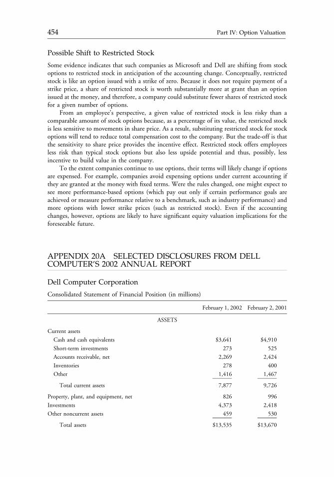
Possible Shift to Restricted Stock
Some evidence indicates that such companies as Microsoft and Dell are shifting from stockoptions to restricted stock in anticipation of the accounting change. Conceptually, restrictedstock is like an option issued with a strike of zero. Because it does not require payment of astrike price, a share of restricted stock is worth substantially more at grant than an optionissued at the money, and therefore, a company could substitute fewer shares of restricted stockfor a given number of options.
From an employee’s perspective, a given value of restricted stock is less risky than acomparable amount of stock options because, as a percentage of its value, the restricted stockis less sensitive to movements in share price. As a result, substituting restricted stock for stockoptions will tend to reduce total compensation cost to the company. But the trade-off is thatthe sensitivity to share price provides the incentive effect. Restricted stock offers employeesless risk than typical stock options but also less upside potential and thus, possibly, lessincentive to build value in the company.
To the extent companies continue to use options, their terms will likely change if optionsare expensed. For example, companies avoid expensing options under current accounting ifthey are granted at the money with fixed terms. Were the rules changed, one might expect tosee more performance-based options (which pay out only if certain performance goals areachieved or measure performance relative to a benchmark, such as industry performance) andmore options with lower strike prices (such as restricted stock). Even if the accountingchanges, however, options are likely to have significant equity valuation implications for theforeseeable future.
APPENDIX 20A SELECTED DISCLOSURES FROM DELLCOMPUTER’S 2002 ANNUAL REPORT
Dell Computer Corporation
Consolidated Statement of Financial Position (in millions)
February 1, 2002 February 2, 2001
ASSETS
Current assets
Cash and cash equivalents $3,641 $4,910
Short-term investments 273 525
Accounts receivable, net 2,269 2,424
Inventories 278 400
Other 1,416 1,467
Total current assets 7,877 9,726
Property, plant, and equipment, net 826 996
Investments 4,373 2,418
Other noncurrent assets 459 530
Total assets $13,535 $13,670
c20 12 September 2012; 14:18:1
454 Part IV: Option Valuation
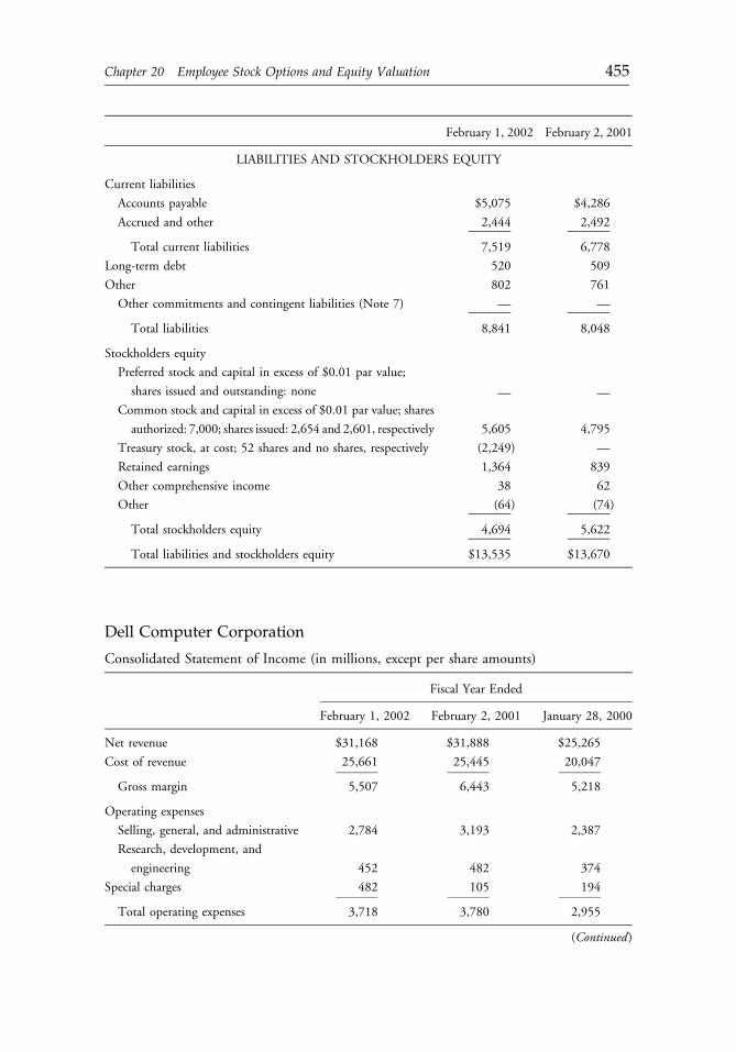
February 1, 2002 February 2, 2001
LIABILITIES AND STOCKHOLDERS EQUITY
Current liabilities
Accounts payable $5,075 $4,286
Accrued and other 2,444 2,492
Total current liabilities 7,519 6,778
Long-term debt 520 509
Other 802 761
Other commitments and contingent liabilities (Note 7) — —
Total liabilities 8,841 8,048
Stockholders equity
Preferred stock and capital in excess of $0.01 par value;
— —shares issued and outstanding: none
Common stock and capital in excess of $0.01 par value; shares
5,605 4,795authorized: 7,000; shares issued: 2,654 and 2,601, respectively
Treasury stock, at cost; 52 shares and no shares, respectively (2,249) —
Retained earnings 1,364 839
Other comprehensive income 38 62
Other (64) (74)
Total stockholders equity 4,694 5,622
Total liabilities and stockholders equity $13,535 $13,670
Dell Computer Corporation
Consolidated Statement of Income (in millions, except per share amounts)
Fiscal Year Ended
February 1, 2002 February 2, 2001 January 28, 2000
Net revenue $31,168 $31,888 $25,265
Cost of revenue 25,661 25,445 20,047
Gross margin 5,507 6,443 5,218
Operating expenses
Selling, general, and administrative 2,784 3,193 2,387
Research, development, and
engineering 452 482 374
Special charges 482 105 194
Total operating expenses 3,718 3,780 2,955
(Continued)
c20 12 September 2012; 14:18:2
Chapter 20 Employee Stock Options and Equity Valuation 455
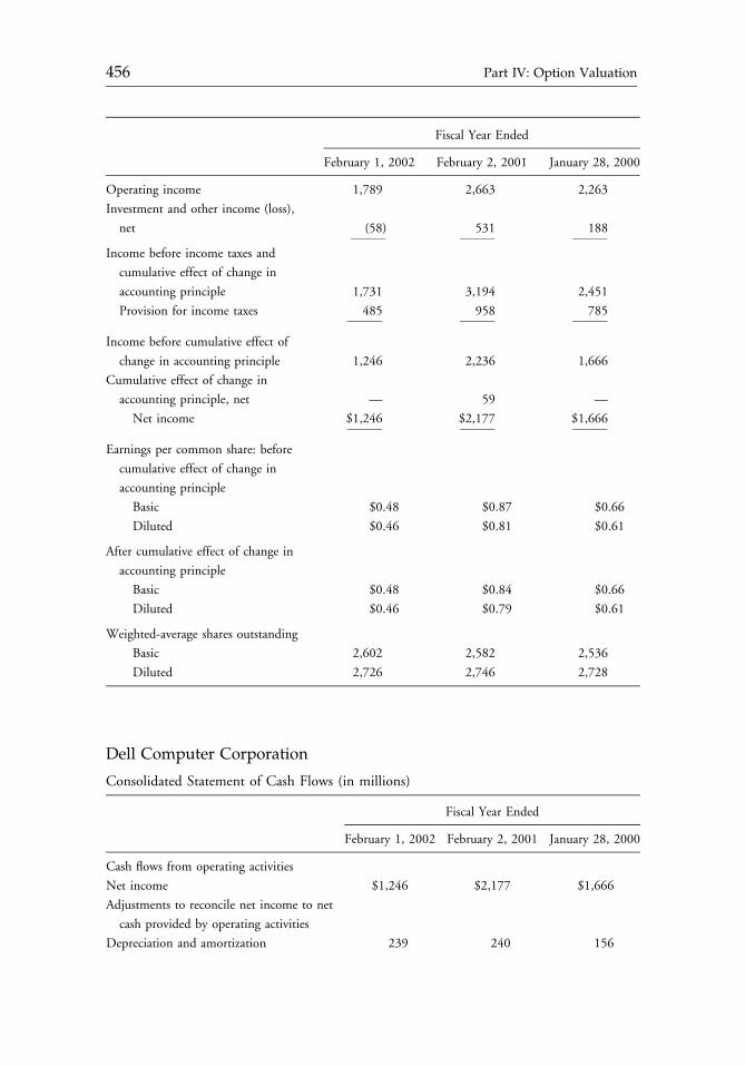
Fiscal Year Ended
February 1, 2002 February 2, 2001 January 28, 2000
Operating income 1,789 2,663 2,263
Investment and other income (loss),
net (58) 531 188
Income before income taxes and
1,731 3,194 2,451
cumulative effect of change in
accounting principle
Provision for income taxes 485 958 785
Income before cumulative effect of
1,246 2,236 1,666change in accounting principle
Cumulative effect of change in
— 59 —accounting principle, net
Net income $1,246 $2,177 $1,666
Earnings per common share: before
cumulative effect of change in
accounting principle
Basic $0.48 $0.87 $0.66
Diluted $0.46 $0.81 $0.61
After cumulative effect of change in
accounting principle
Basic $0.48 $0.84 $0.66
Diluted $0.46 $0.79 $0.61
Weighted-average shares outstanding
Basic 2,602 2,582 2,536
Diluted 2,726 2,746 2,728
Dell Computer Corporation
Consolidated Statement of Cash Flows (in millions)
Fiscal Year Ended
February 1, 2002 February 2, 2001 January 28, 2000
Cash flows from operating activities
Net income $1,246 $2,177 $1,666
Adjustments to reconcile net income to net
cash provided by operating activities
Depreciation and amortization 239 240 156
c20 12 September 2012; 14:18:2
456 Part IV: Option Valuation
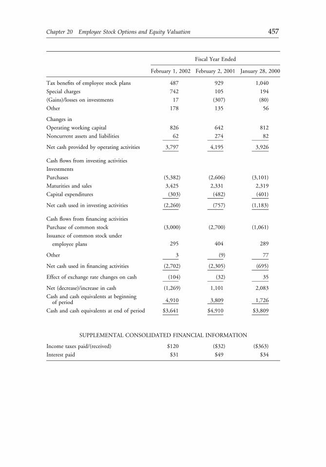
Fiscal Year Ended
February 1, 2002 February 2, 2001 January 28, 2000
Tax benefits of employee stock plans 487 929 1,040
Special charges 742 105 194
(Gains)/losses on investments 17 (307) (80)
Other 178 135 56
Changes in
Operating working capital 826 642 812
Noncurrent assets and liabilities 62 274 82
Net cash provided by operating activities 3,797 4,195 3,926
Cash flows from investing activities
Investments
Purchases (5,382) (2,606) (3,101)
Maturities and sales 3,425 2,331 2,319
Capital expenditures (303) (482) (401)
Net cash used in investing activities (2,260) (757) (1,183)
Cash flows from financing activities
Purchase of common stock (3,000) (2,700) (1,061)
Issuance of common stock under
295 404 289employee plans
Other 3 (9) 77
Net cash used in financing activities (2,702) (2,305) (695)
Effect of exchange rate changes on cash (104) (32) 35
Net (decrease)/increase in cash (1,269) 1,101 2,083
Cash and cash equivalents at beginning4,910 3,809 1,726of period
Cash and cash equivalents at end of period $3,641 $4,910 $3,809
SUPPLEMENTAL CONSOLIDATED FINANCIAL INFORMATION
Income taxes paid/(received) $120 ($32) ($363)
Interest paid $31 $49 $34
c20 12 September 2012; 14:18:2
Chapter 20 Employee Stock Options and Equity Valuation 457
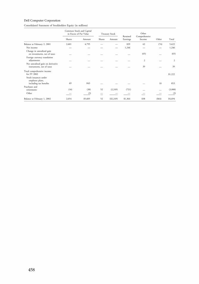
Dell Computer Corporation
Consolidated Statement of Stockholders Equity (in millions)
Common Stock and Capitalin Excess of Par Value Treasury Stock
Shares Amount Shares AmountRetainedEarnings
OtherComprehensive
Income Other Total
Balance at February 2, 2001 2,601 4,795 — — 839 62 (74) 5,622
Net income — — — — 1,246 — — 1,246
Change in unrealized gainon investments, net of taxes — — — — — (65) — (65)
Foreign currency translationadjustments — — — — — 2 — 2
Net unrealized gain on derivativeinstruments, net of taxes — — — — — 39 — 39
Total comprehensive incomefor FY 2002 $1,222
Stock issuances underemployee plans,including tax benefits 69 843 — — — — 10 853
Purchases andretirements (16) (30) 52 (2,249) (721) — — (3,000)
Other — (3) — — — — — (3)
Balance at February 1, 2002 2,654 $5,605 52 ($2,249) $1,364 $38 ($64) $4,694
c20 12 September 2012; 14:18:3
458
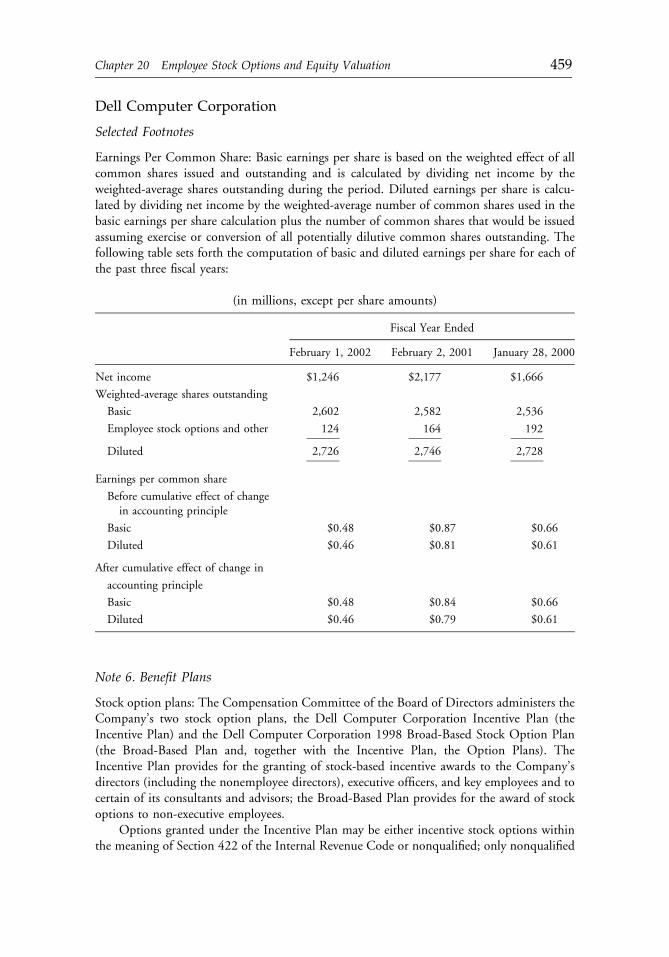
Dell Computer Corporation
Selected Footnotes
Earnings Per Common Share: Basic earnings per share is based on the weighted effect of allcommon shares issued and outstanding and is calculated by dividing net income by theweighted-average shares outstanding during the period. Diluted earnings per share is calcu-lated by dividing net income by the weighted-average number of common shares used in thebasic earnings per share calculation plus the number of common shares that would be issuedassuming exercise or conversion of all potentially dilutive common shares outstanding. Thefollowing table sets forth the computation of basic and diluted earnings per share for each ofthe past three fiscal years:
(in millions, except per share amounts)
Fiscal Year Ended
February 1, 2002 February 2, 2001 January 28, 2000
Net income $1,246 $2,177 $1,666
Weighted-average shares outstanding
Basic 2,602 2,582 2,536
Employee stock options and other 124 164 192
Diluted 2,726 2,746 2,728
Earnings per common share
Before cumulative effect of changein accounting principle
Basic $0.48 $0.87 $0.66
Diluted $0.46 $0.81 $0.61
After cumulative effect of change in
accounting principle
Basic $0.48 $0.84 $0.66
Diluted $0.46 $0.79 $0.61
Note 6. Benefit Plans
Stock option plans: The Compensation Committee of the Board of Directors administers theCompany’s two stock option plans, the Dell Computer Corporation Incentive Plan (theIncentive Plan) and the Dell Computer Corporation 1998 Broad-Based Stock Option Plan(the Broad-Based Plan and, together with the Incentive Plan, the Option Plans). TheIncentive Plan provides for the granting of stock-based incentive awards to the Company’sdirectors (including the nonemployee directors), executive officers, and key employees and tocertain of its consultants and advisors; the Broad-Based Plan provides for the award of stockoptions to non-executive employees.
Options granted under the Incentive Plan may be either incentive stock options withinthe meaning of Section 422 of the Internal Revenue Code or nonqualified; only nonqualified
c20 12 September 2012; 14:18:3
Chapter 20 Employee Stock Options and Equity Valuation 459
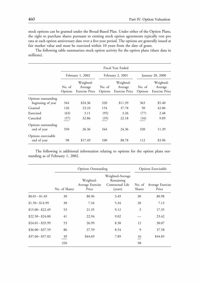
stock options can be granted under the Broad-Based Plan. Under either of the Option Plans,the right to purchase shares pursuant to existing stock option agreements typically vest prorata at each option anniversary date over a five-year period. The options are generally issued atfair market value and must be exercised within 10 years from the date of grant.
The following table summarizes stock option activity for the option plans (share data inmillions).
Fiscal Year Ended
February 1, 2002 February 2, 2001 January 28, 2000
No. ofOptions
Weighted-Average
Exercise PriceNo. ofOptions
Weighted-Average
Exercise PriceNo. ofOptions
Weighted-Average
Exercise Price
Options outstandingbeginning of year 344 $24.36 320 $11.39 363 $5.40
Granted 126 23.24 154 37.78 50 42.86
Exercised (63) 3.11 (95) 3.26 (77) 2.48
Canceled (57) 32.86 (35) 22.18 (16) 9.89
Options outstandingend of year 350 26.36 344 24.36 320 11.39
Options exercisableend of year 98 $17.49 100 $8.78 112 $3.96
The following is additional information relating to options for the option plans out-standing as of February 1, 2002.
Options Outstanding Options Exercisable
No. of Shares
Weighted-Average Exercise
Price
Weighted-AverageRemaining
Contractual Life(years)
No. ofShares
Average ExercisePrice
$0.01�$1.49 30 $0.96 3.49 30 $0.98
$1.50�$14.99 38 7.34 5.34 28 7.13
$15.00�$22.49 53 21.35 9.12 3 17.35
$22.50�$24.00 41 22.94 9.02 — 23.42
$24.01�$35.99 53 26.99 8.30 12 30.07
$36.00�$37.59 86 37.59 8.54 9 37.58
$37.60�$57.82 49 $44.69 7.89 16 $44.85
350 98
c20 12 September 2012; 14:18:3
460 Part IV: Option Valuation
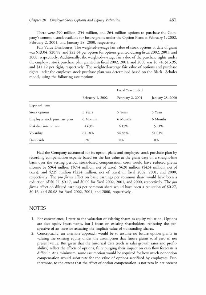
There were 290 million, 254 million, and 264 million options to purchase the Com-pany’s common stock available for future grants under the Option Plans at February 1, 2002,February 2, 2001, and January 28, 2000, respectively.
Fair Value Disclosures: The weighted-average fair value of stock options at date of grantwas $13.04, $20.98, and $22.64 per option for options granted during fiscal 2002, 2001, and2000, respectively. Additionally, the weighted-average fair value of the purchase rights underthe employee stock purchase plan granted in fiscal 2002, 2001, and 2000 was $6.74, $13.95,and $11.12 per right, respectively. The weighted-average fair value of options and purchaserights under the employee stock purchase plan was determined based on the Black�Scholesmodel, using the following assumptions.
Fiscal Year Ended
February 1, 2002 February 2, 2001 January 28, 2000
Expected term
Stock options 5 Years 5 Years 5 Years
Employee stock purchase plan 6 Months 6 Months 6 Months
Risk-free interest rate 4.63% 6.15% 5.81%
Volatility 61.18% 54.85% 51.03%
Dividends 0% 0% 0%
Had the Company accounted for its option plans and employee stock purchase plan byrecording compensation expense based on the fair value at the grant date on a straight-linebasis over the vesting period, stock-based compensation costs would have reduced pretaxincome by $964 million ($694 million, net of taxes), $620 million ($434 million, net oftaxes), and $329 million ($224 million, net of taxes) in fiscal 2002, 2001, and 2000,respectively. The pro forma effect on basic earnings per common share would have been areduction of $0.27, $0.17, and $0.09 for fiscal 2002, 2001, and 2000, respectively. The proforma effect on diluted earnings per common share would have been a reduction of $0.27,$0.16, and $0.08 for fiscal 2002, 2001, and 2000, respectively.
NOTES
1. For convenience, I refer to the valuation of existing shares as equity valuation. Optionsare also equity instruments, but I focus on existing shareholders, reflecting the per-spective of an investor assessing the implicit value of outstanding shares.
2. Conceptually, an alternate approach would be to assume no future option grants invaluing the existing equity under the assumption that future grants total zero in netpresent value. But given that the historical data (such as sales growth rates and profit-ability) reflect the effects of options, fully purging their impact on cash flow forecasts isdifficult. At a minimum, some assumption would be required for how much nonoptioncompensation would substitute for the value of options sacrificed by employees. Fur-thermore, to the extent that the effect of option compensation is not zero in net present
c20 12 September 2012; 14:18:3
Chapter 20 Employee Stock Options and Equity Valuation 461
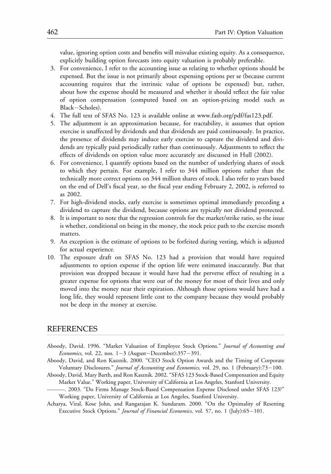
value, ignoring option costs and benefits will misvalue existing equity. As a consequence,explicitly building option forecasts into equity valuation is probably preferable.
3. For convenience, I refer to the accounting issue as relating to whether options should beexpensed. But the issue is not primarily about expensing options per se (because currentaccounting requires that the intrinsic value of options be expensed) but, rather,about how the expense should be measured and whether it should reflect the fair valueof option compensation (computed based on an option-pricing model such asBlack�Scholes).
4. The full text of SFAS No. 123 is available online at www.fasb.org/pdf/fas123.pdf.5. The adjustment is an approximation because, for tractability, it assumes that option
exercise is unaffected by dividends and that dividends are paid continuously. In practice,the presence of dividends may induce early exercise to capture the dividend and divi-dends are typically paid periodically rather than continuously. Adjustments to reflect theeffects of dividends on option value more accurately are discussed in Hull (2002).
6. For convenience, I quantify options based on the number of underlying shares of stockto which they pertain. For example, I refer to 344 million options rather than thetechnically more correct options on 344 million shares of stock. I also refer to years basedon the end of Dell’s fiscal year, so the fiscal year ending February 2, 2002, is referred toas 2002.
7. For high-dividend stocks, early exercise is sometimes optimal immediately preceding adividend to capture the dividend, because options are typically not dividend protected.
8. It is important to note that the regression controls for the market/strike ratio, so the issueis whether, conditional on being in the money, the stock price path to the exercise monthmatters.
9. An exception is the estimate of options to be forfeited during vesting, which is adjustedfor actual experience.
10. The exposure draft on SFAS No. 123 had a provision that would have requiredadjustments to option expense if the option life were estimated inaccurately. But thatprovision was dropped because it would have had the perverse effect of resulting in agreater expense for options that were out of the money for most of their lives and onlymoved into the money near their expiration. Although those options would have had along life, they would represent little cost to the company because they would probablynot be deep in the money at exercise.
REFERENCES
Aboody, David. 1996. “Market Valuation of Employee Stock Options.” Journal of Accounting andEconomics, vol. 22, nos. 1�3 (August�December):357�391.
Aboody, David, and Ron Kasznik. 2000. “CEO Stock Option Awards and the Timing of CorporateVoluntary Disclosures.” Journal of Accounting and Economics, vol. 29, no. 1 (February):73�100.
Aboody, David, Mary Barth, and Ron Kasznik. 2002. “SFAS 123 Stock-Based Compensation and EquityMarket Value.” Working paper, University of California at Los Angeles, Stanford University.
———. 2003. “Do Firms Manage Stock-Based Compensation Expense Disclosed under SFAS 123?”Working paper, University of California at Los Angeles, Stanford University.
Acharya, Viral, Kose John, and Rangarajan K. Sundaram. 2000. “On the Optimality of ResettingExecutive Stock Options.” Journal of Financial Economics, vol. 57, no. 1 (July):65�101.
c20 12 September 2012; 14:18:3
462 Part IV: Option Valuation
Bell, Timothy, Wayne R. Landsman, Bruce L. Miller, and Shu Yeh. 2002. “The Valuation Implicationsof Employee Stock Option Accounting for Profitable Computer Software Firms.” AccountingReview, vol. 77, no. 4 (October):971�996.
Bens, Daniel, Venky Nagar, and M.H. Franco Wong. 2002. “Real Investment Implications ofEmployee Stock Option Exercises.” Journal of Accounting Research, vol. 40, no. 2 (May):359�393.
Black, F., and M. Scholes. 1973. “The Pricing of Options and Corporate Securities.” Journal of PoliticalEconomy, vol. 81, no. 3 (May/June):637�654.
Carpenter, Jennifer. 1998. “The Exercise and Valuation of Executive Stock Options.” Journal ofFinancial Economics, vol. 48, no. 2 (May):127�158.
Carter, Mary Ellen, and Luann J. Lynch. 2003. “The Consequences of the FASB’s 1998 Proposal onAccounting for Stock Option Repricing.” Journal of Accounting and Economics, vol. 35, no. 1(April):51�72.
Core, John, and Wayne Guay. 2001. “Stock Option Plans for Non-Executive Employees.” Journal ofFinancial Economics, vol. 61, no. 2 (August):253�287.
Core, John, Robert Holthausen, and David Larcker. 1999. “Corporate Governance, CEO Compen-sation and Firm Performance.” Journal of Financial Economics, vol. 51, no. 3 (March):371�406.
Erickson, Merle, Michelle Hanlon, and Edward Maydew. 2003. “Is There a Link between ExecutiveCompensation and Accounting Fraud?” Working paper, University of Chicago, University ofMichigan, and University of North Carolina.
Graham, John, Mark Lang, and Doug Shackelford. Forthcoming 2004. “Employee Stock Options,Corporate Taxes, and Debt Policy.” Journal of Finance.
Hall, Brian, and Kevin J. Murphy. 2002. “Stock Options for Undiversified Executives.” Journal ofAccounting and Economics, vol. 33, no. 1 (February):3�42.
———. 2003. “The Trouble with Stock Options.” Journal of Economic Perspectives, vol. 17, no. 3(Summer):49�72.
Hanlon, Michelle, and Terry Shevlin. 2002. “Accounting for Tax Benefits of Employee Stock Optionsand Implications for Research.” Accounting Horizons, vol. 16, no. 1 (March):1�16.
Hanlon, Michelle, Shivaram Rajgopal, and Terry Shevlin. 2003. “Are Executive Stock Options Asso-ciated with Future Earnings?” Journal of Accounting and Economics, vol. 36, nos. 1�3(December):3�43.
Heath, C., S. Huddart, and M. Lang. 1999. “Psychological Factors and Stock Option Exercise.”Quarterly Journal of Economics, vol. 114, no. 2 (May):601�628.
Hemmer, Thomas, Steve Matsunaga, and Terry Shevlin. 1994. “Estimating the ‘Fair Value’ ofEmployee Stock Options with Expected Early Exercise.” Accounting Horizons, vol. 8, no. 4(December):23�42.
———. 1996. “The Influence of Risk Diversification on the Early Exercise of Employee Stock Optionsby Executive Officers.” Journal of Accounting and Economics, vol. 21, no. 1 (February):45�68.
Holmstrom, B. 1979. “Moral Hazard and Observability.” Bell Journal of Economics, vol. 10, no. 1(Spring):74�91.
Huddart, Steven. 1994. “Employee Stock Options.” Journal of Accounting and Economics, vol. 18, no. 2(September):207�231.
Huddart, Steven, and Mark Lang. 1996. “Employee Stock Option Exercises: An Empirical Analysis.”Journal of Accounting and Economics, vol. 21, no. 1 (February):5�43.
———. 2003. “Information Distribution within Firms: Evidence from Stock Option Exercises.”Journal of Accounting and Economics, vol. 34, nos. 1�3 (January):3�31.
Hull, John C. 2002. Options, Futures, and Other Derivatives. 5th ed. Upper Saddle River, NJ:Prentice Hall.
Ittner, Christopher, Richard A. Lambert, and David F. Larcker. 2003. “The Structure and PerformanceConsequences of Equity Grants to Employees of New Economy Firms.” Journal of Accounting andEconomics, vol. 34, no. 1 (January):89�127.
Kulatilaka, Nalin, and Alan J. Marcus. 1994. “Valuing Employee Stock Options.” Financial AnalystsJournal, vol. 50, no. 6 (November/December):46�56.
c20 12 September 2012; 14:18:4
Chapter 20 Employee Stock Options and Equity Valuation 463
Lambert, R.A., W.N. Lanen, and D.F. Larcker. 1989. “Executive Stock Option Plans and CorporateDividend Policy.” Journal of Financial and Quantitative Analysis, vol. 24, no. 4 (December):409�425.
Marquardt, Carol. 2002. “The Cost of Employee Stock Option Grants: An Empirical Analysis.” Journalof Accounting Research, vol. 40, no. 4 (September):1191�1217.
Merton, R. 1973. “Theory of Rational Option Pricing.” Bell Journal of Economics and ManagementScience, vol. 4, no. 1 (Spring):141�183.
Meulbroek, L.K. 2001. “The Efficiency of Equity-Linked Compensation: Understanding the Full Costof Awarding Executive Stock Options.” Financial Management, vol. 30, no. 2 (Summer):5�30.
Murphy, Kevin J. 2003. “Stock-Based Pay in New Economy Firms.” Journal of Accounting andEconomics, vol. 34, nos. 1�3 (January):129�147.
Rajgopal, Shivaram, and Terry Shevlin. 2002. “Empirical Evidence on the Relation between StockOption Compensation and Risk Taking.” Journal of Accounting and Economics, vol. 33, no. 2(June):145�171.
Soffer, Leonard. 2000. “SFAS No. 123 Disclosures and Discounted Cash Flow Valuation.” AccountingHorizons, vol. 14, no. 2 (June):169�189.
Sullivan, M. 2002. “Stock Options Take $50 Billion Bite out of Corporate Taxes.” Tax Notes(March):1396�1401.
c20 12 September 2012; 14:18:4
464 Part IV: Option Valuation
CHAPTER 21EMPLOYEE STOCK OPTION
VALUATION WITHAN EARLY EXERCISE
BOUNDARY
Neil Brisley and Chris K. Anderson
Many companies are recognizing that the Black�Scholes formula is inappropriatefor employee stock options (ESOs) and are moving toward lattice models foraccounting or decision-making purposes. In the most influential of these models, theassumption is that employees exercise voluntarily when the stock price reaches a fixedmultiple of the strike price, effectively introducing a “horizontal” exercise boundaryinto the lattice. In practice, however, employees make a trade-off between intrinsicvalue captured and the opportunity cost of time value forgone. The model proposedhere explicitly recognizes and accounts for this reality and is intuitively appealing,easily implemented, and compliant with U.S. accounting standards.
Another assumption that Lehman made in valuing Mr. Fuld’s pay in 2000 wasthat he would exercise the options two and a half years after receiving them. ButMr. Fuld had a history of holding onto his options until they were about to expire.
Reprinted from the Financial Analysts Journal (September/October 2008):88�100. The paper on whichthis chapter is based won the Second Annual “Best Conference Research Paper Award” from theCanadian Finance Executives Research Foundation at the 2008 Financial Executives International (FEI)Canada conference. When this article was originally published, Neil Brisley was assistant professor offinance at the Richard Ivey School of Business, University of Western Ontario, London, Canada, andChris K. Anderson was assistant professor of operations management at the School of Hotel Admin-istration, Cornell University.
c21 12 September 2012; 14:21:38
465
Indeed, all 2.6 million options that Mr. Fuld has exercised since November 2003were in the last year of their life when he did so.
—Patrick McGeehan (2006)
The need to value employee stock options (ESOs) for accounting and economic purposesmakes the modeling of employee early exercise behavior relevant for corporate financialofficers, security analysts, and those involved in determining option awards. Early exercise byemployees reduces the cost of the ESO to the company in relation to an otherwise identicalEuropean option (which can be exercised only at the end of its life), so ESO-pricing modelsmust make assumptions to describe in what circumstances an employee will exercise an optionbefore expiration. Examples such as the one in the New York Times quotation by McGeehanillustrate the importance of identifying which factors drive early exercise decisions and ofmaking reasonable estimates of the numerical value of those drivers.
A majority of companies have previously used variants of the Black�Scholes option-pricing model to value ESOs, but more and more companies have recognized that theseformulas are inappropriate for ESOs and are moving toward lattice models, such as thatproposed by Hull and White (2004; henceforth, HW).1 This trend can be expected toincrease because under current financial accounting rules, any company that adopts a latticemodel is not permitted subsequently to revert to a Black�Scholes model.2
In a much cited and influential paper, HW proposed a barrier option lattice model forESOs that assumes employees exercise voluntarily whenever the stock price reaches a fixedmultiple, M, of the strike price. Their model is flexible, easily understood and interpreted,and widely used. Conceptually, it introduces into the ESO a “horizontal” boundary; vol-untary early exercise occurs if the stock price reaches this barrier. Empirical evidence (e.g.,Huddart and Lang 1996) is consistent with the implications of financial theory thatemployees require the stock to be at a relatively high multiple of the strike price to inducevoluntary exercise early in the ESO life, but later in the option life, employees will exercisevoluntarily at a relatively low multiple of the strike price.3 This behavior has implicationsnot only for the appropriateness of the HW model but also for the empirical estimation ofthe M parameter from observations of historical early exercise: Two identical companieswith identical employee characteristics could value identical ESO awards significantlydifferently when using the HW model simply because one company previously enjoyedmore rapid stock price growth than the other; that is, the company with the rapid stock pricegrowth experienced a historically higher M in voluntary exercise observations than did theother company.
We propose an alternative model of the voluntary exercise boundary. Our model assumesthat employees exercise voluntarily whenever the “moneyness” of the option reaches a fixedproportion, μ, of its remaining Black�Scholes value. The result is an intuitively appealing“downward-sloping” voluntary exercise boundary, which requires the stock to be at a rela-tively high multiple of the strike price to induce voluntary exercise early in the ESO life butallows voluntary exercise at relatively low multiples of strike price later in the option life. Ourμ model shares the practical simplicity of the M model and can be used to value ESOs incircumstances when the M model can be used. Like HW’s M model, it readily encompassessuch ESO characteristics as vesting restrictions, forfeiture, and forced early exercise as a resultof employment termination. Unlike the HW model, our model takes into accountthroughout the ESO life the early exercise trade-off between intrinsic value captured and theopportunity cost of option value forgone. Moreover, the empirical estimation of the μ
c21 12 September 2012; 14:21:38
466 Part IV: Option Valuation
parameter from observations of historical early exercise is potentially less susceptible than theestimate for the M model to bias caused by atypical stock price histories.
An approach still used by many practitioners (as exemplified in the New York Timesquotation) is simply to take an estimate of the ESO’s expected life and input this as the optionmaturity in the Black�Scholes equation. A lattice model variant of this approach is to assumethat employees exercise voluntarily if a fixed maximum anticipated life, L, is reached. Con-ceptually, this approach introduces a “vertical” voluntary exercise boundary into the ESO.This L model is a third heuristic (rule-of-thumb) approach to the modeling of the voluntaryearly exercise boundary that we use for comparison with the performance of the M model andour proposed μ model.4
A commonly practiced approach to valuing ESOs is to take the average of the parametersdetermined from a heterogeneous population to model a “representative investor.” Thisapproach is conceptually incorrect for the L model and the M model (and causes potentiallysignificant bias in the M model). The reason is that prices produced by the L model andM model are concave in, respectively, L and M, so the model price based on the averageparameter of the population is greater than the average of the model prices found wheneach parameter is used.
In contrast, in the absence of vesting restrictions, forfeiture, and employment termination�related exercise, the μ model has a simple closed-form solution that is linear in μ. We show thatthe grant-date value of an ESO when the employee exercises early if (and only if) she capturesa fixed proportion (μ) of the remaining Black�Scholes value is equal to the same proportion (μ)of the grant-date Black�Scholes value of an otherwise identical European option. Even in thepresence of vesting restrictions and employment termination, the μ-model lattice gives optionprices that are nearly linear in μ; therefore, the use of a representative investor approach ispotentially justified for the μ model—even for option grants for heterogeneous populations ofemployees.
Our analysis also reveals how the particular price history of a stock can systematicallybias the valuations that an L or M model produces when historical data are used to estimateparameters for the models. The reason is as follows: Employees of a company that hasexperienced high stock returns will tend to have voluntarily exercised options relatively earlyin the ESO life but at stock prices representing relatively high multiples of the strike price.The Ls measured in this scenario will be low, and the measured Ms will be high. If these lowLs are used as inputs to value new ESO grants, they are likely to underestimate the true costof the options. If the high Ms are used, they will overestimate ESO value. Conversely, acompany that has had sluggish stock returns will have experienced voluntary option exercisesrelatively late in the term and at relatively low multiples of the strike price, with corre-sponding consequences if those data are used to estimate parameters for an L model or an Mmodel.5 In contrast, Bettis, Bizjak, and Lemmon (2005; henceforth, BBL) found thatvariation in Ratio, which is their measure of the proportion of the remaining Black�Scholesvalue captured at early exercise (our μ) across years, is much smaller than the variation inthe degree of early exercise. Their result provides further motivation for our proposedpricing model.
We show how any one of the L, M, and μ models may, depending on the particularhistorical data of voluntary early exercises used to calculate parameter inputs, give the highestor lowest estimate of ESO price. In general, however, no objectively “correct” option priceexists against which to measure each model’s output for accuracy. We adopted a rationalmodel of voluntary early exercise behavior (used in Carpenter 1998 and BBL) to serve as abenchmark.6 This model is intuitively appealing, has been well studied in the literature, and
c21 12 September 2012; 14:21:38
Chapter 21 Employee Stock Option Valuation with an Early Exercise Boundary 467
has been shown to adequately describe qualitative and quantitative characteristics of empiricaldata. It uses the binomial lattice to depict the voluntary early exercise decision for an ESOheld by a utility-maximizing employee whose outside wealth is invested in an optimalportfolio of stock and bonds. At every node in the lattice, the risk-averse employee comparesthe expected utility from immediate exercise with the expected utility from waiting for at leastone more period. Voluntary exercise is triggered if or when utility from immediate exercise isexpected to be the greater—which enabled us to obtain the voluntary exercise barrier for anESO held by that employee and, hence, to calculate an objective value for the ESO.
Furthermore, we generated the full probability distribution of possible individual “pricehistories” within the lattice and calculated a full distribution of what L, M, and μ an analystcould potentially measure from the associated voluntary early exercises. Using these parametervalues in the respective heuristic models, we could then analyze those models’ accuracy rel-ative to the objective option value.
HEURISTIC MODELS OF A VOLUNTARY EARLYEXERCISE BOUNDARY
To compare the models, we use the following notation: A company’s stock price S evolves withlognormal returns over time t in the interval [0,T] with volatility σ. An ESO is issued at timet 5 0 with maturity T years. The option has strike price X and is issued at the money. Wenormalize the initial stock price so that S0 is equal to X, which is equal to 1. The risk-freeinterest rate is r. The stock price process may have a drift reflecting a positive risk premium (weuse 12 percent drift in our examples), but all valuation of stock options is performed under risk-neutral probabilities. The stock has a constant dividend yield d. We denote the Black�Scholesmodel value of a European call option with these same parameters as B(S, X, r, d, σ, T, t) butsuppress certain parameter arguments when convenient. The employee’s employment mayterminate for exogenous reasons at any time with probability q per year.7 The option may havea vesting date, v, which would be less than T—that is, v , T. If employment terminates beforetime v, the option is forfeited. If employment terminates between vesting and expiry, the optionis exercised (in the money) or forfeited (out of the money).8
We study each option valuation model here in the context of a standard binomial latticemodel that can easily be adapted to encompass state-contingent σ, r (e.g., term structures ofvolatility and interest rates), d, q, and v (e.g., performance vesting). The option can beexercised voluntarily by the employee at any time t in the interval [v,T].
The three models differ only in the modeling of a voluntary early exercise boundary. Asthe stock price evolves over time, voluntary early exercise occurs if it reaches the boundary. AnL model has a vertical barrier at t 5 L. An M model has a horizontal barrier at S 5 M. As weshow, a μ model has a downward-sloping barrier converging to S 5 1 at t 5 T.
“Adjusted Maturity” Approach (an L Model)
The lattice version of this model effectively assumes that at time t 5 L (if the option has notalready been forfeited or exercised early as a result of termination), an employee will vol-untarily exercise (if S . 1) or the option will lapse (if S # 1). In the absence of vestingrestrictions and employee termination, the ESO price obtained from an L model, X(L), issimply the Black�Scholes value, B(L), with modified option life L.
c21 12 September 2012; 14:21:39
468 Part IV: Option Valuation
HW “Multiple of Strike Price” Approach (an M Model)
HW assumed that the employee will voluntarily exercise early whenever the stock pricereaches a fixed multiple, M, of the option strike price. This assumption implies a simplehorizontal boundary at S 5 M. The presence of a vesting date, v, means that exercise cannotoccur at times before v even if S $ M at those times; so, the boundary is vertical at t 5 v,implying that “pent-up” exercise activity may occur at t 5 v at stock prices strictly greaterthan M. At expiry, t 5 T, all in-the-money options will be exercised, so the boundary isvertical at t 5 T, corresponding to exercises that occur at prices between 1 and M. Exercisesthat occur at times v or T (or at any time as a result of employee termination) are necessarilyconstrained; therefore, they should not be included as “voluntary exercises” in data fromwhich the analyst is making estimates of M.
Clearly, M is greater than 1 because only in-the-money options are exercised. HWperformed illustrative option valuations with M in the range of 1.2 to 3.0. Several studieshave calculated the ratio of stock price to strike price, S/X, for data from observed earlyexercises: BBL’s sample of corporate insiders has a median of 2.57 and a mean of 3.55.Carpenter’s (1998) sample of executives has a median of 2.47, a mean of 2.75, and astandard deviation of 1.42. Huddart and Lang (1996) analyzed a much broader sample oflower-level employees than Carpenter or BBL analyzed and found a median of 1.6 and amean of 2.2. Institutional Shareholder Services (ISS), a corporate governance and proxy-voting services firm, uses the HW model to compare option awards among companies (ISSwas acquired by RiskMetrics Group in January 2007). To all awards, the firm applies auniform assumption of M 5 2, which the firm states is the median exercise ratio for S&P1500 Index companies.
We denote by H(M) the HW model price of an ESO with voluntary exercise boundarymultiple M. Prices are concave, increasing in M, and rapidly approaching the Black�Scholesvalue as M increases beyond about 4.0.
Before developing our own model of voluntary exercise based on the proportion ofremaining option value captured, we note at this point what proportion of Black�Scholesvalue captured by an M policy implies. For fixed M, exercise of an option captures adollar value of M 2 1, so the proportion of remaining Black�Scholes value captured at timet is simply (M 2 1)/B(M,T 2 t). For example, with parameter values S0 5 X 5 1, T 5 10,v 5 0, d 5 0, q 5 0, r 5 5 percent, and σ 5 40 percent, Figure 21.1 shows that anemployee with a voluntary exercise boundary at, say, M 5 2 would capture only 65 percentof the remaining option value if the stock price reached that level early in the option life. Yet,for later exercises, less time value would remain and the proportion of remaining option valuecaptured would approach 100 percent as t approached maturity. An employee with anexercise policy of M 5 1.2 could initially capture as little as one-quarter of the remainingBlack�Scholes value.
“Proportion of Option Value Captured” Approach (a μ Model)
As illustrated in Figure 21.2, the exercise boundary for an employee who exercises wheneverhe can capture a fixed proportion μ of the remaining Black�Scholes value of the ESO isdownward sloping, which reflects the intuition that the employee requires a lower moneynessto trigger exercise later in the option life than earlier.9 The presence of a vesting date truncatesthe boundary, introducing a vertical portion at t 5 v and implying that pent-up exerciseactivity can occur at t 5 v at stock prices strictly greater than that implied by a μ policy.
c21 12 September 2012; 14:21:39
Chapter 21 Employee Stock Option Valuation with an Early Exercise Boundary 469
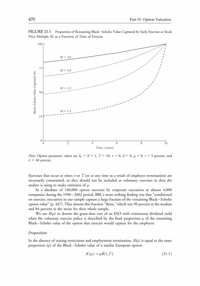
Exercises that occur at times v or T (or at any time as a result of employee termination) arenecessarily constrained, so they should not be included as voluntary exercises in data theanalyst is using to make estimates of μ.
In a database of 140,000 option exercises by corporate executives at almost 4,000companies during the 1996�2002 period, BBL’s most striking finding was that “conditionalon exercise, executives in our sample capture a large fraction of the remaining Black�Scholesoption value” (p. 447). They denote this fraction “Ratio,” which was 90 percent at the medianand 84 percent at the mean for their whole sample.
We use K(μ) to denote the grant-date cost of an ESO with continuous dividend yieldwhen the voluntary exercise policy is described by the fixed proportion μ of the remainingBlack�Scholes value of the option that exercise would capture for the employee.
Proposition
In the absence of vesting restrictions and employment termination, K(μ) is equal to the sameproportion (μ) of the Black�Scholes value of a similar European option:
K ðμÞ ¼ μBð1,T Þ: ð21:1Þ
FIGURE 21.1 Proportion of Remaining Black�Scholes Value Captured by Early Exercise at Stock
Price Multiple M, as a Function of Time of ExerciseBl
ack–
Scho
les V
alue
Cap
ture
d (%
)
M � 3.0
M � 2.0
M � 1.5
M � 1.2
100
75
50
25
00 102 64 8
Time, t (years)
Note: Option parameter values are S0 5 X 5 1, T 5 10, v 5 0, d 5 0, q 5 0, r 5 5 percent, andσ 5 40 percent.
c21 12 September 2012; 14:21:39
470 Part IV: Option Valuation
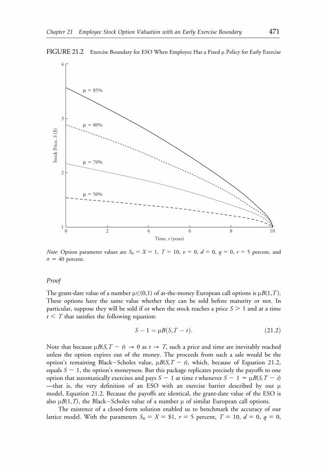
Proof
The grant-date value of a number μ2(0,1) of at-the-money European call options is μB(1,T ).These options have the same value whether they can be sold before maturity or not. Inparticular, suppose they will be sold if or when the stock reaches a price S . 1 and at a timet , T that satisfies the following equation:
S � 1 ¼ μBðS,T � tÞ: ð21:2Þ
Note that because μB(S,T 2 t) - 0 as t - T, such a price and time are inevitably reachedunless the option expires out of the money. The proceeds from such a sale would be theoption’s remaining Black�Scholes value, μB(S,T 2 t), which, because of Equation 21.2,equals S 2 1, the option’s moneyness. But this package replicates precisely the payoffs to oneoption that automatically exercises and pays S 2 1 at time t whenever S 2 1 5 μB(S,T 2 t)—that is, the very definition of an ESO with an exercise barrier described by our μmodel, Equation 21.2. Because the payoffs are identical, the grant-date value of the ESO isalso μB(1,T), the Black�Scholes value of a number μ of similar European call options.
The existence of a closed-form solution enabled us to benchmark the accuracy of ourlattice model. With the parameters S0 5 X 5 $1, r 5 5 percent, T 5 10, d 5 0, q 5 0,
FIGURE 21.2 Exercise Boundary for ESO When Employee Has a Fixed μ Policy for Early ExerciseSt
ock
Pric
e, S
($)
4
3
2
10 102 64 8
Time, t (years)
μ � 85%
μ � 80%
μ � 70%
μ � 50%
Note: Option parameter values are S0 5 X 5 1, T 5 10, v 5 0, d 5 0, q 5 0, r 5 5 percent, andσ 5 40 percent.
c21 12 September 2012; 14:21:39
Chapter 21 Employee Stock Option Valuation with an Early Exercise Boundary 471
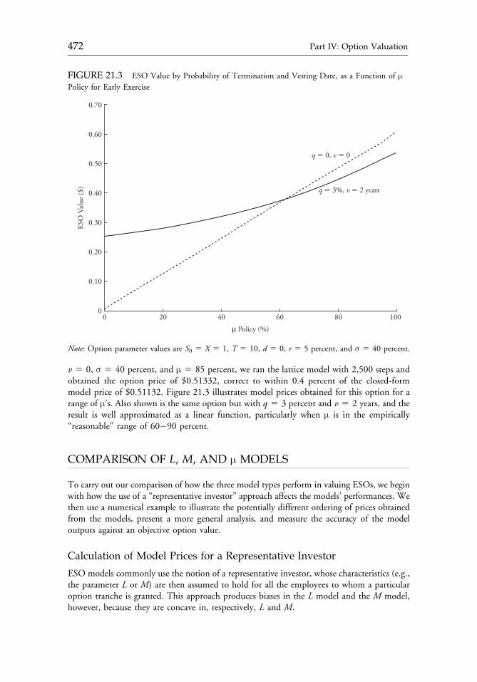
v 5 0, σ 5 40 percent, and μ 5 85 percent, we ran the lattice model with 2,500 steps andobtained the option price of $0.51332, correct to within 0.4 percent of the closed-formmodel price of $0.51132. Figure 21.3 illustrates model prices obtained for this option for arange of μ’s. Also shown is the same option but with q 5 3 percent and v 5 2 years, and theresult is well approximated as a linear function, particularly when μ is in the empirically“reasonable” range of 60�90 percent.
COMPARISON OF L, M, AND μ MODELS
To carry out our comparison of how the three model types perform in valuing ESOs, we beginwith how the use of a “representative investor” approach affects the models’ performances. Wethen use a numerical example to illustrate the potentially different ordering of prices obtainedfrom the models, present a more general analysis, and measure the accuracy of the modeloutputs against an objective option value.
Calculation of Model Prices for a Representative Investor
ESO models commonly use the notion of a representative investor, whose characteristics (e.g.,the parameter L or M) are then assumed to hold for all the employees to whom a particularoption tranche is granted. This approach produces biases in the L model and the M model,however, because they are concave in, respectively, L and M.
FIGURE 21.3 ESO Value by Probability of Termination and Vesting Date, as a Function of μPolicy for Early Exercise
ESO
Val
ue ($
)
q � 0, v � 0
q � 3%, v � 2 years
0.70
0.50
0.30
0.10
0.60
0.40
0.20
00 10020 6040 80
μ Policy (%)
Note: Option parameter values are S0 5 X 5 1, T 5 10, d 5 0, r 5 5 percent, and σ 5 40 percent.
c21 12 September 2012; 14:21:39
472 Part IV: Option Valuation
In the context of an L model, for heterogeneous employees (i.e., those with different L’s),the model price of the average (i.e., representative) employee is strictly greater than the averageof the model prices of each employee. The price of a four-year option and an eight-yearoption combined is not the same as the price of two six-year options, even though many ESO-pricing methodologies implicitly assume that it is.
This same effect is even more striking, quantitatively, when employee behaviors aredescribed by M. Consider the following scenario: The parameters are S0 5 X 5 1, r 5 5percent, T 5 10, d 5 0, q 5 0, v 5 0, and σ 5 40 percent. Employee A has a voluntaryexercise multiple of M 5 1.5, and Employee B has a voluntary exercise multiple ofM 5 3.5.The M-model price of a representative employee with a voluntary exercise multiple ofM 5 (1.5 1 3.5)/2 5 2.5 is $0.50069, whereas the average of the two employees’ M-modelprices is (0.31167 1 0.55358)/2 5 $0.43262. Therefore, in this case, a representativeinvestor approach leads to overvaluation of the options by a factor of 0.50069/0.43262 5 1.1573 (i.e., the value is 16 percent “too high”). Representative investor modelsare biased upward when used to value ESOs in an L model or an M model.
In contrast, and to the extent that the prices obtained from a μ model are linear in μ, theμ-model price of a representative employee is unbiased. Even when vesting restrictions andtermination are present (e.g., with q 5 3 percent and v 5 2 years, as in Figure 21.3), the biasinduced by taking the model price of the mean of voluntary exercise factors is not significant.Hence, a representative investor approach is potentially justified for the μ model, even foroption grants among heterogeneous populations of employees. Nevertheless, for consistencywith the L andMmodels, in our subsequent calculations, we calculate the mean of model pricesrather than the model price of mean parameters.
Relative Prices Obtained from the Models
In analyzing the performance of the three heuristic models, we wish to understand how theycompare when we use data from the same source. The main intuitions are first illustrated witha simple numerical example:
Consider Company X and Company Y, which are (ex ante) identical companies withconstant volatility of 40 percent per year and identical expected returns; the risk-free rate is 5percent per year. Each company issued a single at-the-money 10-year ESO when its (nor-malized) stock price was $1.
Company X’s stock price enjoyed rapid growth, and the ESO was exercised after 1.89years when the stock price was $2.90.
Company Y’s stock price experienced more sluggish growth, and the ESO was exercisedafter 9.87 years when the stock price was $1.45.
These examples exhibit the well-known empirical regularity that employees require ahigher stock price to voluntarily exercise early in the life of the ESO than they require later inthe option life. In fact, these two voluntary exercises were generated by simulation of the earlyexercise decisions of identical rational risk-averse investors (from a well-known utility-basedmodel that we introduce in the next subsection). The investors’ endogenously determinedexercise policies imply an objective (ex ante) “true” option valuation of $0.5214 for ESOsissued by Companies X and Y (normalized to an at-the-money strike price of $1).
An analyst who is trying to value new grants of stock options for Companies X and Ymight turn to these historical exercise data to determine inputs into either an Lmodel or anMmodel. If the analyst uses the realized lives of the options, 1.96 and 9.76 years, respectively, inan L model, the value ascribed to further ESO grants (normalized to an at-the-money strike
c21 12 September 2012; 14:21:40
Chapter 21 Employee Stock Option Valuation with an Early Exercise Boundary 473
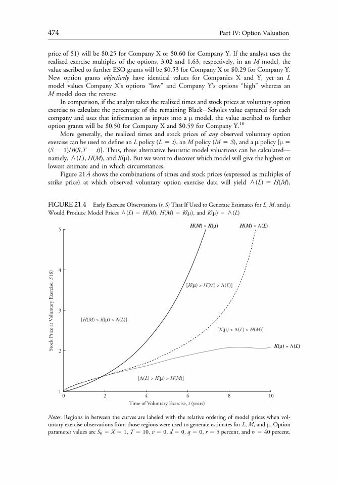
price of $1) will be $0.25 for Company X or $0.60 for Company Y. If the analyst uses therealized exercise multiples of the options, 3.02 and 1.63, respectively, in an M model, thevalue ascribed to further ESO grants will be $0.53 for Company X or $0.29 for Company Y.New option grants objectively have identical values for Companies X and Y, yet an Lmodel values Company X’s options “low” and Company Y’s options “high” whereas anM model does the reverse.
In comparison, if the analyst takes the realized times and stock prices at voluntary optionexercise to calculate the percentage of the remaining Black�Scholes value captured for eachcompany and uses that information as inputs into a μ model, the value ascribed to furtheroption grants will be $0.50 for Company X and $0.59 for Company Y.10
More generally, the realized times and stock prices of any observed voluntary optionexercise can be used to define an L policy (L 5 t), an M policy (M 5 S), and a μ policy [μ 5(S 2 1)/B(S,T 2 t)]. Thus, three alternative heuristic model valuations can be calculated—namely,X(L), H(M), and K(μ). But we want to discover which model will give the highest orlowest estimate and in which circumstances.
Figure 21.4 shows the combinations of times and stock prices (expressed as multiples ofstrike price) at which observed voluntary option exercise data will yield X(L) 5 H(M),
FIGURE 21.4 Early Exercise Observations (t, S) That If Used to Generate Estimates for L,M, and μWould Produce Model Prices X(L) 5 H(M), H(M) 5 K(μ), and K(μ) 5 X(L)
Stoc
k Pr
ice
at V
olun
tary
Exe
rcise
, S ($
)
H(M) = K(μ) H(M) = Λ(L)
[H(M) > K(μ) > Λ(L)]
[Λ(L) > K(μ) > H(M)]
[K(μ) > H(M) > Λ(L)]
[K(μ) > Λ(L) > H(M)]
K(μ) = Λ(L)
5
4
3
2
10 2 64 108
Time of Voluntary Exercise, t (years)
Notes: Regions in between the curves are labeled with the relative ordering of model prices when vol-untary exercise observations from those regions were used to generate estimates for L, M, and μ. Optionparameter values are S0 5 X 5 1, T 5 10, v 5 0, d 5 0, q 5 0, r 5 5 percent, and σ 5 40 percent.
c21 12 September 2012; 14:21:40
474 Part IV: Option Valuation
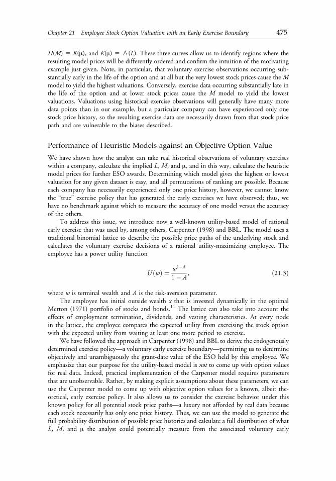
H(M) 5 K(μ), and K(μ) 5 X(L). These three curves allow us to identify regions where theresulting model prices will be differently ordered and confirm the intuition of the motivatingexample just given. Note, in particular, that voluntary exercise observations occurring sub-stantially early in the life of the option and at all but the very lowest stock prices cause the Mmodel to yield the highest valuations. Conversely, exercise data occurring substantially late inthe life of the option and at lower stock prices cause the M model to yield the lowestvaluations. Valuations using historical exercise observations will generally have many moredata points than in our example, but a particular company can have experienced only onestock price history, so the resulting exercise data are necessarily drawn from that stock pricepath and are vulnerable to the biases described.
Performance of Heuristic Models against an Objective Option Value
We have shown how the analyst can take real historical observations of voluntary exerciseswithin a company, calculate the implied L, M, and μ, and in this way, calculate the heuristicmodel prices for further ESO awards. Determining which model gives the highest or lowestvaluation for any given dataset is easy, and all permutations of ranking are possible. Becauseeach company has necessarily experienced only one price history, however, we cannot knowthe “true” exercise policy that has generated the early exercises we have observed; thus, wehave no benchmark against which to measure the accuracy of one model versus the accuracyof the others.
To address this issue, we introduce now a well-known utility-based model of rationalearly exercise that was used by, among others, Carpenter (1998) and BBL. The model uses atraditional binomial lattice to describe the possible price paths of the underlying stock andcalculates the voluntary exercise decisions of a rational utility-maximizing employee. Theemployee has a power utility function
U ðwÞ ¼ w1�A
1� A, ð21:3Þ
where w is terminal wealth and A is the risk-aversion parameter.The employee has initial outside wealth x that is invested dynamically in the optimal
Merton (1971) portfolio of stocks and bonds.11 The lattice can also take into account theeffects of employment termination, dividends, and vesting characteristics. At every nodein the lattice, the employee compares the expected utility from exercising the stock optionwith the expected utility from waiting at least one more period to exercise.
We have followed the approach in Carpenter (1998) and BBL to derive the endogenouslydetermined exercise policy—a voluntary early exercise boundary—permitting us to determineobjectively and unambiguously the grant-date value of the ESO held by this employee. Weemphasize that our purpose for the utility-based model is not to come up with option valuesfor real data. Indeed, practical implementation of the Carpenter model requires parametersthat are unobservable. Rather, by making explicit assumptions about these parameters, we canuse the Carpenter model to come up with objective option values for a known, albeit the-oretical, early exercise policy. It also allows us to consider the exercise behavior under thisknown policy for all potential stock price paths—a luxury not afforded by real data becauseeach stock necessarily has only one price history. Thus, we can use the model to generate thefull probability distribution of possible price histories and calculate a full distribution of whatL, M, and μ the analyst could potentially measure from the associated voluntary early
c21 12 September 2012; 14:21:40
Chapter 21 Employee Stock Option Valuation with an Early Exercise Boundary 475
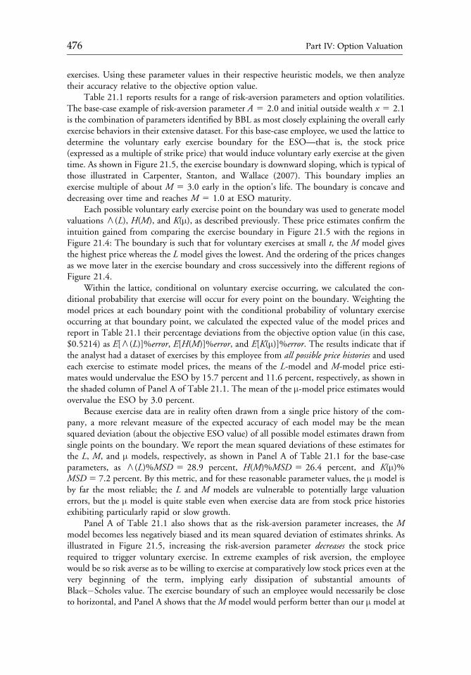
exercises. Using these parameter values in their respective heuristic models, we then analyzetheir accuracy relative to the objective option value.
Table 21.1 reports results for a range of risk-aversion parameters and option volatilities.The base-case example of risk-aversion parameter A 5 2.0 and initial outside wealth x 5 2.1is the combination of parameters identified by BBL as most closely explaining the overall earlyexercise behaviors in their extensive dataset. For this base-case employee, we used the lattice todetermine the voluntary early exercise boundary for the ESO—that is, the stock price(expressed as a multiple of strike price) that would induce voluntary early exercise at the giventime. As shown in Figure 21.5, the exercise boundary is downward sloping, which is typical ofthose illustrated in Carpenter, Stanton, and Wallace (2007). This boundary implies anexercise multiple of about M 5 3.0 early in the option’s life. The boundary is concave anddecreasing over time and reaches M 5 1.0 at ESO maturity.
Each possible voluntary early exercise point on the boundary was used to generate modelvaluations X(L), H(M), and K(μ), as described previously. These price estimates confirm theintuition gained from comparing the exercise boundary in Figure 21.5 with the regions inFigure 21.4: The boundary is such that for voluntary exercises at small t, the M model givesthe highest price whereas the L model gives the lowest. And the ordering of the prices changesas we move later in the exercise boundary and cross successively into the different regions ofFigure 21.4.
Within the lattice, conditional on voluntary exercise occurring, we calculated the con-ditional probability that exercise will occur for every point on the boundary. Weighting themodel prices at each boundary point with the conditional probability of voluntary exerciseoccurring at that boundary point, we calculated the expected value of the model prices andreport in Table 21.1 their percentage deviations from the objective option value (in this case,$0.5214) as E[X(L)]%error, E[H(M)]%error, and E[K(μ)]%error. The results indicate that ifthe analyst had a dataset of exercises by this employee from all possible price histories and usedeach exercise to estimate model prices, the means of the L-model and M-model price esti-mates would undervalue the ESO by 15.7 percent and 11.6 percent, respectively, as shown inthe shaded column of Panel A of Table 21.1. The mean of the μ-model price estimates wouldovervalue the ESO by 3.0 percent.
Because exercise data are in reality often drawn from a single price history of the com-pany, a more relevant measure of the expected accuracy of each model may be the meansquared deviation (about the objective ESO value) of all possible model estimates drawn fromsingle points on the boundary. We report the mean squared deviations of these estimates forthe L, M, and μ models, respectively, as shown in Panel A of Table 21.1 for the base-caseparameters, as X(L)%MSD 5 28.9 percent, H(M)%MSD 5 26.4 percent, and K(μ)%MSD 5 7.2 percent. By this metric, and for these reasonable parameter values, the μ model isby far the most reliable; the L and M models are vulnerable to potentially large valuationerrors, but the μ model is quite stable even when exercise data are from stock price historiesexhibiting particularly rapid or slow growth.
Panel A of Table 21.1 also shows that as the risk-aversion parameter increases, the Mmodel becomes less negatively biased and its mean squared deviation of estimates shrinks. Asillustrated in Figure 21.5, increasing the risk-aversion parameter decreases the stock pricerequired to trigger voluntary exercise. In extreme examples of risk aversion, the employeewould be so risk averse as to be willing to exercise at comparatively low stock prices even at thevery beginning of the term, implying early dissipation of substantial amounts ofBlack�Scholes value. The exercise boundary of such an employee would necessarily be closeto horizontal, and Panel A shows that theM model would perform better than our μ model at
c21 12 September 2012; 14:21:40
476 Part IV: Option Valuation
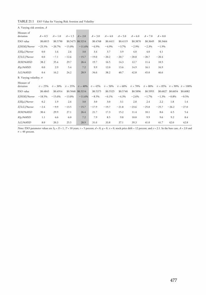
TABLE 21.1 ESO Value for Varying Risk Aversion and Volatility
A. Varying risk aversion, A
Measure ofdeviation A = 0.5 A = 1.0 A = 1.5 A = 2.0 A = 3.0 A = 4.0 A = 5.0 A = 6.0 A = 7.0 A = 8.0
ESO value $0.6015 $0.5790 $0.5475 $0.5214 $0.4768 $0.4411 $0.4119 $0.3870 $0.3649 $0.3464
E[H(M)]%error 225.5% 220.7% 215.0% 211.6% 26.9% 24.9% 23.7% 22.9% 22.3% 21.9%
E[K(μ)]%error 0.0 1.6 2.6 3.0 3.4 3.7 3.9 4.0 4.0 4.1
E[Λ(L)]%error 0.0 27.1 212.6 215.7 219.0 220.2 220.7 220.8 220.7 220.4
H(M)%MSD 38.2 35.4 29.7 26.4 19.7 16.5 14.3 12.7 11.4 10.5
K(μ)%MSD 0.0 2.9 5.4 7.2 9.9 12.0 13.6 14.9 16.1 16.9
Λ(L)%MSD 0.4 16.2 24.2 28.9 34.6 38.2 40.7 42.8 45.0 46.6
B. Varying volatility, σ
Measure ofdeviation σ = 25% σ = 30% σ = 35% σ = 40% σ = 45% σ = 50% σ = 60% σ = 70% σ = 80% σ = 85% σ = 90% σ = 100%
ESO value $0.4845 $0.4914 $0.5048 $0.5214 $0.5375 $0.5525 $0.5740 $0.5896 $0.5993 $0.6027 $0.6054 $0.6082
E[H(M)]%error 218.5% 215.6% 213.0% 211.6% 28.5% 26.1% 24.3% 22.6% 21.7% 21.3% 20.8% 20.5%
E[K(μ)]%error 0.2 1.9 2.6 3.0 3.0 3.0 3.1 2.8 2.4 2.2 1.8 1.4
E[Λ(L)]%error 22.4 29.9 213.5 215.7 217.9 219.7 221.8 223.6 225.0 225.7 226.2 227.0
H(M)%MSD 30.4 29.9 27.1 26.4 21.7 17.3 15.2 11.4 10.1 8.6 6.5 5.4
K(μ)%MSD 1.1 4.6 6.0 7.2 7.9 8.5 9.8 10.0 9.9 9.6 9.2 8.4
Λ(L)%MSD 8.0 20.3 25.5 28.9 31.6 33.8 37.1 39.3 41.0 41.7 42.0 42.8
Notes: ESO parameter values are S0 = X = 1, T = 10 years, r = 5 percent, d = 0, q = 0, v = 0, stock price drift = 12 percent, and x = 2.1. In the base case, A = 2.0 andσ = 40 percent.
c21 12 September 2012; 14:21:41
477
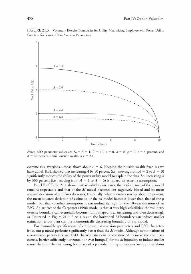
extreme risk aversions—those above about A 5 6. Keeping the outside wealth fixed (as wehave done), BBL showed that increasing A by 50 percent (i.e., moving from A 5 2 to A 5 3)significantly reduces the ability of the power utility model to explain the data. So, increasing Aby 300 percent (i.e., moving from A 5 2 to A 5 6) is indeed an extreme assumption.
Panel B of Table 21.1 shows that as volatility increases, the performance of the μ modelremains respectable and that of the M model becomes less negatively biased and its meansquared deviation of estimates decreases. Eventually, when volatility reaches about 85 percent,the mean squared deviation of estimates of the M model becomes lower than that of the μmodel, but that volatility assumption is extraordinarily high for the 10-year duration of anESO. An artifact of the Carpenter (1998) model is that at very high volatilities, the voluntaryexercise boundary can eventually become hump shaped (i.e., increasing and then decreasing),as illustrated in Figure 21.6.12 As a result, the horizontal M boundary can induce smallerestimation errors than can the monotonically decreasing boundary of a μ model.
For reasonable specifications of employee risk-aversion parameters and ESO character-istics, our μ model performs significantly better than the M model. Although combinations ofrisk-aversion parameters and ESO characteristics can be constructed to make the voluntaryexercise barrier sufficiently horizontal (or even humped) for theM boundary to induce smallererrors than can the decreasing boundary of a μ model, doing so requires assumptions about
FIGURE 21.5 Voluntary Exercise Boundaries for Utility-Maximizing Employee with Power Utility
Function for Various Risk-Aversion ParametersSt
ock
Pric
e, S
($)
5
3
4
2
10 102 64 8
Time, t (years)
A � 1.5
A � 2.0
A � 4.0
A � 6.0
Notes: ESO parameter values are S0 5 X 5 1, T 5 10, v 5 0, d 5 0, q 5 0, r 5 5 percent, andσ 5 40 percent. Initial outside wealth is x 5 2.1.
c21 12 September 2012; 14:21:41
478 Part IV: Option Valuation
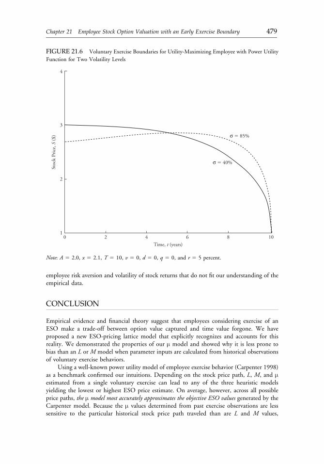
employee risk aversion and volatility of stock returns that do not fit our understanding of theempirical data.
CONCLUSION
Empirical evidence and financial theory suggest that employees considering exercise of anESO make a trade-off between option value captured and time value forgone. We haveproposed a new ESO-pricing lattice model that explicitly recognizes and accounts for thisreality. We demonstrated the properties of our μ model and showed why it is less prone tobias than an L or M model when parameter inputs are calculated from historical observationsof voluntary exercise behaviors.
Using a well-known power utility model of employee exercise behavior (Carpenter 1998)as a benchmark confirmed our intuitions. Depending on the stock price path, L, M, and μestimated from a single voluntary exercise can lead to any of the three heuristic modelsyielding the lowest or highest ESO price estimate. On average, however, across all possibleprice paths, the μ model most accurately approximates the objective ESO values generated by theCarpenter model. Because the μ values determined from past exercise observations are lesssensitive to the particular historical stock price path traveled than are L and M values,
FIGURE 21.6 Voluntary Exercise Boundaries for Utility-Maximizing Employee with Power Utility
Function for Two Volatility LevelsSt
ock
Pric
e, S
($)
4
3
2
10 102 64 8
Time, t (years)
σ � 40%
σ � 85%
Note: A 5 2.0, x 5 2.1, T 5 10, v 5 0, d 5 0, q 5 0, and r 5 5 percent.
c21 12 September 2012; 14:21:41
Chapter 21 Employee Stock Option Valuation with an Early Exercise Boundary 479
estimates from the μ model have much smaller mean squared deviations from objective ESOvalues for reasonable parameters of risk aversion and option specifications. The L model (ormodified Black�Scholes model) is particularly prone to significantly underestimating optionvalues. The M model may be adequate for practical purposes in some circumstances, but it ispotentially vulnerable to significant bias whenever available historical data come from a periodof strong or weak stock returns.
The μ model is intuitively appealing, easily implemented, and compliant with Statementof Financial Accounting Standards No. 123 (revised), Share-Based Payment. Whereas the HWmodel requires the assumption that voluntary early exercise occurs at some fixed multiple ofstrike price, our model assumes that voluntary exercise occurs when the employee can capturesome fixed proportion of the remaining option value. When appropriate, those parameterscan be estimated from historical data. In this regard, we showed why the μ model mayperform more consistently than the HW model.
Our results have management implications for compensation committees and con-sultants who need to understand the potential economic cost of ESO awards to executives andemployees. The findings are also relevant to the work of practitioners who must select ESOvaluation models for accounting disclosure purposes. Academic researchers and other usersof financial statements will also find our results important for understanding the sensitivity ofdisclosed figures to the choice of valuation model and to the estimation of parameter values—which are themselves dependent on the chosen historical dataset.
ACKNOWLEDGMENTS
Neil Brisley acknowledges funding for this research from the Social Sciences and HumanitiesResearch Council of Canada, Grant #410-2007-1564.
NOTES
1. A lattice model divides time between grant and option expiration into N discrete periods.At each time n, possible changes in the underlying stock price between times n andn 1 1 are captured by two (or three) branches. This process is iterated until everypossible path between n 5 0 and n 5 N is mapped. Probabilities are then estimatedalong every stock price path. The stock option payoff outcomes and probabilities flowbackward through the tree until a fair value of the option today is calculated. A simplelattice model for options is the binomial option-pricing model.
2. Statement of Financial Accounting Standards No. 123 (revised), Share-Based Payment(FAS 123R), makes compulsory the expensing of ESOs in the United States as of fiscalyears commencing after June 15, 2005. Similar rules have been implemented by theInternational Accounting Standards Board and the Canadian Accounting StandardsBoard. FAS 123R permits the use of modified Black�Scholes methodologies but alsoenvisages the use of lattice models; the standard specifically cites the HW model andillustrates its use with numerical examples. U.S. SEC Staff Accounting Bulletin No. 107also refers to the HW model.
3. See Huddart (1994); Carpenter (1998); Detemple and Sundaresan (1999).4. Some practitioners using a Black�Scholes approach do not distinguish between vol-
untary early exercise and termination-related exercise or forfeiture. Rather, they combinethese factors into a single expected-life estimate. We do make the distinction here,however, to ensure comparability of the L model with the M and μ models.
c21 12 September 2012; 14:21:41
480 Part IV: Option Valuation
5. In confirmation of this intuition, Carpenter (1998) found that “at firms with strongoverall stock price performance, options are exercised deeper in the money” [p. 139].Bettis, Bizjak, and Lemmon (2005) found “a steady increase in the degree of earlyexercise paralleling the increase in stock market valuations” [p. 457]. Yet, they also statethat “corresponding to the decline in the stock market, we observe options beingexercised later” [p. 457].
6. Carpenter’s model is an extension of earlier work by Huddart (1994) and Kulatilaka andMarcus (1994).
7. Adapting the lattice to make quit rate q endogenous is a simple matter, as in, forexample, Cuny and Jorion (1995).
8. FAS 123R distinguishes between prevesting and postvesting terminations. The assump-tion of a positive quit rate postvesting permanently reduces the accounting value of eachoption granted. Anticipated prevesting termination, however, is ignored in calculating theaccounting value for each option granted. Rather, anticipated prevesting termination istaken into account for accounting purposes by reducing the number of stock options thatare initially recognized to the number expected to vest. The resulting total anticipatedaccounting cost is the same as if prevesting termination were taken into account in thevaluation of each option. The initial expensing effect is precisely the same as if the modelvalue took into account a positive quit rate and did not adjust the number of optionsdownward. The subtle difference is that FAS 123R requires annual adjustment of theaccounting expense, in which companies must adjust the originally anticipated number ofoptions that will vest to the actual number of options that will vest. In this article, we areinterested in comparing the total anticipated accounting cost (which corresponds to theexpected economic cost), so we do not distinguish between pre- and postvesting termi-nation. A trivial adjustment to our model gives the correct FAS 123R treatment.
9. The boundary satisfies the equation S 2 1 5 μB(S,T 2 t). For computational sim-plicity, we measured the full Black�Scholes option value over the remaining term.Alternatively, the lattice itself could be used to determine the remaining option value.
10. The illustrative “past transactions” in this example were generated by the lattice model,for which we already know what stock return volatility to use. With real data, estimatesof μ require estimates of the volatility parameter. BBL are silent, however, about whichmethod they used to calculate volatility for their Ratio statistic. Several approaches arepossible—namely, historical volatility measured in the period prior to exercise, impliedvolatility from comparable traded options or LEAPS (long-term equity anticipationsecurities), or the realized volatility of stock returns in the period after the exercisetransaction until the option’s original maturity date.
11. Carpenter (1998) generalized the power utility approach of Huddart (1994), whoassumed that outside wealth is invested only in the risk-free asset.
12. Carpenter et al. (2007) noted this possibility for certain parameters of risk aversion andvolatility.
REFERENCES
Bettis, J.C., J.M. Bizjak, and M.L. Lemmon. 2005. “Exercise Behavior, Valuation, and the IncentiveEffects of Employee Stock Options.” Journal of Financial Economics, vol. 76, no. 2(May):445�470.
Carpenter, J. 1998. “The Exercise and Valuation of Executive Stock Options.” Journal of FinancialEconomics, vol. 48, no. 2 (May):127�158.
c21 12 September 2012; 14:21:41
Chapter 21 Employee Stock Option Valuation with an Early Exercise Boundary 481
Carpenter, J., R. Stanton, and N. Wallace. 2007. “Optimal Exercise of Executive Stock Options andImplications for Firm Cost.” Working paper.
Cuny, C., and P. Jorion. 1995. “Valuing Executive Stock Options with Endogenous Departure.”Journal of Accounting and Economics, vol. 20, no. 2 (September):193�205.
Detemple, J., and S. Sundaresan. 1999. “Nontraded Asset Valuation with Portfolio Constraints: ABinomial Approach.” Review of Financial Studies, vol. 12, no. 4 (Special Issue):835�872.
Huddart, S. 1994. “Employee Stock Options.” Journal of Accounting and Economics, vol. 18, no. 2(September):207�231.
Huddart, S., and M. Lang. 1996. “Employee Stock Option Exercises: An Empirical Analysis.” Journal ofAccounting and Economics, vol. 21, no. 1 (February):5�43.
Hull, J., and A. White. 2004. “How to Value Employee Stock Options.” Financial Analysts Journal, vol.60, no. 1 (January/February):114�119.
Kulatilaka, N., and A. Marcus. 1994. “Valuing Employee Stock Options.” Financial Analysts Journal,vol. 50, no. 6 (November/December):46�56.10.2469/faj.v50.n6.46
McGeehan, Patrick. 2006. “Options in the Mirror, Bigger Than They Seem.” New York Times (9 April):www.nytimes.com/2006/04/09/business/businessspecial/09fuld.html
Merton, R. 1971. “Optimum Consumption and Portfolio Rules in a Continuous-Time Model.” Journalof Economic Theory, vol. 3, no. 4 (December):373�413.
c21 12 September 2012; 14:21:42
482 Part IV: Option Valuation

PART VREAL OPTIONSVALUATION
Chapter 22 Real Options and Investment Valuation 485
Chapter 23 Real-Options Valuation for a Biotechnology Company 573
c22 12 September 2012; 14:30:33
483

c22 12 September 2012; 14:30:33
CHAPTER 22REAL OPTIONS AND
INVESTMENT VALUATION
DonM. Chance, CFA, and Pamela P. Peterson, CFA
Making an accurate company valuation is the cornerstone of making a soundinvestment decision. But one factor that is often overlooked (and sometimes evenovervalued) is the real options that a company may have. In this chapter, the authorsexplore real-options valuation—looking at these models vis-�a-vis traditional valu-ation models, providing examples and simple case studies, and examining the cri-ticisms and limitations of real-options valuation.
FOREWORD
Real options deal with choices about real investments as opposed to financial investments.Although initially applied to mining, oil, and gas projects, real option valuation has since beenexpanded to address a wide range of managerial choices that affect a company’s value. Tomany financial analysts, the presence of real options is not readily apparent, and even if theyare known, most analysts are unclear about how to value such options. This failure leadsanalysts to incorrectly value companies, and often by a wide margin. With this excellentchapter, Don Chance and Pamela Peterson have produced an invaluable resource to helpfinancial analysts recognize and value real options.
They begin by contrasting real option valuation with traditional discounted cash flowmethods, and they demonstrate the added flexibility associated with real option valuation.Chance and Peterson next use binomial trees to illustrate the valuation of growth options,deferral options, and abandonment options. Growth options offer management the flexibilityto expand the scale of a project. Deferral options enable management to commit quickly
Copyright ª 2002 The Research Foundation of CFA Institute. Reprinted with permission.When this article was originally published (July 2002), Don M. Chance, CFA, was FirstUnion Professor of Financial Risk Management at Virginia Tech and Pamela P. Peterson,CFA, was professor of finance at Florida State University.
c22 12 September 2012; 14:30:33
485
while postponing investment to a future date. Abandonment options grant management theflexibility to terminate further investment and to recover any salvage value.
Chance and Peterson use the continuous time Black�Scholes model to value the realoptions associated with Cisco Systems, and they show how real option valuation uncovers valuethat traditional methods overlook. They are careful, however, to present a balanced view of thisimportant topic by discussing the many challenges associated with real option valuation. Theydescribe, for example, that an increase in volatility raises the value of real options if other factorsare held constant. A rise in volatility, however, may raise the discount rate and thus lower thevalue of the underlying asset, which, in turn, drives down the value of the option. They alsopoint out that real options are not always independent of one another; hence, their values arenot additive. Chance and Peterson underscore the fact that many of the underlying assumptionsassociated with option valuation are not literally true; to wit, returns are not necessarily randomnor precisely lognormally distributed, and volatility is not known and constant. Moreover,valuing real options is usually more difficult than financial options because many of the inputvalues, such as exercise price, discount rate, and time to expiration, are not as easily observable.Chance and Peterson are quick to point out, however, that the opaqueness of these valuespresents a similar challenge to those who rely on traditional valuation methods. They concludewith a review of the empirical research on the accuracy of real option valuation.
Even though real options do not appear on the balance sheet, anyone who is seriousabout asset valuation must be able to identify and value them. These critical tasks are nowmuch easier thanks to Chance and Peterson’s outstanding chapter. The Research Foundationis pleased to present Real Options and Investment Valuation.
Mark Kritzman, CFAResearch Director
The Research Foundation of theAssociation for Investment Management and Research
PREFACE
Real options are opportunities that are associated with investment projects characterized by adegree of flexibility. Real options involve choices: to invest or not, to terminate or continue aninvestment, or to defer or carry on with an investment, to name a few. Real options can haveconsiderable value, not only to the companies possessing them but also to the analystsexamining those companies. Uncovering the value of real options is a challenging task.
The purpose of this chapter is to bridge the gap between theory and practice in theapplication of option valuation methods to capital investment projects and to make realoptions valuation more accessible and comprehensible to practicing financial analysts. A largebody of published literature exists on real options. Some of it is technically quite complex.Much of it oversimplifies the hidden complexities of real options valuation. In this chapter webring to the analyst a consolidated and concise overview of the latest thinking from experts inreal options, showing how these options are structured, how they should be valued, and howto apply the valuation models. In contrast to much of the published work on real options, wealso provide a more critical analysis of the limitations of the models and the difficulties ofusing them.
The chapter is organized in the following manner. In the Introduction, we provide ageneral introduction to the topic of valuing companies and a specific introduction to the topic
c22 12 September 2012; 14:30:33
486 Part V: Real Options Valuation
of valuation techniques with an emphasis on real options valuation. In “Valuation Models:Traditional versus Real Options,” we discuss the traditional approaches to dealing withoptionable elements in an investment opportunity. We demonstrate how discounted cashflow analysis, decision tree analysis, sensitivity analysis, and simulation analysis address theflexibility options in an investment project. We also provide an example of how real optionscan be used in valuation applications beyond capital budgeting. Through examples andapplications presented in “A Framework for the Valuation of Real Options,” we then dem-onstrate a framework for how real options methods provide correct valuations in a variety ofcapital investment settings. Recognizing the many challenges to applying options methods toreal asset investment opportunities, we demonstrate in “Getting Real about Real Options”how to apply real options valuation to a start-up company that has a growth option. In“Pitfalls and Pratfalls in Real Options Valuation,” we discuss the limitations and difficulties ofusing real options, and we challenge the assumptions on which the models are based. In“Empirical Evidence on the Use and Accuracy of Real Options Valuation,” we highlight someempirical evidence on the actual use of real options and the accuracy of the valuations of theseoptions. In the “Summary and Conclusions” section, we provide a capsule summary of thekey findings and conclusions from this chapter.
Some of the terms and phrases in this chapter might be new or only vaguely familiar tosome readers. Thus, to help with the comprehension of this subject, we have included a glossaryat the end of the chapter. To denote a word or phrase found in the glossary, on first use it is givenspecial type treatment. For example, in the following sentence, the phrase “real options valu-ation” is found in the glossary: “This process is referred to as real options valuation.”
We would like to thank the Research Foundation of the Association for InvestmentManagement and Research for its support in making this chapter possible. We especiallyappreciate the assistance, support, and encouragement of Research Director Mark Kritzman.
INTRODUCTION
Analyzing the investment potential of a publicly traded company is a challenging task. Ananalyst assembles a vast amount of information from a variety of sources, carefully avoidinginappropriate nonpublic information and ignoring information in the form of rumor ratherthan fact. Standard discounted cash flow (DCF) techniques are commonly applied to esti-mated future cash flows, leading to an overall assessed value of the company. The analyst mustoften probe not only the finances of a company but also the more subtle possibilities that acompany may have for creating wealth, which is where the task gets really difficult. A goodanalyst uncovers the hidden value in a company. That hidden value may emanate from avariety of sources, but rarely, if ever, will it be easy to detect. Perhaps the difficulty inuncovering hidden value is fortunate, for if it were easy to detect, then in all likelihood, itwould already be built into the current market value. And detecting that hidden value beforeeveryone else is what good analysis is all about.
Although investment analysts rarely delve into the micro level of analyzing specificprojects of companies, they must understand how companies themselves value their owninvestment projects. Some companies make value-enhancing capital investments; others makepoor capital investments. Understanding how companies make capital investments isimportant to an investment analyst looking at a company as an outsider.
The DCF approach to valuation is an important tool in the analysis of a capitalinvestment. The valuation of an investment in physical or real assets typically focuses on a
c22 12 September 2012; 14:30:33
Chapter 22 Real Options and Investment Valuation 487
series of fixed future cash flows that are expected to be generated from this investment.Whether valuing a single project or an entire business enterprise, the valuation process isgenerally the same—estimate future incremental cash flows, discount these flows to thepresent using the appropriate project cost of capital, and compare the present value of thesecash flows with the present value of the investment outlays. Although this approach is gen-erally well accepted, in many instances the DCF approach does not capture the realisticvaluation of an investment. Many investments in real assets have opportunities, such asabandonment, expansion, and deferment, that may alter the investment’s future cash flowsand thus its value. These options generally involve the flexibility to revise decisions in thefuture; hence, they are often referred to as flexibility options.
Consider the valuation of a technology company that has exclusive rights to patents onsoftware that is not yet in the market. Using the DCF approach, the analyst would attempt toestimate the future cash flows that may result when any products using these patents arebrought to market. But missing from the DCF analysis is the ability to capture the flexibilitythat this company has, for example, to delay bringing the products to market, to expand orcontract production once the products are brought to the market, and to abandon produc-tion. And this flexibility is valuable. Moreover, this flexibility is often subtle, if not hidden,and unrecognized by others. Investment analysts should, therefore, understand how com-panies identify and analyze these types of situations.
To properly analyze such opportunities, traditional methods of valuing investments, suchas DCF, should be supplemented with an approach that applies option-pricing methods to thevaluation of capital investments in real assets. This process is referred to as real options val-uation. The importance of real options valuation arises from the fact that traditional methodsof valuation do not directly consider the managerial flexibility available in many investmentdecisions and hence tend to understate the value of investments. Thus, some of a company’svalue can be derived from options that simply do not show up on financial statements.
Real options valuation does not replace traditional DCF methods. Indeed, DCF tech-niques play an important role in the identification of real options and provide input infor-mation for real options valuation. But whereas many analysts are aware of the importance ofincorporating option value in their analysis of an investment, most lack an understanding ofhow to incorporate option valuation into the decision process. For example, Busby and Pitts(1997), in their survey of FTSE 100 companies, found that although most companies areaware of the importance of flexibility options, most do not have procedures for explicitlyincorporating these options in the decision process.1 In turn, investment analysts, observing acompany from the outside, also lack an understanding of the role these options play inassessing the overall value of the company.
Of course, most companies do not possess just one real option. Most have a variety ofdifferent capital investments and many options. This multiplicity of oftentimes interrelatedoptions makes valuing a company and its opportunities even harder. But regardless of thedifficulty, good analysis requires that one face this challenge. And in this day and age when themarket’s valuation of companies, especially technology and Internet-related companies, oftendiffers significantly from that predicted by traditional valuation methods, such as DCFs, P/Es,and dividend valuation models, understanding real options is all the more important.
Real Options in the Technology Sector
Nowhere is the effect of real options on company valuation more apparent than in the Internetand technology sectors. Consider the valuation of Amazon.com, an online retailer. This
c22 12 September 2012; 14:30:33
488 Part V: Real Options Valuation
company has generated losses each year since beginning business in 1995, and it is not expectedto generate a profit at least until 2003. Cash flows are not positive and are not expected to bepositive for a number of years hence. Despite these bleak financial results, its stock has traded ashigh as $113 per share. When Amazon was trading around $64 per share, a little more than halfof that value could be attributed to its cash flows, with at least a part of the remainder attributedto numerous options to expand into different but related markets.2
Amazon’s situation is similar to one discussed in Dunbar (2000). The Real OptionsGroup, a London-based consulting firm, applied real options pricing to value Tiscali, anInternet service provider start-up, and determined that the value of the company exceeded itsDCF because of the company’s options to earn revenues through growth in Europe andthrough growth in the mobile phone market. Although young, start-up technology companieswith little or no earnings histories may be difficult to value and can be overvalued by investorsbased on market hype, cases exist of large companies with established earnings, such as CiscoSystems, that are valued by investors outside the bounds of traditional valuation “yardsticks.”3
Valuation information as of July 28, 2000, for a sampling of companies in both thecomputer services and computer hardware industries is provided in Table 22.1. Industryaverages and the average for the S&P 500 Index are also provided in this table. Although somecompanies have valuations that are in line with those of the traditional valuation indicators(for example, IBM’s P/E of 25.1 is in line with the S&P 500’s P/E of 25.0), several of thecompanies in this table have valuations that are outside traditional reasonable valuationbounds, such as CNET Networks, Lycos, and Yahoo!.
Another example is Yahoo!, a well-known provider of Web services. Yahoo! stock hastraded at a P/E of almost 300 times historical earnings. Unlike some Internet-related com-panies, Yahoo! has generated positive earnings, and its earnings are expected to grow at a rateof 46.3 percent over the next five years (2000�2005). But even with these projected earnings,the current value of the stock far exceeds traditional measures of valuation.4 For example,using the average P/E for the S&P 500 of 25.0, the market cap of Yahoo! is estimated to be$5.9 billion, well below the $68.9 billion actual value.5
So, what do Amazon and Yahoo! have that is valued so highly? The current valuation isnot based on historical performance, and it does not appear to be based on near-term per-formance. In the case of Amazon, the company is a leader in online retailing and hasestablished a significant share of the online retail book market. Being a step ahead in terms oftechnology and marketing strategies online has helped it gain attention and customer loyaltyand has allowed the company to branch out into nonbook markets as well. So, what doesAmazon have? The opportunity to grow not only within its current markets but, moreimportantly, in new markets that leverage its existing infrastructure and customer base. Doesany guarantee exist that Amazon will be able to capitalize on its present position? No, andevaluating the potential rewards and the uncertainties associated with these rewards is difficult.Customer loyalty can be fickle, the company has significant debt obligations, and technologychanges quite rapidly. The first-mover advantage can create short-term value added, but theease of entry into the online market, as seen recently by the traditional “bricks-and-mortar”companies, makes this advantage quite tenuous. In the case of Yahoo!, whose revenues areprimarily from advertising, the company established itself as a portal to the Web and hasadded services, such as auction sites, that expand from its portal existence. So, what doesYahoo! have? The opportunity to grow and, as noted above, to leverage its current operationsinto new activities. Does any guarantee exist that Yahoo! will be able to capitalize on its presentposition as a leading portal that garners significant “hits”? No. The barriers to entry into theportal market are quite low, and technology and tastes change rapidly in this market.
c22 12 September 2012; 14:30:34
Chapter 22 Real Options and Investment Valuation 489
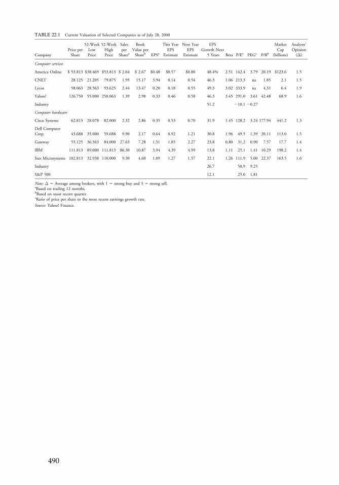
TABLE 22.1 Current Valuation of Selected Companies as of July 28, 2000
CompanyPrice perShare
52-WeekLowPrice
52-WeekHighPrice
Salesper
Sharea
BookValue perShareb EPSa
This YearEPS
Estimate
Next YearEPS
Estimate
EPSGrowth Next
5 Years Beta P/Ea PEGc P/Bb
MarketCap
(billions)
Analysts’Opinion(Δ)
Computer services
America Online $ 53.813 $38.469 $53.813 $ 2.64 $ 2.67 $0.48 $0.57 $0.80 48.4% 2.51 142.4 3.79 20.19 $123.6 1.5
CNET 28.125 21.205 79.875 1.95 15.17 3.94 0.14 0.54 46.3 1.06 213.3 na 1.85 2.1 1.5
Lycos 58.063 28.563 93.625 2.44 13.47 0.20 0.18 0.55 49.3 3.02 333.9 na 4.31 6.4 1.9
Yahoo! 126.750 55.000 250.063 1.39 2.98 0.33 0.46 0.58 46.3 3.45 291.0 3.61 42.48 68.9 1.6
Industry 51.2 210.1 20.27
Computer hardware
Cisco Systems 62.813 28.078 82.000 2.32 2.86 0.35 0.53 0.70 31.9 1.45 128.2 3.24 177.94 441.2 1.3
Dell ComputerCorp. 43.688 35.000 59.688 9.90 2.17 0.64 0.92 1.21 30.8 1.96 49.5 1.39 20.11 113.0 1.5
Gateway 55.125 36.563 84.000 27.63 7.28 1.51 1.85 2.27 23.8 0.80 31.2 0.90 7.57 17.7 1.4
IBM 111.813 89.000 111.813 86.30 10.87 3.94 4.39 4.99 13.8 1.11 25.1 1.41 10.29 198.2 1.4
Sun Microsystems 102.813 32.938 110.000 9.30 4.60 1.09 1.27 1.57 22.1 1.26 111.9 5.00 22.37 163.5 1.6
Industry 26.7 50.9 9.25
S&P 500 12.1 25.0 1.81
Note: Δ 5 Average among brokers, with 1 5 strong buy and 5 5 strong sell.aBased on trailing 12 months.bBased on most recent quarter.cRatio of price per share to the most recent earnings growth rate.
Source: Yahoo! Finance.
c22 12 September 2012; 14:30:35
490
Traditional valuation models that use current and projected earnings and cash flows donot fully capture the potential growth that is not reflected in current and projected earningsand cash flows. Some, such as Schwartz and Moon (2000), have argued that given sufficientlyhigh growth rates and high volatility, the valuations of some of these companies can beexplained using real options. And some, such as Mayor (2001), argue that real options cannotexplain some of the most extreme market valuations relative to DCFs. Furthermore, somehave observed that the extraordinary valuations persist for only the larger companies in theirrespective technology-based industries.6 These examples and more raise the question ofwhether the market is incorporating other factors, such as growth options, into the valuesof the stocks of these companies. These extraordinary valuations have challenged analyststo revise their traditional valuation “yardsticks.” Unless analysts and investors are misvaluingcompanies to an almost unheard-of degree, real options almost surely explain a portion ofthe high values seen in some of these companies.7 Of course, how much real options canaccount for the seemingly excessive valuations of companies is difficult to judge, but withoutan understanding of real options, one might attribute all of an apparent misvaluation toexcessive optimism.
Background and Methodology of Real Options
Real options inherent in capital investment have long been acknowledged. For example,Myers (1977) recognized the importance of considering investment opportunities as growthoptions, and Kester (1984) emphasized the importance of growth options in investmentdecision making. Only recently, however, has much attention been paid to actually applyingthe valuation methods of option-pricing theory to real options. The “bottom line” of realoptions in capital investment is managerial flexibility; every investment project presents somedegree of flexibility in decision making. The first challenge is recognizing the options inherentin investment decisions. The second challenge is to value these options and incorporate theminto the valuation process.
The term “real options” apparently came into being with the 1977 work of Myers, in whichhe breaks down the value of a company into two components—the present value of assets in placeand the present value of future growth opportunities.8 The vast majority of the early academicresearch in real options followingMyers’s work focused on the mining and oil and gas industries.Over time, researchers have explored different options inherent in investment decisions,including the abandonment option, the flexibility to switch, the option to enter and exit, the rightto defer, and the option to exploit successive innovations. A listing of many of the studies on realoptions is provided in Table 22.2. The typical options inherent in an investment opportunityinclude the option to abandon, the option to expand or grow, the option to defer investment, andthe option to change by altering the mix of production or use of the capital assets.
Consider the following two examples that appeared in print recently. Stonier (2001)describes the options inherent in the sales contracts of Airbus Industrie. Aircraft sales contractsinclude many options for the customer—the option to wait to sign a sales contract, the optionfor delivery (specific time), and the option to switch aircraft. Michaels (2000) reports that AirFrance has a nonreported asset whose value is derived from its ability to expand at Charles deGaulle Airport in Paris. Of course, the French air transport industry does not have a monopolyon real options; they appear everywhere. Real options methodology has been applied to valuelease contracts and to the management of foreign currency exposure, among other uses.9 Evensomething as general and as broad as corporate strategy has been described as a “portfolio of realoptions” that cannot be adequately valued using the traditional net present value approach.10
c22 12 September 2012; 14:30:35
Chapter 22 Real Options and Investment Valuation 491
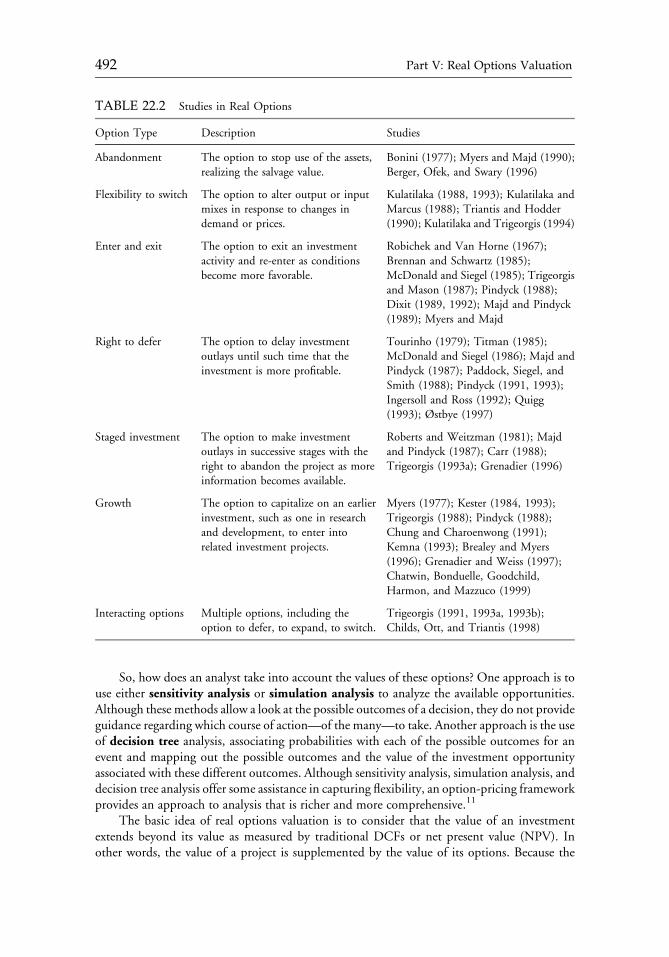
So, how does an analyst take into account the values of these options? One approach is touse either sensitivity analysis or simulation analysis to analyze the available opportunities.Although these methods allow a look at the possible outcomes of a decision, they do not provideguidance regarding which course of action—of the many—to take. Another approach is the useof decision tree analysis, associating probabilities with each of the possible outcomes for anevent and mapping out the possible outcomes and the value of the investment opportunityassociated with these different outcomes. Although sensitivity analysis, simulation analysis, anddecision tree analysis offer some assistance in capturing flexibility, an option-pricing frameworkprovides an approach to analysis that is richer and more comprehensive.11
The basic idea of real options valuation is to consider that the value of an investmentextends beyond its value as measured by traditional DCFs or net present value (NPV). Inother words, the value of a project is supplemented by the value of its options. Because the
TABLE 22.2 Studies in Real Options
Option Type Description Studies
Abandonment The option to stop use of the assets,realizing the salvage value.
Bonini (1977); Myers and Majd (1990);Berger, Ofek, and Swary (1996)
Flexibility to switch The option to alter output or inputmixes in response to changes indemand or prices.
Kulatilaka (1988, 1993); Kulatilaka andMarcus (1988); Triantis and Hodder(1990); Kulatilaka and Trigeorgis (1994)
Enter and exit The option to exit an investmentactivity and re-enter as conditionsbecome more favorable.
Robichek and Van Horne (1967);Brennan and Schwartz (1985);McDonald and Siegel (1985); Trigeorgisand Mason (1987); Pindyck (1988);Dixit (1989, 1992); Majd and Pindyck(1989); Myers and Majd
Right to defer The option to delay investmentoutlays until such time that theinvestment is more profitable.
Tourinho (1979); Titman (1985);McDonald and Siegel (1986); Majd andPindyck (1987); Paddock, Siegel, andSmith (1988); Pindyck (1991, 1993);Ingersoll and Ross (1992); Quigg(1993); Østbye (1997)
Staged investment The option to make investmentoutlays in successive stages with theright to abandon the project as moreinformation becomes available.
Roberts and Weitzman (1981); Majdand Pindyck (1987); Carr (1988);Trigeorgis (1993a); Grenadier (1996)
Growth The option to capitalize on an earlierinvestment, such as one in researchand development, to enter intorelated investment projects.
Myers (1977); Kester (1984, 1993);Trigeorgis (1988); Pindyck (1988);Chung and Charoenwong (1991);Kemna (1993); Brealey and Myers(1996); Grenadier and Weiss (1997);Chatwin, Bonduelle, Goodchild,Harmon, and Mazzuco (1999)
Interacting options Multiple options, including theoption to defer, to expand, to switch.
Trigeorgis (1991, 1993a, 1993b);Childs, Ott, and Triantis (1998)
c22 12 September 2012; 14:30:35
492 Part V: Real Options Valuation
options are considered strategic decisions, the revised or supplemented NPV is referred to asthe strategic NPV. Consider an investment opportunity that has one option associated withit. The strategic NPV is the sum of the traditional NPV, which we call the static NPV, andthe value added of the option analysis:
Strategic NPV ¼ Static NPV þ Value added of the option analysis:
Like options on financial assets, a real option can be a call option, which is the option to buyan asset, or a put option, which is the option to sell an asset. Like other options, a real optioncan be a European option, which is an option that can be exercised only on a specific date, oran American option, which is an option that can be exercised at any time on or before aspecific date. In some cases, a real option can be in the form of an option to exercise anotheroption, which is referred to as a compound option.
All options are characterized by an underlying asset, such as a stock or foreign currency, andpermit the right to buy (if a call) or sell (if a put) the underlying asset at a fixed price. That price iscalled the exercise price, which is also sometimes called the strike price. Options have a finitelife: They expire on a specific date, and either on that date or before (if an American option), adecision is made whether to exercise the option.12 When the holder of a call option exercises it,the exercise price is paid and the underlying asset is acquired; when the holder of a put optionexercises it, the underlying asset is delivered and the exercise price is received.
Determining an option’s value is a task that requires the use of theoretical models. Undercertain assumptions, the valuation of an option is obtained by a formula developed by Black andScholes (1973) and Merton (1973). The formula’s impact on the financial industry has beentremendous and has led to the growth of a large market in financial options and other deri-vatives. It is probably safe to say that this is the most widely applied theoretical model in theentire financial world. In recognition of the tremendous contribution of the model, Scholes andMerton received the 1997 Nobel Prize in economics for their role in its discovery. Black, whohad died in 1995, was ineligible for the award but is widely recognized as a major contributor.Normally referred to as the Black�Scholes model, its derivation is technically quite complex,but its basic structure is simple. This formula relates five factors to the option’s value:
P 5 the underlying asset’s priceX 5 the strike (exercise) price of the optionr 5 the continuously compounded risk-free rate of interestσ 5 volatility (i.e., standard deviation) of the asset’s returnT 5 the time to expiration in years
Mapping the factors that affect the value of a stock option to those that affect the value of areal option, we see that we can capture the value of a real option much as we have with anoption on a financial asset, as shown in Table 22.3.
Although we shall look at the use of this model in more detail in the sections “ValuationModels: Traditional versus Real Options,” “Getting Real about Real Options,” and “Pitfallsand Pratfalls in Real Options Valuation,” consider a simple example, the option to abandon.In this case, the underlying asset consists of the continuing operations, so the value of theunderlying asset is the value associated with the operations. The strike or exercise price for thisoption is the exit value or salvage value of the asset. The time to expiration is a measure ofthe time remaining until the option expires. So, at some point, the option will no longer beavailable. This point may well be at the end of the usable life of the underlying operations, or
c22 12 September 2012; 14:30:35
Chapter 22 Real Options and Investment Valuation 493
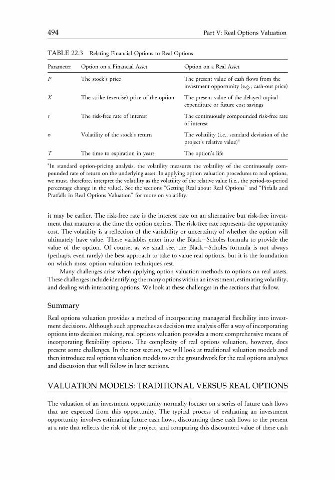
it may be earlier. The risk-free rate is the interest rate on an alternative but risk-free invest-ment that matures at the time the option expires. The risk-free rate represents the opportunitycost. The volatility is a reflection of the variability or uncertainty of whether the option willultimately have value. These variables enter into the Black�Scholes formula to provide thevalue of the option. Of course, as we shall see, the Black�Scholes formula is not always(perhaps, even rarely) the best approach to take to value real options, but it is the foundationon which most option valuation techniques rest.
Many challenges arise when applying option valuation methods to options on real assets.These challenges include identifying themany optionswithin an investment, estimating volatility,and dealing with interacting options. We look at these challenges in the sections that follow.
Summary
Real options valuation provides a method of incorporating managerial flexibility into invest-ment decisions. Although such approaches as decision tree analysis offer a way of incorporatingoptions into decision making, real options valuation provides a more comprehensive means ofincorporating flexibility options. The complexity of real options valuation, however, doespresent some challenges. In the next section, we will look at traditional valuation models andthen introduce real options valuationmodels to set the groundwork for the real options analysesand discussion that will follow in later sections.
VALUATION MODELS: TRADITIONAL VERSUS REAL OPTIONS
The valuation of an investment opportunity normally focuses on a series of future cash flowsthat are expected from this opportunity. The typical process of evaluating an investmentopportunity involves estimating future cash flows, discounting these cash flows to the presentat a rate that reflects the risk of the project, and comparing this discounted value of these cash
TABLE 22.3 Relating Financial Options to Real Options
Parameter Option on a Financial Asset Option on a Real Asset
P The stock’s price The present value of cash flows from theinvestment opportunity (e.g., cash-out price)
X The strike (exercise) price of the option The present value of the delayed capitalexpenditure or future cost savings
r The risk-free rate of interest The continuously compounded risk-free rateof interest
σ Volatility of the stock’s return The volatility (i.e., standard deviation of theproject’s relative value)a
T The time to expiration in years The option’s life
aIn standard option-pricing analysis, the volatility measures the volatility of the continuously com-pounded rate of return on the underlying asset. In applying option valuation procedures to real options,we must, therefore, interpret the volatility as the volatility of the relative value (i.e., the period-to-periodpercentage change in the value). See the sections “Getting Real about Real Options” and “Pitfalls andPratfalls in Real Options Valuation” for more on volatility.
c22 12 September 2012; 14:30:35
494 Part V: Real Options Valuation
flows with the required investment outlay. If the investment is expected to create value—thatis, the present value of these future cash flows exceeds the investment outlay—the project isdesirable; otherwise, the company will not make the investment.
When managers estimate what it costs to invest in a given project and what its benefitswill be in the future, they are coping with uncertainty. The uncertainty arises from differentsources, depending on the type of investment being considered, as well as the circumstancesand the industry in which it is operating. Uncertainty can result from economic factors,market conditions, taxes, and interest rates, among many other sources.
These sources of uncertainty influence future cash flows. Thus, managers need to assess theuncertainty associated with a project’s cash flows in order to select value-adding projects. Oneof the challenges in evaluating an investment opportunity is capturing the flexibility optionsthat a project offers. An approach to dealing with these flexibility options is to use traditionalmethods that have been developed and used to capture some of the uncertainty that a projectcontains. Another approach is to value the project with option-pricing methods. We will firsttake a look at the traditional tools, such as discounted cash flow (DCF) and decision treeanalysis, and then we shall take a look at how option pricing can help value investmentopportunities. These tools will be illustrated by using the following investment opportunity.
Investment Opportunity for the Hokie Company
The Hokie Company is evaluating whether or not to invest in research and devel-opment (R&D). Initially, only two choices exist—to invest $10 million in R&D ornot to invest in R&D. But the investment in R&D is only the beginning. Theoutcome of the R&D is uncertain: The research may yield a product or not. A 70percent chance exists that the R&D will produce a marketable product. For sim-plicity’s sake, assume that the R&D is expected to take three years.
If the research results in what is viewed as a marketable product, the companyfaces another decision—whether to invest $80 million in the manufacturing and saleof the product. Moreover, uncertainty surrounds the actual success of the productintroduction. If the product is successful, the expected cash sales revenues from theproduct are $200 million each year, compared with an unsuccessful product’s rev-enues of $100 million a year. Furthermore, cash expenses are expected to be 75percent of sales revenues. The probability of a successful product in this case is 40percent; the company’s marginal tax rate is 40 percent; and the cost of capital is 20percent, compounded continuously.
Therefore, the Hokie Company has two major decisions to make:
� whether to invest $10 million in R&D, and� depending on the outcome of the R&D, whether to invest $80 million in the
manufacturing and sale of the product, which we shall refer to as production.
This decision process is illustrated in Figure 22.1. The Hokie Company’s decisions andrelated probabilities are indicated by boxes; the circles represent outcomes of those decisions.
We shall take a look at how DCF analysis, sensitivity analysis, simulation analysis,decision tree analysis, and option pricing handle this decision process. Because each methoduses slightly different information in the valuation, where necessary, we will alter the para-meters of the model slightly to help in demonstrating each method.
c22 12 September 2012; 14:30:35
Chapter 22 Real Options and Investment Valuation 495
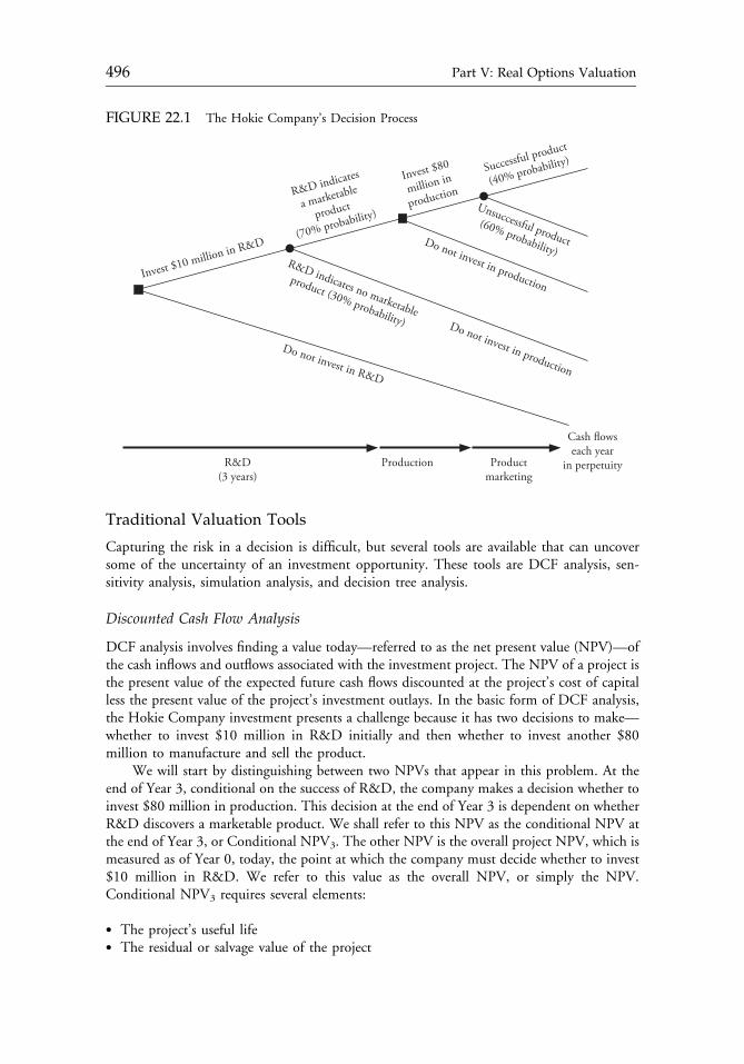
Traditional Valuation Tools
Capturing the risk in a decision is difficult, but several tools are available that can uncoversome of the uncertainty of an investment opportunity. These tools are DCF analysis, sen-sitivity analysis, simulation analysis, and decision tree analysis.
Discounted Cash Flow Analysis
DCF analysis involves finding a value today—referred to as the net present value (NPV)—ofthe cash inflows and outflows associated with the investment project. The NPV of a project isthe present value of the expected future cash flows discounted at the project’s cost of capitalless the present value of the project’s investment outlays. In the basic form of DCF analysis,the Hokie Company investment presents a challenge because it has two decisions to make—whether to invest $10 million in R&D initially and then whether to invest another $80million to manufacture and sell the product.
We will start by distinguishing between two NPVs that appear in this problem. At theend of Year 3, conditional on the success of R&D, the company makes a decision whether toinvest $80 million in production. This decision at the end of Year 3 is dependent on whetherR&D discovers a marketable product. We shall refer to this NPV as the conditional NPV atthe end of Year 3, or Conditional NPV3. The other NPV is the overall project NPV, which ismeasured as of Year 0, today, the point at which the company must decide whether to invest$10 million in R&D. We refer to this value as the overall NPV, or simply the NPV.Conditional NPV3 requires several elements:
� The project’s useful life� The residual or salvage value of the project
FIGURE 22.1 The Hokie Company’s Decision Process
Invest $10 million in R&D Do not invest in production
Do not invest in production
Do not invest in R&D
Production
R&D indicates
a marketable
product
(70% probability)
Invest $80
million in
production
Successful product
(40% probability)
R&D indicates no marketable
product (30% probability)
Unsuccessful product(60% probability)
Cash flowseach year
in perpetuityProductmarketing
R&D(3 years)
c22 12 September 2012; 14:30:36
496 Part V: Real Options Valuation
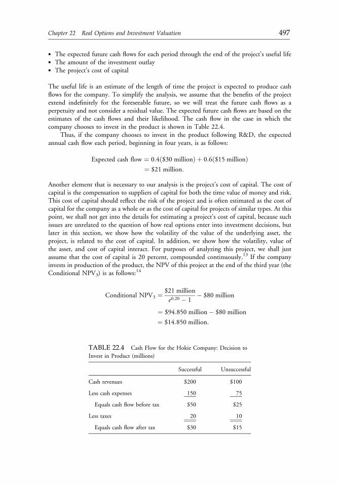
� The expected future cash flows for each period through the end of the project’s useful life� The amount of the investment outlay� The project’s cost of capital
The useful life is an estimate of the length of time the project is expected to produce cashflows for the company. To simplify the analysis, we assume that the benefits of the projectextend indefinitely for the foreseeable future, so we will treat the future cash flows as aperpetuity and not consider a residual value. The expected future cash flows are based on theestimates of the cash flows and their likelihood. The cash flow in the case in which thecompany chooses to invest in the product is shown in Table 22.4.
Thus, if the company chooses to invest in the product following R&D, the expectedannual cash flow each period, beginning in four years, is as follows:
Expected cash flow ¼ 0:4ð$30 millionÞ þ 0:6ð$15 millionÞ¼ $21 million:
Another element that is necessary to our analysis is the project’s cost of capital. The cost ofcapital is the compensation to suppliers of capital for both the time value of money and risk.This cost of capital should reflect the risk of the project and is often estimated as the cost ofcapital for the company as a whole or as the cost of capital for projects of similar types. At thispoint, we shall not get into the details for estimating a project’s cost of capital, because suchissues are unrelated to the question of how real options enter into investment decisions, butlater in this section, we show how the volatility of the value of the underlying asset, theproject, is related to the cost of capital. In addition, we show how the volatility, value ofthe asset, and cost of capital interact. For purposes of analyzing this project, we shall justassume that the cost of capital is 20 percent, compounded continuously.13 If the companyinvests in production of the product, the NPV of this project at the end of the third year (theConditional NPV3) is as follows:
14
Conditional NPV3 ¼ $21 million
e0:20 � 1� $80 million
¼ $94:850 million� $80 million
¼ $14:850 million:
TABLE 22.4 Cash Flow for the Hokie Company: Decision to
Invest in Product (millions)
Successful Unsuccessful
Cash revenues $200 $100
Less cash expenses 150 75
Equals cash flow before tax $50 $25
Less taxes 20 10
Equals cash flow after tax $30 $15
c22 12 September 2012; 14:30:36
Chapter 22 Real Options and Investment Valuation 497
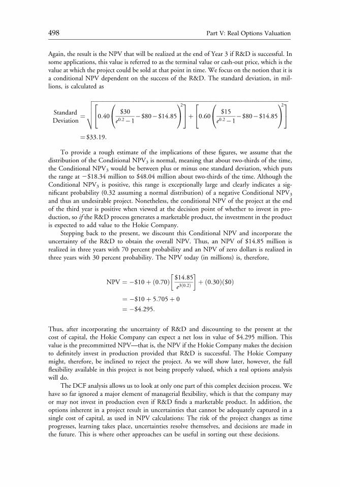
Again, the result is the NPV that will be realized at the end of Year 3 if R&D is successful. Insome applications, this value is referred to as the terminal value or cash-out price, which is thevalue at which the project could be sold at that point in time. We focus on the notion that it isa conditional NPV dependent on the success of the R&D. The standard deviation, in mil-lions, is calculated as
StandardDeviation
¼
ffiffiffiffiffiffiffiffiffiffiffiffiffiffiffiffiffiffiffiffiffiffiffiffiffiffiffiffiffiffiffiffiffiffiffiffiffiffiffiffiffiffiffiffiffiffiffiffiffiffiffiffiffiffiffiffiffiffiffiffiffiffiffiffiffiffiffiffiffiffiffiffiffiffiffiffiffiffiffiffiffiffiffiffiffiffiffiffiffiffiffiffiffiffiffiffiffiffiffiffiffiffiffiffiffiffiffiffiffiffiffiffiffiffiffiffiffiffiffiffiffiffiffiffiffiffiffiffiffiffiffiffiffiffiffiffiffiffiffi0:40
$30
e0:2�1�$80�$14:85
0@
1A22
435þ 0:60
$15
e0:2�1�$80�$14:85
0@
1A22
435
vuuut¼$33:19:
To provide a rough estimate of the implications of these figures, we assume that thedistribution of the Conditional NPV3 is normal, meaning that about two-thirds of the time,the Conditional NPV3 would be between plus or minus one standard deviation, which putsthe range at 2$18.34 million to $48.04 million about two-thirds of the time. Although theConditional NPV3 is positive, this range is exceptionally large and clearly indicates a sig-nificant probability (0.32 assuming a normal distribution) of a negative Conditional NPV3
and thus an undesirable project. Nonetheless, the conditional NPV of the project at the endof the third year is positive when viewed at the decision point of whether to invest in pro-duction, so if the R&D process generates a marketable product, the investment in the productis expected to add value to the Hokie Company.
Stepping back to the present, we discount this Conditional NPV and incorporate theuncertainty of the R&D to obtain the overall NPV. Thus, an NPV of $14.85 million isrealized in three years with 70 percent probability and an NPV of zero dollars is realized inthree years with 30 percent probability. The NPV today (in millions) is, therefore,
NPV ¼ �$10þ ð0:70Þ�$14:85
e3ð0:2Þ
�þ ð0:30Þð$0Þ
¼ �$10þ 5:705þ 0
¼ �$4:295:
Thus, after incorporating the uncertainty of R&D and discounting to the present at thecost of capital, the Hokie Company can expect a net loss in value of $4.295 million. Thisvalue is the precommitted NPV—that is, the NPV if the Hokie Company makes the decisionto definitely invest in production provided that R&D is successful. The Hokie Companymight, therefore, be inclined to reject the project. As we will show later, however, the fullflexibility available in this project is not being properly valued, which a real options analysiswill do.
The DCF analysis allows us to look at only one part of this complex decision process. Wehave so far ignored a major element of managerial flexibility, which is that the company mayor may not invest in production even if R&D finds a marketable product. In addition, theoptions inherent in a project result in uncertainties that cannot be adequately captured in asingle cost of capital, as used in NPV calculations: The risk of the project changes as timeprogresses, learning takes place, uncertainties resolve themselves, and decisions are made inthe future. This is where other approaches can be useful in sorting out these decisions.
c22 12 September 2012; 14:30:36
498 Part V: Real Options Valuation
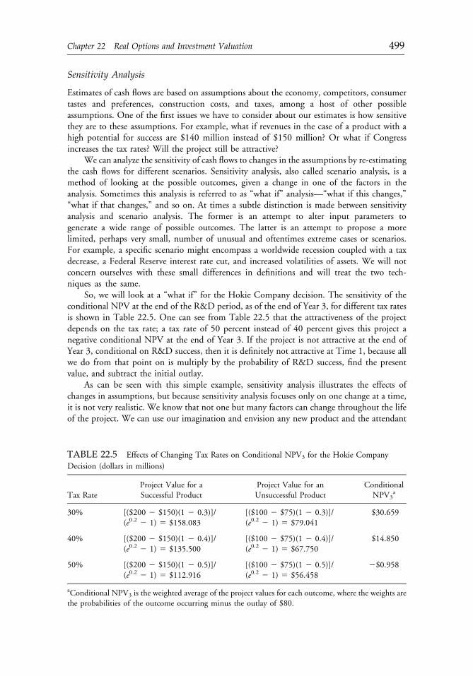
Sensitivity Analysis
Estimates of cash flows are based on assumptions about the economy, competitors, consumertastes and preferences, construction costs, and taxes, among a host of other possibleassumptions. One of the first issues we have to consider about our estimates is how sensitivethey are to these assumptions. For example, what if revenues in the case of a product with ahigh potential for success are $140 million instead of $150 million? Or what if Congressincreases the tax rates? Will the project still be attractive?
We can analyze the sensitivity of cash flows to changes in the assumptions by re-estimatingthe cash flows for different scenarios. Sensitivity analysis, also called scenario analysis, is amethod of looking at the possible outcomes, given a change in one of the factors in theanalysis. Sometimes this analysis is referred to as “what if” analysis—“what if this changes,”“what if that changes,” and so on. At times a subtle distinction is made between sensitivityanalysis and scenario analysis. The former is an attempt to alter input parameters togenerate a wide range of possible outcomes. The latter is an attempt to propose a morelimited, perhaps very small, number of unusual and oftentimes extreme cases or scenarios.For example, a specific scenario might encompass a worldwide recession coupled with a taxdecrease, a Federal Reserve interest rate cut, and increased volatilities of assets. We will notconcern ourselves with these small differences in definitions and will treat the two tech-niques as the same.
So, we will look at a “what if” for the Hokie Company decision. The sensitivity of theconditional NPV at the end of the R&D period, as of the end of Year 3, for different tax ratesis shown in Table 22.5. One can see from Table 22.5 that the attractiveness of the projectdepends on the tax rate; a tax rate of 50 percent instead of 40 percent gives this project anegative conditional NPV at the end of Year 3. If the project is not attractive at the end ofYear 3, conditional on R&D success, then it is definitely not attractive at Time 1, because allwe do from that point on is multiply by the probability of R&D success, find the presentvalue, and subtract the initial outlay.
As can be seen with this simple example, sensitivity analysis illustrates the effects ofchanges in assumptions, but because sensitivity analysis focuses only on one change at a time,it is not very realistic. We know that not one but many factors can change throughout the lifeof the project. We can use our imagination and envision any new product and the attendant
TABLE 22.5 Effects of Changing Tax Rates on Conditional NPV3 for the Hokie Company
Decision (dollars in millions)
Tax RateProject Value for aSuccessful Product
Project Value for anUnsuccessful Product
ConditionalNPV3
a
30% [($200 2 $150)(1 2 0.3)]/(e0.2 2 1) 5 $158.083
[($100 2 $75)(1 2 0.3)]/(e0.2 2 1) 5 $79.041
$30.659
40% [($200 2 $150)(1 2 0.4)]/(e0.2 2 1) 5 $135.500
[($100 2 $75)(1 2 0.4)]/(e0.2 2 1) 5 $67.750
$14.850
50% [($200 2 $150)(1 2 0.5)]/(e0.2 2 1) 5 $112.916
[($100 2 $75)(1 2 0.5)]/(e0.2 2 1) 5 $56.458
2$0.958
aConditional NPV3 is the weighted average of the project values for each outcome, where the weights arethe probabilities of the outcome occurring minus the outlay of $80.
c22 12 September 2012; 14:30:36
Chapter 22 Real Options and Investment Valuation 499
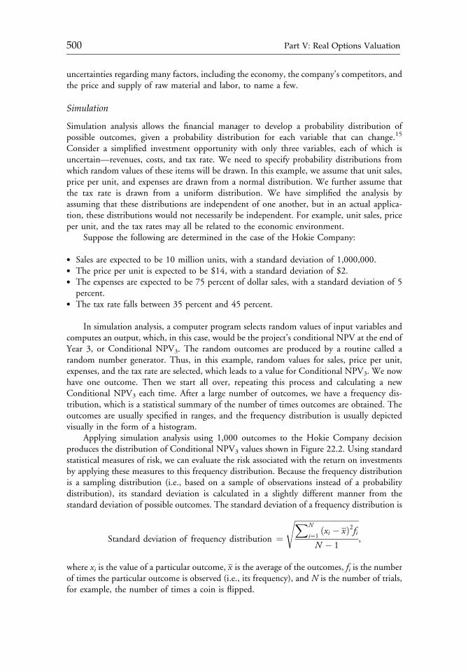
uncertainties regarding many factors, including the economy, the company’s competitors, andthe price and supply of raw material and labor, to name a few.
Simulation
Simulation analysis allows the financial manager to develop a probability distribution ofpossible outcomes, given a probability distribution for each variable that can change.15
Consider a simplified investment opportunity with only three variables, each of which isuncertain—revenues, costs, and tax rate. We need to specify probability distributions fromwhich random values of these items will be drawn. In this example, we assume that unit sales,price per unit, and expenses are drawn from a normal distribution. We further assume thatthe tax rate is drawn from a uniform distribution. We have simplified the analysis byassuming that these distributions are independent of one another, but in an actual applica-tion, these distributions would not necessarily be independent. For example, unit sales, priceper unit, and the tax rates may all be related to the economic environment.
Suppose the following are determined in the case of the Hokie Company:
� Sales are expected to be 10 million units, with a standard deviation of 1,000,000.� The price per unit is expected to be $14, with a standard deviation of $2.� The expenses are expected to be 75 percent of dollar sales, with a standard deviation of 5
percent.� The tax rate falls between 35 percent and 45 percent.
In simulation analysis, a computer program selects random values of input variables andcomputes an output, which, in this case, would be the project’s conditional NPV at the end ofYear 3, or Conditional NPV3. The random outcomes are produced by a routine called arandom number generator. Thus, in this example, random values for sales, price per unit,expenses, and the tax rate are selected, which leads to a value for Conditional NPV3. We nowhave one outcome. Then we start all over, repeating this process and calculating a newConditional NPV3 each time. After a large number of outcomes, we have a frequency dis-tribution, which is a statistical summary of the number of times outcomes are obtained. Theoutcomes are usually specified in ranges, and the frequency distribution is usually depictedvisually in the form of a histogram.
Applying simulation analysis using 1,000 outcomes to the Hokie Company decisionproduces the distribution of Conditional NPV3 values shown in Figure 22.2. Using standardstatistical measures of risk, we can evaluate the risk associated with the return on investmentsby applying these measures to this frequency distribution. Because the frequency distributionis a sampling distribution (i.e., based on a sample of observations instead of a probabilitydistribution), its standard deviation is calculated in a slightly different manner from thestandard deviation of possible outcomes. The standard deviation of a frequency distribution is
Standard deviation of frequency distribution ¼
ffiffiffiffiffiffiffiffiffiffiffiffiffiffiffiffiffiffiffiffiffiffiffiffiffiffiffiffiffiffiffiffiffiXN
i¼1ðxi � xÞ2fi
N � 1
s,
where xi is the value of a particular outcome, x is the average of the outcomes, fi is the numberof times the particular outcome is observed (i.e., its frequency), and N is the number of trials,for example, the number of times a coin is flipped.
c22 12 September 2012; 14:30:36
500 Part V: Real Options Valuation
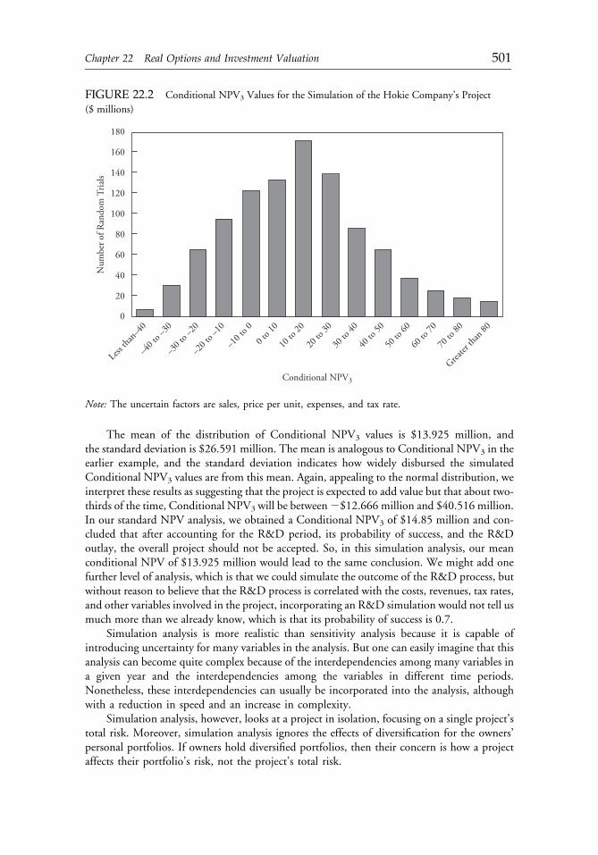
The mean of the distribution of Conditional NPV3 values is $13.925 million, andthe standard deviation is $26.591 million. The mean is analogous to Conditional NPV3 in theearlier example, and the standard deviation indicates how widely disbursed the simulatedConditional NPV3 values are from this mean. Again, appealing to the normal distribution, weinterpret these results as suggesting that the project is expected to add value but that about two-thirds of the time, Conditional NPV3 will be between2$12.666 million and $40.516 million.In our standard NPV analysis, we obtained a Conditional NPV3 of $14.85 million and con-cluded that after accounting for the R&D period, its probability of success, and the R&Doutlay, the overall project should not be accepted. So, in this simulation analysis, our meanconditional NPV of $13.925 million would lead to the same conclusion. We might add onefurther level of analysis, which is that we could simulate the outcome of the R&D process, butwithout reason to believe that the R&D process is correlated with the costs, revenues, tax rates,and other variables involved in the project, incorporating an R&D simulation would not tell usmuch more than we already know, which is that its probability of success is 0.7.
Simulation analysis is more realistic than sensitivity analysis because it is capable ofintroducing uncertainty for many variables in the analysis. But one can easily imagine that thisanalysis can become quite complex because of the interdependencies among many variables ina given year and the interdependencies among the variables in different time periods.Nonetheless, these interdependencies can usually be incorporated into the analysis, althoughwith a reduction in speed and an increase in complexity.
Simulation analysis, however, looks at a project in isolation, focusing on a single project’stotal risk. Moreover, simulation analysis ignores the effects of diversification for the owners’personal portfolios. If owners hold diversified portfolios, then their concern is how a projectaffects their portfolio’s risk, not the project’s total risk.
FIGURE 22.2 Conditional NPV3 Values for the Simulation of the Hokie Company’s Project
($ millions)
Conditional NPV3
Num
ber o
f Ran
dom
Tria
ls
100
80
60
40
20
0
Less th
an–4
0
–40 t
o –30
–30 t
o –20
–20 t
o –10
–10 t
o 0
0 to 1
0
10 to
20
20 to
30
30 to
40
40 to
50
50 to
60
60 to
70
70 to
80
Greater
than
80
120
140
160
180
Note: The uncertain factors are sales, price per unit, expenses, and tax rate.
c22 12 September 2012; 14:30:36
Chapter 22 Real Options and Investment Valuation 501
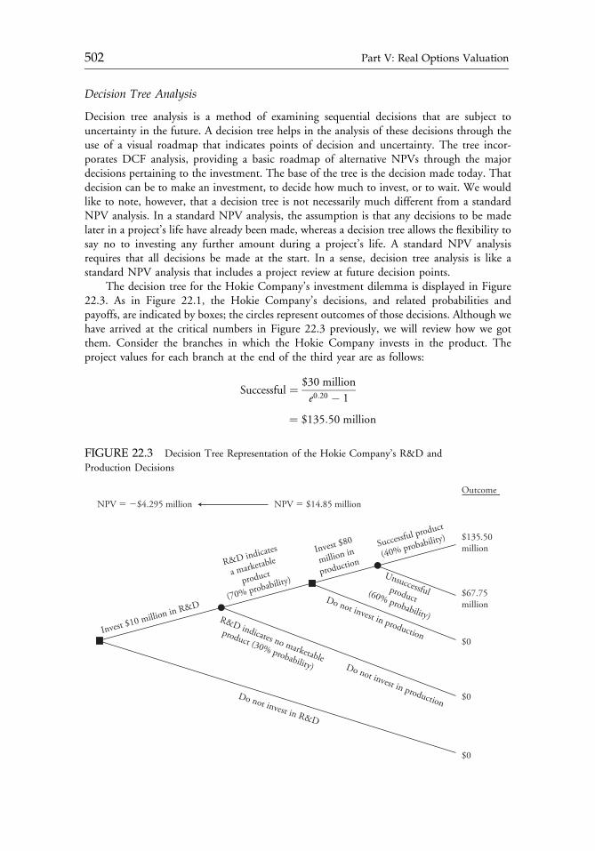
Decision Tree Analysis
Decision tree analysis is a method of examining sequential decisions that are subject touncertainty in the future. A decision tree helps in the analysis of these decisions through theuse of a visual roadmap that indicates points of decision and uncertainty. The tree incor-porates DCF analysis, providing a basic roadmap of alternative NPVs through the majordecisions pertaining to the investment. The base of the tree is the decision made today. Thatdecision can be to make an investment, to decide how much to invest, or to wait. We wouldlike to note, however, that a decision tree is not necessarily much different from a standardNPV analysis. In a standard NPV analysis, the assumption is that any decisions to be madelater in a project’s life have already been made, whereas a decision tree allows the flexibility tosay no to investing any further amount during a project’s life. A standard NPV analysisrequires that all decisions be made at the start. In a sense, decision tree analysis is like astandard NPV analysis that includes a project review at future decision points.
The decision tree for the Hokie Company’s investment dilemma is displayed in Figure22.3. As in Figure 22.1, the Hokie Company’s decisions, and related probabilities andpayoffs, are indicated by boxes; the circles represent outcomes of those decisions. Although wehave arrived at the critical numbers in Figure 22.3 previously, we will review how we gotthem. Consider the branches in which the Hokie Company invests in the product. Theproject values for each branch at the end of the third year are as follows:
Successful ¼ $30 million
e0:20 � 1
¼ $135:50 million
FIGURE 22.3 Decision Tree Representation of the Hokie Company’s R&D and
Production Decisions
NPV � �$4.295 million
Invest $10 million in R&DDo not invest in production
Do not invest in productionDo not invest in R&D
Outcome
$0
$0
$0
NPV � $14.85 million
R&D indicates
a marketable
product
(70% probability)
Invest $80
million in
production
Successful product
(40% probability)
R&D indicates no marketable
product (30% probability)
Unsuccessfulproduct(60% probability)
$135.50million
$67.75million
c22 12 September 2012; 14:30:37
502 Part V: Real Options Valuation
and
Unsuccessful ¼ $15 million
e0:20 � 1
¼ $67:75 million:
As before, the expected payoff of investing in the product, or Conditional NPV3, is
Conditional NPV3 ¼ 0:4ð$135:50 millionÞ þ 0:6ð�$67:75 millionÞ � $80 million
¼ $14:85 million:
As noted previously, the standard deviation of this number is $33.19 million. Basing itsdecision solely on expected NPV, the Hokie Company would invest if the outcome deter-mined by the R&D process yields a payoff of $14.85 million.
From the decision tree analysis, we know that if the R&D is successful, the HokieCompany will definitely invest in the product. Thus, we would discount this $14.85 millionback to the present, weight it by the probability of R&D success, and subtract the initialoutlay. Hence, obtain the overall NPV (in millions) of
NPV ¼ 0:7
�$14:85
e3ð0:20Þ
�þ 0:3ð$0Þ � $10
¼ �$4:295,
which, of course, is the same value we obtained in the DCF analysis.Consider the following variation to this problem. Let the outlay required to initiate
production at the end of Year 3 be $100 million instead of $80 million. We have alreadyshown that the value of the project to invest at the end of Year 3 is $94.85 million. This valuewould not change, but the NPV at the end of Year 3 of investing in production would now be2$5.15 million. Consequently, the decision would be made at the end of Year 3 not to investin production, even if the R&D process produces a successful product. Hence, the value ofthe project today would obviously be zero and the overall NPV would be 2$10 million. Theproject would be rejected. Because a standard NPV analysis with an outlay at the end ofYear 3 of $80 million leads to a negative NPV at Year 0, a standard NPV analysis with anoutlay of $100 million at the end of Year 3 would obviously also lead to a negative NPV atYear 0. These two approaches would, in this case, give the same conclusion but with differentnegative NPVs and for different reasons. Only if the project generates some positive cashflows during the R&D phase would the decision tree approach lead to a different conclusionfrom the one resulting from the standard NPV approach.
With the flexibility afforded by decision trees, one might expect that we could arrive at thecorrect value of the project, but such is not the case. Decision tree analysis, like NPV analysis,relies on the use of a single discount rate to value both the project and the option. As we will showlater, such an approach is not correct. Decision trees, nonetheless, are useful for mapping out thedecision process, especially when there are sequential decisions. As we will show in “A Frame-work for the Valuation of Real Options,” a widely used option valuation approach relies heavilyon the construction of a tree of sequential outcomes much like a decision tree. In contrast to thedecision tree approach, however, option valuation does not require knowledge of the discountrate that reflects risk or knowledge of the actual probabilities of the outcomes. Although optionvaluation imposes other demands, those demands are far less onerous.16
c22 12 September 2012; 14:30:37
Chapter 22 Real Options and Investment Valuation 503
An advantage of using decision tree analysis is its transparency. It does not involve a blackbox of analytical calculations; it is laid out for all to see. This ability to illustrate the decisionpoints and the uncertainties in a concise, clear form makes decision tree analysis attractive. Itis almost surely better than a standard NPV analysis, but neither approach gives the correctanswer when real options are involved. To solve that problem, we turn to an approachdesigned specifically to handle the valuation of options.
Option Valuation
Identifying the options associated with an investment opportunity is the first step toward thecorrect valuation of real options. The second step is to actually assign a value to these options.Consider an opportunity to defer an investment outlay. This investment opportunity issimilar to what a company experiences in its investment in R&D: An expenditure, or series ofexpenditures, is made in R&D, and then sometime in the future, depending on the results ofthe R&D, the actions of competitors, and the approval of regulators, the company decideswhether to go ahead with the investment opportunity.
In the case of the Hokie Company, it has the decision today, Year 0, to invest in R&Dand then a decision at the end of Year 3 to go ahead with production. Consider the elementsof the two decisions—the R&D investment and the production investment. If theHokie Company invests $10 million in R&D, the cash flow today is 2$10 million. Ifthe Hokie Company invests in production, the cash outflow is $80 million. But if the HokieCompany makes this production investment, the expected cash flow each year beyond Year 3is $21 million, as calculated earlier in the DCF analysis. Translating this annual cash flow of$21 million into a project value at the end of Year 3 we arrive at $94.85 million:
Project value at Year 3 ¼ $21 million
e0:20 � 1
¼ $94:85 million:
Subtracting the $80 million investment in production, we find that the conditional NPVat the end of Year 3 is $14.85 million, as shown in Table 22.6—a number we have found inprevious approaches. As we have already shown, the present value of the cash flows, dis-counting at a continuously compounded rate of 20 percent and considering the uncertainty ofR&D, leads to an expected NPV of 2$4.295 million.
So, how much is the option to invest in production at the end of Year 3 worth? We shalluse the Black�Scholes option-pricing formula to value this option. The Black�Scholesformula for a call option is as follows:
Value of option ¼ PN ðd1Þ � Xe�rTN ðd2Þ,
TABLE 22.6 Conditional NPV3 for the Hokie
Company Decision (millions)
Year 0 Year 3
Investment 2$10.00 2$80.00
Terminal value 0.00 94.85
Net cash flow 2$10.00 $14.85
c22 12 September 2012; 14:30:37
504 Part V: Real Options Valuation
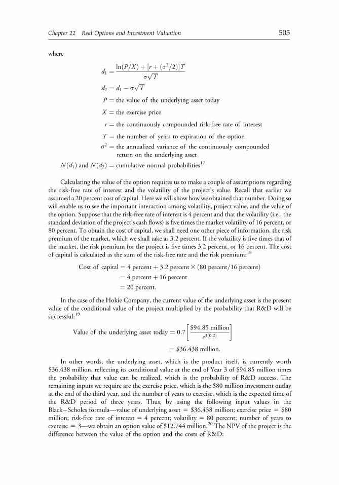
where
d1 ¼ lnðP=X Þ þ ½r þ ðσ2=2Þ�TσffiffiffiffiT
p
d2 ¼ d1 � σffiffiffiffiT
p
P ¼ the value of the underlying asset today
X ¼ the exercise price
r ¼ the continuously compounded risk-free rate of interest
T ¼ the number of years to expiration of the option
σ2 ¼ the annualized variance of the continuously compoundedreturn on the underlying asset
N ðd1Þ and N ðd2Þ ¼ cumulative normal probabilities17
Calculating the value of the option requires us to make a couple of assumptions regardingthe risk-free rate of interest and the volatility of the project’s value. Recall that earlier weassumed a 20 percent cost of capital. Here we will show howwe obtained that number. Doing sowill enable us to see the important interaction among volatility, project value, and the value ofthe option. Suppose that the risk-free rate of interest is 4 percent and that the volatility (i.e., thestandard deviation of the project’s cash flows) is five times the market volatility of 16 percent, or80 percent. To obtain the cost of capital, we shall need one other piece of information, the riskpremium of the market, which we shall take as 3.2 percent. If the volatility is five times that ofthe market, the risk premium for the project is five times 3.2 percent, or 16 percent. The costof capital is calculated as the sum of the risk-free rate and the risk premium:18
Cost of capital ¼ 4 percentþ 3:2 percent3 ð80 percent=16 percentÞ¼ 4 percentþ 16 percent
¼ 20 percent:
In the case of the Hokie Company, the current value of the underlying asset is the presentvalue of the conditional value of the project multiplied by the probability that R&D will besuccessful:19
Value of the underlying asset today ¼ 0:7
�$94:85 million
e3ð0:2Þ
�
¼ $36:438 million:
In other words, the underlying asset, which is the product itself, is currently worth$36.438 million, reflecting its conditional value at the end of Year 3 of $94.85 million timesthe probability that value can be realized, which is the probability of R&D success. Theremaining inputs we require are the exercise price, which is the $80 million investment outlayat the end of the third year, and the number of years to exercise, which is the expected time ofthe R&D period of three years. Thus, by using the following input values in theBlack�Scholes formula—value of underlying asset 5 $36.438 million; exercise price 5 $80million; risk-free rate of interest 5 4 percent; volatility 5 80 percent; number of years toexercise 5 3—we obtain an option value of $12.744 million.20 The NPV of the project is thedifference between the value of the option and the costs of R&D:
c22 12 September 2012; 14:30:37
Chapter 22 Real Options and Investment Valuation 505
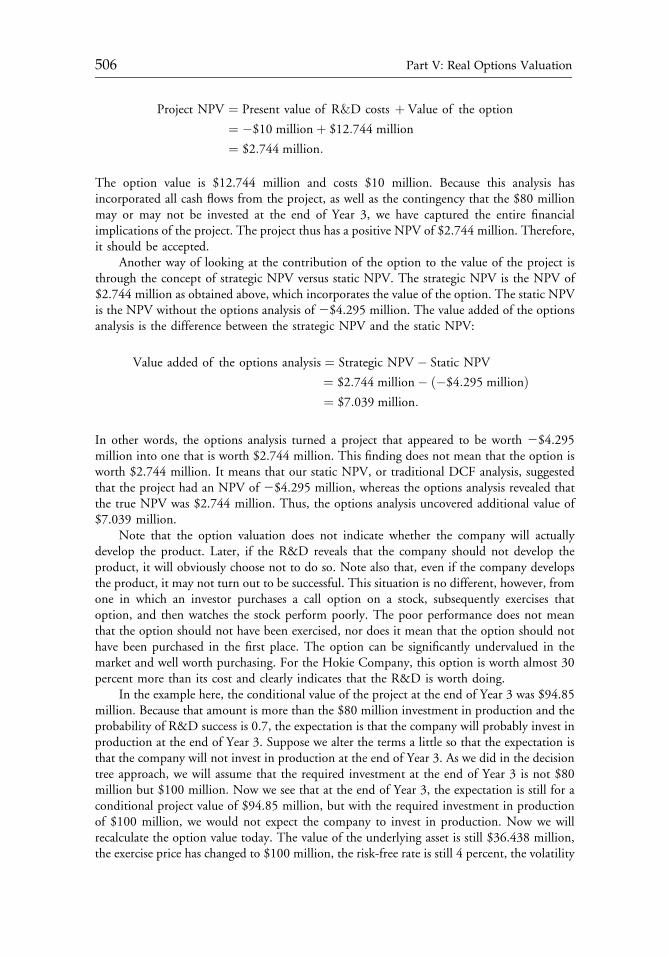
Project NPV ¼ Present value of R&D costs þ Value of the option
¼ �$10 millionþ $12:744 million
¼ $2:744 million:
The option value is $12.744 million and costs $10 million. Because this analysis hasincorporated all cash flows from the project, as well as the contingency that the $80 millionmay or may not be invested at the end of Year 3, we have captured the entire financialimplications of the project. The project thus has a positive NPV of $2.744 million. Therefore,it should be accepted.
Another way of looking at the contribution of the option to the value of the project isthrough the concept of strategic NPV versus static NPV. The strategic NPV is the NPV of$2.744 million as obtained above, which incorporates the value of the option. The static NPVis the NPV without the options analysis of 2$4.295 million. The value added of the optionsanalysis is the difference between the strategic NPV and the static NPV:
Value added of the options analysis ¼ Strategic NPV � Static NPV
¼ $2:744 million� ð�$4:295 millionÞ¼ $7:039 million:
In other words, the options analysis turned a project that appeared to be worth 2$4.295million into one that is worth $2.744 million. This finding does not mean that the option isworth $2.744 million. It means that our static NPV, or traditional DCF analysis, suggestedthat the project had an NPV of 2$4.295 million, whereas the options analysis revealed thatthe true NPV was $2.744 million. Thus, the options analysis uncovered additional value of$7.039 million.
Note that the option valuation does not indicate whether the company will actuallydevelop the product. Later, if the R&D reveals that the company should not develop theproduct, it will obviously choose not to do so. Note also that, even if the company developsthe product, it may not turn out to be successful. This situation is no different, however, fromone in which an investor purchases a call option on a stock, subsequently exercises thatoption, and then watches the stock perform poorly. The poor performance does not meanthat the option should not have been exercised, nor does it mean that the option should nothave been purchased in the first place. The option can be significantly undervalued in themarket and well worth purchasing. For the Hokie Company, this option is worth almost 30percent more than its cost and clearly indicates that the R&D is worth doing.
In the example here, the conditional value of the project at the end of Year 3 was $94.85million. Because that amount is more than the $80 million investment in production and theprobability of R&D success is 0.7, the expectation is that the company will probably invest inproduction at the end of Year 3. Suppose we alter the terms a little so that the expectation isthat the company will not invest in production at the end of Year 3. As we did in the decisiontree approach, we will assume that the required investment at the end of Year 3 is not $80million but $100 million. Now we see that at the end of Year 3, the expectation is still for aconditional project value of $94.85 million, but with the required investment in productionof $100 million, we would not expect the company to invest in production. Now we willrecalculate the option value today. The value of the underlying asset is still $36.438 million,the exercise price has changed to $100 million, the risk-free rate is still 4 percent, the volatility
c22 12 September 2012; 14:30:37
506 Part V: Real Options Valuation
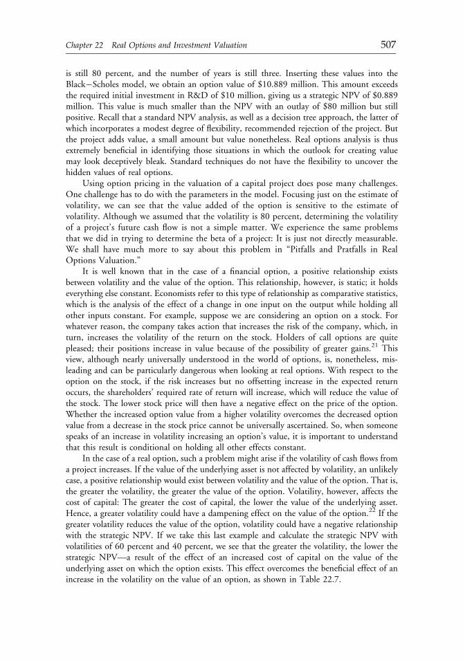
is still 80 percent, and the number of years is still three. Inserting these values into theBlack�Scholes model, we obtain an option value of $10.889 million. This amount exceedsthe required initial investment in R&D of $10 million, giving us a strategic NPV of $0.889million. This value is much smaller than the NPV with an outlay of $80 million but stillpositive. Recall that a standard NPV analysis, as well as a decision tree approach, the latter ofwhich incorporates a modest degree of flexibility, recommended rejection of the project. Butthe project adds value, a small amount but value nonetheless. Real options analysis is thusextremely beneficial in identifying those situations in which the outlook for creating valuemay look deceptively bleak. Standard techniques do not have the flexibility to uncover thehidden values of real options.
Using option pricing in the valuation of a capital project does pose many challenges.One challenge has to do with the parameters in the model. Focusing just on the estimate ofvolatility, we can see that the value added of the option is sensitive to the estimate ofvolatility. Although we assumed that the volatility is 80 percent, determining the volatilityof a project’s future cash flow is not a simple matter. We experience the same problemsthat we did in trying to determine the beta of a project: It is just not directly measurable.We shall have much more to say about this problem in “Pitfalls and Pratfalls in RealOptions Valuation.”
It is well known that in the case of a financial option, a positive relationship existsbetween volatility and the value of the option. This relationship, however, is static; it holdseverything else constant. Economists refer to this type of relationship as comparative statistics,which is the analysis of the effect of a change in one input on the output while holding allother inputs constant. For example, suppose we are considering an option on a stock. Forwhatever reason, the company takes action that increases the risk of the company, which, inturn, increases the volatility of the return on the stock. Holders of call options are quitepleased; their positions increase in value because of the possibility of greater gains.21 Thisview, although nearly universally understood in the world of options, is, nonetheless, mis-leading and can be particularly dangerous when looking at real options. With respect to theoption on the stock, if the risk increases but no offsetting increase in the expected returnoccurs, the shareholders’ required rate of return will increase, which will reduce the value ofthe stock. The lower stock price will then have a negative effect on the price of the option.Whether the increased option value from a higher volatility overcomes the decreased optionvalue from a decrease in the stock price cannot be universally ascertained. So, when someonespeaks of an increase in volatility increasing an option’s value, it is important to understandthat this result is conditional on holding all other effects constant.
In the case of a real option, such a problem might arise if the volatility of cash flows froma project increases. If the value of the underlying asset is not affected by volatility, an unlikelycase, a positive relationship would exist between volatility and the value of the option. That is,the greater the volatility, the greater the value of the option. Volatility, however, affects thecost of capital: The greater the cost of capital, the lower the value of the underlying asset.Hence, a greater volatility could have a dampening effect on the value of the option.22 If thegreater volatility reduces the value of the option, volatility could have a negative relationshipwith the strategic NPV. If we take this last example and calculate the strategic NPV withvolatilities of 60 percent and 40 percent, we see that the greater the volatility, the lower thestrategic NPV—a result of the effect of an increased cost of capital on the value of theunderlying asset on which the option exists. This effect overcomes the beneficial effect of anincrease in the volatility on the value of an option, as shown in Table 22.7.
c22 12 September 2012; 14:30:37
Chapter 22 Real Options and Investment Valuation 507
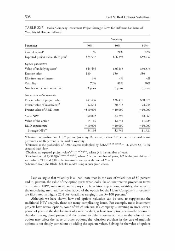
Lest we argue that volatility is all bad, note that in the case of volatilities of 80 percentand 90 percent, the value of the option turns what looks like an unattractive project, in termsof the static NPV, into an attractive project. The relationship among volatility, the value ofthe underlying asset, and the value added of the option for the Hokie Company’s investmentare illustrated in Figure 22.4 for volatilities ranging from 5�100 percent.23
Although we have shown how real options valuation can be used to supplement thetraditional NPV analysis, there are many complicating issues. For example, most investmentprojects have several options, some of which interact. If a company is investing in R&D over aperiod of years in the development of a new product, at least two options exist—the option toabandon during development and the option to defer investment. Because the value of oneoption may affect the value of other options, the valuation problem in the case of multipleoptions is not simply carried out by adding the separate values. Solving for the value of options
TABLE 22.7 Hokie Company Investment Project Strategic NPV for Different Estimates of
Volatility (dollars in millions)
Volatility
Parameter 70% 80% 90%
Cost of capitala 18% 20% 22%
Expected project value, third yearb $74.537 $66.395 $59.737
Option parameters
Value of underlying assetc $43.436 $36.438 $30.875
Exercise price $80 $80 $80
Risk-free rate of interest 4% 4% 4%
Volatility 70% 80% 90%
Number of periods to exercise 3 years 3 years 3 years
Net present value elements
Present value of project value $43.436 $36.438 $30.875
Present value of investmentd 232.634 230.733 228.944
Present value of R&D costs 2$10.000 210.000 210.000
Static NPV $0.802 2$4.295 2$8.069
Value of the option 14.116 12.744 11.724
R&D expenditure 210.000 210.000 210.000
Strategic NPVe $4.116 $2.744 $1.724
aObtained as risk-free rate 1 3.2 percent (volatility/16 percent), where 3.2 percent is the market riskpremium and 16 percent is the market volatility.bObtained as the probability of R&D success multiplied by $21/(ecost of capital 2 1), where $21 is theexpected cash flow.cObtained as expected project value/e33cost of capital, where 3 is the number of years.dObtained as [(0.7)($80)]/e33cost of capital, where 3 is the number of years, 0.7 is the probability ofsuccessful R&D, and $80 is the investment outlay at the end of Year 3.eObtained from the Black�Scholes model using inputs given above.
c22 12 September 2012; 14:30:38
508 Part V: Real Options Valuation
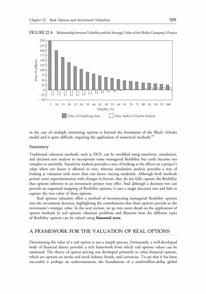
in the case of multiple interacting options is beyond the limitations of the Black�Scholesmodel and is quite difficult, requiring the application of numerical methods.24
Summary
Traditional valuation methods, such as DCF, can be modified using sensitivity, simulation,and decision tree analysis to incorporate some managerial flexibility but easily become toocomplex or unwieldy. Sensitivity analysis provides a way of looking at the effects on a project’svalue when one factor is allowed to vary, whereas simulation analysis provides a way oflooking at valuation with more than one factor varying randomly. Although both methodspermit some experimentation with changes in factors, they do not fully capture the flexibilitythat options inherent in an investment project may offer. And although a decision tree canprovide an organized mapping of flexibility options, it uses a single discount rate and fails tocapture the true value of these options.
Real options valuation offers a method of incorporating managerial flexibility optionsinto the investment decision, highlighting the contributions that these options provide to theinvestment’s strategic value. In the next section, we go into more detail on the application ofoption methods in real options valuation problems and illustrate how the different typesof flexibility options can be valued using binomial trees.
A FRAMEWORK FOR THE VALUATION OF REAL OPTIONS
Determining the value of a real option is not a simple process. Fortunately, a well-developedbody of financial theory provides a rich framework from which real options values can beestimated. The theory of option pricing was developed primarily to value financial options,which are options on stocks and stock indexes, bonds, and currencies. To say that it has beensuccessful is perhaps an understatement; the foundations of a multitrillion-dollar global
FIGURE 22.4 Relationship betweenVolatility and the Strategic Value of theHokieCompany’s ProjectVa
lue
($ m
illio
ns)
75
100125150175200225
50250
�25�50
250
5 10 15 20 25 30 35 40 45 50 55 60 65 70 75 80 85 90 95 100Volatility (%)
Value of Underlying Asset Value Added of Option Analysis
c22 12 September 2012; 14:30:38
Chapter 22 Real Options and Investment Valuation 509
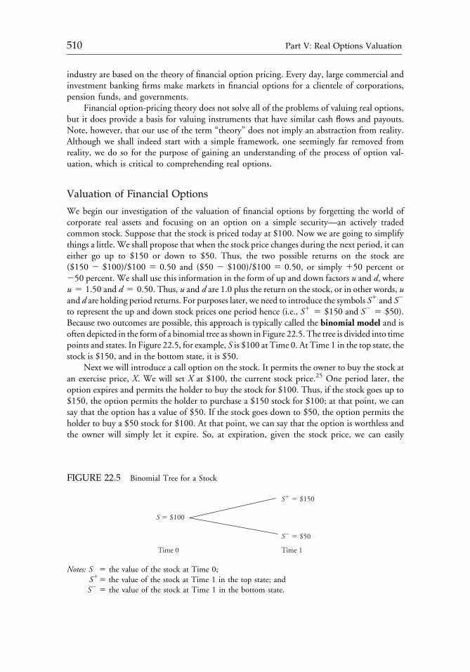
industry are based on the theory of financial option pricing. Every day, large commercial andinvestment banking firms make markets in financial options for a clientele of corporations,pension funds, and governments.
Financial option-pricing theory does not solve all of the problems of valuing real options,but it does provide a basis for valuing instruments that have similar cash flows and payouts.Note, however, that our use of the term “theory” does not imply an abstraction from reality.Although we shall indeed start with a simple framework, one seemingly far removed fromreality, we do so for the purpose of gaining an understanding of the process of option val-uation, which is critical to comprehending real options.
Valuation of Financial Options
We begin our investigation of the valuation of financial options by forgetting the world ofcorporate real assets and focusing on an option on a simple security—an actively tradedcommon stock. Suppose that the stock is priced today at $100. Now we are going to simplifythings a little. We shall propose that when the stock price changes during the next period, it caneither go up to $150 or down to $50. Thus, the two possible returns on the stock are($150 2 $100)/$100 5 0.50 and ($50 2 $100)/$100 5 0.50, or simply 150 percent or250 percent. We shall use this information in the form of up and down factors u and d, whereu 5 1.50 and d 5 0.50. Thus, u and d are 1.0 plus the return on the stock, or in other words, uand d are holding period returns. For purposes later, we need to introduce the symbols S1 and S2
to represent the up and down stock prices one period hence (i.e., S1 5 $150 and S2 5 $50).Because two outcomes are possible, this approach is typically called the binomial model and isoften depicted in the form of a binomial tree as shown in Figure 22.5.The tree is divided into timepoints and states. In Figure 22.5, for example, S is $100 at Time 0. At Time 1 in the top state, thestock is $150, and in the bottom state, it is $50.
Next we will introduce a call option on the stock. It permits the owner to buy the stock atan exercise price, X. We will set X at $100, the current stock price.25 One period later, theoption expires and permits the holder to buy the stock for $100. Thus, if the stock goes up to$150, the option permits the holder to purchase a $150 stock for $100; at that point, we cansay that the option has a value of $50. If the stock goes down to $50, the option permits theholder to buy a $50 stock for $100. At that point, we can say that the option is worthless andthe owner will simply let it expire. So, at expiration, given the stock price, we can easily
FIGURE 22.5 Binomial Tree for a Stock
Time 0 Time 1
S � $100
S� � $150
S� � $50
Notes: S 5 the value of the stock at Time 0;S15 the value of the stock at Time 1 in the top state; andS2 5 the value of the stock at Time 1 in the bottom state.
c22 12 September 2012; 14:30:38
510 Part V: Real Options Valuation
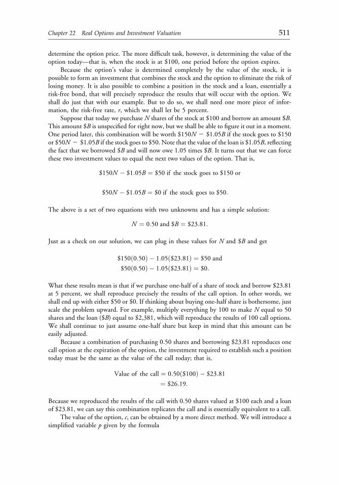
determine the option price. The more difficult task, however, is determining the value of theoption today—that is, when the stock is at $100, one period before the option expires.
Because the option’s value is determined completely by the value of the stock, it ispossible to form an investment that combines the stock and the option to eliminate the risk oflosing money. It is also possible to combine a position in the stock and a loan, essentially arisk-free bond, that will precisely reproduce the results that will occur with the option. Weshall do just that with our example. But to do so, we shall need one more piece of infor-mation, the risk-free rate, r, which we shall let be 5 percent.
Suppose that today we purchase N shares of the stock at $100 and borrow an amount $B.This amount $B is unspecified for right now, but we shall be able to figure it out in a moment.One period later, this combination will be worth $150N 2 $1.05B if the stock goes to $150or $50N 2 $1.05B if the stock goes to $50. Note that the value of the loan is $1.05B, reflectingthe fact that we borrowed $B and will now owe 1.05 times $B. It turns out that we can forcethese two investment values to equal the next two values of the option. That is,
$150N � $1:05B ¼ $50 if the stock goes to $150 or
$50N � $1:05B ¼ $0 if the stock goes to $50:
The above is a set of two equations with two unknowns and has a simple solution:
N ¼ 0:50 and $B ¼ $23:81:
Just as a check on our solution, we can plug in these values for N and $B and get
$150ð0:50Þ � 1:05ð$23:81Þ ¼ $50 and
$50ð0:50Þ � 1:05ð$23:81Þ ¼ $0:
What these results mean is that if we purchase one-half of a share of stock and borrow $23.81at 5 percent, we shall reproduce precisely the results of the call option. In other words, weshall end up with either $50 or $0. If thinking about buying one-half share is bothersome, justscale the problem upward. For example, multiply everything by 100 to make N equal to 50shares and the loan ($B) equal to $2,381, which will reproduce the results of 100 call options.We shall continue to just assume one-half share but keep in mind that this amount can beeasily adjusted.
Because a combination of purchasing 0.50 shares and borrowing $23.81 reproduces onecall option at the expiration of the option, the investment required to establish such a positiontoday must be the same as the value of the call today; that is,
Value of the call ¼ 0:50ð$100Þ � $23:81
¼ $26:19:
Because we reproduced the results of the call with 0.50 shares valued at $100 each and a loanof $23.81, we can say this combination replicates the call and is essentially equivalent to a call.
The value of the option, c, can be obtained by a more direct method. We will introduce asimplified variable p given by the formula
c22 12 September 2012; 14:30:38
Chapter 22 Real Options and Investment Valuation 511
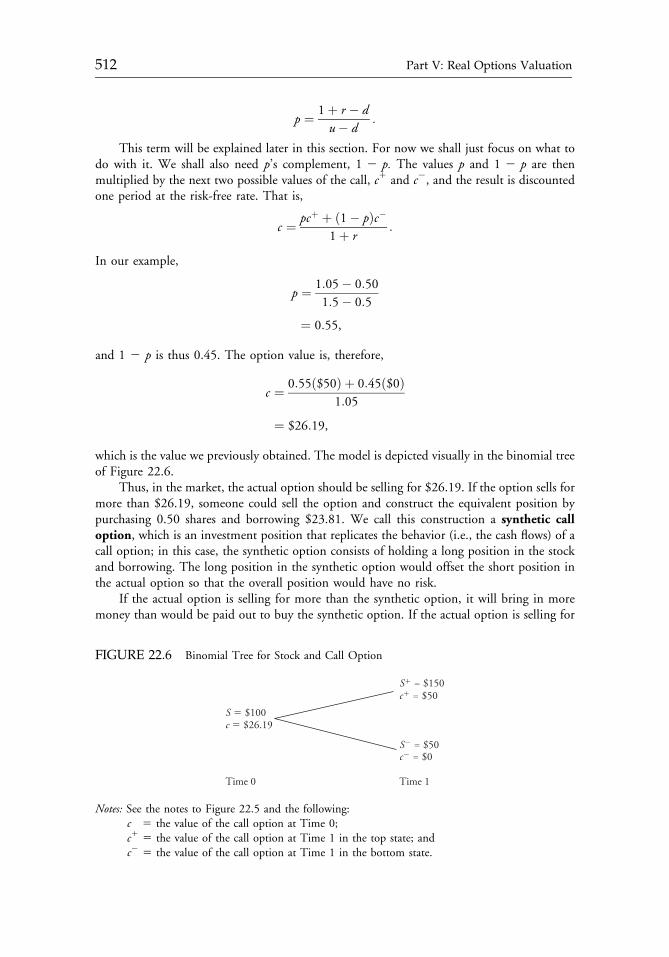
p ¼ 1þ r � du� d
:
This term will be explained later in this section. For now we shall just focus on what todo with it. We shall also need p’s complement, 1 2 p. The values p and 1 2 p are thenmultiplied by the next two possible values of the call, c1 and c2, and the result is discountedone period at the risk-free rate. That is,
c ¼ pcþ þ ð1� pÞc�1þ r
:
In our example,
p ¼ 1:05� 0:50
1:5� 0:5
¼ 0:55,
and 1 2 p is thus 0.45. The option value is, therefore,
c ¼ 0:55ð$50Þ þ 0:45ð$0Þ1:05
¼ $26:19,
which is the value we previously obtained. The model is depicted visually in the binomial treeof Figure 22.6.
Thus, in the market, the actual option should be selling for $26.19. If the option sells formore than $26.19, someone could sell the option and construct the equivalent position bypurchasing 0.50 shares and borrowing $23.81. We call this construction a synthetic calloption, which is an investment position that replicates the behavior (i.e., the cash flows) of acall option; in this case, the synthetic option consists of holding a long position in the stockand borrowing. The long position in the synthetic option would offset the short position inthe actual option so that the overall position would have no risk.
If the actual option is selling for more than the synthetic option, it will bring in moremoney than would be paid out to buy the synthetic option. If the actual option is selling for
FIGURE 22.6 Binomial Tree for Stock and Call Option
Time 1Time 0
c � $26.19S � $100
c� � $50
S� � $50c� � $0
S� � $150
Notes: See the notes to Figure 22.5 and the following:c 5 the value of the call option at Time 0;c1 5 the value of the call option at Time 1 in the top state; andc2 5 the value of the call option at Time 1 in the bottom state.
c22 12 September 2012; 14:30:38
512 Part V: Real Options Valuation
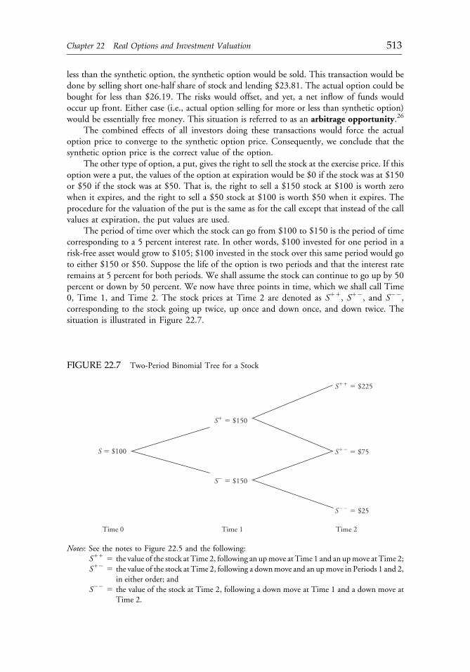
less than the synthetic option, the synthetic option would be sold. This transaction would bedone by selling short one-half share of stock and lending $23.81. The actual option could bebought for less than $26.19. The risks would offset, and yet, a net inflow of funds wouldoccur up front. Either case (i.e., actual option selling for more or less than synthetic option)would be essentially free money. This situation is referred to as an arbitrage opportunity.26
The combined effects of all investors doing these transactions would force the actualoption price to converge to the synthetic option price. Consequently, we conclude that thesynthetic option price is the correct value of the option.
The other type of option, a put, gives the right to sell the stock at the exercise price. If thisoption were a put, the values of the option at expiration would be $0 if the stock was at $150or $50 if the stock was at $50. That is, the right to sell a $150 stock at $100 is worth zerowhen it expires, and the right to sell a $50 stock at $100 is worth $50 when it expires. Theprocedure for the valuation of the put is the same as for the call except that instead of the callvalues at expiration, the put values are used.
The period of time over which the stock can go from $100 to $150 is the period of timecorresponding to a 5 percent interest rate. In other words, $100 invested for one period in arisk-free asset would grow to $105; $100 invested in the stock over this same period would goto either $150 or $50. Suppose the life of the option is two periods and that the interest rateremains at 5 percent for both periods. We shall assume the stock can continue to go up by 50percent or down by 50 percent. We now have three points in time, which we shall call Time0, Time 1, and Time 2. The stock prices at Time 2 are denoted as S11, S12, and S22,corresponding to the stock going up twice, up once and down once, and down twice. Thesituation is illustrated in Figure 22.7.
FIGURE 22.7 Two-Period Binomial Tree for a Stock
S � $100
Time 0 Time 1 Time 2
S� � $150
S�� � $225
S�� � $75
S�� � $25
S� � $150
Notes: See the notes to Figure 22.5 and the following:S11 5 the value of the stock at Time 2, following an upmove at Time 1 and an upmove at Time 2;S12 5 the value of the stock at Time 2, following a downmove and an upmove in Periods 1 and 2,
in either order; andS22 5 the value of the stock at Time 2, following a down move at Time 1 and a down move at
Time 2.
c22 12 September 2012; 14:30:39
Chapter 22 Real Options and Investment Valuation 513
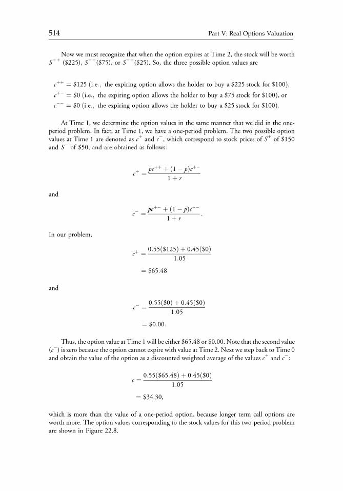
Now we must recognize that when the option expires at Time 2, the stock will be worthS11 ($225), S12($75), or S22($25). So, the three possible option values are
cþþ ¼ $125 ði:e:; the expiring option allows the holder to buy a $225 stock for $100Þ,cþ� ¼ $0 ði:e:; the expiring option allows the holder to buy a $75 stock for $100Þ, orc�� ¼ $0 ði:e:; the expiring option allows the holder to buy a $25 stock for $100Þ:
At Time 1, we determine the option values in the same manner that we did in the one-period problem. In fact, at Time 1, we have a one-period problem. The two possible optionvalues at Time 1 are denoted as c1 and c2, which correspond to stock prices of S1 of $150and S2 of $50, and are obtained as follows:
cþ ¼ pcþþ þ ð1� pÞcþ�
1þ r
and
c� ¼ pcþ� þ ð1� pÞc��
1þ r:
In our problem,
cþ ¼ 0:55ð$125Þ þ 0:45ð$0Þ1:05
¼ $65:48
and
c� ¼ 0:55ð$0Þ þ 0:45ð$0Þ1:05
¼ $0:00:
Thus, the option value at Time 1 will be either $65.48 or $0.00. Note that the second value(c2) is zero because the option cannot expire with value at Time 2. Next we step back to Time 0and obtain the value of the option as a discounted weighted average of the values c1 and c2:
c ¼ 0:55ð$65:48Þ þ 0:45ð$0Þ1:05
¼ $34:30,
which is more than the value of a one-period option, because longer term call options areworth more. The option values corresponding to the stock values for this two-period problemare shown in Figure 22.8.
c22 12 September 2012; 14:30:39
514 Part V: Real Options Valuation
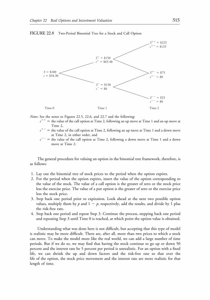
The general procedure for valuing an option in the binomial tree framework, therefore, isas follows:
1. Lay out the binomial tree of stock prices to the period when the option expires.2. For the period when the option expires, insert the value of the option corresponding to
the value of the stock. The value of a call option is the greater of zero or the stock priceless the exercise price. The value of a put option is the greater of zero or the exercise priceless the stock price.
3. Step back one period prior to expiration. Look ahead at the next two possible optionvalues, multiply them by p and 1 2 p, respectively, add the results, and divide by 1 plusthe risk-free rate.
4. Step back one period and repeat Step 3. Continue the process, stepping back one periodand repeating Step 3 until Time 0 is reached, at which point the option value is obtained.
Understanding what was done here is not difficult, but accepting that this type of modelis realistic may be more difficult. There are, after all, more than two prices to which a stockcan move. To make the model more like the real world, we can add a large number of timeperiods. But if we do so, we may find that having the stock continue to go up or down 50percent and the interest rate be 5 percent per period is unrealistic. For an option with a fixedlife, we can shrink the up and down factors and the risk-free rate so that over thelife of the option, the stock price movement and the interest rate are more realistic for thatlength of time.
FIGURE 22.8 Two-Period Binomial Tree for a Stock and Call Option
S � $100
S� � $150
c � $34.30
Time 0 Time 1 Time 2
c� � $65.48
S�� � $225
S�� � $75
S�� � $25
c�� � $0
c�� � $0
S� � $150c� � $0
c�� � $125
Notes: See the notes to Figures 22.5, 22.6, and 22.7 and the following:c11 5 the value of the call option at Time 2, following an up move at Time 1 and an up move at
Time 2,c12 5 the value of the call option at Time 2, following an up move at Time 1 and a down move
at Time 2, in either order, andc22 5 the value of the call option at Time 2, following a down move at Time 1 and a down
move at Time 2.
c22 12 September 2012; 14:30:39
Chapter 22 Real Options and Investment Valuation 515
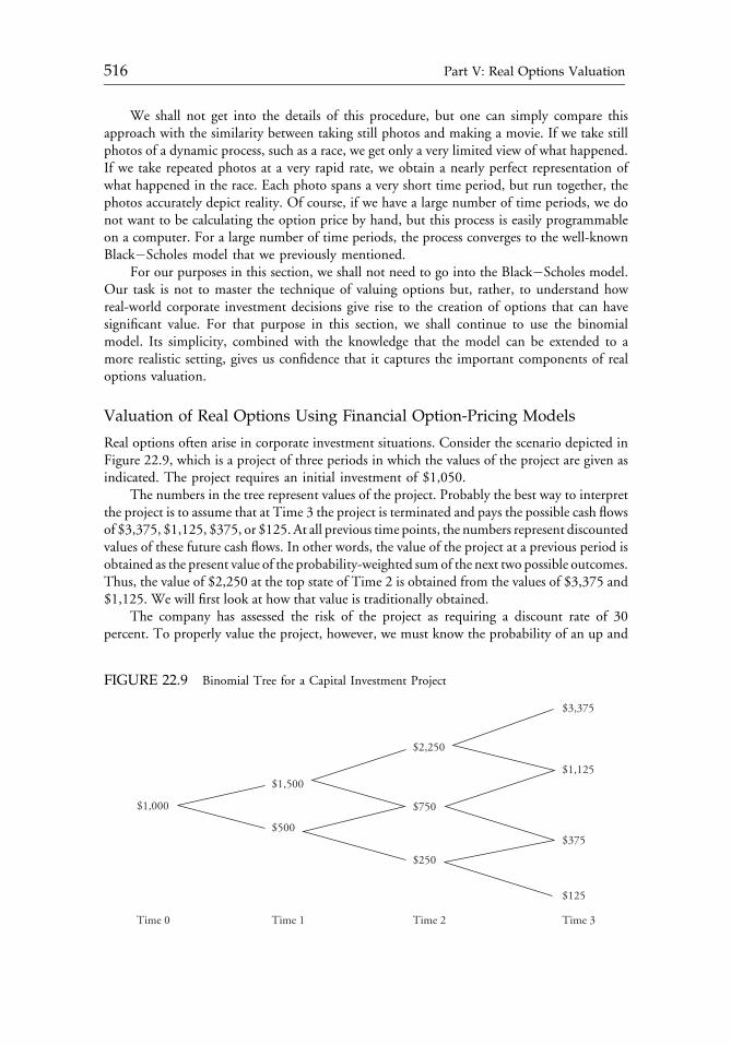
We shall not get into the details of this procedure, but one can simply compare thisapproach with the similarity between taking still photos and making a movie. If we take stillphotos of a dynamic process, such as a race, we get only a very limited view of what happened.If we take repeated photos at a very rapid rate, we obtain a nearly perfect representation ofwhat happened in the race. Each photo spans a very short time period, but run together, thephotos accurately depict reality. Of course, if we have a large number of time periods, we donot want to be calculating the option price by hand, but this process is easily programmableon a computer. For a large number of time periods, the process converges to the well-knownBlack�Scholes model that we previously mentioned.
For our purposes in this section, we shall not need to go into the Black�Scholes model.Our task is not to master the technique of valuing options but, rather, to understand howreal-world corporate investment decisions give rise to the creation of options that can havesignificant value. For that purpose in this section, we shall continue to use the binomialmodel. Its simplicity, combined with the knowledge that the model can be extended to amore realistic setting, gives us confidence that it captures the important components of realoptions valuation.
Valuation of Real Options Using Financial Option-Pricing Models
Real options often arise in corporate investment situations. Consider the scenario depicted inFigure 22.9, which is a project of three periods in which the values of the project are given asindicated. The project requires an initial investment of $1,050.
The numbers in the tree represent values of the project. Probably the best way to interpretthe project is to assume that at Time 3 the project is terminated and pays the possible cash flowsof $3,375, $1,125, $375, or $125. At all previous time points, the numbers represent discountedvalues of these future cash flows. In other words, the value of the project at a previous period isobtained as the present value of the probability-weighted sum of the next two possible outcomes.Thus, the value of $2,250 at the top state of Time 2 is obtained from the values of $3,375 and$1,125. We will first look at how that value is traditionally obtained.
The company has assessed the risk of the project as requiring a discount rate of 30percent. To properly value the project, however, we must know the probability of an up and
FIGURE 22.9 Binomial Tree for a Capital Investment Project
$1,000
$1,500
$500
$2,250
$750
$250
$3,375
$1,125
$375
$125
Time 0 Time 1 Time 2 Time 3
c22 12 September 2012; 14:30:39
516 Part V: Real Options Valuation
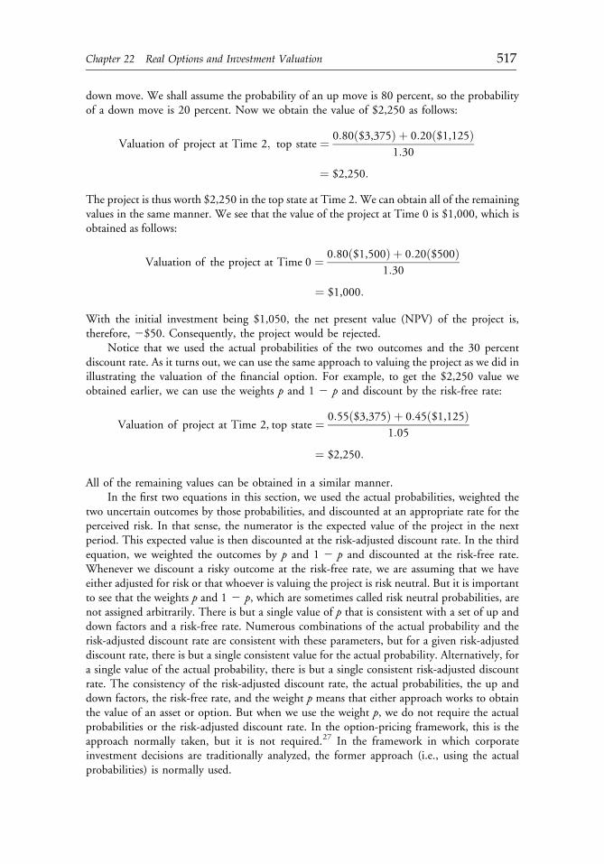
down move. We shall assume the probability of an up move is 80 percent, so the probabilityof a down move is 20 percent. Now we obtain the value of $2,250 as follows:
Valuation of project at Time 2; top state ¼ 0:80ð$3,375Þ þ 0:20ð$1,125Þ1:30
¼ $2,250:
The project is thus worth $2,250 in the top state at Time 2. We can obtain all of the remainingvalues in the same manner. We see that the value of the project at Time 0 is $1,000, which isobtained as follows:
Valuation of the project at Time 0 ¼ 0:80ð$1,500Þ þ 0:20ð$500Þ1:30
¼ $1,000:
With the initial investment being $1,050, the net present value (NPV) of the project is,therefore, 2$50. Consequently, the project would be rejected.
Notice that we used the actual probabilities of the two outcomes and the 30 percentdiscount rate. As it turns out, we can use the same approach to valuing the project as we did inillustrating the valuation of the financial option. For example, to get the $2,250 value weobtained earlier, we can use the weights p and 1 2 p and discount by the risk-free rate:
Valuation of project at Time 2, top state ¼ 0:55ð$3,375Þ þ 0:45ð$1,125Þ1:05
¼ $2,250:
All of the remaining values can be obtained in a similar manner.In the first two equations in this section, we used the actual probabilities, weighted the
two uncertain outcomes by those probabilities, and discounted at an appropriate rate for theperceived risk. In that sense, the numerator is the expected value of the project in the nextperiod. This expected value is then discounted at the risk-adjusted discount rate. In the thirdequation, we weighted the outcomes by p and 1 2 p and discounted at the risk-free rate.Whenever we discount a risky outcome at the risk-free rate, we are assuming that we haveeither adjusted for risk or that whoever is valuing the project is risk neutral. But it is importantto see that the weights p and 1 2 p, which are sometimes called risk neutral probabilities, arenot assigned arbitrarily. There is but a single value of p that is consistent with a set of up anddown factors and a risk-free rate. Numerous combinations of the actual probability and therisk-adjusted discount rate are consistent with these parameters, but for a given risk-adjusteddiscount rate, there is but a single consistent value for the actual probability. Alternatively, fora single value of the actual probability, there is but a single consistent risk-adjusted discountrate. The consistency of the risk-adjusted discount rate, the actual probabilities, the up anddown factors, the risk-free rate, and the weight p means that either approach works to obtainthe value of an asset or option. But when we use the weight p, we do not require the actualprobabilities or the risk-adjusted discount rate. In the option-pricing framework, this is theapproach normally taken, but it is not required.27 In the framework in which corporateinvestment decisions are traditionally analyzed, the former approach (i.e., using the actualprobabilities) is normally used.
c22 12 September 2012; 14:30:39
Chapter 22 Real Options and Investment Valuation 517
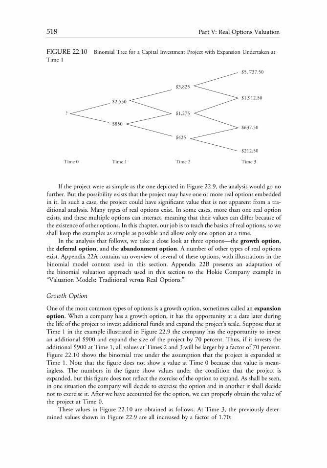
If the project were as simple as the one depicted in Figure 22.9, the analysis would go nofurther. But the possibility exists that the project may have one or more real options embeddedin it. In such a case, the project could have significant value that is not apparent from a tra-ditional analysis. Many types of real options exist. In some cases, more than one real optionexists, and these multiple options can interact, meaning that their values can differ because ofthe existence of other options. In this chapter, our job is to teach the basics of real options, so weshall keep the examples as simple as possible and allow only one option at a time.
In the analysis that follows, we take a close look at three options—the growth option,the deferral option, and the abandonment option. A number of other types of real optionsexist. Appendix 22A contains an overview of several of these options, with illustrations in thebinomial model context used in this section. Appendix 22B presents an adaptation ofthe binomial valuation approach used in this section to the Hokie Company example in“Valuation Models: Traditional versus Real Options.”
Growth Option
One of the most common types of options is a growth option, sometimes called an expansionoption. When a company has a growth option, it has the opportunity at a date later duringthe life of the project to invest additional funds and expand the project’s scale. Suppose that atTime 1 in the example illustrated in Figure 22.9 the company has the opportunity to investan additional $900 and expand the size of the project by 70 percent. Thus, if it invests theadditional $900 at Time 1, all values at Times 2 and 3 will be larger by a factor of 70 percent.Figure 22.10 shows the binomial tree under the assumption that the project is expanded atTime 1. Note that the figure does not show a value at Time 0 because that value is mean-ingless. The numbers in the figure show values under the condition that the project isexpanded, but this figure does not reflect the exercise of the option to expand. As shall be seen,in one situation the company will decide to exercise the option and in another it shall decidenot to exercise it. After we have accounted for the option, we can properly obtain the value ofthe project at Time 0.
These values in Figure 22.10 are obtained as follows. At Time 3, the previously deter-mined values shown in Figure 22.9 are all increased by a factor of 1.70:
FIGURE 22.10 Binomial Tree for a Capital Investment Project with Expansion Undertaken at
Time 1
?
$2,550
$850
$3,825
$1,275
$425
$5, 737.50
$1,912.50
$637.50
$212.50
Time 0 Time 1 Time 2 Time 3
c22 12 September 2012; 14:30:39
518 Part V: Real Options Valuation
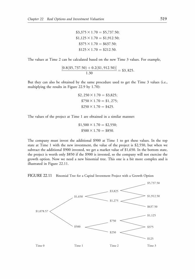
$3,3753 1:70 ¼ $5,737:50;
$1,1253 1:70 ¼ $1,912:50;
$3753 1:70 ¼ $637:50;
$1253 1:70 ¼ $212:50:
The values at Time 2 can be calculated based on the new Time 3 values. For example,
½0:8ð$5; 737:50Þ þ 0:2ð$1; 912:50Þ�1:30
¼ $3; 825:
But they can also be obtained by the same procedure used to get the Time 3 values (i.e.,multiplying the results in Figure 22.9 by 1.70):
$2; 2503 1:70 ¼ $3,825;
$7503 1:70 ¼ $1; 275;
$2503 1:70 ¼ $425:
The values of the project at Time 1 are obtained in a similar manner:
$1,5003 1:70 ¼ $2,550;
$5003 1:70 ¼ $850:
The company must invest the additional $900 at Time 1 to get these values. In the topstate at Time 1 with the new investment, the value of the project is $2,550, but when wesubtract the additional $900 invested, we get a market value of $1,650. In the bottom state,the project is worth only $850 if the $900 is invested, so the company will not exercise thegrowth option. Now we need a new binomial tree. This one is a bit more complex and isillustrated in Figure 22.11.
FIGURE 22.11 Binomial Tree for a Capital Investment Project with a Growth Option
$1,650
$3,825
$1,275
$5,737.50
$1,912.50
$637.50
$500
$750
$250
$1,125
$375
$125
$1,078.57
Time 0 Time 1 Time 2 Time 3
c22 12 September 2012; 14:30:40
Chapter 22 Real Options and Investment Valuation 519
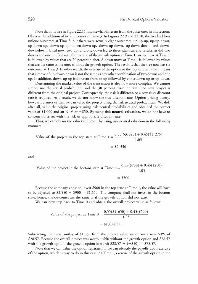
Note that this tree in Figure 22.11 is somewhat different from the other ones in this section.Observe the addition of two outcomes at Time 3. In Figures 22.9 and 22.10, the tree had fourunique outcomes at Time 3, but there were actually eight outcomes: up-up-up, up-up-down,up-down-up, down-up-up, down-down-up, down-up-down, up-down-down, and down-down-down. Until now, two ups and one down led to three identical end results, as did twodowns and one up. But with the exercise of the growth option at Time 1, an up move at Time 1is followed by values that are 70 percent higher. A down move at Time 1 is followed by valuesthat are the same as the ones without the growth option. The result is that the tree now has sixoutcomes at Time 3. In other words, the exercise of the option in the top state at Time 1 meansthat a move of up-down-down is not the same as any other combination of two downs and oneup. In addition, down-up-up is different from an up followed by either down-up or up-down.
Determining the market value of the transaction is also now more complex. We cannotsimply use the actual probabilities and the 30 percent discount rate. The new project isdifferent from the original project. Consequently, the risk is different, so a new risky discountrate is required. As a result, we do not know the true discount rate. Option-pricing theory,however, assures us that we can value the project using the risk neutral probabilities. We did,after all, value the original project using risk neutral probabilities and obtained the correctvalue of $1,000 and an NPV of 2$50. By using risk neutral valuation, we do not have toconcern ourselves with the risk or appropriate discount rate.
Thus, we can obtain the values at Time 1 by using risk neutral valuation in the followingmanner:
Value of the project in the top state at Time 1 ¼ 0:55ð$3; 825Þ þ 0:45ð$1; 275Þ1:05
¼ $2; 550
and
Value of the project in the bottom state at Time 1 ¼ 0:55ð$750Þ þ 0:45ð$250Þ1:05
¼ $500:
Because the company chose to invest $900 in the top state at Time 1, the value will haveto be adjusted to $2,550 2 $900 5 $1,650. The company shall not invest in the bottomstate; hence, the outcomes are the same as if the growth option did not exist.
We can now step back to Time 0 and obtain the overall project value as follows:
Value of the project at Time 0 ¼ 0:55ð$1; 650Þ þ 0:45ð$500Þ1:05
¼ $1; 078:57:
Subtracting the initial outlay of $1,050 from the project value, we obtain a new NPV of$28.57. Because the overall project was worth 2$50 without the growth option and $28.57with the growth option, the growth option is worth $28.57 2 (2$50) 5 $78.57.
Note that we can value the option separately if we can identify the payoffs upon exerciseof the option, which is easy to do in this case. At Time 1, exercise of the growth option in the
c22 12 September 2012; 14:30:40
520 Part V: Real Options Valuation
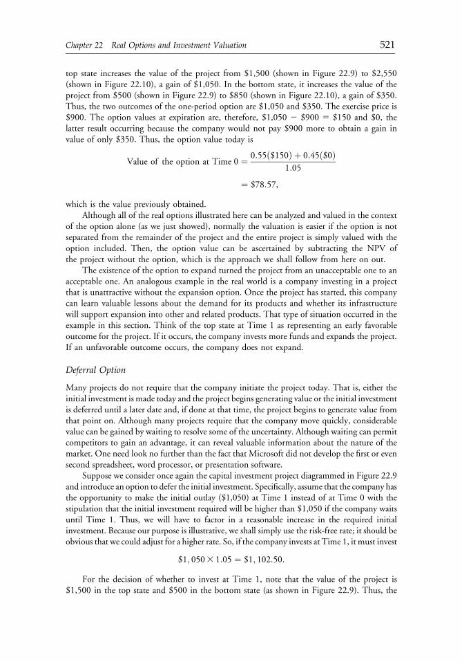
top state increases the value of the project from $1,500 (shown in Figure 22.9) to $2,550(shown in Figure 22.10), a gain of $1,050. In the bottom state, it increases the value of theproject from $500 (shown in Figure 22.9) to $850 (shown in Figure 22.10), a gain of $350.Thus, the two outcomes of the one-period option are $1,050 and $350. The exercise price is$900. The option values at expiration are, therefore, $1,050 2 $900 5 $150 and $0, thelatter result occurring because the company would not pay $900 more to obtain a gain invalue of only $350. Thus, the option value today is
Value of the option at Time 0 ¼ 0:55ð$150Þ þ 0:45ð$0Þ1:05
¼ $78:57,
which is the value previously obtained.Although all of the real options illustrated here can be analyzed and valued in the context
of the option alone (as we just showed), normally the valuation is easier if the option is notseparated from the remainder of the project and the entire project is simply valued with theoption included. Then, the option value can be ascertained by subtracting the NPV ofthe project without the option, which is the approach we shall follow from here on out.
The existence of the option to expand turned the project from an unacceptable one to anacceptable one. An analogous example in the real world is a company investing in a projectthat is unattractive without the expansion option. Once the project has started, this companycan learn valuable lessons about the demand for its products and whether its infrastructurewill support expansion into other and related products. That type of situation occurred in theexample in this section. Think of the top state at Time 1 as representing an early favorableoutcome for the project. If it occurs, the company invests more funds and expands the project.If an unfavorable outcome occurs, the company does not expand.
Deferral Option
Many projects do not require that the company initiate the project today. That is, either theinitial investment is made today and the project begins generating value or the initial investmentis deferred until a later date and, if done at that time, the project begins to generate value fromthat point on. Although many projects require that the company move quickly, considerablevalue can be gained by waiting to resolve some of the uncertainty. Although waiting can permitcompetitors to gain an advantage, it can reveal valuable information about the nature of themarket. One need look no further than the fact that Microsoft did not develop the first or evensecond spreadsheet, word processor, or presentation software.
Suppose we consider once again the capital investment project diagrammed in Figure 22.9and introduce an option to defer the initial investment. Specifically, assume that the company hasthe opportunity to make the initial outlay ($1,050) at Time 1 instead of at Time 0 with thestipulation that the initial investment required will be higher than $1,050 if the company waitsuntil Time 1. Thus, we will have to factor in a reasonable increase in the required initialinvestment. Because our purpose is illustrative, we shall simply use the risk-free rate; it should beobvious that we could adjust for a higher rate. So, if the company invests at Time 1, it must invest
$1; 0503 1:05 ¼ $1; 102:50:
For the decision of whether to invest at Time 1, note that the value of the project is$1,500 in the top state and $500 in the bottom state (as shown in Figure 22.9). Thus, the
c22 12 September 2012; 14:30:40
Chapter 22 Real Options and Investment Valuation 521
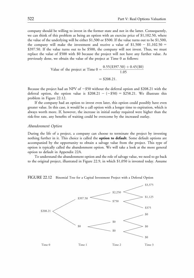
company should be willing to invest in the former state and not in the latter. Consequently,we can think of this problem as being an option with an exercise price of $1,102.50, wherethe value of the underlying will be either $1,500 or $500. If the value turns out to be $1,500,the company will make the investment and receive a value of $1,500 2 $1,102.50 5$397.50. If the value turns out to be $500, the company will not invest. Thus, we mustreplace the value of $500 with $0 because the project will not have any further value. Aspreviously done, we obtain the value of the project at Time 0 as follows:
Value of the project at Time 0 ¼ 0:55ð$397:50Þ þ 0:45ð$0Þ1:05
¼ $208:21:
Because the project had an NPV of 2$50 without the deferral option and $208.21 with thedeferral option, the option value is $208.21 2 (2$50) 5 $258.21. We illustrate thisproblem in Figure 22.12.
If the company had an option to invest even later, this option could possibly have evengreater value. In this case, it would be a call option with a longer time to expiration, which isalways worth more. If, however, the increase in initial outlay required were higher than therisk-free rate, any benefits of waiting could be overcome by the increased outlay.
Abandonment Option
During the life of a project, a company can choose to terminate the project by investingnothing further in it. This choice is called the option to default. Some default options areaccompanied by the opportunity to obtain a salvage value from the project. This type ofoption is typically called the abandonment option. We will take a look at the more generaloption to default in Appendix 22A.
To understand the abandonment option and the role of salvage value, we need to go backto the original project, illustrated in Figure 22.9, in which $1,050 is invested today. Assume
FIGURE 22.12 Binomial Tree for a Capital Investment Project with a Deferral Option
$397.50
$2,250
$750
$3,375
$1,125
$375
$0$0
$0
$0
$0
$0
$208.21
Time 0 Time 1 Time 2 Time 3
c22 12 September 2012; 14:30:40
522 Part V: Real Options Valuation
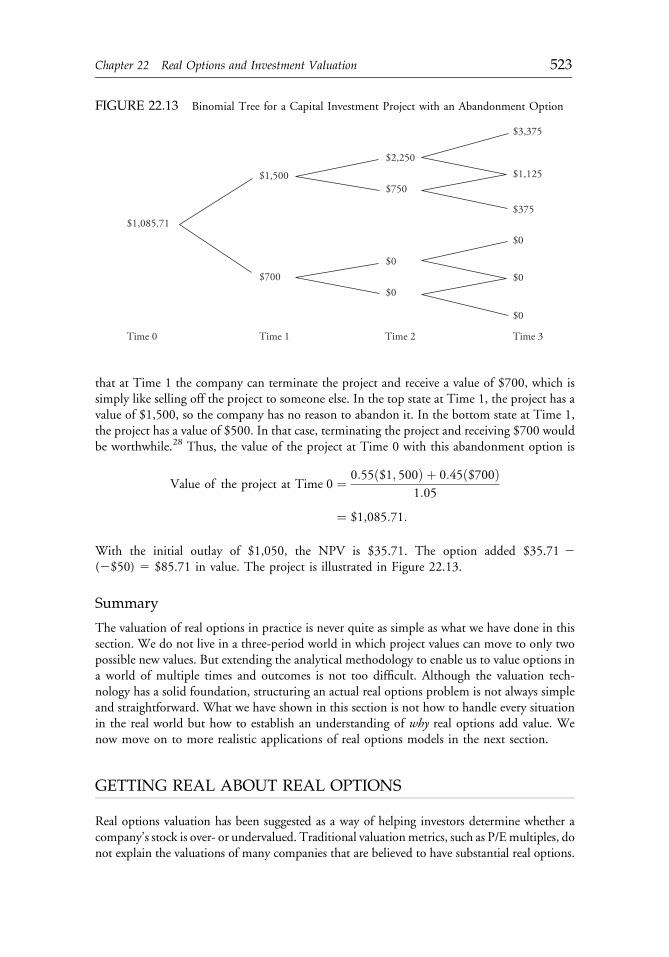
that at Time 1 the company can terminate the project and receive a value of $700, which issimply like selling off the project to someone else. In the top state at Time 1, the project has avalue of $1,500, so the company has no reason to abandon it. In the bottom state at Time 1,the project has a value of $500. In that case, terminating the project and receiving $700 wouldbe worthwhile.28 Thus, the value of the project at Time 0 with this abandonment option is
Value of the project at Time 0 ¼ 0:55ð$1; 500Þ þ 0:45ð$700Þ1:05
¼ $1,085:71:
With the initial outlay of $1,050, the NPV is $35.71. The option added $35.71 2(2$50) 5 $85.71 in value. The project is illustrated in Figure 22.13.
Summary
The valuation of real options in practice is never quite as simple as what we have done in thissection. We do not live in a three-period world in which project values can move to only twopossible new values. But extending the analytical methodology to enable us to value options ina world of multiple times and outcomes is not too difficult. Although the valuation tech-nology has a solid foundation, structuring an actual real options problem is not always simpleand straightforward. What we have shown in this section is not how to handle every situationin the real world but how to establish an understanding of why real options add value. Wenow move on to more realistic applications of real options models in the next section.
GETTING REAL ABOUT REAL OPTIONS
Real options valuation has been suggested as a way of helping investors determine whether acompany’s stock is over- or undervalued. Traditional valuationmetrics, such as P/Emultiples, donot explain the valuations of many companies that are believed to have substantial real options.
FIGURE 22.13 Binomial Tree for a Capital Investment Project with an Abandonment Option
$1,500
$2,250
$750
$3,375
$1,125
$375
$700$0
$0
$0
$0
$0
$1,085.71
Time 0 Time 1 Time 2 Time 3
c22 12 September 2012; 14:30:40
Chapter 22 Real Options and Investment Valuation 523
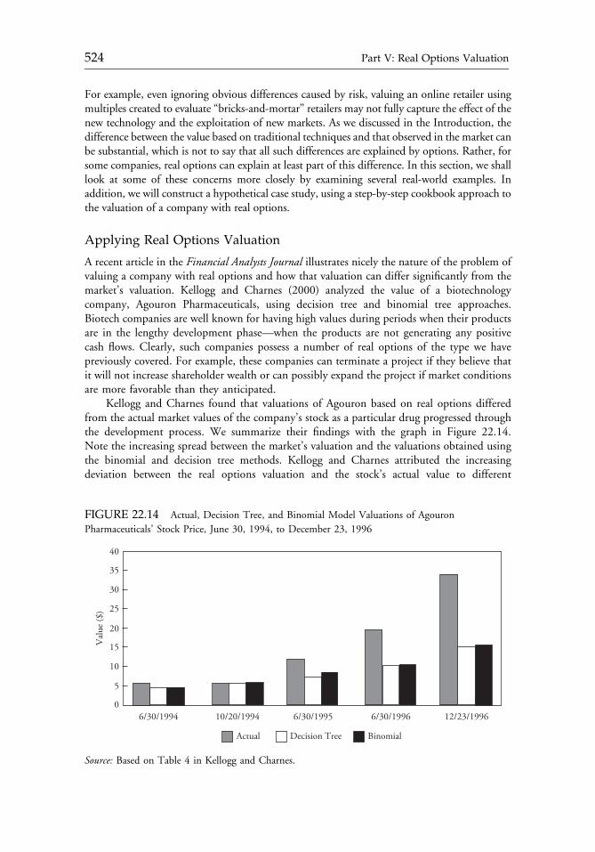
For example, even ignoring obvious differences caused by risk, valuing an online retailer usingmultiples created to evaluate “bricks-and-mortar” retailers may not fully capture the effect of thenew technology and the exploitation of new markets. As we discussed in the Introduction, thedifference between the value based on traditional techniques and that observed in the market canbe substantial, which is not to say that all such differences are explained by options. Rather, forsome companies, real options can explain at least part of this difference. In this section, we shalllook at some of these concerns more closely by examining several real-world examples. Inaddition, we will construct a hypothetical case study, using a step-by-step cookbook approach tothe valuation of a company with real options.
Applying Real Options Valuation
A recent article in the Financial Analysts Journal illustrates nicely the nature of the problem ofvaluing a company with real options and how that valuation can differ significantly from themarket’s valuation. Kellogg and Charnes (2000) analyzed the value of a biotechnologycompany, Agouron Pharmaceuticals, using decision tree and binomial tree approaches.Biotech companies are well known for having high values during periods when their productsare in the lengthy development phase—when the products are not generating any positivecash flows. Clearly, such companies possess a number of real options of the type we havepreviously covered. For example, these companies can terminate a project if they believe thatit will not increase shareholder wealth or can possibly expand the project if market conditionsare more favorable than they anticipated.
Kellogg and Charnes found that valuations of Agouron based on real options differedfrom the actual market values of the company’s stock as a particular drug progressed throughthe development process. We summarize their findings with the graph in Figure 22.14.Note the increasing spread between the market’s valuation and the valuations obtained usingthe binomial and decision tree methods. Kellogg and Charnes attributed the increasingdeviation between the real options valuation and the stock’s actual value to different
FIGURE 22.14 Actual, Decision Tree, and Binomial Model Valuations of Agouron
Pharmaceuticals’ Stock Price, June 30, 1994, to December 23, 1996
Val
ue ($
)
6/30/1995 6/30/1996
25
20
15
10
5
0
30
35
40
Actual Decision Tree Binomial
6/30/1994 10/20/1994 12/23/1996
Source: Based on Table 4 in Kellogg and Charnes.
c22 12 September 2012; 14:30:40
524 Part V: Real Options Valuation
assumptions used by their models and shareholders. For example, investors evidently assumedthat a particular drug would take eight years to reach the market, when, in fact, it took lessthan two. Different assumptions about the probability distribution of sales also accounted forsome of the difference. The important point in this case is not that real options were over-looked by the market but, rather, that they may actually have been overvalued by the market.
In the same issue of the Financial Analysts Journal, Schwartz and Moon (2000) examinedthe valuation of Amazon.com stock to determine the level of volatility and company prof-itability that would explain the current value of the stock. They found that the value of thestock could be explained only if expected volatility were almost twice the historical volatilityor if profitability in the future were five times reasonable expectations based on Amazon’scurrent and historical revenues and expenses. Although Schwartz and Moon did not attributethis discrepancy specifically to real options, real options are apparently responsible for asignificant amount of the difference. For example, Mauboussin (1999) specifically identifiedthe following real options of Amazon:
� scope-up options—opportunities to enter into different product lines,� scale-up options—opportunities to expand capacity,� learning options—opportunities to acquire companies and enter into joint ventures that
give Amazon the ability to enter into new businesses that it has little experience with,perhaps using what it learned in these ventures to help its existing product lines, and
� equity stakes—ownership of interests in related start-up ventures, or in other words, equityinterests in real options owned by other companies.
Indeed Amazon’s viability in light of its poor profitability and cash flow is undoubtedly aresult of its ability to develop and optimally exercise its real options; however, analysts andinvestors do not have an easy time recognizing and properly valuing a company’s real options.Failure to recognize real options can lead to amarket price that greatly understates the true valueof a company. Likewise, real options can also be overvalued. Misvaluation of real options is, inall likelihood, a result of not knowing how to properly value real options, not using reasonableinputs, or not considering the interaction of the many real options a company possesses.
We will next take a look at an actual company that unquestionably holds many realoptions to determine the difference, if any, between the market’s valuation and a valuationbased on traditional discounted cash flow (DCF) methods.
Valuation of Cisco Systems
To see how real options can make valuing a company difficult, consider the valuation of CiscoSystems, a well-known supplier of networking products. Our valuation task is facilitatedsomewhat by the fact that Cisco has no long-term debt and does not pay dividends. Themarket value of equity of Cisco Systems on August 10, 2000, the day following the release ofits fiscal year 2000 (FY2000) earnings information, was $445.1 billion. How much of thisvalue is based on the options that Cisco has and how much is based on the present value offuture cash flows from its assets in place cannot be easily determined. Nonetheless, we willinvestigate the valuation of Cisco first using traditional metrics and then looking at thedifference between actual market value and the value determined by these traditional metrics.This difference in valuation we believe can be attributed at least in part to Cisco’s real options.
A DCF valuation requires that we make forecasts of future cash flows, estimate thecompany’s cost of capital, and then discount those cash flows at the cost of capital. Along
c22 12 September 2012; 14:30:41
Chapter 22 Real Options and Investment Valuation 525
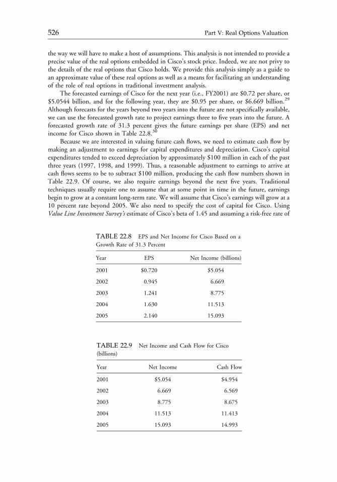
the way we will have to make a host of assumptions. This analysis is not intended to provide aprecise value of the real options embedded in Cisco’s stock price. Indeed, we are not privy tothe details of the real options that Cisco holds. We provide this analysis simply as a guide toan approximate value of these real options as well as a means for facilitating an understandingof the role of real options in traditional investment analysis.
The forecasted earnings of Cisco for the next year (i.e., FY2001) are $0.72 per share, or$5.0544 billion, and for the following year, they are $0.95 per share, or $6.669 billion.29
Although forecasts for the years beyond two years into the future are not specifically available,we can use the forecasted growth rate to project earnings three to five years into the future. Aforecasted growth rate of 31.3 percent gives the future earnings per share (EPS) and netincome for Cisco shown in Table 22.8.30
Because we are interested in valuing future cash flows, we need to estimate cash flow bymaking an adjustment to earnings for capital expenditures and depreciation. Cisco’s capitalexpenditures tended to exceed depreciation by approximately $100 million in each of the pastthree years (1997, 1998, and 1999). Thus, a reasonable adjustment to earnings to arrive atcash flows seems to be to subtract $100 million, producing the cash flow numbers shown inTable 22.9. Of course, we also require earnings beyond the next five years. Traditionaltechniques usually require one to assume that at some point in time in the future, earningsbegin to grow at a constant long-term rate. We will assume that Cisco’s earnings will grow at a10 percent rate beyond 2005. We also need to specify the cost of capital for Cisco. UsingValue Line Investment Survey’s estimate of Cisco’s beta of 1.45 and assuming a risk-free rate of
TABLE 22.8 EPS and Net Income for Cisco Based on a
Growth Rate of 31.3 Percent
Year EPS Net Income (billions)
2001 $0.720 $5.054
2002 0.945 6.669
2003 1.241 8.775
2004 1.630 11.513
2005 2.140 15.093
TABLE 22.9 Net Income and Cash Flow for Cisco
(billions)
Year Net Income Cash Flow
2001 $5.054 $4.954
2002 6.669 6.569
2003 8.775 8.675
2004 11.513 11.413
2005 15.093 14.993
c22 12 September 2012; 14:30:41
526 Part V: Real Options Valuation
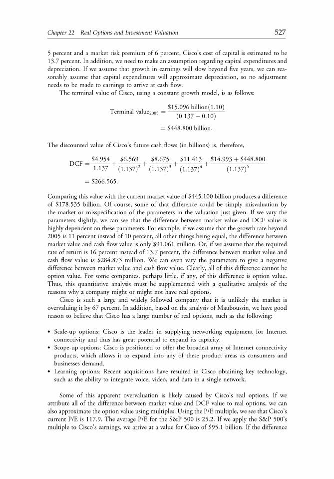
5 percent and a market risk premium of 6 percent, Cisco’s cost of capital is estimated to be13.7 percent. In addition, we need to make an assumption regarding capital expenditures anddepreciation. If we assume that growth in earnings will slow beyond five years, we can rea-sonably assume that capital expenditures will approximate depreciation, so no adjustmentneeds to be made to earnings to arrive at cash flow.
The terminal value of Cisco, using a constant growth model, is as follows:
Terminal value2005 ¼ $15:096 billionð1:10Þð0:137� 0:10Þ
¼ $448:800 billion:
The discounted value of Cisco’s future cash flows (in billions) is, therefore,
DCF ¼ $4:954
1:137þ $6:569
ð1:137Þ2 þ$8:675
ð1:137Þ3 þ$11:413
ð1:137Þ4 þ$14:993þ $448:800
ð1:137Þ5
¼ $266:565:
Comparing this value with the current market value of $445.100 billion produces a differenceof $178.535 billion. Of course, some of that difference could be simply misvaluation bythe market or misspecification of the parameters in the valuation just given. If we vary theparameters slightly, we can see that the difference between market value and DCF value ishighly dependent on these parameters. For example, if we assume that the growth rate beyond2005 is 11 percent instead of 10 percent, all other things being equal, the difference betweenmarket value and cash flow value is only $91.061 million. Or, if we assume that the requiredrate of return is 16 percent instead of 13.7 percent, the difference between market value andcash flow value is $284.873 million. We can even vary the parameters to give a negativedifference between market value and cash flow value. Clearly, all of this difference cannot beoption value. For some companies, perhaps little, if any, of this difference is option value.Thus, this quantitative analysis must be supplemented with a qualitative analysis of thereasons why a company might or might not have real options.
Cisco is such a large and widely followed company that it is unlikely the market isovervaluing it by 67 percent. In addition, based on the analysis of Mauboussin, we have goodreason to believe that Cisco has a large number of real options, such as the following:
� Scale-up options: Cisco is the leader in supplying networking equipment for Internetconnectivity and thus has great potential to expand its capacity.
� Scope-up options: Cisco is positioned to offer the broadest array of Internet connectivityproducts, which allows it to expand into any of these product areas as consumers andbusinesses demand.
� Learning options: Recent acquisitions have resulted in Cisco obtaining key technology,such as the ability to integrate voice, video, and data in a single network.
Some of this apparent overvaluation is likely caused by Cisco’s real options. If weattribute all of the difference between market value and DCF value to real options, we canalso approximate the option value using multiples. Using the P/E multiple, we see that Cisco’scurrent P/E is 117.9. The average P/E for the S&P 500 is 25.2. If we apply the S&P 500’smultiple to Cisco’s earnings, we arrive at a value for Cisco of $95.1 billion. If the difference
c22 12 September 2012; 14:30:41
Chapter 22 Real Options and Investment Valuation 527
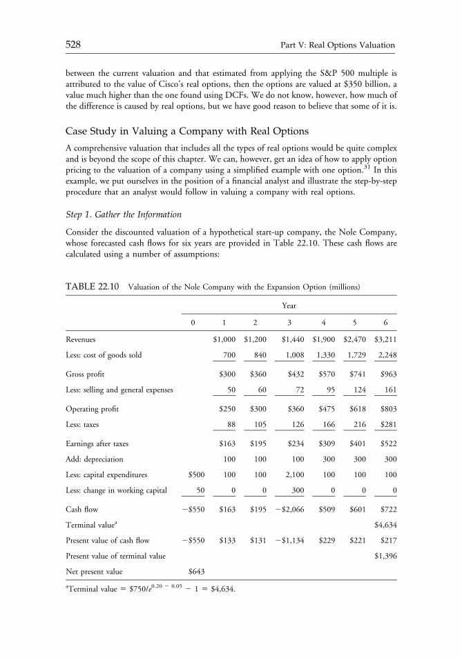
between the current valuation and that estimated from applying the S&P 500 multiple isattributed to the value of Cisco’s real options, then the options are valued at $350 billion, avalue much higher than the one found using DCFs. We do not know, however, how much ofthe difference is caused by real options, but we have good reason to believe that some of it is.
Case Study in Valuing a Company with Real Options
A comprehensive valuation that includes all the types of real options would be quite complexand is beyond the scope of this chapter. We can, however, get an idea of how to apply optionpricing to the valuation of a company using a simplified example with one option.31 In thisexample, we put ourselves in the position of a financial analyst and illustrate the step-by-stepprocedure that an analyst would follow in valuing a company with real options.
Step 1. Gather the Information
Consider the discounted valuation of a hypothetical start-up company, the Nole Company,whose forecasted cash flows for six years are provided in Table 22.10. These cash flows arecalculated using a number of assumptions:
TABLE 22.10 Valuation of the Nole Company with the Expansion Option (millions)
Year
0 1 2 3 4 5 6
Revenues $1,000 $1,200 $1,440 $1,900 $2,470 $3,211
Less: cost of goods sold 700 840 1,008 1,330 1,729 2,248
Gross profit $300 $360 $432 $570 $741 $963
Less: selling and general expenses 50 60 72 95 124 161
Operating profit $250 $300 $360 $475 $618 $803
Less: taxes 88 105 126 166 216 $281
Earnings after taxes $163 $195 $234 $309 $401 $522
Add: depreciation 100 100 100 300 300 300
Less: capital expenditures $500 100 100 2,100 100 100 100
Less: change in working capital 50 0 0 300 0 0 0
Cash flow 2$550 $163 $195 2$2,066 $509 $601 $722
Terminal valuea $4,634
Present value of cash flow 2$550 $133 $131 2$1,134 $229 $221 $217
Present value of terminal value $1,396
Net present value $643
aTerminal value 5 $750/e0.20 2 0.05 2 1 5 $4,634.
c22 12 September 2012; 14:30:41
528 Part V: Real Options Valuation
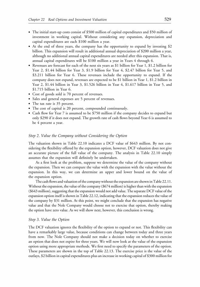
� The initial start-up costs consist of $500 million of capital expenditures and $50 million ofinvestment in working capital. Without considering any expansion, depreciation andcapital expenditures are each $100 million a year.
� At the end of three years, the company has the opportunity to expand by investing $2billion. This expansion will result in additional annual depreciation of $200 million a year,although no additional annual capital expenditures are needed after this expansion. That is,annual capital expenditures will be $100 million a year in Years 4 through 6.
� Revenues are forecast for each of the next six years as $1 billion for Year 1, $1.2 billion forYear 2, $1.44 billion for Year 3, $1.9 billion for Year 4, $2.47 billion for Year 5, and$3.211 billion for Year 6. These revenues include the opportunity to expand. If thecompany does not expand, revenues are expected to be $1 billion in Year 1, $1.2 billion inYear 2, $1.44 billion in Year 3, $1.526 billion in Year 4, $1.617 billion in Year 5, and$1.715 billion in Year 6.
� Cost of goods sold is 70 percent of revenues.� Sales and general expenses are 5 percent of revenues.� The tax rate is 35 percent.� The cost of capital is 20 percent, compounded continuously.� Cash flow for Year 7 is assumed to be $750 million if the company decides to expand but
only $290 if it does not expand. The growth rate of cash flows beyond Year 6 is assumed tobe 4 percent a year.
Step 2. Value the Company without Considering the Option
The valuation shown in Table 22.10 indicates a DCF value of $643 million. By not con-sidering the flexibility offered by the expansion option, however, DCF valuation does not givean accurate picture of the full value of the company. The analysis in Table 22.10 simplyassumes that the expansion will definitely be undertaken.
As a first look at the problem, suppose we determine the value of the company withoutthe expansion. Then we can compare the value with the expansion with the value without theexpansion. In this way, we can determine an upper and lower bound on the value ofthe expansion option.
The cashflows and valuationof the companywithout the expansion are shown inTable 22.11.Without the expansion, the value of the company ($674million) is higher than with the expansion($643million), suggesting that the expansion would not add value. The separate DCF value of theexpansion option itself is shown in Table 22.12, indicating that the expansion reduces the value ofthe company by $31 million. At this point, we might conclude that the expansion has negativevalue and that the Nole Company would choose not to exercise that option, thereby makingthe option have zero value. As we will show next, however, this conclusion is wrong.
Step 3. Value the Option
The DCF valuation ignores the flexibility of the option to expand or not. This flexibility canhave a remarkably large value, because conditions can change between today and three yearsfrom now. The Nole Company should not make a decision today on whether to exercisean option that does not expire for three years. We will now look at the value of the expansionoption using more appropriate methods. We first need to specify the parameters of the option.These parameters are shown in the top of Table 22.13. The exercise price is the value of theoutlays, $2 billion in capital expenditures plus an increase in working capital of $300million for
c22 12 September 2012; 14:30:41
Chapter 22 Real Options and Investment Valuation 529
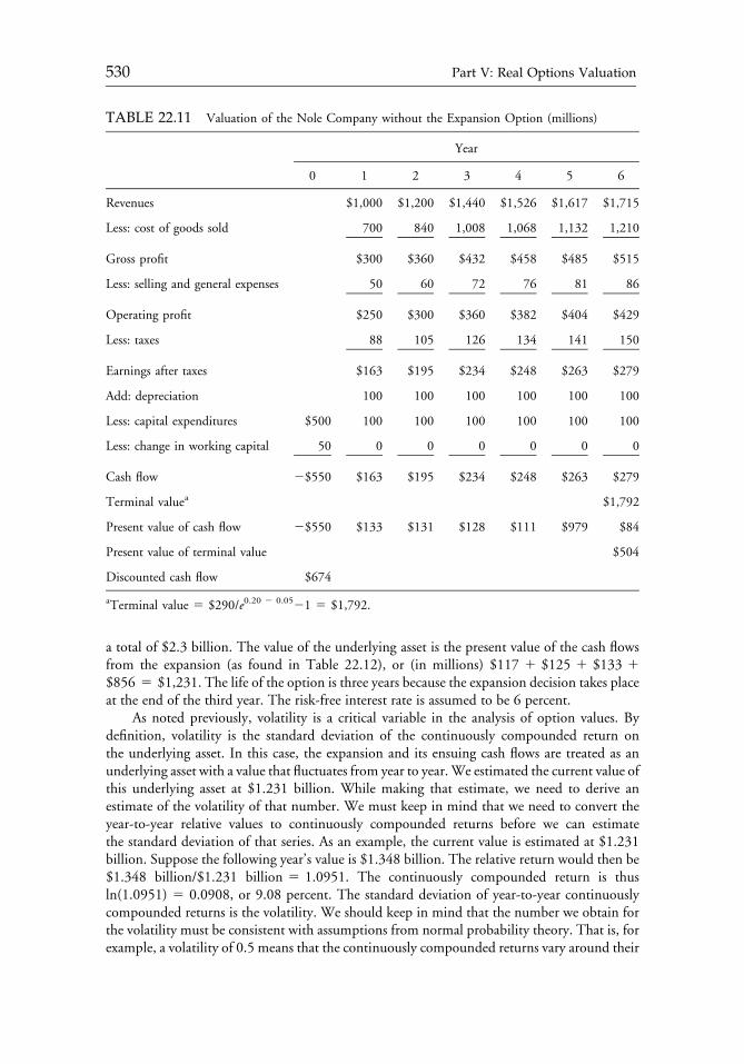
a total of $2.3 billion. The value of the underlying asset is the present value of the cash flowsfrom the expansion (as found in Table 22.12), or (in millions) $117 1 $125 1 $133 1$856 5 $1,231. The life of the option is three years because the expansion decision takes placeat the end of the third year. The risk-free interest rate is assumed to be 6 percent.
As noted previously, volatility is a critical variable in the analysis of option values. Bydefinition, volatility is the standard deviation of the continuously compounded return onthe underlying asset. In this case, the expansion and its ensuing cash flows are treated as anunderlying asset with a value that fluctuates from year to year.We estimated the current value ofthis underlying asset at $1.231 billion. While making that estimate, we need to derive anestimate of the volatility of that number. We must keep in mind that we need to convert theyear-to-year relative values to continuously compounded returns before we can estimatethe standard deviation of that series. As an example, the current value is estimated at $1.231billion. Suppose the following year’s value is $1.348 billion. The relative return would then be$1.348 billion/$1.231 billion 5 1.0951. The continuously compounded return is thusln(1.0951) 5 0.0908, or 9.08 percent. The standard deviation of year-to-year continuouslycompounded returns is the volatility. We should keep in mind that the number we obtain forthe volatility must be consistent with assumptions from normal probability theory. That is, forexample, a volatility of 0.5 means that the continuously compounded returns vary around their
TABLE 22.11 Valuation of the Nole Company without the Expansion Option (millions)
Year
0 1 2 3 4 5 6
Revenues $1,000 $1,200 $1,440 $1,526 $1,617 $1,715
Less: cost of goods sold 700 840 1,008 1,068 1,132 1,210
Gross profit $300 $360 $432 $458 $485 $515
Less: selling and general expenses 50 60 72 76 81 86
Operating profit $250 $300 $360 $382 $404 $429
Less: taxes 88 105 126 134 141 150
Earnings after taxes $163 $195 $234 $248 $263 $279
Add: depreciation 100 100 100 100 100 100
Less: capital expenditures $500 100 100 100 100 100 100
Less: change in working capital 50 0 0 0 0 0 0
Cash flow 2$550 $163 $195 $234 $248 $263 $279
Terminal valuea $1,792
Present value of cash flow 2$550 $133 $131 $128 $111 $979 $84
Present value of terminal value $504
Discounted cash flow $674
aTerminal value 5 $290/e0.20 2 0.0521 5 $1,792.
c22 12 September 2012; 14:30:42
530 Part V: Real Options Valuation
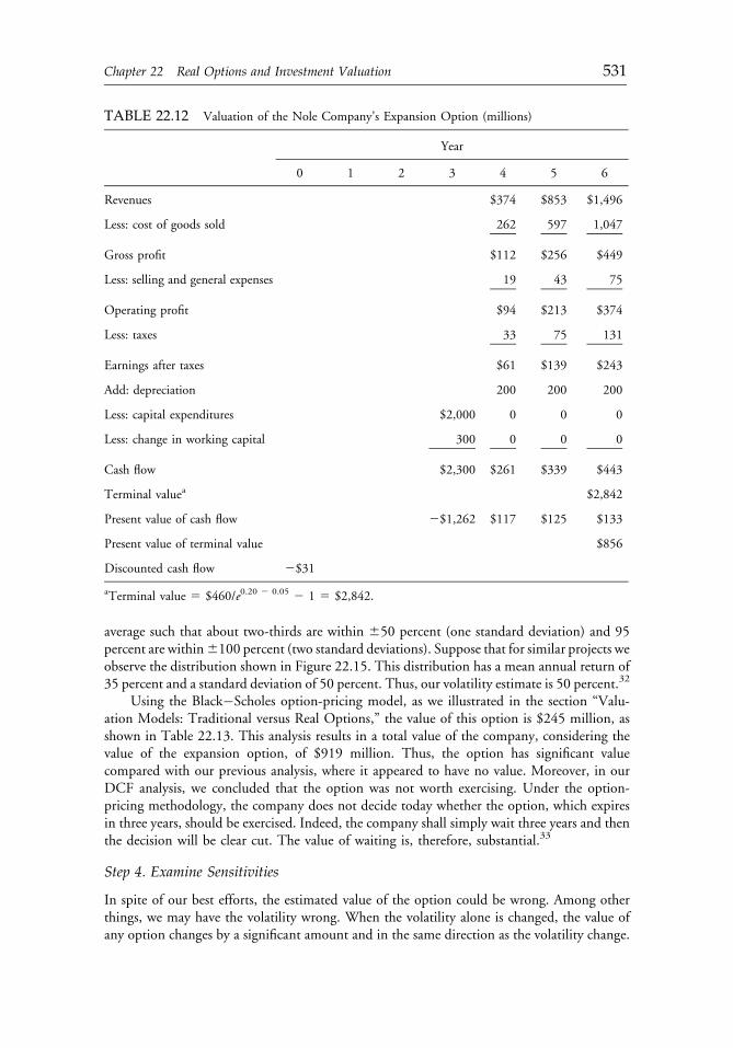
average such that about two-thirds are within 650 percent (one standard deviation) and 95percent are within6100 percent (two standard deviations). Suppose that for similar projects weobserve the distribution shown in Figure 22.15. This distribution has a mean annual return of35 percent and a standard deviation of 50 percent. Thus, our volatility estimate is 50 percent.32
Using the Black�Scholes option-pricing model, as we illustrated in the section “Valu-ation Models: Traditional versus Real Options,” the value of this option is $245 million, asshown in Table 22.13. This analysis results in a total value of the company, considering thevalue of the expansion option, of $919 million. Thus, the option has significant valuecompared with our previous analysis, where it appeared to have no value. Moreover, in ourDCF analysis, we concluded that the option was not worth exercising. Under the option-pricing methodology, the company does not decide today whether the option, which expiresin three years, should be exercised. Indeed, the company shall simply wait three years and thenthe decision will be clear cut. The value of waiting is, therefore, substantial.33
Step 4. Examine Sensitivities
In spite of our best efforts, the estimated value of the option could be wrong. Among otherthings, we may have the volatility wrong. When the volatility alone is changed, the value ofany option changes by a significant amount and in the same direction as the volatility change.
TABLE 22.12 Valuation of the Nole Company’s Expansion Option (millions)
Year
0 1 2 3 4 5 6
Revenues $374 $853 $1,496
Less: cost of goods sold 262 597 1,047
Gross profit $112 $256 $449
Less: selling and general expenses 19 43 75
Operating profit $94 $213 $374
Less: taxes 33 75 131
Earnings after taxes $61 $139 $243
Add: depreciation 200 200 200
Less: capital expenditures $2,000 0 0 0
Less: change in working capital 300 0 0 0
Cash flow $2,300 $261 $339 $443
Terminal valuea $2,842
Present value of cash flow 2$1,262 $117 $125 $133
Present value of terminal value $856
Discounted cash flow 2$31
aTerminal value 5 $460/e0.20 2 0.05 2 1 5 $2,842.
c22 12 September 2012; 14:30:42
Chapter 22 Real Options and Investment Valuation 531
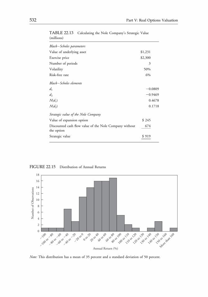
TABLE 22.13 Calculating the Nole Company’s Strategic Value
(millions)
Black�Scholes parameters
Value of underlying asset $1,231
Exercise price $2,300
Number of periods 3
Volatility 50%
Risk-free rate 6%
Black�Scholes elements
d1 20.0809
d2 20.9469
N(d1) 0.4678
N(d2) 0.1718
Strategic value of the Nole Company
Value of expansion option $ 245
Discounted cash flow value of the Nole Company withoutthe option
674
Strategic value $ 919
FIGURE 22.15 Distribution of Annual Returns
Annual Return (%)
Num
ber o
f Obs
erva
tions
10
8
6
4
2
0
�10
0
�10
0 to �
80
�80
to �
60
�60
to �
40
�40
to �
20
�20
to 0
0 to 2
0
20 to
40
40 to
60
60 to
80
80 to
100
100 t
o 110
110 t
o 120
120 t
o 130
130 t
o 140
140 t
o 150
150 t
o 160
More
than
160
12
14
16
18
Note: This distribution has a mean of 35 percent and a standard deviation of 50 percent.
c22 12 September 2012; 14:30:42
532 Part V: Real Options Valuation
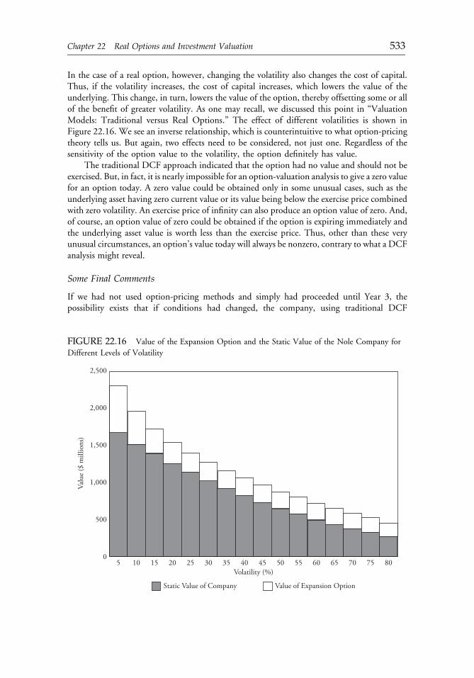
In the case of a real option, however, changing the volatility also changes the cost of capital.Thus, if the volatility increases, the cost of capital increases, which lowers the value of theunderlying. This change, in turn, lowers the value of the option, thereby offsetting some or allof the benefit of greater volatility. As one may recall, we discussed this point in “ValuationModels: Traditional versus Real Options.” The effect of different volatilities is shown inFigure 22.16. We see an inverse relationship, which is counterintuitive to what option-pricingtheory tells us. But again, two effects need to be considered, not just one. Regardless of thesensitivity of the option value to the volatility, the option definitely has value.
The traditional DCF approach indicated that the option had no value and should not beexercised. But, in fact, it is nearly impossible for an option-valuation analysis to give a zero valuefor an option today. A zero value could be obtained only in some unusual cases, such as theunderlying asset having zero current value or its value being below the exercise price combinedwith zero volatility. An exercise price of infinity can also produce an option value of zero. And,of course, an option value of zero could be obtained if the option is expiring immediately andthe underlying asset value is worth less than the exercise price. Thus, other than these veryunusual circumstances, an option’s value today will always be nonzero, contrary to what a DCFanalysis might reveal.
Some Final Comments
If we had not used option-pricing methods and simply had proceeded until Year 3, thepossibility exists that if conditions had changed, the company, using traditional DCF
FIGURE 22.16 Value of the Expansion Option and the Static Value of the Nole Company for
Different Levels of Volatility
Volatility (%)
Valu
e ($
mill
ions
)
2,500
2,000
1,500
1,000
500
05 10 15 20 25 30 35 40 45 50 55 60 65 70 75 80
Value of Expansion OptionStatic Value of Company
c22 12 September 2012; 14:30:42
Chapter 22 Real Options and Investment Valuation 533
methods, might still have chosen to exercise the expansion option and ultimately added valuefrom the expansion. The problem with that way of thinking is that it implies that today thecompany is incorrectly valued. Its option to expand is assumed to be worth nothing, andthe market grossly undervalues the company. For the company itself, this error is simply oneof a market failing to recognize value when it exists, but for financial analysts, this error isespecially critical because they are failing to recognize valuable wealth-creating opportunities.
Summary
In this section, we examined several practical applications of real options. Admittedly we areunable to consider all of the complexities of the real world in our illustrations. But this iswhere financial analysts earn their keep. The use of professional judgment and years ofexperience, combined with an understanding of real options, enables the analyst to obtainmore accurate fair values of the companies under consideration.
Before moving forward, let us review what we have done so far. In the “Introduction,” wediscussed the evolution of real options in financial decision making and how option-pricingmethods can be applied to investment opportunities in real assets. In “Valuation Models: Tra-ditional versus Real Options,” we described the valuation methods used traditionally in capitalbudgeting and showed how real options valuation can supplement DCF analysis to capture thestrategic value of an investment. In “A Framework for the Valuation of Real Options,” we illus-trated, using binominal trees, the different types of real options and their valuations. In the presentsection, we applied real options to the valuation of a company that had an expansion option.
Up to this point, we have presented real options valuation as it has been written about inthe academic and practitioner literature. A remarkable observation from reading this literatureis that real options valuation may seem to be the cure for all valuation problems. Virtually allexamples are presented as though one can easily recognize real options, obtain input values,and apply real options analysis without concern as to whether mistakes are being made orwhether using real options analysis is even appropriate. In short, there is a dearth of criticismon the limitations and difficulties of using real options valuation. Thus, in the followingsection, we will take a more critical look at this methodology.
PITFALLS AND PRATFALLS IN REAL OPTIONS VALUATION
In the previous sections, we examined the many attractions of using real options valuation forcorporations and especially financial analysts. One might get the impression that real optionsvaluation is easy to do or that it is an infallible financial tool. Indeed, a reading of the literatureon the subject reveals a notable absence of criticisms and limitations. But, in fact, real optionsvaluation suffers from numerous criticisms and limitations and can be particularly difficult toimplement. Some of these criticisms are relatively minor, but some are quite important.34 Inthis section, we attempt to address some of the concerns associated with real options valuation,noting weaknesses along with strengths, identifying criticisms that are valid and those that arenot, and showing a more balanced view than is generally found elsewhere. We stress that ourgoal in this chapter is neither to glorify real options valuation nor to tear it down. Our goal is toinform. To that end, we argue that real options valuation is a powerful tool, but as with allpowerful tools, it must be used properly with a recognition of its limitations and weaknesses.
We also would like to emphasize that our treatment of these issues is at a basic level. Ourobjective is a modest one—to apprise the reader of issues, concerns, and caveats. We do not
c22 12 September 2012; 14:30:42
534 Part V: Real Options Valuation
have the space to devote to providing a detailed explanation or resolution of these issues.Indeed, many of the issues are open to considerable debate among the most knowledgeablescholars and practitioners and are unlikely to be resolved in the near future.
Complications from Internal and External Interactions
As we illustrated extensively in “A Framework for the Valuation of Real Options” andAppendix 22A, the body of knowledge of financial option-pricing theory forms the basis forunderstanding real options valuation. Unfortunately, real options valuation suffers from a fewsubtle problems that often are missing from situations involving financial options. Forexample, consider the case of a typical financial option in which an investor buys an option onMicrosoft stock (MSFT). The option’s value is based on its potential payoffs, which aredetermined by the performance of MSFT. With the possible exception of the investor beingBill Gates or another senior officer at Microsoft, an investor cannot influence the performanceof MSFT. When real options are involved, however, the holders and writers of these options(the investors) are generally the companies whose performance is the underlying asset.Obviously, a company can influence the value of its stock. Thus, in the case of real options,the option holder would be able to influence the value of the underlying asset. This possibilityviolates the assumptions on which option-pricing models are based.
Consider a simple real option in which a company can abandon a project and receive asalvage value if it so desires. We illustrated a project of this type in “A Framework for theValuation of Real Options.” The company can increase the value of this option by engagingin actions that increase the volatility of the underlying asset’s value. Such actions permit thecompany to potentially gain on the upside if the option is not needed and yet not lose moreon the downside if the outcome is bad. But further complicating this matter is the fact that ifthe company increases the volatility of the underlying asset’s value, the value of the underlyingasset might decrease. It would make good economic sense for the company to take actionsthat set the volatility of the underlying to the level that maximizes the overall value of theproject plus the option. In the absence of the option, the company might not attempt to raisethe volatility of the value of the underlying asset. Option-pricing models, however, requirethat the underlying be valued separately without the effects of the option. This value andvolatility then enter exogenously into the valuation of the option.
Thus, interactions between the option holder and the underlying asset’s value cancomplicate the analysis of real options. But is this problem unique to real options? No, evensome financial options are subject to this concern. For example, when a company issues aconvertible bond, it effectively sells a call option on the stock to the bondholders. Thebondholders do not influence the value of the underlying asset, but the company, which is theoption writer, obviously influences this value. The company could engage in actions thatlower the volatility of the value of the underlying asset for the purpose of making the optionless valuable. In a similar manner, a company issues warrants on its own stock. So, again, thecompany also affects the value of the underlying asset. Thus, the writer of the option can exertinfluence on the underlying asset.
Lest one think that only writers of financial options can influence the underlying,consider the case of executive stock options. These options are held by executives, who clearlycan influence the performance of the underlying asset.
In addition to the potential for the option holder to influence the underlying asset’svalue, real options are complicated by the possibility of competitor reactions that mightinfluence the underlying asset. Consider the abandonment option just described. Suppose a
c22 12 September 2012; 14:30:42
Chapter 22 Real Options and Investment Valuation 535
company exercises its option to abandon a project. That decision may appear to be optimal inisolation: The salvage value exceeds the market value of the project. But suppose the companyabandons the project and then competitors, smelling an opportunity, step up their efforts toservice the company’s customers, potentially siphoning away business from another part ofthe company. For that reason, many companies are known to engage in low-profit or evenloss-leading activities because of fear that competitors will take customers away, which wouldresult in the loss of other revenues. Thus, the company might even exercise an out-of-the-money option or fail to exercise an expiring in-the-money option. In highly competitiveenvironments, real options are extremely complex because of this added element of theuncertainty of competitors’ reactions. And because competitors’ reactions are decisions madeby humans, they too are subject to a great deal of uncertainty. Competitors may react or maynot, even when it might appear rational to do otherwise.
These points can be summarized by saying that most financial options adhere to the rulethat the value of the underlying asset is in no way influenced by whether the option isexercised. In real options, no such rule exists.
Inability to Explain Absurd Valuations
Consider again the abandonment option, specifically the example in “A Framework for theValuation of Real Options.” In that example, the project without the option to abandon isworth $1,000 (as shown in Figure 22.9). With the option to abandon, the project is worth$1,085.71 (as shown in Figure 22.13). Thus, the option is worth $85.71. The project itself isworth almost 12 times the value of the option. In fact, for most options, the underlying assetis usually worth many times the value of the option. For call options, the value of theunderlying asset is the upper limit on the value of the option. For puts, the exercise price(assuming an American option) is the upper limit on the value of the option.35
These points should immediately call into question the notion that a real option canmake a company be worth many times its fundamental value.36 Certainly, a company that hasone real option probably has other real options. The collective values of these options can addup to a significant amount, but it is unlikely that a company is so blessed with real optionsthat an overall value of many multiples of its fundamental value is obtained. Moreover, whena company has multiple real options, those real options are usually not independent of eachother. Thus, their values are not strictly additive. Therefore, it is extremely questionablewhether the presence of real options can explain the seemingly absurd prices that were wit-nessed in recent years for many Internet stocks. Real options undoubtedly account for some,but certainly not all, of these value differentials.
Model Risk
Model risk is defined as the risk associated with the use of an incorrect model or incorrectinputs in an otherwise correct model or the incorrect use of a correct model, which includessuch problems as programming errors and mistakes in entering otherwise correct inputs. Thefollowing provides a quick overview of the potential dangers of model risk for standardoptions. Consider an American put option on a stock priced at $100. The exercise price is$100, the risk-free rate is 5 percent, the time to expiration is one year, and the volatility is 32percent. The correct model, a binomial model that adjusts for early exercise, gives the value as$16.41. If a European model, such as Black�Scholes, is used, the price will be $15.48, an errorof $0.93, or 5.7 percent. If the correct model is used but the volatility is slightly misestimated
c22 12 September 2012; 14:30:43
536 Part V: Real Options Valuation
at 30 percent, the value will be found to be $15.64, an error of $0.77, or nearly 4.7 percent.If the correct volatility of 32 percent is transposed and entered incorrectly as 23 percent, theoption price is $13.01, an error of $3.40, or almost 21 percent. And if the formula is pro-grammed incorrectly, anything is possible. Although model risk can create large errors, evensmall and subtle errors can add up.
Model risk has emerged as an area of concern to specialists in options.37 Model risk ismuch less severe for simple European-style financial options than for American-style options.The input parameters are somewhat easier to identify, and the general consensus is that theBlack�Scholes model is appropriate for the type of option in question. Model risk usuallybecomes a greater concern as the option becomes more complex. And as we have noted manytimes, real options tend to be fairly complex. So, for real options, a much greater danger existsthat one will use the wrong model or bad inputs in the right model. How much skepticismthis danger should raise in one’s mind before using real options is difficult to judge. If nothingelse, it should force one to think long and hard about getting the right model, the right inputsinto the model, and making no mistakes at the implementation stage.
Failure to Meet Assumptions
A model should not be judged by whether the assumptions on which it is based are realistic.Model builders make assumptions for the purpose of simplifying reality in the hope that theessential characteristics of a complex process can be captured and incorporated into aframework that leads to realistic explanations and/or predictions of results. Hence, a model isa good model not because it meets assumptions but because it explains reality. The old adageof not throwing the baby out with the bathwater applies as much to model building as it doesto anything else.
Nonetheless, in some cases, reality departs so significantly from the assumptions of amodel that before using the model, one begins to question its appropriateness. Nowhereis this caution more critical than in real options valuation. Whether a model works well isusually determined by examining the results of empirical studies. Unfortunately, real optionsvaluation does not lend itself easily to empirical validation. Although a few tests have beenmade of real options models, and we shall examine these later in “Empirical Evidence on theUse and Accuracy of Real Options Valuation,” accepting the validity of real options modelsrelies heavily on one’s faith in the models. Hence, the validity of the assumptions is moreimportant than might be the case for many other financial models for which the abundance ofstatistical data makes empirical testing much easier.
We will examine the assumptions of real options models by classifying them into majorassumptions and minor assumptions. The former are assumptions that are critical. The latterare commonly made assumptions but ones that can be relaxed, albeit with more complexitythat may not always be worthwhile.
Major Assumptions
The major assumptions of real options valuation are lognormality, randomness, and knownand constant volatility over time.
Lognormality One of the foremost assumptions in option-pricing models is that the rate ofreturn on the underlying asset is lognormally distributed. When dealing with an option on astock, the rate of return would be defined as the percentage change in price plus the dividend
c22 12 September 2012; 14:30:43
Chapter 22 Real Options and Investment Valuation 537
yield, if any. If the rate of return is lognormally distributed, then the logarithmic return isnormally distributed. For example, if a nondividend-paying stock sells for $100 and thenmoves up to $110 over the course of one year, the return is 10 percent. The logarithmicreturn is ln(1.10) 5 0.0953, or 9.53 percent. That is, the $100 stock growing at 9.53 percentcontinuously will attain a value of $110 in one year (i.e., 100e0.0953(1) 5 110).38 The con-tinuously compounded return is the logarithmic return. Option-pricing models typicallyassume that the logarithmic return follows a normal distribution, which means that the returnitself (i.e., without taking the logarithm) follows a lognormal distribution.
The lognormal distribution is a particularly appealing one in financial models based on stockreturns. A normal distribution permits unlimited losses, but a lognormal distribution truncateslosses on the downside, which is consistent with the fact that shareholders have limited liability.Moreover, the general consensus is that the lognormal distribution provides a better fit to actualdata, given that it also possesses positive skewness.
Most of the mathematical models of option pricing are based on the notion of a lognormaldistribution. It may appear that the binomial model does not assume a lognormal distribution,and that assumption is true for the simple cases used in this chapter, but in practice, binomialtrees should be much larger than the ones we have illustrated. When expanding the tree,certain formulas tell the user what numbers to place in the tree for the underlying asset values.These formulas are based on the assumption of a lognormal distribution.
The assumption of lognormality is controversial for many types of options. For example,most experts agree that the prices of energy products do not follow the lognormal assumption,but options on these products are often priced using the lognormality assumption. Bond andinterest rate options are often priced based on lognormality, even though the assumptionprobably does not hold. In addition, many people do not believe that stock returns arelognormally distributed, and some empirical evidence suggests that this belief may be thecase.39 More importantly, however, for our purpose is whether the values of assets underlyingreal options follow lognormality. They almost surely do not, but this conclusion does notmean that we should reject the model. Others have not done so with other option-pricingproblems, as described earlier, because the alternatives are no better and potentially are worse.The advantages gained from the assumption of lognormality are often considered well worththe deviation from reality for most applications. And in some cases, departures from log-normality can be appropriately taken.40
Is the assumption of lognormality a likely problem for real options valuation? The valuesof underlying real assets almost surely exhibit properties that make them behave differentlyfrom those of financial assets. For example, real assets do not trade in an open, liquid, and veryefficient market. Whether those differences violate the assumption of lognormality sufficientlyto warrant a rejection of real options models is difficult to tell. But those differences do givecause for concern and force users of real options models to proceed with some caution.
Randomness Virtually all models for pricing financial instruments are based on the notionthat prices evolve randomly. Randomness is a necessary component of financial models,because it assures that markets are competitive and that no one participant or group ofparticipants dominates all others. In financial terminology, markets are required to be effi-cient, or at least sufficiently efficient, to assure the competitiveness that allows pricing modelsto work.
Options on financial assets are generally considered to comply with this requirement.The markets for stocks, bonds, and currencies are relatively, and perhaps highly, efficient. Butthe markets for the assets that underlie real options are not necessarily efficient. These
c22 12 September 2012; 14:30:43
538 Part V: Real Options Valuation
underlying assets represent projects, products, and capital investments and, accordingly, areknown as real asset markets. Real asset markets are definitely not efficient. The existence ofpositive net present values (NPVs) that companies pursue and sometimes generate in theirgoal of maximizing shareholder wealth is evidence of this fact. Companies, particularly newones, operate in highly inefficient markets, exploiting new ideas and technologies to producepositive NPVs, also known as economic profits. The underlying asset is, therefore, aninstrument that does not trade in an efficient market. But the models for pricing real optionsare based on the assumption that the underlying trades in an efficient market. Whether thisproblem is sufficiently important to invalidate real options models is not clear, but it is aconcern that one must keep in mind.
Known and constant volatility Although some advanced option-pricing models incorporatechanging volatility, the assumption that the volatility is known and does not change throughtime is a common and critical one. Option-pricing models are notoriously sensitive to thevolatility. Moreover, the volatility is the only variable in standard option-pricing models that isnot directly observable and relatively easy to obtain. Recall that option-pricing models requirethe exercise price, the time to expiration, the price of the underlying, the risk-free interest rate,and the volatility. The first two items are written into the option contract; the price of theunderlying is generally observable in the market; and the risk-free rate can usually be obtainedfrom the rates on risk-free assets in the market. The volatility, however, is not directly observableand must be estimated. To make matters worse, volatility is itself notoriously volatile. A marketmay be more or less volatile today than it was yesterday. The notion of a volatility of volatilitygives rise to a host of problems that have stumped even the experts on financial option pricing.
So, even though option-pricing models tend to require known and constant volatility, inreality, the volatility is neither known nor constant. The consequences of this problem arelikely to be quite severe. Although the sensitivity of option prices to volatility is probably nomore acute in the real options arena than in the financial options arena, the estimation ofvolatility for real options is a greater concern. Because of the special difficulties of estimatingvolatility for real options, we will address the topic of volatility estimation later in this section.
Minor Assumptions
The minor assumptions of real options valuation are a known and constant risk-free rate, notaxes and transaction costs, no cash flows on the underlying, and use of European-styleoptions. These assumptions are somewhat less critical than ones we just described.
Known and constant risk-free rate Option-pricing models generally assume a known andconstant risk-free rate. Although some controversy surrounds which interest rate is the best proxyfor the risk-free rate, some comfort can be taken in knowing that most option-pricing models arenot very sensitive to the risk-free rate. The rate on a Treasury bill maturing at the option expi-ration is themost often used proxy for the risk-free rate, but others argue that a ratemore reflectiveof a high-quality private borrower is more appropriate. Nonetheless, values obtained usingoption-pricing models, with the exception of those in which the underlying is a bond or interestrate, are not very sensitive to the risk-free rate, so reasonable errors can be tolerated.41
No taxes and transaction costs Financial models nearly always assume the absence of taxes andtransaction costs. Such simplifications facilitate the capture of the most essential elements ofthe economic process being modeled. As it turns out, real options models may suffer less from
c22 12 September 2012; 14:30:43
Chapter 22 Real Options and Investment Valuation 539
this problem than financial option-pricing models do. The market value of the underlyingasset is normally obtained through standard discounted cash flow (DCF) analysis, whichnearly always incorporates taxes and all costs associated with owning the asset. Furthermore,any other costs connected with the ownership of real options either are captured in the modelor can usually be added. Any taxes can, and should, be incorporated into the cash flows andmarket values in a real options model. So, if taxes and transaction costs are ignored, the faultlies not with the real options valuation process but, rather, with the user.
No cash flows on the underlying asset Standard binomial and Black�Scholes models of optionpricing are typically derived for the case of an option on an individual stock. In the simplest case,the stock pays no dividends. Consequently, there are no cash flows on the underlying asset. And ifthe stock pays dividends, incorporating them into the analysis is not difficult, although severalmethods can be used and it is not always clear which approach is the best.
In the case of real options, however, cash flows on the underlying asset are an essentialcomponent of the analysis. The underlying is typically a project, which generates cash inflowsand outflows. As illustrated in previous sections, these cash flows affect the value of the realoption, and they most definitely are incorporated into the analysis.
European-style options A European-style option is one that can be exercised only at expiration.An American-style option is one that can be exercised any time prior to expiration and is besthandled using binomial trees. Because of the tremendous flexibility they offer, real options areoften of the American style. Hence, binomial trees are commonly used in valuing real options.Although binomial trees add some complexity and increase the computational demands, theyafford the flexibility required by most real options problems.42
Difficulty of Estimating Inputs
One of the major criticisms of real options valuation is that estimating the inputs required inthe model is difficult. As it turns out, however, the necessary information is no moredemanding than for a simple DCF/NPV analysis of the underlying project itself. In fact, thedemands are far less. We shall return to this point later in this section, but for now, we willexamine the information required for real options analysis.
As we discussed earlier, to value an option, the user must know the market value of theunderlying, the exercise price of the option, the risk-free rate, the time to expiration, and thevolatility of the underlying. Each of these inputs is discussed below.
Market Value of the Underlying Asset
The market value of the underlying is the value of the project that the real asset is based on.Normally, this value is estimated based on a DCF analysis. Although estimating the DCFvalue of such a project is not easy, the analysis is no more difficult when real options areinvolved. Companies routinely perform NPV analyses. Even though estimating the appro-priate discount rate, the life of a project, and all of the cash flows may be difficult, thoseproblems existed well before anyone recognized the existence of real options, and they existeven when real options are absent. Our goal in this chapter is not to address all of theproblems associated with valuing capital investment projects in the absence of real options.We believe if it is not possible to value the project without any options attached to it, then theproject itself should not be considered. If the project should not be considered, then any real optionsassociated with it should not be considered.
c22 12 September 2012; 14:30:43
540 Part V: Real Options Valuation
Nonetheless, a few technical considerations must be understood when determining thevalue of the underlying project. Interestingly, the literature on real options has overlooked thisproblem. We will identify and discuss this problem here, but we cannot resolve the issue.
Consider the example of a deferral option from “A Framework for the Valuation of RealOptions.” In the basic example (shown in Figure 22.9), the underlying project is worth either$1,500 or $500 at Time 1, and the project is worth $1,000 today, Time 0. The initial outlayis $1,050, so the NPV is 2$50; thus, the project by itself would not be accepted. But thecompany has an option to defer the investment one year, as shown in Figure 22.12. At thattime, the company could invest the greater amount of $1,102.50 ($1,000 adjusted for therisk-free rate) and start the project then. In that case, the value of the project at Time 0 is$208.21. Thus, the option turned an NPV of 2$50 to an NPV of $208.21, so the option todefer is worth $258.21.
What is the market value of the underlying project? It is not the NPV of 2$50 but,rather, the value of the project in the market (i.e., its cost) of $1,050. That is, investing in theunderlying project would cost $1,050. The NPV reflects a decision to purchase the under-lying project and gives the economic value if the investment in the underlying is made. If theunderlying is a stock whose value is $1,000 but costs $1,050 in the market, the value of$1,050 would be used in the real options valuation process. The market is assumed to knowthe true value of the underlying. Even if that value is not correct, real options models (indeedall option-pricing models) are based on the understanding that the underlying asset can bepurchased and used in a hedge with the option. Even if that idea is untenable, and we willdiscuss this point in detail later in this section, one must acknowledge that the true purchaseprice of the underlying project is whatever the market demands.
Strangely, however, the literature on real options consistently treats $1,000, the calcu-lated value of the project, as the value of the underlying asset, even though one could not enterinto the project for that price. The inconsistency arises from the fact that option-pricingtheory, on which real options valuation is based, is grounded in the assumption that theassessed market value of the underlying is the value it would sell for in the market. In otherwords, we are back to the notion that the market is efficient. Option-pricing models make noattempt to inject into the model inefficiency in the market for the underlying. Indeed, there isno way to do so. And even though only two pieces of information are needed about theunderlying to value the real option based on the underlying—its market value and its vola-tility—real options theory is based on the notion that one must value the underlying, oftenrequiring one to perform an NPV analysis and usually finding a nonzero NPV. Most realoptions models take the assessed market value of the underlying as an input. This input isthen used as the underlying asset price in a Black�Scholes-type analysis or as the initial valuein a binomial tree from which future values are calculated.
We shall not attempt to resolve this issue here, but we present it to demonstrate that thestate of real options theory is such that it has not recognized all of its problems.
Exercise Price
The exercise price in a real options analysis is the amount that would be paid or would bereceived if a real option is exercised. For example, in the option to abandon, the project isterminated early if the amount that can be received for terminating the project is more thanthe market value of the project. But the amount that can be received for a project at a futuredate is potentially quite difficult to determine. Consider a plant that a company might want toabandon. It would have to determine the exercise price based on its assessment of the
c22 12 September 2012; 14:30:43
Chapter 22 Real Options and Investment Valuation 541
potential future market value of the plant. Such a situation gives rise to the notion that theexercise price, as well as the market value of the underlying, could be a variable itself.Although the handling of such a situation is complex, option-pricing theory does includemodels that can accommodate such cases.43
In the example in the previous section of the deferral option, a similar problem couldexist. The company could choose to defer the investment for a year, or perhaps later in othersituations. The company would then have to estimate how much more it would have to investif it deferred the outlay. In the problem we worked in “A Framework for the Valuation ofReal Options,” we assumed that the required outlay grows at the risk-free rate. Obviously, wecould assume any other rate, but the possibility always exists that we do not know at what ratethe initial investment will increase.
We cannot go through all the types of real options and the different problems one mightencounter in identifying the exercise price. Suffice it to say that one needs to either know theexercise price for certain, have a very reliable estimate of it and an acceptance of the con-sequences of error in that estimate, or be prepared to use more sophisticated models.
Risk-Free Rate
Fortunately, real options valuation escapes serious problems when it comes to the risk-freerate: One simply needs to know the opportunity cost of money. Although some minor issuesare discussed in the literature from time to time, generally it is acceptable to obtain anestimate of the risk-free rate by estimating the rate on a default-free zero-coupon security. Forexample, consider a situation in which a real option expires in 275 days. Let the bid and askdiscount rates on U.S. government zero-coupon bonds (Treasury bills) for that maturity be4.52 percent and 4.54 percent, respectively. One generally splits the difference and assumes arate of 4.53 percent. The price of a one-year T-bill is
Price ¼ Face value �Discount rate
�Days to maturity
360
�
¼ $100� 4:53
�275
360
�
¼ $96:54:
Although getting an exact match between the option maturity and the real options expirationmay not always be possible, one should come as close as possible or interpolate betweenadjacent rates. Note that the denominator of 360 days is always used to find the price in theU.S. T-bill market.
If the T-bill price is $96.54 per $100 par, the annual rate is
Rate ¼�Face value
Price
�ðDays to maturity=365Þ� 1
¼�
100
96:54
�365=275
� 1
¼ 0:0478:
c22 12 September 2012; 14:30:44
542 Part V: Real Options Valuation
Note that in annualizing, 365 days is used. The exponent is the number of 275-day periods inone year.
The rate of 4.78 percent would be appropriate for the binomial model. To use the rate ina model such as the Black�Scholes model, one would need to obtain its continuouslycompounded analog, which would be
lnð1:0478Þ ¼ 0:0467:
Thus, the continuously compounded rate would be 4.67 percent.As noted in previous sections, the value of an option is not particularly sensitive to the
estimate of the risk-free rate. This outcome is fortunate in the case of real options becausethere are plenty of other problems to occupy us.
Time to Expiration
Nearly all financial option contracts have a well-defined time to expiration. Although anAmerican-style option might be exercised early, it cannot extend beyond the given expirationdate. Real options, however, are not clearly contractual. They involve informal opportunitieswith sometimes ill-defined expirations. For example, a company might have an option toabandon a project and receive a salvage value, but it may not be clear how long the companycan keep the project before abandoning it to claim the salvage value. And it might not becertain how long a company can defer a project and still be able to invest in it, earning thecash flows it originally thought it could obtain.
When projects have uncertain times to expiration, the company will have to recognize,like with some of the other problems described earlier, that either it can obtain a reliableestimate and live with the consequences of errors or it can use more sophisticated models.
Volatility
The volatility in an option-pricing model is one of the most critical variables. In financialoption-pricing applications, it is generally the only unobservable variable. That being the case,a major reason why misestimation of a financial option value occurs is because of a differenceof opinion on the volatility. In addition, the option price is nearly always very sensitive to theestimate of the volatility. Thus, getting a good estimate of the volatility is critical, which ismuch easier said than done, especially for real options.
For financial options, generally two approaches can be used for estimating the volatility—historical volatility and implied volatility. The historical volatility approach uses a recent sampleof the value of the underlying asset. These values are converted into rates of return, which aresimply percentage changes. These rates of return are then converted to continuously com-pounded rates of return by taking the natural log of one plus the return.44 From there, onesimply estimates the sample standard deviation. If the returns are not based on annual data, andthey almost never are, one must annualize the resulting standard deviation.45
Option-pricing models require as an input the volatility over the life of the option. Thus,they require a future volatility. Historical volatility is a past volatility. In using it, one ismaking the assumption that the past volatility can be extrapolated directly to the futurevolatility, which is rarely the case because volatility frequently changes. Although the past is agood starting point for measuring the future, it should rarely be the ending point.
For real options, past volatility is even more of a problem. Oftentimes, there is no past.A particular project may be entirely new. In some cases, a proxy variable can be used to
c22 12 September 2012; 14:30:44
Chapter 22 Real Options and Investment Valuation 543
estimate past volatility, such as the price of a gold mining stock or the price of gold if one isvaluing an option to shut down a gold mine. The potential errors, however, are great in usinga proxy, and the past volatility derived from a proxy may not be a reliable estimate of theproxy’s own future volatility.
The other approach to estimating volatility is the implied volatility. For an option thathas an active market, the value obtained from an option-pricing model can be set to thecurrent market value of the option by appropriately altering the volatility. In this way, themarket price of the option implies a volatility. This approach is an extremely commonmeasure of volatility and indeed of the level of prices in options markets. Unfortunately, it isof almost no use in real options valuation because an actively traded market for the optionalmost never exists.
So, ultimately, users of real options valuation techniques are forced to estimate the vola-tility of the underlying project. The literature provides little guidance on this topic and littleappreciation for the difficulty of estimating the volatility. But such a problem is not uniquelyassociated with real options valuation. Suppose a project does not have a real option associatedwith it. A company would still need to estimate the value of the project using a standard DCFapproach. That approach generally involves estimating the cash flows and discounting them atan appropriate risk-adjusted discount rate. For that valuation to be correct, the net cash flow tobe discounted should be the expected cash flow. Thus, in order to obtain the expected cashflow, one would have to either estimate probabilities and potential outcomes or make aneducated guess at the expected value. Certainly, the former is preferred. But if one can legit-imately use estimated probabilities and potential outcomes in a DCF analysis, then one shouldbe able to legitimately use the same information to estimate volatility.
Furthermore, as noted elsewhere in this chapter, the discount rate in a DCF analysis mustbe adjusted for risk. An appropriate adjustment for risk either comes from a valuation model,such as the capital asset pricing model, or is simply an educated guess. Obviously, the use of amodel that attempts to capture the appropriate premium for the level of risk is preferred. Butany such model requires an estimate of the volatility or, at a minimum, the same informationnecessary to estimate the volatility.
If a company does not use probabilistic information in its DCF analyses, it is shooting inthe dark in trying to value the underlying project. In that case, the company should forget realoptions. In fact, it should forget the underlying project as well.
Some Concluding Comments about Inputs
The input requirements for real options valuation are no more stringent than they are forvaluing the underlying project itself. If a company is not doing a good job of valuing itsprojects and those projects do not have real options, then it is not likely to do a good job ofvaluing those projects if its projects do have real options. If the company has good inputinformation for valuing its underlying projects, it is in a good position to be able to value itsreal options accurately. Real options valuation does not require more information about theunderlying projects than is required for valuing the project in the first place. In some respects,such as not needing a risk-adjusted discount rate, real options valuation requires less infor-mation. But that conclusion does not mean that real options valuation proceeds without ahitch. Identifying the exercise prices and expirations of these options is often difficult.
Finally, we should note that, unfortunately, real options valuation is probably mostvaluable and most necessary in those situations when it is most difficult to use. Companies,projects, and options that have less publicly available information offer the greatest potential
c22 12 September 2012; 14:30:44
544 Part V: Real Options Valuation
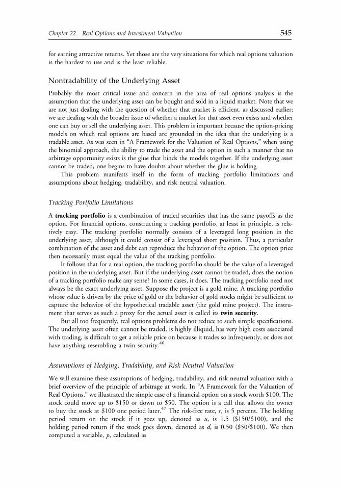
for earning attractive returns. Yet those are the very situations for which real options valuationis the hardest to use and is the least reliable.
Nontradability of the Underlying Asset
Probably the most critical issue and concern in the area of real options analysis is theassumption that the underlying asset can be bought and sold in a liquid market. Note that weare not just dealing with the question of whether that market is efficient, as discussed earlier;we are dealing with the broader issue of whether a market for that asset even exists and whetherone can buy or sell the underlying asset. This problem is important because the option-pricingmodels on which real options are based are grounded in the idea that the underlying is atradable asset. As was seen in “A Framework for the Valuation of Real Options,” when usingthe binomial approach, the ability to trade the asset and the option in such a manner that noarbitrage opportunity exists is the glue that binds the models together. If the underlying assetcannot be traded, one begins to have doubts about whether the glue is holding.
This problem manifests itself in the form of tracking portfolio limitations andassumptions about hedging, tradability, and risk neutral valuation.
Tracking Portfolio Limitations
A tracking portfolio is a combination of traded securities that has the same payoffs as theoption. For financial options, constructing a tracking portfolio, at least in principle, is rela-tively easy. The tracking portfolio normally consists of a leveraged long position in theunderlying asset, although it could consist of a leveraged short position. Thus, a particularcombination of the asset and debt can reproduce the behavior of the option. The option pricethen necessarily must equal the value of the tracking portfolio.
It follows that for a real option, the tracking portfolio should be the value of a leveragedposition in the underlying asset. But if the underlying asset cannot be traded, does the notionof a tracking portfolio make any sense? In some cases, it does. The tracking portfolio need notalways be the exact underlying asset. Suppose the project is a gold mine. A tracking portfoliowhose value is driven by the price of gold or the behavior of gold stocks might be sufficient tocapture the behavior of the hypothetical tradable asset (the gold mine project). The instru-ment that serves as such a proxy for the actual asset is called its twin security.
But all too frequently, real options problems do not reduce to such simple specifications.The underlying asset often cannot be traded, is highly illiquid, has very high costs associatedwith trading, is difficult to get a reliable price on because it trades so infrequently, or does nothave anything resembling a twin security.46
Assumptions of Hedging, Tradability, and Risk Neutral Valuation
We will examine these assumptions of hedging, tradability, and risk neutral valuation with abrief overview of the principle of arbitrage at work. In “A Framework for the Valuation ofReal Options,” we illustrated the simple case of a financial option on a stock worth $100. Thestock could move up to $150 or down to $50. The option is a call that allows the ownerto buy the stock at $100 one period later.47 The risk-free rate, r, is 5 percent. The holdingperiod return on the stock if it goes up, denoted as u, is 1.5 ($150/$100), and theholding period return if the stock goes down, denoted as d, is 0.50 ($50/$100). We thencomputed a variable, p, calculated as
c22 12 September 2012; 14:30:44
Chapter 22 Real Options and Investment Valuation 545

p ¼ 1þ r � du� d
¼ 1:05� 0:50
1:5� 0:5
¼ 0:55:
If the stock goes up, the call is worth $50 ($150 stock price 2 $100 exercise price) atexpiration. If the stock goes down, the call expires out of the money and is worth nothing. Wethen showed that the option price, c, can be obtained by taking the weighted average of $50 and$0, using the weights p 5 0.55 and 1 2 p 5 0.45, and discounting that result to the present:
c ¼ 0:55ð$50Þ þ 0:45ð$0Þ1:05
¼ $26:19:
We will now consider this formula for the price of the option and what it means. First,however, we will segue a little into valuation formulas in general. By definition, the value todayof any asset is found by taking its outcomes and weighting each outcome by the probability ofthat outcome’s occurrence. This result is the asset’s expected value at a future date. This expectedvalue is then discounted back to the present at a discount rate that incorporates an adjustmentfor the risk. Consider the stock in this problem. It can go up to $150 or down to $50.We do notneed to value the stock; the market has done that for us and has assigned a value of $100. If weknow one piece of information, either the probabilities of the outcomes or the discount rate, wecan determine the other. Suppose the probability of the upmove is 0.6. Then, the probability ofthe down move is 0.4 and the stock value is obtained as follows:
$100 ¼ 0:6ð$150Þ þ 0:4ð$50Þ1þ k
,
where k is the risk-adjusted discount rate. In this problem, a value of k 5 0.10 completes theequation. If the probability of an up move is 0.7 (and hence a down move is 0.3), then a valueof k 5 0.20 would be correct. If, instead, we knew that k were 0.12, we would have
$100 ¼ qð$150Þ þ ð1� qÞð$50Þ1:12
,
where q is the probability of the up move. Solving for q, we would obtain q 5 0.62. So, weeither need the probability or the risk-adjusted discount rate.
For traded assets, the market does the valuation for us. We do not need to know k or q.But, of course, the investors in the market have to know both k and q. Option-pricing models,however, take the value of the underlying asset as a given; they do not require k and q.
We know that in a market with rational investors, k would have to exceed the risk-freerate. Investors are risk averse, so they require a higher expected return than the risk-free rate.But we will suspend our imagination for a moment and assume that investors, for whateverreason, are not risk averse. Instead, we let them be risk neutral. Risk neutral investors do notworry or even think about risk. They do not require a higher return than the risk-free rate. Inthat case, notice how they would value the asset:
c22 12 September 2012; 14:30:44
546 Part V: Real Options Valuation
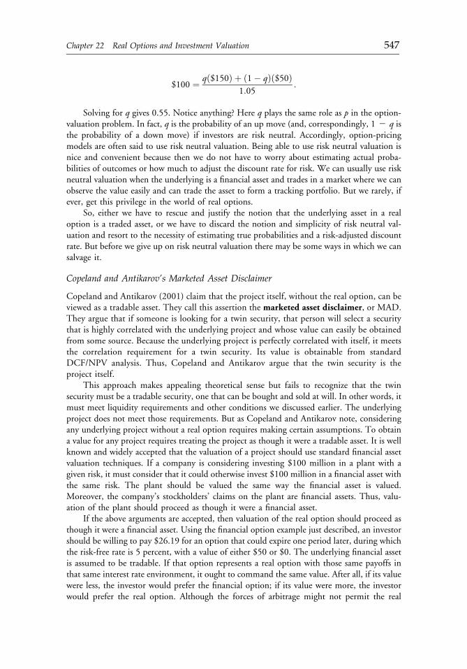
$100 ¼ qð$150Þ þ ð1� qÞð$50Þ1:05
:
Solving for q gives 0.55. Notice anything? Here q plays the same role as p in the option-valuation problem. In fact, q is the probability of an up move (and, correspondingly, 1 2 q isthe probability of a down move) if investors are risk neutral. Accordingly, option-pricingmodels are often said to use risk neutral valuation. Being able to use risk neutral valuation isnice and convenient because then we do not have to worry about estimating actual proba-bilities of outcomes or how much to adjust the discount rate for risk. We can usually use riskneutral valuation when the underlying is a financial asset and trades in a market where we canobserve the value easily and can trade the asset to form a tracking portfolio. But we rarely, ifever, get this privilege in the world of real options.
So, either we have to rescue and justify the notion that the underlying asset in a realoption is a traded asset, or we have to discard the notion and simplicity of risk neutral val-uation and resort to the necessity of estimating true probabilities and a risk-adjusted discountrate. But before we give up on risk neutral valuation there may be some ways in which we cansalvage it.
Copeland and Antikarov’s Marketed Asset Disclaimer
Copeland and Antikarov (2001) claim that the project itself, without the real option, can beviewed as a tradable asset. They call this assertion the marketed asset disclaimer, or MAD.They argue that if someone is looking for a twin security, that person will select a securitythat is highly correlated with the underlying project and whose value can easily be obtainedfrom some source. Because the underlying project is perfectly correlated with itself, it meetsthe correlation requirement for a twin security. Its value is obtainable from standardDCF/NPV analysis. Thus, Copeland and Antikarov argue that the twin security is theproject itself.
This approach makes appealing theoretical sense but fails to recognize that the twinsecurity must be a tradable security, one that can be bought and sold at will. In other words, itmust meet liquidity requirements and other conditions we discussed earlier. The underlyingproject does not meet those requirements. But as Copeland and Antikarov note, consideringany underlying project without a real option requires making certain assumptions. To obtaina value for any project requires treating the project as though it were a tradable asset. It is wellknown and widely accepted that the valuation of a project should use standard financial assetvaluation techniques. If a company is considering investing $100 million in a plant with agiven risk, it must consider that it could otherwise invest $100 million in a financial asset withthe same risk. The plant should be valued the same way the financial asset is valued.Moreover, the company’s stockholders’ claims on the plant are financial assets. Thus, valu-ation of the plant should proceed as though it were a financial asset.
If the above arguments are accepted, then valuation of the real option should proceed asthough it were a financial asset. Using the financial option example just described, an investorshould be willing to pay $26.19 for an option that could expire one period later, during whichthe risk-free rate is 5 percent, with a value of either $50 or $0. The underlying financial assetis assumed to be tradable. If that option represents a real option with those same payoffs inthat same interest rate environment, it ought to command the same value. After all, if its valuewere less, the investor would prefer the financial option; if its value were more, the investorwould prefer the real option. Although the forces of arbitrage might not permit the real
c22 12 September 2012; 14:30:44
Chapter 22 Real Options and Investment Valuation 547
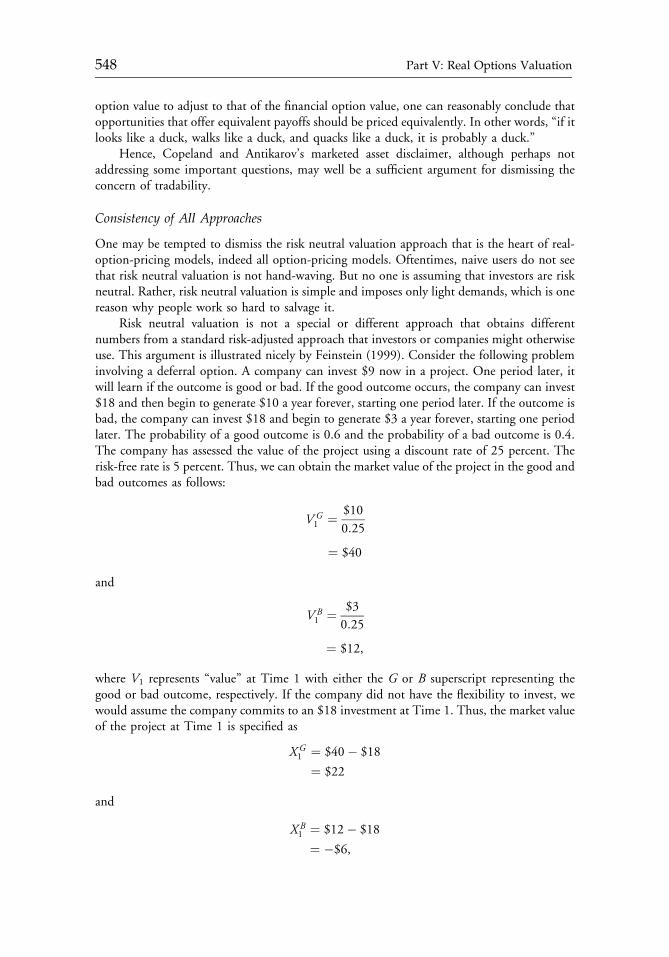
option value to adjust to that of the financial option value, one can reasonably conclude thatopportunities that offer equivalent payoffs should be priced equivalently. In other words, “if itlooks like a duck, walks like a duck, and quacks like a duck, it is probably a duck.”
Hence, Copeland and Antikarov’s marketed asset disclaimer, although perhaps notaddressing some important questions, may well be a sufficient argument for dismissing theconcern of tradability.
Consistency of All Approaches
One may be tempted to dismiss the risk neutral valuation approach that is the heart of real-option-pricing models, indeed all option-pricing models. Oftentimes, naive users do not seethat risk neutral valuation is not hand-waving. But no one is assuming that investors are riskneutral. Rather, risk neutral valuation is simple and imposes only light demands, which is onereason why people work so hard to salvage it.
Risk neutral valuation is not a special or different approach that obtains differentnumbers from a standard risk-adjusted approach that investors or companies might otherwiseuse. This argument is illustrated nicely by Feinstein (1999). Consider the following probleminvolving a deferral option. A company can invest $9 now in a project. One period later, itwill learn if the outcome is good or bad. If the good outcome occurs, the company can invest$18 and then begin to generate $10 a year forever, starting one period later. If the outcome isbad, the company can invest $18 and begin to generate $3 a year forever, starting one periodlater. The probability of a good outcome is 0.6 and the probability of a bad outcome is 0.4.The company has assessed the value of the project using a discount rate of 25 percent. Therisk-free rate is 5 percent. Thus, we can obtain the market value of the project in the good andbad outcomes as follows:
V G1 ¼ $10
0:25
¼ $40
and
V B1 ¼ $3
0:25
¼ $12,
where V1 represents “value” at Time 1 with either the G or B superscript representing thegood or bad outcome, respectively. If the company did not have the flexibility to invest, wewould assume the company commits to an $18 investment at Time 1. Thus, the market valueof the project at Time 1 is specified as
X G1 ¼ $40� $18
¼ $22
and
X B1 ¼ $12� $18
¼ �$6,
c22 12 September 2012; 14:30:44
548 Part V: Real Options Valuation
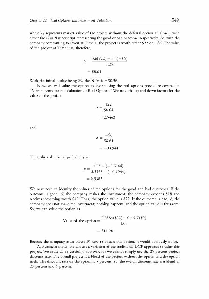
where X1 represents market value of the project without the deferral option at Time 1 witheither the G or B superscript representing the good or bad outcome, respectively. So, with thecompany committing to invest at Time 1, the project is worth either $22 or 2$6. The valueof the project at Time 0 is, therefore,
V0 ¼ 0:6ð$22Þ þ 0:4ð�$6Þ1:25
¼ $8:64:
With the initial outlay being $9, the NPV is 2$0.36.Now, we will value the option to invest using the real options procedure covered in
“A Framework for the Valuation of Real Options.” We need the up and down factors for thevalue of the project:
u ¼ $22
$8:64
¼ 2:5463
and
d ¼ �$6
$8:64
¼ �0:6944:
Then, the risk neutral probability is
p ¼ 1:05� ð�0:6944Þ2:5463� ð�0:6944Þ
¼ 0:5383:
We next need to identify the values of the options for the good and bad outcomes. If theoutcome is good, G, the company makes the investment; the company expends $18 andreceives something worth $40. Thus, the option value is $22. If the outcome is bad, B, thecompany does not make the investment; nothing happens, and the option value is thus zero.So, we can value the option as
Value of the option ¼ 0:5383ð$22Þ þ 0:4617ð$0Þ1:05
¼ $11:28:
Because the company must invest $9 now to obtain this option, it would obviously do so.As Feinstein shows, we can use a variation of the traditional DCF approach to value this
project. We must do so carefully, however, for we cannot simply use the 25 percent projectdiscount rate. The overall project is a blend of the project without the option and the optionitself. The discount rate on the option is 5 percent. So, the overall discount rate is a blend of25 percent and 5 percent.
c22 12 September 2012; 14:30:45
Chapter 22 Real Options and Investment Valuation 549
Recall that once we get out of the risk neutral world, we have to know either the trueprobabilities of the outcomes or the discount rate. Because we want to know the discount rate,we must know the true probabilities. We already gave them as 0.6 and 0.4. AdjustingFeinstein’s approach slightly, the weighted discount rate, kw, is found as
kw ¼ ½qX G1 þ ð1� qÞX B
1 �ð1þ rÞpX G
1 þ ð1� pÞX B1
� 1:
Because the company does not invest in state B, X B1 becomes zero. Thus, in this problem,
we have
kw ¼ ½0:6ð$22Þ þ 0:4ð$0Þ�ð1:05Þ0:5383ð$22Þ þ 0:4617ð$0Þ
¼ 0:1704:
This result means that if we discount the expected cash flows from the project at 17.04percent, we will obtain the correct value, and we do:
0:6ð$22Þ þ 0:4ð$0Þ1:1704
¼ $11:28:
This rate, 17.04 percent, is a blend of the 25 percent rate on the project and the 5 percent rateon the option.48
In other words, nothing about risk neutral valuation, the basis for all option-pricingmodels, is inconsistent with standard DCF analysis. Although we cannot get to the 17.04percent rate without resorting to at least some of the assumptions inherent in option-pricingmodels, we at least know that if we use the correct discount rate, we will be valuing the projectthe same way we have always valued projects, even long before anyone recognized what realoptions were.
Alternative Justifications
Finally, we should note that there are other ways in which risk neutral valuation can sometimesbe salvaged, even when the assumption that the underlying asset is tradable is clearly not met.Rubinstein (1976) derives amodel that shows that all assets in themarket can be valued as if theywere options. This approach involves the use of risk neutral valuation combined with theassumption that the market portfolio follows a type of joint probability distribution withthe underlying asset. Brennan (1979) demonstrates that a risk neutral valuation relationship isappropriate when investors have a particular type of utility function and the return on theunderlying asset follows a particular type of distribution, which is normal or lognormal. Theconditions that must be met for risk neutrality to hold are not terribly restrictive.
Although these papers are all theoretical and highly abstract, they provide a basis forarguing that a risk neutral valuation relationship is appropriate even when assets cannot betraded. To our knowledge, this point has not been recognized in the real options literature.What it says is simply that in spite of many of the criticisms, limitations, and obstacles wehave discussed in this section, using option-pricing models to value real options may beacceptable—something that everyone has been doing anyway but apparently without muchthought to whether it is appropriate to do so.
c22 12 September 2012; 14:30:45
550 Part V: Real Options Valuation

Summary
One source of difficulty in applying real options valuation is the use of option-pricing modelsthat make assumptions that may or may not be appropriate in the case of real options. Theoption-pricing assumptions of lognormality in the distribution of the value of the underlyingasset, randomness of prices, and a known and constant volatility of the value of the underlyingasset are assumptions that should cause some concern in applying real options valuation.Furthermore, the estimation of inputs, such as the value of the underlying, the exercise price,the time to expiration, and the volatility of the value of the underlying asset, is more chal-lenging for real options than for financial options.
Up until now in this chapter, we have discussed the theory and use of real options valuationand its relevance for financial analysts. An obvious question, however, is whether real optionsvaluation is used in practice and whether observed values of real options can be obtained andcompared with values from real options models. In other words, does empirical evidence existon the use and accuracy of real options models? This question will be answered in the nextsection, “Empirical Evidence on the Use and Accuracy of Real Options Valuation.”
EMPIRICAL EVIDENCE ON THE USE AND ACCURACYOF REAL OPTIONS VALUATION
The literature on real options is replete with theory. Many writers have developed interesting,but usually oversimplified, examples of real options—some taken from their consultingexperience. We will take a look at what the empirical research on real options says. In otherwords, does theory match up with practice?
Direct and Indirect Tests
The studies discussed in this section are either direct or indirect tests of whether the pre-dictions of real options models hold up in practice.
Paddock, Siegel, and Smith
James Paddock, Daniel Siegel, and James Smith (1988) develop a real options model forvaluing offshore oil and gas leases in a 1980 federal sale of 21 tracts in the western and centralportions of the Gulf of Mexico. Companies buy the rights to drill in certain tracts. Drillingmay reveal that oil or gas is present, in which case the company can choose to develop thetract into a well. The authors obtain input data and compare option values with prices atwhich the tracts were auctioned by the United States Geological Service (USGS). A com-parison of prices obtained from real options valuation models with bids placed by companies,as well as estimates obtained from the USGS, provides encouraging but not corroborativeresults. In other words, real options models were not able to explain the bids as well as onemight have hoped. Note, however, that this study was published in 1988, a time when realoptions theory was not well known, especially by practitioners who would actually use it. Inaddition, the authors point out that the data provided by the government were not as good aswould be hoped or expected in order to carry out a full and accurate real options analysis.Finally, one must take into consideration that when prices are determined by an auction, the“winner’s curse” (i.e., a tendency for the highest bidder to pay more than fair value)could explain the discrepancies between the model price and the actual winning bid price.
c22 12 September 2012; 14:30:45
Chapter 22 Real Options and Investment Valuation 551
This explanation is consistent with the fact that the winning bids in this auction were higherthan the values obtained by the models.
Quigg
Laura Quigg (1993) examines the real option to wait to develop urban land. Specifically, shelooks at the market prices of 2,700 land transactions in Seattle during the period 1976�1979and compares them with prices obtained using a real options model. Her results support thenotion that the option to wait and develop land at a later date has value approximately equalto 6 percent of the value of the underlying land. Her results are consistent with predictionsfrom real options models, supporting the belief that investors either use real options models ortrade in such a manner that their valuations are consistent with those of real options models.
Bailey
Warren Bailey (1991) tests the effectiveness of real options models by examining the valuationof agricultural companies in Singapore. These companies are well suited for the application ofreal options models because they produce a very limited number of crops and are traded onthe Singapore Stock Exchange, which facilitates the observation of prices and estimation ofvolatility. Other necessary input data are relatively easy to obtain.
The study covers a period from 1978 to 1985. Discounted cash flow (DCF) analysis andreal options models are used to predict the values of seven Singapore companies engaged inthe production of rubber and palm oil. In other words, the shareholdings of these companiesrepresent claims on real options and, therefore, should behave similarly to the real optionsthemselves. Both the DCF and real options models give estimates that are consistently low,but the real options model gives estimates that are closer to the market price. Baileyacknowledges the limitations of the real options models and the data, but he argues that hehas shown that valuations based on real options theory have significant power over thosebased on standard DCF analysis.
Berger, Ofek, and Swary
Philip Berger, Eli Ofek, and Itzhak Swary (1996) examine how investors value the option toabandon a company and claim its exit value. The study uses balance sheet information toestimate exit values. Although this study is not as directly about real options as it is aboutwhether investors take exit value into account in valuing companies, some predictions of realoptions models are relevant to this study. The authors examine a sample of about 1,000companies during the period 1984�1990. They find a highly significant relationship betweena company’s market value and its estimated exit value, suggesting that investors take theoption to exit into account when valuing companies. They also find that the more likelythe option will be exercised, the more valuable is the option.
Hayn
Carla Hayn (1995) examines companies’ earnings, focusing on the frequency of and marketresponse to losses. She studies a sample of 9,752 companies for the years 1962 through 1990,analyzing the relationship between earnings, market value, and returns. She finds evidencethat investors do not respond to losses to the same magnitude that they do to profits.Comparing the reaction to losses for companies whose value is above the net liquidation value
c22 12 September 2012; 14:30:45
552 Part V: Real Options Valuation
with those whose value is below the net liquidation value, she concludes that the option toliquidate is valued by investors.
Burgstahler and Dichev
David Burgstahler and Ilia Dichev (1997) examine whether the option to adapt a company’sresources to alternative, more productive uses is incorporated in the company’s market value.They estimate the adaptation value of a company by relating market value to a company’sbook value. Using observations on a sample of companies for the years 1976 through 1994,they find support for the idea that the exercise of the adaptation option depends on the levelof a company’s earnings and its book value; the lower the company’s value from the currentdeployment of assets, the more important the adaptation option.
Moel and Tufano
Alberto Moel and Peter Tufano (2002) study a sample of 285 North American gold mines inthe period 1988�1997. These mines are periodically opened and closed, a classic exampleof the shutdown option discussed in Appendix 22A. They gather data and test whether thesedecisions are consistent with the predictions of real options models. The tests support thepredictions of the models. Closings are highly related to the price and volatility of gold,the cost of closing a mine, and other factors. Moel and Tufano note, however, that otheraspects of mine closings are not captured by the models, such as whether a company hasother mines operating.
Clayton and Yermack
Matthew Clayton and David Yermack (1999) use real options models to examine the con-tracts of major league baseball players. These contracts commonly contain option clauses—insome cases where a team holds the option to extend the player’s contract and in some caseswhere the player holds the option to extend his contract, both for a fixed salary. They examinea sample of more than 1,100 players in the mid-1990s, of which options are contained inabout 18 percent of the contracts. Statistical analysis reveals that the predictions of realoptions models are upheld in these players’ contracts. Specifically, option values decrease as afunction of the difference between the exercise price and the player’s salary (the moneyness ofthe option) and increase as a function of the time to expiration of the option. Option values,however, are apparently unrelated to the volatility of the player’s ability, which is inconsistentwith real options models.
The Use of Real Options Models by Practitioners
In the two studies in this section, the researchers have attempted to determine if practicingfinancial managers recognize and use real options models.
Howell and Jagle
Sydney Howell and Axel Jagle (1997) conduct a laboratory experiment with 82 professionalmanagers of nine companies in the United Kingdom. They ask these managers to answer aseries of questions on growth options from some investment case studies. In addition, theauthors ask the managers other questions related to their personal situations and the kinds of
c22 12 September 2012; 14:30:45
Chapter 22 Real Options and Investment Valuation 553
investment decisions they make in their work. The authors find that these managers tend tovalue growth options in an erratic manner. This evidence is not consistent with real optionstheory. These results can be interpreted in two possible ways. The first is that this limitedsample of managers is not sufficiently knowledgeable about real options models. The secondis that real options models are simply not used in practice. The small sample size, however, isa major limitation of this study. Perhaps a larger sample of managers would produce findingsmore supportive of real options models.
Busby and Pitts
J.S. Busby and C.G.C. Pitts (1997) conduct a mail survey of senior finance officers in 100U.K. companies, receiving 44 usable replies. They find that these individuals encounter realoptions in their work and tend to recognize them. They also find, however, considerablevariation in the frequency of encountering real options as well as in how important theyperceive real options to be. Most companies do not have procedures in place to identifyand evaluate real options, tending to use cruder tools, such as sensitivity analysis. Therespondents tend to agree with the predictions of real options models, meaning that thefactors that make real options important are indeed perceived in that manner. Interestingly,most of the respondents are not aware of the terminology of “real options” or “growthoptions,” which further suggests that they are unlikely to use the latest knowledge of realoptions models.
Summary
Data availability is the greatest hindrance to conducting empirical studies on real options, andhence, the body of empirical work on real options is quite limited. Real options necessarilyinvolve private data, often internal and specific to a given company. Even when data areavailable, accuracy and reliability are in question. Perhaps for that reason, it is all the moreremarkable that the empirical work cited in this section tends to provide generally supportiveevidence. But perhaps that finding is not so unusual. Real options models are based onrational behavior. Even if individual decision makers do not use such models, they still tend tobehave rationally. Hence, the models will tend to capture the essential characteristics of realoptions in the valuation and decision-making process.
Nevertheless, the survey data presented in this section do not lend much credence to thebelief that managers use or even understand real options. Perhaps this finding is a reflection ofthe fact that real options theory is relatively young and managers have not been trained tounderstand it. After all, not until the decade of the 1990s did financial option-pricing theorybecome widely practiced. Thus, it will likely take longer for real options models to make theirway into the toolkit of practicing financial managers. This does not mean that real optionsmodels should be abandoned until such time as they are taken up by others. Indeed, usinggood models before everyone else is an important ingredient in generating value.
SUMMARY AND CONCLUSIONS
The financial analysis of a company is a difficult undertaking, even under the best of cir-cumstances. Financial information is never completely sufficient to uncover the hidden
c22 12 September 2012; 14:30:45
554 Part V: Real Options Valuation
benefits and costs that distinguish one company from another. Even when information is easyto obtain, the analytical techniques often rely on heroic assumptions and forecasts aboutgrowth rates, dividend policy, capital expenditures, and a host of other factors that are dif-ficult to predict. Further complicating the process of financial analysis is the fact that many, ifnot all, companies have some opportunities that are not so apparent. These opportunities arein the form of options that give a company flexibility in making decisions. Companies canterminate projects, switch to alternatives, enter new markets, exit old markets, delay expan-sions, and expand or contract existing investments. Standard accounting principles do notallow the value of such opportunities to appear on balance sheets, and the gains and lossesfrom changes in the value of these opportunities are never recorded in earnings.Unquestionably, these opportunities are a source of value, but as noted, they are difficult todetect. In fact, we can probably safely say that many companies themselves are unaware ofmany of these valuable opportunities that they possess.
These opportunities are called real options, named as such because they deal withopportunities related to real investments, as opposed to financial investments. Options on thelatter, such as puts and calls that trade on options exchanges and over-the-counter marketsand options that are issued by companies to employees and executives, are well known infinancial markets. A large body of literature exists on the valuation of these instruments, muchof which can be traced to the celebrated Black�Scholes model, for which a Nobel Prize wasawarded in 1997. The field of real options analysis has taken its framework from the valuationof financial options and adapted it to real options. Considerable progress has been made inthis endeavor; the body of literature on real options is almost overwhelming, although muchof it is too complex for practicing financial managers and analysts. In this chapter, we haveattempted to glean the most important results from that body of literature and consolidateand condense them into a single document. At the same time, we have added new material onthe difficulties of applying real options to real investment problems. In this section, weprovide a summary of what we have discussed in this chapter.
� Companies are often highly misvalued in the market, with at least a portion of the dis-crepancy between fundamental values and market values undoubtedly caused by real options. Thisphenomenon seems to be particularly evident in the technology industry, where real optionsare commonly found. Although real options almost surely cannot account for all the seem-ingly absurd valuations seen in recent years in many technology stocks, they just as assuredlyare the source of some of what appears to be overvaluation. Conversely, a failure of the marketto recognize real options can mean that some stocks seem undervalued.
� Corporate investment decisions are typically made using standard discounted cash flow(DCF) techniques, which are not equipped to accommodate real options. When a corporationanalyzes a project, it arrives at a net present value (NPV). If this NPV is positive, the project isacceptable. But an NPV analysis is not capable of accommodating the flexibility in manyinvestment decisions. Even something as simple as an option to defer an investment one ormore years into the future cannot be easily analyzed using an NPV approach. One can cal-culate an NPV based on investing today, another NPV based on investing in one year, andother NPVs based on investing in later years. Should the company make the decision of whento invest based on the NPV that is the largest? No. Suppose the largest NPV is associated withthe choice of waiting three years. Should the company thus decide today whether to invest inthree years? No. What happens if market conditions are not favorable in three years? Realoptions analysis takes into account the fact that market conditions might not be favorable in
c22 12 September 2012; 14:30:45
Chapter 22 Real Options and Investment Valuation 555
three years. The flexibility to forgo investing in three years, if this decision proves to beoptimal, is valuable not just in three years but today as well. Real options analysis captures thevalue of that flexibility today.
� Discounted cash flow techniques that attempt to capture flexibility are not adequate. Simu-lation analysis, sensitivity analysis, and decision trees attempt to capture the value of flexibility,but they impose unnecessarily heavy demands on the user, in particular by requiring a risk-adjusted discount rate. How does one go about assessing the risk of an option? It is not the sameas the risk of the project itself. Real options analysis assesses the risk of an option the same waythat investors assess the risk of the option in an open and liquid market for financial options.Shareholders, after all, can invest in financial options. If real options offer the same payoffs, theyshould be valued in a similar manner.
� The valuation of financial options has benefited from years of study, evolving from thebinomial and Black�Scholes models. These models can be used in the valuation of real options.Binomial models specify a sequential path of future outcomes for each price of the underlyingasset. The option is valued at the expiration at its exercise value. One then steps backward,evaluating at each time point a probability-weighted average of the next two option values atthe next time point and then discounting that value back one period at the risk-free rate. Thebinomial model is extremely flexible and is widely used for valuing complicated options,which certainly describes many real options.
The Black�Scholes model is a mathematical formula that requires five inputs andproduces the value of the option. For a real option, the model requires the value of theunderlying asset on which the real option is based, the exercise price or amount that must bepaid to exercise the option, the length of time before the option expires, the risk-free rate ofinterest, and a measure of the volatility of the underlying asset.
� A number of limitations and difficulties arise in applying real options. Real options oftenexist in multiple forms, leading to complicated interaction effects. Real options, indeed alloptions, are highly sensitive to model risk, which is the use of a wrong model, the use ofwrong inputs in the right model, or the incorrect use of a model. Real options are also subjectto the criticism that the party that controls the underlying asset also controls the real options.Thus, the underlying asset and the real option can often interact in a manner not built intothe models.
� Real options models oftentimes do not meet the assumptions inherent in the models. Theprices of the underlying assets rarely adhere to a lognormal distribution and are often not evenrandom, and volatility is seldom known and constant—all violations of the model assump-tions. These problems exist to some degree even in financial option applications, but they aremuch more severe with real options. At the same time, it is not always necessary that theassumptions of a model be met. Many widely used financial models produce reasonablyaccurate results without conforming strictly to their required assumptions.
� The estimation of inputs in real options models is particularly challenging. The value of theunderlying asset is typically measured using DCF analysis, which is subject to considerablesensitivity and the criticism that for real options the underlying asset is not traded in an active,liquid market. In addition, the exercise price is not always easy to identify, particularly giventhat it is paid at a later date. In some cases, the exercise price can even vary. The time toexpiration can even be difficult to estimate. Furthermore, identifying the lives and termina-tion dates of certain options is not always easy. And the volatility is particularly difficult toestimate. Because typically no active market exists for the underlying asset, rarely can one finda set of data from which to estimate the historical volatility, nor can one determine the
c22 12 September 2012; 14:30:45
556 Part V: Real Options Valuation
implied volatility from the prices of actively traded options because these are not activelytraded options. Only the risk-free rate is fairly easy to obtain.
� Probably the greatest criticism of real options valuation is that the models are based on theidea that one can trade the underlying asset and the option to form a risk-free hedge or trade acombination of the underlying asset and risk- free bonds to replicate the payoffs of the option. Thus,the models require the ability to trade the underlying asset, which is definitely not true fornearly all real options. With this point in mind, this approach to option valuation, called riskneutral valuation, is thought by many to be inappropriate for options. Surprisingly, virtuallyall of the books and articles on real options dismiss this point. But real options valuation isnot dependent on risk neutral valuation and the ability to engage in the hedging and arbitrageas set forth in the models. If real options were valued using DCF approaches with theappropriate risk-adjusted discount rate, they would have the same values as would be obtainedusing option-valuation methods. Yet, the former approach would impose much greaterdemands on the user for obtaining input information, such as the risk-adjusted discount rate,than the latter approach. Furthermore, one can easily argue that if real options producepayoffs at their expirations that are like those of financial options, then financial optionvaluation techniques are appropriate because investors could invest in financial options andreceive those payoffs. Finally, risk neutral valuation actually does not impose terribly heavyrestrictions on users of the models and can be justified if investors and markets have certainreasonable characteristics. In short, risk neutral valuation, the basis for virtually all financialoption-pricing models, is actually not a very demanding framework. Indeed, it demands farless than the DCF methods that have been widely accepted for the valuation of capitalinvestment projects that do not contain real options.
� Empirical research has provided some, but very limited, support for the real-world applica-bility of real options models. Some studies have shown that real options in the real world arevalued in a manner consistent with real options models, but other studies have not been verysupportive of real options valuation. Nevertheless, it is really too early to tell if real optionsvaluation is truly applicable in the real world, because for one, conducting empirical studies onreal options is very difficult. The information associated with real options is primarily privateinformation that companies do not generally release. Even when data are available, the data areoftentimes only crude proxies for the key variables. Thus, the studies tend to be subject tolimitations associated with having small samples and questionable data. Moreover, the studiesdo not make clear that managers and investors really understand real options and real optionsvaluation models well enough to incorporate them into the valuation process. Indeed, studies ofthe knowledge that managers have of real options suggest that managers have much to learn.This finding suggests that real options have a long way to go before managers and investorsbegin to fully appreciate their true value and are able to properly use and evaluate them.
That real options are not well recognized is no reason to ignore them. Indeed, notunderstanding a phenomenon that unquestionably exists is all the more reason to learn aboutit and make use of it as soon as possible. At some time in the not-too-distant future, realoptions may well be widely understood and properly incorporated into corporate investmentdecisions and, accordingly, market valuations. Then, the financial world will be high on thelearning curve, and the marginal benefits of learning about real options valuation will be muchlower. We hope that this chapter has helped the financial analyst gain an appreciation for thepotential benefits of understanding real options and a healthy respect for the difficulties andlimitations of analyzing them and that he or she will undertake further study of real optionswhile the payoffs from the learning process are still quite high.
c22 12 September 2012; 14:30:46
Chapter 22 Real Options and Investment Valuation 557
APPENDIX 22A FURTHER ILLUSTRATIONS OF REALOPTIONS IN INVESTMENT PROJECTS
In the section “A Framework for the Valuation of Real Options,” we focused on three types ofreal options: the growth option, the deferral option, and the abandonment option. In thisappendix, we will look at three additional options: the option to default, the option tocontract, and the option to shut down. To illustrate these options, we will use the same capitalinvestment project as depicted in Figure 22.9, adjusting it as needed.
Option to Default
The option to terminate a project at some time during the project’s life is called the option todefault. By choosing not to invest further and simply dropping the project, the company is, in away, defaulting, except that no legal implications arise from this type of default. As we discussedin the section “A Framework for the Valuation of Real Options,” a default option accompaniedby the opportunity to obtain a salvage value from the project is referred to as an abandonmentoption.
Recall that the initial outlay for this project illustrated in Figure 22.9 is $1,050. Wewill assume that the company can make an initial investment of $400 with the option toinvest the remaining $650 one period later, but this $650 will be increased at the risk-freerate of interest. Thus, the company can invest $650 3 1.05 5 $682.50 at Time 1. Ifthe company does not invest the $682.50 at Time 1, the project terminates and no furthervalue is generated.
Recall from the original binomial tree for the capital investment project (Figure 22.9)that at Time 1 the project has a value of either $1,500 or $500. If the project is worth $1,500,the company will certainly invest the $682.50, but if it is worth $500, the company will notinvest the $682.50 and will terminate the project. Thus, at Time 1, the values of the projectare $1,500 2 $682.50 5 $817.50 or $0. Using the risk neutral valuation approach, asshown in “A Framework for the Valuation of Real Options,” we would find the value of theproject at Time 0 to be $428.21 as follows:
Value of the project at Time 0 ¼ 0:55ð$817:50Þ þ 0:45ð$0Þ1:05
¼ $428:21:
The company is required to invest $400 at Time 0, so the net present value (NPV) of theproject is $428.21 2 $400 5 $28.21. In this scenario, the project has a positive NPV. Recallfrom “A Framework for the Valuation of Real Options” that the value of the project withoutthe option was 2$50. With the option, it is $28.21. Thus, the value of the option is$28.21 2 (2$50) 5 $78.21. This problem is illustrated in Figure 22A.1.
The attractiveness of the project with the option is a result of a combination of the abilityto defer the investment and to choose not to invest the remaining initial outlay at Time 1 ifthe project is not working out. Clearly, this option has value, and in this case, it has enoughvalue to convert the project from an unattractive one to an attractive one.
c22 12 September 2012; 14:30:46
558 Part V: Real Options Valuation
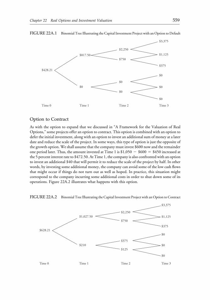
Option to Contract
As with the option to expand that we discussed in “A Framework for the Valuation of RealOptions,” some projects offer an option to contract. This option is combined with an option todefer the initial investment, along with an option to invest an additional sum of money at a laterdate and reduce the scale of the project. In some ways, this type of option is just the opposite ofthe growth option.We shall assume that the company must invest $600 now and the remainderone period later. Thus, the amount invested at Time 1 is $1,050 2 $600 5 $450 increased atthe 5 percent interest rate to $472.50. At Time 1, the company is also confronted with an optionto invest an additional $40 that will permit it to reduce the scale of the project by half. In otherwords, by investing some additional money, the company can avoid some of the low cash flowsthat might occur if things do not turn out as well as hoped. In practice, this situation mightcorrespond to the company incurring some additional costs in order to shut down some of itsoperations. Figure 22A.2 illustrates what happens with this option.
FIGURE 22A.1 Binomial Tree Illustrating the Capital Investment Project with anOption toDefault
$817.50
$2,250
$750
$3,375
$1,125
$375
$0$0
$0
$0
$0
$0
$428.21
Time 0 Time 1 Time 2 Time 3
FIGURE 22A.2 Binomial Tree Illustrating the Capital Investment Project with anOption toContract
$1,027.50$2,250
$750
$3,375
$1,125
$375
$210$375
$125
$0
$0
$0
$628.21
Time 3Time 2Time 1Time 0
c22 12 September 2012; 14:30:46
Chapter 22 Real Options and Investment Valuation 559
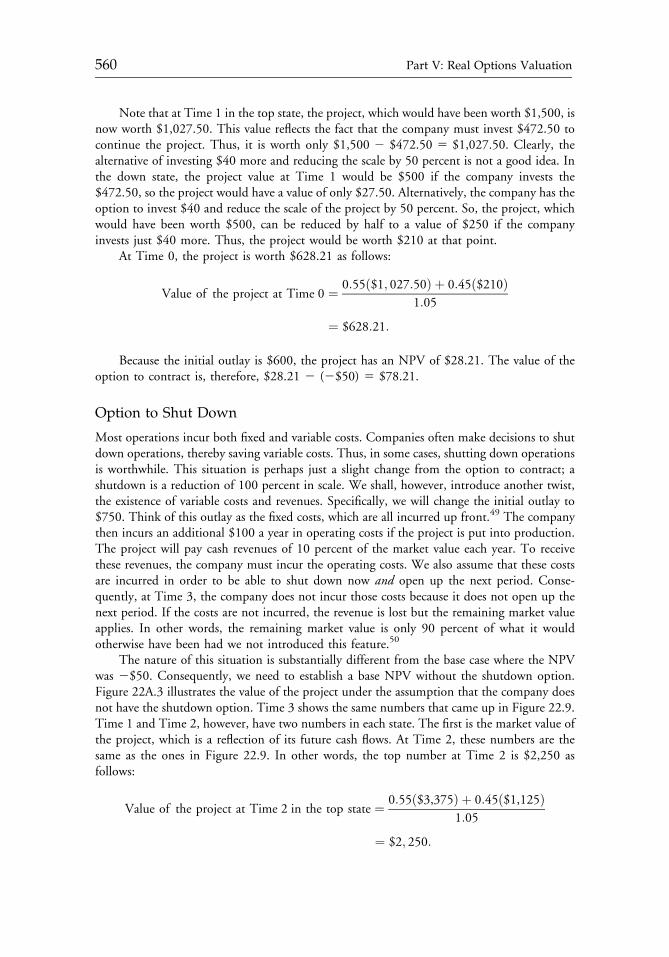
Note that at Time 1 in the top state, the project, which would have been worth $1,500, isnow worth $1,027.50. This value reflects the fact that the company must invest $472.50 tocontinue the project. Thus, it is worth only $1,500 2 $472.50 5 $1,027.50. Clearly, thealternative of investing $40 more and reducing the scale by 50 percent is not a good idea. Inthe down state, the project value at Time 1 would be $500 if the company invests the$472.50, so the project would have a value of only $27.50. Alternatively, the company has theoption to invest $40 and reduce the scale of the project by 50 percent. So, the project, whichwould have been worth $500, can be reduced by half to a value of $250 if the companyinvests just $40 more. Thus, the project would be worth $210 at that point.
At Time 0, the project is worth $628.21 as follows:
Value of the project at Time 0 ¼ 0:55ð$1; 027:50Þ þ 0:45ð$210Þ1:05
¼ $628:21:
Because the initial outlay is $600, the project has an NPV of $28.21. The value of theoption to contract is, therefore, $28.21 2 (2$50) 5 $78.21.
Option to Shut Down
Most operations incur both fixed and variable costs. Companies often make decisions to shutdown operations, thereby saving variable costs. Thus, in some cases, shutting down operationsis worthwhile. This situation is perhaps just a slight change from the option to contract; ashutdown is a reduction of 100 percent in scale. We shall, however, introduce another twist,the existence of variable costs and revenues. Specifically, we will change the initial outlay to$750. Think of this outlay as the fixed costs, which are all incurred up front.49 The companythen incurs an additional $100 a year in operating costs if the project is put into production.The project will pay cash revenues of 10 percent of the market value each year. To receivethese revenues, the company must incur the operating costs. We also assume that these costsare incurred in order to be able to shut down now and open up the next period. Conse-quently, at Time 3, the company does not incur those costs because it does not open up thenext period. If the costs are not incurred, the revenue is lost but the remaining market valueapplies. In other words, the remaining market value is only 90 percent of what it wouldotherwise have been had we not introduced this feature.50
The nature of this situation is substantially different from the base case where the NPVwas 2$50. Consequently, we need to establish a base NPV without the shutdown option.Figure 22A.3 illustrates the value of the project under the assumption that the company doesnot have the shutdown option. Time 3 shows the same numbers that came up in Figure 22.9.Time 1 and Time 2, however, have two numbers in each state. The first is the market value ofthe project, which is a reflection of its future cash flows. At Time 2, these numbers are thesame as the ones in Figure 22.9. In other words, the top number at Time 2 is $2,250 asfollows:
Value of the project at Time 2 in the top state ¼ 0:55ð$3,375Þ þ 0:45ð$1,125Þ1:05
¼ $2; 250:
c22 12 September 2012; 14:30:46
560 Part V: Real Options Valuation
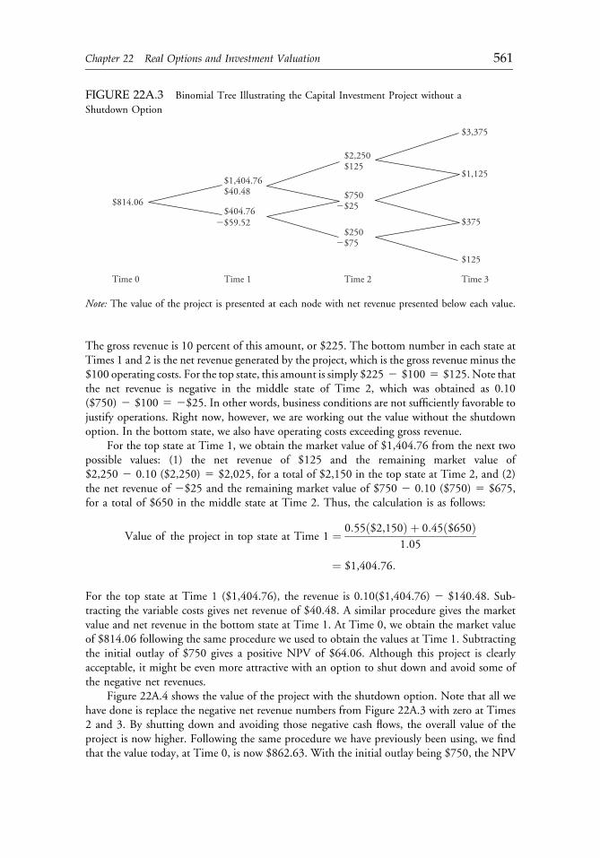
The gross revenue is 10 percent of this amount, or $225. The bottom number in each state atTimes 1 and 2 is the net revenue generated by the project, which is the gross revenue minus the$100 operating costs. For the top state, this amount is simply $225 2 $100 5 $125.Note thatthe net revenue is negative in the middle state of Time 2, which was obtained as 0.10($750) 2 $100 5 2$25. In other words, business conditions are not sufficiently favorable tojustify operations. Right now, however, we are working out the value without the shutdownoption. In the bottom state, we also have operating costs exceeding gross revenue.
For the top state at Time 1, we obtain the market value of $1,404.76 from the next twopossible values: (1) the net revenue of $125 and the remaining market value of$2,250 2 0.10 ($2,250) 5 $2,025, for a total of $2,150 in the top state at Time 2, and (2)the net revenue of 2$25 and the remaining market value of $750 2 0.10 ($750) 5 $675,for a total of $650 in the middle state at Time 2. Thus, the calculation is as follows:
Value of the project in top state at Time 1 ¼ 0:55ð$2,150Þ þ 0:45ð$650Þ1:05
¼ $1,404:76:
For the top state at Time 1 ($1,404.76), the revenue is 0.10($1,404.76) 2 $140.48. Sub-tracting the variable costs gives net revenue of $40.48. A similar procedure gives the marketvalue and net revenue in the bottom state at Time 1. At Time 0, we obtain the market valueof $814.06 following the same procedure we used to obtain the values at Time 1. Subtractingthe initial outlay of $750 gives a positive NPV of $64.06. Although this project is clearlyacceptable, it might be even more attractive with an option to shut down and avoid some ofthe negative net revenues.
Figure 22A.4 shows the value of the project with the shutdown option. Note that all wehave done is replace the negative net revenue numbers from Figure 22A.3 with zero at Times2 and 3. By shutting down and avoiding those negative cash flows, the overall value of theproject is now higher. Following the same procedure we have previously been using, we findthat the value today, at Time 0, is now $862.63. With the initial outlay being $750, the NPV
FIGURE 22A.3 Binomial Tree Illustrating the Capital Investment Project without a
Shutdown Option
$814.06
Time 0 Time 1 Time 2 Time 3
$1,404.76
$404.76�$59.52
$40.48
$2,250$125
$750
$250
�$25
�$75
$3,375
$1,125
$375
$125
Note: The value of the project is presented at each node with net revenue presented below each value.
c22 12 September 2012; 14:30:46
Chapter 22 Real Options and Investment Valuation 561
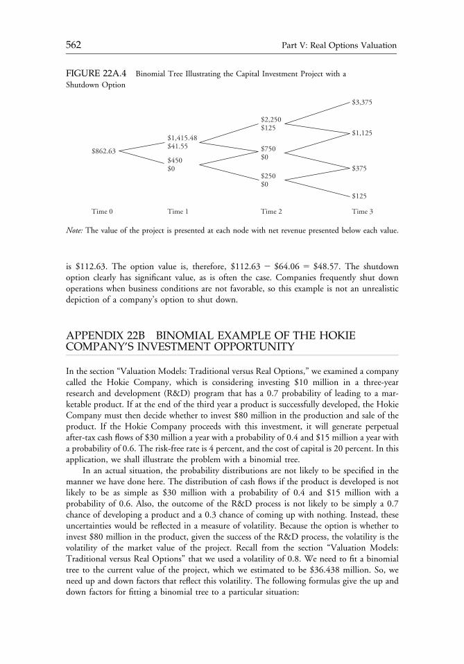
is $112.63. The option value is, therefore, $112.63 2 $64.06 5 $48.57. The shutdownoption clearly has significant value, as is often the case. Companies frequently shut downoperations when business conditions are not favorable, so this example is not an unrealisticdepiction of a company’s option to shut down.
APPENDIX 22B BINOMIAL EXAMPLE OF THE HOKIECOMPANY’S INVESTMENT OPPORTUNITY
In the section “Valuation Models: Traditional versus Real Options,” we examined a companycalled the Hokie Company, which is considering investing $10 million in a three-yearresearch and development (R&D) program that has a 0.7 probability of leading to a mar-ketable product. If at the end of the third year a product is successfully developed, the HokieCompany must then decide whether to invest $80 million in the production and sale of theproduct. If the Hokie Company proceeds with this investment, it will generate perpetualafter-tax cash flows of $30 million a year with a probability of 0.4 and $15 million a year witha probability of 0.6. The risk-free rate is 4 percent, and the cost of capital is 20 percent. In thisapplication, we shall illustrate the problem with a binomial tree.
In an actual situation, the probability distributions are not likely to be specified in themanner we have done here. The distribution of cash flows if the product is developed is notlikely to be as simple as $30 million with a probability of 0.4 and $15 million with aprobability of 0.6. Also, the outcome of the R&D process is not likely to be simply a 0.7chance of developing a product and a 0.3 chance of coming up with nothing. Instead, theseuncertainties would be reflected in a measure of volatility. Because the option is whether toinvest $80 million in the product, given the success of the R&D process, the volatility is thevolatility of the market value of the project. Recall from the section “Valuation Models:Traditional versus Real Options” that we used a volatility of 0.8. We need to fit a binomialtree to the current value of the project, which we estimated to be $36.438 million. So, weneed up and down factors that reflect this volatility. The following formulas give the up anddown factors for fitting a binomial tree to a particular situation:
FIGURE 22A.4 Binomial Tree Illustrating the Capital Investment Project with a
Shutdown Option
$862.63
$1,415.48$41.55
$450$0
$2,250$125
$750$0
$250$0
$3,375
$1,125
$375
$125
Time 0 Time 1 Time 2 Time 3
Note: The value of the project is presented at each node with net revenue presented below each value.
c22 12 September 2012; 14:30:46
562 Part V: Real Options Valuation
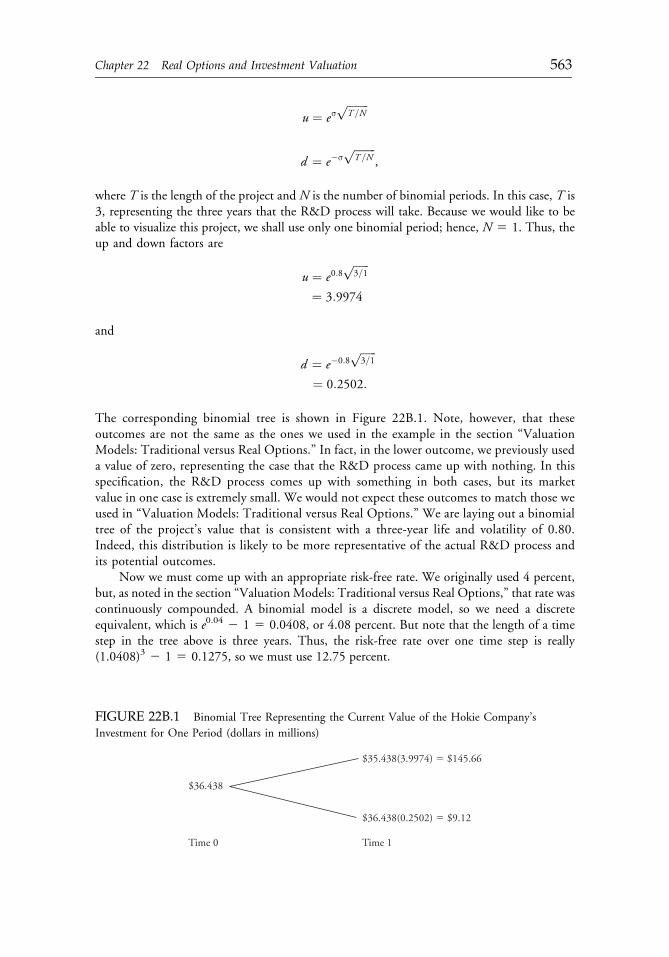
u ¼ eσffiffiffiffiffiffiffiffiT =N
p
d ¼ e�σffiffiffiffiffiffiffiffiT =N
p,
where T is the length of the project and N is the number of binomial periods. In this case, T is3, representing the three years that the R&D process will take. Because we would like to beable to visualize this project, we shall use only one binomial period; hence, N 5 1. Thus, theup and down factors are
u ¼ e0:8ffiffiffiffiffiffi3=1
p
¼ 3:9974
and
d ¼ e�0:8ffiffiffiffiffiffi3=1
p
¼ 0:2502:
The corresponding binomial tree is shown in Figure 22B.1. Note, however, that theseoutcomes are not the same as the ones we used in the example in the section “ValuationModels: Traditional versus Real Options.” In fact, in the lower outcome, we previously useda value of zero, representing the case that the R&D process came up with nothing. In thisspecification, the R&D process comes up with something in both cases, but its marketvalue in one case is extremely small. We would not expect these outcomes to match those weused in “Valuation Models: Traditional versus Real Options.” We are laying out a binomialtree of the project’s value that is consistent with a three-year life and volatility of 0.80.Indeed, this distribution is likely to be more representative of the actual R&D process andits potential outcomes.
Now we must come up with an appropriate risk-free rate. We originally used 4 percent,but, as noted in the section “Valuation Models: Traditional versus Real Options,” that rate wascontinuously compounded. A binomial model is a discrete model, so we need a discreteequivalent, which is e0.04 2 1 5 0.0408, or 4.08 percent. But note that the length of a timestep in the tree above is three years. Thus, the risk-free rate over one time step is really(1.0408)3 2 1 5 0.1275, so we must use 12.75 percent.
FIGURE 22B.1 Binomial Tree Representing the Current Value of the Hokie Company’s
Investment for One Period (dollars in millions)
$36.438
$35.438(3.9974) � $145.66
$36.438(0.2502) � $9.12
Time 1Time 0
c22 12 September 2012; 14:30:46
Chapter 22 Real Options and Investment Valuation 563
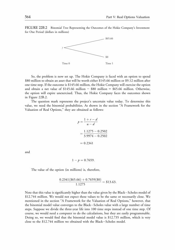
So, the problem is now set up. The Hokie Company is faced with an option to spend$80 million to obtain an asset that will be worth either $145.66 million or $9.12 million afterone time step. If the outcome is $145.66 million, the Hokie Company will exercise the optionand obtain a net value of $145.66 million 2 $80 million 5 $65.66 million. Otherwise,the option will expire unexercised. Thus, the Hokie Company faces the outcomes shownin Figure 22B.2.
The question mark represents the project’s uncertain value today. To determine thisvalue, we need the binomial probabilities. As shown in the section “A Framework for theValuation of Real Options,” they are obtained as follows:
p ¼ 1þ r � du� d
¼ 1:1275� 0:2502
3:9974� 0:2502
¼ 0:2341
and
1� p ¼ 0:7659:
The value of the option (in millions) is, therefore,
0:2341ð$65:66Þ þ 0:7659ð$0Þ1:1275
¼ $13:63:
Note that this value is significantly higher than the value given by the Black�Scholes model of$12.744 million. We would not expect these values to be the same or necessarily close. Wementioned in the section “A Framework for the Valuation of Real Options,” however, thatthe binomial model value converges to the Black�Scholes value with a large number of timesteps. Suppose we divide the three-year life into 100 time steps instead of one time step. Ofcourse, we would need a computer to do the calculations, but they are easily programmable.Doing so, we would find that the binomial model value is $12.735 million, which is veryclose to the $12.744 million we obtained with the Black�Scholes model.
FIGURE 22B.2 Binomial Tree Representing the Outcomes of the Hokie Company’s Investment
for One Period (dollars in millions)
?
$65.66
$0
Time 1Time 0
c22 12 September 2012; 14:30:46
564 Part V: Real Options Valuation
GLOSSARY
Abandonment option: The option to cease a project prior to the end of its useful life and torecover the project’s salvage value.
American option: An option that can be exercised at any time on or before the expiration date.Arbitrage opportunity: A market situation in which an asset is priced differently in two
markets such that an investor can buy the asset in one market at one price and sell it fora higher price in the other market, thereby capturing the difference in the prices andincurring no risk.
Binomial model: A model for valuing options in which only two possible outcomes or statesare associated with the underlying asset for each period of time.
Binomial tree: A graphical representation of a binomial model showing the possibleoutcomes or states associated with an option and its underlying asset.
Black�Scholes model: A model for pricing options in which the value of an option dependson the value of the underlying asset, the time to expiration of the option, the exerciseprice, the volatility of the underlying asset, and the risk-free rate or time value of money.
Call option: An option to buy a particular asset at a specified price within a specified period oftime.
Compound option: An option to buy or sell an option. That is, the underlying asset of theoption is another option.
Decision tree: A graphical representation of decisions and uncertainties over time for aninvestment project.
Deferral option: The option to invest in an investment project at a later date.European option: An option that can be exercised only on the expiration date.Exercise price: The price at which the option allows the owner of the option to buy (in the
case of a call option) or sell (in the case of a put option) the specified asset. In the case ofa real option, the exercise price is the cost of exercising the option (e.g., the cost ofadditional facilities in an expansion option). Also known as strike price, strike, orstriking price.
Exit value: Salvage value or residual value; the cash flow expected in the future upondisposition of a project’s assets.
Expansion option: See growth option.Flexibility option: An option that provides the opportunity to revise decisions in the future.Growth option: The option to expand or grow in the future.Learning option: An option in which the investment in a capital project produces
information that reduces the uncertainty regarding future decisions related to thecapital project.
Lognormality: An assumption typically used in option valuation that the underlying assetfollows a lognormal probability distribution, which implies that the log return on theasset is normally distributed.
Marketed asset disclaimer: The argument that a project can serve as its own twin securitythat can be used to replicate the option on the project. This argument essentially meansthat a project can be viewed as a traded asset.
Model risk: The risk associated with using a wrong valuation model, wrong inputs in anotherwise correct valuation model, or the incorrect use of a correct valuation model,which can include programming errors and other mistakes.
Option to contract: The option to reduce the scale of a project.
c22 12 September 2012; 14:30:47
Chapter 22 Real Options and Investment Valuation 565
Option to default: The option to terminate an investment during the time when investmentoutlays are continuing to be made.
Option to shut down: The option to halt operations, in which this stoppage may betemporary or permanent.
Put option: An option to sell a particular asset within a specified period of time for a specifiedprice.
Real options valuation: The valuation of the options inherent in an investment decisioninvolving a real or intangible asset.
Risk neutral valuation: A process for valuing options based on the assumption that it isimpossible to earn a risk-free (arbitrage) profit by trading the option and replicating anoffsetting position with a combination of other assets at a price different from the value ofthe option. This process leads to the result that an option is valued as though investors arerisk neutral, even though no assumption is made regarding how investors feel about risk.
Salvage value: The expected value of an asset at the end of its useful life.Scale-up option: An option that provides the opportunity to expand the capacity of operations.Scope-up option: An option that provides the opportunity to enter different product lines.Sensitivity analysis: A technique that allows the examination of the outcomes of an
investment resulting from the alteration of one of the variables in the analysis; alsoknown as “what if” analysis.
Simulation analysis: A procedure for determining the value of an investment or option byrandomly generating a large set of outcomes according to an assumed probabilitydistribution and averaging the results. Sometimes called Monte Carlo simulation.
Static NPV: The present value of future cash flows of a capital investment less the presentvalue of the capital investment outlay; the net present value in the traditional model ofcapital budgeting.
Strategic NPV: The sum of the present value of expected net cash flows of a capital projectthat also accounts for the value of any options associated with the capital project.
Synthetic call option: An investment position that replicates the behavior of a call option,such as a long position in the stock and borrowing.
Tracking portfolio: A combination of traded securities that has the same payoffs as anoption.
Twin security: A traded asset or financial instrument that serves as a proxy for the underlyingproject.
NOTES
1. We discuss this study in more detail in the section “Pitfalls and Pratfalls in Real OptionsValuation.”
2. This and other examples of actual valuations in this chapter are written from the per-spective of the end of the year 2000 and will, of course, be out of date by the time thechapter is printed. The principles that we are illustrating, however, will not be out of date.
3. See Pulliam (2000) for the example of Cisco and a discussion of the extent to which itsP/E and PEG (i.e., price�earnings to growth) relations are out of line with traditionalvaluation. We take a closer look at Cisco and Amazon and provide further commentsabout their real options in “Getting Real about Real Options.”
4. Based on the 2000 fiscal year’s earnings and the expected five-year growth rate, the P/E ismore than 90.
c22 12 September 2012; 14:30:47
566 Part V: Real Options Valuation
5. To illustrate the dramatic change in valuations over time for Internet companies, con-sider that the market capitalization of Yahoo! was $8.77 billion in May 2002; thisamount represents a falloff in value of more than 87 percent since 2000.
6. This observation was first made by Michael Mauboussin, chief investment strategist forCredit Suisse First Boston, as reported by Ip (1999).
7. The revision of P/Es by analysts to fit current valuations of some companies is reportedby Pulliam.
8. This breakdown is similar to that used by Leibowitz (1997), in which the value of thefirm is broken down into two components—the tangible value from existing assets andthe value derived from new investments.
9. See Grenadier (1995) for his presentation of the valuation of lease contracts using realoptions, Capel (1997) for an analysis of using a real options approach to manage foreigncurrency exposure, Mayers (1998) for evidence on firms’ matching of real options andfinancial options, and Grenadier (1996) for an application to real estate development.
10. See Luehrman (1998b) for a discussion of the inadequacy of DCF approaches to valuingcorporate strategy. The role of real options in providing insight into corporate strategy isdiscussed by Triantis (1999).
11. We examine each of thesemethods in “ValuationModels: Traditional versus RealOptions.”12. Unlike financial options, which have specific expiration dates, the expiration dates of real
options may not be well defined, a point we shall discuss in “Pitfalls and Pratfalls in RealOptions Valuation.”
13. With continuous compounding, interest accrues by the factor erT, where e is the natural logbase, 2.71828, r is the continuously compounded rate, and T is the number of years.Suppose interest is paid annually at a rate of 6 percent. After one year, $100 will have grownto a balance of $100(1.06) 5 $106. The equivalent continuously compounded rate isln(1.06) 2 0.0583,where “ln” indicates the natural log.Then,we can state alternatively that$100 grows by the factor e0.0583(1), which is also 1.06, leading to a balance of $106. Ananalogous present value factor would be 1/e0.0583(T ), which is the same as 1/(1.06)T.
14. Note that dividing by e0.20 2 1 reflects the fact that this is a perpetuity.15. Simulation analysis is widely used in the sciences as well as in operations research. Its
origins appear to have been during World War II in the work of the famous mathe-matician John Von Neumann, who apparently gave it the name Monte Carlo simula-tion, reflecting the randomness of its approach and the analogy to gambling. It isthought that the first use of simulation analysis in finance was in a capital budgetingapplication by Hertz (1964). Today, simulation analysis is used extensively in derivativespricing and risk management problems.
16. See Copeland and Antikarov (2001) for a comparison of decision tree analysis withoption valuation.
17. These cumulative normal probabilities are often obtained by looking up values in a table.In this day and age of spreadsheets, one can easily obtain the values through such featuresas function 5 NORMSDIST(.) in Microsoft Excel. For example, if d1 is 1.15, theninserting function 5 NORMSDIST(1.15) into a cell in Excel gives a value of 0.8749.The interpretation is that the probability is 0.8749 that in a standard normal distri-bution, which has mean of zero and standard deviation of 1.0, a value of 1.15 or less willoccur at random.
18. We have used the capital market line, which derives from the capital asset pricing model,to obtain an estimate for the cost of capital. Other methods, however, can be used forestimating a cost of capital.
c22 12 September 2012; 14:30:47
Chapter 22 Real Options and Investment Valuation 567
19. Technically, we are also multiplying by a conditional NPV at the end of Year 3 of zerodollars for the event that the R&D process does not generate a marketable product timesthe probability of 0.3 that this outcome occurs.
20. Specifically, we obtain (in millions) d1 5 {ln[36.438/80] 1 [0.04 1 (0.80)2/2]3}/(0.80O3) 5 0.212, d2 5 0.212 2 0.80O3 5 21.174. Then, using Excel, we obtain 5NORMSDIST(0.212) 5 0.5839 and 5 NORMSDIST(21.174) 5 0.1202. The optionvalue is, therefore, $36.438(0.5839) 2 $80 3 e20.04(3) 3 (0.1202) 5 $12.744. Techni-cally, the answer could vary slightly from the one here depending on the numerical precisionof the calculations.
21. Option holders benefit from greater potential gains, while not having to worry aboutgreater losses. If the option expires with no value under the original volatility, a highervolatility will not make the loss any worse.
22. The effect of volatility on the cost of capital, and hence the value of the underlying asset,is often overlooked in simplified demonstrations of real options methodology.
23. Recall that the value of the underlying asset varies with volatility because of the vola-tility’s effect on the cost of capital.
24. For a discussion of these issues and an example of option interactions, see Trigeorgis(1991, 1993a, and 1993b).
25. There is no reason why the exercise price need be set at the current stock price. Such anoption is said to be at the money, which is a common way to structure an option wheninitiated.
26. Arbitrage is the condition that two combinations of instruments provide the same resultsand yet sell for different values. An arbitrageur buys the cheaper combination and sellsthe dearer one, thereby eliminating the risk and netting a clean profit of the difference inthe prices received and paid.
27. We shall have a lot more to say about this point in “Pitfalls and Pratfalls in Real OptionsValuation.”
28. One might reasonably inquire as to why another company would offer $700 for a projectworth only $500. The answer lies in the fact that the other company may have synergiesin its existing business that enable it to use the assets of this project more productivelythan the original company.
29. Yahoo! Finance is used as the source of forecasted earnings, forecasted growth rates,market capitalization, and price multiples. Value Line Investment Survey is used for allother financial data.
30. These projections were based on FY2000 results and projections made at the end ofFY2000. As with most forecasts, the actual results differ from the projections. In the caseof Cisco in FY2001, it had a significant loss resulting from restructuring charges andfrom the impairment of inventory.
31. This example is modeled after the approach used by Luehrman (1998a). For an exampleof valuing a start-up venture, see Amran and Kulatilaka (1999a, 1999b) and Kulatilaka(1999).
32. Clearly, we are not dealing with a truly normal distribution; we shall assume it is closeenough for illustrative purposes.
33. A similar situation is described by Shapiro (1993). In his discussion of the problems withcapital budgeting methods, he points out that a negative net present value project mayprovide a valuable option if it provides, for example, a foothold in a market. Such a projectmay provide the company with the option to expand in that market at a later date, yettraditional DCF methods would not have considered this option to wait to be valuable.
c22 12 September 2012; 14:30:47
568 Part V: Real Options Valuation
34. For an excellent treatment of some myths associated with real options, see Mayor (2001).35. For European options, the delay involved in waiting to exercise the option at expi-
ration means that the upper limit of the option value is the present value of theexercise price.
36. A more rigorous explanation with an example of this point is provided in Mayor.37. See the excellent treatment of model risk in Figlewski (1998).38. See also note 1.39. For example, the existence of multiple implied volatilities for a single stock, based on
options with different exercise prices but the same expiration, a phenomenon called thevolatility smile, is suggestive of violations of the lognormality assumption.
40. For example, managers of financial asset portfolios are often concerned with the likeli-hood of large losses. These “tail events” are almost universally believed to occur withgreater frequency than that suggested by a lognormal distribution. Thus, when focusingon tail events, such as in value-at-risk calculations or stress tests, departures from log-normality are appropriate.
41. See pp. 178�179 in Chance (2001).42. Although closed-form solutions, such as the Black�Scholes model, are used when
possible, binomial trees are clearly the preferred approach in the three major books onreal options: Amran and Kulatilaka (1999b), Trigeorgis (1996), and Copeland andAntikarov (2001).
43. The exchange option model of Margrabe (1978) is suited quite well for this scenario.44. See “Step 3. Value the Option” in the section “Getting Real about Real Options.”45. For details on this procedure, see pp. 189�192 in Chance.46. See pp. 57�58 in Amran and Kulatilaka (1999b).47. For a quick picture of this scenario, see “A Framework for the Valuation of Real
Options,” in particular Figure 22.5.48. Feinstein shows a different approach to arriving at the weighted-average discount rate
and also an approximation method that bypasses the valuation of the overall project.This latter approach allows the user to derive the weighted-average discount rate and useit to value the overall project.
49. We could easily spread these costs out over time, but the important point is that the costsare fixed and cannot be avoided.
50. Revenue paid out of market value corresponds very closely to a dividend if the under-lying asset is a stock, although we do add the feature that certain costs must be incurredto pay the revenue and that the revenue is lost if those costs are not incurred.
REFERENCES
Amran, Martha, and Nalin Kulatilaka. 1999a. “Uncertainty: The New Rules for Strategy.” Journal ofBusiness Strategy, vol. 20, no. 3 (May�June):25�29.
———. 1999b. Real Options. Boston, MA: Harvard Business School Press.Bailey, Warren. 1991. “Valuing Agricultural Firms: An Examination of the Contingent-Claims
Approach to Pricing Real Assets.” Journal of Economic Dynamics and Control, vol. 15, no. 4(October):771�791.
Berger, Philip G., Eli Ofek, and Itzhak Swary. 1996. “Investor Valuation of the Abandonment Option.”Journal of Financial Economics, vol. 42, no. 2 (October):257�287.
Black, Fischer, and Myron Scholes. 1973. “The Pricing of Options and Corporate Liabilities.” Journal ofPolitical Economy, vol. 81, no. 3 (May�June):637�659.
c22 12 September 2012; 14:30:47
Chapter 22 Real Options and Investment Valuation 569
Bonini, Charles P. 1977. “Capital Investment under Uncertainty with Abandonment Options.” Journalof Financial and Quantitative Analysis, vol. 12, no. 1 (March):39�54.
Brealey, R., and S.C. Myers. 1996. Principles of Corporate Finance. 5th ed. New York: McGraw-Hill.Brennan, Michael J. 1979. “The Pricing of Contingent Claims in Discrete Time Models.” Journal of
Finance, vol. 34, no. 1 (March):53�68.Brennan, Michael J., and E.S. Schwartz. 1985. “Evaluating Natural Resource Investment.” Journal of
Business, vol. 58, no. 2 (January):135�157.Burgstahler, David C., and Ilia D. Dichev. 1997. “Earnings, Adaptation and Equity Value.” Accounting
Review, vol. 72, no. 2 (April):187�215.Busby, J.S., and C.G.C. Pitts. 1997. “Real Options in Practice: An Exploratory Survey of How Finance
Officers Deal with Flexibility in Capital Appraisal.” Management Accounting Research, vol. 8, no. 2(June):169�186.
Capel, Jeanette. 1997. “A Real Options Approach to Economic Exposure Management.” Journal ofInternational Financial Management and Accounting, vol. 8, no. 2 (June):87�113.
Carr, P. 1988. “The Valuation of Sequential Exchange Opportunities.” Journal of Finance, vol. 43, no. 5(December):1235�1256.
Chance, Don M. 2001. An Introduction to Derivatives and Risk Management. 5th ed. Fort Worth, TX:Harcourt College Publishers.
Chatwin, R., Y. Bonduelle, A. Goodchild, F. Harmon, and J. Mazzuco. 1999. “Real Option Valuationfor E-Business: A Case Study.” In Real Options and Business Strategy: Applications to Decision-Making. Edited by L. Trigeorgis. London: Risk Books.
Childs, Paul D., Steven H. Ott, and Alexander J. Triantis. 1998. “Capital Budgeting for InterrelatedProjects: A Real Options Approach.” Journal of Financial and Quantitative Analysis, vol. 33, no. 3(September):305�334.
Chung, K., and C. Charoenwong. 1991. “Investment Options, Assets in Place, and the Risk of Stocks.”Financial Management, vol. 20, no. 3 (Autumn):21�33.
Clayton, Matthew, and David Yermack. 1999. “Major League Baseball Player Contracts: An Investi-gation of the Empirical Properties of Real Options.” Working paper, Stern School of Business,New York University.
Copeland, Tom, and Vladimir Antikarov. 2001. Real Options. London: Texere.Dixit, Avinash. 1989. “Entry and Exit Decisions under Uncertainty.” Journal of Political Economy, vol.
97, no. 3 (June):620�638.———. 1992. “Investment andHysteresis.” Journal of Economic Perspectives, vol. 6, no. 1 (Winter):67�87.Dunbar, Nicholas. 2000. “The Power of Real Options.” Risk, vol. 13, no. 8 (August):20�21.Feinstein, Steven P. 1999. “Toward a Better Understanding of Real Options: A Weighted Average
Discount Rate Approach.” Working paper, Babson College.Figlewski, Stephen. 1998. “Derivatives Risks, Old and New.” Wharton-Brookings Papers on Financial
Services, vol. 1, no. 1:159�238.Grenadier, Steven R. 1995. “Valuing Lease Contracts: A Real-Options Approach.” Journal of Financial
Economics, vol. 38, no. 3 (July):297�332.———. 1996. “The Strategic Exercise of Options: Development Cascades and Overbuilding in Real
Estate Markets.” Journal of Finance, vol. 51, no. 5 (December):1653�1679.Grenadier, Steven R., and Allen M. Weiss. 1997. “Investment in Technological Innovations: An Option
Pricing Approach.” Journal of Financial Economics, vol. 44, no. 3 (June):397�416.Hayn, Carla. 1995. “The Information Content of Losses.” Journal of Accounting and Economics, vol. 20,
no. 1 (September):125�153.Hertz, David B. 1964. “Risk Analysis in Capital Investment.” Harvard Business Review, vol. 42, no.
1:95�106.Howell, Sydney D., and Axel J. Jagle. 1997. “Laboratory Evidence on How Managers Intuitively
Value Real Growth Options.” Journal of Business Finance and Accounting, vol. 24, no. 7/8(September):915�935.
c22 12 September 2012; 14:30:48
570 Part V: Real Options Valuation
Ingersoll, J., and S. Ross. 1992. “Waiting to Invest: Investment and Uncertainty.” Journal of Business,vol. 65, no. 1 (January):1�29.
Ip, Greg. 1999. “Analyst Discovers Order in the Chaos of Huge Valuations for Internet Stocks.” WallStreet Journal (December 27):C1, C2.
Kellogg, David, and John M. Charnes. 2000. “Real-Options Valuation for a Biotechnology Company.”Financial Analysts Journal, vol. 56, no. 3 (May/June):76�84.
Kemna, Angelien G.Z. 1993. “Case Studies on Real Options.” Financial Management, vol. 22, no. 3(Autumn):259�270.
Kester, W. Carl. 1984. “Today’s Options for Tomorrow’s Growth.” Harvard Business Review, vol. 84,no. 2 (March�April):153�160.
———. 1993. “Turning Growth Options into Real Assets.” In Capital Budgeting under Uncertainty.Edited by R. Aggarwal. Englewood Cliffs, NJ: Prentice-Hall.
Kulatilaka, N. 1988. “Valuing the Flexibility of Flexible Manufacturing Systems.” IEEE Transactions inEngineering Management, vol. 35, no. 4:250�257.
———. 1993. “The Value of Flexibility: The Case of a Dual-Fuel Industrial Steam Boiler.” FinancialManagement, vol. 22, no. 3 (Autumn):271�280.
_______. 1999. “In Practice: Valuing a New Venture with Real Options Analysis.” CFO Magazine(November). (See www.cfo.com.)
Kulatilaka, Nalin, and Alan J. Marcus. 1988. “A General Formulation of Corporate Real Options.”Research in Finance, vol. 7:183�200.
Kulatilaka, Nalin, and Lenos Trigeorgis. 1994. “The General Flexibility to Switch: Real OptionsRevisited.” International Journal of Finance, vol. 6, no. 2:778�798.
Leibowitz, Martin L. 1997. Sales-Driven Franchise Value. Charlottesville, VA: The Research Foundationof the Institute of Chartered Financial Analysts.
Luehrman, Timothy A. 1998a. “Investment Opportunities as Real Options: Getting Started on theNumbers.” Harvard Business Review, vol. 76, no. 4 (July/August):51�67.
———. 1998b. “Strategy as a Portfolio of Real Options.” Harvard Business Review, vol. 76, no. 5(September/October):89�99.
Magee, J. 1964. “How to Use Decision Trees in Capital Investment.” Harvard Business Review, vol. 42(September/October):79�96.
Majd, Saman, and Robert S. Pindyck. 1987. “Time to Build, Option Value, and Investment Decisions.”Journal of Financial Economics, vol. 18, no. 1 (March):7�27.
———. 1989. “The Learning Curve and Optimal Production under Uncertainty.” Rand Journal ofEconomics, vol. 20, no. 3 (Autumn):331�343.
Margrabe, William. 1978. “The Value of an Option to Exchange One Asset for Another.” Journal ofFinance, vol. 33, no. 1 (March):177�186.
Mauboussin, Michael J. 1999. “Get Real.” Frontiers of Finance, Credit Suisse/First Boston EquityResearch, vol. 10 (June 23).
Mayers, David. 1998. “Why Firms Issue Convertible Bonds: The Matching of Financial and RealInvestment Options.” Journal of Financial Economics, vol. 47, no. 1 (January):83�102.
Mayor, Nick. 2001. “Jackpot.” Wilmott, vol. 1, no. 1 (May):46�53.McDonald, R., and D. Siegel. 1985. “Investment and the Valuation of Firms When There Is an Option
to Shut Down.” International Economic Review, vol. 26, no. 2 (June):331�349.———. 1986. “The Value of Waiting to Invest.” Quarterly Journal of Economics, vol. 101, no. 4
(November):707�727.Merton, Robert C. 1973. “The Theory of Rational Option Pricing.” Bell Journal of Economics, vol. 4,
no. 1 (Spring):141�183.Michaels, Daniel. 2000. “For Air France, Sky’s the Limit on Growth Potential at Hub.” Wall Street
Journal Europe (May 29):3.Moel, Alberto, and Peter Tufano. 2002. “When Are Real Options Exercised? An Empirical Study of
Mine Closings.” Review of Financial Studies, vol. 15, no. 1 (March):35�64.
c22 12 September 2012; 14:30:48
Chapter 22 Real Options and Investment Valuation 571
Myers, Stewart. 1977. “Determinants of Corporate Borrowing.” Journal of Financial Economics, vol. 5,no. 2 (Spring):147�176.
Myers, Stewart, and Saman Majd. 1990. “Abandonment Value and Project Life.” Advances in Futuresand Options Research, vol. 4:1�21.
Østbye, Stein. 1997. “A Real Options Approach to Investment in Factor Demand Models.” AppliedEconomics Letters, vol. 4, no. 3:153�157.
Paddock, J., D. Siegel, and J. Smith. 1988. “Option Valuation of Claims on Real Assets: The Case ofOffshore Petroleum Leases.” Quarterly Journal of Economics, vol. 103, no. 3 (August):479�508.
Pindyck, R. 1988. “Irreversible Investment, Capacity Choice, and the Value of the Firm.” AmericanEconomic Review, vol. 78, no. 5 (December):969�985.
———. 1991. “Irreversibility, Uncertainty, and Investment.” Journal of Economic Literature, vol. 29,no. 3 (September):1110�1148.
———. 1993. “Investments of Uncertain Cost.” Journal of Financial Economics, vol. 34, no. 1:53�76.Pulliam, Susan. 2000. “Analysts Twist Their Yardsticks to Justify P/E of Cisco & Co.” Wall Street
Journal (April 12):C1, C4.Quigg, L. 1993. “Empirical Testing of Real Option-Pricing Models.” Journal of Finance, vol. 48, no. 2
(June):621�640.Roberts, Kevin, and Martin L. Weitzman. 1981. “Funding Criteria for Research, Development, and
Exploration Projects.” Econometrica, vol. 49, no. 5 (September):1261�1288.Robichek, A., and J. Van Horne. 1967. “Abandonment Value and Capital Budgeting.” Journal of
Finance, vol. 22, no. 4:577�590.Rubinstein, Mark. 1976. “The Valuation of Uncertain Income Streams and the Pricing of Options.”
Bell Journal of Economics, vol. 7, no. 2 (Autumn):407�425.Schwartz, Eduardo, and Mark Moon. 2000. “Rational Pricing of Internet Companies.” Financial
Analysts Journal, vol. 56, no. 3 (May/June):62�75.Shapiro, Alan. 1993. “Corporate Strategy and the Capital Budgeting Decision.” In The New Corporate
Finance: Where Theory Meets Practice. Edited by Donald H. Chew, Jr. New York: McGraw-Hill.Stonier, John. 2001. “The Change Process.” In Real Options. Edited by Tom Copeland and Vladimir
Antikarov. London: Texere.Titman, S. 1985. “Urban Land Prices under Uncertainty.” American Economic Review, vol. 75, no. 3
(June):505�514.Tourinho, O. 1979. “The Option Value of Reserves of Natural Resources.” Working Paper 94, Uni-
versity of California at Berkeley.Triantis, Alexander. 1999. “The HiddenWorld of Real Options.” Risk, vol. 12, no. 10 (October):52�54.Triantis, Alexander, and J. Hodder. 1990. “Valuing Flexibility as a Complex Option.” Journal of
Finance, vol. 45, no. 2 (June):549�565.Trigeorgis, L. 1988. “A Conceptual Options Framework for Capital Budgeting.” Advances in Futures
and Options Research, vol. 3:145�167.———. 1991. “A Log-Transformed Binomial Numerical Analysis Method for Valuing Complex
Multi-Option Investments.” Journal of Financial and Quantitative Analysis, vol. 30, no. 3(September):309�326.
———. 1993a. “The Nature of Option Interactions and the Valuation of Investments with MultipleReal Options.” Journal of Financial and Quantitative Analysis, vol. 28, no. 1 (March):1�20.
———. 1993b. “Real Options and Interactions with Financial Flexibility.” Financial Management, vol.22, no. 3 (Autumn):202�224.
———. 1996. Real Options: Managerial Flexibility and Strategy in Resource Allocation. Cambridge, MA:MIT Press.
Trigeorgis, L., and S.P. Mason. 1987. “Valuing Managerial Flexibility.” Midland Corporate FinanceJournal, vol. 5, no. 1 (Spring):14�21.
c22 12 September 2012; 14:30:48
572 Part V: Real Options Valuation
CHAPTER 23REAL-OPTIONS VALUATIONFOR A BIOTECHNOLOGY
COMPANY
David Kellogg and John M. Charnes
Many companies in the biotechnology industry have significant valuations despitehaving no product revenue because their products are in early stages of development.In the past 10�15 years, investors have bid up the stock prices of companies showingpromise of developing a blockbuster drug. We explain the decision-tree method andbinomial-lattice method (which adds a growth option) and use them to value abiotechnology company, Agouron Pharmaceuticals, as the sum of the values of itsdrug-development projects. The growth option was added because the development ofan initial new molecular entity (NME) is similar to purchasing a call option on thevalue of a subsequent NME. We compare our computed values of Agouron withactual market values at selected points in time during the development of Agouron’sViracept, a drug used to treat HIV-positive patients.
Much of the value in the early stages of a pharmaceutical project is contained in the promisethat a blockbuster drug will result. In the biotechnology industry in particular, many com-panies have significant valuations long before they earn any profits from selling their products.In the past 10�15 years, investors have bid up the stock prices of many biotech companies,and their prices have remained high relative to their discounted cash flow valuations. Thisphenomenon is surprising to many market observers because some authors (e.g., Grabowskiand Vernon 1994) have suggested that pharmaceutical research has a net present value closeto zero.
Reprinted from the Financial Analysts Journal (May/June 2000):76�84. When this article was originallypublished, David Kellogg was manager of business planning and analysis at Sprint PCS and John M.Charnes was associate professor of management science and technology at the University of KansasSchool of Business.
c23 12 September 2012; 14:35:25
573
Real-options valuation methods can help assess the value investors are assigning biotechcompanies. The value of the company is derived from the expected profits of the company’sproducts and the potential for growth of the company into one with many profitable drugs.Real-options valuation methods can be applied to estimate the value of individual projects,but the challenge addressed here is how to use real-options valuation models to assess thevalue of a company when it is viewed as a portfolio of projects.
We explain decision-tree and binomial-lattice methods and use the methods to computethe value of a biotechnology company, Agouron Pharmaceuticals, as the sum of the values ofits current projects. Each project’s value is found by using the decision-tree and binomial-lattice methods. Then, we compare our computed values of Agouron with actual marketvalues at selected points in time during the development of Viracept, an Agouron drug usedto treat HIV-positive patients.
Our intention is to illustrate how real-options valuation methods can be used forfinancial analysis. Because our analysis uses data based on results from prior studies, the resultshere reflect the value of Agouron under the assumption that its situation matches that of atypical research-intensive pharmaceutical company in the 1980s and early 1990s. We alsodiscuss, however, some of the ways in which Agouron’s situation differed from that assumedby our model. We are confident that a securities analyst with access to better information thanours would be able to use these methods to improve the results.
The methods presented here provide stock analysts with a means to value biotechnologycompanies that have no current revenue. Financial analysts in pharmaceutical companies canuse the methods to value projects and compare their relative worth for capital-budgetingpurposes. Executive managers of pharmaceutical companies can use the methods to increasetheir understanding of the value of their projects and convey that value to investors. Finally,for academic readers, this interesting case study provides empirical evidence of the usefulnessof real-options valuation methodologies.
NEW-DRUG DEVELOPMENT
Development of a new drug is a risky business. Of the virtually infinite number of molecularcompounds that may have pharmacological effects, drug companies must choose carefully thecompounds in which to invest the millions of development dollars required before launchinga new product on the market. The development process is composed of several stages, duringwhich the drug company gathers evidence to convince government regulators that it canconsistently manufacture a safe and efficacious form of the compound for the medical con-dition it is intended to treat. At the end of each stage, the company uses the technological andmarket information revealed up to that point to decide whether to abandon or continuedevelopment of the compound.
Drugs that reach the market in the United States typically pass through the followingstages.
� Discovery. In this stage, chemists and biologists expend a significant amount of effort todevelop concepts for synthesizing new molecular entities (NMEs). Many such entities areabandoned at this stage.
� Preclinical. The NME is screened for pharmacological activity and toxicity in an artificialenvironment and then in animals. If the NME is a promising candidate for furtherdevelopment, the company files an Investigational New Drug application with the U.S.
c23 12 September 2012; 14:35:25
574 Part V: Real Options Valuation
Food and Drug Administration (FDA). An approved Investigational New Drug applica-tion allows the company to continue development by testing the drug on humans inclinical trials.
� Clinical trials. Clinical trials are generally broken down into three phases.� Phase I. Testing is conducted in a small number of (usually healthy) volunteers to obtain
information on toxicity and safe dosing ranges in humans. Data are also collected on thedrug’s absorption and distribution in the body, the drug’s metabolic effects, and the rateand manner in which the drug is eliminated from the body.
� Phase II. The drug is administered to a larger number of individuals selected fromamong patients for whom the drug is intended. Successful Phase II trials provide sig-nificant evidence on efficacy and additional data on safety.
� Phase III. This final premarketing phase involves large-scale trials on patients to obtainadditional evidence of efficacy. Larger sample sizes increase the likelihood that actualbenefits will be found statistically significant and that any adverse reactions that mayoccur infrequently in patient populations will be observed. Phase III trials are designedto approximate closely the manner in which the drug will be used after marketingapproval.
� FDA filing and review. After the clinical trial phases have been completed and the companybelieves it has sufficient evidence for approval, it submits a New Drug Application (NDA) tothe FDA for review.Marketing for approved usesmay begin upon notification from the FDA.
� Postapproval. While the company is receiving revenues from the sale of its new drug, itconducts additional research to support the marketing efforts and to develop extensions ofthe product. Extensions include alternative formulations and dosages for subsets ofpatients, such as children.
AGOURON PHARMACEUTICALS
Agouron was founded in 1984 and became a publicly traded company in 1987. Until 1997,the company had no operating income from products and most of its efforts focused on thediscovery of NMEs and clinical trials of them. Agouron also formed partnerships with largepharmaceutical companies to collaborate on the discovery, development, and commerciali-zation of drugs based on biotechnology.
Such partnerships are common in the pharmaceutical industry. For the biotech com-panies, the partnerships provide credibility, capital, additional technical expertise, and themeans to market their products in many areas of the world where the larger company hasestablished operations. For the large pharmaceutical companies, the biotech companiesprovide additional sources of innovative ideas and become an extension of their existingresearch and development groups. In a typical partnership, the larger company acquires equityin the biotech company and provides payments to the biotech company upon initiation of aspecified phase of development or governmental approval of a drug. The companies thenshare the resulting cash flows from the approved drug.
In July 1994, Agouron was conducting research on anti-cancer and anti-HIV com-pounds. It had two anti-cancer NMEs in Phase I clinical trials and one anti-HIV NME inpreclinical development. During the next four and a half years, Agouron made several majorannouncements about the progress of its R&D. On January 26, 1999, Agouron announcedthat it was being acquired by Warner Lambert Company for stock valued at $2.1 billion.
c23 12 September 2012; 14:35:25
Chapter 23 Real-Options Valuation for a Biotechnology Company 575
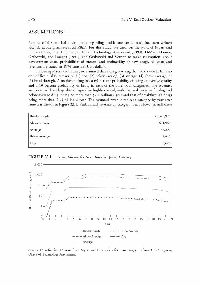
ASSUMPTIONS
Because of the political environment regarding health care costs, much has been writtenrecently about pharmaceutical R&D. For this study, we drew on the work of Myers andHowe (1997), U.S. Congress, Office of Technology Assessment (1993), DiMasi, Hansen,Grabowski, and Lasagna (1991), and Grabowski and Vernon to make assumptions aboutdevelopment costs, probabilities of success, and profitability of new drugs. All costs andrevenues are stated in 1994 constant U.S. dollars.
Following Myers and Howe, we assumed that a drug reaching the market would fall intoone of five quality categories: (1) dog, (2) below average, (3) average, (4) above average, or(5) breakthrough. A marketed drug has a 60 percent probability of being of average qualityand a 10 percent probability of being in each of the other four categories. The revenuesassociated with each quality category are highly skewed, with the peak revenue for dog andbelow-average drugs being no more than $7.4 million a year and that of breakthrough drugsbeing more than $1.3 billion a year. The assumed revenue for each category by year afterlaunch is shown in Figure 23.1. Peak annual revenue by category is as follows (in millions):
Breakthrough $1,323,920
Above average 661,960
Average 66,200
Below average 7,440
Dog 6,620
FIGURE 23.1 Revenue Streams for New Drugs by Quality Category
Year
10,000
1,000
100
10
1
0
Rev
enue
($ m
illio
ns; l
og sc
ale)
215 7 9 11 13 15 17 194 6 8 10 12 14 16 18 20210 3
Breakthrough
Above Average
Average
Below Average
Dog
Sources: Data for first 13 years from Myers and Howe; data for remaining years from U.S. Congress,Office of Technology Assessment.
c23 12 September 2012; 14:35:25
576 Part V: Real Options Valuation
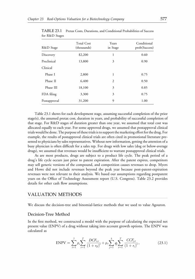
Table 23.1 shows for each development stage, assuming successful completion of the priorstage(s), the assumed pretax cost, duration in years, and probability of successful completion ofthat stage. For R&D stages of duration greater than one year, we assumed that total cost wasallocated equally to each year. For some approved drugs, we assumed that postapproval clinicaltrials wouldbedone.The purpose of these trials is to support themarketing effort for thedrug. Forexample, the results of postapproval clinical trials are often cited in promotional literature pre-sented to physicians by sales representatives.Without new information, getting the attention of abusy physician is often difficult for a sales rep. For drugs with low sales (dog or below-averagedrugs), we assumed that revenues would be insufficient to warrant postapproval clinical trials.
As are most products, drugs are subject to a product life cycle. The peak period of adrug’s life cycle occurs just prior to patent expiration. After the patent expires, competitorsmay sell generic versions of the compound, and competition causes revenues to drop. Myersand Howe did not include revenues beyond the peak year because post-patent-expirationrevenues were not relevant to their analysis. We based our assumptions regarding postpatentyears on the Office of Technology Assessment report (U.S. Congress). Table 23.2 providesdetails for other cash flow assumptions.
VALUATION METHODS
We discuss the decision-tree and binomial-lattice methods that we used to value Agouron.
Decision-Tree Method
In the first method, we constructed a model with the purpose of calculating the expected netpresent value (ENPV) of a drug without taking into account growth options. The ENPV wascalculated as
ENPV ¼X7i¼1
ρiXTt¼1
DCFi,tð1þ rd Þt þ ρ7
X5j¼1
qjXTt¼1
CCFj,tð1þ rcÞt , ð23:1Þ
TABLE 23.1 Pretax Costs, Durations, and Conditional Probabilities of Success
for R&D Stages
R&D StageTotal Cost(thousands)
Yearsin Stage
Conditionalprob(Success)
Discovery $2,200 1 0.60
Preclinical 13,800 3 0.90
Clinical
Phase I 2,800 1 0.75
Phase II 6,400 2 0.50
Phase III 18,100 3 0.85
FDA filing 3,300 3 0.75
Postapproval 31,200 9 1.00
c23 12 September 2012; 14:35:25
Chapter 23 Real-Options Valuation for a Biotechnology Company 577
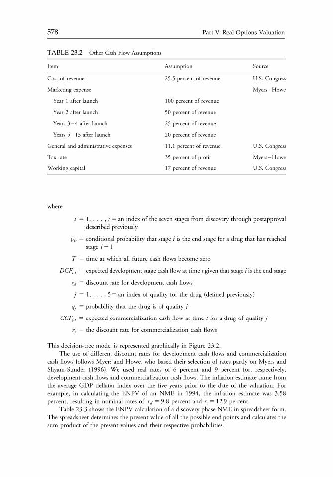
where
i 5 1, . . . , 75 an index of the seven stages from discovery through postapprovaldescribed previously
ρi, 5 conditional probability that stage i is the end stage for a drug that has reachedstage i2 1
T 5 time at which all future cash flows become zero
DCFi,t 5 expected development stage cash flow at time t given that stage i is the end stage
rd 5 discount rate for development cash flows
j 5 1, . . . , 55 an index of quality for the drug (defined previously)
qj 5 probability that the drug is of quality j
CCFj,t 5 expected commercialization cash flow at time t for a drug of quality j
rc 5 the discount rate for commercialization cash flows
This decision-tree model is represented graphically in Figure 23.2.The use of different discount rates for development cash flows and commercialization
cash flows follows Myers and Howe, who based their selection of rates partly on Myers andShyam-Sunder (1996). We used real rates of 6 percent and 9 percent for, respectively,development cash flows and commercialization cash flows. The inflation estimate came fromthe average GDP deflator index over the five years prior to the date of the valuation. Forexample, in calculating the ENPV of an NME in 1994, the inflation estimate was 3.58percent, resulting in nominal rates of rd 5 9.8 percent and rc5 12.9 percent.
Table 23.3 shows the ENPV calculation of a discovery phase NME in spreadsheet form.The spreadsheet determines the present value of all the possible end points and calculates thesum product of the present values and their respective probabilities.
TABLE 23.2 Other Cash Flow Assumptions
Item Assumption Source
Cost of revenue 25.5 percent of revenue U.S. Congress
Marketing expense Myers�Howe
Year 1 after launch 100 percent of revenue
Year 2 after launch 50 percent of revenue
Years 3�4 after launch 25 percent of revenue
Years 5�13 after launch 20 percent of revenue
General and administrative expenses 11.1 percent of revenue U.S. Congress
Tax rate 35 percent of profit Myers�Howe
Working capital 17 percent of revenue U.S. Congress
c23 12 September 2012; 14:35:26
578 Part V: Real Options Valuation
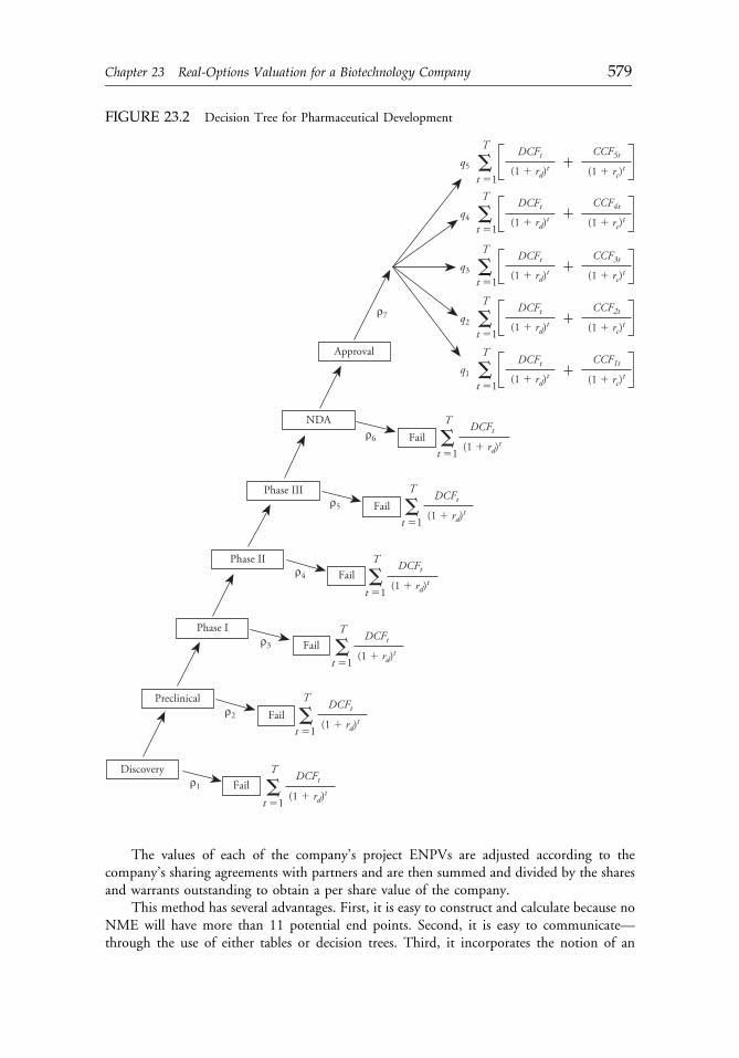
The values of each of the company’s project ENPVs are adjusted according to thecompany’s sharing agreements with partners and are then summed and divided by the sharesand warrants outstanding to obtain a per share value of the company.
This method has several advantages. First, it is easy to construct and calculate because noNME will have more than 11 potential end points. Second, it is easy to communicate—through the use of either tables or decision trees. Third, it incorporates the notion of an
FIGURE 23.2 Decision Tree for Pharmaceutical Development
T
T
T
T
T
Discovery
Preclinical
Fail
Fail
Fail
Fail
Fail
Fail
Approval
NDA
Phase III
Phase II
Phase I
T
q5
q4
q3
q2
q1
DCFt CCF5t
(1 � rd)t (1 � rc)t
DCFt CCF4t
(1 � rd)t (1 � rc)t
DCFt CCF3t
(1 � rd)t (1 � rc)t
DCFt CCF2t
(1 � rd)t (1 � rc)t
DCFt
DCFt
CCF1t
(1 � rd)t
(1 � rd)t
(1 � rc)t
T DCFt
(1 � rd)t
T DCFt
(1 � rd)t
T DCFt
(1 � rd)t
T DCFt
(1 � rd)t
T DCFt
(1 � rd)t
t �1
t �1
t �1
t �1
t �1
t �1
t �1
t �1
t �1
t �1
t �1
ρ7
ρ6
ρ5
ρ4
ρ3
ρ2
ρ1
c23 12 September 2012; 14:35:26
Chapter 23 Real-Options Valuation for a Biotechnology Company 579
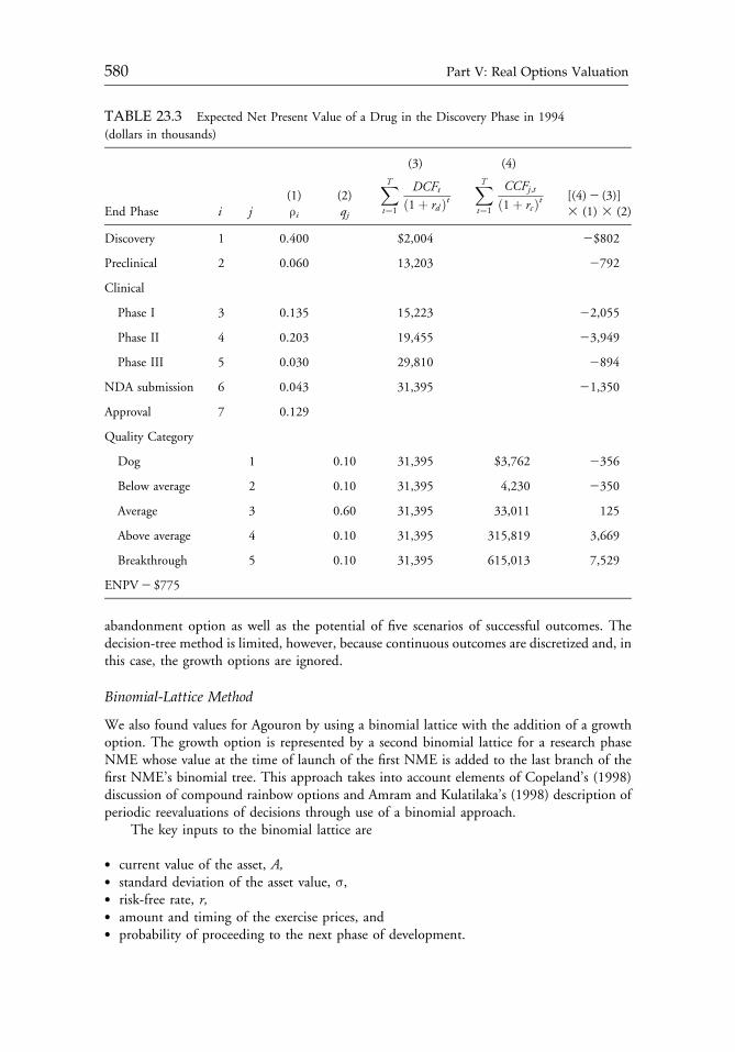
abandonment option as well as the potential of five scenarios of successful outcomes. Thedecision-tree method is limited, however, because continuous outcomes are discretized and, inthis case, the growth options are ignored.
Binomial-Lattice Method
We also found values for Agouron by using a binomial lattice with the addition of a growthoption. The growth option is represented by a second binomial lattice for a research phaseNME whose value at the time of launch of the first NME is added to the last branch of thefirst NME’s binomial tree. This approach takes into account elements of Copeland’s (1998)discussion of compound rainbow options and Amram and Kulatilaka’s (1998) description ofperiodic reevaluations of decisions through use of a binomial approach.
The key inputs to the binomial lattice are
� current value of the asset, A,� standard deviation of the asset value, σ,� risk-free rate, r,� amount and timing of the exercise prices, and� probability of proceeding to the next phase of development.
TABLE 23.3 Expected Net Present Value of a Drug in the Discovery Phase in 1994
(dollars in thousands)
(3) (4)
End Phase i j(1)ρi
(2)qj
XTt¼1
DCFtð1þ rd Þt
XTt¼1
CCFj,tð1þ rcÞt [(4)2 (3)]
3 (1) 3 (2)
Discovery 1 0.400 $2,004 2$802
Preclinical 2 0.060 13,203 2792
Clinical
Phase I 3 0.135 15,223 22,055
Phase II 4 0.203 19,455 23,949
Phase III 5 0.030 29,810 2894
NDA submission 6 0.043 31,395 21,350
Approval 7 0.129
Quality Category
Dog 1 0.10 31,395 $3,762 2356
Below average 2 0.10 31,395 4,230 2350
Average 3 0.60 31,395 33,011 125
Above average 4 0.10 31,395 315,819 3,669
Breakthrough 5 0.10 31,395 615,013 7,529
ENPV2 $775
c23 12 September 2012; 14:35:26
580 Part V: Real Options Valuation
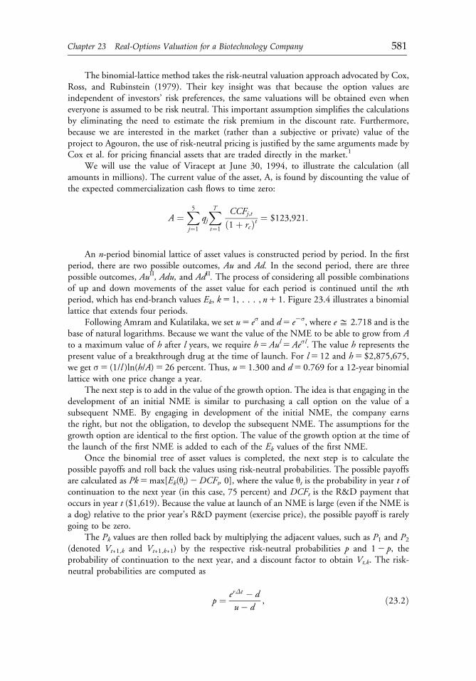
The binomial-lattice method takes the risk-neutral valuation approach advocated by Cox,Ross, and Rubinstein (1979). Their key insight was that because the option values areindependent of investors’ risk preferences, the same valuations will be obtained even wheneveryone is assumed to be risk neutral. This important assumption simplifies the calculationsby eliminating the need to estimate the risk premium in the discount rate. Furthermore,because we are interested in the market (rather than a subjective or private) value of theproject to Agouron, the use of risk-neutral pricing is justified by the same arguments made byCox et al. for pricing financial assets that are traded directly in the market.1
We will use the value of Viracept at June 30, 1994, to illustrate the calculation (allamounts in millions). The current value of the asset, A, is found by discounting the value ofthe expected commercialization cash flows to time zero:
A ¼X5j¼1
qjXTt¼1
CCFj,tð1þ rcÞt ¼ $123,921:
An n-period binomial lattice of asset values is constructed period by period. In the firstperiod, there are two possible outcomes, Au and Ad. In the second period, there are threepossible outcomes, AuII, Adu, and AdII. The process of considering all possible combinationsof up and down movements of the asset value for each period is continued until the nthperiod, which has end-branch values Ek, k5 1, . . . , n1 1. Figure 23.4 illustrates a binomiallattice that extends four periods.
Following Amram and Kulatilaka, we set u5 eσ and d5 e2σ, where eD 2.718 and is thebase of natural logarithms. Because we want the value of the NME to be able to grow from Ato a maximum value of h after l years, we require h5Aul5Aeσl. The value h represents thepresent value of a breakthrough drug at the time of launch. For l5 12 and h5 $2,875,675,we get σ5 (1/l )ln(h/A)5 26 percent. Thus, u5 1.300 and d5 0.769 for a 12-year binomiallattice with one price change a year.
The next step is to add in the value of the growth option. The idea is that engaging in thedevelopment of an initial NME is similar to purchasing a call option on the value of asubsequent NME. By engaging in development of the initial NME, the company earnsthe right, but not the obligation, to develop the subsequent NME. The assumptions for thegrowth option are identical to the first option. The value of the growth option at the time ofthe launch of the first NME is added to each of the Ek values of the first NME.
Once the binomial tree of asset values is completed, the next step is to calculate thepossible payoffs and roll back the values using risk-neutral probabilities. The possible payoffsare calculated as Pk5max[Ek(θt)2DCFt, 0], where the value θt is the probability in year t ofcontinuation to the next year (in this case, 75 percent) and DCFt is the R&D payment thatoccurs in year t ($1,619). Because the value at launch of an NME is large (even if the NME isa dog) relative to the prior year’s R&D payment (exercise price), the possible payoff is rarelygoing to be zero.
The Pk values are then rolled back by multiplying the adjacent values, such as P1 and P2(denoted Vt+1,k and Vt+1,k+1) by the respective risk-neutral probabilities p and 12 p, theprobability of continuation to the next year, and a discount factor to obtain Vt,k. The risk-neutral probabilities are computed as
p ¼ erΔt � du� d
, ð23:2Þ
c23 12 September 2012; 14:35:26
Chapter 23 Real-Options Valuation for a Biotechnology Company 581

where the risk-free rate, r, is the 10-year U.S. T-bill rate, which was 7.09 percent in 1994. Theresult is p5 0.573. Table 23.4 shows all the possible payoff values.
As the option values are rolled back, they are also adjusted for the probability of success atthat phase of development and for the cost of development in that year. Thus, the roll-backoption values are
Vt ,k ¼ maxf½Vtþ1,kpþ Vtþ1,kþ1ð1� pÞ�e�rffiffiffiffiffiΔt
pθt � DCFt ,0g: ð23:3Þ
For a development stage having a duration of more than one year, θt is the probability ofsuccess for that stage in the final year of the stage and 1 is the probability of success for allother years. The amount DCFt can be regarded as an annual exercise price. For example, V12,1
is calculated as follows:
½$2,156,669ð0:573Þ þ $1,276,979ð1� 0:573Þ�0:9316� 1,564 ¼ $1,657,654:
This process is then continued until V1,1 is reached, which is the value of the compoundto the company.
FIGURE 23.3 Four-Period Binomial Lattice
Au
A
Ad
Aud
E1 � AuIV
E2 � AuIIId
AuIId
E3 � AuIId II
Aud II
E4 � Aud III
E5 � Ad IV
Ad III
Ad II
Au II
AuIII
c23 12 September 2012; 14:35:27
582 Part V: Real Options Valuation
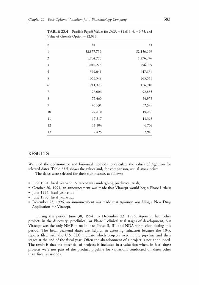
RESULTS
We used the decision-tree and binomial methods to calculate the values of Agouron forselected dates. Table 23.5 shows the values and, for comparison, actual stock prices.
The dates were selected for their significance, as follows:
� June 1994, fiscal year-end. Viracept was undergoing preclinical trials;� October 20, 1994, an announcement was made that Viracept would begin Phase I trials;� June 1995, fiscal year-end;� June 1996, fiscal year-end;� December 23, 1996, an announcement was made that Agouron was filing a New Drug
Application for Viracept.
During the period June 30, 1994, to December 23, 1996, Agouron had otherprojects in the discovery, preclinical, or Phase I clinical trial stages of development, butViracept was the only NME to make it to Phase II, III, and NDA submission during thisperiod. The fiscal year-end dates are helpful in assessing valuation because the 10-Kreports filed with the U.S. SEC indicate which projects were in the pipeline and theirstages at the end of the fiscal year. Often the abandonment of a project is not announced.The result is that the potential of projects is included in a valuation when, in fact, thoseprojects were not part of the product pipeline for valuations conducted on dates otherthan fiscal year-ends.
TABLE 23.4 Possible Payoff Values for DCFt5 $1,619, θt5 0.75, and
Value of Growth Option5 $2,085
k Ek Pk
1 $2,877,759 $2,156,699
2 1,704,795 1,276,976
3 1,010,273 756,085
4 599,041 447,661
5 355,548 265,041
6 211,373 156,910
7 126,006 92,885
8 75,460 54,975
9 45,531 32,528
10 27,810 19,238
11 17,317 11,368
12 11,104 6,708
13 7,425 3,949
c23 12 September 2012; 14:35:27
Chapter 23 Real-Options Valuation for a Biotechnology Company 583
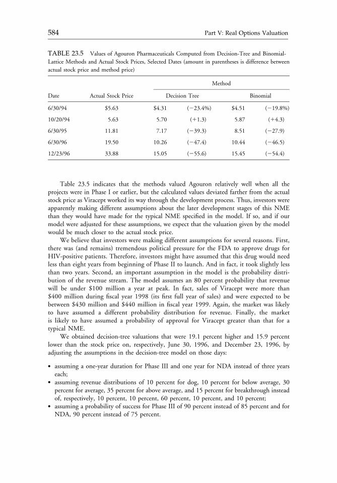
Table 23.5 indicates that the methods valued Agouron relatively well when all theprojects were in Phase I or earlier, but the calculated values deviated farther from the actualstock price as Viracept worked its way through the development process. Thus, investors wereapparently making different assumptions about the later development stages of this NMEthan they would have made for the typical NME specified in the model. If so, and if ourmodel were adjusted for these assumptions, we expect that the valuation given by the modelwould be much closer to the actual stock price.
We believe that investors were making different assumptions for several reasons. First,there was (and remains) tremendous political pressure for the FDA to approve drugs forHIV-positive patients. Therefore, investors might have assumed that this drug would needless than eight years from beginning of Phase II to launch. And in fact, it took slightly lessthan two years. Second, an important assumption in the model is the probability distri-bution of the revenue stream. The model assumes an 80 percent probability that revenuewill be under $100 million a year at peak. In fact, sales of Viracept were more than$400 million during fiscal year 1998 (its first full year of sales) and were expected to bebetween $430 million and $440 million in fiscal year 1999. Again, the market was likelyto have assumed a different probability distribution for revenue. Finally, the marketis likely to have assumed a probability of approval for Viracept greater than that for atypical NME.
We obtained decision-tree valuations that were 19.1 percent higher and 15.9 percentlower than the stock price on, respectively, June 30, 1996, and December 23, 1996, byadjusting the assumptions in the decision-tree model on those days:
� assuming a one-year duration for Phase III and one year for NDA instead of three yearseach;
� assuming revenue distributions of 10 percent for dog, 10 percent for below average, 30percent for average, 35 percent for above average, and 15 percent for breakthrough insteadof, respectively, 10 percent, 10 percent, 60 percent, 10 percent, and 10 percent;
� assuming a probability of success for Phase III of 90 percent instead of 85 percent and forNDA, 90 percent instead of 75 percent.
TABLE 23.5 Values of Agouron Pharmaceuticals Computed from Decision-Tree and Binomial-
Lattice Methods and Actual Stock Prices, Selected Dates (amount in parentheses is difference between
actual stock price and method price)
Method
Date Actual Stock Price Decision Tree Binomial
6/30/94 $5.63 $4.31 (223.4%) $4.51 (219.8%)
10/20/94 5.63 5.70 (11.3) 5.87 (14.3)
6/30/95 11.81 7.17 (239.3) 8.51 (227.9)
6/30/96 19.50 10.26 (247.4) 10.44 (246.5)
12/23/96 33.88 15.05 (255.6) 15.45 (254.4)
c23 12 September 2012; 14:35:27
584 Part V: Real Options Valuation
These adjustments are representative of what a securities analyst might have assumed inlight of the target disease, political environment, and competitive environment at the time.Making the same adjustments to the binomial model yielded similar results.
One other observation is that the inclusion of the growth option in the value of the initialoption did not significantly increase the value of the initial option. The reason is that the valueof a research project (assumed as the growth option) is low relative to the initial NME. Thisrelatively low value is discounted more as a result of multiplying by the probabilities of successof the initial option.
CONCLUSION
The real-options approach can be used to value a biotechnology company. Using averageassumptions works well when the projects in the pipeline are in Phase I or earlier and little isknown about the drug. As projects move into Phase II and later, more-specific assumptionsabout time to launch, market size, and probability of success will reflect the value of thecompany more accurately.
Our Agouron example illustrates these conclusions. The methods used here to find thevalue of Agouron worked best early in the life of the Viracept project, when the use ofindustry averages for completion time and revenue streams were more easily justified. AsViracept progressed, our use of averages did not work as well. A financial analyst closelyfollowing the stock would probably have had better estimates for the later stages of theimportant inputs. Using the real-options approach outlined here with better informationcould be a powerful addition to a security analyst’s toolbox.
NOTE
1. See Amram and Kulatilaka, Trigeorgis (1997), Kasanen and Trigeorgis (1994), andMason and Merton (1985) for more on the use of risk-neutral pricing.
REFERENCES
Amram, M., and N. Kulatilaka. 1998. Real Options: Managing Strategic Investment in an UncertainWorld. Boston, MA: Harvard Business School Press.
Copeland, T. 1998. “A Practitioner’s View of Applications of Real Options.” Second Annual Con-ference on Real Options, Chicago, IL (June).
Cox, J., S. Ross, and M. Rubinstein. 1979. “Option Pricing: A Simplified Approach.” Journal ofFinancial Economics, vol. 7 (September):229�263.
DiMasi, J.A., R.W. Hansen, H.G. Grabowski, and L. Lasagna. 1991. “Cost of Innovation in thePharmaceutical Industry.” Journal of Health Economics, vol. 10, no. 2:107�142.
Grabowski, H.G., and J.M. Vernon. 1994. “Returns to R&D on New Drug Introductions in the1980s.” Journal of Health Economics, vol. 13:383�406.
Kasanen, E., and L. Trigeorgis. 1994. “A Market Utility Approach to Investment Valuation.” EuropeanJournal of Operational Research, vol. 74:294�309.
c23 12 September 2012; 14:35:27
Chapter 23 Real-Options Valuation for a Biotechnology Company 585

Mason, S.P., and R.C. Merton. 1985. “The Role of Contingent Claims Analysis in Corporate Finance.”In Recent Advances in Corporate Finance. Edited by E. Altman. Chicago, IL: Irwin.
Myers, S.C., and C.D. Howe. 1997. “A Life-Cycle Financial Model of Pharmaceutical R&D.” Programon the Pharmaceutical Industry, Massachusetts Institute of Technology.
Myers, S.C., and L. Shyam-Sunder. 1996. “Measuring Pharmaceutical Industry Risk and the Cost ofCapital.” In Competitive Strategies in the Pharmaceutical Industry. Edited by Robert B. Helms.Washington, DC: American Enterprise Institute Press.
Trigeorgis, L. 1997. “Real Options, Managerial Flexibility and Strategy in Resource Allocation.”Cambridge, MA: MIT Press.
U.S. Congress, Office of Technology Assessment. 1993. Pharmaceutical R&D: Costs, Risks, and Rewards,OTA-H-522. Washington, DC: U.S. Government Printing Office (February).
c23 12 September 2012; 14:35:28
586 Part V: Real Options Valuation
ABOUT THECONTRIBUTORS
Xavier Adsera, CEO, Veremonte Group
Chris K. Anderson, Associate Professor, Cornell University School of Hotel Administration
Randall S. Billingsley, CFA, Visiting Professor of Finance, Wake Forest University Schoolsof Business
Neil Brisley, Associate Professor of Finance, School of Accounting and Finance, University ofWaterloo
Don M. Chance, CFA, James C. Flores Endowed Chair of MBA Studies and Professor ofFinance, Louisiana State University
John M. Charnes, President, Syntelli RAPID
Bradford Cornell, Professor Emeritus, UCLA Anderson School of Management
Aswath Damodaran, Kerschner Family Chair in Finance Education and Professor ofFinance, Leonard N. Stern School of Business, New York University
Morris G. Danielson, Associate Professor of Finance, Haub School of Business, SaintJoseph’s University
Pamela Peterson Drake, CFA, J. Gray Ferguson Professor of Finance, James MadisonUniversity
Edward A. Dyl, Sheafe/Neill/Estes Professor of Finance, Eller College of Management,University of Arizona
Gregory A. Gilbert, CFA, Founder and Senior Appraiser, Corporate Valuations, Inc.
Benjamin Graham, Deceased
D. Eric Hirst, Associate Dean for Graduate Programs and John Arch White Professor ofBusiness, McCombs School of Business, University of Texas at Austin
Patrick E. Hopkins, Professor and Deloitte Foundation Accounting Faculty Fellow, KelleySchool of Business, Indiana University
George J. Jiang, Associate Professor of Finance, Eller College of Management, University ofArizona
David Kellogg, Manager, Business Sales Operations Finance, Sprint
both 12 September 2012; 14:38:41
587
Wayne R. Landsman, KPMG Distinguished Professor of Accounting, Kenan-Flagler Busi-ness School, University of North Carolina
Mark Lang, Thomas W. Hudson, Jr./Deloitte and Touche Distinguished Professor, Kenan-Flagler Business School, University of North Carolina
Charles M.C. Lee, Joseph McDonald Professor of Accounting, Stanford University GraduateSchool of Business
Martin L. Leibowitz, Managing Director, Morgan Stanley
Jing Liu, Professor of Accounting and Finance and Associate Dean, Cheung Kong GraduateSchool of Business
Thomas A. Martin, Jr., CFA, Family Investment Officer, GenSpring Family Offices
Matthew B. McLennan, CFA, Portfolio Manager and Head of the Global Value Team, FirstEagle Investment Management
Doron Nissim, Ernst & Young Professor of Accounting and Finance, Columbia BusinessSchool, Columbia University
James A. Ohlson, Professor of Accounting, Leonard N. Stern School of Business, New YorkUniversity
Robert Parrino, CFA, Lamar Savings Centennial Professor of Finance and Director, Hicks,Muse, Tate & Furst Center for Private Equity Finance, McCombs School of Business,University of Texas at Austin
David R. Peterson, Wachovia Professor of Business Administration, Florida State University
Alfred Rappaport, Leonard Spacek Professor Emeritus of J.L. Kellogg Graduate School ofManagement at Northwestern University
Richard G. Sloan, L.H. Penney Chair in Accounting, Haas School of Business, University ofCalifornia, Berkeley
Jacob Thomas, Williams Brothers Professor of Accounting and Finance, Yale School ofManagement, Yale University
Pere Vinolas, CEO, Inmobiliaria Colonial, S.A.
both 12 September 2012; 14:38:41
588 About the Contributors
INDEX
Abandonment option valuation, 522,535�536, 558�559
AB Astra/Merck, 117Accounting:accrual, 301�302changes in, 320�322choice of system for and DAE valuation,
308�309clean surplus, 363consolidation, 370�371discovering poor, with accruals, 378�381,382, 383
pooling and purchase, 220for stock options, 415�419type of, and business type, 376
Accounting benefits of employee stockoption plans, 441
Accounting earnings. See EarningsAccounting method, FCF analysis as
independent of, 354, 359Accounting profit, 41Accrual accounting, 301�302Accruals:decomposing earnings, 381�385insurance companies and, 386mergers and acquisitions and, 386SEC enforcement actions and, 385use of to discover poor accounting,378�381, 382, 383
Acquisitions:cost of capital for, 227�228FEVA model and, 236�237pooling accounting and, 220
Adjusted book value approach,262�263
“Adjusted maturity” approach to ESOvaluation, 468
Adjusted present value (APV) method,267�268
Affordable dividends:book value and economic value weights,101�102, 103
conventional dividends compared to,96�101, 102�103
overview of, 94�96Agouron Pharmaceuticals:methods for valuation of, 524�525,577�583
overview of, 575results of valuation of, 583�585Viracept drug, 574
Allied Chemical & Dye, 9�10All-inclusive approach to reporting income,
309�310Allocation of capital, 362�363Amazon.com, 363, 364, 488�489, 525American options, 493America Online. See AOLAmgen, 423Amortization:earnings focus and, 352�353of goodwill, 220, 224
Analysis, methods of. See also Equity securitiesanalysis; Free cash flow (FCF) analysis;Fundamental analysis; Quality of earningsanalysis; Sensitivity analysis
benefit-cost, 33�34cash flow, 349competitive strategy, 120, 136�138, 147decision tree, 492, 502�504,
577�580DuPont, 38, 341n24guideline multiples, 263�265guideline transactions, 265leveraged buyout, 268security, 1, 293�294simulation, 492, 500�501transactions, 265
bindex 12 September 2012; 12:16:1
589

Analysts, use of earnings in valuation by,303�304, 327�337
Anticipated return (r) in FCF analysis,355�356
Antikarov, Vladimir, 547�548AOL, 376�377, 423, 490Arbitrage, principle of, 545�546Arbitrage opportunity, 513Arbitrage pricing theory:CAPM compared to, 113equity securities analysis and,121�122
Asset approach to estimating capital,48, 50
Asset/cost approaches to valuation:adjusted book value, 262�263overview of, 261replacement cost, 263
Asset life in CFROI, 58Assets. See also Illiquid common stock;
Underlying assetsevaluating, 386�387exit or salvage value of, 493fair market value of, 260�261net financing, 245, 248net operating, 245, 248, 378nondepreciating, in CFROI, 59nonoperating, 107passive financial, 350return on, 37, 65
Assets in place, cash flows from, 221�222Asset value, equity value compared to,
23�24Asset-value factor in formula valuations,
8�9, 10Assumptions, failure to meet, and real
options valuation:known and constant volatility, 539lognormality, 537�538minor assumptions, 539�540overview of, 537randomness, 538�539
AT&T, 314At-the-money options, 411�413Australia, tax laws in, 400Available-for-sale marketable equity securities,
328�329
Bailey, Warren, 552Balance sheet approach, 244
Bankruptcy costs, present value of, 232Barrier option lattice model for valuing
employee stock options, 466Basic earning power ratio, 37, 65Benchmark variables for stock price
performance, 63�64Benefit-cost analysis, techniques for, 33�34Berger, Philip, 552Bernstein, Richard, 224Beta:definition of, 52, 264estimations for cost of equity, 217�219in traditional valuation methods, 175
Bethlehem Steel, 8Bettis, J. C., 467, 469, 470, 475, 476, 478Bias in option-valuation models, 437�439Bing, Ralph A., 8Binomial models, 510�516, 556, 562�564,
580�583Biotechnology companies, valuation of:assumptions, 576�577binomial-lattice method, 580�583decision tree method, 577�580overview of, 524�525, 573�574results of, 583�585
Bizjak, J. M., 467, 469, 470,475, 476, 478
Black�Scholes model:for employee stock options, 466formula for, 493modified, 434�435, 436�437Nobel Prize for, 555for non-dividend-paying stock, 418for real options valuation, 556for traded options, 428�429variation including dividends, 275,418�419
Black�Scholes option-pricing formula forcall options, 504
Book capital, 224Book value (BV). See also Price-to-book ratioadjusted book value approach, 262�263changes in, 381�382description of, 157as value driver, 392�393
Book value of equity approach to estimatingcapital, 48�49, 50
Book value of equity to market value of equityratio (BV/MV), 39�40
Book value weights, 101�102, 103
bindex 12 September 2012; 12:16:1
590 Index
Bottom-up approach to avoiding destructionof capital, 21�24
Brazil, Russia, India, and China (BRIC), asmonetary epicenters, 21
Brown Shoe Company, 250�251Burgstahler, David, 553Busby, J. S., 554Businesses. See CompaniesBusiness model erosion, 23Buy-side analysts, use of reported earnings by,
303, 327�337BV. See Book valueBV/MV (book value of equity to market
value of equity ratio), 39�40
Call options:binomial tree for, 515definition of, 493synthetic, 512
Cancellations and option exercise, 432Capital. See also Cost of capital; Return on
capitalasset approach to estimating, 48, 50avoiding permanent impairment of, 18,
21, 25in calculation of economic profit,48�51
definition of, 48definitions of in valuation models, 248efficient allocation of, 362�363invested, 8, 354, 355
Capital asset pricing model (CAPM):cost of equity and, 79�82, 212, 264equity securities analysis and, 121�122finite-growth model and, 177general risk premium estimationand, 110
limitations of, 113Capital-budgeting techniques, 33�34Capital deficiency or surplus, 108Capital expenditures, maintenance and
growth of, 277“Capital invested game” and EVA, 225Capitalization rate in discounted cash flow
approach, 111Capital structure, vulnerability from, 23�24CAPM. See Capital asset pricing modelCarpenter utility-based model of rational early
exercise, 475, 478, 479Cash, in investment approach, 20, 27
Cash-driven valuation models. See Discountedcash flow (DCF) approach
Cash earnings valuation models, rush to, 296Cash flow. See alsoDiscounted cash flow (DCF)
approachfrom assets in place, 221�222assumptions of, 540exercise of stock options and, 429�430information content of, compared toearnings, 301�303
manipulation and timing of, 340n18option tax effects on, 423�427uncertainty and, 495in valuation models, 245�247as value driver, 389�390, 402�403
Cash flow analysis, 349. See also Free cash flow(FCF) analysis
Cash flow approach to stock options,413�415
Cash flow return on investment (CFROI):HOLT method, 57�61origins of, 32
“Cash is king” perspective, 340n17, 350�351Cash operating taxes, 47�48CFROI (cash flow return on investment):HOLT method, 57�61origins of, 32
Circularity problem, solution for,232�235
Cisco Systems, 172, 423, 490Clayton, Matthew, 553Clean surplus accounting, 363Clean-surplus relation, 256, 257n6Clinical trials of drugs, 575Clinton administration, 119Colgate-Palmolive Company, 357, 358Commodity businesses, valuation of, 22�23Common stock, cost of, 79�82Companies. See also Biotechnology companies,
valuation ofcommodity, valuation of, 22�23comparable, selection of, 252�255,
263�264discounted cash flows of, 25equity as residual claim on, 23�24franchise, valuation of, 22�23high-P/E, 185insurance, and accruals, 386management of, 24misvaluation of, 555
bindex 12 September 2012; 12:16:1
Index 591
Companies (continued )opportunistic earnings management by,
328, 335overpayment for, 22�23perpetuity assumption for, 23, 56“recovering dogs,” 250start-up, and FEVA model, 237�238terminal phase of, 189�190, 205using stock to fund CAPEX, 277value-enhancing actions of, 220�223value-neutral actions of, 220
Company-specific risk premium, 110Comparables, finding, 252�255, 263�264Comparative advantage, 34Comparative analysis in ROE
performance, 146Comparative statistics, 507Compensation. See also Employee stock optionsdesign of, 441�442incentive effects and, 444�446performance and, 33
Competition. See also Franchise valuationunder Q-type competition
in pharmaceutical industry, 117, 118�119Q-type competitive equilibrium, 192�193
Competitive advantage, 22, 23, 34, 56, 84,136, 178�187, 210, 308, 386
Competitive equilibrium, 192�193,307�308
Competitive strategy analysis framework, 120,138�140, 147
Compound options, 493Comprehensive income, reporting,
322�323, 324�326, 335�337Computation of present value, 6Conditional NPV:in DCF analysis, 496�498in option valuation, 504in simulation analysis, 500�501
Consolidation accounting, 370�371Consolidation in pharmaceutical industry, 118Constant-earnings model, formula for,
191, 198Constant growth DDM, 271�273Contingency claims approach, 244,
274�275Contingent claims approach to valuation,
261�262, 274�275Contingent liability, valuing, 114Continuing operations, income from, 312
Continuing value in FCF analysis, 351Contracts with related parties, 107Contrarian approaches in valuation
models, 157Controlling interest, valuing, 276Conventional dividend approach, affordable
dividends compared to, 96�101,102�103
Copeland, Tom, 547�548Cost of capital:for acquisitions, 228in calculation of economic profit, 51�54cost of common equity, 79�82cost-of-debt capital, 78cost of preferred stock, 79in DCF analysis, 497definition of, 41overview of, 78volatility and, 533weighted-average cost of capital, 82
Cost-of-debt capital, 78Cost of equity:in CAPM, 79�82, 264estimations of, 211�219
Costs:of common equity, 79�82of financing, 222of preferred stock, 79transaction, assumptions of, 539�540
Counterparty risk and hedging withoptions, 20
Country risk premiums, estimation of,213�215
DAE (discounted abnormal earnings)valuation framework, 300�301, 302,306�309, 335. See also Economicvalue added
Daily returns, use of in estimation of stockreturn volatility, 285
DCF. See Discounted cash flow (DCF)approach
DDM. See Dividend discount modelDebt-to-capital ratio, 276�277Decay model, 194�196, 197, 201�202Decision tree analysis, 492, 502�504,
577�580Decomposing earnings, 381�385Deferral option valuation, 521�522Deflation and democracy, 18
bindex 12 September 2012; 12:16:1
592 Index

Dell Computer Corporation:cash flows, 424�426consolidated statement of cash flows,
456�457consolidated statement of financial position,
454�455consolidated statement of income, 455�456consolidated statement of stockholdersequity, 458
current valuation of, 490financial statement of, 424footnote disclosure, 419�420, 424future option grants, 421�422income statement, 329modified Black�Scholes model and, 434,
435NQOs of, 423option exercise and, 429�430selected footnotes, 459�461value of outstanding options, 420�421
Depreciation:earnings focus and, 352�353economic estimates of, 369Krispy Kreme Doughnuts and, 376Netflix and, 376�377operating income after, 42�43
Dichev, Ilia, 553Dilution and employee stock option plans,
446�448Direct valuation methods:forecast-cash-flow approach, 244�245overview of, 244terminal-value problem, 245�248
Discontinued operations, 316�320Discounted abnormal earnings (DAE)
valuation framework, 300�301, 302,306�309, 335. See also Economicvalue added
Discounted cash flow (DCF) approach:adjusted book value and, 262�263capital expenditures and, 114cash flow estimation, 106�108challenges of, 210in Cisco Systems valuation, 525�528discount rate determination, 108�110to employee stock option plans, 450�451estimation issues in, 211�219EVA compared to, 225�227flexibility and, 556formula for, 105�106, 210
free cash flow and, 246historical earnings and, 364�365intrinsic value calculation, 120�122in Merck valuation, 122�123minority-interest and controlling-interestvalues, 112
minority valuation and, 113MM approach, EVA, and, 232�235multistage, 140�141net present value and, 496�498operating cash flow, net income, and, 113overview of, 85n7, 105, 112,
244�245, 487range of discount rates used in, 112real options and, 555�556risk-free rate and, 113single-stage constant-growth, 140as subjective, 113two-stage model for calculating intrinsicvalue, 148
valuation of investment projects and,487�488
value enhancement in, 219�220Discount factor (r) in FCF analysis, 351,
355�356Discount rate:components, 109�110definition of, 108external factors in, 108growth patterns and, 182�183, 184internal factors in, 108�109range and application of, 175�176two-stage DDM and, 166�167, 168, 169
Discounts:for illiquidity, 286�288for nonmarketability, 281
Dividend discount model (DDM):cash flow analysis and, 349cash flow and, 246for companies paying no dividend, 175constant growth DDM, 271�273earnings-based models derived from, 306free cash flow analysis and, 350as income approach to valuation, 270Modern Portfolio Theory and, 100normalized earnings in, 175overview of, 93�94, 244�245as traditional valuation method, 158two-stage, 164�167, 168, 169, 273�274,277�278
bindex 12 September 2012; 12:16:2
Index 593
Dividend growth models, 96Dividends, affordable:book value and economic value weights,101�102, 103
conventional dividends compared to,96�101, 102�103
overview of, 94�96Dividends per share (DPS):definition of, 404earnings per share compared to, 398�401
Dividend valuation model (DVM),79�80, 82
Dodd, David, 1, 2, 381Dow Chemical, 8Dow-Jones Industrial Average, 8�16, 252DPS (dividends per share):definition of, 404earnings per share compared to, 398�401
Drug development, 574�575, 576�577Du Pont (company), 13DuPont analysis, 38, 341n24DuPont/Merck venture, 116DuPont ROE decomposition approach, 117,
119, 120, 139, 152�153DVM (dividend valuation model), 79�80, 82
Early exercise of stock options, 429�434,466�467. See also Voluntary earlyexercise boundary
Earnings. See also Earnings-based models;Earnings management; Future earnings;Price-to-earnings ratio; Quality ofearnings analysis; Reporting income
classified income statements, 309�312decomposition of, 381�385definition of, 337�338determinants of price reaction, 299free cash flow compared to, 352�354historical, definition of, 364�365information content of, compared to cashflows, 301�303
long return intervals and, 299�300measures of, 363�366persistent components of, 365�366policy implications of measures of, 370�371pro forma, 361�362, 363�364, 365, 369quality of, 7�8, 361�363relevance of, to valuation, 296�297, 304reporting of, 304�305security prices and, 297�301
unexpected, and stock-price changes,297�299
use of, in valuation, 303�304, 327�337as value driver, 389�390, 392�393,
402�403Earnings-based models. See also Discounted
abnormal earnings (DAE) valuationframework
benefits of, 334�335free cash flow models compared to, 305�309
Earnings before interest and taxes(EBIT), 22�23
Earnings before interest, taxes, depreciation,and amortization (EBITDA), 176,392�393
Earnings management:definition of, 344n39opportunistic, 328, 335
Earnings measures, tests of quality of:comparison of methods, 367�368component data, 369�370economic earnings measures, 368�369information content method, 367predictive ability method, 367value relevance method, 366�367
Earnings per share (EPS):absolute valuation performance of forecastsof, 401�402
calculation of intrinsic value using,150
definition of, 403dividends per share compared to, 398�401as estimate of cash flow per share, 278operating cash flow compared to, 397as value drivers, 392�393
Earnings power duration, 23Earnings quality analysis. See Quality of
earnings analysisEarnings response coefficient (ERC), 299Earnings surprise, 156, 377eBay, 273�274EBIT (earnings before interest and taxes),
22�23EBITDA (earnings before interest, taxes,
depreciation, and amortization), 176,392�393
EBO (Edwards-Bell-Ohlson) model, 244�245,248, 249
Economic capital expenditures, 114Economic earnings measures, 368�369
bindex 12 September 2012; 12:16:2
594 Index

Economic profit. See also Economicvalue added
accounting profit compared to, 41calculation of, 42�54capital and, 48�51cash operating taxes and, 47�48challenges applying, 56�57cost of capital and, 51�54estimating, 35net present value and, 41�42NOPAT, 42�46overview of, 40�41performance and, 54�55return on capital and, 51stock price performance and, 65�66, 70
Economic profit model, 247, 248Economic value added (EVA). See also
Profit, economiccaveats for, 225DCF compared to, 225�227formula for, 230�231increases in, 228MM approach and, 233�235origins of, 32overview of, 35, 224�225, 244�245, 369reconciling market value added with,
55�56Economic value weights, 101�102, 103Edwards-Bell-Ohlson (EBO) model,
244�245, 248, 249Embedded cost of capital, 78Emerging markets, betas for, 218Empirical studies. See also Earnings measures,
tests of quality of; Experiment in use ofreported earnings in valuation
of quality of company earnings, 366�370of real options valuation, 551�554of stock price performance, 67�74
Employee stock options (ESOs). See alsoVoluntary early exercise boundary
accounting for, 415�419compensation design and repricing,
441�442consequences of for valuation, 413�415DCF analysis and, 450�451Dell example, 419�422determination of option grants, 443dilution and, 446�448diversification and, 439early exercise modeling, 466�467
future issues with, 453growth in importance of, 410implications of research on, 451�453incentive benefits, accounting benefits,and, 441
incentive effects, 444�446lattice models for valuing, 466�467,475�479
market valuation of, 448�450origins of, 410�411patterns of option exercise, 428�434,465�466, 479�480
“representative investor” approach to valuing,467, 472�473
repurchases, dilution, and, 444risk aversion, incentive effects, and, 439shift to restricted stock, 454tax issues, 422�428typical features of, 411�413valuation models, 434�439volatility and, 439�441
Enron, 369�370, 387Enterprises, ownership of, 21. See also
CompaniesEnterprise value, definition of, 278n1Enterprise value to earnings before interest,
taxes, depreciation, and amortization (EV/EBITDA), 244
Enterprise value to sales (EV/S), 251Entropy and business model erosion, 23EPS. See Earnings per shareEquity, 23�24. See also Return on equityEquity-r in FCF analysis, 356�357Equity securities analysis. See also Merck &
Company; Pharmaceutical industryplan for, 119�125qualitative factors of, 153�154quantitative factors of, 152�154research for, 116�119
Equity value, formula for, 96ERC (earnings response coefficient), 299ESOs. See Employee stock optionsEstimation issues:cost of equity, 211�219nominal and real valuation, 211
European options, 493, 540EVA. See Economic value addedEV/EBITDA (enterprise value to earnings
before interest, taxes, depreciation, andamoritization), 244
bindex 12 September 2012; 12:16:2
Index 595

EVPV (expected net present value), formulafor, 577�578
EV/S (enterprise value to sales), 251Ex ante value, 425Excess return in DCF analysis, 219Executive compensation and performance, 33Exercise-date accounting, 423Exercise of stock options:assumptions about, 428�429empirical evidence of early exercise,
430�434timing of, 429�430
Exercise price:definition of, 493in real options valuation, 541�542
Exit value, 493Expansion options, valuation of, 518�521,
528�531Expectational models, 156�157Expected earnings, 252Expected growth rate, 222Expected net present value (EVPV), formula
for, 577�578Expected option life assumption, 438Expected rates of return, conventional
compared to affordable dividendapproaches, 100�101
Expensing options, arguments against, 417Experiment in use of reported earnings
in valuation:analysis of stock-price estimates, 332�334case materials, 329�331conclusions from, 334�335follow-up study, 335�337objectives and procedures, 328�329overview of, 327�328participants, 332
Ex post value, 425Extraordinary items, income from, 319�320Exxon Corporation, 319, 320
Fade, buying businesses priced for, 23Fairly priced companies, 172Fair market value:definition of, 261estimating, formula for, 106
FASB. See Financial Accounting StandardsBoard
FCF. See Free cash flowFCF analysis. See Free cash flow (FCF) analysis
FCFE (free cash flow to equity) approach,269�270
FCFF (free cash flow to firm) approach,266�268
Federal Reserve, monetary policy of, 21FEVA (financial and economic value added):derivation of formula, 239�241implementation of, 235�238
Finance balance sheet, 260Financial Accounting Standards Board (FASB):Accounting for Stock-Based Compensation,417�418
Emerging Issues Task Force of, 314“Reporting Information about the FinancialPerformance of Business Enterprises,”362, 370
Share-Based Payment, 480Financial analysis, challenges of, 554�555Financial and economic value added (FEVA):derivation of formula, 239�241implementation of, 235�238
Financial options:real options compared to, 494valuation of, 510�516volatility and value of, 507
Financial risk and discount rate, 109Financial statements, rules guiding
preparation of, 295Finite-growth model:application of, 178comparison of new model with Gordonand Gordon model, 186�187
evaluation of reasonableness of P/E,183�185
of Gordon and Gordon, 178�179, 216market expectations and, 181�183overview of, 177, 185�186partial reinvestment of earnings inpositive-NPV projects, 180�181
total reinvestment of earnings inpositive-NPV projects, 179�180
First Eagle:asset buying of, 23�24gold and, 20margin of safety and, 26mind-set of, 17, 18�19portfolios of, 25track record of, 24�25
Flexibility options, 488, 495Food and Drug Administration, 119
bindex 12 September 2012; 12:16:2
596 Index

Forecast-cash-flow approach, 244�245Forecasting:earnings-based models and, 334�335free cash flows, 351marginal tax rate, 427�428measures of earnings in, 363option grants, 443overview of, 243�244, 256�257
Formula valuations:based on market price, 10, 13�16based on past performance, 7�10,
11�12Franchise businesses, valuation of,
22�23Franchise factor model, 234, 240Franchise glides, 190Franchise P/E, 84Franchise rides, 190Franchise slides, 190, 192, 193Franchise valuation under Q-type competition:competitive equilibrium, 192�193general decay model, 194�196, 197,
201�202overview of, 205PV-equivalent ROE, 196�198single-phase no-growth model, 191two-phase growth model, 198�204
Franchise value, 35Free cash flow (FCF):ability of current to predict future, 302accruals and, 378capital expenditures, maintenance and
growth of, 277definition of, 210, 245earnings compared to, 305�309estimation of, 106�108forecasting, 351off-balance-sheet items and, 276
Free cash flow (FCF) analysis:applications of, 359calculating levered r, 356changes in working capital and, 359earnings focus compared to, 352�354estimating anticipated growth inFCF, 355
estimating current FCF, 354example of, 357, 358implementation problems with, 351�352as independent of accounting method,354, 359
inferring expected return on unlevered firm,355�356
issues in, 351justification for, 350�351limitations and benefits of, 357overview of, 349�350relating Equity-r to risk, 356�357for stock valuation, 354�357
Free cash flow generation, 24, 26Free cash flow to equity (FCFE) approach,
269�270Free cash flow to firm (FCFF) approach,
266�268Fundamental analysis:of financial statements, 302�303market efficiency and, 375purpose of, 156traditional valuation methods in, 164�172two-stage dividend discount model,164�167, 168, 169
valuation, 167�172Fundamental value and real options, 536Future earnings:challenges of estimating, 5�6methods for estimating, 6�7as predicted by market price,10, 13�16
as predicted by past performance,7�10, 11�12
Future returns and option exercise,433�434
GAAP. See Generally accepted accountingprinciples
The Gap, 224General decay model, 194�196, 197,
201�202General Electric, 13Generalized DDM, 158Generally accepted accounting principles
(GAAP):capital expenditures, 114flexibility in application of, 320latitude allowed by, 295measures of earnings, 364, 370
General risk premium, 109�110Generic drugs, regulatory approval process
for, 118Goals of investors, 17�18Going-concern value, 262
bindex 12 September 2012; 12:16:2
Index 597
Gold:in investment approach, 20value of, 26�27
Goodwill, amortization of, 220, 224Goodyear, 10Gordon, J., 177, 178�179, 186�187Gordon, M., 1, 177, 178�179, 186�187Gordon and Gordon model, 178�179,
186�187, 216Graham, Benjamin, 1, 2, 381Graham, John, 427�428Grant-date accounting of option expense,
416, 423Gross cash flow in CFROI, 57�59Gross cash investment in CFROI, 59Growth characteristics of model portfolios,
161�163Growth duration, formula for, 171“Growth game” and EVA, 225Growth models. See also
Finite-growth modeldividend, 96in terminal phase, 205three-stage, 96two-phase, 198�204
Growth options:market capitalization and, 366valuation of, 518�521, 528�531
Growth rates and two-stage DDM,164�166, 168, 169
Growth stocks, 172, 174GTE Corporation, 321Guideline multiples analysis, 263�265Guideline transactions analysis, 265
Harmonic means, 252, 391Harnischfeger Industries:extraordinary item disclosure, 319, 321income statement, 310, 311nonrecurring item disclosure, 312,313�314
restructuring charge, 313, 314Hayn, Carla, 553�554Health care reform, 116, 117Heath, C., 433Hedge funds, liquidity restrictions
on, 288Hedging:assumptions of, 545�547with options, and macro risk, 20
Hershey Foods Corporation:capital calculation for, 50cash operating taxes of, 47�48CFROI calculation for, 58�60cost of capital calculation for, 51�54economic profit of, 54�55market value added for, 55NOPAT calculation for, 43�46return on capital calculation for, 51
“High flyer” stocks, 172, 173High-growth periods, lengthening,
222High-P/E companies, 185Historical earnings, definition of, 364�365Historical risk premiums and cost of equity
estimations, 212�219Historical stock market return:data on, 110extrapolating from, 153volatilities, 282
Historical volatility approach, 543�544H-model, 121, 124, 125, 141, 152Hokie Company case example:binomial model for, 562�564cash flow for, 497DCF analysis for, 496�498decision tree analysis of, 502�504investment opportunity for, 495�496option valuation for, 504�509sensitivity analysis of, 499�500simulation analysis of, 500�501
Holding gains on securities, 328�329HOLT method, 57�61Homer, Sidney, 1Hong Kong, tax laws in, 400Howell, Sydney, 553�554Huddart, Steven, 430�433, 435, 441Huddart model, 435�436Hull, J., 466, 469, 480HW (Hull and White) model of ESO
valuation, 466, 469, 480
I/B/E/S International Summary files, 393IBM, 95, 312, 490Identification of unusual items, 313�314Illiquid common stock:case study, 286�288options-based framework for, 280�282stock return volatility, 282�286valuing, 279�280, 288
bindex 12 September 2012; 12:16:2
598 Index

Implied equity premium, estimating,215�217, 227
Implied volatility approach, 543, 544Incentive benefits of employee stock
options, 441Incentive effects of employee stock options,
439, 444�446Incentive stock options (ISOs), 422Income. See Comprehensive income, reporting;
Earnings; Reporting incomeIncome approaches to valuation:dividend discount model, 270�274free cash flow to equity, 269�270free cash flow to firm, 266�268overview of, 261
Income statements, 309�312Industry multiples, 389�390. See also
Multiples-based approachesInformation content method, 367, 368Inputs for real options valuation, difficulty
of estimating, 540�545, 556�557Institutional Shareholder Services
(ISS), 469Insurance companies and accruals, 386Intangibles, 157Interest expense, implied, 45Internal rate of return (IRR):for benefit-cost analysis, 34CFROI compared to, 57net present value compared to, 42, 83quality of earnings and, 378
International Nickel, 10International Paper, 164, 165, 166, 167Interquartile (IQ) range, 395Intrinsic value:calculating, 147�148calculating with H-model, 151calculating with P/E and EPS, 150�151calculating with two-stage DCF model,148
market price as proxy for, 403sensitivity analysis, 149of stocks, 243
Inverse of price/cash-flow ratio plus growthmethod, 109�110
Invested capital:definition of, 354estimating growth in, 355rate of earnings on, 8
Investigational New Drugs, 574�575
Investment projects:with abandonment option, binomial treesfor, 523
binomial trees for, 516, 518with deferral option, binomial treesfor, 522
with growth option, binomial treesfor, 519
valuation of, 487�488Investment value, definition of, 261Investors:caveats for EVA, 225goals of, 17�18“representative” and ESO valuation, 467,472�473
IQ (interquartile) range, 395IRR (internal rate of return):for benefit-cost analysis, 34CFROI compared to, 57net present value compared to, 42, 83quality of earnings and, 378
ISOs (incentive stock options), 422ISS (Institutional Shareholder Services), 469
Jagle, Axel, 553�554Johnson & Johnson/Merck venture, 116Joint ventures in pharmaceutical industry, 118Judgment in determining value:choice of earnings measures, 366insight into factors affecting, 303�304sector composition, 159�160traditional methods and, 155, 172, 175
Kimberly-Clark Corporation, 353Knight, Frank, 2Krispy Kreme Doughnuts, 376
L (fixed maximum anticipated life), 467L (fixed maximum anticipated life) model of
ESO valuation, 468, 472�479Lang, Mark, 427�428, 430�433,
435, 441Lattice models:for valuing biotechnology companies,580�583
for valuing employee stock options,466�467, 475�479
Learning options, 525, 527Lehman Brothers, 465�466Leibowitz, Martin, 1
bindex 12 September 2012; 12:16:2
Index 599

Lemmon, M. L., 467, 469, 470, 475,476, 478
Level of value, defining, 260Leveraged buyout analysis, 268Liquidity:of hedge funds, 288value of, 280�282
Lognormality, assumption of, 537�538Longstaff, F. A., 280Longstaff model, 280�281, 282, 285,
286�288Loss companies, 253Losses and earnings focus, 353Lucent Technologies, 423
M (fixed multiple of strike price), 466, 467M (fixed multiple of strike price) model of
ESO valuation, 469, 470, 472�479MacMillan Bloedel, 316Macro risk, dealing with, 19�20Management:of earnings, 328, 335, 344n39of enterprises, 24expenses written off by, 176goal of, 62value-based, 369value created by, 33�35
Management discussion and analysis (MD&A)sections of annual reports, 313
Mandatory accounting changes, 320�322MAR (market model-adjusted return)
variable, 63�64, 71�72, 73�74,75�76
Marginal cost of capital, 78Margin of safety:asset value and, 23�24business model erosion and, 23business valuation and, 22�23combining elements of, 24�25macro risk and, 18�19management of enterprises and, 24as mind-set, 17overview of, 26seeking, 21�24uncertainty and, 18�19
Market approaches to valuation, 261,263�265
Marketed asset disclaimer, 547�548Market expectations and finite-growth
model, 181�183
Market model-adjusted return (MAR)variable, 63�64, 71�72, 73�74,75�76
Market multiples:EV/S, 251P/B, 249, 250P/E, 249�251selection of comparable companies,252�255
Market price:elements of, 36formula valuation based on, 10, 13�16as proxy for intrinsic value, 403
Market risk premium, 52, 57, 81Market share, increases in, 223Markets outside U.S., risk premiums in,
213�215Market/strike ratio, 431�432Market valuation of options, 448�450Market value added (MVA):challenges applying, 56�57overview of, 35, 55reconciling economic value added with,55�56
stock returns compared to, 77�78Market value of underlying assets, 540�541Markowitz, Harry, 1MD&A (management discussion and analysis)
sections of annual reports, 313Mean-reversion approaches in valuation
models, 157Measures of earnings:comparison of methods, 367�368component data, 369�370economic earnings measures, 368�369information content method, 367overview of, 363�366predictive ability method, 367value relevance method, 366�367
Measures of firm performance, traditional,37�40. See also Measures of value added
Measures of option expense, 416�417Measures of value added. See also Economic
value added; Profit, economicbenefits of, 61�62challenges applying, 56�57Holt CFROI, 57�61limitations of, 61market value added, 55�56overview of, 40
bindex 12 September 2012; 12:16:2
600 Index

Merck & Company:comparative financial ratios, 121competitive strategy analysis of, 145description of, 115financial data, 128�133intrinsic value calculation, 147�148outlook for future, 117position on health care reform, 117price performance, 125pricing and demand for pharmaceuticals,
118�119qualitative analysis of, 153�154quantitative analysis of, 152�153ROE decomposition analysis, 120, 153ROE performance evaluation, 145�146strategic objectives, 116�117structural reorganization, 116�117Value Line on, 123
Mergers and acquisitions (M&A). See alsoAcquisitions
accruals and, 386gross cash flow and, 24
Microsoft Corporation, 164, 165, 166, 167,172, 423
Miller, M., 231. See also Modigliani andMiller (MM) approach
Minority interest, valuing, 276Model risk, 536�537Models. See also specific modelsdifferent results yielded by, 229failure to meet assumptions of, 537�540as snapshots in time, 172, 175
Modern Portfolio Theory and dividenddiscount models, 100
Modified Black�Scholes model, 434�435,436�437
Modigliani, F., 231Modigliani and Miller (MM) approach,
231, 232�235Moel, Alberto, 553Momentum measures in expectational
models, 156Money, price of, as fake, 18μ (mu, fixed proportion) model:accuracy of, 479�480comparison to L and M models,
472�479overview of, 466, 467, 469�470proof, 471�472proposition, 470�471
“Multiple of strike price” approach to ESOvaluation, 469, 470
Multiples-based approaches:dominance of earnings in U.S. sample,392�393
earnings compared to cash flow in, 402�403EV/S, 251forecasting in, 244guideline multiples, 263�265historical earnings and, 365international results from, 395�402international sample for, 393�395overview of, 255�256, 390�392P/B, 249, 250P/E, 249�251selection of comparable companies,252�255
Multistage DCF model, 140�141Multistage DDM, 158MVA. See Market value added
NASDAQ 100, 427�428Nasdaq Composite Index, 168, 170,
171, 283Net book value, 300�301, 339n8Net cash flow, estimation of, 106�108Net financing assets (NFA), 245, 248Netflix, 376Net income, accrual-basis, 302Net operating assets (NOA), 245, 248,
378, 382Net operating profit after taxes (NOPAT),
42�46, 354Net present value (NPV):in benefit-cost analysis, 33�34Conditional, 496�498, 500�501, 504in DCF analysis, 496�498economic profit and, 41�42for investment projects, 35IRR and, 42, 83strategic, 492�493, 506
New-economy stocks, 255, 296New molecular entities (NMEs), 574, 575New York Stock Exchange (NYSE), stock
return volatilities, 283NFA (net financing assets), 245, 248Nike, 250�251, 304NMEs (new molecular entities), 574, 575NOA (net operating assets), 245, 248,
378, 382
bindex 12 September 2012; 12:16:3
Index 601
Nominal valuation, 211Nondepreciating assets in CFROI, 59Nonoperating assets, 107Nonparametric correlations, 88n52Nonqualified stock options (NQOs), 422�423Nonrecurring income, 107, 312�314NOPAT (net operating profit after taxes),
42�46, 354Normal growth periods, projections for, 96�97Normalized earnings in DDM approach, 175Normal profit, 84NPV. See Net present valueNQOs (nonqualified stock options), 422�423
OCF (operating cash flow), 392�393, 397OE (operating expenses), 245Ofek, Eli, 552Off-balance-sheet items in free cash flow
analysis, 276One-time charges, adjustments for, 224OPEB (other postemployment benefits), 321Operating capital, 50Operating cash flow (OCF), 392�393, 397Operating cash flow per share, definition
of, 403Operating expenses (OE), 245Operating income after depreciation, 42�43Operating leases:of The Gap, 224present value of, 46
Operating profit margin, 251Operating revenue (OR), 245Operating risk and discount rate, 109Opportunistic earnings management by
companies, 328, 335Option-pricing (option valuation) method:assumptions of, 551employee stock options, 426as example of contingent claims approach,262, 274�275
Huddart model, 435�436investigations of, 436�437modified Black�Scholes model, 434�435potential for bias in, 437�439real options valuation using, 516�523underlying asset value and, 535�536volatility in, 543�544
Option-pricing theory:overview of, 509�510real options and, 491
Options. See also Employee stock options;Financial options; Growth options;Real options
American, 493at-the-money, 411�413call, 493, 515compound, 493European, 493, 540expansion, valuation of, 518�521,
528�531expensing, arguments against, 417flexibility, 488, 495hedging with, and macro risk, 20learning, 525, 527put, 493, 513repricing, 441�442repurchases of, to avoid dilution, 444scale-up, 525, 527scope-up, 525, 527synthetic call, 512value of, and volatility, 507�508, 509
Options-based framework for valuing illiquidcommon stock, 280�282
Option to contract, 559�560Option to default, valuation of, 522�523,
558�559Option to shut down, 560�562Option valuation, 504�509OR (operating revenue), 245Other postemployment benefits (OPEB), 321Overpayment for businesses, 22�23Overpriced companies, 172Overpriced high-P/E stocks, 185Owner compensation, 107
Paddock, James, 551�552Passive approach to investing, 25Passive financial assets, 350Past earnings history:formula valuation based on, 7�10, 11�12historical earnings, definition of, 364�365relationship to future earnings, 6
Pay and performance, 33Payback period method, net present value
compared to, 42P/B (price-to-book ratio):as multiple-based approach, 249, 250overview of, 157as relative valuation method, 244as valuation tool, 144
bindex 12 September 2012; 12:16:3
602 Index
P/CF (price-to-cash-flow) ratio, 391P/E. See Price-to-earnings ratioPeer analysis in ROE performance, 145Peer-based relative valuation tools, 249�252PeopleSoft, 172Performance evaluation. See also Measures of
value added; Stock price performancecontrollable and uncontrollable aspects of
investments, 36criteria for, 36overview of, 33return-on-investment ratios, 37�38Tobin’s q, 38�40traditional measures of performance,37�40
value creation and, 33�35Perpetuity assumption for businesses,
23, 56Persistence:of earnings, determining, 323, 327of stock return volatility, 283�284
Persistent components of earnings,365�366
Pharmaceutical industry. See also AgouronPharmaceuticals; Merck & Company
comparative financial ratios, 121competitive structure of, 145�146drug development, 574�575five-year earnings growth rate forecasts, 121fundamentals of, 117marketing pharmaceuticals, 142�143price performance, 125pricing and demand for pharmaceuticals,
118�119research and development expenses
of, 308statistical data, 132�136
PIG (price-implied growth) rate,168�169, 171
Pitts, C.G.C., 554Pooling accounting, 220Popper, Karl, 21Porter, Michael E., 136Postemployment benefits, 321Postemployment expenses and earnings
focus, 353“Preannouncing” earnings, 296�297Predictive ability method, 367Preferred stock, cost of, 79Preselling products, 341n25
Present value (PV):of expected future payoffs, 243in free cash flow analysis, 350of free cash flows, formula for, 355
Preservation of purchasing power, 21Price-implied growth (PIG) rate,
168�169, 171Price reaction, determinants of, 299Price-to-book ratio (P/B):as multiple-based approach, 249, 250overview of, 157as relative valuation method, 244as valuation tool, 144
Price-to-cash-flow (P/CF) ratio, 391Price-to-earnings ratio (P/E):calculation of intrinsic value using, 150characteristics determining, 264components of, 35for decay rate scenarios, 196, 197effect of franchise slide on, 193evaluation of reasonableness of, 183�185franchise, 84growth patterns and, 181�182within industries, 391as multiple-based approach, 249�251for no-growth and growth models,
203�204as relative valuation method, 244as traditional valuation method, 158as valuation tool, 141�142
Price-to-revenue ratio, 265Price-to-sales ratio (P/S), 144, 157�158, 244Principle of one value, 229�232, 235Probability trees, 113Problem, defining, 259�262Profit. See also Profit, economicaccounting, 41normal, 84
Profit, economic. See also Economicvalue added
accounting profit compared to, 41calculation of, 42�54capital and, 48�51cash operating taxes and, 47�48challenges applying, 56�57cost of capital and, 51�54estimating, 35net present value and, 41�42NOPAT, 42�46overview of, 40�41
bindex 12 September 2012; 12:16:3
Index 603
Profit, economic (continued )performance and, 54�55return on capital and, 51stock price performance and, 65�66, 70
Pro forma earnings, 361�362, 363�364,365, 369
Property rights, respect for, 27“Proportion of option value captured”
approach to ESO valuation, 469�472Proxy for q ratio, 39Prudent man rule, 289n8P/S (price-to-sales ratio), 142,
157�158, 244Purchase accounting, 220Purchasing power, preservation of, 21Pure plays, 264Purpose of valuation, specifying,
260�261Put options, 493, 513PV. See Present valuePV-equivalent ROE, 196�198
Q-type competitive equilibrium, 192�193.See also Franchise valuation underQ-type competition
Qualcomm, 423Qualitative factors of equity securities
analysis, 153�154Quality of earnings:empirical tests of, 366�370evaluation of, 7�8, 361�363
Quality of earnings analysis:accruals example, 378�381, 382, 383decomposing earnings, 381�385defining earnings quality, 378earnings surprises, impact of, 377overview of, 375�376, 385purpose of, 376�377
Quality-of-earnings ratios, 353�354Quantitative factors of equity securities
analysis, 152�153Quigg, Laura, 552Q-values, 38�40
R (anticipated return) in FCF analysis,355�356
R (cost of capital for project), 90n71Randomness, assumption of, 538�539R&D. See Research and development
(R&D) expenses
Real options. See also Real options valuationbackground and methodology of, 491�494definition of, 485, 486financial options compared to, 494studies in, 492in technology sector, 488�491
Real options valuation:of Agouron Pharmaceuticals, results of,583�585
applying, 524�525, 557binomial example of Hokie Company,562�564
binomial-lattice method, 580�583of biotechnology companies, 573�574,
585Cisco Systems case study, 525�528complications from internal and externalinteractions, 535�536
criticism of, 557decision tree method, 577�580definition of, 488direct and indirect tests of, 551�553examining sensitivities, 531�533failure to meet assumptions, 537�540framework for, 509�523gathering information, 528�529inputs for, 540�545, 556�557in investment projects, 558�562limitations of, 534�535, 556model risk, 536�537Nole case study, 528�534nontradability of underlying asset,545�550
option to contract, 559�560option to default, 558�559option to shut down, 560�562overview of, 494, 555�557traditional valuation compared to, 494�509use of, 553�555valuing company without consideringoption, 529
valuing option, 529�531Real valuation, 211Recording option expense, 416�417Reebok International, 250�251Regression beta problem, solutions to,
218�219Reinvestment of earnings in positive-NPV
projects, finite-growth model for,179�181
bindex 12 September 2012; 12:16:3
604 Index
Relative valuation methods, 244, 249�252Replacement cost approach, 263Reporting income:accounting changes, 320�322all-inclusive approach to, 309�310comprehensive income, 322�323,
324�326, 335�337from continuing operations, 312discontinued operations, 316�319extraordinary items, 319�320income statements, 309�312model for, 305�309overview of, 304�305, 323, 327restructurings, 314�316, 353unusual and nonrecurring items, 312�314
“Representative investor” approach to ESOvaluation, 467, 472�473
Repricing options, 441�442Repurchases of options to avoid dilution, 444Research and development (R&D) expenses:earnings focus and, 353EVA and, 224for new drugs, 574�575, 576�577of pharmaceutical companies, 308
Residual income (RI), 247�248, 256�257,341n22
Residual income model (RIM), 244�245, 246,248, 256, 257
Restricted stocks, 288, 454Restructuring charges, 314�317, 353Return on assets, 37, 65Return on capital:in calculation of economic profit, 51definition of, 42stock price performance and, 66, 70, 77
Return on equity (ROE):in DAE model, 308definition of, 65DuPont ROE decomposition approach, 119,
120, 139, 152�153formula for, 37growth-driven, 199�200Merck case study, 145�147P/B and, 157PV-equivalent, 196�198terminal, in Q-type competition, 200�204
Return on investment, 84. See also Cash flowreturn on investment
Return-on-investment ratios, 37�38Revenue. See Earnings; Income; Profit
RI (residual income), 247�248, 256�257,341n22
RIM (residual income model), 244�245, 246,248, 256, 257
Risk. See also Risk-free rate; Risk neutralvaluation; Risk premiums
counterparty, and hedging with options, 20expectations, performance characteristics ofmodel portfolios, and, 163�164
macro, dealing with, 19�20model risk, 536�537operating, and discount rate, 109relating Equity-r to, 356�357stock options and willingness to take on, 445uncertainty compared to, 2
Risk aversion and employee stock option plans,439�441, 476�479
Risk-free rate:assumptions of, 539cost of equity capital and, 52cost of equity estimations and, 212definition of, 494discount rate and, 109in real options valuation, 542�543
“Risk game” and EVA, 225Risk neutral probabilities, 517Risk neutral valuation, 520, 545�547,
548�550, 581Risk premiums, 212�219, 227ROE. See Return on equityROE composition of model portfolios, 161
Sales-driven context for terminal phase, 190Sales-driven franchise value. See Franchise
valuation under Q-type competitionSalvage value, 493SAR (size-adjusted return) variable, 64, 71�72,
73�74, 75�76Scale-up options, 525, 527SCE (statement of changes in equity),
335�337Scenario analysis. See Sensitivity analysisScope-up options, 525, 527Screening uses of traditional valuation methods:growth characteristics, 161�163risk, expectations, and performance,163�164
ROE composition, 161sector composition, 159�160valuation, 160�161
bindex 12 September 2012; 12:16:3
Index 605
Security analysis:central function of, 293�294history of, 1
Security market line, 272�273Security returns, 39�40Sell-side analysts, 303Sensitivity analysis, 126, 149�150, 492,
499�500, 501Shackelford, Doug, 427�428Share price performance. See Stock price
performanceSharpe, Bill, 1Siegel, Daniel, 551�552Simulation analysis, 492, 500�501Single-phase no-growth model, 191Single-stage constant-growth DCF model, 140Size-adjusted return (SAR) variable, 64,
71�72, 73�74, 75�76Size and stock market volatility, 283, 284Smith, James, 551�552Source of financing approach to estimating
capital, 48�49, 50S&P 100 option deductions, 427S&P 500 Index, 159, 160, 168, 170,
171�172Special-purpose entities, 370�371Start-up companies and FEVA model,
237�238Statement of changes in equity (SCE),
335�337Stern Stewart EVA, 248Stewart, G. Bennett, III, 42Stock. See also Employee stock options;
Illiquid common stock; Stock priceperformance
binomial model for, 510�516growth, 172, 174“high flyer,” 172, 173intrinsic value of, 243new-economy, 255, 296overpriced high-P/E, 185prices of and accounting earnings,
297�301restricted, 288, 454unregistered, 279using to fund CAPEX, 277
Stockholders:aligning interests of employees and, 409caveats for EVA, 225employee stock options plans and, 413
Stock options. See OptionsStock price performance:accounting earnings and, 368empirical results, 67�74market value added compared to, 77�78measures of, 74, 77option exercise and, 432�433overview of, 62quantifying expectations implied by,185�186
sample selection, 62�63traditional measures results, 67�69value-added measures results, 70�74,75�76
variables, 63�67Strategic NPV, 492�493, 506Stride Rite Corporation, 250�251Strike price and employee stock options, 411,
445�446Sunbeam Corporation, 341n25Sun Microsystems, 423, 490Supernormal growth periods:multistage DCF model and, 140�141projections for, 96�97
Swary, Itzhak, 552Synthetic call options, 512
Tail-hedging strategies, 20“Talking down” earnings expectations,
296�297Tax effects of employee stock options:on cash flows, 423�427forecasting marginal tax rate, 427�428overview of, 422�423
Taxes. See also Tax effects of employee stockoptions
assumptions of, 539�540cash operating, 47�48
Tax Reform Act of 1996, 422Tax shields, present value of, 232Technology sector, real options in, 488�491Terminal phase. See also Franchise valuation
under Q-type competitiongrowth models in, 205overview of, 189�190
Terminal value:in discounted cash flow approach,111�112
problem of, 245�248, 256using constant growth model, 527
bindex 12 September 2012; 12:16:3
606 Index
Thematic growth trends, 18Three-stage growth models, 96Timberland Company, 250�251Time to expiration in real options
valuation, 543Timing of option exercise, 429�434Tobin’s q, 38�40, 65, 190, 192Total stock return (TSR) variable, 63, 71�72,
73�74, 75�76Tracking error, minimizing, 25Tracking portfolios, 545Tradability, assumptions of, 545�547Traditional performance variables for stock
price performance, 64�65, 67�69Traditional valuation methods. See also
Discounted cash flow (DCF) approach;Price-to-earnings ratio; specific methods
decision tree analysis, 502�504dividend discount model, 158economic value added as, 225�226in fundamental analysis, 164�172as mathematically equivalent, 229, 239option valuation, 504�509price-to-book ratio, 142, 157, 244,249, 250
price-to-sales ratio, 142, 157�158, 244purpose of, 156real options valuation compared to,494�509
role of beta in, 175screening uses of, 159�164sensitivity analysis, 124, 149�150, 492,
499�500, 501simulation analysis, 492, 500�501
Transaction costs, assumptions of,539�540
Transactions analysis, 265Trend analysis in ROE performance,
145�146TSR (total stock return) variable, 63, 71�72,
73�74, 75�76Tufano, Peter, 553Turner, Lynn, 362, 363Turnover ratios, 353�354Twin security, 545Two-phase growth models, 198�204Two-stage discounted cash flow model, 148Two-stage dividend discount model,
164�167, 168, 169, 273�274,277�278
Uncertainty:cash flows and, 495lessons from history, 18�19risk compared to, 2in valuation, 295
Underlying assets:assumptions of, 540influence on value of, 535�536market value of, 540�541nontradability of, 545�551
United Aircraft, 10Unregistered stock, 279Unusual items, income from, 312�314U.S. Federal Reserve, monetary policy of, 21
Valuation date, defining, 260, 264�265Valuation models, 157, 244�245Valuation performance, definition of, 389�390Value. See also Intrinsic value; Terminal value;
Value driverscreation of, 33�35, 219�222inputs in, 210
Value-added performance variables for stockprice performance, 65�67, 70�74,75�76
Value-based management, 369Value drivers:choices for, 389�390earnings as, 392�393earnings compared to cash flow, 402�403in financial and economic value addedmodel, 235�236
variations among countries in definitionsof, 404
Value enhancement models, 209, 227. See alsoEconomic value added
Value relevance method, 366�368Vesting dates and option exercise, 432, 469,
472, 473, 475Volatility:assumptions of, 539cost of capital and, 533in option-pricing models, 543�544in real options valuation, 530
Volatility of stock returns:employee stock option plans and, 439�441measuring, 282�283option exercise and, 432value of options and, 507�508, 509
Voluntary accounting changes, 322
bindex 12 September 2012; 12:16:4
Index 607

Voluntary early exercise boundary:comparison of models of, 472�479heuristic models of, 468�472overview of, 466�468, 479�480
WACC (weighted-average cost of capital),53�54, 57, 82, 266�268, 350
Wal-Mart, 34Walt Disney Company, 219Warner Lambert Company, 575Warranted EV/S (WEVS) values, 253�255Waxman�Hatch Act of 1984, 116Wealth creation, measures of, 247
Weighted-average cost of capital (WACC),53�54, 57, 82, 266�268, 350
Westinghouse, 10WEVS (warranted EV/S) values, 253�255“Whisper forecasts,” 296�297White, A., 466, 469, 480Williams, John Burr, 1Wolverine World Wide, 250�251
XY factor, 6
Yahoo!, 489, 490Yermack, David, 553
bindex 12 September 2012; 12:16:4
608 Index

bindex 12 September 2012; 12:16:4
bindex 12 September 2012; 12:16:4