Valuation of synthetic CDOs

This article was published in an Elsevier journal. The attached copyis furnished to the author for non-commercial research and

education use, including for instruction at the author’s institution,sharing with colleagues and providing to institution administration.

Other uses, including reproduction and distribution, or selling orlicensing copies, or posting to personal, institutional or third party

websites are prohibited.

In most cases authors are permitted to post their version of thearticle (e.g. in Word or Tex form) to their personal website orinstitutional repository. Authors requiring further information

regarding Elsevier’s archiving and manuscript policies areencouraged to visit:

http://www.elsevier.com/copyright

http://www.elsevier.com/copyright

Author's personal copy

Valuation of synthetic CDOs

Ian Iscoe, Alexander Kreinin *

Algorithmics Inc., 185 Spadina Avenue, Toronto, Ontario, Canada M5T 2C6

Available online 7 April 2007

Abstract

In this paper, we consider the valuation of a synthetic collateralized debt obligation (CDO), apool of underlying credit risky securities, ‘‘partitioned’’ into several tranches, each of which absorbslosses in accordance with its size and seniority. We derive a closed-form solution for credit spreads ofthe tranches of homogeneous pools and find an approximation for the credit spreads of inhomoge-neous pools. The method leads to an accurate estimation of the credit spreads of synthetic CDOs andcan be used in risk management applications.Crown Copyright � 2007 Published by Elsevier B.V. All rights reserved.

JEL classification: G13; G32; G33; C63

Keywords: Pricing; Collateralized debt obligation; Credit risk analysis

1. Introduction

Valuation of synthetic CDOs is an important problem in credit risk management. Atraditional CDO is a credit derivative security whose underlying collateral is a portfolioof risky bonds or bank loans. A synthetic CDO is a credit derivative security whose under-lying collateral is a portfolio (or pool) of credit default swaps (CDS) (Fabozzi and Good-man, 2001; Lando, 2004). For general descriptions of the various types of CDO that are inthe market, we refer the reader to Fabozzi and Goodman (2001). We restrict our attentionto synthetic CDOs.

To offset the pool owner’s risk from these default swaps, a portion of the premiumsfrom them, is allocated to a collection of securities called tranches of the CDO. There is

0378-4266/$ - see front matter Crown Copyright � 2007 Published by Elsevier B.V. All rights reserved.

doi:10.1016/j.jbankfin.2007.04.004

* Corresponding author. Tel.: +1 416 217 4112.E-mail address: [email protected] (A. Kreinin).

Available online at www.sciencedirect.com

Journal of Banking & Finance 31 (2007) 3357–3376

www.elsevier.com/locate/jbf


a priority scheme for the tranches to absorb the pool losses, up to fixed, maximumamounts for each tranche. Losses are based on the recovery-adjusted CDS notional values.The buyer of one or more of these tranches sells partial protection to the pool owner, byagreeing to absorb up to the set amount of the pool’s losses, in exchange for periodic pay-ments, the tranche premiums. These payments are funded from the CDS premiums andare based on the residual amount of protection.1 For the sake of brevity, we shall referto a synthetic CDO simply as a CDO.

In this paper we consider the most popular scheme called strict subordination: SeniorCDO notes are paid premiums before Mezzanine and Junior notes; the residual cash flowis directed to the Equity tranche. This subordination scheme is often called waterfall dia-

gram. According to this scheme, the Equity tranche is the first to absorb the pool losses.After the Equity tranche is exhausted, the next tranches in the priority scheme are the sub-ordinated ones. The last tranche affected by the collateral losses is the senior or Super-Senior tranche.2 We will call the priority scheme for the losses, the inverse waterfall

diagram.Risk management and pricing of CDOs are topics of active debate among practitioners

and academics. We mention here several papers in this area. Credit risk management ofCDOs is discussed in the monographs Lando (2004) and Schonbucher (2003) and in thepaper Gordy and Jones (2003). Analysis of a homogeneous CDO was proposed by Hulland White (2004). They also suggested an extension of their method for the analysis ofa more general case using convolution of loss distributions of homogeneous groups ofinstruments in the CDO pool.

Andersen et al. (2003) proposed a simple and elegant recursive algorithm for computationof pool loss distribution. We will refer to their method as the ABS method in what follows.Brasch found improvement of the ABS method (Brasch, 2005). He proposed a similar recur-sion directly for the mean of the payoff function of the CDO tranches. An efficient implemen-tation of the both recursive methods requires that the notionals in the CDO pool belong to acommon lattice. The complexity of these algorithms is O(K2), where K is the number ofinstruments in the CDO pool. Although the ABS method is slower than the method inBrasch (2005) the performance advantage of the latter becomes asymptotically negligible.

Financial economics of CDOs is described by many authors, in particular, in the mono-graphs (Bielecki and Rutkowski, 2002; Bluhm et al., 2002; Duffie and Singleton, 2003;Lando, 2004; Schonbucher, 2003), and in the presentation by Finger (2002). The mainpricing equation for a tranche of a CDO (Finger, 2002) can be expressed as follows:

E

Z T

0

DðtÞdLt

� �¼ E

Z T

0

DðtÞP tdt� �

;

where D(t) is the discount factor, Lt is the cumulative credit loss process, Pt is the premiumpayment at time t, the symbol E denotes expectation computed with respect to the risk-neutral measure and T is the maturity of the contract.

The latter equation allows us to find the tranche spreads in terms of average tranchelosses and discount factors. The main difficulty is to find the dependency between the pool

1 In practice, the maximum protection can be paid up front, so that the CDO is structured as credit linkednotes; or the protection can be paid as pool losses are realised, thereby structuring the CDO as swaps. Thisdistinction has no effect on our results.

2 The names may vary depending on the CDO structure.

3358 I. Iscoe, A. Kreinin / Journal of Banking & Finance 31 (2007) 3357–3376


characteristics, the tranche parameters (tranche thickness and protection level) and themean tranche losses.

In this paper we consider a simple discrete-time model that allows us to find a closed-form solution for this problem. Our method is based on the factor model considered inAndersen et al. (2003), Hull and White (2004) and in Laurent (2003). In this model, theobligors in the pool are described by their creditworthiness indices that in turn dependon a number of macro-economic risk factors. These risk factors are represented by latentrandom variables.

This approach is now standard in pricing and valuation of CDOs. Practitioners todayuse this model for Monte Carlo simulation despite the fact that the default correlations arestatic in this model. What we propose is an analytical approach in the same framework.The reason is, obviously, performance of the valuation algorithm, plays an important rolein risk management applications. Indeed, in risk management applications we have tovalue complex portfolios in thousands scenarios on market risk factors. For this reason,Monte Carlo pricing may not be feasible inside Monte Carlo scenario generation, espe-cially with a multifactor model.

The paper is organized as follows. In Section 2 we describe the model for the pricingand valuation of CDO. In Section 3 we describe the main results for the mean tranchelosses. The explicit closed-form solution is found for a pool of homogeneous collateralinstruments. By homogeneous, we mean common recovery-adjusted notionals and com-mon term structure of risk-neutral default probabilities, among the names in the pool.For an inhomogeneous pool we propose a solution based on an efficient approximationof the pool losses by an inhomogeneous compound Poisson process. This stochastic pro-cess is often applied in insurance and other areas of stochastic modeling (see e.g., Bertoin,1996; Panjer and Willmot, 1992). We will refer to this approximation as compound Pois-son approximation (CPA) method. The main theoretical results of the paper are describedin Section 3; the proofs of the results formulated in Section 3 are placed in Appendix.

In Section 4, we compare the results of the computation of the tranche spreads obtainedusing our results in Section 3, with that obtained by using the ABS method. We focusmainly on accuracy comparison. Further results related to performance comparison ofthe CPA with the Hull–White method and Monte Carlo estimation of credit spreadscan be found in De Prisco et al. (2005). The paper concludes with remarks related to a per-formance and accuracy comparison, in Section 5.

2. The pricing equation

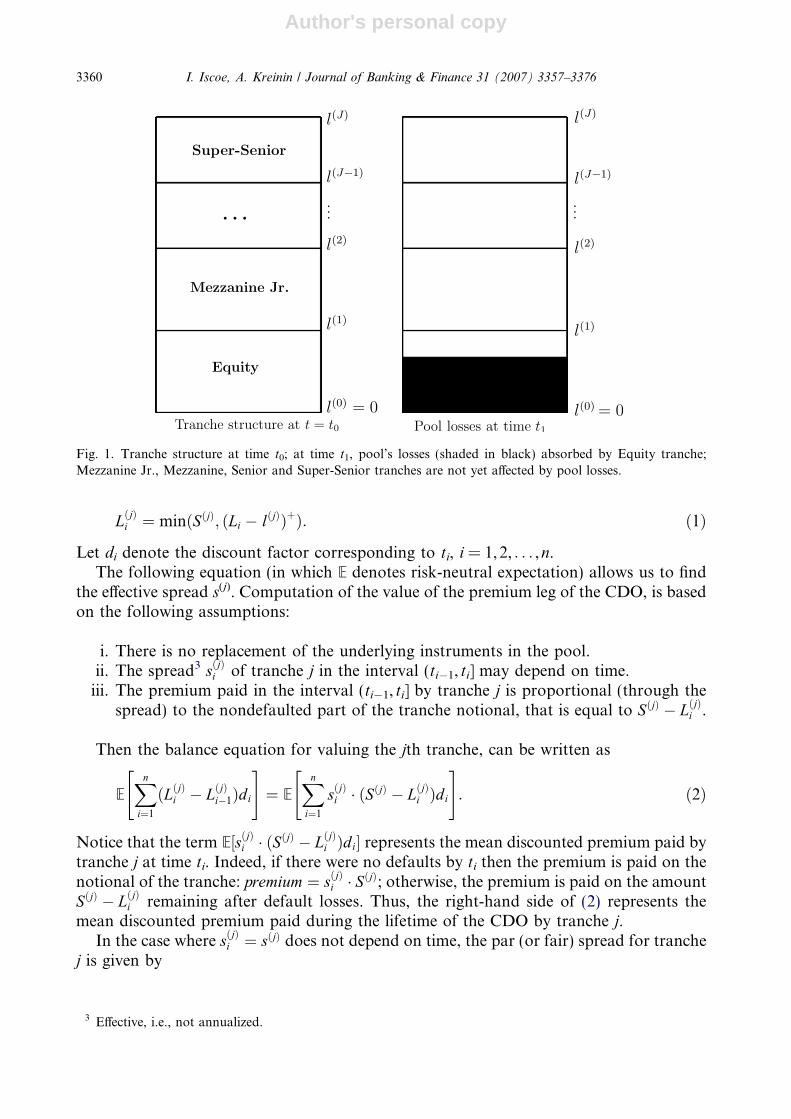
We consider a discrete-time model for the pricing of a CDO. Let T ¼ ft0 ¼ 0; t1; . . . ;ti; . . . ; tn ¼ T g denote the set of times, with T denoting the maturity of the CDO. The poolof securities contains K instruments (whose individual maturities are greater than T).Denote by Nk the recovery-adjusted notional value of the kth instrument initially in thepool, k = 1,2, . . . ,K; the pool notional is N. The CDO consists of J tranches, (enumerated0,1, . . . ,J � 1) into which cash flows from the pool, and losses are absorbed (due todefaults on instruments in the collateral pool), both in accordance with the size and senior-ity of the tranches (see Fig. 1). The size of tranche j, in monetary units, is S(j) = l(j+1) � l(j),l(j) being the lower limit of the tranche; l(0) = 0 and we refer to the 0th tranche as theEquity tranche; l(J) = N. Denote by Li the pool’s cumulative losses up to time ti. Then tran-che j absorbs an amount, LðjÞi , of those losses (by ti):

I. Iscoe, A. Kreinin / Journal of Banking & Finance 31 (2007) 3357–3376 3359


LðjÞi ¼ minðSðjÞ; ðLi � lðjÞÞþÞ: ð1Þ

Let di denote the discount factor corresponding to ti, i = 1,2, . . . ,n.The following equation (in which E denotes risk-neutral expectation) allows us to find

the effective spread s(j). Computation of the value of the premium leg of the CDO, is basedon the following assumptions:

i. There is no replacement of the underlying instruments in the pool.ii. The spread3 sðjÞi of tranche j in the interval (ti�1, ti] may depend on time.

iii. The premium paid in the interval (ti�1, ti] by tranche j is proportional (through thespread) to the nondefaulted part of the tranche notional, that is equal to SðjÞ � LðjÞi .

Then the balance equation for valuing the jth tranche, can be written as

EXn

i¼1

ðLðjÞi � LðjÞi�1Þdi

" #¼ E

Xn

i¼1

sðjÞi � ðSðjÞ � LðjÞi Þdi

" #: ð2Þ

Notice that the term E½sðjÞi � ðSðjÞ � LðjÞi Þdi� represents the mean discounted premium paid bytranche j at time ti. Indeed, if there were no defaults by ti then the premium is paid on thenotional of the tranche: premium ¼ sðjÞi � SðjÞ; otherwise, the premium is paid on the amountSðjÞ � LðjÞi remaining after default losses. Thus, the right-hand side of (2) represents themean discounted premium paid during the lifetime of the CDO by tranche j.

In the case where sðjÞi ¼ sðjÞ does not depend on time, the par (or fair) spread for tranchej is given by

Fig. 1. Tranche structure at time t0; at time t1, pool’s losses (shaded in black) absorbed by Equity tranche;Mezzanine Jr., Mezzanine, Senior and Super-Senior tranches are not yet affected by pool losses.

3 Effective, i.e., not annualized.



sðjÞ ¼EPn

i¼1ðLðjÞi � LðjÞi�1Þdi

h iEPn

i¼1ðSðjÞ � LðjÞi Þdi

h i : ð3Þ

In the case where the spreads are not to be calibrated, i.e., they are direct market inputs,the value of the CDO at time ti is given by the difference between the right- and left-handsides of (2). The buyer’s value of the CDO’s tranche j, at time ti, is

V buy ¼ sðjÞ � EXn

i¼1

ðSðjÞ � LðjÞi Þdi

" #� E

Xn

i¼1

ðLðjÞi � LðjÞi�1Þdi

" #:

In both cases, the problem is reduced to computation of the mean absorbed losses, LðjÞi .For that, we must specify the default model, which is the topic of the next section.

3. Tranche loss model: Analytical results

The tranche loss model can be developed in the conditional independence framework(Finger, 2002; Iscoe et al., 1999). Conditional on a scenario on macro-economic variables,default events are determined by a specific-risk component and, therefore, are indepen-dent. This idea allows us to compute the conditional expectation of the tranche losses;using the conditional expectation formula we can then find ELðjÞi and compute constantcredit spreads s(j) from Eq. (3). In order to simplify computation, we assume in what fol-lows that the interest rate process determining the discount factors and the pool losses areindependent stochastic process. In this case the result of the computation in (3) will dependon the expected value of discount factors. Thus, we can assume that the discount curve isdeterministic in the model.

In this section, we introduce a model for the conditional risk-neutral default probabil-ities and after that we focus on the most simplistic and then the important case of indepen-dent default events and find an analytically tractable solution for the expected tranchelosses. First, we derive an explicit solution for a homogeneous pool. This case plays therole of a benchmark in our numerical analysis. Following that, we find an efficient approx-imation for the case of a large inhomogeneous pool.

3.1. Conditional default probabilities

The model for the conditional risk-neutral default probabilities can be described interms of the state variables Y(k)(t), (k = 1,2, . . . ,K), where the parameter t takes discretevalues t0, t1, t2, . . . , tn; briefly Y ðkÞi � Y ðkÞðtiÞ. The random variables Y ðkÞi are defined to bethe (constant) process

Y ðkÞi � Y ðkÞ ¼XM

m¼1

bðkÞm X m þ rðkÞeðkÞ; i ¼ 1; 2; . . . ; n; k ¼ 1; . . . ;K; ð4Þ

where Xm are macro-economic risk factors or latent random variables, usually called credit

drivers, and e(k) are random variables describing the specific-risk of the kth obligor. Weassume that Xm are jointly normal random variables, each having a standard normal dis-tribution; C denotes their correlation matrix. The specific-risk components are assumed tobe mutually independent standard normal random variables and also independent of all



the credit drivers. In practice, Y(k) is some measure of obligor k’s financial health, which islinearly regressed onto the credit drivers, in case the credit drivers are not latent.

Without loss of generality (by rescaling Y(k)), we can and do assumeXM

m¼1

XM

m0¼1

bðkÞm Cmm0aðkÞm0 þ ðrðkÞÞ

2 ¼ 1:

Therefore, Y ðkÞi all have a standard normal distribution.Although the random variables Y ðkÞi do not actually vary over time, we preserve the time

index, i, in the notation, to suggest an analogy to – actually, a simplification of – a mul-tistep credit risk model (cf. Iscoe et al., 1999). In detail, with s(k) denoting the realised timeof default of the kth obligor (s(k) 2 {t1, t2, . . . , tn,+1}), we connect s(k) to the chainðY ðkÞi ; 1 6 i 6 nÞ through a default boundary, ðH ðkÞi Þ

ni¼1, such that

sðkÞ ¼ minfti : Y ðkÞi < H ðkÞi g ðsðkÞ ¼ þ1 if Y ðkÞi P H ðkÞi ; 1 6 i 6 nÞ: ð5ÞGiven the constancy of the process Y ðkÞi in our model (4) and (5) simplifies to

sðkÞ ¼ minfti : Y ðkÞ < H ðkÞi g ðsðkÞ ¼ þ1 if Y ðkÞ P H ðkÞi ; 1 6 i 6 nÞ: ð6ÞIn practice, the distribution of s(k) is given from market data and the boundary ðH ðkÞi Þ

ni¼1 is

determined from it, as follows. Denote the risk-neutral, cumulative default probabilities ofthe kth obligor by pðkÞi :

PðsðkÞ 6 tiÞ ¼ pðkÞi ; i ¼ 1; 2; . . . ; n:

We make the (standing) natural assumption that pðkÞi is strictly increasing with i.

Lemma 1. Under the assumption that pðkÞi is strictly increasing with i, then for all 1 6 i 6 n

and all 1 6 k 6 K

H ðkÞi ¼ U�1ðpðkÞi Þ; ð7Þ(U denotes the standard normal cdf) so that H ðkÞi is strictly increasing with i; and

sðkÞ 6 ti iff Y ðkÞ < H ðkÞi : ð8ÞLet X denote the vector of macro-economic variables, X :¼ (X1, . . . ,XM); and letx = (x1, . . . ,xM) be a particular value of X. Using (8) of Lemma 1, the conditional risk-neutral default time distribution of the kth obligor is determined by the relation

pðkÞi ðxÞ :¼ PðsðkÞ 6 tijX ¼ xÞ ¼ PðY ðkÞ < H ðkÞi jX ¼ xÞ; ð9Þfor i = 1,2, . . . ,n. It follows from (9) and (4) that the conditional risk-neutral default prob-abilities are given by

pðkÞi ðxÞ ¼ U ½H ðkÞi �XM

m¼1

bðkÞxm�=rðkÞ !

: ð10Þ

In our framework, the default events of the obligors are conditionally independent. Thisassumption allows us to reduce the problem of computation of the mean tranche losses,ELðjÞi , to the case of independent obligors:



ELðjÞi ¼Z

RMExL

ðjÞi duðxÞ; ð11Þ

where ExLðjÞi is the conditional mean tranche losses if the default probabilities are given by

(10) and u is the joint distribution of the credit drivers.In particular, if M = 1 the integral in Eq. (11) has an especially simple form:

ELðjÞi ¼Z 1

�1ExL

ðjÞi dUðxÞ; ð12Þ

and can be computed using one-dimensional quadratures. For the remaining sections ofthe paper, we restrict attention to this case of a single credit driver.

In Sections 3.2 and 3.3, we find the mean tranche losses, ExLðjÞi in a given scenario on a

single credit driver. To simplify our notation, we will omit the parameter x in the deriva-tion of the formulas for the mean tranche losses since the scenario x is fixed.

3.2. Homogeneous pool

Let us first consider the simple case: the underlying instruments in the pool have a com-mon term structure of default probabilities:

pi ¼ Pðs ¼ tiÞ; i ¼ 1; 2; . . . ; n;

where s denotes the default time of a generic instrument in the pool. We also introduceconditional probabilities pi ¼ Pðs ¼ tijs P tiÞ

pi ¼pi

1�Pi�1

m¼1pm

; qi ¼ 1� pi; i ¼ 1; 2; . . . ; n;

from which the pi’s can be recovered (see Fig. 2)

Fig. 2. Conditional default probabilities.



pi ¼ pi �Yi�1

m¼1

qm: ð13Þ

Denote by mi the number of instruments in default state at time ti. Then m1 is binomiallydistributed:

Pðm1 ¼ k1Þ ¼K

k1

� �pk1

1 qK�k11 ; q1 ¼ 1� p1;

and Ezm11 ¼ ðp1z1 þ q1Þ

K . We now find the generating function of the vectorm = (m1,m2, . . . ,mn).

Proposition 2. The generating function PðKÞn ðz1; . . . ; znÞ � EQn

i¼1zmii is given by

PðKÞn ðz1; . . . ; znÞ ¼Xn

i¼1

pi

Yn

m¼i

zm þ 1�Xn

i¼1

pi

!K

: ð14Þ

Proposition 2 is proved in Appendix A by induction over the index n.

We now present several corollaries to Proposition 2, concerning the distributions of themarginal and incremental tranche losses, with respect to time, for a further specializationof the homogeneous case in which the pool’s instruments have a common notional value,N1. The results will be presented for both finite pool size, K, and also the limiting case,K!1.

Corollary 3. Let pi ¼Pi

m¼1pm; 1 6 i 6 n; then mi � BinðK; piÞ. If all the pool’s instruments

have a common notional value, N1, then

E½LðjÞi � ¼X

1_lðjÞN16k<lðjþ1Þ

N1

ðN 1k � lðjÞÞBinðk; K; piÞ þ SðjÞX

lðjþ1ÞN16k6K

Binðk; K; piÞ: ð15Þ

The following corollary describes the limit distribution of the number of instruments indefault state as K!1.

Corollary 4. Let ki ¼ Kpi; 1 6 i 6 n; then for large K, the distribution of mi is approximately

PoisðkiÞ:

Pðmi ¼ kÞ¼: e�kiðkiÞk=k!; k ¼ 0; 1; . . . ð16ÞThe error in the approximation in (16), is bounded by ðkiÞ2=K. If all the pool’s instruments

have a common notional value, N1, then

E½LðjÞi � ¼X

1_lðjÞN16k<lðjþ1Þ

N1

ðN 1k � lðjÞÞPoisðk; piÞ þ SðjÞX

lðjþ1ÞN16k6K

Poisðk; piÞ: ð17Þ

The error in the approximation in (17), is bounded by ðN 1ki þ SðjÞÞðkiÞ2=K.

The last corollary in this subsection describes the joint limit distribution of the incrementsDmi = mi � mi�1, as K!1.



Corollary 5. Let pi depend on K such that ki = limK!1Kpi, exists for each 1 6 i 6 n, and

denote Dm � ðDmiÞni¼1 :¼ ðm1; m2 � m1; . . . ; mn � mn�1Þ. In the limit, as K!1, the distribution

of Dm converges to that of independent, Poisson-distributed random variables: asymptotically,

Dmi � Pois(ki), 1 6 i 6 n, and ðDmiÞni¼1 are mutually independent.

3.3. Inhomogeneous pool

In this subsection, we consider the general case: the underlying instruments in the poolhave individual term structures of default probabilities:

pðkÞi ¼ PðsðkÞ ¼ tiÞ; i ¼ 1; 2; . . . ; n; k ¼ 1; 2; . . . ;K;

where s(k) denotes the default time of the ith instrument in the pool.Although we could have generalized the results in Section 3.2 immediately to the case in

which the notionals varied from instrument to instrument, and for which recovery is non-zero, we delayed this generalization until the present section, in order to keep simple, thenotation.

Concerning recovery rates, for the purposes of analytical evaluations and approxima-tions, one need only replace the individual notionals with the loss given defaults, as thereis negligible probability of the entire pool defaulting. We shall not use a separate notation,such as eN k, to distinguish the loss given default from the original notional, Nk; the latterwill be assumed to be already recovery-adjusted. Set N* = mink Nk.

The symbol, N, will be used as a possible notional amount (individual or aggregate) inthis section.

In order to generalize the results, we need the following additional notation:

pðkÞi ¼Xi

m¼1

pðkÞm ; ki ¼XK

k¼1

pðkÞi ; f iðNÞ ¼X

k:Nk¼N

pðkÞi =ki; 1 6 i 6 n:

We remark that in the case where pðkÞi does not depend on k, fi is simply the relative fre-quency of the notional values:

fiðNÞ ¼ ½#k 2 f1; 2; . . . ;Kg : N k ¼ N �=K:

Although the notionals in the pool are not random, it is useful to consider a random var-iable, which we shall denote by Ni, having the probability mass function fi, above. The m-fold convolution of fi with itself (as a probability mass function) will be denoted by f Hm

i :

f H1i � fi; f Hðmþ1Þ

i ðNÞ ¼X

N 0fiðN 0Þf Hm

i ðN � N 0Þ; m P 1:

We now proceed to the generalizations of the results of Section 3.2.Assume that the probabilities pðkÞi satisfy the relation

limK!1

XK

k¼1

ðpðkÞi Þ2 ¼ 0: ð18Þ

Proposition 6. In the limiting case of a large pool (K large), the generating function,

GiðxÞ ¼ EzLi , of the pool’s cumulative losses up to time, ti, is given by

EzLi¼: expðki½EzNi � 1�Þ; 1 6 i 6 n:



Thus we have the approximate equality in distribution, for fixed i = 1,2, . . . , n

Li�D XMi

m¼1

NðmÞi ; ð19Þ

where ðNðmÞi Þ

Km¼1 is an i.i.d. sequence of copies of Ni and independent of Mi � PoisðkiÞ.

More precisely

maxN

PðLi ¼ NÞ � PXMi

m¼1

NðmÞi ¼ N

!�� ¼ O

XK

k¼1

ðpðkÞi Þ2

!: ð20Þ

The right-hand side of (19) is a non-stationary compound Poisson process.

Corollary 7. In the limiting case of a large pool (K large), the expected cumulative losses

absorbed by tranche j up to time ti, is

ELðjÞi ¼: SðjÞð1� e�kiÞ � e�ki SðjÞ

X16m6lðjÞ=N�

kmi

m!

XmN�6N6lðjÞ

f Hmi ðNÞ

8<:þ

X16m<lðjþ1Þ=N�

kmi

m!

XlðjÞ<N<lðjþ1Þ

½lðjþ1Þ � N �f Hmi ðNÞ

9=;: ð21Þ

In particular, for the Equity tranche (j = 0)

ELð0Þi ¼: Sð0Þð1� e�kiÞ � e�ki

X16m<Sð0Þ=N�

kmi

m!

XmN�6N<Sð0Þ

½Sð0Þ � N �f Hmi ðNÞ

8<:9=;:

We close this section with a specialization of the previous results to the case where allnotionals coincide, Nk � N1 for all k, in which case, fiðNÞ ¼ dN ;N1

, the Kronecker delta;f Hm

i ðNÞ ¼ dN ;mN1. Therefore, we have the following simplifications of Proposition 6 and

its Corollary 7.

Corollary 8. In the limiting case of a large pool (K large), when Nk � N1 for all k, we have

the approximate equality in distribution, for fixed i = 1,2, . . . , n, for the pool’s cumulative

losses, Li, up to time, ti

Li�D

N 1 �Mi; ð22Þ

where Mi � PoisðkiÞ.

Proof. This is a special case of Proposition 6 because the random variable, Ni, and hencethe random variables, ðNðmÞ

i ÞKm¼1, are degenerate, with constant value, N1. h

Corollary 9. In the limiting case of a large pool (K large), when Nk � N1 for all k, the

expected cumulative losses absorbed by the jth tranche up to time ti, is



ELðjÞi ¼: SðjÞð1� e�kiÞ � e�ki SðjÞ

X16m6lðjÞ=N1

kmi

m!�

XlðjÞN1<m<lðjþ1Þ

N1

e�kikm

i

m!½lðjþ1Þ � mN 1�: ð23Þ

In particular, for the equity-tranche (j = 0)

ELð0Þi ¼: Sð0Þð1� e�kiÞ � e�ki

X16m<Sð0Þ=N1

kmi

m!½Sð0Þ � mN 1�

8<:9=;:

4. Accuracy of CPA method

In applying the theoretical results of Section 3, in practice and in our examples, the sizeof the pool is usually moderate as opposed to being ‘‘large’’, in the sense of a limiting sit-uation. Furthermore, the tranche thicknesses are usually expressed as moderate, not varysmall, percentages of the pool’s total notional value. In particular, error estimates of theform in Corollary 4, do not yield useful criteria for comparison, as S(j)/K may not be small.As such, it becomes important to carry out numerical experiments to assess the accuracyof the results of Section 3, for moderately sized pools.

In this section, we compare the results of the computation of the tranche spreads usingthe ABS method proposed in Andersen et al. (2003) with that obtained using the analyticalsolutions in Section 3. We make a standing assumption throughout this section, that thespreads do not vary over time. Also we assume that the number of credit drivers M = 1.

The CDO structure is determined by the protection levels of the tranches. In our exper-iments, the Equity tranche absorbs 3% of the total potential losses. The next tranche, Mez-zanine Junior, absorbs 1% of losses. The Mezzanine tranche absorbs 2.1% of the poolnotional. The last two tranches, Senior and Super-Senior, absorb 6% and 87.9%, respec-tively. This structure is rather typical for CDO: the Senior (Super-Senior) tranches usuallyhave the highest exposure. The protection level of the Super-Senior tranche is in the range12–25% of the pool notional. The credit spreads in the experiments were computed underthe assumption that the interest rates4 are non-random, and are r1 = 4.6%, r2 = 5%,r3 = 5.6%, r4 = 5.8% and r5 = 6%. Except in the last example, the common recovery rateof the instruments in the pool is 30%. In the first experiment, we analyze a CDO with thehomogeneous pool consisting of K instruments with a common notional N1 = $100. Thetime horizon T = 5 years. All instruments have the same initial credit rating. The cumula-tive default probabilities corresponding to various credit grades are shown in Table 1. Forexample, if the initial credit state of the kth obligor is Baa2 then the default probabilitiesare

pðkÞ1 ¼ 0:0007; pðkÞ2 ¼ 0:003; pðkÞ3 ¼ 0:0068; pðkÞ4 ¼ 0:0119; pðkÞ5 ¼ 0:0182:

The risk-neutral default probabilities are computed from the market quotes of credit riskysecurities (usually risky bonds and credit default swaps). This involves the solution of theinverse problem for the prices of risky bonds and, usually, requires parameter optimiza-tion of the model. This problem is not considered in the present paper.

4 Continuously compounded, actual/365.



We assume that the default events of the counterparties are independent in this exper-iment. Then bðkÞi ¼ 0. Let us now compare the results of the credit-spread computationsusing the closed-form solution (15) and the Poisson approximation (21).

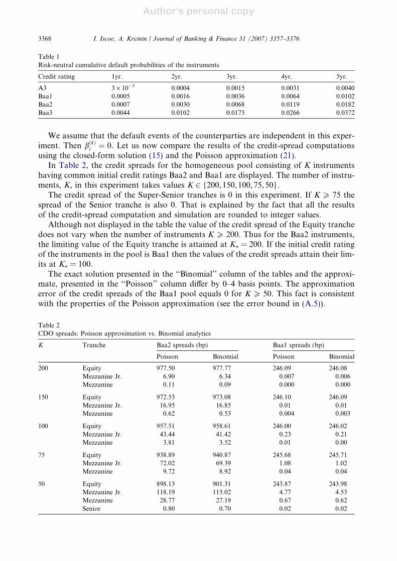
In Table 2, the credit spreads for the homogeneous pool consisting of K instrumentshaving common initial credit ratings Baa2 and Baa1 are displayed. The number of instru-ments, K, in this experiment takes values K 2 {200,150,100,75,50}.

The credit spread of the Super-Senior tranches is 0 in this experiment. If K P 75 thespread of the Senior tranche is also 0. That is explained by the fact that all the resultsof the credit-spread computation and simulation are rounded to integer values.

Although not displayed in the table the value of the credit spread of the Equity tranchedoes not vary when the number of instruments K P 200. Thus for the Baa2 instruments,the limiting value of the Equity tranche is attained at K* = 200. If the initial credit ratingof the instruments in the pool is Baa1 then the values of the credit spreads attain their lim-its at K* = 100.

The exact solution presented in the ‘‘Binomial’’ column of the tables and the approxi-mate, presented in the ‘‘Poisson’’ column differ by 0–4 basis points. The approximationerror of the credit spreads of the Baa1 pool equals 0 for K P 50. This fact is consistentwith the properties of the Poisson approximation (see the error bound in (A.5)).

Table 2CDO spreads: Poisson approximation vs. Binomial analytics

K Tranche Baa2 spreads (bp) Baa1 spreads (bp)

Poisson Binomial Poisson Binomial

200 Equity 977.50 977.77 246.09 246.08Mezzanine Jr. 6.90 6.34 0.007 0.006Mezzanine 0.11 0.09 0.000 0.000




50 Equity 898.13 901.31 243.87 243.98Mezzanine Jr. 118.19 115.02 4.77 4.53Mezzanine 28.77 27.19 0.67 0.62Senior 0.80 0.70 0.02 0.02

Table 1Risk-neutral cumulative default probabilities of the instruments

Credit rating 1yr. 2yr. 3yr. 4yr. 5yr.

A3 3 · 10�5 0.0004 0.0015 0.0031 0.0040Baa1 0.0005 0.0016 0.0036 0.0064 0.0102Baa2 0.0007 0.0030 0.0068 0.0119 0.0182Baa3 0.0044 0.0102 0.0175 0.0266 0.0372



The credit spreads appeared to be very sensitive to the credit rating. A change in onegrade caused a significant change in the spreads. For example, the Equity tranche spreaddrops by 3 times; the Mezzanine Jr. spread – almost 10 times if the number of the instru-ments is 25. If the number of instruments is 75 then the Equity spread changes by morethan 4 times and the Mezzanine Jr. tranche spread – almost 70 times.

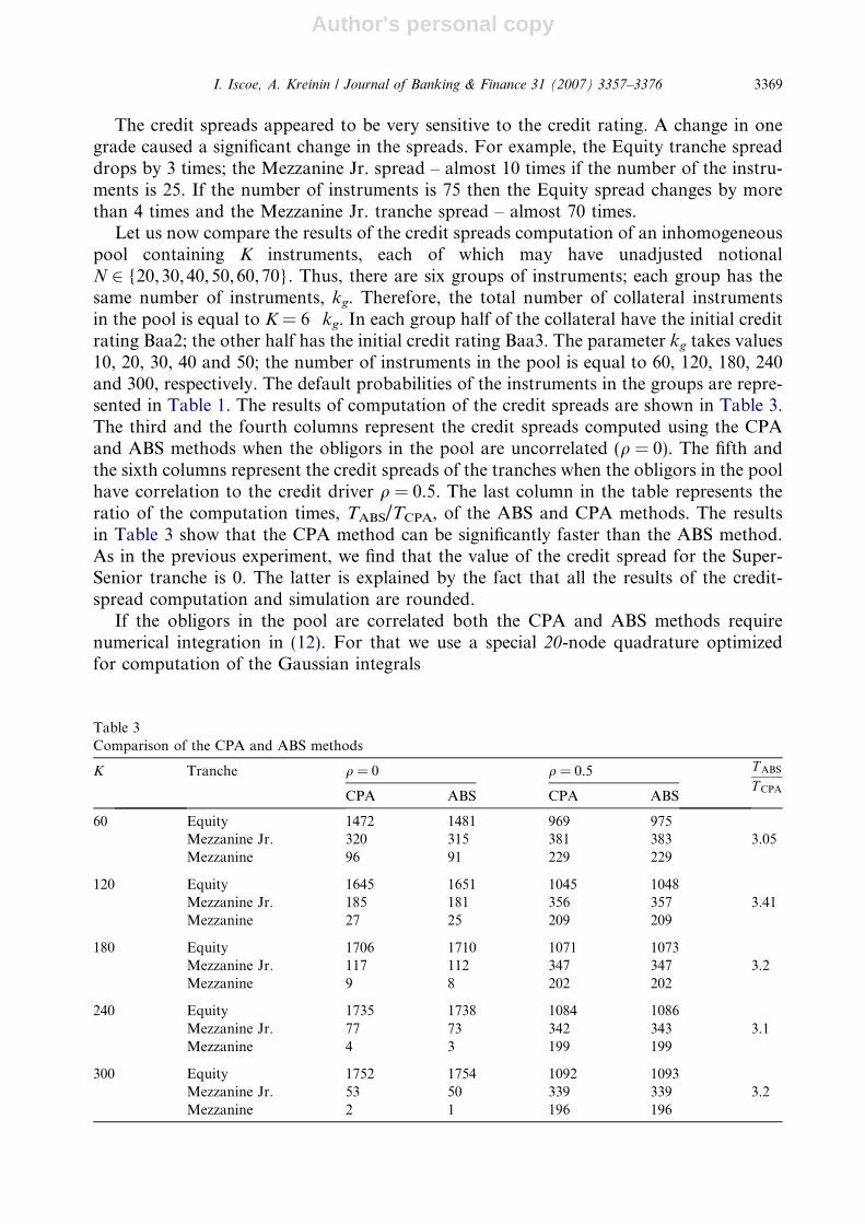
Let us now compare the results of the credit spreads computation of an inhomogeneouspool containing K instruments, each of which may have unadjusted notionalN 2 {20,30,40,50,60,70}. Thus, there are six groups of instruments; each group has thesame number of instruments, kg. Therefore, the total number of collateral instrumentsin the pool is equal to K = 6 Æ kg. In each group half of the collateral have the initial creditrating Baa2; the other half has the initial credit rating Baa3. The parameter kg takes values10, 20, 30, 40 and 50; the number of instruments in the pool is equal to 60, 120, 180, 240and 300, respectively. The default probabilities of the instruments in the groups are repre-sented in Table 1. The results of computation of the credit spreads are shown in Table 3.The third and the fourth columns represent the credit spreads computed using the CPAand ABS methods when the obligors in the pool are uncorrelated (q = 0). The fifth andthe sixth columns represent the credit spreads of the tranches when the obligors in the poolhave correlation to the credit driver q = 0.5. The last column in the table represents theratio of the computation times, TABS/TCPA, of the ABS and CPA methods. The resultsin Table 3 show that the CPA method can be significantly faster than the ABS method.As in the previous experiment, we find that the value of the credit spread for the Super-Senior tranche is 0. The latter is explained by the fact that all the results of the credit-spread computation and simulation are rounded.

If the obligors in the pool are correlated both the CPA and ABS methods requirenumerical integration in (12). For that we use a special 20-node quadrature optimizedfor computation of the Gaussian integrals

Table 3Comparison of the CPA and ABS methods

K Tranche q = 0 q = 0.5 T ABS

T CPACPA ABS CPA ABS

60 Equity 1472 1481 969 975Mezzanine Jr. 320 315 381 383 3.05Mezzanine 96 91 229 229







IðvÞ ¼Z 1

�1ðx� vÞþdUðxÞ;

(v > 0); each node x1,x2, . . . ,x20 represents a scenario on the credit driver. The conditionaldefault probabilities take very large values in the scenario x1 (x1 < 0). For example, the fiveyear conditional default probability of the Baa3 obligor equals 81% while the uncondi-tional default probability is only 3.7%. Despite the high level of the default probabilities,the Poisson approximation for LðjÞi ðxÞ in Eq. (12) leads to an accurate approximation of thetranche spreads.

The results of this numerical experiment show that correlation of the obligors does notincrease the Poisson approximation error in the tranche spreads.

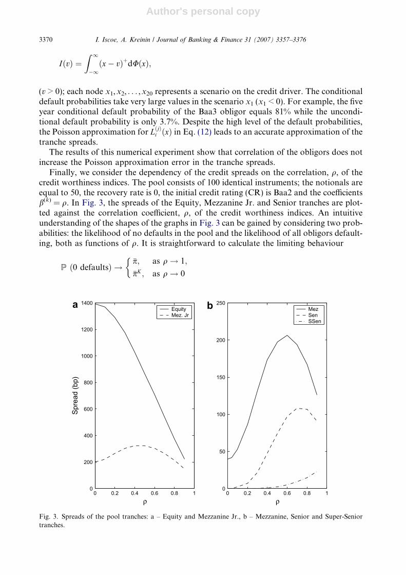
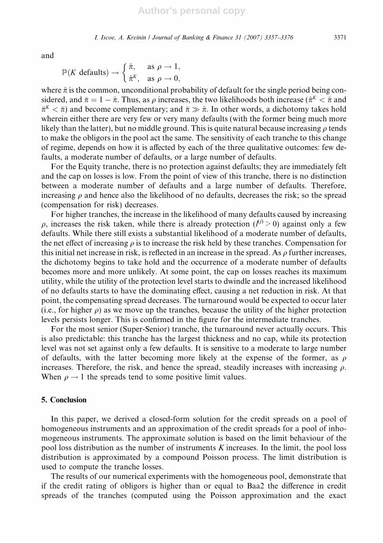
Finally, we consider the dependency of the credit spreads on the correlation, q, of thecredit worthiness indices. The pool consists of 100 identical instruments; the notionals areequal to 50, the recovery rate is 0, the initial credit rating (CR) is Baa2 and the coefficientsb(k) = q. In Fig. 3, the spreads of the Equity, Mezzanine Jr. and Senior tranches are plot-ted against the correlation coefficient, q, of the credit worthiness indices. An intuitiveunderstanding of the shapes of the graphs in Fig. 3 can be gained by considering two prob-abilities: the likelihood of no defaults in the pool and the likelihood of all obligors default-ing, both as functions of q. It is straightforward to calculate the limiting behaviour

P ð0 defaultsÞ !�p; as q! 1;

�pK ; as q! 0

�

0 0.2 0.4 0.6 0.8 10

200

400

600

800

1000

1200

1400

ρ

Spre

ad (b

p)

a EquityMez. Jr

0 0.2 0.4 0.6 0.8 10

50

100

150

200

250

ρ

MezSenSSen

b

Fig. 3. Spreads of the pool tranches: a – Equity and Mezzanine Jr., b – Mezzanine, Senior and Super-Seniortranches.



and

PðK defaultsÞ !p; as q! 1;

pK ; as q! 0;

�where p is the common, unconditional probability of default for the single period being con-sidered, and �p ¼ 1� p. Thus, as q increases, the two likelihoods both increase (pK < p and�pK < �p) and become complementary; and �p p: In other words, a dichotomy takes holdwherein either there are very few or very many defaults (with the former being much morelikely than the latter), but no middle ground. This is quite natural because increasing q tendsto make the obligors in the pool act the same. The sensitivity of each tranche to this changeof regime, depends on how it is affected by each of the three qualitative outcomes: few de-faults, a moderate number of defaults, or a large number of defaults.

For the Equity tranche, there is no protection against defaults; they are immediately feltand the cap on losses is low. From the point of view of this tranche, there is no distinctionbetween a moderate number of defaults and a large number of defaults. Therefore,increasing q and hence also the likelihood of no defaults, decreases the risk; so the spread(compensation for risk) decreases.

For higher tranches, the increase in the likelihood of many defaults caused by increasingq, increases the risk taken, while there is already protection (l(j) > 0) against only a fewdefaults. While there still exists a substantial likelihood of a moderate number of defaults,the net effect of increasing q is to increase the risk held by these tranches. Compensation forthis initial net increase in risk, is reflected in an increase in the spread. As q further increases,the dichotomy begins to take hold and the occurrence of a moderate number of defaultsbecomes more and more unlikely. At some point, the cap on losses reaches its maximumutility, while the utility of the protection level starts to dwindle and the increased likelihoodof no defaults starts to have the dominating effect, causing a net reduction in risk. At thatpoint, the compensating spread decreases. The turnaround would be expected to occur later(i.e., for higher q) as we move up the tranches, because the utility of the higher protectionlevels persists longer. This is confirmed in the figure for the intermediate tranches.

For the most senior (Super-Senior) tranche, the turnaround never actually occurs. Thisis also predictable: this tranche has the largest thickness and no cap, while its protectionlevel was not set against only a few defaults. It is sensitive to a moderate to large numberof defaults, with the latter becoming more likely at the expense of the former, as qincreases. Therefore, the risk, and hence the spread, steadily increases with increasing q.When q! 1 the spreads tend to some positive limit values.

5. Conclusion

In this paper, we derived a closed-form solution for the credit spreads on a pool ofhomogeneous instruments and an approximation of the credit spreads for a pool of inho-mogeneous instruments. The approximate solution is based on the limit behaviour of thepool loss distribution as the number of instruments K increases. In the limit, the pool lossdistribution is approximated by a compound Poisson process. The limit distribution isused to compute the tranche losses.

The results of our numerical experiments with the homogeneous pool, demonstrate thatif the credit rating of obligors is higher than or equal to Baa2 the difference in creditspreads of the tranches (computed using the Poisson approximation and the exact



formula) does not exceed 3 bp for all tranches. In the case of an inhomogeneous pool, thedetailed analysis showed that in the vast majority of cases, the difference between theapproximate spread and its value obtained using ABS method does not exceed 3 bp forthe Mezzanine and Senior tranches and does not exceed 9 bp for the Equity tranche.

The performance of the CPA method can be significantly higher than that of the ABSand the Brasch’s methods. However, the acceleration is sensitive to the number of differentrecovery-adjusted notionals. Performance comparison of different analytical methods forCDO valuation requires special research; it is discussed in a separate paper (De Priscoet al., 2005) (see also Andersen et al., 2003; Hull and White, 2004; Laurent, 2003).

Acknowledgements

We are very grateful to Tomasz Bielecki, Raphael Douady, Peter Carr, Ludger Over-beck and Stan Uryasev for the comments that significantly improved the paper. We alsothank our colleagues Ben De Prisco, Sarah Hodgson, Jennifer Lai, Asif Lakhany, HelmutMausser, Ahmed Nagi and Dan Rosen for useful discussions.

Appendix A. Proof of the results

Proof of Lemma 1. Clearly s(k) > ti iff Y ðkÞ P max16m6i H ðkÞm ; so

sðkÞ 6 ti iff Y ðkÞ < max16m6i

H ðkÞm : ðA:1Þ

Then

pðkÞi ¼ P Y ðkÞ < max16m6i

H ðkÞm

� �¼ U max

16m6iH ðkÞm

� �;

which implies that

max16m6i

H ðkÞm ¼ U�1ðpðkÞi Þ:

It follows that H ðkÞi ¼ U�1ðpðkÞi Þ, under our assumption that pðkÞi is strictly increasing with i,and that the thresholds H ðkÞi satisfy the inequality

H ðkÞi < H ðkÞiþ1; i ¼ 1; . . . ; n� 1: ðA:2Þ

Then from (A.1) and (A.2) we obtain (8). h

Proof of Proposition 2. We prove Proposition 2 by induction over the index n. The casen = 1 has already been established just before the statement of the proposition, sincep1 = p1 and q1 = 1 � p1 = 1 � p1. More generally, it is easy to show that

Qni¼1qi ¼

1�Pn

i¼1pi; also recall (13). It is in this form that we will establish (14). First of all, thedistribution of the vector~m is given as

Pð~m ¼~kÞ ¼K

k1

� �pk1

1 qK�k11 �

K � k1

k2 � k1

� �pk2�k1

2 qK�k22 � � �

K � kn�1

kn � kn�1

� �pkn�kn�1

n qK�knn ;

ðA:3Þwhere ~k ¼ ðk1; . . . ; knÞ; 0 6 k1 6 k2 6 . . . 6 kn.



We now turn to the induction, assuming the statement of the proposition for aparticular value of n and proving it for n + 1. It is easy to see, from (A.3), that theconditional distribution of ~m :¼ ðm2; . . . ; mnþ1Þ, given m1 = k1, coincides with the uncondi-tional distribution of (m1 + k1, . . . ,mn + k1) with the parameters p = (p1, . . . ,pn+1) and K

replaced by ~p ¼ ðp2; . . . ; pnþ1Þ and ~K ¼ K � k1, respectively. We make the role of theparameters explicit as subscripts on probability measures and expectations. For 1 6 i 6 n,set ~zi ¼ ziþ1. Then we have

Ep;K

Ynþ1

i¼2

zmii m1 ¼ k1j

" #¼ Ep;K

Yn

i¼1

~z~mii

" ��m1 ¼ k1

#¼ E~p;~K

Yn

i¼1

~zmiþk1i

" #;

and by the inductive hypothesis

Ep;K

Ynþ1

i¼2

zmii jm1 ¼ k1

" #¼

Yn

i¼1

~zi

!k1 Xn

i¼1

~pi

Yi�1

m0¼1

~qm0Yn

m¼i

~zm þYn

i¼1

~qi

!~K

¼Ynþ1

i¼2

zi

!k1 Xnþ1

i¼2

pi

Yi�1

m0¼2

qm0

Ynþ1

m¼i

zm þYnþ1

i¼2

qi

!K�k1

: ðA:4Þ

Then from (A.4) we derive

Ep;K

Ynþ1

i¼1

zmii

" #¼XK

k1¼0

Pp;Kðm1 ¼ k1ÞEp;K

Ynþ1

i¼1

zmii jm1 ¼ k1

" #

¼XK

k1¼0

K

k1

!pk1

1 qK�k11

Ynþ1

i¼1

zi

!k1 Xnþ1

i¼2

pi

Yi�1

m0¼2

qm0

Ynþ1

m¼i

zm þYnþ1

i¼2

qi

!K�k1

¼XK

k1¼0

K

k1

!p1

Ynþ1

i¼1

zi

!k1 Xnþ1

i¼2

pi

Yi�1

m0¼1

qm0

Ynþ1

m¼i

zm þYnþ1

i¼1

qi

!K�k1

¼Xnþ1

i¼1

pi

Yi�1

m0¼1

qm0

Ynþ1

m¼i

zm þYnþ1

i¼1

qi

!K

:

Finally, taking into account that pi

Qi�1m0¼1qm0 ¼ pi, we obtain that the generating function

PðKÞn ðz1; . . . ; znÞ satisfies (14) as was to be proved. h

Proof of Corollary 3. The generating function for mi is just PðKÞn ð1; . . . ; 1; z; 1; . . . ; 1Þ, with z

in the ith coordinate; and by Proposition 2, that is

PðKÞn ð1; . . . ;1;z;1; . . . ;1Þ¼ p1zþ�� þpizþXn

m¼iþ1

pmþ1�Xn

m¼1

pm

" #K

¼ ½pizþ1� pi�K ;

which is the generating function of a BinðK; piÞ-distributed random variable.Now, under the extra hypothesis (common notional, N1), Li = N1mi and by (1), we

obtain (15). h



Proof of Corollary 4. The Poisson approximation to the binomial distribution iswell known – see e.g., Section 6 of Chapter 8 in Ross (1994), where in particular theestimate

maxAjPðBinðK; pÞ 2 AÞ � PðPoisðKpÞ 2 AÞj 6 Kp2 ðA:5Þ

is derived, and also Gerber (1984). The first part of the corollary follows directly from thefirst part of Corollary 3 and the estimate (A.5). The proof of (17) and the error bound fol-low from (15) and (A.5). h

Proof of Corollary 5. The generating function, PðDmÞðu1; . . . ; unÞ, of the increments satisfiesthe relation

PðDmÞðu1; . . . ; unÞ ¼ PðKÞn

u1

u2

;u2

u3

; . . . ;un�1

un; un

� �:

If zi ¼ uiuiþ1

for i = 1,2, . . . ,n with un+1 � 1, the productQn

m¼izm ¼ ui. Therefore

PðDmÞðu1; . . . ; unÞ ¼Xn

i¼1

piui þ 1�Xn

i¼1

pi

!K

¼ 1þPn

i¼1Kpi½ui � 1�K

� �K

:

From the latter equation we obtain

limK!1

PðDmÞðu1; . . . ; unÞ ¼ expXn

i¼1

ki½ui � 1� !

¼Yn

i¼1

eki ½ui�1�:

h

Proof of Proposition 6. Denote

X ki ¼1; if instrument k defaults by ti;

0; otherwise:

�Then PðX ki ¼ 1Þ ¼ pðkÞi and Li ¼

PKk¼1NkX ki. Therefore

EzLi ¼YKk¼1

E½zNk X ki � ¼YKk¼1

½1þ pðkÞi ðzNk � 1Þ�:

Then, using the result: logð1þ xÞ ¼ xþ Oðx2Þ;�0:5 < x < 1, we obtain

log EzLi ¼XK

k¼1

log½1þ pðkÞi ðzNk � 1Þ� ¼XK

k¼1

pðkÞi ðzNk � 1Þ þ OXK

k¼1

ðpðkÞi Þ2

!: ðA:6Þ

The first term on the right-hand side of Eq. (A.6) satisfies the relation

XK

k¼1

pðkÞi ðzNk � 1Þ ¼X

m

Xk:Nk¼m

pðkÞi ðzm � 1Þ ¼ ki

Xm

ðzm � 1ÞfiðmÞ ¼ kiE½zNi � 1�:



On the other hand

E z

PMi

m¼1

NðmÞi

264375 ¼X1

m¼0

E z

Pmm0¼1

Nðm0 Þi

24 35PðMi ¼ mÞ ¼X1m¼0

½EzNi �mPðMi ¼ mÞ

¼ e�kiX1m¼0

kmi

m!½EzNi �m ¼ expðki½EzNi � 1�Þ:

Let us now obtain the bound (20). The probabilities PðLm ¼ NÞ satisfy the relation

PðLm ¼ NÞ ¼ 1

2pi

Ijzj¼1

GmðzÞzNþ1

dz; N ¼ 1; 2; . . . ;

where Gm denotes the generating function of the random variablePMm

j¼1NðjÞm ,

GmðzÞ ¼ E zPMm

j¼1NðjÞm

� �m ¼ 1; 2; . . . ; n. From well known properties of probability generat-

ing functions, Eq. (A.6) and the latter formula, we obtain for m = 1,2, . . . ,n

maxN

PðLm¼NÞ�PXMm

j¼1

NðjÞm ¼N

!��¼max

N

1

2pi

Ijzj¼1

GmðzÞzNþ1

� 1� exp OXK

k¼1

ðpðkÞi Þ2

! !" #dz

��:

The latter relation implies (20). h

Proof of Corollary 7. Define the function / � /j, on the interval 0 6 L < +1, by

/jðLÞ ¼SðjÞ; 0 6 L 6 lðjÞ;

lðjþ1Þ � L; lðjÞ < L 6 lðjþ1Þ;

0; otherwise:

8><>:Then, by (1), the cumulative losses for tranche j by time ti, LðjÞi ¼ SðjÞ � /jðLiÞ. For theremainder of the proof, to simplify the notation and clarify the techniques, we will sup-press most subscripts and superscripts, as both j and i are fixed; and we will begin withthe case j = 0. We will comment on the minor differences for j > 0, at the end.

When j = 0, as l(0) = 0, /(L) can be written simply as [S � L]+; S � S(0) = l(1). Therefore

ELð0Þ ¼ S � E½/ðLÞ�¼: S � E /XMm0¼1

Nðm0Þ

!" #; by ð19Þ:

Thus we obtain by conditioning on M, independent of all NðmÞ

ELð0Þ ¼ S � e�kX1m¼0

km

m!E /

Xm

m0¼1

Nðm0Þ

!" #

¼ S � e�k S þX1m¼1

km

m!

XN<S

½S � N �f HmðNÞ( )

¼ S � e�k S þX

16m<S=N�

km

m!

XmN�6N<S

½S � N �f HmðNÞ( )

;



the last line following from the fact that, with probability 1 (i.e., for N such thatfwm(N) > 0), N P mN*.

When j > 0, the only modification required to the previous calculation, is to split thesum,

PmN �6N<lðjþ1Þ/ðNÞ into the sum over those N satisfying N 6 l(j) (which is impossible if

m > l(j)/N*, as N P mN* with probability 1) and the sum over those vectors N satisfyingl(j) < N < l(j+1) (which is impossible if m > l(j+1)/N*, again because N P mN* withprobability 1). h

References

Andersen, L., Sidenius, J., Basu, S., 2003. All your hedges in one basket. Risk 16 (11), 67–72.Bertoin, J., 1996. Levy Processes. Cambridge University Press, Cambridge, UK.Bielecki, T.R., Rutkowski, M., 2002. Credit Risk: Modeling, Valuation and Hedging. Springer, Berlin.Bluhm, Ch., Overbeck, L., Wagner, Ch., 2002. An Introduction to Credit Risk Modeling. CRC Press, p. 304.Brasch, H.J., 2005. A note on efficient pricing and risk calculation of credit basket products, working paper.

Available from: <www.defaultrisk.com>.De Prisco, B., Iscoe, I., Kreinin, A., 2005. Loss in translation. Risk 18 (6), 77–82.Duffie, D., Singleton, K., 2003. Credit Risk: Pricing, Measurement and Management. Princeton University Press,

Princeton and Oxford, USA.Fabozzi, F., Goodman, L., 2001. Investing in Collateralized Debt Obligations. Frank J. Fabozzi and Assoc.,

Pennsylvania.Finger, C., 2002. Closed-form pricing of synthetic CDO’s and applications. ICBI Risk Management, Geneva,

December 2002.Gerber, H., 1984. Error bounds for the compound Poisson approximation. Insurance: Mathematics and

Economics 3, 191–194.Gordy, M., Jones, D., 2003. Random tranches. Risk, 78–83.Hull, J., White, A., 2004. Valuation of a CDO and an nth to default CDS without Monte Carlo simulation.

Journal of Derivatives 12 (2), 8–23.Iscoe, I., Kreinin, A., Rosen, D., 1999. An integrated market and credit risk portfolio model. Algo Research

Quarterly 2(1), 21–37. Available from: <www.gloriamundi.com>.Lando, D., 2004. Credit Risk Modeling: Theory and Applications. Princeton University Press, Princeton and

Oxford, USA.Laurent, J.-P., 2003. Accurately valuing basket default swaps and CDO’s using factor models. Quant’03, London,

September. Available from: <www.defaultrisk.com>.Panjer, H., Willmot, G., 1992. Insurance Risk Models, Society of Actuarities, Shaumburg.Ross, S., 1994. A First Course in Probability, fourth ed. Macmillan.Schonbucher, P., 2003. Credit Derivatives Pricing Models. John Wiley & Sons.


Documents

Valuation of synthetic CDOs