arX

iv:a

stro

-ph/

0312

339v

1 1

2 D

ec 2

003

Electrostatic Decay of Beam-generated Plasma Turbulence

Alberto M. Vasquez 1 and Daniel O. Gomez1

Instituto de Astronomıa y Fısica del Espacio,

CC 67 - Suc 28, (1428) Ciudad de Buenos Aires, Argentina.

albert@iafe.uba.ar

ABSTRACT

The study of the evolution of a suprathermal electron beam traveling through

a background plasma is relevant for the physics of solar flares and their associ-

ated type III solar radio bursts. As they evolve guided by the coronal magnetic

field-lines, these beams generate Langmuir turbulence. The beam-generated tur-

bulence is in turn responsible for the emission of radio photons at the second

harmonic of the local plasma frequency, which are observed during type III solar

radio bursts. To generate the radio emission, the beam-aligned Langmuir waves

must coalesce, and therefore a process capable of re-directioning the turbulence

in an effective fashion is required. Different theoretical models identify the elec-

trostatic (ES) decay process L1 → L2 + S (L: Langmuir wave; S: Ion-acoustic

wave) as the re-directioning mechanism for the L waves. Two different regimes

have been proposed to play a key role: the back-scattering and the diffusive

(small angle) scattering. This paper is a comparative analysis of the decay rate

of the ES decay for each regime, and of the different observable characteristics

that are expected for the resulting ion-acoustic waves.

Subject headings: Sun: corona — Turbulence — Sun: radio radiation

1. Introduction

During solar flares, large amounts of energy are released and transformed in coronal

heating and particle acceleration, where regions of magnetic reconnection are believed to

be the acceleration sites for suprathermal electron beams. Once accelerated, these beams

travel through the coronal plasma guided by the coronal magnetic field-lines, and generating

1Also at the Department of Physics of the University of Buenos Aires, Argentina.

– 2 –

a variety of observable emissions. One long standing discrepancy in the modeling of this

phenomena is that a beam with a given energy flux seems not to be able to simultaneously

reproduce the observed emissivities in HXR (due to non-thermal bremsstrahlung at the chro-

mosphere) and radio emission (due to beam-generated Langmuir turbulence in the corona).

Once the beam energy flux is set to reproduce the HXR levels, the derived radio emissivities

tend to be much higher than observed levels (Emslie & Smith 1984; Hamilton & Petrosian

1987).

In this context, we have developed a model for the evolution of electron beams and

the generation of Langmuir turbulence, and we have also computed the emission of radio

waves due to the coalescence of the beam-excited Langmuir waves. Our models describe the

evolution of the beam and the produced Langmuir turbulence, consistently considering the

effect of both collisions and quasi-linear wave-particle interaction. The level of turbulence

derived from our models is up to two orders of magnitude lower than previous attempts

(Vasquez & Gomez 1997). The production of photons at the second harmonic of the plasma

frequency (radio waves), is the result of the coalescense ot two Langmuir waves. In our

model we assume that the beam-generated Langmuir waves become isotropic in an effective

way, due to electrostatic decay L1 + L2 → T (2ωpe). We found that an adequate treatment

of the second harmonic photons generation (relaxing the head-on approximation) yields to

further reductions of the radio emission (Vasquez et al. 2002). Although these results help

to reduce the gap between the predicted HXR and radio emissivities, we find that further

reductions are required.

The observed radio emission requires the coalescense of the beam-generated Langmuir

waves. Therefore, a process capable of re-directioning the turbulence in an effective fashion

is required. Different models in the literature resort to the electrostatic (ES) decay L1 →

L2 + S (L: Langmuir wave; S: Ion-acoustic wave) as the re-directioning mechanism for

the L waves. Two different regimes have been proposed to play a key role. One of them

is the so called back-scattering limit of the ES decay (Edney & Robinson 2001; Cairns

1987). In this limit, the primary Langmuir wave decays into another one that propagates

almost in the opposite direction. The other asymptotic regime is the small-angle limit of

the ES decay, which has also been pointed out by some authors as potentially relevant

in this context (Melrose 1982; Tsytovich 1970). In this limit, the propagation directions

of both Langmuir waves (L1 and L2) form a small angle, and the ES decay acts on the

beam-generated Langmuir waves as a difussion mechanism through k-space. In our models

described above, the isotropization of Langmuir waves has been an assumption rather than

a result obtained from our beam-turbulence quasi-linear equations. If the timescale of the

ES decay is short enough (as compared to the timescale for the Langmuir waves to escape

their generation region), it is reasonable to expect that the small-angle limit will render the

– 3 –

beam-generated Langmuir turbulence isotropic. In this work we revise this approximation

in detail. We compare the rate of ion-acoustic wave generation in both limits, for a given

set of beam-generated Langmuir spectra. We also analize the resulting frequencies of the

ion-acoustic waves produced in each limit, and compare against reported in-situ observations.

In-situ observations of type III solar radio bursts have shown clear evidence in support

of the ocurrence of the ES decay simultaneously with Langmuir waves. For example, Cairns

& Robinson (1995) have analyzed ISEE 3 data that shows the coexistence of high and low

frequency electrostatic waves, identified as Langmuir and ion-acoustic waves respectively,

during a type III radio event. They analyze the observed low frequency waves, and find

that their frequencies are consistent with those predicted by assuming the existence of the

ES decay acting in the back-scattering limit. Similar observational works by Thejappa et

al. (2003) and Thejappa & MacDowall (1998), analyzing URPE/Ulysses data, also support

the occurence of the ES decay in association to impulsive Langmuir waves excited during

type III radio events. In the present paper we make a similar analysis to the one by Cairns

& Robinson (1995), and find out that the URPE data analyzed by Thejappa & MacDowall

(1998) and Thejappa et al. (2003) is consistent with the occurrence of the ES decay acting

in the diffusive limit.

This paper is organized as follows. In section 2 we revisit the ES decay and the general

expression of its rate of occurrence. In section 3 we apply the general results to the specific

case of a beam-generated Langmuir spectrum. We make a quantitative comparison between

the diffusive and back-scattering cases. In section 4 we compute the expected frequencies for

the generated ion-acustic waves for the particular type III solar radio bursts observed and

studied by Thejappa & MacDowall (1998) and Thejappa et al. (2003). Finally, in section 5

we list our main conclusions.

2. Electrostatic Decay Rate

The electrostatic decay L1 → L2 + S (where L1,2: Langmuir; S: Ion-acustic), must

verify the momentum and energy conservation, so that their wave vectors and frequencies

satisfy

kL1 = kL2 + kS ; ΩL1 = ΩL2 + ΩS (1)

where the dispersion relationships are,

– 4 –

ΩL(kL) ≈ ωpe

(

1 +3

2(kLλDe)

2

)

; ΩS(kS) ≈ kSVS (2)

From these relations, we obtain the modulus and direction of the wave vectors of the resulting

waves L2 and S (see Figure 1), with respect to the wave vector of the initial Langmuir wave

L1

cos (α) ≡kL1 · kL2

kL1kL2

=kL1 − µ kS

kL2

(3)

µ ≡ cos (β) =kL1 · kS

kL1kS

=kS + 2k0

2kL

; k0 ≡1

3

ωe

VTe

√

me

mi

(4)

k2L2 = k2

L1 − 2k0kS (5)

The spectral density Nσk

of the plasmons of type σ (with σ = L, S in this case), is

defined such that the volumetric density of plasmons is nσ =∫

dk(2π)3

Nσk. In terms if these

spectral densities, the rate of production of ion-acoustic (S) waves is (Tsytovich 1970)

dNSkS

dt=

∫

dkL1dkL2

(2π)6wSL

L ×

[

NLkL1

NSkS

+ NLkL1

NLkL2

− NLkL2

NSkS

]

(6)

where the probability of the decay is

wSLL =

~e2Ω3Smp(2π)6

8πm3eV

4Tek

2S

[

kL1 · kL2

kL1kL2

]2

δ (kL1 − kL2 − kS) ×

δ (ΩL1 − ΩL2 − ΩS) (7)

where me, mp are the electron and proton mass respectively, VTe is the electron thermal

velocity, and the delta functions express the momentum and energy conservation.

3. Results for beam-generated Langmuir waves

We use the expresions of the previous section to compute the decay rate of a beam-

generated Langmuir spectrum. Hereafter we adopt a given shape for a beam generated

– 5 –

Langmuir spectrum. The dependence of the spectrum upon the modulus of wavenumber,

has been obtained by Vasquez & Gomez (1997). We also assume this spectrum to by

axisymmetric and with a gaussian angular spread about the direction of the beam, and

analyze the initial ES decay rates.

The beam-generated Langmuir turbulence is initially aligned with the beam propagation

axis (the local magnetic field). As it proceeds, we expect the ES decay to re-directionate the

Langmuir waves. We thus divide our analysis in two cases. In a first place we analyze the

ES decay of a perfectly colimated Lanmguir spectrum. Later on, we analize the same rates

for a non-colimated spectrum. In both stages of our analysis we compute and compare the

rates for both difussive and back-scattering cases.

3.1. Colimated Langmuir spectra

Let us evaluate the initial rate of production of S waves generated by a Langmuir

spectrum, which is in turn produced by a perfectly colimated beam (i.e. we take NLkL2

= 0),

1

τ(kS)≡

1

NSkS

dNSkS

dt≈

∫

dkL1dkL2

(2π)6wSL

L NLkL1

=

K(Te, ne)

(2π)3

∫

dkL1

(2π)3

[kL1 · (kL1 − kS)]2

k2L1(kL1 − kS)2

NLkL1

δ

(

k1µ −ks + 2k0

2

)

(8)

where the integral in kL2 has been performed using the momentum conservation, and the

function K is given by

K(Te, ne) =~e2Ω3

Smi(2π)6

8πm3eV

4Tek

2S

ωpe

3kSV 2Te

(9)

In a previous work (Vasquez & Gomez 1997; Vasquez et al. 2002) we developed a model

to derive the spectrum of beam-generated Langmuir waves. According to this model, the

wavenumber of the excited Langmuir waves lays in the range

k1 = [kmin, kmax] ≈ [6, 12] k0

√

T6 (10)

where T6 ≡ Te[K]/106. Approximating to a constant level for the perfectly colimated spec-

trum, and calling eZ to the direction of the beam,

– 6 –

NLkL1

= (2π)3 nL

∆kLδ(k1x)δ(k1y), (11)

where ∆kL is the spectral width, the result for the initial production rate of ion-acoustic

waves is

1

τ(kS)=

1

τ0P (kS, µ) (12)

1

τ0≡

π

4

k0

∆kL

ωpeWL

nemeV 2Te

where the dimensionless function P (kS, µ) is given by

P (kS, µ) ≡1

µ

[2 + (kS/k0)(1 − 2µ2)]2

4 + (kS/k0)2 + 4(kS/k0)(1 − 2µ2); if 6

√

T6 <k + 2k0

2µ< 12

√

T6 (13)

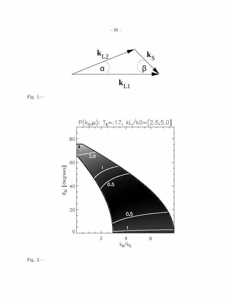
and is zero otherwise. Figure 2 shows the dimensionless decay rate P (kS, µ) given by equation

(13), as a function of the wave number kS and the angle θSL between kS and kL. Here we

have taken T6 = 0.17 as a characteristic number for a type III solar radio bursts analyzed in

section 4. This graphic confirms that the cases of maximum probability of occurrence are the

back-scattering (with θSL → 0, P ∼ 1) and the diffusive scattering (with θSL ∼ 75, P ∼ 4).

The factor of four in the diffusive decay rate results from the modulation factor 1/µ in

equation (13). The propagation direction of the resulting ion-acoustic wave is parallel to the

beam propagation in the case of back-scattering, and almost perpendicular to the beam in

the diffusive case (with kS ≪ kL). We therefore find that the decay rate becomes maximum

for two limiting cases: a) small-angle (diffusive) scattering: α → 0, and b) back-scattering:

α → π.

Under the diffusive scattering approximation, estimates for the characteristic isotropiza-

tion and energy transfer timescales, indicate that the latter is much larger, implying that

the isotropization occurs in a quasi-elastic fashion Tsytovich (1970) (see also Vasquez et al.

2002). The quasi-conservation of the total energy is readily seen from the following argu-

ment. The ES decay conserves the total number of Langmuir plasmons. Now, given the weak

dependence of their energy on the wave-number (see equation (2)), we can approximate the

energy of each plasmon as ωpe. Therefore, this decay can not produce a significant change

in the total Langmuir wave energy.

– 7 –

3.2. Non-colimated Langmuir spectra

In the previous section we found that the ES decay of the 1D Langmuir spectrum

generated by a perfectly colimated beam is initially dominated by small-angle decay processes

and, in second place, by back-scattering. We then expect that after a transient stage,

the Langmuir spectrum is not longer perfectly aligned with the beam direction, and that

a growing back-scattered spectrum also arises. Nonetheless, we expect that the forward

spectrum will contain much more energy than the backward spectrum, at least during the

early stages of the evolution. Under this assumption, we consider now an axisymmetric

spectrum around the beam direction, and model it through functions Nk = N(θ, k) that

peak in the forward direction and monotonically decrease as θ → π.

Let us start by analyzing the small angle scattering limit, i.e. kS ≪ kL. For the diffusive

decay we have that the spectral width of the ion-acoustic waves produced is much smaller

than the spectral width of the primary Langmuir waves. More specifically, we have

∆kS

∆kL∼ 3

〈kS〉

〈kL〉≪ 1 (14)

where 〈kS〉 = kSmax/2 and 〈kL〉 = (kmin + kmax)/2 indicate mean wavenumber values. As the

decay proceeds, each ES decay process will produce one ion-acoustic wave, hence

NL∆kL ∼ NS∆kS →NL

NS∼

∆kS

∆kL≪ 1 (15)

i.e. the spectral density of the (emitting) Langmuir waves becomes much lower than that

of the (emitted) ion-acoustic waves (even though the Langmuir energy density can be much

larger than that of the ion-acoustic waves). Thus, we neglect the term NLNL in the decay

rate given by equation (6) and approximate

1

τ(kS)≡

1

NSkS

dNSkS

dt≈

∫

dkL1dkL2

(2π)6wSL

L

(

NLkL1

− NLkL2

)

= (16)

K

(2π)6

∫

dkL1cos2 (α)

µ

(

NLkL1

− NLkL2

)

δ

(

kL1 −2k0 + kS

2µ

)

where K is given by equation (9) (see also equation (8)). Using the energy conservation,

equation (17) reduces to the double integral,

– 8 –

1

τ(kS)≈

K

(2π)6

∫ 2π

0

dφ1

∫ π

0

dθ1 sin θ1

[

k21cos2 (α)

µ(N(k1, θ1) − N(k2, θ2))

]

k1=(kS+2k0)/(2µ)

(17)

where we have assumed the Langmuir spectrum Nk to be symmetric about the beam pro-

pagation axis eZ (i.e. independent of the angle φ), and the values k2, θ2 are related to k1, θ1

through

k2 =√

k21 − 2k0k1 (18)

cos (θ2) =(kL1 − kS) · eZ

k2

(19)

and cos (α) is given by equation (3). We note here that in the back-scattering limit, the

term NL1NL2 can not be neglected. Instead, for back-scattering, we expect that NL2 ≪ NL1

(at early stages of the evolution), and hence we can neglect the two last terms in equation

(6). Therefore, the rate for back-scattering can be obtained from equation (17) by simply

neglecting the second term Nθ2, and also taking the limits cos (α) → −1 and µ → +1.

To compare these rates against the perfectly colimated case (equation (12)), let us

multiply and divide the RHS of equation (17) by K1 ≡ (2π)3nL/∆kL, to obtain

1

τ(kS)=

1

τ0P1(kS, θS) (20)

where 1/τ0 is the reference rate given by equation (12), θS is the angle between the ion

acoustic wave vector and the beam propagation direction eZ, and the dimensionless function

P1(kS, θS) is given by

P1(kS, θS) =∆kL

nL

1

(2π)3

∫ 2π

0

dφ1

∫ π

0

dθ1 sin θ

[

k21cos2 (α)

µ(N(k1, θ1) − N(k2, θ2))

]

k1=(kS+2k0)/(2µ)

(21)

We use this expression to evaluate the decay rate for a spectral model that is stronger in

the forward direction (but not colimated). Here we neglect the dependence in wavenumber,

and assume the spectral density as constant within the range [kmin, kmax] given by equation

(10). More specifically we consider

– 9 –

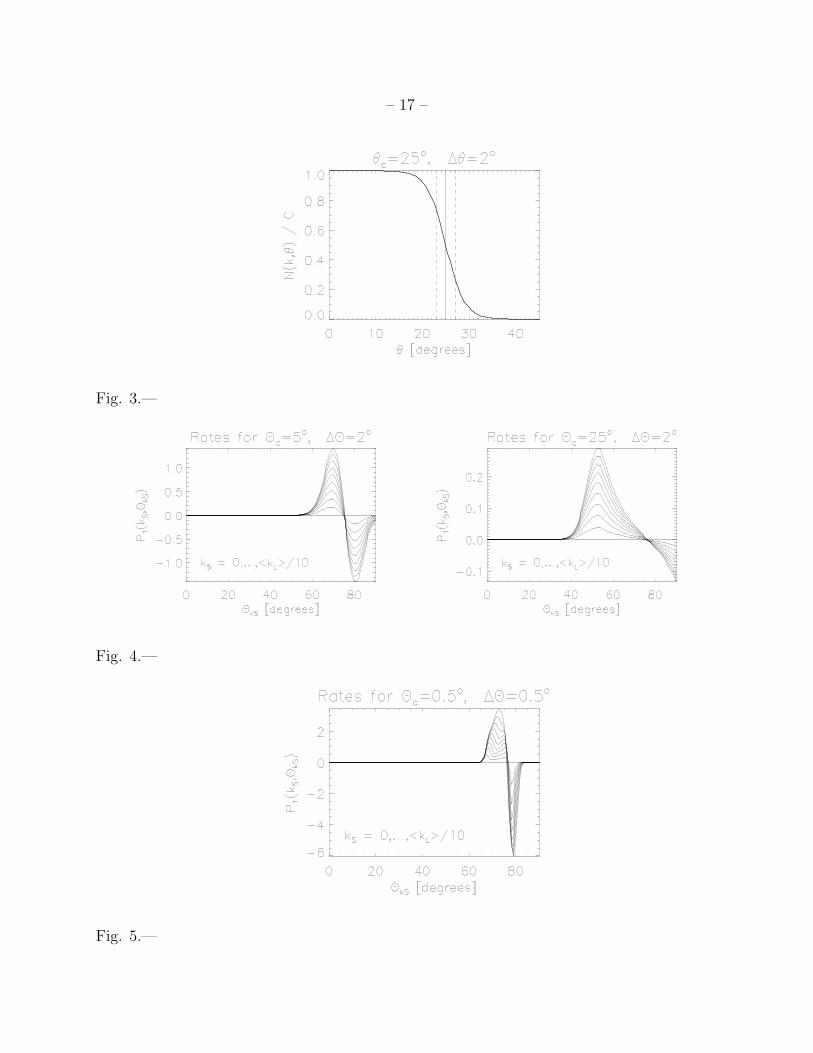
N(k, θ) = C1 + e−θc/∆θ

1 + e(θ−θc)/∆θ; if kmin < k < kmax (22)

where the normalization constant C is such that the number density of Langmuir plasmons

is nL =∫

k

(2π)3Nk. As an example, Figure 3 shows this function for θc = 25, ∆θ = 2. This

angular distribution peaks at θ = 0 and monotonically decreases with increasing θ. The

mean value is reached at θc. Thus, for smaller values of this parameter the spectrum is more

colimated. The parameter ∆θ measures the half-width over which the function varies from

75% to 25% of its maximum value. For smaller values of this parameter, the spectrum has

a sharper angular edge.

Figure 4 shows the resulting P1 for two sharp-edged angular spectra with ∆θ = 2.

One spectrum is well concentrated along the beam direction with θc = 5, and the other

corresponds to a wider distribution with θc = 25. Our expression for P1 (equation (21))

is valid in the diffusive regime kS ≪ kL, so we show results for kS = 0, .., 〈kL〉 /10. Rates

monotonically increase with kS, until they saturate at about 〈kL〉 /5. For larger values of kS

the rates decrease with increasing kS.

Higher rates are obtained for a more colimated beam, and the peak value is reached at

a larger angle θS. This behaviour can be understood in terms of our analytic decay analysis

for the perfectly colimated case. The peak is expected to occur as the result of the decay of

Langmuir waves located in regions where the angular gradient of the spectrum is maximum,

i.e. located around θc. This is because in this region the difference N(k1, θ1) − N(k2, θ2) in

equation (21) reaches its largest value. On the other hand, for the characteristic numbers of

type III solar radio bursts being used in this analysis, our results (see Figure 2) show that

the ion-acoustic waves are preferentially directed toward angles around the value θS ∼ 75

(with respect to the direction of the decaying Langmuir wave). We can therefore expect

then that Langmuir waves with an angle θc respect to the eZ axis will preferentially produce

ion-acoustic waves with an angle θS ∼ 75 − θc. This rough estimate gives peak angles of

70and 50 for the two values of θc considered here, which is in agreement with the detailed

numerical results shown in Figure 4.

Also, in the perfectly colimated limit (θc → 0, ∆θ → 0), from comparison with equation

(13), we expect that peak values of P1 will be close to the peak value P ∼ 4 corresponding to

the perfectly colimated case (see Figure 2). The numerical results of Figure 4 are consistent

with this. As a consistency check, Figure 5 shows the same results for a highly colimated

distribution with θc = 0.5, ∆θ = 0.5, with peak rates of P1 = 3.5, at θS ∼ 74.

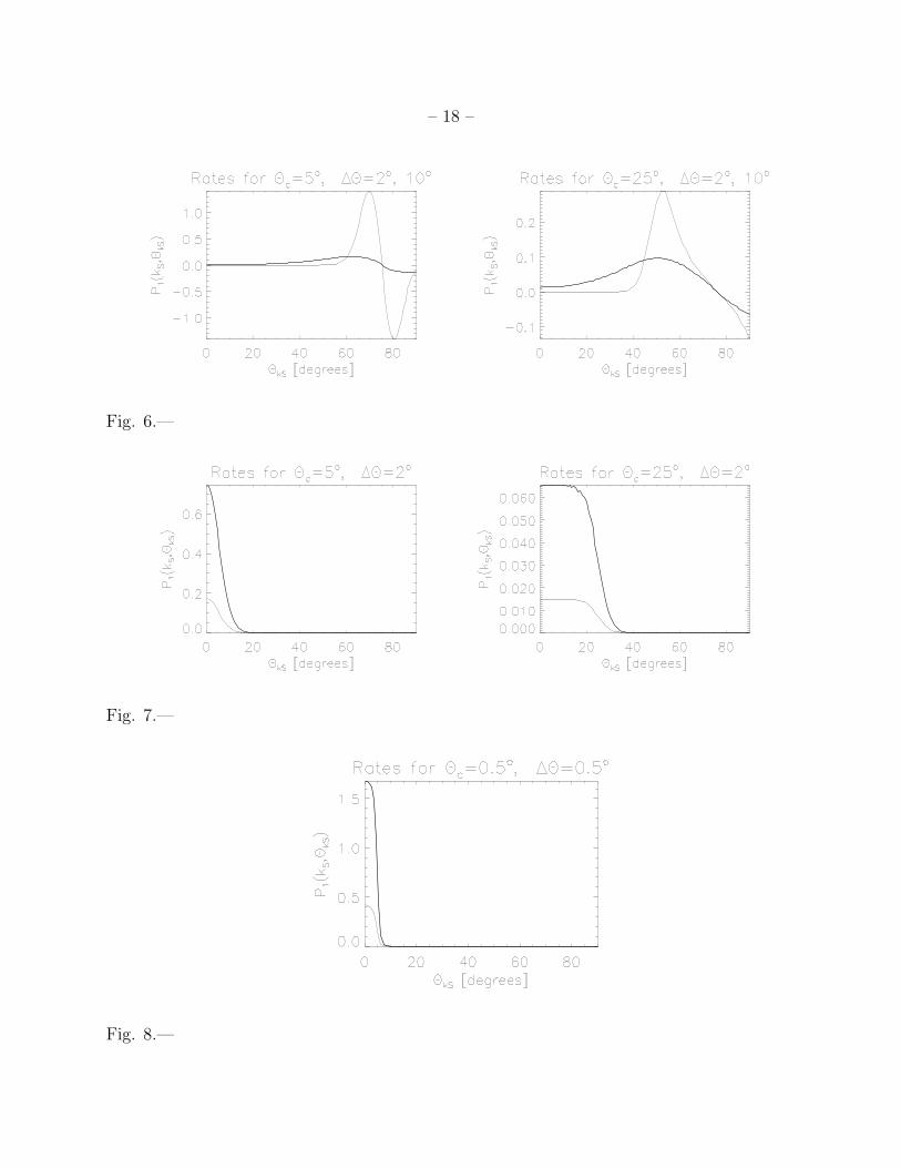
For a fixed kS = 〈kL〉 /10, Figure 6 shows the effect of reducing the Langmuir wave

distribution angular gradient. For the distribution with the edge centered on the angle

– 10 –

θc = 5, left panel shows the resulting rates for ∆θ = 2, 10. The right panel shows the

corresponding results for the distribution with edge on the angle θc = 25. The effect of a

smoother distribution is to extend the possible angles of the produced ion-acoustic waves

over a much wider range. Also, as the angular gradient of the Langmuir spectrum is reduced,

the difference N1 − N2 in equation (21) decreases, and hence P1(θS) yields lower values.

Let us also compare the different diffusive decay rates against the corresponding back-

scattering decay rates. The backscattering of a Langmuir plasmon of wavenumber kL pro-

duces an ion-acoustic plasmon of wavenumber kS = 2kL − 2k0, as follows from taking the

limit µ → +1 in equation (4). Figure 7 shows the resulting back-scattering P1 for the same

two Langmuir spectra analyzed in Figure 4. Thin curves correspond to kS = 2kL,min − 2k0

and thick curves to kS = 2kL,max − 2k0. In this case, being the result of back-scattering, the

angular distribution of the decay rate closely follows that of the decaying Langmuir waves

N(k1, θ1) in equation (21) (compare for example the right panel of Figure 7 with Figure 3).

A comparison between the back-scattering results of Figure 7 against the diffusive decay

results Figure 4 shows that the diffusive rates are always larger, by factors of order 2 to 5.

Figure 8 shows the same results for a highly colimated distribution with θc = 0.5, ∆θ = 0.5.

The resulting rates are of order P1 ∼ 1.5, or about a factor of 2 lower than the corresponding

diffusive decay values of Figure 5. These results are consistent with the perfectly colimated

beam results of Figure 2. Therefore we find that, in all cases, diffusive decay rates are

systematically larger (though comparable) than the corresponding back-scattering rates.

4. Frequencies of the ion-acoustic Waves

Several space-based missions, located at distances of order 1 AU from the Sun, are

designed to perform in-situ measurements of the extended solar wind. These missions are

able then to perform in-situ measurements of type III solar radio bursts, that sometimes

extend far away from the Sun and reach the Earth. One of these instruments is the Unified

Radio and Plasma Wave Experiment (URAP) aboard the Ulysses mission. For the purpose

of interpreting type III burst data collected by this experiment, let us suppose that an

ion-acoustic wave travels through the region of the experiment. If Vsw is the local solar

wind velocity, the Doppler-shifted frequency of the ion-acoustic wave, as measured by the

experiment, is given by

fS =1

2π(kSVS + kS ·Vsw) =

– 11 –

=kS

2π(VS + Vsw cos (θSr)) =

= 2fpe

Vφ

(

cos (θSL) −VSVφ

3V 2Te

)

(VS + Vsw cos (θSr)) (23)

where kS has been eliminated from equation (4), θSL and θSr are the angles between the

propagation direction of the ion-acoustic wave and those of the primary (beam aligned)

Langmuir waves, and the (radial) solar wind, respectively. This formula is analogous to

the one used by Cairns & Robinson (1995) to analyze a type III solar radio burst. They

assume the ES decay products only in the back-scattering limit, and hence they consider

the particular case cos (θSL) = +1. Also in that limit, the produced ion-acoustic waves

propagate aligned with the beam direction, so that θSr = θLr, i.e. the angle between the

primary Langmuir waves and the solar wind direction. On the other hand, in the diffusive

limit, θSL > 0 so that the angle θSr takes the range of values |θSL − θLr| < θSr < θSL + θLr.

To quantify the predicted frequencies for the ion-acoustic waves in each of these two

limiting cases, we refer to a specific observational case, analyzed by Thejappa & MacDowall

(1998). They show the data of a type III solar radio event recorded by URAP/Ulysses on

March 14 1995. Their detailed analysis shows radio emissions at both the plasma and

second harmonic frequencies. At the same time, impulsive electrostatic fluctuations were

recorded at the local plasma frequency, which turns out to be fpe ∼ 23 kHz, identified

as Langmuir wave bursts. The WFA (Wave Form Analyzer) instrument detected electric

fluctuations, highly correlated in time with the observed Langmuir impulsive peaks, in the

range 0 → 450 Hz. The instrument also detected magnetic field fluctuations in the range

0 → 50 Hz. The combination of these facts indicates that the electric field fluctuations in the

range 50 → 450 Hz are of a pure electrostatic nature, such as ion-acoustic waves. If this is the

case, its strong temporal correlation with the Langmuir bursts supports the idea that the ion-

acoustic waves may be produced by the ES decay of the L-waves (see also Cairns & Robinson

1995). On the other hand, below 50 Hz fluctuations are most likely of electromagnetic nature,

such as whistlers. Summarizing, the analysis by Thejappa & MacDowall (1998) strongly

suggests the presence of ion-acoustic waves in the range 50 → 450 Hz, for this particular

event, and that these waves are produced as the result of the ES decay of the beam-excited

Langmuir waves.

For the event under consideration, the numerical values of the relevant parameters are

(Thejappa & MacDowall 1998): VS = 5.1×106cm/seg, VTe = 1.6×108cm/seg (corresponding

to Te = 1.7× 105K), Vsw = 3.4× 107cm/seg, Vφ ∼ Vbeam ± 25%, with a mean beam velocity

estimated to be Vbeam = 3.5 × 109cm/seg, fpe = 2.3 × 104Hz, θLr ∼ 45.

Using these numerical values we compute now, in the two limit cases under analysis, the

– 12 –

predicted ion-acoustic wave frequencies. In all cases, we assume that the primary (beam-

excited) Langmuir waves form a mean angle θLr = 45 with respect to the solar wind

direction, and that the primary Langmuir waves have phase speeds in the range Vφ = Vbeam±

25%.

Figure 2 shows that, in the diffusive limit, decays proceed most likely for angles θSL in the

range 60 → 75 (in this range the probability is about twice the back-scattering probability).

Using this range of angles in equation (23), we find that the diffusive-scattering assumption

yields ion-acoustic waves in the range 50 Hz → 215Hz. On the other hand, if back-scattering

is assumed, we have θSL = 0, and equation (23) yields ion-acoustic frequencies in the range

215 Hz → 415 Hz. The difference between the predictions in both limits is due to the term(

cos (θSL) −VSVφ

3V 2

Te

)

, that is maximized in the back-scattering case as cos (θSL) ∼ +1.

If the the primary Langmuir waves form a variable angle 0 < θLr < 90 with re-

spect to the solar wind direction, the frequency ranges predicted in both limits overlap each

other, within the observed range. In this case, the back-scattering limit yields predicted

ion-acoustic frequencies over the whole observed range (as already pointed out by Thejappa

& MacDowall 1998). We thus find that the predictions, for both asymptotic cases are consis-

tent with the observations. Taking mean values of the different parameters, we find out that

for the back-scattering assumption the predicted frequencies are consistent with the higher

frequency portion of the observations (see also Cairns & Robinson 1995). On the other hand,

the diffusive-scattering limit yields predicted frequencies that are consistent with the lower

frequency portion of the observed electrostatic fluctuations.

Further empirical support arises from a recent observational work by Thejappa et al.

(2003), where they analyze URAP data for another type III burst, in a similar fashion to

the case already described. This case corresponds to in-situ observations at much larger

heliocentric distances, specifically at 5.2 AU, where the local ambient plasma parameters

are very different (fpe ∼ 2 kHz, Te ∼ 8.8 × 104K) to those of the previous case. The beam

velocity (and hence the primary Langmuir waves phase velocity) is estimated to be Vφ ∼

1.5×109cm/seg ± 30%. In this other case, the WFA-URAP instrument also detected electric

field fluctuations correlated in time with Langmuir bursts. The electric waves that can be

safely assumed to be of electrostatic nature (i.e. with no simultaneous detection of magnetic

field fluctuations above the background level) are in the frequency range 20 → 200 Hz.

We repeated our probability calculations for this case, and find out that, in the diffusive

limit, decays proceed most likely for angles θSL in the range 55 → 73 (in this range the

probability is about twice the back-scattering probability). Using this range of angles, in the

diffusive limit, the predicted ion-acoustic frequencies result in the range 0Hz → 60 Hz. On

the other hand, under the back-scattering assumption the predicted frequencies are in the

– 13 –

range 55 Hz → 105 Hz.

5. Conclusions

From the theoretical point of view, an analysis of the ES decay rate indicates that

the process is dominated by two limiting cases: diffusive (small angle) scattering and back-

scattering. We find that the decay rates are comparable for both cases, being the diffusive

decay rates systematically larger than those of the back-scattering limit. Given the results of

our quantitative comparative analysis, we believe that both limiting cases are acting at the

same time. Furthermore, we speculate the net effect of diffusive decay and back-scattering

acting simultaneously is then that of a diffusive isotropization of the beam-generated Lang-

muir spectrum. The back-scattering generates a backwards directed spectrum (respect to

the beam propagation direction), but then this secondary spectrum can also diffuse by small-

angle decay. Thus, if the ES decay is assumed to be present in solar flare and type III solar

radio burst scenarios, we believe that its capability to isotropize Langmuir waves can not be

neglected.

From an observational point of view, we refer to analyses of a type III bursts by The-

jappa & MacDowall (1998) and Thejappa et al. (2003). They registered low frequency elec-

trostatic fluctuations which are strongly correlated in time with impulsive Langmuir wave

bursts. We find that the observed frequencies of these fluctuations are consistent with the

predicted frequencies of ion-acoustic waves produced by the ES decay of the primary (beam-

excited) Langmuir waves. Under the back-scattering assumption the predicted frequencies

are consistent with the higher frequency portion of the observations. On the other hand,

the diffusive-scattering limit yields predicted frequencies that are consistent with the lower

frequency portion of the observed electrostatic fluctuations. The relative burst intensities

at the two frequency ranges could then serve as a proxy for the relative effectiveness of the

occurrence of the ES decay in both limits, that we anticipate to be comparable from our

theoretical analysis.

From this analysis, we speculate that both the back-scattering and diffusive limits of

the ES decay may be relevant in type III bursts (and presumably also in solar flare radio

events). Also, the beam-generated Langmuir turbulence may become isotropic as the ES

decay proceeds mainly in the two limit cases of diffusive scattering and back-scattering. We

postpone for a future work the investigation of the coupling between the ES decay and the

quasi-linear beam-turbulence interaction. We believe that the simultaneous consideration

of both effects can bring HXR and radio emission predictions into a better agreement with

observations. This is due to the fact that its inclusion will imply a limitation of the effective-

– 14 –

ness of the quasi-linear relaxation, yielding to lower Langmuir turbulence levels, and hence

lower radio emissivity.

We thank the anonymous referee for useful suggestions that helped to clarify our main

conclusions. This work was funded by the Agencia Nacional de Promocion de Ciencia

y Tecnologıa (ANPCyT, Argentina) through grant 03-09483. We also thank Fundacion

Antorchas (Argentina) for partial support through grant 14056-20.

REFERENCES

Cairns, I.H. 1987, J. Plasma Phys., 39, 179

Cairns, I.H. & Robinson, P.A. 1995, ApJ, 453, 959

Edney, S.D. & Robinson, P.A. 2001, Phys. Plasmas, V.8 N.2, 428

Emslie, A.G. & Smith, D.F. 1984, ApJ, 279, 882

Hamilton, R.J. & Petrosian, V. 1987, ApJ, 321, 721

Melrose, D.B. 1982, Sol. Phys., 79, 173

Thejappa G., MacDowall R.J., Scime, E.E. & Littleton, J.E. 2003, J. Geophys. Res., 108,

No. A3, 1139

Thejappa G. & MacDowall R. J. 1998, ApJ, 498, 465

Tsytovich, V.N. 1970, Nonlinear Effects in Plasma, New York: Plenum Press

Vasquez, A.M. & Gomez, D.O. 2003, Anales AFA, Vol. 14, 106

Vasquez, A.M., Gomez, D.O., & Ferro Fontan, C. 2002, ApJ, 564, 1035

Vasquez, A.M. & Gomez, D.O. 1997, ApJ, 484, 463

This preprint was prepared with the AAS LATEX macros v5.0.

– 15 –

Fig. 1.— Momentum conservation in the electrostatic decay, kL1 = kL2 + kS. Angles α and

β are given by equations (4) and (5).

Fig. 2.— Dimensionless decay rate P (kS), as a function of (kS, θSL).

Fig. 3.— Model for the angular distribution of the Langmuir spectrum, with θc = 25 and

∆θ = 2. The vertical lines indicate the angles θc (full line), and θc ± ∆θ (dashed lines).

Fig. 4.— Diffusive decay: dimensionless factor P1(ks, θS) for θc = 5, 25, and ∆θ =

2. Profiles are ploted as a function of θS, with different curves corresponding to kS =

0, .., 〈kL〉 /10 (curves with larger P1 values correspond to larger kS).

Fig. 5.— Diffusive decay: dimensionless factor P1(ks, θS) for θc = 0.5 and ∆θ = 0.5. Pro-

files are ploted as a function of θS , with different curves corresponding to kS = 0, .., 〈kL〉 /10

(curves with larger P1 values correspond to larger kS).

Fig. 6.— Diffusive decay: for a fixed kS = 〈kL〉 /10, dimensionless factor P1(ks, θS) for

θc = 5, 25, and ∆θ = 2, 10. Profiles are ploted as a function of θS, with thin curve

corresponding to ∆θ = 2 and thick curve to ∆θ = 10.

Fig. 7.— Back-scattering: dimensionless factor P1(ks, θS) for θc = 5, 25, and ∆θ = 2.

Profiles are ploted as a function of θS, with thin curves corresponding to kS = 2kL,min − 2k0

and thick curves to kS = 2kL,max − 2k0.

Fig. 8.— Back-scattering: dimensionless factor P1(ks, θS) for θc = 0.5 and ∆θ = 0.5.

Profiles are ploted as a function of θS, with thin curves corresponding to kS = 2kL,min − 2k0

and thick curves to kS = 2kL,max − 2k0.

– 16 –

k

k k

βαSL2

L1

Fig. 1.—

Fig. 2.—

– 17 –

Fig. 3.—

Fig. 4.—

Fig. 5.—

– 18 –

Fig. 6.—

Fig. 7.—

Fig. 8.—