Embed Size (px)
Citation preview
arX
iv:n
ucl-
th/0
4100
59v1
13
Oct
200
4
Weak decay of hypernuclei
W. M. Alberico and G. Garbarino
Dipartimento di Fisica Teorica, Universita di Torino and INFN, Sezione di Torino,
I–10125 Torino, Italy
1. – Introduction
The focus of these lectures is on the weak decay modes of hypernuclei, with special
attention to Λ–hypernuclei. The subject involves many fields of modern theoretical and
experimental physics, from nuclear structure to the fundamental constituents of matter
and their interactions. The peculiar behaviour of matter containing strange quarks has
raised in recent years many interesting problems, one of which being the physics of
hypernuclei.
Hypernuclear physics was born in 1952, when the first hypernucleus was observed
through its decays [1]. Since then, it has been characterized by more and more new
challenging questions and answers. The interest was further raised by the great advances
made in the last 15–20 years. Moreover, the existence of hypernuclei gives a new dimen-
sion to the traditional world of nuclei (states with new symmetries, selection rules, etc).
They represent the first kind of flavoured nuclei, in the direction of other exotic systems
(charmed nuclei and so on).
Hyperons (Λ, Σ, Ξ, Ω) have lifetimes of the order of 10−10 sec (apart from the Σ0,
which decays into Λγ). They decay weakly, with a mean free path λ ≈ cτ = O(10 cm).
A hypernucleus is a bound system of neutrons, protons and one or more hyperons. We
will denote with A+1Y Z a hypernucleus with Z protons, A−Z neutrons and a hyperon Y .
In order to describe the structure of these strange nuclei it is crucial the knowledge of the
elementary hyperon–nucleon (Y N) and hyperon–hyperon (Y Y ) interactions. Hyperon
masses differ remarkably from the nucleonic mass, hence the flavour SU(3) symmetry is
broken. The amount of this breaking is a fundamental question in order to understand
c© Societa Italiana di Fisica 1
2 W. M. Alberico and G. Garbarino
the baryon–baryon interaction in the strange sector.
Nowadays, the knowledge of hypernuclear phenomena is rather good, but some open
problems still remain. The study of this field may help in understanding some important
questions, related to:
1. some aspects of the baryon–baryon weak interactions;
2. the Y N and Y Y strong interactions in the JP = 1/2+ baryon octet;
3. the possible existence of di–baryon particles;
4. the renormalization of hyperon and meson properties in the nuclear medium;
5. the nuclear structure: for instance, the long standing question of the origin of the
spin–orbit interaction and other aspects of the many–body nuclear dynamics;
6. the role played by quark degrees of freedom, flavour symmetry and chiral models
in nuclear and hypernuclear phenomena.
Many of these aspects can be discussed and understood by investigating the hypernuclear
weak decays. Important related arguments, which here will not be considered or only
briefly mentioned, can be found in the lectures by A. Gal [2] and T. Nagae [3], while the
experimental viewpoint on the same subject is presented by H. Outa [4].
In these lectures the various weak decay modes of Λ–hypernuclei are described: in-
deed in a nucleus the Λ can decay by emitting a nucleon and a pion (mesonic mode) as it
happens in free space, but its (weak) interaction with the nucleons opens new channels,
customarily indicated as non–mesonic decay modes. These are the dominant decay chan-
nels of medium–heavy nuclei, where, on the contrary, the mesonic decay is disfavoured by
Pauli blocking effect on the outgoing nucleon. In particular, one can distinguish between
one–body and two–body induced decays, according whether the hyperon interacts with
a single nucleon or with a pair of correlated nucleons.
An interesting rule for the amount of isospin violation (∆I = 1/2) is strongly sug-
gested by the mesonic decay of free Λ’s, whose branching ratios are almost in the pro-
portion 2 to 1, according whether a π−p or π0n are emitted. This totally empirical rule
has been generally adopted in most of the models proposed for the evaluation of the Λ–
hypernuclei decay widths: some of the expected consequences, however, seem to require
additional work and investigation. Indeed, the total non–mesonic (ΓNM = Γn+Γp (+Γ2))
and mesonic (ΓM = Γπ0 + Γπ−) decay rates are well explained by several calculations;
however, for many years the main open problem in the decay of Λ–hypernuclei has been
the discrepancy between theoretical and experimental values of the ratio Γn/Γp. This
topic will be discussed at length here, together with the most recent indications toward
a solution of the puzzle.
Another interesting and open question concerns the asymmetric non–mesonic decay
of polarized hypernuclei: strong inconsistencies appear already among data. Also in
this case, as for the Γn/Γp puzzle, one can expect important progress from the present
Weak decay of hypernuclei 3
and future improved experiments, which will provide a guidance for a deeper theoretical
understanding of hypernuclear dynamics and decay mechanisms.
For a comprehensive review on the subject of these lectures we refer the reader to
Ref. [5] and references therein.
2. – Weak decay modes of Λ–hypernuclei
In the production of hypernuclei, the populated state may be highly excited, above
one or more threshold energies for particle decays. These states are unstable with respect
to the emission of the hyperon, of photons and nucleons. The spectroscopic studies of
strong and electromagnetic de–excitations give information on the hypernuclear structure
which are complementary to those we can extract from excitation functions and angular
distributions studies. Once the hypernucleus is stable with respect to electromagnetic
and strong processes, it is in the ground state, with the hyperon in the 1s level, and can
only decay via a strangeness–changing weak interaction, through the disappearance of
the hyperon.
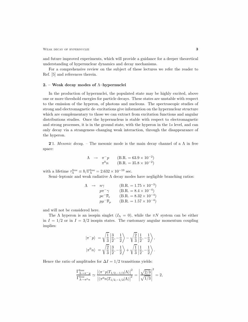
2.1. Mesonic decay. – The mesonic mode is the main decay channel of a Λ in free
space:
Λ → π−p (B.R. = 63.9 × 10⁻²)
π0n (B.R. = 35.8 × 10⁻²)
with a lifetime τ freeΛ ≡ ~/Γfree
Λ = 2.632× 10⁻¹⁰ sec.
Semi–leptonic and weak radiative Λ decay modes have negligible branching ratios:
Λ → nγ (B.R. = 1.75 × 10⁻³)
pπ−γ (B.R. = 8.4 × 10⁻⁴)
pe−νe (B.R. = 8.32 × 10⁻⁴)
pµ−νµ (B.R. = 1.57 × 10⁻⁴)
and will not be considered here.
The Λ hyperon is an isospin singlet (IΛ = 0), while the πN system can be either
in I = 1/2 or in I = 3/2 isospin states. The customary angular momentum coupling
implies:
|π−p〉 =
√
1
3
∣
∣
∣
∣
3
2,−1
2
⟩
−√
2
3
∣
∣
∣
∣
1
2,−1
2
⟩
,
|π0n〉 =
√
2
3
∣
∣
∣
∣
3
2,−1
2
⟩
+
√
1
3
∣
∣
∣
∣
1
2,−1
2
⟩
.
Hence the ratio of amplitudes for ∆I = 1/2 transitions yields:
ΓfreeΛ→π−p
ΓfreeΛ→π0n
≃∣
∣〈π−p|T1/2,−1/2|Λ〉∣
∣
2
∣
∣〈π0n|T1/2,−1/2|Λ〉∣
∣
2 =
∣
∣
∣
∣
∣
√
2/3√
1/3
∣
∣
∣
∣
∣
2
= 2,
4 W. M. Alberico and G. Garbarino
while a ∆I = 3/2 process should give:
ΓfreeΛ→π−p
ΓfreeΛ→π0n
≃∣
∣〈π−p|T3/2,−1/2|Λ〉∣
∣
2
∣
∣〈π0n|T3/2,−1/2|Λ〉∣
∣
2 =
∣
∣
∣
∣
∣
√
1/3√
2/3
∣
∣
∣
∣
∣
2
=1
2.
Experimentally the above ratio turns out to be:
ΓfreeΛ→π−p
ΓfreeΛ→π0n
Exp
≃ 1.78,
which is very close to 2 and strongly suggests the ∆I = 1/2 rule on the isospin change.
From the above considerations and from analyses of the Λ polarization observables it
follows that the measured ratio between ∆I = 1/2 and ∆I = 3/2 transition amplitudes
is very large:
∣
∣
∣
∣
A1/2
A3/2
∣
∣
∣
∣
≃ 30.
The ∆I = 1/2 rule is based on experimental observations but its dynamical origin is not
yet understood on theoretical grounds. It is also valid for the decay of the Σ hyperon
and for pionic kaon decays (namely in non–leptonic strangeness–changing processes).
Actually, this rule is slightly violated in the Λ free decay, and it is not clear whether it
is a universal characteristic of all non–leptonic processes with ∆S 6= 0. The Λ free decay
in the Standard Model can occur through both ∆I = 1/2 and ∆I = 3/2 transitions,
with comparable strengths: an s quark converts into a u quark through the exchange of
a W boson. Moreover, the effective 4–quark weak interaction derived from the Standard
Model including perturbative QCD corrections gives too small |A1/2/A3/2| ratios (≃ 3÷4,
as calculated at the hadronic scale of about 1 GeV by using renormalization group
techniques [6]). Therefore, non–perturbative QCD effects at low energy (such as hadron
structure and reaction mechanism), which are more difficult to handle, and/or final state
interactions could be responsible for the enhancement of the ∆I = 1/2 amplitude and/or
the suppression of the ∆I = 3/2 amplitude(1).
TheQ–value for free–Λ mesonic decay at rest isQΛ ≃ mΛ−mN−mπ ≃ 40 MeV. Then,
taking into account energy–momentum conservation, mΛ ≃√
~p 2 +m2π +
√
~p 2 +m2N in
the center–of–mass system and the momentum of the final nucleon turns out to be p ≃ 100
MeV. Inside a hypernucleus, the binding energies of the recoil nucleon (BN ≃ −8 MeV)
and of the Λ (BΛ ≥ −27 MeV) tend to further decrease QΛ [QΛ,bound = QΛ +BΛ −BN ]
and hence p.
As a consequence, in nuclei the Λ mesonic decay is disfavoured by the Pauli principle,
particularly in heavy systems. It is strictly forbidden in normal infinite nuclear matter
(1) See, for example, a recent work based on the Instanton Liquid Model [7]
Weak decay of hypernuclei 5
(where the Fermi momentum is k0F ≃ 270 MeV), while in finite nuclei it can occur because
of three important effects:
1. In nuclei the hyperon has a momentum distribution (being confined in a limited
spatial region) that allows larger momenta to be available to the final nucleon;
2. The final pion feels an attraction by the medium such that for fixed momentum ~q it
has an energy smaller than the free one [ω(~q) <√
~q 2 +m2π], and consequently, due
to energy conservation, the final nucleon again has more chance to come out above
the Fermi surface. Indeed it has been shown [8, 9] that the pion distortion increases
the mesonic width by one or two orders of magnitude for very heavy hypernuclei
(A ≃ 200) with respect to the value obtained without the medium distortion;
3. At the nuclear surface the local Fermi momentum is considerably smaller than k0F ,
and the Pauli blocking is less effective in forbidding the decay.
In any case the mesonic width rapidly decreases as the nuclear mass number A of the
hypernucleus increases.
The mesonic channel also gives information on the pion–nucleus optical potential
since ΓM = Γπ− + Γπ0 is very sensitive to the pion self–energy in the medium: the
latter is enhanced by the attractive P–wave π–nucleus interaction and reduced by the
repulsive S–wave one. Evidence for a central repulsion in the Λ–nucleus mean potential
was obtained from the mesonic decays of s–shell hypernuclei [10, 11].
2.2. Non–mesonic decay. – In hypernuclei the weak decay can occur through processes
which involve a weak interaction of the Λ with one or more nucleons. Sticking to the
weak hadronic vertex Λ → πN , when the emitted pion is virtual, then it will be absorbed
by the nuclear medium, resulting in a non–mesonic process of the following type:
Λn → nn (Γn) ,(1)
Λp → np (Γp) ,(2)
ΛNN → nNN (Γ2) .(3)
The total weak decay rate of a Λ–hypernucleus is then:
ΓT = ΓM + ΓNM,
where:
ΓM = Γπ− + Γπ0 , ΓNM = Γ1 + Γ2, Γ1 = Γn + Γp,
and the lifetime is τ = ~/ΓT. The channel (3) can be interpreted by assuming that the
pion is absorbed by a pair of nucleons, correlated by the strong interaction. Obviously,
the non–mesonic processes can also be mediated by the exchange of more massive mesons
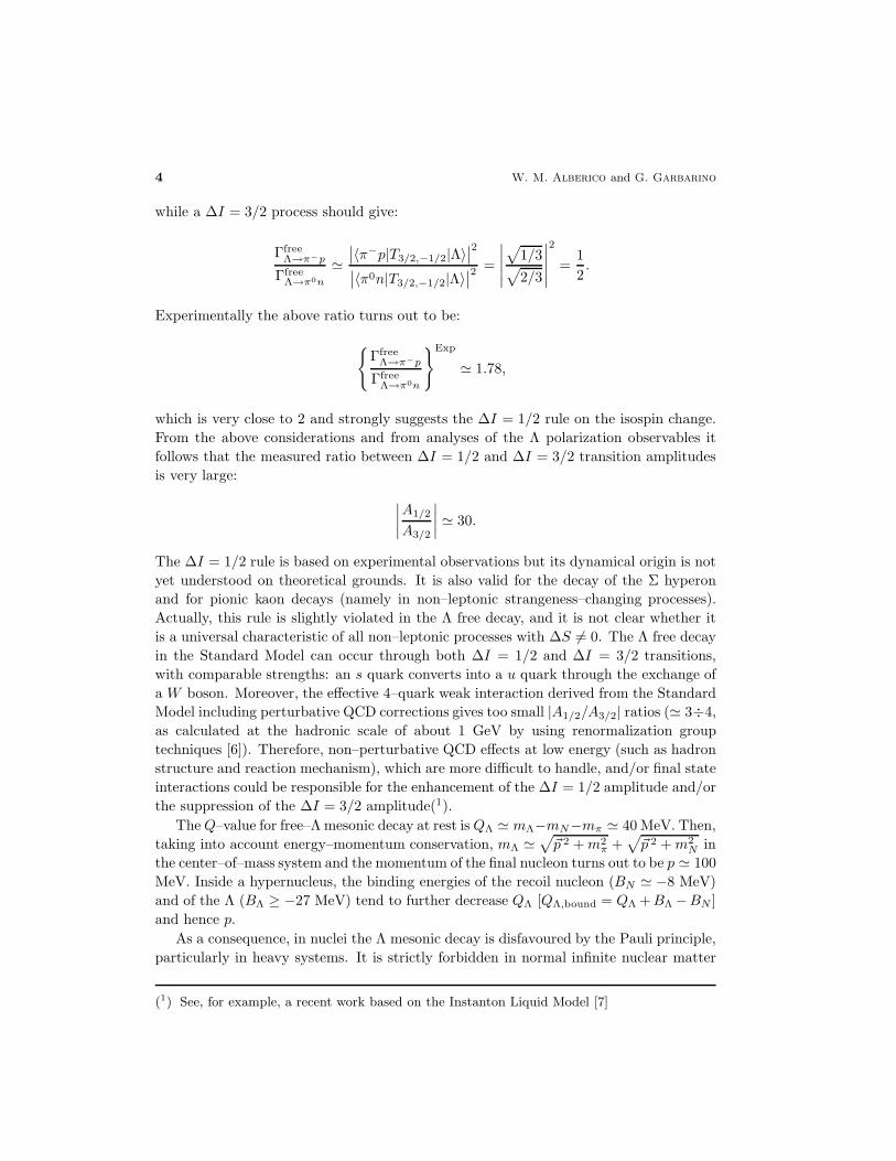
than the pion (see figure 1).
6 W. M. Alberico and G. Garbarino
N
π, ρ, ω, η, Κ, Κ
N N NN
NNNΛ Λ
*π, ρ, ω, η, Κ, Κ*
Fig. 1. – One–nucleon (a) and two–nucleon (b) induced Λ decay in nuclei.
The non–mesonic mode is only possible in nuclei and, nowadays, the systematic study
of the hypernuclear decay is the only practical way to get information on the weak
process ΛN → NN (which provides the first extension of the weak ∆S = 0 NN → NN
interaction to strange baryons), especially on its parity–conserving part, which is masked
by the strong interaction in the weak NN → NN reaction.
The final nucleons in the non–mesonic processes emerge with large momenta: dis-
regarding the Λ and nucleon binding energies and assuming the available energy Q =
mΛ −mN ≃ 176 MeV to be equally splitted among the final nucleons, it turns out that
pN ≃ 420 MeV for the one–nucleon induced channels [Eqs. (1), (2)] and pN ≃ 340 MeV
in the case of the two–nucleon induced mechanism [Eq. (3)]. Therefore, the non–mesonic
decay mode is not forbidden by the Pauli principle: on the contrary, the final nucleons
have great probability to escape from the nucleus. The non–mesonic mechanism dom-
inates over the mesonic mode for all but the s–shell hypernuclei. Only for very light
systems the two decay modes are competitive.
Since the non–mesonic channel is characterized by large momentum transfer, the
details of the hypernuclear structure do not have a substantial influence (then providing
useful information directly on the hadronic weak interaction). On the other hand, the
NN and ΛN short range correlations turn out to be very important.
It is interesting to observe that there is an anticorrelation between mesonic and non–
mesonic decay modes such that the experimental lifetime is quite stable from light to
heavy hypernuclei [12, 13], apart from some fluctuation in light systems because of shell
structure effects: τΛ = (0.5 ÷ 1) τ freeΛ . Since the mesonic width is less than 1% of the
total width for A > 100, the above consideration implies that the non–mesonic rate is
rather constant in the region of heavy hypernuclei.
This can be simply understood from the following consideration. If one naively as-
sumes a zero range approximation for the non–mesonic weak interaction ΛN → nN , then
Weak decay of hypernuclei 7
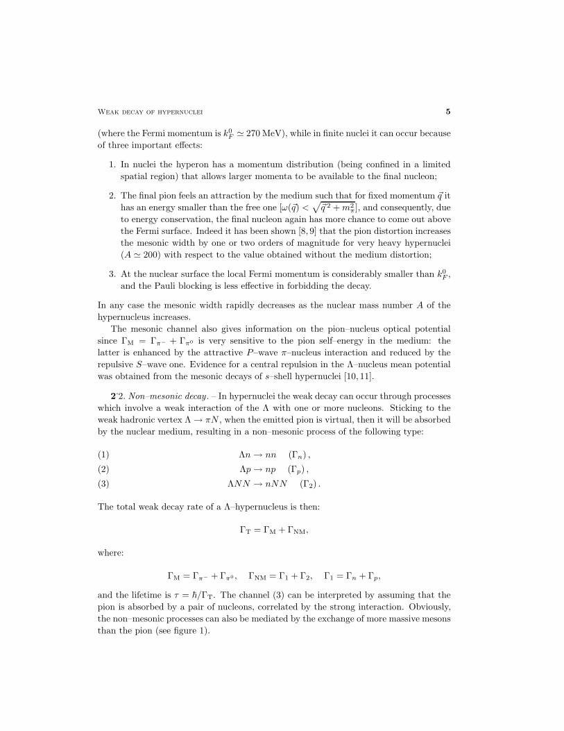
Fig. 2. – Qualitative behaviour of mesonic, non–mesonic and total decay widths as a functionof the hypernuclear baryonic number A + 1.
Γ1 is proportional to the overlap between the Λ wave function and the nuclear density:
Γ1(A) ∝∫
d~r |ψΛ(~r)|2ρA(~r),
where the Λ wave function ψΛ (nuclear density ρA) is normalized to unity (to the nuclear
mass number A). This overlap integral increases with the mass number and reaches
a constant value: by using, e.g., Λ harmonic oscillator wave functions (with frequency
ω adjusted to the experimental hyperon levels in hypernuclei) and Fermi distributions
for the nuclear densities, we find Γ1(12Λ C)/Γ1(
208Λ Pb) ≃ 0.56, while Γ1 is 90 % of the
saturation value for A ≃ 65. In figure 2 the qualitative behaviour of mesonic, non–
mesonic and total widths as a function of the nuclear mass number A is shown.
For A ≤ 11 the experimental data are quite well fitted by ΓNM/ΓfreeΛ ≃ 0.1A: Γ1
is proportional to the number of ΛN pairs, A, as it is expected from the above simple
description, where we neglect the contribution of Γ2. However, Γ1 saturates when the
radius of the hypernucleus becomes sensitively larger than the range of the ΛN → nN
interaction. For a more quantitative explanation it will be important to collect data with
good precision. Yet, from the available data one can roughly say that the long distance
component of the ΛN → nN transition has a range of about 1.5 fm and corresponds, as
we expect, to the one–pion–exchange component of the interaction.
8 W. M. Alberico and G. Garbarino
2.3. The Γn/Γp puzzle. – Nowadays, an important question concerning the weak decay
rates is the longstanding disagreement between theoretical estimates and experimental
determinations of the ratio Γn/Γp between the neutron– and the proton–induced decay
widths.
This problem will be extensively discussed in Section 5. However, it is worth re-
calling here that, up to short time ago, all theoretical calculations appeared to strongly
underestimate the available central data measured in several hypernuclei:
Γn
Γp
Th
≪
Γn
Γp
Exp
, 0.5 <∼
Γn
Γp
Exp
<∼ 2.
Until recently the data were quite limited and not precise because of the difficulty in
detecting the products of the non–mesonic decays, especially the neutrons. Moreover,
the experimental energy resolution for the detection of the outgoing nucleons does not
allow to identify the final state of the residual nuclei in the processes AΛZ → A−2Z + nn
and AΛZ → A−2(Z − 1) + np. As a consequence, the measurements supply decay rates
averaged over several nuclear final states.
In the one–pion–exchange (OPE) approximation, by assuming the ∆I = 1/2 rule in
the Λ → π−p and Λ → π0n free couplings, the calculations (which will be reported
later) give small ratios, in the range 0.05÷ 0.20 for all the considered systems. However,
as we shall see in Section 4, the OPE model with ∆I = 1/2 couplings has been able to
reproduce the one–body stimulated non–mesonic rates Γ1 = Γn+Γp for light and medium
hypernuclei. Hence, the problem seems to consist in overestimating the proton–induced
and underestimating the neutron–induced transition rates.
In order to solve this puzzle (namely to explain both Γn + Γp and Γn/Γp), many
attempts have been made up to now, mainly without success. We recall the inclusion in
the ΛN → nN transition potential of mesons heavier than the pion (also including the
exchange of correlated or uncorrelated two–pions) [14–18], the inclusion of interaction
terms that explicitly violate the ∆I = 1/2 rule [19] and the description of the short
range baryon–baryon interaction in terms of quark degrees of freedom [20, 21], which
automatically introduces ∆I = 3/2 contributions.
3. – Theoretical models for the decay rates
We illustrate here the theoretical approaches which have been utilized for the formal
derivation of Λ decay rates in nuclei. We discuss first the general features of the approach
used for direct finite nucleus calculations. It is usually called Wave Function Method
(WFM), since it makes use of shell model nuclear and hypernuclear wave functions (both
at hadronic and quark level) as well as pion wave functions generated by pion–nucleus
optical potentials. Then we consider the Polarization Propagator Method (PPM), which
relies on a many–body description of the hyperon self–energy in nuclear matter. The
Local Density Approximation allows then one to implement the calculation in finite
nuclei. Finally, a microscopic approach, based again on the PPM, is shortly sketched: in
Weak decay of hypernuclei 9
this case the full Λ self–energy is evaluated on the basis of Feynman diagrams, which are
derived, within a functional integral approach, in the framework of the so–called bosonic
loop expansion.
3.1. Wave Function Method: mesonic width. – The weak effective Hamiltonian for
the Λ → πN decay can be parameterized in the form:
(4) HWΛπN = iGm2
πψN (A+Bγ5)~τ · ~φπψΛ,
where the values of the weak coupling constants G = 2.211 × 10⁻⁷/m2π, A = 1.06 and
B = −7.10 are fixed on the free Λ decay. The constants A and B determine the strengths
of the parity violating and parity conserving Λ → πN amplitudes, respectively. In order
to enforce the ∆I = 1/2 rule (which fixes Γfreeπ−
/Γfreeπ0 = 2), in Eq. (4) the hyperon is
assumed to be an isospin spurion with I = 1/2, Iz = −1/2.
In the non–relativistic approximation, the free Λ decay width ΓfreeΛ = Γfree
π−+ Γfree
π0 is
given by:
Γfreeα = cα(Gm2
π)2∫
d~q
(2π)3 2ω(~q)2π δ[mΛ − ω(~q) − EN ]
(
S2 +P 2
m2π
~q 2
)
,
where cα = 1 for Γπ0 and cα = 2 for Γπ− (expressing the ∆I = 1/2 rule), S = A,
P = mπB/(2mN), whereas EN and ω(~q) are the total energies of nucleon and pion,
respectively. One finds the well known result:
Γfreeα = cα(Gm2
π)21
2π
mNqc.m.
mΛ
(
S2 +P 2
m2π
q2c.m.
)
,
which reproduces the observed rates. In the previous equation, qc.m. ≃ 100 MeV is the
pion momentum in the center–of–mass frame.
In a finite nucleus approach, the mesonic width ΓM = Γπ− + Γπ0 can be calculated
by means of the following formula [8, 9]:
Γα = cα(Gm2π)2
∑
N/∈F
∫
d~q
(2π)3 2ω(~q)2π δ[EΛ − ω(~q) − EN ]
×
S2
∣
∣
∣
∣
∫
d~rφΛ(~r)φπ(~q, ~r)φ∗N (~r)
∣
∣
∣
∣
2
+P 2
m2π
∣
∣
∣
∣
∫
d~rφΛ(~r)~φπ(~q, ~r)φ∗N (~r)
∣
∣
∣
∣
2
,
where the sum runs over non–occupied nucleonic states and EΛ is the hyperon total
energy. The Λ and nucleon wave functions φΛ and φN are obtainable within a shell
model. The pion wave function φπ corresponds to an outgoing wave, solution of the
Klein–Gordon equation with the appropriate pion–nucleus optical potential Vopt:
~2 −m2π − 2ωVopt(~r) + [ω − VC(~r)]2
φπ(~q, ~r) = 0,
10 W. M. Alberico and G. Garbarino
where VC(~r) is the nuclear Coulomb potential and the energy eigenvalue ω depends on
~q.
Different calculations [8, 9] have shown how strongly the mesonic decay is sensitive to
the pion–nucleus optical potential, which can be parameterized in terms of the nuclear
density, as discussed in Refs. [9], or evaluated microscopically, as in Ref. [8].
3.2. Wave Function Method: non–mesonic width. – Within the one–meson–exchange
(OME) mechanism, the weak transition ΛN → nN is assumed to proceed via the media-
tion of virtual mesons of the pseudoscalar (π, η and K) and vector (ρ, ω and K∗) octets
[14, 15] (see Fig 1).
The fundamental ingredients for the calculation of the ΛN → nN transition within
a OME model are the weak and strong hadronic vertices. The ΛπN weak Hamiltonian
is given in Eq. (4). For the strong NNπ Hamiltonian one has the usual pseudoscalar
coupling:
HSNNπ = igNNπψNγ5~τ · ~φπψN ,
gNNπ being the strong coupling constant for the NNπ vertex. In momentum space, the
non–relativistic transition potential in the OPE approximation is then:
Vπ(~q) = −Gm2π
gNNπ
2mN
(
A+B
2m~σ1 · ~q
)
~σ2 · ~q~q 2 +m2
π
~τ1 · ~τ2,
where m = (mΛ +mN )/2 and ~q is the momentum of the exchanged pion.
Due to the large momenta (≃ 420 MeV) exchanged in the ΛN → nN transition,
the OPE mechanism describes the long range part of the interaction, and more massive
mesons are expected to contribute at shorter distances.
Non–trivial difficulties arise with the heavier mesons, since their weak couplings in the
ΛN vertex are not known experimentally. For example, if one includes in the calculation
the contribution of the ρ–meson, the weak ΛNρ and strong NNρ Hamiltonians give rise
to the following ρ–meson transition potential:
Vρ(~q) = Gm2π
[
gVNNρα−
(α+ β)(gVNNρ + gT
NNρ)
4mnm(~σ1 × ~q) · (~σ2 × ~q)
+iǫ(gV
NNρ + gTNNρ)
2mm(~σ1 × ~σ2) · ~q
]
~τ1 · ~τ2~q 2 +m2
ρ
,
where the weak coupling constants α, β and ǫ must be evaluated theoretically and turn
out to be quite model–dependent.
The most general OME potential accounting for the exchange of pseudoscalar and
vector mesons can be expressed through the following decomposition:
(5) V (~r) =∑
m
Vm(~r) =∑
m
∑
α
V αm(r)Oα(~r)Im,
Weak decay of hypernuclei 11
where m = π, ρ, K, K∗, ω, η; the spin operators Oα are (PV stands for parity–violating):
Oα(~r) =
1 central spin–independent,
~σ1 · ~σ2 central spin–dependent ,
S12(~r) = 3(~σ1 · ~r)(~σ2 · ~r) − ~σ1 · ~σ2 tensor,
~σ2 · ~r PV for pseudoscalar mesons,
(~σ1 × ~σ2) · ~r PV for vector mesons,
whereas the isospin operators Im are:
Im =
1 isoscalars mesons (η, ω),
~τ1 · ~τ2 isovector mesons (π, ρ),
linear combination of 1 and ~τ1 · ~τ2 isodoublet mesons (K, K∗).
For details concerning the potential (5), see Ref. [15, 17].
Assuming the initial hypernucleus to be at rest, the one–body induced non–mesonic
decay rate can then be written as:
(6) Γ1 =
∫
d~p1
(2π)3
∫
d~p2
(2π)32π δ(E.C.)
∑
|M(~p1, ~p2)|2 ,
where δ(E.C.) stands for the energy conserving delta function:
δ(E.C.) = δ
(
mH − ER − 2mN − ~p 21
2mN− ~p 2
2
2mN
)
.
Moreover:
M(~p1, ~p2) ≡ 〈ΨR;N(~p1)N(~p2)|TΛN→NN |ΨH〉
is the amplitude for the transition of the initial hypernuclear state |ΨH〉 of mass mH into
a final state composed by a residual nucleus |ΨR〉 with energyER and an antisymmetrized
two nucleon state |N(~p1)N(~p2)〉, ~p1 and ~p2 being the nucleon momenta. The sum∑
in
Eq. (6) indicates an average over the third component of the hypernuclear total spin and
a sum over the quantum numbers of the residual system and over the spin and isospin
third components of the outgoing nucleons. Customarily, in shell model calculations
the weak–coupling scheme is used to describe the hypernuclear wave function |ΨH〉, the
nuclear core wave function being obtained through the technique of fractional parentage
coefficients [15]. The many–body transition amplitude M(~p1, ~p2) is then expressed in
terms of two–body amplitudes 〈NN |V |ΛN〉 of the OME potential of Eq. (5).
Two merits of the WFM must be remarked:
12 W. M. Alberico and G. Garbarino
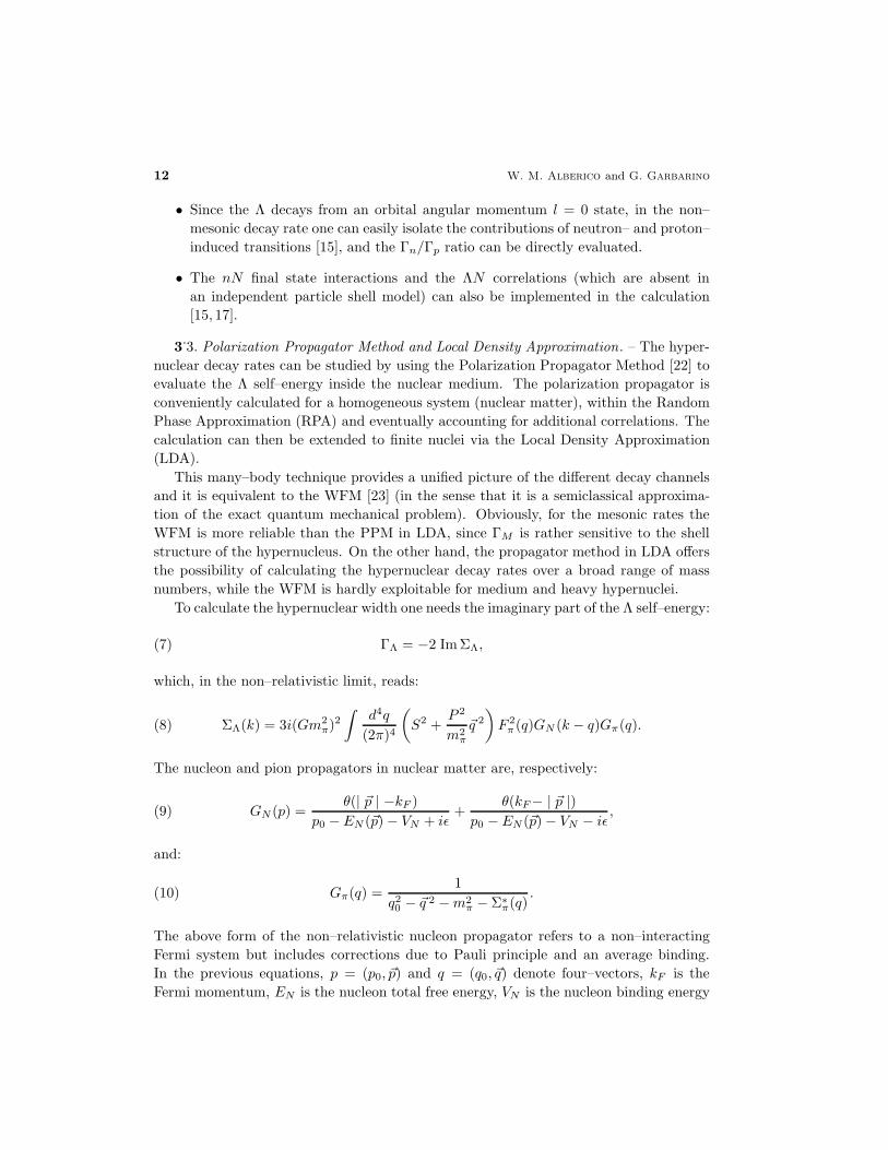
• Since the Λ decays from an orbital angular momentum l = 0 state, in the non–
mesonic decay rate one can easily isolate the contributions of neutron– and proton–
induced transitions [15], and the Γn/Γp ratio can be directly evaluated.
• The nN final state interactions and the ΛN correlations (which are absent in
an independent particle shell model) can also be implemented in the calculation
[15, 17].
3.3. Polarization Propagator Method and Local Density Approximation. – The hyper-
nuclear decay rates can be studied by using the Polarization Propagator Method [22] to
evaluate the Λ self–energy inside the nuclear medium. The polarization propagator is
conveniently calculated for a homogeneous system (nuclear matter), within the Random
Phase Approximation (RPA) and eventually accounting for additional correlations. The
calculation can then be extended to finite nuclei via the Local Density Approximation
(LDA).
This many–body technique provides a unified picture of the different decay channels
and it is equivalent to the WFM [23] (in the sense that it is a semiclassical approxima-
tion of the exact quantum mechanical problem). Obviously, for the mesonic rates the
WFM is more reliable than the PPM in LDA, since ΓM is rather sensitive to the shell
structure of the hypernucleus. On the other hand, the propagator method in LDA offers
the possibility of calculating the hypernuclear decay rates over a broad range of mass
numbers, while the WFM is hardly exploitable for medium and heavy hypernuclei.
To calculate the hypernuclear width one needs the imaginary part of the Λ self–energy:
(7) ΓΛ = −2 ImΣΛ,
which, in the non–relativistic limit, reads:
(8) ΣΛ(k) = 3i(Gm2π)2
∫
d4q
(2π)4
(
S2 +P 2
m2π
~q 2
)
F 2π (q)GN (k − q)Gπ(q).
The nucleon and pion propagators in nuclear matter are, respectively:
(9) GN (p) =θ(| ~p | −kF )
p0 − EN (~p) − VN + iǫ+
θ(kF− | ~p |)p0 − EN (~p) − VN − iǫ
,
and:
(10) Gπ(q) =1
q20 − ~q 2 −m2π − Σ∗
π(q).
The above form of the non–relativistic nucleon propagator refers to a non–interacting
Fermi system but includes corrections due to Pauli principle and an average binding.
In the previous equations, p = (p0, ~p) and q = (q0, ~q) denote four–vectors, kF is the
Fermi momentum, EN is the nucleon total free energy, VN is the nucleon binding energy
Weak decay of hypernuclei 13
Λ
+++π
1
2
(a) (b) (c) (d)
+
(e)
. . .++++
(f) (g) (h)
N
Λ
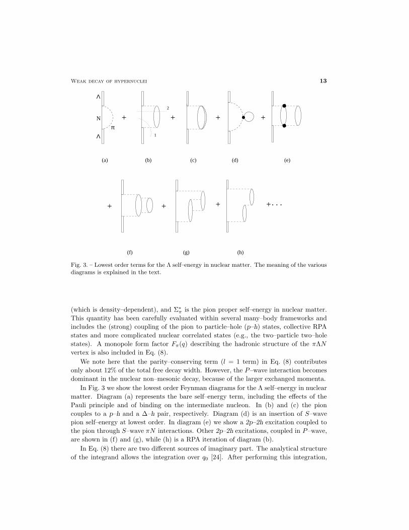
Fig. 3. – Lowest order terms for the Λ self–energy in nuclear matter. The meaning of the variousdiagrams is explained in the text.
(which is density–dependent), and Σ∗
π is the pion proper self–energy in nuclear matter.
This quantity has been carefully evaluated within several many–body frameworks and
includes the (strong) coupling of the pion to particle–hole (p–h) states, collective RPA
states and more complicated nuclear correlated states (e.g., the two–particle two–hole
states). A monopole form factor Fπ(q) describing the hadronic structure of the πΛN
vertex is also included in Eq. (8).
We note here that the parity–conserving term (l = 1 term) in Eq. (8) contributes
only about 12% of the total free decay width. However, the P–wave interaction becomes
dominant in the nuclear non–mesonic decay, because of the larger exchanged momenta.
In Fig. 3 we show the lowest order Feynman diagrams for the Λ self–energy in nuclear
matter. Diagram (a) represents the bare self–energy term, including the effects of the
Pauli principle and of binding on the intermediate nucleon. In (b) and (c) the pion
couples to a p–h and a ∆–h pair, respectively. Diagram (d) is an insertion of S–wave
pion self–energy at lowest order. In diagram (e) we show a 2p–2h excitation coupled to
the pion through S–wave πN interactions. Other 2p–2h excitations, coupled in P–wave,
are shown in (f) and (g), while (h) is a RPA iteration of diagram (b).
In Eq. (8) there are two different sources of imaginary part. The analytical structure
of the integrand allows the integration over q0 [24]. After performing this integration,
14 W. M. Alberico and G. Garbarino
an imaginary part is obtained from the (renormalized) pion–nucleon pole and physically
corresponds to the mesonic decay of the hyperon. Moreover, the pion proper self–energy
Σ∗
π(q) has an imaginary part itself for (q0, ~q) values which correspond to the excitation of
p–h, ∆–h, 2p–2h, etc states on the mass shell. By expanding the pion propagator Gπ(q)
as in Fig. 3 and integrating Eq. (8) over q0, the nuclear matter Λ decay width of Eq. (7)
becomes [24]:
ΓΛ(~k, ρ) = −6(Gm2π)2
∫
d~q
(2π)3θ(| ~k − ~q | −kF )θ(k0 − EN (~k − ~q) − VN )
×Im [α(q)]q0=k0−EN (~k−~q)−VN
,(11)
where:
α(q) =
(
S2 +P 2
m2π
~q 2
)
F 2π (q)G0
π(q) +S2(q)UL(q)
1 − VL(q)UL(q)
+P 2
L(q)UL(q)
1 − VL(q)UL(q)+ 2
P 2T (q)UT (q)
1 − VT (q)UT (q).(12)
In Eq. (11) the first θ function forbids intermediate nucleon momenta smaller than the
Fermi momentum, while the second one requires the pion energy q0 to be positive. More-
over, the Λ energy, k0 = EΛ(~k) + VΛ, contains a phenomenological binding term. With
the exception of diagram (a), the pion lines of Fig. 3 have been replaced, in Eq. (12),
by the effective interactions S, PL, PT ,VL, VT (L and T stand for spin–longitudinal and
spin–transverse, respectively), which include π– and ρ–exchange modulated by the effect
of short range repulsive correlations. The potentials VL and VT represent the (strong) p–h
interaction and include a Landau parameter g′, which accounts for the short range repul-
sion, while S, PL and PT correspond to the lines connecting weak and strong hadronic
vertices and contain another Landau parameter, g′Λ, which is related to the strong ΛN
short range correlations.
Furthermore, in Eq. (12):
G0π(q) =
1
q20 − ~q 2 −m2π
,
is the free pion propagator, while UL(q) and UT (q) contain the Lindhard functions for
p–h and ∆–h excitations [25] and also account for the irreducible 2p–2h polarization
propagator:
(13) UL,T (q) = Uph(q) + U∆h(q) + U2p2hL,T (q).
They appear in Eq. (12) within the standard RPA expression:
UL(T )(q)
1 − VL(T )(q)UL(T )(q)= UL(T )(q) + UL(T )(q)VL(T )(q)UL(T )(q) +
+UL(T )(q)VL(T )(q)UL(T )(q)VL(T )(q)UL(T )(q) + . . .(14)
Weak decay of hypernuclei 15
The decay width (11) depends both explicitly and through UL,T (q) on the nuclear matter
density ρ = 2k3F /3π
2.
The Lindhard function Uph (U∆h) is given by:
(15) Uph(∆h)(q) = −4i
∫
d4p
(2π)3G0
N (p)G0N(∆)(p+ q),
with the free nucleon and Delta propagators:
(16) G0N (p) =
θ(| ~p | −kF )
p0 − TN (~p) + iǫ+
θ(kF− | ~p |)p0 − TN(~p) − iǫ
,
(17) G0∆(p) =
4
9
1
p0 − T∆(~p) − δM∆N + iΓ∆/2,
where TN(∆) is the nucleon (Delta) kinetic energy, Γ∆ the free ∆ width and δM∆N =
m∆ −mN . We remind that Uph(q) and U∆h(q) can be analytically evaluated in nuclear
matter.
For the evaluation of U2p2hL,T we discuss two different approaches. In Refs. [26, 27]
a phenomenological parameterization was adopted: this consists in relating U2p2hL,T to
the available phase space for on–shell 2p–2h excitations in order to extrapolate for off–
mass shell pions the experimental data of P–wave absorption of real pions in pionic
atoms. In an alternative approach [28], U2p2hL,T is evaluated microscopically, starting from
a classification of the relevant Feynman diagrams according to the so–called bosonic loop
expansion, which is obtained within a functional approach.
We notice here, in connection with Eqs. (8) and (10), that the full (proper) pion
self–energy
Σ∗
π(q) = Σ(S) ∗π (q) + Σ(P ) ∗
π (q),
contains a P–wave term, which is related to the spin–longitudinal polarization propagator
UL(q) according to:
(18) Σ(P ) ∗π (q) =
~q 2 f2π
m2π
F 2π (q)UL(q)
1 − f2π
m2π
gL(q)UL(q)
,
the Landau function gL(q) being given in the appendix of Ref. [5]. Σ∗
π(q) also contains
an S–wave term, which, by using the parameterization of Ref. [29], can be written as:
(19) Σ(S) ∗π (q) = −4π
(
1 +mπ
mN
)
b0ρ.
16 W. M. Alberico and G. Garbarino
UL(T)
Polarization
Propagator
+
w
w
N
Λ
π
π
s
s
N
w
w
π=
Λ
Λ
Σ
Λ
ΣΛ
free
Λ
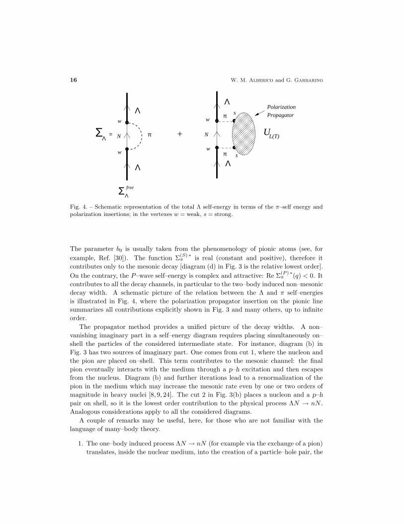
Fig. 4. – Schematic representation of the total Λ self-energy in terms of the π–self energy andpolarization insertions; in the vertexes w = weak, s = strong.
The parameter b0 is usually taken from the phenomenology of pionic atoms (see, for
example, Ref. [30]). The function Σ(S) ∗π is real (constant and positive), therefore it
contributes only to the mesonic decay [diagram (d) in Fig. 3 is the relative lowest order].
On the contrary, the P–wave self–energy is complex and attractive: Re Σ(P ) ∗π (q) < 0. It
contributes to all the decay channels, in particular to the two–body induced non–mesonic
decay width. A schematic picture of the relation between the Λ and π self–energies
is illustrated in Fig. 4, where the polarization propagator insertion on the pionic line
summarizes all contributions explicitly shown in Fig. 3 and many others, up to infinite
order.
The propagator method provides a unified picture of the decay widths. A non–
vanishing imaginary part in a self–energy diagram requires placing simultaneously on–
shell the particles of the considered intermediate state. For instance, diagram (b) in
Fig. 3 has two sources of imaginary part. One comes from cut 1, where the nucleon and
the pion are placed on–shell. This term contributes to the mesonic channel: the final
pion eventually interacts with the medium through a p–h excitation and then escapes
from the nucleus. Diagram (b) and further iterations lead to a renormalization of the
pion in the medium which may increase the mesonic rate even by one or two orders of
magnitude in heavy nuclei [8, 9, 24]. The cut 2 in Fig. 3(b) places a nucleon and a p–h
pair on shell, so it is the lowest order contribution to the physical process ΛN → nN .
Analogous considerations apply to all the considered diagrams.
A couple of remarks may be useful, here, for those who are not familiar with the
language of many–body theory.
1. The one–body induced process ΛN → nN (for example via the exchange of a pion)
translates, inside the nuclear medium, into the creation of a particle–hole pair, the
Weak decay of hypernuclei 17
(in nuclear medium)
πNN
N Λ
N
π
N −1N
(hole)(particle)
Λ
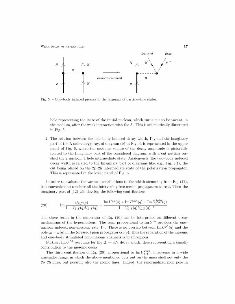
Fig. 5. – One–body induced process in the language of particle–hole states.
hole representing the state of the initial nucleon, which turns out to be vacant, in
the medium, after the weak interaction with the Λ. This is schematically illustrated
in Fig. 5.
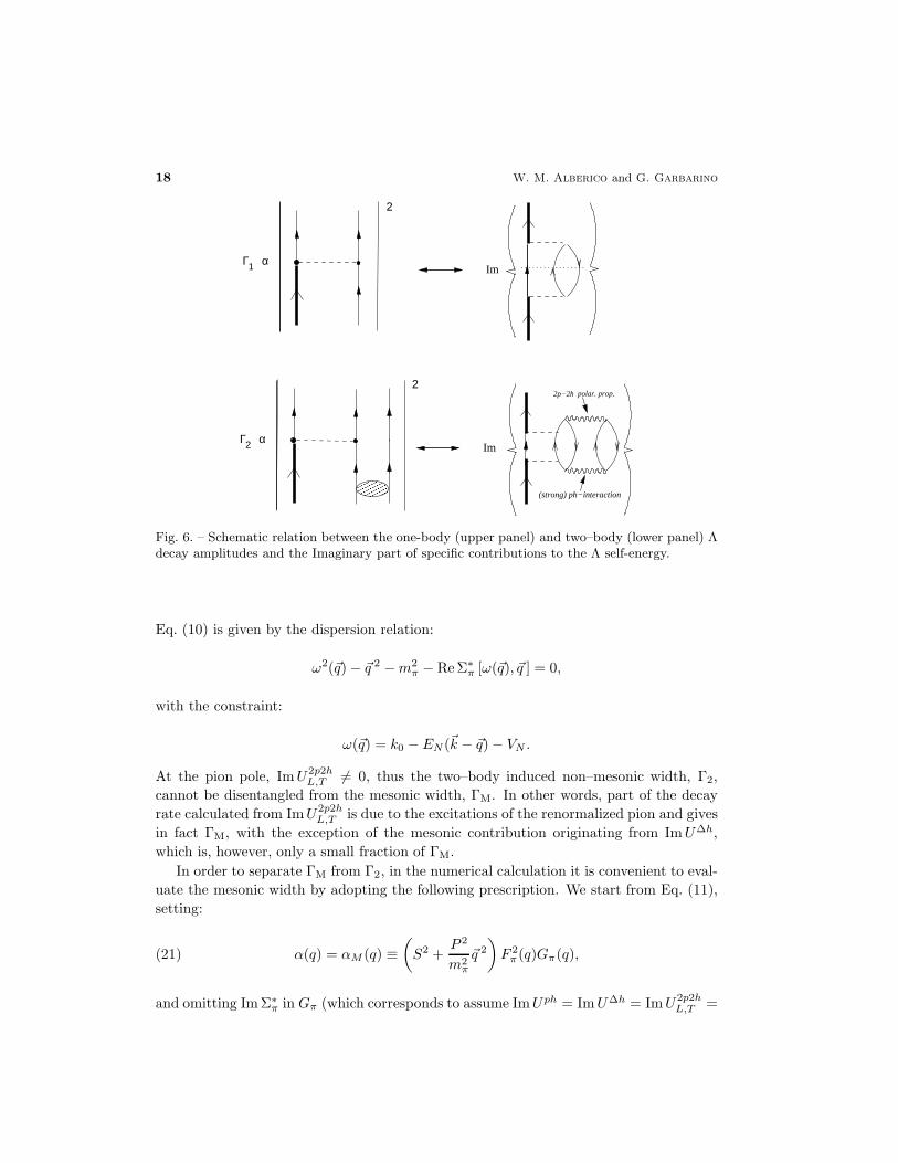
2. The relation between the one–body induced decay width, Γ1, and the imaginary
part of the Λ self–energy, say, of diagram (b) in Fig. 3, is represented in the upper
panel of Fig. 6, where the modulus square of the decay amplitude is pictorially
related to the Imaginary part of the considered diagram, with a cut putting on–
shell the 2 nucleon, 1 hole intermediate state. Analogously, the two–body induced
decay width is related to the Imaginary part of diagrams like, e.g., Fig. 3(f), the
cut being placed on the 2p–2h intermediate state of the polarization propagator.
This is represented in the lower panel of Fig. 6.
In order to evaluate the various contributions to the width stemming from Eq. (11),
it is convenient to consider all the intervening free meson propagators as real. Then the
imaginary part of (12) will develop the following contributions:
(20) ImUL,T (q)
1 − VL,T (q)UL,T (q)=
ImUph(q) + ImU∆h(q) + ImU2p2hL,T (q)
| 1 − VL,T (q)UL,T (q) |2 .
The three terms in the numerator of Eq. (20) can be interpreted as different decay
mechanisms of the hypernucleus. The term proportional to ImUph provides the one–
nucleon induced non–mesonic rate, Γ1. There is no overlap between ImUph(q) and the
pole q0 = ω(~q) in the (dressed) pion propagatorGπ(q): thus the separation of the mesonic
and one–body stimulated non–mesonic channels is unambiguous.
Further, ImU∆h accounts for the ∆ → πN decay width, thus representing a (small)
contribution to the mesonic decay.
The third contribution of Eq. (20), proportional to ImU2p2hL,T , intervenes in a wide
kinematic range, in which the above mentioned cuts put on the mass shell not only the
2p–2h lines, but possibly also the pionic lines. Indeed, the renormalized pion pole in
18 W. M. Alberico and G. Garbarino
Γ1
Γ2
polar. prop.2p−2h
αIm
2
2
αIm
(strong) ph−interaction
Fig. 6. – Schematic relation between the one-body (upper panel) and two–body (lower panel) Λdecay amplitudes and the Imaginary part of specific contributions to the Λ self-energy.
Eq. (10) is given by the dispersion relation:
ω2(~q) − ~q 2 −m2π − Re Σ∗
π [ω(~q), ~q ] = 0,
with the constraint:
ω(~q) = k0 − EN (~k − ~q) − VN .
At the pion pole, ImU2p2hL,T 6= 0, thus the two–body induced non–mesonic width, Γ2,
cannot be disentangled from the mesonic width, ΓM. In other words, part of the decay
rate calculated from ImU2p2hL,T is due to the excitations of the renormalized pion and gives
in fact ΓM, with the exception of the mesonic contribution originating from ImU∆h,
which is, however, only a small fraction of ΓM.
In order to separate ΓM from Γ2, in the numerical calculation it is convenient to eval-
uate the mesonic width by adopting the following prescription. We start from Eq. (11),
setting:
(21) α(q) = αM (q) ≡(
S2 +P 2
m2π
~q 2
)
F 2π (q)Gπ(q),
and omitting ImΣ∗
π in Gπ (which corresponds to assume ImUph = ImU∆h = ImU2p2hL,T =
Weak decay of hypernuclei 19
0). Then ImαM (q) only accounts for the (real) contribution of the pion pole:
ImGπ(q) = −πδ[
q20 − ~q 2 −m2π − Re Σ∗
π(q)]
.
Once the mesonic decay rate is known, one can calculate the three–body non–mesonic
rate by subtracting ΓM and Γ1 from the total rate ΓT, which one gets via the full
expression for α(q) [Eq. (12)].
Using the PPM, the decay widths of finite nuclei can be obtained from the ones
evaluated in nuclear matter via the LDA: in this approach the Fermi momentum is made
r–dependent (namely a local Fermi sea of nucleons is introduced) and related to the
nuclear density by the same relation which holds in nuclear matter:
(22) kF (~r) =
3
2π2ρ(~r)
1/3
.
More specifically, one usually assumes the nuclear density to be a Fermi distribution:
ρA(r) =ρ0
1 + exp
[
r − R(A)
a
]
withR(A) = 1.12A1/3−0.86A−1/3 fm, a = 0.52 fm and ρ0 = A
43πR
3(A)
(
1 +[
πaR(A)
]2)−1
.
Moreover, the nucleon binding potential VN also becomes r–dependent in LDA. In
Thomas–Fermi approximation one assumes:
ǫF (~r) + VN (~r) ≡ k2F (~r)
2mN+ VN (~r) = 0.
With these prescriptions one can then evaluate the decay width in finite nuclei by
using the semiclassical approximation, through the relation:
(23) ΓΛ(~k) =
∫
d~r |ψΛ(~r)|2ΓΛ
[
~k, ρ(~r)]
,
where ψΛ is the appropriate Λ wave function and ΓΛ[~k, ρ(~r)] is given by Eqs. (11), (12)
with a position dependent nuclear density. This decay rate can be regarded as the ~k–
component of the Λ decay rate in the nucleus with density ρ(~r). It can be used to
estimate the decay rates by averaging over the Λ momentum distribution |ψΛ(~k)|2. One
then obtains the following total width:
(24) ΓT =
∫
d~k |ψΛ(~k)|2ΓΛ(~k),
which can be compared with the experimental results.
20 W. M. Alberico and G. Garbarino
3.3.1. Phenomenological 2p–2h propagator. Coming to the phenomenological evalu-
ation of the 2p–2h contributions in the Λ self–energy, the momentum dependence of the
imaginary part of U2p2hL,T can be obtained from the available phase space, through the
following equation [26]:
(25) ImU2p2hL,T (q0, ~q; ρ) =
P (q0, ~q; ρ)
P (mπ,~0; ρeff)ImU2p2h
L,T (mπ ,~0; ρeff),
where ρeff = 0.75ρ. By neglecting the energy and momentum dependence of the p–
h interaction, the phase space available for on–shell 2p–2h excitations [calculated, for
simplicity, from diagram 3(e)] at energy–momentum (q0, ~q) and density ρ turns out to
be:
P (q0, ~q; ρ) ∝∫
d4k
(2π)4ImUph
( q
2+ k; ρ
)
ImUph(q
2− k; ρ
)
×θ(q0
2+ k0
)
θ(q0
2− k0
)
.
In the region of (q0, ~q) where the p–h and ∆–h excitations are off–shell, the relation
between U2p2hL and the P–wave pion–nucleus optical potential Vopt is given by [see also
Eq. (18), in the language of pion self–energy]:
(26)
~q 2 f2π
m2π
F 2π (q)U2p2h
L (q)
1 − f2π
m2π
gL(q)UL(q)
= 2q0Vopt(q).
At the pion threshold Vopt is usually parameterized as:
(27) 2q0Vopt(q0 ≃ mπ, ~q ≃ ~0; ρ) = −4π~q 2ρ2C0,
where C0 is a complex number which can be extracted from experimental data on pionic
atoms. By combining Eqs. (26) and (27) it is possible to parameterize the proper 2p–2h
excitations in the spin–longitudinal channel through Eq. (25), by setting:
(28) ~q 2 f2π
m2π
F 2π (q0 ≃ mπ, ~q ≃ ~0)U2p2h
L (q0 ≃ mπ, ~q ≃ ~0; ρ) = −4π~q 2ρ2C∗
0 .
The relation between C0 and C∗
0 is fixed on the basis of the same RPA expression for
the polarization propagator contained in Eq. (26); hence the value of C∗
0 also depends
on the correlation function gL. From the analysis of pionic atoms data made in Ref. [31]
and taking g′ ≡ gL(0) = 0.615, one obtains:
C∗
0 = (0.105 + i0.096)/m6π.
Weak decay of hypernuclei 21
The spin–transverse component of U2p2h is assumed to be equal to the spin–longitudinal
one, U2p2hT = U2p2h
L , and the real parts of U2p2hL and U2p2h
T are considered constant [by
using Eq. (28)] because they are not expected to be too sensitive to variations of q0 and
~q. The assumption U2p2hT = U2p2h
L is not a priori a good approximation, but it is the
only one which can be employed in the present phenomenological description. Yet, the
differences between U2p2hL and U2p2h
T can only mildly change the partial decay widths [5]:
in fact, U2p2hL,T are summed to Uph, which gives the dominant contribution. Moreover, for
U2p2hL = U2p2h
T the transverse contribution to Γ2 [fourth term in the right hand side of
Eq. (12)] is only about 16% of Γ2 (namely 2 ÷ 3% of the total width) in medium–heavy
hypernuclei.
The simplified form of the phenomenological 2p–2h propagator, together with the
availability of analytical expressions for Uph and U∆−h, makes this approach particularly
suitable for employing the above mentioned LDA.
3.3.2. Functional approach to the Λ self–energy. In alternative to the above men-
tioned phenomenological approach for the two–body induced decay width, we briefly
discuss here a truly microscopic approach. Indeed the most relevant Feynman diagrams
for the calculation of the Λ self–energy can be obtained in the framework of a functional
method: following Ref. [28], one can derive a classification of the diagrams according to
the prescription of the so–called bosonic loop expansion.
The functional techniques can provide a theoretically founded derivation of new classes
of Feynmann diagram expansions in terms of powers of suitably chosen parameters. For
example, the already mentioned ring approximation (a subclass of RPA) automatically
appears in this framework at the mean field level. This method has been extensively ap-
plied to the analysis of different processes in nuclear physics [32–34]. Here it is employed
for the calculation of the Λ self–energy in nuclear matter, which can be expressed through
the nuclear responses to pseudoscalar–isovector and vector–isovector fields. The polar-
ization propagators obtained in this framework include ring–dressed meson propagators
and almost the whole spectrum of 2p–2h excitations (expressed in terms of a one–loop
expansion with respect to the ring–dressed meson propagators), which are required for
the evaluation of Γ2.
Let us first consider the polarization propagator in the pionic (spin–longitudinal)
channel. To illustrate the procedure, it is useful to start from a Lagrangian describing a
system of nucleons interacting with pions through a pseudoscalar–isovector coupling:
(29) LπN = ψ(i/∂ −mN )ψ +1
2∂µ~φ · ∂µ~φ− 1
2m2
π~φ 2 − iψ~Γψ · ~φ,
where ψ (~φ) is the nucleonic (pionic) field and ~Γ = gγ5~τ (g = 2fπmN/mπ) is the spin–
isospin matrix in the spin–longitudinal isovector channel. We remind the reader that in
the calculation of the hypernuclear decay rates one also needs the polarization propagator
in the transverse channel [see Eqs. (11) and (12)]: hence, one has to include in the model
other mesonic degrees of freedom, like the ρ meson. Since the bosonic loop expansion is
22 W. M. Alberico and G. Garbarino
characterized by the topology of the diagrams, this is relatively straightforward and the
same scheme can be easily applied to mesonic fields other than the pionic one.
The generating functional, expressed in terms of Feynman path integrals, associated
with the Lagrangian (29) has the form:
(30) Z[~ϕ ] =
∫
D[
ψ, ψ, ~φ]
exp
i
∫
dx[
LπN (x) − iψ(x)~Γψ(x) · ~ϕ(x)]
,
where a classical external field ~ϕ with the quantum numbers of the pion has been in-
troduced (here and in the following the coordinate integrals are 4–dimensional). All the
fields in the functional integrals have to be considered as classical variables, but with the
correct commuting properties (hence the fermionic fields are Grassman variables).
The physical quantities of interest for the problem are then deduced from the gener-
ating functional by means of functional differentiations. In particular, by introducing a
new functional Zc such that:
(31) Z[~ϕ ] = exp iZc[~ϕ ],
the spin–longitudinal, isovector polarization propagator turns out to be the second func-
tional derivative of Zc with respect to the source ~ϕ of the pionic field:
(32) Πij(x, y) = −[
δ2Zc[~ϕ ]
δϕi(x)δϕj(y)
]
~ϕ=0
.
We note that the use of Zc instead of Z in Eq. (32) amounts to cancel the disconnected
diagrams of the corresponding perturbative expansion (linked cluster theorem). From
the generating functional Z one can obtain different approximation schemes according
to the order in which the functional integrations are performed.
For the present purpose, it is convenient to integrate Eq. (30) over the nucleonic
degrees of freedom first. Introducing the change of variable ~φ→ ~φ− ~ϕ one obtains:
Z [~ϕ ] = exp
i
2
∫
dx dy ~ϕ(x) ·G0−1
π (x− y)~ϕ(y)
(33)
×∫
D[
ψ, ψ, ~φ]
exp
i
∫
dx dy[
ψ(x)G−1N (x− y)ψ(y)
+1
2~φ(x) ·G0−1
π (x− y)(
~φ(y) + 2~ϕ(y))
]
,
where the integral over[
ψ, ψ]
is gaussian:
∫
D[
ψ, ψ]
exp
i
∫
dx dy ψ(x)G−1N (x− y)ψ(y)
= (detGN )−1.
Weak decay of hypernuclei 23
Hence, after multiplying Eq. (33) by the unessential factor detG0N (G0
N being the free
nucleon propagator), which only redefines the normalization constant of the generating
functional, and using the property detX = exp Tr lnX, one obtains:
Z[~ϕ ] = exp
i
2
∫
dx dy ~ϕ(x) ·G0−1
π (x− y)~ϕ(y)
(34)
×∫
D[
~φ]
exp
iSBeff
[
~φ]
.
In this expression we have introduced the bosonic effective action:
(35) SBeff
[
~φ]
=
∫
dx dy
1
2~φ(x) ·G0−1
π (x− y)[
~φ(y) + 2~ϕ(y)]
+ Vπ
[
~φ]
,
where(2):
Vπ
[
~φ]
= iTr
∞∑
n=1
1
n
(
i~Γ · ~φG0N
)n
(36)
=1
2
∑
i,j
Tr (ΓiΓj)
∫
dx dyΠ0(x, y)φi(x)φj(y)
+1
3
∑
i,j,k
Tr (ΓiΓjΓk)
∫
dx dy dzΠ0(x, y, z)φi(x)φj(y)φk(z) + O(~φ4).
and:
−iΠ0(x, y) = iG0N (x− y)iG0
N (y − x),(37)
−iΠ0(x, y, z) = iG0N (x− y)iG0
N (y − z)iG0N (z − x), etc.(38)
The bosonic effective action (35) contains a term for the free pion field and also a highly
non–local pion self–interaction Vπ. This effective interaction is given by the sum of all
diagrams containing one closed fermion loop and an arbitrary number of pionic legs.
We note that the function in Eq. (37) is the free particle–hole polarization propagator.
Moreover, the functions Π0(x, y, . . . , z) are symmetric for cyclic permutations of the
arguments.
The next step is the evaluation of the functional integral over the bosonic degrees of
freedom in Eq. (34). A perturbative approach to the bosonic effective action (35) does
(2) Eq. (36) is a compact writing: for example, the n = 2 term must be interpreted as:
i
2Tr
(
i~Γ ·~φG
0
N
)2
=i
2
∫
dx dy Tr∑
i.j
iΓiG0
N (x − y) iΓjG0
N (y − x)φi(x)φj(y),
where the trace in the right hand side acts on the vertices ~Γ, and so on.
24 W. M. Alberico and G. Garbarino
not seem to provide any valuable results within the capabilities of the present computing
tools and in Ref. [28] another approximation scheme, the semiclassical method, was
followed.
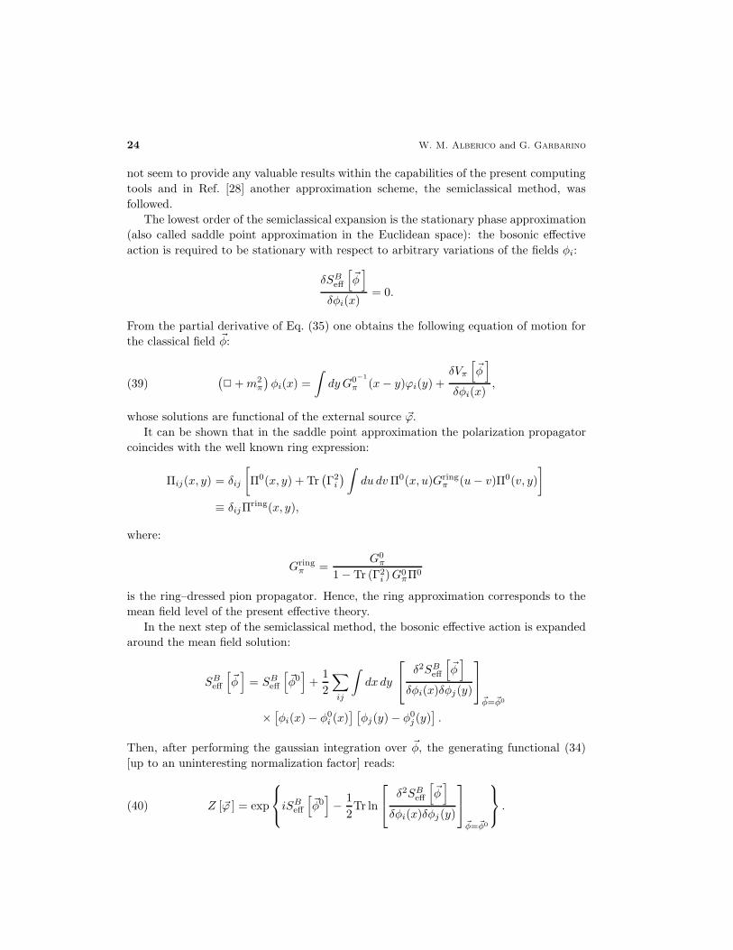
The lowest order of the semiclassical expansion is the stationary phase approximation
(also called saddle point approximation in the Euclidean space): the bosonic effective
action is required to be stationary with respect to arbitrary variations of the fields φi:
δSBeff
[
~φ]
δφi(x)= 0.
From the partial derivative of Eq. (35) one obtains the following equation of motion for
the classical field ~φ:
(39)(
2 +m2π
)
φi(x) =
∫
dy G0−1
π (x− y)ϕi(y) +δVπ
[
~φ]
δφi(x),
whose solutions are functional of the external source ~ϕ.
It can be shown that in the saddle point approximation the polarization propagator
coincides with the well known ring expression:
Πij(x, y) = δij
[
Π0(x, y) + Tr(
Γ2i
)
∫
du dvΠ0(x, u)Gringπ (u− v)Π0(v, y)
]
≡ δijΠring(x, y),
where:
Gringπ =
G0π
1 − Tr (Γ2i )G
0πΠ0
is the ring–dressed pion propagator. Hence, the ring approximation corresponds to the
mean field level of the present effective theory.
In the next step of the semiclassical method, the bosonic effective action is expanded
around the mean field solution:
SBeff
[
~φ]
= SBeff
[
~φ0]
+1
2
∑
ij
∫
dx dy
δ2SBeff
[
~φ]
δφi(x)δφj(y)
~φ=~φ0
×[
φi(x) − φ0i (x)
] [
φj(y) − φ0j (y)
]
.
Then, after performing the gaussian integration over ~φ, the generating functional (34)
[up to an uninteresting normalization factor] reads:
(40) Z [~ϕ ] = exp
iSBeff
[
~φ0]
− 1
2Tr ln
δ2SBeff
[
~φ]
δφi(x)δφj(y)
~φ=~φ0
.
Weak decay of hypernuclei 25
(f)
(a) (b) (c) (d)
(e)
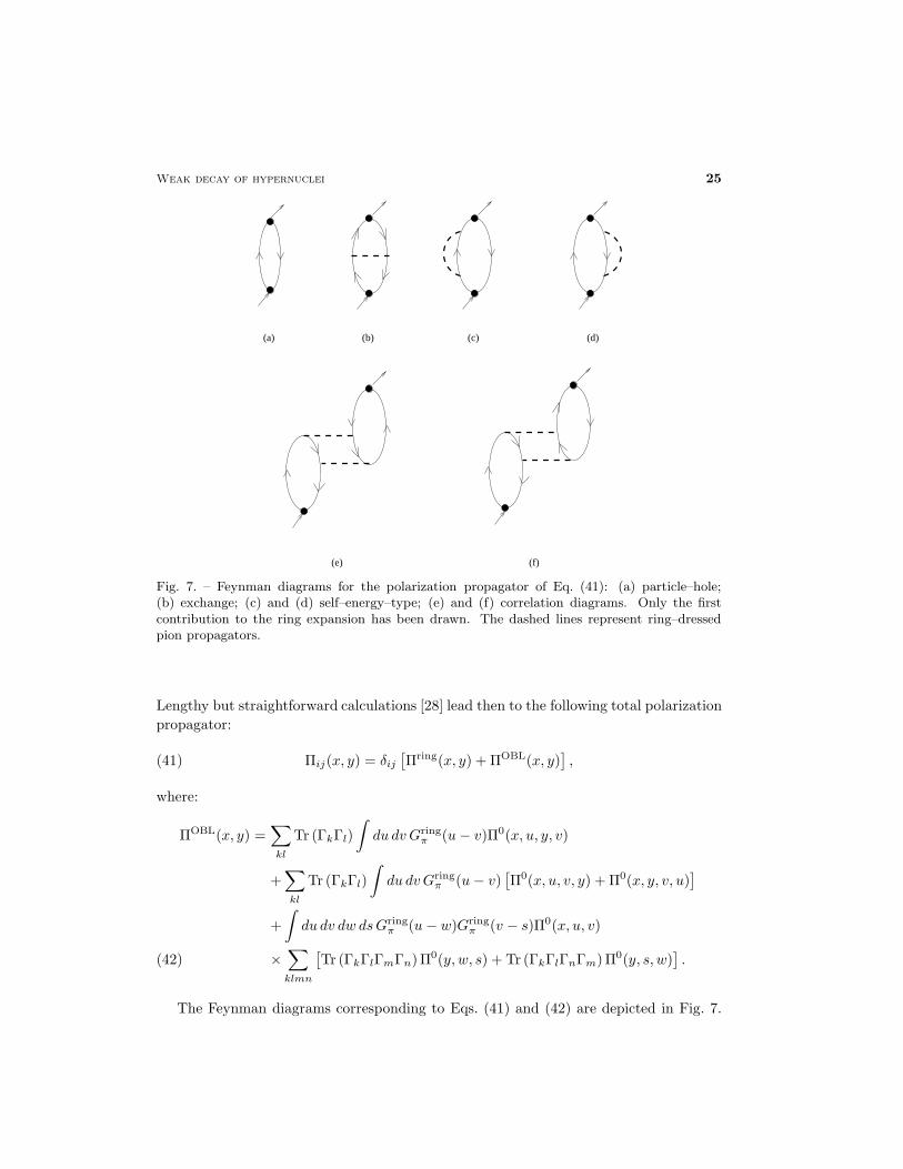
Fig. 7. – Feynman diagrams for the polarization propagator of Eq. (41): (a) particle–hole;(b) exchange; (c) and (d) self–energy–type; (e) and (f) correlation diagrams. Only the firstcontribution to the ring expansion has been drawn. The dashed lines represent ring–dressedpion propagators.
Lengthy but straightforward calculations [28] lead then to the following total polarization
propagator:
(41) Πij(x, y) = δij[
Πring(x, y) + ΠOBL(x, y)]
,
where:
ΠOBL(x, y) =∑
kl
Tr (ΓkΓl)
∫
du dv Gringπ (u− v)Π0(x, u, y, v)
+∑
kl
Tr (ΓkΓl)
∫
du dvGringπ (u − v)
[
Π0(x, u, v, y) + Π0(x, y, v, u)]
+
∫
du dv dw dsGringπ (u − w)Gring
π (v − s)Π0(x, u, v)
×∑
klmn
[
Tr (ΓkΓlΓmΓn)Π0(y, w, s) + Tr (ΓkΓlΓnΓm)Π0(y, s, w)]
.(42)
The Feynman diagrams corresponding to Eqs. (41) and (42) are depicted in Fig. 7.
26 W. M. Alberico and G. Garbarino
Diagram (a) represents the Lindhard function Π0(x, y), which is just the first term of
Πring(x, y). In (b) we have an exchange diagram (the thick dashed lines representing
ring–dressed pion propagators); (c) and (d) are self–energy diagrams, while in (e) and (f)
we show the correlation diagrams of the present approach. The approximation scheme
discussed here is also referred to as bosonic loop expansion (BLE). The practical rule
to classify the Feynman diagrams according to their order in the BLE is to reduce to a
point all its fermionic lines and to count the number of bosonic loops left out. In this
case the diagrams (b)–(f) of Fig. 7, which correspond to ΠOBL Eq. (42), reduce to a
one–boson–loop (OBL).
The polarization propagator of Eq. (42) is the central result of the present microscopic
approach and it has been used [28] for the calculation of the Λ decay width in nuclear
matter. Note that the model can easily include the excitation of baryonic resonances,
by replacing the fermionic field with multiplets. The topology of the diagrams remains
the same as in Fig. 7 but, introducing for example the ∆ resonance, each fermionic line
represents either a nucleon or a ∆, taking care of isospin conservation. Obviously this
procedure substantially increases the number of diagrams.
Moreover, being the BLE characterized by the topology of the diagrams, additional
mesonic degrees of freedom together with phenomenological short range correlations can
be included by changing the definition of the vertices Γi in Eq. (42). In particular, the
formalism can be applied to evaluate the functions UL,T of Eq. (13), which are required
in Eqs. (11), (12). In the OBL approximation of Eq. (41) and Fig. 7 one has to replace
Eq. (12) with:
α(q) =
(
S2 +P 2
m2π
~q 2
)
F 2π (q)G0
π(q) +S2(q)U1(q)
1 − VL(q)U1(q)(43)
+P 2
L(q)U1(q)
1 − VL(q)U1(q)+ 2
P 2T (q)U1(q)
1 − VT (q)U1(q)
+[
S2(q) + P 2L(q)
]
UOBLL (q) + 2P 2
T (q)UOBLT (q),
where
U1 = Uph + U∆h,
while UOBLL,T are evaluated from the diagrams 7(b)–7(f) using the standard Feynman
rules. The normalization of these functions is such that Uph(x, y) = 4Π0(x, y), Π0 being
given by Eq. (37). One relevant difference between the OBL formula (43) and the RPA
expression of Eq. (12) lies in the fact that in the former, to be consistent with Eq. (42),
the 2p–2h diagrams (which contribute to UOBLL,T ) are not RPA–iterated.
4. – Theory versus Experiment
In this Section the predictions of different theoretical models for the total mesonic
and non–mesonic weak decay rates are compared with experimental data. We mainly
Weak decay of hypernuclei 27
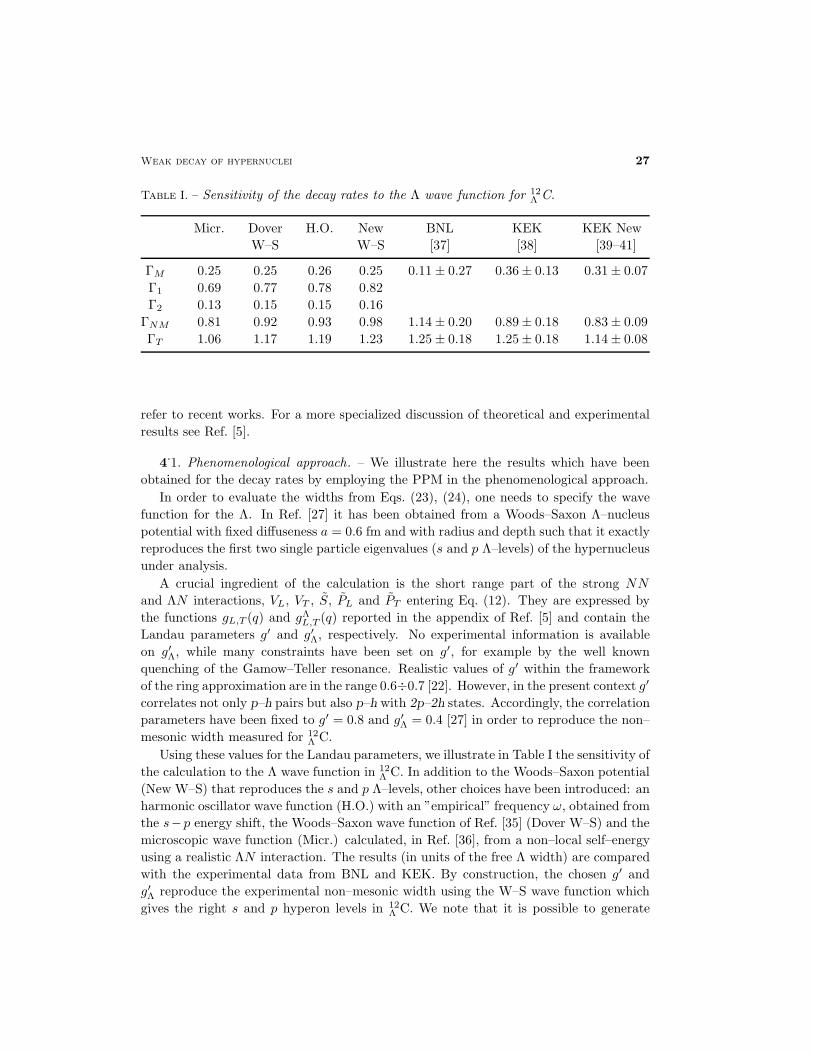
Table I. – Sensitivity of the decay rates to the Λ wave function for 12Λ C.
Micr. Dover H.O. New BNL KEK KEK New
W–S W–S [37] [38] [39–41]
ΓM 0.25 0.25 0.26 0.25 0.11 ± 0.27 0.36 ± 0.13 0.31 ± 0.07
Γ1 0.69 0.77 0.78 0.82
Γ2 0.13 0.15 0.15 0.16
ΓNM 0.81 0.92 0.93 0.98 1.14 ± 0.20 0.89 ± 0.18 0.83 ± 0.09
ΓT 1.06 1.17 1.19 1.23 1.25 ± 0.18 1.25 ± 0.18 1.14 ± 0.08
refer to recent works. For a more specialized discussion of theoretical and experimental
results see Ref. [5].
4.1. Phenomenological approach. – We illustrate here the results which have been
obtained for the decay rates by employing the PPM in the phenomenological approach.
In order to evaluate the widths from Eqs. (23), (24), one needs to specify the wave
function for the Λ. In Ref. [27] it has been obtained from a Woods–Saxon Λ–nucleus
potential with fixed diffuseness a = 0.6 fm and with radius and depth such that it exactly
reproduces the first two single particle eigenvalues (s and p Λ–levels) of the hypernucleus
under analysis.
A crucial ingredient of the calculation is the short range part of the strong NN
and ΛN interactions, VL, VT , S, PL and PT entering Eq. (12). They are expressed by
the functions gL,T (q) and gΛL,T (q) reported in the appendix of Ref. [5] and contain the
Landau parameters g′ and g′Λ, respectively. No experimental information is available
on g′Λ, while many constraints have been set on g′, for example by the well known
quenching of the Gamow–Teller resonance. Realistic values of g′ within the framework
of the ring approximation are in the range 0.6÷0.7 [22]. However, in the present context g′
correlates not only p–h pairs but also p–h with 2p–2h states. Accordingly, the correlation
parameters have been fixed to g′ = 0.8 and g′Λ = 0.4 [27] in order to reproduce the non–
mesonic width measured for 12Λ C.
Using these values for the Landau parameters, we illustrate in Table I the sensitivity of
the calculation to the Λ wave function in 12Λ C. In addition to the Woods–Saxon potential
(New W–S) that reproduces the s and p Λ–levels, other choices have been introduced: an
harmonic oscillator wave function (H.O.) with an ”empirical” frequency ω, obtained from
the s−p energy shift, the Woods–Saxon wave function of Ref. [35] (Dover W–S) and the
microscopic wave function (Micr.) calculated, in Ref. [36], from a non–local self–energy
using a realistic ΛN interaction. The results (in units of the free Λ width) are compared
with the experimental data from BNL and KEK. By construction, the chosen g′ and
g′Λ reproduce the experimental non–mesonic width using the W–S wave function which
gives the right s and p hyperon levels in 12Λ C. We note that it is possible to generate
28 W. M. Alberico and G. Garbarino
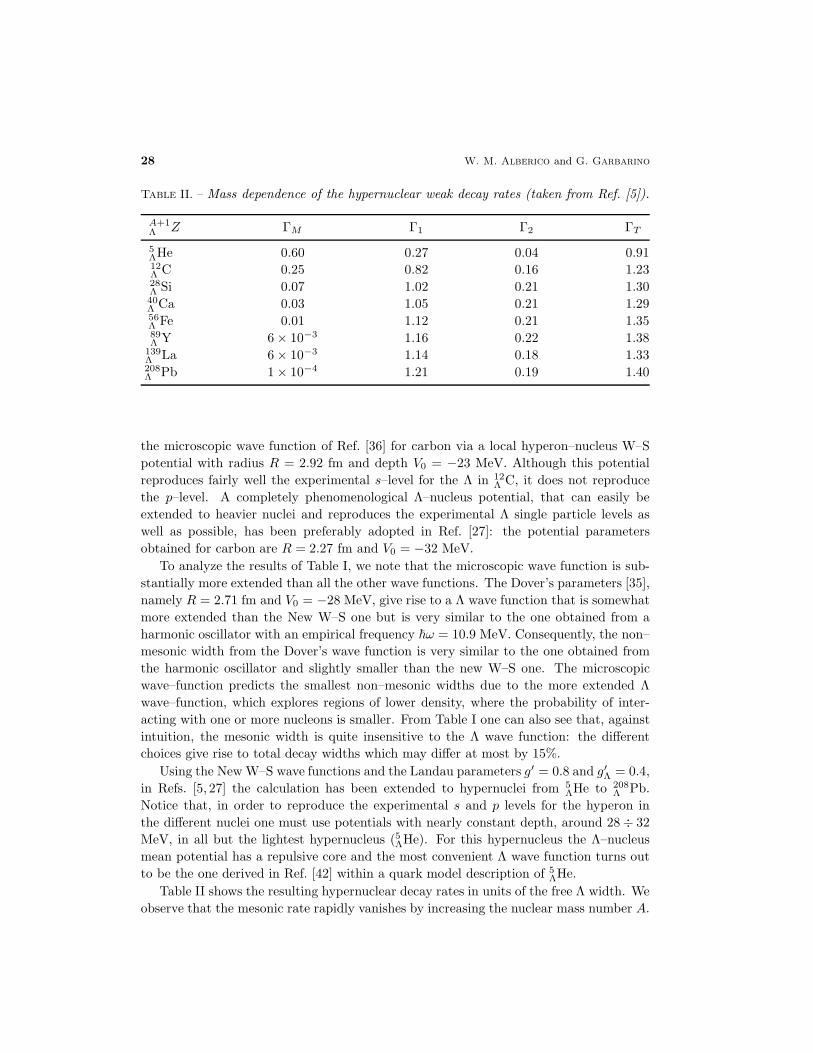
Table II. – Mass dependence of the hypernuclear weak decay rates (taken from Ref. [5]).
A+1Λ Z ΓM Γ1 Γ2 ΓT
5ΛHe 0.60 0.27 0.04 0.9112Λ C 0.25 0.82 0.16 1.2328Λ Si 0.07 1.02 0.21 1.3040Λ Ca 0.03 1.05 0.21 1.2956Λ Fe 0.01 1.12 0.21 1.3589Λ Y 6 × 10⁻³ 1.16 0.22 1.38
139Λ La 6 × 10⁻³ 1.14 0.18 1.33208Λ Pb 1 × 10⁻⁴ 1.21 0.19 1.40
the microscopic wave function of Ref. [36] for carbon via a local hyperon–nucleus W–S
potential with radius R = 2.92 fm and depth V0 = −23 MeV. Although this potential
reproduces fairly well the experimental s–level for the Λ in 12Λ C, it does not reproduce
the p–level. A completely phenomenological Λ–nucleus potential, that can easily be
extended to heavier nuclei and reproduces the experimental Λ single particle levels as
well as possible, has been preferably adopted in Ref. [27]: the potential parameters
obtained for carbon are R = 2.27 fm and V0 = −32 MeV.
To analyze the results of Table I, we note that the microscopic wave function is sub-
stantially more extended than all the other wave functions. The Dover’s parameters [35],
namely R = 2.71 fm and V0 = −28 MeV, give rise to a Λ wave function that is somewhat
more extended than the New W–S one but is very similar to the one obtained from a
harmonic oscillator with an empirical frequency ~ω = 10.9 MeV. Consequently, the non–
mesonic width from the Dover’s wave function is very similar to the one obtained from
the harmonic oscillator and slightly smaller than the new W–S one. The microscopic
wave–function predicts the smallest non–mesonic widths due to the more extended Λ
wave–function, which explores regions of lower density, where the probability of inter-
acting with one or more nucleons is smaller. From Table I one can also see that, against
intuition, the mesonic width is quite insensitive to the Λ wave function: the different
choices give rise to total decay widths which may differ at most by 15%.
Using the New W–S wave functions and the Landau parameters g′ = 0.8 and g′Λ = 0.4,
in Refs. [5, 27] the calculation has been extended to hypernuclei from 5ΛHe to 208
Λ Pb.
Notice that, in order to reproduce the experimental s and p levels for the hyperon in
the different nuclei one must use potentials with nearly constant depth, around 28 ÷ 32
MeV, in all but the lightest hypernucleus (5ΛHe). For this hypernucleus the Λ–nucleus
mean potential has a repulsive core and the most convenient Λ wave function turns out
to be the one derived in Ref. [42] within a quark model description of 5ΛHe.
Table II shows the resulting hypernuclear decay rates in units of the free Λ width. We
observe that the mesonic rate rapidly vanishes by increasing the nuclear mass number A.
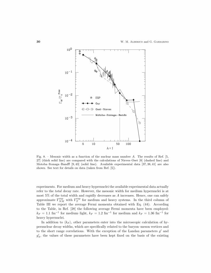
Weak decay of hypernuclei 29
This is well known and it is related to the decreasing phase space allowed for the mesonic
channel, and to smaller overlaps between the Λ wave function and the nuclear surface,
as A increases. In Fig. 8 the results of Ref. [5, 27] for ΓM are compared with the ones of
Nieves–Oset [8] and Motoba–Itonaga–Bando [9, 43], which were obtained within a shell
model framework. Also the central values of the available experimental data are shown.
Although the WFM is more reliable than the LDA for the evaluation of the mesonic
rates (since the small energies involved in the decay amplify the effects of the nuclear
shell structure), one sees that the LDA calculation of Ref. [27] fairly agrees with the WFM
ones and with the data. In particular, Table II shows that the results for 12Λ C and 28
Λ Si are
in agreement with the very recent KEK measurements [41]: ΓM(12Λ C)/ΓfreeΛ = 0.31±0.07,
Γπ−(28Λ Si)/ΓfreeΛ = 0.046±0.011. The results for 40
Λ Ca, 56Λ Fe and 89
Λ Y are in agreement with
the old emulsion data (quoted in Ref. [12]), which indicates Γπ−/ΓNM ≃ (0.5÷ 1)× 10−2
in the region 40 < A < 100. Moreover, the recent KEK experiments [41] obtained the
limit: Γπ−(56Λ Fe)/ΓfreeΛ < 0.015 (90% CL). It is worth noticing, in figure 8, the rather
pronounced oscillations of ΓM in the calculation of Refs. [9, 43], which are caused by shell
effects.
As a final comment to Table II, we note that, with the exception of 5ΛHe, the two–
body induced decay is rather independent of the hypernuclear dimension and it is about
15% of the total width. Previous works [26, 44] gave more emphasis to this new channel,
without, however, reproducing the experimental non–mesonic rates. The total width
does not change much with A, as it is also shown by the experiment.
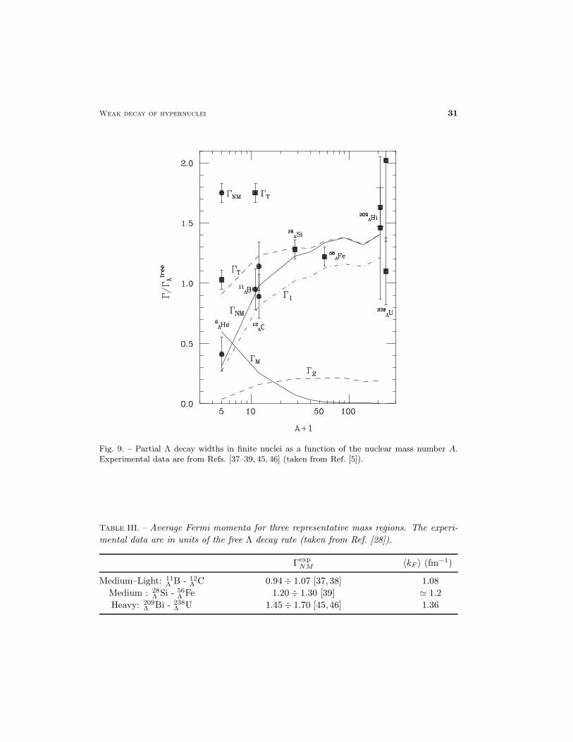
In Fig. 9 the results of Table II are compared with recent (after 1990) experimental
data for ΓNM and ΓT. The theoretical results are in good agreement with the data
over the whole hypernuclear mass range explored. The saturation of the ΛN → nN
interaction in nuclei is well reproduced.
4.2. Microscopic approach. – The results discussed in this subsection have been ob-
tained by applying the one–boson–loop formalism developed in Section 3.3.2 for nuclear
matter. Although, in principle, one could extend this calculation to finite nuclei through
the local density approximation, in practice this would require prohibitive computing
times. Indeed, the latter are already quite conspicuous for the evaluation of the dia-
grams of Fig. 7 at fixed Fermi momentum. Hence, in order to compare the results with
the experimental data in finite nuclei, different Fermi momenta have been employed in
the nuclear matter calculation. The average, fixed Fermi momentum, which is appropri-
ate for the present purposes, has been obtained by weighting each local Fermi momentum
kAF (r) with the probability density of the hyperon in the considered nucleus:
(44) 〈kF 〉A =
∫
d~r kAF (~r)|ψΛ(~r)|2.
It is then possible to classify the hypernuclei for which experimental data on the non–
mesonic decay rate are available into three mass regions (medium–light: A ≃ 10; medium:
A ≃ 30÷ 60; and heavy hypernuclei: A >∼ 200), as shown in Table III. The experimental
bands include values of the non–mesonic widths which are compatible with the quoted
30 W. M. Alberico and G. Garbarino
Fig. 8. – Mesonic width as a function of the nuclear mass number A. The results of Ref. [5,27] (thick solid line) are compared with the calculations of Nieves–Oset [8] (dashed line) andMotoba–Itonaga–Bando [9, 43] (solid line). Available experimental data [37, 38, 41] are alsoshown. See text for details on data (taken from Ref. [5]).
experiments. For medium and heavy hypernuclei the available experimental data actually
refer to the total decay rate. However, the mesonic width for medium hypernuclei is at
most 5% of the total width and rapidly decreases as A increases. Hence, one can safely
approximate ΓexpNM with Γexp
T for medium and heavy systems. In the third column of
Table III we report the average Fermi momenta obtained with Eq. (44). According
to the Table, in Ref. [28] the following average Fermi momenta have been employed:
kF = 1.1 fm−1 for medium–light, kF = 1.2 fm−1 for medium and kF = 1.36 fm−1 for
heavy hypernuclei.
In addition to 〈kF 〉, other parameters enter into the microscopic calculation of hy-
pernuclear decay widths, which are specifically related to the baryon–meson vertices and
to the short range correlations. With the exception of the Landau parameters g′ and
g′Λ, the values of these parameters have been kept fixed on the basis of the existing
Weak decay of hypernuclei 31
Fig. 9. – Partial Λ decay widths in finite nuclei as a function of the nuclear mass number A.Experimental data are from Refs. [37–39, 45, 46] (taken from Ref. [5]).
Table III. – Average Fermi momenta for three representative mass regions. The experi-
mental data are in units of the free Λ decay rate (taken from Ref. [28]).
ΓexpNM 〈kF 〉 (fm−1)
Medium–Light: 11Λ B - 12
Λ C 0.94 ÷ 1.07 [37, 38] 1.08
Medium : 28Λ Si - 56
Λ Fe 1.20 ÷ 1.30 [39] ≃ 1.2
Heavy: 209Λ Bi - 238
Λ U 1.45 ÷ 1.70 [45, 46] 1.36
32 W. M. Alberico and G. Garbarino
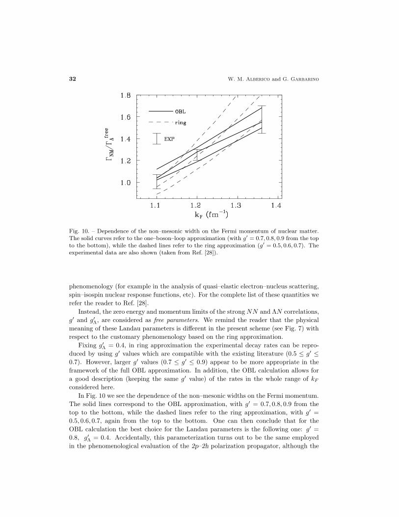
Fig. 10. – Dependence of the non–mesonic width on the Fermi momentum of nuclear matter.The solid curves refer to the one–boson–loop approximation (with g′ = 0.7, 0.8, 0.9 from the topto the bottom), while the dashed lines refer to the ring approximation (g′ = 0.5, 0.6, 0.7). Theexperimental data are also shown (taken from Ref. [28]).
phenomenology (for example in the analysis of quasi–elastic electron–nucleus scattering,
spin–isospin nuclear response functions, etc). For the complete list of these quantities we
refer the reader to Ref. [28].
Instead, the zero energy and momentum limits of the strongNN and ΛN correlations,
g′ and g′Λ, are considered as free parameters. We remind the reader that the physical
meaning of these Landau parameters is different in the present scheme (see Fig. 7) with
respect to the customary phenomenology based on the ring approximation.
Fixing g′Λ = 0.4, in ring approximation the experimental decay rates can be repro-
duced by using g′ values which are compatible with the existing literature (0.5 ≤ g′ ≤0.7). However, larger g′ values (0.7 ≤ g′ ≤ 0.9) appear to be more appropriate in the
framework of the full OBL approximation. In addition, the OBL calculation allows for
a good description (keeping the same g′ value) of the rates in the whole range of kF
considered here.
In Fig. 10 we see the dependence of the non–mesonic widths on the Fermi momentum.
The solid lines correspond to the OBL approximation, with g′ = 0.7, 0.8, 0.9 from the
top to the bottom, while the dashed lines refer to the ring approximation, with g′ =
0.5, 0.6, 0.7, again from the top to the bottom. One can then conclude that for the
OBL calculation the best choice for the Landau parameters is the following one: g′ =
0.8, g′Λ = 0.4. Accidentally, this parameterization turns out to be the same employed
in the phenomenological evaluation of the 2p–2h polarization propagator, although the
Weak decay of hypernuclei 33
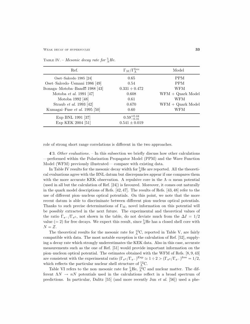
Table IV. – Mesonic decay rate for 5ΛHe.
Ref. ΓM/ΓfreeΛ Model
Oset–Salcedo 1985 [24] 0.65 PPM
Oset–Salcedo–Usmani 1986 [49] 0.54 PPM
Itonaga–Motoba–Bando 1988 [43] 0.331 ÷ 0.472 WFM
Motoba et al. 1991 [47] 0.608 WFM + Quark Model
Motoba 1992 [48] 0.61 WFM
Straub et al. 1993 [42] 0.670 WFM + Quark Model
Kumagai–Fuse et al. 1995 [50] 0.60 WFM
Exp BNL 1991 [37] 0.59+0.44−0.31
Exp KEK 2004 [51] 0.541 ± 0.019
role of strong short range correlations is different in the two approaches.
4.3. Other evaluations . – In this subsection we briefly discuss how other calculations
—performed within the Polarization Propagator Model (PPM) and the Wave Function
Model (WFM) previously illustrated— compare with existing data.
In Table IV results for the mesonic decay width for 5ΛHe are reported. All the theoreti-
cal evaluations agree with the BNL datum but discrepancies appear if one compares them
with the more accurate KEK observation. A repulsive core in the Λ–α mean potential
(used in all but the calculation of Ref. [24]) is favoured. Moreover, it comes out naturally
in the quark model descriptions of Refs. [42, 47]. The results of Refs. [43, 48] refer to the
use of different pion–nucleus optical potentials. On this point, we note that the more
recent datum is able to discriminate between different pion–nucleus optical potentials.
Thanks to such precise determinations of ΓM, novel information on this potential will
be possibly extracted in the next future. The experimental and theoretical values of
the ratio Γπ−/Γπ0 , not shown in the table, do not deviate much from the ∆I = 1/2
value (= 2) for free decays. We expect this result, since 5ΛHe has a closed shell core with
N = Z.
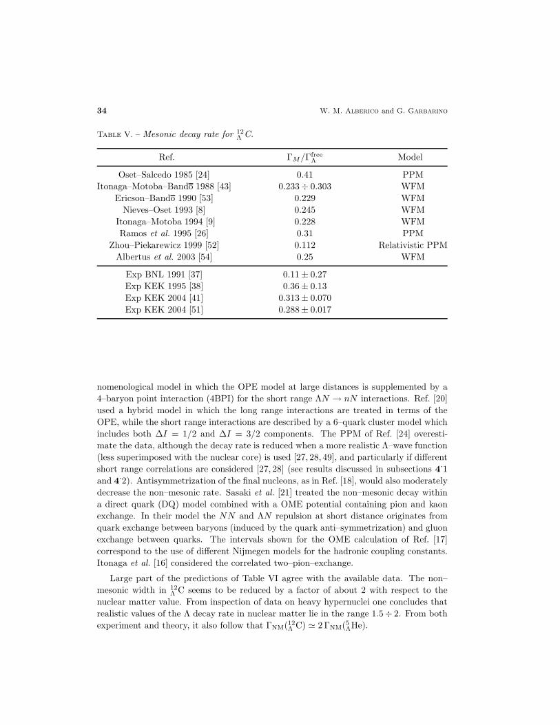
The theoretical results for the mesonic rate for 12Λ C, reported in Table V, are fairly
compatible with data. The most notable exception is the calculation of Ref. [52], supply-
ing a decay rate which strongly underestimates the KEK data. Also in this case, accurate
measurements such as the one of Ref. [51] would provide important information on the
pion–nucleon optical potential. The estimates obtained with the WFM of Refs. [8, 9, 43]
are consistent with the experimental ratio (Γπ0/Γπ−)Exp ≃ 1÷ 2 > (Γπ0/Γπ−)free = 1/2,
which reflects the particular nuclear shell structure of 12Λ C.
Table VI refers to the non–mesonic rate for 5ΛHe, 12
Λ C and nuclear matter. The dif-
ferent ΛN → nN potentials used in the calculations reflect in a broad spectrum of
predictions. In particular, Dalitz [55] (and more recently Jun et al. [56]) used a phe-
34 W. M. Alberico and G. Garbarino
Table V. – Mesonic decay rate for 12Λ C.
Ref. ΓM/ΓfreeΛ Model
Oset–Salcedo 1985 [24] 0.41 PPM
Itonaga–Motoba–Bando 1988 [43] 0.233÷ 0.303 WFM
Ericson–Bando 1990 [53] 0.229 WFM
Nieves–Oset 1993 [8] 0.245 WFM
Itonaga–Motoba 1994 [9] 0.228 WFM
Ramos et al. 1995 [26] 0.31 PPM
Zhou–Piekarewicz 1999 [52] 0.112 Relativistic PPM
Albertus et al. 2003 [54] 0.25 WFM
Exp BNL 1991 [37] 0.11 ± 0.27
Exp KEK 1995 [38] 0.36 ± 0.13
Exp KEK 2004 [41] 0.313± 0.070
Exp KEK 2004 [51] 0.288± 0.017
nomenological model in which the OPE model at large distances is supplemented by a
4–baryon point interaction (4BPI) for the short range ΛN → nN interactions. Ref. [20]
used a hybrid model in which the long range interactions are treated in terms of the
OPE, while the short range interactions are described by a 6–quark cluster model which
includes both ∆I = 1/2 and ∆I = 3/2 components. The PPM of Ref. [24] overesti-
mate the data, although the decay rate is reduced when a more realistic Λ–wave function
(less superimposed with the nuclear core) is used [27, 28, 49], and particularly if different
short range correlations are considered [27, 28] (see results discussed in subsections 4.1
and 4.2). Antisymmetrization of the final nucleons, as in Ref. [18], would also moderately
decrease the non–mesonic rate. Sasaki et al. [21] treated the non–mesonic decay within
a direct quark (DQ) model combined with a OME potential containing pion and kaon
exchange. In their model the NN and ΛN repulsion at short distance originates from
quark exchange between baryons (induced by the quark anti–symmetrization) and gluon
exchange between quarks. The intervals shown for the OME calculation of Ref. [17]
correspond to the use of different Nijmegen models for the hadronic coupling constants.
Itonaga et al. [16] considered the correlated two–pion–exchange.
Large part of the predictions of Table VI agree with the available data. The non–
mesonic width in 12Λ C seems to be reduced by a factor of about 2 with respect to the
nuclear matter value. From inspection of data on heavy hypernuclei one concludes that
realistic values of the Λ decay rate in nuclear matter lie in the range 1.5÷ 2. From both
experiment and theory, it also follow that ΓNM(12Λ C) ≃ 2 ΓNM(5ΛHe).
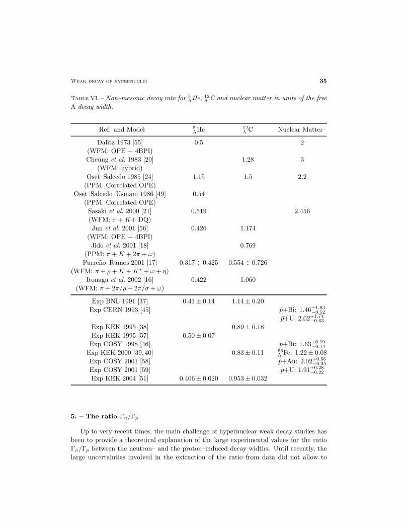
Weak decay of hypernuclei 35
Table VI. – Non–mesonic decay rate for 5ΛHe, 12
Λ C and nuclear matter in units of the free
Λ decay width.
Ref. and Model 5ΛHe 12
Λ C Nuclear Matter
Dalitz 1973 [55] 0.5 2
(WFM: OPE + 4BPI)
Cheung et al. 1983 [20] 1.28 3
(WFM: hybrid)
Oset–Salcedo 1985 [24] 1.15 1.5 2.2
(PPM: Correlated OPE)
Oset–Salcedo–Usmani 1986 [49] 0.54
(PPM: Correlated OPE)
Sasaki et al. 2000 [21] 0.519 2.456
(WFM: π +K+ DQ)
Jun et al. 2001 [56] 0.426 1.174
(WFM: OPE + 4BPI)
Jido et al. 2001 [18] 0.769
(PPM: π +K + 2π + ω)
Parreno–Ramos 2001 [17] 0.317÷ 0.425 0.554 ÷ 0.726
(WFM: π + ρ+K +K∗ + ω + η)
Itonaga et al. 2002 [16] 0.422 1.060
(WFM: π + 2π/ρ+ 2π/σ + ω)
Exp BNL 1991 [37] 0.41 ± 0.14 1.14 ± 0.20
Exp CERN 1993 [45] p+Bi: 1.46+1.83−0.52
p+U: 2.02+1.74−0.63
Exp KEK 1995 [38] 0.89 ± 0.18
Exp KEK 1995 [57] 0.50 ± 0.07
Exp COSY 1998 [46] p+Bi: 1.63+0.19−0.14
Exp KEK 2000 [39, 40] 0.83 ± 0.11 56Λ Fe: 1.22 ± 0.08
Exp COSY 2001 [58] p+Au: 2.02+0.56−0.35
Exp COSY 2001 [59] p+U: 1.91+0.28−0.22
Exp KEK 2004 [51] 0.406± 0.020 0.953 ± 0.032
5. – The ratio Γn/Γp
Up to very recent times, the main challenge of hypernuclear weak decay studies has
been to provide a theoretical explanation of the large experimental values for the ratio
Γn/Γp between the neutron– and the proton–induced decay widths. Until recently, the
large uncertainties involved in the extraction of the ratio from data did not allow to
36 W. M. Alberico and G. Garbarino
reach any definitive conclusion. The data were quite limited and not precise due to the
difficulty of detecting the products of the non–mesonic decays, especially the neutrons.
Moreover, up to now it has not been possible to distinguish between nucleons produced
by the one–body induced and the (non–negligible) two–body induced decay mechanism.
However, due to recent theoretical [16–18, 21, 60] and experimental [61–63] progress, we
are now towards a solution of the Γn/Γp puzzle. In this section we review these important
developments.
The one–pion–exchange approximation with the ∆I = 1/2 rule provides small ratios:
(45)
[
Γn
Γp
]OPE
≃ 0.05 ÷ 0.20,
for all the considered systems. This is due to the ∆I = 1/2 rule, which fixes the vertex
ratio VΛπ−p/VΛπ0n = −√
2 (both in S– and P–wave interactions), and to the particular
form of the OPE potential, which has a strong tensor component requiring isospin 0 np
pairs in the antisymmetric final state. In p–shell and heavier hypernuclei the relative
ΛN L = 1 state is found to give only a small contribution to tensor transitions for the
neutron–induced decay, so it cannot improve the OPE ratio. The contribution of the ΛN
L = 1 relative state to ΓNM seems to be of about 5 ÷ 15% in p–shell hypernuclei [17].
For these systems we expect the dominance of the S–wave interaction in the initial state,
due to the small ΛN relative momentum. By using a simple argument about the isospin
structure of the transition ΛN → nN in OPE, it is possible to estimate that for pure
∆I = 3/2 transitions (VΛπ−p/VΛπ0n = 1/√
2) the OPE ratio can increase up to about
0.5. However, the OPE model with ∆I = 1/2 couplings has been able to reproduce the
one–body stimulated non–mesonic rates Γ1 = Γn + Γp for light and medium hypernuclei
[16–18, 21, 27, 28].
Other interaction mechanisms beyond the OPE might then be responsible for the
overestimation of Γp and the underestimation of Γn. Many attempts have been made up
to now in order to solve the Γn/Γp puzzle. We recall here the inclusion in the ΛN → nN
transition potential of mesons heavier than the pion [14–18], the inclusion of interaction
terms that explicitly violate the ∆I = 1/2 rule [19] and the description of the short range
baryon–baryon interaction in terms of quark degrees of freedom [20, 21], which automat-
ically introduces ∆I = 3/2 contributions. It is important to note that a few calculations
with ΛN → nN transition potentials including heavy–meson–exchange and/or direct
quark contributions [16–18, 21] have improved the situation, without providing, never-
theless, a satisfactory explanation of the origin of the puzzle. The tensor component
of K–exchange has opposite sign with respect to the one for π–exchange, resulting in a
reduction of Γp. The parity violating ΛN(3S1) → nN(3P1) transition, which contributes
to both the n– and p–induced processes, is considerably enhanced by K–exchange and
direct quark mechanism and tends to increase Γn/Γp.
In table VII we summarize the calculations that predicted ratios considerably en-
hanced with respect to the OPE values. Experimental data are given for comparison.
Almost all calculations reproduce the observed non–mesonic widths Γn + Γp, as one can
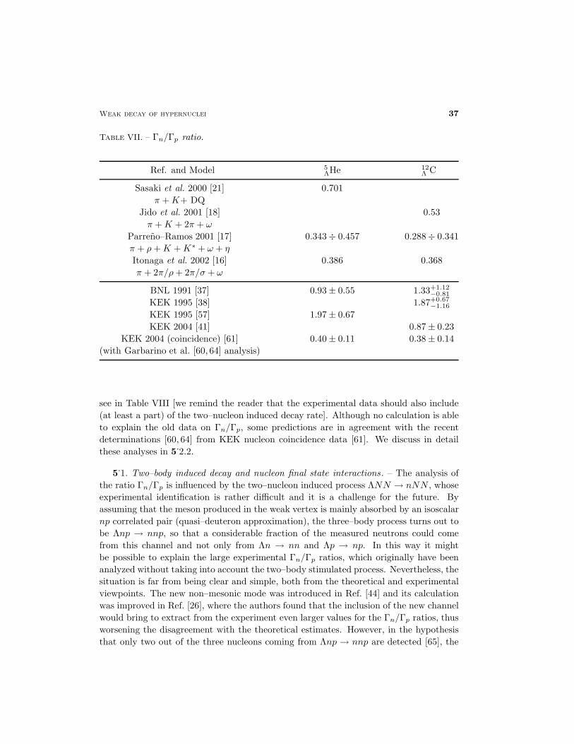
Weak decay of hypernuclei 37
Table VII. – Γn/Γp ratio.
Ref. and Model 5ΛHe 12
Λ C
Sasaki et al. 2000 [21] 0.701
π +K+ DQ
Jido et al. 2001 [18] 0.53
π +K + 2π + ω
Parreno–Ramos 2001 [17] 0.343 ÷ 0.457 0.288÷ 0.341
π + ρ+K +K∗ + ω + η
Itonaga et al. 2002 [16] 0.386 0.368
π + 2π/ρ+ 2π/σ + ω
BNL 1991 [37] 0.93 ± 0.55 1.33+1.12−0.81
KEK 1995 [38] 1.87+0.67−1.16
KEK 1995 [57] 1.97 ± 0.67
KEK 2004 [41] 0.87 ± 0.23
KEK 2004 (coincidence) [61] 0.40 ± 0.11 0.38 ± 0.14
(with Garbarino et al. [60, 64] analysis)
see in Table VIII [we remind the reader that the experimental data should also include
(at least a part) of the two–nucleon induced decay rate]. Although no calculation is able
to explain the old data on Γn/Γp, some predictions are in agreement with the recent
determinations [60, 64] from KEK nucleon coincidence data [61]. We discuss in detail
these analyses in 5.2.2.
5.1. Two–body induced decay and nucleon final state interactions . – The analysis of
the ratio Γn/Γp is influenced by the two–nucleon induced process ΛNN → nNN , whose
experimental identification is rather difficult and it is a challenge for the future. By
assuming that the meson produced in the weak vertex is mainly absorbed by an isoscalar
np correlated pair (quasi–deuteron approximation), the three–body process turns out to
be Λnp → nnp, so that a considerable fraction of the measured neutrons could come
from this channel and not only from Λn → nn and Λp → np. In this way it might
be possible to explain the large experimental Γn/Γp ratios, which originally have been
analyzed without taking into account the two–body stimulated process. Nevertheless, the
situation is far from being clear and simple, both from the theoretical and experimental
viewpoints. The new non–mesonic mode was introduced in Ref. [44] and its calculation
was improved in Ref. [26], where the authors found that the inclusion of the new channel
would bring to extract from the experiment even larger values for the Γn/Γp ratios, thus
worsening the disagreement with the theoretical estimates. However, in the hypothesis
that only two out of the three nucleons coming from Λnp → nnp are detected [65], the
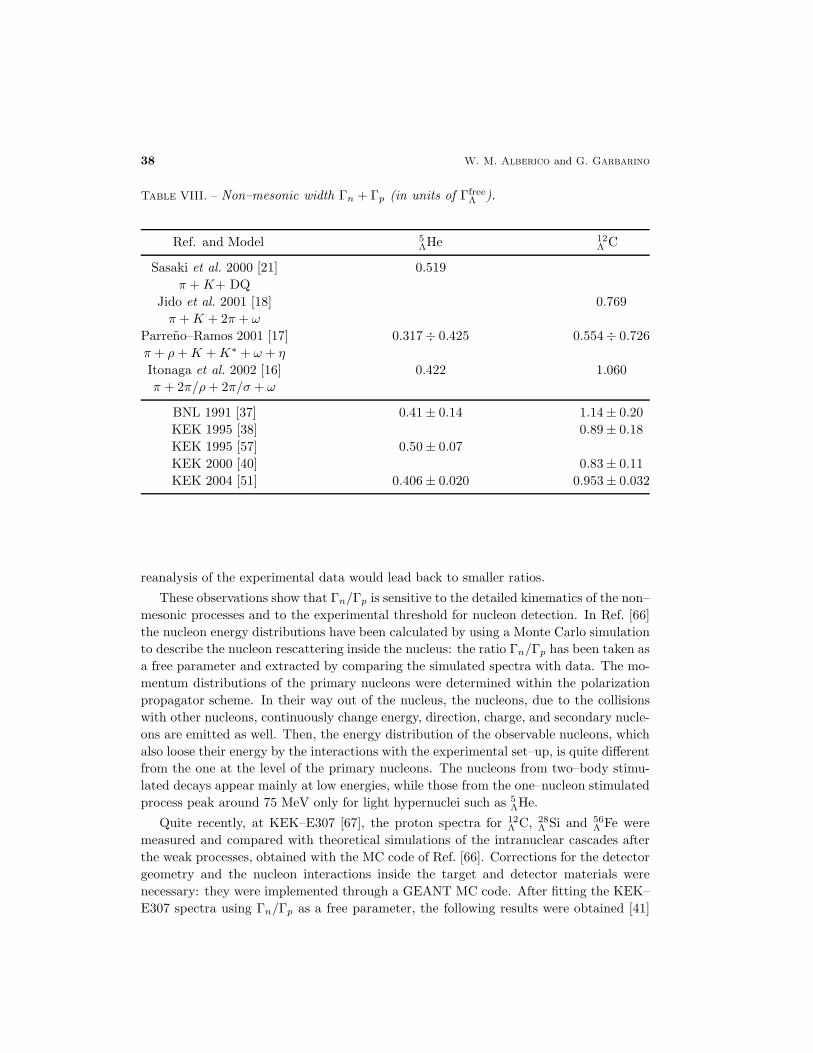
38 W. M. Alberico and G. Garbarino
Table VIII. – Non–mesonic width Γn + Γp (in units of ΓfreeΛ ).
Ref. and Model 5ΛHe 12
Λ C
Sasaki et al. 2000 [21] 0.519
π +K+ DQ
Jido et al. 2001 [18] 0.769
π +K + 2π + ω
Parreno–Ramos 2001 [17] 0.317 ÷ 0.425 0.554÷ 0.726
π + ρ+K +K∗ + ω + η
Itonaga et al. 2002 [16] 0.422 1.060
π + 2π/ρ+ 2π/σ + ω
BNL 1991 [37] 0.41 ± 0.14 1.14 ± 0.20
KEK 1995 [38] 0.89 ± 0.18
KEK 1995 [57] 0.50 ± 0.07
KEK 2000 [40] 0.83 ± 0.11
KEK 2004 [51] 0.406 ± 0.020 0.953± 0.032
reanalysis of the experimental data would lead back to smaller ratios.
These observations show that Γn/Γp is sensitive to the detailed kinematics of the non–
mesonic processes and to the experimental threshold for nucleon detection. In Ref. [66]
the nucleon energy distributions have been calculated by using a Monte Carlo simulation
to describe the nucleon rescattering inside the nucleus: the ratio Γn/Γp has been taken as
a free parameter and extracted by comparing the simulated spectra with data. The mo-
mentum distributions of the primary nucleons were determined within the polarization
propagator scheme. In their way out of the nucleus, the nucleons, due to the collisions
with other nucleons, continuously change energy, direction, charge, and secondary nucle-
ons are emitted as well. Then, the energy distribution of the observable nucleons, which
also loose their energy by the interactions with the experimental set–up, is quite different
from the one at the level of the primary nucleons. The nucleons from two–body stimu-
lated decays appear mainly at low energies, while those from the one–nucleon stimulated
process peak around 75 MeV only for light hypernuclei such as 5ΛHe.
Quite recently, at KEK–E307 [67], the proton spectra for 12Λ C, 28
Λ Si and 56Λ Fe were
measured and compared with theoretical simulations of the intranuclear cascades after
the weak processes, obtained with the MC code of Ref. [66]. Corrections for the detector
geometry and the nucleon interactions inside the target and detector materials were
necessary: they were implemented through a GEANT MC code. After fitting the KEK–
E307 spectra using Γn/Γp as a free parameter, the following results were obtained [41]
Weak decay of hypernuclei 39
by neglecting the two–nucleon induced decay channel:
Γn
Γp(12Λ C) = 0.87 ± 0.23,(46)
Γn
Γp(28Λ Si) = 0.79+0.28
−0.26,
Γn
Γp(56Λ Fe) = 1.13+0.29
−0.27.
All the existing calculations underestimate the 12Λ C result (see Table VII). The Γn/Γp
ratios of Eq. (46) confirm the results of previous experiments: the neutron– and proton–
induced decay rates appear to be of the same order of magnitude over a large hypernuclear
mass number range. However, since the new experiments have significantly improved the
quality of the data, small values of Γn/Γp (say smaller than 0.5 for 12Λ C, as predicted by
theory) seem to be excluded.
5.2. Towards a solution of the Γn/Γp puzzle. – Fortunately, recent important devel-
opments have contributed to approach the solution of the Γn/Γp puzzle. This progress
has been based on the following main ideas:
1) The proton spectra originating from neutron– and proton–induced processes (and,
eventually, from two–nucleon stimulated decays) are added incoherently in the
Monte Carlo intranuclear cascade code used to determine Γn/Γp from data. In
this way a possible quantum–mechanical interference effect between the two chan-
nels is lost. Therefore, extracting Γn/Γp from data with the help of a classical
intranuclear cascade calculation may not be a clean task. The consequences of this
idea have been explored in Ref. [60].
2) In order to perform, as desirable, a direct measurement of Γn/Γp one needs to
detect the outgoing neutrons. In principle, neutron spectra can be measured down
to about 10 MeV kinetic energy since they are less affected than the proton ones
by energy losses in the target and detector materials. Besides, the joint observa-
tion of proton and neutron spectra could help to disentangle the set–up material
effects from the nucleon FSI occurring inside the residual nucleus. A recent ex-
periment, KEK–E369, measured neutron spectra from 12Λ C and 89
Λ Y non–mesonic
decays [62]. With other experiments, KEK–E462 and KEK–E408 [63], proton and
neutron spectra could be simultaneously measured for 5ΛHe and 12
Λ C. An analysis
of these data has been done in Ref. [60] and is discussed in 5.2.1.
3) One could avoid the possible deficiencies of the single nucleon spectra measure-
ments discussed in point 1) by employing nucleon–nucleon coincidence measure-
ments, which should indeed permit a cleaner extraction of Γn/Γp. Coincidence
observations are also expected to be less affected by FSI effects and to help in the
direct observation of two–nucleon induced decay events. In the experiments KEK–
E462 and KEK–E508 [61], nn and np angular and energy correlation measurements
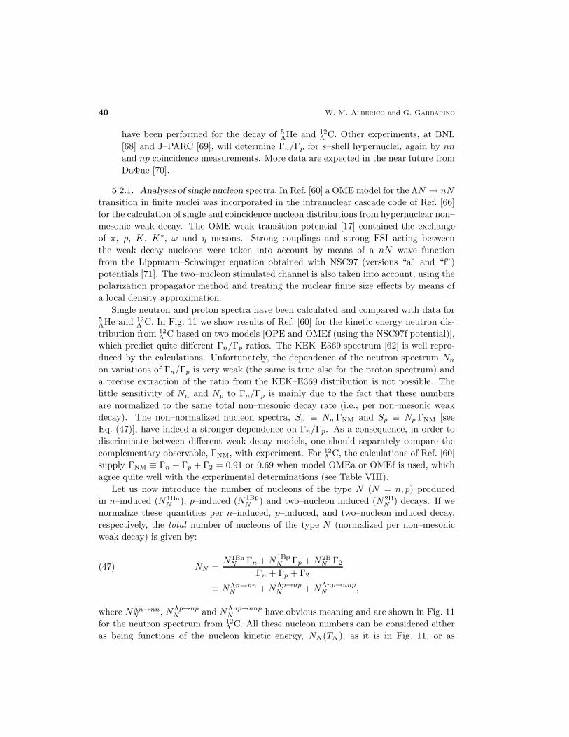
40 W. M. Alberico and G. Garbarino
have been performed for the decay of 5ΛHe and 12
Λ C. Other experiments, at BNL
[68] and J–PARC [69], will determine Γn/Γp for s–shell hypernuclei, again by nn
and np coincidence measurements. More data are expected in the near future from
DaΦne [70].
5.2.1. Analyses of single nucleon spectra. In Ref. [60] a OME model for the ΛN → nN
transition in finite nuclei was incorporated in the intranuclear cascade code of Ref. [66]
for the calculation of single and coincidence nucleon distributions from hypernuclear non–
mesonic weak decay. The OME weak transition potential [17] contained the exchange
of π, ρ, K, K∗, ω and η mesons. Strong couplings and strong FSI acting between
the weak decay nucleons were taken into account by means of a nN wave function
from the Lippmann–Schwinger equation obtained with NSC97 (versions “a” and “f”)
potentials [71]. The two–nucleon stimulated channel is also taken into account, using the
polarization propagator method and treating the nuclear finite size effects by means of
a local density approximation.
Single neutron and proton spectra have been calculated and compared with data for5ΛHe and 12
Λ C. In Fig. 11 we show results of Ref. [60] for the kinetic energy neutron dis-
tribution from 12Λ C based on two models [OPE and OMEf (using the NSC97f potential)],
which predict quite different Γn/Γp ratios. The KEK–E369 spectrum [62] is well repro-
duced by the calculations. Unfortunately, the dependence of the neutron spectrum Nn
on variations of Γn/Γp is very weak (the same is true also for the proton spectrum) and
a precise extraction of the ratio from the KEK–E369 distribution is not possible. The
little sensitivity of Nn and Np to Γn/Γp is mainly due to the fact that these numbers
are normalized to the same total non–mesonic decay rate (i.e., per non–mesonic weak
decay). The non–normalized nucleon spectra, Sn ≡ Nn ΓNM and Sp ≡ Np ΓNM [see
Eq. (47)], have indeed a stronger dependence on Γn/Γp. As a consequence, in order to
discriminate between different weak decay models, one should separately compare the
complementary observable, ΓNM, with experiment. For 12Λ C, the calculations of Ref. [60]
supply ΓNM ≡ Γn + Γp + Γ2 = 0.91 or 0.69 when model OMEa or OMEf is used, which
agree quite well with the experimental determinations (see Table VIII).
Let us now introduce the number of nucleons of the type N (N = n, p) produced
in n–induced (N1BnN ), p–induced (N1Bp
N ) and two–nucleon induced (N2BN ) decays. If we
normalize these quantities per n–induced, p–induced, and two–nucleon induced decay,
respectively, the total number of nucleons of the type N (normalized per non–mesonic
weak decay) is given by:
NN =N1Bn
N Γn +N1BpN Γp +N2B
N Γ2
Γn + Γp + Γ2(47)
≡ NΛn→nnN +NΛp→np
N +NΛnp→nnpN ,
where NΛn→nnN , NΛp→np
N and NΛnp→nnpN have obvious meaning and are shown in Fig. 11
for the neutron spectrum from 12Λ C. All these nucleon numbers can be considered either
as being functions of the nucleon kinetic energy, NN(TN ), as it is in Fig. 11, or as
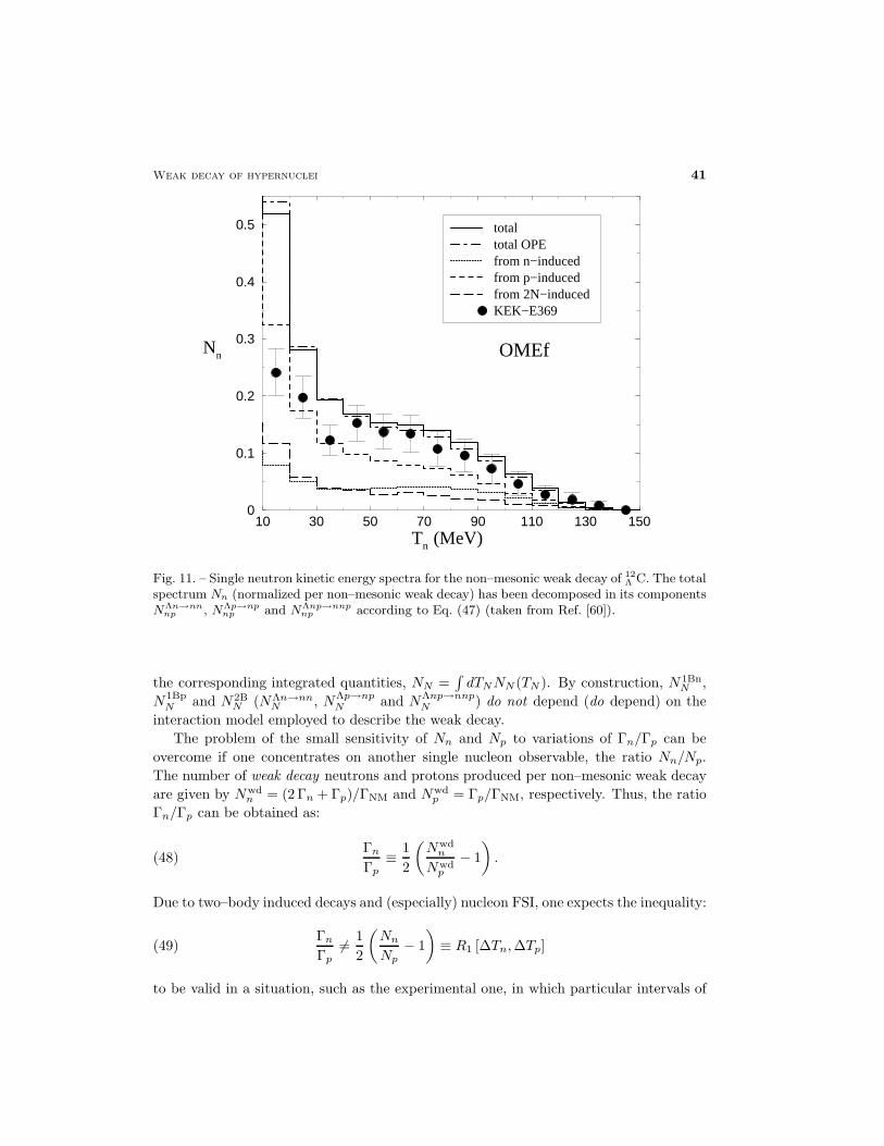
Weak decay of hypernuclei 41
10 30 50 70 90 110 130 150Tn (MeV)
0
0.1
0.2
0.3
0.4
0.5
Nn
total total OPE from n−induced from p−induced from 2N−induced KEK−E369
OMEf
Fig. 11. – Single neutron kinetic energy spectra for the non–mesonic weak decay of 12
Λ C. The totalspectrum Nn (normalized per non–mesonic weak decay) has been decomposed in its componentsNΛn→nn
np , NΛp→npnp and NΛnp→nnp
np according to Eq. (47) (taken from Ref. [60]).
the corresponding integrated quantities, NN =∫
dTNNN (TN ). By construction, N1BnN ,
N1BpN and N2B
N (NΛn→nnN , NΛp→np
N and NΛnp→nnpN ) do not depend (do depend) on the
interaction model employed to describe the weak decay.
The problem of the small sensitivity of Nn and Np to variations of Γn/Γp can be
overcome if one concentrates on another single nucleon observable, the ratio Nn/Np.
The number of weak decay neutrons and protons produced per non–mesonic weak decay
are given by Nwdn = (2 Γn + Γp)/ΓNM and Nwd
p = Γp/ΓNM, respectively. Thus, the ratio
Γn/Γp can be obtained as:
(48)Γn
Γp≡ 1
2
(
Nwdn
Nwdp
− 1
)
.
Due to two–body induced decays and (especially) nucleon FSI, one expects the inequality:
(49)Γn
Γp6= 1
2
(
Nn
Np− 1
)
≡ R1 [∆Tn,∆Tp]
to be valid in a situation, such as the experimental one, in which particular intervals of
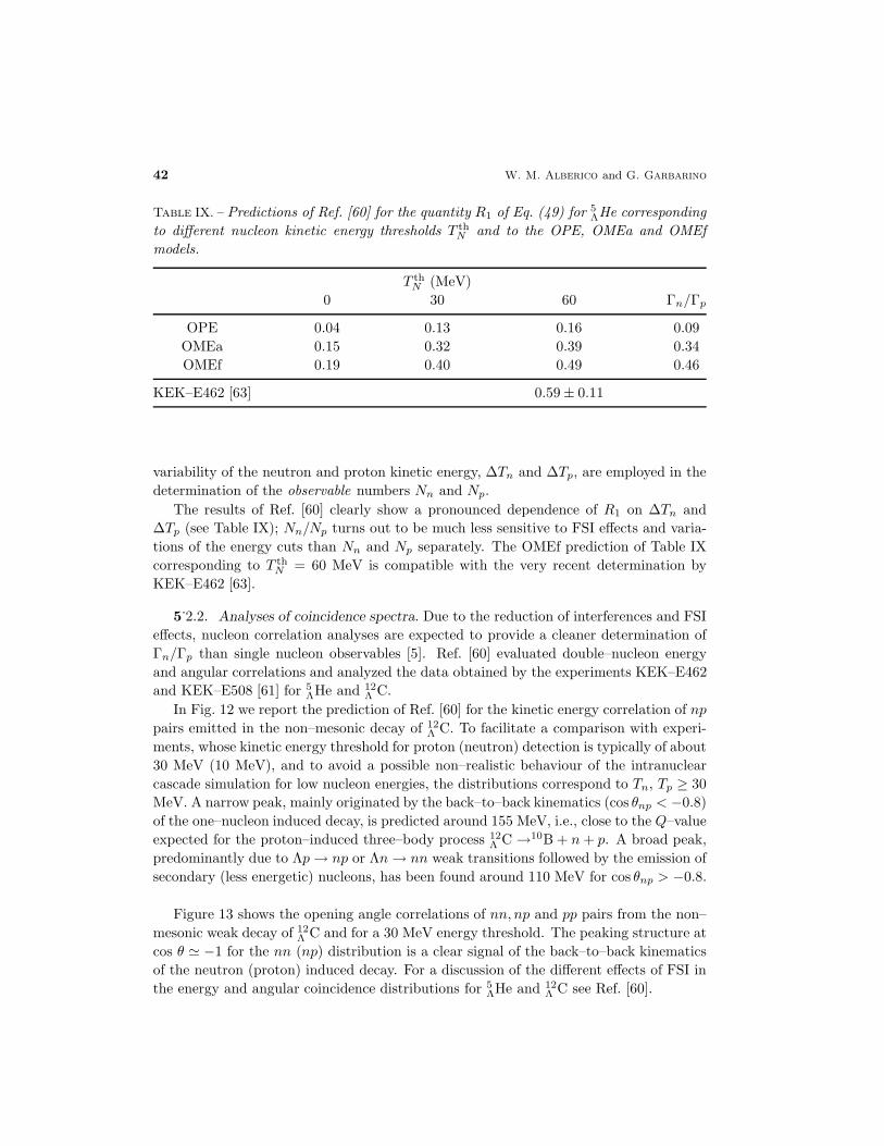
42 W. M. Alberico and G. Garbarino
Table IX. – Predictions of Ref. [60] for the quantity R1 of Eq. (49) for 5ΛHe corresponding
to different nucleon kinetic energy thresholds T thN and to the OPE, OMEa and OMEf
models.
T thN (MeV)
0 30 60 Γn/Γp
OPE 0.04 0.13 0.16 0.09
OMEa 0.15 0.32 0.39 0.34
OMEf 0.19 0.40 0.49 0.46
KEK–E462 [63] 0.59 ± 0.11
variability of the neutron and proton kinetic energy, ∆Tn and ∆Tp, are employed in the
determination of the observable numbers Nn and Np.
The results of Ref. [60] clearly show a pronounced dependence of R1 on ∆Tn and
∆Tp (see Table IX); Nn/Np turns out to be much less sensitive to FSI effects and varia-
tions of the energy cuts than Nn and Np separately. The OMEf prediction of Table IX
corresponding to T thN = 60 MeV is compatible with the very recent determination by
KEK–E462 [63].
5.2.2. Analyses of coincidence spectra. Due to the reduction of interferences and FSI
effects, nucleon correlation analyses are expected to provide a cleaner determination of
Γn/Γp than single nucleon observables [5]. Ref. [60] evaluated double–nucleon energy
and angular correlations and analyzed the data obtained by the experiments KEK–E462
and KEK–E508 [61] for 5ΛHe and 12
Λ C.
In Fig. 12 we report the prediction of Ref. [60] for the kinetic energy correlation of np
pairs emitted in the non–mesonic decay of 12Λ C. To facilitate a comparison with experi-
ments, whose kinetic energy threshold for proton (neutron) detection is typically of about
30 MeV (10 MeV), and to avoid a possible non–realistic behaviour of the intranuclear
cascade simulation for low nucleon energies, the distributions correspond to Tn, Tp ≥ 30
MeV. A narrow peak, mainly originated by the back–to–back kinematics (cos θnp < −0.8)
of the one–nucleon induced decay, is predicted around 155 MeV, i.e., close to the Q–value
expected for the proton–induced three–body process 12Λ C →10B + n+ p. A broad peak,
predominantly due to Λp→ np or Λn→ nn weak transitions followed by the emission of
secondary (less energetic) nucleons, has been found around 110 MeV for cos θnp > −0.8.
Figure 13 shows the opening angle correlations of nn, np and pp pairs from the non–
mesonic weak decay of 12Λ C and for a 30 MeV energy threshold. The peaking structure at
cos θ ≃ −1 for the nn (np) distribution is a clear signal of the back–to–back kinematics
of the neutron (proton) induced decay. For a discussion of the different effects of FSI in
the energy and angular coincidence distributions for 5ΛHe and 12
Λ C see Ref. [60].
Weak decay of hypernuclei 43
0 50 100 150 200 250Tn+Tp (MeV)
0
0.05
0.1
0.15
0.2
Nnp
Totalcos θnp > −0.8cos θnp < −0.8
Τn, Tp > 30 MeV
Fig. 12. – Kinetic energy correlations of np pairs emitted per non–mesonic decay of 12
Λ C (takenfrom Ref. [60]).
The ratio Γn/Γp is defined as the ratio between the number of weak decay nn and np
pairs, Nwdnn and Nwd
np . However, due to two–body induced decays and (especially) nucleon
FSI effects, one has:
(50)Γn
Γp≡ Nwd
nn
Nwdnp
6= Nnn
Nnp≡ R2 [∆θ12,∆Tn,∆Tp]
when the observable numbers Nnn and Nnp are determined by employing particular
intervals of variability of the pair opening angle, ∆θ12, and the nucleon kinetic energies,
∆Tn and ∆Tp. The discussion of Ref. [60] proves that Nnn/Nnp is much less sensitive to
FSI effects and variations of the energy cuts and angular restrictions than Nnn and Nnp
separately.
The numbers of nucleon pairs NNN discussed up to now and normalized per non–
mesonic weak decay are related to the corresponding quantities for the one–nucleon
(N1BNN ) and two–nucleon (N2B
NN ) induced processes [the former (latter) being normal-
ized per one–body (two–body) stimulated non–mesonic weak decay] via the following
equation:
(51) NNN =N1B
NN Γ1 +N2BNN Γ2
Γ1 + Γ2≡ NΛn→nn
NN +NΛp→npNN +NΛnp→nnp
NN ,
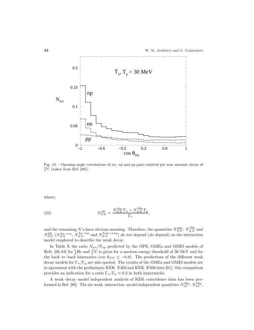
44 W. M. Alberico and G. Garbarino
−1 −0.6 −0.2 0.2 0.6 1cos θNN
0
0.05
0.1
0.15
0.2
NNN
Τn, Tp > 30 MeV
pp
nn
np
Fig. 13. – Opening angle correlations of nn, np and pp pairs emitted per non–mesonic decay of12
Λ C (taken from Ref. [60]).
where:
N1BNN =
N1BnNN Γn +N1Bp
NN Γp
Γ1,(52)
and the remaining N ’s have obvious meaning. Therefore, the quantities N1BnNN , N1Bp
NN and
N2BNN (NΛn→nn
NN , NΛp→npNN and NΛnp→nnp
NN ) do not depend (do depend) on the interaction
model employed to describe the weak decay.
In Table X the ratio Nnn/Nnp predicted by the OPE, OMEa and OMEf models of
Refs. [60, 64] for 5ΛHe and 12
Λ C is given for a nucleon energy threshold of 30 MeV and for
the back–to–back kinematics (cos θNN ≤ −0.8). The predictions of the different weak
decay models for Γn/Γp are also quoted. The results of the OMEa and OMEf models are
in agreement with the preliminary KEK–E462 and KEK–E508 data [61]: this comparison
provides an indication for a ratio Γn/Γp ≃ 0.3 in both hypernuclei.
A weak–decay–model independent analysis of KEK coincidence data has been per-
formed in Ref. [60]. The six weak–interaction–model independent quantitiesN1Bnnn , N1Bp
nn ,
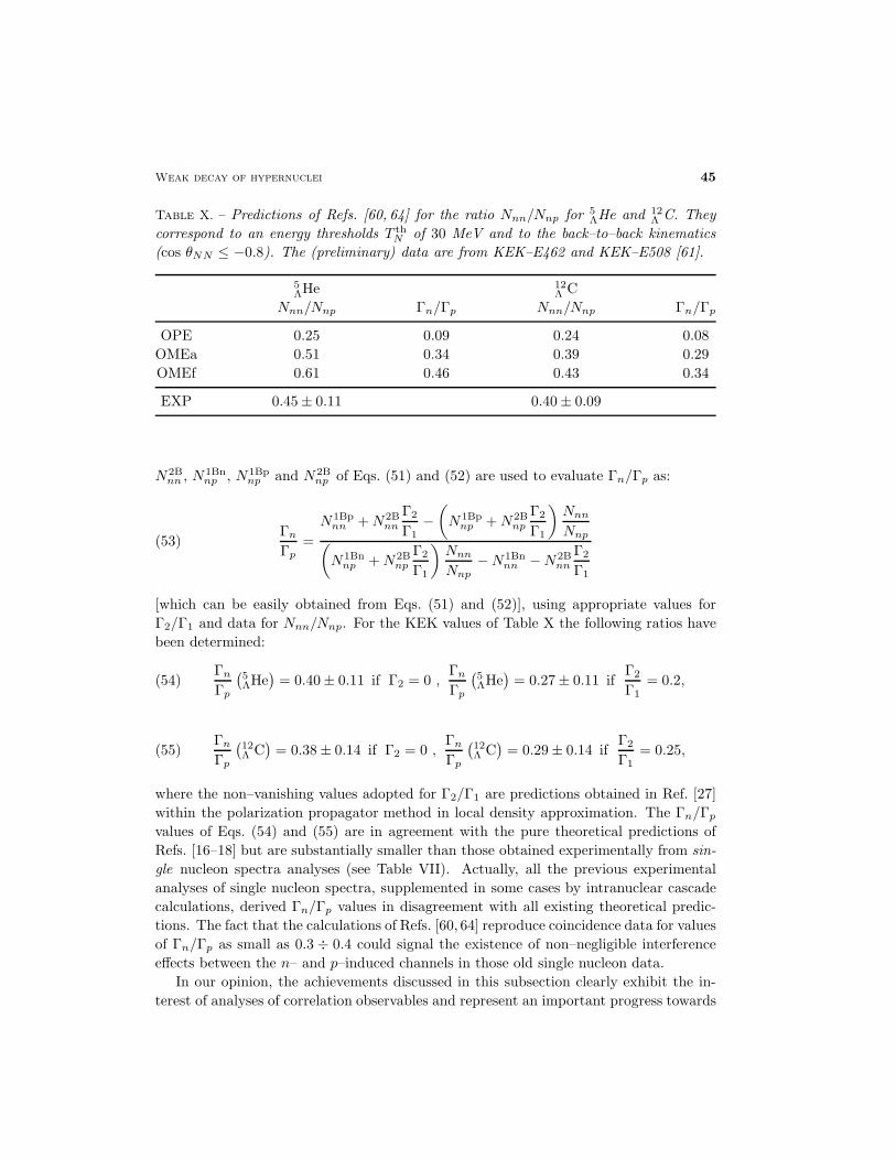
Weak decay of hypernuclei 45
Table X. – Predictions of Refs. [60, 64] for the ratio Nnn/Nnp for 5ΛHe and 12
Λ C. They
correspond to an energy thresholds T thN of 30 MeV and to the back–to–back kinematics
(cos θNN ≤ −0.8). The (preliminary) data are from KEK–E462 and KEK–E508 [61].
5ΛHe 12
Λ C
Nnn/Nnp Γn/Γp Nnn/Nnp Γn/Γp
OPE 0.25 0.09 0.24 0.08
OMEa 0.51 0.34 0.39 0.29
OMEf 0.61 0.46 0.43 0.34
EXP 0.45 ± 0.11 0.40 ± 0.09
N2Bnn , N1Bn
np , N1Bpnp and N2B
np of Eqs. (51) and (52) are used to evaluate Γn/Γp as:
(53)Γn
Γp=
N1Bpnn +N2B
nn
Γ2
Γ1−
(
N1Bpnp +N2B
np
Γ2
Γ1
)
Nnn
Nnp(
N1Bnnp +N2B
np
Γ2
Γ1
)
Nnn
Nnp−N1Bn
nn −N2Bnn
Γ2
Γ1
[which can be easily obtained from Eqs. (51) and (52)], using appropriate values for
Γ2/Γ1 and data for Nnn/Nnp. For the KEK values of Table X the following ratios have
been determined:
(54)Γn
Γp
(
5ΛHe
)
= 0.40 ± 0.11 if Γ2 = 0 ,Γn
Γp
(
5ΛHe
)
= 0.27 ± 0.11 ifΓ2
Γ1= 0.2,
(55)Γn
Γp
(
12Λ C
)
= 0.38 ± 0.14 if Γ2 = 0 ,Γn
Γp
(
12Λ C
)
= 0.29 ± 0.14 ifΓ2
Γ1= 0.25,
where the non–vanishing values adopted for Γ2/Γ1 are predictions obtained in Ref. [27]
within the polarization propagator method in local density approximation. The Γn/Γp
values of Eqs. (54) and (55) are in agreement with the pure theoretical predictions of
Refs. [16–18] but are substantially smaller than those obtained experimentally from sin-
gle nucleon spectra analyses (see Table VII). Actually, all the previous experimental
analyses of single nucleon spectra, supplemented in some cases by intranuclear cascade
calculations, derived Γn/Γp values in disagreement with all existing theoretical predic-
tions. The fact that the calculations of Refs. [60, 64] reproduce coincidence data for values
of Γn/Γp as small as 0.3 ÷ 0.4 could signal the existence of non–negligible interference
effects between the n– and p–induced channels in those old single nucleon data.
In our opinion, the achievements discussed in this subsection clearly exhibit the in-
terest of analyses of correlation observables and represent an important progress towards
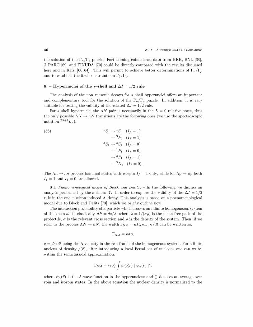
46 W. M. Alberico and G. Garbarino
the solution of the Γn/Γp puzzle. Forthcoming coincidence data from KEK, BNL [68],
J–PARC [69] and FINUDA [70] could be directly compared with the results discussed
here and in Refs. [60, 64]. This will permit to achieve better determinations of Γn/Γp
and to establish the first constraints on Γ2/Γ1.
6. – Hypernuclei of the s–shell and ∆I = 1/2 rule
The analysis of the non–mesonic decays for s–shell hypernuclei offers an important
and complementary tool for the solution of the Γn/Γp puzzle. In addition, it is very
suitable for testing the validity of the related ∆I = 1/2 rule.
For s–shell hypernuclei the ΛN pair is necessarily in the L = 0 relative state, thus
the only possible ΛN → nN transitions are the following ones (we use the spectroscopic
notation 2S+1LJ):
1S0 → 1S0 (If = 1)(56)
→ 3P0 (If = 1)3S1 → 3S1 (If = 0)
→ 1P1 (If = 0)
→ 3P1 (If = 1)
→ 3D1 (If = 0).
The Λn→ nn process has final states with isospin If = 1 only, while for Λp → np both
If = 1 and If = 0 are allowed.
6.1. Phenomenological model of Block and Dalitz . – In the following we discuss an
analysis performed by the authors [72] in order to explore the validity of the ∆I = 1/2
rule in the one–nucleon induced Λ–decay. This analysis is based on a phenomenological
model due to Block and Dalitz [73], which we briefly outline now.
The interaction probability of a particle which crosses an infinite homogeneous system
of thickness ds is, classically, dP = ds/λ, where λ = 1/(σρ) is the mean free path of the
projectile, σ is the relevant cross section and ρ is the density of the system. Then, if we
refer to the process ΛN → nN , the width ΓNM = dPΛN→nN/dt can be written as:
ΓNM = vσρ,
v = ds/dt being the Λ velocity in the rest frame of the homogeneous system. For a finite
nucleus of density ρ(~r), after introducing a local Fermi sea of nucleons one can write,
within the semiclassical approximation:
ΓNM = 〈vσ〉∫
d~rρ(~r) | ψΛ(~r) |2,
where ψΛ(~r) is the Λ wave function in the hypernucleus and 〈〉 denotes an average over
spin and isospin states. In the above equation the nuclear density is normalized to the
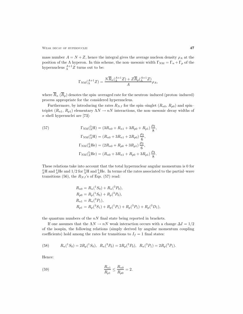
Weak decay of hypernuclei 47
mass number A = N +Z, hence the integral gives the average nucleon density ρA at the
position of the Λ hyperon. In this scheme, the non–mesonic width ΓNM = Γn +Γp of the
hypernucleus A+1Λ Z turns out to be:
ΓNM(A+1Λ Z) =
NRn(A+1Λ Z) + ZRp(
A+1Λ Z)
AρA,
where Rn (Rp) denotes the spin–averaged rate for the neutron–induced (proton–induced)
process appropriate for the considered hypernucleus.
Furthermore, by introducing the rates RNJ for the spin–singlet (Rn0, Rp0) and spin–
triplet (Rn1, Rp1) elementary ΛN → nN interactions, the non–mesonic decay widths of
s–shell hypernuclei are [73]:
ΓNM(3ΛH) = (3Rn0 +Rn1 + 3Rp0 +Rp1)ρ2
8,(57)
ΓNM(4ΛH) = (Rn0 + 3Rn1 + 2Rp0)ρ3
6,
ΓNM(4ΛHe) = (2Rn0 +Rp0 + 3Rp1)ρ3
6,
ΓNM(5ΛHe) = (Rn0 + 3Rn1 +Rp0 + 3Rp1)ρ4
8.
These relations take into account that the total hypernuclear angular momentum is 0 for4ΛH and 4
ΛHe and 1/2 for 3ΛH and 5
ΛHe. In terms of the rates associated to the partial–wave
transitions (56), the RNJ ’s of Eqs. (57) read:
Rn0 = Rn(1S0) +Rn(3P0),
Rp0 = Rp(1S0) +Rp(
3P0),
Rn1 = Rn(3P1),
Rp1 = Rp(3S1) +Rp(
1P1) +Rp(3P1) +Rp(
3D1),
the quantum numbers of the nN final state being reported in brackets.
If one assumes that the ΛN → nN weak interaction occurs with a change ∆I = 1/2
of the isospin, the following relations (simply derived by angular momentum coupling
coefficients) hold among the rates for transitions to If = 1 final states:
(58) Rn(1S0) = 2Rp(1S0), Rn(3P0) = 2Rp(
3P0), Rn(3P1) = 2Rp(3P1).
Hence:
(59)Rn1
Rp1≤ Rn0
Rp0= 2.
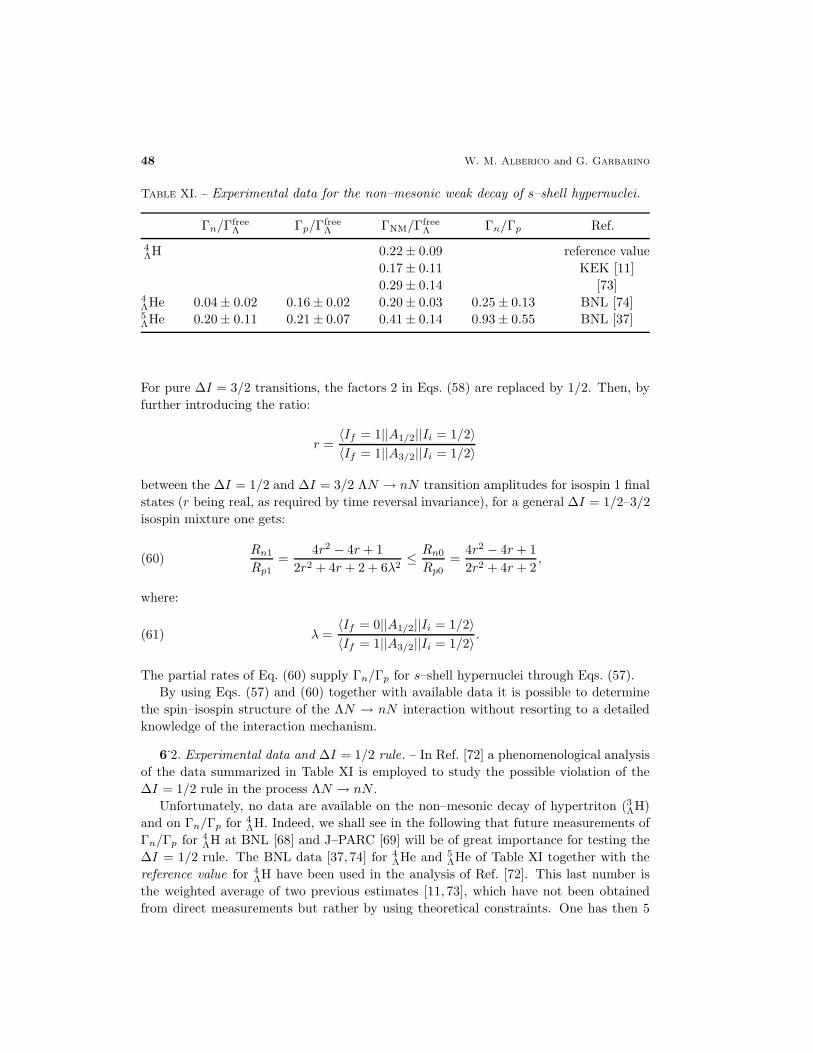
48 W. M. Alberico and G. Garbarino
Table XI. – Experimental data for the non–mesonic weak decay of s–shell hypernuclei.
Γn/ΓfreeΛ Γp/Γ
freeΛ ΓNM/Γ
freeΛ Γn/Γp Ref.
4ΛH 0.22 ± 0.09 reference value
0.17 ± 0.11 KEK [11]
0.29 ± 0.14 [73]4ΛHe 0.04 ± 0.02 0.16 ± 0.02 0.20 ± 0.03 0.25 ± 0.13 BNL [74]5ΛHe 0.20 ± 0.11 0.21 ± 0.07 0.41 ± 0.14 0.93 ± 0.55 BNL [37]
For pure ∆I = 3/2 transitions, the factors 2 in Eqs. (58) are replaced by 1/2. Then, by
further introducing the ratio:
r =〈If = 1||A1/2||Ii = 1/2〉〈If = 1||A3/2||Ii = 1/2〉
between the ∆I = 1/2 and ∆I = 3/2 ΛN → nN transition amplitudes for isospin 1 final
states (r being real, as required by time reversal invariance), for a general ∆I = 1/2–3/2
isospin mixture one gets:
(60)Rn1
Rp1=
4r2 − 4r + 1
2r2 + 4r + 2 + 6λ2≤ Rn0
Rp0=
4r2 − 4r + 1
2r2 + 4r + 2,
where:
(61) λ =〈If = 0||A1/2||Ii = 1/2〉〈If = 1||A3/2||Ii = 1/2〉 .
The partial rates of Eq. (60) supply Γn/Γp for s–shell hypernuclei through Eqs. (57).
By using Eqs. (57) and (60) together with available data it is possible to determine
the spin–isospin structure of the ΛN → nN interaction without resorting to a detailed
knowledge of the interaction mechanism.
6.2. Experimental data and ∆I = 1/2 rule. – In Ref. [72] a phenomenological analysis
of the data summarized in Table XI is employed to study the possible violation of the
∆I = 1/2 rule in the process ΛN → nN .
Unfortunately, no data are available on the non–mesonic decay of hypertriton (3ΛH)
and on Γn/Γp for 4ΛH. Indeed, we shall see in the following that future measurements of
Γn/Γp for 4ΛH at BNL [68] and J–PARC [69] will be of great importance for testing the
∆I = 1/2 rule. The BNL data [37, 74] for 4ΛHe and 5
ΛHe of Table XI together with the
reference value for 4ΛH have been used in the analysis of Ref. [72]. This last number is
the weighted average of two previous estimates [11, 73], which have not been obtained
from direct measurements but rather by using theoretical constraints. One has then 5
Weak decay of hypernuclei 49
independent data which allow to fix, from Eqs. (57), the 4 rates RN,J and ρ3. Indeed,
the average nucleon density at the Λ position for 5ΛHe, also entering Eqs. (57), has been
estimated to be ρ4 = 0.045 fm−3 by employing the Λ wave function of Ref. [42] (which
was obtained through a quark model description of the ΛN interaction) and the gaussian
density for 4He that reproduces the experimental mean square radius of the nucleus. For4ΛH and 4
ΛHe, instead, no realistic hyperon wave function is available and we can obtain
the value ρ3 = 0.026 fm−3 from the data of Table XI, by imposing that [see Eqs. (57)]:
Γp(5ΛHe)
Γp(4ΛHe)=
3
4
ρ4
ρ3.
The best choice to determine the rates RN,J by fitting measured values corresponds
to use the relations for the observables:
ΓNM(4ΛH), ΓNM(4ΛHe), ΓNM(5ΛHe),Γn
Γp(4ΛHe),
which have the smallest experimental uncertainties. After solving these equations we
obtained the following partial rates (as usual, the decay widths of Eqs. (57) are considered
in units of the free Λ decay width):
Rn0 = (4.7 ± 2.1) fm3,(62)
Rp0 = (7.9+16.5−7.9 ) fm3,(63)
Rn1 = (10.3 ± 8.6) fm3,(64)
Rp1 = (9.8 ± 5.5) fm3,(65)
Rn(5ΛHe) ≡ 1
4(Rn0 + 3Rn1) = (8.9 ± 6.5) fm3,
Rp(5ΛHe) ≡ 1
4(Rp0 + 3Rp1) = (9.3 ± 5.8) fm3.
The errors have been obtained with the standard method, i.e., by treating the data as
independent and uncorrelated.
For the ratios of Eq. (60) we have then:
Rn0
Rp0= 0.6+1.3
−0.6,(66)
Rn1
Rp1= 1.0+1.1
−1.0.(67)
while the ratios of the spin–triplet to the spin–singlet interaction rates are:
Rn1
Rn0= 2.2 ± 2.1,
Rp1
Rp0= 1.2+2.7
−1.2.
50 W. M. Alberico and G. Garbarino
The large uncertainties do not allow to draw definite conclusions about the possible
violation of the ∆I = 1/2 rule and the spin–dependence of the transition rates. Eqs. (66)
and (67) are still compatible with Eq. (59), namely with the ∆I = 1/2 rule, although the
central value in Eq. (66) is more in agreement either with a pure ∆I = 3/2 transition
(r ≃ 0) or with r ≃ 2 [see Eq. (60)]. Actually, Eq. (66) is compatible with r in the range
−1/4 ÷ 40, while the ratio λ of Eqs. (60) and (61) is completely undetermined.
By using the results of Eqs. (62)–(65) one predicts:
Γn
Γp(3ΛH) = 0.7+1.1
−0.7,
Γn
Γp(4ΛH) = 2.3+5.0
−2.3,
Γn
Γp(5ΛHe) = 0.95 ± 0.92,
and, by using ρ2 = 0.001 fm−3 [73],
ΓNM(3ΛH) = 0.007± 0.006.
The ratio obtained for 5ΛHe is in agreement with the data of Table XI and with the recent
determinations discussed in 5.2.2. An accurate measurement of ΓNM(3ΛH) and Γn/Γp for
3ΛH and 4
ΛH would then provide a test of the weak decay model of Eqs. (57) if the rates
of Eqs. (62)–(65) could be extracted with less uncertainty from data.
The compatibility of the data with the ∆I = 1/2 rule can be discussed in a different
way: by assuming this rule, we fix Rn0/Rp0 = 2. Then, by using the observables:
ΓNM(4ΛHe), ΓNM(5ΛHe),Γn
Γp(4ΛHe),
the extracted partial rates are (Rn0, Rn1, Rn and Rp are unchanged with respect to the
above derivation):
Rn0 = (4.7 ± 2.1) fm3,
Rp0 ≡ Rn0/2 = (2.3 ± 1.0) fm3,
Rn1 = (10.3 ± 8.6) fm3,
Rp1 = (11.7 ± 2.4) fm3.
These values are compatible with the ones in Eqs. (62)–(65). For pure ∆I = 1/2 transi-
tions the spin–triplet interactions seem to dominate over the spin–singlet ones:
Rn1
Rn0= 2.2 ± 2.1,
Rp1
Rp0= 5.0 ± 2.4.
Weak decay of hypernuclei 51
Moreover, since:
Rn1
Rp1= 0.9 ± 0.8,
from Eq. (60) one obtains the following estimate for the ratio between the ∆I = 1/2
amplitudes:
∣
∣
∣
∣
〈If = 0||A1/2||Ii = 1/2〉〈If = 1||A1/2||Ii = 1/2〉
∣
∣
∣
∣
≃ 1
3.7÷ 2.3.
The other independent observables which have not been utilized are then predicted to
be:
ΓNM(4ΛH) = 0.17 ± 0.11,
(68)Γn
Γp(5ΛHe) = 0.95 ± 0.72,
in agreement with the data of Table XI, with a χ2 for one degree of freedom of 0.31
(corresponding to a 0.56 σ deviation). This means that these data are consistent with
the hypothesis of validity of the ∆I = 1/2 rule at the level of 60%. In other words, the
∆I = 1/2 rule is excluded at the 40% confidence level. On the contrary, if, according
to the analysis of subsection 5.2.2, one compares with the datum Γn/Γp = 0.40 ± 0.11
for 5ΛHe, the ∆I = 1/2 rule turns out to be completely excluded by the central value of
Eq (68).
The observables for which experimental data are not available at present are predicted
to be:
Γn
Γp(3ΛH) = 1.3 ± 0.6,
Γn
Γp(4ΛH) = 7.6 ± 6.2,
and, for ρ2 = 0.001 fm−3,
ΓNM(3ΛH) = 0.005± 0.003.
We note that the central value of Γn/Γp for 4ΛH in the analysis which enforces the
∆I = 1/2 rule is considerably larger than the central value obtained in the general
analysis previously discussed. Thus, the future measurements [68, 69] of this quantity
will represent an important test of the ∆I = 1/2 rule.
52 W. M. Alberico and G. Garbarino
7. – Non–mesonic decay of polarized Λ–hypernuclei: the asymmetry puzzle
Lambda hypernuclear states can be produced with a sizeable amount of polarization
[75]. The development of angular distribution measurements of decay particles (photons,
pions and protons) from polarized hypernuclei is of crucial importance in order to extract
new information on hypernuclear production, structure and decay.
Despite the recent progress discussed in section 5, the reaction mechanism for the
non–mesonic weak decay does not seem to be fully understood. Indeed, a new intriguing
problem, of more recent origin, is open: it concerns a strong disagreement between
theory and experiment on the asymmetry of the angular emission of non–mesonic decay
protons from polarized hypernuclei. This asymmetry is due to the interference between
parity–violating and parity–conserving ~Λp → np transition amplitudes [76]. The non–
mesonic rates Γn and Γp are dominated by parity–conserving amplitudes. The study
of the asymmetric emission of protons from polarized hypernuclei, with its information
on the spin–parity structure of the Λp → np process, is thus supposed to provide new
constraints on the dynamics of the non–mesonic decay.
Thanks to the large momentum transfer involved, the n(π+,K+)Λ reaction has been
used [77, 78], at pπ = 1.05 GeV and small K+ laboratory scattering angles (2 <∼ θK <∼15), to produce hypernuclear states with a substantial amount of spin–polarization pref-
erentially aligned along the axis normal to the reaction plane. The origin of hypernuclear
polarization is twofold [75]. It is known that the distortions (absorptions) of the initial
(π+) and final (K+) meson–waves produce a small polarization of the hypernuclear or-
bital angular momentum up to laboratory scattering angles θK ≃ 15 (at larger scattering
angles, the orbital polarization increases with a negative sign). At small but non–zero
angles, the main source of polarization is due to an appreciable spin–flip term in the
elementary reaction π+n → ΛK+, which interferes with the spin–nonflip amplitude. In
a typical experimental situation with pπ = 1.05 GeV and θK ≃ 15, the polarization of
the hyperon spin in the free π+n→ ΛK+ process is about 0.75.
7.1. Spin–polarization observables . – The intensity of protons emitted in ~Λp → np
decays along a direction forming an angle Θ with the polarization axis is given by (see
Ref. [79] for more details):
(69) I(Θ, J) = I0(J) [1 + A(Θ, J)] ,
where
(70) I0(J) =
∑
M σ(J,M)
2J + 1
is the (isotropic) intensity for an unpolarized hypernucleus. In Eq. (70):
σ(J,M) =∑
F
|〈F |M|I; J,M〉|2
Weak decay of hypernuclei 53
is the intensity of protons emitted along the quantization axis for a projection M of the
hypernuclear total spin J . The proton asymmetry parameter, A, can be written in the
following form [79]:
(71) A(Θ, J) = Py(J)Ay(J) cos Θ.
The quantity:
Ay(J) =3
J + 1
∑
M M σ(J,M)∑
M σ(J,M),
which is a property of the hypernuclear non–mesonic decay only, is usually referred to
as the hypernuclear asymmetry parameter. The hypernuclear polarization Py depends
both on the kinematics (pπ and θK) and dynamics of the production reaction.
In the shell model weak–coupling scheme, Py is directly related to the polarization
pΛ of the Λ spin in the hypernucleus as follows:
(72) pΛ(J) =
− J
J + 1Py(J) if J = JC − 1
2
Py(J) if J = JC + 12 ,
JC being the total spin of the nuclear core. It is useful to introduce an intrinsic lambda
asymmetry parameter aΛ, which is characteristic of the elementary process ~Λp→ np and
should be independent of the hypernucleus, such that:
(73) A(Θ, J) = pΛ(J) aΛ cosΘ.
From Eqs. (71) and (72) it follows then:
aΛ =
−J + 1
JAy(J) if J = JC − 1
2
Ay(J) if J = JC + 12 .
7.2. Experiment versus theory. – Nucleon FSI acting after the non–mesonic weak
decay are expected to modify the weak decay intensity of Eq. (69). Experimentally one
has access to a proton intensity IM(Θ, J) which is generally assumed to have the same
Θ–dependence as I(Θ, J):
(74) IM(Θ, J) = IM0 (J)
[
1 + pΛ(J) aMΛ (J) cosΘ
]
.
The observable asymmetry, aMΛ (J), which is expected to depend on the hypernucleus, is
then determined as:
(75) aMΛ (J) =
1
pΛ(J)
IM(0, J) − IM(180, J)
IM(0, J) + IM(180, J).
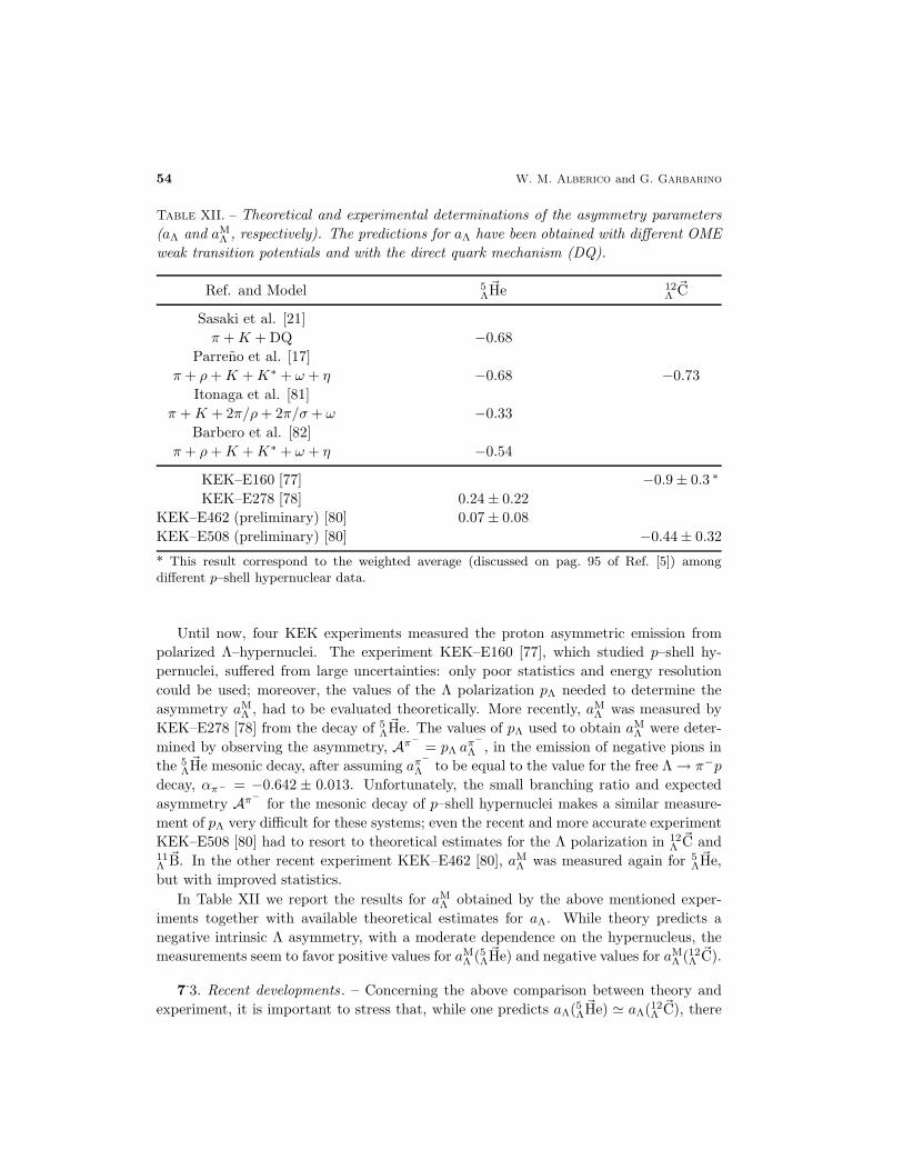
54 W. M. Alberico and G. Garbarino
Table XII. – Theoretical and experimental determinations of the asymmetry parameters
(aΛ and aMΛ , respectively). The predictions for aΛ have been obtained with different OME
weak transition potentials and with the direct quark mechanism (DQ).
Ref. and Model 5Λ~He 12
Λ~C
Sasaki et al. [21]
π +K + DQ −0.68
Parreno et al. [17]
π + ρ+K +K∗ + ω + η −0.68 −0.73
Itonaga et al. [81]
π +K + 2π/ρ+ 2π/σ + ω −0.33
Barbero et al. [82]
π + ρ+K +K∗ + ω + η −0.54
KEK–E160 [77] −0.9 ± 0.3 ∗
KEK–E278 [78] 0.24 ± 0.22
KEK–E462 (preliminary) [80] 0.07 ± 0.08
KEK–E508 (preliminary) [80] −0.44 ± 0.32
* This result correspond to the weighted average (discussed on pag. 95 of Ref. [5]) amongdifferent p–shell hypernuclear data.
Until now, four KEK experiments measured the proton asymmetric emission from
polarized Λ–hypernuclei. The experiment KEK–E160 [77], which studied p–shell hy-
pernuclei, suffered from large uncertainties: only poor statistics and energy resolution
could be used; moreover, the values of the Λ polarization pΛ needed to determine the
asymmetry aMΛ , had to be evaluated theoretically. More recently, aM
Λ was measured by
KEK–E278 [78] from the decay of 5Λ~He. The values of pΛ used to obtain aM
Λ were deter-
mined by observing the asymmetry, Aπ−
= pΛ aπ−
Λ , in the emission of negative pions in
the 5Λ~He mesonic decay, after assuming aπ−
Λ to be equal to the value for the free Λ → π−p
decay, απ− = −0.642 ± 0.013. Unfortunately, the small branching ratio and expected
asymmetry Aπ−
for the mesonic decay of p–shell hypernuclei makes a similar measure-
ment of pΛ very difficult for these systems; even the recent and more accurate experiment
KEK–E508 [80] had to resort to theoretical estimates for the Λ polarization in 12Λ~C and
11Λ~B. In the other recent experiment KEK–E462 [80], aM
Λ was measured again for 5Λ~He,
but with improved statistics.
In Table XII we report the results for aMΛ obtained by the above mentioned exper-
iments together with available theoretical estimates for aΛ. While theory predicts a
negative intrinsic Λ asymmetry, with a moderate dependence on the hypernucleus, the
measurements seem to favor positive values for aMΛ (5Λ
~He) and negative values for aMΛ (12Λ
~C).
7.3. Recent developments . – Concerning the above comparison between theory and
experiment, it is important to stress that, while one predicts aΛ(5Λ~He) ≃ aΛ(12Λ
~C), there
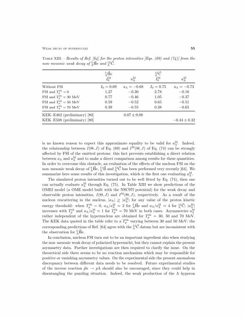
Weak decay of hypernuclei 55
Table XIII. – Results of Ref. [64] for the proton intensities [Eqs. (69) and (74)] from the
non–mesonic weak decay of 5Λ~He and 12
Λ~C.
5Λ~He 12
Λ~C
IM0 aM
Λ IM0 aM
Λ
Without FSI I0 = 0.69 aΛ = −0.68 I0 = 0.75 aΛ = −0.73
FSI and T thp = 0 1.27 −0.30 2.78 −0.16
FSI and T thp = 30 MeV 0.77 −0.46 1.05 −0.37
FSI and T thp = 50 MeV 0.59 −0.52 0.65 −0.51
FSI and T thp = 70 MeV 0.39 −0.55 0.38 −0.65
KEK–E462 (preliminary) [80] 0.07 ± 0.08
KEK–E508 (preliminary) [80] −0.44 ± 0.32
is no known reason to expect this approximate equality to be valid for aMΛ . Indeed,
the relationship between I(Θ, J) of Eq. (69) and IM(Θ, J) of Eq. (74) can be strongly
affected by FSI of the emitted protons: this fact prevents establishing a direct relation
between aΛ and aMΛ and to make a direct comparison among results for these quantities.
In order to overcome this obstacle, an evaluation of the effects of the nucleon FSI on the
non–mesonic weak decay of 5Λ~He, 11
Λ~B and 12
Λ~C has been performed very recently [64]. We
summarize here some results of this investigation, which is the first one evaluating aMΛ .
The simulated proton intensities turned out to be well fitted by Eq. (74), then one
can actually evaluate aMΛ through Eq. (75). In Table XIII we show predictions of the
OMEf model (a OME model built with the NSC97f potential) for the weak decay and
observable proton intensities, I(Θ, J) and IM(Θ, J), respectively. As a result of the
nucleon rescattering in the nucleus, |aΛ| >∼ |aMΛ | for any value of the proton kinetic
energy threshold: when T thp = 0, aΛ/a
MΛ ≃ 2 for 5
Λ~He and aΛ/a
MΛ ≃ 4 for 12
Λ~C; |aM
Λ |increases with T th
p and aΛ/aMΛ ≃ 1 for T th
p = 70 MeV in both cases. Asymmetries aMΛ
rather independent of the hypernucleus are obtained for T thp = 30, 50 and 70 MeV.
The KEK data quoted in the table refer to a T thp varying between 30 and 50 MeV: the
corresponding predictions of Ref. [64] agree with the 12Λ~C datum but are inconsistent with
the observation for 5Λ~He.
In conclusion, nucleon FSI turn out to be an important ingredient also when studying
the non–mesonic weak decay of polarized hypernuclei, but they cannot explain the present
asymmetry data. Further investigations are then required to clarify the issue. On the
theoretical side there seems to be no reaction mechanism which may be responsible for
positive or vanishing asymmetry values. On the experimental side the present anomalous
discrepancy between different data needs to be resolved. Future experimental studies
of the inverse reaction ~pn → pΛ should also be encouraged, since they could help in
disentangling the puzzling situation. Indeed, the weak production of the Λ–hyperon
56 W. M. Alberico and G. Garbarino
could give a richer and cleaner (with respect to the non–mesonic hypernuclear decay)
piece of information on the lambda–nucleon weak interaction and especially on the Λ
polarization observables [83].
8. – Summary and perspectives
In these Lectures we have discussed several aspects of the weak decay of Λ–hypernuclei.
Beyond the mesonic channel, which is observed also for a free Λ, the hypernuclear decay
proceeds through non–mesonic processes, mainly induced by the interaction of the Λ
with one nucleon or with a pair of correlated nucleons. This channel is the dominant one
in medium–heavy hypernuclei, where the Pauli principle strongly suppresses the mesonic
decay.
Various models have been proposed to describe the mesonic and non–mesonic decay
rates as well as the asymmetry parameters in the decay of the Λ–hyperon in nuclei. The
results obtained within these models have been thoroughly discussed. The mesonic rates
have been reproduced quite well by calculations performed in different frameworks. Also
the non–mesonic rates have been considered within a variety of phenomenological and
microscopic models. In this context, particular interest has been devoted to the ratio
Γn/Γp. Indeed, in spite of the fact that several calculations were able to reproduce,
already at the OPE level, the total non–mesonic width, ΓNM = Γn + Γp(+Γ2), the val-
ues therewith obtained for Γn/Γp revealed a strong disagreement with the experimental
data. Although some of these calculations represented an improvement of the situation,
further efforts were required in order to approach a solution the Γn/Γp puzzle. From the
experimental side, recent experiments measured nucleon–nucleon coincidence observables
with good statistics. Recent analyses of these data, complemented with the theoretical
estimate of final state interactions, allowed the determination of Γn/Γp values in agree-
ment with the theoretical expectations. Yet, good statistics coincidence measurements
of nn and np emitted pairs are further required. These correlation measurements will
also allow to establish the first constraints on the two–nucleon induced decay width, thus
testing the various models which have been proposed for the evaluation of the different
decay channels.
The analysis of the ∆I = 1/2 rule in the non–mesonic decay of light hypernuclei
appears to be feasible, also within a relatively simple phenomenological model: again,
the measurements of a few delicate, missing decay rates, would help in understanding
the role of this empirical selection rule.
As far as the decay of polarized hypernuclei is concerned, the situation is even more
puzzling. While theory predicts negative values for both the intrinsic asymmetry aΛ and
the observable asymmetry aMΛ , with a moderate dependence on the hypernucleus, experi-
ments seem to favour negative values for aMΛ (12Λ
~C) but small, positive values for aMΛ (5Λ
~He).
Further investigations are then required to clarify the issue. Theoretically, there seems to
be no reaction mechanism which may be responsible for positive or vanishing aMΛ values.
Improved experiments, establishing with certainty the sign and magnitude of aMΛ for s–
and p–shell hypernuclei, are strongly awaited.
Weak decay of hypernuclei 57
We conclude this work by reminding the reader that hypernuclear physics is 52 years
old, yet a lot of efforts remain to be done, both experimentally and theoretically, in order
to fully understand the hyperon dynamics and decay inside the nuclear medium. The
impressive progress experienced in the last few years is promising and we hope that it
deserves a definite answer to the intriguing open questions which we have illustrated
here.
∗ ∗ ∗
We warmly acknowledge our colleagues A. De Pace, R. Cenni, A. Parreno and A.
Ramos, who collaborated with us in obtaining some of the results discussed in these
Lectures.
REFERENCES
[1] M. Danysz and J. Pniewski, Philos. Mag., 44 (1953) 348.[2] A. Gal, These Proceedings.[3] T. Nagae, These Proceedings.[4] H. Outa, These Proceedings.[5] W. M. Alberico and G. Garbarino, Phys. Rep., 369 (2002) 1.[6] F. J. Gillman and M. B. Wise, Phys. Rev. D, 20 (1979) 2392.[7] M. Cristoforetti, P. Faccioli, E. V. Shuryak and M. Traini, Phys. Rev. D, 70
(2004) 054016.[8] J. Nieves and E. Oset, Phys. Rev. C, 47 (1993) 1478.[9] T. Motoba and K. Itonaga, Prog. Theor Phys. Suppl., 117 (1994) 477.
[10] Y. Akaishi and T. Yamazaki, Prog. Part. Nucl. Phys., 39 (1997) 565.[11] H. Outa et al., Nucl. Phys. A, 639 (1998) 251c.[12] J. Cohen, Prog. Part. Nucl. Phys., 25 (1990) 139.[13] E. Oset and A. Ramos, Prog. Part. Nucl. Phys., 41 (1998) 191.[14] J. F. Dubach, G. B. Feldman and B. R. Holstein, Ann. Phys., 249 (1996) 146.[15] A. Parreno, A. Ramos and C. Bennhold, Phys. Rev. C, 56 (1997) 339.[16] K. Itonaga, T. Ueda and T. Motoba, Phys. Rev. C, 65 (2002) 034617.[17] A. Parreno and A. Ramos, Phys. Rev. C, 65 (2002) 015204.[18] D. Jido, E. Oset and J. E. Palomar, Nucl. Phys. A, 694 (2001) 525.[19] A. Parreno, A. Ramos, C. Bennhold and K. Maltman, Phys. Lett. B, 435 (1998) 1.[20] C.-Y. Cheung, D. P. Heddle and L. S. Kisslinger, Phys. Rev. C, 27 (1983) 335; D.
P. Heddle and L. S. Kisslinger, Phys. Rev. C, 33 (1986) 608.[21] K. Sasaki, T. Inoue and M. Oka, Nucl. Phys. A, 669 (2000) 331; 678 (2000) 455(E);
707 (2002) 477.[22] E. Oset, H. Toki and W. Weise, Phys. Rep., 83 (1982) 281.[23] E. Oset, P. Fernandez de Cordoba, J. Nieves, A. Ramos and L. L. Salcedo, Prog.
Theor. Phys. Suppl., 117 (1994) 461.[24] E. Oset and L. L. Salcedo, Nucl. Phys. A, 443 (1985) 704.[25] A. L. Fetter and J. D. Walecka, Quantum Theory of Many Particle Systems (McGraw–
Hill, New York) 1971.[26] A. Ramos, E. Oset and L. L. Salcedo, Phys. Rev. C, 50 (1994) 2314.[27] W. M. Alberico, A De Pace, G. Garbarino and A. Ramos, Phys. Rev. C, 61 (2000)
044314.
58 W. M. Alberico and G. Garbarino
[28] W. M. Alberico, A. De Pace, G. Garbarino and R. Cenni, Nucl. Phys. A, 668 (2000)113.
[29] R. Seki and K. Masutani, Phys. Rev. C, 27 (1983) 2799.[30] E. Friedman and A. Gal, Nucl. Phys. A, 724 (2003) 143[31] C. Garcia-Recio, J. Nieves and E. Oset, Nucl. Phys. A, 547 (1992) 473.[32] J. W. Negele, Rev. Mod. Phys., 54 (1982) 813.[33] W. M. Alberico, R. Cenni, A. Molinari and P. Saracco, Ann. Phys., 174 (1987)
131.[34] R. Cenni, F. Conte and P. Saracco, Nucl. Phys. A, 623 (1997) 391.[35] C. B. Dover, A. Gal and D. J. Millener, Phys. Rev. C, 38 (1988) 2700.[36] J. Vidana, A. Polls, A. Ramos and M. Hjorth-Jensen, Nucl. Phys. A, 644 (1998)
201.[37] J. J. Szymanski et al., Phys. Rev. C, 43 (1991) 849.[38] H. Noumi et al., Phys. Rev. C, 52 (1995) 2936.[39] H. C. Bhang et al., Phys. Rev. Lett., 81 (1998) 4321; H. Park et al., Phys. Rev. C, 61
(2000) 054004.[40] H. Outa et al., Nucl. Phys. A, 670 (2000) 281c.[41] Y. Sato et al., nucl–ex/0409007 (submitted to Phys. Rev. C).[42] U. Straub, J. Nieves, A. Faessler and E. Oset, Nucl. Phys. A, 556 (1993) 531.[43] K. Itonaga, T. Motoba and H. Bando, Z. Phys. A, 330 (1988) 209; Nucl. Phys. A,
489 (1988) 683.[44] W. M. Alberico, A. De Pace, M. Ericson and A. Molinari, Phys. Lett. B, 256 (1991)
134.[45] T. A. Armstrong et al., Phys. Rev. C, 47 (1993) 1957.[46] H. Ohm et al., Phys. Rev. C, 55 (1997) 3062; P. Kulessa et al., Phys. Lett. B, 427 (1998)
403.[47] T. Motoba, H. Bando, T. Fukuda and J. Zofka, Nucl. Phys. A, 534 (1991) 597.[48] T. Motoba, Nucl. Phys. A, 547 (1992) 115c.[49] E. Oset, L. L. Salcedo and Q. N. Usmani, Nucl. Phys. A, 450 (1986) 67c.[50] I. Kumagai-Fuse, S. Okabe and Y. Akaishi, Phys. Lett. B, 345 (1995) 386.[51] S. Okada et al., VIII International Conference on Hypernuclear and Strange Particle
Physics (HYP2003), JLab, Newport News, Virginia, nucl–ex/0402022 [Nucl. Phys. A
(to be published)].[52] L. Zhou and J. Piekarewicz, Phys. Rev. C, 60 (1999) 024306.[53] M. Ericson and H. Bando, Phys. Lett. B, 237 (1990) 169.[54] C. Albertus, J. E. Amaro, and J. Nieves, Phys. Rev. C, 67 (2003) 034604.[55] R. H. Dalitz, Proceedings of the Summer Study Meeting on Nuclear and Hypernuclear
Physics with Kaon Beams, BNL Report No. 18335 (1973) p. 41.[56] J.-H. Jun and H. C. Bhang, Nuovo Cim., 112 A (1999) 649; J.-H. Jun, Phys. Rev. C,
63 (2001) 044012.[57] H. Noumi et al., Proceedings of the IV International Symposium on Weak and
Electromagnetic Interactions in Nuclei, H. Ejiri, T. Kishimoto and T. Sato eds, WorldScientific (1995) p. 550.
[58] B. Kamys et al., Eur. Phys. J. A, 11 (2001) 1.[59] P. Kulessa et al., Acta Phys. Polon. B, 33 (2002) 603.[60] G. Garbarino, A. Parreno and A. Ramos, Phys. Rev. Lett., 91 (2003) 112501; Phys.
Rev. C, 69 (2004) 054603.[61] H. Outa, these proceedings and in VIII International Conference on Hypernuclear and
Strange Particle Physics (HYP2003), JLab, Newport News, Virginia [Nucl. Phys. A (tobe published)].
Weak decay of hypernuclei 59
[62] J. H. Kim et al., Phys. Rev. C, 68 (2003) 065201.[63] S. Okada et al., Phys. Lett. B, 597 (2004) 249.[64] W. M. Alberico, G. Garbarino, A. Parreno and A. Ramos, DAPHNE2004: Physics
at meson factories, Laboratori Nazionali di Frascati, Frascati, Italy, nucl–th/0407046[Frascati Physics Series (to be published)].
[65] A. Gal, in Weak and electromagnetic interactions in nuclei, H. Ejiri, T. Kishimoto andT. Sato eds, World Scientific (1995) p. 573.
[66] A. Ramos, M. J. Vicente–Vacas and E. Oset, Phys. Rev. C, 55 (1997) 735; 66 (2002)039903E.
[67] O. Hashimoto et al., Phys. Rev. Lett., 88 (2002) 042503.[68] R. L. Gill, Nucl. Phys. A, 691 (2001) 180c.[69] S. Ajimura, Precise measurement of the non–mesonic weak decay of A = 4, 5 Λ–
hypernuclei, Letter of intent (LOI21) for experiments at J–PARC (2003).[70] A. Zenoni, these proceedings; A. Feliciello, Nucl. Phys. A, 691 (2001) 170c; P.
Gianotti, Nucl. Phys. A, 691 (2001) 483c.[71] V. G. J. Stoks and Th. A. Rijken, Phys. Rev. C, 59 (1999) 3009.[72] W. M. Alberico and G. Garbarino, Phys. Lett. B, 486 (2000) 362.[73] M. M. Block and R. H. Dalitz, Phys. Rev. Lett., 11 (1963) 96.[74] V. J. Zeps, Nucl. Phys. A, 639 (1998) 261c.[75] H. Bando, T. Motoba M. Sotona and J. Zofka, Phys. Rev. C, 39 (1989) 587; H.
Ejiri, T. Fukuda, T. Shibata, H. Bando and K.-I. Kubo, Phys. Rev. C, 36 (1987)1435.
[76] H. Bando, T. Motoba and J. Zofka, Int. J. Mod. Phys. A, 5 (1990) 4021.[77] S. Ajimura et al., Phys. Lett. B, 282 (1992) 293.[78] S. Ajimura et al., Phys. Rev. Lett., 84 (2000) 4052.[79] A. Ramos, E. van Meijgaard, C. Bennhold and B. K. Jennings, Nucl. Phys. A, 544
(1992) 703.[80] T. Maruta et al., VIII International Conference on Hypernuclear and Strange Particle
Physics (HYP2003), JLAB, Newport News, Virginia, nucl–ex/0402017 [Nucl. Phys. A(to be published)].
[81] K. Itonaga, T. Motoba and T. Ueda, in Electrophoto–production of Strangeness on
Nucleons and Nuclei (Sendai03), K. Maeda, H. Tamura, S. N. Nakamura and O. Hashimotoeds, World Scientific (2004) p. 397.
[82] C. Barbero, C. De Conti, A. P. Galeao and F. Krmpotic, Nucl. Phys. A, 726 (2003)267.
[83] H. Nabetani, T. Ogaito, T. Sato and T. Kishimoto, Phys. Rev. C, 60 (1999) 017001.