ELECTROSTATIC FORCE AND ELECTRIC FIELD - eGyanKosh

153

Unit 5 Electrostatic Force and Electric Field

UNIT 5

ELECTROSTATIC FORCE AND ELECTRIC FIELD

Structure

5.1 Introduction

Expected Learning Outcomes

5.2 Electrostatic Force

Electric Charge

Coulomb’s Law

The Principle of Superposition

STUDY GUIDE

5.3 Electric Field

Electric Field due to a Point Charge

Electric Field due to Multiple Discrete Charges

Electric Field due to Continuous Charge Distributions

5.4 Summary

5.5 Terminal Questions

5.6 Solutions and Answers

We hope that you have studied thoroughly the concepts of vector algebra given in Block 1 of

the course BPHCT-131 on Mechanics and the concepts of vector calculus presented in

Block 1 of this course. You can revise the basic concepts of vector algebra from the Appendix

given in Block 1 of this course. You have to make sure that you know all these concepts very

well and only then you should study this block and the remaining blocks of this course. In this

unit, you will learn about the basic concept of electrostatic force between charges, its

quantitative definition given by Coulomb’s law, which you have learnt in school physics. You

will also learn the concept of electric field and its relation with the electrostatic force. The

presentation of these concepts may be new to you. To help you learn the concepts and their

application better, we have given many Examples and SAQs within the unit and Terminal

Questions at its end. Most of these should take you at most 5 to 10 minutes to solve. You

should study all sections thoroughly and make sure that you can solve the SAQs and

Terminal Questions on your own before studying the next unit.

Lightning in clouds is the most

powerful display of strong

electrostatic forces and electric

fields in nature!

“Science is beautiful when it makes simple explanations of

phenomena or connections between different observations.”

Stephen Hawking

154

Block 2 Electrostatics

5.1 INTRODUCTION

In your school physics, you have studied about electrostatic force between

electric charges and Coulomb’s law. How are these concepts related to your

direct experiences?

During the rainy season, you must have seen flashes of lightning in dark

clouds lighting them up. You may have wondered what causes lightning. Do

you know that it was Benjamin Franklin who first proved the electric nature of

lightning through his experiment with the flying kite? He also gave the idea

that clouds possess electric charges, which when discharged in the

atmosphere, give rise to a giant spark of lightning.

Actually, human beings have known about the effect of electric charges for

thousands of years the Greeks knew that rubbing amber on a piece of fur

made it attract light objects such as feathers. It was later found that many

materials such as silk, wax, precious stones, flannel, etc., when rubbed with

other materials developed the ability to attract light objects. For example,

rubbing glass with silk made it attract pieces of paper. Such materials were

called ‘electrics’. It was said that the materials became ‘electrified’ or ‘acquired

vitreous or resinous electricity’. You may have observed this effect yourself. If

you run a comb through your dry hair or rub any dry synthetic fabric, you will

notice that small bits of paper or hair cling to them.

The concept of ‘positive’ and ‘negative’ charges was developed by Benjamin

Franklin and other scientists in the eighteenth century to explain a large

number of such observations (as above) made in many experiments. A

notable thing about electric charges is that the force between them is

extremely large. This force is now known as the electrostatic force. As you

may recall from Sec. 6.2.5 of Unit 6 of the course Mechanics (BPHCT-131),

the electrostatic force is a fundamental force in nature that controls everyday

phenomena such as friction, tension, normal force, etc. It helps form

electrically neutral stable atoms, molecules, solids and liquids.

So in Sec. 5.2, we explain the concept of electrostatic force between positive

and negative charges. To do so, we revise the concept of electric charge.

Then we give the mathematical expression of the force law known as

Coulomb’s law and use it to calculate the electrostatic force between two

charges. We then discuss the concept of electric field in Sec. 5.3. You have

been introduced to vector fields in the first block of this course. You have

learnt that the electric field is a vector field, which is set up due to a charge or

distribution of charges in the region surrounding it. You will learn how to

calculate the electric field due to different simple charge distributions. In the

next unit, you will study the concept of electric flux. You will use it to learn the

easier and more elegant Gauss’s law for determining the electric field due to

various charge distributions.

Expected Learning Outcomes After studying this unit, you should be able to:

use Coulomb’s law to calculate the electrostatic force between two given

charges at rest;

‘Electrica’ is a Latin word

coined from elektron, the

Greek word for amber.

Electrica was translated

as electrics in English

and later the two words

electrical and electricity

were coined. All

electrical effects due to

rubbing together of

various materials were

ascribed to two forms of

electricity – ‘vitreous’

electricity and ‘resinous’

electricity. Franklin

identified the term

‘positive’ with vitreous

electricity and ‘negative’

with resinous electricity.

Benjamin Franklin

(1706- 1790), an

American polymath

(meaning expert in many

subjects), was one of

the founding fathers of

the United States of

America. In physics, he

is well known for his

pioneering work on

electricity. He was also a

great inventor. The

lightning rod, bifocal

glasses and urinary

catheter are some of his

well known inventions in

use today. Franklin

coined several terms in

electricity which we use

today: battery, charge,

conductor, plus, minus,

positively, negatively,

condenser (

capacitor).

155


apply the principle of superposition of forces to calculate the resultant

force due to a system of more than two charges;

define electric field due to multiple discrete charges and continuous

distribution of charges; and

calculate the net electric field due to a distribution of multiple discrete

charges and infinite uniform line charge.

5.2 ELECTROSTATIC FORCE

Do you recall the concepts of charge and electrostatic forces between like and

unlike charges and Coulomb’s law from school physics? Do you remember

studying that like charges repel each other and unlike charges attract each

other? You have studied about positive and negative charges and the forces

between them in your school physics. You may like to revise the concepts by

solving the problems in the pre-test given below. Otherwise, study this section

and then try to solve these problems again.

1. A glass rod rubbed with silk is said to be ‘positively’ charged and amber or

plastic rubbed with fur, ‘negatively’ charged. Select the correct conclusion

for each observation given below:

Observation 1: An object is repelled by a piece of glass that has been

rubbed with silk.

a) The object is positively charged.

b) The object is negatively charged.

Observation 2: Two objects are both attracted to a piece of amber that has

been rubbed with fur.

a) Both objects are positively charged.

b) Both objects are negatively charged.

2. State whether the following statements are true or false:

a) The charge on free particles has also been measured to be a fraction

of the charge on the electron, 19106.1 C.

b) Objects are electrically neutral because they have equal numbers of

positive protons and negative electrons.

c) The total charge in the universe is conserved.

d) The force between two charges at rest is independent of their

magnitude.

e) The force between two charged particles at rest is proportional to the

product of the magnitudes of the charge on them.

f) The force between two charged particles at rest is an inverse square

force.

PRE-TEST

156


If you have solved these problems correctly, you know the basic concepts

about charges and the force between them. You may like to quickly go

through the remaining part of Sec. 5.2 and solve the SAQs given in it.

Otherwise, study it thoroughly and try the pre-test and SAQs again.

5.2.1 Electric Charge

In this section, we will quickly revise what you have learnt about electric

charges in your school physics, viz., the types of charge, the unit of charge,

quantisation of charge and charge conservation.

Types of Charge and the Unit of Charge

You have learnt in school physics that charge is a scalar quantity and is of

two types: positive and negative. Electrons and protons are the most

familiar examples of negative and positive charges having the same

magnitude of charge, i.e., 19106.1 C. As you can see, the SI unit of charge

is coulomb (denoted by C) named after the French physicist

Charles-Augustin de Coulomb (1736 – 1806).

Atoms and molecules are electrically neutral because they are made up of an

equal number of electrons and protons. You may also have read an

explanation of how two materials when rubbed together become electrically

charged. On rubbing, electrons flow from one material (which becomes

positively charged) to another (which is then negatively charged). This way of

charge transfer is called charging by friction (because you are rubbing one

material with another). There are other ways of charging an object about

which you have studied in your school physics and we will not go into those

details here.

Quantisation of Charge

In the eighteenth century, scientists (including Benjamin Franklin) thought that

electric charge was a continuous invisible fluid present in all matter and could

flow in and out of objects to charge them positively or negatively. Later

experiments about the nature of matter revealed that it was made up of atoms,

and molecules and atoms were made up of electrons, protons and neutrons.

Today we know that the smallest free charge that is possible to obtain is that

of an electron or proton. The magnitude of this charge is denoted by e.

Electric charge was first measured in 1909 by an American Nobel Laureate

physicist Robert Millikan (1868 – 1953). His famous experiment known as the

oil-drop experiment is now performed in school and college laboratories. In

this experiment, you can observe the motion of a charged oil drop falling

between two electrified metallic plates under the influence of two forces: the

force of gravitation and an electric force being exerted on it in a direction

opposite to the gravitational force. Millikan made observations on a large

number of drops and found that charges on different drops were integral

multiples of an elementary charge 19106.1 C. This is not only true for

negative charges but also for positive charges.

Mathematically, any positive or negative charge on a free particle is written as

Actually, electric charge

could have been given

any other name by

scientists. How it came

to be used is interesting.

In older English

language, the word

charge was used for a

load carried by

anything, such as a

cannon or a horse.

Since the property/

substance/‘fluid’ was

‘carried’ by matter, it

was called ‘electric

charge’.

Coulomb, the unit of

charge is defined in

terms of magnetic forces

and you will learn about

them in Block 3.

157


.....,3,2,1, nneq (5.1a)

where

19106.1 e C (5.1b)

You may know that when a physical quantity can have only discrete values

rather than any arbitrary continuous value, we say that it is quantised. We do

not know why electric charge is quantised. But it is an experimental

observation that has had no exception so far. Thus, we say that

Charge is quantised; it takes discrete values that are integral multiples of e.

For example, we can find a free particle (such as positron, -particle) or

charged object (say, a charged sphere or a charged drop) that has a charge

equal to an integral multiple of e, i.e., 4e or 4e, but never a free particle

having a charge of, say, 0.77e or 2.55e. You may know that protons and

neutrons are made up of tightly bound quarks having charges e/3 and

.3/2e However, quarks are yet to be detected as free particles. So on the

basis of experimental evidence so far, we can say that

Conservation of Charge

Experiments on electric charges also show that whenever any two objects are

in contact (e.g., due to rubbing, touching, etc.) and there is an excess charge

on any one of these two objects after contact, then there is an excess charge

on the other object too. These excess charges on the two objects in contact

are equal in amount but opposite in sign. This means that when electric

charge (electrons) is transferred from one object to another, no electrons are

destroyed or created. Thus, the amount of charge contained in the two objects

is a conserved quantity. This is true for all isolated systems in nature.

Actually, based on his experiments Benjamin Franklin was the first scientist to

propose the hypothesis of conservation of charge. No violations of this law

have been found in countless experiments done on microscopic particles such

as elementary particles, nuclei, atoms and molecules as well as large charged

objects. So, we can add electric charge to the list of conserved quantities such

as linear momentum, energy and angular momentum and state the law of

conservation of charge. Experimental evidence shows that

Charge is quantised, i.e., charges on free particles have always been

measured to be integral multiples of 19106.1 C, never a fraction.

In an isolated system, the total amount of electric charge (that is, the

algebraic sum of the positive and negative charge present in the

system at any time) never changes. We say that it is conserved.

Charge-carrying particles can be transferred from one object to

another, but the charge associated with those particles cannot be

created or destroyed. It follows that the total electric charge in the

universe is conserved.

Conservation of total

electric charge in the

universe also points to

the existence of

anti-particles.

158


You may like to go back to the pre-test and attempt questions 1 and 2a to c

before studying further. We now revise Coulomb’s law which tells us how

much force is exerted by one charged object on another.

5.2.2 Coulomb’s Law

The force law for charged particles at rest was arrived at after a series of

careful experiments by Coulomb. He discovered that the magnitude of the

force (electric, Coulomb or electrostatic force as we know it today) between

two charged particles 1q and 2q at rest is given by

2

21

r

qqkF (5.2)

where r is the distance between the charged particles and k is the constant of

proportionality. The force is directed along the line joining the two particles.

The force on either particle is directed toward the other particle if the two have

opposite (unlike) charges and away if the two have similar (like) charges. So

we say that like charges repel and unlike charges attract each other. Since

force is a vector quantity, let us write down Eq. (5.2) in vector form for both

like and unlike charges in one place.

2q

1q

21r

21F

1r

2r

O

Fig. 5.1: The electrostatic

force between two

electric charges at rest.

The electrostatic force on a particle carrying a charge 1q by a particle

carrying a charge 2q situated at a distance r from it is given by

21221

2121 r

rF

qqk (5.3a)

where 21r is the unit vector along the line joining the particles and

directed from 2q to 1q (see Fig. 5.1) and k is called the Coulomb

constant. Note that 2121 rrr

and .21 rr

Here 1r

and 2r

are the

position vectors of 1q and ,2q respectively. Note that the particles are at

rest. In SI units, Coulomb’s law is written as

21221

21

021 ˆ

4

1r

rF

qq

(5.3b)

where the units of 1q and 2q are coulomb, those of 21r

and 21F

are

metre and newton, respectively. Here 0 is the permittivity of free space.

Coulomb constant .CmN1099.84

1 229

0

Note that Eqs. (5.3a and b) account for the attractive and repulsive nature

of the electrostatic force if 1q and 2q include the sign of the charge. So, if

the charges are like, that is, both charges are either positive or negative,

the force 21F

on 1q points away from ,2q along 21r

, i.e., it is repulsive.

If the charges are unlike, that is, one of them is positive and the other

negative, the force 21F

on 1q is towards ,2q in the direction opposite to

21r

, i.e., it is attractive.

COULOMB’S LAW

Charles-Augustin de

Coulomb (1736 – 1806)

was a French physicist

who is best known for

his law describing the

electrostatic forces

between charged

particles. Coulomb’s law

has been firmly

established after

countless experiments.

It applies to all electrical

charges whether free or

between the positively

charged nucleus and

electrons bound within

an atom. It accounts for

the forces that bind

atoms to form

molecules, and atoms

and molecules to form

all types of matter. Thus,

it accounts for the

stability of matter.

159


Did you notice that the expression for the attractive Coulomb force between

unlike charges is similar to the expression of the gravitational force you have

studied in Unit 7 of Block 2 of the course on Mechanics (BPHCT-131)?

We have used the same sign convention here. The force of repulsion differs

only in sign. So, the mathematical expression of Coulomb’s law given by

Eq. (5.3a or b) sums up four experimental observations:

Let us now take up an example to show you how to apply Coulomb’s law.

Determine the magnitudes and directions of the electrostatic force on the

following charged particles at rest and show them on a diagram:

C,0.51 q C122 q at a distance of 30 m.

SOLUTION The electrostatic force on each charge is given by

Coulomb’s law, i.e., Eq. (5.3b).

We substitute the values of 21, qq and r in each case and take

.CmN1099.84

1 229

0

The magnitude of the force on each particle is

N100.6m)30(

C12C0.5)CmN1099.8( 8

2

229

F

Since the charges on the particles are unlike, they will attract each other.

The force on each particle will be directed toward the other particle.

Mathematically, we write the forces as:

Force on 1q by 2q is 218

21 ˆN100.6 rF

and

Force on 2q by 1q is 218

128

12 ˆN100.6ˆN100.6 rrF

since .ˆˆ 2112 rr Both forces are shown in Fig. 5.2.

You can see that the force is very large.

XAMPLE 5.1 : APPLYING COULOMB’S LAW

Fig. 5.2: The electrostatic

forces for Example 5.1.

2q

1q

21r 12F

21F

1. Unlike charges attract and like charges repel;

2. The force between two charged particles is exerted along the line

joining them;

3. The force between any two charged particles is proportional to the

magnitude of charge on each particle; and

4. It is an inverse square force, i.e., it is inversely proportional to the

square of the distance between the particles.

160


Let us take up another example of applying Coulomb’s law and then you can

test yourself by solving an SAQ.

SAQ 1 - Coulomb’s law

In Example 5.2, we have used the term point charge. What does it mean? A

point charge is a hypothetical charge located at a single point in space. In

that sense, it has no size: it is dimensionless. It is a purely abstract

mathematical concept used in electrostatics. For many purposes, we consider

Two point charges 1Q and 2Q are 3.0 m apart and their combined charge

is 20 C. If one charge repels the other with a force of 0.075 N, what are

the magnitudes of the two charges?

SOLUTION Once again we use Coulomb’s law given by Eq. (5.3b).

We are given that the charges repel each other. Therefore, they are like

charges. Let 1Q and 2Q represent their magnitudes.

Substituting the values of the distance and the force in the scalar form of

Eq. (5.3b), we get

2

21229

m)0(3.)CmN1099.8(N075.0

QQ

or 22621221 C)(75C)10(75C1075 QQ (i)

Also 1221 C20C20 QQQQ (ii)

Substituting 2Q from Eq. (ii) in Eq. (i), we get a quadratic equation in 1Q :

07520)C20(C)(75 12111

2 QQQQ

where 1Q is in C. Solving the equation gives the magnitudes of the

charges

C0.51 Q and C152 Q or C151 Q and C0.52 Q

XAMPLE 5.2 : APPLYING COULOMB’S LAW

a) Determine the electrostatic force on 1q due to 2q for :

i) C,0.81 q C0.82 q at a distance of 0.04 m.

ii) C,m151 q Cm102 q at a distance of 3.0 m.

b) The hydrogen atom consists of an electron and a proton separated by an

average distance of .m103.5 11 Calculate the magnitude of the

electrostatic force between the electron and proton taking them to be at

rest. Compare it with the magnitude of the gravitational force between

them. It is given that the mass of the electron is kg,101.9 31 mass of

the proton is kg107.1 27 and .kgmN107.6 2211 G

c)

161


the electron to be a point charge. However, its size can be characterized by a

length scale known as the electron radius. We often use the term point

charge in electrostatics when we do not wish to take the size (dimensions)

of the particle into consideration.

So far, you have learnt how to determine the electrostatic force between two

static charged particles. How do we calculate the electrostatic force on a

charge in a system having more than two charges at rest? We use the

principle of superposition. Recall that you have studied this principle for the

force of gravitation in Sec. 7.2.1 of Unit 7 of the course BPHCT-131 entitled

Mechanics. Let us now explain it for electrostatic forces.

5.2.3 The Principle of Superposition

The first thing to understand is that electrostatic forces are two-body forces.

This means that the electrostatic force between any pair of charged objects

does not change if other charged objects are present in their surroundings. In

a system having more than two charged objects, the electrostatic force

between each pair of objects is given by Coulomb’s law.

To determine the net electrostatic force on any given charged particle in a

system of charged particles, exerted by the other charged particles in the

system, we simply take the vector sum of the forces being exerted on it by the

other charged particles in the system.

Suppose there are three charges 21, qq and 3q at rest in the system. Then

the net electrostatic force 1F

exerted on 1q by 2q and 3q is the vector sum of

the electrostatic force 21F

exerted on 1q by 2q and the electrostatic force 31F

exerted on 1q by 3q , i.e.,

31211 F F F

(5.4a)

or 13231

31

0212

21

21

01 ˆ

4

1ˆ

4

1rrF

r

qq

r

qq

(5.4b)

In general, the electrostatic force iF

on the ith charge iq due to all other

charges ,...,..., .,21 jqqq in a many-particle system of charged particles is given

by

ij

jiji

ji

ij

jiir

qqrFF ˆ

4

12

0

(5.4c)

Note that the summation in Eq. (5.4c) does not include the ith charge. This is indicated by putting ij under the summation signs.

Note that while

applying Eqs. (5.4b

and 5.4c), you have to

take into account the

sign of the charges as

shown in Example 5.3.

PRINCIPLE OF SUPERPOSITION

According to the principle of superposition, in a many-particle system

of charged particles, the resultant electrostatic force on any charged

particle is the vector sum of the electrostatic forces exerted by all

other charged particles on it [as given by Eq. (5.4c)].

162


You may like to work through an example to apply the principle of

superposition.

So far you have revised the concepts of charge and electrostatic force

between charged particles/objects at rest. You have also revised Coulomb’s

law and the superposition principle, and learnt how to determine the

magnitude and direction of electrostatic forces between like and unlike

charges. We now discuss the concept of electric field that you have also learnt

in school physics.

5.3 ELECTRIC FIELD

Although the notion of electric field first figured in the work of British physicist

Michael Faraday (1791 – 1867) on electromagnetic induction, he did not

develop its concept. This was done by James Clerk Maxwell (1831 – 1879), a

Scottish physicist. You will read more about the work of these two physicists in

Block 4 of this course. You are familiar with the concept of vector fields from

Fig. 5.3: Diagram for

Example 5.3.

2q

1q

3q

x

y

0.3 m

0.4

m

Three charges C,0.21 q C0.92 q and C0.163 q are

situated at the corners of a right-angled triangle as shown in Fig. 5.3.

Calculate the electrostatic force exerted on 1q by 2q and .3q

SOLUTION We use the principle of superposition given by Eq. (5.4b) for

a system of three charges. Since ir ˆ21 and ,31 jr we have

)ˆ(

)()ˆ(

)(4

12

31

312

21

21

01 jiF

r

qq

r

qq (i)

where i and j are unit vectors along the x and y-axes (Fig. 5.3).

Substituting all numerical values (with the sign of the charges) in

Eq. (5.4b), we get

j

i

F

)ˆ(m)4.0(

C)100.16(C)100.2(

)ˆ(m)3.0(

C)100.9(C)100.2(

)CmN1099.8(

2

66

2

66

2291

(ii)

or Nˆ1.8ˆ8.11 jiF

The magnitude of the force is N5.2N)8.1()8.1( 22

The direction of the force is given by the angle it makes with the positive

x-axis: 45)1(tan8.1

8.1tan 11

XAMPLE 5.3 : PRINCIPLE OF SUPERPOSITION

163


Block 1. You have studied about the gravitational field in Unit 7 of the course

on Mechanics. You know that the concept of electric field is a very powerful

concept that gives us a simple tool for determining the electrostatic force on

any charge due to another charge.

The advantage of this concept is that to calculate the net electrostatic force on

a given charge due to other charges, we need not follow the lengthy process

of Coulomb’s law (where we need to know the relative positions of these

charges) and vector addition. You will appreciate this point better as you study

this section further and learn the concept of electric field. You may ask: How

do we define electric field? We begin with the simplest case of a point

charge.

5.3.1 Electric Field due to a Point Charge

Let us define the electric field due to a point charge.

You have learnt how to visualise electric fields due to a point charge Q defined

by Eqs. (5.6a and b) in Sec. 2.2.2 of Unit 2. The representations of these

electric fields are shown in Figs. 5.5a and b for positive and negative charges.

A point charge Q sets up an electric field in the region surrounding it. If

another charge, say ,q is placed in this region, it experiences the

electrostatic force in accordance with Coulomb’s law. The electric field

generated by an electric charge or a group of charges is a vector field

defined as follows:

Suppose a positive charge q of an infinitesimal (negligibly small)

magnitude, called a test charge, is placed at a position r

relative to a

point charge Q (Fig. 5.4). According to Coulomb’s law, at that point, the test

charge q will experience the electrostatic force

rrF ˆ4

1)(

20 r

qQ

(5.5)

where r is the unit vector along .r

Then the electric field of the point charge

Q at a point having position vector r

is defined as the electrostatic force on

a test charge at that point divided by the magnitude of the test charge. It is

denoted by ).(rE

Mathematically, it is given by

rrF

rE ˆ4

1)()(

20 r

Q

q

(5.6a)

Its magnitude is given by

2

04

1

r

QE

(5.6b)

ELECTRIC FIELD

Fig. 5.4: Unit vector for

electric field at point P

due to a point charge

Q.

Q

P

r

r

164


Note that the magnitude of the electric field is the same for both positive and

negative electric charge ( Q or Q). However, the directions are different as

these are given by the direction of the electrostatic force experienced by the

respective test charges. The electric field due to a positive point charge is

directed away from the charge (Fig. 5.5a). For a negative point charge, it

points towards the charge (Fig. 5.5b). The arrows in both Figs. 5.5a and b

indicate the direction of the electric field. The continuous lines are called field

lines (or the lines of force).

Fig. 5.5: Electric field lines around a) positive electric charge; b) negative

electric charge.

So, to draw electric field lines, you should always remember that

From Eq. (5.6a), you should also note that the electrostatic force on the

charge q when it is placed in the electric field of charge Q is given by

EF

q (5.7)

So, if you know the electric field in a region of space (could be due to a charge

or system of charges), you can determine the electrostatic force on any

charge placed in that electric field using Eq. (5.7).

Before studying further, you may like to calculate the electric field due to a few

point charges. Work out SAQ 2.

SAQ 2 - Electric field due to point charge

a) Determine the electric field due to the point charges (i) 5 C at a point

30 cm from it and (ii) 10 C at a point 1 m from it. Show them in

properly labelled diagrams.

b) If a point charge 6C is placed in the electric fields at the respective

points given in part (a), what electrostatic force would be exerted on it

in both cases?

Electric field lines (or lines of force) begin at positive charges and

end at negative charges. Electric field lines may also go to infinity

without terminating. These lines do not intersect.

These are close together near the point charges where the electric

field is strong and far apart at large distances from the charges

where the electric field is weak.

(a) (b)

165


You may now like to ask: How is the electric field due to a group of

charges defined? This is what you will now learn.

5.3.2 Electric Field due to Multiple Discrete Charges

Consider a group of point charges ,jq having position vectors .jr

Let us place

a test charge iq having position vector ir

in the electric field of these charges.

From the principle of superposition for electrostatic forces, the net electrostatic

force on the test charge iq due to this group of charges is given by

ij

ji

ji

ji qqr

rr

F ˆ4

12

0

(5.8)

The electric field due to the group of charges at the point with position vector

ir

is defined as

ij

ji

ji

j

i

q

qr

rr

FE ˆ

4

12

0

(5.9)

Eq. (5.9) defines the electric field at a point in space due to a group of

point charges. Now, in Eq. (5.9), each charge appears only once. So if only

one charge, say ,jq were present, we could write the electric field due to it as

ji

ji

jj

qr

rr

E ˆ4

12

0

(5.10)

So, Eq. (5.9) becomes

j

jEE

(5.11)

In other words, the total electric field due to a group of charges is the

vector sum of the individual electric fields of the charges. This is just the

principle of superposition at work. You may like to study Fig. 5.6 to get a

sense of the vectors involved in Eq. (5.10) before reading further.

Once again, if a charge q is placed in the electric field given by Eq. (5.9), the

electrostatic force exerted on it will be given by Eq. (5.7). This makes the

calculation of electrostatic force on a charge due to a group of charges much

easier than using Coulomb’s law. Let us now consider an example to calculate

Fig. 5.6: The vectors involved in defining the electric field due to a group of charges.

The vector )(jiji

rrr

represents the vector joining jq to the point P

having position vector .i

r

The vector ji

r is the unit vector along .ji

r

1q

P

1r

2q

3q

jq

O

2r

3r

jr

ir

)(

jirr

166


the electric field due to a special arrangement of two charges called the

electric dipole.

You may like to solve an SAQ to determine the electric field of a dipole.

Let us now calculate the electric field of an electric dipole at a point off its axis.


SAQ 3.

q

q

d

C

d

r

SAQ 3 - Electric field due to an electric dipole

Determine the electric field due to an electric dipole at the midpoint of its axis.

Fig. 5.7: An electric

dipole made up of equal

and opposite charges, ,q separated by

distance 2d. The

vector d

2 along the

axis of the dipole is

drawn from the

negative to the

positive charge. The

point P lies on the

dipole axis at a distance

r from the midpoint C.

d

q q P C r

r

Two point charges q and

q are separated by distance 2d (see

Fig. 5.7). Such an arrangement of equal and opposite charges placed at

some distance from each other is called an electric dipole. Determine the

net electric field due to the charges at the point P located on the dipole

axis (i.e., the line joining the charges) at a distance r from the midpoint C of

the dipole axis.

SOLUTION From Eq. (5.10), we determine the electric field due to each

charge at the point P and then use Eq. (5.11).

From Eq. (5.9), the electric fields due to both charges at the point P are,

respectively,

2

0 )(

ˆ

4 dr

qq

rE

and 2

0 )(

ˆ

4

)(

dr

qq

rE

Here r is the unit vector pointing from the charge q to the charge

q along the line joining them and d is the distance of the midpoint from

each charge (see Fig. 5.7). From Eq. (5.11), the resultant or net electric

field at the point P due to the two charges is:

222

0 )(

4

4

ˆ

dr

rdqqq

rEEE

If we assume that the point P lies far away from the dipole so that ,dr

we can neglect the term 2d in comparison to 2r in the denominator of the

expression for .E

Under this assumption, the net electric field at P is

3

04

0

2

4

1)4(ˆ

4

1

rr

rdq prE

(i)

where )2(ˆ2 d rp

qqd is a vector quantity called dipole moment.

XAMPLE 5.4 : ELECTRIC FIELD OF AN ELECTRIC DIPOLE

Determine the net electric field due to the electric dipole of Example 5.4 at

a point P situated on the perpendicular bisector at a distance r from the

midpoint C of the dipole axis.

XAMPLE 5.5 : ELECTRIC FIELD OF AN ELECTRIC DIPOLE

167


You may now like to learn how to determine the electric field due to a system

of more than two charges. Consider the following example.

SOLUTION As in Example 5.4, we use Eq. (5.10) to determine the

electric field due to each charge at point P and then apply Eq. (5.11).

The distance of the point P from both the charges q and q is

22( rd and therefore, from Eq. (5.10), the magnitudes of the electric

fields at P due to these charges are equal and, respectively, given by:

22

04

1

rd

qE q

and

2204

1

rd

qE q

From Fig. 5.9a, you can see that the direction of the field is away from the

charge q and towards the charge q. To obtain the expression for the

resultant field at P, we take the vector sum of the two electric fields using

the parallelogram law of vector addition. From Fig. 5.9a, note that the

angle between the two electric field vectors is 2. So we obtain the

magnitude and direction of the resultant electric field as follows

[Eqs. (A1.3a and b) in the Appendix A1 of Block 1]:

cos2

4

12cos2

220

22

rd

qEEEEE qqqq

or 2/322

0 )(

2

4

1

rd

qdE

since

22cos

rd

d

The direction of the resultant electric field is given by the angle it makes

with qE

(Fig. 5.9b):

tantan2cos

2sintan 11

qq

q

EE

E

Note that E

is anti-parallel to .p

So, we can express E

at point P as

2/322

0 )(4 dr

pE

If the point P is located far away from the dipole so that ,dr we can

express the electric field due to the electric dipole at the point as

3

04 r

pE

(i)


Example 5.5.

(a)

(b)

q q

2d

P

d

r

qE

qE

P

qE

qE

E

Three charges q, 2q and q are kept in the xy plane at three vertices of

a square ABCD of side a (as shown in Fig. 5.10). Determine the net electric

field due to these charges at the point B.

SOLUTION We use Eq. (5.10) to determine the electric field at point B

due to each charge. Then we apply Eq. (5.11) to obtain the net electric

field.

XAMPLE 5.6 : ELECTRIC FIELD OF MANY CHARGES


Example 5.6.

A B

C D

q

2q

q

a

a

y

x

45

168


Before studying further, you may like to practice how to calculate the electric

field due to many charges.

So far, we have defined the electric field and calculated its value for an

isolated point charge or an arrangement of two or more point charges. You

may like to ask: What is the electric field of a continuous charge

distribution, for example, charge distribution on a wire, lamina or

sphere? Let us find out.

The electric field at B due to charge q is iE ˆ4

12

0 a

qq

where i is

the unit vector along the x-axis. To simplify the algebra, we write

2

00

4

1

a

qE

so that iE ˆ

0Eq

The electric field at B due to charge q is jjE ˆ)ˆ(4

102

0

Ea

qq

Using the geometry of Fig. 5.10, we resolve the electric field at B due to

charge 2q along the x and y-axes to get

jiE ˆ45sinˆ45cos 222

qqq EE where 02

02

)2(

2

4

1E

a

qE q

The net electric field at B is, therefore,

)ˆˆ(2

ˆˆ 0002 jijiEEEE

EEEqqq

or jiE ˆ)2

11(ˆ)

2

11( 00 EE

The magnitude of the resultant electric field is [Eq. (A1.3a), Appendix A1 of

Block 1]:

022

0 3)2

11()

2

11( EEE

The direction of the resultant electric field is given by the angle

6.917.0tan

)2

11(

)2

11(

tan 11

The resultant electric field has magnitude .4

32

0 a

q

It makes an angle of 9.6 with the x-axis.

SAQ 4 - Electric field due to many charges

Four charges 2q, 2q, 4q and 4q are placed at the vertices of a square

of side a (Fig. 5.11). Determine the net electric field due to the charges at the

centre P of the square given that C100.1 9q and .cm0.6a

Fig. 5.11: Diagram

for SAQ 4.

2q

2q

4q

4q

P

169


5.3.3 Electric Field due to Continuous Charge Distributions

Let us calculate the electric field at point P with position vector ir

due to any

continuous distribution of charge (like the one shown in Fig. 5.12). Let us take

the continuous charge distribution to be made up of infinitesimal charges .jdq

Then from Eq. (5.10), the electric field jdE

due to the infinitesimal charge jdq

(having position vector )jr

at the point P is given by

ji

ji

jj

dqd r

rr

E ˆ4

12

0

(5.12)

From the principle of superposition [Eqs. (5.11 and 5.9)], the net electric field

E

at point P due to the charge distribution will be just the vector sum of

electric fields due to all such infinitesimal charges comprising the

distribution:

j

ji

ji

j

j

j

dqd r

rr

EE ˆ4

12

0

(5.13)

But in the limit as the charges are infinitesimally small and tend to zero, the

sum in Eq. (5.13) can be written as the following integral:

rE ˆ4

12

0

r

dq (5.14)

The limits of the integral are defined so that the entire region over which

charge is distributed is included. Remember that in Eq. (5.14), r is the unit

vector from the charge dq to the point P (having position vector )r

at which

the electric field is being determined (see Fig. 5.12).

Now, the charge may be continuously distributed over a line, a surface or a

volume as shown in Figs. 5.13a, b and c. In such distributions, instead of

charges, we speak of the density of charges. The charge density (line, surface

or volume) will, in general, be a function of the coordinates. However, in this

course, we will consider only those charge distributions that have constant

charge density.

If the charge is distributed over a line, as in a wire, (Fig. 5.13a), then we speak

of the line charge density, i.e., charge per unit length and usually denote it

by . The SI unit of is .mC 1

Fig. 5.12: Determining

electric field at a point

due to a continuous

charge distribution.

P

r

dq

Fig. 5.13: Determining electric field due to a) line charge distribution;

b) surface charge distribution; c) volume charge distribution.

(b)

Surface charge density

P

r

ad

P

(c)

Volume charge density

r

d

(a)

Line charge density

P

r

ld

170


The line charge is, in general, a function of the position along the line. Its

expression is given in the margin. If the line charge is distributed uniformly,

i.e., the line charge density is constant, then we have

dLdq (5.15a)

So, the electric field due to a uniformly distributed line charge is defined by

rE ˆ4

12

0

Cr

dL or rE ˆ

4 20

Cr

dL (5.15b)

For continuous charge distribution over a surface (Fig. 5.13b), we define the

surface charge density as the charge per unit area. Its SI unit is .mC 2 It

is constant for a uniformly distributed charge on any surface. In this case,

dSdq (5.16a)

and the electric field due to a uniformly distributed surface charge is

defined as

rE ˆ4 2

0

Sr

dS (5.16b)

Eq. (5.16b) is a surface integral about which you have studied in Unit 4.

If the continuous charge distribution is spread over a volume (Fig. 5.13c), then

we use the volume charge density , which is the charge per unit volume.

Its SI unit is .Cm 3 For a uniformly distributed charge over any volume, is

constant and

dVdq (5.17a)

The electric field due to a uniformly distributed volume charge is defined as

Vr

dVrE ˆ

4 20

(5.17b)

Let us take up an example to apply the simplest of these equations,

Eq. (5.15b), to calculate the electric field of a uniform line charge.

In general, when the

line charge density is

not constant, we have

Lddq )(r

and C

Ldq )(r

(i)

Suppose we use the

Cartesian coordinates

to solve these

integrals. Then in

Eq. (i), we will

integrate with respect

to only one variable x,

y or z depending on

whether the line

charge is distributed

along the x, y or z-axis.

For a non-uniform

surface charge

distribution, is not

constant, and we have

Sddq )(r

S

Sdq )(r

(ii)

Since an area is

defined in two

dimensions, we will

integrate Eq. (ii) with

respect to any two

variables x and y, y

and z or z and x.

For a non-uniform

volume charge

distribution, is not

constant, and we have

Vddq )(r

and

V

Vdq )(r

(iii)

Now we will have to

integrate Eq. (iii)

with respect to the

variables x, y and z

since volume is

defined in three

dimensions. These

calculations are

beyond the scope of

this course.

A straight line of infinite length carries a uniform charge with line charge

density . Determine the electric field at a distance y above the midpoint of

the line.

SOLUTION We apply Eq. (5.15b) to determine the electric field due to a

uniformly distributed infinite line charge.

Study Fig. 5.14, which shows the charge distribution in the given geometry.

Let us choose the xy coordinate system to solve this problem with its origin

at the midpoint.

XAMPLE 5.7 : ELECTRIC FIELD OF INFINITE LINE CHARGE

171


You will agree that this way of calculating the electric field is quite lengthy as it

involves solving complicated integrals. You will learn a much simpler way of

Here dxdq (i)

By definition, the magnitude of the electric field due to dq at the point P

directly above the origin is given by

rE ˆ4

12

0 r

dqd

(ii)

where r is the distance of dq from P and ,r the unit vector from dq to P.

Note that the direction of r will be different for different elements of

charge. Now to determine the net electric field, we write the electric field

E

d in terms of its x and y-components and then integrate each component

over the respective variable x or y.

Our choice of the coordinate system simplifies the calculation. Note that for

each infinitesimal charge dq placed at the point x to the right of the origin,

we can place a corresponding infinitesimal charge dq at the point x to the

left of the origin. So these form a pair. Now the x-components of the

electric fields due to this pair cancel out as shown in Fig. 5.14. This will be

the case for each pair of points x on the x-axis. Therefore, the

x-component of the electric field E

d will be zero. The y-component of the

electric field due to the element of charge dq is given by

r

y

r

dq

r

dqdEdE y 2

02

0 4

1cos

4

1

)cos(

r

y (iii)

where is the angle between r and the y-axis. We add the y-components

of the electric fields of the two elements at the points x that will be in the

same direction to get the net electric field due to them as,

jjE ˆ

)(

2

4

1ˆ2

4

12/322

02

0 yx

dxy

r

y

r

dqd net

)( dxdq

The net electric field due to the infinite line charge is obtained by

integrating netdE

with respect to x with the limits from 0 to .

Although the line extends from to , we integrate over only half the

line because the expression we are integrating is already the electric field

of a charge pair dq.

Thus, jEE ˆ

)(

2

4

12/322

0 0 yx

dxyd

x

x

netnet

(iv)

Integrating the right hand side of Eq. (iv) gives (read the margin remark):

jE ˆ2

4

1

0 y

Let .tan yx

Then 2

secdydx

with the limits from 0 to

.2

The electric field is

then given by

2/

033

2

0

ˆ

sec

sec

2j

E

y

dyy

net

2/

00

ˆcos2

jdy

jsin2

2/

00

y

j2 0y

Fig. 5.14: Electric field of

a uniform infinite line

charge.

dq dq O

y

E

d

xdE

x

y

E

d

xdE

r r

r r

P

172


determining the electric field of such continuous charge distributions that have

some symmetry of this kind in the next unit.

Let us now stop and review what you have learnt in this section. To sum up,

you have learnt the definition of the electric field and calculated it for a point

charge, arrangements of discrete point charges and a continuous line charge.

But while going through this section, this question may still have puzzled you:

What exactly is an electric field?

You should think of the electric field as a real physical entity which exists in

the space in the neighbourhood of any charge, groups of charges or

continuous charge distributions, which set up the electric field. Any charge

kept in the electric field experiences the electrostatic force given by Eq. (5.7).

The concept of electric field is abstract and it is difficult to imagine it

concretely. But you have learnt how to calculate the electric field and also the

electrostatic force experienced by a charge kept in the electric field.

This is actually all that we are supposed to do in electrostatics: Determine the

electrostatic forces and electric fields due to a given charge distribution.

However, as you may have felt while working through Example 5.7, the

integrals involved in calculating electric fields can be quite complicated even

for simple charge distributions. So, much of electrostatics is about learning the

tools and methods that simplify these calculations so that we have no need to

solve such complicated integrals. This is what you will be learning in the

remaining units of this block and Units 10 and 11 of the next block.

We now summarise the concepts you have studied in this unit.

5.4 SUMMARY

Concept Description

Electric charge

From a large number of observations and experiments, it has been

deduced that there exist two types of electric charges in nature, which are

arbitrarily called positive and negative charges. In SI system, the unit of

electric charge is coulomb denoted by C.

Like charges repel and unlike charges attract.

In an isolated system, electric charge is always conserved. Thus, the total

positive charge is equal to the total negative charge in an isolated system.

Free electric charge is quantised and can take only discrete values that are

integer multiples of the charge on the electron.

Electrostatic force

and Coulomb’s law

The magnitude of the electrostatic force between two charged particles at

rest is proportional to the product of the magnitudes of charges on them

and inversely proportional to the square of the distance between them. The

quantitative expression of the electrostatic force between two charges is

given by Coulomb’s law: The electrostatic force on a particle carrying a

charge 1q by a particle carrying a charge 2q situated at a distance r from it

is given by

173


21221

2121 r

rF

qqk

where 21r is the unit vector along the line joining the particles and is

directed from 2q to 1q . Note that r21r

and 2121 rrr

where 1r

and 2r

are the position vectors of 1q and ,2q respectively. In SI units,

Coulomb’s law is written as

21221

21

021 ˆ

4

1r

rF

qq

Principle of

superposition

According to the principle of superposition, in a many-particle system of

charged particles at rest, the resultant electrostatic force on any charged

particle is the vector sum of the electrostatic forces exerted by all other

particles on it. In general, the electrostatic force iF

on the ith charged

particle due to all other charges ,...,..., .,21 jqqq in a many-particle system

of charged particles at rest is given by

ij

jiji

ji

ij

jiir

qqrFF ˆ

4

12

0

Note that the above summation does not include the ith charge and jir is

the unit vector along the line joining the ith and jth particles and is directed

from jq to .iq

Electric field due

to a point charge

The electric field due to a point charge or charge distribution at a point is

defined in terms of the electrostatic force experienced by a test charge q

placed at that point divided by the magnitude of the test charge:

q

FE

The electric field due to a charge Q at a point having position vector r

is

given by

rF

E ˆ4

12

0 r

Q

q

where r is the unit vector pointing from the charge to the point at which

the electric field is being calculated.

Electric field due

to multiple discrete

charges

The electric field due to a distribution of charges at the point with position

vector ir

is given from the principle of superposition as

j

ji

ji

j

i

q

qr

rr

FE ˆ

4

12

0

where jir is the unit vector along the line joining the ith and jth particles and

is directed from jq to .iq We can write this equation as

j

jEE

174


5.5 TERMINAL QUESTIONS

1. The electrostatic force exerted by two point charges on each other has

magnitude 10 N when these are at rest and placed a distance r apart.

What would the magnitude of the electrostatic force between them be if

the distance between them is a) 4r, b) 100r, c) 4

r and d) ?

100

r

2. Two identical charged particles are placed at rest at a separation of 1 m.

What is the charge on them if the magnitude of the electrostatic force

exerted on each particle is 1 N?

3. Three charged particles A, B and C, each having a charge of 1.0 C, are

placed at rest on a straight line. The distance between A and B is 0.01 m.

What is the net electrostatic force exerted on particle C if it is placed a) at

a distance 0.01 m to the right of the particle B along the line AB, b) to the

left of the particle B along the line AB, at the midpoint of AB?

4. Two point charges 4q and q are placed at rest at a distance ‘a’ from

each other. Determine the position of a charge q placed on a straight

line joining these two charges, if it is in equilibrium.

5. What is the electric field of a particle having charge C100.9 9 at a

point 1.0 m away from it? Determine the electrostatic force exerted on a

proton placed at that point.

where ji

ji

jj

qr

rr

E ˆ4

12

0

So, the total electric field due to a group of charges is the vector sum

of the electric fields due to individual charges of the distribution.

Electric field due

to continuous

charge

distributions

The electric field due to a continuous distribution of charge is given by,

rE ˆ4

12

0

r

dq

The electric field due to a uniformly distributed line charge with constant

line charge density is given by

rE ˆ4 2

0

Cr

dL

The electric field due to a uniformly distributed surface charge with

constant surface charge density is given by the surface integral

rE ˆ4 2

0

Sr

dS

The electric field due to a uniformly distributed volume charge with

constant volume charge density is given by the volume integral

Vr

dVrE ˆ

4 20

175


6. The electric field due to a charged particle at a point 0.5 m away from it

has magnitude .CN36 1

What is the magnitude of the electric charge on

the particle?

7. When a particle having charge C109 9 is placed at a certain point in

an electric field, the electrostatic force exerted on it is of

magnitude N103 9

and directed along the negative x-axis. What is the

electric field at this point? What would the magnitude and direction of the

electrostatic force acting on an electron placed at this point be?

8. Three particles each having charge q are placed at the vertices of an

equilateral triangle with each side of length r. Calculate the magnitude of

the net electric field at the midpoint of any side of the triangle.

9. Three particles having charge q, q and 2q are placed at the same

distance a from the origin as shown in Fig. 5.15. Calculate the net electric

field at the origin.

10. Four charges 2q, 2q, 2q and 2q are placed at the vertices of a

rectangle of sides 3.0 m and 4.0 m. What is the net electric field due to

the charges at the point of intersection of the diagonals given that

C?100.3 9q

5.6 SOLUTIONS AND ANSWERS

Pre-test

1. Observation 1: Correct answer is (a) since the glass rubbed with silk is

positively charged. Since the object is repelled by the glass, it must have

the same charge as the glass.

Observation 2: Correct answer is (a) since the amber rubbed with fur is

negatively charged. Since both objects are attracted to it, therefore, both

must have the opposite charge to that of amber.

2. a) False. So far, no such measurements have been made for free

particles.

b) True.

c) True.

d) False. It depends on the product of their magnitudes.

e) True.

f) True.

Self-Assessment Questions

1. a) From Eq. (5.3b), the electrostatic force on charge 1q due to charge 2q

at rest is given by Coulomb’s law as 21221

21

021 ˆ

4

1r

rF

qq

where 21r

is the unit vector along the line joining the particles and directed from

2q to 1q and .21 rr

Also .CmN1099.84

1 229

0


TQ 9.

q

q

2q

O

a

a

120

a

176


Substituting the values of ,1q 2q and r for both cases, we get

i) 21212

22921 ˆN360ˆ

m)04.0(

C)0.8(C)0.8(CmN1099.8 rrF

ii) 212

22921 ˆ

m)0.3(

C)m10(C)m15(CmN1099.8 rF

215 ˆN105.1 r

b) From Eq. (5.3b), the magnitude of the electrostatic force between the

electron and the proton is given by

2

21

04

1

r

qqFelec

since .21 rr

Substituting the values of the magnitudes of the charges of electron

and proton, i.e., C106.1 1921

qq and m,103.5 11r we

get

211

1919229

m)103.5(

C)106.1(C)106.1(CmN1099.8

elecF

N102.8 8

The gravitational force between the electron and the proton is given by

2

21

r

mmGFgrav

Substituting the values of the masses of electron and proton, i.e.,

kg,101.9 311

m kg,107.1 272

m m103.5 11r and

,kgmN107.6 2211 G

we get

211

27312211

m)103.5(

kg)107.1(kg)101.9(kgmN107.6

gravF

N107.3 47

Hence, 39

47

8

102.2107.3

102.8

grav

elec

F

F

Thus, the electrostatic force is much stronger ( 3910 times stronger)

than the gravitational force.

2. a) Substituting for Q (with its sign) and r in Eq. (5.6a), we get

(i) For C5Q and m,30.0r

rrE ˆm)30.0(

C)105(CmN1099.8)(

2

6229

rCN105 15

(ii) For C10Q and m,1r

rrrE ˆCN109ˆm)1(

C)1010(CmN1099.8)( 14

2

6229

177


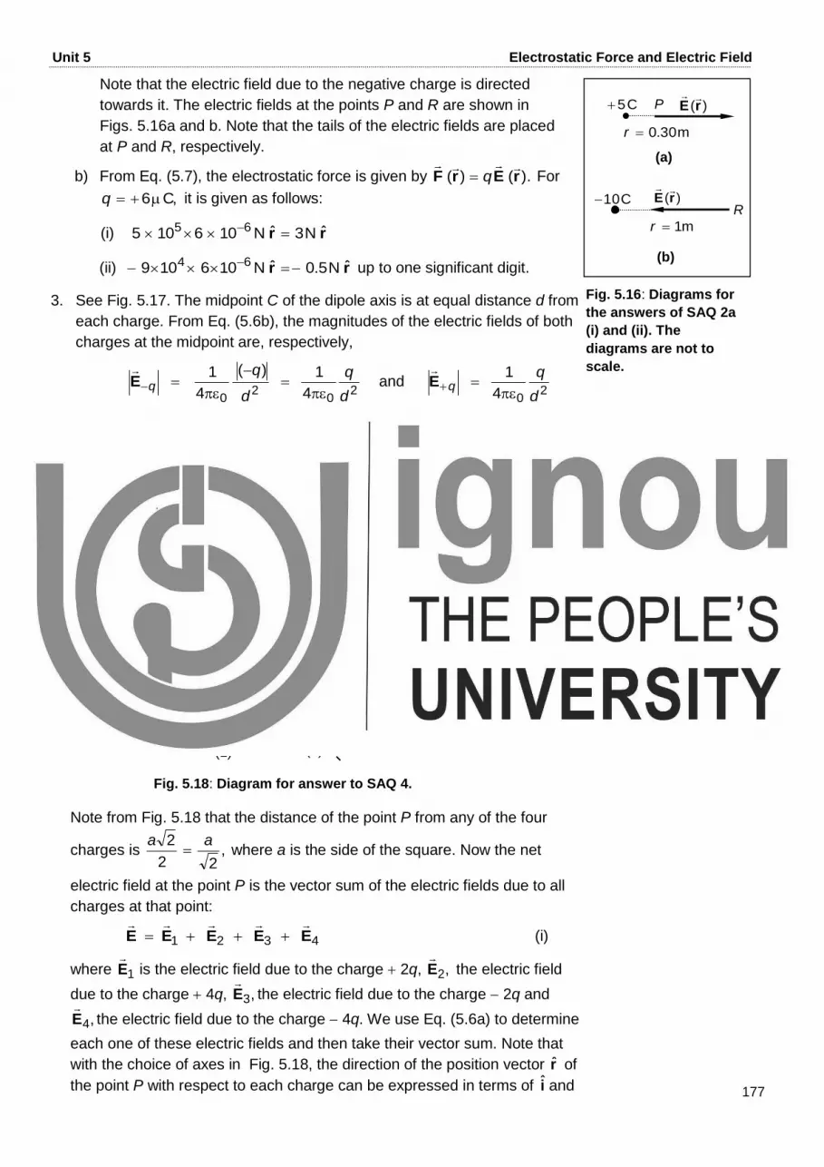
Note that the electric field due to the negative charge is directed

towards it. The electric fields at the points P and R are shown in

Figs. 5.16a and b. Note that the tails of the electric fields are placed

at P and R, respectively.

b) From Eq. (5.7), the electrostatic force is given by ).()( rErF

q For

C,6q it is given as follows:

(i) rr ˆN3ˆN106105 65

(ii) rr ˆN5.0ˆN106109 64 up to one significant digit.

3. See Fig. 5.17. The midpoint C of the dipole axis is at equal distance d from

each charge. From Eq. (5.6b), the magnitudes of the electric fields of both

charges at the midpoint are, respectively,

2

02

0 4

1)(

4

1

d

q

d

qq

E

and

204

1

d

qq

E

The directions of the electric fields at the point C due to both charges are

opposite to ,r the unit vector along the line joining the two charges as

shown in Fig. 5.17. From Eq. (5.11), the resultant or net electric field at the

midpoint C due to the two charges is:

rEEE ˆ2

4

12

0 d

qqq

4. Let us choose the x and y-axes as shown in Fig. 5.18 by the dashed

arrows.

Note from Fig. 5.18 that the distance of the point P from any of the four

charges is ,22

2 aa where a is the side of the square. Now the net

electric field at the point P is the vector sum of the electric fields due to all

charges at that point:

4321 EEEEE

(i)

where 1E

is the electric field due to the charge 2q, ,2E

the electric field

due to the charge 4q, ,3E

the electric field due to the charge 2q and

,4E

the electric field due to the charge 4q. We use Eq. (5.6a) to determine

each one of these electric fields and then take their vector sum. Note that

with the choice of axes in Fig. 5.18, the direction of the position vector r of

the point P with respect to each charge can be expressed in terms of i and

Fig. 5.16: Diagrams for

the answers of SAQ 2a

(i) and (ii). The

diagrams are not to

scale.

(a)

)(rE

m30.0r

C5

C10

(b)

)(rE

m1r

P

R

Fig. 5.18: Diagram for answer to SAQ 4.

2q

2q

4q

4q

P a

(1) (2)

(3) (4)

x y

2/a

a


the answer of SAQ 3.

q

q

d

C

d

r

178


j or their combinations. Also .2

ar So, from Fig. 5.18, we can write

the electric field at P due to the charge 1 as

iiiE ˆ4

4

1ˆ22

4

1ˆ

)2/(

)2(

4

12

02

02

01

a

q

a

q

a

q

( i r ˆˆ ) (ii)

We write 2

00

4

4

1

a

qE

so that the expressions become simpler to write.

The electric fields at P due to the charges 2, 3, 4 are:

,2ˆ42

4

102

02 jjE E

a

q

)ˆˆ( j r (iii)

iiE ˆ)ˆ()2(2

4

102

03 E

a

q

( i r ˆˆ ) (iv)

and jjE ˆ2)ˆ()4(2

4

102

04 E

a

q

)ˆˆ( j r (v)

Substituting Eqs. (ii) to (v) in Eq. (i), we can write

)ˆ2ˆ(2ˆ4ˆ2 0004321 jijiEEEEE EEE

(vi)

Now for C100.1 9q and m,06.0a

2

9229

20

0m)06.0(

C100.14CmN1099.8

4

4

1

a

qE

140 CN100.1 E and )ˆ2ˆ(CN100.2 14 jiE

Terminal Questions

1. We use Eq. (5.2) for the magnitude of the electrostatic force with

.4

1

0k It is given that N10

4

12

21

01

r

qqF is the magnitude of

the electrostatic force exerted by two point charges on each other when

these are placed a distance r apart. The magnitudes of the electrostatic

force between them for various distances will be, respectively,

a) N8

5

16)(164

1

)4(4

1 12

21

02

21

02

F

r

qq

r

qqF since

N104

12

21

01

r

qqF

b) N10N10000

10

10000)100(4

1 312

21

03

F

r

qqF

c) N16016)4/(4

112

21

04

F

r

qqF and

179


d) N1010000)100/(4

1 512

21

05

F

r

qqF

2. Let the charge on the identical particles be q. We use Eq. (5.2) for the

magnitude of the electrostatic force with 04

1

k . It is given that the

charges are identical and the distance between them is 1m. Substituting

these values in Eq. (5.2), we have

2

2

0 m)1(4

1N1

q

or Cm33.0CmN1099.8

m)1(N1

229

2

q

3. a) Refer to Fig. 5.19a. The net electrostatic force exerted on particle C is

the vector sum of the electrostatic forces exerted on it by the particles

A and B as given by Eq. (5.4b). In terms of the unit vector i along the

x-axis, it is given by

i

FFF ˆ

m)01.0(

C)0.1(

m)02.0(

C)0.1(

4

12

2

2

2

0

BCAC

ii ˆN101.1ˆ)m104

5C10CmN1099.8( 224212229

b) Refer to Fig. 5.19b. The net electrostatic force exerted on particle C is

the vector sum of the electrostatic forces exerted on it by the particles

A and B. In this case, the electric field due to B will be in the opposite

direction to that of A since it points away from the positive charge. In

terms of the unit vector i along the x-axis, it is given by Eq. (5.4b):

0i

i

FFF

ˆ

m)005.0(

C)1(ˆ

m)005.0(

C)1(

4

12

2

2

2

0BCAC

4. Refer to Fig. 5.20. Let the charges lie along the x-axis. Let the position

of the charge 3 ( q) be at a distance x from the charge 1 ( 4q)

such that x a. At this point the charge 2 ( q) is at a distance (a x)

from the charge 3. Therefore, the net electrostatic force exerted on the

charge 3 due to the charges 1 and 2 is given by Eq. (5.4b) as

)ˆ(

)(

ˆ4

4

122

023133 i

i

FFF

xa

qq

x

qq

When the charge 3 is in equilibrium, the net force on it is zero. Thus,

0i

i

F

)ˆ(

)(

ˆ4

4

122

03

xa

qq

x

qq


the answer of TQ 4.

q

4q q

x

(a x)

13F

23F

1

2

3

B A

0.005 m

C

(b)

x


the answer of TQ 3.

B A

0.01 m 0.01 m

C

(a)

x

180


or 22 )(

14

xax

22)(4 xxa xxa )(2

For the positive sign of x, 3

2ax and for the negative sign of x, .2ax

Since x a, 3

2ax is the only possible value of x. Therefore, for the

charge 3 ( q) to be in equilibrium, it should be placed at a distance 3

2a

from the charge 4q.

5. From Eq. (5.6a), the electric field of a particle having charge

C109 9Q at a point 1 m away from it is given by

rrrrE ˆCN81ˆm)1(

C)109(CmN1099.8ˆ

4

1)( 1

2

9229

20

r

Q

It is directed towards the negatively charged particle. The electrostatic

force experienced by a proton placed at that point is an attractive force

directed towards the charge Q and is given by

rrErF ˆ)CN81(C)106.1()()( 119

e rN101.3 17

up to 2 significant digits.

6. Substituting 1NC36 E and m5.0r in Eq. (5.6a), we have

1

2

229

20

CN36m)5.0(

CmN1099.84

1)(

Q

r

QE r

nC1C101 9 Q

7. From Eq. (5.7), we have

)()( rErF

Q (i)

where C109 9Q and .N103 9 iF

Substituting these values

in Eq. (i), we get

iirF

rE ˆNC3.0ˆ

C109

N103)()( 1

9

9

Q

It is directed along the positive x-axis. The electrostatic force exerted on

an electron placed at this point is given by

Nˆ105Nˆ1048.0

ˆ)NC3.0(C)106.1()()(

2019

119

ii

irErF

e

8. Refer to Fig. 5.21. Let us take the x and y-axes as shown in the figure.

Then the electric fields at the midpoint P due to two charges 1 and 2 of

Fig. 5.21: Diagram for the

answer to TQ 8.

a

x

y

1

q

q

r

r/2

r/2 q

2

3

P

181


magnitude q along the x-axis will be equal in magnitude and opposite in

direction to each other:

irE ˆ

)2/(4

1)(

20

1r

q

and irE ˆ

)2/(4

1)(

20

2r

q

The magnitude of the net electric field will be just the magnitude of the

electric field due to charge 3 on the y-axis. The distance of the charge 3

from the midpoint of the side of the triangle along the x-axis is given by

rr

ra2

3

2

22

Therefore, the magnitude of the net electric field at the midpoint of the

base of this equilateral triangle is given by

2

02

02

03

33

4

4

1

4

1)(

r

q

r

q

a

qE

r

This result holds for any side of the equilateral triangle.

9. Refer to Fig. 5.22. Let us choose the coordinate axes so that the problem

becomes simplified. We choose the x-axis to be along the line joining the

charges 1 and 2 as shown in the figure. The net electric field at the origin

is the vector sum of the electric fields due to the charges 1, 2 and 3:

)()()()( 321 rErErErE

(i)

Let us determine the electric fields due to the three charges at the origin.

You can see that the charges q and q are at the same distance (a)

from the origin. So, the origin is at the midpoint of the line joining them.

Therefore, for our choice of the x-axis, we get

irErE ˆ2

4

1)()(

20

21a

q

(ii)

The magnitude of the electric field due to the third charge q2 is

2

03

2

4

1)(

a

qE

r

Since the charge 3 is a negative charge, the direction of the electric field

due to it is towards the charge. The net electric field E

due to the charges

1 and 2 and the electric field 3E

due to charge 3 are shown in Fig. 5.23.

Note that the tails of the vectors are placed at the point where the net

electric field is to be determined. To determine the net electric field at the

origin, we resolve the electric field )(3 rE

along the x and y-axes:

2

120cos 333

EEE x and 333

2

3120sin EEE y (iii)

Therefore, combining the results of Eqs. (ii) and (iii) with Eq. (i), the net

electric field at O is given as:

q


the answer of TQ 9.

q 2q

O

a

x

y

a

120

a

1

2

3

Fig. 5.23: Electric fields

for the answer of TQ 9.

O

a

y

120

E

3E

x

182


jijiirE ˆ3ˆ4

1ˆ2

4

1

2

3ˆ2

4

1

2

1ˆ2

4

1)(

20

20

20

20

a

q

a

q

a

q

a

q

The magnitude of the net electric field is given by

20

20

22

2

131

4

1)(

a

q

a

qEEE yx

r

10. Refer to Fig. 5.24 showing the four charges A, B, C, D, viz. 2q, 2q,

2q and 2q placed at the vertices of a rectangle of sides m0.3AB

and .m0.4BC The net electric field due to the charges at the point of

intersection of the diagonals is the vector sum of the electric fields of the

respective charges at that point. Let us choose the x and y-axes as shown

in the figure. The length of the diagonal of the rectangle is

.m0.5m)0.4()0.3( 22 Note from Fig. 5.24 that the electric fields

due to the charges placed at the vertices A and C point in the same

direction since the charges are unlike. So is the case for the charges

placed at the vertices B and D. The magnitudes of the electric fields due to

all four charges are the same since the magnitudes of the charges are

equal and their distances from the point P are equal. Thus, the magnitude

of the electric field due to each charge is given by

1

2

9229

20

CN6.8m)5.2(

C100.6CmN1099.8

2

4

1

r

qE

The net electric field is the resultant of the electric fields 1E

and 2E

shown

in Fig. 5.24 with their tails at the point P. Note that their magnitudes are:

EEE 221

Note also from Fig. 5.24 that the x-components of these electric fields are

equal and opposite so they cancel out. Their y-components are equal in

magnitude and in the same direction and are given by:

11121 CN8.13

5

4CN6.822sin

AC

BCEEEE yy

So, the magnitude of the net electric field is

11121 CN28CN8.13CN8.13 yy EEE

up to 2 significant digits. It is directed along the y-axis.


the answer of TQ 10.

2q

P

3.0 m x

y

A

C

B

2q

D

2q 2q

4.0 m

1E

2E

Documents

ELECTROSTATIC FORCE AND ELECTRIC FIELD - eGyanKosh