Durability of Rubber Componentsunder Multiaxial Cyclic Stresses

Federico Coren

School of Mechanical Engineering

Thesis submitted for examination for the degree of Master ofScience in Technology.Espoo 27.11.2017

Thesis Supervisor :

Ass.Prof. Heikki Remes

Thesis advisor:

Dipl.-Ing. Andreas Dutzler

aalto universityschool of engineering

abstract of themaster’s thesis

Author: Federico Coren

Title: Durability of Rubber Componentsunder Multiaxial Cyclic Stresses

Date: 27.11.2017 Language: English Number of pages: 6+94

Department of Solid Mechanics

Professorship: Fatigue of materials

Supervisor: Ass.Prof. Heikki Remes

Advisor: Dipl.-Ing. Andreas Dutzler

An accurate understanding of the fatigue behaviour of structural components through theirworking life, is a key factor for a light-weight and optimal design. Fatigue life has to take intoconsideration a series of parameters spacing from material properties, to working condition to thenature of the cyclic loads. This work consist in the development of a technique able to determinefatigue life of rubber components as well as the location and direction of the cracks.

An hyper-elastic, third-order, five-parameter, phenomenological material model has been selectedand multiple components have been simulated under variable cyclic multi-axial loading.Severalfatigue indicators and damage accumulation models have been taken into account. EventuallyCauchy rotated stresses have been chosen as fatigue indicator, coupled with Palgrem-Minerdamage accumulation rule calculated in different spacial directions using critical-plane method.The Cauchy rotated stresses have been selected in order to be able to implement Haigh diagramdata from existing literature. Furthermore the use of this tensor enables the determination ofthe location and orientation of critical planes referred to the un-deformed configuration. Acustom equivalent stress method has been implemented in order to take into account mean stresssensitivity deriving from phenomena like strain induced crystallization.

The developed method has been tested against literature as well as experimental data in orderthe evaluate its quality. Correct calculation of the co-rotated Cauchy tensor has been verifiedagainst a uni-axially loaded specimen subjected to a rotation in the reference system. A diabolospecimen has been simulated under torsional loading in order to verify the correct location andorientation of cracks. Correct interpolation of multi-axial stress states deriving from multipleexternal loads have been verified against results from a FEM solver. Lastly a component fromliterature has been tested using different load signals, and the data from fatigue life, cracklocation and crack orientation have been gathered.

The procedure proved to be successful in the prediction of the location and orientation of cracksreferred to the un-deformed configuration. Furthermore a precise fatigue life estimation ofcomponents under different load signals has been achieved. The procedure is highly customizabledepending on fatigue and material properties of the specimen analysed. This procedure hasproven to be a successful predictor tool for fatigue life estimation of multi-axially, cyclic loadedrubber components.

Keywords: Rubber,Durability,Fatigue,Multiaxial Loading

iii

Thanks

I want to thank my tutor Andreas Dutzler for the great support received and my supervisorHeikki Remes for the support he provided me.

A special thank to my family for the love, support, and constant encouragement I havegotten over the years and throughout my whole studies.

A thanks also to all the wonderful people I met during my studies for all the opportunitiesthey gave me.

Otaniemi, 27.11.2017

Federico Coren

iv

Symbols and abbreviations

Symbols

W Strain energy densityF Deformation gradient TensorC Right Green-Cauchy deformation tensorB Left Green-Cauchy deformation tensorR Rotation tensorE Lagrangian strainP 1st Piola Kirchhoff stress tensorS 2st Piola Kirchhoff stress tensorσ Cauchy stressJ Determinant of FB Bulk ModulusWc Cracking energy densityθ crack orientation angleD Damage 0 ≤ D ≤ 1Nf Number of Cycles

Operators

∇A gradient of function A∇×A curl of vector Addt derivative with respect to variable t

∂

∂tpartial derivative with respect to variable t∑

i sum over index iA ·B dot product of tensors A and BA×B vectorial product of tensors A and BA⊗B cross product of tensors A and B

AbbreviationsCB Carbon BlackNR Natural RubberCS Carbon SteelUV Ultra Violet radiationw% w Mass fraction of a component into the bulk.

v

Contents

Abstract ii

Contents v

1 Introduction 11.1 Rubber . . . . . . . . . . . . . . . . . . . . . . . . . . . . . . . . . . . . . . 11.2 State of the Art . . . . . . . . . . . . . . . . . . . . . . . . . . . . . . . . . . 11.3 Scope of the Thesis . . . . . . . . . . . . . . . . . . . . . . . . . . . . . . . . 3

2 Material Behaviour of Elastomers 42.1 Elastomer and rubber components . . . . . . . . . . . . . . . . . . . . . . . 42.2 Stress-strain relation . . . . . . . . . . . . . . . . . . . . . . . . . . . . . . . 82.3 Viscoplasticity . . . . . . . . . . . . . . . . . . . . . . . . . . . . . . . . . . 102.4 Mullin Effect . . . . . . . . . . . . . . . . . . . . . . . . . . . . . . . . . . . 112.5 Temperature Dependency . . . . . . . . . . . . . . . . . . . . . . . . . . . . 122.6 Strain induced crystallization . . . . . . . . . . . . . . . . . . . . . . . . . . 13

3 Constitutive Equations 143.1 Hyperelasticity theory . . . . . . . . . . . . . . . . . . . . . . . . . . . . . . 143.2 Stress-Strain relations . . . . . . . . . . . . . . . . . . . . . . . . . . . . . . 143.3 Third Order Deformation . . . . . . . . . . . . . . . . . . . . . . . . . . . . 15

4 Fatigue Behaviour of Rubber 174.1 Influence of material properties . . . . . . . . . . . . . . . . . . . . . . . . . 184.2 Influence of surface finish . . . . . . . . . . . . . . . . . . . . . . . . . . . . 214.3 Environmental conditions . . . . . . . . . . . . . . . . . . . . . . . . . . . . 214.4 Stress Levels . . . . . . . . . . . . . . . . . . . . . . . . . . . . . . . . . . . 22

5 Fatigue Life Modelling 235.1 Stretches . . . . . . . . . . . . . . . . . . . . . . . . . . . . . . . . . . . . . 245.2 Stresses . . . . . . . . . . . . . . . . . . . . . . . . . . . . . . . . . . . . . . 255.3 Stresses from continuum damage mechanics . . . . . . . . . . . . . . . . . . 255.4 Energy based criteria . . . . . . . . . . . . . . . . . . . . . . . . . . . . . . . 28

5.4.1 Strain Energy Density . . . . . . . . . . . . . . . . . . . . . . . . . . 285.4.2 Cracking Energy Density . . . . . . . . . . . . . . . . . . . . . . . . 28

5.5 Configurational Mechanics . . . . . . . . . . . . . . . . . . . . . . . . . . . . 31

6 Damage accumulation theory 326.1 Continuum damage mechanics . . . . . . . . . . . . . . . . . . . . . . . . . 326.2 Palgrem-Miner linear damage accumulation . . . . . . . . . . . . . . . . . . 33

7 Mean stress sensitivity 36

8 Critical plane method 38

vi

9 Cycle counting 419.1 Cycle counting techniques . . . . . . . . . . . . . . . . . . . . . . . . . . . . 43

9.1.1 Rainflow counting . . . . . . . . . . . . . . . . . . . . . . . . . . . . 439.1.2 Markov-Matrix . . . . . . . . . . . . . . . . . . . . . . . . . . . . . . 459.1.3 Range Pair Method or Reservoir counting . . . . . . . . . . . . . . . 46

9.2 Level Crossing . . . . . . . . . . . . . . . . . . . . . . . . . . . . . . . . . . 469.3 Peak Counting Method . . . . . . . . . . . . . . . . . . . . . . . . . . . . . 47

9.3.1 Signal Filtering . . . . . . . . . . . . . . . . . . . . . . . . . . . . . . 48

10 Work procedure description 5010.1 Cauchy rotated in reference configuration . . . . . . . . . . . . . . . . . . . 5010.2 Haigh diagram creation . . . . . . . . . . . . . . . . . . . . . . . . . . . . . 52

10.2.1 Haigh diagram using interpolating polynomial surface . . . . . . . . 5210.2.2 Haigh diagram using interpolating planes . . . . . . . . . . . . . . . 53

10.3 Mean stress sensitivity Correction . . . . . . . . . . . . . . . . . . . . . . . 5610.4 Haigh Diagram Testing . . . . . . . . . . . . . . . . . . . . . . . . . . . . . 5710.5 Multiaxial Load Signals . . . . . . . . . . . . . . . . . . . . . . . . . . . . . 57

11 Method implementation 60

12 Model Validation 6412.1 Single-Element Cube . . . . . . . . . . . . . . . . . . . . . . . . . . . . . . . 6512.2 Eight Block Cube . . . . . . . . . . . . . . . . . . . . . . . . . . . . . . . . . 7012.3 Diabolo Test n.1 . . . . . . . . . . . . . . . . . . . . . . . . . . . . . . . . . 7212.4 Diabolo Test n. 2 . . . . . . . . . . . . . . . . . . . . . . . . . . . . . . . . . 78

12.4.1 Material properties . . . . . . . . . . . . . . . . . . . . . . . . . . . . 7812.4.2 Element type . . . . . . . . . . . . . . . . . . . . . . . . . . . . . . . 7812.4.3 Signal for diabolo test . . . . . . . . . . . . . . . . . . . . . . . . . . 8212.4.4 Life estimation . . . . . . . . . . . . . . . . . . . . . . . . . . . . . . 84

13 Discussion and Conclusions 85

List of Figures 87

Bibliography 91

1

1 Introduction

1.1 Rubber

Rubber has a long application history in many engineering fields. Thanks to its nature,rubber can withstand elongations many time its lengths, returning to almost the sameinitial dimension. From aerospace, to car industry, its sealing and damping propertieshave come to use in thousands of different applications. When used as dampers, the workprinciple consist in imposing great deformation to bulks of rubber. The effect is dual: itworks as springs as well as a damper. As a matter of fact the micro-structure consist inlong polymeric chains cross-linked together [39]. Any external load results in the internalmovement of such chains, and the sub-sequential relative movement of the chains leads toa dissipation of energy. This is a valuable property when the designer goal is to limit thestresses and vibration transmitted between different structures.

Estimation of fatigue of rubber has becoming more and more important due to theneed of correctly designing rubber based components. The need to optimize the wholelife-cycle of engineered specimen has pushed towards the study of the nature and entityof the damage due to multi-axial loads. Knowing the exact service life allows to deploylonger inspection time-intervals and through the proper dimensioning of the components,the material can be allocated in the zones where it is more stressed.

1.2 State of the Art

Life influencing factor in rubber materials can be divided in four main categories: 1)material properties, 2) surface properties, 3) working conditions and 4) geometrical prop-erties. Material properties derive from the base material composition as well as on thepresence of possible impurities deriving from both the manufacturing and processing ofthe base material[14, 17, 26]. Surface conditions also are closely related to the manufac-turing processes such as composition of mould detacher, curing agents and anti-oxidizers.Working conditions are determined by the specific application the component is supposedto endure, and mostly consist in the environment temperature, environment chemicalcomposition[3, 31] and load frequency, intensity and mean level. The geometrical propertieshave a direct effect in the load distribution inside the components and are one of the mainchallenges in fatigue design of rubber components. Since most of the properties aboveregard the production processes, this work has focused on the load distributions inside therubber components and their relation with fatigue life.

Constitutive models describing the behaviour of rubber materials must take into ac-count a series of phenomena such as hyperplastic behaviours, cycle softening [11], creepand strain dependent viscoelastic storage modulus. In order to get an accurate materialdescription, a hyperplastic model has been selected. Since the material studied presentedstrong strain induced crystallization [36, 22], some stress-compensation techniques fortackling with mean stress sensitivity deriving from this phenomena have been developed.

2

In fact a procedure has been develop that allows for a mean stress correction based onexperimental data. The Haigh diagram is parametrically described as a combination oflogarithmic planes that are tuned to fit onto experimental data. The fitted Haigh diagramis then used to calculate equivalent stresses for any given R value. Due to the natureof the procedure, materials with extremely different mean stress sensitivity can be modelled.

Fatigue life for rubber components follows a power law, where the cycles to failure arerelated with a fatigue estimator. Among the possible ones, the most used are max principalstresses, strains, strain energy density, cracking energy density, and J integral (Eshelbystress tensor)[5]. During the work life of a component, two different damage phenomenacan be found. The first regards the crack nucleation: the life associated with this damagecan be described through a Wöhler relation. The second describes crack growths, but sinceit usually regards less than 10% of the component life, it can be neglected in fatigue design.As a matter of fact the crack propagation regime is usually associated with a deteriorationof the mechanical properties below acceptable levels.

From literature, the indicators with the highest fatigue prediction capabilities areprincipal stresses and cracking energy density[13, 6]. The latest has been deemed as notsuitable for design purpose since the parameters needed to determine such quantity areextremely challenging. Among damage accumulation methods two have usually beendeployed, namely Palmgren-Miner linear accumulation damage and Continuum damagemechanics [4]. Whereas the latest allows to take into consideration load sequence effectsand a precise description of damage due to crack formation and crack propagation, the pa-rameters governing such models were deemed not feasible for design purposes. Furthermorethe typical components’ load history, consisting of millions of cycles, would have made theassociated calculations too long, so linear damage accumulation is the most widely adoptedsolution for design purposes.

One of the most common practise adopted in industry is to gather data from the realworld and to slightly modify the designs if failures are seen. This conservative and somehowun-efficient practise is quite expensive and time demanding. As a matter of fact relying onimplementation of designs that might not be optimised can result in working life way shorterthen expected. Furthermore this technique lack a predictability power when new designsmust be implemented. On the other hand extremely refinate models exist, where cracknucleation and growth can be successfully described [4, 5, 6, 13, 37]. The proposed methodin such works do apply well only on highly controlled test environment where it is possibleto deternime a series of parameters regulating these models. Nevertheless the derivationof such parameters is painstaking [30] and they are usually highly dependent from thecomposition of the rubber mixture [34, 18, 17]. Such data can be almost impossible to bedetermined in Industrial application, where many times the only information available onthe rubber mixture is the Macro Mechanics properties. For this reason such models cannotbe easily implemented in an industrial world.

Some commercial software such as FEMFAT [1] and MSC.Fatigue [2] do have the

3

possibility to perform multiaxial fatigue analysis, but having been designed for metalmaterial lack some of the features that have been developed in this procedure. Namely therubber mean stress sensitivity and the rotation of the stress tensors is not possible. Ontop of that the procedure developed during this work is able to automatically retrieve thestress states obtained from the combination of multiple external loads. The possibility tosimulate multiaxial load conditions ensure the ability to represent the complexity of realworld stress states.

1.3 Scope of the Thesis

There is no available method today to perform an accurate fatigue life estimation of elas-tomer components in industrial application. Current industrial design practice involve eithera process of trials and error or the use of software that have been designed primarely formetal components.[1, 2]. Laboratories practices involves the use of extremely complicatedmodels, whose practical application is hampered by the presence of parameters that are hardto be determined. For this reason this work aims at developing a procedure that can predictwith enough confidence the fatigue life of rubber components, but considering at the sametime the need have a reliable, effective and time-efficient design procedure, thus reducingthe gap between laboratories and industrial procedures. Compared to existing techniquesthis work is one of the first able to cope with fatigue of multiaxially loaded rubber specimen.

The model accuracy will be verified with experimental data derived from literaturework as well as by real world component given by Siemens Mobility (Graz). The fatiguedesign method will consist in the developing of a procedure able to cope with large strainsof the component, to take into account the mean stress sensitivity present and to determinethe fatigue life of the component as well as the crack location and crack orientation. Themodel will be able to interpolate multiaxial stress states deriving from up to three differentexternal loads. The model will be limited in the description of the crack nucleation onlysince it describes the majority of the fatigue life scenarios. This choice is also backed up bythe fact that crack propagation regime is usually associated with a deterioration of themechanical properties below acceptable levels for industrial application. This work focuseson long fatigue life ( Ncycles > 104) and this is related to long signal loads. In order to avoidsimulating with FEM the whole load history, some technique must be deployed in order todecrease the simulation time. Note that a multi-axial stress states might also develop frommono-axially loaded specimen if geometry features or material constitution allow it, so it isimportant to understand how different signals might interfere each other to give a specificstress state. The possibility of describing dynamically the change of the mechanical andfatigue properties as well as the capability of describing load sequence effects of the rubberhas been discarded. This allows to develop a time-efficient analysis method suitable forrubber components and industry application. Models describing load sequence effect anddynamic change of rubber properties are way too complex and computational heavy to beused in any real world scenario.

4

2 Material Behaviour of Elastomers

2.1 Elastomer and rubber components

Elastomer are a family of material made up by polymers presenting viscoelasticity propertiesand very weak inter-molecular forces. They usually present low Young modulus and thecapability to sustain large strains without incurring in permanent deformation. Monomerscomposition is usually based upon hydrogen, carbon, silicon or oxygen. Their structure isamorphous, existing above glass transition temperature. Due to the length of the polymericchains and the few cross-links, a great segmental motion is possible. Their applicationspace from sealant, to adhesive to soft molded parts. As a matter of fact the ability tobe greatly deformed and the capability of some elastomers to be phobic towards specificsolvents, makes them ideal to be used as sealant components. The peculiar micro-structureallows them to dissipate mechanical energy in form of heat due to friction and entropy.This phenomena can be described as entropic elasticity ([16]). In particular stretching asample results in the widening of the polymeric ends, and this causes an overall increasein the order of the system, thus leading to a decrease in the configuration entropy. Tocompensate such decrease the material heats up, and if a proper heat exchange mechanismcan take place, the component will dissipate thermal energy with the environment. Due tothe possibility of being moulded in a great variety of shapes, their ability to bond withmetal while curing, and their damping properties, elastomer are widely used in manyindustrial application. From Automotive to Railway to Aeronautical industry, their field ofapplication is wide.

Elastomer in industry usually consist in Natural Rubber, and for this reason thiswork will focus on them. Natural rubber is a thermoplast consisting in long chains ofNatural Polyisopropene ( cis-1,4 Polyisopropene). The polymerization process consist inthe creation of long chains, like the one in fig 2. Typical chain molecular weight are around105 up to 106 Dalton.

Figure 1: cis-1,4 Polyisopropene, the monomer at the base of the structure of the Naturalrubber polymeric chain in fig:2 source [39]

5

Figure 2: Polymerization principle and final polymer structure. source [39]

Due to the natural origin of the rubber, the presence of impurity is non negligible.Minerals absorbed by the plant are transferred to the rubber, and impurities derivingfrom the manufacture locations can be found in the rubber matrix [18]. In order totackle degradation due to environment contaminants such as Oxygen, Ozone, UV andother chemicals, many addictive are incorporated in the mass of rubber prior to finalmanufacturing.[18] This addictive space form accelerators of the curing process, to moulddetacher to mechanical properties enhances.Radical scavenger of low molecular weight are added to the mixture when high temperatureapplication are required [3]. Other addictive are added to the mixture in order to improvelong term durability and Zinc oxides are normally added to act as polymerization catalysts.In order to improve the dispersion of the various fillers, strearic acids are used. BlackCarbon is normally added to improve mechanical properties specifically the strength andstiffness[32]. On top of that rubber might be aided with the presence of waxes on itssurface, that acting as a physical barrier reduce the amount of contaminants entering thecomponent.All of these addiction to the base material might be a source of problems when the particlesize of the fillers is big enough to become a crack initiator. As a matter of fact, aggregatesof Carbon Black particles have been observed to become the preferred location to crackinitiation, due to their action of stress concentrator.[32, 22]

6

The biggest commercial source of natural rubber consist in cultivation of Haveabrasiliensis even if other sources exist.

Figure 3: Havea Brasilianis. source [39]

The bark of the tree ( fig: 3) is incided and the Latex collected. Due to this manifac-turing process almost 6 percent in weight is composed by other particles: lipids (1.5–3%w/w), proteins and polypeptides (2% w/w), carbohydrates (0.4% w/w) and minerals (0.2%w/w).[30]

Rubber components are usually manufactured through mould injection, compressionmould or transfer moulding. Rubber Injection Mould (fig:4 )consist in forcing a uncuredand preheated mass into a metallic mold. Here curing process happens and the componentscan be then extracted. Compression molding (fig:4)consist in the shaping of a preformthought the aid of metallic forms. This is an ideal process where the geometry of the rubbercomponents are not too complicated. Transfer molding (fig:4)differs from compression oneonly in the placement of the raw material, this time at the top of it.

7

(a) (b)(c)

Figure 4: Figure 4: Injection Molding (a), Compression Molding (b) and Transfer Molding(c)

The production process is of great importance concerning fatigue life. Some of thegreater problems derive from the initial mixture of the raw material and from the mouldenvironment. Aggregate from uneven mixing of rubber with mechanical enhances such asCarbon Black particles might result in crack precursor when their size exceed the 30-40µ m. [23]. As a matter of fact the stress gradient on the interface surface of such parti-cles might be high enough to create the correct condition for a crack to nucleate and develop.

Surface condition deriving from the moulding process poses also a great influence onthe life. On the mold surface there are usually some detached substances, like waxes,that prevent the rubber to bond with the metallic surface while curing. This wax layerdetermines the surface roughness, and to higher smoothness level correspond longer servicelife. Surface imperfection as small as 1 mm are considered to be an initial stage of a crack,thus shifting the component from a regime of crack nucleation to a way shorter regime ofcrack propagation.

8

2.2 Stress-strain relation

Elastomer possess a peculiar material behaviour, that cannot be fully described via asimple elastic relation (fig:5). Characteristic of the material is a very high capacity ofreversibly retaining several hundred percent of strain. Elastomers are generally consideredto be incompressible materials. The polymeric structure,consisting of monomeric chainscross-linked together, allow the material to behave like a solid. At the same time thecovalent bonds allow the overall structure to be heavily deformed, thus acting like a liquid.On top of that the elastomers present a highly packed atomic structure, resulting in agreat resistance to change the volume. Furthermore, like liquid, polymer chain can greatlymove in respect one to another, resulting in an ease to change shape. Stress strain curveobtained from experiment data shows a non linear progression up to failure point. Thecurve usually presents one or two turning points during an extension cycle. Qualitatively astress-strain shown in fig: 5.

Figure 5: Example of measured stress strain curve.

To model material behaviour the most success full models are Hyper-elastic ones, wherethe stress-strain relation is derived form a definition of strain energy density function.Several models are available (fig:7) and a comparison made by [21] (fig:6)reports principaladvantages and drawbacks of each. After some evaluation (tab:6), the model adopted inthis work has been a 3rd order, 5 Parameters Phenomenological method (Mooney Rivlin5 param in fig 7) , that will be further discussed in following sections. The choice forthis method is its ability to correctly predict the stress-strain relation and to be relativelystable.

9

Material Model Strenghts Weakeness Evaluation

Arruda Boyce Physical base, stableonly two parameters Limited phisical description,can represent ´´ up turn ´´ only Limited

Marlow Correctly predicts measurement results Not parametrizable, rarely commercially implemented Limited O

gden

1. Order Not sufficient for proper phisical description Unsatifactory

2. OrderFrom second order on, it describe withenough accuracy the profile of the stress strain curve

Numerical instability arises for some materialsUnsatisfactory

3. Order4. Order5. Order

6. Order Numerical instability due to too high order

Poly

-no

mia

l 1. Order Mooney RivlinClassic Literature Method Numerical instability arises for some materials Unsatisfactory

2. Order Mooney Rivlin

Red

uced

Pol

ynom

ial

1. Order Neo HookeOne parameter only, stable most of the times. Classic literature model The ´´up turn´´ cannot be modelled Satisfactory

2. Order Not better results then Neo Hooke, although of higher grade Unsatisfactory

3. Order Yeoh

Correct prediction of stress-strain relations,classic material model

Not innerly numerically stableSatisfactory

4. Order Numerical instability arises for some materials Unsatisfactory5. Order Correct prediction of stress-strain relations Not better compared to Yeoth, despite the higher grade Unsatisfactory6. Order Unsatisfactory

Van der Waals Correct prediction of stress-strain relations, physical base rarely commercially implemented Limited

Figure 6: Comparison of constituive models.

Figure 7: Example of different constitutive models

10

2.3 Viscoplasticity

Cyclic deformation of elastomers leads to energy dissipation in form of heat due to twodifferent phenomena. The first one is linked to the relative movement and interactionof the polymeric chains with the filler material and themselves, thus leading to a en-ergy loss due to friction. The second phenomena relates with configuration entropy [16].As a matter of fact as the elastomer is stretched, the tendency of the fibres will be toaligned in an orderly fashion. This will lead to a decrease in the local entropy thatwill be compensated via an increase of the rubber temperature.(fig:8) A difference inthe temperature between the rubber and the surrounding will lead to a dissipative heatflux.Due to this phenomena, the rubber will exhibit an Hysteric behaviour depicted in fig:9).

Figure 8: Depiction of temperature increase due to straining of rubber. Source [39]

11

Figure 9: Hysteresis behaviour during a loading-unloading cycle. Source [24]

The pronounced damping properties of elastomer is due to this large hysteresis. Elas-tomer material exhibit a frequency dependent behaviour under mechanical stresses. Undercyclic loading, elastomer exhibit a dependence of the viscoelastic storage modulus on theamplitude of the applied stress. Over approximately 20 % elongation, the storage modulusapproaches a lower bound. This property is called Payne effect and it is dependent fromfiller content. It can furthermore be linked with a breaking of weak bonds at microscopicallevel. The models used in fatigue design are nevertheless not able to include such effect, soits contribution will be excluded in this work.

2.4 Mullin Effect

During the first cyclic loads, most of the rubber components will be subject to a degradationof the mechanical properties in the form of a cyclic softening as seen in fig: 10. This effectgoes under the name of Mullins effect. The entity of such relaxation depends from themagnitude of the loads. After an amount of loads around 102 cycles the effect will not benoticeable anymore. [11] Mullins effect has a great influence in the material characterization,and for this reason standard procedure require an initial amount of pre-stretches beforemeasuring mechanical properties. Mullins effect are in close connection with the filler’snature and size [26]

12

Figure 10: mullins effect during showed for different strain level. Source [21]

2.5 Temperature Dependency

The mechanical properties of rubber are dependent from temperature. Below the glasstransition temperature, the elastomer will crystallize and become brittle. Glass transitiontemperature for Natural rubber are usually around −70◦ Celsius. With increase in tem-perature two phenomena will occur. At room temperatures they will exhibit a negativethermal expansion with temperature increase. This can be easily explained by referringto image 8, as a matter of fact the increase of thermal energy will allow a more intricateconfiguration of the polymer chain, thus reducing the occupied volume.

13

2.6 Strain induced crystallization

Elastomers subjected to strains over 200 exhibit a behaviour called strain induced crys-tallization.(fig:11) This phenomena is based upon a local crystallization of the polymerchain due to stretching. This event is reversible and the crystallized part returns to anamorphous conditions upon relaxing[36] .

Figure 11: Effect of the strain induced crystallization on the Polymeric chains. Source [29]

This phenomena is of great interest in rubber since it can lead to an increase of thefatigue life. As a matter of fact, crack tip are interested to a zone of high stresses andstrains. The formation of a crystallized area at the crack tip acts as a crack-propagatorpreventer. This phenomena is at the base of the peculiar shape of Haigh diagrams, wherefor R values greater than 0 the fatigue life increases.

14

3 Constitutive Equations

3.1 Hyperelasticity theory

Rubber materials, due to their peculiar mechanical behaviour, need to be described throughadvanced material models, usually referred to Hyperelastic Materials or Green ElasticMaterials. Hyperelastic models are successfully used in application on non-linearly elas-tic, isotropic, non compressible materials, and these models are special cases of Cauchymaterials. The stress state at each point is univocally determined by the present stateof deformation compared to an arbitrary initial one. In this work, the initial state willalso be referred to the reference configuration, and the deformed one also to the spatial(current) configuration. In the constitutive equation of a Cauchy material, the stress statedoes not depend upon the deformation path to which a material is subjected, nor on thedeformation rate to reach a certain configuration. Moreover volume forces (body forces)and inertial forces, do not affect material properties.Special case of Cauchy materials are the Hyperelastic or Green elastic ones. This class ofconstitutive model derive the stress-strain relations through a function known as strainenergy density.Strain energy density is a scalar valued function that associates the Right Cauchy-Greendeformation tensor to the strain energy density release.

W = W (C) (1)

3.2 Stress-Strain relations

Due to its molecular nature, for solicited elastomer is easier to change shape rather thenchanging volume. As a matter of fact shear modulus is much smaller when comparedto the bulk one. The stress strain relation can be described through the use of the1st P iola−Kirckhoff stress tensor and the Deformation Gradient F, but in order toobtain them the hydrostatic pressure must be derived. In order to do so it is importantto start from the Bulk modulus definition for a nearly incompressible material. TheBulk Modulus is described as the ratio in change of pressure over the fractional volumecompression and for elastomer is very high.

B = ∆P∆V/V (2)

For incompressible materials, J := detF = 1 . Where F is the two point DeformationGradient Tensor. In order to maintain the incompressibility throughout the equations, thestrain energy function can be described as

15

W = W (F)− p(J − I) (3)

The hydrostatic pressure p functions as a Lagrange multiplier, used to enforce the incom-pressibility constraint. Under this hypothesis the 1st Piola-Kirchhoff stress is given by:

P = −p J F−T + ∂W

∂F = −p F−T + F · ∂W∂E = −p F−T + 2F · ∂W

∂C (4)

Where E is the Lagrangian Strain, C is the Right Cauchy-Green deformation tensor.Any stress tensor can be derived from the previous expression. Since in for fatigue predictionCauchy and rotated Cauchy stresses are important, we report the definition of Cauchy stress:

σ = P · FT = −p I + ∂W

∂F · FT = −p I + F · ∂W

∂E · FT = −p I + 2F · ∂W

∂C · FT (5)

3.3 Third Order Deformation

The model used in this work for describing the material properties is an invariant based,Third Order Deformation model with 5 describing parameters. Phenomenological modelrefers to the fact that the physical description of the material behaviour is not based upona theoretical physical description, whereas is backed only by relations inferred through theempirical observation of certain phenomena. For this reason the 5 describing parametersensure that the function describing the stress/strain relation passes through the measuredstress/strain points. These parameters are obtained using a least square method for theparametrized function over the measured experimental data. In particular the strain energydensity is here described as a linear combination of the two invariants λ1, λ2 of the LeftCauchy-Green deformation tensor B. Strain invariants are derived from the followingrelation:

J = λ1λ2λ3 (6)

The five parameter models is chosen since it can successfully describe the upturn inthe stress strain curve as seen in picture 5. This leads to the parametrization of W in thefollowing way

16

W5 =C10 (I1 − 1) + C01 (I2 − 1) + C20 (I1 − 1)2 + C01 (I2 − 1)2

+ C11 (I1 − 1)(I2 − 1) + 1d

(J − 1)2(7)

With this definition of strain energy density, the uni-axial stresses are given as:

S =2C10

(λ− 1

λ

)+ 2C10

(λ− 1

λ3

)+ 6C11

(λ2 − λ− 1 + 1

λ2 + 1λ3 −

1λ4

)+ 4C20λ

(λ− 1

λ3

)(λ2 − 2

λ− 3

)+ 4C02λ

(2λ− 1

λ2 − 3)(

1− 1λ3

) (8)

Stability criterion are met for∂σij∂εij

≥ 0 and ∂σij∂εij ≥ 0 (9)

Equation 9 refers to the monotony of the strain-stress curve for any given stress state.The monotonic trend can be seen in fig: 12. In particular the monotony of the functionassures that the force applied to the specimen always increases. As a matter of fact anegative value of the derivative of the stress in regards of the strain would suggest thata negative force applied to the specimen would result in a positive elongation, and thiseffect would be not physically viable. The derivation of all the parameters described in 9 isobtained through an optimization fitting process. Experimental data are gathered and theparameters are usually optimized with a least square method.

Figure 12: Comparison between measured data and Model prediction on Stress-Strainrelation.

17

4 Fatigue Behaviour of Rubber

Fatigue life of Rubber can be divided in three different stages:

1. Crack nucleation. This represent from 80% to 90% percent of the component lifeup to complete failure. In this stage the cyclic loads starts creating some microcrackign, usually around rubber defects, that might in a second stage grow to cracks.This part of fatigue life is well described by Wholer life relations.[32]

2. Crack growth. This phenomena occurs when a single crack develops enough tostart being noticeable. Once a micro-crack becomes big enough to promoted to crack( usually has to be bigger then 1 mm) the crack growth becomes somehow fast. Inthis stage the crack growth related to the cyclic stress levels is governated by anexponential law similar to the Paris one. [15]

3. Component failure. The failure of a component might be defined in several ways.Underling them all is the assumption that a failed component is not longer able toperform the task it was designed for.

Fatigue in rubber is a quite challenging phenomena to tackle with. As a matter of factmany parameters have a great influence on the overall life of components:

• material properties deriving from manufacturing of the raw materials as well asbeing influenced by the producing processes.

– Fillers

– Curing accelerators (ZnOx, stearic acid,...)

– Detacher Residuals from manufacturing processes ( SiO2, CaCO3,...)

– Anti-Degradants (Antioxidants, UV shielders,...)

– Mixing residuals (Carbon Black aggregates, Zinc Oxide aggregates,...

• Surface condition

• Working conditions

– Temperature

– Load frequency

– Load Level

– Chemical environment

– UV exposure

• Component geometry for the distribution of stresses inside the components.

18

Many of the previous parameters are closely related with production and serviceparameters that should be analysed case by case when putting a component into service.Since this work is intended to serve as a tool for understanding the fatigue life derivingfrom solicitation, the main focus will be on the geometrical properties of the componentsand how they affect the stress state at various locations.The following section will briefly analyse the different influencing factor in order to get acomplete overview of the topic.

4.1 Influence of material properties

Rubber is composed primarily by polymeric chains cross-linked by covalent atomic bonds.Nevertheless due to the natural origin of most of the rubber used in industry, a nonindifferent part of it is composed by impurities. These consist manly of lipids (1.5–3%w/w), proteins and polypeptides (2% w/w), carbohydrates (0.4% w/w) and minerals (0.2%w/w).[30]. Also natural fibers contaminants as well as carbon-based inclusion are knownto exist in the specimen.[32]. Such impurities are important in determining mechanicalproperties of rubber as well as they have a great influence on fatigue life.

Figure 13: TEM micrographs of composites: (a) NR-0; (b) CB-10.7; (c) CNTs-1.2; (d)GO-1.6. Source: [12]

Apart from natural impurities, natural rubber is often mixed with mineral compoundssuch as Carbon Black, Silica Oxide and Zircon Oxides, (fig:13) in order to improve mechan-ical properties[14][32]. Other mineral-based filler such as Si2 and CaCO3 are added to themixture to improve processability. Fillers might have beneficial properties in increasingfracture toughness and fatigue life, especially with the increase of the CB content.[14]. Thepresence of Carbon Filler has been observed to produce the highest strain amplificationlevel and area at the crack tip. This leads to the optimal dissipation of input energy, thus

19

improving fracture and fatigue performances.[12]. Carbon Black fillers is an inexpensivematerial obtained as a by product from combustion of hydrocarbons ( eg. from powerplants).Many other fillers have been investigated, but choosing the wrong one might result in adetrimental effect. As an example Natural rubber filled with Carbon Nanotubes ( CNTs)exhibit a much higher hysteresis loss compared with CB that results in weakened fatigueresistance. Some other fillers, like planar Graphene oxide, play a very limited rove infatigue and crack growth prevention. [12]. Uneven mixing of the raw material might resultin worse fatigue properties. It has been observed by that black carbon aggregate with sizeover 200− 400µm might act as crack precursor (fig:14)[9][23].

The two failure mechanism at microscopic level as indicated by[32] are:

• Rubber de-cohesion: is a phenomena that happens at rigid inclusion location (e.g.SiO2, CaCO3), and consist in the particle surface getting clear of the rubber. Thisthen induce an extreme local deformation that, over cyclic loading, can lead to thetearing of the rubber material. These kind of rigid inclusion present a clear interfacewith the rubber matrix.

Figure 14: Images of cracks due to decohesion processes in a specimen deformed stateSource: [32]

• Rubber cavitation: is a phenomena occurring at agglomerate location ( e.g. Carbonblack and ZnO2)(fig:16,15) that do not present a clear interface with the rubbermatrix. These are consequence of non homogeneous mixing processes, but can hardlybe avoided. Cavitation consist in the spontaneous void nucleation under a certainstress-state.

20

Figure 15: Images of cracks in a specimen deformed state Source: [32]

Figure 16: Images of Micro and Macroscopic craks inside a specimen Source: [9]

21

4.2 Influence of surface finish

Surface finish plays a great role in the fatigue life of rubber components. Most of thecomponents are created when a raw mass is heated and shaped against a mold. In order toavoid the adhesion between the rubber and the mold, some detacher agents, like gypsum (Mg3Si4O10(OH)2) can be used. Also this compond can create agglomerates detrimentalto fatigue life, sine they represent the perfect location for a crack to develop. (fig:17)[9, 19]

Figure 17: Images of cracks in a specimen deformed state Source: [9]

The progressive cooling of big components can also results in the presence of stresseslocated under the skin of the component at a distance approximately 200− 400µm fromthe surface. This is due to the low conductivity of the rubber that in a cooling process canallows the formation of very steep temperature gradients.

4.3 Environmental conditions

Working conditions are described by the following parameters

• Temperature: Temperature has a great influence on the mechanical and fatigueproperties of rubber. Temperatures below glass transition temperature will renderthe rubber brittle and decrease significantly fatigue life. Higher temperatures willinitially increase the elastic coefficient, thus changing the stress state. Even highertemperatures will increase the reactivity of the rubber with the atmospheric oxygenuntil burning event occurrence.

• Chemical Environment. Presence of solvents, Oxygen O2 and Ozone O3 willinduce a deterioration of the mechanical properties of the rubber. [31]. The degradedsurfaces will start presenting cracks and crevices, and the surface properties such aswettability and hardness will also change [31].

22

• Ultra-Violet radiation. Radiation on spectra more energetic then the visible one,will also contribute to the material degeneration. [31]

4.4 Stress Levels

Due to the very nature of fatigue, higher stressess level will result in shorter service life.On top of that the load frequency is important in determining the temperature at wichthe component will work. As a matter of fact the energy converted into heat thanks tohysteretic processes tends to accumulate inside the component, since its flow is hamperedby a very low thermal conductivity.The increase in the operating temperature due to selfheat properties is detrimental to fatigue life.[40]

23

5 Fatigue Life Modelling

The components analysed in during this work are usually considered to fail after a certainstiffness quantity is lost (20%). For this reason the specimen will pass most of their workinglife under a stage of crack nucleation. Since the crack growth is happening only during avery limited amount of service life, this fatigue phenomena will be left out. On top of thatthe models describing crack growth in rubber materials are governed by a great amountof parameters, which determination is everything but simple. Since this work aims atdeveloping a procedure useful in practical application, the fatigue crack-growth modelswere deemed infeasible to be applied.Fatigue life under crack nucleation can be easily described as a power-law, where the fatiguelife is related to a suitable fatigue indicator.(fig:18)

Figure 18: A generic Wöhler line, where W is a generic fatigue life indicator

From literature several life indicators have been studied:

• Stretches based criteria

• Stress based criteria

• Energy based criteria

• Configurational Mechanics

24

5.1 Stretches

The use of principal stretches has been adopted in order to predict fatigue life in manyworks [8], [20] [40]. The advantages of using such indicator reside in the possibility of easilymeasure them through direct measurement techniques such strain gauges or Digital ImageCorrelation processes.They successfully predict the direction of the crack propagation, but fail to predict fatiguelife if used on multiaxially loaded specimen. In the figure 19 is possible to observe as thismethod presents a too big scatter of data, thus failing to unify experimental multiaxialfatigue data. [6]. Furthermore since the hydrostatic stress seems to be a very good indicator,the strain tensor is not able to predict fatigue life since it does not effect the hydrostaticcomponent of the stress.[7]

Figure 19: Wöhler curves created using the maximum principal stretch. They clearly showa disagreement in the life estimation, thus defining the principal stretch as not a suitablefatigue life indicator. a and b refer to different experimental setups. Source[6]

25

5.2 Stresses

Principal stress direction can also be used as fatigue indicator.(fig:20) In particular Cauchystresses criteria have shown as the crack direction is perpendicular to the direction ofthe highest principal Chauchy stress. This method has proven to be excellent in unifyingexperimental data from multiaxial experiments[6].Stress criteria are suitable for rubbers exhibiting strain induced crystallization as well[6].During a load sequence, the maximum stress components endured by a material is givenby:

φ = 12 maxt=t0,tc

[σ(t)] (10)

Where tc refers to the final time of the time interval analysed.

This criteria unifies experimental data from different load conditions as possible to beseen in fig:(20)

Figure 20: Wöhler curves created using the maximum principal Cauchy stress. a and brefer to different experimental setups. Source[6]

5.3 Stresses from continuum damage mechanics

It is possible to formulate a stress indicator based on continuum damage mechanics thatcopes with multiaxial loading.[5]. Continuum damage mechanics is a theory that takesinto account the initiation and propagation of cracks through a specimen. The principalassumption is that the presence of these microcraks and defects decrease the net sectionof the specimen, determining an increase of the load transfer to the material elements.Using the Second Piola-Kirchoff stress tensor, the effective principal stresses relate withthe following relation:

Seff = S(1−D) (11)

26

Where D is a damage parameter assuming values between 1 (fracture) and 0 ( virginmaterial). Furthermore it is a parameter evolving from the net section decrease. Damagekinetic can be described as :

D = −∂ϕ∗∂y

(12)

Where y is the damage strain energy release rate and ∂ϕ∗ is the dissipation potential

ϕ∗ = A

a+ 1

(−yA

)a+1(13)

Where A and a are fitting parameters that need to be obtained experimentally. For thenext series of derivation, the use of any Strain energy density is possible. Following thedecription of [5] the Ogden formulation of Strain Energy Density is deployed.

W =n∑i=1

µiαi

(λαi1 + λαi

2 + λαi3 − 3) + 9

2K(J13 − 1)2 (14)

where K is the Bulk modulus, J is the Jacobian ( =1 for incompressible materials),µi and αi are material parameters, µ =

∑µi is the shear modulus.

Damage strain energy release rate is

− y = ∂W∂D

(15)

The damage strain energy release rate can be written differently since the W is afunction of the effective principal stresses Seff .

− y = ∂W(Seff )∂D

(16)

Differentiating 11 with respect to D damage variable,

∂λi(Seff )∂D

= Seff(1−D)∂Seff

∂λi

with 1 ≤ i ≤ 3 (17)

27

Using 14,15,17 the damage strain energy release rate becomes

− y = Seff1−D (18)

Where eventually Seff can be defined with the following parameters

Seff =3∑i=1

∂W∂λi

=3∑i=1

(∑nj=1 µjλ

−2i + pλ−2

i )(∑nj=1 µjλ

αj−1i )

(∑nj=1 µj(αj − 2)λαj−3

i + ∂p∂λi

λ−2 − 2pλ−3i )

(19)

The life expectation prediction using this indicator has poven to be effective [6]. Thefigure21 shows how life of two different specimen geometry under different load cases aresuccessful.

Figure 21: Wöhler curves created using the continuum damage mechanics. a and b referto different experimental setups. Source[6]

The drawback from using such predictor is the high number of parameters that need tobe defined in order to correctly describe Seff , as well as the correct determination of aStresh. This value is correspond to the stress values below which no crack nucleate. Thedetermination of such value is purely empirical, adding further complexity to an alreadycomplex model.The great number of parameters needed to correctly implement such technique, coadiuvatedby the great parameter sensitivity of this model, has deemed it as not feasible for industrial

28

application. On top of that the parameter of Seff changes continuously with every cycle.Such property enables the model to take into account load history of the signal, but onthe other hand require the simulation of every single cycle, thus making it not a feasibledamage calculation technique for long and complicated load signals.Furthermore the need to accurately describe the loss of section due to the damage accumu-lation would result in the need of having a FEM model with and extraordinary fine mesh.This would result in an increase of computational requirements that is not suitable forapplication on large specimen.

5.4 Energy based criteria

5.4.1 Strain Energy Density

One of the proposed fatigue indicator is the Strain Energy Density.(fig:22) Since rubbermaterial are successfully described by hyperelastic constitutive models, the strain energyfunction is already defined. Nevertheless this quantity does not successfully describe fatiguelife as described by [6].Specifically they are not able to cope neither with mono-axial normultiaxial loading of specimens.Moreover being the strain energy density a scalar entity, it does not provide useful infor-mation on the direction of the crack propagation.

Figure 22: Wöhler curves created using strain energy density indicator. a and b refer todifferent experimental setups. Source[6]

5.4.2 Cracking Energy Density

Cracking energy density is a theory that modifies the strain energy density tensor througha critical-plane based approach. In this case the assumption underliyng this theory is thatonly a certain part of the strain energy density is available for crack growth. This quantityis defined as Wc. Once this quantity is defined, for a certain load cycle, there is the needto find a material plane that maximize such quantity. The plane that succeed in doing sois designed as the critical plane, and it will nbe the location of the crack growth. More

29

specifically, let r be the normal direction of a given material plane. Under the infinitesimalstrain framework, lets consider an incrementt of cracking energy density. This quantity isdefined as the dot product between the Cauchy traction vector σ r and a strain incrementdε in the r-direction.[6]:

dWc = (σr)(dεr) (20)

Extending eq. 20 to the Finite strain framework,

dWc = 1RTθ C−1Rθ

RTθ SdE(FTF)−1Rθ = RT

θ SdEC−1Rθ

RTθ C−1Rθ

(21)

Where Rθ = (cos θ, sin θ) with θ crack orientation angle referring to the material con-figuration.

The use of this quantity can lead to correct prediction of life endurance.(fig:23) Theoutcomes of such results are highly dependent from the material parameters. In particularin the following images it can be seen as the presence of a correctly scaled Sth ( thresholdvalue for nucleation) determines the success or failure of the theory.(fig:24)

Figure 23: Wöhler curves created using continuum damage model. Note that the pre-diction not able to unify all experimental data. a and b refer to different experimentalsetups.Source[6]

30

Figure 24: Wöhler curves created using continuum damage mechanics, where the intro-duction of a threshold value for the effective stress Seff allows the model to successfullypredict fatigue life. a and b refer to different experimental setups Source[6]

The need of a series of parameter used in the correct implementation of such procedure,deemed it as not feasible to be adopted in this work. As a matter of fact the governingparameters for the Cracking energy density are hard to define and require a further seriesof mechanical testing. Due also to the great sensitivity of such model to the parameterschoice, it has been not taken into consideration in this work as a feasible fatigue indicator.

31

5.5 Configurational Mechanics

The configurationa mechanics model has been initially proposed by [38]. The foundationof such theory is based on the assumption of the existence of an intrinsic defect locatedinto the rubber specimen. In order to extend this theory to multiaxiality, the critical planemethod developed by [38] was adapted in recent works by [28]. This has been done on theprinciple that a material tends to reduce its potential energy b:

b∗ = |min[(bi)i=1,2,3, 0]| (22)

For b∗ 6= 0 the propagation of the crack will develop on the first principal direction ofthe configurational stress defined as:

b = W I−CS (23)

where W is the strain energy density, I the identity tensor, C the right Cauchy-Greentensor and S the second Piola Kirchhoff stress tensor. Since the eigenvalues of b are thesame ones as C and S, the criterion in eq. 22 can be re-written as

b∗ = Smaxλ2max −W (24)

With Smax and λmax the maximum components of the two respective tensors. Sincethis model uses the stretch tensor ( that proved to be un-effective 5.1) if fails as well atgiving satisfactory fatigue life.(fig:25)

Figure 25: Wöhler curves created using configurational mechanics. Such technique doesnot allow a satisfactory fatigue life prediction. a and b refer to different experimentalsetups. Source[6]

32

6 Damage accumulation theory

The need for accounting the progressive damage deriving from the stress history, has ledto the formulation of several damage accumulation theories. The three most used ones arethe Linear damage accumulation one (Plagrem Miner rule), a modified version of it andone based upon the Continuum damage Mechanics theory [5]. Due to the very complexnature of the fatigue problem, where the fatigue life is extraordinarily sensitive materialand fatigue parameters, the use of complicated damage accumulation method may notresult in any tangible advantage. The implementation of sophisticated models rises thecomputational effort and require the determination of several more parameters that mightnot be easy to determine. For this reason the Linear damage accumulation method hasbeen commonly used for fatigue design purposes.

In the following section a description of all three methods is presented, with particularcare on the description of the pros and cons of every method.

6.1 Continuum damage mechanics

Using the continuum damage mechanics (5.3), it is possible to define both a fatigue lifecriterion as well as a damage accumulation method. As a matter of fact the damageaccumulation can be derived from the description of how the damage parameter D evolvesthrough the cycle history.[5]. For a given step, the increment of Di is given by:

Di = 1−[(1−Di−1)1−a − (1 + a)

(SeqA

)aNi

] 11+a

(25)

Where Seq is the effective stress acting at a certain time step i. D0 is the damage level fortime=0 and Df is the damage after a certain cycle. A and a are fitting parameters to beexperimentally determined. Given a series of n signal blocks of given amplitude, fatiguelife Nf = Nn can be derived from

∫ Df

D0(1−D)a dD =

n−1∑i=0

∫ Nf

Ni

(Seq(i+1)A

)adN (26)

This model parameters depend on the material ones plus the two damage parameters.Furthermore equation 25 can be re-written in order to show that this is a linear cumulativelaw:

(1−Di−1)1+a − (Di − 1)1+a = Ni

Nfi(27)

Noting again that the value of D evolves from 0 till 1 (complete failure), the relation27 is behaving similarly to a Palgrem-Miner cumulative damage. The parameters neededto describe the previous relation(a and A) must be determined with some axial loading

33

experiment, thus increasing the workload needed to apply such technique [6]

Strong point of this method is the capability of taking into consideration the sequenceeffect of the cyclic loading. This is extremely useful if the material present a strong loadsequence sensitivity. On the other hand such technique burdens the analyser with a hugeamount of calculations, since analysis must be performed to determine the stress statefor each cycle. Such peculiarity deems this technique as infeasible for long signals or bigmodels, since the computational load would be staggering.

Under the proper condition, this method presents some of the highest accuracy inpredicting fatigue life, as possible to be seen in fig:26.

Figure 26: Comparison of predicted life vs measured fatigue life using continuum mechanicstecniques. a and b refer to different experimental setups. Source[6]

6.2 Palgrem-Miner linear damage accumulation

Palgrem-Miner damage accumulation theory, is one of the most widely adopted techniquesto calculate damage accumulation. Its effectiveness resides in the simplicity of this model.If on one hand it does not consider load sequence effects, and its linearly summing up thedamage deriving from each cycle, on the other hand, most of the time the data availableto the designer on the load history or on working conditions would not anyway be enoughto use some more refined model.This rule is based on the principle that the damage D can be expressed in the following form:

Di = Ni

Nf(28)

Where D is the damage induced by Ni cycles of a load that would require Nf cyclesat constant amplitude to bring the component to failure.

34

For expressing the total damage, it suffices to sum the partial damages:

D =n∑i=1

Di =n∑i=1

Ni

Nf(29)

Figure 27: Stresses S and corresponding fatigue life N. Source [29]

For D = 1 the component will be subjected to failure. The following image showslife predicted vs measured for two samples subjected to different external stresses conditions.

Figure 28: Comparison of predicted life vs measured fatigue life using Palgrem-Miner linearaccumulation damage. a and b refer to different experimental setups.Source[6]

35

Modified Palgrem-Miner

In order to tackle the non-linear nature of damage in rubber components, [5] has proposeda non-linear parameter to the classical Palgrem-Miner relation in the form of:

D =n∑i=1

Di =n∑i=1

(Ni

Nf

)β(30)

With the proper choice of the β fatigue parameter is possible to get a better agreementbetween the predicted and measured fatigue life. Weak point of this technique is the needto determine a further empirical parameter in order to make life prediction. As a matterof fact the β parameter has so far no physically understood meaning.

Figure 29: Comparison of predicted life vs measured fatigue life using Palgrem-Minermodified accumulation damage. a and b refer to different experimental setups. Source[6]

36

7 Mean stress sensitivity

Mean stress levels affect the fatigue life of components.

Mean stress is defined as

R = σminσmax

(31)

Extreme mean stresses can be high enough to be greater then the maximal stress that thematerial can bear, thus leading to complete component failure. On the other opposite,also negative mean stresses can be higher than the maximum allowable compressing stress.In between this extremes lies a zone where some peculiar behaviour might appear. Formost of material, compressive mean stresses increase fatigue life. Crack nucleation andpropagation are related to the values of tensional stress, that lead to a de-cohesion of thematerial. For this reason a compressive mean stress, reduces the tensile stress at the cracktip, thus slowing down the damage process. On the other hand a positive mean stressapplied on the component will raise the value of the tensile stresses also at the crack tip,thus accelerating the failure process.

Natural rubber as well as carbon filled synthetic rubber present a peculiarity propertyof increasing fatigue life for increasing mean stresses level. This phenomena is due to thecapability of such polymers to crystallize under strain. For a detail description refer tochapter 2.6.The relation between mean stresses and stress amplitude can be easily visualized througha Haigh Diagram.(fig:30)

Figure 30: Haigh Diagram for Natural Rubber with Shore Hardness 60A. Source[21]

37

In the figure 30 is possible to observe the representation of a Scalar field, where forcoordinates there are the mean stresses ( Mittelwert) and Cauchy stress amplitude. Thedata represented are the iso life lines, representing the life for different combinations ofmean stress and amplitude. The figure 31 gives a graphical representation of the data fieldobtained from [24].

Figure 31: Data points used to determine the Haigh Diagram, view from side. The heightof the point is in accordance with life value.

Following any given line from left to right is possible to be seen as with the increase ofthe mean stress the stress amplitude tolerable by the component decrease until reaching avalue or R=0 where due to the strain crystallization process, the allowable stresses increase,to flatter out after R=0.2.

38

8 Critical plane method

Critical plane methods have been developed on the observation that crack growth developsalong preferential directions. Depending on the material is possible to use an indicator ofthe location and direction of the crack preferred developing plane. In particular for rubbermaterials it has been observed that cracks are growing perpendicularly to the maximumCauchy stress[13].

Critical planes method based on strain definition have also been proposed, but theylack the ability to predict failure direction [13]. The idea behind is that during a cycle thestress levels vary in different direction, but only the direction of the maximum stress isdesigned to receive a damage.

This method calculates the stresses over a certain amount of direction, selects the moststresses direction and calculates the damage for the specific direction.(fig:32) The damagedata is stored and when the element plane should be subjected to a subsequent damagingstress, the damage will be summed to the value of the existing one.

Figure 32: Critical plane method. In the fist image is possible to see the plane directionsand the normal axe of the plane sheaf. Second picture shows the parameters defining planedirections and components. Picture to the right shows how a stress tensor has differentcomponents along a path into space. Source [27]

In a Formal way [7], let’s consider a stress variable T, and a generic plane ∆ describedas normal to a versor n. This versor can be described in the cartesian coordinate systemwith two angles φ and θ.Projecting the stress tensor with the versor leads to:

T = σ · n

Modules and coordinate of the normal stress tensor N is obtained by projecting T inthe n direction as follows:

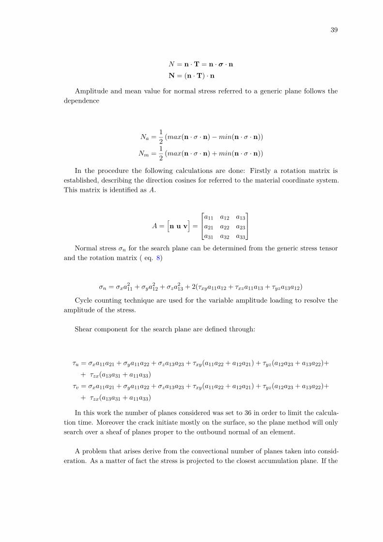
39

N = n ·T = n · σ · nN = (n ·T) · n

Amplitude and mean value for normal stress referred to a generic plane follows thedependence

Na = 12 (max(n · σ · n)−min(n · σ · n))

Nm = 12 (max(n · σ · n) +min(n · σ · n))

In the procedure the following calculations are done: Firstly a rotation matrix isestablished, describing the direction cosines for referred to the material coordinate system.This matrix is identified as A.

A =[n u v

]=

a11 a12 a13a21 a22 a23a31 a32 a33

Normal stress σn for the search plane can be determined from the generic stress tensor

and the rotation matrix ( eq. 8)

σn = σxa211 + σya

212 + σza

213 + 2(τxya11a12 + τxza11a13 + τyza13a12)

Cycle counting technique are used for the variable amplitude loading to resolve theamplitude of the stress.

Shear component for the search plane are defined through:

τu = σxa11a21 + σya11a22 + σza13a23 + τxy(a11a22 + a12a21) + τyz(a12a23 + a13a22)++ τzx(a13a31 + a11a33)

τv = σxa11a21 + σya11a22 + σza13a23 + τxy(a11a22 + a12a21) + τyz(a12a23 + a13a22)++ τzx(a13a31 + a11a33)

In this work the number of planes considered was set to 36 in order to limit the calcula-tion time. Moreover the crack initiate mostly on the surface, so the plane method will onlysearch over a sheaf of planes proper to the outbound normal of an element.

A problem that arises derive from the convectional number of planes taken into consid-eration. As a matter of fact the stress is projected to the closest accumulation plane. If the

40

stress is not laying on the same plane as the nearest plane, the stress will be projected onit and thus it will be smaller then the original. The natural way of tackling such problemwould be to have a very high number of search planes, but the calculation time increaseslinearly with the amount of planes.

41

9 Cycle counting

Load signals ( fig:33) refers to measure of quantity such as displacements, forces, elonga-tions,etc. that might affect a specimen. They must be recorded and then associated withsome technique to the fatigue life of the component.

Figure 33: Example of a Load signal

For components working under specific conditions, it is possible to extrapolate a ’char-acteristic’ load history. Once this is defined, it is possible to simulate it on the componentand to estimate the damage associated. Following a linear damage accumulation model, itis then possible to understand the life fraction that this specific cycles series will cause,and to get a estimation on the whole fatigue life. One example might derive from the useof a typical signal for a train carriage travelling every day between two cities. As a matterof fact it is expected that the load signal affecting the train components, given same trackaverage speed, will be very similar day by day.

Once a signal is analysed, the information about the solicitation amplitude and meanare stored in a more convenient way. With only the loss of the load sequence information itis possible to make a further simplification hypothesis in order to decrease computationaltime. This hypothesis consist in the quantization of the signal values. In this way it ispossible to run a finite quantity of simulation process, and to gather the associated stressstates.(fig:34) As a matter of fact signal amplitudes close one each other will create similarstress states into the specimen. By averaging the signal over a limited amount of levels,amplitude data higher than the average will be compensated by the ones that are lower.In fact for small amplitude variations it is possible to consider the stress increments aslinear with the load increase. For short signal loads problems might arise from phenomenacalled sequence effect (fig:36). This phenomena consist in the occurrence of different fatiguelife for a signal whose components are applied in different orders. On long signals thisphenomenon can be ignored.

42

Figure 34: Example of signal block that can be repeated through time. Source [29]

In order to have a signal that would resemble the properties of the measured one, it isalso possible to randomly rearrange the sequence of the transformed signals’ blocks.(fig:35)This is a useful procedure when testing procedure must be done on some physical component.In fact this procedure will inhibit if not eliminate life estimation discrepancies due to loadsequence effect.[29]

Figure 35: Example of signal block with random block sequence. Source [29]

It has been observed in the years that different load sequence produces different lifeoutcomes[29]. Sequence effect exist both at early fatigue stages ( micro-craking) and inlater stages ( crack propagation). Many service histories on the other hand present aresuch that sequence effects elide one each other. This phenomena is seen especially for longmulti-axial fatigue loads where the load signal is not constantly repeating. [29]

43

Figure 36: Examples of different sequences of the same load. Depending on the materialproperties they might influence the fatigue life of the component . Source [29]

9.1 Cycle counting techniques

Signal analysis techniques aim at condensing the information from a signal in a form usefulto the fatigue calculation. Many different techniques have been implemented throughoutthe history of fatigue analysis, nevertheless the most important ones are the ones able torepresent mean load and load amplitude, since this two parameters are of great importancein determining fatigue life.

9.1.1 Rainflow counting

This is one of the most diffused and implemented cycle counting method, which results arethe same as for the reservoir method. With the load time plotted such that the time is thevertical axis, simulating rain pouring down a pagoda’s roof, the lines go horizontally froma reversal to a succeeding range. Peaks and valley of the signal represent the roof of thepagoda. The calculation method consists of the following steps as described by [29] anddepicted in figure 37 and 38.

1. The history must be rearranged in order to start either with the highest peak or thelowest valley

2. Starting from the highest peak go down until the reversal. The rain-flow processcontinue unless either the magnitude of the following peak is equal or larger than thepeak from which is initiated or a previous rain-flow is encountered.

3. Repeat the same procedure for the next reversal and continue these steps to the end

44

4. Repeat the procedure for all the ranges and parts of a range that were not used inprevious steps.

Figure 37: Left Top: load stress signal. Right Top: rainflow counting illustration. LeftBottom: Resulting count. Source [29]

Figure 38: Result of the previous Rain-Flow counting .Source [29]

45

9.1.2 Markov-Matrix

A graphical way to represent signals after rainflow counting is represented by MarkovMatrix (fig: 39). The plot consist in a vectorial field where the height of the columns isproportionate to the number of occurrence of a certain cycle. On the axis there are meanand amplitude of the signal.

Figure 39: Result of the previous Rain-Flow counting .Source [29]

46

9.1.3 Range Pair Method or Reservoir counting

This method consist in the initial count of cycles containing small ranges. Their reversalpoints are then removed from the original signal.(40) The counting procedure produces thesame data as the rainflow method, and is one of the most used counting method adoptedtoday.

Figure 40: Range pair counting. In step (a) the smaller cycles are counted and eliminatedfrom the signal. Increasing with cycle size as in (b). In (c) there is the last cycle left bythe method.Source [29]

9.2 Level Crossing

Level crossing consist in the counting on how many times a certain signal crosses somepre-defined levels. After the counting is performed, an equivalent signal can be created.This starts with the creation of the most fatigue-damaging cycles when the largest possiblecycle is obtained form the recorder list. This is followed by the second largest possible.(fig:41) This process is iterated until all the values of the count have been used. This methodcannot be used when load sequence effect has to be taken into consideration.

47

Figure 41: Level Crossing Method.Source [29]

9.3 Peak Counting Method

This method consist in simply counting the number of occurrence of peaks present ina given load history. The equivalent signal is then recreated starting from the biggestamplitude achievable, continuing to move to the smaller values until no more peaks areavailable.(fig: 42)As for the Level crossing method, load sequence effect is lost in the signaltransformation.

Figure 42: peak counting method. Source [29]

48

9.3.1 Signal Filtering

In order to decrease the amount of data present in a signal without affecting too much thequality of the information carried by it, it is possible to filter away some low influencingcomponents. As a matter of fact since the fatigue is dependent to a fatigue indicator by apower law, the effect of a signal component is exponentially depended from its magnitude.For this reason signals whose amplitude components are below certain level will onlyminimally influence fatigue life. (fig: 43)Racetrack ( or race track) method are based on the filtering of all the cycles whose amplitudeis lower then a certain threshold. The reference amplitude is represented by the highestamplitude inside the signal.

Figure 43: Racetrack filtering. This technique allows smoothing of the signal in order toexclude small amplitude cycles, whose effect is negligible. Source [29]

49

In fig: 44 is brought an example of a filtering that has been performed on a signal usedon some components.

Figure 44: Original signal and signal filtered with a 40% racetrack filter. It is possible tosee how in the filtered signal all the small cycle components have been eliminated.

50

10 Work procedure description

The fatigue procedure used in this work has been created with the help of existing literatureand methods.[27]. The further formulation is done in order to create a suitable method foranalysing rubber components. Having the original procedure being written for Metallicmaterial, a series of radical changes have been applied.

10.1 Cauchy rotated in reference configuration

Due to the very nature of the Hyperelastic material models, the stresses and strains referredto the Reference and the Material system differs greatly. Cauchy stresses, some of themost reliable and used fatigue predictor (5.2), refer to the deformed configuration. For thisreason it is not intuitive to understand the correct location of failure and crack orientationin the un-deformed configuration. (fig:45)

Figure 45: Deformation process of a body. The un-deformed configuration ( Referenceor Material )is represented with Capital letters. The deformed configuration (Spatial orCurrent) is represented by small letters. Source [39]

For this reason a rotation of the Cauchy stresses has been performed using the rotationtensor derived from the polar decomposition of the Deformation Gradient. Such approachhas also been performed by [40][5][33]. This procedure is derived starting from the definitionof the Cauchy stress through the deformation gradient

S = 1J· F SFT =

3∑α=1

σαα · nαnTα (32)

Where nα represent any direction in the space considered and σαα are the normal stresscomponents in the nth direction.Written in vectorial notation,

51

σαα = nTα · σ · nα (33)

The following derivation aims at finding suitable definition of nα.

Nα = Fnα|Fnα|

(34)

Starting from this relation:

FNα = λ Nα (35)

where λα = |F nα| are the stretches in the α direction.

RUNα = λαNα (36)

where R is the rotational component derived from the polar decomposition of thedeformation tensor.U is on the other hand the deviatoric component derived from thepolar decomposition of the deformation tensor. This tensor in three dimensional spaceis represented with a diagonal matrix, which elements will be constitute by the values ofstretches along the direction of the material system. Since these values coincide with the λs of the left side of eq 36, it is possible to rewrite eq 36 as follows:

R UNα = λα Nα (37)

Inserting the definition for the normal vector of eq 37 in the equation 35, the Cauchystresses referred to the reference configuration can be written as

σαα = (Rnα)T σ (Rnα) (38)

Calculating the transpose of the first left term, the previous expression becomes

σαα = nTα RT σ R nα (39)

WhereRT σ R = σcorotated

This results shows that for getting the Cauchy stresses expressed in the referenceconfiguration, it is necessary to rotate the stress tensor with the appropriate rotationalmatrix. Following this procedure is possible to obtain fatigue life calculation equal to theone using the Cauchy stresses, with the advantage of being able to identify crack directionreferred to the undeformed configuration.

52

10.2 Haigh diagram creation

In order to create a procedure able to cope with data coming from different experiments(fig:47,31), a procedure has been developed that takes as parameter the data coming fromexperiments and uses them to modify the stresses following this order.

10.2.1 Haigh diagram using interpolating polynomial surface

An option to create a Haigh diagram is to use a polynomial interpolant surface in order toapproximate the Haigh function. This has been performed as shown in fig 46.

Figure 46: Interpolation made using a surface interpolation. In order to achieve a sufficientsurface smoothness a very high number of data points are needed. Most of the times it isunlikely to dispose of such data quantity.

The option of using a linear surface interpolation as seen in fig:46 has been deemed notfeasible since for reaching a smooth surface, the number of points required is too high. Theuse of just some dozen points for the creation of this surface will in fact result in peaksand irregularities that do not well represent the physical behaviour of the rubber.

53

10.2.2 Haigh diagram using interpolating planes

In order to represent an Haigh Diagram based on a smaller number of points, the followingprocedure has been implemented using plane approximants:

1. The data file containing triplets with mean stresses, stress amplitude and correspond-ing fatigue life are given as input-parameter. The life associated to a point in themap is transformed using a logarithm.(fig:47) This is done in order to be able to fitplanes on the data given. As a matter of fact, since life data are well described by alogaritmic law, by changing the domain of the life to a logaritmic one, is possible touse a linear relation between amplitude and mean stress and fatigue life.

Figure 47: Data points used to determine the Haigh Diagram.Top view. Different pointscolour refers to different interpolation section. X axis contains the mean stress, y axis theamplitude stress.

2. The Haigh diagram area is divided in 5 sections as seen in fig:47. The dividing linesused to define five different areas are set to be lines passing by (0,0) and using thefollowing angular coefficients: -0.625, -1, 1.2 , 0.5. These cohefficient are used for aRubber of Shore Hardness 60. Depending from the material properties, other dividinglines can be used.The zones are defined using the following selection criteria:

• Selection area n1: This refers to a zone where the fatigue life is not affected bythe mean stress. Although this description does not correspond to the real one,no material data are available for the zone, so it is safer to assume no meanstress influence. {

amplitude+mean ≤ 0 (40)

54

• Selection area n2: This zone is defined as

{amplitude− |mean| ≥ 0

amplitude+ 1.2 ∗mean ≥ 0

• Selection area n3: This zone is defined as{amplitude−mean ≤ 0

amplitude− 0.625 ∗mean ≥ 0

• Selection area n4: Also this refers to a zone where the fatigue life is not affectedby the mean stress. Although this description does not correspond to the realone, no material data are available for the zone, so it is safer to assume no meanstress influence. {

amplitude− 0.625 ∗mean ≥ 0

• Selection area n5: This zone is removed from the data set. As a matter of factthe data here are due to previous interpolation processes made by [24] and donot correspond to reality. Specifically the data in this zone would suggest andecrease of fatigue life with a decrease of mean value for compressive stressees,and this is not observed in reality.{

amplitude+mean ≤ 0

3. After the data is selected by belonging region, a plane fitting procedure is performed.This procedure consist in fitting four different planes using the existing data.( withthe possibility of customizing the number of planes in case different fatigue behaviourswould request it). Specifically there are two zones where the fatigue life does notdepend any more from the value of the mean stress ( between R=-∞ going counter-clockwise and from R=0 going clockwise).The real behaviour of the rubber in thesezones might also differ from the representation used in this work, but no test dataare for such amplitude-mean stress conditions.

The choice of using simple plane for interpolating the logarithmic life has beenpreferred over higher order interpolation in order to avoid un-physical behaviour atthe connecting zones ( R=-∞ ). As a matter of fact, observing the Haigh diagramobtained by [21], it is possible to see an abrupt change in the derivative of the linesassociated with the iso-life lines, that would suggest a decrease of life for values of Rapproaching value of - ∞. This phenomena is not known to happen.

On the other hand the use of plane approximation allow to a very time and computa-tional resource efficient calculation, and the error associated with the approximationhas been evaluated as comparable to the one deriving from the use of higher orderapproximation.

55

The planes on the zones 1 and 4 are created on the outbound values of the planesdescribing the inner sections. In this way it is possible to have a better continuity ofthe interpolating surface. (fig:48)

Figure 48: Representation of the interpolation planes.

56

Manual corrections

In order to reduce discontinuity between the two central fitting planes, is possible tomanually intervene on the steepness and elevation of the singular planes. The externalplane on the other hand develop from the boundary values of the central ones, thus notcreating any hole in the surface.(fig:49)

Figure 49: In in this image is shown how the parameters can be changed to manuallymodify slope and height of interpolating surfaces

10.3 Mean stress sensitivity Correction

After the Haigh diagram has been created, the following procedure is used in order tocreate an equivalent stress value for a fully reversed cycle.

• The stress signal contains mean stress and amplitude, is given as input to theprocedure. For every coordinates couple, the maximum life is calculated.

• The values of the Wöhler curve for fully reversed loading ( R=-1) is extrapolatedfrom the existing data.

• The value of the life associated with a point on the map, is used to find the equivalentstress that would allow the same life for a fully reversed cycle

• The data with the equivalent allowable stresses is given as an input

57

10.4 Haigh Diagram Testing

Since no data were avaiable on the statistical aspects of the haigh diagram from [24], ithas been assumed that the data refers to a 50% probability failure. Different assumptionswould lead to different Haigh data.The effectiveness of this method and its correct implementation has been tested against acustom made signal containing means and amplitude stresses, and the results (table 6)havebeen compared to the Haigh diagram of figure 30.

Original Amplitude Mean Equivalent amplitude

1.0 1.0 1.701.0 2.0 1.471.0 -2.0 0.411.7 0.0 1.691.7 -2.0 0.701.7 -3.0 0.702.0 1.7 3.192.0 2.5 3.072.0 2.4 3.13

Table 1: Signal processing through Haigh Diagram for accounting of mean stress sensitivity

10.5 Multiaxial Load Signals

The aim of this work is to develop an analysis procedure able to predict fatigue life ofworking parts. Many fatigue work focused on mono-axially loaded components. Suchconfiguration allow for ease of testing and part simulation but is somehow not representativeof real world components. As a matter of fact component that are subjected to loads duringworking conditions are usually subjected to multi-axial loading. This loading configurationwill induce multi-axial stress states inside the material, even thouhg for complex geometriesmulti-axial stress states might arise also from mono-axial loading.

In order to analyze more than one signal at the time, it is important to get the signalsvalue at every turning point of each signal. Such process is exemplified in the followingimage 50, where some sinusoidal loads are subjected to an extremization process and thento a rain-flow counting. The extremization process clears the signal from any point that isnot useful for the definition of a cycle. If in a time series a point is located on a straight lineconnecting two subsequent peaks, it does not define any cycle, thus it will be eliminated.On the other hand the simple elimination of such points might lead to the omission of signalcomponents in conjunction with a stress state deriving from a peak into another signal.Since it is important to consider the components of all the signals for a given peak event, allthe values of the other signal components will be taken as well for that specific time-location.

58

Figure 50: Original signal and signal after extremization process has taken place. The datapoint are indicated with small circle. Please note the presence of data at the same timeinstant on all the signal when a peak or valley event happen in any of them.

If the input signal is not represented by a triangular signal, ( like the sinusoidal infig:50) a method has to be used in parallel with the extremization process in order to takeinto account the real value of the components of the signal at a certain time. As a matterof fact the signal extremized in fig:50, second image, shows how the pure extremizationprocess has some issued in determining the signal values for the corresponding peak. Asa matter of fact the extremization process involves a linearization of the signals into atriangular signal. In order to avoid such dicrepancies between extremized and originalsignal, a method has been deployed that collects the true value state of all the signalcomponents for any extreme event using the original signal value. This leads to the thirdimage in fig:50 that presents the correct values as in the first image of fig:50.

59

The technique adopted in this work consist in the interpolation of stress states derivingfrom a maximum of three external signals. A space defined by different values of the signalinterferences must be calculated. Every point corresponds to a tern of signal values, forwinch an associated stress state is calculated via the FEM analyser.

60

11 Method implementation

The whole analysis procedure is composed of different parts that by working in concertallow to a fatigue estimation of the model analysed as well as providing useful informationfor the crack location and direction of crack propagation.(fig: 51). There are four main sec-tions: model definition, stress calculation, signal analysis and stress interpolation, damagecalculation.

Figure 51: Procedure schematic. Source [27]

61

The process begins with the calculation of the stress state for a series of steps of a loadsignal. For every signal component, a certain amount of stress states associated with afinite quantity of signal levels is calculated. In this way there is a direct relation betweenthe external signal and the stress state associated with it. If the input signal has more thenone component, a more complicated process has to be implemented in order to accountfor interference of stress states due to combination of external loads. In facts the loadboundaries are set and some load intervals are defined on these boundaries. Based on adiscrete amount of load configuration for each signal, the procedure calculates the stressstate corresponding to the combination of the external load.(fig: 52)

Figure 52: Points of stress state calculation via FEM method. The highlighted pointcorrespond to the combination of 0 value of the first signal, 1 of the second signal and 0.5of the third signal.

The cube of fig: 52 represents the concept expressed before. For each of the point in thespace, corresponding to a load combination, a stress tensor has been calculated. This stressderives from FEM model. After all the stress states corresponding to the the signal couplesor triplets are calculated, a linear interpolation method is used in order to determine thevalues on the whole domain. In this way, for every signal superposition corresponds adefined stress state.

62

Using the interpolated stresses derived from the procedure before and the external loadhistory, a stress fatigue history is created. Following this step, through and an appropriatecycle counting method ( rain-flow or range pair method), the stress load history is analysed.If using the critical plane method described in section 8, the higher stresses direction for eachcycle is stored. The stress spectrum is then created in order to effectively store the fatiguehistory in a compact way. The stress-life curve has to be given as an input to the procedure,and it will not be modified during following calculations. Using the Haigh correctionmethod for mean stress sensitivity , described in section7, the information deriving from theamplitude and mean stress is converted into an equivalent stress quantity with zero meanstress. (it is also possible to change the procedure to give as output the stresses referred toany value of R, since the values of the Wöhler curves for any R value can be extractedfrom the Haigh diagram). The equivalent damages are then calculated and the equivalentlife is calculated. In case of critical plane method, the damages will be accumulated overdistinct planes. Failure in this case will occur when the total damage accumulated ona plane will pass a damage threshold. Once identified the location of the failure, it isalso possible to identify the direction of the crack propagation. Due to the use of theco-rotated Cauchy stresses, obtained with the aid of the rotational component of the defor-mation gradient, the direction of the crack will be referred to the underformed configuration.

The whole procedure is based upon MSC Marc software for the non linear FEM analysisand a Matlab script. The Matlab code takes as input the model and the loads and feedsthem to the solver in order to obtain data regarding Cauchy stresses and deformationgradient. In order to adapt the existing script written for Metallic material to Rubbermaterials a series of procedures described in section:10 have been incorporated. TheHaigh correction is also fully automatized and needs as an input only the text file containexperimental data.

In order to implement the fatigue concepts described before, a series of methods had tobe developed in order to tackle with the following tasks:

• Creation an automated procedure for writing the Input file for the FEM solver. Ainput file is created for every combination of external load.

• Creation of an automated execution procedure for the running of all simulations.

• Creation of an automated gatherer of nodal Cauchy Stresses as well as the informationregarding the Deformation Gradient.

• Creation of an automated procedure for calculating the polar decomposition of eachDeformation gradient and calculating the co-rotated Cauchy stresses for each pointof every simulation.

• Modification of the existing Matlab script [27], in order to accept three dimensionalload signals.

63

• Creation of a script able to cope with the peculiar Haigh diagram of the Rubber.

• Creation of a signal creator able to take as input means and amplitude data withcorresponding cycle count, that gives as output a complete signal in time.

64

12 Model Validation

In order to verify the correct implementation of the procedure developed, different samplewere studied. In particular some models have been custom created in order to verify thecorrect implementation of the rotation for the stresses and for the correct interpolation ofthe stress states based upon the FEM data.

Furthermore examples of real tested components from the work of [21] as well as fromthe work of [33] have been used. The testing has been made using increasingly complexesmodels, in order to verify step by step the correct implementation of the created procedures.

For this reason the following models have been studied:

• A single element cube (fig:53) subjected to cyclic axial loading and a solid bodyrotation. This has been performed in order to verify that the pull-back process onthe Cauchy stress tensor was correct.

• A eight element cube (fig:60) subjected to triaxial loading. This has been used inorder to verify the correct three dimensional stress interpolation, as well as the correctfunctioning of the stress calculation procedure.

• A diabolo specimen from [33] used in order to assess the correct direction and locationof the most critical element and the critical plane direction associated.

• A diabolo specimen from [21] coupled with three different load signal in order todetermine the predicted fatigue life of the specimen and to compare the quality ofthe results.

65

12.1 Single-Element Cube

The aim of this particular model was to verify the correct calculation of the rotated Cauchystresses ( co-rotated Cauchy stress tensor). In order to verify the procedure, a simpleelement made out of a rubber material has been modelled.(fig: 53) A series of mono-axialloads ( fig: 54 and fig reffig:loady) have been applied throughout the simulation withapplication point always on the same face. The opposite face has been locked. After 5peaks the whole element has been subjected to a rigid body motion consisting in a rotationof 90 degrees around the z reference axis. After the body rotation, the Cauchy stressesalong the principal X direction are zeros. (fig 59) Through the use of the mposition waspossible to deformation gradient polar decocalculate the rotational matrix associated withthe change in the reference system between the material and the reference system. Therotated Cauchy stresses assumed the correct value as seen in chapter 6.

The following material parameters have been used:

C10 C01 C11 C20 C30

0.284 0.105 0.106E-2 0.237E-2 0.104

Table 2: Material Parameters for the cube

Figure 53: The simple cube element used to verify the correct implementation of therotation of the Cauchy stresses. The initial orientation of the stress is outbound on theright face. Once the 90 degree rotation is enacted, the stress will continue to be exerted onthe same face, thus pulling ’down’ the initial stresses face.

The stress load used is a simple displacement controlled one. The amplitude andfrequency of the peaks before and after the rotation are the same.

66

Figure 54: Load in the X direction over time.

Figure 55: Load in the Y direction over time.

67

Figure 56: The simple cube element used to verify the correct implementation of therotation of the Cauchy stresses. The initial orientation of the stress is outbound on.

Figure 57: The simple cube element used to verify the correct implementation of therotation of the Cauchy stresses. The initial orientation of the stress is outbound on.

68

Figure 58: Deformation of the element referring to the initial spacial configuration and therotated one. Note that in the rotated configuration , the stresses are almost zero ( 3.4 e-7Mpa)

69

Figure 59: The peaks in the signal correspond to the peaks in stress. In green is representedthe Cauchy stress along the xx component. The peaks in red are the one referring tothe direction yy. It is clearly shown how the Cauchy stresses depend from the spacialorientation of the specimen.

Cauchy Stress xx Cauchy Stress xx Corotated Stess in X Corotated Stess in Xinc 100 inc 400 inc 100 inc 400

5.846039772034 -117 E-06 5.846039772034 5.846039772034

Table 3: Stresses level at peaks 100 ( horizontal orientation ) and peak 400 ( verticalorientation). The procedure works as expected, modifying the stresses only when the rigidbody motion takes place.

The Cauchy stresses show a dependency from the spatial orientation of the body,wherase the Co-Rotated ones are seen as independent as seen in table 3

70

12.2 Eight Block Cube

This model ( fig:60) was tested in order to assess the correct implementation of the 3 loadsignal interpolation. A simple geometry consisting of a cube made by eight elements wascreated. A series of progressive displacement loads were imposed on the model. An axialdisplacement along x direction, a displacement on the y direction and a rotation along thex direction were performed.

The following material parameters have been used:

C10 C01 C11 C20 C30

0.284 0.105 0.106E-2 0.237E-2 0.104

Table 4: Material Parameters

Figure 60: The eight block cube used to verify the correct 3D interpolation of the stressstate. The boundary conditions are a fixed back face and a slave and leader boundarycondition on the right face. The lead node on the right is the one used to impose adisplacement along x and y axis as well as a rotation along the z axe.

The choice of this peculiar load condition is to assess the ability of the procedure totackle with extremely complicated load cases. As a matter of fact in real world scenariois highly unlikely to have a pure mono-axial load case, and the ability to calculate stressstates deriving from the interference of multiple loads might result in a more accuratefatigue life prediction.

71

A third order, five parameter, non linear constitutive model was used to describe therubber material.

In order to take into account the non linearity of the model, the loads spanned from anegative value to the equivalent positive one. All the different combination of loads wereperformed with three values possible for each load signal. A total of 27 combination of loadsignal were tested. For every load combination Cauchy stresses and deformation gradientwere requested as output. For each load combination the rotated Cauchy stresses werecalculated. Once all the 27 stress states were calculated, their values have been fed asinput for the interpolation process.

Stresses values derived from the interpolation have been checked against the onesderiving from the FEM solver and a satisfactory agreement has been found between thetwo.

Figure 61: Stress level obtained through Marc FEM. The first component of the Cauchystresses is shown. External loads are 1 for X and Y displacement and 0.1 radiant in therotation.

72

Figure 62: Stress levels due to interpolation process through the procedure. Data fromthree different signals are merged into the model. A sinusoidal external signal is usedonly to obtain data. The peaks in the right graph refers to the first component of theCauchy stresses. External loads are 0.9 for X and Y displacement and 0.09 radiant in therotation. This slightly smaller values are needed in order to avoid the extreme values of theinterpolation method. The stress levels reached are in accordance with the FEM solver.

12.3 Diabolo Test n.1

Model description

This test has been performed in order to verify the correct location and direction of thecrack onto a diabolo shaped specimen. In order to verify the tecnique developed, datafrom [32] diabolo specimen have been used.The geometry is shown in fig:63 with materialdata defined in tab:6

The following material parameters have been used:

C10 C01 C11 C20 C30

0.284 0.105 0.106E-2 0.237E-2 0.104

Table 5: Material Parameters of the specimen

In order to reduce calculation time, the axial-symmetry of the specimen has beenused. Only a slice of the diabolo has been tested, using the Marc possibility of performingaxial-symmetric analysis.(fig: 63, fig : 67) The rotation imposed was of 15 degrees aroundthe symmetry axis.Mesh structure and location of boundary can be seen in fig:64.

73

Figure 63: Diabolo Geometry. Source [32]

Figure 64: Mesh and boundary conditions of the Diabolo specimen. In order to simulatethe torsional load, the axisimmetry is exploited to generate only three elements along thecircumference of the specimen. Each element occupies 5 degrees along the circumference.

74

Figure 65: Boundary conditions are set on the left face as fixed and a slave and master onthe right. The master node is used in order to impose the rotation

The nature of the loading induced a multi-axial stress state into the material. Displace-ment along the symmetry axis (x) has been created as shown in fig:67

Figure 66: Deformed view of the specimen. The color scale represents the Cauchy stressesalong first principal direction. ( Cauchy 11)

75

Figure 67: Deformed view of the specimen. The colour map indicates the axial (x)displacement resulting from the torsion. It is possible to see how a monoaxial load inducesa multiaxial stress state inside the specimen. The prospective also shows the size anddisposition of the model’s elements.

76

Figure 68: Comparison between stresses distribution using simple Cauchy stresses andCo-rotated Cauchy. The left image depicts stress distribution of Cauchy stresses. The onon the right depicts the Cauchy rotated stresses. The rotation value imposed to the modelis of 15 degrees

The difference between the Cauchy stresses and the rotated ones has been found tobe remarkable. As possible to be seen in fig: 68, the stress distribution is different whenthe rotation is performed.The Cauchy stresses do not correctly predict the location of thecrack location, whereas after the rotation, they most critical area is correctly located.

The data from the FEM solver were imported into the Fatigue tool, and the zone ofmaximum stresses were correctly predicted as being located on the skin of the specimen.The highest stresses corresponding with the preferred crack location, are situated on the

77

center of the specimen.(fig: 69)

Figure 69: Colour Map of the most damaged area. This has been found to be in accordancewith literature. [33] The critical plane angle is dependent of the torsion imposed.

Through the use of the critical plane method was possible to determine the direction ofthe crack direction referred to every single elelment. As possible to see in the figure 70 theorientation of the cracks are diagonal in respect with the simmetry axis. The orientationof the crack is in relation with the torsional level. This has been found to be in accordancewith the results of [32].

Figure 70: Direction of all the critical planes and detail of the most stressed area.

78

12.4 Diabolo Test n. 2

This model has been simulated using the data deriving from the work of [24]. A diabolospecimen was modelled using a third order, five parameter, phenomenological model. Theloading conditions consists in a mono-axial displacement over the symmetry axe. The mono-axial load case and the symmetry of the model, allowed the exploitation of a axial simulation.

12.4.1 Material properties

C10 C01 C11 C20 C30

0.506237 0.023480 0.004979 -0.112556 0.031628

Table 6: Material Parameters of the specimen

12.4.2 Element type

Elements used in the simulation are a Marc Type 82 (Hermann formulation), correspondingto a four-node, isoparametric quadrilateral element, purposely written for axy-simmetricincompressible materials . This element uses bi-linear interpolation functions, and thus thestrains tend to be constant thought the element. [10]

Figure 71: Geometry of the Diabolo specimen. Source [24]

79

Here shown the mesh created for the model (fig:72a) and an example of a deformedconfiguration deriving from a mono-axial tension.(fig:72b)

(a) Mesh of the diabolo specimen (b) Deformed view due to axial loading

Figure 72

In order to test the accuracy of the material model used, a series of data from com-pression and extension have been retrieved. (fig: 73) In particular the model tested hasbeen used to simulate the force-elongation and stress-elongation and the data have beencompared to the ones from [24]. The model results were found to be in accordance withthe ones from literature as seen in the following figure.

80

Figure 73: First row: Comparison of Force-Displacement between literature [24] modeland simulated model.Second row: Comparison between Cauchy 1st component stress and displacement betweenliterature [24] model and simulated model.

Stresses have been calculated using an automated procedure that calculated the valuesat various steps using the FEM solver as a source. The correct interpolation of the stressesobtained through the FEM solver has been checked (fig: 74). Good accordance betweenthe FEM solver and the interpolation procedure has been found.

Figure 74: Test for verification of quality of interpolation method for the stresses in theFATLAB environment

81

The rotated Cauchy stresses and the Cauchy ones have been compared for this model(fig:75). Neverhteless the loading condition resulted in a cauchy stress very close to therotated one as possible to be seen in the image below.

Figure 75: Comparison between Cauchy stresses along first principal direction and theCo-rotated ones. For this load configuration no great difference is seen.

82

12.4.3 Signal for diabolo test

Since no original data signal were available, three test signals have been recreated usingthe amplitude, mean and number of occurrence given in the table 7. The signals have beencreated using a saw-tooth signal of constant frequency.

Block nr Amplitude Mean Load R Repetitions

1 8 8 0 202 10 0 -1 703 7 0 -1 1504 4.5 4.5 0 805 6 0 -1 2206 7 7 0 307 8 0 -1 1208 6 6 0 50

Table 7: Data for signal n.1 Source [24]

The first signal created ( n.1, fig:76) looks like the following.

Figure 76: Signal n. 1. The eight blocks are then repeated during the fatigue simulation.

83

For creating the signal n. 2 (fig:77) the data from tab n 8 have been used.

Block nr Amplitude Mean Load R Repetitions

1 9.9 1.2 1276 1292 5.9 1.2 1511 15453 9.9 -0.6 0.886 214 5.9 -0.6 0.814 6785 5.9 4.7 8834 1026 9.9 4.7 2808 37 5.9 3 3069 4988 9.9 3 1.87 9

Table 8: Data for signal n. 2. Source [24]

Figure 77: Signal n. 2. The eight blocks are then repeated during the fatigue simulation.

84

12.4.4 Life estimation

Signal ID Experimental Literature Life[24] Estimated Life Relative Difference( literature/estimated)

1 1434 1610 478 3.362 838 539 155 3.47

Table 9: Life estimation differences between literature and Estimated ones

The procedure consisting of performing the stress analysis, the interpolation of the stressstates and the load simulation produced three different life estimation. The model correctlypredicted the location of the most stresses area on the surface of the specimen. Theimplementation of the whole procedure proven to be stable and requiring a moderateamount of time ( approx 5 minutes for each signal case)

Nevertheless the results obtained (tab:9) have been significantly different from the onein [24]. As a matter of fact they were off by a factor 3. The method nevertheless produceda result that was precise although not accurate. The relative difference between Estimatedlife and Literature life has attested to a constant value. This results might be attributedto a difference in the Haigh data used by [24] and the ones used in this work.

85

13 Discussion and Conclusions

This work considered many aspect of fatigue life, such as material parameters, working con-ditions, loads, and production processes. The aim of this work was to develop a procedurethat could be used by designers to estimate and improve fatigue life of components. Afteran overview on the possible life indicators Stresses have been selected as the most fit to thepurpose of predicting fatigue life as well as crack location and crack direction. Furthermorethe use of a conventional Stress tensor such as the Cauchy one, allows for the use of thestress-life data that are already present in literature. A damage accumulation method hasbeen selected having in mind the possibility of implementing it on long time history, withoutrequiring the need of excessively time and calculation consuming simulation, as well as theneed of having a very limited amount of parameters. Since the components are usuallydesigned and inspected into a un-deformed configuration, a procedure to rotate the stressesfrom the deformed to the un-deformed configuration has been implemented. This allows forthe correct orientation of the crack direction referred to the undeformed configuration. Suchprocedure allows also the calculation of any stress tensor that might be needed for futureworks (1st Piola-Kirchhoff, 2nd Piola-Kirkhhoff,...). Rubber material exhibit a peculiarmean stress sensitivity, and for this reason a procedure has been developed in order tomodify the loads based on the mean stresses and the original amplitude. The outcomeof such process is an equivalent stress load that takes account the peculiar mean stresssensitivity deriving from phenomena such Strain induced crystallization. This procedure isbased on experimental data in order to have a very adaptable procedure that could closelydescribe the real fatigue behaviour of rubber.

The whole procedure has been validated with a series of models: The rotation procedureused for obtaining alternative stress measures has proven to be successful, and its correctimplementation has been tested on three separate specimen. The ability to create Haighdiagrams with a highly flexible interpolating procedure has been tested and validated. Thecapability of the method to generate equivalent stresses based on amplitude and meanstress of the signal has been tested, and the results have proven to be good. The stressdistribution resulting from the interpolation of calculated stress have been verified withthree different tests, and the values have proven to be excellent. Location and direction ofthe cracks has proven to be in accordance with literature data. The rotation of the stressesinto the deformed configuration has proven to successfully determine the crack direction inthe un-deformed configuration. The fatigue life of real components have been estimatedusing different load signals. A relative difference in fatigue life estimation has been found,and its value has attested on estimation 3 times bigger then the ones from experimentaldata. These discrepancies between fatigue might be attributed to different Whöler databetween the literature case and the one of this work. The relative difference of a constantfactor of 3 between literature and simulated fatigue life has given a good insight on theconsistency of the model developed in this work.

86

Most of the rubber design implemented in the industrial world are based on simple trialand error design processes. Despite the presence in Literature of extremely complex modelsfor the description of fatigue life of rubber components,[4, 5, 6, 13, 37] most of them focus onlaboratory samples whose nature is highly tunable and controllable. Such control level overmaterial properties is usually not possible during Industrial application, and most of the pa-rameter needed are highly dependent from the composition of the rubber mixture.[34, 18, 17]

The method created in this work aims at bridging the gap between the laboratoryand the industrial world. This procedure is able to use accurate fatigue life estimatorscoped with calculation efficient damage-accumulation tecniques, being able to handlethe peculiarities deriving from the nature of the Natural rubber. At the same time theprocedure is able to automatically gather and analyse data from FEM solver, Haigh dataand external laod signals, thus comprising of all the aspect of fatigue life. The flexibility inthe interpolation process of the Haigh diagrams allows for the use of this procedure onrubber material presenting fatigue properties also very different from the ones studied inthis thesis. The high parametrization level of the procedure developed during this work,makes its implementation fast and effective. The complete automation of the interpolationof multi-axial stress states deriving from up to three external loads allows for an efficientcalculation of the stress states with a time efficiency not possible using existing approaches[4, 6, 13, 37, 25].

For the reasons described above this procedure could be adopted in the estimation offatigue life of rubber components and its implementation into industrial world might bring agreat advantage in terms of fatigue design of rubber. In particular it presents the capabilityof correctly estimate fatigue life and crack location while at the same time retaining a highlyautomated nature and a simple enough structure for being used in an industrial environment.

Future work

A possible extension of this work is the extension of the interpolation process to thefull 6 external signal dimensions. This option would on the other hand be extremelycomputational heavy on a program that, being written in Matlab, was not written with thecalculation efficiency in mind. Further testing on some different specimen data would allowalso to tweak the Haigh diagram creation procedure in order to narrow the gap betweenpredicted and real fatigue life. Testing on components subjected to real life conditions wouldalso allow for testing the accuracy of the model for industrial application. Future workcould also include in the model a description of the crack growth dynamic, in particularfor analysis of failed components, since during nucleation phase the mechanical propertiedusually degrade beyond acceptable levels. An extension of the procedure might also includephenomena such as like Mullins effect (cyclic softening) or great changes in the mechanicalproperties. Load sequence effect simulation might be further investigated if shorter fatiguelife would become of interest.

87

List of Figures

1 cis-1,4 Polyisopropene, the monomer at the base of the structure of theNatural rubber polymeric chain in fig:2 source [39] . . . . . . . . . . . . . . 4

2 Polymerization principle and final polymer structure. source [39] . . . . . . 53 Havea Brasilianis. source [39] . . . . . . . . . . . . . . . . . . . . . . . . . . 64 Figure 4: Injection Molding (a), Compression Molding (b) and Transfer

Molding (c) . . . . . . . . . . . . . . . . . . . . . . . . . . . . . . . . . . . . 75 Example of measured stress strain curve. . . . . . . . . . . . . . . . . . . . . 86 Comparison of constituive models. . . . . . . . . . . . . . . . . . . . . . . . 97 Example of different constitutive models . . . . . . . . . . . . . . . . . . . . 98 Depiction of temperature increase due to straining of rubber. Source [39] . 109 Hysteresis behaviour during a loading-unloading cycle. Source [24] . . . . . 1110 mullins effect during showed for different strain level. Source [21] . . . . . . 1211 Effect of the strain induced crystallization on the Polymeric chains. Source

[29] . . . . . . . . . . . . . . . . . . . . . . . . . . . . . . . . . . . . . . . . . 1312 Comparison between measured data and Model prediction on Stress-Strain

relation. . . . . . . . . . . . . . . . . . . . . . . . . . . . . . . . . . . . . . . 1613 TEM micrographs of composites: (a) NR-0; (b) CB-10.7; (c) CNTs-1.2; (d)

GO-1.6. Source: [12] . . . . . . . . . . . . . . . . . . . . . . . . . . . . . . . 1814 Images of cracks due to decohesion processes in a specimen deformed state

Source: [32] . . . . . . . . . . . . . . . . . . . . . . . . . . . . . . . . . . . . 1915 Images of cracks in a specimen deformed state Source: [32] . . . . . . . . . 2016 Images of Micro and Macroscopic craks inside a specimen Source: [9] . . . . 2017 Images of cracks in a specimen deformed state Source: [9] . . . . . . . . . . 2118 A generic Wöhler line, where W is a generic fatigue life indicator . . . . . . 2319 Wöhler curves created using the maximum principal stretch. They clearly

show a disagreement in the life estimation, thus defining the principal stretchas not a suitable fatigue life indicator. a and b refer to different experimentalsetups. Source[6] . . . . . . . . . . . . . . . . . . . . . . . . . . . . . . . . . 24

20 Wöhler curves created using the maximum principal Cauchy stress. a andb refer to different experimental setups. Source[6] . . . . . . . . . . . . . . 25

21 Wöhler curves created using the continuum damage mechanics. a and brefer to different experimental setups. Source[6] . . . . . . . . . . . . . . . 27

22 Wöhler curves created using strain energy density indicator. a and b referto different experimental setups. Source[6] . . . . . . . . . . . . . . . . . . 28

23 Wöhler curves created using continuum damage model. Note that theprediction not able to unify all experimental data. a and b refer to differentexperimental setups.Source[6] . . . . . . . . . . . . . . . . . . . . . . . . . . 29

24 Wöhler curves created using continuum damage mechanics, where the intro-duction of a threshold value for the effective stress Seff allows the modelto successfully predict fatigue life. a and b refer to different experimentalsetups Source[6] . . . . . . . . . . . . . . . . . . . . . . . . . . . . . . . . . 30

88

25 Wöhler curves created using configurational mechanics. Such technique doesnot allow a satisfactory fatigue life prediction. a and b refer to differentexperimental setups. Source[6] . . . . . . . . . . . . . . . . . . . . . . . . . 31

26 Comparison of predicted life vs measured fatigue life using continuum me-chanics tecniques. a and b refer to different experimental setups. Source[6]. . . . . . . . . . . . . . . . . . . . . . . . . . . . . . . . . . . . . . . . . . . 33

27 Stresses S and corresponding fatigue life N. Source [29] . . . . . . . . . . . 3428 Comparison of predicted life vs measured fatigue life using Palgrem-Miner lin-

ear accumulation damage. a and b refer to different experimental setups.Source[6]. . . . . . . . . . . . . . . . . . . . . . . . . . . . . . . . . . . . . . . . . . . 34

29 Comparison of predicted life vs measured fatigue life using Palgrem-Minermodified accumulation damage. a and b refer to different experimentalsetups. Source[6] . . . . . . . . . . . . . . . . . . . . . . . . . . . . . . . . . 35

30 Haigh Diagram for Natural Rubber with Shore Hardness 60A. Source[21] . 3631 Data points used to determine the Haigh Diagram, view from side. The

height of the point is in accordance with life value. . . . . . . . . . . . . . 3732 Critical plane method. In the fist image is possible to see the plane directions

and the normal axe of the plane sheaf. Second picture shows the parametersdefining plane directions and components. Picture to the right shows how astress tensor has different components along a path into space. Source [27] 38

33 Example of a Load signal . . . . . . . . . . . . . . . . . . . . . . . . . . . . 4134 Example of signal block that can be repeated through time. Source [29] . . 4235 Example of signal block with random block sequence. Source [29] . . . . . . 4236 Examples of different sequences of the same load. Depending on the material

properties they might influence the fatigue life of the component . Source [29] 4337 Left Top: load stress signal. Right Top: rainflow counting illustration. Left

Bottom: Resulting count. Source [29] . . . . . . . . . . . . . . . . . . . . . 4438 Result of the previous Rain-Flow counting .Source [29] . . . . . . . . . . . . 4439 Result of the previous Rain-Flow counting .Source [29] . . . . . . . . . . . . 4540 Range pair counting. In step (a) the smaller cycles are counted and eliminated

from the signal. Increasing with cycle size as in (b). In (c) there is the lastcycle left by the method.Source [29] . . . . . . . . . . . . . . . . . . . . . . 46

41 Level Crossing Method.Source [29] . . . . . . . . . . . . . . . . . . . . . . . 4742 peak counting method. Source [29] . . . . . . . . . . . . . . . . . . . . . . . 4743 Racetrack filtering. This technique allows smoothing of the signal in order

to exclude small amplitude cycles, whose effect is negligible. Source [29] . . 4844 Original signal and signal filtered with a 40% racetrack filter. It is possible

to see how in the filtered signal all the small cycle components have beeneliminated. . . . . . . . . . . . . . . . . . . . . . . . . . . . . . . . . . . . . 49

45 Deformation process of a body. The un-deformed configuration ( Referenceor Material )is represented with Capital letters. The deformed configuration(Spatial or Current) is represented by small letters. Source [39] . . . . . . . 50

89

46 Interpolation made using a surface interpolation. In order to achieve asufficient surface smoothness a very high number of data points are needed.Most of the times it is unlikely to dispose of such data quantity. . . . . . . 52

47 Data points used to determine the Haigh Diagram.Top view. Different pointscolour refers to different interpolation section. X axis contains the meanstress, y axis the amplitude stress. . . . . . . . . . . . . . . . . . . . . . . . 53

48 Representation of the interpolation planes. . . . . . . . . . . . . . . . . . . 5549 In in this image is shown how the parameters can be changed to manually

modify slope and height of interpolating surfaces . . . . . . . . . . . . . . . 5650 Original signal and signal after extremization process has taken place. The

data point are indicated with small circle. Please note the presence of dataat the same time instant on all the signal when a peak or valley event happenin any of them. . . . . . . . . . . . . . . . . . . . . . . . . . . . . . . . . . 58

51 Procedure schematic. Source [27] . . . . . . . . . . . . . . . . . . . . . . . . 6052 Points of stress state calculation via FEM method. The highlighted point

correspond to the combination of 0 value of the first signal, 1 of the secondsignal and 0.5 of the third signal. . . . . . . . . . . . . . . . . . . . . . . . . 61

53 The simple cube element used to verify the correct implementation of therotation of the Cauchy stresses. The initial orientation of the stress isoutbound on the right face. Once the 90 degree rotation is enacted, thestress will continue to be exerted on the same face, thus pulling ’down’ theinitial stresses face. . . . . . . . . . . . . . . . . . . . . . . . . . . . . . . . . 65

54 Load in the X direction over time. . . . . . . . . . . . . . . . . . . . . . . . 6655 Load in the Y direction over time. . . . . . . . . . . . . . . . . . . . . . . . 6656 The simple cube element used to verify the correct implementation of the

rotation of the Cauchy stresses. The initial orientation of the stress isoutbound on. . . . . . . . . . . . . . . . . . . . . . . . . . . . . . . . . . . . 67

57 The simple cube element used to verify the correct implementation of therotation of the Cauchy stresses. The initial orientation of the stress isoutbound on. . . . . . . . . . . . . . . . . . . . . . . . . . . . . . . . . . . . 67

58 Deformation of the element referring to the initial spacial configuration andthe rotated one. Note that in the rotated configuration , the stresses arealmost zero ( 3.4 e-7 Mpa) . . . . . . . . . . . . . . . . . . . . . . . . . . . . 68

59 The peaks in the signal correspond to the peaks in stress. In green isrepresented the Cauchy stress along the xx component. The peaks in redare the one referring to the direction yy. It is clearly shown how the Cauchystresses depend from the spacial orientation of the specimen. . . . . . . . . 69

60 The eight block cube used to verify the correct 3D interpolation of the stressstate. The boundary conditions are a fixed back face and a slave and leaderboundary condition on the right face. The lead node on the right is the oneused to impose a displacement along x and y axis as well as a rotation alongthe z axe. . . . . . . . . . . . . . . . . . . . . . . . . . . . . . . . . . . . . . 70

90

61 Stress level obtained through Marc FEM. The first component of the Cauchystresses is shown. External loads are 1 for X and Y displacement and 0.1radiant in the rotation. . . . . . . . . . . . . . . . . . . . . . . . . . . . . . . 71

62 Stress levels due to interpolation process through the procedure. Data fromthree different signals are merged into the model. A sinusoidal externalsignal is used only to obtain data. The peaks in the right graph refers to thefirst component of the Cauchy stresses. External loads are 0.9 for X and Ydisplacement and 0.09 radiant in the rotation. This slightly smaller valuesare needed in order to avoid the extreme values of the interpolation method.The stress levels reached are in accordance with the FEM solver. . . . . . . 72

63 Diabolo Geometry. Source [32] . . . . . . . . . . . . . . . . . . . . . . . . . 7364 Mesh and boundary conditions of the Diabolo specimen. In order to simulate

the torsional load, the axisimmetry is exploited to generate only threeelements along the circumference of the specimen. Each element occupies 5degrees along the circumference. . . . . . . . . . . . . . . . . . . . . . . . . 73

65 Boundary conditions are set on the left face as fixed and a slave and masteron the right. The master node is used in order to impose the rotation . . . 74

66 Deformed view of the specimen. The color scale represents the Cauchystresses along first principal direction. ( Cauchy 11) . . . . . . . . . . . . . 74

67 Deformed view of the specimen. The colour map indicates the axial (x)displacement resulting from the torsion. It is possible to see how a monoaxialload induces a multiaxial stress state inside the specimen. The prospectivealso shows the size and disposition of the model’s elements. . . . . . . . . . 75

68 Comparison between stresses distribution using simple Cauchy stresses andCo-rotated Cauchy. The left image depicts stress distribution of Cauchystresses. The on on the right depicts the Cauchy rotated stresses. Therotation value imposed to the model is of 15 degrees . . . . . . . . . . . . . 76

69 Colour Map of the most damaged area. This has been found to be inaccordance with literature. [33] The critical plane angle is dependent of thetorsion imposed. . . . . . . . . . . . . . . . . . . . . . . . . . . . . . . . . . 77

70 Direction of all the critical planes and detail of the most stressed area. . . . 7771 Geometry of the Diabolo specimen. Source [24] . . . . . . . . . . . . . . . . 7872 . . . . . . . . . . . . . . . . . . . . . . . . . . . . . . . . . . . . . . . . . . . 7973 First row: Comparison of Force-Displacement between literature [24] model

and simulated model. Second row: Comparison between Cauchy 1st compo-nent stress and displacement between literature [24] model and simulatedmodel. . . . . . . . . . . . . . . . . . . . . . . . . . . . . . . . . . . . . . . 80

74 Test for verification of quality of interpolation method for the stresses inthe FATLAB environment . . . . . . . . . . . . . . . . . . . . . . . . . . . 80

75 Comparison between Cauchy stresses along first principal direction and theCo-rotated ones. For this load configuration no great difference is seen. . . . 81

76 Signal n. 1. The eight blocks are then repeated during the fatigue simulation. 8277 Signal n. 2. The eight blocks are then repeated during the fatigue simulation. 83

91

Bibliography

[1] http://femfat.magna.com/FEMFAT-software.2881.0.html. 2017.

[2] http://www.mscsoftware.com/product/msc-fatigue. 2017.

[3] S. Ata, S. Tomonoh, T. Yamda, and K. Hata. Improvement in thermal durability offluorinated rubber by the addition of single-walled carbon nanotubes as a thermallytable radical scavenger. Polymer, 119:112–117, jun 2017. doi: 10.1016/j.polymer.2017.05.025. URL https://doi.org/10.1016/j.polymer.2017.05.025.

[4] G. Ayoub, M. Naït-abdelaziz, F. Zaïri, and J. Gloaguen. Multiaxial fatigue lifeprediction of rubber-like materials using the continuum damage mechanics approach.Procedia Engineering, 2(1):985–993, apr 2010. doi: 10.1016/j.proeng.2010.03.107.URL https://doi.org/10.1016/j.proeng.2010.03.107.

[5] G. Ayoub, M. Naït-Abdelaziz, F. Zaïri, J. Gloaguen, and P. Charrier. A continuumdamage model for the high-cycle fatigue life prediction of styrene-butadiene rubberunder multiaxial loading. International Journal of Solids and Structures, 48(18):2458–2466, sep 2011. doi: 10.1016/j.ijsolstr.2011.04.003. URL https://doi.org/10.1016/j.ijsolstr.2011.04.003.

[6] G. Ayoub, M. Naït-Abdelaziz, and F. Zaïri. Multiaxial fatigue life predictors forrubbers: Application of recent developments to a carbon-filled SBR. InternationalJournal of Fatigue, 66:168–176, sep 2014. doi: 10.1016/j.ijfatigue.2014.03.026. URLhttps://doi.org/10.1016/j.ijfatigue.2014.03.026.

[7] J.-B. Brunac, O. Gérardin, and J.-B. Leblond. On the heuristic extension of haigh’sdiagram for the fatigue of elastomers to arbitrary loadings. International Journalof Fatigue, 31(5):859–867, may 2009. doi: 10.1016/j.ijfatigue.2008.11.008. URLhttps://doi.org/10.1016/j.ijfatigue.2008.11.008.

[8] S. C. Y. F. Cadwell SM, Merrill RA. Dynamic fatigue life of rubber. 1940.

[9] J.-B. L. Cam, B. Huneau, and E. Verron. Fatigue damage in carbon black fillednatural rubber under uni- and multiaxial loading conditions. International Journalof Fatigue, 52:82–94, jul 2013. doi: 10.1016/j.ijfatigue.2013.02.022. URL https://doi.org/10.1016/j.ijfatigue.2013.02.022.

[10] M. S. Corporation. User guide. may 2017.

[11] J. Diani, B. Fayolle, and P. Gilormini. A review on the mullins effect. EuropeanPolymer Journal, 45(3):601–612, mar 2009. doi: 10.1016/j.eurpolymj.2008.11.017.URL https://doi.org/10.1016/j.eurpolymj.2008.11.017.

[12] B. Dong, L. Zhang, and Y. Wu. Influences of different dimensional carbon-basednanofillers on fracture and fatigue resistance of natural rubber composites. PolymerTesting, 63:281–288, oct 2017. doi: 10.1016/j.polymertesting.2017.08.035. URLhttps://doi.org/10.1016/j.polymertesting.2017.08.035.

92

[13] A. Fatemi and N. Shamsaei. Multiaxial fatigue: An overview and some approximationmodels for life estimation. International Journal of Fatigue, 33(8):948–958, aug 2011.doi: 10.1016/j.ijfatigue.2011.01.003. URL https://doi.org/10.1016/j.ijfatigue.2011.01.003.

[14] O. K. Garishin, V. V. Shadrin, A. L. Svistkov, A. K. Sokolov, andW. K. Stöckelhuber.Visco-elastic-plastic properties of natural rubber filled with carbon black and layeredclay nanoparticles. experiment and simulation. Polymer Testing, 63:133–140, oct2017. doi: 10.1016/j.polymertesting.2017.08.002. URL https://doi.org/10.1016/j.polymertesting.2017.08.002.

[15] A. Griffith. The phenomena of rupture and flow in solids Philosophical Transactions,volume 221 of pp. 163-198. Royal Society of London A„ 1921.

[16] D. Guyomar, Y. Li, G. Sebald, P.-J. Cottinet, B. Ducharne, and J.-F. Capsal.Elastocaloric modeling of natural rubber. Applied Thermal Engineering, 57(1-2):33–38,aug 2013. doi: 10.1016/j.applthermaleng.2013.03.032. URL https://doi.org/10.1016/j.applthermaleng.2013.03.032.

[17] G. Heinrich, editor. Advanced Rubber Composites. Springer Berlin Heidel-berg, 2011. doi: 10.1007/978-3-642-19504-4. URL https://doi.org/10.1007/978-3-642-19504-4.

[18] N. Huntink. Durability of rubber products - Development of new antidegradants forlong-term protection. PhD thesis, Netherlands, 11 2003.

[19] W. Irwing. Catch-22. Paperback, 1961.

[20] F. JH. Flex life and crystallization of syntetic rubber. Ind En Chem, 1943.

[21] S. Kaindl. Simulation der Schwingfestigkeit von Elastomerbauteilen. PhD thesis,Martin Luther Universität Halle Wittenberg, 2014.

[22] J. KIM and H. JEONG. A study on the material properties and fatigue life of naturalrubber with different carbon blacks. International Journal of Fatigue, 27(3):263–272,mar 2005. doi: 10.1016/j.ijfatigue.2004.07.002. URL https://doi.org/10.1016/j.ijfatigue.2004.07.002.

[23] F. Li, J. Liu, W. Mars, T. W. Chan, Y. Lu, H. Yang, and L. Zhang. Crack precursorsize for natural rubber inferred from relaxing and non-relaxing fatigue experiments.International Journal of Fatigue, 80:50–57, nov 2015. doi: 10.1016/j.ijfatigue.2015.05.011. URL https://doi.org/10.1016/j.ijfatigue.2015.05.011.

[24] C. Madritsch. Ein konzept zur lebensdauerberechnung von elastomerbauteilen fürfahrwerke von schienenfahrzeugen unter mehrachsiger dynamischer belastung. Master’sthesis, Tu Graz, 2009.

[25] Y. Marco, B. Huneau, I. Masquelier, V. L. Saux, and P. Charrier. Prediction offatigue properties of natural rubber based on the descriptions of the cracks population

93

and of the dissipated energy. Polymer Testing, 59:67–74, may 2017. doi: 10.1016/j.polymertesting.2017.01.015. URL https://doi.org/10.1016/j.polymertesting.2017.01.015.

[26] I. A. Morozov, L. A. Komar, and B. Lauke. Structural–mechanical model offilled rubber: Influence of filler arrangement. International Journal of MechanicalSciences, 107:160–169, mar 2016. doi: 10.1016/j.ijmecsci.2016.01.013. URL https://doi.org/10.1016/j.ijmecsci.2016.01.013.

[27] M. M. Pedersen. https://www.fatiguetoolbox.org/. 2017.

[28] G. Previati and M. Kaliske. Crack propagation in pneumatic tires: Continuummechanics and fracture mechanics approaches. International Journal of Fatigue, 37:69–78, apr 2012. doi: 10.1016/j.ijfatigue.2011.10.002. URL https://doi.org/10.1016/j.ijfatigue.2011.10.002.

[29] R. R. Ralph I. Stephens, Ali Fatemi. Metal Fatigue in Engineering. Wiley-Interscience,2000.

[30] S. Rolere, S. Liengprayoon, L. Vaysse, J. Sainte-Beuve, and rédéric Bonfils. Investigat-ing natural rubber composition with fourier transform infrared (FT-IR) spectroscopy:A rapid and non-destructive method to determine both protein and lipid contentssimultaneously. Polymer Testing, 43:83–93, may 2015. doi: 10.1016/j.polymertesting.2015.02.011. URL https://doi.org/10.1016/j.polymertesting.2015.02.011.

[31] M. D. Romero-Sánchez, M. M. Pastor-Blas, J. M. Martín-Martínez, and M. Walzak.Addition of ozone in the UV radiation treatment of a synthetic styrene-butadiene-styrene (SBS) rubber. International Journal of Adhesion and Adhesives, 25(4):358–370,aug 2005. doi: 10.1016/j.ijadhadh.2004.12.001. URL https://doi.org/10.1016/j.ijadhadh.2004.12.001.

[32] N. SAINTIER, G. CAILLETAUD, and R. PIQUES. Crack initiation and propagationunder multiaxial fatigue in a natural rubber. International Journal of Fatigue, 28(1):61–72, jan 2006. doi: 10.1016/j.ijfatigue.2005.03.006. URL https://doi.org/10.1016/j.ijfatigue.2005.03.006.

[33] N. SAINTIER, G. CAILLETAUD, and R. PIQUES. Multiaxial fatigue life predictionfor a natural rubber. International Journal of Fatigue, 28(5-6):530–539, may 2006.doi: 10.1016/j.ijfatigue.2005.05.011. URL https://doi.org/10.1016/j.ijfatigue.2005.05.011.

[34] S. Seichter, V.-M. Archodoulaki, T. Koch, A. Holzner, and A. Wondracek. Investiga-tion of different influences on the fatigue behaviour of industrial rubbers. PolymerTesting, 59:99–106, may 2017. doi: 10.1016/j.polymertesting.2017.01.018. URLhttps://doi.org/10.1016/j.polymertesting.2017.01.018.

[35] timco. https://www.timcorubber.com/rubber-resources/rubber-molding-process/. 2017.

94

[36] S. Toki, T. Fujimaki, and M. Okuyama. Strain-induced crystallization of naturalrubber as detected real-time by wide-angle x-ray diffraction technique. Polymer,41(14):5423–5429, jun 2000. doi: 10.1016/s0032-3861(99)00724-7. URL https://doi.org/10.1016/s0032-3861(99)00724-7.

[37] S. Vantadori, A. Carpinteri, G. Fortese, C. Ronchei, D. Scorza, and A. Zanichelli.Fatigue lifetime evaluation of notched components: Implementation of the controlvolume concept in a strain-based LCF criterion. Theoretical and Applied FractureMechanics, jul 2017. doi: 10.1016/j.tafmec.2017.07.001. URL https://doi.org/10.1016/j.tafmec.2017.07.001.

[38] E. VERRON and A. ANDRIYANA. Definition of a new predictor for multiaxialfatigue crack nucleation in rubber. Journal of the Mechanics and Physics of Solids,56(2):417–443, feb 2008. doi: 10.1016/j.jmps.2007.05.019. URL https://doi.org/10.1016/j.jmps.2007.05.019.

[39] Wikipedia. https://en.wikipedia.org/wiki/Isoprene. 2017.

[40] A. Zine, N. Benseddiq, and M. N. Abdelaziz. Rubber fatigue life under multiaxialloading: Numerical and experimental investigations. International Journal of Fatigue,33(10):1360–1368, oct 2011. doi: 10.1016/j.ijfatigue.2011.05.005. URL https://doi.org/10.1016/j.ijfatigue.2011.05.005.