Rubber band recoil

doi: 10.1098/rspa.2006.1781, 641-658463 2007 Proc. R. Soc. A

R Vermorel, N Vandenberghe and E Villermaux Rubber band recoil

Supplementary data

63.2079.641.DC1.html http://rspa.royalsocietypublishing.org/content/suppl/2009/03/09/4

"Data Supplement"

References

ated-urlshttp://rspa.royalsocietypublishing.org/content/463/2079/641.full.html#rel

Article cited in: ml#ref-list-1http://rspa.royalsocietypublishing.org/content/463/2079/641.full.ht

This article cites 9 articles, 1 of which can be accessed free

Email alerting service herethe box at the top right-hand corner of the article or click Receive free email alerts when new articles cite this article - sign up in

http://rspa.royalsocietypublishing.org/subscriptions go to: Proc. R. Soc. ATo subscribe to

This journal is © 2007 The Royal Society

on October 13, 2011rspa.royalsocietypublishing.orgDownloaded from

http://rspa.royalsocietypublishing.org/content/suppl/2009/03/09/463.2079.641.DC1.html

http://rspa.royalsocietypublishing.org/content/463/2079/641.full.html#ref-list-1

http://rspa.royalsocietypublishing.org/content/463/2079/641.full.html#related-urls

http://rspa.royalsocietypublishing.org/cgi/alerts/ctalert?alertType=citedby&addAlert=cited_by&saveAlert=no&cited_by_criteria_resid=royprsa;463/2079/641&return_type=article&return_url=http://rspa.royalsocietypublishing.org/content/463/2079/641.full.pdf

http://rspa.royalsocietypublishing.org/subscriptions

http://rspa.royalsocietypublishing.org/


Rubber band recoil

BY R. VERMOREL, N. VANDENBERGHE* AND E. VILLERMAUX†

IRPHE, Aix-Marseille Universite, CNRS, 49 rue Joliot-Curie,F-13384 Marseille Cedex, France

When an initially stretched rubber band is suddenly released at one end, an axial-stressfront propagating at the celerity of sound separates a free and a stretched domain of theelastic material. As soon as it reaches the clamped end, the front rebounds and acompression front propagates backward. When the length of the compressed area exceedsEuler critical length, a dynamic buckling instability develops. The rebound is analysedusing Saint-Venant’s theory of impacts and we use a dynamical extension of theEuler–Bernoulli beam equation to obtain a relation between the buckled wavelength, theinitial stretching and the rubber band thickness. The influence of an external fluid mediumis also considered: owing to addedmass and viscosity, the instability growth rate decreases.With a high viscosity, the axial-stress front spreads owing to viscous frictional forces duringthe release phase. As a result, the selected wavelength increases significantly.

Keywords: rubber band; elastic instability; dynamic buckling

Elehtt

*A†Al

RecAcc

1. Introduction

In his classical treatment of the elastica, Euler (1744) proved that for a givenlength and for given boundary conditions, there exists a critical load at which arod buckles. Among the different possible bent shapes, only the one with thesmallest number of inflections is stable, i.e. the shape corresponding to thefundamental flexural mode (e.g. Love 1944). Thus, the only characteristic lengthassociated with the buckling instability is the length of the rod itself.

However, when a compressive load several times higher than the Euler criticalforce is suddenly applied to an elastica at rest, the buckling instability developsdynamically and a characteristic wavelength is selected. Lindberg (1965) studiedthe growth of the different flexural modes of an Euler–Bernoulli beam suddenlycompressed. The theory predicts that the most amplified wavelength decreaseslike the inverse square root of the compression strain. He also devised aningenious way to determine the buckled wavelength from experiments onmetallic elastic beam and on rubber bands. In the case of the metallic beam, hefound a fair agreement with theory, while in the case of the rubber band,discrepancies were stronger: the measured wavelength was 70% higher thanpredicted for reasons that were not elucidated.

Proc. R. Soc. A (2007) 463, 641–658

doi:10.1098/rspa.2006.1781

Published online 31 October 2006

ctronic supplementary material is available at http://dx.doi.org/10.1098/rspa.2006.1781 or viap://www.journals.royalsoc.ac.uk.

uthor for correspondence ([email protected]).so at Institut Universitaire de France.

eived 19 July 2006epted 21 September 2006 641 This journal is q 2006 The Royal Society

http://dx.doi.org/10.1098/rspa.2006.1781

http://www.journals.royalsoc.ac.uk


R. Vermorel et al.642


The aim of the present work is to study in detail the dynamic buckling instabilityresponsible for the recoil of a rubber band. Indeed, the rubber band is an interestingsystem for the study of dynamic buckling because the characteristic speed of sound inrubber is moderate (about 40 m sK1) and strains and displacements can be large. Italso represents a simple case study of more general situations where flexural andcompressionwaves are coupled, as those encountered in the relatedproblemof brittlerod fragmentation under impact (Gladden et al. 2005). The question is envisaged inits most general setting, including the influence of a surrounding medium as weperform experiments in air and in liquids, namelywater andwater–glycerolmixturesto investigate the effect of added mass and fluid viscosity.

2. Experimental set-up

We first consider the recoil of a cantilever rubber band. One end of the rubber band isfirmly clamped on the experimentation table. The operator holds the free end,stretches the elastic to the desired length and releases it suddenly. A set-up was alsodesigned to stretch and release the rubberband fromboth ends simultaneously.A thinfishing line is glued to both ends of the elastic in such away that the line and the elasticmaterial form a loop. This loop is placed around two pulleys. Thus, the operator canstretch and release the rubber band by pulling and dropping the fishing line.

The elastics were cut from natural latex rubber sheets of thicknesses from0.254 up to 1.270 mm. The length and width of the rubber bands are [ 0Z150 mmand bZ4 mm. The measurement of the force-extension curve reveals that in therange of stretching between 0 and 100%, the elastic behaviour of the rubberremains linear (within 3%) with the Young modulus EZ1.5 MPa and nosignificant hysteretic behaviour or stress softening of the rubber (Bouasse &Carriere 1903; also called the Mullins effect after Mullins 1947) were observed.For higher stretching, significant deviation from the ideal Hookean behaviourwas observed and in most experiments, the stretching has been limited to therange 0–100%. The density of the rubber is rZ990 kg mK3 and thus the nominalwave speed for longitudinal disturbances is cZ(E/r)1/2Z39 m sK1.

We used a Phantom V5 high-speed video camera to record movies at typicalframe rates of 10 000–30 000 frames per second. The rubber band is illuminatedfrom behind using a white light source and a diffusing screen or by direct lightingusing a black or white background. Regularly spaced marks are drawn on theelastic to follow the motion of the material points.

To study the influence of the external medium, experiments were also conductedwith the set-up immersed in a tank filled with water or with water–glycerol mixturesof controlled viscosity. Viscosities were measured using a Couette viscosimeter andwe used viscosities from hZ1.0!10K3 (pure water) up to 6.5!10K1 Pa s.

3. Recoil of a rubber band in air

(a ) Phenomenology

Stretching and releasing a rubber band is a common experience. The typical time-scale of this phenomenon is [ 0/cz3.8 ms, hence the use of high-speed imaging.When the tension is suddenly released, a front propagates towards the clamped end

Proc. R. Soc. A (2007)


(i)

(ii)

(iii)

(iv)

(v)

(vi)

(vii)

(viii)

(ix)

(i)

(ii)

(iii)

(iv)

(v)

(vi)

(vii)

(viii)

(ix)

(x)1 cm

1 cm

(a)

(b)

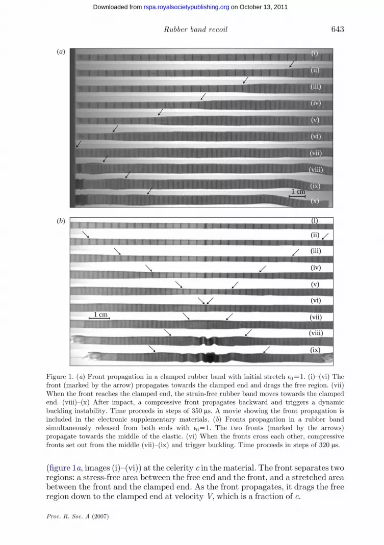
Figure 1. (a) Front propagation in a clamped rubber band with initial stretch e0Z1. (i)–(vi) Thefront (marked by the arrow) propagates towards the clamped end and drags the free region. (vii)When the front reaches the clamped end, the strain-free rubber band moves towards the clampedend. (viii)–(x) After impact, a compressive front propagates backward and triggers a dynamicbuckling instability. Time proceeds in steps of 350 ms. A movie showing the front propagation isincluded in the electronic supplementary materials. (b) Fronts propagation in a rubber bandsimultaneously released from both ends with e0Z1. The two fronts (marked by the arrows)propagate towards the middle of the elastic. (vi) When the fronts cross each other, compressivefronts set out from the middle (vii)–(ix) and trigger buckling. Time proceeds in steps of 320 ms.

643Rubber band recoil


(figure 1a, images (i)–(vi)) at the celerity c in the material. The front separates tworegions: a stress-free area between the free end and the front, and a stretched areabetween the front and the clamped end. As the front propagates, it drags the freeregion down to the clamped end at velocity V, which is a fraction of c.



1cm

(a) (b)

l / 2

(i)

(ii)

(iii)

(iv)

(v)

1cm

l / 2

(i)

(ii)

(iii)

(iv)

(v)

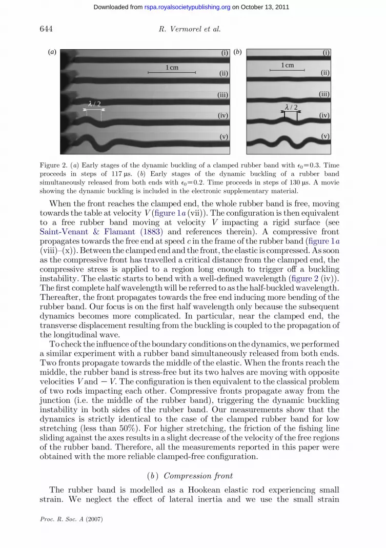
Figure 2. (a) Early stages of the dynamic buckling of a clamped rubber band with e0Z0.3. Timeproceeds in steps of 117 ms. (b) Early stages of the dynamic buckling of a rubber bandsimultaneously released from both ends with e0Z0.2. Time proceeds in steps of 130 ms. A movieshowing the dynamic buckling is included in the electronic supplementary material.



When the front reaches the clamped end, the whole rubber band is free, movingtowards the table at velocityV (figure 1a (vii)). The configuration is then equivalentto a free rubber band moving at velocity V impacting a rigid surface (seeSaint-Venant & Flamant (1883) and references therein). A compressive frontpropagates towards the free end at speed c in the frame of the rubber band (figure 1a(viii)–(x)).Between the clamped endand the front, the elastic is compressed.As soonas the compressive front has travelled a critical distance from the clamped end, thecompressive stress is applied to a region long enough to trigger off a bucklinginstability. The elastic starts to bend with a well-defined wavelength (figure 2 (iv)).The first complete halfwavelengthwill be referred to as the half-buckledwavelength.Thereafter, the front propagates towards the free end inducing more bending of therubber band. Our focus is on the first half wavelength only because the subsequentdynamics becomes more complicated. In particular, near the clamped end, thetransverse displacement resulting from the buckling is coupled to the propagation ofthe longitudinal wave.

To check the influence of theboundary conditions on thedynamics,weperformeda similar experiment with a rubber band simultaneously released from both ends.Two fronts propagate towards the middle of the elastic. When the fronts reach themiddle, the rubber band is stress-free but its two halves are moving with oppositevelocitiesV andKV. The configuration is then equivalent to the classical problemof two rods impacting each other. Compressive fronts propagate away from thejunction (i.e. the middle of the rubber band), triggering the dynamic bucklinginstability in both sides of the rubber band. Our measurements show that thedynamics is strictly identical to the case of the clamped rubber band for lowstretching (less than 50%). For higher stretching, the friction of the fishing linesliding against the axes results in a slight decrease of the velocity of the free regionsof the rubber band. Therefore, all the measurements reported in this paper wereobtained with the more reliable clamped-free configuration.

(b ) Compression front

The rubber band is modelled as a Hookean elastic rod experiencing smallstrain. We neglect the effect of lateral inertia and we use the small strain



0 f (t)

c V

= 0 =0

(a)

x

x (x, t)

b

h

(c)

0

c V

= − 0 / (1+ 0) =0

(b)f (t) �

�

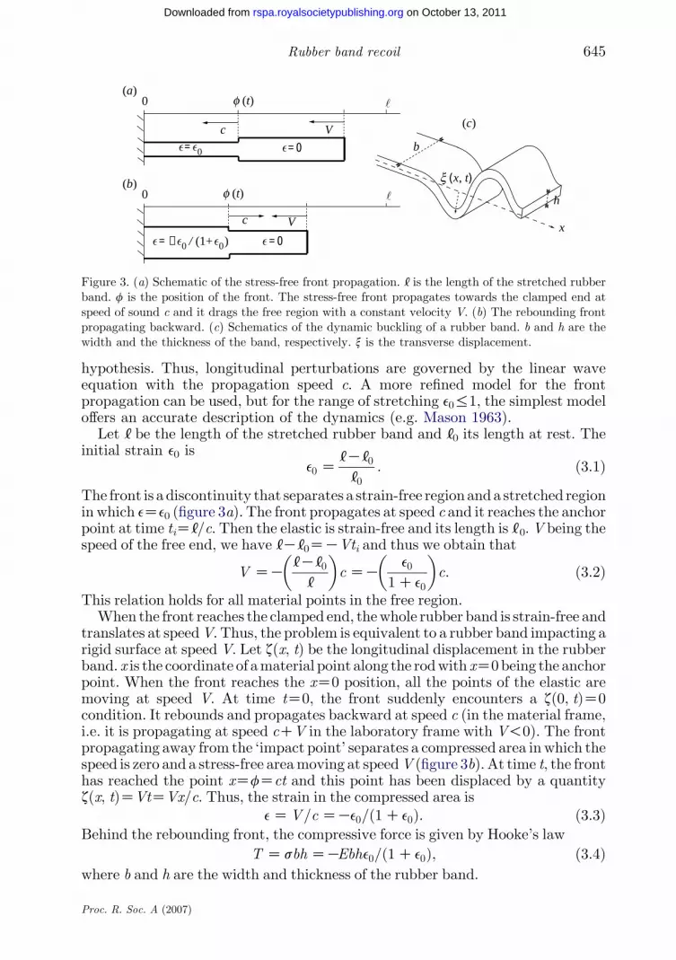
Figure 3. (a) Schematic of the stress-free front propagation. [ is the length of the stretched rubberband. f is the position of the front. The stress-free front propagates towards the clamped end atspeed of sound c and it drags the free region with a constant velocity V. (b) The rebounding frontpropagating backward. (c) Schematics of the dynamic buckling of a rubber band. b and h are thewidth and the thickness of the band, respectively. x is the transverse displacement.



hypothesis. Thus, longitudinal perturbations are governed by the linear waveequation with the propagation speed c. A more refined model for the frontpropagation can be used, but for the range of stretching e0%1, the simplest modeloffers an accurate description of the dynamics (e.g. Mason 1963).

Let [ be the length of the stretched rubber band and [0 its length at rest. Theinitial strain e0 is

e0 Z[K[0[0

: ð3:1Þ

The front is a discontinuity that separates a strain-free region anda stretched regionin which eZe0 (figure 3a). The front propagates at speed c and it reaches the anchorpoint at time tiZ[/c. Then the elastic is strain-free and its length is [0.V being thespeed of the free end, we have [K[0ZKVti and thus we obtain that

V ZK[K[0[

� �cZK

e0

1Ce0

� �c: ð3:2Þ

This relation holds for all material points in the free region.When the front reaches the clamped end, thewhole rubber band is strain-free and

translates at speedV. Thus, the problem is equivalent to a rubber band impacting arigid surface at speed V. Let z(x, t) be the longitudinal displacement in the rubberband. x is the coordinate of amaterial point along the rodwith xZ0being the anchorpoint. When the front reaches the xZ0 position, all the points of the elastic aremoving at speed V. At time tZ0, the front suddenly encounters a z(0, t)Z0condition. It rebounds and propagates backward at speed c (in the material frame,i.e. it is propagating at speed cCV in the laboratory frame with V!0). The frontpropagating away from the ‘impact point’ separates a compressed area inwhich thespeed is zero and a stress-free areamoving at speedV (figure 3b). At time t, the fronthas reached the point xZfZct and this point has been displaced by a quantityz(x, t)ZVtZVx/c. Thus, the strain in the compressed area is

eZV=cZKe0=ð1Ce0Þ: ð3:3ÞBehind the rebounding front, the compressive force is given by Hooke’s law

T Zsbh ZKEbhe0=ð1Ce0Þ; ð3:4Þwhere b and h are the width and thickness of the rubber band.





(c ) Mode selection

We introduce an equation for the transverse displacement x(x, t) (figure 3c) byplugging the above compressive force into the equation describing the dynamicsof the bending waves and using Euler–Bernoulli description

rbhv2x

vt2K

v

vxT

vx

vx

� �CEI

v4x

vx4Z 0; ð3:5Þ

where IZbh3/12 is the flexural inertia momentum in the flexion plane.We look for solutions of the form x(x, t)Zx0exp(ikxKiut). With T constant

along the rod, the dispersion relation reads

u2 ZEI

rbhk2 k2 C

T

EI

� �: ð3:6Þ

For a compressive force, T is negative. Unstable modes have wavenumbers in therange 0 to kc where kc is the marginal wavenumber,

kc Z

ffiffiffiffiffiffiffijT jEI

r: ð3:7Þ

The most amplified wavenumber is kmZkc=ffiffiffi2

p, so that, making use of equation

(3.4) for T, the most amplified wavelength writes, mutatis mutandis

lm Zph

ffiffiffi2

3

r ffiffiffiffiffiffiffiffiffiffiffiffiffi1Ce0

e0

s; ð3:8Þ

and its associated growth rate is

sm Zffiffiffi3

p e0

1Ce0

c

h: ð3:9Þ

The selected mode depends on both the material elastic properties and intensityof the compression, but since the compression is itself a function of the materialelasticity, a cancellation effect makes lm depend on geometrical parameters only,namely the thickness of the rubber band and initial stretching.

Of course, this naive expectation assumes that the compression front hastravelled by a distance at least equal to lm during a time lapse given by sK1

m . Amore general mode-selection criterion would thus be that the amplifiedwavenumber k is the one for which

tðkÞcxkK1; ð3:10Þand kZkm otherwise if t(k)c[kK1. There, t(k) is the instability time-scale associated with k through the dispersion relation (3.6) such that t(k)K1ZRe{Kiu}.

The above reasonings are made within the long wave approximation (kh/1)and disregard three-dimensional effects when the wavelength becomes of the orderof the thickness h, as it is nevertheless the case for the higher initial elongations e0.We also do not account for any coupling between the instability development andthe compression force, nor any nonlinear elastic response of the material. Finally,the model based on a constant compression force T gives satisfactory results and itwas not necessary to couple explicitly the axial front propagation with the bucklingdynamics (as in Lepik (2001) and Vaughn & Hutchinson (2006)).



0.1

0.2

0.3

0.4

0.5

0.6

0.1 0.2 0.3 0.4 0.5 0.6

V/c

0/ (1+ 0)

0/(1+ 0)0

x (cm)

(a) (b)

0.2

0.4

0.6

0.8

1.0

05 10 15 20 25 30

0 0.2 0.4

c (m

s–1

)

35

40

45

50

0.6

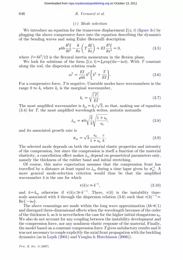
Figure 4. (a) Stretch profile during the propagation of the stress-free front. x is the materialcoordinate. (b) Ratio V/c versus e0/(1Ce0). The dots stand for the measurements and the linestands for the theoretical prediction with no adjusted parameters. Here, c is the measured frontspeed which is slightly higher than (E/r)1/2z39 m sK1 (see insert).



(d ) Experimental results

To measure the propagation speeds, we draw regularly spaced marks along therubber band (figure 1). The theoretical value of the front velocity for the rubberbands that we used in the experiments is 39 m sK1, which is in agreement withthe measurements for small initial stretching. However, the speed of the front isslightly higher, typically 50 m sK1, in particular, for high initial stretching(e0R0.6). This is probably due to the effect of the strain rate on the elongationalmodulus known in rubber (Kolsky 1949), not taken into account here.

The measured value of V typically ranges from 4 to 20 m sK1, depending onthe initial stretch (figure 4b). The evolution of the ratio V/c (c is the measuredfront speed) is in fair agreement with the theoretical prediction. Measurements ofthe stretching profile show that the front shape is well approximated by a stepfunction (figure 4a). Actually, the dependency of V on initial stretch e0 found in§3b is valid even for high initial stretching (e0x1), i.e. beyond the limitations ofthe small strain hypothesis.

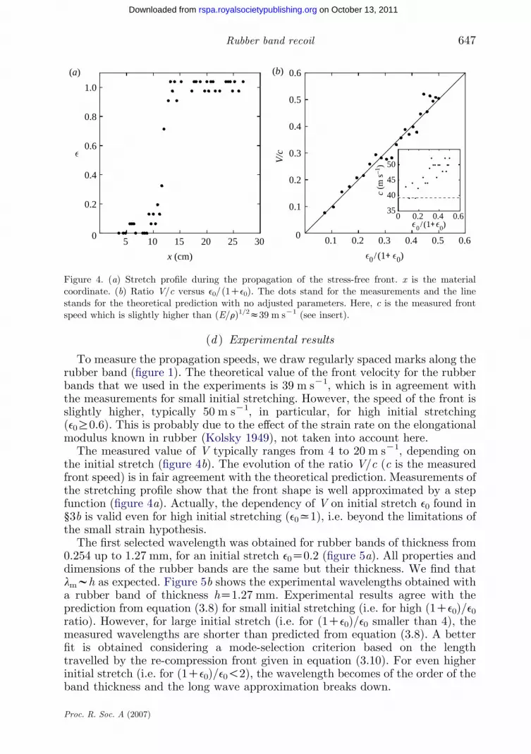
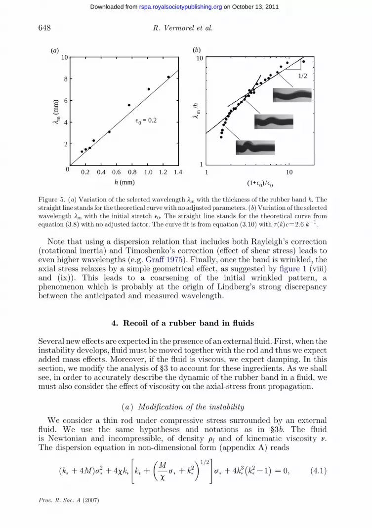
The first selected wavelength was obtained for rubber bands of thickness from0.254 up to 1.27 mm, for an initial stretch e0Z0.2 (figure 5a). All properties anddimensions of the rubber bands are the same but their thickness. We find thatlmwh as expected. Figure 5b shows the experimental wavelengths obtained witha rubber band of thickness hZ1.27 mm. Experimental results agree with theprediction from equation (3.8) for small initial stretching (i.e. for high (1Ce0)/e0ratio). However, for large initial stretch (i.e. for (1Ce0)/e0 smaller than 4), themeasured wavelengths are shorter than predicted from equation (3.8). A betterfit is obtained considering a mode-selection criterion based on the lengthtravelled by the re-compression front given in equation (3.10). For even higherinitial stretch (i.e. for (1Ce0)/e0!2), the wavelength becomes of the order of theband thickness and the long wave approximation breaks down.



2

4

6

8

10

0.2 0.4 0.6 0.8 1.2 1.4

l m (

mm

)

h (mm)

0 = 0.2 lm

/h

1.00

(a)10

11

10

(b)

1/2

(1+ 0) / 0

Figure 5. (a) Variation of the selected wavelength lm with the thickness of the rubber band h. Thestraight line stands for the theoretical curvewith no adjusted parameters. (b) Variation of the selectedwavelength lm with the initial stretch e0. The straight line stands for the theoretical curve fromequation (3.8) with no adjusted factor. The curve fit is from equation (3.10) with t(k)cZ2.6 kK1.



Note that using a dispersion relation that includes both Rayleigh’s correction(rotational inertia) and Timoshenko’s correction (effect of shear stress) leads toeven higher wavelengths (e.g. Graff 1975). Finally, once the band is wrinkled, theaxial stress relaxes by a simple geometrical effect, as suggested by figure 1 (viii)and (ix)). This leads to a coarsening of the initial wrinkled pattern, aphenomenon which is probably at the origin of Lindberg’s strong discrepancybetween the anticipated and measured wavelength.

4. Recoil of a rubber band in fluids

Several new effects are expected in the presence of an external fluid. First, when theinstability develops, fluid must be moved together with the rod and thus we expectadded mass effects. Moreover, if the fluid is viscous, we expect damping. In thissection, we modify the analysis of §3 to account for these ingredients. As we shallsee, in order to accurately describe the dynamic of the rubber band in a fluid, wemust also consider the effect of viscosity on the axial-stress front propagation.

(a ) Modification of the instability

We consider a thin rod under compressive stress surrounded by an externalfluid. We use the same hypotheses and notations as in §3b. The fluidis Newtonian and incompressible, of density rf and of kinematic viscosity n.The dispersion equation in non-dimensional form (appendix A) reads

ðk�C4MÞs2� C4ck� k�CM

cs� Ck2�

� �1=2" #

s�C4k3� k2�K1� �

Z 0; ð4:1Þ



0.2

0.4

0.6

0.8

1.0s ∗=

s/s

m

k∗= k/kc

vacuum

water

glycerol

0

0.5

1.0

1.5

2.0

2.5

0.2 0.4 0.6 0.8

l m (

cm)

0

0 1.00.2 0.4 0.6 0.8 1.0

(a) (b)

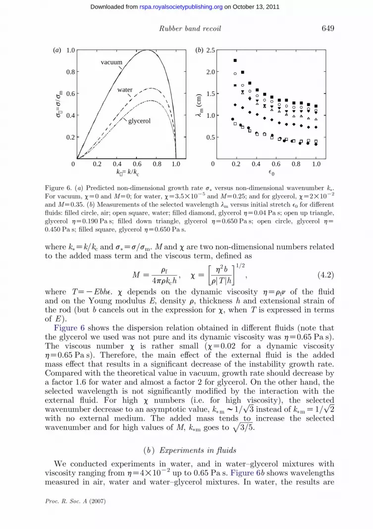
Figure 6. (a) Predicted non-dimensional growth rate s� versus non-dimensional wavenumber k�.For vacuum, cZ0 and MZ0; for water, cZ3.5!10K5 and MZ0.25; and for glycerol, cZ2!10K2

and MZ0.35. (b) Measurements of the selected wavelength lm versus initial stretch e0 for differentfluids: filled circle, air; open square, water; filled diamond, glycerol hZ0.04 Pa s; open up triangle,glycerol hZ0.190 Pa s; filled down triangle, glycerol hZ0.650 Pa s; open circle, glycerol hZ0.450 Pa s; filled square, glycerol hZ0.650 Pa s.



where k�Zk/kc and s�Zs/sm. M and c are two non-dimensional numbers relatedto the added mass term and the viscous term, defined as

M Zrf

4prkch; cZ

h2b

rjT jh

� 1=2; ð4:2Þ

where TZKEbhe. c depends on the dynamic viscosity hZrfn of the fluidand on the Young modulus E, density r, thickness h and extensional strain ofthe rod (but b cancels out in the expression for c, when T is expressed in termsof E ).

Figure 6 shows the dispersion relation obtained in different fluids (note thatthe glycerol we used was not pure and its dynamic viscosity was hZ0.65 Pa s).The viscous number c is rather small (cZ0.02 for a dynamic viscosityhZ0.65 Pa s). Therefore, the main effect of the external fluid is the addedmass effect that results in a significant decrease of the instability growth rate.Compared with the theoretical value in vacuum, growth rate should decrease bya factor 1.6 for water and almost a factor 2 for glycerol. On the other hand, theselected wavelength is not significantly modified by the interaction with theexternal fluid. For high c numbers (i.e. for high viscosity), the selectedwavenumber decrease to an asymptotic value, k�mw1=

ffiffiffi3

pinstead of k�mZ1=

ffiffiffi2

p

with no external medium. The added mass tends to increase the selectedwavenumber and for high values of M, k�m goes to

ffiffiffiffiffiffiffiffi3=5

p.

(b ) Experiments in fluids

We conducted experiments in water, and in water–glycerol mixtures withviscosity ranging from hZ4!10K2 up to 0.65 Pa s. Figure 6b shows wavelengthsmeasured in air, water and water–glycerol mixtures. In water, the results are



0.5

1.0

1.5

2.0

2.5

3.0

3.5

4.0

d (m

m)

x (cm)0 1 2 3 4 5

U (m s–1)

y (m

m)

103 s–1

(a) (b)

0 1 2 3 4 5 6 7

1

2

3

4

5

6

Figure 7. (a) Thickness of the boundary layer d versus axial coordinate x at one instant of time.The origin for x is the position of the stress-free front. The continuous line is a square root fit. (b)Velocity profile in the boundary layer at the position xZ85 mm and 13 ms after the passage of thefront. Data is fitted by a function of the form U0(1Kerf(y/d)) and we find dZ4.74 mm, which isclose to the theoretical prediction (4n[tKx/c])1/2Z4.89 mm.



similar to those performed in air. With more viscous fluids, we observe asignificant increase of the selected wavelength. The wavelength is morethan doubled in the glycerol (hZ0.65 Pa s). As discussed above, that effect istoo large to be attributed to the impact of viscosity on mode selection in thebuckling instability.

To clarify the effect of viscosity on the propagation of the compression front,we visualized the flow field. Particles were added to the fluid (glycerol withdynamic viscosity hZ0.65 Pa s) and the elastic was illuminated by a laser sheet.After the release of the rubber band, a boundary layer follows the axial-stressfront. The spatial profile of the boundary layer in the plane of the length andthickness of the rubber band (which was the plane illuminated by the laser sheet)is shown in figure 7a. The profile of the boundary layer is well fitted by a squareroot function of the axial coordinate. A movie showing the development of theboundary layer is included in the electronic supplementary material.

Let U(x, y, t) be the velocity profile in the fluid at a given instant of time andaxial location. Direction y is perpendicular to the band surface located in yZ0.Figure 7b shows such a profile. The viscous frictional force per unit length of theband is given by

tf ZK2bhvU

vy

� �yZ0

; ð4:3Þ

the factor 2 accounting for the two sides of the band. Using the velocitygradient measured on figure 7b and [0 as an estimate of the length the fronthas gone through, an order of magnitude of the frictional force is Ffwtf[0-x0.5 N. A typical value of the velocity of the free end of the rubber band is6 m sK1. Thus, the order of magnitude of the drag force FdxbhU at the freeend of the rubber band is Fdx1.5!10K2 N. Obviously, the drag force at theend is small compared with the frictional force. Moreover, the frictionincreases as the stress-free front propagates and as the region dragged by thefront gets wider.





An equation for the longitudinal displacement z accounting for frictional forces is

rbhv2z

vt2ZEbh

v2z

vx2Ctf : ð4:4Þ

In this plane boundary layer approximation, we first neglect the contribution ofthe small dimension h and disregard the contribution of the corners. LetU0(x, t)ZU(x, 0, t)Zvz(x, t)/vt be the axial velocity of the band. When U0 is afunction of time, the net force per unit length applied to the band is (see Stokes(1850) cited in Lamb (1932))

tf ZK2hbffiffiffiffiffiffipn

pðN0

vU0

vtðtKt 0Þ dt

0ffiffiffiffit 0

p ; ð4:5Þ

so that equation (4.4) becomes

rhv2z

vt2ZEh

v2z

vx2K

2hffiffiffiffiffiffipn

pðN0

v2z

vt2ðtKx=cKt 0Þ dt

0ffiffiffiffit 0

p ; ð4:6Þ

where t has been replaced by tKx/c (where c is the velocity of the front) becausethe viscous term vanishes for t!x/c, i.e. when the front has not yet reached thematerial point x.

Now, this integro-differential equation can be simplified by considering figure 7suggesting that the transverse velocity profile in the fluid is, in fact, very close tothat developing over a plate initially at rest and moved suddenly at tZx/c at aconstant velocity (Stokes 1850),

Uðx; y; tÞzU0ðx; tÞ 1Kerfyffiffiffiffiffiffiffiffiffiffiffiffiffiffiffiffiffiffiffiffiffiffiffi

4nðtKx=cÞp

!( ): ð4:7Þ

Then, using equation (4.7), we obtain in place of equation (4.4)

rhv2z

vt2ZEh

v2z

vx2K

2hffiffiffiffiffiffiffiffiffiffiffiffiffiffiffiffiffiffiffiffiffiffiffipnðtKx=cÞ

p vz

vt: ð4:8Þ

This equation has no analytic solution. However, if we focus on the long timedynamics for t[x/c (far from the front and close to the released end) andtherefore neglect inertia, an asymptotic solution can be found. Equation (4.8)being linear, the stretch eZvz/vx obeys the same equation as the longitudinaldisplacement z, thus, in the above mentioned limit

ve

vTZD

v2e

vx2; ð4:9Þ

where DZEhffiffiffiffiffiffipn

p=ð3hÞ. We use the time-scale TZt 3/2 and consider that

e(0, t)Z0. Then the asymptotic solution is

eðx;TÞe0

Z erfx

2ffiffiffiffiffiffiffiffiDT

p� �

; ð4:10Þ

which implies that the width of the front scales like T1/2Zt 3/4 for largepropagation time. Integrating e(x, T) with respect to x, we find the expression forthe displacement z,

zðx;TÞZ e0x erfx

2ffiffiffiffiffiffiffiffiDT

p� �

C2e0

ffiffiffiffiffiffiffiffiDT

pffiffiffip

p exp Kx2

4DT

� �; ð4:11Þ

which implies that the displacement of the free end of the rubber band goeslike T1/2Zt 3/4 for large propagation time. The consistency of the inertialess



0.1

D / �

1.0

0.1

3/4

t /t01.0

1.0

0.10.1

1.0t*

3/4

(b)(a)

5

10

15

20

25

15 20 25

z (c

m)z*

(0,t* )

x (cm)

t = 5.25mst = 8.75ms

5 100

Figure 8. (a) Dimensionless width D/[ versus dimensionless time t/t0. [ is the length of the stretchedrubber band and t0 is the time such thatDt

3=40 Z[2.D is obtained by fitting the strain front profile (see

text). (b) Dimensionless displacement at the free end versus dimensionless time. The front profile iswell fitted by expression (4.11) (insert) and displacement of the free end goes like t 3/4 at large times.



approximation is justified a posteriori noticing that both the terms retained inthe balance of equation (4.9) are of order eTK1 while the inertial term is of ordereTK4/3, i.e. subdominant at large time.

The displacement and the strain were measured by tracking the motion ofmarks drawn on the rubber band. For different values of time, the strain profile isfitted by a function erf(x/D) and the values of D are plotted on figure 8a. Forsufficiently large time, we observe the expected behaviour Dwt3/4. Thedisplacement front is well fitted by expression (4.11) and that of the free endproceeds like t 3/4 at large times.

However, in all cases, the apparent coefficient in front offfiffiffiffiffiffiDt

pwas about half

the expected one. This deviation indicates that the experimental friction is largerthan the one anticipated by approximating the total friction as the sum of thetwo boundary layers friction on both sides of the band (equations (4.3) and(4.4)). The reason is the influence of the band section corners, negligible at shorttime, but contributing by an amount of the same order than the one from theboundary layers when their thickness d becomes comparable to the width b. Thetotal friction per unit length writes in fact (in the limit h/b)

tf Z 2hU0bffiffiffiffiffiffiffipnt

p 1C2ffiffiffiffint

pffiffiffip

pb

� �; ð4:12Þ

and is indeed twice that obtained by simply adding the plane boundary layerscontributions when dx

ffiffiffiffint

pzb, a condition soon reached in the present case

(figure 7).

(c ) Dynamic buckling with a linear stress profile

Owing to skin friction, in glycerol, when the front reaches the clamped end itsshape is approximately a straight line. Indeed, eZerfðx=2


pÞwx=2


pfor

x/ffiffiffiffiffiffiffiffiDT

p. Thus, as an approximate model, we consider the rebound of a linear



0.10.1 1.0

1

10

–1/3

l/l

0

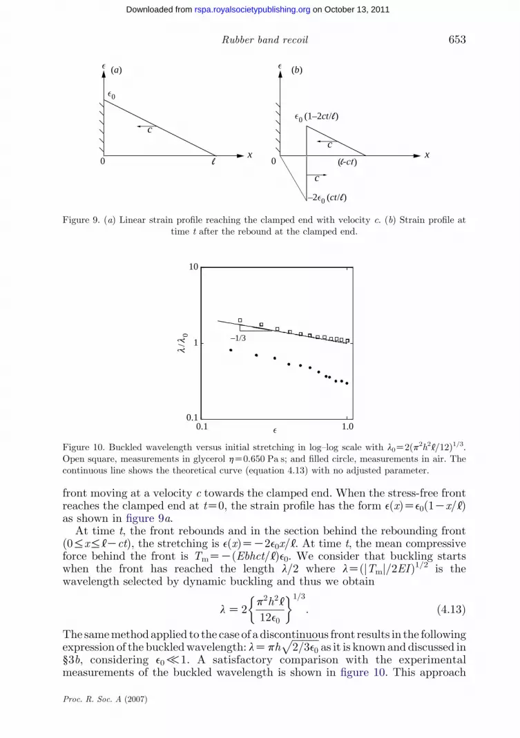
Figure 10. Buckled wavelength versus initial stretching in log–log scale with l0Z2(p2h2[/12)1/3.Open square, measurements in glycerol hZ0.650 Pa s; and filled circle, measurements in air. Thecontinuous line shows the theoretical curve (equation 4.13) with no adjusted parameter.

x

0

0x

0

c

0 (1–2ct/ )

( )

–2 0 (ct/ )

c

c

(a) (b)

Figure 9. (a) Linear strain profile reaching the clamped end with velocity c. (b) Strain profile attime t after the rebound at the clamped end.



front moving at a velocity c towards the clamped end. When the stress-free frontreaches the clamped end at tZ0, the strain profile has the form e(x)Ze0(1Kx/[)as shown in figure 9a.

At time t, the front rebounds and in the section behind the rebounding front(0%x%[Kct), the stretching is e(x)ZK2e0x/[. At time t, the mean compressiveforce behind the front is TmZK(Ebhct/[)e0. We consider that buckling startswhen the front has reached the length l/2 where lZ(jTmj/2EI)1/2 is thewavelength selected by dynamic buckling and thus we obtain

lZ 2p2h2[

12e0

� �1=3

: ð4:13Þ

The samemethodapplied to the case of a discontinuous front results in the followingexpression of the buckledwavelength: lZph

ffiffiffiffiffiffiffiffiffiffiffi2=3e0

pas it is known and discussed in

§3b, considering e0/1. A satisfactory comparison with the experimentalmeasurements of the buckled wavelength is shown in figure 10. This approach





shows that taking into account the spreading of the front is sufficient to explain thegreater observed wavelengths. Therefore, the increase of the buckled wavelength isnot due to viscous effects involved during the dynamic buckling itself.

5. Conclusion

The main phenomena involved in the recoil of an initially stretched rubber bandare the propagation of an axial-stress front, its rebound and the development of abuckling instability. A simple description of longitudinal and transverse elasticwaves provides a good insight on the dynamics. The main point is that, at earlystage of the recoil, the wavelength is correctly predicted in this framework atleast for moderate initial elongation (i.e. e0!1).

At higher initial strain, the wavelength becomes of the order of the bandthickness and the long wave description is no longer appropriate. Three-dimensional deformations lead to even smaller wavelength. Once the band iswrinkled, the axial stress relaxes by a simple geometrical effect leading to acoarsening of the initial undulations.

When the rubber band is immersed in a fluid, the major effect is the spreadingof the initial front owing to boundary layer friction. The smoother stress profileleads to longer wavelength, and a simple model based on a linear compressivestrain profile gives a good estimate of the most amplified wavelength. Addedmass effects slow down the instability but do not modify mode selectionappreciably. The impact of both fluid viscosity and density on the instabilitydevelopment are quantified with appropriate dimensionless numbers.

It was not necessary to account for a possible nonlinear elastic response ofthe material.

This work was supported by the Agence Nationale de la Recherche through the grant ANR-05-BLAN-0222-01. R.V. was supported by the Delegation Generale a l’Armement.

Appendix A. Dispersion relation for the buckling of a rod interactingwith a surrounding fluid.

We derive the dispersion relation (equation (4.1)) for waves propagating alongthe rubber band in a viscous fluid, in two dimensions. In the reference state, theelastic rod is of infinite extent in the x-direction and its thickness is h. The twofluid domains, denoted by the index 1 for the upper domain (yO0 in the referenceconfiguration) and 2 for the lower domain separated by the rubber band. Themodel is based on the linearized Navier–Stokes equation for the two fluiddomains.

rvU1;2

vtZK

vP1;2

vxCh

v2U1;2

vx2C

v2U1;2

vy2

� �; ðA 1Þ

rvV1;2

vtZK

vP1;2

vyCh

v2V1;2

vx2C

v2V1;2

vy2

� �: ðA 2Þ





The fluid is incompressible. Thus, V2P1,2Z0 and we look for P1 and P2 of the form

P1 Z pð0Þ1 Cp1expðKkyÞexpðstKikxÞ; ðA 3Þ

P2 Z pð0Þ2 Cp1expðkyÞexpðstKikxÞ; ðA 4Þ

where we have used the condition that pressure must remain finite at infinity. Welook for V1,2 of the form

V1;2 Z v1;2ðyÞexpðstKikxÞ: ðA 5Þ

Using these forms for P1,2 and V1,2 in equations (A 1) and (A 2), we have

q2v1Kv2v1vy2

ZKk

hp1expðKkyÞ; ðA 6Þ

q2v2Kv2v2vy2

Zk

hp2expðKkyÞ; ðA 7Þ

where

q2 Zrs

hCk2: ðA 8Þ

Thus, for V1 and V2, we have (using the condition that Vmust remain finite)

V1 Z fA1expðKqyÞCB1expðKkyÞgexpðstKikxÞ; ðA 9Þ

V2 Z fA2expðqyÞCB2expðkyÞgexpðstKikxÞ; ðA 10Þwith

p1 Zh

kðq2Kk2ÞB1 and p2 Z

h

kðq2Kk2ÞB2: ðA 11Þ

We use the continuity equations

vU1;2

vxC

vV1;2

vyZ 0; ðA 12Þ

to obtain U1,2

U1;2 ZK1

ik

vV1;2

vy: ðA 13Þ

There are four boundary conditions at the interface between the fluid and rod.

† Assuming that the cross-sections of the rod are moving along the y-directionwithout being stretched or compressed, the transverse displacement ishomogenous in a section yielding the kinetic conditions at both interfaces(yZGh/2) in the transverse direction

V1jyZh=2 ZV2jyZKh=2 Zvx

vt: ðA 14Þ

† With a fluid initially at rest and in the slender slope limit, the difference ofhorizontal velocity across a section is

U1jyZh=2KU2jyZKh=2 ZKhv2x

vtvx: ðA 15Þ





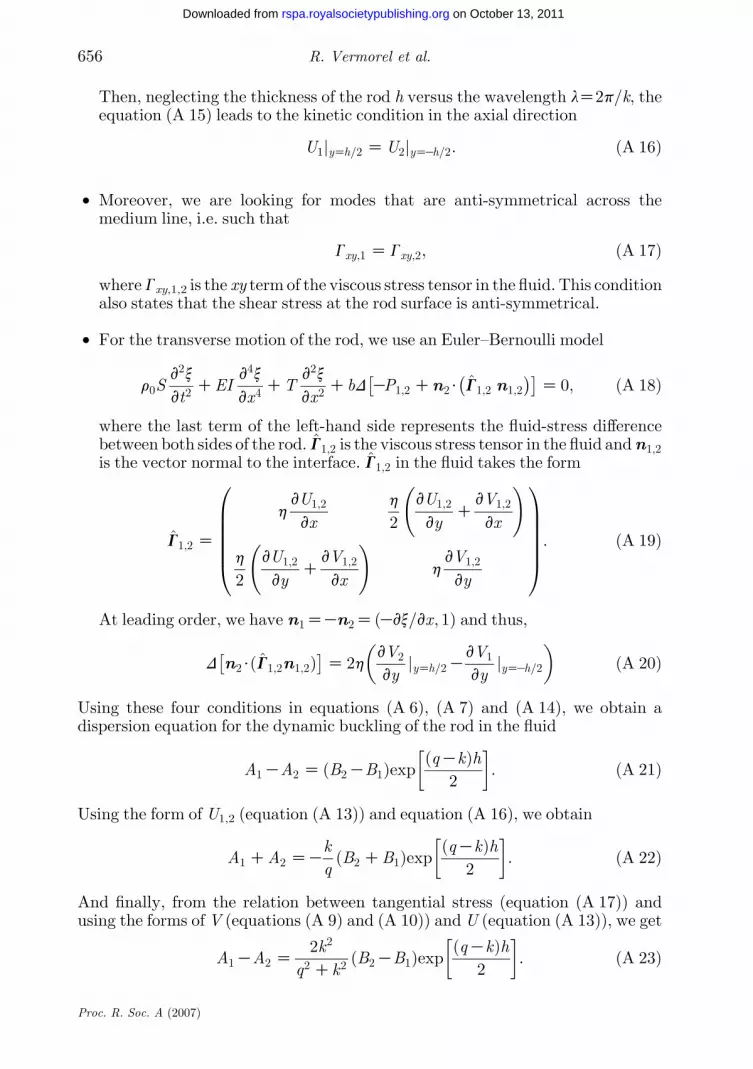
Then, neglecting the thickness of the rod h versus the wavelength lZ2p/k, theequation (A 15) leads to the kinetic condition in the axial direction

U1jyZh=2 ZU2jyZKh=2: ðA 16Þ

† Moreover, we are looking for modes that are anti-symmetrical across themedium line, i.e. such that

Gxy;1 ZGxy;2; ðA 17Þ

whereGxy,1,2 is the xy term of the viscous stress tensor in the fluid. This conditionalso states that the shear stress at the rod surface is anti-symmetrical.

† For the transverse motion of the rod, we use an Euler–Bernoulli model

r0Sv2x

vt2CEI

v4x

vx4CT

v2x

vx2CbDKP1;2 Cn2$ G1;2 n1;2

� � �Z 0; ðA 18Þ

where the last term of the left-hand side represents the fluid-stress differencebetween both sides of the rod. G1;2 is the viscous stress tensor in the fluid andn1;2

is the vector normal to the interface. G1;2 in the fluid takes the form

G1;2 Z

hvU1;2

vx

h

2

vU1;2

vyC

vV1;2

vx

!

h

2

vU1;2

vyC

vV1;2

vx

!hvV1;2

vy

0BBBBB@

1CCCCCA: ðA 19Þ

At leading order, we have n1ZKn2ZðKvx=vx; 1Þ and thus,

D n2$ðG1;2n1;2Þ �

Z 2hvV2

vyjyZh=2K

vV1

vyjyZKh=2

� �ðA 20Þ

Using these four conditions in equations (A 6), (A 7) and (A 14), we obtain adispersion equation for the dynamic buckling of the rod in the fluid

A1KA2 Z ðB2KB1ÞexpðqKkÞh

2

� : ðA 21Þ

Using the form of U1,2 (equation (A 13)) and equation (A 16), we obtain

A1 CA2 ZKk

qðB2 CB1Þexp

ðqKkÞh2

� : ðA 22Þ

And finally, from the relation between tangential stress (equation (A 17)) andusing the forms of V (equations (A 9) and (A 10)) and U (equation (A 13)), we get

A1KA2 Z2k2

q2 Ck2ðB2KB1Þexp

ðqKkÞh2

� : ðA 23Þ





Combining equations (A 21) and (A 23) and using equation (A 11), we have

A1 ZA2; ðA 24Þ

B1 ZB2; ðA 25Þ

p1 ZKp2: ðA 26ÞUsing equation (A 22), we find

A1 ZKk

qB1exp

ðqKkÞh2

� : ðA 27Þ

We write DðKP1;2Cn2$G1;2n1;2ÞÞ in terms of B1,

DðKP1;2Cn2:ðG1;2n1;2ÞÞ

Z ðp1Kp2ÞeKkh=2ChqðA1 CA2ÞeKqh=2 ChkðB1CB2ÞeKkh=2n o

estKikx

Z 2hðq2Kk2Þ

kB1e

Kkh=2

� �estKikx :

ðA 28Þ

The expression of x is obtained from the transversal boundary condition(equation A 14)

xZ1

sfA1e

Kqh=2CB1eKkh=2gestKikx : ðA 29Þ

Introducing this expression in (A 18) and using relations (A 21) and (A 28), weobtain the dispersion equation

r0SC2rb

k

� �s2C2bhðkCqÞsCEIk4KTk2 Z 0: ðA 30Þ

In dimensionless form, this relation reads

fk�C4Mgs2� C4ck� k�CM

cs�Ck2�

� �1=2( )

s� C4k3� k2�K1� �

Z 0; ðA 31Þ

with k�Zk/kc and s�Zs/sm. The two dimensionless coefficients are

cZh2b

r0Th

� �1=2

andM Zrlc

4pr0h: ðA 32Þ

References

Bouasse, H. & Carriere, Z. 1903 Sur les courbes de traction du caoutchouc vulcanise. Annales de lafaculte des sciences de Toulouse, 2e serie 5, 257–283.

Euler, L. 1744 Addidentum I de curvis elasticis, methodus inveniendi lineas curvas maximiminimivi proprietate gaudentes. In Opera Omnia I, pp. 231–297. Lausanne.

Gladden, J. R., Handzy, N. Z., Belmonte, A. & Villermaux, E. 2005 Dynamic buckling andfragmentation in brittle rods. Phys. Rev. Lett. 94, 035503. (doi:10.1103/PhysRevLett.94.035503)


http://dx.doi.org/doi:10.1103/PhysRevLett.94.035503

http://dx.doi.org/doi:10.1103/PhysRevLett.94.035503




Graff, K. G. 1975 Wave motion in elastic solids. New York, NY: Dover Publications.Kolsky, H. 1949 An investigation of the mechanical properties of materials at very high rates of

loading. Proc. Phys. Soc. B 62, 676–700. (doi:10.1088/0370-1301/62/11/302)Lamb, H. 1932 Hydrodynamics. Cambridge, UK: Cambridge University Press.Lepik, U. 2001 Dynamic buckling of elastic-plastic beams including effects of axial stress waves.

Int. J. Impact Eng. 25, 537–552. (doi:10.1016/S0734-743X(00)00070-1)Lindberg, H. E. 1965 Impact buckling of a bar. J. Appl. Mech. 32, 315–322.Love, A. E. H. 1944 A treatise on the mathematical theory of elasticity, 4th edn. New York, NY:

Dover Publications.Mason, P. 1963 Finite elastic wave propagation in rubber. Proc. R. Soc. A 272, 315–330.Mullins, L. 1947 Effect of stretching on the properties of rubber. J. Rubber Res. 16, 275–289.Saint-Venant, M. & Flamant, A. 1883 Resistance vive ou dynamique des solides. Representtaion

graphique des lois du choc longitudinal, subi a une des extremites par une tige ou barreprismatique assujettie a l’extremite opposee. C.R. Acad. Sci. 97, 127–133.

Stokes, G. G. 1850 On the effect of the internal friction of fluids on the motion of pendulums.Trans. Camb. Phil. Soc. IX, 8 sec 52.

Vaughn, D. G. & Hutchinson, J. W. 2006 Bucklewaves. Eur. J. Mech. A/Solids 25, 1–12. (doi:10.1016/j.euromechsol.2005.09.003)


http://dx.doi.org/doi:10.1088/0370-1301/62/11/302

http://dx.doi.org/doi:10.1016/S0734-743X(00)00070-1

http://dx.doi.org/doi:10.1016/j.euromechsol.2005.09.003

http://dx.doi.org/doi:10.1016/j.euromechsol.2005.09.003


Documents

Rubber band recoil