Embed Size (px)
Citation preview


International Journal of
Intelligent Systems and
Applications in Engineering
Advanced Technology and Science
ISSN:2147-67992147-6799 www.atscience.org/IJISAE Original Research Paper
International Journal of Intelligent Systems and Applications in Engineering IJISAE, 2018, 6(4), 248–250 | 248
A Review of Smart Parking System based on Internet of Things
Harkiran Kaur 1, Jyoteesh Malhotra2
Accepted : 08/11/2018 Published: 31/12/2018 DOI: 10.1039/b000000x
Abstract: The Internet of Things expands the wireless paradigm to the edge of the network, which enables to develop a different kind of
applications or services. By using IoT the application becomes more reliable, flexible or portable. It has a large amount of nodes on the
various geographic positions, to increase the awareness of location or reduce the latency. There are numerous IoT applications like smart
grid, smart hospital, smart industry, smart traffic management etc. In this paper, we describe the smart traffic management and parking
system using the internet to control the chaos and also discuss the various researches on this concept.
Keywords: Bluetooth, Cloud Computing, Information Communication Technology (ICT), Internet of Things (IoT), Wireless Sensor
Network (WSN)
1. Introduction
The use of IoT in the practical world become more relevant in the
recent year by the rapid growth of technologies like mobile,
embedded system, wireless system, cloud computing etc. Internet
of Things helps to connect the living beings and the non-living
things, which generates the communication between the virtual
and non-virtual data. So, there are a large amount of data
generated by the various number of nodes connected via the
internet. After that, the relevant information should be converted
from the pool of data. The WSN plays a very imperative role in
the development of IoT. The concept of the smart city is the best
suitable example for the integration of IoT and WSN with ICT.
Smart City provides an advanced step for groundbreaking and
cooperative amenities for all the social events such as healthcare,
transportation, business etc. It uses IoT in an effective and secure
manner to access the IP address of the object, and generate the
communication link between the object and the system with the
help of internet.
2. Related Work
IoT has a vital role in the traffic management in smart cities.
Nowadays, many techniques like wireless sensor network, radio
frequency, digital image processing based smart transportation
system are introduced for traffic management. There are used to
control the traffic in the more efficient way. In 2012, J. Yang uses
GPS (Global Positioning system) and Android based application
to provide the information related to the parking space. It has a
better interface but it does not have the reservation feature [1].
M. Patil implements the WSN and RFID for the smart parking in
2013 [2]. In this system, the Inter-Integrated Circuit protocol is
used according to that the car will guide the driver to find the
path for parking by using RFID and WSN. This system is time-
consuming and expensive which are the major drawbacks. H.
Singh introduced the automated parking system with the help of
Bluetooth access. In this system, the Bluetooth is used for the
communication or network. This system is based on the rack and
pinion mechanism for the linear motion. So the main drawback of
this system is the whole parking is designed according to the rack
and pinion mechanism which is quite expensive and time-
consuming [3].
According to Hilal Al-Khaurasi, the intelligent parking system
was introduced which is based on image processing. In this paper,
the concept of image processing is used. The sensor camera is
used to capture the images which help to provide the results that
are slots for parking are free or not. But, in term of visibility, the
weather conditions like rain, fog, snow etc. may affect the system
[4]. Another system is made by A.Sayeeraman in 2012. In this
system, ZigBee is used to check the vacancy in the parking area.
In this, the security feature is added i.e. exist password, without
entering the password user cannot leave the parking. The gate
will open when the user put the right exit password. The exit
password is sent to the user at the entry time via SMS. The
problem of this system is network congestion due to which user
unable to receive the SMS. However, the use of SMS, GSM or
ZigBee makes the system more expensive [5]. The other authors
develop the parking reservation system by using the SMS. In this
paper, the microcontroller is used which makes the system
portable but the cost of implementation is very high because of
the use of the microcontroller. The major problem is the system
will crash if the workload on the microcontroller will
increase[6].This [7] paper introduced the use of RFID, WSN,
object ad-hoc network and information systems in which the
traffic objects can be automatically tracked and controlled over a
network. The concept of RFID is used as a new technology to
reduce the installation cost and time [8].According to J. Sherly
IoT-based transportation system is developed according to smart
city view. The main aim of this paper is to develop the advanced
and powerful communication between the technologies for the
administration of the city and the citizens[9]. The raspberry pi 2
is used for the smart high defined picture. There are some
ultrasonic sensors are used to detect the vehicle intensity and
sends the signal to RASPBERRY PI 2 which controls the traffic
problem [10].
Y K. Zang [11] designed an efficient decentralized framework for
reducing the fuel consumption at any time of expedition or
stoppage. This algorithm provides a solution for congestion
________________________________________________________________________________________________________________________________________________________________________________________________________________________________________________
1Department of Computer Science and Engineering, GNDU RC
Jalandhar, Punjab, India 2Department of Electrical and Computer Engineering, GNDU RC
Jalandhar, Punjab, India
* Corresponding Author: Email: [email protected]
International Journal of Intelligent Systems and Applications in Engineering IJISAE, 2018, 6(4), 248–250 | 249
Table 1. Current State-of-the-art
Sr.
No. Paper Name
Year
Description Merits Demerits
1. Smart Parking Services based on
Wireless Sensor Network[1]. 2012
In this paper, the android application is used. It provides the better
interface but it does not have reservation feature.
Usage of Android platform provides
better interface
Easy to use.
This system has not reservation feature.
2. Wireless Sensor Network and RFID for
the Smart Parking System[2]. 2013
In this paper, the RFID and the wireless sensors are used to make the
Parking, according to this, it guide the driver to find the spot but this
system is time-consuming and expensive.
It provides the slot information as
well as guides the driver.
It is compatible in existing parking.
High cost
More time required for implementation.
3. Automated Parking System with
Bluetooth access[3]. 2014
In this system, the Bluetooth is used for the communication or network.
This system is based on the rack and pinion mechanism for the linear
motion. So the main drawback of this system is the whole parking is
designed according to the rack and pinion mechanism which is quite
expensive and time-consuming.
Bluetooth is used for registration or
identification.
Detect the unique registration number
if a new vehicle is parked.
Cannot be used in the existing system.
Whole parking is to be designed.
Costly.
Time-consuming.
4. Intelligent Parking Management System
based on Image Processing[4]. 2014
In this paper, the concept of image processing is used. The sensor camera
is used to capture the images which help to provide the results that are slots
for parking are free or not. But, in term of visibility, the weather conditions
like rain, fog, snow etc. may affect the system.
Easily detect the presence of vehicles.
The camera is used as a sensor.
Not compatible with some weather
conditions such as rain, fog etc.
Fixed position of the system.
GPS is not provided.
5.
Zigbee and GSM based Secure Vehicle
parking management and reservation
system[5].
2012
In this system, ZigBee is used to check the vacancy in the parking area. In
this, the security feature is added i.e. exist password, without entering the
password user cannot leave the parking. The gate will open when the user
put the right exit password.
Secure
Based on password system.
Use of GSM
Use of SMS
Expensive.
The problem of this system is network
congestion due to which user unable to
receive the SMS.
6. Smart Parking Reservation System using
short message services (SMS)[6]. 2009
In this paper, the microcontroller is used which makes the system portable
but the cost of implementation is very high because of the use of the
microcontroller. The major problem is the system will crash if the
workload on the microcontroller will increase.
More
Secure.
Ease of usage.
The cost of implementation is high.
GSM feature create bottlenecks
Overload of microcontroller leads to
system crash.
7.
Intelligent Traffic Information System
Based on Integration of Internet of
Things and Agent Technology[7].
2015
This paper introduced the use of RFID, WSN, object ad-hoc network and
information systems in which the traffic objects can be automatically
tracked and controlled over a network.
Provides tracking feature.
Use of WSN made this system more
reliable.
Networking congestion.
8. Smart Traffic Management System[8]. 2013 The concept of RFID is used as a new technology to reduce the installation
cost and time. Reduce the installation time and cost. GPS is not used.
9. Internet of Things Based Smart
Transportation System[9]. 2015
In this paper, the IoT-based transportation system is developed according
to smart city view. The main aim of this paper is to develop the advanced
and powerful communication between the technologies for the
administration of the city and the citizens.
Provide instant results.
Use for real-time traffic.
The problem in data storage.
Use of image processing system.
10. Innovative Technology for Smart Roads
by using IoT devices[10]. 2016
In this paper, the raspberry pi 2 is used for the smart high defined picture.
There are some ultrasonic sensors are used to detect the vehicle intensity
and sends the signal to RASPBERRY PI 2 which controls the traffic
problem.
Automatically detect the vehicles.
Controls traffic related problems. Expensive.
11.
Optimal control and coordination of
connected and automated vehicles at
urban traffic intersections[11].
2016
An efficient decentralized framework for reducing the fuel consumption at
any time of expedition or stoppage. This algorithm provides solution for
congestion control and helps to reduce the traveling time
Efficient framework.
Solve congestion problem.
Reduce traveling time.
Large time for implementation.
High cost.
12.
Assessing the mobility and
environmental benefits of reservation-
based intelligent intersections using an
integrated simulator[12].
2012
In this designed intersection control on reservation based system to take
more advantage of extraordinary connectivity that provides dynamism to
connected transports
Online reservation.
Dynamism connectivity of transports.
The cost of reservation is high.
Network congestion.
13.
Analysis of reservation algorithms for
cooperative planning at
intersections[13].
2010
This represents the designed the fully automated car that has the major
differences compared to nowadays. This paper also describes the
improvement of the reservation algorithm.
Based on reservation algorithm Not practically implemented.
14.
Analysis and modeled design of one
state-driven autonomous passing-
through algorithm for driverless vehicles
at intersections[14].
2013
In this paper, proposed the centralized scheduling algorithm i.e.
reservation-oriented. This ensures the high request to be answered as per
the preference. This algorithm is simulated on high priority vehicles
Simulated on high priority vehicles.
Based on centralized scheduling
algorithm
Complex
The difficulty of understanding.
15. Cloud-based Intelligent Transport
System[15]. 2015
This paper represent the multilayered vehicular data cloud platform which
was supported by IoT technologies and cloud computing Support multiple technologies.
The problem in data storage.
Hard to manage a large amount of data.
16.
Visible light communication:
Application, architecture,
standardization and research
challenges[16].
2016
In this paper, the unique computer code is designed that can communicate
with various devices within the road. In this technological era, visible light
communication is also used for vehicle to vehicle communication.
Strong communication between
machines to the machine.
Consume a lot of time for
implementation.
17. Enabling Reliable and Secure IOT-
based Smart City Application[17]. 2014
According to Elias Z. Tragos in this paper the IoT is used as the real-time
traffic monitor to reduce the overall traffic from the downtown area.
Monitor real-time traffic.
Helps to reduce the overall traffic. -
18. Smart City Architecture and its
Application based on IoT[18]. 2015
This paper mainly based on customized services for communication with
the help of Wi-Fi, WI-Max, Zig-Bee, Satellite Communication etc. to
convert the city into the smart city. For instance, we combine the health
and transportation domain by this sensor can easily measure the all health
related parameter of the driver while driving like pulse rate, blood pressure
etc. and provide the real-time health condition to the driver. This helps to
create the safer environment.
User-friendly.
Ease to communicate.
Measure all health related parameters.
Safer environment.
Lots of sensors are used.
Required more time as compared to
another system.
19. Automatic Smart Parking System using
Internet of Things(IoT)[19]. 2015
In this, the system designs a simple smart car parking system which is cost
effective and also helps to decrease the carbon dioxide that makes this
system eco-friendly.
Cost effective
Eco-friendly.
Not solve the congestion related
problems.
20.
Automatic Parking Management System
and Parking fee collection based on
number plate recognition[20].
2012 The author utilizes wide-point camera as a sensor which records or find
free space. These records are used for proper utilization of space. Proper utilization of space.
Use of camera makes the system
unreliable.

International Journal of Intelligent Systems and Applications in Engineering IJISAE, 2018, 6(4), 248–250 | 250
control and helps to reduce the traveling time. S. Huang[12]
designed intersection control on the reservation based system to
take more advantage of extraordinary connectivity that provides
dynamism to connected transports. A. Fortella[13] represents the
designed fully automated car that has the major differences
compared to nowadays. This paper also describes the
improvement of the reservation algorithm. The K.Zang [14]
proposed the centralized scheduling algorithm i.e. reservation-
oriented. This ensures the high request to be answered as per the
preference. This algorithm is simulated on high priority vehicles.
K. Ashokkumar [15] represent the multilayered vehicular data
cloud platform which was supported by IoT technologies and
cloud computing. In this paper, the unique computer code is
designed that can communicate with various devices within the
road. In this technological era, visible light communication is also
used for vehicle to vehicle communication [16].According to
Elias Z. Tragos [17] IoT is used as the real-time traffic monitor to
reduce the overall traffic from the downtown area. [18] This
paper mainly based on customized services for communication
with the help of Wi-Fi, WI-Max, Zig-Bee, Satellite
Communication etc. to convert the city into a smart city. For
instance, we combine the health and transportation domain by
this sensor can easily measure the all health related parameter of a
driver while driving like pulse rate, blood pressure etc. and
provide the real-time health condition to the driver. This helps to
create the safer environment. Basavaraju [19] design a simple
smart car parking system which is cost effective and also helps to
decrease the carbon dioxide that makes this system eco-friendly.
The author utilizes wide-point camera as a sensor which records
or find free space and these records are used for proper utilization
of space for the smart parking [20].
3. Current State-of-the-art
Based on literature survey done the following papers have been
abstracted to find out the key merits and demerits.
4. Open Issues and Challenges
Nowadays, there are various challenges which are faced by
today’s driver as well as whole transportation system on daily
basis likewise traffic congestion, parking system etc. To improve
this transportation system, the following issues and factors are
considered:
Be able to sense vehicle accurately.
Provide congestion free road.
Manage a large amount of data.
Enable to make smart decisions using real-time data.
Reduce frustration and improve time-saving.
Alleviate the problem related to pollution emission and fuel
consumption.
5. Conclusion
Overall, in this paper, there are various types of methods or
techniques are discussed. This review provides the gather
information about the traffic management or smart parking
methods which are used for the smart cities. The wide availability
of sensors or wireless devices made the system more reliable or
flexible and enables effective development of the IoT-based
application. IoT provides enormous kind of solution for the traffic
controlling and provide the vehicle to vehicle communication for
the optimal result. This paper helps to understand all various
methods of traffic management under the concept of the smart
city.
References
[1] Yang Jihoon Jorge Portilla Teresa Riesgo, “Smart parking service
based on wireless sensors Network,” IEEE, 2012.
[2] ManjushaPatil Vasant N. Bhonge, “Wireless Sensor Network and
RFID for Smart Parking System,” Int. J. Emerg. Technol. Adv.
Eng. Website www.ijetae.com, vol. 3, no. 4, 2013.
[3] Harmeet Singh ChetanAnand Vinay Kumar Ankit Sharma,
“Automated Parking System With Bluetooth Access,” Int. J. Eng.
Comput. Sci. ISSN2319-7242, vol. 3, no. 5, pp. 5773–5775.
[4] H. A.-K. I. Al-Bahadly, “Intelligent Parking Management System
Based on Image Processing,” J. Eng. Technol., vol. 2, pp. 55–67,
2014.
[5] AshwinSayeeraman P.S.Ramesh, “ZigBee and GSM based secure
vehicle parking management and reservation system,” J. Theor.
Appl. Inf. Technol., vol. 37, 2012.
[6] HanitaDaud Noor HazrinHanyMohamadHanif Mohd Hafiz
Badiozaman, “Smart parking reservation system using short
message services (SMS),” IEEE, 2009.
[7] H. O. Al-Sakran, “Intelligent Traffic Information System Based on
Integration of Internet of Things and Agent Technology,” Int. J.
Adv. computer Sci. Appl., vol. 6, no. 2, 2015.
[8] N. Lanke, “Smart Traffic Management System,” Int. J. Comput.
Appl., vol. 75, no. 7.
[9] J. Sherly D. Sonasundareswari, “Internet of Thing Based Smart
Transport System,” Int. J. Eng. Technol., vol. 75, no. 7, 2013.
[10] Sheela.S, “Innovative Technology for Smart Roads by Using IOT
Devices,” Int. J. Innov. Res. Sci. Eng. Technol., vol. 5, no. 10.
[11] Y. J. Zhang or A. A. Malikopoulos and C. G. Cassandras, “Optimal
control and coordination of connected and automated vehicles at
urban traffic intersections,” in Proc. Amer. Control
Conference[online], 2016.
[12] S. Huang or A. W. Sadek and Y. Zhao, “Assessing the mobility
and environmental benefits of reservation-based intelligent
intersections using an integrated simulator,” IEEE Trans. Intell.
Transp. Syst., vol. 13, 2012.
[13] A. d. La Fortelle, “Analysis of reservation algorithms for
cooperative planning at intersections,” in Proceding. 13th
International IEEE Conference Intelligent Transport System, 2010.
[14] K. Zhang A. de La Fortelle D. Zhang and X. Wu, “Analysis and
modeled design of one state-driven autonomous passing-through
algorithm for driverless vehicles at intersections,” in Proc. IEEE
16th Int. Conf. Comput.Sci. Eng, 2013.
[15] K. Ashokkumar, “CLOUD BASED INTELLIGENT
TRANSPORT SYSTEM,” Sci. Direct, vol. 50, pp. 58–63, 2015.
[16] L. U. Khan, “Visible light communication: Application,
architecture, standardization, and research challenges.,” Digit.
Commun. Networks, Elsevier, pp. 1–10, 2016.
[17] E. Z.Tragos, “Enabling Reliable and Secure IOT- based Smart City
Application,” IEEE, pp. 111–116, 2014.
[18] G. Aditya, S. Bryan, P. Gerard, and M. Sally, “Smart City
Architecture and its Application based on IoT,” Sci. Direct,,
Elsevier, vol. 52, pp. 1089–1094, 2015.
[19] S. R. Basavaraju, “Automatic Smart Parking System using Internet
of Things(IoT),” Int. J. Sci. Res. Publ., vol. 5, no. 12, pp. 629–632,
2015.
[20] R. M.M, A.Musa, AtaurRahman, N.Farahana, and A.Farahana,
“Automatic Parking Management System and Parking fee
collection based on number plate recognition,” Int. Mach. Learn.
Comput., vol. 2, 2012.
International Journal of
Intelligent Systems and
Applications in Engineering
Advanced Technology and Science
ISSN:2147-67992147-6799 www.atscience.org/IJISAE Original Research Paper
International Journal of Intelligent Systems and Applications in Engineering IJISAE, 2018, 6(4), 251–261 | 251
Text line Segmentation in Compressed Representation of Handwritten
Document using Tunneling Algorithm
Amarnath R.*1, Nagabhushan P. 1
Accepted : 01/10/2018 Published: 31/12/2018 DOI: 10.1039/b000000x
Abstract: In this research work, we perform text line segmentation directly in compressed representation of an unconstraint handwritten
document image using tunneling algorithm. In this relation, we make use of text line terminal point which is the current state-of-the-art
that enables text line segmentation. The terminal points spotted along both margins (left and right) of a document image for every text
line are considered as source and target respectively. The effort in spotting the terminal positions is performed directly in the compressed
domain. The tunneling algorithm uses a single agent (or robot) to identify the coordinate positions in the compressed representation to
perform text-line segmentation of the document. The agent starts at a source point and progressively tunnels a path routing in between
two adjacent text lines and reaches the probable target. The agent’s navigation path from source to the target bypassing obstacles, if any,
results in segregating the two adjacent text lines. However, the target point would be known only when the agent reaches destination; this
is applicable for all source points and henceforth we could analyze the correspondence between source and target nodes. In compressed
representation of a document image, the continuous pixel values in a spatial domain are available in the form of batches known as white-
runs (background) and black-runs (foreground). These batches are considered as features of a document image represented in a Grid.
Performing text-line segmentation using these features makes the system inexpensive when compared to spatial domain processing.
Artificial Intelligence in Expert systems, dynamic programming and greedy strategies are employed for every search space while
tunneling. An exhaustive experimentation is carried out on various benchmark datasets including ICDAR13 and the performances are
reported.
Keywords: Compressed Representation, Handwritten Document Image, Text-Line Terminal Point, Text-Line Segmentation, Search
Space, Grid.
1. Introduction
Technological advances of storage and transfer have made it
possible to maintain many documents in the digital format. It is
also necessary to preserve these documents in digital image
format only, particularly in case of handwritten documents for
verification and authentication purposes [1, 2, 3, 4, 5].
Maintaining these document images in the digital form would
require huge storage space and network bandwidth. Therefore, an
efficient compressed representation would be an effective
solution to the storage and transfer issues [6, 7, 8] particularly
arising from document image. Generally, the document image
compression format follows the guidelines of CCITT Standards
[9, 10] which is a part of the ITU (International Telegraph
Union). These standards were specifically targeted towards
document images stored in digital libraries. On the other hand, if
document images, audios and videos are to be archived and
communicated in the compressed form itself, then it would be
considered as a third advantage in addition to storage and
transmission.
The digital libraries with document images in their compressed
formats could imply a solution to a big data problem arising from
the document images, particularly about storage and transmission
[11]. The compressed image file formats such as TIFF, JPEG,
and PNG, strictly follow CCITT standards [7, 8, 9, 10, 11, 12].
For any digital document analysis (DDA), the image in its
compressed format must undergo the decompression stage.
However, performing operations on decompressed documents
would unwarrantedly suppress the advantages of both the time
and buffer space [6, 13, 14, 15]. If DDA could be achieved in the
compressed version of the document image without
decompression, then the document image compression could be
viewed as an effective solution to the immense data problems
arising from document images [13].
The idea of operating and analysing directly in the compressed
version of the document image without decompression is known
as Compressed Domain Processing (CDP) [6, 13, 14, 15). A
recent literature [12] on CDP shows the strategies to perform
document image analysis in its compressed representation.
However, the model is subjected to the printed documents only.
The challenging job is to perform DDA in compressed
representation of handwritten document image. Performing DDA
on uncompressed handwritten document could be a difficult task
because of oscillatory variations, inclined orientation and
frequent touching of text lines while scribing on un-ruled paper
[13]. An initial attempt [13] to spot the separator points at every
line terminals in compressed unconstrained handwritten
document images using run-length features (Run Length
Encoding or RLE) is the state-of-the-art technology. This
motivates to carryout text-line segmentation in compressed
document image. In this research, we have attempted to segment
the text lines in the compressed representation with the help of
these spotted terminal points. In this context, a research [16]
_______________________________________________________________________________________________________________________________________________________________________________________________________________________________________________________________________________________________________________________________
1 Department of Studies in Computer Science, University of Mysore,
Karnataka, India
* Corresponding Author Email: [email protected]
International Journal of Intelligent Systems and Applications in Engineering IJISAE, 2018, 6(4), 251–261 | 252
shows a method of extracting run-length features from the
compressed image format supported by CCITT group 3 and
CCITT group 4 standards. These protocols use run-length
encoding, which is widely accepted for binary document image
compression. Our paper aims to segment the text lines of the
document image using the run-length data which is represented in
a grid. The detailed explanation about the RLE format of the
document image is provided in Section 3.
The current state-of-the-art uses a single column (first column) of
the grid to find the separator points at every line terminal along
left margin of the document image. But the last column of RLE
does not infer the depth of right margin of the document for
spotting separator points. To work on the right margin of the
document image, the final non-zero entry of every row in RLE
data was observed for creating a virtual column and thus
separator points are spotted. Now, these identified separator
points at both the margins are considered as source (separator
points along left margin) and target (separator points along right
margin) nodes. In this paper, we make use of single agent (or
robot) for text-line segmentation. The agent’s job is to tunnel or
trace the path by navigating between the two-adjacent text-lines
starting from a source point at one end of a document and
reaching the destination point present at the other end of the
document. This process is applied to all the source nodes
resulting in segmentation of all text-lines. Some interesting
observations inculcated includes analysing the correspondence
between the source nodes and terminal nodes. We also addressed
some of the issues related to wrong segmentation that is when
two or more paths converge to one destination traced by the
agent. Corrective measurements are taken to tackle this issue by
understanding the correlation between two adjacent paths.
Our approach identifies the text line positions operating directly
in the RLE representation of the document images which results
in text-line segmentation. The rest of the paper is organized as
follows. A survey of related research is presented in section 2. In
section 3, we have explained the RLE representation of a
document image. Further, we provide the terminologies and
corollaries used in this paper. Section 4 describes the algorithmic
modelling along with comparative time complexity with respect
to both RLE and uncompressed document versions. Further,
experimental results conducted on benchmark handwritten
datasets such as ICDAR 13 and other databases [17] are
described in Section 5. Section 6 summarizes the research work
with future avenues.
2. Related Works
In the recent past, we could trace few related works on CDP, but
restricted to printed document images. A literature [15] on CDP
provides a detailed study on document image analysis techniques
from the perspectives of image processing, image compression
and compressed domain processing. This enabled various
operations carried out in the field of skew detection / correction,
document matching, document archival.
Recent article [18], demonstrates straight line detection in RLE
representation of the handwritten document image. Incremental
learning-based text-line segmentation in compressed handwritten
document images are reported in literature [19]. Further, there
was a technical article [13] that discusses about performing direct
operations on the compressed representation of handwritten
document. The effort is to spot the separator points at every text
lines in both margins of the document image enabling text line
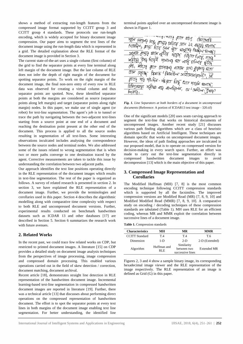
segmentation. For better understanding, the identified line
terminal points applied over an uncompressed document image is
shown in Figure 1.
Fig. 1. Line Separators at both borders of a document in uncompressed
documents (Reference: A portion of ICDAR13 test image - 320.tif)
One of the significant models [20] uses seam carving approach to
segment the text-line that works on historical documents of
uncompressed images. Another recent study [21] discusses
various path finding algorithms which are a class of heuristic
algorithms based on Artificial Intelligent. These techniques are
domain specific that works on uncompressed document images.
However, the ideas of path finding approaches are inculcated in
our proposed model, that is to operate on compressed version for
decision-making in every search space. Further, an effort was
made to carry out the text-line segmentation directly in
compressed handwritten document images to avoid
decompression [13] which is the main objective of this paper.
3. Compressed Image Representation and Corollaries
The Modified Huffman (MH) [7, 8] is the most common
encoding technique following CCITT compression standards
which is supported by all the facsimiles. The improved
compression versions are Modified Read (MR) [7, 8, 9, 10] and
Modified Modified Read (MMR) [7, 8, 9, 10]. A comparative
study on encoding / decoding techniques of these compression
standards are tabulated (Table 1). MH uses RLE for an efficient
coding, whereas MR and MMR exploit the correlation between
successive lines of a document image.
Table 1. Compression standards
Characteristics MH MR MMR
CCITT Standard T.4 T.4 T.6
Dimension 1-D 2-D 2-D (Extended)
Algorithm Huffman and
RLE
Similarity
between two successive lines
Extended MR
Figures 2, 3 and 4 show a sample binary image, its corresponding
hexadecimal image viewer and the RLE representation of the
image respectively. The RLE representation of an image is
defined as Grid (G) in this paper.

International Journal of Intelligent Systems and Applications in Engineering IJISAE, 2018, 6(4), 251–261 | 253
Fig. 2. A sample image of size 18X10 (WidthXHeight)
Fig. 3. Hexadecimal visualization of the image from Fig. 2
Fig. 4. RLE data inferred as Grid of the image from Fig 2
The odd and even columns of the RLE data represent the count of
white-runs and the black-runs of an uncompressed document
image. The number of continuous pixel value, say ‘0’
(background), is called as white-runs [22, 23, 24, 25, 26].
Similarly, the number of continuous pixel value, say ‘1’
(foreground) is called as black-runs [22, 23, 24, 25, 26]. If a row
in an image starts directly with foreground, then the value in the
first column of the corresponding row in RLE has an entry zero
(‘0’). This infers that odd columns and even columns in the grid
contain count of white-runs and black-runs respectively. The
white-runs represent background whereas the black-runs
represent foreground as text-content.
Some of the corollaries used in this article are listed here:
a. Each separator points spotted in the first column of the Grid
( ) is considered as Source Node ( ).
b. Each separator points spotted in the virtual column is
considered as Target Node ( ). Final non-zero entry in
every row of G makes this virtual column.
c. A path ( ) is defined as segmentation of adjacent text lines;
an agent (or robot) navigates along blank space (white-
runs) available between two adjacent text-lines from to
with reference to .
d. Edges ( ) are defined as sequences of white-runs that exist or
tunneled between two adjacent text-lines. These sequence
of formulates .
e. An obstacle ( ) appears because of touching characters
between two adjacent text-lines, which is a hurdle while
tracing from to . This may also occur due to ascenders
and descenders of characters, which appears larger in length
when compared to a given threshold ( ).
f. t is the length covered by an agent tracing both the direction
vertically up and down ( ) from the current
position , where arguments and refer to the
position in along (columns) and (rows) axis
respectively; this search space is induced whenever there is
an . is chosen empirically based on experiments
conducted on the datasets.
g. For every , there is a . The relationship between and is
one-to-one function defined as and strictly
follows the ascending order. The correspondence of and
is not defined in the literature [13]. However, in this
paper, we could find the probable correspondence between
and with help of an agent (or robot) and algorithmic
strategies.
h. When relationship between and is onto function or
crossover, then it is observed as wrong segmentation. Even
though and hold a relation one-to-one and there exist
crossovers, then it is considered as wrong segmentation.
i. The distance ( ) calculated between and denotes the
shortest covering longest distance (weights), which is
defined by a function, . depends on the number of
edges ( ) used in by an agent to cover between and
.
j. The terminal points and does not necessarily possess
larger white-runs because, they are heuristically chosen as
mid-points of the bands corresponding to the two-adjacent
text-lines along axis (columns) of . Therefore, may
not be an actual start point, in the given situation, whereas
the weight of the is longer than . So, the actual start
point would be and it would be within the search space of
from .
k. The distance between two intermediate hubs such as
and must be equal or greater than a given threshold ( ).
is calculated by finding a maximum number of bins
observed from the histogram of with respect to odd
columns (white-runs) only.
Some of the assumptions concerning the state space search
(tunnel or traversal or ) are given below:
a. and are finite.
b. There must be at-least one between and
c. One agent (or robot) is employed at a time for tracing
.
d. There is no self-loop in (a cycle of length one).
e. Tunnel (Move to next state) if exist on .
Figure 5 shows the terminal points of and in an
uncompressed version for better understanding. It depicts 10
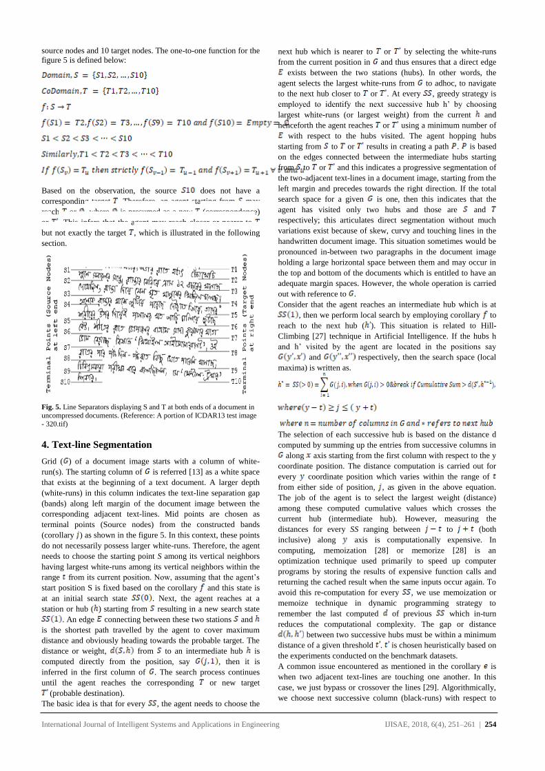
International Journal of Intelligent Systems and Applications in Engineering IJISAE, 2018, 6(4), 251–261 | 254
source nodes and 10 target nodes. The one-to-one function for the
figure 5 is defined below:
Based on the observation, the source does not have a
corresponding target . Therefore, an agent starting from may
reach or , where is presumed as a new (correspondence)
or . This infers that the agent may reach closer or nearer to
but not exactly the target , which is illustrated in the following
section.
Fig. 5. Line Separators displaying S and T at both ends of a document in
uncompressed documents. (Reference: A portion of ICDAR13 test image
- 320.tif)
4. Text-line Segmentation
Grid ( ) of a document image starts with a column of white-
run(s). The starting column of is referred [13] as a white space
that exists at the beginning of a text document. A larger depth
(white-runs) in this column indicates the text-line separation gap
(bands) along left margin of the document image between the
corresponding adjacent text-lines. Mid points are chosen as
terminal points (Source nodes) from the constructed bands
(corollary ) as shown in the figure 5. In this context, these points
do not necessarily possess larger white-runs. Therefore, the agent
needs to choose the starting point S among its vertical neighbors
having largest white-runs among its vertical neighbors within the
range from its current position. Now, assuming that the agent’s
start position S is fixed based on the corollary and this state is
at an initial search state . Next, the agent reaches at a
station or hub ( ) starting from resulting in a new search state
. An edge connecting between these two stations and
is the shortest path travelled by the agent to cover maximum
distance and obviously heading towards the probable target. The
distance or weight, from to an intermediate hub is
computed directly from the position, say , then it is
inferred in the first column of . The search process continues
until the agent reaches the corresponding or new target
(probable destination).
The basic idea is that for every , the agent needs to choose the
next hub which is nearer to or by selecting the white-runs
from the current position in and thus ensures that a direct edge
exists between the two stations (hubs). In other words, the
agent selects the largest white-runs from to adhoc, to navigate
to the next hub closer to or . At every , greedy strategy is
employed to identify the next successive hub h’ by choosing
largest white-runs (or largest weight) from the current and
henceforth the agent reaches or using a minimum number of
with respect to the hubs visited. The agent hopping hubs
starting from to or results in creating a path . is based
on the edges connected between the intermediate hubs starting
from to or and this indicates a progressive segmentation of
the two-adjacent text-lines in a document image, starting from the
left margin and precedes towards the right direction. If the total
search space for a given is one, then this indicates that the
agent has visited only two hubs and those are and
respectively; this articulates direct segmentation without much
variations exist because of skew, curvy and touching lines in the
handwritten document image. This situation sometimes would be
pronounced in-between two paragraphs in the document image
holding a large horizontal space between them and may occur in
the top and bottom of the documents which is entitled to have an
adequate margin spaces. However, the whole operation is carried
out with reference to .
Consider that the agent reaches an intermediate hub which is at
, then we perform local search by employing corollary to
reach to the next hub ( ). This situation is related to Hill-
Climbing [27] technique in Artificial Intelligence. If the hubs h
and h’ visited by the agent are located in the positions say
and respectively, then the search space (local
maxima) is written as.
The selection of each successive hub is based on the distance d
computed by summing up the entries from successive columns in
along axis starting from the first column with respect to the y
coordinate position. The distance computation is carried out for
every coordinate position which varies within the range of
from either side of position, , as given in the above equation.
The job of the agent is to select the largest weight (distance)
among these computed cumulative values which crosses the
current hub (intermediate hub). However, measuring the
distances for every SS ranging between to (both
inclusive) along axis is computationally expensive. In
computing, memoization [28] or memorize [28] is an
optimization technique used primarily to speed up computer
programs by storing the results of expensive function calls and
returning the cached result when the same inputs occur again. To
avoid this re-computation for every , we use memoization or
memoize technique in dynamic programming strategy to
remember the last computed of previous which in-turn
reduces the computational complexity. The gap or distance
between two successive hubs must be within a minimum
distance of a given threshold . is chosen heuristically based on
the experiments conducted on the benchmark datasets.
A common issue encountered as mentioned in the corollary is
when two adjacent text-lines are touching one another. In this
case, we just bypass or crossover the lines [29]. Algorithmically,
we choose next successive column (black-runs) with respect to
International Journal of Intelligent Systems and Applications in Engineering IJISAE, 2018, 6(4), 251–261 | 255
the current position. In other case, the same strategy is extended
when the ascenders and descenders appear to be greater than the
given threshold value , where the agent would not be able to go
beyond the search limit, say . One of the important issues
mentioned in corollary is when a distance between
hubs is greater than . is given below.
t’= maximum(histogram(values in odd colums of G))
where values in odd columns of G represents white runs
In this case, we calculate t’ by considering the largest bin from
the histogram of G with respect to the counts of white runs (odd
columns). If the distance is found to be larger than t’, then we
apply both the concepts namely ‘don’t care condition’ [29] and
‘minimal cut-sets’ [30] from graph theoretical domain. Therefore,
with a minimal number of crossovers, the agent bypasses and
reaches the next successive hubs. Finally, the agent will update its
knowledge base about each visited hub with reference to G
covering the distance from S to T or T’. Below we present the
proposed algorithm for text-line segmentation using .
Algorithm: Finding text-line segmentation in G using tunneling
approach
Input: Compressed representation G of a document image,
Terminal points – Source Nodes (Sn) at ever line terminals.
Vertical neighboring search threshold t.
Output: Text-line segmentation in G=TS
1. For-each Source Node (S) from Sn, with the position G(y’,x’), where, x’=1;
CurrentSum=0; Maximum=0; GridY=y’
While j=G(y’-t,x’) to G(y’+t,x’) the agent vertical search range is
between y’-t to y’+t (both inclusive), where j>=1 and j<=high of G.
a. Calculate: Cumulative Sum (Initialize Csum=0) for each j or
Use Dynamic Programming. Use Memoize to check data in
Knowledge base (KB)
a. Find Maximum and update coordinate position:
2. Update and coordinate position of :
The positions chosen in the grid is update
in
Goto Step 2 until
3. Stop: When the agent covers the distance .
4.1. Time Complexity for Text-line Segmentation
The following provides the time complexity estimated for the
proposed algorithm to identify the text-line segmentation
positions in compressed representation of a document image. The
worst-case scenario is calculated as where and
represent the number of rows and number of columns of the grid
respectively.
Usage of memoize technique [28] in dynamic programming
strategy has reduced to the complexity from
, that is which is a non-
deterministic polynomial.
For comparative study, the time complexity is also estimated for
a document image in its uncompressed format. For this, the
worst-case scenario is where and represent the
height and width of an uncompressed image respectively. It is
noted that is equal to whereas is lesser than .
Time complexity of spotting the line terminal points mentioned in
the literature [13] is estimated as in the worst-case
scenario. Therefore, the complexity for the proposed algorithm is
computed by cascading the two algorithms which result in
. Finally, the proposed method
takes .
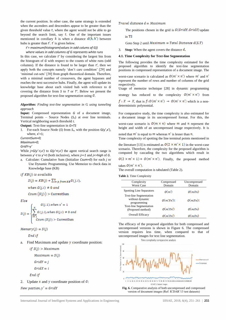
The overall computation is tabulated (Table 2).
Table 2. Time Complexity
Complexity
Worst Case
Compressed
Domain
Uncompressed
Domain
Spotting Line Separators
Text-line Segmentation
without dynamic
programming
Text-line Segmentation
(Proposed method)
Overall Efficacy
The efficacy of the proposed algorithm for both compressed and
uncompressed versions is shown in Figure 6. The compressed
version requires less time, when compared to that of
uncompressed images for text line segmentation.
Fig. 6. Comparative analysis of both uncompressed and compressed
version of document images (Ref: ICDAR’13 test datasets)
International Journal of Intelligent Systems and Applications in Engineering IJISAE, 2018, 6(4), 251–261 | 256
4.2. Illustration
In this section, we illustrate the working principle of Tunneling
algorithm using an example. The coordinate positions are tracked
by the agent (or robot) for text line segmentation with respect to
is shown in Table 3.
Table 3. RLE coordinate positions (Reference: A portion of ICDAR13
test image – 320.tif – text-lines 21 and 22)
Hubs
(Stations) Y-Coordinate X-Coordinate
Distance From
Source Node
Source 1977 1 767
Hub 1 1984 1 1058
Hub 2 2000 9 1295
Hub 3 2020 59 1325
Hub 4 2014 53 1626
Hub 5 2029 67 1901
Hub 6 2049 77 2085
For better understanding, an experimental result is shown in the
uncompressed version as well. Figure 7 shows segmentation of
two text-lines of a document image. Figure 8 illustrates the text-
line segmentation depicting transition hubs and a path tunneled
by an agent.
Fig. 7. Segmentation of two text lines depicted in uncompressed
documents (Reference: A portion of ICDAR13 test image – 320.tif – text-
lines 21 and 22)
Fig. 8. Segmentation of two text lines depicted in uncompressed
documents (Reference: A portion of ICDAR13 test image – 320.tif – text-
lines 21 and 22)
From the example, the agent starts from the Source Node ( ) and
reaches the Target Node ( ) visiting six intermediate hubs such
as Hub 1, Hub 2, Hub 3, Hub 4, Hub 5 and Hub 6. Here, the
source node is identified in a position, say . The agent
predicts that the Hub 1 in the position could be an
effective source node than the initial source [13] as articulated in
corollary . This is because the weight (distance) of Hub 1 is
larger when compared to the initial source as illustrated in table 3.
The total distance covered by the agent is 2085 units. The
threshold is chosen as 20 units and the total computation to
cover the distance along coordinates in both the direction by the
agent ranges from to
, i.e., to
respectively. We employ memoization technique to
reduce the complexity. Therefore, we make use of a knowledge
base ( ) which would be empty initially. Once we compute the
distances for both Source and Hub 1, we feed all the weights
(distances) ranging from to ,
i.e., to respectively into the KB. The size
of the KB would be a column size of . The triggers the agent
to choose next hub as Hub 2 as a successor of the Hub 1 which
covers the distance of 1295 units and perhaps the distance is
greater than the distance of current hub, that is the Hub 1 possess
1058 units. Next, agent archives the information from the KB to
avoid the total computation.
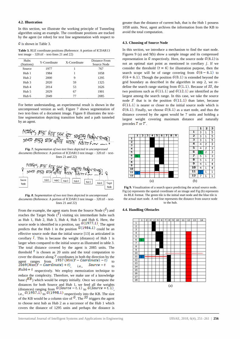
4.3. Choosing of Source Node
In this section, we introduce a mechanism to find the start node.
Figures 9 (a) and 9(b) show a sample image and its compressed
representation in respectively. Here, the source node is
not an optimal start point as mentioned in corollary . If we
consider the threshold for illustration purpose, then the
search scope will be of range covering from to
. Though the position is extended beyond the
grid boundary as described in the algorithm in step 2, we re-
define the search range starting from . Because of , the
two positions such as and are identified as the
largest among the search range. In this case, we take the source
node that is in the position than latter, because
is nearer or closer to the initial source node which is
. Finally, we choose as a start node, and thus the
distance covered by the agent would be 7 units and holding a
largest weight covering maximum distance and naturally
precedes or .
(a) (b)
Fig 9. Visualization of a search space predicting the actual source node.
Fig (a) represents the spatial coordinate of an image and Fig (b) represents
its RLE format. The green tile is the initial start node and the blue tile is
the actual start node. A red line represents the distance from source node
to the hub.
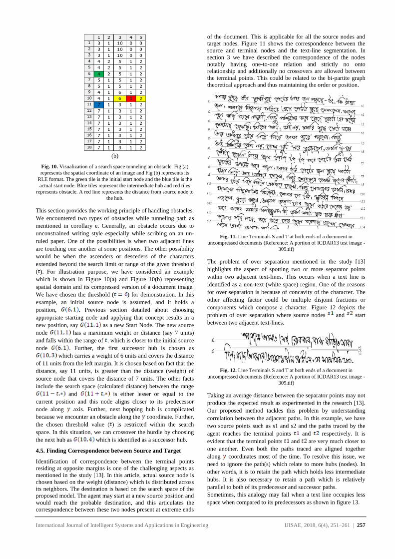
4.4. Handling Obstacles
(a)
International Journal of Intelligent Systems and Applications in Engineering IJISAE, 2018, 6(4), 251–261 | 257
(b)
Fig. 10. Visualization of a search space tunneling an obstacle. Fig (a)
represents the spatial coordinate of an image and Fig (b) represents its
RLE format. The green tile is the initial start node and the blue tile is the
actual start node. Blue tiles represent the intermediate hub and red tiles
represents obstacle. A red line represents the distance from source node to
the hub.
This section provides the working principle of handling obstacles.
We encountered two types of obstacles while tunneling path as
mentioned in corollary e. Generally, an obstacle occurs due to
unconstrained writing style especially while scribing on an un-
ruled paper. One of the possibilities is when two adjacent lines
are touching one another at some positions. The other possibility
would be when the ascenders or desceders of the characters
extended beyond the search limit or range of the given threshold
( ). For illustration purpose, we have considered an example
which is shown in Figure 10(a) and Figure 10(b) representing
spatial domain and its compressed version of a document image.
We have chosen the threshold ( ) for demonstration. In this
example, an initial source node is assumed, and it holds a
position, . Previous section detailed about choosing
appropriate starting node and applying that concept results in a
new position, say as a new Start Node. The new source
node has a maximum weight or distance (say 7 units)
and falls within the range of , which is closer to the initial source
node . Further, the first successor hub is chosen as
which carries a weight of 6 units and covers the distance
of 11 units from the left margin. It is chosen based on fact that the
distance, say 11 units, is greater than the distance (weight) of
source node that covers the distance of 7 units. The other facts
include the search space (calculated distance) between the range
and is either lesser or equal to the
current position and this node aligns closer to its predecessor
node along axis. Further, next hopping hub is complicated
because we encounter an obstacle along the coordinate. Further,
the chosen threshold value ( ) is restricted within the search
space. In this situation, we can crossover the hurdle by choosing
the next hub as which is identified as a successor hub.
4.5. Finding Correspondence between Source and Target
Identification of correspondence between the terminal points
residing at opposite margins is one of the challenging aspects as
mentioned in the study [13]. In this article, actual source node is
chosen based on the weight (distance) which is distributed across
its neighbors. The destination is based on the search space of the
proposed model. The agent may start at a new source position and
would reach the probable destination, and this articulates the
correspondence between these two nodes present at extreme ends
of the document. This is applicable for all the source nodes and
target nodes. Figure 11 shows the correspondence between the
source and terminal nodes and the text-line segmentation. In
section 3 we have described the correspondence of the nodes
notably having one-to-one relation and strictly no onto
relationship and additionally no crossovers are allowed between
the terminal points. This could be related to the bi-partite graph
theoretical approach and thus maintaining the order or position.
Fig. 11. Line Terminals S and T at both ends of a document in
uncompressed documents (Reference: A portion of ICDAR13 test image -
309.tif)
The problem of over separation mentioned in the study [13]
highlights the aspect of spotting two or more separator points
within two adjacent text-lines. This occurs when a text line is
identified as a non-text (white space) region. One of the reasons
for over separation is because of concavity of the character. The
other affecting factor could be multiple disjoint fractions or
components which compose a character. Figure 12 depicts the
problem of over separation where source nodes and start
between two adjacent text-lines.
Fig. 12. Line Terminals S and T at both ends of a document in
uncompressed documents (Reference: A portion of ICDAR13 test image -
309.tif)
Taking an average distance between the separator points may not
produce the expected result as experimented in the research [13].
Our proposed method tackles this problem by understanding
correlation between the adjacent paths. In this example, we have
two source points such as s1 and s2 and the paths traced by the
agent reaches the terminal points and respectively. It is
evident that the terminal points and are very much closer to
one another. Even both the paths traced are aligned together
along coordinates most of the time. To resolve this issue, we
need to ignore the path(s) which relate to more hubs (nodes). In
other words, it is to retain the path which holds less intermediate
hubs. It is also necessary to retain a path which is relatively
parallel to both of its predecessor and successor paths.
Sometimes, this analogy may fail when a text line occupies less
space when compared to its predecessors as shown in figure 13.

International Journal of Intelligent Systems and Applications in Engineering IJISAE, 2018, 6(4), 251–261 | 258
Fig. 13. Line Terminals S and T at both ends of a document in
uncompressed documents (Reference: A portion of ICDAR13 test image -
309.tif)
This occurs mostly with a last text-line of a paragraph having less
number of words. However, this situation is addressed by
understanding the average distance between the two adjacent
paths as mentioned above. It is computed by
We illustrate the distance between the adjacent paths with an
example. Figure 14 shows the paths traced along the two text-line
gaps.
Table 4 shows the coordinate positions of paths traced along
axis. We assume as 500 for illustration purpose. For every
interval , we take the coordinate positions for both paths.
Table 5 shows coordinate positions for the paths with an
interval gap of . The distance calculated for the paths (path 1
and path 2) is given under.
Fig. 14. Two paths traced along the text-lines
Table 4. RLE coordinate positions for two adjacent paths.
Path 1 Path 2
Hubs Y-Coordinates Distance
covered from
left margin
Y-Coordinates Distance
covered from
left margin
Source 1977 767 2079 186
Hub 1 1984 1058 2059 367
Hub 2 2000 1295 2073 682
Hub 3 2020 1325 2087 1132
Hub 4 2014 1626 2105 1389
Hub 5 2029 1901 2123 1665
Hub 6 2049 2085 2132 1870
Hub 7 - - 2124 2085
Table 5. RLE coordinate positions for two adjacent paths.
Hubs t’ Y-Coordinates
(Path 1), u
Y-Coordinates
(Path 2), v
Source 1-500 1977 2059
Hub 1 501-1000 1977 2073
Hub 2 1001-1500 2020 2105
Hub 3 1500-2000 2029 2132
Hub 4 2001-2500 2049 2124
5. Experimental Evaluation
5.1. Datasets
Our proposed method is evaluated on various benchmark
handwritten datasets such as ICDAR’13 [31] and others [17]
comprising of Kannada, Oriya, Persian and Bangla documents.
For experimental purpose, the compression standards for these
datasets are preserved as discussed in one of the studies [16].
5.2. Results
Our proposed method is evaluated based on two factors that we
came across in a study [31] - (i) Detection Rate ( ) and (ii)
Recognition Accuracy ( ). and are defined as follows:
The DR in spotting the separator points at both the left side and
the right side of the document is provided in literature [13] and
also been tabulated (Table 6).
Table 6. Detection Rate
Datasets
(Handwritten)
Total
Lines (N)
Detected
o2o Rate (%)
Left Right Left Right
ICDAR13 [31] 2649 2578 2502 97.31 94.45
Kannada [20] 4298 4173 4082 97.09 94.97
Oriya [20] 3108 3012 2911 96.91 93.66
Bangla [20] 4850 4650 4598 95.87 94.80
Persia [20] 1787 1690 1723 94.57 96.41
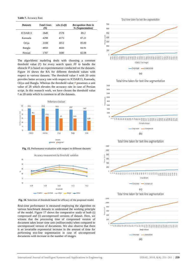
Table 7 shows the result of the proposed model applied on the
benchmark datasets. Our method focuses only on a terminal point
that is spotted on the left side of the document, so the RA for
segmenting the text line, entirely depends upon the separator
points spotted along left margin of the document. Figure 15
shows the comparative performance analyses of both DR and RA
for various benchmark datasets. It is evident that the algorithm
works better in the case of ICDAR datasets. We also witness that
the RA for the dataset of Persian script is lower when compared
to other datasets. This is because of the reason that the Persian
writing style starts from right end of the document and precedes
towards left direction unlike most of the other scripts. The other
reasons include more concavity and disjoints in the composition
of the character.
International Journal of Intelligent Systems and Applications in Engineering IJISAE, 2018, 6(4), 251–261 | 259
Table 7. Accuracy Rate
Datasets Total Lines
(N)
o2o (Left) Recognition Rate in
% (Segmentation)
ICDAR13 2649 2578 89.2
Kannada 4298 4173 87.21
Oriya 3108 3012 85.00
Bangla 4850 4650 84.91
Persian 1787 1690 82.08
The algorithmic modeling deals with choosing a common
threshold value ( ) for every search space to handle the
obstacle is based on experimentation conducted on the datasets.
Figure 16 shows the RA for different threshold values with
respect to various datasets. The threshold value with 20 units
provides better accuracy rate with respect to ICDAR13, Kannada,
Oriya and Bangla. Whereas the threshold value possesses a unit
value of 28 which elevates the accuracy rate in case of Persian
script. In this research work, we have chosen the threshold value
as 20 units which is common to all the datasets.
Fig. 15. Performance evaluation with respect to different datasets
Fig. 16. Selection of threshold based for efficacy of the proposed model.
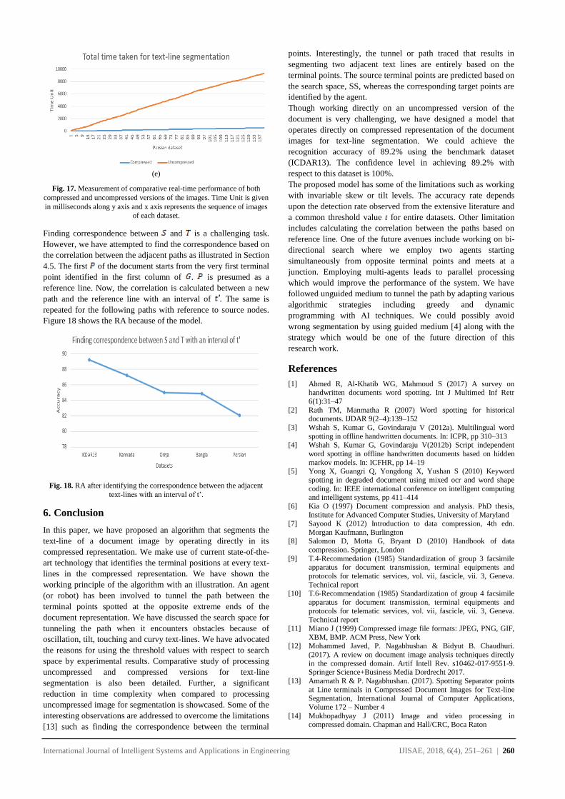
Real-time performance is measured employing the algorithm on
various benchmark datasets to understand the working principle
of the model. Figure 17 shows the comparative study of both (i)
compressed and (i) uncompressed versions of dataset. Here, we
witness that the processing time of compressed version of
document takes lesser time unit (milliseconds) when compared to
uncompressed version of documents. We also observe that there
is an invariable exponential increase in the amount of time for
performing text-line segmentation in case of uncompressed
documents with increase in the number of images.
(a)
(b)
(c)
(d)
International Journal of Intelligent Systems and Applications in Engineering IJISAE, 2018, 6(4), 251–261 | 260
(e)
Fig. 17. Measurement of comparative real-time performance of both
compressed and uncompressed versions of the images. Time Unit is given
in milliseconds along y axis and x axis represents the sequence of images
of each dataset.
Finding correspondence between and is a challenging task.
However, we have attempted to find the correspondence based on
the correlation between the adjacent paths as illustrated in Section
4.5. The first of the document starts from the very first terminal
point identified in the first column of . is presumed as a
reference line. Now, the correlation is calculated between a new
path and the reference line with an interval of . The same is
repeated for the following paths with reference to source nodes.
Figure 18 shows the RA because of the model.
Fig. 18. RA after identifying the correspondence between the adjacent
text-lines with an interval of t’.
6. Conclusion
In this paper, we have proposed an algorithm that segments the
text-line of a document image by operating directly in its
compressed representation. We make use of current state-of-the-
art technology that identifies the terminal positions at every text-
lines in the compressed representation. We have shown the
working principle of the algorithm with an illustration. An agent
(or robot) has been involved to tunnel the path between the
terminal points spotted at the opposite extreme ends of the
document representation. We have discussed the search space for
tunneling the path when it encounters obstacles because of
oscillation, tilt, touching and curvy text-lines. We have advocated
the reasons for using the threshold values with respect to search
space by experimental results. Comparative study of processing
uncompressed and compressed versions for text-line
segmentation is also been detailed. Further, a significant
reduction in time complexity when compared to processing
uncompressed image for segmentation is showcased. Some of the
interesting observations are addressed to overcome the limitations
[13] such as finding the correspondence between the terminal
points. Interestingly, the tunnel or path traced that results in
segmenting two adjacent text lines are entirely based on the
terminal points. The source terminal points are predicted based on
the search space, SS, whereas the corresponding target points are
identified by the agent.
Though working directly on an uncompressed version of the
document is very challenging, we have designed a model that
operates directly on compressed representation of the document
images for text-line segmentation. We could achieve the
recognition accuracy of 89.2% using the benchmark dataset
(ICDAR13). The confidence level in achieving 89.2% with
respect to this dataset is 100%.
The proposed model has some of the limitations such as working
with invariable skew or tilt levels. The accuracy rate depends
upon the detection rate observed from the extensive literature and
a common threshold value t for entire datasets. Other limitation
includes calculating the correlation between the paths based on
reference line. One of the future avenues include working on bi-
directional search where we employ two agents starting
simultaneously from opposite terminal points and meets at a
junction. Employing multi-agents leads to parallel processing
which would improve the performance of the system. We have
followed unguided medium to tunnel the path by adapting various
algorithmic strategies including greedy and dynamic
programming with AI techniques. We could possibly avoid
wrong segmentation by using guided medium [4] along with the
strategy which would be one of the future direction of this
research work.
References
[1] Ahmed R, Al-Khatib WG, Mahmoud S (2017) A survey on handwritten documents word spotting. Int J Multimed Inf Retr
6(1):31–47
[2] Rath TM, Manmatha R (2007) Word spotting for historical documents. IJDAR 9(2–4):139–152
[3] Wshah S, Kumar G, Govindaraju V (2012a). Multilingual word
spotting in offline handwritten documents. In: ICPR, pp 310–313
[4] Wshah S, Kumar G, Govindaraju V(2012b) Script independent
word spotting in offline handwritten documents based on hidden
markov models. In: ICFHR, pp 14–19 [5] Yong X, Guangri Q, Yongdong X, Yushan S (2010) Keyword
spotting in degraded document using mixed ocr and word shape
coding. In: IEEE international conference on intelligent computing and intelligent systems, pp 411–414
[6] Kia O (1997) Document compression and analysis. PhD thesis, Institute for Advanced Computer Studies, University of Maryland
[7] Sayood K (2012) Introduction to data compression, 4th edn.
Morgan Kaufmann, Burlington [8] Salomon D, Motta G, Bryant D (2010) Handbook of data
compression. Springer, London
[9] T.4-Recommedation (1985) Standardization of group 3 facsimile apparatus for document transmission, terminal equipments and
protocols for telematic services, vol. vii, fascicle, vii. 3, Geneva.
Technical report [10] T.6-Recommendation (1985) Standardization of group 4 facsimile
apparatus for document transmission, terminal equipments and
protocols for telematic services, vol. vii, fascicle, vii. 3, Geneva.
Technical report
[11] Miano J (1999) Compressed image file formats: JPEG, PNG, GIF,
XBM, BMP. ACM Press, New York [12] Mohammed Javed, P. Nagabhushan & Bidyut B. Chaudhuri.
(2017). A review on document image analysis techniques directly
in the compressed domain. Artif Intell Rev. s10462-017-9551-9. Springer Science+Business Media Dordrecht 2017.
[13] Amarnath R & P. Nagabhushan. (2017). Spotting Separator points
at Line terminals in Compressed Document Images for Text-line Segmentation, International Journal of Computer Applications,
Volume 172 – Number 4
[14] Mukhopadhyay J (2011) Image and video processing in compressed domain. Chapman and Hall/CRC, Boca Raton
International Journal of Intelligent Systems and Applications in Engineering IJISAE, 2018, 6(4), 251–261 | 261
[15] Adjeroh D, Bell T, Mukherjee A (2013) Pattern matching in
compressed texts and images. Now Publishers. [16] Mohammed Javed, Krishnanand S.H, P. Nagabhushan, & B. B.
Chaudhuri. (2016). Visualizing CCITT Group 3 and Group 4 TIFF
Documents and Transforming to Run-Length Compressed Format Enabling Direct Processing in Compressed Domain International
Conference on Computational Modeling and Security (CMS 2016)
Procedia Computer Science 85 (2016) 213 – 221. Elsevier. [17] Alireza Alaei, P. Nagabhushan, Umapada Pal, Fumitaka Kimura,
"An Effcient Skew Estimation Technique for Scanned
Documents:An Application of Piece-wise Painting Algorithm", Journal of Pattern Recognition Research (JPRR), Vol 11, No 1
doi:10.13176/11.635 (2016).
[18] Amarnath R, P. Nagabhushan and Mohammed Javed, (2018) Line Detection in Run-Length Encoded Document Images using
Monotonically Increasing Graph Model, Accepted in 2018
International Conference on Advances in Computing, Communications and Informatics (ICACCI), September 19-22,
2018, Bangalore.
[19] Amarnath R, P. Nagabhushan and Mohammed Javed, (2018) Enabling Text-line Segmentation in Run-Length Encoded
Handwritten Document Image using Entropy Driven Incremental
Learning”, Third International Conference on Computer Vision & Image Processing (Accepted in CVIP-2018) September 29-October
01, 2018, IIIT Jabalpur, MP, India.
[20] N. Arvanitopoulos Darginis and S. Süsstrunk. Seam Carving for Text Line Extraction on Color and Grayscale Historical
Manuscripts. 14th International Conference on Frontiers in
Handwriting Recognition (ICFHR), Crete, Greece, 2014. [21] Zeyad Abd Algfoor, Mohd Shahrizal Sunar, & Afnizanfaizal
Abdullah. (2017). A new weighted pathfinding algorithm to reduce
the search time on grid maps. Expert Systems with Applications: An International Journal Archive Volume 71 Issue C, April 2017.
Pages 319-331
[22] Ronse C, Devijver P (1984) Connected components in binary images: the detection problem. Research Studies Press, Letchworth
[23] Breuel TM (2008) Binary morphology and related operations on
run-length representations. In: International conference on computer vision theory and applications - VISAPP, pp 159–166
[24] Hinds S, Fisher J, D’Amato D (1990) A document skew detection method using run-length encoding and the hough transform. In:
Proceedings of 10th international conference on pattern
recognition, vol 1, pp 464–468 [25] Shima Y, Kashioka S, Higashino J (1989) A high-speed
rotationmethod for binary images based on coordinate operation of
run data. Syst Comput Jpn 20(6):91–102 [26] ShimaY, Kashioka S, Higashino J (1990) A high-speed algorithm
for propagation-type labeling based on block sorting of runs in
binary images. In: Proceedings of 10th international conference on pattern recognition (ICPR), vol 1, pp 655–658
[27] Andrés Cano, Manuel Gómez-Olmedo, Serafín Moral, Joaquín
Abellán: Hill-climbing and branch-and-bound algorithms for exact and approximate inference in credal networks. Int. J. Approx.
Reasoning 44(3): 261-280 (2007)
[28] Peter Norvig. Paradigms of Artificial Intelligence Programming 1st Edition. Case Studies in Common Lisp.28th June 2014
[29] Nazih Ouwayed, Abdel Bela¨ıd. Multi-Oriented Text Line
Extraction from Handwritten Arabic Documents. 8th IAPR International Workshop on Document Analysis Systems - DAS’08,
Sep 2008, Nara, Japan. pp.339-346, 2008.
[30] Zhayida Simayijiang & Stefanie Grimm “Segmentation Graph-Cut”.
[31] Nikolaos Stamatopoulos, Basilis Gatos, Georgios Louloudis,
Umapada Pal, & Alireza Alaei Proceeding. (2013). ICDAR '13 Proceedings of the 2013 12th International Conference on
Document Analysis and Recognition Pages 1402-1406
International Journal of
Intelligent Systems and
Applications in Engineering
Advanced Technology and Science
ISSN:2147-67992147-6799 www.atscience.org/IJISAE Original Research Paper
International Journal of Intelligent Systems and Applications in Engineering IJISAE, 2018, 6(4), 262–270 | 262
Knowledge Discovery on Investment Fund Transaction Histories and
Socio-Demographic Characteristics for Customer Churn
Fatih CIL1, Tahsin CETINYOKUS*2, Hadi GOKCEN2
Accepted : 11/12/2018 Published: 31/12/2018 DOI: 10.1039/b000000x
Abstract: The need of turning huge amounts of data into useful information indicates the importance of data mining. Thanks to latest
improvement in information technologies, storing huge data in computer systems becomes easier. Thus, “knowledge discovery” concept
becomes more important. Data mining is the process of finding hidden and unknown patterns in huge amounts of data. It has a wide
application area such as marketing, banking and finance, medicine and manufacturing. One of the most commonly used application areas
of data mining is recognizing customer churn. Data mining is used to obtain behavior of churned customers by analyzing their previous
transactions. In the same manner using with obtained tendency, other active customers are held in the system. It is possible to make by
various marketing and customer retention activities. In this paper, it is aimed to recognize the churned customers of a bank who closed
their saving accounts and determine common socio-demographic characteristics of these customers.
Keywords: Data mining, Customer churn, Decision trees and classification rules, Mutual funds
1. Introduction
After the increase in the amount of data about customer’s
transactions and escalating competition in the industries, firms
have attempted to use their existing data efficiently in order to
obtain information which is used to understand purchasing and
service characteristics of customers. Due to increasing competition
and improvements in IT Technologies, obtained information will
provide advantage to firms, so it has been gaining importance.
The increasing usage of database systems and their extraordinary
increase in volume have made firms to be faced with the issue how
firms will derive benefit from these data. Traditional query or
reporting tools are inadequate in the face of massive amounts of
data. This is why the new tendencies and Data Mining is a result
of this search [1].
In this study, it is focused on two objectives. The first of these is
to learn the details of the transactions of the customers buying and
selling bank mutual funds including former customers who closed
their bank accounts after a stated transaction history. The second
objective is to obtain socio-demographic characteristics of the
customers who closed their investment account. With obtained
results, the rules are determined to prevent losing customers who
are tended to close their accounts. The main contribution is the first
study in literature considering mutual funds customer churn based
on data mining techniques.
It is organized as follows. In the second section, data mining and
classification algorithms used in the study are discussed. Then, a
general overview to bank mutual funds is presented in the third
section. In the fourth section, the study conducted is mentioned and
finally the results of the study are covered.
2. Data Mining, Decision Trees and Classification Rules
2.1. Data Mining
Data mining is a set of techniques that enable the extraction of
large volume data sets useful results. In problem solving, located
data in different sources or databases are analyzed. As a result of
this analysis, hidden images will emerge. Using the obtained
patterns can be given strategic management decisions.
Data mining is discovery driven. It involves various techniques
including statistics, decision trees, neural networks, genetic
algorithms and visualization techniques. Data mining has been
applied in many fields such as marketing, finance, banking, health
care, customer relationship management and organizational
learning [2].
Owing to the advancement of information technologies and global
competitiveness, data mining has increasingly become an
important and a widely known field. Data mining applications has
been varied recently, although exists in academic framework for
long years [3].
The major reason that data mining has attracted a great deal of
attention in the information industry in recent years is due to the
wide availability of huge amounts of data and the imminent need
for turning such data into useful information and knowledge. The
information and knowledge gained can be used for applications
ranging from business management, production control and market
analysis to engineering design and science exploration [1].
Data mining is searching of relations and rules for future prediction
by using software. Assuming that near future will not be very
different from today or past; rules obtained from existent data will
help us to form correct estimates of future trends.
Knowledge discovery in databases (KDD) is processing of data by
data mining techniques in databases. Processing large amounts of
data in data warehouses can be possible with new generation tools
and techniques. So, studies applied about KDD keep up to date.
_______________________________________________________________________________________________________________________________________________________________________________________________________________________________________________________________________________________________________________________________
1 Operations Business Development at Finansbank İstanbul, TURKEY 2 Industrial Eng., Gazi University, Ankara – 06570, TURKEY
* Corresponding Author: Email: [email protected]
International Journal of Intelligent Systems and Applications in Engineering IJISAE, 2018, 6(4), 262–270 | 263
According to some sources; knowledge discovery in databases
refers to the overall process of discovering useful knowledge from
data, and data mining refers to a particular step in this process [4].
2.2. Decision Trees and Classification Rules
Classification data mining techniques are used when the dependent
(prediction) variable is discrete. Inferential techniques are used to
create decision trees and rules that effectively classify the dataset
as a function of its characteristics. Decision tree solution methods
provide automated techniques for discovering how to effect such
classifications [5,6]. At the top of the tree there is a root node, at
which the classification process begins. The test at the root node
tests all instances, which pass to the left if true, or to the right if
false. At each of the resulting nodes, further tests serve to continue
classifying the data. Each leaf of the tree represents a classification
rule. Rule-based solutions translate the tree by forming a conjunct
of every test that occurs on a path between the root node and the
leaf node of the tree [5]. One of the advantages offered by rule
induction algorithms is that the results may be directly inspected to
understand the variables that can be effectively used to classify the
data. Variables at the root node represent the strongest classifiers
(denoted as level 1 in the results section), followed by the next
strongest classifiers at each of the leaf nodes (denoted as level 2,
3, etc.).
In this study Id3 and J4.8 decision tree algorithm with PART, JRip
ve OneR classification rules are used. Id3 (basic divide-and-
conquer decision tree algorithm), J4.8 (implementation of C4.5
decision tree learner), PART (obtain rules from partial decision
trees built using J4.8), JRip (RIPPER algorithm for fast, effective
rule induction), OneR (1R classifier) (Witten and Frank, 2005).
3. Bank Investment Funds
The accumulation of all kinds of investors, whether large or small,
is managed by professional managers by distributing to the various
capital market instruments. These assets are called funds. Fund
portfolios consisting of treasury bonds, government securities,
repo, common stocks and other capital market instruments are
managed by professional portfolio managers in accordance with
internal regulations.
According to Capital Market Regulations investment fund
portfolios must be managed by institutions and portfolio
management companies. Investment funds are audited periodically
by Capital Markets Board and independent external audit firms.
Fund prices are determined by fund founder and these determined
prices are used next day in buying and selling funds.
Fund portfolio value is calculated in accordance with stock market
prices that funds are bought and sold. Total fund value is divided
by total share number that circulates on the day of valuation and
fund price is calculated.
Interests, dividends, trading gains and daily gains of portfolio
assets are recorded as income to fund at the same day and reflected
to the fund prices. Therefore, if an investor sells his/her funds,
he/she gets his/her share from the fund gaining
3.1. Discovery Studies on Investment Fund and Customer
Churn
Data mining are often used in studies about marketing, finance,
banking, manufacturing, health care, customer relations
management and organizational learning. Some of these studies
have been interested in the retaining the customers and minimizing
the customer churn.
Masand et al. [8] developed an automated system used historical
data of cellular phone customers. The system periodically
identifies churn factors for several statuses. In this study, decision
trees algorithms and neural networks algorithms were used.
Poel and Larivière [9] investigate predictors of churn incidence for
financial services as part of customer relationship management
(CRM) in their stuies. Their findings suggest that: demographic
characteristics, environmental changes and stimulating ‘interactive
and continuous’ relationships with customers are of major concern
when considering retention; customer behaviour predictors only
have a limited impact on attrition in terms of total products owned
as well as the interpurchase time.
Ahn et al., [9] investigated determinants of customer churn in the
Korean mobile telecommunications service market. In the study,
mediating effects of a customer's partial defection on the
relationship between the churn determinants and total defection
were analyzed and their implications were discussed. Results
indicate that customer's status change explains the relationship
between churn determinants and the probability of churn.
Ruta et al., [10] proposed a new k nearest sequence (kNS)
algorithm along with temporal sequence fusion technique to
predict the whole remaining customer data sequence path up to the
churn event in telecom industry.
Chu et al., [11] proposed a hybridized architecture to deal with
customer retention problems. In the system, common clustering-
followed- by- classification approaches have been used.
Aydoğan et al., [12] studied in a cosmetic firm to determine the
customer segment which tends to leave. So they developed
customized campaigns and marketing strategies for customer
profile who likely to leave. Clustering techniques were used for
segmentation and classification techniques were used for
determining the customer churn.
Telecommunications industry, customer churn is recognized as an
important research topic. In this view, Gopal and Meher [13] have
discussed the use of ordinal regression method to estimate the time
of customer churn and the duration of customer retention. On the
modeling of the customer churn, ordinal regression technic has
used in this study for the first time.
Farquad et al., [14] proposed a hybrid algorithm to predict churn
rates of customer using credit card. This algorithm is combination
of Support Vector Machine method and Naive Bayes method.
Huang et al., [15] presented a new set of features for broadband
internet customer churn prediction, based on Henley segments, the
broadband usage, dial types, the spend of dial-up, line-information,
bill and payment information, account information. The
experimental results showed that the new features with using these
four models (Logistic Regressions, Decision Trees, Multilayer
Perceptron Neural Networks and Support Vector Machines)
techniques are efficient for customer churn prediction in the
broadband service field.
Chen and Fan [16] proposed a framework of distributed customer
behavior prediction using multiplex data. Framework that is to
adapt to the emerging distributed computing environment, a novel
approach called collaborative multiple kernel support vector
machine (C-MK-SVM) is developed for modeling multiplex data
in a distributed manner, and the alternating direction method of
multipliers (ADMM) is used for the global optimization of C-MK-
SVM.
Zhang et al., [17] investigated the effects of interpersonal influence
on the accuracy of customer churn predictions and proposed a
novel prediction model that is based on interpersonal influence and
that combined the propagation process and customers’
personalized characters.
Slavescu and Panait [18] in their studies focuses on how to better
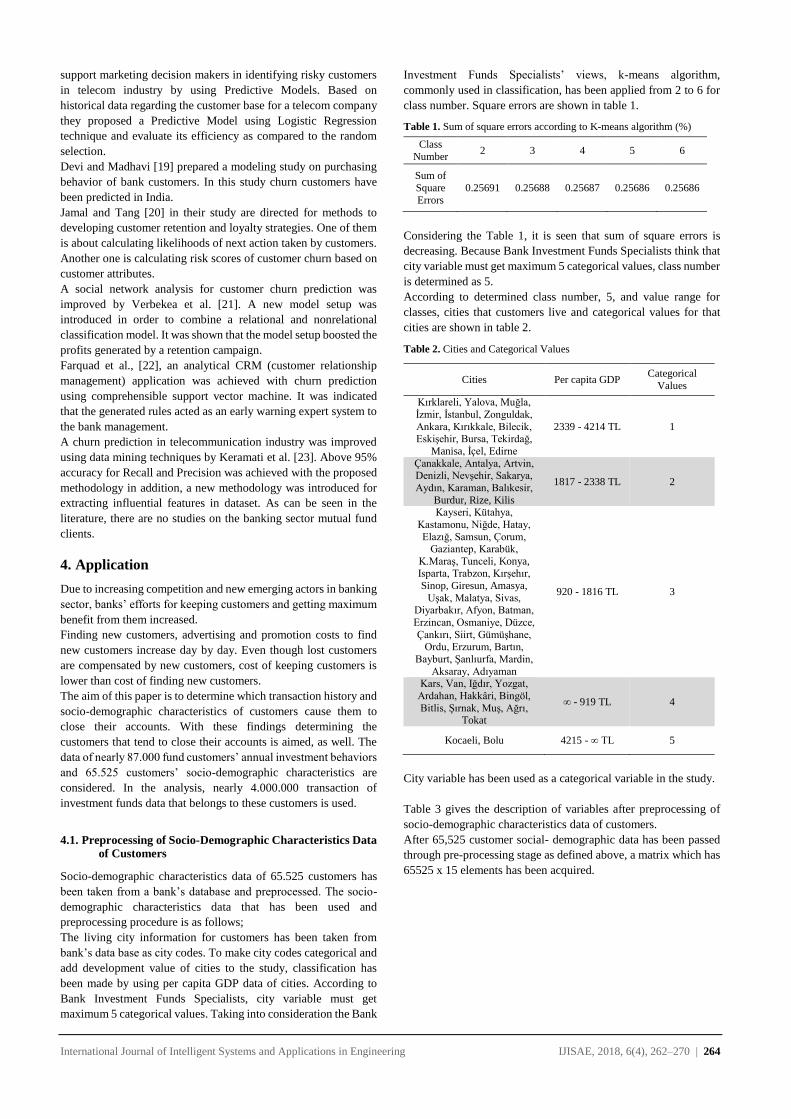
International Journal of Intelligent Systems and Applications in Engineering IJISAE, 2018, 6(4), 262–270 | 264
support marketing decision makers in identifying risky customers
in telecom industry by using Predictive Models. Based on
historical data regarding the customer base for a telecom company
they proposed a Predictive Model using Logistic Regression
technique and evaluate its efficiency as compared to the random
selection.
Devi and Madhavi [19] prepared a modeling study on purchasing
behavior of bank customers. In this study churn customers have
been predicted in India.
Jamal and Tang [20] in their study are directed for methods to
developing customer retention and loyalty strategies. One of them
is about calculating likelihoods of next action taken by customers.
Another one is calculating risk scores of customer churn based on
customer attributes.
A social network analysis for customer churn prediction was
improved by Verbekea et al. [21]. A new model setup was
introduced in order to combine a relational and nonrelational
classification model. It was shown that the model setup boosted the
profits generated by a retention campaign.
Farquad et al., [22], an analytical CRM (customer relationship
management) application was achieved with churn prediction
using comprehensible support vector machine. It was indicated
that the generated rules acted as an early warning expert system to
the bank management.
A churn prediction in telecommunication industry was improved
using data mining techniques by Keramati et al. [23]. Above 95%
accuracy for Recall and Precision was achieved with the proposed
methodology in addition, a new methodology was introduced for
extracting influential features in dataset. As can be seen in the
literature, there are no studies on the banking sector mutual fund
clients.
4. Application
Due to increasing competition and new emerging actors in banking
sector, banks’ efforts for keeping customers and getting maximum
benefit from them increased.
Finding new customers, advertising and promotion costs to find
new customers increase day by day. Even though lost customers
are compensated by new customers, cost of keeping customers is
lower than cost of finding new customers.
The aim of this paper is to determine which transaction history and
socio-demographic characteristics of customers cause them to
close their accounts. With these findings determining the
customers that tend to close their accounts is aimed, as well. The
data of nearly 87.000 fund customers’ annual investment behaviors
and 65.525 customers’ socio-demographic characteristics are
considered. In the analysis, nearly 4.000.000 transaction of
investment funds data that belongs to these customers is used.
4.1. Preprocessing of Socio-Demographic Characteristics Data
of Customers
Socio-demographic characteristics data of 65.525 customers has
been taken from a bank’s database and preprocessed. The socio-
demographic characteristics data that has been used and
preprocessing procedure is as follows;
The living city information for customers has been taken from
bank’s data base as city codes. To make city codes categorical and
add development value of cities to the study, classification has
been made by using per capita GDP data of cities. According to
Bank Investment Funds Specialists, city variable must get
maximum 5 categorical values. Taking into consideration the Bank
Investment Funds Specialists’ views, k-means algorithm,
commonly used in classification, has been applied from 2 to 6 for
class number. Square errors are shown in table 1.
Table 1. Sum of square errors according to K-means algorithm (%)
Class
Number 2 3 4 5 6
Sum of
Square
Errors
0.25691 0.25688 0.25687 0.25686 0.25686
Considering the Table 1, it is seen that sum of square errors is
decreasing. Because Bank Investment Funds Specialists think that
city variable must get maximum 5 categorical values, class number
is determined as 5.
According to determined class number, 5, and value range for
classes, cities that customers live and categorical values for that
cities are shown in table 2.
Table 2. Cities and Categorical Values
Cities Per capita GDP Categorical
Values
Kırklareli, Yalova, Muğla,
İzmir, İstanbul, Zonguldak,
Ankara, Kırıkkale, Bilecik, Eskişehir, Bursa, Tekirdağ,
Manisa, İçel, Edirne
2339 - 4214 TL 1
Çanakkale, Antalya, Artvin, Denizli, Nevşehir, Sakarya,
Aydın, Karaman, Balıkesir,
Burdur, Rize, Kilis
1817 - 2338 TL 2
Kayseri, Kütahya,
Kastamonu, Niğde, Hatay,
Elazığ, Samsun, Çorum, Gaziantep, Karabük,
K.Maraş, Tunceli, Konya, Isparta, Trabzon, Kırşehır,
Sinop, Giresun, Amasya,
Uşak, Malatya, Sivas, Diyarbakır, Afyon, Batman,
Erzincan, Osmaniye, Düzce,
Çankırı, Siirt, Gümüşhane, Ordu, Erzurum, Bartın,
Bayburt, Şanlıurfa, Mardin,
Aksaray, Adıyaman
920 - 1816 TL 3
Kars, Van, Iğdır, Yozgat,
Ardahan, Hakkâri, Bingöl,
Bitlis, Şırnak, Muş, Ağrı, Tokat
∞ - 919 TL 4
Kocaeli, Bolu 4215 - ∞ TL 5
City variable has been used as a categorical variable in the study.
Table 3 gives the description of variables after preprocessing of
socio-demographic characteristics data of customers.
After 65,525 customer social- demographic data has been passed
through pre-processing stage as defined above, a matrix which has
65525 x 15 elements has been acquired.
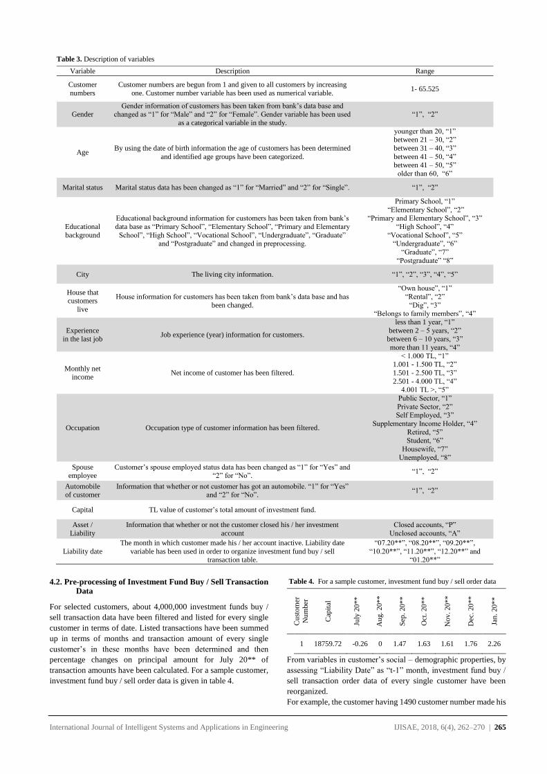
International Journal of Intelligent Systems and Applications in Engineering IJISAE, 2018, 6(4), 262–270 | 265
4.2. Pre-processing of Investment Fund Buy / Sell Transaction Data
For selected customers, about 4,000,000 investment funds buy /
sell transaction data have been filtered and listed for every single
customer in terms of date. Listed transactions have been summed
up in terms of months and transaction amount of every single
customer’s in these months have been determined and then
percentage changes on principal amount for July 20** of
transaction amounts have been calculated. For a sample customer,
investment fund buy / sell order data is given in table 4.
Table 4. For a sample customer, investment fund buy / sell order data
Cu
stom
er
Nu
mber
Cap
ital
July
20
**
Au
g. 2
0**
Sep
. 20*
*
Oct
. 20
**
No
v. 2
0**
Dec
. 20
**
Jan
. 20*
*
1 18759.72 -0.26 0 1.47 1.63 1.61 1.76 2.26
From variables in customer’s social – demographic properties, by
assessing “Liability Date” as “t-1” month, investment fund buy /
sell transaction order data of every single customer have been
reorganized.
For example, the customer having 1490 customer number made his
Table 3. Description of variables
Variable Description Range
Customer
numbers
Customer numbers are begun from 1 and given to all customers by increasing
one. Customer number variable has been used as numerical variable. 1- 65.525
Gender Gender information of customers has been taken from bank’s data base and
changed as “1” for “Male” and “2” for “Female”. Gender variable has been used
as a categorical variable in the study.
“1”, “2”
Age By using the date of birth information the age of customers has been determined
and identified age groups have been categorized.
younger than 20, “1” between 21 – 30, “2”
between 31 – 40, “3”
between 41 – 50, “4” between 41 – 50, “5”
older than 60, “6”
Marital status Marital status data has been changed as “1” for “Married” and “2” for “Single”. “1”, “2”
Educational
background
Educational background information for customers has been taken from bank’s
data base as “Primary School”, “Elementary School”, “Primary and Elementary
School”, “High School”, “Vocational School”, “Undergraduate”, “Graduate” and “Postgraduate” and changed in preprocessing.
Primary School, “1”
“Elementary School”, “2” “Primary and Elementary School”, “3”
“High School”, “4”
“Vocational School”, “5” “Undergraduate”, “6”
“Graduate”, “7”
“Postgraduate” “8”
City The living city information. “1”, “2”, “3”, “4”, “5”
House that customers
live
House information for customers has been taken from bank’s data base and has
been changed.
“Own house”, “1”
“Rental”, “2”
“Dig”, “3” “Belongs to family members”, “4”
Experience in the last job
Job experience (year) information for customers.
less than 1 year, “1”
between 2 – 5 years, “2” between 6 – 10 years, “3”
more than 11 years, “4”
Monthly net income
Net income of customer has been filtered.
< 1.000 TL, “1” 1.001 - 1.500 TL, “2”
1.501 - 2.500 TL, “3”
2.501 - 4.000 TL, “4” 4.001 TL >, “5”
Occupation Occupation type of customer information has been filtered.
Public Sector, “1”
Private Sector, “2” Self Employed, “3”
Supplementary Income Holder, “4”
Retired, “5” Student, “6”
Housewife, “7”
Unemployed, “8”
Spouse employee
Customer’s spouse employed status data has been changed as “1” for “Yes” and “2” for “No”.
“1”, “2”
Automobile of customer
Information that whether or not customer has got an automobile. “1” for “Yes” and “2” for “No”.
“1”, “2”
Capital TL value of customer’s total amount of investment fund.
Asset /
Liability
Information that whether or not the customer closed his / her investment
account
Closed accounts, “P”
Unclosed accounts, “A”
Liability date
The month in which customer made his / her account inactive. Liability date
variable has been used in order to organize investment fund buy / sell transaction table.
“07.20**”, “08.20**”, “09.20**”,
“10.20**”, “11.20**”, “12.20**” and “01.20**”
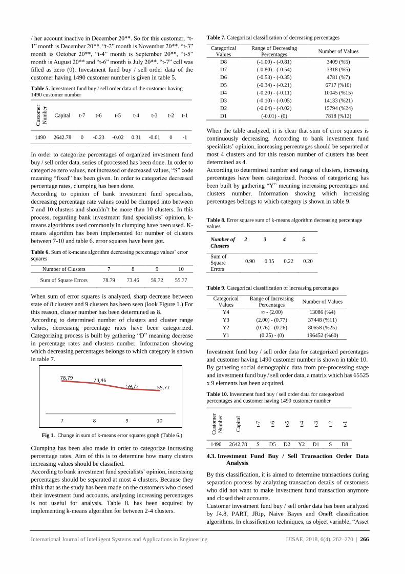
International Journal of Intelligent Systems and Applications in Engineering IJISAE, 2018, 6(4), 262–270 | 266
/ her account inactive in December 20**. So for this customer, “t-
1” month is December 20**, “t-2” month is November 20**, “t-3”
month is October 20**, “t-4” month is September 20**, “t-5”
month is August 20** and “t-6” month is July 20**. “t-7” cell was
filled as zero (0). Investment fund buy / sell order data of the
customer having 1490 customer number is given in table 5.
Table 5. Investment fund buy / sell order data of the customer having
1490 customer number
Cu
stom
er
Nu
mber
Capital t-7 t-6 t-5 t-4 t-3 t-2 t-1
1490 2642.78 0 -0.23 -0.02 0.31 -0.01 0 -1
In order to categorize percentages of organized investment fund
buy / sell order data, series of processed has been done. In order to
categorize zero values, not increased or decreased values, “S” code
meaning “fixed” has been given. In order to categorize decreased
percentage rates, clumping has been done.
According to opinion of bank investment fund specialists,
decreasing percentage rate values could be clumped into between
7 and 10 clusters and shouldn’t be more than 10 clusters. In this
process, regarding bank investment fund specialists’ opinion, k-
means algorithms used commonly in clumping have been used. K-
means algorithm has been implemented for number of clusters
between 7-10 and table 6. error squares have been got.
Table 6. Sum of k-means algorithm decreasing percentage values’ error
squares
Number of Clusters 7 8 9 10
Sum of Square Errors 78.79 73.46 59.72 55.77
When sum of error squares is analyzed, sharp decrease between
state of 8 clusters and 9 clusters has been seen (look Figure 1.) For
this reason, cluster number has been determined as 8.
According to determined number of clusters and cluster range
values, decreasing percentage rates have been categorized.
Categorizing process is built by gathering “D” meaning decrease
in percentage rates and clusters number. Information showing
which decreasing percentages belongs to which category is shown
in table 7.
Fig 1. Change in sum of k-means error squares graph (Table 6.)
Clumping has been also made in order to categorize increasing
percentage rates. Aim of this is to determine how many clusters
increasing values should be classified.
According to bank investment fund specialists’ opinion, increasing
percentages should be separated at most 4 clusters. Because they
think that as the study has been made on the customers who closed
their investment fund accounts, analyzing increasing percentages
is not useful for analysis. Table 8. has been acquired by
implementing k-means algorithm for between 2-4 clusters.
Table 7. Categorical classification of decreasing percentages
Categorical
Values
Range of Decreasing
Percentages Number of Values
D8 (-1.00) - (-0.81) 3409 (%5)
D7 (-0.80) - (-0.54) 3318 (%5)
D6 (-0.53) - (-0.35) 4781 (%7)
D5 (-0.34) - (-0.21) 6717 (%10)
D4 (-0.20) - (-0.11) 10045 (%15)
D3 (-0.10) - (-0.05) 14133 (%21)
D2 (-0.04) - (-0.02) 15794 (%24)
D1 (-0.01) - (0) 7818 (%12)
When the table analyzed, it is clear that sum of error squares is
continuously decreasing. According to bank investment fund
specialists’ opinion, increasing percentages should be separated at
most 4 clusters and for this reason number of clusters has been
determined as 4.
According to determined number and range of clusters, increasing
percentages have been categorized. Process of categorizing has
been built by gathering “Y” meaning increasing percentages and
clusters number. Information showing which increasing
percentages belongs to which category is shown in table 9.
Table 8. Error square sum of k-means algorithm decreasing percentage values
Number of
Clusters
2 3 4 5
Sum of Square
Errors
0.90 0.35 0.22 0.20
Table 9. Categorical classification of increasing percentages
Categorical
Values
Range of Increasing
Percentages Number of Values
Y4 ∞ - (2.00) 13086 (%4)
Y3 (2.00) - (0.77) 37448 (%11)
Y2 (0.76) - (0.26) 80658 (%25)
Y1 (0.25) - (0) 196452 (%60)
Investment fund buy / sell order data for categorized percentages
and customer having 1490 customer number is shown in table 10.
By gathering social demographic data from pre-processing stage
and investment fund buy / sell order data, a matrix which has 65525
x 9 elements has been acquired.
Table 10. Investment fund buy / sell order data for categorized
percentages and customer having 1490 customer number
Cu
stom
er
Nu
mber
Cap
ital
t-7
t-6
t-5
t-4
t-3
t-2
t-1
1490 2642.78 S D5 D2 Y2 D1 S D8
4.3. Investment Fund Buy / Sell Transaction Order Data Analysis
By this classification, it is aimed to determine transactions during
separation process by analyzing transaction details of customers
who did not want to make investment fund transaction anymore
and closed their accounts.
Customer investment fund buy / sell order data has been analyzed
by J4.8, PART, JRip, Naive Bayes and OneR classification
algorithms. In classification techniques, as object variable, “Asset
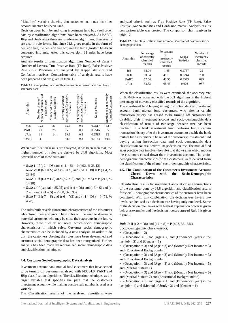
International Journal of Intelligent Systems and Applications in Engineering IJISAE, 2018, 6(4), 262–270 | 267
/ Liability” variable showing that customer has made his / her
account inactive has been used.
Decision trees, built by analyzing investment fund buy / sell order
data by classification algorithms have been analyzed. As PART,
JRip and OneR algorithms are rule-learner algorithms, their results
are also in rule forms. But since J4.8 gives results in the form of
decision tree, the decision tree acquired by J4.8 algorithm has been
converted into rule. After this conversion, 31 rules have been
acquired.
Analysis results of classification algorithms Number of Rules /
Number of Leaves, True Positive Rate (TP Rate), False Positive
Rate (FP), Precision are analyzed by Kappa statistics and
Confusion matrixes. Comparison table of analysis results have
been prepared and are given in table 11.
Table 11. Comparison of classification results of investment fund buy /
sell order data
Alg
ori
thm
Nu
mber
of
rule
s /
Nu
mber
of
elem
ents
of
dec
isio
n t
ree
Nu
mber
of
rule
s fo
r
pas
sive
cust
om
ers
Co
rrec
tly c
lass
ifie
d
per
centa
ges
fo
r p
assi
ve
cust
om
ers
No
t co
rrec
tly c
lass
ifie
d
per
centa
ges
fo
r p
assi
ve
cust
om
ers
Kap
pa
Sta
tist
ics
Nu
mber
of
no
t co
rrec
tly
clas
sifi
ed c
ust
om
ers
J4.8 123 31 95.8 0.1 0.9517 62
PART 79 25 95.6 0.1 0.9516 65
JRip 14 14 99.2 0.2 0.9515 12
OneR 1 1 38.5 0.2 0.5144 914
When classification results are analyzed, it has been seen that, the
highest number of rules are derived by J4.8 algorithm. Most
powerful ones of these rules are;
• Rule 1: If (t-2 = D8) and (t-1 = S) = P (492, % 33.13)
• Rule 2: If (t-7 = S) and (t-6 = S) and (t-1 = D8) = P (354, %
23.84)
• Rule 3: If (t-3 = D8) and (t-2 = S) and (t-1 = S) = P (212, %
14.28)
• Rule 4: If (capital > 85.95) and (t-4 = D8) and (t-3 = S) and (t-
2 = S) and (t-1 = S) = P (88, % 5.93)
• Rule 5: If (t-7 = S) and (t-6 = Y2) and (t-1 = D8) = P (71, %
4.78)
The rules built reveals transaction characteristics of the customers
who closed their accounts. These rules will be used to determine
potential customers who may be close their accounts in the future.
However, these rules do not reveal which social demographic
characteristics in which rules. Customer social demographic
characteristics can be included by a new analysis. In order to do
this, the customers obeying the rules have been determined and
customer social demographic data has been reorganized. Further
analysis has been made by reorganized social demographic data
and classification techniques.
4.4. Customer Socio-Demographic Data Analysis
Investment account bank mutual fund customers that have ceased
to be turning off customers analyzed with Id3, J4.8, PART and
JRip classification algorithms. The classification techniques as the
target variable that specifies the path that the customer's
investment account while making passive rule number is used as a
variable.
The Classification results of the analyzed algorithms were
analyzed criteria such as True Positive Rate (TP Rate), False
Positive, Kappa statistics and Confusion matrix. Analysis results
comparison table was created. The comparison chart is given in
table 12.
Table 12. The classification results comparison chart of customer socio-
demographic data
Algorithm
Percentage
of correctly classified
records
Percentage
of incorrectly
classified records
Kappa Statistics
Number of
incorrectly classified
records
Id3 98.04 1.95 0.9757 29
J4.8 50.84 49.15 0.3244 730
PART 57.64 42.35 0.4373 629
JRip 33.53 66.46 0.008 987
When the classification results were examined, the accuracy rate
of 98.04% was observed with the Id3 algorithm is the highest
percentage of correctly classified records of the algorithm.
The investment fund buying selling instruction data of investment
account bank mutual fund customers, who after a certain
transaction history has ceased to be turning off customers by
disabling their investment account and socio-demographic data
classification of results of two-stage decision tree has been
reached. In a bank investment fund performs but a certain
transaction history after the investment account to disable the bank
mutual fund customers to be out of the customers’ investment fund
buying selling instruction data and socio-demographic data
classification has resulted two-stage decision tree. The mutual fund
sales practice data involves the rules that shows after which motion
the customers closed down their investment account. The socio-
demographic characteristics of the customers were derived from
the classification of the clients’ socio-demographic characteristics.
4.5. The Combination of the Customer's Investment Account Closed Down with the Socio-Demographic Characteristics
Classification results for investment account closing transactions
of the customer done by J4.8 algorithm and classification results
for social – demographic characteristics of the customer have been
combined. With this combination, the decision tree having two
levels can be used as a decision tree having only one level. Some
of the decision tree leaves with highest explanation power is given
below as examples and the decision tree structure of Rule 1 is given
figure 2.
Rule 1: If (t-2 = D8) and (t-1 = S) = P (492, 33.13%)
Socio-demographic characteristics;
• (Occupation = 2)
• (Occupation = 3) and (Age = 2) and (Experience (year) in the
last job = 2) and (Gender = 1)
• (Occupation = 3) and (Age = 3) and (Monthly Net Income = 3)
and (Educational Background= 6)
• (Occupation = 3) and (Age = 3) and (Monthly Net Income = 3)
and (Educational Background= 8)
• (Occupation = 3) and (Age = 3) and (Monthly Net Income = 5)
and (Marital Status= 1)
• (Occupation = 3) and (Age = 3) and (Monthly Net Income = 5)
and (Marital Status= 2) and (Educational Background= 5)
• (Occupation = 3) and (Age = 4) and (Experience (year) in the
last job = 1) and (Method of Study= 3) and (Gender = 1)
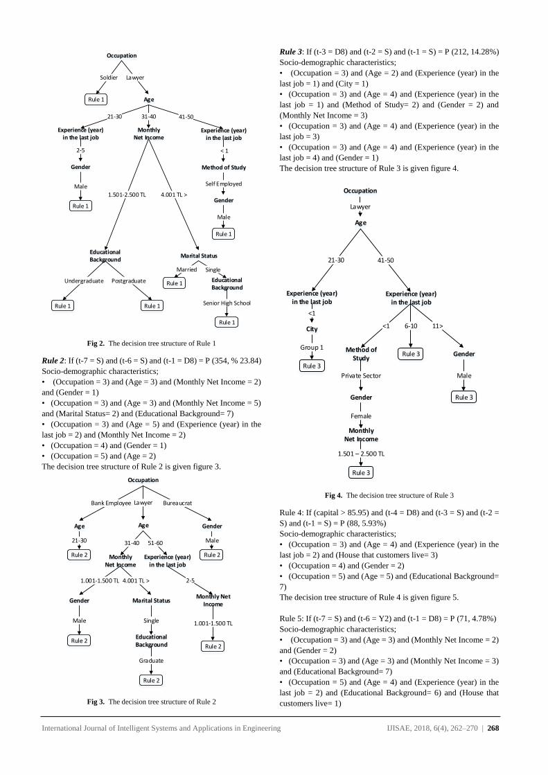
International Journal of Intelligent Systems and Applications in Engineering IJISAE, 2018, 6(4), 262–270 | 268
Fig 2. The decision tree structure of Rule 1
Rule 2: If (t-7 = S) and (t-6 = S) and (t-1 = D8) = P (354, % 23.84)
Socio-demographic characteristics;
• (Occupation = 3) and (Age = 3) and (Monthly Net Income = 2)
and (Gender = 1)
• (Occupation = 3) and (Age = 3) and (Monthly Net Income = 5)
and (Marital Status= 2) and (Educational Background= 7)
• (Occupation = 3) and (Age = 5) and (Experience (year) in the
last job = 2) and (Monthly Net Income = 2)
• (Occupation = 4) and (Gender = 1)
• (Occupation = 5) and (Age = 2)
The decision tree structure of Rule 2 is given figure 3.
Fig 3. The decision tree structure of Rule 2
Rule 3: If (t-3 = D8) and (t-2 = S) and (t-1 = S) = P (212, 14.28%)
Socio-demographic characteristics;
• (Occupation = 3) and (Age = 2) and (Experience (year) in the
last job = 1) and (City = 1)
• (Occupation = 3) and (Age = 4) and (Experience (year) in the
last job = 1) and (Method of Study= 2) and (Gender = 2) and
(Monthly Net Income = 3)
• (Occupation = 3) and (Age = 4) and (Experience (year) in the
last job = 3)
• (Occupation = 3) and (Age = 4) and (Experience (year) in the
last job = 4) and (Gender = 1)
The decision tree structure of Rule 3 is given figure 4.
Fig 4. The decision tree structure of Rule 3
Rule 4: If (capital > 85.95) and (t-4 = D8) and (t-3 = S) and (t-2 =
S) and (t-1 = S) = P (88, 5.93%)
Socio-demographic characteristics;
• (Occupation = 3) and (Age = 4) and (Experience (year) in the
last job = 2) and (House that customers live= 3)
• (Occupation = 4) and (Gender = 2)
• (Occupation = 5) and (Age = 5) and (Educational Background=
7)
The decision tree structure of Rule 4 is given figure 5.
Rule 5: If (t-7 = S) and (t-6 = Y2) and (t-1 = D8) = P (71, 4.78%)
Socio-demographic characteristics;
• (Occupation = 3) and (Age = 3) and (Monthly Net Income = 2)
and (Gender = 2)
• (Occupation = 3) and (Age = 3) and (Monthly Net Income = 3)
and (Educational Background= 7)
• (Occupation = 5) and (Age = 4) and (Experience (year) in the
last job = 2) and (Educational Background= 6) and (House that
customers live= 1)
Rule 1
Soldier Lawyer
Occupation
Age
21-30 31-40
Experience (year) in the last job
Monthly Net Income
2-5
Gender
Male
Rule 1
1.501-2.500 TL 4.001 TL >
Educational Background
Marital Status
Undergraduate Postgraduate
Rule 1 Rule 1
Married Single
Rule 1Educational Background
Senior High School
Rule 1
Experience (year) in the last job
41-50
Method of Study
< 1
Self Employed
Gender
Male
Rule 1
Rule 2
Bank Employee Lawyer
Occupation
Age
21-30 31-40
Monthly Net Income
1.001-1.500 TL 4.001 TL >
Marital Status
Male
Rule 2
Single
Educational Background
Graduate
Rule 2
Experience (year) in the last job
51-60
Monthly Net Income
2-5
1.001-1.500 TL
Rule 2
Bureaucrat
GenderAge
Male
Rule 2
Gender
Lawyer
Occupation
Age
21-30
Experience (year) in the last job
Monthly Net Income
<1
City
Group 1
Rule 3
<1 6-10
Method of Study
Private Sector
Rule 3
Experience (year) in the last job
41-50
Gender
11>
Male
Rule 3
Rule 3
Gender
Female
1.501 – 2.500 TL
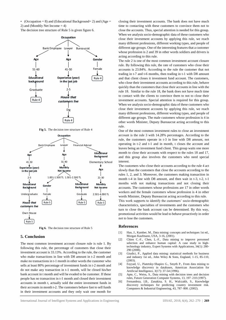
International Journal of Intelligent Systems and Applications in Engineering IJISAE, 2018, 6(4), 262–270 | 269
• (Occupation = 8) and (Educational Background= 2) and (Age =
2) and (Monthly Net Income = 4)
The decision tree structure of Rule 5 is given figure 6.
Fig 5. The decision tree structure of Rule 4
Fig 6. The decision tree structure of Rule 5
5. Conclusion
The most common investment account closure rule is rule 1. By
following this rule, the percentage of customers that close their
investment account is 33.13%. According to the rule, the customer
who make transactions in line with D8 amount in t-2 month and
make no transactions in t-1 month in other words the customer who
sells at least 80% percentage of investment funds in t-2 month and
do not make any transaction in t-1 month, will be closed his/her
bank account in t month and will be evaded to be customer. If these
people has no transaction in t-1 month and closed their investment
accounts in month t, actually sold the entire investment funds in
their accounts in month t-2. The customers behave fast to sell funds
in their investment accounts and they only wait one month for
closing their investment accounts. The bank does not have much
time to contacting with these customers to convince them not to
close the accounts. Thus, special attention is needed for this group.
When we analysis socio-demographic data of these customers who
close their investment accounts by applying this rule, we reach
many different professions, different working types, and people of
different age groups. One of the interesting features that a customer
whose profession is 2 and 39 in other words soldiers and drivers is
acting according to this rule.
The rule 2 is one of the most common investment account closure
rule. By following this rule, the rate of customers who close their
accounts is 23.84%. According to the rule the customer that not
trading in t-7 and t-6 months, then trading in t-1 with D8 amount
and that client closes it investment fund account. The customers,
who close their investment accounts according to this rule, behave
quickly than the customers that close their accounts in line with the
rule 18. Similar to the rule 18, the bank does not have much time
to contact with the clients to convince them to not to close their
investment accounts. Special attention is required for this group.
When we analysis socio-demographic data of these customers who
close their investment accounts by applying this rule, we reach
many different professions, different working types, and people of
different age groups. The male customers whose profession is 4 in
other words Minister, Deputy Bureaucrat acting according to this
rule.
One of the most common investment rules to close an investment
account is the rule 3 with 14.28% percentages. According to the
rule, the customers operate in t-3 in line with D8 amount, not
operating in t-2 and t-1 and in month, t closes the account and
leaves being an investment fund client. This group waits one more
month to close their accounts with respect to the rules 18 and 17,
and this group also involves the customers who need special
interest.
The customers who close their accounts according to the rule 4 act
slowly than the customers that close the accounts according to the
rules 1, 2, and 3. Moreover, the customers making transaction in
month t-4 in line with D8 amount, and then wait in t-3, t-2, t-1
months with not making transactions and not closing their
accounts. The customers whose professions are 17 in other words
workers and the female customers whose profession is 4 in other
words Minister, Deputy Bureaucrat acting according to this rule.
This work supports to identify the customers’ socio-demographic
characteristics, specialties of investments and the customers who
turn to close the bank account can be determined. By this way,
promotional activities would be lead to behave proactively in order
not to lose the customers.
References
[1] Han, J., Kamber, M., Data mining: concepts and techniques 1st ed., Morgan Kaufmann, USA, 3-16, (2001).
[2] Chien C.-F., Chen, L.-F., Data mining to improve personnel
selection and enhance human capital: A case study in high-technology industry, Expert Systems with Applications, 34(1): 280-
290 (2008).
[3] Giudici, P., Applied data mining: statistical methods for business and industry 1st ed., John Wiley & Sons, England, 1-15, 85-110,
(2003).
[4] Fayyad, U., Piatetsky-Shapiro G., Smyth P., From data mining to knowledge discovery in databases, American Association for
Artificial Intelligence, 3(17): 37-54 (1996).
[5] Apte, C., Weiss, S., Data mining with decision trees and decision rules, Future Generation Computer Systems, 13, 197–210 (1997).
[6] Fernandeza, I.B., Zanakisa, S. H., Walczakb, S., Knowledge discovery techniques for predicting country investment risk.
Computers & Industrial Engineering, 43, 787–800. (2002).
Rule 4
Bank Employee Lawyer
Occupation
Age
51-60
Graduate
Experience (year) in the last job
41-50
House that customers live
2-5
Dig
Rule 4
Bureaucrat
GenderAge
Female
Rule 4Educational background
Bank Employee Lawyer
Occupation
Age
41-50 31-40
Monthly Net Income
1.001-1.500 TL 1.501-2.500 TL
Female
Rule 5
Educational Background
Graduate
Rule 5
Financial Advisor
Age
Gender
Experience (year) in the last job
2-5
Educational Background
Undergraduate
House that customers live
Own House
Rule 5
Educational Background
Elementary School
Age
21-30
Monthly Net Income
2.501-4.000 TL
Rule 5
International Journal of Intelligent Systems and Applications in Engineering IJISAE, 2018, 6(4), 262–270 | 270
[7] Witten, I., H., Frank, E., Data mining: practical machine learning
tools and techniques 2nd ed., Morgan Kaufmann, USA, 62-415 (2005).
[8] Masand, B., Datta, P., Mani, D.R., Li, B., CHAMP: A prototype for
automated cellular churn prediction, Data Mining and Knowledge Discovery 3, Netherlands, 219 - 225 (1999).
[9] Poel, D., and Lariviere, B., Customer attrition analysis for financial
services using proportional hazard models, European Journal of Operational Research, 2004, vol. 157, No 1, 196-217.
[10] Ahn, J.H., Han, S.P., Lee, Y.S., Customer churn analysis: churn
determinants and mediation effects of partial defection in the Korean mobile telecommunications service industry, Science Direct,
Telecommunications Policy, 30: 552 - 568 (2006).
[11] Ruta, D., Nauck, D., Azvine, B., K nearest sequence method and its application to churn prediction, Springer-Verlag, Berlin Heidelberg,
207 - 215 (2006).
[12] Chu, B.H., Tsai, M.S., Ho, C.S., Toward a hybrid data mining model for customer retention, Knowledge-Based Systems, 20 (8) (2007),
pp. 703–718.
[13] Aydoğan, E., Gencer, C., Akbulut, S., Churn analysis and customer segmentation of a cosmetics brand using data mining techniques,
Journal of Engineering and Natural Sciences, Sigma, 26 (2008).
[14] Gopal, R. K., Meher, S. K., Customer churn time prediction in mobile telecommunication industry using ordinal regression,
Springer-Verlag, Berlin Heidelberg, 884 - 889 (2008).
[15] Farquad, M.A.H., Ravi, V., Raju, S.B., Data mining using rules extracted from svm: an application to churn prediction in bank credit
cards, Springer-Verlag, Berlin Heidelberg, 390 - 397 (2009).
[16] Huang, B. Q., Kechadi, M. T., Buckley, B., Customer churn prediction for broadband internet services, Springer-Verlag, Berlin
Heidelberg, 229 - 243 (2009).
[17] Chen, Z.-Y., Fan, Z.-P., Distributed customer behavior prediction using multiplex data: a collaborative MK-SVM approach,
Knowledge-Based Systems, 35 (2012), pp. 111–119.
[18] Zhang, X., Zhu, J., Xu, S., Wan, Y., Predicting customer churn through interpersonal influence, Knowledge-Based Systems, 28
(2012), pp. 97–104.
[19] Slavescu, E., Panait, I., Improving customer churn models as one of customer relationship management business solutions for the
telecommunication industry, “Ovidius” University Annals, Economic Science Series, 2012, vol. 12, Issue 1/201.
[20] Devi P., U., Madhavi, S., Prediction of churn behavior of bank
customers using data mining tools, Business Intelligence Journal, 2012, vol.5, 96-101.
[21] Jamal, Z., Tang, H.K., Methods and systems for identifying
customer status for developing customer retention and loyalty strategies, United States, Patent Application Publication, (2013).
[22] Verbeke, W., Martens, D., Baesens, B., Social network analysis for
customer churn prediction, Applied Soft Computing, 2014, vol. 14, 431–446.
[23] Farquad, M.A.H., Ravi, V., Raju, S.B., Churn prediction using
comprehensible support vector machine:An analytical CRM application, Applied Soft Computing, 2014, vol. 19, 31–40.
[24] Keramati, A., Jafari-Marandi, R., Aliannejadi, M., Ahmadian, I.,
Mozaffari, M., Abbasi, U., Improved churn prediction in telecommunication industry using datamining techniques, Applied
Soft Computing, 2014, vol.24, 994–1012.
International Journal of
Intelligent Systems and
Applications in Engineering
Advanced Technology and Science
ISSN:2147-67992147-6799www.atscience.org/IJISAE Original Research Paper
International Journal of Intelligent Systems and Applications in Engineering IJISAE, 2018, 6(4), 271–274 |271
Improved Nelder-Mead Optimization Method in Learning Phase of
Artificial Neural Networks
Hasan Erdinc KOCER1, Mustafa Merdan*2, Mohammed Hussein IBRAHIM3
Accepted : 14/12/2018 Published: 31/12/2018 DOI: 10.1039/b000000x
Abstract: Artificial neural networks method is the most important/preferred classification algorithm in machine learning area. The weights
on the nets in artificial neural directly affect the classification accuracy of artificial neural networks. Therefore, finding optimum values of
these weights is a difficult optimization problem. In this study, the Nelder-Mead optimization method has been improved and used for
training of artificial neural networks. The optimum weights of artificial neural networks are determined in the training stage. The
performance of the proposed improved Nelder-Mead-Artificial neural networks classification algorithm has been tested on the most
common datasets from the UCI machine learning repository. The classification results obtained from the proposed improved Nelder-Mead-
Artificial neural networks classification algorithm are compared with the results of the standard Nelder-Mead-Artificial neural networks
classification algorithm. As a result of this comparison, the proposed improved Nelder-Mead-Artificial neural networks classification
algorithm has given best results in all datasets.
Keywords: Artificial neural networks, Nelder-Mead optimization method, Training algorithm.
1. Introduction
Artificial neural networks (ANNs) is a vital part of artificial
intelligence. Machine learning and cognitive sciences depend on
ANNs to solve various nonlinear mappings relationships [1].
ANN’s are normally used a back-propagation algorithm to fix
different problems on account of their approximation features.
With respecting to the weights back-propagation algorithm
computes explicit gradients of the error such as the mean of square
error. However, ANNs trained with gradient descent based
learning algorithm generally fall of slow convergence and local
minima. To get rid of these issues metaheuristic algorithm that uses
global search to find the solution has been used to train ANNs. For
instance, the genetic algorithm utilized to training ANNs [2];
another method employed in order to train artificial neural network
is reported by Slowik [3]. He used an adaptive differential
evolution algorithm to train ANNs. The aim of the calculation that
is achieved is to find optimal weights regarding an error rate [3].
Salman Mohaghegi et al. analyze the performance of particle
swarm optimization (PSO) and they compared its convergence
speed and robustness of the algorithm with the back-propagation
algorithm. The learning algorithms have been utilized in order to
modify the output synaptic weight array, and in each algorithm, the
centers and widths in the hidden layer are inferred utilizing an
offline clustering approach. According to the results, the PSO
algorithm showed good performance even with a fewnumbers of
particles. The statistical result proved PSO as a robust algorithm
for learning ANNs [4]. David J. Montana and Lawrence Davis
utilized an evolutionary algorithm for enhancing the performance
of feed word artificial neural networks. In addition, the algorithm
added more domain-specific knowledge into ANNs [5]. Malinak
and Jaksa utilized evolutionary algorithm with a local search
algorithm to get the best performance [6]. Kenndy and Eberhat
used swarm intelligence PSO for the first time [7]. Carvalho and
Ludermir applied PSO to medical benchmark problems. They
compared the statistical result with a local search operator in order
to learn ANNs. The result showed a better performance than other
well-studied algorithm [8]. Apart from PSO, the scientists applied
other swarm intelligence such as ant colony algorithm. Blum and
Socha employed a new version of ACO algorithm for training
artificial neural network [9]. Liang Hu, Longhui Qin, Kai Mao,
Wenyu Chen,and Xin Fu used a genetic algorithm for training
ANNs to solve the real-life problem of Multipath Ultrasonic Gas
Flowmeter. They used GANNs for multipath ultrasonic flowmeter
(UFM) to help decrease its error rate when detecting the flowrate
of the complicated flow field. The evaluation of results showed by
ANNs and GANNs demonstrated better achievement for ANNs
trained by genetic algorithm compared with once trained with
gradient descent based algorithm [10]. In addition to genetic
algorithm, to find the optimal weight for a neural network, the
genetic algorithm has been utilized to enhance the whole structure
for artificial neural networks. For example, K. G. Kapanova,
Dimov and M. Sellier utilized GA for optimizing the architecture
of ANNs. This approach allowed rearranging hidden layers,
neurons in every hidden layer, the connections between neurons
and the activation function [11].
In this study, we improved the Nelder-Mead optimization method
and used to determine the optimum weight values of ANNs.vIn the
proposed improved Nelder-Mead-ANNs classification algorithm,
ANNs classification algorithm performs well in the learning stage.
The paper is organized as follows: The ANNs classification
algorithm is explained in the second section. The standard Nelder-
Mead optimization method is explained in the third section. The
improved Nelder-Mead optimization method is explained in the
fourth section and the experimental results are discussed in the fifth
section. Finally, the conclusion is explained in the last section.
_______________________________________________________________________________________________________________________________________________________________________________________________________________________________________________________________________________________________________________________________
1 Electronics and Computer Edu.,Selcuk University, Konya, Turkey 2 Stud. In computer Engg., Selcuk University, Konya, Turkey 3 Computer Engg.,Necmettin Erbakan University, Konya, Turkey
* Corresponding Author:Email: [email protected]
International Journal of Intelligent Systems and Applications in Engineering IJISAE, 2018, 6(4), 271–274 |272
2. Artificial Neural Networks
ANNs consist of neurons and these neurons that connect together.
These neurons can bind to each other very complexly as in the real
neurons system. Each neuron has a different weight input and one
output. For this purpose, the sum of the entries with different
weights is expressed by the following Equation 1 [12].
𝑛𝑒𝑡 = ∑ 𝐼𝑖𝑊𝑖𝑗
𝑚
𝑖=1
+ 𝑏 (1)
Where, m is the number of neurons in the layer, w is the weight
between i and j neuron and b is a bias neuron. The neuron output
value is obtained after the output of net function passes through the
activation function. Usually, in ANNs systems, the sigmoid
activation function is used. The sigmoid activation function is
shown in Equation 2 [13].
𝐹(𝑛𝑒𝑡) =1
1 + 𝑒−𝑛𝑒𝑡 (2)
The error rate between the output from the ANNs system and the
actual output is calculated. The mean square error is given in
Equation 3 below.
𝑀𝑆𝐸 =1
𝑛∑(𝑂𝑥 − 𝑇𝑥)2
𝑛
𝑥=1
(3)
Where, n representsa number of instances in datasets, Ox is the
output generated from the xth inputs and Tx is the target output of
the xth inputs. After training data is completed, the trained network
can estimate the result of any given dataset according to the last
state of the weight values. This process is called network training.
There are different training algorithms in network learning. In this
study, the Nelder-Mead optimization method is used in the
network training process.
3. Nelder-Mead optimization method
Nelder-Mead is a simple optimization method developed by
Nelder&Mead [17]. It is also called as Amoeba method in many
kinds of literature. It is a method widely used in multi-dimensional
unconstrained optimization problems. It is very simple to
understand the basic Nelder-Mead method and its usage is very
easy. For this reason, it is a very popular method especially in
many fields of chemistry and medicine and monolith. It is widely
used for solving parameter estimation and statistical problems. It
can also be used in the field of experimental mathematics [14].
The Nelder-mead optimization method is a simple method used to
find the local minimum of several variable functions generated by
Nelder and Mead. Simplex is an n-dimensional geometric shape. It
includes (N + 1) points in N dimensions. The simplex in two
dimensions consists of a triangle. It becomes a triangular prism in
three dimensions (4 surfaces). It is an example of a research
method that compares the function values at three corner points of
a triangle. By analyzing the function at all given points, the
program moves the highest and lowest values to the reflection
point relative to the surface above the highest and lowest elements.
In two dimensions, this method is a model search method that
compares the function values at the corners of a triangle. When we
consider the minimization state of a bivariate z=f (x, y) function,
the value of the z function at the worst corner of the triangle (w
worst vertex) is greatest.
For this reason, this worst corner is replaced by a new point. So we
get a new triangle. The search is now resumed in this new triangle,
so that the process becomes a triangle array where the function
value becomes smaller and smaller at the corner point value [15].
The steps of the Nelder-Mead optimization method are given
below.
𝑆𝑡𝑒𝑝 1: 𝐼𝑛𝑖𝑡𝑖𝑎𝑙𝑖𝑧𝑒 𝑤𝑖𝑡ℎ 𝑟𝑎𝑛𝑑𝑜𝑚 𝑠𝑜𝑙𝑢𝑡𝑖𝑜𝑛
𝑆𝑡𝑒𝑝 2: 𝑂𝑟𝑑𝑒𝑟 𝑠𝑜𝑙𝑢𝑡𝑖𝑜𝑛𝑠 𝑎𝑐𝑐𝑜𝑟𝑑𝑖𝑛𝑔 𝑡𝑜 𝑡ℎ𝑒 𝑓𝑖𝑡𝑛𝑒𝑠𝑠 𝑣𝑎𝑙𝑢𝑒𝑠(𝑥1) ≤ 𝑓(𝑥2) ≤ ⋯ ≤ 𝑓(𝑥𝑛+1)
𝑆𝑡𝑒𝑝 3: 𝐶𝑎𝑙𝑐𝑢𝑙𝑎𝑡𝑒 𝑥0 𝑡ℎ𝑒 𝑐𝑒𝑛𝑡𝑟𝑜𝑖𝑑 𝑜𝑓 𝑎𝑙𝑙 𝑝𝑜𝑖𝑛𝑡𝑠 𝑒𝑥𝑐𝑒𝑝𝑡 𝑥(𝑛+1)
𝑆𝑡𝑒𝑝 4: 𝐶𝑜𝑚𝑝𝑢𝑡𝑒 𝑟𝑒𝑓𝑙𝑒𝑐𝑡𝑖𝑜𝑛 𝑝𝑜𝑖𝑛𝑡 𝑥𝑟 = 𝑥0 + 𝛼(𝑥0 − 𝑥𝑛)
𝑆𝑡𝑒𝑝 5. 𝐼𝑓 (𝑥0 ) ≤ 𝑓(𝑥𝑟 ) < 𝑓(𝑥𝑛 ) 𝑡ℎ𝑒𝑛 𝑎𝑐𝑐𝑒𝑝𝑡 𝑥𝑟 𝑎𝑛𝑑 𝑡𝑒𝑟𝑚𝑖𝑛𝑎𝑡𝑒 𝑡ℎ𝑒 𝑖𝑡𝑒𝑟𝑎𝑡𝑖𝑜𝑛
𝑆𝑡𝑒𝑝 6. 𝐸𝑥𝑝𝑎𝑛𝑠𝑖𝑜𝑛, 𝐼𝑓 (𝑥𝑟) < 𝑓(𝑥1) 𝑡ℎ𝑒𝑛 𝑐𝑜𝑚𝑝𝑢𝑡𝑒 𝑡ℎ𝑒 𝑒𝑥𝑝𝑎𝑛𝑑𝑒𝑑 𝑝𝑜𝑖𝑛𝑡 𝑥𝑒 = 𝑥𝑟 + 𝛾(𝑥𝑟 − 𝑥0). 𝐼𝑓 (𝑥𝑒) < 𝑓(𝑥𝑟)
𝑎𝑐𝑐𝑒𝑝𝑡 𝑥𝑒𝑎𝑛𝑑 𝑡𝑒𝑟𝑚𝑖𝑛𝑎𝑡𝑒 𝑡ℎ𝑒 𝑖𝑡𝑒𝑟𝑎𝑡𝑖𝑜𝑛, 𝑜𝑡ℎ𝑒𝑟𝑤𝑖𝑠𝑒 𝑎𝑐𝑐𝑒𝑝𝑡 𝑥𝑟𝑎𝑛𝑑 𝑡𝑒𝑟𝑚𝑖𝑛𝑎𝑡𝑒 𝑡ℎ𝑒 𝑖𝑡𝑒𝑟𝑎𝑡𝑖𝑜𝑛. 𝑆𝑡𝑒𝑝 7. 𝐶𝑜𝑛𝑡𝑟𝑎𝑐𝑡𝑖𝑜𝑛, 𝐼𝑓 (𝑥𝑟) ≥ 𝑓(𝑥𝑛) 𝑝𝑒𝑟𝑓𝑜𝑟𝑚 𝑎 𝑐𝑜𝑛𝑡𝑟𝑎𝑐𝑡𝑖𝑜𝑛 𝑏𝑒𝑡𝑤𝑒𝑒𝑛 𝑥0𝑎𝑛𝑑 𝑥𝑛. 𝑥𝑐 = 𝑥0 + 𝜌(𝑥0 − 𝑥𝑛). 𝐼𝑓 (𝑥𝑐) < 𝑓(𝑥𝑛) 𝑎𝑐𝑐𝑒𝑝𝑡 𝑥𝑐 𝑎𝑛𝑑 𝑡𝑒𝑟𝑚𝑖𝑛𝑎𝑡𝑒 𝑖𝑡𝑒𝑟𝑎𝑡𝑖𝑜𝑛. 𝑆𝑡𝑒𝑝 8. 𝑆ℎ𝑟𝑖𝑛𝑘, 𝑅𝑒𝑝𝑙𝑎𝑐𝑒 𝑎𝑙𝑙 𝑝𝑜𝑖𝑛𝑡𝑠 𝑒𝑥𝑐𝑒𝑝𝑡 𝑡ℎ𝑒 𝑏𝑒𝑠𝑡 𝑥1
𝑤𝑖𝑡ℎ 𝑥𝑖 = 𝑥0 + 𝜎(𝑥𝑖 − 𝑥1) 𝑎𝑛𝑑 𝑔𝑜 𝑡𝑜 𝑠𝑡𝑒𝑝 2.
4. Improved Nelder-Mead optimization method
Since the Nelder-Mead optimization method is simple, it is also
known as a simple optimization method. In this study, the Nelder-
Mead optimization method is combined with PSO algorithm to
find optimum value of ANNs weights. In the proposed
classification algorithm, firstly, the weights of the ANNs
classification algorithm are generated randomly and the MSE is
calculated, then the best result is selected. The weights are updated
according to the best solution obtained from random solutions
according to the Nelder-Mead optimization method. Then the best
MSE is selected. In the next iteration, if the difference error of the
previous iteration and of the current error is less than 0.5 update
the weights according to the velocity equation of the PSO
algorithm is given in equations 4 and 5 below.
𝑣𝑖𝑡+1 = 𝑤 ∗ 𝑣𝑖
𝑡 + 𝑐1𝑟1(𝑃𝑏𝑒𝑠𝑡𝑖 − 𝑥𝑖𝑡)
+ 𝑐2𝑟2(𝐺𝑏𝑒𝑠𝑡 − 𝑥𝑖𝑡)
(4)
𝑥𝑖𝑡+1 = 𝑥𝑖
𝑡 + 𝑣𝑖𝑡+1 (5)
Where, t is the number of iteration, w is inertia weight, d is
dimension, xid current position of particle, vt the previous velocity
of particle, Pbesti is a better fitness value, Gbest is a better fitness
value of all particles, c1 and c2 are two positive constants represents
accelerate factor and r1 and r2 are two random functions in the
range [0,1]. Otherwise, the weight updating according to the
Nelder-Mead optimization method functions. Optimization
algorithms are used in many engineering areas and aim to find the
best end result. In this study, the improved Nelder-Mead
optimization method is used to find the optimum weights in the
ANNs classification model. The flowchart of the proposed ANNs
classification model is given in Fig. 1 below.
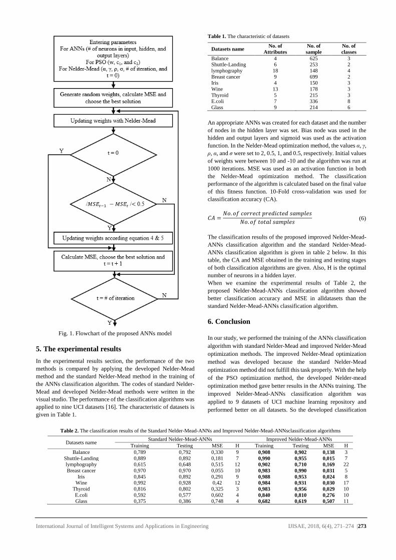
International Journal of Intelligent Systems and Applications in Engineering IJISAE, 2018, 6(4), 271–274 |273
Fig. 1. Flowchart of the proposed ANNs model
5. The experimental results
In the experimental results section, the performance of the two
methods is compared by applying the developed Nelder-Mead
method and the standard Nelder-Mead method in the training of
the ANNs classification algorithm. The codes of standard Nelder-
Mead and developed Nelder-Mead methods were written in the
visual studio. The performance of the classification algorithms was
applied to nine UCI datasets [16]. The characteristic of datasets is
given in Table 1.
Table 1. The characteristic of datasets
Datasets name No. of
Attributes
No. of
sample
No. of
classes
Balance 4 625 3 Shuttle-Landing 6 253 2
lymphography 18 148 4
Breast cancer 9 699 2 Iris 4 150 3
Wine 13 178 3
Thyroid 5 215 3 E.coli 7 336 8
Glass 9 214 6
An appropriate ANNs was created for each dataset and the number
of nodes in the hidden layer was set. Bias node was used in the
hidden and output layers and sigmoid was used as the activation
function. In the Nelder-Mead optimization method, the values α, γ,
ρ, α, and σ were set to 2, 0.5, 1, and 0.5, respectively. Initial values
of weights were between 10 and -10 and the algorithm was run at
1000 iterations. MSE was used as an activation function in both
the Nelder-Mead optimization method. The classification
performance of the algorithm is calculated based on the final value
of this fitness function. 10-Fold cross-validation was used for
classification accuracy (CA).
𝐶𝐴 =𝑁𝑜. 𝑜𝑓 𝑐𝑜𝑟𝑟𝑒𝑐𝑡 𝑝𝑟𝑒𝑑𝑖𝑐𝑡𝑒𝑑 𝑠𝑎𝑚𝑝𝑙𝑒𝑠
𝑁𝑜. 𝑜𝑓 𝑡𝑜𝑡𝑎𝑙 𝑠𝑎𝑚𝑝𝑙𝑒𝑠 (6)
The classification results of the proposed improved Nelder-Mead-
ANNs classification algorithm and the standard Nelder-Mead-
ANNs classification algorithm is given in table 2 below. In this
table, the CA and MSE obtained in the training and testing stages
of both classification algorithms are given. Also, H is the optimal
number of neurons in a hidden layer.
When we examine the experimental results of Table 2, the
proposed Nelder-Mead-ANNs classification algorithm showed
better classification accuracy and MSE in alldatasets than the
standard Nelder-Mead-ANNs classification algorithm.
6. Conclusion
In our study, we performed the training of the ANNs classification
algorithm with standard Nelder-Mead and improved Nelder-Mead
optimization methods. The improved Nelder-Mead optimization
method was developed because the standard Nelder-Mead
optimization method did not fulfill this task properly. With the help
of the PSO optimization method, the developed Nelder-mead
optimization method gave better results in the ANNs training. The
improved Nelder-Mead-ANNs classification algorithm was
applied to 9 datasets of UCI machine learning repository and
performed better on all datasets. So the developed classification
Table 2. The classification results of the Standard Nelder-Mead-ANNs and Improved Nelder-Mead-ANNsclassification algorithms
Datasets name Standard Nelder-Mead-ANNs Improved Nelder-Mead-ANNs
Training Testing MSE H Training Testing MSE H
Balance 0,789 0,792 0,330 9 0,908 0,902 0,138 3
Shuttle-Landing 0,889 0,892 0,181 7 0,990 0,955 0,015 7 lymphography 0,615 0,648 0,515 12 0,902 0,710 0,169 22
Breast cancer 0,970 0,970 0,055 10 0,983 0,990 0,031 5
Iris 0,845 0,892 0,291 9 0,988 0,953 0,024 8 Wine 0,992 0,928 0,42 12 0,984 0,931 0,030 17
Thyroid 0,816 0,802 0,325 3 0,983 0,956 0,029 10
E.coli 0,592 0,577 0,602 4 0,840 0,810 0,276 10 Glass 0,375 0,386 0,748 4 0,682 0,619 0,507 11

International Journal of Intelligent Systems and Applications in Engineering IJISAE, 2018, 6(4), 271–274 |274
algorithm can be applied to many fields such as medical,
engineering and recognition systems.
Acknowledgement
This study presents the results of Master thesis of Mustafa Merdan in
Selcuk University Natural and Applied Science Institute Computer
Engineering Programme.
References
[1] APA Kecman, V. (2001). Learning and soft computing: support
vector machines, neural networks, and fuzzy logic models. MIT press.
[2] Alhamdoosh, M., & Wang, D. (2014). Fast decorrelated neural
network ensembles with random weights. Information Sciences, 264,
104-117.
[3] Slowik, A. (2011). Application of an adaptive differential evolution
algorithm with multiple trial vectors to artificial neural network
training. IEEE Transactions on Industrial Electronics, 58(8), 3160-
3167.
[4] Mohaghegi, S., del Valle, Y., Venayagamoorthy, G. K., & Harley, R.
G. (2005, June). A comparison of PSO and backpropagation for
training RBF neural networks for identification of a power system with
STATCOM. In Swarm Intelligence Symposium, 2005. SIS 2005.
Proceedings 2005 IEEE (pp. 381-384).
[5] Montana, D. J., & Davis, L. (1989, August). Training Feedforward
Neural Networks Using Genetic Algorithms. In IJCAI (Vol. 89, pp.
762-767).
[6] Malinak, P., &Jaksa, R. (2007, September). Simultaneous gradient and
evolutionary neural network weights adaptation methods. In
Evolutionary Computation, 2007. CEC 2007. IEEE Congress on (pp.
2665-2671). IEEE.
[7] Kennedy, J. (2011). Particle swarm optimization. In Encyclopedia of
machine learning (pp. 760-766). Springer US.
[8] Carvalho, M., &Ludermir, T. B. (2007, September). Particle swarm
optimization of neural network architectures and weights. In Hybrid
Intelligent Systems, 2007. HIS 2007. 7th International Conference on
(pp. 336-339). IEEE.
[9] Dorigo, M., Birattari, M., &Stutzle, T. (2006). Ant colony
optimization. IEEE computational intelligence magazine, 1(4), 28-39.
[10] Hu, Liang, et al. "Optimization of neural network by genetic algorithm
for flowrate determination in multipath ultrasonic gas flowmeter."
IEEE Sensors Journal 16.5 (2016): 1158-1167.
[11] Kapanova, K. G., Dimov, I., &Sellier, J. M. A genetic approach to
automatic neural network architecture optimization. Neural
Computing and Applications, 1-12.
[12] Han, J., Pei, J., &Kamber, M. (2011). Data mining: concepts and
techniques. Elsevier.
[13] Schalkoff, R. J. (1997). Artificial neural networks (Vol. 1). New York:
McGraw-Hill.
[14] Kelley, C. T. (1999). Detection and remediation of stagnation in the
nelder-mead algorithm using a sufficient decrease condition. SIAM
journal on optimization, 10(1), 43-55.
[15] Lagarias J. C., J. A. Reeds, M. H. Wright, and P. E. Wright, 1998.
Convergence properties of the Nelder-Mead simplex method in low
dimensions. SIAM Journal on Optimization, 9(1), p. 112- 147.
[16] Asuncion, A., & Newman, D. (2007). UCI machine learning
repository.
[17] Nelder, John A., R. Mead (1965). A simplex method for function
minimization. Computer Journal. 7: 308–313.
International Journal of
Intelligent Systems and
Applications in Engineering
Advanced Technology and Science
ISSN:2147-67992147-6799www.atscience.org/IJISAE Original Research Paper
International Journal of Intelligent Systems and Applications in Engineering IJISAE, 2018, 6(4), 275–281 | 275
A fuzzy-genetic based design of permanent magnet synchronous motor
Mumtaz MUTLUER1*
Accepted : 08/11/2018 Published: 31/12/2018 DOI: 10.1039/b000000x
Abstract: This paper presents a fuzzy-genetic based design of permanent magnet synchronous motor. The selected motor structure with
surface magnet and double layer winding is for high torque and low speed applications. The design approach involves combining fuzzy
logic and genetic algorithm in a powerful combination. While the genetic algorithm is used in scanning of the solution space, the fuzzy
logic approach has been utilized in selecting the most appropriate solutions. While choosing geometric parameters as input for optimization,
design equations are obtained by using geometrical, electrical and magnetic properties of the motor. The output results are evaluated with
motor efficiency, motor weight and weight of magnets as the objective function. Furthermore, the multiobjective design optimization
results are compared with the results obtained for each single objective and tested with a finite element program. The results are finally
remarkable and quite compatible with the finite element results.
Keywords: Design optimization, fuzzy-genetic approach, permanent magnet synchronous motor
1. Introduction
Induction motor and permanent magnet synchronous motor
(PMSM) are among the most used electric motors in industrial
fields. While induction motors are of interest because of their low
cost and ease of maintenance, permanent magnet synchronous
motors have high power density and high efficiency. In addition,
in today’s control applications, drive systems affect the motor
selection. After all, whatever the performance criteria, due to high
efficiency it is clear that the use of PMSMs is increasing. Most
prominent feature of PMSMs is that they show structural
differences according to the placement of the magnets. Naturally
this affects the performances and the production costs of PMSMs.
Due to the ease of design and low production cost, surface mounted
PMSMs are the most preferred types for low speed applications.
This structure is also preferred because of its low cogging torque
based on slot and pole combination [1].
The design of electric motors is the most complex engineering
problem. It is because the electric motors have the non-linear
structures. To overcome this situation, when some simplifications
are taken, linear equations are used in electric motor design studies.
This is even more preliminary in optimization applications wherein
artificial intelligence algorithms are used. In academic or industrial
fields complex and realistic designs are provided by commercial
programs using finite element method. In fact, analytically and
numerically, two methods are basically applied in the design of
electric motors. Working with the analytic equations is weak in
terms of accuracy but advantageous in terms of duration. On the
other hand working with the numerical methods such as finite
element method is effective in terms of correctness of the results
but weak in terms of duration [2]. Nevertheless, in the design
optimization studies where analytic equations are used, electric
motor designs can be flexibly directed to single objective or
multiobjective.
With a general evaluation, the design optimization studies which
artificial intelligence used are based on the effectiveness of the
algorithms. One of them is undoubtedly the most recognizable
genetic algorithm. This algorithm has been applied to so many
different electric motor design problems up to date [3-5]. In
addition, the more strong algorithms constructed by combining the
different artificial intelligence algorithms or other methods with
genetic algorithm have been used [6-9].
The designs of permanent magnet synchronous motors are more
complex and non-linear engineering problems and also contain
some fuzzy facts such as other electric motor designs [10, 11]. The
fuzzy-genetic approach is quite useful in terms of decision
structure and ease of application in the choice of objective
function. By using the fuzzy-genetic structure, a large solution
space can be scanned and the designer’s experience, view and
judgment are well reflected [10-14]. In this study, as
multiobjective, a fuzzy-genetic based approach was firstly used in
the design optimization of the surface mounted permanent magnet
synchronous motor. Motor efficiency, motor weight and weight of
magnets were selected as objective function and then the objective
and constraint values were determined by using fuzzy rules. Single
and multi objective optimization results were given comparatively,
and the results were tested by a finite element program. The effects
of the fuzzy-genetic structure used were shown in the PMSM
design with graphics and tables. In this respect, PMSM design
optimization has been examined in a versatile way and useful
inferences have been provided for the technical staffs.
2. Multidirectional Analysis of The PMSM
Electrical, magnetic, thermal and mechanical analyzes are carried
out in the designs of electric motors. The solution of the differential
equations obtained for each analysis is quite complex. Moreover,
due to the non-linearity of the electric motors, it is almost
impossible to do very precise solutions. Numerical methods such
as finite element method are used in this case. Obviously, the use
of linear equations for a basic design is sufficient. The geometrical
model of the PMSM, the electrical and the magnetic circuits are
investigated in each subdivision as follows.
_______________________________________________________________________________________________________________________________________________________________________________________________________________________________________________
_
1Department of Electrical and Electronic Engineering, Necmettin Erbakan
University, Konya, Turkey
* Corresponding Author Email: [email protected]
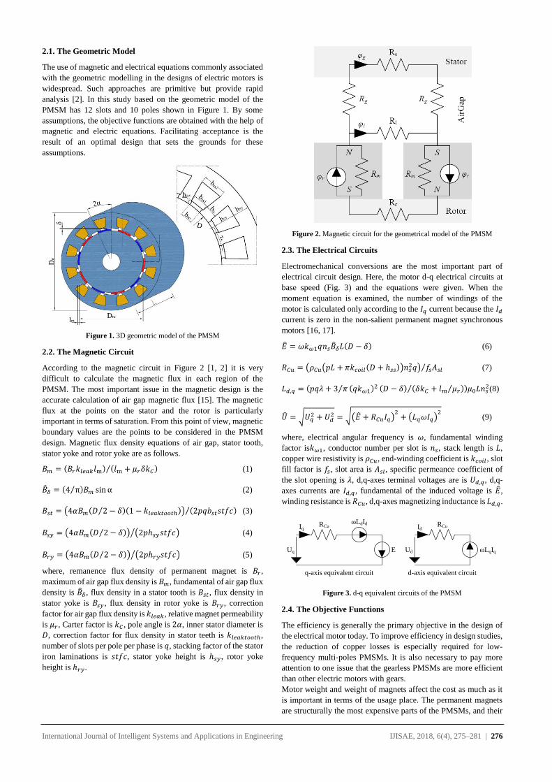
International Journal of Intelligent Systems and Applications in Engineering IJISAE, 2018, 6(4), 275–281 | 276
2.1. The Geometric Model
The use of magnetic and electrical equations commonly associated
with the geometric modelling in the designs of electric motors is
widespread. Such approaches are primitive but provide rapid
analysis [2]. In this study based on the geometric model of the
PMSM has 12 slots and 10 poles shown in Figure 1. By some
assumptions, the objective functions are obtained with the help of
magnetic and electric equations. Facilitating acceptance is the
result of an optimal design that sets the grounds for these
assumptions.
Figure 1. 3D geometric model of the PMSM
2.2. The Magnetic Circuit
According to the magnetic circuit in Figure 2 [1, 2] it is very
difficult to calculate the magnetic flux in each region of the
PMSM. The most important issue in the magnetic design is the
accurate calculation of air gap magnetic flux [15]. The magnetic
flux at the points on the stator and the rotor is particularly
important in terms of saturation. From this point of view, magnetic
boundary values are the points to be considered in the PMSM
design. Magnetic flux density equations of air gap, stator tooth,
stator yoke and rotor yoke are as follows.
𝐵𝑚 = (𝐵𝑟𝑘𝑙𝑒𝑎𝑘𝑙m) (𝑙m + 𝜇𝑟𝛿𝑘𝐶)⁄ (1)
�̂�𝛿 = (4 π⁄ )𝐵𝑚 sin α (2)
𝐵𝑠𝑡 = (4𝛼𝐵𝑚(𝐷 2⁄ − 𝛿)(1 − 𝑘𝑙𝑒𝑎𝑘𝑡𝑜𝑜𝑡ℎ)) (2𝑝𝑞𝑏𝑠𝑡𝑠𝑡𝑓𝑐)⁄ (3)
𝐵𝑠𝑦 = (4𝛼𝐵𝑚(𝐷 2⁄ − 𝛿)) (2𝑝ℎ𝑠𝑦𝑠𝑡𝑓𝑐)⁄ (4)
𝐵𝑟𝑦 = (4𝛼𝐵𝑚(𝐷 2⁄ − 𝛿)) (2𝑝ℎ𝑟𝑦𝑠𝑡𝑓𝑐)⁄ (5)
where, remanence flux density of permanent magnet is 𝐵𝑟,
maximum of air gap flux density is 𝐵𝑚, fundamental of air gap flux
density is �̂�𝛿 , flux density in a stator tooth is 𝐵𝑠𝑡, flux density in
stator yoke is 𝐵𝑠𝑦 , flux density in rotor yoke is 𝐵𝑟𝑦, correction
factor for air gap flux density is 𝑘𝑙𝑒𝑎𝑘, relative magnet permeability
is 𝜇𝑟 , Carter factor is 𝑘𝐶 , pole angle is 2𝛼, inner stator diameter is
𝐷, correction factor for flux density in stator teeth is 𝑘𝑙𝑒𝑎𝑘𝑡𝑜𝑜𝑡ℎ,
number of slots per pole per phase is 𝑞, stacking factor of the stator
iron laminations is 𝑠𝑡𝑓𝑐, stator yoke height is ℎ𝑠𝑦, rotor yoke
height is ℎ𝑟𝑦.
Figure 2. Magnetic circuit for the geometrical model of the PMSM
2.3. The Electrical Circuits
Electromechanical conversions are the most important part of
electrical circuit design. Here, the motor d-q electrical circuits at
base speed (Fig. 3) and the equations were given. When the
moment equation is examined, the number of windings of the
motor is calculated only according to the 𝐼𝑞 current because the 𝐼𝑑
current is zero in the non-salient permanent magnet synchronous
motors [16, 17].
�̂� = 𝜔𝑘𝜔1𝑞𝑛𝑠�̂�𝛿𝐿(𝐷 − 𝛿) (6)
𝑅𝐶𝑢 = (𝜌𝐶𝑢(𝑝𝐿 + 𝜋𝑘𝑐𝑜𝑖𝑙(𝐷 + ℎ𝑠𝑠))𝑛𝑠2𝑞) 𝑓𝑠𝐴𝑠𝑙⁄ (7)
𝐿𝑑,𝑞 = (𝑝𝑞𝜆 + 3 𝜋⁄ (𝑞𝑘𝜔1)2 (𝐷 − 𝛿) (𝛿𝑘𝐶 + 𝑙𝑚 𝜇𝑟⁄ )⁄ )𝜇0𝐿𝑛𝑠
2(8)
�̂� = √𝑈𝑞2 +𝑈𝑑
2 = √(�̂� + 𝑅𝐶𝑢𝐼𝑞)2+ (𝐿𝑞𝜔𝐼𝑞)
2 (9)
where, electrical angular frequency is 𝜔, fundamental winding
factor is𝑘𝜔1, conductor number per slot is 𝑛𝑠, stack length is 𝐿,
copper wire resistivity is 𝜌𝐶𝑢, end-winding coefficient is 𝑘𝑐𝑜𝑖𝑙 , slot
fill factor is 𝑓𝑠, slot area is 𝐴𝑠𝑙, specific permeance coefficient of
the slot opening is 𝜆, d,q-axes terminal voltages are is 𝑈𝑑,𝑞, d,q-
axes currents are 𝐼𝑑,𝑞 , fundamental of the induced voltage is �̂�,
winding resistance is 𝑅𝐶𝑢, d,q-axes magnetizing inductance is 𝐿𝑑,𝑞.
Figure 3. d-q equivalent circuits of the PMSM
2.4. The Objective Functions
The efficiency is generally the primary objective in the design of
the electrical motor today. To improve efficiency in design studies,
the reduction of copper losses is especially required for low-
frequency multi-poles PMSMs. It is also necessary to pay more
attention to one issue that the gearless PMSMs are more efficient
than other electric motors with gears.
Motor weight and weight of magnets affect the cost as much as it
is important in terms of the usage place. The permanent magnets
are structurally the most expensive parts of the PMSMs, and their
IqRCu
ωLdId
EUq
IdRCu
Ud ωLqIq
q-axis equivalent circuit d-axis equivalent circuit
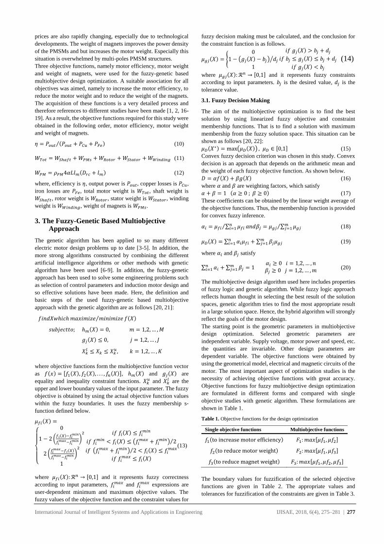
International Journal of Intelligent Systems and Applications in Engineering IJISAE, 2018, 6(4), 275–281 | 277
prices are also rapidly changing, especially due to technological
developments. The weight of magnets improves the power density
of the PMSMs and but increases the motor weight. Especially this
situation is overwhelmed by multi-poles PMSM structures.
Three objective functions, namely motor efficiency, motor weight
and weight of magnets, were used for the fuzzy-genetic based
multiobjective design optimization. A suitable association for all
objectives was aimed, namely to increase the motor efficiency, to
reduce the motor weight and to reduce the weight of the magnets.
The acquisition of these functions is a very detailed process and
therefore references to different studies have been made [1, 2, 16-
19]. As a result, the objective functions required for this study were
obtained in the following order, motor efficiency, motor weight
and weight of magnets.
𝜂 = 𝑃𝑜𝑢𝑡 (𝑃𝑜𝑢𝑡 + 𝑃𝐶𝑢 + 𝑃𝐹𝑒)⁄ (10)
𝑊𝑇𝑜𝑡 = 𝑊𝑆ℎ𝑎𝑓𝑡 +𝑊𝑃𝑀𝑠 +𝑊𝑅𝑜𝑡𝑜𝑟 +𝑊𝑆𝑡𝑎𝑡𝑜𝑟 +𝑊𝑊𝑖𝑛𝑑𝑖𝑛𝑔 (11)
𝑊𝑃𝑀 = 𝜌𝑃𝑀4𝛼𝐿𝑙𝑚(𝐷𝑟𝑐 + 𝑙𝑚) (12)
where, efficiency is 𝜂, output power is 𝑃𝑜𝑢𝑡, copper losses is 𝑃𝐶𝑢,
iron losses are 𝑃𝐹𝑒, total motor weight is 𝑊𝑇𝑜𝑡, shaft weight is
𝑊𝑆ℎ𝑎𝑓𝑡, rotor weight is 𝑊𝑅𝑜𝑡𝑜𝑟, stator weight is 𝑊𝑆𝑡𝑎𝑡𝑜𝑟, winding
weight is 𝑊𝑊𝑖𝑛𝑑𝑖𝑛𝑔, weight of magnets is 𝑊𝑃𝑀𝑠.
3. The Fuzzy-Genetic Based Multiobjective Approach
The genetic algorithm has been applied to so many different
electric motor design problems up to date [3-5]. In addition, the
more strong algorithms constructed by combining the different
artificial intelligence algorithms or other methods with genetic
algorithm have been used [6-9]. In addition, the fuzzy-genetic
approach has been used to solve some engineering problems such
as selection of control parameters and induction motor design and
so effective solutions have been made. Here, the definition and
basic steps of the used fuzzy-genetic based multiobjective
approach with the genetic algorithm are as follows [20, 21]:
𝑓𝑖𝑛𝑑𝑋𝑤ℎ𝑖𝑐ℎ𝑚𝑎𝑥𝑖𝑚𝑖𝑧𝑒 𝑚𝑖𝑛𝑖𝑚𝑖𝑧𝑒⁄ 𝑓(𝑋)
𝑠𝑢𝑏𝑗𝑒𝑐𝑡𝑡𝑜; ℎ𝑚(𝑋) = 0, 𝑚 = 1,2,… ,𝑀
𝑔𝑗(𝑋) ≤ 0, 𝑗 = 1,2,… , 𝐽
𝑋𝑘𝑙 ≤ 𝑋𝑘 ≤ 𝑋𝑘
𝑢, 𝑘 = 1,2,… , 𝐾
where objective functions form the multiobjective function vector
as 𝑓(𝑥) = [𝑓1(𝑋), 𝑓2(𝑋), . . . , 𝑓𝑛(𝑋)], ℎ𝑚(𝑋) and 𝑔𝑗(𝑋) are
equality and inequality constraint functions. 𝑋𝑘𝑢 and 𝑋𝑘
𝑙 are the
upper and lower boundary values of the input parameter. The fuzzy
objective is obtained by using the actual objective function values
within the fuzzy boundaries. It uses the fuzzy membership s-
function defined below.
𝜇𝑓𝑖(𝑋) =
{
0
1 − 2 (𝑓𝑖(𝑋)−𝑓𝑖
𝑚𝑖𝑛
𝑓𝑖𝑚𝑎𝑥−𝑓𝑖
𝑚𝑖𝑛)2
2 (𝑓𝑖𝑚𝑎𝑥−𝑓𝑖(𝑋)
𝑓𝑖𝑚𝑎𝑥−𝑓𝑖
𝑚𝑖𝑛)2
1
𝑖𝑓 𝑓𝑖(𝑋) ≤ 𝑓𝑖𝑚𝑖𝑛
𝑖𝑓 𝑓𝑖𝑚𝑖𝑛 < 𝑓𝑖(𝑋) ≤ (𝑓𝑖
𝑚𝑎𝑥 + 𝑓𝑖𝑚𝑖𝑛) 2⁄
𝑖𝑓 (𝑓𝑖𝑚𝑎𝑥 + 𝑓𝑖
𝑚𝑖𝑛) 2⁄ < 𝑓𝑖(𝑋) ≤ 𝑓𝑖𝑚𝑎𝑥
𝑖𝑓 𝑓𝑖𝑚𝑎𝑥 ≤ 𝑓𝑖(𝑋)
(13)
where 𝜇𝑓𝑖(𝑋):ℛ𝑛 → [0,1] and it represents fuzzy correctness
according to input parameters, 𝑓𝑖𝑚𝑎𝑥 and 𝑓𝑖
𝑚𝑎𝑥 expressions are
user-dependent minimum and maximum objective values. The
fuzzy values of the objective function and the constraint values for
fuzzy decision making must be calculated, and the conclusion for
the constraint function is as follows.
𝜇𝑔𝑗(𝑋) = {0
1 − (𝑔𝑗(𝑋) − 𝑏𝑗) 𝑑𝑗⁄
1
𝑖𝑓 𝑔𝑗(𝑋) > 𝑏𝑗 + 𝑑𝑗𝑖𝑓 𝑏𝑗 ≤ 𝑔𝑗(𝑋) ≤ 𝑏𝑗 + 𝑑𝑗
𝑖𝑓 𝑔𝑗(𝑋) < 𝑏𝑗
(14)
where 𝜇𝑔𝑗(𝑋):ℛ𝑛 → [0,1] and it represents fuzzy constraints
according to input parameters. 𝑏𝑗 is the desired value, 𝑑𝑗 is the
tolerance value.
3.1. Fuzzy Decision Making
The aim of the multiobjective optimization is to find the best
solution by using linearized fuzzy objective and constraint
membership functions. That is to find a solution with maximum
membership from the fuzzy solution space. This situation can be
shown as follows [20, 22]:
𝜇𝐷(𝑋∗) = max(𝜇𝐷(𝑋)) , 𝜇𝐷 ∈ [0,1] (15)
Convex fuzzy decision criterion was chosen in this study. Convex
decision is an approach that depends on the arithmetic mean and
the weight of each fuzzy objective function. As shown below.
𝐷 = 𝛼𝑓(𝑋) + 𝛽𝑔(𝑋) (16)
where 𝛼 and 𝛽 are weighting factors, which satisfy
𝛼 + 𝛽 = 1 (𝛼 ≥ 0 ; 𝛽 ≥ 0) (17)
These coefficients can be obtained by the linear weight average of
the objective functions. Thus, the membership function is provided
for convex fuzzy inference.
𝛼𝑖 = 𝜇𝑓𝑖 ∑ 𝜇𝑓𝑖𝑛𝑖=1⁄ 𝑎𝑛𝑑𝛽𝑗 = 𝜇𝑔𝑗 ∑ 𝜇𝑔𝑗
𝑚𝑗=1⁄ (18)
𝜇𝐷(𝑋) = ∑ 𝛼𝑖𝜇𝑓𝑖𝑛𝑖=1 + ∑ 𝛽𝑗𝜇𝑔𝑗
𝑚𝑗=1 (19)
where 𝛼𝑖 and 𝛽𝑗 satisfy
∑ 𝛼𝑖𝑛𝑖=1 + ∑ 𝛽𝑗
𝑚𝑗=1 = 1
𝛼𝑖 ≥ 0 𝑖 = 1,2, … , 𝑛𝛽𝑗 ≥ 0 𝑗 = 1,2, … ,𝑚
(20)
The multiobjective design algorithm used here includes properties
of fuzzy logic and genetic algorithm. While fuzzy logic approach
reflects human thought in selecting the best result of the solution
spaces, genetic algorithm tries to find the most appropriate result
in a large solution space. Hence, the hybrid algorithm will strongly
reflect the goals of the motor design.
The starting point is the geometric parameters in multiobjective
design optimization. Selected geometric parameters are
independent variable. Supply voltage, motor power and speed, etc.
the quantities are invariable. Other design parameters are
dependent variable. The objective functions were obtained by
using the geometrical model, electrical and magnetic circuits of the
motor. The most important aspect of optimization studies is the
necessity of achieving objective functions with great accuracy.
Objective functions for fuzzy multiobjective design optimization
are formulated in different forms and compared with single
objective studies with genetic algorithm. These formulations are
shown in Table 1.
Table 1. Objective functions for the design optimization
Single objective functions Multiobjective functions
𝑓1(to increase motor efficiency) 𝐹1: 𝑚𝑎𝑥[𝜇𝑓1, 𝜇𝑓2]
𝑓2(to reduce motor weight) 𝐹2: 𝑚𝑎𝑥[𝜇𝑓1, 𝜇𝑓3]
𝑓3(to reduce magnet weight) 𝐹3:𝑚𝑎𝑥[𝜇𝑓1 , 𝜇𝑓2, 𝜇𝑓3]
The boundary values for fuzzification of the selected objective
functions are given in Table 2. The appropriate values and
tolerances for fuzzification of the constraints are given in Table 3.
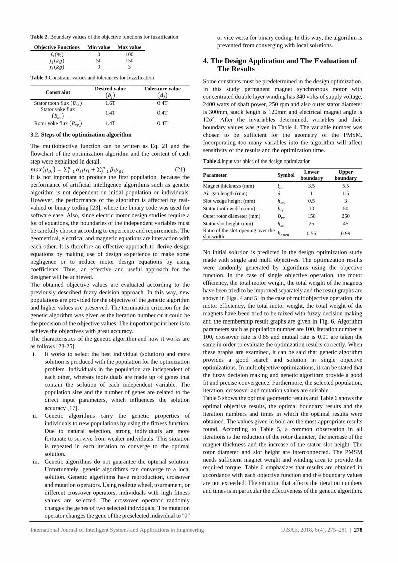
International Journal of Intelligent Systems and Applications in Engineering IJISAE, 2018, 6(4), 275–281 | 278
Table 2. Boundary values of the objective functions for fuzzification
Objective Functions Min value Max value
𝑓1(%) 0 100
𝑓2(𝑘𝑔) 50 150
𝑓3(𝑘𝑔) 0 3
Table 3.Constraint values and tolerances for fuzzification
Constraint Desired value
(𝒃𝒋) Tolerance value
(𝒅𝒋)
Stator tooth flux (𝐵𝑠𝑡) 1.6T 0.4T
Stator yoke flux
(𝐵𝑠𝑦) 1.4T 0.4T
Rotor yoke flux (𝐵𝑟𝑦) 1.4T 0.4T
3.2. Steps of the optimization algorithm
The multiobjective function can be written as Eq. 21 and the
flowchart of the optimization algorithm and the content of each
step were explained in detail.
𝑚𝑎𝑥(𝜇𝐷𝑖) = ∑ 𝛼𝑖𝜇𝑓𝑖𝑛𝑖=1 + ∑ 𝛽𝑗𝜇𝑔𝑗
𝑚𝑗=1 (21)
It is not important to produce the first population, because the
performance of artificial intelligence algorithms such as genetic
algorithm is not dependent on initial population or individuals.
However, the performance of the algorithm is affected by real-
valued or binary coding [23], where the binary code was used for
software ease. Also, since electric motor design studies require a
lot of equations, the boundaries of the independent variables must
be carefully chosen according to experience and requirements. The
geometrical, electrical and magnetic equations are interaction with
each other. It is therefore an effective approach to derive design
equations by making use of design experience to make some
negligence or to reduce motor design equations by using
coefficients. Thus, an effective and useful approach for the
designer will be achieved.
The obtained objective values are evaluated according to the
previously described fuzzy decision approach. In this way, new
populations are provided for the objective of the genetic algorithm
and higher values are preserved. The termination criterion for the
genetic algorithm was given as the iteration number or it could be
the precision of the objective values. The important point here is to
achieve the objectives with great accuracy.
The characteristics of the genetic algorithm and how it works are
as follows [23-25].
i. It works to select the best individual (solution) and more
solution is produced with the population for the optimization
problem. Individuals in the population are independent of
each other, whereas individuals are made up of genes that
contain the solution of each independent variable. The
population size and the number of genes are related to the
direct input parameters, which influences the solution
accuracy [17].
ii. Genetic algorithms carry the genetic properties of
individuals to new populations by using the fitness function.
Due to natural selection, strong individuals are more
fortunate to survive from weaker individuals. This situation
is repeated in each iteration to converge to the optimal
solution.
iii. Genetic algorithms do not guarantee the optimal solution.
Unfortunately, genetic algorithms can converge to a local
solution. Genetic algorithms have reproduction, crossover
and mutation operators. Using roulette wheel, tournament, or
different crossover operators, individuals with high fitness
values are selected. The crossover operator randomly
changes the genes of two selected individuals. The mutation
operator changes the gene of the preselected individual to "0"
or vice versa for binary coding. In this way, the algorithm is
prevented from converging with local solutions.
4. The Design Application and The Evaluation of The Results
Some constants must be predetermined in the design optimization.
In this study permanent magnet synchronous motor with
concentrated double layer winding has 340 volts of supply voltage,
2400 watts of shaft power, 250 rpm and also outer stator diameter
is 300mm, stack length is 120mm and electrical magnet angle is
126°. After the invariables determined, variables and their
boundary values was given in Table 4. The variable number was
chosen to be sufficient for the geometry of the PMSM.
Incorporating too many variables into the algorithm will affect
sensitivity of the results and the optimization time.
Table 4.Input variables of the design optimization
Parameter Symbol Lower
boundary
Upper
boundary
Magnet thickness (mm) 𝑙𝑚 3.5 5.5
Air gap length (mm) 𝛿 1 1.5
Slot wedge height (mm) ℎ𝑠𝑤 0.5 3
Stator tooth width (mm) 𝑏𝑡𝑠 10 50
Outer rotor diameter (mm) 𝐷𝑟𝑐 150 250
Stator slot height (mm) ℎ𝑠𝑠 25 45
Ratio of the slot opening over the slot width
𝑘𝑜𝑝𝑒𝑛 0.55 0.99
No initial solution is predicted in the design optimization study
made with single and multi objectives. The optimization results
were randomly generated by algorithms using the objective
function. In the case of single objective operation, the motor
efficiency, the total motor weight, the total weight of the magnets
have been tried to be improved separately and the result graphs are
shown in Figs. 4 and 5. In the case of multiobjective operation, the
motor efficiency, the total motor weight, the total weight of the
magnets have been tried to be mixed with fuzzy decision making
and the membership result graphs are given in Fig. 6. Algorithm
parameters such as population number are 100, iteration number is
100, crossover rate is 0.85 and mutual rate is 0.01 are taken the
same in order to evaluate the optimization results correctly. When
these graphs are examined, it can be said that genetic algorithm
provides a good search and solution in single objective
optimizations. In multiobjective optimizations, it can be stated that
the fuzzy decision making and genetic algorithm provide a good
fit and precise convergence. Furthermore, the selected population,
iteration, crossover and mutation values are suitable.
Table 5 shows the optimal geometric results and Table 6 shows the
optimal objective results, the optimal boundary results and the
iteration numbers and times in which the optimal results were
obtained. The values given in bold are the most appropriate results
found. According to Table 5, a common observation in all
iterations is the reduction of the rotor diameter, the increase of the
magnet thickness and the increase of the stator slot height. The
rotor diameter and slot height are interconnected. The PMSM
needs sufficient magnet weight and winding area to provide the
required torque. Table 6 emphasizes that results are obtained in
accordance with each objective function and the boundary values
are not exceeded. The situation that affects the iteration numbers
and times is in particular the effectiveness of the genetic algorithm.
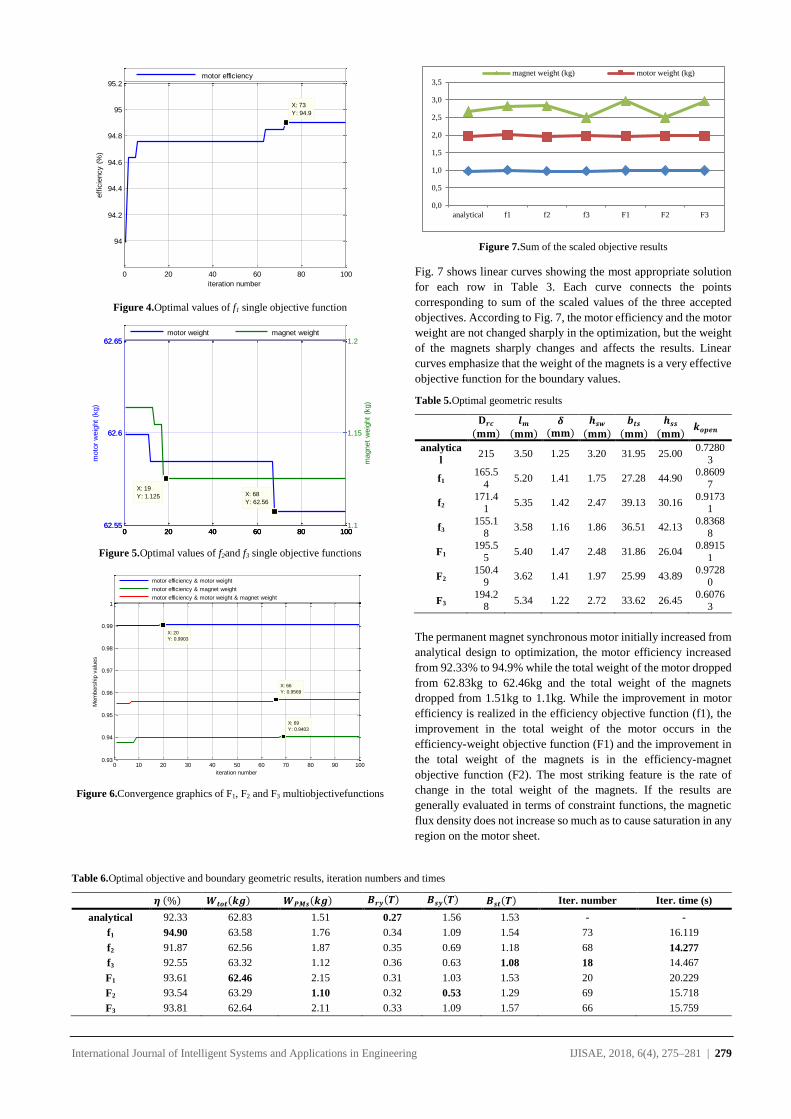
International Journal of Intelligent Systems and Applications in Engineering IJISAE, 2018, 6(4), 275–281 | 279
Figure 4.Optimal values of f1 single objective function
Figure 5.Optimal values of f2and f3 single objective functions
Figure 6.Convergence graphics of F1, F2 and F3 multiobjectivefunctions
Figure 7.Sum of the scaled objective results
Fig. 7 shows linear curves showing the most appropriate solution
for each row in Table 3. Each curve connects the points
corresponding to sum of the scaled values of the three accepted
objectives. According to Fig. 7, the motor efficiency and the motor
weight are not changed sharply in the optimization, but the weight
of the magnets sharply changes and affects the results. Linear
curves emphasize that the weight of the magnets is a very effective
objective function for the boundary values.
Table 5.Optimal geometric results
𝐃𝒓𝒄(𝐦𝐦)
𝒍𝒎
(𝐦𝐦)
𝜹(𝐦𝐦)
𝒉𝒔𝒘(𝐦𝐦)
𝒃𝒕𝒔(𝐦𝐦)
𝒉𝒔𝒔(𝐦𝐦)
𝒌𝒐𝒑𝒆𝒏
analytica
l 215 3.50 1.25 3.20 31.95 25.00
0.7280
3
f1 165.5
4 5.20 1.41 1.75 27.28 44.90
0.8609
7
f2 171.4
1 5.35 1.42 2.47 39.13 30.16
0.91731
f3 155.1
8 3.58 1.16 1.86 36.51 42.13
0.8368
8
F1 195.5
5 5.40 1.47 2.48 31.86 26.04
0.8915
1
F2 150.4
9 3.62 1.41 1.97 25.99 43.89
0.97280
F3 194.2
8 5.34 1.22 2.72 33.62 26.45
0.60763
The permanent magnet synchronous motor initially increased from
analytical design to optimization, the motor efficiency increased
from 92.33% to 94.9% while the total weight of the motor dropped
from 62.83kg to 62.46kg and the total weight of the magnets
dropped from 1.51kg to 1.1kg. While the improvement in motor
efficiency is realized in the efficiency objective function (f1), the
improvement in the total weight of the motor occurs in the
efficiency-weight objective function (F1) and the improvement in
the total weight of the magnets is in the efficiency-magnet
objective function (F2). The most striking feature is the rate of
change in the total weight of the magnets. If the results are
generally evaluated in terms of constraint functions, the magnetic
flux density does not increase so much as to cause saturation in any
region on the motor sheet.
Table 6.Optimal objective and boundary geometric results, iteration numbers and times
𝜼 (%) 𝑾𝒕𝒐𝒕(𝒌𝒈) 𝑾𝑷𝑴𝒔(𝒌𝒈) 𝑩𝒓𝒚(𝑻) 𝑩𝒔𝒚(𝑻) 𝑩𝒔𝒕(𝑻) Iter. number Iter. time (s)
analytical 92.33 62.83 1.51 0.27 1.56 1.53 - -
f1 94.90 63.58 1.76 0.34 1.09 1.54 73 16.119
f2 91.87 62.56 1.87 0.35 0.69 1.18 68 14.277
f3 92.55 63.32 1.12 0.36 0.63 1.08 18 14.467
F1 93.61 62.46 2.15 0.31 1.03 1.53 20 20.229
F2 93.54 63.29 1.10 0.32 0.53 1.29 69 15.718
F3 93.81 62.64 2.11 0.33 1.09 1.57 66 15.759
0 20 40 60 80 100
94
94.2
94.4
94.6
94.8
95
95.2
X: 73
Y: 94.9
eff
icie
ncy (
%)
iteration number
motor efficiency
0 20 40 60 80 10062.55
62.6
62.65
0 20 40 60 80 10062.55
62.6
62.65
X: 68
Y: 62.56
moto
r w
eig
ht
(kg)
0 20 40 60 80 1001.1
1.15
1.2
X: 19
Y: 1.125
magnet
weig
ht
(kg)
motor weight magnet weight
0 10 20 30 40 50 60 70 80 90 1000.93
0.94
0.95
0.96
0.97
0.98
0.99
1
X: 69
Y: 0.9403
Mem
bers
hip
valu
es
iteration number
X: 66
Y: 0.9569
X: 20
Y: 0.9903
motor efficiency & motor weight
motor efficiency & magnet weight
motor efficiency & motor weight & magnet weight
0,0
0,5
1,0
1,5
2,0
2,5
3,0
3,5
analytical f1 f2 f3 F1 F2 F3
magnet weight (kg) motor weight (kg)
International Journal of Intelligent Systems and Applications in Engineering IJISAE, 2018, 6(4), 275–281 | 280
This is good news. A clear observation is that the thickness of the
rotor yoke increases all the optimization results. It is seen from the
values in Table 5, Table 6 and Fig. 7 that the most effective
geometric parameter are permanent magnets. Results of the
preliminary design and the F3 multiobjective optimization have
been tested by means of a finite element program.
According to the finite element analyses, the input power of the
motor is 2502.8W, the output power is 2251.6W, the efficiency is
89.96% and the torque is 86Nm for preliminary design. Also for
the F3 fuzzy multiobjective design optimization, the input power
of the motor is 2546.6W, the output power is 2366.9W, the
efficiency is 92.94% and the moment is 90.4Nm. Efficiency error
values are 2.63% and 0.94% for preliminary design and for the F3
fuzzy multiobjective design optimization respectively. In this case,
the fuzzy multiobjective design optimization is confirmed with a
low error and the design aims have been realized. In addition, the
magnetic flux densities obtained by a finite element program are
𝐵𝑠𝑡 = 1.14T, 𝐵𝑠𝑦 = 1.42T and 𝐵ry = 0.85T for the analytical
design and 𝐵𝑠𝑡 = 1.57T, 𝐵𝑠𝑦 = 1.28T and 𝐵ry = 1.14T for the F3
multiobjective design optimization. In this case, it can be said that
the magnetic flux densities obtained as a result of the optimization
are below the limit values and the multiobjective optimization
modelling is useful.
Motor performance is evaluated in terms of operating
performance; torque ripples of the PMSM are about 7.49% for
preliminary design and 7.16% for the F3 fuzzy multiobjective
design optimization on average, which is due to the magnet angle
and stator winding. The cogging torque is effectively 1.1Nm for
preliminary design which corresponds to 1.28% of the nominal
torque and 1.3Nm for the F3 fuzzy multiobjective design
optimization which corresponds to 1.44% of the nominal torque.
The choice of the slot number and the number of poles is influential
in the formation of this value. As a result, PMSM design
optimization with a very complex and non-linear structure has been
tried to be solved with a different approach such as fuzzy-genetic.
Taking into account the obtained optimization values, the finite
element results and the iteration times, the fuzzy-genetic approach
is quite useful for PMSM design and the designed PMSM provides
the desired performance with great precision.
5. Conclusion
In this study, design optimization of the permanent magnet
synchronous motor, which is frequently used in low speed high
torque applications, was realized by using fuzzy decision making
and genetic algorithm. Motor efficiency, motor weight and weight
of magnets were selected as the single objective functions and to
form multiobjective the single objective functions are combined
with the fuzzy decision process. Here the goal was to achieve any
single objective while other objectives were to achieve the desired
values.
Convergence curves of algorithms show performance. It can be
argued that ability of the genetic algorithm to fall locally has been
overcome by the fuzzy decision making process, which seems to
be promising. Sensitive values in the obtained design parameters
also demonstrate the ability of the algorithms to investigate. The
most successful aspect of the multiobjective algorithm is to provide
a highly flexible approach to the goals. It can be seen that both
results, fuzzy multiobjective optimization and finite element
program are very close to each other and the error margin can be
deducted from the evaluation.
References
[1] J.R. Hendershot, T.H.E. Miller (1994). Design of brushless
permanent magnet motors. Oxford University Press Inc.,
New York.
[2] D.C. Hanselman (2006). Brushless permanent magnet motor
design. Magna Physics Publishing, Ohio.
[3] S. D. Sudhoff (2014). Power magnetic devices: a multi-
objective design approach. John Wiley&Sons Inc., New
Jersey.
[4] B. N. Cassimere, S. Sudhoff (2009). Population-based
design of surface-mounted permanent-magnet synchronous
machines. IEEE Transactions on Energy Conversion, Vol.
24, No. 2, pp 338-346, doi:10.1109/TEC.2009.2016150.
[5] Y. Duan, R. G. Harley, Y. G. Habetler (2009). Comparison
of particle swarm optimization and genetic algorithm in the
design of permanent magnet motors. IEEE 6th International
Power Electronics and Motion Control Conference, pp 822-
825, doi:10.1109/IPEMC.2009.5157497.
[6] G. Zhang, M. Dou, S. Wang (2009). Hybrid genetic
algorithm with particle swarm optimization technique.
International Conference on Computational Intelligence and
Security, Vol. 1, pp 103-106, doi:10.1109/CIS.2009.236.
[7] W. H. Ho, J. T. Tsai, J. H. Chou, J. B. Yue (2016). Intelligent
hybrid taguchi-genetic algorithm for multi-criteria
optimization of shaft alignment in marine vessel. IEEE
Access, Vol. 4, pp 2304-2313,
doi:10.1109/ACCESS.2016.2569537.
[8] K. Pytel (2016). Hybrid fuzzy-genetic algorithm applied to
clustering problem. Proceedings of the Federated
Conference on Computer Science and Information Systems,
pp. 137-140, INSPEC Accession Number:16428579.
[9] A. Wang, Y. Wen, W. L. Soong, H. Li (2016). Application
of a hybrid genetic algorithm for optimal design of interior
permanent magnet synchronous machines. IEEE Conference
on Electromagnetic Field Computation, pp 1-1,
doi:10.1109/CEFC.2016.7816299.
[10] J. T. Park, C. G. Lee, M. K. Kim, H. K. Jung (1997).
Application of fuzzy decision to optimization of induction
motor design. IEEE Transactions On Magnetics, Vol. 33,
No. 2, pp 1939-1942, doi:10.1109/20.582672.
[11] E. Koskimäki, J. Göös (1997). Electric machine
dimensioning by global optimization. First International
Conference on Knowledge-Based Intelligent Electronic
Systems, doi:10.1109/KES.1997.616930.
[12] B. Mirzaeian, M. Moallem, V. Tahani, C. Lucas (2002).
Multiobjective optimization method based on a genetic
algorithm for switched reluctance motor design. IEEE
Transactions On Magnetics, Vol. 38, No. 3, pp 1524-1527,
doi:10.1109/20.999126.
[13] S. Owatchaiphong, N. H. Fuengwarodsakul (2009). Multi-
objective based optimization for switched reluctance
machines using fuzzy and genetic algorithms. International
Conference on Power Electronics and Drive Systems,
doi:10.1109/PEDS.2009.5385926.
[14] C. Choi, D. Lee, K. Park (2000). Fuzzy design of a switched
reluctance motor based on the torque profile optimization.
IEEE Transactions On Magnetics, Vol. 36, No. 5, pp 3548-
3550, doi:10.1109/20.908894.
[15] J. Pyrhonen, T. Jokinen, V. Hrabovcová (2008). Design of
rotating electrical machines. John Wiley & Sons Ltd.
[16] F. Libert (2004). Design, optimization and comparison of
permanent magnet motors for a low-speed direct-driven
mixer. Technical Licentiate, School of Computer Science,

International Journal of Intelligent Systems and Applications in Engineering IJISAE, 2018, 6(4), 275–281 | 281
Electrical Engineering and Engineering Physics, KTH,
Sweden.
[17] F. Libert, J. Soulard (2004). Design study of different direct-
driven permanent-magnet motors for a low speed
application. Proc of the Nordic Workshop on Power and
Indus Electro (NORPIE).
[18] M. Mutluer, O. Bilgin (2016). An intelligent design
optimization of a permanent magnet synchronous motor by
artificial bee colony algorithm. Turkish Journal of Electrical
Engineering & Computer Sciences, Vol. 24, pp 1826-1837,
doi:10.3906/elk-1311-150.
[19] M. Mutluer, O. Bilgin (2012) Comparison of stochastic
optimization methods for design optimization of permanent
magnet synchronous motor. Neural Computing and
Applications, Vol. 21, No 8, pp 2049-2056,
doi:10.1007/s00521-011-0627-1.
[20] M. Çunkaş (2008). Intelligent design of induction motors by
multiobjective fuzzy-genetic algorithm, Journal of
Intelligent Manufacturing, 21 (4) 393-402.
[21] A. Trebi-Ollennu, B. A. White (1997). Multiobjective fuzzy-
genetic algorithm optimization approach to nonlinear control
system design. IEE Proceedings of Control Theory and
Applications, 144 2.
[22] Y. Minghua, X. Changwen (1994). Multiobjective fuzzy
optimization of structures based on generalized fuzzy
decision making. Computers and Structures, 53(2), 411–417,
doi:10.1016/0045-7949(94)90213-5.
[23] Z. Michalewicz (1996). Genetic algorithms + data structures
= evolution programs - third, revised and extended edition.
Springer-Verlag, Berlin, Heidelberg.
[24] X. S. Yang (2010). Engineering optimization – an
introduction with metaheuristic applications. John Wiley &
Sons, Inc., Hoboken, New Jersey.
[25] S. S. Rao (2009). Engineering optimization theory and
practice – fourth edition. John Wiley & Sons, Inc., Hoboken,
New Jersey.
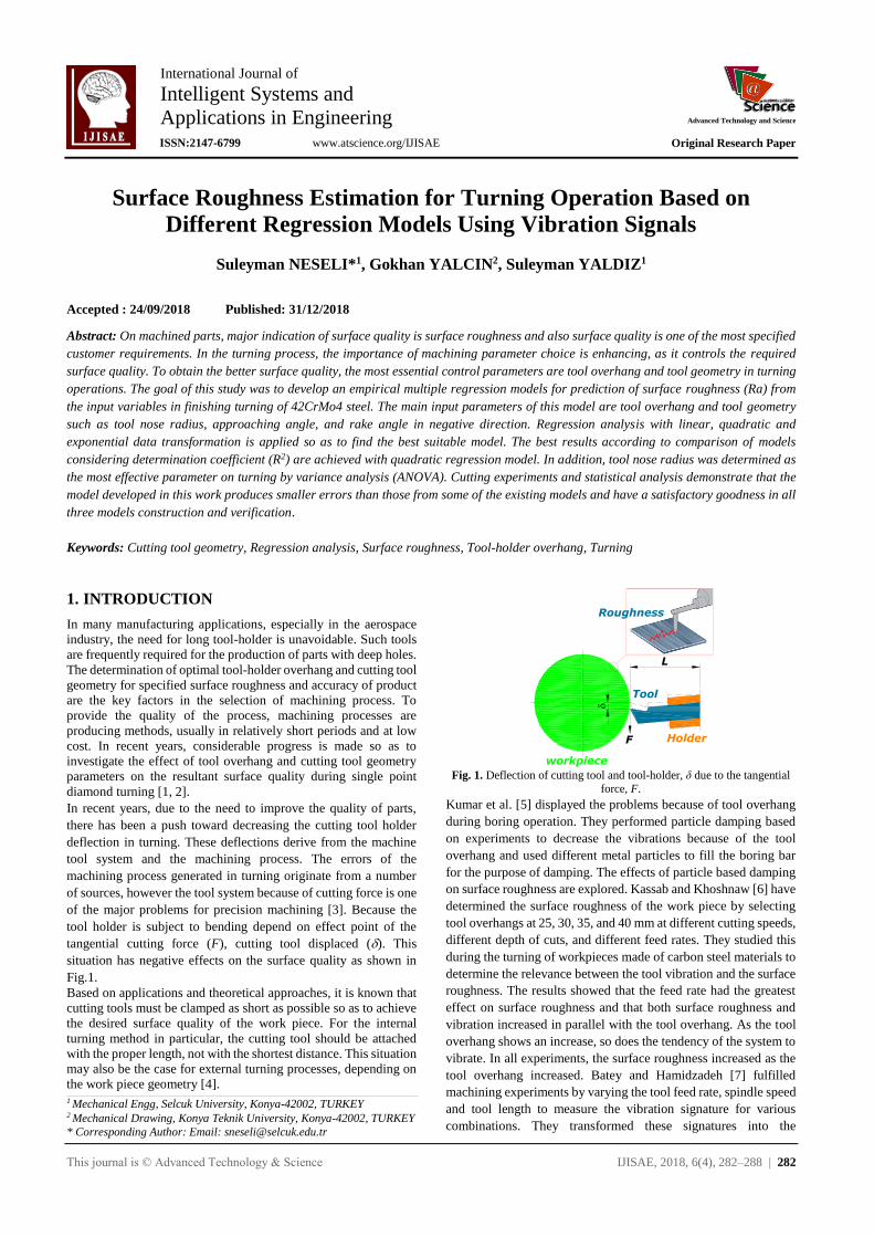
International Journal of
Intelligent Systems and
Applications in Engineering
Advanced Technology and Science
ISSN:2147-67992147-6799 www.atscience.org/IJISAE Original Research Paper
This journal is © Advanced Technology & Science IJISAE, 2018, 6(4), 282–288 | 282
Surface Roughness Estimation for Turning Operation Based on
Different Regression Models Using Vibration Signals
Suleyman NESELI*1, Gokhan YALCIN2, Suleyman YALDIZ1
Accepted : 24/09/2018 Published: 31/12/2018 DOI: 10.1039/b000000x
Abstract: On machined parts, major indication of surface quality is surface roughness and also surface quality is one of the most specified
customer requirements. In the turning process, the importance of machining parameter choice is enhancing, as it controls the required
surface quality. To obtain the better surface quality, the most essential control parameters are tool overhang and tool geometry in turning
operations. The goal of this study was to develop an empirical multiple regression models for prediction of surface roughness (Ra) from
the input variables in finishing turning of 42CrMo4 steel. The main input parameters of this model are tool overhang and tool geometry
such as tool nose radius, approaching angle, and rake angle in negative direction. Regression analysis with linear, quadratic and
exponential data transformation is applied so as to find the best suitable model. The best results according to comparison of models
considering determination coefficient (R2) are achieved with quadratic regression model. In addition, tool nose radius was determined as
the most effective parameter on turning by variance analysis (ANOVA). Cutting experiments and statistical analysis demonstrate that the
model developed in this work produces smaller errors than those from some of the existing models and have a satisfactory goodness in all
three models construction and verification.
Keywords: Cutting tool geometry, Regression analysis, Surface roughness, Tool-holder overhang, Turning
1. INTRODUCTION
In many manufacturing applications, especially in the aerospace
industry, the need for long tool-holder is unavoidable. Such tools
are frequently required for the production of parts with deep holes.
The determination of optimal tool-holder overhang and cutting tool
geometry for specified surface roughness and accuracy of product
are the key factors in the selection of machining process. To
provide the quality of the process, machining processes are
producing methods, usually in relatively short periods and at low
cost. In recent years, considerable progress is made so as to
investigate the effect of tool overhang and cutting tool geometry
parameters on the resultant surface quality during single point
diamond turning [1, 2].
In recent years, due to the need to improve the quality of parts,
there has been a push toward decreasing the cutting tool holder
deflection in turning. These deflections derive from the machine
tool system and the machining process. The errors of the
machining process generated in turning originate from a number
of sources, however the tool system because of cutting force is one
of the major problems for precision machining [3]. Because the
tool holder is subject to bending depend on effect point of the
tangential cutting force (F), cutting tool displaced (). This
situation has negative effects on the surface quality as shown in
Fig.1.
Based on applications and theoretical approaches, it is known that
cutting tools must be clamped as short as possible so as to achieve
the desired surface quality of the work piece. For the internal
turning method in particular, the cutting tool should be attached
with the proper length, not with the shortest distance. This situation
may also be the case for external turning processes, depending on
the work piece geometry [4].
L
F
Tool
workpiece
Holder
Roughness
Fig. 1. Deflection of cutting tool and tool-holder, δ due to the tangential
force, F.
Kumar et al. [5] displayed the problems because of tool overhang
during boring operation. They performed particle damping based
on experiments to decrease the vibrations because of the tool
overhang and used different metal particles to fill the boring bar
for the purpose of damping. The effects of particle based damping
on surface roughness are explored. Kassab and Khoshnaw [6] have
determined the surface roughness of the work piece by selecting
tool overhangs at 25, 30, 35, and 40 mm at different cutting speeds,
different depth of cuts, and different feed rates. They studied this
during the turning of workpieces made of carbon steel materials to
determine the relevance between the tool vibration and the surface
roughness. The results showed that the feed rate had the greatest
effect on surface roughness and that both surface roughness and
vibration increased in parallel with the tool overhang. As the tool
overhang shows an increase, so does the tendency of the system to
vibrate. In all experiments, the surface roughness increased as the
tool overhang increased. Batey and Hamidzadeh [7] fulfilled
machining experiments by varying the tool feed rate, spindle speed
and tool length to measure the vibration signature for various
combinations. They transformed these signatures into the
_______________________________________________________________________________________________________________________________________________________________________________________________________________________________________________________________________________________________________________________________
1 Mechanical Engg, Selcuk University, Konya-42002, TURKEY 2 Mechanical Drawing, Konya Teknik University, Konya-42002, TURKEY
* Corresponding Author: Email: [email protected]
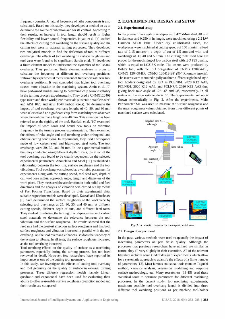
International Journal of Intelligent Systems and Applications in Engineering IJISAE, 2018, 6(4), 282–288 | 283
frequency domain. A natural frequency of lathe components is also
calculated. Based on this study, they developed a method so as to
determine the source of vibration and for its control. According to
their results, an increase in tool length should result in higher
flexibility and lower natural frequencies. Kiyak et al. [4] studied
the effects of cutting tool overhang on the surface quality and the
cutting tool wear in external turning processes. They developed
two analytical models to find the deflection of tool at different
overhangs. The effects of tool overhang on surface roughness and
tool wear were found to be significant. Sardar et al. [8] developed
a finite element model to understand the dynamics of tool shank
overhang. They performed finite element analyses in order to
calculate the frequency at different tool overhang positions,
followed by experimental measurement of frequencies at these tool
overhang positions. It was concluded that higher tool overhang
causes more vibration in the machining system. Amin et al. [9]
have performed studies aiming to determine chip form instability
in the turning process experimentally. They used a CNMG120408
type insert and three workpiece materials (austenitic stainless steel
and AISI 1020 and AISI 1040 carbon steels). To determine the
impact of tool overhang, overhang lengths of 40, 50, and 60 mm
were selected and no significant chip form instability was observed
when the tool overhang length was 40 mm. This situation has been
referred to as the rigidity of the tool. Haddadi et al. [10] examined
the impact of worn tools and brand new tools on vibration
frequency in the turning process experimentally. They examined
the effects of rake angle and tool overhang under orthogonal and
oblique cutting conditions. In experiments, they used a workpiece
made of low carbon steel and high-speed steel tools. The tool
overhangs were 20, 30, and 50 mm. In the experimental studies
that they conducted using different depth of cuts, the effect of the
tool overhang was found to be clearly dependent on the selected
experimental parameters. Abouelatta and Mádl [11] established a
relationship between the tool life, surface roughness and the tool
vibrations. Tool overhang was selected as a variable parameter for
experiments along with the cutting speed, tool feed rate, depth of
cut, tool nose radius, approach angle, length and diameters of the
work piece. They measured the acceleration in both radial and feed
directions and the analysis of vibration was carried out by means
of Fast Fourier Transforms. Based on their experimental data,
suitable regression models were developed. Kassab and Khoshnaw
[6] have determined the surface roughness of the workpiece by
selecting tool overhangs at 25, 30, 35, and 40 mm at different
cutting speeds, different depth of cuts, and different feed rates.
They studied this during the turning of workpieces made of carbon
steel materials to determine the relevance between the tool
vibration and the surface roughness. The results showed that the
feed rate had the greatest effect on surface roughness and that both
surface roughness and vibration increased in parallel with the tool
overhang. As the tool overhang enhances, so does the tendency of
the system to vibrate. In all tests, the surface roughness increased
as the tool overhang increased.
Tool overhang effects on the quality of surface as a machining
parameter, especially during the turning process, has not been
reviewed in detail. However, few researchers have reported its
importance as one of the cutting tool geometry.
In this study, we investigate the effects of cutting tool overhang
and tool geometry on the quality of surface in external turning
processes. Three different regression models namely Linear,
quadratic and exponential have been used for evaluating their
ability to offer reasonable surface roughness prediction model and
their results are compared.
2. EXPERIMENTAL DESIGN and SETUP
2.1. Experimental setup
In the present investigation workpieces of 42CrMo4 steel, 40 mm
in diameter and 0.250 m in length, were machined using a 2.2 kW
Harrison M300 lathe. Under dry unlubricated cases, the
workpieces were machined at cutting speeds of 150 m.min-1, a feed
rate of 0.15 mm.rev-1, a depth of cut of 1.5 mm and with tool
overhangs of 30, 40 and 50 mm. The cutting tools used here are
proper for the machining of low carbon steel with ISO P25 quality,
which is equal to LC215K code. The inserts were produced by
Böhler Inc., with the ISO designation of CNMG 120404-BF,
CNMG 120408-BF, CNMG 120412-BF (80° Rhombic inserts).
The inserts were mounted rigidly on three different right hand style
tool holders designated by ISO as PCLNR/L 2020 K12 AA9,
PCLNR/L 2020 K12 AA6, and PCLNR/L 2020 K12 AA3 thus
giving back rake angle of -9°, -6° and -3°, respectively. In all
instances, the side rake angle is 6°. The experimental set up is
shown schematically in Fig. 2. After the experiments, Mahr
Perthometer M1 was used to measure the surface roughness and
the mean roughness values obtained from three different points of
machined surface were calculated.
Negative back
rake angle
Approach
angle
Nose radius
Tool overhang
limits
COMPUTER
SURFACE
ROUGHNESS
PREDICTION
PROCESS
PARAMETERS
SURFACE
RUGHNESS
MEASUREMENT
OPERATOR
STATISTICAL
SOFTWARE
Fig. 2. Schematic diagram for the experimental setup
2.2. Design of experiment
In the past, various methods were used to quantify the impact of
machining parameters on part finish quality. Although the
processes that previous researchers have utilized are similar in
nature, they all vary slightly in their execution. All of the relevant
literature includes some kind of design of experiments which allow
for a systematic approach to quantify the effects of a finite number
of parameters [12]. Most famous statistical tools contain: Taguchi
method, variance analysis, regression modelling and response
surface methodology, etc. Many researchers [13-15] used these
statistical tools to optimize parameters for different machining
processes. In the current study, for machining experiments,
maximum possible tool overhang length is divided into three
different tool overhang positions as per machine tool-holder
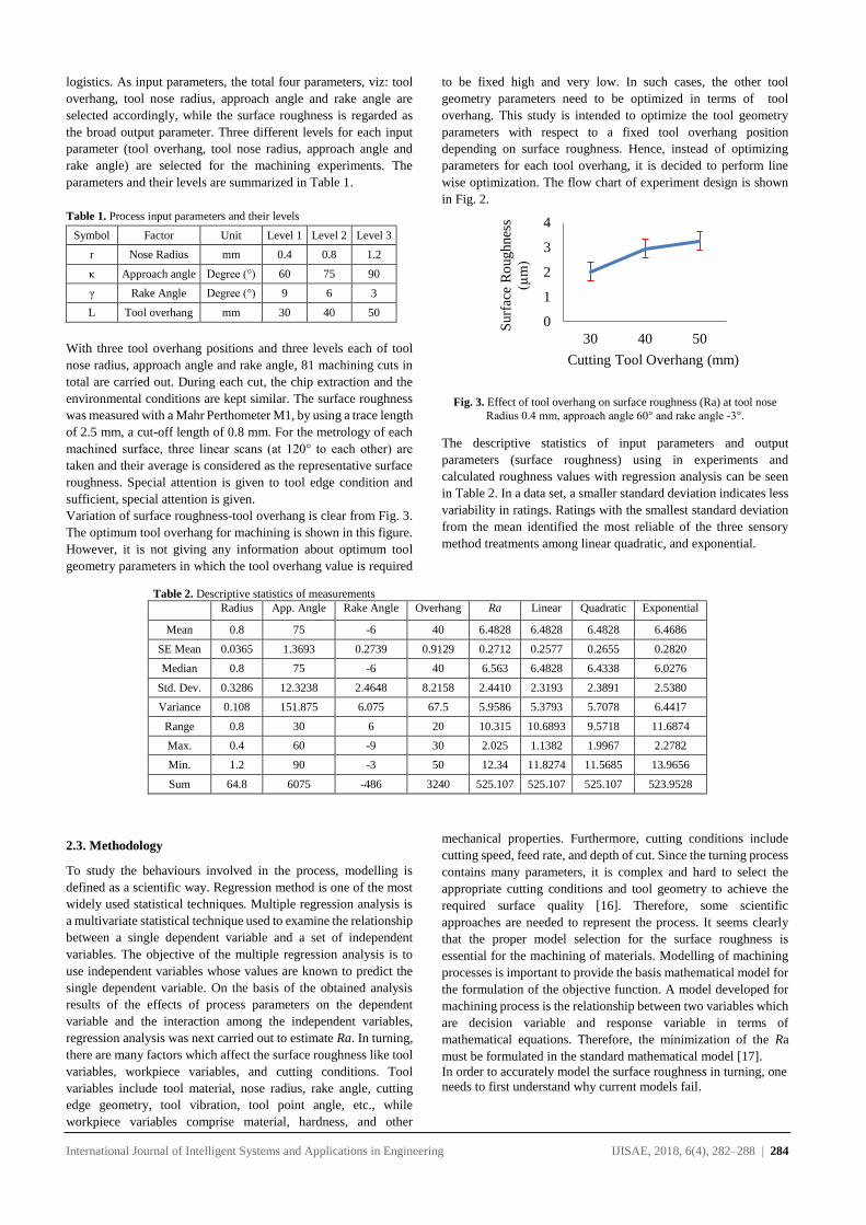
International Journal of Intelligent Systems and Applications in Engineering IJISAE, 2018, 6(4), 282–288 | 284
logistics. As input parameters, the total four parameters, viz: tool
overhang, tool nose radius, approach angle and rake angle are
selected accordingly, while the surface roughness is regarded as
the broad output parameter. Three different levels for each input
parameter (tool overhang, tool nose radius, approach angle and
rake angle) are selected for the machining experiments. The
parameters and their levels are summarized in Table 1.
Table 1. Process input parameters and their levels
Symbol Factor Unit Level 1 Level 2 Level 3
r Nose Radius mm 0.4 0.8 1.2
κ Approach angle Degree (°) 60 75 90
γ Rake Angle Degree (°) 9 6 3
L Tool overhang mm 30 40 50
With three tool overhang positions and three levels each of tool
nose radius, approach angle and rake angle, 81 machining cuts in
total are carried out. During each cut, the chip extraction and the
environmental conditions are kept similar. The surface roughness
was measured with a Mahr Perthometer M1, by using a trace length
of 2.5 mm, a cut-off length of 0.8 mm. For the metrology of each
machined surface, three linear scans (at 120° to each other) are
taken and their average is considered as the representative surface
roughness. Special attention is given to tool edge condition and
sufficient, special attention is given.
Variation of surface roughness-tool overhang is clear from Fig. 3.
The optimum tool overhang for machining is shown in this figure.
However, it is not giving any information about optimum tool
geometry parameters in which the tool overhang value is required
to be fixed high and very low. In such cases, the other tool
geometry parameters need to be optimized in terms of tool
overhang. This study is intended to optimize the tool geometry
parameters with respect to a fixed tool overhang position
depending on surface roughness. Hence, instead of optimizing
parameters for each tool overhang, it is decided to perform line
wise optimization. The flow chart of experiment design is shown
in Fig. 2.
Fig. 3. Effect of tool overhang on surface roughness (Ra) at tool nose
Radius 0.4 mm, approach angle 60° and rake angle -3°.
The descriptive statistics of input parameters and output
parameters (surface roughness) using in experiments and
calculated roughness values with regression analysis can be seen
in Table 2. In a data set, a smaller standard deviation indicates less
variability in ratings. Ratings with the smallest standard deviation
from the mean identified the most reliable of the three sensory
method treatments among linear quadratic, and exponential.
Table 2. Descriptive statistics of measurements
Radius App. Angle Rake Angle Overhang Ra Linear Quadratic Exponential
Mean 0.8 75 -6 40 6.4828 6.4828 6.4828 6.4686
SE Mean 0.0365 1.3693 0.2739 0.9129 0.2712 0.2577 0.2655 0.2820
Median 0.8 75 -6 40 6.563 6.4828 6.4338 6.0276
Std. Dev. 0.3286 12.3238 2.4648 8.2158 2.4410 2.3193 2.3891 2.5380
Variance 0.108 151.875 6.075 67.5 5.9586 5.3793 5.7078 6.4417
Range 0.8 30 6 20 10.315 10.6893 9.5718 11.6874
Max. 0.4 60 -9 30 2.025 1.1382 1.9967 2.2782
Min. 1.2 90 -3 50 12.34 11.8274 11.5685 13.9656
Sum 64.8 6075 -486 3240 525.107 525.107 525.107 523.9528
2.3. Methodology
To study the behaviours involved in the process, modelling is
defined as a scientific way. Regression method is one of the most
widely used statistical techniques. Multiple regression analysis is
a multivariate statistical technique used to examine the relationship
between a single dependent variable and a set of independent
variables. The objective of the multiple regression analysis is to
use independent variables whose values are known to predict the
single dependent variable. On the basis of the obtained analysis
results of the effects of process parameters on the dependent
variable and the interaction among the independent variables,
regression analysis was next carried out to estimate Ra. In turning,
there are many factors which affect the surface roughness like tool
variables, workpiece variables, and cutting conditions. Tool
variables include tool material, nose radius, rake angle, cutting
edge geometry, tool vibration, tool point angle, etc., while
workpiece variables comprise material, hardness, and other
mechanical properties. Furthermore, cutting conditions include
cutting speed, feed rate, and depth of cut. Since the turning process
contains many parameters, it is complex and hard to select the
appropriate cutting conditions and tool geometry to achieve the
required surface quality [16]. Therefore, some scientific
approaches are needed to represent the process. It seems clearly
that the proper model selection for the surface roughness is
essential for the machining of materials. Modelling of machining
processes is important to provide the basis mathematical model for
the formulation of the objective function. A model developed for
machining process is the relationship between two variables which
are decision variable and response variable in terms of
mathematical equations. Therefore, the minimization of the Ra
must be formulated in the standard mathematical model [17].
In order to accurately model the surface roughness in turning, one
needs to first understand why current models fail.
0
1
2
3
4
30 40 50
Surf
ace
Ro
ughnes
s
(µm
)
Cutting Tool Overhang (mm)
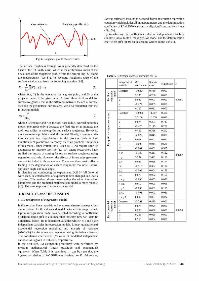
International Journal of Intelligent Systems and Applications in Engineering IJISAE, 2018, 6(4), 282–288 | 285
Fig. 4. Roughness profile characteristics.
The surface roughness average Ra is generally described on the
basis of the ISO 4287 norm, which is the arithmetical mean of the
deviations of the roughness profile from the central line (lm) along
the measurement (see Fig. 4). Average roughness (Ra) of the
surface is calculated from the following equation [18].
0
1( , )aR Z x y dxdy
S (1)
where Z(X, Y) is the elevation for a given point, and S0 is the
projected area of the given area. A basic theoretical model for
surface roughness, that is, the difference between the actual surface
area and the geometrical surface area, was also calculated from the
following model: 2
32 e
fRa
r (2)
where f is feed rate and re is the tool nose radius. According to this
model, one needs only a decrease the feed rate or an increase the
tool nose radius to develop desired surface roughness. However,
there are several problems with this model. Firstly, it does not take
into account any imperfections in the process, such as tool
vibration or chip adhesion. Secondly, there are practical limitations
to this model, since certain tools (such as CBN) require specific
geometries to improve tool life [12, 19]. Many researchers have
studied the impact of cutting factors on surface roughness using
regression analysis. However, the effects of insert edge geometry
are not included in those models. There are three main effects
leading to the degradation of surface roughness: tool nose Radius,
approach angle and rake angle.
In planning and conducting the experiment, DoE 3k full factorial
were used. Selected factors of experiment have changed in 3 levels
of value. This method allows investigating the wider interval of
parameters and the predicted mathematical model is more reliable
[20]. The next step was to estimate the model.
3. RESULTS and DISCUSSION
3.1. Development of Regression Model
In this section, linear, quadric and exponential regression equations
are introduced for Ra values and model factor effects are provided.
Optimum regression model was detected according to coefficient
of determination (R2), is a number that indicates how well data fit
a statistical model. Ra is dependent variables while r, κ, γ and L are
independent variables in regression models. Linear, quadratic and
exponential regression modelling and analysis of variance
(ANOVA) for Ra values are developed using Statistica software.
The correlation coefficients (R) value of modelled independent
variable Ra is given in Tables 3, respectively.
In the next step, Ra estimation procedures were performed by
creating mathematical (linear, quadratic and exponential)
equations. When Table 3 is examined, it can be seen that the
highest correlation of R=0.9787 was obtained for Ra. Moreover,
Ra was estimated through the second degree interaction regression
equation which includes all input parameters and the determination
coefficient of R2=0.9579 was statistically significant and consistent
(Fig. 5b).
By transferring the coefficients value of independent variables
(Tables 1) into Table 4, the regression model and the determination
coefficient (R2) for Ra values can be written in the Table 4.
Table 3. Regression coefficients values for Ra
Independent
variable
Ra
coefficient
Standart
error Significant R
Fo
r li
nea
r
reg
ress
ion
mo
del
Constant -10.324 0.749 0.000
0.9501
r 5.185 0.266 0.000
0.082 0.007 0.000
-0.277 0.035 0.000
L 0.120 0.011 0.000 F
or
qu
adra
tic
reg
ress
ion
mod
el Constant -12.086 14.387 0.404
0.9787
r 27.166 16.070 0.096
0.074 0.203 0.717
-2.428 2.143 0.262
L 0.459 0.356 0.202
r2 -4.629 0.845 0.000
2 0.001 0.001 0.080
2 -0.007 0.015 0.636
L2 -0.001 0.001 0.565
r. -0.330 0.211 0.122
r. 3.234 2.471 0.195
. 0.039 0.028 0.174
r.L -0.515 0.392 0.194
.L -0.006 0.004 0.159
.L 0.076 0.052 0.150
r. . -0.058 0.033 0.078
r. .L 0.010 0.005 0.048
r. .L -0.099 0.061 0.108
..L -0.001 0.001 0.061
r. ..L 0.002 0.001 0.034
Fo
r ex
pon
enti
al
reg
ress
ion
mo
del
Constant -5.391 0.420 0.000
0.9498
r 0.673 0.029 0.000
0.959 0.080 0.000
0.266 0.029 0.000
L 0.768 0.064 0.000
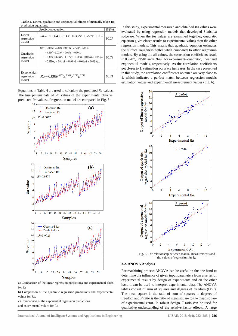
International Journal of Intelligent Systems and Applications in Engineering IJISAE, 2018, 6(4), 282–288 | 286
Table 4. Linear, quadratic and Exponential effects of manually taken Ra
prediction equations.
Prediction equation R2(%)
Linear regression
model
10.324 5.186 0.082 0.277 0.12Ra r L
90.27
Quadratic
regression model
2 2 2 2
12.086 27.166 0.074 2.428 0.459
4.63 0.001 0.007 0.001
0.33 3.234 0.039 0.515 0.006 0.076
0.058 0.01 0.099 0.001 0.002
Ra r L
r L
r r rL L L
r r L r L L r L
95.79
Exponential
regression
model
0.673 0.959 0.266 0.7690.005Ra r L 90.21
Equations in Table 4 are used to calculate the predicted Ra values.
The line pattern data of Ra values of the experimental data vs.
predicted Ra values of regression model are compared in Fig. 5.
a) Comparison of the linear regression predictions and experimental alues
for Ra
b) Comparison of the quadratic regression predictions and experimental
values for Ra.
c) Comparison of the exponential regression predictions
and experimental values for Ra
In this study, experimental measured and obtained Ra values were
evaluated by using regression models that developed Statistica
software. When the Ra values are examined together, quadratic
equation gives closer results to experimental values than the other
regression models. This means that quadratic equation estimates
the surface roughness better when compared to other regression
models. By using the all values, the correlation coefficients result
in 0.9787, 0.9501 and 0.9498 for experiment- quadratic, linear and
exponential models, respectively. As the correlation coefficients
get closer to 1, estimation accuracy increases. In the case presented
in this study, the correlation coefficients obtained are very close to
1, which indicates a perfect match between regression models
estimation values and experimental measurement values (Fig. 6).
Fig. 6. The relationship between manual measurements and
the values of regression for Ra
3.2. ANOVA Analysis
For machining process ANOVA can be useful on the one hand to
determine the influence of given input parameters from a series of
experimental results by design of experiments and on the other
hand it can be used to interpret experimental data. The ANOVA
tables consist of sum of squares and degrees of freedom (DoF).
The mean-square is the ratio of sum of squares to degrees of
freedom and F ratio is the ratio of mean square to the mean square
of experimental error. In robust design F ratio can be used for
qualitative understanding of the relative factor effects. A large
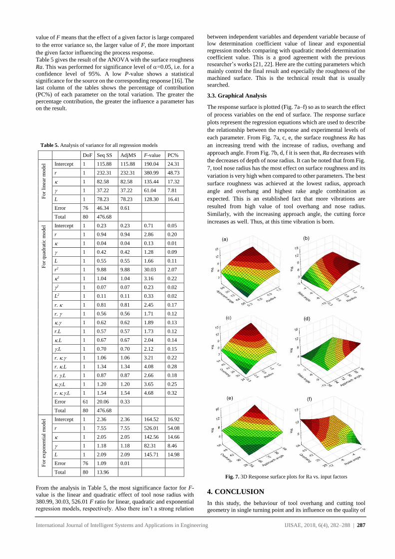
International Journal of Intelligent Systems and Applications in Engineering IJISAE, 2018, 6(4), 282–288 | 287
value of F means that the effect of a given factor is large compared
to the error variance so, the larger value of F, the more important
the given factor influencing the process response.
Table 5 gives the result of the ANOVA with the surface roughness
Ra. This was performed for significance level of =0.05, i.e. for a
confidence level of 95%. A low P-value shows a statistical
significance for the source on the corresponding response [16]. The
last column of the tables shows the percentage of contribution
(PC%) of each parameter on the total variation. The greater the
percentage contribution, the greater the influence a parameter has
on the result.
Table 5. Analysis of variance for all regression models
DoF Seq SS AdjMS F-value PC%
Fo
r li
nea
r m
od
el Intercept 1 115.88 115.88 190.04 24.31
r 1 232.31 232.31 380.99 48.73
1 82.58 82.58 135.44 17.32
1 37.22 37.22 61.04 7.81
L 1 78.23 78.23 128.30 16.41
Error 76 46.34 0.61
Total 80 476.68
Fo
r qu
adra
tic
mo
del
Intercept 1 0.23 0.23 0.71 0.05
r 1 0.94 0.94 2.86 0.20
1 0.04 0.04 0.13 0.01
1 0.42 0.42 1.28 0.09
L 1 0.55 0.55 1.66 0.11
r2 1 9.88 9.88 30.03 2.07
2 1 1.04 1.04 3.16 0.22
2 1 0.07 0.07 0.23 0.02
L2 1 0.11 0.11 0.33 0.02
r. 1 0.81 0.81 2.45 0.17
r. 1 0.56 0.56 1.71 0.12
. 1 0.62 0.62 1.89 0.13
r.L 1 0.57 0.57 1.73 0.12
.L 1 0.67 0.67 2.04 0.14
.L 1 0.70 0.70 2.12 0.15
r. . 1 1.06 1.06 3.21 0.22
r. .L 1 1.34 1.34 4.08 0.28
r. .L 1 0.87 0.87 2.66 0.18
..L 1 1.20 1.20 3.65 0.25
r. ..L 1 1.54 1.54 4.68 0.32
Error 61 20.06 0.33
Total 80 476.68
Fo
r ex
pon
enti
al m
odel
Intercept 1 2.36 2.36 164.52 16.92
r 1 7.55 7.55 526.01 54.08
1 2.05 2.05 142.56 14.66
1 1.18 1.18 82.31 8.46
L 1 2.09 2.09 145.71 14.98
Error 76 1.09 0.01
Total 80 13.96
From the analysis in Table 5, the most significance factor for F-
value is the linear and quadratic effect of tool nose radius with
380.99, 30.03, 526.01 F ratio for linear, quadratic and exponential
regression models, respectively. Also there isn’t a strong relation
between independent variables and dependent variable because of
low determination coefficient value of linear and exponential
regression models comparing with quadratic model determination
coefficient value. This is a good agreement with the previous
researcher’s works [21, 22]. Here are the cutting parameters which
mainly control the final result and especially the roughness of the
machined surface. This is the technical result that is usually
searched.
3.3. Graphical Analysis
The response surface is plotted (Fig. 7a–f) so as to search the effect
of process variables on the end of surface. The response surface
plots represent the regression equations which are used to describe
the relationship between the response and experimental levels of
each parameter. From Fig. 7a, c, e, the surface roughness Ra has
an increasing trend with the increase of radius, overhang and
approach angle. From Fig. 7b, d, f it is seen that, Ra decreases with
the decreases of depth of nose radius. It can be noted that from Fig.
7, tool nose radius has the most effect on surface roughness and its
variation is very high when compared to other parameters. The best
surface roughness was achieved at the lowest radius, approach
angle and overhang and highest rake angle combination as
expected. This is an established fact that more vibrations are
resulted from high value of tool overhang and nose radius.
Similarly, with the increasing approach angle, the cutting force
increases as well. Thus, at this time vibration is born.
Fig. 7. 3D Response surface plots for Ra vs. input factors
4. CONCLUSION
In this study, the behaviour of tool overhang and cutting tool
geometry in single turning point and its influence on the quality of
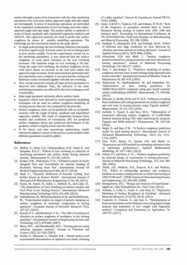
International Journal of Intelligent Systems and Applications in Engineering IJISAE, 2018, 6(4), 282–288 | 288
surface through a series of its interaction with the other machining
parameters (viz: tool nose radius, approach angle and rake angle)
are investigated. A series of machining operations are performed
in the sequential combinations of tool overhang, tool nose radius,
approach angle and rake angle. The surface quality is analysed in
terms of linear, quadratic and exponential regression analysis and
ANOVA. The regression analyses are used to predict the surface
roughness by means of suitable modelling operations. The
followings are the conclusions based on the study above:
In single point turning, the tool overhang influences the quality
of surface significantly. Extreme values of tool overhang result
in poor surface quality. From the experiments carried out on
the machining parameters, it was observed that the surface
roughness of work piece increases as the tool overhang
increases. The optimum range of tool overhang is 30 mm.
Using the same tool overhang, the surface roughness of the
work piece shows an increase as the tool nose radius and
approach angle increases. In the measurements performed after
the experiments were complete, it was seen that the cutting tool
deflection values increased together with the tool overhang.
Also, strong interaction among all input process parameters is
observed and validated. Thus, the selection of the other
machining parameters are affected by the tool overhang as well
considerably.
Rake angle parameter adversely affects surface finish.
Equations which were derived by multi-regression modelling
techniques can be used for surface roughness modelling of
turning process that can’t be computed by theoretically.
Surface roughness value can be predicted with an acceptable
accuracy with the usage of linear, quadratic and exponential
regression models. The result of comparison between these
models and coefficient of correlations (R2) for predicted
surface roughness shows that prediction performance of the
quadratic model is slightly better than the others.
In the future, real time monitoring, optimization, model
referenced adaptive control of the process can be studied while
different parameters would be added.
References
[1] Mishra, V., Khan, G.S., Chattopadhyay, K.D., Nand, K., and
Sarepaka, R.G.V., “Effects of tool overhang on selection of
machining parameters and surface finish during diamond
turning”, Measurement 55, 353-361, (2014).
[2] Kotkar, D.R., Wakchaure, V.D., “Vibration control of newly
designed Tool and Tool-Holder for internal treading of
Hydraulic Steering Gear Nut”, International Journal Of
Modern Engineering Research 4(6), 46-57, (2014).
[3] Hadi, Y., “Dynamic Deflection of Periodic Cutting Tool
Holder Based on Passive Model”, International Journal of
Mechanical & Mechatronics Engineering 11 No: 06, (2011).
[4] Kiyak, M., Kaner, B., Sahin, I., Aldemir, B., and Cakir, O.,
“The Dependence of Tool Overhang on Surface Quality and
Tool Wear in the Turning Process”, International Advanced
Manufacturing Technology 51(5), 431-438, (2010).
[5] Sathishkumar, B., Mohanasundaram, K.M. and Senthilkumar,
M., “Experimental studies on impact of particle damping on
surface roughness of machined components in boring
operation”, European Journal of Scientific Research 71(3),
327-337, (2012).
[6] Kassab, S.Y., and Khoshnaw, Y.K., “The effect of cutting tool
vibration on surface roughness of workpiece in dry turning
operation”, International Journal of Engineering Science and
Technology 25(7), 879-889, (2007).
[7] Batey, M.C., and Hamidzadeh, H.R., “Turning process using
vibration signature analysis”, Journal of Vibration and
Control 13(5), 527-536, (2007).
[8] Sardar, N., Bhaumik, A., Mandal, N.K., “Modal analysis and
experimental determination of optimum tool shank overhang
of a lathe machine”, Sensors & Transducers Journal 99(12),
53-65, (2008).
[9] Amin, A.K.M.N., Nashron, F.R. and Zubaire, W.W.D., “Role
of the frequency of secondary serrated teeth in chatter
formation during turning of carbon steel AISI 1040 and
stainless steel”, Proceeding 1st International Conference &
7th AUN/SEED-Net, Field-wise Seminar on Manufacturing
and Material Processing, 181-186, (2006).
[10] Haddadi, E., Shabghard, M.R. and Ettefagh, M.M., “Effect
of different tool edge conditions on wear detection by
vibration spectrum analysis in turning operation”, Journal of
Applied Sciences 8(21), 3879-3886, (2008).
[11] Abouelatta, O.B. and Mádl, J., “Surface roughness
prediction based on cutting parameters and tool vibrations in
turning operations”, Journal of Materials Processing
Technology 118, 269-277, (2001).
[12] Özel, T. and Karpat, Y., “Predictive modeling of surface
roughness and tool wear in hard turning using regression and
neural networks”, International Journal of Machine Tools &
Manufacture 45, 467-479, (2005).
[13] Adalarasan, R., Santhanakumar, M. and Rajmohan, M.,
“Optimization of laser cutting parameters for
Al6061/SiCp/Al2O3 composite using grey based response
surface methodology (GRSM)”, Measurement, 73, 596-606,
(2015).
[14] Debnath, S., Reddy, M.M. and Yi, Q.S., “Influence of cutting
fluid conditions and cutting parameters on surface roughness
and tool wear in turning process using Taguchi method”,
Measurement, 78, 111-119, (2016).
[15] Asiltürk, İ., Neşeli, S. and İnce, M.A., “Optimisation of
parameters affecting surface roughness of Co28Cr6Mo
medical material during CNC lathe machining by using the
Taguchi and RSM methods”, Measurement, 78, 120-128,
(2016).
[16] Singh, D. and Rao, P.W., “A Surface roughness prediction
model for hard turning process”, International Journal of
Advanced Manufacturing Technology, 32(11–12), 1115–
1124, (2007).
[17] Zain, A.M., Haron, H., Qasem, S.N. and Sharif, S.,
“Regression and ANN models for estimating minimum value
of machining performance”, Applied Mathematical
Modelling, 36, 1477-1492, (2012).
[18] Arbizu, P.I. and Pérez, C.J.L., “Surface roughness prediction
by factorial design of experiments in turning processes”,
Journal of Materials Processing Technology, 143–144, 390-
396, (2003).
[19] Thiele, J.D., Melkote, S.N., Peascoe, R.A. and Watkins,
T.R., “Effect of cutting-edge geometry and workpiece
hardness on surface residual stresses in finish hard turning of
AISI 52100 steel”, ASME Journal of Manufacturing Science
and Engineering, 122, 642-649, (2000).
[20] Montgomerty, D.C., “Design and Analysis of Experiments”,
eighth ed., John Willey&Sons Inc., New York, (2013).
[21] Asilturk, I., Celik, L., Canlı, E., and Onal, G., “Regression
Modeling of Surface Roughness in Grinding”, Advanced
Materials Research, 271(273), 34-39, (2011).
[22] Tasdemir, S., Urkmez, A., and Inal, S., “Determination of
body measurements on the Holstein cows using digital image
analysis and estimation of live weight with regression
analysis”, Computers and Electronics in Agriculture, 76,
189-197, (2011).

International Journal of
Intelligent Systems and
Applications in Engineering
Advanced Technology and Science
ISSN:2147-67992147-6799 www.atscience.org/IJISAE Original Research Paper
International Journal of Intelligent Systems and Applications in Engineering IJISAE, 2018, 6(4), 289–293 | 289
Breast Cancer Diagnosis by Different Machine Learning Methods Using
Blood Analysis Data
Muhammet Fatih Aslan*1, Yunus Celik1, Kadir Sabanci1, Akif Durdu2
Accepted : 18/11/2018 Published: 31/12/201x DOI: 10.1039/b000000x
Abstract: Today, one of the most common types of cancer is breast cancer. It is crucial to prevent the propagation of malign cells to reduce
the rate of cancer induced mortality. Cancer detection must be done as early as possible for this purpose. Machine Learning techniques are
used to diagnose or predict the success of treatment in medicine. In this study, four different machine learning algorithms were used to
early detection of breast cancer. The aim of this study is to process the results of routine blood analysis with different ML methods and to
understand how effective these methods are for detection. Methods used can be listed as Artificial Neural Network (ANN), standard
Extreme Learning Machine (ELM), Support Vector Machine (SVM) and K-Nearest Neighbor (k-NN). Dataset used were taken from UCI
library. In this dataset age, body mass index (BMI), glucose, insulin, homeostasis model assessment (HOMA), leptin, adiponectin, resistin
and chemokine monocyte chemoattractant protein 1 (MCP1) attributes were used. Parameters that have the best accuracy values were
found by using four different Machine Learning techniques. For this purpose, hyperparameter optimization method was used. In the end,
the results were compared and discussed.
Keywords: Breast cancer, Artificial Neural Network, Extreme Learning Machine, Support Vector Machine, K-Nearest Neighbors,
Hyperparameter Optimization
1. Introduction
Different cancer types have long been a major threat to human life
[1]. Among these types, breast cancer has a high mortality rate in
women. Unfortunately, this rate is increasing in developed
countries day by day [2, 3]. Moreover, breast cancer is the second
biggest cause of death all over the world [4]. According to World
Health Organization (WHO) data [5], breast cancer has been
detected in 25% of women in the United Nations [6]. 16% of all
female cancers is breast cancer [5].
Cancer is a sickness that starts in the cell and spreads into the other
part of the body [7]. That is the reason why early detection is
crucial to prevent before it spreads. Early diagnosis of breast
cancer is the most important and difficult part of breast imaging
[8]. The works for early detection of breast cancer are not new but
the current works are not capable enough for early detection so, in
addition to current works, scientist are searching for new methods
[9]. Specially Computer-Aided Detection (CAD) systems play a
crucial role in early detection [10].
Machine Learning (ML) techniques are used in the CAD system
applications. ML [11] is an Artificial Intelligence (AI) topic that
enables the machines to learn a special task by experience. In
recent years, ML methods have become widespread in predicting
and detecting applications in order to make strong decisions in
recent years. For example, ML methods can be used to determine
whether a cancer is benign or malign [9].
2. Related Works
There are many works exist for the detection of breast cancer using
ML techniques in the literature. In this part, some of these works
were shown. The performance comparison of Support Vector
Machine (SVM), K-Nearest Neighbor (k-NN), Decision Tree
(C4.5) and Naive Bayes (NB) Machine Learning (ML) techniques
were shown [12]. Wisconsin Diagnosis Breast Cancer (WDBC)
dataset [13] was used for this work. The best result was obtained
with SVM technique as 97.13%. The paper with [14] reference
number includes a work that K-Means and SVM algorithms were
used as a hybrid for the purpose of detection of a tumour. A
classification with a high accuracy rate was performed as a result
of 10 times cross-validation. In this work, the WDBC dataset [13]
was used. 97.38% accuracy was achieved. The paper [15] shows
the success of SVM and Artificial Neural Network (ANN)
techniques together. WDBC dataset was also used in this paper.
Accuracy was obtained as 97.14% with SVM and 96.71% with
ANN. According to these results, SVM gives better results than
ANN. Another paper [16] it was also shown that SVM has better
performance for the detection of breast cancer. On the other hand,
the performance of the SVM depends on the kernel function. In
this paper, the performance of different types of kernel functions
were compared. In the paper [17], k-NN algorithm was optimized
for a faster and more reliable classification. 94.1% accuracy was
obtained. The paper [18] is about the usage of different ML
techniques for breast cancer. The research is about the usage of
ANN, SVM, Decision Tree (DT) and k-NN techniques in breast
cancer diagnosis. In the paper [19] DT, Bayesian Belief Network,
and SVM techniques were compared. In the last paper [20], breast
cancer was detected using ANN classification. The work focuses
on the optimal activation function that minimizes the classification
error by using fewer blocks.
_______________________________________________________________________________________________________________________________________________________________________________________________________________________________________________________________________________________________________________________________
1Department of Electrical-Electronic Engineering, Karamanoğlu
Mehmetbey University,Karaman,-70100, Turkey 2Department of Electrical-Electronic Engineering, Konya Technical
University,Konya,-42000, Turkey,
* Corresponding Author: Email: [email protected]

International Journal of Intelligent Systems and Applications in Engineering IJISAE, 2018, 6(4), 289–293 | 290
3. Material and Methods
In this section, dataset and ML methods used were presented.
3.1. Data Understanding
When related works were analysed, it is clear that there are several
different techniques for the detection of breast cancer and detection
problem still exist. There are several types of the dataset for the
detection of breast cancer. In this paper, Breast Cancer Coimbra
dataset [22] taken from UCI [21] ML Repository was used. This
dataset includes features that can be collected in routine blood
analysis. These features are age (years), BMI (kg/m2), Glucose
(mg/dL), Insulin (µU/mL), HOMA, Leptin (ng/mL), Adiponectin
(µg/mL), Resistin (ng/mL) and MCP1(pg/dL). According to these
input features, target data can be classified as healthy or unhealthy.
These features were measured from 64 patients with breast cancer
and 52 healthy people [22,23]. This dataset differs from others in
terms of the features it contains.
3.2. Artificial Neural Network (ANN)
The structure of the ANN is quite similar to biological neural
networks [24]. An ANN composed of three layers as an input layer,
hidden layer, and an output layer. The neurons in each layer are
connected to each other with a specific weight. These weights are
updated themselves iteratively until they are close enough to target
values. When the weights are tuned, the system can be expressed
as trained. After this phase, the testing process can be performed
[25].
3.3. Extreme Learning Machine (ELM)
ELM is a method invented by Huang and friends [26]. It is actually
having the same structure with ANN. The difference is that while
ANN has more than one hidden layer, standard ELM should have
only one hidden layer. Moreover, Unlike ANN, there are more than
1000 hidden layer neurons in a standard ELM [27]. ELM offers
advantages over other ML methods in terms of speed. Because
ELM completes training with a single iteration [28]. Weights are
assigned randomly and according to target values, β values are
calculated. Moore-Penrose generalized inverse matrix method is
used for the calculation [29].
3.4. Support Vector Machine (SVM)
SVM is one of the best advised ML methods in terms of speed and
accuracy [30]. SVM forms optimal hyperplanes in a
multidimensional plane and in this way classifies multi-class
property data [31]. The SVM contains calculations for the creation
of this plane. If the properties can be classified as linear, the plane
can be created by simple calculations. The kernel trick is used for
non-linear features. With kernel trick, features can be converted to
a higher-level and can be separated linearly [32].
3.5. K-Nearest Neighbors (k-NN)
With the help of k-NN, data in the feature space are classified
according to distance. The distances can be calculated with
different methods. In order to classify the data, the decision is made
by looking at the distance from k numbered neighbor. Data is
assigned to the nearest class [33]. Since there is no training phase,
understanding and implementation of the method are quite easy
[34].
4. Application and Results
In this study, the dataset was taken from the UCI library [21] and
blood analysis data taken from the paper [22] were used. There are
116 samples in total. Some of these data are shown in Table 1.
Target values indicate that the person is healthy or unhealthy.
Considering the input values, max and min of these values are quite
different from each other. Normalization must first be applied to
normalize the distribution and increase the success rate.
Feature Scaling method is used for normalization. The formula for
this method is shown in (1).
𝑥′ =𝑥 − 𝑥𝑚𝑖𝑛
𝑥𝑚𝑎𝑥 − 𝑥𝑚𝑖𝑛 (1)
After normalization using (1), training and test data were generated
randomly from the data. 80% percent of the whole data were used
in the test phase and 20% percent were used in the training phase.
After separation of training and test data, results were obtained for
each ML method.
An interface was created in MATLAB GUI environment for
classification with ANN (see Fig. 1). In ANN, there are a number
of hyperparameters that affect the accuracy of the system. The
important parameters can be listed as Number of Hidden Layer
Neuron, Epoch Number, Learning Rate and Momentum
Coefficient. These values must be set by trial and error to obtain
the most optimal result of ANN. For this reason, at the interface, a
certain range of these parameters can be adjusted by the user. The
graphs in the interface give Root Mean Square Error (RMSE)
values according to the changing parameter values. The results of
the RMSE values are plotted according to the changed parameter
and the parameters which give the minimum error were recorded.
After that, training and test process was managed by using the best
parameters. As a result, the average test accuracy rate is 79.4304%,
average training time 0.4282 second and average RMSE value was
obtained as 0.3954. Comparison of these values with ELM is
shown in Table 2.
Table 1. Some data used for breast cancer detection
Age BMI Glucose Insulin HOMA Leptin Adiponectin Resistin MCP.1 Class
48 23.5 70 2.707 0.4674087 8.8071 9.7024 7.99585 417.114 1
83 20.690495 92 3.115 0.7068973 8.8438 5.429285 4.06405 468.786 1
82 23.12467 91 4.498 1.0096511 17.9393 22.43204 9.27715 554.697 1
68 21.367521 77 3.226 0.6127249 9.8827 7.16956 12.766 928.22 1
45 21.303949 102 13.852 3.4851632 7.6476 21.056625 23.0341 552.444 2
45 20.829995 74 4.56 0.832352 7.7529 8.237405 28.0323 382.955 2
49 20.956607 94 12.305 2.8531193 11.2406 8.412175 23.1177 573.63 2
34 24.242424 92 21.699 4.9242264 16.7353 21.823745 12.0653 481.949 2
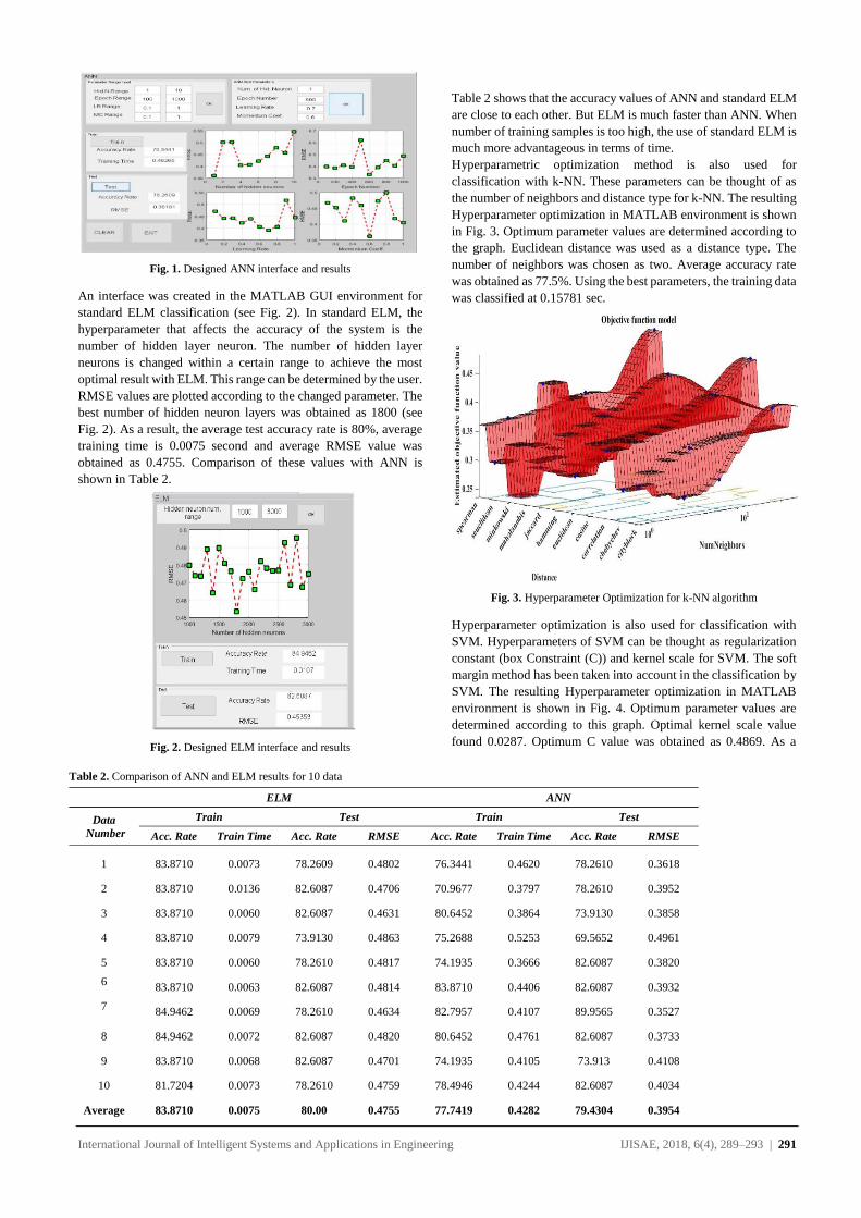
International Journal of Intelligent Systems and Applications in Engineering IJISAE, 2018, 6(4), 289–293 | 291
Fig. 1. Designed ANN interface and results
An interface was created in the MATLAB GUI environment for
standard ELM classification (see Fig. 2). In standard ELM, the
hyperparameter that affects the accuracy of the system is the
number of hidden layer neuron. The number of hidden layer
neurons is changed within a certain range to achieve the most
optimal result with ELM. This range can be determined by the user.
RMSE values are plotted according to the changed parameter. The
best number of hidden neuron layers was obtained as 1800 (see
Fig. 2). As a result, the average test accuracy rate is 80%, average
training time is 0.0075 second and average RMSE value was
obtained as 0.4755. Comparison of these values with ANN is
shown in Table 2.
Fig. 2. Designed ELM interface and results
Table 2 shows that the accuracy values of ANN and standard ELM
are close to each other. But ELM is much faster than ANN. When
number of training samples is too high, the use of standard ELM is
much more advantageous in terms of time.
Hyperparametric optimization method is also used for
classification with k-NN. These parameters can be thought of as
the number of neighbors and distance type for k-NN. The resulting
Hyperparameter optimization in MATLAB environment is shown
in Fig. 3. Optimum parameter values are determined according to
the graph. Euclidean distance was used as a distance type. The
number of neighbors was chosen as two. Average accuracy rate
was obtained as 77.5%. Using the best parameters, the training data
was classified at 0.15781 sec.
Fig. 3. Hyperparameter Optimization for k-NN algorithm
Hyperparameter optimization is also used for classification with
SVM. Hyperparameters of SVM can be thought as regularization
constant (box Constraint (C)) and kernel scale for SVM. The soft
margin method has been taken into account in the classification by
SVM. The resulting Hyperparameter optimization in MATLAB
environment is shown in Fig. 4. Optimum parameter values are
determined according to this graph. Optimal kernel scale value
found 0.0287. Optimum C value was obtained as 0.4869. As a
Table 2. Comparison of ANN and ELM results for 10 data
ELM ANN
Data
Number
Train Test Train Test
Acc. Rate Train Time Acc. Rate RMSE Acc. Rate Train Time Acc. Rate RMSE
1 83.8710 0.0073 78.2609 0.4802 76.3441 0.4620 78.2610 0.3618
2 83.8710 0.0136 82.6087 0.4706 70.9677 0.3797 78.2610 0.3952
3 83.8710 0.0060 82.6087 0.4631 80.6452 0.3864 73.9130 0.3858
4 83.8710 0.0079 73.9130 0.4863 75.2688 0.5253 69.5652 0.4961
5 83.8710 0.0060 78.2610 0.4817 74.1935 0.3666 82.6087 0.3820
6 83.8710 0.0063 82.6087 0.4814 83.8710 0.4406 82.6087 0.3932
7 84.9462 0.0069 78.2610 0.4634 82.7957 0.4107 89.9565 0.3527
8 84.9462 0.0072 82.6087 0.4820 80.6452 0.4761 82.6087 0.3733
9 83.8710 0.0068 82.6087 0.4701 74.1935 0.4105 73.913 0.4108
10 81.7204 0.0073 78.2610 0.4759 78.4946 0.4244 82.6087 0.4034
Average 83.8710 0.0075 80.00 0.4755 77.7419 0.4282 79.4304 0.3954
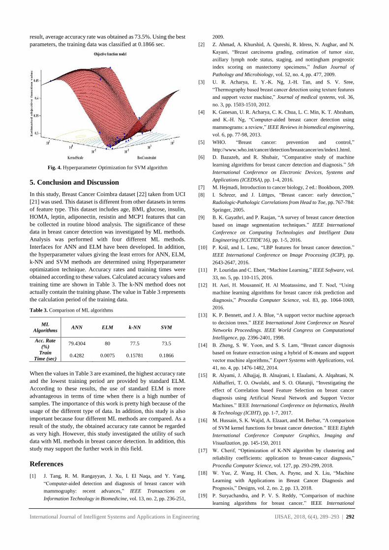
International Journal of Intelligent Systems and Applications in Engineering IJISAE, 2018, 6(4), 289–293 | 292
result, average accuracy rate was obtained as 73.5%. Using the best
parameters, the training data was classified at 0.1866 sec.
Fig. 4. Hyperparameter Optimization for SVM algorithm
5. Conclusion and Discussion
In this study, Breast Cancer Coimbra dataset [22] taken from UCI
[21] was used. This dataset is different from other datasets in terms
of feature type. This dataset includes age, BMI, glucose, insulin,
HOMA, leptin, adiponectin, resistin and MCP1 features that can
be collected in routine blood analysis. The significance of these
data in breast cancer detection was investigated by ML methods.
Analysis was performed with four different ML methods.
Interfaces for ANN and ELM have been developed. In addition,
the hyperparameter values giving the least errors for ANN, ELM,
k-NN and SVM methods are determined using Hyperparameter
optimization technique. Accuracy rates and training times were
obtained according to these values. Calculated accuracy values and
training time are shown in Table 3. The k-NN method does not
actually contain the training phase. The value in Table 3 represents
the calculation period of the training data.
Table 3. Comparison of ML algorithms
ML
Algorithms ANN ELM k-NN SVM
Acc. Rate
(%) 79.4304 80 77.5 73.5
Train
Time (sec) 0.4282 0.0075 0.15781 0.1866
When the values in Table 3 are examined, the highest accuracy rate
and the lowest training period are provided by standard ELM.
According to these results, the use of standard ELM is more
advantageous in terms of time when there is a high number of
samples. The importance of this work is pretty high because of the
usage of the different type of data. In addition, this study is also
important because four different ML methods are compared. As a
result of the study, the obtained accuracy rate cannot be regarded
as very high. However, this study investigated the utility of such
data with ML methods in breast cancer detection. In addition, this
study may support the further work in this field.
References
[1] J. Tang, R. M. Rangayyan, J. Xu, I. El Naqa, and Y. Yang,
“Computer-aided detection and diagnosis of breast cancer with
mammography: recent advances,” IEEE Transactions on
Information Technology in Biomedicine, vol. 13, no. 2, pp. 236-251,
2009.
[2] Z. Ahmad, A. Khurshid, A. Qureshi, R. Idress, N. Asghar, and N.
Kayani, “Breast carcinoma grading, estimation of tumor size,
axillary lymph node status, staging, and nottingham prognostic
index scoring on mastectomy specimens,” Indian Journal of
Pathology and Microbiology, vol. 52, no. 4, pp. 477, 2009.
[3] U. R. Acharya, E. Y.-K. Ng, J.-H. Tan, and S. V. Sree,
“Thermography based breast cancer detection using texture features
and support vector machine,” Journal of medical systems, vol. 36,
no. 3, pp. 1503-1510, 2012.
[4] K. Ganesan, U. R. Acharya, C. K. Chua, L. C. Min, K. T. Abraham,
and K.-H. Ng, “Computer-aided breast cancer detection using
mammograms: a review,” IEEE Reviews in biomedical engineering,
vol. 6, pp. 77-98, 2013.
[5] WHO. “Breast cancer: prevention and control,”
http://www.who.int/cancer/detection/breastcancer/en/index1.html.
[6] D. Bazazeh, and R. Shubair, “Comparative study of machine
learning algorithms for breast cancer detection and diagnosis.” 5th
International Conference on Electronic Devices, Systems and
Applications (ICEDSA), pp. 1-4, 2016.
[7] M. Hejmadi, Introduction to cancer biology, 2 ed.: Bookboon, 2009.
[8] I. Schreer, and J. Lüttges, “Breast cancer: early detection,”
Radiologic-Pathologic Correlations from Head to Toe, pp. 767-784:
Springer, 2005.
[9] B. K. Gayathri, and P. Raajan, “A survey of breast cancer detection
based on image segmentation techniques.” IEEE International
Conference on Computing Technologies and Intelligent Data
Engineering (ICCTIDE'16), pp. 1-5, 2016.
[10] P. Král, and L. Lenc, “LBP features for breast cancer detection.”
IEEE International Conference on Image Processing (ICIP), pp.
2643-2647, 2016.
[11] P. Louridas and C. Ebert, “Machine Learning,” IEEE Software, vol.
33, no. 5, pp. 110-115, 2016.
[12] H. Asri, H. Mousannif, H. Al Moatassime, and T. Noel, “Using
machine learning algorithms for breast cancer risk prediction and
diagnosis,” Procedia Computer Science, vol. 83, pp. 1064-1069,
2016.
[13] K. P. Bennett, and J. A. Blue, “A support vector machine approach
to decision trees.” IEEE International Joint Conference on Neural
Networks Proceedings. IEEE World Congress on Computational
Intelligence, pp. 2396-2401, 1998.
[14] B. Zheng, S. W. Yoon, and S. S. Lam, “Breast cancer diagnosis
based on feature extraction using a hybrid of K-means and support
vector machine algorithms,” Expert Systems with Applications, vol.
41, no. 4, pp. 1476-1482, 2014.
[15] R. Alyami, J. Alhajjaj, B. Alnajrani, I. Elaalami, A. Alqahtani, N.
Aldhafferi, T. O. Owolabi, and S. O. Olatunji, “Investigating the
effect of Correlation based Feature Selection on breast cancer
diagnosis using Artificial Neural Network and Support Vector
Machines.” IEEE International Conference on Informatics, Health
& Technology (ICIHT), pp. 1-7, 2017.
[16] M. Hussain, S. K. Wajid, A. Elzaart, and M. Berbar, “A comparison
of SVM kernel functions for breast cancer detection.” IEEE Eighth
International Conference Computer Graphics, Imaging and
Visualization, pp. 145-150, 2011
[17] W. Cherif, “Optimization of K-NN algorithm by clustering and
reliability coefficients: application to breast-cancer diagnosis,”
Procedia Computer Science, vol. 127, pp. 293-299, 2018.
[18] W. Yue, Z. Wang, H. Chen, A. Payne, and X. Liu, “Machine
Learning with Applications in Breast Cancer Diagnosis and
Prognosis,” Designs, vol. 2, no. 2, pp. 13, 2018.
[19] P. Suryachandra, and P. V. S. Reddy, “Comparison of machine
learning algorithms for breast cancer.” IEEE International
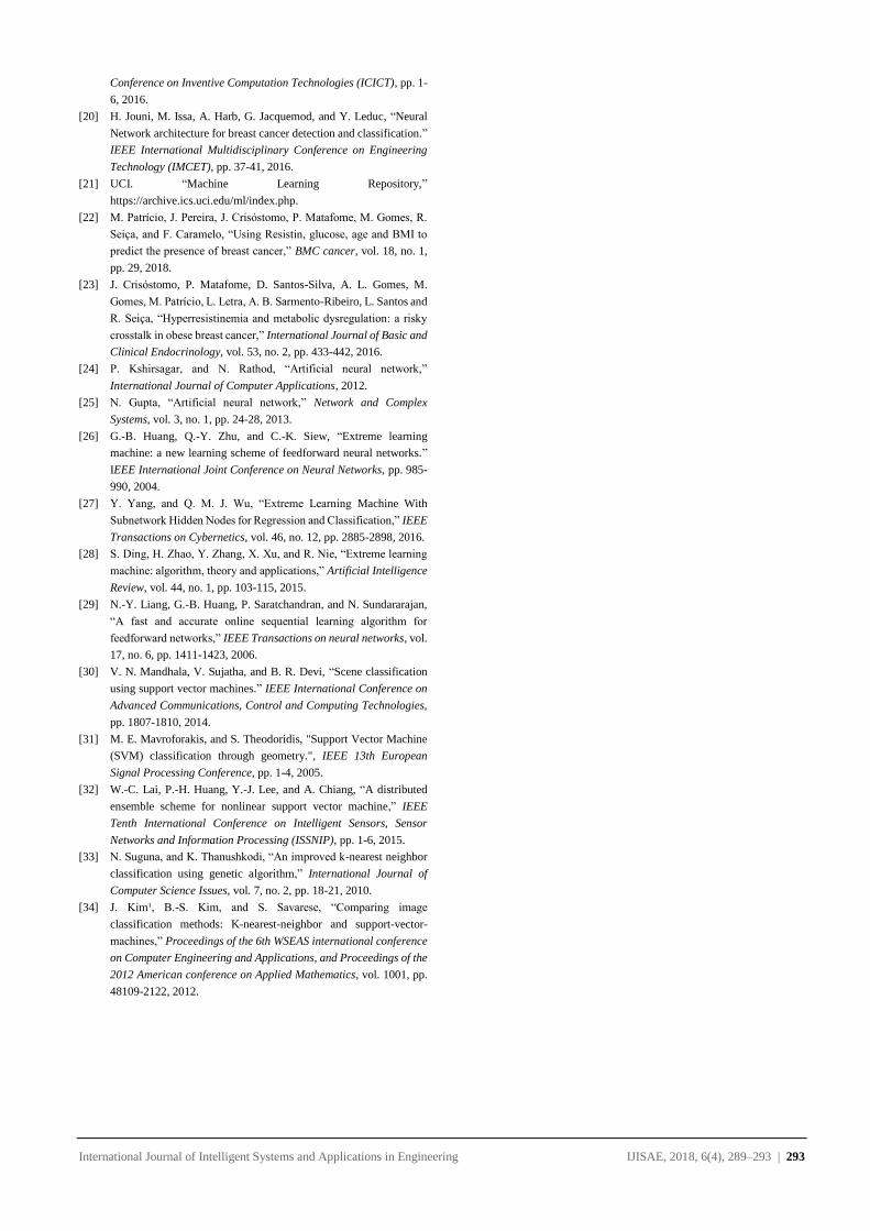
International Journal of Intelligent Systems and Applications in Engineering IJISAE, 2018, 6(4), 289–293 | 293
Conference on Inventive Computation Technologies (ICICT), pp. 1-
6, 2016.
[20] H. Jouni, M. Issa, A. Harb, G. Jacquemod, and Y. Leduc, “Neural
Network architecture for breast cancer detection and classification.”
IEEE International Multidisciplinary Conference on Engineering
Technology (IMCET), pp. 37-41, 2016.
[21] UCI. “Machine Learning Repository,”
https://archive.ics.uci.edu/ml/index.php.
[22] M. Patrício, J. Pereira, J. Crisóstomo, P. Matafome, M. Gomes, R.
Seiça, and F. Caramelo, “Using Resistin, glucose, age and BMI to
predict the presence of breast cancer,” BMC cancer, vol. 18, no. 1,
pp. 29, 2018.
[23] J. Crisóstomo, P. Matafome, D. Santos-Silva, A. L. Gomes, M.
Gomes, M. Patrício, L. Letra, A. B. Sarmento-Ribeiro, L. Santos and
R. Seiça, “Hyperresistinemia and metabolic dysregulation: a risky
crosstalk in obese breast cancer,” International Journal of Basic and
Clinical Endocrinology, vol. 53, no. 2, pp. 433-442, 2016.
[24] P. Kshirsagar, and N. Rathod, “Artificial neural network,”
International Journal of Computer Applications, 2012.
[25] N. Gupta, “Artificial neural network,” Network and Complex
Systems, vol. 3, no. 1, pp. 24-28, 2013.
[26] G.-B. Huang, Q.-Y. Zhu, and C.-K. Siew, “Extreme learning
machine: a new learning scheme of feedforward neural networks.”
IEEE International Joint Conference on Neural Networks, pp. 985-
990, 2004.
[27] Y. Yang, and Q. M. J. Wu, “Extreme Learning Machine With
Subnetwork Hidden Nodes for Regression and Classification,” IEEE
Transactions on Cybernetics, vol. 46, no. 12, pp. 2885-2898, 2016.
[28] S. Ding, H. Zhao, Y. Zhang, X. Xu, and R. Nie, “Extreme learning
machine: algorithm, theory and applications,” Artificial Intelligence
Review, vol. 44, no. 1, pp. 103-115, 2015.
[29] N.-Y. Liang, G.-B. Huang, P. Saratchandran, and N. Sundararajan,
“A fast and accurate online sequential learning algorithm for
feedforward networks,” IEEE Transactions on neural networks, vol.
17, no. 6, pp. 1411-1423, 2006.
[30] V. N. Mandhala, V. Sujatha, and B. R. Devi, “Scene classification
using support vector machines.” IEEE International Conference on
Advanced Communications, Control and Computing Technologies,
pp. 1807-1810, 2014.
[31] M. E. Mavroforakis, and S. Theodoridis, "Support Vector Machine
(SVM) classification through geometry.", IEEE 13th European
Signal Processing Conference, pp. 1-4, 2005.
[32] W.-C. Lai, P.-H. Huang, Y.-J. Lee, and A. Chiang, “A distributed
ensemble scheme for nonlinear support vector machine,” IEEE
Tenth International Conference on Intelligent Sensors, Sensor
Networks and Information Processing (ISSNIP), pp. 1-6, 2015.
[33] N. Suguna, and K. Thanushkodi, “An improved k-nearest neighbor
classification using genetic algorithm,” International Journal of
Computer Science Issues, vol. 7, no. 2, pp. 18-21, 2010.
[34] J. Kim¹, B.-S. Kim, and S. Savarese, “Comparing image
classification methods: K-nearest-neighbor and support-vector-
machines,” Proceedings of the 6th WSEAS international conference
on Computer Engineering and Applications, and Proceedings of the
2012 American conference on Applied Mathematics, vol. 1001, pp.
48109-2122, 2012.

International Journal of
Intelligent Systems and
Applications in Engineering
Advanced Technology and Science
ISSN:2147-67992147-6799 www.atscience.org/IJISAE Original Research Paper
International Journal of Intelligent Systems and Applications in Engineering IJISAE, 2018, 6(4), 294–298 | 294
FACE VERIFICATION SYSTEM IN MOBILE DEVICES BY USING
COGNITIVE SERVICES
Adem Alpaslan ALTUN*1, Cagatay KOLUS2
Accepted : 19/10/2018 Published: 31/12/2018 DOI: 10.1039/b000000x
Abstract: Biometric systems enable people to distinguish between physical and behavioral characteristics. Face recognition systems, a
type of biometric systems, use peoples’ facial features to recognize them. The aim of this study is to perform face recognition and
verification system that can run on mobile devices. The developed application is based on comparing the faces in two photographs. The
user uploads two photos to the system, the system identifies the faces in these photos and performs authentication between the two faces.
As a result, the system gives the output that the two faces in the photo belong to the same or different persons. It provides a security measure
thanks to the face identification and verification feature included in this application. This application can be integrated into various
applications and used in systems such as user login.
Keywords: Cognitive services, Face identification, Face verification, Image Processing, Mobile application
1. Introduction
Facial recognition technology is used in many different areas today
[1-3]. The use of the system as an input method, detection of
criminals can be given as an example of some of these areas of use
[4, 5]. According to the researchers, the face recognition method is
seen as a more natural and effective biometric method than the
identification methods such as iris, fingerprint [6].
Facial recognition technology provides a variety of output for the
inputs that are trained as a result of the system being trained. The
success of the system depends on the most effective way of
learning, and on the success of various processes applied to inputs
[7]. Face recognition is based on calculating the ratio of the face to
be recognized to the faces in the database. This is accomplished by
finding that the queried photo matches more closely with the
photos in the database [8].
2. Materials and Method
Mobile applications are software programs developed for mobile
devices such as smartphones and tablets [9, 10]. In this study,
Android Studio application development platform and Microsoft
Cognitive Services were used. Android Studio is a mobile
application development environment that provides features such
as code editing, debugging, and performance tracking, enabling
applications to run on any Android device [11].
Microsoft Cognitive Services are collection of machine learning
algorithm which helps in solving various problems in the field of
artificial intelligence, like language processing, machine learning
search, computer vision etc. Basically Cognitive Services are
collection of APIs, SDKs and services designed for developers.
These services can make the applications more intelligent and
more interactive. The aim of these services is to supply interesting
and well - off computing experience. The available APIs of
Microsoft Cognitive Services are Language API, Vision API,
Speech API, Knowledge API , etc . Each API performs different
functions such as language API identifies and discovers the
requirements of the user , vision API examines the images an d
videos for useful information , speech API helps in identifying the
speaker and knowledge API captures research from scientific
account. By using these APIs developers can add the intelligent
features like understanding face detection, speech detection, vision
detection and recognition, emotion detection and video detection.
The characteristics which distinguish Microsoft Cognitive
Services from other services are multiple face tracking in less time,
more accuracy in face recognition, presence of emotions with their
types and percentages , better APIs. Microsoft Cognitive Service
APIs are used in various field s like enhancing the security,
expressing farcical moments, engaging customers via chat, etc.
[12]
Microsoft Cognitive Services helps developers create intelligent
applications. It provides many features for developers such as
speech and image recognition, face and emotion detection [13].
This API performs functions such as detecting face attributes and
recognizing the face. It basically helps in detecting, analyzing and
organizing in given images. This API detects human face with high
precision. It allows us to tag faces in any given photo.
Alternatively, face detection allows extraction of face attributes
like gender, age, facial hair, glasses, head pose etc. This API
provides four face recognition func tions: face verification, finding
similar faces, face grouping, and identification. This API helps in
adding super cool intelligence while building the applications [14,
15]. The face validation API provided in Microsoft Cognitive
Services offers the ability to control the likelihood that people
identified in different photos are the same person. This API returns
a confidence score about the likelihood of two faces belonging to
a single person. There are a total of 30,000 process limits and a
maximum of 20 process limits per minute [16]. The
implementation was developed using the Microsoft Cognitive face
verification API, which includes the ability to detect, identify,
analyse, organize, and tag faces in photos.
_______________________________________________________________________________________________________________________________________________________________________________________________________________________________________________________________________________________________________________________________
1 Computer Eng. Dept., Selcuk University, Konya – 42002, TURKEY 2 Inst. of Natural Sciences, Selcuk University, Konya – 42002, TURKEY
* Corresponding Author: Email: [email protected]

International Journal of Intelligent Systems and Applications in Engineering IJISAE, 2018, 6(4), 294–298 | 295
Genymotion is an Android emulator with a set of features for
interacting with a virtual Android environment. With Genymotion,
Android applications can be developed, run and tested with a wide
variety of virtual devices [17]. The app was tested by creating an
Android device in the Genymotion environment.
In this study, Android application in Java language was developed
in Android Studio 3.0.1 environment.
The working principle of the developed application is described
below:
1. The captured image from the camera or the selected image from
the gallery is uploaded to the application as the 1st photo
2. The system detects the faces in the 1st photo after the 1st photo
is uploaded.
3. The faces detected in the photo are listed on the side of the photo.
4. The captured image from the camera or the selected image from
the gallery is uploaded to the application, 1st photo
5. The system detects the faces in the 2nd photo after the 2nd photo
is uploaded.
6. The faces detected in the photo are listed on the side of the photo.
7. Make a selection from the recognized faces in photo 1 and photo
2 and click on the "Verify" button.
8. The system detects whether the selected two faces are the same
person and notifies the user.
9. The similarity rate of the selected faces is shown as a value
between 0 and 100.
3. Experimental Results
The developed application consists of two parts. These sections are
the section on application and about. In the application section,
there is a button that directs the division, which allows the face
identification and verification process to be performed. The About
section contains information about the application. Fig. 1 shows a
screenshot of the application area.
Fig. 1. Application Start Page
When you click on the Start button, the section that performs the
face identification and verification process opens. In Fig. 2, this
section has been given a screenshot. In this section, two images
should be selected for identification and verification. There is a
button showing the records of the transactions made.
Fig. 2. Image Selection Phase
In the realization of the face recognition process, two sample
photographs were used. These photographs are shown in Fig. 3.
In the application, click the select image button and the 1st photo
shown in Fig. 3 is selected. The system identifies the faces and lists
the detected faces in thumbnail. The list contains the ability to
scroll down. In addition, the number of faces detected in the first
photo is given. A visual representation of this application is given
in Fig. 4.
Fig. 3. Sample Photographs
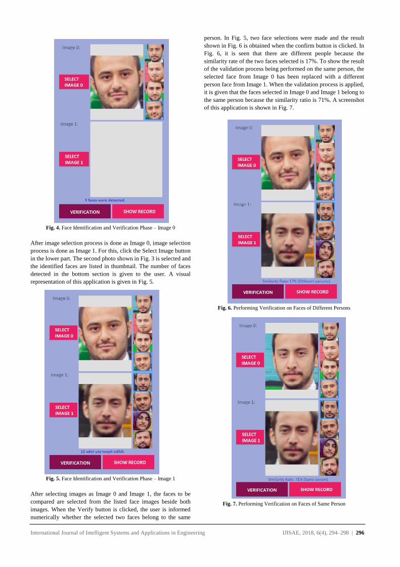
International Journal of Intelligent Systems and Applications in Engineering IJISAE, 2018, 6(4), 294–298 | 296
Fig. 4. Face Identification and Verification Phase – Image 0
After image selection process is done as Image 0, image selection
process is done as Image 1. For this, click the Select Image button
in the lower part. The second photo shown in Fig. 3 is selected and
the identified faces are listed in thumbnail. The number of faces
detected in the bottom section is given to the user. A visual
representation of this application is given in Fig. 5.
Fig. 5. Face Identification and Verification Phase – Image 1
After selecting images as Image 0 and Image 1, the faces to be
compared are selected from the listed face images beside both
images. When the Verify button is clicked, the user is informed
numerically whether the selected two faces belong to the same
person. In Fig. 5, two face selections were made and the result
shown in Fig. 6 is obtained when the confirm button is clicked. In
Fig. 6, it is seen that there are different people because the
similarity rate of the two faces selected is 17%. To show the result
of the validation process being performed on the same person, the
selected face from Image 0 has been replaced with a different
person face from Image 1. When the validation process is applied,
it is given that the faces selected in Image 0 and Image 1 belong to
the same person because the similarity ratio is 71%. A screenshot
of this application is shown in Fig. 7.
Fig. 6. Performing Verification on Faces of Different Persons
Fig. 7. Performing Verification on Faces of Same Person

International Journal of Intelligent Systems and Applications in Engineering IJISAE, 2018, 6(4), 294–298 | 297
Records of all transactions made are kept. A list of all the actions
performed when clicking the Show Record button is visible. In this
section where the records are displayed, information about resizing
of two images uploaded to the system, successful detection of the
images, the number of faces detected in the visuals, request for
sending the faces to be verified to the server, the status of the
returned response and the result of the response appear. Fig. 8
shows a screenshot of the system register with two
requests. The first response was successful and the result was
negative. The second response was successful and the result was
positive.
In practice, each process takes about 3 seconds, such as uploading
photos to the system, detecting and verifying faces in uploaded
photos because Microsoft Cognitive Services is used in the process
of performing transactions. An information screen informing the
user is developed as shown in Fig. 9.
Fig. 8. Screenshot of the system register
Fig. 9. User Information Screens
The determination of whether the system is stable or not has been
done on photographs containing more than one person. As shown
in Fig. 10, a test for face detection and verification of persons
labelled A, B, C, D, E was performed. This test involves comparing
each face in the photo with each other.
(a)
(b)
Fig. 10. Face detection and verification of persons
The result of this test is given in Table 1. The rows represent the
faces on the upper photo in Fig. 10 and the columns represent the
faces on the lower. Similarity ratios of 25% comparisons were
obtained. When the results obtained were observed, it was seen that
all persons were correctly verified.
Table 1. Similarity Rates after Verification Process
Faces in Fig. 10 (a)
A B C D E
Fac
es i
n F
ig. 10
(b
)
A
87 13 46 32 31
B
08 87 19 35 16
C
27 24 82 39 32
D
35 38 35 80 27
E
24 13 29 38 85
When the results obtained were observed, the highest similarity
rate was obtained as 87% for persons A and B. Despite being the
same person in both photographs, the similarity rate for D person
was 80%. Some of the reasons for the similarity ratio being
different are the effect of the person's posing position and light.

International Journal of Intelligent Systems and Applications in Engineering IJISAE, 2018, 6(4), 294–298 | 298
4. Conclusion
The Cognitive Services are very up - and - coming, assuring and
sum of these services are already being used in various application
areas. The dev elopers use these services to improve the
applications by adding some new, rich and intelligent features.
These services basically aim at providing more personal and rich
computing experiences for users as well as developers. The range
of application areas of these cognitive services is less but it can be
expanded by using their services along with other modern services
and techniques.
In this work, an Android application was developed that includes
face identification and authentication methods that can work on
mobile devices. The developed application provides a security
measure through its face identification and authentication feature.
This application can be integrated into various applications and
used in systems such as user login. User authentication can be
performed by scanning the user's face without the need for
password entry.
References
[1] F. C. Elbizim, M. C. Kasapbasi, (2017) Implementation and
Evaluation of Face Recognition Based Identification System,
International Journal of Intelligent Systems and Applications in
Engineering, pp. 17-20
[2] A. Eleyan, (2017) Simple and Novel Approach for Image
Representation with Application to Face Recognition, International
Journal of Intelligent Systems and Applications in Engineering, vol.
5(3), pp. 89-93.
[3] S. Nikan, M. Ahmadi, (2015) Performance Evaluation of Different
Feature Extractors and Classifiers for Recognition of Human Faces
with Low Resolution Images, International Journal of Intelligent
Systems and Applications in Engineering, vol. 3(2), pp. 72-77.
[4] W. Zhao, R. Chellappa, P. J. Phillips and A. Rosenfeld, 2003, “Face
Recognition: A Literature Survey”, ACM Computing. Surveys;
35(4): 399–458
[5] J. A. Lee, A. Szabo, Y. Li, (2013) AIR: An Agent for Robust Image
Matching and Retrieval, International Journal of Intelligent Systems
and Applications in Engineering, vol. 1(2), pp. 34-39.
[6] H. Mliki, E. Fendri, M. Hammami, 2015, “Face Recognition
Through Different Facial Expressions”, Journal of Signal Processing
Systems, vol 81(3), pp. 433-446.
[7] N. Delbiaggio, A comparison of facial recognition’s algorithms,
Bachelor's Degree, Haaga-Helia, 2017
[8] E. Sütçüler, 2006, “Real-Time Face Localization and Recognition
System by Using Video Sequences”, Msc Thesis, Yıldız Technical
University.
[9] P. Kirci, G. Kurt, (2016) Long Term and Remote Health Monitoring
with Smart Phones, International Journal of Intelligent Systems and
Applications in Engineering, vol. 4(4), pp. 80-83.
[10] G. Eryigit, G. Celikkaya, (2017) Use of NLP Techniques for an
Enhanced Mobile Personal Assistant: The Case of Turkish,
International Journal of Intelligent Systems and Applications in
Engineering, vol. 5(3), pp. 94-104.
[11] Beginning Android Programming with Android Studio, John Wiley
& Sons, 2016, ISBN: 1118707427, 9781118707425
[12] R. Arora, J. Sharma, U. Mali, A. Sharma, p. Raina (2018), Microsoft
Cognitive Services, International Journal of Engineering Science
and Computing, vol. 8(4), pp. 17323-17326.
[13] A. Del Sole, Introducing Microsoft Cognitive Services, In:
Microsoft Computer Vision APIs Distilled. Apress, Berkeley, CA,
https://doi.org/10.1007/978-1-4842-3342-9_1
[14] A.A. Vinay, S.S. Vinay, J.B. Rituparna, A. Tushar, K.N.
Balasubramanya Murthya, S. Natarajanb. (2015), Cloud Based Big
Data Analytics Framework for Face Recognition in Social Networks
using Machine Learning, 2nd International Symposium on Big Data
and Cloud Computing (ISBCC’15) .
[15] L. Larsen (2017), Learning Microsoft Cognitive Services - Create
intelligent apps with vision, speech, language, and knowledge
capabilities using Microsoft Cognitive Services, Packt Publishing
Ltd.
[16] Face Verification, https://azure.microsoft.com/tr-
tr/services/cognitive-services/face [Access Date: 05.01.2018]
[17] Genymotion User Guide – Version 2.11
https://docs.genymotion.com/pdf/PDF_User_Guide/Genymotion-
2.11-User-Guide.pdf [Access Date: 06.01.2018]
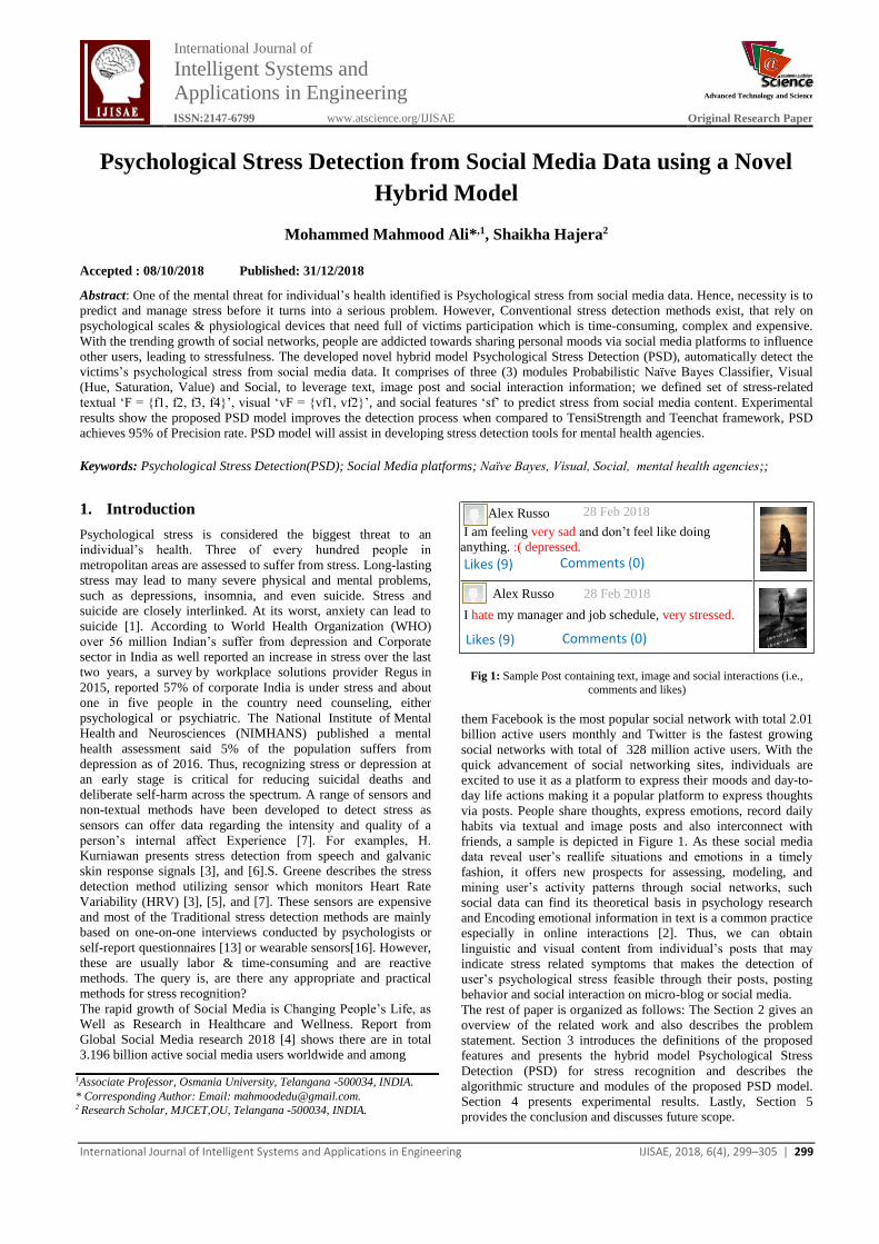
International Journal of
Intelligent Systems and
Applications in Engineering
Advanced Technology and Science
ISSN:2147-67992147-6799 www.atscience.org/IJISAE Original Research Paper
International Journal of Intelligent Systems and Applications in Engineering IJISAE, 2018, 6(4), 299–305 | 299
Psychological Stress Detection from Social Media Data using a Novel
Hybrid Model
Mohammed Mahmood Ali*,1, Shaikha Hajera2
Accepted : 08/10/2018 Published: 31/12/2018 DOI: 10.1039/b000000x
Abstract: One of the mental threat for individual’s health identified is Psychological stress from social media data. Hence, necessity is to
predict and manage stress before it turns into a serious problem. However, Conventional stress detection methods exist, that rely on
psychological scales & physiological devices that need full of victims participation which is time-consuming, complex and expensive.
With the trending growth of social networks, people are addicted towards sharing personal moods via social media platforms to influence
other users, leading to stressfulness. The developed novel hybrid model Psychological Stress Detection (PSD), automatically detect the
victims’s psychological stress from social media data. It comprises of three (3) modules Probabilistic Naïve Bayes Classifier, Visual
(Hue, Saturation, Value) and Social, to leverage text, image post and social interaction information; we defined set of stress-related
textual ‘F = {f1, f2, f3, f4}’, visual ‘vF = {vf1, vf2}’, and social features ‘sf’ to predict stress from social media content. Experimental
results show the proposed PSD model improves the detection process when compared to TensiStrength and Teenchat framework, PSD
achieves 95% of Precision rate. PSD model will assist in developing stress detection tools for mental health agencies.
Keywords: Psychological Stress Detection(PSD); Social Media platforms; Naïve Bayes, Visual, Social, mental health agencies;;
1. Introduction
Psychological stress is considered the biggest threat to an
individual’s health. Three of every hundred people in
metropolitan areas are assessed to suffer from stress. Long-lasting
stress may lead to many severe physical and mental problems,
such as depressions, insomnia, and even suicide. Stress and
suicide are closely interlinked. At its worst, anxiety can lead to
suicide [1]. According to World Health Organization (WHO)
over 56 million Indian’s suffer from depression and Corporate
sector in India as well reported an increase in stress over the last
two years, a survey by workplace solutions provider Regus in
2015, reported 57% of corporate India is under stress and about
one in five people in the country need counseling, either
psychological or psychiatric. The National Institute of Mental
Health and Neurosciences (NIMHANS) published a mental
health assessment said 5% of the population suffers from
depression as of 2016. Thus, recognizing stress or depression at
an early stage is critical for reducing suicidal deaths and
deliberate self-harm across the spectrum. A range of sensors and
non-textual methods have been developed to detect stress as
sensors can offer data regarding the intensity and quality of a
person’s internal affect Experience [7]. For examples, H.
Kurniawan presents stress detection from speech and galvanic
skin response signals [3], and [6].S. Greene describes the stress
detection method utilizing sensor which monitors Heart Rate
Variability (HRV) [3], [5], and [7]. These sensors are expensive
and most of the Traditional stress detection methods are mainly
based on one-on-one interviews conducted by psychologists or
self-report questionnaires [13] or wearable sensors[16]. However,
these are usually labor & time-consuming and are reactive
methods. The query is, are there any appropriate and practical
methods for stress recognition?
The rapid growth of Social Media is Changing People’s Life, as
Well as Research in Healthcare and Wellness. Report from
Global Social Media research 2018 [4] shows there are in total
3.196 billion active social media users worldwide and among
Fig 1: Sample Post containing text, image and social interactions (i.e.,
comments and likes)
them Facebook is the most popular social network with total 2.01
billion active users monthly and Twitter is the fastest growing
social networks with total of 328 million active users. With the
quick advancement of social networking sites, individuals are
excited to use it as a platform to express their moods and day-to-
day life actions making it a popular platform to express thoughts
via posts. People share thoughts, express emotions, record daily
habits via textual and image posts and also interconnect with
friends, a sample is depicted in Figure 1. As these social media
data reveal user’s reallife situations and emotions in a timely
fashion, it offers new prospects for assessing, modeling, and
mining user’s activity patterns through social networks, such
social data can find its theoretical basis in psychology research
and Encoding emotional information in text is a common practice
especially in online interactions [2]. Thus, we can obtain
linguistic and visual content from individual’s posts that may
indicate stress related symptoms that makes the detection of
user’s psychological stress feasible through their posts, posting
behavior and social interaction on micro-blog or social media.
The rest of paper is organized as follows: The Section 2 gives an
overview of the related work and also describes the problem
statement. Section 3 introduces the definitions of the proposed
features and presents the hybrid model Psychological Stress
Detection (PSD) for stress recognition and describes the
algorithmic structure and modules of the proposed PSD model.
Section 4 presents experimental results. Lastly, Section 5
provides the conclusion and discusses future scope.
I am feeling very sad and don’t feel like doing
anything. :( depressed.
I hate my manager and job schedule, very stressed.
1Associate Professor, Osmania University, Telangana -500034, INDIA.
* Corresponding Author: Email: [email protected]. 2 Research Scholar, MJCET,OU, Telangana -500034, INDIA.
Alex Russo 28 Feb 2018
Comments (0) Likes (9)
Alex Russo 28 Feb 2018
Likes (9) Comments (0)

International Journal of Intelligent Systems and Applications in Engineering IJISAE, 2018, 6(4), 299–305 | 300
2. Related Work And Problem Defination
There have been research efforts on harnessing social media data
for developing mental and physical healthcare tools. K. Lee
et.al’s [8] proposed to leverage social media data for real-time
disease investigation; while [10] tried to link the vocabulary gaps
between health seekers and providers using the community
generated health data. Psychological stress detection is
interrelated to the topics of sentiment assessment and emotion
recognition. Our recent work [25] presented relative analysis of
various psychological stress recognition Approaches. Study on
Emotion Detection in Social Networks, Computer-aided
recognition, scrutiny, and application of emotion, especially in
social media, have drawn considerable attention in current years
[11], [12], and [15]. Associations between psychological stress
and personality traits can be a thought-provoking issue to
contemplate [17], [18], and [20]. Several studies on social
networks based emotion analysis uses text-based linguistic
features and typical classification approaches. As discussed
above a range of sensors and non-textual methods have been
developed to detect stress but they are expensive. With the
development of social networks people are willing to share their
daily events and moods, and interact with friends through the
social networks, making it possible to leverage online social
network data for stress detection. There are also some exploration
[22], and [27] using user posting contents on social network to
identify user’s stress revealed that leveraging this social media
data for healthcare, and in particular stress detection, is feasible.
However, these mechanisms mainly leverage the textual contents
and consider only single post of an individual in social networks.
In certainty, data in social networks are typically composed of
chronological and inter-connected items from diverse sources i.e.,
it also contains images posts apart from textual posts, making it
be actually multi-media data and single post reflects the instant
emotion but people’s emotion or psychological stress states are
habitually more persistent, fluctuating over different time periods.
In recent years, extensive study started to focus on emotion
detection in social networks from sequential post series [21],
[23], and [24]. Our work is to leverage sequential post (multi-
media data) content over specific sampling period to detect stress.
The proposed novel hybrid model Psychological Stress Detection
(PSD) defines set of stress-related textual ‘F = {f1, f2, f3, f4}’,
visual ‘vF = {vf1, vf2}’, and social ‘sf’ features that makes the
detection efficient and effective leveraging textual and visual post
content.
Before presenting our problem definition, let’s first define
necessary notations. Let P be a set of users posts on a social
media network i.e., pi ∈ P. Let U be set of users. Each user ui ∈
U, posts on social media containing text, image. Where i denotes
number of posts and users that can range from 1 to ‘n’ i.e., i = {1,
2, 3, …, n}.
Stress state: stress state denoted by‘s’ of user ui ∈ U at
time t is represented as a triple (s, ui, t), or . In the study,
a binary stress state ∈ {0, 1} is considered, where = 1
specifies that user ui is stressed at time t, and = 0
specifies that the user is non-stressed at time t.
Stress feature set: Let F, vF and sf be the stress feature sets
in study i.e., F = {f1, f2, f3, f4}, vF ={vf1,vf2}, sf , where
f1 – f4 are linguistic stress lexicon features, vf1 and vf2 are
visual features and sf is social feature as shown above in
table 4.2.(page number 19).
Problem Statement: To Detect Psychological Stress state
‘s’ Given a series of user posts P. To address this problem
we first define the stress feature sets they are Textual
feature (F), Visual feature (vF) and social feature (sf) then
propose Psychological Stress Detection (PSD) model to
leverage the social media content for stress detection.
3. Proposed Psychological Stress Detection (PSD)
Model
3.1. Feature Categorizations
To cope with the problem of psychological stress detection we
have defined set of stress-related textual ‘F = {f1, f2, f3, f4}’,
visual ‘vF = {vf1, vf2}’, social ‘sf’ features. Table 1 shows
categorization of these features. Textual Feature is a set of four
features, F = {f1, f2, f3, f4}, these feature stores word count of a
particular sentence comparing them with linguistic stress lexicon
explained in Table 1. ‘f1’ stores number of stress and negative
words present in the sentence posted. ‘f2’ stores number of
positive emotion words present in the sentence posted, ‘f3’ stores
negative emoticons if present and ‘f4’ stores negating words
present in the sentence posted. These features help the
probabilistic module in calculating the probability of each class
and labeling the textual post to its particular class as shown in
Figure 4.
Visual Feature is a set of two features, vF = {vf1, vf2} they stores
the mean value of the brightness and saturation, which is
calculated in the visual module algorithm as shown in Figure 5.
Value of Image brightness and saturation will be compared with
threshold value to categorize the particular image post as stress or
non-stress as shown in Figure 3. Social Feature ‘sf’ stores the
mean value of number of likes a particular post gets it give us the
social attention degree that means when user posts are negative or
stressful it gets more attention from the friends of that particular
user via likes or comments. Thus, we will find the mean of
number of likes and categories the posts accordingly as shown in
Figure 3.
The detail Architecture of the model is shown in the Figure 2.
Psychological stress detection has many challenges to overcome
them first have categorized features as discussed in section 3.1,
now will design modules to utilize these features for stress
detection. Probabilistic module fetches textual feature ‘F = {f1,
f2, f3, f4}’, from content of user’s post comparing with
Linguistic Stress Lexicon. Visual module fetches visual features
‘vF = {vf1, vf2}’ from image post, and Social module will fetch
social attention feature ‘sf’ as discussed in section 3.1.
3.2. Architecture
Figure 2 shows the architecture of our model. There are three
types of information that we can use as the initial inputs, i.e.,
Textual features, Visual features and Social features whose
detailed computation will be described later. We address the
solution through the following three key modules:
Design the Probabilistic module to fetch textual feature ‘F
= {f1, f2, f3, f4}’, from content of user’s post comparing
with Linguistic Stress Lexicon.
Visual module fetches visual features ‘vF = {vf1, vf2}’
from image post, and
Social module fetches social attention feature ‘sf’ as
discussed in section 3.1.
Steps involved in the architecture of the proposed system are as
follows:
i. The first step captures the Post and messages sent
between the users of Social Networking Site (SNS).
These messages are saved in the database.
ii. In this step, a text post is taken and this text message is
converted to plain text removing stop-words (such as
articles, preposition). Next, will check if the user has
also posted an image if yes, then will send it to visual
module to process its mean value of brightness and
saturation. Next, will check social attention feature to
calculate the mean of likes.
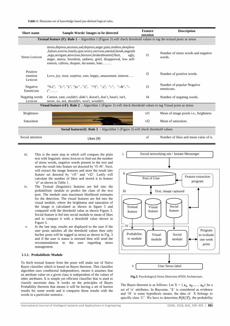
International Journal of Intelligent Systems and Applications in Engineering IJISAE, 2018, 6(4), 299–305 | 301
Table 1: Illustrates set of knowledge based pre-defined logical rules.
Short name Sample Words/ Images to be detected Feature
notation Description
Textual feature (F): Rule 1 – Algorithm 1 (Figure 3) will check threshold values to tag the textual posts as stress
Stress Lexicon
stress,depress,anxious,sad,depress,anger,pain,restless,sleepless
,failure,sorrow,lonely,quit,worry,nervous,mental,break,anguish
,argu,arrogant,atrocious,bereave,brokenhearted,Hurt, ugly,
anger, annoy, boredom, sadness, grief, disapproval, low self-
esteem, callous, despair, devastate, hate……..
f1 Number of stress words and negative
words.
Positive
emotion
Lexicon
Love, joy, trust, surprise, care, happy, amazement, interest….. f2 Number of positive words.
Negative
Emoticons
"%-(", ")-:", "):", ")o:" , ":(", ":*(", ":,(", ":-", ":-&", ":-
("……. f3
Number of popular Negative
emoticons.
Negating words
Lexicon
Cannot, cant, couldn't, didn’t, doesn't, don’t, hasn't, isn't,
never, no, not, shouldn't, won't, wouldn't. f4 Number of negating words.
Visual feature (vF): Rule 2 - Algorithm 1 (Figure 3) will check threshold values to tag Visual posts as stress
Brightness vf1 Mean of image pixels i.e., brightness
Saturation vf2 Mean of saturation.
Social feature(sf): Rule 3 - Algorithm 1 (Figure 3) will check threshold values
Social attention sf Number of likes and mean value of it.
iii. This is the main step in which will compare the plain
text with linguistic stress lexicon to find out the number
of stress words, negative words present in the text and
store the result into feature set denoted by ‘f1-f4’. Next,
will extract the image features and store the result into
feature set denoted by ‘vf1’ and ‘vf2’. Lastly will
calculate the number of likes and stored it in feature
‘sf’ as shown in Table 1.
iv. The Textual (linguistic) features are fed into the
probabilistic module to predict the class of the text
post. The module uses maximum likelihood estimates
for the detection. The visual features are fed into the
visual module, where the brightness and saturation of
the image is calculated as shown in figure 5 and
compared with the threshold value as shown Figure 3.
Social feature is fed into social module to mean of likes
and to compare it with a threshold value shown in
Figure 3.
v. In the last step, results are displayed to the user if the
user posts satisfies all the threshold values then only
his/her posts will be tagged as stress as shown in Fig. 3
and if the user is status is stressed then will send the
recommendation to the user regarding stress
management.
1.1.1. Probabilistic Module
To fetch textual feature from the posts will make use of Naïve
Bayes classifier which is based on Bayes theorem. This classifier
algorithm uses conditional independence, means it assumes that
an attribute value on a given class is independent of the values of
other attributes. It is simple yet efficient classifier that is used to
classify uncertain data. It works on the principles of Bayes
Probability theorem that means it will be having a set of known
results for some words and it compares those results with the
words in a particular sentence.
Fig.2: Psychological Stress Detection (PSD) Architecture.
The Bayes theorem is as follows: Let X = { } be a
set of ‘n’ attributes. In Bayesian, ‘X’ is considered as evidence
and ‘H’ is some hypothesis means, the data of X belongs to
specific class ‘C’. We have to determine , the probability
Likes (9)
Social networking site / Instant Messenger
Feature extraction
program Post of User
Social
feature
Textual
feature
Visual
feature
Program
to evaluate
one week
posts
User Stress label
Text, image captured
Probabilist
-ic module
Visual
module Social
module
i
ii
iii
iv
v

International Journal of Intelligent Systems and Applications in Engineering IJISAE, 2018, 6(4), 299–305 | 302
that the hypothesis H holds given evidence i.e. data sample X
[30]. According to Bayes theorem the is expressed as
shown in equation 1 or 2.
or
Where is any one of the class in the list i.e., ‘No-Stress’,
‘Stress’ and Neutral. - are Number of words in the given
sentence, here wordn = fn, where n = 4 refer Table 1. If textual
feature fetched from the given sentence matches the words in the
linguistic stress lexicon explained in Table 1 will assign class to
that sentence according to the probability score of each class.
The detail computation of probabilistic module is shown in
Probabilistic Module Algorithm Figure 4. As discussed in section
3.1 the textual Feature are a set of four features, F = {f1, f2, f3,
f4}, these feature stores word count of a particular sentence
comparing them with linguistic stress lexicon explained in Table
1. ‘f1’ stores number of stress and negative words present in the
sentence posted. ‘f2’ stores number of positive emotion words
present in the sentence posted, ‘f3’ stores negative emoticons if
present and ‘f4’ stores negating words present in the sentence
posted. These features help the probability module in labeling the
posted sentence is having stress or non-stress by calculating the
probability of each class.
3.2.1. Visual Module
Based on previous work on color psychology theories [28], we
combine the following features as the visual middle-level
representation: - Saturation: the mean value of saturation and its
contrast. It describes the colorfulness and the differences of an
image. Psychological experiments in S. R. Ireland’s [29] find out
that people under stress and anxiety prefer lower saturation than
normal states, revealing the correlation between stress and
saturation of images. Brightness: the mean value of brightness
and its contrast. It illustrates the perception elicited by the
luminance and the related differences of an image (e.g., low
brightness makes people feel negative, while high brightness
elicits mainly positive emotional associations). To calculate
image brightness first, we need to (briefly) analyze what is the
result of the average value of the sum of the RGB channels. For
humans, it is meaningless. Is pink brighter than green ? I.e., why
would you want (0, 255, 0) to give a lower brightness value than
(255, 0, 255) ? Also, is a mid gray (128, 128, 128) bright just like
a mid green (128, 255, 0) ? To take this into consideration, I only
deal with the color brightness of the channel as is done in the
HSV color space [14]. This is simply the maximum value of a
given RGB triplet. The rest is heuristics. Let max_rgb = max
(RGB-i) for some point i. If max_rgb is lower than 128
(assuming a 8bpp image), then we found a new point i that is
dark, otherwise it is light. Doing this for every point i, we
get A points that are light and B points that are dark. If (A - B)/(A
+ B) >= 0.5 then we say the image is light. Note that if every
point is dark, then you get a value of -1, conversely if every point
is light you get +1. The previous formula can be tweaked so you
can accept images barely dark. In the code I named the variable
as fuzzy, but it does no justice to the fuzzy field in Image
Processing. So, we say the image is light if (A - B)/(A + B) +
fuzzy >= 0.5.Following is the mathematical relationship between
RGB space to HSI (hue, saturation, and intensity) or Hue,
Saturation, Value (HSV) color space model.
• Brightness or Intensity formula
• Saturation formula
Where vf1 is brightness or Intensity and vf2 is saturation as
shown in equation 3 and 4. The detail computation of visual
module is shown in Visual Module Algorithm figure 5. Visual
Feature is a set of two features, vF = {vf1, vf2} they stores the
mean value of the brightness and saturation, which is calculated
in the visual module algorithm. Value of Image brightness and
saturation will be compared with threshold value to categorize the
particular image post as stress or non-stress as shown in Figure 3.
3.2.2. Social Module
Besides the text content and image content of a post, some
additional features such as likes can also imply one’s stress state
to some degree. We define a post’s social attention degree based
on these additional features into social attributes. As apparently
stressful posts may attract more attention from friends. The
number of comments, likes reveals how much attention a post
attracts. To find out the changes of attention degree of one’s post,
we first calculate the sample mean sf shown in equation 5, all M -
values and total number of items in the samples.
Social Feature ‘sf’ stores the mean value of number of likes a
particular post gets it give us the social attention degree that
means when user posts are negative or stressful it gets more
attention from the friends of that particular user via likes or
comments. Thus, we will find the mean of number of likes and
categories the posts accordingly as shown in Figure 3.
Algorithm 1: Psychological stress Detector (PSD) Algorithm
Require: pi, ui, (Social media posts P of users U).
Ensure: ‘s’ (Detection of Stress state i.e., stress or non-stress)
1 Initialize P, U, s = {stress , non-stress}, F ,vF ,sf .
2 u = getusername() //getusername function returns
current user name
3 While(i < U and P != NULL ) do
4 F = Stress (P) //stress function of probability module calculates
stress from textual posts and return stress state
5 vF = getImageLightness (image) //getImageLightness function of visual module calculates and return image brightness
6 sf = num_likes() //num_likes function of social module calculates
and return number of likes and mean value of the likes.
7 if(F = 1 and vF <= 0.5 or sf >= 5) then //To display stress status
for a week.
8 stress_status = stress //tag that user having
stress
9 //if the user have more than five posts tagged as stress in a week then system will display result as stress.
if(loggedin_user == u and stress_status >= 5 ) then
10 s = stress //stress state
11 else
12 s = non-stress //stress state
13 end if
14 end if
15 end while
Fig.3: Psychological Stress Detection (PSD) Algorithm.
(1)
(2)
(3)
(4)
(5)
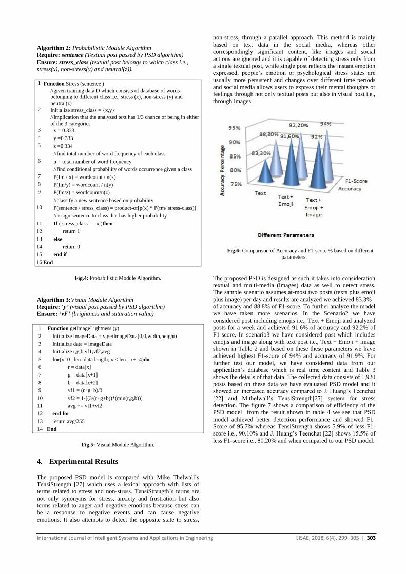
International Journal of Intelligent Systems and Applications in Engineering IJISAE, 2018, 6(4), 299–305 | 303
Algorithm 2: Probabilistic Module Algorithm
Require: sentence (Textual post passed by PSD algorithm)
Ensure: stress_class (textual post belongs to which class i.e.,
stress(x), non-stress(y) and neutral(z)).
1 Function Stress (sentence )
//given training data D which consists of database of words belonging to different class i.e., stress (x), non-stress (y) and
neutral(z)
2 Initialize stress_class = {x,y}
//Implication that the analyzed text has 1/3 chance of being in either
of the 3 categories 3 x = 0.333
4 y =0.333
5 z =0.334
//find total number of word frequency of each class
6 n = total number of word frequency
//find conditional probability of words occurrence given a class
7 P(fm / x) = wordcount / n(x)
8 P(fm/y) = wordcount / n(y)
9 P(fm/z) = wordcount/n(z)
//classify a new sentence based on probability
10 P(sentence / stress_class) = product-of[p(x) * P(fm/ stress-class)]
//assign sentence to class that has higher probability
11 If ( stress_class == x )then
12 return 1
13 else
14 return 0
15 end if
16 End
Fig.4: Probabilistic Module Algorithm.
Algorithm 3:Visual Module Algorithm
Require: ‘y’ (visual post passed by PSD algorithm)
Ensure: ‘vF’ (brightness and saturation value)
1 Function getImageLightness (y)
2 Initialize imageData = y.getImageData(0,0,width,height)
3 Initialize data = imageData
4 Initialize r,g,b,vf1,vf2,avg
5 for(x=0 , len=data.length; x < len ; x+=4)do
6 r = data[x]
7 g = data[x+1]
8 b = data[x+2]
9 vf1 = (r+g+b)/3
10 vf2 = 1-[(3/(r+g+b))*(min(r,g,b))]
11 avg += vf1+vf2
12 end for
13 return avg/255
14 End
Fig.5: Visual Module Algorithm.
4. Experimental Results
The proposed PSD model is compared with Mike Thelwall’s
TensiStrength [27] which uses a lexical approach with lists of
terms related to stress and non-stress. TensiStrength’s terms are
not only synonyms for stress, anxiety and frustration but also
terms related to anger and negative emotions because stress can
be a response to negative events and can cause negative
emotions. It also attempts to detect the opposite state to stress,
non-stress, through a parallel approach. This method is mainly
based on text data in the social media, whereas other
correspondingly significant content, like images and social
actions are ignored and it is capable of detecting stress only from
a single textual post, while single post reflects the instant emotion
expressed, people’s emotion or psychological stress states are
usually more persistent and changes over different time periods
and social media allows users to express their mental thoughts or
feelings through not only textual posts but also in visual post i.e.,
through images.
Fig.6: Comparison of Accuracy and F1-score % based on different parameters.
The proposed PSD is designed as such it takes into consideration
textual and multi-media (images) data as well to detect stress.
The sample scenario assumes at-most two posts (texts plus emoji
plus image) per day and results are analyzed we achieved 83.3%
of accuracy and 88.8% of F1-score. To further analyze the model
we have taken more scenarios. In the Scenario2 we have
considered post including emojis i.e., Text + Emoji and analyzed
posts for a week and achieved 91.6% of accuracy and 92.2% of
F1-score. In scenario3 we have considered post which includes
emojis and image along with text post i.e., Text + Emoji + image
shown in Table 2 and based on these these parameters we have
achieved highest F1-score of 94% and accuracy of 91.9%. For
further test our model, we have considered data from our
application’s database which is real time content and Table 3
shows the details of that data. The collected data consists of 1,920
posts based on these data we have evaluated PSD model and it
showed an increased accuracy compared to J. Huang’s Teenchat
[22] and M.thelwall’s TensiStrength[27] system for stress
detection. The figure 7 shows a comparison of efficiency of the
PSD model from the result shown in table 4 we see that PSD
model achieved better detection performance and showed F1-
Score of 95.7% whereas TensiStrength shows 5.9% of less F1-
score i.e., 90.10% and J. Huang’s Teenchat [22] shows 15.5% of
less F1-score i.e., 80.20% and when compared to our PSD model.
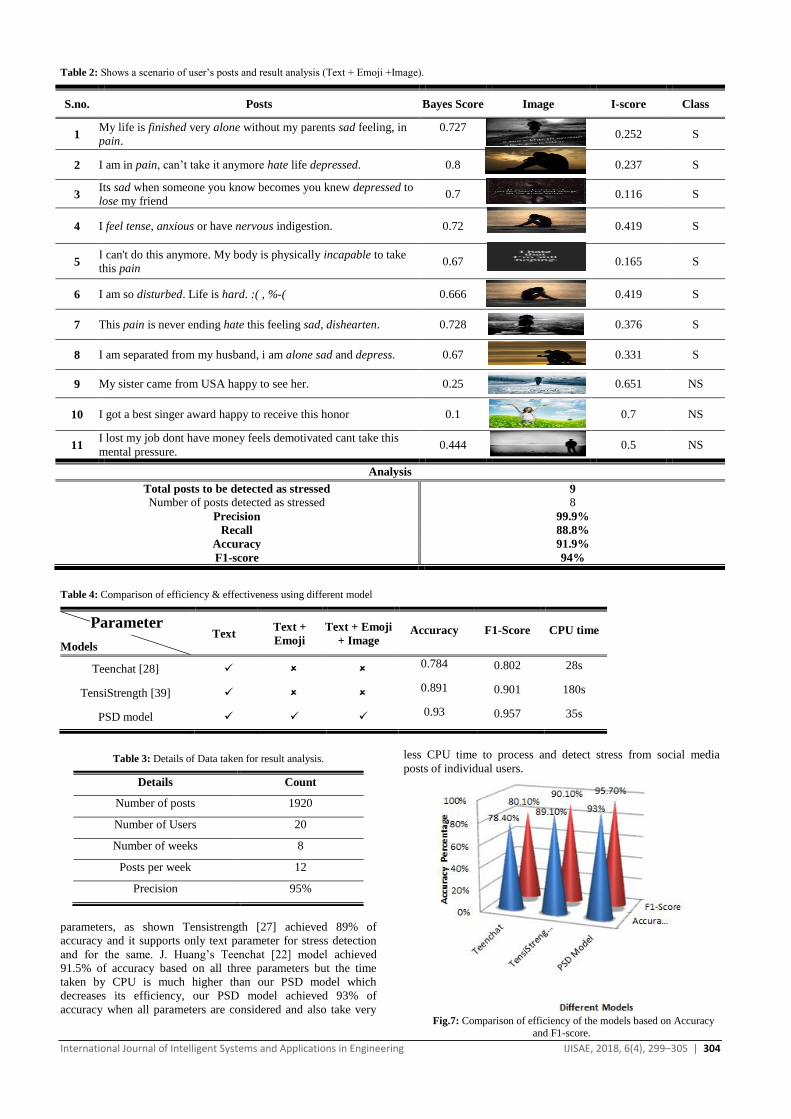
International Journal of Intelligent Systems and Applications in Engineering IJISAE, 2018, 6(4), 299–305 | 304
Table 2: Shows a scenario of user’s posts and result analysis (Text + Emoji +Image).
S.no. Posts Bayes Score Image I-score Class
1 My life is finished very alone without my parents sad feeling, in
pain.
0.727
0.252 S
2 I am in pain, can’t take it anymore hate life depressed. 0.8
0.237 S
3 Its sad when someone you know becomes you knew depressed to
lose my friend 0.7
0.116 S
4 I feel tense, anxious or have nervous indigestion. 0.72
0.419 S
5 I can't do this anymore. My body is physically incapable to take
this pain 0.67
0.165 S
6 I am so disturbed. Life is hard. :( , %-( 0.666
0.419 S
7 This pain is never ending hate this feeling sad, dishearten. 0.728
0.376 S
8 I am separated from my husband, i am alone sad and depress. 0.67
0.331 S
9 My sister came from USA happy to see her. 0.25
0.651 NS
10 I got a best singer award happy to receive this honor 0.1
0.7 NS
11 I lost my job dont have money feels demotivated cant take this
mental pressure. 0.444
0.5 NS
Analysis
Total posts to be detected as stressed 9
Number of posts detected as stressed 8
Precision 99.9%
Recall 88.8%
Accuracy 91.9%
F1-score 94%
Table 4: Comparison of efficiency & effectiveness using different model
Models Text
Text +
Emoji
Text + Emoji
+ Image Accuracy F1-Score CPU time
Teenchat [28] 0.784 0.802 28s
TensiStrength [39] 0.891 0.901 180s
PSD model 0.93 0.957 35s
Table 3: Details of Data taken for result analysis.
Details Count
Number of posts 1920
Number of Users 20
Number of weeks 8
Posts per week 12
Precision 95%
parameters, as shown Tensistrength [27] achieved 89% of
accuracy and it supports only text parameter for stress detection
and for the same. J. Huang’s Teenchat [22] model achieved
91.5% of accuracy based on all three parameters but the time
taken by CPU is much higher than our PSD model which
decreases its efficiency, our PSD model achieved 93% of
accuracy when all parameters are considered and also take very
less CPU time to process and detect stress from social media
posts of individual users.
Fig.7: Comparison of efficiency of the models based on Accuracy
and F1-score.
Parameter

International Journal of Intelligent Systems and Applications in Engineering IJISAE, 2018, 6(4), 299–305 | 305
5. Conclusion
Psychological Stress is an increasing problem in the world, it is
essential to monitor and control it regularly. In this paper, we
presented a Model for detecting user’s stress status from user’s
daily social media data, leveraging post’s content along with
user’s social interactions. The inefficiency of the conventional
methods [5], [16], [19], [22], and [27] motivates to adopt a novel
technique which is transparent and inexpensive. Similar to our
another ontological approach is developed for stress detection
that works better on Textual stress words [31]. Thus, the
proposed strategy utilizes not only social media data (text and
images), but also uses social interaction content to detect
psychological stress employing a Novel Hybrid model i.e.,
Psychological Stress Detection (PSD). To completely leverage
user’s posts content, we proposed a hybrid PSD model which
combines the probabilistic module (Bayes classifier) with the
visual module (HSV model). In our model the user’s stress states
are monitored daily, weekly, bi-weekly or monthly so that it
improves the accuracy of stress detection at different levels.
Experimental results show that the proposed model can improve
the detection performance when compared to J. Huang’s
Teenchat [22], and TensiStrength [27], and achieved 95% of
precision and 93% of accuracy.
5.1 Future Scope
Recent studies show apart from leveraging cross-media content
and social interactions, Social Connectivity also plays a vital role
in detecting stress states of an individual, which is a useful
reference for future related studies. Some more useful references
for future related studies:
Need to explore our research on stressor responsible for
stress as it is noteworthy to know the type of stress the
user is dealing.
Support for short form and slang language used in text
post to be included.
Support for Multilingual languages to be included.
References
[1] J. Herbert, “Fortnightly review: Stress, the brain, and mental
illness”, British Medical J., pp. 530–535, Vol. 315, No. 7107, 1997.
[2] Liew, and Jasy Suet Yan, “fine-grained emotion detection in
microblog text”, Dissertations – ALL. pp 440, 2016. [3] F.-T. Sun, C. Kuo, H.-T. Cheng, S. Buthpitiya, P. Collins, and M.
L. Griss, “Activity-Aware Mental Stress Detection Using
Physiological Sensors”, In Proc. Of Intl. Conf. on Mobile Computing, Application, and Services (MobiCASE), Santa Clara,
CA, 2010.
[4] Social,https://www.smartinsights.com/social-media-marketing/social-media-strategy/new-global-social-media-
research.(online).
[5] H. Kurniawan, A.V. Maslov, and M. Pechenizkiy, “Stress detection from speech and galvanic skin response signals”, in:
Proceedings of the 26th IEEE International Symposium on
Computer-Based Medical Systems, pp. 209–214, 2013. [6] V.P. Patil, K.K. Nayak, and M. Saxena, “Voice stress detection”,
Int. J. Electr. Electron. Comput. Eng., pp. 148–154, 2013.
[7] S. Greene, H. Thapliyal, and A. C. Holt, “A survey of affective computing for stress detection: Evaluating technologies in stress
detection for better health”, IEEE Consum. Electron. Mag., Vol. 5, No. 4, pp. 44–56, 2016.
[8] K. Lee, A. Agrawal, and A. Choudhary, “Real-time disease
surveillance using twitter data: Demonstration on FLU and cancer”, in Proc. ACM SIGKDD Int. Conf. Knowl. Discovery
Data Mining, pp. 1474–1477, 2013.
[9] Sztajzel, “Heart rate variability: a noninvasive electrocardiographic method to measure the autonomic nervous
system”, Swiss Med. Weekly, pp. 514–522, 2004.
[10] L. Nie, Y.-L. Zhao, M. Akbari, J. Shen, and T.-S. Chua, “Bridging
the vocabulary gap between health seekers and healthcare
knowledge,” IEEE Trans. Knowl. Data Eng., vol. 27, no. 2, pp.
396–409, Feb. 2015.
[11] G. Coppersmith, C. Harman, and M. Dredze, “Measuring post
traumatic stress disorder in twitter,” in Proc. Int. Conf. Weblogs
Soc. Media, 2014, pp. 579–582.
[12] R. Fan, J. Zhao, Y. Chen, and K. Xu, “Anger is more influential
than joy: Sentiment correlation in weibo,” PLoS One, vol. 9, 2014,
Art. no. e110184.
[13] Stressassessments,https://www.nysut.org/~/media/files/nysut/resou
rces/2013/april/socialservices/socialservices_stressassessments.pdf?la=e.(online).
[14] HSV,
https://shodhganga.inflibnet.ac.in/bitstream/10603/18613/12/12_chapert-3 (online).
[15] Y. Zhang, J. Tang, J. Sun, Y. Chen, and J. Rao, “Moodcast:
Emotion prediction via dynamic continuous factor graph model,”
Proc. IEEE 13th Int. Conf. Data Mining, 2010, pp. 1193–1198.
[16] A. Sano, and R. W. Picard, “Stress recognition using wearable sensors and mobile phones”, In Proceedings of ACII, pp. 671–676,
2013.
[17] G. Farnadi, et al., “Computational personality recognition in social
media,” UserModel User-Adapted Interaction, vol. 26, pp. 109–
142, 2016.
[18] J. Golbeck, C. Robles, M. Edmondson, and K. Turner, “Predicting
personality from Twitter,” in Proc. IEEE 3rd Int. Conf. Privacy,
Security, Risk Trust, IEEE 3rd Int. Conf. Soc. Comput., 2011, pp.
149–156.
[19] A. Fernandes, R. Helawar, R. Lokesh, T. Tari, and A. V. Shahapurkar, “Determination of stress using blood pressure and
galvanic skin response”, In Proceedings of the International
Conference on Communication and Network Technologies (ICCNT’14), pp. 165–168, Sivakasi, India, 2014.
[20] B. Verhoeven, W. Daelemans, and B. Plank, “Twisty: A
multilingual twitter stylometry corpus for gender and personality
profiling,” in Proc. 10th Int. Conf. Language Resources Eval., PP.
1632–1637 2016.
[21] F. A. Pozzi, D. Maccagnola, E. Fersini, and E. Messina, “Enhance
user-level sentiment analysis on microblogs with approval
relations,” in Proc. 13th Int. Conf. AI* IA: Advances Artif. Intell.,
PP. 133–144, 2013.
[22] J. Huang, Q. Li, Y. Xue, T. Cheng, S. Xu, J. Jia, and L. Feng.:
“Teenchat: a chatterbot system for sensing and releasing
adolescents’ stress”, In: X. Yin, K. Ho, D. Zeng, U. Aickelin, R. Zhou, H. Wang. (eds.) HIS LNCS, Vol. 9085, pp. 133–145.
Springer, Heidelberg, 2015.
[23] C. Tan, L. Lee, J. Tang, L. Jiang, M. Zhou, and P. Li, “User-level
sentiment analysis incorporating social networks,” in Proc.
SIGKDD Int. Conf. Knowl. Discovery Data Mining, 2011, pp.
1397–1405.
[24] J.W. Pennebaker, R.J. Booth, and M.E. Francis, “Linguistic
Inquiry and Word Count (LIWC)”, 2007. [25] Shaikha Hajera and Mohammed Mahmood Ali, “A Comparative
Analysis of Psychological Stress Detection Methods”, In IJCEM,
Vol. 21 Issue 2, March 2018. [26] Y.R. Tausczik, and J. W. Pennebaker, “The psychological
meaning of words: LIWC and computerized text analysis
methods”, Journal of Language and Social Psychology, pp. 24-54, 2010.
[27] Thelwall M. “TensiStrength: stress and relaxation magnitude
detection for social media texts”, J Inf Process Manag pp: 106–121, 2017.
[28] X. Wang, J. Jia, H. Liao, and L. Cai, “Affective image
colorization”, Journal of Computer Science and Technology, Vol. 27, No. 6, pp. 1119-1128, 2012.
[29] S. R. Ireland, Y. M. Warren, and L. G. Herringer, “Anxiety and
color saturation preference”, Perceptual and Motor Skills, Vol. 75, pp. 545-546, 1992.
[30] Keogh, Eamonn, “Naive bayes classifier” Accessed: Sept. 1
(2006): 2018. [31] Mohammed Mahmood Ali, Mohd Tajuddin, and M Kabee, “SDF:
psychological Stress Detection Framework from Microblogs using
Predefined rules and Ontologies”, International Journal of Intelligent Systems and Applications in Engineering, Vol. 6, issue
2, pp. 158-164, 2018.

International Journal of
Intelligent Systems and
Applications in Engineering
Advanced Technology and Science
ISSN:2147-67992147-6799 www.atscience.org/IJISAE Original Research Paper
International Journal of Intelligent Systems and Applications in Engineering IJISAE, 2018, 6(4), 306–310 | 306
A Modified Artificial Algae Algorithm for Large Scale Global
Optimization Problems
Havva Gul KOCER1, Sait Ali UYMAZ2
Accepted : 18/12/2018 Published: 31/12/2018 DOI: 10.1039/b000000x
Abstract: Optimization technology is used to accelerate decision-making processes and to increase the quality of decision making in
management and engineering problems. The development technology has made real world problems large and complex. Many optimization
methods that proposed for solving large-scale global optimization (LSGO) problems suffer from the “curse of dimensionality”, which
implies that their performance deteriorates quickly as the dimensionality of the search space increases. Therefore, more efficient and robust
algorithms are needed. When literature on large-scale optimization problems is examined, it is seen that algorithms with effective global
search ability have better results. For the purpose, in this paper Modified Artificial Algae Algorithm (MAAA) is proposed by modifying
original version of Artificial Algae Algorithm (AAA) inspiring by Differential Evolution Algorithm (DE)’s mutation strategies. AAA and
MAAA are compared with each other by operating with the first 10 benchmark functions of CEC2010 Special Session on Large Scale
Global Optimization. The results show that hybridization process that applied by updating an additional fourth dimension with mutation
strategies of DE after the helical motion of the AAA algorithm, contributes exploration phase and improves the AAA performance on
LSGO.
Keywords: artificial algae algorithm,CEC2010 benchmark,large scale global optimization
1. Introduction
There are various high dimensional problems in the modern world.
Because most modern data, such as computational biology, data
from consumer preferences, images, videos, are often high
dimensional. Optimization is a technique for solving problems and
it is the calculation of the parameters that will produce the best
result of a function. However, as the dimension of problem
increases, the process of reaching a definitive solution becomes
very complex, difficult and costly. This is because when the
dimensionality increases, the volume of the space increases
exponentially and probability of finding good solutions with
limited search amount decreases dramatically. R. Bellman used
"curse of dimensionality" term in the introduction of his book
“Dynamic programming” in 1957 for this situation [1]. This term
refers to the difficulties of finding optimum in high-dimensional
space using extensive search. Therefore, there is a need to use
effective and efficient new techniques beyond what exists to solve
large-scale optimization problems.
Metaheuristic methods that find the most suitable solution around
the real solution at an acceptable time, are preferred as an effective
solution technique for large-scale optimization problems. While
metaheuristic algorithms are shown excellent search abilities when
applied to some small dimensional problems, usually their
performance deteriorates quickly as the dimensionality of search
space increases. Therefore, a more efficient search strategy is
required to explore all the promising regions in a given time or
fitness evaluation count limits.
Some attempts have been made by the researchers, such as modify
original version of an algorithm [2,3], hybridize with another
algorithm [4], using additional local search methods [5,6] or
develop solution techniques [7] to make metaheuristic algorithms
suitable to overcome the difficulties of solving large-scale
optimization problems.
Inspired by Differential Evolution mutation strategies, this paper
presents an improved variant of the AAA algorithm called
Modified Artificial Algae Algorithm(MAAA) for solving large-
scale global optimization problems.
The rest of the paper is organized as follows. First, Artificial Algae
Algorithm, Differential Evolution are described briefly. Then
Modified Artificial Algae Algorithm is described. In the following
section benchmark set used in tests, parameters of algorithms and
working environment are analyzed. Finally, results and
interpretations are given and are followed by conclusions and
recommendations.
2. Artificial Algae Algorithm
Artificial Algae Algorithm (AAA) is a bio-inspired meta-heuristic
optimization algorithm designed to solve continuous and real-
value optimization problems. It is developed by inspiration of
foraging behaviour of micro-algae. In this population-based
algorithm each individual is named as artificial algal colony and
each artificial algal colony corresponds to a solution in the problem
space. Artificial algae, like algae in real life, moves to the light
source (better solutions) in order to do photosynthesis. Their
movement is in the form of helical swimming. Their life cycle
consists of adapting to the environment, changing the dominant
species and multiplying by mitosis. AAA mimics these lifecycle
_______________________________________________________________________________________________________________________________________________________________________________________________________________________________________________________________________________________________________________________________
1 Distance Education Application and Research Center, Selçuk University,
Konya – 42002, TURKEY 2 Department of Computer Engineering, Konya Technical University,
Konya – 42002, TURKEY
* Corresponding Author: Email: [email protected]

International Journal of Intelligent Systems and Applications in Engineering IJISAE, 2018, 6(4), 306–310 | 307
behaviours in three phases. These phases are helical movement,
evolutionary process and adaptation. Pseudo-code of AAA is given
in Table 1 [8,9].
AAA is proposed in 2015 by Uymaz et al. [8]. In the same year
Uymaz et al. made a modification on AAA by multi light source
[9]. And then many researchers have been worked on AAA. For
example, Babalık et.al. studied AAA for multi-objective
optimization [10], Zhang et al. studied binary version of AAA [11],
Kumar & Dhillon studied hybrid version of AAA by hybridized
with simplex search method (SSM) [12]. AAA applied on real-
world problems such as wind turbine placement problem [13],
economic load dispatch problem [12]. But there is no study on
large-scale optimization with AAA. The lack of a study of AAA
on a large-scale optimization is the motivation of this work. Results
of the original version of AAA were promising, so a modification
was applied on AAA to increase the performance on LSGO.
Table 1. AAA pseudo-code
1 : generate an initial population of n algal colonies with random
solutions
2 : evaluate f(xi), i = 1, 2, …, D
3 : while stopping condition not reached do
4 : for i = 1 to n do
5 : while energy of ith colony not finished do
6 : modify the colony with helical movement
7 : end while
8 : end for
9 : apply evolutionary strategy
10 : apply adaptation strategy
11 : end while
3. Differential Evolution
Differential evolution (DE), proposed by Storn and Price [14], is
an efficient and versatile population-based direct search algorithm.
Among its advantages are its simple structure, ease of use, speed,
and robustness, which enables its application on many real-world
applications.
DE is an effective algorithm frequently used in the LSGO
[15,16,17]. The algorithm achieved third rank in CEC 2008 special
session and competition on high-dimensional real-parameter
optimization [18]. Therefore, effects of crossover and mutation
operators of DE algorithm [19,20] for LSGO performance is also
investigated.
Mutation is treated as a random change of some parameter. Thanks
to the changes in the mutation phase, the solution point
representing the chromosome is moved in the solution space. In
DE-literature, a parent vector from the current generation is called
target vector, a mutant vector obtained through the differential
mutation operation is known as donor vector and finally an
offspring formed by recombining the donor with the target vector
is called trial vector [20]. In mutation stage, several DE trial vector
generation strategies have been proposed. Well-known mutation
strategies were listed in [21,22]. One of the DE mutation strategies
in the literature defined as follows:
𝑉𝑔+1 = 𝑥𝑔 + 𝐹(𝑥𝑏𝑔 − 𝑥𝑔) + 𝐹(𝑥𝑟1𝑔 − 𝑥𝑟2𝑔) + 𝐹(𝑥𝑟3𝑔 − 𝑥𝑟4𝑔) (1)
In (1) which calculates the donor vector V, the index g + 1
indicates the next generation and the index b refers to the best
individual. In this equitation, four distinct parameter vectors r1, r2,
r3, r4 are sampled randomly from the current population. The
difference of these vectors is scaled by a scalar number F and the
scaled difference is added to the grand total.
4. Modified Artificial Algae Algorithm
In order to achieve successful results in the LSGO field, it is
necessary to use an algorithm which has powerful exploration and
exploitation. While the evolutionary and adaptation processes of
AAA support exploitation mechanism, the process of helical
movement contributes to both exploration and exploitation
mechanisms. In other words, exploration and exploitation process
of AAA are provided by a spiral movement through modification
of algal colonies. Therefore, in order to increase the search
capabilities, we made the modification in the process of helical
movement. Helical movement pattern like as follow Fig. 1 [23].
Fig. 1. Helical movement pattern of Algae.
Helical movement is a process which updates each algal colony. In
this process, colony is selected with tournament selection and only
three algal cells of each algal colony, which are also selected
randomly and represented as k, l and m, are modified by the
following formulas:
Calculation for Linear Movement:
𝑥𝑖𝑚𝑡+1 = 𝑥𝑖𝑚
𝑡 + (𝑥𝑗𝑚𝑡 − 𝑥𝑖𝑚
𝑡 )(∆ − 𝜏𝑡(𝑥𝑖))𝑝 (2)
Calculation for Angular Movement:
𝑥𝑖𝑘𝑡+1 = 𝑥𝑖𝑘
𝑡 + (𝑥𝑗𝑘𝑡 − 𝑥𝑖𝑘
𝑡 )(∆ − 𝜏𝑡(𝑥𝑖)) cos 𝛼 (3)
𝑥𝑖𝑙𝑡+1 = 𝑥𝑖𝑙
𝑡 + (𝑥𝑗𝑙𝑡 − 𝑥𝑖𝑙
𝑡 )(∆ − 𝜏𝑡(𝑥𝑖)) sin 𝛽 (4)
Parameters which are used in (2), (3), (4) , are ∆ and 𝜏 , shear
force and friction surface of algal colonies, respectively.
It was thought that making an update in a fourth algal cell of each
algal colony immediately after the helical movement in AAA could
be useful for increasing exploration capability of the algorithm.
Therefore, a modification has been made in AAA inspired by
Differential Evolution mutation strategy in (1) and this approach
was called as MAAA. While DE uses differences of random
vectors in current population, we used difference of helical
movement calculation results(𝑥𝑖𝑚𝑡+1, 𝑥𝑖𝑘
𝑡+1, 𝑥𝑖𝑙𝑡+1). Random selected
fourth algal cell (n) of same algal colony are modified by following
formula:
𝑥𝑖𝑛𝑡+1 = 𝑥𝑏𝑒𝑠𝑡
𝑡 + (𝑥𝑖𝑚𝑡+1 − 𝑥𝑖𝑘
𝑡+1) + (𝑥𝑖𝑘𝑡+1 − 𝑥𝑖𝑙
𝑡+1) + (𝑥𝑖𝑙𝑡+1 − 𝑥𝑖𝑚
𝑡+1) (5)
Pseudo-code of MAAA is given in Table 2.
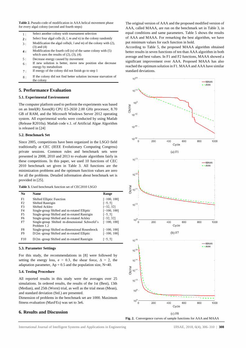
International Journal of Intelligent Systems and Applications in Engineering IJISAE, 2018, 6(4), 306–310 | 308
Table 2. Pseudo-code of modification in AAA helical movement phase
for every algal colony (second and fourth steps)
1 : Select another colony with tournament selection
2 : Select four algal cells (k, l, m and n) in the colony randomly
3 : Modification the algal cells(k, l and m) of the colony with (2), (3) and (4)
4 : Modification the fourth cell (n) of the same colony with (5)
which uses the results of (2), (3), (4).
5 : Decrease energy caused by movement
6 : If new solution is better, move new position else decrease
energy by metabolism
7 : If energy of the colony did not finish go to step 1
8 : If the colony did not find better solution increase starvation of the colony
5. Performance Evaluation
5.1. Experimental Environment
The computer platform used to perform the experiments was based
on an Intel(R) Xeon(R) CPU E5-2650 2.00 GHz processor, 8.70
GB of RAM, and the Microsoft Windows Server 2012 operating
system. All experimental works were conducted by using Matlab
(Release R2010a). Matlab code v.1. of Artificial Algae Algorithm
is released in [24]
5.2. Benchmark Set
Since 2005, competitions have been organized in the LSGO field
traditionally at CEC (IEEE Evolutionary Computing Congress)
private sessions. Common rules and benchmark sets were
presented in 2008, 2010 and 2013 to evaluate algorithms fairly in
these competitions. In this paper, we used 10 functions of CEC
2010 benchmark set given in Table 3. All functions are the
minimization problems and the optimum function values are zero
for all the problems. Detailed information about benchmark set is
provided in [25].
Table 3. Used benchmark function set of CEC2010 LSGO
No Name Range
F1 Shifted Elliptic Function [−100, 100]
F2 Shifted Rastrigin [−5, 5]
F3 Shifted Ackley [−32, 32] F4 Single-group Shifted and m-rotated Elliptic [−100, 100]
F5 Single-group Shifted and m-rotated Rastrigin [−5, 5]
F6 Single-group Shifted and m-rotated Ackley [−32, 32] F7 Single-group Shifted m-dimensional Schwefel’s
Problem 1.2
[−100, 100]
F8 Single-group Shifted m-dimensional Rosenbrock [−100, 100] F9 D/2m -group Shifted and m-rotated Elliptic [−100, 100]
F10 D/2m -group Shifted and m-rotated Rastrigin [−5, 5]
5.3. Parameter Settings
For this study, the recommendations in [8] were followed by
setting the energy loss, e = 0.3, the shear force, Δ = 2, the
adaptation parameter, Ap = 0.5 and the population size, N=40.
5.4. Testing Procedure
All reported results in this study were the averages over 25
simulations. In ordered results, the results of the 1st (Best), 13th
(Median), and 25th (Worst) trial, as well as the trial mean (Mean),
and standard deviation (Std.) are presented.
Dimension of problems in the benchmark set are 1000. Maximum
fitness evaluation (MaxFEs) was set to 3e6.
6. Results and Discussion
The original version of AAA and the proposed modified version of
AAA, called MAAA, are run on the benchmark set in Table 3, in
equal conditions and same parameters. Table 5 shows the results
of AAA and MAAA. For remarking the best algorithm, we have
put minimum values for each function in bold.
According to Table 5, the proposed MAAA algorithm obtained
better results in seven functions of ten than AAA algorithm in both
average and best values. In F1 and F2 functions, MAAA showed a
significant improvement over AAA. Proposed MAAA has also
reached the optimum solution in F1. MAAA and AAA have similar
standard deviations.
(a) F1
(b) F7
(c) F8
Fig. 2. Convergence curves of sample functions for AAA and MAAA
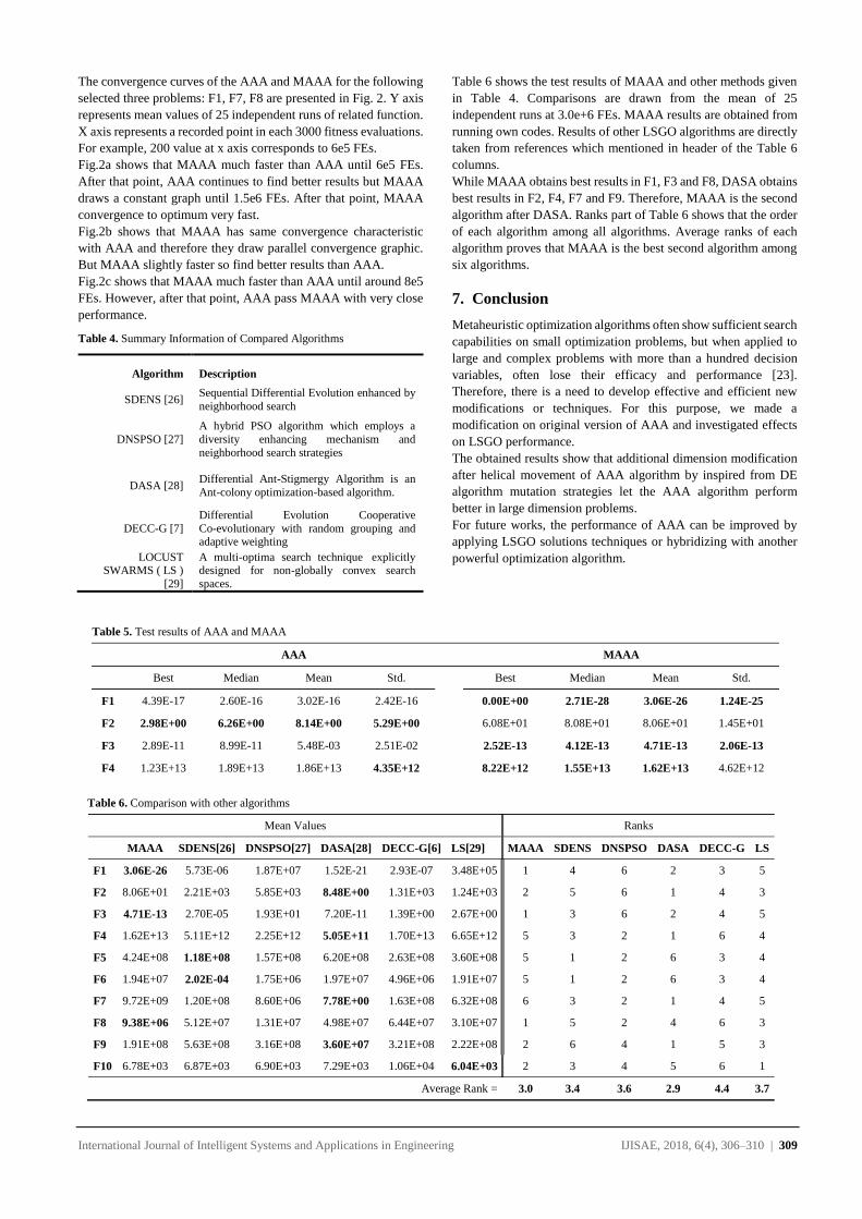
International Journal of Intelligent Systems and Applications in Engineering IJISAE, 2018, 6(4), 306–310 | 309
The convergence curves of the AAA and MAAA for the following
selected three problems: F1, F7, F8 are presented in Fig. 2. Y axis
represents mean values of 25 independent runs of related function.
X axis represents a recorded point in each 3000 fitness evaluations.
For example, 200 value at x axis corresponds to 6e5 FEs.
Fig.2a shows that MAAA much faster than AAA until 6e5 FEs.
After that point, AAA continues to find better results but MAAA
draws a constant graph until 1.5e6 FEs. After that point, MAAA
convergence to optimum very fast.
Fig.2b shows that MAAA has same convergence characteristic
with AAA and therefore they draw parallel convergence graphic.
But MAAA slightly faster so find better results than AAA.
Fig.2c shows that MAAA much faster than AAA until around 8e5
FEs. However, after that point, AAA pass MAAA with very close
performance.
Table 4. Summary Information of Compared Algorithms
Algorithm Description
SDENS [26] Sequential Differential Evolution enhanced by
neighborhood search
DNSPSO [27]
A hybrid PSO algorithm which employs a
diversity enhancing mechanism and
neighborhood search strategies
DASA [28] Differential Ant-Stigmergy Algorithm is an
Ant-colony optimization-based algorithm.
DECC-G [7]
Differential Evolution Cooperative
Co-evolutionary with random grouping and adaptive weighting
LOCUST SWARMS ( LS )
[29]
A multi-optima search technique explicitly designed for non-globally convex search
spaces.
Table 6 shows the test results of MAAA and other methods given
in Table 4. Comparisons are drawn from the mean of 25
independent runs at 3.0e+6 FEs. MAAA results are obtained from
running own codes. Results of other LSGO algorithms are directly
taken from references which mentioned in header of the Table 6
columns.
While MAAA obtains best results in F1, F3 and F8, DASA obtains
best results in F2, F4, F7 and F9. Therefore, MAAA is the second
algorithm after DASA. Ranks part of Table 6 shows that the order
of each algorithm among all algorithms. Average ranks of each
algorithm proves that MAAA is the best second algorithm among
six algorithms.
7. Conclusion
Metaheuristic optimization algorithms often show sufficient search
capabilities on small optimization problems, but when applied to
large and complex problems with more than a hundred decision
variables, often lose their efficacy and performance [23].
Therefore, there is a need to develop effective and efficient new
modifications or techniques. For this purpose, we made a
modification on original version of AAA and investigated effects
on LSGO performance.
The obtained results show that additional dimension modification
after helical movement of AAA algorithm by inspired from DE
algorithm mutation strategies let the AAA algorithm perform
better in large dimension problems.
For future works, the performance of AAA can be improved by
applying LSGO solutions techniques or hybridizing with another
powerful optimization algorithm.
Table 5. Test results of AAA and MAAA
AAA MAAA
Best Median Mean Std. Best Median Mean Std.
F1 4.39E-17 2.60E-16 3.02E-16 2.42E-16 0.00E+00 2.71E-28 3.06E-26 1.24E-25
F2 2.98E+00 6.26E+00 8.14E+00 5.29E+00 6.08E+01 8.08E+01 8.06E+01 1.45E+01
F3 2.89E-11 8.99E-11 5.48E-03 2.51E-02 2.52E-13 4.12E-13 4.71E-13 2.06E-13
F4 1.23E+13 1.89E+13 1.86E+13 4.35E+12 8.22E+12 1.55E+13 1.62E+13 4.62E+12
F5 3.34E+08 4.21E+08 4.32E+08 5.73E+07 2.97E+08 4.19E+08 4.24E+08 6.88E+07
F6 1.89E+07 1.96E+07 1.95E+07 1.90E+05 1.78E+07 1.95E+07 1.94E+07 3.76E+05
F7 7.55E+09 1.24E+10 1.28E+10 3.61E+09 4.26E+09 9.48E+09 9.72E+09 2.87E+09
F8 4.15E+03 1.61E+06 2.99E+06 3.88E+06 1.46E+04 1.90E+06 9.38E+06 1.31E+07
F9 1.65E+08 2.21E+08 2.13E+08 2.51E+07 1.49E+08 1.86E+08 1.91E+08 2.16E+07
F10 5.65E+03 6.16E+03 6.12E+03 2.64E+02 6.41E+03 6.75E+03 6.78E+03 3.02E+02
Table 6. Comparison with other algorithms
Mean Values Ranks
MAAA SDENS[26] DNSPSO[27] DASA[28] DECC-G[6] LS[29] MAAA SDENS DNSPSO DASA DECC-G LS
F1 3.06E-26 5.73E-06 1.87E+07 1.52E-21 2.93E-07 3.48E+05 1 4 6 2 3 5
F2 8.06E+01 2.21E+03 5.85E+03 8.48E+00 1.31E+03 1.24E+03 2 5 6 1 4 3
F3 4.71E-13 2.70E-05 1.93E+01 7.20E-11 1.39E+00 2.67E+00 1 3 6 2 4 5
F4 1.62E+13 5.11E+12 2.25E+12 5.05E+11 1.70E+13 6.65E+12 5 3 2 1 6 4
F5 4.24E+08 1.18E+08 1.57E+08 6.20E+08 2.63E+08 3.60E+08 5 1 2 6 3 4
F6 1.94E+07 2.02E-04 1.75E+06 1.97E+07 4.96E+06 1.91E+07 5 1 2 6 3 4
F7 9.72E+09 1.20E+08 8.60E+06 7.78E+00 1.63E+08 6.32E+08 6 3 2 1 4 5
F8 9.38E+06 5.12E+07 1.31E+07 4.98E+07 6.44E+07 3.10E+07 1 5 2 4 6 3
F9 1.91E+08 5.63E+08 3.16E+08 3.60E+07 3.21E+08 2.22E+08 2 6 4 1 5 3
F10 6.78E+03 6.87E+03 6.90E+03 7.29E+03 1.06E+04 6.04E+03 2 3 4 5 6 1
Average Rank = 3.0 3.4 3.6 2.9 4.4 3.7

International Journal of Intelligent Systems and Applications in Engineering IJISAE, 2018, 6(4), 306–310 | 310
Acknowledgment
This study was financially supported by The Coordinatorship of
Scientific Research Projects of Selçuk University [Grant no:
18101012].
References
[1] R. E. Bellman, Dynamic Programming, Princeton University Press,
Princeton, 1957.
[2] Y. Sun, X. Wang, Y. Chen and Z. Liu,” A modified whale optimization
algorithm for large-scale global optimization problems”, Expert
Systems with Applications, 2018.
[3] W. Long, J. Jiao, X. Liang and M. Tang,” Inspired grey wolf optimizer
for solving large-scale function optimization problems”, Applied
Mathematical Modelling, 2018, pp. 112-126.
[4] A. F. Ali, M. A. Tawhid, “A hybrid particle swarm optimization and
genetic algorithm with population partitioning for large scale
optimization problems”, Ain Shams Engineering Journal, 2017.
[5] N. Noman and H. Iba, “Enhancing differential evolution performance
with local search for high dimensional function optimization”,
In Proceedings of the 7th annual conference on Genetic and
evolutionary computation, 2005, pp. 967-974.
[6] D. Molina, M. Lozano and F. Herrera,”MA-SW-Chains: Memetic
algorithm based on local search chains for large scale continuous
global optimization”, In Evolutionary Computation (CEC), 2010, pp.
1-8.
[7] Z. Yang, K. Tang, and X. Yao,” Large scale evolutionary optimization
using cooperative coevolution”. Information Sciences, 2008, pp. 2985-
2999.
[8] S.A. Uymaz, G. Tezel and E. Yel,” Artificial algae algorithm (AAA)
for nonlinear global optimization”, Applied Soft Computing, 2015a,
pp. 153–171.
[9] S.A. Uymaz, G. Tezel and E. Yel, “Artificial algae algorithm with
multi-light source for numerical optimization and applications”,
Biosystems, 2015b, pp. 25-38.
[10] A.Babalik, A. Ozkis, S.A Uymaz and M.S. Kiran, ”A multi-objective
artificial algae algorithm”, Applied Soft Computing, 2018, pp. 377-
395.
[11] X. Zhang, C. Wu, J. Li, X. Wang, Z. Yang, J. M. Lee and K. H. Jung,
”Binary artificial algae algorithm for multidimensional knapsack
problems”, Applied Soft Computing, 2016, 43, pp. 583-595.
[12] M. Kumar and J. S. Dhillon, “Hybrid artificial algae algorithm for
economic load dispatch”, Applied Soft Computing, 2018, 71, pp.89-
109.
[13] M. Beşkirli, İ. Koç, H. Haklı and H. Kodaz,” A new optimization
algorithm for solving wind turbine placement problem: Binary
artificial algae algorithm”, Renewable Energy, 2018, 121, pp. 301-308.
[14] R. Storn and K. V. Price, “Differential evolution: A simple and
efficient adaptive scheme for global optimization over continuous
spaces,” ICSI, USA, Tech. Rep. TR-95-012, 1995 [Online]. Available:
http://www1.icsi.berkeley.edu/~storn/TR-95-012.pdf
[15] Y. Gao and Y. Wang, “A memetic differential evolutionary algorithm
for high dimensional function spaces optimization”, in Proc. 3rd ICNC
20, 2007, pp. 188–192.
[16] Z. Yang, K. Tang, and X. Yao, “Differential evolution for high
dimensional function optimization,” in Proc. IEEE Congr. Evol.
Comput., 2007, pp. 3523–3530.
[17] J. Brest, A. Zamuda, B. Boskovic, M. S. Maucec and V. Zumer,
“High dimensional real-parameter optimization using self-adaptive
Differential evolution algorithm with population size reduction,” in
Proc. IEEE Congr. Evol. Comput., 2008, pp. 2032–2039
[18] K. Tang, X. Yao, P. N. Suganthan, C. MacNish, Y. P. Chen, C. M.
Chen, and Z. Yang, “Benchmark functions for the CEC’2008 special
session and competition on large scale global optimization”, Nature
Inspired Comput. Applicat. Lab., USTC, China, Nanyang Technol.
Univ., Singapore, Tech. Rep., 2007
[19] T. Keskintürk, “Diferansiyel Gelişim Algoritması”, İstanbul Ticaret
Üniversitesi Fen Bilimleri Dergisi Yıl: 5 Sayı: 9 Bahar 2006, pp.85-99
[20] S. Das and P. N. Suganthan,”Differential evolution: a survey of the
state-of-the-art”. IEEE transactions on evolutionary computation,
2011, pp 4-31.
[21] W. Gong, Á. Fialho, Z. Cai and H. Li,” Adaptive strategy selection in
differential evolution for numerical optimization: an empirical study”,
Information Sciences, 2011, 181(24), pp. 5364-5386.
[22] A. Banitalebi, M. I. A. Aziz and Z. A. Aziz,” A self-adaptive binary
differential evolution algorithm for large scale binary optimization
problems”, Information Sciences, 2016, 367, pp.487-511.
[23] H. C. Lund and J. W. G. Lund, “Freshwater Algae-Their micoscopic
world explored”, Biopress Limited, Bristol, England, 1996.
[24] http://aaa.selcuk.edu.tr/, Accessed on: October 8, 2018.
[25] K. Tang, X. Li, P. N. Suganthan, Z. Yang, T. Weise,” Benchmark
functions for the CEC’2010 special session and competition on large
scale global”, Nature Inspired Comput. Applicat. Lab., Tech. Rep.,
2009
[26] H. Wang, Z. Wu, S. Rahnamayan and D. Jiang,” Sequential DE
enhanced by neighborhood search for large scale global optimization”,
in Proc. IEEE Congr. Evol. Comput., 2010, pp. 1-7.
[27] H. Wang, H. Sun, C. Li and S. Rahnamayan and J.S. Pan,” Diversity
enhanced particle swarm optimization with neighborhood search”
Information Sciences, 2013, pp. 119-135.
[28] P. Korošec, K. Tashkova and J. Šilc,” The differential ant-stigmergy
algorithm for large-scale global optimization”, in Proc. IEEE Congr.
Evol. Comput, 2010, pp. 1-8.
[29] S. Chen, ”Locust Swarms for Large Scale Global Optimization of
Nonseparable Problems”, Kukkonen, Benchmarking the Classic
Differential Evolution Algorithm on Large-Scale Global Optimization
Google Scholar.

International Journal of
Intelligent Systems and
Applications in Engineering
Advanced Technology and Science
ISSN:2147-67992147-6799 www.atscience.org/IJISAE Original Research Paper
International Journal of Intelligent Systems and Applications in Engineering IJISAE, 2018, 6(4), 311–321 | 311
An Investigation of the Effect of Meteorological Parameters on Wind
Speed Estimation Using Machine Learning Algorithms
Cem Emeksiz*1, Gulden Demir2
Accepted : 16/12/2018 Published: 31/12/2018 DOI: 10.1039/b000000x
Abstract: Wind speed is the most important parameter of the wind energy conversion system. Therefore temperature, humiditiy and
pressure data, which has significant effect on the wind speed, have become extremely important. In the literature, various models have
been used to realize the wind speed estimation. In this study; Six different data mining algorithms were used to determine the effect of
meteorological parameters on wind speed estimation. The data were collected from the measurement station established on the campus of
Gaziosmanpaşa University. We focused on the bagging algorithm to determine the appropriate combination of wind speed estimates. The
bagging algorithm was used for the first time in estimation of wind speed by taking into account meteorological parameters. To find the
most efficiency method on such problem 10-fold cross validation technique was used for comparision. From results, It is concluded that
bagging algorithm and temperature-humiditiy-pressure combination showed the best performance. Additionaly, temperature and pressure
data are more effective in the wind speed estimation.
Keywords: Bagging algorithm, Data mining, Renewable energy, Wind speed estimation.
1. Introduction
With industrialization, basic energy resources emerge as an
indispensable phenomenon to maintain the daily life of human
beings. In industrial societies, fossil fuels are used as the main
energy source. Nowadays, while a large part of energy needs are
met by fossil fuels, it is a necessity to turn to alternative sources
when the negative impact of these resources on the environment is
taken into consideration. At the same time, global warming,
seasonal changes and the political approaches of the countries have
accelerated the search for alternative energy sources in the future
where fossil fuel reserves can not meet their needs. This is
especially the case for wind energy and solar energy, which are
among the renewable energy sources.
Renewable energy sources can be renewed owing to the variety of
energy that does not emit to the environment, which is thought to
take its power from the sun and never to be consumed. When we
look at the energy policies of developed and developing countries,
we see that they are turning to renewable energy sources and
accelerating their efforts to develop these resources. Solar energy,
wind energy, hydrolic energy, biomass energy, hydrogen energy,
geothermal energy, wave energy, tidal energy are the categories of
renewable energy resources.
According to the 2017 Renewable Energy Global Situation Report,
in 2016, a total of 161 GW renewable energy is installed in the
power system. The total global capacity has increased by about 9%
compared to 2015 and is almost 2.017 GW at the end of the year.
In 2016, about 47% of the newly established renewable energy
capacity was solar energy. This ratio was followed by wind energy
with 34% and hydroelectric energy with 15.5% [1].
Wind energy is at the forefront of the renewable energy sources
that are the most used owing to cost efficiency in the world. In the
past, wind energy was used to move sails, run ships, windmills and
in irrigation. Recently, the use of wind turbines operating in the
world by wind energy in the production of electricity has become
increasingly widespread. According to the 2016 Global Wind
Statistics report on the situation of the global wind industry of
Global Wind Energy Council (GWEC), countries with the highest
installed power are shown in Table 1 [2].
Table1 The top 10 cumulative capacity DEC 2016
Country MW %Share
PR China 168.690 34.7
USA 82.184 16.9
Germany 50.018 10.3
India 28.700 5.9
Spain 23.074 4.7
United K. 14.543 3.0
France 12.066 2.5
Canada 11.900 2.4
Brazil 10.740 2.2
Italy 9.257 1.9
Rest of theworld 75.577 15.5
Total TOP 10 411.172 84
World Total 486.749 100
To benefit technologically from wind energy; it is very important
to know the possibilities of utilization, to determine the zones with
high wind energy potential, to be able to predict the wind
characteristics and wind speeds. In particular, estimating wind
speeds is necessary for estimating the energy expected to be
generated from wind turbines in short, medium and long period.
According to these estimation values, the profitability of the power
generation plants can be calculated and it is determined whether or
not the investment of wind energy in a region will be profitable. In
this way, the operating and production costs can be calculated more
accurately [3].
Wind energy estimations are generally produced by hybrid models
_______________________________________________________________________________________________________________________________________________________________________________________________________________________________________________________________________________________________________________________________
1 Electric-Electronic Eng. Tokat Gaziosmanpasa University, Tokat, Turkey 2 Electric-Electronic Eng. Tokat Gaziosmanpasa University, Tokat, Turkey
* Corresponding Author: Email: [email protected]
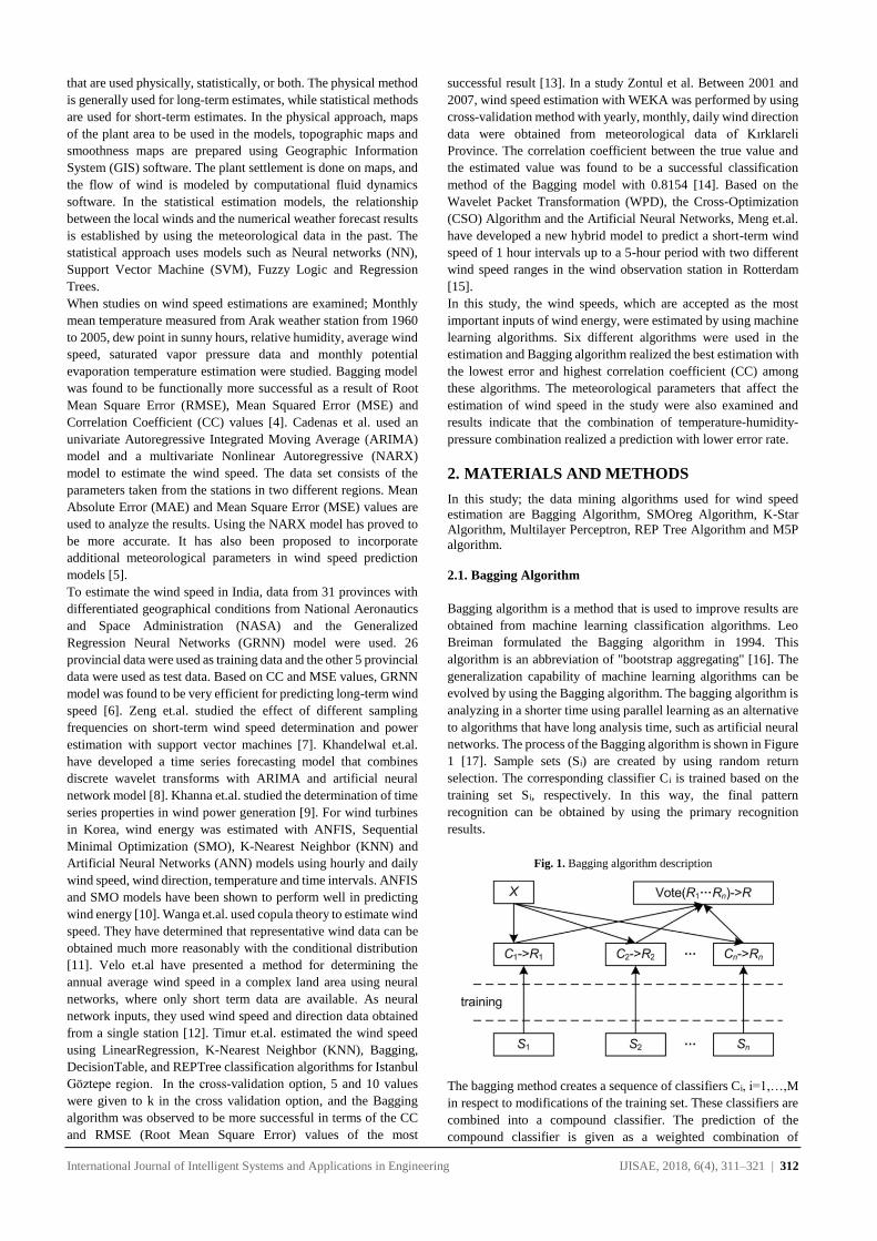
International Journal of Intelligent Systems and Applications in Engineering IJISAE, 2018, 6(4), 311–321 | 312
that are used physically, statistically, or both. The physical method
is generally used for long-term estimates, while statistical methods
are used for short-term estimates. In the physical approach, maps
of the plant area to be used in the models, topographic maps and
smoothness maps are prepared using Geographic Information
System (GIS) software. The plant settlement is done on maps, and
the flow of wind is modeled by computational fluid dynamics
software. In the statistical estimation models, the relationship
between the local winds and the numerical weather forecast results
is established by using the meteorological data in the past. The
statistical approach uses models such as Neural networks (NN),
Support Vector Machine (SVM), Fuzzy Logic and Regression
Trees.
When studies on wind speed estimations are examined; Monthly
mean temperature measured from Arak weather station from 1960
to 2005, dew point in sunny hours, relative humidity, average wind
speed, saturated vapor pressure data and monthly potential
evaporation temperature estimation were studied. Bagging model
was found to be functionally more successful as a result of Root
Mean Square Error (RMSE), Mean Squared Error (MSE) and
Correlation Coefficient (CC) values [4]. Cadenas et al. used an
univariate Autoregressive Integrated Moving Average (ARIMA)
model and a multivariate Nonlinear Autoregressive (NARX)
model to estimate the wind speed. The data set consists of the
parameters taken from the stations in two different regions. Mean
Absolute Error (MAE) and Mean Square Error (MSE) values are
used to analyze the results. Using the NARX model has proved to
be more accurate. It has also been proposed to incorporate
additional meteorological parameters in wind speed prediction
models [5].
To estimate the wind speed in India, data from 31 provinces with
differentiated geographical conditions from National Aeronautics
and Space Administration (NASA) and the Generalized
Regression Neural Networks (GRNN) model were used. 26
provincial data were used as training data and the other 5 provincial
data were used as test data. Based on CC and MSE values, GRNN
model was found to be very efficient for predicting long-term wind
speed [6]. Zeng et.al. studied the effect of different sampling
frequencies on short-term wind speed determination and power
estimation with support vector machines [7]. Khandelwal et.al.
have developed a time series forecasting model that combines
discrete wavelet transforms with ARIMA and artificial neural
network model [8]. Khanna et.al. studied the determination of time
series properties in wind power generation [9]. For wind turbines
in Korea, wind energy was estimated with ANFIS, Sequential
Minimal Optimization (SMO), K-Nearest Neighbor (KNN) and
Artificial Neural Networks (ANN) models using hourly and daily
wind speed, wind direction, temperature and time intervals. ANFIS
and SMO models have been shown to perform well in predicting
wind energy [10]. Wanga et.al. used copula theory to estimate wind
speed. They have determined that representative wind data can be
obtained much more reasonably with the conditional distribution
[11]. Velo et.al have presented a method for determining the
annual average wind speed in a complex land area using neural
networks, where only short term data are available. As neural
network inputs, they used wind speed and direction data obtained
from a single station [12]. Timur et.al. estimated the wind speed
using LinearRegression, K-Nearest Neighbor (KNN), Bagging,
DecisionTable, and REPTree classification algorithms for Istanbul
Göztepe region. In the cross-validation option, 5 and 10 values
were given to k in the cross validation option, and the Bagging
algorithm was observed to be more successful in terms of the CC
and RMSE (Root Mean Square Error) values of the most
successful result [13]. In a study Zontul et al. Between 2001 and
2007, wind speed estimation with WEKA was performed by using
cross-validation method with yearly, monthly, daily wind direction
data were obtained from meteorological data of Kırklareli
Province. The correlation coefficient between the true value and
the estimated value was found to be a successful classification
method of the Bagging model with 0.8154 [14]. Based on the
Wavelet Packet Transformation (WPD), the Cross-Optimization
(CSO) Algorithm and the Artificial Neural Networks, Meng et.al.
have developed a new hybrid model to predict a short-term wind
speed of 1 hour intervals up to a 5-hour period with two different
wind speed ranges in the wind observation station in Rotterdam
[15].
In this study, the wind speeds, which are accepted as the most
important inputs of wind energy, were estimated by using machine
learning algorithms. Six different algorithms were used in the
estimation and Bagging algorithm realized the best estimation with
the lowest error and highest correlation coefficient (CC) among
these algorithms. The meteorological parameters that affect the
estimation of wind speed in the study were also examined and
results indicate that the combination of temperature-humidity-
pressure combination realized a prediction with lower error rate.
2. MATERIALS AND METHODS
In this study; the data mining algorithms used for wind speed
estimation are Bagging Algorithm, SMOreg Algorithm, K-Star
Algorithm, Multilayer Perceptron, REP Tree Algorithm and M5P
algorithm.
2.1. Bagging Algorithm
Bagging algorithm is a method that is used to improve results are
obtained from machine learning classification algorithms. Leo
Breiman formulated the Bagging algorithm in 1994. This
algorithm is an abbreviation of "bootstrap aggregating" [16]. The
generalization capability of machine learning algorithms can be
evolved by using the Bagging algorithm. The bagging algorithm is
analyzing in a shorter time using parallel learning as an alternative
to algorithms that have long analysis time, such as artificial neural
networks. The process of the Bagging algorithm is shown in Figure
1 [17]. Sample sets (Si) are created by using random return
selection. The corresponding classifier Ci is trained based on the
training set Si, respectively. In this way, the final pattern
recognition can be obtained by using the primary recognition
results.
Fig. 1. Bagging algorithm description
The bagging method creates a sequence of classifiers Ci, i=1,…,M
in respect to modifications of the training set. These classifiers are
combined into a compound classifier. The prediction of the
compound classifier is given as a weighted combination of
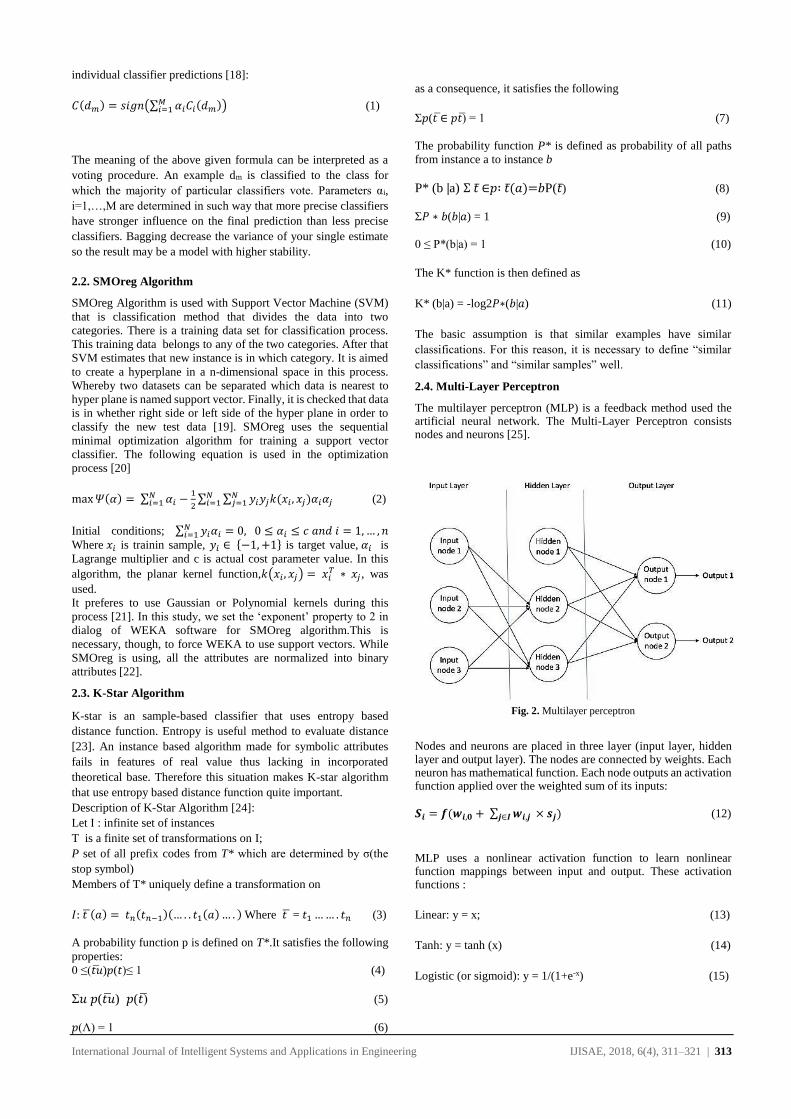
International Journal of Intelligent Systems and Applications in Engineering IJISAE, 2018, 6(4), 311–321 | 313
individual classifier predictions [18]:
𝐶(𝑑𝑚) = 𝑠𝑖𝑔𝑛(∑ 𝛼𝑖𝐶𝑖(𝑑𝑚)𝑀𝑖=1 ) (1)
The meaning of the above given formula can be interpreted as a
voting procedure. An example dm is classified to the class for
which the majority of particular classifiers vote. Parameters αi,
i=1,…,M are determined in such way that more precise classifiers
have stronger influence on the final prediction than less precise
classifiers. Bagging decrease the variance of your single estimate
so the result may be a model with higher stability.
2.2. SMOreg Algorithm
SMOreg Algorithm is used with Support Vector Machine (SVM)
that is classification method that divides the data into two
categories. There is a training data set for classification process.
This training data belongs to any of the two categories. After that
SVM estimates that new instance is in which category. It is aimed
to create a hyperplane in a n-dimensional space in this process.
Whereby two datasets can be separated which data is nearest to
hyper plane is named support vector. Finally, it is checked that data
is in whether right side or left side of the hyper plane in order to
classify the new test data [19]. SMOreg uses the sequential
minimal optimization algorithm for training a support vector
classifier. The following equation is used in the optimization
process [20]
max𝛹(𝛼) = ∑ 𝛼𝑖 −1
2∑ ∑ 𝑦𝑖𝑦𝑗𝑘(𝑥𝑖 , 𝑥𝑗)𝛼𝑖𝛼𝑗
𝑁𝑗=1
𝑁𝑖=1
𝑁𝑖=1 (2)
Initial conditions; ∑ 𝑦𝑖𝛼𝑖 = 0, 0 ≤ 𝛼𝑖 ≤ 𝑐 𝑎𝑛𝑑 𝑖 = 1,… , 𝑛𝑁𝑖=1
Where 𝑥𝑖 is trainin sample, 𝑦𝑖 ∈ {−1,+1} is target value, 𝛼𝑖 is
Lagrange multiplier and c is actual cost parameter value. In this
algorithm, the planar kernel function,𝑘(𝑥𝑖 , 𝑥𝑗) = 𝑥𝑖𝑇 ∗ 𝑥𝑗 , was
used.
It preferes to use Gaussian or Polynomial kernels during this
process [21]. In this study, we set the ‘exponent’ property to 2 in
dialog of WEKA software for SMOreg algorithm.This is
necessary, though, to force WEKA to use support vectors. While
SMOreg is using, all the attributes are normalized into binary
attributes [22].
2.3. K-Star Algorithm
K-star is an sample-based classifier that uses entropy based
distance function. Entropy is useful method to evaluate distance
[23]. An instance based algorithm made for symbolic attributes
fails in features of real value thus lacking in incorporated
theoretical base. Therefore this situation makes K-star algorithm
that use entropy based distance function quite important.
Description of K-Star Algorithm [24]:
Let I : infinite set of instances
T is a finite set of transformations on I;
P set of all prefix codes from T* which are determined by σ(the
stop symbol)
Members of T* uniquely define a transformation on
𝐼: 𝑡 ̅(𝑎) = 𝑡𝑛(𝑡𝑛−1)(… . . 𝑡1(𝑎)… . ) Where 𝑡 ̅ = 𝑡1…… . 𝑡𝑛 (3)
A probability function p is defined on T*.It satisfies the following
properties:
0 ≤(�̅�𝑢)𝑝(𝑡)≤ 1 (4)
Σ𝑢 𝑝(𝑡 ̅𝑢) 𝑝(𝑡 ̅) (5)
𝑝(Λ) = 1 (6)
as a consequence, it satisfies the following
Σ𝑝(�̅� ∈ 𝑝�̅�) = 1 (7)
The probability function P* is defined as probability of all paths
from instance a to instance b
P* (b |a) Σ 𝑡 ∈𝑝∶ 𝑡 (𝑎)=𝑏P(𝑡 ) (8)
Σ𝑃 ∗ 𝑏(𝑏|𝑎) = 1 (9)
0 ≤ P*(b|a) = 1 (10)
The K* function is then defined as
K* (b|a) = -log2𝑃∗(𝑏|𝑎) (11)
The basic assumption is that similar examples have similar
classifications. For this reason, it is necessary to define “similar
classifications” and “similar samples” well.
2.4. Multi-Layer Perceptron
The multilayer perceptron (MLP) is a feedback method used the artificial neural network. The Multi-Layer Perceptron consists nodes and neurons [25].
Fig. 2. Multilayer perceptron
Nodes and neurons are placed in three layer (input layer, hidden layer and output layer). The nodes are connected by weights. Each neuron has mathematical function. Each node outputs an activation function applied over the weighted sum of its inputs:
𝑺𝒊 = 𝒇(𝒘𝒊,𝟎 + ∑ 𝒘𝒊,𝒋 × 𝒔𝒋)𝒋∈𝑰 (12)
MLP uses a nonlinear activation function to learn nonlinear function mappings between input and output. These activation functions :
Linear: y = x; (13)
Tanh: y = tanh (x) (14)
Logistic (or sigmoid): y = 1/(1+e-x) (15)
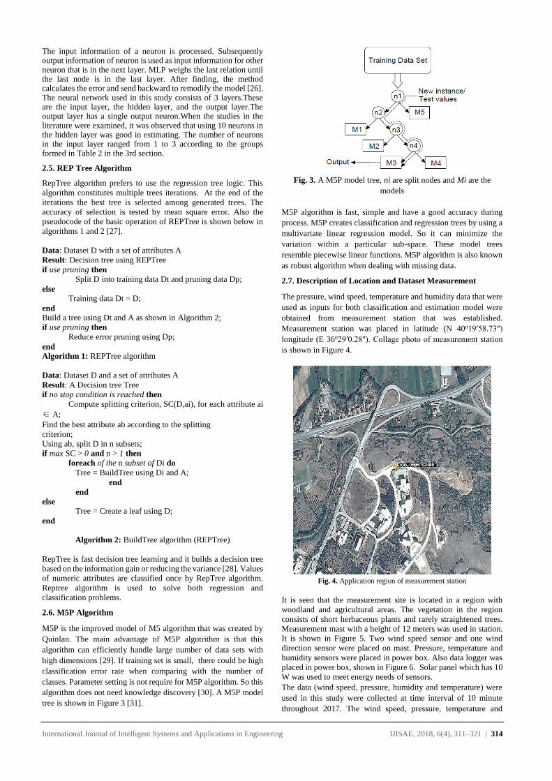
International Journal of Intelligent Systems and Applications in Engineering IJISAE, 2018, 6(4), 311–321 | 314
The input information of a neuron is processed. Subsequently output information of neuron is used as input information for other neuron that is in the next layer. MLP weighs the last relation until the last node is in the last layer. After finding, the method calculates the error and send backward to remodify the model [26]. The neural network used in this study consists of 3 layers.These are the input layer, the hidden layer, and the output layer.The output layer has a single output neuron.When the studies in the literature were examined, it was observed that using 10 neurons in the hidden layer was good in estimating. The number of neurons in the input layer ranged from 1 to 3 according to the groups formed in Table 2 in the 3rd section.
2.5. REP Tree Algorithm
RepTree algorithm prefers to use the regression tree logic. This
algorithm constitutes multiple trees iterations. At the end of the
iterations the best tree is selected among generated trees. The
accuracy of selection is tested by mean square error. Also the
pseudocode of the basic operation of REPTree is shown below in
algorithms 1 and 2 [27].
Data: Dataset D with a set of attributes A
Result: Decision tree using REPTree
if use pruning then
Split D into training data Dt and pruning data Dp;
else
Training data Dt = D;
end
Build a tree using Dt and A as shown in Algorithm 2;
if use pruning then
Reduce error pruning using Dp;
end
Algorithm 1: REPTree algorithm
Data: Dataset D and a set of attributes A
Result: A Decision tree Tree
if no stop condition is reached then
Compute splitting criterion, SC(D,ai), for each attribute ai
∈ A;
Find the best attribute ab according to the splitting
criterion;
Using ab, split D in n subsets;
if max SC > 0 and n > 1 then
foreach of the n subset of Di do
Tree = BuildTree using Di and A;
end
end
else
Tree = Create a leaf using D;
end
Algorithm 2: BuildTree algorithm (REPTree)
RepTree is fast decision tree learning and it builds a decision tree
based on the information gain or reducing the variance [28]. Values
of numeric attributes are classified once by RepTree algorithm.
Reptree algorithm is used to solve both regression and
classification problems.
2.6. M5P Algorithm
M5P is the improved model of M5 algorithm that was created by
Quinlan. The main advantage of M5P algotrithm is that this
algorithm can efficiently handle large number of data sets with
high dimensions [29]. If training set is small, there could be high
classification error rate when comparing with the number of
classes. Parameter setting is not require for M5P algorithm. So this
algorithm does not need knowledge discovery [30]. A M5P model
tree is shown in Figure 3 [31].
Fig. 3. A M5P model tree, ni are split nodes and Mi are the
models
M5P algorithm is fast, simple and have a good accuracy during
process. M5P creates classification and regression trees by using a
multivariate linear regression model. So it can minimize the
variation within a particular sub-space. These model trees
resemble piecewise linear functions. M5P algorithm is also known
as robust algorithm when dealing with missing data.
2.7. Description of Location and Dataset Measurement
The pressure, wind speed, temperature and humidity data that were
used as inputs for both classification and estimation model were
obtained from measurement station that was established.
Measurement station was placed in latitude (N 40o19ʹ58.73ʺ)
longitude (E 36o29ʹ0.28ʺ). Collage photo of measurement station
is shown in Figure 4.
Fig. 4. Application region of measurement station
It is seen that the measurement site is located in a region with
woodland and agricultural areas. The vegetation in the region
consists of short herbaceous plants and rarely straightened trees.
Measurement mast with a height of 12 meters was used in station.
It is shown in Figure 5. Two wind speed sensor and one wind
direction sensor were placed on mast. Pressure, temperature and
humidity sensors were placed in power box. Also data logger was
placed in power box, shown in Figure 6. Solar panel which has 10
W was used to meet energy needs of sensors.
The data (wind speed, pressure, humidity and temperature) were
used in this study were collected at time interval of 10 minute
throughout 2017. The wind speed, pressure, temperature and

International Journal of Intelligent Systems and Applications in Engineering IJISAE, 2018, 6(4), 311–321 | 315
humidity data which are "dat" format were converted into "arff"
format to process in WEKA software. "WEKA" stands for the
Waikato Environment for Knowledge Analysis, is developed by
University of Waikato, New Zealand in 1993. WEKA is a
collection of machine learning algorithms for solving real-world
data mining tasks. It contains tools for data pre-processing,
classification, regression, clustering, association rules and
visualization [32].
Fig. 5. Measurement station
Fig. 6. Power box
3. IMPLEMENTATION OF MACHINE LEARNING ALGORITHMS
At first the missing or inconsistent data in the database were
extracted because this kind of data must be extracted to obtain
successful results. Also it is necessary to remove data repetitions
from the database and increase the data consistency (correctness).
So all data were normalized.
Seven combinations were created from the normalized data
(pressure, humidity and temperature). Groups are given in Table 2.
Table2 Combinations
Combinations
1. Combination Temperature-Humiditiy-Pressure
2. Combination Temperature-Humiditiy
3. Combination Temperature- Pressure
4. Combination Humiditiy-Pressure
5. Combination Temperature
6. Combination Humiditiy
7. Combination Pressure
In order to find the most efficiency method we used 10-fold cross
validation technique which divided data into ten sets of size n/10
(n is number of records). Every data set is tested by using the
remaining sets as its training set. It is shown in Figure 7. The 52560
data were used in the estimation process.
Fig. 7. Schematic representation of 10-fold cross-validation
Fig. 8. Flow chart of estimation model
Anemometers
AIR-X 400W Wind Turbine
Wind
direction
sensors Test Training Training
Training Test Training
Training Training Training
Training Training Training
Training Training ……………………… Training
Training Training Training
Training Training Training
Training Training Training
Training Training Training
Training Training Test
Power supply Pressure sensor Data logger
Temperature sensor Power supply of sensors
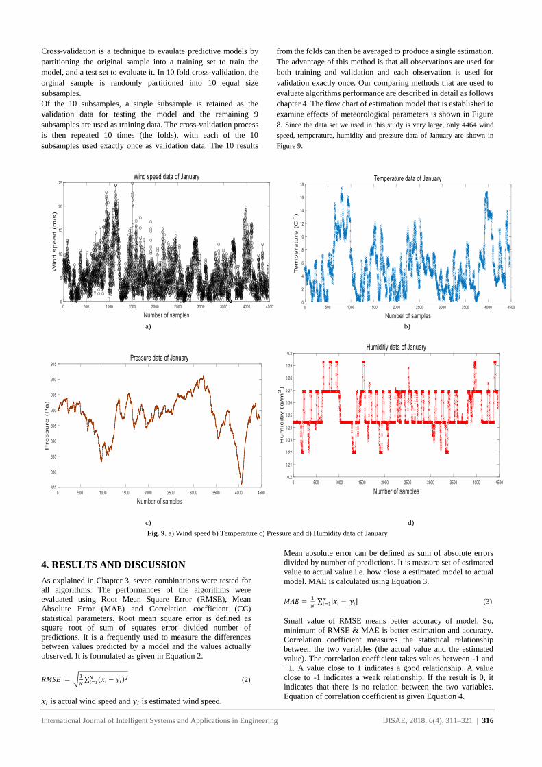
International Journal of Intelligent Systems and Applications in Engineering IJISAE, 2018, 6(4), 311–321 | 316
Cross-validation is a technique to evaulate predictive models by
partitioning the original sample into a training set to train the
model, and a test set to evaluate it. In 10 fold cross-validation, the
orginal sample is randomly partitioned into 10 equal size
subsamples.
Of the 10 subsamples, a single subsample is retained as the
validation data for testing the model and the remaining 9
subsamples are used as training data. The cross-validation process
is then repeated 10 times (the folds), with each of the 10
subsamples used exactly once as validation data. The 10 results
from the folds can then be averaged to produce a single estimation.
The advantage of this method is that all observations are used for
both training and validation and each observation is used for
validation exactly once. Our comparing methods that are used to
evaluate algorithms performance are described in detail as follows
chapter 4. The flow chart of estimation model that is established to
examine effects of meteorological parameters is shown in Figure
8. Since the data set we used in this study is very large, only 4464 wind
speed, temperature, humidity and pressure data of January are shown in
Figure 9.
a) b)
c) d)
Fig. 9. a) Wind speed b) Temperature c) Pressure and d) Humidity data of January
4. RESULTS AND DISCUSSION
As explained in Chapter 3, seven combinations were tested for
all algorithms. The performances of the algorithms were
evaluated using Root Mean Square Error (RMSE), Mean
Absolute Error (MAE) and Correlation coefficient (CC)
statistical parameters. Root mean square error is defined as
square root of sum of squares error divided number of
predictions. It is a frequently used to measure the differences
between values predicted by a model and the values actually
observed. It is formulated as given in Equation 2.
𝑅𝑀𝑆𝐸 = √1
𝑁∑ (𝑥𝑖 − 𝑦𝑖)
2𝑁𝑖=1 (2)
𝑥𝑖 is actual wind speed and 𝑦𝑖 is estimated wind speed.
Mean absolute error can be defined as sum of absolute errors
divided by number of predictions. It is measure set of estimated
value to actual value i.e. how close a estimated model to actual
model. MAE is calculated using Equation 3.
𝑀𝐴𝐸 = 1
𝑁 ∑ |𝑥𝑖 − 𝑦𝑖|
𝑁𝑖=1 (3)
Small value of RMSE means better accuracy of model. So,
minimum of RMSE & MAE is better estimation and accuracy.
Correlation coefficient measures the statistical relationship
between the two variables (the actual value and the estimated
value). The correlation coefficient takes values between -1 and
+1. A value close to 1 indicates a good relationship. A value
close to -1 indicates a weak relationship. If the result is 0, it
indicates that there is no relation between the two variables.
Equation of correlation coefficient is given Equation 4.
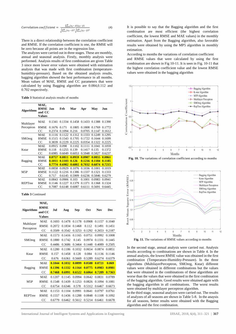
International Journal of Intelligent Systems and Applications in Engineering IJISAE, 2018, 6(4), 311–321 | 317
𝐶𝑜𝑟𝑟𝑒𝑙𝑎𝑡𝑖𝑜𝑛 𝑐𝑜𝑒𝑓𝑓𝑖𝑐𝑖𝑒𝑛𝑡 = ∑ (𝑥𝑖− 𝑥 )(𝑦𝑖− �̅�)𝑁𝑖=1
√∑ (𝑥𝑖− 𝑥 )2𝑁
𝑖=1 √∑ (𝑦𝑖− �̅�)2𝑁
𝑖=1
(4)
There is a direct relationship between the correlation coefficient
and RMSE. If the correlation coefficient is one, the RMSE will
be zero because all points are in the regression line.
The analyzes were carried out in three stages. These are monthly,
annual and seasonal analysis. Firstly, monthly analysis were
performed. Analysis results of first combination are given Table
3 since more lower error values were obtained with estimation
analysis that was made with first combination (temperature-
humiditiy-pressure). Based on the obtained analysis results,
bagging algorithm showed the best performance in all months.
Mean values of MAE, RMSE and CC parameters that were
calculated by using Bagging algorithm are 0.084,0.112 and
0.702 respectively.
Table 3 Statistical analysis results of months
Table 3 Continued
Algorithms
MAE,
RMSE
and CC
Values
Jul Aug Sep Oct Nov Dec
Multilayer
Perceptron
MAE 0.1693 0.1478 0.1178 0.0908 0.1157 0.1040
RMSE 0.2072 0.1834 0.1468 0.112 0.1491 0.1451
CC 0.3509 0.3542 0.3253 0.1292 0.2653 0.2187
SMOreg
MAE 0.1573 0.1416 0.1165 0.0751 0.0992 0.1008
RMSE 0.1880 0.1742 0.145 0.0974 0.1331 0.1445
CC 0.4486 0.3686 0.3464 0.1448 0.4089 0.2505
Kstar
MAE 0.1280 0.1186 0.1032 0.0654 0.0874 0.0851
RMSE 0.157 0.1458 0.128 0.084 0.1136 0.1146
CC 0.676 0.6361 0.5669 0.5289 0.6274 0.6379
Bagging
MAE 0.1044 0.1032 0.0899 0.0588 0.0721 0.069
RMSE 0.1396 0.1332 0.1164 0.0775 0.0983 0.0981
CC 0.7468 0.6991 0.6522 0.6064 0.7289 0.7363
M5P
MAE 0.1207 0.1145 0.0994 0.0642 0.0831 0.0789
RMSE 0.1548 0.1439 0.1253 0.0826 0.1094 0.1081
CC 0.6754 0.6346 0.578 0.5312 0.6467 0.6673
REPTree
MAE 0.1153 0.1104 0.0991 0.0641 0.0797 0.0761
RMSE 0.1557 0.1436 0.1288 0.0848 0.1108 0.1092
CC 0.6779 0.6462 0.5612 0.5214 0.6461 0.6678
It is possible to say that the Bagging algorithm and the first
combination are most efficient (the highest correlation
coefficient, the lowest RMSE and MAE values) in the monthly
estimation. Apart from the Bagging algorithm, also favorable
results were obtained by using the MP5 algorithm in monthly
estimation.
According to months the variations of correlation coefficient
and RMSE values that were calculated by using the first
combination are shown in Fig 10-11. It is seen in Fig. 10-11 that
the highest correlation coefficient value and the lowest RMSE
values were obtained in the bagging algorithm
Fig. 10. The variations of correlation coefficient according to months
Fig. 11. The variations of RMSE values according to months
In the second stage, annual analysis were carried out. Analysis
results according to combinations are shown in Table 4. In the
annual analysis, the lowest RMSE value was obtained in the first
combination (Temperature-Humidity-Pressure). In the three
algorithms (MultilayerPerceptron, SMOreg, Kstar) different
values were obtained in different combinations but the values
that were obtained in the combinations of these algorithms are
worse than the values that were obtained in the first combination
of the bagging algorithm. Good results were obtained again with
the bagging algorithm in all combinations. The worst results
were obtained by multilayer perceptron algorithm.
In the third stage, seasonal analyzes were carried out. The results
of analyzes of all seasons are shown in Table 5-8. In the anaysis
for all seasons, better results were obtained with the Bagging
algorithm and the first combination.
Algorithms
MAE,
RMSE
and CC
Values
Jan
Feb
Mar
Apr
May
Jun
Multilayer
Perceptron
MAE 0.1341 0.1334 0.1458 0.1433 0.1388 0.1390
RMSE 0.1676 0.171 0.1805 0.1808 0.1769 0.1772
CC 0.2374 0.1094 0.216 0.0705 0.1147 0.1612
SMOreg
MAE 0.1116 0.1122 0.1312 0.1333 0.1249 0.1295
RMSE 0.1515 0.1543 0.1705 0.1722 0.1644 0.1699
CC 0.3839 0.2229 0.2225 0.0354 0.1322 0.2225
Kstar MAE 0.0915 0.098 0.1102 0.1111 0.1041 0.1059 RMSE 0.118 0.1255 0.139 0.1417 0.135 0.1372
CC 0.6985 0.6049 0.6053 0.5948 0.5827 0.6237
Bagging MAE 0.0757 0.0811 0.0959 0.0907 0.0855 0.0861
RMSE 0.1011 0.1103 0.126 0.1216 0.1184 0.1185
CC 0.7774 0.6982 0.6802 0.7032 0.6874 0.7215
M5P
MAE 0.0858 0.0929 0.1076 0.1036 0.1001 0.1019
RMSE 0.1122 0.1216 0.1386 0.1337 0.1321 0.1333 CC 0.717 0.6145 0.5909 0.6236 0.5846 0.6279
REPTree
MAE 0.0843 0.0906 0.103 0.1001 0.0983 0.0941
RMSE 0.1146 0.1227 0.1379 0.1371 0.1368 0.1324
CC 0.7087 0.6148 0.6087 0.6111 0.5691 0.6445
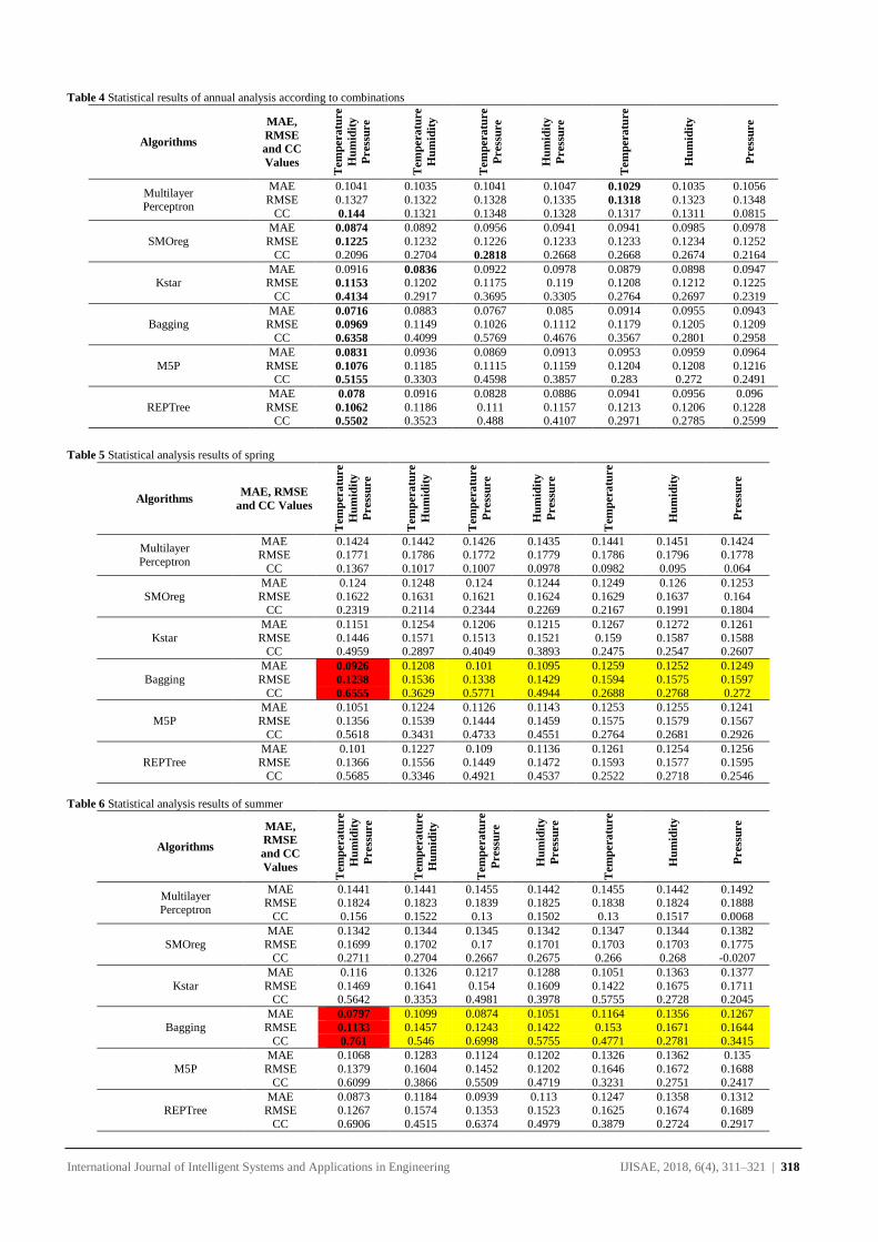
International Journal of Intelligent Systems and Applications in Engineering IJISAE, 2018, 6(4), 311–321 | 318
Table 4 Statistical results of annual analysis according to combinations
Algorithms
MAE,
RMSE
and CC
Values
Tem
pera
ture
Hu
mid
ity
Press
ure
Tem
pera
ture
Hu
mid
ity
Tem
pera
ture
Press
ure
Hu
mid
ity
Press
ure
Tem
pera
ture
Hu
mid
ity
Press
ure
Multilayer Perceptron
MAE 0.1041 0.1035 0.1041 0.1047 0.1029 0.1035 0.1056
RMSE 0.1327 0.1322 0.1328 0.1335 0.1318 0.1323 0.1348
CC 0.144 0.1321 0.1348 0.1328 0.1317 0.1311 0.0815
SMOreg
MAE 0.0874 0.0892 0.0956 0.0941 0.0941 0.0985 0.0978
RMSE 0.1225 0.1232 0.1226 0.1233 0.1233 0.1234 0.1252
CC 0.2096 0.2704 0.2818 0.2668 0.2668 0.2674 0.2164
Kstar MAE 0.0916 0.0836 0.0922 0.0978 0.0879 0.0898 0.0947
RMSE 0.1153 0.1202 0.1175 0.119 0.1208 0.1212 0.1225
CC 0.4134 0.2917 0.3695 0.3305 0.2764 0.2697 0.2319
Bagging MAE 0.0716 0.0883 0.0767 0.085 0.0914 0.0955 0.0943
RMSE 0.0969 0.1149 0.1026 0.1112 0.1179 0.1205 0.1209
CC 0.6358 0.4099 0.5769 0.4676 0.3567 0.2801 0.2958
M5P
MAE 0.0831 0.0936 0.0869 0.0913 0.0953 0.0959 0.0964
RMSE 0.1076 0.1185 0.1115 0.1159 0.1204 0.1208 0.1216 CC 0.5155 0.3303 0.4598 0.3857 0.283 0.272 0.2491
REPTree
MAE 0.078 0.0916 0.0828 0.0886 0.0941 0.0956 0.096
RMSE 0.1062 0.1186 0.111 0.1157 0.1213 0.1206 0.1228 CC 0.5502 0.3523 0.488 0.4107 0.2971 0.2785 0.2599
Table 5 Statistical analysis results of spring
Algorithms MAE, RMSE
and CC Values
Tem
pera
ture
Hu
mid
ity
Press
ure
Tem
pera
ture
Hu
mid
ity
Tem
pera
ture
Press
ure
Hu
mid
ity
Press
ure
Tem
pera
ture
Hu
mid
ity
Press
ure
Multilayer
Perceptron
MAE 0.1424 0.1442 0.1426 0.1435 0.1441 0.1451 0.1424 RMSE 0.1771 0.1786 0.1772 0.1779 0.1786 0.1796 0.1778
CC 0.1367 0.1017 0.1007 0.0978 0.0982 0.095 0.064
SMOreg
MAE 0.124 0.1248 0.124 0.1244 0.1249 0.126 0.1253
RMSE 0.1622 0.1631 0.1621 0.1624 0.1629 0.1637 0.164 CC 0.2319 0.2114 0.2344 0.2269 0.2167 0.1991 0.1804
Kstar
MAE 0.1151 0.1254 0.1206 0.1215 0.1267 0.1272 0.1261
RMSE 0.1446 0.1571 0.1513 0.1521 0.159 0.1587 0.1588 CC 0.4959 0.2897 0.4049 0.3893 0.2475 0.2547 0.2607
Bagging
MAE 0.0926 0.1208 0.101 0.1095 0.1259 0.1252 0.1249
RMSE 0.1238 0.1536 0.1338 0.1429 0.1594 0.1575 0.1597
CC 0.6555 0.3629 0.5771 0.4944 0.2688 0.2768 0.272
M5P
MAE 0.1051 0.1224 0.1126 0.1143 0.1253 0.1255 0.1241
RMSE 0.1356 0.1539 0.1444 0.1459 0.1575 0.1579 0.1567
CC 0.5618 0.3431 0.4733 0.4551 0.2764 0.2681 0.2926
REPTree MAE 0.101 0.1227 0.109 0.1136 0.1261 0.1254 0.1256
RMSE 0.1366 0.1556 0.1449 0.1472 0.1593 0.1577 0.1595
CC 0.5685 0.3346 0.4921 0.4537 0.2522 0.2718 0.2546
Table 6 Statistical analysis results of summer
Algorithms
MAE,
RMSE
and CC
Values
Tem
pera
ture
Hu
mid
ity
Press
ure
Tem
pera
ture
Hu
mid
ity
Tem
pera
ture
Press
ure
Hu
mid
ity
Press
ure
Tem
pera
ture
Hu
mid
ity
Press
ure
Multilayer
Perceptron
MAE 0.1441 0.1441 0.1455 0.1442 0.1455 0.1442 0.1492 RMSE 0.1824 0.1823 0.1839 0.1825 0.1838 0.1824 0.1888
CC 0.156 0.1522 0.13 0.1502 0.13 0.1517 0.0068
SMOreg
MAE 0.1342 0.1344 0.1345 0.1342 0.1347 0.1344 0.1382
RMSE 0.1699 0.1702 0.17 0.1701 0.1703 0.1703 0.1775 CC 0.2711 0.2704 0.2667 0.2675 0.266 0.268 -0.0207
Kstar
MAE 0.116 0.1326 0.1217 0.1288 0.1051 0.1363 0.1377
RMSE 0.1469 0.1641 0.154 0.1609 0.1422 0.1675 0.1711 CC 0.5642 0.3353 0.4981 0.3978 0.5755 0.2728 0.2045
Bagging
MAE 0.0797 0.1099 0.0874 0.1051 0.1164 0.1356 0.1267
RMSE 0.1133 0.1457 0.1243 0.1422 0.153 0.1671 0.1644
CC 0.761 0.546 0.6998 0.5755 0.4771 0.2781 0.3415
M5P
MAE 0.1068 0.1283 0.1124 0.1202 0.1326 0.1362 0.135
RMSE 0.1379 0.1604 0.1452 0.1202 0.1646 0.1672 0.1688
CC 0.6099 0.3866 0.5509 0.4719 0.3231 0.2751 0.2417
REPTree MAE 0.0873 0.1184 0.0939 0.113 0.1247 0.1358 0.1312
RMSE 0.1267 0.1574 0.1353 0.1523 0.1625 0.1674 0.1689
CC 0.6906 0.4515 0.6374 0.4979 0.3879 0.2724 0.2917
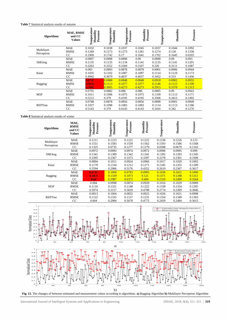
International Journal of Intelligent Systems and Applications in Engineering IJISAE, 2018, 6(4), 311–321 | 319
Table 7 Statistical analysis results of autumn
Algorithms
MAE, RMSE
and CC
Values
Tem
pera
ture
Hu
mid
ity
Press
ure
Tem
pera
ture
Hu
mid
ity
Tem
pera
ture
Press
ure
Hu
mid
ity
Press
ure
Tem
pera
ture
Hu
mid
ity
Press
ure
Multilayer Perceptron
MAE 0.1032 0.1038 0.1037 0.1045 0.1037 0.1044 0.1092
RMSE 0.1269 0.1273 0.1273 0.1281 0.1274 0.128 0.1358
CC 0.1909 0.1742 0.17 0.1641 0.1702 0.1645 0.0203
SMOreg MAE 0.0897 0.0898 0.0898 0.09 0.0898 0.09 0.093 RMSE 0.1135 0.1135 0.1134 0.1141 0.1135 0.1141 0.1201
CC 0.3263 0.3252 0.3269 0.3107 0.326 0.3111 0.1087
Kstar MAE 0.083 0.0893 0.0878 0.0878 0.0901 0.0906 0.0944 RMSE 0.1035 0.1102 0.1087 0.1087 0.1114 0.1119 0.1173
CC 0.4942 0.3679 0.4037 0.4037 0.3452 0.333 0.1456
Bagging
MAE 0.0737 0.0888 0.0848 0.0848 0.0918 0.0902 0.0955
RMSE 0.0956 0.1113 0.1077 0.1077 0.1146 0.1115 0.1199 CC 0.5902 0.3605 0.4273 0.4273 0.2915 0.3379 0.1313
M5P
MAE 0.0795 0.0882 0.086 0.086 0.0895 0.09 0.0943
RMSE 0.1011 0.1096 0.1075 0.1075 0.1109 0.1113 0.1171 CC 0.5212 0.379 0.4195 0.4195 0.3506 0.3413 0.1492
REPTree
MAE 0.0788 0.0878 0.0856 0.0856 0.0898 0.0901 0.0949
RMSE 0.1027 0.1098 0.1083 0.1083 0.1114 0.1113 0.1186
CC 0.5143 0.379 0.4143 0.4143 0.3416 0.342 0.1276
Table 8 Statistical analysis results of winter
Algorithms
MAE,
RMSE
and CC
Values
Tem
pera
ture
Hu
mid
ity
Press
ure
Tem
pera
ture
Hu
mid
ity
Tem
pera
ture
Press
ure
Hu
mid
ity
Press
ure
Tem
pera
ture
Hu
mid
ity
Press
ure
Multilayer
Perceptron
MAE 0.1211 0.1223 0.1222 0.1222 0.1236 0.1226 0.123
RMSE 0.1551 0.1583 0.1559 0.1562 0.1593 0.1586 0.1568 CC 0.1325 0.0735 0.1277 0.1279 0.0588 0.0679 0.1163
SMOreg
MAE 0.0972 0.0993 0.0974 0.0972 0.0996 0.0995 0.099
RMSE 0.1341 0.1389 0.1342 0.1341 0.1392 0.1393 0.1345
CC 0.3395 0.2367 0.3373 0.3397 0.2278 0.2301 0.3308
Kstar
MAE 0.0894 0.1011 0.0924 0.0966 0.1017 0.1029 0.1002
RMSE 0.1179 0.1334 0.1212 0.1271 0.1345 0.1355 0.1309
CC 0.5594 0.2906 0.5176 0.4352 0.2619 0.2367 0.3617
Bagging MAE 0.0747 0.1004 0.0793 0.0905 0.1036 0.1021 0.1000
RMSE 0.1021 0.1339 0.1073 0.121 0.1371 0.1348 0.1311
CC 0.68 0.2987 0.6372 0.499 0.2329 0.2499 0.3564
M5P MAE 0.084 0.0998 0.0874 0.0929 0.1016 0.1029 0.0989
RMSE 0.1116 0.1321 0.1148 0.1222 0.1338 0.1354 0.1285
CC 0.5974 0.3157 0.5659 0.4788 0.2774 0.2309 0.3846
REPTree
MAE 0.0813 0.1004 0.0852 0.0922 0.1026 0.1021 0.0998
RMSE 0.1122 0.1335 0.1157 0.1231 0.1354 0.1349 0.1303 CC 0.604 0.2984 0.5678 0.4772 0.2459 0.2484 0.3615
a)
b) Fig. 12. The changes of between estimated and measurement values according to algorithms. a) Bagging Algorithm b) Multilayer Perceptron Algorithm
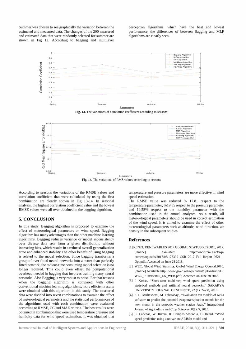
International Journal of Intelligent Systems and Applications in Engineering IJISAE, 2018, 6(4), 311–321 | 320
Summer was chosen to see graphically the variation between the
estimated and measured data. The changes of the 200 measured
and estimated data that were randomly selected for summer are
shown in Fig 12. According to bagging and multilayer
perceptron algorithms, which have the best and lowest
performance, the differences of between Bagging and MLP
algorithms are clearly seen.
Fig. 13. The variations of correlation coefficient according to seasons
Fig. 14. The variations of RMS values according to seasons
According to seasons the variations of the RMSE values and
correlation coefficient that were calculated by using the first
combination are clearly shown in Fig 13-14. In seasonal
analysis, the highest correlation coefficient value and the lowest
RMSE values were all over obtained in the bagging algorithm.
5. CONCLUSION
In this study, Bagging algorithm is proposed to examine the
effect of meteorological parameters on wind speed. Bagging
algorithm has many advantages than the other machine learning
algorithms. Bagging reduces variance or model inconsistency
over diverse data sets from a given distribution, without
increasing bias, which results in a reduced overall generalization
error and enhanced stability.The other benefit of using bagging
is related to the model selection. Since bagging transforms a
group of over fitted neural networks into a better-than perfectly
fitted network, the tedious time consuming model selection is no
longer required. This could even offset the computational
overhead needed in bagging that involves training many neural
networks. Also Bagging is very robust to noise. For that reasons
when the bagging algorithm is compared with other
conventional machine learning algorithms, more efficient results
were obtained with this algorithm in this study. The measured
data were divided into seven combinations to examine the effect
of meteorological parameters and the statistical performances of
the algorithms used with each combination were evaluated
according to RMSE, CC and MAE criteria. The best results were
obtained in combination that were used temperature pressure and
humidity data for wind speed estimation. It was obtained that
temperature and pressure parameters are more effective in wind
speed estimation.
The RMSE value was reduced % 17.81 respect to the
temperature parameter, %19.85 respect to the pressure parameter
and 19.58% respect to the humidity parameter with the
combination used in the annual analyzes. As a result, all
meteorological parameters should be used in correct estimation
of the wind speed. It is aimed to examine the effect of other
meteorological parameters such as altitude, wind direction, air
density in the subsequent studies.
References
[1] REN21, RENEWABLES 2017 GLOBAL STATUS REPORT, 2017,
[Online]. Available: http://www.ren21.net/wp-
content/uploads/2017/06/178399_GSR_2017_Full_Report_0621_
Opt.pdf.; Accessed on June 28 2018.
[2] WEC, Global Wind Statistics, Global Wind Energy Councıl,2016,
[Online].Available:http://www.gwec.net/wpcontent/uploads/vip/G
WEC_PRstats2016_EN_WEB.pdf.; Accessed on June 28 2018.
[3] I. Kırbas, “Short-term multi-step wind speed prediction using
statistical methods and artificial neural networks,” SAKARYA
UNIVERSITY JOURNAL OF SCIENCE, 22 (1), 24-38, 2018.
[4] S. H. Mirhashemi, M. Tabatabayi, “Evaluation ten models of weka
software to predict the potential evapotranspiration month for the
next month in the synoptic weather station Arak,” International
Journal of Agriculture and Crop Sciences, 8(1), 5, 2015.
[5] E. Cadenas, W. Rivera, R. Campos-Amezcua, C. Heard, “Wind
speed prediction using a univariate ARIMA model and a
International Journal of Intelligent Systems and Applications in Engineering IJISAE, 2018, 6(4), 311–321 | 321
multivariate NARX model,” Energies, 9(2), 109, 2016.
[6] M. A. Ansari, N. S. Pal, H. Malik, “Wind speed and power
prediction of prominent wind power potential states in India using
GRNN, In Power Electronics, Intelligent Control and Energy
Systems (ICPEICES),” IEEE International Conference on IEEE ,
1-6, 2016.
[7] M. Zeng, X. Zhang, J. Li, Q. Meng, “Multifractal analysis of short-
term wind speed time series with different sampling frequencies,”
12th World Congress on Intelligent Control and Automation
(WCICA), pp. 3213–3218, 2016.
[8] I. Khandelwal, R. Adhikari, G. Verma, “Time Series Forecasting
Using Hybrid ARIMA and ANN Models Based on DWT
Decomposition,” Procedia Comput. Sci., vol. 48, pp. 173–179,
2015.
[9] M. Khanna, N. K. Srinath, J. K. Mendiratta, “Feature Extraction of
Time Series Data for Wind Speed Power Generation,” 6th
International Conference on Advanced Computing (IACC), pp.
169–173, 2016.
[10] H. G. Lee, M. Piao, Y. H. Shin, “Wind Power Pattern Forecasting
Based on Projected Clustering and Classification Methods,” Etri
Journal, 37(2), 283-294, 2015.
[11]Y. Wanga, H. Mab, D. Wanga, G. Wangc, J. Wua, J. Biand, J.
Liud, “A new method for wind speed forecasting based on copula
theory,” Environmental Research, 160, 365–371, 2018.
[12]R. Velo, P. López, F. Maseda, “Wind speed estimation using
multilayer perceptron,” Energy Conversion and Management, 81,
1–9, 2014.
[13] M. Timur, F. Aydın, T.Ç. Akıncı, “İstanbul Göztepe Bölgesinin
Makine Öğrenmesi Yöntemi ile Rüzgâr Hızının Tahmin
Edilmesi,” Makine Teknolojileri Elektronik Dergisi 8(4), 75-80, (in
Turkish) 2011.
[14]M. Zontul, F. Aydın, G. Doğan, S. Şener, O. Kaynar, “Wind Speed
Forecasting Using REPTree and Bagging Methods in Kirklareli-
Turkey,” J. Theor. Appl. Inf. Technol., 56, 17–29, 2013.
[15] A. Meng, J. Ge, H. Yin, S. Chen, “Wind speed forecasting based on
wavelet packet decomposition and artificial neural networks trained
by crisscross optimization algorithm,” Energy Conversion and
Management,114, 75-88, 2016.
[16] L. Breiman, “Bagging predictors,” Univ. California, Dept. Stat.,
Berkeley, Tech. Rep. 421, 1994.
[17] T. Jiang, J. Li, Y. Zheng, C. Sun, “Improved Bagging Algorithm for
Pattern Recognition in UHF Signals of Partial Discharges,”
Energies, 4, 1087-1101; doi:10.3390/en4071087, 2011.
[18] K. Machová, F. Barčák, P. Bednár, “A Bagging Method using
Decision Trees in the Role of Base Classifiers,” Acta Polytechnica
Hungarica, Vol. 3, No. 2, 2006.
[19] C. Doukas, I. Maglogiannis, P. Tragas, D. Liapis, G. Yovanof,
“Patient fall detection using support vector machines,” International
Federation for Information Processing, vol. 247, pp. 147-156, 2007.
[20] T. W. Kuan, J. F. Wang, J. C. Wang, P. C. Lin, et al., “VLSI Design
of an SVM Learning Core on Sequential Minimal Optimization
Algorithm,” IEEETransactions on Very Large Scale Integration
(Vlsi) Systems, 20(4), 673-683, 2012.
[21] J. Platt, “Fast training of support vector machines using sequential
minimal optimization,” In B. Schölkopf, C. Burges, and A. Smola,
editors, Advances in kernel methods: Support vector learning.
Cambridge, MA: MIT Press. 1998.
[22] A. J. Smola, B. Schölkopf, “A tutorial on support vector regression,”
Statistics and Computing, 14(3), 199-222, 2004.
[23] C. K. Madhusudana, H. Kumar, S. Narendranath, “Condition
monitoring of face milling tool using K-star algorithm and
histogram features of vibration signal,” Engineering Science and
Technology, an International Journal, 19 1543–1551, 2016.
[24] R. Satishkumar, V. Sugumaran, “ Remaining Life Time Prediction
of Bearings Using K-Star Algorithm – A Statistical Approach”,
Journal of Engineering Science and Technology Vol. 12, No. 1
168 – 181, 2017.
[25] A. W. Harley, “An Interactive Node-Link Visualization of
Convolutional Neural Networks,” in ISVC, pages 867-877, 2015
[26] Y. Kumar, G. Sahoo, “Analysis of Parametric & Non Parametric
Classifiers for Classification Technique using WEKA,” I.J.
Information Technology and Computer Science, 7, 43-49, 2012.
[27] D.P.Alonso, S.P. Tejedor, M. Navarro, C. Rad, Á.A. González,
J.F.D.Pastor, “Decision Trees for the prediction of environmental
and agronomic effects of the use of Compost of Sewage Sludge
(CSS),” Sustainable Production and Consumption 12 119 –
133, 2017.
[28]S. Kalmegh, “Analysis of WEKA Data Mining Algorithm
REPTree, Simple Cart and RandomTree for Classification of Indian
News,” International Journal of Innovative Science, Engineering &
Technology, Vol. 2 Issue 2, February, 2015.
[29] A. Behnood, V. Behnood, M. M. Gharehveran, K. E. Alyamac,
“Prediction of the compressive strength of normal and high-
performance concretes using M5P model tree algorithm,”
Construction and Building Materials, 142, 199–207, 2017.
[30] R. Sharma, S. Kumar, R. Maheshwari, “Comparative Analysis of
Classification Techniques in Data Mining Using Different
Datasets,” International Journal of Computer Science and Mobile
Computing, Vol. 4, Issue. 12, December, pg.125 – 134, 2015.
[31] E. K. Onyari, F. M. Ilunga, “Application of MLP Neural Network
and M5P Model Tree in Predicting Streamflow: A Case Study of
Luvuvhu Catchment, South Africa,” International Journal of
Innovation, Management and Technology, Vol. 4, No. 1, February
2013.
[32] R. Meenal, A. I. Selvakumar, “Assessment of SVM, Empirical and
ANN based solar radiation prediction models with most influencing
input parameters,” Renewable Energy, Volume 121, June, Pages
324-343, 2018.
International Journal of
Intelligent Systems and
Applications in Engineering
Advanced Technology and Science
ISSN:2147-67992147-6799 www.atscience.org/IJISAE Original Research Paper
International Journal of Intelligent Systems and Applications in Engineering IJISAE, 2018, 6(4), 322–328 | 322
Lupsix: A Cascade Framework for Lung Parenchyma
Segmentation in Axial CT Images
Hasan Koyuncu*1
Accepted : 31/12/2018 Published: 31/12/2018 DOI: 10.1039/b000000x
Abstract: Lung imaging and computer aided diagnosis (CAD) play a critical role in detection of lung diseases. The most significant part
of a lung based CAD is to fulfil the parenchyma segmentation, since disease information is kept in the parenchyma texture. For this purpose,
parenchyma segmentation should be accurately performed to find the necessary diagnosis to be used in the treatment. Besides, lung
parenchyma segmentation remains as a challenging task in computed tomography (CT) owing to the handicaps oriented with the imaging
and nature of parenchyma. In this paper, a cascade framework involving histogram analysis, morphological operations, mean shift
segmentation (MSS) and region growing (RG) is proposed to perform an accurate segmentation in thorax CT images. In training data, 20
axial CT images are utilized to define the optimum parameter values, and 150 images are considered as test data to objectively evaluate
the performance of system. Five statistical metrics are handled to carry out the performance assessment, and a literature comparison is
realized with the state-of-the-art techniques. As a result, parenchyma tissues are segmented with success rates as 98.07% (sensitivity),
99.72% (specificity), 99.3% (accuracy), 98.59% (Dice similarity coefficient) and 97.23% (Jaccard) on test dataset.
Keywords: Axial Analysis, Computed Tomography, Cascade Framework, Lung Parenchyma, Medical Image Segmentation
1. Introduction
Lung segmentation reserves a significant place before important
objectives like detection of pulmonary nodules, pulmonary
vessels, cancer types and various diseases [1-4]. In medical area,
computed tomography (CT) scans are frequently preferred to
perform a diagnostic about aforementioned subjects. Herein,
thorax CT images constitute some challenging handicaps for an
accurate parenchyma segmentation. These handicaps arise as: 1-)
Similar grey levels between the lung parenchyma and other tissues,
2-) Disease based deformation inside of parenchyma, 3-) Non-
stable shape features of lung tissues. For this purpose, various
segmentation algorithms are asserted in the literature:
Thresholding approaches, Region-based algorithms, Shape-based
methods, Neighboring anatomy-guided techniques and Machine
learning-based structures [5-7].
Thresholding approaches work efficient, once lung intensities
clearly differentiate from the close tissues. However, these
techniques cannot be used on conditions that spatial information
and variability gain importance related to the disease based
deformations. At this point, deformations can sharply change the
grey values in lung [5]. Region-based algorithms (region growing,
fuzzy connectedness, graph cut, etc.) are seen as impressive
techniques containing spatial information with region phenomena.
Region-based methods are actively utilized on homogenous-field
in lung, but the performance of techniques vary on the
segmentation of heterogeneous fields [5]. Shape-based methods
(atlas or model – based methods, active contours, level sets, etc.)
are frequently appealed to segment the abnormal tissues on which
thresholding approaches remain insufficient [5]. Neighboring
anatomy-guided techniques consider neighboring anatomic objects
around lung for separating the lung from objects (organs).
Nevertheless, these techniques cannot be processed on extremely
abnormal or artifacted lung parenchyma [5]. Similarly,
performance of machine learning-based methods can deteriorate
sharply because of the extreme deformation inside of lung
parenchyma [5]. In the literature, aforementioned techniques have
been applied to the lung segmentation, and hybrid techniques are
being designed to handle the parenchyma segmentation with
higher performance [5-8].
Wei et al. [9] developed a system based on improved chain code
and Bresenham algorithm to segment the lungs. Proposed system
performed the task with an accuracy of 95.2%. Dai et al. [10]
designed a pipeline involving graph cuts, Gaussian mixture models
(GMMs) and expectation maximization (EM) to segment the
lungs. According to the results, proposed model obtained the Dice
similarity coefficient (DSC) as 98.74%. Noor et al. [11] realized
lung segmentation with a framework in which thresholding and
morphology based process are used. In experiments, it was
revealed that proposed method performed the segmentation with
high DSC (98.4%). Pulagam et al. [12] utilized the modified
convex hull approach and morphological operators for
segmentation. According to the experiments, proposed approach
obtained 98.62% DSC on overall. Chae et al. [13] generated a
Level-set based approach named MLevel-set that achieved 98.4%
accuracy on lung segmentation. Zhang et al. [14] produced a
hybrid geometric active contour model and attained with 97.7%
DSC on average.
In this paper, a cascade framework is presented to segment the
parenchyma tissue in CT images as more proper than the state-of-
the-art methods. Histogram analysis, morphological operations,
mean shift segmentation (MSS) and region growing (RG) are
handled to design an efficient framework. Proposed system is
named according to the tasks to be realized including the number
of units (six): Lupsix (lung parenchyma segmentation in axial CT).
_______________________________________________________________________________________________________________________________________________________________________________________________________________________________________________________________________________________________________________________________
1 Konya Technical University, Konya, TURKEY
* Corresponding Author: Email: [email protected]

International Journal of Intelligent Systems and Applications in Engineering IJISAE, 2018, 6(4), 322–328 | 323
Performance of Lupsix is evaluated in CT images taken from
LUNA16 dataset, with the use of five different metrics [15-17].
The rest of paper is organized as follows. In Section 2, the utilized
methods and Lupsix are comprehensively explained. In Section 3,
performance evaluation is examined in detail, and visual
perspectives of results are presented to qualify the operation of
system. The interpretations of work are mentioned, and a literature
comparison is tendered. In Section 4, concluding remark is given.
2. Methods
The principle of this study is to obtain the lungs in thorax-axial CT
images in which shape features of lungs varies
uncharacteristically, diseases based deformation can be available
and lung parenchyma can own to close grey levels with the nearby
tissues. This situation requires a robust framework that will not
effected from these handicaps, and the following methods are
utilized to design a robust system:
Gamma correction
Morphological closing
Contrast-limited adaptive histogram equalization
Mean shift segmentation
Region growing
The filling process
2.1. Morphological Algorithms
Gamma correction: Gamma correction (GC) stands for a contrast
enhancement method explicitly revealing the objects in image. GC
is generally utilized to improve the nonlinearity of image and
regarding this, the intensities are rearranged as in (1) [18].
𝑣𝑜𝑢𝑡 = (𝐴. 𝑣𝑖𝑛𝑝𝑢𝑡)𝛾 (1)
vinput, A and γ respectively symbolize the input image, constant and
the power. Mapping process of gamma correction constitutes a
linear transformation in the event that A and γ are equal to “1”, and
pixel intensities are settled within the range [0,1] as in our study
[18].
Morphological closing: Morphological closing (MC) is used to
combine the familiar pixel intensities according to the structuring
element (diamond, disk, line, etc.). For this purpose, closing
process (A•B) is formed as in (2) of which A⊕B and θB
respectively symbolize the dilation of A and B, and erosion of B
[19].
𝐴 • B = (𝐴 ⊕ 𝐵)𝜃𝐵 (2)
As a result of MC, the objects in an image come to the forefront
better than the initial conditions. Hence, MC can be efficiently
preferred on object detection and segmentation tasks [19,20].
Contrast - limited adaptive histogram equalization: Contrast-
limited adaptive histogram equalization (CLAHE) varies from the
adaptive histogram equalization (AHE) with the use of contrast
limiting (CL). Herein, AHE is a transformation of pixels
concerning the histogram and neighboring so as to improve the
irregular contrast distribution. CL represses the increase in noise
level arisen as a result of contrast level increase [21].
Filling process: The filling process is used to fill the areas
connected with each other, and these areas consist of closed shapes
to be filled [22].
2.2. Mean Shift Segmentation
Mean shift segmentation (MSS) defines the 2D features of an
image into the joint spatial-range domain. In operation of MSS,
mode values are considered to rearrange the pixels’ intensities of
different clusters. Two kernels are analyzed to attach the pixels of
an object: 1-) Spatial kernel, 2-) Range kernel. The bandwidths of
kernels play a critical role for the optimum attachment of pixels of
the same cluster (object). MSS algorithm includes three parameters
to approximate the pixels [23]:
Spatial kernel bandwidth (hs)
Range kernel bandwidth (hr)
Convergence criterion threshold (M)
To attach the pixels, MSS operates a multiple-kernel stated in (3)
[23,24].
𝐾ℎ𝑠ℎ𝑟(𝑥) =
𝐶
ℎ𝑠2ℎ𝑟
𝑃 𝑘 (‖𝑥𝑠
ℎ𝑠‖
2
) 𝑘 (‖𝑥𝑟
ℎ𝑟‖
2
) (3)
xs and xr symbolize the vectors concerning with the spatial and
range phenomena; k(x), C and p respectively mean the general
profile, normalization coefficient and dimension. Herein, the
spatial (hs) and range (hr) kernel bandwidths should be carefully
assigned to optimally detect the objects. Besides, the pixels owing
to lower grey values than threshold M, are ignored to perform the
specified-size segmentation. For a detailed explanation about
MSS, please see [23] and [24].
2.3. Region Growing
Region growing (RG) starts with a random or user-defined point
(seed) in image. According to seed intensity, the extension of
pixels continue until similar intensities are not available. For this
purpose, a parameter is needed to decide which pixel value will be
included or excluded. This parameter (tolerance) is regarded to
restrict the extension of pixels. RG algorithm processes step by
step according to the following rules [24]:
Assignment of seed point(s)
The extension is realized which is restricted by tolerance
The extension is performed according to neighbor pixel
intensities until termination is met
2.4. Lupsix Framework
In Lupsix; histogram analysis, morphological operators, MSS and
RG algorithms are chosen to reveal the parenchyma tissue, and to
design a robust system against aforementioned handicaps. For this
purpose, Lupsix runs the operation steps in Figure 1:
1. GC differentiates the regions inside of thorax CT image.
At this point, lung parenchyma differs from the nearby
tissues like ribs, subcutaneous fats, etc.
2. MC is performed with disk type structuring element,
since this type element remains as the most proper one
in terms of fitting to the concavity of lungs. After MC is
processed, the parenchyma intensities come to closer
grey levels for an accurate object segmentation.
3. CLAHE sharpens the outer edges of parenchyma.
However, this situation puts forward more sensitive
changes inside of parenchyma, and some parts of lung
(like nodules, vessels, etc.) are sharpened too.
4. MSS attaches the tissue parts of parenchyma to reveal
and to smooth the parenchyma more explicit. Regarding
this, thorax CT image becomes more convenient before
object segmentation.
5. RG is fulfilled using two user-defined seed points, and
lung parenchyma is segmented with the use of MSS
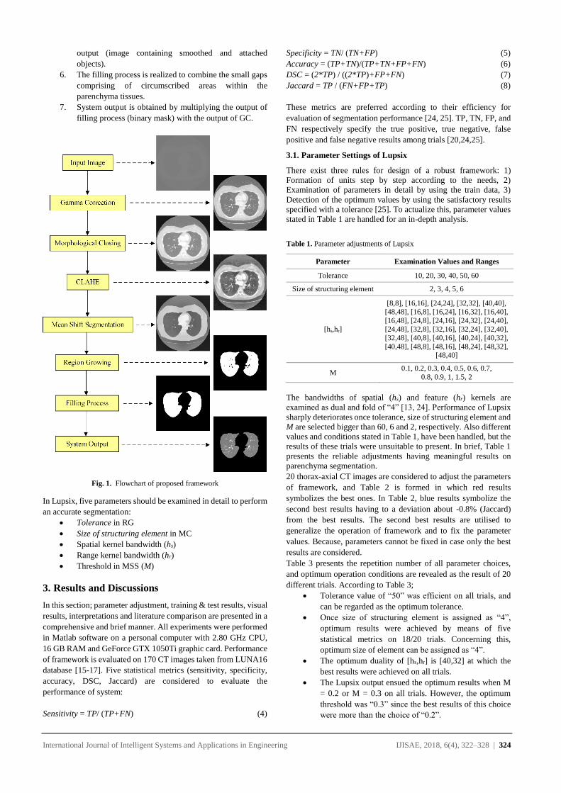
International Journal of Intelligent Systems and Applications in Engineering IJISAE, 2018, 6(4), 322–328 | 324
output (image containing smoothed and attached
objects).
6. The filling process is realized to combine the small gaps
comprising of circumscribed areas within the
parenchyma tissues.
7. System output is obtained by multiplying the output of
filling process (binary mask) with the output of GC.
Fig. 1. Flowchart of proposed framework
In Lupsix, five parameters should be examined in detail to perform
an accurate segmentation:
Tolerance in RG
Size of structuring element in MC
Spatial kernel bandwidth (hs)
Range kernel bandwidth (hr)
Threshold in MSS (M)
3. Results and Discussions
In this section; parameter adjustment, training & test results, visual
results, interpretations and literature comparison are presented in a
comprehensive and brief manner. All experiments were performed
in Matlab software on a personal computer with 2.80 GHz CPU,
16 GB RAM and GeForce GTX 1050Ti graphic card. Performance
of framework is evaluated on 170 CT images taken from LUNA16
database [15-17]. Five statistical metrics (sensitivity, specificity,
accuracy, DSC, Jaccard) are considered to evaluate the
performance of system:
Sensitivity = TP/ (TP+FN) (4)
Specificity = TN/ (TN+FP) (5)
Accuracy = (TP+TN)/(TP+TN+FP+FN) (6)
DSC = (2*TP) / ((2*TP)+FP+FN) (7)
Jaccard = TP / (FN+FP+TP) (8)
These metrics are preferred according to their efficiency for
evaluation of segmentation performance [24, 25]. TP, TN, FP, and
FN respectively specify the true positive, true negative, false
positive and false negative results among trials [20,24,25].
3.1. Parameter Settings of Lupsix
There exist three rules for design of a robust framework: 1)
Formation of units step by step according to the needs, 2)
Examination of parameters in detail by using the train data, 3)
Detection of the optimum values by using the satisfactory results
specified with a tolerance [25]. To actualize this, parameter values
stated in Table 1 are handled for an in-depth analysis.
Table 1. Parameter adjustments of Lupsix
Parameter Examination Values and Ranges
Tolerance 10, 20, 30, 40, 50, 60
Size of structuring element 2, 3, 4, 5, 6
[hs,hr]
[8,8], [16,16], [24,24], [32,32], [40,40],
[48,48], [16,8], [16,24], [16,32], [16,40],
[16,48], [24,8], [24,16], [24,32], [24,40], [24,48], [32,8], [32,16], [32,24], [32,40],
[32,48], [40,8], [40,16], [40,24], [40,32],
[40,48], [48,8], [48,16], [48,24], [48,32], [48,40]
M 0.1, 0.2, 0.3, 0.4, 0.5, 0.6, 0.7,
0.8, 0.9, 1, 1.5, 2
The bandwidths of spatial (hs) and feature (hr) kernels are
examined as dual and fold of “4” [13, 24]. Performance of Lupsix
sharply deteriorates once tolerance, size of structuring element and
M are selected bigger than 60, 6 and 2, respectively. Also different
values and conditions stated in Table 1, have been handled, but the
results of these trials were unsuitable to present. In brief, Table 1
presents the reliable adjustments having meaningful results on
parenchyma segmentation.
20 thorax-axial CT images are considered to adjust the parameters
of framework, and Table 2 is formed in which red results
symbolizes the best ones. In Table 2, blue results symbolize the
second best results having to a deviation about -0.8% (Jaccard)
from the best results. The second best results are utilised to
generalize the operation of framework and to fix the parameter
values. Because, parameters cannot be fixed in case only the best
results are considered.
Table 3 presents the repetition number of all parameter choices,
and optimum operation conditions are revealed as the result of 20
different trials. According to Table 3;
Tolerance value of “50” was efficient on all trials, and
can be regarded as the optimum tolerance.
Once size of structuring element is assigned as “4”,
optimum results were achieved by means of five
statistical metrics on 18/20 trials. Concerning this,
optimum size of element can be assigned as “4”.
The optimum duality of [hs,hr] is [40,32] at which the
best results were achieved on all trials.
The Lupsix output ensued the optimum results when M
= 0.2 or M = 0.3 on all trials. However, the optimum
threshold was “0.3” since the best results of this choice
were more than the choice of “0.2”.
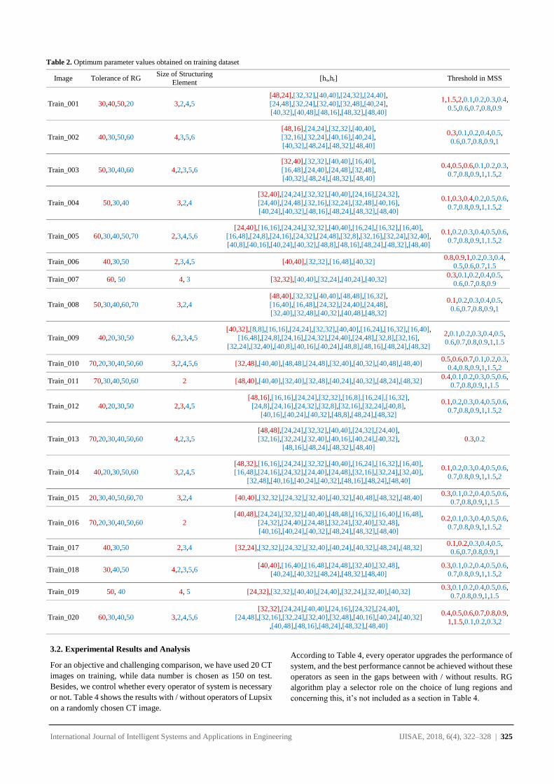
International Journal of Intelligent Systems and Applications in Engineering IJISAE, 2018, 6(4), 322–328 | 325
3.2. Experimental Results and Analysis
For an objective and challenging comparison, we have used 20 CT
images on training, while data number is chosen as 150 on test.
Besides, we control whether every operator of system is necessary
or not. Table 4 shows the results with / without operators of Lupsix
on a randomly chosen CT image.
According to Table 4, every operator upgrades the performance of
system, and the best performance cannot be achieved without these
operators as seen in the gaps between with / without results. RG
algorithm play a selector role on the choice of lung regions and
concerning this, it’s not included as a section in Table 4.
Table 2. Optimum parameter values obtained on training dataset
Image Tolerance of RG Size of Structuring
Element [hs,hr] Threshold in MSS
Train_001 30,40,50,20 3,2,4,5 [48,24],[32,32],[40,40],[24,32],[24,40], [24,48],[32,24],[32,40],[32,48],[40,24],
[40,32],[40,48],[48,16],[48,32],[48,40]
1,1.5,2,0.1,0.2,0.3,0.4,
0.5,0.6,0.7,0.8,0.9
Train_002 40,30,50,60 4,3,5,6
[48,16],[24,24],[32,32],[40,40],
[32,16],[32,24],[40,16],[40,24], [40,32],[48,24],[48,32],[48,40]
0.3,0.1,0.2,0.4,0.5,
0.6,0.7,0.8,0.9,1
Train_003 50,30,40,60 4,2,3,5,6
[32,40],[32,32],[40,40],[16,40],
[16,48],[24,40],[24,48],[32,48], [40,32],[48,24],[48,32],[48,40]
0.4,0.5,0.6,0.1,0.2,0.3,
0.7,0.8,0.9,1,1.5,2
Train_004 50,30,40 3,2,4
[32,40],[24,24],[32,32],[40,40],[24,16],[24,32],
[24,40],[24,48],[32,16],[32,24],[32,48],[40,16], [40,24],[40,32],[48,16],[48,24],[48,32],[48,40]
0.1,0.3,0.4,0.2,0.5,0.6,
0.7,0.8,0.9,1,1.5,2
Train_005 60,30,40,50,70 2,3,4,5,6 [24,40],[16,16],[24,24],[32,32],[40,40],[16,24],[16,32],[16,40],
[16,48],[24,8],[24,16],[24,32],[24,48],[32,8],[32,16],[32,24],[32,40],
[40,8],[40,16],[40,24],[40,32],[48,8],[48,16],[48,24],[48,32],[48,40]
0.1,0.2,0.3,0.4,0.5,0.6,
0.7,0.8,0.9,1,1.5,2
Train_006 40,30,50 2,3,4,5 [40,40],[32,32],[16,48],[40,32] 0.8,0.9,1,0.2,0.3,0.4,
0.5,0.6,0.7,1.5
Train_007 60, 50 4, 3 [32,32],[40,40],[32,24],[40,24],[40,32] 0.3,0.1,0.2,0.4,0.5,
0.6,0.7,0.8,0.9
Train_008 50,30,40,60,70 3,2,4
[48,40],[32,32],[40,40],[48,48],[16,32],
[16,40],[16,48],[24,32],[24,40],[24,48], [32,40],[32,48],[40,32],[40,48],[48,32]
0.1,0.2,0.3,0.4,0.5,
0.6,0.7,0.8,0.9,1
Train_009 40,20,30,50 6,2,3,4,5
[40,32],[8,8],[16,16],[24,24],[32,32],[40,40],[16,24],[16,32],[16,40],
[16,48],[24,8],[24,16],[24,32],[24,40],[24,48],[32,8],[32,16],
[32,24],[32,40],[40,8],[40,16],[40,24],[48,8],[48,16],[48,24],[48,32]
2,0.1,0.2,0.3,0.4,0.5, 0.6,0.7,0.8,0.9,1,1.5
Train_010 70,20,30,40,50,60 3,2,4,5,6 [32,48],[40,40],[48,48],[24,48],[32,40],[40,32],[40,48],[48,40] 0.5,0.6,0.7,0.1,0.2,0.3,
0.4,0.8,0.9,1,1.5,2
Train_011 70,30,40,50,60 2 [48,40],[40,40],[32,40],[32,48],[40,24],[40,32],[48,24],[48,32] 0.4,0.1,0.2,0.3,0.5,0.6,
0.7,0.8,0.9,1,1.5
Train_012 40,20,30,50 2,3,4,5 [48,16],[16,16],[24,24],[32,32],[16,8],[16,24],[16,32], [24,8],[24,16],[24,32],[32,8],[32,16],[32,24],[40,8],
[40,16],[40,24],[40,32],[48,8],[48,24],[48,32]
0.1,0.2,0.3,0.4,0.5,0.6,
0.7,0.8,0.9,1,1.5,2
Train_013 70,20,30,40,50,60 4,2,3,5
[48,48],[24,24],[32,32],[40,40],[24,32],[24,40],
[32,16],[32,24],[32,40],[40,16],[40,24],[40,32], [48,16],[48,24],[48,32],[48,40]
0.3,0.2
Train_014 40,20,30,50,60 3,2,4,5 [48,32],[16,16],[24,24],[32,32],[40,40],[16,24],[16,32],[16,40], [16,48],[24,16],[24,32],[24,40],[24,48],[32,16],[32,24],[32,40],
[32,48],[40,16],[40,24],[40,32],[48,16],[48,24],[48,40]
0.1,0.2,0.3,0.4,0.5,0.6,
0.7,0.8,0.9,1,1.5,2
Train_015 20,30,40,50,60,70 3,2,4 [40,40],[32,32],[24,32],[32,40],[40,32],[40,48],[48,32],[48,40] 0.3,0.1,0.2,0.4,0.5,0.6,
0.7,0.8,0.9,1,1.5
Train_016 70,20,30,40,50,60 2
[40,48],[24,24],[32,32],[40,40],[48,48],[16,32],[16,40],[16,48],
[24,32],[24,40],[24,48],[32,24],[32,40],[32,48],
[40,16],[40,24],[40,32],[48,24],[48,32],[48,40]
0.2,0.1,0.3,0.4,0.5,0.6, 0.7,0.8,0.9,1,1.5,2
Train_017 40,30,50 2,3,4 [32,24],[32,32],[24,32],[32,40],[40,24],[40,32],[48,24],[48,32] 0.1,0.2,0.3,0.4,0.5, 0.6,0.7,0.8,0.9,1
Train_018 30,40,50 4,2,3,5,6 [40,40],[16,40],[16,48],[24,48],[32,40],[32,48],
[40,24],[40,32],[48,24],[48,32],[48,40] 0.3,0.1,0.2,0.4,0.5,0.6,
0.7,0.8,0.9,1,1.5,2
Train_019 50, 40 4, 5 [24,32],[32,32],[40,40],[24,40],[32,24],[32,40],[40,32] 0.3,0.1,0.2,0.4,0.5,0.6,
0.7,0.8,0.9,1,1.5
Train_020 60,30,40,50 3,2,4,5,6 [32,32],[24,24],[40,40],[24,16],[24,32],[24,40],
[24,48],[32,16],[32,24],[32,40],[32,48],[40,16],[40,24],[40,32]
,[40,48],[48,16],[48,24],[48,32],[48,40]
0.4,0.5,0.6,0.7,0.8,0.9,
1,1.5,0.1,0.2,0.3,2
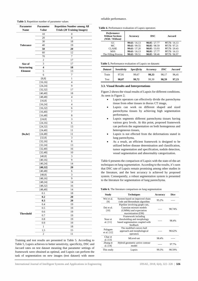
International Journal of Intelligent Systems and Applications in Engineering IJISAE, 2018, 6(4), 322–328 | 326
Training and test results are presented in Table 5. According to
Table 5, Lupsix achieves to better sensitivity, specificity, DSC and
Jaccard rates on test dataset meaning that parameter settings of
framework were obtained as optimal, and Lupsix can perform the
task of segmentation on new images (test dataset) with more
reliable performance.
Table 4. Performance evaluation of Lupsix operators
Performance
Without Sections
(With / Without)
Accuracy DSC Jaccard
GC 99.63 / 16.13 98.85 / 27.77 97.73 / 16.13
MC 99.63 / 99.55 98.85 / 98.59 97.73 / 97.21 CLAHE 99.63 / 37.20 98.85 / 33.93 97.73 / 20.43
MSS 99.63 / 16.13 98.85 / 27.77 97.73 / 16.13
The Filling Process 99.63 / 99.51 98.85 / 98.46 97.73 / 96.97
Table 5. Performance evaluation of Lupsix on datasets
Dataset Sensitivity Specificity Accuracy DSC Jaccard
Train 97,91 99,67 99,33 98,17 96,41
Test 98,07 99,72 99,30 98,59 97,23
3.3. Visual Results and Interpretations
Figure 2 shows the visual results of Lupsix for different conditions.
As seen in Figure 2;
Lupsix operators can effectively divide the parenchyma
tissue from other tissues in thorax CT image,
Lupsix can work on different shaped and sized
parenchyma tissues by achieving high segmentation
performance,
Lupsix segments different parenchyma tissues having
various grey levels. At this point, proposed framework
can perform the segmentation on both homogenous and
heterogeneous tissues,
Lupsix is not effected from the deformations stated in
lung parenchyma,
As a result, an efficient framework is designed to be
utilized before disease determination and classification,
tumor segmentation and specification, nodule detection,
vessel segmentation and abnormality categorization.
Table 6 presents the comparison of Lupsix with the state-of-the-art
techniques on lung segmentation. According to the results, it’s seen
that DSC rate of Lupsix remain promising among other studies in
the literature, and the best accuracy is achieved by proposed
system. Consequently, a robust segmentation system is presented
to the literature for segmentation of lung parenchyma.
Table 6. The literature comparison on lung segmentation
Study Techniques Accuracy Dice
Wei et al.
[9]
System based on improved chain
code and Bresenham algorithm 95.2% -----
Dai et al.
[10]
Pipeline involving graph cuts,
Gaussian mixture models
(GMMs) and expectation
maximization (EM)
----- 98.74%
Noor et
al. [11]
Framework including thresholding and morphology
based segmentation coupled with
feedback
----- 98.4%
Pulagam
et al. [12]
The modified convex hull
approach and morphological
operators
----- 98.62%
Chae et
al. [13] MLevel-set 98.4% -----
Zhang et
al. [14]
Hybrid geometric active contour
model ----- 97.7%
This study Lupsix 99.3% 98.59%
Table 3. Repetition number of parameter values
Parameter
Name
Parameter
Value
Repetition Number among All
Trials (20 Training Images)
Tolerance
10 0
20 8
30 18
40 19
50 20
60 12
70 7
Size of
Structuring
Element
2 17
3 17
4 18
5 13
6 7
[hs,hr]
[8,8] 1
[16,16] 4
[24,24] 9
[32,32] 17
[40,40] 18
[48,48] 4
[16,8] 1
[16,24] 4
[16,32] 6
[16,40] 7
[16,48] 8
[24,8] 3
[24,16] 6
[24,32] 13
[24,40] 11
[24,48] 11
[32,8] 3
[32,16] 8
[32,24] 13
[32,40] 16
[32,48] 10
[40,8] 3
[40,16] 9
[40,24] 14
[40,32] 20
[40,48] 6
[48,8] 3
[48,16] 9
[48,24] 14
[48,32] 16
[48,40] 14
Threshold
0.1 18
0.2 20
0.3 20
0.4 19
0.5 19
0.6 19
0.7 19
0.8 19
0.9 19
1 18
1,5 15
2 11
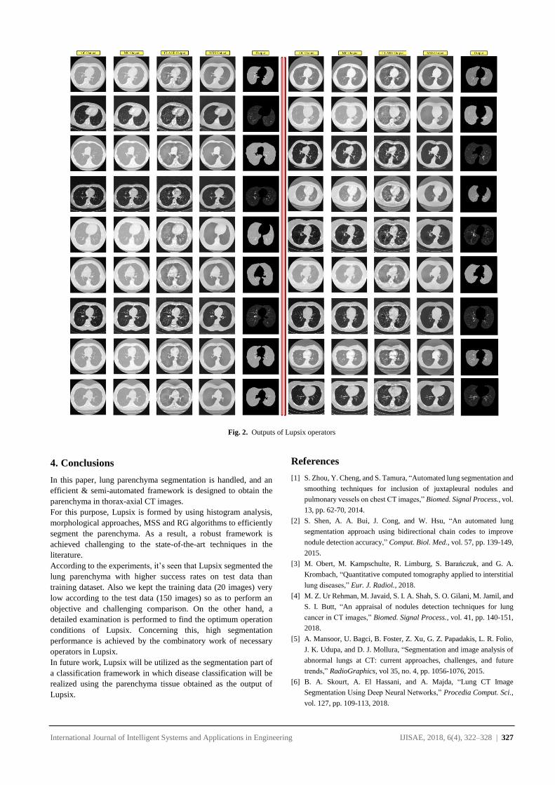
International Journal of Intelligent Systems and Applications in Engineering IJISAE, 2018, 6(4), 322–328 | 327
4. Conclusions
In this paper, lung parenchyma segmentation is handled, and an
efficient & semi-automated framework is designed to obtain the
parenchyma in thorax-axial CT images.
For this purpose, Lupsix is formed by using histogram analysis,
morphological approaches, MSS and RG algorithms to efficiently
segment the parenchyma. As a result, a robust framework is
achieved challenging to the state-of-the-art techniques in the
literature.
According to the experiments, it’s seen that Lupsix segmented the
lung parenchyma with higher success rates on test data than
training dataset. Also we kept the training data (20 images) very
low according to the test data (150 images) so as to perform an
objective and challenging comparison. On the other hand, a
detailed examination is performed to find the optimum operation
conditions of Lupsix. Concerning this, high segmentation
performance is achieved by the combinatory work of necessary
operators in Lupsix.
In future work, Lupsix will be utilized as the segmentation part of
a classification framework in which disease classification will be
realized using the parenchyma tissue obtained as the output of
Lupsix.
References
[1] S. Zhou, Y. Cheng, and S. Tamura, “Automated lung segmentation and
smoothing techniques for inclusion of juxtapleural nodules and
pulmonary vessels on chest CT images,” Biomed. Signal Process., vol.
13, pp. 62-70, 2014.
[2] S. Shen, A. A. Bui, J. Cong, and W. Hsu, “An automated lung
segmentation approach using bidirectional chain codes to improve
nodule detection accuracy,” Comput. Biol. Med., vol. 57, pp. 139-149,
2015.
[3] M. Obert, M. Kampschulte, R. Limburg, S. Barańczuk, and G. A.
Krombach, “Quantitative computed tomography applied to interstitial
lung diseases,” Eur. J. Radiol., 2018.
[4] M. Z. Ur Rehman, M. Javaid, S. I. A. Shah, S. O. Gilani, M. Jamil, and
S. I. Butt, “An appraisal of nodules detection techniques for lung
cancer in CT images,” Biomed. Signal Process., vol. 41, pp. 140-151,
2018.
[5] A. Mansoor, U. Bagci, B. Foster, Z. Xu, G. Z. Papadakis, L. R. Folio,
J. K. Udupa, and D. J. Mollura, “Segmentation and image analysis of
abnormal lungs at CT: current approaches, challenges, and future
trends,” RadioGraphics, vol 35, no. 4, pp. 1056-1076, 2015.
[6] B. A. Skourt, A. El Hassani, and A. Majda, “Lung CT Image
Segmentation Using Deep Neural Networks,” Procedia Comput. Sci.,
vol. 127, pp. 109-113, 2018.
Fig. 2. Outputs of Lupsix operators
International Journal of Intelligent Systems and Applications in Engineering IJISAE, 2018, 6(4), 322–328 | 328
[7] X. Liao, J. Zhao, C. Jiao, L. Lei, Y. Qiang, and Q. Cui, “A
segmentation method for lung parenchyma image sequences based on
superpixels and a self-generating neural forest,” Plos One, vol. 11, no.
8, e0160556, 2016.
[8] T. Doel, D. J. Gavaghan, and V. Grau, “Review of automatic
pulmonary lobe segmentation methods from CT,” Comput. Med. Imag.
Grap., vol. 40, pp. 13-29, 2015.
[9] Y. Wei, G. Shen, and J. J. Li, “A fully automatic method for lung
parenchyma segmentation and repairing,” J. Digit. Imaging, vol. 26,
no.3, pp. 483-495, 2013.
[10] S. Dai, K. Lu, J. Dong, Y. Zhang, and Y. Chen, “A novel approach of
lung segmentation on chest CT images using graph cuts,”
Neurocomputing, vol. 168, pp. 799-807, 2015.
[11] N. M. Noor, J. C. Than, O. M. Rijal, R. M. Kassim, A. Yunus, A. A.
Zeki, M. Anzidei, L. Saba, and J. S. Suri, “Automatic lung
segmentation using control feedback system: morphology and texture
paradigm,” J. Med. Syst., vol. 39, no.3, 22, 2015.
[12] A. R. Pulagam, G. B. Kande, V. K. R. Ede, and R. B. Inampudi,
“Automated lung segmentation from HRCT scans with diffuse
parenchymal lung diseases,” J. Digit. Imaging, vol. 29, no.4, pp. 507-
519, 2016.
[13] S. H. Chae, H. M. Moon, Y. Chung, J. Shin, and S. B. Pan, “Automatic
lung segmentation for large-scale medical image management,”
Multimed. Tools Appl., vol. 75, no.23, pp. 15347-15363, 2016.
[14] W. Zhang, X. Wang, P. Zhang, and J. Chen, “Global optimal hybrid
geometric active contour for automated lung segmentation on CT
images,” Comput. Biol. Med., vol. 91, pp. 168-180, 2017.
[15] S. Armato III, G. McLennan, L. Bidaut, M. McNitt-Gray, C. Meyer,
A. Reeves, and L. Clarke, “Data from LIDC-IDRI,” The cancer
imaging archive, 2015
[16] S. G. Armato et al., “The lung image database consortium (LIDC) and
image database resource initiative (IDRI): a completed reference
database of lung nodules on CT scans,” Med. Phys., vol. 38, no.2, pp.
915-931, 2011.
[17] K. Clark et al., “The Cancer Imaging Archive (TCIA): maintaining
and operating a public information repository,” J. Digit. Imaging, vol.
26, no. 6, pp. 1045-1057, 2013.
[18] P. Charles, “Digital Video and HDTV Algorithms and Interfaces,”
Morgan Kaufmann Publishers, San Francisco, 2003.
[19] R. C. Gonzalez, R. E. Woods, S. L. Eddins, “Digital image processing
using MATLAB,” McGraw Hill Education, New York, 2009.
[20] H. Koyuncu, R. Ceylan, M. Sivri, H. Erdogan, “An Efficient Pipeline
for Abdomen Segmentation in CT Images,” J. Digit. Imaging, vol. 31,
no.2, pp. 262-274, 2018.
[21] K. Zuiderveld, “Contrast limited adaptive histogram equalization,” in:
Graphics gems IV, P. S. Heckbert, Ed. San Diego, CA, USA:
Academic Press Professional Inc., 1994, pp. 474–485.
[22] P. Soille, “Morphological Image Analysis: Principles and
Applications,” Springer-Verlag, 1999, pp. 173-174.
[23] D. Comaniciu, P. Meer, “Mean shift: A robust approach toward feature
space analysis,” IEEE T. Pattern Anal., vol. 24, no. 5, pp. 603-619,
2002.
[24] H. Koyuncu, R. Ceylan, H. Erdogan, M. Sivri, “A novel pipeline for
adrenal tumour segmentation,” Comput. Meth. Prog. Bio., vol. 159, pp.
77-86, 2018.
[25] S. W. Franklin, S. E. Rajan, “Computerized screening of diabetic
retinopathy employing blood vessel segmentation in retinal images,”
Biocybern. Biomed. Eng., vol. 34, pp. 117-124, 2014.