Design of autonomous photovoltaic power plant for telecommunication relay station

Design of autonomous photovoltaic power plant fortelecommunication relay station

S. Liu, R.A. Dougal and E.V. Solodovnik

Abstract: The design and prototyping of an autonomous photovoltaic power generation systemusing the Virtual Test Bed software environment is presented. The comprehensive design of thephotovoltaic power plant is very important for achieving the best performance, durability andreliability of the system. The goal of the design is to optimise the system performance by accountingfor various data available at the design time. These data may include statistical data of weatherconditions at particular geographic locations, the statistics of the load profiles and, finally, theprojected outlook of the system use. The design of the autonomous photovoltaic power systempresented in this work includes establishing physics-based models for components, prototypingsystem architectures, implementing control algorithms, testing and evaluating the systemperformance using the actual weather data at a particular geographical location. The dynamicperformance of the photovoltaic power system and its components are revealed in great detailthrough the system-level simulation. This knowledge is used for verification and improvements ofthe system design in order to achieve the best system power capability, efficiency and size.

1 Introduction

Photovoltaic (PV) cells have been used for electrical powergeneration since the 1950s [1, 2]. During the early years,using PV power was rare, except for high-value remoteapplications such as military facilities and space satellitepower systems [3], because of the relatively low efficiencyand the high cost of PV modules. The oil crisis of 1973 ledto a general public awareness of the limitation of fossil fuels,and to a search for alternative energy sources. Publiccontroversy over nuclear fission reactors and a series ofaccidents in nuclear power plants, especially those of ThreeMile Island (1979) and Chernobyl (1986), caused a majorreorientation in the general perception of the energy supplyproblem and greatly reinforced the position of solar energy.Thus, the past two decades have seen constant andsubstantial progress in the field of PV modules: commercialprices of modules have been decreased dramatically, from$1.00/kWh in 1980 US dollars to $0.20/kWh in 2000 USdollars; while the worldwide module production capacity isincreasing ten-fold every decade [4, 5], and the efficiencies ofPV arrays are increasing steadily, some of which, such asthose of silicon (Si), gallium arsenide (GaAs), and indiumphosphide (InP), have been increased to nearly theirtheoretical limits [6]. In addition, materials research ismaking significant breakthroughs for stabilised, low-costand high specific energy cells, such as amorphous silicon(a-Si) cells and CIGS (CuIn1-xGaxSe2) thin-film cells. It isprojected [4] that the PV energy price will be verycompetitive in the market within the next 10 or 20 years.This creates a great opportunity for widespread terrestrial

applications of PV power. Furthermore, solar energyresource is abundant, pollution-free, and well suited fordistributed generation.

This paper addresses the modelling and design of anautonomous PV power plant for telecommunicationapplications using the computer software: the Virtual TestBed [7]. Large-scale systems, such as a PV power plant,consist of many interdisciplinary and nonlinear compo-nents. For example, the PV cell and the battery arecomponents that invoke either a photovoltaic process (in aPV array) or an electrochemical process (in a battery) forenergy conversion and storage, and they interact with thecircuit electrically and the surroundings thermally. Thus,electrical, chemical and thermal disciplines are involved. Inaddition, the control discipline is also required since amaximum power point tracker (MPPT) is needed foroperating the power system at high efficiencies.

The Virtual Test Bed (VTB) is a simulation environmentthat was developed for the purpose of modelling andsimulation of interdisciplinary systems. Compared to someindustrial standard software tools such as MatLab/Simu-link, Advanced Continuous Simulation Language (ACSL)and SPICE, the VTB offers unique capabilities. First, itaccommodates a multi-language platform [8] for establish-ing native models, for importing models from othersimulation environments, for co-simulation with othersoftware applications, for distributed simulations, and forsimulation with hardware in the loop. These features allowusers to make the most effective use of discipline-specific orlanguage-specific knowledge resources of their own orothers, thus achieving an efficient design process in terms ofeffort spent. Secondly, the VTB provides users with anenvironment for easy and straightforward system declara-tion based on object-oriented implementation, and forinteractive design and prototyping. Users can changecomponent parameters or redefine the system topology atVTB runtime while a simulation executes, thereby rapidlyexploring parametric and topologic influences on the systemperformance. Finally, the VTB is furnished with advanced

The authors are with the Department of Electrical Engineering, University ofSouth Carolina, Columbia, SC 29208, USA

E-mail: [email protected]

r IEE, 2005

IEE Proceedings online no. 20045028

doi:10.1049/ip-gtd:20045028

Paper first received 4th May 2004 and in final revised form 22nd June 2005

IEE Proc.-Gener. Transm. Distrib., Vol. 152, No. 6, November 2005 745

visualisation mechanisms that are linked to live simulationdata. Users can activate either the data-driven graphicanimation of 3D objects or simple oscilloscope-like graphs,thus helping the user in an intuitive understanding of thesystem performance. The latest freeware version of theVTB, VTB 2003, is available for download at the WorldWide Web link provided in [7]. In addition, free technicalassistance for installation, troubleshooting, as well as aid indevelopment of new models and in system simulation areoffered by the VTB development team.

For a complicated system like that of a PV powerplant, it is often inadequate for a design of an electricsystem without considering its interaction with the thermalenvironment, as the behaviour of both PV array andbatteries is subject significantly to the temperature effects.Because of a lack of a unified design tool, system engineerstypically perform their thermal designs separately from theirelectrical designs using different sets of tools. Therefore,it is difficult to take the dynamic interactions of thetwo subsystems (electrical and thermal) into account inthe design. The novelty of the VTB-aided design is that thesystem is considered in multidisciplinary perspectives, andall disciplines of the system are conveniently handled withinone platform. In this work, the autonomous PV powergeneration plant is designed for the application to a specificload profile at a particular geographical location where theactual weather conditions, both the solar insolation and theair temperatures, are considered. In addition, the tempera-ture effects of the PV array and the battery are included inthe models. The dynamic performance of the PV systemand its components under the effects of weather changesand load variations are studied in great details through thesystem level simulation, and the results are used forverification and improvement of the system design in orderto achieve the best system power capability, efficiency andsize. The procedures illustrated here can be applied fordesigning PV systems for different load profiles at differentgeographical locations.

2 PV power plant modelling in VTB

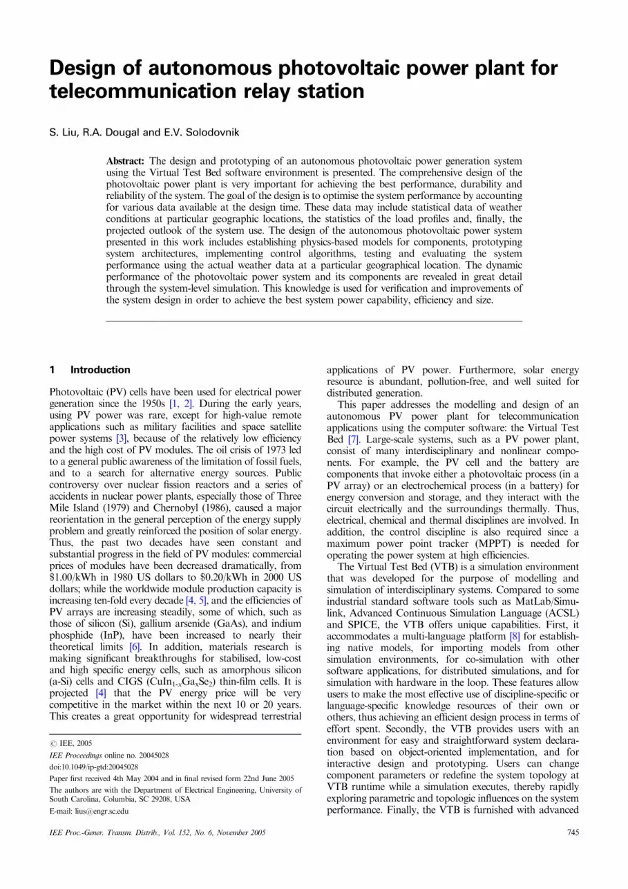
A typical schematic of a PV power plant is shown in Fig. 1.The basic operation of the system is as follows. The PVarray converts the solar energy into electricity when it isexposed to sunlight. Through a step-down converter, thepower is delivered to a load for consumption and to abattery for energy storage if there is an excess of powerproduction. The MPPT system is designed such that the PVarray always operates at its maximum power point. Boththe array voltage and current signals are fed to thecontroller for the purpose of MPP tracking. For betterconversion efficiencies, the heat in the PV array and in thebattery is discharged to the ambient via heatsinks. An

ultracapacitor is connected in parallel with the battery onthe load side to boost the power capability. The solarinsolation received by the PV array is modelled by theirradiance (sun) and the cloud, the characteristics of whichdepend on geographical location and time.

The task of the MPPT is to tune the system continuouslyso that it draws maximum power from the PV arrayregardless of weather or load conditions. Since the PV arrayhas a non-ideal voltage–current characteristic, and theweather conditions that affect the output of the solar arrayare unpredictable, the tracker must contend with anonlinear and time-varying system. Among many trackingtechniques that have been developed, the incrementalconductance method [9] has a relatively good accuracyand efficiency for rapidly changing atmospheric conditions,compared to the perturb and observe [10], the short-circuitcurrent tracking [11], and the open-circuit voltage tracking[12, 13] methods. The method tracks the MPP of the PVmodule by comparing the incremental conductance with theinstantaneous conductance. With the advances of digitalsignal processors (DSP), the implementation of this methodbecomes simple. Thus, in the design of the PV power plantthat we describe here, the incremental conductance MPPtracker was employed.

3 Design of PV power plant

The process of engineering design and prototyping of acomplex system can be very time-consuming and costly.This process becomes simplified, time- and cost-effective ifthe system is virtually prototyped using the validatedcomponent models in the VTB environment.

The procedures for the design and prototyping of anautonomous PV power plant, as that shown in Fig. 1, maybe described as follows. First, the data for the local weatherconditions are collected to yield yearly-averaged dailyactivities on the insolation and the air temperature. Themodels for the insolation and the ambient temperature arecreated using these data. Secondly, the load profile isprojected, and the corresponding model is built. Duringthese two steps, the insolation level data and the outputpower requirement are prepared. The basic virtual proto-type of the system architecture is established in the thirdstep. In the fourth step, the sizes and the configurations ofthe PV array and the battery are prototyped based on thesystem information, the actual weather data and the loadprofile. The preliminary sizes of the energy components canbe calculated based on the data of the insolation and theload profile. During the fifth, and final, step the entiresystem is simulated under nominal and other scenarios forthe design verification and improvement.

Prototyping the circuit system and the energy compo-nents are the major steps in design. The goal of theseprocedures is not only to find the appropriate systemtopologies and the component configurations, but also tomeet some dynamic specifications and performance require-ments. One objective of the system design may be theachievement of high specific power and high efficiency,which is not only a component issue, but also a systemoperation issue. Another objective may focus on the ach-ievement of a certain durability or reliability of the system.For example, the total daily energy converted by the PVarray must satisfy the load requirement in one day andone night in general, while the energy stored in the batteryduring the daytime must meet the need of the nightoperation. As the daytime varies and the weather changesduring the year, there are ‘flood’ and ‘drought’ seasons withrespect to the PV power generation. As a result, the battery

Vi Vo

−+P T

sensor converter

MPPT battery

ultracap

load

heatsink

ambient temperature

heatsink

sun cloud PV

D

Fig. 1 Design of PV power plant in VTBCharacteristics of major components are listed in the Appendix

746 IEE Proc.-Gener. Transm. Distrib., Vol. 152, No. 6, November 2005

may be subject to overcharge or deep discharge due topower imbalance, which significantly affects the cyclelifetime. Thus, it is essential to take measures to protectthe battery from overcharges and deep discharges.

A practical application of the PV power plant shown inFig. 1 may be a telecommunication relay station located ina remote area with plenty of sunshine. Let us now presentthe detailed design procedures for a system that is to behypothetically located at the mountaintop of the San DimasExperimental Forest (SDEF) in the San Gabriel Mountainsarea, California.

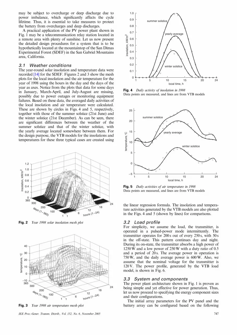
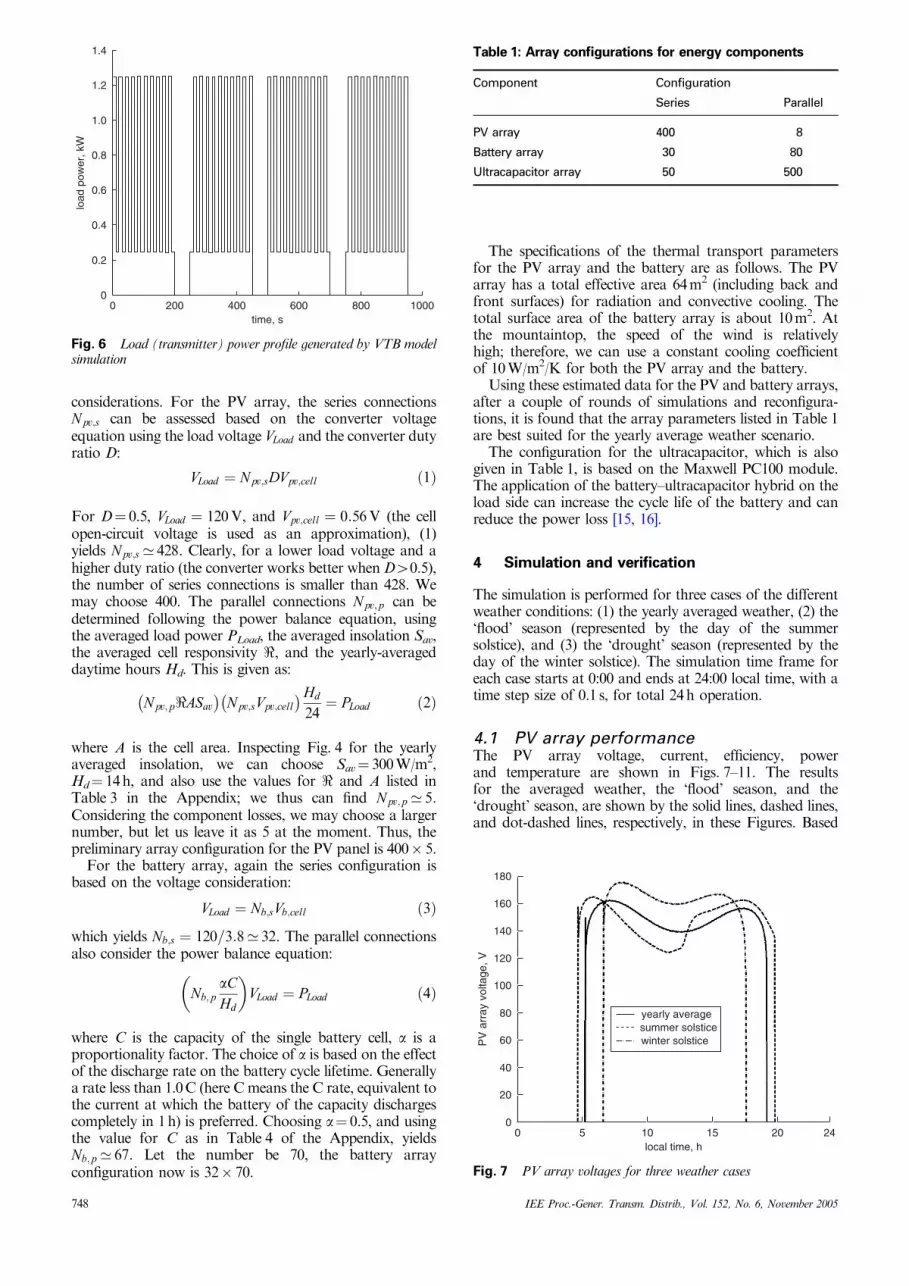
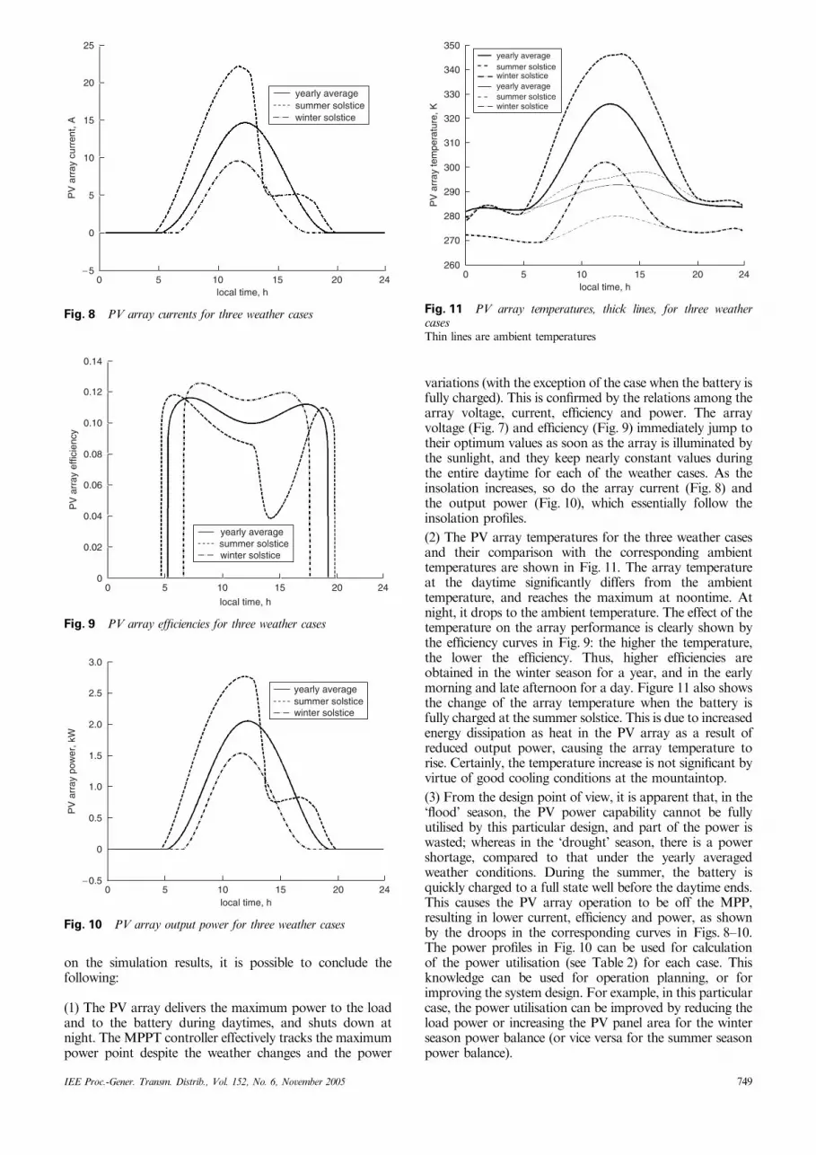
3.1 Weather conditionsThe year-round solar insolation and temperature data wererecorded [14] for the SDEF. Figures 2 and 3 show the meshplots for the local insolation and the air temperature for theyear of 1998 using the hours in the day and the days of theyear as axes. Notice from the plots that data for some daysin January, March-April, and July-August are missing,possibly due to power outages or monitoring equipmentfailures. Based on these data, the averaged daily activities ofthe local insolation and air temperature were calculated.These are shown by circles in Figs. 4 and 5, respectively,together with those of the summer solstice (21st June) andthe winter solstice (21st December). As can be seen, thereare significant differences between the weather of thesummer solstice and that of the winter solstice, withthe yearly average located somewhere between them. Forthe design purpose, the VTB models for the insolations andtemperatures for these three typical cases are created using

the linear regression formula. The insolation and tempera-ture activities generated by the VTB models are also plottedin the Figs. 4 and 5 (shown by lines) for comparisons.

3.2 Load profileFor simplicity, we assume the load, the transmitter, isoperated in a pulsed-power mode intermittently. Thetransmitter operates for 200 s out of every 250 s, with 50 sin the off-state. This pattern continues day and night.During its on-state, the transmitter absorbs a high power of1250W and a low power of 250W with a duty ratio of 0.5and a period of 20 s. The average power in operation is750W, and the daily average power is 600W. Also, weassume that the nominal voltage for the transmitter is120V. The power profile, generated by the VTB loadmodel, is shown in Fig. 6.

3.3 System and componentsThe power plant architecture shown in Fig. 1 is proven asbeing simple and yet effective for power generation. Thus,let us now proceed to specifying the energy component sizesand their configurations.

The initial array parameters for the PV panel and thebattery array can be configured based on the following

1.2

1.0

0.8

0.6

0.4

0.2

0365

300

200

100

1 16

1218

24

inso

latio

n, k

W/m

2

days (1–365) hours (1–24)

Fig. 2 Year 1998 solar insolation mesh plot

40

30

20

10

0

−10365

300

200

100

1 16

1218

24

days (1–365) hours (1–24)

tem

pera

ture

, °C

Fig. 3 Year 1998 air temperature mesh plot

local time, h1

0

0.1

0.2

0.3

0.4

0.5

0.6

0.7

0.8

0.9

1.0

5 10 15 20 24

inso

latio

n, k

W/m

2

summer solstice

yearly average

winter solstice

Fig. 4 Daily activity of insolation in 1998Data points are measured, and lines are from VTB models

1 5 10 15 20 24local time, h

−5

0

5

10

15

20

25

summer solstice

yearly average

winter solstice

tem

pera

ture

,°C

Fig. 5 Daily activities of air temperature in 1998Data points are measured, and lines are from VTB models


considerations. For the PV array, the series connectionsNpv;s can be assessed based on the converter voltageequation using the load voltage VLoad and the converter dutyratio D:

VLoad ¼ Npv;sDVpv;cell ð1Þ

For D¼ 0.5, VLoad ¼ 120V, and Vpv;cell ¼ 0:56V (the cellopen-circuit voltage is used as an approximation), (1)yields Npv;s’ 428. Clearly, for a lower load voltage and ahigher duty ratio (the converter works better when D40.5),the number of series connections is smaller than 428. Wemay choose 400. The parallel connections Npv;p can bedetermined following the power balance equation, usingthe averaged load power PLoad, the averaged insolation Sav,the averaged cell responsivity <, and the yearly-averageddaytime hours Hd. This is given as:

Npv;p<ASav� �

Npv;sVpv;cell� �Hd

24¼ PLoad ð2Þ

where A is the cell area. Inspecting Fig. 4 for the yearlyaveraged insolation, we can choose Sav¼ 300W/m2,Hd¼ 14h, and also use the values for < and A listed inTable 3 in the Appendix; we thus can find Npv;p ’ 5.Considering the component losses, we may choose a largernumber, but let us leave it as 5 at the moment. Thus, thepreliminary array configuration for the PV panel is 400� 5.

For the battery array, again the series configuration isbased on the voltage consideration:

VLoad ¼ Nb;sVb;cell ð3Þ

which yields Nb;s ¼ 120=3:8’ 32. The parallel connectionsalso consider the power balance equation:

Nb;paCHd

� �VLoad ¼ PLoad ð4Þ

where C is the capacity of the single battery cell, a is aproportionality factor. The choice of a is based on the effectof the discharge rate on the battery cycle lifetime. Generallya rate less than 1.0C (here C means the C rate, equivalent tothe current at which the battery of the capacity dischargescompletely in 1h) is preferred. Choosing a¼ 0.5, and usingthe value for C as in Table 4 of the Appendix, yieldsNb;p ’ 67. Let the number be 70, the battery arrayconfiguration now is 32� 70.

The specifications of the thermal transport parametersfor the PV array and the battery are as follows. The PVarray has a total effective area 64m2 (including back andfront surfaces) for radiation and convective cooling. Thetotal surface area of the battery array is about 10m2. Atthe mountaintop, the speed of the wind is relativelyhigh; therefore, we can use a constant cooling coefficientof 10W/m2/K for both the PV array and the battery.

Using these estimated data for the PV and battery arrays,after a couple of rounds of simulations and reconfigura-tions, it is found that the array parameters listed in Table 1are best suited for the yearly average weather scenario.

The configuration for the ultracapacitor, which is alsogiven in Table 1, is based on the Maxwell PC100 module.The application of the battery–ultracapacitor hybrid on theload side can increase the cycle life of the battery and canreduce the power loss [15, 16].

4 Simulation and verification

The simulation is performed for three cases of the differentweather conditions: (1) the yearly averaged weather, (2) the‘flood’ season (represented by the day of the summersolstice), and (3) the ‘drought’ season (represented by theday of the winter solstice). The simulation time frame foreach case starts at 0:00 and ends at 24:00 local time, with atime step size of 0.1 s, for total 24h operation.

4.1 PV array performanceThe PV array voltage, current, efficiency, powerand temperature are shown in Figs. 7–11. The resultsfor the averaged weather, the ‘flood’ season, and the‘drought’ season, are shown by the solid lines, dashed lines,and dot-dashed lines, respectively, in these Figures. Based

0 200 400 600 800 1000time, s

1.4

1.2

1.0

0.8

0.6

0.4

0.2

0

load

pow

er, k

W

Fig. 6 Load (transmitter) power profile generated by VTB modelsimulation

Table 1: Array configurations for energy components

Component Configuration

Series Parallel

PV array 400 8

Battery array 30 80

Ultracapacitor array 50 500

summer solsticeyearly average

winter solstice

local time, h

PV

arr

ay v

olta

ge, V

00

20

40

60

80

100

120

140

160

180

5 10 15 20 24

Fig. 7 PV array voltages for three weather cases


on the simulation results, it is possible to conclude thefollowing:

(1) The PV array delivers the maximum power to the loadand to the battery during daytimes, and shuts down atnight. The MPPT controller effectively tracks the maximumpower point despite the weather changes and the power

variations (with the exception of the case when the battery isfully charged). This is confirmed by the relations among thearray voltage, current, efficiency and power. The arrayvoltage (Fig. 7) and efficiency (Fig. 9) immediately jump totheir optimum values as soon as the array is illuminated bythe sunlight, and they keep nearly constant values duringthe entire daytime for each of the weather cases. As theinsolation increases, so do the array current (Fig. 8) andthe output power (Fig. 10), which essentially follow theinsolation profiles.

(2) The PV array temperatures for the three weather casesand their comparison with the corresponding ambienttemperatures are shown in Fig. 11. The array temperatureat the daytime significantly differs from the ambienttemperature, and reaches the maximum at noontime. Atnight, it drops to the ambient temperature. The effect of thetemperature on the array performance is clearly shown bythe efficiency curves in Fig. 9: the higher the temperature,the lower the efficiency. Thus, higher efficiencies areobtained in the winter season for a year, and in the earlymorning and late afternoon for a day. Figure 11 also showsthe change of the array temperature when the battery isfully charged at the summer solstice. This is due to increasedenergy dissipation as heat in the PV array as a result ofreduced output power, causing the array temperature torise. Certainly, the temperature increase is not significant byvirtue of good cooling conditions at the mountaintop.

(3) From the design point of view, it is apparent that, in the‘flood’ season, the PV power capability cannot be fullyutilised by this particular design, and part of the power iswasted; whereas in the ‘drought’ season, there is a powershortage, compared to that under the yearly averagedweather conditions. During the summer, the battery isquickly charged to a full state well before the daytime ends.This causes the PV array operation to be off the MPP,resulting in lower current, efficiency and power, as shownby the droops in the corresponding curves in Figs. 8–10.The power profiles in Fig. 10 can be used for calculationof the power utilisation (see Table 2) for each case. Thisknowledge can be used for operation planning, or forimproving the system design. For example, in this particularcase, the power utilisation can be improved by reducing theload power or increasing the PV panel area for the winterseason power balance (or vice versa for the summer seasonpower balance).

yearly averagesummer solsticewinter solstice

local time, h5 10 15 20 240

−5

0

5

10

15

20

25

PV

arr

ay c

urre

nt, A

Fig. 8 PV array currents for three weather cases


local time, h

00

0.02

0.04

0.06

0.08

0.10

0.12

0.14

5 10 15 20 24

PV

arr

ay e

ffici

ency

Fig. 9 PV array efficiencies for three weather cases


0 5 10 15 20 24local time, h

−0.5

0

0.5

1.0

1.5

2.0

2.5

3.0

PV

arr

ay p

ower

, kW

Fig. 10 PV array output power for three weather cases

350

330

310

300

290

280

270

260

320

340

0 5 10 15 20 24local time, h

PV

arr

ay te

mpe

ratu

re, K

yearly averagesummer solsticewinter solsticeyearly averagesummer solsticewinter solstice

Fig. 11 PV array temperatures, thick lines, for three weathercasesThin lines are ambient temperatures


4.2 Performance of batteryThe initial state of charge (SOC) of the battery is set to 60%at 0:00 hour at the beginning of each simulation. The resultsfor the battery voltage, current, power and SOC are shownin Figs. 12–15 for the averaged weather (solid lines), the‘flood’ season (dashed lines) and the ‘drought’ season (dot-dashed lines). From these Figures, one can observe thefollowing:

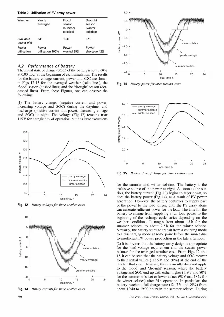
(1) The battery charges (negative current and power,increasing voltage and SOC) during the daytime, anddischarges (positive current and power, decreasing voltageand SOC) at night. The voltage (Fig. 12) remains near115V for a single day of operation, but has large excursions

for the summer and winter solstices. The battery is theexclusive source of the power at night. As soon as the sunrises, the battery current (Fig. 13) begins to taper down, sodoes the battery power (Fig. 14), as a result of PV powergeneration. However, the battery continues to supply partof the power to the load longer, until the PV array alonecan generate sufficient power for the load. The time for thebattery to change from supplying a full load power to thebeginning of the recharge cycle varies depending on theweather conditions. It ranges from about 1.8h for thesummer solstice, to about 2.5h for the winter solstice.Similarly, the battery starts to transit from a charging modeto a discharging mode at some point before the sunset dueto insufficient PV power production in the late afternoon.

(2) It is obvious that the battery array design is appropriatefor the load voltage requirement and the system powerbalance for the averaged weather case. From Figs. 12 and15, it can be seen that the battery voltage and SOC recoverto their initial values (115.5V and 60%) at the end of theday for that case. However, this apparently does not applyto the ‘flood’ and ‘drought’ seasons, where the batteryvoltage and SOC end up with either higher (119V and 80%for the summer solstice) or lower values (98V and 18% forthe winter solstice) after 24h operation. In particular, thebattery reaches a full charge state (124.7V and 99%) fromabout 12:40 to 19:00 hours in the summer solstice. During

10

5

0

−5

−10

−15

−20

batte

ry c

urre

nt, A

0 5 10 15 20 24local time, h

winter solstice

yearly average

summer solstice

Fig. 13 Battery currents for three weather cases

1.0

0.5

−0.5

−1.5

−2.5

−1.0

−2.0

0

batte

ry p

ower

, kW

0 10 20 245 15local time, h

winter solstice

yearly average

summer solstice

Fig. 14 Battery power for three weather cases

Table 2: Utilisation of PV array power

Weather Yearlyaveraged

Floodseason(summersolstice)

Droughtseason(wintersolstice)

Availablepower (W)

638 1049 371

Powerutilisation

Powerutilisation 100%

Powerwasted 39%

Powershortage 42%

yearly average

summer solsticewinter solstice

batte

ry v

olta

ge, V

local time, h

120

130

110

100

105

95

115

125

0 5 10 15 20 24

Fig. 12 Battery voltages for three weather cases

0.4

1.0

0.8

0.6

0.2

0

batte

ry s

tate

of c

harg

e

local time, h0 5 10 15 20 24


Fig. 15 Battery state of charge for three weather cases


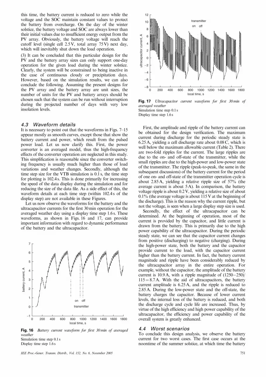
this time, the battery current is reduced to zero while thevoltage and the SOC maintain constant values to protectthe battery from overcharge. On the day of the wintersolstice, the battery voltage and SOC are always lower thantheir initial values due to insufficient energy output from thePV array. Obviously, the battery voltage will reach thecutoff level (single cell 2.5V, total array 75V) next day,which will inevitably shut down the load operation.

(3) It can be concluded that this particular design for thePV and the battery array sizes can only support one-dayoperation for the given load during the winter solstice.Clearly, the system will be constrained to being inactive inthe case of continuous cloudy or precipitation days.However, based on the simulation results, we can alsoconclude the following. Assuming the present designs forthe PV array and the battery array are unit sizes, thenumber of units for the PV and battery arrays should bechosen such that the system can be run without interruptionduring the projected number of days with very lowinsolation levels.

4.3 Waveform detailsIt is necessary to point out that the waveforms in Figs. 7–15appear mostly as smooth curves, except those that show thebattery current and power, which result from the pulsedpower load. Let us now clarify this. First, the powerconverter is an averaged model, thus the high-frequencyeffects of the converter operation are neglected in this study.This simplification is reasonable since the converter switch-ing frequency is usually much higher than those of loadvariations and weather changes. Secondly, although thetime step size for the VTB simulation is 0.1 s, the time stepfor plotting is 102.4 s. This is done primarily for increasingthe speed of the data display during the simulation and forreducing the size of the data file. As a side effect of this, thewaveform details at each time step (within 102.4 s of thedisplay step) are not available in these Figures.

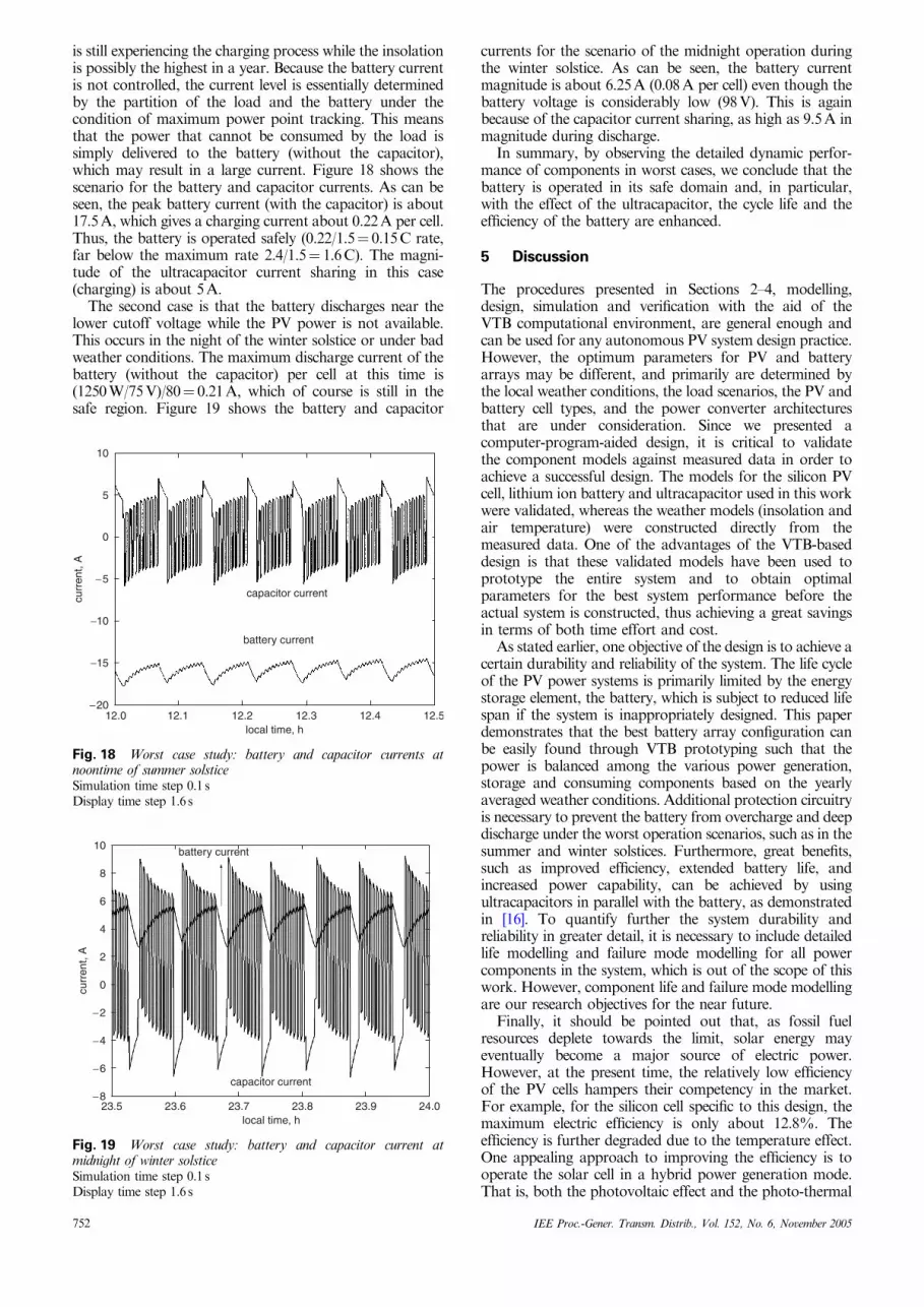
Let us now observe the waveforms for the battery and theultracapacitor currents for the first 30min operation for theaveraged weather day using a display time step 1.6 s. Thesewaveforms, as shown in Figs. 16 and 17, can provideimportant information with regard to dynamic performanceof the battery and the ultracapacitor.

First, the amplitude and ripple of the battery current canbe obtained for the design verification. The maximumcurrent during discharge for the periodic steady state is6.25A, yielding a cell discharge rate about 0.08C, which iswell below the maximum allowable current (Table 2). Thereare two-fold ripples for the current. The large ripples aredue to the on- and off-state of the transmitter, while thesmall ripples are due to the high-power and low-power stateof the transmitter. The ripple (peak-to-peak, the same in thesubsequent discussions) of the battery current for the periodof one on- and off-state of the transmitter operation cycle isabout 2.85A, yielding a relative ripple size of 57% (theaverage current is about 5A). In comparison, the batteryvoltage ripple is about 0.2V, yielding a relative size of about0.1% (the average voltage is about 115V at the beginning ofthe discharge). This is the reason why the current ripple, butnot the voltage, is seen when a large display step size is used.

Secondly, the effect of the ultracapacitor can bedetermined. At the beginning of operation, most of thecurrent is provided by the capacitor, and little current isdrawn from the battery. This is primarily due to the highpower capability of the ultracapacitor. During the periodicsteady state, we can see that the capacitor current changesfrom positive (discharging) to negative (charging). Duringthe high-power state, both the battery and the capacitorprovide current to the load, with the capacitor currenthigher than the battery current. In fact, the battery currentmagnitude and ripple have been considerably reduced bythe ultracapacitor array in the entire operation. Forexample, without the capacitor, the amplitude of the batterycurrent is 10.9A, with a ripple magnitude of (1250�250)/115¼ 8.7A. With the aid of ultracapacitors, the batterycurrent amplitude is 6.25A, and the ripple is reduced to2.85A. During the low-power state and the off-state, thebattery charges the capacitor. Because of lower currentlevels, the internal loss of the battery is reduced, and boththe discharge cycle and cycle life are increased. Thus, byvirtue of the high efficiency and high power capability of theultracapacitor, the efficiency and power capability of theoverall system is greatly enhanced.

4.4 Worst scenariosTo conclude this design analysis, we observe the batterycurrent for two worst cases. The first case occurs at thenoontime of the summer solstice, at which time the battery

on off

transmitter

local time, s

batte

ry c

urre

nt, A

7

6

4

3

5

2

1

0

−10 200 1200400 1400600 1600800 18001000

Fig. 16 Battery current waveform for first 30 min of averagedweatherSimulation time step 0.1 sDisplay time step 1.6 s

transmitter

on off

ultr

acap

acito

r cu

rren

t, A

local time, s

12

10

8

6

4

2

0

−2

−4

−6

−80 200 400 600 800 1000 1200 1400 1600 1800

Fig. 17 Ultracapacitor current waveform for first 30 min ofaveraged weatherSimulation time step 0.1 sDisplay time step 1.6 s


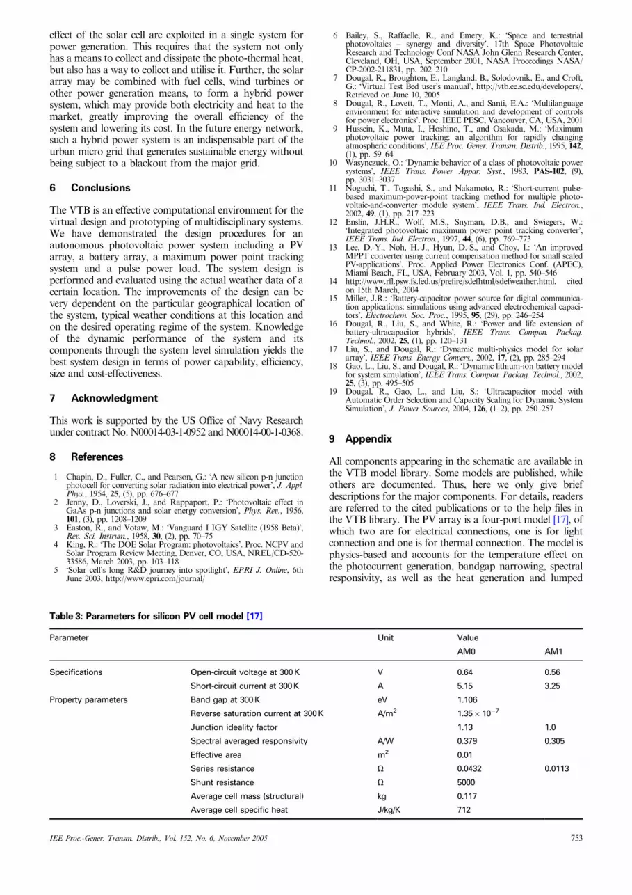
is still experiencing the charging process while the insolationis possibly the highest in a year. Because the battery currentis not controlled, the current level is essentially determinedby the partition of the load and the battery under thecondition of maximum power point tracking. This meansthat the power that cannot be consumed by the load issimply delivered to the battery (without the capacitor),which may result in a large current. Figure 18 shows thescenario for the battery and capacitor currents. As can beseen, the peak battery current (with the capacitor) is about17.5A, which gives a charging current about 0.22A per cell.Thus, the battery is operated safely (0.22/1.5¼ 0.15C rate,far below the maximum rate 2.4/1.5¼ 1.6C). The magni-tude of the ultracapacitor current sharing in this case(charging) is about 5A.

The second case is that the battery discharges near thelower cutoff voltage while the PV power is not available.This occurs in the night of the winter solstice or under badweather conditions. The maximum discharge current of thebattery (without the capacitor) per cell at this time is(1250W/75V)/80¼ 0.21A, which of course is still in thesafe region. Figure 19 shows the battery and capacitor

currents for the scenario of the midnight operation duringthe winter solstice. As can be seen, the battery currentmagnitude is about 6.25A (0.08A per cell) even though thebattery voltage is considerably low (98V). This is againbecause of the capacitor current sharing, as high as 9.5A inmagnitude during discharge.

In summary, by observing the detailed dynamic perfor-mance of components in worst cases, we conclude that thebattery is operated in its safe domain and, in particular,with the effect of the ultracapacitor, the cycle life and theefficiency of the battery are enhanced.

5 Discussion

The procedures presented in Sections 2–4, modelling,design, simulation and verification with the aid of theVTB computational environment, are general enough andcan be used for any autonomous PV system design practice.However, the optimum parameters for PV and batteryarrays may be different, and primarily are determined bythe local weather conditions, the load scenarios, the PV andbattery cell types, and the power converter architecturesthat are under consideration. Since we presented acomputer-program-aided design, it is critical to validatethe component models against measured data in order toachieve a successful design. The models for the silicon PVcell, lithium ion battery and ultracapacitor used in this workwere validated, whereas the weather models (insolation andair temperature) were constructed directly from themeasured data. One of the advantages of the VTB-baseddesign is that these validated models have been used toprototype the entire system and to obtain optimalparameters for the best system performance before theactual system is constructed, thus achieving a great savingsin terms of both time effort and cost.

As stated earlier, one objective of the design is to achieve acertain durability and reliability of the system. The life cycleof the PV power systems is primarily limited by the energystorage element, the battery, which is subject to reduced lifespan if the system is inappropriately designed. This paperdemonstrates that the best battery array configuration canbe easily found through VTB prototyping such that thepower is balanced among the various power generation,storage and consuming components based on the yearlyaveraged weather conditions. Additional protection circuitryis necessary to prevent the battery from overcharge and deepdischarge under the worst operation scenarios, such as in thesummer and winter solstices. Furthermore, great benefits,such as improved efficiency, extended battery life, andincreased power capability, can be achieved by usingultracapacitors in parallel with the battery, as demonstratedin [16]. To quantify further the system durability andreliability in greater detail, it is necessary to include detailedlife modelling and failure mode modelling for all powercomponents in the system, which is out of the scope of thiswork. However, component life and failure mode modellingare our research objectives for the near future.

Finally, it should be pointed out that, as fossil fuelresources deplete towards the limit, solar energy mayeventually become a major source of electric power.However, at the present time, the relatively low efficiencyof the PV cells hampers their competency in the market.For example, for the silicon cell specific to this design, themaximum electric efficiency is only about 12.8%. Theefficiency is further degraded due to the temperature effect.One appealing approach to improving the efficiency is tooperate the solar cell in a hybrid power generation mode.That is, both the photovoltaic effect and the photo-thermal

capacitor current

battery current

curr

ent,

A

local time, h

10

5

0

−5

−10

−15

−2012.0 12.1 12.2 12.3 12.4 12.5

Fig. 18 Worst case study: battery and capacitor currents atnoontime of summer solsticeSimulation time step 0.1 sDisplay time step 1.6 s

battery current

curr

ent,

A

capacitor current

local time, h23.5 23.6 23.7 23.8 23.9 24.0

10

8

6

4

2

0

−2

−4

−8

−6

Fig. 19 Worst case study: battery and capacitor current atmidnight of winter solsticeSimulation time step 0.1 sDisplay time step 1.6 s


effect of the solar cell are exploited in a single system forpower generation. This requires that the system not onlyhas a means to collect and dissipate the photo-thermal heat,but also has a way to collect and utilise it. Further, the solararray may be combined with fuel cells, wind turbines orother power generation means, to form a hybrid powersystem, which may provide both electricity and heat to themarket, greatly improving the overall efficiency of thesystem and lowering its cost. In the future energy network,such a hybrid power system is an indispensable part of theurban micro grid that generates sustainable energy withoutbeing subject to a blackout from the major grid.

6 Conclusions

The VTB is an effective computational environment for thevirtual design and prototyping of multidisciplinary systems.We have demonstrated the design procedures for anautonomous photovoltaic power system including a PVarray, a battery array, a maximum power point trackingsystem and a pulse power load. The system design isperformed and evaluated using the actual weather data of acertain location. The improvements of the design can bevery dependent on the particular geographical location ofthe system, typical weather conditions at this location andon the desired operating regime of the system. Knowledgeof the dynamic performance of the system and itscomponents through the system level simulation yields thebest system design in terms of power capability, efficiency,size and cost-effectiveness.

7 Acknowledgment

This work is supported by the US Office of Navy Researchunder contract No. N00014-03-1-0952 andN00014-00-1-0368.

8 References

1 Chapin, D., Fuller, C., and Pearson, G.: ‘A new silicon p-n junctionphotocell for converting solar radiation into electrical power’, J. Appl.Phys., 1954, 25, (5), pp. 676–677

2 Jenny, D., Loverski, J., and Rappaport, P.: ‘Photovoltaic effect inGaAs p-n junctions and solar energy conversion’, Phys. Rev., 1956,101, (3), pp. 1208–1209

3 Easton, R., and Votaw, M.: ‘Vanguard I IGY Satellite (1958 Beta)’,Rev. Sci. Instrum., 1958, 30, (2), pp. 70–75

4 King, R.: ‘The DOE Solar Program: photovoltaics’. Proc. NCPV andSolar Program Review Meeting, Denver, CO, USA, NREL/CD-520-33586, March 2003, pp. 103–118

5 ‘Solar cell’s long R&D journey into spotlight’, EPRI J. Online, 6thJune 2003, http://www.epri.com/journal/

6 Bailey, S., Raffaelle, R., and Emery, K.: ‘Space and terrestrialphotovoltaics – synergy and diversity’. 17th Space PhotovoltaicResearch and Technology Conf NASA John Glenn Research Center,Cleveland, OH, USA, September 2001, NASA Proceedings NASA/CP-2002-211831, pp. 202–210

7 Dougal, R., Broughton, E., Langland, B., Solodovnik, E., and Croft,G.: ‘Virtual Test Bed user’s manual’, http://vtb.ee.sc.edu/developers/,Retrieved on June 10, 2005

8 Dougal, R., Lovett, T., Monti, A., and Santi, E.A.: ‘Multilanguageenvironment for interactive simulation and development of controlsfor power electronics’. Proc. IEEE PESC, Vancouver, CA, USA, 2001

9 Hussein, K., Muta, I., Hoshino, T., and Osakada, M.: ‘Maximumphotovoltaic power tracking: an algorithm for rapidly changingatmospheric conditions’, IEE Proc. Gener. Transm. Distrib., 1995, 142,(1), pp. 59–64

10 Wasynczuck, O.: ‘Dynamic behavior of a class of photovoltaic powersystems’, IEEE Trans. Power Appar. Syst., 1983, PAS-102, (9),pp. 3031–3037

11 Noguchi, T., Togashi, S., and Nakamoto, R.: ‘Short-current pulse-based maximum-power-point tracking method for multiple photo-voltaic-and-converter module system’, IEEE Trans. Ind. Electron.,2002, 49, (1), pp. 217–223

12 Enslin, J.H.R., Wolf, M.S., Snyman, D.B., and Swiegers, W.:‘Integrated photovoltaic maximum power point tracking converter’,IEEE Trans. Ind. Electron., 1997, 44, (6), pp. 769–773

13 Lee, D.-Y., Noh, H.-J., Hyun, D.-S., and Choy, I.: ‘An improvedMPPT converter using current compensation method for small scaledPV-applications’. Proc. Applied Power Electronics Conf. (APEC),Miami Beach, FL, USA, February 2003, Vol. 1, pp. 540–546

14 http://www.rfl.psw.fs.fed.us/prefire/sdefhtml/sdefweather.html, citedon 15th March, 2004

15 Miller, J.R.: ‘Battery-capacitor power source for digital communica-tion applications: simulations using advanced electrochemical capaci-tors’, Electrochem. Soc. Proc., 1995, 95, (29), pp. 246–254

16 Dougal, R., Liu, S., and White, R.: ‘Power and life extension ofbattery-ultracapacitor hybrids’, IEEE Trans. Compon. Packag.Technol., 2002, 25, (1), pp. 120–131

17 Liu, S., and Dougal, R.: ‘Dynamic multi-physics model for solararray’, IEEE Trans. Energy Convers., 2002, 17, (2), pp. 285–294

18 Gao, L., Liu, S., and Dougal, R.: ‘Dynamic lithium-ion battery modelfor system simulation’, IEEE Trans. Compon. Packag. Technol., 2002,25, (3), pp. 495–505

19 Dougal, R., Gao, L., and Liu, S.: ‘Ultracapacitor model withAutomatic Order Selection and Capacity Scaling for Dynamic SystemSimulation’, J. Power Sources, 2004, 126, (1–2), pp. 250–257

9 Appendix

All components appearing in the schematic are available inthe VTB model library. Some models are published, whileothers are documented. Thus, here we only give briefdescriptions for the major components. For details, readersare referred to the cited publications or to the help files inthe VTB library. The PV array is a four-port model [17], ofwhich two are for electrical connections, one is for lightconnection and one is for thermal connection. The model isphysics-based and accounts for the temperature effect onthe photocurrent generation, bandgap narrowing, spectralresponsivity, as well as the heat generation and lumped

Table 3: Parameters for silicon PV cell model [17]

Parameter Unit Value

AM0 AM1

Specifications Open-circuit voltage at 300K V 0.64 0.56

Short-circuit current at 300K A 5.15 3.25

Property parameters Band gap at 300K eV 1.106

Reverse saturation current at 300K A/m2 1.35�10�7

Junction ideality factor 1.13 1.0

Spectral averaged responsivity A/W 0.379 0.305

Effective area m2 0.01

Series resistance O 0.0432 0.0113

Shunt resistance O 5000

Average cell mass (structural) kg 0.117

Average cell specific heat J/kg/K 712


transport process. The model is currently validated for thesingle-junction silicon cell. However, it can also be tailoredto any single junction cells by specifying the parameters aslisted in Table 3.

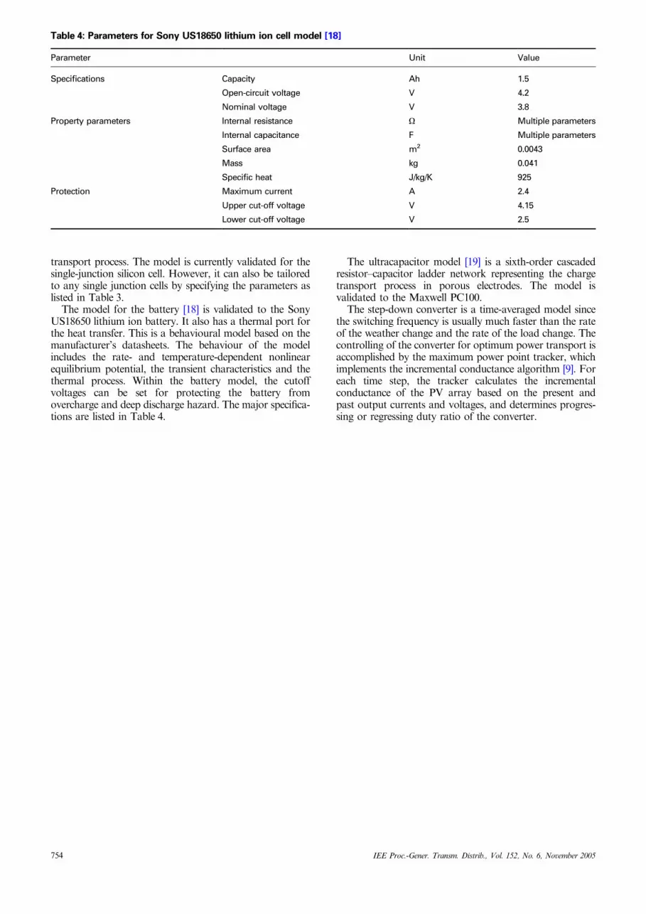
The model for the battery [18] is validated to the SonyUS18650 lithium ion battery. It also has a thermal port forthe heat transfer. This is a behavioural model based on themanufacturer’s datasheets. The behaviour of the modelincludes the rate- and temperature-dependent nonlinearequilibrium potential, the transient characteristics and thethermal process. Within the battery model, the cutoffvoltages can be set for protecting the battery fromovercharge and deep discharge hazard. The major specifica-tions are listed in Table 4.

The ultracapacitor model [19] is a sixth-order cascadedresistor–capacitor ladder network representing the chargetransport process in porous electrodes. The model isvalidated to the Maxwell PC100.

The step-down converter is a time-averaged model sincethe switching frequency is usually much faster than the rateof the weather change and the rate of the load change. Thecontrolling of the converter for optimum power transport isaccomplished by the maximum power point tracker, whichimplements the incremental conductance algorithm [9]. Foreach time step, the tracker calculates the incrementalconductance of the PV array based on the present andpast output currents and voltages, and determines progres-sing or regressing duty ratio of the converter.

Table 4: Parameters for Sony US18650 lithium ion cell model [18]

Parameter Unit Value

Specifications Capacity Ah 1.5

Open-circuit voltage V 4.2

Nominal voltage V 3.8

Property parameters Internal resistance O Multiple parameters

Internal capacitance F Multiple parameters

Surface area m2 0.0043

Mass kg 0.041

Specific heat J/kg/K 925

Protection Maximum current A 2.4

Upper cut-off voltage V 4.15

Lower cut-off voltage V 2.5


Documents

Design of autonomous photovoltaic power plant for telecommunication relay station