Derivatives Replication Under Greenian Motion

Deriv atives ReplicationUnder Greenian Motion

PETER CARR

Head of Quantitative Financial Research, Bloomberg LP, New YorkDirector of the Masters Program in Math Finance, Courant Institute, NYU

CU IEOR Practitioners Seminar, New York file reference:ColUpres.tex January 22nd, 2007

Disc laimer

• The material is this presentation is preliminary and the conclusions reached aretentative.

• The results obtained in no way reflect the opinions of employees of either Bloombergor NYU.

• I am indebted to my colleagues at Bloomberg for many helpful discussions. Iam especially indebted to David Eliezer for the mathematical background and toBruno Dupire for his deep insights on local volatility models.

2

Overview

• There are five parts to this talk:

1. Introduction

2. Model-free Results on Calendar Spreads

3. Derivatives Replication in Markovian Models

4. Derivatives Replication under Greenian Motion

5. Simplifications Arising under Laplace Dynamics

3

Part I - Intr oduction

• As is very well known, in models which go by the names of Cox Ross Rubinstein(CRR) and Black Merton Scholes (BMS), payoffs to derivative securities can bereplicated by restricting price processes.

• For example, in discrete time, the CRR model assumes Bernoulli dynamics. Incontinuous time, the BMS model assumes continuous price paths.

• When the derivative security is written on the price path of a single underlyingasset, model-based replication requires positions in just two assets.

• Parameter inputs are obtained either from time series (historical vol) or the marketprice of a single option (implied vol).

4

Markovian Models with Temporal and Spatial Homog eneity

• The CRR and BMS model are both Markovian Models in which the log price hasstationary independent increments.

• When the term structure of ATM implied vol is not flat, temporal homogeneity canbe relaxed and time-dependent CRR and BMS models can be used to price andhedge derivative securities.

• Now the model is calibrated to a whole term structure of option prices, but whenthe derivative security is written on the price path of a single underlying asset,model-based replication still requires positions in just two assets.

5

Strike Structure of Implied Vol

• When one or more implied volatility smiles are not flat, time-dependent CRR andBMS models are contradicted; a different kind of model is required.

• One of the more popular successors to time-dependent CRR and BMS modelsis the set of local vol models. These models further relax spatial homogeneity,but the basic nature of the motion is unaltered. In discrete time, the Derman Kanilocal vol model still assumes Bernoulli dynamics. In continuous time, the Dupirelocal vol model still assume no jumps. The Markovian nature of the dynamics ispreserved.

• Local vol models are calibrated to a whole term and strike structure of optionprices. When the derivative security is written on the price path of a single under-lying asset, model-based replication still requires positions in just two assets.

6

What About Jumps?

• In binomial models, single period OTM options struck outside the allowed pricerange are worthless. In diffusion models, the analogous statement is that forevery ε > 0:

limh↓0

Q{|St+h−S| > ε|St = S}h

= 0,

for all S in the domain of the diffusion. In words, as time to maturity goes to zerothe prices of all OTM binary options decline towards zero sublinearly.

• Do near-dated OTM binary option prices behave this way in the data? In “ASimple Robust Test for the Presence of Jumps in Option Prices”, Liuren Wu and Ifind that for S&P500 options prices, the decline is linear, not sublinear, consistentwith jumps being priced into near-dated OTM options. In fact, here’s a quote fromformer RFS editor Ken Singleton as he rejected our paper:

“Every study that went looking for jumps has found them.”

7

Do Jumps Matter for Long Dated Options?

• Some people argue that jumps are required to price short-dated options, but thatthe effects of jumps on pricing wash out over long horizons. This argument mixesup jumps with independent increments, an assumption that is often made to makejumps tractable.

• Every long-dated option eventually becomes short-dated, but in markets with zeronet supply, short-dated options need not be held.

• So do jumps necessarily matter for the pricing of long dated options?

8

An Illuminating Example

• Consider the problem of pricing a down-and-out call DOC(K,M;L) with strike K,maturity M, and lower barrier L ≤K, written on a co-terminal forward price F(M).

• In 1994, Bowie and Carr showed that when the underlying forward price cannotjump over the barrier, a down-and-out call struck at L has no time value, i.e.:

DOC0(L,M;L) = B0(M)[F0(M)−L],

where B0(M) is the discount factor.

• In contrast, when the underlying forward price can jump over the barrier, a down-and-out call has positive time value i.e.:

DOC0(L,M;L) > B0(M)[F0(M)−L].

• Hence, any continuous model will underprice this down-and-out call, assumingonly that it reprices the forward. The continuity assumption kills the convexityvalue of the DOC.

9

Hedging Under Jumps

• Assuming that the log price is affine in a standard Poisson process, Cox and Ross(1976) showed that the payoff of a derivative security written on the price path ofa single underlying asset can still be replicated by dynamic trading in just twoassets.

• If two jump sizes are possible at any instant, then in general, replication requiresdynamic trading in three assets, eg. stock, bond, and variance swap.

• However, every rule has an exception, (except for this rule of course). For exam-ple, to replicate the payoff of a variance swap, one can show that one only needsa static position in the log contract and dynamic trading in the underlying.

• When markets are incomplete, there still exist payoffs which can be spanned inthe existing structure eg. Put Call Parity. The discovery of the nature of suchpayoffs and their hedge is a subject of much practitioner interest.

10

Hedging Under a Contin uum of Possib le Jump Sizes

• The more jump sizes that are allowed, the more assets one needs to hedge.

• In this paper, we will focus on the case where a continuum of jump sizes is possi-ble at any instant.

• Not surprisingly, for a derivative security written on the price path of a singleunderlying asset, perfect replication of the payoff will in general require dynamictrading in European options of all strikes and maturities up to that of the security.

11

Replicating Barrier Options

• Throughout this talk, we will focus on the problem of how to replicate the payoffto a barrier option via dynamic trading in European options.

• When the underlying asset has price dynamics that are Markovian in itself andtime, we show that there exists a replicating strategy even though jumps of anysize are possible at every time.

• In general, the replicating strategy has positions in European options of all strikesand maturities up to that of the barrier option. The positions in European optionsare altered as the options become near-dated. Otherwise, the holdings are static.

12

Greenian Motion

• When we add a particular structure to the jump dynamics called Greenian motion,we no longer require positions in intermediate maturity options struck away fromthe barrier. A memoryless property allows their role to be captured by optionsstruck on the barrier.

• Furthermore, the model can be explicitly calibrated to a single observation of themarket prices of European options of all strikes and maturities up to that of thebarrier option.

• Under Greenian motion, the determination of option value functions only requiresnumerically solving a sequence of linear second order ODE’s.

• When we further require deterministic volatility, we get closed form solutions forbarrier option values and hedge ratios.

13

The Setting

• Without loss of generality, we will focus on the problem of how to replicate thepayoff to a down-and-out call (DOC) struck above a lower barrier.

• For simplicity, we will work in discrete time and assume that barrier monitoringoccurs on the same frequency as price changes.

• For simplicity, we will assume that the underlying is a forward price and that inter-est rates are zero.

• For simplicity, we let the underlying forward price go negative. Hence, at eachperiod, the support of possible forward prices at each future time is the whole realline.

14

Consequences of Frictionless Markets and No Arbitra ge

• We assume frictionless markets and in particular that market prices are unaf-fected by the trading of an individual.

• We assume no arbitrage and hence the existence of a probability measure Qunder which (forward) prices are martingales.

• Initially, we will not place further restrictions on the dynamics of the underlyingforward price.

15

Butterfl y Spreads

• Let n = 0,1, . . . ,∞ index the natural numbers and denote discrete calendar time.

• For n = 0,1, . . . ,∞, let Fn be the price at time n of some underlying asset.

• For n = 0,1, . . . ,m, suppose that one can trade calls paying (Fm −K)+ at itsmaturity m. Let Cn(F ;K,m) denote the conditional market price at time n of aEuropean call of strike K ∈R and maturity m ≥ n. The market price is conditionalon Fn = F and is in general random for n > 0. The conditional call price is alsonot directly observable for n > 0 or F 6= F0, but can be observed at n = 0 andF = F0.

• Suppose that for each date n and each maturity m ≥ i, the call pricing functionCn(F ;K,m) is C2 in K. Then Breeden and Litzenberger (1978) show that:

Q{Fm ∈ dK|Fn = F} =∂2

∂K2Cn(F;K,m)dK.

16

Butterfl y Spreads (Con’d)

• Recall that:

Q{Fm ∈ dK|Fn = F} =∂2

∂K2Cn(F;K,m)dK.

• In words, the conditional risk-neutral density of the future forward price Fm at levelK is given by the market price at time n of a butterfly spread paying δ(Fn −K) atits maturity m ≥ n.

• Are there any other model-free results concerning option spreads?

17

Calendar Spread of Binar y Calls

• Recall that a butterfly spread maturing at m pays δ(Fm −K) when n crosses mfrom below. Thus a cash inflow of infinite magnitude arises if Fm = K at this time.

• If time could run backward, then this infinite inflow would turn into an outflow ifFm = K as n crosses m from above.

• In contrast to time, a price F can cross a given level K from above or below.

• Reversing the roles of space and time, we now show that a calendar spread ofbinary calls has the same action as a butterfly spread of calls.

Parsifal∗: I hardly tread- though it seems I already have come far.Gurnemanz: You see, my son, here time becomes space.

From the first act of the opera Parsifal by Wolfgang Wagner.∗I thank Lane Hughston for suggesting this quote.

18

Calendar Spread of Binar y Calls (Con’d)

• For n = 0,1, . . ., let BCn(F ;K,m) ≡− ∂∂KCn(K,m) denote market prices at time n

of binary calls of all strikes K ∈ R at each discrete maturity m ≥ n Each binarycall pays H (Fm−K) at its maturity m, where H (x) is the Heaviside function.

• For m ≥ n + 1, consider the value at time n of a calendar spread of binary callswhen the two maturities are adjacent: BCn(F ;K,m+1)−BCn(F ;K,m).

• Examining the 2×2 = 4 cases, we find that the payoff at time m+1 is:

H (K −Fm)H (Fm+1−K)−H (Fm−K)H (K −Fm+1).

• In words, one dollar is received at time m+1 if F crosses K from below, but onedollar is paid at time m+1 if F crosses K from above.

19

Calendar Spread of Standar d Calls

• The results on the last slide imply that BCn(F;K,m + 1)−BCn(F;K,m) is theconditional price at time n of purchasing a claim that provides both a unit increasein value at K if F upcrosses K just after time m and a unit decrease in value if Fdowncrosses K just after time m.

• On the next slide, we show that Cn(F ;K,m + 1)−Cn(F ;K,m) is the conditionalprice at time n of purchasing a claim that provides both a unit increase in slope ifF upcrosses K just after time m and a unit decrease in slope if F downcrosses Kjust after time m.

20

Calendar Spread of Standar d Calls (Con’d)

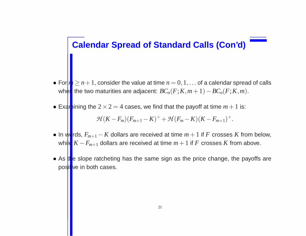
• For m ≥ n+1, consider the value at time n = 0,1, . . . of a calendar spread of callswhen the two maturities are adjacent: BCn(F ;K,m+1)−BCn(F ;K,m).

• Examining the 2×2 = 4 cases, we find that the payoff at time m+1 is:

H (K −Fm)(Fm+1−K)+ +H (Fm−K)(K−Fm+1)+.

• In words, Fm+1−K dollars are received at time m+1 if F crosses K from below,while K −Fm+1 dollars are received at time m+1 if F crosses K from above.

• As the slope ratcheting has the same sign as the price change, the payoffs arepositive in both cases.

21

Down-and-Out Calls and Generalizations

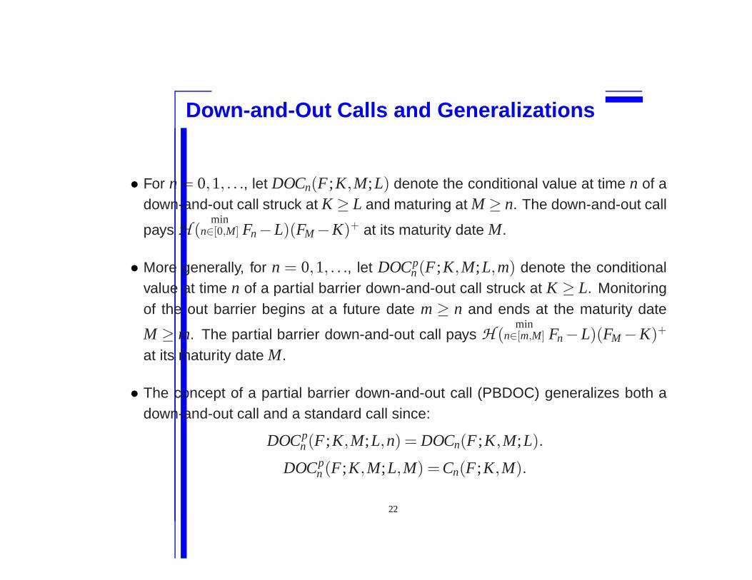
• For n = 0,1, . . ., let DOCn(F ;K,M;L) denote the conditional value at time n of adown-and-out call struck at K ≥ L and maturing at M ≥ n. The down-and-out call

pays H (min

n∈[0,M] Fn −L)(FM −K)+ at its maturity date M.

• More generally, for n = 0,1, . . ., let DOCpn (F ;K,M;L,m) denote the conditional

value at time n of a partial barrier down-and-out call struck at K ≥ L. Monitoringof the out barrier begins at a future date m ≥ n and ends at the maturity date

M ≥ m. The partial barrier down-and-out call pays H (min

n∈[m,M] Fn −L)(FM −K)+

at its maturity date M.

• The concept of a partial barrier down-and-out call (PBDOC) generalizes both adown-and-out call and a standard call since:

DOCpn (F ;K,M;L,n) = DOCn(F ;K,M;L).

DOCpn (F;K,M;L,M) = Cn(F;K,M).

22

Calendar Spread of Partial Barrier Calls

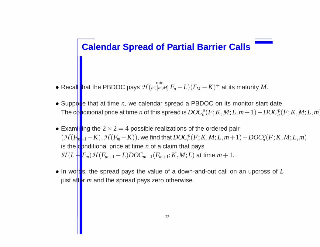
• Recall that the PBDOC pays H (min

n∈[m,M] Fn−L)(FM −K)+ at its maturity M.

• Suppose that at time n, we calendar spread a PBDOC on its monitor start date.The conditional price at time n of this spread is DOCp

n (F ;K,M;L,m+1)−DOCpn(F ;K,M;L,m)

• Examining the 2×2 = 4 possible realizations of the ordered pair(H (Fm+1−K),H (Fm−K)), we find that DOCp

n (F ;K,M;L,m+1)−DOCpn(F ;K,M;L,m)

is the conditional price at time n of a claim that paysH (L−Fm)H (Fm+1−L)DOCm+1(Fm+1;K,M;L) at time m+1.

• In words, the spread pays the value of a down-and-out call on an upcross of Ljust after m and the spread pays zero otherwise.

23

Replicating a Down-and-Out Call

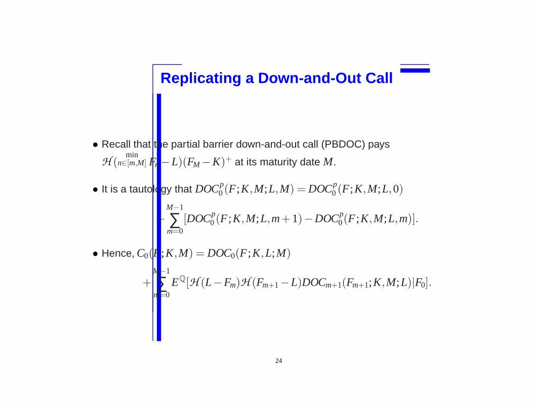
• Recall that the partial barrier down-and-out call (PBDOC) pays

H (min

n∈[m,M] Fn −L)(FM −K)+ at its maturity date M.

• It is a tautology that DOCp0 (F;K,M;L,M) = DOCp

0 (F;K,M;L,0)

+M−1

∑m=0

[DOCp0 (F ;K,M;L,m+1)−DOCp

0(F ;K,M;L,m)].

• Hence, C0(F;K,M) = DOC0(F ;K,L;M)

+M−1

∑m=0

EQ[H (L−Fm)H (Fm+1−L)DOCm+1(Fm+1;K,M;L)|F0].

24

Replicating a Down-and-Out Call (Con’d)

• Recall that C0(F ;K,M) = DOC0(F ;K,L;M)

+M−1

∑m=0

EQ[H (L−Fm)H (Fm+1−L)DOCm+1(Fm+1;K,M;L)|F0].

• But by Taylor series with remainder, H (Fm+1−L)DOCm+1(Fm+1;K,M;L):

=∂

∂FDOCm+1(L;K,M;L)(Fm+1−L)+

+∫ ∞

L

∂2

∂F2DOCm+1(J;K,M;L)(Fm+1− J)+dJ.

• Hence, EQH (L−Fm)H (Fm+1−L)DOCm+1(Fm+1;K,M;L)|F0] =:

EQ{

H (L−Fm)∂

∂FDOCm+1(L;K,M;L)[Cm(Fm,L,m+1)−Cm(Fm,L,m)]|F0

}

+EQ{

H (L−Fm)∫ ∞

L

∂2

∂F2DOCm+1(J;K,M;L)[Cm(Fm;J,m+1)−Cm(Fm;J,m)]dJ|F0

}.

25


• Substitution implies: C0(F ;K,M) = DOC0(F ;K,L;M)+M−1∑

m=0EQ{ fm(Fm)|F0}, where

fm(F) ≡ H (L−F)∂

∂FDOCm+1(L;K,M;L)[Cm(F,L,m+1)−Cm(F,L,m)]

+ +H (L−F)∫ ∞

L

∂2

∂F2DOCm+1(J;K,M;L)[Cm(F ;J,m+1)−Cm(F;J,m)]dJ.

• We now assume that the underlying forward price is Markov in itself and time.

• Consequently, the value functions for C and DOC at any future time and price aredetermined by numerically solving a partial integro difference equation (PIDE).

• As the DOC’s delta and gamma also become determined, each function fm be-comes known.

26


• Recall that the equation at the top of the previous slide had the form

C0(F ;K,M) = DOC0(F ;K,L;M)+M−1

∑m=0

EQ{ fm(Fm)} ,

where f is a known function of its argument.

• Using the Breeden and Litzenberger result, we can hold a portfolio of butterflyspreads of all strikes below the barrier and all maturities up to that of the DOC.

DOC0(F0;K,M;L) = C0(F0;K,M)−M

∑m=1

∫ L

−∞Nbs(F,m)

∂2

∂K2C(F0;F,m)dF,

where:

Nbs(F,m) =∂

∂FDOCm+1(L;K,M;L)[Cm(F,L,m+1)−Cm(F,L,m)]

+∫ ∞

L

∂2

∂F2DOCm+1(J;K,M;L)[Cm(F ;J,m+1)−Cm(F ;J,m)]dJ.

27

Semi-Static Hedging

• To show how the hedge works, note that if the underlying never crosses the barrierbefore M, then all of the butterflies expire worthless while the standard call givesthe desired payoff.

• If the underlying crosses the barrier before M, then at the first passage time to thebarrier, the standard option portfolio is worthless. The reason is that one can usethe payoff from each maturing butterfly spread to buy near-dated OTM calls struckat L and above. These call positions finance transitions into a short position in analive down-and-out call held only in the continuation region. This self-financingsemi-static trading strategy in barrier options has a final payoff equal to a shortcall payoff. The long call hedges this liability and thus the standard option portfoliomust have zero value for stock prices below L at any time prior to T .

28

Drawbac ks of the General Markovian Hege

• When hedging the sale of a DOC, an obvious drawback of the general Markovianapproach is that it requires the ability to take positions in puts of all strikes belowthe barrier.

• A second drawback is that it is not clear how to choose the Markov model. Intheory, one can calibrate to the prices of standard options at all strikes and matu-rities at all past times. However, the inversion problem is too big and the data isprobably lacking.

• A third drawback is computational - one has to numerically solve a PIDE to imple-ment the hedge.

29

Greenian Motion

• We introduce a new type of Markovian dynamics called “Greenian Motion”(GM)as a way to overcome all three drawbacks of general Markovian hedging.

• We will see that under GM, positions in all intermediate maturity options struckaway from the barrier are no longer needed in the hedge.

• Furthermore, the risk-neutral dynamics of the underlying forward price processcan be explicitly identified on day 0 from the initial market prices of standardoptions of all strikes and maturities up to that of the DOC.

• Finally, on the computational side, one need only numerically solve a sequence ofsecond order linear ordinary differential equations (ODE’s) to obtain both valuesand hedge ratios.

30

Review of Green’s Functions

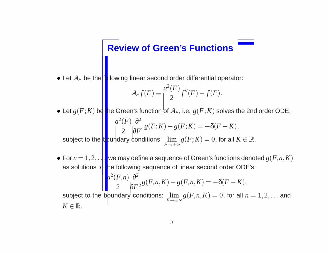
• Let AF be the following linear second order differential operator:

AF f (F) ≡a2(F)

2f ′′(F)− f (F).

• Let g(F ;K) be the Green’s function of AF , i.e. g(F ;K) solves the 2nd order ODE:

a2(F)2

∂2

∂F2g(F ;K)−g(F;K) = −δ(F −K),

subject to the boundary conditions: limF→±∞

g(F ;K) = 0, for all K ∈ R.

• For n = 1,2, . . ., we may define a sequence of Green’s functions denoted g(F,n,K)as solutions to the following sequence of linear second order ODE’s:

a2(F,n)2

∂2

∂F2g(F,n,K)−g(F,n,K) = −δ(F −K),


g(F,n,K) = 0, for all n = 1,2, . . . and

K ∈ R.

31

Adjoint Equation

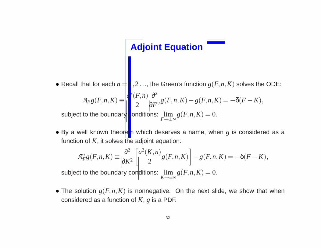
• Recall that for each n = 1,2 . . ., the Green’s function g(F,n,K) solves the ODE:

AFg(F,n,K)≡ a2(F,n)2

∂2

∂F2g(F,n,K)−g(F,n,K) = −δ(F −K),


g(F,n,K) = 0.

• By a well known theorem which deserves a name, when g is considered as afunction of K, it solves the adjoint equation:

A∗Fg(F,n,K)≡

∂2

∂K2

[a2(K,n)

2g(F,n,K)

]−g(F,n,K) = −δ(F −K),

subject to the boundary conditions: limK→±∞

g(F,n,K) = 0.

• The solution g(F,n,K) is nonnegative. On the next slide, we show that whenconsidered as a function of K, g is a PDF.

32

Integral Transf orm

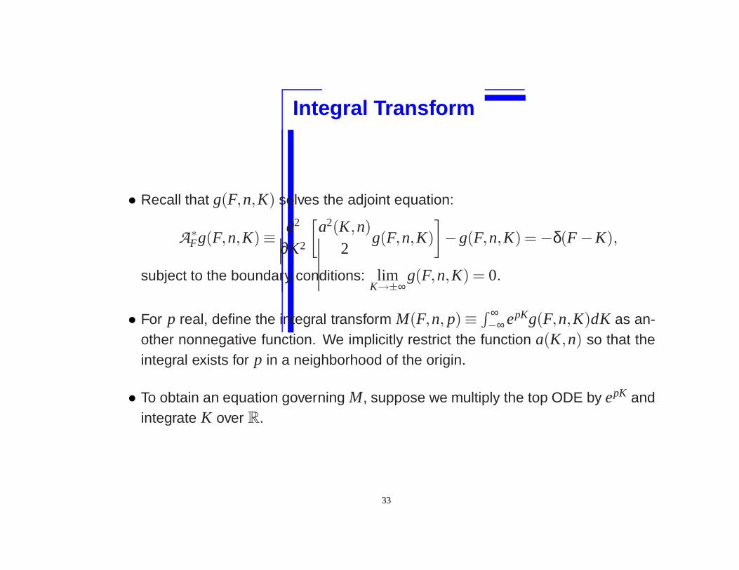
• Recall that g(F,n,K) solves the adjoint equation:

A∗Fg(F,n,K)≡

∂2

∂K2

[a2(K,n)

2g(F,n,K)

]−g(F,n,K) = −δ(F −K),


g(F,n,K) = 0.

• For p real, define the integral transform M(F,n, p)≡∫ ∞−∞ epKg(F,n,K)dK as an-

other nonnegative function. We implicitly restrict the function a(K,n) so that theintegral exists for p in a neighborhood of the origin.

• To obtain an equation governing M, suppose we multiply the top ODE by epK andintegrate K over R.

33

Integral Transf orm (Con’d)

• As a result, M(F,n, p) solves the equation:∫ ∞

−∞epK ∂2

∂K2

[a2(K,n)

2g(F,n,K)

]dK−M(F,n, p) = −epF.

• Integrating by parts twice and assuming that:

limK→±∞

∂∂K

[a2(K,n)

2g(F,n,K)

]= 0, lim

K→±∞

a2(K,n)2

g(F,n,K) = 0,

we get that M(F,n, p) solves the equation:

p2

2

∫ ∞

−∞epKa2(K,n)g(F,n,K)dK−M(F,n, p) = −epF.

• Evaluating at p = 0 implies that when considered as a function of K, g is a prob-ability density function (PDF):∫ ∞

−∞g(F,n,K)dK = 1, for all F ∈ R,n = 1,2 . . .

34

First Moment

• Since g is a PDF in K, M(F,n, p)≡∫ ∞−∞ epKg(F,n,K)dK is the moment generat-

ing function (MGF) of the random variable whose PDF is g.

• Recall that the MGF M(F,n, p) solves the equation:

p2

2

∫ ∞


• Differentiating once w.r.t. p and setting p = 0 implies that:∫ ∞

−∞Kg(F,n,K)dK = F,

for all F ∈ R and n = 1,2 . . ..

• Thus, the first moment of the mystery random variable is F for all n.

35

Second Moment and Variance

• Recall again that the MGF M(F,n, p) solves the equation:

p2

2

∫ ∞


• Differentiating twice w.r.t. p and setting p = 0 implies that:∫ ∞

−∞K2g(F,n,K)dK = F2 +

∫ ∞

−∞a2(K,n)g(F,n,K)dK,

for all F ∈ R and n = 1,2 . . .

• As a result, we have that:∫ ∞

−∞(K−F)2g(F,n,K)dK =

∫ ∞

−∞a2(K,n)g(F,n,K)dK,

for all F ∈ R and n = 1,2 . . .

36

What is Greenian Motion?

• Consider a discrete time Markov process F defined over a finite time horizon.

• We say that F follows Greenian Motion if for every n, its transition PDF at time nis the Green’s function g(F,n,K), i.e.:

Q{Fn+1 ∈ dK|Fn = F} = g(F,n,K).

• Since∫ ∞−∞ Kg(F,n,K)dK = F, we see that F is a martingale:

EQ[Fn+1|Fn = F ] = F.

37

Interpreting a2

• Suppose we interpret F as a continuous time process which only jumps at integertimes.

• When a2 is constant, the distribution of each increment is Laplace with mean zeroand variance a2.

• When a2 is constant, the process has independent increments and enjoys a scal-ing property, viz c(Fn−F0) has the same law as Fc2n−F0. As a consequence, wecan alternatively draw from a Laplace with unit standard deviation and assign theoutcome to a time step of length 1/a2. European options should have the sameprice.

• When a2 depends on F and n, we may continue to draw from a standard Laplaceand have the result apply to random time steps of length 1/a2(Fn,n).

38

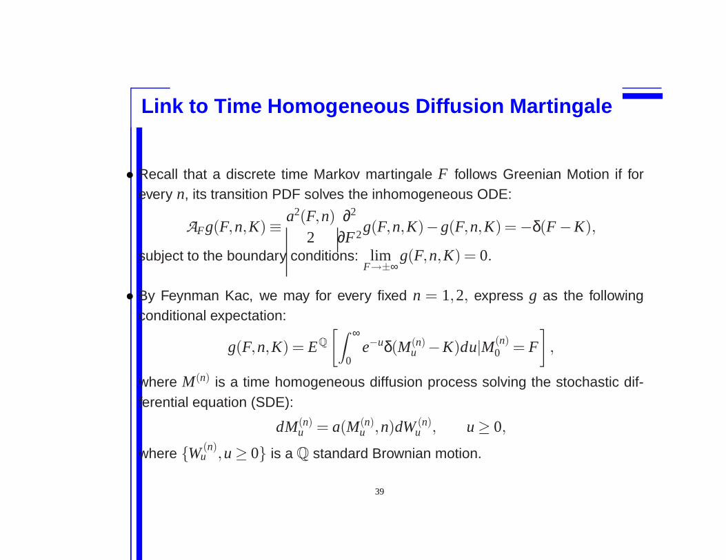
Link to Time Homog eneous Diffusion Martingale

• Recall that a discrete time Markov martingale F follows Greenian Motion if forevery n, its transition PDF solves the inhomogeneous ODE:


∂2

∂F2g(F,n,K)−g(F,n,K) = −δ(F −K),


g(F,n,K) = 0.

• By Feynman Kac, we may for every fixed n = 1,2, express g as the followingconditional expectation:

g(F,n,K) = EQ[∫ ∞

0e−uδ(M(n)

u −K)du|M(n)0 = F

],

where M(n) is a time homogeneous diffusion process solving the stochastic dif-ferential equation (SDE):

dM(n)u = a(M(n)

u ,n)dW (n)u , u ≥ 0,

where {W (n)u ,u ≥ 0} is a Q standard Brownian motion.

39

Link to a Time Inhomog eneous Diffusion Martingale

• Instead of linking the n-th increment in F with the entire trajectory of a time ho-mogeneous diffusion M(n), we may link the whole F process with a time inhomo-geneous diffusion D, which is locally time homogeneous.

• Suppose that D is a time inhomogeneous diffusion whose diffusion coefficientjumps from a(D,n) to a(D,n+1) when an independent and completely standardPoisson process N jumps from level n to level n+1.

• By running the diffusion process D on N, we obtain the discrete time process F .

• This link makes clear why F is a local martingale and it also permits a familiarinterpretation of the function a(F,n) as a diffusion coefficient.

40

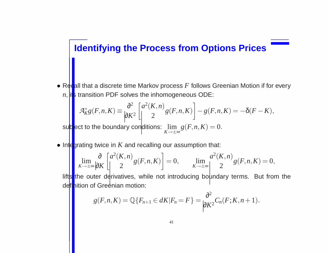
Identifying the Process from Options Prices

• Recall that a discrete time Markov process F follows Greenian Motion if for everyn, its transition PDF solves the inhomogeneous ODE:

A∗Kg(F,n,K)≡ ∂2

∂K2

[a2(K,n)

2g(F,n,K)

]−g(F,n,K) = −δ(F −K),


g(F,n,K) = 0.

• Integrating twice in K and recalling our assumption that:

limK→±∞

∂∂K

[a2(K,n)

2g(F,n,K)

]= 0, lim

K→±∞

a2(K,n)2

g(F,n,K) = 0,

lifts the outer derivatives, while not introducing boundary terms. But from thedefinition of Greenian motion:

g(F,n,K) = Q{Fn+1 ∈ dK|Fn = F} =∂2

∂K2Cn(F ;K,n+1).

41

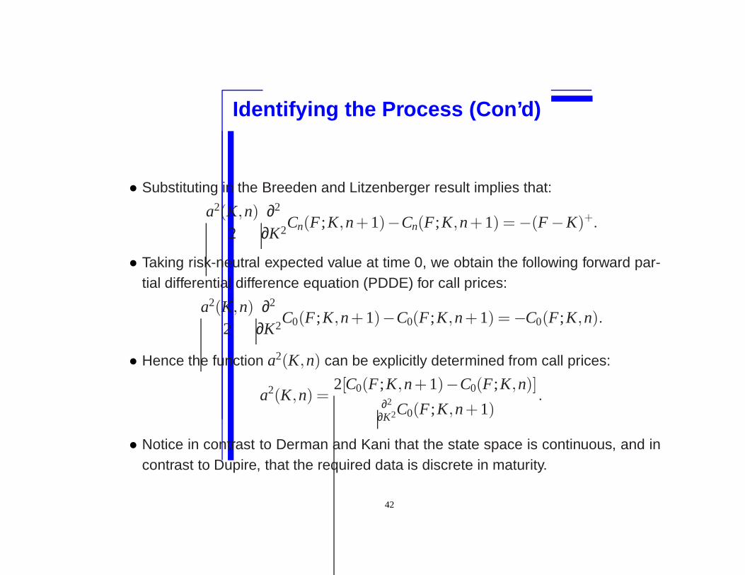
Identifying the Process (Con’d)

• Substituting in the Breeden and Litzenberger result implies that:

a2(K,n)2

∂2

∂K2Cn(F ;K,n+1)−Cn(F;K,n+1) = −(F −K)+.

• Taking risk-neutral expected value at time 0, we obtain the following forward par-tial differential difference equation (PDDE) for call prices:

a2(K,n)2

∂2

∂K2C0(F ;K,n+1)−C0(F ;K,n+1) = −C0(F;K,n).

• Hence the function a2(K,n) can be explicitly determined from call prices:

a2(K,n) =2[C0(F ;K,n+1)−C0(F;K,n)]

∂2

∂K2C0(F ;K,n+1).

• Notice in contrast to Derman and Kani that the state space is continuous, and incontrast to Dupire, that the required data is discrete in maturity.

42

Backwar d PDDE for Butterfl y Spread Values

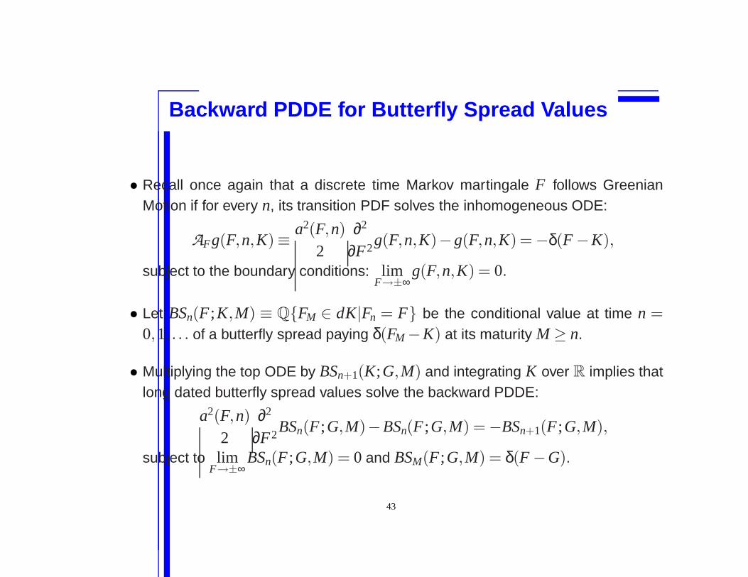
• Recall once again that a discrete time Markov martingale F follows GreenianMotion if for every n, its transition PDF solves the inhomogeneous ODE:


∂2

∂F2g(F,n,K)−g(F,n,K) = −δ(F −K),


g(F,n,K) = 0.

• Let BSn(F ;K,M) ≡ Q{FM ∈ dK|Fn = F} be the conditional value at time n =0,1, . . . of a butterfly spread paying δ(FM −K) at its maturity M ≥ n.

• Multiplying the top ODE by BSn+1(K;G,M) and integrating K over R implies thatlong dated butterfly spread values solve the backward PDDE:

a2(F,n)2

∂2

∂F2BSn(F ;G,M)−BSn(F ;G,M) = −BSn+1(F ;G,M),

subject to limF→±∞

BSn(F ;G,M) = 0 and BSM(F ;G,M) = δ(F −G).

43

Backwar d PDDE for Claim Values

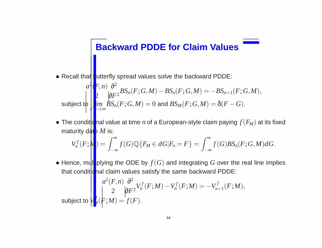
• Recall that butterfly spread values solve the backward PDDE:

a2(F,n)2

∂2

∂F2BSn(F ;G,M)−BSn(F ;G,M) = −BSn+1(F ;G,M),

subject to limF→±∞

BSn(F ;G,M) = 0 and BSM(F ;G,M) = δ(F −G).

• The conditional value at time n of a European-style claim paying f (FM) at its fixedmaturity date M is:

V fn (F ;M) =

∫ ∞

−∞f (G)Q{FM ∈ dG|Fn = F} =

∫ ∞

−∞f (G)BSn(F ;G,M)dG.

• Hence, multiplying the ODE by f (G) and integrating G over the real line impliesthat conditional claim values satisfy the same backward PDDE:

a2(F,n)2

∂2

∂F2V f

n (F ;M)−V fn (F;M) = −V f

n+1(F ;M),

subject to V fM(F ;M) = f (F).

44

Backwar d PDDE for Barrier and Berm udan Option Values

• We may similarly numerically solve a sequence of ODE’s for discretely monitoredknockout barrier options. In the knockout region, the continuation value is set tozero.

• Bermudan options are handled similarly; before recursing backward, the continu-ation value is replaced by the maximum of it and the reward for exercising early.

45

Summar y

• Working in discrete time and under zero rates, we first presented some newmodel-free results concerning the values of calendar spreads of binary, standard,and partial barrier calls.

• We then showed how one can replicate the payoff to a down-and-out call whenthe underlying price process is Markov in itself.

• Since we allowed the possibility of jumps of all sizes, the replicating portfoliorequired positions in options of all strikes and maturities.

• By restricting dynamics down to Greenian motion, the calibration, valuation, andreplication problems all simplify quite dramatically.

• An open question concerns the impact that the Greenian Motion assumption hason the range of permitted dynamics.

46

Other Proper ties of Greenian Motion

• Although we presented GM in discrete time, it has a continuous time counterpartbeing worked our presently. This continuous time counterpart is needed whenbarriers are monitored continuously.

• Although we presented GM with just one underlying source of uncertainty, onecan also generalize it to multiple sources of uncertainty (eg. stochastic vol ormultiple underlyings). Unlike its Markovian generalization, the single factor GMapproach “leaves room” for hedging an additional uncertainty. Now one solves asequence of elliptic PDE’s rather than ODE’s.

• Finally, the single factor GM approach is semi-analytic: using variation of param-eters, one can write down formulas for values and hedge ratios in terms of asolution to a linear second order homogeneous ODE with variable coefficients. Ifthe ODE has a closed form solution, then so do claim values and hedge ratios.

47

Documents

Derivatives Replication Under Greenian Motion