Deep Learning in Unconventional Domains

Thesis byMilan Cvitkovic

In Partial Fulfillment of the Requirements for theDegree of

Doctor of Philosophy

CALIFORNIA INSTITUTE OF TECHNOLOGYPasadena, California

2020Defended March 10, 2020

ii

© 2020

Milan CvitkovicORCID: 0000-0003-4188-452X

All rights reserved

iii

ACKNOWLEDGEMENTS

To my parents, Kate Turpin and Michael Cvitkovic, and my sister, Adriana Cvitkovic:thank you for your boundless love and support. And all the teasing.

To my thesis committee, Prof. Anima Anandkumar, Prof. Yisong Yue, Prof. AdamWierman, and Prof. Thomas Vidick: thank you for your invaluable guidance andencouragement throughout my time at Caltech, both in your roles as committeemembers and beyond.

To Prof. Anima Anandkumar, Prof. Pietro Perona, and Prof. Stefano Soatto: thankyou for facilitating my affiliation with Amazon Web Services, without which thisdissertation would never have been possible.

To all my coauthors who helped with the work in this thesis — Badal Singh, Prof.Anima Anandkumar, Dr. Günther Koliander, and Dr. Zohar Karnin — and to all myother collaborators during my PhD — Joe Marino, Dr. Grant Van Horn, Dr. HamedAlemohammad, Prof. Yisong Yue, Keng Wah Loon, Laura Graesser, Jiahao Su, andProf. Furong Huang: thank you for your generosity and your brilliance.

To Lee, Carmen, Kirsten, Leslie, James, Alex, Josh, Claudia, and Patricia: thank youfor being cheerful stewards of daily rituals.

And most of all to my advisor, Prof. Thomas Vidick: thank you for your unwaveringsupport of a non-traditional advisee.

iv

ABSTRACT

Machine learning methods have dramatically improved in recent years thanks toadvances in deep learning (LeCun, Bengio, and Hinton, 2015), a set of methodsfor training high-dimensional, highly-parameterized, nonlinear functions. Yet deeplearning progress has been concentrated in the domains of computer vision, vision-based reinforcement learning, and natural language processing. This dissertationis an attempt to extend deep learning into domains where it has thus far had littleimpact or has never been applied. It presents new deep learning algorithms andstate-of-the-art results on tasks in the domains of source-code analysis, relationaldatabases, and tabular data.

v

PUBLISHED CONTENT AND CONTRIBUTIONS

Cvitkovic, Milan (2020). “Supervised Learning on Relational Databases with GraphNeural Networks”. In: Current version in submission; previous version in RLGMworkshop ICLR 2019. url: https://arxiv.org/abs/2002.02046.M.C. conceived of and designed the project, developed and implemented themethod, ran the experiments, and wrote the manuscript.

Cvitkovic, Milan and Zohar Karnin (2020). “Subset-Restricted Finetuning on TabularData with Transformers”. In: In preparation.M.C. participated in designing the project and developing the method; he alsoimplemented and ran the experiments and wrote the manuscript.

Cvitkovic, Milan (2019). “Some Requests for Machine Learning Research fromthe East African Tech Scene”. In: Proceedings of the Conference on Computing& Sustainable Societies, ACM COMPASS 2019, Accra, Ghana, July 3-5, 2019,pp. 37–40. doi: 10.1145/3314344.3332492. url: https://doi.org/10.1145/3314344.3332492.M.C. designed the project, performed the interviews, and wrote the manuscript.

Cvitkovic, Milan and Günther Koliander (2019). “Minimal Achievable SufficientStatistic Learning”. In: Proceedings of the 36th International Conference onMachine Learning, ICML 2019, 9-15 June 2019, Long Beach, California, USA,pp. 1465–1474. url: http://proceedings.mlr.press/v97/cvitkovic19a.html.M.C. participated in designing the project, developing the theory and method,running the experiments, and writing the manuscript.

Cvitkovic, Milan, Badal Singh, and Anima Anandkumar (2019). “Open VocabularyLearning on Source Code with a Graph-Structured Cache”. In: Proceedings of the36th International Conference on Machine Learning, ICML 2019, 9-15 June 2019,Long Beach, California, USA, pp. 1475–1485. url: http://proceedings.mlr.press/v97/cvitkovic19b.html.M.C. participated in designing the project, developing the method, running theexperiments, and writing the manuscript.

vi

TABLE OF CONTENTS

Acknowledgements . . . . . . . . . . . . . . . . . . . . . . . . . . . . . . . iiiAbstract . . . . . . . . . . . . . . . . . . . . . . . . . . . . . . . . . . . . . ivPublished Content and Contributions . . . . . . . . . . . . . . . . . . . . . . vTable of Contents . . . . . . . . . . . . . . . . . . . . . . . . . . . . . . . . viChapter I: Introduction . . . . . . . . . . . . . . . . . . . . . . . . . . . . . 1Chapter II: Some Requests for Machine Learning Research from the East

African Tech Scene . . . . . . . . . . . . . . . . . . . . . . . . . . . . . 32.1 Introduction . . . . . . . . . . . . . . . . . . . . . . . . . . . . . . 32.2 Research Problems . . . . . . . . . . . . . . . . . . . . . . . . . . . 32.3 Interviews Conducted . . . . . . . . . . . . . . . . . . . . . . . . . 9

Chapter III: Open Vocabulary Learning on Source Code with a Graph–Structured Cache . . . . . . . . . . . . . . . . . . . . . . . . . . . . . . 113.1 Introduction . . . . . . . . . . . . . . . . . . . . . . . . . . . . . . 113.2 Prior Work . . . . . . . . . . . . . . . . . . . . . . . . . . . . . . . 123.3 Preliminaries . . . . . . . . . . . . . . . . . . . . . . . . . . . . . . 143.4 Model . . . . . . . . . . . . . . . . . . . . . . . . . . . . . . . . . 173.5 Experiments . . . . . . . . . . . . . . . . . . . . . . . . . . . . . . 183.6 Discussion . . . . . . . . . . . . . . . . . . . . . . . . . . . . . . . 253.7 Acknowledgements . . . . . . . . . . . . . . . . . . . . . . . . . . . 27

Chapter IV: Supervised Learning on Relational Databases with Graph NeuralNetworks, Part 1 . . . . . . . . . . . . . . . . . . . . . . . . . . . . . . . 324.1 Introduction . . . . . . . . . . . . . . . . . . . . . . . . . . . . . . 324.2 Relational Databases . . . . . . . . . . . . . . . . . . . . . . . . . . 324.3 Supervised Learning on Relational Databases . . . . . . . . . . . . . 334.4 Related Work . . . . . . . . . . . . . . . . . . . . . . . . . . . . . . 374.5 Datasets . . . . . . . . . . . . . . . . . . . . . . . . . . . . . . . . 394.6 Experiments . . . . . . . . . . . . . . . . . . . . . . . . . . . . . . 404.7 Discussion . . . . . . . . . . . . . . . . . . . . . . . . . . . . . . . 414.8 Acknowledgments . . . . . . . . . . . . . . . . . . . . . . . . . . . 424.9 Appendix: Experiment Details . . . . . . . . . . . . . . . . . . . . 424.10 Appendix: Dataset Information . . . . . . . . . . . . . . . . . . . . 45

Chapter V: Strengths and Weaknesses of Deep Learning for Tabular Data . . 575.1 Introduction . . . . . . . . . . . . . . . . . . . . . . . . . . . . . . 575.2 Related Work . . . . . . . . . . . . . . . . . . . . . . . . . . . . . . 585.3 Benchmarking Deep Models for Tabular Data . . . . . . . . . . . . . 595.4 Subset-Restricted Finetuning with Deep Models . . . . . . . . . . . 615.5 Discussion . . . . . . . . . . . . . . . . . . . . . . . . . . . . . . . 645.6 Acknowledgments . . . . . . . . . . . . . . . . . . . . . . . . . . . 655.7 Appendix: Experiment and Model Details . . . . . . . . . . . . . . 65

vii

5.8 Appendix: Benchmark Dataset Information . . . . . . . . . . . . . . 67Chapter VI: Minimal Achievable Sufficient Statistic Learning: Addressing

Issues in the Information Bottleneck . . . . . . . . . . . . . . . . . . . . 766.1 Introduction . . . . . . . . . . . . . . . . . . . . . . . . . . . . . . 766.2 Conserved Differential Information . . . . . . . . . . . . . . . . . . 776.3 MASS Learning . . . . . . . . . . . . . . . . . . . . . . . . . . . . 796.4 Related Work . . . . . . . . . . . . . . . . . . . . . . . . . . . . . . 816.5 Experiments . . . . . . . . . . . . . . . . . . . . . . . . . . . . . . 836.6 Discussion . . . . . . . . . . . . . . . . . . . . . . . . . . . . . . . 876.7 Acknowledgements . . . . . . . . . . . . . . . . . . . . . . . . . . . 926.8 Appendix: Omitted Proofs . . . . . . . . . . . . . . . . . . . . . . . 92

Chapter VII: Supervised Learning on Relational Databases with Graph NeuralNetworks, Part 2 . . . . . . . . . . . . . . . . . . . . . . . . . . . . . . . 1137.1 Introduction . . . . . . . . . . . . . . . . . . . . . . . . . . . . . . 1137.2 Lessons Learned . . . . . . . . . . . . . . . . . . . . . . . . . . . . 1137.3 Experiments . . . . . . . . . . . . . . . . . . . . . . . . . . . . . . 1147.4 Results . . . . . . . . . . . . . . . . . . . . . . . . . . . . . . . . . 1147.5 Appendix: Additional Results . . . . . . . . . . . . . . . . . . . . . 1167.6 Appendix: Experiment Details . . . . . . . . . . . . . . . . . . . . 117

1

C h a p t e r 1

INTRODUCTION

Over the past eight years deep learning (LeCun, Bengio, and Hinton, 2015) hasbecome the dominant approach to machine learning, and machine learning hasbecome the dominant approach to artificial intelligence.

Yet progress in deep learning has been concentrated in the domains of computervision, vision-based reinforcement learning, and natural language processing. Uponseeing the revolution deep learning has sparked in these fields, one must ask: to whatother problem domains can deep learning be applied, and to what effect?

This dissertation is an attempt to help answer this question.

The brief history of modern deep learning suggests that necessary conditions fordeep learning efficacy include having lots of high-dimensional data and appropriatecomputer hardware to process it. So why have domains like database analysis, ge-nomics, tabular machine learning, chemistry, industrial control systems, informationsecurity, formal methods, or neuroscience, which meet these criteria, not had deeplearning revolutions of their own (yet)?

One reason is that deep learning research moves at the pace of deep learning software,and support for domains beyond images, reinforcement learning simulators, and textis slow in coming. This is a major reason why all code written in service of thisdissertation has been open-sourced.

Another reason, in parallel to software, is that machine learning research requiresdatasets and benchmarks. For many less-well-studied domains data are inaccessibleor difficult to use, and there is no consensus on benchmarks. The work presented inthis dissertation includes the curation and release of three new, large-scale datasetsand benchmarks in hopes of addressing this issue.

But perhaps the most important reason is the dependence of deep learning on modelarchitecture. Convolutional networks for vision and transformer models for naturallanguage are not successful merely because they are deep, but because their structurematches their domain of application. Much is not understood about why this isthe case, but it is clear that new domains require new model designs. Most of thisdissertation is devoted to developing them.

2

Besides the benefits to other fields of science, engineering, and technology, bringingdeep learning to other domains is important for machine learning itself. Machinelearning is a discipline defined by benchmarks, and if all benchmarks are computervision, reinforcement learning, or natural language benchmarks, the field risksunhelpfully narrowing its scope. In particular, it risks narrowing its scope to theproblems most immediately visible to the types of people who do deep learningresearch.

This leads us to the deeper motivation for this dissertation, which is to push deeplearning into domains that matter for those with fewer resources, computational andotherwise. To that end, this dissertation proceeds as follows:

Chapter 2 presents the results of extensive interviews with scientists, engineers, andexecutives in East Africa on what problems they face and how machine learningmight help solve them. This project, though nontechnical, was a significant factor inorienting the research direction taken in this dissertation.

Chapter 3 delves into the domain of deep learning on computer source code. Wepresent an extension to graph neural network-based models that addresses the uniqueopen-vocabulary problem faced in learning tasks on computer source code andthereby improves performance.

Chapter 4 presents a new application of deep learning to supervised learningproblems on relational databases. We introduce new datasets and a promising graphneural network-based system for this domain of considerable practical importance.

Chapter 5 explores the performance of deep learning models on tabular data, oftenconsidered an area where deep learning has little to offer. We introduce a newbenchmark that mostly confirms this notion, but also explore a new regime calledsubset-restricted finetuning for which deep learning proves useful.

Chapter 6 examines issues with information-theoretic regularization methods usedin Chapter 5, and presents a method called Minimal Achievable Sufficient StatisticLearning for circumvents them.

Finally, Chapter 7 takes the lessons learned in Chapters 5 and 6 and applies them tothe problems of Chapter 4, leading to noticeable performance improvements.

References

LeCun, Yann, Yoshua Bengio, and Geoffrey Hinton (2015). “Deep learning”. In:Nature 521.7553, pp. 436–444.

3

C h a p t e r 2

SOME REQUESTS FOR MACHINE LEARNING RESEARCHFROM THE EAST AFRICAN TECH SCENE

2.1 IntroductionBased on 46 in-depth interviews with scientists, engineers, and executives, thischapter presents a list of concrete machine research problems, progress on whichwould directly benefit technology ventures in East Africa.1

The goal of this chapter is to give machine learning researchers a fuller picture ofwhere and how their efforts as scientists can be useful. The goal is not to highlightresearch problems that are unique to East Africa — indeed many of the problemslisted below are of general interest in machine learning. The problems on the listare united solely by the fact that technology practitioners and organizations in EastAfrica reported a pressing need for their solution.

We are aware that listing machine learning problems without also providing data forthem is not a recipe for getting those problems solved. If the reader is interested inany of the problems below, we will gladly introduce them to the organizations orpeople with access to data for those problems. But to protect privacy and intellectualproperty, we have not attributed problems to specific organizations or people.

2.2 Research ProblemsNatural Language ProcessingMobile phone ownership and use, particularly of feature phones, is widespread inEast Africa. SMS and voice interactions are one of the few big data sources in theregion. Moreover, since literacy, technological and otherwise, remains low, naturallanguage interfaces and conversational agents have huge potential for impact.

A few organizations in East Africa are trying to leverage NLP methods, but they facemany challenges, including the following:

Handling Rapid Code-Switching with Models trained on Single Language Corpora:In SMS and voice communication, many East Africans rapidly code-switch (switch

1This chapter’s focus on East Africa is based on where the author had work experience andconnections. But many of the problems listed are likely relevant to other regions.

4

between languages). This is usually done multiple times per sentence, throughout aninteraction, and usually between English and another language.

Despite perhaps striking some readers as a fringe linguistic phenomenon, everyengineer interviewed herein who had worked with NLP models reported that thiswas a significant issue for them. It makes using models trained on single-languagecorpora — the most widely available corpora — difficult. Additionally, the numberof possible combinations of local languages plus English makes training languagemodels for each combination infeasible.

Named Entity Recognition with Multiple-Use Words: NER is an important partof NLP pipelines in East Africa. However, the entity detection step of NER iscomplicated by the fact that English words are commonly used as names in EastAfrica, e.g. Hope, Wednesday, Silver, Editor, Angel, Constant. Capitalization is notused regularly enough in SMS to help.

Location Extraction from Natural Language: Despite the proliferation of mobilephones, GPS availability and accuracy is limited in East Africa. Extraction oflocations from natural language is therefore critical for numerous applications, fromlocalization of survey respondents to building speech-only navigation apps (for usewith feature phones).

This task is complicated by the fact that most rural locales, and many urban ones,lack usable addressing schemes. Most people specify locations and directionscontextually, e.g. “My house is in Kasenge; it’s the yellow one two minutes down thedirt road across from the Medical Center.”

Even approximate or probabilistic localization based on such location informationfrom natural language would be invaluable. Combining satellite imagery or userinteraction would be particularly impressive.

Priors for Autocorrect and Low-Literacy SMSUse: SMS text contains many languagemisuses due to a combination of autocorrection and low literacy, e.g. “poultry farmer”becoming “poetry farmer”. Such mistakes are bound to occur in any written languagecorpus, but engineers working with rural populations in East Africa report that thisis a prevalent issue for them, confounding the use of pretrained language models.This problem also exists to some degree in voice data with respect to English spokenin different accents. Priors over autocorrect substitution rules, or custom, per-dialectconfusion matrices between phonetically similar words could potentially help.

Disambiguating Similar Languages: Numerous languages are spoken in East Africa,

5

many of which are quite distinct in meaning but can be difficult to identify in smallinputs or when rendered into text (especially when combined with typographicalerrors). Even when data are available for tasks like sentiment analysis in multiplesimilar languages, performing tasks when the input language is ambiguous and froma set of similar languages remains an open problem.

Data Gaps: Specific domains for which data and pretrained models are limitedinclude East African languages; non-Latin-character text; non-Western English.

Computer VisionSatellite data and mobile phone data (including mobile money data) are the primarysources of big data in East Africa. But satellite data are the more abundant and openof the two, which has led to widespread use of computer vision models for satellitedata in the region. Mobile phone cameras also have enabled the use of computervision for applications ranging from disease identification to stock management. Yetmany research problems remain to be solved to maximize the utility of computervision in East Africa.

Specialized Models for Satellite Imagery:2 Excellent work has been done usingsatellite data in East Africa, and its importance to the region cannot be overstated.But satellite data, as a subset of general image data, have many unique properties.Little work has been done to develop specialized image models to exploit/compensatefor these properties, some of which include:

• The presence of reliable image metadata, such as precise geolocation of imageson the Earth’s surface, camera position and orientation, image acquisition time,and pixel resolution.

• The inherent time-series nature of satellite imagery, which consists of repeatedimages of the same location across time.

• Imagery that is captured at different wavelengths and modes, each with uniqueproperties, e.g. optical vs. near-infrared or passive vs. active/radar.

• The presence of cloud occlusion (particularly in passive measurements), cloudshadows, and the ensuing illumination variability these both cause.2A more detailed explanation of this topic, written with the help of Dr. Hamed Alemohammad,

can be found at https://milan.cvitkovic.net/assets/documents/Satellite_Imagery_2018.pdf.

6

• Multiple resolutions of imagery for the same ground truth, and the frequent needto transfer models trained on one resolution to another.

Map Generation: Generating road maps and identifying homes in rural areas arecritical tasks for many East African organizations. But road networks and buildingschange rapidly in East Africa due to construction and weather, and road identificationis challenging when roads are unpaved. Rapid, frequent, satellite-imagery-basedmap making is thus a high value use of computer vision in East Africa.

While the general task of generating maps and road-networks from satellite images isnot new (Bastani et al., 2018), the scarcity of labeled map data in East Africa meansstructured prediction models for map making in the region need to be developed thatcan better leverage prior knowledge about road network structure.

Document Understanding and OCR: Many East African government agencies,organizations, and businesses have all their records on paper. Given the generalscarcity of data in the region, solutions for automated information extraction fromsuch documents is greatly desired. These documents are usually handwritten,however, so existing OCR extraction pipelines have not proven usable.

Data Gaps: Specific domains for which data and pretrained models are limitedinclude: dark-skinned faces; high-resolution satellite imagery of East Africangeography; general ground-level imagery of East Africa (models pretrained on, e.g.,ImageNet have trouble identifying East African consumer goods, vehicles, buildings,flora, etc.); low-resolution imagery of documents (bank statements, governmentrecords, IDs); images taken with feature phone cameras.

Data Au NaturelData from East Africa are scarce and expensive to obtain, and they almost never cometo practitioners as perfectly i.i.d. real-valued vector pairs. Research into models bettersuited for data-as-they-are was the most common request heard from interviewees.

Learning Directly on Relational Databases: Many data in East Africa (and the restof the world) are stored in relational, usually SQL, databases, including perhaps themost abundant, though least open, source of data in the region: private business data.Extracting data from a relational database and converting them to real-valued vectorsis one of the largest time expenditures of working data scientists and engineers inEast Africa. Moreover, converting the inherently relational data in a SQL database

7

into vectors that a machine learning model can pretend are i.i.d. is, even when doneby the best data scientist, a fraught process.

A system that could build a structured model based on a relational database’sparticular schema and train it without requiring manual ETL and flattening of datainto vectors would be beneficial for many of the organizations interviewed. Wedevelop such a system in Chapter 4.

Merging datasets: The most common way interviewees handled data scarcity was bymerging datasets. Versions of this tactic included:

• Combining surveys containing differently-phrased versions of essentially thesame question.

• Combining customer or surveyee interaction histories gathered over different butoverlapping times.

• Augmenting survey data with satellite data, without accurate location informationin the surveys.

No interviewee was familiar with any techniques or models well-suited for thesescenarios. The obvious choice given recent advances in natural language processingis some form of transfer learning. We are not aware of any work on transfer learningfor general tabular data, though we explore this briefly in Chapter 5.

Adversarial Inputs (no, not that kind): East African economies are low-trust relativeto those of wealthier regions (Zak and Knack, 2001). Interviewees who use machinelearning with surveys or customer interaction data reported spending significanteffort fighting fraud or dishonesty.

This issue is pervasive not only with companies that offer products, e.g. loans, basedon survey responses. It is present even in surveys where the surveyee stands togain nothing. Prof. Tim Brown suggests distinguishing such adversarial inputsinto two categories: “defensive”, where surveyees do not trust your intent and thusobfuscate or misrepresent themselves in responses, and “offensive”, where surveyeesare searching for the answer you want to hear.

Handling fraud is not exclusively a machine learning problem by any means. Butthere are interesting open research questions around building models, especiallyinteractive systems, that are wary of being gamed, e.g. safe reinforcement learningmodels for when the danger is not extreme variance in rewards, but rather adversarialcorruption of observations.

8

Resource-Limited Machine LearningCellular access is widespread in East Africa, but it remains patchy in many ruralareas, and electrical power for devices is scarce. Additionally, some countries likeKenya have laws that prevent some data from leaving the country. These issues limitthe utility of existing machine learning technologies.

Models for small, low-powered devices: The utility of reducing the computation andmemory requirements of modern machine learning models is well known (Chenget al., 2017). It is listed here simply to reiterate its importance to East Africanorganizations trying to use deep learning.

Communication-Limited Active Learning and Decision Making: Survey collectionis an expensive, slow process, usually done by sending enumerators (human datacollectors) across large regions to conduct interviews. But it is also one of theonly sources of data about East Africa, especially about poorer and rural regions.Maximizing the information collected in such surveys is thus critical.

One potential strategy to do this is active learning. Survey enumerators typically haveaccess to smartphones with data-collection software like ODK,3 making it potentiallyviable to employ machine learning techniques like active learning in surveying.However, this active learning scenario does not fit neatly into the standard settingsof query synthesis, stream-based, or pool-based. It is a multi-agent, cost-sensitiveactive learning task, where the agents cannot reliably communicate with one another,and where the agent’s decision is not just whom to survey but also which subset of alarge set of questions to ask each surveyee.

In a similar vein, some organizations are piloting automatedmoney or food distributionprograms in rural areas based on satellite, weather, survey, and other data. This is adistributed decision-making task with the same complications as the surveying casedescribed above.

OtherReinforcement Learning: No interviewee reported using any reinforcement learningmethods. However interest was expressed in it, particularly regarding machineteaching and using reinforcement learning in simulations, e.g. using reinforcementlearning in epidemiological simulations to find worst case scenarios in outbreakplanning.

3https://opendatakit.org/software/

9

Machine Teaching: There is a shortage of good educational resources and teachers inEast Africa. Several initiatives exist that use mobile phones as an education platform.Practitioners were interested in using ideas from machine teaching in their workto personalize content delivered. However, we did not encounter anyone who hademployed any results from the machine teaching literature at this point.

Uncertainty Quantification: An important factor that keeps the wealth of rich regionsfrom moving into poorer regions like East Africa, despite the fact that it should earngreater returns there, is risk (Alfaro, Kalemli-Ozcan, and Volosovych, 2008). Not allrisk can be machine-learned away by any means. But (accurate) predictive modelsare risk-reduction tools.

Machine learningmodels aremost useful for risk-reductionwhen they can (accurately)quantify their uncertainty. This is particularly true when data are scarce, as theyusually are in East Africa. UQ is hardly a new problem in machine learning, but it islisted here to reiterate its importance to the organizations interviewed. Importantly,when used in East Africa, UQ is typically much more concerned with conservativelyquantifying overall downside risk, with respect to some quantity of interest, thancharacterizing overall model uncertainty around point predictions.

2.3 Interviews Conducted

• Chris Albon, Devoted Health

• HamedAlemohammad, Radiant EarthFoundation

• Elvis Bando, Independent Data Sci-ence Consultant

• Joanna Bichsel, Kasha

• Prof. Tim Brown, Carnegie MellonUniversity Africa

• Ben Cline, Apollo Agriculture

• Johannes Ebert, Gravity.Earth

• Dylan Fried, Lendable

• Sam Floy, The East Africa BusinessPodcast

• Lukas Lukoschek, MeshPower

• Daniel Maison, Sky.Garden

• Lauren Nkuranga, GET IT

• Mehdi Oulmakki, African LeadershipUniversity

• Jim Savage, Lendable

• Rob Stanley, Wefarm

• Linda Dounia Rebeiz, Eneza Educa-tion

• Kamande Wambui, mSurvey

• Muthoni Wanyoike, Instadeep

• Anonymous individuals with the fol-lowing affiliations:Fenix International, Kasha, GET IT,Carnegie Mellon University Africa,

10

kLab, Safaricom, Give Directly (2),Sankofa.africa, Rwanda Online, WeEffect, Andela, Moringa School (2),Nelson Mandela African Institute ofScience and Technology, IBM Re-

search Africa, Sky.Garden (2), MedicMobile, Engineering and data sciencestudents (9), independent data scienceconsultant, anonymous company

References

Alfaro, Laura, Sebnem Kalemli-Ozcan, and Vadym Volosovych (2008). “WhyDoesn’t Capital Flow from Rich to Poor Countries? An Empirical Investigation”.In: The Review of Economics and Statistics 90.2, pp. 347–368. doi: 10.1162/rest.90.2.347. url: https://doi.org/10.1162/rest.90.2.347.

Bastani, Favyen et al. (2018). “RoadTracer: Automatic Extraction of Road Networksfrom Aerial Images”. In:

Cheng, Yu et al. (2017). “A Survey of Model Compression and Acceleration forDeep Neural Networks”. In: CoRR abs/1710.09282. url: http://arxiv.org/abs/1710.09282.

Zak, Paul J. and Stephen Knack (2001). “Trust and Growth”. In: The EconomicJournal 111.470, pp. 295–321. doi: 10.1111/1468-0297.00609. url: https://onlinelibrary.wiley.com/doi/abs/10.1111/1468-0297.00609.

11

C h a p t e r 3

OPEN VOCABULARY LEARNING ON SOURCE CODE WITH AGRAPH–STRUCTURED CACHE

3.1 IntroductionComputer program source code is an abundant and accessible form of data fromwhich machine learning algorithms could learn to perform many useful softwaredevelopment tasks, including variable name suggestion, code completion, bugfinding, security vulnerability identification, code quality assessment, or automatedtest generation. But despite the similarities between natural language and sourcecode, deep learning methods for Natural Language Processing (NLP) have not beenstraightforward to apply to learning problems on source code (Allamanis, Barr, et al.,2017).

There are many reasons for this, but two central ones are:

1. Code’s syntactic structure is unlike natural language. While code containsnatural language words and phrases in order to be human-readable, code is notmeant to be read like a natural language text. Code is written in a rigid syntaxwith delimiters that may open and close dozens of lines apart; it consists ingreat part of references to faraway lines and different files; and it describescomputations that proceed in an order often quite distinct from its writtenorder.

2. Code is written using an open vocabulary. Natural language is composedof words from a large but mostly unchanging vocabulary. Standard NLPmethods can thus perform well by fixing a large vocabulary of words beforetraining, and labeling the few words they encounter outside this vocabulary as“unknown”. But in code every new variable, class, or method declared requiresa name, and this abundance of names leads to the use of many obscure words:abbreviations, brand names, technical terms, etc.1 A model must be able to

1We use the terminology that a name in source code is a sequence of words, split on CamelCaseor snake_case, e.g. the method name addItemToList is composed of the words add, item, to,and list.We also use the term variable in its slightly broader sense to refer to any user-named languageconstruct, including function parameter, method, class, and field names, in addition to declaredvariable names.

12

reason about these newly-coined words to understand code.

The second of these issues is significant. To give one indication: 28% of variablenames contain out-of-vocabulary words in the test set we use in our experimentsbelow. But more broadly, the open vocabulary issue in code is an acute example of afundamental challenge in machine learning: how to build models that can reasonover unbounded domains of entities, sometimes called “open-set” learning. Despitethis, the open vocabulary issue in source code has received relatively little attentionin prior work.

The first issue, however, has received attention. A common strategy in prior work isto represent source code as an Abstract Syntax Tree (AST) rather than as linear text.Once in this graph-structured format, code can be passed as input to models likeRecursive Neural Networks or Graph Neural Networks (GNNs) that can, in principle,exploit the relational structure of their inputs and avoid the difficulties of readingcode in linear order (Allamanis, Brockschmidt, and Khademi, 2018).

In this chapter we present a method for extending such AST-based models forsource code in order to address the open vocabulary issue. We do so by introducinga Graph-Structured Cache (GSC) to handle out-of-vocabulary words. The GSCrepresents vocabulary words as additional nodes in the AST as they are encounteredand connects them with the edges to where they are used in the code. We thenprocess the AST+GSC with a GNN to produce outputs. See Figure 3.1.

We empirically evaluated the utility of a Graph-Structured Cache on two tasks: acode completion (a.k.a. fill-in-the-blank) task and a variable naming task. We foundthat using a GSC improved performance on both tasks at the cost of an approximately30% increase in training time. More precisely: even when using hyperparametersoptimized for the baseline model, adding a GSC to a baseline model improved itsaccuracy by at least 7% on the fill-in-the-blank task and 103% on the variable namingtask. We also report a number of ablation results in which we carefully demonstratethe necessity of each part of the GSC to a model’s performance.

3.2 Prior WorkRepresenting Code as a GraphGiven their prominence in the study of programming languages, Abstract SyntaxTrees (ASTs) and parse trees are a natural choice for representing code and havebeen used extensively. Often models that operate on source code consume ASTs by

13

linearizing them, usually with a depth-first traversal, as in (Amodio, Chaudhuri, andReps, 2017), (Liu et al., 2017), or (J. Li et al., 2017) or by using AST paths as inputfeatures as in (Alon et al., 2018), but they can also be processed by deep learningmodels that take graphs as input, as in (White et al., 2016) and (Chen, Liu, and Song,2018) who use Recursive Neural Networks (RveNNs) (Goller and Kuchler, 1996) onASTs. RveNNs are models that operate on tree-topology graphs, and have been usedextensively for language modeling (Socher et al., 2013) and on domains similar tosource code, like mathematical expressions (Zaremba, Kurach, and Fergus, 2014;Arabshahi, Singh, and Anandkumar, 2018). They can be considered a special caseof Message Passing Neural Networks (MPNNs) in the framework of (Gilmer et al.,2017): in this analogy RveNNs are to Belief Propagation as MPNNs are to LoopyBelief Propagation. They can also be considered a special case of Graph Networksin the framework of (Battaglia et al., 2018). ASTs also serve as a natural basis formodels that generate code as output, as in (Maddison and Tarlow, 2014), (Yin andNeubig, 2017), (Rabinovich, Stern, and Klein, 2017), (Chen, Liu, and Song, 2018),and (Brockschmidt et al., 2019).

Data-flow graphs are another type of graphical representation of source code with along history (Krinke, 2001), and they have occasionally been used to featurize sourcecode for machine learning (Chae et al., 2017).

Most closely related to our work is the work of (Allamanis, Brockschmidt, andKhademi, 2018), on which our model is heavily based. (Allamanis, Brockschmidt,and Khademi, 2018) combine the data-flow graph and AST representation strategiesfor source code by representing code as an AST augmented with extra labeled edgesindicating semantic information like data- and control-flow between variables. Theseaugmentations yield a directed multigraph rather than just a tree,2 so in (Allamanis,Brockschmidt, and Khademi, 2018) a variety of MPNN called a Gated Graph NeuralNetwork (GGNN) (Y. Li et al., 2016) is used to consume the Augmented AST andproduce an output for a supervised learning task.

Graph-basedmodels that are not based on ASTs are also sometimes used for analyzingsource code, like Conditional Random Fields for joint variable name predictionin (Raychev, Vechev, and Krause, 2015).

2This multigraph was referred to as a Program Graph in (Allamanis, Barr, et al., 2017) and iscalled an Augmented AST herein.

14

Reasoning about Open SetsThe question of how to gracefully reason over an open vocabulary is longstandingin NLP. Character-level embeddings are a typical way deep learning models handlethis issue, whether used on their own as in (Kim et al., 2016), or in conjunctionwith word-level embedding Recurrent Neural Networks (RNNs) as in (Luong andManning, 2016), or in conjunction with an n-gram model as in (Bojanowski etal., 2017). Another approach is to learn new word embeddings on-the-fly fromcontext (Kobayashi et al., 2016). Caching novel words, as we do in our model, isyet another strategy (Grave, Cissé, and Joulin, 2017) and has been used to augmentN-gram models for analyzing source code (Hellendoorn and Devanbu, 2017).

In terms of producing outputs over variable-sized input and outputs, also known asopen-set learning, attention-based pointer mechanisms were introduced in (Vinyals,Fortunato, and Jaitly, 2015) and have been used for tasks on code, e.g. in (Bhoopchandet al., 2016) and (Vasic et al., 2019). Such methods have been used to great effect inNLP in e.g. (Gulcehre et al., 2016) and (Merity et al., 2017). The latter’s pointersentinel mixture model is the direct inspiration for the readout function we use in theVariable Naming task below.

Using graphs to represent arbitrary collections of entities and their relationshipsfor processing by deep networks has been widely used (Johnson, 2017; Bansal,Neelakantan, and McCallum, 2017; Pham, Tran, and Venkatesh, 2018; Lu et al.,2017), but to our knowledge we are the first to use a graph-building strategy forreasoning at train and test time about an open vocabulary of words.

3.3 PreliminariesAbstract Syntax TreesAn Abstract Syntax Tree (AST) is a graph— specifically an ordered tree with labelednodes — that is a representation of some written computer source code. There is a1-to-1 relationship between source code and an AST of that source code, modulocomments and whitespace in the written source code.

Typically the leaves of an AST correspond to the tokens written in the sourcecode, like variable and method names, while the non-leaf nodes represent syntacticlanguage constructs like function calls or class definitions. The specific node labelsand construction rules of ASTs can differ between or within languages. The first stepin Figure 3.1 shows an example.

15

Graph Neural NetworksA Graph Neural Network (GNN) is any differentiable, parameterized function thattakes a graph as input and produces an output by computing successively refinedrepresentations of the input. Many GNNs have been presented in the literature, andseveral nomenclatures have been proposed for describing the computations theyperform, in particular in (Gilmer et al., 2017) and (Battaglia et al., 2018). Here wegive a brief recapitulation of supervised learning with GNNs using the MessagePassing Neural Network framework of (Gilmer et al., 2017).

A GNN is trained using pairs (G, y) where G = (V, E) is a graph defined by itsvertices V and edges E , and y is a label. y can be any sort of mathematical object:scalar, vector, another graph, etc. In the most general case, each graph in the datasetcan be a directed multigraph, each with a different number of nodes and differentconnectivity. In each graph, each vertex v ∈ V has associated features xv, and eachedge (v,w) ∈ E has features evw.

A GNN produces a prediction y for the label y of a graph G = (V, E) by the followingprocedure:

1. A function S is used to initialize a hidden state vector h0v for each vertex v ∈ V

as a function of the vertex’s features (e.g. if the xv are words, S could be aword embedding function):

h0v = S(xv)

2. For each round t from 1 to T :

a) Each vertex v ∈ V receives the vector mtv , which is the sum of “messages”

from its neighbors, each produced by a function Mt :

mtv =

∑w∈neighbors of v

Mt(ht−1v , ht−1

w , evw).

b) Each vertex v ∈ V updates its hidden state based on the message itreceived via a function Ut :

htv = Ut(ht−1

v ,mtv).

3. A function R, the “readout function”, produces a prediction based on thehidden states generated during the message passing (usually just those at fromtime T):

y = R({htv |v ∈ V, t ∈ {1, . . . ,T}}).

16

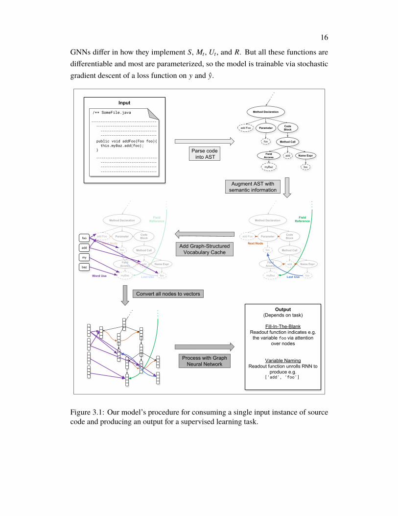
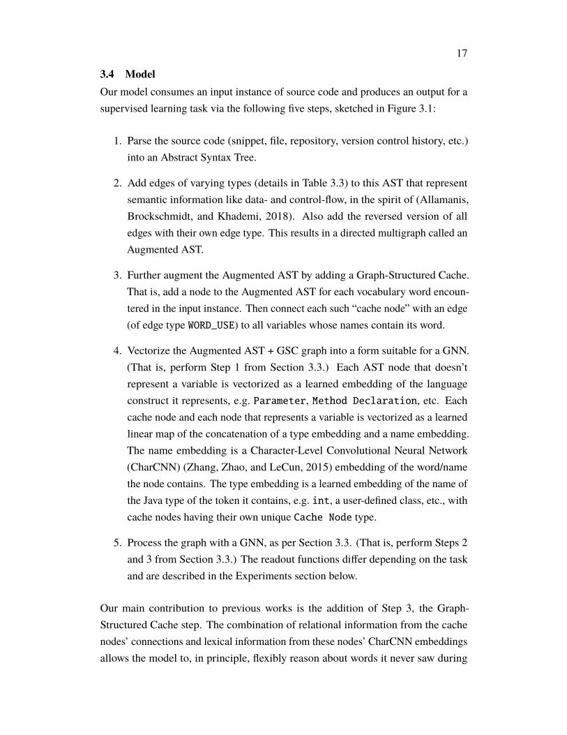
GNNs differ in how they implement S, Mt , Ut , and R. But all these functions aredifferentiable and most are parameterized, so the model is trainable via stochasticgradient descent of a loss function on y and y.

Method Declaration

Parameter Code Block

Method Call

add Foo

myBaz

add

foo

Name Expr

foo

Field Access

Input

/** SomeFile.java

public void addFoo(Foo foo){ this.myBaz.add(foo); }

Process with Graph Neural Network

Method Declaration

Parameter Code Block

Method Call

add Foo

myBaz

add

foo

Name Expr

foo

Field Access

Last Use

Field Reference

Next Nodefoo

add

my

baz

Method Declaration

Parameter Code Block

Method Call

add Foo

myBaz

add

foo

Name Expr

foo

Field Access

Last Use

Field Reference

Next Node

Word Use

Add Graph-Structured Vocabulary Cache

Augment AST with semantic information

Parse code into AST

Convert all nodes to vectors

Output(Depends on task)

Fill-In-The-BlankReadout function indicates e.g. the variable foo via attention

over nodes

Variable NamingReadout function unrolls RNN to

produce e.g. [‘add’, ‘foo’]

Figure 3.1: Our model’s procedure for consuming a single input instance of sourcecode and producing an output for a supervised learning task.

17

3.4 ModelOur model consumes an input instance of source code and produces an output for asupervised learning task via the following five steps, sketched in Figure 3.1:

1. Parse the source code (snippet, file, repository, version control history, etc.)into an Abstract Syntax Tree.

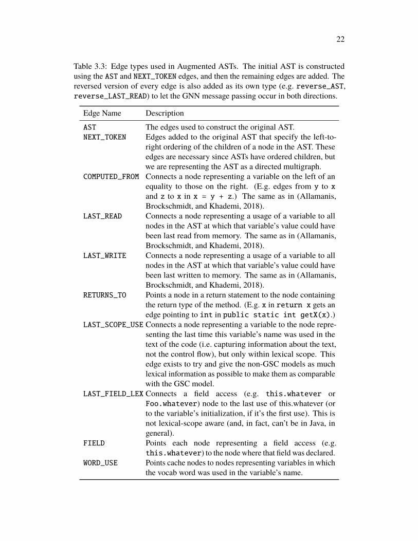
2. Add edges of varying types (details in Table 3.3) to this AST that representsemantic information like data- and control-flow, in the spirit of (Allamanis,Brockschmidt, and Khademi, 2018). Also add the reversed version of alledges with their own edge type. This results in a directed multigraph called anAugmented AST.

3. Further augment the Augmented AST by adding a Graph-Structured Cache.That is, add a node to the Augmented AST for each vocabulary word encoun-tered in the input instance. Then connect each such “cache node” with an edge(of edge type WORD_USE) to all variables whose names contain its word.

4. Vectorize the Augmented AST + GSC graph into a form suitable for a GNN.(That is, perform Step 1 from Section 3.3.) Each AST node that doesn’trepresent a variable is vectorized as a learned embedding of the languageconstruct it represents, e.g. Parameter, Method Declaration, etc. Eachcache node and each node that represents a variable is vectorized as a learnedlinear map of the concatenation of a type embedding and a name embedding.The name embedding is a Character-Level Convolutional Neural Network(CharCNN) (Zhang, Zhao, and LeCun, 2015) embedding of the word/namethe node contains. The type embedding is a learned embedding of the name ofthe Java type of the token it contains, e.g. int, a user-defined class, etc., withcache nodes having their own unique Cache Node type.

5. Process the graph with a GNN, as per Section 3.3. (That is, perform Steps 2and 3 from Section 3.3.) The readout functions differ depending on the taskand are described in the Experiments section below.

Our main contribution to previous works is the addition of Step 3, the Graph-Structured Cache step. The combination of relational information from the cachenodes’ connections and lexical information from these nodes’ CharCNN embeddingsallows the model to, in principle, flexibly reason about words it never saw during

18

training, but also recognize words it did. For example, it could potentially see a classnamed “getGuavaDictionary” and a variable named “guava_dict” and both (a)utilize the fact that the word “guava” is common to both names despite having neverseen this word before, and (b) exploit learned representations for words like “get”,“dictionary”, and “dict” that it has seen during training.

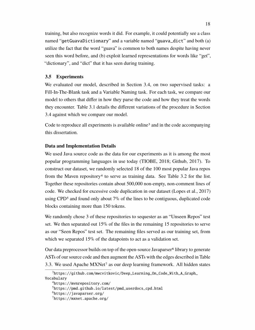
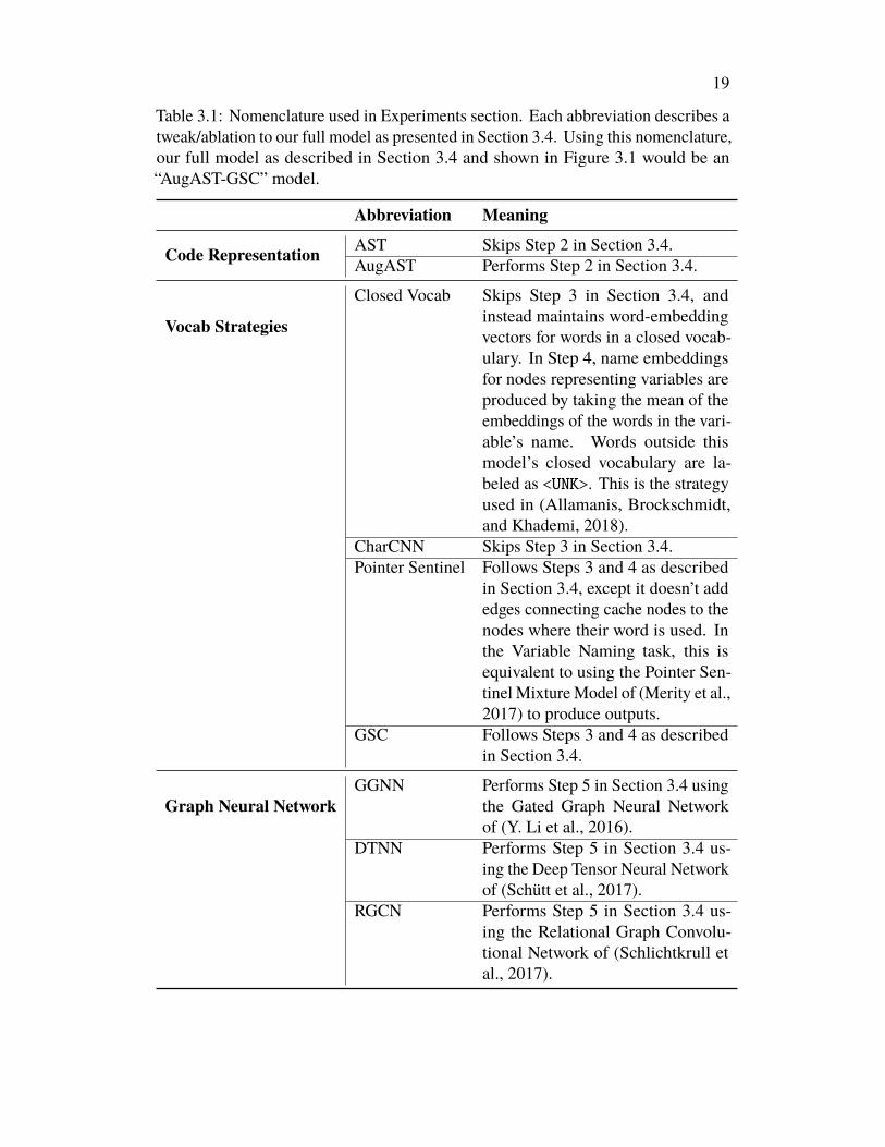
3.5 ExperimentsWe evaluated our model, described in Section 3.4, on two supervised tasks: aFill-In-The-Blank task and a Variable Naming task. For each task, we compare ourmodel to others that differ in how they parse the code and how they treat the wordsthey encounter. Table 3.1 details the different variations of the procedure in Section3.4 against which we compare our model.

Code to reproduce all experiments is available online3 and in the code accompanyingthis dissertation.

Data and Implementation DetailsWe used Java source code as the data for our experiments as it is among the mostpopular programming languages in use today (TIOBE, 2018; Github, 2017). Toconstruct our dataset, we randomly selected 18 of the 100 most popular Java reposfrom the Maven repository4 to serve as training data. See Table 3.2 for the list.Together these repositories contain about 500,000 non-empty, non-comment lines ofcode. We checked for excessive code duplication in our dataset (Lopes et al., 2017)using CPD5 and found only about 7% of the lines to be contiguous, duplicated codeblocks containing more than 150 tokens.

We randomly chose 3 of these repositories to sequester as an “Unseen Repos” testset. We then separated out 15% of the files in the remaining 15 repositories to serveas our “Seen Repos” test set. The remaining files served as our training set, fromwhich we separated 15% of the datapoints to act as a validation set.

Our data preprocessor builds on top of the open-source Javaparser6 library to generateASTs of our source code and then augment the ASTs with the edges described in Table3.3. We used Apache MXNet7 as our deep learning framework. All hidden states

3https://github.com/mwcvitkovic/Deep_Learning_On_Code_With_A_Graph_Vocabulary

4https://mvnrepository.com/5https://pmd.github.io/latest/pmd_userdocs_cpd.html6https://javaparser.org/7https://mxnet.apache.org/

19

Table 3.1: Nomenclature used in Experiments section. Each abbreviation describes atweak/ablation to our full model as presented in Section 3.4. Using this nomenclature,our full model as described in Section 3.4 and shown in Figure 3.1 would be an“AugAST-GSC” model.

Abbreviation Meaning

Code Representation AST Skips Step 2 in Section 3.4.AugAST Performs Step 2 in Section 3.4.

Vocab Strategies

Closed Vocab Skips Step 3 in Section 3.4, andinstead maintains word-embeddingvectors for words in a closed vocab-ulary. In Step 4, name embeddingsfor nodes representing variables areproduced by taking the mean of theembeddings of the words in the vari-able’s name. Words outside thismodel’s closed vocabulary are la-beled as <UNK>. This is the strategyused in (Allamanis, Brockschmidt,and Khademi, 2018).

CharCNN Skips Step 3 in Section 3.4.Pointer Sentinel Follows Steps 3 and 4 as described

in Section 3.4, except it doesn’t addedges connecting cache nodes to thenodes where their word is used. Inthe Variable Naming task, this isequivalent to using the Pointer Sen-tinel Mixture Model of (Merity et al.,2017) to produce outputs.

GSC Follows Steps 3 and 4 as describedin Section 3.4.

Graph Neural NetworkGGNN Performs Step 5 in Section 3.4 using

the Gated Graph Neural Networkof (Y. Li et al., 2016).

DTNN Performs Step 5 in Section 3.4 us-ing the Deep Tensor Neural Networkof (Schütt et al., 2017).

RGCN Performs Step 5 in Section 3.4 us-ing the Relational Graph Convolu-tional Network of (Schlichtkrull etal., 2017).

20

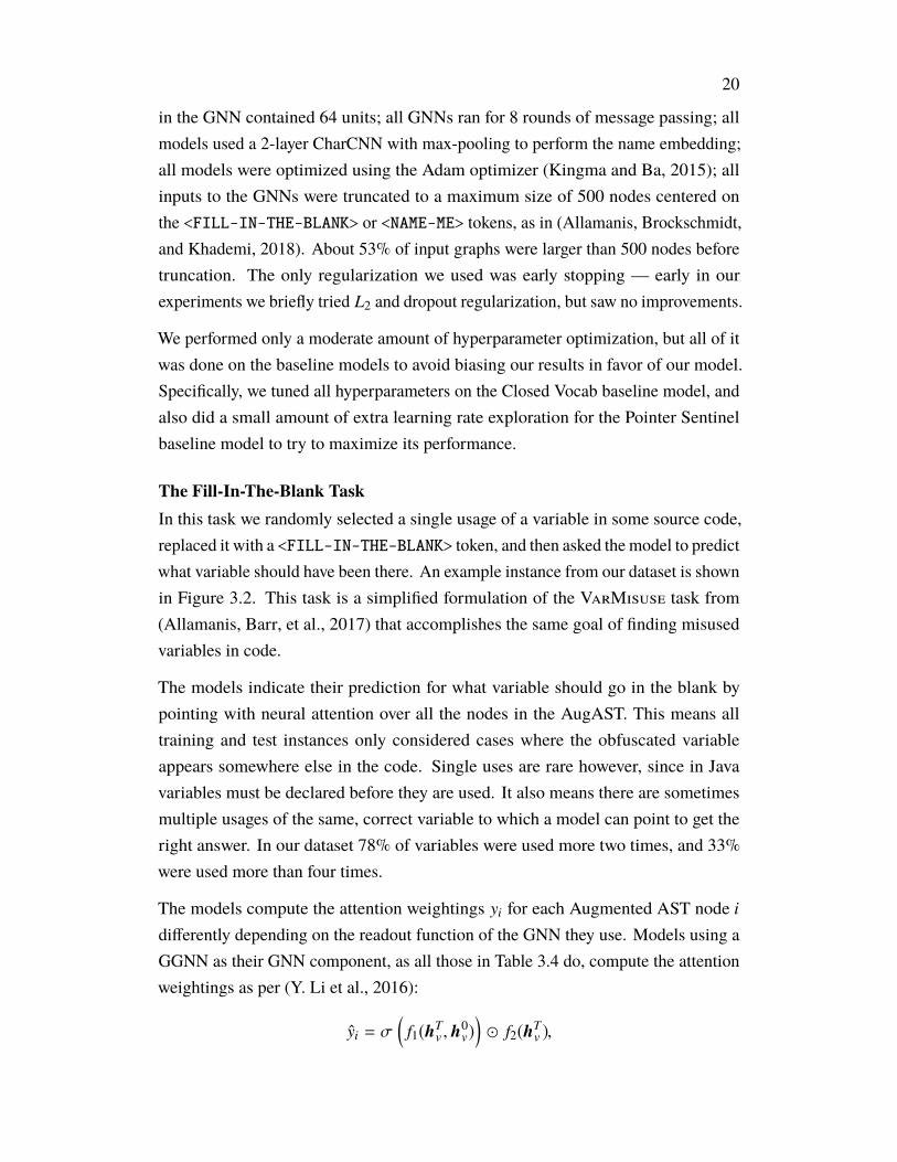
in the GNN contained 64 units; all GNNs ran for 8 rounds of message passing; allmodels used a 2-layer CharCNN with max-pooling to perform the name embedding;all models were optimized using the Adam optimizer (Kingma and Ba, 2015); allinputs to the GNNs were truncated to a maximum size of 500 nodes centered onthe <FILL-IN-THE-BLANK> or <NAME-ME> tokens, as in (Allamanis, Brockschmidt,and Khademi, 2018). About 53% of input graphs were larger than 500 nodes beforetruncation. The only regularization we used was early stopping — early in ourexperiments we briefly tried L2 and dropout regularization, but saw no improvements.

We performed only a moderate amount of hyperparameter optimization, but all of itwas done on the baseline models to avoid biasing our results in favor of our model.Specifically, we tuned all hyperparameters on the Closed Vocab baseline model, andalso did a small amount of extra learning rate exploration for the Pointer Sentinelbaseline model to try to maximize its performance.

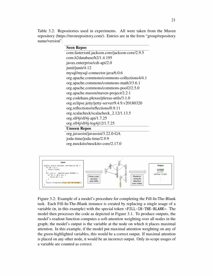
The Fill-In-The-Blank TaskIn this task we randomly selected a single usage of a variable in some source code,replaced it with a <FILL-IN-THE-BLANK> token, and then asked the model to predictwhat variable should have been there. An example instance from our dataset is shownin Figure 3.2. This task is a simplified formulation of the VarMisuse task from(Allamanis, Barr, et al., 2017) that accomplishes the same goal of finding misusedvariables in code.

The models indicate their prediction for what variable should go in the blank bypointing with neural attention over all the nodes in the AugAST. This means alltraining and test instances only considered cases where the obfuscated variableappears somewhere else in the code. Single uses are rare however, since in Javavariables must be declared before they are used. It also means there are sometimesmultiple usages of the same, correct variable to which a model can point to get theright answer. In our dataset 78% of variables were used more two times, and 33%were used more than four times.

The models compute the attention weightings yi for each Augmented AST node i

differently depending on the readout function of the GNN they use. Models using aGGNN as their GNN component, as all those in Table 3.4 do, compute the attentionweightings as per (Y. Li et al., 2016):

yi = σ(

f1(hTv , h

0v))� f2(hT

v ),

21

Table 3.2: Repositories used in experiments. All were taken from the Mavenrepository (https://mvnrepository.com/). Entries are in the form “group/repositoryname/version”.

Seen Reposcom.fasterxml.jackson.core/jackson-core/2.9.5com.h2database/h2/1.4.195javax.enterprise/cdi-api/2.0junit/junit/4.12mysql/mysql-connector-java/6.0.6org.apache.commons/commons-collections4/4.1org.apache.commons/commons-math3/3.6.1org.apache.commons/commons-pool2/2.5.0org.apache.maven/maven-project/2.2.1org.codehaus.plexus/plexus-utils/3.1.0org.eclipse.jetty/jetty-server/9.4.9.v20180320org.reflections/reflections/0.9.11org.scalacheck/scalacheck_2.12/1.13.5org.slf4j/slf4j-api/1.7.25org.slf4j/slf4j-log4j12/1.7.25Unseen Reposorg.javassist/javassist/3.22.0-GAjoda-time/joda-time/2.9.9org.mockito/mockito-core/2.17.0

Input

Parse code, process

with GNN

public static boolean isPrime(int n) { if (n < 2) { return false; } for (int p : SmallPrimes.PRIMES) { if (0 == (n % p)) { return n == p; } } return PrimeTest(<FILL-IN-THE-BLANK>);}

. . .

Readout:compute attention

over nodes

Output

n = 0.91p = 0.7

isPrime = 0.001...

Figure 3.2: Example of a model’s procedure for completing the Fill-In-The-Blanktask. Each Fill-In-The-Blank instance is created by replacing a single usage of avariable (n, in this example) with the special token <FILL-IN-THE-BLANK>. Themodel then processes the code as depicted in Figure 3.1. To produce outputs, themodel’s readout function computes a soft-attention weighting over all nodes in thegraph; the model’s output is the variable at the node on which it places maximalattention. In this example, if the model put maximal attention weighting on any ofthe green-highlighted variables, this would be a correct output. If maximal attentionis placed on any other node, it would be an incorrect output. Only in-scope usages ofa variable are counted as correct.

22

Table 3.3: Edge types used in Augmented ASTs. The initial AST is constructedusing the AST and NEXT_TOKEN edges, and then the remaining edges are added. Thereversed version of every edge is also added as its own type (e.g. reverse_AST,reverse_LAST_READ) to let the GNN message passing occur in both directions.

Edge Name Description

AST The edges used to construct the original AST.NEXT_TOKEN Edges added to the original AST that specify the left-to-

right ordering of the children of a node in the AST. Theseedges are necessary since ASTs have ordered children, butwe are representing the AST as a directed multigraph.

COMPUTED_FROM Connects a node representing a variable on the left of anequality to those on the right. (E.g. edges from y to xand z to x in x = y + z.) The same as in (Allamanis,Brockschmidt, and Khademi, 2018).

LAST_READ Connects a node representing a usage of a variable to allnodes in the AST at which that variable’s value could havebeen last read from memory. The same as in (Allamanis,Brockschmidt, and Khademi, 2018).

LAST_WRITE Connects a node representing a usage of a variable to allnodes in the AST at which that variable’s value could havebeen last written to memory. The same as in (Allamanis,Brockschmidt, and Khademi, 2018).

RETURNS_TO Points a node in a return statement to the node containingthe return type of the method. (E.g. x in return x gets anedge pointing to int in public static int getX(x).)

LAST_SCOPE_USE Connects a node representing a variable to the node repre-senting the last time this variable’s name was used in thetext of the code (i.e. capturing information about the text,not the control flow), but only within lexical scope. Thisedge exists to try and give the non-GSC models as muchlexical information as possible to make them as comparablewith the GSC model.

LAST_FIELD_LEX Connects a field access (e.g. this.whatever orFoo.whatever) node to the last use of this.whatever (orto the variable’s initialization, if it’s the first use). This isnot lexical-scope aware (and, in fact, can’t be in Java, ingeneral).

FIELD Points each node representing a field access (e.g.this.whatever) to the node where that field was declared.

WORD_USE Points cache nodes to nodes representing variables in whichthe vocab word was used in the variable’s name.

23

where the f s are MLPs, htv is the hidden state of node v after t message passing

iterations, σ is the sigmoid function, and � is elementwise multiplication. TheDTNN and RGCN GNNs compute the attention weightings as per (Schütt et al.,2017):

yi = f (hTv ),

where f is a single hidden layer MLP. The models were trained using a binary crossentropy loss computed across the nodes in the graph.

The performance of models using our GSC versus those using other methods isreported in Table 3.4. For context, a baseline strategy of random guessing amongall variable nodes within an edge radius of 8 of the <FILL-IN-THE-BLANK> tokenachieves an accuracy of 0.22. We also compare the performance of different GNNsin Table 3.5.

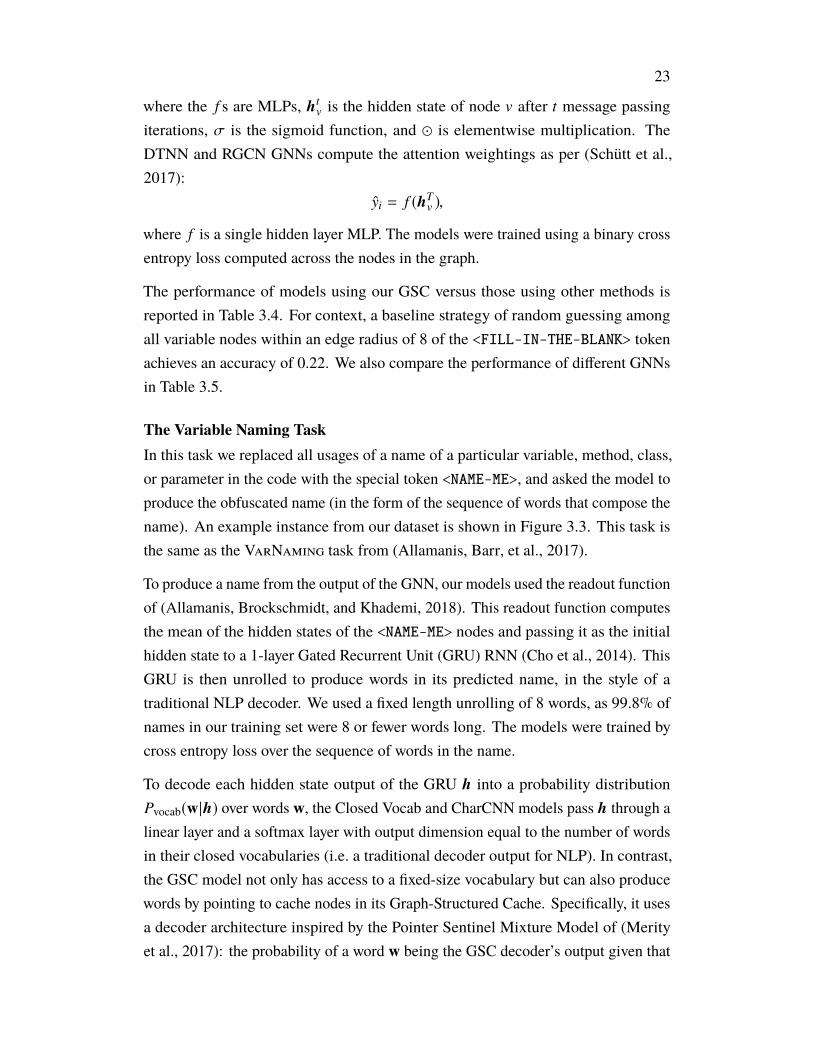
The Variable Naming TaskIn this task we replaced all usages of a name of a particular variable, method, class,or parameter in the code with the special token <NAME-ME>, and asked the model toproduce the obfuscated name (in the form of the sequence of words that compose thename). An example instance from our dataset is shown in Figure 3.3. This task isthe same as the VarNaming task from (Allamanis, Barr, et al., 2017).

To produce a name from the output of the GNN, our models used the readout functionof (Allamanis, Brockschmidt, and Khademi, 2018). This readout function computesthe mean of the hidden states of the <NAME-ME> nodes and passing it as the initialhidden state to a 1-layer Gated Recurrent Unit (GRU) RNN (Cho et al., 2014). ThisGRU is then unrolled to produce words in its predicted name, in the style of atraditional NLP decoder. We used a fixed length unrolling of 8 words, as 99.8% ofnames in our training set were 8 or fewer words long. The models were trained bycross entropy loss over the sequence of words in the name.

To decode each hidden state output of the GRU h into a probability distributionPvocab(w|h) over words w, the Closed Vocab and CharCNN models pass h through alinear layer and a softmax layer with output dimension equal to the number of wordsin their closed vocabularies (i.e. a traditional decoder output for NLP). In contrast,the GSC model not only has access to a fixed-size vocabulary but can also producewords by pointing to cache nodes in its Graph-Structured Cache. Specifically, it usesa decoder architecture inspired by the Pointer Sentinel Mixture Model of (Merityet al., 2017): the probability of a word w being the GSC decoder’s output given that

24

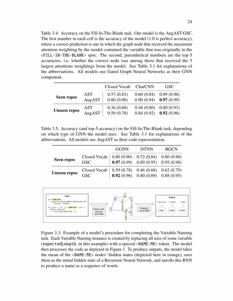
Table 3.4: Accuracy on the Fill-In-The-Blank task. Our model is the AugAST-GSC.The first number in each cell is the accuracy of the model (1.0 is perfect accuracy),where a correct prediction is one in which the graph node that received the maximumattention weighting by the model contained the variable that was originally in the<FILL-IN-THE-BLANK> spot. The second, parenthetical numbers are the top-5accuracies, i.e. whether the correct node was among those that received the 5largest attentions weightings from the model. See Table 3.1 for explanations ofthe abbreviations. All models use Gated Graph Neural Networks as their GNNcomponent.

Closed Vocab CharCNN GSC

Seen repos AST 0.57 (0.83) 0.60 (0.84) 0.89 (0.96)AugAST 0.80 (0.90) 0.90 (0.94) 0.97 (0.99)

Unseen repos AST 0.36 (0.68) 0.48 (0.80) 0.80 (0.93)AugAST 0.59 (0.78) 0.84 (0.92) 0.92 (0.96)

Table 3.5: Accuracy (and top-5 accuracy) on the Fill-In-The-Blank task, dependingon which type of GNN the model uses. See Table 3.1 for explanations of theabbreviations. All models use AugAST as their code representation.

GGNN DTNN RGCN

Seen repos Closed Vocab 0.80 (0.90) 0.72 (0.84) 0.80 (0.90)GSC 0.97 (0.99) 0.89 (0.95) 0.95 (0.98)

Unseen repos Closed Vocab 0.59 (0.78) 0.46 (0.68) 0.62 (0.79)GSC 0.92 (0.96) 0.80 (0.89) 0.88 (0.95)

Input

Parse code, process

with GNN

int <NAME-ME> = assertArraysAreSameLength(expected, actuals, header); for (int i = 0; i < <NAME-ME>; i++) { Object expected = Array.get(expected, i);

. . .

Readout:unroll RNN

Output

‘expected’ ‘length’ ‘<EOS>’

RNN RNN RNN

Figure 3.3: Example of a model’s procedure for completing the Variable Namingtask. Each Variable Naming instance is created by replacing all uses of some variable(expectedLength, in this example) with a special <NAME-ME> token. The modelthen processes the code as depicted in Figure 1. To produce outputs, the model takesthe mean of the <NAME-ME> nodes’ hidden states (depicted here in orange), usesthem as the initial hidden state of a Recurrent Neural Network, and unrolls this RNNto produce a name as a sequence of words.

25

the GRU’s hidden state was h is

P(w|h) = Pgraph(s|h)Pgraph(w|h) +(1 − Pgraph(s|h))Pvocab(w|h)

where Pgraph(·|h) is a conditional probability distribution over cache nodes in theGSC and the sentinel s, and Pvocab(·|h) is a conditional probability distribution overwords in a closed vocabulary. Pgraph(·|h) is computed by passing the hidden states ofall cache nodes and the sentinel node through a single linear layer and then computingthe softmax dot-product attention of these values with h. Pvocab(·|h) is computedas the softmax of a linear mapping of h to indices in a closed vocabulary, as inthe Closed Vocab and CharCNN models. If there is no cache node for w in theAugmented AST or if w is not in the model’s closed dictionary then Pgraph(w|h) andPvocab(w|h) are 0, respectively.

The performance of our GSC versus other methods is reported in Table 3.6. Moregranular performance statistics are reported in Table 3.7. We also compare theperformance of different GNNs in Table 3.8.

3.6 DiscussionAs can be seen in Tables 3.4 and 3.6, the addition of a GSC improved performanceon all tasks. Our full model, the AugAST-GSC model, outperforms the other modelstested and does comparatively well at maintaining accuracy between the Seen andUnseen test repos on the Variable Naming task.

To some degree the improved performance from adding the GSC is unsurprising: itsaddition to a graph-based model is adding extra features and does not remove anyinformation or flexibility. Under a satisfactory training regime in which overfitting isavoided, a model could simply learn to ignore it if it is unhelpful, so its inclusionshould never hurt performance. The degree to which it helps, though, especiallyon the Variable Naming task, suggests that a GSC is well worth using for sometasks, whether on source code or in NLP tasks in general. Moreover, the fact thatthe Pointer Sentinel approach shown in Table 3.6 performs noticeably less well thanthe full GSC approach suggests that the relational aspect of the GSC is key. Simplyhaving the ability to output out-of-vocabulary words without relational informationabout their usage, as in the Pointer Sentinal model, is insufficient for our task.

The downside of using a GSC is the computational cost. Our GSC models ran about30% slower than the Closed Vocab models. Since we capped the graph size at 500

26

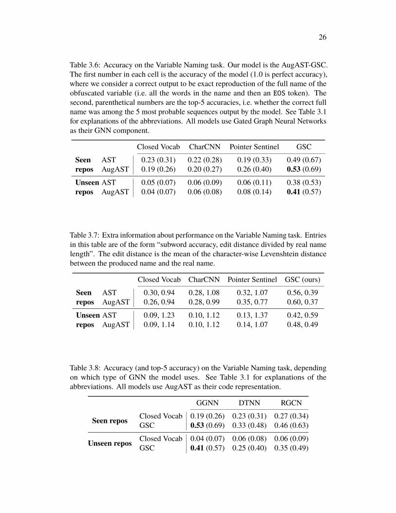
Table 3.6: Accuracy on the Variable Naming task. Our model is the AugAST-GSC.The first number in each cell is the accuracy of the model (1.0 is perfect accuracy),where we consider a correct output to be exact reproduction of the full name of theobfuscated variable (i.e. all the words in the name and then an EOS token). Thesecond, parenthetical numbers are the top-5 accuracies, i.e. whether the correct fullname was among the 5 most probable sequences output by the model. See Table 3.1for explanations of the abbreviations. All models use Gated Graph Neural Networksas their GNN component.

Closed Vocab CharCNN Pointer Sentinel GSC

Seenrepos

AST 0.23 (0.31) 0.22 (0.28) 0.19 (0.33) 0.49 (0.67)AugAST 0.19 (0.26) 0.20 (0.27) 0.26 (0.40) 0.53 (0.69)

Unseenrepos

AST 0.05 (0.07) 0.06 (0.09) 0.06 (0.11) 0.38 (0.53)AugAST 0.04 (0.07) 0.06 (0.08) 0.08 (0.14) 0.41 (0.57)

Table 3.7: Extra information about performance on the Variable Naming task. Entriesin this table are of the form “subword accuracy, edit distance divided by real namelength”. The edit distance is the mean of the character-wise Levenshtein distancebetween the produced name and the real name.

Closed Vocab CharCNN Pointer Sentinel GSC (ours)

Seenrepos

AST 0.30, 0.94 0.28, 1.08 0.32, 1.07 0.56, 0.39AugAST 0.26, 0.94 0.28, 0.99 0.35, 0.77 0.60, 0.37

Unseenrepos

AST 0.09, 1.23 0.10, 1.12 0.13, 1.37 0.42, 0.59AugAST 0.09, 1.14 0.10, 1.12 0.14, 1.07 0.48, 0.49

Table 3.8: Accuracy (and top-5 accuracy) on the Variable Naming task, dependingon which type of GNN the model uses. See Table 3.1 for explanations of theabbreviations. All models use AugAST as their code representation.

GGNN DTNN RGCN

Seen repos Closed Vocab 0.19 (0.26) 0.23 (0.31) 0.27 (0.34)GSC 0.53 (0.69) 0.33 (0.48) 0.46 (0.63)

Unseen repos Closed Vocab 0.04 (0.07) 0.06 (0.08) 0.06 (0.09)GSC 0.41 (0.57) 0.25 (0.40) 0.35 (0.49)

27

nodes, the slowdown is presumably due to the large number of edges to and from thegraph cache nodes. Better support for sparse operations on GPU in deep learningframeworks would be useful for alleviating this downside.

There remain a number of design choices to explore regarding AST- and GNN-models for processing source code. Adding information about word order to the GSCmight improve performance, as might constructing the vocabulary out of subwordsrather than words. It also might help to treat variable types as the GSC treats words:storing them in a GSC and connecting them with edges to the variables of those types;this could be particularly useful when working with code snippets rather than fullycompilable code. For the Variable Naming task, there are also many architecturechoices to be explored in how to produce a sequence of words for a name: how tounroll the RNN, what to use as the initial hidden state, etc.

Given that all results above show that augmenting ASTs with data- and control-flowedges improves performance, it would be worth exploring other static analysisconcepts from the Programming Language and Software Verification literatures andseeing whether they could be usefully incorporated into Augmented ASTs. Betterunderstanding of how Graph Neural Networks learn is also crucial, since they arecentral to the performance of our model and many others. Additionally, the entiredomain of machine learning on source code faces the practical issue that many of thebest data for supervised learning on source code — things like high-quality codereviews, integration test results, code with high test coverage, etc. — are not availableoutside private organizations.

3.7 AcknowledgementsMany thanks to Miltos Allamanis and Hyokun Yun for their advice and usefulconversations.

References

Allamanis, Miltiadis, Earl T. Barr, et al. (2017). “A Survey of Machine Learning forBig Code and Naturalness”. In: arXiv:1709.06182 [cs]. url: https://arxiv.org/abs/1709.06182.

Allamanis,Miltiadis,Marc Brockschmidt, andMahmoudKhademi (2018). “Learningto Represent Programs with Graphs”. In: International Conference on LearningRepresentations. url: https://openreview.net/forum?id=BJOFETxR-.

Alon, Uri et al. (2018). “A General Path-based Representation for PredictingProgram Properties”. In: Proceedings of the 39th ACM SIGPLAN Conference on

28

Programming Language Design and Implementation. PLDI 2018. Philadelphia,PA, USA: ACM, pp. 404–419. isbn: 978-1-4503-5698-5. doi: 10.1145/3192366.3192412. url: http://doi.acm.org/10.1145/3192366.3192412.

Amodio, Matthew, Swarat Chaudhuri, and Thomas Reps (2017). “Neural AttributeMachines for Program Generation”. In: arXiv:1705.09231 [cs]. url: http://arxiv.org/abs/1705.09231 (visited on 04/02/2018).

Arabshahi, Forough, Sameer Singh, and Animashree Anandkumar (2018). “Com-bining Symbolic Expressions and Black-box Function Evaluations for TrainingNeural Programs”. In: International Conference on Learning Representations.url: https://openreview.net/forum?id=Hksj2WWAW.

Bansal, Trapit, Arvind Neelakantan, and Andrew McCallum (2017). “RelNet: End-to-End Modeling of Entities & Relations”. In: arXiv:1706.07179 [cs]. url:http://arxiv.org/abs/1706.07179.

Battaglia, PeterW. et al. (2018). “Relational inductive biases, deep learning, and graphnetworks”. In: abs/1806.01261. url: https://arxiv.org/abs/1806.01261.

Bhoopchand, Avishkar et al. (2016). “Learning Python Code Suggestion with aSparse Pointer Network”. In: abs/1611.08307. url: https://arxiv.org/abs/1611.08307.

Bojanowski, Piotr et al. (2017). “EnrichingWord Vectors with Subword Information”.In: TACL 5, pp. 135–146.

Brockschmidt, Marc et al. (2019). “Generative Code Modeling with Graphs”. In:International Conference on Learning Representations abs/1805.08490. url:https://arxiv.org/abs/1805.08490.

Chae, Kwonsoo et al. (2017). “Automatically Generating Features for LearningProgram Analysis Heuristics for C-like Languages”. In: Proc. ACM Program.Lang. 1.OOPSLA, 101:1–101:25. issn: 2475-1421. doi: 10.1145/3133925. url:http://doi.acm.org/10.1145/3133925.

Chen, Xinyun, Chang Liu, and Dawn Song (2018). Tree-to-tree Neural Networksfor Program Translation. url: https://openreview.net/forum?id=rkxY-sl0W.

Cho, Kyunghyun et al. (2014). “Learning Phrase Representations using RNNEncoder–Decoder for Statistical Machine Translation”. In: Proceedings of the2014 Conference on EmpiricalMethods in Natural Language Processing (EMNLP).Doha, Qatar: Association for Computational Linguistics, pp. 1724–1734. doi:10.3115/v1/D14-1179. url: http://www.aclweb.org/anthology/D14-1179.

Gilmer, Justin et al. (2017). “Neural Message Passing for Quantum Chemistry”. In:Proceedings of the 34th International Conference on Machine Learning. Ed. byDoina Precup and Yee Whye Teh. Vol. 70. Proceedings of Machine Learning

29

Research. International Convention Centre, Sydney, Australia: PMLR, pp. 1263–1272. url: http://proceedings.mlr.press/v70/gilmer17a.html.

Github (2017). The State of the Octoverse 2017. url: https://octoverse.github.com/.

Goller, C. and A. Kuchler (1996). “Learning task-dependent distributed representa-tions by backpropagation through structure”. In: Neural Networks, 1996., IEEEInternational Conference on. Vol. 1, 347–352 vol.1. doi: 10.1109/ICNN.1996.548916.

Grave, Edouard, Moustapha Cissé, and Armand Joulin (2017). “Unbounded cachemodel for online language modeling with open vocabulary”. In: NIPS.

Gulcehre, Caglar et al. (2016). “Pointing the Unknown Words”. In: Proceedings ofthe 54th Annual Meeting of the Association for Computational Linguistics (Volume1: Long Papers). Berlin, Germany: Association for Computational Linguistics,pp. 140–149. doi: 10.18653/v1/P16-1014. url: http://www.aclweb.org/anthology/P16-1014.

Hellendoorn, Vincent J. and Premkumar T. Devanbu (2017). “Are deep neuralnetworks the best choice for modeling source code?” In: ESEC/SIGSOFT FSE.

Johnson, Daniel D. (2017). “Learning Graphical State Transitions”. In: InternationalConference on Learning Representations. url: https://openreview.net/forum?id=HJ0NvFzxl.

Kim,Yoon et al. (2016). “Character-awareNeural LanguageModels”. In:Proceedingsof the Thirtieth AAAI Conference on Artificial Intelligence. AAAI’16. Phoenix,Arizona: AAAI Press, pp. 2741–2749. url: http://dl.acm.org/citation.cfm?id=3016100.3016285.

Kingma, Diederik P. and Jimmy Ba (2015). “Adam: A Method for StochasticOptimization”. In: International Conference on Learning Representations. url:https://arxiv.org/abs/1412.6980.

Kobayashi, Sosuke et al. (2016). “Dynamic Entity Representation with Max-poolingImproves Machine Reading”. In: Proceedings of the 2016 Conference of the NorthAmerican Chapter of the Association for Computational Linguistics: HumanLanguage Technologies. San Diego, California: Association for ComputationalLinguistics. url: http://www.aclweb.org/anthology/N16-1099 (visitedon 04/03/2018).

Krinke, Jens (2001). “Identifying Similar Code with Program Dependence Graphs”.In: Proceedings of the Eighth Working Conference on Reverse Engineering(WCRE’01). WCRE ’01.Washington, DC, USA: IEEE Computer Society, pp. 301–.isbn: 0-7695-1303-4. url: http://dl.acm.org/citation.cfm?id=832308.837142.

30

Li, Jian et al. (2017). “Code Completion with Neural Attention and Pointer Networks”.In: arXiv:1711.09573 [cs]. url: http://arxiv.org/abs/1711.09573 (visitedon 01/15/2018).

Li, Yujia et al. (2016). “Gated Graph Sequence Neural Networks”. In: InternationalConference on Learning Representations. url: https://arxiv.org/abs/1511.05493.

Liu, Chang et al. (2017). “Neural CodeCompletion”. In:url:https://openreview.net/forum?id=rJbPBt9lg&noteId=rJbPBt9lg.

Lopes, Cristina V. et al. (2017). “DéjàVu: a map of code duplicates on GitHub”. In:PACMPL 1, 84:1–84:28.

Lu, Zhengdong et al. (2017). “Object-oriented Neural Programming (OONP) forDocument Understanding”. In: arXiv:1709.08853 [cs]. arXiv: 1709.08853. url:http://arxiv.org/abs/1709.08853 (visited on 04/14/2018).

Luong, Minh-Thang and Christopher D. Manning (2016). “Achieving Open Vo-cabulary Neural Machine Translation with Hybrid Word-Character Models”. In:arXiv:1604.00788 [cs]. url: http://arxiv.org/abs/1604.00788 (visited on02/13/2018).

Maddison, Chris J. and Daniel Tarlow (2014). “Structured Generative Models ofNatural Source Code”. In: ICML’14, pp. II-649–II-657. url: http://dl.acm.org/citation.cfm?id=3044805.3044965.

Merity, Stephen et al. (2017). “Pointer Sentinel Mixture Models”. In: InternationalConference on Learning Representations. url: https://openreview.net/pdf?id=Byj72udxe.

Pham, Trang, Truyen Tran, and Svetha Venkatesh (2018). “Graph Memory Networksfor Molecular Activity Prediction”. In: arXiv:1801.02622 [cs]. url: http://arxiv.org/abs/1801.02622 (visited on 04/13/2018).

Rabinovich, Maxim, Mitchell Stern, and Dan Klein (2017). “Abstract Syntax Net-works for Code Generation and Semantic Parsing”. In: Proceedings of the 55thAnnual Meeting of the Association for Computational Linguistics (Volume 1:Long Papers). Vancouver, Canada: Association for Computational Linguistics,pp. 1139–1149. doi: 10.18653/v1/P17-1105. url: http://www.aclweb.org/anthology/P17-1105.

Raychev, Veselin, Martin Vechev, and Andreas Krause (2015). “Predicting ProgramProperties from "Big Code"”. In: Proceedings of the 42Nd Annual ACM SIGPLAN-SIGACT Symposium on Principles of Programming Languages. POPL ’15. Mum-bai, India: ACM, pp. 111–124. isbn: 978-1-4503-3300-9. doi: 10.1145/2676726.2677009. url: http://doi.acm.org/10.1145/2676726.2677009.

Schlichtkrull, Michael et al. (2017). “Modeling Relational Data with Graph Convo-lutional Networks”. In: arXiv:1703.06103 [cs, stat]. url: http://arxiv.org/abs/1703.06103 (visited on 04/09/2018).

31

Schütt, Kristof T. et al. (2017). “Quantum-chemical insights from deep tensor neuralnetworks”. In: Nature communications.

Socher, Richard et al. (2013). “Recursive DeepModels for Semantic CompositionalityOver a Sentiment Treebank”. In: Proceedings of the 2013 Conference on EmpiricalMethods in Natural Language Processing. Seattle, Washington, USA: Associationfor Computational Linguistics, pp. 1631–1642. url: http://www.aclweb.org/anthology/D13-1170.

TIOBE (2018). TIOBE Index for September 2018. url: https://www.tiobe.com/tiobe-index/.

Vasic, Marko et al. (2019). “Neural Program Repair by Jointly Learning to Localizeand Repair”. en. In: url: https://arxiv.org/abs/1904.01720v1 (visited on05/07/2019).

Vinyals, Oriol, Meire Fortunato, and Navdeep Jaitly (2015). “Pointer Networks”.In: Advances in Neural Information Processing Systems 28. Ed. by C. Corteset al. Curran Associates, Inc., pp. 2692–2700. url: http://papers.nips.cc/paper/5866-pointer-networks.pdf.

White, M. et al. (2016). “Deep learning code fragments for code clone detec-tion”. In: 2016 31st IEEE/ACM International Conference on Automated SoftwareEngineering (ASE), pp. 87–98. url: http://www.cs.wm.edu/~mtufano/publications/C5.pdf.

Yin, Pengcheng and Graham Neubig (2017). “A Syntactic Neural Model for General-Purpose Code Generation”. In: Proceedings of the 55th Annual Meeting of theAssociation for Computational Linguistics (Volume 1: Long Papers). Vancouver,Canada: Association for Computational Linguistics, pp. 440–450. doi: 10.18653/v1/P17-1041. url: http://www.aclweb.org/anthology/P17-1041.

Zaremba, Wojciech, Karol Kurach, and Rob Fergus (2014). “Learning to DiscoverEfficient Mathematical Identities”. In: Advances in Neural Information ProcessingSystems 27. Ed. by Z. Ghahramani et al. Curran Associates, Inc., pp. 1278–1286.

Zhang, Xiang, Junbo Zhao, and Yann LeCun (2015). “Character-level ConvolutionalNetworks for Text Classification”. In: Advances in Neural Information ProcessingSystems 28. Ed. by C. Cortes et al. CurranAssociates, Inc., pp. 649–657. url: http://papers.nips.cc/paper/5782-character-level-convolutional-networks-for-text-classification.pdf.

32

C h a p t e r 4

SUPERVISED LEARNING ON RELATIONAL DATABASESWITH GRAPH NEURAL NETWORKS, PART 1

4.1 IntroductionRelational data is the most widely used type of data across all industries (Kaggle, Inc.,2017). Besides HTML/CSS/Javascript, relational databases (RDBs) are the mostpopular technology among developers (Stack Exchange, Inc., 2018). The marketmerely for hosting RDBs is over $45 billion USD (Asay, 2016), which is to saynothing of the societal value of the data they contain.

Yet learning on data in relational databases has received relatively little attentionfrom the deep learning community. The standard strategy for working with RDBs inmachine learning is to “flatten” the relational data they contain into tabular form, sincemost popular supervised learning methods expect their inputs to be fixed–size vectors.This flattening process not only destroys potentially useful relational informationpresent in the data, but the feature engineering required to flatten relational data isoften the most arduous and time-consuming part of a machine learning practitioner’swork.

In this chapter, we introduce a method based on Graph Neural Networks (GNNs)that operates on RDB data in its relational form without the need for manual featureengineering or flattening. (For an introduction to GNNs, see the previous chapter’sSection 3.3.)

4.2 Relational DatabasesA relational database1 (RDB) is a set of tables, {T 1,T 2, . . . ,TT }. An example isshown in Figure 4.1. Each table represents a different type of entity: its rowscorrespond to different instances of that type of entity and its columns correspond tothe features possessed by each entity. Each column in a table may contain a differenttype of data, like integers, real numbers, text, images, date, times, geolocations, etc.Unless otherwise specified, any entry in a table can potentially be empty, i.e. containa null value. We denote row i of table t as T t

i,: and column j of table t as T t:, j .

What makes RDBs “relational” is that the values in a column in one table can refer1RDBs are sometimes informally called “SQL databases”.

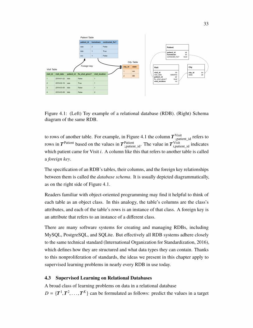
33

patient_id hometown contracted_flu?

aaa 2 False

bbb 1 True

ccc 1 False

visit_id visit_date patient_id flu_shot_given? visit_location

1 2019-01-22 bbb False 1

2 2019-02-16 aaa True 1

3 2019-03-05 bbb False 1

4 2019-03-08 bbb False 2

city_id state

1 AA

2 BB

Patient Table

Visit Table

City Table

Foreign key

visit_id strvisit_date datetimepatient_id strflu_shot_given? boolvisit_location int

Visit

patient_id strhometown intcontracted_flu? bool

Patient

city_id intstate str

City

Figure 4.1: (Left) Toy example of a relational database (RDB). (Right) Schemadiagram of the same RDB.

to rows of another table. For example, in Figure 4.1 the column TVisit:,patient_id refers to

rows in TPatient based on the values in TPatient:,patient_id. The value in T

Visiti,patient_id indicates

which patient came for Visit i. A column like this that refers to another table is calleda foreign key.

The specification of an RDB’s tables, their columns, and the foreign key relationshipsbetween them is called the database schema. It is usually depicted diagrammatically,as on the right side of Figure 4.1.

Readers familiar with object-oriented programming may find it helpful to think ofeach table as an object class. In this analogy, the table’s columns are the class’sattributes, and each of the table’s rows is an instance of that class. A foreign key isan attribute that refers to an instance of a different class.

There are many software systems for creating and managing RDBs, includingMySQL, PostgreSQL, and SQLite. But effectively all RDB systems adhere closelyto the same technical standard (International Organization for Standardization, 2016),which defines how they are structured and what data types they can contain. Thanksto this nonproliferation of standards, the ideas we present in this chapter apply tosupervised learning problems in nearly every RDB in use today.

4.3 Supervised Learning on Relational DatabasesA broad class of learning problems on data in a relational databaseD = {T 1,T 2, . . . ,TK} can be formulated as follows: predict the values in a target

34

column T k:,target of T k ∈ D given all other relevant information in the database.2

In this chapter, supervised learning on relational databases refers to this problemformulation.

This formulation encompasses all classification and regression problems in whichwe wish to predict the values in a particular column in D, or predict any aggregationsor combinations of values in D. This includes time series forecasting or predictingrelationships between entities. Traditional supervised learning problems like imageclassification or tabular regression are trivial cases of this formulation where D

contains one table.

There are several approaches for predicting values in T k:,target, including first-order

logic- and graphical model inference-based approaches (Getoor and Taskar, 2007).In this chapter we consider the empirical risk minimization (ERM) approach. TheERM approach is commonly used, though not always mentioned by name: it is theapproach being implicitly used whenever a machine learning practitioner “flattens”or “extracts” or “feature engineers” data from an RDB into tabular form for use witha tabular, supervised, machine learning model.

More precisely, ERM assumes the entries of T k:,target are sampled i.i.d. from some

distribution, and we are interested in finding a function f that minimizes the empiricalrisk

minf ∈F

1N

N∑i=1L

(f(T 1,T 2, . . . ,T k

:,:\target, . . . ,TK),T k

i,target

)(4.1)

for a real-valued loss function L and a suitable function class F, where T k:,:\target

denotes table k with the target column removed, and we assume that rows 1, . . . , Nof T k contain the training samples.

To solve, or approximately solve, Equation 4.1, we must choose a hypothesis class Fand an optimization procedure over it. We will accomplish this by framing supervisedlearning on RDBs in terms of learning tasks on graphs.

Connection to Learning Problems on GraphsA relational database can be interpreted as a directed graph — specifically, a directedmultigraph where each node has a type and has associated features that depend on itstype. The analogy is laid out in Table 4.1.

2We ignore issues of target leakage for the purposes of this chapter, but in practice care is needed.

35

Table 4.1: Corresponding terms when interpreting a relational database as a graph.

Relational Database Graph

Row NodeTable Node typeForeign key column Edge typeNon-foreign-key column Node featureForeign key from T A

u,i to TBv, j Edge from node u of type A to node v of type B

ith target value in table k, T ki,target Target feature on node i of type k

Note that the RDB’s schema diagram (an example of which is in Figure 4.1) is notthe same as this interpretation of the entire RDB as a graph. The former, which hastables as nodes, is a diagrammatic description of the properties of the latter, whichhas rows as nodes.

Note also that the RDB-as-graph interpretation is not bijective: directed multigraphscannot in general be stored in RDBs by following the correspondence in Table 4.1.3An RDB’s schema places restrictions on which types of nodes can be connected bywhich types of edges, and on which features are associated with each node type, thatgeneral directed multigraphs may not satisfy.

The interpretation of an RDB as a graph shows that supervised learning on RDBsreduces to a node classification problem (Atwood and Towsley, 2016). (For concisionwe only refer to classification problems, but our discussion applies equally toregression problems.) In addition, the interpretation suggests that GNN methods areapplicable to learning tasks on RDBs.

Learning on RDBs with GNNsThe first challenge in defining a hypothesis class F for use in Equation 4.1 isspecifying how functions in F will interact with the RDB. Equation 4.1 is writtenwith f ∈ F taking the entire database D (excluding the target values) as input. But itis so written only for completeness. In reality processing the entire RDB to producea single output is intractable and inadvisable from a modeling perspective. Thealgorithms in the hypothesis class F must retrieve and process only the informationin the RDB that is relevant for making their prediction.

Stated in the language of node classification: wemust choose how to select a subgraph3In principle one could use many-to-many tables to store any directed multigraph in an RDB, but

this would not follow the correspondence in Table 4.1.

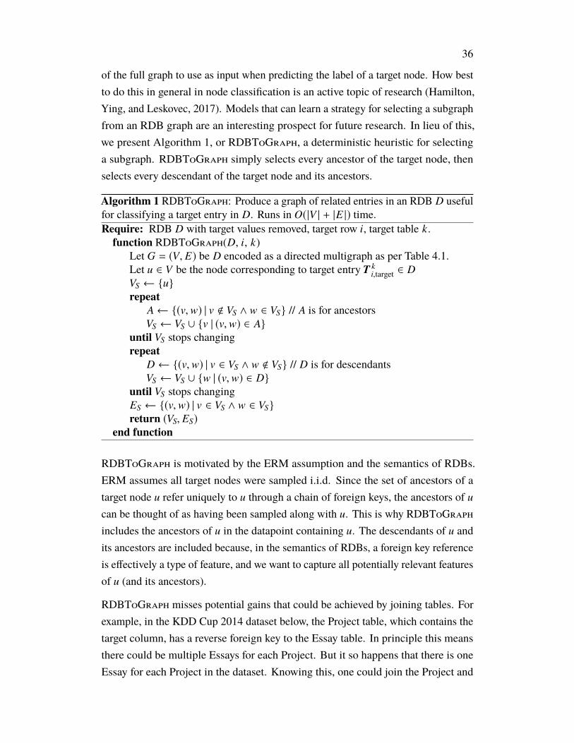
36

of the full graph to use as input when predicting the label of a target node. How bestto do this in general in node classification is an active topic of research (Hamilton,Ying, and Leskovec, 2017). Models that can learn a strategy for selecting a subgraphfrom an RDB graph are an interesting prospect for future research. In lieu of this,we present Algorithm 1, or RDBToGraph, a deterministic heuristic for selectinga subgraph. RDBToGraph simply selects every ancestor of the target node, thenselects every descendant of the target node and its ancestors.

Algorithm 1 RDBToGraph: Produce a graph of related entries in an RDB D usefulfor classifying a target entry in D. Runs in O(|V | + |E |) time.Require: RDB D with target values removed, target row i, target table k.

function RDBToGraph(D, i, k)Let G = (V, E) be D encoded as a directed multigraph as per Table 4.1.Let u ∈ V be the node corresponding to target entry T k

i,target ∈ DVS ← {u}repeat

A← {(v,w) | v < VS ∧ w ∈ VS} // A is for ancestorsVS ← VS ∪ {v | (v,w) ∈ A}

until VS stops changingrepeat

D← {(v,w) | v ∈ VS ∧ w < VS} // D is for descendantsVS ← VS ∪ {w | (v,w) ∈ D}

until VS stops changingES ← {(v,w) | v ∈ VS ∧ w ∈ VS}return (VS, ES)

end function

RDBToGraph is motivated by the ERM assumption and the semantics of RDBs.ERM assumes all target nodes were sampled i.i.d. Since the set of ancestors of atarget node u refer uniquely to u through a chain of foreign keys, the ancestors of u

can be thought of as having been sampled along with u. This is why RDBToGraphincludes the ancestors of u in the datapoint containing u. The descendants of u andits ancestors are included because, in the semantics of RDBs, a foreign key referenceis effectively a type of feature, and we want to capture all potentially relevant featuresof u (and its ancestors).

RDBToGraph misses potential gains that could be achieved by joining tables. Forexample, in the KDD Cup 2014 dataset below, the Project table, which contains thetarget column, has a reverse foreign key to the Essay table. In principle this meansthere could be multiple Essays for each Project. But it so happens that there is oneEssay for each Project in the dataset. Knowing this, one could join the Project and

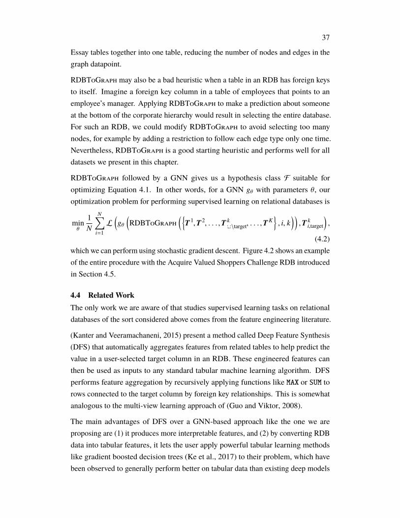
37

Essay tables together into one table, reducing the number of nodes and edges in thegraph datapoint.

RDBToGraph may also be a bad heuristic when a table in an RDB has foreign keysto itself. Imagine a foreign key column in a table of employees that points to anemployee’s manager. Applying RDBToGraph to make a prediction about someoneat the bottom of the corporate hierarchy would result in selecting the entire database.For such an RDB, we could modify RDBToGraph to avoid selecting too manynodes, for example by adding a restriction to follow each edge type only one time.Nevertheless, RDBToGraph is a good starting heuristic and performs well for alldatasets we present in this chapter.

RDBToGraph followed by a GNN gives us a hypothesis class F suitable foroptimizing Equation 4.1. In other words, for a GNN gθ with parameters θ, ouroptimization problem for performing supervised learning on relational databases is

minθ

1N

N∑i=1L

(gθ

(RDBToGraph

({T 1,T 2, . . . ,T k

:,:\target, . . . ,TK}, i, k

)),T k

i,target

),

(4.2)which we can perform using stochastic gradient descent. Figure 4.2 shows an exampleof the entire procedure with the Acquire Valued Shoppers Challenge RDB introducedin Section 4.5.

4.4 Related WorkThe only work we are aware of that studies supervised learning tasks on relationaldatabases of the sort considered above comes from the feature engineering literature.

(Kanter and Veeramachaneni, 2015) present a method called Deep Feature Synthesis(DFS) that automatically aggregates features from related tables to help predict thevalue in a user-selected target column in an RDB. These engineered features canthen be used as inputs to any standard tabular machine learning algorithm. DFSperforms feature aggregation by recursively applying functions like MAX or SUM torows connected to the target column by foreign key relationships. This is somewhatanalogous to the multi-view learning approach of (Guo and Viktor, 2008).

The main advantages of DFS over a GNN-based approach like the one we areproposing are (1) it produces more interpretable features, and (2) by converting RDBdata into tabular features, it lets the user apply powerful tabular learning methodslike gradient boosted decision trees (Ke et al., 2017) to their problem, which havebeen observed to generally perform better on tabular data than existing deep models

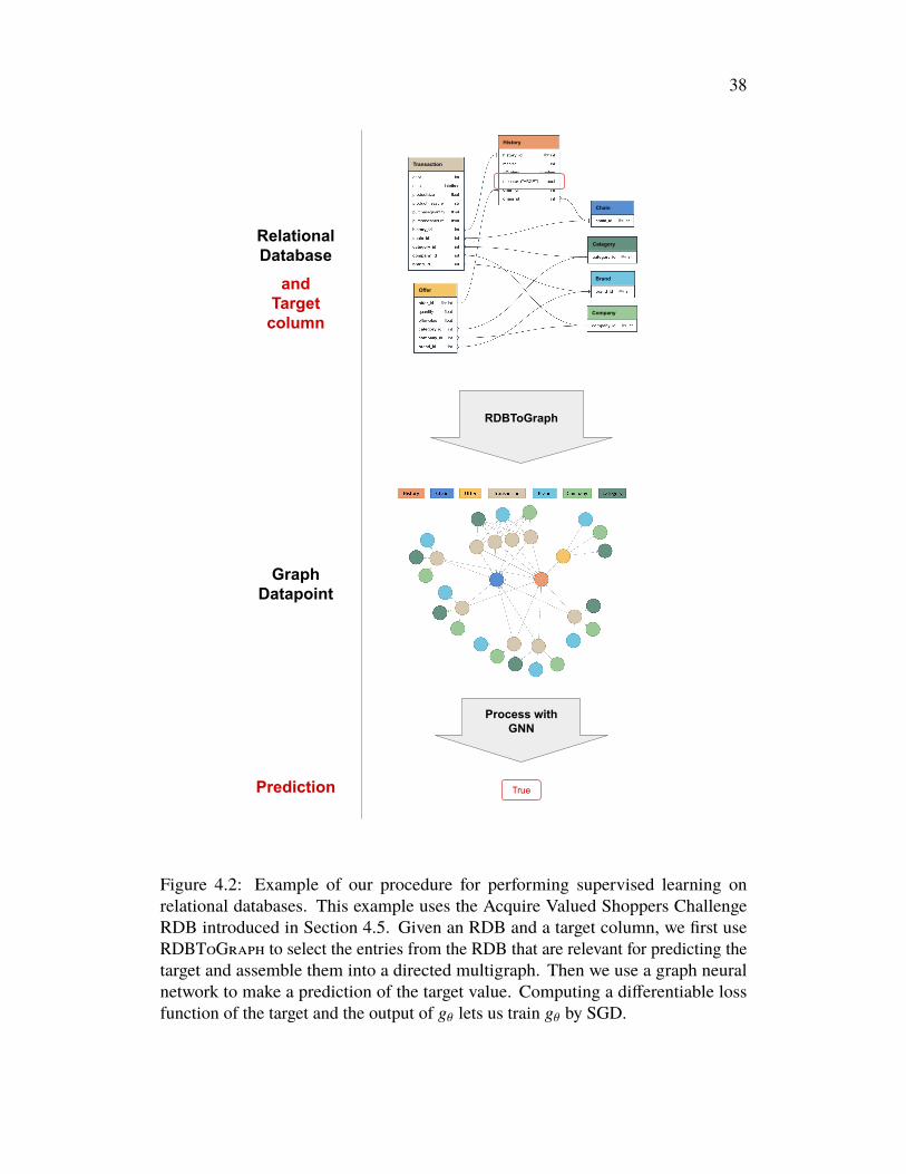
38

Process with GNN

True

RelationalDatabase

Graph Datapoint

Prediction

RDBToGraph

and Target

column

Transaction

History

Chain

Category

Brand

Company

Offer

Figure 4.2: Example of our procedure for performing supervised learning onrelational databases. This example uses the Acquire Valued Shoppers ChallengeRDB introduced in Section 4.5. Given an RDB and a target column, we first useRDBToGraph to select the entries from the RDB that are relevant for predicting thetarget and assemble them into a directed multigraph. Then we use a graph neuralnetwork to make a prediction of the target value. Computing a differentiable lossfunction of the target and the output of gθ lets us train gθ by SGD.

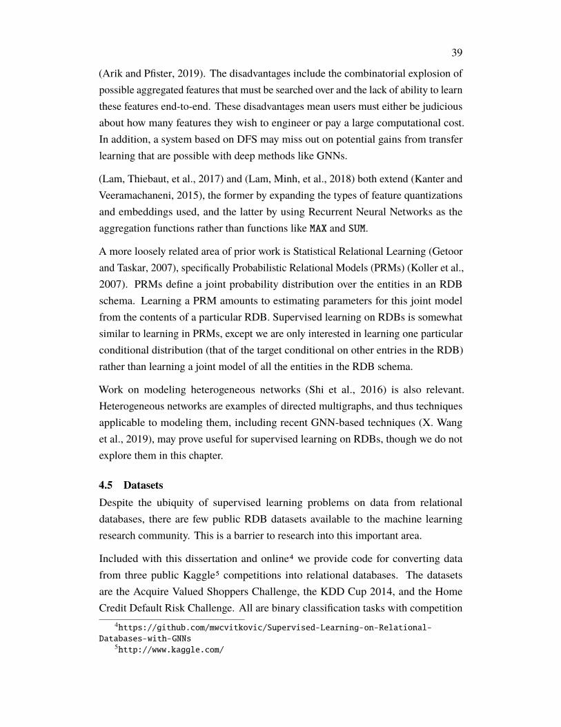
39

(Arik and Pfister, 2019). The disadvantages include the combinatorial explosion ofpossible aggregated features that must be searched over and the lack of ability to learnthese features end-to-end. These disadvantages mean users must either be judiciousabout how many features they wish to engineer or pay a large computational cost.In addition, a system based on DFS may miss out on potential gains from transferlearning that are possible with deep methods like GNNs.

(Lam, Thiebaut, et al., 2017) and (Lam, Minh, et al., 2018) both extend (Kanter andVeeramachaneni, 2015), the former by expanding the types of feature quantizationsand embeddings used, and the latter by using Recurrent Neural Networks as theaggregation functions rather than functions like MAX and SUM.

A more loosely related area of prior work is Statistical Relational Learning (Getoorand Taskar, 2007), specifically Probabilistic Relational Models (PRMs) (Koller et al.,2007). PRMs define a joint probability distribution over the entities in an RDBschema. Learning a PRM amounts to estimating parameters for this joint modelfrom the contents of a particular RDB. Supervised learning on RDBs is somewhatsimilar to learning in PRMs, except we are only interested in learning one particularconditional distribution (that of the target conditional on other entries in the RDB)rather than learning a joint model of all the entities in the RDB schema.

Work on modeling heterogeneous networks (Shi et al., 2016) is also relevant.Heterogeneous networks are examples of directed multigraphs, and thus techniquesapplicable to modeling them, including recent GNN-based techniques (X. Wanget al., 2019), may prove useful for supervised learning on RDBs, though we do notexplore them in this chapter.

4.5 DatasetsDespite the ubiquity of supervised learning problems on data from relationaldatabases, there are few public RDB datasets available to the machine learningresearch community. This is a barrier to research into this important area.

Included with this dissertation and online4 we provide code for converting datafrom three public Kaggle5 competitions into relational databases. The datasetsare the Acquire Valued Shoppers Challenge, the KDD Cup 2014, and the HomeCredit Default Risk Challenge. All are binary classification tasks with competition

4https://github.com/mwcvitkovic/Supervised-Learning-on-Relational-Databases-with-GNNs

5http://www.kaggle.com/

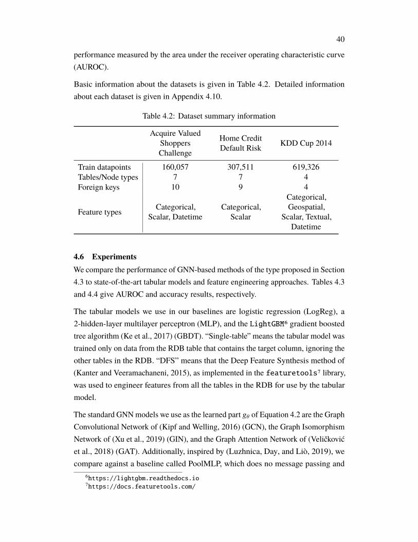
40

performance measured by the area under the receiver operating characteristic curve(AUROC).

Basic information about the datasets is given in Table 4.2. Detailed informationabout each dataset is given in Appendix 4.10.

Table 4.2: Dataset summary information

Acquire ValuedShoppersChallenge

Home CreditDefault Risk KDD Cup 2014

Train datapoints 160,057 307,511 619,326Tables/Node types 7 7 4Foreign keys 10 9 4

Feature types Categorical,Scalar, Datetime

Categorical,Scalar

Categorical,Geospatial,

Scalar, Textual,Datetime

4.6 ExperimentsWe compare the performance of GNN-based methods of the type proposed in Section4.3 to state-of-the-art tabular models and feature engineering approaches. Tables 4.3and 4.4 give AUROC and accuracy results, respectively.

The tabular models we use in our baselines are logistic regression (LogReg), a2-hidden-layer multilayer perceptron (MLP), and the LightGBM6 gradient boostedtree algorithm (Ke et al., 2017) (GBDT). “Single-table” means the tabular model wastrained only on data from the RDB table that contains the target column, ignoring theother tables in the RDB. “DFS” means that the Deep Feature Synthesis method of(Kanter and Veeramachaneni, 2015), as implemented in the featuretools7 library,was used to engineer features from all the tables in the RDB for use by the tabularmodel.

The standard GNNmodels we use as the learned part gθ of Equation 4.2 are the GraphConvolutional Network of (Kipf and Welling, 2016) (GCN), the Graph IsomorphismNetwork of (Xu et al., 2019) (GIN), and the Graph Attention Network of (Veličkovićet al., 2018) (GAT). Additionally, inspired by (Luzhnica, Day, and Liò, 2019), wecompare against a baseline called PoolMLP, which does no message passing and

6https://lightgbm.readthedocs.io7https://docs.featuretools.com/

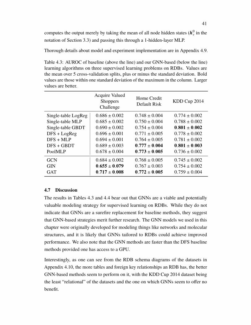
41

computes the output merely by taking the mean of all node hidden states (h0v in the

notation of Section 3.3) and passing this through a 1-hidden-layer MLP.

Thorough details about model and experiment implementation are in Appendix 4.9.

Table 4.3: AUROC of baseline (above the line) and our GNN-based (below the line)learning algorithms on three supervised learning problems on RDBs. Values arethe mean over 5 cross-validation splits, plus or minus the standard deviation. Boldvalues are those within one standard deviation of the maximum in the column. Largervalues are better.

Acquire ValuedShoppersChallenge

Home CreditDefault Risk KDD Cup 2014

Single-table LogReg 0.686 ± 0.002 0.748 ± 0.004 0.774 ± 0.002Single-table MLP 0.685 ± 0.002 0.750 ± 0.004 0.788 ± 0.002Single-table GBDT 0.690 ± 0.002 0.754 ± 0.004 0.801 ± 0.002DFS + LogReg 0.696 ± 0.001 0.771 ± 0.005 0.778 ± 0.002DFS + MLP 0.694 ± 0.001 0.764 ± 0.005 0.781 ± 0.002DFS + GBDT 0.689 ± 0.003 0.777 ± 0.004 0.801 ± 0.003PoolMLP 0.678 ± 0.004 0.773 ± 0.005 0.736 ± 0.002

GCN 0.684 ± 0.002 0.768 ± 0.005 0.745 ± 0.002GIN 0.655 ± 0.079 0.767 ± 0.003 0.754 ± 0.002GAT 0.717 ± 0.008 0.772 ± 0.005 0.759 ± 0.004

4.7 DiscussionThe results in Tables 4.3 and 4.4 bear out that GNNs are a viable and potentiallyvaluable modeling strategy for supervised learning on RDBs. While they do notindicate that GNNs are a surefire replacement for baseline methods, they suggestthat GNN-based strategies merit further research. The GNN models we used in thischapter were originally developed for modeling things like networks and molecularstructures, and it is likely that GNNs tailored to RDBs could achieve improvedperformance. We also note that the GNN methods are faster than the DFS baselinemethods provided one has access to a GPU.

Interestingly, as one can see from the RDB schema diagrams of the datasets inAppendix 4.10, the more tables and foreign key relationships an RDB has, the betterGNN-based methods seem to perform on it, with the KDD Cup 2014 dataset beingthe least “relational” of the datasets and the one on which GNNs seem to offer nobenefit.

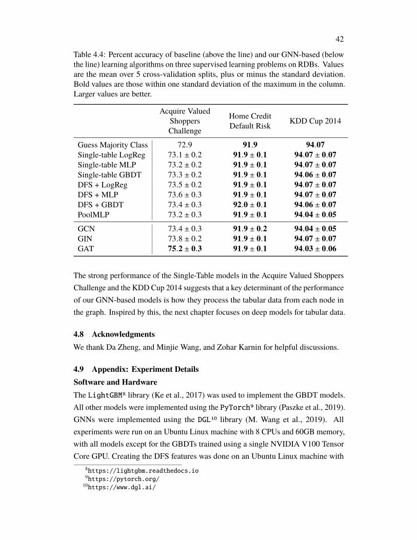
42

Table 4.4: Percent accuracy of baseline (above the line) and our GNN-based (belowthe line) learning algorithms on three supervised learning problems on RDBs. Valuesare the mean over 5 cross-validation splits, plus or minus the standard deviation.Bold values are those within one standard deviation of the maximum in the column.Larger values are better.

Acquire ValuedShoppersChallenge

Home CreditDefault Risk KDD Cup 2014

Guess Majority Class 72.9 91.9 94.07Single-table LogReg 73.1 ± 0.2 91.9 ± 0.1 94.07 ± 0.07Single-table MLP 73.2 ± 0.2 91.9 ± 0.1 94.07 ± 0.07Single-table GBDT 73.3 ± 0.2 91.9 ± 0.1 94.06 ± 0.07DFS + LogReg 73.5 ± 0.2 91.9 ± 0.1 94.07 ± 0.07DFS + MLP 73.6 ± 0.3 91.9 ± 0.1 94.07 ± 0.07DFS + GBDT 73.4 ± 0.3 92.0 ± 0.1 94.06 ± 0.07PoolMLP 73.2 ± 0.3 91.9 ± 0.1 94.04 ± 0.05

GCN 73.4 ± 0.3 91.9 ± 0.2 94.04 ± 0.05GIN 73.8 ± 0.2 91.9 ± 0.1 94.07 ± 0.07GAT 75.2 ± 0.3 91.9 ± 0.1 94.03 ± 0.06

The strong performance of the Single-Table models in the Acquire Valued ShoppersChallenge and the KDD Cup 2014 suggests that a key determinant of the performanceof our GNN-based models is how they process the tabular data from each node inthe graph. Inspired by this, the next chapter focuses on deep models for tabular data.

4.8 AcknowledgmentsWe thank Da Zheng, and Minjie Wang, and Zohar Karnin for helpful discussions.

4.9 Appendix: Experiment DetailsSoftware and HardwareThe LightGBM8 library (Ke et al., 2017) was used to implement the GBDT models.All other models were implemented using the PyTorch9 library (Paszke et al., 2019).GNNs were implemented using the DGL10 library (M. Wang et al., 2019). Allexperiments were run on an Ubuntu Linux machine with 8 CPUs and 60GB memory,with all models except for the GBDTs trained using a single NVIDIA V100 TensorCore GPU. Creating the DFS features was done on an Ubuntu Linux machine with

8https://lightgbm.readthedocs.io9https://pytorch.org/10https://www.dgl.ai/

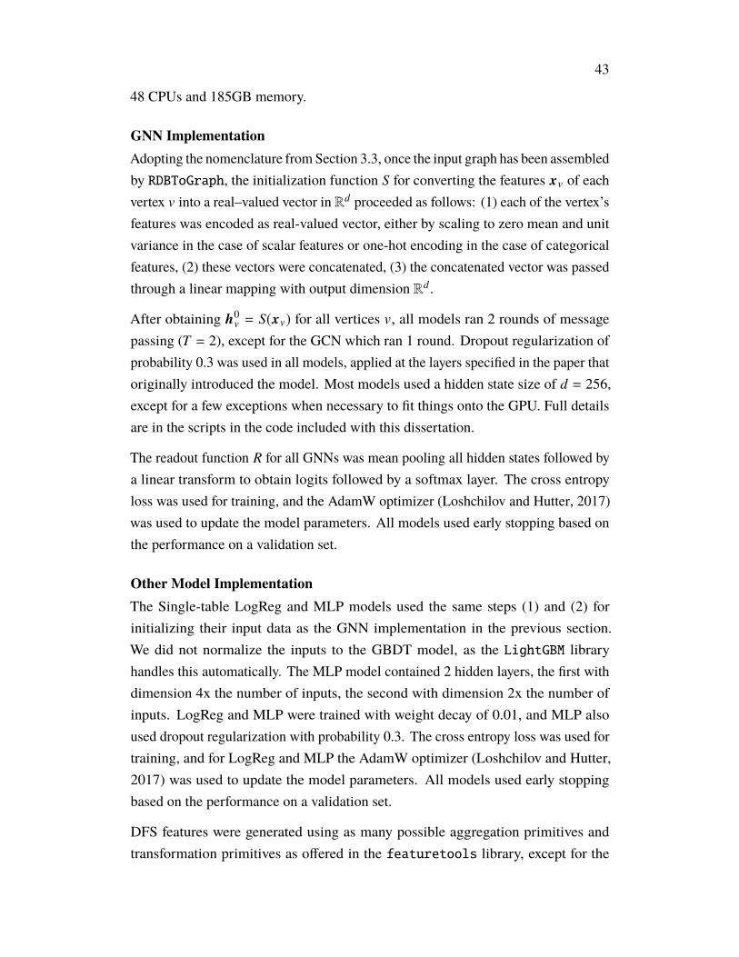
43

48 CPUs and 185GB memory.

GNN ImplementationAdopting the nomenclature from Section 3.3, once the input graph has been assembledby RDBToGraph, the initialization function S for converting the features xv of eachvertex v into a real–valued vector in Rd proceeded as follows: (1) each of the vertex’sfeatures was encoded as real-valued vector, either by scaling to zero mean and unitvariance in the case of scalar features or one-hot encoding in the case of categoricalfeatures, (2) these vectors were concatenated, (3) the concatenated vector was passedthrough a linear mapping with output dimension Rd .

After obtaining h0v = S(xv) for all vertices v, all models ran 2 rounds of message

passing (T = 2), except for the GCN which ran 1 round. Dropout regularization ofprobability 0.3 was used in all models, applied at the layers specified in the paper thatoriginally introduced the model. Most models used a hidden state size of d = 256,except for a few exceptions when necessary to fit things onto the GPU. Full detailsare in the scripts in the code included with this dissertation.

The readout function R for all GNNs was mean pooling all hidden states followed bya linear transform to obtain logits followed by a softmax layer. The cross entropyloss was used for training, and the AdamW optimizer (Loshchilov and Hutter, 2017)was used to update the model parameters. All models used early stopping based onthe performance on a validation set.

Other Model ImplementationThe Single-table LogReg and MLP models used the same steps (1) and (2) forinitializing their input data as the GNN implementation in the previous section.We did not normalize the inputs to the GBDT model, as the LightGBM libraryhandles this automatically. The MLP model contained 2 hidden layers, the first withdimension 4x the number of inputs, the second with dimension 2x the number ofinputs. LogReg and MLP were trained with weight decay of 0.01, and MLP alsoused dropout regularization with probability 0.3. The cross entropy loss was used fortraining, and for LogReg and MLP the AdamW optimizer (Loshchilov and Hutter,2017) was used to update the model parameters. All models used early stoppingbased on the performance on a validation set.

DFS features were generated using as many possible aggregation primitives andtransformation primitives as offered in the featuretools library, except for the

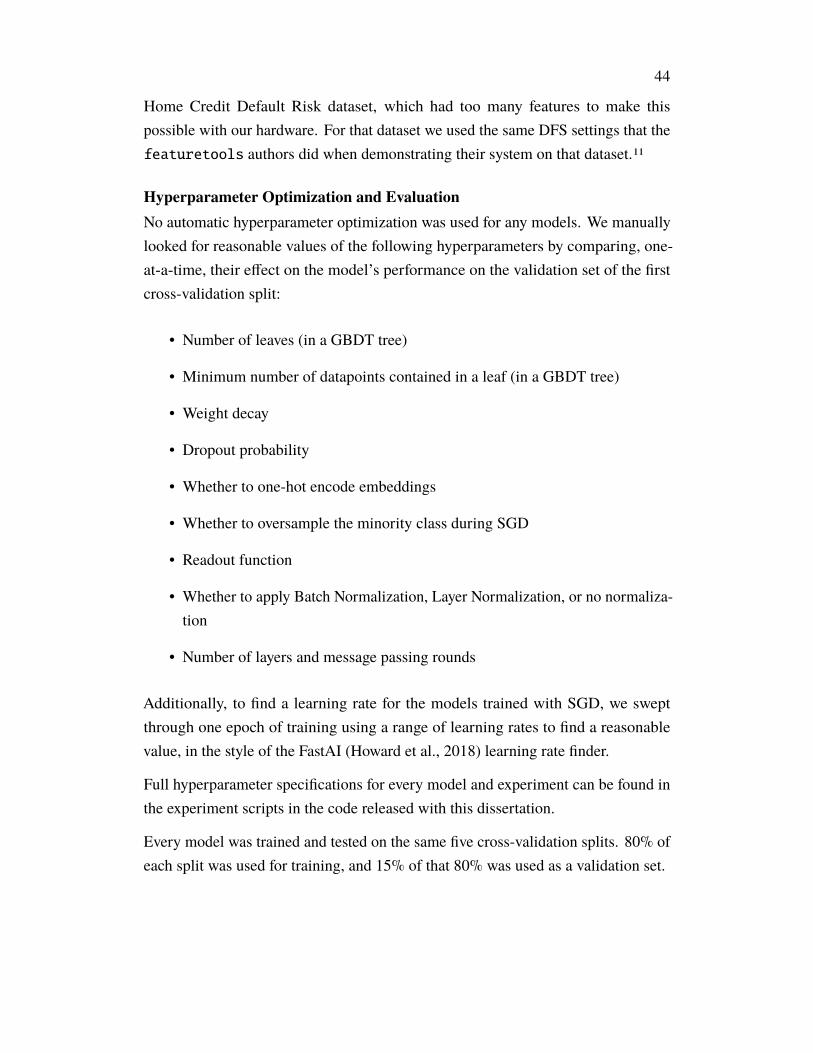
44

Home Credit Default Risk dataset, which had too many features to make thispossible with our hardware. For that dataset we used the same DFS settings that thefeaturetools authors did when demonstrating their system on that dataset.11

Hyperparameter Optimization and EvaluationNo automatic hyperparameter optimization was used for any models. We manuallylooked for reasonable values of the following hyperparameters by comparing, one-at-a-time, their effect on the model’s performance on the validation set of the firstcross-validation split:

• Number of leaves (in a GBDT tree)

• Minimum number of datapoints contained in a leaf (in a GBDT tree)

• Weight decay

• Dropout probability

• Whether to one-hot encode embeddings

• Whether to oversample the minority class during SGD

• Readout function

• Whether to apply Batch Normalization, Layer Normalization, or no normaliza-tion

• Number of layers and message passing rounds

Additionally, to find a learning rate for the models trained with SGD, we sweptthrough one epoch of training using a range of learning rates to find a reasonablevalue, in the style of the FastAI (Howard et al., 2018) learning rate finder.

Full hyperparameter specifications for every model and experiment can be found inthe experiment scripts in the code released with this dissertation.

Every model was trained and tested on the same five cross-validation splits. 80% ofeach split was used for training, and 15% of that 80% was used as a validation set.

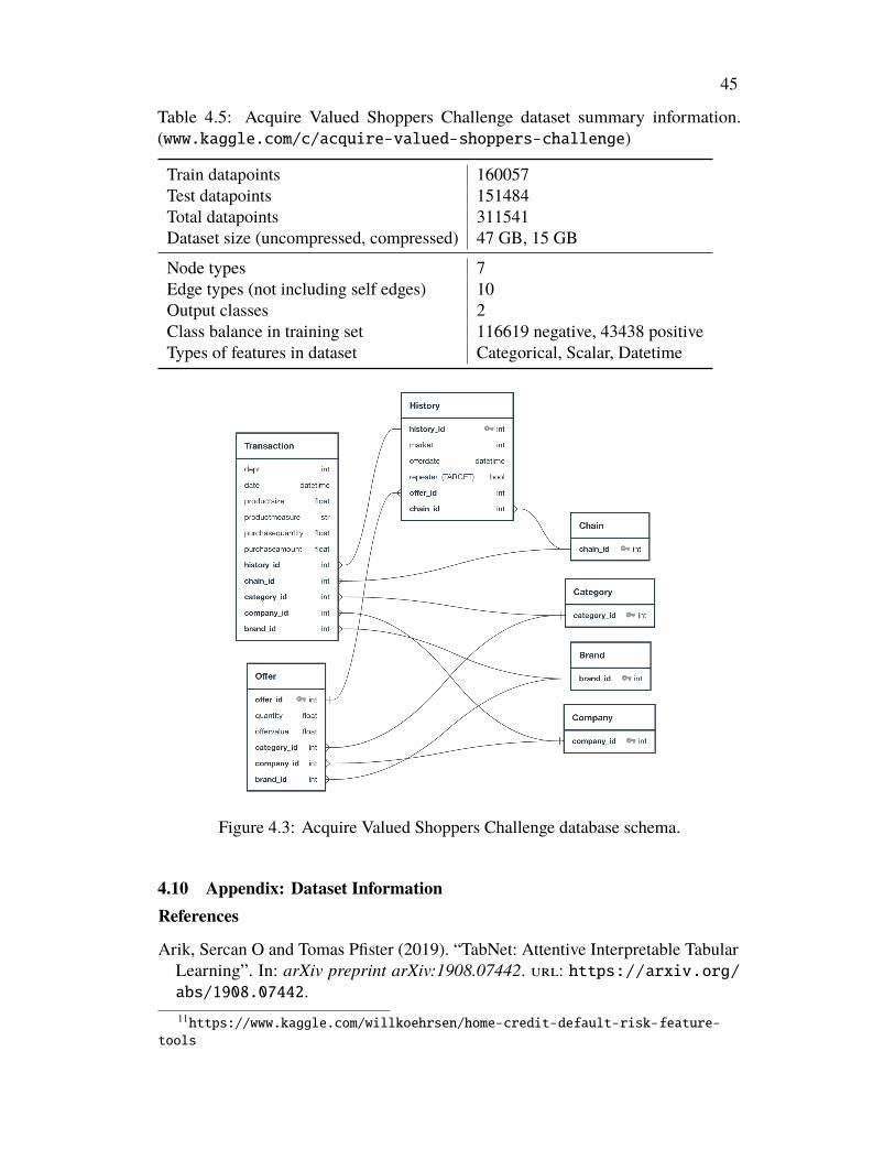
45

Table 4.5: Acquire Valued Shoppers Challenge dataset summary information.(www.kaggle.com/c/acquire-valued-shoppers-challenge)

Train datapoints 160057Test datapoints 151484Total datapoints 311541Dataset size (uncompressed, compressed) 47 GB, 15 GB

Node types 7Edge types (not including self edges) 10Output classes 2Class balance in training set 116619 negative, 43438 positiveTypes of features in dataset Categorical, Scalar, Datetime

Figure 4.3: Acquire Valued Shoppers Challenge database schema.

4.10 Appendix: Dataset InformationReferences

Arik, Sercan O and Tomas Pfister (2019). “TabNet: Attentive Interpretable TabularLearning”. In: arXiv preprint arXiv:1908.07442. url: https://arxiv.org/abs/1908.07442.11https://www.kaggle.com/willkoehrsen/home-credit-default-risk-feature-

tools

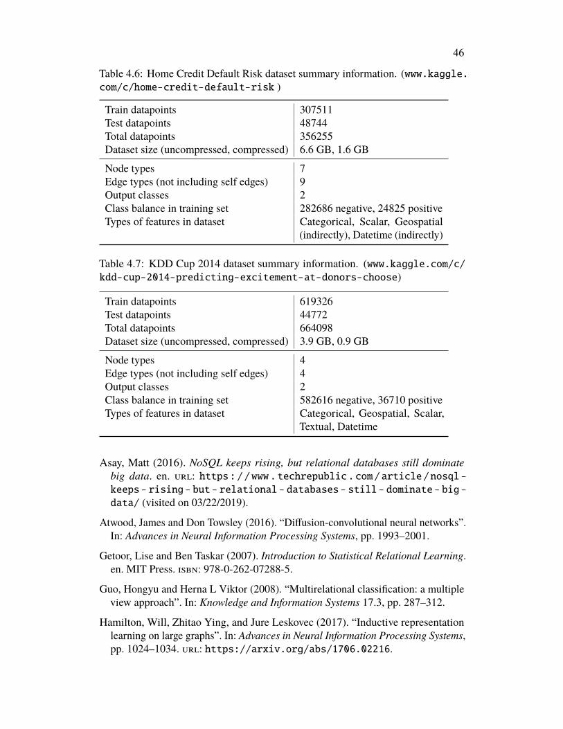
46

Table 4.6: Home Credit Default Risk dataset summary information. (www.kaggle.com/c/home-credit-default-risk )

Train datapoints 307511Test datapoints 48744Total datapoints 356255Dataset size (uncompressed, compressed) 6.6 GB, 1.6 GB

Node types 7Edge types (not including self edges) 9Output classes 2Class balance in training set 282686 negative, 24825 positiveTypes of features in dataset Categorical, Scalar, Geospatial

(indirectly), Datetime (indirectly)

Table 4.7: KDD Cup 2014 dataset summary information. (www.kaggle.com/c/kdd-cup-2014-predicting-excitement-at-donors-choose)

Train datapoints 619326Test datapoints 44772Total datapoints 664098Dataset size (uncompressed, compressed) 3.9 GB, 0.9 GB

Node types 4Edge types (not including self edges) 4Output classes 2Class balance in training set 582616 negative, 36710 positiveTypes of features in dataset Categorical, Geospatial, Scalar,

Textual, Datetime

Asay, Matt (2016). NoSQL keeps rising, but relational databases still dominatebig data. en. url: https://www.techrepublic.com/article/nosql-keeps- rising- but- relational- databases- still- dominate- big-data/ (visited on 03/22/2019).

Atwood, James and Don Towsley (2016). “Diffusion-convolutional neural networks”.In: Advances in Neural Information Processing Systems, pp. 1993–2001.

Getoor, Lise and Ben Taskar (2007). Introduction to Statistical Relational Learning.en. MIT Press. isbn: 978-0-262-07288-5.

Guo, Hongyu and Herna L Viktor (2008). “Multirelational classification: a multipleview approach”. In: Knowledge and Information Systems 17.3, pp. 287–312.

Hamilton, Will, Zhitao Ying, and Jure Leskovec (2017). “Inductive representationlearning on large graphs”. In: Advances in Neural Information Processing Systems,pp. 1024–1034. url: https://arxiv.org/abs/1706.02216.

47

Howard, Jeremy et al. (2018). FastAI. https://github.com/fastai/fastai.

International Organization for Standardization (2016). ISO/IEC 9075-1:2016: Infor-mation technology – Database languages – SQL – Part 1: Framework (SQL/Frame-work). en. url: http://www.iso.org/cms/render/live/en/sites/isoorg / contents / data / standard / 06 / 35 / 63555 . html (visited on03/21/2019).

Kaggle, Inc. (2017). The State of ML and Data Science 2017. url: https://www.kaggle.com/surveys/2017 (visited on 03/22/2019).

Kanter, James Max and Kalyan Veeramachaneni (2015). “Deep feature synthe-sis: Towards automating data science endeavors”. In: 2015 IEEE InternationalConference on Data Science and Advanced Analytics (DSAA), pp. 1–10. doi:10.1109/DSAA.2015.7344858. url: https://www.jmaxkanter.com/static/papers/DSAA_DSM_2015.pdf.

Ke, Guolin et al. (2017). “LightGBM: A highly efficient gradient boosting decisiontree”. In: Advances in Neural Information Processing Systems, pp. 3146–3154.url: https://papers.nips.cc/paper/6907- lightgbm- a- highly-efficient-gradient-boosting-decision-tree.pdf.

Kipf, Thomas N and Max Welling (2016). “Semi-supervised classification withgraph convolutional networks”. In: International Conference on Learning Repre-sentations. url: https://arxiv.org/abs/1609.02907.

Koller, Daphne et al. (2007). “Introduction to statistical relational learning”. In: MITpress. Chap. 2, pp. 129–174.

Lam, Hoang Thanh, Tran Ngoc Minh, et al. (2018). “Neural Feature LearningFrom Relational Database”. In: arXiv:1801.05372 [cs]. arXiv: 1801.05372. url:http://arxiv.org/abs/1801.05372 (visited on 02/22/2019).

Lam, Hoang Thanh, Johann-Michael Thiebaut, et al. (2017). “One button machinefor automating feature engineering in relational databases”. In: arXiv:1706.00327[cs]. arXiv: 1706.00327. url: http://arxiv.org/abs/1706.00327 (visitedon 02/23/2019).

Loshchilov, Ilya and Frank Hutter (2017). “DecoupledWeight Decay Regularization”.In: International Conference on Learning Representations. url: https://arxiv.org/abs/1711.05101.

Luzhnica, Enxhell, Ben Day, and Pietro Liò (2019). “On Graph ClassificationNetworks, Datasets and Baselines”. In: ArXiv abs/1905.04682. url: https://arxiv.org/abs/1905.04682.

Paszke, Adam et al. (2019). “PyTorch: An Imperative Style, High-Performance DeepLearning Library”. In: Advances in Neural Information Processing Systems 32.Ed. by H. Wallach et al. Curran Associates, Inc., pp. 8024–8035. url: http://papers.neurips.cc/paper/9015-pytorch-an-imperative-style-high-performance-deep-learning-library.pdf.

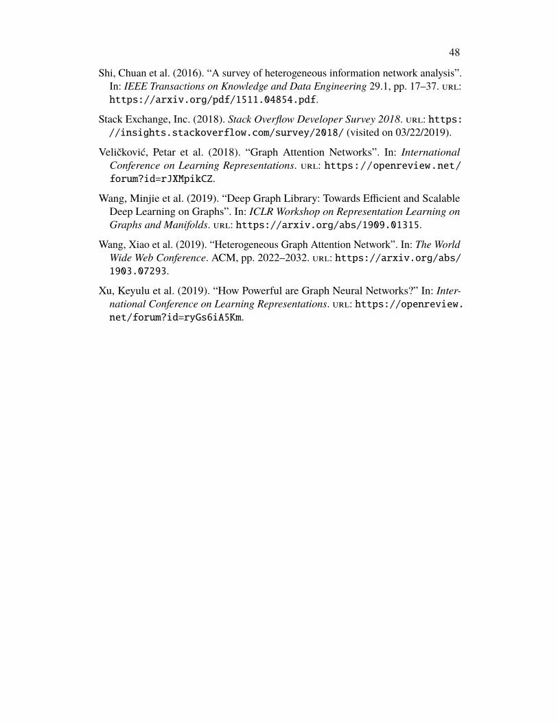
48

Shi, Chuan et al. (2016). “A survey of heterogeneous information network analysis”.In: IEEE Transactions on Knowledge and Data Engineering 29.1, pp. 17–37. url:https://arxiv.org/pdf/1511.04854.pdf.

Stack Exchange, Inc. (2018). Stack Overflow Developer Survey 2018. url: https://insights.stackoverflow.com/survey/2018/ (visited on 03/22/2019).

Veličković, Petar et al. (2018). “Graph Attention Networks”. In: InternationalConference on Learning Representations. url: https://openreview.net/forum?id=rJXMpikCZ.

Wang, Minjie et al. (2019). “Deep Graph Library: Towards Efficient and ScalableDeep Learning on Graphs”. In: ICLR Workshop on Representation Learning onGraphs and Manifolds. url: https://arxiv.org/abs/1909.01315.

Wang, Xiao et al. (2019). “Heterogeneous Graph Attention Network”. In: The WorldWide Web Conference. ACM, pp. 2022–2032. url: https://arxiv.org/abs/1903.07293.

Xu, Keyulu et al. (2019). “How Powerful are Graph Neural Networks?” In: Inter-national Conference on Learning Representations. url: https://openreview.net/forum?id=ryGs6iA5Km.

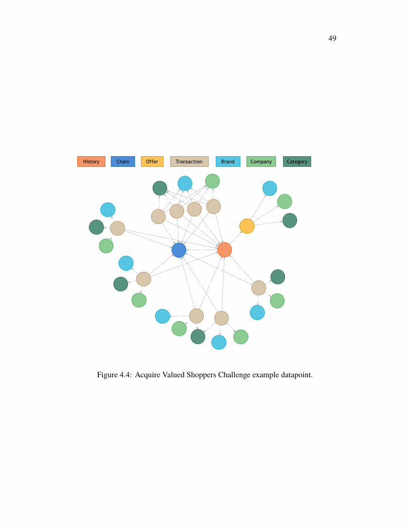
49

History Chain Offer Transaction Brand Company Category

Figure 4.4: Acquire Valued Shoppers Challenge example datapoint.

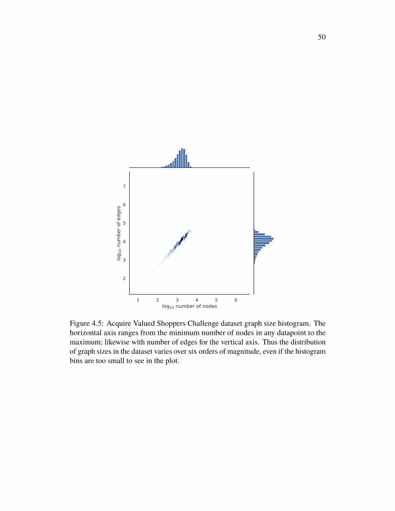
50

Figure 4.5: Acquire Valued Shoppers Challenge dataset graph size histogram. Thehorizontal axis ranges from the minimum number of nodes in any datapoint to themaximum; likewise with number of edges for the vertical axis. Thus the distributionof graph sizes in the dataset varies over six orders of magnitude, even if the histogrambins are too small to see in the plot.

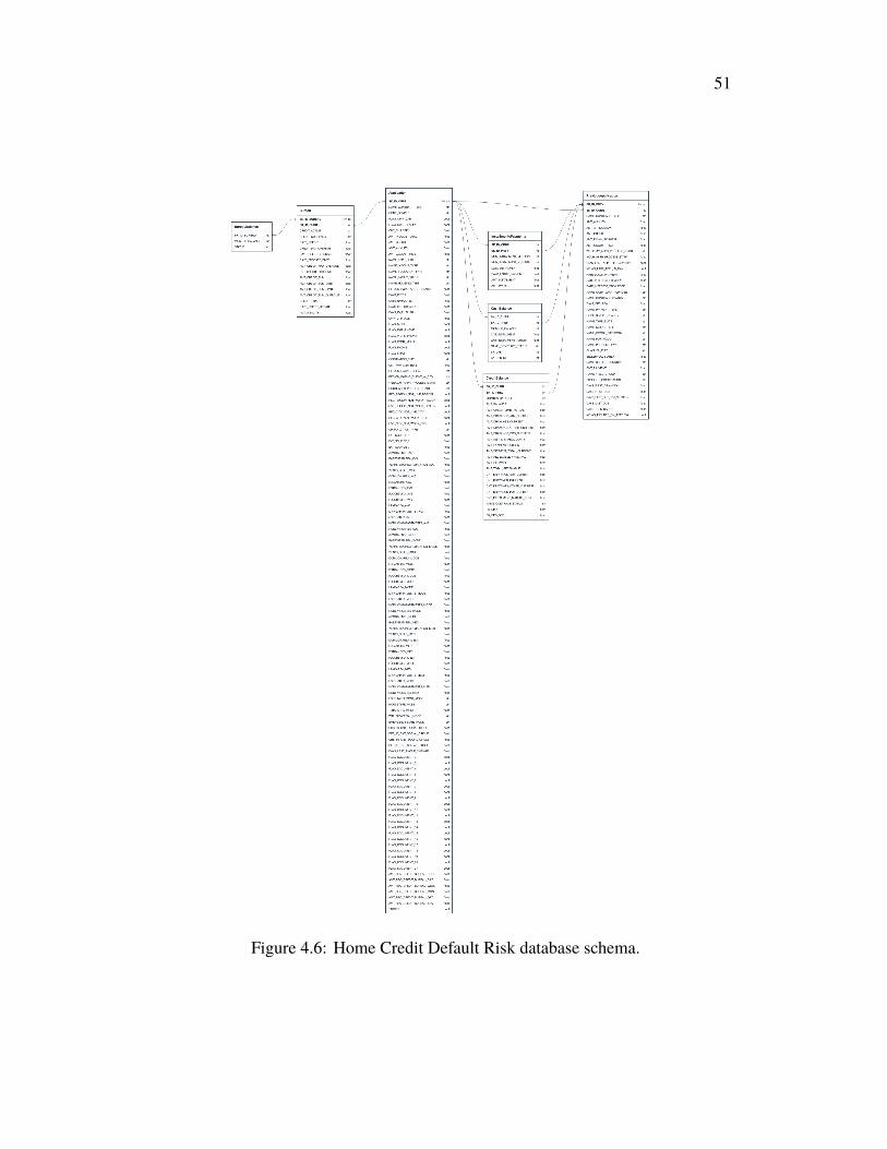
51

Figure 4.6: Home Credit Default Risk database schema.

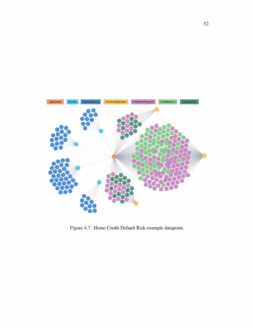
52

Application Bureau BureauBalance PreviousApplication InstallmentPayment CreditBalance CashBalance

Figure 4.7: Home Credit Default Risk example datapoint.

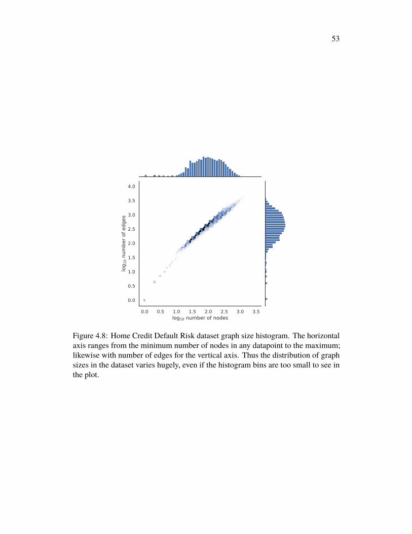
53

Figure 4.8: Home Credit Default Risk dataset graph size histogram. The horizontalaxis ranges from the minimum number of nodes in any datapoint to the maximum;likewise with number of edges for the vertical axis. Thus the distribution of graphsizes in the dataset varies hugely, even if the histogram bins are too small to see inthe plot.

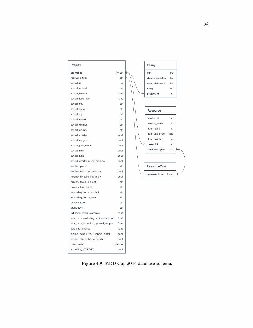
54

Figure 4.9: KDD Cup 2014 database schema.

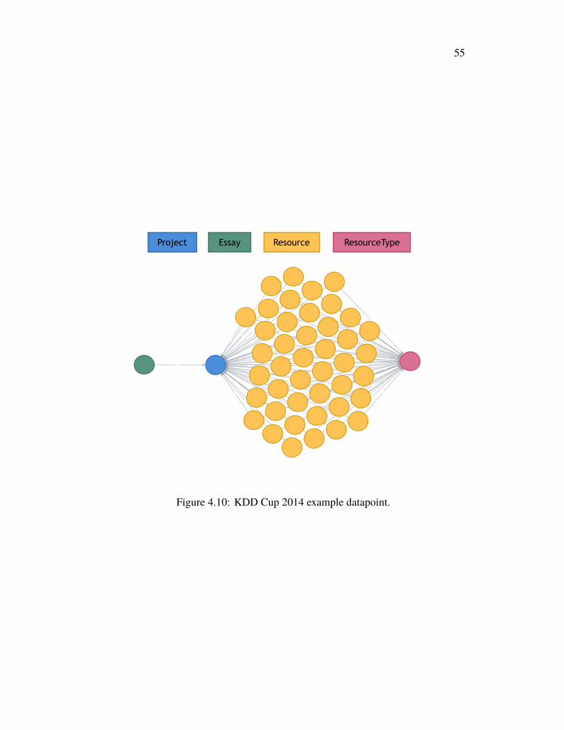
55

Project Essay Resource ResourceType

Figure 4.10: KDD Cup 2014 example datapoint.

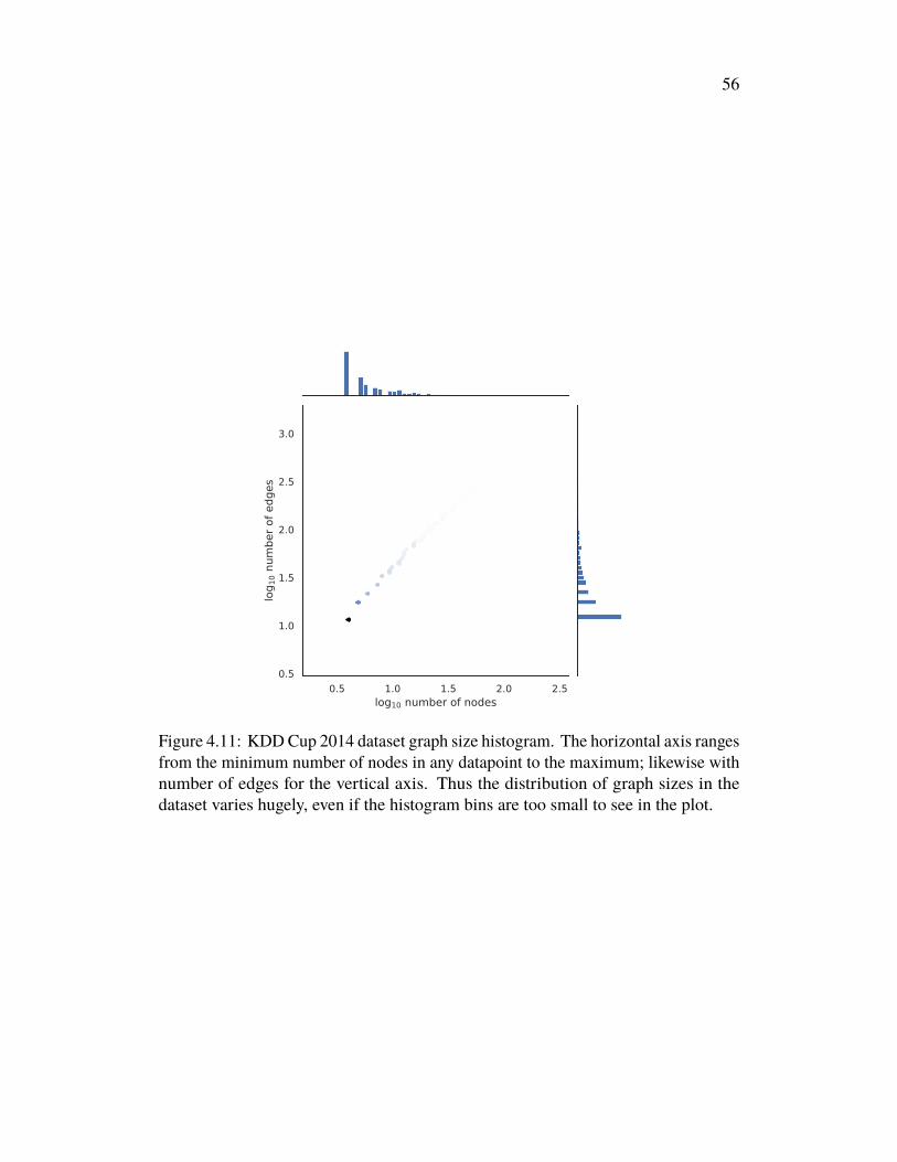
56

Figure 4.11: KDDCup 2014 dataset graph size histogram. The horizontal axis rangesfrom the minimum number of nodes in any datapoint to the maximum; likewise withnumber of edges for the vertical axis. Thus the distribution of graph sizes in thedataset varies hugely, even if the histogram bins are too small to see in the plot.

57

C h a p t e r 5

STRENGTHS AND WEAKNESSES OF DEEP LEARNING FORTABULAR DATA

5.1 IntroductionTabular data refers to data about which we have no prior knowledge regarding thestructure or relationships between their features.1 Typically stored in a table, hencetheir name, with datapoints as rows and features as columns, tabular data are widelyused in practical machine learning and data science, as evidenced by their abundanceon sites like Kaggle.2

The established wisdom among data scientists is that decision tree-based models,especially gradient boosted decision trees (GBDTs), are the best choice for supervisedlearning on tabular data (Goldbloom, 2017). While it is surprising that a categoryas broad as tabular data would be dominated by a single type of model, reasonableexplanations have been given, including that GBDTs are built to find low-orderfeature interactions and avoid overfitting (Arik and Pfister, 2019), which would makethem well suited to data defined by the lack of known relationships between theirfeatures.

Despite the dominance of GBDTs for tabular data, much effort has gone intodeveloping deep models for tabular data. Indeed, most papers presenting new deepmodels for tabular data give evidence that they outperform GBDTs, or do not botherto compare to them at all; see the Related Work below. Yet it is notable that none hasgone on to supplant GBDTs as the method of choice for tabular data.

This gap between published results and practice raises the question of whethermachine learning researchers are assessing the performance of deep methods fortabular a useful way. In a benchmark-driven field like machine learning, it is notablethat there is no standard benchmark for supervised learning on tabular data.

To address this issue, in Section 5.3 below we introduce a new benchmark consistingof 20 binary classification tasks on tabular data. We use this benchmark to presentthe first, as far as we are aware, large-scale, evenly-matched comparison of deep

1Confusingly, given this definition, tabular data are sometimes known as “structured data” in theliterature.

2https://www.kaggle.com/

58

models for tabular data. Giving the same hyperparameter tuning budget to each of sixtypes of deep models for tabular data, along with GBDTs and logistic regression, wefind that while deep models can often match the performance of GBDTs, they almostnever outperform it, and simple MLPs often perform as well as models designed fortabular data.

Deep models do have some comparative advantages over tree-based models, however.In the context of this dissertation, deep models for tabular data are of interest as a wayto improve the performance of the GNN-based methods presented in the previouschapter. The initial features from each table in an RDB can be passed through a deepmodel before passing through the GNN. So improvements to deep models tabulardata might improve performance on supervised learning on RDBs. (Q.v. Chapter 7.)

Of more general interest, though, is that deep models allow us to leverage unlabeleddata and data from other sources to improve performance on our dataset of interest,a feat which has proved difficult for tree-based models (Tanha, Someren, andAfsarmanesh, 2017). Variants of this idea include unsupervised pretraining (Caronet al., 2019), semi-supervised learning (Stretcu et al., 2019), transductive learning(Elezi et al., 2018), and transfer learning (Devlin et al., 2019).

As a demonstration of the utility that deep learning methods can have for tabulardata, in Section 5.4 below we introduce a variant of semi-supervised learning calledsubset-restricted finetuning and show that training techniques adapted from naturallanguage processing lead deep models to generally outperform GBDTs in this regime.

5.2 Related WorkStandard multilayer perceptrons (MLPs) have been applied to tabular data for manyyears, sometimes to good effect (De Brébisson et al., 2015). More modern deeplearning techniques like batch normalization and learnable embeddings for categoricalfeatures can significantly improve the performance of MLPs for tabular data (Howardet al., 2018).

The major problem when using MLPs for tabular data is overfitting. A number ofmethods for combating overfitting in MLPs have been tried at least partly on tabulardata, notably sparsification and pruning methods (Hassibi et al., 1993; Mocanu et al.,2018) and information bottleneck-based methods (Tishby, Pereira, and Bialek, 2000;Strouse and Schwab, 2015).

In terms of deep models designed specifically for tabular data, many “deep versions”of non-deep-learning-based machine learning algorithms have been proposed. These

59

include deep versions of factorization machines (Guo et al., 2018; Xiao et al., 2017),extensions of these based on transformers and multi-head attention (Song et al., 2019;Li et al., 2020; Sun et al., 2019), and deep versions of decision-tree-based algorithms(Ke, Zhang, et al., 2019; Yang, Morillo, and Hospedales, 2018).

Other models have been designed around the purported properties of tabular datasuch as low-order and sparse feature interactions. These include Deep & CrossNetworks (Wang et al., 2017), Wide & Deep Networks (Cheng et al., 2016), andTabNets (Arik and Pfister, 2019).

5.3 Benchmarking Deep Models for Tabular DataWe assembled 20 publicly available tabular, binary classification datasets from theUCI repository (Dua and Graff, 2017), the AutoML Challenge (Guyon et al., 2019),and Kaggle.com. As shown in Table 5.1, the number of datapoints and number offeatures in the datasets vary over 3 orders of magnitude, and include a mix of scalarand categorical features along with some missing values. We annotated each columnin each dataset as to whether it contains a scalar or categorical variable, though itis up to the model how to use this information in preprocessing. Full details oneach dataset is in Appendix Tables 5.2 and 5.3. In order to encourage adoption ofthe benchmark, we provide code with this dissertation to automatically obtain alldatasets and convert them into a common format.

For the benchmark, each dataset is divided into 5 cross-validation splits, each with80% of the datapoints available for training and 20% for testing. 15% of this 80% isthen split off as a validation set. All these splits are obtained with a fixed random seedso that every model tested receives exactly the same training and testing conditions.

The diversity of datasets in the benchmark makes it critical to perform hyperparameteroptimization (HPO) for each model. Equally critical is giving each model the sameHPO budget to make the comparison fair. In our experiments, each model wasgiven 10 HPO rounds on each of the 5 cross-validation splits for each dataset, withthe best-performing model among these 10 HPO rounds then evaluated on the testset. All models used early stopping on the validation set to identify the best set ofparameters in each training run.

The models tested are logistic regression, GBDT as implemented in the LightGBMlibrary (Ke, Meng, et al., 2017), multilayer perceptron (MLP), a transformer-stylemodel (Tfmr) (Vaswani et al., 2017) modified for use on tabular data in the styleof (Song et al., 2019; Li et al., 2020; Sun et al., 2019), a novel, heterogeneous

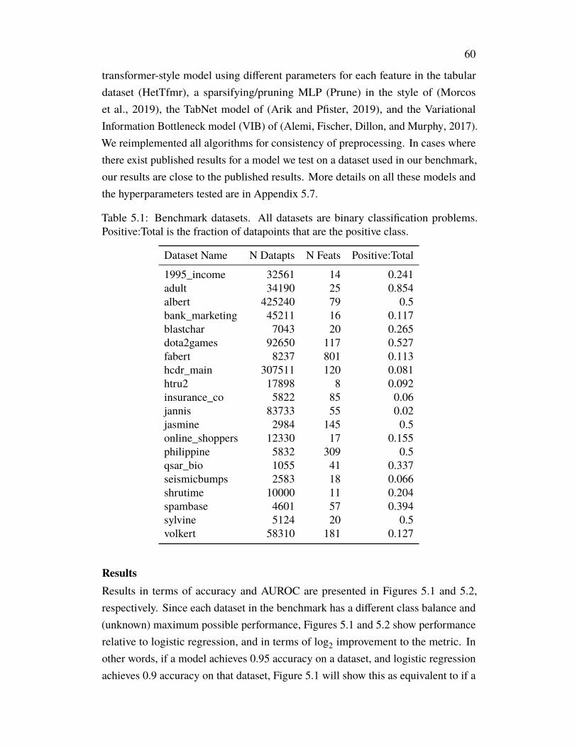
60

transformer-style model using different parameters for each feature in the tabulardataset (HetTfmr), a sparsifying/pruning MLP (Prune) in the style of (Morcoset al., 2019), the TabNet model of (Arik and Pfister, 2019), and the VariationalInformation Bottleneck model (VIB) of (Alemi, Fischer, Dillon, and Murphy, 2017).We reimplemented all algorithms for consistency of preprocessing. In cases wherethere exist published results for a model we test on a dataset used in our benchmark,our results are close to the published results. More details on all these models andthe hyperparameters tested are in Appendix 5.7.

Table 5.1: Benchmark datasets. All datasets are binary classification problems.Positive:Total is the fraction of datapoints that are the positive class.

Dataset Name N Datapts N Feats Positive:Total

1995_income 32561 14 0.241adult 34190 25 0.854albert 425240 79 0.5bank_marketing 45211 16 0.117blastchar 7043 20 0.265dota2games 92650 117 0.527fabert 8237 801 0.113hcdr_main 307511 120 0.081htru2 17898 8 0.092insurance_co 5822 85 0.06jannis 83733 55 0.02jasmine 2984 145 0.5online_shoppers 12330 17 0.155philippine 5832 309 0.5qsar_bio 1055 41 0.337seismicbumps 2583 18 0.066shrutime 10000 11 0.204spambase 4601 57 0.394sylvine 5124 20 0.5volkert 58310 181 0.127

ResultsResults in terms of accuracy and AUROC are presented in Figures 5.1 and 5.2,respectively. Since each dataset in the benchmark has a different class balance and(unknown) maximum possible performance, Figures 5.1 and 5.2 show performancerelative to logistic regression, and in terms of log2 improvement to the metric. Inother words, if a model achieves 0.95 accuracy on a dataset, and logistic regressionachieves 0.9 accuracy on that dataset, Figure 5.1 will show this as equivalent to if a

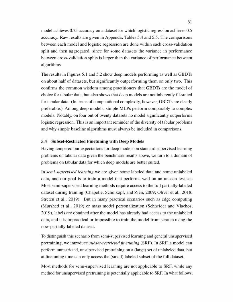
61

model achieves 0.75 accuracy on a dataset for which logistic regression achieves 0.5accuracy. Raw results are given in Appendix Tables 5.4 and 5.5. The comparisonsbetween each model and logistic regression are done within each cross-validationsplit and then aggregated, since for some datasets the variance in performancebetween cross-validation splits is larger than the variance of performance betweenalgorithms.

The results in Figures 5.1 and 5.2 show deep models performing as well as GBDTson about half of datasets, but significantly outperforming them on only two. Thisconfirms the common wisdom among practitioners that GBDTs are the model ofchoice for tabular data, but also shows that deep models are not inherently ill-suitedfor tabular data. (In terms of computational complexity, however, GBDTs are clearlypreferable.) Among deep models, simple MLPs perform comparably to complexmodels. Notably, on four out of twenty datasets no model significantly outperformslogistic regression. This is an important reminder of the diversity of tabular problemsand why simple baseline algorithms must always be included in comparisons.

5.4 Subset-Restricted Finetuning with Deep ModelsHaving tempered our expectations for deep models on standard supervised learningproblems on tabular data given the benchmark results above, we turn to a domain ofproblems on tabular data for which deep models are better suited.

In semi-supervised learning we are given some labeled data and some unlabeleddata, and our goal is to train a model that performs well on an unseen test set.Most semi-supervised learning methods require access to the full partially-labeleddataset during training (Chapelle, Scholkopf, and Zien, 2009; Oliver et al., 2018;Stretcu et al., 2019). But in many practical scenarios such as edge computing(Murshed et al., 2019) or mass model personalization (Schneider and Vlachos,2019), labels are obtained after the model has already had access to the unlabeleddata, and it is impractical or impossible to train the model from scratch using thenow-partially-labeled dataset.

To distinguish this scenario from semi-supervised learning and general unsupervisedpretraining, we introduce subset-restricted finetuning (SRF). In SRF, a model canperform unrestricted, unsupervised pretraining on a (large) set of unlabeled data, butat finetuning time can only access the (small) labeled subset of the full dataset.

Most methods for semi-supervised learning are not applicable to SRF, while anymethod for unsupervised pretraining is potentially applicable to SRF. In what follows,

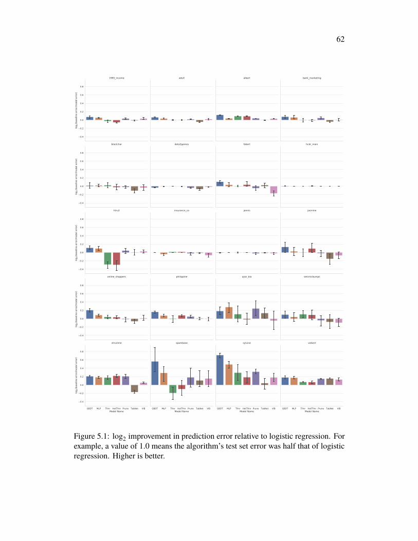
62

0.4

0.2

0.0

0.2

0.4

0.6

0.8

log 2

(bas

elin

e er

ror/m

odel

erro

r)1995_income adult albert bank_marketing

0.4

0.2

0.0

0.2

0.4

0.6

0.8

log 2

(bas

elin

e er

ror/m

odel

erro

r)

blastchar dota2games fabert hcdr_main

0.4

0.2

0.0

0.2

0.4

0.6

0.8

log 2

(bas

elin

e er

ror/m

odel

erro

r)

htru2 insurance_co jannis jasmine

0.4

0.2

0.0

0.2

0.4

0.6

0.8

log 2

(bas

elin

e er

ror/m

odel

erro

r)

online_shoppers philippine qsar_bio seismicbumps

GBDT MLP Tfmr HetTfmr Prune TabNet VIBModel Name

0.4

0.2

0.0

0.2

0.4

0.6

0.8

log 2

(bas

elin

e er

ror/m

odel

erro

r)

shrutime

GBDT MLP Tfmr HetTfmr Prune TabNet VIBModel Name

spambase

GBDT MLP Tfmr HetTfmr Prune TabNet VIBModel Name

sylvine

GBDT MLP Tfmr HetTfmr Prune TabNet VIBModel Name

volkert

Figure 5.1: log2 improvement in prediction error relative to logistic regression. Forexample, a value of 1.0 means the algorithm’s test set error was half that of logisticregression. Higher is better.

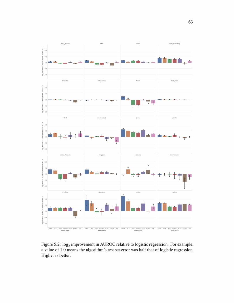
63

1.0

0.5

0.0

0.5

1.0

log 2

(bas

elin

e (1

-AUR

OC)/m

odel

(1-A

UROC

))1995_income adult albert bank_marketing

1.0

0.5

0.0

0.5

1.0

log 2

(bas

elin

e (1

-AUR

OC)/m

odel

(1-A

UROC

))

blastchar dota2games fabert hcdr_main

1.0

0.5

0.0

0.5

1.0

log 2

(bas

elin

e (1

-AUR

OC)/m

odel

(1-A

UROC

))

htru2 insurance_co jannis jasmine

1.0

0.5

0.0

0.5

1.0

log 2

(bas

elin

e (1

-AUR

OC)/m

odel

(1-A

UROC

))

online_shoppers philippine qsar_bio seismicbumps

GBDT MLP Tfmr HetTfmr Prune TabNet VIBModel Name

1.0

0.5

0.0

0.5

1.0

log 2

(bas

elin

e (1

-AUR

OC)/m

odel

(1-A

UROC

))

shrutime

GBDT MLP Tfmr HetTfmr Prune TabNet VIBModel Name

spambase

GBDT MLP Tfmr HetTfmr Prune TabNet VIBModel Name

sylvine

GBDT MLP Tfmr HetTfmr Prune TabNet VIBModel Name

volkert

Figure 5.2: log2 improvement in AUROC relative to logistic regression. For example,a value of 1.0 means the algorithm’s test set error was half that of logistic regression.Higher is better.

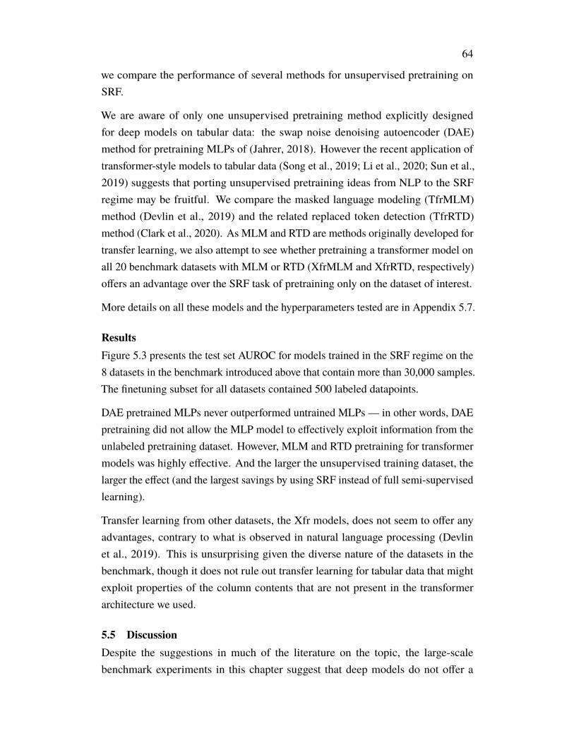
64

we compare the performance of several methods for unsupervised pretraining onSRF.

We are aware of only one unsupervised pretraining method explicitly designedfor deep models on tabular data: the swap noise denoising autoencoder (DAE)method for pretraining MLPs of (Jahrer, 2018). However the recent application oftransformer-style models to tabular data (Song et al., 2019; Li et al., 2020; Sun et al.,2019) suggests that porting unsupervised pretraining ideas from NLP to the SRFregime may be fruitful. We compare the masked language modeling (TfrMLM)method (Devlin et al., 2019) and the related replaced token detection (TfrRTD)method (Clark et al., 2020). As MLM and RTD are methods originally developed fortransfer learning, we also attempt to see whether pretraining a transformer model onall 20 benchmark datasets with MLM or RTD (XfrMLM and XfrRTD, respectively)offers an advantage over the SRF task of pretraining only on the dataset of interest.

More details on all these models and the hyperparameters tested are in Appendix 5.7.

ResultsFigure 5.3 presents the test set AUROC for models trained in the SRF regime on the8 datasets in the benchmark introduced above that contain more than 30,000 samples.The finetuning subset for all datasets contained 500 labeled datapoints.

DAE pretrained MLPs never outperformed untrained MLPs — in other words, DAEpretraining did not allow the MLP model to effectively exploit information from theunlabeled pretraining dataset. However, MLM and RTD pretraining for transformermodels was highly effective. And the larger the unsupervised training dataset, thelarger the effect (and the largest savings by using SRF instead of full semi-supervisedlearning).

Transfer learning from other datasets, the Xfr models, does not seem to offer anyadvantages, contrary to what is observed in natural language processing (Devlinet al., 2019). This is unsurprising given the diverse nature of the datasets in thebenchmark, though it does not rule out transfer learning for tabular data that mightexploit properties of the column contents that are not present in the transformerarchitecture we used.

5.5 DiscussionDespite the suggestions in much of the literature on the topic, the large-scalebenchmark experiments in this chapter suggest that deep models do not offer a

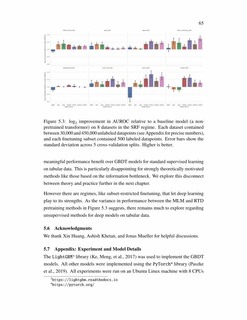
65

0.4

0.2

0.0

0.2

0.4

log 2

((1-b

asel

ine

AURO

C)(1

-mod

el A

UROC

))

1995_income_500 adult_500 albert_500 bank_marketing_500

GBDT MLP DAE TfrMLM TfrRTD XfrMLM XfrRTDModel Name

0.4

0.2

0.0

0.2

0.4

log 2

((1-b

asel

ine

AURO

C)(1

-mod

el A

UROC

))

dota2games_500

GBDT MLP DAE TfrMLM TfrRTD XfrMLM XfrRTDModel Name

hcdr_main_500

GBDT MLP DAE TfrMLM TfrRTD XfrMLM XfrRTDModel Name

jannis_500

GBDT MLP DAE TfrMLM TfrRTD XfrMLM XfrRTDModel Name

volkert_500

Figure 5.3: log2 improvement in AUROC relative to a baseline model (a non-pretrained transformer) on 8 datasets in the SRF regime. Each dataset containedbetween 30,000 and 450,000 unlabeled datapoints (seeAppendix for precise numbers),and each finetuning subset contained 500 labeled datapoints. Error bars show thestandard deviation across 5 cross-validation splits. Higher is better.

meaningful performance benefit over GBDT models for standard supervised learningon tabular data. This is particularly disappointing for strongly theoretically motivatedmethods like those based on the information bottleneck. We explore this disconnectbetween theory and practice further in the next chapter.

However there are regimes, like subset-restricted finetuning, that let deep learningplay to its strengths. As the variance in performance between the MLM and RTDpretraining methods in Figure 5.3 suggests, there remains much to explore regardingunsupervised methods for deep models on tabular data.

5.6 AcknowledgmentsWe thank Xin Huang, Ashish Khetan, and Jonas Mueller for helpful discussions.

5.7 Appendix: Experiment and Model DetailsThe LightGBM3 library (Ke, Meng, et al., 2017) was used to implement the GBDTmodels. All other models were implemented using the PyTorch4 library (Paszkeet al., 2019). All experiments were run on an Ubuntu Linux machine with 8 CPUs

3https://lightgbm.readthedocs.io4https://pytorch.org/

66

and 60GB memory, with all models except for the GBDTs trained using a singleNVIDIA V100 Tensor Core GPU.

All scalar features were normalized to zero median and unit interquartile range5 andhad a binary flag appended for missing values.

Exact values for all hyperparameter searches can be found in the scripts in the codeincluded with this dissertation.

Benchmark ExperimentsThe cross entropy loss was used for training, and for all deep models the AdamWoptimizer (Loshchilov and Hutter, 2017) was used to update the model parameters.All models used early stopping based on the performance on the validation set.

The hyperparameters tuned for the GBDT model were the number of leaves in thetrees, the minimum number of datapoints required to split a leaf in the trees, theboosting learning rate, and the number of trees used for boosting.

The MLP had varying numbers of hidden units and layers, but all used SELUactivations (Klambauer et al., 2017) followed by batch normalization followed bydropout in each layer. The hyperparameters tuned were the weight decay factor,the learning rate, the dropout probability, whether to one-hot encode categoricalvariables or train learnable embeddings for each, and the number of layers and hiddenunit sizes (relative to the input size).

The transformer models we used (Tfmr and HetTfmr) were simplified versions of thevarious flavors of multi-head attention-based models described in the Related Worksection above. The model was implemented as described in (Vaswani et al., 2017),though the position encoding was not used and instead separate embeddings werelearned for each feature in the dataset. In order to convert scalar features into thecategorical embeddings required by a transformer, scalar features were discretizedinto 8 quantiles and an embedding learned for each quantile. The HetTfmr modelwas identical to the transformer model except it maintained different parameters forthe multihead attention and linear mappings for each column. This increased theparameter count of the model significantly, but not its computational complexity.

The hyperparameters tuned were the weight decay factor, the dropout probability,whether to learn an additional embedding for each column’s embeddings, the number

5https://scikit-learn.org/stable/modules/generated/sklearn.preprocessing.RobustScaler.html

67

of attention heads, the hidden dimension, the number of layers, and what typeof readout to use for producing a prediction from the hidden state output of thetransformer (taking the mean, using a readout embedding, or the concat pool methodof (Howard and Ruder, 2018)).

The sparsifyingMLP (Prune)was the same as theMLP except at every k epochs duringtraining the fraction p of weights with the smallest magnitude were permanently setto zero The hyperparameters tuned were the weight decay factor, the learning rate,the number of layers and hidden unit sizes (relative to the input size), k and p.

The TabNet model was implemented exactly as described in (Arik and Pfister, 2019),though we also added the option to use a softmax attention instead of a sparsemaxattention, and did not include the sparsification term in the loss function. Thehyperparameters tuned were the weight decay factor, the learning rate, the number oflayers, the hidden dimension, and the attention function.

The VIB model was implemented as described in (Alemi, Fischer, and Dillon, 2018).We used a diagonal covariance, with 10 samples from the variational distributionduring training and 20 during testing. The hyperparameters tuned were the learningrate, the number of layers and hidden unit sizes (relative to the input size), the βcoefficient, and the number of mixture components in the mixture of gaussians usedin the marginal distribution.

Subset-Restricted FinetuningAll models and hyperparameter searches were implemented as described above,except each model was given 20 rounds of HPO instead of 10, and for pretrainedmodels HPO included searching over two learning rates: one for the new last fullyconnected layer, and one for the rest of the model parameters.

DAE pretraining used swap noise as described in (Jahrer, 2018). MLM pretrainingused the protocol described in (Devlin et al., 2019), though separate parameters wereused to make predictions from each final hidden state since each hidden state had adifferent categorical input. RTD pretraining was carried out as described in (Clarket al., 2020), except using random noise instead of a generator model.

5.8 Appendix: Benchmark Dataset InformationReferences

Alemi, Alexander A., Ian Fischer, and Joshua V. Dillon (2018). “Uncertaintyin the Variational Information Bottleneck”. In: arXiv:1807.00906 [cs, stat].

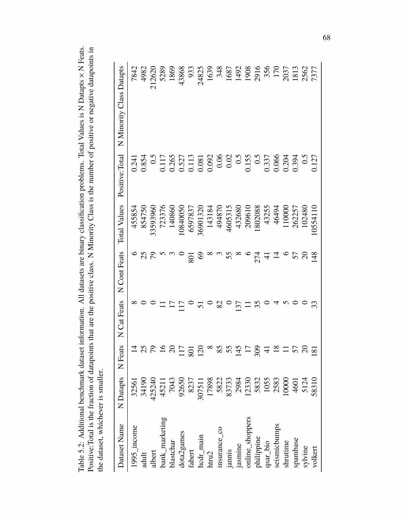
68

Table5.2:

Add

ition

albenchm

arkdatasetinformation.

Alldatasetsarebinary

classifi

catio

nprob

lems.

TotalV

aluesisN

Datapts×NFeats.

Positive:To

talisthe

fractionof

datapointsthatarethepositiveclass.

NMinority

Classisthe

numbero

fpositive

ornegativ

edatapointsin

thedataset,whichever

issm

aller.

DatasetNam

eNDatapts

NFeats

NCatFeats

NCon

tFeats

TotalV

alues

Positiv

e:To

tal

NMinority

Class

Datapts

1995

_incom

e32

561

148

645

5854

0.24

178

42adult

3419

025

025

8547

500.85

449

82albert

4252

4079

079

3359

3960

0.5

2126

20bank

_marketin

g45

211

1611

572

3376

0.11

752

89blastchar

7043

2017

314

0860

0.26

518

69do

ta2gam

es92

650

117

117

010

8400

500.52

743

868

fabert

8237

801

080

165

9783

70.11

393

3hcdr_m

ain

3075

1112

051

6936

9013

200.08

124

825

htru2

1789

88

08

1431

840.09

216

39insurance_co

5822

8582

349

4870

0.06

348

jann

is83

733

550

5546

0531

50.02

1687

jasm

ine

2984

145

137

843

2680

0.5

1492

onlin

e_shop

pers

1233

017

116

2096

100.15

519

08ph

ilipp

ine

5832

309

3527

418

0208

80.5

2916

qsar_b

io10

5541

041

4325

50.33

735

6seismicbu

mps

2583

184

1446

494

0.06

617

0shrutim

e10

000

115

611

0000

0.20

420

37spam

base

4601

570

5726

2257

0.39

418

13sylvine

5124

200

2010

2480

0.5

2562

volkert

5831

018

133

148

1055

4110

0.12

773

77

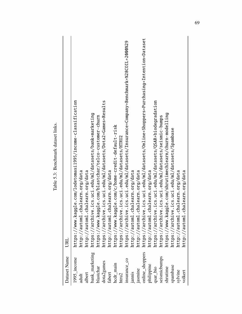
69

Table5.3:

Benchmarkdatasetlinks.

DatasetNam

eURL

1995

_incom

ehttps://www.kaggle.com/lodetomasi1995/income-classification

adult

http://automl.chalearn.org/data

albert

http://automl.chalearn.org/data

bank

_marketin

ghttps://archive.ics.uci.edu/ml/datasets/bank+marketing

blastchar

https://www.kaggle.com/blastchar/telco-customer-churn

dota2gam

eshttps://archive.ics.uci.edu/ml/datasets/Dota2+Games+Results

fabert

http://automl.chalearn.org/data

hcdr_m

ain

https://www.kaggle.com/c/home-credit-default-risk

htru2

https://archive.ics.uci.edu/ml/datasets/HTRU2

insurance_co

https://archive.ics.uci.edu/ml/datasets/Insurance+Company+Benchmark+%28COIL+2000%29

jann

ishttp://automl.chalearn.org/data

jasm

ine

http://automl.chalearn.org/data

onlin

e_shop

pershttps://archive.ics.uci.edu/ml/datasets/Online+Shoppers+Purchasing+Intention+Dataset

philipp

ine

http://automl.chalearn.org/data

qsar_b

iohttps://archive.ics.uci.edu/ml/datasets/QSAR+biodegradation

seismicbu

mps

https://archive.ics.uci.edu/ml/datasets/seismic-bumps

shrutim

ehttps://www.kaggle.com/shrutimechlearn/churn-modelling

spam

base

https://archive.ics.uci.edu/ml/datasets/Spambase

sylvine

http://automl.chalearn.org/data

volkert

http://automl.chalearn.org/data

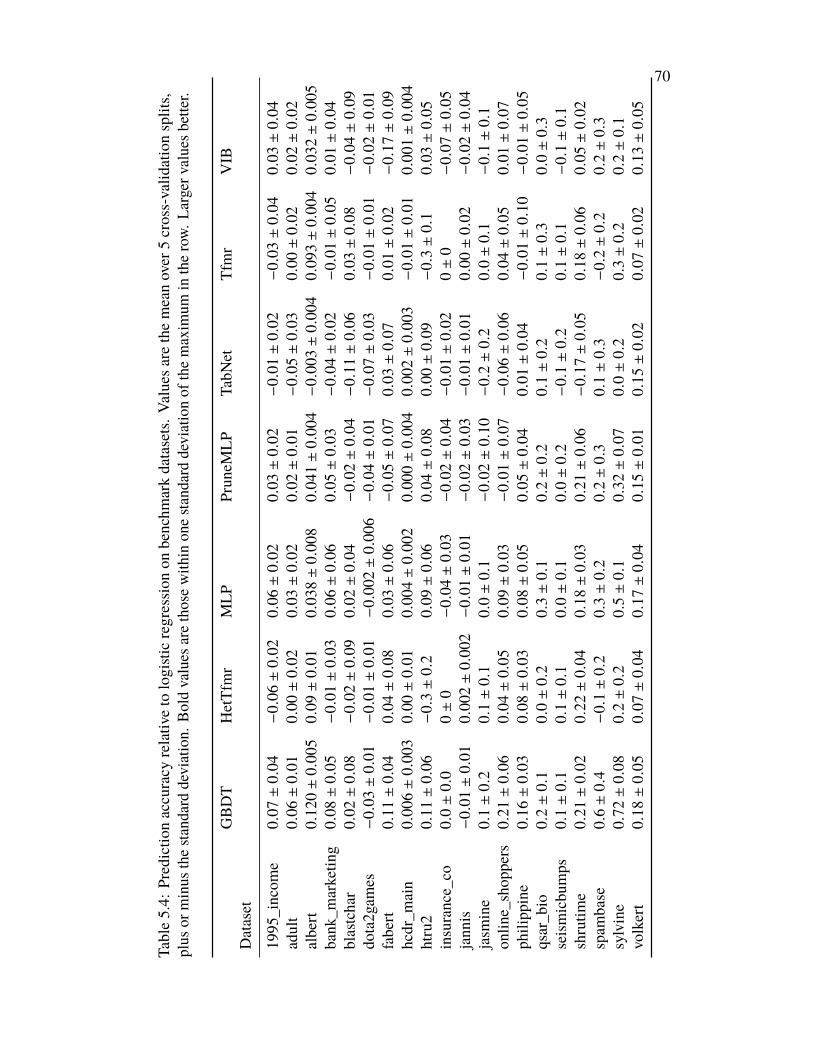
70

Table5.4:

Predictio

naccuracy

relativ

eto

logisticregression

onbenchm

arkdatasets.V

aluesa

rethemeanover

5cross-valid

ationsplits,

plus

orminus

thesta

ndarddeviation.

Bold

values

arethosewith

inon

esta

ndarddeviationof

themaxim

umin

therow.

Larger

values

bette

r.

GBDT

HetTfmr

MLP

Prun

eMLP

TabN

etTfmr

VIB

Dataset

1995

_incom

e0.

07±

0.04

−0.0

6±

0.02

0.06±

0.02

0.03±

0.02

−0.0

1±

0.02

−0.0

3±

0.04

0.03±

0.04

adult

0.06±

0.01

0.00±

0.02

0.03±

0.02

0.02±

0.01

−0.0

5±

0.03

0.00±

0.02

0.02±

0.02

albert

0.12

0±

0.00

50.

09±

0.01

0.03

8±

0.00

80.

041±

0.00

4−0.0

03±

0.00

40.

093±

0.00

40.

032±

0.00

5bank

_marketin

g0.

08±

0.05

−0.0

1±

0.03

0.06±

0.06

0.05±

0.03

−0.0

4±

0.02

−0.0

1±

0.05

0.01±

0.04

blastchar

0.02±

0.08

−0.0

2±

0.09

0.02±

0.04

−0.0

2±

0.04

−0.1

1±

0.06

0.03±

0.08

−0.0

4±

0.09

dota2gam

es−0.0

3±

0.01

−0.0

1±

0.01

−0.0

02±

0.00

6−0.0

4±

0.01

−0.0

7±

0.03

−0.0

1±

0.01

−0.0

2±

0.01

fabert

0.11±

0.04

0.04±

0.08

0.03±

0.06

−0.0

5±

0.07

0.03±

0.07

0.01±

0.02

−0.1

7±

0.09

hcdr_m

ain

0.00

6±

0.00

30.

00±

0.01

0.00

4±

0.00

20.

000±

0.00

40.

002±

0.00

3−0.0

1±

0.01

0.00

1±

0.00

4htru2

0.11±

0.06

−0.3±

0.2

0.09±

0.06

0.04±

0.08

0.00±

0.09

−0.3±

0.1

0.03±

0.05

insurance_co

0.0±

0.0

0±

0−0.0

4±

0.03

−0.0

2±

0.04

−0.0

1±

0.02

0±

0−0.0

7±

0.05

jann

is−0.0

1±

0.01

0.00

2±

0.00

2−0.0

1±

0.01

−0.0

2±

0.03

−0.0

1±

0.01

0.00±

0.02

−0.0

2±

0.04

jasm

ine

0.1±

0.2

0.1±

0.1

0.0±

0.1

−0.0

2±

0.10

−0.2±

0.2

0.0±

0.1

−0.1±

0.1

onlin

e_shop

pers

0.21±

0.06

0.04±

0.05

0.09±

0.03

−0.0

1±

0.07

−0.0

6±

0.06

0.04±

0.05

0.01±

0.07

philipp

ine

0.16±

0.03

0.08±

0.03

0.08±

0.05

0.05±

0.04

0.01±

0.04

−0.0

1±

0.10

−0.0

1±

0.05

qsar_b

io0.

2±

0.1

0.0±

0.2

0.3±

0.1

0.2±

0.2

0.1±

0.2

0.1±

0.3

0.0±

0.3

seismicbu

mps

0.1±

0.1

0.1±

0.1

0.0±

0.1

0.0±

0.2

−0.1±

0.2

0.1±

0.1

−0.1±

0.1

shrutim

e0.

21±

0.02

0.22±

0.04

0.18±

0.03

0.21±

0.06

−0.1

7±

0.05

0.18±

0.06

0.05±

0.02

spam

base

0.6±

0.4

−0.1±

0.2

0.3±

0.2

0.2±

0.3

0.1±

0.3

−0.2±

0.2

0.2±

0.3

sylvine

0.72±

0.08

0.2±

0.2

0.5±

0.1

0.32±

0.07

0.0±

0.2

0.3±

0.2

0.2±

0.1

volkert

0.18±

0.05

0.07±

0.04

0.17±

0.04

0.15±

0.01

0.15±

0.02

0.07±

0.02

0.13±

0.05

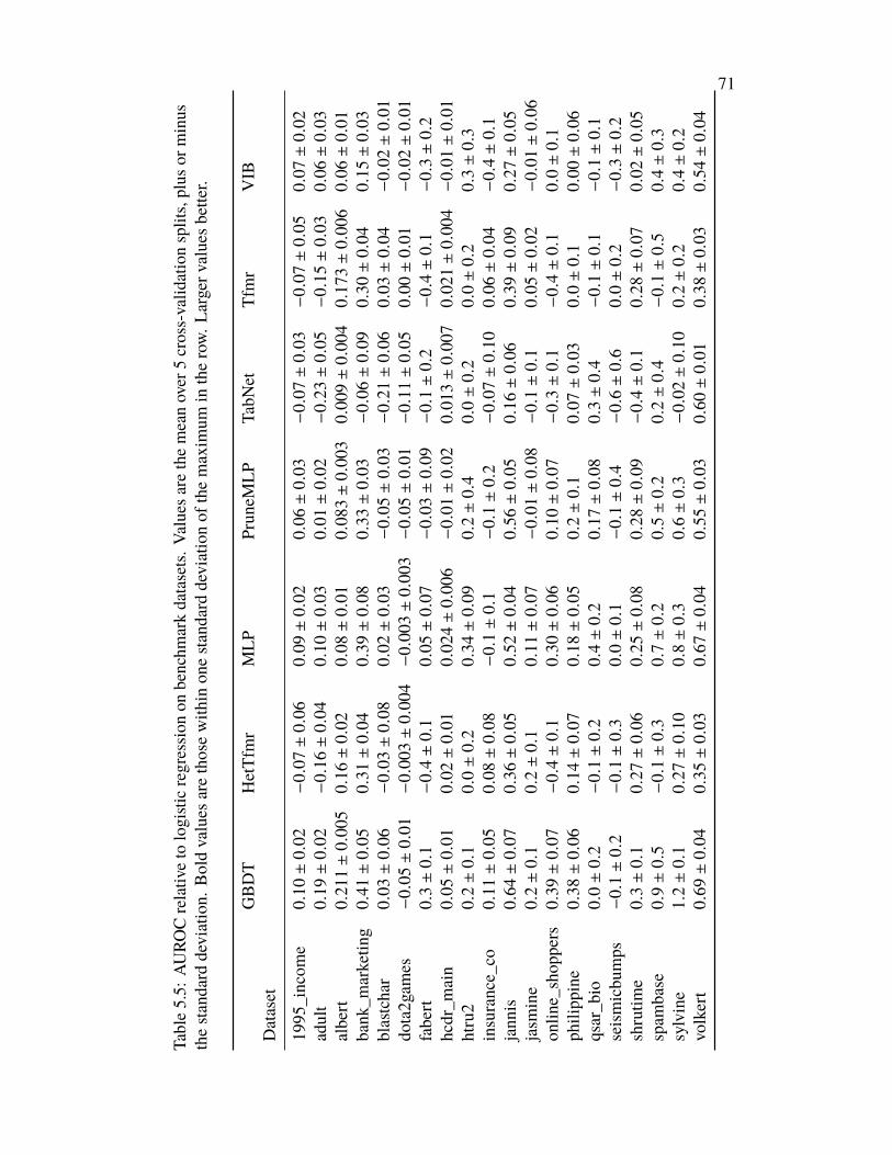
71

Table5.5:

AURO

Crelativ

eto

logisticregressio

non

benchm

arkdatasets.

Values

arethemeanover

5cross-valid

ationsplits,plus

orminus

thesta

ndarddeviation.

Boldvalues

arethosewith

inon

esta

ndarddeviationof

themaxim

umin

therow.

Larger

values

bette

r.

GBDT

HetTfmr

MLP

Prun

eMLP

TabN

etTfmr

VIB

Dataset

1995

_incom

e0.

10±

0.02

−0.0

7±

0.06

0.09±

0.02

0.06±

0.03

−0.0

7±

0.03

−0.0

7±

0.05

0.07±

0.02

adult

0.19±

0.02

−0.1

6±

0.04

0.10±

0.03

0.01±

0.02

−0.2

3±

0.05

−0.1

5±

0.03

0.06±

0.03

albert

0.21

1±

0.00

50.

16±

0.02

0.08±

0.01

0.08

3±

0.00

30.

009±

0.00

40.

173±

0.00

60.

06±

0.01

bank

_marketin

g0.

41±

0.05

0.31±

0.04

0.39±

0.08

0.33±

0.03

−0.0

6±

0.09

0.30±

0.04

0.15±

0.03

blastchar

0.03±

0.06

−0.0

3±

0.08

0.02±

0.03

−0.0

5±

0.03

−0.2

1±

0.06

0.03±

0.04

−0.0

2±

0.01

dota2gam

es−0.0

5±

0.01

−0.0

03±

0.00

4−0.0

03±

0.00

3−0.0

5±

0.01

−0.1

1±

0.05

0.00±

0.01

−0.0

2±

0.01

fabert

0.3±

0.1

−0.4±

0.1

0.05±

0.07

−0.0

3±

0.09

−0.1±

0.2

−0.4±

0.1

−0.3±

0.2

hcdr_m

ain

0.05±

0.01

0.02±

0.01

0.02

4±

0.00

6−0.0

1±

0.02

0.01

3±

0.00

70.

021±

0.00

4−0.0

1±

0.01

htru2

0.2±

0.1

0.0±

0.2

0.34±

0.09

0.2±

0.4

0.0±

0.2

0.0±

0.2

0.3±

0.3

insurance_co

0.11±

0.05

0.08±

0.08

−0.1±

0.1

−0.1±

0.2

−0.0

7±

0.10

0.06±

0.04

−0.4±

0.1

jann

is0.

64±

0.07

0.36±

0.05

0.52±

0.04

0.56±

0.05

0.16±

0.06

0.39±

0.09

0.27±

0.05

jasm

ine

0.2±

0.1

0.2±

0.1

0.11±

0.07

−0.0

1±

0.08

−0.1±

0.1

0.05±

0.02

−0.0

1±

0.06

onlin

e_shop

pers

0.39±

0.07

−0.4±

0.1

0.30±

0.06

0.10±

0.07

−0.3±

0.1

−0.4±

0.1

0.0±

0.1

philipp

ine

0.38±

0.06

0.14±

0.07

0.18±

0.05

0.2±

0.1

0.07±

0.03

0.0±

0.1

0.00±

0.06

qsar_b

io0.

0±

0.2

−0.1±

0.2

0.4±

0.2

0.17±

0.08

0.3±

0.4

−0.1±

0.1

−0.1±

0.1

seismicbu

mps

−0.1±

0.2

−0.1±

0.3

0.0±

0.1

−0.1±

0.4

−0.6±

0.6

0.0±

0.2

−0.3±

0.2

shrutim

e0.

3±

0.1

0.27±

0.06

0.25±

0.08

0.28±

0.09

−0.4±

0.1

0.28±

0.07

0.02±

0.05

spam

base

0.9±

0.5

−0.1±

0.3

0.7±

0.2

0.5±

0.2

0.2±

0.4

−0.1±

0.5

0.4±

0.3

sylvine

1.2±

0.1

0.27±

0.10

0.8±

0.3

0.6±

0.3

−0.0

2±

0.10

0.2±

0.2

0.4±

0.2

volkert

0.69±

0.04

0.35±

0.03

0.67±

0.04

0.55±

0.03

0.60±

0.01

0.38±

0.03

0.54±

0.04

72

arXiv: 1807.00906. url: http://arxiv.org/abs/1807.00906 (visitedon 01/09/2019).

Alemi, Alexander A., Ian Fischer, Joshua V. Dillon, and KevinMurphy (2017). “DeepVariational Information Bottleneck”. In: International Conference on LearningRepresentations abs/1612.00410. url: https://arxiv.org/abs/1612.00410.

Arik, Sercan O and Tomas Pfister (2019). “TabNet: Attentive Interpretable TabularLearning”. In: arXiv preprint arXiv:1908.07442. url: https://arxiv.org/abs/1908.07442.

Caron, Mathilde et al. (2019). “Unsupervised Pre-Training of Image Features onNon-Curated Data”. In: arXiv:1905.01278 [cs]. arXiv: 1905.01278. url: http://arxiv.org/abs/1905.01278 (visited on 02/23/2020).

Chapelle, Olivier, Bernhard Scholkopf, andAlexander Zien (2009). “Semi-supervisedlearning)”. In: IEEE Transactions on Neural Networks 20.3, pp. 542–542.

Cheng, Heng-Tze et al. (2016). “Wide & deep learning for recommender systems”.In: Proceedings of the 1st workshop on deep learning for recommender systems,pp. 7–10.

Clark, Kevin et al. (2020). “ELECTRA: Pre-training Text Encoders as DiscriminatorsRather Than Generators”. In: International Conference on Learning Representa-tions. url: https://openreview.net/forum?id=r1xMH1BtvB.

De Brébisson, Alexandre et al. (2015). “Artificial Neural Networks Applied to TaxiDestination Prediction”. In: Proceedings of the 2015th International Conferenceon ECML PKDD Discovery Challenge - Volume 1526. ECMLPKDDDC’15. Porto,Portugal: CEUR-WS.org, pp. 40–51.

Devlin, Jacob et al. (2019). “BERT: Pre-training of Deep Bidirectional Transformersfor Language Understanding”. In: NAACL-HLT.

Dua, Dheeru and Casey Graff (2017). UCI Machine Learning Repository. url:http://archive.ics.uci.edu/ml.

Elezi, Ismail et al. (2018). “Transductive label augmentation for improved deepnetwork learning”. In: 2018 24th International Conference on Pattern Recognition(ICPR). IEEE, pp. 1432–1437.

Goldbloom, Anthony (2017).What Kaggle has learned from almost a million datascientists - Anthony Goldbloom (Kaggle). url: https://www.youtube.com/watch?v=jmHbS8z57yI&feature=youtu.be.

Guo, Huifeng et al. (2018). “DeepFM: An End-to-EndWide &Deep Learning Frame-work for CTR Prediction”. en. In: arXiv:1804.04950 [cs, stat]. arXiv: 1804.04950.url: http://arxiv.org/abs/1804.04950 (visited on 02/08/2020).

73

Guyon, Isabelle et al. (2019). “Analysis of the AutoML Challenge series 2015-2018”. In: AutoML. Springer series on Challenges in Machine Learning. url:https://www.automl.org/wp-content/uploads/2018/09/chapter10-challenge.pdf.

Hassibi, Babak et al. (1993). “Optimal Brain Surgeon: Extensions and PerformanceComparisons”. In: Proceedings of the 6th International Conference on NeuralInformation Processing Systems. NIPS’93. Denver, Colorado: Morgan KaufmannPublishers Inc., pp. 263–270.

Howard, Jeremy et al. (2018). FastAI. https://github.com/fastai/fastai.

Howard, Jeremy and Sebastian Ruder (2018). “Universal language model fine-tuningfor text classification”. In: arXiv preprint arXiv:1801.06146.

Jahrer, Michael (2018). Porto Seguro’s Safe Driver Prediction. en. url: https://kaggle.com/c/porto-seguro-safe-driver-prediction (visited on02/24/2020).

Ke, Guolin, Qi Meng, et al. (2017). “LightGBM: A highly efficient gradient boostingdecision tree”. In: Advances in Neural Information Processing Systems, pp. 3146–3154. url: https://papers.nips.cc/paper/6907-lightgbm-a-highly-efficient-gradient-boosting-decision-tree.pdf.

Ke, Guolin, Jia Zhang, et al. (2019). TabNN: A Universal Neural Network Solutionfor Tabular Data. url: https://openreview.net/forum?id=r1eJssCqY7.

Klambauer, Günter et al. (2017). “Self-normalizing neural networks”. In: Advancesin neural information processing systems, pp. 971–980.

Li, Zeyu et al. (2020). “Interpretable Click-Through Rate Prediction through Hi-erarchical Attention”. en. In: Proceedings of the 13th International Confer-ence on Web Search and Data Mining. Houston TX USA: ACM, pp. 313–321. isbn: 978-1-4503-6822-3. doi: 10.1145/3336191.3371785. url: http://dl.acm.org/doi/10.1145/3336191.3371785 (visited on 02/08/2020).

Loshchilov, Ilya and Frank Hutter (2017). “DecoupledWeight Decay Regularization”.In: International Conference on Learning Representations. url: https://arxiv.org/abs/1711.05101.

Mocanu, Decebal Constantin et al. (2018). “Scalable training of artificial neuralnetworks with adaptive sparse connectivity inspired by network science”. In:Nature Communications.

Morcos, Ari S. et al. (2019). “One ticket to win them all: generalizing lottery ticketinitializations across datasets and optimizers”. en. In: arXiv:1906.02773 [cs, stat].arXiv: 1906.02773. url: http://arxiv.org/abs/1906.02773 (visited on01/15/2020).

Murshed, M. G. Sarwar et al. (2019). “Machine Learning at the Network Edge:A Survey”. In: url: https://arxiv.org/abs/1908.00080v2 (visited on02/24/2020).

74

Oliver, Avital et al. (2018). “Realistic evaluation of deep semi-supervised learningalgorithms”. In: Advances in Neural Information Processing Systems, pp. 3235–3246.

Paszke, Adam et al. (2019). “PyTorch: An Imperative Style, High-Performance DeepLearning Library”. In: Advances in Neural Information Processing Systems 32.Ed. by H. Wallach et al. Curran Associates, Inc., pp. 8024–8035. url: http://papers.neurips.cc/paper/9015-pytorch-an-imperative-style-high-performance-deep-learning-library.pdf.

Schneider, Johannes and Michail Vlachos (2019). “Mass Personalization of DeepLearning”. en. In: url: https://arxiv.org/abs/1909.02803v2 (visited on02/24/2020).

Song, Weiping et al. (2019). “AutoInt: Automatic Feature Interaction Learningvia Self-Attentive Neural Networks”. en. In: Proceedings of the 28th ACMInternational Conference on Information and Knowledge Management - CIKM’19. arXiv: 1810.11921, pp. 1161–1170. doi: 10.1145/3357384.3357925. url:http://arxiv.org/abs/1810.11921 (visited on 02/08/2020).

Stretcu, Otilia et al. (2019). “Graph Agreement Models for Semi-Supervised Learn-ing”. In:Advances in Neural Information Processing Systems 32. CurranAssociates,Inc., pp. 8713–8723. url: http://papers.nips.cc/paper/9076-graph-agreement-models-for-semi-supervised-learning.pdf.

Strouse, Daniel and David J. Schwab (2015). “The Deterministic InformationBottleneck”. In: Neural Computation 29, pp. 1611–1630. url: https://arxiv.org/abs/1604.00268.

Sun, Qiang et al. (2019). “DeepEnFM: Deep neural networks with Encoder enhancedFactorization Machine”. In: url: https://openreview.net/forum?id=SJlyta4YPS (visited on 02/15/2020).

Tanha, Jafar, Maarten van Someren, and Hamideh Afsarmanesh (2017). “Semi-supervised self-training for decision tree classifiers”. In: International Journal ofMachine Learning and Cybernetics 8, pp. 355–370.

Tishby, Naftali, Fernando C. Pereira, and William Bialek (2000). “The informationbottleneck method”. In: arXiv:physics/0004057. arXiv: physics/0004057. url:http://arxiv.org/abs/physics/0004057 (visited on 12/11/2018).

Vaswani, Ashish et al. (2017). “Attention is all you need”. In: Advances in neuralinformation processing systems, pp. 5998–6008.

Wang, Ruoxi et al. (2017). “Deep & Cross Network for Ad Click Predictions”. In:ADKDD@KDD.

Xiao, Jun et al. (2017). “Attentional Factorization Machines: Learning the Weightof Feature Interactions via Attention Networks”. en. In: Proceedings of theTwenty-Sixth International Joint Conference on Artificial Intelligence. Melbourne,

75

Australia: International Joint Conferences on Artificial Intelligence Organiza-tion, pp. 3119–3125. isbn: 978-0-9992411-0-3. doi: 10.24963/ijcai.2017/435. url: https://www.ijcai.org/proceedings/2017/435 (visited on02/08/2020).

Yang, Yongxin, Irene Garcia Morillo, and Timothy M Hospedales (2018). “Deepneural decision trees”. In: arXiv preprint arXiv:1806.06988.

76

C h a p t e r 6

MINIMAL ACHIEVABLE SUFFICIENT STATISTIC LEARNING:ADDRESSING ISSUES IN THE INFORMATION BOTTLENECK

6.1 IntroductionThe representation learning approach to machine learning focuses on finding arepresentation Z of an input random variable X that is useful for predicting a randomvariable Y (Goodfellow, Y. Bengio, and Courville, 2016).

What makes a representation Z “useful” is much debated, but a common assertionis that Z should be a minimal sufficient statistic of X for Y (Adragni, Kofi P. andCook, R. Dennis, 2009; Shamir, Sabato, and Tishby, 2010; James, Mahoney, andCrutchfield, 2017; Achille and Soatto, 2018b). That is:

1. Z should be a statistic of X . This means Z = f (X) for some function f .

2. Z should be sufficient for Y . This means p(X |Z,Y ) = p(X |Z).

3. Given that Z is a sufficient statistic, it should be minimal with respect to X .This means for any measurable, non-invertible function g, g(Z) is no longersufficient for Y .1

In other words: a minimal sufficient statistic is a random variable Z that tellsyou everything about Y you could ever care about, but if you do any irreversibleprocessing to Z , you are guaranteed to lose some information about Y . Sucha representation would be extremely desirable in machine learning, as it would(essentially by definition) preclude overfitting by excluding any information notrelevant to the task.

Minimal sufficient statistics have a long history in the field of statistics (Lehmann andScheffe, 1950; Dynkin, 1951). But the minimality condition (3, above) is perhapstoo strong to be useful in machine learning, since it is a statement about any functiong, rather than about functions in a practical hypothesis class like the class of deepneural networks. As we will discuss below, this strictness erodes the mathematical

1This is not the most common phrasing of statistical minimality, but we feel it is more under-standable. For the equivalence of this phrasing and the standard definition see Section 6.8.

77

justification for the popular Information Bottleneck method (Tishby, Pereira, andBialek, 2000).

Instead, in this chapter we consider minimal achievable sufficient statistics: sufficientstatistics that are minimal among some particular set of functions.

Definition 1 (Minimal Achievable Sufficient Statistic). Let Z = f (X) be a sufficientstatistic of X for Y . Z is minimal achievable with respect to a set of functions F iff ∈ F and for any Lipschitz continuous, non-invertible function g where g ◦ f ∈ F,g(Z) is no longer sufficient for Y .

In this chapterwe introduceConservedDifferential Information (CDI), an information-theoretic quantity that, unlike mutual information, is meaningful for deterministically-dependent continuous random variables, such as the input and output of a deepnetwork. We also introduce Minimal Achievable Sufficient Statistic Learning(MASS Learning), a training objective based on CDI for finding minimal achievablesufficient statistics that achieves competitive performance on supervised learningand uncertainty quantification benchmarks.

6.2 Conserved Differential InformationBefore we present MASS Learning, we need to introduce Conserved DifferentialInformation (CDI), on which MASS Learning is based.

CDI is an information-theoretic quantity that addresses an oft-cited issue in machinelearning (Bell and Sejnowski, 1995; Amjad and Geiger, 2018; Saxe et al., 2018; Nash,Kushman, and Williams, 2018; Goldfeld et al., 2018), which is that for a continuousrandom variable X and a continuous, non-constant function f , the mutual informationI(X, f (X)) is infinite. (See Section 6.8 for details.) This makes I(X, f (X)) unsuitablefor use in a learning objective when f is, for example, a standard deep network.

The infinitude of I(X, f (X)) has been circumvented in prior works by two strategies.One is to discretize X and f (X) (Tishby and Zaslavsky, 2015; Shwartz-Ziv andTishby, 2017), though this is controversial (Saxe et al., 2018). Another is to use arandom variable Z with distribution p(Z |X) as the representation of X rather thanusing f (X) itself as the representation (Alemi, Fischer, Dillon, and Murphy, 2017;Kolchinsky, Tracey, and Wolpert, 2017; Achille and Soatto, 2018b). In this latterapproach, p(Z |X) is usually implemented by adding noise to a deep network thattakes X as input.

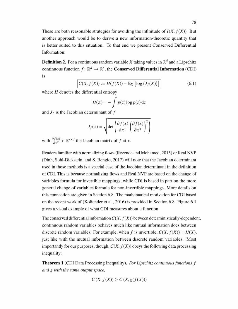
78

These are both reasonable strategies for avoiding the infinitude of I(X, f (X)). Butanother approach would be to derive a new information-theoretic quantity thatis better suited to this situation. To that end we present Conserved DifferentialInformation:

Definition 2. For a continuous random variable X taking values inRd and a Lipschitzcontinuous function f : Rd → Rr , the Conserved Differential Information (CDI)is

C(X, f (X)) := H( f (X)) − EX[log

(J f (X)

) ](6.1)

where H denotes the differential entropy

H(Z) = −∫

p(z) log p(z) dz

and J f is the Jacobian determinant of f

J f (x) =

√√√det

(∂ f (x)∂xT

(∂ f (x)∂xT

)T)

with ∂ f (x)∂xT ∈ Rr×d the Jacobian matrix of f at x.

Readers familiar with normalizing flows (Rezende andMohamed, 2015) or Real NVP(Dinh, Sohl-Dickstein, and S. Bengio, 2017) will note that the Jacobian determinantused in those methods is a special case of the Jacobian determinant in the definitionof CDI. This is because normalizing flows and Real NVP are based on the change ofvariables formula for invertible mappings, while CDI is based in part on the moregeneral change of variables formula for non-invertible mappings. More details onthis connection are given in Section 6.8. The mathematical motivation for CDI basedon the recent work of (Koliander et al., 2016) is provided in Section 6.8. Figure 6.1gives a visual example of what CDI measures about a function.

The conserved differential informationC(X, f (X)) between deterministically-dependent,continuous random variables behaves much like mutual information does betweendiscrete random variables. For example, when f is invertible, C(X, f (X)) = H(X),just like with the mutual information between discrete random variables. Mostimportantly for our purposes, though, C(X, f (X)) obeys the following data processinginequality:

Theorem 1 (CDI Data Processing Inequality). For Lipschitz continuous functions f

and g with the same output space,

C (X, f (X)) ≥ C (X, g( f (X)))

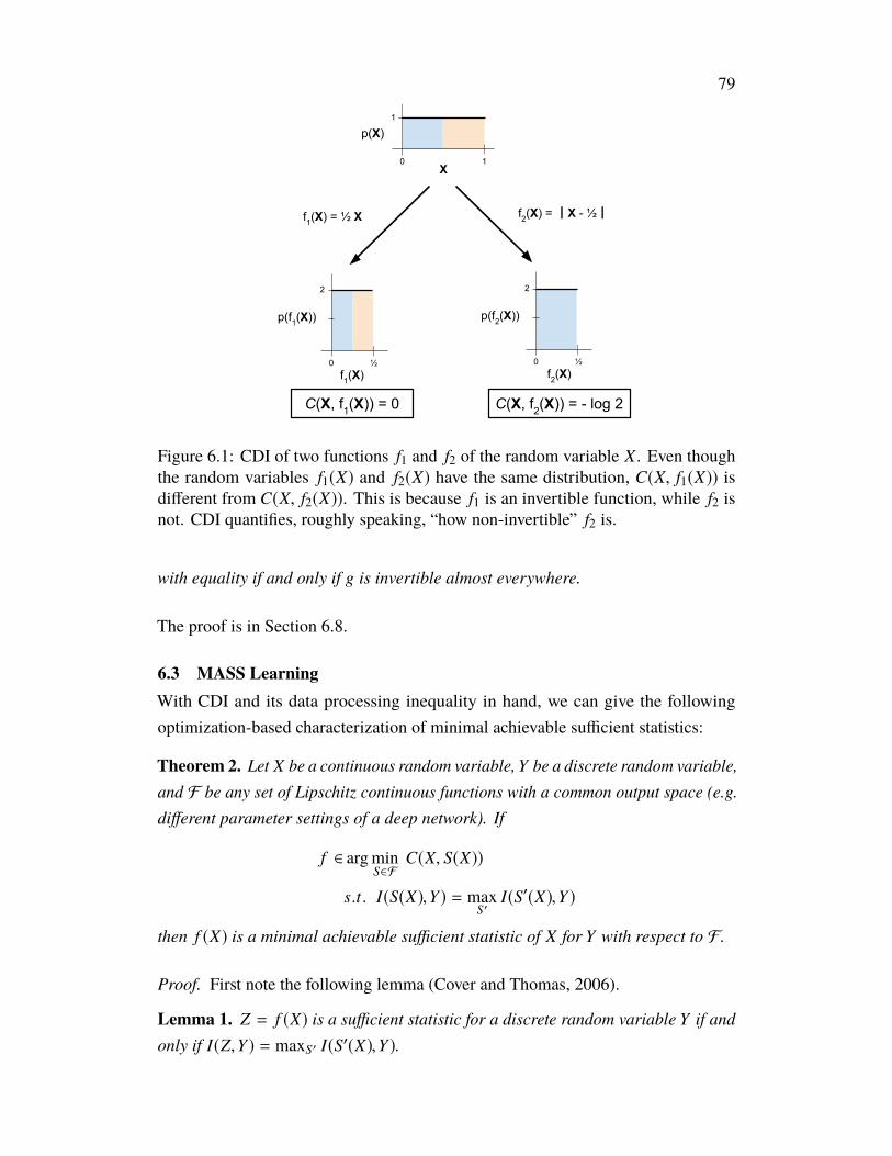
79

0 1

1

X

p(X)

0 ½

2

f1(X)

p(f1(X))

f1(X) = ½ X f2(X) = ┃X - ½┃

0 ½

2

f2(X)

p(f2(X))

C(X, f1(X)) = 0 C(X, f2(X)) = - log 2

Figure 6.1: CDI of two functions f1 and f2 of the random variable X . Even thoughthe random variables f1(X) and f2(X) have the same distribution, C(X, f1(X)) isdifferent from C(X, f2(X)). This is because f1 is an invertible function, while f2 isnot. CDI quantifies, roughly speaking, “how non-invertible” f2 is.

with equality if and only if g is invertible almost everywhere.

The proof is in Section 6.8.

6.3 MASS LearningWith CDI and its data processing inequality in hand, we can give the followingoptimization-based characterization of minimal achievable sufficient statistics:

Theorem 2. Let X be a continuous random variable,Y be a discrete random variable,and F be any set of Lipschitz continuous functions with a common output space (e.g.different parameter settings of a deep network). If

f ∈ arg minS∈F

C(X, S(X))

s.t. I(S(X),Y ) = maxS′

I(S′(X),Y )

then f (X) is a minimal achievable sufficient statistic of X for Y with respect to F.

Proof. First note the following lemma (Cover and Thomas, 2006).

Lemma 1. Z = f (X) is a sufficient statistic for a discrete random variable Y if andonly if I(Z,Y ) = maxS′ I(S′(X),Y ).

80

Lemma 1 guarantees that any f satisfying the conditions in Theorem 2 is sufficient.Suppose such an f was not minimal achievable. Then by Definition 1 there wouldexist a non-invertible, Lipschitz continuous g such that g( f (X)) was sufficient. Butby Theorem 1, it would then also be the case that C(X, g( f (X))) < C(X, f (X)),which would contradict f minimizing C(X, S(X)). �

We can turn Theorem 2 into a learning objective over functions f by relaxing thestrict constraint into a Lagrangian formulation with Lagrange multiplier 1/β forβ > 0:

C(X, f (X)) − 1β

I( f (X),Y )

The larger the value of β, the more our objective will encourage minimality oversufficiency. We can then simplify this formulation using the identity I( f (X),Y ) =H(Y ) − H(Y | f (X)), which gives us the following optimization objective:

LM ASS( f ) := H(Y | f (X)) + βH( f (X))− βEX[log J f (X)].

(6.2)

We refer to minimizing this objective asMASS Learning.

Practical implementationIn practice, we are interested in using MASS Learning to train a deep network fθwith parameters θ using a finite dataset {(xi, yi)}Ni=1 of N datapoints sampled fromthe joint distribution p(x, y) of X and Y . To do this, we introduce a parameterizedvariational approximation qφ( fθ(x)|y) ≈ p( fθ(x)|y). Using qφ, we minimize thefollowing empirical upper bound to LM ASS:

LM ASS ≤ LM ASS(θ, φ) :=1N

N∑i=1− log qφ(yi | fθ(xi))

− β log qφ( fθ(xi))− β log J fθ (xi),

where the quantity qφ( fθ(xi)) is computed as∑

y qφ( fθ(xi)|y)p(y) and the quantityqφ(yi | fθ(xi)) is computed with Bayes rule as qφ( fθ (xi)|yi)p(yi)∑

y qφ( fθ (xi)|y)p(y) . When Y is discreteand takes on finitely many values, as in classification problems, and when we choosea variational distribution qφ that is differentiable with respect to φ (e.g. a multivariateGaussian), then we can minimize LM ASS(θ, φ) using stochastic gradient descent(SGD).

81

To perform classification using our trained network, we use the learned variationaldistribution qφ and Bayes rule:

p(yi |xi) ≈ p(yi | fθ(xi)) ≈qφ( fθ(xi)|yi)p(yi)∑y qφ( fθ(xi)|y)p(y)

.

Computing the J fθ term in LM ASS for every sample in an SGD minibatch is tooexpensive to be practical. For fθ : Rd → Rr , doing so would require on the order of r

times more operations than in standard training of deep networks by, since computingthe J fθ term involves computing the full Jacobian matrix of the network, which, inour implementation, involves performing r backpropagations. Thus to make trainingtractable, we use a subsampling strategy: we estimate the J fθ term using only a 1/rfraction of the datapoints in a minibatch. In practice, we have found this subsamplingstrategy to not noticeably alter the numerical value of the J fθ term during training.

Subsampling for the J fθ term results in a significant training speedup, but it mustnevertheless be emphasized that, even with subsampling, our implementation ofMASS Learning is roughly eight times as slow as standard deep network training.(Unless β = 0, in which case the speed is the same.) This is by far the mostsignificant drawback of (our implementation of) MASS Learning. There are manyeasier-to-compute upper bounds or estimates of J fθ that one could use to makeMASS Learning faster, and one could also potentially find non-invertible networkarchitectures which admit more efficiently computable Jacobians, but we do notexplore these options.

6.4 Related WorkConnection to the Information BottleneckThe well-studied Information Bottleneck learning method (Tishby, Pereira, andBialek, 2000; Tishby and Zaslavsky, 2015; Strouse and Schwab, 2015; Alemi,Fischer, Dillon, and Murphy, 2017; Saxe et al., 2018; Amjad and Geiger, 2018;Goldfeld et al., 2018; Kolchinsky, Tracey, and Van Kuyk, 2019; Achille and Soatto,2018b; Achille and Soatto, 2018a) is based on minimizing the Information BottleneckLagrangian

LIB(Z) := βI(X, Z) − I(Y, Z)

for β > 0, where Z is the representation whose conditional distribution p(Z |X) oneis trying to learn.

The LIB learning objective can be motivated based on pure information-theoreticelegance. But some works like (Shamir, Sabato, and Tishby, 2010) also point out

82

the connection between the LIB objective and minimal sufficient statistics, which isbased on the following theorem:

Theorem 3. Let X be a discrete random variable drawn according to a distributionp(X |Y ) determined by the discrete random variableY . LetF be the set of deterministicfunctions of X to any target space. Then f (X) is a minimal sufficient statistic of X

for Y if and only if

f ∈ arg minS∈F

I(X, S(X))

s.t . I(S(X),Y ) = maxS′∈F

I(S′(X),Y ).

The LIB objective can then be thought of as a Lagrangian relaxation of the optimiza-tion problem in this theorem.

Theorem 3 only holds for discrete random variables. For continuous X it holdsonly in the reverse direction, so minimizing LIB for continuous X has no formalconnection to finding minimal sufficient statistics, not to mention minimal achievablesufficient statistics. See Section 6.8 for details.

Nevertheless, the optimization problems in Theorem 2 and Theorem 3 are extremelysimilar, relying as they both do on Lemma 1 for their proofs. And the idea ofrelaxing the optimization problem in Theorem 2 into a Lagrangian formulation to getLM ASS is directly inspired by the Information Bottleneck. So while MASS Learningand Information Bottleneck learning entail different network architectures and lossfunctions, there is an Information Bottleneck flavor to MASS Learning.

Jacobian RegularizationThe presence of the J fθ term in LM ASS is reminiscent of contrastive autoencoders(Rifai et al., 2011) and Jacobian Regularization (Sokolic et al., 2017; Ross and Doshi-Velez, 2018; Varga, Csiszárik, and Zombori, 2017; “Sensitivity and Generalizationin Neural Networks” 2018; Jakubovitz and Giryes, 2018). Both these techniques arebased on the notion that minimizing EX[‖D f (X)‖F], where D f (x) = ∂ f (x)

∂xT ∈ Rr×d isthe Jacobian matrix, improves generalization and adversarial robustness.

This may seem paradoxical at first, since by applying the AM-GM inequality to the

83

eigenvalues of D f (x)D f (x)T we have

EX[‖D f (X)‖2rF ] = EX[Tr(D f (X)D f (X)T)r]≥ EX[rr det(D f (X)D f (X)T)]= EX[rr J f (X)2]≥ logEX[rr J f (X)2]≥ 2EX[log J f (X)] + r log r

and EX[log J f (X)] is being maximized by LM ASS. So LM ASS might seem to beoptimizing for worse generalization according to the Jacobian regularization literature.However, the entropy term in LM ASS strongly encourages minimizing EX[‖D f (X)‖F].So overall LM ASS seems to be seeking the right balance of sensitivity (dependent onthe value of β) in the network to its inputs, which is precisely in alignment with whatthe Jacobian regularization literature suggests.

6.5 ExperimentsIn this section we compare MASS Learning to other approaches for training deepnetworks. Code to reproduce all experiments is available online.2 Full details on allexperiments is in Section 6.8.

We use the abbreviation “SoftmaxCE” to refer to the standard approach of trainingdeep networks for classification problems by minimizing the softmax cross entropyloss

LSo f tmaxCE (θ) := − 1N

N∑i=1

(log softmax( fθ(xi))yi

)where softmax( fθ(xi))yi is the yith element of the softmax function applied to theoutputs fθ(xi) of the network’s last linear layer. As usual, softmax( fθ(xi))yi is takento be the network’s estimate of p(yi |xi).

We also compare against the Variational Information Bottleneck method (Alemi,Fischer, Dillon, and Murphy, 2017) for representation learning, which we abbreviateas “VIB”.

We use two networks in our experiments. “SmallMLP” is a feedforward networkwith two fully-connected layers of 400 and 200 hidden units, respectively, both withelu nonlinearities (Clevert, Unterthiner, and Hochreiter, 2015). “ResNet20” is the20-layer residual network of (He et al., 2016).

2https://github.com/mwcvitkovic/MASS-Learning

84

We performed all experiments on the CIFAR-10 dataset (Krizhevsky, 2009) to ensureconsistency with previously published results and implemented all experiments usingPyTorch (Paszke et al., 2017).

Classification Accuracy and RegularizationWe first confirm that networks trained by MASS Learning can make accuratepredictions in supervised learning tasks. We compare the classification accuracyof networks trained on varying amounts of data to see the extent to which MASSLearning regularizes networks.

Classification accuracies for the SmallMLP network are shown in Table 6.1, and forthe ResNet20 network in Table 6.2. For the SmallMLP network, MASS Learningperforms slightly worse than SoftmaxCE and VIB training. For the larger ResNet20network, MASS Learning performs equivalently to the other methods. It is notablethat with the ResNet20 network VIB and MASS Learning both perform well whenβ = 0, and neither perform significantly better than SoftmaxCE. This may be becausethe hyperparameters used in training the ResNet20 network, which were taken directlyfrom the original paper (He et al., 2016), are specifically tuned for SoftmaxCEtraining and are more sensitive to the specifics of the network architecture than to theloss function.

Uncertainty QuantificationWe also evaluate the ability of networks trained by MASS Learning to properlyquantify their uncertainty about their predictions. We assess uncertainty quantificationin two ways: using proper scoring rules (Lakshminarayanan, Pritzel, and Blundell,2017), which are scalar measures of how well a network’s predictive distributionp(y | fθ(x)) is calibrated, and by assessing performance on an out-of-distribution(OOD) detection task.

Tables 6.3 through 6.8 show the uncertainty quantification performance of networksaccording to two proper scoring rules: the Negative Log Likelihood (NLL) and theBrier Score. The entropy and test accuracy of the predictive distributions are alsogiven, for reference.

For the SmallMLP network in Tables 6.3, 6.4, and 6.5, VIB provides the bestcombination of high accuracy and low NLL and Brier score across all sizes oftraining set, despite SoftmaxCE with weight decay achieving the best scoring rulevalues. For the larger ResNet20 network in Tables 6.6 and 6.7, MASS Learning

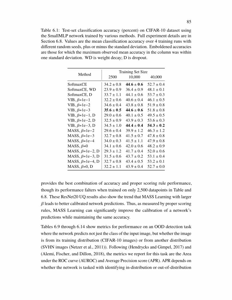
85

Table 6.1: Test-set classification accuracy (percent) on CIFAR-10 dataset usingthe SmallMLP network trained by various methods. Full experiment details are inSection 6.8. Values are the mean classification accuracy over 4 training runs withdifferent random seeds, plus or minus the standard deviation. Emboldened accuraciesare those for which the maximum observed mean accuracy in the column was withinone standard deviation. WD is weight decay; D is dropout.

Method Training Set Size2500 10,000 40,000

SoftmaxCE 34.2 ± 0.8 44.6 ± 0.6 52.7 ± 0.4SoftmaxCE, WD 23.9 ± 0.9 36.4 ± 0.9 48.1 ± 0.1SoftmaxCE, D 33.7 ± 1.1 44.1 ± 0.6 53.7 ± 0.3VIB, β=1e−1 32.2 ± 0.6 40.6 ± 0.4 46.1 ± 0.5VIB, β=1e−2 34.6 ± 0.4 43.8 ± 0.8 51.9 ± 0.8VIB, β=1e−3 35.6 ± 0.5 44.6 ± 0.6 51.8 ± 0.8VIB, β=1e−1, D 29.0 ± 0.6 40.1 ± 0.5 49.5 ± 0.5VIB, β=1e−2, D 32.5 ± 0.9 43.9 ± 0.3 53.6 ± 0.3VIB, β=1e−3, D 34.5 ± 1.0 44.4 ± 0.4 54.3 ± 0.2MASS, β=1e−2 29.6 ± 0.4 39.9 ± 1.2 46.3 ± 1.2MASS, β=1e−3 32.7 ± 0.8 41.5 ± 0.7 47.8 ± 0.8MASS, β=1e−4 34.0 ± 0.3 41.5 ± 1.1 47.9 ± 0.8MASS, β=0 34.1 ± 0.6 42.0 ± 0.6 48.2 ± 0.9MASS, β=1e−2, D 29.3 ± 1.2 41.7 ± 0.4 52.0 ± 0.6MASS, β=1e−3, D 31.5 ± 0.6 43.7 ± 0.2 53.1 ± 0.4MASS, β=1e−4, D 32.7 ± 0.8 43.4 ± 0.5 53.2 ± 0.1MASS, β=0, D 32.2 ± 1.1 43.9 ± 0.4 52.7 ± 0.0

provides the best combination of accuracy and proper scoring rule performance,though its performance falters when trained on only 2,500 datapoints in Table and6.8. These ResNet20 UQ results also show the trend that MASS Learning with largerβ leads to better calibrated network predictions. Thus, as measured by proper scoringrules, MASS Learning can significantly improve the calibration of a network’spredictions while maintaining the same accuracy.

Tables 6.9 through 6.14 show metrics for performance on an OOD detection taskwhere the network predicts not just the class of the input image, but whether the imageis from its training distribution (CIFAR-10 images) or from another distribution(SVHN images (Netzer et al., 2011)). Following (Hendrycks and Gimpel, 2017) and(Alemi, Fischer, and Dillon, 2018), the metrics we report for this task are the Areaunder the ROC curve (AUROC) and Average Precision score (APR). APR depends onwhether the network is tasked with identifying in-distribution or out-of-distribution

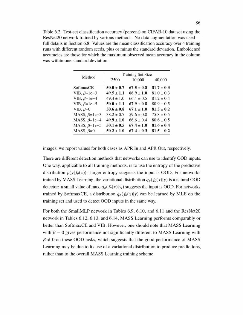
86

Table 6.2: Test-set classification accuracy (percent) on CIFAR-10 dataset using theResNet20 network trained by various methods. No data augmentation was used —full details in Section 6.8. Values are the mean classification accuracy over 4 trainingruns with different random seeds, plus or minus the standard deviation. Emboldenedaccuracies are those for which the maximum observed mean accuracy in the columnwas within one standard deviation.

Method Training Set Size2500 10,000 40,000

SoftmaxCE 50.0 ± 0.7 67.5 ± 0.8 81.7 ± 0.3VIB, β=1e−3 49.5 ± 1.1 66.9 ± 1.0 81.0 ± 0.3VIB, β=1e−4 49.4 ± 1.0 66.4 ± 0.5 81.2 ± 0.4VIB, β=1e−5 50.0 ± 1.1 67.9 ± 0.8 80.9 ± 0.5VIB, β=0 50.6 ± 0.8 67.1 ± 1.0 81.5 ± 0.2MASS, β=1e−3 38.2 ± 0.7 59.6 ± 0.8 75.8 ± 0.5MASS, β=1e−4 49.9 ± 1.0 66.6 ± 0.4 80.6 ± 0.5MASS, β=1e−5 50.1 ± 0.5 67.4 ± 1.0 81.6 ± 0.4MASS, β=0 50.2 ± 1.0 67.4 ± 0.3 81.5 ± 0.2

images; we report values for both cases as APR In and APR Out, respectively.

There are different detection methods that networks can use to identify OOD inputs.One way, applicable to all training methods, is to use the entropy of the predictivedistribution p(y | fθ(x)): larger entropy suggests the input is OOD. For networkstrained by MASS Learning, the variational distribution qφ( fθ(x)|y) is a natural OODdetector: a small value of maxi qφ( fθ(x)|yi) suggests the input is OOD. For networkstrained by SoftmaxCE, a distribution qφ( fθ(x)|y) can be learned by MLE on thetraining set and used to detect OOD inputs in the same way.

For both the SmallMLP network in Tables 6.9, 6.10, and 6.11 and the ResNet20network in Tables 6.12, 6.13, and 6.14, MASS Learning performs comparably orbetter than SoftmaxCE and VIB. However, one should note that MASS Learningwith β = 0 gives performance not significantly different to MASS Learning withβ , 0 on these OOD tasks, which suggests that the good performance of MASSLearning may be due to its use of a variational distribution to produce predictions,rather than to the overall MASS Learning training scheme.

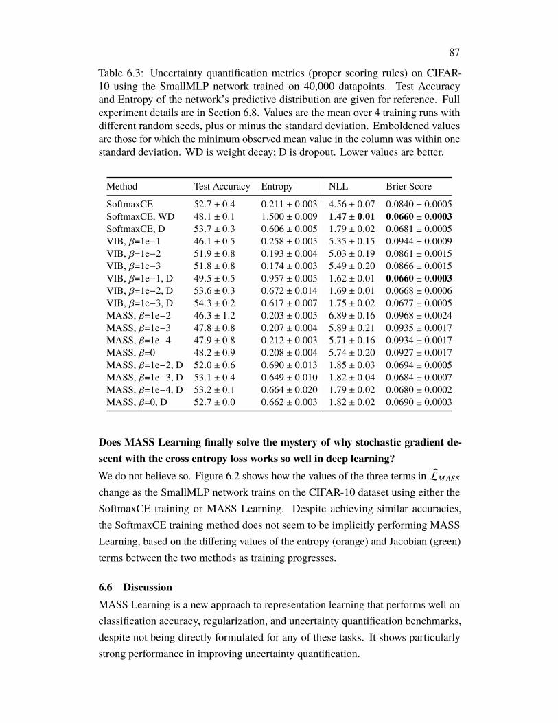
87

Table 6.3: Uncertainty quantification metrics (proper scoring rules) on CIFAR-10 using the SmallMLP network trained on 40,000 datapoints. Test Accuracyand Entropy of the network’s predictive distribution are given for reference. Fullexperiment details are in Section 6.8. Values are the mean over 4 training runs withdifferent random seeds, plus or minus the standard deviation. Emboldened valuesare those for which the minimum observed mean value in the column was within onestandard deviation. WD is weight decay; D is dropout. Lower values are better.

Method Test Accuracy Entropy NLL Brier Score

SoftmaxCE 52.7 ± 0.4 0.211 ± 0.003 4.56 ± 0.07 0.0840 ± 0.0005SoftmaxCE, WD 48.1 ± 0.1 1.500 ± 0.009 1.47 ± 0.01 0.0660 ± 0.0003SoftmaxCE, D 53.7 ± 0.3 0.606 ± 0.005 1.79 ± 0.02 0.0681 ± 0.0005VIB, β=1e−1 46.1 ± 0.5 0.258 ± 0.005 5.35 ± 0.15 0.0944 ± 0.0009VIB, β=1e−2 51.9 ± 0.8 0.193 ± 0.004 5.03 ± 0.19 0.0861 ± 0.0015VIB, β=1e−3 51.8 ± 0.8 0.174 ± 0.003 5.49 ± 0.20 0.0866 ± 0.0015VIB, β=1e−1, D 49.5 ± 0.5 0.957 ± 0.005 1.62 ± 0.01 0.0660 ± 0.0003VIB, β=1e−2, D 53.6 ± 0.3 0.672 ± 0.014 1.69 ± 0.01 0.0668 ± 0.0006VIB, β=1e−3, D 54.3 ± 0.2 0.617 ± 0.007 1.75 ± 0.02 0.0677 ± 0.0005MASS, β=1e−2 46.3 ± 1.2 0.203 ± 0.005 6.89 ± 0.16 0.0968 ± 0.0024MASS, β=1e−3 47.8 ± 0.8 0.207 ± 0.004 5.89 ± 0.21 0.0935 ± 0.0017MASS, β=1e−4 47.9 ± 0.8 0.212 ± 0.003 5.71 ± 0.16 0.0934 ± 0.0017MASS, β=0 48.2 ± 0.9 0.208 ± 0.004 5.74 ± 0.20 0.0927 ± 0.0017MASS, β=1e−2, D 52.0 ± 0.6 0.690 ± 0.013 1.85 ± 0.03 0.0694 ± 0.0005MASS, β=1e−3, D 53.1 ± 0.4 0.649 ± 0.010 1.82 ± 0.04 0.0684 ± 0.0007MASS, β=1e−4, D 53.2 ± 0.1 0.664 ± 0.020 1.79 ± 0.02 0.0680 ± 0.0002MASS, β=0, D 52.7 ± 0.0 0.662 ± 0.003 1.82 ± 0.02 0.0690 ± 0.0003

Does MASS Learning finally solve the mystery of why stochastic gradient de-scent with the cross entropy loss works so well in deep learning?We do not believe so. Figure 6.2 shows how the values of the three terms in LM ASS

change as the SmallMLP network trains on the CIFAR-10 dataset using either theSoftmaxCE training or MASS Learning. Despite achieving similar accuracies,the SoftmaxCE training method does not seem to be implicitly performing MASSLearning, based on the differing values of the entropy (orange) and Jacobian (green)terms between the two methods as training progresses.

6.6 DiscussionMASS Learning is a new approach to representation learning that performs well onclassification accuracy, regularization, and uncertainty quantification benchmarks,despite not being directly formulated for any of these tasks. It shows particularlystrong performance in improving uncertainty quantification.

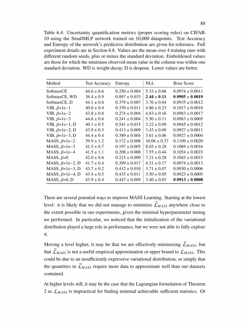
88

Table 6.4: Uncertainty quantification metrics (proper scoring rules) on CIFAR-10 using the SmallMLP network trained on 10,000 datapoints. Test Accuracyand Entropy of the network’s predictive distribution are given for reference. Fullexperiment details are in Section 6.8. Values are the mean over 4 training runs withdifferent random seeds, plus or minus the standard deviation. Emboldened valuesare those for which the minimum observed mean value in the column was within onestandard deviation. WD is weight decay; D is dropout. Lower values are better.

Method Test Accuracy Entropy NLL Brier Score

SoftmaxCE 44.6 ± 0.6 0.250 ± 0.004 5.33 ± 0.06 0.0974 ± 0.0011SoftmaxCE, WD 36.4 ± 0.9 0.897 ± 0.033 2.44 ± 0.11 0.0905 ± 0.0019SoftmaxCE, D 44.1 ± 0.6 0.379 ± 0.007 3.76 ± 0.04 0.0935 ± 0.0012VIB, β=1e−1 40.6 ± 0.4 0.339 ± 0.011 4.86 ± 0.23 0.1017 ± 0.0016VIB, β=1e−2 43.8 ± 0.8 0.274 ± 0.004 4.83 ± 0.16 0.0983 ± 0.0017VIB, β=1e−3 44.6 ± 0.6 0.241 ± 0.004 5.50 ± 0.11 0.0983 ± 0.0005VIB, β=1e−1, D 40.1 ± 0.5 0.541 ± 0.015 3.22 ± 0.09 0.0945 ± 0.0012VIB, β=1e−2, D 43.9 ± 0.3 0.413 ± 0.009 3.43 ± 0.09 0.0927 ± 0.0011VIB, β=1e−3, D 44.4 ± 0.4 0.389 ± 0.004 3.61 ± 0.06 0.0927 ± 0.0004MASS, β=1e−2 39.9 ± 1.2 0.172 ± 0.008 10.06 ± 0.37 0.1109 ± 0.0020MASS, β=1e−3 41.5 ± 0.7 0.197 ± 0.005 8.03 ± 0.28 0.1069 ± 0.0016MASS, β=1e−4 41.5 ± 1.1 0.208 ± 0.008 7.55 ± 0.44 0.1054 ± 0.0023MASS, β=0 42.0 ± 0.6 0.215 ± 0.009 7.21 ± 0.28 0.1043 ± 0.0015MASS, β=1e−2, D 41.7 ± 0.4 0.399 ± 0.017 4.21 ± 0.17 0.0974 ± 0.0013MASS, β=1e−3, D 43.7 ± 0.2 0.412 ± 0.010 3.71 ± 0.07 0.0930 ± 0.0006MASS, β=1e−4, D 43.4 ± 0.5 0.435 ± 0.011 3.50 ± 0.05 0.0923 ± 0.0005MASS, β=0, D 43.9 ± 0.4 0.447 ± 0.009 3.40 ± 0.03 0.0913 ± 0.0008

There are several potential ways to improve MASS Learning. Starting at the lowestlevel: it is likely that we did not manage to minimize LM ASS anywhere close tothe extent possible in our experiments, given the minimal hyperparameter tuningwe performed. In particular, we noticed that the initialization of the variationaldistribution played a large role in performance, but we were not able to fully exploreit.

Moving a level higher, it may be that we are effectively minimizing LM ASS, butthat LM ASS is not a useful empirical approximation or upper bound to LM ASS. Thiscould be due to an insufficiently expressive variational distribution, or simply thatthe quantities in LM ASS require more data to approximate well than our datasetscontained.

At higher levels still, it may be the case that the Lagrangian formulation of Theorem2 as LM ASS is impractical for finding minimal achievable sufficient statistics. Or

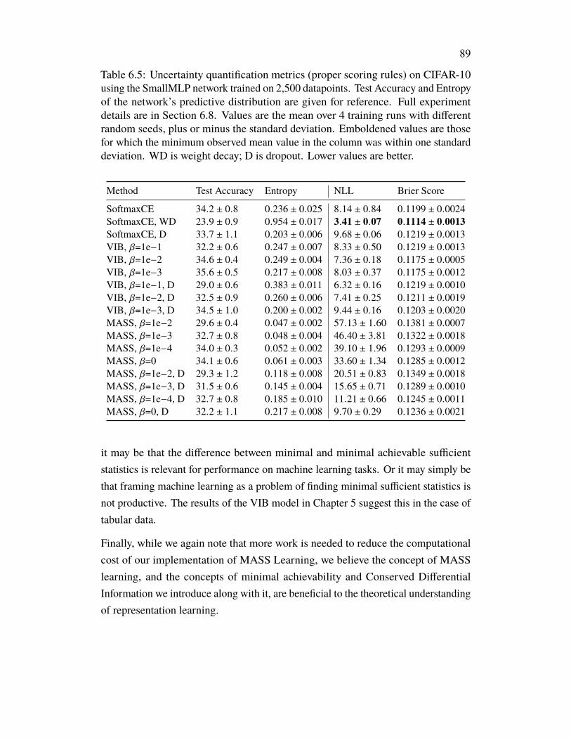
89

Table 6.5: Uncertainty quantification metrics (proper scoring rules) on CIFAR-10using the SmallMLP network trained on 2,500 datapoints. Test Accuracy and Entropyof the network’s predictive distribution are given for reference. Full experimentdetails are in Section 6.8. Values are the mean over 4 training runs with differentrandom seeds, plus or minus the standard deviation. Emboldened values are thosefor which the minimum observed mean value in the column was within one standarddeviation. WD is weight decay; D is dropout. Lower values are better.

Method Test Accuracy Entropy NLL Brier Score

SoftmaxCE 34.2 ± 0.8 0.236 ± 0.025 8.14 ± 0.84 0.1199 ± 0.0024SoftmaxCE, WD 23.9 ± 0.9 0.954 ± 0.017 3.41 ± 0.07 0.1114 ± 0.0013SoftmaxCE, D 33.7 ± 1.1 0.203 ± 0.006 9.68 ± 0.06 0.1219 ± 0.0013VIB, β=1e−1 32.2 ± 0.6 0.247 ± 0.007 8.33 ± 0.50 0.1219 ± 0.0013VIB, β=1e−2 34.6 ± 0.4 0.249 ± 0.004 7.36 ± 0.18 0.1175 ± 0.0005VIB, β=1e−3 35.6 ± 0.5 0.217 ± 0.008 8.03 ± 0.37 0.1175 ± 0.0012VIB, β=1e−1, D 29.0 ± 0.6 0.383 ± 0.011 6.32 ± 0.16 0.1219 ± 0.0010VIB, β=1e−2, D 32.5 ± 0.9 0.260 ± 0.006 7.41 ± 0.25 0.1211 ± 0.0019VIB, β=1e−3, D 34.5 ± 1.0 0.200 ± 0.002 9.44 ± 0.16 0.1203 ± 0.0020MASS, β=1e−2 29.6 ± 0.4 0.047 ± 0.002 57.13 ± 1.60 0.1381 ± 0.0007MASS, β=1e−3 32.7 ± 0.8 0.048 ± 0.004 46.40 ± 3.81 0.1322 ± 0.0018MASS, β=1e−4 34.0 ± 0.3 0.052 ± 0.002 39.10 ± 1.96 0.1293 ± 0.0009MASS, β=0 34.1 ± 0.6 0.061 ± 0.003 33.60 ± 1.34 0.1285 ± 0.0012MASS, β=1e−2, D 29.3 ± 1.2 0.118 ± 0.008 20.51 ± 0.83 0.1349 ± 0.0018MASS, β=1e−3, D 31.5 ± 0.6 0.145 ± 0.004 15.65 ± 0.71 0.1289 ± 0.0010MASS, β=1e−4, D 32.7 ± 0.8 0.185 ± 0.010 11.21 ± 0.66 0.1245 ± 0.0011MASS, β=0, D 32.2 ± 1.1 0.217 ± 0.008 9.70 ± 0.29 0.1236 ± 0.0021

it may be that the difference between minimal and minimal achievable sufficientstatistics is relevant for performance on machine learning tasks. Or it may simply bethat framing machine learning as a problem of finding minimal sufficient statistics isnot productive. The results of the VIB model in Chapter 5 suggest this in the case oftabular data.

Finally, while we again note that more work is needed to reduce the computationalcost of our implementation of MASS Learning, we believe the concept of MASSlearning, and the concepts of minimal achievability and Conserved DifferentialInformation we introduce along with it, are beneficial to the theoretical understandingof representation learning.

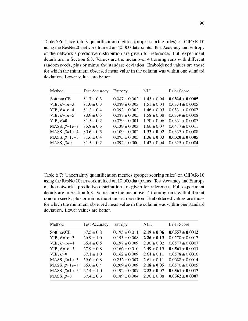
90

Table 6.6: Uncertainty quantification metrics (proper scoring rules) on CIFAR-10using the ResNet20 network trained on 40,000 datapoints. Test Accuracy and Entropyof the network’s predictive distribution are given for reference. Full experimentdetails are in Section 6.8. Values are the mean over 4 training runs with differentrandom seeds, plus or minus the standard deviation. Emboldened values are thosefor which the minimum observed mean value in the column was within one standarddeviation. Lower values are better.

Method Test Accuracy Entropy NLL Brier Score

SoftmaxCE 81.7 ± 0.3 0.087 ± 0.002 1.45 ± 0.04 0.0324 ± 0.0005VIB, β=1e−3 81.0 ± 0.3 0.089 ± 0.003 1.51 ± 0.04 0.0334 ± 0.0005VIB, β=1e−4 81.2 ± 0.4 0.092 ± 0.002 1.46 ± 0.05 0.0331 ± 0.0007VIB, β=1e−5 80.9 ± 0.5 0.087 ± 0.005 1.58 ± 0.08 0.0339 ± 0.0008VIB, β=0 81.5 ± 0.2 0.079 ± 0.001 1.70 ± 0.06 0.0331 ± 0.0007MASS, β=1e−3 75.8 ± 0.5 0.139 ± 0.003 1.66 ± 0.07 0.0417 ± 0.0011MASS, β=1e−4 80.6 ± 0.5 0.109 ± 0.002 1.33 ± 0.02 0.0337 ± 0.0008MASS, β=1e−5 81.6 ± 0.4 0.095 ± 0.003 1.36 ± 0.03 0.0320 ± 0.0005MASS, β=0 81.5 ± 0.2 0.092 ± 0.000 1.43 ± 0.04 0.0325 ± 0.0004

Table 6.7: Uncertainty quantification metrics (proper scoring rules) on CIFAR-10using the ResNet20 network trained on 10,000 datapoints. Test Accuracy and Entropyof the network’s predictive distribution are given for reference. Full experimentdetails are in Section 6.8. Values are the mean over 4 training runs with differentrandom seeds, plus or minus the standard deviation. Emboldened values are thosefor which the minimum observed mean value in the column was within one standarddeviation. Lower values are better.

Method Test Accuracy Entropy NLL Brier Score

SoftmaxCE 67.5 ± 0.8 0.195 ± 0.011 2.19 ± 0.06 0.0557 ± 0.0012VIB, β=1e−3 66.9 ± 1.0 0.193 ± 0.008 2.26 ± 0.13 0.0570 ± 0.0017VIB, β=1e−4 66.4 ± 0.5 0.197 ± 0.009 2.30 ± 0.02 0.0577 ± 0.0007VIB, β=1e−5 67.9 ± 0.8 0.166 ± 0.010 2.49 ± 0.13 0.0561 ± 0.0011VIB, β=0 67.1 ± 1.0 0.162 ± 0.009 2.64 ± 0.11 0.0578 ± 0.0016MASS, β=1e−3 59.6 ± 0.8 0.252 ± 0.007 2.61 ± 0.11 0.0688 ± 0.0014MASS, β=1e−4 66.6 ± 0.4 0.209 ± 0.009 2.18 ± 0.05 0.0570 ± 0.0005MASS, β=1e−5 67.4 ± 1.0 0.192 ± 0.007 2.22 ± 0.07 0.0561 ± 0.0017MASS, β=0 67.4 ± 0.3 0.189 ± 0.004 2.30 ± 0.08 0.0562 ± 0.0007

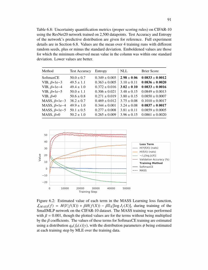
91

Table 6.8: Uncertainty quantification metrics (proper scoring rules) on CIFAR-10using the ResNet20 network trained on 2,500 datapoints. Test Accuracy and Entropyof the network’s predictive distribution are given for reference. Full experimentdetails are in Section 6.8. Values are the mean over 4 training runs with differentrandom seeds, plus or minus the standard deviation. Emboldened values are thosefor which the minimum observed mean value in the column was within one standarddeviation. Lower values are better.

Method Test Accuracy Entropy NLL Brier Score

SoftmaxCE 50.0 ± 0.7 0.349 ± 0.005 2.98 ± 0.06 0.0833 ± 0.0012VIB, β=1e−3 49.5 ± 1.1 0.363 ± 0.005 3.10 ± 0.11 0.0836 ± 0.0020VIB, β=1e−4 49.4 ± 1.0 0.372 ± 0.016 3.02 ± 0.10 0.0833 ± 0.0016VIB, β=1e−5 50.0 ± 1.1 0.306 ± 0.021 3.48 ± 0.15 0.0849 ± 0.0013VIB, β=0 50.6 ± 0.8 0.271 ± 0.019 3.80 ± 0.15 0.0850 ± 0.0007MASS, β=1e−3 38.2 ± 0.7 0.469 ± 0.012 3.75 ± 0.08 0.1010 ± 0.0017MASS, β=1e−4 49.9 ± 1.0 0.344 ± 0.001 3.24 ± 0.08 0.0837 ± 0.0017MASS, β=1e−5 50.1 ± 0.5 0.277 ± 0.008 3.81 ± 0.11 0.0859 ± 0.0005MASS, β=0 50.2 ± 1.0 0.265 ± 0.009 3.96 ± 0.15 0.0861 ± 0.0020

Figure 6.2: Estimated value of each term in the MASS Learning loss function,LM ASS( f ) = H(Y | f (X)) + βH( f (X)) − βEX[log J f (X)], during training of theSmallMLP network on the CIFAR-10 dataset. The MASS training was performedwith β = 0.001, though the plotted values are for the terms without being multipliedby the β coefficients. The values of these terms for SoftmaxCE training are estimatedusing a distribution qφ( fθ(x)|y), with the distribution parameters φ being estimatedat each training step by MLE over the training data.

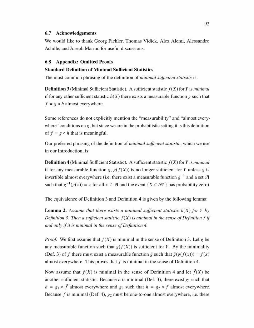
92

6.7 AcknowledgementsWe would like to thank Georg Pichler, Thomas Vidick, Alex Alemi, AlessandroAchille, and Joseph Marino for useful discussions.

6.8 Appendix: Omitted ProofsStandard Definition of Minimal Sufficient StatisticsThe most common phrasing of the definition of minimal sufficient statistic is:

Definition 3 (Minimal Sufficient Statistic). A sufficient statistic f (X) forY isminimalif for any other sufficient statistic h(X) there exists a measurable function g such thatf = g ◦ h almost everywhere.

Some references do not explicitly mention the “measurability” and “almost every-where” conditions on g, but since we are in the probabilistic setting it is this definitionof f = g ◦ h that is meaningful.

Our preferred phrasing of the definition of minimal sufficient statistic, which we usein our Introduction, is:

Definition 4 (Minimal Sufficient Statistic). A sufficient statistic f (X) forY isminimalif for any measurable function g, g( f (X)) is no longer sufficient for Y unless g isinvertible almost everywhere (i.e. there exist a measurable function g−1 and a set Asuch that g−1(g(x)) = x for all x ∈ A and the event {X ∈ Ac} has probability zero).

The equivalence of Definition 3 and Definition 4 is given by the following lemma:

Lemma 2. Assume that there exists a minimal sufficient statistic h(X) for Y byDefinition 3. Then a sufficient statistic f (X) is minimal in the sense of Definition 3 ifand only if it is minimal in the sense of Definition 4.

Proof. We first assume that f (X) is minimal in the sense of Definition 3. Let g beany measurable function such that g( f (X)) is sufficient for Y . By the minimality(Def. 3) of f there must exist a measurable function g such that g(g( f (x))) = f (x)almost everywhere. This proves that f is minimal in the sense of Definition 4.

Now assume that f (X) is minimal in the sense of Definition 4 and let f (X) beanother sufficient statistic. Because h is minimal (Def. 3), there exist g1 such thath = g1 ◦ f almost everywhere and g2 such that h = g2 ◦ f almost everywhere.Because f is minimal (Def. 4), g2 must be one-to-one almost everywhere, i.e. there

93

exists a g2 such that g2 ◦ h = g2 ◦ g2 ◦ f = f almost everywhere. In turn, we obtainthat g2 ◦ g1 ◦ f = f almost everywhere, and since f was arbitrary this proves theminimality of f in the sense of Definition 3. �

The Mutual Information Between the Input and Output of a Deep Network isInfiniteTypically the mutual information between continuous random variables X and Y isgiven by

I(X,Y ) =∫

p(x, y) logp(x, y)

p(x)p(y)dxdy,

but this quantity is only defined when the joint density p(x, y) is integrable, whichit is not in the case that Y = f (X). (The technical term for p(x, y) in this case is a“singular distribution”.) Instead, to compute I(X, f (X)) we must refer to the “masterdefinition” of mutual information (Cover and Thomas, 2006), which is

I(X,Y ) = supP,Q

I([X]P, [Y ]Q), (6.3)

where P and Q are finite partitions of the range of X and Y , respectively, and [X]Pis the random variable obtained by quantizing X using partition P, and analogouslyfor [Y ]Q .

From this definition, we can prove the following Lemma:

Lemma 3. If X and Y are continuous random variables, and there are open sets OX

and OY in the support of X and Y , respectively, such that y = f (x) for x ∈ OX andy ∈ OY , then I(X,Y ) = ∞.

This includes all X and Y where Y = f (X) for an f that is continuous somewhere onits domain, e.g. any deep network (considered as a function from an input vector toan output vector).

Proof. Suppose X and Y satisfy the conditions of the lemma. Let OX and OY beopen sets with f (OX) = OY and P[X ∈ OX] =: δ > 0, which exist by the lemma’sassumptions. Then let Pn

OYbe a partition of OY into n disjoint sets. Because Y is

continuous and hence does not have any atoms, we may assume that the probability ofY belonging to each element of Pn

OYis equal to the same nonzero value δ/n. Denote

by PnOX

the partition of OX into n disjoint sets, where each set in PnOX

is the preimageof one of the sets in Pn

OY. We can construct partitions of the whole domains of X and

94

Y as PnOX∪Oc

X and PnOY∪Oc

Y , respectively. Using these partitions in equation 6.3,we obtain

I(X,Y )

≥ (1 − δ) log(1 − δ) +∑

A∈[X]PnOX

P[X ∈ A,Y ∈ f (A)] logP[X ∈ A,Y ∈ f (A)]P[X ∈ A]P[Y ∈ f (A)]

= (1 − δ) log(1 − δ) + nδ

nlog

δnδnδn

= (1 − δ) log(1 − δ) + δ lognδ.

By letting n go to infinity, we can see that the supremum in Eq. 6.3 is infinity. �

The Change of Variables Formula for Non-invertible MappingsThe change of variables formula is widely used in machine learning and is key torecent results in density estimation and generative modeling like normalizing flows(Rezende and Mohamed, 2015), NICE (Dinh, Krueger, and Y. Bengio, 2014), andReal NVP (Dinh, Sohl-Dickstein, and S. Bengio, 2017). But all uses of the change ofvariables formula in the machine learning literature that we are aware of use it withrespect to bijective mappings between random variables, despite the formula alsobeing applicable to non-invertible mappings between random variables. To addressthis gap, we offer the following brief tutorial.

The familiar form of the change of variables formula for a random variable X withdensity p(x) and a bijective, differentiable function f : Rd → Rd is∫

Rdp(x)J f (x) dx =

∫Rd

p( f −1(y)) dy. (6.4)

where J f (x) =�� det ∂ f (x)

∂xT

��.A slightly more general phrasing of Equation 6.4 is∫

f −1(B)g(x)J f (x) dx =

∫Bg( f −1(y)) dy. (6.5)

where g : Rd → R is any non-negative measurable function, and B ⊆ Rd is anymeasurable subset of Rd .

We can extend Equation 6.5 to work in the case that f is not invertible. To do this,we must address two issues. First, if f is not invertible, then f −1(y) is not a singlepoint but rather a set. Second, if f is not invertible, then the Jacobian matrix ∂ f (x)

∂xT

95

may not be square, and thus has no well defined determinant. Both issues can beresolved and lead to the following change of variables theorem (Krantz and Parks,2009), which is based on the so-called coarea formula (Federer, 1969).

Theorem 4. Let f : Rd → Rr with r ≤ d be a differentiable function, g : Rd → Ra non-negative measurable function, B ⊆ Rd a measurable set, and J f (x) =√

det(∂ f (x)∂xT

(∂ f (x)∂xT

)T). Then

∫f −1(B)

g(x)J f (x) dx =∫B

∫f −1(y)

g(x) dH d−r(x) dy. (6.6)

where H d−r is the (d − r)-dimensional Hausdorff measure (one can think of this asa measure for lower-dimensional structures in high-dimensional space, e.g. the areaof 2-dimensional surfaces in 3-dimensional space).3

We see in Theorem 4 that Equation 6.6 looks a lot like Equations 6.4 and 6.5, butwith f −1(y) replaced by an integral over the set f −1(y), which for almost every y is a(d − r)-dimensional set. And if f in Equation 6.6 happens to be bijective, Equation6.6 reduces to Equation 6.5.

We also see that the Jacobian determinant in Equation 6.5 was replaced by theso-called r-dimensional Jacobian√√√

det

(∂ f (x)∂xT

(∂ f (x)∂xT

)T)

in Equation 6.6. A word of caution is in order, as the r-dimensional Jacobian doesnot have the same nice properties for concatenated functions as does the Jacobianin the bijective case. In particular, we cannot calculate J f2◦ f1 based on the values

of J f1 and J f2 because the product∂ f2(x)∂xT

∂ f1(x)∂xT

(∂ f2(x)∂xT

∂ f1(x)∂xT

)Tdoes not decompose

into a product of ∂ f2(x)∂xT

(∂ f2(x)∂xT

)Tand ∂ f1(x)

∂xT

(∂ f1(x)∂xT

)T. In other words, the trick used

in techniques like normalizing flows and NICE to compute determinants of deepnetworks for use in the change of variables formula by decomposing the network’sJacobian into the product of layerwise Jacobians does not work straightforwardly inthe case of non-invertible mappings.

3In what follows, we will sometimes replace g by g/Jf such that the Jacobian appears on theright-hand side. Furthermore, we will not only use non-negative g. This can be justified by splitting ginto positive and negative parts provided that either part results in a finite integral.

96

Motivation for Conserved Differential InformationFirst, we present an alternative definition of conditional entropy that is meaningfulfor singular distributions (e.g. the joint distribution p(X, f (X)) for a function f ).More information on this definition can be found in (Koliander et al., 2016).

Singular Conditional Entropy

Assume that the random variable X has a probability density function pX(x) on Rd .For a given differentiable function f : Rd → Rr (r ≤ d), we want to analyze theconditional differential entropy H(X | f (X)). Following (Koliander et al., 2016), wedefine this quantity as:

H(X | f (X)) =

−∫Rr

p f (X)(y)∫

f −1(y)θd−rPr{X∈·| f (X)=y}(x) log

(θd−rPr{X∈·| f (X)=y}(x)

)dH d−r(x) dy

(6.7)

where H d−r denotes (d − r)-dimensional Hausdorff measure. The function p f (X) isthe probability density function of the randomvariable f (X). Although θd−r

Pr{X∈·| f (X)=y}can also be interpreted as a probability density, it is not the commonly used densitywith respect to Lebesgue measure (which does not exist for X | f (X) = y) but adensity with respect to a lower-dimensional Hausdorff measure. We will analyze thetwo functions p f (X) and θd−r

Pr{X∈·| f (X)=y} in more detail. The density p f (X) is definedby the relation ∫

f −1(B)pX(x) dx =

∫B

p f (X)(y) dy , (6.8)

which has to hold for every measurable set B ⊆ Rr . Using the coarea formula (orthe related change-of-variables theorem), we see that∫

f −1(B)pX(x) dx =

∫B

∫f −1(y)

pX(x)J f (x)

dH d−r(x) dy , (6.9)

where J f (x) =√

det(∂ f (x)∂xT

(∂ f (x)∂xT

)T)is the r-dimensional Jacobian determinant.

Thus, we identified

p f (X)(y) =∫

f −1(y)

pX(x)J f (x)

dH d−r(x) . (6.10)

The second function, namely θd−rPr{X∈·| f (X)=y}, is the Radon-Nikodym derivative of

the conditional probability Pr{X ∈ ·| f (X) = y} with respect to H d−r restricted

97

to the set where X | f (X) = y has positive probability (in the end, this will bethe set f −1(y)). To understand this function, we have to know something aboutthe conditional distribution of X given f (X). Formally, a (regular) conditionalprobability Pr{X ∈ ·| f (X) = y} has to satisfy three conditions:

• Pr{X ∈ ·| f (X) = y} is a probability measure for each fixed y ∈ Rr .

• Pr{X ∈ A| f (X) = ·} is measurable for each fixed measurable set A ⊆ Rd .

• For measurable sets A ⊆ Rd and B ⊆ Rr , we have

Pr{(X, f (X)) ∈ A × B} =∫BPr{X ∈ A| f (X) = y}p f (X)(y) dy . (6.11)

In our setting, equation 6.11 becomes∫A∩ f −1(B)

pX(x) dx =∫BPr{X ∈ A| f (X) = y}p f (X)(y) dy . (6.12)

Choosing

Pr{X ∈ A| f (X) = y} = 1p f (X)(y)

∫A∩ f −1(y)

pX(x)J f (x)

dH d−r(x) , (6.13)

the right-hand side in equation 6.12 becomes∫BPr{X ∈ A| f (X) = y}p f (X)(y) dy =

∫B

∫A∩ f −1(y)

pX(x)J f (x)

dH d−r(x) dy

=

∫A∩ f −1(B)

pX(x) dx , (6.14)

where the final equality is again an application of the coarea formula. Thus, weidentified

θd−rPr{X∈·| f (X)=y}(x) =

pX(x)J f (x) p f (X)(y)

. (6.15)

Although things might seem complicated up to this point, they simplify signifi-cantly once we put everything together. In particular, inserting equation 6.15 into

98

equation 6.7, we obtain

H(X | f (X))

= −∫Rr

p f (X)(y)∫

f −1(y)

pX(x)J f (x) p f (X)(y)

log(

pX(x)J f (x) p f (X)(y)

)dH d−r(x) dy

= −∫Rr

∫f −1(y)

pX(x)J f (x)

log(

pX(x)J f (x) p f (X)(y)

)dH d−r(x) dy

= −∫Rd

pX(x) log(

pX(x)J f (x) p f (X)( f (x))

)dx (6.16)

= H(X) +∫Rd

pX(x) log(J f (x)p f (X)( f (x))

)dx

= H(X) +∫Rd

pX(x) log(p f (X)( f (x))

)dx +

∫Rd

pX(x) log(J f (x)

)dx

= H(X) +∫Rr

∫f −1(y)

pX(x)J f (x)

log(p f (X)( f (x))

)dH d−r(x) dy + E

[log

(J f (X)

) ](6.17)

= H(X) +∫Rr

∫f −1(y)

pX(x)J f (x)

dH d−r(x) log(p f (X)(y)

)dy + E

[log

(J f (X)

) ]= H(X) +

∫Rr

p f (X)(y) log(p f (X)(y)

)dy + E

[log

(J f (X)

) ]= H(X) − H( f (X)) + E

[log

(J f (X)

) ](6.18)

where equation 6.16 and equation 6.17 hold by the coarea formula.

So, altogether we have that for a random variable X and a function f , the singularconditional entropy between X and f (X) is

H(X | f (X)) = H(X) − H( f (X)) + E[log

(J f (X)

) ]. (6.19)

This quantity can loosely be interpreted as being the difference in differential entropiesbetween X and f (X) but with an additional term that corrects for any “uninformative”scaling that f does.

Conserved Differential Information

For random variables that are not related by a deterministic function, mutualinformation can be expanded as

I(X,Y ) = H(X) − H(X |Y ) (6.20)

where H(X) and H(X |Y ) are differential entropy and conditional differential entropy,respectively. As we would like to measure information between random variables

99

that are deterministically dependent, we can mimic this behavior by defining for aLipschitz continuous mapping f :

C(X, f (X)) := H(X) − H(X | f (X)) . (6.21)

By equation 6.18, this can be simplified to

C(X, f (X)) = H( f (X)) − E[log

(J f (X)

) ](6.22)

yielding our definition of CDI.

Proof of CDI Data Processing InequalityCDI Data Processing Inequality (Theorem 1)

For Lipschitz continuous functions f and g with the same output space,

C(X, f (X)) ≥ C(X, g( f (X))

with equality if and only if g is one-to-one almost everywhere.

Proof. We calculate the difference between C(X, f (X)) and C(X, g( f (X))).

C(X, f (X)) − C(X, g( f (X))) (6.23)

= H( f (X)) − EX[log J f (X)

]− H(g( f (X))) + EX

[log Jg◦ f (X)

]= H( f (X)) − H(g( f (X))) + EX

[log

Jg( f (X))J f (X)J f (X)

](6.24)

= −EX[log p f (X)( f (X))] + EX

[log

∑z∈g−1(g( f (X)))

p f (X)( f (z))Jg( f (z))

]+ EX[log Jg( f (X))]

(6.25)

= EX

log ©­«∑

z∈g−1(g( f (X)))p f (X)( f (z))

Jg( f (z))p f (X)( f (X))

Jg( f (X))

ª®¬ (6.26)

where equation 6.24 holds because the Jacobian determinant Jg◦ f can be decom-posed as g has the same domain and codomain and equation 6.25 holds becausethe probability density function of g( f (X)) can be calculated as pg( f (X))(z) =∑

z∈g−1(g( f (X)))p f (X)( f (z))

Jg( f (z)) using a change of variables argument. The resulting term inequation 6.26 is clearly always nonnegative which proves the inequality.

To prove the equality statement, we first assume that equation 6.26 is zero. Inthis case,

∑z∈g−1(g( f (x)))

p f (X)( f (z))Jg( f (z)) =

p f (X)( f (x))Jg( f (x)) almost everywhere. Of course, we

100

also have that p f (X)( f (x)) > 0 almost everywhere. Thus, there exists a set A ofprobability one such that

∑z∈g−1(g( f (x)))

p f (X)( f (z))Jg( f (z)) =

p f (X)( f (x))Jg( f (x)) and p f (X)( f (x)) > 0

for all x ∈ A. In particular, the set g−1(g( f (x))) ∩ A = { f (x)} and hence g isone-to-one almost everywhere.

For the other direction, assume that there exists g such that g(g( f (x))) = f (x) almosteverywhere. We can assume without loss of generality that p f (X)( f (x)) = 0 for all x

that do not satisfy this equation. Restricting the expectation in equation 6.26 to thevalues that satisfy g(g( f (x))) = f (x) does not change the expectation and gives thevalue zero. �

Theorem 3 Only Holds in the Reverse Direction for Continuous X

The specific claim we are making is as follows:

Theorem5. Let X be a continuous random variable drawn according to a distributionp(X |Y ) determined by the discrete random variableY . Let F be the set of measurablefunctions of X to any target space. If f (X) is a minimal sufficient statistic of X for Y

then

f ∈ arg minS∈F

I(X, S(X))

s.t . I(S(X),Y ) = maxS′∈F

I(S′(X),Y ). (6.27)

However, there may exist a function f satisfying equation 6.27 such that f (X) is nota minimal sufficient statistic.

Proof. First, we prove the forward direction. According to Lemma 1, Z = f (X) is asufficient statistic for Y if and only if I(Z,Y ) = I(X,Y ) = maxS′ I(S′(X),Y ). To showthe minimality condition in equation 6.27 for a minimal sufficient statistic, assumethat there exists S(X) such that I(S(X),Y ) = maxS′∈F I(S′(X),Y ) and I(X, S(X)) <I(X, f (X)). Because f is assumed to be a minimal sufficient statistic, there existsg such that f (X) = g(S(X)) and by the data-processing inequality I(X, S(X)) ≥I(X, f (X)), a contradiction.

Next, we give an example of a function satisfying equation 6.27 such that f (X) is nota minimal sufficient statistic. The example is the case when I(X, f (X)) is not finite,as is the case when f is a deterministic function and X is continuous. (See Lemma3.) In this case, I(X, S(X)) is infinite for all deterministic, sufficient statistics S. Thusthe set arg minS I(X, S(X)) contains not only the minimal sufficient statistics, but all

101

deterministic sufficient statistics. As a concrete example, consider two i.i.d. normally-distributed random variables with mean µ: X = (X1, X2) ∼ N(µ, 1). T(X) = X1+X2

2 isaminimal sufficient statistic for µ. T ′(X) = ( X1+X2

2 , X1 ·X2) is a non-minimal sufficientstatistic for µ. However, both statistics satisfy T,T ′ ∈ arg minS∈F I(X, S(X)) sinceminS∈F I(X, S(X)) = ∞ under the constraint I(S(X),Y ) = maxS′∈F I(S′(X),Y ). �

Experiment DetailsCode to reproduce all experiments is available online at https://github.com/mwcvitkovic/MASS-Learning.

Data

In all experiments above, the models were trained on the CIFAR-10 dataset(Krizhevsky, 2009). In the out-of-distribution detection experiments, the SVHNdataset (Netzer et al., 2011) was used as the out-of-distribution dataset. All channelsin all datapoints were normalized to have zero mean and unit variance across theirdataset. No data augmentation was used in any experiments.

Networks

The SmallMLP network is a 2-hidden-layer, fully-connected network with elunonlinearities (Clevert, Unterthiner, and Hochreiter, 2015). The first hidden layercontains 400 hidden units; the second contains 200 hidden units. Batch normwas applied after the linear mapping and before the nonlinearity of each hiddenlayer. Dropout, when used, was applied after the nonlinearity of each hidden layer.When used in VIB and MASS, the representation fθ(x) was in R15, with the VIBencoder outputting parameters for a fully-covariant Gaussian distribution in R15. Themarginal distribution in VIB and each component of the variational distribution qφ(one component for each possible output class) in MASS were both mixtures of 10full-covariance, 15-dimensional multivariate Gaussians.

The ResNet20 network is the 20-layer residual net of (He et al., 2016). We adaptedour implementation from https://github.com/akamaster/pytorch_resnet_cifar10, to whose authors we are very grateful. When used in VIB and MASS,the representation fθ(x) was in R20, with the VIB encoder outputting parametersfor a diagonally-covariant Gaussian distribution in R20. The marginal distributionin VIB and each component of the the variational distribution qφ (one component

102

for each possible output class) in MASS were both mixtures of 10 full-covariance,20-dimensional multivariate Gaussians.

In experiments where a distribution qφ( fθ(x)|y) is used in conjunction with a functionfθ trained by SoftmaxCE, each component of qφ( fθ(x)|y) was a mixture of 10 full-covariance, 10-dimensional multivariate Gaussians, the parameters φ of which wereestimated by MLE on the training set.

Training

The SmallMLP network in all experiments and with all training methods was trainedusing the Adam optimizer (Kingma and Ba, 2015) with a learning rate of 0.0005for 100,000 steps of stochastic gradient descent, using minibatches of size 256. Allquantities we report in this chapter were fully-converged to stable values by 100,000steps. When training VIB, 5 encoder samples per datapoint were used during training,and 10 during testing. When training MASS, the learning rate of the parameters ofthe variational distribution qφ was set at 2.5e−5 to aid numerical stability.

The ResNet20 network in all experiments and with all training methods was trainedusing SGD with an initial learning rate of 0.1, decayed by a multiplicative factorof 0.1 at epochs 100 and 150, a momentum factor of 0.9, and minibatches of size128. These values were taken directly from the original paper (He et al., 2016).However, unlike the original paper, we did not use data augmentation in order to keepthe comparison between different numbers of training points more rigorous. This,combined with the smaller number of training points used, accounts for the around82% accuracy we observe on CIFAR-10 compared to the around 91% accuracy inthe original paper. We trained the network for 70,000 steps of stochastic gradientdescent. All quantities we report in this chapter were fully-converged to stable valuesby 70,000 steps. When training VIB, 10 encoder samples per datapoint were usedduring training, and 20 during testing. When training MASS, the learning rate of theparameters of the variational distribution was the same as those of the network.

The values of β we chose for VIB and MASS were selected so that the largest β valueused in each experiment was much larger in magnitude than the remaining terms inthe VIB or MASS training loss, and the smallest β value used was much smaller thanthe remaining terms. We made this choice in the hope of clearly observing the effectof the β parameter and more fairly comparing SoftmaxCE, VIB, and MASS. But wenote that a finer-tuning of the β parameter would likely result in better performancefor both VIB and MASS. We also note that the reason we omit a β = 0 run for VIB

103

with the SmallMLP network was that we could not prevent training from failing dueto numerical instability with β = 0 with this network.

References

Achille, Alessandro and Stefano Soatto (2018a). “Emergence of Invariance andDisentanglement in Deep Representations”. In: 2018 Information Theory andApplications Workshop (ITA), pp. 1–9.

– (2018b). “Information Dropout: Learning Optimal Representations ThroughNoisy Computation”. In: IEEE Transactions on Pattern Analysis and MachineIntelligence, pp. 2897–2905.

Adragni, Kofi P. and Cook, R. Dennis (2009). “Sufficient dimension reduction andprediction in regression”. In: Philosophical Transactions of the Royal SocietyA: Mathematical, Physical and Engineering Sciences 367.1906, pp. 4385–4405.doi: 10.1098/rsta.2009.0110. url: https://royalsocietypublishing.org/doi/full/10.1098/rsta.2009.0110 (visited on 01/16/2019).

Alemi, Alexander A., Ian Fischer, and Joshua V. Dillon (2018). “Uncertaintyin the Variational Information Bottleneck”. In: arXiv:1807.00906 [cs, stat].arXiv: 1807.00906. url: http://arxiv.org/abs/1807.00906 (visitedon 01/09/2019).

Alemi, Alexander A., Ian Fischer, Joshua V. Dillon, and KevinMurphy (2017). “DeepVariational Information Bottleneck”. In: International Conference on LearningRepresentations abs/1612.00410. url: https://arxiv.org/abs/1612.00410.

Amjad, Rana Ali and Bernhard C. Geiger (2018). “Learning Representations forNeural Network-Based Classification Using the Information Bottleneck Principle.”In: IEEE transactions on pattern analysis and machine intelligence.

Bell, A. J. and T. J. Sejnowski (1995). “An information-maximization approachto blind separation and blind deconvolution”. eng. In: Neural Computation 7.6,pp. 1129–1159. issn: 0899-7667.

Clevert, Djork-Arné, Thomas Unterthiner, and Sepp Hochreiter (2015). “Fast andAccurate Deep Network Learning by Exponential Linear Units (ELUs)”. In:arXiv:1511.07289 [cs]. arXiv: 1511.07289. url: http://arxiv.org/abs/1511.07289 (visited on 05/13/2019).

Cover, Thomas M. and Joy A. Thomas (2006). Elements of Information Theory 2ndEdition. English. 2 edition. Hoboken, NJ: Wiley-Interscience. isbn: 978-0-471-24195-9.

Dinh, Laurent, David Krueger, and Yoshua Bengio (2014). “NICE: Non-linearIndependent Components Estimation”. In: arXiv:1410.8516 [cs]. arXiv: 1410.8516.url: http://arxiv.org/abs/1410.8516 (visited on 11/10/2017).

104

Dinh, Laurent, Jascha Sohl-Dickstein, and Samy Bengio (2017). “Density estimationusing Real NVP”. en. In: International Conference on Learning Representations.url: https://arxiv.org/abs/1605.08803 (visited on 12/17/2018).

Dynkin, E. B. (1951). “Necessary and sufficient statistics for a family of probabilitydistributions”. In: Uspekhi Mat. Nauk 6.1, pp. 68–90. url: http : / / www .mathnet.ru/php/archive.phtml?wshow=paper&jrnid=rm&paperid=6820&option_lang=eng (visited on 01/18/2019).

Federer, H. (1969). Geometric Measure Theory. New York, NY: Springer.

Goldfeld, Ziv et al. (2018). “Estimating Information Flow in Neural Networks”. In:arXiv:1810.05728 [cs, stat]. arXiv: 1810.05728. url: http://arxiv.org/abs/1810.05728 (visited on 12/12/2018).

Goodfellow, Ian, Yoshua Bengio, and Aaron Courville (2016). Deep Learning. MITPress.

He, Kaiming et al. (2016). “Deep Residual Learning for Image Recognition”. In:2016 IEEE Conference on Computer Vision and Pattern Recognition (CVPR),pp. 770–778.

Hendrycks, Dan and Kevin Gimpel (2017). “A Baseline for Detecting Misclassifiedand Out-of-Distribution Examples in Neural Networks”. en. In: InternationalConference on Learning Representations. url: https://arxiv.org/abs/1610.02136v3 (visited on 01/09/2019).

Jakubovitz, Daniel and Raja Giryes (2018). “Improving DNN Robustness to Adver-sarial Attacks Using Jacobian Regularization”. In: ECCV. url: https://arxiv.org/abs/1803.08680.

James, Ryan G., John R. Mahoney, and James P. Crutchfield (2017). “Trimmingthe Independent Fat: Sufficient Statistics, Mutual Information, and Predictabilityfrom Effective Channel States”. In: Physical Review E 95.6. arXiv: 1702.01831.issn: 2470-0045, 2470-0053. doi: 10.1103/PhysRevE.95.060102. url:http://arxiv.org/abs/1702.01831 (visited on 12/17/2018).

Kingma, Diederik and Jimmy Ba (2015). “Adam: A Method for Stochastic Op-timization”. In: International Conference on Learning Representations. url:http://arxiv.org/abs/1412.6980 (visited on 11/19/2016).

Kolchinsky, Artemy, Brendan D. Tracey, and Steven Van Kuyk (2019). “Caveats forinformation bottleneck in deterministic scenarios”. In: International Conferenceon Learning Representations. arXiv: 1808.07593. url: http://arxiv.org/abs/1808.07593 (visited on 12/16/2018).

Kolchinsky, Artemy, Brendan D. Tracey, and David H. Wolpert (2017). “NonlinearInformation Bottleneck”. In: arXiv:1705.02436 [cs, math, stat]. arXiv: 1705.02436.url: http://arxiv.org/abs/1705.02436 (visited on 01/15/2018).

105

Koliander,Günther et al. (2016). “Entropy andSourceCoding for Integer-DimensionalSingular Random Variables”. In: IEEE Transactions on Information Theory62.11. arXiv: 1505.03337, pp. 6124–6154. issn: 0018-9448, 1557-9654. doi:10.1109/TIT.2016.2604248. url: http://arxiv.org/abs/1505.03337(visited on 03/12/2018).

Krantz, Steven G. and Harold R. Parks (2009). Geometric Integration Theory. Basel,Switzerland: Birkhäuser.

Krizhevsky, Alex (2009). “Learning Multiple Layers of Features from Tiny Images”.In:

Lakshminarayanan, Balaji, Alexander Pritzel, and Charles Blundell (2017). “Simpleand Scalable Predictive Uncertainty Estimation using Deep Ensembles”. In: NIPS.

Lehmann, E. L. and Henry Scheffe (1950). “Completeness, Similar Regions, andUnbiased Estimation: Part I”. In: Sankhya: The Indian Journal of Statistics (1933-1960) 10.4, pp. 305–340. issn: 0036-4452. url: https://www.jstor.org/stable/25048038 (visited on 01/18/2019).

Nash, Charlie, Nate Kushman, and Christopher K. I. Williams (2018). “InvertingSupervised Representations with Autoregressive Neural Density Models”. en. In:url: https://arxiv.org/abs/1806.00400 (visited on 12/16/2018).

Netzer, Yuval et al. (2011). “Reading Digits in Natural Images with UnsupervisedFeature Learning”. In:

Paszke, Adam et al. (2017). “Automatic differentiation in PyTorch”. In: NIPS-W.

Rezende, Danilo Jimenez and Shakir Mohamed (2015). “Variational Inference withNormalizing Flows”. In: International Conference on Machine Learning. url:https://arxiv.org/abs/1505.05770.

Rifai, Salah et al. (2011). “Higher Order Contractive Auto-Encoder”. en. In:MachineLearning and Knowledge Discovery in Databases. Lecture Notes in ComputerScience. Springer Berlin Heidelberg, pp. 645–660. isbn: 978-3-642-23783-6.

Ross, Andrew Slavin and Finale Doshi-Velez (2018). “Improving the AdversarialRobustness and Interpretability of Deep Neural Networks by Regularizing TheirInput Gradients”. In: AAAI. url: https://arxiv.org/abs/1711.09404.

Saxe, Andrew Michael et al. (2018). “On the Information Bottleneck Theory ofDeep Learning”. In: International Conference on Learning Representations. url:https://openreview.net/forum?id=ry_WPG-A- (visited on 12/11/2018).

“Sensitivity and Generalization in Neural Networks” (2018). “Sensitivity and Gener-alization in Neural Networks: an Empirical Study”. In: International Conferenceon Learning Representations. url: http://arxiv.org/abs/1802.08760(visited on 12/17/2018).

106

Shamir, Ohad, Sivan Sabato, and Naftali Tishby (2010). “Learning and generalizationwith the information bottleneck”. In: Theoretical Computer Science. AlgorithmicLearning Theory (ALT 2008) 411.29, pp. 2696–2711. issn: 0304-3975. doi:10.1016/j.tcs.2010.04.006. url: http://www.sciencedirect.com/science/article/pii/S030439751000201X (visited on 12/11/2018).

Shwartz-Ziv, Ravid and Naftali Tishby (2017). “Opening the Black Box of DeepNeural Networks via Information”. In: arXiv:1703.00810 [cs]. url: http://arxiv.org/abs/1703.00810.

Sokolic, Jure et al. (2017). “Robust Large Margin Deep Neural Networks”. In:IEEE Transactions on Signal Processing 65.16. arXiv: 1605.08254, pp. 4265–4280. issn: 1053-587X, 1941-0476. doi: 10.1109/TSP.2017.2708039. url:http://arxiv.org/abs/1605.08254 (visited on 12/17/2018).

Strouse, Daniel and David J. Schwab (2015). “The Deterministic InformationBottleneck”. In: Neural Computation 29, pp. 1611–1630. url: https://arxiv.org/abs/1604.00268.

Tishby, Naftali, Fernando C. Pereira, and William Bialek (2000). “The informationbottleneck method”. In: arXiv:physics/0004057. arXiv: physics/0004057. url:http://arxiv.org/abs/physics/0004057 (visited on 12/11/2018).

Tishby, Naftali and Noga Zaslavsky (2015). “Deep Learning and the InformationBottleneck Principle”. en. In: 2015 IEEE Information Theory Workshop (ITW),pp. 1–5. url: https://arxiv.org/abs/1503.02406 (visited on 12/12/2018).

Varga, Dániel, Adrián Csiszárik, and Zsolt Zombori (2017). “Gradient Regulariza-tion Improves Accuracy of Discriminative Models”. In: arXiv:1712.09936 [cs].arXiv: 1712.09936. url: http://arxiv.org/abs/1712.09936 (visited on12/17/2018).

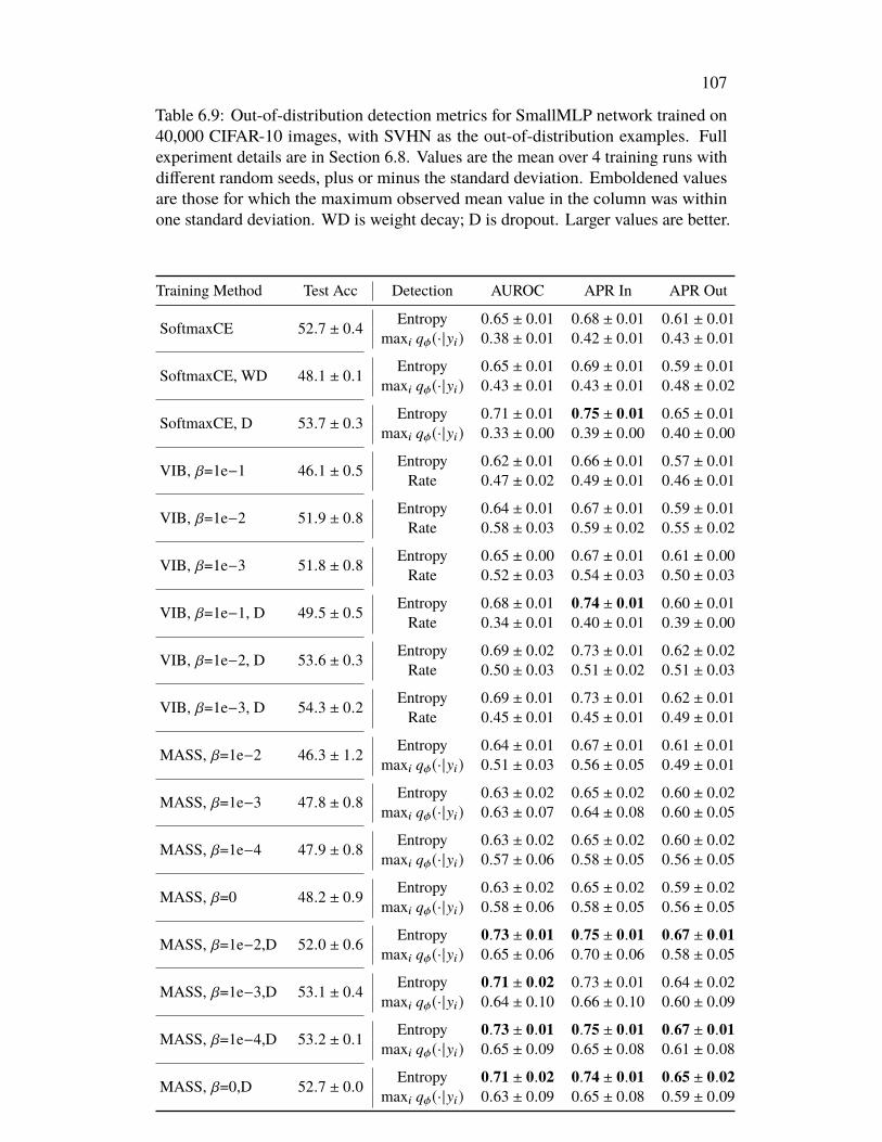
107

Table 6.9: Out-of-distribution detection metrics for SmallMLP network trained on40,000 CIFAR-10 images, with SVHN as the out-of-distribution examples. Fullexperiment details are in Section 6.8. Values are the mean over 4 training runs withdifferent random seeds, plus or minus the standard deviation. Emboldened valuesare those for which the maximum observed mean value in the column was withinone standard deviation. WD is weight decay; D is dropout. Larger values are better.

Training Method Test Acc Detection AUROC APR In APR Out

SoftmaxCE 52.7 ± 0.4 Entropy 0.65 ± 0.01 0.68 ± 0.01 0.61 ± 0.01maxi qφ(·|yi) 0.38 ± 0.01 0.42 ± 0.01 0.43 ± 0.01

SoftmaxCE, WD 48.1 ± 0.1 Entropy 0.65 ± 0.01 0.69 ± 0.01 0.59 ± 0.01maxi qφ(·|yi) 0.43 ± 0.01 0.43 ± 0.01 0.48 ± 0.02

SoftmaxCE, D 53.7 ± 0.3 Entropy 0.71 ± 0.01 0.75 ± 0.01 0.65 ± 0.01maxi qφ(·|yi) 0.33 ± 0.00 0.39 ± 0.00 0.40 ± 0.00

VIB, β=1e−1 46.1 ± 0.5 Entropy 0.62 ± 0.01 0.66 ± 0.01 0.57 ± 0.01Rate 0.47 ± 0.02 0.49 ± 0.01 0.46 ± 0.01

VIB, β=1e−2 51.9 ± 0.8 Entropy 0.64 ± 0.01 0.67 ± 0.01 0.59 ± 0.01Rate 0.58 ± 0.03 0.59 ± 0.02 0.55 ± 0.02

VIB, β=1e−3 51.8 ± 0.8 Entropy 0.65 ± 0.00 0.67 ± 0.01 0.61 ± 0.00Rate 0.52 ± 0.03 0.54 ± 0.03 0.50 ± 0.03

VIB, β=1e−1, D 49.5 ± 0.5 Entropy 0.68 ± 0.01 0.74 ± 0.01 0.60 ± 0.01Rate 0.34 ± 0.01 0.40 ± 0.01 0.39 ± 0.00

VIB, β=1e−2, D 53.6 ± 0.3 Entropy 0.69 ± 0.02 0.73 ± 0.01 0.62 ± 0.02Rate 0.50 ± 0.03 0.51 ± 0.02 0.51 ± 0.03

VIB, β=1e−3, D 54.3 ± 0.2 Entropy 0.69 ± 0.01 0.73 ± 0.01 0.62 ± 0.01Rate 0.45 ± 0.01 0.45 ± 0.01 0.49 ± 0.01

MASS, β=1e−2 46.3 ± 1.2 Entropy 0.64 ± 0.01 0.67 ± 0.01 0.61 ± 0.01maxi qφ(·|yi) 0.51 ± 0.03 0.56 ± 0.05 0.49 ± 0.01

MASS, β=1e−3 47.8 ± 0.8 Entropy 0.63 ± 0.02 0.65 ± 0.02 0.60 ± 0.02maxi qφ(·|yi) 0.63 ± 0.07 0.64 ± 0.08 0.60 ± 0.05

MASS, β=1e−4 47.9 ± 0.8 Entropy 0.63 ± 0.02 0.65 ± 0.02 0.60 ± 0.02maxi qφ(·|yi) 0.57 ± 0.06 0.58 ± 0.05 0.56 ± 0.05

MASS, β=0 48.2 ± 0.9 Entropy 0.63 ± 0.02 0.65 ± 0.02 0.59 ± 0.02maxi qφ(·|yi) 0.58 ± 0.06 0.58 ± 0.05 0.56 ± 0.05

MASS, β=1e−2,D 52.0 ± 0.6 Entropy 0.73 ± 0.01 0.75 ± 0.01 0.67 ± 0.01maxi qφ(·|yi) 0.65 ± 0.06 0.70 ± 0.06 0.58 ± 0.05

MASS, β=1e−3,D 53.1 ± 0.4 Entropy 0.71 ± 0.02 0.73 ± 0.01 0.64 ± 0.02maxi qφ(·|yi) 0.64 ± 0.10 0.66 ± 0.10 0.60 ± 0.09

MASS, β=1e−4,D 53.2 ± 0.1 Entropy 0.73 ± 0.01 0.75 ± 0.01 0.67 ± 0.01maxi qφ(·|yi) 0.65 ± 0.09 0.65 ± 0.08 0.61 ± 0.08

MASS, β=0,D 52.7 ± 0.0 Entropy 0.71 ± 0.02 0.74 ± 0.01 0.65 ± 0.02maxi qφ(·|yi) 0.63 ± 0.09 0.65 ± 0.08 0.59 ± 0.09

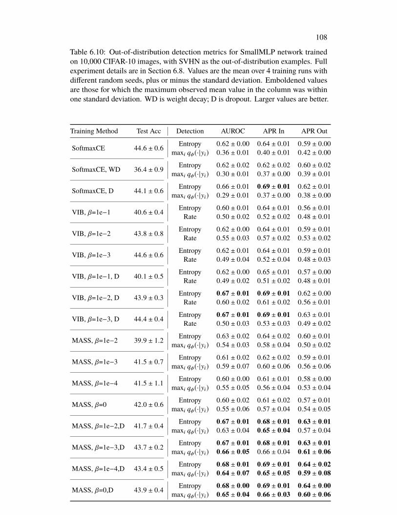
108

Table 6.10: Out-of-distribution detection metrics for SmallMLP network trainedon 10,000 CIFAR-10 images, with SVHN as the out-of-distribution examples. Fullexperiment details are in Section 6.8. Values are the mean over 4 training runs withdifferent random seeds, plus or minus the standard deviation. Emboldened valuesare those for which the maximum observed mean value in the column was withinone standard deviation. WD is weight decay; D is dropout. Larger values are better.

Training Method Test Acc Detection AUROC APR In APR Out

SoftmaxCE 44.6 ± 0.6 Entropy 0.62 ± 0.00 0.64 ± 0.01 0.59 ± 0.00maxi qφ(·|yi) 0.36 ± 0.01 0.40 ± 0.01 0.42 ± 0.00

SoftmaxCE, WD 36.4 ± 0.9 Entropy 0.62 ± 0.02 0.62 ± 0.02 0.60 ± 0.02maxi qφ(·|yi) 0.30 ± 0.01 0.37 ± 0.00 0.39 ± 0.01

SoftmaxCE, D 44.1 ± 0.6 Entropy 0.66 ± 0.01 0.69 ± 0.01 0.62 ± 0.01maxi qφ(·|yi) 0.29 ± 0.01 0.37 ± 0.00 0.38 ± 0.00

VIB, β=1e−1 40.6 ± 0.4 Entropy 0.60 ± 0.01 0.64 ± 0.01 0.56 ± 0.01Rate 0.50 ± 0.02 0.52 ± 0.02 0.48 ± 0.01

VIB, β=1e−2 43.8 ± 0.8 Entropy 0.62 ± 0.00 0.64 ± 0.01 0.59 ± 0.01Rate 0.55 ± 0.03 0.57 ± 0.02 0.53 ± 0.02

VIB, β=1e−3 44.6 ± 0.6 Entropy 0.62 ± 0.01 0.64 ± 0.01 0.59 ± 0.01Rate 0.49 ± 0.04 0.52 ± 0.04 0.48 ± 0.03

VIB, β=1e−1, D 40.1 ± 0.5 Entropy 0.62 ± 0.00 0.65 ± 0.01 0.57 ± 0.00Rate 0.49 ± 0.02 0.51 ± 0.02 0.48 ± 0.01

VIB, β=1e−2, D 43.9 ± 0.3 Entropy 0.67 ± 0.01 0.69 ± 0.01 0.62 ± 0.00Rate 0.60 ± 0.02 0.61 ± 0.02 0.56 ± 0.01

VIB, β=1e−3, D 44.4 ± 0.4 Entropy 0.67 ± 0.01 0.69 ± 0.01 0.63 ± 0.01Rate 0.50 ± 0.03 0.53 ± 0.03 0.49 ± 0.02

MASS, β=1e−2 39.9 ± 1.2 Entropy 0.63 ± 0.02 0.64 ± 0.02 0.60 ± 0.01maxi qφ(·|yi) 0.54 ± 0.03 0.58 ± 0.04 0.50 ± 0.02

MASS, β=1e−3 41.5 ± 0.7 Entropy 0.61 ± 0.02 0.62 ± 0.02 0.59 ± 0.01maxi qφ(·|yi) 0.59 ± 0.07 0.60 ± 0.06 0.56 ± 0.06

MASS, β=1e−4 41.5 ± 1.1 Entropy 0.60 ± 0.00 0.61 ± 0.01 0.58 ± 0.00maxi qφ(·|yi) 0.55 ± 0.05 0.56 ± 0.04 0.53 ± 0.04

MASS, β=0 42.0 ± 0.6 Entropy 0.60 ± 0.02 0.61 ± 0.02 0.57 ± 0.01maxi qφ(·|yi) 0.55 ± 0.06 0.57 ± 0.04 0.54 ± 0.05

MASS, β=1e−2,D 41.7 ± 0.4 Entropy 0.67 ± 0.01 0.68 ± 0.01 0.63 ± 0.01maxi qφ(·|yi) 0.63 ± 0.04 0.65 ± 0.04 0.57 ± 0.04

MASS, β=1e−3,D 43.7 ± 0.2 Entropy 0.67 ± 0.01 0.68 ± 0.01 0.63 ± 0.01maxi qφ(·|yi) 0.66 ± 0.05 0.66 ± 0.04 0.61 ± 0.06

MASS, β=1e−4,D 43.4 ± 0.5 Entropy 0.68 ± 0.01 0.69 ± 0.01 0.64 ± 0.02maxi qφ(·|yi) 0.64 ± 0.07 0.65 ± 0.05 0.59 ± 0.08

MASS, β=0,D 43.9 ± 0.4 Entropy 0.68 ± 0.00 0.69 ± 0.01 0.64 ± 0.00maxi qφ(·|yi) 0.65 ± 0.04 0.66 ± 0.03 0.60 ± 0.06

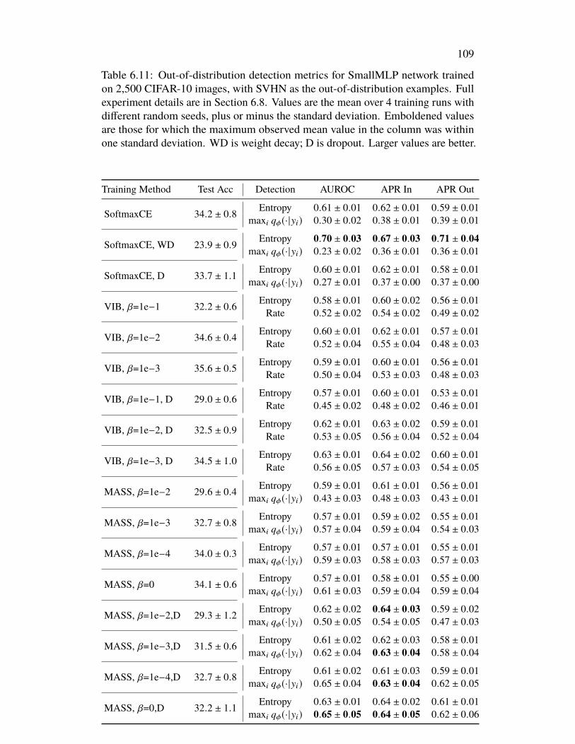
109

Table 6.11: Out-of-distribution detection metrics for SmallMLP network trainedon 2,500 CIFAR-10 images, with SVHN as the out-of-distribution examples. Fullexperiment details are in Section 6.8. Values are the mean over 4 training runs withdifferent random seeds, plus or minus the standard deviation. Emboldened valuesare those for which the maximum observed mean value in the column was withinone standard deviation. WD is weight decay; D is dropout. Larger values are better.

Training Method Test Acc Detection AUROC APR In APR Out

SoftmaxCE 34.2 ± 0.8 Entropy 0.61 ± 0.01 0.62 ± 0.01 0.59 ± 0.01maxi qφ(·|yi) 0.30 ± 0.02 0.38 ± 0.01 0.39 ± 0.01

SoftmaxCE, WD 23.9 ± 0.9 Entropy 0.70 ± 0.03 0.67 ± 0.03 0.71 ± 0.04maxi qφ(·|yi) 0.23 ± 0.02 0.36 ± 0.01 0.36 ± 0.01

SoftmaxCE, D 33.7 ± 1.1 Entropy 0.60 ± 0.01 0.62 ± 0.01 0.58 ± 0.01maxi qφ(·|yi) 0.27 ± 0.01 0.37 ± 0.00 0.37 ± 0.00

VIB, β=1e−1 32.2 ± 0.6 Entropy 0.58 ± 0.01 0.60 ± 0.02 0.56 ± 0.01Rate 0.52 ± 0.02 0.54 ± 0.02 0.49 ± 0.02

VIB, β=1e−2 34.6 ± 0.4 Entropy 0.60 ± 0.01 0.62 ± 0.01 0.57 ± 0.01Rate 0.52 ± 0.04 0.55 ± 0.04 0.48 ± 0.03

VIB, β=1e−3 35.6 ± 0.5 Entropy 0.59 ± 0.01 0.60 ± 0.01 0.56 ± 0.01Rate 0.50 ± 0.04 0.53 ± 0.03 0.48 ± 0.03

VIB, β=1e−1, D 29.0 ± 0.6 Entropy 0.57 ± 0.01 0.60 ± 0.01 0.53 ± 0.01Rate 0.45 ± 0.02 0.48 ± 0.02 0.46 ± 0.01

VIB, β=1e−2, D 32.5 ± 0.9 Entropy 0.62 ± 0.01 0.63 ± 0.02 0.59 ± 0.01Rate 0.53 ± 0.05 0.56 ± 0.04 0.52 ± 0.04

VIB, β=1e−3, D 34.5 ± 1.0 Entropy 0.63 ± 0.01 0.64 ± 0.02 0.60 ± 0.01Rate 0.56 ± 0.05 0.57 ± 0.03 0.54 ± 0.05

MASS, β=1e−2 29.6 ± 0.4 Entropy 0.59 ± 0.01 0.61 ± 0.01 0.56 ± 0.01maxi qφ(·|yi) 0.43 ± 0.03 0.48 ± 0.03 0.43 ± 0.01

MASS, β=1e−3 32.7 ± 0.8 Entropy 0.57 ± 0.01 0.59 ± 0.02 0.55 ± 0.01maxi qφ(·|yi) 0.57 ± 0.04 0.59 ± 0.04 0.54 ± 0.03

MASS, β=1e−4 34.0 ± 0.3 Entropy 0.57 ± 0.01 0.57 ± 0.01 0.55 ± 0.01maxi qφ(·|yi) 0.59 ± 0.03 0.58 ± 0.03 0.57 ± 0.03

MASS, β=0 34.1 ± 0.6 Entropy 0.57 ± 0.01 0.58 ± 0.01 0.55 ± 0.00maxi qφ(·|yi) 0.61 ± 0.03 0.59 ± 0.04 0.59 ± 0.04

MASS, β=1e−2,D 29.3 ± 1.2 Entropy 0.62 ± 0.02 0.64 ± 0.03 0.59 ± 0.02maxi qφ(·|yi) 0.50 ± 0.05 0.54 ± 0.05 0.47 ± 0.03

MASS, β=1e−3,D 31.5 ± 0.6 Entropy 0.61 ± 0.02 0.62 ± 0.03 0.58 ± 0.01maxi qφ(·|yi) 0.62 ± 0.04 0.63 ± 0.04 0.58 ± 0.04

MASS, β=1e−4,D 32.7 ± 0.8 Entropy 0.61 ± 0.02 0.61 ± 0.03 0.59 ± 0.01maxi qφ(·|yi) 0.65 ± 0.04 0.63 ± 0.04 0.62 ± 0.05

MASS, β=0,D 32.2 ± 1.1 Entropy 0.63 ± 0.01 0.64 ± 0.02 0.61 ± 0.01maxi qφ(·|yi) 0.65 ± 0.05 0.64 ± 0.05 0.62 ± 0.06

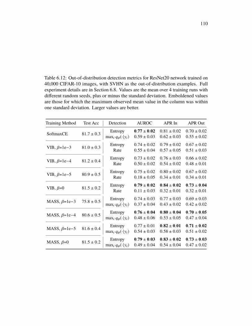
110

Table 6.12: Out-of-distribution detection metrics for ResNet20 network trained on40,000 CIFAR-10 images, with SVHN as the out-of-distribution examples. Fullexperiment details are in Section 6.8. Values are the mean over 4 training runs withdifferent random seeds, plus or minus the standard deviation. Emboldened valuesare those for which the maximum observed mean value in the column was withinone standard deviation. Larger values are better.

Training Method Test Acc Detection AUROC APR In APR Out

SoftmaxCE 81.7 ± 0.3 Entropy 0.77 ± 0.02 0.81 ± 0.02 0.70 ± 0.02maxi qφ(·|yi) 0.59 ± 0.03 0.62 ± 0.03 0.55 ± 0.02

VIB, β=1e−3 81.0 ± 0.3 Entropy 0.74 ± 0.02 0.79 ± 0.02 0.67 ± 0.02Rate 0.55 ± 0.04 0.57 ± 0.05 0.51 ± 0.03

VIB, β=1e−4 81.2 ± 0.4 Entropy 0.73 ± 0.02 0.76 ± 0.03 0.66 ± 0.02Rate 0.50 ± 0.02 0.54 ± 0.02 0.48 ± 0.01

VIB, β=1e−5 80.9 ± 0.5 Entropy 0.75 ± 0.02 0.80 ± 0.02 0.67 ± 0.02Rate 0.18 ± 0.05 0.34 ± 0.01 0.34 ± 0.01

VIB, β=0 81.5 ± 0.2 Entropy 0.79 ± 0.02 0.84 ± 0.02 0.73 ± 0.04Rate 0.11 ± 0.03 0.32 ± 0.01 0.32 ± 0.01

MASS, β=1e−3 75.8 ± 0.5 Entropy 0.74 ± 0.03 0.77 ± 0.03 0.69 ± 0.03maxi qφ(·|yi) 0.37 ± 0.04 0.43 ± 0.02 0.42 ± 0.02

MASS, β=1e−4 80.6 ± 0.5 Entropy 0.76 ± 0.04 0.80 ± 0.04 0.70 ± 0.05maxi qφ(·|yi) 0.48 ± 0.06 0.53 ± 0.05 0.47 ± 0.04

MASS, β=1e−5 81.6 ± 0.4 Entropy 0.77 ± 0.01 0.82 ± 0.01 0.71 ± 0.02maxi qφ(·|yi) 0.54 ± 0.03 0.58 ± 0.03 0.51 ± 0.02

MASS, β=0 81.5 ± 0.2 Entropy 0.79 ± 0.03 0.83 ± 0.02 0.73 ± 0.03maxi qφ(·|yi) 0.49 ± 0.04 0.54 ± 0.04 0.47 ± 0.02

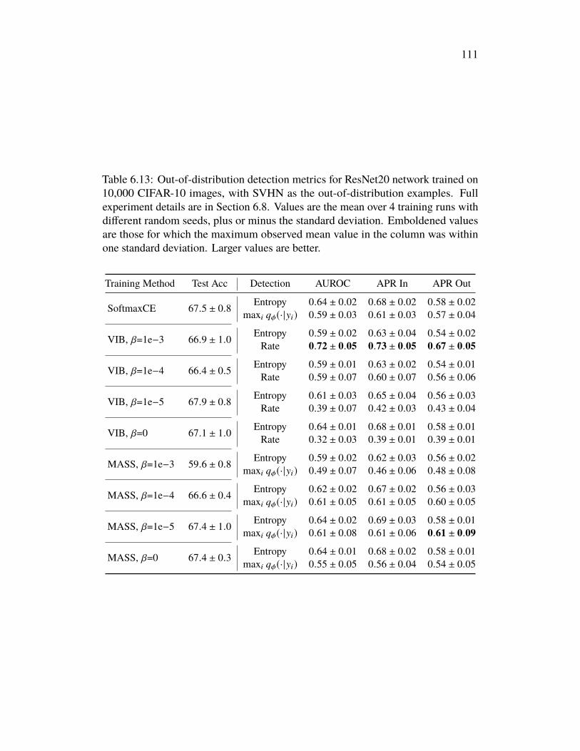
111

Table 6.13: Out-of-distribution detection metrics for ResNet20 network trained on10,000 CIFAR-10 images, with SVHN as the out-of-distribution examples. Fullexperiment details are in Section 6.8. Values are the mean over 4 training runs withdifferent random seeds, plus or minus the standard deviation. Emboldened valuesare those for which the maximum observed mean value in the column was withinone standard deviation. Larger values are better.

Training Method Test Acc Detection AUROC APR In APR Out

SoftmaxCE 67.5 ± 0.8 Entropy 0.64 ± 0.02 0.68 ± 0.02 0.58 ± 0.02maxi qφ(·|yi) 0.59 ± 0.03 0.61 ± 0.03 0.57 ± 0.04

VIB, β=1e−3 66.9 ± 1.0 Entropy 0.59 ± 0.02 0.63 ± 0.04 0.54 ± 0.02Rate 0.72 ± 0.05 0.73 ± 0.05 0.67 ± 0.05

VIB, β=1e−4 66.4 ± 0.5 Entropy 0.59 ± 0.01 0.63 ± 0.02 0.54 ± 0.01Rate 0.59 ± 0.07 0.60 ± 0.07 0.56 ± 0.06

VIB, β=1e−5 67.9 ± 0.8 Entropy 0.61 ± 0.03 0.65 ± 0.04 0.56 ± 0.03Rate 0.39 ± 0.07 0.42 ± 0.03 0.43 ± 0.04

VIB, β=0 67.1 ± 1.0 Entropy 0.64 ± 0.01 0.68 ± 0.01 0.58 ± 0.01Rate 0.32 ± 0.03 0.39 ± 0.01 0.39 ± 0.01

MASS, β=1e−3 59.6 ± 0.8 Entropy 0.59 ± 0.02 0.62 ± 0.03 0.56 ± 0.02maxi qφ(·|yi) 0.49 ± 0.07 0.46 ± 0.06 0.48 ± 0.08

MASS, β=1e−4 66.6 ± 0.4 Entropy 0.62 ± 0.02 0.67 ± 0.02 0.56 ± 0.03maxi qφ(·|yi) 0.61 ± 0.05 0.61 ± 0.05 0.60 ± 0.05

MASS, β=1e−5 67.4 ± 1.0 Entropy 0.64 ± 0.02 0.69 ± 0.03 0.58 ± 0.01maxi qφ(·|yi) 0.61 ± 0.08 0.61 ± 0.06 0.61 ± 0.09

MASS, β=0 67.4 ± 0.3 Entropy 0.64 ± 0.01 0.68 ± 0.02 0.58 ± 0.01maxi qφ(·|yi) 0.55 ± 0.05 0.56 ± 0.04 0.54 ± 0.05

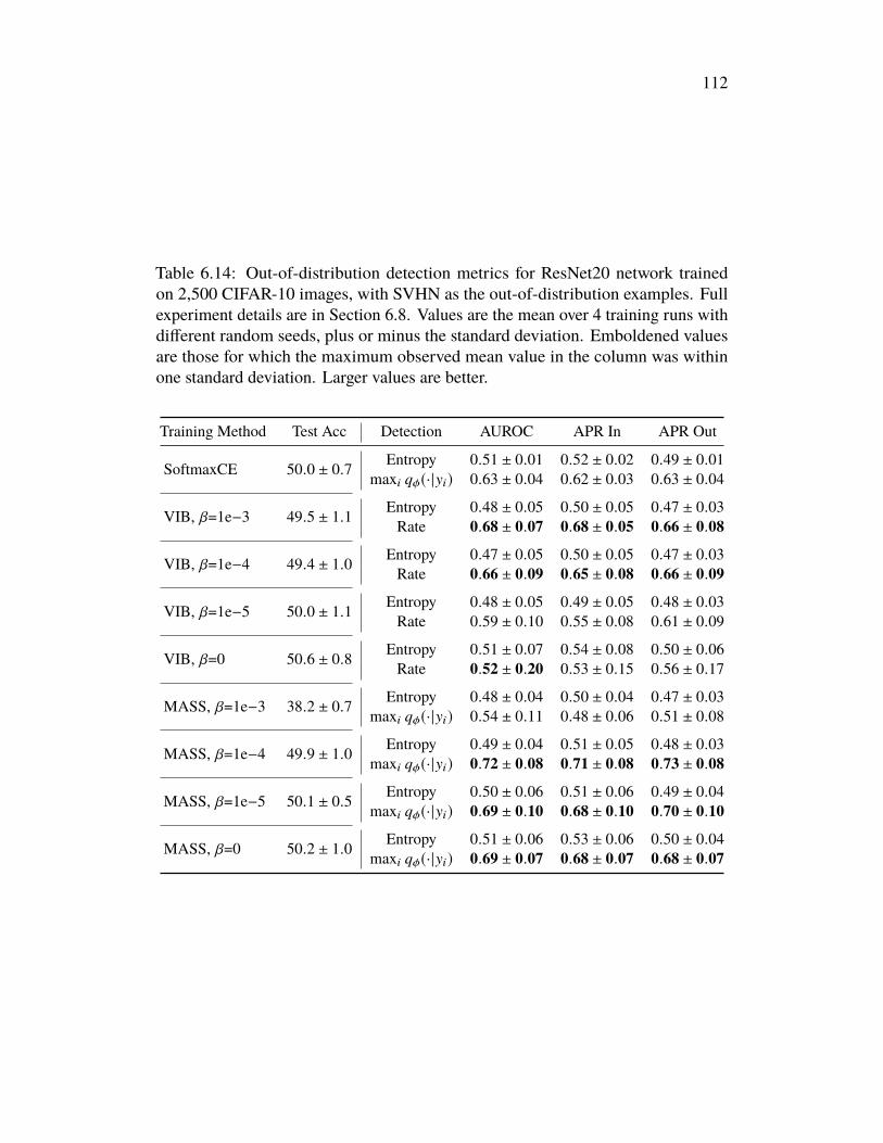
112

Table 6.14: Out-of-distribution detection metrics for ResNet20 network trainedon 2,500 CIFAR-10 images, with SVHN as the out-of-distribution examples. Fullexperiment details are in Section 6.8. Values are the mean over 4 training runs withdifferent random seeds, plus or minus the standard deviation. Emboldened valuesare those for which the maximum observed mean value in the column was withinone standard deviation. Larger values are better.

Training Method Test Acc Detection AUROC APR In APR Out

SoftmaxCE 50.0 ± 0.7 Entropy 0.51 ± 0.01 0.52 ± 0.02 0.49 ± 0.01maxi qφ(·|yi) 0.63 ± 0.04 0.62 ± 0.03 0.63 ± 0.04

VIB, β=1e−3 49.5 ± 1.1 Entropy 0.48 ± 0.05 0.50 ± 0.05 0.47 ± 0.03Rate 0.68 ± 0.07 0.68 ± 0.05 0.66 ± 0.08

VIB, β=1e−4 49.4 ± 1.0 Entropy 0.47 ± 0.05 0.50 ± 0.05 0.47 ± 0.03Rate 0.66 ± 0.09 0.65 ± 0.08 0.66 ± 0.09

VIB, β=1e−5 50.0 ± 1.1 Entropy 0.48 ± 0.05 0.49 ± 0.05 0.48 ± 0.03Rate 0.59 ± 0.10 0.55 ± 0.08 0.61 ± 0.09

VIB, β=0 50.6 ± 0.8 Entropy 0.51 ± 0.07 0.54 ± 0.08 0.50 ± 0.06Rate 0.52 ± 0.20 0.53 ± 0.15 0.56 ± 0.17

MASS, β=1e−3 38.2 ± 0.7 Entropy 0.48 ± 0.04 0.50 ± 0.04 0.47 ± 0.03maxi qφ(·|yi) 0.54 ± 0.11 0.48 ± 0.06 0.51 ± 0.08

MASS, β=1e−4 49.9 ± 1.0 Entropy 0.49 ± 0.04 0.51 ± 0.05 0.48 ± 0.03maxi qφ(·|yi) 0.72 ± 0.08 0.71 ± 0.08 0.73 ± 0.08

MASS, β=1e−5 50.1 ± 0.5 Entropy 0.50 ± 0.06 0.51 ± 0.06 0.49 ± 0.04maxi qφ(·|yi) 0.69 ± 0.10 0.68 ± 0.10 0.70 ± 0.10

MASS, β=0 50.2 ± 1.0 Entropy 0.51 ± 0.06 0.53 ± 0.06 0.50 ± 0.04maxi qφ(·|yi) 0.69 ± 0.07 0.68 ± 0.07 0.68 ± 0.07

113

C h a p t e r 7

SUPERVISED LEARNING ON RELATIONAL DATABASESWITH GRAPH NEURAL NETWORKS, PART 2

7.1 IntroductionIn this final short chapter, we take lessons learned in Chapters 5 and 6 and apply themto the GNN models for supervised learning on relational databases from Chapter 4,yielding noticeable improvement.

7.2 Lessons LearnedThe encoding used to prepare tabular features for input into a deep model has asignificant effect on performance. As with all modeling decisions regarding tabulardata, questions of feature encoding matter most in terms of how they affect overfitting.

Options for categorical variables include whether to one-hot encode versus learningan embedding, what embedding size to use, and how to apply dropout regularization(whether to drop vector elements or whole embeddings). In our experiments wefound that learned embeddings nearly always improved performance as long as thecardinality of the categorical variable was significantly less than the number ofdatapoints, otherwise the feature was merely a means for the model to overfit.

Options for scalar variables include how to rescale the variable (via quantiles,normalization, or log scaling) or whether to quantize the feature and treat it like acategorical variable. In our experiments we found that the best strategy was simplyto use all the different types of encoding in parallel, turning each scalar feature intothree rescaled features and one categorical feature. Unlike learning embeddings forhigh-cardinality categorical features, adding potentially-redundant encodings forscalar variables does not lead to overfitting, but can make the difference between afeature being useful or not.

For variables encoding specific information like geospatial or datetime information,converting the feature from a single scalar or categorical representation into a set ofinformative features can make a significant impact. See Appendix 4.9 for details.

Normalization was also crucial to experiment with. While batch normalization andlayer normalization are standard practice in deep learning, they must be used withcare in GNNs. Normalization can accelerate training but also make it impossible for

114

a GNN to learn functions that are sensitive to the degree of a node, since differencesin absolute magnitudes of hidden state vectors between nodes and datapoints will benormalized away.

7.3 ExperimentsCode to reproduce all experiments may be found online.1

We modified the GNN model implementations introduced in Chapter 4 with all thelessons discussed in the previous section. In addition, based on the results of thebenchmark in Chapter 5, we added a single-hidden-layer multilayer perceptron tothe initialization function S for each node, using different MLP parameters for eachnode type.

Though the heterogeneous transformer model of Chapter 5 did not perform better thana standard transformer or MLP, it inspired us to try a new type of GNN architecture forRDBs. Given that each table in an RDB contains different features and each foreignkey encodes a different type of relationship, it seemed reasonable to use GNNs thatmaintained different parameters for each node-update and message-passing function,depending on the node type and edge type respectively. These are in the spirit of(Schlichtkrull et al., 2018) and (X. Wang et al., 2019), though are different models.We refer to these as HetGCN, HetGIN, and HetGAT, respectively.

Additionally, inspired by the centrality of overfitting in determining the performanceof deep models for tabular data and the consistently strong performance of GBDTs,we tested whether a stacking strategy (Wolpert, 1992) would offer any benefit. Inthese “Stacked” models, we train a GBDT on a concatenation of single-table featuresand the pre-logit activations of a trained GNN. In principle, if the GNN is learninguseful features but overfitting in its final layers, this strategy should ameliorate theoverfitting issue.

All other models are the same as described in Chapter 4. Thorough details aboutmodel and experiment implementation are in Appendix 7.6.

7.4 ResultsTable 7.1 shows the AUROC performance of models relative to the best-performingtabular model on each dataset. We compare relative performance rather than absoluteperformance since for some datasets the variance in performance between cross-

1https://github.com/mwcvitkovic/Supervised-Learning-on-Relational-Databases-with-GNNs

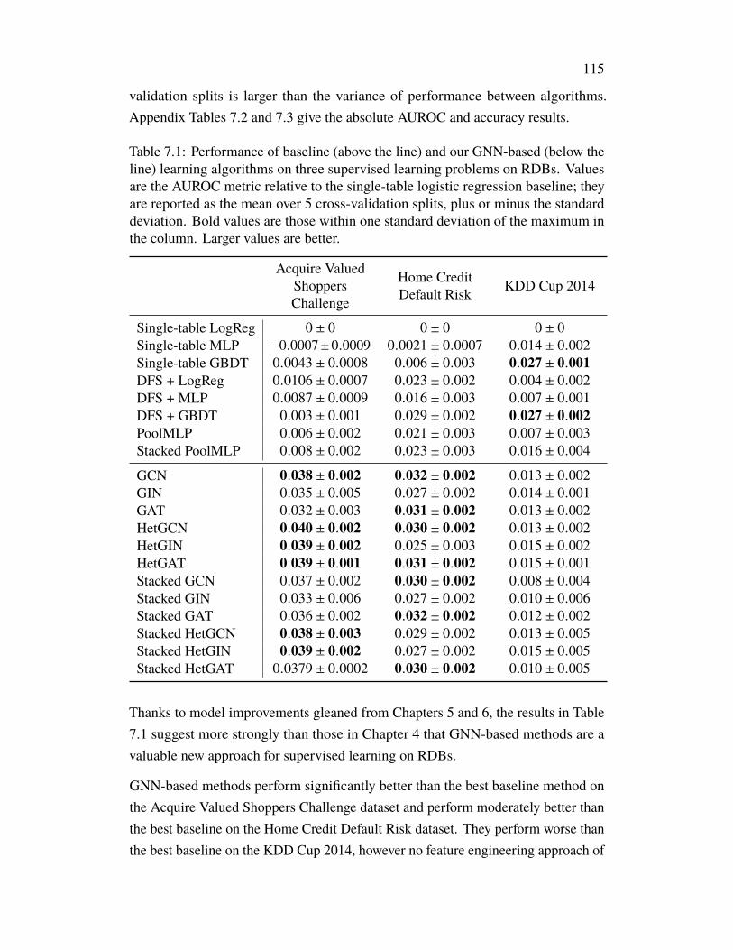
115

validation splits is larger than the variance of performance between algorithms.Appendix Tables 7.2 and 7.3 give the absolute AUROC and accuracy results.

Table 7.1: Performance of baseline (above the line) and our GNN-based (below theline) learning algorithms on three supervised learning problems on RDBs. Valuesare the AUROC metric relative to the single-table logistic regression baseline; theyare reported as the mean over 5 cross-validation splits, plus or minus the standarddeviation. Bold values are those within one standard deviation of the maximum inthe column. Larger values are better.

Acquire ValuedShoppersChallenge

Home CreditDefault Risk KDD Cup 2014

Single-table LogReg 0 ± 0 0 ± 0 0 ± 0Single-table MLP −0.0007±0.0009 0.0021 ± 0.0007 0.014 ± 0.002Single-table GBDT 0.0043 ± 0.0008 0.006 ± 0.003 0.027 ± 0.001DFS + LogReg 0.0106 ± 0.0007 0.023 ± 0.002 0.004 ± 0.002DFS + MLP 0.0087 ± 0.0009 0.016 ± 0.003 0.007 ± 0.001DFS + GBDT 0.003 ± 0.001 0.029 ± 0.002 0.027 ± 0.002PoolMLP 0.006 ± 0.002 0.021 ± 0.003 0.007 ± 0.003Stacked PoolMLP 0.008 ± 0.002 0.023 ± 0.003 0.016 ± 0.004

GCN 0.038 ± 0.002 0.032 ± 0.002 0.013 ± 0.002GIN 0.035 ± 0.005 0.027 ± 0.002 0.014 ± 0.001GAT 0.032 ± 0.003 0.031 ± 0.002 0.013 ± 0.002HetGCN 0.040 ± 0.002 0.030 ± 0.002 0.013 ± 0.002HetGIN 0.039 ± 0.002 0.025 ± 0.003 0.015 ± 0.002HetGAT 0.039 ± 0.001 0.031 ± 0.002 0.015 ± 0.001Stacked GCN 0.037 ± 0.002 0.030 ± 0.002 0.008 ± 0.004Stacked GIN 0.033 ± 0.006 0.027 ± 0.002 0.010 ± 0.006Stacked GAT 0.036 ± 0.002 0.032 ± 0.002 0.012 ± 0.002Stacked HetGCN 0.038 ± 0.003 0.029 ± 0.002 0.013 ± 0.005Stacked HetGIN 0.039 ± 0.002 0.027 ± 0.002 0.015 ± 0.005Stacked HetGAT 0.0379 ± 0.0002 0.030 ± 0.002 0.010 ± 0.005

Thanks to model improvements gleaned from Chapters 5 and 6, the results in Table7.1 suggest more strongly than those in Chapter 4 that GNN-based methods are avaluable new approach for supervised learning on RDBs.

GNN-based methods perform significantly better than the best baseline method onthe Acquire Valued Shoppers Challenge dataset and perform moderately better thanthe best baseline on the Home Credit Default Risk dataset. They perform worse thanthe best baseline on the KDD Cup 2014, however no feature engineering approach of

116

any kind offers an advantage on that dataset. The determinant of success on the KDDCup 2014 dataset does not seem to be information outside the dataset’s main table.

Though every GNN-based method we tested matches or exceeds the best baselinemethod on the Acquire Valued Shoppers Challenge and Home Credit DefaultRisk datasets, there is no clearly superior GNN model among them. Neither theheterogeneous models nor stacking offers a noticeable benefit. But we emphasizethat all our experiments used off-the-shell GNNs or straightforward modificationsthereof — the space of possible RDB-specific GNNs is large and mostly unexplored.

Acknowledgments

We thank Da Zheng, and Minjie Wang, and Zohar Karnin for helpful discussions.

7.5 Appendix: Additional Results

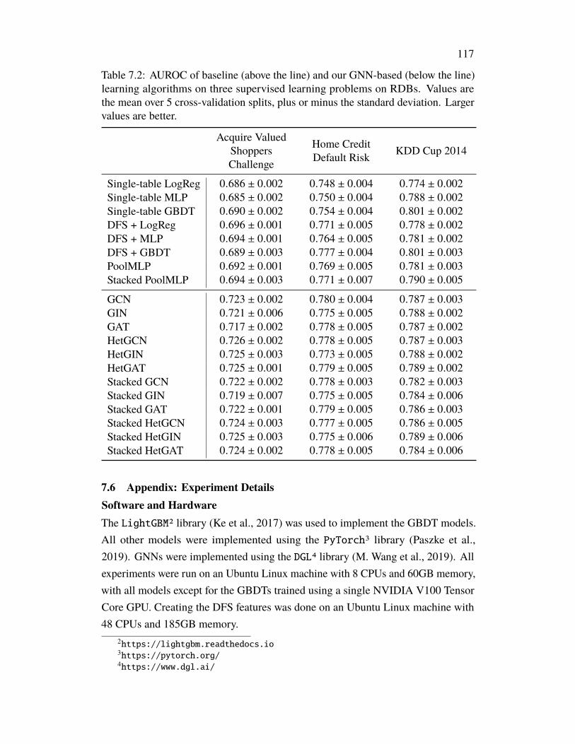
117

Table 7.2: AUROC of baseline (above the line) and our GNN-based (below the line)learning algorithms on three supervised learning problems on RDBs. Values arethe mean over 5 cross-validation splits, plus or minus the standard deviation. Largervalues are better.

Acquire ValuedShoppersChallenge

Home CreditDefault Risk KDD Cup 2014

Single-table LogReg 0.686 ± 0.002 0.748 ± 0.004 0.774 ± 0.002Single-table MLP 0.685 ± 0.002 0.750 ± 0.004 0.788 ± 0.002Single-table GBDT 0.690 ± 0.002 0.754 ± 0.004 0.801 ± 0.002DFS + LogReg 0.696 ± 0.001 0.771 ± 0.005 0.778 ± 0.002DFS + MLP 0.694 ± 0.001 0.764 ± 0.005 0.781 ± 0.002DFS + GBDT 0.689 ± 0.003 0.777 ± 0.004 0.801 ± 0.003PoolMLP 0.692 ± 0.001 0.769 ± 0.005 0.781 ± 0.003Stacked PoolMLP 0.694 ± 0.003 0.771 ± 0.007 0.790 ± 0.005

GCN 0.723 ± 0.002 0.780 ± 0.004 0.787 ± 0.003GIN 0.721 ± 0.006 0.775 ± 0.005 0.788 ± 0.002GAT 0.717 ± 0.002 0.778 ± 0.005 0.787 ± 0.002HetGCN 0.726 ± 0.002 0.778 ± 0.005 0.787 ± 0.003HetGIN 0.725 ± 0.003 0.773 ± 0.005 0.788 ± 0.002HetGAT 0.725 ± 0.001 0.779 ± 0.005 0.789 ± 0.002Stacked GCN 0.722 ± 0.002 0.778 ± 0.003 0.782 ± 0.003Stacked GIN 0.719 ± 0.007 0.775 ± 0.005 0.784 ± 0.006Stacked GAT 0.722 ± 0.001 0.779 ± 0.005 0.786 ± 0.003Stacked HetGCN 0.724 ± 0.003 0.777 ± 0.005 0.786 ± 0.005Stacked HetGIN 0.725 ± 0.003 0.775 ± 0.006 0.789 ± 0.006Stacked HetGAT 0.724 ± 0.002 0.778 ± 0.005 0.784 ± 0.006

7.6 Appendix: Experiment DetailsSoftware and HardwareThe LightGBM2 library (Ke et al., 2017) was used to implement the GBDT models.All other models were implemented using the PyTorch3 library (Paszke et al.,2019). GNNs were implemented using the DGL4 library (M. Wang et al., 2019). Allexperiments were run on an Ubuntu Linux machine with 8 CPUs and 60GB memory,with all models except for the GBDTs trained using a single NVIDIA V100 TensorCore GPU. Creating the DFS features was done on an Ubuntu Linux machine with48 CPUs and 185GB memory.

2https://lightgbm.readthedocs.io3https://pytorch.org/4https://www.dgl.ai/

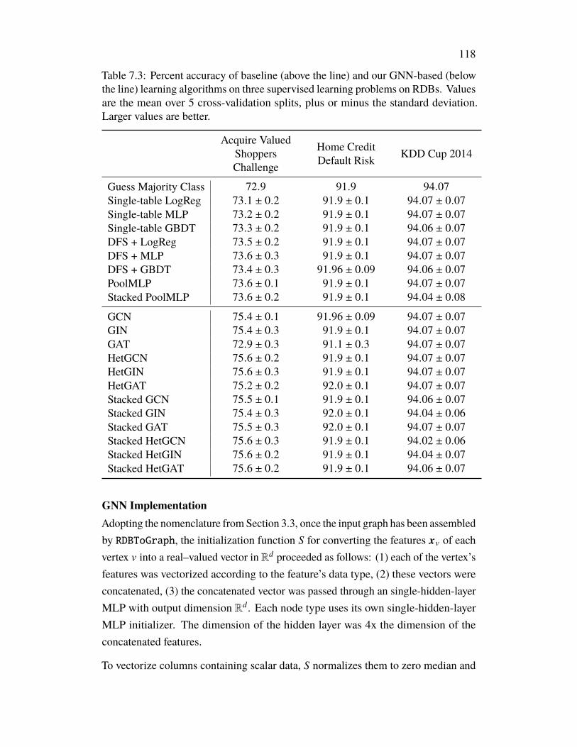
118

Table 7.3: Percent accuracy of baseline (above the line) and our GNN-based (belowthe line) learning algorithms on three supervised learning problems on RDBs. Valuesare the mean over 5 cross-validation splits, plus or minus the standard deviation.Larger values are better.

Acquire ValuedShoppersChallenge

Home CreditDefault Risk KDD Cup 2014

Guess Majority Class 72.9 91.9 94.07Single-table LogReg 73.1 ± 0.2 91.9 ± 0.1 94.07 ± 0.07Single-table MLP 73.2 ± 0.2 91.9 ± 0.1 94.07 ± 0.07Single-table GBDT 73.3 ± 0.2 91.9 ± 0.1 94.06 ± 0.07DFS + LogReg 73.5 ± 0.2 91.9 ± 0.1 94.07 ± 0.07DFS + MLP 73.6 ± 0.3 91.9 ± 0.1 94.07 ± 0.07DFS + GBDT 73.4 ± 0.3 91.96 ± 0.09 94.06 ± 0.07PoolMLP 73.6 ± 0.1 91.9 ± 0.1 94.07 ± 0.07Stacked PoolMLP 73.6 ± 0.2 91.9 ± 0.1 94.04 ± 0.08

GCN 75.4 ± 0.1 91.96 ± 0.09 94.07 ± 0.07GIN 75.4 ± 0.3 91.9 ± 0.1 94.07 ± 0.07GAT 72.9 ± 0.3 91.1 ± 0.3 94.07 ± 0.07HetGCN 75.6 ± 0.2 91.9 ± 0.1 94.07 ± 0.07HetGIN 75.6 ± 0.3 91.9 ± 0.1 94.07 ± 0.07HetGAT 75.2 ± 0.2 92.0 ± 0.1 94.07 ± 0.07Stacked GCN 75.5 ± 0.1 91.9 ± 0.1 94.06 ± 0.07Stacked GIN 75.4 ± 0.3 92.0 ± 0.1 94.04 ± 0.06Stacked GAT 75.5 ± 0.3 92.0 ± 0.1 94.07 ± 0.07Stacked HetGCN 75.6 ± 0.3 91.9 ± 0.1 94.02 ± 0.06Stacked HetGIN 75.6 ± 0.2 91.9 ± 0.1 94.04 ± 0.07Stacked HetGAT 75.6 ± 0.2 91.9 ± 0.1 94.06 ± 0.07

GNN ImplementationAdopting the nomenclature from Section 3.3, once the input graph has been assembledby RDBToGraph, the initialization function S for converting the features xv of eachvertex v into a real–valued vector in Rd proceeded as follows: (1) each of the vertex’sfeatures was vectorized according to the feature’s data type, (2) these vectors wereconcatenated, (3) the concatenated vector was passed through an single-hidden-layerMLP with output dimension Rd . Each node type uses its own single-hidden-layerMLP initializer. The dimension of the hidden layer was 4x the dimension of theconcatenated features.

To vectorize columns containing scalar data, S normalizes them to zero median and

119

unit interquartile range5 and appends a binary flag for missing values. To vectorizecolumns containing categorical information, S uses a trainable embedding withdimension the minimum of 32 or the cardinality of categorical variable. To vectorizetext columns, S simply encodes the number of words in the text and the length ofthe text. To vectorize latlong columns, S concatenates the following:

1. cos(lat) ∗ cos(long)

2. y = cos(lat) ∗ sin(long)

3. z = sin(lat)

4. lat/90

5. long/180

And to vectorize datetime columns, S concatenates the following commonly useddate and time features:

1. Year (scalar value)

2. Month (one-hot encoded)

3. Week (one-hot encoded)

4. Day (one-hot encoded)

5. Day of week (one-hot encoded)

6. Day of year (scalar value)

7. Month end? (bool, one-hot encoded)

8. Month start? (bool, one-hot encoded)

9. Quarter end? (bool, one-hot encoded)

10. Quarter start? (bool, one-hot encoded)

11. Year end? (bool, one-hot encoded)

12. Year start? (bool, one-hot encoded)5https://scikit-learn.org/stable/modules/generated/sklearn.preprocessing.

RobustScaler.html

120

13. Day of week cos (scalar value)

14. Day of week sin (scalar value)

15. Day of month cos (scalar value)

16. Day of month sin (scalar value)

17. Month of year cos (scalar value)

18. Month year sin (scalar value)

19. Day of year cos (scalar value)

20. Day of year sin (scalar value)

The cos and sin values are for representing cyclic information, and are given bycomputing cos or sin of 2π value

period . E.g. “day of week cos” for Wednesday, the thirdday of seven in the week, is cos(2π 3

7 ).

After obtaining h0v = S(xv) for all vertices v, all models ran 2 rounds of message

passing (T = 2), except for the GCN and HetGCN which ran 1 round. Dropoutregularization of probability 0.5 was used in all models, applied at the layers specifiedin the paper that originally introduced the model. Most models used a hidden statesize of d = 256, except for a few exceptions where required to fit things onto theGPU. Full hyperparameter specifications for every model and experiment can befound in the experiment scripts in the code released with this dissertation.

The readout function R for all GNNs was the Gated Attention Pooling method of (Liet al., 2016) followed by a linear transform to obtain logits followed by a softmaxlayer. The only exception is the PoolMLP model, which uses average pooling ofhidden states followed by a 1-hidden-layer MLP as R. The cross entropy loss wasused for training, and the AdamW optimizer (Loshchilov and Hutter, 2017) wasused to update the model parameters. All models used early stopping based on theperformance on a validation set.

References

Ke, Guolin et al. (2017). “LightGBM: A highly efficient gradient boosting decisiontree”. In: Advances in Neural Information Processing Systems, pp. 3146–3154.url: https://papers.nips.cc/paper/6907- lightgbm- a- highly-efficient-gradient-boosting-decision-tree.pdf.

121

Li, Yujia et al. (2016). “Gated graph sequence neural networks”. In: InternationalConference on Learning Representations. url: https://arxiv.org/abs/1511.05493.

Loshchilov, Ilya and Frank Hutter (2017). “DecoupledWeight Decay Regularization”.In: International Conference on Learning Representations. url: https://arxiv.org/abs/1711.05101.

Paszke, Adam et al. (2019). “PyTorch: An Imperative Style, High-Performance DeepLearning Library”. In: Advances in Neural Information Processing Systems 32.Ed. by H. Wallach et al. Curran Associates, Inc., pp. 8024–8035. url: http://papers.neurips.cc/paper/9015-pytorch-an-imperative-style-high-performance-deep-learning-library.pdf.

Schlichtkrull, Michael et al. (2018). “Modeling relational data with graph convolu-tional networks”. In: European Semantic Web Conference. Springer, pp. 593–607.url: https://arxiv.org/abs/1703.06103.

Wang, Minjie et al. (2019). “Deep Graph Library: Towards Efficient and ScalableDeep Learning on Graphs”. In: ICLR Workshop on Representation Learning onGraphs and Manifolds. url: https://arxiv.org/abs/1909.01315.

Wang, Xiao et al. (2019). “Heterogeneous Graph Attention Network”. In: The WorldWide Web Conference. ACM, pp. 2022–2032. url: https://arxiv.org/abs/1903.07293.

Wolpert, David H (1992). “Stacked generalization”. In: Neural networks 5.2, pp. 241–259.