applied sciences

Article

Stabilization of an Unconventional Large AirshipWhen Hovering

Naoufel Azouz 1,* , Mahmoud Khamlia 2, Jean Lerbet 3 and Azgal Abichou 4

Citation: Azouz, N.; Khamlia, M.;

Lerbet, J.; Abichou, A. Stabilization of

an Unconventional Large Airship

When Hovering. Appl. Sci. 2021, 11,

3551. https://doi.org/10.3390/

app11083551

Academic Editor: Silvio Cocuzza

Received: 23 February 2021

Accepted: 12 April 2021

Published: 15 April 2021

Publisher’s Note: MDPI stays neutral

with regard to jurisdictional claims in

published maps and institutional affil-

iations.

Copyright: © 2021 by the authors.

Licensee MDPI, Basel, Switzerland.

This article is an open access article

distributed under the terms and

conditions of the Creative Commons

Attribution (CC BY) license (https://

creativecommons.org/licenses/by/

4.0/).

1 Lab LMEE, University of Evry Paris Saclay, 91020 Evry CEDEX, France2 Lab IBISC, University of Evry Paris Saclay, 91020 Evry CEDEX, France; mahmoud.khamlia@univ-evry.fr3 Lab LAMME, University of Evry Paris Saclay, 91020 Evry CEDEX, France; jean.lerbet@univ-evry.fr4 Lab LIM, Polytechnic Tunisia, La Marsa 2078, Tunisia; azgal.abichou@ept.rnu.tn* Correspondence: naoufel.azouz@univ-evry.fr

Featured Application: Large capacity airships (LCA) began the last straight line before the startof their commercial flights during this decade. Many countries are interested in the tremendouspotential of these devices and the growing number of applications that could be assigned tothem. These include, for example, the transport of logs from areas that are difficult to access,the transport of wind turbine blades to areas that are often remote and far from infrastructure,and the loading and unloading of container ships on the high seas in regions where there are noadequate structures to accommodate these giants of the seas. Additionally, the list goes on.

Abstract: In this paper, we present the stabilization of an unconventional unmanned airship above aloading and unloading area. The study concerns a quad-rotor flying wing airship. This airship isdevoted to freight transport. However, during the loading and unloading phases, the airship is verysensitive to squalls. In this context, we present in this paper the dynamic model of the airship, andwe propose a strategy for controlling it under the effects of a gust of wind. A feedforward/feedbackcontrol law is proposed to stabilize the airship when hovering. As part of the control allocation,the non-linear equations between the control vectors and the response of the airship actuators arehighlighted and solved analytically through energy optimization constraints. A comparison withclassical numerical algorithms was performed and demonstrated the power and interest of ouranalytic algorithm.

Keywords: unconventional large airship; modelling; stabilization; feedforward/feedback technique;control allocation

1. Introduction

Interest in airships has boomed in this century after a long hibernation due to variousfactors. This interest has focused on missions that differ from those entrusted to airshipsin the first half of the 20th century. They relate, in particular, to the use of stratosphericairships [1,2] as surveillance or communication satellites or even the use of large airshipsfor freight transport. Much research has been carried out on the latter subject. Let us quote,for example, the AIRLANDER manufactured by the company Hybrid Air Vehicles, themost successful of these large airships, which made more or less conclusive demonstrationflights. The latest version of this airship showed weaknesses during low-speed flight in theapproach phase, ultimately leading to a crash in 2016. Other examples of airships from theturn of the century can be seen in [3,4].

The most prominent objectives for these airships are the transport of heavy loads(mobile homes, wind turbine blades, field hospitals, etc.) to places lacking infrastructure,or the unloading of container ships in the absence of a port, and many other applicationswhere other means of air transport would be inefficient or too expensive.

Appl. Sci. 2021, 11, 3551. https://doi.org/10.3390/app11083551 https://www.mdpi.com/journal/applsci

Appl. Sci. 2021, 11, 3551 2 of 24

However, in order to achieve this potential, several problems must be resolved, inparticular, the stabilization of these machines in the presence of gusts of wind, mainlywhen hovering during the critical phases of loading and unloading.

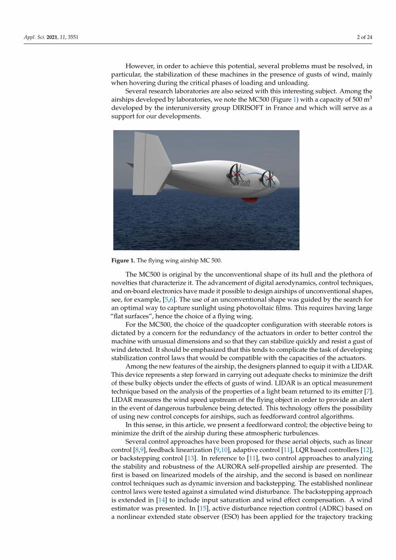
Several research laboratories are also seized with this interesting subject. Among theairships developed by laboratories, we note the MC500 (Figure 1) with a capacity of 500 m3

developed by the interuniversity group DIRISOFT in France and which will serve as asupport for our developments.

Figure 1. The flying wing airship MC 500.

The MC500 is original by the unconventional shape of its hull and the plethora ofnovelties that characterize it. The advancement of digital aerodynamics, control techniques,and on-board electronics have made it possible to design airships of unconventional shapes,see, for example, [5,6]. The use of an unconventional shape was guided by the search foran optimal way to capture sunlight using photovoltaic films. This requires having large“flat surfaces”, hence the choice of a flying wing.

For the MC500, the choice of the quadcopter configuration with steerable rotors isdictated by a concern for the redundancy of the actuators in order to better control themachine with unusual dimensions and so that they can stabilize quickly and resist a gust ofwind detected. It should be emphasized that this tends to complicate the task of developingstabilization control laws that would be compatible with the capacities of the actuators.

Among the new features of the airship, the designers planned to equip it with a LIDAR.This device represents a step forward in carrying out adequate checks to minimize the driftof these bulky objects under the effects of gusts of wind. LIDAR is an optical measurementtechnique based on the analysis of the properties of a light beam returned to its emitter [7].LIDAR measures the wind speed upstream of the flying object in order to provide an alertin the event of dangerous turbulence being detected. This technology offers the possibilityof using new control concepts for airships, such as feedforward control algorithms.

In this sense, in this article, we present a feedforward control; the objective being tominimize the drift of the airship during these atmospheric turbulences.

Several control approaches have been proposed for these aerial objects, such as linearcontrol [8,9], feedback linearization [9,10], adaptive control [11], LQR based controllers [12],or backstepping control [13]. In reference to [11], two control approaches to analyzingthe stability and robustness of the AURORA self-propelled airship are presented. Thefirst is based on linearized models of the airship, and the second is based on nonlinearcontrol techniques such as dynamic inversion and backstepping. The established nonlinearcontrol laws were tested against a simulated wind disturbance. The backstepping approachis extended in [14] to include input saturation and wind effect compensation. A windestimator was presented. In [15], active disturbance rejection control (ADRC) based ona nonlinear extended state observer (ESO) has been applied for the trajectory tracking

Appl. Sci. 2021, 11, 3551 3 of 24

of a stratospheric airship in the horizontal plane. The simplified model of the airshipin this plane is transformed into a two single input and single output subsystem usingthe input-output linearization method. The two equivalent linear systems are separatelyprocessed in order to use the observer (ESO) in real time to estimate the model parametersand to attenuate the wind force that affects the airship. In the same field of trajectorytracking, Yang [16] chose to use sliding mode control. In his study, he suggested a slidingmanifold composed of predefined nonlinear functions.

The previous control algorithms are based on the robustness technique and the ob-servers to compensate for the uncertainties of the model and the effect of an externalperturbation. However, the presence of a strong wind causes significant effects on theairship, and stabilization is difficult to obtain when the wind speed exceeds the limit re-quired by the robustness of the control. During a measured disturbance, the use of advancecontrols allows us to compensate for the effects of an exogenous signal before it influencesthe system. The minimization of the effects of a perturbation on the output to be controlledis treated as a problem of decoupling between the output of the system and the exogenousinput considered.

This problem has been solved using differential geometric analysis tools [17,18]. Analternative formulation based on the relative degree has been introduced in [19,20]. Theauthors have shown that the coupling problem is solved if the relative degree of theperturbation is greater than or equal to that of the output.

We applied this last methodology to our airship and we demonstrated the power ofthis technique and its interest in the control and stabilization of these large flying machines.

A study on a robust method is in progress. It is based on the model-free controltheory developed by Fliess [21]. This technique is freed from the dynamic model and itsuncertainties and seems promising for the stabilization of our airship. The results of thismethod will be published shortly.

A problem closely related to stabilization but little traced in the literature concerns theallocation of control. In order to prove that the established control can be implemented onthe machine, it would be necessary to verify the ability of the actuators to apply them. Theairship actuators, represented by the angles of orientation and the forces produced by therotors, actually have saturation limits. For the MC500 airship, the subject of this study, theactuators are twelve, but the “virtual” controls are six. The connection between the “virtual”controls and the actuators is thus described by a strongly nonlinear rectangular system,which makes solving this complex system a challenge. Usually, the control allocation isprocessed numerically. In this context, we cite the pseudo-inverse method used to solve theproblem of unconstrained control allocation [22], while the linear quadratic optimizationmethod with constraints is used in [23–25]. These methods use numerical techniques tofind the minimum of a quadratic cost function. However, the question of the applicabilityof these algorithms in real time in the face of an external disturbance arises. In fact, when agust of wind occurs, the robustness margin of the virtual controls can be exceeded, so theobjective function to be minimized cannot admit a minimum, and there will be a risk ofinstability of the airship.

This is why, in this study, we propose an original algorithm based on algebraicequations determined analytically according to energy arguments. This new algorithmwill allow the airship to be piloted even in bad weather conditions. A comparative studywith a numerical algorithm is presented.

We organized this paper as follows: in Section 2 a dynamic model of the airship MC500is proposed, in Section 3 we precisely present the stabilization strategy developed and acontrol algorithm based on a feedforward/feedback technique. In Section 4 we presentthe analytical algorithm developed for the control allocation that we compare with othernumerical techniques. Finally, in Section 5, numerical simulations are presented.

Appl. Sci. 2021, 11, 3551 4 of 24

2. Modeling2.1. Kinematic Description

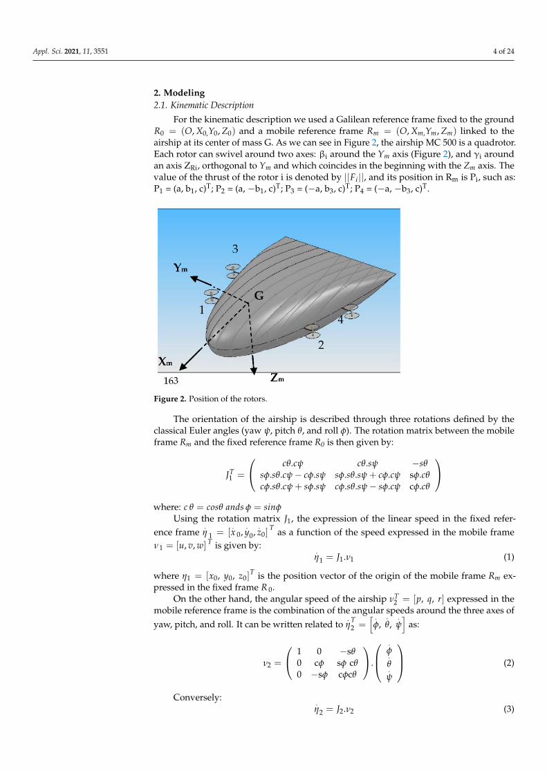
For the kinematic description we used a Galilean reference frame fixed to the groundR0 = (O, X0,Y0, Z0) and a mobile reference frame Rm = (O, Xm,Ym, Zm) linked to theairship at its center of mass G. As we can see in Figure 2, the airship MC 500 is a quadrotor.Each rotor can swivel around two axes: βi around the Ym axis (Figure 2), and γi aroundan axis ZRi, orthogonal to Ym and which coincides in the beginning with the Zm axis. Thevalue of the thrust of the rotor i is denoted by ||Fi||, and its position in Rm is Pi, such as:P1 = (a, b1, c)T; P2 = (a, −b1, c)T; P3 = (−a, b3, c)T; P4 = (−a, −b3, c)T.

Figure 2. Position of the rotors.

The orientation of the airship is described through three rotations defined by theclassical Euler angles (yaw ψ, pitch θ, and roll φ). The rotation matrix between the mobileframe Rm and the fixed reference frame R0 is then given by:

JT1 =

cθ.cψ cθ.sψ −sθsφ.sθ.cψ− cφ.sψ sφ.sθ.sψ + cφ.cψ sφ.cθcφ.sθ.cψ + sφ.sψ cφ.sθ.sψ− sφ.cψ cφ.cθ

where: c θ = cosθ ands φ = sinφ

Using the rotation matrix J1, the expression of the linear speed in the fixed refer-ence frame

.η 1 = [

.x 0,

.y0,

.z0]

T as a function of the speed expressed in the mobile frameν1 = [u, v, w] T is given by:

.η1 = J1.ν1 (1)

where η1 = [x0, y0, z0]T is the position vector of the origin of the mobile frame Rm ex-

pressed in the fixed frame R 0.On the other hand, the angular speed of the airship νT

2 = [p, q, r] expressed in themobile reference frame is the combination of the angular speeds around the three axes ofyaw, pitch, and roll. It can be written related to

.η

T2 =

[ .φ,

.θ,

.ψ]

as:

ν2 =

1 0 −sθ0 cφ sφ cθ0 −sφ cφcθ

.

.φ.θ.ψ

(2)

Conversely:.η2 = J2.ν2 (3)

Appl. Sci. 2021, 11, 3551 5 of 24

where the transformation matrix J2 is represented by: J2 =

1 sφ tan θ cφ tan θ0 cφ −sφ

0 sφcθ

cφcθ

.

It is important to mention that the parametrization by the angles of Euler presents asingularity for θ = π

2 + kπ; however, this configuration is not reachable for the airship.The kinematics of the airship can then be written as:( .

η1.η2

)=

(J1 00 J2

)(ν1ν2

)(4)

2.2. Dynamics

In a compact form, the whole dynamic system of the airship can be expressed asfollows [26]:

M..ν = τ + QG (5)

With ν =

(ν1ν2

)as the velocity vector and M =

(MTT 0

0 MRR

)as the mass

matrix. MTT and MRR are, respectively, the translation and the rotation part of the massmatrix of the airship. We denote by Mij the components of the 6 × 6 matrix M.

Let us note that this mass matrix comprises the terms of inertia of a solid body, butalso the terms of added masses. The acceleration of a moving body in a fluid creates aresistance force exerted by the latter, proportional to the acceleration of the solid. This forcecan therefore be likened to an increase in the mass of the solid, hence the notion of addedmass. The values of these added masses are important and not negligible in the case ofsubmarines or airships [27]. The computation of these added masses can be done thanks toexperiments, or analytically as was done, for example, for the MC500 [28].

In the right side, τ =

(τ1τ2

), τ1, and τ2 are, respectively, the external forces and

torques, including the rotors effects, the weight (m.g), the buoyancy B, the wind Force Fv, and

the aerodynamic lift (FL) and drag (FD). While QG =

(−ν2 ∧ (MTTν1)

−ν2 ∧ (MRRν2)− ν1 ∧ (MTTν1)

)are the gyroscopic forces and torques, we will denote by QGi its components, ∧ being thevector product.

When combining with the kinematic relations (4), the global dynamic model in itsdeveloped form becomes:

.x0 = cψ.cθ.u + (−sψ.cφ + cψsφsθ)v + (sψsφ + cψcφsθ)w

.y0 = sψcθ.u + (cψcφ + sψsφsθ)v + (−cψsφ + sψcφsθ)w

.z0 = −sθ.u + sφ.cθ.v + cφcθw.φ = p + sφ. tan θ. q + cφ. tan θ.r

.θ = cφ.q− sφ.r

.ψ = sφ

cθ q + cφcθ r

M11.u = α1 + QG1 + Fv1

M22.v = α2 + QG2 + Fv2

M33.

w = α3 + QG3 + Fv3(M2

46 −M66M44) .

p = M46α6 + M46QG6 −M66α4 −M66QG4M55

.q = α5 + QG5(

M246 −M66M44

) .r = M46α4 −M44α6 + M46QG4 −M44QG6

(6)

where Fvi are the components of the wind applied forces and αi the components of thecontrol vector α. The different characteristics of the actuators will be developed in detail inSection 4.

Appl. Sci. 2021, 11, 3551 6 of 24

3. Stabilization Strategy3.1. Mathematical Tools

In some applications, exogenous perturbation is known in advance. This is often thecase for the airship. The MC500 is equipped with LIDAR sensors that can measure the forceof a wind gust. From the control point of view, the purpose of using this information is toreduce or minimize the influence of the disturbance that affects the airship. To deal withthe problem of minimizing the impact of a wind gust, we propose the use of feedforwardcontrols. This control vector is built using techniques of differential geometry. The diagramof this method is described in Figure 3.

Figure 3. Block diagram of the control vector.

The feedforward/feedback method controls a set of nonlinear systems which areas follows:

.x = f (x) + g(x)u +

m∑

i=1pidi

y = h(x)(7)

Here, x ∈ Rn represents the state system, y is the output system, u ∈ Rm the inputsystem, g(x) = [g1(x), · · · , gm(x)]T , gi(i = 1, · · · , m) is an m-dimensional vector field,f (x) ∈ Rn is a vector field, and h(x) = [h1(x), · · · , hm(x)]T , hi(i = 1, · · · , m) is a suffi-ciently smooth scalar function, di the disturbance inputs, and pi are vectors detailed inAppendix A.

Definition 1. If we assume that the vector fields h and f are sufficiently smooth, the Lie derivativeof h with respect to f can be defined as:

L f h =n

∑i=1

∂hi∂xi

fi(x) (8)

Definition 2. In the system of Equations (7), if the two ensuing conditions are satisfied forallx ∈ Rn in the vicinity of an equilibrium point xe [17]:

Lgj Lkf hi(x) = 0 (9)

Appl. Sci. 2021, 11, 3551 7 of 24

The (m ×m) matrix of decoupling D is not singular at x = xe, with:

D(x) =

Lg1 Lr1−1

f h1(x) . . . Lgm Lr1−1f h1(x)

Lg1 Lr2−1f h2(x) . . . Lgm Lr2−1

f h2(x). . . . . . . . .

Lg1 Lrm−1f hm(x) . . . Lgm Lrm−1

f hm(x)

(10)

Then, the system (7) is said to have a relative degree:

r =m

∑i=1

ri (11)

The indices I, j, and k verify: 1 ≤ j, i ≤ m, 1 ≤ k ≤ ri − 1. ri are the relative degree ofthe outputs. Examples of the derivatives Lgj Lk

f hi(x) are presented later in Section 3.2.1.

Definition 3. The relative order ρji of the output yi of Y with respect to the disturbance input di is

defined [19,20] as the smallest integer for which: Lpi Lρi

j−1f hj 6= 0

Proposal 1. The system of Equation (7) is feedback linearizable if it exists as a function h ∈ Rm

sufficiently smooth such that the system has the relative degree r = n = dim(x), x is the state.

We will apply this result to demonstrate that the model of the airship MC500 subjectedto a wind gust is linearizable. We can thus apply the input-output linearization method todefine a control vector that anticipates the effect of a wind gust pre-detected by LIDAR.

3.2. Scheme of the Control Vector

In order to stabilize the airship when hovering in the vicinity of a loading and un-loading point around a desired state Ψ = [xd, yd, zd, φd, θd, ψd]

T , and to anticipate theeffect of a gust of wind, we will consider as a new output the error (ξi)1≤i≺6 defined by:ξi = yi −Ψi with: Y = [x0, y0, z0, φ, θ, ψ]T . The objective is to make the output convergetowards the desired state, in other words, to make the error ξi converge towards zero.

Without losing generality, we assume that Fν2 = Fν3 = 0 (the gust of wind comes onlyfrom the X axis without creating any torque).

The system of errors associated with the system in Equation (6) could be written inthe same form given by Equation (7) as: .

X = f (X) + g(X)α + p1Fv1

Y = h = [x0, y0, z0, ϕ, θ, ψ]t(12)

With: X the system of error defined as: X = [ξ1, ξ2, ξ3, ξ4, ξ5, ξ6, u, v, w, p, q, r],α = [α1, α2, α3, α4, α5, α6]

T the control vector, and p1, f and g are vectors of R12 (seeAppendix A for more details).

The input-output linearization method is summarized in two steps (see Figure 4). Thefirst is to transform the system into a decoupled linear system using the techniques ofdifferential geometry. The second is to construct a control vector by using the theory oflinear control to ensure the stability of the new system.

Appl. Sci. 2021, 11, 3551 8 of 24

Figure 4. Control method of feedforward/feedback control.

3.2.1. Relative Degree of Outputs Associated with the Control Vector

Let r be the relative degree of the system (12).To determine the relative degree

(rj)

1≤j≤6 corresponding to the output yj, this isderived last until at least one input appears.

In their work, Daoutidis [19,20] proposes the following expression for ξ(rj)

j :

ξ(rj)

j = Lrjf hj +

6

∑i=1

Lgi Lrj−1f hjαi +

6

∑i=1

Lpi Lrj1−1f hjd1 (13)

Here, we have: Lgi h1 = 0Then: .

ξ1 = L f h1 = f1 (14)

The first derivative of ξ 1 does not include any of the controls. Therefore, anotherderivation of ξ 1 is necessary:

..ξ1 = L2

f h1 + Lg1 L f h1α1 + Lg2 L f h1α2 + Lg3 L f h1α3 + Lp1 L f h1Fv1 (15)

With:L2

f h1 =∂ f1

∂φf4 +

∂ f1

∂θf5 +

∂ f1

∂ψf6 +

∂ f1

∂uf7 +

∂ f1

∂vf8 +

∂ f1

∂wf9

Lg1 L f h1 = ∇ f1.g1 =cψcθ

M11; Lg2 L f h1 = ∇ f1.g2 =

−sφ + cφsθ

M22

Lg3 L f h1 = ∇ f1.g3 =sφ + cφsθ

M33; Lgj L f h1 = 0, j = 4, 5, 6

∇ is the gradient. We notice that the second derivative of ξ1 is written as a function ofthe control. Hence, the degree r1 associated with the output is equal to 2.

In the same way, the other relative degrees are computed, and we thus obtain:

r1 = r2 = · · · = r6 = 2

The total relative degree of the system is then r = 12, we conclude that the nonlinearmodel of the airship in Equation (11) satisfies the conditions in proposal 1. We can then

Appl. Sci. 2021, 11, 3551 9 of 24

deduce that the system in Equation (11) is feedback linearizable. Therefore, a state offeedback control and a diffeomorphism that transforms the nonlinear system into anequivalent linear system exist.

3.2.2. Relative Degree Associated with Disturbances

The relative degree of the output(rj)

1≤j≤6 and that of the disturbance ρj1 play afundamental role in characterizing the influence of the perturbation on the outputs. Twocases may arise [19]:

• ρj1 rj the disturbance does not directly affect the output, so the stabilization of theairship is ensured by a feedback control law.

• ρj1 ≤ rj the disturbance affects the output. We use a feedforward/feedback control tostabilize the airship and anticipate the effect of this exogenous signal.

The relative degree ρj1 of the disturbance associated with the output yi is then deter-mined using Definition 3:

• for the output, y1 = x0, y2 = y0, y3 = z0, we have:Lp1 h1 = Lp1 h2 = Lp1 h3 = 0

Lp1 L f h1 = cψcθM11

Lp1 L f h2 = −sθM11

Lp1 L f h2 = sψ cθM11

(16)

then:ρ11 = ρ21 = ρ31 = ρ2 = 0 r2 = 2 (17)

For the outputs y4 = φ, y5 = θ and y6 = ψ, we have:

Lp1 L−1+ρj1f hi = 0 ∀i = 4, 5, 6 (18)

We then deduce that:ρj1 rj ∀j = 4, 5, 6 (19)

On the basis of the two previous findings, the outputs x, y, and z are affected bothby the disturbance and by the input in the same way. Therefore, to anticipate the effect ofthe exogenous signal, the feedforward control is necessary. We will combine it with thefeedback control to realize the control schema.

However, for the other degrees of freedom (y, z, φ, θ, and ψ ), we noticed in Equation (19)that the effect of the inputs is preponderant compared to the effect of the disturbance ofthe outputs. This indicates that we do not need a feedforward control to minimize thedisturbance effect.

3.2.3. Coordinate Change and New Linear System

Following the recommendations of Isidori [17], we can define a diffeomorphism Φ.This diffeomorphism allows us to transform the nonlinear system into another nonlinear

Appl. Sci. 2021, 11, 3551 10 of 24

system, as we can see below, in order to determine the control vector which linearizes thesystem. This diffeomorphism is given by:

x0cψcθ.u + (−sψcφ + cφsθ)v + (sψsφ + cφsθ)w

y0sψcθ.u + (cφ + sφsθ)v + (−cφ + sφsθ)w

z0−sθ.u + sφ.c + cφ.c

φp + sφ. tan θ.q + cφ. tan θ.r

θcφ.q− sφ.r

ψsφcθ + cφ

cθ r

(20)

Using the new coordinates, by applying the diffeomorphism, the system in Equation (12)can be written as follows:

.ξ1..ξ1.ξ2..ξ2.ξ3..ξ3.ξ4..ξ4.ξ5..ξ5.ξ6..ξ6

=

L f h1

L2f h1 +

3∑

i=1Lgi L

2f h1αi + Lp1 L f h1Fv1

L f h2

L2f h2 +

3∑

i=1Lgi L

2f h2αi

L f h3

L2f h3 +

3∑

i=1Lgi L

2f h3αi

L f h4

L2f h4 +

6∑

i=4Lgi L

2f h4αi

L f h5

L2f h5 +

6∑

i=4Lgi L

2f h5αi

L f h6

L2f h6 +

6∑

i=4Lgi L

2f h6αi

(21)

By combining the equations containing the control vector αi and Equation (16),it becomes:

..ξ1..ξ2..ξ3..ξ4..ξ5..ξ6

=

L2f h1

L2f h2

L2f h3

L2f h4

L2f h5

L2f h6

︸︷︷︸

ň

+ D

α1α2α3α4α5α6

︸︷︷︸

α

+ Fv1 .

cψcθM11sψcθM11−sθM11000

︸︷︷︸

Ω

= ň + Dα + Fv1 .Ω = ℵ (22)

3.2.4. The Linearizing Control Law

According to Equation (22), we can deduce the linearizing control α. This controlvector will ensure the decoupling and can be written as:

α = D−1(ℵ − ň− Fv1 .Ω) (23)

Appl. Sci. 2021, 11, 3551 11 of 24

Note that the linearization would only be possible if the decoupling matrix D isinvertible. However, the decoupling matrix D given by:

D =

(Π 00 Γ

)(24)

is invertible, and we have:

D−1 =

(Π−1 0

0 Γ−1

)(25)

(For the expressions of Π, Γ, Π−1, and Γ−1 see Appendix B).Replacing Equation (23) in Equation (22), the equivalent system becomes linear and

completely decoupled. It can be written as follows:

..ξ1..ξ2..ξ3..ξ4..ξ5..ξ6

=

.z1

2.z2

2.z3

2.z4

2.z5

2.z6

2

=

ℵ1ℵ2ℵ3ℵ4ℵ5ℵ6

(26)

Finally, we obtain the following six decoupled linear sub-systems with their outputs:.zi

1 = zi2

.zi

2 = ℵiξi = zi

1

(27)

The vector ℵ is designed according to the control objectives. In general, for a trackingtrajectory problem, the expressions of ℵi are:

ℵi = ω(ri)i + σri−1

(y(ri−1)

i −ω(ri−1)i

)+ . . . + σ1(yi −ωi) (28)

ω( r i)i are reference trajectories. In our case these are functions in steps

( .ω(ri)i =

..ω(ri)i = 0

).

σri−1 are the gains. If the σi are chosen so that the polynomial sri + σri−1.sri−1 +· · · σ2.s + σ1 = 0, the polynomial is said to be a Hurwitz polynomial (possesses roots withnegative real parts), then it can be shown that the error ξi = yi − Ψi tends towards zero.

We have chosen the following poles P = −10,−4 for the system in Equation (28) to bestable, then the gains of the control ℵi, which are solutions of the equation s2 + σ2.s+ σ1 = 0,are given by: σ1 = 40 and σ2 = 14.

This values are needed in the numerical simulations to assess the performance of theproposed controller.

Previous developments show that it is possible to anticipate the effect of a gust ofwind on the airship. The feedforward control that we have just established is a key part ofthis objective. Indeed, this control ensures the accelerated attenuation of the effect of thewind disturbance when this is known in advance, and it gives the control vector a certainrobustness with respect to any modeling errors.

We have also demonstrated the following result:Proposal. Consider the Multiple-Input Multiple-Output (MIMO) system of the airship

MC500 described by Equation (12).We define

(rj)

1≤j≤6 as the relative degree of the outputs and ρ11 as the relative degreeof the disturbance Fν1 associated with the outputs y1 = x0.

It is assumed that the decoupling matrix D is invertible, then the control vector Ugiven in Equation (23):

Appl. Sci. 2021, 11, 3551 12 of 24

• anticipates the effect of a gust of wind.• ensures the stability of the airship in the vicinity of a target state.

Note:

1. We have restricted ourselves to a single excitation force along the X axis to limit thesize of the equations. However, to take into account the effect of other force andtorque components, the same steps described above would be followed.

2. The airship is operated by electric motors having sufficient degrees of freedom. Asmentioned previously, the airship is over-actuated. It will thus be possible to anticipatethe effect of all types of wind gusts and thus prevent against the main destabilizingelement of the airship (the wind).

It should be remembered that the latter is the main factor in delaying the expansion ofthe use of the airships as flying cranes or as means of transport of heavy loads.

4. Control Allocation

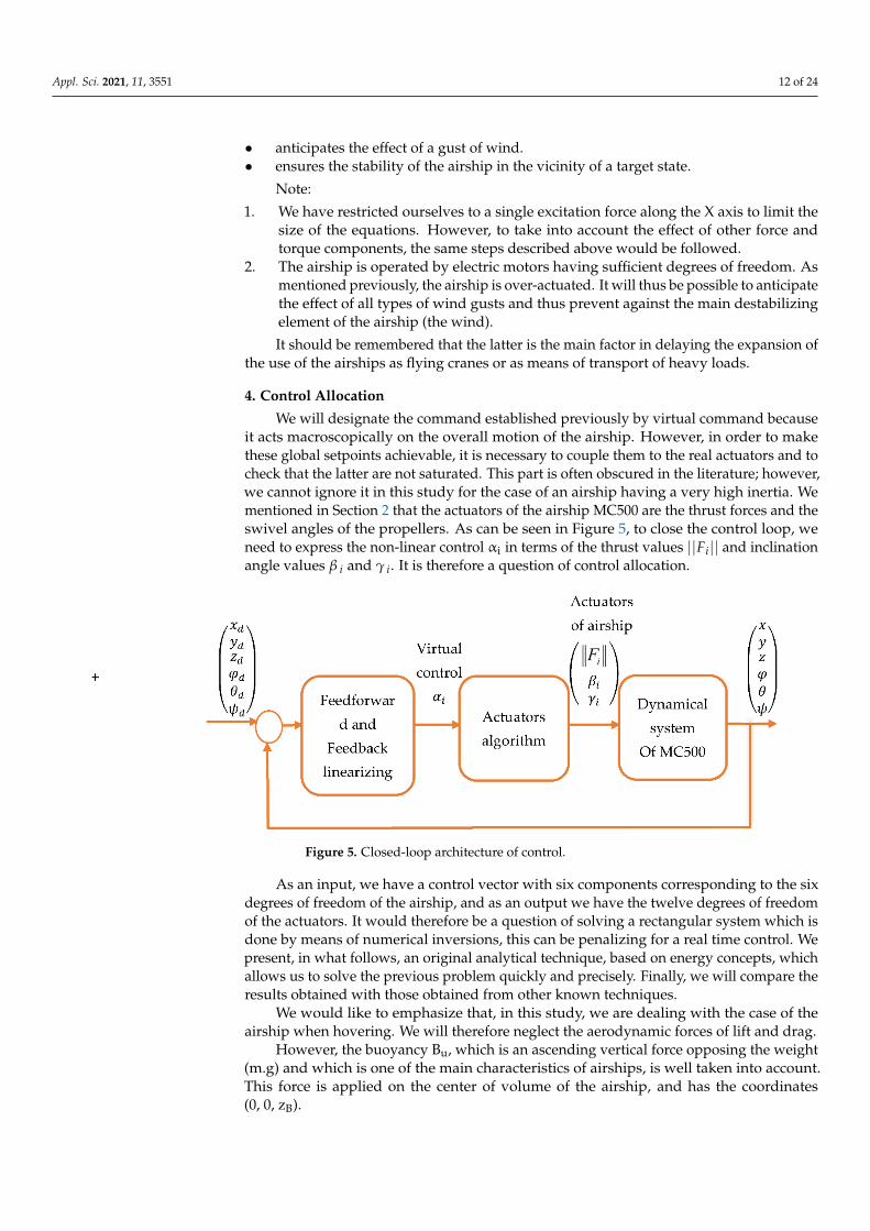
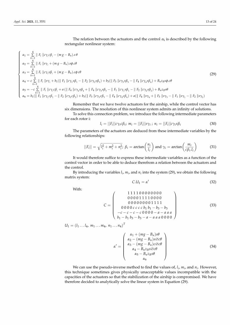
We will designate the command established previously by virtual command becauseit acts macroscopically on the overall motion of the airship. However, in order to makethese global setpoints achievable, it is necessary to couple them to the real actuators and tocheck that the latter are not saturated. This part is often obscured in the literature; however,we cannot ignore it in this study for the case of an airship having a very high inertia. Wementioned in Section 2 that the actuators of the airship MC500 are the thrust forces and theswivel angles of the propellers. As can be seen in Figure 5, to close the control loop, weneed to express the non-linear control αi in terms of the thrust values ||Fi|| and inclinationangle values β i and γ i. It is therefore a question of control allocation.

Figure 5. Closed-loop architecture of control.

As an input, we have a control vector with six components corresponding to the sixdegrees of freedom of the airship, and as an output we have the twelve degrees of freedomof the actuators. It would therefore be a question of solving a rectangular system which isdone by means of numerical inversions, this can be penalizing for a real time control. Wepresent, in what follows, an original analytical technique, based on energy concepts, whichallows us to solve the previous problem quickly and precisely. Finally, we will compare theresults obtained with those obtained from other known techniques.

We would like to emphasize that, in this study, we are dealing with the case of theairship when hovering. We will therefore neglect the aerodynamic forces of lift and drag.

However, the buoyancy Bu, which is an ascending vertical force opposing the weight(m.g) and which is one of the main characteristics of airships, is well taken into account.This force is applied on the center of volume of the airship, and has the coordinates(0, 0, zB).

Appl. Sci. 2021, 11, 3551 13 of 24

The relation between the actuators and the control αi is described by the followingrectangular nonlinear system:

α1 =4∑

k=1‖ Fi ‖cγi cβi − (m g− Bu).s θ

α2 =4∑

k=1‖ Fi ‖sγi + (m g− Bu).sφ.cθ

α3 =4∑

k=1‖ Fi ‖cγi sβi + (m g− Bu).cφ cθ

α4 = c4∑

k=1‖ Fi ‖sγi + b1(‖ F1 ‖cγ1 sβ1 − ‖ F2 ‖cγ2 sβ2) + b3(‖ F3 ‖cγ3 sβ3 − ‖ F4 ‖cγ4 sβ4) + BuzBsφ.cθ

α5 = −c4∑

k=1‖ Fi ‖cγi cβi + a (‖ F4 ‖cγ4 sβ4 + ‖ F4 ‖cγ3 sβ3 − ‖ F1 ‖cγ1 sβ1 − ‖ F2 ‖cγ2 sβ2) + BuzBsθ

α6 = b1(‖ F1 ‖cγ1 cβ1 − ‖ F2 ‖cγ2 cβ2) + b3(‖ F3 ‖cγ3 cβ3 − ‖ F4 ‖cγ4 cβ4) + a(‖ F4 ‖sγ4 + ‖ F3 ‖sγ3 − ‖ F1 ‖sγ1 − ‖ F2 ‖sγ2)

(29)

Remember that we have twelve actuators for the airship, while the control vector hassix dimensions. The resolution of this nonlinear system admits an infinity of solutions.

To solve this connection problem, we introduce the following intermediate parametersfor each rotor i:

li = ||Fi||cγicβi; mi = ||Fi||sγi ; ni = ||Fi||cγisβi (30)

The parameters of the actuators are deduced from these intermediate variables by thefollowing relationships:

||Fi|| =√

l2i + m2

i + n2i ; βi = arctan

(nili

)and γi = arctan

(mi

cβi.li

)(31)

It would therefore suffice to express these intermediate variables as a function of thecontrol vector in order to be able to deduce therefrom a relation between the actuators andthe control.

By introducing the variables li, mi, and ni into the system (29), we obtain the followingmatrix system:

C.U1 = α′ (32)

With:

C =

1 1 1 1 0 0 0 0 0 0 0 00 0 0 0 1 1 1 1 0 0 0 00 0 0 0 0 0 0 0 1 1 1 1

0 0 0 0 c c c c b1 b1 − b3 − b3−c− c− c− c 0 0 0 0− a− a a ab1 − b1 b3 − b3 − a− a a a 0 0 0 0

(33)

U1 = (l1 . . . l4, m1 . . . m4, n1 . . . n4)T

α′ =

α1 + (mg− Bu)sθα2 − (mg− Bu)s∅cθα3 − (mg− Bu)c∅cθ

α4 − BuzBs∅cθα5 − BuzBsθ

α6

(34)

We can use the pseudo-inverse method to find the values of, li, mi, and ni. However,this technique sometimes gives physically unacceptable values incompatible with thecapacities of the actuators so that the stabilization of the airship is compromised. We havetherefore decided to analytically solve the linear system in Equation (29).

Appl. Sci. 2021, 11, 3551 14 of 24

4.1. Analytical Approach

The system in Equation (29), according to the new variables li, mi, and ni, can bedivided into two subsystems that will be separately investigated:

4∑

k=1ni = α′3

b1(n1 − n2) + b3(n3 − n4) = α′4 − cα′2a(n3 + n4 − n1 − n2) = cα′1 + α′5

(35)

4∑

k=1li = α′1

4∑

k=1mi = α′2

b1(l1 − l2) + b3(l3 − l4) + a(m4 + m3 −m1 −m2) = α′6

(36)

The first and third equation of the system in Equation (35) give:

n3 + n4 =α′32

+cα′1 + α′5

2a(37)

We initially imposed this choice:

n3 = n4 =α′34

+cα′1 + α′5

4a(38)

Substituting h3 and h4 by their values in the system in Equation (36), one can obtain:

n1 =α′32

+α′4 − cα′2

2b1− 2n3 (39)

Additionally, then:n2 = α′4 − n1 − n3 (40)

By combining the second and the third equation of the system in Equation (36),this gives:

b1(l1 − l2) + b3(l3 − l4) + 2a(m4 + m3) = α′6 + aα′2 (41)

We decided to add these two conditions according to the logical operation of the actuators:

and : m3 = m4 =α′24

(42)

b1(l1 − l2) = b3(l3 − l4) =α′62

(43)

These assumptions allowed us to retrieve the expressions of the missing variablesthrough the following relations:

m1 = m2 = α′24 ; l2 = l4 = α′1

4 − ( 18b1

+ 18b3

)α′

l1 = α′62b1

+ l2 ; l3 = α′62b3

+ l4

(44)

The block diagram shown in Figure 6 describes the original algorithm establishedto define the relationship between the actuators of the MC500 and the controllers. Thealgorithm is based on algebraic relations which will be solved analytically.

Appl. Sci. 2021, 11, 3551 15 of 24

Figure 6. Block diagram of the proposed control system.

The proposed approach is based on energy principles. Indeed, and in the case of thehovering flight of a propeller-driven quadcopter, there are several solutions. However, thesolution that induces the minimum energy consumption is the one that balances the thrustof the four rotors. To this goal, we have imposed some constraints to be as close as possibleto the equilibrium configuration of the different thrusts whenever the operating conditionsallow it.

As a comparative analysis, we present in the next paragraph a numerical approachestablishing the control allocation.

The comparison of the results of these two methods will be performed in the chapterdevoted to numerical simulations.

4.2. Numerical Approach

To check this approximate approach, we compare our results here with a numericalmethod. We used the fixed-step gradient method to compute the solution numerically.This algorithm is iterative based on the minimization of a cost function J(U1).

The principle of the algorithm is to generate a vector series U1,k from an arbitrarypoint U1,0 such that the cost value of the function J(U1) decreases with each iteration, i.e.,:

J(U1,k+1) < J(U1,k)

For the fixed-step gradient method, the vector U1,k is updated in this way:

U1,k+1 = U1,k −12

µ∂J(U1,k)

∂U1(45)

The index k denotes the iteration and µ is a positive constant parameter.To solve the linear system in Equation (32) we propose the use of the cost function J

defined by:

J(τ) =6

∑i=1

(α′ i − τi

)2 (46)

The terms of the quadratic function penalize the error ei = α′ i− τi between the controlvector, the vector forces τ1, and the torques τ2 (see Equation (29)).

We can see that when the quadratic function is minimal, the terms ei tend toward zero,then τi tend to α′ i.

Hence, the intermediate parameters obtained, li, mi, and ni, are the components of thevector that minimize the cost function.

Appl. Sci. 2021, 11, 3551 16 of 24

By using the matrix relations in Equation (32)–(34), the cost function J can be written as:

J(U1) =6

∑i=1

(α′ i − CiU1

)2 (47)

With Ci is the ith line of the matrix C.The gradient of J is:

∇J(U1) = −26

∑i=1

Cti(α′ i − CiU1

)(48)

Then, Equation (45) becomes:

U1,k+1 = U1,k + 2µ6

∑i=1

Cti(α′ i − CiU1,k

)(49)

This method has the advantage of being easy to implement. Unfortunately, theconvergence of this method is generally slow. The steps for obtaining the numericalsolution are detailed in Algorithm 1:

Algorithm 1 fixed-step gradient

Step 1: Initializationk = 0: Choice of li,0, mi,0, ni,0 and µ, ε > 0Step 2: Iteration k (i = 1, · · · , 4)[li,k+1, mi,k+1, ni,k+1

]t=[li,k, mi,k, ni,k

]t+ 2µ

6∑

i=1Ct

i

(α′ i − Ci

[li,k, mi,k, ni,k

]t)Step 3: Stop criterion:∣∣∣|[li,k+1, mi,k+1, ni,k+1

]t,−,[li,k, mi,k, ni,k

]t∣∣∣| < ε

Note:

1. In order to implement the proposed algorithm, the convergence of it is an importantfactor to take into account. The gradient algorithm that minimizes the quadratic func-tion in Equation (46) converges if: 0 ≺ µ ≺ 2M2

M21

with M1 = max(λi); M2 = min(λi),

Where (λi)1≤i≤12 are the eigenvalues of the symmetric matrix C1 = 26∑

i=1CT

i Ci.

For both the analytical and the numerical methods, we have succeeded in stabiliz-ing the airship. However, during a short transient phase, the actuators’ capacities wereexceeded. In this first approach, we have introduced a saturation block assuming that thepropellers are in saturation abutment. Further studies are underway to solve this problemusing constrained optimization techniques. This will be dealt with in future work.

5. Numerical Results

We present here some examples demonstrating the utility of the proposed formulationin different cases.

For this, we used data from the MC500 airship, such as:The volume V = 500 m3; zG = 0.5 m; a = 2.5 m; b1 = 5.4 m; b3 = 6.5 m; c = 2 m;The added mass matrix and the inertia are given by:M11 = 583 kg; M46 = 160 kg.m2; µ = 0.01; ε = 10−3; M22 = 620 kg; M33 = 687 kg;

M44 = 9413 kg.m2; M55 = 10,456 kg.m2; M66 = 18,700 kg.m2;

5.1. Ideal Case: No Wind Disturbance

In the first step we check the efficiency of the control vector and the performances ofthe proposed algorithms to solve the connection problem envisaged under ideal conditions,i.e., the wind speed is zero.

Appl. Sci. 2021, 11, 3551 17 of 24

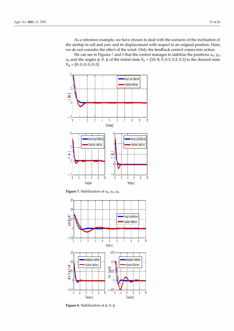
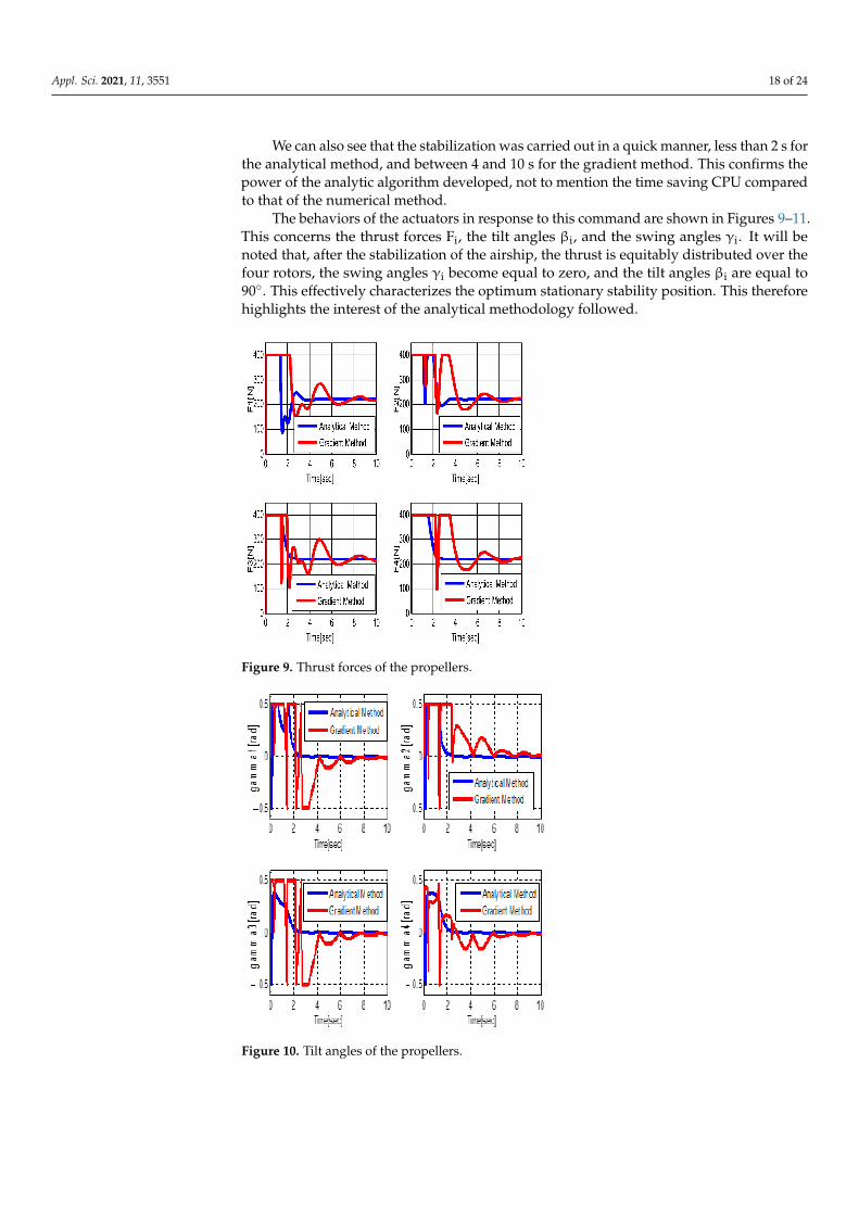
As a reference example, we have chosen to deal with the scenario of the inclination ofthe airship in roll and yaw and its displacement with respect to an original position. Here,we do not consider the effect of the wind. Only the feedback control comes into action.

We can see in Figures 7 and 8 that the control manages to stabilize the positions x0, y0,z0 and the angles φ, θ, ψ of the initial state Xe = [10; 8; 5; 0.3; 0.2; 0.1] to the desired stateXd = [0; 0; 0; 0; 0; 0].

Figure 7. Stabilization of x0, y0, z0.

Figure 8. Stabilization of φ, θ, ψ.

Appl. Sci. 2021, 11, 3551 18 of 24

We can also see that the stabilization was carried out in a quick manner, less than 2 s forthe analytical method, and between 4 and 10 s for the gradient method. This confirms thepower of the analytic algorithm developed, not to mention the time saving CPU comparedto that of the numerical method.

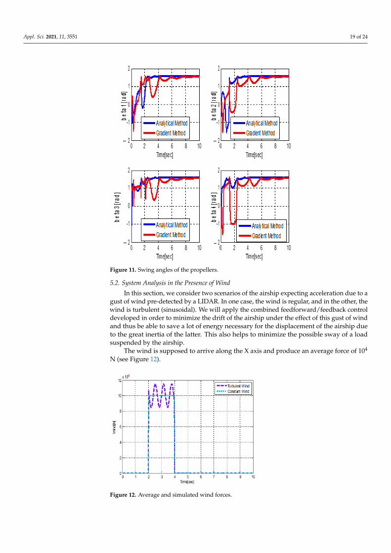
The behaviors of the actuators in response to this command are shown in Figures 9–11.This concerns the thrust forces Fi, the tilt angles βi, and the swing angles γi. It will benoted that, after the stabilization of the airship, the thrust is equitably distributed over thefour rotors, the swing angles γi become equal to zero, and the tilt angles βi are equal to90. This effectively characterizes the optimum stationary stability position. This thereforehighlights the interest of the analytical methodology followed.

Figure 9. Thrust forces of the propellers.

Figure 10. Tilt angles of the propellers.

Appl. Sci. 2021, 11, 3551 19 of 24

Figure 11. Swing angles of the propellers.

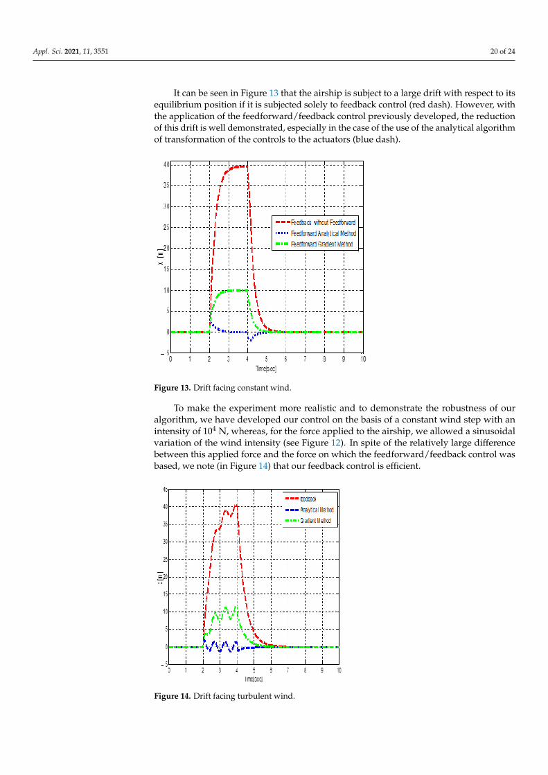
5.2. System Analysis in the Presence of Wind

In this section, we consider two scenarios of the airship expecting acceleration due to agust of wind pre-detected by a LIDAR. In one case, the wind is regular, and in the other, thewind is turbulent (sinusoidal). We will apply the combined feedforward/feedback controldeveloped in order to minimize the drift of the airship under the effect of this gust of windand thus be able to save a lot of energy necessary for the displacement of the airship dueto the great inertia of the latter. This also helps to minimize the possible sway of a loadsuspended by the airship.

The wind is supposed to arrive along the X axis and produce an average force of 104

N (see Figure 12).

Figure 12. Average and simulated wind forces.

Appl. Sci. 2021, 11, 3551 20 of 24

It can be seen in Figure 13 that the airship is subject to a large drift with respect to itsequilibrium position if it is subjected solely to feedback control (red dash). However, withthe application of the feedforward/feedback control previously developed, the reductionof this drift is well demonstrated, especially in the case of the use of the analytical algorithmof transformation of the controls to the actuators (blue dash).

Figure 13. Drift facing constant wind.

To make the experiment more realistic and to demonstrate the robustness of ouralgorithm, we have developed our control on the basis of a constant wind step with anintensity of 104 N, whereas, for the force applied to the airship, we allowed a sinusoidalvariation of the wind intensity (see Figure 12). In spite of the relatively large differencebetween this applied force and the force on which the feedforward/feedback control wasbased, we note (in Figure 14) that our feedback control is efficient.

Figure 14. Drift facing turbulent wind.

Appl. Sci. 2021, 11, 3551 21 of 24

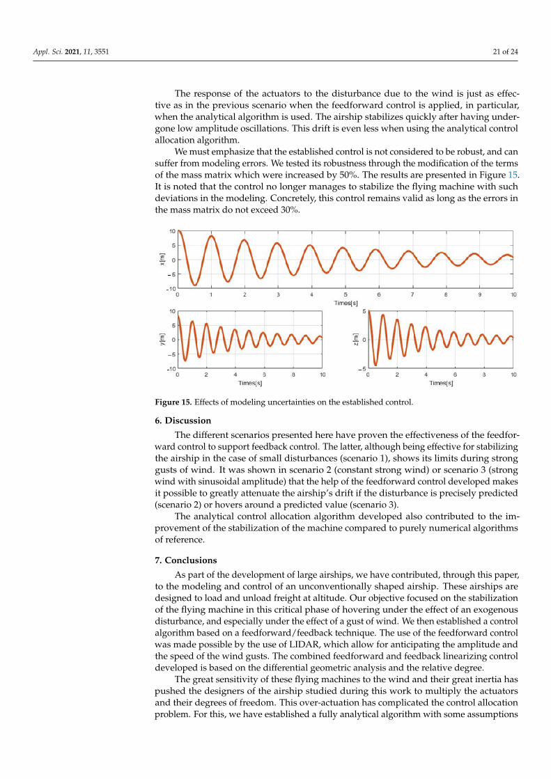
The response of the actuators to the disturbance due to the wind is just as effec-tive as in the previous scenario when the feedforward control is applied, in particular,when the analytical algorithm is used. The airship stabilizes quickly after having under-gone low amplitude oscillations. This drift is even less when using the analytical controlallocation algorithm.

We must emphasize that the established control is not considered to be robust, and cansuffer from modeling errors. We tested its robustness through the modification of the termsof the mass matrix which were increased by 50%. The results are presented in Figure 15.It is noted that the control no longer manages to stabilize the flying machine with suchdeviations in the modeling. Concretely, this control remains valid as long as the errors inthe mass matrix do not exceed 30%.

Figure 15. Effects of modeling uncertainties on the established control.

6. Discussion

The different scenarios presented here have proven the effectiveness of the feedfor-ward control to support feedback control. The latter, although being effective for stabilizingthe airship in the case of small disturbances (scenario 1), shows its limits during stronggusts of wind. It was shown in scenario 2 (constant strong wind) or scenario 3 (strongwind with sinusoidal amplitude) that the help of the feedforward control developed makesit possible to greatly attenuate the airship’s drift if the disturbance is precisely predicted(scenario 2) or hovers around a predicted value (scenario 3).

The analytical control allocation algorithm developed also contributed to the im-provement of the stabilization of the machine compared to purely numerical algorithmsof reference.

7. Conclusions

As part of the development of large airships, we have contributed, through this paper,to the modeling and control of an unconventionally shaped airship. These airships aredesigned to load and unload freight at altitude. Our objective focused on the stabilizationof the flying machine in this critical phase of hovering under the effect of an exogenousdisturbance, and especially under the effect of a gust of wind. We then established a controlalgorithm based on a feedforward/feedback technique. The use of the feedforward controlwas made possible by the use of LIDAR, which allow for anticipating the amplitude andthe speed of the wind gusts. The combined feedforward and feedback linearizing controldeveloped is based on the differential geometric analysis and the relative degree.

The great sensitivity of these flying machines to the wind and their great inertia haspushed the designers of the airship studied during this work to multiply the actuatorsand their degrees of freedom. This over-actuation has complicated the control allocationproblem. For this, we have established a fully analytical algorithm with some assumptions

Appl. Sci. 2021, 11, 3551 22 of 24

for solving this problem. Our algorithm has proved its efficiency in comparison withother classical numerical methods, and especially its superiority in the face of these samealgorithms in terms of minimizing the computation time.

In future works, the feedforward control vector algorithm will be applied to thetrajectory tracking.

Author Contributions: Conceptualization, N.A. and M.K.; methodology, N.A. and J.L.; software,M.K.; validation, all authors; investigation, all authors, writing—original draft preparation, N.A.;writing—review and editing, N.A. and M.K.; supervision, J.L. and A.A.; project administration, N.A.;All authors have read and agreed to the published version of the manuscript.

Funding: This research received no external funding. All authors certify that they have no affiliationswith or involvement in any organization or entity with any financial interest or non-financial interestin the subject matter or materials discussed in this manuscript.

Institutional Review Board Statement: Not applicable

Informed Consent Statement: Not applicable

Data Availability Statement: The data presented in this study are available on request from thecorresponding author.

Conflicts of Interest: The authors declare that they have no conflict of interest.

Appendix A

p1 =

[0, 0, 0, 0, 0, 0,

1M11

0, 0, 0, 0, 0]t

f (X) = [ f1, . . . , f12]t

=

cψcθu + (−sψcφ + cφsθ)v + (sψsφ + cφsθ)wsψcθu + (cφ + sφsθ)v + (−cφ + sφsθ)w

−sθu + sφc + cφcp + sφtθq + cφtθr

cφq− sφrsφcθ q + cφ

cθ rQ1

M11Q2

M22Q3

M33M46Q6−M66Q4M2

46−M66 M44Q5

M55M46Q4−M44Q6M2

46−M66 M44

Additionally, the vectors gi are given by:

g1 =

[0, 0, 0, 0, 0, 0,

1M11

, 0, 0, 0, 0, 0]t

g2 =

[0, 0, 0, 0, 0, 0, 0,

1M22

, 0, 0, 0, 0]t

g3 =

[0, 0, 0, 0, 0, 0, 0, 0,

1M33

, 0, 0, 0]t

g4 =

[0, 0, 0, 0, 0, 0, 0, 0, 0,

−M66

(M462 −M66M44

,M46

(M462 −M66M44

, 0]t

Appl. Sci. 2021, 11, 3551 23 of 24

g5 =

[0, 0, 0, 0, 0, 0, 0, 0, 0, 0, 0,

1M55

, 0]t

g6 =

[0, 0, 0, 0, 0, 0, 0, 0, 0,

M46

(M462 −M66M44

,−M44

(M462 −M66M44

, 0]t

Appendix B

Γ =

−M66

M246−M66 M44

+ M46cφtθ

M246−M66 M44

sφtθM55

M46M2

46−M66 M44+ −M44cφtθ

M246−M66 M44

−M46sφ

M246−M66 M44

cφM55

M44sφ

M246−M66 M44

M46cφ

(M246−M66 M44)cθ

sφM55cθ

−M44cφ

(M246−M66 M44)cθ

Π−1 =

M11cψcθ M11sψcθ −M11sθ−M22(−cφsθ + sφ) M22(cφcψ + sφsθ) M22sφcθM33(sθcφcψ + sφ) (−sφcθ + sφsθ)M33 cφM33

The blocks of the inverse of the matrix D are:

Γ−1 =

M44 M46sφ (−M46cφ + M44tθ)cθM55cφ 0 −sφcθM55

M46 M66sφ (−M66cφ + M46tθ)cθ

;Π =

cψcθM11

−sψcφ+cψsφsθM22

sφ+cψcφsθM33

sθM11

cφ+sφsθM22

−cφ+sφsθM33

−sθM11

sφcθM22

cφcθM33

The developed form of the feedforward/feedback control U.

α1 = Π−111 (−Lr1

f h1 − Lρ1p h1Fv1 + v1 − cψcθ Fv1)+

Π−112 (−L2

f h2 − L2ph2Fv1 + v2)+

Π−113 (−L2

f h3 − L2ph3Fv1 + v3)

α2 = Π−121 (−Lr1

f h1 − Lρ1p h1Fv1 + v1)+

Π−122 (−L2

f h2 − L2ph2Fv1 + v2)+

Π−123 (−L2

f h3 − L2ph3Fv1 + v3)

α3 = Π−131 (−Lr1

f h1 − Lρ1p h1Fv1 + v1)+

Π−132 (−L2

f h2 − L2ph2Fv1 + v2)+

Π−133 (−L2

f h3 − L2ph3Fv1 + v3)

α4 = Γ−111 (−L2

f h4 + v4) + Γ−112

(−L2f h5 + v5)+

Γ13(−L2f h6 + v6)

α5 = Γ−122

(−L2f h5 + v5) + Γ23(−L2

f h6 + v6)

α6 = Γ−132

(−L2f h4 + v4) + Γ−1

32(−L2

f h5 + v5)+

Γ33(−L2f h6 + v6)

References1. Chen, L.; Zhou, H.; Wen, Y.B.; Duan, D.P. Control of the horizontal position of a stratospheric airship during ascent and descent.

Aeronaut. J. 2015, 119, 523–541. [CrossRef]2. Pei, H.; Kong, B.; Jiang, Y.; Shi, H. Forced Convection Heat Transfer for Stratospheric Airship Involved Flight State. Appl. Sci.

2020, 10, 1294. [CrossRef]3. Liao, L.; Pasternak, I. A review of airship structural research and development. Prog. Aerosp. Sci. 2009, 45, 83–96. [CrossRef]4. Li, Y.; Nahon, M.; Sharf, I. Airship dynamics modeling: A literature review. Prog. Aerosp. Sci. 2011, 47, 217–239. [CrossRef]5. Song, Y.; Mai, J.; Yang, S.; Tan, J.; Huang, Y.; Wang, Q. An Unconventional Unmanned Autonomous Blimp: Design, Modeling and

Simulation. Commun. Comput. Inf. Sci. 2014, 474, 356–367.

Appl. Sci. 2021, 11, 3551 24 of 24

6. Battipede, M.; Lando, M.; Gili, P. Mathematical modelling of an innovative unmanned airship for its control law design. In IFIPConference on System Modeling and Optimization; Springer: Boston, MA, USA, 2005; pp. 31–42.

7. Lang, S.; McKeogh, E. LIDAR and SODAR Measurements of Wind Speed and Direction in Upland Terrain for Wind EnergyPurposes. Remote Sens. 2011, 3, 1871–1901. [CrossRef]

8. Azinheira, J.R.; De Paiva, E.C.; Carvalho, J.R.H.; Ramos, J.J.G.; Bueno, S.S.; Bergermann, M.; Ferreira, P.A.V. Lateral/directionalcontrol for an autonomous, unmanned airship. Aircr. Eng. Aerosp. Technol. 2001, 73, 453–459. [CrossRef]

9. Kulczycki, E.A.; Joshi, S.S.; Hess, R.A.; Elfes, A. Towards controller design for autonomous airships using SLC and LQR methods.In Proceedings of the AIAA Guidance, Navigation, and Control Conference and Exhibit, AIAA 2006-6778, Keystone, CO, USA,21–24 August 2006.

10. Moutinho, A.; Azinheira, J.R. Stability and robustness analysis of the aurora airship control system using dynamic inversion. InProceedings of the IEEE International Conference on Robotics and Automation, Barcelona, Spain, 18–22 April 2005. [CrossRef]

11. De Paiva, E.C.; Azinheira, J.R.; Ramos, J.J.G.; Moutinho, A.; Bueno, S.S. Project AURORA: Infrastructure and flight controlexperiments for a robotic airship. J. Field Robot. 2006, 23, 201–222. [CrossRef]

12. Saeed, A.; Wang, L.; Liu, Y.; Shah, M.Z.; Zuo, Z.Y. Modeling and control of unmanned finless airship with robotic arms. ISA Trans.2020, 103, 103–111. [CrossRef]

13. Beji, L.; Abichou, A. Tracking control of trim trajectories of a blimp for ascent and descent flight manoeuvres. Int. J. Control 2005,78, 706–719. [CrossRef]

14. Azinheira, J.R.; Moutinho, A.; De Paiva, E.C. A backstepping controller for path-tracking of an underactuated autonomousairship. Int. J. Robust Nonlinear Control 2009, 19, 418–441. [CrossRef]

15. Zhu, E.; Pang, J.; Sun, N.; Gao, H.; Sun, Q.; Chen, Z. Airship horizontal trajectory tracking control based on active disturbancerejection control (ADRC). Nonlinear Dyn. 2014, 75, 725–734. [CrossRef]

16. Yang, Y. A time-specified nonsingular terminal sliding mode control approach for trajectory tracking of robotic airships. NonlinearDyn. 2018, 92, 1359–1367. [CrossRef]

17. Isidori, A. Nonlinear Control Systems; Bertelsmann Springer Publishing Group: London, UK, 2005.18. Isidori, A.; Krener, A.; Gori-Giorgi, C.; Monaco, S. Nonlinear decoupling via feedback: A differential geometric approach. IEEE

Trans. Autom. Control 1981, 26, 331–345. [CrossRef]19. Daoutidis, P.; Kravaris, C. Synthesis of feedforward/state feedback controllers for nonlinear processes. AIChE J. 1989, 35,

1602–1616. [CrossRef]20. Daoutidis, P.; Soroush, M.; Kravaris, C. Feedforward/feedback control of multivariable nonlinear processes. AIChE J. 1990, 36,

1471–1484. [CrossRef]21. Fliess, M.; Join, C. Model-Free Control and intelligent PID controllers: Towards a possible trivialization of nonlinear control?

IFAC Proc. Vol. 2009, 42, 1531–1550. [CrossRef]22. Maekawa, S.; Nakadate, M.; Takegaki, A. Structures of the Low Altitude Stationary Flight Test Vehicle. J. Aircr. 2007, 44,

662–666. [CrossRef]23. Zheng, Z.; Liu, L.; Zhu, M. Integrated guidance and control path following and dynamic control allocation for a stratospheric

airship with redundant control systems. J. Aerosp. Eng. 2016, 230, 1813–1826. [CrossRef]24. Cui, L.; Chen, L.; Duan, D.; Wen, Y. Design of composite control system based on MPC for unmanned airship. In Proceedings of

the IEEE Advanced Information Technology, Electronic and Automation Control Conference (IAEAC), Chongqing, China, 19–20December 2015; pp. 722–728. [CrossRef]

25. Zhu, M.; Liu, L.; Zheng, Z. Dynamic control allocation for a stratospheric airship with redundant control systems. In Proceedingsof the 27th Chinese Control and Decision Conference (CCDC), Qingdao, China, 23–25 May 2015; pp. 2716–2723. [CrossRef]

26. Shabana, A. Dynamics of Multibody Systems, 5th ed.; Cambridge University Press: Cambridge, UK, 2020.27. Bennaceur, S.; Azouz, N. Contribution of the added masses in the dynamic modelling of flexible airships. Nonlinear Dyn. 2011, 67,

215–226. [CrossRef]28. Azouz, N.; Chaabani, S.; Lerbet, J.; Abichou, A. Computation of the Added Masses of an Unconventional Airship. J. Appl. Math.

2012, 2012, 1–19. [CrossRef]