Embed Size (px)
Citation preview
Core (COR) Package Reference Manual
The MELCOR Core (COR) package calculates the thermal response of the core and lower plenum internal structures, including the portion of the lower head directly below the core. The package also models the relocation of core and lower plenum structural materials during melting, slumping, and debris formation, including failure of the reactor vessel and ejection of debris into the reactor cavity. Energy transfer to and from the Control Volume Hydrodynamics package and the Heat Structure package is calculated. This Reference Manual gives a description of the physical models in the COR package, including the nodalization scheme and calculational framework of the package, the heat transfer and oxidation models, the mass relocation models, and the default lower head model. An alternate (and more detailed) model for debris behavior in the lower plenum of a reactor (BWR or PWR) is available by invoking the Bottom Head package, described in the BH Package Reference Manual.
User input for running MELGEN and MELCOR with the COR package activated is described in the COR Package Users' Guide.
NUREG/CR-6119Rev 2 COR-RM-1
COR Package Reference Manual
Contents
Introduction ...................................................................................................... 6 1.1 Nodalization Scheme ........................................................................... 7
1.1.1 Core/Lower Plenum ..................................................................... 7 1.1.2 Lower Head ............................................................................. 13
1.2 Calculation Framework ........................................................................ 15
2 Heat Transfer and Oxidation Models .............................................................. 16 2.1 Radiation ............................................................................................. 17
2.1.1 Em issivities ................................................................................ 18 2.1.2 View Factors .............................................................................. 20 2.1.3 Implementation Logic .............................................................. 23
2.2 Conduction ........................................................................................... 26 2.2.1 Axial Conduction ....................................................................... 27 2.2.2 Radial Conduction ..................................................................... 30 2.2.3 Intra-Cell Conduction ................................................................. 30 2.2.4 Fuel-Cladding Gap Heat Transfer ............................................. 31 2.2.5 Consideration of Heat Capacity of Components ....................... 33 2.2.6 Effective Heat Capacity of Cladding ........................................ 33 2.2.7 Conduction to Boundary Heat Structures .................................. 34
2.3 Convection ........................................................................................... 35 2.3.1 Lam inar Forced Convection ...................................................... 36 2.3.2 Turbulent Forced Convection ................................................... 37 2.3.3 Lam inar and Turbulent Free Convection .................................. 37 2.3.4 Convection from Particulate Debris ........................................... 38 2.3.5 Boiling ....................................................................................... 38 2.3.6 Heat Transfer from Horizontal Surfaces of Plates ..................... 39 2.3.7 Debris Quenching and Dryout ................................................. 40
2.4 Oxidation ............................................................................................. 42 2.4.1 Zircaloy and Steel ..................................................................... 44 2.4.2 Sim ple Boron Carbide Reaction Model .................................... 47 2.4.3 Advanced Boron Carbide Reaction Model ................................ 49 2.4.4 Steam/Oxygen Allocation ......................................................... 50
2.5 Control Volume Temperature Distribution (dT/dz) Model ..................... 52 2.6 Power Generation ................................................................................ 55
2.6.1 Fission Power Generation ....................................................... 55 2.6.2 Decay Power Distribution ......................................................... 58
2.7 Material Interactions (Eutectics) .......................................................... 60 2.7.1 M ixture Formation ..................................................................... 60 2.7.2 Mixture Properties ..................................................................... 61 2.7.3 Chem ical Dissolution of Solids ................................................. 63
3 Core/In-Vessel Mass Relocation Models ....................................................... 65
Rev 2 COR-RM-3 NUREG/CR-6119
COR Package Reference Manual
3.1 Candling ............................................................................................. 65 3.1.1 Steady Flow .............................................................................. 65 3.1.2 Flow Blockages ........................................................................ 69 3.1.3 Holdup by Oxide Shells ............................................................ 71 3.1.4 Solid Material Transport ............................................................ 72 3.1.5 Radial Relocation of Molten Materials ...................................... 73 3.1.6 Surface Area Effects of Conglomerate Debris ........................... 74
3.2 Particulate Debris ................................................................................ 77 3.2.1 Formation of Particulate Debris ............................................... 78 3.2.2 Debris Addition from Heat Structure Melting ............................ 80 3.2.3 Exclusion of Particulate Debris ................................................. 80 3.2.4 Radial Relocation of Particulate Debris .................................... 84 3.2.5 Gravitational Settling ................................................................. 84
3.3 Displacement of Fluids in CVH ............................................................ 86
4 Structure Support Model........... ................................................... 88 4.1 M odelf or OS. ......................................... ....................................... 88 4.2 Models for SS ...................................................................................... 88
4.2.1 The PLATEG Model ..................................................................... 89 4.2.2 The PLATE M odel .................................................................. 90 4.2.3 The PLATEB Model ................................................................... 92 4.2.4 The COLUMN Model .................................................................. 92 | 4.2.5 User Flexibility in Modeling ........................................................... 93
4.3 SS Failure Models .... in.Modeli...... .................... ............................ 94 4.3.1 Failure by Yielding ........................................................................ 94 4.3.2 Failure by Buckling ................................................................... 94 4.3.3 Failure by Creep ................................................................... 95
5 Lower Head Model. by. ...... ............................. .................................... 96 5.1 Heat Mod e r .......................................................................................... 97 5.2 Failureans...... ...................................... ........................................... 103 5.3 Debris Ejection .............................................. ........................................ 106
6 Discussion and Development Plans ................................................................. 109 6.1 Radiation ............................................................................................... 109 6.2 Reflood Behavior ................................................................................... 109 6.3 Lower Plenum Debris Behavior and Vessel Failure .............................. 109 6.4 Updating of Core Degradation Models .................................................. 110
References ................................................................................................................. 117
N
NUREG/CR-61 19 COR-RM-4 Rev 2
COR Package Reference Manual
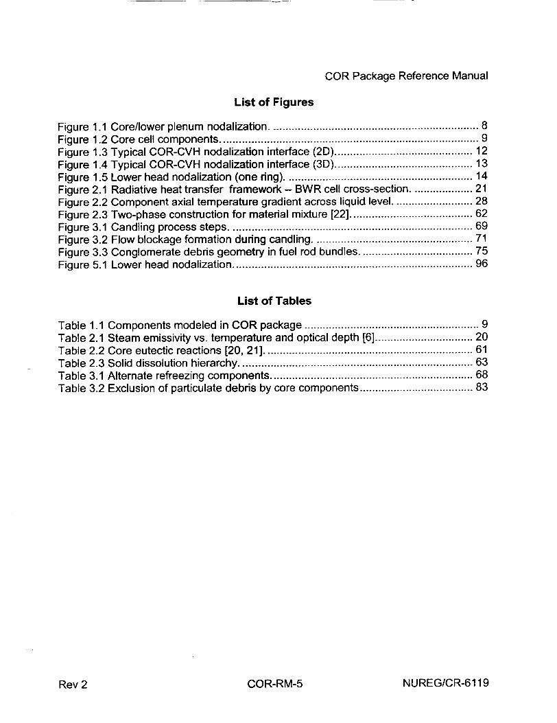
List of Figures
Figure 1.1 Core/lower plenum nodalization ................................................................. 8 Figure 1.2 Core cell components ................................................................................ 9 Figure 1.3 Typical COR-CVH nodalization interface (2D) ......................................... 12 Figure 1.4 Typical COR-CVH nodalization interface (3D) ......................................... 13 Figure 1.5 Lower head nodalization (one ring) ........................................................ 14 Figure 2.1 Radiative heat transfer framework - BWR cell cross-section ................ 21 Figure 2.2 Component axial temperature gradient across liquid level ...................... 28 Figure 2.3 Two-phase construction for material mixture [22] ..................................... 62 Figure 3.1 Candling process steps ........................................................................... 69 Figure 3.2 Flow blockage formation during candling ............................................... 71 Figure 3.3 Conglomerate debris geometry in fuel rod bundles ................................. 75 Figure 5.1 Lower head nodalization .......................................................................... 96
List of Tables
Table 1.1 Components modeled in COR package .................................................... 9 Table 2.1 Steam emissivity vs. temperature and optical depth [6] ............................ 20 Table 2.2 Core eutectic reactions [20, 21] ............................................................... 61 Table 2.3 Solid dissolution hierarchy ....................................................................... 63 Table 3.1 Alternate refreezing components ............................................................. 68 Table 3.2 Exclusion of particulate debris by core components ................................ 83
NUREG/CR-6119Rev 2 COR-RM-5
COR Package Reference Manual
I Introduction
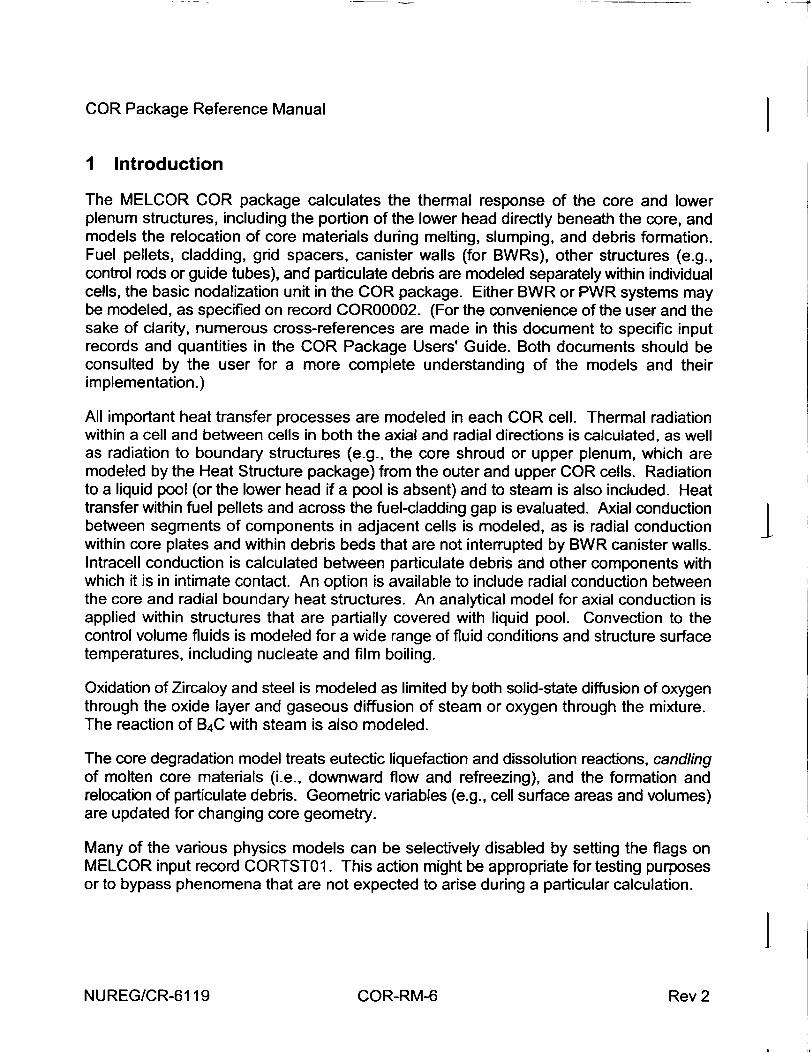
The MELCOR COR package calculates the thermal response of the core and lower plenum structures, including the portion of the lower head directly beneath the core, and models the relocation of core materials during melting, slumping, and debris formation. Fuel pellets, cladding, grid spacers, canister walls (for BWRs), other structures (e.g., control rods or guide tubes), and particulate debris are modeled separately within individual cells, the basic nodalization unit in the COR package. Either BWR or PWR systems may be modeled, as specified on record COR00002. (For the convenience of the user and the sake of clarity, numerous cross-references are made in this document to specific input records and quantities in the COR Package Users' Guide. Both documents should be consulted by the user for a more complete understanding of the models and their implementation.)
All important heat transfer processes are modeled in each COR cell. Thermal radiation within a cell and between cells in both the axial and radial directions is calculated, as well as radiation to boundary structures (e.g., the core shroud or upper plenum, which are modeled by the Heat Structure package) from the outer and upper COR cells. Radiation to a liquid pool (or the lower head if a pool is absent) and to steam is also included. Heat transfer within fuel pellets and across the fuel-cladding gap is evaluated. Axial conduction between segments of components in adjacent cells is modeled, as is radial conduction I within core plates and within debris beds that are not interrupted by BWR canister walls. Intracell conduction is calculated between particulate debris and other components with which it is in intimate contact. An option is available to include radial conduction between the core and radial boundary heat structures. An analytical model for axial conduction is applied within structures that are partially covered with liquid pool. Convection to the control volume fluids is modeled for a wide range of fluid conditions and structure surface temperatures, including nucleate and film boiling.
Oxidation of Zircaloy and steel is modeled as limited by both solid-state diffusion of oxygen through the oxide layer and gaseous diffusion of steam or oxygen through the mixture. The reaction of B4C with steam is also modeled.
The core degradation model treats eutectic liquefaction and dissolution reactions, candling of molten core materials (i.e., downward flow and refreezing), and the formation and relocation of particulate debris. Geometric variables (e.g., cell surface areas and volumes) are updated for changing core geometry.
Many of the various physics models can be selectively disabled by setting the flags on MELCOR input record CORTST01. This action might be appropriate for testing purposes or to bypass phenomena that are not expected to arise during a particular calculation.
INUREG/CR-6119 COR-RM-6 Rev 2
COR Package Reference Manual
1.1 Nodalization Scheme
1.1.1 CorelLower Plenum
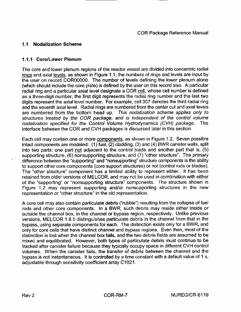
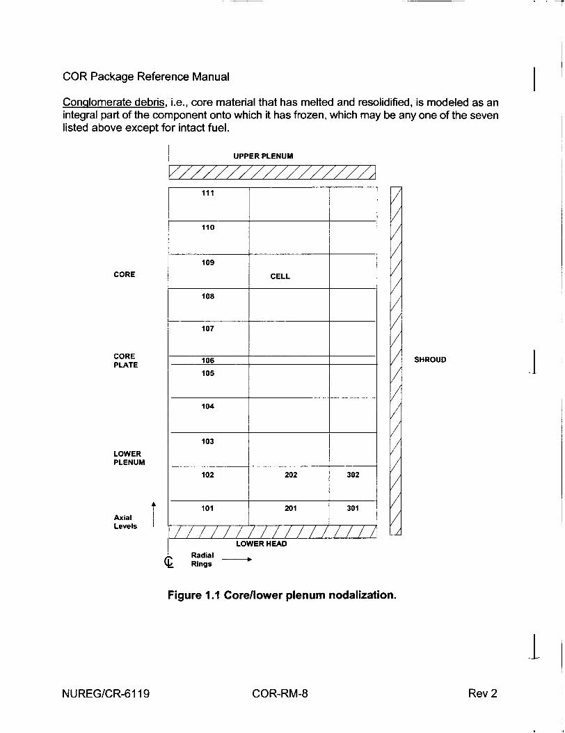
The core and lower plenum regions of the reactor vessel are divided into concentric radial riO and axial levels, as shown in Figure 1.1; the numbers of rings and levels are input by the user on record COROOOOO. The number of levels defining the lower plenum alone (which should include the core plate) is defined by the user on this record also. A particular radial ring and a particular axial level designate a COR cell, whose cell number is defined as a three-digit number; the first digit represents the radial ring number and the last two digits represent the axial level number. For example, cell 307 denotes the third radial ring and the seventh axial level. Radial rings are numbered from the center out and axial levels are numbered from the bottom head up. This nodalization scheme applies only to structures treated by the COR package, and is independent of the control volume nodalization specified for the Control Volume Hydrodynamics (CVH) package. The interface between the COR and CVH packages is discussed later in this section.
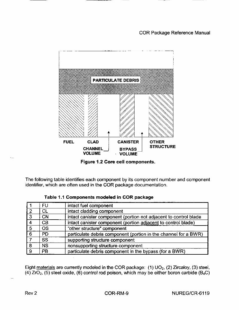
Each cell may contain one or more components, as shown in Figure 1.2. Seven possible intact components are modeled: (1) fuel, (2) cladding, (3) and (4) BWR canister walls, split into two parts: one part not adjacent to the control blade and another part that is, (5) supporting structure, (6) nonsupporting structure, and (7) "other structure". The primary difference between the "supporting" and "nonsupporting" structure components is the ability to support other core components (core support structures) or not (control rods or blades). The "other structure" component has a limited ability to represent either. It has been retained from older versions of MELCOR, and may not be used in combination with either of the "supporting" or "nonsupporting structure" components. The structure shown in Figure 1.2 may represent supporting and/or nonsupporting structures in the new representation or "other structure" in the old representation.
A core cell may also contain particulate debris ("rubble") resulting from the collapse of fuel rods and other core components. In a BWR, such debris may reside either inside or outside the channel box, in the channel or bypass region, respectively. Unlike previous versions, MELCOR 1.8.5 distinguishes particulate debris in the channel from that in the bypass, using separate components for each. The distinction exists only for a BWR, and only for core cells that have distinct channel and bypass regions. Even then, most of the distinction is lost when the channel box fails, and the two debris fields are assumed to be mixed and equilibrated. However, both types of particulate debris must continue to be tracked after canister failure because they typically occupy space in different CVH control volumes. When the canister fails, the transfer of debris between the channel and the bypass is not instantaneous. It is controlled by a time constant with a default value of 1 s, adjustable through sensitivity coefficient array C1021.
NUREG/CR-6119Rev 2 COR-RM-7
COR Package Reference Manual I
Conglomerate debris, i.e., core material that has melted and resolidified, is modeled as an integral part of the component onto which it has frozen, which may be any one of the seven listed above except for intact fuel.
I UPPER PLENUM
V1111111211
CORE
CORE PLATE
LOWER PLENUM
Levels~
110
109
CELL
108
107
106 _____
105
104
103
102 202 302
101 201 301
/7T/77 /Tm / rI//nLOWER HEAD
SHROUD I
(~Radial Rings
Figure 1.1 Core/lower plenum nodalization.
I1NUREG/CR-61 19 CRR- e
__Z
COR-RM-8 Rev 2
COR Package Reference Manual
Figure 1.2 Core cell components.
The following table identifies each component by its component number and component identifier, which are often used in the COR package documentation.
Table 1.1 Components modeled in COR package
1 FU intact fuel component 2 CL intact cladding component 3 CN intact canister component (portion not adjacent to control blade 4 CB intact canister component (portion adiacent to control blade) 5 OS "other structure" component 6 PD particulate debris component (portion in the channel for a BWR) 7 SS supporting structure component 8 NS nonsupporting structure component 9 PB particulate debris component in the bypass (for a BWR)
Eight materials are currently modeled in the COR package: (1) U0 2, (2) Zircaloy, (3) steel, (4) ZrO 2, (5) steel oxide, (6) control rod poison, which may be either boron carbide (B4C)
NUREG/CR-6119Rev 2 COR-RM-9
COR Package Reference Manual
or silver-indium-cadmium alloy (Ag-In-Cd) as specified on record COR00002, (7) Inconel, and (8) an electric heating element material, specified on record COR00002. Each component may be composed of one or more of these materials. For example, the cladding component may be composed of Zircaloy, Inconel (to simulate grid spacers), and ZrO2 (either initially present or calculated by the COR package oxidation models). The melting and candling of materials results in the possibility of any or all materials being found in a given component. The "heating element material" is intended for use in analysis of electrically heated experiments. Its use requires that the user modify subroutine ELHEAT to provide a calculation of the associated heating power in all cells containing the material.
Zircaloy is considered as single material in the COR package, with no distinction made between zirconium and the zircaloy alloying elements. Steel and steel oxide are also each modeled as single materials within the COR package, but the user must specify the fractions of iron, nickel, and chromium in the steel so that oxidation can be properly treated and the right amounts of each species can be transmitted to the Cavity (CAV) package during debris ejection. Inconel is treated as a single material, and currently it has the same properties as steel (and is ejected as steel), but it is not permitted to oxidize. Properties of the materials are obtained from MELCOR's Material Properties (MP) package. In MELCOR versions after 1.8.4, the user was given increased flexibility to use properties other than those of the default materials._j
Several geometric variables are defined by the user to further describe the cells and components. Representative dimensions for the intact components are specified on record COR00001, and elevations and lengths (heights) for each cell are input on record CORZjj01. Equivalent diameters for each component in each cell for use in various heat transfer correlations also must be specified on record CORijjO4. Cell boundary areas for inter-cell radiation (both axially and radially) are defined by the user on records CORijj05 and CORRii01. Initial volumes of components and the "empty" CVH fluid volume are calculated based on user input for component masses and cell flow areas (records CORijJ02 and CORijj05), and are then tracked during core slumping and flow blockage calculations.
For each intact component in each cell, a surface area is input by the user on record CORijJ06 for convection and oxidation calculations. (The single surface area value input for a canister is multiplied by elements in sensitivity coefficient array C1501 to obtain values for each side of each canister component to communicate separately with the channel and bypass control volumes.) For particulate debris, a surface area is calculated from the total mass and a user-defined particle size input on record CORijJ04. (For oxidation of particulate debris, separate Zircaloy and steel surface areas are calculated.) The effects of conglomerate debris on component surface areas are factored into the heat transfer, oxidation, and candling calculations; this model is described in Section 3.1.5.
As discussed later in Sections 2.3 and 2.5, the Control Volume Hydrodynamics (CVH) package supplies fluid conditions for use by the COR package in calculating heat transfer INUREG/CR-6119 COR-RM-10 Rev 2
COR Package Reference Manual
and oxidation rates, which are then multiplied by the time step and passed back to the CVH package as energy and mass sources or sinks. The nodalization for the reactor vessel used in the CVH package is typically much coarser than that used in the COR package, but finer CVH nodalizations can be used to simulate in-vessel natural circulation. The COR nodalization applies only to those components in the core and lower plenum treated by the COR package, and is independent of the CVH nodalization, with some restrictions imposed.
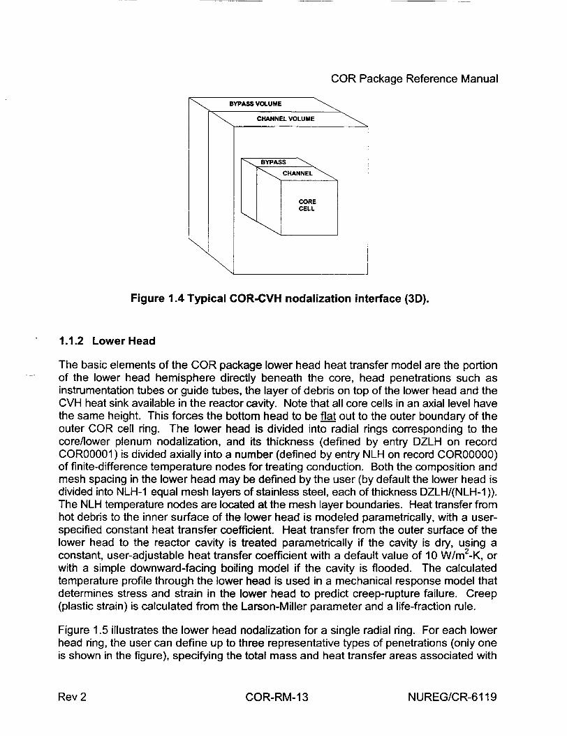
Figure 1.3 gives a 2-D representation of the interface between the COR and CVH packages, but to more accurately depict the relationship between the two nodalizations requires a 3-D illustration, shown in Figure 1.4. Each COR cell interfaces with a CVH control volume (input on record CORijj01) representing the primary flow (channel volume), which provides boundary conditions for most core surfaces. Typically many core or lower plenum cells will interface with the same control volume. For BWRs, a separate CVH control volume (shown behind the channel volume in Figure 1.4) may also be specified for COR cells on record CORijjO1 to represent the interstitial space between fuel assemblies (bypass volume). The outer canister surfaces and the supporting and nonsupporting structure (or "other structure") surfaces, as well as the surface of any particulate debris in the bypass of a BWR, all communicate with this bypass control volume if it is distinguished from the channel control volume. The total number of control volumes interfaced to the COR package is a required input quantity on record COROOOOO. The only restrictions between CVH and COR nodalizations are that control volumes occupy a rectangular grid of core cells and have boundaries lying either on cell boundaries or entirely outside the core nodalization.
NUREG/CR-6119Rev 2 COR-RM-1 1

. . --
COR Package Reference Manual I
STEAM DOME
STEAM SEPARATORS, STANDPIPES, SHROUD DOME
w
0 z
0
Figure 1.3 Typical COR-CVH nodalization interface (2D).
NUREG/CR-6119
CORE & BYPASS (2 CVs)
LOWER PLENUM
COR-RM-12 Rev 2
COR Package Reference Manual
BYPASS VOLUME
CHANNEL VOLUME
CHANNEL
CORE CELL
Figure 1.4 Typical COR-CVH nodalization interface (3D).
1.1.2 Lower Head
The basic elements of the COR package lower head heat transfer model are the portion of the lower head hemisphere directly beneath the core, head penetrations such as instrumentation tubes or guide tubes, the layer of debris on top of the lower head and the CVH heat sink available in the reactor cavity. Note that all core cells in an axial level have the same height. This forces the bottom head to be flat out to the outer boundary of the outer COR cell ring. The lower head is divided into radial rings corresponding to the core/lower plenum nodalization, and its thickness (defined by entry DZLH on record COROOQ0l) is divided axially into a number (defined by entry NLH on record COROQOQO) of finite-difference temperature nodes for treating conduction. Both the composition and mesh spacing in the lower head may be defined by the user (by default the lower head is divided into NLH-1 equal mesh layers of stainless steel, each of thickness DZLH/(NLH-1 )). The NLH temperature nodes are located at the mesh layer boundaries. Heat transfer from hot debris to the inner surface of the lower head is modeled parametrically, with a userspecified constant heat transfer coefficient. Heat transfer from the outer surface of the lower head to the reactor cavity is treated parametrically if the cavity is dry, using a constant, user-adjustable heat transfer coefficient with a default value of 10 W/m2 -K, or with a simple downward-facing boiling model if the cavity is flooded. The calculated temperature profile through the lower head is used in a mechanical response model that determines stress and strain in the lower head to predict creep-rupture failure. Creep (plastic strain) is calculated from the Larson-Miller parameter and a life-fraction rule.
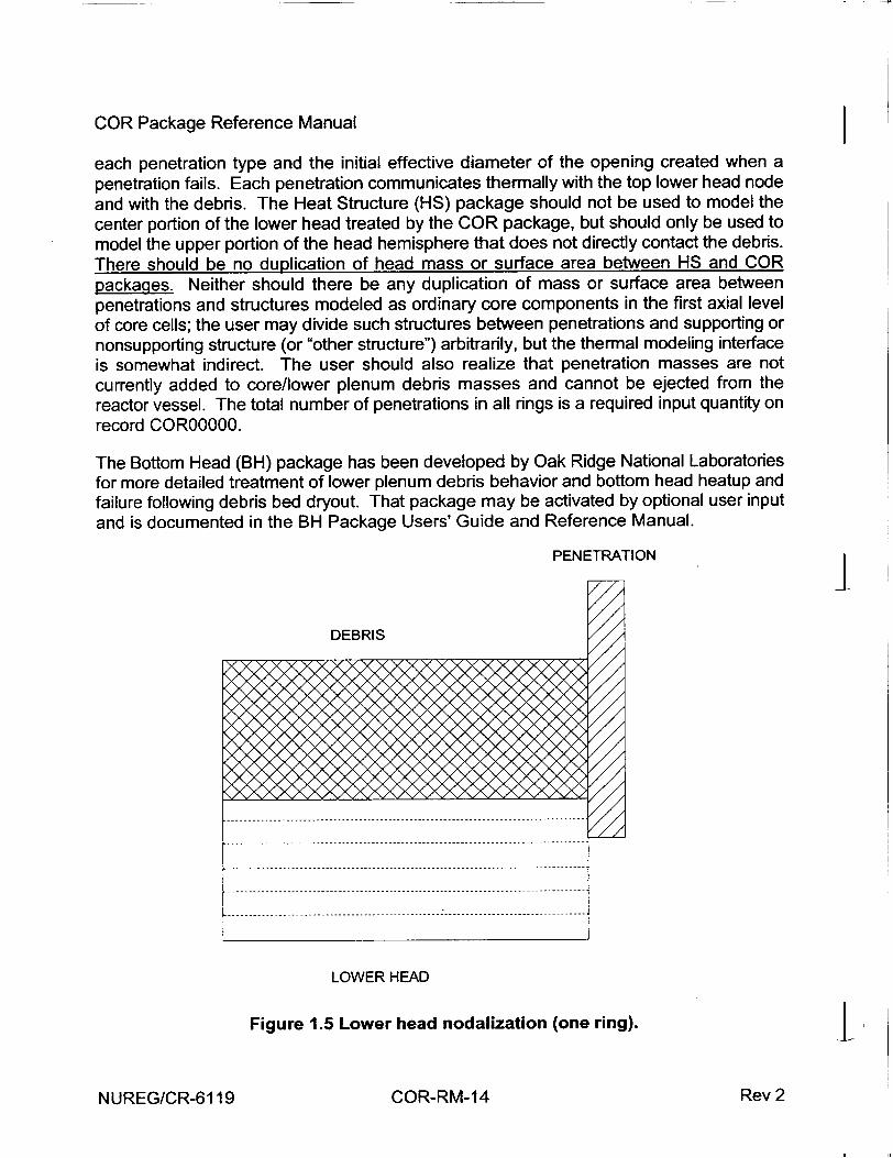
Figure 1.5 illustrates the lower head nodalization for a single radial ring. For each lower head ring, the user can define up to three representative types of penetrations (only one is shown in the figure), specifying the total mass and heat transfer areas associated with
NUREG/CR-6119Rev 2 COR-RM-13
COR Package Reference Manual
each penetration type and the initial effective diameter of the opening created when a penetration fails. Each penetration communicates thermally with the top lower head node and with the debris. The Heat Structure (HS) package should not be used to model the center portion of the lower head treated by the COR package, but should only be used to model the upper portion of the head hemisphere that does not directly contact the debris. There should be no duplication of head mass or surface area between HS and COR packages. Neither should there be any duplication of mass or surface area between penetrations and structures modeled as ordinary core components in the first axial level of core cells; the user may divide such structures between penetrations and supporting or nonsupporting structure (or "other structure") arbitrarily, but the thermal modeling interface is somewhat indirect. The user should also realize that penetration masses are not currently added to core/lower plenum debris masses and cannot be ejected from the reactor vessel. The total number of penetrations in all rings is a required input quantity on record COROOOOO.
The Bottom Head (BH) package has been developed by Oak Ridge National Laboratories for more detailed treatment of lower plenum debris behavior and bottom head heatup and failure following debris bed dryout. That package may be activated by optional user input and is documented in the BH Package Users' Guide and Reference Manual.
PEN ETRATI ON
LOWER HEAD
Figure 1.5 Lower head nodalization (one ring).
NUREG/CR-6119
ICOR-RM-14 Rev 2
COR Package Reference Manual
1.2 Calculation Framework
All thermal calculations in the COR package (both in the core/lower plenum components and in the lower head) are done using internal energies of the materials (i.e., temperature is a derived variable calculated from the material internal energies; initial temperatures are defined on record CORijjO3). The mass and internal energy of each material in each component are tracked separately to conserve total mass and energy to within machine roundoff accuracy.
The COR package uses an explicit numerical scheme for advancing the thermal state of the core, lower plenum, and lower head through time. To mitigate numerical instabilities, a subcycling capability has been developed to allow the COR package to take multiple time steps across a single Executive package time step. All energy generation, heat transfer, and oxidation rates are evaluated at the beginning of a COR package subcycle based on current temperatures, geometric conditions, and an estimate of the local fluid conditions (calculated by the COR package dT/dz model to reflect the temperature variation within a control volume containing many individual COR cells). The net energy gain (or loss) across the subcycle is determined for each component by multiplying these rates by the COR package time step.
The temperature change of most components is limited to a user-input maximum; if the calculated temperature change for a component is greater than this limit, the COR package subcycle time step is reduced accordingly, but not lower than the minimum time step input by the user for the COR package. Components with a total mass below a critical minimum are not subjected to this limit. If the energy input to any fluid volume changes from previous values in such a way as to possibly result in numeric instability between the COR and control volume packages, the system time step may be cut immediately, or a reduction may be requested for the next Executive time step. The various time step control parameters may be specified by the user on record CORDTC01 and using sensitivity coefficient arrays C1401 and C1502 (see COR Package Users' Guide).
At the end of a COR package time step, after the thermal state of the core has been updated by the heat transfer and oxidation models described in Section 2, relocation of core materials and debris formation are calculated by the core degradation models described in Section 3. Molten portions of intact structures are transferred to the conglomerate debris associated with the structure. Liquefaction of intact structures caused by eutectic reactions between materials within the structure and dissolution of intact structures by existing molten material within the core cell are calculated, if the materials interactions model has been activated. Molten materials are relocated downward by the candling model (provided there is no flow blockage) and intact components are converted to debris if various debris formation criteria are met.
Downward relocation of particulate debris from one cell to a lower one by gravitational settling is generally modeled as a logical process and relocation is completed over a single time step, with consideration given only to constraints imposed by the porosity of the
NUREG/CR-6119Rev 2 COR-RM-1 5
. .
COR Package Reference Manual 1
debris, the availability of free (open) volume to hold it, and support by structures such as the core plate. (These constraints are not imposed on molten debris, which will always relocate to lower regions unless the path is totally blocked.) However, numerical limits are imposed to ensure that the mass relocated goes to zero in the limit of small timesteps, and a rate limitation is imposed for the falling debris quench heat transfer model. In MELCOR 1.8.5, debris in the bypass of a BWR is distinguished from that in the channel. In core cells containing a canister, the downward relocation of particulate or molten debris can be blocked separately in the channel and in the bypass. After the canister has failed, debris in the channel and that in the bypass are mixed and equilibrated. As long as the canister is intact, the majority of the particulate debris in the bypass of a BWR will be the remnants of control blades. Most of the space available to it will be in the bladed bypass region, adjacent to canister component CB. Therefore, the existence of CB is taken as the criterion for separation of particulate debris in the bypass from that in the channel.
Reactor components such as control rods and blades may be supported from above or below, with parametric models for failure based on the temperature and the remaining thickness of the structural metal. Either load-based structural models or simpler parametric models may be used for the failure of components such as the core plate and the Control Rod Guide Tubes (CRGTs) in a BWR.
Gravitational leveling of molten pools and debris beds across the core rings is calculated with a user-adjustable time constant. In a BWR, this leveling is blocked by the presence of intact canisters, so that no leveling is possible until any distinction between the debris in the channel and that in the bypass has disappeared. Debris beds are completely leveled; the angle of repose is not considered. Whenever mass is relocated or debris formed, material energies in the new or changed components are re-evaluated and the temperature updated to maintain thermal equilibrium, and any relevant geometric variables are recalculated to reflect the change in geometry.
2 Heat Transfer and Oxidation Models
This section describes the models implemented in the COR package to treat various modes of heat transfer and oxidation within the core and lower plenum; lower head heat transfer models are discussed separately in Section 5. Radiation, conduction, and convection are covered in Sections 2.1, 2.2 and 2.3, respectively, and oxidation is covered in Section 2.4. Section 2.5 describes the "dT/dz" model used by the COR package to provide approximate local (core cell) fluid temperatures and gas compositions within the possibly larger CVH control volume. Fission power generation in ATWS accident sequences (and in some experiments) is covered in Section 2.6.
Most of the constants (including exponents) used in the correlations described in this section have been implemented as sensitivity coefficients, thus allowing the user to change them from the default values described in this document if desired. Sensitivity coefficients are grouped into numbered arrays, Cnnnn(k), where 'nnnn' is an identifying number that INUREG/CR-6119 COR-RM-1 6 Rev 2
COR Package Reference Manual
refers to a set of related coefficients, such as the several constants appearing in a single correlation (see the MELGEN/MELCOR Users' Guide). Appendix A gives a table of sensitivity coefficients used in the COR package and their default values. Unless otherwise noted, all variables and dimensional constants are in SI units, in conformance to MELCOR coding conventions.
2.1 Radiation
Thermal radiation among components within COR cells, across cell boundaries, and from components to steam is modeled as exchange of radiation between pairs of gray surfaces with an intervening gray medium; the model is constructed following the description provided in Kreith [1]. The radiosity, J1, is defined as the total energy flux leaving the i-th surface (i=1 or 2 in this model), both reflected and emitted:
Ji = (1 - --i ) G; + --i E,,; (2.1)
where
e; = emissivity of surface i
Gj= radiation flux incident on surface i
Ebi= blackbody emissive power of surface i, o-T
The net heat transfer rate from the i-th surface is the difference between the radiosity and the incident radiation, multiplied by the area of surface i, Aj:
qj = A,(Jj -Gj) (2.2)
Combining Equations (2.1) and (2.2) gives qi in terms of the radiosity and blackbody emissive power:
t' (Ebi - Ji) (2.3)
The net heat transfer rate from surface i to surface j is given in terms of the surface radiosities by the expression:
qiJ =Ai5 ri (JA - Jj (2.4)
where
Fj= geometric view factor from surface i to surface j
NUREG/CR-6119Rev 2 COR-RM-1 7
COR Package Reference Manual 4 I-# = geometric mean transmittance between surfaces i and j
Radiation heat transfer also occurs between each of the surfaces and the steam medium, according to the expression:
qj,=A,=A Am (J; -Eb,,) (2.5)
where
EM = steam emissivity/absorptivity = (0 - r-•)
Eb,m= blackbody emissive power of medium, o TM
With the additional requirement:
qi = qj, + qij (2.6)
Equations (2.3), (2.4), (2.5), and (2.6) are solved in the COR package to obtain qi and qim (i = 1, 2) for various pairs of surfaces. The subsections below discuss the calculation of surface and steam emissivities ei and e,,,, the geometric view factors F,,, and the implementation logic (i.e., how pairs of surfaces are chosen for multiple cell components A that may relocate during the course of a calculation).
2.1.1 Emissivities
The surface and steam emissivities are evaluated by models adapted from MARCON 2.1 B [2], an extended version of MARCH 2 [3]. For cladding and canister components, the surface emissivity of Zircaloy is used, which is calculated in these models as a function of temperature and oxide thickness from the equations used in MATPRO [4]. For Zircaloy surfaces whose maximum temperature has never reached 1500 K, the surface emissivity is given by:
ej =0.325+0.1246 x1O'Ar,,o [Ar0x < 3.88 x10--] (2.7)
', =0.808642- 50.0 Aro [Aro. _> 3.88 xl0-6] (2.8)
where Ar, is the oxide thickness. For surfaces that have reached temperatures greater than 1500 K at some time, the emissivity is calculated by Equation (2.7) or (2.8) and then multiplied by the factor:
NUREG/CR-6119 COR-RM-18 Rev 2
COR Package Reference Manual
f = exp L500.0 -T ] (2.9)
where Tmax is the maximum temperature the surface has reached. This factor is limited to a lower bound of 0.325.
The surface emissivity of SS and NS (or OS) components in these models is calculated from the relation used in MARCON 2.1B for stainless steel, taken from Reference [5]:
Ei= 0.042 + 0.000347. Ti (2.10)
The steam emissivities, ern, are evaluated in these models from a table taken from Reference [6] (see Table 2.1), which specifies the steam emissivity versus steam temperature and optical depth (steam partial pressure times mean beam length Le) at the high-pressure limit. Mean beam lengths are supplied for each component type based only on representative distances for an intact core geometric configuration using these equations [7]:
Lec =3.5 (P - 2rc,,) (2.11)
Lecn =Le. = 1.8 rc, cn (2.12)
Lecbb= Leos = 1.8 rcn,cb (2.13)
Lecnb =1.8 rcn, (2.14)
Le.pd Le.pb = 0 (2.15)
where the second subscripts on the mean beam length represent cladding (cl); canister (not by blade) inner surface (cn); canister (by blade) inner surface (cb); canister (by blade) outer surface (cbb); other structure (xs, representing ss, ns, or os); canister (not by blade) outer surface (cnb); and particulate debris (pd and pb); and where P is the fuel rod pitch, rc, is the cladding radius, rdcnl is the distance between the outer fuel rods and the canister wall, rcn,,, is the distance between the canister and control blade, and rcn., is the distance between adjacent canister walls. For the particulate debris component, a surface emissivity of unity is assumed.
NUREG/CR-6119Rev 2 COR-RM-19
COR Package Reference Manual
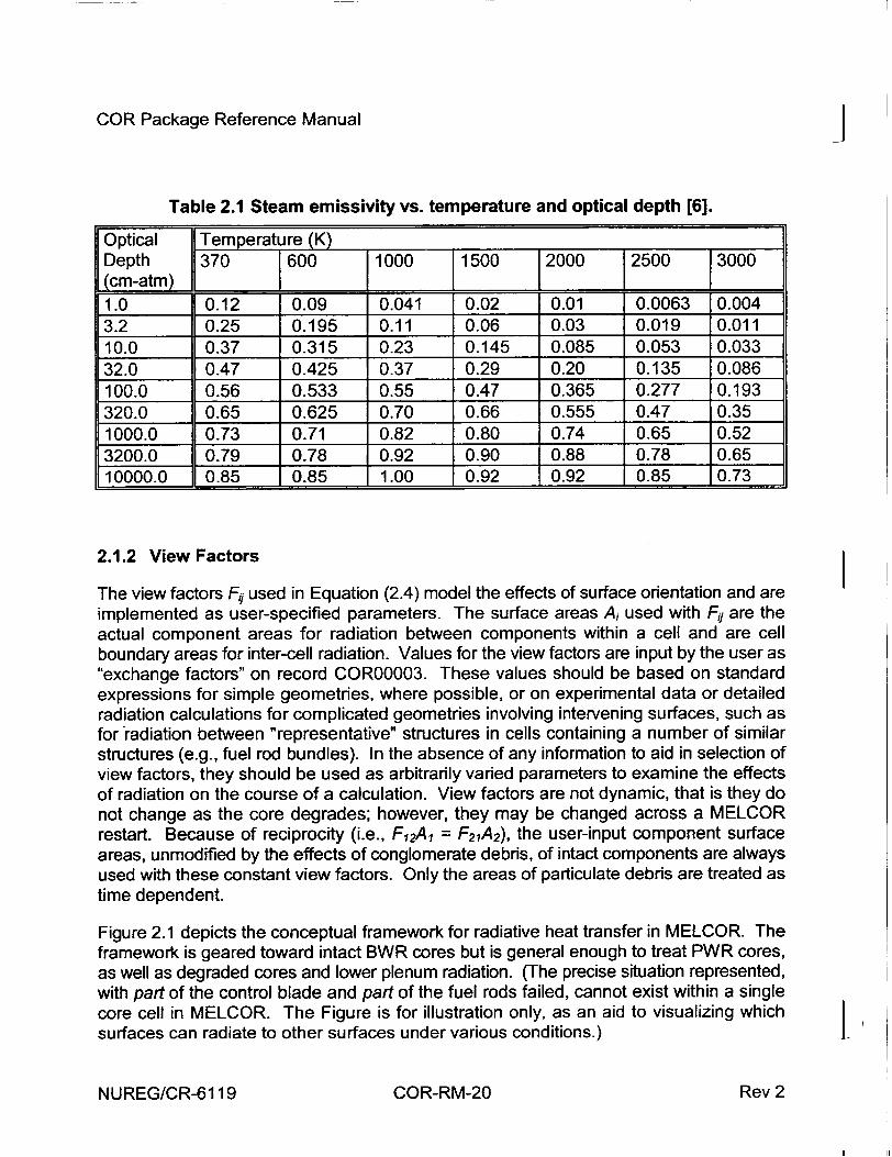
Table 2.1 Steam emissivity vs. temperature and optical depth [6].
Optical Temperature (K) Depth 370 600 1000 1500 2000 2500 3000 (cm-atm) I I I I I I 1.0 0.12 0.09 0.041 0.02 0.01 0.0063 0.004 3.2 0.25 0.195 0.11 0.06 0.03 0.019 0.011 10.0 0.37 0.315 0.23 0.145 0.085 0.053 0.033 32.0 0.47 0.425 0.37 0.29 0.20 0.135 0.086 100.0 0.56 0.533 0.55 0.47 0.365 0.277 0.193 320.0 0.65 0.625 0.70 0.66 0.555 0.47 0.35 1000.0 0.73 0.71 0.82 0.80 0.74 0.65 0.52 3200.0 0.79 0.78 0.92 0.90 0.88 0.78 0.65 10000.0 0.85 0.85 1.00 0.92 0.92 0.85 0.73
2.1.2 View Factors
The view factors F#, used in Equation (2.4) model the effects of surface orientation and are implemented as user-specified parameters. The surface areas A, used with Fj are the actual component areas for radiation between components within a cell and are cell boundary areas for inter-cell radiation. Values for the view factors are input by the user as "exchange factors" on record COR00003. These values should be based on standard expressions for simple geometries, where possible, or on experimental data or detailed radiation calculations for complicated geometries involving intervening surfaces, such as forradiation between "representative" structures in cells containing a number of similar structures (e.g., fuel rod bundles). In the absence of any information to aid in selection of view factors, they should be used as arbitrarily varied parameters to examine the effects of radiation on the course of a calculation. View factors are not dynamic, that is they do not change as the core degrades; however, they may be changed across a MELCOR restart. Because of reciprocity (i.e., F12A1 = F21A 2), the user-input component surface areas, unmodified by the effects of conglomerate debris, of intact components are always used with these constant view factors. Only the areas of particulate debris are treated as time dependent.
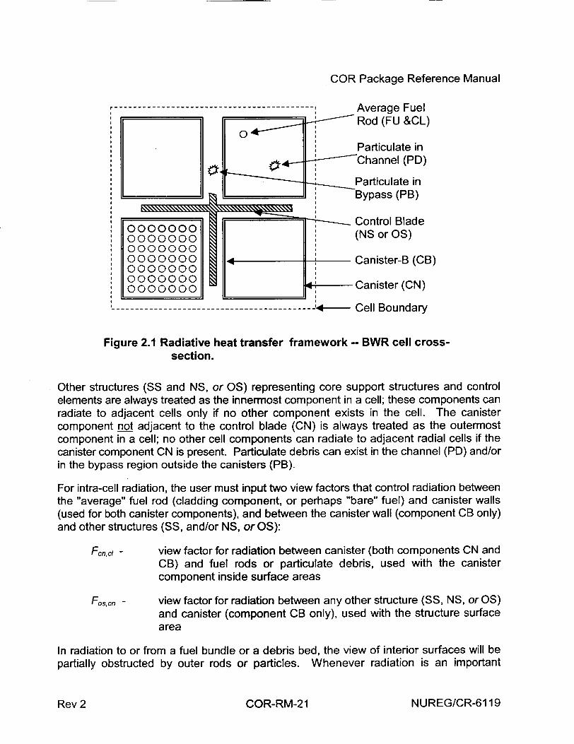
Figure 2.1 depicts the conceptual framework for radiative heat transfer in MELCOR. The framework is geared toward intact BWR cores but is general enough to treat PWR cores, as well as degraded cores and lower plenum radiation. (The precise situation represented, with part of the control blade and part of the fuel rods failed, cannot exist within a single core cell in MELCOR. The Figure is for illustration only, as an aid to visualizing which surfaces can radiate to other surfaces under various conditions.) t
NUREG/CR-6119 COR-RM-20 Rev 2
COR Package Reference Manual
----------------------------------- IAeaeFl -: Average Fuel Rod (FU &CL)
0 * Particulate in
Channel (PD)
Particulate in * Bypass (PB)
0000 Control Blade
0000000 0000000 0000000 O O-OCanister-B (CB) 0000000
000000 Canister (CN) 0000000
-------------------------------- '- Cell Boundary
Figure 2.1 Radiative heat transfer framework -- BWR cell crosssection.
Other structures (SS and NS, or OS) representing core support structures and control elements are always treated as the innermost component in a cell; these components can radiate to adjacent cells only if no other component exists in the cell. The canister component not adjacent to the control blade (CN) is always treated as the outermost component in a cell; no other cell components can radiate to adjacent radial cells if the canister component CN is present. Particulate debris can exist in the channel (PD) and/or in the bypass region outside the canisters (PB).
For intra-cell radiation, the user must input two view factors that control radiation between the "average" fuel rod (cladding component, or perhaps "bare" fuel) and canister walls (used for both canister components), and between the canister wall (component CB only) and other structures (SS, and/or NS, or OS):
Fc,,,ý - view factor for radiation between canister (both components CN and CB) and fuel rods or particulate debris, used with the canister component inside surface areas
Fos~cn - view factor for radiation between any other structure (SS, NS, or OS) and canister (component CB only), used with the structure surface area
In radiation to or from a fuel bundle or a debris bed, the view of interior surfaces will be partially obstructed by outer rods or particles. Whenever radiation is an important
NUREG/CR-6119Rev 2 COR-RM-21

COR Package Reference Manual J mechanism for heat transfer, a temperature gradient will be established within the fuel bundle or debris bed. Therefore, the effective temperature difference for radiative exchange with another surface will be less than would be predicted from the average temperature of the bundle or bed. This effect can be important in reducing the radiation to a surrounding canister, and may be captured by assigning the view factor Fcn,,d a value significantly less than unity. The value input for Fos a, on the other hand, should ordinarily be some value close to unity since the entire control blade surface is directly adjacent to the surface to which it radiates.
For radiation between any other structure (SS, NS, or OS) and another component within the same cell, the "other structure" surface area and the view factor Fos0 cn are used in Equation (2.4). For radiation between either of the two canister components and the cladding, the canister surface areas and the view factor Fcnl,d are used.
As discussed in Section 1.2, particulate debris in the bypass of a BWR (PB) can exist separated from that in the channel (PD) only in the presence of intact canister component CB. Otherwise, the two are assumed to be mixed and equilibrated. In the following discussion, "PD" will therefore be used to mean all particulate debris (including any in the bypass region of a BWR) in a cell unless there is intact canister component CB in that cell.
If particulate debris is present in a cell containing fuel rods, an implicit view factor Fcpd of 1.0 is used with the cladding (or bare fuel) surface area to model radiation from the rods to the debris. Otherwise, if debris is present in a cell with either canister or "other structure" (SS, NS, or OS) components, implicit view factors F,,pd and Fos,p of 1.0 are used with the canister or "other structure" surface areas to model radiation between these components and the debris.
If a cell contains both components of a BWR canister (CN and CB) but no fuel rods, the view factor from the inner surface of CN to the inner surface of CB, FCn,,Cb, is taken as 2-1/2 (from standard tables, assuming a square canister), used with the area of the inner surface of CN.
For inter-cell radiation the user must input two view factors that control radiation in the radial and axial directions:
Fcelr - view factor for radiation radially from one cell to the next outer one, used with cell outer radial boundary area
Fceil,a - view factor for radiation axially from one cell to the next higher one, used with cell axial boundary area
Intra-cell radiation is calculated for the outermost ("most visible") components. Again, because of temperature gradients, the effective temperature difference for radiative exchange will be less than would be predicted from cell-average temperatures. This effect, which is dependent on the coarseness of the nodalization, should be considered in
NUREG/CR-6119
I ---------- t
COR-RM-22 Rev 2
COR Package Reference Manual
choosing the values input for these view factors. For radiation from any component to another cell, the appropriate cell boundary area and Fce,1,r or Fcet,a are used in Equation (2.4), although the actual component temperatures are used. For radiation between the liquid pool or lower head and the first cell containing a component, the lower head surface area and Flp,,p (defined below) are used in Equation (2.4).
If no components exist in the next outer or higher cell, the radial ring or axial level beyond that is used, until a boundary heat structure is reached. Thus, components in one cell can communicate to nonadjacent cells all the way across the core if there are no components in intervening cells. The boundary heat structures, both radially and axially, specified on records CORZjj02 and CORRii02, respectively, receive energy from the outermost cells that contain a component. An additional view factor controls radiation to the liquid pool, if one exists, or to the lower head:
Flpup - view factor for radiation axially from lowermost uncovered COR cell to lower head or liquid pool, used with lower head surface area
2.1.3 Implementation Logic
As already noted, the radiation model employs a superposition of pairwise surface-tosurface radiation calculations. The determination of which surfaces "see" which other surfaces is not exhaustive, but is intended to assure that (1) the most important radiation exchange paths are included and (2) no surface is isolated, with each being allowed to radiate to at least one other surface. Assumptions about which terms dominate in a BWR are based largely on Figure 2.1, as qualitatively described above.
When a dominant radiation path for some surface involves an adjacent radial or axial cell, only a single "selected" surface in that cell is considered. In considering other structures, NS takes precedence over SS; OS can occur only in a calculation that does not employ SS or NS. In the radial case, surfaces in the next cell are considered in the following order: outside of CN, CL, FU, inside of CB, NS, SS, OS, and PD. If none of these exist, the next radial cell is considered. In the axial case, the order is: CL, FU, inside of CN, inside of CB, NS, SS, OS, and PD. If none of these exist, the next axial cell is considered. Note that particulate debris in the bypass (PB) does not appear in either of these lists. This is because if it exists independent of particulate in the channel (PD), CB must also be present which will define a more important radiation path (in the axial direction), or shield it from external view (in the radial direction).
View factors are used only in combination with areas, as the product A1F 12 = A 2F21 = AF, where the equality is required by reciprocity. In some cases, limits are imposed because direct use of the view factors and areas cited Section 2.1.2 would result in an implied reciprocal view factor greater than unity.
NUREG/CR-6119Rev 2 COR-RM-23
COR Package Reference Manual
1. For radiation exchange between surfaces 1 and 2 that crosses a cell boundary, the product actually used is Fcel., MIN(Am11,., A1, A 2), where x may be r or a.
2. For radiation exchange involving particulate debris PD, the product actually used is F MIN(A 1, ApD), where F is the view factor cited in Section 2.1.2.
The following describes the model implementation in MELCOR 1.8.5. It is based on the logic used in MELCOR 1.8.4, with the treatment of OS generalized to apply to SS and NS and the addition of PB and a more careful distinction of channel and bypass. It is clear that improvements are possible.
The logic begins by considering the outer surfaces of an intact canister in a BWR.
la. That portion of the outer surface of intact canister CB in a core cell that does not see other outer CB surface in the same cell must radiate to "other structure" xS representing the control blade and/or to PB in the same core cell. Here x is N or 0; NS and OS cannot be used in the came calculation. Similarly, some portion of the xS surface may radiate to PB. The fraction of the surface of xS and of the outer surface of CB, that sees PB is proportional to the fraction f of the available space in the bypass that is occupied by PB. AF = MIN (f Au,- Apb/2) where surf is xs or cbb.
1 b. The remaining portions of these surfaces, A',urf = MAX(Asd - AFfpb , 0) see each other with AF = MAX(A'XS Fos, cn, A''b ). This formulation, rather than simple use of a factor (1-f), accounts for that fact that porosity may result in large "holes" through the debris bed.
2. That portion of the outer surface of intact canister CN in a core cell that does not see other outer CN surface in the same cell radiates to a component in the next radial cell. AF = MIN(Ace,,r, Acnb, As,ot) Fce, r.
If fuel rods are present in a core cell in a BWR or PWR, their view factors are considered next. If intact CL is present, only its outer surface is included, with FU-to-CL radiation treated as part of the gap model. The surface of bare FU, however, can radiate to other components.
3a. Fuel rods radiate to the inner surface of canister CB in the same cell, if present (AF = Acb F•,,,d); otherwise they radiate to other structure (SS, NS, or OS) present in the same core cell, (AF = Ax, Fos, c) with the same precedence as in item 1.
3b. Fuel rods radiate to PD in the same core cell (AF = MIN(Arod, Ap) 1), if any is present.
I
NUREG/CR-6119 COR-RM-24 Rev 2
COR Package Reference Manual
3c. If intact canister CN is present in the same core cell, fuel rods radiate to its inner surface (AF = A, F,,d); otherwise they radiate to a selected component in the next radial cell (AF = MIN(Acei,r, Aod, Asout) Fcei,,r).
3d. Fuel rods also radiate to a selected component in the next axial cell, with AF = MIN(Acet,a, Armd, As,up) Fc.eia.
If there is canister but no fuel rods in a core cell, the view factors for the inner canister surfaces are considered next.
4. If there are no fuel rods in a cell, the inner surface of canister CN radiates to the next axial level (AF = MIN(Ace1 1,a, A,,, A,,up) Fce,,a) unless there is PD in the same cell. This case is covered later.
5. If there are no fuel rods in a cell, the inner surface of canister CB radiates to the inner surface of CN in the same cell, if present (AF = Acb 2112); or to a selected component in the next radial cell (AF = MIN(AceIi,r, Acb, As,ot) Fceir).
The major view factors for "other structures" in a cell are the outer surface of canister CB, or fuel rods, if either or both exist. Canister CB will block the view of fuel rods. These are covered by items 1 and 3a above. Otherwise, the dominant radiative heat transfer for "other structures" will involve some other surface.
6a. In the absence of fuel rods and canister CB in a cell, "other structures" radiate to the inner surface of canister CN (AF = A,, Fo,,) unless there is PD in the same cell. This case is covered later.
6b. In the absence of fuel rods and both canister components (CN and CB) in a cell, "other structures" partition radiation between any PD in the same cell and selected surfaces in the next axial and radial cells. The fraction going to other cells is taken to be MAX(O, 1-Ap/Axs), where xS represents NS, SS, or OS, with NS taking precedence over SS, as previously discussed. AF = MIN(Acely, Axs, As,oud Fce/ly, where y is a or r. Radiation to PD is covered later.
Radiative heat transfer for PD is assumed to be dominated by any fuel rods in the same cell. This is covered by item 3b above. If there is no PD in the core cell, other surfaces must be considered.
7a. In the absence of fuel rods PD radiates to the inner surface of canister CB with AF = MIN(Acb, Ap,) Fcd or, if there is no CB, to some "other structure" in the same cell with AF = MIN(AxS, Apd) Fos,,. (As with intercell radiation, NS takes precedence over SS). The latter case completes items 6a and 6b.
NUREG/CR-6119COR-RM-25Rev 2

COR Package Reference Manual 4 7b. In the absence of fuel rods PD also radiates to the inner surface of canister CN
(AF = MIN(AcI, Apd) Fn, d) or, if there is no CN, to a selected component in the next radial cell (AF = MIN(Ace,,r, Apd, A,...t) Fceitr). The former case completes item 4.
7c. In the absence of fuel rods PD also radiates to a selected component in the next axial cell (AF = MIN(Aceii, a, Apd, As, p) Fceiia).
If a water pool is present, radiation is considered between its surface in each radial ring and a selected component in the first non-empty core cell in the same ring above the pool. If there is no water pool, radiation is considered between the lower head and a selected component in the first axial level in each ring. MELCOR 1.8.5 allows additional control of the emissivity and view factor to be used when this component is a supporting structure, through input on COROOOPR, CORZjjPR, CORRiiPR, and/or CORijjPR records. This can aid in modeling radiation to the core support plate.
2.2 Conduction
Conduction heat transfer between components in axially adjacent cells is described in Section 2.2.1. Cell-to-cell radial conduction is treated for supporting structure (SS) representing a continuous plate, and for particulate debris (PD and/or PB) following failure of any intact canister component in the two cells. In addition, a component in the outermost ring may optionally be designated to conduct heat directly to the boundary heat structures. (This is useful in simulating some experiment geometries.) Conduction between particulate debris (PD and/or PB) and other components within the same cell is also treated, as described in Section 2.2.3. Radial conduction through the fuel pellets and across the gap to the cladding is calculated by an analytic expression, as described in Section 2.2.4. Conduction within the lower head is discussed in Section 5.
The core package does not treat convection in molten debris pools. Hence, whenever the larger of the two component temperatures used to calculate inter-component conduction exceeds an assumed "melt" temperature, TKMIN, the rate of conduction is increased to simulate convection in a molten pool. The enhancement factor for axial, radial and intracell conduction is given by
FAC = max{1.0,[TKFAC (Tmax - TKMIN)r } (2.16)
where T,. is the larger of the component temperatures and TKFAC and TKMIN are given by sensitivity coefficients C1250 with default values of .01 K-1 and 3200. K, respectively. (The default values give an enhancement factor of 10 when Tr, exceeds the melting point of U0 2 by about 300 K and are primarily intended to eliminate excessive hot spots when rapid convection/radiation, etc. would clearly preclude their existence.) The enhancement factor for conduction in the lower head uses a hard-wired value of TKFAC=O.01 and uses the melting temperature of the material between adjacent temperature nodes in the lower head for TKMAX. dNUREG/CR-6119 COR-RM-26 Rev 2
COR Package Reference Manual
2.2.1 Axial Conduction
Axial conduction is computed between like components in adjacent axial cells (e.g., cladding-to-cladding). Heat transfer is also calculated between any supporting structure modeling a plate and all components supported by it. In addition, if a given component exists in only one of the two adjacent cells (because of the specification of intact geometry or the failure of the component in one of the cells), conduction will be evaluated between the component and particulate debris in the adjacent cell if it exists and if physical contact between debris and component is predicted. Such contact is assumed if the debris resides in the overlying cell where it is presumed to rest on components in the underlying cell, or if the debris completely fills the available volume in the underlying cell so that it reaches the overlying cell. The heat transfer rate axially from one cell component to another is given by:
qq = Keff (T, - Tj) (2.17)
where Keff is an effective conductance between the two cells, defined in terms of the individual component conductances by:
Ke-= 1// 1 (2.18)
Ki - kA1 (2.19)
Ax,
and where
ki = thermal conductivity of component in cell i
A; = axial conduction area of component in cell i
Axi = axial conduction distance in cell i
Ti = temperature of component in cell i
For axial conduction, the axial conduction area is taken as the average horizontal cross section of the component, including conglomerate,
Ai-Vtt°P' (2.20) A, = tot ,cornmL(.0
Azi
and the conduction distance is taken as
NUREG/CR-6119Rev 2 COR-RM-27
COR Package Reference Manual
(2.21)Axi = -1 Azi
where Azi is the height of the core cell
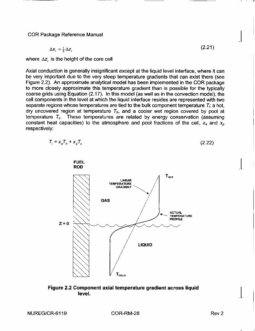
Axial conduction is generally insignificant except at the liquid level interface, where it can be very important due to the very steep temperature gradients that can exist there (see Figure 2.2). An approximate analytical model has been implemented in the COR package to more closely approximate this temperature gradient than is possible for the typically coarse grids using Equation (2.17). In this model (as well as in the convection model), the cell components in the level at which the liquid interface resides are represented with two separate regions whose temperatures are tied to the bulk component temperature Ti: a hot, dry uncovered region at temperature Th, and a cooler wet region covered by pool at temperature T.. These temperatures are related by energy conservation (assuming constant heat capacities) to the atmosphere and pool fractions of the cell, xa and xP respectively:
(2.22)
LINEAR TEMPERATURE
GRADIENT
GAS
T.OT
ACTUAL
PROFILE
LIQUID
TCo-o
Figure 2.2 Component axial temperature gradient across liquid level.
NUREG/CR-6119
I - --- 41
I
T = XaT.h + xPT,
FUEL ROD I
Z=O
I1COR-RM-28 Rev 2
COR Package Reference Manual
The temperatures of the two regions are determined by individual energy equations:
Cp xp (T, - To)=CP (T0 - T,' ) max(O,x, - x') P (2.23) + [K (Th - Tý )hp Xp A (7c - Tp )+ xP Q] At
C,, xa (T" - T•O )=C,, (T:0 - T,' ) max(O,xa - x') P . Th -h P Tý* T,(2.24)
+[K (Tc - T,)-h ax. A (Th - Ta)+X, Q1 At
where Cp is the total heat capacity of the component (Z mcpi), K is an effective axial
conductance (discussed below), Tp and Ta are pool and atmosphere fluid temperatures, respectively, and Q is the net component heat input from other sources.
In each of these equations, the first term on the right hand side represents the averaging of a region Ixp-xp0 l = Ixa-xa0 l that has just quenched or just uncovered with the old quenched or uncovered regions, respectively. The axial conduction term K(Th-Tc) is derived from a fin equation, as discussed below. Equations (2.22) through (2.24) can be solved simultaneously to eliminate Q and determine T. and Th from known values of xa, xp, Ta, and Tp, and new or projected values for the bulk component temperature Ti. The pool and atmosphere heat transfer rates are calculated from these temperatures and the respective fluid temperatures, pool fractions, and heat transfer coefficients.
Because of the large temperature gradient at the liquid level interface, simply using Equation (2.17) with Keff given by Equation (2.18) will significantly underpredict the conduction between the hot and cold regions. Instead, application is made of the onedimensional conduction equation for fins, given by the ordinary differential equation:
k d2l-h A (T - Tf )+q=0 (2.25) dz -2 -V
where q is the volumetric heat source, A / V is the surface area to volume ratio and the thermal conductivity k is assumed constant. Assuming the following boundary conditions:
(a) above the interface (z = 0) the fluid temperature is a constant atmosphere temperature Ta; below the interface the fluid temperature is a constant pool temperature Tp;
(b) the heat transfer coefficient is much larger for the pool than for the atmosphere (hp >) ha);
(c) T approaches Th for z above the interface and T, for z below the interface, the steady state values of which are dependent on the volumetric heat source q;
NUREG/CR-6119Rev 2 COR-RM-29
COR Package Reference Manual J the approximate solution for the temperature gradient at the liquid interface is:
dT A (Z-=k)V- ( Th - T0 ) (2.26)
dz k V
and therefore the value of K used in Equations (2.23) and (2.24) is
SK i A; hV A (2.27)
2.2.2 Radial Conduction
Conduction is calculated between elements of supporting structure (SS) modeling contiguous segments of a plate in radially adjacent core cells. Conduction is also calculated between particulate debris in radially adjacent core cells unless the path is blocked by intact canisters. It is based on equations Equations (2.17) - (2.19), with the conduction area and conduction distance for use in Equation (2.19) taken as
A1 = totcompj A (2.28) Vtot.cel •
(a
Vtet,i x; 2A (2.29)
where Vtt 0ce11 is the total volume of cell i and Amd is the area of the common radial boundary between cell i and cell j. Equation (2.28) accounts for the fraction of the height of the cell that is occupied by the component. It also introduces a factor of (1 - porosity) into the conductance for particulate debris.
2.2.3 Intra-Cell Conduction
As debris accumulates in a core cell and the free volume in the cell vanishes, there will undoubtedly be intimate contact between the debris and any remaining intact core components. Therefore, conduction between the debris and core components in the same cell is calculated from Equations (2.17) - (2.19) with
A, = AJ V=o+ VPD A intact (2.30) YOLPD + V in
NUREG/CR-6119 Rev 2COR-RM-30
COR Package Reference Manual
Ax Vtotintact (2.31) A~n~ -2 Aintad
VXxD bed (2.32)
2 Abed
where
Aintact = initial component surface area for the intact component
Vfree = additional volume available to PD
Vbed = total volume of debris bed (including porosity)
Abed = surface area of debris bed (boundary with other components, as opposed to surface area of debris particles)
and a factor of VtotPD/Vbed is included in the conductivity of the particulate debris.
An intact canister (specifically, component CB), will separate particulate debris in the bypass from that in the channel. Under these circumstances, intracell conduction from PD will be calculated only to fuel rods and both canister components (CN and CB). Conduction from PB will be calculated to the outer surface of CB, and to the other structures SS, NS, and OS.
2.2.4 Fuel-Cladding Gap Heat Transfer
Conduction radially across the fuel pellet and the fuel-cladding gap is calculated assuming "a parabolic temperature profile across the fuel, negligible cladding thermal resistance, and "a constant user-specified gap thickness (input on record COR00001). An effective total gap conductance is calculated by combining in conventional fashion the various serial and parallel resistances:
1 1 1
hgap hf I + (2.33) -- +
h9 hCF
where
hf=4 kf / rf (2.34)
NUREG/CR-6119Rev 2 COR-RM-31

COR Package Reference Manual 4 h9 = kg / Arg (2.35)
h ia i = 1_ +-a1 _ (2.36)
6f 6c
and where
a- = Stefan-Boltzmann constant
rf = radius of fuel pellet
A rg = thickness of fuel-cladding gap
kf = fuel thermal conductivity
kg = gap gas thermal conductivity
hCF = conductance calculated by control function
Tf = fuel bulk temperature L Tc = cladding bulk temperature
Ta = average temperature = (Tf + Tc) / 2
ef = fuel surface emissivity (default value, 0.8)
6C = cladding inner surface emissivity (default value, 0.325)
The term representing the thermal resistance of the fuel pellet, 1/hf, is combined in series with an effective resistance of the gap. This gap resistance includes radiation across the gap in parallel with the conductive resistance of the gap gas. An additional resistance, l/hcF, calculated via a control function and added serially to the conductive resistance of the gap gas, may be specified by the user on record COR00004. The fuel and cladding emissivities used to calculate radiation across the gap are stored in sensitivity coefficient array Cl 101.
The total effective gap conductance is then used to calculate the heat transfer rate from the fuel to the cladding by the equation:
qg•, = hgap Af ( T/ - Tc ) (2.37) I
NUREG/CR-6119 Rev 2COR-RM-32
COR Package Reference Manual
where Af is the surface area of fuel pellet and the superscript "i" denotes projected newtime temperature values. Because of the tight coupling between the fuel and the cladding, an implicit treatment is necessary to prevent numerical oscillations for reasonable time steps. The projected temperatures are found as solutions of the equations
C, (Tf" - T,= (AECO + AECOv + AE,,d + AEoxid)f - qgap At (2.38)
C, (T" - T' )= (A ECord + AE=,, + AE• + AEox.. )ý + qgap At (2.39)
where Cf and CQ are the total heat capacities of the fuel and cladding, respectively, and the AE terms on the right hand sides are other terms in their respective energy equations. These terms, which account for conduction, convection, radiation, and oxidation, are calculated as described in the corresponding sections of this report. The projected temperatures are used only in evaluating the gap heat transfer.
2.2.5 Consideration of Heat Capacity of Components
The heat transferred between components by conduction is evaluated from a numerically implicit form of Equation (2.17)
At= ~ _efrl ql2 At'] 0T + q12 At At~ L\.t= ef [ I _ T C 2 ) (2.40)
C1 C2 (To -Tr:)At = C C2 + (Cl + C2 KII At
Here C1 is again the total heat capacity of component i.
2.2.6 Effective Heat Capacity of Cladding
The formulation of gap heat transfer in Section 2.2.4 implicitly considers the finite heat capacities of the fuel and the cladding. Equations (2.38) (2.39) are solved for Tc in the form
= (AEcond + AEconv + AEra + AEoxd )ý + other terms TC + CFU hgap A, At (2.41)
CFu + hgap Af At
which may be interpreted as defining an effective heat capacity
NUREG/CR-6119Rev 2 COR-RM-33
COR Package Reference Manual j
CCL eff ý-CCL + C FU h gap Af At (2.42) CFu+ hgap Af At
for the cladding. This effective heat capacity implicitly accounts for energy transferred to the fuel pellets through the relatively tight coupling of CL to FU. It is used in estimating the temperature change of cladding in Equation (2.40) and in several other heat transfer models.
2.2.7 Conduction to Boundary Heat Structures
Optionally, conduction from a designated component in the outermost radial ring to the radial boundary heat structures specified on input records CORZhjO2 may be calculated. The heat flux is given by
qc-HS - (2.43) R
where Tc is the temperature of the core component and THs is the temperature of the first node of the heat structure (typically an insulator), and R is the total contact resistance, defined as
R =Rgap + Rdi, (2.44)
where
Rgap =Argp / kgap (2.45)
,r•-At
Rdkf A (2.46)
In the above equations, Argap is the thickness of a gap between the core component and the heat structure, kgap is the thermal conductivity of the gap material (calculated from the Material Properties package), At is the COR package time step, and k, p, and cp are the thermal conductivity, density, and specific heat, respectively, of the heat structure material. The thermal diffusive resistance Rdif is used to mitigate temperature oscillations that may arise from the numerically explicit coupling between the COR and Heat Structure packages. The user may specify on input record COR00011 which core component is used in this model, what the gap material and thickness are, and the value of the thermal diffusion constant (;r /k pCp)1 / 2 for the heat structure (since these properties are not currently accessed from the MP package). I
NUREG/CR-6119 COR-RM-34 Rev 2
COR Package Reference Manual
2.3 Convection
Convective heat transfer is treated for a wide range of fluid conditions. Emphasis has been placed on calculating heat transfer to single-phase gases, since this mode is the most important for degraded core accident sequences. A simple set of standard correlations has been used for laminar and turbulent gas flow in both forced and free convection; these correlations give the Nusselt (Nu) number as a function of Reynolds (Re) and Rayleigh (Ra) numbers. Because the numerical method is only partially implicit, the dependence of heat transfer coefficients on surface and fluid temperatures can induce numerical oscillations in calculated temperatures. The calculated heat transfer coefficients for both vapor and liquid heat transfer are therefore "relaxed" by averaging each with its previously calculated value to mitigate the oscillations.
Since the COR cell nodalization is typically much finer than the Control Volume Hydrodynamics (CVH) nodalization, approximate temperature and mass fraction distributions in the control volumes interfacing with the core and lower plenum must be calculated in the COR package to properly determine the convective heat transfer rates for each COR cell. This temperature distribution is calculated in the COR package in what is termed the "dT/dz" model, which is described separately in Section 2.5.
In previous versions of MELCOR, limitations in several models made it difficult-if not impossible-to perform calculations using a fine CVH nodalization with one control volume for each core cell or small number of core cells. MELCOR 1.8.4 included improvements in the dT/dz model and incorporates a core flow blockage model (in the FL package). These make such calculations more practical, although some penalty in terms of increased CPU time requirements should still be expected. It is recommended that the new default dT/dz modeling should be used (no CORTIN records), and that the flow blockage model be invoked and momentum flux terms calculated in the core flow paths (see the FL Package Users' Guide). In the discussion that follows, all fluid temperatures refer to local temperatures, whether calculated by the dT/dz model or taken directly from a fine-scale CVH nodalization.
Heat transfer rates are calculated for each component by the equation:
q = hf. A, (T.- T,.) (2.47)
where
h,,, = relaxed heat transfer coefficient
A, = component surface area for heat transfer, accounting for the effects of conglomerate debris (see Section 3.1.5)
T, = component surface temperature
NUREG/CR-6119Rev 2 COR-RM-35
-4.
COR Package Reference Manual j Tf = local fluid temperature
MELCOR 1.8.4 and earlier versions used estimated new-time component temperatures in an effort to prevent numerical oscillations in the component heat transfer rates. This approach has been replaced by a semi-implicit calculation of the gap term, described in Section 2.2.4, that has been found to be more effective and reliable.
The unrelaxed heat transfer coefficient, hcorr, is calculated from various correlations for the Nusselt number, which will be discussed in the following subsections:
N u =hco, Dh / k (2.48)
where
Dh = hydraulic diameter for each component surface, defined by the user on input record CORijj04
k = fluid thermal conductivity
Relaxed heat transfer coefficients for COR subcycle n are given by
hIX.f = foldf hx,2j; + (1 - foIdf ) hCof,,f (2.49) 1 where foldf is the fraction of the old value to be used for fluid f (vapor or liquid), adjustable through sensitivity coefficient array C1200 with default values of 0.5 and 0.9 for vapor and liquid heat transfer, respectively.
2.3.1 Laminar Forced Convection
For laminar forced flow in intact geometry, the Nusselt number is given by a constant, representing the fully developed Nusselt number for constant heat flux, multiplied by a developing flow factor:
Nu = C(n) •de, (2.50)
where the constant C(n) is currently defined for both rod bundle arrays (n=l) and circular tubes (n=2) to be 4.36 and is implemented as sensitivity coefficient array C1212. The developing flow factor is currently that used in MARCH 2 in connection with gaseous diffusion-limited oxidation [8], with the Prandtl number used instead of the Schmidt number
dev =1 + 0.00826 F(z) + 0.0011 ( I
NUREG/CR-6119 COR-RM-36 Rev 2

COR Package Reference Manual
In Equation (2.50), the constants have been implemented in sensitivity coefficient array C1213, and F(z) is a nondimensional entrance length:
F(z) = (z - zo )
D. Re Pr (2.52)
where (z - zo) is the distance from the flow entrance, Dh is the hydraulic diameter, Re is the Reynolds number, and Pr is the Prandtl number. In the present version of the code, (z - Zo) is set to 1000 m, effectively eliminating any developing flow effects.
2.3.2 Turbulent Forced Convection
For turbulent flow in channels, the Dittus-Boelter correlation [9] is used:
Nu = 0.023 Re0 8 Pr0-4 (2.53)
The coefficients and exponents in Equation (2.53) are implemented in sensitivity coefficient array C1214.
Rather than defining a critical Reynolds number controlling whether laminar or turbulent correlations are used, both correlations are evaluated and the maximum of the turbulent and laminar Nusselt numbers is used to calculate the forced convection heat transfer coefficient.
2.3.3 Laminar and Turbulent Free Convection
For laminar free convection in narrow channels, the following correlation for an enclosed air space between vertical walls is used [10]:
Nu = 0.18 Ra'4 (L / D, )Y19 (2.54)
where L is the channel length. For turbulent free convection a similar correlation is used, differing only in the default values for the multiplicative constant and the exponent for the Rayleigh number [10]:
Nfu=0.065 Ra' (L/Dh)119 (2.55)
The coefficients and exponents in Equations (2.54) and (2.55) have been implemented as sensitivity coefficient arrays C1221 and C1222, respectively.
As for forced convection, the maximum of the laminar and turbulent Nusselt numbers is used to evaluate the free convection heat transfer coefficient. The maximum of the forced and free convection heat transfer coefficients is then used in Equation (2.47) to calculate
NUREG/CR-6119Rev 2 COR-RM-37
COR Package Reference Manual 4 the heat transfer rate for a given component. This treatment alleviates some numerical difficulties that may occur if ranges are defined for the various flow regimes, with discontinuities in Nusselt number at the transition points between regimes.
2.3.4 Convection from Particulate Debris
For particulate debris, correlations for isolated spherical particles are currently used in the COR package for convection to gases. (Surface areas for particulate debris are normally so high that practically any correlation will almost completely equilibrate the gas temperature with the debris temperature.) For forced convection, the following correlation is used [11]:
Nu = 2.0 + 0.6 Re'12 prY (2.56)
For free convection, the Reynolds number is replaced by the square root of the Grashof number [11]:
Nu = 2.0 + 0.6 Gr'4 Prf3 (2.57)
The coefficients and exponents in Equations (2.56) and (2.57) have been implemented as sensitivity coefficient arrays C1231 and C1232, respectively. In both equations, the I properties are evaluated at the film temperature (i.e., the average of the debris and dT/dz model fluid temperatures). The maximum of the free and forced convection Nusselt numbers is once again used to calculate the heat transfer coefficient.
2.3.5 Boiling
By default for liquid-covered components, the COR package uses the correlations from the HS package to treat boiling (see the HS Reference Manual). However, by changing the default value of sensitivity coefficient C1241(5), the simplified boiling curves from the MARCH 2.0 code [3] can be used to calculate the heat transfer coefficient:
h=34.5 p114 T-523 ( T < 23.4K) (2.58)
h=1.41(10 7 ) P114 T--575 ( T >_ 23.4K) (2.59)
where
P = pressure
T = surface superheat, (T, - Tsat) I
NUREG/CR-6119 COR-RM-38 Rev 2
COR Package Reference Manual
and the constants have been implemented as sensitivity coefficient arrays C1241 and C1242.
For the film boiling regime ( T Ž_ 23.4 K), a radiation component is added to the convective heat transfer coefficient:
hrd =o;- s (2.60)
where e is a hardwired constant emissivity of 0.4.
2.3.6 Heat Transfer from Horizontal Surfaces of Plates
For most core components-fuel rods, BWR canisters, control elements, and BWR Control Rod Guide Tubes--convective heat transfer takes place from a lateral (vertical) surface. If there is a water pool in the associated core cell, the component surface will be progressively and smoothly covered or uncovered as the pool surface rises or falls.
Plates, however, have horizontal bottom and top surfaces that can be covered or uncovered with a relatively small change in the pool level. Moreover, different CVH control volumes are ordinarily used to model the regions above and below the core plate, which can be associated with (at most) one of these volumes. Thus, (at least) its other horizontal surface will see fluid in a different control volume than that from which other boundary conditions for the core cell are derived.
When the SS component is used to represent a plate, an optional model exists to calculate heat transfer from its horizontal surfaces to water pools above and/or below. The model may be controlled independently for the two surfaces, and is off by default. If the model is on, the heat transfer coefficient for the top surface is ordinarily evaluated from the built-in pool boiling correlation (Section 2.3.5) and that for the bottom surface from the built in correlation for downward-facing boiling (Section 5.1). Either or both may be overridden by constant values or by values calculated as control functions. In any case, the temperature difference is based on the average temperature of the plate in the core cell and that of the pool.
For either plate surface, the total area is taken as the total cross-sectional area of the core cell. However, the surface of a water pool is not an idealized plane. One would therefore expect some contact with the bottom of the plate while the average pool surface is some finite distance below it, and less-than-complete coverage of the top until the average surface is some finite distance above it. In order to account for this, the fraction of the lower horizontal surface involved in heat transfer to a pool is linearly ramped on as the surface of the pool in the core cell below rises to the bottom surface of the plate. Similarly, the fraction covered above is ramped off as the surface of the pool in the core cell above falls to the top surface of the plate. User input is required for both the clearance below the
NUREG/CR-6119Rev 2 COR-RM-39
COR Package Reference Manual J plate required for no contact and the pool depth over the plate required for complete coverage.
This model is activated and the necessary input supplied using COROOOPC, CORZjJPC, CORRiiPC, and/or CORijjPC records, as described in the COR Package Users' Guide.
2.3.7 Debris Quenching and Dryout
Heat transfer from debris to liquid water pools may occur in two distinct modes. In the falling-debris quench mode, failure of the core support plate triggers the relocation of a large mass of hot debris from the core region to the lower plenum. In this mode it is assumed that transient heat transfer rates may be sufficient to rapidly quench the hot debris and/or generate large steam pressure excursions. Following the quench mode it is assumed that continued decay heat generation in the stationary debris bed in the lower plenum will either boil off any remaining water in the lower plenum or quickly lead to debrisbed dryout with an overlying water pool. The heat transfer from the debris bed to the overlying pool of water following debris-bed dryout is relatively modest and is calculated with an appropriate dryout heat flux correlation described below.
The falling-debris quench model is active by default. If deactivated through user input, the debris is assumed to relocate instantaneously from the core region to an unquenched debris bed in the lower plenum. The model may be deactivated by specifying a value of 0.0 for the quench heat transfer coefficient on input record COROOO12. No other parameters on this record are then necessary. The heat transfer calculated by the model may or may not be sufficient to fully quench the debris before it reaches the bottom of the lower plenum, depending on the values chosen for the model parameters described below.
Beginning from the time of core support plate failure in each radial ring, the elevation of the leading edge of the falling debris is determined assuming a constant user-specified descent velocity (default of 5 m/s). The axial elevation of the leading edge of the falling debris is given by
Zd =zc CS -Vd (t -t4) (2.61)
where zcsp is the initial elevation of the core support plate, vd is the velocity of the falling debris, t is the current time and tfail is the failure time of the support plate in the particular ring. Debris from core cells above elevation z will be relocated downwards subject to the availability of free volume and the absence of additional supporting structures.
When the leading edge of the falling debris enters the pool of water in the lower plenum, quench heat transfer begins. The heat transfer surface area is the value calculated assuming the debris particles have an equivalent spherical diameter equal to the userspecified hydraulic diameter for particulate debris (input on record CORijjO4). The userspecified quench heat transfer coefficient (input on record COR00012) is assumed to INUREG/CR-6119 COR-RM-40 Rev 2
COR Package Reference Manual
remain constant until the leading edge of the falling debris reaches the bottom of the lower plenum (the elevation of the lower head). After that time a decay factor initially equal to unity is applied to the user-specified heat transfer coefficient.
The decay factor is intended to simulate the reduction in heat transfer that occurs during the transition from the quench period to the debris bed configuration. During this period of transition, additional hot debris from the core region may relocate to the lower plenum as a result of radial spreading between the rings in the core region. Therefore, the decay factor has a time constant equal to the time constant for radial spreading of solid debris (see Section 3.2.4). The decay factor also includes a term to arrest the decay as long as significant amounts of debris continue to migrate into the failed ring from other core regions. Soon after the bulk of the debris has relocated the decay factor will quickly decrease. When the value of the decay factor falls below 0.01, it is assumed that the transition to a stable debris bed geometry is complete, and all subsequent debris-to-pool heat transfer in that radial ring will be limited by the dryout heat flux correlation discussed below. The time-dependent heat transfer decay factor, f(t), is given by
f(t+At)=min [1,f(t) exp(-At / z, )+V.or / VLp 1 (2.62)
where Z-spr is the time constant for radial spreading of solid debris described in Section 3.2.4, Vcor is the volume of debris which relocates into the ring from radial spreading in the core region during the core time step At and VLP is the volume of debris in the ring beneath the level of the core support plate.
During the short period between the failure of the core support plate and the time at which the leading edge of the falling debris reaches the lower head, the models for candling, dissolution and radial spreading of debris in the affected ring are deactivated. This action is taken because those models implicitly assume a stationary debris configuration. In addition to the quench heat transfer coefficient, the user may specify a reactor vessel failure pressure (default value of 2.0e7 Pa). When the differential pressure between the lower plenum CVH volume and the reactor cavity CVH volume reaches the failure pressure, it is assumed that the lower head in all the core rings contained in the lower plenum CVH volume fails totally. When this happens all of the debris in the core cells above the failed lower head is ejected immediately, and further quench heat transfer in those rings is suppressed. Currently, it is suggested that users do not specify a failure pressure in excess of the critical pressure of water (22. MPa) because the CVH package may encounter problems above that pressure.
Because of the relatively low value of the default value for the failure pressure (compared to actual failure pressures that may be much higher) the quench model may have a rather limited range of usefulness for some PWR calculations. If the PWR relief valves cycle around 16-17 MPa, then there is very little margin (3-5 MPa) for steam generation between the relief pressure and the critical pressure; hence, even modest fuel-coolant interactions following support plate failure tend to cause "vessel failure."
NUREG/CR-6119COR-RM-41Rev 2
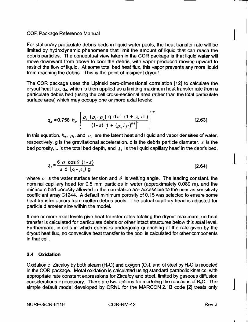
COR Package Reference Manual 4 For stationary particulate debris beds in liquid water pools, the heat transfer rate will be limited by hydrodynamic phenomena that limit the amount of liquid that can reach the debris particles. The conceptual view taken in the COR package is that liquid water will move downward from above to cool the debris, with vapor produced moving upward to restrict the flow of liquid. At some total bed heat flux, this vapor prevents any more liquid from reaching the debris. This is the point of incipient dryout.
The COR package uses the Lipinski zero-dimensional correlation [12] to calculate the dryout heat flux, qd, which is then applied as a limiting maximum heat transfer rate from a particulate debris bed (using the cell cross-sectional area rather than the total particulate surface area) which may occupy one or more axial levels:
q• =0.756 h, Pv (p, - v) g d 3 (1 + Ac/L)1 (2.63) d (1-6) [1 + (v J
In this equation, hk,, pl, and pv are the latent heat and liquid and vapor densities of water, respectively, g is the gravitational acceleration, d is the debris particle diameter, 6 is the bed porosity, L is the total bed depth, and Ac is the liquid capillary head in the debris bed,
6 o cos0 (1-e) (./ •c - d(P g (2.64)
where o is the water surface tension and 0 is wetting angle. The leading constant, the nominal capillary head for 0.5 mm particles in water (approximately 0.089 m), and the minimum bed porosity allowed in the correlation are accessible to the user as sensitivity coefficient array C1244. A default minimum porosity of 0.15 was selected to ensure some heat transfer occurs from molten debris pools. The actual capillary head is adjusted for particle diameter size within the model.
If one or more axial levels give heat transfer rates totaling the dryout maximum, no heat transfer is calculated for particulate debris or other intact structures below this axial level. Furthermore, in cells in which debris is undergoing quenching at the rate given by the dryout heat flux, no convective heat transfer to the pool is calculated for other components in that cell.
2.4 Oxidation
Oxidation of Zircaloy by both steam (H20) and oxygen (02), and of steel by H2 0 is modeled in the COR package. Metal oxidation is calculated using standard parabolic kinetics, with appropriate rate constant expressions for Zircaloy and steel, limited by gaseous diffusion considerations if necessary. There are two options for modeling the reactions of B4C. The simple default model developed by ORNL for the MARCON 2.1B code [2] treats only INUREG/CR-6119 COR-RM-42 Rev 2
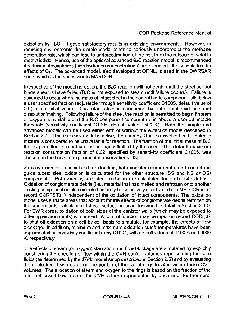
COR Package Reference Manual
oxidation by H2 0. It gave satisfactory results in oxidizing environments. However, in reducing environments the simple model tends to seriously underpredict the methane generation rate, which can lead to underestimation of the risk from the release of volatile methyl iodide. Hence, use of the optional advanced B4C reaction model is recommended if reducing atmospheres (high hydrogen concentrations) are expected. It also includes the effects of 02. The advanced model, also developed at ORNL, is used in the BWRSAR code, which is the successor to MARCON.
Irrespective of the modeling option, the B4C reaction will not begin until the steel control blade sheaths have failed (B4C is not exposed to steam until failure occurs). Failure is assumed to occur when the mass of intact steel in the control blade component falls below a user specified fraction (adjustable through sensitivity coefficient C1 005, default value of 0.9) of its initial value. The intact steel is consumed by both steel oxidation and dissolution/melting. Following failure of the steel, the reaction is permitted to begin if steam or oxygen is available and the B4 C component temperature is above a user-adjustable threshold (sensitivity coefficient C1005, default value 1500 K). Both the simple and advanced models can be used either with or without the eutectics model described in Section 2.7. If the eutectics model is active, then any B4C that is dissolved in the eutectic mixture is considered to be unavailable for reaction. The fraction of the initial mass of B4C that is permitted to react can be arbitrarily limited by the user. The default maximum reaction consumption fraction of 0.02, specified by sensitivity coefficient C1005, was chosen on the basis of experimental observations [13].
Zircaloy oxidation is calculated for cladding, both canister components, and control rod guide tubes; steel oxidation is calculated for the other structure (SS and NS or OS) components. Both Zircaloy and steel oxidation are calculated for particulate debris. Oxidation of conglomerate debris (i.e., material that has melted and refrozen onto another existing component) is also modeled but may be selectively deactivated (on MELCOR input record CORTST01) independent of the oxidation of intact components. The oxidation model uses surface areas that account for the effects of conglomerate debris refrozen on the components; calculation of these surface areas is described in detail in Section 3.1.5. For BWR cores, oxidation of both sides of the canister walls (which may be exposed to differing environments) is modeled. A control function may be input on record CORijj07 to shut off oxidation on a cell by cell basis to simulate, for example, the effects of flow blockage. In addition, minimum and maximum oxidation cutoff temperatures have been implemented as sensitivity coefficient array C1 004, with default values of 1100 K and 9900 K, respectively.
The effects of steam (or oxygen) starvation and flow blockage are simulated by explicitly considering the direction of flow within the CVH control volumes representing the core fluids (as determined by the dT/dz model setup described in Section 2.5) and by evaluating the unblocked flow area along the portion of the radial rings located within these CVH volumes. The allocation of steam and oxygen to the rings is based on the fraction of the total unblocked flow area of the CVH volume represented by each ring. Furthermore,
NUREG/CR-6119COR-RM-43Rev 2
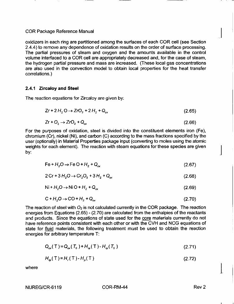
COR Package Reference Manual j oxidizers in each ring are partitioned among the surfaces of each COR cell (see Section 2.4.4) to remove any dependence of oxidation results on the order of surface processing. The partial pressures of steam and oxygen and the amounts available in the control volume interfaced to a COR cell are appropriately decreased and, for the case of steam, the hydrogen partial pressure and mass are increased. (These local gas concentrations are also used in the convection model to obtain local properties for the heat transfer correlations.)
2.4.1 Zircaloy and Steel
The reaction equations for Zircaloy are given by:
Zr+2H 2 0 -. ZrO2 +2 H 2 + Qox (2.65)
Zr + 02 -- ZrO2 + Qox (2.66)
For the purposes of oxidation, steel is divided into the constituent elements iron (Fe), chromium (Cr), nickel (Ni), and carbon (C) according to the mass fractions specified by the user (optionally) in Material Properties package input (converting to moles using the atomic weights for each element). The reaction with steam equations for these species are given by:
Fe+H 20--FeO+H2 + Qx (2.67)
2Cr +3 H20 -> Cr2 0 3 + 3 H2 + Qox (2.68)
Ni+H 20 -Ni O + H2 + Qox (2.69)
C+H 20 -CO + H2 + Qox (2.70)
The reaction of steel with 02 is not calculated currently in the COR package. The reaction energies from Equations (2.65) - (2.70) are calculated from the enthalpies of the reactants and products. Since the equations of state used for the core materials currently do not have reference points consistent with each other or with the CVH and NCG equations of state for fluid materials, the following treatment must be used to obtain the reaction energies for arbitrary temperature T:
Qox( T )=Q(T0 )+(HT(o T )-H(T ,(To0 ) (2.71)
HP ( T ) = Hr( ( T H ( T) (2.72)
where t
NUREG/CR-6119 COR-RM-44 Rev 2
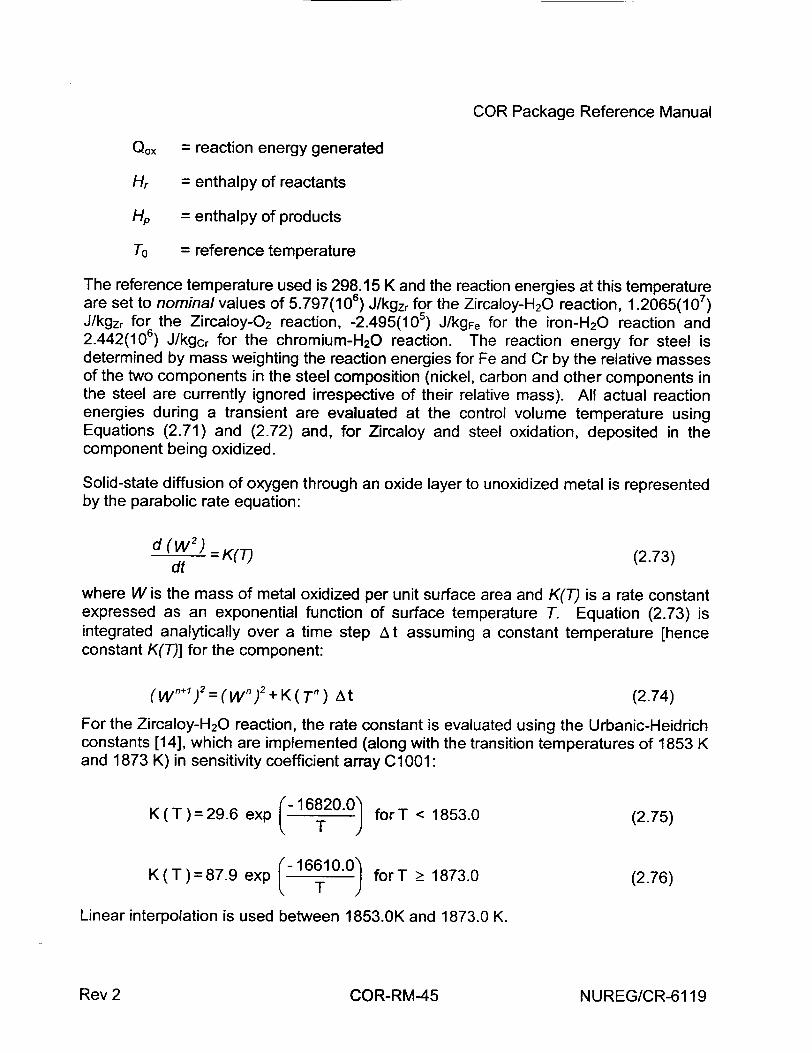
COR Package Reference Manual
Qox = reaction energy generated
Hr = enthalpy of reactants
Hp = enthalpy of products
To = reference temperature
The reference temperature used is 298.15 K and the reaction energies at this temperature are set to nominal values of 5.797(106) J/kgzr for the Zircaloy-H 20 reaction, 1.2065(1 07) J/kgzr for the Zircaloy-0 2 reaction, -2.495(105) J/kgFe for the iron-H 20 reaction and 2.442(10 6) J/kgcr for the chromium-H 20 reaction. The reaction energy for steel is determined by mass weighting the reaction energies for Fe and Cr by the relative masses of the two components in the steel composition (nickel, carbon and other components in the steel are currently ignored irrespective of their relative mass). All actual reaction energies during a transient are evaluated at the control volume temperature using Equations (2.71) and (2.72) and, for Zircaloy and steel oxidation, deposited in the component being oxidized.
Solid-state diffusion of oxygen through an oxide layer to unoxidized metal is represented by the parabolic rate equation:
d (W 2 ) =K(T) (2.73) dt
where W is the mass of metal oxidized per unit surface area and K(T) is a rate constant expressed as an exponential function of surface temperature T. Equation (2.73) is integrated analytically over a time step A t assuming a constant temperature [hence constant K(T)] for the component:
(W n*) 2 =(Wn) 2 +K(Tn) At (2.74)
For the Zircaloy-H20 reaction, the rate constant is evaluated using the Urbanic-Heidrich constants [14], which are implemented (along with the transition temperatures of 1853 K and 1873 K) in sensitivity coefficient array C1001:
K(T)=29.6 exp - 16820.0 forT < 1853.0 (2.75)
K(T)=87.9 exp - 16610.0) forT Ž_ 1873.0 (2.76) a lT
Linear interpolation is used between 1853.0K and 1873.0 K.
NUREG/CR-6119Rev 2 COR-RM-45
COR Package Reference Manual
For the Zircaloy-0 2 reaction, the rate constant is evaluated using constants from Reference [15], which are also implemented in sensitivity coefficient array C1 001:
K(T)=50.4 exp 14630) (2.77)
For the steel-H20 reaction, the rate constant is evaluated using constants from White [16], which are implemented as sensitivity coefficient array C1002:
K(T)=2.42-109exp- 4 2 40 0 .0) (2.78)
For very low oxidant concentrations, gaseous diffusion may limit the reaction rate. A mass transfer coefficient is calculated via a heat-mass transfer analogy from the heat transfer correlations in Section 2.3 by substituting the Schmidt number for the Prandtl number and the Sherwood number for the Nusselt number. The oxidation rate when limited by gaseous diffusion is given by:
dW _MW k. P.. (2.79) dt nRTf (279
where
MW = molecular weight of metal being oxidized
k, = mass transfer coefficient
Pox = partial pressure of oxidant (H20 or 02)
n = number of moles of oxidant (H20 or 02) consumed per mole of metal
R = universal gas constant
Tf = gas film temperature, (T + Tgas) / 2
The gaseous diffusion oxidation rate is used if it is less than the rate calculated by Equation (2.74). Although the molecular weight MW and the number of moles n of H2 0
consumed are defined by the reaction, the quantity (MW/nR) has been implemented for reactions with H2 0 as sensitivity coefficient array C1003 to allow the user a measure of separate control over the gaseous diffusion oxidation rate. That sensitivity coefficient is multiplied by two intemally in the code to obtain an equivalent value for gaseous diffusion of oxygen (nH20 = 2no2). I
NUREG/CR-6119 COR-RM--46 Rev 2
COR Package Reference Manual
For the oxidation of Zircaloy in environments containing both H2 0 and 02, the maximum oxidation rate calculated for the two gases is used:
dW = max I IdW II (2.80) dt ['K dt )H20 I(' d o]
There are two options for partitioning the oxidant consumption between the oxygen and steam. The default option is recommended and does not permit the consumption of steam until all of the available oxygen has been consumed. This option is equivalent to assuming that all hydrogen produced by steam oxidation is instantaneously converted back to steam by combustion with the available oxygen. The default option should prevent time step reductions associated with the normal combustion of in-vessel hydrogen by the BUR package. For the second option the reactions given by Equations (2.65) and (2.66) are proportioned by the relative rates:
f H20 dW (2.81) (dWd Fdt )O dt
= 1 - f0 (2.82)
2.4.2 Simple Boron Carbide Reaction Model
In the simple default B4C reaction model, the B4C in BWR control blades is reacted with steam using the model from MARCON 2.1 B [2]. This model uses three reaction equations:
B4C + 7H 20 --+ 2B 20 3 + CO + 7H 2 + Q1 (2.83)
B4C + 8H 20 --. 2B 20 3 + C0 2 + 8H 2 + Q2 (2.84)
B4C + 6H 20 -> 2B20 3 + CH4 + 4H 2 + Q3 (2.85)
Chemical equilibrium of reaction products is assumed, and the model uses the steam and hydrogen partial pressures and B4C temperature to determine the relative extent of each reaction. The equilibrium C0/C02 and CO/CH4 mole ratios Yco/co2 and YCO/CH4, respectively, are given by the expressions:
NUREG/CR-6119Rev 2 COR-RM-47
COR Package Reference Manual
[-3001 S PH,2 exp 3605.0 T 3.427 (2.86)
PHY0 C27350.0 1
YCO CH4 - PH2, exp L T + 30.50 (2.87) (PH2 Y)T
where the steam and hydrogen partial pressures are in atmospheres. The extents of reactions (2.83) - (2.85), expressed as relative percentages of CO, C0 2, and CH4 produced (Xco, Xc0 2, and XCH4, respectively), can then be given in terms of the CO/CO2 and COICH4
mole ratios as:
1 xc + 1/Ycoico 2 + 1/ YcoIcH, (2.88)
XC02= Xco /Yco/co2 (2.89)
XcH. =1- Xco - Co2 (2.90)
The reaction energies (in J/kg-mole B4C reacted) for reaction Equations (2.83) - (2.85) are given by the equations: I
Q, = 8.238(18 ) -58380.0 T (2.91)
Q2 = 8.674(10 8 )- 67060.0 T (2.92)
Q3 = 1.056(10 8)- 61 4 30.0 T (2.93)
The gaseous reaction products are transferred to the CVH package, while the B 2 0 3
generated is transferred to the Radionuclide (RN) package as an aerosol. All the energy generated by the B4C reaction is added to the CVH package. The reaction energies calculated by Equations (2.91) - (2.93) above are inconsistent with reaction energies that would be calculated using the present equations of state for the noncondensible gases and the B4C and B 2 0 3 (i.e., the temperature dependence implied by those equations is not consistent with the actual temperature dependence of the equations of state used). This discrepancy is ignored at present, due to the lack of reliable enthalpy data for B4C and B2 0 3.
The B4C oxidation rate is given as a fractional change per second in the initial (intact) B4C mass by:
t
NUREG/CR-6119 COR-RM-48 Rev 2
COR Package Reference Manual
d(M 840IMM-) 9.973(1 06) (- 22641.2) - dt B4_ 60. ep ( T ) (2.94)
The constants in Eq. (2.94) are programmed as sensitivity coefficients C1006. Given the amount of B4C reacted, the amounts of the various products are calculated from Equations (2.83) - (2.90) above.
2.4.3 Advanced Boron Carbide Reaction Model
In the optional advanced B4C reaction model the B4C in BWR control blades is reacted with vapors in the surrounding atmosphere using the model from BWRSAR and SCDAP [17]. This model determines the equilibrium composition in each control volume that is achieved when the Gibbs free energy of the system is minimized. The difference between the initial composition in the control volume and the equilibrium composition determines the rate of consumption of the reactants. The algorithm that is used to determine the composition that minimizes the free energy is based on the Swedish SOLGASMIX computer code [18]. In this method, the quantity
R n- I L +ln(aj (2.95) RT i i(T)
is minimized with respect to the variables ni for constant temperature and pressure values, where G denotes the total free energy of the system, R the gas constant, T the thermodynamic temperature, ni the number of moles of the ith species, g' the standard chemical potential, and a the activity. The values for ni corresponding to the equilibrium mixture must be non-negative and the mass balance constraints must be satisfied. Lagrange's method of undetermined multipliers is used for determining the constrained minimum, and the logarithmic equations thus obtained are expanded in a Taylor series about initially estimated n,-values, neglecting terms involving derivatives of second and higher orders. The linear equations represent approximations of the exact expressions, so a series of iterations is performed to obtain the final solution.
The advanced BC reaction model assumes that chemical equilibrium is achieved between the reactants during each time step. The mass of reactants considered during each time step is linearly dependent on the size of the time step, so that as the time step size goes to zero, the rate of reaction goes to zero. The mass of B4C available for reaction during each time step is determined by Eq. (2.94), as in the simple model. The availability of all other reactants is limited by the rate of steam diffusion to the reaction surface during the given time step. For example, if only 5% of the steam in the control volume can diffuse to the surface during the time step, then only 5% of all the other reactants in the control volume (except B4C) is considered to be available for equilibration with the steam (5% of control volume total) and B4C (given by Eq. (2.94)). The model considers the following 18
NUREG/CR-6119Rev 2 COR-RM-49
COR Package Reference Manual 4/ species that contain one or more of the five elements: argon, oxygen, hydrogen, boron and carbon (argon occurs only in elemental form and is included for simulation of fuel damage experiments that employ this inert gas):
H2 (g) CO2 (g) B (s) H3B30 6 (g) H20 (g) CH4 (g) B4C (s) HBO 2 (g) C (s) 0 (g) B20 3 (Cs) BH 3 (g) CO (g) 02 (g) B20 3 (g) B2H6 (g)
Ar (g) BOH (g)
The quantity g°/RT is determined from the thermodynamic relationship g = h - Ts. The enthalpy h and entropy s are calculated as integrals of the specific heat capacity,
T
h f 'cpdT'+h2 8
298
(2.96) T C
s f= -, dT'+So 8 2298 T?
and the specific heat capacity for each species above is expressed as a function of temperature over various temperature ranges,
cp = a+bT+cT2 +d/T2 +e/T 3 (2.97)
Deviations from ideality are not modeled, so that the activities of all gaseous species are equal to their respective mole fractions in the gas mixture. The condensed species are treated as a mechanical mixture only; their activities are set to unity and they have no effect on the minimization of the Gibbs free energy in Eq. (2.95).
Because a thermochemical reference is used, the heat of reaction is simply the difference between the total enthalpy of the products and that of the reactants.
The reaction products are passed to either the CVH or RN package for tracking and subsequent use as input to the chemical equilibrium routine. Steam, oxygen, hydrogen, carbon monoxide, carbon dioxide, methane and argon are tracked by the CVH package, while elemental boron and carbon and all the boron compounds are tracked by the RN package.
2.4.4 Steam/Oxygen Allocation
As mentioned earlier, steam (and oxygen) from the core region CVH volumes is supplied to the COR Package component surfaces for oxidation purposes in a manner that takes INUREG/CR-6119 COR-RM-50 Rev 2
COR Package Reference Manual
into account the effects of both steam (and oxygen) starvation and flow blockage. To account for the effect of flow blockage within each core CVH volume, the minimum unblocked flow area for each of the rings interfaced to the volume is evaluated and then summed across all constituent rings. The CVH volume steam allocated to each constituent ring is the fraction of total unblocked flow area of the CVH volume represented by the ring. The calculation of unblocked flow areas may be bypassed if desired by the user (input record CORVOL). The mass of steam within each ring is decremented as oxidation consumes the steam and no sharing of steam among the constituent rings is permitted during a COR subcycle. Thus the situation may arise such that the components of some rings may completely consume the ring inventory of steam while other rings may remain steam rich.
To account for the effect of steam starvation on a ring by ring basis, the processing of oxidation effects is conducted for each radial ring of the CVH volume in the direction of flow. The direction of flow is determined from CVH results or may be set via evaluation of a user prescribed control function (see input record CORRiiO4). Therefore, if the flow direction is upward, the progression of oxidation processing in the axial direction is from bottom to top. For the up-flow condition, the entire ring inventory of steam is initially allocated to the surfaces of the lowermost axial cell in the ring adjacent to the CVH volume, the inventory adjusted to account for oxidation, and the remaining steam is supplied to the components in the overlying cell in the ring. This axial marching is repeated until the uppermost axial segment of the ring within the CVH volume has been processed. All rings associated with the CVH volume are processed in this manner for each COR subcycle.
A second level of oxidant partitioning is performed at the cell level (axial segment-IA, ringIR) within the CVH volume during the axial marching process. The object is to make results independent of the order in which the various oxidation reactions are evaluated. A fraction of the total available oxidant (steam or oxygen) available in this level of this ring is allocated to each possible oxidation reaction on each surface in proportion to the area available for that reaction. The reactions may include oxidation of zirconium, steel, and/or B4C (Sections 2.4.1, 2.4.2, and 2.4.3). The portion of each intact component surface that is not blocked by candled materials (conglomerate debris) and the surface of the conglomerate debris on that component are each considered separately.
Because oxidation is calculated using rate equations subject to availability of steam, it is possible that all of the oxidant allocated to some surfaces may be consumed while only some of the oxidant allocated to other surfaces is consumed. In this situation, the oxidant that was not consumed is reallocated (using the same algorithm) among the starved surfaces, and the oxidation calculations for these surfaces repeated. This process is repeated (a maximum of 10 times) until either
(1) the ring oxidant inventory is exhausted, or
(2) for each surface, either the metal content of each surface is consumed or the limit established by rate considerations is reached.
NUREG/CR-6119Rev 2 COR-RM-51
COR Package Reference Manual
If the ring oxidant inventory is not exhausted, the calculation proceeds to the next cell in the direction of flow.
Because COR package calculations may result in total blockage (and thus steam/oxygen deprivation) of rings, the effect upon oxidation results and upon accident progression may be significant. Due to this dependence, sensitivity coefficient C1007 has been defined to provide a lower limit on the unblocked area fractions to be used in the partitioning of CVH volume oxidant inventories among the associated rings.
If the calculated unblocked area fraction for a ring falls below the corresponding limit specified for that ring by sensitivity coefficient 1007, then the fraction of CVH volume oxidant inventory allocated to the ring is held at the limit and the remainder of the oxidant is divided among the remaining unblocked rings. If all rings are blocked, then the oxidant is divided among the rings according to the limits prescribed by sensitivity coefficient C1007 and any remaining oxidant is unavailable for oxidation. A check is made during input processing to ensure that the sum of the ring fractions prescribed by sensitivity coefficient 01007 does not exceed unity.
2.5 Control Volume Temperature Distribution (dT/dz) Model
To accurately model the heat transfer to the gas from multiple COR cells interfaced to a single control volume, an estimate of the temperature distribution in the control volume atmosphere must be made in the COR package. Approximate local fluid temperatures are calculated for cells above the uppermost liquid level in the core; the remaining cells use control volume pool and atmosphere temperatures.
The "dT/dz" model used for this approximation assumes steady gas flow through the channel or bypass with known or specified inlet gas temperature and no cross-flow between core rings within any single CVH control volume. The model uses time-smoothed ("relaxed") CVH steam and/or oxygen outflow at the top of the core to determine whether the flow direction is upwards or downwards during each COR package subcycle. The flow relaxation time constant is adjustable through sensitivity coefficient C1030(2), which has a default value of 10. s. (The user can prohibit the consideration of downward flow, in imitation of earlier versions of MELCOR, by changing the default value of sensitivity coefficient C1030(1), but this will degrade the calculation.) Because fluid temperatures are defined in the CVH package only as volume-averaged quantities, and are not defined at particular flow path locations, various methods have been implemented to obtain a suitable inlet temperature for a control volume.
The default treatment is to take the inlet temperature as the temperature of the atmosphere flow actually entering the control volume, as calculated by CVH. If the CVH nodalization permits more than one such flow, a heat-capacity-weighted average temperature of the actual inflows is used. If water is boiling in the CVH control volume, the steam generation is treated as an "inflow" at the saturation temperature. INUREG/CR-6119 COR-RM-52 Rev 2
COR Package Reference Manual
The default treatment will include the effects of cross flows between control volumes representing different radial portions of the core when a detailed CVH nodalization is used. It also minimizes the discrepancies between the calculated dT/dz temperatures and the CVH temperatures. (Note that donor differencing is used in the hydrodynamic equations, so that fluid is advected out of a control volume with enthalpy corresponding to the CVH temperature. For a core volume, this temperature should therefore correspond to the exit temperature for the portion of the core contained in that volume.) Because CVH and COR equations are not solved simultaneously, imperfections in the coupling may result in apparent discontinuities in the profile of dT/dz temperatures between core cells in different CVH volumes. We have found the consequences to be relatively minor, particularly in comparison to the consequences of major discrepancies between dT/dz and CVH temperatures, which will cause termination of an execution if a temperature becomes nonphysical.
MELCOR 1.8.3 and earlier versions required the user to specify the definition of inlet temperature. This model has been extended slightly to allow consideration of downflow, and is still available (input of IDTDZ=1 on input record COR00006 is required), but its use is now strongly discouraged. (Consideration of downflow may also be disabled, allowing retum to the 1.8.3 model, using sensitivity coefficient array C1030(1).) In this older model, the inlet temperature to the control volume atmosphere is taken as the saturation temperature if a pool is present and flow is upwards. Otherwise, there are several options available to the user (via the CORTINxx input record) to control how the inlet temperature to a control volume is determined:
1. As a first option, the user may specify that the inlet temperature for any control volume be taken as the exit temperature from the control volume directly upstream of it, in the direction of assumed axial flow, as calculated with the dT/dz model described below. This option is the default except for the bottommost and topmost control volumes in the reactor vessel that contain core cells, for which it is not applicable.
2. Alternatively, the user may specify that the inlet temperature for a control volume be taken as the CVH atmosphere temperature of some other control volume (or itself), as defined by the user. This option could be used for the lower head volume, for example, where the downcomer atmosphere temperature might be appropriate.
3. As a third alternative, the user may specify that the value of a control function be used as the inlet temperature for a control volume. This option allows the user great flexibility in defining the inlet temperature, and may be appropriate for complex flows or geometries, such as flows from more than one control volume entering the channel or bypass.
4. The model may also be disabled or the current default treatment selected, for specified volumes.
NUREG/CR-6119Rev 2 COR-RM-53
COR Package Reference Manual j Once the inlet temperature for a control volume is determined, the temperature at each successive COR cell axial location, moving through the core or lower plenum in the direction of flow, is obtained by performing a simple energy and mass balance. The basic energy balance relates the change in energy in a cell, AEsto1 , during a time step to the enthalpy flow through the cell, Hfl0o, and any energy sources, q:
AEt +Hn,ow At=q At (2.98)
The terms in Equation (2.98) are expressed in terms of masses, mass flow rates, and temperatures at the entrance and exit to the cell (note the canceling quantities):
AEsto0 = mn hn - 0m ho=mo cp (Tn - T) + (rhin - rhout ) hn At (2.99)
Hffow = modt h-min hi =mi, cp (T" - T, )-(in , - mo) h° (2.100)
q=(h*A)e (Tse - Ton. )+q.o (2.101)
where
At =time step
m =fluid mass in cell
m =mass flow rate
Cp =gas specific heat
h =enthalpy
T =cell temperature
(h*A)e =effective average heat transfer coefficient times surface area for the various cell components in contact with the current CVH control volume
Ts, e =effective surface temperature for cell components
qsou =source heat rate, from fission product decay heat and B4C reaction energy deposited in the atmosphere and from heat transfer from heat structures
and superscripts "n" and "o" represent new and old time values, respectively.
The model solves for the value of 7", which is then used as Ti' for the next higher cell.
Control volume average values for mass and mass flow rates are currently used at the inlet INUREG/CR-6119 COR-RM-54 Rev 2
COR Package Reference Manual
to the control volume, and are updated for the effects of oxidation for each cell. For multiple core rings within the same control volume, the inlet mass flow rate is multiplied by the fraction of the total flow area for each ring, thus partitioning the flow across all rings.
For the dT/dz model to function correctly and model the phenomena appropriately, it is important that the heat structures representing the radial core boundary (e.g., core shroud) communicate with the fluid temperatures calculated by this model. The outer ring core cells must be specified as the fluid temperature boundary on input records HSCCCCCO04 (see the HS Package Users' Guide) unless the IHSDT option switch provided on input record COR00006 has been set to 1.
The heat transfer rates obtained by using the dT/dz temperatures in conjunction with the core component surface areas and temperatures in all the core cells associated with each CVH control volume within the core are summed and compared to the value which would be obtained if the CVH vapor temperature in that volume had been used instead of the dT/dz temperatures. If the heat transfer rates thus obtained are of opposite sign, then it is assumed that the dT/dz model is malfunctioning (probably because prevailing conditions are outside the scope of its intended application) and the dT/dz temperatures are overwritten by relaxing their beginning-of-step values with the value of the CVH vapor temperature in the corresponding CVH volume. Hence, if the model is malfunctioning, then relaxed CVH vapor temperatures are used instead, and the relaxation time constant for the CVH temperatures is adjustable through sensitivity coefficient C1 030(3). Also, if the dT/dz model is deactivated by user input, then relaxed CVH temperatures are always used in place of results from the deactivated model.
2.6 Power Generation
2.6.1 Fission Power Generation
For ATWS accident sequences (or for fission-powered experiments), fission power will be generated in addition to the decay heat. The COR package contains a simple model that calculates the fission power as a function of downcomer liquid level using the ChexalLayman correlation [19]:
qf = 0.037 (C.H,r)o7 (p,. ). 3 (H I H, ) 7 (2.102)
where H is defined in terms of the downcomer liquid level L relative to the top of active fuel and the distance Lf below the top of active fuel where fission power drops to zero:
H=max [0.0,(L +Lf)] (2.103)
Lf = 2.4384 (P / Pr ) 045 (2.104)
NUREG/CR-6119Rev 2 COR-RM-55
COR Package Reference Manual J and
qf ---fraction of full operating power, which is defined by the Decay Heat package on input record DCHFPOW
C, =dimensional constant = 3.28084 m-1
Hr =arbitrary reference height, selected as 1 m
P =system pressure
Pr =reference pressure, with default value 7.65318 MPa
L =height of downcomer water relative to the top of active fuel
The Chexal-Layman correlation is based largely on work presented in Reference 17, in which steady state power levels were calculated using coupled, 3-D neutronic and thermalhydraulic models of the reactor power and fluid flow. The correlation assumes that the core inlet enthalpy is always at saturation. The constants in this correlation are implemented in sensitivity coefficient array C1301.
The downcomer liquid level must be calculated by a control function specified on record COR00004. Alternatively, this control function may directly calculate the fission power and the Chexal-Layman correlation is not used, as discussed in the input description for record COR00004.
The energy generated in the fission power model (as well as the decay heat if the RN Package is inactive) is distributed over the core cells using the radial and axial relative power densities input on records CORZjj03 and CORRiiO3. The user has the option (as described in the input description for record COR00004) for the fission energy to be deposited in the intact fuel components of all core cells (not lower plenum cells), or only in the intact fuel component of cells that are fully or partially liquid covered. For the latter case, the radial and axial relative power densities for these cells are renormalized to achieve this distribution.
Further, because this energy is not all deposited at the point of the fission (some of it is carried by energetic particles and radiation, e.g., gamma rays), the user has the option to specify the distribution of the total fission power in a core cell over the components and materials within that cell using sensitivity coefficients arrays C1311 and C1312. (Direct transport of fission power to adjacent core cells is not modeled.) These coefficients specify relative absorbing efficiencies for the core materials and core components for a fraction, fesc, of the fission power that is specified to "escape" the fuel. A single absorption efficiency is used for steel and steel oxide, and a single coefficient for Zircaloy, ZrO2, and Inconel in grid spacers. The default values of these coefficients were modified in MELCOR
NUREG/CR-6119 COR-RM-56 Rev 2
COR Package Reference Manual
1.8.4 to model generation of fission power in components other than intact fuel to simulate gamma and neutron heating in non-fuel components. Thus,
mukk =mTFcet, (1-fe ) M + fe.Fjk (2.105) k' [ j ;Mj, k e oU
is the fission power deposited in component k in cell i,] (radial ring i, axial level ]), where
f'f j E Mi~k,UO2
Fcef =k (2.106)
i' j' k
is the fraction of the total fission power, PT , born in cell ij. Note that it is assumed that the fraction of that power born in component k is proportional to the U0 2 mass in component k, and the term involving
I f= M f,,ijk (2.107) Fj'Aj =
k' m
represents the absorption by materials in that component of fission power not initially deposited in U0 2. For these equations,
fi =radial relative power density (input record CORRii03)
fj =axial relative power density (input record CORZjjO3)
Mij,k,m =mass of material m in component k in cell i,j
fm =relative material absorbing efficiency for escaping fission energy (sensitivity coefficient array C1311)
fesc =fraction of fission energy escaping U0 2 (1 - C1312(1) from sensitivity coefficient array C0 312)
The sum on k' in Equation (2.107) extends only over active components, as specified by the remainder of sensitivity coefficient array C1312. The sum over cells in Equation (2.106) extends only over the core region, that is, only over axial levels j>NTLP, where NTLP is the value input on record COROOOOO, and it is to be understood that Pijk is nonzero only for active components (as specified by sensitivity coefficient array C1312) in the core region. Therefore, no fission power will be associated with components in the lower plenum. Note that the sum of Fijk,m over all materials and components is unity, as is the
NUREG/CR-6119COR-RM-57Rev 2
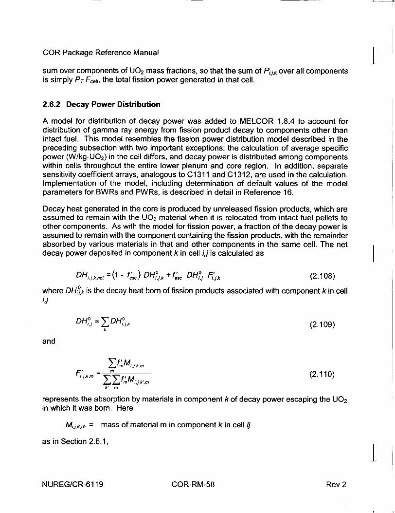
COR Package Reference Manual
sum over components of U0 2 mass fractions, so that the sum of Pik over all components is simply PT F,,,e, the total fission power generated in that cell.
2.6.2 Decay Power Distribution
A model for distribution of decay power was added to MELCOR 1.8.4 to account for distribution of gamma ray energy from fission product decay to components other than intact fuel. This model resembles the fission power distribution model described in the preceding subsection with two important exceptions: the calculation of average specific power (W/kg-U0 2 ) in the cell differs, and decay power is distributed among components within cells throughout the entire lower plenum and core region. In addition, separate sensitivity coefficient arrays, analogous to C1311 and C1312, are used in the calculation. Implementation of the model, including determination of default values of the model parameters for BWRs and PWRs, is described in detail in Reference 16.
Decay heat generated in the core is produced by unreleased fission products, which are assumed to remain with the U0 2 material when it is relocated from intact fuel pellets to other components. As with the model for fission power, a fraction of the decay power is assumed to remain with the component containing the fission products, with the remainder absorbed by various materials in that and other components in the same cell. The net decay power deposited in component k in cell ij is calculated as
DHij.net =( 1- f,) DH2Ik + fe'• DH'1 FJir (2.108)
where DHIj°k is the decay heat born of fission products associated with component k in cell i,j
DH2 k QZDH2jk (2.109)
and
Sm Fir, •. .fM ,.~ (2.110)
k' m
represents the absorption by materials in component k of decay power escaping the U0 2 in which it was born. Here
Mijk,m = mass of material m in component k in cell #j
as in Section 2.6.1,
NUREG/CR-6119 COR-RM-58 Rev 2
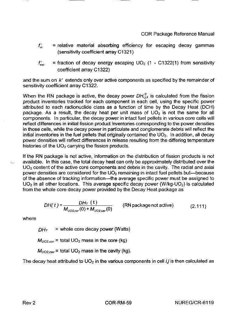
COR Package Reference Manual
f,• = relative material absorbing efficiency for escaping decay gammas (sensitivity coefficient array C1321 )
f,, = fraction of decay energy escaping U0 2 (1 - C1322(1) from sensitivity
coefficient array C1322)
and the sum on k' extends only over active components as specified by the remainder of sensitivity coefficient array C1322.
When the RN package is active, the decay power DHi,°k is calculated from the fission product inventories tracked for each component in each cell, using the specific power attributed to each radionuclide class as a function of time by the Decay Heat (DCH) package. As a result, the decay heat per unit mass of U0 2 is not the same for all components. In particular, the decay power in intact fuel pellets in various core cells will reflect differences in initial fission product inventories corresponding to the power densities in those cells, while the decay power in particulate and conglomerate debris will reflect the initial inventories in the fuel pellets that originally contained the U0 2. In addition, all decay power densities will reflect differences in release resulting from the differing temperature histories of the U0 2 carrying the fission products.
If the RN package is not active, information on the distribution of fission products is not available. In this case, the total decay heat can only be approximately distributed over the U0 2 content of the active core components and debris in the cavity. The radial and axial power densities are considered for the U0 2 remaining in intact fuel pellets but-because of the absence of tracking information-the average specific power must be assigned to U0 2 in all other locations. This average specific decay power (W/kg-U0 2) is calculated from the whole core decay power provided by the Decay Heat package as
DH~t)=DHT (t) DH(t) = cor()+ Muo2 cav(0) (RN package not active) (2.111)
where
DHT = whole core decay power (Watts)
MUo2,cor = total U0 2 mass in the core (kg)
Muo2.cav = total U0 2 mass in the cavity (kg).
The decay heat attributed to U0 2 in the various components in cell ij is then calculated as
NUREG/CR-6119Rev 2 COR-RM-59
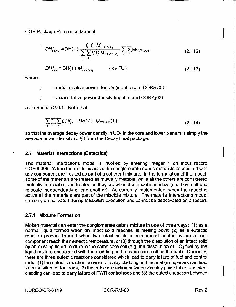
COR Package Reference Manual
DHO =DH~~t f,. fj M i~jFuuo, 2YF~o
OiHj.F = H ) ,.fi'fM,.JFuuo. . -,iFU U M .uoi (2.112)
i, j'
DH2Jk = DH( t) M,,,kuo2 (k # FU) (2.113)
where
fi =radial relative power density (input record CORRiiO3)
fj =axial relative power density (input record CORZjjO3)
as in Section 2.6.1. Note that
ZZ DH°Jk =DH(t) Muo,.cor(t) (2.114) i j k
so that the average decay power density in U0 2 in the core and lower plenum is simply the average power density DH(t) from the Decay Heat package.
2.7 Material Interactions (Eutectics)
The material interactions model is invoked by entering integer 1 on input record COR00006. When the model is active the conglomerate debris materials associated with any component are treated as part of a coherent mixture. In the formulation of the model, some of the materials are treated as mutually miscible, while all the others are considered mutually immiscible and treated as they are when the model is inactive (i.e. they melt and relocate independently of one another). As currently implemented, when the model is active all the materials are part of the miscible mixture. The material interactions model can only be activated during MELGEN execution and cannot be deactivated on a restart.
2.7.1 Mixture Formation
Molten material can enter the conglomerate debris mixture in one of three ways: (1) as a normal liquid formed when an intact solid reaches its melting point, (2) as a eutectic reaction product formed when two intact solids in mechanical contact within a core component reach their eutectic temperature, or (3) through the dissolution of an intact solid by an existing liquid mixture in the same core cell (e.g. the dissolution of U0 2 fuel by the liquid mixture associated with the cladding in the same core cell as the fuel). Currently, there are three eutectic reactions considered which lead to early failure of fuel and control rods: (1) the eutectic reaction between Zircaloy cladding and Inconel grid spacers can lead to early failure of fuel rods, (2) the eutectic reaction between Zircaloy guide tubes and steel cladding can lead to early failure of PWR control rods and (3) the eutectic reaction betweenl
NUREG/CR-6119 COR-RM-60 Rev 2
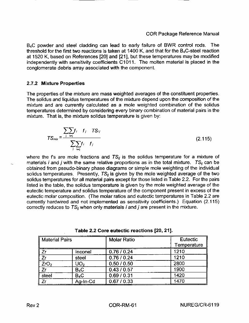
COR Package Reference Manual
B4C powder and steel cladding can lead to early failure of BWR control rods. The threshold for the first two reactions is taken at 1400 K, and that for the B4C-steel reaction at 1520 K, based on References [20] and [21], but these temperatures may be modified independently with sensitivity coefficients C1011. The molten material is placed in the conglomerate debris array associated with the component.
2.7.2 Mixture Properties
The properties of the mixture are mass weighted averages of the constituent properties. The solidus and liquidus temperatures of the mixture depend upon the composition of the mixture and are currently calculated as a mole weighted combination of the solidus temperatures determined by considering every binary combination of material pairs in the mixture. That is, the mixture solidus temperature is given by:
Z-j•'f , f j TSij
TSmix= j ij (2.115)
i i: j
where the f's are mole fractions and TSj is the solidus temperature for a mixture of materials i and j with the same relative proportions as in the total mixture. TS,. can be obtained from pseudo-binary phase diagrams or simple mole weighting of the individual solidus temperatures. Presently, TSj is given by the mole weighted average of the two solidus temperatures for all material pairs except for those listed in Table 2.2. For the pairs listed in the table, the solidus temperature is given by the mole weighted average of the eutectic temperature and solidus temperature of the component present in excess of the eutectic molar composition. (The molar ratios and eutectic temperatures in Table 2.2 are currently hardwired and not implemented as sensitivity coefficients.) Equation (2.115) correctly reduces to TSq when only materials i and j are present in the mixture.
Table 2.2 Core eutectic reactions [20, 21].
Material Pairs Molar Ratio Eutectiu I ITem pert r
Zr Inconel 0.76 /0.24 1210 Zr steel 0.76 / 0.24 1210 ZrO 2 U0 2 0.50/0.50 2800 Zr B4C 0.43 / 0.57 1900 steel B4C 0.69 / 0.31 1420 Zr Ag-In-Cd 0.67 / 0.33 1470
NUREG/CR-6119Rev 2 COR-RM-61
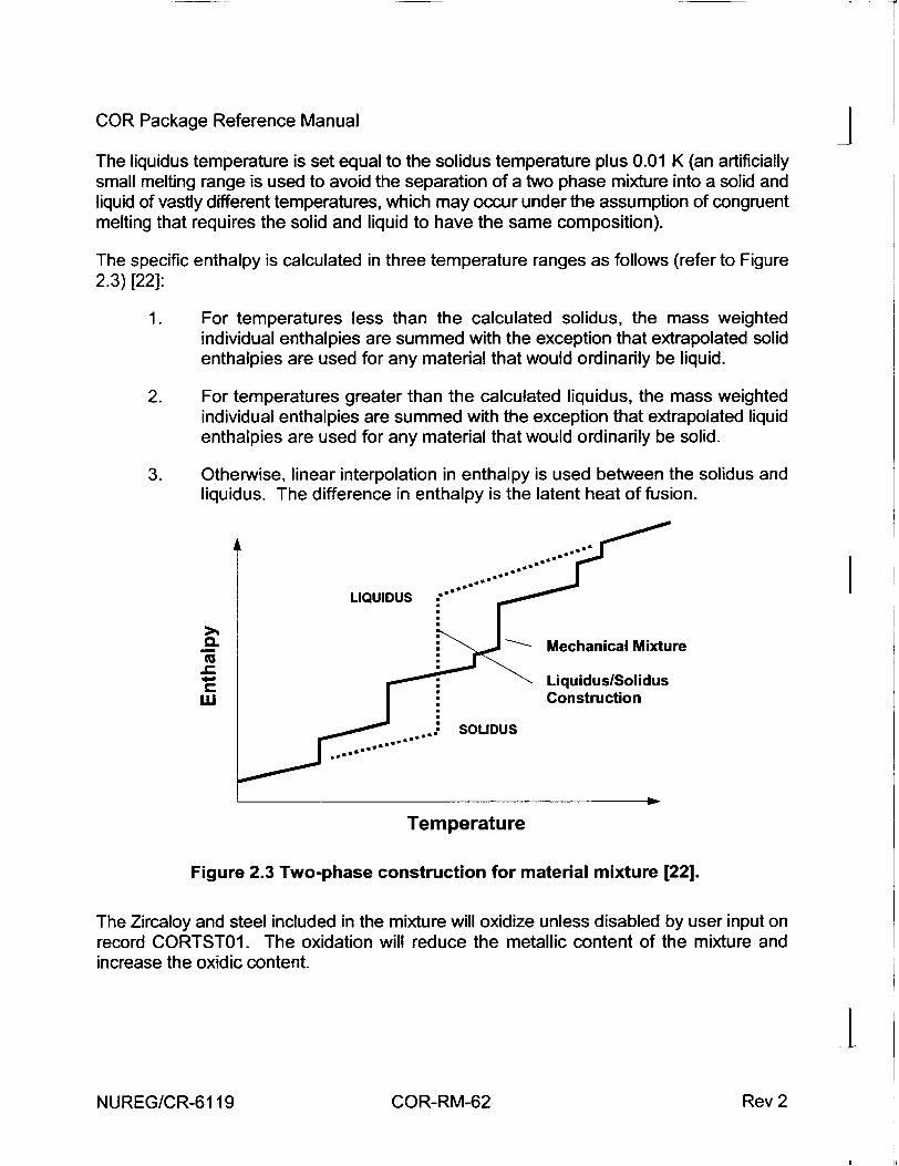
COR Package Reference Manual
The liquidus temperature is set equal to the solidus temperature plus 0.01 K (an artificially small melting range is used to avoid the separation of a two phase mixture into a solid and liquid of vastly different temperatures, which may occur under the assumption of congruent melting that requires the solid and liquid to have the same composition).
The specific enthalpy is calculated in three temperature ranges as follows (refer to Figure 2.3) [22]:
1. For temperatures less than the calculated solidus, the mass weighted individual enthalpies are summed with the exception that extrapolated solid enthalpies are used for any material that would ordinarily be liquid.
2. For temperatures greater than the calculated liquidus, the mass weighted individual enthalpies are summed with the exception that extrapolated liquid enthalpies are used for any material that would ordinarily be solid.
3. Otherwise, linear interpolation in enthalpy is used between the solidus and liquidus. The difference in enthalpy is the latent heat of fusion.
0.
U.I
LIQUIDUS
Mechanical Mixture
Liquidus/Solidus Construction
Temperature
Figure 2.3 Two-phase construction for material mixture [22].
The Zircaloy and steel included in the mixture will oxidize unless disabled by user input on record CORTST01. The oxidation will reduce the metallic content of the mixture and increase the oxidic content.
INUREG/CR-6119
J
I
COR-RM-62 Rev 2
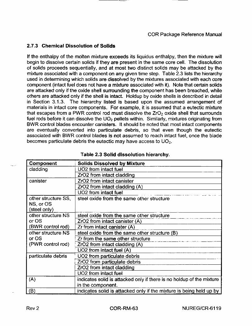
COR Package Reference Manual
2.7.3 Chemical Dissolution of Solids
If the enthalpy of the molten mixture exceeds its liquidus enthalpy, then the mixture will begin to dissolve certain solids if they are present in the same core cell. The dissolution of solids proceeds sequentially, and at most two distinct solids may be attacked by the mixture associated with a component on any given time step. Table 2.3 lists the hierarchy used in determining which solids are dissolved by the mixtures associated with each core component (intact fuel does not have a mixture associated with it). Note that certain solids are attacked only if the oxide shell surrounding the component has been breached, while others are attacked only if the shell is intact. Holdup by oxide shells is described in detail in Section 3.1.3. The hierarchy listed is based upon the assumed arrangement of materials in intact core components. For example, it is assumed that a eutectic mixture that escapes from a PWR control rod must dissolve the ZrO2 oxide shell that surrounds fuel rods before it can dissolve the U0 2 pellets within. Similarly, mixtures originating from BWR control blades encounter canisters. It should be noted that most intact components are eventually converted into particulate debris, so that even though the eutectic associated with BWR control blades is not assumed to reach intact fuel, once the blade becomes particulate debris the eutectic may have access to U0 2.
Table 2.3 Solid dissolution hierarchy.
Component F Solids Dissolved by Mixture cladding [U02 from intact fuel
ZrO2 from intact cladding canister ZrO2 from intact canister
ZrO2 from intact cladding (A) U02 from intact fuel
other structure SS, steel oxide from the same other structure NS, or OS (steel only) other structure NS steel oxide from the same other structure or OS ZrO2 from intact canister (A) (BWR control rod) Zr from intact canister (A) other structure NS steel oxide from the same other structure (B) or OS Zr from the same other structure (PWR control rod) ZrO2 from intact cladding (A)
U02 from intact fuel (A) particulate debris U02 from particulate debris
ZrO2 from particulate debris ZrO2 from intact cladding U02 from intact fuel
(A) indicates solid is attacked only if there is no holdup of the mixture in the component.
(B) indicates solid is attacked only if the mixture is being held up by
NUREG/CR-6119Rev 2 COR-RM-63
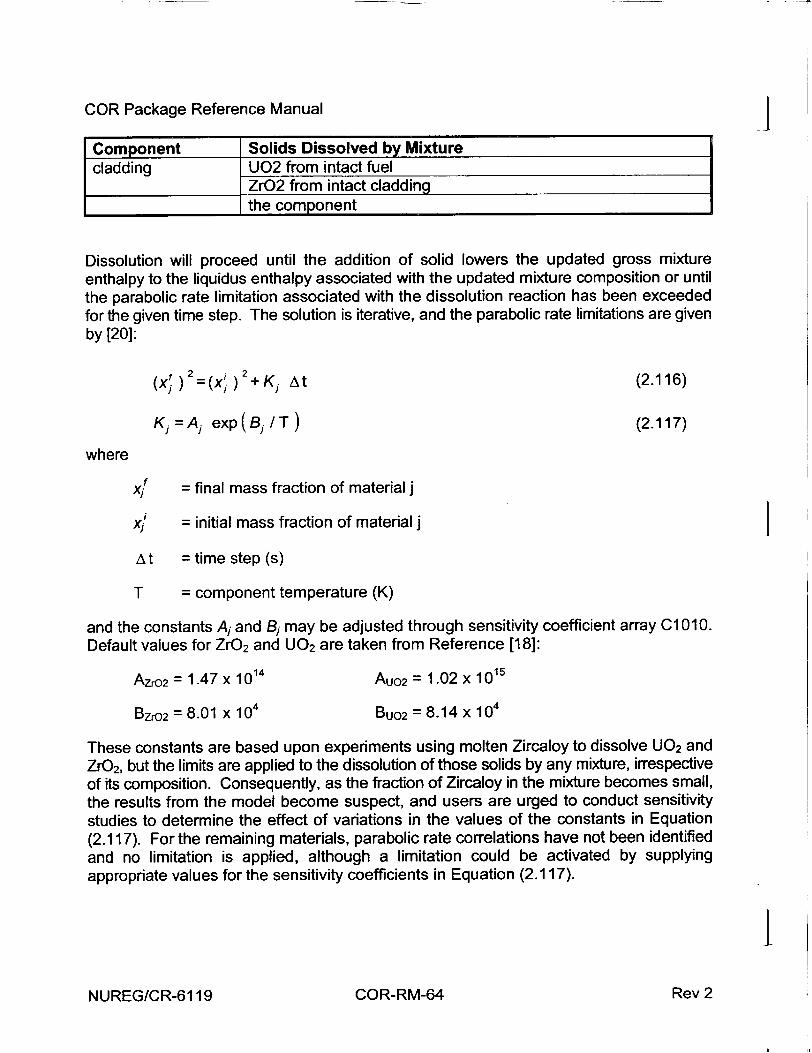
COR Package Reference Manual j Component Solids Dissolved by Mixture cladding U02 from intact fuel
ZrO2 from intact cladding the component
Dissolution will proceed until the addition of solid lowers the updated gross mixture enthalpy to the liquidus enthalpy associated with the updated mixture composition or until the parabolic rate limitation associated with the dissolution reaction has been exceeded for the given time step. The solution is iterative, and the parabolic rate limitations are given by [20]:
(X) 2 =(Xi ) 2 +K At (2.116)
Kj=Aj exp(B 1 /T) (2.117)
where
xjf = final mass fraction of material j
xj = initial mass fraction of material j
At = time step (s)
T = component temperature (K)
and the constants A1 and Bj may be adjusted through sensitivity coefficient array C1010. Default values for ZrO 2 and U0 2 are taken from Reference [18]:
Azr0o2 = 1.47 x 10¹⁴ Auo2 = 1.02 x 10 15
Bzro 2 = 8.01 x 10⁴ Buo2 = 8.14 x 10⁴
These constants are based upon experiments using molten Zircaloy to dissolve U0 2 and ZrO2, but the limits are applied to the dissolution of those solids by any mixture, irrespective of its composition. Consequently, as the fraction of Zircaloy in the mixture becomes small, the results from the model become suspect, and users are urged to conduct sensitivity studies to determine the effect of variations in the values of the constants in Equation (2.117). For the remaining materials, parabolic rate correlations have not been identified and no limitation is applied, although a limitation could be activated by supplying appropriate values for the sensitivity coefficients in Equation (2.117).
I
NUREG/CR-6119 COR-RM-64 Rev 2
COR Package Reference Manual
3 Core/In-Vessel Mass Relocation Models
This section describes the mass relocation models in the COR package. Candling of molten core materials, the transport of additional unmolten materials with the molten material, the radial relocation of molten pools, and the formation of flow blockages and molten pools are described in Section 3.1. The models for the radial relocation of molten pools and particulate debris are described in Section. Formation of particulate debris by various means from intact component, radial spreading of this debris, and its axial relocation by gravitational settling and collapse of supporting components is described in Section 3.2. The model that limits volumes available to accept the relocation of particulate debris (new in MELCOR 1.8.5) is described in Section 3.2.3.
3.1 Candling
The term candling is used here to refer to the downward flow of molten core materials and the subsequent refreezing of these materials as they transfer latent heat to cooler structures below. The COR package candling model is semi-mechanistic, based on fundamental thermal/hydraulic principles, but with incorporation of user-specified refreezing heat transfer coefficients defined for each material on record COR00005. The model is adaptable to steady flow of either films or rivulets (with smaller contact area than a film) by appropriate adjustment of these refreezing coefficients.
The model does not solve a momentum equation for a flow velocity. Instead it assumes steady generation and flow of molten material, with all material generated within a time step reaching its final destination within that step. For a steady melt generation rate, the amount of material entering into the candling model is proportional to the time step, and, for small time steps, the amount of material that refreezes at a particular location is also approximately proportional to the time step. In other words, if for a given time step a certain amount of molten material is calculated with varying amounts refreezing at different axial locations, the assumption is that for a time step twice as large, twice as much molten material would be generated and approximately twice as much would refreeze at each location. Thus, the cumulative behavior of the model should be relatively independent of time step history. For situations involving release of a larger amount of molten material built up over several time steps, alternative assumptions are used regarding the flow of that material and its contact time with structural surfaces to avoid time step dependencies, as described in Section 3.1.2.
3.1.1 Steady Flow
Following the heat transfer and oxidation calculations, molten material may exist on the surfaces of components in various locations in core. This molten mass is assumed to have been generated at a constant rate over the time step, A t. The candling model follows it
NUREG/CR-6119Rev 2 COR-RM-65
COR Package Reference Manual /
as it flows down (because of gravity) through a column of cells. (A model to hold up molten material by an oxide shell until it is breached is described below.)
The amount of mass that refreezes on each lower cell component is determined by integrating the heat transfer rate between the molten film and the component:
q=h. P. AZ (T,m - T,) (3.1)
over the time step A t, where
hm = user-specified refreezing heat transfer coefficient
A z = cell height
P,, = film or rivulet width (area of contact divided by Az)
Tm = temperature of the molten film
Tý, = temperature of the component
As energy is transferred between the melt and the component, their temperatures change. To account for this, implicitly projected new temperatures are used in Equation (3.1)
qAt CT+ (3.2) cps
Tm,= maxt.T. MMmc , Tmp. (3.3)
where
T°O = temperature of the component before candling
Cps = total heat capacity of the component
Mm = molten mass that enters the cell on surface s
Cp.m = molten film specific heat capacity
T° = temperature of molten film entering the cell
"Tmp = melting point of film material
and Equation (3.3) reflects the fact that although the molten film may carry a superheat
NUREG/CR-6119 COR-RM-66 Rev 2
COR Package Reference Manual
Qsh = MM cp"j ( Tm, - TMp) (3.4)
it will not be cooled below its melting point.
Equations (3.1) to (3.3) may be solved in the form
Q =q At = hm P, Az max(ATf ,AT2)At (3.5)
CpS McpM (To - TS) (3.6) Ac = c,,s MMCp + (cps + Mgcpm)hm P, Az At
cps (T.. - T-0) (37) cps + Cps hm Pw Az At
If Q is less than Qsh, sensible heat is transferred but no mass is refrozen. If Q is greater than Qsh, a mass
AMm,= - (3.8) Hf
is refrozen as conglomerate debris on the component surface, and then thermally equilibrated with the component.
If the underlying component is cladding, its effective heat capacity from Equation (2.42) is used for Cps. This includes the effects of coupling to underlying fuel pellets. However, the candling calculation is performed after other heat transfer has been evaluated, so that the results are not included in the implicit fuel-cladding gap heat transfer calculation described in Section 2.2.4. Therefore, only the appropriate fraction of the candling heat transfer to cladding from Equation (3.5) is transferred to the cladding, with the remainder going directly to the underlying fuel.
Cc
QCL = CCL Q (3.9) CCL eff
QFU = - QCL (3.10)
Molten mass is relocated downward in stepwise fashion according to Equation (3.8) until it has all refrozen on components in one or more lower cells or until it encounters a blockage (see Section 3.1.2). Figure 3.1 illustrates several steps in this process. The material refrozen on a component is termed conglomerate debris (as opposed to particulate debris), and becomes an integral part of that component.
NUREG/CR-6119Rev 2 COR-RM-67
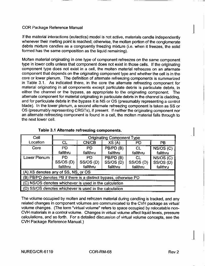
L - - --
COR Package Reference Manual 4 If the material interactions (eutectics) model is not active, materials candle independently whenever their melting point is reached; otherwise, the molten portion of the conglomerate debris mixture candles as a congruently freezing mixture (i.e. when it freezes, the solid formed has the same composition as the liquid remaining).
Molten material originating in one type of component refreezes on the same component type in lower cells unless that component does not exist in those cells. If the originating component type does not exist in a cell, the molten material refreezes on an alternate component that depends on the originating component type and whether the cell is in the core or lower plenum. The definition of alternate refreezing components is summarized in Table 3.1. As indicated there, in the core the alternate refreezing component for material originating in all components except particulate debris is particulate debris, in either the channel or the bypass, as appropriate to the originating component. The alternate component for material originating in particulate debris in the channel is cladding, and for particulate debris in the bypass it is NS or OS (presumably representing a control blade). In the lower plenum, a second alternate refreezing component is taken as SS or OS (presumably representing CRGTs), if present. If neither the originating component nor an alternate refreezing component is found in a cell, the molten material falls through to the next lower cell.
Table 3.1 Alternate refreezing components. j Cell Originating Component Type
Location CL CN/CB 1jS j I PD PB Core PD PD PB/PD (B) CL NS/OS (C)
fallthru fallthru fallthru fallthru fallthru Lower Plenum PD PD PB/PD (B) CL NS/OS (C)
SS/OS (D) SS/OS (D) SS/OS (D) SS/OS (D) SS/OS (D) fallthru fallthru fallthru fallthru fallthru
(A) XS denotes any of SS, NS, or OS (B) PB/PD denotes PB if there is a distinct bypass, otherwise PD (C) NS/OS denotes whichever is used in the calculation (D) SS/OS denotes whichever is used in the calculation
The volume occupied by molten and refrozen material during candling is tracked, and any related changes in component volumes are communicated to the CVH package as virtual volume changes. (The term "virtual volume" refers to space occupied by relocatable nonCVH materials in a control volume. Changes in virtual volume affect liquid levels, pressure calculations, and so forth. For a detailed discussion of virtual volume concepts, see the CVH Package Reference Manual.)
I1
NUREG/CR-6119 COR-RM-68 Rev 2

COR Package Reference Manual
MOLTEN
I• REFROZEN
STEPI STEP 2 STEP 3 STEP 4
Figure 3.1 Candling process steps.
3.1.2 Flow Blockages
Flow blockages are allowed to form, as illustrated in Figure 3.2, whenever refrozen material completely fills all the available volume in a COR cell. In a core cell that contains an intact canister, the channel and bypass regions may be blocked independently. When candling material reaches a flow blockage (or the lower head), some material may remain molten because the designated refreezing component in the cell above the blockage cannot absorb the latent heat. Any such material becomes conglomerate debris associated with particulate, even if no particulate debris previously existed in that cell, and may form a molten pool. Molten material will be transferred between radial rings to achieve a uniform surface level across the pool as discussed below in Section 3.2.1. Candling of molten pools accumulated above a blockage after failure of that blockage is discussed below in Section 3.1.3.
Relocation of core materials may result in a reduction of area and increase of flow resistance, or even total blocking of flow, within various parts of the core. The effects on hydrodynamic flows may be modeled by using the core flow blockage model in the hydrodynamics package, which requires input of FLnnnBk records for the associated flow paths. In addition to modeling the change in flow area, this model calculates the change in flow resistance. The resistance is based on a model for flow through porous media when particulate debris is present; otherwise, the input flow resistance for intact geometry
NUREG/CR-6119Rev 2 COR-RM-69
COR Package Reference Manual j is simply modified to account for any change in flow area. This model, described in Section 6.7 of the CVH/FL Reference Manual, uses a porosity based on the ratio of available hydrodynamic volume to total volume (see Section 3.2.3 below); a minimum porosity is imposed by sensitivity coefficient C1503(1), with a default value of 10-3 .
MELCOR 1.8.5 also includes a model for the opening of a flow path between the channel and bypass regions of the core upon failure of the canister in a BWR.
Activation of these models is not automatic. Input on FLnnnBk records is required to specify which core cells are associated with each flow path involving the core. Furthermore, because only CVH and FL model the flow of water and gases, the effects of
blockages on circulation can be modeled only to the extent that the CVH/FL nodalization can resolve that circulation. For more details, see discussion in Section 1.5.5 of the COR Users' Guide and input instructions in the FL Users' Guide.
NUREG/CR-6119 COR-RM-70
I
Rev 2
1 11
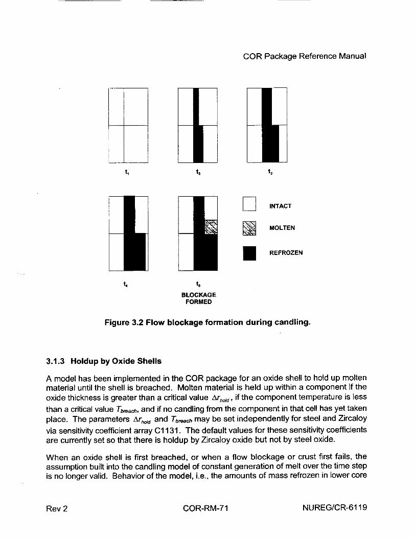
COR Package Reference Manual
i 1t2 t'
D INTACT
-. MOLTEN
I REFROZEN
t4 t5
BLOCKAGE FORMED
Figure 3.2 Flow blockage formation during candling.
3.1.3 Holdup by Oxide Shells
A model has been implemented in the COR package for an oxide shell to hold up molten material until the shell is breached. Molten material is held up within a component if the oxide thickness is greater than a critical value A~ho~d, if the component temperature is less
than a critical value Tbrah, and if no candling from the component in that cell has yet taken place. The parameters Ar, ,Id and Tbgac may be set independently for steel and Zircaloy
via sensitivity coefficient array C1131. The default values for these sensitivity coefficients are currently set so that there is holdup by Zircaloy oxide but not by steel oxide.
When an oxide shell is first breached, or when a flow blockage or crust first fails, the assumption built into the candling model of constant generation of melt over the time step is no longer valid. Behavior of the model, i.e., the amounts of mass refrozen in lower core
NUREG/CR-6119COR-RM-71Rev 2
COR Package Reference Manual
cells as described in Section 3.1, would thus be highly dependent on the size of the current time step. Therefore, for those situations involving the sudden release of a large mass of molten material, Mm, built up over perhaps several previous time steps, application of the candling model is modified slightly. For breach of an oxide shell, a constant time step Atbra is used in Equation (3.3) to avoid time step dependencies. For failure of a flow
blockage holding up a molten pool, a time step Atcontact is used in Equation (3.3). This time step is calculated as a function of a parameter Fmax, which represents a maximum flow rate (per unit surface width) of the molten pool after breakthrough:
Atot =maxA, M AZ (3.11) L Fmax As
In other words, a large molten pool is allowed to discharge at a maximum rate of [max and the amount refreezing onto structures below will be a linear function of the total mass of the pool. Both At&ak and Fm. are accessible in sensitivity coefficient array 01141; their default values of I s and 1 kg/m-s have been set so that this model is only active for large molten pools breaching a crust.
3.1.4 Solid Material Transport
A simple model has been implemented to allow transport of unmolten secondary materials (currently ZrO2, U0 2, steel oxide, and control poison) via the candling process. This model could be used to treat the breaking off of pieces of thin oxide shells that are carded with the molten material or to simulate the dissolution of U0 2 by molten Zr. On input record COR00007, the user may specify relocation of a secondary material, AM,, as either an
input fraction F1 of the molten mass AMm deposited on a component:
AMS = F, AMm (3.12)
or in fractional proportion to its existing fraction within a component:
AM =F MloAmM,,,, 3 M,,, (3.13)
where F 2 is an input parameter specifying the fraction of direct proportional relocation, Ms~totai is the total secondary material mass in the component in the cell of origin, Mmtotal is the total material mass (molten and solid) in the cell of origin, and AMm is the secondary material mass deposited with refrozen material AMM . L
NUREG/CR-6119 COR-RM-72 Rev 2

COR Package Reference Manual
This model is inactive if the COR materials interactions (eutectics) model, which is described in Section 2.7 and treats dissolution mechanistically, is active.
3.1.5 Radial Relocation of Molten Materials
There are two radial relocation models-the first relocates molten core material that still exists following the candling/refreezing algorithm just described. The second, which relocates particulate debris, is essentially similar. Both models are intended to simulate the gravitational leveling between adjacent core rings that will tend to equalize the hydrostatic head in a fluid medium. Either of the two radial relocation models can be deactivated by user input on MELCOR input record CORTST01, but they are both active by default.
The molten material radial relocation model considers each axial level of the core independently, and is invoked after the axial relocation (candling) model. A simple algorithm loops over all adjacent pairs of radial rings between which relocation is possible, and compares the calculated liquid levels in the two. If the levels are unequal, then a calculation is performed to determine the volume of molten material, Veq, that must be moved between the rings to balance the levels. Radial relocation is assumed to be blocked by the presence of an intact BWR canister structure in either ring. In addition, radial relocation is not allowed within a core plate. The actual implementation prevents such relocation to or from a core cell containing supporting structure modeled as a plate or, for the older representation using combined other structure, between cells in level IAXSUP containing other structure.
The relocation rate has a time constant of rs, which may be adjusted by user input, so
that the actual volume relocated, Vre, during the core time step, At,, is given by:
V,.,= V [1 - exp(-At /rv-,)J (3.14)
The default value of 60 s for rspr was chosen as an order-of-magnitude value based on
engineering judgment and recommendations of code users. It is accessible as sensitivity coefficient C1020(2).
If the volume of the material that must be relocated is trivial [specifically, less than 0.01 m3/kg times the mass below which any component will be eliminated, C1502(1), which has a default value of 1.0xl0-2 kg], then no relocation is performed during that time step; otherwise, the fraction of the molten material that must be transferred from the "deep" ring to the "shallow" ring is determined by dividing the mass of melt that must be relocated by the total mass of melt in the deep ring. That fraction of molten mass is then transferred from each core component in the deep ring to the conglomerate debris associated with the particulate debris component in the shallow ring, and the component volumes in each ring
NUREG/CR-6119Rev 2 COR-RM-73
COR Package Reference Manual
are adjusted accordingly. Any fission product transfers or virtual volume adjustments resulting from the relocation are performed by calls to interface routines with the RN Package and CVH Package, respectively.
Radial relocations are directed inward preferentially; that is, at each axial level the algorithm begins at the innermost ring, marches radially outward and transfers molten material from ring i to ring i-1 if the liquid level in ring i exceeds that in ring i-1. Following the march from ring 1 outward, a reverse march is made inward from the outermost ring to perform any outward relocations from ring i to ring i+1 still required to achieve a uniform liquid level across the axial level.
3.1.6 Surface Area Effects of Conglomerate Debris
The addition of conglomerate debris refrozen on component structures affects the surface area exposed to fluid convection, oxidation, and further refreezing during candling. For fuel rods and particulate debris, conglomerate debris can fill interstitial spaces, thus occluding some or all of the surface of the underlying component. The following paragraphs describe in detail a model specifically developed for fuel bundles. The general form of this model is incorporated into the COR package for all core components, but with different coefficients for each. With the default values of these coefficients, it is actually used only for fuel rods and particulate debris.
Consider the candling process idealized for a fuel rod unit cell as shown in Figure 3.3. Molten debris refreezing on the rod is assumed to begin forming a half-cylinder on the rod at the point directly adjacent to the next rod [Figure 3.3(a,b)]. As this half-cylinder of conglomerate continues to grow, its surface area expands, and the intact area shielded also grows, albeit at a lesser rate. Eventually it meets the conglomerate on the adjacent rod, and forms a bridge between the two rods [Figure 3.3(c)]. As additional material is added, more of the intact rod is covered by the conglomerate, until a cylindrical void region centered in the interstitial region among a set of four rods is created [Figure 3.3(d)]. This central void then shrinks to nothing as the interstitial area is completely plugged up [Figure 3.3(e)].
For purposes of calculation, the above-described process is divided into three stages. The first stage lasts until the conglomerate debris half-cylinders bridge the gap between rods, as shown in Figure 3.3(b). The second stage lasts until that bridge has widened to cover the entire surface area of the fuel rods, forming a central cylindrical void, as shown in Figure 3.3(c). The third stage continues until the central void is completely plugged up as shown in Figure 3.3(e). The surface area of the conglomerate debris in the unit cell is calculated in approximate fashion from the fraction of the interstitial volume that it occupies.
It is convenient to define areas and volumes relative to the unit cell rod surface area A, and initial interstitial volume Vi. The latter is related to the volume of the rods by
NUREG/CR-6119 COR-RM-74 Rev 2
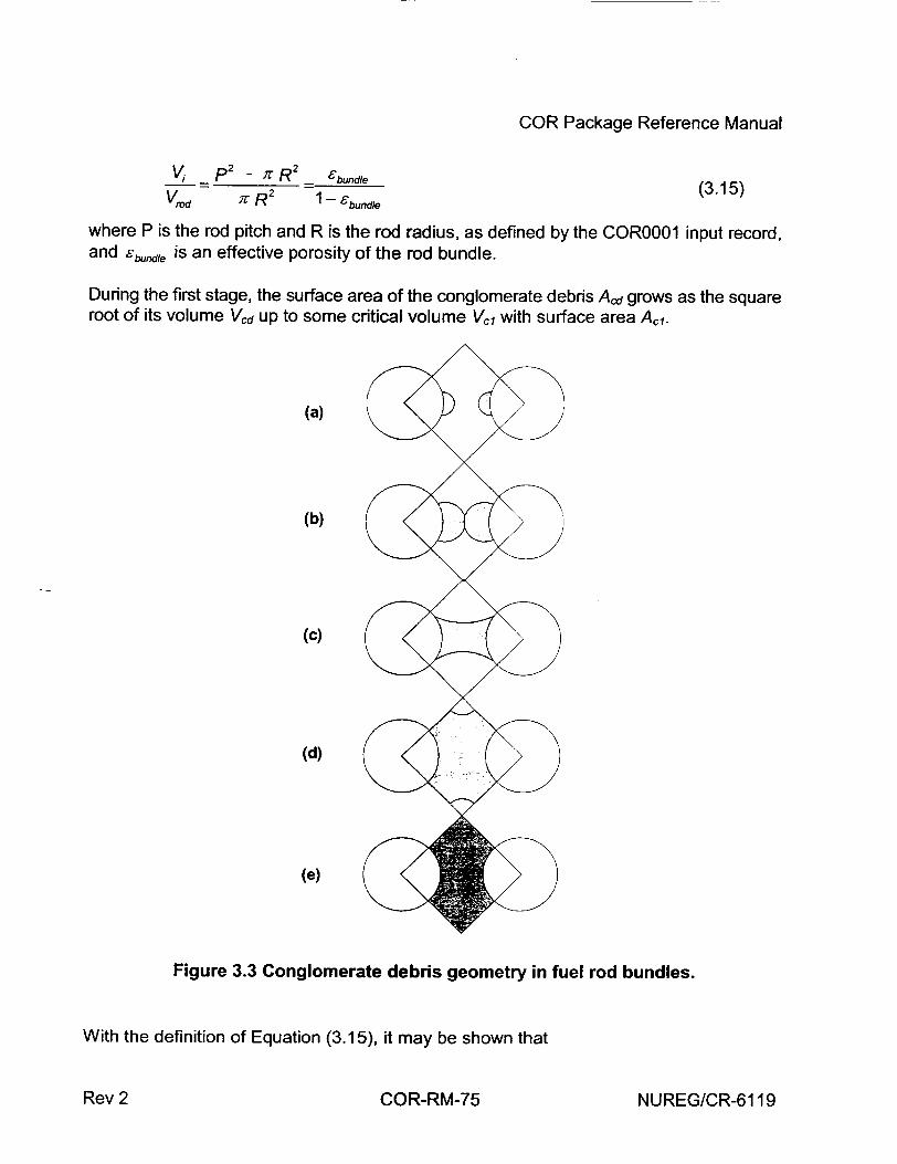
COR Package Reference Manual
V . _ p2 _ ,r R2 _ bundle
Vd /T R2 1 - bundle(3.15)
where P is the rod pitch and R is the rod radius, as defined by the COR0001 input record, and Ebule is an effective porosity of the rod bundle.
During the first stage, the surface area of the conglomerate debris Ad grows as the square root of its volume Vd up to some critical volume V, with surface area A, 1 .
(a)
(b)
(c)
(d)
(e)
Figure 3.3 Conglomerate debris geometry in fuel rod bundles.
With the definition of Equation (3.15), it may be shown that
NUREG/CR-6119Rev 2 COR-RM-75
-T
COR Package Reference Manual
Acd= A A diY (3.16)
A~lFA, P- 2R - FAl = R (3.17)
A, R
VcF =_Fv ._ (P- 2R) (3.18) Vi ' 2 (p_•2) V l ,max 2 P2 7- 2
During the third stage, beyond some critical volume Vc2 with surface area At 2, the surface area of the conglomerate debris decreases as the square root of the empty volume (Vi - Vcd). In terms of area and volume fractions:
Acd= ik) ~ I )11 (3.19)
Ai2 1 P1- Rý /V Ac2 _FA2m,_ P / 2-2 - R (3.20) Ai R
VC 2 - Fv2,,,ax =1- (P/V- (3.21)
A minimum area fraction FA,mI may be imposed for the third stage to prevent the surface area of central void from being completely reduced to zero. In any case, the surface area of conglomerate debris will not be reduced below a minimum surface-to-volume ratio as described below.
During the second stage, the surface area of the conglomerate debris is interpolated linearly with volume between A., and Ac2.
The area of the intact rods wetted by the conglomerate, and thus blocked from further oxidation and convection, is treated in two stages. For volumes greater than Vc2, the fraction of intact surface area Ai blocked is set to a maximum value:
Fb =Fbmx (3.22)
For volumes less than Vc2, the fraction blocked is linearly interpolated:
INUREG/CR-6119 COR-RM-76 Rev 2
COR Package Reference Manual
F =Fb~o Voa Vb b. (3.23)
The same form is applied for all components. For particulate debris, the user-input porosity of the debris bed is used to replace Ebundle in Equation (3.15); for all other
components, the interstitial volume, Vi, is taken as zero. The parameters FA,,max, Fvimax,
FA2,max, FV2,max, FA,min, and Fb,max are accessible for each component as sensitivity coefficient array C1151. Currently, all components have default values based on' typical BWR rod geometries with pitch 16 mm and rod radius 6.26 mm. However, they will be used only for fuel rods and particulate debris.
For conglomerate debris that does not occupy interstitial volume (either the component does not have interstitial volume via the porosity input or the debris overflows what is available), a simple surface area to volume ratio is applied to the excess conglomerate debris volume Vcd,excess:
Acdexcess = Vcd~excess Rsv (3.24)
The parameter Rsv is also accessible in sensitivity coefficient array C1151 with a default value of 100. The surface area of the excess debris is added to the area calculated from Equations (3.16) to (3.23). The total surface area of conglomerate debris (excess plus interstitial) cannot fall below the value obtained by multiplying the debris volume Vcd by Rsv.
Furthermore, to avoid overheating a vanishing CVH fluid, the sum of the surface areas of the intact component and its associated conglomerate debris, which constitutes the total effective surface area for heat transfer to CVH, cannot exceed
Aot,rpax = VCVHRsV (3.25)
where Rsvf is a limiting surface to volume ratio, accessible in sensitivity coefficient array C1152 with a default value of 1000 mi1 .
3.2 Particulate Debris
After core components collapse, the materials that composed them are treated as particulate debris. Once it has been formed, this debris can spread radially and/or settle vertically, subject to the availability of free volume and the presence or absence of support.
NUREG/CR-6119Rev 2 COR-RM-77
COR Package Reference Manual
3.2.1 Formation of Particulate Debris
The COR package contains several simple models that consider the structural integrity and support of intact components, and convert them to particulate debris when either is lost. Most are logical models rather than structural models; no stress calculations are performed for any component other than supporting structure (SS). Even for SS, such a calculation is optional. Complex debris formation mechanisms, such as quench-induced shattering, have not been implemented into the COR package at this time.
All components other than fuel rods (FU and CL) will be immediately converted to particulate debris whenever the unoxidized metal thickness is reduced below a userdefined minimum value. The thickness criterion is also used for cladding (CL), which is assumed to support fuel pellets (FU), but other criteria are also considered for fuel rods. The user may define one minimum thickness parameter, Arc,,, on record COR00008,
with a default of 0.1 mm, that is used for Zircaloy in the cladding and the two canister components (CL, CN, and CB). In calculations using the old combined other structure component (OS), an independent minimum thickness, Ar - , also input on record
COR00008 with a default of 0.1 mm, is applied to the steel in the OS.
For the nonsupporting structure component (NS), the structural metal may be taken either as steel (the default) or as Zircaloy. The default minimum thickness is also 0.1 mm. Both the structural metal to which it will be applied and the minimum thickness may be specified independently for each core cell containing NS.
Setting any Ar,,,, to zero will prevent collapse of the associated components by this mechanism, although MELCOR may still predict their collapse using one of the other criteria described below. If the user has specified electric heating element material in the fuel rods, formation of particulate debris is suppressed, and the minimum thickness parameter Ar,,, must be set to zero.
Unoxidized metal thickness is reduced both by oxidation and by melting and candling of metal. It is considered to be increased, except for the case of cladding, by refreezing of metal candled from above. If candling of molten material is not possible because of a flow blockage or holdup by an oxide shell (Sections 3.1.2 and 3.1.3), the retained metal is considered as part of the unoxidized thickness. In effect, the component is considered to be supported by the oxide shell that contains the held-up melt or by the surrounding pool of molten material. Particulate debris will be formed from CN, CB, or OS whenever the temperature of the component reaches the melting temperature of the associated oxide (ZrO 2 for CN and CB, and steel oxide for OS). The temperature at which NS will be converted to particulate debris, independent of metal thickness, may be independently specified for each core cell containing NS, with a default value of the melting point of the structural metal identified for NS in that cell.
NUREG/CR-6119 Rev 2COR-RM-78
COR Package Reference Manual
Fuel rods, composed of cladding and fuel pellets (the CL and FU components), are treated somewhat differently. Oxidized rods are assumed to retain their identity until the cladding reaches 2500 K, and to collapse unconditionally if the fuel temperature reaches 3100 K (the approximate melting temperature of U0 2). In MELCOR 1.8.4, the former temperature was taken as 2800 K, the approximate melting temperature of the U0 2/ZrO 2 eutectic, but experience with Phebus has shown that the lower temperature is more appropriate for irradiated fuels. Both temperatures are accessible to the user through sensitivity coefficient array C1132. It is possible for a fuel rod to be hot but unoxidized, either as a result of heating in an inert environment or following total loss of ZrO2 through candling involving secondary transport (Section 3.1.4) or eutectics (Section 2.7). As currently coded, such a rod will be converted to particulate debris when the remaining metal thickness falls below A rc,min .
Finally, an intact component will be converted to particulate debris whenever support of that component is lost. This support may be provided by either the same component or unfailed supporting structure (SS) component in the cell below; the portion of a fuel rod in level n supports the portion in level n+1, and the core support plate is considered to support all components above it.
If the old representation is being used, support is provided by unfailed "other structure" (OS) component that was initialized with the "tens" digit of the support flag set to 1 on input record CORZjjO2. In addition, for this representation only, all components in any level may also be specified as unconditionally supported, i.e. "self supporting," by setting the "ones" digit of the support flag to 1. This is ordinarily done only for the level containing the core support plate, thus modeling it as requiring no external support.
When a component of the core of a BWR collapses to form particulate debris within the core region, this debris can occupy space either inside or outside the channel boxes. In earlier versions of MELCOR, only a single particulate field was available, and all components collapsed to form particulate in the channel. In MELCOR 1.8.5, particulate debris in the bypass (PB) is distinguished from that in the channel (PD). In any core cell with a distinct bypass, the structural components SS, NS, and OS are modeled as collapsing to form PB, while all others collapse to form PD. As this debris is later relocated, it may-depending on geometry-occupy the channel or bypass region of other cells, or be split between them.
Particulate debris is characterized by user-specified particle diameters, Dp,, and Dpb, entered as hydraulic diameters on input record CORijj04. The two diameters are equal by default, but this is not required. However, there is no provision at this point for considering more than a single representative diameter for either. The surface area of the particulate portion of each type of debris is calculated from Dp= and the total volume of the particulate, Vp,, as:
NUREG/CR-6119Rev 2 COR-RM-79

COR Package Reference Manual
6v As.p - (3.26)
where "x" can be "d" or "b". The fraction of this area used for oxidizing the Zircaloy portion of the particulate debris is the fraction of the particulate debris volume that is Zircaloy plus ZrO2. The fraction of this area used for oxidizing the steel portion of the particulate is the fraction of the particulate volume that is steel plus steel oxide. ZrO 2 and steel oxide in particulate debris are modeled to exist as layers covering the Zr and steel, respectively. The particulate areas of the debris are further modified by the addition of conglomerate debris according to the model described in Section 3.1.5 to obtain actual areas for oxidation and heat transfer.
3.2.2 Debris Addition from Heat Structure Melting
During degraded core conditions, many reactor vessel structures that are modeled by the Heat Structures (HS) package in MELCOR are subjected to intense radiative and convective heating, and may be expected to melt. These structures are often designated on input records CORZjjO2 and CORRiiO2 as the radial and axial boundary heat structures for heat transfer from the core. An example of such a structure is the BWR core shroud, a relatively thin (5 cm) structure that surrounds the entire core and extends into the upper plenum.
Although the HS package does not model melting in general, the melting of these structures may be calculated by special application of the HS package degassing model, using material type 'SS' (see the HSDGCCCCCx input records), and the resulting molten steel passed to the COR package. The melting model tracks the mass and volume changes associated with the molten steel added to the core. The model requires that any melting steel HS structure must lie either along the core, corresponding directly with one of the axial segments represented in the COR package, or above the core.
The molten steel produced from the degassing model is passed to the outermost radial ring (NRAD) in the axial segment corresponding to the origin of the melt. It is entered as particulate debris with energy corresponding to fully molten steel with no superheat. The model is flexible to the extent that additional HS package structures above the core can also be identified to melt via the degassing model, with material passed to the uppermost axial segment (NAXL) in the outer ring. Subsequent relocation of the molten steel from its initial core position is performed by the candling model described in Section 3.1 and the particulate debris relocation logic discussed below.
3.2.3 Exclusion of Particulate Debris
Core cells need not be completely filled to block entry of particulate debris; debris can enter a core cell only if there is 'free" volume in that cell. The free volume can be less than the
NUREG/CR-6119 COR-RM-80 Rev 2
1 11
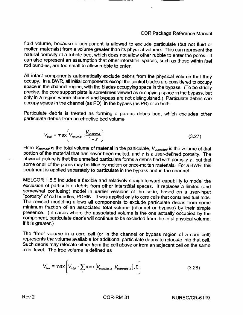
COR Package Reference Manual
fluid volume, because a component is allowed to exclude particulate (but not fluid or molten materials) from a volume greater than its physical volume. This can represent the natural porosity of a rubble bed, which does not allow other rubble to enter the pores. It can also represent an assumption that other interstitial spaces, such as those within fuel rod bundles, are too small to allow rubble to enter.
All intact components automatically exclude debris from the physical volume that they occupy. In a BWR, all initial components except the control blades are considered to occupy space in the channel region, with the blades occupying space in the bypass. (To be strictly precise, the core support plate is sometimes viewed as occupying space in the bypass, but only in a region where channel and bypass are not distinguished.) Particulate debris can occupy space in the channel (as PD), in the bypass (as PB) or in both.
Particulate debris is treated as forming a porous debris bed, which excludes other particulate debris from an effective bed volume
Ye = max Vmate.na, _ " (3.27)
Here Vmatena• is the total volume of material in the particulate, V,,umelt is the volume of that portion of the material that has never been melted, and 6 is a user-defined porosity. The physical picture is that the unmelted particulate forms a debris bed with porosity 6, but that some or all of the pores may be filled by molten or once-molten materials. For a BWR, this treatment is applied separately to particulate in the bypass and in the channel.
MELCOR 1.8.5 includes a flexible and relatively straightforward capability to model the exclusion of particulate debris from other interstitial spaces. It replaces a limited (and somewhat confusing) model in earlier versions of the code, based on a user-input "porosity" of rod bundles, PORIN. It was applied only to core cells that contained fuel rods. The revised modeling allows all components to exclude particulate debris from some minimum fraction of an associated total volume (channel or bypass) by their simple presence. (In cases where the associated volume is the one actually occupied by the component, particulate debris will continue to be excluded from the total physical volume, if it is greater.)
The "free" volume in a core cell (or in the channel or bypass region of a core cell) represents the volume available for additional particulate debris to relocate into that cell. Such debris may relocate either from the cell above or from an adjacent cell on the same axial level. The free volume is defined as
Vtree =max Vta,, - I-max(VmatefiVk IVexcI' ,,)' k] (3.28) L k I
NUREG/CR-6119Rev 2 COR-RM-81
-r
COR Package Reference Manual 4 where the sum is over all components. For particulate debris, Vexdcudedk is the bed volume given by Equation (3.27). For all other components, it is a user defined fraction of the total volume of the cell if the component exists in the cell.
Based on examination of the geometry of typical US reactors, we would expect that no particulate debris could enter fuel bundles so long as there are intact fuel rods present. In BWRs, we would expect that particulate could not enter the unbladed bypass so long as there is intact CN, nor the bladed bypass so long as there is intact NS representing control blades. After the control blades have failed, this debris would be free to enter the bladed bypass, but not the unbladed bypass (assuming that CN was still intact).
The default exclusion fractions, selected in accordance with this picture, are shown in Table 3.2. In the table, "RD" means "fuel rod"; the exclusion is associated with the presence of FU, CL, or both. By default, the presence of intact fuel rods in a core cell excludes particulate debris from the entire channel region, but has no effect on the bypass. The presence of intact CN excludes particulate from 30% of the bypass, representing the unbladed portion, and intact NS representing control blades will exclude it from the remaining 70%. NS representing PWR control rods, SS, and OS have no effect.
A
NUREG/CR-6119 COR-RM-82 Rev 2
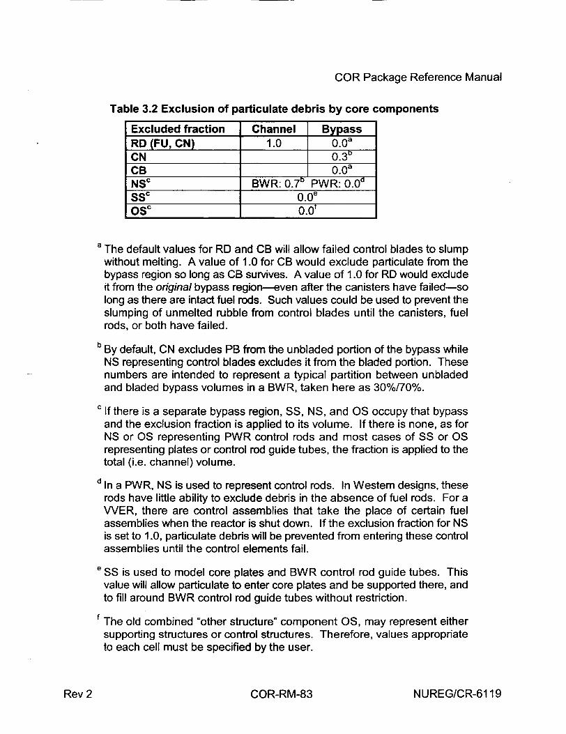
COR Package Reference Manual
Table 3.2 Exclusion of particulate debris by core components
Excluded fraction Channel Bypass RD (FU, CN) 1.0 0.0a
CN 0.3" CB 0.0a
NSc BWR: 0.7" PWR: 0.00 SSC 0.0e
OSc 0.01
a The default values for RD and CB will allow failed control blades to slump
without melting. A value of 1.0 for CB would exclude particulate from the bypass region so long as CB survives. A value of 1.0 for RD would exclude it from the original bypass region-even after the canisters have failed-so long as there are intact fuel rods. Such values could be used to prevent the slumping of unmelted rubble from control blades until the canisters, fuel rods, or both have failed.
b By default, CN excludes PB from the unbladed portion of the bypass while
NS representing control blades excludes it from the bladed portion. These numbers are intended to represent a typical partition between unbladed and bladed bypass volumes in a BWR, taken here as 30%/70%.
c If there is a separate bypass region, SS, NS, and OS occupy that bypass
and the exclusion fraction is applied to its volume. If there is none, as for NS or OS representing PWR control rods and most cases of SS or OS representing plates or control rod guide tubes, the fraction is applied to the total (i.e. channel) volume.
In a PWR, NS is used to represent control rods. In Western designs, these rods have little ability to exclude debris in the absence of fuel rods. For a WER, there are control assemblies that take the place of certain fuel assemblies when the reactor is shut down. If the exclusion fraction for NS is set to 1.0, particulate debris will be prevented from entering these control assemblies until the control elements fail.
eSS is used to model core plates and BWR control rod guide tubes. This
value will allow particulate to enter core plates and be supported there, and to fill around BWR control rod guide tubes without restriction.
The old combined "other structure" component OS, may represent either supporting structures or control structures. Therefore, values appropriate to each cell must be specified by the user.
NUREG/CR-6119Rev 2 COR-RM-83
COR Package Reference Manual
Other analysts might want to examine the consequences of other assumptions, or might want to apply MELCOR to different reactor designs. For example, when VVER reactors are shut down, some of the fuel bundles are lowered out of the main core, with their place taken by control elements. Under the assumptions appropriate to US designs, these control elements would have no capability to exclude debris and, when the upper core starts to collapse, the resulting debris would immediately spread into the rings containing these elements and fall to the lower plenum. Therefore, the default exclusion fractions can be modified globally, level by level, ring by ring, or cell by cell through user input. Consequences of default and alternate values are indicated in footnotes to the table.
These constraints on availability of space are considered in the models for radial and axial relocation of debris described in the following subsections. The absence of free volume is not allowed to prevent particulate debris from being formed in a core cell. For example, whenever a control rod or blade disintegrates, it is converted to particulate debris in place. The debris must be allowed to occupy the space previously occupied by the blade, even if geometric restrictions might have prevented any rubble from falling into that space. In addition, if a support plate has failed and lost the ability to support particulate debris, the absence of free volume within the plate is not allowed to prevent the passage of particulate debris through it. This allows such particulate to continue to relocate downward to space available below the plate. Note that free volume in the sense discussed here is not I relevant to the relocation of molten materials, which can fill all volume not physically occupied by materials, i.e., it is the volume available to fluids.
3.2.4 Radial Relocation of Particulate Debris
The particulate debris leveling model is very similar to the molten material leveling model described in Section 3.1.5 except that material is moved only from the particulate debris component in the "deep" ring to the particulate debris component in the "shallow" ring. The time constant for particulate debris relocation has an ad hoc default value of 360 s, is accessible as sensitivity coefficient C1020(1). There is no consideration of an angle of repose; debris is completely leveled across the core. Particulate debris relocation is subject to the same constraints concerning BWR canisters and core support plates as molten material relocation. Component volumes and associated fission products are adjusted following relocations.
3.2.5 Gravitational Settling
The downward relocation of particulate debris by gravitational settling is modeled in MELCOR as a constant-velocity process, with the velocity given by VFALL from the COR00012 input record. Each ring in the COR nodalization is treated independently. For a given ring, each core cell containing particulate debris is considered in turn as a potential INUREG/CR-6119
I - --- 41
COR-RM-84 Rev 2
COR Package Reference Manual
source of falling debris, working from the bottom up. The model first determines how far particulate from that cell can fall during the time step, subject to limitations of available volume and support. Falling debris can be stopped by the absence of available space (a "blockage") or by encountering a structure that can support it, typically, a support plate with the capability to support particulate. Note that, because of the debris exclusion model discussed in Section 3.2.3, core cells can be blocked without being completely filled.
Once the lowest core cell that particulate can reach has been determined, the algorithm fills the available space from that level up until the debris in the source cell has been exhausted or all available volume has been filled. It then moves on to consider the next higher cell in the ring as a possible source of slumping debris, subject to the updated availability of space.
The model accounts for the distinction between particulate in the channel (or what was originally the channel), PD, and that in the bypass (or what was originally the bypass), PB. It allows particulate debris to slump from the channel or bypass of one cell into the channel and/or bypass of the cell below, depending on the conditions in those cells. The situation is complicated by the fact that the distinction between channel and bypass does not exist everywhere in the core. For example, cells such as those in the lower plenum that never contained canisters-and therefore can have no "bypass" region-are permitted to contain only PD. Thus, any debris that slumps into such a cell as PB must be considered there as PD. In addition, the distinction is almost entirely lost for cells that originally contained canisters once those canisters fail, and all particulate debris in such a cell is considered as well mixed and equilibrated. (However, separate volumes in the "channel" and the "bypass" must be calculated for such cells in order to define the volumes displaced in the associated CVH control volumes, which do remain distinct.)
The details of the algorithm implemented are as follows, where it is to be understood that "intact canister" means "component CB present in the cell":
1. The split between channel and bypass regions is preserved when particulate debris slumps from a core cell with an intact canister into another core cell with an intact canister. That is, debris in the channel passes into the channel while debris in the bypass passes into the bypass;
2. All particulate debris that originates in, or enters, a core cell where there is no intact canister to separate channel and bypass is treated as mixed, and any distinction between origin as PD or PB is lost;
3. Particulate debris that slumps from a core cell without an intact canister into one with an intact canister is split between channel and bypass in proportion to the available cross-sectional areas of the two regions;
4. If the fall of particulate is blocked in the channel or the bypass in a core cell that contains an intact canister, it will fill that region from the blocked level up. If
NUREG/CR-6119Rev 2 COR-RM-85
COR Package Reference Manual J both are blocked, it will fill each independently, based on debris entering the corresponding region. If there is sufficient debris to fill all available volume in the channel or bypass to a point above which there is no intact canister, any remaining debris will be used to fill from that cell upwards;
5. If the fall of particulate is blocked in a core cell that does not contain an intact canister, it will fill from that level up. If channel and bypass are distinguished in that cell because it originally contained a canister, the particulate debris will be divided between PD and PB in proportion to the available cross-sectional areas of the two regions. If there is sufficient debris to fill all available volume to a point above which there is an intact canister, the two regions will be filled independently, based on the split of debris between them at the point where falling particulate entered the region containing a canister.
3.3 Displacement of Fluids in CVH
When core materials relocate from one core cell to another by any of the mechanisms discussed in the previous sections, they cease displacing fluid in the old location and commence displacing it in the new one. Candled material (conglomerate debris) is treated as occupying space in the same region, channel or bypass, as the component that supports it. As already implied, each core component (fuel rods, control elements, canisters, and j particulate debris) is treated as occupying space in an associated CVH control volume. However, the spatial nodalizations used in COR and CVH are largely independent, and may be quite different. The two representations are maintained independently throughout a MELCOR calculation.
In order to treat the displacement of fluid in CVH, each control volume is considered to have "virtual" volume in addition to the current fluid volume. The virtual volume includes the total volume of all core components within the volume. Part or all of it will become available to CVH fluids when and if these core components relocate. The COR package handles relocation by directing CVH to free virtual volume in the original location, and to occupy it in the new location. The vertical distribution of the virtual volume is defined only within the resolution provided by the Volume/Altitude (VIA) table for the CVH volume. (See the CVH/FL Packages Reference Manual for more details about Volume/Altitude tables and virtual volume.) The most detailed agreement will be obtained if the elevations in the CVH V/A table match those in the core nodalization. Checks included as part of MELGEN input processing will generate warning messages if there are not points in the appropriate CVH Volume/Altitude tables in CVH input to correspond to all axial limits of core cells in COR input.
Further checks are included as part of MELGEN input processing to ensure that the CVH and COR representations of the distribution of fluid volume are compatible. If there is an initial inconsistency, an error message will be generated and processing terminated without generation of a restart file. (An option is available to override these checks if the user is INUREG/CR-6119 COR-RM-86 Rev 2
COR Package Reference Manual
determined to continue with inconsistent data.) Specifically, the tests require that no fluid volume in COR may exceed those in CVH, thus ensuring that core debris cannot overfill the CVH volume. The requirement actually enforced is on the total fluid volume in all core cells (or fractions of core cells) associated with each range of elevations in the V/A tables for each CVH control volume. Separate checks are performed for channel and bypass regions.
One subtle point must be dealt with to maintain consistency between the representations as a simulation progresses. Although each component is assumed to displace fluid in either the channel or the bypass, but not in both, canisters have two sides that interface with different volumes and may oxidize independently. By convention, canisters are assumed to occupy the channel (there would be no essential difference if they were assumed to occupy the bypass). If the interior of a canister is completely filled, any further oxidation of its inner surface will be precluded, but steam and/or oxygen present outside (in the bypass volume) can continue to oxidize its outer surface. Because the volume of oxide produced is greater than the volume of metal consumed, this produces a volume of oxide that cannot be accommodated in the channel, but must be put somewhere.
The solution devised to this conundrum involves "borrowing" the necessary volume from the bypass. Thus, if there is more material associated with channel components than can be accommodated there, the excess will be treated as reducing the fluid volume in the bypass. In a sense, canisters are allowed to occupy bypass volume "when necessary." Borrowing of channel volume by bypass components is also allowed, in the interest of symmetry, but should be necessary only in cases involving roundoff. The borrowing is, of course, limited to the actual fluid volume available.
A single call at the completion of the advancement in the COR package communicates the net changes in occupied volumes as calculated within the COR package to the CVH package. There, they are converted to the nodalization used by CVH, for later use in advancing the hydrodynamic equations. For each portion (channel or bypass) of each core cell, the quantity actually communicated is the negative of the change in fluid volume rather than the sum of changes in occupied volumes. This "insulates" CVH from the details of volume "borrowed" within the core representation.
As a simulation advances in time, the COR package repeatedly rechecks the internal consistency of its representation of volumes, and warns of any discrepancies that may develop. The treatment of errors is controlled by elements of sensitivity coefficient array, 1504. If the borrowed volume in any core cell exceeds a limit set by C1504(2), a warning message will be issued. (Issuance of the message is terminated after 100 such messages in any execution.) Checking of total volume occupied in a core cell is really only a test on the logical consistency of the coding. If the total occupied volume exceeds that available by more than a limit set by C1504(1), an error message will be issued (also terminated after 100 such messages). If it exceeds that limit by a factor of 100 times, the calculation will be terminated.
NUREG/CR-6119Rev 2 COR-RM-87
COR Package Reference Manual j If the representations of volumes within CVH and COR are initially consistent, the one in CVH should remain consistent so long as that in COR does. However, even if they are initially consistent, the CVH and COR representations remain independent. Therefore, it is still possible that they will diverge as a result of accumulated roundoff. If the divergence is great enough, the COR package may attempt to relocate debris to regions where there is no volume in CVH to accommodate it. If this occurs, a warning message is issued, but the calculation is allowed to continue.
4 Structure Support Model
4.1 Model for OS
There are no mechanical models for the combined other structure component, OS. Therefore only simple, parametric models are available for its failure. OS initially has the ability to support other intact components and particulate debris in any cell where the support flag for that axial level was specified as ISUP=1x on input record CORZjjO2. That ability is lost when the temperature of the OS reaches the failure temperature defined for that axial level by TSFAIL on input record CORZjj04. Failure also occurs if an optional logical control function defined on input record CORijjO7 becomes TRUE. On failure, all components supported by the OS are converted to particulate debris (PD) which, with any I PD previously supported by the OS, are allowed to fall through to lower cells. (This is done by resetting the "tens" digit of ISUP to 0.) The OS component itself remains in place until it melts.
4.2 Models for SS
The supporting structure component, SS, in any core cell may be treated as representing an edge-supported plate, a grid-supported plate, a BWR core plate, or BWR control rod guide tubes. The model used is determined by user input on records CORO0OSS, CORZjjSS, CORRiiSS, and/or CORijjSS, where these four models are associated with the keywords "PLATE," "PLATEG," "PLATEB," and "COLUMN," respectively.
There are differences in the ability of each form of OS to support other intact components and particulate debris, and in the resulting loads on and stresses in the structure. Failure of the structure may be based on the calculated stresses. Parametric models equivalent to those for OS are also available. The consequences of failure (in terms of which components collapse) also differ for the various models. Subsections 4.2.1-4.2.4 describe the four models, while Subsection 4.2.5 describes further flexibility available to the user. Subsection 4.3 describes the failure models.
I
NUREG/CR-6119
I
COR-RM-88 Rev 2
COR Package Reference Manual
4.2.1 The PLATEG Model
The PLATEG model represents a plate that is supported by an underlying array or grid of beams, which may be formed as an integral part of the plate. In general, the beams have sufficient strength that their failure is not an issue, and the interest is in failure of the web between them. PLATEG is not dependent on support from SS in any other core cell. After failure, the plate element will remain in place until it melts.
Until it fails, PLATEG in each cell supports itself and intact components and debris above it, and is loaded by that total weight. When failure occurs in any ring, only the capability to support PD and intact components in cells above is removed. Thus, everything resting on the plate will fall, but the plate will remain in place until it melts. The picture corresponds to failure of the plate portion with survival of the grid, and closely resembles the modeling using OS.
For small deflections of solid plates, the stress is related to the bending moment per unit length, M, by
M -e = 6 hM2 (4.1)
where h is the thickness of the plate.
Only numerical solutions are available for most cases involving uniform loading of plates with underlying supports. If the support involves a rectangular grid of stiff beams of negligible width, the maximum bending moment for use in Equation (4.1) occurs at the point of support at the midpoint of the longer edge, and is given by [23]
M=Kq x 2 (4.2)
where q is the load per unit area, x is the short dimension of the supporting grid, and K is a function of the aspect ratio of the supporting grid.
The stress in the plate in any ring is calculated as
•e,•P•EG--6K qx 2 _ x2 1
he.dngPLATEG = 6K A Wi, (4.3)
Here Wing is the load carded in that ring and A,,• is the ring area. By default, the PLATEG model uses a value of K corresponding to a square supporting grid of beams (or an eggcrate plate) and Poisson's ratio v = 0.3 appropriate to stainless steel, for which
NUREG/CR-6119COR-RM-89Rev 2
COR Package Reference Manual
Ksqua =0.0513 (4.4)
The value may be changed through user input.
4.2.2 The PLATE Model
The PLATE model represents a simple edge-supported plate that may span more than one ring of the core. It initially supports itself and intact components above it, and is loaded (as a whole) by its own weight and that of the other supported components including particulate debris. Inner rings of the plate are allowed to fail before the outer ones, leaving the outer portion of the core still supported by the annular remains of the plate. If the failure mechanism is stress based, the local stress is calculated as a function of the total load, the position in the plate, and the fraction of the plate that has not yet failed.
When failure occurs in any ring, support is removed for the SS representing the portion of the PLATE in that ring and any surviving inner rings, as is support for intact components and PD in cells above these. Thus, a failed section of the plate and everything resting on it will be converted to PD and allowed to fall, taking with it any as-yet-unfailed inner rings of the plate together with everything resting on them. The outermost ring of the plate is treated as self-supporting until it fails.
As with the PLATEG model, the stress is related to the bending moment per unit length through Equation (4.1). For uniform loading of a round plate of constant thickness, the bending moments vary radially, and the tangential moment is always greater than the radial moment. The value of the tangential bending moment per unit length, denoted as Mo(r), is [24]
Mo(r)= Km'o(r)q a2 (4.5)
KMO (r) = 3+v [1 1+3v K2 ]=Ko[1 -l(r)2 (4.6)
where q is the load per unit area, a is the radius of the plate and v is Poisson's ratio.
Any variation in loading across the plate is neglected, and q is considered to be the total load on the plate divided by its total area. Equations (4.5) and (4.6) capture the variation of the bending moment, and therefore the stress, from the center to the outside of an intact plate.
If an inner ring of the plate fails before the outer ones, it leaves the outer portion of the core still supported by the annular remains of the plate. Although the resulting configuration will surely be messy, one can expect certain qualitative changes in the stress pattern. The decrease in the total load on the plate will tend to decrease stresses while the loss of the INUREG/CR-6119 COR-RM-90 Rev 2
COR Package Reference Manual
stiffness of the central portion will tend to increase them. The dominant effect of the formation of a central hole in the plate by failure of inner rings is a stress concentration that will tend to accelerate the failure of the innermost surviving ring. The magnitude of the effect decreases as the hole grows to include a substantial fraction of the original plate.
The model implemented in the MELCOR COR package uses a very simple expression to capture these effects, in the form
M. (r;ro)= KM (r;ro) q a2 (4.7)
KM(r;rO) = KM.o(r)[1,-- j2] [+-i12] (4.8)
Here ro is the size of the hole, the first factor in Equation (4.8) reflects the reduction in load, while the second factor reflects the stress-concentrating effects of the hole. Note that this equation can be considered to be the general form. It is "exact" in the absence of a hole (r0=0), where
KM(r,;O)= KMO(r) (4.9)
and Equations (4.7) and (4.8) become equivalent to Equation (4.5).
The approximation given by Equation (4.8) has been compared [25] to the exact solution for a uniformly loaded annular plate with a free inner boundary and simple edge support at the outer boundary [26]. The simplified form agrees quite well with the exact solutionrather better, in fact, than the "exact" model corresponds to the expected geometry of a degraded core.
Under the assumption of continued uniform loading of the surviving portion of the plate, the total load on the plate may be written as
Woa, = 7r(a2 - ro2 )q (4.10)
Wtotaj is evaluated as the total load on the entire plate or annulus, summed over all core rings in which an unfailed portion of the plate is present. For a given ring, the stress will be greatest at its inner edge, or at the center of the plate for the innermost ring. Therefore
°'e.,i I = 6 Ko 1 1 2 Wtotal (4.11)
NUREG/CR-6119Rev 2 COR-RM-91
" -- r
COR Package Reference Manual 4 Cein i =6 0- 21 I K1+ r l 0_ Wtot, (4.12)
Here r, is the outer radius of ring i, and the coefficients Ko and K1 are defined by Equation (4.6). The values used by default correspond to a Poisson's ratio v = 0.3, for which K0=0.206 and /1=0.576. These coefficients can be changed through user input.
4.2.3 The PLATEB Model
For a BWR, the primary support of the core is the control rod guide tubes (CRGTs), functioning as columns. The core plate is supported by beams, and is loaded only by its own weight and that of debris on it. Although it does not bear the weight of the fuel and canisters, the presence of the plate is required for the CRGTs to support them.
SS representing PLATEB is not dependent on support from SS in adjacent radial rings, or in any other core cell. When the plate fails in any ring, it loses the ability to support PD, which will then fall, but the plate remains in place until it melts.
Stresses in the plate for the PLATEB model are calculated using Equation (4.3) for the case of beam support without cross beams, neglecting the fact that supporting beams span 1 more than one ring of the core. The value of x in this equation is the spacing between the beams. The differences from the PLATEG model are that the loading is limited to the weight of the plate and any PD resting on it, and that the default value of K is taken as
Kam = 0.0833 (4.13)
This corresponds to the limit of the grid result cited above for an infinite aspect ratio of the grid and a Poisson's ratio of v = 0.3. The default may be changed by user input.
4.2.4 The COLUMN Model
SS representing an unfailed COLUMN in a core cell directly supports SS modeled as COLUMN in the level immediately above. Failure of SS representing COLUMN in one core cell implies failure of contiguous COLUMN elements higher in the same radial ring, resulting in their collapse to PD. The lowest element of a COLUMN is treated as self supporting; it will not collapse until it itself fails.
If there is SS modeled as PLATEB in the level above an unfailed COLUMN, the COLUMN indirectly supports (and is further loaded by) intact fuel assemblies, canisters, and control blades in and above that level, but not the plate or any PD. The internal coding logic treats the PLATEB as if it supported the intact components in the levels above (without being loaded by them) by transferring the load to the COLUMN in the cell below. This support INUREG/CR-6119 COR-RM-92 Rev 2
COR Package Reference Manual
is dependent on the existence of the COLUMN. If it fails (or is initially absent), the fuel assemblies and control blades "supported" by PLATEB will immediately collapse to PD.
For thick columns in compression, the relationship between stress and load is simply
W ('e = -• (4.14)
where W is the load (including the column itself and the indirectly supported fuel assemblies, canisters, and control blades) and Ac is the cross-sectional area. If there are N identical circular columns in a ring of the core nodalization, each with inner radius r, and outer radius r0, the stress is evaluated as
1 M u ,0 Crejng'COLUMN = N•(r2 - 2) M, n" Wn (4.15)
The factor of the ratio of the original column mass to its current mass is included to account for any reduction in the load bearing area of the column by oxidation or melting.
4.2.5 User Flexibility in Modeling
As noted in preceding subsections, the coefficients in the equations that relate stress to load for the various models can be modified through user input. This capability can be used to model variations in the form of the structure. For example, if a plate is supported on a square grid of columns of radius c and spacing x, the maximum bending moment per unit length is at the support: The value is given by Equation (4.2) with a modulus [27]
Ksu•,t= (1+ v)[In(x/c)-0.811] (4.16)
4z
A value can be computed from this equation (for example, for v = 0.3 and (x/c)=5, Ksuppo,=0.0826) and used in the PLATEG model to represent a column-supported plate.
MELPROG [28] used this expression for a column-supported plate, and accounted for the effects of holes in the plate by dividing K by a "ligament efficiency" C. For the case of 4 holes per cell of radius b and spacing d, this is given by
6 = 1- bld (4.17)
In fact, the results of a full structural analysis (outside of MELCOR) of a more complicated structure could be used to calculate an effective K for use in one of the plate models.
NUREG/CR-6119Rev 2 COR-RM-93
COR Package Reference Manual 4 Thus, the relatively simple models could be used to represent quite complicated support structures, should a user so desire.
4.3 SS Failure Models
Several mechanisms for failure of structures are included in the modeling of supporting structures using the SS core component. These include equivalences to the failure temperature and control function models used for the OS core component. There are also mechanical models that consider the stresses in SS, as calculated from the models in the preceding subsections.
The stress-based failure models include the failure of plates and columns by yielding and the failure of columns by buckling. These are both catastrophic failure models. In addition, structures can fail over time by creep at stresses below the yield stress. This possibility is represented using a Larson-Miller creep-rupture model, which is closely related to the (default) zero-dimensional form of the model for failure of the lower head described in Section 5.2.
4.3.1 Failure by Yielding
Unless a parametric model has been specified, failure will occur if the stress in a structural element exceeds the yield stress. For this analysis, the stress is calculated using equations in Section 4.2 for the loading model specified on the relevant CORxxxSS input record. The temperature-dependent yield stress is represented by the following equation, which has a form similar to that used for the lower head
6FF (TV/]- F (1700."VV-1l
c- (T)= 260. x 106 1 + ( [-1+ (1700. (4.18) 1 00 800.jj
The constants 260. x 106, 1700., 800., and 3. were chosen to approximate the data for 304 stainless steel in the Nuclear Systems Materials Handbook [29], have been implemented as sensitivity coefficient array, C1606.
4.3.2 Failure by Buckling
Columns will buckle if the load exceeds the value given by [30]
Wbv =2 2E-/ (4.19)
NUREG/CR-6119 COR-RM-94 Rev 2
COR Package Reference Manual
where / is the moment of inertia, E is the elastic modulus, and f is the length of the column. For a circular column with outer and inner radii r. and rn, respectively, the moment of inertia is
I= 4(r4 -_r)=i4(r2- r,2)(r2 +r,2) (4.20)
Comparison with Equation (4.15) shows that for N identical columns in a ring, buckling will occur if the stress exceeds
Crbuckling < 7 (r°2 +r. S (4.21) 4NW
2
The elastic modulus is represented by the following equation, which has a form similar to that for the lower head
E(T)=370. x 1 0 9J 1 i 1650.) L - 1650.) J (4.22)
The constants 370.x 09, 1700., 1650., and 3. were chosen to approximate the data for 304 stainless steel in the Nuclear Systems Materials Handbook [31]. They are implemented as sensitivity coefficient array, C1605.
4.3.3 Failure by Creep
The Larson-Miller creep-rupture failure model [32] gives the time to rupture, tR, in seconds as
f'tL16.44~
tRl=1O T (4.23)
where the temperature, T, is in K. The Larson-Miller parameter, PLM, for stainless steel can be fit as a function of the effective stress, e-,, in Pa=N/m 2, as
PLM = 81000 - 7500log 0 (Oe) (4.24)
from ASME data [33]. The three constants in Equations (4.23) and (4.24) have been implemented as sensitivity coefficient array, C1604.
Because stress and temperature are not constant, a fractional lifetime rule is applied, and failure is assumed to occur when
NUREG/CR-6119Rev 2 COR-RM-95
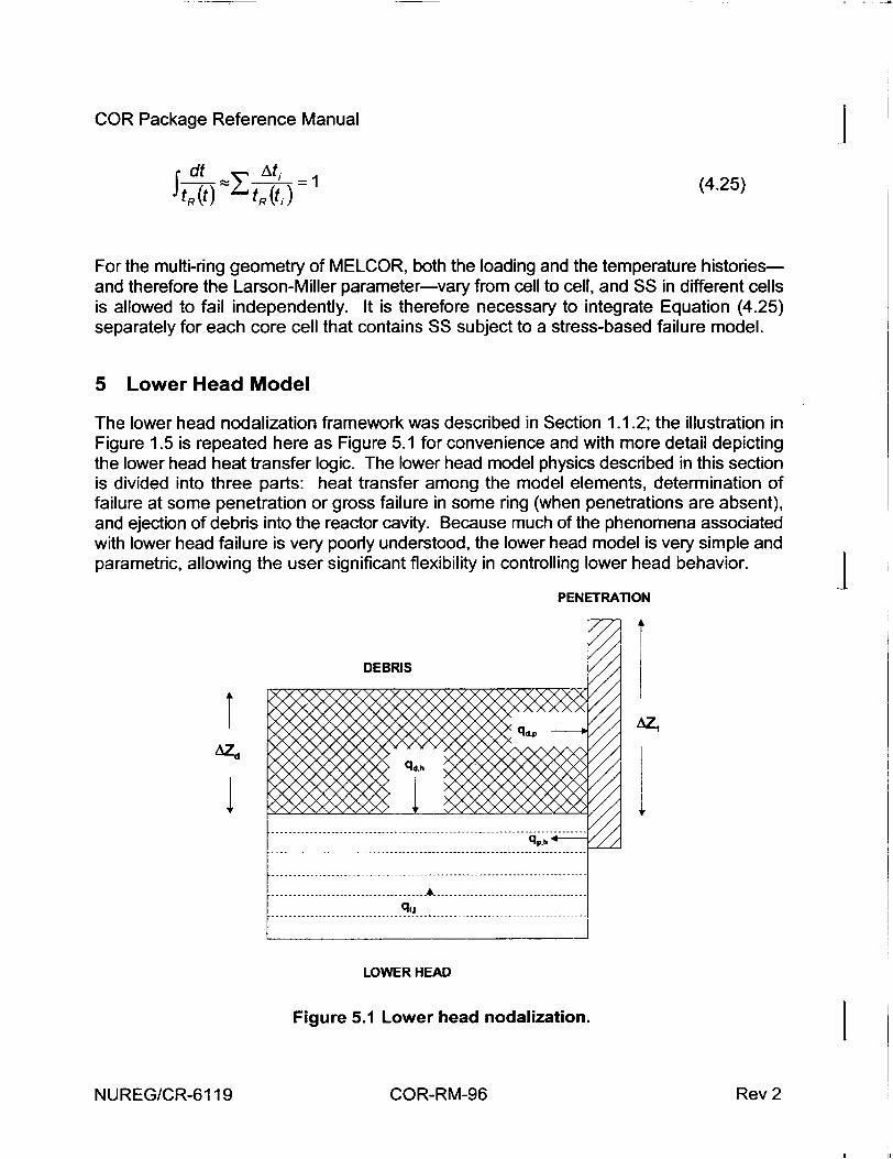
COR Package Reference Manual
ftdt At R -tt) ; tR(t,)(4.25)
For the multi-ring geometry of MELCOR, both the loading and the temperature historiesand therefore the Larson-Miller parameter-vary from cell to cell, and SS in different cells is allowed to fail independently. It is therefore necessary to integrate Equation (4.25) separately for each core cell that contains SS subject to a stress-based failure model.
5 Lower Head Model
The lower head nodalization framework was described in Section 1.1.2; the illustration in Figure 1.5 is repeated here as Figure 5.1 for convenience and with more detail depicting the lower head heat transfer logic. The lower head model physics described in this section is divided into three parts: heat transfer among the model elements, determination of failure at some penetration or gross failure in some ring (when penetrations are absent), and ejection of debris into the reactor cavity. Because much of the phenomena associated with lower head failure is very poorly understood, the lower head model is very simple and parametric, allowing the user significant flexibility in controlling lower head behavior.
PENETRATION
DEBRIS
T4
LOWER HEAD
Figure 5.1 Lower head nodalization.
NUREG/CR-6119
I
I
I - __
ICOR-RM-96 Rev 2
COR Package Reference Manual
5.1 Heat Transfer
Heat transfer from the debris to the lower head and its penetrations (e.g., instrumentation tubes, control rod guide tubes, or drain plugs) is modeled parametrically using heat transfer coefficients (specified on record COR00009), heat transfer areas (calculated from ring radii specified on record CORLHDii or specified directly on record CORPENnn), and masses (also calculated from composition and nodalization input specified on record CORLHDii or specified directly on record CORPENnn). The heat transfer rate from the debris in the bottommost axial level to the lower head is given by:
qd.h = hd,h Ah (Td - Ths) (5.1)
where
qdh = heat transfer rate between debris and lower head
hdh = debris-lower head heat transfer coefficient
Ah = lower head surface area
Td = debris temperature
Th,S = lower head inner surface temperature
The heat transfer rate from the debris in the bottommost axial level to a penetration is similarly given by:
qT,,p= hdp zd) AP (Td ) (5.2) Az1
where
qd,p = heat transfer rate between debris and penetration
hd,p = debris-penetration heat transfer coefficient
Ap = penetration area
Azd = debris height in the bottom axial level
NUREG/CR-6119Rev 2 COR-RM-97
COR Package Reference Manual j Az1 = bottom axial level height
Tp = penetration temperature
The penetration area is based on the height of the bottom axial level, Azj, and the multiplier (Azd - Azj) accounts for the partial covering of the penetration area by the debris
of height Azd.
The heat transfer rate from the penetration to the top lower head node is based on the conduction area between the penetration and lower head specified by the user:
qph = kP Apb h, (5.3) Az1
where
qp,h = heat transfer rate between penetration and lower head
kp = penetration thermal conductivity
Ap,h = conduction area between penetration and head J The conduction area Ap,h should be chosen to appropriately model the two-dimensional nature of the heat conduction; note that conduction to only the top lower head node is modeled.
Conduction heat transfer rates within the lower head are given by:
T - Ttl qi,,.+= k; FAC Ah Thi -i (5.4)
where
qijj+= heat transfer rate from node i to node /+1
ki =thermal conductivity of mesh layer i
Thj = temperature of lower head node i
AzI = width of mesh layer i
and FAC is a factor to enhance conduction through material that exceeds the melting point, as discussed in Section 2.2. The use of a planar finite-difference equation to model heat j
NUREG/CR-6119 COR-RM-98 Rev 2
COR Package Reference Manual
transfer in hemispherical geometry is an adequate approximation because the thickness of the lower head is much smaller than the radius.
Convection heat transfer rates from the penetrations, debris, and inner surface of the lower head to the fluids in the lower plenum control volume ICVHC (specified on record CORijj01), qp,v, qd,v, and qh,v respectively, are modeled by the methods described in Section 2.3.
Heat transfer from the outer boundary of the lower head to the reactor cavity control volume specified on record CORLHDO1 is partitioned between the atmosphere and the pool in the control volume based upon the pool fraction of the surface area of the lower head in each radial ring as follows:
qhxC = hATM(1 - FpL)Ah(Thl - TATM) + h(XPL FPLAh(Th,1 - TSAT) (5.5)
where
hATg = heat transfer coefficient from lower head to reactor cavity atmosphere
hf, pL = relaxed heat transfer coefficient from lower head to reactor cavity pool
FPL = pool fraction of surface area Ah
TATM = temperature of reactor cavity atmosphere obtained from CVH
TSAT = saturation temperature of reactor cavity pool obtained from CVH
Th,1 = lower head outer surface temperature at the beginning of the time step
The first term on the right hand side of Equation (5.5) accounts for heat transfer to the reactor cavity atmosphere, while the second term accounts for heat transfer to the reactor cavity pool. The pool fraction, FpL, is simply the fraction of the area which is immersed in the pool based upon the depth of the pool obtained from the CVH data base at the beginning of each time step. The heat transfer coefficient to the reactor cavity atmosphere, hATM, is implemented as sensitivity coefficient C1246(1) with a default value of 10 W/m2 -K. The unrelaxed heat transfer coefficient to the reactor cavity pool, hpL, is calculated using a simple downward-facing saturated pool boiling model. Relaxation of hpL is implemented exactly as discussed in Section 2.3. Heat transfer to the pool prior to boiling is currently ignored, as is subcooling of the pool; it is calculated only when the temperature of the outer surface of the lower head exceeds the saturation temperature in the reactor cavity. Hence, the second term on the right-hand side of Equation (5.5) cannot be negative.
The downward-facing saturated pool boiling model treats three heat transfer regimes:
NUREG/CR-61 19Rev 2 COR-RM-99
COR Package Reference Manual 4 1. fully-developed nucleate boiling with no dependence on the orientation of the
boiling surface,
2. transition boiling between the fully developed and film boiling regimes, in which the heat flux is obtained by logarithmic interpolation between the critical heat flux and the minimum heat flux based upon the temperature difference between the surface and saturation, and
3. stable film boiling which depends upon the orientation of the boiling surface.
The boundaries between the heat transfer regimes are determined by a correlation for the critical heat flux, which separates fully developed and transition boiling, and a correlation for the minimum-stable-film-boiling heat flux, which separates transition and stable film boiling. Although heat transfer in the nucleate boiling regime is assumed to be independent of the orientation of the surface, the critical heat flux, which determines its upper limit, is dependent on surface orientation and is given by [34]:
qCHF(O) = (0.034 + 0.003700.6)p2h, [g u(p, - (5.6)
where
0 =inclination angle of the surface in degrees (0 = 00 for a downward-facing I surface),
Pl, pv =densities of water and steam, respectively,
g =acceleration of gravity,
0- =interfacial surface tension between steam and water,
hv =latent heat of vaporization of water,
and the constants 0.034, 0.0037 and 0.656 have been implemented in sensitivity coefficient array C1245. Similarly, the minimum-stable-film-boiling heat flux, which separates transition boiling from stable film boiling, is given as a function of 0 as [34]:
qM,N(9) = (4.8xl -4 + 82.xl 0-4 00.407 )p/22h V[ga p, -_ v)]/ (5.7)
where the constants 4.8x10 4 , 8.2x10 4 and 0.407 have also been implemented in sensitivity coefficient array C1245.
In the nucleate boiling regime, the heat flux as a function of the difference between the surface temperature and the saturation temperature, AT - TSRF - TsAT, is given by: I
NUREG/CR-6119 COR-RM-100 Rev 2
COR Package Reference Manual
qB (AT)= h, 8 AT (5.8)
where hNB is given as a function of AT (and pressure) by Equation (2.58). In the stable film boiling regime, the heat flux as a function of AT is given by:
qFum(AT)=hFLm AT (5.9)
and the user has two options for determining the hFLM as a function of AT. The default option gives the heat transfer coefficient as [35]:
hFLM (AT)=O.14 2 k [hiv p, g(, - PV )]3 (sin )03333 (5.10)
where the constants 0.142 and 0.3333333 have been implemented in sensitivity coefficients array C1245. The other option, which is invoked when the user changes the value of sensitivity coefficient C1245(7) to 1.0, gives the heat transfer coefficient as [36]:
hFLM( AT)=(0.055+0.016005)kv hpv T (p'-P)J113 (5.11)
where the constants 0.055, 0.016 and 0.5 have been implemented in sensitivity coefficient array C1245.
Equations (5.6) to (5.11) give values of heat fluxes and heat transfer coefficients for particular values of 0 (except for Equation (5.8), which is independent of 8 ). To obtain an average value, f,, of function f(9), which is appropriate for ring i in the lower head model, f(8 ) is averaged over the wetted surface area of ring i as follows:
OU
J f(0) sine dO (5.12) fi 0-1
cosoi-1 - cOSou
OU = min[Ormax(Oj-,,GpL)] (5.13)
where OPL is the angle from the bottom of the lower head to the pool surface, 80 = 0 o and
8NAD = 90 o. This averaging results in positive values for all quantities in Equations (5.6) to (5.11), even though the heat transfer coefficient in Equation (5.10) is zero at 8 = 0°. Note, however, that specifying very small values of 9,, (i.e. defining a very small innermost
ring) is discouraged because the lower head model does not include azimuthal conduction that tends to limit the formation of local hot spots where boiling heat removal is low (i.e. at the very bottom of the lower head). Hence, the specification of a very small inner ring may
NUREG/CR-6119Rev 2 COR-RM-101
COR Package Reference Manual
lead to a prediction of vessel failure at a hot spot on the vessel bottom, which would not occur if azimuthal heat conduction in the vessel were modeled.
If the heat flux from Equation (5.8) is set equal to the average heat flux from Equation (5.6) for any ring and solved for AT, the result is equal to ATcHF, the temperature difference at the critical heat flux for that ring. If the average heat flux from Equation (5.9) is set equal to the average heat flux from Equation (5.7) and solved for AT, the result is equal to ATMIN, the temperature difference at the minimum-stable-film-boiling heat flux for that ring. Since the actual value of AT is known from the data base at the beginning of each COR time step, it can be compared to ATcHF and ATmjN to determine the appropriate heat
transfer regime. If the value is less than ATcHF, then fully-developed nucleate boiling
occurs and hpL is given by hNB from Equation (2.58). If AT is greater than ATMIN, then stable film boiling occurs and hpL is given by Equation (5.10) or (5.11), as specified by the user. If the value of AT lies between ATcHF and ATMjN, then hpL is equal to the transition
boiling heat transfer coefficient, which is found by logarithmic interpolation as follows:
[ Iog(qc,/qH,,,) 1
hTN mIN~ TL Iog0(ATCHF ATMI)j 5.4 h ~T~ Tm/Nj(.4
The net energy transfer for each of the model elements is given by the following equations:
cPIo (r T T-) = )(qdp qp,h- qpv) A t (5.15)
Cpd ( T- T-)=(q= - •- qdoh - qd,v - qdd) At (5.16)
Cp,hn ( h,n - Th,n)=(qn-l,n + qdh + qp,h - qh,v) At (5.17)
cph, ( Th., - rh,i)=(qi,,i - qj',.,) At (5.18)
C0b,( h,-To.,) = (-qdc - ql,2)At (5.19)
where many of these variables were defined in Section 5.1 and
Cpj = total heat capacity of model element j, (MjCpj)
qS = debris heat source from oxidation and decay heat
qd,d = debris cell-to-cell heat transfer rate
A t = COR package time step 4
NUREG/CR-6119 COR-RM-1 02 Rev 2

COR Package Reference Manual
and superscripts o and n refer to old-time and new-time temperatures, respectively. All temperatures in Equations (5.1) through (5.4) are considered to be new time temperatures, and Equations (5.5) through (5.8) are solved implicitly for new-time temperatures by matrix inversion.
5.2 Failure
Failure of the lower head will occur if any of four criteria is met:
1. the temperature of a penetration (or the temperature of the innermost node of the lower head) reaches a failure temperature (TPFAIL) specified by the user on record COR00009,
2. a failure logical control function (specified by the user on record CORRiiO2) is found to be .TRUE. For example, such a control function might refer to a table of differential failure pressures as a function of lower head temperature,
3. overpressure from the falling-debris quench model occurs (see Section 2.3.6). The lower head is allowed to fail from overpressure, with a default failure criterion of 20 MPa that may be changed on input record COR00012 or
4. creep-rupture failure of a lower head ring occurs, in response to mechanical loading under conditions of material weakening at elevated temperatures.
The creep-rupture failure model uses the temperature profile through the lower head to calculate creep based on a Larson-Miller parameter and a life-fraction rule whenever the effective differential pressure across the lower head exceeds a user-specified minimum value (implemented as sensitivity coefficient C1600(3) with a default value of 1000 Pa). The effective differential pressure is the sum of the actual differential pressure between the lower plenum and the reactor cavity and the pressure caused by the weight of any debris resting on the lower head. The lower limit on the effective pressure differential was imposed to bypass the model and save computational resources when the threat of creeprupture is minuscule.
The model is applied to the load-bearing mesh layers in the lower head, which include all NLH-1 mesh layers by default. However, by entering a positive value for NINSLH on input record COROOOOO, the user defines the outer NINSLH layers to consist of non-load-bearing insulation. An optional one-dimensional mechanical model that calculates the thermal and plastic strain in each load-bearing mesh layer may be invoked by setting the value of sensitivity coefficient C1600(1) equal to 1.0. By default, however, a zero-dimensional model based on the mass-averaged temperatures in the load-bearing mesh layers is used with the effective membrane stress induced by the effective differential pressure to calculate a single Larson-Miller parameter for each radial ring.
NUREG/CR-6119Rev 2 COR-RM-1 03
COR Package Reference Manual /
The Larson-Miller creep-rupture failure model [32] gives the time to rupture, tR in seconds, as:
tR = 1 T ) (5.20)
where PLM is the Larson-Miller parameter given by:
PLM = 7.722x1 0-4 - 7.294x1 03 log10 ae (5.21)
where 0-e is the effective stress in Pa and the constants 7.722x10 4 and -7.294x1 03, which are appropriate for reactor vessel carbon steel [37] and 16.44 (Equation (5.21)), have been implemented in sensitivity coefficient array C1601. The life-fraction rule gives the cumulative damage, expressed as plastic strain, e,(t), as:
At -(t + At)= , (t)+0.18 (5.22)
tR
where the constant 0.18, which has been implemented as sensitivity coefficient C1 601 (4), implies that failure (defined as when the integrated value of At/tR reaches unity) occurs when the strain reaches 18% [36].
For the zero-dimensional default option, the effective stress is given by:
(AP + pdgAzd )R? 2 2-(5.23)
R0 - R1
where A P is the pressure difference across the lower head, Pd and Azd are the density and depth of the debris resting on the lower head, and Ri and R, are the inner vessel radius and outer radius of load-bearing vessel steel, respectively. Substitution of -e from
Equation (5.23) into Equation (5.21) yields a value of PLM for each ring. Substitution of the temperature, mass-averaged over all the load-bearing mesh layers in each lower head ring, and the value of PLM into Equation (5.20) yields tR (the predicted time lapse until failure for a specimen subjected to the current temperature and stress). And, finally, substitution of tR into Equation (5.22) yields the accumulated plastic strain at each time step. Failure is declared when 6. (t) reaches failure strain given by sensitivity coefficient C1601(4), with
a default of 0.18, and the mechanical calculation in that ring ceases.
The optional one-dimensional mechanical model predicts the stress-strain distribution through the lower head, and treats stress redistribution from both thermal strain and material property degradation. The elastic modulus as a function of temperature is given by [36]: INUREG/CR-6119 COR-RM-104 Rev 2
COR Package Reference Manual
E (T)= 2.0x10¹¹[ i 1 6. 1(9Q0 ~ E _______ .)6 (5.24)
where the constants 2.0x10 1', 1800., 900. and 6., which are appropriate for reactor vessel steel, have been implemented as sensitivity coefficient array C1602. The yield stress as a function of temperature is given by [36]:
oy (T) =4.0x10⁸ 1 .61 9.6, (5.25) 900. 900.6
where the constants 4.Ox1 0', 1800., 900. and 6., which are appropriate for reactor vessel steel, have been implemented as sensitivity coefficient array 01603.
The one-dimensional model requires that the stress distribution integrated over the vessel thickness be equal to the imposed load:
2- (22i- ~+ •-•r (5.26)R~ '
AP + Pd gAzd lRo o'i ( R (Tj) / (5. i i 5.6
where the first sum on the right-hand side is over all layers that have not yielded, NNy, and the second sum is over all layers that have yielded, Ny. The stress, o', in layers that have not yielded is given by:
a, = E(T,) [Etot - (6Pj + Eth,)I (5.27)
where E(T1) is the value of the elastic modulus at the average temperature in mesh layer i, which is equal to the average of the node temperatures on the two boundaries, -tot is the total strain across the lower head in the particular ring, which is the same for mesh layers in that ring, and E. and eti are the plastic and thermal strains, respectively, in mesh layer
i. The thermal strain is given by:
Eth, = 1.0x1 0-5 (T, - Tm,) (5.28)
where the constant 1.Oxl 05 is the linear thermal expansivity, which has been implemented as sensitivity coefficient C1600(2), and T,.f is the reference temperature, which is equal to
NUREG/CR-6119Rev 2 COR-RM-1 05
COR Package Reference Manual
the initial temperature specified by the user for that ring of the lower head. Equations (5.26) and (5.27) are solved implicitly and iteratively for Ett, oi and epli (eth,i is known
since the temperature profile is known) using Equation (5.20) - (5.22) to update the plastic strain profile with the latest stress profile after each iteration. Failure is declared when 6 tot
reaches 18% (the use of 6tot rather than ep, makes little difference because the elastic and
thermal strains are insignificant compared to the plastic strain when 6 tot becomes large).
Whenever any failure condition is satisfied, an opening with an initial diameter defined by the user on record CORPENnn or with an initial diameter of 0.1 m if there are no penetrations (this gives a relatively rapid ejection of debris without numerical difficulties), is established, and the COR package control function argument COR-ABRCH (see Section 4 of the COR Package Users' Guide) is set to the initial failure flow area calculated from this diameter. COR-ABRCH can then be used to open a valve in the flow path from the lower plenum control volume to the reactor cavity control volume. COR-ABRCH may be increased by additional penetration failures (up to three per radial ring) or by ablation of the failure openings, as described in the next section.
5.3 Debris Ejection
After a failure has occurred, the mass of each material in the bottom axial level that is available for ejection (but not necessarily ejected) is calculated. Two simple options exist. In the default option (IDEJ = 0 on record CORTST01), the masses of each material available for ejection are the total debris material masses, regardless of whether or how much they are molten. Note, however, that this option has been observed to lead to ejection of much more solid debris with the melt than is realistic.
In the second option (IDEJ = 1 on MELCOR record CORTST01), the masses of steel, Zircaloy, and U0 2 available for ejection are simply the masses of these materials that are molten; the masses of steel oxide and control poison materials available for ejection are the masses of each of these materials multiplied by the steel melt fraction, based on an assumption of proportional mixing; and similarly the mass of ZrO2 available for ejection is the ZrO 2 mass multiplied by the Zircaloy melt fraction. Additionally, the mass of solid U0 2
available for ejection is the Zircaloy melt fraction times the mass of U0 2 that could be relocated with the Zircaloy as calculated in the candling model using the secondary material transport model (see Section 3.1). An option parallel to the methodology used in the materials interactions (eutectics) model has not yet been developed.
Regardless of which of the options described above is chosen, other constraints have been imposed on the mass to be ejected at vessel failure. A total molten mass of 5000 kg or a melt fraction of 0.1 (total molten mass divided by total debris mass) is necessary before debris ejection can begin, to avoid calculational difficulties with the core-concrete interactions modeling. Also, whenever the bottom lower head node exceeds the
NUREG/CR-6119 Rev 2COR-RM-1 06
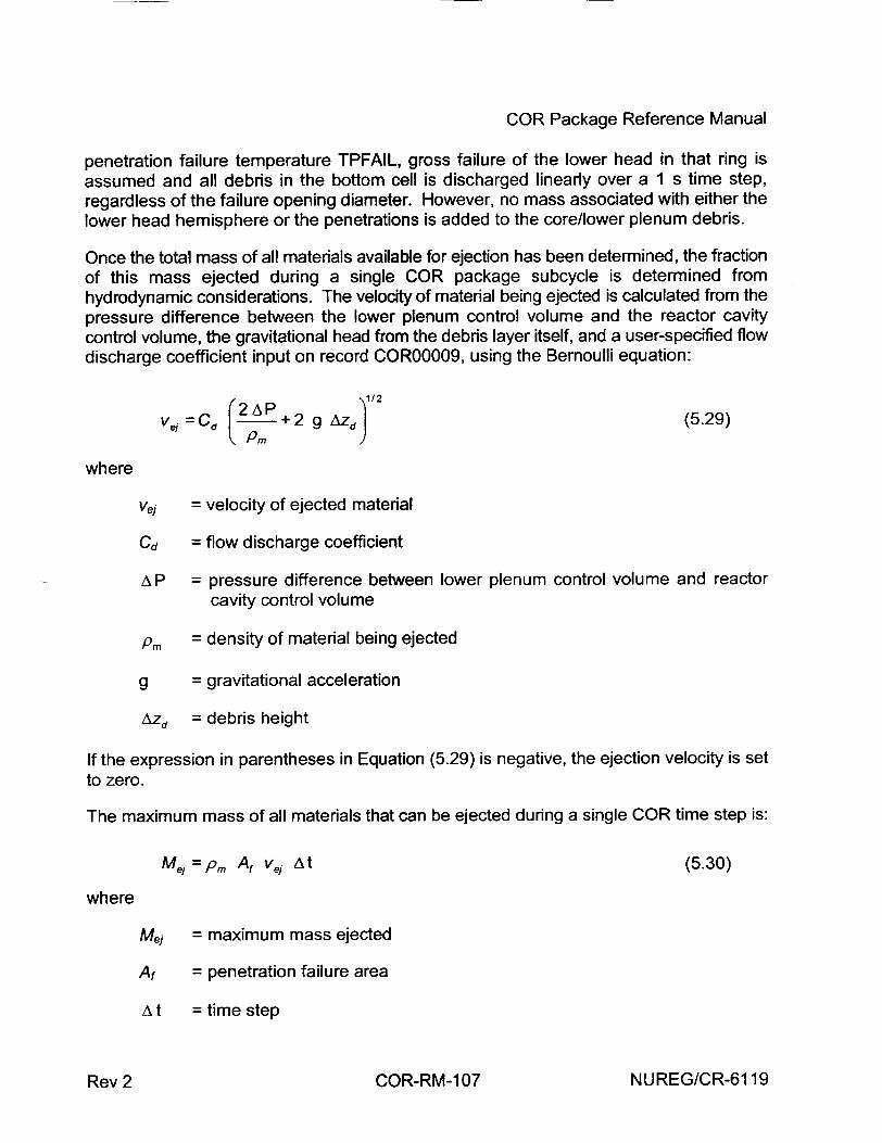
COR Package Reference Manual
penetration failure temperature TPFAIL, gross failure of the lower head in that ring is assumed and all debris in the bottom cell is discharged linearly over a 1 s time step, regardless of the failure opening diameter. However, no mass associated with either the lower head hemisphere or the penetrations is added to the core/lower plenum debris.
Once the total mass of all materials available for ejection has been determined, the fraction of this mass ejected during a single COR package subcycle is determined from hydrodynamic considerations. The velocity of material being ejected is calculated from the pressure difference between the lower plenum control volume and the reactor cavity control volume, the gravitational head from the debris layer itself, and a user-specified flow discharge coefficient input on record COR00009, using the Bernoulli equation:
Ve =Cd 2AP+ AZd)12 (5.29)
where
vej = velocity of ejected material
Cd = flow discharge coefficient
A P = pressure difference between lower plenum control volume and reactor cavity control volume
PM = density of material being ejected
g = gravitational acceleration
Azd = debris height
If the expression in parentheses in Equation (5.29) is negative, the ejection velocity is set to zero.
The maximum mass of all materials that can be ejected during a single COR time step is:
Mej = P, Af Vej At (5.30)
where
Mej = maximum mass ejected
Af = penetration failure area
A t = time step
NUREG/CR-6119COR-RM-107Rev 2
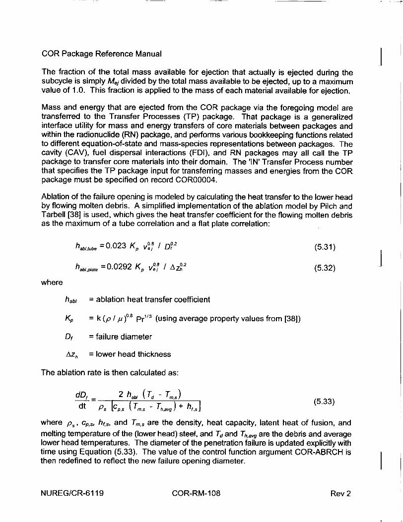
COR Package Reference Manual
The fraction of the total mass available for ejection that actually is ejected during the subcycle is simply Mej divided by the total mass available to be ejected, up to a maximum value of 1.0. This fraction is applied to the mass of each material available for ejection.
Mass and energy that are ejected from the COR package via the foregoing model are transferred to the Transfer Processes (TP) package. That package is a generalized interface utility for mass and energy transfers of core materials between packages and within the radionuclide (RN) package, and performs various bookkeeping functions related to different equation-of-state and mass-species representations between packages. The cavity (CAV), fuel dispersal interactions (FDI), and RN packages may all call the TP package to transfer core materials into their domain. The 'IN' Transfer Process number that specifies the TP package input for transferring masses and energies from the COR package must be specified on record COR00004.
Ablation of the failure opening is modeled by calculating the heat transfer to the lower head by flowing molten debris. A simplified implementation of the ablation model by Pilch and Tarbell [381 is used, which gives the heat transfer coefficient for the flowing molten debris as the maximum of a tube correlation and a flat plate correlation:
habltube = 0.023 Kp V / D' 2 (5.31)
hab•plate =0.0292 Kp v° / AzV2 (5.32)
where
habl = ablation heat transfer coefficient
Kp = k (p / ,u)°.8 Pr" 3 (using average property values from [38])
Df = failure diameter
Azh = lower head thickness
The ablation rate is then calculated as:
dD, _ 2 hab ( Td - T,.,,n) dt ps [cps (Tin,. - Thmavg)+ h,..J (5.33)
where p., cp,,, hf,, and T,,s are the density, heat capacity, latent heat of fusion, and
melting temperature of the (lower head) steel, and Td and Tha•, are the debris and average lower head temperatures. The diameter of the penetration failure is updated explicitly with time using Equation (5.33). The value of the control function argument COR-ABRCH is then redefined to reflect the new failure opening diameter.
NUREG/CR-6119 COR-RM-1 08 Rev 2
COR Package Reference Manual
6 Discussion and Development Plans
In its inception, MELCOR was envisioned as a PRA tool that was to be fast running, making use of necessarily simplified physics models. In recent years, however, MELCOR has found increasing use as a best estimate tool for severe accident analyses, and many of the physics models, including many in the COR package have been improved considerably. Nevertheless, some of the simplified COR models remain today. In some cases, simplistic parametric models have been implemented until more advances have been made in furthering our understanding of the phenomena. In other cases, more sophisticated models are planned for implementation in the near future.
The following paragraphs are based on assessments of improvement needs for MELCOR in the area of core modeling, including deficiencies identified as part of the MELCOR Peer Review [39], and include work in progress. Suggestions from users regarding additional modification and/or upgrading of the COR package are welcomed and should be directed to the MELCOR Code Development Group using the MELCOR Defect Investigation Report (DIR) forms.
6.1 Radiation
Radiation view factors in the COR package are defined globally, based on simple user input. Since correct characterization of many of these view factors is dependent on local geometry and nodalization, they should be definable on a local cell basis and updated internally with changing geometry. This upgrade would give the user more freedom to satisfactorily model radiative heat transfer within the core, a dominant heat transfer mechanism in reactor accidents.
6.2 Reflood Behavior
To adequately assess the possibly deleterious effects of reflooding and the potential to avoid vessel failure, models to credibly predict the interactions between water and overheated fuel rods or core debris are desirable. This involves the ability to predict quenching rates in the geometries of interest, spallation of oxide from the fuel rod cladding with accelerated oxidation, shattering of the fuel rods during quench, the occurrence and effects of clad ballooning (discussed separately below), and the possibility of forming a molten pool. Models are currently under development for post-i.8.5 MELCOR release.
6.3 Lower Plenum Debris Behavior and Vessel Failure
The COR package in MELCOR does not include consideration of natural circulation of a molten debris pool in the lower head. Such pools can form if the debris temperature and relocation rate are such as to prevent early failure of the bottom head or its penetration (if
NUREG/CR-6119Rev 2 COR-RM-1 09
COR Package Reference Manual
there are any), and is of particular importance if the lower head is externally cooled by flooding the reactor cavity with water. It also fails to account for head curvature effects, freezing and remelting of core debris in penetrations, and crust formation, growth, and remelting.
The Bottom Head (BH) package models, developed as part of the BWRSAR program at
Oak Ridge National Laboratory (ORNL), address some of these deficiencies. In MELCOR 1.8.4, the BH package was extended to treat PWRs as well as BWRs, and may be invoked by supplying appropriate input as described in the BH package Users' Guide. However, it will not become active in a calculation until complete dryout of the lower head has been achieved; until that time the much simpler models of the COR package will be used.
Either the BH models should be much more completely and tightly coupled into existing COR models, or the domain for each package should be carefully redefined with overlap minimized and interfaces between them and between other MELCOR packages rigorously specified. In either case, the BH lower plenum models should be made more flexible for more complete treatment of different accident scenarios (e.g., debris heat transfer before complete pool boiloff) and to allow greater user control (e.g., with sensitivity coefficients).
6.4 Updating of Core Degradation Models
Understanding of the mechanisms of core degradation has increased significantly since
the inception of MELCOR and the original design of the degradation models. There has
been an increased appreciation of the importance of melting and materials interactions
compared with rubble formation. In addition, application of the code has been
expanded from PRA calculations for which simple parametric models would be
adequate, to source term calculations requiring more detailed validation against the
latest experimental data. Some improvements to core degradation models were made
for MELCOR 1.8.4. In the course of this work, it became apparent that the basic
modeling approach should be reexamined to determine if changes are be necessary
to accommodate models that reflect current understanding of the important
phenomena. Some such improvements have been made in MELCOR 1.8.5, and others are being considered for later versions of the code.
I
NUREG/CR-6119 Rev 2COR-RM-1 10
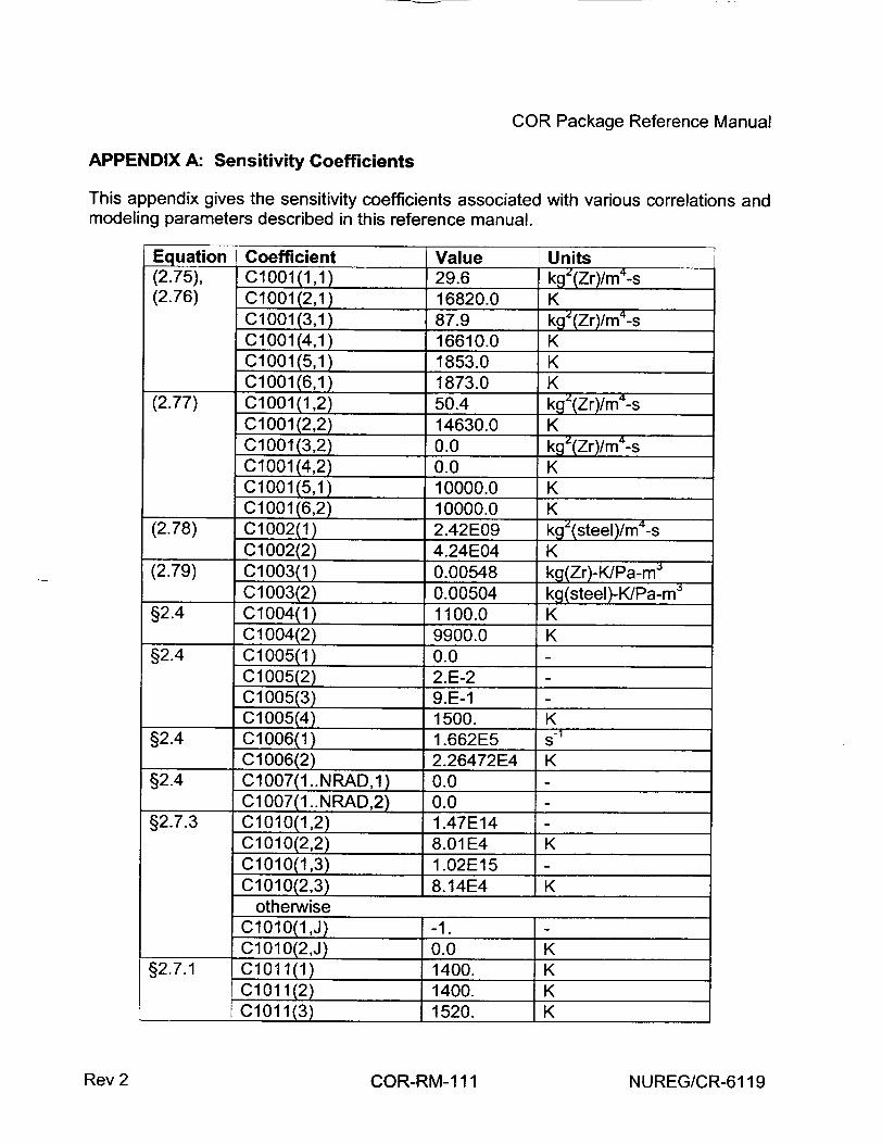
COR Package Reference Manual
APPENDIX A: Sensitivity Coefficients
This appendix gives the sensitivity coefficients associated modeling parameters described in this reference manual.
with various correlations and
Equation Coefficient Value Units (2.75), C1001(1,1) 29.6 kgz(Zr)/m'-s (2.76) C1001(2,1) 16820.0 K
C1001(3,1) 87.9 kg (Zr)/m 4-s C1001(4,1) 16610.0 K C1001(5,1 1853.0 K C1001(6,1) 1873.0 K
(2.77) C1001(1,2) 50.4 kgz(Zr)/m 4-s C1001(2,2) 14630.0 K C1001(3,2) 0.0 kgz(Zr)/m 4_s C1001(4,2) 0.0 K C1001(5,1) 10000.0 K C1001(6,2) 10000.0 K
(2.78) C1002(1) 2.42E09 kgz(steel)/m4-s C1002(2) 4.24E04 K
(2.79) C1003(1) 0.00548 kg(Zr)-K/Pa-m3 C1003(2) 0.00504 kg(steel)-K/Pa-m3
§2.4 C1004(1) 1100.0 K C1004(2) 9900.0 K
§2.4 C1005(1) 0.0 C1005(2) 2.E-2 C1005(3) 9.E-1 C1005(4) 1500. K
§2.4 C1006(1 1.662E5 s-1
C1006(2) 2.26472E4 K §2.4 C1007(1..NRAD,1) 0.0
C1007(I..NRAD,2) 0.0 §2.7.3 C1010(1,2) 1.47E14
C1010(2,2) 8.01E4 K C1010(1,3) 1.02E15 C1010(2,3) 8.14E4 K
otherwise C1010(1,J) -1. C1010(2,J) 0.0 K
§2.7.1 C1011(1) 1400. K C1011(2) 1400. K C1011(3) 1520. K
NUREG/CR-6119Rev 2 COR-RM-1 11
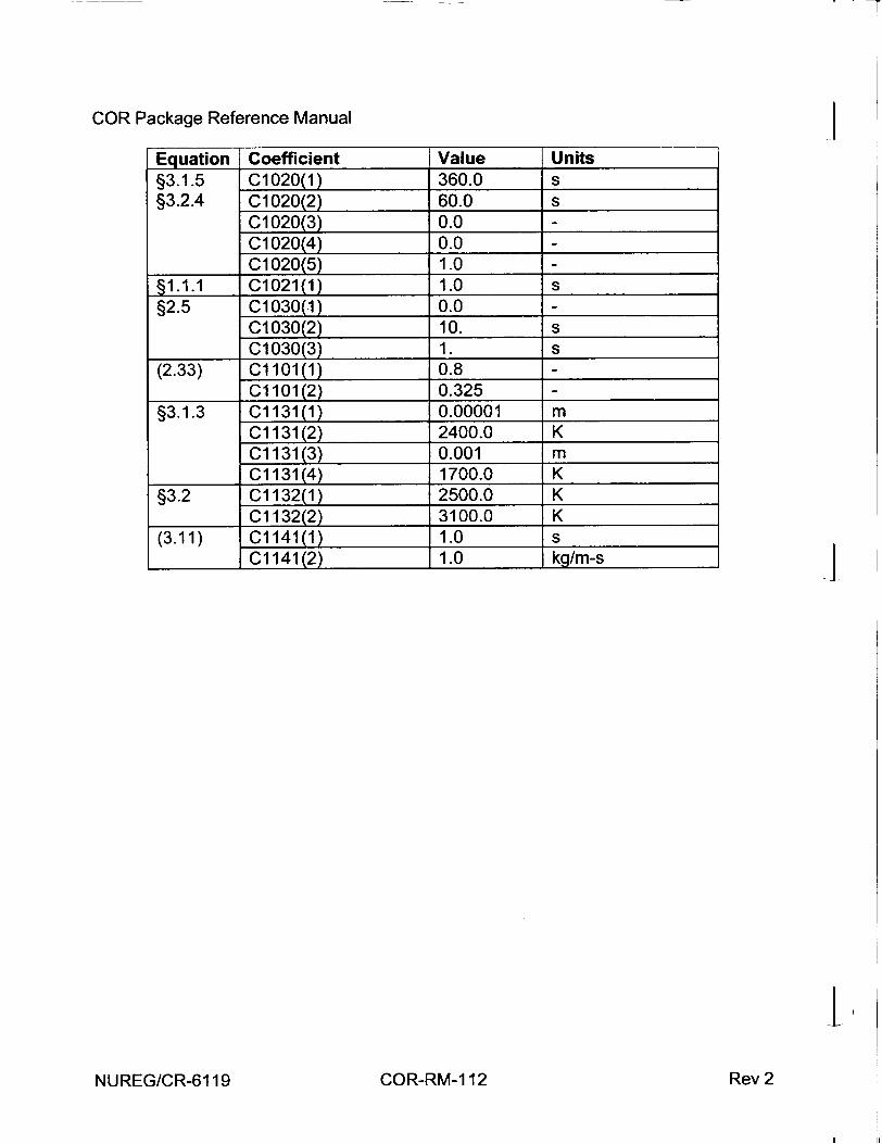
COR Package Reference Manual
Equation Coefficient Value Units §3.1.5 C1020(1) 360.0 s §3.2.4 C1020(2) 60.0 s
C1020(3) 0.0 C1020(4) 0.0 C1020(5) 1.0
§1.1.1 C1021(1) 1.0 s §2.5 C1030(1) 0.0
C1030(2) 10. s C1030(3) 1. s
(2.33) C1101(1) 0.8 C1 101(2) 0.325
§3.1.3 C1131(1) 0.00001 m C1131(2) 2400.0 K C1 131(3) 0.001 m C1 131(4) 1700.0 K
§3.2 C1132(1) 2500.0 K C1 132(2) 3100.0 K
(3.11) C1141(1) 1.0 s C1 141(2) 1.0 kg/m-s
INUREG/CR-6119
I
I
Rev 2COR-RM-1 12
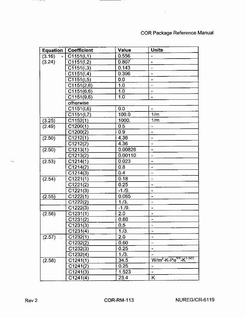
COR Package Reference Manual
Equation Coefficient Value Units (3.16) - C1151(1,1) 0.556 (3.24) C1151(1,2) 0.807
C1151(1,3) 0.143 C1151(1,4) 0.396 C1151(1,5) 0.0 C1151(2,6) 1.0 Cl151(6,6) 1.0 C1151(9,6) 1.0 otherwise C1151(1,6) 0.0 C1151(1,7) 100.0 1/m
(3.25) C1152(1) 1000. 1/m (2.49) C1200(1) 0.5
C1200(2) 0.9 (2.50) C1212(1) 4.36
C1212(2) 4.36 (2.50) C1213(1) 0.00826
C1213(2) 0.00110 (2.53) C1214(1) 0.023
C1214(2) 0.8 C1214(3) 0.4
(2.54) C1221(1) 0.18 C1221(2) 0.25 C1221(3) -1./9.
(2.55) C1222(1) 0.065 C1222(2) 1./3. C1222(3) -1./9.
(2.56) C1231( 1) 2.0 C1231(2) 0.60 C1231(3) 0.5 C1231(4) 1./3.
(2.57) C1232(1) 2.0 C1232(2) 0.60 C1232(3) 0.25 C1232(4) 1./3.
(2.58) C1241 (1) 34.5 W/m2-K-Pa'14-K152 3 C1241(2) 0.25 C1241(3) 1.523 C1 241(4) 23.4 K
NUREG/CR-6119Rev 2 COR-RM-1 13
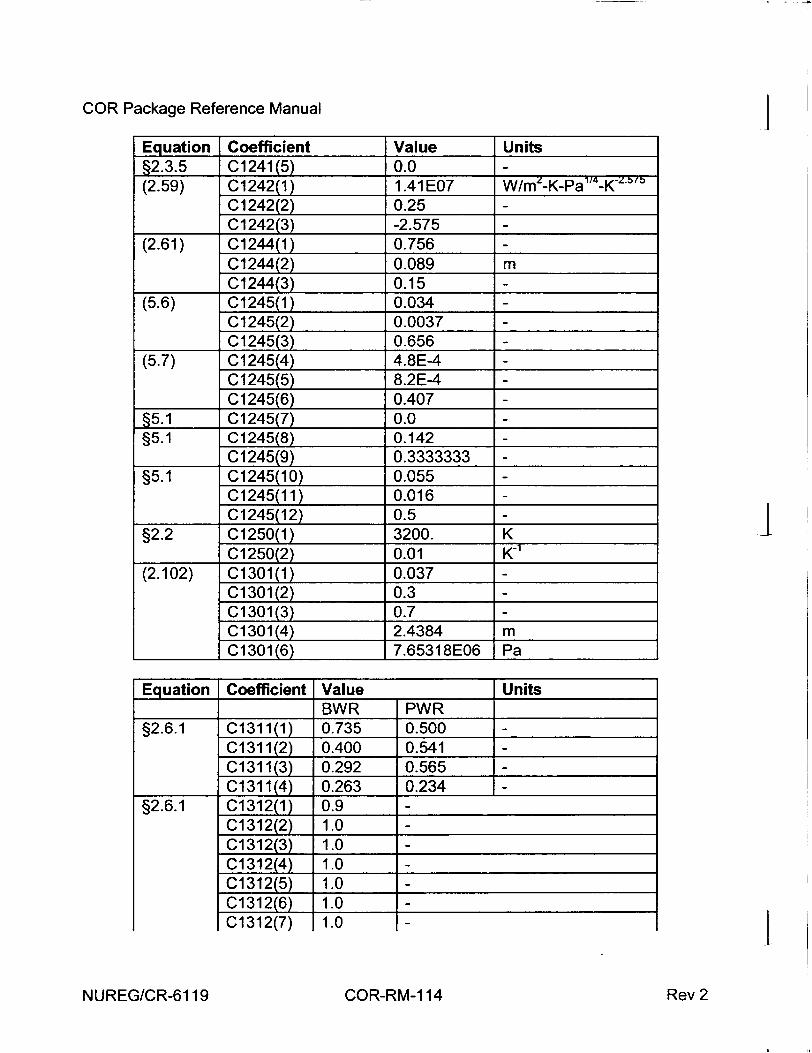
COR Package Reference Manual
Equation Coefficient Value Units §2.3.5 C1241(5) 0.0 (2.59) C1242(1) 1.41 E07 W/m2-K-Pa 114-K-z•b
C1242(2) 0.25 C1242(3) -2.575
(2.61) C1244(1) 0.756 C1244(2) 0.089 m C1244(3) 0.15
(5.6) C1245(1) 0.034 C1245(2) 0.0037 C1245(3) 0.656
(5.7) C1245(4) 4.8E-4 C1245(5) 8.2E-4 C 1245(6) 0.407
§5.1 C1245(7) 0.0 §5.1 C1245(8) 0.142
C1245(9) 0.3333333 §5.1 C1245(10) 0.055
C1245(11) 0.016 C 1245(12) 0.5
§2.2 C1250(1) 3200. K C 1250(2) 0.01 K-1
(2.102) C1301(1) 0.037 C1301(2) 0.3 C1301(3) 0.7 C1301(4) 2.4384 m C1301(6) 7.65318E06 Pa
Equation Coefficient Value Units BWR PWR
§2.6.1 C1311(1) 0.735 0.500 C1311(2) 0.400 0.541 C1311(3) 0.292 0.565 C1311(4) 0.263 0.234 -
§2.6.1
C1312(7) 1.0
NUREG/CR-6119
I
j
0131 2(2) 10. C1312(2) 1.001 312(3 1.0C013T12(4-) 1 .0
01312(6) 1.0-
C131201) 0.9
-1
COR-RM-1 14 Rev 2
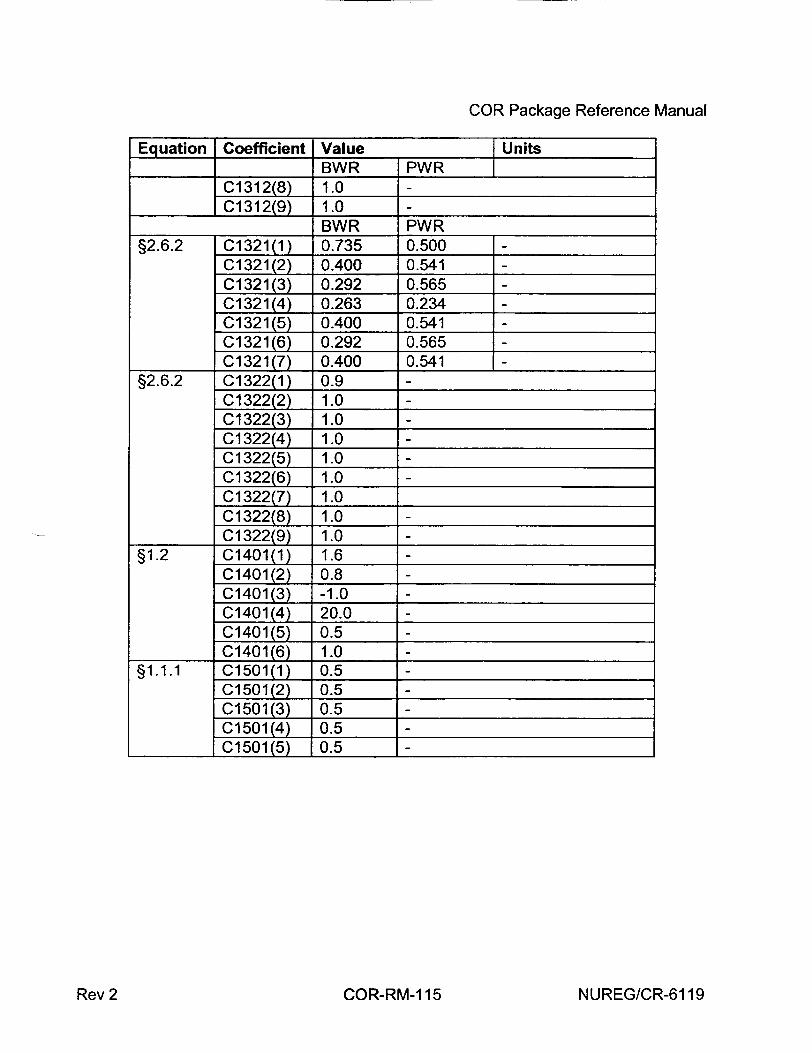
COR Package Reference Manual
Equation Coefficient Value Units BWR PWR
C1312(8) 1.0 C1312(9) 1.0
BWR PWR §2.6.2 C1 321 (1) 0.735 0.500
C1321(2) 0.400 0.541 C1321(3) 0.292 0.565 C1321(4) 0.263 0.234 C1 321(5) 0.400 0.541 C1 321(6) 0.292 0.565 C1 321(7) 0.400 0.541
§2.6.2 C1322(1) 0.9 C1322(2) 1.0 C1322(3) 1.0 C1322(4) 1.0 C1322(5) 1.0 C1322(6) 1.0 C1322(7) 1.0 C1322(8) 1.0 C 1322(9) 1.0
§1.2 C1401(1) 1.6 C1401(2) 0.8 C1401(3) -1.0 C1401(4) 20.0 C1401(5) 0.5 C1401(6) 1.0
§1.1.1 C1501(1) 0.5 C1501(2) 0.5 C1501(3) 0.5 C1501(4) 0.5 C 1501(5) 0.5 -
NUREG/CR-6119Rev 2 COR-RM-1 15
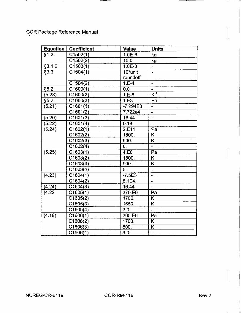
COR Package Reference Manual
Equation Coefficient Value Units §1.2 C1502(1) 1.OE-6 kg
C1502(2) 10.0 kg §3.1.2 C1503(1) 1.OE-3 §3.3 C1504(1) 10*unit
roundoff C1504(2) 1.E-4
§5.2 C1600(1) 0.0 (5.28) C1600(2) 1.E-5 K-1
§5.2 C1600(3) 1.E3 Pa (5.21) C1601(1) -7.294E3
C1601(2) 7.722e4 (5.20) C1601(3) 16.44 (5.22) C1601(4) 0.18 (5.24) C1602(1) 2.Ell Pa
C1602(2) 1800. K C1602(3) 900. K C1602(4) 6.
(5.25) C1603(1) 4.E8 Pa C1603(2) 1800. K C1603(3) 900. K C1603(4) 6.
(4.23) C1604(1) -7.5E3 C 1604(2) 8.1E4.
(4.24) C1604(3) 16.44 (4.22 C1605(1) 370.E9 Pa
C1605(2) 1700. K C1605(3) 1650. K C1605(4) 3.0
(4.18) C1606(1) 260.E6 Pa C1606(2) 1700. K C1606(3) 800. K C 1606(4) 3.0
INUREG/CR-6119
I
I
COR-RM-1 16 Rev 2
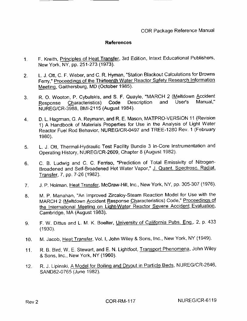
COR Package Reference Manual
References
1. F. Kreith, Principles of Heat Transfer, 3rd Edition, Intext Educational Publishers,
New York, NY, pp. 251-273 (1973).
2. L. J. Ott, C. F. Weber, and C. R. Hyman, "Station Blackout Calculations for Browns
Ferry," Proceedings of the Thirteenth Water Reactor Safety Research Information
Meeting, Gaithersburg, MID (October 1985).
3. R. 0. Wooton, P. Cybulskis, and S. F. Quayle, "MARCH 2 (Meltdown Accident
Response Characteristics) Code Description and User's Manual,"
NUREG/CR-3988, BMI-2115 (August 1984).
4. D. L. Hagrman, G. A. Reymann, and R. E. Mason, MATPRO-VERSION 11 (Revision
1) A Handbook of Materials Properties for Use in the Analysis of Light Water
Reactor Fuel Rod Behavior, NUREG/CR-0497 and TREE-1 280 Rev. 1 (February 1980).
5. L. J. Ott, Thermal-Hydraulic Test Facility Bundle 3 In-Core Instrumentation and
Operating History, NUREG/CR-2609, Chapter 8 (August 1982).
6. C. B. Ludwig and C. C. Ferriso, "Prediction of Total Emissivity of Nitrogen
Broadened and Self-Broadened Hot Water Vapor," J. Quant. Spectrosc. Radiat. Transfer, 7, pp. 7-26 (1982).
7. J. P. Holman, Heat Transfer, McGraw-Hill, Inc., New York, NY, pp. 305-307 (1976).
8. M. P. Manahan, "An Improved Zircaloy-Steam Reaction Model for Use with the MARCH 2 (Meltdown Accident Response Characteristics) Code," Proceedings of
the International Meeting on Light-Water Reactor Severe Accident Evaluation,
Cambridge, MA (August 1983).
9. F. W. Dittus and L. M. K. Boelter, University of California Pubs. Enq., 2, p. 433 (1930).
10. M. Jacob, Heat Transfer, Vol. I, John Wiley & Sons, Inc., New York, NY (1949).
11. R. B. Bird, W. E. Stewart, and E. N. Lightfoot, Transport Phenomena, John Wiley
& Sons, Inc., New York, NY (1960).
12. R. J. Lipinski, A Model for Boiling and Dryout in Particle Beds, NUREG/CR-2646, SAND82-0765 (June 1982).
NUREG/CR-6119COR-RM- 117Rev 2
COR Package Reference Manual
13. G. W. Parker and A. L. Sutton, Jr., "Boron Control Material Behavior in Large-Scale, Core-Melt Experiments," presented at the Severe Fuel Damage and Source Term Research Program Review Meeting, Oak Ridge Associated Universities Conference Center, Oak Ridge, TN, April 7-10, 1986.
14. V. F. Urbanic and T. R. Heidrich, "High-Temperature Oxidation of Zircaloy-2 and Zircaloy-4 in Steam," J. Nuc. Matls., 75, pp. 251-261 (1978).
15. A. S. Benjamin, D. J. McCloskey, D.A. Powers, and S. A. Dupree, Spent Fuel Heatup Following Loss of Water During Storage, SAND77-1371, NUREG/CR-0649, Sandia National Laboratories, Albuquerque, NM, March 1979.
16. J. F. White et al., "Fifth Annual Report-High Temperature Material Programs, Part A," GEMP-400A (February 1966).
17. Fred Griffin, "BWR Control Blade Channel Box Interaction and Melt Relocation Models for SCDAP," Letter Report ORNL/NRC/LTR-92/12/R2 to Dr. Yi-Shung Chen, Accident Evaluation Branch, Division of Systems Research, RES USNRC, December 30, 1993.
18. G. Eriksson, "Thermodynamic Studies of High Temperature Equilibria: XII. SOLGASMIX, a computer program for calculation of equilibrium compositions in multiphase systems," Chemica Scripta, 8, 1975, pp. 100-103.
19. "Reducing BWR Power by Water Level Control During an ATWS, a Quasi-Static Analysis," NSAC-69, S. Levy, Inc. Final Report (May 1984).
20. P. Hofmann et al., "Reactor Core Materials Interactions at Very High Temperatures," Nuclear Technology, 87, pp. 146-186, August 1989.
21. W. Hering and K. Muller, "Modelling of Eutectic Interactions in KESS-III (Module EUTECT)," International CORA Workshop 1992, Karlsruhe, FRG, October 5-8, 1992.
22. R. K. Cole, et al., CORCON-Mod2: A Computer Program for Analysis of MoltenCore Concrete Interactions, NUREG/CR-3920, SAND84-1246, August 1984, pp. 6465.
23. R. J. Roark and W. C. Young, Formulas for Stress and Strain, Fifth Edition, McGraw-Hill Book Company, New York, NY, 1982, Case 8 of Table 26.
24. Ibid. The equation is extracted from Case 10 of Table 24.
INUREG/CR-6119
I - ___*
COR-RM-1 18 Rev 2

COR Package Reference Manual
25. R. K. Cole, Jr., "Modifications to MELCOR to Improve Modeling of Core Structure Supports, Final Implementation Report," letter report to Mr. John Ridgely, USNRC, April 15, 1999.
26. R. J. Roark and W. C. Young, op. cit., Case 2a of Table 24.
27. S. Timoshenko and S. Woinowsky-Krieger, Theory of Plates and Shells, Mcgraw-Hill Book Company, New York, NY, Second Edition, 1959. Parameters are taken from Table 58.
28. R. C. Schmidt et al., MELPROG-PWR/MOD1 Models and Correlations, SAND893123, June 1992.
29. Nuclear Systems Materials Handbook, Vol. 1 - Design Data, "Yield strength, minimum expected," 1974.
30. T. H. Lin, Theory of Inelastic Structures, John Wiley and Sons, NY, 1983.
31. Nuclear Systems Materials Handbook, Vol. 1 - Design Data, "Young's modulus, static," 1974.
32. F. R. Larson and J. Miller, "A Time-Temperature Relationship for Rupture and Creep Stress," Transactions of the ASME, pp. 765-775, July 1952.
33. American Society of Mechanical Engineers, "ASME Boiler and Pressure Vessel Code Case N-47-22," April 5, 1984.
34. M. S. EI-Genk and Z. Guo, "Transient Critical Heat Flux for Inclined and DownwardFacing Flat Surfaces," ANS Proceedings, HTC-6 Volume 6, 1992, National Heat Transfer Conference, August 9-12, 1992, San Diego.
35. T. Y. Chu, "A Correlational Approach to Turbulent Saturated Film Boiling," Journal of Heat Transfer, Volume 115, November 1993.
36. K. B. Cady, V. K. Dhir and R. J. Witt, "Peer Review of Models for Lower Vessel Head Heat Transfer and Larson-Miller Failure Criterion Proposed for Implementation into MELCOR," ERI/NRC 94-202 March 1994.
37. J. L. Rempe et. al., Light Water Reactor Lower Head Failure Analysis (Draft), INEL, NUREG/CR-5642, EGG-2618, December 1991.
38. M. Pilch and W. W. Tarbell, High Pressure Ejection of Melt from a Reactor Pressure Vessel-the Discharge Phase, NUREG/CR-4383, SAND85-0012 (September 1985).
NUREG/CR-6119Rev 2 COR-RM-1 19
COR Package Reference Manual
39. B. E. Boyack, et al., MELCOR Peer Review, LA-12240, Los Alamos National Laboratory (March 1992).
NUREG/CR-6119 COR-RM-120
I1
Rev 2
1 11
Thermal Hydraulic (CVH and FL) Packages Reference Manual
Two packages in the MELCOR code, the Control Volume Hydrodynamics (CVH) package and the Flow Path (FL) package, are responsible for modeling the thermal-hydraulic behavior of coolant liquids and gases. The former is concerned with control volumes and their contents, the latter with the connections which allow transfer of these contents between control volumes. The distinction between CVH and FL is useful primarily for discussion of MELCOR input and output. It will frequently be ignored in this Reference Manual, where many aspects of the thermal-hydraulic modeling will be described without concern for which package contains the relevant coding.
If phenomena modeled by other packages in MELCOR influence thermal-hydraulic behavior, the consequences are represented as sources and sinks of mass, energy, or available volume, or as changes in the area or flow resistance of flow paths in CVH. [Changes involving flow paths may currently be handled only through use of the Control Function (CF) package.]
Equations of state for the hydrodynamic materials are contained in the Control Volume Thermodynamics (CVT) package, which in turn makes use of the water properties (H20) and NonCondensible Gas (NCG) packages.
This Reference Manual describes the assumptions, models, and solution strategies used in the various subroutines which make up the CVH and FL packages. The user is referred to the appropriate Reference Manuals and other documentation for details of the equations of state and the boundary conditions provided by other packages in MELCOR.
NUREG/CR-6119Rev 2 CVH/FL-RM-1

CVH/FL Packages Reference Manual
Contents
1. Introduction .................................................................................................. 6
2. Basic Control Volume Concepts ..................................................................... 8 2.1 Control Volume Geometry ..................................................................... 8 2.2 Control Volume Contents ..................................................................... 10 2.3 Control Volume Thermodynam ic Properties ........................................ 11
3. Basic Flow Path Concepts ............................................................................. 13 3.1 Flow Path Definition ........................................................................... 13 3.2 Flow Path Geometry ............................................................................ 13
4. Governing Equations ....................................................................................... 16 4.1 Ordinary Differential Equations .......................................................... 17 4.2 Finite Difference Equations ................................................................. 20
4.2.1 Inclusion of Bubble-Separation Terms within the Im plicit Form ulation ............................................................................. 26
4.3 Solution Strategy ................................................................................ 29 4.4 Definition of Donor Quantities ............................................................ 35 4.5 Tim estep Control and Subcycling ......................................................... 37
5. Constitutive Relations .................................................................................... 40 5.1 Pool/Atmosphere Mass and Energy Transfer .................................... 40
5.1.1 M ass Transfer at the Pool Surface ......................................... 40 5.1.2 Heat Transfer at the Interface ................................................ 44 5.1.3 Bubble Rise and Phase Separation ....................................... 46 5.1.4 Fog Deposition ....................................................................... 47
5.2 Flow Path Void Fractions .................................................................. 48 5.2.1 Norm al Flow Paths ................................................................. 48 5.2.2 Pool-First and Atmosphere-First Flow Paths ......................... 49
5.3 Hydrostatic (Gravitational) Heads ...................................................... 49 5.4 Form Loss and W all Friction .............................................................. 52
5.4.1 Flow Path Segm ents ............................................................. 52 5.4.2 Single-Phase Friction Factor .................................................. 55
5.5 Interphase Forces ................................................................................ 55 5.6 Pum ps and Fans ................................................................................ 57
5.6.1 The FANA Model .................................................................. 57
6. Other Models ................................................................................................. 58 6.1 Bubble Physics ......................................................................................... 58 6.2 Time-Dependent (Specified) Flow Paths .............................................. 61 6.3 Critical Flow Models ........................................................................... 61
6.3.1 RETRAN Critical Flow Model .................................................. 63
Rev 2 CVH/FL-RM-3 NUREG/CR-6119
T
CVH/FL Packages Reference Manual J 6.4 V alves .............................................................................................. 64 6.5 Volume-Averaged Velocities .............................................................. 64 6.6 Special (Time-Specified) Volumes ..................................................... 65 6.7 Core Flow Blockage ........................................................................... 66
6.7.1 Debris Geometry ................................................................... 67 6.7.2 Interpretation of Flow Areas .................................................. 69 6.7.3 Transition between Intact and Debris Geometries ................. 70
7. Discussion and Development Plans ............................................................... 70 7.1 Interphase Forces ............................................................................... 70 7.2 Critical Flow Modeling ......................................................................... 70
APPENDIX A: Sensitivity Coefficients ..................................................................... 72
APPENDIX B: The Interphase Force and the Flooding Curve ................................... 77
APPENDIX C: Moody Critical Flow ............................................................................ 81
8. R eferences .................................................................................................... 83
List of Tables j Table 6.1 Coefficients in Friction Correlations for Porous Media .............................. 68
List of Figures
Figure 2.1 Relation of Spatial Volume to Volume/Altitude Table ................................ 9 Figure 2.2 Virtual Volume and Associated Volume/Altitude Tables .......................... 10 Figure 2.3 Control Volume Contents and Pool Surface ............................................. 11 Figure 3.1 Junction Geometry .................................................................................. 14 Figure 3.2 Relationship among Junction Opening, Pool Surface Elevation, and Void
F ractio n ................................................................................................................. 15 Figure 3.3 Multiple Flow Paths Connecting Two Volumes, to Model Natural Circulation
16 Figure 4.1 Solution of Hydrodynamics Equations .................................................... 31 Figure 4.2 Linearization of Pressure vs. Mass .......................................................... 33 Figure 5.1 Elevations Involved in Gravitational Head Terms .................................... 50 Figure 5.2 Fan Model Operating Characteristics ..................................................... 58
Figure B.1 Drift Flux Lines and the Flooding Curve ................................................. 78
Figure C.1 Moody Critical Flow Data and Approximate Fit ...................................... 81 |
NUREG/CR-6119Rev 2 CVH/FL-RM-4
CVH/FL Packages Reference Manual
This front page intentionally left blank
NUREG/CR-6119CVH/FL-RM-5Rev 2
CVH/FL Packages Reference Manual
1. Introduction
Thermal-hydraulic processes interact with and are coupled to all aspects of accident phenomenology. In the MELCOR code, thermal-hydraulic data calculated by the Control Volume Hydrodynamics (CVH) and Flow Path (FL) packages provide boundary conditions to other phenomenological packages such as Bum (BUR), Cavity (CAV), Core (COR), Fuel Dispersal Interactions (FDI), and Heat Structures (HS). These packages, in turn, calculate sources and sinks of mass and energy for CVH. COR and HS also calculate changes to the volumes available to hydrodynamic materials. In some cases, CVH results are used directly by another package: the RadioNuclide (RN) package uses CVH results for advection to transport aerosols and vapors from one calculational volume to another; RN also uses CVH results for the liquid water content of the atmosphere (fog) as the water content of aerosols, rather than integrating a separate equation for condensation and evaporation. Therefore, even though the primary interest in accident research is not solely thermal-hydraulics, the thermal-hydraulic modeling in CVH and FL forms the backbone of the MELCOR code.
The choice of modeling in CVH and FL was influenced by a number of often conflicting requirements. The packages were desired to be computationally fast, but also reliable and accurate. They should not produce minor nonphysical variations in behavior that would adversely affect the performance of other packages, and should not be unduly sensitive | to such variations in the conditions calculated by other packages. They should permit great flexibility in nodalization to simplify sensitivity studies and should extract the maximum amount of information from coarse nodalizations while allowing more detailed ones for comparison to more specialized codes. In addition, they should be user friendly with respect to input.
The calculational method chosen uses a control volume/flow path approach similar to RELAP4 [1], HECTR [2], and CONTAIN [3]. The same models and solution algorithms are used for all volumes; i.e., the primary, secondary, and containment volumes are modeled consistently and the resulting equations are solved simultaneously. Within the basic control volume formulation, the treatment is quite general; unlike the MAAP code [4], no specific nodalization is built in. No component models are explicitly included; pipes, vessels, pressurizers, steam generators, etc., are built through user input from control volumes, flow paths, and elements of other packages such as heat structures. Control logic used to simulate active or passive systems is introduced using control functions. (There are separate models for a few special safety systems including fan coolers and containment sprays.) We anticipate that, as experience with MELCOR grows, a set of "standard" nodalizations will be developed, validated, and employed for most calculations. However the freedom exists to investigate sensitivities to variations in nodalization (and to develop representations of systems) entirely from code input, without modification to MELCOR itself.
INUREG/CR-6119CVH/FL-RM-6Rev 2
CVH/FL Packages Reference Manual
A semi-implicit (linearized) formulation of the governing equations is used to permit timesteps greater than the acoustic Courant limit. The numerical solution technique is similar to that in RELAP4 [1], with two major differences: (1) MELCOR uses a full two-fluid treatment rather than the drift-flux formulation of RELAP4 and (2) the resulting equations are iterated when necessary so that the result is fully implicit with respect to pressures used in the momentum equation. A significant feature of this method is that the resulting equations are exactly conservative (to within machine roundoff) with respect to masses and to thermal energy.
All hydrodynamic material in a MELCOR calculation, together with its energy, resides in control volumes. "Hydrodynamic material" includes the coolant (water), vapor (steam), and noncondensible gases; it does not include the core or core debris, other structures, fission products, aerosols, or water films on heat structures. The hydrodynamic materials are divided into two independent fields referred to as pool and atmosphere. The names refer to the frequently-employed picture of separation under gravity within a control volume, but the actual interpretation is less restrictive. The shape of the volume is defined in enough detail to allow the elevation of the pool surface to be determined. Beyond this, a control volume has no internal structure and is characterized by a single pressure and two temperatures, one temperature for the pool and one for the atmosphere. (Of course, various constitutive models in CVH/FL and other packages may infer greater detail such as boundary and interface temperatures, and temperature or pressure gradients, but they are not part of the CVH/FL database.)
The control volumes are connected by flow paths through which the hydrodynamic materials may move without residence time, driven by a separate momentum equation for each field. Each control volume may be connected to an arbitrary number of others and parallel flow paths (connecting the same pair of volumes) are permitted. There are no restrictions on the connectivity of the network built up in this way. Both pool and atmosphere, pool only, or atmosphere only may pass through each flow path, based on the elevations of the pool surfaces in the connected control volumes relative to the junctions with the flow paths. Appropriate hydrostatic head terms are included in the momentum equations for the flow paths, allowing calculation of natural circulation.
The control volumes and flow paths may be used to model physical systems in a variety of ways. In some cases, the control volumes may correspond to physical tanks, with the flow paths representing pipes (of negligible volume) connecting them. In others, the volumes may be geometrical regions-perhaps portions of larger physical rooms-with the flow paths representing the geometrical surfaces separating them. Representations approaching a finite difference approximation to the one-, two-, or three-dimensional hydrodynamic equations may be built up using the latter approach. However, because the momentum equation for each flow path is only one-dimensional and there is no momentum associated with a control volume, multidimensional effects associated with advection of momentum ("momentum flux") cannot be correctly calculated. (The one-dimensional momentum flux term for the direction of flow may be optionally included.)
NUREG/CR-6119CVH/FL-RM-7Rev 2
CVH/FL Packages Reference Manual 4 In addition to phenomena within the CVH and FL packages, calculations performed in other packages in MELCOR may lead to sources and sinks of mass or energy in control volumes, or to changes in the volume available to hydrodynamic materials. These are imposed as numerically explicit boundary conditions in CVH/FL. In addition to heat sources from the Decay Heat (DCH) package, mass and energy source/sinks include heat from the HS, COR, CAV, and FDI packages, water from condensation or evaporation of films or melting of ice in the HS package or deposition of aerosol droplets in the RN package, and various gas sources from outgassing of structures in the HS package or from concrete ablation in the CAV package.
Oxidation chemistry in the COR and BUR packages is modeled as a sink of reactants (water vapor or oxygen in COR, hydrogen or carbon monoxide in BUR) and a source of reaction products (hydrogen in COR, water vapor or carbon dioxide in BUR). All equations of state referenced by the Control Volume Thermodynamics (CVT) package employ consistent thermochemical reference points, with the heat of formation included in the enthalpy functions as in JANAF tables [5]. Therefore, no energy source is involved in such a reaction; total energy is conserved, and the "heat of reaction" associated with changes in chemical bonding energies appears as sensible heat because of changes in the reference-point enthalpy of the system.
Changes in available volume result from such phenomena as candling (relocation of molten core materials by downward flow along fuel rods) and core collapse, which move I nonhydrodynamic materials into or out of a control volume. Nonhydrodynamic materials may be moved by other packages either independently of CVH/FL flows (e.g., core relocation) or piggybacked on the flows (e.g., motion of aerosols and associated radionuclides).
2. Basic Control Volume Concepts
The basic concepts, definitions, and terminology associated with control volumes are described in this section. Most of the details of the models will be deferred until after the conservation equations have been presented and discussed.
2.1 Control Volume Geometry
The spatial geometry within a control volume is defined by a volume/altitude table. (The terms "altitude" and "elevation" will be used interchangeably in this manual.) Each point in the table gives an altitude and the total volume available to hydrodynamic materials in the CVH package below that altitude in that control volume. In this usage, "altitude" means elevation with respect to some reference point. This reference point is arbitrary, but must be consistent throughout all input for any problem (i.e., the same for all CVH, FL, COR, HS, and other data) to allow differences in elevation to be evaluated correctly.
NUREG/CR-61 19Rev 2 CVH/FL-RM-8
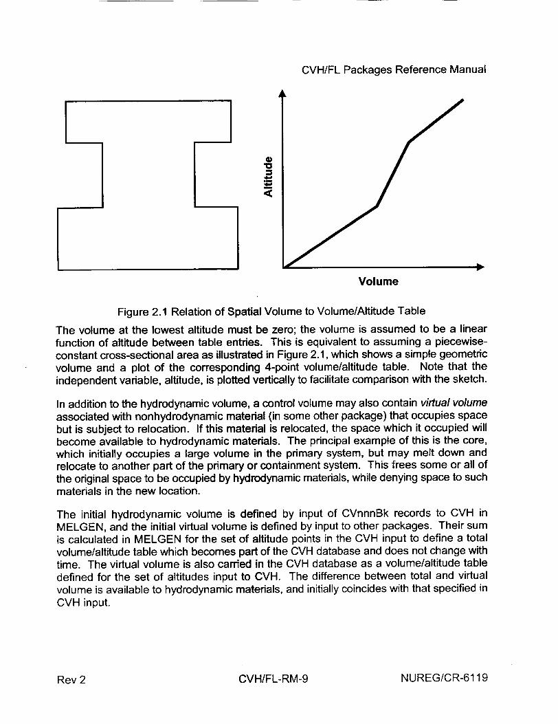
CVH/FL Packages Reference Manual
Volume
Figure 2.1 Relation of Spatial Volume to Volume/Altitude Table
The volume at the lowest altitude must be zero; the volume is assumed to be a linear function of altitude between table entries. This is equivalent to assuming a piecewiseconstant cross-sectional area as illustrated in Figure 2.1, which shows a simple geometric volume and a plot of the corresponding 4-point volume/altitude table. Note that the independent variable, altitude, is plotted vertically to facilitate comparison with the sketch.
In addition to the hydrodynamic volume, a control volume may also contain virtual volume associated with nonhydrodynamic material (in some other package) that occupies space but is subject to relocation. If this material is relocated, the space which it occupied will become available to hydrodynamic materials. The principal example of this is the core, which initially occupies a large volume in the primary system, but may melt down and relocate to another part of the primary or containment system. This frees some or all of the original space to be occupied by hydrodynamic materials, while denying space to such materials in the new location.
The initial hydrodynamic volume is defined by input of CVnnnBk records to CVH in MELGEN, and the initial virtual volume is defined by input to other packages. Their sum is calculated in MELGEN for the set of altitude points in the CVH input to define a total volume/altitude table which becomes part of the CVH database and does not change with time. The virtual volume is also carried in the CVH database as a volume/altitude table defined for the set of altitudes input to CVH. The difference between total and virtual volume is available to hydrodynamic materials, and initially coincides with that specified in CVH input.
NUREG/CR-6119CVH/FL-RM-9Rev 2

CVH/FL Packages Reference Manual
0
Volume
Figure 2.2 Virtual Volume and Associated Volume/Altitude Tables
Virtual volume is illustrated by Figure 2.2, where the total volume is shown in grey and the virtual volume as the white space (i.e., volume on the RHS graph) between the virtual volume and the cell boundary. Note that the points in the virtual-volume/altitude table correspond to the altitudes in the CVH database and not to those in whatever package defined the occupied (shaded) region.
Virtual volume within a control volume is modified as nonhydrodynamic materials are relocated by their controlling packages. In consequence, the hydrodynamic volume is also modified as the space which was occupied by nonhydrodynamic materials becomes available and the space it now occupies is denied to the hydrodynamic materials. The other packages may track the location of their materials in more (or less) detail than is permitted by the set of altitudes recognized by CVH; this has no effect on hydrodynamic calculations.
2.2 Control Volume Contents
The contents of each volume are divided into a so-called pool and an atmosphere. These terms reflect a static, gravitationally separated situation, such as would exist in containment or in a primary system in the absence of strong forced circulation by pumps, and we conventionally depict the pool as occupying the lower portion of the control volume while the atmosphere fills the remainder. However, as discussed later, this picture is not interpreted so narrowly that it invalidates the use of MELCOR hydrodynamics in other situations.
INUREG/CR-6119
I
I
CVH/FL-RM-1 0Rev 2
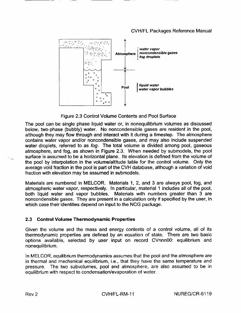
CVH/FL Packages Reference Manual
"water vapor "'Amosphere 4noncondensible gases
I fog droplets
o 0 o o o o0 o0
o 0 e 00 liquid water
Pool water vapor bubbles
o 0
o °0000
Figure 2.3 Control Volume Contents and Pool Surface
The pool can be single phase liquid water or, in nonequilibrium volumes as discussed below, two-phase (bubbly) water. No noncondensible gases are resident in the pool, although they may flow through and interact with it during a timestep. The atmosphere contains water vapor and/or noncondensible gases, and may also include suspended water droplets, referred to as fog. The total volume is divided among pool, gaseous atmosphere, and fog, as shown in Figure 2.3. When needed by submodels, the pool surface is assumed to be a horizontal plane. Its elevation is defined from the volume of the pool by interpolation in the volume/altitude table for the control volume. Only the average void fraction in the pool is part of the CVH database, although a variation of void fraction with elevation may be assumed in submodels.
Materials are numbered in MELCOR. Materials 1, 2, and 3 are always pool, fog, and atmospheric water vapor, respectively. In particular, material 1 includes all of the pool, both liquid water and vapor bubbles. Materials with numbers greater than 3 are noncondensible gases. They are present in a calculation only if specified by the user, in which case their identities depend on input to the NCG package.
2.3 Control Volume Thermodynamic Properties
Given the volume and the mass and energy contents of a control volume, all of its thermodynamic properties are defined by an equation of state. There are two basic options available, selected by user input on record CVnnnOO: equilibrium and nonequilibrium.
In MELCOR, equilibrium thermodynamics assumes that the pool and the atmosphere are in thermal and mechanical equilibrium, i.e., that they have the same temperature and pressure. The two subvolumes, pool and atmosphere, are also assumed to be in equilibrium with respect to condensation/evaporation of water.
NUREG/CR-6119Rev 2 CVH/FL-RM-1 1
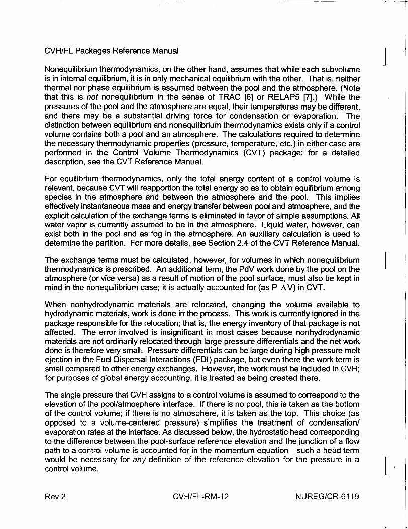
CVH/FL Packages Reference Manual
Nonequilibrium thermodynamics, on the other hand, assumes that while each subvolume is in internal equilibrium, it is in only mechanical equilibrium with the other. That is, neither thermal nor phase equilibrium is assumed between the pool and the atmosphere. (Note that this is not nonequilibrium in the sense of TRAC [6] or RELAP5 [7].) While the pressures of the pool and the atmosphere are equal, their temperatures may be different, and there may be a substantial driving force for condensation or evaporation. The distinction between equilibrium and nonequilibrium thermodynamics exists only if a control volume contains both a pool and an atmosphere. The calculations required to determine the necessary thermodynamic properties (pressure, temperature, etc.) in either case are performed in the Control Volume Thermodynamics (CVT) package; for a detailed description, see the CVT Reference Manual.
For equilibrium thermodynamics, only the total energy content of a control volume is relevant, because CVT will reapportion the total energy so as to obtain equilibrium among species in the atmosphere and between the atmosphere and the pool. This implies effectively instantaneous mass and energy transfer between pool and atmosphere, and the explicit calculation of the exchange terms is eliminated in favor of simple assumptions. All water vapor is currently assumed to be in the atmosphere. Liquid water, however, can exist both in the pool and as fog in the atmosphere. An auxiliary calculation is used to determine the partition. For more details, see Section 2.4 of the CVT Reference Manual.
The exchange terms must be calculated, however, for volumes in which nonequilibriumr thermodynamics is prescribed. An additional term, the PdV work done by the pool on the atmosphere (or vice versa) as a result of motion of the pool surface, must also be kept in mind in the nonequilibrium case; it is actually accounted for (as P AV) in CVT.
When nonhydrodynamic materials are relocated, changing the volume available to hydrodynamic materials, work is done in the process. This work is currently ignored in the package responsible for the relocation; that is, the energy inventory of that package is not affected. The error involved is insignificant in most cases because nonhydrodynamic materials are not ordinarily relocated through large pressure differentials and the net work done is therefore very small. Pressure differentials can be large during high pressure melt ejection in the Fuel Dispersal Interactions (FDI) package, but even there the work term is small compared to other energy exchanges. However, the work must be included in CVH; for purposes of global energy accounting, it is treated as being created there.
The single pressure that CVH assigns to a control volume is assumed to correspond to the elevation of the pool/atmosphere interface. If there is no pool, this is taken as the bottom of the control volume; if there is no atmosphere, it is taken as the top. This choice (as opposed to a volume-centered pressure) simplifies the treatment of condensation/ evaporation rates at the interface. As discussed below, the hydrostatic head corresponding to the difference between the pool-surface reference elevation and the junction of a flow path to a control volume is accounted for in the momentum equation-such a head term would be necessary for any definition of the reference elevation for the pressure in a control volume.I
NUREG/CR-6119Rev 2 CVH/FL-RM-12
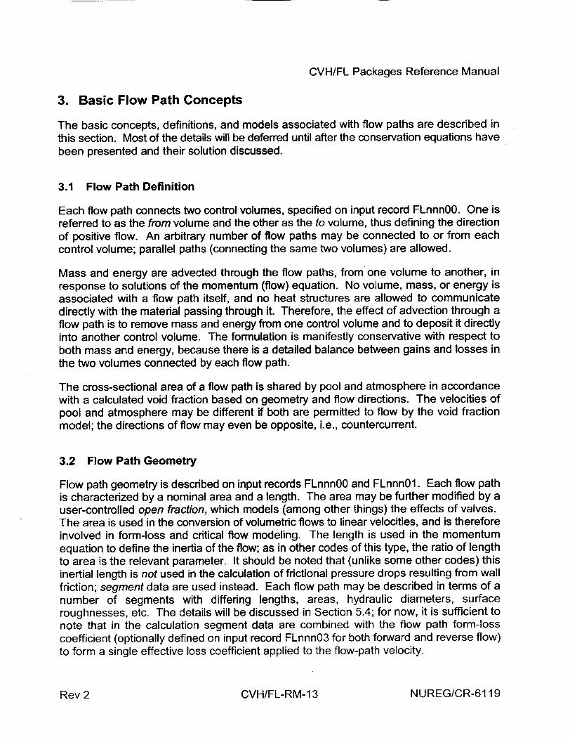
CVH/FL Packages Reference Manual
3. Basic Flow Path Concepts
The basic concepts, definitions, and models associated with flow paths are described in this section. Most of the details will be deferred until after the conservation equations have been presented and their solution discussed.
3.1 Flow Path Definition
Each flow path connects two control volumes, specified on input record FLnnnOO. One is referred to as the from volume and the other as the to volume, thus defining the direction of positive flow. An arbitrary number of flow paths may be connected to or from each control volume; parallel paths (connecting the same two volumes) are allowed.
Mass and energy are advected through the flow paths, from one volume to another, in response to solutions of the momentum (flow) equation. No volume, mass, or energy is associated with a flow path itself, and no heat structures are allowed to communicate directly with the material passing through it. Therefore, the effect of advection through a flow path is to remove mass and energy from one control volume and to deposit it directly into another control volume. The formulation is manifestly conservative with respect to both mass and energy, because there is a detailed balance between gains and losses in the two volumes connected by each flow path.
The cross-sectional area of a flow path is shared by pool and atmosphere in accordance with a calculated void fraction based on geometry and flow directions. The velocities of pool and atmosphere may be different if both are permitted to flow by the void fraction model; the directions of flow may even be opposite, i.e., countercurrent.
3.2 Flow Path Geometry
Flow path geometry is described on input records FLnnnOO and FLnnn01. Each flow path is characterized by a nominal area and a length. The area may be further modified by a user-controlled open fraction, which models (among other things) the effects of valves. The area is used in the conversion of volumetric flows to linear velocities, and is therefore involved in form-loss and critical flow modeling. The length is used in the momentum equation to define the inertia of the flow; as in other codes of this type, the ratio of length to area is the relevant parameter. It should be noted that (unlike some other codes) this inertial length is not used in the calculation of frictional pressure drops resulting from wall friction; segment data are used instead. Each flow path may be described in terms of a number of segments with differing lengths, areas, hydraulic diameters, surface roughnesses, etc. The details will be discussed in Section 5.4; for now, it is sufficient to note that in the calculation segment data are combined with the flow path form-loss coefficient (optionally defined on input record FLnnn03 for both forward and reverse flow) to form a single effective loss coefficient applied to the flow-path velocity.
NUREG/CR-6119Rev 2 CVH/FL-RM-1 3
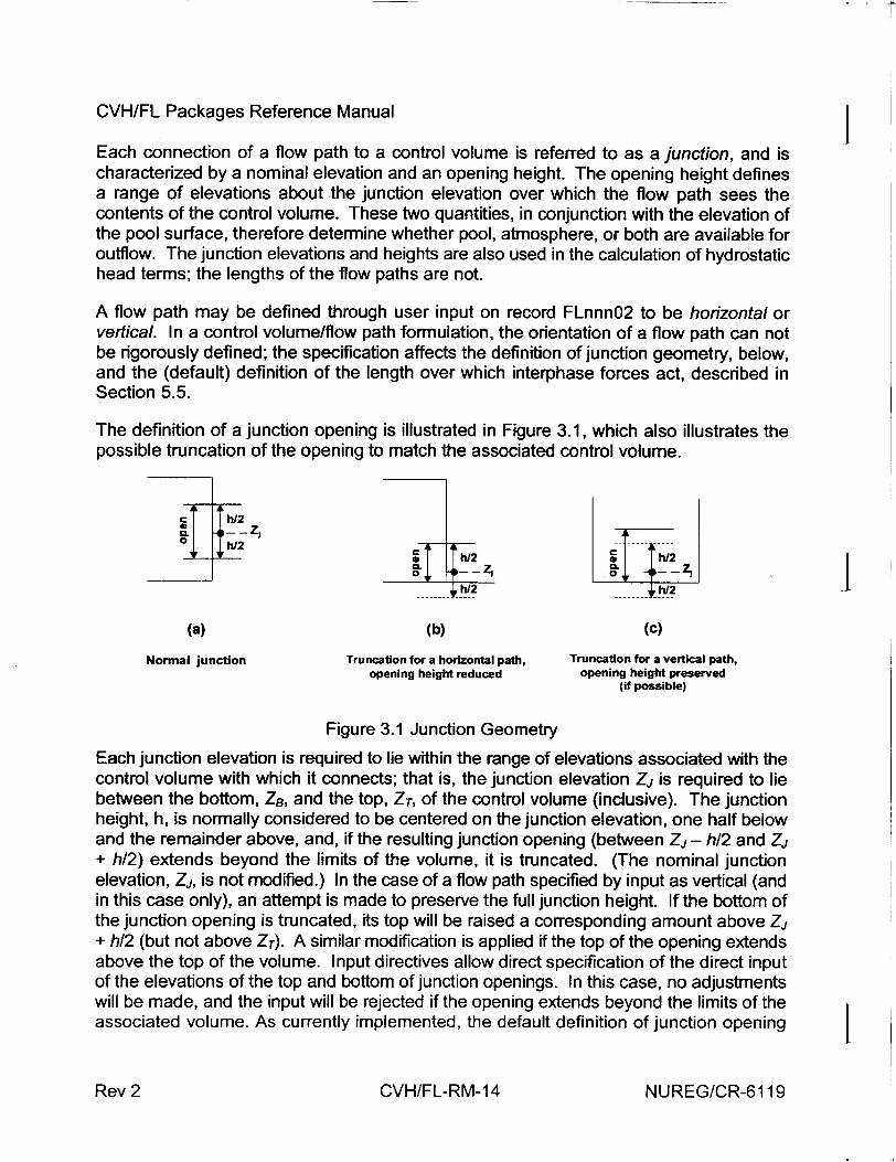
CVH/FL Packages Reference Manual
Each connection of a flow path to a control volume is referred to as a junction, and is characterized by a nominal elevation and an opening height. The opening height defines a range of elevations about the junction elevation over which the flow path sees the contents of the control volume. These two quantities, in conjunction with the elevation of the pool surface, therefore determine whether pool, atmosphere, or both are available for outflow. The junction elevations and heights are also used in the calculation of hydrostatic head terms; the lengths of the flow paths are not.
A flow path may be defined through user input on record FLnnn02 to be horizontal or vertical. In a control volume/flow path formulation, the orientation of a flow path can not be rigorously defined; the specification affects the definition of junction geometry, below, and the (default) definition of the length over which interphase forces act, described in Section 5.5.
The definition of a junction opening is illustrated in Figure 3.1, which also illustrates the possible truncation of the opening to match the associated control volume.
1
h/ C...., 2....• 0..ý
CLC
h/2 h/2
(a) (b) (c)
Normal junction Truncation for a horizontal path, Truncation for a vertical path, opening height reduced opening height preserved
(if possible)
Figure 3.1 Junction Geometry
Each junction elevation is required to lie within the range of elevations associated with the control volume with which it connects; that is, the junction elevation Zj is required to lie between the bottom, ZB, and the top, ZT, of the control volume (inclusive). The junction height, h, is normally considered to be centered on the junction elevation, one half below and the remainder above, and, if the resulting junction opening (between ZI - h12 and Z7 + h12) extends beyond the limits of the volume, it is truncated. (The nominal junction elevation, Zj, is not modified.) In the case of a flow path specified by input as vertical (and in this case only), an attempt is made to preserve the full junction height. If the bottom of the junction opening is truncated, its top will be raised a corresponding amount above Zj + h12 (but not above ZT). A similar modification is applied if the top of the opening extends above the top of the volume. Input directives allow direct specification of the direct input of the elevations of the top and bottom of junction openings. In this case, no adjustments will be made, and the input will be rejected if the opening extends beyond the limits of the associated volume. As currently implemented, the default definition of junction opening
NUREG/CR-6119Rev 2 CVH/FL-RM-14
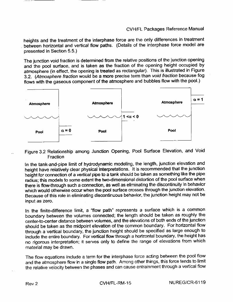
CVH/FL Packages Reference Manual
heights and the treatment of the interphase force are the only differences in treatment between horizontal and vertical flow paths. (Details of the interphase force model are
presented in Section 5.5.)
The junction void fraction is determined from the relative positions of the junction opening
and the pool surface, and is taken as the fraction of the opening height occupied by
atmosphere (in effect, the opening is treated as rectangular). This is illustrated in Figure
3.2. (Atmosphere fraction would be a more precise term than void fraction because fog
flows with the gaseous component of the atmosphere and bubbles flow with the pool.)
Atmosphere Atmosphere Atmosphere
1 <a < 0
Pool a=0 Pool Pool
Figure 3.2 Relationship among Junction Opening, Pool Surface Elevation, and Void Fraction
In the tank-and-pipe limit of hydrodynamic modeling, the length, junction elevation and
height have relatively clear physical interpretations. It is recommended that the junction
height for connection of a vertical pipe to a tank should be taken as something like the pipe
radius; this models to some extent the two-dimensional distortion of the pool surface when
there is flow-through such a connection, as well as eliminating the discontinuity in behavior which would otherwise occur when the pool surface crosses through the junction elevation. Because of this role in eliminating discontinuous behavior, the junction height may not be input as zero.
In the finite-difference limit, a "flow path" represents a surface which is a common
boundary between the volumes connected; the length should be taken as roughly the
center-to-center distance between volumes, and the elevations of both ends of the junction
should be taken as the midpoint elevation of the common boundary. For horizontal flow
through a vertical boundary, the junction height should be specified as large enough to
include the entire boundary. For vertical flow through a horizontal boundary, the height has
no rigorous interpretation; it serves only to define the range of elevations from which
material may be drawn.
The flow equations include a term for the interphase force acting between the pool flow
and the atmosphere flow in a single flow path. Among other things, this force tends to limit
the relative velocity between the phases and can cause entrainment through a vertical flow
NUREG/CR-6119CVH/FL-RM-1 5Rev 2
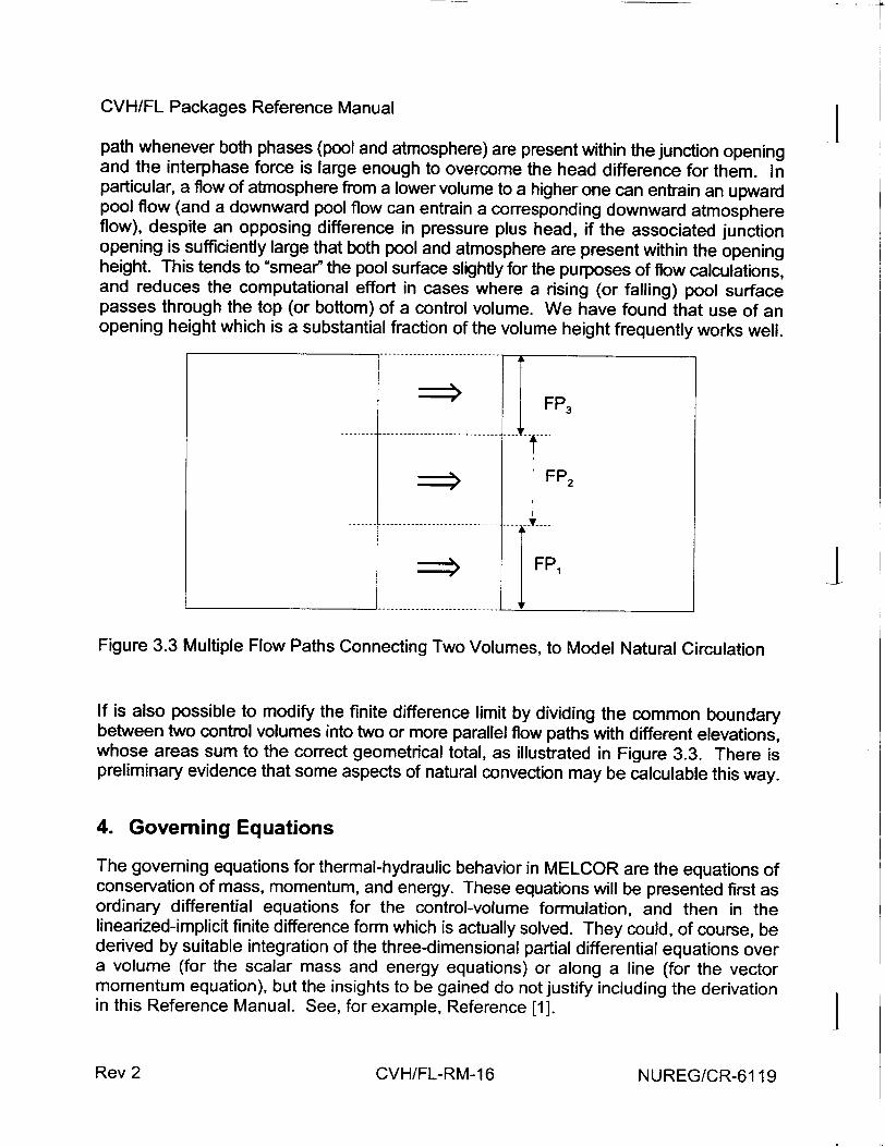
1 � t
CVH/FL Packages Reference Manual j path whenever both phases (pool and atmosphere) are present within the junction opening and the interphase force is large enough to overcome the head difference for them. In particular, a flow of atmosphere from a lower volume to a higher one can entrain an upward pool flow (and a downward pool flow can entrain a corresponding downward atmosphere flow), despite an opposing difference in pressure plus head, if the associated junction opening is sufficiently large that both pool and atmosphere are present within the opening height. This tends to "smear" the pool surface slightly for the purposes of flow calculations, and reduces the computational effort in cases where a rising (or falling) pool surface passes through the top (or bottom) of a control volume. We have found that use of an opening height which is a substantial fraction of the volume height frequently works well.
j FP 3
TFP2
Figure 3.3 Multiple Flow Paths Connecting Two Volumes, to Model Natural Circulation
If is also possible to modify the finite difference limit by dividing the common boundary between two control volumes into two or more parallel flow paths with different elevations, whose areas sum to the correct geometrical total, as illustrated in Figure 3.3. There is preliminary evidence that some aspects of natural convection may be calculable this way.
4. Governing Equations
The governing equations for thermal-hydraulic behavior in MELCOR are the equations of conservation of mass, momentum, and energy. These equations will be presented first as ordinary differential equations for the control-volume formulation, and then in the linearized-implicit finite difference form which is actually solved. They could, of course, be derived by suitable integration of the three-dimensional partial differential equations over a volume (for the scalar mass and energy equations) or along a line (for the vector momentum equation), but the insights to be gained do not justify including the derivation in this Reference Manual. See, for example, Reference [1].
NUREG/CR-6119Rev 2 CVH/FL-RM-16
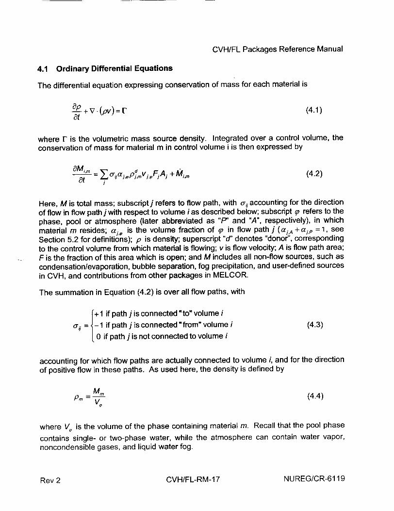
CVH/FL Packages Reference Manual
4.1 Ordinary Differential Equations
The differential equation expressing conservation of mass for each material is
ap+ V- (pv) = r (4.1) at
where r is the volumetric mass source density. Integrated over a control volume, the conservation of mass for material m in control volume i is then expressed by
Mr= I .,Vai,,,p vi.,FjAi +Mi.,, (4.2)
at
Here, M is total mass; subscriptj refers to flow path, with o-, accounting for the direction of flow in flow path j with respect to volume i as described below; subscript (P refers to the phase, pool or atmosphere (later abbreviated as "Pl" and "A", respectively), in which
material m resides; aj,, is the volume fraction of 9 in flow path j (aiA + a,, = 1, see
Section 5.2 for definitions); p is density; superscript "d" denotes "donor", corresponding to the control volume from which material is flowing; v is flow velocity; A is flow path area;
F is the fraction of this area which is open; and M includes all non-flow sources, such as condensation/evaporation, bubble separation, fog precipitation, and user-defined sources in CVH, and contributions from other packages in MELCOR.
The summation in Equation (4.2) is over all flow paths, with
+_1 if path j is connected "to" volume i
-= if path j is connected "from" volume i (4.3)
0 if path j is not connected to volume i
accounting for which flow paths are actually connected to volume i, and for the direction of positive flow in these paths. As used here, the density is defined by
Pm- (4.4)
1P~V
where V, is the volume of the phase containing material m. Recall that the pool phase
contains single- or two-phase water, while the atmosphere can contain water vapor, noncondensible gases, and liquid water fog.
NUREG/CR-6119Rev 2 CVH/FL-RM-1 7
I - __
CVH/FL Packages Reference Manual
The equations expressing conservation of energy in the pool and in the atmosphere are derived similarly from the partial differential equations, neglecting all gravitational potential energy and volume-average kinetic energy terms. Conservation of energy in phase (P (pool or atmosphere) is then expressed by
E,,p = I Pdmhd.VFA + (4.5)
at J.J i l ,}J,~
where E is total internal energy; m in the second summation runs over all materials in phase (p; h is the specific enthalpy (the difference between h and the specific internal energy, e, accounts for flow work); and H is the non-flow energy source, including the enthalpy of all relevant mass sources in Equation (4.2).
Finally, the equations for pool flow and for atmosphere flow in a flow path are obtained from line integrals of the acceleration equations along a stream line from the center of the from volume to the center of the to volume. The temporal rate of change of the void fraction, aa & at, is neglected. The results (in nonconservative form) are expressed by
or. P. L yL-- =a (PI-Pk)+a (p gAz), 9, + a, AP(4.6)
-- 1K. aP ,,v ,,v. -a,,,a j.Pf 2.L 2.i vi - V.)q 2 "
+ appv (Av0.
where Lj is the inertial length of the flow path; i and k are the "from" and "to" control volumes, respectively, for flow path ]; g is the acceleration of gravity; APj represents any
pump head developed in the flow path; K* is the net form- and wall-loss coefficient; fI, is the interphase force (momentum exchange) coefficient; L2j is the effective length over which the interphase force acts (not necessarily equal to the inertial length, see Section 5.5); (Av)j,, represents the change in velocity through the flow path (the "momentum flux"); and - q denotes the "other" phase relative to rp (atmosphere if op is pool and vice versa).
Unless a phase is present within at least one of the junction openings associated with a flow path, flow of that phase through that path is impossible and the corresponding flow equation (Equation (4.6)) need not be solved; vjq, is simply set to zero.
The density of a phase in a flow path is ordinarily taken as the density in the donor volume; the phase densities are evaluated from Equation (4.4), with a summation over the materials in the atmosphere. In general, the set of flow equations must be solved iteratively (see
NUREG/CR-6119Rev 2 CVH/FL-RM-1 8
CVH/FL Packages Reference Manual
Section 4.2) with "donor" redefined, if necessary for each iteration. If a phase is present within only one of the junction openings, so that flow of that phase within that flow path is only possible in one direction, the donor density is taken as that in the only possible donor volume.
The redefinition of a flow path density between iterations as a result of reversal of the associated flow introduces a discontinuity in the equations. We have observed that this can prevent convergence of the solution under some conditions. Therefore, the nextiterate flow path density is taken as
p(i) =f i-l)+0- d
= f9 9(1-fm (4.7)
For the first third of the permitted total number of iterations, f is taken as zero, resulting in use of a pure donor density. If further iterations are required, f is increased linearly from zero to one for the next third of the permitted total number, introducing an increasing degree of averaging into the definition of density. Finally, f is taken as one for the last third of the iterations (if such are required), totally eliminating the numerical discontinuity.
The gravitational head term and the loss term are each somewhat complicated, and will be discussed in detail in Sections 5.3 and 5.4, respectively. The accounting for interphase forces represented by f2j is described in Section 5.5, and the models available for the pump head are presented in Section 5.6. Note that, as written, the volume fraction, a,, cancels
identically in the equation.
The last term in Equation (4.6), v.,,(Av)j•,, represents the advection of momentum through
the flow path, and arises from integration of the term v(av / ax) in the continuum equations. The formulation presented here is essentially one-dimensional; in more general geometry, v in Equation (4.6) may be interpreted as the velocity component in the direction of flow (denoted by "x"); however, the treatment will be incomplete because the cross terms arising from vy (avx /a,) are not included in the equations.
By default, even the diagonal momentum flux term in Equation (4.6) is neglected in the solution of the hydrodynamic equations in MELCOR. This is consistent with omission of the kinetic energy in Equation (4.5). These terms (momentum flux and kinetic energy) have traditionally been sources of difficulty in control volume codes because they involve a volume-centered velocity, which requires a multi-dimensional formulation for proper definition. (Note that codes such as RELAP5 [7] make very specific geometric assumptions concerning the relationship between control volumes and flow paths.) The neglected terms in both equations are of order Ma , where Ma is the Mach number based on volume-centered velocities, and are ordinarily small (although they may be important for flow boiling with large density gradients). Velocities in flow paths may be sonic or near sonic, but constancy of h + 1/ 2v 2 for adiabatic (not necessarily isentropic) flow assures
NUREG/CR-6119Rev 2 CVH/FL-RM-19
CVH/FL Packages Reference Manual
that only volume-centered velocities appear in the equations. Choking is treated as an imposed limit on flows based on correlations (see Section 6.4). In any case, consistent inclusion of the v2 terms would require a proper definition of a volume-centered velocity, including multidimensional effects, and it is clear that this can be done in anything but a full finite difference code (see Section (6.5)). In most cases, no difficulties will arise if MELCOR pressures and enthalpies are considered to be stagnation pressures and stagnation enthalpies.
4.2 Finite Difference Equations
The ordinary differential equations presented in Section 4.1 are converted to linearizedimplicit finite difference equations for solution in MELCOR.
For each timestep, At, the new (end-of-step) velocities are used in the advection (flow) terms in the mass and energy equations to write
Mi", M' ia'p ? - At M
Si J. JV.FAjAt + -I'm (4.8)
E=,.7= E},F + iija pd h dnj.FAjAt +SH, (4.9)
where superscripts n and o refer to the new and old time levels, respectively; and bM and
SH are the net external sources (integrals from to to to + At).
The time levels on the donor properties are not explicitly shown in Equations (4.8) and
(4.9); they are essentially old values (at to), but see the further discussion in Section 4.4.
It is clear that this formulation is conservative with respect to both masses and internal energies because every term representing a flow transfer from a volume is exactly balanced by a transfer to the volume at the other end of the flow path. Therefore, masses and energies are conserved to within the accumulation of roundoff on the computer used.
In the interest of numerical stability, linearized-implicit ("semi-implicit") differencing is used in several terms in the momentum equation (Equation (4.6)). Specifically, the equation is differenced using projected end-of-step pressures and heads in the acceleration terms, and end-of-step velocities in the frictional loss and momentum exchange terms. Because of the nonlinearity of the frictional loss term, the resulting finite difference equation must be solved iteratively. (Because of nonlinearity of the equation of state used to project the end-of-step pressures, a further iteration may be required. We will return to this in Section 4.3.) We will first discuss the treatment of velocities and then define and discuss the other terms in the finite difference equation. [
NUREG/CR-6119CVH/FL-RM-20Rev 2
CVH/FL Packages Reference Manual
At each velocity iteration, the form- and wall-loss term is linearized about the best available estimate of vn, denoted v- (this is initially V'), to obtain the finite difference equation for the estimated new, end-of-step velocity:
nv , L+(p gAz), + v,(pAv)O
____ o f L v o (4.10) __ __ + vP; -+ v A v, - 2, 2L7 j pA•,L
- J9A V -+V, J~ f, ai- ,,2j2~ n_ _n__(4.10)
The nature of the linearization in velocity is determined by the choice of V'. For the first iteration, v' is taken as v", giving a tangent (Taylor series) linearization. For later iterations, it is taken as vP- from the previous iteration if the velocity did not reverse during that iteration, or as zero otherwise. The result is to approximate vNby the secant from the latest iterate through the next oldest iterate or by the secant through the origin, respectively. Note that the interphase force term is fully implicit with respect to velocities, and that the length over which this force acts, L2j, may differ from the inertial length of the flow path, Li. See discussion for definition of P5.
The superscript "o+" on the velocity on the right-hand side of Equation (4.10) indicates that it has been modified from the old value to account for changes in the flow-path void fraction, as discussed below. This was found necessary to prevent initiation of a nonphysical transient whenever the motion of a pool surface through a small junction opening produced a major change in void fraction during a single timestep.
The problem is that the old velocities, V/, were computed with the old void fraction, a0 ; with a , they may correspond to a quite different flow state, both in mass flow and in total volumetric flow. This may require large accelerations (and pressure differentials) to maintain the "correct" flow. The cause is, in part, that the time derivative of the void fraction does not appear in the momentum equation. (There are no further problems involving the time level of data on which a is based, and the fact that its treatment is not numerically implicit.)
The definition of "void fraction" in MELCOR is necessarily much more complicated than in a simple fine-zoned finite difference code, and an attempt to include aa /Iat in the momentum equation seemed unlikely to be productive. Therefore, we have chosen to employ an ad hoc modification of the "old" velocities to account for changes in void fractions. (Sensitivity coefficient 4408 may be used to disable this modification.) The criteria used are preservation of the total volumetric flux, expressed by
aoA v' + aopv" =a' + ° (4.11) 1.~v° +, aJ~,. =- ajAViA + aj. Vjp
NUREG/CR-6119Rev 2 CVH/FL-RM-21
CVH/FL Packages Reference Manual
and preservation of the relative velocity between the phases, expressed by
0.+ - , 0.+ = V 0. V 0 (.2 °A °* ° ° (4.12)
SA jp P jP
This results in
v? =Vo+(a -a n )V-Vo o) (4.13) V- j4•=V,• jA4- •jA j.A -Vjp,
It is interesting to note that there is an analogous relationship implicit in drift-flux codes. In such codes, the total mass flux (momentum density) is determined by a single momentum equation for each flow path, and a constitutive relation (the drift flux correlation) is then used to partition this flux into liquid and vapor components as a function of void fraction. Thus, when a new void fraction is computed at the start of a timestep, the total mass flux is preserved but the individual phase velocities and the total volumetric flux are not. MELCOR calculations more often involve quasi-steady flows than pressure waves; therefore, preservation of the volumetric flow rather than the momentum density (mass flux) was chosen as the default treatment. (Note that there is no way that both the mass fluxes and volumetric flows could be preserved as the void fraction changes.) J As noted previously, the momentum flux term, v(p Av) in Equation (4.10), will be omitted
by default. We have found no need for implicit treatment of this term if it is included; therefore, start-of-step velocities are used in its evaluation. If the term is to be included in the momentum equation for flow path j, the user is required to specify on input record FLnnnMx the flow paths that are logically upstream and downstream from flow path j, as described in the FL Users' Guide. The specification of "no such flow path" is permitted, to allow treatment of a flow path connected to a dead-end volume or to one with no other appropriately oriented connection.
The term (p Av), representing a spatial difference in momentum density, is treated as a donored quantity. It is evaluated based on the direction of flow through flow path j, as
F A V4 _j Fj AV Vo > 0
(P AV), = o Ak (4.14) SFjAyjvo Fj+_Aj, vj+,• o
Pkj. A+~~q V 0 < 0 1 • Ai Ak • vjAP <
Here, subscripts i and k denote the donor and acceptor volumes, respectively; Ai and Ak
are the corresponding user-defined flow areas for these volumes in the direction of flow INUREG/CR-6119CVH/FL-RM-22Rev 2
CVH/FL Packages Reference Manual
appropriate to flow path j; and subscripts j- and j+ refer to the designated flow paths that are logically upstream and down stream of j, and must connect to volumes i and k, respectively.
The area ratios in Equation (4.14) serve to convert the momentum density in each flow path to corresponding densities at the volume center, under the assumption of incompressible flow. The volume areas, which may differ from those used in the control volume velocity calculation, must be specified by the user on record FLnnnMk. This allows more accurate description of the actual flow geometry. For example, most of the momentum of a small jet entering a large room will be dissipated close to the point of entry, leaving little momentum to be advected through a second flow path and, in general, this effect will be captured through the ratio of the small flow path area to the large volume area. However, if the two flow paths are closely aligned, so that a fluid jet from one will be captured by the other, the user may capture the effect by specifying a volume flow area appropriate for the jet.
If either flow path j- orj+ is absent (as defined by user input), the corresponding term in Equation (4.14) is neglected, which is equivalent to setting the associated flow path area to zero.
As noted previously, the pressures, P5, used in the acceleration terms in Equation (4.10) are predicted end-of-step pressures; they are calculated from the linearization of the equation of state about a reference point (denoted by "*") as
P,• = Pi" + Z-ý (M -M ,
"*m (Em (4.15) + ci" (E. - Ei-p + api'' (E,, aEp-i-P aEA - iEs
The choice of the linearization point will be discussed in detail in Section 4.3.
The static head terms, (p gAz);, are also predicted values at end-of-step. However, only
changes in pool mass and hydrodynamic volume are included in the projection, with changes in atmosphere mass and phase densities neglected. Specifically,
(p gAz)n = (p gAz)o + ( .9 -MO i9-9 aM i p 'P i. (4.16)
alp gAz) ( - MO. aMkPP
NUREG/CR-6119CVH/FL-RM-23Rev 2
CVH/FL Packages Reference Manual J In this equation M" is the mass of pool which can be accommodated below the former
elevation of the pool surface at the old pool density. It differs from M;". only if there has
been a change in the volume/altitude table resulting from a change of virtual volume in control volume i. In this case, the difference accounts for the change in pool surface elevation-and therefore in static head-in the absence of a change in pool mass.
The new masses and new energies in Equations (4.15) and (4.16) are given by Equations (4.8) and (4.9), respectively. The derivatives aP / aM and aP / aE are calculated by the CVT package, and represent the linearized effect of changing mass and energy contents of the control volumes. See the CVT Reference Manual for further details. The derivatives a(p gAz)IaM reflect the linearized effect of changing pool mass on the flow-path head terms; they are defined in Section 5.3.
When all terms associated with each flow are collected together for a given volume, the projected new pressure in Equation (4.15) has the form
SaP
Pa = t5, + Z -L-. a , F., A.v.,At (4.17)
w here 6
m .. i. (4.18)
-i- aE ,A i'A
Mirn =M; + 5M. (4.19)
Etq = E'., + &H,.,, (4.20)
and
api aP d aP d + ph (4.21) a Vs ami'-m,, as,,+•-fj,, ) aE,--A
Here "S" is used as an abbreviation for "s,V' ", and
(p h)., - _. m h '.n.M (4.22) m in•
NUREG/CR-6119Rev 2 CVH/FL-RM-24

CVH/FL Packages Reference Manual
Because donor densities are used in the advection terms, they appear in the definition of aP1/8V in Equations (4.21) and (4.22). Therefore, aP/ aV depends on the direction of flow. In general, if s, V/ represents a pool (atmosphere) flow, only the pool (atmosphere)
energy and materials will be associated with non-zero densities in the evaluation of aPi / aV,.,. However, the code is written with the greater generality of allowing atmosphere
(pool) materials to be associated with pool (atmosphere) flows, and different donor density arrays are used to describe flows entering and leaving a flow path. This allows some interactions to be treated as occurring within a flow path. This capability is currently used in conjunction with the SPARC model, as described in Section 6.1.
Substitution of the predicted pressures and heads into the velocity equation leads to a set of linear equations to be solved for the new velocities:
nKt- + a1.4f zjLzjAtv" _ a._Jf2,jL2 JAt n 2L ') `9 pL
+ • C(jqp: SVI):n s.4v
0+ J9 ( ++At _( ,- ,k) 2L- pj.Ljj
c30, MO+j. (4.23)
+ a(. kp gAZ`)j,. (Aý,p - MO,+ )
?MkP kM k,
The summation on the left-hand side is over both phases, V/, in all flow paths, s, although
only those paths which connect either to volume i or to volume k contribute, as will be seen below. The coefficients in the sum are given by
NUREG/CR-6119CVH/FL-RM-25Rev 2

CVH/FL Packages Reference Manual
(At)2
_p_ , a(P gAz)jq, S- (4.24)
Sapk ,ac5(p g4z)j.•, } + a. av-- + P aMkP
where
=i '. (4.25)
by the Kronecker delta. Because of the appearance of o-;i and o-ks, the coefficient given
by Equation (4.24) is non-zero only for flow paths which connect to volume i or to volume k; because of the appearance of .5,, the head term appears only in cases where s, V is
a pool flow. _
Equation (4.24) could be made somewhat more compact by obtaining the two sets of terms on the right (for volumes i and k ) from a sum over all volumes with appropriate coefficients to pick out the desired terms with the correct signs and eliminate the contributions of all others. However, this would only further conceal the essential point that two flows are coupled by the matrix if and only if there is a volume to which both connect, allowing each flow to affect the pressure differential driving the other.
As mentioned previously, the nonlinearity of the loss (friction) terms and the possibility of flow reversals affecting donor quantities require that the solution of the set of linear Equations (4.23) be repeated until all the new velocities have converged. The control of this iteration is described in Section 4.3.
4.2.1 Inclusion of Bubble-Separation Terms within the Implicit Formulation
To this point, only the contribution of advection terms has been treated within a numerically implicit formulation. The effects of all sources were included in the WM and &H terms in Equations (4.8) and (4.9), which are then treated explicitly. These sources were considered to include several processes that could transfer mass and energy between the pool and atmosphere of a single volume within CHV: condensation/evaporation, bubble separation, and fog deposition. Experience has shown that inclusion of the effects of bubble separation as part of the explicit sources could lead to severe numerical instabilities, particularly in problems involving boiling pools at low pressures. One problem is that the I
NUREG/CR-6119CVH/FL-RM-26Rev 2

CVH/FL Packages Reference Manual
resulting large oscillations in the calculated elevation of the pool surface resulting from large oscillations in the calculated void (bubble) fraction in the pool can have a significant impact on heat transfer in the COR and HS packages. This was identified as a deficiency in the FLECHT SEASET assessment calculations [8].
The finite difference equations were modified in MELCOR 1.8.3 and later versions to include the transfer of vapor mass and energy from the pool to the atmosphere of a control volume within the implicit formulation. Because bubble separation is an intravolume process, its effects may be included along with those of the equation of state in defining a generalized form of Equation (4.15) in which bubble separation is included implicitly, and then eliminated algebraically before proceeding with the solution. The effect is to define net derivatives that include the linearized effect of bubble separation.
The rates of separation of mass and energy by bubbles are primarily functions of the pool void fraction, a, and geometry, and the fact that the observed problems arise from instability in the calculated pool void fraction. We therefore linearize the bubble separation terms within volume i with respect to the pool void fraction in that volume as
&Msj = ±M.+ -+ (4.26)
h ) -a') (4.27)
where 6M* and 8H" are evaluated using the pool void fraction at the linearization point,
a*, and a" is the projected end-of-step pool void fraction. (The details of the bubble separation model itself will be presented in Section 5.1.3.)
The pool void fraction is a natural function of the specific enthalpy of the pool and the enthalpies of saturated liquid and vapor, and may therefore be considered as a function of the total pool mass, the total pool energy, and the control volume pressure. In response to a variation in these quantities, the change in a is
aa i i d,,-dM hvdRA) 'a'ct. -= dM. , -afEp hpi (4.28)
where the primes denote changes in addition to bubble separation, i.e., other sources and advection. Using the same convention, the linearization of the volume pressure (from which Equation (4.15) was derived) becomes
NUREG/CR-6119CVH/FL-RM-27Rev 2
CVH/FL Packages Reference Manual j dPP," (dM'-,5 dMa,5 dM
i'm o m (4.29)
+ a (dE - h dM,) +aP,- (dE., A+ hvdMs4 ) aEi ' "+ ,.A
Equation Error! Reference source not found. can be used to eliminate dMBJ from
Equations (4.28) and (4.29), and the resulting equations solved for a0, and aai as linear functions of the variables WM, and aE.. The results take the form
dP1 = m," dM' + dE',, + -L- dE' (4.30)
aa 0& aa; da,= dMW' + dE' + - dE:"A (4.31)
ig,'n aSE• ' aE•,"
Here the modified pressure derivatives are J
am," c 0a, amP, am," Ia am," ax .ame aX ame aX a 1Xi" a~0MBPJX )At (4.32) OX' 1-f Ca' +a, O
0MB,, 00, aMB,,
where dX' represents any of the variables dM, and aEv,, and
a -i•aM,. h, a'i (4.33)
Mg, k---OM. 3 +hv -- A 1 +h, -- (4.34)
are convenient combinations of the derivatives in Equations (4.28) and (4.29).
The momentum equation is constructed and solved as before, but now using Equation (4.30) to project the new pressures. The only differences that result are that the derivatives I
NUREG/CR-6119Rev 2 CVH/FL-RM-28

CVH/FL Packages Reference Manual
aP /aX' appear in Equations (4.18) and (4.21) rather than aP* laX, and that only 9M and 5H" from Equations (4.26) and Error! Reference source not found. are included in the source terms in Equations Error! Reference source not found. and (4.20). During the solution, any change in bubble separation will be implicitly included by virtue of the modified pressure derivatives.
Once the new velocities are determined, the contribution of advection to new mass and energy inventories (the sums over flow paths in Equations (4.8) and (4.9)) is determined as before. The additional mass and energy transfers resulting from the implicit change in bubble separation in Equations (4.26) and Error! Reference source not found. must also be included-in addition to AM and SI-/-in defining the new mass and energy inventories in Equations (4.8) and (4.9). Once the contribution of advection has been determined, the contribution of implicit bubble separation is evaluated from
o a.* ++ 6 -a (A M +M im
i.p
+aa&i (f,A + (Hi.A. 8d, -E*A aEp ,,
where the derivatives of the pool void fraction are given by
aa, + aa, aF'" aa, ax aP, ax ax'- c ( aa:+ aa, aP" >At (4.36)
SaM-- aP- aM-)
in analogy with Equation (4.32), with the understanding that a" ! aX is zero unless X is M1 or Ep.
4.3 Solution Strategy
As written, Equation (4.23) represents a set of linear equations for the latest estimates of the new velocities, v,.", and is solved by use of a standard linear equation solver. The complete solution procedure, however, is iterative on two levels. As already mentioned, the code requires convergence of the velocity field, so that the velocities v;.A, used in the loss terms in Equation (4.23) are acceptably close to the new velocities v;i,, found by
NUREG/CR-6119Rev 2 CVH/FL-RM-29
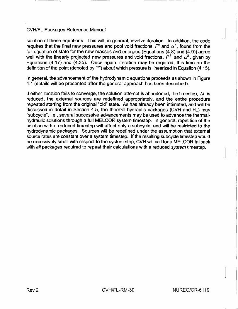
CVH/FL Packages Reference Manual 4 solution of these equations. This will, in general, involve iteration. In addition, the code requires that the final new pressures and pool void fractions, P2 and a", found from the full equation of state for the new masses and energies (Equations (4.8) and (4.9)) agree well with the linearly projected new pressures and void fractions, P;5 and an, given by Equations (4.17) and (4.35). Once again, iteration may be required, this time on the definition of the point (denoted by "*") about which pressure is linearized in Equation (4.15).
In general, the advancement of the hydrodynamic equations proceeds as shown in Figure 4.1 (details will be presented after the general approach has been described).
If either iteration fails to converge, the solution attempt is abandoned, the timestep, At is reduced, the external sources are redefined appropriately, and the entire procedure repeated starting from the original "old" state. As has already been intimated, and will be discussed in detail in Section 4.5, the thermal-hydraulic packages (CVH and FL) may "subcycle", i.e., several successive advancements may be used to advance the thermalhydraulic solutions through a full MELCOR system timestep. In general, repetition of the solution with a reduced timestep will affect only a subcycle, and will be restricted to the hydrodynamic packages. Sources will be redefined under the assumption that external source rates are constant over a system timestep. If the resulting subcycle timestep would be excessively small with respect to the system step, CVH will call for a MELCOR fallback with all packages required to repeat their calculations with a reduced system timestep.
INUREG/CR-6119Rev 2 CVH/FL-RM-30
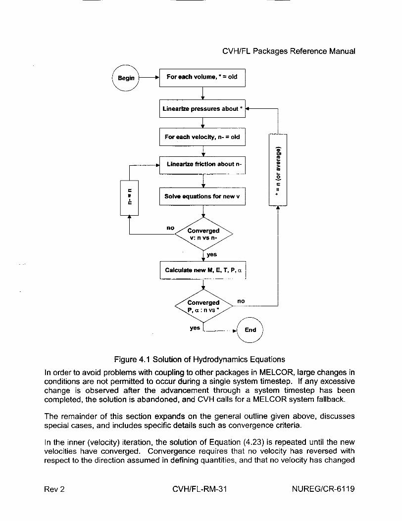
CVH/FL Packages Reference Manual
Begin [
Figure 4.1 Solution of Hydrodynamics Equations
In order to avoid problems with coupling to other packages in MELCOR, large changes in conditions are not permitted to occur during a single system timestep. If any excessive change is observed after the advancement through a system timestep has been completed, the solution is abandoned, and CVH calls for a MELCOR system fallback.
The remainder of this section expands on the general outline given above, discusses special cases, and includes specific details such as convergence criteria.
In the inner (velocity) iteration, the solution of Equation (4.23) is repeated until the new velocities have converged. Convergence requires that no velocity has reversed with respect to the direction assumed in defining quantities, and that no velocity has changed
NUREG/CR-6119Rev 2 CVH/FL-RM-31
CVH/FL Packages Reference Manual 4 in magnitude by more than 9% compared to the value that was used in linearizing the friction terms. (The latter criterion is coded using an absolute tolerance and a relative tolerance included as sensitivity coefficients in array C4401.) Note that the relatively loose tolerance on magnitudes affects only friction terms; conservation of mass and energy is assured by the form of the equations. Our experience has shown that tightening the convergence criterion affects only the details of very rapid transients, which are of little significance in typical MELCOR calculations.
At each iteration, the friction terms are updated, replacing the velocity, Vn-, about which they are linearized by the latest iterate, vn, for flows which have not converged. If one or more of the new velocities has reversed with respect to the direction assumed in defining donor quantities, these quantities are also redefined to reflect the correct flow direction. If there are no flow reversals, new velocities will also be accepted if the corresponding volumetric flows have converged (subject to the same tolerances), starting with the second iteration. The user may also require that after a number of iterations specified by sensitivity coefficient C4401 (4) new velocities will be accepted-even if they have not converged to
the stated tolerance-if the projected new pressures, P1, have converged within 0.05% (comparing successive velocity iterations). The current default is not to accept convergence on this basis.
In some cases, a phase (pool or atmosphere) is available within the junction opening height at only one end of a flow path, and its flow is therefore possible in one direction only. If the donoring assumed in construction of Equation (4.23) makes such a flow
"impossible," the corresponding momentum equation is still carried as part of the equation set, but with its coupling to predicted new pressures eliminated by setting the contribution to new mass and energy inventories to zero in Equations (4.8) and (4.9). Therefore, a calculated "impossible" flow has no effect on "real" flows, but its sign indicates the direction the flow would take (if possible) in response to projected end-of-step pressures. If the sign indicates that the calculated new flow remains impossible, the flow will be set to zero. If the sign is reversed-and the flow is therefore possible-the equations must be re-solved with the assumed donor definition reversed.
If the iteration fails (either by exceeding the permitted number of iterations, or by entering an invalid region of the equation of state defined by the CVT package), the entire set of equations is reformulated with a shorter timestep and re-solved. In general, this is handled within the CVH/FL package by subcycling, rather than by calling for a fallback and a reduction of the MELCOR timestep.
After the new velocities are determined (by convergence of the iterative solution to the finite difference equations), they are used to update the masses and energies in the control volumes through Equations (4.8) and (4.9); in the process, the masses moved by flows are limited to the contents of the donor control volumes. While the mass, momentum, and energy equations could be solved simultaneously, this procedure assures that mass and energy are conserved as accurately as possible. Final end-of-step pressures and pool void j
NUREG/CR-6119Rev 2 CVH/FL-RM-32
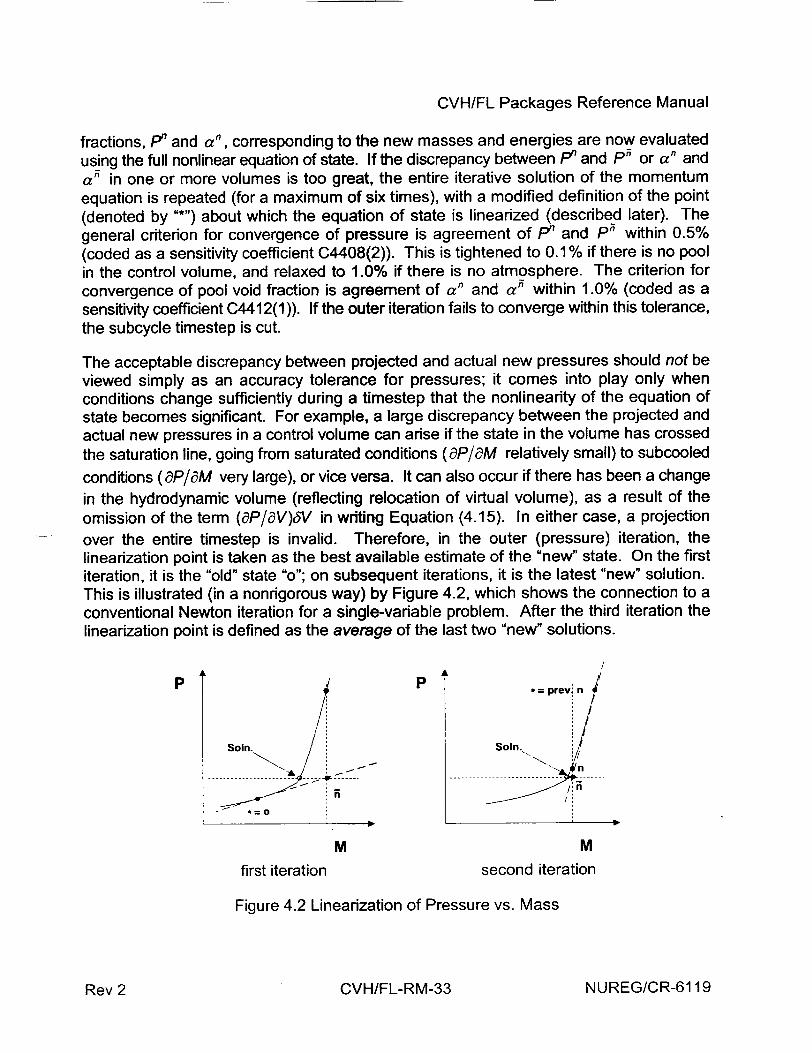
CVH/FL Packages Reference Manual
fractions, P" and a", corresponding to the new masses and energies are now evaluated using the full nonlinear equation of state. If the discrepancy between P" and P5 or a" and a" in one or more volumes is too great, the entire iterative solution of the momentum equation is repeated (for a maximum of six times), with a modified definition of the point (denoted by "*") about which the equation of state is linearized (described later). The general criterion for convergence of pressure is agreement of p" and Pi within 0.5% (coded as a sensitivity coefficient C4408(2)). This is tightened to 0.1 % if there is no pool in the control volume, and relaxed to 1.0% if there is no atmosphere. The criterion for convergence of pool void fraction is agreement of a' and aii within 1.0% (coded as a sensitivity coefficient C4412(1)). If the outer iteration fails to converge within this tolerance, the subcycle timestep is cut.
The acceptable discrepancy between projected and actual new pressures should not be viewed simply as an accuracy tolerance for pressures; it comes into play only when conditions change sufficiently during a timestep that the nonlinearity of the equation of state becomes significant. For example, a large discrepancy between the projected and actual new pressures in a control volume can arise if the state in the volume has crossed the saturation line, going from saturated conditions (aPaM relatively small) to subcooled
conditions (aP/aM very large), or vice versa. It can also occur if there has been a change
in the hydrodynamic volume (reflecting relocation of virtual volume), as a result of the omission of the term (aP/aV)SV in writing Equation (4.15). In either case, a projection
over the entire timestep is invalid. Therefore, in the outer (pressure) iteration, the linearization point is taken as the best available estimate of the "new" state. On the first iteration, it is the "old" state "o"; on subsequent iterations, it is the latest "new" solution. This is illustrated (in a nonrigorous way) by Figure 4.2, which shows the connection to a conventional Newton iteration for a single-variable problem. After the third iteration the linearization point is defined as the average of the last two "new" solutions.
P P prev; n
Soln. Soln.
n
M M
first iteration second iteration
Figure 4.2 Linearization of Pressure vs. Mass
NUREG/CR-6119Rev 2 CVH/FL-RM-33
I - __4
CVH/FL Packages Reference Manual
There is a slight subtlety in the redefinition of the linearization point because the PdV work done by the pool on the atmosphere (or vice versa) in a nonequilibrium volume is calculated in CVT rather than in CVH (note that it does not appear in Equation (4.9)).
W = p•(V. -_Vn) (4.37)
based on the old (start-of-step) volume, will be transferred from the atmosphere to the pool in CVT. Therefore, if the new results returned by CVT are M",, t:,, and Pi', and that solution is rejected, the work must be subtracted from these results to define conditions about which the equations may be linearized. That is, if a solution is rejected, the new linearization point is taken as
M*, =Mn
E;, = E. -P(V-V) (4.38)
E, =E7, + P,o(v,' - v)
where n denotes the "new" solution returned by CVT. The essential point is that if M", En, and V' are sent as nonequilibrium arguments to CVT, an additional PdV work term will be computed, and the pressure and volumes returned will not be Pn and V . If, on the other hand, the arguments sent to CVT are M, E*, and V/, the work computed there will balance that subtracted off Equation (4.38), and the desired values, P" and V1, will be returned.
Note that the choice of the point * should have little effect on the results obtained (if the solution is successful) because, while the predicted new (end-of-step) pressures are used in the flow equation, they are required by the convergence criteria described earlier to agree well with the actual new pressures. Any small variations in the predictions can have only a modest effect on the results. Therefore, the primary effect of the choice of the point * is on the success of the solution procedure; a poor choice can slow or even prevent convergence.
After the thermal-hydraulic state of the system has been advanced through a MELCOR system timestep, which may involve convergence of the entire calculation described above for several CVH subcycles, the new pressures and temperatures in all control volumes are examined to determine if the changes from old values are acceptably small. The criteria are less than 10% change in pressure and less than 20% plus 1 K change in the temperature of each phase containing more than 1 % of the mass in the control volume. These are coded as sensitivity coefficients included in the array C4400. If any change exceeds that permitted, a fallback is requested and the calculation repeated with a reduced MELCOR system timestep.
INUREG/CR-6119Rev 2 CVH/FL-RM-34

CVH/FL Packages Reference Manual
4.4 Definition of Donor Quantities
The preceding discussion concerns only the finite-difference equations and the solution technique. The definition of the donor densities and enthalpies, p0 and hd, in the matrix coefficients on the left-hand side of the set of flow equations is a completely independent question. (Of course, the choice can affect the accuracy and/or the numerical stability of the entire scheme.)
In the conventional approach, donor quantities are start-of-step ("old") values in the volume from which material is moved; thus, they are not affected by sources. This is consistent with the fact that they are not affected by mass or energy removed, e.g., through flow paths-there are no implicit terms in the donor quantities.
In MELCOR, the sources include changes of material identity resulting from chemical reactions in other packages (COR, BUR, and FDI) as well as from phase changes involving boiling/flashing or fog precipitation within the CVH package itself. The existence of negative mass sources can easily lead to the computation of a negative mass contents in a control volume for one or more materials. An example would be a volume where water vapor was consumed by a clad-oxidation reaction and was also allowed to flow out of the volume through flow paths.
One approach to the problem, as employed by HECTR [2], is to retain the conventional donor definition in terms of pre-source conditions, and to use timestep controls to prevent catastrophes. Non-negativity checks on individual material masses are a necessary part of this approach, and negative-mass fix-ups must sometimes be employed.
This does not seem practical for use in MELCOR, where (for example) clad oxidation may be extremely rapid. There may be conditions where, in the "real world," no steam leaves the volume where the reaction is taking place. However, if any is present at the start of the timestep, some would be calculated to leave it under the conventional definition of donor properties. Reduction of the timestep to follow the kinetics of the reaction is not a viable solution; all available steam is really consumed, leaving none available for flow out of the volume. Therefore, the problem is handled in MELCOR by modification of the donor quantities (mass and enthalpy) to include the effects of mass sources. The treatment of energy sources depends on the mass sources, as described below.
Mass additions are treated as taking place at constant pressure and temperature. This is a reasonable approximation if conditions in the control volume do not change much during a timestep; if conditions do change significantly, the timestep (or subcycle step) is too long by definition, and will be cut as a result of other checks. For each noncondensible gas, for liquid water, and for water vapor, constancy of pressure and temperature implies constancy of the specific volume and of the specific enthalpy. Thus, if liquid water and water vapor are considered to be separate materials, donor partial densities and specific enthalpies are unaffected by sources, and only the amount of each material available for flow is changed. In general, a modification of the volume of this material is involved.
NUREG/CR-6119CVH/FL-RM-35Rev 2
4-.
CVH/FL Packages Reference Manual j Heat sources, as well as the difference between the enthalpy of added materials and the enthalpy that these materials would have at start-of-step conditions, are not included in this definition of donor quantities. For heat sources, this follows conventional practice. For mass sources, we argue that the enthalpy difference is exactly parallel to a simple heat source because "new" material will be mixed and equilibrated with old, and that it should therefore be treated in the same way as a heat source. The effect of this treatment of sources in MELCOR is to restrict the immediate heating effects of all sources to the control volumes in which they occur. While far from a rigorous proof of the correctness of our interpretation, it should be noted that all other approaches tried in the development of MELCOR led to violations of the second law of thermodynamics.
In the current coding, the total post-source mass of each material and its total enthalpy at the pre-source temperature and pressures are calculated, together with the corresponding volume of pool, of fog, and of the gaseous atmosphere. These are used to define donor quantities.
As implied above, addition of mass at constant pressure and temperature requires changes in the volume of the pool, of the fog, and/or of the atmosphere, which must be calculated. There is a complication in that temperature and pressure are not sufficient to define the state of saturated (two-phase) water. Thus, intemal energy must be considered to determine the quality of water in the pool and the partition of atmospheric water between vapor and fog.
For a mixture of ideal gases, the total volume is given by
V M= E MMRM, (4.39) m
where Mm is the mass of species m; Rm is the corresponding gas constant, equal to the universal gas constant divided by the molecular weight; T is temperature; and P is pressure.
This equation is applied to the gaseous atmosphere (subscript A) to yield
b-V = MmR•I T (4.40)
where the superscript "o" again denotes old (start of step). The gas constant for water vapor is evaluated as
INUREG/CR-6119Rev 2 CVH/FL-RM-36
CVH/FL Packages Reference Manual
RH 20 _- PAH20 (4.41)
As noted above, temperature and pressure are not sufficient to define the post-source state of two-phase water. It is assumed that sources of atmospheric vapor and fog remain in those fields for the purposes of defining donor densities. Enthalpies and densities corresponding to the start of the advancement step are used if available; otherwise, appropriate saturation properties are assumed. Similarly, pool sources are now treated as having the same mass quality as the pool mass present at the start of the timestep. If
there was none, saturated liquid properties at the old (total) pressure are used.
4.5 Timestep Control and Subcycling
As mentioned in previous sections of this Reference Manual, the thermal-hydraulic packages (CVH and FL) are permitted to subcycle. That is, they may employ several successive sub steps to advance the state of the system through a MELCOR system
timestep from to to tn = to + At. Only the final state (at to) becomes part of the MELCOR database.
The code keeps track of the maximum subcycle timestep that it is willing to attempt,
Atsub~max. Each attempted advancement starts from the last point successfully reached, last, with a step given by
Atsub = min(Atsubmax,tn _ tast) (4.42)
Following a failed attempt, Atsbm,ax is reduced by a factor of 2. (The possible reasons for
failure of a subcycle were discussed in Section 4.3.) Following a successful advancement, it is reevaluated as
Atub•,ax = max(At, 1.6FAtsub ma) (4.43)
where F is a factor which allows a faster increase if the convergence of pressures in the outer iteration if the solution of the momentum equation was much closer than required by the tolerance. Specifically,
F = maxi1 2 - 10 cP/Pmax (4.44)
NUREG/CR-6119CVH/FL-RM-37Rev 2
CVH/FL Packages Reference Manual 4 where -P/P is the relative error in the predicted pressure (compared to the new pressure); the subscripts "max" and "tol" denote a maximum over volumes and a tolerance, respectively; and the superscript "V" again denotes the previous subcycle. The tolerance is coded as a sensitivity coefficient, part of the array C4408(2), with a default value of 0.005.
If the failure of an attempted advancement results in a subcycle length, Atsub which is less than 0.01 At, the timestep is aborted, and the executive level of MELCOR is directed to perform a fallback. That is, the advancement of all packages is repeated from tf with a reduced value of At. As currently coded, this reduction is by a factor of 2.
When, as a result of one or more steps, the thermal-hydraulic packages have advanced the state of the system from t' to t, the changes in pressures and temperatures in all control volumes are examined. As mentioned in Section 4.3, a change of more than 10% in pressure, or of more than 20% plus 1 K in the temperature of each phase containing more than 1 % of the mass in a control volume, will result in a fallback, where the tolerances are coded as sensitivity coefficients included in the array C4400. As currently coded, the fallback is not performed if the MELCOR system timestep is already within a factor of 2 of the minimum. The change is accepted, and the calculation is allowed to continue.
If these tolerances are met, a maximum acceptable timestep is estimated for the next MELCOR step, such that certain stability and accuracy criteria will (most probably) be met. This estimate considers several factors.
First, changes in pressures and temperatures must be acceptably small. An acceptable step is estimated, based on the rates of change of temperatures and pressures for the justcompleted step. For pressures, the change in the pressure of control volume i is desired to be no more than 0.0 + 0.05 P°. This will (probably) be the case if the timestep, based on pressure change, is not greater than
Atp = mini 0.0 + 0.05 t(4.45)
where i includes all control volumes in the problem. Similar limiting timesteps are estimated for changes in temperature, as
4NUREG/CR-6119Rev 2 CVH/FL-RM-38
CVH/FL Packages Reference Manual
n 1.0 +0.1T;,0 At? T= min IT; -- o;i At (4.46)
where ýp is P or A. If a phase represents less than one percent of the mass in a control
volume, it is excluded from these calculations. All of the constants in Equations (4.45) and (4.46) (including the zero) are coded as sensitivity coefficients, included in array C4400, and can be modified by user input if desired. The default values provide a safety factor of two between the desired maximum changes and the changes which will lead to a fallback. Changes in timestep control should be made in parallel with changes in the corresponding fallback criteria.
The (material) Courant condition provides another restriction through the stability requirement that a timestep may not be long enough to permit replacement of all of the material in a volume. (While not a rigorous statement of the condition, this is a workable approximation to it.) This leads to the limitation that the timestep be no greater than
Atn=0.5min4 vI JAt (4.47)
where Vi is the total volume of materials initially in the volume, including mass sources (at the old temperature and pressure, see Section 4.4), and AV,,1 Ut is the total volume, pool and atmosphere, moved out of the volume during the timestep. Note that AV,.o accounts for flow from volume i and flow to volume i. The factor of 0.5 is coded as a sensitivity coefficient in the array C4400.
The accuracy of the solution of the momentum equation (as estimated by the linear equation solver) is also considered. It is used to define
Atnm { fo.9At N<2 (4.48) At[" (N-0.9)At N>_2
where N is the number of significant figures in the velocities, as estimated by the solver. Note: the factor 0.9 is coded as a sensitivity coefficient in array C4400.
Finally, the timestep given by the most restrictive of the desired CVH constraints,
AtcVH = min(Atp, AtTn, AtT , Atno, AtMo) (4.49)
NUREG/CR-6119Rev 2 CVH/FL-RM-39
CVH/FL Packages Reference Manual j is chosen as an upper bound on the acceptable timestep and communicated to the executive routines for consideration in setting the next system timestep.
5. Constitutive Relations
5.1 Pool/Atmosphere Mass and Energy Transfer
When equilibrium thermodynamics is used in a control volume, mass and energy transfer between the pool and the atmosphere is implicitly determined by the assumption that the pool and the atmosphere are in thermal and evaporative equilibrium. In this case, CVT performs the transfers which are, effectively, instantaneous.
If a volume in which nonequilibrium thermodynamics is specified contains both a pool and an atmosphere, CVT will not transfer mass between them, and will only transfer energy in the amount of the PdV work done by one on the other. CVH must therefore calculate the energy exchange at the pool surface, the evaporation or condensation, and the phase separation in the pool as bubbles rise and join the atmosphere or as fog settles into the pool. The mass/energy transfer at the pool surface, which is driven by convection and/or conduction, and any phase separation resulting from bubble rise, are treated as two separate processes. The deposition of fog is ordinarily treated by the aerosol dynamics portion of the RN package, but a simple, non-mechanistic limit on fog density, described A in Section 5.1.4, is imposed by the CVH package when large fog densities are encountered.
Bubble rise is accounted for only if nonequilibrium is specified. Given the assumption that there are no noncondensible gases in the pool, the equilibrium assumptions prohibit the presence in bubbles in the pool whenever such gases are present. (Total pressure exceeds saturation pressure by the partial pressure of the noncondensible gases. The liquid water is therefore subcooled, and cannot be in equilibrium with a bubble containing only water vapor.) All water vapor in an equilibrium volume is therefore assumed to reside in the atmosphere to avoid a discontinuity in behavior, and the vapor content of the pool is always calculated as zero by CVI for equilibrium volumes.
5.1.1 Mass Transfer at the Pool Surface
Calculation of phenomena at the pool surface requires simultaneous solution of the equations of heat and mass transfer. It may be reduced to finding the temperature of the pool surface that satisfies the requirements that
(1) the mass flux (evaporation or condensation) is that given by the mass diffusion equation for the existing gradient in the partial pressure of water vapor between the surface and the bulk atmosphere,J
NUREG/CR-6119Rev 2 CVH/FL-RM-40
CVH/FL Packages Reference Manual
(2) the net heat flux delivered to the interface by convection, conduction, and radiation is equal to the latent heat required by the evaporation or condensation heat flux, and
(3) the partial pressure of water vapor at the pool surface corresponds to saturation at the surface temperature.
In the presence of noncondensible gases, the mass flux, defined as positive for evaporation, is given by
rh" =CIn CPA (5.1)
where PA is the total pressure; P,,,A is the partial pressure of water vapor in the bulk atmosphere; P,,, is the partial pressure of water vapor at the interface; and C is a coefficient.
This equation is also applied in the absence of noncondensibles, requiring only that P.J = P,A ; it will be used in a modified form (Equation (5.6)) in which there is not even the
appearance of a singularity.
Using the analogy between mass transfer and heat transfer [9], C is obtained from
C L = hAL 1 (5.2)
where Pr and Sc are the Prandtl and Schmidt numbers given by
Pr =P/ACP-A (5.3) kA
and
Sc PA (5.4) PAD,,.A
respectively. In these equations, L is a characteristic length, which cancels in the final result; h is the coefficient of convective heat transfer; pv is the density of saturated water vapor at total pressure; cpis the specific heat at constant pressure; u is dynamic viscosity;
NUREG/CR-6119CVH/FL-RM-41Rev 2
CVH/FL Packages Reference Manual J k is thermal conductivity; p is density; D, is the mass diffusivity of water vapor; and
subscript A refers to the atmosphere.
Properties are calculated for the current bulk atmosphere composition. Density and specific heat are calculated in the CVT package, as described in the Control Volume Thermodynamics (CVT) Package Reference Manual, while the viscosity and thermal conductivity are calculated by the MP package, as described in the Material Properties Package Reference Manual. The general model in the MP package (based on Reference [10], but using the complete composition of the atmosphere) will be used.
Conditions at the interface are assumed to be saturated, thus relating the partial pressure at the interface, Pw, h to the temperature there, TI, through
P"., = Put (TI ) (5.5)
If Equation (5.1) is solved for P,,j, the inverse of Equation (5.5) may be expressed as
T =T: T[PA -(PA- PWA)exp -h] (5.6)
Simultaneous with mass transfer, there are temperature-driven heat flows from the pool to the surface (interface), Qps, and from the atmosphere to the surface, QAS. These do not include mass-transfer effects, and may be approximated by using ordinary heat-transfer correlations. Processes (such as radiation) treated by other packages may also deposit energy directly "in" the surface, at a rate QRS. The net heat flow to the surface is then related to the evaporation rate by
r= QPS + QAS + QRS (5.7) hfg
where
hfg = hg -h (5.8)
is the latent heat of evaporation. In current coding, the enthalpies hf and hg are evaluated at bulk conditions for the pool and atmosphere, respectively. (Other interpretations are possible but, in all cases investigated, other choices had no significant effect on calculated results.)
INUREG/CR-6119Rev 2 CVH/FL-RM-42
CVH/FL Packages Reference Manual
The heat flows, Qps and QAs, from the pool and atmosphere to the surface, may both be considered to be proportional to the corresponding temperature differences
eps = h'p(Tp - T" )A,4 (5.9)
QAS = h'A(TA - T, )AS (5.10)
where As is the surface area of the pool and the h* are effective heat transfer coefficients, including radiation within the CVH package, as discussed in Section 5.1.2. This allows Equation (5.7) to be solved for T, in the form
T_ hpTp + hATA +(QRS -irhh)/As (5.11) hp +h
Equations (5.6) and (5.11) provide two simultaneous equations for T, and rn, which are solved iteratively with a bound-and-bisect method. The fact that h*, hA and the mass
transfer coefficient C are themselves functions of the interface temperature, T,, is accounted for during the iteration.
In MELCOR, the rate given by this solution is calculated using start-of-step conditions and is then applied to the entire step, At.
The resulting transfers of mass and energy are
AMP = -rhAt (5.12)
AEp = -(rhh, + Qps)At (5.13)
AMW.A = rhAt (5.14)
AEA = -(rh hg - QAS )At (5.15)
If condensation is occurring at a rate that exceeds 90% of the total water vapor in the atmosphere during the timestep, the mass transfer is limited to this value to avoid numerical problems. Equations (5.12) through (5.15) are then recalculated so as to conserve mass and energy. The limiting value is coded as a sensitivity coefficient in array C4407.
NUREG/CR-6119Rev 2 CVH/FL-RM-43

CVH/FL Packages Reference Manual
The energy transfers are written as internal energies, " AE s", because they are added to the internal energy of the material, but are actually enthalpies, "AH s". The difference, PAV, is later cancelled by the volume work accounted for in calculations in the CVT package. The necessity for this may be seen by considering a case where essentially all of the pool is evaporated; its energy inventory must be decremented by its total enthalpy to ensure that the final energy content will be near zero after the work term is accounted for in CVT.
This formulation clearly conserves both mass and energy, with the net heat added to the control volume being
AEp + AEA = QRSAt (5.16)
as is easily shown from the preceding equations. Note from Equations (5.13) and (5.15) that the use of bulk values for hf and hg eliminates the possibility of nonphysical cooling of an evaporating subcooled pool or heating of a condensing superheated atmosphere. Other nonphysical results from the explicit numerics are avoided by limiting the sensible heat flow from the pool or atmosphere to the heat content above the interface temperature, as
QfsAt = min[Q sM,Mcp,(T. - T)] if T4, > T, (5.17) 1 where M. is the phase mass, 9 is P or A, and Qs is the value calculated as described
in the following section.
5.1.2 Heat Transfer at the Interface
The heat flows at the pool and atmosphere interface (surface) are calculated from
Qq,s = [h,,(T9 -T, ) +(T -T~J ~(5.18)
where o-a is the Stefan-Boltzmann constant and all other variables were defined above. Note that view factors and emissivities of unity are assumed in the radiation contributions. The effective heat transfer coefficient, including radiation, is then
h* =h + + T,2 XT +T,) (5.19)
The normal heat transfer coefficient, corresponding to convection or conduction in the absence of mass transfer, is defined by
NUREG/CR-6119
I - -4.
CVH/FL-RM-44Rev 2
CVH/FL Packages Reference Manual
h9, = max(h fore,p.9,hft,v 9,kp / L9, ) (5.20)
The forced convection correlation, taken from TRAC [6], is appropriate for horizontal stratified flow:
ho fo, = O.02 p• cpQVv., (5.21)
The control-volume average velocity, v,.,, is discussed in Section 6.5. The natural
convection heat transfer used is taken as the maximum of laminar and turbulent correlations appropriate for horizontal surfaces [11] as
hfP = max[O.27(GrPr)'4, 0.27(Gr Pr) ]x-P (5.22)
hfr, = max[0.54(Gr Pr)"', 0.14(Gr Pr)A' (5.23)
where the characteristic dimension is
X = min(DS,L) (5.24)
Here Pr is the Prandtl number, defined in Equation (5.3), and Gr is the Grashof number,
Gr = g ,8ATIX3(p/P)2 (5.25)
In these equations, in addition to variables previously defined, 8 is the thermal expansion
coefficient; L is thickness (depth); g is the acceleration of gravity; and Ds is the diameter of the surface.
Note that the absolute value of the temperature difference is used in the Grashof number. Therefore, the same correlation is used for both signs of the temperature gradient, although it is only appropriate for one of them. In fact, the correlations were derived for rather simpler geometries than exist in reactor primary and containment systems. In particular, the effects of other heated or cooled surfaces may well be more important in establishing convection than is the pool surface itself. A recent review of the modeling in MELCOR [12] concluded that "Wall effects are probably sufficiently important and dependent upon geometric details that no general correlation could be constructed." This
NUREG/CR-6119CVH/FL-RM-45Rev 2
CVH/FL Packages Reference Manual
review also compares MELCOR to a number of other codes including TRAC [6], RELAP5 [7], HECTR [2], CONTAIN [3] and MAAP [4], and found that "there is no clearly accepted model. Treatment in the other codes suffers from limitations no less significant than those in MELCOR."
In Equations (5.22) and (5.23), the first expression refers to laminar convection and the second to turbulent. Note that the value for (Gr Pr) at the laminar-turbulent transition is implicitly defined such that the heat transfer coefficient is continuous there. All of the numerical constants in Equations (5.21), (5.22), and (5.23) are coded as sensitivity coefficients in the array C4407, and may therefore be modified through user input. In particular, a laminar-turbulent transition may be introduced into the correlation for free convection in the pool even though there is none in the default version of Equation (5.22). The final term in Equation (5.20), kIL, is the conduction limit.
5.1.3 Bubble Rise and Phase Separation
Boiling, as a result of heat deposition in the pool, or flashing, in response to a reduction in the pressure of a control volume, may cause vapor bubbles to appear in the pool. As these bubbles rise to the surface, they transport mass and energy from the pool to the atmosphere. In general, the velocity is insufficient to remove all the bubbles, resulting in a two-phase pool.
The bubble rise model in MELCOR is very simple. It assumes steady state with an upward volume flow of bubbles that varies linearly from zero at the bottom of the control volume to a value of Jmax at the top, and a constant rise velocity, Vo, of 0.3 m/s for the bubbles. This value is approximately correct for typical gas bubbles rising in water under nearatmospheric pressures, where the effect is most important, and is not seriously in error under other conditions. (The rise velocity is coded as a sensitivity coefficient in array C4407.) For a volume of constant cross-sectional area, the assumptions correspond to a uniform generation rate of vapor throughout the volume with no bubbles entering the bottom. Other assumptions would lead to different results, but within roughly a factor of 2 of those presented here.
Under the stated assumptions, the average void fraction and the volume of bubbles which leave the volume during a time At are given by
__JMaxZP za 2VP (5.26)
B 8 °- Vma x At (5.27)
INUREG/CR-6119Rev 2 CVH/FL-RM-46
CVH/FL Packages Reference Manual
where Vp is the total (swollen) volume of the pool; Zp is the depth; V.°t is the sum of the
initial volume of bubbles and the volume created in the pool as a result of sources during At; and V,"" is the volume of bubbles remaining at the end of the step.
Therefore, since
VFial= FVp (5.28)
the average void fraction may be eliminated to show that only a fraction
finaL 1 (5.29) V°'O 1 + 2voAt I Zp
of the bubbles that were in the pool during the timestep will remain after bubble-rise is accounted for.
The total mass of vapor in the pool is calculated as
M tot = hp - h,( v'p =V -v h gp (5.30)
where MR and hp are the total pool mass and enthalpy, including the vapor component. The specific enthalpies hv and h, correspond to saturated vapor and liquid, respectively, at the pressure of the control volume (M' is then limited to Mp). In accordance with Equation
(5.29), all but a fraction f of this is moved to the atmosphere; if this is insufficient to reduce the average void fraction in the pool to 0.40 or less, additional mass is moved to reach that limit. (This limit is coded as a sensitivity coefficient in array C4407. The default value is the approximate upper limit of the bubbly flow regime [13].) The mass moved takes with it the enthalpy of saturated vapor, hv. The limit is imposed after sources are accounted for, and again after the entire flow solution for a CVH subcycle has been successfully completed.
5.1.4 Fog Deposition
Fog in MELCOR consists of water droplets suspended in the atmosphere. If the RadioNuclide (RN) package is active, this fog also forms the water component of the aerosol field treated by the MAEROS [14] model, and is subject to various deposition mechanisms. The CVH package has no mechanistic models for fog removal and ordinarily relies on the MAEROS model to calculate these mechanisms. For cases where the RN package is not active, an upper limit (coded as a sensitivity coefficient, C4406(1)) is
NUREG/CR-6119Rev 2 CVH/FL-RM-47

CVH/FL Packages Reference Manual
imposed on the average density of fog in a control volume atmosphere, and excess fog is removed as "rain." (This procedure will also be followed if the RN package is active but its calculated aerosol removal rate is insufficient to reduce the fog density below the limiting value.) The default value of the limit is 0.1 kg/m 3, is based on the practical upper limit observed in a number of MAEROS calculations. If the fog density in any volume exceeds that limit, the excess is summarily transferred to the pool in that volume. The possibility of such rain is considered after mass sources are added, and again after the entire flow solution for a CVH subcycle has been successfully completed.
5.2 Flow Path Void Fractions
The void fraction assigned to a flow path determines the extent to which it is shared by pool and atmosphere. It will depend in general on the conditions at the ends of the flow path (its junctions with the from and to control volumes), and on the direction of flow. Input options are provided to allow the user to override the geometrical calculation performed for normal flow paths and enforce preferential flow of pool or atmosphere. These options are discussed below.
5.2.1 Normal Flow Paths
A flow path connects two control volumes; a void fraction can therefore be defined at each junction, based on the fraction of the junction area that lies above the pool surface in the corresponding volume. The void fraction for the from connection is calculated as
afm = ZTJfm - (5.31)
ZTJ• - ZaBJ
where TJ, BJ, and P refer to the top of the junction, the bottom of the junction, and the pool, respectively, and "fm" denotes the from volume or connection. In effect, the opening is treated as if it were rectangular. The void fraction for the to connection is defined similarly.
From these two junction void fractions, a single flow path void fraction must be defined. Unless the flow, based on velocities from the previous iteration in the flow solution, is strictly countercurrent (meaning that pool and atmosphere velocities are non-zero and have opposite signs), the void fraction in the flow path is taken as that at the donor junction. That is, ai is taken as a,,, if the flow is positive and as ato if it is negative. (If there is no
flow, so that both velocities are zero, ai is taken as acfm.)
If the previous-iteration flows are countercurrent, the flow-path void fraction is taken as a weighted average of the junction values, Saverag
NUREG/CR-6119Rev 2 CVH/FL-RM-48
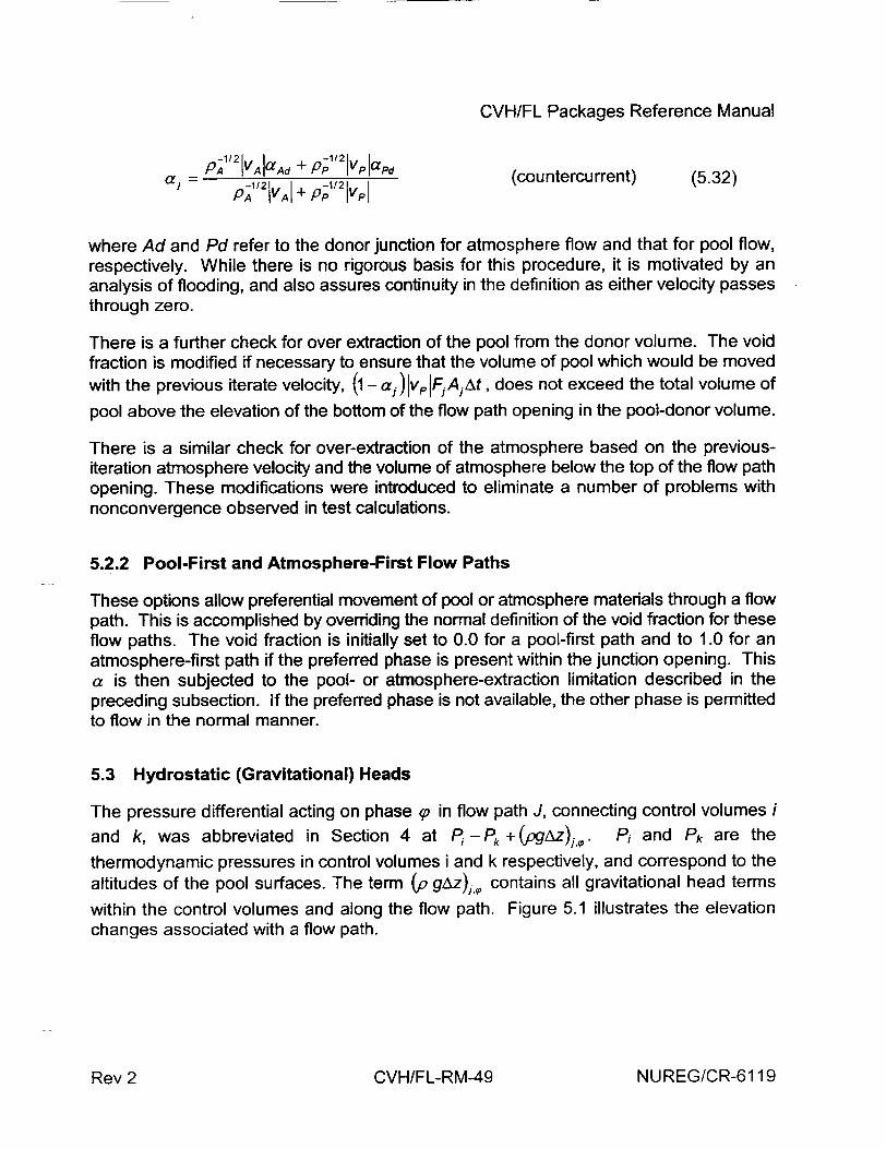
CVH/FL Packages Reference Manual
=PA1/2 VAa •Ad + ,P 112 Vp Japd (countercurrent) (5.32) J = A 1/2 IVAJ + PP 21Pv
where Ad and Pd refer to the donor junction for atmosphere flow and that for pool flow, respectively. While there is no rigorous basis for this procedure, it is motivated by an analysis of flooding, and also assures continuity in the definition as either velocity passes through zero.
There is a further check for over extraction of the pool from the donor volume. The void fraction is modified if necessary to ensure that the volume of pool which would be moved with the previous iterate velocity, (0 - a,) vpIFjAAt, does not exceed the total volume of
pool above the elevation of the bottom of the flow path opening in the pool-donor volume.
There is a similar check for over-extraction of the atmosphere based on the previousiteration atmosphere velocity and the volume of atmosphere below the top of the flow path opening. These modifications were introduced to eliminate a number of problems with nonconvergence observed in test calculations.
5.2.2 Pool-First and Atmosphere-First Flow Paths
These options allow preferential movement of pool or atmosphere materials through a flow path. This is accomplished by overriding the normal definition of the void fraction for these flow paths. The void fraction is initially set to 0.0 for a pool-first path and to 1.0 for an atmosphere-first path if the preferred phase is present within the junction opening. This a is then subjected to the pool- or atmosphere-extraction limitation described in the preceding subsection. If the preferred phase is not available, the other phase is permitted to flow in the normal manner.
5.3 Hydrostatic (Gravitational) Heads
The pressure differential acting on phase (p in flow path J, connecting control volumes i
and k, was abbreviated in Section 4 at P -Pk+ -(pgAz)jP. Pi and Pk are the
thermodynamic pressures in control volumes i and k respectively, and correspond to the altitudes of the pool surfaces. The term (p gAz),, contains all gravitational head terms
within the control volumes and along the flow path. Figure 5.1 illustrates the elevation changes associated with a flow path.
NUREG/CR-6119CVH/FL-RM-49Rev 2
CVH/FL Packages Reference Manual
ZpjA
Figure 5.1 Elevations Involved in Gravitational Head Terms
Examination of Figure 5.1 shows that there are three contributions to the gravitational head. The first is the pressure difference between the pool surface at zp,,i (where the volume pressure is defined) and that at the average elevation, zj.,.i, of the phase in the
junction opening in volume i
(P,- P) =Pi(zPi - (5.33)
,O~gzj- Zjq~j) zj <z,,,,
In this equation, the average elevations of the phases in the junction openings are given by
zj~p~i = max 1 ,. [zj + min(zp.i + ZTj] (5.34)
ZJA,, = min{zTJ, .[zTJi + max(zp, + z•.)]} (5.35)
where BJ and TJ again refer to the top and bottom of the junction opening, as in Section 5.2.
The second contribution to the static head comes from the corresponding pressure difference in volume k
NUREG/CR-6119CVH/FL-RM-50Rev 2
CVH/FL Packages Reference Manual
(PJ'k - Pk {P,7g(zp.k -zJ*A) Zp~k < (5.36)
and the third term is the gravitational head in phase q' along the flow path
(PJ'k - p~)p= 5J9(J, - ZJk (5.37)
based on the density of that phase in the flow path. The density of a phase in a flow path is taken as the maximum of the volume values,
; 9 maxd a0,
5,= max , (5.38)
because use of a donor value would introduce an unacceptable discontinuity in the gravitational head whenever the direction of a flow reversed. The maximum rather than a simple average is used because the value in a volume where the phase is not present may not be well defined.
The net gravitational head term is then defined as the sum of these three contributions:
(0 gAz),4, = (PJ i - Pi),p + (PJ~k - PJ i), -(PJk - Pk ), (5.39)
Figure 5.1 shows only two of the three possible cases: z, > zTj and ZTj > Zp > z.n, but the
third (zj > zp) should be easily visualized.
The derivatives of Equation (5.39) with respect to pool masses at constant densities are required for the implicit projection of the head terms as shown in Equation (4.16). These are then used in the implicit flow equation, Equations (4.23) and (4.24). Under the assumption of constant pool density, we have
a 1 a M p(5.40) a•mp pp Ap a~zp
where Ap is the cross-sectional area of the control volume at Zp (the area of the pool surface). Evaluation of the derivatives is greatly complicated by the fact that A., , Pk.,, and
,5j, are all potentially different. However, by ignoring this difference and neglecting all
terms which contain PA rather than pp, we may obtain the approximate result
NUREG/CR-6119CVH/FL-RM-51Rev 2
CVH/FL Packages Reference Manual
a(, gT~, UIAos9 ZP's > zJq~s a(p gAz)=~ _ J0 (5.41)
am 's Zp~s <! Zj g,s
where s is either i or k, and -js provides the appropriate sign. This approximation has been found to be adequate in practice, and is currently employed in MELCOR.
Equation (5.41) may be derived from the preceding equations by performing the indicated derivative under the stated assumptions and approximations. These assumptions and approximations are equivalent to considering only the effect of changes in Zp on the pool contribution to the static head; this observation also allows the equation to be written down by inspection of Figure 5.1.
5.4 Form Loss and Wall Friction
The frictional pressure drops resulting from material flows contain contributions from both form loss and wall friction. The form-loss contribution is based on user-input coefficients; the wall-friction terms are computed within MELCOR, based on segment lengths and I roughnesses input by the user. Because a single MELCOR flow path may be used to represent a rather complicated hydraulic path, the wall-friction terms may be computed for a path composed of one or more segments which are connected in series. (As will be noted below, a MELCOR segment may represent a number of parallel pipes.) This approach may also be used to approximately account for frictional losses within the control volumes themselves-MELCOR does not calculate any loss terms based on volumecentered velocities (see Section 6.5).
The flow resistances (and open fractions) for specified flow paths involving core cells are automatically adjusted to represent partial or total blockage of the flow by core debris, as calculated by the COR package. See Section 6.7 for a discussion of this model.
5.4.1 Flow Path Segments
If a flow path j is imagined to consist of a number of pipe-like segments, the total frictional pressure drop for phase (, (P or A) is given by
f1 2.vP~J( fp 2 0 L, APj,., = -D pq,+fV(.jv Ps. (5.42) S sD
NUREG/CR-6119Rev 2 CVH/FL-RM-52
CVH/FL Packages Reference Manual
where K is the form loss coefficient for the entire flow path, and f is the Fanning friction coefficient for segment s, which has length L, and hydraulic diameter D,. The sum is over the segments in the flow path.
In Equation (5.42), the pressure drops associated with sudden area changes or bends (the K term) and wall friction losses for the pipe segments (the f terms) are quadratic in velocity but, as written, each term involves a different velocity. For each flow path, MELCOR computes phase velocities vjp and VjA for the pool and the atmosphere. These define the volumetric flow of pool and atmosphere through the flow path,
Jj., = a, jFjAjv,,, (5.43)
where Aj is the flow path area and Fj is the fraction of that area which is open. If the flow
is assumed to be incompressible, i.e., p,8 = p,,,, the volumetric flow of each phase in the
segments is constant, and the segment velocities are given by
v •.As = v •.FjAj (5.44)
where A, is the segment area. (Note that if a segment is to represent a number of parallel pipes, As should be the total flow area while Ds should be the hydraulic diameter of each pipe.) Therefore, all the loss terms may be combined to give an effective loss coefficient K.
K. = q+ E 4f,sL, (F)AJ (5.45) K;'Ki+ Ds ( A, S
The frictional pressure loss can be cast in the following form
PJ", = 2Kjpj,,,v j., (5.46)
The input form-loss coefficient for positive or negative flow (FRICFO or FRICRO on input
record FLnnn03) is used for Kj., depending on the sign of vi..
The wall-friction terms are calculated following the method of Beattie and Whalley [15]. A mixture Reynolds number is defined for each segment as
NUREG/CR-6119CVH/FL-RM-53Rev 2
CVH/FL Packages Reference Manual j Res = (a PA vA. + (1- a)ppIvp D., FjAj ( Re- P i) (5.47)
using a mixture viscosity
Pm =aA + (I-- aX1 + 2.5a)up (5.48)
Here PA is calculated by the MP Package for a mixture of gases with the composition of the atmosphere. The viscosity of liquid water is used for pp (despite the fact that the pool
may contain bubbles). Note that pm has the proper limits (,p or PA, respectively) as a goes to 0.0 or 1.0.
The flow-path void fraction computed by MELCOR (Section 5.2.1) is used in Equations (5.47) and (5.48) rather than the homogeneous void fraction originally proposed in Reference [151. The constants in Equation (5.48) are coded as sensitivity coefficients in array C4404, and may therefore be modified by user input if desired.
The Reynolds number calculated from Equation (5.47) is used in a standard single-phaseflow friction correlation (which will be described in Section 5.4.2) to determine a singlephase friction factor fl, which is used directly for fp.
The flow quality,
a PAVA x = 6(5.49) WpAVA + (1 -- a)ppVp
is used to interpolate the atmosphere friction factor fA linearly between the single-phase value f, when only atmosphere is flowing in the path (x = 1.0) and zero for x < x 0 . [Xo is
coded as sensitivity parameter (C4404(12), with a default value of 0.9.) This is intended to reflect the tendency toward annular flow, with the gas phase preferentially occupying the center of a flow path, away from the walls and therefore not directly affected by wall friction.
The wall friction terms depend only on the velocity in the segment. Therefore, for a given volumetric flow (Equation (5.43)), they are independent of F (the fraction of the flow path which is open). This is as it should be, since F is intended to model a local restriction such as a valve which has no effect on wall losses in pipe segments.
On the other hand, the entire form loss term (K) depends on the nominal flow path velocity which, for a given volumetric flow, is dependent on F. Thus, if F can vary (i.e., if the flow path contains a valve), F cannot be used to represent the effects of bends, contractions,
NUREG/CR-6119
I - __*
Rev 2 CVH/FL-RM-54
CVH/FL Packages Reference Manual
and/or expansions in that flow path. This is not a serious defect because such losses may be modeled using equivalent lengths of pipe [16] in the segment data; in addition, most valves are either fully open or closed, and the current form is correct in either case. At some later date, the restriction may be removed by allowing form loss coefficients to be input for each segment, in addition to this single coefficient now permitted for the path, with the segment form losses based on the segment velocities rather than the MELCOR flow path velocities.
5.4.2 Single-Phase Friction Factor
The single-phase friction factor correlation used in MELCOR includes laminar, turbulent, and transition regions. In the laminar region, 0 < Re < 2000.0, the expression used is
f = 1(5.50)
Re
The Colebrook-White equation [17]
1 = 3.48- 4"01°g° 2 e+ 9 (5.51) JfID + (5.51
is used in the turbulent region Re > 5000.0. Here e is the surface roughness. This equation must be solved iteratively. In the transition region 2000.0•< Re • 5000.0, log(f)
is linearly interpolated as a function of log(Re) between the limiting values for the laminar and turbulent regimes.
The various constants in these equations, including the limiting Reynolds numbers, are coded as sensitivity coefficients in the array C4404, and may therefore be modified by user input.
5.5 Interphase Forces
The force (momentum exchange) between pool and atmosphere flows sharing a single flow path is important both in entraining concurrent flows and in limiting countercurrent ones. In the latter case, it is responsible for the phenomenon of flooding, or countercurrent flow limitation (CCFL).
A model is required for use in MELCOR, but without the complicated flow-regime maps and constitutive equations of the type employed in TRAC [6] or RELAP5 [7]. Therefore, a simple form is used which will reproduce a flooding curve in the form given by Wallis [13]:
NUREG/CR-6119CVH/FL-RM-55Rev 2
CVH/FL Packages Reference Manual J (5.52)
where jg = avg / v, and j, = (1 - a•lf / v0 are scaled (dimensionless) volumetric flows of gas and fluid, respectively. In the following, we will adopt conventional MELCOR notation, where the conventional subscripts "g" and 'T become "A" and "P", respectively. As is shown in Appendix B, such a flooding curve will result if the relative velocity is modeled as a function of void fraction defined by
1 1 al1-a = = (5.53)
Vr VA -Vp V1 V 0
Here v1 and v0 are the velocities used to scale jA and jp, respectively; they also turn out to be the limiting values of vr for a, equal to 1.0 and 0.0, respectively.
Appendix B also shows that the steady (time-independent) solution of the two-phase momentum equation will agree with this result if the interphase force in Equation (4.6) is represented as
f =Vo(PP(-P a+1a (5.54)
In the interest of simplicity, only the form of Vo and v, [18],
V = FPA (5.55)
V1 Pp
is used in MELCOR to produce
f2 = 900"'kJ/-l• + (1 -Ia)NP p (5.56)
in SI units. The constant chosen gives a value of about 0.3 m/s for the limiting relative velocity as a goes to zero for vertical flow of gas and normal density water, corresponding to the terminal rise velocity of bubbles. This equation is applied to all geometries, and the results are usually qualitatively acceptable. The term f2j in the finite-difference Equation (4.23) is multiplied by the length over which the interphase force acts rather than the inertial length of the flow path. A distinct length is used for momentum exchange. The default is taken as the inertial length for horizontal flow paths and as the difference in
NUREG/CR-6119CVH/FL-RM-56Rev 2
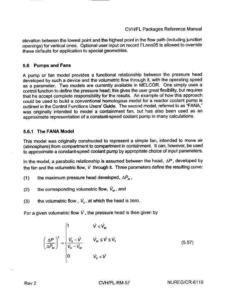
CVH/FL Packages Reference Manual
elevation between the lowest point and the highest point in the flow path (including junction openings) for vertical ones. Optional user input on record FLnnnO5 is allowed to override these defaults for application to special geometries.
5.6 Pumps and Fans
A pump or fan model provides a functional relationship between the pressure head developed by such a device and the volumetric flow through it, with the operating speed as a parameter. Two models are currently available in MELCOR. One simply uses a control function to define the pressure head; this gives the user great flexibility, but requires that he accept complete responsibility for the results. An example of how this approach could be used to build a conventional homologous model for a reactor coolant pump is outlined in the Control Functions Users' Guide. The second model, referred to as "FANA,"
was originally intended to model a containment fan, but has also been used as an approximate representation of a constant-speed coolant pump in many calculations.
5.6.1 The FANA Model
This model was originally constructed to represent a simple fan, intended to move air (atmosphere) from compartment to compartment in containment. It can, however, be used to approximate a constant-speed coolant pump by appropriate choice of input parameters.
In the model, a parabolic relationship is assumed between the head, AP, developed by
the fan and the volumetric flow, Vý through it. Three parameters define the resulting curve:
(1) the maximum pressure head developed, APM,
(2) the corresponding volumetric flow, VM, and
(3) the volumetric flow, V0 , at which the head is zero.
For a given volumetric flow V, the pressure head is then given by
[1 V <V
AP _ = _Vo -M<Vo (5.57)
0
NUREG/CR-6119CVH/FL-RM-57Rev 2
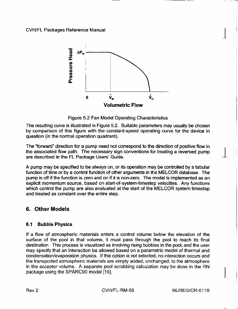
CVH/FL Packages Reference Manual 4
t•AP,
IL
0 IU/)
h._
0 VM V
Volumetric Flow
Figure 5.2 Fan Model Operating Characteristics
The resulting curve is illustrated in Figure 5.2. Suitable parameters may usually be chosen by comparison of this figure with the constant-speed operating curve for the device in question (in the normal operation quadrant).
The "forward" direction for a pump need not correspond to the direction of positive flow in the associated flow path. The necessary sign conventions for treating a reversed pump are described in the FL Package Users' Guide.
A pump may be specified to be always on, or its operation may be controlled by a tabular function of time or by a control function of other arguments in the MELCOR database. The pump is off if the function is zero and on if it is non-zero. The model is implemented as an explicit momentum source, based on start-of-system-timestep velocities. Any functions which control the pump are also evaluated at the start of the MELCOR system timestep and treated as constant over the entire step.
6. Other Models
6.1 Bubble Physics
If a flow of atmospheric materials enters a control volume below the elevation of the surface of the pool in that volume, it must pass through the pool to reach its final destination. This process is visualized as involving rising bubbles in the pool, and the user may specify that an interaction be allowed based on a parametric model of thermal and condensation/evaporation physics. If this option is not selected, no interaction occurs and the transported atmospheric materials are simply added, unchanged, to the atmosphere in the acceptor volume. A separate pool scrubbing calculation may be done in the RN package using the SPARC90 model [19].
NUREG/CR-6119Rev 2 CVH/FL-RM-58
CVH/FL Packages Reference Manual
The physics modeled involves breakup of the injected gas stream into a swarm of bubbles, thermal equilibration of the gases with the pool, and saturation of the bubbles with water vapor at local conditions. These bubbles are not considered to reside in the pool, and do not contribute to pool swelling. The efficiency of the mass and energy transfer processes is affected by two factors, which are treated as independent.
The distance that gases must rise in order to reach the surface of the pool is involved in the breakup of the stream and the corresponding increase in surface area. It is modeled
as an efficiency, c,, represented as
z - zJ - 0.01 m 0 (6.1) 1.0h h O<1
where zp is the elevation of the pool surface in the acceptor volume; zj is the junction elevation in the acceptor volume; and h is the height of the junction opening.
That is, there is assumed to be no breakup until the bubbles have risen at least 1 cm, and breakup is assumed to be complete if they must rise through the junction opening height plus 1 cm.
The effect of subcooling of the pool is represented as the efficiency
T t(P)- Tp -0.1K 0: <1 (6.2) 5.0K
This requires subcooling by at least 0.1 K for any effect, and by at least 5.1 K for the maximum possible effect to be predicted.
The overall efficiency is taken as the product of these two efficiencies
6 = CZEr (6.3)
If only water vapor and fog are present in the bubbles, it is assumed that a fraction 6 of the vapor condenses, and an equal fraction of the fog in the flow path is deposited in the pool, with the remainder passing through to the atmosphere; no modification is made to the specific enthalpy (temperature) of material which passes through. In this case, the entire flow will be deposited in the pool if the depth and subcooling are adequate.
If noncondensible gases are present, and the depth and subcooling are sufficiently large, it is assumed that bubbles leave the pool at the pool temperature and, further, that the relative humidity in the bubbles will be 0.99, i.e., that the partial pressure of water vapor will
NUREG/CR-6119Rev 2 CVH/FL-RM-59
I
CVH/FL Packages Reference Manual 4 be 0.99 of the saturation pressure at the pool temperature. If 6 = 1 as calculated from Equations (6.1), (6.2), and (6.3), this result is used directly, while the trivial result for no interaction is used for - = 0. For 0 < •1, a linear interpolation (on the overall 6, Equation (6.3)) is performed between these limits. As in the case of no noncondensibles, a fraction e of the fog flow is assumed to be deposited in the pool, with the remainder transmitted to the atmosphere.
All constants in this model (those in Equations (6.1) and (6.2)), and the limiting relative humidity) are coded as sensitivity coefficients, included in array C4405, and may therefore be modified by user input. The default values are those discussed here.
The effects of this model are implemented by appropriately modifying the definitions of donor properties; the normal donor properties are used for removal of atmospheric material from the actual donor volume, but a modified set of properties is used for the acceptor volume to which they are added. Specifically, if the volume of atmosphere moved through the flow path is
JAVj = aiFjAj AVj.AlAt (6.4)
the masses and energies removed from the donor volume, d, are
AMmd -JAVj Mmd (6.5) VA~d
--A~ -Ij vI (6.6) where, of course, the material index m in Equation (6.5) is limited to materials in the atmosphere. The masses added to the acceptor volume, a, however, have the more general form
AMma P=n,.A Vji (6.7)
AEAa. =(p h)Aa. AVi (6.8)
AEpa =(p h)p..I AVj (6.9)
where m in Equation (6.7) includes the pool. The bubble physics model gives the masses and energies delivered to the acceptor volume (AMma, AEA,a and AEpa) in terms of the
NUREG/CR-6119Rev 2 CVH/FL-RM-60
CVH/FL Packages Reference Manual
entering masses and energies (AMmd and AEA~d). Therefore, Equations (6.7) through
(6.9) serve as definitions of the quantities Pr,,a, (P h)*.a, and (p h)p,, which are subject to
the constraints
. M21d + M Ud
P1,a + PZa + P3. VA,M d (6.10)
Pn A n>4(NCG) (6.11)
VAVd
For atmospheric materials, the differences reflect the changes in composition and specific enthalpy described above; the pool terms reflect heat and mass exchange with the pool.
If evaporation takes place, p,8 can be negative. In this case, it is further constrained so
that use of Equation (6.7) does not result in a negative pool mass.
6.2 Time-Dependent (Specified) Flow Paths
The velocity in any flow path may be defined by the user, either as a Tabular Function of time or as a Control Function of other arguments in the MELCOR database. The resulting velocity is imposed on both pool and atmosphere (if present), with the void fraction computed using the standard model described in Section 5.2.
6.3 Critical Flow Models
After the solution of the flow (momentum) equation is complete, the computed flow in each flow path is compared with a calculated critical flow to determine if choking should be imposed. The test is bypassed if neither the pool velocity nor the atmosphere velocity is greater than a threshold of 20.0 m/s, coded as a sensitivity coefficient in C4402. If the flow exceeds the critical value, the flow path is added temporarily to a list of specified-flow flow paths, and the entire solution is repeated with the velocity constrained to be the critical value.
If only atmosphere is flowing through the path, the critical mass flux is taken as the sonic flux at the minimum section. For an ideal gas, this may be related to the sonic flux at stagnation conditions through the relation [20]
NUREG/CR-6119Rev 2 CVH/FL-RM-61
CVH/FL Packages Reference Manual j
GcA ~ ~ = A S +1 _cAp-CA (" 2 (6.1-3)•)
where G - pv is mass flux; subscript C denotes "critical"; Cs is the sonic velocity; and
y = CP/cv is the ratio of the specific heat at constant pressure to that at constant volume.
The use of the superscript "d' reflects the fact that in MELCOR the donor volume is assumed to be at stagnation conditions. The sonic velocity is evaluated in the CVT package. The multiplier is only a very weak function of y, having a value within 5% of 0.58
for 1.1 < ry •1.8, and is therefore evaluated at a nominal value of r = 1.4. There are two factors contributing to this function of r:
(1) reduction in density because of expansion and
(2) reduction in sound speed because of cooling between stagnation conditions and the minimum section.
CONTAIN [3] includes both factors, HECTR [2] only the latter.
If only pool is flowing, the RETRAN [21] model (to be discussed in Section 6.3.1) for the _ critical mass flux is used, based on the pressure and specific enthalpy of the pool,
GcP = Gc.RETRN(Pd,h h) (6.14)
If both phases are flowing, the critical mass flux is taken as a weighted average of that for the two phases,
a p•+(1-a)p- ap• + (1-a)pp (6.15) GC,2ph GcA G c,p
This rather peculiar averaging scheme was motivated by the observation that it provides an almost exact representation of the Moody choking model if Gcp and GCA are replaced by GCMoody (a =0) and Gc,Moody (a = 1), respectively (see Appendix C).
If the mass flux evaluated using the new velocities calculated by the momentum equation exceeds the appropriate critical value, the velocity imposed (on both phases) is
INUREG/CR-6119Rev 2 CVH/FL-RM-62
CVH/FL Packages Reference Manual
vc'j ajpd G1 )pd (6.16)
Possible improvements in this model are described in Section 7.2.
Discharge coefficients are available (on FLnnn03 input records) as multipliers for the critical flow values calculated by these models. Different values may be used for forward (positive) and reverse (negative) flows in each flow path; the default values are 1. The appropriate discharge coefficient is included both in the test for choking in each flow path and in the velocity imposed if choking is detected. Use of a very large value is the only way to eliminate the possibility of choking in a flow path.
6.3.1 RETRAN Critical Flow Model
The RETRAN critical flow model consists of two 36-parameter, double-polynomial fits to extended Henry-Fauske critical flow for subcooled water (below and above 300 psia), and two 36-parameter fits to Moody critical flow for saturated (two-phase) water (below and above 200 psia), all as functions of stagnation pressure and enthalpy. It also includes a 9-parameter expression for a "transition" enthalpy as a function of pressure. A linear transition is constructed between the Henry-Fauske model at and below this enthalpy and the Moody model at and above saturation. The reader is referred to Reference [21] for a description of the basic models and the fitting procedure employed.
Two modifications to the RETRAN model were made for use in MELCOR. First, the fits are stated in Reference [21] to be valid only above 170 Btu/Ibm, and were observed to yield unreasonable (sometimes negative) values not far below this value. Therefore, a linear interpolation was introduced between the fit at the lower limit of its applicability and the solution for orifice flow.
Go = 2-Ppp (6.17)
imposed at hp = 0. Second, it was observed that the transition enthalpy, which defined the upper bound for application of the Henry-Fauske model, was calculated as greater than the enthalpy of saturated liquid at the lower end of the pressure range (below about 21 psia). Therefore, the transition enthalpy was further bounded to be at least 10 Btu/Ibm below saturation.
The fits themselves leave something to be desired; they appear to be excessively complicated, include modest discontinuities (several percent) at region boundaries, and have terrible extrapolation properties. Plans for improvement are described in Section 7.2.
NUREG/CR-6119CVH/FL-RM-63Rev 2
CVH/FL Packages Reference Manual
6.4 Valves
A valve may be included in any flow path in MELCOR. Its operation is modeled as a change in the fraction of the area of the flow path which is open. This fraction may be defined directly as a Tabular Function of time, or as a Control Function of other arguments in the MELCOR database. Trips may also be used to model irreversible changes in flow areas such as ruptures of vessels or compartment walls, or to model the hysteresis in the operation of, say, a relief valve. The open fraction is limited to the range 0.0 < F < 1.0 and, if the controlling function returns a value outside this range, it will be suitably truncated. The upper bound corresponds to a flow area equal to that input for the flow path, the lower bound to a closed path in which no flow is permitted.
Flow paths can be defined to permit only one-way flow, either forward or reverse. Such flow paths provide a simple way to represent idealized check valves. MELCOR also allows the open fractions (and flow resistances) for specified flow paths involving core cells to be automatically adjusted to represent partial or total blockage of the flow by core debris, as calculated by the COR package. See Section 6.7 for a discussion of this model.
6.5 Volume-Averaged Velocities
Volume-averaged (centered) velocities are used in MELCOR only in the calculation of forced-flow heat transfer coefficients (in a number of packages). This is because both control volume kinetic energies and momentum flux terms are neglected in the governing hydrodynamic equations. The only forced-flow heat transfer coefficients used in the CVH or FL packages are those associated with the pool atmosphere interface in nonequilibriurn volumes (Section 5.1.2).
MELCOR is a lumped-parameter code which is often used to model three-dimensional volumes. A rigorously defined volume-averaged velocity would involve multi-dimensional effects, but the essential geometric information is simply not available. The model used in RELAP5 [7], which is also a lumped-parameter code, was considered for use in MELCOR. It may be written in the form
Jv O= avq,Vv4Av = -1 ( I-, + (RELAP5) (6.18) ' ~ ~ .- so v if.vs
Jj.B = aj. v Fi.,1FAj (6.19)
where J is volumetric flow; q' = P or A, and denotes pool or atmosphere; Av is the flow
area associated with volume V; av, (p are the area fractions for the volume flows; and all
other symbols have been defined before. The sums in Equation (6.18) are over flow paths which connect to or from volume V. I
NUREG/CR-6119CVH/FL-RM-64Rev 2
CVH/FL Packages Reference Manual
Volume flows and velocities calculated from Equation (6.18) are strongly dependent on the logical direction of flow paths. For example, reversing both the sign of a velocity and the associated direction of positive flow (so that the actual volume moved from and the volume moved to are unchanged) does not preserve the volume flow. In particular, the net flow in a volume with a flow +J to it and +J from it is +J, while the net flow in a volume with +J to it and -J to it is zero. This is because it is assumed in the RELAP5 formulation that all to connections are on the left of a volume and all from connections on the right; in the second case cited above, the flows cancel and there is no resulting flow at the volume center.
We have found that this is often not the desired result in MELCOR nodalizations. Furthermore, the expected results cannot be obtained in any nodalization which connects volumes in a regular grid to approximate a finite-difference representation of a twodimensional region; the best that can be done is to calculate the velocity component along one diagonal of the grid. Therefore, MELCOR uses a simplification of Equation (6.18) which treats all flow paths on an equal footing:
Jv,9 =• v.9,VAAv =, 1 1 (MELCOR) (6.20)
where the sum is over all connected flow paths, and the void fraction associated with the volume flow is taken as a simple weighted average over connected flow paths in the form
Y ajFjA1
av= JFIAI (6.21)
This model can be understood qualitatively using the simple argument that, under steady conditions, a flow through a volume is counted twice: once where it enters the volume and once where it leaves. It makes no attempt to assign a direction to the volume velocity, and would therefore be unacceptable if it were necessary to calculate the momentum flux terms
arising from V •.(pvv). In accord with this simple double-counting argument, a term is
added to the sum in Equation (6.20) for the vapor flow to account for vapor generation in boiling in a nonequilibrium volume.
6.6 Special (Time-Specified) Volumes
MELCOR hydrodynamics allows boundary conditions to be defined by specifying the state of one or more volumes as functions of time. This is frequently necessary for simulation
NUREG/CR-6119CVH/FL-RM-65Rev 2
CVH/FL Packages Reference Manual J of experiments. It is also useful for defining the outside-containment environment for a full reactor plant calculation.
In the simplest case, a volume may be specified as time-independent, with properties that do not change as the calculation progresses. Volumes can also be defined whose properties are maintained constant for a specified period of time, after which they are "freed" to function as normal volumes. This can simplify initialization of an operating steady state in a reactor. An initially time-independent pressurizer will enforce a constant pressure boundary condition, while initially time-independent steam generators enforce a constant thermal boundary condition during a pre-transient phase of the calculation.
In addition, several options are available for specifying the pressures, temperatures, and compositions of boundary volumes as functions of time, in terms of user-defined tabular functions, external data files, or control functions, as explained in the CVH Users' Guide.
A time-specified volume can serve any of the functions of a normal volume. It can provide boundary conditions for in- or out-flows, or for heat transfer. However, no volumeaveraged velocity (Section 6.5) is calculated for a time-specified volume; forced convection heat transfer will therefore not be considered in the Heat Structure (HS) package. All phenomena modeled by the RadioNuclide (RN) package will be treated, with the sole exception that radionuclides are not allowed to advect out of such a volume. (This is intended to prevent radionuclides from reentering a failed containment building from the environment.) A time-specified volume can also be used in conjunction with a timespecified flow path (Section 6.2) to define a mass source with well-defined properties. This approach is particularly useful for water sources, for which temperature alone is insufficient to define the complete thermodynamic state; it also provides a way for gas sources to be made to participate in the bubble interactions described in Section 6.1.
Any mass or energy transferred to or from a time-specified volume is recorded as "created" in the CVH package for accounting purposes.
6.7 Core Flow Blockage
MELCOR includes a core flow blockage model to account for the changes in flow resistance in the degraded core states that will arise during a postulated reactor accident. It treats the entire range of degradation, from partially blocked rod geometry to debris bed geometry. The markedly increased resistance to flow in severely degraded geometries is particularly important because it will limit the flow available both to carry away decay heat and to provide steam for core oxidation. In addition to improving the basic modeling, inclusion of blockage effects has been found to improve code performance, particularly when a detailed CVH nodalization is used in the core region. The neglect of blockage can lead to prediction of unphysically large flows through regions containing very little fluid; the material Courant condition will then force extremely small timesteps, greatly increasing execution times.
NUREG/CR-6119Rev 2 CVH/FL-RM-66
CVH/FL Packages Reference Manual
At the start of a MELCOR calculation the core will (usually) be in a state for which the
representation of friction (in terms of user input for intact geometry) is appropriate. This will change, however, following relocation of core materials. The blockage model, when invoked, will modify flow areas and flow resistances to account for the effects of refreezing of conglomerate debris onto fuel rods and/or other structures, or a loss of simple rod geometry through the creation or relocation of particulate debris.
The current model considers two flow regimes. For severely damaged core geometries, after particulate debris has been formed, it uses correlations developed for flow in porous media. Until this occurs, a simple modification to the flow resistance in intact geometry is
used to account for changes in flow area associated with refrozen conglomerate debris. (Clad ballooning, which would have a similar effect, is not modeled.) As currently coded, the switch in regimes is made on a flow path by flow path basis, triggered by the first appearance of particulate debris in any core cell associated with the flow path. When the uncertainty in predicting the actual geometry of core debris is considered, we believe that this simple treatment is adequate for MELCOR use.
6.7.1 Debris Geometry
There are several correlations for the pressure drop for flow in porous media that can all be represented in the general form
APpuosbd1 j 2 L (6.22)_ P 163[C + C2(--Lj + C3--ej (622)
where j is the superficial velocity (volumetric flux), e is the porosity of the medium, Dp is the effective particle diameter, and Re is the Reynolds number based on these quantities,
Re = p-j DP (6.23)
The average velocity of fluid in the medium (strictly, the average of the component of that velocity that lies in the direction of positive net flow) is given by
V =(6.24)
This is further discussed by Dobranich [22], who lists coefficients for four published correlations in a table equivalent to the one below.
NUREGICR-6119CVH/FL-RM-67Rev 2
CVH/FL Packages Reference Manual
Table 6.1 Coefficients in Friction Correlations for Porous Media
Correlation C1 C2 C3 C4 Reference
Ergun (original) 3.5 300. 0.0 - [25]
Modified Ergun (smooth) 3.6 360. 0.0 - [23]
Modified Ergun (rough) 8.0 360. 0.0 - [24]
Achenbach 1.75 320. 20. 0.4 [24]
This correlational form is used to calculate the effects of core blockage on flow resistance once particulate debris has been formed. The coefficients in the correlation were coded as a sensitivity coefficient array, with C, = C4413(i); default values for I = 1, 2, and 3 are those for the original Ergun Equation [25].
In any flow path for which the blockage model has been invoked, the average porosity, 6, of core cells in the flow path is calculated from the ratio of hydrodynamic volume to total volume in the cells. This accounts for the effects of particulate and refrozen ("conglomerate") debris as described in the COR Package Reference Manual. In addition, the open fraction, Fj(t), for that flow path is set equal to the porosity, 6, as an intemally defined valve model. As a result, the nominal velocity in the flow path, vj, calculated by MELCOR is consistent with the velocity in Equation (6.24), so long as the nominal area of the flow path, Aj, is equal to the geometric area, Age,, of the cell(s) involved. After particulate debris has been formed, the pressure drop, Equation (6.22), can be cast in the form of an effective loss coefficient as
K =K,, = C,+ Ree +C 3 1 R ] ) ] (1 O (6.25)
to replace the "normal" value in Equation (5.46). Here, the Reynolds number expressed in terms of that nominal velocity is
Re = p e (6.26)
and a term K/mpty has been added to define the flow resistance in the "empty" path that will result when no core materials remain, the porosity is 1.0, and the porous medium modelused outside its range of applicability-would predict no friction.
INUREG/CR-6119Rev 2 CVH/FL-RM-68

CVH/FL Packages Reference Manual
6.7.2 Interpretation of Flow Areas
The nominal area and the open fraction are specified as part of user input to the FL package. In the regular nodalization of a finite difference code, there would be no need to distinguish the nominal area associated with a cell-boundary flow from the geometric area of the associated cell boundary. However, the distinction is essential in a control volume code such as MELCOR, where the definition of control volume geometry is limited and arbitrary interconnection of volumes is allowed. This is because a flow path must be able to represent the connection of a duct or pipe to a room or plenum as well as the boundary surface between two sections of a larger room or volume.
To avoid complications, MELCOR requires that the nominal flow path area be equal to the geometric area of the core cell(s) for all flow paths in which the blockage model is used. In order to eliminate the need for changes to existing decks when flow blockage modeling is added, the user input area is replaced by the geometric area, and the initial open fraction is simultaneously redefined as the porosity associated with core cell(s) in the flow path, for all flow paths in which the blockage model is invoked. The redefined values are flagged in MELGEN and MELCOR output as having been modified by the Flow Blockage model.
This may modify the open area, F A, associated with the initial geometry, which will result in different values being calculated for the velocity. However, because the advection terms in MELCOR hydrodynamics depend only on the total volumetric flow
J = jjA1(t) = F,(t)vj (t)Ai (6.27)
(see Equations (4.2) and (4.5)), as do the wall friction terms (see the discussion following Equation (5.42)), only the form loss coefficient used for intact geometry must be adjusted to compensate for the change in open area. (For more discussion, see the final report on the model in Reference [26].)
The input form loss coefficient is replaced by an "equivalent" coefficient, Keq, that is related to that input by the user through
K Kev K_ Kp (6.28) [F(0)Ano,,m (F~nputA,,,)2(628
for which the calculated pressure drop in intact geometry will match that which would be calculated from the user-input area, open fraction, and form loss. All such values are flagged in MELGEN and MELCOR output as having been modified by the Flow Blockage model.
NUREG/CR-6119CVH/FL-RM-69Rev 2
CVH/FL Packages Reference Manual J 6.7.3 Transition between Intact and Debris Geometries
If there is a period before the first appearance of particulate debris in any core cell associated with a flow path during which there is conglomerate debris frozen onto fuel rods (or other structures), the resulting reduction in flow area is accounted for by modification of the calculation for intact geometry. The presence of such material will change the porosity and therefore the open fraction for a flow path. However, the contribution of wall losses, represented by segment data, ordinarily dominates the pressure drop and-as calculated-this contribution is independent of the open fraction of the flow path. Therefore, a multiplier is applied to the friction calculated for intact geometry to account for the actual change in flow area, fluid velocity, and wall friction resulting from the presence of conglomerate debris prior to rod failure. The modified pressure drop is calculated as
(AP)net,-nsi = a L(0)2 (AP)].t. (6.29) SL e(t) 1
7. Discussion and Development Plans
7.1 Interphase Forces [ An assessment of the simple model for interphase forces (described in Section 5.5) appears to have eliminated the more obvious limitations of the previous implementation. Calculations need to be done and compared with data (as represented by more general slip correlations) to assess the overall adequacy of the revised model.
7.2 Critical Flow Modeling
Atmosphere velocities which are significantly supersonic have been observed in some calculations, despite the presence of the critical flow model. This can arise if the phase velocities calculated by the momentum equation are very different. (Because of its greater inertia, the velocity of the pool is sometimes much less than that of the atmosphere before choking is considered.) The problem is that the net mass flux, calculated with the disparate velocities, may be subcritical (according to the current calculational model) even though one velocity is supersonic.
The entire concept of choking in a two-velocity model may need further examination. In the short term, however, the introduction of the interfacial momentum-exchange term, by reducing the differences between the calculated phase velocities, has gone a long way toward eliminating this problem.
INUREG/CR-6119Rev 2 CVH/FL-RM-70
CVH/FL Packages Reference Manual
The relatively complicated fits [21] used for Moody and Henry critical flow are not particularly good (a few percent). They are each constructed for two pressure ranges, and exhibit discontinuities of several percent at the matching line. The extrapolation properties are poor, the extrapolation often goes negative just outside the fit region. We have found (see Appendix C) that there are simpler representations, with comparable or better accuracy and good extrapolation properties; we will implement them in MELCOR when time permits.
NUREG/CR-6119Rev 2 CVH/FL-RM-71
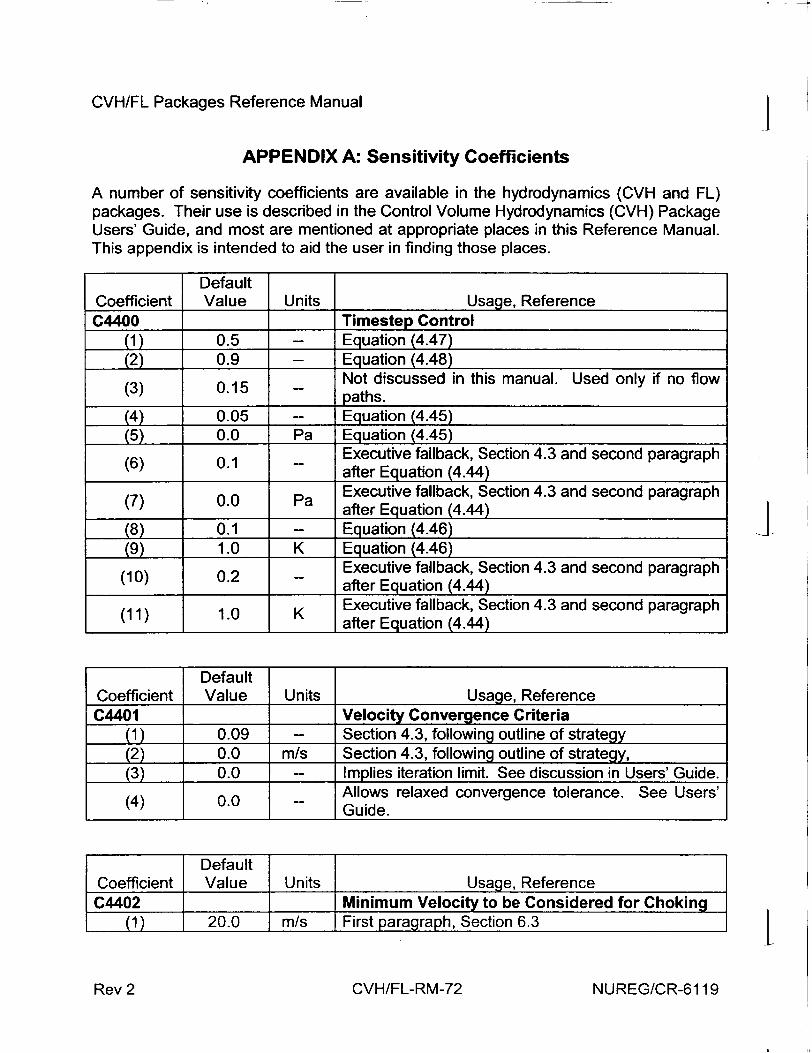
CVH/FL Packages Reference Manual
APPENDIX A: Sensitivity Coefficients
A number of sensitivity coefficients are available in the hydrodynamics (CVH and FL) packages. Their use is described in the Control Volume Hydrodynamics (CVH) Package Users' Guide, and most are mentioned at appropriate places in this Reference Manual. This appendix is intended to aid the user in finding those places.
Default Coefficient Value Units Usage, Reference C4400 Timestep Control
(1) 0.5 - Equation (4.47) (2) 0.9 - Equation (4.48)
Not discussed in this manual. Used only if no flow (3) 0.15 - pts paths.
(4) 0.05 P Equation (4.45) (5) 0.0 Pa Equation (4.45)
()0.1 - Executive fallback, Section 4.3 and second paragraph after Equation (4.44)
)0.0 Pa Executive fallback, Section 4.3 and second paragraph after Equation (4.44)
(8) 0.1 - Equation (4.46) (9) 1.0 K Equation (4.46)
)0.2 Executive fallback, Section 4.3 and second paragraph ( after Equation (4.44) Executive fallback, Section 4.3 and second paragraph after Equation (4.44)
Default Coefficient Value Units Usage, Reference C4401 Velocity Convergence Criteria
(1) 0.09 - Section 4.3, following outline of strategy (2) 0.0 m/s Section 4.3, following outline of strategy,
0.0 - Implies iteration limit. See discussion in Users' Guide. Allows relaxed convergence tolerance. See Users'
(4) 0.0 - Gie Guide.
Default Coefficient Value Units Usage, Reference C4402 Minimum Velocity to be Considered for Choking
(1) 20.0 m/s First paragraph, Section 6.3
NUREG/CR-6119
I
I
I
Rev 2 CVH/FL-RM-72
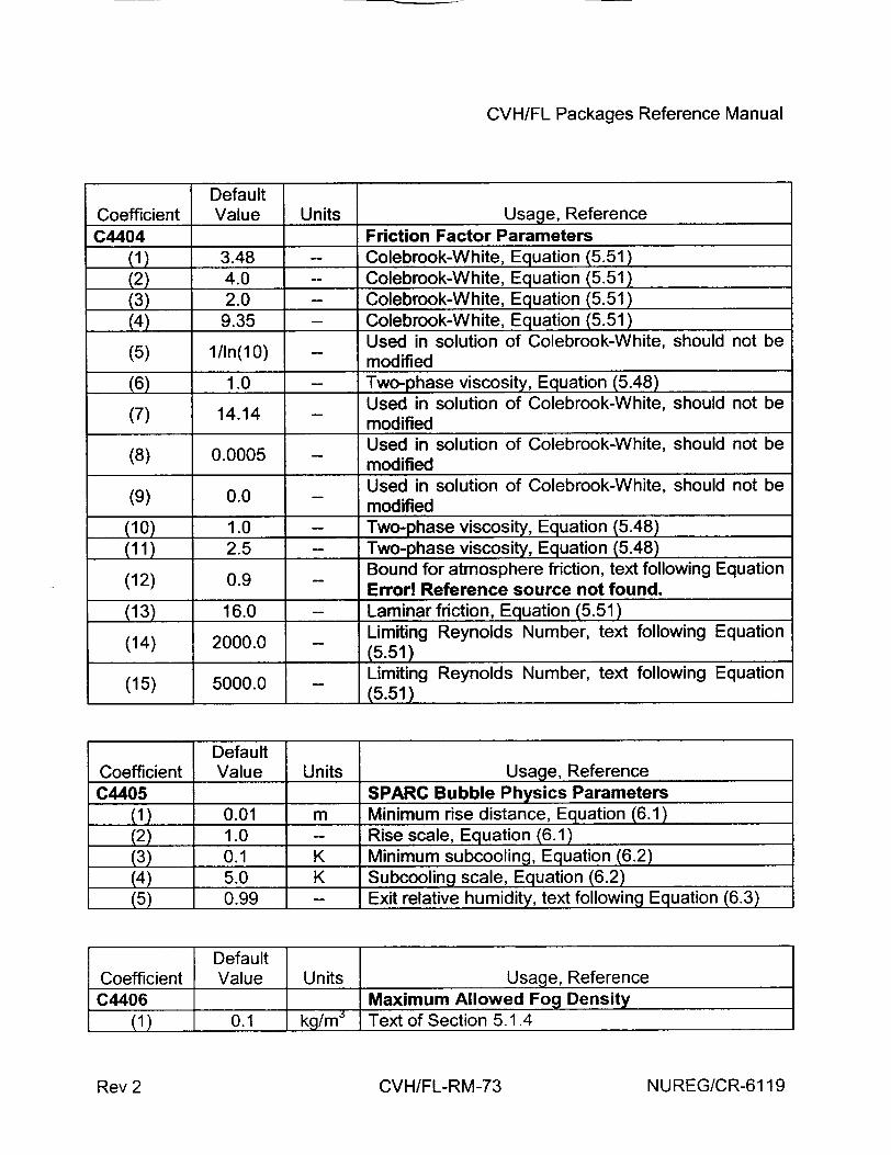
CVH/FL Packages Reference Manual
Default Coefficient Value Units Usage, Reference C4404 Friction Factor Parameters
(1) 3.48 - Colebrook-White, Equation (5.51) (2) 4.0 - Colebrook-White, Equation (5.51) (3) 2.0 - Colebrook-White, Equation (5.51) (4) 9.35 - Colebrook-White, Equation (5.51)
Used in solution of Colebrook-White, should not be (5) 1/In(10) -- mdfe modified
(6) 1.0 -- Two-phase viscosity, Equation (5.48) Used in solution of Colebrook-White, should not be (7) 14.14 -- mdfe modified
Used in solution of Colebrook-White, should not be (8) 0.0005 mdfe modified
Used in solution of Colebrook-White, should not be (9) 0.0 - mdfe modified
(10) 1.0 - Two-phase viscosity, Equation (5.48) (11 ) 2.5 - Two-phase viscosity, Equation (5.48)
Bound for atmosphere friction, text following Equation Error! Reference source not found.
(13) 16.0 -- Laminar friction, Equation (5.51)
(14) 2000.0 Limiting Reynolds Number, text following Equation (5.51)
(15) 5000.0 - Limiting Reynolds Number, text following Equation (5)_ 5o00.0 _(5.51)
Default Coefficient Value Units Usage, Reference C4405 SPARC Bubble Physics Parameters
(1) 0.01 m Minimum rise distance, Equation (6.1) (2) 1.0 - Rise scale, Equation (6.1) (3) 0.1 K Minimum subcooling, Equation (6.2) (4) 5.0 K Subcooling scale, Equation (6.2) (5) 0.99 -- Exit relative humidity, text following Equation (6.3)
Default Coefficient Value Units Usage, Reference C4406 Maximum Allowed Fog Density
(1) 0.1 kg/m Text of Section 5.1.4
NUREG/CR-6119CVH/FL-RM-73Rev 2
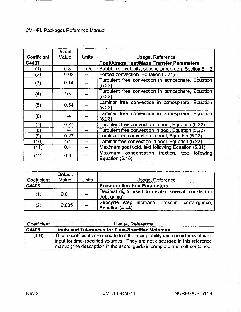
CVH/FL Packages Reference Manual
Default Coefficient Value Units Usage, Reference C4407 Pooll/Atmos Heat/Mass Transfer Parameters
(1 0.3 m/s Bubble rise velocity, second paragraph, Section 5.1.3 (2) 0.02 - Forced convection, Equation (5.21)
Turbulent free convection in atmosphere, Equation (3) 0.14 - (5.23)
)1/3 - Turbulent free convection in atmosphere, Equation (4) 1/3 52)frecnetoni toperEuto (5.23)
Laminar free convection in atmosphere, Equation (5.23)
(6) /4 - Laminar free convection in atmosphere, Equation (5.23)
(7) 0.27 -- Turbulent free convection in pool, Equation (5.22) (8) 1/4 - Turbulent free convection in pool, Equation (5.22) (9) 0.27 - Laminar free convection in pool, Equation (5.22)
(10) 1/4 - Laminar free convection in pool, Equation (5.22) (11) 0.4 -- Maximum pool void, text following Equation (5.31)
Maximum condensation fraction, text following (12) 0.9 - Equation (5.15)
Default Coefficient Value Units Usage, Reference C4408 Pressure Iteration Parameters
() 0.0 Decimal digits used to disable several models (for debugging) Subcycle step increase, pressure convergence,
(2) 0.005 - Equation (4.44)
Coefficient Usage, Reference C4409 Limits and Tolerances for Time-Specified Volumes
(1-6) These coefficients are used to test the acceptability and consistency of user input for time-specified volumes. They are not discussed in this reference manual; the description in the users' guide is complete and self-contained.
INUREG/CR-6119
I
Rev 2 CVH/FL-RM-74
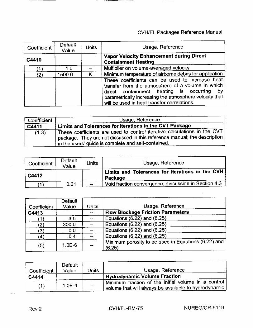
CVH/FL Packages Reference Manual
Coefficient Default Units Usage, Reference Value
C4410 Vapor Velocity Enhancement during Direct C4410 _ Containment Heating
(1) 1.0 -- Multiplier on volume-averaged velocity
(2) 1500.0 K Minimum temperature of airborne debris for application These coefficients can be used to increase heat transfer from the atmosphere of a volume in which direct containment heating is occurring by parametrically increasing the atmosphere velocity that will be used in heat transfer correlations.
Coefficient Usage, Reference C441 I Limits and Tolerances for Iterations in the CVT Package
(1-3) These coefficients are used to control iterative calculations in the CVT package. They are not discussed in this reference manual; the description in the users'_guide is complete and self-contained.
Coefficient Default Units Usage, Reference Value
C4412 Limits and Tolerances for Iterations in the CVH Package
(1) 0.01 Void fraction convergence, discussion in Section 4.3
Default Coefficient Value Units Usage, Reference C4413 - Flow Blockage Friction Parameters
(1) 3.5 - Equations (6.22) and (6.25) (2) 300.0 - Equations (6.22) and (6.25) (3) 0.0 - Equations (6.22) and (6.25)
(4) 0.4 - Equations (6.22) and (6.25) Minimum porosity to be used in Equations (6.22) and
(5) 1 .0E-6 (6.25)
Default Coefficient Value Units Usage, Reference C4414 Hydrodynamic Volume Fraction
(1) 1 .OE-4 Minimum fraction of the initial volume in a control (1)_ 1.0E-4 volume that will always be available to hydrodynamic
NUREG/CR-6119CVH/FL-RM-75Rev 2
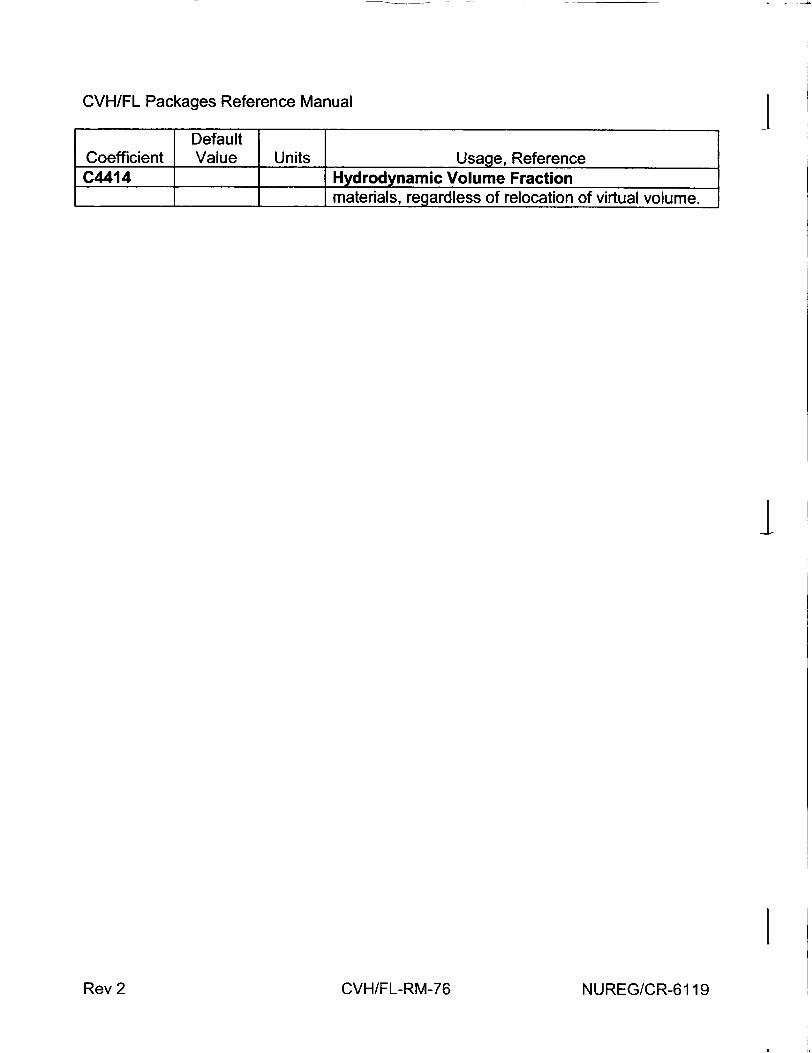
L - -- 4.
CVH/FL Packages Reference Manual
Coefficient C4414
Default Value Units Usage, Reference
Hydrodynamic Volume Fraction materials, regardless of relocation of virtual volume.
NUREG/CR-6119
I
Rev 2 CVH/FL-RM-76
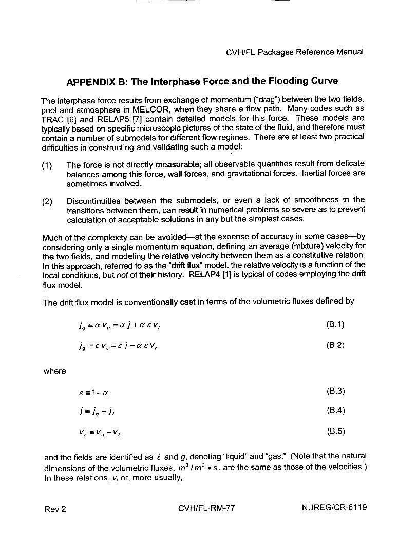
CVH/FL Packages Reference Manual
APPENDIX B: The Interphase Force and the Flooding Curve
The interphase force results from exchange of momentum ("drag") between the two fields,
pool and atmosphere in MELCOR, when they share a flow path. Many codes such as
TRAC [6] and RELAP5 [7] contain detailed models for this force. These models are
typically based on specific microscopic pictures of the state of the fluid, and therefore must
contain a number of submodels for different flow regimes. There are at least two practical difficulties in constructing and validating such a model:
(1) The force is not directly measurable; all observable quantities result from delicate balances among this force, wall forces, and gravitational forces. Inertial forces are sometimes involved.
(2) Discontinuities between the submodels, or even a lack of smoothness in the transitions between them, can result in numerical problems so severe as to prevent
calculation of acceptable solutions in any but the simplest cases.
Much of the complexity can be avoided-at the expense of accuracy in some cases-by considering only a single momentum equation, defining an average (mixture) velocity for
the two fields, and modeling the relative velocity between them as a constitutive relation. In this approach, referred to as the "drift flux" model, the relative velocity is a function of the
local conditions, but not of their history. RELAP4 [1] is typical of codes employing the drift flux model.
The drift flux model is conventionally cast in terms of the volumetric fluxes defined by
ig -avg = a j+ a 6 vr (B.1)
ig -•-V = ej-a vr (B.2)
where
(B.3)
j ji + j, (B.4)
Vr, = v - v, (B.5)
and the fields are identified as £ and g, denoting "liquid" and "gas." (Note that the natural
dimensions of the volumetric fluxes, m3 /m2 m s, are the same as those of the velocities.) In these relations, v, or, more usually,
NUREG/CR-6119CVH/FL-RM-77Rev 2
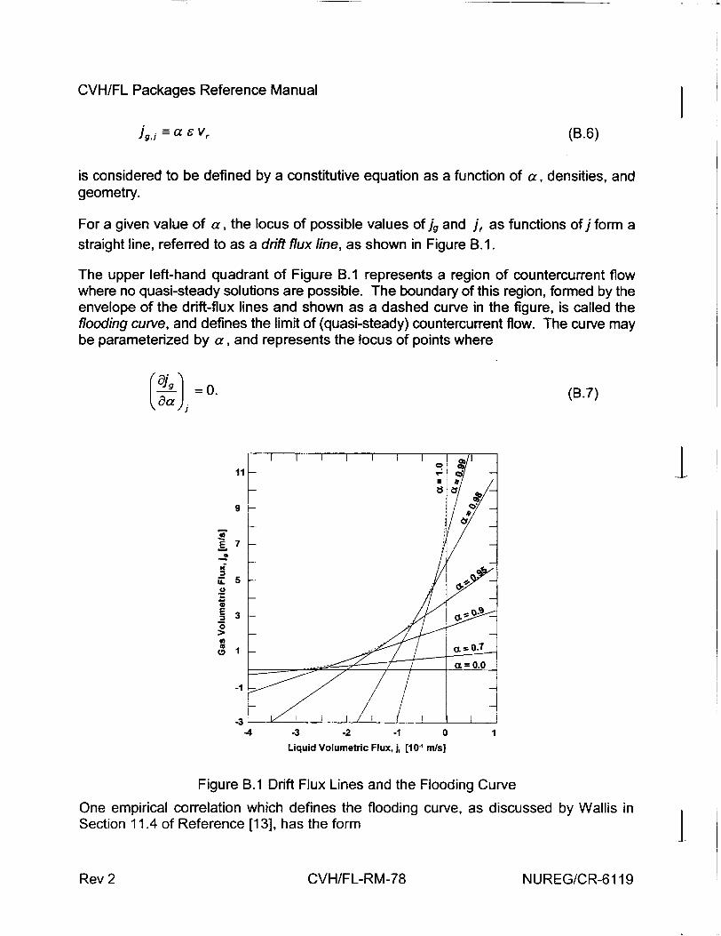
4.
CVH/FL Packages Reference Manual
jg,j -a Vr (B.6)
is considered to be defined by a constitutive equation as a function of a, densities, and geometry.
For a given value of a, the locus of possible values of jg and j, as functions of j form a
straight line, referred to as a drift flux line, as shown in Figure B.1.
The upper left-hand quadrant of Figure B.1 represents a region of countercurrent flow where no quasi-steady solutions are possible. The boundary of this region, formed by the envelope of the drift-flux lines and shown as a dashed curve in the figure, is called the flooding curve, and defines the limit of (quasi-steady) countercurrent flow. The curve may be parameterized by a, and represents the locus of points where
Oa °=0-
11
9
7
uS 5
3
0
-1
-,3-4
(B.7)
-3 -2 -1 0
Liquid Volumetric Flux, j, [10-1 m/s]
I
Figure B.1 Drift Flux Lines and the Flooding Curve
One empirical correlation which defines the flooding curve, as discussed by Wallis in Section 11.4 of Reference [13], has the form
NUREG/CR-6119
I
I
I
Rev 2 CVH/FL-RM-78
CVH/FL Packages Reference Manual
1 N
Here jgF and jl, define a point on the flooding curve, and vo and v, are scaling velocities
independent of a. Note that this equation is often written with a constant other than 1 on the right-hand side and/or with a coefficient multiplying either or both terms on the left-hand side; these can be absorbed into the scaling velocities without loss of generality.
It is a straightforward exercise to show that if
1 vr(a) = (B.9)
a/v1 + e/Vo
the flooding curve defined by Equation B.7 is given by
/vF = C2 (B.1O) (a/v1 + c/v 0 )2
J'== (a/v1 + c/Vo )2 (.1
Equations B.10 and B. 11 clearly satisfy the Wallis flooding relation given by Equation B.8. In addition, they give a parameterization of that curve by the void fraction a. MELCOR uses velocities rather than volumetric fluxes as the basic variable. In terms of velocities, the parameterization is
aF = VgF 'Iv 1 (B.12)
The drift flux model is most often used for quasi-steady, nearly incompressible flow. It is relatively simple to ensure that a two-fluid model will give similar results in the corresponding regime. In this limit, where a/ at -> 0 and derivatives of density may be
neglected, the momentum equations for the two fields-neglecting momentum flux (vev / Ox) terms-may be written as
a =Fgvg -a F,.(v,-v,) (B.13) aO x g
NUREG/CR-6119CVH/FL-RM-79Rev 2
-4
CVH/FL Packages Reference Manual
- p,gx - s F,v, -a s Fg(v, - vg) (B.14) ax
The coefficients Fg, F•, and Feg in the various momentum exchange terms are
abbreviations for the usual 2 f pIvIlD terms, in the form most commonly employed in
simulation codes for two-phase flow. In these equations, gx is the component of the gravitational acceleration in the x direction; in particular, it is -g if x is measured positive in the upward vertical direction.
If the pressure gradient is eliminated between Equations B.13 and B.14, the result can be cast in the form
a(F, + Fg) a -(p, - p (B1g J a - ,+- g+F a F, + e Fg + Feg a F, + aF.6F++F- (B.15)
Comparison of this equation with Equation B.1 shows that the quasi-steady solutions of the two-fluid equations will have a relative velocity given by
Vr (Pe -=Pg ýX (B.16) a F,+e6Fg+ Fjg
and comparison of this result with Equation B.9 suggests that the interphase force be
defined by
a F, +±SFg + Fg =(p, - pg)gx(a/v, + c/Vo) (B.17)
In MELCOR, we are most concerned with the flooding curve, which defines the limit of
countercurrent flow. In most cases of interest, the net wall force, F, + Fg, is small
compared to the interphase force when flooding occurs. Therefore, wall forces are neglected in Equation B.17, and the interphase force term, F~g, is set directly equal to the
right-hand side of this equation.
Finally, when the differential form of the momentum equation is integrated from volume center to volume center, the integral of gxdx becomes - gAz.
INUREG/CR-6119Rev 2 CVH/FL-RM-80
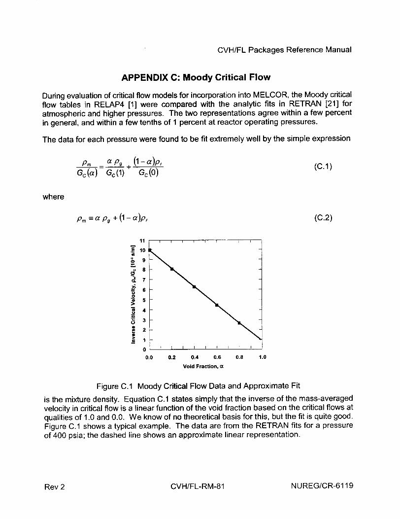
CVH/FL Packages Reference Manual
APPENDIX C: Moody Critical Flow
During evaluation of critical flow models for incorporation into MELCOR, the Moody critical flow tables in RELAP4 [1] were compared with the analytic fits in RETRAN [21] for atmospheric and higher pressures. The two representations agree within a few percent in general, and within a few tenths of I percent at reactor operating pressures.
The data for each pressure were found to be fit extremely well by the simple expression
(c.1)Gc(a) Gc(1) Gc(O)
where
Pm -a pg + (1- a)p,
0.
0 .5 _U
11
10 I
9
8
7
6
5
4
3
2
0 0.0
(C.2)
0.2 0.4 0.6 0.8 1.0
Void Fraction, a
Figure C.1 Moody Critical Flow Data and Approximate Fit
is the mixture density. Equation C.1 states simply that the inverse of the mass-averaged velocity in critical flow is a linear function of the void fraction based on the critical flows at qualities of 1.0 and 0.0. We know of no theoretical basis for this, but the fit is quite good. Figure C.1 shows a typical example. The data are from the RETRAN fits for a pressure of 400 psia; the dashed line shows an approximate linear representation.
NUREG/CR-6119CVH/FL-RM-81Rev 2
CVH/FL Packages Reference Manual
References
1. RELAP4/MOD5 A Computer Program for Transient Thermal-Hydraulic Analysis of Nuclear Reactors and Related Systems User's Manual, Volume 1, RELAP4/MOD5 Description, ANCR-NUREG-1335, Idaho Nuclear Engineering Laboratory, Idaho Falls, ID (September 1976).
2. S. E. Dingman, et al., HECTR Version 1.5 User's Manual, NUREG/CR-4507, SAND860101, Sandia National Laboratories, Albuquerque, NM (April 1986).
3. K. K. Murata, et al., "Code Manual for CONTAIN 2.0: A Computer Code for Nuclear Reactor Containment Analysis," NUREG/CR-6533, SAND97-1735, 1997.
4. "MAAP4, Modular Accident Analysis Program User's Manual," Volumes 1 and 2, EPRI (1994).
5. JANAF Thermochemical Tables, Dow Chemical Company, Thermal Research Laboratory, Midland, MI (1965).
6. TRAC-PF1. An Advanced Best-Estimate Computer Program for Pressurized Water Reactor Analysis, NUREG/CR-3567, LA-9944-MS, Los Alamos National Laboratory, Los Alamos, NM (February 1984).
7. V. H. Ransom, et al, RELAP5/MOD1 Code Manual Volume 1. System Model and Numerical Methods; Volume 2: Users Guide and Input Requirements, NUREG/CR1826, EGG-2070, Idaho National Engineering Laboratory (March 1982).
8. L. N. Kmetyk, MELCOR 1.8.1 Assessment: FLECHT SEASET Natural Circulation Experiments, SAND91-2218, Sandia National Laboratories, Albuquerque, NM (December 1991).
9. J. G. Collier, Convective Boiling and Condensation, 2 nd ed., McGraw-Hill, New York (1981), p. 326.
10. R. B. Bird, W. E. Stewart, and E. N. Lightfoot, Transport Phenomena, John Wiley & Sons, New York (1960), Equation 18.4-25.
11. See, for example, W. H. McAdams Heat Transmission, McGraw Hill, New York (1959). The correlation for the atmosphere is for an unstable temperature gradient; that for the pool is for a stable gradient and a finite surface.
12. R. K. Cole, Jr., Letter Report to Ron Foulds, USNRC, "CVH Pool/Atmosphere Condensation," under FIN A 1339 (August 1992).
NUREG/CR-6119CVH/FL-RM-83Rev 2
CVH/FL Packages Reference Manual j
13. G. B. Wallis, One-dimensional Two-phase Flow, McGraw-Hill Book Company, New York, NY (1969), Chapter 9.
14. F. Gelbard and J. H. Seinfeld, "Simulation of Multicomponent Aerosol Dynamics," J. Colloid and Interface Science, 78 (2) (December 1980).
15. D. R. H. Beattie and P. B. Whalley, "A Simple Two-Phase Frictional Pressure Drop Calculational Method," Int. J. Multiphase Flow, 8 (1) pp. 83-87 (1982).
16. "Flow of Fluids through Valves, Pipes, and Fittings," Technical Paper 410, Crane Co., Chicago, IL (1969).
17. R. D. Blevins, Applied Fluid Dynamics Handbook, Van Nostrand Reinhold, New York (1984); Section 6.3, with conversion of the Darcy-Weisbach form to the Fanning form used in MELCOR.
18. G. B. Wallis, One-dimensional Two-phase Flow, McGraw-Hill, New York (1969), Section 11.4.
19. P. C. Owczarski and K. W. Burk, SPARC-90: A Code for Calculating Fission Product Capture in Suppression Pools, NUREG/CR-5765, PNL-7723 (October 1991).
20. R. B. Bird, W. E. Stewart, and E. N. Lightfoot, Transport Phenomena, John Wiley & Sons, New York (1960), Equation 15.5-42, with identification of the sound speed as (P/p)11 2 .
21. RETRAN-02-A Program for Transient Thermal-Hydraulic Analysis of Complex Fluid Systems, Volumes 1-3, NP-1850-CCM, Electric Power Research Institute, Palo Alto, CA (May 1981).
22. D. Dobranich, SAFSIM Theory Manual-A Computer Program for the Engineering Simulation of Flow Systems. SAND92-0693, Sandia National Laboratories, Albuquerque, NM (1993).
23 I. F. Macdonald, M. S. EI-Sayed, K. Mow, and F. A. L. Dullien, "Flow Through Porous Media - the Ergun Equation Revisited," in Ind. Eng. Chem. Fundam., Vol. 18, No. 3, pp. 199-208, 1979.
24 E. Achenbach, "Heat Transfer and Pressure Drop of Pebble Beds Up to High Reynolds Number," in Proceedinqs of Seventh International Heat Transfer Conference, Vol. 1, pp. 3-8, 1982.
INUREG/CR-6119
I __ ___*
Rev 2 CVH/FL-RM-84
CVH/FL Packages Reference Manual
25. S. Ergun, "Fluid Flow Through Packed Columns," in Chem. En-q. Proc.ress, Vol. 48, No.
2, p. 504 (1952) (as cited in Reference 11).
26 R. K. Cole, Jr., "Incorporation of a Core flow Blockage Model into MELCOR," letter
report to John Ridgely, USNRC, November 30, 1995.
NUREG/CR-6119CVH/FL-RM-85Rev 2
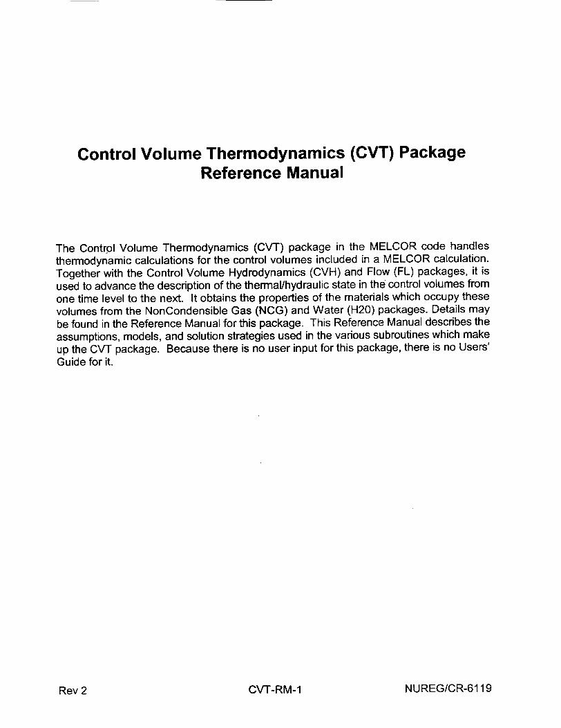
Control Volume Thermodynamics (CVT) Package Reference Manual
The Control Volume Thermodynamics (CVT) package in the MELCOR code handles thermodynamic calculations for the control volumes included in a MELCOR calculation. Together with the Control Volume Hydrodynamics (CVH) and Flow (FL) packages, it is used to advance the description of the thermal/hydraulic state in the control volumes from one time level to the next. It obtains the properties of the materials which occupy these volumes from the NonCondensible Gas (NCG) and Water (H20) packages. Details may
be found in the Reference Manual for this package. This Reference Manual describes the assumptions, models, and solution strategies used in the various subroutines which make up the CVT package. Because there is no user input for this package, there is no Users' Guide for it.
NUREG/CR-6119CVT-RM-1Rev 2

CVT Package Reference Manual
Contents
1. Introduction .................................................................................................. 5
2. Equilibrium Thermodynam ics ........................................................................... 7 2.1 Governing Assum ptions ......................................................................... 8 2.2 Governing Equations ............................................................................. 8 2.3 Required Derivatives ........................................................................... 15 2.4 Partition of Liquid Water between Pool and Atmosphere ..................... 15
3. Nonequilibrium Thermodynam ics ................................................................... 16 3.1 Governing Assum ptions ....................................................................... 16 3.2 Governing Equations ........................................................................... 17 3.3 Required Derivatives ..................................................... ...... 18 3.4 Lim it of Vanishing Pool or Atmosphere ............................................... 20
4. Other Required Properties ............................................................................. 21 4.1 Specific Heat at Constant Pressure ................................................... 21 4.2 Sound Speed ...................................................................................... 21
Appendix A: A.1 A.2 A.3
Derivatives ......................................................................................... 23 Derivatives of the Pressure ................................................................ 23 Derivatives of the Volume Available to NCG ........................................ 26 Derivatives of the Vapor Volume ........................................................ 28
List of Figures
Figure 1.1 CVT model structure .................................................................................. 7
NUREG/CR-6119CVT-RM-3Rev 2
CVT Package Reference Manual
1. Introduction
MELCOR's Control Volume Thermodynamics (CVT) package calculates the thermodynamic state of the materials in each control volume from the total volume, the energies, and the masses calculated by the Control Volume Hydrodynamics (CVH) package. The contents of the control volume may be divided into a pool containing water which may be subcooled (liquid) or saturated (two-phase), and an atmosphere containing water vapor, liquid water fog, and noncondensible gases (NCGs). While the terms "pool" and "atmosphere" suggest a quiescent, stratified configuration, the modeling in CVI assumes only that the two components occupy disjoint subvolumes of the total control volume. (Modeling in other areas of MELCOR, however, often assumes stratification.)
In addition to familiar thermodynamic properties such as pressure, heat capacity, and compressibility, the CVT package also calculates the derivatives of the pressure in the volume with respect to its energy and mass contents for use by the implicit flow solver in the CVH package.
Two thermodynamic options are available: equilibrium and nonequilibrium. In MELCOR, equilibrium thermodynamics assumes that the pool and the atmosphere are in thermal and mechanical equilibrium, i.e., that they have the same temperatures and pressures. This implies instantaneous energy and mass transfers between pool and atmosphere.
When the equilibrium option is used, the distinction between pool and atmosphere does not affect the thermodynamics. CVT uses the total mass and energy contents of the control volume to determine its pressure and temperature. All NCGs are assumed to reside in the atmosphere; the assignment of water to pool or atmosphere is made using time-dependent information from the CVH package. Under current modeling, no water vapor is assigned to the pool, but liquid water may be assigned to the atmosphere as fog.
Nonequilibrium thermodynamics, on the other hand, assumes mechanical equilibrium but not thermal equilibrium, so that pressures are equal but temperatures may be different. Complete equilibrium is assumed to exist within the subvolume occupied by the pool and within that occupied by the atmosphere, making this a more limited definition of nonequilibrium than is used in some other codes. The pool may contain water vapor, called void, and the atmosphere may contain fog. Energy and mass transfers between pool and atmosphere resulting from convection/conduction, radiation, and boiling are explicitly calculated in the CVH package. The elimination of void is also computed in the CVH package, using a bubble rise model. The precipitation of fog is treated by the RadioNuclide package (if it is active) and by the CVH package. The volume (PdV) work done by the pool on the atmosphere (or vice versa) must also be accounted for; this is handled in the CVT package itself.
NUREG/CR-6119Rev 2 CVT-RM-5
CVT Package Reference Manual J When the nonequilibrium option is used, the thermodynamic state is calculated based on the mass and the total energy of the pool, the masses of the individual components of the atmosphere and their total energy as defined by CVH, and the total volume available to be shared by pool and atmosphere. Part of CVT's job is to determine the partition of the total volume between the pool and the atmosphere such that the pressures of each are equal. Each subvolume is treated as adiabatic in this calculation; thus PdV work is accounted for within the CVT package but heat and mass transfer are not. Because the pool and the atmosphere are each in internal equilibrium, the nonequilibrium option requires application of the equilibrium assumptions within each subvolume.
The CVT package consists of various interfaces to -a mixed-material (water and noncondensible gases) equation of state. Properties for water and for noncondensible gases are obtained from the H20 and NCG packages, respectively. An important feature of the formulation is that it is analytic as well as thermodynamically consistent. Therefore, in contrast to equations of state based on tables or independent polynomial fits, all calculated properties are consistent (for example, a small change in mass or energy produces a change in pressure that agrees to several significant figures with that estimated from the derivatives). The structure of CVT modeling is illustrated in Figure 1.1. The block in the figure labeled "subvolume" implements the mixed-material equation of state in MELCOR as described in Section 2; its use in the nonequilibrium model is described in Section 3. 1
I
NUREG/CR-6119 CVT-RM-6 Rev 2
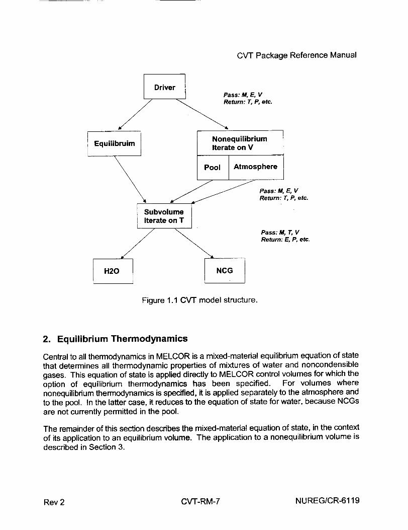
CVT Package Reference Manual
Pass: M, E, V Return: T, P, etc.
Pass: M, E, V Return: T, P, etc.
Return: E, P, etc.
H20 NCG
Figure 1.1 CVT model structure.
2. Equilibrium Thermodynamics
Central to all thermodynamics in MELCOR is a mixed-material equilibrium equation of state that determines all thermodynamic properties of mixtures of water and noncondensible gases. This equation of state is applied directly to MELCOR control volumes for which the option of equilibrium thermodynamics has been specified. For volumes where nonequilibrium thermodynamics is specified, it is applied separately to the atmosphere and to the pool. In the latter case, it reduces to the equation of state for water, because NCGs are not currently permitted in the pool.
The remainder of this section describes the mixed-material equation of state, in the context of its application to an equilibrium volume. The application to a nonequilibrium volume is described in Section 3.
NUREG/CR-6119Rev 2 CVT-RM-7
CVT Package Reference Manual J 2.1 Governing Assumptions
Equilibrium thermodynamics assumes that the pool and atmosphere temperatures are identical. Given the total volume, the total internal energy, and the masses of water and NCGs, the problem is to calculate the temperature, the total pressure, the partial pressures of each material, and various other thermodynamic properties. Because all temperatures are assumed equal and surface tension effects are not modeled, the distinction between liquid water as fog or in the pool is immaterial within equilibrium thermodynamics, as is the distinction between water vapor in the atmosphere or in a saturated pool. The assignment of liquid and vapor water to the different possible locations is made after the equilibrium state is determined, using time-dependent information from the CVH package. Therefore, within this section, pool will be used to mean "liquid water" and atmosphere to mean 'Water vapor plus NCGs." In defining the pressure, there are three basic cases:
(1) If no atmosphere is present (which can only occur if there is no NCG), the pressure is that of the pool.
(2) If no pool is present, the NCGs occupy the total volume together with the water vapor; the total pressure is the sum of their partial pressures.
(3) If both pool and atmosphere are present, their pressures as well as their temperatures are equal, and the partial pressure of water in the atmosphere is the saturation pressure for that temperature. If the atmosphere contains NCG, the pool
must be subcooled (its pressure is equal to the sum of the saturation pressure and the partial pressures of the NCGs), and its density is therefore greater than saturation density. Thus, the volume of the atmosphere is greater than that which would be occupied by water vapor in the absence of NCGs. As will be noted below, certain linearizations of the equation of state of water will be used to simplify this calculation.
2.2 Governing Equations
The equilibrium state for a mixture of water and NCGs in a volume, under the assumptions that the NCGs are insoluble in liquid water and form an ideal mixture with water vapor, is given by the simultaneous solution of the equations
Pt=-- , (2.1)
v,
NUREG/CR-6119 CVT-RM-8 Rev 2
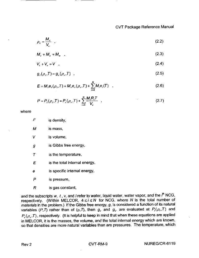
CVT Package Reference Manual
-Mv (2.2) Vv
Mt+ Mv =MW , (2.3)
V, + Vv =V , (2.4)
gj(p1,T)= gv(PvT) , (2.5)
N
E = M,e,(p,,T) + Mvev(pv,T) + IXMi e,(T) (2.6) i=4
P = Pt(p,,T) = Pv(pv,T) + N , (2.7)
i=4 Vv
where
P is density,
M is mass,
V is volume,
g is Gibbs free energy,
T is the temperature,
E is the total internal energy,
e is specific internal energy,
P is pressure,
R is gas constant,
and the subscripts w, f, v, and i refer to water, liquid water, water vapor, and the j• NCG, respectively. (Within MELCOR, 4 <i_< N for NCG, where N is the total number of
materials in the problem.) If the Gibbs free energy, g, is considered a function of its natural
variables (P,T) rather than of (p,T), then g, and gv are evaluated at P,(p,,T) and
Pv(pv,T), respectively. (It is helpful to keep in mind that when these equations are applied
in MELCOR, it is the masses, the volume, and the total internal energy which are known, so that densities are more natural variables than are pressures. The temperature, which
NUREG/CR-6119CVT-RM-9Rev 2
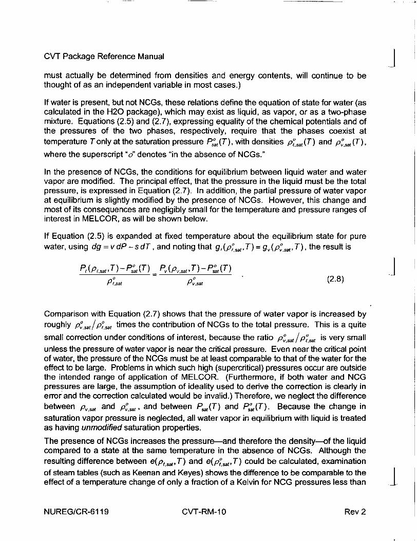
I - -4
CVT Package Reference Manual j must actually be determined from densities and energy contents, will continue to be thought of as an independent variable in most cases.)
If water is present, but not NCGs, these relations define the equation of state for water (as calculated in the H20 package), which may exist as liquid, as vapor, or as a two-phase mixture. Equations (2.5) and (2.7), expressing equality of the chemical potentials and of the pressures of the two phases, respectively, require that the phases coexist at temperature T only at the saturation pressure P' (T), with densities P~'sat(T) and pv°,,(T),
where the superscript "d' denotes "in the absence of NCGs."
In the presence of NCGs, the conditions for equilibrium between liquid water and water vapor are modified. The principal effect, that the pressure in the liquid must be the total pressure, is expressed in Equation (2.7). In addition, the partial pressure of water vapor at equilibrium is slightly modified by the presence of NCGs. However, this change and most of its consequences are negligibly small for the temperature and pressure ranges of interest in MELCOR, as will be shown below.
If Equation (2.5) is expanded at fixed temperature about the equilibrium state for pure water, using dg = v dP - s dT, and noting that g,(pofat, T) = gv(pv°.•t, T), the result is
P(Pesat'T)-P,•t(T) Pv(pvsatT)-Pst(T) 0 0 (2.8)
P f.sat IPv,sat
Comparison with Equation (2.7) shows that the pressure of water vapor is increased by roughly p,°.sat!pO°•t times the contribution of NCGs to the total pressure. This is a quite
small correction under conditions of interest, because the ratio Pvsat/Pt°at is very small unless the pressure of water vapor is near the critical pressure. Even near the critical point of water, the pressure of the NCGs must be at least comparable to that of the water for the effect to be large. Problems in which such high (supercritical) pressures occur are outside the intended range of application of MELCOR. (Furthermore, if both water and NCG pressures are large, the assumption of ideality used to derive the correction is clearly in error and the correction calculated would be invalid.) Therefore, we neglect the difference between pv.t and povt, and between P~t(T) and Ps,,(T). Because the change in
saturation vapor pressure is neglected, all water vapor in equilibrium with liquid is treated as having unmodified saturation properties.
The presence of NCGs increases the pressure-and therefore the density-of the liquid compared to a state at the same temperature in the absence of NCGs. Although the resulting difference between e(p,,t, T) and e(p,.•t, T) could be calculated, examination of steam tables (such as Keenan and Keyes) shows the difference to be comparable to the effect of a temperature change of only a fraction of a Kelvin for NCG pressures less than INUREG/CR-6119 CVT-RM-1 0 Rev 2
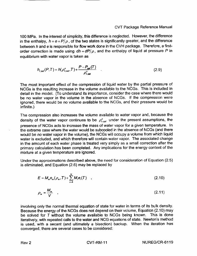
CVT Package Reference Manual
100 MPa. In the interest of simplicity, this difference is neglected. However, the difference in the enthalpy, h = e + P/p, of the two states is significantly greater, and the difference
between h and e is responsible for flow work done in the CVH package. Therefore, a first
order correction is made using dh = dP/p, and the enthalpy of liquid at pressure P in
equilibrium with water vapor is taken as
ht,..t(P, T) = h(p•'sat, T)+ P- T (2.9)
The most important effect of the compression of liquid water by the partial pressure of NCGs is the resulting increase in the volume available to the NCGs. This is included in detail in the model. (To understand its importance, consider the case where there would be no water vapor in the volume in the absence of NCGs. If the compression were ignored, there would be no volume available to the NCGs, and their pressure would be infinite.)
The compression also increases the volume available to water vapor and, because the
density of the water vapor continues to be p°,t under the present assumptions, the
presence of NCGs acts to increase the mass of water vapor for a given temperature. In the extreme case where the water would be subcooled in the absence of NCGs (and there would be no water vapor in the volume), the NCGs will occupy a volume from which liquid water is excluded, and which therefore will contain water vapor. The associated change in the amount of each water phase is treated very simply as a small correction after the primary calculation has been completed. Any implications for the energy content of the mixture at a given temperature are ignored.
Under the approximations described above, the need for consideration of Equation (2.5) is eliminated, and Equation (2.6) may be replaced by
N
E =Me,(p.,T)+ZMge,(T) (2.10) i=4
=MW (2.11) V
involving only the normal thermal equation of state for water in terms of its bulk density. Because the energy of the NCGs does not depend on their volume, Equation (2.10) may be solved for T without the volume available to NCGs being known. This is done iteratively, with repeated calls to the water and NCG equations of state. Newton's method is used, with a secant (and ultimately a bisection) backup. When the iteration has converged, there are several cases to be considered:
NUREG/CR-6119CVT-RM-I 1Rev 2
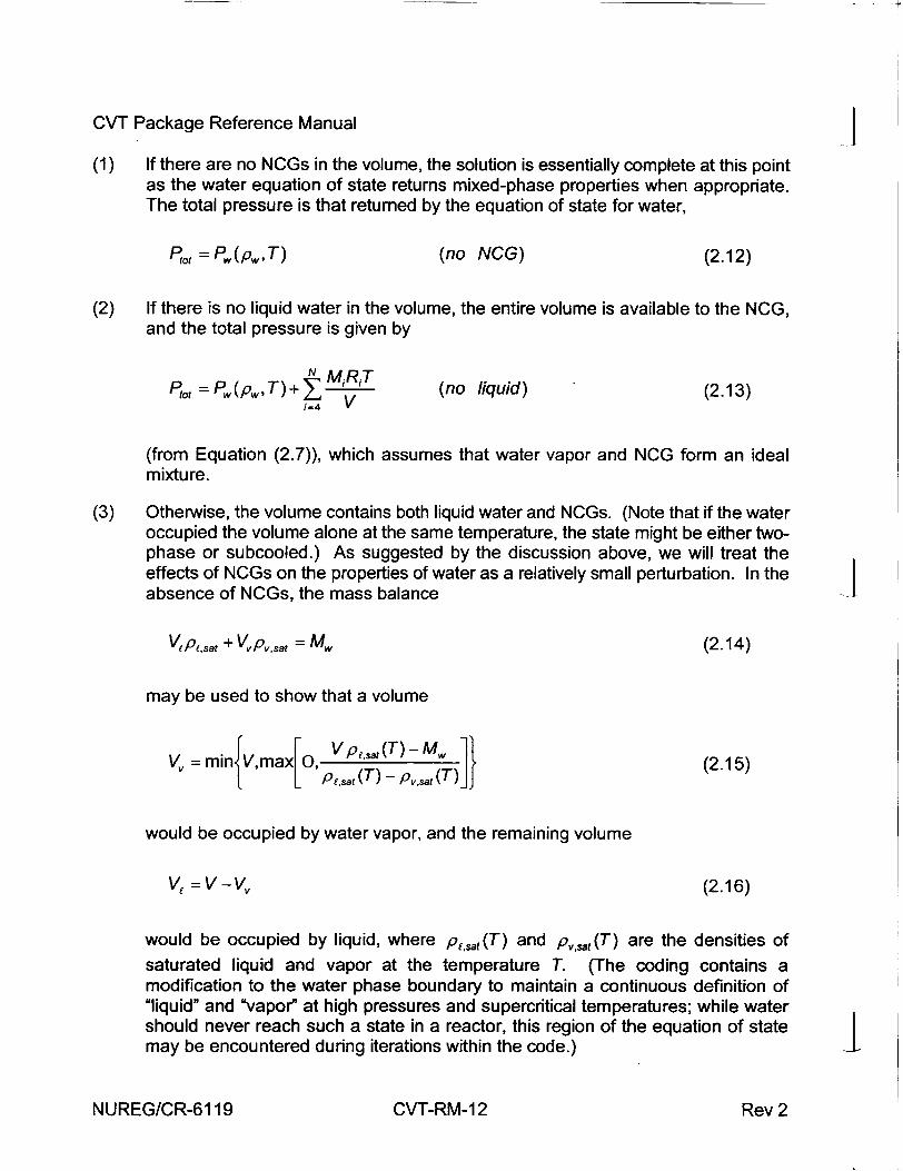
CVT Package Reference Manual 4 (1) If there are no NCGs in the volume, the solution is essentially complete at this point
as the water equation of state returns mixed-phase properties when appropriate. The total pressure is that returned by the equation of state for water,
Pt., = P.,(p.,T) (no NCG) (2.12)
(2) If there is no liquid water in the volume, the entire volume is available to the NCG, and the total pressure is given by
Pto, = P.,(p., T)+ N.MiR.T (no liquid) (2.13)
i=4 V
(from Equation (2.7)), which assumes that water vapor and NCG form an ideal mixture.
(3) Otherwise, the volume contains both liquid water and NCGs. (Note that if the water occupied the volume alone at the same temperature, the state might be either twophase or subcooled.) As suggested by the discussion above, we will treat the effects of NCGs on the properties of water as a relatively small perturbation. In the absence of NCGs, the mass balance
VVP,.sa + VvPvP.• = M., (2.14)
may be used to show that a volume
Vv =min V,max O, Vpesat (T) - MW (2.15) P1,,at (T) - Pv,.st (T)
would be occupied by water vapor, and the remaining volume
V, =V-Vv (2.16)
would be occupied by liquid, where pt.sat(T) and pv,,t(T) are the densities of
saturated liquid and vapor at the temperature T. (The coding contains a modification to the water phase boundary to maintain a continuous definition of "liquid" and "vapor" at high pressures and supercritical temperatures; while water should never reach such a state in a reactor, this region of the equation of state may be encountered during iterations within the code.) I
NUREG/CR-6119 CVT-RM-12 Rev 2
CVT Package Reference Manual
The requirement that pool and atmosphere have the same pressure when NCGs are included is imposed by assuming: (1) that the presence of the NCGs causes a reduction of the volume of the liquid by WV; (2) that the NCGs then occupy the new volume V,, where
V, = Vv + SV; (2.17)
and (3) that the resulting pressure is given by the linearization of Equation (2.7) as
P. T) 5V
I mw(p,,,T) + KV, mtot N M R t
t jPsat (T) + Y M -A-T , [ =' vv + 6v
(pool)
(atmosphere)
where P, in Equation (2.7) has been replaced by P,, (the two are equal in this case,
and P, has been replaced by P•(T), the partial pressure of water vapor in the
atmosphere. K is defined in terms of the compressibility of the liquid phase as
K: p' 7ap,t
Equation (2.18) results in a quadratic equation for 5V,
N
(5"/)2 +(V, +KVAP)bV-KK, M, RiT = 0 i=4
(2.19)
(2.20)
where
AP = Pv -Pst (T) ; (2.21)
and the fact that either Vv or AP is zero has been used (the former if the water
would be subcooled in the absence of NCGs, the latter if it would be two-phase). If the water is two-phase, the total pressure is best evaluated from the second form of Equation (2.18),
NUREG/CR-6119
(2.18)
CVT-RM-1 3Rev 2
CVT Package Reference Manual
N M RiT P, = P.,(p., T) +• I(2.22) i=4 Vv + ob/
noting that P,(p.,T)= Psat(T). Otherwise, for pure liquid (saturated or subcooled),
the first form of Equation 2.18 gives
~5V Ptot = P. (p., T) + Kv (2.23)
noting that V, = V.
At this point, the new atmosphere volume, V,, is greater than the volume of water vapor from the water equation of state, Vv, by an amount W1V (Equation (2.17)). Therefore, in order to maintain the density of water vapor in the atmosphere as pv.sat(T), a mass of water equal to p,.•t(T)SV is transferred from the liquid to the vapor state by simply
modifying the quality of water in the volume to be
x/ =X+ Pv.T)SV (2.24)
The mass involved is an extremely small fraction of the liquid mass because W'V is much smaller than V4 (liquid water is almost incompressible), and pv•t (T) is much smaller than
p,.J(T). The energy implications of assigning vapor energy rather than liquid energy to this mass are also very small, and are dealt with by the final adjustment to internal energy described below.
Just as V, is greater than Vv, the remaining liquid volume is less than the value V, used in the water equation of state. In addition to the correction to the liquid enthalpy given by Equation (2.9), a correction is made to the liquid density. As discussed in conjunction with Equation (2.9), the effect on liquid internal energy is small, and has been ignored. Because the uncorrected value has been used consistently, there are no implications with respect to conservation of energy.
The solution is now complete. A temperature has been found such that the known total internal energy is matched within the convergence tolerance of the iterative solution procedure. The pressure and all other thermodynamic properties have been evaluated consistently using that temperature and the known volume and masses. Because the total internal energy is the primary-and conserved-quantity, a final adjustment is made to the INUREG/CR-6119 CVT-RM-14 Rev 2
CVT Package Reference Manual
calculated specific internal energies so that Equation (2.10) is satisfied exactly. The adjustment is made either to the water or to the NCGs, depending of which has the greater total heat capacity.
2.3 Required Derivatives
A number of derivatives of the total pressure are required for the implicit solution of the flow equation (see the CVH/FL Reference Manual) or, as will be shown in a later section, for use in solving the nonequilibrium thermodynamic relations in volumes which employ that option. The natural variables for these derivatives are the total energy in the volume, E, the vector of masses in the volume, M, and the available hydrodynamic volume, V. The
required derivatives are (aPlaE)MV, (aP/aM,)EvI (aPI/MI)E.v [where 4 < i < N denotes
the NCGs], and (aP / aV)E.M. Evaluation of these derivatives is straightforward but tedious.
The required expressions are presented in Appendix A.
2.4 Partition of Liquid Water between Pool and Atmosphere
Preceding discussions describe a mixed-material equation of state in which it is assumed that water vapor and noncondensible gases (if both are present) are mixed within a common (sub)volume. For a volume in which nonequilibrium thermodynamics is specified, this equation of state will be applied to the pool and atmosphere separately as described in Section 3. Separate mass inventories are calculated for the pool and the atmosphere, and the pool is assumed to contain no noncondensible gases. Therefore, water vapor in the pool is unambiguously interpreted as vapor bubbles (void) and liquid water in the atmosphere as vapor droplets (fog).
For a volume in which equilibrium thermodynamics is specified, and the equation of state is applied to the entire contents of the volume, the situation is not so simple. The reason is that heat and mass transfer between pool and atmosphere are implicitly included. Therefore, only the total water content and the total energy of the control volume are known, and not the energies and water contents of pool and atmosphere individually.
As stated in the introduction, a basic assumption of the model is that the pool contains water only. If NCGs are present in an equilibrium volume, any liquid water must be subcooled as a consequence of the additional partial pressures of the NCGs. The poolwhich can contain no NCGs--can therefore contain no bubbles. In the absence of NCGs, there is no such restriction but, to avoid introduction of an unacceptable discontinuity between the two cases, the equilibrium model assumes that there is no void in the pool.
There is no such thermodynamic basis for defining the partition of liquid water between pool and fog. Both consist of subcooled (in the presence of NCGs) or saturated (in their absence) liquid water. As currently coded, the equilibrium model also assumes that there
NUREG/CR-6119CVT-RM-1 5Rev 2
CVT Package Reference Manual /
is preferential evaporation of, or condensation to, fog, so that the mass of water in the atmosphere is conserved if possible. That is, the new fog mass is calculated as
Mfw= max(Ml + Mo - Mv,) (2.25)
and any remaining mass of liquid water (as calculated by the equilibrium equation of state) is assigned to the pool.
3. Nonequilibrium Thermodynamics
As discussed in Section 1, the implementation of nonequilibrium thermodynamics in MELCOR is more restrictive than in some other codes. The underlying equation of state is strictly equilibrium, and does not allow subcooled vapor or superheated liquid. However, if the nonequilibrium option is selected, the pool and atmosphere within a control volume (which are also the two fields in the hydrodynamic equations) are not required to be in thermal or evaporative equilibrium.
3.1 Governing AssumptionsL4
Nonequilibrium thermodynamics assumes that the pool and the atmosphere have equal pressures but that their temperatures may be unequal. As currently implemented, it assumes that all NCGs are in the atmosphere. The pool may contain some water vapor as well as liquid, and the atmosphere may contain some liquid water (fog) in addition to vapor. For each field, the total water is determined by the mass inventory; the liquid/vapor state is determined implicitly by the energy content.
Given the total volume, the start-of-timestep subvolumes of the pool and of the atmosphere, the total internal energies of the pool and of the atmosphere at these start-oftimestep subvolumes, the mass of water in the pool, and the masses of water and NCGs in the atmosphere, the problem is to calculate the new subvolumes of the pool and of the atmosphere, the temperatures of each, and the common pressure. In computing the subvolumes, it is assumed that the boundary between pool and atmosphere is adiabatic because all heat and mass transfer has already been calculated in the CVH package. However the work done by displacement of the interface has not yet been calculated, and must be included in CVT. It is for this reason that the start-of-timestep subvolumes are needed.
The general equilibrium model described above for volumes in which equilibrium thermodynamics is specified is used to determine the properties of the atmosphere. It may be seen that the same three cases listed in Section 2.1 for equilibrium thermodynamics may occur: 1
NUREG/CR-6119 CVT-RM-16 Rev 2
CVT Package Reference Manual
(1) The atmosphere may contain liquid only (only if there are no NCGs),
(2) It may contain no liquid, and
(3) It may contain water vapor and/or NCGs in addition to liquid.
The first case, of course, has no physical significance because an "atmosphere" containing liquid water only is indistinguishable from "pool". It is included for completeness and then dealt with outside of the CVT package.
Because of the assumption that there are no NCGs in the pool, it could be treated by using the equation of state for water alone. However, in the interest of consistency, the same general equilibrium model is also used to determine its properties. This will also simplify changes to allow NCGs in the pool if desired in future versions of MELCOR.
3.2 Governing Equations
If a volume is to be treated in the nonequilibrium approximation, the pool and the atmosphere are each described by equilibrium thermodynamics. If we consider the pressure to be a function of masses, energy, and volume, and denoted by Pq,,i(M,E,V)
the function defined by the treatment of equilibrium thermodynamics in Section 2.2, the problem is to partition the total volume, V, into two components V, and Va such that
VP + Va = V (3.1)
and
Pequj, [Mp,Ep + P°'d (v;,'d - Vp), VP]
(3.2)
-Pequj[M.,E. +P Od(V."'d -. V)V]
Here the superscript "old" refers to the value at the start of the timestep. The terms in Equation (3.2) use the old pressure and the change in volume during the timestep to represent the volume work done by the pool on the atmosphere and vice versa. The old pressure (rather than some average over the timestep) must be used for consistency because, for the solution scheme used in the CVH package, mass moved through the flow paths carries old enthalpies, and therefore does work with old pressures. For example, in an extreme case where all but an insignificant amount of the atmosphere leaves a control
volume during a timestep, it will transport an energy of MO'dh'd in the limit as the remaining
mass of the atmosphere goes to zero, consisting of its internal energy plus the volume
NUREG/CR-6119CVT-RM-17Rev 2
1.4
CVT Package Reference Manual
work done by its motion. This will leave the remaining atmosphere with an energy approaching - Po°dV"d before the work done on it by the pool is accounted for in CVT. Its
new volume and new energy as determined by CVT must also go to zero, which can only happen if the old pressure is used in the volume work term.
Equation (3.2) is solved iteratively, subject to the constraint of Equation (3.1), by using Newton's method with a secant (and ultimately a bisection) backup. In order to avoid roundoff problems, the smaller of VP and Va is treated as the primary variable within the iteration. The same model used for equilibrium thermodynamics is used to evaluate Peo and its derivatives for the pool and for the atmosphere subvolumes. Because no heat transfer is included in CVT, the constant entropy (S) (adiabatic) derivatives of pressure with respect to volume
Cv oPs avVEN (3.3)
for the pool and for the atmosphere are used in the Newton iteration. This is consistent with inclusion of the PdV terms in Equation (3.2) [note that (aE I aV)s,M = -P].
3.3 Required Derivatives
Once Equation (3.2) has been solved to determine the volumes VP and Va, the derivatives required for solution of the flow equation are easily found from those already available for the subvolumes alone. For a differential change in some variable (mass, energy, or volume) for the pool or for the atmosphere, the differential change in pressure (under the current nonequilibrium assumptions) may be found by simultaneous solution of
IP IE p (dE - Pd, Pp
___-p ) Vo taM.,p )E
+ I "EM_. + 1I dV V i=4 taMi,,, )E..vp ( a VP )Ep,,,,
I
(3.4)
dP= "( )1 (dE
N P( ,
"a -PdVa)+- dM)a
. w.a
W,+ "r dV aVa EM,
NUREG/CR-6119
(3.5)
I
- ,a-Ea,,,,v
CVT-RM-18 Rev 2
CVT Package Reference Manual
subject to
dP=dPP =dP, , (3.6)
(3.7)dVP + dVa =0
(The summation over NCGs in the pool is retained in Equation (3.4) to allow future generalization, but the corresponding NCG masses are identically zero under current modeling assumptions.) In these equations PP and P, are used to represent P•,;• (pool)
and PequiI (atmosphere) and, to avoid further complicating the notation, it has been
assumed that a derivative with respect to a component mass is evaluated with all other component masses held constant. Note the inclusion of the PdV terms in Equations (3.4) and (3.5); here dE includes only those changes in energy treated by the CVH package, which does not consider volume work done by the pool on the atmosphere of the same calculational volume (or vice versa).
Solution of these equations leads to the desired derivatives. For example, if only dEP is
non-zero, Equations (3.4), (3.5), and (3.6) yield
dP= dP
dP = dP, = [C 2IP- )
IEP + IaCý~p]E. .M-
app
aEP )P'VPI dV
IdV, ,
(3.8)
(3.9)
Eliminating dVP and dV, by using Equation (3.7), and
defined by Equation (3.3), leads to the result
ap )"'(appv av aEP M
C " Opp )EMp,M,.V ( Va S.o]
identifying the adiabatic derivatives
C a ) .M(3.10)
NUREG/CR-61 19
-P aE,
(_ýP_. )Malv.
Rev 2 CVT-RM-19
4.
CVT Package Reference Manual /
The general expressions from which all the required derivatives may be evaluated may be seen to be
ap~ "P,,. )soa apMj..I
I _ 0 aý a (3 .1 1 )
"av) av) "M av sa'8 + a P
and
("PP)S", (". )--)(3.12)
where • is any one of the variables Eq, Mv,,, or Mi.,, "(," is "p" or "a", and {...}denotes
that set of variables which is to be kept constant under variation of •.
3.4 Limit of Vanishing Pool or Atmosphere
The separate mass and energy inventories calculated by CVH for the pool and the atmosphere are used to determine the thermodynamic properties of nonequilibrium volumes. In the limit where either the pool or the atmosphere in such a volume becomes extremely small, any loss of precision in calculating the energy content of the vanishing subvolume will have a large effect on the calculated temperature, since its heat capacity goes to zero. Blind application of the model described above leads to unacceptably large excursions in the calculated temperatures of very small pools and atmospheres.
This problem is handled within current coding by switching to the equilibrium formulation whenever a volume specified as nonequilibrium contains only an extremely small (10-6) volume fraction of pool or of atmosphere. One result is that when a nonequilibrium volume becomes completely filled by a two-phase pool, application of the equilibrium model results in an inappropriate separation of the two-phase pool into a pool containing only saturated liquid and an atmosphere containing the saturated water vapor from the bubbles.
This is clearly not a satisfactory solution. The principal problem is that the equilibrium model does not correspond to the infinite mass-and-heat-transfer limit of the nonequilibrium model. However, making the treatment of equilibrium and nonequilibrium INUREG/CR-6119 CVT-RM-20 Rev 2
CVT Package Reference Manual
volumes completely consistent would not be trivial, and might require elimination of the assumption that a pool can contain no NCGs.
On the other hand, extending the nonequilibrium model to handle the limit of a vanishing pool or atmosphere would require some modification to constrain the calculated temperature difference between pool and atmosphere. This would almost certainly require inclusion of an implicit contribution to the heat transfer (and possibly the mass transfer) between the pool and the atmosphere, either in CVH or (more likely) within CVT.
4. Other Required Properties
Other thermodynamic properties may be calculated from those returned by the H20 and NCG packages, using familiar thermodynamic relationships.
4.1 Specific Heat at Constant Pressure
The H20 package does not return the specific heat of water at constant pressure. Where this is needed, it is evaluated from the standard relationship
c -, =T cv +(4.1) ,2aP T
4.2 Sound Speed
The speed of sound in the pool and that in the atmosphere are calculated by CVT for use in other packages. The speed of sound, Cs, in a material is defined in terms of the adiabatic bulk modulus as
C ap (4.2)
Through the use of standard thermodynamic manipulations, Equation (4.2) may be recast in the form
NUREG/CR-6119CVT-RM-21Rev 2
CVT Package Reference Manual
C 2 IJTT aT 2
+ p 2 C v (4.3)
All of the variables in the latter form are available from the H20 and NCG packages. For a mixture, the sound speed calculated is that given by Equation (4.3) using mixture properties. It corresponds to an equilibrium (long-wavelength) limit, where there is adequate time for energy exchange between species.
NUREG/CR-6119
I - -4
l
CVT-RM-22 Rev 2
CVT Package Reference Manual
Appendix A: Derivatives
This Appendix presents the equations necessary for evaluation of the derivatives of the
pressure of an equilibrium mixture with respect to energy, total volume, and various
masses. Considerable care has been taken to indicate, using subscripts, what is kept
constant in each derivative. When no subscripts are present, the explicit derivative is
intended-that is, the derivative in terms of variables appearing explicitly in the definition
of the function. However, subscripts are included in some cases where the derivative is,
in fact, an explicit one. In order to avoid further complicating the notation, it has been
assumed that a derivative with respect to a component mass is evaluated with all other
component masses held constant.
In the following sections, the pressure is considered to be an explicit function of p,,, T, V,
and V, and of MiRi for each NCG. The chain rule will be used in evaluating the desired
results. V, will be treated as an explicit function of T, M,,, and V, and the MiRi, with
derivatives given in Section A.2. Vv will be treated as an explicit function of T, M, and
V, with derivatives given in Section A.3.
A.1 Derivatives of the Pressure
The various results presented in Equations (2.12), (2.13), (2.22), and (2.23) reduce to only two cases. They are:
(1) If the water would be single-phase (saturated or subcooled) liquid in the absence of NCGs, the total pressure including the effects of NCG is given by Equation (2.23) (noting that 6V = Vj) as
Vn Vn (A.1) P = P,,(p,'T) -+ KV (A1
KV
with explicit derivatives
aP_ aPw , (A.2)
ap.w
aP_ aP, (A.3) 5T aT
NUREG/CR-6119CVT-RM-23Rev 2
CVT Package Reference Manual
ap V_ aV KV 2 '
8P 1 av, KV
aP =0 a(MiRi)
(2) In all other cases, the pressure is
NMR P = P.(p., T)+ I,
i=4 V1
with explicit derivatives
a8P aP,, ap• ap"
a~p caP,,, MiRi
a - aT -t=4 V,
aP av
ap a Vn
N MRT
i=4 Vn
aP T
F(M,R, ) -V,
The derivative of pressure with respect to energy is evaluated from
IF )MV
where
(ao~m~ a.T)M C OFm~ aT ),
NUREG/CR-6119
I - -4.
(A.4)
(A.5)
(A.6)
(A.7)
I(A.8)
(A.9)
(A. 10)
(A.11)
(A.12)
(A.13)
I
I
CVT-RM-24 Rev 2
CVT Package Reference Manual
.ap .V=-+ -P (aV), (A.14) aT) aT aV,,YaT)m~v
=M + (A.15) SMYV ' "=4
Here, c, is the specific heat at constant volume, all water properties and their derivatives
come from the H20 package, and NCG properties come from the NCG package.
Derivatives of V,, will be discussed in Section A.2.
The derivative of pressure with respect to total volume is given by
a- =- av aV aVT Vap +aT )MVY (A.16)
EM av + a vf9 apo,, _T. MAv-E.M
Derivation of Equation (A.16) requires multiple application of the chain rule since, for
example, V, is an explicit function of T rather than of E. The additional term is
responsible for the appearance of (aPlaT)M~v (Equation (A.14)) rather than simply
(DP / aT). Finally,
aT E a3E C 8•, = •,r,(-•EM , (A.17)
(aV)EM a V)TM' UiMV
in which
=E -Pv,+T apW (A.18) ST,M aT
derivation of Equation (A.18) requires use of the Maxwell relation
(aS / aV)T.M = (aP I 8 T)M.v, and only water contributes because the internal energy of an
ideal gas is independent of its volume.
The derivative of pressure with respect to water mass is given by
NUREG/CR-6119CVT-RM-25Rev 2
CVT Package Reference Manual
C al'_ ai (aV~' 1 aP +li(a aM )E.v -y, U• aM)T~v V/ L +T )-.v aM, lEfv , (A.19)
where
aMT OE OETV t 5T) (A.20) C I _1aE>] aE ) = ev(p.,,T)- 1 aV) (A.21)
am TYV(a ,
the relation between (aE / aM.,)T.v and (aE / aV)T.M given by Equation (A. 18) is easily seen
from Equation (2.10).
The derivative of pressure with respect to the mass of the NCG is given by
C- ai + a p a Vr -(-'P)avy- (A.22) am, a(MR,) aV, a(M,R,) K V avJ
where
A.2 Derivatives of the Volume Available to NCG
The equations in the preceding section contain derivatives of the volume available to NCGs, V,. Unless there are both NCGs and liquid water in the volume, 5V is zero, V, is
identical to Vv, and we have
CNn) :ITMVv (no NCG or no liquid) (A.24)
C aTIJV. I : L-v (no NCG or no liquid) (A.25) -aT•v aT ), 'IV, )M. )M.
NUREG/CR-6119 CVT-RM-26 Rev 2
CVT Package Reference Manual
am,, va Vv Y (no NCG or no liquid) (A.26) 'I, )T,.V =- •-TV
(Expressions for derivatives of V, are given in Section A.3.) The derivative with respect
to NCG masses is more complicated, and must be found from the general case below.
If 6V is non-zero (case 3 of Section 2.2), we form the differential of Equation (2.20), the
quadratic defining W5V. It may be put in the form
(V * +265V)dV, (V * bV- Vn b .id Vv + , W fd V Vt) N(V, (A.27)
- KVcoVd(AP) + KVd IMRIT i=4
where
V* =V, +KVAP (A.28)
through use of Equation (2.20) itself. As noted in the discussion of Equation (2.20), either
Vv = 0 if the water is subcooled, or AP = 0 if it is saturated. The variable V * is used to
simplify the analysis by reducing the number of cases to be considered.
From Equation (A.27), we may identify the following derivatives (noting that the pressure
derivatives vanish unless the water is subcooled, in which case V, = V):
(V -2 ,*'v f • = (v . -,-b - ,, _V v (Lv,)T ,-M (A.29)
+ V. bVt + K bVp, ap.O' VVn . ap T
(V *T+2 V ) aT)M =V * + bV - Vn 9V '-)MV DM YV
MY( [,VdP. 1 P (A.30) _ + J+ MiRM i dT T i=4
NUREG/CR-6119CVT-RM-27Rev 2
-4.
CVT Package Reference Manual
(V * +265V• aVn ) =CV*+o3lVn-•,8M ?JtT v
KV apm ap,,
(V* +26V aV 1 = KVT "a(MiRi) TYv
Unless there are both NCGs and liquid water, Equations (A.29), (A.30), and to Equations (A.24), (A.25), and (A.26), respectively.
(A.31) reduce
If there are no NCGs, the derivative of pressure with respect to NCG mass, given by Equation (A.32), reduces to
[ (MR, )lTYkV * (no NCG) I
a result which could not have been obtained from the results derived in the absence of NCGs. Some care must be taken in evaluating Equation (A.33) in the case of saturated liquid. Whether this situation is approached from the subcooled side (Vv = 0,P -> 0+) or from the two-phase side (AP = 0,Vv -> 0+), the denominator V * goes to 0.
Ideally, one should maintain consistency regardless of how this state of saturated liquid water and no NCG is approached, taking into account that it may involve either case 1 or case 2 in Section A.1. The current coding simply prevents the division by zero. This simple approach has not been found to cause any problems in practice.
A.3 Derivatives of the Vapor Volume
The equations in the preceding section contain derivatives of the volume which would be occupied by water vapor in the absence of NCG with respect to total volume, temperature, and water mass. There are three cases to be considered:
(1) If there is no liquid (no water, or vapor only), Vv = V and
INUREG/CR-6119
and
(A.31)
(A.32)
(A.33)
-1
CVT-RM-28 Rev 2
CVT Package Reference Manual
av-)T,M,
( aT)MV
= 1
=0 ,
IaVv )=
(2) If there is water but no vapor (liquid only), Vv = 0, and
aV, )T,MW
aTMV/ =0
C ST•,,
- >1),.V =0
Otherwise (two-phase water), Vv is given by the primary form of Equation (2. bounds), and the derivatives are
CavL IIT,Mw P, sat P,
C ST
al MVV ) T. V
Vdpt~a + V, dpv,, dT VdT Pe.sat - P'a
1
(A.39)
15) (not the
(A.40)
(A.41)
(A.42)
NUREG/CR-6119
(A.34)
(A.35)
(A.36)
(A.37)
(A.38)
Rev 2 CV-I-RM-29
I - -t
CVT Package Reference Manual J The total derivatives of saturation densities with respect to temperature are, of course, to be taken along the phase boundaries. They are evaluated from tables included in the H20 package.
I_
I
NUREG/CR-6119 CVT-RM-30 Rev 2
Decay Heat (DCH) Package Reference Manual
The MELCOR decay heat (DCH) package models the decay heat power resulting from the radioactive decay of fission products. Decay heat is evaluated for core materials in the reactor vessel and cavity and for suspended or deposited aerosols and gases. MELCOR couples thermal-hydraulic processes and fission product behavior during the calculation.
Both the radionuclides present in the reactor at the time of the accident and the radionuclide daughter products contribute to the decay heat. In the calculation of decay heat, MELCOR does not explicitly treat each decay chain, since detailed tracking of radionuclide decay chains would be too costly. When the RadioNuclide package is active, the decay heat is calculated for each radionuclide class by using pre-calculated tables from ORIGEN calculations. If the RadioNuclide package is not active, the whole-core decay heat is computed from one of several possible user-specified calculations.
This Reference Manual describes the various models and options available in the DCH package. User input for these models and options is described in the DCH Package Users' Guide.
NUREG/CR-6119DCH-RM-1Rev 2
DCH Package Reference Manual
Contents
1. Introduction ..................................................................................................... 5
2. Elemental and Radionuclide Class Decay Heat ................................................ 5 2.1 SANDIA-ORIGEN Calculations ............................................................ 5 2.2 Radionuclide Classes ............................................................................ 7
3. Whole Core Decay Heat Calculation .............................................................. 8 3.1 Summation of ORIGEN Data ................................................................. 9 3.2 ANS Standard Calculation ...................................................................... 9 3.3 User-Defined Functions ........................................................................ 14
R efe re nces .................................................................................................................... 15
List of Tables
Table 2.1. Default Radionuclide Classes and Member Elements .............................. 8 Table 3.1. Tabular Values from ANS Standard [3] Used in MELCOR ...................... 10 Table 3.2. DCH Package Input Variables for ANS Decay Heat Power ..................... 14
NUREG/CR-6119DCH-RM-3Rev 2
DCH Package Reference Manual
1. Introduction
The MELCOR Decay Heat Power (DCH) package models the heating from the radioactive decay of fission products. Decay heat power is evaluated for the fission products assumed to reside in reactor core materials, cavity materials, and in suspended or deposited aerosols and vapors. Decay heat power levels as a function of time are supplied as a utility function within MELCOR that may be called by other phenomenological packages. The DCH package is not involved in the calculation of fission product transport or chemical interactions. These processes are calculated by the RadioNuclide (RN) package (see the RN Package Reference Manual).
Both the radionuclides present in the reactor core and/or cavity from the time of reactor shutdown and the radionuclide daughters from decay contribute to the total decay heat power. In the calculation of decay heat power, the DCH package does not explicitly treat decay chains. Detailed tracking of radionuclide decay chains was seen as computationally costly and too detailed for MELCOR. Instead, when the RN package is active, elemental decay heat power information based on ORIGEN calculations[1,2] is summed into the RN class structure, as described in Section 2.
There are also several options for calculating decay heat power when the RN package is not active (that is, when tracking of fission products is not desired). These are called wholecore calculations in the DCH package, although they may be applied to cavity inventories of melt debris as well, and are described in Section 3.
2. Elemental and Radionuclide Class Decay Heat
The DCH package models the decay heat power as a function of time and the total initial inventories of individual elements. The default decay heat curves and inventories were obtained from ORIGEN calculations [1], as described in Section 2.1. The grouping of elements into classes for use by the RadioNuclide package is described in Section 2.2.
2.1 SANDIA-ORIGEN Calculations
Calculations were made for prototypical BWR and PWR reactors using the Sandia National Laboratories version of the ORIGEN computer code, and tables of the associated fission product initial inventories and their decay heat powers out to ten days were generated [1,2]. In these tables, all isotopes of an element were summed, and daughters were assumed to remain with the parents. This resulted in 29 elemental groups accounting for over 99% of the decay heat power out to at least two days after reactor shutdown.
NUREG/CR-6119Rev 2 DCH-RM-5
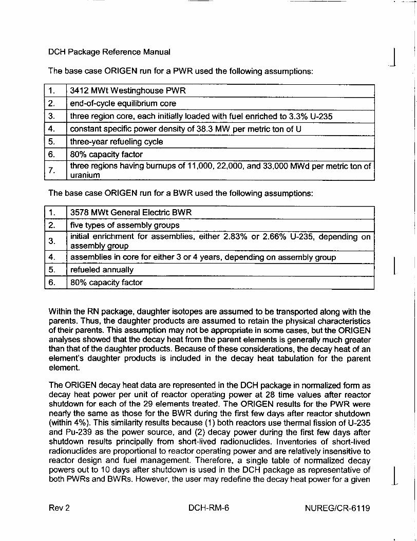
DCH Package Reference Manual
The base case ORIGEN run for a PWR used the following assumptions:
1. 3412 MWt Westinghouse PWR
2. end-of-cycle equilibrium core
3. three region core, each initially loaded with fuel enriched to 3.3% U-235
4. constant specific power density of 38.3 MW per metric ton of U
5. three-year refueling cycle
6. 80% capacity factor three regions having bumups of 11,000, 22,000, and 33,000 MWd per metric ton of uranium
The base case ORIGEN run for a BWR used the following assumptions:
1. 3578 MWt General Electric BWR
2. five types of assembly groups initial enrichment for assemblies, either 2.83% or 2.66% U-235, depending on assembly group
4. assemblies in core for either 3 or 4 years, depending on assembly group
5. refueled annually
6. 80% capacity factor
Within the RN package, daughter isotopes are assumed to be transported along with the parents. Thus, the daughter products are assumed to retain the physical characteristics of their parents. This assumption may not be appropriate in some cases, but the ORIGEN analyses showed that the decay heat from the parent elements is generally much greater than that of the daughter products. Because of these considerations, the decay heat of an element's daughter products is included in the decay heat tabulation for the parent element.
The ORIGEN decay heat data are represented in the DCH package in normalized form as decay heat power per unit of reactor operating power at 28 time values after reactor shutdown for each of the 29 elements treated. The ORIGEN results for the PWR were nearly the same as those for the BWR during the first few days after reactor shutdown (within 4%). This similarity results because (1) both reactors use thermal fission of U-235 and Pu-239 as the power source, and (2) decay power during the first few days after shutdown results principally from short-lived radionuclides. Inventories of short-lived radionuclides are proportional to reactor operating power and are relatively insensitive to reactor design and fuel management. Therefore, a single table of normalized decay powers out to 10 days after shutdown is used in the DCH package as representative of both PWRs and BWRs. However, the user may redefine the decay heat power for a given
NUREG/CR-6119
j
1
IRev 2 DCH-RM-6
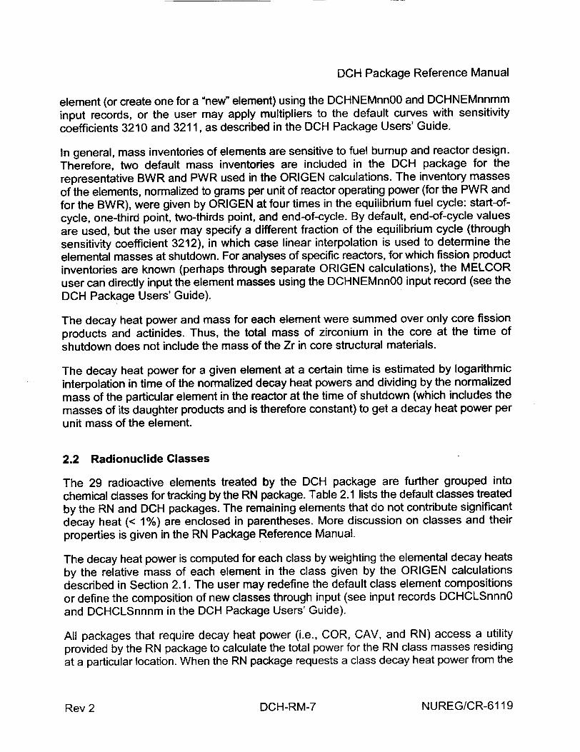
DCH Package Reference Manual
element (or create one for a "new" element) using the DCHNEMnnOO and DCHNEMnnmm
input records, or the user may apply multipliers to the default curves with sensitivity
coefficients 3210 and 3211, as described in the DCH Package Users' Guide.
In general, mass inventories of elements are sensitive to fuel burnup and reactor design. Therefore, two default mass inventories are included in the DCH package for the representative BWR and PWR used in the ORIGEN calculations. The inventory masses of the elements, normalized to grams per unit of reactor operating power (for the PWR and for the BWR), were given by ORIGEN at four times in the equilibrium fuel cycle: start-ofcycle, one-third point, two-thirds point, and end-of-cycle. By default, end-of-cycle values are used, but the user may specify a different fraction of the equilibrium cycle (through sensitivity coefficient 3212), in which case linear interpolation is used to determine the elemental masses at shutdown. For analyses of specific reactors, for which fission product inventories are known (perhaps through separate ORIGEN calculations), the MELCOR user can directly input the element masses using the DCHNEMnnOO input record (see the
DCH Package Users' Guide).
The decay heat power and mass for each element were summed over only core fission products and actinides. Thus, the total mass of zirconium in the core at the time of shutdown does not include the mass of the Zr in core structural materials.
The decay heat power for a given element at a certain time is estimated by logarithmic interpolation in time of the normalized decay heat powers and dividing by the normalized mass of the particular element in the reactor at the time of shutdown (which includes the masses of its daughter products and is therefore constant) to get a decay heat power per unit mass of the element.
2.2 Radionuclide Classes
The 29 radioactive elements treated by the DCH package are further grouped into chemical classes for tracking by the RN package. Table 2.1 lists the default classes treated by the RN and DCH packages. The remaining elements that do not contribute significant decay heat (< 1%) are enclosed in parentheses. More discussion on classes and their properties is given in the RN Package Reference Manual.
The decay heat power is computed for each class by weighting the elemental decay heats by the relative mass of each element in the class given by the ORIGEN calculations described in Section 2.1. The user may redefine the default class element compositions or define the composition of new classes through input (see input records DCHCLSnnnO and DCHCLSnnnm in the DCH Package Users' Guide).
All packages that require decay heat power (i.e., COR, CAV, and RN) access a utility provided by the RN package to calculate the total power for the RN class masses residing at a particular location. When the RN package requests a class decay heat power from the
NUREG/CR-61 19DCH-RM-7Rev 2
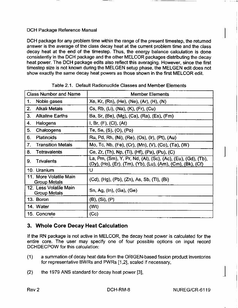
DCH Package Reference Manual
DCH package for any problem time within the range of the present timestep, the returned answer is the average of the class decay heat at the current problem time and the class decay heat at the end of the timestep. Thus, the energy balance calculation is done consistently in the DCH package and the other MELCOR packages distributing the decay heat power. The DCH package edits also reflect this averaging. However, since the first timestep size is not known during the MELGEN setup phase, the MELGEN edit does not show exactly the same decay heat powers as those shown in the first MELCOR edit.
Table 2.1. Default Radionuclide Classes and Member Elements
Class Number and Name Member Elements
1. Noble gases Xe, Kr, (Rn), (He), (Ne), (Ar), (H), (N)
2. Alkali Metals Cs, Rb, (Li), (Na), (K), (Fr), (Cu)
3. Alkaline Earths Ba, Sr, (Be), (Mg), (Ca), (Ra), (Es), (Fm)
4. Halogens I, Br, (F), (Cl), (At)
5. Chalcogens Te, Se, (S), (0), (Po)
6. Platinoids Ru, Pd, Rh, (Ni), (Re), (Os), (Ir), (Pt), (Au)
7. Transition Metals Mo, Tc, Nb, (Fe), (Cr), (Mn), (V), (Co), (Ta), (W)
8. Tetravalents Ce, Zr, (Th), Np, (Ti), (Hf), (Pa), (Pu), (C)
9. Trivalents La, Pm, (Sm), Y, Pr, Nd, (AI), (Sc), (Ac), (Eu), (Gd), (Tb), (Dy), (Ho), (Er), (Tm), (Yb), (Lu), (Am), (Cm), (Bk), (Cf)
10. Uranium U 11. More Volatile Main
Group Metals (Cd), (Hg), (Pb), (Zn), As, Sb, (TI), (Bi) 12. Less Volatile Main Sn, Ag, (In), (Ga), (Ge)
Group Metals 13. Boron (B), (Si), (P)
14. Water (Wt)
15. Concrete (Cc)
3. Whole Core Decay Heat Calculation
If the RN package is not active in MELCOR, the decay heat power is calculated for the entire core. The user may specify one of four possible options on input record DCHDECPOW for this calculation:
(1) a summation of decay heat data from the ORIGEN-based fission product inventories for representative BWRs and PWRs [1,2], scaled if necessary,
(2) the 1979 ANS standard for decay heat power [3],
NUREG/CR-6119
I -
j
I
-1
DCH-RM-8Rev 2
DCH Package Reference Manual
(3) a user-specified tabular function of whole-core decay as a function of time, or
(4) a user-specified control function to define decay heat.
Each option is described in the following subsections.
3.1 Summation of ORIGEN Data
As discussed in Section 2, a Sandia version of ORIGEN [2] has been used to perform decay heat calculations for prototypical PWR and BWR systems [1]. For the whole-core calculation, the tabulated results of the ORIGEN calculation are summed to produce a total reactor decay heat power, Pwc. No elemental or class information is retained; a single decay power value is returned when called by other packages. This is the default wholecore calculation and is the same for PWRs and BWRs.
3.2 ANS Standard Calculation
MELCOR can compute the total decay heat power from the American Nuclear Society's National Standard for light water reactors [3]. This standard prescribes fission product decay heat power for reactor operating histories. Currently, the DCH package uses a userspecified operating time (input on record DCHOPRTIME) with a constant reactor power, and it also assumes an instantaneous shutdown. The standard prescribes the recoverable energy release rates from fission product decay, but it does not specify the spatial distribution of the deposition of the energy in the reactor materials. This aspect of the problem is reactor specific and must be dealt with by the MELCOR Core package.
The decay heat power is related to the operating power of the reactor via the fission rate and the recoverable energy per fission during operation. The ANS standard assumes that the energy release per fission is independent of time and depends upon the energy spectrum of the neutron flux in the operating reactor and the composition of the reactor core. The energies per fission for U-235, Pu-239, and U-238 are defined in sensitivity coefficient array 3201.
Decay heat power from activation products in reactor structural materials is not specified in the standard, but decay heat powers from U-239 and Np-239 as prescribed by the standard are implemented in the DCH package. The effect of neutron capture in fission products is accounted for by using a formula from the ANS standard for the correction out to a time-since-shutdown of 10 s. The DCH package then uses Table 10 from the standard that sets an upper bound on the effect of neutron capture and provides a conservative estimate of the decay heat power. The values from this table are reproduced here in Table 3.1. Because of the conservatism of this table, the ANS standard decay heat power actually contains a discontinuity manifested by a small increase at 104 seconds.
NUREG/CR-6119DCH-RM-9Rev 2
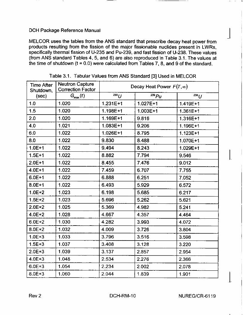
DCH Package Reference Manual
MELCOR uses the tables from the ANS standard that prescribe decay heat power from products resulting from the fission of the major fissionable nuclides present in LWRs, specifically thermal fission of U-235 and Pu-239, and fast fission of U-238. These values (from ANS standard Tables 4, 5, and 6) are also reproduced in Table 3.1. The values at the time of shutdown (t = 0.0) were calculated from Tables 7, 8, and 9 of the standard.
Table 3.1. Tabular Values from ANS Standard [3] Used in MELCOR
Time After Neutron Capture Decay Heat Power F(T, O) Shutdown, Correction Factor
(sec) Gm (t) Z35 u _ __pu • U
1.0 1.020 1.231 E+1 1.027E+1 1.419E+1
1.5 1.020 1.198E+1 1.003E+1 1.361 E+I
2.0 1.020 1.169E+1 9.816 1.316E+1
4.0 1.021 1.083E+1 9.206 1.196E+1
6.0 1.022 1.026E+1 8.795 1.123E+1
8.0 1.022 9.830 8.488 1.070E+1
1.OE+1 1.022 9.494 8.243 1.029E+1
1.5E+1 1.022 8.882 7.794 9.546
2.OE+1 1.022 8.455 7.476 9.012
4.OE+1 1.022 7.459 6.707 7.755
6.OE+1 1.022 6.888 6.251 7.052
8.OE+1 1.022 6.493 5.929 6.572
1.OE+2 1.023 6.198 5.685 6.217
1.5E+2 1.023 5.696 5.262 5.621
2.OE+2 1.025 5.369 4.982 5.241
4.OE+2 1.028 4.667 4.357 4.464
6.OE+2 1.030 4.282 3.993 4.072
8.OE+2 1.032 4.009 3.726 3.804
1.OE+3 1.033 3.796 3.516 3.598
1.5E+3 1.037 3.408 3.128 3.220
2.OE+3 1.039 3.137 2.857 2.954
4.OE+3 1.048 2.534 2.276 2.366
6.OE+3 1.054 2.234 2.002 2.078
8.OE+3 1.060 2.044 1.839 1.901
NUREG/CR-6119
I - -�
I
Rev 2 DCH-RM-10
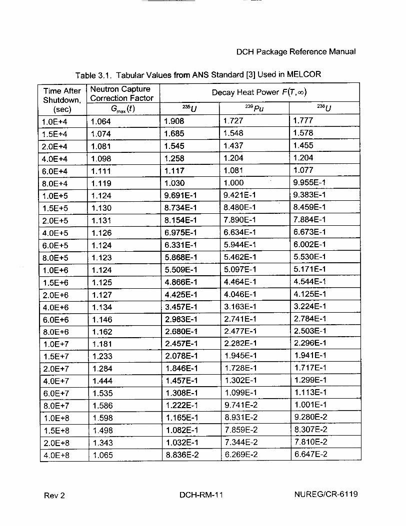
DCH Package Reference Manual
Table 3.1. Tabular Values from ANS Standard [3] Used in MELCOR
Time After Neutron Capture Decay Heat Power F(T, o) Shutdown, Correction Factor
(sec) Gm. (t) _ _5_ U 239 Pu 238_u
1.OE+4 1.064 1.908 1.727 1.777
1.5E+4 1.074 1.685 1.548 1.578
2.0E+4 1.081 1.545 1.437 1.455
4.OE+4 1.098 1.258 1.204 1.204
6.OE+4 1.111 1.117 1.081 1.077
8.OE+4 1.119 1.030 1.000 9.955E-1
1.OE+5 1.124 9.691E-1 9.421E-1 9.383E-1
1.5E+5 1.130 8.734E-1 8.480E-1 8.459E-1
2.OE+5 1.131 8.154E-1 7.890E-1 7.884E-1
4.OE+5 1.126 6.975E-1 6.634E-1 6.673E-1
6.OE+5 1.124 6.331E-1 5.944E-1 6.002E-1
8.OE+5 1.123 5.868E-1 5.462E-1 5.530E-1
1.OE+6 1.124 5.509E-1 5.097E-1 5.171E-1
1.5E+6 1.125 4.866E-1 4.464E-1 4.544E-1
2.OE+6 1.127 4.425E-1 4.046E-1 4.125E-1
4.OE+6 1.134 3.457E-1 3.163E-1 3.224E-1
6.OE+6 1.146 2.983E-1 2.741E-1 2.784E-1
8.OE+6 1.162 2.680E-1 2.477E-1 2.503E-1
1.OE+7 1.181 2.457E-1 2.282E-1 2.296E-1
1.5E+7 1.233 2.078E-1 1.945E-1 1.941 E-1
2.OE+7 1.284 1.846E-1 1.728E-1 1.717E-1
4.OE+7 1.444 1.457E-1 1.302E-1 1.299E-1
6.OE+7 1.535 1.308E-1 1.099E-1 1.113E-1
8.OE+7 1.586 1.222E-1 9.741 E-2 1.001 E-1
1.OE+8 1.598 1.165E-1 8.931E-2 9.280E-2
1.5E+8 1.498 1.082E-1 7.859E-2 8.307E-2
2.OE+8 1.343 1.032E-1 7.344E-2 7.810E-2
4.OE+8 1.065 8.836E-2 6.269E-2 6.647E-2
NUREG/CR-6119Rev 2 DCH-RM-1 1
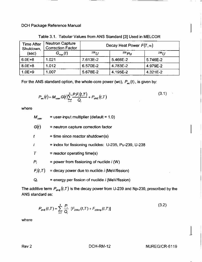
DCH Package Reference Manual J Table 3.1. Tabular Values from ANS Standard [3] Used in MELCOR
Time After Neutron Capture Decay Heat Power F(T, cc) Shutdown, Correction Factor
(sec) G(t) 23U 239 Pu 238 U
6.0E+8 1.021 7.613E-2 5.466E-2 5.746E-2
8.OE+8 1.012 6.570E-2 4.783E-2 4.979E-2
1.OE+9 1.007 5.678E-2 4.195E-2 4.321E-2
For the ANS standard option, the whole-core power (wc), P.' (t), is given by:
P.0 . ~t3 P, F (,T),P"(t,T) (3.1) P.•(uter M•G(t)Z,= I 5 + PdHE(t,T)
where
Muser = user-input multiplier (default = 1.0)
G(t) = neutron capture correction factor
t = time since reactor shutdown(s)
i = index for fissioning nuclides: U-235, Pu-239, U-238
T = reactor operating time(s)
Pi = power from fissioning of nuclide i (W)
F,.(t,T) = decay power due to nuclide i (MeV/fission)
Qi = energy per fission of nuclide i (MeV/fission)
The additive term PdHE(tT) is the decay power from U-239 and Np-239, prescribed by the
ANS standard as:
3, p.(3.2) PdHE(tT) Y - [F239A(t,T) + F239 Np(t,T)]
where
INUREG/CR-6119
L - -+
Rev 2 DCH-RM-12
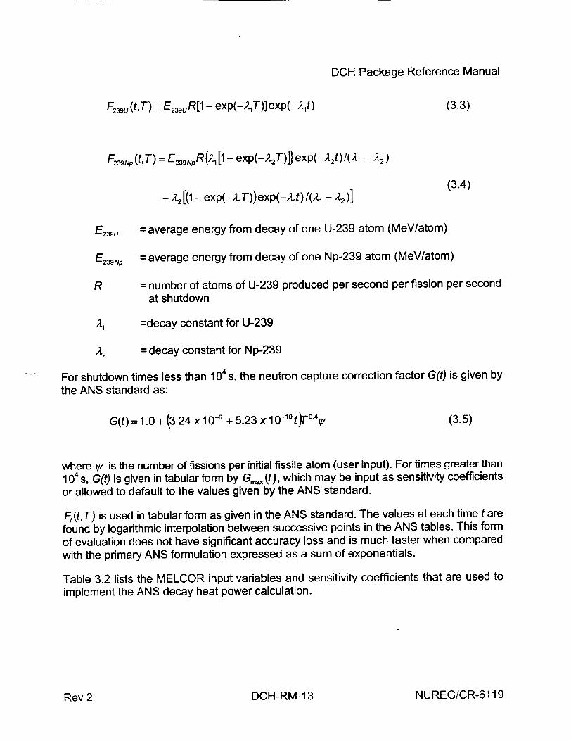
DCH Package Reference Manual
F239 (t,T) = E239uR[1 - exp(-2 1T)]exp(-, 1 t) (3.3)
F239Np(t,T) = E239NPR{A, [1 - exp(-A2T)D exp(--t) /( 1 - A2)
- A2[(1 - exp(-,2 T)) exp(-).t)/(,% - )](3.4)
E239 U = average energy from decay of one U-239 atom (MeV/atom)
E239NP = average energy from decay of one Np-239 atom (MeV/atom)
R = number of atoms of U-239 produced per second per fission per second at shutdown
=decay constant for U-239
A2 = decay constant for Np-239
For shutdown times less than 104 s, the neutron capture correction factor G(t) is given by
the ANS standard as:
G(t) = 1.0 + (3.24 xl 0- + 5.23 x 10⁻¹°t)T°0. (3.5)
where y/ is the number of fissions per initial fissile atom (user input). For times greater than
104s, G(t) is given in tabular form by G. (t), which may be input as sensitivity coefficients or allowed to default to the values given by the ANS standard.
F,(t,T) is used in tabular form as given in the ANS standard. The values at each time t are
found by logarithmic interpolation between successive points in the ANS tables. This form
of evaluation does not have significant accuracy loss and is much faster when compared with the primary ANS formulation expressed as a sum of exponentials.
Table 3.2 lists the MELCOR input variables and sensitivity coefficients that are used to implement the ANS decay heat power calculation.
NUREG/CR-6119DCH-RM-1 3Rev 2

DCH Package Reference Manual
3.3 User-Defined Functions
The whole-core decay heat power, P,, can be defined by a user-input tabular function of time after shutdown. Alternatively, P, can be defined as a user-specified control function of other MELCOR system variables. Either option may be specified on input record DCHDECPOW.
Table 3.2. DCH Package Input Variables for ANS Decay Heat Power
ANS Parameter MELCOR Variable Input Record
P,i = 1, 2,3 U235P, PU239P, U238P DCHFPOW
T OPRTIM DCHOPRTIME
SPSIN C D C H N C PS I
Qi,i = 1,2,3 FEU235, FEP239, FEU238 SC3201(I), 1=1,2,3
t, time in tabular functions TIMDCH(I), 1=1,...,56 SC3202(l), 1=1,...,56 Fj (t, ooý i = 1,2,3 DCHPOW(I,J),I=I ..... 56, SC3203(I), 1=1,...,.56
J=1,2,3 J=1,2,3 GMAX (t)X10 4 <t < 1091 CAPNEUl(I),I=I .... ,56 SC3204(I), 1=1,...,.56
R R SC3205(1)
EMU E239U SC3205(2)
EZ39Np E239NP SC3205(3)
,• DCU SC3205(4)
A2 DCNP SC3205(5)
M_ _ _ ANSMUL SC3200(1)
INUREG/CR-6119
I
DCH-RM-14Rev 2
DCH Package Reference Manual
References
1. R. M. Ostmeyer, An Approach to Treating Radionuclide Decay Heating for Use in the MELCOR Code System, NUREG/CR-4169, SAND84-1404, Sandia National Laboratories, Albuquerque, NM (May 1985).
2. D. E. Bennett, SANDIA-ORIGEN User's Manual, NUREG/CR-0987, SAND79-0299, Sandia National Laboratories, Albuquerque, NM (October 1979).
3. American Nuclear Society Standards Committee Working Group ANS-5.1, American National Standard for Decay Heat Power in Light Water Reactors, ANSI/ANS-5.11979, American Nuclear Society, La Grange Park, IL (1979).
NUREG/CR-61 19DCH-RM-1 5Rev 2
Fan Cooler (FCL) Package Reference Manual
The MELCOR ESF Package models the physics for the various Engineered Safety
Features (ESFs) in a nuclear power plant. The Fan Cooler (FCL) package constitutes a
subpackage within the ESF Package, and calculates the heat and mass transfer resulting
from operation of the fan coolers. The removal of fission product vapors and aerosols by
fan coolers is to be modeled within the RN package. Those models have not yet been
implemented. This Reference Manual gives a description of the physical models and
numerical solution schemes implemented in the FCL package.
User input for running MELGEN and MELCOR with the FCL package activated is
described separately in the Fan Cooler Package Users' Guide.
NUREG/CR-6119FCL-RM-1Rev 2
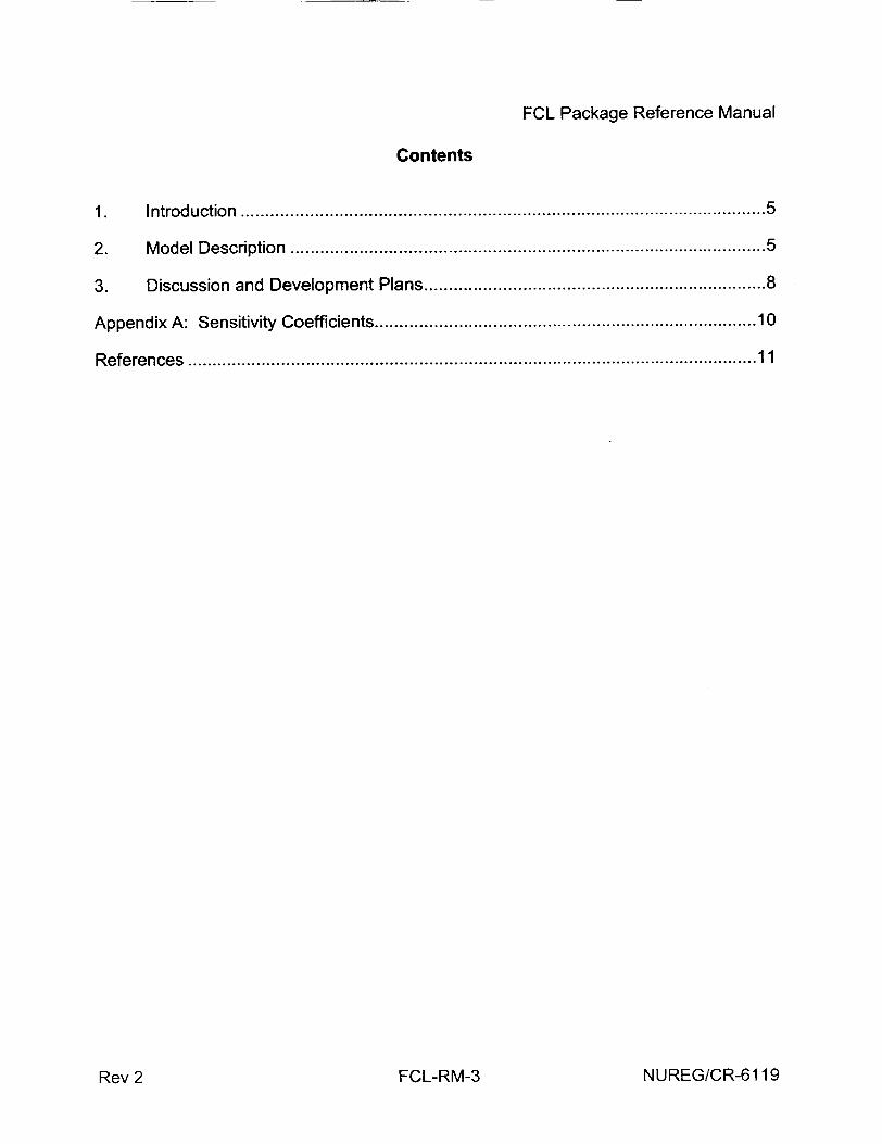
FCL Package Reference Manual
Contents
1. Introduction ................................................................................................. 5
2. Model Description ............................................................................................ 5
3. Discussion and Development Plans ................................................................. 8
Appendix A: Sensitivity Coefficients .......................................................................... 10
References .................................................................................................................... 11
NUREG/CR-6119Rev 2 FCL-RM-3
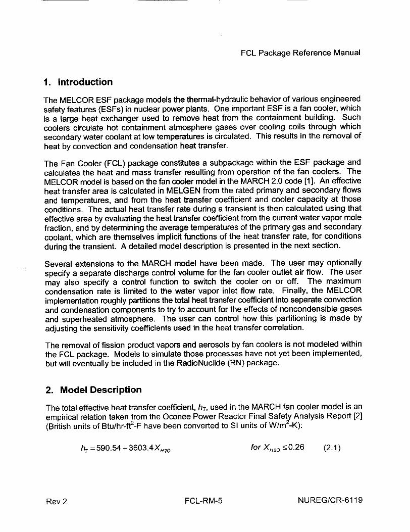
FCL Package Reference Manual
1. Introduction
The MELCOR ESF package models the thermal-hydraulic behavior of various engineered safety features (ESFs) in nuclear power plants. One important ESF is a fan cooler, which is a large heat exchanger used to remove heat from the containment building. Such coolers circulate hot containment atmosphere gases over cooling coils through which secondary water coolant at low temperatures is circulated. This results in the removal of heat by convection and condensation heat transfer.
The Fan Cooler (FCL) package constitutes a subpackage within the ESF package and calculates the heat and mass transfer resulting from operation of the fan coolers. The MELCOR model is based on the fan cooler model in the MARCH 2.0 code [1]. An effective heat transfer area is calculated in MELGEN from the rated primary and secondary flows and temperatures, and from the heat transfer coefficient and cooler capacity at those conditions. The actual heat transfer rate during a transient is then calculated using that effective area by evaluating the heat transfer coefficient from the current water vapor mole fraction, and by determining the average temperatures of the primary gas and secondary coolant, which are themselves implicit functions of the heat transfer rate, for conditions during the transient. A detailed model description is presented in the next section.
Several extensions to the MARCH model have been made. The user may optionally specify a separate discharge control volume for the fan cooler outlet air flow. The user may also specify a control function to switch the cooler on or off. The maximum condensation rate is limited to the water vapor inlet flow rate. Finally, the MELCOR implementation roughly partitions the total heat transfer coefficient into separate convection and condensation components to try to account for the effects of noncondensible gases and superheated atmosphere. The user can control how this partitioning is made by adjusting the sensitivity coefficients used in the heat transfer correlation.
The removal of fission product vapors and aerosols by fan coolers is not modeled within the FCL package. Models to simulate those processes have not yet been implemented, but will eventually be included in the RadioNuclide (RN) package.
2. Model Description
The total effective heat transfer coefficient, hT, used in the MARCH fan cooler model is an empirical relation taken from the Oconee Power Reactor Final Safety Analysis Report [2] (British units of Btu/hr-ft2-F have been converted to SI units of W/m -K):
hT = 590.54 + 3603.4XH20 for XH2o _<0.26 (2.1)
NUREG/CR-6119Rev 2 FCL-RM-5
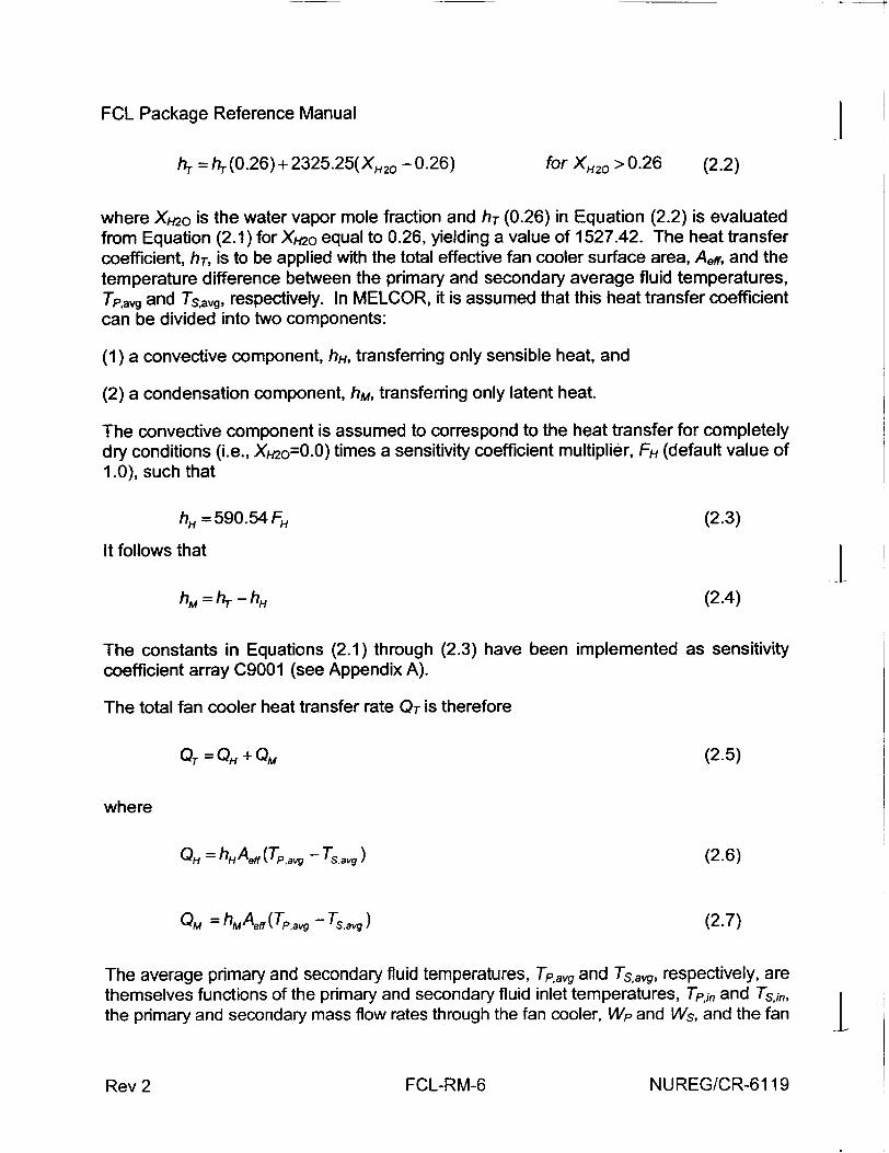
FCL Package Reference Manual
hT =hT(O.26)+2325.25(XH2o -0.26) for XH2o >0.26 (2.2)
where Xh2O is the water vapor mole fraction and hT (0.26) in Equation (2.2) is evaluated from Equation (2.1) for Xh2O equal to 0.26, yielding a value of 1527.42. The heat transfer coefficient, hT, is to be applied with the total effective fan cooler surface area, Aeff, and the temperature difference between the primary and secondary average fluid temperatures, Tpag and Tsavg, respectively. In MELCOR, it is assumed that this heat transfer coefficient can be divided into two components:
(1) a convective component, hH, transferring only sensible heat, and
(2) a condensation component, hM, transferring only latent heat.
The convective component is assumed to correspond to the heat transfer for completely dry conditions (i.e., Xo20=0.0) times a sensitivity coefficient multiplier, FH (default value of 1.0), such that
hH = 590.54 FH (2.3)
It follows that L h -=hT -hH (2.4)
The constants in Equations (2.1) through (2.3) have been implemented as sensitivity coefficient array C9001 (see Appendix A).
The total fan cooler heat transfer rate QT is therefore
QT= P + QM (2.5)
where
QH= hHAeff (Tp,avg - Ts.avg) (2.6)
QM = hMAeff(TPavg - Tsavg) (2.7)
The average primary and secondary fluid temperatures, Tpavg and Tsavg, respectively, are themselves functions of the primary and secondary fluid inlet temperatures, Tpn and Ts,, I the primary and secondary mass flow rates through the fan cooler, Wp and Ws, and the fan £
NUREG/CR-6119Rev 2 FCL-RM-6
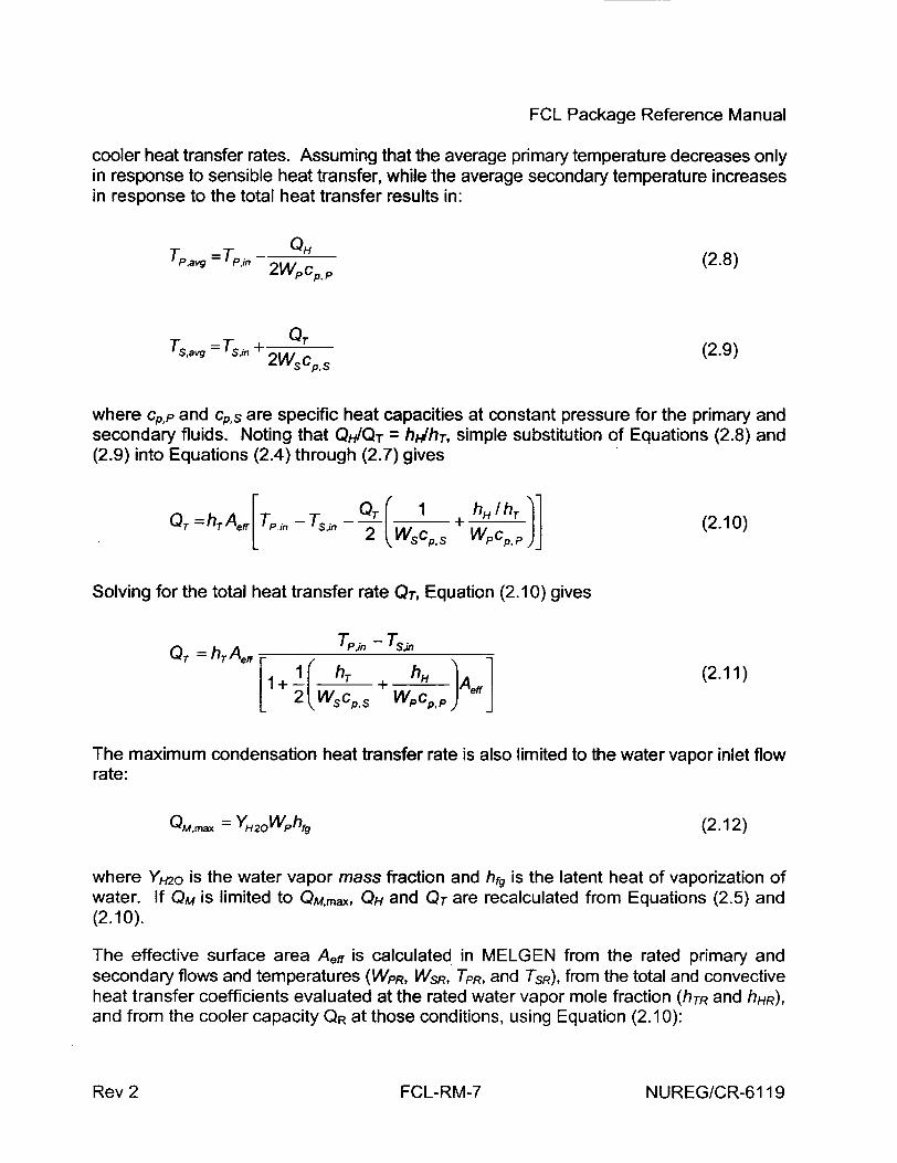
FCL Package Reference Manual
cooler heat transfer rates. Assuming that the average primary temperature decreases only in response to sensible heat transfer, while the average secondary temperature increases in response to the total heat transfer results in:
T p 'a v = T p ý -2 Q 2WpCp,
Tsvg T W + - .s 2Wscp~s
(2.8)
(2.9)
where Cp,p and cps are specific heat capacities at constant pressure for the primary and secondary fluids. Noting that QHIQT = hdhT, simple substitution of Equations (2.8) and (2.9) into Equations (2.4) through (2.7) gives
QT = hT Aff[TP.in S'"2W p
+ hH/hT wpcp, p (2.10)
Solving for the total heat transfer rate QT, Equation (2.10) gives
T"- Tai,,QT =hTAeff [
1+ hT + ,hH JAef 2+ WsCp, s pP'P,P I (2.11)
The maximum condensation heat transfer rate is also limited to the water vapor inlet flow rate:
QM,max = YH2oWPhfg (2.12)
where YH20 is the water vapor mass fraction and hfg is the latent heat of vaporization of water. If QM is limited to QM,max, QH and QT are recalculated from Equations (2.5) and (2.10).
The effective surface area Aeff is calculated in MELGEN from the rated primary and secondary flows and temperatures (WpR, WSR, TpR, and TSR), from the total and convective heat transfer coefficients evaluated at the rated water vapor mole fraction (hTR and hHR), and from the cooler capacity QR at those conditions, using Equation (2.10):
NUREG/CR-61 19Rev 2 FCL-RM-7
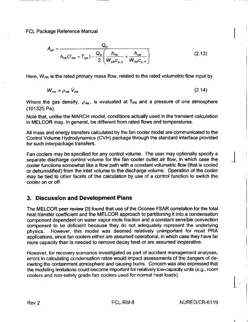
FCL Package Reference Manual
Aeff QR hTR(TPRTSR)- QR i hTR + hHR (2.13)
2 WSRCPs WPRCP.P)
Here, WPR is the rated primary mass flow, related to the rated volumetric flow input by
WPR PPR V'Pp (2.14)
Where the gas density, pp., is evaluated at TPR and a pressure of one atmosphere (101325 Pa).
Note that, unlike the MARCH model, conditions actually used in the transient calculation in MELCOR may, in general, be different from rated flows and temperatures.
All mass and energy transfers calculated by the fan cooler model are communicated to the Control Volume Hydrodynamics (CVH) package through the standard interface provided for such interpackage transfers.
Fan coolers may be specified for any control volume. The user may optionally specify a separate discharge control volume for the fan cooler outlet air flow, in which case the cooler functions somewhat like a flow path with a constant volumetric flow (that is cooled or dehumidified) from the inlet volume to the discharge volume. Operation of the cooler may be tied to other facets of the calculation by use of a control function to switch the cooler on or off.
3. Discussion and Development Plans
The MELCOR peer review [3] found that use of the Oconee FSAR correlation for the total heat transfer coefficient and the MELCOR approach to partitioning it into a condensation component dependent on water vapor mole fraction and a constant sensible convection component to be deficient because they do not adequately represent the underlying physics. However, this model was deemed relatively unimportant for most PRA applications, since fan coolers either are assumed operational, in which case they have far more capacity than is needed to remove decay heat or are assumed inoperative.
However, for recovery scenarios investigated as part of accident management analyses, errors in calculating condensation rates would impact assessments of the dangers of deinerting the containment atmosphere and causing bums. Concern was also expressed that the modeling limitations could become important for relatively low-capacity units (e.g., room coolers and non-safety grade fan coolers used for normal heat loads).
NUREG/CR-6119
- --- ]
Rev 2 FCL-RM-8

FCL Package Reference Manual
Mechanistic models (e.g., from CONTAIN [4]) could be fairly easily adapted for use in MELCOR if found necessary for accident management applications, but there are no current plans to do this.
NUREG/CR-6119FCL-RM-9Rev 2

FCL Package Reference Manual
Appendix A: Sensitivity Coefficients
This section lists the sensitivity coefficients in the FCL package associated with various correlations and modeling parameters described in this reference manual.
Coefficient Default Units Equation Value
C9001 (1) 590.54 W/m2 -K 2.1,2.3 C9001(2) 1.0 - 2.3 C9001(3) 0.26 - 2.1,2.2 1C9001(4) 3603.4 W/m2-K 2.1 C9001(5) 2325.25 W/mz-K 2.2
I
j
INUREG/CR-6119
I - -k.
Rev 2 FCL-RM-1 0
FCL Package Reference Manual
References
I R.O. Wooton, P. Cybulskis, and S.F. Quayle, MARCH 2 (Meltdown Accident Response Characteristics) Code Description and Users Manual, NUREG/CR-3988, BMI-2115 (August 1984).
2 Duke Power Company, Oconee Nuclear Station Units 1, 2, and 3: Final Safety Analysis Report (1987).
3 B. E. Boyack, et al., MELCOR Peer Review, LA-12240, Los Alamos National Laboratory (March 1992).
4 K. K. Murata, et al., Code Manual for CONTAIN 2.0: A Computer Code for Nuclear Reactor Containment Analysis, NUREG/CR-6533, SAND97-1735, Sandia National Laboratories (December 1997).
NUREG/CR-6119FCL-RM-1 1Rev 2
Fuel Dispersal Interactions (FDI) Package Reference Manual
This document describes in detail the various models incorporated in the Fuel Dispersal Interactions (FDI) package in MELCOR. New in MELCOR 1.8.5 is a FDI sensitivity coefficient used to control the numerical order in which oxygen or steam is used to oxidize
DCH metals. This parameter affects the amount of hydrogen that results from burning DCH
materials in steam/oxygen atmospheres.
Details on input to the FDI Package can be found in the FDI Users' Guide.
NUREG/CR-6119FDI-RM-1Rev 2
FDI Package Reference Manual
Contents
1. Introduction ........................................................................................................... 5
2. Detailed Models ............................................................................................... 6 2.1 General Information ............................................................................. 6 2.2 Low-Pressure Melt Ejection (LPM E) Modeling ...................................... 6 2.3 High-Pressure Melt Ejection (HPM E) Modeling .................................... 11
3. Sensitivity Coefficients .................................................................................. 20
4. Discussion and Development Plans ............................................................... 21
References .................................................................................................................... 23
P,,, 9 FI'I-RM-3 NUREG/CR-61191%•K,./ V •..
FDI Package Reference Manual
1. Introduction
The Fuel Dispersal Interactions (FDI) Package in MELCOR calculates the behavior of debris in containment unless or until it is deposited in a cavity modeled by the MELCOR Cavity (CAV) package. Debris enters the package in basically two ways:
(1) if the Core (COR) package is active, debris enters the FDI package via the Transfer Process (TP) package after the failure of the reactor vessel, or
(2) in the stand-alone high-pressure melt ejection (HPME) model, debris enters the FDI package through a user interface, which may be either tabular function input or input from an external data file (EDF) via the TP package.
Two types of phenomena are treated in the FDI package:
(1) low-pressure molten fuel ejection (LPME) from the reactor vessel and
(2) high-pressure molten fuel ejection from the reactor vessel (direct containment heating). There is currently no plan to model steam explosions within or outside the FDI package in MELCOR.
There is no fission product modeling associated with the FDI package, with one minor exception. In particular, there is no release of fission products from fuel debris modeled in the FDI package. In general, the only function performed by the FDI package with respect to radionuclide modeling is inventory transport. That is, if the FDI package transports fuel debris from one location to another, it calls the RadioNuclide (RN) package and instructs it to transport the fission products associated with the fuel debris in exactly the same way.
The one exception to the foregoing concerns decay heat associated with debris deposited on heat structures by the HPME model. The decay heat associated with deposited debris is treated in essentially the same way as the decay heat associated with fission product aerosols and vapors that settle/deposit on heat structures in the RN package modeling. The RadioNuclide Package Reference Manual discusses this modeling in detail. The decay heat associated with airborne debris in the HPME model and all debris during its short residence in the low-pressure melt ejection (LPME) model is ignored; the energy error associated with its omission should be quite small.
NUREG/CR-6119FDI-RM-5Rev 2
FDI Package Reference Manual 4 2. Detailed Models
2.1 General Information
The FDI package becomes active whenever debris material enters the package. Debris material typically enters the FDI package in one of three ways. In a reactor plant accident calculation, debris enters the FDI package via the TP package interface from the core (COR) package after failure of the reactor pressure vessel has been calculated. In a stand-alone direct containment heating (DCH) calculation, debris material is sourced into the FDI package either directly from tabular function user input or via the TP package interface to a user-provided external data file (EDF) containing the source. The Transfer Process Package Users' Guide and External Data File Package Users' Guide, along with the FDI Package Users' Guide, provide example input to illustrate the interfaces.
After the introduction of debris material, the FDI package classifies the ejection event as either a low- or a high-pressure melt ejection event on the basis of the ejection velocity passed through the TP package or a flag set by the user for stand-alone DCH calculations.
2.2 Low-Pressure Melt Ejection (LPME) Modeling
The heart of the LPME model that has been incorporated into MELCOR was developed I by Corradini et al. [1] at the University of Wisconsin. In this model, heat is transferred from the molten debris to the water pool (if present in the associated control volume) as it breaks up and falls to the cavity floor. The heat transfer is normally dominated by radiation, but a lower bound determined by conduction through a vapor film (the Bromley model for film boiling) is also considered. All of the energy transfer from the molten debris is used to boil the pool water (i.e., no sensible heating is considered so, e.g., a subcooled pool will remain subcooled and its temperature will not change). The LPME model does not consider oxidation of the metallic elements in the ejected debris. If no pool is present, material passes through FDI without any energy removal. At the cavity floor, the material is normally passed to the CAV package (CORCON) by way of the TP interface.
The first step in the LPME calculational sequence involves retrieving the variables describing the debris state entering the model at the beginning of each calculational cycle (timestep). The debris variables are passed from the COR package to the TP package prior to execution of the FDI package, so the values of the variables are current for the timestep. The variables retrieved from the TP package by the FDI package include the mass, composition and temperature of the debris ejected from the vessel during the timestep and the velocity and diameter of the ejection stream (see COR reference manual for a description of the calculation of these variables).
The second step in the LPME sequence is to determine the axial position of the head and tail of the ejected debris with respect to the FDI calculational volume. The user specifies INUREG/CR-6119 FDI-RM-6 Rev 2
FDI Package Reference Manual
ZTOP and ZBOT, the elevation of the top and bottom of the calculational volume, respectively,
(which typically are equal to the elevation of the bottom of the reactor vessel and the
bottom of the reactor cavity). Then the positions of the head and tail of the ejected debris
and its length are given by
ZHED = ZTOP - U/fAt (2.1)
ZTAIL ZHEAD + mf I(7rD 2pf /4) (2.2)
ZLE = ZTAIL - ZH EA (2.3)
where Uf, mf, Dfo and pf are the velocity, mass, initial diameter (determined by the COR
package and equal to the diameter of reactor vessel breach, which may increase if hole
ablation occurs) and density of the ejection stream, respectively. Any debris below
elevation ZBOT accumulates on the cavity floor, and its mass is designated mFLR and given
by
mFLR = "m,MAX {O, MIN[1, (zBoT - ZH•AD) / ZLEN ]} (2.4)
The portion of mf that does not reach the floor remains in the FDI calculational volume until
the next timestep and is designated mcAv. If there was already mass in the volume (mCAVO
from the previous timestep), then it is added to mFLR and deposited on the cavity floor on
this timestep. If mf is zero (i.e., if mass ejection from the vessel has ceased), then any pre
existing mcAvo is transferred to mFLR. If mf is greater than zero, but ZHEAD is greater than ZBOT, then only pre-existing mcAvo is deposited on the floor and given by
mFLR = MIN(mr, mCAVO) (2.5)
mCAV = mf + mCAVO -mFu (2.6)
In effect, this means that if mass is being ejected from the vessel but the timestep is too
short for newly ejected debris to reach the cavity floor, then pre-existing debris that has not
reached the cavity floor is deposited on the cavity floor at a rate equal to the vessel ejection
rate, and the newly ejected debris takes the place of the deposited debris. However, as
soon as vessel ejection ceases, then all remaining debris that has not reached the cavity
floor is immediately deposited in the cavity floor in a single timestep.
NUREG/CR-6119FDI-RM-7Rev 2
-� -4.
FDI Package Reference Manual 4 After the mass of debris reaching the floor during the current timestep has been determined, heat transfer to water in the cavity is evaluated. Although the heat transfer occurs during the passage of the debris through the cavity pool, the actual heat transfer associated with a given packet of debris is not transferred to the pool until that packet is deposited on the cavity floor. Debris which does not reach the floor during the current timestep does not participate in heat transfer to the water until a later timestep.
The rate of heat transfer from the debris to the water is determined primarily by the interfacial surface area, which is a function of the debris particle size. The particle size for molten debris particles descending through the cavity pool is given by a modified theoretical correlation for droplet breakup under hydrodynamic force. The original correlation as formulated by Chu [2] for a water/air system is
Df (t) = D,0 exp(-C, °r0 7 72 We246 ) (2.7)
We is the Weber number, which is defined by
We = PCUfDf, o Ir (2.8)
where p, is the coolant density, U,, D,0, and a- are the velocity, initial diameter and surface I tension of the droplets, respectively. r is the dimensionless time, which is defined by
S= (U ft I Do )(p& I P, )12 (2.9)
where the time of descent, t, is zero when the debris is at the pool surface and increases as the debris descends through the pool. Constant C1 is taken to be
C1 = 0.171-0.149(pc / p,) 112 (2.10)
To provide an easily integrable form for analytic use in MELCOR, Chu's correlation is modified as follows
Df (t) = Df0 exp(-C 1 r We 0 25) (2.11)
with constant C, taken to be
C1 = 0.1232-0.149(p, /Ip,) 11 2 (2.12) 1
NUREG/CR-6119 FDI-RM-8 Rev 2
FDI Package Reference Manual
A comparison of Chu's correlation to this modified correlation for the water/air and
corium/water systems reveals reasonable agreement [1]. Assuming constant velocity, Uf, Equation (2.11) can be converted to a function of the elevation of the pool surface, ZPOOL, as shown below
Df(z) = Dfo exp(-Z) (2.13)
for z •OT < z ZPOOL where the variable Z is
Z = (ClWe°254 I Dfo)(pc / p,)"2 (z)oOL -_z) (2.14)
Equation (2.13) is valid only as long as the debris remains molten. After the debris
solidifies, (Tf < T,.f as determined by the solution of Equation (2.17) to follow), there is no
further breakup, and the heat transfer area is constant.
Another important factor affecting the rate of heat transfer is the heat transfer regime. In
the early stage of heat transfer from the debris, the debris temperature is very high; hence,
radiation heat transfer would be the dominant heat transfer mechanism. As the debris
temperature falls, eventually other mechanisms become important.
Although radiation and conduction through the vapor film occur in parallel, the model
incorporated into MELCOR only considers the dominant mechanism at any given time.
Hence, the model switches from radiation-dominated to conduction-dominated film boiling
heat transfer when the debris temperature falls below the "regime transition temperature". The regime transition temperature, TTRAN, is defined as the temperature at which the net
radiation heat flux between the debris and pool is equal to the conduction-dominated film boiling heat flux from the debris to the pool and is given by the solution to the following equation
a(TT•N 4 -T•4 ) = hF_(TT•N -T ) (2.15)
where a- is the Stefan-Boltzmann constant (and the emissivity is assumed to be unity) and
hFB is the conduction-dominated film boiling heat transfer coefficient given by Bromley [3]
hFB = (1/2) kg{kgI,uD, (Tg - T,)/[p,(pc - p, ) g i, 114 (2.16)
where k9 and jug are the thermal conductivity and viscosity of the vapor film, respectively,
if9 is the latent heat of vaporization of water and g is the acceleration of gravity. To derive
NUREG/CR-6119FDI-RM-9Rev 2
FDI Package Reference Manual j this equation, it was assumed that the vapor saturation temperature, Tst, the debris diameter, Df, and the vapor temperature, Tg, are constant. Tg is the arithmetic average of the debris and saturation temperatures. Equation (2.15) can be solved iteratively to yield TTRAN, the heat transfer regime transition temperature.
The rate of change of the debris temperature, Tf, is given by
p~C1 (I(rD3 16)UfdT, Idz = q,_ (MD2) (2.17)
where cf is the specific heat capacity of the debris and qf-c is the heat flux from the debris
to the coolant. For Tf > T, 1 , Df is given by Equation (2.13); otherwise Df remains equal to its value at the instant solidification begins. For Tf > T q,- is calculated assuming
only radiative heat transfer; otherwise, q,-, is calculated assuming only transition film
boiling. Equation (2.17) can be integrated from z = ZPOOL to Z = ZBOT to yield Tf.,OT, the debris temperature at the bottom of the coolant pool.
Once the debris temperature at the bottom of the pool is known, the total amount of heat transferred to the pool is given by
QeC = H (To) Hf (T.OT )(2.18)
where
NMAT.
H,(T) = , [m,Ruhi(T)] (2.19) i=1
and h1(T) is the specific enthalpy of debris component i at temperature T. The mass of
steam generated by the heat transfer is given by
mSTEAM = Q,-c /(hscv - hpooL ) (2.20)
where hscv is the specific enthalpy of saturated steam at the total pressure in the FDI
control volume and hpooL is the specific enthalpy of the water in the cavity pool. Note that
all heat transfer is assumed to generate steam; hence, the pool temperature should not change. If mSTEAM exceeds the mass of coolant in the pool, then H(7.o800) and T.BOT are
back-calculated to provide just enough heat transfer to vaporize the mass of coolant in the pool.
NUREG/CR-6119 FDI-RM-10 Rev 2
FDI Package Reference Manual
Following the calculation of steam generation, the increments to the pool and vapor
masses and energies are passed to the CVH package, the debris deposited on the floor
at temperature TfBOT is passed to the CAV package, where core-concrete interactions are
modeled, and the radionuclides associated with the debris passed to CAV are transferred
from FDI to the radionuclide package.
2.3 High-Pressure Melt Ejection (HPME) Modeling
If the velocity of the molten debris ejected from the reactor vessel exceeds a critical value
prescribed by sensitivity coefficient C4602 (with a default value of 10 m/s), or if the user
has invoked the stand-alone option for high-pressure melt ejection modeling, then the FDI will be treated by the high-pressure model instead of the low-pressure model.
The parametric high-pressure model requires user input to control both the distribution of
debris throughout the containment and the interaction of the hot debris with the containment atmosphere. The processes modeled include oxidation of the metallic components of the debris (Zircaloy, aluminum and steel) in both steam and oxygen, surface deposition of the airborne debris by trapping or settling and heat transfer to the atmosphere and deposition surfaces.
The HPME model does not include a mechanistic debris transport model; rather, the user
specifies a set of debris destinations with a corresponding set of transport fractions that prescribe where the ejected debris is assumed to go. The debris destinations may include the atmosphere of any CVH control volume, the surface of any heat structure and cavities defined by the CAV package. The sum of the transport fractions over all the specified control volume atmospheres, heat structure surfaces and cavities must equal one. Transport of the ejected debris to its assumed destinations occurs instantaneously, with no interactions occurring between the point of ejection and the destination sites. As long as the HPME model is active (i.e., as long as the ejection velocity exceeds the LPME/HPME transition velocity prescribed by sensitivity coefficient C4602 or if the user has invoked the stand-alone HPME model), the ejected debris will be partitioned among the destinations as specified by the transport fractions. When the ejection velocity falls below the LPME/HPME transition velocity for non-stand-alone applications, any debris
subsequently ejected is passed to the LPME model, which uses LPME model input instead of the HPME transport model to determine the debris destination. However, debris that was transported to the HPME debris destinations before the model transition occurred will continue to be treated by the HPME model.
Debris which is transported to cavity destinations is not treated further by the FDI package; rather, subsequent treatment is provided by the CAV package. As implemented in the HPME model, surface deposition of debris can occur in two distinct ways. Ejected debris which impacts structures prior to any significant interaction with the atmosphere is sourced directly to the destination surface via the user-specified transport fraction for that surface. This process is referred to as trapping in MELCOR. Alternatively, debris which interacts
NUREG/CR-6119FDI-RM-1 1Rev 2
FDI Package Reference Manual
significantly with the atmosphere should be sourced to the appropriate control volume, in which a user-specified settling time constant will determine the rate of deposition to the specified settling destination (either a heat structure surface or a cavity). This process is referred to as settling in MELCOR.
First-order rate equationswith user-specified time constants for oxidation, heat transfer and settling are used to determine the rate of each process. Oxidation of airborne and deposited debris is only calculated if the debris temperature exceeds a minimum value, TOXMIN, which is adjustable through sensitivity coefficient 4609 and has a default value of 600 K. If a pool of water exists in the reactor cavity at the time of debris ejection, then the water is ejected into the droplet field (fog) of the atmosphere at a rate proportional to the rate of injection of the debris into the pool. The proportionality constant is adjustable through sensitivity coefficient C4605 and has a default value of 10. This proportionality constant is strictly parametric and intended for exploratory purposes only. The rate of dispersal of the cavity water may be very important in determining containment loads, if interaction between the debris and cavity water is a primary contributor to the load. Excessive values of this coefficient may disperse the cavity water prematurely and limit subsequent interactions between ejected debris and cavity water, while deficient values will excessively limit the overall interaction of debris and water. Consequently, it is strongly recommended that the effects of variations in the value of this sensitivity coefficient be examined both because of its inherent uncertainty, and because of the large impact it may have on containment loads. The HPME model does not consider any thermal interaction between the ejected debris and the water in the cavity pool such as that described above for the LPME model.
When the HPME model first initiates direct containment heating in a control volume, the FDI package requests a fallback of the cycle if the timestep exceeds the recommended start-up value prescribed by sensitivity coefficient C4607 (with a default value of 10 s). The start-up value should be reasonably small both to avoid numerical problems associated with excessive energy transfers to the CVH atmosphere per timestep and to capture the detail associated with the HPME phenomena, which occurs on a time scale comparable to the user-specified time constants for the phenomena. Experience has indicated that for most realistic scenarios, the rapid excursions in pressure and temperature caused by direct containment heating dictate the use of very small timesteps for several cycles following DCH initiation. See the input record SOFTDTMIN in the Executive Package Users' Guide for help with this requirement.
The airborne masses of U0 2 and other materials that neither oxidize nor are the products of oxidation are described by the following first-order linear differential equation:
dmi,(t) _ m,k(t) +Sik (2.21)
dt - STk ( I
NUREG/CR-6119 FDI-RM-12 Rev 2
FDI Package Reference Manual
where mi.k(t) is the mass of component k in control volume i at time t, rST,i is the time
constant for settling in control volume i and Sik is the constant mass source rate of
component k in control volume i associated with the high-pressure melt ejection process. The solution of Equation (2.21) is given by
m,.k (t) = [m;lk (to ) - S,.kTSTJ ] exp( dt ) + Si,krSTi (2.22) TST~i
where mi,k(tO) is the mass at arbitrary initial time to and dt is the difference between the
final time, t, and time to.
The airborne masses of Zr, Al and steel (the only materials that are oxidized in the presence of oxygen or steam) are described by the following first-order linear differential equation:
dm,k(t) - m, + (t)S (2.23) dt Tsoj
where r-so, the time constant for simultaneous oxidation and settling/trapping, is given by
(2.24) "SOi='STj -+- OXJ
and where roxj, is the oxidation time constant in control volume i. The solution to Equation
(2.23) is identical to Equation (2.22) except that -STJi is replaced by -rso•.
The airborne masses of ZrO2 and other materials that are products of oxidation reactions are given by
dm,.k(t) _m~k (t) m, (t) dt- ( R + S, (2.25) dt rSTi IOXj
where R is the mass of product k formed by the oxidation of a unit mass of reactant I. The solution of Equation (2.25) is
NUREG/CR-6119FDI-RM-13Rev 2
FDI Package Reference Manual 4 mik (t) = [mi,k (to) C - C2 ]exp(-dt /rSTj) + C2 exp(-dt /rso, ) + C1 (2.26)
where
C, = (Sj'k + RSuz'jsoj / rox• )Z'STr
and
C2 = R[S, rso., - m,.,(to)]
The HPME model contains two options for oxidation modeling. These may be selected independently for each control volume. The first is the sequential oxidation option, in which the order of oxidation is Zr, Al then steel (typical metallic elements associated with reactor cores and/or simulation experiments). This is invoked by specifying a positive value for the oxidation time constant, -oxJ,. The second option is simultaneous oxidation of the metals,
which is invoked by specifying a negative value of roxj, in which case the time constant
will be equal to the absolute value of v-oxj. Under normal conditions where the metallic
constituents exist in a more or less well-mixed state, the sequential oxidation option is I recommended because it is more realistic. Elements with higher oxidation potentials will tend to be preferentially oxidized unless some kinetic limitation exists.
In the sequential oxidation model, a separate oxidation rate is first calculated for each metal independently of all others, with the given value of z-oxj. Then the mass of metal B
consumed will be converted into an equivalent mass of metal A, where metal A is assumed to oxidize in preference to metal B, until all of metal A is consumed. Hence, steel (and Inconel, which is included in the steel mass in the FDI package) will not be consumed until all the Zr and Al have been consumed, and Al will not be consumed until the Zr is exhausted. This implies that the effective time constant for metal A oxidation when metal B is present may be significantly shorter than roxj. The actual values of the effective
oxidation time constants will be used in determining the end of timestep airborne mass inventories in Equation (2.23) and Equation (2.26) above.
Both oxidation options are constrained by the availability of oxygen or steam. Oxidation is apportioned between steam and oxygen by their relative mole fractions in the atmosphere. This is a change in MELCOR 1.8.5; previously, the oxygen would react first, followed by steam only after the oxygen had been consumed. Although this assumption probably reflects the relative oxidation potential of oxygen versus steam, it does not consider diffusion transport in the atmosphere and generally resulted in insufficient hydrogen generation during DCH. The relative oxidation effectiveness of oxygen versus steam can
NUREG/CR-6119 FDI-RM-14 Rev 2
FDI Package Reference Manual
be adjusted through sensitivity coefficient C4610. The default setting of C4610 is 1.0, giving an oxidation ratio proportional to the moles of oxygen divided by the moles of oxygen plus steam:
Rox = (2.27) WX 0 2 + X't
where W is the weighting factor given by sensitivity coefficient C4610, X 0 2 is the moles
of oxygen, and Xst is the moles of steam in the atmosphere. Making W a large number
will weight the oxygen moles and give the previous "oxygen first" behavior. If there is insufficient oxidant to support the calculated rates of oxidation for zirconium and iron, then the zirconium will have first priority. The oxidation reactions will proceed at the start of timestep values of debris temperature in each control volume, and any hydrogen formed by the steam reaction will enter the atmosphere at that temperature.
The temperature of the airborne debris is affected by debris sources, oxidation and heat transfer from the debris to the atmosphere. The temperature of the atmosphere, Tgas, is
assumed to remain constant and equal to the beginning of timestep value obtained from the CVH package data base. This explicit coupling between FDI and CVH may limit the timestep size during energetic transients, as discussed below. The enthalpy of the airborne debris is given by the solution of the following simple equation:
dHi(t) (t)_Qcs,(t)+SH, (2.28) dt
where E-oxj(t) is the rate of heat generation by the oxidation reaction, S,,, is the enthalpy
source rate associated with the HPME source, and the rate of heat transfer to the gas is approximated as:
QGAsj(t) = egi(t) = H,(Td, ) H,(Tga,) (2.29) 'rHTj r HTj
where Qg.;(t) is the enthalpy available for transfer to the gas, --HTi is the user-specified
time constant for heat transfer from the airborne debris to the atmosphere in control volume i, Hi(Tdbr ) is the enthalpy content of the debris at its actual temperature, Tdbr, and
Hi(Tga,) is the enthalpy content of the debris in equilibrium with the gas at temperature
Tas. The solution to Equation (2.28) is given by:
Hi(t) = Hi(to) + Eoxi(t)-QGAs.i(t) (2.30)
NUREG/CR-6119Rev 2 FDI-RM-1 5
I . -- 4,
FDI Package Reference Manual
where H,(to) is the enthalpy of the debris after the addition of the integrated enthalpy
source SHidt and after adjustments to its composition associated with the oxidation
reactions, where Eox0 i(t) is the oxidation enthalpy generated between times to and t, and
where QGAsi(t) is the amount of heat transferred to the gas between times to and t.
QGAs.i(t) is given by
to+dt
QGA~j(0)= J[Qgj(t)1IfT.&] dt (2.31) to
where the available enthalpy Qgj(t) increases as a result of oxidation and the addition of
high-temperature debris source material and decreases as enthalpy is transferred to the gas. Qgi(t) satisfies
dQgj(t) Qg~i(t)+ [QsRc, I dt + (Eoxj + QoJ)I dt] (2.32)
dt THTj
QSRC., = SHJ(T .)- SHJ(TgaS) I is the available source enthalpy and
eox = Hoxj,(Tdb ) - Hox i(Tgas)
is the available enthalpy created by composition adjustments during oxidation. The solution to Equations (2.31) and (2.32) is:
QeASj(t) = QoLoA[1- exp(- dt / HTj )A + [QsRc.i / dt + (EoXj + Qoxj )/ dtJ {dt - HTJi[1-- exp(- dt /HTJ)J (2.33)
where QoLo,i = Hi (T(to)) - Hi (Tga) is the initial available enthalpy.
The inclusion of the HPME source terms in Equations (2.21) through (2.33) reduces some timestep dependencies that would arise if the sources were added prior to the calculation of oxidation, heat transfer and settling/trapping. After the total enthalpy at the advanced time, t, is determined, it is compared to the enthalpy corresponding to a maximum I
NUREG/CR-6119 FDI-RM-16 Rev 2
FDI Package Reference Manual
permissible temperature, HMAx. If Hi(t) exceeds HmAx, then Equation (2.30) is solved for
QGAs.,i(t) with Hi(t) set equal to HMx as follows:
QGAs.i (t) = Hi (to) + Eox,i (t)- HMAx (2.34)
so that the heat transferred to the gas is increased sufficiently to limit the advanced time debris temperature to the maximum prescribed value, Tx. Tx is given by
Tmx = MAX (Tgas , Tdb, (to),Tdf (t'), T4603) (2.35)
where Tgas is the gas temperature, T ,(to) is the debris temperature at the beginning of the
timestep, Tdbr (t') the debris temperature after addition of new source material to the initial
inventory and T4603 is the temperature limit prescribed by sensitivity coefficient C4603, which normally exceeds the other arguments in the max function of Equation (2.35). The default value of T4603 is approximately equal to the boiling temperature of U0 2-temperatures much in excess of this value would likely result in very rapid fragmentation of debris droplets and significantly increased droplet-to-gas heat transfer.
After an advanced time temperature for the airborne debris has been determined, the projected change in the CVH atmosphere temperature as a result of direct containment heating during the timestep is calculated. If the change exceeds a value prescribed by sensitivity coefficient C4604 (with a default value of 500 K), then the FDI package requests a fallback with a decreased timestep. This feature provides control over numerical problems associated with excessive energy transfers to the CVH atmosphere. If the value of sensitivity coefficient C4604 is set too high, it is possible that the CVH package will encounter numerical difficulties that cannot be resolved by CVH fallbacks. In practice, the default value was found to prevent numerical problems in CVH without excessively limiting the timestep.
Following the determination of the advanced time temperature for the airborne debris, the advanced time mass equations, Equations (2.21) through (2.26), are used to determine how much material is removed from the atmosphere by settling/trapping. The settled material and its energy content are removed from the airborne inventory and deposited on the appropriate surface specified by user input. After the settling calculation has been performed, the advanced time total airborne mass in each control volume is determined by summing over all components. If the advanced time total airborne mass is insignificant compared to the total mass of material sourced into the control volume atmosphere over the duration of the DCH event, then all of the remaining airborne mass in the control volume is immediately deposited on the appropriate settling surface and a message is issued to notify the user that direct containment heating has ceased in that particular control volume. The ratio used to determine when the airborne mass has become
NUREG/CR-6119Rev 2 FDI-RM-1 7
FDI Package Reference Manual 4 insignificant is adjustable through sensitivity coefficient 4606 and has a default value of 0.001. This implies that only 0.1 percent of the mass source will be prematurely deposited, which was judged to be a reasonable compromise between the demands of accuracy and calculational effort.
Deposited Debris
The mass of material k on surface i at time t is given by
mik (t) = mik (to) + S•.kdt (2.36)
where
to+dt
S;.k = Si, + _j J[mTi (t')/ VSTj]dt'/dt (2.37) to
and Si,k is the constant mass source rate of component k to surface i from trapping. The
second term on the right-hand side of Equation (2.37) accounts for settling to the surface, where the sum is over all control volumes that have surface i as the user-specified settling I surface, and mik(t)and rST.j are the airborne mass of component k in control volumej and
the settling time constant in control volume j, respectively.
For U0 2 and other materials not associated with oxidation, the settling term is given by
t0+dt
mk W(t')dt'l STJ = m .,(to )[1 - exp(-dt / r-sTj)] (2.38) to 4+ Sjk {dt - "STI [1 - exp(-dt / rST.j )D
For metals that oxidize, the settling term is given by
t0 +dt
ftmjk (t'dt'l rCSTJ = ('sOj / ST.J )(mlk (to )[1- exp(-dt / rsO°j)] (2.39)
+ Sik {dt- rSOj [1 - exp(-dt /rsozj )D)
which reduces to Equation (2.38) if -rox.i >> »ST, because in that case Tsoj = TSTj as
shown by Equation (2.24). For oxidation products, the settling term is given by
NUREG/CR-6119 FDI-RM-1 8 Rev 2
FDI Package Reference Manual
to +dt
fmj.k (t')dt' / ISTJ = MJk (to )[1 - exp(-dt / TSTJ )] + S1 .k {dt- TSTj
to
[1 - exp(-dt / rSTJ )]} + R{(so, I /rox,j )[mjj (to ) + Sjj (dt - rsoj (2.40)
- vSTJ )] - [min1 (to ) - Sj vST.j] exp(-dt / STJ ) + ([vSOJ / STrj ]
[m, (to )- SPvso5 j]exp(-dt / rsoj )}
where material I is the metal from which the oxide is formed and R is the mass of product k formed by the oxidation of a unit mass of material .
The energy of the deposited debris is calculated with equations almost identical to Equations (2.28) through (2.35) except the source term SH,j also includes the enthalpy
associated with debris settling. It is assumed that the enthalpy of the settled debris is equal to the end of timestep value calculated with Equation (2.30). The settled mass with the end of step enthalpy is applied to the deposition surface during the timestep at a constant rate as implied by Equation (2.36). The other difference between the treatment of the energy of airbome and deposited debris concerns heat transfer. As discussed above, the user specifies a time constant for heat transfer from the airborne debris to the atmosphere. However, for heat transfer from deposited debris to the structure, a different approach is taken. Because the CVH package does not recognize the deposited debris temperature as the effective surface temperature, in order to effectively simulate the heat transfer from the hot debris to the CVH pool and/or atmosphere associated with the surface, it is necessary to couple the debris temperature tightly to the HS surface temperature that CVH does recognize.
The debris temperature and HS surface temperature will be tightly coupled if the effective heat transfer coefficient from the debris to the surface, hSRF, is large compared to the heat transfer from the surface to the first interior node in the structure, which is given by kHs,l /AXHS,¶ (structure thermal conductivity divided by the node thickness). In order to
generate a large value of hSRF, a very small time constant equal to the minimum of half the surface oxidation time constant and a value of 0.001 s is used to calculate the amount of heat transfer from the debris to the deposition surface using the analog of Equation (2.33) for heat transfer to surfaces. The value obtained is then used to determine hSRF as follows:
hsRF = QsRF•,(t)I(AsRF A Tdt) (2.41)
where ASRF is the surface area of the structure, AT is the difference between the
beginning of timestep debris temperature and the structure surface temperature and QSRF
is the value obtained from the analog of Equation (2.33). This value will almost always
exceed the value of kHs, / Axs,l. In fact, the value of hsRF may be large enough to induce
oscillations in the structure surface temperature because of the explicit coupling between
NUREG/CR-6119Rev 2 FDI-RM-19
FDI Package Reference Manual
FDI and HS packages. Therefore, a limit is placed on the value of hsRF. If hSRF exceeds
a maximum value, hsRF,, specified by sensitivity coefficient 4608 (default value 1000.
W/m2 -K), then the value of QSRF is reduced by the ratio hSRFmx / hsRF to limit it to the value
consistent with hsRF,.. Whenever, the QSRF is limited by hSRFM=a the direction of heat
transfer (i.e., debris-to-surface or surface-to-debris) is compared to the direction from the previous timestep. If the direction is alternating, this probably indicates that the surface temperature has been driven into an oscillation about the debris temperature because the timestep exceeds the stability limit associated with the explicit coupling between the FDI and HS packages. In such cases, FDI requests a system fallback with the timestep
reduced by a factor of one half. Normally, the value of hsRFm• should be chosen large
enough to promote rapid equilibration of the debris and surface temperatures, yet not so large as to induce instability in the surface temperature for reasonable values of the timestep. Users should refer to the HS Reference Manual for a further discussion of stability/accuracy concerns associated with structure nodalization and timestep size.
If the MELCOR RadioNuclide (RN) package is active, then FDI will call RN1 of the RN Package anytime fuel is moved so that the associated radionuclides can be moved simultaneously. Furthermore, the decay heat associated with the radionuclides will be deposited in the appropriate location. t
3. Sensitivity Coefficients
For convenient reference, the sensitivity coefficients for the FDI package are summarized below, taken from the FDI Reference manual.
Sensitivity Definition Coefficients C4602 Vessel ejection velocity at transition between high- and low-pressure
ejection modeling. (default = 10., units = m/s, equiv = none)
C4603 Airborne debris temperature above which oxidation energy is deposited directly in the atmosphere-approximate vaporization point. (default = 3700., units = K, equiv = none)
C4604 Maximum change in the temperature of the CVH atmosphere permitted without a timestep cut. (default = 500., units = K, equiv = none)
C4605 Ratio of the mass of water ejected from a pool into the reactor cavity atmosphere to the mass of the debris injected from the vessel into the cavity pool.
I (default = 10., units = none, equiv = none)
NUREG/CR-6119
IFDI-RM-20 Rev 2
FDI Package Reference Manual
Sensitivity Definition Coefficients C4606 Ratio of the current airborne debris mass to the integrated airborne debris
mass source in a control volume below which the mass will be deposited onto the settling surface associated with the control volume-deactivates DCH when the remaining airborne mass becomes insignificant. (default = 0.001, units = none, equiv = none)
C4607 Initial timestep size for HPME initiation. (default = 0.0001, units = s, equiv = DTHPME)
C4608 Maximum debris-to-surface heat transfer coefficient. (default = 1000., units = W/m--K, equiv = HTCMAX)
C4609 Minimum temperature for oxidation. (default = 600., units = K, equiv = TOXMIN)
C4610 Oxygen-steam oxidation weighting factor. (default = 1., units = none, equiv = none)
4. Discussion and Development Plans
The simple direct containment heating model described above in Section 2.3 is not intended to predict all details of DCH events from first principles. Nodalization requirements would be much greater than normal MELCOR models. Rather, it is intended to allow users to evaluate the overall effect of varying the relative rates of the most important processes controlling DCH loads.
HPME model results are sensitive to the relative values of -oxJI, -rHT.I and VST, specified by
the user for each control volume. Reasonable values for these time constants can be obtained in basically two ways. First, results from detailed codes such as CONTAIN can be used to obtain appropriate values; or, second, reasonable assumptions concerning particle sizes and velocities in conjunction with simplified hand calculations can yield a range of time constants in the correct range. In most cases, this second method should be adequate for parametric PRA studies. Specified time constants of less than 10-6 s will be reset to that value to avoid potential numerical problems associated with vanishing time constants. For time scales of interest, a time constant of 10-6 s implies an essentially instantaneous process (i.e., instantaneous complete oxidation, instantaneous thermal equilibration with the atmosphere or instantaneous settling).
Users are cautioned that the absence of mechanistic debris transport in the HPME model currently limits the scope of phenomena that may be investigated. Specifically, decoupling the debris transport from the vessel blowdown precludes accurately investigating effects associated with the coherence between the debris and steam ejection. If the severity of the DCH threat is primarily limited by the amount of thermal and chemical energy available in the ejected debris, then the model should prove useful. However, if the threat is primarily
NUREG/CR-6119FDI-RM-21Rev 2

FDI Package Reference Manual 4 limited by the amount of steam that has an opportunity to interact with the airborne debris, then the model may fail to capture the important phenomena and can underpredict the DCH load. The user should suspect that this condition may exist whenever the following two conditions hold:
(1) Most of the debris is specified to not reach the main volume of the containment.
(2) In the cavity and/or subcompartment volumes which are specified to receive most of the debris, maximum gas temperatures approach the initial debris temperature and/or oxidant concentrations (02 + H20) fall to low levels during the time period that airborne debris concentrations are relatively high.
I
INUREG/CR-6119 FDI-RM-22 Rev 2
FDI Package Reference Manual
References
1. M. H. Kim, M. D. Oh, G. A. Moses, and M. L. Corradini, "MELCOR Fuel Dispersion Interactions Model," University of Wisconsin, Reactor Safety Research, Nuclear Engineering Department document (November 1986).
2. C. C. Chu, M. L. Corradini, "One-Dimensional Transient Model for Fuel-Coolant Fragmentation and Mixing," Proc. Int'l Mtq. on Thermal Reactor Safety, San Diego CA (February 1986).
3. L. A. Bromley, "Heat Transfer in Stable Film Boiling," Chemical Engineering Progress, Vol. 46, No. 5, pp. 221-227, 1950.
NUREG/CR-6119FDI-RM-23Rev 2