Constraint analysis for DSP code generation

44 IEEE TRANSACTIONS ON COMPUTER-AIDED DESIGN OF INTEGRATED CIRCUITS AND SYSTEMS, VOL. 18, NO. 1, JANUARY 1999

Constraint Analysis for DSP Code GenerationBart Mesman, Adwin H. Timmer, Jef L. van Meerbergen, and Jochen A. G. Jess

Abstract— Code generation methods for digital signal-processing (DSP) applications are hampered by the combinationof tight timing constraints imposed by the performancerequirements of DSP algorithms and resource constraintsimposed by a hardware architecture. In this paper, we present amethod for register binding and instruction scheduling based onthe exploitation and analysis of the combination of resource andtiming constraints. The analysis identifies implicit sequencingrelations between operations in addition to the precedingconstraints. Without the explicit modeling of these sequencingconstraints, a scheduler is often not capable of finding a solutionthat satisfies the timing and resource constraints. The presentedapproach results in an efficient method to obtain high-qualityinstruction schedules with low register requirements.

Index Terms—Code generation, register binding, scheduling.

I. INTRODUCTION

DIGITAL signal-processing (DSP) design groups andembedded processor users indicate the increasing use

of application-domain-specific instruction-set processors(ASIP’s) [1] as a significant trend [2]. ASIP’s are tuned towardspecific application domains and have become popular due totheir advantageous tradeoff between flexibility and cost. Thistradeoff is present neither in application-specific integratedcircuit (ASIC) design, where emphasis is placed on cost, nor inthe design of general-purpose DSP’s, where emphasis is placedon flexibility. Because of the importance of time-to-market,software for these ASIP’s is preferably written in a high-levelprogramming language, thus requiring the use of a compiler.In this paper, we will address some of the compiler issuesthat have not been addressed thoroughly yet: the problemsof register binding and scheduling under timing constraints.Note that we do not consider resource binding. Althoughresource binding can have a major effect on the quality ofthe code, much work has been done on this subject [3].Furthermore, ASIP’s mostly have such irregular architecturesthat there is often little choice for mapping an operation.For example, addresses are calculated on a dedicated unitcomplying with the desired bit width, there is usually onlyone functional unit performing barrel shifting, etc. Because weconsider distributed register-file architectures where a register

Manuscript received April 1, 1998; revised August 27, 1998. This paperwas recommended by Associate Editor G. Borriello.

B. Mesman and J. L. van Meerbergen are with Philips Research Lab-oratories, Eindhoven 5656 AA The Netherlands and the Department ofElectrical Engineering, Eindhoven University of Technology, Eindhoven, TheNetherlands.

A. H. Timmer is with Philips Research Laboratories, Eindhoven 5656 AAThe Netherlands.

J. A. G. Jess is with the Department of Electrical Engineering, EindhovenUniversity of Technology, Eindhoven, The Netherlands.

Publisher Item Identifier S 0278-0070(99)00810-6.

file usually provides input for only one functional unit, theresource binding induces a binding of values to register files.In our experiments (Section IX), resource binding has beendone by the Mistral2 toolset [4] for a very long instructionword (VLIW) architecture.

The reason that register binding and scheduling under timingconstraints have not yet been addressed thoroughly is that mostof the currently available software compiling techniques wereoriginally developed for general-purpose processors (GPP’s),which have characteristics different from those of ASIP’s.

• GPP’s most often have a single large register file, ac-cessible from all functional units, thus providing a lotof freedom for both scheduling and register binding.ASIP’s usually have a distributed register-file architecture(for a large access bandwidth) accompanied by special-purpose registers. Automated register binding is severelyhampered by this type of architecture.

• ASIP’s are mostly used for implementing DSP func-tionality that enforces strict real-time constraints on theschedule. GPP compilers use timing as an optimizationcriterion but do not take timing constraints as a guidelineduring scheduling.

• Designing a compiler comprises a tradeoff between com-pile time and code quality. Typically, GPP softwareshould compile quickly, and code quality is less im-portant. For embedded software (that is, for an ASIP),however, code quality is of utmost importance, whichmay require intensive user interaction and longer compiletimes.

As a result of these characteristics, compiling techniquesoriginating from the GPP world are less suitable for themapping problems of ASIP architectures. The field of high-level synthesis [5], concerned with generating application-specific hardware, has also been engaged in the scheduling andregister-binding problem. Because the resource-constrainedscheduling problem was proven NP-complete [6], most so-lution approaches from this field have chosen to maintain thefollowing two characteristics.

• Decomposition in a scheduling and register allocationphase. Because these phases have to be ordered, the resultof the first phase is a constraint for the second phase.A decision in the first phase may lead to an infeasibleconstraint set for the second phase.

• The use of heuristics in both phases.

Heuristics for register binding and operation scheduling areruntime efficient. When used in an ASIP compiler, however,they are unable to cope with the interactions of timing,resource, and register constraints. The user often has to provide

0278–0070/99$10.00 1999 IEEE

Authorized licensed use limited to: Eindhoven University of Technology. Downloaded on July 07,2010 at 10:11:07 UTC from IEEE Xplore. Restrictions apply.

MESMAN et al.: DSP CODE GENERATION 45

pragmas (compiler hints) to help the scheduler in satisfying theconstraints. Furthermore, in order to obtain higher utilizationrates for the resources and to satisfy the timing constraints,software pipelining [7], also called loop pipelining or loopfolding, is required. In Section III, we will show that aheuristic-like list scheduling is already unable to satisfy thetiming and resource constraints on a very simple pipelineexample.

We discuss related work in Section II. In Section III, thedataflow graph (DFG) model is introduced with some defini-tions. An example of a tightly constrained schedule problemwill demonstrate why traditional heuristics are not suitableto cope with the combination of different types of tightconstraints. In Section IV, the problem statement is given anda global solution strategy is proposed. Sections V–VII focuson analysis. In Section VIII, complexity issues are discussed.Section IX shows some experimental results.

II. RELATED WORK

Code generation for embedded processors has become amajor trend in the CAD community. Most active in this areaare the group of Paulin with the FlexWare environment [8],Marwedel’s group [9], IMEC with the Chess environment[10], and Philips [11]. Because of the pressure for smallinstructions, mostly irregular processor architectures are used.A structural processor model for these irregular architectures,combined with the demand forretargetability,caused a greatemphasis on code selection [12]. Compilers for these platformshave produced rather disappointing results when comparedto manually written program code. Therefore, we choose tomodel the instruction-set irregularities procedural as hardwareconflicts during the scheduling phase. This reduces the de-pendencies between the different code-generation phases andenables the expression of all different constraints (instruction-set irregularities, resource constraints, timing and throughputconstraints, precedence, register binding, etc.) as much aspossible in a single model.

Software pipelining has been the subject of many researchprojects. The modulo scheduling scheme by Rau [13] hasinspired many researchers. His approach is essentially a list-scheduling heuristic. Backtracking is used when an operationcannot be scheduled.

Many more approaches are based on the list-schedulingheuristic, notably the work of Goossens [7] and Lam [14].

The group of Nicolau [15] devised a heuristic that oftenfinds an efficient schedule with respect to timing. It doesnot take constraints on the timing into account, however,and the latency and initiation interval are difficult to control.Because implicit unrolling is performed until a steady state hasbeen reached, code duplication occurs frequently, resulting inpossibly large code sizes. These are intolerable for embeddedprocessors with on-chip instruction memory, especially forVLIW architectures.

Integer linear programming (ILP) approaches to findingpipelined schedules started with the work of Hwang [16].A considerable amount of constraints caused most formalmethods to generate intolerable runtimes for DFG’s containingmore than about 20 operations.

Rauet al. [17] successfully performed register binding tunedto pipelined loops. They mention that for better code quality,“concurrent scheduling and register allocation is preferable,”but for reasons of runtime efficiency they solve the problemof scheduling and register binding in separate phases.

Some approaches have been reported that perform schedul-ing (with loop pipelining) and register binding simultaneously.Eichenbergeret al. [18] solve some of the shortcomings of theapproach used by Govindarajanet al. [19], but both try to solvethe entire problem using an ILP approach, which is computa-tionally too expensive for practical instances of the problemdepicted above. Following is a summary of these points.

• On one hand, the combination of timing, resource, andregister constraints does not describe a search space thatcan be suitably traversed by simple heuristics.

• On the other hand, practical instances of the total problemare too large to be efficiently solved with ILP-basedmethods.

Therefore, we will try a different approach based on theanalysis of the constraints without exhaustively exploringthe search space. Timmeret al. [20] successfully performedconstraint analysis on a schedule problem using bipartitematching, but this work is difficult to extend to registerconstraints.

III. D EFINITIONS

In this section, we will introduce the general high-levelsynthesis scheduling problem. The difficulty of solving thisproblem when the constraints are tight is illustrated with asimple example. A perspective is introduced to understand thereasons why this is a difficult problem to solve for traditionalmethods.

A. High-Level Synthesis Scheduling

A DSP application can be expressed using a DFG [21].Definition 1—DFG: A DFG is a five-tuple ( , ,, , ), where:

• is the set of vertices (operations);

• is the set of sequence precedence edges;

• is the set of data precedence edges;

• Y is a set of values;

• is a function describing which value iscommunicated over a data precedence edge;

• ZZ is a function describing the timing delayassociated with a precedence edge.

In Fig. 13(a), for example, the set of operations source,a, b, c, d, e, sink. The set of sequence precedence edges= (source, a), (b, c), (d, e), (e, sink), and the set of dataprecedence edges (a, b), (c, d) . The set of values

. Furthermore (a, b) , and (c, d). Every edge has except

(source, a) .Two (dummy) operations are always (implicitly) part of the

DFG: the source and the sink. They have no execution delay,but they do have a start time. The source operation is the “first”operation, and the sink operation is the “last” one.



A DFG describes the primitive actions performed in a DSPalgorithm and the dependencies between those actions. Ascheduledefines when these actions are performed.

Definition 2: A schedule ZZ describes the starttimes of operations.

For , denotes the start time of operation. Wealso considerpipelinedschedules: in a loop construction, theloop bodyis executed a number of times. In a traditional sched-ule, iteration of the loop body is executed strictly afterthe execution of theth iteration. Goossens [7] demonstratesa practical way to overlap the executions of different loop-body iterations, thus obtaining potentially much more efficientschedules. The pipelined schedule is executed periodically.

Definition 3—Initiation Interval (II): An II is the periodbetween the start times of the execution of two successiveloop-body iterations.

A schedule has to satisfy the following constraints. Theprecedence constraints,specified by the precedence edges,state that

Furthermore, the source and sink operations have an implicitprecedence relation with the other operations

source

When a DFG is mapped on a hardware platform, weencounter several resource limitations. Theseresource con-straints are given by the function

, defined by

if and have a conflictotherwise.

A conflict can be anything that prevents the operationsand from executing simultaneously. For example, they areexecuted on the same functional unit, transport the result of thecomputation over the same bus, or there is no instruction forthe parallel execution of and [20]. A resource constraint

thus states that

For loop-pipelined schedules, the implication of a resourceconstraint is

mod II

For reasons of simplicity, we assume that all operations havean execution delay of one clock cycle. In Section V-A, wewill show how pipelined or multicycle operations are modeledusing precedence constraints. The general high-level synthesisscheduling problem (HLSSP) is formulated as follows.

Problem Definition 1—HLSSP:Given are a DFG, a set ofresource constraints , an II, and a constraint on thelatency (completion time). Find a schedule that satisfiesthe precedence constraints , the resource constraints,and the timing constraints II and.

In Section V-A, we will introduce some additional con-straints that characterize our specific problem. We note thatHLSSP is NP-hard [6].

B. Schedule Freedom

In the previous subsection, we introduced the high-levelsynthesis scheduling problem. In order to solve this problem(and the extended scheduling problem from Section IV), itis convenient to describe the set of possible solutions: thesolution space.In this subsection, we will describe the solutionspace as a range of possible start times for each operation.Because this set of feasible start times is as difficult to find asit is to find a schedule, we will approximate it by the “as soonas possible/as late as possible” (ASAP–ALAP; Definitions 8and 9) interval, the construction of which is solely based onthe precedence constraints . By generating additionalprecedence constraints that are implied by the combinationof all constraints, the ASAP–ALAP interval provides anincreasingly more accurate estimate of the set of feasible starttimes.

We start with a description of the solution space.Definition 4: The set of feasible schedules is the set

of schedules such that each schedule satisfies theprecedence constraints, the resource constraints, and the timingconstraints.

An operation thus has a range of feasible start times, eachcorresponding to a different schedule.

Definition 5: The actual schedule freedom of a DFG is theaverage size of the set of feasible start times minus one

The actual schedule freedom quantifies the amount of choicefor making schedule decisions. For traditional schedule heuris-tics, a large actual schedule freedom is advantageous becauseit gives the scheduler more room for optimization. The actualschedule freedom is defined by the application (the DFG andthe timing constraints) and the available hardware platform. Alarge actual schedule freedom is not guaranteed, and we haveto deal with a tightly constrained scheduling problem.

Because of the complexity of finding the set of feasible starttimes, a conservative ASAP–ALAP estimate is more practical.For the definition of the ASAP–ALAP interval, we need thenotion of immediate predecessors and successors.

Definition 6: The immediate predecessors, successors

The ASAP value is recursively defined as follows.Definition 7—ASAP Value:

ASAP

if

ASAP otherwise.

The latest possible start time is called the ALAP value. Letdenote the latency constraint. Then ALAP(sink) , and for

all other operations, the following holds.



Definition 8—ALAP Value:

ALAP

sink if

ALAP otherwise.

The start time of each operation must lie in between theASAP and ALAP values, inclusively

ASAP ALAP

Therefore, the ASAP–ALAP interval is a conservative esti-mate of (contains) the set of feasible start times.

In this paper, we will extract sequencing constraints thatare necessarily implied by the combination of all constraints.These sequencing constraints are then explicitly added to theDFG as precedence constraints. Because the ASAP–ALAPinterval is based solely on the precedence constraints, itprovides an increasingly more accurate estimate of the setof feasible start times. For most scheduling methods, eitherthe ASAP–ALAP intervals or the precedence constraints arean extremely important guideline: these methods take theprecedence or the ASAP–ALAP interval explicitly as a basis.Schedule choices are made with respect to the availableresources. When the ASAP–ALAP interval does not reflectthe actual schedule freedom very accurately, there will oftencome a point in the schedule process where there are noavailable resources for an operation, and the operation cannotbe scheduled. In this way, the precedence constraints andthe resulting ASAP–ALAP interval implicitly represent the“search scope” of the scheduler. Therefore, we also define the“apparent freedom,” also called mobility or slack.

Definition 9—Apparent Schedule Freedom (Mobility, Slack):The apparent schedule freedom is the average size of the setof ASAP–ALAP intervals

ALAP ASAP

Because the precedence and the ASAP–ALAP interval formthe basis for making schedule decisions, the performance ofa scheduler depends largely on the accuracy of the interval.When the ASAP–ALAP interval is an accurate estimate ofthe set of feasible start times , the mobility is anaccurate estimate of the actual schedule freedom and viceversa. Therefore, we will use the mobility before and after theconstraint analysis as a performance measure of the analysis.

C. A Small Example

Often a schedule heuristic is “deceived” by the apparentschedule freedom and is unable to generate a feasible schedule.A combination of several types of constraints is responsiblefor the fact that the actual schedule freedom is smaller than theapparent freedom. A small example illustrates the difficulty ofhandling the combination of different types of constraints.

In Fig. 1, a precedence graph of five operations is given (thearrows indicate a precedence relation). The [ASAP, ALAP]interval is printed directly left of the corresponding operation.In order to meet the constraint of three clock cycles on an

Fig. 1. Example with loop folding: (a) precedence graph, (b) list-schedule,and (c) only feasible schedule in six clock cycles.

II, loop folding has to be applied [indicated by the arrowin Fig. 1(b) and (c)]. Because folding introduces extra code,we do not want to fold more than once, which constrainsthe latency to six clock cycles. In Fig. 1(b), the result of alist scheduler is shown. The left column contains thetimepotential(schedule time modulo II). The list scheduler greedilyschedules A, B, and C as soon as possible (ASAP), andconcludes that D cannot be scheduled. In Fig. 1(c), a feasibleschedule is given. The key to obtaining this schedule is topostpone B one clock cycle relative to its ASAP value. InFig. 1, the apparent freedom or mobility equals one clockcycle per operation. The reader can verify that the combinationof precedence, resource, latency, and throughput constraintsleaves no actual schedule freedom at all: the schedule inFig. 1(c) is the only possible schedule in six clock cycles.The [ASAP, ALAP] estimate of the schedule interval was notaccurate enough, and the other constraints should have beenconsidered as well. In Section V-B, we will show how theanalysis of the combination of all constraints provides the mostaccurate ASAP–ALAP intervals (equal to the actual schedulefreedom) for the schedule problem of Fig. 1.

IV. PROBLEM STATEMENT AND GLOBAL APPROACH

In the previous section, we introduced the general HLSSP.In this section, we define our characteristic scheduling problemand combine it with the problem of finding a register binding.We will decompose the problem and construct a block diagramof the global approach. Our characteristic problem statementfor finding a feasible schedule and register assignment is asfollows.

Problem Definition 2—Register Binding and OperationScheduling Problem:Given a cyclic DFG, the resourceconstraints , a binding of values to register files,an II, and a constraint on the latency, find an assignment ofvalues to registers and a schedulethat satisfies the precedenceconstraints , the resource constraints, and the timingconstraints II and .

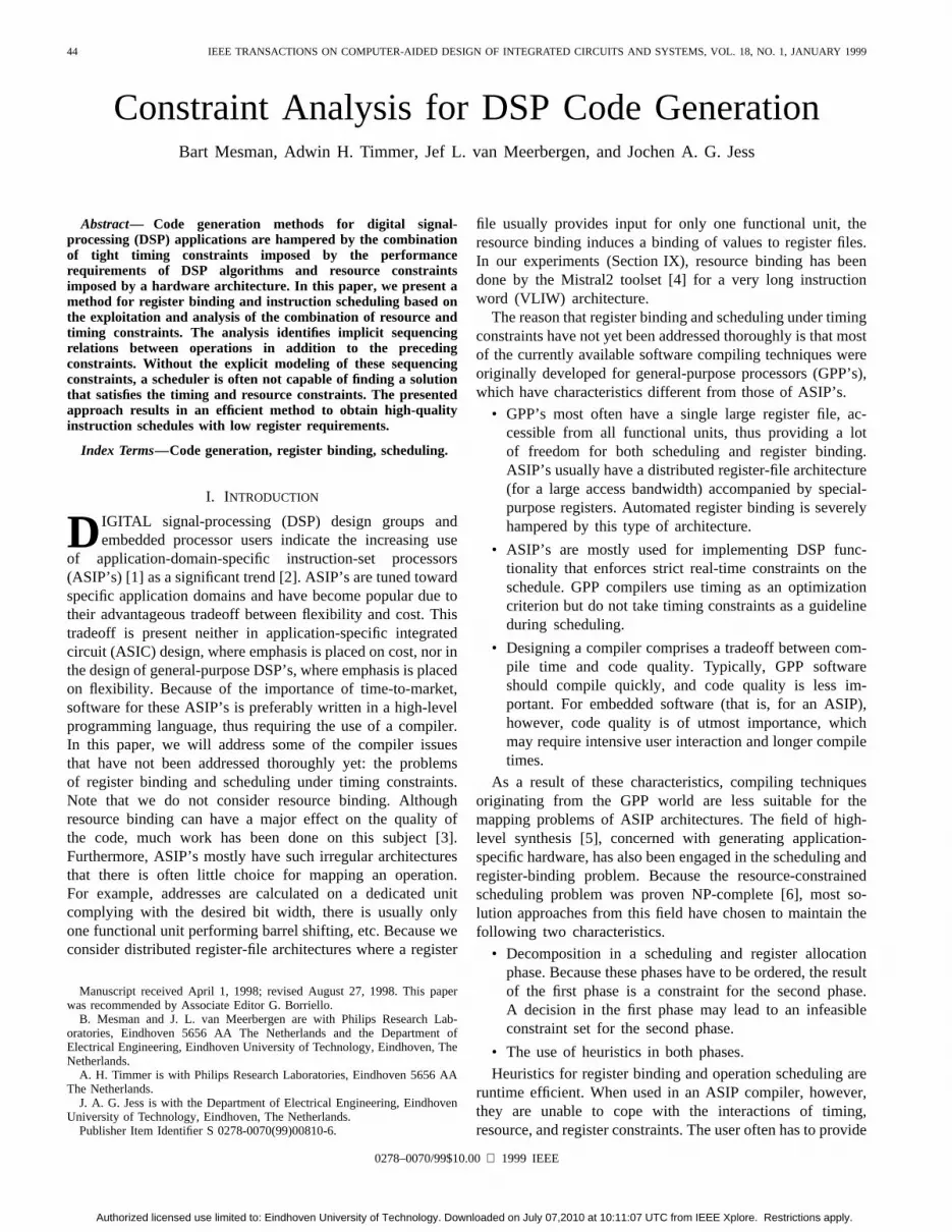
Because it is difficult to make a register binding anda schedule simultaneously, we decompose the problem inseparate phases, as depicted in Fig. 2. First, an initial registerbinding (discussed in Section VII-A) is constructed in a simplemanner. The II for each hierarchical level is also fixed prior tothe analysis. Most often, it is set by the designer. Otherwise,we start with a lower bound based on loop-carried dependen-



Fig. 2. Global approach.

cies [22] and available resources. When this II is not feasible,it is incremented by one clock cycle. Profiling suggests thatthe optimal II is usually only one or two clock cycles awayfrom the lower bound.

The central part, the constraint analyzer (discussedin Sections V and VI), generates additional precedenceconstraints that are implied by the combination of allconstraints, including the given register binding. Theseadditional precedence refine the ASAP–ALAP intervals, thusproviding a much more accurate estimate of the set of feasiblestart times. They will guide the scheduler and often prevent itfrom making schedule decisions leading to infeasibility.

The new precedence constraints are such that the registerbinding is guaranteed: all lifetimes between values residingin the same register have been sequentialized. The con-straint analyzer (and the lifetime sequencer) thus replacesthe register-binding constraints completely by precedence con-straints. When the constraint set leaves some room for differentlifetime sequentializations, thelifetime sequencer,discussed inSection VI-C, chooses between several alternatives. When theconstraint set is tight, as is the case in most of the benchmarksof Section IX, only one or two choices are made by thelifetime sequencer. A branch and bound algorithm is thereforeruntime-efficient enough for the lifetime sequencer.

The added precedence may cause violation of the constraintset (including the register binding). Aninfeasibility analysis(discussed in Section VII-B) uses the administrative book-keeping done by the constraint analyzer to find the bottleneckin the constraint set and the register binding. The “changeregister binding” block in Fig. 2 tries to solve this bottleneckby rebinding a value to a different register. This schemeis iterated until the constraint set and the register bindingare feasible. Last, the precedence generated by the constraintanalyzer is fed to a simple external schedule heuristic.

An advantage of this new approach is that in practice, asimple off-the-shelf scheduler can be used to complete theschedule. Although the existence of a schedule is not strictlyguaranteed after the constraint analyzer, a schedule was foundfor all problem instances. As the scheduler and its heuristicsare not critical in this approach, we will not focus on themin this paper.

Note that a main characteristic of our approach is thatwe perform register binding prior to schedule analysis. The

Fig. 3. Modeling the latency.

primary reason for this is our goal to obtain an efficient registerbinding given the timing and resource constraints. Therefore,we first want to fix the register binding, and constrain theschedule accordingly without violating the other constraints.The additional precedence constraints will guide the schedulermore accurately toward a feasible solution.

When violation of the constraint set does occur, the infea-sibility analyzer should be able to find the bottleneck.

A. Problem Statement for the Constraint Analyzerand the Infeasibility Analyzer

It is necessary that the constraint analyzer does someadministrative bookkeeping, such that the infeasibility anal-ysis is able to indicate a bottleneck in the register binding.The problem statement for the constraint analyzer and theinfeasibility analyzer is therefore as follows.

Problem Definition 3—Operation Ordering and BottleneckIdentification Problem (OOBIP):Given a cyclic DFG, a reg-ister binding, a set of resource constraints , an II,and a constraint on the latency, find either a partial order ofoperations satisfying the register binding (if the constraint setis feasible) or a smallest infeasible subset of value conflicts.

B. Effect of the Scheduler

The question rises as to whether or not the scheduler isalways able to find a solution when the constraint set passesthe infeasibility check. We distinguish two situations: pipelinedand nonpipelined schedules.

For nonpipelined schedules, the scheduler is always ableto find a solution that complies with the register binding.Experience shows, however, that the latency constraint maynot always be satisfied in the final schedule.

A pipelined schedule is more difficult to obtain; sometimesa decision is made that inevitably violates the constraint set. Itis therefore wise to alternate between scheduler and constraintanalyzer; first the scheduler makes a schedule decision. Thedecision is then modeled in terms of precedence relations(Section V-A), and the constraint analyzer computes the effectof this decision on the mobility of the other operations. In thisway, the search space of the scheduler is reduced according todecisions previously made in the schedule process. Althoughthere is still no absolute guarantee that a solution is foundin this way, a solution was found on all problem instancestried so far. If the scheduler fails after all, the infeasibilityanalyzer will indicate which value conflicts, resource conflicts,and schedule decisions are responsible for this failure. The



designer himself will then have to enforce a different scheduledecision or partial rebinding.

The following sections comprise a solution to OOBIP.Section V is concerned with the analysis of resource conflicts,precedence, and timing constraints. Section VI extends theanalysis to a given register binding. In Section VII-B, we willdemonstrate the infeasibility analyzer based on the results ofSections V and VI.

V. RESOURCE-CONSTRAINED ANALYSIS

In the previous section, we introduced a block diagramof our global approach. This section will focus on part ofthe constraint analyzer [23]. Section V-A models the differ-ent constraints as much as possible in terms of precedence.Section V-B analyzes the resource constraints, and generatesprecedence as well, so that most of the constraint set isexpressed in a unified model (the DFG). The analysis isillustrated on the example from Section III-C. In Section VI,the analysis is extended to handlevalue conflictsthat resultfrom a given register binding.

A. Modeling the Constraints

We start this section by showing how some of the constraintscan be represented in the DFG model introduced in Section III.

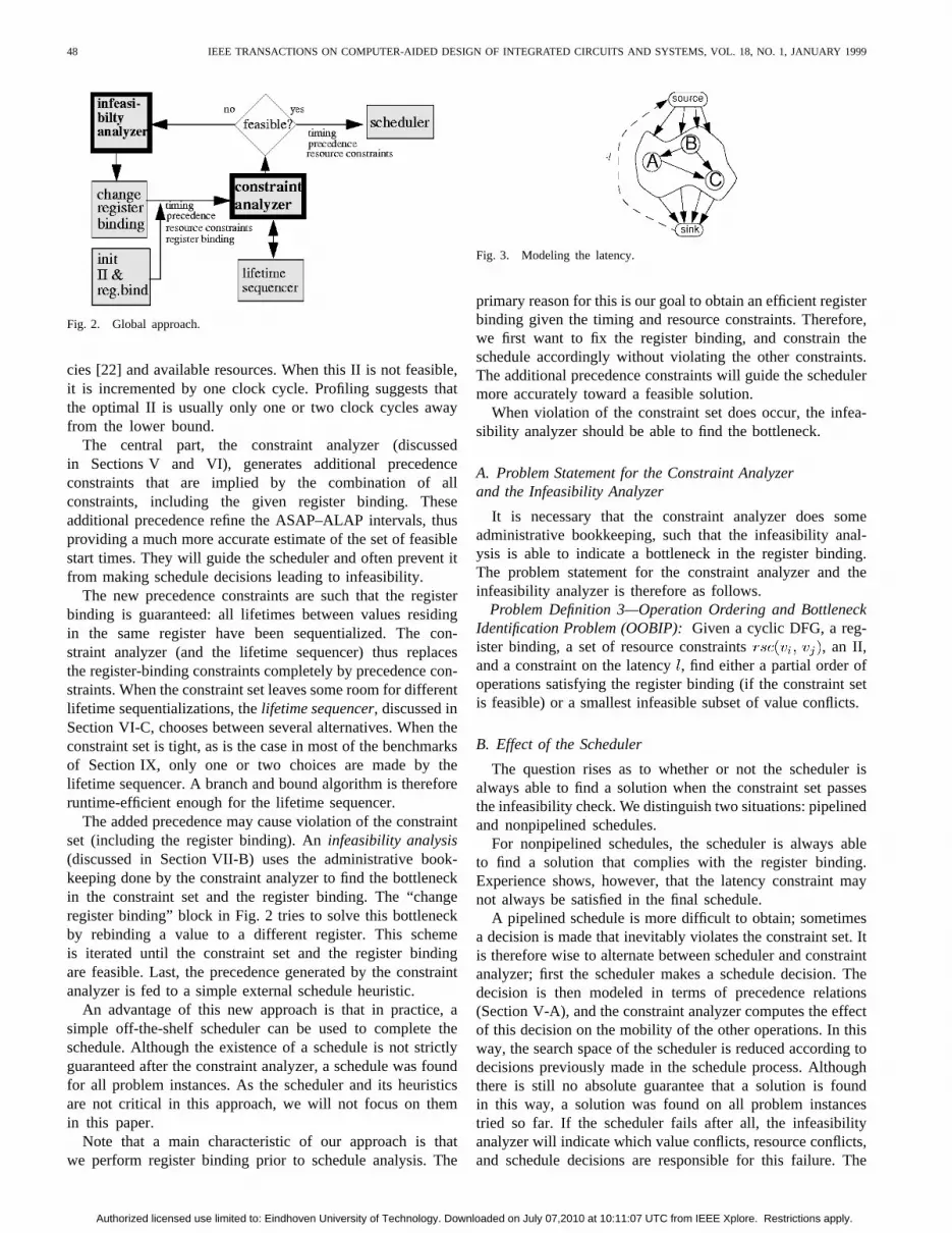
• Latency: A constraint on the latency is translated to anarc (sink, source) with , as illustrated in Fig. 3.This is interpreted as source sink , which isequivalent to sink source , meaning the lastoperation may not be executed more thanclock cyclesafter the start of the first operation.

• Microcoded controller and loop folding:We assume thatthe architecture contains a microcoded controller. Asa consequence, the same code is executed every loopiteration. This implies that a communicated value iswritten in the same register each iteration. When loopiterations overlap, we have to ensure that a value isconsumed before it is overwritten by the next production.Since subsequent productions are exactly II clock cyclesapart, a value cannot be alive longer than II clock cycles.So the operation C that consumes a value must executewithin II clock cycles after the operation P that producesthe value. Just like the latency constraint, a necessary andsufficient translation to the precedence model is that foreach data dependency (P, C), there is an arc (C, P) with

II. Lemma 8 gives conditions when this timingconstraint can be tightened.

• Pipelined executions and multicycle opera-tions: Pipelined executions and multicycle operationscan be modeled by introducing an operation for eachstage of the execution. Subsequent stages are linked intime using two sequence edges, as indicated in Fig. 4.For multicycle operations, A and B occupy the sameresource.

• Scheduling decisions:When schedule decisions are takenduring the process, the schedule intervals of other opera-tions are affected. Therefore, it is desirable to be able to

Fig. 4. Modeling pipelined and multicycle operations.

Fig. 5. Modeling a schedule decision.

express a schedule decision in the DFG so that its effectcan be analyzed in the context of the other constraints.Scheduling decisions may take different forms. A timingrelation between two operations can be directly translatedto a sequence edge. When an operationis fixed at acertain clock cycle , we need two sequence edges, asindicated in Fig. 5.

• Resource conflicts and instruction-set conflicts:We usemethod [20] to model instruction set conflicts as resourceconflicts , introduced in Section III-A.

B. Resource-Constraint Analysis

We now come to the point of explaining the analysisprocess. By observing a combination of constraints, we canreduce the search space. This reduction is made explicitby adding precedence constraints (sequence edges). In thissection, a lemma will be given that observes the interactionbetween resource conflicts, precedence, and timing constraints.The next section demonstrates lemmas to incorporate registerconflicts. All the lemmas used in our approach rely on theconcept of a path between operations.

Definition 10—Path:A path of length from operationto operation is a chain of precedence

that implies .Definition 11—Distance:The distance from op-

eration to is the length of the longest path from to.A path in the graph thus represents a minimum timing delay.

For example, in Fig. 1, the path A B C indicates aminimum timing delay of two clock cycles between the starttimes of A and C. The first lemma presented below affects thetiming relation between conflicting operations. It is based onthe fact that two operations with a resource conflict cannot bescheduled at the same potential. Thetime potentialassociatedto a time is mod II. So if the distance between theseoperations would cause them to be scheduled at the samepotential, the distance has to be increased by at least oneclock cycle.

Lemma 1: If mod II and ,we can add a sequence precedence edge with weight

without excluding any feasible schedules.This lemma will help us to solve the schedule problem in

Fig. 1. Remember that the key decision to obtaining a feasible



Fig. 6. Derivation of a schedule for Fig. 1.

schedule is to put a gap of one clock cycle between A and B.So our goal is to derive that A B . This derivationis given in Fig. 6. Fig. 6(a) represents the DFG model ofFig. 1(a). In Fig. 6(a), we see a path A B C Dof length mod II from A to D. According to Lemma1, we can add a sequence edge AD of weightbecause A and D have a resource conflict. This edge is drawnin Fig. 6(b). Next, there is a path D E sink sourceA B of length clock cycles. Becauseof the resource conflict D–B, this length has to be increased byone clock cycle. This gives a sequence edge DB of weight

2, as given in Fig. 6(c). We conclude by finding a path oflength clock cycles. In Fig. 6(d), the associatedsequence edge (A, B) of weight two is explicitly drawn. Theprecedence relations now completely fix the schedule. Thereader can verify that the [ASAP, ALAP] intervals based onthe extended DFG of Fig. 6(d) all contain just one clock cycle,and the estimated schedule freedom equals zero.

VI. REGISTER-CONSTRAINT ANALYSIS

The previous section introduced the methodology used inthe constraint analyzer of Fig. 2. In this section, we will extendthe techniques to analyze value conflicts that result from agiven register binding [24]. This will be done by introducinglemmas similar to Lemma 1 in the previous section. Theselemmas provide necessary conditions (in terms of precedencerelations) to guarantee a given register binding. Section VI-A is restricted to nonfolded schedules in order to explainthe concept more clearly. The lemmas will be generalized inSection VI-B for register conflicts that cross loop boundaries,which occur when folded schedules are considered.

A. Nonfolded Schedules

In this subsection, two lemmas observe the combination of agiven register binding, precedence, and timing constraints fornonfolded schedules. Their use is demonstrated with a small

Fig. 7. Lemma 2 for sequentialized value lifetimes.

example. In all given examples, a path is indicated using adashed arc labeled with the length of the path. Sequence edgesare dotted. Standard delay (if not labeled) for a sequence edgeis zero clock cycle; for a data dependence, it is one clock cycle.

Lemma 2: Let value , produced by operation P1 andconsumed by C1, and value, produced by operation P2 andconsumed by C2, reside in the same register. If(P1, P2) ,we can add a sequence precedence edge (C1, P2) with weightzero without excluding any feasible schedules.

Lemma 2 is illustrated in Fig. 7. The values and arebound to the same register. If there is a path of positive lengthfrom P1 to P2, then the whole lifetime of value has toprecede the lifetime of . This is made explicit by addinga sequence edge from the consumer C1 to the producer P2.A similar lemma is valid when there is a path between theconsumers of the values.

Lemma 3: Let value , produced by operation P1 andconsumed by C1, and value, produced by operation P2 andconsumed by C2, reside in the same register. If(C1, C2) ,we can add a sequence precedence edge (C1, P2) with weightzero without excluding any feasible schedules.

When there is a path between the producer of one value andthe consumer of the other, we can only exclude a possibilityif the delay of the path is strictly greater than zero. Otherwise,the alternative sequentializations, C2P1, could still yield afeasible schedule when P1 and C2 are scheduled in the sameclock cycle.

Lemma 4: Let value , produced by operation P1 andconsumed by C1, and value, produced by operation P2 andconsumed by C2, reside in the same register. If(P1, C2) ,we can add a sequence precedence edge (C1, P2) with weightzero without excluding any feasible schedules.

Lemma 4 is illustrated in Fig. 8. The overall method ofanalysis is demonstrated in Fig. 9. In this figure, valuesand reside in the same register, as do values and

. Because operation 1 consumes valueand operation7 consumes value , the lifetime of has to precede thelifetime of as a result of the precedence (Lemma 3applies). Therefore, the sequence edge is added. Nowthere is a path from the consumer of to theconsumer of , and Lemma 3 applies again. The sequenceedge is added as a result. Any schedule heuristic cannow find a schedule without violating the register binding,which is not the case if the sequence edges were not added.

B. Folded Schedules

In this section, we extend the lemmas from Section VI-A for sequentialized value lifetimes to handle pipelined loopschedules. An example demonstrates the use of the extendedlemmas.




Fig. 9. Example demonstrating the use of Lemma 3.

Fig. 10. Timing perspective of serializing alternatives.

When schedules are not folded, it is relatively simple toavoid overlapping lifetimes of values residing in the same reg-ister. Only two alternatives have to be considered, as depictedin Fig. 10, where the solid lines indicate the occupation of theregister. When loop iterations overlap in time, we also haveto take care that theth lifetime of value does not overlapwith the st (and the st) lifetime of value , asdepicted in Fig. 11. Applying the lemmas in this section willeliminate some alternatives, but it is not guaranteed that onlyone alternative remains. In this case, the lifetime sequencerin Fig. 2 will have to make a decision in order to avoidoverlapping lifetimes. This is the subject of Section VI-C.

Sequentialized value lifetimes that belong to different loopiterations pose a problem for the graph model because itmakes no difference between operation Aand A (whereA denotes theth execution of A). This suggests that a timingrelation between Aand B has to be translated to a timingrelation between Aand B. This translation is straightforward:

B B II, so that the relation A Bis translated to the relation A B II , which

Fig. 11. Serializing alternatives when folding once.


is equivalent to a sequence edge B A with delay II .Lemmas 2 and 3 are now easily generalized to Lemmas 5 and6.

Lemma 5: Let value , produced by operation P1 andconsumed by C1, and value, produced by operation P2 andconsumed by C2, reside in the same register. If(P1, P2)

II, we can add a sequence precedence edge (C1, P2) withweight II without excluding any feasible schedules.

Lemma 6: Let value , produced by operation P1 andconsumed by C1, and value, produced by operation P2 andconsumed by C2, reside in the same register. If(C1, C2)

II, we can add a sequence precedence edge (C1, P2) withweight II without excluding any feasible schedules.

Lemma 5 is illustrated in Fig. 12. Lemma 4 is generalizedto Lemma 7.

Lemma 7: Let value , produced by operation P1 andconsumed by C1, and value, produced by operation P2 andconsumed by C2, reside in the same register. If(P1, C2)

II , we can add a sequence precedence edge (C1, P2)with weight II without excluding any feasible schedules.

The last lemma we introduce with respect to folded sched-ules does not serialize lifetimes like the previous lemmas butrestricts the lifetime of a value when there exist other valuesassigned to the same register.

Lemma 8: Let be the set of values that reside in aregister , and let minlt( ) denote the minimal lifetime of value

(the distance from the producer ofto the last consumer of). Then each value has a maximum lifetime equal to

II minlt

Initially, all values have a minimum lifetime of one clockcycle. The lifetime expression in Lemma 8 is then simplifiedto II , where equals the number of values assigned toregister . When, for example, II , and there are two valuesin register , each of these values has a maximum lifetimeof clock cycles. When three values residein , the maximum lifetime becomes two clock cycles. This



Fig. 13. Derivation of a partial schedule.

Fig. 14. Folded ASAP schedule for Fig. 13.

maximum lifetime is modeled as a sequence edge with weight-maxlt from the consumer to the producer of the value, similarto modeling the latency.

We illustrate the use of these lemmas with the example inFig. 13. It is similar to the example of Fig. 1, but it is extendedwith a register binding. Value, communicated from operationA to B, and value , communicated from operation C to D, arebound to the same register. The same resource conflicts andthe same initiation interval are used, but there is no constrainton the latency. The first step from (a) to (b) is the same asthe first step in Fig. 6.

From Fig. 13(b) to (c), the value is produced by A andconsumed by B. Value is produced by C and consumed byD. Because of Lemma 7 and(A, D) II , we canadd a sequence edge (B, C) with weight II withoutexcluding any feasible schedules.

In Fig. 14, a folded ASAP schedule is given that satisfies thenewly added precedence constraints, and thus also the resourceconstraints and the register binding. In Fig. 14, the leftmostcolumn indicates the time potential (schedule time modulo II),so operation C is scheduled in clock cycle 4, D in clock cycle5, etc. Notice that the constraints have forced a gap of twoclock cycles between operations B and C. A greedy schedulingapproach does not put gaps between operations and wouldnever have found a schedule that satisfies all constraints.

In Fig. 15, it is proven that operations A, B, C, and Dare actually fixed at their schedule times given in Fig. 14.Fig. 15(a) shows a sequence edge (C, B) with weightII

as a result of modeling the loop-folding constraint as givenin Section V-A. It is also a special case of Lemma 8, where

contains only one value.From Fig. 15(a) to (b), the sequence edge generates a path

from C (producer of value ) to B (consumer of value) withdistance II . Because of Lemma 7, we

Fig. 15. Derivation of Fig. 13 continued.

can now add a sequence edge from D (consumer of value)to A (producer of value ) of weight II .

From Fig. 15(b) to (c), there is now a path from D to Aof distance II. Because A and D have a resourceconflict, Lemma 1 states that the distance is increased by oneclock cycle. Accordingly, a sequence edge (D, A) with weight

5 is added.As a result of this last sequence constraint, operation D

cannot be scheduled further than five clock cycles fromoperation A, which is also the minimum distance becauseof the sequence edge from B to C of weight three. Theintermediate operations (B and C) are also fixed in this way.Only operation E can be scheduled at clock cycle 6, 7, or 8.

We have now covered the basic techniques used in theconstraint analyzer of Fig. 2. Note that these techniques donot guarantee that every conflict is solved (that all lifetimesof values in the same register are serialized); especially whenthe schedule is not pipelined, the constraints are often notsufficient to eliminate every conflict. In such a case, a scheduledecision has to be made to serialize two value lifetimes, whichis the subject of the next section.

C. Lifetime Sequencing

Suppose we have a value conflict between value, pro-duced by operation P1 and consumed by C1, and value,produced by operation P2 and consumed by C2. We distinguishtwo situations:

• nonpipelined schedules;

• pipelined schedules.

In the first situation, the lifetime sequencer has to solve avalue conflict by choosing either C2 P1 or C1 P2. Inthe pipelined situation, the iteration index must be consideredas well: the alternatives are C2 P1 and C1 P2for possibly more than one value of. This is illustrated inFig. 11 for .

Nonpipelined blocks are sometimes large (1000 opera-tions), and constraints are not tight. This has two effects:

• many decisions have to be made;

• a lot of schedule freedom is available.



An actual branch and bound approach does not seem ap-propriate in this case: the number of decisions are too large toguarantee reasonable runtimes, and because of all the availableschedule freedom, a heuristic approach suffices. Although it isnot guaranteed that a feasible schedule is found in this way(in this case the values are simply separated), we have not yetencountered infeasibility in practice. Therefore, we choose oneof the sequentializations by reusing the schedule proceduresapplied in the actual scheduler (in Fig. 2) so that our approachis maximally tuned to the existing design flow. Since ourapproach is being integrated in the Mistral2 [4] compiler, theASAP values of P1 and P2 determine the highest priority. InSection IX, we included an experiment showing the effects ofsequencing lifetimes for a nonpipelined schedule.

For pipelined schedules, the reverse is true: pipelined loopsconsist of relatively few operations (typically200), and theconstraints are much more tight (all lifetimes are restrictedto II, resource constraints and value conflicts cross the loopiteration boundaries, etc.). As a result, only a few actualschedule decisions have to be made (typically10). Thepipelined benchmarks in Section IX required at most twodecisions. In this case, a branch and bound approach is runtimeefficient. Such an approach is also required because in thecontext of different types of very tight constraints, the effectsof a schedule decision are very difficult to anticipate, andwe are likely to make a “wrong” decision. For the samereason, we do not want to reuse the schedule procedures ofthe actual scheduler in Fig. 2: the constraints are simply tootight to take any optimization criteria into account. Instead,our first choice is determined by the alternative (C2 P1or C1 P2 for some ) that reduces the mobility ofP1, C1, P2, and C2 the least. Note that there is no actual“cost function” involved in this branch and bound approach:the detection of infeasibility (violation of the constraints)determines when to backtrack.

The infeasibility analysis is able to assist in selecting thedecision to backtrack: in Section VII-B, it is explained in detailthat infeasibility is detected as a positive delay cycle in theprecedence graph. A decision is backtrackedonly when it ispart of such a cycle, because only then may it be inconsistentwith the constraints or previously made decisions.

VII. REGISTER BINDING

In this section, we cover two blocks from our globalapproach of Fig. 2 that are related to the register binding. Thefirst is the initial binding, addressed in Section VII-A, and thesecond is the infeasibility analyzer, addressed in Section VII-B.

A. Initial Binding

It is clear from Fig. 16 that an initial register binding has tobe made to start the iteration of the constraint analyzer, giventhe binding of values to register files. We choose the bindingsuch that each register file holds one register. In this way, allvalues bound to a registrableneed to have their lifetimessequentialized. This choice is made for two reasons. First, itproduces the least hardware when ASIC’s are concerned, and

Fig. 16. Example of a precedence graph.

Fig. 17. v andw cannot be in the same register.

provides useful user feedback when programmable platformsare concerned. Second, when the constraints are more tight,the constraint analyzer generates more precedence constraints,so it is better able to guide the scheduler toward a feasiblesolution.

Starting from this minimum binding, some changes can bemade trivially based on the hierarchy of basic blocks. Forexample, if value is produced before loop and consumedafter loop , it occupies a register during the entire executionof loop . During the analysis of loop, a register is thereforereserved for value . Another trivial decision is based ondataflow. For example, in the precedence graph in Fig. 17,values and cannot reside in the same register because thevalue lifetimes cannot be sequentialized.

B. Infeasibility Analysis

The schedule analysis is often capable of detecting thatthe register binding together with the constraint set yields aninfeasible result. In order to make a sensible change in theregister binding, we want the infeasibility analyzer to identifythe bottleneck in the register binding. More precisely, wewant the analyzer to give asmallest infeasible subset of valueconflicts,that is, a subset of value conflicts (two values residingin the same register) that together cause infeasibility. Identi-fying such a subset of decisions is tightly related to detectinginfeasibility. The constraint analyzer detects infeasibility basedon longest path information in the following way: when thelongest path algorithm finds a path from an operationto itself(a cycle in the precedence graph) and this path has a positivelength, the operation is forced to execute strictly before itsown start time, which is clearly not possible. So a precedencecycle of strictly positive length indicates infeasibility.

The bottleneck lies directly in the way that the positivelength cycle came into existence. For example, if in Fig. 13the latency was constrained to six clock cycles, there was asequence edge from the sink to the source with a delay of



Fig. 18. Infeasibility analysis for Fig. 16.

6 clock cycles. In Fig. 13(c), that would yield a positivedelay cycle. Most edges in the precedence cycle involve dataprecedence, one involves the latency, and one involves aregister conflict. The sequence edge BC is a result of twocomponents: 1) the register conflict and 2) a path oflength four from A to D. The path from A to D consists of onesequence edge that is added as a result of the resource conflictA–D and a path A D of length three that consists entirelyof data precedence. We can thus conclude that infeasibility iscaused as a result of the following combination of factors:

1) a register conflict ;

2) a resource conflict A–D;

3) the latency constraint;

4) data precedence.

When all constraints are fixed except for the register binding,we conclude that the decision to put the valuesandtogether in a single register is the cause of infeasibility.

Another example is the graph depicted in Fig. 16. Theconstraint set is infeasible with the register binding, whichis derived as follows. The infeasibility analysis is graphicallydepicted in Fig. 18. Each block represents a path, and eachdownward arrow represents an inference. The derivation istop down. The path D G of length two ( II) and registerconflict lead to the sequence edge D F of weightII as a consequence of Lemma 6 (where ). Thedownward arrows show that this sequence edge is part in thepath underneath. The second block from the top indicates apath C F of length three. Together with the register conflict

, this yields a sequence edge C D of weight two asa result of Lemma 6. In the block at the bottom of Fig. 18,the sequence edge D C of weight 1 is generated as aresult of Lemma 8. (value and in the same register limitstheir lifetimes to II clock cycles). Thesame block shows that this sequence edge causes a positiveprecedence cycle C D C with a delay ofclock cycle. As a result of this positive precedence cycle, weconclude that the register binding is infeasible.

The infeasibility analysis is done in bottom-up fashion toidentify exactly those sequence edges and conflicts that havecontributed to the positive precedence cycle. The combinationof register conflicts that yield infeasibility is identified as:

1) on register 1;

2) on register 3.

Fig. 19. The only two feasible schedules for Fig. 16 with changes in theregister binding.

Note that the conflict on register 2 did not contributeto the infeasibility, and thus it is useless to put the valuesand in separate registers. Instead, we have to choose to spliteither register 1 or register 3. Both decisions yield a feasibleschedule, as depicted in Fig. 19.

C. Rebinding

The infeasibility analysis generates a list of value conflicts.A conflict arises between two values. The list of value conflictsis ordered on a number of criteria.

• The number of times the conflict appears in the conflictlist. When a conflict occurs more often in the list, theconflict contributes more extensively to the bottleneck.

For ASIC’s, it is ordered on the following.

• The type of the values; we prefer allocating an additional6-bit register to an additional 28-bit register.

• Addressability; when a register file contains four registers,allocating an additional register requires an additionaladdressing bit in the instruction word. We prefer to extenda register file with three or five to seven registers.

For ASIP’s, it is ordered on the following.

• Availability of registers; we prefer to move values withina register file that contains more spare registers.

After the conflict list is ordered, only the top conflict is chosen.One of the two conflicting values is then allocated to thenext register. In this way, convergence is guaranteed. Thedisadvantage is that the same value conflicts may arise insubsequent iterations of the scheme in Fig. 2. Because thishas not proven to be a problem on our problem instances, nowork has been done to overcome the disadvantage.

VIII. C OMPLEXITY

In this section, we analyze the runtime complexity and mem-ory requirements of our approach. The two major contributionsto runtime are:

• finding the longest paths and updating the paths as a resultof applying the lemmas from Sections V and VI;

• infeasibility analysis and changing the register binding.

A. Finding and Updating the Longest Paths

We will first consider the complexity of the former contri-bution. In our implementation, the longest path between eachpair of operations is administrated. The memory requirementsthus have order .



If a new edge is added, the impact on the current longestpaths has to be calculated. Therefore, the complexity of addinga sequence edge is the dominant factor in runtime. Thiscomplexity is essentially determined by the number of pathsthat need to be updated as a result of the new sequence edge.Because we are only interested in the longest paths found sofar, the number of updates equals in the worst case. In mostcases, the addition of a sequence edge will affect a few paths.In cases where many paths need to be updated, the estimatesof schedule intervals will also be improved substantially.

An upper bound on the number of path updates (as a resultof adding a sequence edge) can be derived as follows. Apath can have a length between and , where is theconstraint on the latency. Because a path is updated only if itslength is increased (by at least one clock cycle), the number oftimes a path can be updated is at most. Since the maximumnumber of paths we keep track of equals, the number ofpath updates can be at most . A single path updatetakes constant time, so the runtime of the constraint analysisis polynomially bounded.

B. Infeasibility Analysis and Rebinding

As the reader may have noticed in the examples, theinfeasibility analysis requires a lot of administrative bookkeep-ing. Almost every path constructed during the longest pathanalysis has to be kept in memory for reference. A feasibleimplementation requiring a limited amount of memory to runan implementation of our method is only guaranteed if thestorage of a path has a memory cost of . This is possiblewith the use of anadjacency matrix[25], which is based onthe following fact of longest paths: if the longest path from Ato C travels through B, then the part B to C is the longest pathfrom B to C. As a result, the only administration necessaryfor the path from A (row of the matrix) to C (column ofthe matrix) is the first node on the path after A. To facilitatethe infeasibility analysis, we also administrate the first edgetraversed on the path A to C. Each sequence edge on its turnhas a pointer to a register conflict (if there is one) and thematrix entry representing the path that gave rise to the edge.The complexity of the infeasibility analysis is thus boundedby . We assume, however, that the longest pathshave already been calculated in the constraint analyzer.

The complexity of rebinding is determined by the procedureof ordering the conflict list as explained in Section VII-C.Because a value conflict gives rise to a sequence edge, thenumber of conflicts in the list cannot exceed the number ofedges in the precedence graph. Therefore, the complexity ofrebinding is bounded by .

We conclude that the complexity of one iteration of thescheme in Fig. 2 equals . In the worstcase, the number of iterations is bounded by, the numberof values in the dataflow graph. In the results section, we willalso depict the iteration count for the different applications.

IX. RESULTS

Our implementation on an HP 9000/735 has been testedon the inner loops from four different real-life industrial

TABLE IRESULTS OF EXPERIMENTS

examples that have been mapped on a VLIW architecture withdistributed register files. The results are shown in Table I.The fourth column represents the number of iterations overthe constraint analyzer (see Fig. 2) before a feasible solutionwas found. The last two columns indicate the mobility ofthe operations in terms of average number of clock cyclesper operation (Definition 10). The sixth column indicates themobility before the analysis; the last column, after analysis(what is left for the scheduler to fill in). With respect to thenumbers in Table I, no comparison could be made to otherapproaches because the register allocator and the schedulersavailable to us (several list schedulers) are unable to find anysolution for the given constraints.

The first experiment concerns an infinite impulse response(IIR) filter of 23 operations, including fetching the coefficientsand data from memory. The minimum latency is ten clockcycles, which equals the latency constraint. The other exper-iments concern fast Fourier transform (FFT) applications, thelargest of which holds 81 operations. Note in Table I that theruntimes are mainly determined by the number of iterationsover the constraint analyzer. The number of iterations is ameasure of the difficulty of finding a register binding becauseit reflects the number of changes made to the original bindingin order to get a feasible schedule. In these experiments, theschedule generated by our method provided a more efficientregister binding than a handmade schedule. Analyses of theminimal value lifetimes suggested that little or no improve-ment could be made on the generated register binding.

The mobility is decreased by a factor ranging from 3.6(Rad4) to 13.2 (FFTb) as a result of the schedule analysis.Because this decrease of mobility is due to the constraints,it is a measure for the analyzers’ capability of directing thescheduler and preventing it from making schedule decisionsthat violate the constraints.

We have included one more experiment to test the perfor-mance of our method on a problem instance that was notconstrained with respect to timing. It is a preliminary testexecuted by Frontier Design, who are integrating our methodwithin the Mistral2 toolset. The benchmark, Par2, contains 91operations. The original schedule, generated by the Mistral2toolset, counts 61 clock cycles. As a result of the availableparallelism and the number of memory accesses, the registerbinder required six registers at the address-generation unit.The schedule generated by our method counts only 56 clockcycles and requires only one register at the address-generationunit. Because of the schedule freedom, a total of 111 scheduledecisions had to be made by the lifetime sequencer. Runtimewas less than a second. The efficient register binding of the



new schedule was expected (it was enforced), unlike thereduction in the number of clock cycles. This reduction isexplained as follows: because of the serialization of the addresslifetimes, the precedence graph became more regular. It isa well-known fact that heuristics such as the list schedulingare able to find more efficient schedules when the precedencegraph contains more regularity.

X. CONCLUSIONS AND FURTHER RESEARCH

In this paper, we presented an approach for register bindingand scheduling in the context of loop pipelining, based onthe analysis of precedence, timing, and resource constraints.By expressing as much of the constraints as possible in agraph model and calculating the longest paths, we are ableto see the interaction between the different constraints andcompute the effect on the mobility available to a scheduler.When the combination of constraints and the register binding isinfeasible, an efficient infeasibility analyzer is able to indicatea change in the binding that is necessary to obtain a feasibleschedule. The results in Section IX show that our method isable to find a register binding and a pipelined schedule in shortruntimes for industrially relevant designs. We also showed thatthe obtained reduction in mobility really prevents a greedyscheduler from making a wrong decision. When constraintsare not very tight, we are still able to find more efficientschedules than heuristics. We conclude that analysis tools suchas our implementation are needed in order to obtain a feasibleschedule when facing resource constraints, register constraints,and tight timing constraints. Our method is being integratedin the Mistral2 toolset by Frontier Design.

Further research will focus on the analysis of other register-file models, such as first-in, first-out and stacks.

ACKNOWLEDGMENT

The authors would like to thank M. Strik, K. van Eijk, andP. Lippens for their support and constructive discussions.

REFERENCES

[1] R. Leupers, W. Schenk, and P. Marwedel, “Microcode generationfor flexible parallel architectures,” inProc. Working Conf. ParallelArchitectures and Compiler Technology,1994.

[2] P. G. Paulin, C. Liem, T. C. May, and S. Sutarwala, “DSP design toolrequirements for embedded systems: A telecommunications industrialperspective,”J. VLSI Signal Process.,vol. 9, no. 1, 1995.

[3] P. Marwedel and G. Goossens, Eds.,Code Generation for EmbeddedProcessors. Boston, MA: Academic, 1995.

[4] M. T. J. Strik, “Efficient code generation for application domain specificprocessors,” Eindhoven University of Technology, The Netherlands,Tech. Rep. 90-5282-390-1, 1994.

[5] M. C. McFarland, A. C. Parker, and R. Camposano, “Tutorial onhigh-level synthesis,” inProceedings of the 25th ACM/IEEE DesignAutomation Conference. Anaheim, CA: ACM and IEEE ComputerSociety, 1988, pp. 330–336.

[6] M. R. Garey and D. S. Johnson,Computers and Intractability: A Guideto the Theory of NP-Completeness.San Francisco, CA: Freeman, 1979.

[7] G. Goossens, J. Vandewalle, and H. De Man, “Loop optimizationin register-transfer scheduling for DSP-systems,” inProceedings ofthe 26th ACM/IEEE Design Automation Conference.Las Vegas, NV:ACM and IEEE Computer Society, 1989, pp. 826–831.

[8] P. G. Paulin, C. Liem, T. C. May, and S. Sutarwala, “FlexWare: Aflexible firmware development environment for embedded systems,” inP. Marwedel and G. Goossens, Eds.,Code Generation for EmbeddedProcessors. Boston, MA: Academic, 1995.

[9] R. Leupers and P. Marwedel, “Retargetable code generation based onstructural processor descriptions,”Design Automation Embedded Syst.,vol. 3, no. 1, 1998.

[10] D. Lanneer, J. van Praet, A. Kifli, K. Schoofs, W. Geurts, F. Thoen, andG. Goossens, “Chess: Retargetable code generation for embedded DSPprocessors,” in P. Marwedel and G. Goossens, Eds.,Code Generationfor Embedded Processors.Boston, MA: Academic, 1995.

[11] M. T. J. Strik, J. L. van Meerbergen, A. H. Timmer, and J. A. G.Jess, “Efficient code generation for in-house DSP-cores,” inProceedingsof the European Design and Test Conference. Paris, France: IEEEComputer Society Press, 1995, pp. 244–249.

[12] C. Liem, T. May, and P. Paulin, “Instruction-set matching and selectionfor DSP and ASIP code generation,” inProceedings the EuropeanDesign and Test Conference. Paris, France: IEEE Computer SocietyPress, 1997, pp. 31–37.

[13] B. R. Rau and C. D. Glaeser, “Some scheduling techniques and aneasily schedulable horizontal architecture for high performance scientificcomputing,” inProc. Ann. Workshop Microprogramming,Oct. 1981, pp.183–198.

[14] M. Lam, “Software pipelining: An effective scheduling technique forVLIW machines,” in Proc. SIGPLAN Conf. Programming LanguageDesign and Implementation,June 1988, p. 328.

[15] A. Aiken, A. Nicolau, and S. Novack, “Resource-constrained softwarepipelining,” IEEE Trans. Parallel Distrib. Syst.,vol. 6, pp. 1248–1270,Dec. 1995.

[16] C. T. Hwang, Y. C. Hsu, and Y. L. Lin, “A formal approach to thescheduling problem in high level synthesis,”IEEE Trans. Computer-Aided Design,vol. 10, pp. 464–475, Apr. 1991.

[17] B. R. Rau, M. Lee, P. P. Tirumalai, and M. S. Schlansker, “Registerallocation for software pipelined loops,” inProc. SIGPLAN Conf.Programming Language Design and Implementation,June 1992, pp.283–299.

[18] A. E. Eichenberger, E. S. Davidson, and S. G. Abraham, “Optimummodulo schedules for minimum register requirements,” inProc. Int.Conf. Supercomputing,Barcelona, Spain, July 1995, pp. 31–40.

[19] R. Govindarajan, E. R. Altman, and G. R. Gao, “Minimizing registerrequirements under resource-constrained rate-optimal software pipelin-ing,” in Proc. Symp. Microarchitecture,Nov. 1994, pp. 85–94.

[20] A. H. Timmer, M. T. J. Strik, J. L. van Meerbergen, and J. A. G. Jess,“Conflict modeling and instruction scheduling in code generation forin-house DSP cores,” inProceedings of the 32nd ACM/IEEE Design Au-tomation Conference. San Francisco, CA: ACM and IEEE ComputerSociety, 1995.

[21] D. C. Ku and G. De Micheli, Eds.,High Level Synthesis of ASIC’sUnder Timing and Synchronization Constraints.Norwell, MA: KluwerAcademic, 1992.

[22] R. Reiter, “Scheduling parallel computation,”J. ACM, vol. 15, pp.590–599, 1968.

[23] B. Mesman, M. T. J. Strik, A. H. Timmer, J. L. van Meerbergen, andJ. A. G. Jess, “Constraint analysis for DSP code generation,” inProc.Int. Symp. System Synthesis,Antwerp, Sept. 1997.

[24] , “A constraint driven approach to loop pipelining and registerbinding,” in Proceeding of the Design Automation and Test in Europe.Paris, France: IEEE Computer Society Press, 1998.

[25] T. H. Cormen, C. E. Leiserson, and R. L. Rivest,Introduction toAlgorithms. Cambridge, MA: MIT Press, 1990.

Bart Mesman received the Electrical Engineeringdegree (with honors) from the Eindhoven Univer-sity of Technology, Eindhoven, The Netherlands,in 1995, where he currently is pursuing the Ph.D.degree.

His doctoral work is on the subject of sched-uling for embedded DSP processor architectureswith the explicit goal of codesigning processorarchitectures and a code-generation methodologybased on constraint analysis. Since 1995, he hasbeen a Member of both the Digital VLSI Group

at Philips Research, Eindhoven, and the Information and CommunicationSystems Group of the Electrical Engineering Department at the University ofTechnology, Eindhoven. His research interests include high-level synthesis,ASIP architectures, and code generation for embedded DSP’s.



Adwin H. Timmer received the Electrical Engi-neering and Ph.D. degrees from the EindhovenUniversity of Technology, Eindhoven, The Nether-lands, in 1990 and 1996, respectively.

In 1995, he joined Philips Research Laboratories,Eindhoven. In 1998, he was a Visiting IC Architectwith the Philips Semiconductors WSG businessline, Mountain View, CA. His current interests arein IC architectures for high-performance signal-processing applications, system-level design meth-ods, hardware/software codesign, and compilation

techniques for embedded DSP’s.

Jef L. van Meerbergen received the ElectricalEngineering and Ph.D. degrees from the KatholiekeUniversiteit Leuven, Belgium, in 1975 and 1980,respectively.

In 1979, he joined Philips Research Laboratoriesin Eindhoven, The Netherlands. He was engaged inthe design of MOS digital circuits, domain-specificprocessors, and general-purpose digital signal pro-cessors. In 1985, he began working on application-driven high-level synthesis. Initially, this work wastargeted toward audio and telecom DSP applica-

tions. Later, the application domain shifted toward high-throughput appli-cations (Phideo). His current interests are in system-level design methods,heterogeneous multiprocessor systems, and reconfigurable architectures. Heis a Philips Research Fellow and, since 1998, a Professor at the EindhovenUniversity of Technology. He is an Associate Editor ofDesign Automationfor Embedded Systems.

Dr. van Meerbergen received the Best Paper Award at the 1997 ED&TCconference.

Jochen A. G. Jessreceived the master’s and Ph.D.degrees from Aken University of Technology, Ger-many, in 1961 and 1963, respectively.

He became a Full Professor of electrical engi-neering at the Eindhoven University of Technology,Eindhoven, The Netherlands, in 1971. For a numberof years, he had various research and teaching ap-pointments at Karlsruhe University of Technology,where he was one of the founders of the ComputerScience Department. During 1968–1969, he spenta sabbatical year at the University of Maryland,

College Park. In Eindhoven, he was involved in founding and running theDesign Automation Section. This task implied devising a long-term researchprogram in the area of VLSI design automation and complementing it with thenecessary curricular components. His is a coauthor of about 125 papers. Heguided 31 Ph.D. students to graduation. In 1985, he joined IBM T. J. WatsonLaboratories, Yorktown Heights, NY, for a short period to contribute to asilicon compilation path for the 801 RISC pipeline in a project guided by R. K.Brayton and R. Otten. Recently, his interest has focused on hardware platformsfor multimedia systems and the problems of compilation for performancewhen mapping high-performance, real-time tasks onto those platforms. He ismember of the board of the European Design Automation Association andhas been its Chairman for a number of years. He is a Cofounder of theDesign Automation and Test in Europe conference. He was Program Chairand General Chair, respectively, of ICCAD-93 and ICCAD-94.


Documents

Constraint analysis for DSP code generation