Embed Size (px)
Citation preview

MITSUBISHI ELECTRIC RESEARCH LABORATORIEShttp://www.merl.com
Compressed Sensing for Fusion Frames
Petros Boufounos, Gitta Kutyniok, Holger Rauhut
TR2009-053 September 2009
Abstract
Compressed Sensing (CS) is a new signal acquisition technique that allows sampling of sparsesignals using significantly fewer measurements than previously thought possible. On the otherhand, a fusion frame is a new signal representation method that uses collections of subspacesinstead of vectors to present signals. This work combines these exciting new fields to introduce anew sparsity model for fusion frames. Signals that are sparse under the new model can be com-pressively sampled and uniquely reconstructed in ways similar to sparse signals using standardsCS. The combination provides a promising new set of mathematical tools and signal models use-ful in a variety of applications. With the new model, a sparse signal has energy in very few of thesubspaces of the fusion frame, although it needs not be sparse within each of the subspaces it oc-cupies. We define a mixed l1/l2 norm for fusion frames. A signal sparse in the subspaces of thefusion frame can thus be sampled using very few random projections and exactly reconstructedusing a convex optimization that minimizes this mixed l1/l2 norm. The sampling conditions wederive are very similar to the coherence and RIP conditions used in standard CS theory.
SPIE 2009
This work may not be copied or reproduced in whole or in part for any commercial purpose. Permission to copy in whole or in partwithout payment of fee is granted for nonprofit educational and research purposes provided that all such whole or partial copies includethe following: a notice that such copying is by permission of Mitsubishi Electric Research Laboratories, Inc.; an acknowledgment ofthe authors and individual contributions to the work; and all applicable portions of the copyright notice. Copying, reproduction, orrepublishing for any other purpose shall require a license with payment of fee to Mitsubishi Electric Research Laboratories, Inc. Allrights reserved.
Copyright c©Mitsubishi Electric Research Laboratories, Inc., 2009201 Broadway, Cambridge, Massachusetts 02139

MERLCoverPageSide2

Compressed Sensing for Fusion Frames
Petros Boufounosa, Gitta Kutyniokb, and Holger Rauhutc
aMitsubishi Electric Research Laboratories, 201 Broadway, Cambrige, MA 02139 USA;bInstitute of Mathematics,University of Osnabruck, 49069 Osnabruck, Germany;
cHausdorff Center for Mathematics & Institute for Numerical Simulation, University of Bonn, Endenicher Allee 60,53115 Bonn, Germany
ABSTRACT
Compressed Sensing (CS) is a new signal acquisition technique that allows sampling of sparse signals usingsignificantly fewer measurements than previously thought possible. On the other hand, a fusion frame is a newsignal representation method that uses collections of subspaces instead of vectors to represent signals. This workcombines these exciting new fields to introduce a new sparsity model for fusion frames. Signals that are sparseunder the new model can be compressively sampled and uniquely reconstructed in ways similar to sparse signalsusing standard CS. The combination provides a promising new set of mathematical tools and signal models usefulin a variety of applications.
With the new model, a sparse signal has energy in very few of the subspaces of the fusion frame, although itneeds not be sparse within each of the subspaces it occupies. We define a mixed `1/`2 norm for fusion frames.A signal sparse in the subspaces of the fusion frame can thus be sampled using very few random projectionsand exactly reconstructed using a convex optimization that minimizes this mixed `1/`2 norm. The samplingconditions we derive are very similar to the coherence and RIP conditions used in standard CS theory.
Keywords: Compressed Sensing. `1 minimization. Sparse Recovery. Mutual Coherence. Fusion Frames.
1. INTRODUCTION AND BACKGROUND
Compressed Sensing (CS) has recently emerged as a very powerful field in signal processing, enabling the ac-quisition of signals at rates much lower than previously thought possible.1,2 To achieve such performance, CSexploits the structure inherent in many naturally occurring and man-made signals. Specifically, CS uses classicalsignal representations and imposes a sparsity model on the signal of interest. The sparsity model, combined withrandomized linear acquisition, guarantees that non-linear reconstruction can be used to efficiently and accuratelyrecover the signal.
Fusion frames are recently emerged mathematical structures that can better capture the richness of the naturaland man-made signals compared to classically used representations.3 In particular, fusion frames generalize frametheory by using subspaces in the place of vectors as signal building blocks. Thus signals can be representedas linear combinations of components that lie in particular, and often overlapping, signal subspaces. Sucha representation provides significant flexibility in representing signals of interest compared to classical framerepresentations.
In this paper we extend the concepts and methods of Compressed Sensing to fusion frames. In doing so wedemonstrate that it is possible to recover signals from underdetermined measurements if the signals lie only onvery few subspaces of the fusion frame. Our generalized model does not require that the signals are sparse withineach subspace. The rich structure of the fusion frames framework allows us to characterize more complicatedsignal models than the standard sparse or compressible signals used in compressive sensing techniques. Ourresults are applicable in target detection and tracking, and in audio segmentation applications, to name a few.
Further author information: (Send correspondence to P. Boufounos)P.B.: E-mail: [email protected], Telephone: 1 617 621 7575G.K.: E-mail: [email protected], Telephone: 49 541 969 3516H.R.: E-mail: [email protected], Telephone: 49 228 736 2245

Our ultimate motivation is to generalize the notion of sparsity to more general mathematical objects, such asvector-valued data points.4 Toward that goal, we demonstrate that the generalization we present in this paperencompasses joint sparsity models5,6 as a special case. Furthermore, it is itself a special case of block-sparsitymodels,7 with significant additional structure that enhances existing results.
In the remainder of this section we describe some possible applications and provide some background onCompressed Sensing and on fusion frames. In Section 2 we formulate the problem and establish notation. Wefurther explore the connections with existing research in the field, as well as possible extensions. In Section 3 weprove recovery guarantees using the coherence properties of the sampling matrix. In Section 4 we prove similarguarantees using the restricted isometry properties (RIP) of the sampling matrix. We conclude with a discussionof our results.
1.1 ApplicationsAlthough the development in this paper provides a general theoretical perspective, the principles and the methodswe develop are widely applicable. In particular, the special case of joint (or simultaneous) sparsity has alreadybeen widely used in radar,8 sensor arrays,9 and MRI pulse design.10 In these applications a mixed `1/`2 normwas used heuristically as a sparsity proxy. Part of our goals in this paper is to provide a solid theoreticalunderstanding of such methods.
In addition, the richness of fusion frames allows the application of this work to other cases, such as targetrecognition and music segmentation. The goal in such applications is to identify, measure and track targets thatare not well described by a single vector but by a whole subspace. In music segmentation, for example, each noteis not characterized by a single frequency, but by the subspace spanned by the fundamental frequency of theinstrument and its harmonics.11 Furthermore, depending on the type of instrument in use, certain harmonicsmight or might not be present in the subspace. Similarly, in vehicle tracking and identification, the subspaceof a vehicle’s acoustic signature depends on the type of vehicle, its engine and its tires.12 Note that in bothapplications, there might be some overlap in the subspaces that distinct instruments or vehicles occupy.
Fusion frames are quite suitable for such representations. The subspaces defined by each note and eachinstrument or each tracked vehicle generate a fusion frame for the whole space. Thus the fusion frame serves asa dictionary of targets to be acquired, tracked, and identified. The fusion frame structure further enables theuse of sensor arrays to perform joint source identification and localization using far fewer measurements than aclassical sampling framework.
1.2 Compressed Sensing BackgroundCompressed Sensing (CS) is a recently emerged field in signal processing that enables signal acquisition usingvery few measurements compared to the signal dimension, as long as the signal is sparse in some basis. It predictsthat a signal x ∈ RN with only k non-zero coefficients can be recovered from only n = O(k log(N/k)) suitablychosen linear non-adaptive measurements, compactly represented using
y = Ax,y ∈ Rn,A ∈ Rn×N .
A necessary condition for exact signal recovery is that
Ax 6= 0 for all x 6= 0, ‖x‖0 ≤ 2k,
where the `0 ‘norm,’ ‖x‖0, counts the number of non-zero coefficients in x. In this case recovery is possible usingthe following combinatorial optimization,
x = argmin x∈RN ‖x‖0 subject to y = Ax,
Unfortunately this is an NP-hard problem13 in general, hence becomes infeasible in high dimensions.
Exact signal recovery using computationally tractable methods can be guaranteed if the coherence of themeasurement matrix A is sufficiently small.4,14 The coherence of a matrix A with unit norm columns ai,‖ai‖2 = 1, is defined as
µ = maxi 6=j
|〈ai,aj〉| .

Exact signal recovery is also guaranteed if A obeys a restricted isometry property (RIP) of order 2k, i.e., if thereexists a constant δ2k such that for all 2k-sparse signals x
(1− δ2k)‖x‖22 ≤ ‖Ax‖22 ≤ (1 + δ2k)‖x‖22.
If the coherence of A is small or if A has a small RIP constant, then the following convex optimization programexactly recovers the signal from the measurement vector y,1
x = argmin x∈RN ‖x‖1 subject to y = Ax.
A surprising result is that random matrices with sufficient number of rows can achieve small coherence and smallRIP constants with overwhelming probability.
A large body of literature extends these results to measurements of signals in the presence of noise, to signalsthat are not exactly sparse but compressible,1 to several types of measurement matrices15–19 and to measurementmodels beyond simple sparsity.20
1.3 Background on Fusion FramesFusion frames are generalizations of frames that provide a richer description of signal spaces. A fusion frame is acollection of subspaces Wj ⊆ RM and associated weights vj , compactly denoted using (vj ,Wj)N
j=1, that satisfies
A‖f‖22 ≤N∑
j=1
v2j ‖Pj(f)‖22 ≤ B‖f‖22
for some universal fusion frame bounds 0 < A ≤ B < ∞ and for all f ∈ RM , where Pj(·) denotes orthogonalprojection onto the subspace Wj . We use mj to denote the dimension of the jth subspace Wj , j = 1, . . . , N . Aframe is a special case of a fusion frame in which all the subspaces Wj are one-dimensional (i.e., mj = 1, j =1, . . . , N), and the weights vj are the norms of the frame vectors.
The generalization to fusion frames allows us to capture interactions between frame vectors to form specificsubspaces that are not possible in classical frame theory. Similar to classical frame theory, we call the fusionframe tight if the frame bounds are equal, A = B. If the fusion frame has vj = 1, j = 1, . . . , N , we call it aunit-norm fusion frame.
Using the fusion frame we define the Hilbert space H as
H = {(xj)Nj=1 : xj ∈ Wj for all j} ⊆ RM×N .
Finally, we use Uj ∈ RM×mj to denote a known but otherwise arbitrary left-orthogonal basis forWj , j = 1, . . . , N .That is UT
j Uj = Imj , where Imj is the mj ×mj identity matrix, and UjUTj = Pj .
The fusion frame mixed `q,p norm is defined as
∥∥(xj)Nj=1
∥∥q,p≡
N∑j=1
(vj‖xj‖q)p
1/p
, (1)
where {vj} are the frame weights. When the q parameter of the norm is omitted, it is implied to be q = 2:
∥∥(xj)Nj=1
∥∥p≡
N∑j=1
(vj‖xj‖2)p
1/p
.
Furthermore, for a sequence c = (cj)Nj=1, cj ∈ Rmj , we similarly define the mixed norm
‖c‖2,1 =N∑
j=1
‖cj‖2.
The `0–‘norm’ (which is actually not even a quasi-norm) is defined as
‖x‖0 = #{j : xj 6= 0}.
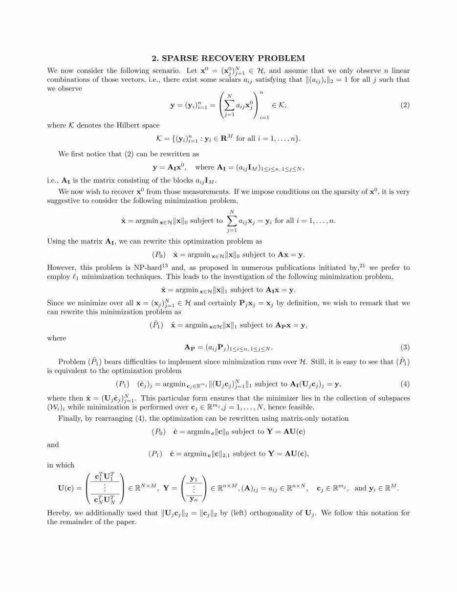
2. SPARSE RECOVERY PROBLEMWe now consider the following scenario. Let x0 = (x0
j )Nj=1 ∈ H, and assume that we only observe n linear
combinations of those vectors, i.e., there exist some scalars aij satisfying that ‖(aij)i‖2 = 1 for all j such thatwe observe
y = (yi)ni=1 =
N∑j=1
aijx0j
n
i=1
∈ K, (2)
where K denotes the Hilbert space
K = {(yi)ni=1 : yi ∈ RM for all i = 1, . . . , n}.
We first notice that (2) can be rewritten as
y = AIx0, where AI = (aijIM )1≤i≤n, 1≤j≤N ,
i.e., AI is the matrix consisting of the blocks aijIM .We now wish to recover x0 from those measurements. If we impose conditions on the sparsity of x0, it is very
suggestive to consider the following minimization problem,
x = argmin x∈H‖x‖0 subject toN∑
j=1
aijxj = yi for all i = 1, . . . , n.
Using the matrix AI, we can rewrite this optimization problem as
(P0) x = argmin x∈H‖x‖0 subject to Ax = y.
However, this problem is NP-hard13 and, as proposed in numerous publications initiated by,21 we prefer toemploy `1 minimization techniques. This leads to the investigation of the following minimization problem,
x = argmin x∈H‖x‖1 subject to AIx = y.
Since we minimize over all x = (xj)Nj=1 ∈ H and certainly Pjxj = xj by definition, we wish to remark that we
can rewrite this minimization problem as
(P1) x = argmin x∈H‖x‖1 subject to APx = y,
whereAP = (aijPj)1≤i≤n, 1≤j≤N . (3)
Problem (P1) bears difficulties to implement since minimization runs over H. Still, it is easy to see that (P1)is equivalent to the optimization problem
(P1) (cj)j = argmin cj∈Rmj ‖(Ujcj)Nj=1‖1 subject to AI(Ujcj)j = y, (4)
where then x = (Uj cj)Nj=1. This particular form ensures that the minimizer lies in the collection of subspaces
(Wi)i while minimization is performed over cj ∈ Rmj ,j = 1, . . . , N , hence feasible.Finally, by rearranging (4), the optimization can be rewritten using matrix-only notation
(P0) c = argmin c‖c‖0 subject to Y = AU(c)
and(P1) c = argmin c‖c‖2,1 subject to Y = AU(c),
in which
U(c) =
cT1 UT
1...
cTNUT
N
∈ RN×M , Y =
y1...
yn
∈ Rn×M , (A)ij = aij ∈ Rn×N , cj ∈ Rmj , and yi ∈ RM .
Hereby, we additionally used that ‖Ujcj‖2 = ‖cj‖2 by (left) orthogonality of Uj . We follow this notation forthe remainder of the paper.

2.1 ExtensionsSeveral extensions of this formulation and the work in this paper are possible, but beyond the scope of this paper.For example, the analysis we provide is on the exactly sparse, noiseless case. As with classical compressed sensing,it is possible to accommodate sampling in the presence of noise. It is also natural to consider the extension of thiswork to sampling signals that are not k-sparse in a fusion frame representation but can be very well approximatedby such a representation.
The richness of fusion frames also allows us to consider richer sampling matrices. Specifically, it is possible toconsider sampling matrices with matrix entries, each operating on a different subspace of the fusion frame. Suchextensions open the use of `1 methods to general vector-valued mathematical objects, to the general problem ofsampling such objects,4 and to general model-based CS problems.20
We should also note that in this paper we only consider a worst-case analysis. Such an analysis is quitepessimistic in practice. An average case analysis, similar to the one in,22 can be more informative for severalpractical applications. We defer the average case analysis to a future publication.23
2.2 Relation with Previous WorkA special case of the problem above appears when all subspaces (Wj)N
j=1 are equal and also equal to the ambientspace Wj = RM for all j. Thus, Pj = IM and the observation setup of Eq. (2) is identical to the matrix product
Y = AX,
where
X =
x1...
xN
∈ RN×M .
This special case is the same as the well studied joint-sparsity setup of5,6, 22,24,25 in which a collection of Msparse vectors in RN is observed through the same measurement matrix A, and the recovery assumes that allthe vectors have the same sparsity structure. The use of mixed `1/`2 optimization has been proposed and widelyused in this case.
Our formulation is a special case of the bock sparsity problem,7 where we impose a particular structure onthe measurement matrix A. This relationship is already known for the joint sparsity model, which is also aspecial case of block sparsity. In other words the fusion frames formulation we examine here specializes blocksparsity problems and generalizes joint sparsity ones. As we discussed in the introduction, fusion frames providesignificant structure to enhance the existing block-sparsity results, especially in the form of the fusion framecoherence, which we discuss in the next section.
3. SPARSE RECOVERY VIA COHERENCE BOUNDS
In this section we derive conditions on c0 and A so that c0 is the unique solution of (P0) as well as of (P1).Our approach generalizes the notion of mutual coherence, a commonly used measure of morphological differencebetween the vectors of a measuring matrix. An excellent survey of the role of mutual coherence in sparserepresentations can be found in.4
3.1 Fusion CoherenceFirst, we require some analog of mutual coherence. In particular, we need to consider an adaptation of thisnotion to our more complicated situation involving the angles between the subspaces generated by the bases Uj ,j = 1, . . . , N . In other words, here we face the problem of recovery of vector-valued (instead of scalar-valued)components. This leads to the following definition.
Definition 3.1. The fusion coherence of a matrix A ∈ Rn×N with normalized ‘columns’ (aj = a·,j)Nj=1 and a
collection of orthogonal projection matrices (Pi)ni=1 in RM×M is given by
µf = µf (A, (Pi)ni=1) = max
j 6=k[|〈aj ,ak〉| · ‖PjPk‖2] .

Since the Pj ’s are projection matrices, we can also rewrite the definition of fusion coherence as
µf = maxj 6=k
[|〈aj ,ak〉| · |λmax(PjPk)|1/2
]with λmax denoting the largest eigenvalue, simply due to the fact that the eigenvalues of PkPjPk and PjPk
coincide. Let us also remark that |λmax(PjPk)|1/2 equals the largest absolute value of the cosines of the principleangles between Wj and Wk.
3.2 Main Result
We first formulate the main result of this section using the new notions previously developed.
Theorem 3.2. Let A ∈ Rn×N with normalized columns (aj)Nj=1, let (Pi)n
i=1 be a collection of orthogonalprojection matrices in RM×M , and let Y ∈ Rn×M . If there exists a solution c0 of the system AU(c) = Ysatisfying
‖c0‖0 <12(1 + µ−1
f ), (5)
then this solution is the unique solution of (P0) as well as of (P1).
Before we continue with the proof, let us for a moment consider the following special cases of this theorem.
Case M = 1: In this case the projection matrices equal 1, and hence the problem reduces to the classicalrecovery problem Ax = y with x ∈ RN and y ∈ Rn. Thus our result reduces to the result obtained in,26 andthe fusion coherence coincides with the commonly used mutual coherence, i.e., µf = maxj 6=k |〈aj ,ak〉|.
Case Pi = IM for all i: In this case the problem becomes the standard joint sparsity recovery. We recover amatrix X0 ∈ RN×M with few non-zero rows from knowledge of AX0 ∈ Rn×M , without any constraints on thestructure of each row of X0 (the general case has the constraint that X0 is required to be of the form U(c0)).Again fusion coherence coincides with the commonly used mutual coherence, i.e., µf = maxj 6=k |〈aj ,ak〉|.
Case Wi ⊥ Wj for all i, j: In this case the fusion coherence becomes 0. And this is also the correct answer,since in this case there exists precisely one solution of the system AU(c) = Y for a given Y. Hence the condition(5) becomes meaningless.
General Case: In the general case we can consider two scenarios: either we are given the subspaces (Wi)i orwe are given the measuring matrix A. In the first situation we face the task of choosing the measuring matrixsuch that µf is as small as possible. Intuitively, we would choose the vectors (aj)j so that a pair (ai,aj) hasa large angle if the associated two subspaces (Wi,Wj) have a small angle, hence balancing the two factors andtry to reduce the maximum. In the second situation, we can use a similar strategy now designing the subspaces(Wi)i accordingly.
3.3 Proof of Theorem 3.2
We first derive a reformulation of the equation AU(c) = Y, which will turn out to be useful in proving Theorem3.2. Set AP as in (3) and define the map ϕk : Rk×M → RkM , k ≥ 1 by
ϕk(Z) = ϕk
z1...zk
= (z1 . . . zk)T , i.e., the concatenation of the rows.

Then it is easy to see that
AU(c) = Y ⇔ APϕN (U(c)) = ϕn(Y). (6)
We now split the proof of Theorem 3.2 into two lemmata, and wish to remark that many parts are closelyinspired by the techniques employed in.26
We first show that c0 satisfying (5) is the unique solution of (P1).
Lemma 3.3. If there exists a solution U(c0) ∈ RN×M of the system AU(c) = Y with c0 satisfying (5), then c0
is the unique solution of (P1).
Proof. In the following we will refer to
supp(U(c0)) = {j ∈ {1, . . . , N} : (c0j )
T UTj 6= 0}
as the support of U(c0) (as well as of c0) and denote it by S. Let c1 be an arbitrary solution of the systemAU(c) = Y, and set
h = c0 − c1.
Denoting by a subscript S a vector restricted to the set S, we obtain
‖c0‖2,1 − ‖c1‖2,1 = ‖c0Sc‖2,1 + ‖c0
S‖2,1 − ‖c1S‖2,1 ≥ ‖hSc‖2,1 − ‖hS‖2,1.
We have to show that this term is greater than zero for any h 6= 0, which is the case provided that
‖hSc‖2,1 > ‖hS‖2,1 (7)
or, in other words,12‖h‖2,1 > ‖hS‖2,1, (8)
which we next aim to prove.
Since h satisfies AU(h) = 0, by using the reformulation (6), it follows that
APϕN (U(h)) = 0.
This implies thatA∗
PAPϕN (U(h)) = 0.
Defining aj by aj = (aij)i for each j, the previous equality can be computed to be
(〈ai,aj〉PiPj)ijϕN (U(h)) = 0.
Recall that we have required the vectors aj to be normalized. Hence, for each i,
Uihi = −∑j 6=i
〈ai,aj〉PiPjUjhj .
Since ‖Uihi‖2 = ‖hi‖2 for any i, this gives
‖hi‖2 ≤∑j 6=i
|〈ai,aj〉| · ‖PiPj‖2‖hj‖2 ≤ µf (‖h‖2,1 − ‖hi‖2),
which implies‖hi‖2 ≤ (1 + µ−1
f )−1‖h‖2,1.
Thus, we have‖hS‖2,1 ≤ #(S) · (1 + µ−1
f )−1‖h‖2,1 = ‖c0‖0 · (1 + µ−1f )−1‖h‖2,1.

Concluding, (5) and (8) show that h satisfies (8) unless h = 0, which implies that c0 is the unique minimizer of(P1) as claimed.
Using Lemma 3.3 it is easy to show the following lemma.
Lemma 3.4. If there exists a solution U(c0) ∈ RN×M of the system AU(c) = Y with c0 satisfying (5), then c0
is the unique solution of (P0).
Proof. Assume c0 satisfies (5) and AU(c0) = Y. Then by Lemma 3.3 it is the unique solution of (P1).Assume there is a c satisfying AU(c) such that ‖c‖0 ≤ ‖c0‖0. Then c also satisfies (5) and again by Lemma 3.3c is also the unique solution to (P1). But this means that c = c0 and c0 is the unique solution to (P0).
We observe that Theorem 3.2 now follows immediately from Lemmata 3.4 and 3.3.
4. SPARSE RECOVERY USING THE RESTRICTED ISOMETRY PROPERTY (RIP)
In this section we consider an alternative condition for sparse recovery using the restricted isometry property(RIP) of the sampling matrix. This property on the sampling matrix, first introduced in,1 complements themutual coherence conditions and is often preferred in the literature.
Definition 4.1. A matrix A ∈ Rn×N satisfies a restricted isometry property (RIP) of order k if there existsconstant δk such that for all x ∈ RN , ‖x‖0 ≤ k
(1− δk)‖x‖22 ≤ ‖Ax‖22 ≤ (1 + δk)‖x‖22.
Note that this is the classical definition of the RIP, used in the classical CS literature to measure a singlesparse vector. However, we use that property to recover signals that have a sparse fusion frame representation.Specifically, in the remainder of this section we demonstrate that if our matrix A satisfies the RIP, we can recovera k-sparse signal X ∈ H from its fusion frame measurements Y = AX by solving the `1 minimization (P1).Notice that we follow the line of proof from,1 but are required to make changes to adapt it to our situation.
We first show that imposing the RIP condition on the matrix A implies a form of RIP we require for ourmodified situation.
Lemma 4.2. Suppose that the matrix A ∈ Rn×N satisfies the RIP of order k with constant δk. Then
(1− δk)‖c‖22,2 ≤ ‖AU(c)‖22,2 ≤ (1 + δk)‖c‖22,2
for all c satisfying ‖c‖0 ≤ k.
Theorem 4.3. Let A ∈ Rn×N with normalized columns (aj)Nj=1, and suppose that it satisfies RIP of order k
such that δ3k + 3δ4k < 2. Let (Pi)ni=1 be a collection of projection matrices in RM×M , and let Y ∈ Rn×M . If
there exists a solution c0 of the system AU(c) = Y such that ‖c0‖0 ≤ k, then this solution is both the uniquesolution of (P0) and (P1).
Proof. Let the support of U(c0) be denoted by S, set |S| = k, and define h := c1− c0, where c1 is a solutionto the system. We then partition the indexing set {1, . . . , N} into subsets S`, ` = 1, . . . , ρ−1 · (N/k− 1) for someρ to be chosen later such that
(i) |S`| = ρ · k for all `,
(ii) {1, . . . , N} = S ∪⋃
` S`,
(iii) ‖hj1‖2 ≥ ‖hj2‖2 if and only if j1 ∈ S`1 and j2 ∈ S`2 with `1 ≤ `2.
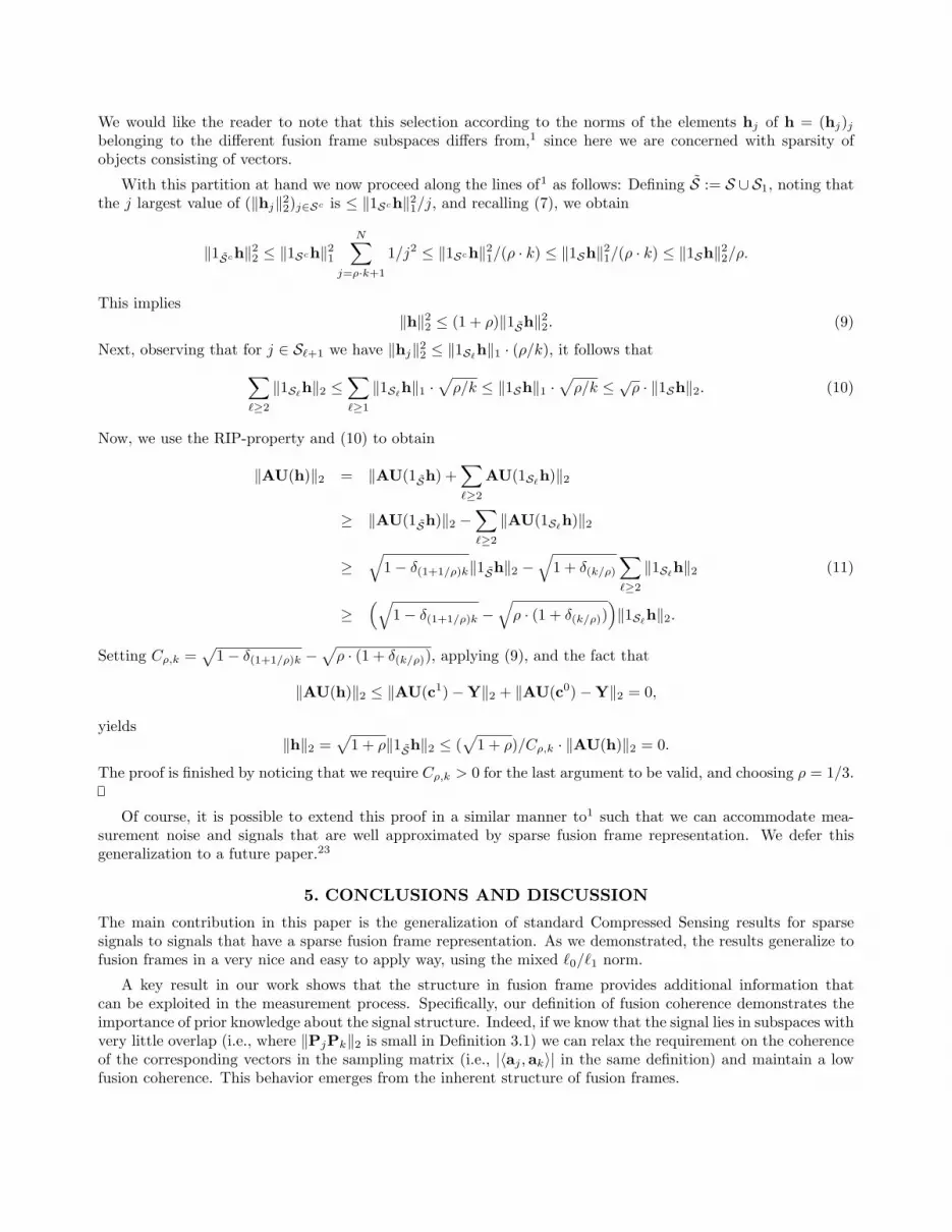
We would like the reader to note that this selection according to the norms of the elements hj of h = (hj)j
belonging to the different fusion frame subspaces differs from,1 since here we are concerned with sparsity ofobjects consisting of vectors.
With this partition at hand we now proceed along the lines of1 as follows: Defining S := S ∪ S1, noting thatthe j largest value of (‖hj‖22)j∈Sc is ≤ ‖1Sch‖21/j, and recalling (7), we obtain
‖1Sch‖22 ≤ ‖1Sch‖21N∑
j=ρ·k+1
1/j2 ≤ ‖1Sch‖21/(ρ · k) ≤ ‖1Sh‖21/(ρ · k) ≤ ‖1Sh‖22/ρ.
This implies‖h‖22 ≤ (1 + ρ)‖1Sh‖
22. (9)
Next, observing that for j ∈ S`+1 we have ‖hj‖22 ≤ ‖1S`h‖1 · (ρ/k), it follows that∑
`≥2
‖1S`h‖2 ≤
∑`≥1
‖1S`h‖1 ·
√ρ/k ≤ ‖1Sh‖1 ·
√ρ/k ≤ √
ρ · ‖1Sh‖2. (10)
Now, we use the RIP-property and (10) to obtain
‖AU(h)‖2 = ‖AU(1Sh) +∑`≥2
AU(1S`h)‖2
≥ ‖AU(1Sh)‖2 −∑`≥2
‖AU(1S`h)‖2
≥√
1− δ(1+1/ρ)k‖1Sh‖2 −√
1 + δ(k/ρ)
∑`≥2
‖1S`h‖2 (11)
≥(√
1− δ(1+1/ρ)k −√
ρ · (1 + δ(k/ρ)))‖1S`
h‖2.
Setting Cρ,k =√
1− δ(1+1/ρ)k −√
ρ · (1 + δ(k/ρ)), applying (9), and the fact that
‖AU(h)‖2 ≤ ‖AU(c1)−Y‖2 + ‖AU(c0)−Y‖2 = 0,
yields‖h‖2 =
√1 + ρ‖1Sh‖2 ≤ (
√1 + ρ)/Cρ,k · ‖AU(h)‖2 = 0.
The proof is finished by noticing that we require Cρ,k > 0 for the last argument to be valid, and choosing ρ = 1/3.
Of course, it is possible to extend this proof in a similar manner to1 such that we can accommodate mea-surement noise and signals that are well approximated by sparse fusion frame representation. We defer thisgeneralization to a future paper.23
5. CONCLUSIONS AND DISCUSSION
The main contribution in this paper is the generalization of standard Compressed Sensing results for sparsesignals to signals that have a sparse fusion frame representation. As we demonstrated, the results generalize tofusion frames in a very nice and easy to apply way, using the mixed `0/`1 norm.
A key result in our work shows that the structure in fusion frame provides additional information thatcan be exploited in the measurement process. Specifically, our definition of fusion coherence demonstrates theimportance of prior knowledge about the signal structure. Indeed, if we know that the signal lies in subspaces withvery little overlap (i.e., where ‖PjPk‖2 is small in Definition 3.1) we can relax the requirement on the coherenceof the corresponding vectors in the sampling matrix (i.e., |〈aj ,ak〉| in the same definition) and maintain a lowfusion coherence. This behavior emerges from the inherent structure of fusion frames.

Unfortunately, our analysis of this property currently only applies to the guarantees provided using the fusioncoherence of the matrix, not the RIP property as described in Section 4. While an extension of such analysis forthe RIP guarantees is desirable, it is still an open problem.
We should also note that our analysis is worst case in the sense that it applies to any sparse signal c.Theorem 4.3, for instance, requires that the RIP constant δk be sufficiently small, but imposes no conditionon the dimensions mj , i.e. the number of channels in the joint sparsity setup. Intuitively, one would think,however, that recovery becomes easier the higher the dimensions mj , because then more information should beavailable on the a priori unknown support set. However, in the worst case this is not true because if the samesignal appears in each channel, we actually do not have additional information.22 To overcome this problem andindeed show that recovery becomes more likely the higher the number of channels is, in22 a probability modelon jointly sparse signals was set up that allowed to deduce an exponential decrease of the failure probabilitywith respect to the number of channels provided a mild condition on the matrix A and the sparsity k holds. Wedefer an extension of such an average case analysis of fusion frame measurements that will show higher recoveryprobability for larger mj ’s to a future publication.23
Acknowledgements
The first author did part of this work while at Rice university. This part was was supported by the grants NSFCCF-0431150, CCF-0728867, CNS-0435425, and CNS-0520280, DARPA/ONR N66001-08-1-2065, ONR N00014-07-1-0936, N00014-08-1-1067, N00014-08-1-1112, and N00014-08-1-1066, AFOSR FA9550-07-1-0301, ARO MURIW311NF-07-1-0185, and the Texas Instruments Leadership University Program. The author would also likeacknowledge Mitsubishi Electric Research Laboratories (MERL) for their support. The second author wouldlike to thank Peter Casazza, David Donoho, and Ali Pezeshki for inspiring discussions on `1 minimization andfusion frames. The second author would also like to thank the Department of Statistics at Stanford Universityand the Department of Mathematics at Yale University for their hospitality and support during her visits. Thiswork was partially supported by Deutsche Forschungsgemeinschaft (DFG) Heisenberg Fellowship KU 1446/8-1.The third author acknowledges support by the Hausdorff Center for Mathematics and by the WWTF projectSPORTS (MA 07-004).
REFERENCES[1] Candes, E. J., Romberg, J. K., and Tao, T., “Stable signal recovery from incomplete and inaccurate mea-
surements,” Comm. Pure Appl. Math. 59(8), 1207–1223 (2006).[2] Donoho, D. L., “Compressed sensing,” IEEE Trans. Inform. Theory 52(4), 1289–1306 (2006).[3] Casazza, P. G., Kutyniok, G., and Li, S., “Fusion Frames and Distributed Processing,” Appl. Comput.
Harmon. Anal. 25, 114–132 (2008).[4] Bruckstein, A. M., Donoho, D. L., and Elad, M., “From Sparse Solutions of Systems of Equations to Sparse
Modeling of Signals and Images,” SIAM Review 51(1), 34–81 (2009).[5] Fornasier, M. and Rauhut., H., “Recovery algorithms for vector valued data with joint sparsity constraints,”
SIAM J. Numer. Anal. 46(2), 577–613 (2008).[6] Tropp, J. A., “Algorithms for simultaneous sparse approximation: part II: Convex relaxation,” Signal
Processing 86(3), 589–602 (2006).[7] Eldar, Y. C. and Bolcskei, H., “Block-sparsity: Coherence and efficient recovery,” in [IEEE Int. Conf.
Acoustics, Speech and Signal Processing, 2009 (ICASSP 2009) ], 2885–2888 (April 2009).[8] Model, D. and Zibulevsky, M., “Signal reconstruction in sensor arrays using sparse representations,” Signal
Processing 86(3), 624–638 (2006).[9] Malioutov, D., A Sparse Signal Reconstruction Perspective for Source Localization with Sensor Arrays,
Master’s thesis, MIT, Cambridge, MA (July 2003).[10] Zelinski, A. C., Goyal, V. K., Adalsteinsson, E., and Wald, L. L., “Sparsity in MRI RF excitation pulse
design,” in [Proc. 42nd Annual Conference on Information Sciences and Systems (CISS 2008) ], 252–257(March 2008).
[11] Daudet, L., “Sparse and structured decompositions of signals with the molecular matching pursuit,” IEEETrans. Audio, Speech, and Language Processing 14(5), 1808–1816 (2006).
[12] Cevher, V., Chellappa, R., and McClellan, J. H., “Vehicle Speed Estimation Using Acoustic Wave Patterns,”IEEE Trans. Signal Processing 57, 30–47 (Jan 2009).
[13] Natarajan., B. K., “Sparse approximate solutions to linear systems,” SIAM J. Comput. 24, 227–234 (1995).[14] Tropp., J. A., “Greed is good: Algorithmic results for sparse approximation.,” IEEE Trans. Inf. The-
ory 50(10), 2331–2242 (2004).[15] Candes, E. J. and Tao, T., “Near optimal signal recovery from random projections: universal encoding
strategies?,” IEEE Trans. Inf. Theory 52(12), 5406–5425 (2006).[16] Rauhut., H., “Stability results for random sampling of sparse trigonometric polynomials,” IEEE Trans.
Info. Theory 54(12), 5661–5670 (2008).[17] Pfander, G. E. and Rauhut, H., “Sparsity in time-frequency representations,” J. Fourier Anal. Appl. (to
appear).[18] Joel Tropp, Laska, J., Duarte, M., Romberg, J., and Baraniuk, R., “Beyond Nyquist: Efficient sampling of
sparse, bandlimited signals,” preprint (2009).[19] Rauhut., H., “Circulant and Toeplitz matrices in compressed sensing,” in [Proc. SPARS ’09 ], (2009).[20] Baraniuk, R., Cevher, V., Duarte, M., and Hedge, C., “Model-based compressive sensing,” preprint (2008).[21] Chen, S. S., Donoho, D. L., and Saunders, M. A., “Atomic decomposition by basis pursuit,” SIAM Rev. 43,
129–159 (2001).[22] Eldar, Y. and Rauhut., H., “Average case analysis of multichannel sparse recovery using convex relaxation,”
preprint (2009).[23] Boufounos, P., Kutyniok, G., and Rauhut, H., “Sparse recovery from combined fusion frame measurements,”
in preparation (2009).[24] Baron, D., Wakin, M. B., Duarte, M. F., Sarvotham, S., and Baraniuk, R. G., “Distributed compressed
sensing,” preprint (2005).[25] Gribonval, R., Rauhut, H., Schnass, K., and Vandergheynst, P., “Atoms of all channels, unite! Average case
analysis of multi-channel sparse recovery using greedy algorithms,” J. Fourier Anal. Appl. 14(5), 655–687(2008).
[26] Donoho, D. L. and Elad, M., “Optimally sparse representation in general (nonorthogonal) dictionaries vial1 minimization,” Proc. Natl. Acad. Sci. USA 100(5), 2197–2202 (2003).