1

Compressed Sensing MRIMichael Lustig,Student Member, IEEE,David L. Donoho Member, IEEE

Juan M. SantosMember, IEEE, and John M. Pauly,Member, IEEE

I. I NTRODUCTION

Compressed sensing (CS) aims to reconstruct signals and images from significantly fewer

measurements than were traditionally thought necessary. Magnetic Resonance Imaging (MRI) is

an essential medical imaging tool with an inherently slow data acquisition process. Applying CS

to MRI offers potentially significant scan time reductions, with benefits for patients and health

care economics.

MRI obeys two key requirements for successful application of CS: (1) medical imagery is

naturally compressibleby sparse coding in an appropriate transform domain (e.g., by wavelet

transform); (2) MRI scanners naturally acquireencodedsamples, rather than direct pixel samples

(e.g. inspatial-frequency encoding).

In this paper we review the requirements for successful CS, describe their natural fit to MRI,

and then give examples of four interesting applications of CS in MRI. We emphasize an intuitive

understanding of CS by describing the CS reconstruction as a process of interference cancellation.

We also emphasize an understanding of the driving factors in applications, including limitations

imposed by MRI hardware, by the characteristics of different types of images, and by clinical

concerns.

II. PRINCIPLES OFMAGNETIC RESONANCEIMAGING

We first briefly sketch properties of MRI related to CS. More complete descriptions of MRI can

be found in the excellent survey paper by Wright [1] from this magazine, and in MRI textbooks.

A. Nuclear Magnetic Resonance Physics

The MRI signal is generated by protons in the body, mostly those in water molecules. A strong

static fieldB0 polarizes the protons, yielding a net magnetic moment oriented parallel to the static

field. Applying a radio frequency (RF) excitation fieldB1 produces a magnetization component

m transverse to the static field. This magnetization precesses at a frequency proportional to the

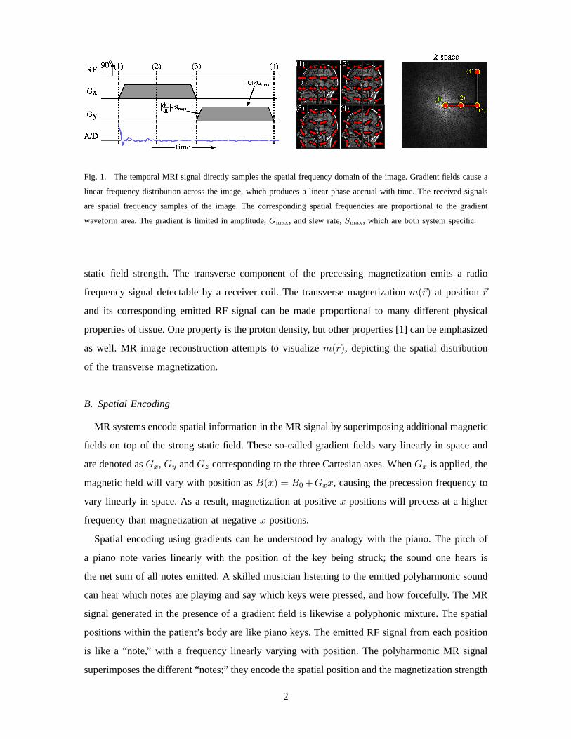
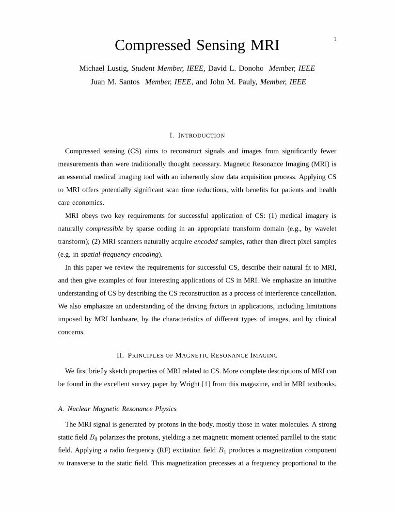
Fig. 1. The temporal MRI signal directly samples the spatial frequency domain of the image. Gradient fields cause a

linear frequency distribution across the image, which produces a linear phase accrual with time. The received signals

are spatial frequency samples of the image. The corresponding spatial frequencies are proportional to the gradient

waveform area. The gradient is limited in amplitude,Gmax, and slew rate,Smax, which are both system specific.

static field strength. The transverse component of the precessing magnetization emits a radio

frequency signal detectable by a receiver coil. The transverse magnetizationm(~r) at position~r

and its corresponding emitted RF signal can be made proportional to many different physical

properties of tissue. One property is the proton density, but other properties [1] can be emphasized

as well. MR image reconstruction attempts to visualizem(~r), depicting the spatial distribution

of the transverse magnetization.

B. Spatial Encoding

MR systems encode spatial information in the MR signal by superimposing additional magnetic

fields on top of the strong static field. These so-called gradient fields vary linearly in space and

are denoted asGx, Gy andGz corresponding to the three Cartesian axes. WhenGx is applied, the

magnetic field will vary with position asB(x) = B0 +Gxx, causing the precession frequency to

vary linearly in space. As a result, magnetization at positivex positions will precess at a higher

frequency than magnetization at negativex positions.

Spatial encoding using gradients can be understood by analogy with the piano. The pitch of

a piano note varies linearly with the position of the key being struck; the sound one hears is

the net sum of all notes emitted. A skilled musician listening to the emitted polyharmonic sound

can hear which notes are playing and say which keys were pressed, and how forcefully. The MR

signal generated in the presence of a gradient field is likewise a polyphonic mixture. The spatial

positions within the patient’s body are like piano keys. The emitted RF signal from each position

is like a “note,” with a frequency linearly varying with position. The polyharmonic MR signal

superimposes the different “notes;” they encode the spatial position and the magnetization strength

2

at those positions. A signal processing engineer will recognize the Fourier relation between the

received MR signal and the magnetization distribution, and that the magnetization distribution

can be decoded by a spectral decomposition.

Multi-dimensional spatial encoding can be further understood by introducing the notion of

k-space. Gradient-induced variation in precession frequency causes a location-dependent linear

phase dispersion to develop. Therefore the receiver coil detects a signal encoded by the linear

phase. It can be shown [1] that the signal equation in MRI has the form of a Fourier integral,

s(t) =∫

Rm(~r)e−i2π~k(t)·~r dr,

where k(t) ∝∫ t0 G(s)ds. In words, the received signal at timet is the Fourier transform of

the objectm(~r) sampled at the spatial frequency~k(t). Such Fourier encoding is fundamentally

encoded and very different than traditional optical imaging where pixel samples are measured

directly.

The design of an MRI acquisition method centers on developing the gradient waveforms~G(t) =

[Gx(t), Gy(t), Gz(t)]T that drive the MR system. These waveforms, along with the associated RF

pulses used to produce the magnetization, are called apulse sequence. The integral of the~G(t)

waveforms traces out a trajectory~k(t) in spatial frequency space, ork-space. For illustration,

consider the simple example in Fig. 1 where, immediately after the RF excitation, aGx gradient

field is applied followed by aGy gradient. The phases of the magnetization are shown at different

time points, along with thek-space trajectory and the MR signal. This encoded sampling and

the freedom in choosing the sampling trajectory play a major role in making CS ideas naturally

applicable to MRI.

C. Image Acquisition

Constructing a single MR image commonly involves collecting a series of frames of data,

calledacquisitions. In each acquisition, an RF excitation produces new transverse magnetization,

which is then sampled along a particular trajectory ink-space. Due to various physical and

physiological constraints [1] most MRI imaging methods use a sequence of acquisitions, each one

samples part ofk-space. The data from this sequence of acquisitions are then used to reconstruct

an image. Traditionally thek-space sampling pattern is designed to meet the Nyquist criterion,

which depends on the resolution and field of view (FOV) as shown in Fig. 2. Violation of the

Nyquist criterion causes image artifacts in linear reconstructions. The appearance of such artifacts

depends on the details in the sampling pattern, as discussed below.

3

Fig. 2. The Nyquist criterion sets the requiredk-space

coverage, which can be achieved using various sampling

trajectories. Image resolution is determined by the extent

of the k-space coverage. The supported field of view

is determined by the sampling density. Violation of the

Nyquist criterion causes artifacts in linear reconstructions,

which depend on the sampling pattern.

In MRI, it is possible to selectively excite

a thin slice through the three-dimensional

volume. This reduces the data collection to

two dimensions ink-space for each slice.

The volumetric object is imaged by exciting

more slices, known as a multi-slice acqui-

sition. When a volume or a thick slab is

excited, a three-dimensionalk-space volume

must be sampled. Each of these approaches is

very common, and has advantages in specific

applications.

We have considerable freedom in designing

the k-space trajectory for each acquisition.

Some trajectories are illustrated in Fig. 2. By

far the most popular trajectory uses straight

lines from a Cartesian grid. Most pulse se-

quences used in clinical imaging today are Cartesian. Reconstruction from such acquisitions

is wonderfully simple: apply the inverse Fast Fourier Transform (FFT). More importantly,

reconstructions from Cartesian sampling are robust to many sources of system imperfections.

While Cartesian trajectories are by far the most popular, some other trajectories are in use,

including sampling along radial lines and sampling along spiral trajectories. Radial acquisi-

tions are less susceptible to motion artifacts than Cartesian trajectories, and can be significantly

undersampled [2], especially for high contrast objects [3]. Spirals make efficient use of the

gradient system hardware, and are used in real-time and rapid imaging applications [4]. Efficient

reconstruction from such non-Cartesian trajectories requires using filtered back-projection or

interpolation schemes (e.g. gridding [5]).

D. Rapid Imaging

MR acquisition is inherently a process of traversing curves in multi-dimensionalk-space.

The speed ofk-space traversal is limited by physical constraints. In current systems, gradients

are limited by maximum amplitude and maximum slew-rate (See Fig. 1). In addition, high

4

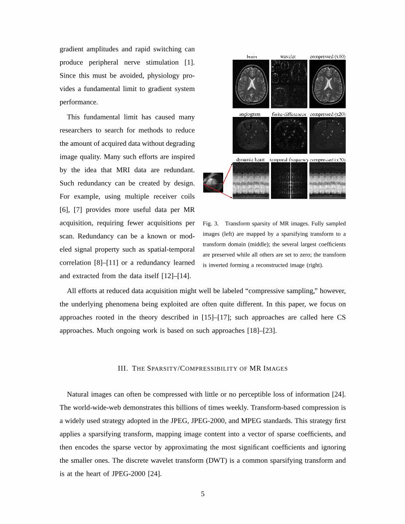
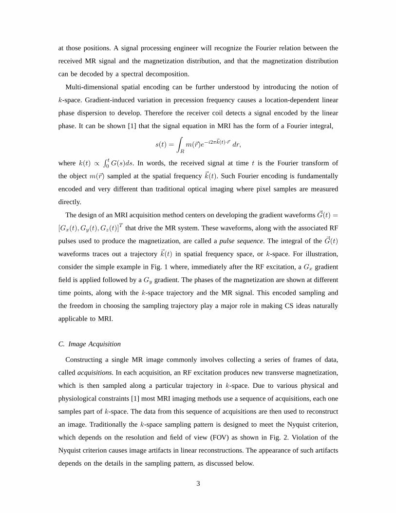
Fig. 3. Transform sparsity of MR images. Fully sampled

images (left) are mapped by a sparsifying transform to a

transform domain (middle); the several largest coefficients

are preserved while all others are set to zero; the transform

is inverted forming a reconstructed image (right).

gradient amplitudes and rapid switching can

produce peripheral nerve stimulation [1].

Since this must be avoided, physiology pro-

vides a fundamental limit to gradient system

performance.

This fundamental limit has caused many

researchers to search for methods to reduce

the amount of acquired data without degrading

image quality. Many such efforts are inspired

by the idea that MRI data are redundant.

Such redundancy can be created by design.

For example, using multiple receiver coils

[6], [7] provides more useful data per MR

acquisition, requiring fewer acquisitions per

scan. Redundancy can be a known or mod-

eled signal property such as spatial-temporal

correlation [8]–[11] or a redundancy learned

and extracted from the data itself [12]–[14].

All efforts at reduced data acquisition might well be labeled “compressive sampling,” however,

the underlying phenomena being exploited are often quite different. In this paper, we focus on

approaches rooted in the theory described in [15]–[17]; such approaches are called here CS

approaches. Much ongoing work is based on such approaches [18]–[23].

III. T HE SPARSITY/COMPRESSIBILITY OFMR IMAGES

Natural images can often be compressed with little or no perceptible loss of information [24].

The world-wide-web demonstrates this billions of times weekly. Transform-based compression is

a widely used strategy adopted in the JPEG, JPEG-2000, and MPEG standards. This strategy first

applies a sparsifying transform, mapping image content into a vector of sparse coefficients, and

then encodes the sparse vector by approximating the most significant coefficients and ignoring

the smaller ones. The discrete wavelet transform (DWT) is a common sparsifying transform and

is at the heart of JPEG-2000 [24].

5

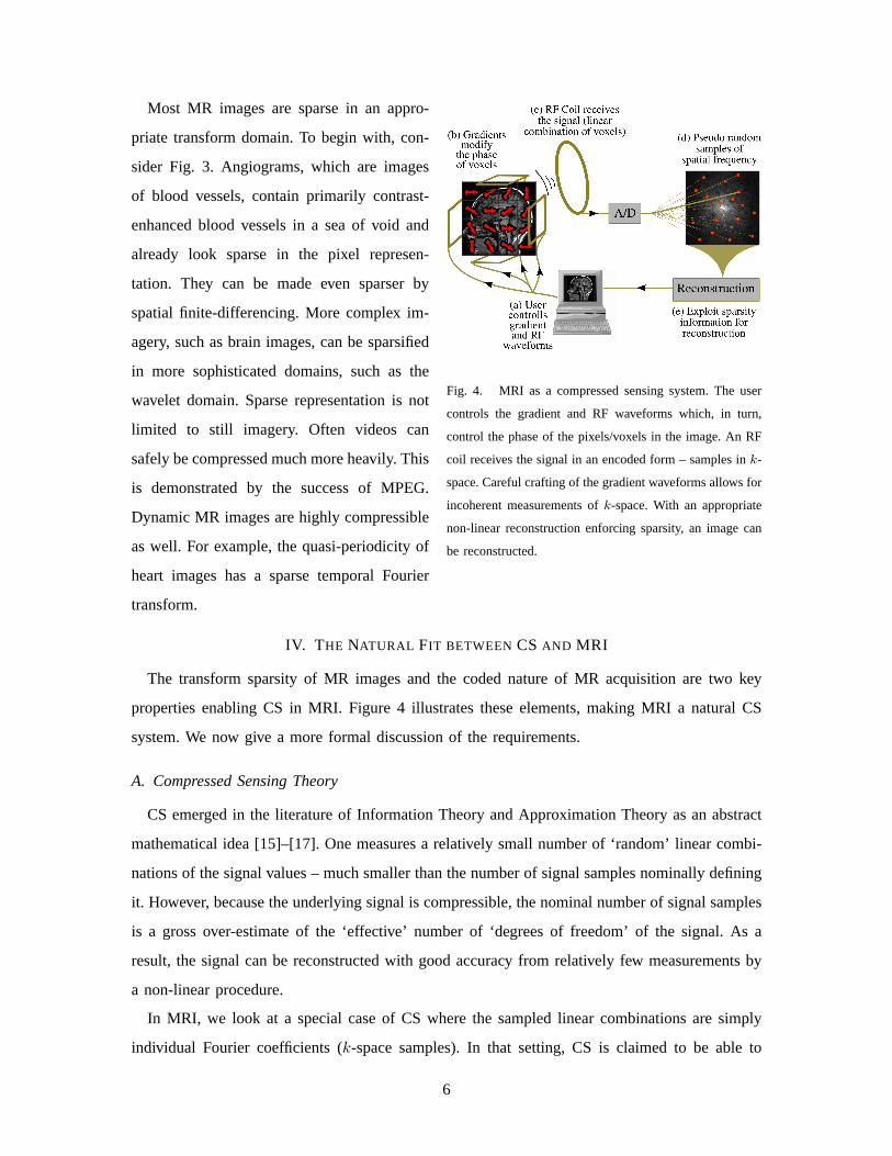
Fig. 4. MRI as a compressed sensing system. The user

controls the gradient and RF waveforms which, in turn,

control the phase of the pixels/voxels in the image. An RF

coil receives the signal in an encoded form – samples ink-

space. Careful crafting of the gradient waveforms allows for

incoherent measurements ofk-space. With an appropriate

non-linear reconstruction enforcing sparsity, an image can

be reconstructed.

Most MR images are sparse in an appro-

priate transform domain. To begin with, con-

sider Fig. 3. Angiograms, which are images

of blood vessels, contain primarily contrast-

enhanced blood vessels in a sea of void and

already look sparse in the pixel represen-

tation. They can be made even sparser by

spatial finite-differencing. More complex im-

agery, such as brain images, can be sparsified

in more sophisticated domains, such as the

wavelet domain. Sparse representation is not

limited to still imagery. Often videos can

safely be compressed much more heavily. This

is demonstrated by the success of MPEG.

Dynamic MR images are highly compressible

as well. For example, the quasi-periodicity of

heart images has a sparse temporal Fourier

transform.

IV. T HE NATURAL FIT BETWEEN CS AND MRI

The transform sparsity of MR images and the coded nature of MR acquisition are two key

properties enabling CS in MRI. Figure 4 illustrates these elements, making MRI a natural CS

system. We now give a more formal discussion of the requirements.

A. Compressed Sensing Theory

CS emerged in the literature of Information Theory and Approximation Theory as an abstract

mathematical idea [15]–[17]. One measures a relatively small number of ‘random’ linear combi-

nations of the signal values – much smaller than the number of signal samples nominally defining

it. However, because the underlying signal is compressible, the nominal number of signal samples

is a gross over-estimate of the ‘effective’ number of ‘degrees of freedom’ of the signal. As a

result, the signal can be reconstructed with good accuracy from relatively few measurements by

a non-linear procedure.

In MRI, we look at a special case of CS where the sampled linear combinations are simply

individual Fourier coefficients (k-space samples). In that setting, CS is claimed to be able to

6

make accurate reconstructions from a small subset ofk-space, rather than an entirek-space grid.

The original paper by Candes, Romberg and Tao [15] was motivated in large part by MRI since

it looked at random undersampling of Fourier coefficients.

Theoretical and technical aspects of CS are discussed elsewhere in this special issue. However,

the key points can be reduced to nontechnical language. A successful application of CS has three

requirements:Transform Sparsity – the desired image should have a sparse representation in

a known transform domain (i.e., it must be compressible by transform coding);Incoherence

of Undersampling Artifacts – the artifacts in linear reconstruction caused byk-space under-

sampling should be incoherent (noise-like) in the sparsifying transform domain; andNonlinear

Reconstruction – the image should be reconstructed by a non-linear method which enforces

both sparsity of the image representation and consistency of the reconstruction with the acquired

samples.

The first condition is clearly met for MR images, as explained in Section III above. The

fact that incoherence is important, that MR acquisition can be designed to achieve incoherent

undersampling, and the fact that there are efficient and practical algorithms for reconstruction

will not, at this point in the article, be at all obvious. So we turn to a very simple example.

B. Intuitive example: Interference Cancellation

To develop intuition for the importance of incoherence and the feasibility of CS, consider the

1D case illustrated in Fig. 5. A sparse signal (Fig. 5.1), is sub-Nyquist (8-fold) sampled ink-space

(Fig. 5.2). Simply zero-filling the missing values and inverting the Fourier transform results in

artifacts which depend on the sampling pattern. With equispaced undersampling (Fig. 5.3a), this

reconstruction generates a superposition of shifted signal copies. In this case, recovery of the

original signal is hopeless, as each replica is an equally likely candidate.

With random undersampling, the situation is very different. The zero-filled Fourier reconstruc-

tion exhibits incoherent artifacts that actually behave much like additive random noise (Fig. 5.3).

Despite appearances, the artifacts are not noise; rather, undersampling causes leakage of energy

away from each individual nonzero value of the original signal. This energy appears in other

reconstructed signal coefficients, including those which had been zero in the original signal.

It is possible, starting from knowledge of thek-space sampling scheme and the underlying

original signal, to calculate this leakage analytically. This observation immediately suggests a

nonlinear iterative technique which enables accurate recovery, even though the signal in Fig. 5.1

was 8-fold undersampled.

7

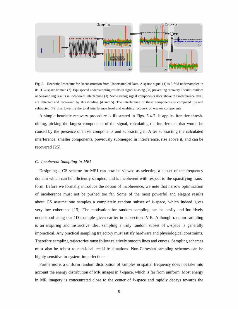
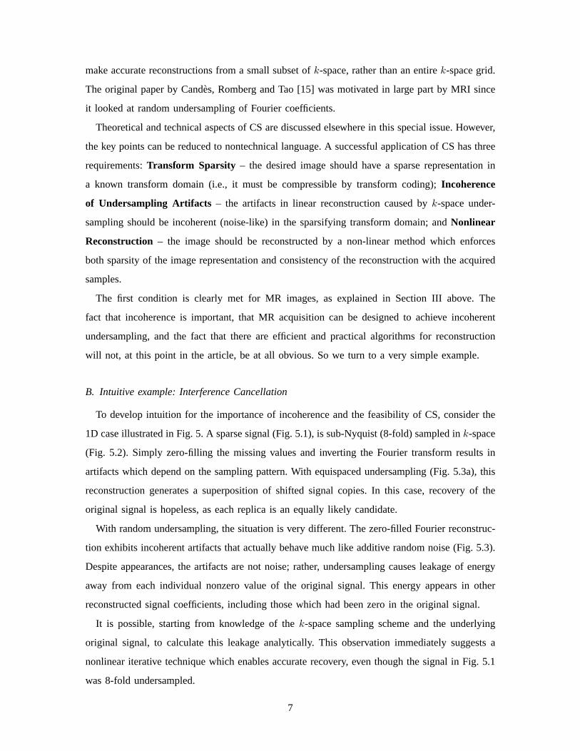
Fig. 5. Heuristic Procedure for Reconstruction from Undersampled Data. A sparse signal (1) is 8-fold undersampled in

its 1Dk-space domain (2). Equispaced undersampling results in signal aliasing (3a) preventing recovery. Pseudo-random

undersampling results in incoherent interference (3). Some strong signal components stick above the interference level,

are detected and recovered by thresholding (4 and 5). The interference of these components is computed (6) and

subtracted (7), thus lowering the total interference level and enabling recovery of weaker components

A simple heuristic recovery procedure is illustrated in Figs. 5.4-7. It applies iterative thresh-

olding, picking the largest components of the signal, calculating the interference that would be

caused by the presence of those components and subtracting it. After subtracting the calculated

interference, smaller components, previously submerged in interference, rise above it, and can be

recovered [25].

C. Incoherent Sampling in MRI

Designing a CS scheme for MRI can now be viewed as selecting a subset of the frequency

domain which can be efficiently sampled, and is incoherent with respect to the sparsifying trans-

form. Before we formally introduce the notion of incoherence, we note that narrow optimization

of incoherence must not be pushed too far. Some of the most powerful and elegant results

about CS assume one samples a completely random subset ofk-space, which indeed gives

very low coherence [15]. The motivation for random sampling can be easily and intuitively

understood using our 1D example given earlier in subsection IV-B. Although random sampling

is an inspiring and instructive idea, sampling a truly random subset ofk-space is generally

impractical. Any practical sampling trajectory must satisfy hardware and physiological constraints.

Therefore sampling trajectories must follow relatively smooth lines and curves. Sampling schemes

must also be robust to non-ideal, real-life situations. Non-Cartesian sampling schemes can be

highly sensitive to system imperfections.

Furthermore, a uniform random distribution of samples in spatial frequency does not take into

account the energy distribution of MR images ink-space, which is far from uniform. Most energy

in MR imagery is concentrated close to the center ofk-space and rapidly decays towards the

8

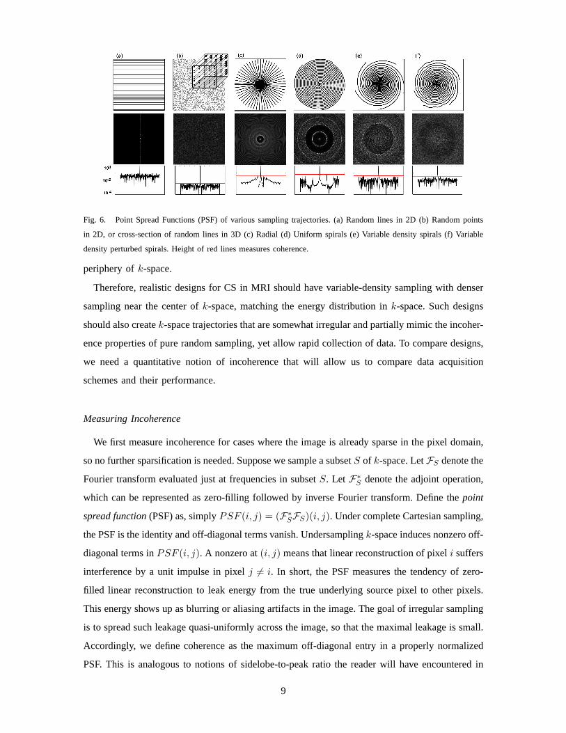
Fig. 6. Point Spread Functions (PSF) of various sampling trajectories. (a) Random lines in 2D (b) Random points

in 2D, or cross-section of random lines in 3D (c) Radial (d) Uniform spirals (e) Variable density spirals (f) Variable

density perturbed spirals. Height of red lines measures coherence.

periphery ofk-space.

Therefore, realistic designs for CS in MRI should have variable-density sampling with denser

sampling near the center ofk-space, matching the energy distribution ink-space. Such designs

should also createk-space trajectories that are somewhat irregular and partially mimic the incoher-

ence properties of pure random sampling, yet allow rapid collection of data. To compare designs,

we need a quantitative notion of incoherence that will allow us to compare data acquisition

schemes and their performance.

Measuring Incoherence

We first measure incoherence for cases where the image is already sparse in the pixel domain,

so no further sparsification is needed. Suppose we sample a subsetS of k-space. LetFS denote the

Fourier transform evaluated just at frequencies in subsetS. Let F∗S denote the adjoint operation,

which can be represented as zero-filling followed by inverse Fourier transform. Define thepoint

spread function(PSF) as, simplyPSF (i, j) = (F∗SFS)(i, j). Under complete Cartesian sampling,

the PSF is the identity and off-diagonal terms vanish. Undersamplingk-space induces nonzero off-

diagonal terms inPSF (i, j). A nonzero at(i, j) means that linear reconstruction of pixeli suffers

interference by a unit impulse in pixelj 6= i. In short, the PSF measures the tendency of zero-

filled linear reconstruction to leak energy from the true underlying source pixel to other pixels.

This energy shows up as blurring or aliasing artifacts in the image. The goal of irregular sampling

is to spread such leakage quasi-uniformly across the image, so that the maximal leakage is small.

Accordingly, we define coherence as the maximum off-diagonal entry in a properly normalized

PSF. This is analogous to notions of sidelobe-to-peak ratio the reader will have encountered in

9

many branches of signal processing. Figure 6 shows some PSF’s of irregular trajectories.

Most MR images are sparse in a transform domain other than the pixel domain. In such settings,

we use the notion of thetransform point spread function(TPSF). LetΨ denote the sparsifying

transform; and then defineTPSF (i, j) = (Ψ∗FS∗FSΨ)(i, j). With this notation, coherence is

formally measured bymaxi6=j |TPSF (i, j)|, the maximum size of any off-diagonal entry in the

TPSF. Small coherence, e.g. incoherence, is desirable. More discussion about the TPSF can be

found in [18].

Incoherent MRI Acquisition

We now consider several schemes and their associated coherence properties. In 2D Cartesian

MRI, complete Cartesian sampling is often implemented as a series ofnpe acquisitions (called

phase encodes) along very simple trajectories: parallel equispaced lines. This scheme yieldsnfe

k-space samples per trajectory (calledfrequency encodes), producing a Cartesian grid ofnpe×nfe

samples overall. In 3D there is an additional encoding dimension (calledslice encode) requiring

npe×nse line acquisitions resulting innpe×nse×nfe grid size. The sampling along a trajectory,

e.g. the frequency encodes, are rarely a limiting factor in terms of sampling-rate and in terms of

the scan time. The number of acquisition lines, e.g. the phase and slice encodes,is limiting.

This immediately suggests speeding up a scan by simply dropping entire lines from an existing

complete grid. This is indeed practical: one has complete freedom in choosing the lines to acquire,

and the number of lines is what determines the overall scan time, so scan time reduction is exactly

proportional to the degree of undersampling. In fact, implementation of this scheme requires only

minor modifications to existing pulse sequences– simply skip certain acquisitions. Since most

pulse sequences in clinical use are Cartesian, it is very convenient to implement a CS acquisition

this way.

Undersampling parallel lines suffers a drawback: the achievable coherence is significantly worse

than with truly randomk-space sampling. In 2D imaging, only one dimension is undersampled, so

we are only exploiting 1D sparsity. This reduced incoherence is visible in Fig. 6a. In 3D Cartesian

imaging the situation greatly improves (see Fig. 6b.) since two dimensions are undersampled, and

2D cross-sections are significantly more compressible than their 1D profiles, so the effectiveness

of CS is much higher.

Getting completely away from a Cartesian grid allows far greater flexibility in designing

sampling trajectories with low coherence. Popular non-Cartesian schemes include sampling along

radial lines or spirals. Traditionally, undersampled radial trajectories [2], [3] and variable density

10

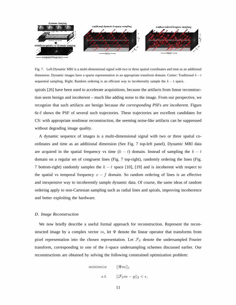
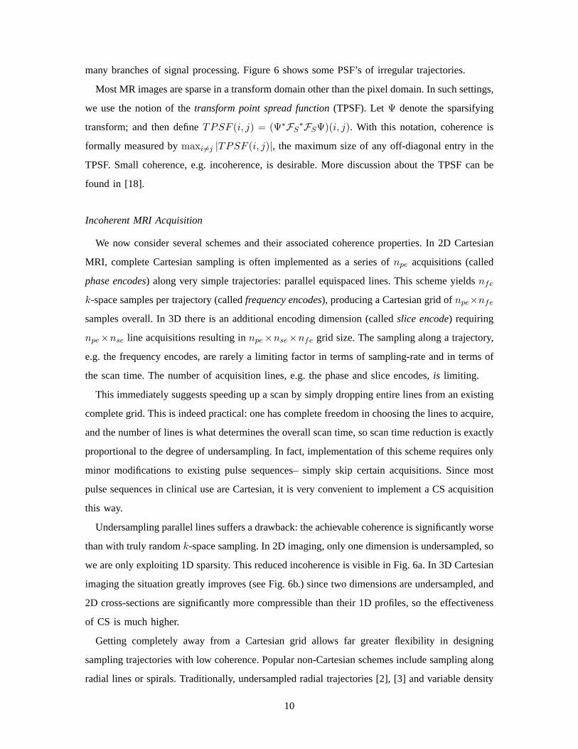
Fig. 7. Left:Dynamic MRI is a multi-dimensional signal with two or three spatial coordinates and time as an additional

dimension. Dynamic images have a sparse representation in an appropriate transform domain. Center: Traditionalk− t

sequential sampling. Right: Random ordering is an efficient way to incoherently sample thek − t space.

spirals [26] have been used to accelerate acquisitions, because the artifacts from linear reconstruc-

tion seem benign and incoherent – much like adding noise to the image. From our perspective, we

recognize that such artifacts are benign becausethe corresponding PSFs are incoherent. Figure

6c-f shows the PSF of several such trajectories. These trajectories are excellent candidates for

CS: with appropriate nonlinear reconstruction, the seeming noise-like artifacts can be suppressed

without degrading image quality.

A dynamic sequence of images is a multi-dimensional signal with two or three spatial co-

ordinates and time as an additional dimension (See Fig. 7 top-left panel). Dynamic MRI data

are acquired in the spatial frequency vs time (k − t) domain. Instead of sampling thek − t

domain on a regular set of congruent lines (Fig. 7 top-right), randomly ordering the lines (Fig.

7 bottom-right) randomly samples thek − t space [10], [19] and is incoherent with respect to

the spatial vs temporal frequencyx − f domain. So random ordering of lines is an effective

and inexpensive way to incoherently sample dynamic data. Of course, the same ideas of random

ordering apply to non-Cartesian sampling such as radial lines and spirals, improving incoherence

and better exploiting the hardware.

D. Image Reconstruction

We now briefly describe a useful formal approach for reconstruction. Represent the recon-

structed image by a complex vectorm, let Ψ denote the linear operator that transforms from

pixel representation into the chosen representation. LetFS denote the undersampled Fourier

transform, corresponding to one of thek-space undersampling schemes discussed earlier. Our

reconstructions are obtained by solving the following constrained optimization problem:

minimize ||Ψm||1

s.t. ||FSm− y||2 < ε,

11

Fig. 8. 3D Contrast enhanced angiography. Right: Even with 10-fold undersampling CS can recover most blood vessel

information revealed by Nyquist sampling; there is significant artifact reduction compared to linear reconstruction; and

a significant resolution improvement compared to a low-resolution centric k-space acquisition. Left: The 3D Cartesian

random undersampling configuration.

wherey is the measuredk-space data from the MRI scanner andε controls the fidelity of the

reconstruction to the measured data. The threshold parameterε is roughly the expected noise

level. Here the 1 norm ||x||1 =∑

i |xi|.

Minimizing the`1 norm of ||Ψm||1 promotes sparsity [15]–[17]. The constraint||FSm−y||2 <

ε enforces data consistency. In words, among all solutions which are consistent with the acquired

data, we want to find a solution which is compressible by the transformΨ. It is worth mentioning

that when finite-differencing is used as the sparsifying transform, the objective becomes the well

known total tariation (TV) penalty [27].

The reader may well ask how such formal optimization-based reconstructions relate to the

informal idea of successive interference cancellation. In fact, iterative algorithms for solving such

formal optimization problems in effect perform thresholding and interference cancellation at each

iteration, so there is a close connection between our exposition and more formal approaches [25],

[28], [29].

V. A PPLICATIONS OFCOMPRESSEDSENSING TOMRI

We now describe four potential applications of CS in MRI. The three requirements for suc-

cessful CS come together differently in different applications. Of particular interest is the way

in which different applications face different constraints, imposed by MRI scanning hardware or

by patient considerations, and how the inherent freedom of CS to choose sampling trajectories

and sparsifying transforms plays a key role in matching the constraints.

A. Rapid 3D Angiography

Angiography is important for diagnosis of vascular disease. Often, a contrast agent is injected,

significantly increasing the blood signal compared to the background tissue. In angiography, im-

portant diagnostic information is contained in the dynamics of the contrast agent bolus. Capturing

12

Fig. 9. Single breath-hold whole-heart coronary artery imaging. Left panel: the imaging sequence timing diagram.

Right panel: A slice through the volume of the heart showing the right coronary artery (3). The incoherent artifacts of

undersampled variable-density spirals (white arrow) appear as noiselike interference in the linear gridding reconstruction

(left). These artifacts are suppressed in the CS reconstruction (right) without compromising image quality. The slice

shows: (1) Aorta (2) Chest wall (3) Right coronary artery (4) Right ventricle (5) Left ventricle (6) Liver

the dynamics requires high spatial and temporal resolution of a large FOV – obviously a very

difficult task. Today MR angiography scans are often undersampled [3], [11] obtaining improved

spatial resolution and temporal resolution at the expense of undersampling artifacts.

CS is particularly suitable for angiography. As shown in Fig. 3 angiograms are are inherently

sparse in the pixel representation and by spatial finite differencing. The need for high temporal

and spatial resolution strongly encourages undersampling. CS improves current strategies by

significantly reducing the artifacts that result from undersampling.

In this example, we apply CS to 3D Cartesian contrast-enhanced angiography, which is the

most common scheme in clinical practice. Figure 8 illustrates the collection scheme, acquiring

equispaced parallel lines ink-space. Choosing a pseudo-random subset with variablek-space

density of 10% of those lines combines undersampling with low coherence. Figure 8 shows

a maximum intensity projection (MIP) through the 3D volume of several reconstructions. CS

is able to significantly accelerate MR angiography, enabling better temporal resolution or al-

ternatively improving the resolution of current imagery without compromising scan time. The

nonlinear reconstruction in CS avoids most of the artifacts that appear in linear reconstruction

from undersampled data.

B. Whole-Heart Coronary Imaging

X-ray coronary angiography is the gold standard for evaluating coronary artery disease, but it

is invasive. Multi-slice x-ray CT is a non-invasive alternative, but requires high doses of ionizing

radiation. MRI is emerging as a non-invasive, non-ionizing alternative.

13

Coronary arteries are constantly in motion, making high-resolution imaging a challenging

task. The effects of heart motion can be minimized by synchronizing acquisitions to the cardiac

cycle. The effect of breathing can be minimized by tracking and compensating for respiratory

motion, or by simply imaging during a short breath-held interval. However, breath-held cardiac-

triggered approaches face strict timing constraints and very short imaging windows. The number

of acquisitions is limited to the number of cardiac cycles in the breath-hold period. The number of

heart-beats per period is itself limited – sick patients cannot be expected to hold their breath for

long! Also, each acquisition must be very short to avoid motion blurring. In addition, many slices

must be collected to cover the whole heart. These constraints on breath-held cardiac triggered

acquisitions traditionally resulted in limited spatial resolution with partial coverage of the heart.

Compressed sensing can accelerate data acquisition, allowing the entire heart to be imaged in a

single breath-hold [30].

Figure 9 shows a diagram of the multi-slice acquisition. To meet the strict timing requirements,

an efficient spiralk-space trajectory is used. For each cardiac trigger, a single spiral ink-space

is acquired for each slice. The timing limitations still require 2-foldk-space undersampling.

Therefore we used variable density spirals [26] which have an incoherent PSF (Fig. 6e), in

which linear gridding reconstruction [5] produces artifacts that appear as added noise.

Coronary images are generally piece-wise smooth and are sparsified well by finite-differences.

CS reconstruction suppresses undersampling-induced interference without degrading the image

quality. Figure 9 shows a comparison of the linear direct gridding reconstruction and CS, on the

right coronary artery reformatted from a single breath-hold whole-heart acquisition. The linear

gridding reconstruction suffers from apparent noise artifacts actually caused by undersampling.

The CS reconstruction suppresses those artifacts, without impairing the image quality.

C. Brain Imaging

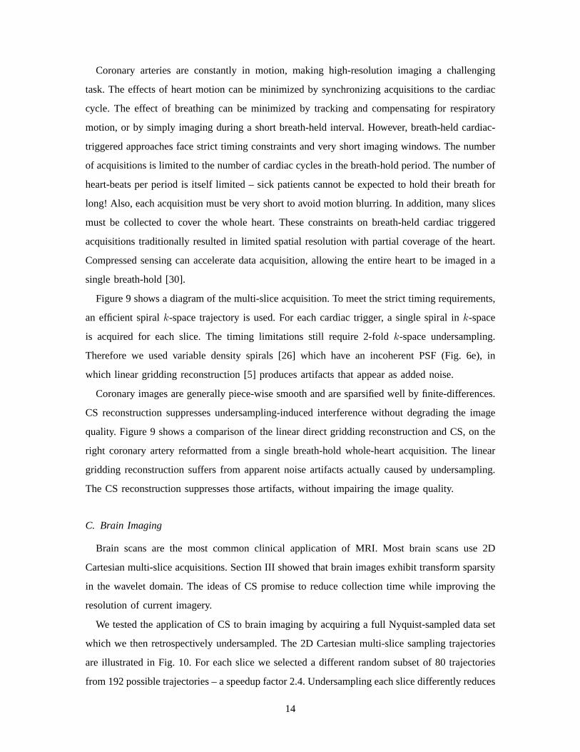
Brain scans are the most common clinical application of MRI. Most brain scans use 2D

Cartesian multi-slice acquisitions. Section III showed that brain images exhibit transform sparsity

in the wavelet domain. The ideas of CS promise to reduce collection time while improving the

resolution of current imagery.

We tested the application of CS to brain imaging by acquiring a full Nyquist-sampled data set

which we then retrospectively undersampled. The 2D Cartesian multi-slice sampling trajectories

are illustrated in Fig. 10. For each slice we selected a different random subset of 80 trajectories

from 192 possible trajectories – a speedup factor 2.4. Undersampling each slice differently reduces

14

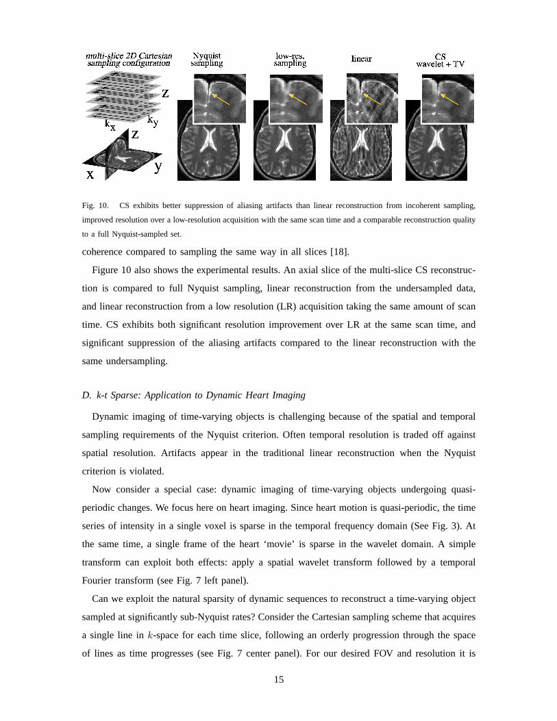
Fig. 10. CS exhibits better suppression of aliasing artifacts than linear reconstruction from incoherent sampling,

improved resolution over a low-resolution acquisition with the same scan time and a comparable reconstruction quality

to a full Nyquist-sampled set.

coherence compared to sampling the same way in all slices [18].

Figure 10 also shows the experimental results. An axial slice of the multi-slice CS reconstruc-

tion is compared to full Nyquist sampling, linear reconstruction from the undersampled data,

and linear reconstruction from a low resolution (LR) acquisition taking the same amount of scan

time. CS exhibits both significant resolution improvement over LR at the same scan time, and

significant suppression of the aliasing artifacts compared to the linear reconstruction with the

same undersampling.

D. k-t Sparse: Application to Dynamic Heart Imaging

Dynamic imaging of time-varying objects is challenging because of the spatial and temporal

sampling requirements of the Nyquist criterion. Often temporal resolution is traded off against

spatial resolution. Artifacts appear in the traditional linear reconstruction when the Nyquist

criterion is violated.

Now consider a special case: dynamic imaging of time-varying objects undergoing quasi-

periodic changes. We focus here on heart imaging. Since heart motion is quasi-periodic, the time

series of intensity in a single voxel is sparse in the temporal frequency domain (See Fig. 3). At

the same time, a single frame of the heart ‘movie’ is sparse in the wavelet domain. A simple

transform can exploit both effects: apply a spatial wavelet transform followed by a temporal

Fourier transform (see Fig. 7 left panel).

Can we exploit the natural sparsity of dynamic sequences to reconstruct a time-varying object

sampled at significantly sub-Nyquist rates? Consider the Cartesian sampling scheme that acquires

a single line ink-space for each time slice, following an orderly progression through the space

of lines as time progresses (see Fig. 7 center panel). For our desired FOV and resolution it is

15

Fig. 11. Dynamic imaging of quasi-periodic change. Left: Phantom experiment showing a reconstruction from 4-fold

undersampling. Right: Dynamic acquisition of the heart motion showing a reconstruction from 7-fold undersampling.

impossible to meet the spatial-temporal Nyquist rate using this scheme.

In fact, this approach is particularly inefficient for dynamic imaging with traditional acquisition

and reconstruction methods. Instead, we make one change: make thek-space line orderingrandom

instead of orderly [10], [19]. The random ordering comes much closer to randomly samplingk−t

space (See Fig. 7 right panel) and the sampling operator becomes much less coherent with the

sparsifying transform.

Fig. 11 shows results from two experiments. The first result used synthetic data: a motion

phantom, periodically changing in a cartoon of heart motion. The figure depicts an image sequence

reconstructed from a sampling rate 4 times slower than the Nyquist rate, using randomly-ordered

acquisition and nonlinear reconstruction. The second result involved dynamic real-time acquisition

of heart motion. The given FOV (16cm), resolution (2.5mm) and repetition time (4.4ms) allows a

Nyquist rate of 3.6 frames per second (FPS). This leads to temporal blurring and artifacts in the

traditionally-reconstructed image. By instead using random ordering and CS reconstruction we

were able to recover the dynamic sequence at the much higher rate of 25FPS with significantly

reduced image artifacts.

VI. CONCLUSIONS

We presented four applications where CS improves on current imaging techniques. The con-

cepts and approaches we discussed may potentially allow entirely new applications of MRI –

ones currently thought to be intractable.

CS-MRI is still in its infancy. Many crucial issues remain unsettled. These include: optimizing

sampling trajectories, developing improved sparse transforms that are incoherent to the sampling

operator, studying reconstruction quality in terms of clinical significance, and improving the

speed of reconstruction algorithms. The signal processing community has a major opportunity

here. There are fascinating theoretical and practical research problems, promising substantial

payoffs in improved medical care.

16

VII. A CKNOWLEDGMENTS

This project was supported by NIH grants: P41 RR09784, R01 HL074332, R01 HL075803

and GE healthcare. The authors would like to thank Walter Block for his help, and Peder Larson,

Daeho Lee, Seung-Jean Kim and Yonit Lustig for their help with the manuscript.

REFERENCES

[1] G. Wright, “Magnetic resonance imaging,”Signal Processing Magazine, IEEE, vol. 14, no. 1, pp. 56–66, Jan.

1997.

[2] K. Scheffler and J. Hennig, “Reduced circular field-of-view imaging,”Magn Reson Med, vol. 40, no. 3, pp.

474–480, 1998.

[3] D. C. Peters, F. R. Korosec, T. M. Grist, W. F. Block, J. E. Holden, K. K. Vigen, and C. A. Mistretta,

“Undersampled projection reconstruction applied to MR angiography,”Magn Reson Med, vol. 43, no. 1, pp.

91–101, 2000.

[4] C. H. Meyer, B. S. Hu, D. G. Nishimura, and A. Macovski, “Fast spiral coronary artery imaging,”Magn Reson

Med, vol. 28, no. 2, pp. 202–213, 1992.

[5] J. I. Jackson, C. H. Meyer, D. G. Nishimura, and A. Macovski, “Selection of a convolution function for Fourier

inversion using gridding,”IEEE Trans Med Imaging, vol. 10, no. 3, pp. 473–478, 1991.

[6] D. K. Sodickson and W. J. Manning, “Simultaneous acquisition of spatial harmonics (SMASH): Fast imaging

with radiofrequency coil arrays,”Magn Reson Med, vol. 38, no. 4, pp. 591–603, 1997.

[7] K. P. Pruessmann, M. Weiger, M. B. Scheidegger, and P. Boesiger, “SENSE: Sensitivity encoding for fast MRI,”

Magn Reson Med, vol. 42, no. 5, pp. 952–962, 1999.

[8] N. P. B. Madore, G.H. Glover, “Unaliasing by fourier-encoding the overlaps using the temporal dimension

(UNFOLD), applied to cardiac imaging and fMRI,”Magn Reson Med, vol. 42, no. 5, pp. 813–828, 1999.

[9] N. P. Willis and Y. Bresler, “Optimal scan for time-varying tomography. I. Theoretical analysis and fundamental

limitations.” IEEE Trans Image Process, vol. 4, pp. 642–653, 1995.

[10] T. Parrish and X. Hu, “Continuous update with random encoding (CURE): a new strategy for dynamic imaging,”

Magn Reson Med, vol. 33, no. 3, pp. 326–336, Mar 1995.

[11] F. R. Korosec, R. Frayne, T. M. Grist, and C. A. Mistretta, “Time-resolved contrast-enhanced 3D MR

angiography,”Magn Reson Med, vol. 36, no. 3, pp. 345–351, Sep 1996.

[12] J. M. Hanson, Z. P. Liang, R. L. Magin, J. L. Duerk, and P. C. Lauterbur, “A comparison of RIGR and SVD

dynamic imaging methods,”Magn Reson Med, vol. 38, no. 1, pp. 161–167, Jul 1997, comparative Study.

[13] J. Tsao, P. Boesiger, and K. P. Pruessmann, “k-t BLAST and k-t SENSE: Dynamic MRI with high frame rate

exploiting spatiotemporal correlations,”Magn Reson Med, vol. 50, no. 5, pp. 1031–1042, 2003.

[14] C. A. Mistretta, O. Wieben, J. Velikina, W. Block, J. Perry, Y. Wu, K. Johnson, and Y. Wu, “Highly constrained

backprojection for time-resolved MRI,”Magn Reson Med, vol. 55, no. 1, pp. 30–40, Jan 2006.

[15] E. Candes, J. Romberg, and T. Tao, “Robust uncertainty principles: Exact signal reconstruction from highly

incomplete frequency information,”IEEE Transactions on Information Theory, vol. 52, pp. 489–509, 2006.

[16] D. Donoho, “Compressed sensing,”IEEE Transactions on Information Theory, vol. 52, pp. 1289–1306, 2006.

[17] E. Candes and T. Tao, “Near optimal signal recovery from random projections: Universal encoding strategies?”

IEEE Transactions on Information Theory, vol. 52, pp. 5406–5425, 2006.

17

[18] M. Lustig, D. L. Donoho, and J. M. Pauly, “Sparse MRI: The application of compressed sensing for rapid MR

imaging,” Magn Reson Med, vol. 58, pp. 1182–1195, 2007.

[19] M. Lustig, J. M. Santos, D. L. Donoho, and J. M. Pauly, “k-t Sparse: High frame rate dynamic MRI exploiting

spatio-temporal sparsity,” inProceedings of the 13th Annual Meeting of ISMRM, Seattle, 2006, p. 2420.

[20] J. C. Ye, S. Tak, Y. Han, and H. W. Park, “Projection reconstruction MR imaging using FOCUSS,”Magn Reson

Med, vol. 57, no. 4, pp. 764–775, Apr 2007.

[21] K. T. Block, M. Uecker, and J. Frahm, “Undersampled radial MRI with multiple coils. Iterative image

reconstruction using a total variation constraint,”Magn Reson Med, vol. 57, no. 6, pp. 1086–1098, Jun 2007.

[22] T.-C. Chang, L. He, and T. Fang, “MR image reconstruction from sparse radial samples using bregman iteration,”

in Proceedings of the 13th Annual Meeting of ISMRM, Seattle, 2006, p. 696.

[23] F. Wajer, “Non-cartesian MRI scan time reduction through sparse sampling,” Ph.D. dissertation, Delft University

of Technology, 2001.

[24] D. S. Taubman and M. W. Marcellin,JPEG 2000: Image Compression Fundamentals, Standards and Practice.

Kluwer International Series in Engineering and Computer Science., 2002.

[25] D. Donoho, Y. Tsaig, I. Drori, and J.-L. Starck, “Sparse solution of underdetermined linear equations by stagewise

orthogonal matching pursuit,”Technical Report, Department of Statistics, Stanford University, 2006, preprint.

[26] C.-M. Tsai and D. Nishimura, “Reduced aliasing artifacts using variable-densityk-space sampling trajectories,”

Magn Reson Med, vol. 43, no. 3, pp. 452–458, 2000.

[27] L. Rudin, S. Osher, and E. Fatemi, “Non-linear total variation noise removal algorithm,”Phys. D, vol. 60, pp.

259–268, 1992.

[28] E. Candes and J. Romberg, “Practical signal recovery from random projections,”Caltech, Technical Report, 2005,

preprint.

[29] M. Elad, B. Matalon, and M. Zibulevsky, “Coordinate and subspace optimization methods for linear least squares

with non-quadratic regularization,”Journal on Applied and Computational Harmonic Analysis, 2006, in Press.

[30] J. M. Santos, C. H. Cunningham, M. Lustig, B. A. Hargreaves, B. S. Hu, D. G. Nishimura, and J. M. Pauly,

“Single breath-hold whole-heart MRA using variable-density spirals at 3T,”Magnetic Resonance in Medicine,

vol. 55, no. 2, pp. 371–379, 2006.

18