Ecole Centrale de Nantes Université de Nantes

MASTER SCIENCES MECANIQUES APPLIQUEES CONCEPTION DE SYSTEMES ET PRODUITS

Année 2013/2015

Thèse de Master SMA

Diplôme cohabilité par l'École Centrale de Nantes et l'Université de Nantes

présentée et soutenue par :

PRABANDH CHAKRABORTY

le date 29 Septembre 2015

à l’Ecole Centrale de Nantes

CENTRE BASED PLACEMENT STRATEGY FOR UNEQUAL AREA STATICFACILITY LAYOUT PROBLEM

Institut de Recherche en Communications et Cybernétique de Nantes (IRCCyN)

Résumé

Le problème de placement ou d’agencement est un problème bien connu et étudié dans la littérature. Il couvre de nombreux domaines comme l’organisation des ateliers, poste de

travail, plan d’architecture, conception et agencement de satellite, automobile et Navires.

Etant donné que ce problème est NP complet, de nombreux algorithmes et méthodologies sont élaborés pour réduire la complexité et le temps de calcul. Ce rapport, propose une étude d’optimisation d’un problème d’agencement d’espaces incluant un coût différent entre les

espaces. L’objectif étant de minimiser la somme des produits coût*distance toute en respectant les contraintes de collision et d’encombrement. La méthode proposée est

heuristique et Quasi-optimal combinant une recherche locale et une globale. Le principe consiste à générer aléatoirement un ordre de placement et une orientation des différents espaces (boucle d’optimisation globale) et puis un placement séquentiel sélectif par rapport

aux espaces déjà placés (boucle d’optimisation locale) Cette stratégie a été testé et comparée

aux méthodes existantes et donne des résultats encourageants. Cette stratégie d'optimisation de SPCB intégré avec l'algorithme de recherche locale a été testée à l'aide des exemples de problèmes disponibles choisis de la littérature. Dans ce rapport, la méthode développée a été comparé avec les résultats de la littérature sur l'une des techniques d'optimisation essaim de particules développée pour le même problème particulier. En outre, les résultats de cette stratégie d'optimisation proposée sont comparés avec des algorithmes standards de méthode de gradient et algorithme génétique. En comparant les résultats, il a été trouvé la stratégie d'optimisation développé est tout à fait efficace notamment en temps de calcul par rapport avec autres méthodes.

Mots-clés

Optimisation, Placement, Agencement, Stratégie de Placement orienté Centre, algorithme de cherche locale, méthode de gradient, algorithme génétique

ABSTRACT Facility layout problem is one of the well-studied and researched problems applicable to many fields like shop floor, architecture plan, satellite layout design, automobile layout design etc. Since, the mere fact that Facility layout problem is an NP hard problem many algorithms and methodologies have been developed and proposed to optimize facility layout problem but, very less have been effective with more computational time taken to solve. For the most part the more effective algorithms are not having lesser computational time taken to solve. This article studies an NP hard problem Unequal-Area Static Facility Layout Problem (UA-SFLP) in order to minimize the sum of the material handling costs with application of new heuristic quasi-optimal state of art optimization strategy named as Centre Based Placement Strategy (CBPS) integrated with local search algorithm. This algorithm is based on selective sequential placement of facilities with initial placement or first placement of first facility at the center of whole planar site or a given boundary where these facilities or facilities are to be placed. The order of placement is random and so as, the orientation during the placement. The local search algorithm is integrated with CBPS for better quality and controlled flow of optimization. This optimization strategy of CBPS integrated with local search algorithm has been tested using the available problem instances chosen from the literature. In this paper, the method developed has been compared with the results from literature on one of the Particle Swarm Optimization technique developed for the same particular problem dealing with UA-SFLP. Also, the results of this proposed strategy of optimization is compared with standard algorithms of Gradient method and Genetic Algorithm. Comparing the results it has been found the optimization strategy developed is quiet effective and has very less computational time compared to the other methods. Keywords Optimization , Unequal-area static facility layout problems, NP hard, Static facility layout problems, facility layout problem, Centre Based Placement Strategy, local search algorithm, gradient method, genetic algorithm,placement

ACKNOWLEDGEMENTS This thesis work was completed with significant contributions from Ranjan Hasda of Institut de Recherche en Communications et Cybernétique de Nantes (École Centrale de Nantes ), and Dr. Ramakrishnan Ramachandran. Special thanks to my thesis advisor, Prof. Fouad Bennis (École Centrale de Nantes ), and Prof. Rajib Bhattacharjya (Indian Institute of Technology, Guwahati). Without the guidance, co-operation and sharing of knowledge of previous research by these people this project would not have been successful. It has been an honour working with all these people especially Prof. Fouad Bennis and Ranjan Hasda. I wish highly for Ranjan Hasda, for successful completion of PhD and glorious future ahead.

Contents List of Figures i List of Tables iii

REFERENCES ..................................................................................................................................... 63

APPENDIX A:Matlab code for CBPS-Corner Points Method for 8Facilities...................................... 74

APPENDIX B:Matlab code for CBPS-Selective Sequential Method for 8Facilities ........................... 78

APPENDIX C:Matlab code for CBPS with Local Search Algorithm 8 Facilities,11 Facilities and 20 Facilities ................................................................................................................................................ 83

APPENDIX D:Matlab code for CBPS for Gradient Method................................................................ 89

APPENDIX E:Matlab code for CBPS for Genetic Algorithm ............................................................. 97

List of Figures Fig. 1: Trend of SFLP ............................................................................................................................. 2 Fig. 2: Classification procedure of facility layout problems ................................................................... 2 Fig. 3: EA-SFLP ..................................................................................................................................... 3 Fig. 4: UA-SFLP ..................................................................................................................................... 3 Fig. 5a):Pareto Front ............................................................................................................................... 9 Fig. 5b): Phenomenon of Pareto dominance ......................................................................................... 10 Fig. 6: Possible Pareto fronts for two objective functions showing maximum and minimum ............. 10 Fig. 7: Pareto fronts for multilple objective problem for objectives more than 2 ................................ 11 Fig. 8:Slicing tree representation of floor plan ..................................................................................... 15 Fig. 9: String scheme of a discrete layout representation based on a space filling curve ..................... 16 Fig. 10: Separation Algorithm at work ................................................................................................. 17 Fig. 11: Configuration model of the shelter in 2D ................................................................................ 18 Fig. 12: Bathroom relocation by using Michalek’s Approach .............................................................. 19 Fig. 13: Human–Algorithm–Knowledge-based layout Design (HAKD) working principle ................ 20 Fig. 14a):Simplified schematics of satellite in 3D ................................................................................ 20 Fig. 14b): Simplified schematics of satellite in 2D of each supporting surface after HAKD .............. 21 Fig. 15: Bottom-up approach ................................................................................................................ 27 Fig. 16: Application of Centre Based Placement Strategy for 8 facilities problem .............................. 28 Fig. 17: Basic flow chart of basic CBPS ............................................................................................... 29 Fig. 18: Planar site layout Placement .................................................................................................... 30 Fig. 19: When the rotation vector is applied to the facility to be placed on the placed facility ............ 30 Fig. 20: The first facility from random order at the center ................................................................... 30 Fig. 21: Undesirable overlapping of the where to be placed facility with facility to be placed ............ 31 Fig. 22: Undesirable overlapping of facilities which is to be placed with other except where to be placed ................................................................................................................................................... 31 Fig. 23: Undesirable overlapping of facilities which is to be placed with all the other facilities ......... 31 Fig. 24: Initial order and size of facilities for 8 Facilities ..................................................................... 32 Fig. 25: Initial order and size of facilities for 11 Facilities ................................................................... 33 Fig. 26: Initial order and size of facilities for 20 Facilities ................................................................... 34 Fig. 27: Discretised placement methodology ........................................................................................ 35 Fig. 28: Corner and mid-point of a facility after the generation of points ............................................ 36 Fig. 29: Interpolated positive-negative with respect to corner points of a facility be placed on placed facility(green facility) using Corner Point Method ............................................................................... 36 Fig. 30: Interpolated positive-negative positions with respect to mid-points of a facility to be placed on placed facility (green facility) .......................................................................................................... 36 Fig. 31: Interpolated positive-negative with respect to corner points of a facility be placed on placed facility (green facility )using selective sequential method .................................................................... 37 Fig. 32: Interpolated positive-negative with respect to mid-points of a facility to be placed on placed facility (green facility) based on Selective Sequential Method ............................................................ 38 Fig. 33: Checking of overlapping of facility to be placed using case b) and facility to be placed when placed on where to be placed facility .................................................................................................... 38 Fig. 34: Flow chart for application of condition in CBPS: Selective Sequential Method .................... 39 Fig. 35: Flow chart of local search algorithm integrated with CBPS ................................................... 40

i

Fig. 36: Effect of strictly less than in Local Search Algorithm ............................................................ 41 Fig. 37: The comparison of corner point method with selective sequential method for total cost Vs time ....................................................................................................................................................... 46 Fig. 38: CBPS with Local Search Algorithm for 8 Facilities ............................................................... 49 Fig. 39: CBPS with Local Search Algorithm for 11 Facilities ............................................................. 50 Fig. 40: CBPS with Local Search Algorithm for 20 Facilities ............................................................. 50 Fig. 41: Comparison of layouts for best solutions of CBPS with best results of PSO for 8 facilities .. 53 Fig. 42: Comparison of layouts for best solutions of CBPS with best results of PSO for 11 facilities 54 Fig. 43: Comparison of layouts for best solutions of CBPS with best results of PSO for 11 facilities 55 Fig. 44: Convergence of objective function for feasible solution ......................................................... 56 Fig. 45: Missing of best feasible solution by gradient algorithm .......................................................... 57 Fig. 46: Layout design obtained for best result of 8 Facilities UA-SFLP by applying Gradient method .............................................................................................................................................................. 57 Fig. 47: Basic flow chart of GA ............................................................................................................ 58 Fig. 48: Crossover in GA ...................................................................................................................... 59 Fig. 49: Mutation in GA ........................................................................................................................ 59 Fig. 50: Layout design obtained for best result of 8 Facilities UA-SFLP by applying GA .................. 60

ii

List of Tables Table-1: Data of Corner point method and selective sequential method at the given number of iteration for 8 Facility problem ............................................................................................................. 46 Table-2: CBPS -Corner points method data for 8 Facilities (placement order, co-ordinates, orientation, & Layout) .............................................................................................................................................. 47 Table-3: CBPS-Selective sequential method data (placement order, co-ordinates, orientation, & Layout) .................................................................................................................................................. 48 Table-4: 3 Best results and the time to reach that result for CBPS method for each of the three problems ................................................................................................................................................ 50 Table-5: Application of CBPS on 11 Facilities (placement order, co-ordinates, orientation, & Layout) .............................................................................................................................................................. 51 Table-6: Application of CBPS on 20 Facilities (placement order, co-ordinates, orientation, & Layout) .............................................................................................................................................................. 52 Table-7: Comparison of best results of CBPS and PSO w.r.t. Cost Vs time ........................................ 53 Table-8: Orientation and center coordinates of best result obtained for 8 Facilities by PSO ............... 54 Table-9: Orientation and center coordinates of best result obtained for 11 Facilities by PSO ............. 55 Table-10: Orientation and center coordinates of best result obtained for 20 Facilities by PSO ........... 56 Table-11: Corner coordinates of best result obtained for 8 Facilities by Gradient method .................. 57 Table-12: Corner coordinates of best result obtained for 8 Facilities by GA ....................................... 60

iii

1

CHAPTER 1: Introduction

1.1. Facility layout problems: Facility layout problems (FLPs) cope are type of problems where the main objectives are to find the locations of departments, or facilities in a shop floor in order to minimize the sum of the material handling costs. Facility layout problem are based on non-overlapping planar orthogonal arrangement of n rectangular facilities within a given rectangular plan site so as to minimize the distance based measure. Facility design is one of the most promising field in the manufacturing environment in the future. As per general approximations 20–50% of the overall operating cost within manufacturing environments is attributed to material handling and by creating a means for an effective facilities arrangement can reduce the material handling cost by 10–30% (Tompkins et al. 2010 [1] ). Moreover, good facility planning could also improve the material handling efficiency, reduce the throughput time, decrease the space utilization area of manufacturing system, etc. So, the facility layout affects the total performance of manufacturing system, such as, material flow, information flow, productivity, etc. FLP problem are complicated with respect to selection of right positioning pattern and right algorithm for minimum material handling costs. Let us try to understand the basic classification of FLP and possible selection.

1.2. Classification of facility layout problem Two main categories of FLPs that can be considered are: static facility layout problems (SFLPs) and dynamic facility layout problems (DFLPs). SFLPs, material flows among facilities are stable throughout the time horizon, and this type of formulation is suitable for industries where the material flows among facilities do not change for a long duration. DFLPs are the extension of SFLPs such that the material flows among facilities can be changed in different periods but are fixed in each period. The solution for a DFLP is one layout for each period but it is a single layout for an SFLP. There is the third kind a robust layout is one that is good for a wide variety of demand scenarios even though it may not be optimal under any specific ones (P. Kouvelis, A.A. Kurawarwala[2]). A robust layout procedure considers minimizing the total expected material handling costs over a specific planning horizon. Robust layout is selected when the demand is stochastic and the re-layout is prohibited. Broadly, FLPs can be split into two parts, the first is those with equal areas and the second is those with unequal areas. In the former, each of the facilities or departments has the same area. However, this is not the case in the latter. In accordance with Fig.1, SFLPs are divided into two categories, the first is equal-area SFLPs (EA SFLPs) and the second is unequal-area SFLPs (UA SFLPs). Similarly, there are two divisions for DFLPs as follows: equal-area DFLPs (EA DFLPs) and unequal-area DFLPs (UA DFLPs). Specifically, there are three main categories for UA DFLPs, which are: -UA DFLPs where the areas and shapes of departments or facilities are fixed throughout the whole time. -UA DFLPs where the areas of departments or facilities are fixed in all periods but their shapes are not constant and can change in consecutive periods.

2

-UA DFLPs where both the areas and shapes of departments or facilities are not fixed and can change in consecutive period of time. Fig.3 represents the output of problem on EA-SFLP and Fig.4 represents the output of problem on UA-SFLP. The unequal-area FLP was originally formulated by Armour and Buffa (1963) [3].

Fig. 1: Trend of SFLP [5]

Selecting the suitable type of layout problem is one of the prerequisite before solving the problem. To find good layouts for problems in an efficient manner, it is essential to select a strong meta-heuristic algorithm (Yildiz and Solanki 2012 [4] ) .The classification procedure of facility layout problem where a researcher has to choose the appropriate type of layout problem which can be based on the judgment conditions (Xiaohong Suo et al. 2012[5]). The judgment conditions can be either the material handling flows change over a long time or it it can be ease for rearrangement or the production requirement. If the material handling flows the change over a long time, it is better to choose DFLP. In case changes are negligible with respect to the material flows it is better to choose SFLP [5].

Fig.2: Classification procedure of facility layout problems [5]

Facility Layout

Model Layout /Resolution Approach

Judgement condition

Robust Layout SFLP DFLP

Solution Methodologies to solve FLP

UA-SFLP

EA-SFLP

UA-DFLP

EA-DFLP

3

Fig. 3: EA-SFLP

Fig. 4: UA-SFLP

1.3. SFLP vs. DFLP It has been observed the process of converting SFLP to DFLP, causes the rise of rearrangement costs so a researcher has to be very keen while choosing the method based on either SFLP or DFLP. In today’s competitive market scenario around the world makes SFLP covert to DFLP because of incorporation of effective time period with material handling cost. Under today’s volatile market scenario, demand is changed irregularly from one production period to another. As per one of the study it is said 40% of a company’s sales come from new

products that have only recently been introduced (A.L. Page, 1991[6]). When these changes frequently occur and the location of an existing facility is a decision variable, SFLP convert to DFLP. However, the change in product mix yields to modify the production flow and thus affects the layout. Gupta and Seifoddini (1990) [7] stated that 1/3 of USA companies undergo major reorganization of the production facilities every 2 years. A researcher has to take such an important issue into account when designing the layout. Most of the cases in facility layout problem implicitly considered as static; because of the fact that the key data about the tooling

5 7

1 4 8

2 6 3

5 4 6

2 3 1 7 8

4

and production facility and it is assumed the production rate remains constant enough over a long period of time. The changes in locations of facility can reduce the material flows between department pairs during a planning horizon. Meanwhile, rearranging the locations of facility will result in some rearrangement costs depending on the departments involved in this and the placement patterns and locations of those facilities. The changes in locations of facility can reduce the material flows between department pairs during a planning horizon. However, rearranging the locations of facility causes the some arise in costs incurred due to rearrangements of the facilities depending on the departments involved a rearrangement. Generally, when the products change often and the facility location is static, the material flows are increased drastically. In order to reduce the material flows, the facilities are shifted to different location which results in the rearrangement costs. Recently decade the idea of dynamic layout problems has been one of the most studied researches by the researchers. Dynamic layout problems take into account possible changes in the material handling flow over multiple time periods (Balakrishnan, Cheng, Conway, & Lau, 2003[8]; Braglia, Zanoni, & Zavanella, 2003[9]; Kouvelis, Kurawarwala, & Gutierrez, 1992[10]; Meng, Heragu, & Zijm, 2004[11]).

5

CHAPTER 2: Literature Review

2.1. Formulation of Facility layout problems It is one of the most important links for solving the facility layout problem. It is also the most challenging part to solve facility layout problem. Better the formulation more effective and more possibility of getting the global optimum for facility layout. This formulation of static and dynamic layout problems can be based on several types of mathematical and numerical models, vital ingredient for incorporating complex relationships between the different elements involved in a layout problem to be expressed. Such models can rely on different principles, which include graph theory (Kim & Kim, 1995 [12]; Leung, 1992 [13]; Proth, 1992 [14]) or neural network (Tsuchiya, Bharitkar, & Takefuji, 1996 [15]). These models are generally used to suggest solutions to the layout problems, which is also considered as optimization problems, with either single or multiple objectives. Depending on the strategy used for formulating the problem, it can be discrete or continuous. The most formulations lead to Quadratic Assignment Problems (QAP) (discussed in 2.1.1) or Mixed Integer Programming (MIP) (discussed in details 2.1.2.), which are the most commonly used formulation techniques. In some cases it has been argued nerby many researchers that the available data is very difficult to obtain so it has been suggested fuzzy formulation is better alternative which will be discussed in details in 2.1.3. Let’s start understand each type of

formulation and the contribution of researcher.

2.1.1. Discrete formulation

In this formulation the each plant sites are divided and discretized to cover as maximum as possible location during solving so that best possible placement positions can be covered. In many such cases the formulation is generally addressed by using QAP. In this formulation a plant site is divided into rectangular facilities with the same area and shape, and each facility is assigned to a facility (Fruggiero, Lambiase, & Negri, 2006 [16]). If facilities have unequal areas, they can occupy different facilities (Wang, Hu, & Ku, 2005 [17]).However, in most of the Equal Area Static Facility Layout Problem the QAP formulation is widely preferred. A typical formulation, when determining the relative locations of facilities so as to minimize the total material handling cost, is as follows (Balakrishnan, Cheng, & Wong, 2003[18]): 𝑚𝑖𝑛 ∑ ∑ ∑ ∑𝑁

𝑙=1𝑁𝑘=1

𝑁𝑗=1

𝑁𝑖=1 fik djl XijXkl

(1)

∑𝑁𝑖=1 Xij=1 j=1, 2,…………N; ∀ i≠j

(2) ∑𝑁

𝑗=1 Xij=1 i=1, 2,…………N, ∀ i≠j (3) where N is the number of facilities in the layout, fik the flow cost from facility i to k, djl the distance from location j to l and Xij the 0, 1 variable for locating facility i at location j. The objective function (1) represents the sum of the flow costs over every pair of facilities. Eq. (2) ensures that each location contains only one facility and Eq. (3) guarantees that each facility is placed only in one location. Discrete formulations are suggested, for example, by Kouvelis and Chiang (1992) and Braglia (1996) [19] to minimize part backtrack in single row layouts. The same type of approach is also used by Afentakis (1989) [20], to design a loop layout, so as to minimize the loop layout network congestion, i.e., the number of times a part traverses the loop before all its operations are completed. There are two kinds of measures placement

6

commonly used in loop layout design: Min-Sum and Min-Max. A Min-Sum problem attempts to minimize the total placement of all parts; while a Min-Max problem attempts to minimize the maximum congestion among a family of parts (Cheng & Gen, 1998[21]; Cheng et al., 1996[22]; Nearchou, 2006[23]). Discrete representation of the layout is also used for dynamic layout problems. The problems addressed can be equal size facilities (Baykasoglu & Gindy, 2001[24]; Lacksonen & Enscore, 1993[25]) and must respect constraints ensuring that each location is assigned to only one facility at each period, and that exactly one facility is assigned to each location at each period ([24]; [25]). Cost constraints can be added to carry out the placement of facilities on the floor plant (Balakrishnan, Robert Jacobs, & Venkataramanan, 1992[26]; Baykasoglu et al., 2006[27]). However, the costs incurred during placement and rearrangement must not exceed a certain level of the total cost allocated. It is generally believed by certain researchers that discrete representations are not suited to represent the exact position of facilities in the plant site and can’t model appropriately specific constraints as the orientation of facilities, pick-up and drop-off points or clearance between facilities. In such cases, a continuous representation is found to be more relevant by several authors (Das, 1993[28]; Dunker, Radonsb, & Westkampera, 2005[29]; Lacksonen, 1997[30]).

2.1.2. Continual formulation

In this formulation continuous flow of material is considered. Mostly it is preferred to address such problems by using Mixed Integer Programming Problems [28]. One of the prerequisite is that all the facilities are to be placed anywhere within the planar site and must not overlap each other ([28]; [29]; Meller et al., 1999[31]). MIP is generally used for unequal area static facility layout. The facilities in the plant site are located either by their centroid coordinates (xi, yi), half-length li and half width wi or by the coordinates of bottom-left corner, length Li and width Wi of the facility. The distance between two facilities can be, for example, expressed through the rectilinear norm (Chwif et al., 1998[32]): dij((xi,yi),( xj,yj)) = | xi- xj| +| yi- yj| (4) The pick-up and drop-off points can generate constraints in the layout problem formulation (Kim & Kim, 2000[33]; Welgama & Gibson, 1993[34]; Yang et al., 2005[35]). In this case, the distance traveled by a part from the drop-off of facility i to the pick-up of facility j, can for example, be given by Eq. (5) ([33]). dij= | xi

O- xjI| +| yi

O- yjI| (5)

where (xi

O , yiO) designate the coordinates of the drop-off point of facility i, and (xj

I, yjI) the

coordinates of the pick-up point of facility j. Area constraints on the plant site exist, which require the total area available to be superior or equal to the sum of all the facility areas. The area allocated to each machine on the floor plan must also take into account the space of other resources or buffers, which are needed to operate the machine [30]. The clearance between facilities can be included or not in the facility surface (Braglia, 1996[36]; Heragu & Kusiak, 1988[37], 1991[38]). Another very important constraint is that facilities must not overlap with each other. Mir and Imam (2001) [39] defined an overlap area Aij between two facilities to formulate this constraint. The layout optimization problem is expressed as follows:

7

Minimize objective function Subject to Ai j ≤ 0 Ai j=λij (ΔXij)( ΔYij)

ΔXij= λij(Li+Lj

2) -| xi- xj|

ΔYij= λij(Wi+Wj

2) -| yi- yj|

λij={−1 for ΔXij ≤ 0 and ΔYij ≤ 0

+1 𝑜𝑡ℎ𝑒𝑟𝑤𝑖𝑠𝑒 (6)

(Li, Wi) are the length and width of facility i, and (xi, yi) are coordinates of facility i. Other constraints can also be considered in the layout formulation, such as a pre-defined orientation of certain facilities [31]. Given such constraints, a typical formulation of the optimization problem can be as follows: 𝑚𝑖𝑛 ∑ ∑𝑁

𝑗=1𝑁𝑖=1 fij (| xi

O- xjI| +| yi

O- yjI|) (7)

where N is the number of facilities, fij the amount/cost of material flow from drop-off point of facility i to pick-up point of facility j, (xi

O, yiO) the coordinates of drop-off point of facility

i, and (xjI, yj

I) are the coordinates of pick-up point of facility j. Very few works seem to deal with dynamic layout problems with a continuous representation. Dunker et al. (2005) [40] addressed unequal size layout problems in a dynamic environment and assumed that the facility sizes vary from one period to another. There is also another method of calculating distance between to facilities dij Centroid-to-centroid (CTC) (Tate & Smith, 1993 [41]). When the input and output points of the departments are not known, the department centroid is used to represent the department I/O point. The shortcomings of CTC distances include the optimal layout is one with concentric rectangles; an algorithm based on CTC attempts to align the department centroids as close as possible, which may make the departments very long and narrow. There are two metrics used to measure the distance between two points Rectilinear distance is the most common distance metric used because is based on travel along paths parallel to a set of perpendicular (orthogonal) axes. The second distance metric is Euclidean distance, which is appropriate when distances are measured along a straight-line path connecting two points. Distances are measured with the Euclidean metric. Hence, the distance is given as

dij =√| 𝑥 − 𝑥 | + | 𝑦 − 𝑦 | (8) Where (xi

c, yic) and (xj

c, yjc) are centroids of two consecutive facilities and in xi

c, suffix c represents the centroid.

2.1.3. Fuzzy formulation:

The concept of Fuzzy Logic (FL) was pioneered by Lotfi Zadeh (1965) [42] as a system of logic for representing conditions that could not be easily denoted by crisp values like ‘true’ or

‘false’ in Boolean and conventional logic. The FL is based on a proposition that is based on not only on neither True nor False, but also may be true or false to some degree. FL provides a means to model these continuums of values through fuzzy sets. In many cases, it is very difficult to understand which data is affecting the facility layout problem. FL has been proposed to handle the imprecision or uncertainty that is often encountered. Indeed, there are

ic j

c i

c j

c

8

various formalisms available for dealing with missing information (Liu et al., 1997[43]; Tresp et al., 1994[44]). However, the formulation available in FL for tolerating or predicting missing information has demonstrated to be more robust and tractable than other formalisms (Negnevitsky, 2002[45]). Certain researchers believed just a few fuzzy rules may provide better results than a few thousand rules of other common formulations (Berthold & Huber, 1998[46]). The fuzzy modeling and inferencing techniques have successfully been applied to placement decisions in general layout design problem and this is widely developing field and growing more with time(Ahmad et al., 2003[47]; Ahmad et al., 2004b[48]; Aiello & Enea, 2001[49]; Badiru & Arif, 1996[50]; Deb & Bhattacharyya, 2005[51]; Dweiri & Meier, 1996[52]; Evans et al., 1987[53]; Grobelny, 1987a;[54] Grobelny, 1987b[55]; Karray et al. 2000b[56]; Kang et al., 1994[57]; Kim et al., 2001[58]; Raoot & Rakshit, 1993[59]; Raoot & Rakshit, 1991[60]; Soltani & Fernando, 2004[61]; Youssef et al., 2003a[62]; Whyte & Wilhelm 1999a[63], 1999b[64]; Zha & Lim, 2003[65]). Most research employing FL in layout design has used FL as a linguistic modeling tool. However, Ahmed (2005) [66] introduced a FL in layout design which uses both linguistic and analytical tools. Evans et al. (1987) [53] addressed the placement of unequal size facilities on the plant area. A relation between every pair of facilities by fuzzy relations has been expressed described based on closeness and level of importance. These relations has been quiet beneficial for the analyst to specify the importance associated with each pair of facilities to be located at any distance from each other. The authors proposed a fuzzy formulation of the problem through linguistic variables and propose a heuristic. To tackle the problem of locating n facilities to n fixed locations Grobelny (1987a, 1987b) [54] [55] proposed a method based on FL to minimize the total material handling cost. In this approach the data impacting the layout, such as closeness links and traffic intensity, are fuzzy and modeled with linguistic variables and fuzzy implications. In this method a new heuristic procedure was developed, based on binary fuzzy relations, is developed for the selection and the placement of facilities in the available locations many of these principles of this approach are also used by Raoot and Rakshit (1991) [60], who considered the problem of finding the best arrangement on the plant site of facilities based on specifications about their inter-relationship, which are characterized through linguistic variables. Gen, Ida, and Cheng (1995) [67] addressed a multi-objective multi-rows layout problem with unequal area for the situations where the clearance is very difficult to define be precisely, and is therefore considered as fuzzy. In Dweiri and Meier (1996)[52], who proposed an approach based on FL for discrete facility layout problem, which is based on the amount of parts circulating between facilities, the amount of communications between facilities and the number of material handling equipment used to transfer parts between facilities are incorporated into fuzzy factors. A state of art Activity Relationship Chart (ARC) has been proposed based on the judgment of experts that is used to specify relationships between each pair of facilities. ARC is then integrated in the well-known heuristic CORELAP [86] to find the best placement of facilities. Aielloor this and Enea (2001) [49] believed that the product market demands are uncertain data that cannot be approaches solved by other well-known approaches like discreet and continual so for this FL is proposed to be used. By application of the proposed method [49] minimization of the total material handling cost, along a single row configuration, under the constraints that the capacity of production for each department is limited. To solve a single row layout problem, they split the fuzzy demands in to cuts and determine the a-level fuzzy cost for each possible layout. Deb and Bhattacharyya (2005) [51], addressed the placement of facilities with pick-up and drop-off points in a continual plane, so as to minimize the total material handling cost.

9

The position of facilities depends on such factors as: the personal flow, the supervision relationships, the environmental relationships and the information relationships, which are rated using linguistic variables (e.g., high, medium, low). The authors developed a fuzzy decision support system based on a set of fuzzy IF–THEN rules. A construction heuristic is then used to determine the placement of facilities in the plant site.

2.1.4. Multi-Objective Optimization:

A multi-objective optimization problem is an optimization problem that involves more than one objective functions. In mathematical terms, a multi-objective optimization problem can be formulated as:

For design variable x =( x1 x2 x3…… xn)

x* =min F(x)= (f1(x), f2(x), f3(x), f4(x),…….fn(x)) s.t: g(x) ≤ 0 and h(x) = 0 (9)

Where x * is point of convergence for the solution all the objective functions called Feasible solution. While, g(x) and h(x) are constraint functions. In case, when x * satisfies all the constraints and objective functions it is called feasible solution. The h(x) is called active constraints while, g(x) non-active constraints until g(x) =0. Most authors combine the different objectives into a single one either by means of Analytic Hierarchy Process (AHP) methodology (Harmonosky & Tothero, 1992 [68]; Yang & Kuo, 2003 [69]) or using a linear combination of the different objectives (Chen & Sha, 2005 [70]).While few researchers used a Pareto approach to generate a set of non-dominated solutions as explained in 1.4.4.1.

2.1.4.1. Pareto front and Pareto dominance: In multi-objective optimization, generally not possible to get a feasible solution that minimizes all objective functions simultaneously. Therefore, attention is paid to Pareto optimal solutions; that is, solutions that cannot be improved in any of the objectives without degrading at least one of the other objectives. Consider two functions in which f1 is increasing and f2 is decreasing as shown in Fig.5 a). A feasible solution x1 is said to be Pareto dominated to another x 2 if:

1. fi(x1) << fi(x2) for all indices i∈{1…k}

2. fj(x1) << fj(x2)for at least one index j∈{1…k}

x1 is called Pareto optimal, if there is no another solution that dominates it. This set Pareto optimal points is called Pareto frontiers. As shown in Fig.5b), for a point in the domain of pareto front, all points are dominated by point A.

f1

f2

Pareto Front

Fig.5 a) Pareto Front

10

Fig.5 b) Phenomenon of Pareto dominance A feasible solution x1 is said to be Pareto dominated to another x 2 if: At X2

f1(x1) >f1(x2) f1(x1) >f1(x2) For domain 1, all points dominated by A. For domain 2 and 4, no dominating relationships are found between A and domain 2 and 4.Here X represent the feasibility domain where the possible feasibility solution is possible for point A. In Fig.5(b), the black line represents the Pareto fronts while the blue represents the space of the problem.

a) min f 1(x),min f 2(x) b) min f 1(x),maxf 2(x) c) max f 1(x),max f 2(x)

d) min f 1(x), max f 2(x)

f1(x)

f2(x) f2(x)

f1(x) f1(x)

f2(x)

f1(x)

f2(x)

Fig.6: Possible Pareto fronts for two objective functions showing maximum and minimum

f1

f2

Pareto Front

x 1

x 2

Feasible domain X=(X1, X2)

1 2

3 4

A(f 1(x), f 2(x))

X1

X2

11

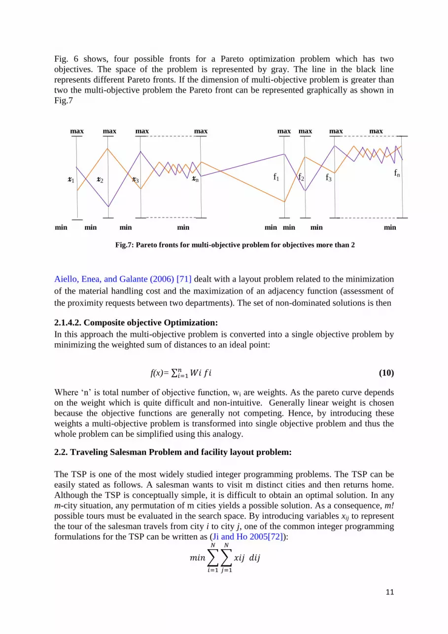
Fig. 6 shows, four possible fronts for a Pareto optimization problem which has two objectives. The space of the problem is represented by gray. The line in the black line represents different Pareto fronts. If the dimension of multi-objective problem is greater than two the multi-objective problem the Pareto front can be represented graphically as shown in Fig.7 max max max max max max max max

Aiello, Enea, and Galante (2006) [71] dealt with a layout problem related to the minimization of the material handling cost and the maximization of an adjacency function (assessment of the proximity requests between two departments). The set of non-dominated solutions is then

2.1.4.2. Composite objective Optimization: In this approach the multi-objective problem is converted into a single objective problem by minimizing the weighted sum of distances to an ideal point:

f(x)= ∑ 𝑊𝑖 𝑓𝑖𝑛𝑖=1 (10)

Where ‘n’ is total number of objective function, wi are weights. As the pareto curve depends on the weight which is quite difficult and non-intuitive. Generally linear weight is chosen because the objective functions are generally not competing. Hence, by introducing these weights a multi-objective problem is transformed into single objective problem and thus the whole problem can be simplified using this analogy.

2.2. Traveling Salesman Problem and facility layout problem: The TSP is one of the most widely studied integer programming problems. The TSP can be easily stated as follows. A salesman wants to visit m distinct cities and then returns home. Although the TSP is conceptually simple, it is difficult to obtain an optimal solution. In any m-city situation, any permutation of m cities yields a possible solution. As a consequence, m! possible tours must be evaluated in the search space. By introducing variables xij to represent the tour of the salesman travels from city i to city j, one of the common integer programming formulations for the TSP can be written as (Ji and Ho 2005[72]):

𝑚𝑖𝑛 ∑ ∑ 𝑥𝑖𝑗 𝑑𝑖𝑗

𝑁

𝑗=1

𝑁

𝑖=1

min min min min min min min min

Fig.7: Pareto fronts for multi-objective problem for objectives more than 2

x1 x2 x3 xn f1 f2 f3 fn

12

(11) ∑𝑚

𝑖=1 xij=1 j=1, 2,…………N; ∀ i≠j (12) ∑𝑚

𝑗=1 xij=1 i=1, 2,…………N;∀ i≠j (13) ui- uj +mxij ≤ m-1 i,j=2,3,…………N;∀ i≠j (14) The distance between city i and city j is denoted as dij. The objective function (11) is simply to minimize the total distance traveled in the tour. Constraint set (12) ensures that the salesman once at only day. Constraint set (14) ensures that the salesman leaves each city once. Constraint set (15) is to avoid the presence of sub tour ([72]). TSP with QAP can be integrated solved by genetic algorithm ([72]; Al-Dulaimi & Ali 2008[73]). A pure integer nonlinear integrated model of TSP and QAP can be formulated as follows ykl is placement order ([72]): 𝑚𝑖𝑛 ∑ ∑ ∑ ∑𝑚

𝑙=1𝑚𝑘=1

𝑁𝑗=1

𝑁𝑖=1 fij (dik +djl) xijxkl ykl + 𝑚𝑖𝑛 ∑ ∑ 𝑁

𝑗=1𝑁𝑖=1 xijdij

(15)

∑𝑁𝑖=1 xij=1 j=1, 2,…………N; ∀ i≠j

∑𝑁

𝑗=1 xij=1 i=1, 2,…………N, ∀ i≠j ∑𝑚

𝑘=1 ykl=1 i=1, 2,…………N, ∀ k≠l ∑𝑚

𝑙=1 ykl=1 i=1, 2,…………N, ∀ k≠l Whitely, Starkweather, & Shaner (1991)[74], used a recombination approach using genetic algorithm to solve the traveling salesman problem. This method is based on creating a crucial link in each iteration by using an edge recombination operator. The basic concept is similar objective wise as in both the cases in facility layout problem and traveling salesman problem the objectives are to reduce the path or distance and hence the cost. There are certain methods developed for solving the facility layout with application of genetic algorithm especially in crossover phase (Mak, Wong & Chan (1998) [75]; Kaveh & Safari (2014) [76]).

2.3. Resolution approaches Several approaches exist to address the different types of problems. They aim either at finding good solutions, which satisfies certain constraints given by the decision maker or at searching for an global or local optimum solutions given one or several performance objectives. This has yield heuristic based methods or optimization algorithms, as explained in the following of this section. There are numerous methods and approaches which is used in placement of facilities or facilities it can be exact or approximation based. In this section I will explain all the resolution approaches based on earlier work with the detailed description but in CHAPTER 4 &5 the Center Based Placement Strategy on which this paper is based.

13

2.3.1. Exact Approach:

This is one of the difficult methods and generally very less chance of success. This method is based on exact solution of the problem. Among articles that dealt with exact methods, Kouvelis and Kim (1992) [77] developed a branch and bound algorithm for the unidirectional loop layout problem. Meller et al. (1999) [78] also used this approach to solve the problem of placing n rectangular facilities within a given rectangular available area. They proposed general classes of valid inequalities, based on an acyclic sub-graph structure, to increase the range of solvable problems and use them in a branch-and-bound algorithm. Kim and Kim (1999) [79] addressed the problem of finding P/D locations on fixed size facilities for a given layout. The objective of the problem is to minimize the total distance of material flows between the P/D points. Authors suggested a branch and bound algorithm to find an optimal location of the P/D points of each facility. Rosenblatt (1986) [80] used a dynamic programming method to solve a dynamic layout problem with equal size facilities. However, only small problem instances have been solved optimally (six facilities and five time periods). André (2008) [81], introduced an exact approach for one dimensional facility layout problem which uses 0-1 quadratic programming model consist of 0-1 variables. Subsequently, this model is cast as an equivalent mixed-integer program and then reduced by preprocessing. Next, additional redundant constraints are introduced and linearized in a higher space to achieve an equivalent mixed 0-1 linear program, whose continuous relaxation provides an approximation of the convex hull of solutions to the quadratic program. Ravi Kothari and Diptesh Ghosh (2012) [82], introduced a heuristic approaches that have been used to solve single row facility layout problem (SRFLP) which is a NP-hard problem concerned with the arrangement of facilities of given lengths on a line so as to minimize the weighted sum of the distances between all the pairs of facilities. They have been applied to relatively small instances, with up to 42 facilities. But the results are very far from obtaining the optimal solutions. Love and Wong (1976) [83], formulated the problem as a linear mixed-integer program. Let M be an arbitrarily large number and let U be the sum of the lengths of all departments. Denote by ui the endpoint location of department i on the interval [0, U] farthest from the line origin. Define αij = 1 when department i is to the left of department j and αij = 0 otherwise. Let Rij be the distance between the centroids of departments i and j if department i is to the right of department j, and Rij = 0 otherwise. Let Lij be the distance between the centroids of departments i and j if department i is to the left of department j, and Lij = 0 otherwise. Then, Love and Wongs model is,

𝑚𝑖𝑛 ∑ ∑𝑛𝑗=𝑖+1

𝑛−1𝑖=1 Cij (Rij +Lij) : Rij -Lij= ui- uj+

1

2(lj- li),

ui- uj +M αij ≥ li- ui+ uj +M(1- αij) ≥ lj. li≤ ui ≤ U, αij ∈{0,1}, Rij, Lij ≥ 0 (i=1,….,n ; j=i+1,….,n ) (16) The first constraint set converts the distance between two endpoints ui and uj into the distance between the two centroids of departments i and j (Rij or Lij). The second and third constraint sets ensure that interdepartmental distance requirements are respected. The fourth constraint set ensures that any department lies on the interval [0, U].

14

Heragu and Kusiak (1991) [84], presented a model for the problem, which they called ABSMODEL. Let u+ be the distance between the centroid of department i and the line origin and let sij be the minimum separation between departments i and j. Their model is given by

𝑚𝑖𝑛 ∑ ∑𝑛𝑗=𝑖+1

𝑛−1𝑖=1 Cij| ui

+- uj+|: | ui

+- uj+| ≥

1

2(li+ lj) + sij(i=1,….,n ; j=i+1,….,n ) (17)

As the absolute value for the distance between the centroids are used, it does not matter if department i is to the left or to the right of department j. Note that the minimum value of the distance between the centroid | ui

+- uj+| can assume could be set greater than (li+ lj) /2 if we

are given a value sij. Heragu (1997) [85] shows how to transform the above nonlinear optimization problem into an equivalent linear mixed-integer programming model, denoted by LMIP1, and which is similar to the model of Love and Wong (1976) [83]. Heragu (1997) [85] also shows how LMIP1 can be solved by means of Benders decomposition.

2.3.2. Approximated approaches

Since exact approaches are often found not to be suited for large size problems, numerous researchers have developed heuristics and meta-heuristics. This is an approach which is based on the principles of random approximations to get the best possible placement of layout. Construction approaches have been developed gradually with time where the facilities evolves sequentially until the complete layout is obtained whereas enhancement of the methods start from first initial solution and they try to improve the solution with producing new solution. Construction heuristics include: CORELAP (Lee & Moore, 1967 [86]), ALDEP (Seehof & Evans, 1967 [87]) and COFAD (Tompkins & Reed, 1976 [88]), SHAPE (Hassan, Hogg, & Smith, 1986 [89]). Example of some of the improved heuristics are: CRAFT (Armour & Buffa, 1963 [90]), FRAT (Khalil, 1973 [91]) and DISCON (Drezner, 1987 [92]). Among these approaches based on meta-heuristics, one can distinguish global search methods (Tabu search and simulated annealing) and evolutionary approaches (genetic and ant colony algorithms). Chiang and Kouvelis (1996) [93] developed a tabu search algorithm to solve a facility layout problem. They used a neighborhood based on the exchange of two locations of facilities and included a long term memory structure, a dynamic tabu list size, an intensification criteria and diversification strategies. Chwif et al. (1998) [32] used a simulated annealing algorithm to solve the layout problem with aspect ratio facilities sizes. Two neighborhood procedures are proposed: a pairwise exchange between facilities and random moves on the planar site in the four main directions (upwards, downwards, leftwards and rightward). McKendall et al. (2006) [25] suggested two simulated annealing approaches for a dynamic layout problem with equal size facilities. The first simulated annealing approach used a neighborhood based on a descent pairwise exchange method, which consists in randomly changing the location of two facilities while the solution is improved. The second approach combines the first simulated annealing algorithm and improvement strategy called ‘‘look-ahead and look-back strategy’’. Genetic Algorithms (GA) are stochastic search techniques based on the mechanism of natural selection and genetic (Goldberg, 1989) [94]. The basic concept of GA is designed to stimulate processes in natural system necessary for evolution. As such that represents an intelligent

15

exploitation of a random search within a defined search space to solve a given problem.

Genetic algorithms seem to become quite popular in solving facility layout problems (Pierreval et al., 2003 [95]). In fact, a large number of studies using such approaches have been published: see Banerjee and Zhou (1995) [96], [75], Azadivar and Wang (2000) [97], Wu and Appleton (2002) [98], [29], and [17] for the static layout problems, and Balakrishnan and Cheng (2000)[99], Balakrishnan, Cheng, Conway, et al. (2003)[100], and [40] for the dynamic layout problems. A popular representation of the continual layout is the slicing tree (Shayan & Chittilappilly, 2004[101]). A slicing tree is composed of internal nodes partitioning the floor plan and of external nodes representing the facilities. Each internal node can be labeled either h (horizontal) or v (vertical), indicating whether it is a horizontal or vertical slice whereas external nodes label the facility index (1, 2, 3, . . ., n for n facilities). Each rectangular partition corresponds to a space allocated to a facility. Fig.8 shows a particular layout and the corresponding slicing tree.

Fig.8: Slicing tree representation of floor plan

Wu and Appleton (2002) [98] suggested a slicing tree to represent simultaneously the layout and the aisles and adapted genetic operators. From a given layout, the slicing tree is generally encoded into a string form, in order to use particular genetic operators. Tam (1992) [102] suggested coding a solution by a binary string with two parts, which represent operators and operands, and later in three parts: the tree structure, the operators and the operands (Tam & Chan, 1998) [103]. Al-Hakim (2000) [104] improved Tam Chan’s approach (1998) [103] and proposed a new operator named ‘transplanting’, to ensure the coherence of an offspring. The problem of avoiding reparation procedures when dealing with slicing trees is tackled by Shayan and Chittilappilly (2004) [101]. When authors addressed discrete layout problems, the algorithm differs from continual representation. For discrete representation, a popular solution for solving layouts is based on Space Filling Curves (SFC) [17]. The plant area being divided into grids, a space filling curve defines a continuous sequence through all neighbored squares in the underlying layout (Fig. 9).Space-filling curves ensure that a facility is never split (Bock & Hoberg, 2007)[105]. Nevertheless, this technique requires many rules to verify the connection of all positions of a layout as for example using expert rules [17]. When a space filling strategy is defined, solutions have to be coded. Islier (1998) [106] decomposed strings into three segments, encoding the sequence of facilities, the area required for each facility and the width of each sweeping band. Recently, [17] encoded the chromosome’s genes through five segments strings. The first segment shows the department

16

placement sequence. The second gives the required areas of each department. The third segment indicates the site size (length and width). The fourth segment shows the sweeping direction (1: horizontal, 2: vertical) and the fifth segment indicates the sweeping bands. An example is illustrated in Fig. 9.

Fig.9: String scheme of a discrete layout representation based on a space filling curve [17]

The objective function used in evolutionary methods is generally expressed as a mathematical cost function, which is derived from the problem formulation under consideration. To take into account in a more realistic way the system performance, simulation models have been connected to evolutionary methods to evaluate the candidate solutions [97]. Hamamoto, Yih, and Salvendy (1999) [107] addressed a real problem of pharmaceutical industry. The chromosome evaluation is performed through the simulation of a 4 months production. Ant colony optimization has been recently applied for solving layout problems. Solimanpur, Vrat, and Shankar (2005) [108] developed an ant algorithm for a sequence-dependent single row machine layout problem. Baykasoglu et al. (2006) [26] proposed an ant colony algorithm for solving the unconstrained and budget constrained dynamic layout problems. The hybridization of different metaheuristics has also been considered for solving facility layout problems. Lee and Lee (2002) [109] presented a hybrid genetic algorithm for a fixed shape and unequal area facility layout problem. Tabu search and simulated annealing are first used to find global solutions and the genetic algorithm is introduced in the middle of the local search process to search for a global solution. Balakrishnan, Cheng, Conway, et al. (2003) [100] developed a hybrid genetic algorithm to solve the dynamic layout problem previously tackled by Rosenblatt (1986) [82]. The initial population is generated with two methods: a random method and an Urban’s procedure (Urban, 1993) [110]. The crossover is based on a dynamic programming approach and the mutation is achieved by the CRAFT heuristic [3]. McKendall and Shang (2006) [25] developed and compare three hybrid ant colony algorithms

17

for a dynamic facility layout problem. They combine an ant colony with three local search procedures staring with a random descent pairwise exchange procedures, followed by a simulated annealing algorithm and at the end with a look-ahead/look-back procedure.

2.3.3. Interactive Approach

Interactive layout optimization design problem is a type of problem in which a user has the liberty to change parameters and criteria whenever needed for the purpose of optimization by interaction of user. Ultimately, the user-interaction aims at finding the global optimal solution of a problem under target. In layout optimization problem, sometimes it is difficult to obtain a global optimum due to inability of interaction during the process of optimization, but by provision of interaction tools for parameters or criteria as per the requirement of design based on expertise of designer it amplifies the possibility to reach the global optimum. The parameters can be the objective functions, constraints, units, and generations, population and individuals in case of using evolutionary algorithm. While, the criteria can be qualitative or quantitative criteria.

Guillaume Jacquenot and Fouad Bennis (2009)[111] another hybrid metaheuristics in which the positioning of the layouts with each other is optimized by genetic algorithm with effect exploration search space while a separation algorithm (Imamichi, 2008[112]) used to get the relax the placement constraints. Here the geometry for placement characterization used is the circle for 2D and the sphere for 3D clubbed with separation algorithm with unconstrained minimization problem, possibility of getting better result especially for non-uniform shaped layout as shown in Fig.10. One of the problems with this method is that, after obtaining the Pareto set there are large disparities as two different initial populations do not converge towards the same trade-off surface. Due to this reason, the population in variable space and objective space is lost. Hence, good solutions are not selected for the next generation also, if the good solution is ever found it is difficult to change the topology. This hybrid metaheuristics is further developed by Bénabès and Fouad Bennis (2010) [113] with interactive strategy with creation of optimization tool development for separation and genetic algorithm for EA-SFLP and UA-SFLP so that user has liberty to intervene between the optimization and change the placement of the layout to apply the experience and knowledge of the user. This method used in a mulit-objective shelter problem as show in Fig.11 and 12. In this optimization strategy, the population of initial individuals of genetic algorithm can be modified by a separation algorithm with a new concept of space density principle is utilized for qualitative criteria during the interactions of designer provided, the geometrical placement constraints must be non-overlapping.

Fig.10: Separation Algorithm at work ([111] and Dige & Jackiela1996 [114])

18

Fig.11: Overall view of the shelter [113]

Fig.11: Configuration model of the shelter in 2D [113]

19

Michalek et al. 2002 [114], devised an Interactive Weighted Tchebycheff approach in that converts multi-objective layout problem is into single objective layout problem by utilization of linear weights. An interaction tool for architecture layout optimization problem is introduced in which the user has the liberty to delete, add or change the objective function, constraints, units, and variables as per the wisdom of the user during the optimization. By ability to change the variable the optimization search can be guided as per the requirement of designer. In fig. 12 describes how an initial location of bathroom is relocated by the help of an interactive strategy. Hence, the designer has the ability to use his knowledge and experience with this strategy especially for architectural and civil engineering floor planning.

Fig. 12: Bathroom relocation by using Michalek’s Approach [114]

Brintrup et al. 2005[115], proposed an interactive tool incorporated with genetic algorithm developed for both single and multi-objective layout problem with close loop with provision of selection of either qualitative, or quantitative criteria during the optimization of the layout problem. As per this proposed method, the user can choose an option between sequential single objective interactive genetic algorithm (IGA) and multiple objective interactive genetic algorithms (IGA). But, both have different structures. Moreover, the qualitative criteria are determined by user defined rating (values between 0 to 9) for the fitness function. However, the quantitative criteria is determined for fitness function for the given generation count.

Liu et al. 2008[116], developed a Human–Algorithm–Knowledge-based layout Design (HAKD) method comprise of a new interactive tool developed for spacecraft for the solution provided with human, algorithm and layout schemes are unified into one string of solution. In this interactive tool, the commercial CAD file of layout is accessed in the genetic algorithm

20

via Hough Transfer technology encoded into an evolutionary algorithm that incorporates the layout schematic made by human user. In HAKD method, the unification for all the three solutions is done by creating an individual pool for each solution into a genetic algorithm.Fig.13 depicts the principal of HAKD and Fig 14a) and 14b) are the simplified schematics of satellite in 2D and 3D.

Fig. 13: Human–Algorithm–Knowledge-based layout Design (HAKD) working principle [116]

Fig.14a): Simplified schematics of satellite in 3D [116]

21

Fig.14b): Simplified schematics of satellite in 2D of each supporting surface after HAKD [116]

Ahmad et al. 2005[66], proposed an Intelligent System for Decision Support & Expert Analysis in Layout Design (IDEAL) designed based on an expert system paradigm. An Intelligent Layout Generator (ILG) which generates superior layout with preference mechanism employing expert or intelligent interference mechanism or any other knowledge source incorporated with hybrid genetic algorithm based on meta-heuristic search with deterministic heuristic with decoder and turner of layout solution. IDEAL approach supports interactive, efficient, and knowledge-based manipulations for best set of layout solutions.

Miettinen et al. 1995[117], proposed a Non-differentiable Interactive Multi-objective BUndle-based optimization System (NIMBUS) consist of nonlinear and linear, single and multiple objective functions evaluated having option of five classes based on values of objective function. Based on these classifications these functions are further classified into sub classification based on graphics, parameters, and, etc. These sub-classified functions are then evaluated for Pareto-optimality. This system uses Multi-objective Proximal Bundle method as explained by (Mäkelä, 1993[118]). The strategy of handling multi objective functions is based on the ideas presented in (Kiwiel, 1984[119]) and (Wang, 1989[120]). This technique is further developed for interaction platform of internet graphic user interference on World Wide Web (WWW) to make it more user friendly as presented in Miettinen et al. 2000[121].The problem with NIMBUS is that convexity problems is not satisfied by valid constraints, as weaker results are obtained. Tappeta et al. 2001[122], proposed an interactive Multi-Objective Optimization Design Strategy (iMOODS) which consist of including Pareto sensitivity analysis, Pareto surface approximation and local preference functions to capture the Decision Maker’s (DM)

preferences in an Iterative Decision Making Strategy (IDMS).In this method, class functions are used to capture DM preference, the generation of Pareto data and construction of Pareto surface. In this method, Compromise Programming (CP) approach with an augmented Tchebyshev norm (Tappeta 1999[123]) for the generation of Pareto points and surface for both convex and non-convex regions of Pareto surface. For CP Sequential Quadratic Programming (SQP) is used and General Reduced Method (Gabriele, 1988[124]) for projection method. In this method, the DM has liberty to choose a new set of approximate Pareto points, change the existing preference, and to give the condition of satisfaction. However, the result depends on DM’s wisdom in this interactive frame work of iMOODS. Ligget and Mitchell et al 1981[125], developed a method of interactive solution for floor layout problem which is based upon the use of probability theory to predict the likely consequences of activity location decisions. In this method, the spatial allocation of task is assigned by quadratic assignment problem (Koopmans and Beckmann 1957[126]) to

22

individual location on floors that is subdivided by a grid into equal-sized squares. The probability theory is used to compute the expected value of objective function for each location. In this method, the objective function attached to each location is cost function that measures fixed and interactive cost data for particular activities. In this interactive method, the user has two decisions making one for activities in the next location other for next position. The information is displayed in the form of a color or grey-scale 'contour map' superimposed on the plan with darker-toned areas indicating the more advantageous locations. Hungerländer et al. 2015[127], proposed a method concerning Multi-Row facility Layout Problem. In this method the Space-Free Multi-Row Facility Layout Problem (SRFLP) is extended to Multi-Row Facility Layout Problem (MRFLP) that expresses the problem into discrete optimization problem. This method is based on principal for all length to be integer there is always optimal solution on the half grid. In this interactive method, size and number of spaces between departments can be controlled by the user. Semi-definite programming (SDP) models are used for relaxation for each row assignment in discrete optimization formulation to have possibility to reach global optimum by computing lower and upper bounds for every row assignment. It is observed that the result obtained for upper and lower bound is not significant, it improves for unbalanced row assignment. Moreover, the computational time including space is quiet high if the lengths of departments are diverse. Wieghardt et al. 1997 [128], proposed a concept for interactive shape optimization of plane and axisymmetric continuum structures by using a shape optimization tool PICASSO. In this shape optimization technique, mathematical programming (MP), computer-aided geometric design (CAGD), and structural and sensitivity analysis partial model are integrated into PICASSO. Thus, interchangeability of any of the models during the optimization is possible. The PICASSO is incorporated with AutoCAD for graphical interactions and editions during any point of optimization. Moreover, a SCP algorithm (Vanderplaats and Sugimoto, [129]) is used for nonlinear optimization problem. In case of structural and sensitivity feature a FEM tool is incorporated in the optimization loop for Mesh generation using NURBS-curves, for the interactive shape and mesh change. In addition, the mesh generation used can be adaptive mesh generation using an h-adaptive mesh generation technique by using an algorithm (Olden, 1997 [130]) with feature of mesh density evaluated for the posteriori error distribution and a hybrid mixed finite element mesh generation containing the displacement models. The result depends on number of iterations in this method, higher the number of iteration better the result. Michalek et al. 2002[131], proposed an optimization model which intakes the human decision making power at conceptual stage during the optimization process for architectural floor plan. In this method, at first geometrical optimization is done by creating a decision model based unit geometry that can represent the unit area of room, passage, hallways, etc., which can be added or removed any time during the optimization process based on designers decision. Moreover, a mathematical model is used for geometric decision in layout problem with a gradient based method and hybrid heuristic global based method for the topology decisions and other interactions. In addition, for local optimization a C implementation of Feasibility Sequential Quadratic Program (CFSQ) [132] is used, where the good solution is based on starting point and there is less possibility to get the global optimum. While, for global optimum for both Simulated Annealing (SA) and Genetic Algorithm (GA) were used. SA/GA is used for searching the starting point and SQP is used for local minimum before start point. However, an interactive topological preferences like proximity, openness, etc., are taken into

23

account by a discrete optimization algorithm incorporated with evolutionary algorithm of steady state GA is applied. The only demerit with this method is the solutions and all the results depend on starting point which based on designer’s wisdom. Michalek et al. 2001[133], developed interactive and automated tools for architectural layout optimization. Where, the automated tools deal with topological decomposition strategy which separates the geometrical decisions with topological decisions. While, the interactive tool deals with feedback from the designer during the optimization process for reaching the global optimum by adding or removing or enhancing the parameters like objective functions, constraints, and units of the geometry, etc., during the optimization process. However, to define the geometrical decision for the optimization and the interactive tool developed here is quiet similar to Michalek et al. 2002[131]. Garcia-Hernandez et al. 2013[134], developed an interactive technique incorporated in genetic algorithm for Unequal Area Facility Layout Problem (UA-FLP) ,where the interaction of Decision Maker(DM) is considered in the genetic algorithm. In this interactive technique, the rectangular area is divided into bays of different width on one direction, and is flexible in nature as the width varies with number of facilities. Each individual of the population in genetic algorithm is encoded into three different parts composed of three different information evaluated for subjective evaluations. Moreover, these subjective evaluations are made by DM (graded between 1 and 5) from a subset of solutions provided from the population (to avoid human fatigue). Where, the population is classified into clusters in each generation using fuzzy c-means algorithm (Bezdek, 1984[135]) to adjust the evaluation of the solution provided, the highest representative value is taken from the subjective evaluation. Although, in this method the DM has the ability to interact for the subjective evaluation, compare the result and save good result in memory during the optimization process but, as many data needed to analyze by DM there is a possibility of distraction of DM. Čmolík and Bittner et al. 2010[136], developed an interactive technique for optimization for 3D labeling layout problem, where the desired layout already in the stage of searching for salient points of the labeled areas for multi-criteria optimization. In this technique, designer can interact to correct the initial layout during the optimization. Moreover, the greedy optimization technique entangled with fuzzy logic is used for positioning of anchors, leader lines and label box. In addition, this method runs on GPU to seed the Voronoi diagram and Euclidian distance for each pixel with the application of jump flooding algorithm to achieve the interactive rates for middle size layouts.

24

CHAPTER3: Defining Problem and Objectives In this chapter I will describe the problem for which this paper is dedicated and the need and purpose to write this paper. As said in CHAPTER 1 facility layout affects the total performance of manufacturing system, such as, material flow, information flow, productivity, and Cost of Material flow. Cost of material flow in any facility layout is linked with the distance between each facility with each other and the order and the placement technique. Lower the distance lowers the cost of material flow. Lowering the cost of material flow is the one of the preliminary goal of any manufacturer as it reduces the manufacturing cost by 10–

30% [1]. Hence, we require an approach in which facilities of a manufacturing are placed in such a way the distance between each reduces and thus the cost. However, sometimes a designer has to deliver the layout design which a layout design in a given allotted time along with best optimized position. So, we also require an approach which not only minimizes the time but also the computational time and hence computational cost.

3.1. Objectives Hence as discussed above I come to following objectives are to be tackled in this following paper by proposing a method or strategy: - Where an approach is developed for a placement technique which can reduce the following as the objectives: 1. Total cost of material flow comparable with the results in Asl & Wong 2. Reduction of computational time - Which can take into account of all possible position covered for each facility with all the other to get the best option of placement or to reach the global optimum or rather, comparable position with respect to minimum distance between each of the facility layout with adjacent other based on principle of discretization (2.1.1.) -Where there will not be any overlap between any facilities with each other. -Where any number of facilities can be placed regardless the size of facilities i.e., of unequal areas of all the facility layouts to be included in a given plant or a manufacturing set up. -Where the order of placement is random and based on the principle of approximation approach (2.3.2.) In CHAPTER 4 I will explain in details how these objectives have been achieved and what are the challenges to overcome all these objectives. In CHAPTER 5 I will discuss the results and the analysis of the results and how we achieve all these objectives by using the approach developed in this paper. In CHAPTER 6 the achievement in this paper will be discussed along with future possibilities and research can be done in this research

3.2. Problem Formulation:

3.2.1. Calculating Total Cost and Total Distance between all the adjacent Facilities

As said in 3.1. this paper deals with Unequal Area Static Facility Layout Problem(UA-SFLP) so, the most famous mathematical formulation to tackle this kind of problem is Quadratic

25

Assignment Problem (2.1.1.). In this case as the main objective function is cost incurred with each placement with each other (Asl &Wong, 2015[137]) the equation (7) changes as: 𝑚𝑖𝑛 ∑ ∑𝑁

𝑗=1𝑁𝑖=1 Cij (| xi- xj| +| yi- yj|) ∀ i≠j (18)

Where Cij =fij= Cost incurred rate for given dij for placement of facility j on i, while 𝑚𝑖𝑛 ∑ ∑𝑁

𝑗=1𝑁𝑖=1 Cij forms the cost matrix where the cost rate i with respect j is stored.

Also, 𝑚𝑖𝑛 dij=| xi- xj| +| yi- yj|, (19)

Xi=xi+ Wi

2 (20)

Xj= xj + Wj

2 (21)

Yi= yi + Li

2 (22)

Yj= yj + Lj

2 (23)

Where, n is the initial order of the facility generally starts with n=1. (Li, Wi ) and (Lj, Wj ) are the length and width of facility i & j. In equation (19) 𝑚𝑖𝑛 dij is the minimum distance between of facility layout i and j, while (Xi, Yi) & (Xj, Yj) are the center co-ordinates of facility i & j while (xi, yi) & (xj, yj) are corner co-ordinates. During the placement of the one facility with another it 𝑚𝑖𝑛 dij are the set of the objective functions which require to be solved before the placement during the optimization process. However, equations (20), (21), (22), and (23) which converts the corner co-ordinate points into center points.

3.2.2. Calculating width-height matrix and rotation vector

In this paper to increase the possibility by using approximation approach (2.3.2.) a rotation vector is added as described below: WH=∑𝑛

𝑖=1 whi= w1 h1 ∑𝑛𝑖=1 (1-ri)

⋮ ⋮ wn ℎn

Where, WH is the width height matrix which contains the width height values of each facility layout and; 1 ri= ∀i∈I 0 In this paper r is generated randomly so if ri =1 then the facility is rotated by 90 degree such that width becomes height and height becomes width vice versa. By including rotation there is more possibility of getting better solution the rotation which is generally generated randomly. Here, i is the number of facilities to be incorporated in the manufacturing facility.

3.2.3. Calculating overlapping area

One of the very important constraints solving facility layout problem is that facilities must not overlap with each other. In this paper the overlapping area is one of the constraints for

26

solving the problem where it is expected the overlapping area to be zero during the placement optimization of the facility layout problem. Hence, as explained in 2.1.2. the equation (6) is changed as given below: Constraint function Subject to Ai j → 0 Ai j=λij (ΔXij)( ΔYij)

ΔXij=(Li+Lj

2) -| xi- xj|

ΔYij=(Wi+Wj

2) -| yi- yj| (24)

Where, λij={

0 for ΔXij ≤ 0 and ΔYij ≤ 0 𝑎𝑛𝑑 ∀ 𝑖 ≠ 𝑗 𝑠. 𝑡.

∀𝑖, 𝑗 ∈ I+1 𝑜𝑡ℎ𝑒𝑟𝑤𝑖𝑠𝑒

(25)

(Li, Wi ) and (Lj, Wj ) are the length and width of facility i & j, and (xi, yi) & (xj, yj) are coordinates of facility i & j. Equations (24) and (25) are the overlapping condition and constraint definition which shall be used in this paper during the placement of facility layout during the optimization.

3.2.4. Calculating Multi Objective problem by using Composite Objective Analogy

As explained in 2.1.4.2. to convert the multi-objective into single objective function some linear weights added as shown in equation (10). If we compare the equation (10), (1) and (18): Cij=Wij

i.e. Material flow cost rate =Linear weights Thus, material flow cost rate is the analogous with weights in composite objective analogy (2.1.4.2.) which converts multi objective minimum distance functions as mentioned in 3.2.1. condition into single objective function. Hence, for F(x) be the weighted composite objective function ⇒F(x) = min ∑ 𝑊𝑖 𝑓𝑖𝑁

𝑖=1 = 𝑚𝑖𝑛 ∑ ∑𝑁𝑗=1

𝑁𝑖=1 Cij dij

= 𝑚𝑖𝑛 ∑ ∑𝑁𝑗=1

𝑁𝑖=1 Cij (| xi- xj| +| yi- yj|) ∀ i≠j (26)

Hence, the multi-objective problem is converted into single objective problem based on composite objective analogy as explained in equation (26). In this paper, I will be using this as the single objective function F(x) to calculate the total material flow cost for placing the N number of facilities in a given plant layout.

3.2.5. Calculating the Condition for Boundary Constraint:

It is important to have constraint which controls the placement of all the facilities in a given planar site. So, it can be controlled by using the following expression:

Xmax-Xmin ≤ W Ymax-Ymin ≤ H (27) Where, in equation (27) (Xmax, Ymax) & (Xmin, Ymin) are the maximum and minimum co-ordinates of the facilities placed. W and H are width and height of the planar site where all facilities are to be placed.

27

CHAPTER4: Sate of Art -Centre Based Placement Strategy (CBPS) for Unequal Area Static Facility Layout Problem

The problem of facility layout as discussed in previous chapter always has the challenge the proper positioning of the facilities in a given planar site. So better the positioning lower the material cost which also is one of the objectives of this paper (3.1.). As it is well known fact that facility layout problem is NP-complete combinational optimization problem it can have various application in many context including space planning, manufacturing cell layout and VLSI design(Tam and Li, 1991[138]) .There are various placement method develop which are based on initial positioning and direction like bottom up approach ( Meller and Kliener (2004)[139], Meller and Chen (2009) [140], Meller and Chen (2010)[141]) where the placement starts from the initial placement in the lower side with any two sibling rectangular facilities of the planar site towards the upper from left to right as starts from the origin and proceeds as per the condition of lower cost at each consecutive placement. Also, there are top-down approach where the planar layout is first build than the details of the placement facility is determined, Slicing tree method as discussed in 2.3.2. (Page 16) is also based on on same approach ([98][101][102][103][104]). The problem with the bottom up approach if there is any better solution in the left side of the two consecutive facility layout than it cannot be taken into the account as shown in Fig. 15 while, in case of top to down method where the solvable limits are used to solve the problem instead placement approach where facility by facility whole facilities are placed in a given planar site so, the discretized best positioning is not possible in this type of approach. So, we require a method where we can have a placement strategy where all the possible or most of the possible position can be incorporated before placing each facility with consecutive facility based on lowest total material cost flow with a constraint of whole planar site. In this chapter of the paper I will discuss about a new placement method which incorporates all the difficulties of bottom up and top to down methodology.

Fig.15: Bottom-up approach

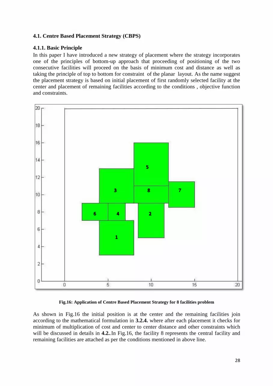
28

4.1. Centre Based Placement Strategy (CBPS)

4.1.1. Basic Principle In this paper I have introduced a new strategy of placement where the strategy incorporates one of the principles of bottom-up approach that proceeding of positioning of the two consecutive facilities will proceed on the basis of minimum cost and distance as well as taking the principle of top to bottom for constraint of the planar layout. As the name suggest the placement strategy is based on initial placement of first randomly selected facility at the center and placement of remaining facilities according to the conditions , objective function and constraints.

Fig.16: Application of Centre Based Placement Strategy for 8 facilities problem As shown in Fig.16 the initial position is at the center and the remaining facilities join according to the mathematical formulation in 3.2.4. where after each placement it checks for minimum of multiplication of cost and center to center distance and other constraints which will be discussed in details in 4.2..In Fig.16, the facility 8 represents the central facility and remaining facilities are attached as per the conditions mentioned in above line.

29

4.2. CBPS: Steps followed: : : 1 r e

Until nth facility YES : e m e e .

The strategy of placement is described in as following:

Step-1: Before any placement procedure start to place the whole planar site where the whole facilities are to be placed. As shown in Fig.18 Step-2: Generate a random order of n number of facilities should be placed step by step. For example, for facilities of 10 given as: 1 2 3 4 5 6 7 8 910

It can be randomly arranged as:

8 5 4 2 7 3 10 1 9 6

In this paper I am applying the CBPS, for 8 11 and 20 UA-SFLP problem as used in Asl &Wong (2015)[137] .As per [137] for 8,11 and department problem the initial condition of the facility can be shown as in Fig.24, Fig.25 and Fig.26. without orientation or rotation

Step-3: After the generation of order of facilities the orientation of the facilities are changed based on the principle as explained in 3.2.2. where a binary form of numbers are generated as for the above example say for 10 facilities as: ri =1 0 0 0 1 0 0 0 0 1 In this ri is the rotation or orientation vector which rotate the width with height when it and

vice versa is ‘1’ i.e., orientation changes by 90̊

and the orientation does not change when it is ‘0’. As explained in Fig.19, the maroon facility

is the facility to be placed and green one is placed facility.

Step-4: After the random generation we place the first facility which is generated after the random generation as per the example stated it will be 8. As shown in Fig. 20 here the facility at the center is the first one.

Place the layout of the planar Layout site

Generate random order of facilities

Place the 1st facility at the centre based on random

generation and orientation order

Start

Generate the random order of rotation or orientation ri

Check if

1. 𝒎𝒊𝒏 ∑ ∑𝑵𝒋=𝟏

𝑵𝒊=𝟏 Cij dij

and 2. ∑ ∑𝑵

𝒋=𝟏𝑵𝒊=𝟏 Aij=0

and 3. Xmax-Xmin ≤ W

Ymax-Ymin ≤ H

Place the consecutive facility

End

Fig. 17: Basic flow chart of basic CBPS

Discretisation

30

Fig.18: Planar site layout Placement

Fig.19: When the rotation vector is applied to the facility to be placed on the placed facility

90̊ rotation when . ri=1 on placed facility

Step-5: In this step the facility checks for discretized positions which are created (discussed in 4.3.) where the facilities will be checked for the condition of placement as explained in Step-6. Step-6: As shown in Fig.17, after each placement of the facility, the next facility checks following conditions in all the discreet positions: 1. To check where the minimum of product of cost around each facility and center to center distance i.e, 𝑚𝑖𝑛 ∑ ∑𝑁

𝑗=1𝑁𝑖=1 Cij dij

as show in Fig.17.

2. To check for overlapping of ith facility on the jth facility for overlapping, as overlapping is undesirable for placement. Here, the jth facilities are the placed facilities (here all the placed facilities are checked) and ith facility is the facility which is to be placed on. The overlapping has three cases: a) The overlapping of one facility which is

to be placed with the facility where to be placed as shown in Fig.21.In Fig.21, the center facility is the facility where to be placed. The black shade represents the undesirable overlapping between where to be placed facility with which is to be placed.

b) The overlapping of the facility to be placed to the other entire facilities except where to be placed facility as shown in Fig.22. In this Fig.22, the maroon facility and the white facility represents the facility where to be placed and green represents all the other remaining facilities .The blue shade represents undesirable overlapping between facilities to be placed to the other entire facility except where to be placed facility.

c) The overlapping of all the facilities with each other as shown in Fig.23.In Fig.23 pink color shade represents overlap.

3. To check the constraint of boundary of the planar site for width ‘W’ and height ‘H’ as shown in Fig.17 and Fig.18. It is the condition (as explained in equation (27)) so

H

w

Fig.20: The first facility from random order at the center

31

that, the placement of the facilities (or department ) do not cross the given boundary of planar site to have the best positioning with of the facilities with lowest material flow cost. Step-7: After checking all the conditions in Step-3 the facility is placed based on the best position. At each step the new facility checks for best position at all the facility placed based on the condition on Step-3 which places all the facilities step by step on the basis of the order as explained in Step-2. After placement of the last facility or the facility the whole placement stops and look like Fig.17. which is a 8 facility problem [137].

Fig.21: Undesirable overlapping of the where to be placed facility with facility to be placed

Fig.22: Undesirable overlapping of facilities which is to be placed with the other except where to be

placed

Fig.23: Undesirable overlapping of facilities which is to be placed with all the other facilities

32

Fig. 24: Initial order and size of facilities for 8 facilities [137]

33

Fig. 25: Initial order and size of facilities for 11 facilities [137]

34

Fig. 26: Initial order and size of facilities for 20 facilities [137]

35

4.3. CBPS: The Methods of Placement: In this paper two methods have been developed have been developed which only differ only by discretized placement strategy. Before understanding the methodology which has been developed let us start with understanding of discretized placement strategy. Discretized placement strategy is the type of strategy where we interpolate the possible positions of consecutive facilities based on different methodology two of these methodologies have been developed by me .As shown in the Fig.27,the blue dots represents the discretized position possible for the dotted facility at the green facility . The best position is chosen based on the conditions mentioned in 4.2. (Step-5) .In this paper, I have developed two kinds of methods one which based mainly on discretization of the corner points and other is based on corner as well as mid-point but also with biased overlapping constraint strategy of the placed facility which will be discussed 4.3.1 and 4.3.2..However, based on result the second method is better than the first one which will be discussed in CHAPTER 5.

Fig.27: Discretised placement methodology

In 4.2. I have described the basic steps which are followed in the CBPS, but the details description of all the steps with discretization and utilization of the condition was not discussed in details in 4.3.1. and 4.3.2. .In the following paper I will be applying CBPS in unequal area problem used in by Asl & Wong et al. 2015[137] in this two section we will only discuss the methodology not the results which will be discussed in CHAPTER 5.

4.3.1. CBPS: Corner Points Method (1st discretized placement Method developed):

In this section, I will discuss the first methodology of CBPS with discretization which was first developed based on corner points and why there was the need of new methodology. In this discretization technique, we consider discretization of 64 positions with combined checking of overlapping (all the 3 cases explained in 4.2. Step-6 at 2.) and minimization of product of cost and distance( as explained in 4.2. Step-6 at 1. and 26) before each placement of the facility. If among the conditions of overlapping and minimum cost is satisfied then the facility is placed. Before checking 64 positions 8 points of the facility is generated which is placed as shown in Fig.28. These 8 points are corner and mid points of each side of the facility as shown in Fig.28.These 64 positions are based on corner points of the rectangle. 32

36

of these positions are positive and negative position of each corner and mid-point as show in Fig. 29.

Fig.28: Corner and mid-point of a facility after the generation of points

Fig.29: Interpolated positive-negative with respect to corner points of a facility be placed on placed facility (green facility)using Corner Point Method In Fig.29, light blue point represents the possible interpolated corner points of the facility to be placed on green facility. Remaining 32 positions are the possible positions of mid-points of facilities as shown in Fig.30.

Fig.30: Interpolated positive-negative positions with respect to mid-points of a facility to be placed on placed

facility (green facility)

37

In Fig.30 the big blue point represents the mid-points of side of placement of dotted facility (as well as mid-point and corner points of the green facility) and small light blue points represent the corner point of the dotted facility. After application of the constraints of the overlapping (all the 3 cases explained in 4.2. Step-6 at 2.) around 32 of the possible position are removed (if we see carefully in Fig.29 we can see 12 are removed and in Fig.30 there 20 are removed from interpolation of possible positions). The Matlab code for this algorithm can be shown in APPENDIX A. It has been known by analyzing the result which has been discussed in CHAPTER 5 the computational time increases for calculating for the same problem and solving method, as at each placement a facility has to go extra 32 interpolation check with help of condition of 𝑚𝑖𝑛 ∑ ∑𝑁

𝑗=1𝑁𝑖=1 Cij dij (as explained in Step-6 and equation (26)). This is the reason a new

method has been developed so that the extra computational time can be saved with better result.

4.3.2. CBPS: Selective Sequential Method (2nd discretized placement Method developed)

As discussed earlier in 4.3.1. we need a method where we can check only 32 locations compared to 64 location in Corner Point Method (explained in 4.2.) so to achieve this I have developed a Selective Sequential Method. In this method before each placement of facility it generates 8 points as explained in 4.3.2. and Fig.28 after generation of these points we go for interpolating the positions of the facilities to be placed on the placed facility for 32 cases. Out of these 32 cases of interpolation of 20 positions of which are interpolated on the basis of corner point as shown in Fig.31., where the overlapping positions as shown in Fig.29 are avoided and similarly if we compare Fig. 30 and Fig. 32.

Fig.31: Interpolated positive-negative with respect to corner points of a facility be placed on placed facility (green facility) using selective sequential method In Fig.31, the small blue point represents the corner point of the dotted facility which is to be placed on the green facility. Out of 32, 12 of the interpolating positions are based on mid-points as shown in Fig. 32. In Fig. 32, the big blue point represents the mid-points of side of placement of dotted facility.

38

In this method, to avoid the checking of overlapping position and checking the 32 position as shown in Fig.31 and Fig.32, the sequence of applying condition is changed. In this method, before each placement the facility to be placed we not only interpolate the 32 positions but we introduce a sequence operation of first start with overlapping then check for cost calculation thus the flow chart of Fig.17. from discretization to end changes into the one as explained in Fig. 34.Moreover, during the overlapping checking condition by the facility to be placed on the placed facility follows the case b) and case c) but not case a) explained in Step-6 of 4.2. also, explained in Fig.22, Fig. 23, and Fig. 33.The reason for not checking case a) is because of the fact that, the possible placement avoids the intersection as shown in Fig. 31 and Fig.32.In Fig.33, 2 represents facility after placement and 1 represents the checking of overlapping condition of the facility following case b). Hence, the overlapping for the facility to be placed on the facility where to be placed is not checked during placement. This, is also one of the reason the computational time is reduced which will be discussed in CHAPTER 5. The code for this method is shown in APPENDIX B

Fig.32: Interpolated positive-negative with respect to mid-points of a facility to be placed on placed facility (green facility) based on Selective Sequential Method

Fig.33: Checking of overlapping of facility to be placed using case b) and facility to be placed when placed on where to be placed facility

39

YES

YES

Until nth facility YES

if

𝒎𝒊𝒏 ∑ ∑𝑵𝒋=𝟏

𝑵𝒊=𝟏 Cij dij

Discretisation

if

Xmax-Xmin ≤ W

Ymax-Ymin ≤ H

if Aij=0 For Case b) &Case c)

End

Fig. 34: Flow chart for application of condition in CBPS: Selective Sequential Method

Place the consecutive facility

40

4.4. Solving Algorithm: Local search Algorithm

In CBPS we can get quasi-optimized result which is based on the random order of the facilities or department to be placed in a given planar site. We need a solving algorithm which gets the best result and thus, gives a best solution. So, to optimize the best result which is the I use local search technique. In this technique number of random search is initiated at first followed by a condition to get the best result. Total material flow Cost and the final layout after placement of all the facilities is the final result we require. Thus, by best result I mean the lowest Total material flow Cost and the layout design at this lowest Total material flow Cost. To achieve the lowest Total material flow Cost by local search technique I have used the condition:

Total material flow Cost<Previous best result

The algorithm for this technique is shown in Fig.35. As shown in Fig.35, the technique starts with the given size of iteration the at each iteration the algorithm tacks the result from the CBPS to pick the best result (i.e. the Total material flow Cost) from previous random search at each iteration and it goes on until reaching the limit of search. The code of CBPS integrated with this solving algorithm using selective sequential method can be seen in APPENDIX C for calculating all the problems. In this paper I use strictly less than as the condition for the best result which will be explained in 4.4.1. NO Fig.35: Flow chart of local search algorithm integrated with CBPS

Start

Random search

if Total Cost

<best

YES

if No. of

Iteration <=N

YES

Pick the best result after each iteration

Display the best result out of N

iterations and plot the layout

CBPS

End

41

4.4.1. Impact of strictly less than on the result in Local Search Algorithm

For an iteration using CBPS if we check for the value less than equal to say ‘C’ from the

previous iterations. In this case, if the value is exactly equal to C it will pick the value C rather than the value less than C and thus, better solution can be lost. As shown in Fig.36, maroon color facility at position 1 represents the condition when in the local search algorithm if the condition given is strictly less than and white color facility at position 2. Both the maroon and white facilities are the same facility but with different positions 1 and 2. The basic difference between both the conditions is the applicability of the algorithm. The applicability of strictly less than is that, when the result from the previous iterations and the current iteration are same. In this case algorithm goes to next iteration until finds the lower value. While, in case of less than and equal to case the algorithm takes any random position out of the two iteration as both are having same result. So, sometimes good results can be lost due to this. Although we can get similar results in both the conditions but if the case of similar results occurs as explained above the, best optimum solution can be lost. Hence, due to these reasons strictly less than is used for local search algorithm for solving CBPS in this paper.

Fig.36: Effect of strictly less than in Local Search Algorithm

42

CHAPTER5: Application of CBPS on UA-SFLP, Results & Analysis

5.1. Problem description of UA-SFLP: The problem used for applying the CBPS consist of three problem instances as follows: 8 facilities, 11 facilities, and 20 facilities which were taken from Asl and Wong et al. (2015) [137]. All of these problems are of type Unequal Area Static Facility Layout Problem (as discussed in 1.2.).

5.1.1. Problem data:

In this problem we have following data given: 1. Condition of boundary:

a. For 8 facilities(or departments) problem the planar site size is of: Width (W) =12

Height (H) =12 b. For 11 facilities problem the planar site size is of:

Width (W) =15 Height (H) =15

c. For 20 facilities problem the planar site size is of: Width (W) =14

Height (H) =14 2. The initial width and height data with order (also shown in Fig. 24,25 and 26) :

a. For 8 facilities problem width(w) and height(h) matrix and order : order

[w h]= 2 3 1 4 5 2 2 2 3 3 3 4 2 4 5 4 4 6 4 4 7 3 4 8 b. For 11 facilities problem w and h matrix and order :

order [w h]= 4 4 1 1 2 2 1 2 3 2 5 4 3 2 5 1.4 4 6 4 3 7 2.6 2 8 4 2.8 9 4 7 10 5 5 11

43

c. For 20 facilities problem w and h matrix and order : order [w h]= 1 2 1 2 2 2 1 1 3 2 3 4 3 3 5 2 2 6 2 1 7 2 3 8 3 2 9 3 3 10 2 3 11 1 2 12 3 2 13 3 3 14

3 3 15 2 2 16 3 2 17

2 2 18 2 2 19 2 1 20

3. Cost rate matrix i.e.,∑ ∑𝑵

𝒋=𝟏𝑵𝒊=𝟏 Cij (where here i and j represents the row and column

position in the matrix and N is number of facilities) as explained in CHAPTER 3(3.2.1.): a. For 8 facilities problem: Cij = 0 1 2 0 0 0 2 0 0 0 4 3 6 0 0 2 0 0 0 2 0 3 1 0 0 0 0 0 5 2 0 2 0 0 0 0 0 0 0 4 0 0 0 0 0 0 4 0 0 0 0 0 0 0 0 1 0 0 0 0 0 0 0 0 b. For 11 facilities problem:

Cij = 0 2 1 1 2 6 2 6 6 3 6 0 0 1 1 2 6 4 6 6 3 6 0 0 0 2 2 6 1 6 6 6 6 0 0 0 0 1 5 1 6 6 3 6 0 0 0 0 0 4 3 6 4 5 6 0 0 0 0 0 0 3 6 4 5 6 0 0 0 0 0 0 0 4 4 1 1 0 0 0 0 0 0 0 0 6 3 3 0 0 0 0 0 0 0 0 0 5 5 0 0 0 0 0 0 0 0 0 0 2 0 0 0 0 0 0 0 0 0 0 0

44

c. For 20 facilities problem: Cij = 0 3 0 0 4 2 0 0 4 0 0 5 3 0 5 0 0 1 0 0 3 0 1 0 1 2 5 0 3 0 0 0 2 0 3 0 3 1 2 3 0 1 0 4 0 0 3 0 0 0 1 0 0 0 0 0 5 0 2 3 0 0 4 0 4 0 0 1 5 3 0 2 0 0 4 5 0 1 0 0 4 1 0 4 0 0 0 0 1 4 1 5 0 0 3 2 0 5 0 4 2 2 0 0 0 0 3 0 0 5 0 0 3 0 0 0 2 0 0 0 0 5 3 0 0 3 0 0 0 0 0 0 4 0 2 0 3 2 0 1 0 0 0 1 0 0 0 0 0 0 2 0 0 5 0 4 0 1 0 0 4 3 0 5 1 0 0 0 0 3 0 5 0 0 0 2 0 0 0 0 0 0 0 3 4 5 0 0 3 0 0 5 0 1 2 4 0 3 4 0 0 0 1 0 1 0 0 2 0 0 0 0 0 5 5 4 0 4 3 1 5 0 0 2 5 0 0 0 5 5 0 0 5 0 2 0 0 1 0 0 3 2 0 0 0 3 4 0 0 0 0 5 0 0 3 0 2 0 0 0 0 0 0 0 0 0 0 5 0 1 5 0 0 0 0 5 0 5 1 0 5 3 0 4 3 0 2 0 0 2 5 2 3 0 0 0 1 4 3 3 0 0 0 5 2 0 0 4 2 4 4 0 0 5 0 0 4 5 0 0 0 3 5 0 0 2 3 0 0 0 0 0 2 0 1 4 0 0 1 5 1 1 0 1 5 0 2 1 0 3 4 1 0 5 4 5 0 0 4 1 0 2 2 0 0 0 0 0 0 4 3 0 0 1 3 0 1 4 0 5 0 3 3 0 4 0 1 0 0 0 1 0 0 0 3 0 5 1 5 0

After application of random order the cost rate matrix changes according to the random order when CBPS is applied as shown in APPENDIX A, B, and C.

5.1.2. Objective of the problem

The objectives of the problem can be given as: 1. To optimize the facility layout for lowest total material handling cost flow for the

given data of 8Facilities, 11 Facilities, and 20Facilities. 2. To place all the facilities within the given boundary as shown in 5.1.1. in 1. As there are boundary conditions which should be satisfied for this problem I have used the equation (27) to fulfill this condition while applying the CBPS as also explained in 4.2. at Step-6 in 3., hence this problem can be categorize as Robust layout problem as explained in 1.2.

5.2. Comparisons of results Before comparing the data and results I have compared the results for 8 facilities to check the followings in each case to check the following: 1. Time taken to run each method 2. The total cost obtained in each method If any of this conditions is not comparatively to the previous one then the next one the remaining analysis is not preferred for the 11 facilities and 20 facilities. In this section I will give the comparison two CBPS Methods are compared and the reason for choosing the selective sequential method, also I have discussed the results of the 11 facilities and 20 facilities of CBPS and compared with the results of Asl &Wong et al. (2015)[137] . Moreover, this problem as explained in 5.1. is used for solving using genetic algorithm and gradient based method and then compared the results with the CBPS method.

45

5.2.1. Comparison of different CBPS methods (Selective sequential method Vs Corner point method)

As explained in 4.3., especially in case of 4.3.2. the algorithm of Selective sequential method was developed with sole cause of reducing computational time. As we can see by the Table-1, 30% of the computational time is reduced by applying Selective sequential method compared to the Corner points method. Not only it reduces the computational time but, also gives better result and thus, decreases the average total material flow cost by 13.5% .If we see the graph for Selective sequential method and Corner points method between total material flow cost and time to solve for particular same number of iteration as shown in Fig.37, we can be see the difference of rate reduction in total material flow cost with time for both the methods. As shown in Fig.37, we can see the rate of decrement of total material cost is not rapid in case of Selective sequential method compared to Corner points method. Moreover, the best result for Selective sequential method by using local search algorithm (as explained in 4.4. ) is total material flow cost 192 compared with Corner points method it is 210 with a significant difference of 18 and computational time decrease of 30%. If we see the Table 2, and Table 3 we can see the layout designs, corner coordinates and orientation (as explained in 3.2. 2. and 4.2. at Step-3)at the given number of iterations of local search algorithm for Selective sequential method and Corner points method. It can be seen all the results are in a given boundary condition limit of 12 as explained in 5.1.1. and using the mathematical expression as explained in 3.2.5..However, it can be argued that though we can say our result for our best optimized result is not the best for a designer because, various prospect of design is considered before selecting a layout design except the precondition given in the problem(as explained in 5.1.1.). So, by these kinds of tables a designer can pick not only the best solution but, the result that suits a designer the best. Hence, based on the parameters of results we can conclude among these two method developed based on CBPS (as explained in CHAPTER 4) the best method will be selective sequential method so, in the remaining sections in this chapter I will be using Selective sequential method for further discussions to compare CBPS with other methods and for future research also, I will prefer to use the Selective sequential method. In this section, I have not comparisons the results with 11 facilities and 20 facilities as it is quiet understood that if the number of facilities increases so the complexity thus, the computational time. Also, as for Corner points method to solve the problem of 8 facilities problem is more compared to Selective sequential method as explained above so, we do not require to solve for remaining 11facilities and 20 Facilities problems.

46

Fig.37: The comparison of corner point method with selective sequential method for total cost Vs time

NO. of iterations

Total Cost

Time (Sec)

Total Cost

Time (Sec)

146 229 33,75sec 193.5 15.8

1870 218 451.24sec 193 313

11327 210 2702.27 192 1888.3

Table 1: Data of Corner point method and selective sequential method at the given number of iteration for 8 facility problem

190

195

200

205

210

215

220

225

230

235

0 5 10 15 20

Tota

l co

st

Time(Sec)

Corner Point Methodwith local searchmethod[8Blocks]

Selective sequentialMethod with local searchmethod(New)[8Blocks]

47

Total Cost

Facility order placement

7 4 8 3 1 5 2 6

218

Corner co-ordinate 4 5 4 8 3 8 10 8

x y 4 1 -2 2 1 -2 -1 4

Orientation(ri) 0 0 1 0 0 0 1 1

Total Cost

Facility order placement

8 7 6 5 2 1 3 4

229

Corner co-ordinate 4 4 8 4 3 2 8 8

x y 4.5 0.5 0.5 7.5 9. 5 4.5 5.5 8

Orientation(ri) 0 1 0 1 1 1 0 1

(Xmax-Xmin)

(Ymax-Ymin)

10 12

Total Cost

Facility order placement

2 5 4 3 6 1 7 8

210

Corner co-ordinate 4 4 4.5 8 7.5 8 10 0

x y 3.5 1.5 -1.5 1.5 -2.5 3.5 1.5 1

Orientation(ri) 0 0 1 1 1 1 0 1

(Xmax-Xmin)

(Ymax-Ymin)

12 10

(Xmax-Xmin)

(Ymax-Ymin)

12 11.5

Total Cost

Cor

ner

Poi

nts

Met

hod

Table2: CBPS -Corner points method data for 8 facilities (placement order, co-ordinates, orientation, & Layout)

48

Total Cost

Facilities’ order of placement

5 2 3 6 7 4 8 1

193

Corner co-ordinates 4 4 8 10 10 8 4 8 x

y 5 0 1.5 0.5 -3.5 4.5 7 -1.5 Orientation(ri) 0 0 1 0 0 0 1 1

193.5

Facilities’ order of placement

5 8 4 6 3 2 1 7

Corner co-ordinates: x 5 2 7 10 8 4 8 10

y 4 4 4.5 4 2.5 -1 -0.5 0 Orientation(ri) 0 0 0 1 0 1 0 1

(Xmax-Xmin)

(Ymax-Ymin)

12 9

Total Cost

Facilities’ order of placement

5 2 8 4 6 3 7 1

192

Corner co-ordinates 4 3.5 4 1 -3 1.5 -3 1.5

x y 5 1 7 5 4.5 3 0.5 0

Orientation(ri) 1 1 1 1 0 1 0 0

(Xmax-Xmin)

(Ymax-Ymin)

10 11.5

(Xmax-Xmin)

(Ymax-Ymin)

11 10

Sele

ctiv

e Se

quen

tial

Met

hod

Table3: CBPS-Selective sequential method data (order, co-ordinates, orientation, & Layout)

Total Cost

49

5.2.2. Comparison of results CBPS with PSO method developed by Asl &Wong (2015)

In this section I will discuss the best results of 8 facilities, 11 facilities, and 20 facilities problem of CBPS method and then compare the best results of all with PSO method of Asl & Wong (2015) [137] . If we see Table-4, which shows the 3 best results found for all the three cases of 8 facilities, 11 facilities, and 20 facilities problems. If we see Fig.38, and Fig.39 we find a gradual decreasing curve with respect to time for 8 facilities and 11 facilities but, if we see Fig.40 the curve is literally not visible in case 20 after getting the solution of 1251 in 297 seconds the next best comes after approximately 1.5 days i.e., 129651 seconds that is the reason why in Fig.40 the curve looks flat as next best results comes after such a long period.

No. of Facilities

No. of Iterations

Total Cost

Time (sec)

8 Facilities

146 193.5 15.8

1870 193 313

11327 192 1888.3

11 Facilities

382 1282 121

1481 1263 458

3452 1253 1067

20 Facilities

136 1256 182

192 1251 297

51576 1197.5 129651

Table-4: 3 Best results and the time to reach that result for CBPS method for each of the three problems

Fig.38: CBPS with Local Search Algorithm for 8 Facilities

191

192

193

194

0 1000 2000

Tota

l Co

st

Time (Sec)

CBPS with local search Algorithm[8Facilities]

CBPS with localsearchAlgorithm[8Blocks]

Total Cost

193.5

Facilities’ order of placement

5 8 4 6 3 2 1 7

Corner co-ordinates: x 5 2 7 10 8 4 8 10

y 4 4 4.5 4 2.5 -1 -0.5 0 Orientation(ri) 0 0 0 1 0 1 0 1

Total Cost

50

Fig.39: CBPS with Local Search Algorithm for 11 Facilities

Fig.40: CBPS with Local Search Algorithm for 20 Facilities

In Table-3, Table-5 and Table-6, we see the data of best 3 solutions of CBPS with local search algorithm for each 8 facilities, 11 facilities and 20 facilities problem, which contains the left corner coordinates of facilities, the orientation (as explained in 3.2. 2. and 4.2. at Step-3),and the order of placement of facilities. It can be seen all the results of 8 facilities, 11 facilities and 20 facilities problem are in a given boundary condition limit of 12,15,and 14 as explained in 5.1.1. and using the mathematical expression as explained in 3.2.5. By these tables a designer can compare the best design as per his or her own criteria as explained in 5.2.1. (paragraph 2).

1250

1255

1260

1265

1270

1275

1280

1285

0 500 1000 1500

Titr

e d

e l'

axe

Titre de l'axe

CBPS with local search Algorithm [11Facilities]

CBPS with localsearchAlgorithm(New)[11Blocks]

0

0,2

0,4

0,6

0,8

1

0 50000 100000 150000

CBPS with local search Algorithm

[20 Facilities]

CBPS with localsearchAlgorithm(New)[20 Blocks]

51

Total Cost

Facilities’ order of placement

6 3 11 8 5 2 1 10 4 9 7

1262.8

Corner co-ordinates 5 7 5 8 5 7 10 1 5.5 10.6 6 x y 6.8 8.2 1.8 8.2 8.2 10.8 5.5 6.2 11.8 9.5 13.8

Orientation(ri) 1 0 1 1 1 1 1 0 1 1 0

Total Cost

Facilities’ order of placement

2 5 6 3 11 8 9 4 1 10 7

1282.3

Corner co-ordinates x 6.5 6.5 5 7 5 4.4 3.7

8 0.4 4 8.5

y 7 4 8.5 9.4 11.4 9.4 4 9.4 8.4 0 4

Orientation(ri) 1 1 1 0 0 0 1 1 1 1 1 (Xmax-Xmin)

(Ymax-Ymin)

12.6 14.4

Total Cost

Facilities’ order of placement

8 5 2 3 9 11 6 10 4 7 1

1253

Corner co-ordinates 6.5 8.5 5.5 4.5 1.7 4.5 4.5 10.5 4.5 -1.3 0.5 x y 6.2 6 6.5 6.5 5.5 1 9 4 10.4 5.5 1.5

Orientation(ri) 1 1 0 0 1 0 1 0 1 1 1

(Xmax-Xmin)

(Ymax-Ymin)

13 15

(Xmax-Xmin)

(Ymax-Ymin)

14.5 11.4

14

Table5: Application of CBPS on 11 Facilities (placement order, co-ordinates, orientation, & Layout)

52

Total Cost

Facilities’ order of

placement 11 15 1 6 2 3 13 20 12 9 16 19 14 8 7 4 18 17 10 5

1256

Corner co-ordinates 6 3 6 3.5 1 5 -2 3 1 0.5 6 3.5 8 8 -1 3.5 6 0.5 0.5 3.5

x y 5.5 5.5 1 8.5 4 4.5 5.5 4.5 8 9 8.5 2.5 5.5 8.5 4.5 8.5 3.5 2 11 11.5

Orientation(ri) 0 0 0 0 1 0 1 0 1 0 0 0 0 0 0 0 1 0 0 0

(Xmax-Xmin)

(Ymax-Ymin)

13 12.5

Total Cost

Facilities’ order of

placement 13 15 3 1 2 17 9 20 7 10 6 5 18 11 14 8 4 16 12 19

1251

Corner co-ordinates 6 3 5 3.5 5.5 6 3.5 4 8 0.5 7.5 0 2 3 0 -2 -2 0 1.5 6

x y 5.5 5.5 4.5 8.5 8.5 3.5 9.5 3.5 6.5 9.5 8.5 5.5 3.5 1.5 0.5 0.5 5.5 3.5 8.5 1.5

Orientation(ri) 1 1 0 1 1 0 1 0 0 0 0 1 1 1 0 0 0 1 1 0

(Xmax-Xmin)

(Ymax-Ymin)

12 12

Total Cost

Facilities’ order of placement

19 20 18 14 5 11 2 12 4 7 6 10 16 15 1 13 3 9 8 17

1197.5

Corner co-ordinates 6 6 4 3.5 3 6.5 6 3.5 1 6 6 3 2 8 8 9 8 1 0.5 9

x y 6 5 6 8 3 8 3 2 3 2 0 -1 6 3 1 0 6 0 8.5 6

Orientation(ri) 0 0 0 0 1 0 0 1 0 0 1 1 1 0 0 1 0 1 1 1

(Xmax-Xmin)

(Ymax-Ymin)

11 11.4

Table6: Application of CBPS on 20 Facilities (placement order, co-ordinates, orientation, & Layout)

53

In this paper I have used Matlab to develop and solve all the problems of 8 facilities, 11facilities and 20facilities. The computer of following specification used: an Intel Xenon E3-1240 CPU of 3.4GHz and 16GB RAM. Let's compare the best results of all the 3 cases by using CBPS and PSO or Particle Swarm Optimization method (Asl & Wong (2015) [137]). Before going further let’s understand basic principle of Particle Swarm Optimization. PSO is based on social behavior of animal which if mathematically formulated is a meta-heuristic form of algorithm. In this method, at each iteration the velocity behavior of the particle is checked at each iteration for a mathematical expression used to control flow and direction of algorithm. In case of UA-SFLP proposed by Asl & Wong (2015) [137] the boundary condition (using the equations as explained in 3.2.2. and 3.2.5.)is taken into consideration at each iteration along with random orientation of facility taken into consideration at each iteration instead of velocity. Also, instead of particles position of facilities is used.

NO. of Facilities

Best results of PSO

Time takena*

Similar results with CBPS

Time takenb**

Best results of

CBPS

Time takenc***

8 Facilities 193.75 220.7 193.5 15.8 192 1888.3

11 Facilities 1286.1 888.3 1282.3 120.63 1253 1067.2

20Facilities 1206.65 2352 1251 182 1197.5 129651

Table-7: Comparison of best results of CBPS and PSO [137] w.r.t. Cost Vs time

a) Best result of UA-SFLP 8Facilities b) Similar result using CBPS of UA-SFLP 8Facilities by PSO[137]

c) Best result of UA-SFLP for 8Facilities by CBPS

Fig.41: Comparison of layouts for best solutions of CBPS with best results of PSO [137] for 8 facilities

*Time takena –Time taken by best results of PSO

**Time takenb-Time taken by similar results of CBPS *** Time takenc- Time taken by best results of CBPS

54

Table-8: Orientation and center coordinates of best result obtained for 8 Facilities by PSO [137]

In Table-6, if I compare the best results of PSO [137] with similar result obtain from CBPS with the help of local search algorithm there is a significant difference in the result obtained with respect to computational time. In case of 8 facilities problem if we compare PSO[137] with the similar result of CBPS for 8 facilities there is a 92.8% of difference in computational time if we see Table-6.For more better result for 8 Facilities case it takes significant time of 1888.3 seconds to get the best solution 192 which decreases the material handling cost by around 0.9% compare to PSO [137].The comparison of optimized layout design for best solutions of CBPS with best results of PSO [137] for 8 facilities is shown in Fig.41.If we observe the result obtained for both the best results for 8Facilities using CBPS and PSO[137] we can find there is a similarity in appearance although there are some difference and moreover we can see the impact of orientation difference(as shown in Table-3 and Table-8). But, there is no significant similarity for similar result obtained from CBPS to PSO [137].

a) Best result of UA-SFLP 11 Facilities b) Similar result using CBPS of UA-SFLP 11 Facilities by PSO[137]

c) Best result of UA-SFLP for 11 Facilities by CBPS

In Table-7, in case of 11 facilities problem if we compare PSO [137] with the similar result of CBPS for 11 facilities there is 86.4% of difference in computational time. For better result for 11 Facilities case it takes significant time of 1067.2 seconds to get the best solution 1253 which decreases the material handling cost by around 2.5%.The comparison of optimized

Facilities 1 2 3 4 5 6 7 8 Center co-ordinates

5.8198 2.3152 5.8197 5.8161 2.3160 9.3163 9.3199 2.3160 x y 9.5878 7.7533 7.5874 4.3512 4.2532 5.5626 9.5628 1.7529

Orientation(ri) 1 0 0 0 1 1 0 1

Fig.42: Comparison of layouts for best solutions of CBPS with best results of PSO [137] for 11 facilities

55

layout design for best solutions of CBPS with best results of PSO [137] for 11 facilities is shown in Fig.42.

Facilities 1 2 3 4 5 6 7 8 9 10 11 Center co-ordinates 2 6 .45 6 .41 8 .48 8.94 6.51 5.48 6.14 3.44 12.46 6.5 x

y 4 .48 9 .92 6 .91 10 .92 7.41 5.70 11.98 8.41 8.48 7.36 2.5 Orientation(ri) 0 1 1 0 0 1 0 0 1 0 1

Table-9: Orientation and center coordinates of best result obtained for 11 Facilities by PSO [137]

If we observe the result obtained for both the best results for 11Facilities using CBPS and PSO [137] we can find there is no similarity in all the three cases shown in Fig. 42 .Moreover, if we see the layout design of best result of PSO [137] and similar result obtained for 11 facilities problem by CBPS we can't find any pattern. However in best result CBPS we observe carefully all the smaller facilities are towards the center and bigger facilities outwards the center. Table-9 shows the orientation of 11 facilities by PSO [137]

a) Best result of UA-SFLP 20 Facilities b) Similar result using CBPS of UA-SFLP 20 Facilities by PSO[137]

c) Best result of UA-SFLP for 20 Facilities by CBPS

In Table-7, in case of 20 facilities problem if we compare PSO [137] with the similar result of CBPS for 20 facilities there is a 92.2% of difference in computational time. For better result for 20 Facilities case it takes significant time of 129651seconds to get the best solution 1197.5 which decreases the material handling cost by around 0.7%.The comparison of optimized layout design for best solutions of CBPS with best results of PSO [137] for 20 facilities is shown in Fig.43. If we observe the result obtained for both the best results for 20 Facilities using CBPS and PSO [137] we can find that there is no similarities found in all the three cases except the fact lower the value of material flow cost more compact the layout design becomes as in Fig. 43 c) we can see the compactness compared to the best result solved by PSO [137] as shown in Fig.43a).

Fig.43: Comparison of layouts for best solutions of CBPS with best results of PSO [137] for 20 facilites.

56

Table-10: Orientation and center coordinates of best result obtained for 20 Facilities by PSO [137]

5.2.3. Comparison of results CBPS with other standard algorithms

In this section, I will discuss the other standard algorithm used and compare their best results with CBPS .In this section I will discuss the results of Gradient based algorithm and Genetic Algorithm to solve the whole problem. Both the algorithm was developed by team of two Prof. Fouad Bennis and Ranjan Hasda( IRCCyN, PhD, 2013-16). The purpose was to check the feasibility of algorithms to solve this problem and to compare the best results of 8 facility problem with CBPS first and then go further if result are better than present method of CBPS. Let’s understand first gradient method and then genetic algorithm along with comparison of best results to that of CBPS.

5.2.3.1. Gradient based method, application on UA-SFLP and comparison of results with that of CBPS. The gradient based method is based on basic principle of gradient based minimization or of given functional objective followed with a given list of constraints to control the flow of optimization. Till a feasible solution is reached the optimization continues. Mathematically, for an objective function f(x) the gradient problem can be defined by: ∃ x*s.t F(x*)= minF(x )

∀ minF(x ) exist if 𝜕𝐹

𝜕𝑥=0 and

𝜕𝐹

𝜕𝑥 >0 exists &

∃ g(x)≤ 0 and h(x)=0 (28) Where x* is the value at which feasible solution exist and g(x) and h(x) are constraint functions needs to satisfy it. The h(x) is called active constraints while, g(x) non-active constraints, the selection depends of the type depends upon the problem. During optimization these conditions are checked at each iteration and if all of these conditions are satisfied is found then the feasible solution is displayed and it shows all the feasible solution in a given space. The Fig.44a) and 44b) describes the convergence of solution towards feasible solution.

a) 3D convergence of objective function b) 2D convergence of objective function [142]

Fig.44: Convergence of objective function for feasible solution

Facilities 1 2 3 4 5 6 7 8 9 10 11 12 13 14 15 16 17 18 19 20

Corner co-ordinates 1.96 4.63 7.03 4.5 1.5 4.6 6.66 9.6 2 4.56 9.1 2 2 11.6 4.5 7.1 7.1 7.1 7.1 7

x

y 4.5 3.03 4.73 11.06 7.5 1 3.43 11.5 10.5 8.54 9 5.5 2.8 1.5 5.5 11.5 2 9.2 7.2 5.7

Orientation(ri) 1 0 0 1 1 0 0 1 1 0 0 1 0 1 0 0 0 1 0 0

2

2

h(x)=0

57

Now in this paper, the problem for UA-SFLP will become as: 1. Objective function: F(x*)= minF(x)= 𝑚𝑖𝑛 ∑ ∑𝑁

𝑗=1𝑁𝑖=1 Cij (| xi- xj| +| yi- yj|) ∀ i≠j

( As explained in 3.2.1. and equation (18) ) (29) 2. Constraint function: ∀h(x)= ∑ ∑𝑵

𝒋=𝟏𝑵𝒊=𝟏 Aij=0

( As explained in 3.2.3.(equation (24)&(25)),4.2. (Step-6) and Fig.17 ) (30) After testing the gradient method for UA-SFLP it can be found that finding the best solution is quiet difficult and quiet random as the algorithm sometimes most of the time not able to find the feasible solution with respect to constraint. The Fig.45 represents the case when good feasible solutions are missed by this algorithm. As seen in Fig.45, there are two feasible solution x1

* and x2*, but x1

* is best feasible solution but gradient algorithm picks x2* as random

selection. So, it is a kind of trial and error to get a good solution in this method of optimization.

Fig.45: Missing of best feasible solution by gradient algorithm

After many days of random search of result the best solution found the best solution as was found as 191.53 (as shown in Table-11) which is arguably the best solution obtained throughout the paper but, the effort and randomness of chances of getting the same always is very less likely. Table-11 also shows the left corner co- ordinates of facilities or facilities obtained after getting the best result.

Total cost Facilities 1 2 3 4 5 6 7 8

191.53

Corner co-ordinates 5.9852 0.9853 5.9851 4.9940 2.9996 7.9913 7.9885 0.0049

x y 7.3385 5.8183 5.3313 2.3198 1.8194 2.8373 6.8368 1.8198

F(x)

x

F(x2*)

F(x1*)

x1* x2

*

Gradient Algorithm picking best solution

Best feasible solution

Table-11: Corner coordinates of best result obtained for 8 Facilities by Gradient method

Fig.46: Layout design obtained for best result of 8 Facilities UA-SFLP by applying Gradient method

58

If we see Fig.41c) and compare it with Fig.46 we can conclude that the best result obtained the layout design obtained for the best result of gradient method is more compact compared to the layout design obtained for the best result of CBPS for 8Facilities UA-SFLP. Also, it can be said there is almost negligible gap in case of layout design obtained for best result of gradient method. Although, we obtained the best result we didn’t decided to check the remaining facilities in this case reason for this is explained in Page 59.The algorithm is return in Matlab and the code for can be found in APPENDIX D.

5.2.3.2. Genetic Algorithm, application on UA-SFLP and comparison of results with that of CBPS The genetic algorithm (GA) is based on basic principle of natural biological evolution and genetics. It is basically based on principal of Darwin’s theory-“the survival the fittest”. In this

algorithm by various evolutionary procedures are used into mathematical formulation to reach the optimal solution of the problem. GA works on following main principles: -It is based on mimicking the natural evolution process i.e. Selection, Reproduction, Crossover, Mutation, and Acceptance. -It is an adaptive heuristic search based on evolutionary based on natural selection. -It intelligently exploits random search for optimization problem. -It although randomized uses the historical background of information to direct the search into the direct search better solution.

YES

End

Fig. 47: Basic flow chart of GA

Start

Initial Population/Individuals

Reproduction/Matting

Crossover

Mutation

Selection

Formation of new population

Stopping Criteria?

NO

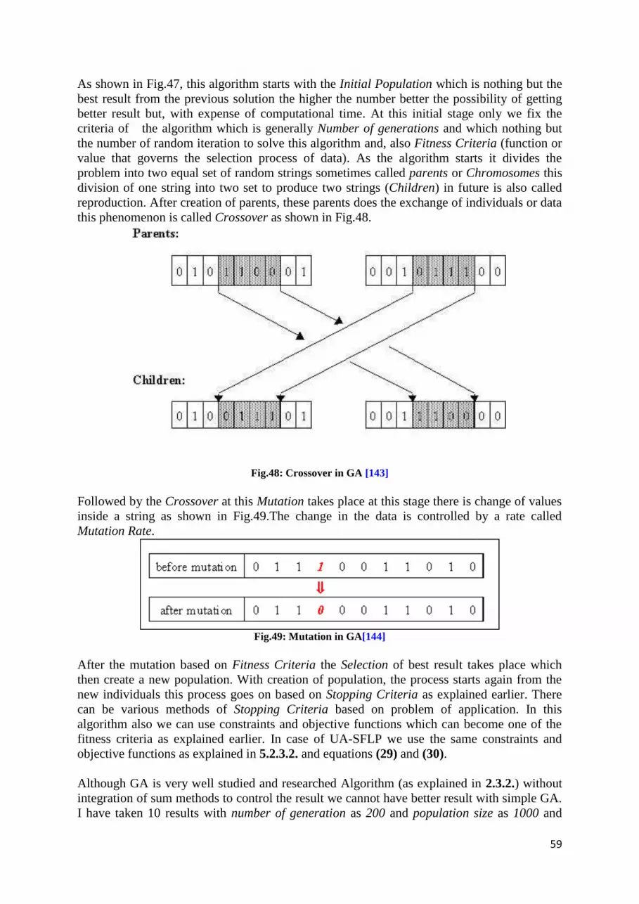
59

As shown in Fig.47, this algorithm starts with the Initial Population which is nothing but the best result from the previous solution the higher the number better the possibility of getting better result but, with expense of computational time. At this initial stage only we fix the criteria of the algorithm which is generally Number of generations and which nothing but the number of random iteration to solve this algorithm and, also Fitness Criteria (function or value that governs the selection process of data). As the algorithm starts it divides the problem into two equal set of random strings sometimes called parents or Chromosomes this division of one string into two set to produce two strings (Children) in future is also called reproduction. After creation of parents, these parents does the exchange of individuals or data this phenomenon is called Crossover as shown in Fig.48.

Fig.48: Crossover in GA [143]

Followed by the Crossover at this Mutation takes place at this stage there is change of values inside a string as shown in Fig.49.The change in the data is controlled by a rate called Mutation Rate.

Fig.49: Mutation in GA[144]

After the mutation based on Fitness Criteria the Selection of best result takes place which then create a new population. With creation of population, the process starts again from the new individuals this process goes on based on Stopping Criteria as explained earlier. There can be various methods of Stopping Criteria based on problem of application. In this algorithm also we can use constraints and objective functions which can become one of the fitness criteria as explained earlier. In case of UA-SFLP we use the same constraints and objective functions as explained in 5.2.3.2. and equations (29) and (30). Although GA is very well studied and researched Algorithm (as explained in 2.3.2.) without integration of sum methods to control the result we cannot have better result with simple GA. I have taken 10 results with number of generation as 200 and population size as 1000 and

60

solved for 8 Facilities UA-SFLP. Out of solution none of them has better result even than the results of old method developed (Corner Points Methods explained in 4.3.1. and 5.2.1.). The best result obtained was 259.4625 for a time span of 77.9 seconds. Table-12 also shows the left corner co- ordinates of facilities or facilities obtained after getting the best result.

If we see Fig.41c) and compare it with Fig.50 we can conclude that the best result obtained the layout design obtained for the best result of CBPS is more compact compared to the layout design obtained for the best result of GA for 8Facilities UA-SFLP. Also, it can be said there is almost lots of gap can be seen in case of layout design obtained for best result of GA. Due to all reasons stated above it was decided not check the result for other facilities bases on criteria principle as explained initially in 5.2. The Matlab code can be found in APPENDIX E for GA

Total cost Facilities 1 2 3 4 5 6 7 8

259. 4625

Corner co-ordinates 5.0740 5.8363 3.6786 0.6188 9.9007 1.0763 1.0725 7.1590

x y 2.5838 5.6323 5.6568 4.7038 5.5518 7.7070 0.6897 1.5852

Table-12: Corner coordinates of best result obtained for 8 Facilities by GA

Fig.50: Layout design obtained for best result of 8 Facilities UA-SFLP by applying GA

61

CHAPTER6: Conclusion In this paper, I have successfully established a new quasi-optimal heuristic strategy or methodology to solve Un-Equal Area Static Facility Layout problem. In this method the initial placement of facility is at the center so, the name given for this strategy is as Centre Based Placement Strategy (CBPS) with the order of placement as random. Also, random orientation technique was used. This CBPS is integrated with Local Search Algorithm to have meta-heuristic solutions. The results of the finalized method of CBPS (Selective Sequential) integrated with Local Search Algorithm was compared with Particle Swarm Optimization [137], Gradient Method and Genetic Algorithm for 8 Facilities, 11 Facilities and 20 Facilities UA-SFLPs in case of PSO [137] and only 8 Facilities problem with Gradient Method and Genetic Algorithm. The problem and the initial conditions were taken from Asl and Wong (2015) [137]. With all the comparisons it can be concluded that results obtained are either comparable or having better result in prospect of optimal material flow cost and computational time compared to other methods as explained in CHAPTER 5.Althogh in case of 20 facilities for better result than PSO [137] the computational time is tremendously high but comparable result are obtained at very fast rate for this particular case. The reason for successful reduction in computational time and better optimal solution in most of the cases is because of the sequential organization structure of algorithm to remove extra search during the discretization stage for interpolation of positions of facilities as explained in CHAPTER 4. In case of Gradient Method and Genetic Algorithm the results of CBPS is only checked with 8 Facilities problem due to the mere fact that in case of Gradient Method computational time is long and ease of using is difficult, while in case of Genetic Algorithm the result obtained is with very high material flow cost as an optimal result in all the results. Although we got good results for UA-SFLP using this method but further research is still needed for better result which is discussed in CHAPTER 7.

62

CHAPTER7: Prospective for Future Research As said earlier a heuristic method has been created successfully in this paper. Although in this paper I have used local search algorithm for meta-heuristic purpose but, a better methodology is need to be developed integrated with this heuristic method where the whole algorithm can be used as an objective. However, there is a trend of using GA, SA, ST, ACO and PSO to optimize multi-objective FLP can be observed with minor modifications in the core developed algorithms by certain researchers as explained in CHAPTER 2. But, without hybridization of any of these standard algorithms with this heuristic method of CBPS we cannot have better result. So, to have better result with CBPS a hybridization technique is needed to be developed so we can have better result. For achieving that customization of either of these of algorithms GA, SA, ST, ACO and PSO according with CBPS is required. So, it is expected that doing such hybridization along with CBPS a global optimum result for UA-SFLP can be achieved. Moreover, if we add interactive tool as explained in CHPTER 2 along with hybridization of CBPS we can have user interactive algorithm which can help the designer to check the possible positioning along with the algorithm running which can, not only provide better result but helps to add experience of the designer before optimizing the final result.

63

REFERENCES [1] J.A. Tompkins, J.A. White, Y.A. Bozer and J.M.A. Tanchoco (2010). Facilities Planning.

John Wiley & Sons. URL: https://books.google.fr/books?hl=en&lr=&id=-xBIq6Qm2SQC&oi=fnd&pg=PA3&dq=Tompkins+JA,+White+JA,+Bozer+YA+and+Tanchoco+JMA+%282010%29.+Facilities+Planning.+John+Wiley+%26+Sons.&ots=sB3xlcFlW3&sig=RYcc5lIta0w4b07-0pRIOLybtoQ#v=onepage&q&f=false [2] P. Kouvelis, A.A. Kurawarwala (1992). Algorithms for robust single and multiple period

layout planning for manufacturing systems. European Journal of Operational Research Volume 63.Pages 287-303.

URL: http://www.sciencedirect.com/science/article/pii/0377221792900325 [3] G.C. Armour and E.S. Buffa (1963). A Heuristic Algorithm and Simulation Approach to

Relative Location of Facilities. Management Science.Volume-9,Issue 2 URL: http://pubsonline.informs.org/doi/abs/10.1287/mnsc.9.2.294 [4] R. A. Yildiz , K. N. Solanki(2012). Multi-objective optimization of vehicle

crashworthiness using a new particle swarm based approach. The International Journal of Advanced Manufacturing Technology . Volume 59, Issue 1, Pages 367-376

URL: http://link.springer.com/article/10.1007/s00170-011-3496-y

[5] X. Suo (2012) .Facility Layout. China Institute of Industrial Relations, Beijing URL: http://cdn.intechopen.com/pdfs/36421/InTech-Facility_layout.pdf [6] A. L. Page (1991). New product development survey: Performance, and best practices.

PDMA Conference. [7] T. Gupta, H.I. Seifoddini (1990). Production data based similarity coefficient for

machine-component grouping decisions in the design of a cellular manufacturing system. International Journal of Production Research. Volume 28, Issue 7, 1990.

URL: http://www.tandfonline.com/doi/abs/10.1080/00207549008942791 [8] J. Balakrishnan , C. H. Cheng, D. G. Conway and C.M. Lau (2003) A hybrid genetic

algorithm for the dynamic plant layout problem. The International Journal of Production Economics. Volume 86, Issue 2, Pages 107–120.

URL: http://www.sciencedirect.com/science/article/pii/S0925527303000276#

[9] M. Braglia, S. Zanoni, & L.Zavanella(2003). Layout design in dynamic environments: Strategies and quantitative indices. The International Journal of Production Research. Volume 41, Issue 5, 2003.

URL: http://www.tandfonline.com/doi/abs/10.1080/00207540210162983

[10] P. Kouvelis, A.A. Kurawarwala (1992). Algorithms for robust single and multiple period layout planning for manufacturing systems. European Journal of Operational Research Volume 63.Pages 287-303.

URL: http://www.sciencedirect.com/science/article/pii/0377221792900325 [11] G. Meng, S.S. Heragu, & H. Zijm, (2004).Reconfigurable layout problem. The

International Journal of Production Research .Volume 42, Issue 22 URL: http://www.tandfonline.com/doi/abs/10.1080/0020754042000264590 [12] J. Y. Kim & Y. D. Kim (1995). Graph theoretic heuristics for unequal-sized facility

layout problems. Omega, 23(4), 391–401. URL: http://www.sciencedirect.com/science/article/pii/030504839500016H [13] J. Leung (1992). A New Graph-Theoretic Heuristic for Facility Layout. Management

Science. Volume 38, Issue 4 URL: http://pubsonline.informs.org/doi/abs/10.1287/mnsc.38.4.594

64

[14] S. Jajodia, I. Minis, G. Harhalakis & J. M.Proth (1991). Computerized Layout Solutions using Simulated annealing. International Journal of Production Research. Volume 30, Issue 1

URL: http://www.tandfonline.com/doi/abs/10.1080/00207549208942880 [15] K. Tsuchiya, S. Bharitkar, & Y. Takefuji (1996). A neural network approach to

facility layout problems. European Journal of Operational Research. Volume 89, Issue 3 URL: http://www.sciencedirect.com/science/article/pii/0377221795000518 [16] F. Fruggiero, A. Lambiase, & F. Negri (2006). Design and optimization of a facility

layout problem in virtual environment. Proceeding of ICAD 4thInternational Conference on Axiome Design.

URL: http://ns.dfss-software.com/technology/icad/icad2006/icad2006_06.pdf [17] M.J. Wang, M.H. Hu & M.Y. Ku (2005).A solution to the unequal area facilities

layout problem by genetic algorithm. Computers in Industry. Volume 56, Issue 2 Pages 207–220.

URL: http://www.sciencedirect.com/science/article/pii/S0166361504001022 [18] J. Balakrishnan, C.H. Cheng, & K.F.Wong (2003). FACOPT: a user friendly FACility

layout OPTimization system. Computer &Operation Research. Volume 30, Issue11.Pages1625-1641.

[19] P. Kouvelis and W.C. Chiang (1992). Intelligent local search strategies for solving facility layout problems with the quadratic assignment problem formulation European Journal of Operation Research. Volume 106, Issue2-3.Pages 457-488.

URL: http://www.sciencedirect.com/science/article/pii/S0377221797002853 [20] P. Afentakis (1989). A loop layout design problem for flexible manufacturing

systems. International Journal of Flexible Manufacturing.Volume 1.Issue2.Pages 175-196.

URL: http://link.springer.com/article/10.1007/BF00223021#page-1 [21] R. Cheng, M. Gen (1998).Loop layout design problem in flexible manufacturing

systems using genetic algorithms. Computers and Industrial Engineering. Volume 34 Issue 1.Pages 53-61.

URL: http://www.sciencedirect.com/science/article/pii/S0360835297001502 [22] R. Cheng (1996). Genetic Algorithms and Manufacturing Systems Design. John Wiley

& Sons, Inc. New York, NY, USA.ISBN : 0471127418 URL: http://dl.acm.org/citation.cfm?id=548162 [23] A.C. Nearchou (2006). Meta-heuristics from nature for the loop layout design

problem. Volume 101,Issue2. Pages 312-328. URL: http://www.sciencedirect.com/science/article/pii/S0925527305000484 [24] A. Baykasoglu & N.N.Z. Gindy (2001). A simulated annealing algorithm for dynamic

layout problem. Computer &Operation Research . Volume 28, Issue14. Pages 1403-1426. URL: http://www.sciencedirect.com/science/article/pii/S0305054800000496 [25] T.A. Lacksonen, E.E. Enscore (1993). Quadratic assignment algorithms for the

dynamic layout problem. International Journal of Production Research. Volume 31, Issue3. Pages 503-517.

URL: http://www.tandfonline.com/doi/abs/10.1080/00207549308956741#.Venqovlx6VA [26] F.R. Jacobs, M.A. Venkataramanan(1992). Solutions for the constrained dynamic

facility layout problem. European journal of Operational Research. Volume 57, Issue2. Pages 280-286.

URL: http://www.sciencedirect.com/science/article/pii/037722179290049F [27] A. Baykasoglu, T. Dereli, I. Sabuncu (2006). An ant colony algorithm for solving

budget constrained and unconstrained dynamic facility layout problems. Omega. Volume 34, Issue4. Pages 385-396.

65

URL: http://www.sciencedirect.com/science/article/pii/S0305048304001914 [28] S.K. Das (1993).A Facility layout for a flexible manufacturing system. International

Journal of Production Research. Volume 34, Issue4. Pages 385-396. [29] T. Dunker, G. Radonsb, & E. Westkämpera (2005). Combining evolutionary

computation and dynamic programming for solving a dynamic facility layout problem. European Journal of Operational Research, Volume 165, Issue 1. Pages 55–69.

URL: http://www.sciencedirect.com/science/article/pii/S0377221704000530 [30] T. A. Lacksonen (1997). Preprocessing for static and dynamic facility layout

problems. International Journal of Production Research. Volume 35, Issue 4. Pages 1095–1106.

URL: http://www.tandfonline.com/doi/abs/10.1080/002075497195560#.VerYiflx6VA [31] R. D. Meller, V.Narayanan, & P. H. Vance (1999). Optimal facility layout design.

Operations Research Letters. Volume 23, Issue 3–5. Pages 117–127. URL: http://www.sciencedirect.com/science/article/pii/S0167637798000248 [32] L. Chwif, M. R. Pereira Barretto, & L. A. Moscato (1998). A solution to the facility

layout problem using simulated annealing. Computers in Industry. Volume 36, Issue 1–

2.Pages 125–132. URL: http://www.sciencedirect.com/science/article/pii/S0166361597001061 [33] J. G. Kim & Y. D. Kim (2000). Layout planning for facilities with fixed shapes and

input and output points. International Journal of Production Research. Volume- 38, Issue- 18. Pages 4635–4653.

URL: http://www.tandfonline.com/doi/abs/10.1080/00207540050205550 [34] P. S. Welgama, & P. R. Gibson (1993). A construction algorithm for the machine

layout problem with fixed pick-up and drop-off points. International Journal of Production Research, Volume 31, Issue- 11. Pages 2575–2590.

URL: http://www.tandfonline.com/doi/abs/10.1080/00207549308956884 [35] T. Yang, B. A. Peters, & M. Tu (2005). Layout design for flexible manufacturing

systems considering single-loop directional flow patterns. European Journal of Operational Research, Volume 164, Issue- 2. Pages 440–455.

URL: http://www.sciencedirect.com/science/article/pii/S0377221703008920 [36] M. Braglia (1996). Optimization of a simulated-annealing-based heuristic for single

row machine layout problem by genetic algorithm. International Transactions in Operational Research, Volume 3, Issue-1. Pages 37–49.

URL: http://onlinelibrary.wiley.com/doi/10.1111/j.1475-3995.1996.tb00034.x/abstract;jsessionid=B2D3945BDA7D245EE197F0CE8A4E1E16.f04t04 [37] S. S. Heragu, & A. Kusiak (1988). Machine layout problem in flexible manufacturing

systems. Operations Research, 36(2), Pages 258–268. URL: http://pubsonline.informs.org/doi/abs/10.1287/opre.36.2.258 [38] S. S. Heragu, & A. Kusiak (1991). Efficient models for the facility layout problem.

European Journal of Operational Research, 53(1) Pages, 1–13. URL: http://www.sciencedirect.com/science/article/pii/037722179190088D [39] M. Mir & M. H. Imam (2001). A hybrid optimization approach for layout design of

unequal-area facilities. Computers & Industrial Engineering, 39(1–2), Pages 49–63. URL: http://www.sciencedirect.com/science/article/pii/S0360835200000656 [40] T. Dunker, G. Radonsb, & E. Westkämpera (2005). Combining evolutionary

computation and dynamic programming for solving a dynamic facility layout problem. European Journal of Operational Research, 165(1), Pages 55–69.

URL: http://www.sciencedirect.com/science/article/pii/S0377221704000530

66

[41] A.E. Tate & D.M. Smith (1993). Expected Allele Coverage and the Role of Mutation in Genetic Algorithms. Department of Industrial Engineering, University of Pittsburgh Pittsburgh, PA 15261.

URL: http://citeseerx.ist.psu.edu/viewdoc/download?doi=10.1.1.39.943&rep=rep1&type=pdf [42] L.A. Zadeh (1965).Fuzzy Sets. Information and Control. Volume 8, Issue3. Pages

338-353. URL: http://www.sciencedirect.com/science/article/pii/S001999586590241X [43] W.Z. Liu, A.P. White, S.G. Thompson, and M.A. Bramer (1997). Techniques for

Dealing with Missing Values in Classification..Advances in Intelligent Data Analysis, LNCS, Volume 1280, Pages 527-536,

URL: http://link.springer.com/chapter/10.1007/BFb0052868#page-1 [44] V. Tresp, S. Ahmadand & R. Neuneier (1994). Training Neural Networks with

Deficient Data. Advances in Neural Information Processing Systems. Morgan Kaufman, Volume 6. Pages 128-135

URL: http://www.researchgate.net/profile/Volker_Tresp/publication/2399012_Training_Neural_Networks_with_Deficient_Data/links/53d243790cf228d363e92ba8.pdf [45] M. Negnevitsky (2002).Artificial Intelligence: A Guide to Intelligent Systems.

Pearson, Sydney URL: https://books.google.fr/books?hl=en&lr=&id=1BxYQnrfv9MC&oi=fnd&pg=PR11&dq=%5B45%5D%09M.+Negnevitsky+(2002).Artificial+Intelligence:+A+Guide+to+Intelligent+Systems.+Pearson,+Sydney+&ots=GVbqZIMhXx&sig=BKEsN97mZp_OQERJWsA8CUIuXCQ#v=onepage&q&f=false [46] M.R. Berthold, and K.P. Huber (1998).Missing values and learning of fuzzy rules,

International Journal of Uncetainty, Fuzziness, and Knowledge-Based Systems, Volume-6 Issue- 2. Pages 171-178.

URL: http://www.worldscientific.com/doi/abs/10.1142/S021848859800015X [47] A.R. Ahmad, O.A. Basir, , K. Hassanein (2003). Fuzzy Inferencing in the Web Page

Layout Design. Proceedings of the 1st Workshop on Web Services: Modeling, Architecture and Infrastructure (WSMAI-2003), in conjunction with the 5th Int’l

Conference on Enterprise Information Systems (ICEIS-2003), ICEIS Press, Angers, France. Pages 33-41

URL: http://www.researchgate.net/profile/Jen_Yao_Chung/publication/220901926_An_Architecture_for_Building_Web_Service_Applications/links/02e7e537aff21d76fa000000.pdf#page=40 [48] A.R. Ahmad, O.A. Basir, , K. Hassanein (2004). Intelligent Decision Support System

for Layout Design. Proc. of the 9th Asia-Pacific Decision Sciences Institute Conf. (APDSI’04), Seoul, Korea.

[49] G. Aiello, and M. Enea (2001). Fuzzy approach to the robust facility layout in uncertain production environment. International Journal of Production Research. Volume39, Issue18, Pages 4089-4101.

URL: http://www.tandfonline.com/doi/abs/10.1080/00207540110061643 [50] A. Badiru, and A. Arif (1996). FLEXPERT: Facility Layout Expert System using

Fuzzy Linguistic Relationship Codes. IIE Transactions, Volume 28, Issue 4, Pages 295-309

URL: http://www.tandfonline.com/doi/abs/10.1080/07408179608966277 [51] S. S. K. Deb, & B. Bhattacharyya, (2005). Fuzzy decision support systems for

manufacturing facilities layout planning. Decision Support Systems, Volume 40, 305–314. URL:http://www.sciencedirect.com/science/article/pii/S0167923604000351

67

[52] F. Dweiri & F.A. Meier (1996).Application of fuzzy decision-making in facilities layout planning. International Journal of Production Research. Volume 34, Issue 11, Pages 3207-3225.

URL: http://www.tandfonline.com/doi/abs/10.1080/00207549608905085 [53] G.W. Evans, M.R. Wilhelm, and W. Karwoski (1987). “A layout design heuristic

employing the theory of fuzzy sets”, International Journal of Production Research, Volume 25, Issue 10, Pages 1431-1450,

URL: http://www.tandfonline.com/doi/abs/10.1080/00207548708919924 [54] J. Grobelny (1987). The fuzzy approach to facilities layout problems. Fuzzy Sets

Systems, Volume 23, Pages 175-190. URL: http://www.sciencedirect.com/science/article/pii/0165011487900571 [55] J. Grobelny (1987). One possible fuzzy approach to facility layout problems

Internationall Journal of Production Research, Volume 25, Pages 1123-1141 URL: http://cat.inist.fr/?aModele=afficheN&cpsidt=7552419 [56] F. Karray, E. Zaneldin, T. Hegazy, A.H.M. Shabeeb, and E. Elbelgati (2000).

Computational Intelligence Tools for Solving Facilities Layout Planning Problem”,

Proceedings of the American Control Conference, Chicago, Illinois, Volume 8, Issue 4, Pages 367-379.

URL: http://ieeexplore.ieee.org/xpl/login.jsp?tp=&arnumber=876964&url=http%3A%2F%2Fieeexplore.ieee.org%2Fxpls%2Fabs_all.jsp%3Farnumber%3D876964 [57] E.Q. Kang, R.B. Lin, and E. Shragowitz, (1994).Fuzzy Logic Approach to VLSI

Placement”, IEEE Transactions on Very Large Scale Integration Systems, Volume 2, Issue 4.

URL: http://ieeexplore.ieee.org/xpl/login.jsp?tp=&arnumber=335016&url=http%3A%2F%2Fieeexplore.ieee.org%2Fxpls%2Fabs_all.jsp%3Farnumber%3D335016 [58] J.K. Kim, H.L. Kwang, and S.W. Yoo (2001). Fuzzy bin packing problem. Fuzzy Sets

and Systems, Volume 2, Issue 4. Pages. 429-434. URL: http://www.sciencedirect.com/science/article/pii/S0165011499000731 [59] A.D. Raoot, and A. Rakshit (1993). A ‘linguistic pattern’ approach for multiple

criteria facilities layout problems”, International Journal of Production Research. Volume 31, Pages 203-222.

URL: http://www.tandfonline.com/doi/abs/10.1080/00207549308956721 [60] A.D. Raoot, and A. Rakshit (1991).A fuzzy approach to facilities layout planning.

International Journal of Production Research, Volume 29, Pages 835-857. URL: http://www.tandfonline.com/doi/abs/10.1080/00207549308956721 [61] A.R. Soltani, and T. Fernando (2004). A fuzzy based multi-objective path planning of

construction sites. Automation in Construction. Volume 13, Issue 6. Pages 717–734. URL: http://www.sciencedirect.com/science/article/pii/S0926580504000354 [62] H. Youssef, S.M. Sait, and H. Ali (2003). Fuzzy Simulated Evolution Algorithm for

VLSI Placement. International Journal on Applied Intelligence, Special issue on Applied Metaheuristics.

URL: http://www.sciencedirect.com/science/article/pii/S0360835202001778 [63] T.C. Whyte and M.R. Wilhelm (1999).The Use of Fuzzy Methodologies And Space

Filling Curves In Facility Layout Design. Proceedings of IIE Research Conference, Phoenix, Arizona.

[64] T.C. Whyte (1999). Facility layout design using fuzzy linguistic variables and fractals. Proceedings of IIE Research Conference, Phoenix, Arizona.

68

[65] X.F. Zha, and S.Y.E. Lim (2003). Intelligent design and planning of manual assembly workstations: A neurofuzzy approach. Computers & Industrial Engineering, Volume 44, Pages 611-632.

URL: http://www.sciencedirect.com/science/article/pii/S0360835202002383 [66] A. R. Ahmad (2005). An Intelligent Expert System for Decision Analysis and Support

in Multi-Attribute Layout Optimization. PhD, University of Waterloo. URL: http://link.springer.com/chapter/10.1007/978-3-540-76829-6_12 [67] M. Gen, K. Ida, & C. Cheng (1995). Multi row machine layout problem in fuzzy

environment using genetic algorithms. Computers & Industrial Engineering, Volume 29, Issue 1–4, Pages, 519–523.

URL: http://www.sciencedirect.com/science/article/pii/036083529500127M [68] C. M. Harmonosky, & G. K. Tothero (1992). A multi-factor plant layout

methodology. International Journal of Production Research. Volume 30,Issue8,Pages 1773–1789

URL: http://www.tandfonline.com/doi/abs/10.1080/00207549208948121 [69] T. Yang, & C. Kuo (2003). A hierarchical AHP/DEA methodology for the facilities

layout design problem. European Journal of Operational Research, Volume 147, Issue Pages, 128–136.

URL: http://www.sciencedirect.com/science/article/pii/S0377221702002515 [70] C. W. Chen, & D. Y. Sha (2005). Heuristic approach for solving the multiobjective

facility layout problem. International Journal of Production Research. Volume 43, Issue-21. Pages 4493–4507.

URL: http://www.tandfonline.com/doi/abs/10.1080/00207540500056383 [71] G. Aiello, M. Enea, & G. Galante (2006). Multi-objective approach to facility layout

problem by genetic search algorithm and Electre method. Robotics and Computer-Integrated Manufacturing. Volume 22, Issue 5-6.Pages 447–455.

URL: http://www.sciencedirect.com/science/article/pii/S0736584506000573 [72] P. Ji, W. Ho (2005). The Traveling Salesman and the Quadratic Assignment

Problems: Integration, Modeling and Genetic Algorithm. Proceedings of the 5th International symposium on Operation Research and its applications

URL: http://www.researchgate.net/profile/Ping_Ji4/publication/250729284_The_Traveling_Salesman_and_the_Quadratic_Assignment_Problems_Integration_Modeling_and_Genetic_Algorithm/links/5412b0ab0cf2fa878ad3b083.pdf [73] B.F. Al-Dulaimi, H.A. Ali (2008). Enhanced traveling salesman problem solving by

genetic algorithm technique. International Journal of Mathematical, Computational, Physical, Electrical and Computer Engineering Volume2, Issue2

URL: http://www.waset.org/publications/6555 [74] D. Whitley, T. Starkweather, D. Shaner (1991). The traveling salesman and sequence

scheduling: Quality solutions using genetic edge recombination. Handbook of Genetic Algorithms.

URL: http://citeseerx.ist.psu.edu/viewdoc/summary?doi=10.1.1.18.8193 [75] K.L. Mak, Y.S. Wong, & F.T.S. Chan (1998). A genetic algorithm for facility layout

problems. Computer Integrated Manufacturing. Volume 11, Issues 1–2. Pages 113–127 URL: http://www.sciencedirect.com/science/article/pii/S0951524098000184 [76] A. Kaveh & H. Safari (2014). Charged system search adopted for solution of

traveling salesman problem: An application to single-row facility layout problem. International Journal of Civil Engineering, Structural Engineering. Volume 12, Issue 3.

69

URL: http://ijce.iust.ac.ir/files/site1/user_files_6k93w6/eng/alikaveh-A-10-218-66-2a49e20.pdf [77] P. Kouvelis, M.W. Kim (1992). Unidirectional loop network layout problem in

automated manufacturing systems. Operations Research. Volume 40, Issue 3. URL: http://pubsonline.informs.org/doi/abs/10.1287/opre.40.3.533 [78] R. D. Meller, V.Narayanan & P. H. Vance (1999). Optimal facility layout design.

Operations Research Letters, Volume 23, Issue 3–5, Pages 117–127. URL: http://www.sciencedirect.com/science/article/pii/S0167637798000248 [79] J. G. Kim & Y. D. Kim. (1999). A branch and bound algorithm for locating input and

output points of departments on the block layout. Journal of the Operational Research Society. Volume 50, Issue 5, Pages 517–525.

URL: http://www.sciencedirect.com/science/article/pii/S0167637798000248 [80] M. J. Rosenblatt (1986). The dynamics of plant layout. Management Science. Volume

32, Issue 1. Pages 76–86. URL: http://pubsonline.informs.org/doi/abs/10.1287/mnsc.32.1.76 [81] A. R. S. Amaral. An Exact Approach to the One-Dimensional Facility Layout

Problem. Operations Research. Volume 56, Issue 4. Pages 1026–1033. URL: http://pubsonline.informs.org/doi/abs/10.1287/opre.1080.0548 [82] R. Kothari & D. Ghosh (2012). The single row facility layout problem: state of

the art. OPSEARCH Volume 49, Issue 4. Pages 442-462. URL: http://link.springer.com/article/10.1007/s12597-012-0091-4 [83] R.F. Love & J.Y. Wong (1976).Solving quadratic assignment problems with

rectangular distances and integer programming. Naval Research Logistics Quarterly. Volume 23, Issue 4. Pages 623-627.

URL: http://onlinelibrary.wiley.com/doi/10.1002/nav.3800230407/abstract [84] S.S. Heragu & A. Kusiak (1991). Efficient models for the facility layout problem.

European Journal of Operational Research. Volume 53, Issue 1, Pages 1–13. URL: http://www.sciencedirect.com/science/article/pii/037722179190088D [85] S. S. Heragu (1997). Facilities Design. 2 ed. Boston: PWS Publishing Co. URL: https://books.google.fr/books?id=AgDMBQAAQBAJ&pg=PA586&lpg=PA586&dq=S.+S.+Heragu+(1997)&source=bl&ots=a-fG6LwFJe&sig=QpPhB1oBb_gtxs6-14Fj03atKJw&hl=en&sa=X&ved=0CCwQ6AEwAmoVChMI-cOw38XlxwIVxVkUCh2oDQoS#v=onepage&q=S.%20S.%20Heragu%20(1997)&f=false [86] R.C. Lee (1967). Computerized relationship layout planning (CORELAP). Journal of

Industrial Engineering, Volume18, Issue 3. Pages195-200. URL: http://www.researchgate.net/publication/44179469_Computerized_relationship_layout_planning_(CORELAP) [87] M. J. Seehof, and W. O. Evans (1967). Automated layout design program. Journal of

Industrial Engineering. Volume 18, Issue12. Pages 690-695. URL: http://dl.acm.org/citation.cfm?id=810696 [88] J.A. Tompkins & R. Reed (1976). An applied model for the facilities design problem.

International Journal of Production Research. Volume 14, Issue 5. Pages 583-595. URL: http://www.tandfonline.com/doi/abs/10.1080/00207547608956377#.Ve3Tnvmqqko [89] M.M.D. Hassan, G.L. Hogg & D.R. Smith (1986). SHAPE: a construction algorithm

for area placement evaluation. International Journal of Production Research. Volume 24, Issue 5. Pages 1283-1295.

URL: http://www.tandfonline.com/doi/abs/10.1080/00207548608919803

70

[90] G. C. Armour, & E. S. Buffa (1963). A heuristic algorithm and simulation approach to relative allocation of facilities. Management Science, Volume 9, Issue 2. Pages 294–300.

URL: http://pubsonline.informs.org/doi/abs/10.1287/mnsc.9.2.294 [91] T. M. Khalil (1973). Facilities relative allocation technique (FRAT). International

Journal of Productions Research. Volume 11, Issue 2.Pages 183–194. URL: http://www.tandfonline.com/doi/abs/10.1080/00207547308929959 [92] Z. Drezner (1987). A heuristic procedure for the layout of a large number of facilities.

International Journal of Management Science, Volume 33, Issue7.Pages 907–915. URL: http://pubsonline.informs.org/doi/abs/10.1287/mnsc.33.7.907 [93] W. C. Chiang, & P. Kouvelis (1996). An improved tabu search heuristic for solving

facility layout design problems. International Journal of Production Research. Volume 34 Issue 9, Pages 2565–2585.

URL: http://www.tandfonline.com/doi/abs/10.1080/00207549608905045#.Ve4S9_mqqko [94] D.E. Goldberg, B. Korb, &K. Deb (1989). Messy genetic algorithms: Motivation,

analysis, and first results. Complex Systems. Volume 3 Issue 5, Pages 493-530. URL: http://repository.ias.ac.in/82726/ [95] H. Pierreval, C.Caux, J. L. Paris, & F. Viguier (2003). Evolutionary approaches to the

design and organization of manufacturing systems. Computers & Industrial Engineering, Volume 44 Issue 3.Pages 339–364.

URL: http://www.sciencedirect.com/science/article/pii/S036083520200195X [96] P. Banerjee, & Y. Zhou (1995). Facilities layout design optimization with single

loop material flow path configuration. International Journal of Production Research, Volume 33, Issue 1.Pages 183–204.

URL: http://www.tandfonline.com/doi/abs/10.1080/00207549508930143#.Ve4em_mqqko [97] Azadivar, F., & Wang, J. (2000). Facility layout optimization using simulation and

genetic algorithms. International Journal of Production Research, Volume38, Issue 17. Pages 4369–4383.

URL: http://www.tandfonline.com/doi/abs/10.1080/00207540050205154 [98] Y.Wu, & E. Appleton (2002). The optimisation of block layout and aisle structure by

a genetic algorithm. Computers & Industrial Engineering, Volume 41 Issue 4. Pages371–

387. URL: http://www.sciencedirect.com/science/article/pii/S0360835201000638 [99] J. Balakrishnan & C. H. Cheng (2000). Genetic search and the dynamic layout

problem. Computers & Operations Research. Volume 27, Issue 6. Pages 587–593. URL:http://www.sciencedirect.com/science/article/pii/S0305054899000520 [100] J. Balakrishnan, C. H. Cheng, & K. F. Wong (2003). FACOPT: A user friendly

FACility layout OPTimization system. Computers & Operations Research. Volume 30, Issue 11.Pages 1625–1641.

URL: http://www.sciencedirect.com/science/article/pii/S0305054802000965 [101] E. Shayan, & A. Chittilappilly (2004). Genetic algorithm for facilities layout problems

based on slicing tree structure. International Journal of Production Research. Volume 42 Issue 19.Pages 4055–4067.

URL: http://www.tandfonline.com/doi/abs/10.1080/00207540410001716471 [102] K. Y. Tam (1992). Genetic algorithms, function optimization and facility layout

design. European Journal of Operational Research, Volume 63 Issue 2.Pages 322–346. URL: http://www.sciencedirect.com/science/article/pii/0377221792900347 [103] K. Y. Tam, & S. K. Chan (1998). Solving facility layout problems with geometric

constraints using parallel genetic algorithms: Experimentation and findings. International Journal of Production Research. Volume 36 Issue 12.Pages 3253–3272.

URL: http://www.tandfonline.com/doi/abs/10.1080/002075498192058#.Ve4_IPmqqko

71

[104] L. Al-Hakim (2000). On solving facility layout problems using genetic algorithms. International Journal of Production Research. Volume 38, Issue 11.Pages 2573–2582.

URL: http://www.tandfonline.com/doi/abs/10.1080/00207540050031922 [105] S. Bock & K. Hoberg (2007). Detailed layout planning for irregularly-shaped

machines with transportation path design. European Journal of Operational Research. Volume 177. Pages 693–718.

URL: http://www.sciencedirect.com/science/article/pii/S0377221705009410 [106] A. A. Islier (1998). A genetic algorithm approach for multiple criteria facility layout

design. International Journal of Production Research. Volume 36 Issue 6.Pages 1549–

1569. URL: http://www.tandfonline.com/doi/abs/10.1080/002075498193165?journalCode=tprs20#.Ve5Gufmqqko [107] S. Hamamoto, Y. Yih & G. Salvendy (1999). Development and validation of genetic

algorithm-based facility layout-a case study in the pharmaceutical industry. International Journal of Production Research. Volume 37.Pages 749–768.

URL: http://www.tandfonline.com/doi/abs/10.1080/002075499191508 [108] M. Solimanpur, P. Vrat, & R. Shankar (2005). An ant algorithm for the single row

layout problem in flexible manufacturing systems. Computers & Operations Research. Volume 32, Issue 3.Pages 583–598.

URL: http://www.sciencedirect.com/science/article/pii/S0305054803002557 [109] Y. H. Lee & M. H. Lee (2002). A shape-based block layout approach to facility layout

problems using hybrid genetic algorithm. Computers & Industrial Engineering. Volume 42.Pages 237–248.

URL: http://www.sciencedirect.com/science/article/pii/S0360835202000189 [110] T. L. Urban (1993). A heuristic for the dynamic facility layout problem. IIE

Transactions, Volume 25, Issue 4.Pages 57–63. URL: http://www.tandfonline.com/doi/abs/10.1080/07408179308964304#.Ve5XJPmqqko [111] G. Jacquenot, F. Bennis, J.J. Maisonneuve, P. Wenger (2009). 2D Multi-Objective

Placement Algorithm For Free-Form Components. Proceedings of ASME 2009 International Design Engineering Technical Conferences & Computers and Information in Engineering Conference IDETC/CIE 2009, San Diego, USA.

URL: http://proceedings.asmedigitalcollection.asme.org/proceeding.aspx?articleid=1649933 [112] T. Imamichi, and H. Nagamochi (2008). Designing algorithms with multi-sphere

scheme. In ICKS ’08: Proceedings of the International Conference on Informatics

Education and Research for Knowledge-Circulating Society (icks 2008), IEEE Computer Society, pp. 125–130.

URL: http://ieeexplore.ieee.org/xpls/abs_all.jsp?arnumber=4460479&tag=1 [113] J. Bénabès, F. Bennis, E. Poirson, Y. Ravaut. (2010). Interactive optimization

strategies for layout problems. International Journal on Interactive Design and Manufacturing, Volume 4, Issue 3, pp 181-190

URL: http://link.springer.com/article/10.1007/s12008-010-0100-x [114] Michalek (2001). Interactive Design Optimization of Architectural Layouts.

Engineering Optimization, 2002, Volume 34, Issue-5.Pages 485–501. URL: http://www.tandfonline.com/doi/abs/10.1080/03052150214021 [115] A. M. Brintrup (2006). An Interactive Genetic Algorithm-Based Framework For

Handling Qualitative Criteria in Design Optimization. Computers in Industry. Volume 58. Pages 279–291.

URL: http://www.sciencedirect.com/science/article/pii/S016636150600159X

72

[116] Z. Liu and T. Hong (2008). Human–computer cooperative layout design method and its application. Computers & Industrial Engineering. Volume 55. Pages735–757.

URL: http://www.sciencedirect.com/science/article/pii/S0360835208000545 [117] K. Mittenen and M. M. Mäkelä (1995). Interactive Bundle-Based Method For Non-

differentiable Multi-objective Optimization: Nimbus. Optimization: A Journal of Mathematical Programming and Operations. Research, Volume 34, Issue-3.Pages 231-246.

URL: http://www.tandfonline.com/doi/abs/10.1080/02331939508844109 [118] M. M. Mäkelä (1993). Issues of lmplementing a Fortran Subroutine Package NSOLIB

for Non-smooth Optimization, Report 511993, University of Jyvaskyla, Department of Mathematics, Laboratory of Scientific Computing, Jyväskylä.

URL: https://books.google.fr/books/about/Issues_of_Implementing_a_Fortran_Subrout.html?id=wdYzAAAACAAJ&hl=en [119] K. C. Kiwiel (1984).An Aggregate Subgradient Descent Method for Solving Large

Convex Non-smooth Multi-objective Minimization Problems. Large Scale Systems: Theory and Applications 1983. Edited by Straszak, A. Pergamon Press. Pages 283-288.

[120] S. Wang (1989). Algorithms for Multiobjectice and Nonsmooth Optimization. Methods of Operations Research. Volume 58.Pages 131-142.

[121] K. Mittenen and M. M. Mäkelä. (2000). Interactive multiobjective optimization system WWW-NIMBUS on the Internet. Computers and Operations Research, Volume 27, 709–723.

URL: http://www.sciencedirect.com/science/article/pii/S030505489900115X [122] R.V. Tappeta, and J. E. Renaud (1999). Interactive multi-objective optimization

design strategy for decision based design. Proceedings of the 1999 ASME. International Design Engineering Technical Conferences and Computers and Information in Engineering Conference, DETC99=DAC-8581, 1–15.

URL: http://mechanicaldesign.asmedigitalcollection.asme.org/article.aspx?articleid=1446364 [123] R.V. Tappeta, and J. E. Renaud (1999). Interactive Multi-Objective Optimization

Procedure. AIAA J., 37, No. 7, July, pp. 881–889. URL: http://arc.aiaa.org/doi/abs/10.2514/2.7537?journalCode=aiaaj [124] G. A. Gabriele, and T. J. Beltracchi (1988).OPT3.2: A Fortran Implementation of the

Generalized Reduced Gradient Method. User’s Manual, Department of Mechanical

Engineering, Aerospace Engineering and Mechanical, Rensselaer Polytechnic Institute. [125] R. S. Liggett and W. J. Mitchell (1981). Interactive graphic floor plan layout method.

Computer-Aided Design, 13(5), 289–298. URL: http://www.sciencedirect.com/science/article/pii/0010448581903183 [126] J.C. Koopmans, and M J. Beckmann(1957). Assignment problems and the location of

economic activities. Econometrica Vol 25 pp 53-76. URL: http://www.jstor.org/stable/1907742 [127] P. Hungerländer, M. Anjos (2015). A semidefinite optimization-based approach for

global optimization of multi-row optimization. European journal of operational Research 245(2015) 46-61.

URL: http://www.sciencedirect.com/science/article/pii/S0377221715001691 [128] K. Wieghardt, D. Hartmann, and K. R. Leimbach (1997). Interactive shape

optimization of continuum structures. Engineering Structures. Volume 19 Issue-4.Pages 325–331

URL: http://www.sciencedirect.com/science/article/pii/S0141029696000776 [129] G. N. Vanderplaats and H. Sugimoto (1986). A general-purpose optimization program

for engineering design. Computational Structures. Volume 24. Pages 13-21

73

URL: http://www.sciencedirect.com/science/article/pii/0045794986903317 [130] J. Olden (1997) .Fehlergesteuerte Finite-Elemente-Analyse von Platten- tragwerken,

PhD thesis, Technische Hochschulc Darmstadt, Germany [131] J. Michalek, R. Choudhary, and P. Y. Papalambros (2002). Architectural layout

design optimization. Engineering Optimization, Volume 34, Issue 5. pp 461-484 URL: http://www.tandfonline.com/doi/abs/10.1080/03052150214016 [132] J.L. Zhou, A.L. Tits. (1996). An SQP algorithm for finely discretized continuous

minimax problems and other minimax problems with many objective functions. SIAM Journal on Optimization,Volume 6, Issue 2, 10.1137/0806025

URL: http://epubs.siam.org/doi/abs/10.1137/0806025 [133] J. Michalek (2001). Interactive layout design optimization. MS Thesis, University of

Michigan. URL: http://www.cmu.edu/me/ddl/publications/2001-Michalek-MSThesis.pdf [134] L.Garcia-Hernandez, H. Pierreval, L. Salas-Morera, & A. Arauzo-

Azofra.(2010).Handling qualitative aspects in Unequal Area Facility Layout Problem: An Interactive Genetic Algorithm. Applied Soft Computing. Volume 13.Pages 1718–1727.

URL: http://www.sciencedirect.com/science/article/pii/S1568494613000203 [135] J.C. Bezdek, R. Ehrlich, W. Full. (1984). FCM: the fuzzy c-means clustering

algorithm. Computers and Geosciences. Volume 10. Pages 192–203. URL: http://www.sciencedirect.com/science/article/pii/0098300484900207 [136] L. Čmolík and J. Bittener. (2010). Layout-aware optimization for interactive labeling

of 3D models. Computers & Graphics. Volume 34. Pages 378–387. URL: http://www.sciencedirect.com/science/article/pii/S0097849310000695 [137] A.D. Asl & K.Y. Wong (2015). Solving unequal-area static and dynamic facility

layout problems using modified particle swarm optimization. Journal of Intelligent Manufacturing. DOI 10.1007/s10845-015-1053-5.

URL: http://link.springer.com/article/10.1007/s10845-015-1053-5 [138] K.Y. Tam & S.G. Li (1991). A hierarchical approach to the facility layout problem.

The International Journal of Production Research. Volume 29,Issue 1. Pages 165–184. URL: http://www.tandfonline.com/doi/abs/10.1080/00207549108930055 [139] R. D. Meller, B. M. Kleiner, and M. A. Nussbaum (2004). The facility layout

problem: A new model to support a bottom-up approach to facility design. Progress in Material Handling Research. Pages 399–414.

URL: http://faculty.ineg.uark.edu/rmeller/downloads/ResearchPapers/ [140] R.D. Meller, Z Kirkizoglu, & W Chen (2009). Detailed testing results of a new model

to support a bottom-up approach to facility design. Proceedings of the, NSF engineering research and innovation conference.

URL: http://faculty.ineg.uark.edu/rmeller/downloads/ResearchPapers/Meller-Kirkizoglu-Chen-Bottom-Up-Layout-Detailed-Results.pdf [141] R.D. Meller, Z Kirkizoglu, & W Chen (2010). A new optimization model to support

a bottom-up approach to facility design. Computers & Operations Research. Volume 37, Issue-1. Pages 42–49

URL: http://www.sciencedirect.com/science/article/pii/S0305054809000823 [142] L. Vandenberghe (2013).Gradient method. lecture, UCLA Henry Samueli School of

Engineering,USA. URL: http://www.seas.ucla.edu/~vandenbe/236C/lectures/gradient.pdf [143] http://www.stumptown.com/diss/chapter2.html [144] http://www.geatbx.com/docu/algindex-04.html

74

APPENDIX A: Matlab code for CBPS-Corner Points Method for 8 Facilities

function [TotalCost, AvlDept] = cornerpoints( ) % layout mid centre as starting point clear all; clc; close all; %rand('state',2) % Cost Data for material handling between each facility cData = [0 1 2 0 0 0 2 0 0 0 4 3 6 0 0 2 0 0 0 2 0 3 1 0 0 0 0 0 5 2 0 2 0 0 0 0 0 0 0 4 0 0 0 0 0 0 4 0 0 0 0 0 0 0 0 1 0 0 0 0 0 0 0 0]; % Facility Data dData = [2 3 4 5 2 2 3 3 2 4 4 4 4 4 3 4]; bounds = [20 20]; % layout boundary rMax = size(dData,1); % Number of Facilities z = randperm(rMax) % facility call order %Orientation of Facilities t=round(rand(1,8)) p=t.' for i=1:8 if(p(i)==1) dData(i,:) = [dData(i,2) dData(i,1)]; end end %First Layout placement figure(1); close all; figure(1); hold on; axis equal; rectangle('Position',[0 0 bounds]); % Plot Layout Boundary % First facility for Initilisation nextDeptData = dData(z(1),:); % Next facility Data nextDept = [bounds(1)/2 - nextDeptData(1)/2, bounds(2)/2 - nextDeptData(2)/2, nextDeptData]; % first facility at layout center rectangle('Position', nextDept,'FaceColor','g'); % plot the first facility pause; AvlDept = nextDept; % Initialise already placed facility % Available points AvlPts = getcoordinate(nextDept); % possible starting points initialization

75

cExtracted = 0; for i = 2:rMax nextDeptData = dData(z(i),:); PossiblePt = PossiblePoints(AvlPts, nextDeptData);%Checking the 64 possible locations PossibleDept = CheckOverlap(AvlDept, PossiblePt, nextDeptData, bounds);%Checking overlap cExtracted = CostNew(cData,cExtracted,z(1:i));%Changing the matrix of cost rate according to order PlacedDept = PlacedDepartment(cExtracted, AvlDept, PossibleDept);%Checking condition of placement AvlDept = [AvlDept; PlacedDept]; PlacedDeptPts = getcoordinate(PlacedDept);%Generating corner and mid-points AvlPts = [AvlPts; PlacedDeptPts]; AvlPts = unique(AvlPts,'rows'); rectangle('Position', PlacedDept,'FaceColor','g'); clear nextDeptData possiblePt placedDept; pause; end DistMat = DistanceMat(AvlDept ); TotalCost = sum(sum(cExtracted.*DistMat)); BCond = BoundaryCondition( AvlDept, bounds);%Checking the boundary condition AvlFacilitiesort = []; if BCond == 0 [~, SI] = sort(z); AvlFacilitiesort = AvlDept(SI,:); else TotalCost = []; end end function PlacedDept = PlacedDepartment(cExtracted, AvlDept, PossibleDept) dista = zeros(size(PossibleDept,1),1); for i = 1:size(PossibleDept,1) PsblDeptPos = PossibleDept(i,:); Dept = [AvlDept; PsblDeptPos]; distMat = DistanceMat(Dept); dista(i) = sum(sum(cExtracted*distMat)); clear distMat end cc = [PossibleDept dista]; x = sortrows(cc,5); PlacedDept = x(1,1:4); end function DistMat = DistanceMat(Dept)%Distance matrix of ith facility with jth facility s = size(Dept,1); DistMat = zeros(s,s); for i = 1:s for j = 1:s x1 = Dept(i,1)+Dept(i,3)/2; x2 = Dept(j,1)+Dept(j,3)/2; y1 = Dept(i,2)+Dept(i,4)/2;

76

y2 = Dept(j,2)+Dept(j,4)/2; DistMat(i,j) = abs(x1-x2)+abs(y1-y2); end end end function cExtracted = CostNew(cData,cExtracted,u) % cData CostData s = size(u,2); cUpdated = zeros(s,s); cUpdated(1:s-1,1:s-1) = cExtracted; for i = 1:size(u,2)-1 cUpdated(i,size(u,2)) = cData(u(i),u(end)); cUpdated(size(u,2),i) = cData(u(end),u(i)); end cExtracted = cUpdated; end function PossibleDept = CheckOverlap(AvlDept, PossiblePt, nextDeptData, bounds) PossibleDept = []; whData = repmat(nextDeptData,size(PossiblePt,1),1); PDept = [ PossiblePt whData]; for i = 1:size(PDept,1) summ = 0; if rectint(PDept(i,:),[0 0 bounds]) == PDept(i,3)*PDept(i,4) for j = 1:size(AvlDept,1) xx = rectint(AvlDept(j,:),PDept(i,:)); summ = summ + xx; end if summ == 0 PossibleDept = [PossibleDept; PDept(i,:)]; end end end end function ptMat = getcoordinate(rec) ptMat = [rec(1) rec(2) rec(1)+rec(3) rec(2) rec(1)+rec(3) rec(2)+rec(4) rec(1) rec(2)+rec(4) rec(1)+rec(3)/2 rec(2) rec(1) rec(2)+rec(4)/2 rec(1)+rec(3)/2 rec(2)+rec(4) rec(1) rec(2)+rec(4)/2]; end function possiblePt = PossiblePoints(AvlPts,nextDeptData) possiblePt = []; for i = 1:size(AvlPts,1) PsblPt = [AvlPts(i,1) AvlPts(i,2) AvlPts(i,1)-nextDeptData(1) AvlPts(i,2) AvlPts(i,1)-nextDeptData(1) AvlPts(i,2)-nextDeptData(2) AvlPts(i,1) AvlPts(i,2)-nextDeptData(2)

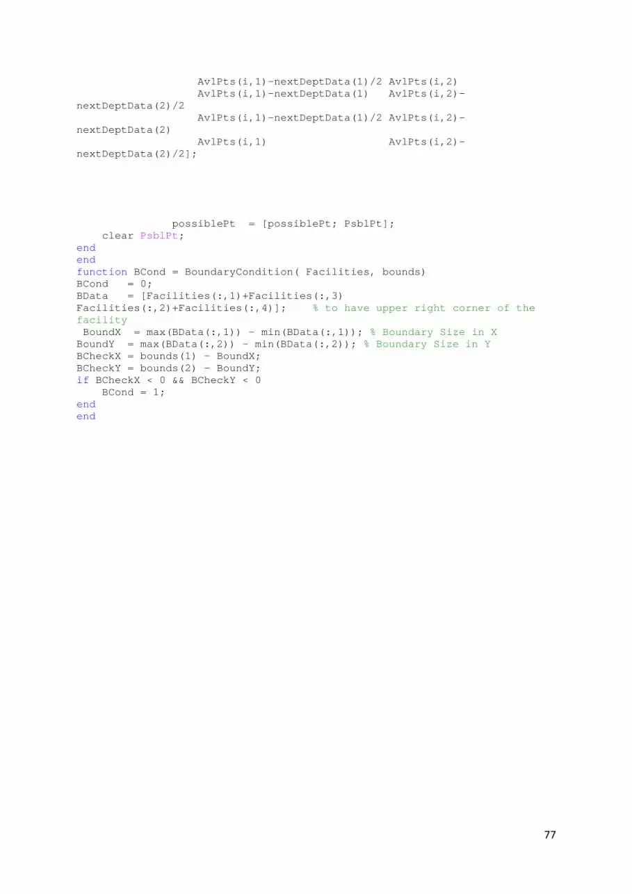
77

AvlPts(i,1)-nextDeptData(1)/2 AvlPts(i,2) AvlPts(i,1)-nextDeptData(1) AvlPts(i,2)-nextDeptData(2)/2 AvlPts(i,1)-nextDeptData(1)/2 AvlPts(i,2)-nextDeptData(2) AvlPts(i,1) AvlPts(i,2)-nextDeptData(2)/2]; possiblePt = [possiblePt; PsblPt]; clear PsblPt; end end function BCond = BoundaryCondition( Facilities, bounds) BCond = 0; BData = [Facilities(:,1)+Facilities(:,3) Facilities(:,2)+Facilities(:,4)]; % to have upper right corner of the facility BoundX = max(BData(:,1)) - min(BData(:,1)); % Boundary Size in X BoundY = max(BData(:,2)) - min(BData(:,2)); % Boundary Size in Y BCheckX = bounds(1) - BoundX; BCheckY = bounds(2) - BoundY; if BCheckX < 0 && BCheckY < 0 BCond = 1; end end

78

APPENDIX B: Matlab code for CBPS-Selective Sequential method for 8Facilities function [Cbest, AvlBlock] = selectivesequential( ) % layout mid centre as starting point clear all; clc; close all; rand('state',2) % Cost Data for material handling between each facility cData = [0 1 2 0 0 0 2 0 0 0 4 3 6 0 0 2 0 0 0 2 0 3 1 0 0 0 0 0 5 2 0 2 0 0 0 0 0 0 0 4 0 0 0 0 0 0 4 0 0 0 0 0 0 0 0 1 0 0 0 0 0 0 0 0]; % Facility Data dData = [2 3 4 5 2 2 3 3 2 4 4 4 4 4 3 4]; bounds = [20 20]; % layout boundary rMax = size(dData,1); % Number of Facilities z = randperm(rMax) % Facility random order generation cArr = cData(z,z);%Arrange the Cost matrix cData as per the random order % DArr = dData(z,:);%Arrange the Cost matrix as per the random order of weidth and hight data matrix dData r = round(rand(rMax,1));%for random generation of 0 and 1 for i = 1:rMax %loop for interchanging the weidth and height data if r(i)==1 dData(i,:) = [dData(i,2) dData(i,1)];%condition to rotate weidth by height or vice versa(column swap) end end clear i figure(1); close all; figure(1); hold on; axis equal;%To plot the figure with equal axis length rectangle('Position',[0 0 bounds]); % Plot Layout Boundary % First Facility for Initilisation at layout center nextBlockData = dData(1,:); % Next Facility Data from Arranged dData matrix Block = [bounds(1)/2 - nextBlockData(1)/2, bounds(2)/2 - nextBlockData(2)/2, nextBlockData];%co-ordinate and width height data of first facility by random order defined in z rectangle('Position', Block,'FaceColor','g'); % plot the first facility

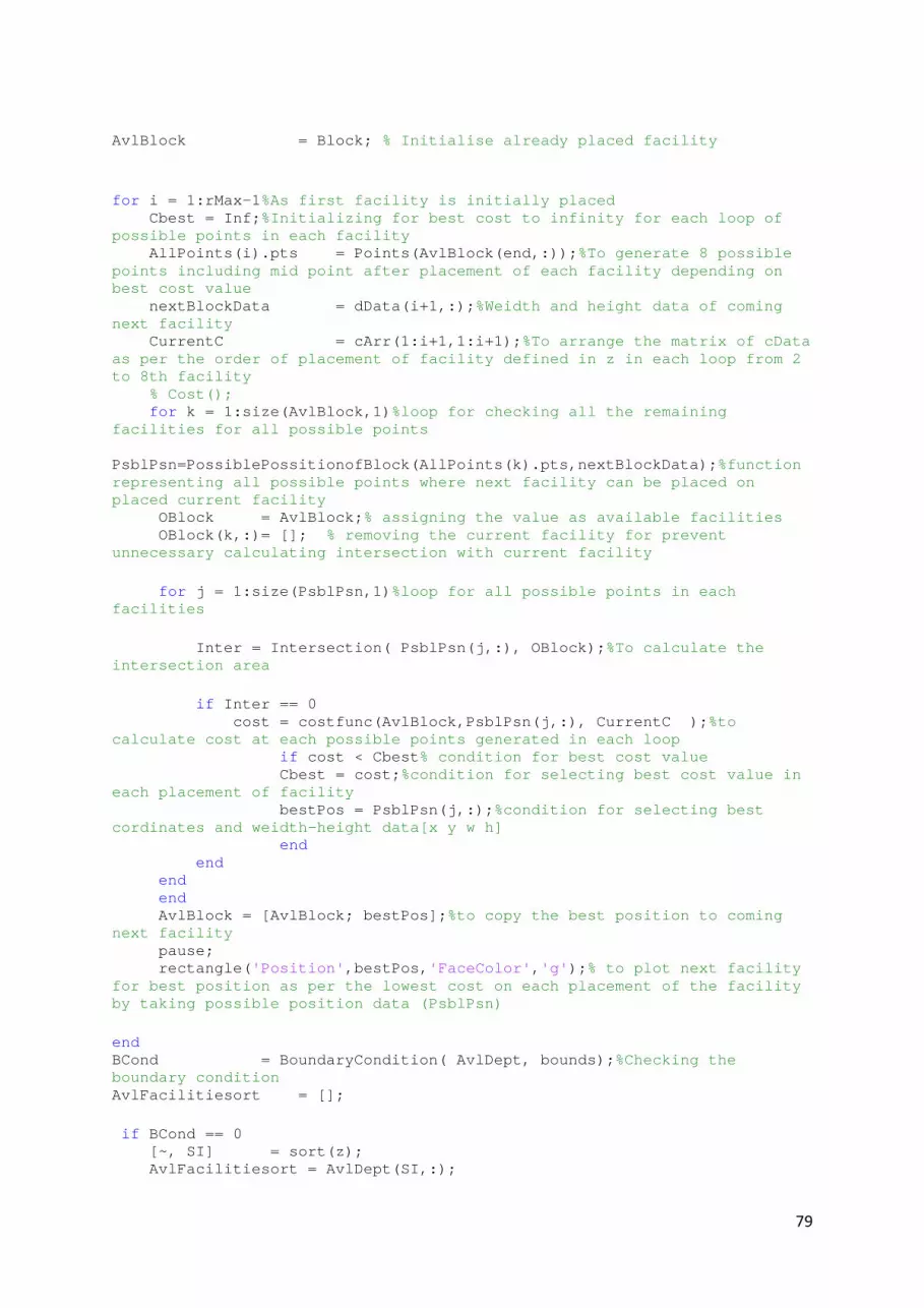
79

AvlBlock = Block; % Initialise already placed facility for i = 1:rMax-1%As first facility is initially placed Cbest = Inf;%Initializing for best cost to infinity for each loop of possible points in each facility AllPoints(i).pts = Points(AvlBlock(end,:));%To generate 8 possible points including mid point after placement of each facility depending on best cost value nextBlockData = dData(i+1,:);%Weidth and height data of coming next facility CurrentC = cArr(1:i+1,1:i+1);%To arrange the matrix of cData as per the order of placement of facility defined in z in each loop from 2 to 8th facility % Cost(); for k = 1:size(AvlBlock,1)%loop for checking all the remaining facilities for all possible points PsblPsn=PossiblePossitionofBlock(AllPoints(k).pts,nextBlockData);%function representing all possible points where next facility can be placed on placed current facility OBlock = AvlBlock;% assigning the value as available facilities OBlock(k,:)= []; % removing the current facility for prevent unnecessary calculating intersection with current facility for j = 1:size(PsblPsn,1)%loop for all possible points in each facilities Inter = Intersection( PsblPsn(j,:), OBlock);%To calculate the intersection area if Inter == 0 cost = costfunc(AvlBlock,PsblPsn(j,:), CurrentC );%to calculate cost at each possible points generated in each loop if cost < Cbest% condition for best cost value Cbest = cost;%condition for selecting best cost value in each placement of facility bestPos = PsblPsn(j,:);%condition for selecting best cordinates and weidth-height data[x y w h] end end end end AvlBlock = [AvlBlock; bestPos];%to copy the best position to coming next facility pause; rectangle('Position',bestPos,'FaceColor','g');% to plot next facility for best position as per the lowest cost on each placement of the facility by taking possible position data (PsblPsn) end BCond = BoundaryCondition( AvlDept, bounds);%Checking the boundary condition AvlFacilitiesort = []; if BCond == 0 [~, SI] = sort(z); AvlFacilitiesort = AvlDept(SI,:);

80

else TotalCost = []; end end function PsblPsn = PossiblePositionofFacilities(AP, nextBlockData)% function to check possible points on current facility % Matrix representing 32 position on current facility with respect to generated corner and center points of current facility and available facilities PsblPsn = [AP(1,1)-nextBlockData(1) AP(1,2) nextBlockData AP(1,1)-nextBlockData(1) AP(1,2)-nextBlockData(2)/2 nextBlockData AP(1,1)-nextBlockData(1) AP(1,2)-nextBlockData(2) nextBlockData AP(1,1)-nextBlockData(1)/2 AP(1,2)-nextBlockData(2) nextBlockData AP(1,1) AP(1,2)-nextBlockData(2) nextBlockData AP(2,1)-nextBlockData(1) AP(3,2)-nextBlockData(2) nextBlockData AP(2,1)-nextBlockData(1)/2 AP(2,2)-nextBlockData(2) nextBlockData AP(2,1) AP(2,2)-nextBlockData(2) nextBlockData AP(3,1)-nextBlockData(1) AP(1,2)-nextBlockData(2) nextBlockData AP(3,1)-nextBlockData(1)/2 AP(3,2)-nextBlockData(2) nextBlockData AP(3,1) AP(3,2)-nextBlockData(2) nextBlockData AP(3,1) AP(3,2)-nextBlockData(2)/2 nextBlockData AP(3,1) AP(3,2) nextBlockData AP(4,1) AP(4,2)-nextBlockData(2) nextBlockData AP(4,1) AP(4,2)-nextBlockData(2)/2 nextBlockData AP(4,1) AP(4,2) nextBlockData AP(5,1) AP(5,2)-nextBlockData(2) nextBlockData AP(5,1) AP(5,2)-nextBlockData(2)/2 nextBlockData AP(5,1) AP(5,2) nextBlockData AP(5,1)-nextBlockData(1)/2 AP(5,2) nextBlockData AP(5,1)-nextBlockData(1) AP(5,2) nextBlockData

81

AP(6,1) AP(6,2) nextBlockData AP(6,1)-nextBlockData(1)/2 AP(6,2) nextBlockData AP(6,1)-nextBlockData(1) AP(6,2) nextBlockData AP(7,1) AP(7,2) nextBlockData AP(7,1)-nextBlockData(1)/2 AP(7,2) nextBlockData AP(7,1)-nextBlockData(1) AP(7,2) nextBlockData AP(7,1)-nextBlockData(1) AP(7,2)-nextBlockData(2)/2 nextBlockData AP(7,1)-nextBlockData(1) AP(7,2)-nextBlockData(2) nextBlockData AP(8,1)-nextBlockData(1) AP(8,2) nextBlockData AP(8,1)-nextBlockData(1) AP(8,2)-nextBlockData(2)/2 nextBlockData AP(8,1)-nextBlockData(1) AP(8,2)-nextBlockData(2) nextBlockData]; %32 possible positions for each available facility to check before placement end function cost = costfunc(AvlBlock, PsblPosn,c)%to calculate cost by taking posible position data bestPos = [AvlBlock; PsblPosn]; DistMat = DistanceMat(bestPos); cost = sum(sum(c.*DistMat)); end function DistMat = DistanceMat(Dept)%Distance matrix generation s = size(Dept,1); DistMat = zeros(s,s); for i = 1:s for j = 1:s x1 = Dept(i,1)+Dept(i,3)/2; x2 = Dept(j,1)+Dept(j,3)/2; y1 = Dept(i,2)+Dept(i,4)/2; y2 = Dept(j,2)+Dept(j,4)/2; DistMat(i,j) = abs(x1-x2)+abs(y1-y2); end end end function AllPoints = Points(Block) AllPoints = [Block(1) Block(2) Block(1)+Block(3)/2 Block(2) Block(1)+Block(3) Block(2) Block(1)+Block(3) Block(2)+ Block(4)/2

82

Block(1)+Block(3) Block(2)+ Block(4) Block(1)+Block(3)/2 Block(2)+ Block(4) Block(1) Block(2)+ Block(4) Block(1) Block(2)+ Block(4)/2]; end function Inter = Intersection(PsblPosn, OBlock) Inter=0; for i = 1:size(OBlock,1) xx = rectint( PsblPosn,OBlock(i,:)); Inter = Inter + xx; if Inter ~= 0 Inter = 1; break; end end end function BCond = BoundaryCondition( Facilities, bounds) BCond = 0; BData = [Facilities(:,1)+Facilities(:,3) Facilities(:,2)+Facilities(:,4)]; % to have upper right corner of the facility BoundX = max(BData(:,1)) - min(BData(:,1)); % Boundary Size in X BoundY = max(BData(:,2)) - min(BData(:,2)); % Boundary Size in Y BCheckX = bounds(1) - BoundX; BCheckY = bounds(2) - BoundY; if BCheckX < 0 && BCheckY < 0 BCond = 1; end end

83

APPENDIX C: Matlab code for CBPS with local Search Algorithm for 8Facilities,11Facilities and 20Facilities

function [best, AvlBlock,zbest,rbest] = localpositioning_loop() clear all; close all; clc; tic % rand('state', 51576); nb=20; best = Inf; n=Inf; for i = 1:n i [Cbest, AvlBlock, z,r] = localpositioning04(i,nb); if nb == 8 sol = 192; elseif nb == 11 sol = 1254.5; elseif nb == 20 sol = 2510; end if Cbest <best && Cbest<=sol best = Cbest; zbest= z; rbest=r; BestAvlBlock = AvlBlock; display(i); display(best); display(zbest'); display(rbest); display(BestAvlBlock); break; end end toc end function [Cbest, AvlFacilitiesort, z,r] = localpositioning04(seed,nb) % layout mid center as starting point % clear all; clc; close all; rand('state', seed); % Cost Data for material handling between each facility switch nb case 8 cData = [0 1 2 0 0 0 2 0 0 0 4 3 6 0 0 2 0 0 0 2 0 3 1 0 0 0 0 0 5 2 0 2 0 0 0 0 0 0 0 4 0 0 0 0 0 0 4 0 0 0 0 0 0 0 0 1 0 0 0 0 0 0 0 0]; dData = [2 4 2 3 2 4 4 3 3 5 2 3 4 4 4 4]'; bounds = [12 12];

84

case 11 cData = [0 2 1 1 2 6 2 6 6 3 6; 0 0 1 1 2 6 4 6 6 3 6; 0 0 0 2 2 6 1 6 6 6 6; 0 0 0 0 1 5 1 6 6 3 6; 0 0 0 0 0 4 3 6 4 5 6; 0 0 0 0 0 0 3 6 4 5 6; 0 0 0 0 0 0 0 4 4 1 1; 0 0 0 0 0 0 0 0 6 3 3; 0 0 0 0 0 0 0 0 0 5 5; 0 0 0 0 0 0 0 0 0 0 2; 0 0 0 0 0 0 0 0 0 0 0]; dData = [4 1 1 2 3 1.4 4 2.6 4.0 4 5 4 2 2 5 2 5.0 3 2.0 2.8 7 5]'; % facility data bounds = [15 15]; case 20 cData = [0 3 0 0 4 2 0 0 4 0 0 5 3 0 5 0 0 1 0 0; 3 0 1 0 1 2 5 0 3 0 0 0 2 0 3 0 3 1 2 3; 0 1 0 4 0 0 3 0 0 0 1 0 0 0 0 0 5 0 2 3; 0 0 4 0 4 0 0 1 5 3 0 2 0 0 4 5 0 1 0 0; 4 1 0 4 0 0 0 0 1 4 1 5 0 0 3 2 0 5 0 4; 2 2 0 0 0 0 3 0 0 5 0 0 3 0 0 0 2 0 0 0; 0 5 3 0 0 3 0 0 0 0 0 0 4 0 2 0 3 2 0 1; 0 0 0 1 0 0 0 0 0 0 2 0 0 5 0 4 0 1 0 0; 4 3 0 5 1 0 0 0 0 3 0 5 0 0 0 2 0 0 0 0; 0 0 0 3 4 5 0 0 3 0 0 5 0 1 2 4 0 3 4 0; 0 0 1 0 1 0 0 2 0 0 0 0 0 5 5 4 0 4 3 1; 5 0 0 2 5 0 0 0 5 5 0 0 5 0 2 0 0 1 0 0; 3 2 0 0 0 3 4 0 0 0 0 5 0 0 3 0 2 0 0 0; 0 0 0 0 0 0 0 5 0 1 5 0 0 0 0 5 0 5 1 0; 5 3 0 4 3 0 2 0 0 2 5 2 3 0 0 0 1 4 3 3; 0 0 0 5 2 0 0 4 2 4 4 0 0 5 0 0 4 5 0 0; 0 3 5 0 0 2 3 0 0 0 0 0 2 0 1 4 0 0 1 5; 1 1 0 1 5 0 2 1 0 3 4 1 0 5 4 5 0 0 4 1; 0 2 2 0 0 0 0 0 0 4 3 0 0 1 3 0 1 4 0 5; 0 3 3 0 4 0 1 0 0 0 1 0 0 0 3 0 5 1 5 0]; dData = [1 2 1 2 3 2 2 2 3 3 2 1 3 3 3 2 3 2 2 2 2 2 1 3 3 2 1 3 2 3 3 2 2 3 3 2 2 2 2 1]'; bounds = [14 14]; end % bounds = [12 12]; % layout boundary rMax = size(dData,1); % Number of Facilities z = randperm(rMax); % facility call order cArr = cData(z,z); % To arrange the cost dArr = dData(z,:); % To arrange the width and height matrix of the facility adding to random selection % To rotate the width to height or vice versa r = round(rand(rMax,1)); % generation of random 0 and 1 number for dData

85

for i = 1:rMax if r(i) == 1 dArr(i,:) = [dArr(i,2) dArr(i,1)]; end end clear i figure(1); close all; figure(1); hold on; axis equal; % rectangle('Position',[0 0 bounds]); % Plot Layout Boundary % First facility for Initilisation at layout center nextBlockData = dArr(1,:); % Next Facility Data Block = [bounds(1)/2 - nextBlockData(1)/2, bounds(2)/2 - nextBlockData(2)/2, nextBlockData]; rectangle('Position', Block,'FaceColor','g'); % plot the first facility AvlBlock = Block; % Initialise already placed facility for i = 1:rMax-1 Cbest = Inf; % Initializing hte best cost before checking 32 possible location for respective facility AllPoints(i).pts = Points(AvlBlock(end,:)); % To generate all the 8 points of the facility including the center of edges after the placement of the facility before placing another facility nextBlockData = dArr(i+1,:); CurrentC = cArr(1:i+1,1:i+1); for k = 1:size(AvlBlock,1) PsblPsn = PossiblePositionofFacilities(AllPoints(k).pts,nextBlockData); OBlock = AvlBlock; % assigning the value as available facilities OBlock(k,:)= []; % removing the current facility for prevent unnecessary calculating intersection with current facility for j = 1:size(PsblPsn,1) % Loop for checking best Possible points based on best cost value on all possible points 32 for each facility Inter = Intersection( PsblPsn(j,:), OBlock); % To check the intersection with all other facilities except the current facility if Inter == 0 % Condition of intersection cost = costfunc(AvlBlock,PsblPsn(j,:), CurrentC );%cost function taking the input possible position if cost < Cbest % Condition for selecting the cost Cbest = cost; bestPos = PsblPsn(j,:); % Condition for selecting best position for facility to placed based on lowest cost end end end clear PsblPsn OBlock end AvlBlock = [AvlBlock; bestPos]; % copying the best position to coming next facility rectangle('Position',bestPos,'FaceColor','g'); % to plot the best position end BCond = BoundaryCondition( AvlBlock, bounds); AvlFacilitiesort = []; if BCond == 0 [~, SI] = sort(z);

86

AvlFacilitiesort = AvlBlock(SI,:); % DFinal = dArr(SI,:); % zData = [z; r']; % clear z; % display(AvlFacilitiesort); % display(DFinal); % else % Cbest = []; end end function PsblPsn = PossiblePositionofFacilities(AP, nextBlockData)% function to check possible points on current facility % Matrix representing 32 position on current facility with respect to generated corner and center points of current facility and available facilities PsblPsn = [AP(1,1)-nextBlockData(1) AP(1,2) nextBlockData AP(1,1)-nextBlockData(1) AP(1,2)-nextBlockData(2)/2 nextBlockData AP(1,1)-nextBlockData(1) AP(1,2)-nextBlockData(2) nextBlockData AP(1,1)-nextBlockData(1)/2 AP(1,2)-nextBlockData(2) nextBlockData AP(1,1) AP(1,2)-nextBlockData(2) nextBlockData AP(2,1)-nextBlockData(1) AP(3,2)-nextBlockData(2) nextBlockData AP(2,1)-nextBlockData(1)/2 AP(2,2)-nextBlockData(2) nextBlockData AP(2,1) AP(2,2)-nextBlockData(2) nextBlockData AP(3,1)-nextBlockData(1) AP(1,2)-nextBlockData(2) nextBlockData AP(3,1)-nextBlockData(1)/2 AP(3,2)-nextBlockData(2) nextBlockData AP(3,1) AP(3,2)-nextBlockData(2) nextBlockData AP(3,1) AP(3,2)-nextBlockData(2)/2 nextBlockData AP(3,1) AP(3,2) nextBlockData AP(4,1) AP(4,2)-nextBlockData(2) nextBlockData AP(4,1) AP(4,2)-nextBlockData(2)/2 nextBlockData AP(4,1) AP(4,2) nextBlockData AP(5,1) AP(5,2)-nextBlockData(2) nextBlockData AP(5,1) AP(5,2)-nextBlockData(2)/2 nextBlockData AP(5,1) AP(5,2) nextBlockData

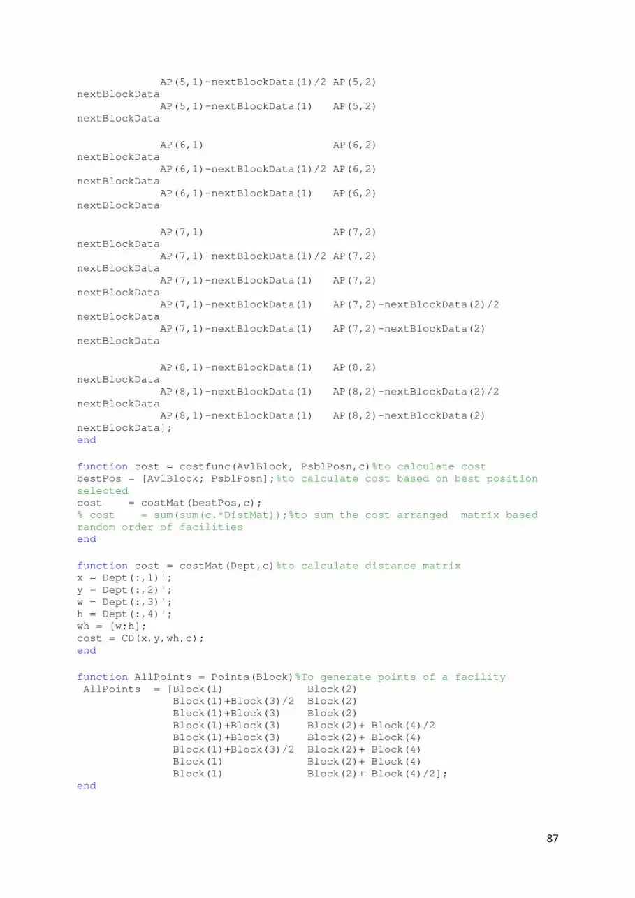
87

AP(5,1)-nextBlockData(1)/2 AP(5,2) nextBlockData AP(5,1)-nextBlockData(1) AP(5,2) nextBlockData AP(6,1) AP(6,2) nextBlockData AP(6,1)-nextBlockData(1)/2 AP(6,2) nextBlockData AP(6,1)-nextBlockData(1) AP(6,2) nextBlockData AP(7,1) AP(7,2) nextBlockData AP(7,1)-nextBlockData(1)/2 AP(7,2) nextBlockData AP(7,1)-nextBlockData(1) AP(7,2) nextBlockData AP(7,1)-nextBlockData(1) AP(7,2)-nextBlockData(2)/2 nextBlockData AP(7,1)-nextBlockData(1) AP(7,2)-nextBlockData(2) nextBlockData AP(8,1)-nextBlockData(1) AP(8,2) nextBlockData AP(8,1)-nextBlockData(1) AP(8,2)-nextBlockData(2)/2 nextBlockData AP(8,1)-nextBlockData(1) AP(8,2)-nextBlockData(2) nextBlockData]; end function cost = costfunc(AvlBlock, PsblPosn,c)%to calculate cost bestPos = [AvlBlock; PsblPosn];%to calculate cost based on best position selected cost = costMat(bestPos,c); % cost = sum(sum(c.*DistMat));%to sum the cost arranged matrix based random order of facilities end function cost = costMat(Dept,c)%to calculate distance matrix x = Dept(:,1)'; y = Dept(:,2)'; w = Dept(:,3)'; h = Dept(:,4)'; wh = [w;h]; cost = CD(x,y,wh,c); end function AllPoints = Points(Block)%To generate points of a facility AllPoints = [Block(1) Block(2) Block(1)+Block(3)/2 Block(2) Block(1)+Block(3) Block(2) Block(1)+Block(3) Block(2)+ Block(4)/2 Block(1)+Block(3) Block(2)+ Block(4) Block(1)+Block(3)/2 Block(2)+ Block(4) Block(1) Block(2)+ Block(4) Block(1) Block(2)+ Block(4)/2]; end

88

function Inter = Intersection(PsblPosn, OBlock)%To plot the intersection area point by point on the possible points of position of next facility coming facility % Output is either 0 or 1 % 0 means no intersection detected % 1 means intersection is detected Inter=0; for i = 1:size(OBlock,1)%Loop for intersection size for other facility except the current facility Inter = Inter + rectint( PsblPosn,OBlock(i,:));%Intersection between possible position and remaining other facility if Inter ~= 0 Inter = 1; break; end end end function f = CD(x,y,wh,c) x = x + wh(1,:)./2; y = y + wh(2,:)./2; for i = 1:size(x,2) for j = 1:size(x,2) dd(i,j) = abs(x(i)-x(j))+abs(y(i)-y(j)); end end f = sum(sum(c.*dd)); end function BCond = BoundaryCondition( Facilities, bounds) BCond = 0; BData = [Facilities(:,1)+Facilities(:,3) Facilities(:,2)+Facilities(:,4)]; % to have upper right corner of the facility BoundX = max(BData(:,1)) - min(BData(:,1)); % Boundary Size in X BoundY = max(BData(:,2)) - min(BData(:,2)); % Boundary Size in Y BCheckX = bounds(1) - BoundX; BCheckY = bounds(2) - BoundY; if BCheckX < 0 && BCheckY < 0 BCond = 1; end end

89

APPENDIX D: Matlab code for Gradient Method

function [best , Rec_best,besti , Solution]=MyComparativeLoop2() clear all; close all; clc; tic; test=8 ; method = 2 ; Forloop=200; seed=28 ; % Test à réaliser : 8, 11 , 20 ou autre [cData, dData, bounds] =InitialiseTest(test) ; switch method case 1 Forloop=Forloop; rand('state', seed); [best, BestAvlBlock,zbest,rbest]= LocalPositionnning(Forloop,cData, dData, bounds)%Checking CBPS case 2 % fimincon [best , Rec_best,besti , Solution]= GlobalePositionning(Forloop, cData, dData, bounds) ; %Checking Gradient Method end t=toc end function [best, BestAvlBlock,zbest,rbest]=LocalPositionnning(For_loop,cData, dData, bounds) % méthode d'optimisation best=inf;k=0; for i = 100:For_loop i [cost,AvlBlock, z,r] = localpositioning01(cData, dData, bounds); if cost< best best=cost; zbest=z; rbest=r; BestAvlBlock=AvlBlock; end end cost best zbest rbest display(BestAvlBlock) toc end function [Cbest, AvlBlock,z,r] = localpositioning01(cData, dData, bounds) % layout mid centre as starting point % clear all; clc; close all; % rand('state',2)

90

rMax = size(dData,1); % Number of facilities z = randperm(rMax); % Facility call order cArr = cData(z,z); dArr = dData(z,:); r = round(rand(rMax,1)); dArr=~[r r].*dData+[r r].*[dData(:,2) dData(:,1)] ; close all; figure ; hold on; axis equal; rectangle('Position',[0 0 bounds]); % Plot Layout Boundary % First facility for Initialization at layout center nextBlockData = dArr(1,:); % Next facility Data Block = [bounds(1)/2 - nextBlockData(1)/2, bounds(2)/2 - nextBlockData(2)/2, nextBlockData]; rectangle('Position', Block,'FaceColor','g'); % plot the first facility AvlBlock = Block; % Initialise already placed facility for i = 1:rMax-1 Cbest = Inf; AllPoints(i).pts = Points(AvlBlock(end,:)); nextBlockData = dArr(i+1,:); CurrentC = cArr(1:i+1,1:i+1); % Cost(); for k = 1:size(AvlBlock,1) PsblPsn=PossiblePossitionofBlock(AllPoints(k).pts,nextBlockData); OBlock = AvlBlock;% assigning the value as available facilities OBlock(k,:)= []; % removing the current facility for prevent unnecessary calculating intersection with current facility end for j = 1:size(PsblPsn,1) Inter = Intersection( PsblPsn(j,:), OBlock); if Inter == 0 cost = costfunc(AvlBlock,PsblPsn(j,:), CurrentC ); if cost < Cbest Cbest = cost; bestPos = PsblPsn(j,:); end end end AvlBlock = [AvlBlock; bestPos]; rectangle('Position',bestPos,'FaceColor','g'); end cost=Cbest; end function PsblPsn=PossiblePossitionofBlock(AP,nextBlockData) PsblPsn = [AP(3,1) AP(3,2) nextBlockData AP(3,1) AP(3,2)-nextBlockData(2)/2 nextBlockData

91

AP(4,1) AP(4,2)-nextBlockData(2)/2 nextBlockData AP(4,1) AP(4,2)-nextBlockData(2) nextBlockData AP(3,1) AP(3,2)-nextBlockData(2) nextBlockData AP(5,1) AP(5,2)-nextBlockData(2) nextBlockData AP(5,1) AP(5,2)-nextBlockData(2)/2 nextBlockData AP(5,1) AP(5,2) nextBlockData AP(4,1) AP(4,2) nextBlockData AP(7,1)-nextBlockData(1) AP(7,2) nextBlockData AP(7,1)-nextBlockData(1) AP(7,2)-nextBlockData(2) nextBlockData AP(7,1)-nextBlockData(1) AP(7,2)-nextBlockData(2)/2 nextBlockData AP(8,1)-nextBlockData(1) AP(8,2)-nextBlockData(2) nextBlockData AP(8,1)-nextBlockData(1) AP(8,2)-nextBlockData(2)/2 nextBlockData AP(8,1)-nextBlockData(1) AP(8,2) nextBlockData AP(1,1)-nextBlockData(1) AP(1,2)-nextBlockData(2)/2 nextBlockData AP(1,1)-nextBlockData(1) AP(1,2)-nextBlockData(2) nextBlockData AP(1,1)-nextBlockData(1) AP(1,2) nextBlockData AP(5,1)-nextBlockData(1)/2 AP(5,2) nextBlockData AP(6,1) AP(6,2) nextBlockData AP(5,1)-nextBlockData(1) AP(5,2) nextBlockData AP(6,1)-nextBlockData(1) AP(6,2) nextBlockData AP(7,1) AP(7,2) nextBlockData AP(7,1)-nextBlockData(1)/2 AP(7,2) nextBlockData AP(6,1)-nextBlockData(1)/2 AP(6,2) nextBlockData AP(1,1) AP(1,2)-nextBlockData(2) nextBlockData AP(3,1)-nextBlockData(1) AP(1,2)-nextBlockData(2) nextBlockData AP(2,1)-nextBlockData(1)/2 AP(2,2)-nextBlockData(2) nextBlockData AP(2,1) AP(2,2)-nextBlockData(2) nextBlockData AP(3,1)-nextBlockData(1)/2 AP(3,2)-nextBlockData(2) nextBlockData AP(2,1)-nextBlockData(1) AP(3,2)-nextBlockData(2) nextBlockData

92

AP(1,1)-nextBlockData(1)/2 AP(1,2)-nextBlockData(2) nextBlockData]; end function cost = costfunc(AvlBlock, PsblPosn,c) bestPos = [AvlBlock; PsblPosn]; DistMat = DistanceMat(bestPos); cost = sum(sum(c.*DistMat)); end function DistMat = DistanceMat(Dept) s = size(Dept,1); DistMat = zeros(s,s); for i = 1:s for j = 1:s x1 = Dept(i,1)+Dept(i,3)/2; x2 = Dept(j,1)+Dept(j,3)/2; y1 = Dept(i,2)+Dept(i,4)/2; y2 = Dept(j,2)+Dept(j,4)/2; DistMat(i,j) = abs(x1-x2)+abs(y1-y2); end end end function AllPoints = Points(Block) AllPoints = [Block(1) Block(2) Block(1)+Block(3)/2 Block(2) Block(1)+Block(3) Block(2) Block(1)+Block(3) Block(2)+ Block(4)/2 Block(1)+Block(3) Block(2)+ Block(4) Block(1)+Block(3)/2 Block(2)+ Block(4) Block(1) Block(2)+ Block(4) Block(1) Block(2)+ Block(4)/2]; end function Inter = Intersection(PsblPosn, OBlock) Inter=0; for i = 1:size(OBlock,1) xx = rectint( PsblPosn,OBlock(i,:)); Inter = Inter + xx; if Inter ~= 0 Inter = 1; break; end end end

93

%% Continus with Fmincon GlobalePositionning(Forloop, cData, dData, bounds) function [best, Rec_best,besti,Solution]= GlobalePositionning(Forloop, cData, dData, bounds)%Initial condition and problem structure for Gradient method global Rec best =inf ; k=0; for i= 1 :Forloop Rec=[]; figure(1) ; clf; AXE=gca; set(AXE,... 'XLim',[0 12], ... 'YLim', [0 12],... 'XLimMode', 'manual','YLimMode','manual'); [x0 DData LB UB]=createRandData(cData, dData, bounds) ; Rec=CreateFacilities(x0,DData) ; options=optimset('Display', 'off', 'MaxFunEvals',3000,... 'MaxIter', 100, 'TolX',1.e-4, 'TolFun',1.e-4, 'TolCon',1.e-10) ; hObjective =@(x)Objective(x,cData,DData) ; hConstraints =@(x)Constraints(x,DData) ; [x fval]=fmincon( hObjective ,x0, [],[],[],[],LB,UB,hConstraints, options) ; %drawnow [i fval best(end)] % n=inf; % for i=1:n i Solution{i}=[x DData] ; if fval<best k=k+1; Rec_best=[x,DData] best(k) =fval ; besti(k)=i ; best end end end function [X DDATA LB UB]=createRandData(cData, dData, bounds)%Boundary Condition s=size(dData,1) ; r = round(rand(s,1)); DDATA=~[r r].*dData+[r r].*[dData(:,2) dData(:,1)] ; xmin=0; ymin=0 ; xmax=bounds(1,1)-DDATA(:,1); ymax=bounds(1,2)-DDATA(:,2); LB=[xmin, ymin]; UB= [xmax, ymax]; x=xmin+(xmax-xmin).*rand(s,1) ; y=ymin+(ymax-ymin).*rand(s,1) ;

94

X=[x y]; end %% function Rec=CreateFacilities(x,DData) %Plotting Facilities for i=1 : size(x,1) Rec(i)=rectangle('Position', [x(i,:) DData(i,:)],'FaceColor','g'); end end %% Objective function fval=Objective(x,cData,DData)%Condition of cost at each placement as objective function global Rec Rec=updatedRec(Rec,x,DData) ; s=size(DData,1); xc=x+DData/2; d=zeros(s,s) ; for i=1:s if i<s for j=i+1:s d(i,j)=abs(xc(i,1)-xc(j,1))+abs(xc(i,2)-xc(j,2)) ; end end end fval=sum(sum(cData.*d)) ; %drawnow end function [g geq]= Constraints(x,DData) %Overlapping condition as constraint global Rec Rec=updatedRec(Rec,x,DData) ; geq=[]; s=size(DData,1); G=zeros(s,1) ; for i=1:s for j=1:s if i~=j ; G(i)=G(i)+ rectint(get(Rec(i),'Position'), get(Rec(j),'Position')) ; end end end %G' ; G(end+1)=sum(G); g=G-0.001; end %% Affiche Rectangle function Rec=updatedRec(Rec,x,DData) for i=1 : size(x,1) set(Rec(i),'Position',[x(i,:) DData(i,:)]); end end

95

%% Initialization function of Objective and Data function [cData, dData, bounds] =InitialiseTest(test)%Cost rate matrix and given boundry condition for 8,11 and 20 Facilities switch test case 8 % Cost Data for material handling between each facility cData = [0 1 2 0 0 0 2 0 0 0 4 3 6 0 0 2 0 0 0 2 0 3 1 0 0 0 0 0 5 2 0 2 0 0 0 0 0 0 0 4 0 0 0 0 0 0 4 0 0 0 0 0 0 0 0 1 0 0 0 0 0 0 0 0]; % Facility Data dData = [2 3 4 5 2 2 3 3 2 4 4 4 4 4 3 4]; bounds = [12 12]; % layout boundary case 11 % Cost Data for material handling between each facility cData = [0 2 1 1 2 6 2 6 6 3 6 0 0 1 1 2 6 4 6 6 3 6 0 0 0 2 2 6 1 6 6 6 6 0 0 0 0 1 5 1 6 6 3 6 0 0 0 0 0 4 3 6 4 5 6 0 0 0 0 0 0 3 6 4 5 6 0 0 0 0 0 0 0 4 4 1 1 0 0 0 0 0 0 0 0 6 3 3 0 0 0 0 0 0 0 0 0 5 5 0 0 0 0 0 0 0 0 0 0 2 0 0 0 0 0 0 0 0 0 0 0]; % Facility Data dData = [4 4 1 2 1 2 2 5 3 2 1.4 5 4 3 2.6 2 4 2.8 4 7 5 5] ; bounds = [15 15]; % layout boundary

96

case 20 % Cost Data for material handling between each facility cData = [ 0 3 0 0 4 2 0 0 4 0 0 5 3 0 5 0 0 1 0 0 3 0 1 0 1 2 5 0 3 0 0 0 2 0 3 0 3 1 2 3 0 1 0 4 0 0 3 0 0 0 1 0 0 0 0 0 5 0 2 3 0 0 4 0 4 0 0 1 5 3 0 2 0 0 4 5 0 1 0 0 4 1 0 4 0 0 0 0 1 4 1 5 0 0 3 2 0 5 0 4 2 2 0 0 0 0 3 0 0 5 0 0 3 0 0 0 2 0 0 0 0 5 3 0 0 3 0 0 0 0 0 0 4 0 2 0 3 2 0 1 0 0 0 1 0 0 0 0 0 0 2 0 0 5 0 4 0 1 0 0 4 3 0 5 1 0 0 0 0 3 0 5 0 0 0 2 0 0 0 0 0 0 0 3 4 5 0 0 3 0 0 5 0 1 2 4 0 3 4 0 0 0 1 0 1 0 0 2 0 0 0 0 0 5 5 4 0 4 3 1 5 0 0 2 5 0 0 0 5 5 0 0 5 0 2 0 0 1 0 0 3 2 0 0 0 3 4 0 0 0 0 5 0 0 3 0 2 0 0 0 0 0 0 0 0 0 0 5 0 1 5 0 0 0 0 5 0 5 1 0 5 3 0 4 3 0 2 0 0 2 5 2 3 0 0 0 1 4 3 3 0 0 0 5 2 0 0 4 2 4 4 0 0 5 0 0 4 5 0 0 0 3 5 0 0 2 3 0 0 0 0 0 2 0 1 4 0 0 1 5 1 1 0 1 5 0 2 1 0 3 4 1 0 5 4 5 0 0 4 1 0 2 2 0 0 0 0 0 0 4 3 0 0 1 3 0 1 4 0 5 0 3 3 0 4 0 1 0 0 0 1 0 0 0 3 0 5 1 5 0]; % facility Data dData = [1 2 2 2 1 1 2 3 3 3 2 2 2 1 2 3 3 2 3 3 2 3 1 2 3 2 3 3 3 3 2 2 3 2 2 2 2 2 2 1]; bounds = [14 14]; % layout boundary end end

97

APPENDIX E: Matlab code for Genetic Algorithm function [fval, Facilities] = GALGORITHM()%Starting Condition clear all; close all; clc tic nob = 8; % change accordingly i.e. 8, 11 or 20 facilities if nob == 8 lbxy = [0 0]; ubxy = [12 12]; cData = [0 1 2 0 0 0 2 0 0 0 4 3 6 0 0 2 0 0 0 2 0 3 1 0 0 0 0 0 5 2 0 2 0 0 0 0 0 0 0 4 0 0 0 0 0 0 4 0 0 0 0 0 0 0 0 1 0 0 0 0 0 0 0 0]; Colour = [1.0 0.5 0.4; 1.0 0.8 0.0 0.6 1.0 0.6 0.0 1.0 0.5 0.5 0.8 1.0 0.2 0.4 0.9 0.6 0.4 0.8 0.9 0.5 0.9]; dData = [2 4 2 3 2 4 4 3 3 5 2 3 4 4 4 4]; elseif nob == 11 lbxy = [0 0]; ubxy = [15 15]; cData = [0 2 1 1 2 6 2 6 6 3 6; 0 0 1 1 2 6 4 6 6 3 6; 0 0 0 2 2 6 1 6 6 6 6; 0 0 0 0 1 5 1 6 6 3 6; 0 0 0 0 0 4 3 6 4 5 6; 0 0 0 0 0 0 3 6 4 5 6; 0 0 0 0 0 0 0 4 4 1 1; 0 0 0 0 0 0 0 0 6 3 3; 0 0 0 0 0 0 0 0 0 5 5; 0 0 0 0 0 0 0 0 0 0 2; 0 0 0 0 0 0 0 0 0 0 0]; Colour = [0.9 0.5 0.5 1.0 0.6 0.4 1.0 0.9 0.7 0.6 1.0 0.6 0.0 1.0 0.6 0.7 0.9 0.9 0.5 0.8 1.0 0.2 0.4 0.9 0.6 0.4 0.8 0.7 0.3 0.8 0.9 0.5 0.9]; dData = [4 1 1 2 3 1.4 4 2.6 4.0 4 5 4 2 2 5 2 5.0 3 2.0 2.8 7 5];

98

elseif nob == 20 lbxy = [0 0]; ubxy = [14 14]; cData = [0 3 0 0 4 2 0 0 4 0 0 5 3 0 5 0 0 1 0 0; 3 0 1 0 1 2 5 0 3 0 0 0 2 0 3 0 3 1 2 3; 0 1 0 4 0 0 3 0 0 0 1 0 0 0 0 0 5 0 2 3; 0 0 4 0 4 0 0 1 5 3 0 2 0 0 4 5 0 1 0 0; 4 1 0 4 0 0 0 0 1 4 1 5 0 0 3 2 0 5 0 4; 2 2 0 0 0 0 3 0 0 5 0 0 3 0 0 0 2 0 0 0; 0 5 3 0 0 3 0 0 0 0 0 0 4 0 2 0 3 2 0 1; 0 0 0 1 0 0 0 0 0 0 2 0 0 5 0 4 0 1 0 0; 4 3 0 5 1 0 0 0 0 3 0 5 0 0 0 2 0 0 0 0; 0 0 0 3 4 5 0 0 3 0 0 5 0 1 2 4 0 3 4 0; 0 0 1 0 1 0 0 2 0 0 0 0 0 5 5 4 0 4 3 1; 5 0 0 2 5 0 0 0 5 5 0 0 5 0 2 0 0 1 0 0; 3 2 0 0 0 3 4 0 0 0 0 5 0 0 3 0 2 0 0 0; 0 0 0 0 0 0 0 5 0 1 5 0 0 0 0 5 0 5 1 0; 5 3 0 4 3 0 2 0 0 2 5 2 3 0 0 0 1 4 3 3; 0 0 0 5 2 0 0 4 2 4 4 0 0 5 0 0 4 5 0 0; 0 3 5 0 0 2 3 0 0 0 0 0 2 0 1 4 0 0 1 5; 1 1 0 1 5 0 2 1 0 3 4 1 0 5 4 5 0 0 4 1; 0 2 2 0 0 0 0 0 0 4 3 0 0 1 3 0 1 4 0 5; 0 3 3 0 4 0 1 0 0 0 1 0 0 0 3 0 5 1 5 0]; Colour = [0.5 0.8 1.0 0.2 0.4 0.9 0.6 0.4 0.8 0.9 0.5 0.9 1.0 0.5 0.4 1.0 0.8 0.0 0.6 1.0 0.6 0.0 1.0 0.5 0.5 0.8 1.0 0.2 0.4 0.9 0.6 0.4 0.8 0.9 0.5 0.9 1.0 0.5 0.4 1.0 0.8 0.0 0.6 1.0 0.6 0.0 1.0 0.5 0.5 0.8 1.0 0.2 0.4 0.9 0.6 0.4 0.8 0.9 0.5 0.9]; dData = [1 2 1 2 3 2 2 2 3 3 2 1 3 3 3 2 3 2 2 2 2 2 1 3 3 2 1 3 2 3 3 2 2 3 3 2 2 2 2 1]; end popsize = 1000;%Population size ngen = 200;%Number of generation nvars = 2*nob;%Mutation rate %Boundary condition lb = [lbxy(1).*ones(1,nob) lbxy(2).*ones(1,nob)]; ub = [ubxy(1).*ones(1,nob)-dData(1,:) ubxy(2).*ones(1,nob)-dData(2,:)]; for i = 1:popsize inipop(i,:) = lb(1:nvars)+(ub(1:nvars)-lb(1:nvars)).*(rand(1,nvars));

99

end objective = @(x)obj(x,cData,dData);%Objective function for GA constraint = @(x)confuct(x,dData);%Constraint function for GA options = gaoptimset('Display','iter','PopulationSize',popsize,... 'InitialPopulation',inipop,'TolCon',1e-3,'TolFun',1e-3,'Generations',ngen);%Matlab structure to solve GA [x, fval] = ga(objective,nvars,[],[],[],[],lb,ub,constraint,options);%To check Fitness criteria in Matlab timetaken = toc; Facilities = [x(1:nob); x(nob+1:2*nob); dData]'; rectangle('Position',[lbxy ubxy-lbxy]); hold on; axis equal; figure('name','Local Placement Strategy','numbertitle','off','ToolBar','none'); clf; axes('Box','on'); hold on; axis equal; set(gca,'XLim',[lbxy(1) ubxy(1)],'YLim', [lbxy(2) ubxy(2)]); %Plot facility after end of algorithm for ii = 1:nob rectangle('Position',Facilities(ii,:),'FaceColor',Colour(ii,:)); text(Facilities(ii,1)+Facilities(ii,3)/2,Facilities(ii,2)+Facilitys(ii,4)/2,num2str(i)); end display(timetaken); display(fval); display(Facilities); end function fval = obj(x,cData,dData)%Objective function i.e. cost xNew = [x(1:length(x)/2)' x(1+length(x)/2:length(x))']; dNew = dData'; s = size(dNew,1); xc = xNew+dNew/2; d = zeros(s,s) ; for i=1:s if i<s for j=i+1:s d(i,j)=abs(xc(i,1)-xc(j,1))+abs(xc(i,2)-xc(j,2)) ; end end end fval = sum(sum(cData.*d)); end

function [g, geq] = confuct(x,dData)%Const function i.e. Overlapping condition xNew = [x(1:length(x)/2)' x(1+length(x)/2:length(x))']; dNew = dData'; rec = [xNew dNew]; geq = []; s = size(dNew,1); G = zeros(s,1) ; for i=1:s for j=1:s if i~=j G(i)=G(i)+ rectint(rec(i,:),rec(j,:)) ; %condition of Overlapping end end end g = G-0.01 %Tolerance of Overlapping end