Embed Size (px)
Citation preview

Final Master ThesisMaster in Innovation and Research in Informatics
Infrastructure and functionalcorrectness in the verification of a
RISC-V Vector Accelerator
January 2021
Author: Mario Rodríguez Pérez
Director: Òscar Palomar
Codirector: Nehir Sonmez
Ponent: Miquel Moretó Planas
Facultat d’Informàtica de Barcelona (FIB)


AcknowledgmentsI want to thankmy thesis andwork supervisors, MiquelMoretó, Òscar Palomar andNehirSonmez from Barcelona Supercomputing Center. Firstly, I want to thank them for all theirsupport during these months of thesis writing and secondly for the supervision duringthis long journey. Without them, I would probably never dig down in verification asmuchas I have done.
My thanks to the whole Verification team in Barcelona Supercomputing Center, as theverification of the Vector Accelerator is a big mechanism that would not work without theefforts of everyone. I want to mention to my colleges Josep Sans, Marc Domínguez andVíctor Jimenez for their invaluable friendship and efforts on the project.
Finally, I want to thank my family and Judit, who, without their support and love, thisthesis would not be possible.
1

AbstractWhen we talk about hardware development, many efforts are made to tape out a bug-free design. The hardware fabrication process costs enormous amounts of money to thecompanies, so they can not afford to produce faulty hardware. That is why companieshave big teams to check that everything is functioning as expected. Verification Teamsare the ones in charge of that big duty. Verification could be seen as a trivial task, butcolossal efforts must be made to do it correctly. Those are needed to present a reliableenvironment that produces reliable results and help the Design Team to debug them eas-ily. Techniques such Universal Verification Methodology, coverage, assertions are de factostandard in verification.
This thesis presents the contributions made in the environment developed for the Verifi-cation of a RISC-V Vector Accelerator, made by the Barcelona Supercomputing Center. AUVM testbench capable of sending vector instructions to the Design Under Test and oncethey complete, to compare instruction-by-instruction with the ones provided by the refer-ence model of the design. Moreover, it describes the continuous integration efforts whichprovided the needed infrastructure to arrive at the current design health.
2
Contents
1 Introduction 81.1 Motivation . . . . . . . . . . . . . . . . . . . . . . . . . . . . . . . . . . . . . 81.2 Contributions . . . . . . . . . . . . . . . . . . . . . . . . . . . . . . . . . . . 91.3 Thesis Structure . . . . . . . . . . . . . . . . . . . . . . . . . . . . . . . . . . 9
2 Background and Related Work 112.1 Digital Design . . . . . . . . . . . . . . . . . . . . . . . . . . . . . . . . . . . 112.2 Design Verification . . . . . . . . . . . . . . . . . . . . . . . . . . . . . . . . 12
2.2.1 Universal Verification Methodology (UVM) . . . . . . . . . . . . . 132.3 RISC-V . . . . . . . . . . . . . . . . . . . . . . . . . . . . . . . . . . . . . . . 18
2.3.1 Vector Extensions . . . . . . . . . . . . . . . . . . . . . . . . . . . . . 192.4 Related Work . . . . . . . . . . . . . . . . . . . . . . . . . . . . . . . . . . . 19
3 EPAC Architecture and Verification Infrastructure 223.1 EPI Architecture . . . . . . . . . . . . . . . . . . . . . . . . . . . . . . . . . . 223.2 EPAC Environment . . . . . . . . . . . . . . . . . . . . . . . . . . . . . . . . 233.3 Vector Accelerator Architecture . . . . . . . . . . . . . . . . . . . . . . . . . 25
3.3.1 Open Vector Interface (OVI) . . . . . . . . . . . . . . . . . . . . . . 273.4 Verification Infrastructure . . . . . . . . . . . . . . . . . . . . . . . . . . . . 29
3.4.1 UVM testbench . . . . . . . . . . . . . . . . . . . . . . . . . . . . . . 303.4.2 RISCV-DV . . . . . . . . . . . . . . . . . . . . . . . . . . . . . . . . . 343.4.3 Coverage . . . . . . . . . . . . . . . . . . . . . . . . . . . . . . . . . . 35
4 Spike and Scoreboard 374.1 Spike . . . . . . . . . . . . . . . . . . . . . . . . . . . . . . . . . . . . . . . . 374.2 UVM Integration . . . . . . . . . . . . . . . . . . . . . . . . . . . . . . . . . 40
4.2.1 Direct Programing Interface . . . . . . . . . . . . . . . . . . . . . . . 414.2.2 Questasim Setup . . . . . . . . . . . . . . . . . . . . . . . . . . . . . 424.2.3 Defined Functions . . . . . . . . . . . . . . . . . . . . . . . . . . . . 42
4.3 UVM . . . . . . . . . . . . . . . . . . . . . . . . . . . . . . . . . . . . . . . . 444.3.1 Spike sequence . . . . . . . . . . . . . . . . . . . . . . . . . . . . . . 444.3.2 Structure . . . . . . . . . . . . . . . . . . . . . . . . . . . . . . . . . . 47
4.4 Scoreboard . . . . . . . . . . . . . . . . . . . . . . . . . . . . . . . . . . . . . 48
5 Continous Integration 555.1 Introduction . . . . . . . . . . . . . . . . . . . . . . . . . . . . . . . . . . . . 555.2 Verification Requirements . . . . . . . . . . . . . . . . . . . . . . . . . . . . 55
3
5.3 Docker . . . . . . . . . . . . . . . . . . . . . . . . . . . . . . . . . . . . . . . 575.4 Reporter . . . . . . . . . . . . . . . . . . . . . . . . . . . . . . . . . . . . . . 615.5 First Approach . . . . . . . . . . . . . . . . . . . . . . . . . . . . . . . . . . . 625.6 Second approach . . . . . . . . . . . . . . . . . . . . . . . . . . . . . . . . . 64
6 Evaluation 706.1 Verification Results . . . . . . . . . . . . . . . . . . . . . . . . . . . . . . . . 70
6.1.1 Statistics . . . . . . . . . . . . . . . . . . . . . . . . . . . . . . . . . . 716.1.2 Coverage . . . . . . . . . . . . . . . . . . . . . . . . . . . . . . . . . . 72
6.2 Contributions evaluation . . . . . . . . . . . . . . . . . . . . . . . . . . . . . 74
7 Conclusions and Future Work 787.1 Conclusions . . . . . . . . . . . . . . . . . . . . . . . . . . . . . . . . . . . . 787.2 Future Work . . . . . . . . . . . . . . . . . . . . . . . . . . . . . . . . . . . . 78
Bibliography 80
4

List of Figures
2.1 Design Flow [40] . . . . . . . . . . . . . . . . . . . . . . . . . . . . . . . . . 122.2 UVM inheritance, based on UVM Cookbook [40] . . . . . . . . . . . . . . . 142.3 UVM phases . . . . . . . . . . . . . . . . . . . . . . . . . . . . . . . . . . . . 152.4 UVM test architecture . . . . . . . . . . . . . . . . . . . . . . . . . . . . . . 17
3.1 EPI environment . . . . . . . . . . . . . . . . . . . . . . . . . . . . . . . . . 233.2 EPAC testchip tape out [13] . . . . . . . . . . . . . . . . . . . . . . . . . . . 233.3 EPAC scheme [34] . . . . . . . . . . . . . . . . . . . . . . . . . . . . . . . . . 243.4 VPU Overall diagram [14] . . . . . . . . . . . . . . . . . . . . . . . . . . . . 253.5 Vector Registers overview [14] . . . . . . . . . . . . . . . . . . . . . . . . . 273.6 Open Vector Interface . . . . . . . . . . . . . . . . . . . . . . . . . . . . . . . 283.7 Verification Flow . . . . . . . . . . . . . . . . . . . . . . . . . . . . . . . . . 303.8 UVM diagram . . . . . . . . . . . . . . . . . . . . . . . . . . . . . . . . . . . 313.9 UVM Virtual sequence example [40] . . . . . . . . . . . . . . . . . . . . . . 323.10 VPU load example [42] . . . . . . . . . . . . . . . . . . . . . . . . . . . . . . 333.11 VPU store example [42] . . . . . . . . . . . . . . . . . . . . . . . . . . . . . 33
4.1 Spike structure . . . . . . . . . . . . . . . . . . . . . . . . . . . . . . . . . . . 384.2 UVM ports connection . . . . . . . . . . . . . . . . . . . . . . . . . . . . . . 47
5.1 First Approach pipelines schemes . . . . . . . . . . . . . . . . . . . . . . . . 625.2 New Tests pipelines schemes . . . . . . . . . . . . . . . . . . . . . . . . . . 655.3 Selection and Retry pipelines schemes . . . . . . . . . . . . . . . . . . . . . 665.4 Regression pipeline schemes . . . . . . . . . . . . . . . . . . . . . . . . . . . 675.5 UVM Regressions pipeline scheme . . . . . . . . . . . . . . . . . . . . . . . 685.6 Spike build pipeline scheme . . . . . . . . . . . . . . . . . . . . . . . . . . . 68
6.1 Overall bugs chart (nov 2020 - nov 2021) . . . . . . . . . . . . . . . . . . . 716.2 Bugs found per month plot . . . . . . . . . . . . . . . . . . . . . . . . . . . 726.3 Gitlab Night Report . . . . . . . . . . . . . . . . . . . . . . . . . . . . . . . . 756.4 Jenkins New Tests Report . . . . . . . . . . . . . . . . . . . . . . . . . . . . 756.5 Jenkins Spike pipeline . . . . . . . . . . . . . . . . . . . . . . . . . . . . . . 76
5

List of Tables
2.1 RISC-V Vector CSRs . . . . . . . . . . . . . . . . . . . . . . . . . . . . . . . . 19
3.1 Maximum elements with the different SEWs . . . . . . . . . . . . . . . . . 26
4.1 Relevant Spike arguments . . . . . . . . . . . . . . . . . . . . . . . . . . . . 394.2 DPI types table . . . . . . . . . . . . . . . . . . . . . . . . . . . . . . . . . . 41
5.1 Possible environment exit codes . . . . . . . . . . . . . . . . . . . . . . . . . 625.2 Gitlab Issues table example . . . . . . . . . . . . . . . . . . . . . . . . . . . 63
6.1 Functional coverage per design unit . . . . . . . . . . . . . . . . . . . . . . 736.2 Code coverage for the whole VPU . . . . . . . . . . . . . . . . . . . . . . . 73
6
List of Codes
2.1 Factory types of requirements . . . . . . . . . . . . . . . . . . . . . . . . . . 162.2 Factory requirements . . . . . . . . . . . . . . . . . . . . . . . . . . . . . . . 162.3 Factory requirements . . . . . . . . . . . . . . . . . . . . . . . . . . . . . . . 16
4.1 Spike’s Boot Routine . . . . . . . . . . . . . . . . . . . . . . . . . . . . . . . 394.2 Compile script configure . . . . . . . . . . . . . . . . . . . . . . . . . . . . . 414.3 DPI C++ Example . . . . . . . . . . . . . . . . . . . . . . . . . . . . . . . . 414.4 DPI SystemVerilog Example . . . . . . . . . . . . . . . . . . . . . . . . . . . 414.5 Library arguments to the simulator . . . . . . . . . . . . . . . . . . . . . . . 424.6 DPI defined functions . . . . . . . . . . . . . . . . . . . . . . . . . . . . . . 434.7 Run Until Vector Function . . . . . . . . . . . . . . . . . . . . . . . . . . . . 434.8 Spike Sequence DPI imports . . . . . . . . . . . . . . . . . . . . . . . . . . . 454.9 Spike Sequence Part 1 . . . . . . . . . . . . . . . . . . . . . . . . . . . . . . . 454.10 Spike Sequence Part 2 . . . . . . . . . . . . . . . . . . . . . . . . . . . . . . . 454.11 Spike Sequence Part 3 . . . . . . . . . . . . . . . . . . . . . . . . . . . . . . . 454.12 Spike Sequence Part 4 . . . . . . . . . . . . . . . . . . . . . . . . . . . . . . . 464.13 Spike Sequence Part 5 . . . . . . . . . . . . . . . . . . . . . . . . . . . . . . . 464.14 UVM issue sequencer . . . . . . . . . . . . . . . . . . . . . . . . . . . . . . . 474.15 Scoreboard declaration . . . . . . . . . . . . . . . . . . . . . . . . . . . . . . 494.16 Comparator task . . . . . . . . . . . . . . . . . . . . . . . . . . . . . . . . . . 514.17 Transaction retrieve . . . . . . . . . . . . . . . . . . . . . . . . . . . . . . . . 514.18 Illegal treatment modes . . . . . . . . . . . . . . . . . . . . . . . . . . . . . 524.19 Result Comparison function . . . . . . . . . . . . . . . . . . . . . . . . . . . 534.20 Scoreboard memory mask comparison function . . . . . . . . . . . . . . . 54
5.1 Tools installation image . . . . . . . . . . . . . . . . . . . . . . . . . . . . . . 585.2 Toolchain compilation image . . . . . . . . . . . . . . . . . . . . . . . . . . 595.3 Final base image . . . . . . . . . . . . . . . . . . . . . . . . . . . . . . . . . . 595.4 Verification Image . . . . . . . . . . . . . . . . . . . . . . . . . . . . . . . . . 605.5 UVM report file . . . . . . . . . . . . . . . . . . . . . . . . . . . . . . . . . . 615.6 Empty sequence . . . . . . . . . . . . . . . . . . . . . . . . . . . . . . . . . . 64
7

Chapter 1
Introduction
Making hardware is a highly complex and expensive process. Thismanufacturing processinvolves employees, fabrication, distribution and licensing. These costs are why not manycompanies can do this complex process themselves, usually, big hardware ones [38] likeIntel, AMD or NVIDIA, externalize some of the steps to reduce the costs.
Lately, some efforts have been made to relieve the costs of licensing. This is why RISC-Vhas been the open-source development trend over the past years. Unlike other InstrucitonSet Architectures (ISA) that require paying a massive amount of money and the owner’swill to let others use them, RISC-V is an open-source ISA that does not require any licenseto be used.
These last years, Europe has started investing in hardware projects to avoid being depen-dent on other countries, which have materialized in hardware European Projects, whichlet European Businesses and Research Centers contribute to this expensive goal.
1.1 Motivation
When evaluating the Computer Science degrees, little is explained of software/hardwareverification. Usually, all the subjects were focused on developing, but extensive verifica-tion is rarely applied. This absence of verification also happens in the hardware special-izations, where hardware verification is not explained.
Besides the degrees, not much documentation can be found about it, as the business pro-cesses, which are the most interesting ones, are never disclosed. No business wants topublish their precious techniques to find bugs as there are millions invested in those.
When the projects started to come to the Barcelona Supercomputing Center, many newtaskswere required tomake hardware, and one of thosewas verification. Even verificationcan be a highly engineering task, we wanted to add more documentation and insightsto the public documentation, which will end up helping newcomers to see the effortsdeveloped in a real verification process.
8

Chapter 1. Introduction pag. 9
1.2 Contributions
This thesis was done in the context of the Verification Team at Barcelona SupercomputingCenter, and it presents some of thework performed in the verification process ofVitruvius,a RISC-V Vector Accelerator.
Mainly, this thesis covers the following four aspects of the project:
• Reference model: Key component in a Universal Verification Methodology structurewhich is used to produce the correct results which are compared with the ones ofthe Design Under Test.
• Sequence: Key component in the Universal Verification Methodology which is the re-sponsible of generating the input that will be driven to the Device Under Test.
• Scoreboard: Key component in the Universal Verification Methodology structure whichduty is to check the results recived from the reference model and the Design UnderTest.
• Continuous Integration: Infrastructure used to automatize testing and to maximizethe number of bugs found in the Design Under Test.
The verification of the Vector Accelerator was the result of many months of hard work,and in this period, we have developed many features. Each of the verification teammem-bers has developed expertise in the tools they have worked on. Josep Sans and Iván Díazwere in charge of the test generation using tools like RISCV-DV or ForceRISCV. VíctorJimenez was responsible for making the UVM testbench which issued instructions to theUVM alongside Marc Domínguez. Also, Victor developed the logic regarding memoryoperations, a crucial feature of the UVM testbench. What the other members of the teamdeveloped will be explained in Sections 3.4.2, 3.4.1.
Firstly, the reference model, a component used to check the results, will be explainedalongside the changes that were made to adapt an existing behavioural RISC-V modelto our needs. For example, modifications to match the targeted vector specification orstructural changes to make the integration with the whole environment possible.
Secondly, the UVMparts related to the referencemodel will be explained: how the resultsare retrieved from it, how they are driven inside the UVM structure or how the results arecompared to the DUT ones.
Thirdly, the Continous Integration infrastructure made for the project will be detailedfrom the self-checking pipelines to other pipelines to check the behaviour of the DesignUnder Test.
1.3 Thesis Structure
The thesis will follow the following structure:
• Chapter 2 describes the essential background required to understand the project.It dives into the RISC-V world and provides information about Digital Design and

Chapter 1. Introduction pag. 10
Verification.
• Chapter 3 provides an overview of the EPI project architecture and some insightsabout the structure of the Design Under Test.
• Chapter 4 does an in-depth explanation of how the reference model and the score-board component interact with each other and how they were developed.
• Chapter 5 provides an extended explanation of the continuous integration strategyused tomaximize the number of bugs found in the design during thewhole process.
• Chapter 6 discusses the results obtained and gives an evaluation of the contributionsmade.
• Chapter 7 ends by describing the conclusions of the thesis and the possible futurework.

Chapter 2
Background and Related Work
In this chapter, we present the context of the thesis and the several concepts required tofully understand the overall process.
In Section 2.1 wewill talk about theDigital Design as it is needed to understand the impor-tance of the work done. Later, in Section 2.2 we will explain the basic concepts of DesignVerification. To conclude, in Section 2.3, we will present the new RISC-V ecosystem as it isthe pillar on which everything presented is based.
2.1 Digital Design
Many years have passed since the first commercial processor wasmade, yet it is a complexprocess. It still is a complex task that not many companies can do even nowadays. Todeliver functional hardware, everything must work perfectly, and all the teams must besynchronized as a perfect mechanism.
In the following list, we comment some of the most crucial tasks which each one of theteams will be in charge of:
• Design Specification: Team which makes the specification of the design. This is thebase of the flow, and if its correctly done, it can avoid later efforts on re-specifyng,implementing and verifiying.
• Design Implementation: Teamwhich takes the specifications of the previous team andimplements the code according to these using the best-fit HDL language as Verilog,Chisel.
• Design Verification: Team in charge of checking the functionality of the implementeddesign. They usually use UVM, assertions, and coverage to complete that purpose.
• Synthesis: Team which transforms the RTL implementation to logic-gates. They domore accurate simulations with everything that should be taped such as memoriesand other components; this process generates statistics about the design, such as themaximum frequency it could reach.
11

Chapter 2. Background and Related Work page. 12
• Place and Route: Team that places the components in the design and then route theconnections to make them functional. This process is done with the assistance of atool specialized which does this algorithm. Due to the algorithm’s complexity, thisprocess can take considerable time.
• Fabrication: The layout is sent to the factory to be produced. This step requires manypeople, even more time, and even more money depending on the targeted technol-ogy.
• PostSilicon Verification: Team specialized in detecting manufacturing errors, usuallywith a bunch of tests that are run after receiving the chips. These tests are used tosee what parts of the design are non functional or unhealthy. Usually, if the partsare not essential for the design are disabled by hardware.
Figure 2.1: Design Flow [40]
In Figure 2.1 there is a more simplified scheme of mentioned tasks. This whole processtakes shape as a colossal pipeline where many teams work in parallel. It also has to besaid that this can usually be amultiple-year process, andmany projects are in the pipelinesimultaneously.
2.2 Design VerificationWe will explain a little deeper verification, as it is the basis of this thesis. Verification isthe task of checking if the Design Under Test (DUT) is doing what it is meant to. It canseem an easy task, but it is very complex. When we say "what it is meant to", we are notreferring just in a functional way; for example, it also has to respect the timing constraints.

Chapter 2. Background and Related Work page. 13
The RTL team usually describes all these rules in a specification of theDUT, which shouldbe detailed enough to guarantee that the efforts made by the verification team are correct.
Once the Verification Team has the specification documents, they will elaborate a Verifi-cation plan, defining what they want to test and how they will do it. In order to test whatthey want to, the Verification Team will use:
• Formal: Technique used in verification which uses formal mathematic methods tocheck the correctness of the design [27]. It uses certain requirements (properties)to analyze if the design has some error. It is one of the alternatives to the randomconstrained based simulation.
• Coverage: Metrics collected to ensure that the Design Under Test is verified appro-priately. It indicates which scenarios or cases have been tested. Somewill be definedby the Verification Engineers and others will be auto-generated by the tool as State-ments, Toggle, Branches, Expressions or Conditions.
• Assertions: Properties checked dynamically in the simulations, which ensure thatcertain rules of the design are fulfilled.
• UVM: Universal Verification Methodology is a standardized methodology of verifi-cation. It mainly uses the characteristics of System Verilog to make an Environmentprepared for that objective.
There are two main ways to approach a verification of a specific design:
• System Level: This approach relies on verifying the DUT at the highest level possi-ble. With it, the verification of the DUT is easier, but it is more difficult to explorethe design and find corner cases.
• Block Level: This approach try to verify each one of the modules of the design,checking its functionality. It requires stability of the modules interfaces and goodspecifications. This is a good approach if a deeper exploration is desired.
The recommended methodology is first to verify the DUT using the Block Level approachand then verify it using the System Level. Even if that is a good approach many peopleand resources are needed to apply it.
2.2.1 Universal Verification Methodology (UVM)
The Universal Verification Methodology or UVM was made to standardize how the ver-ification environments are made. It enables faster development and reusability of theenvironments. It is a derived work from Open Verification Methodology (OVM), and manyEDA company tools support it as Siemens Mentor or Synopsys. It defines a collection ofcomponents used in all environments with a specific purpose as agents, monitors, score-boards, drivers, or sequencers.
These defined components will be assembled in a testbench capable of driving stimulusto the Design Under Test. All the components will work in the transaction layer, whichwill make the environment agnostic on the driven data. This enables the test writer to putless effort into how the testbench is designed and more work on the components above
Chapter 2. Background and Related Work page. 14
this layer as the stimulus generation, scoreboards or coverage.
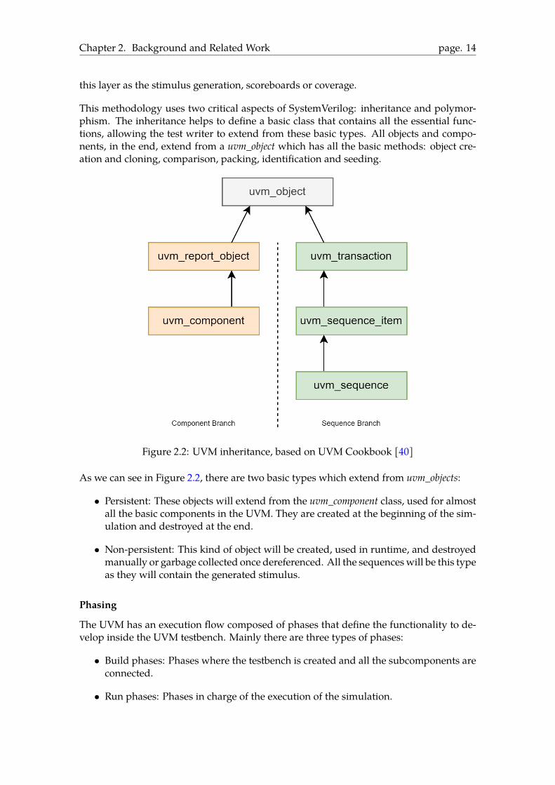
This methodology uses two critical aspects of SystemVerilog: inheritance and polymor-phism. The inheritance helps to define a basic class that contains all the essential func-tions, allowing the test writer to extend from these basic types. All objects and compo-nents, in the end, extend from a uvm_object which has all the basic methods: object cre-ation and cloning, comparison, packing, identification and seeding.
Figure 2.2: UVM inheritance, based on UVM Cookbook [40]
As we can see in Figure 2.2, there are two basic types which extend from uvm_objects:
• Persistent: These objects will extend from the uvm_component class, used for almostall the basic components in the UVM. They are created at the beginning of the sim-ulation and destroyed at the end.
• Non-persistent: This kind of object will be created, used in runtime, and destroyedmanually or garbage collected once dereferenced. All the sequenceswill be this typeas they will contain the generated stimulus.
Phasing
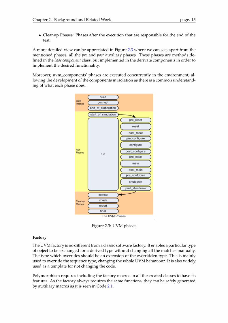
The UVM has an execution flow composed of phases that define the functionality to de-velop inside the UVM testbench. Mainly there are three types of phases:
• Build phases: Phases where the testbench is created and all the subcomponents areconnected.
• Run phases: Phases in charge of the execution of the simulation.
Chapter 2. Background and Related Work page. 15
• Cleanup Phases: Phases after the execution that are responsible for the end of thetest.
A more detailed view can be appreciated in Figure 2.3 where we can see, apart from thementioned phases, all the pre and post auxiliary phases. These phases are methods de-fined in the base component class, but implemented in the derivate components in order toimplement the desired functionality.
Moreover, uvm_components’ phases are executed concurrently in the environment, al-lowing the development of the components in isolation as there is a common understand-ing of what each phase does.
Figure 2.3: UVM phases
Factory
TheUVM factory is no different from a classic software factory. It enables a particular typeof object to be exchanged for a derived type without changing all the matches manually.The type which overrides should be an extension of the overridden type. This is mainlyused to override the sequence type, changing the whole UVM behaviour. It is also widelyused as a template for not changing the code.
Polymorphism requires including the factory macros in all the created classes to have itsfeatures. As the factory always requires the same functions, they can be safely generatedby auxiliary macros as it is seen in Code 2.1.

Chapter 2. Background and Related Work page. 16
1 class test_component extends uvm_component;
2 // Component factory registration macro
3 `uvm_component_utils(test_component)
Code 2.1: Factory types of requirements
After generating the required functions for the registrationwith themacros, the new func-tions must be added to standardize the creation methods. As we can see in Code 2.2 thefactory has two new() functions, one for the uvm_components, which are bondedwith theirparent component, and one for the uvm_object or uvm_sequence.
1 class test_component extends uvm_component;
2 function new(string name = "test_component", uvm_component parent = null);
3 super.new(name, parent);
4 endfunction
5
6 // For an object:
7 class test_sequence extends uvm_sequence_item;
8 function new(string name = "test_sequence");
9 super.new(name);
10 endfunction
Code 2.2: Factory requirements
The function in Code 2.3 allows the factory to create the objects with the defaults chosenby the test writer. If parameters are needed to create the objects, they can be specified inthe class definition and passed later in the object creation.
1 class agent extends uvm_agent;
2 my_component_with_params m_component;
3
4 function void build_phase( uvm_phase phase)
5 super.build_phase(phase);
6 m_component = my_component_with_params #(param1,
param2)::type_idd::create("m_component", this);↪→
7 endfunction : build_phase
8 endclass
Code 2.3: Factory requirements
Components
As commented earlier, a core feature of UVM testbenches is that there are predefinedclasses that have a specific purpose inside the environment. In Figure 2.4 we can seean example extracted from the UVM Cookbook [40] which represents a typical UVMtestbench.

Chapter 2. Background and Related Work page. 17
Figure 2.4: UVM test architecture
These core classes, which are used as the base for the development, are:
• testbench: It is the top module of the whole UVM architecture, it contains the testharness, and it is the one in charge of calling the function run_test(). It will trans-parently create and start the phases of the given test through theUVM_TESTNAMEparameter.
• Test Harness: It is not a component and it neither exists inside the UVM Cookbook[40], but it is commonly used as the module in charge of all the connections withthe actual DUT. Following this pattern, the top testbench will not be responsible forthe initialization or the connection of the DUT interfaces.
• Environment: It is the component that contains all the UVM agents. It is recom-mended for reusability of the testbenche. If this component did not exist, significantefforts should be madeto have several tests.
• Agent: It is a component that contains a group of components that have a commonpurpose. It normally contains a sequencer, a driver, a monitor and other analysiscomponents. It has two basic modes of operation, which are active and passive. Theactive state is when the agent is feeding the DUT, but in the passive mode, severalcomponents, like the sequencer and driver, are not working. The agents normallyhave a configuration object that defines what gets constructed and the agent’s be-haviour. It has the following subcomponents:
– Driver: Component in charge of driving the sequence data via TLM commu-nication to the DUT virtual interface. In most cases, this component gets atransaction and transforms it into the signals sent to the DUT. Sometimes thesecomponents are responsible for responding to stimulus instead of driving.
– Monitor: Component responsible for the snooping of the interface, it is alwayspassive, and it does the same process as the driver but inverted. It transforms
Chapter 2. Background and Related Work page. 18
the stimulus of the DUT in transactions that other components can understand.With the Drivers, they are the components that interact with the DUT at theinterface level. The transaction created, with the stimulus of the DUT, will bebroadcasted to all the interested observers.
– Sequencer: Component in charge of generating all the transactions that willbe sent to the driver through a TLM port. It contains the sequence which is theone that will generate the data. Normally, factory properties are used in thesequence, such as overriding, to change the stimuli generation.
Also, UVM can have configuration objects that can modify the entire behaviour, allowingthe environment to behave different depending on the test. All the mentioned classeswhich extend of uvm_components may have a configuration object which is the one incharge of changing its behaviour at the test writer will.
2.3 RISC-V
RISC-V is a rather new ISA that is fighting for its place among the other ISAs. It appearedin the University of California Berkeley in 2010 [46], and besides having started in an aca-demic setting, it was created to be usable in actual computers.
RISC-V has been designed as a modular ISA, which has a base specification that has tobe implemented and many optional extensions. Even though there are many base ISA,only two of them have been ratified, the base for 32 bits (rv32i) and the one for 64 bits(rv64i). The base ISA is composed by the unpriviledged specification [2] and the priv-iledged specification [3].
The extensions are classified into two types: the ratified ones, approved and reviewed bythe RISC-V foundation, and the open ones currently in development or not reviewed yet.
These are some of the ratified extensions that can be implemented:
• "M": specifies the multiplication and division between scalar registers.
• "A": specifies the atomic memory operations. It is a basic extension if the designhas many cores and inter-core communication is required.
• "F": specifies the single-precision floating-point operations
• "D": specifies the double-precision floating-point operations.
• "Q": specifies the quad precision floating-point operations.
• "C": specifies the compressed instructions, which are the ones that have a 16-bitencoding. These types of instructions are used to reduce the instruction code forcommon operations.
• "V": specifies the vector-processing instructions. It helps speed up computing in-tensive programs by simultaneously doing the same operations to a vector of values.

Chapter 2. Background and Related Work page. 19
2.3.1 Vector Extensions
The Single Instruction Multiple Data or SIMD [36] is a parallel way to process data. It usescustom instructions designed to operate in a set of elements. Usually, these instructionsare executed in specialized units, which typically have a relation of master-slave with aCPU.
In x86-64 history, many vector specifications have been released, like the 128-bit SSE, 256-bit AVX or the 512-bit AVX-512 [21]. The maximum vector length has been growing re-cently as the older specifications had a fixed number of bits. For industry, it is interestingto grow the vector length as it allows operating with larger vectors, potentially increasingperformance.
TheRISC-V specification [22] takes an alternative approach, and it defines a variable vectorlength and instructions that are agnostic to each possible implementation. This approachmakes it easier as high-end and low-end CPUs would implement the same specification,but it could be adapted to their needs.
Address Privilege Name Description0x008 URW vstart Vector start position0x009 URW vxsat Fixed-Point Saturate Flag0x00A URW vxrm Fixed-Point Rounding Mode0x00F URW vcsr Vector control and status register0xC21 URO vtype Vector data type register0xC22 URO vlenb VLEN/8 (vector length in bytes)
Table 2.1: RISC-V Vector CSRs
The vector extension adds 32 new registers that are the ones used in the vector units to dotheir operations. It also adds several Control Status Registers (CSR), as described in Table2.1, which configure the execution parameters of the implemented Vector Unit. The mostimportant ones are:
• vl: The Vector Length stores the elements operated on in the vector unit.
• vtype: The Vector Type stores many configuration fields such as:
– vsew: This field stores the length of each element, being the possible values{8,16,32,64,128}.
– vlmul: This field indicates howmany vector registers are grouped and treatedas one. The specification allows {1,2,4,8}.
• vstart: The Vector Start denotes which element will be the first element treated in avector instruction.
2.4 Related Work
There is little information on what the industry does when discussing verification. Prob-ably we all use the same techniques, which are the ones that the books explain [47] [30]
Chapter 2. Background and Related Work page. 20
[18], like UVM/OVM, assertions and coverage.
However, this lack of informationmakes it challenging for some to enter the sectorwithouthaving anything industrial grade to look up to.
With the rise of RISC-V, more institutions have published documentation of their effortson design and verification of taped-out designs. This provided documentation is muchmore than valuable, as they are the only documents explaining insights of Verificationprocesses.
With the documents of the open-source projects, one thing is clear, each different verifi-cation teams make verification differently. Besides that, all of the teams have a functionalinfrastructure and their design is completely verified. Even that they publish the meth-ods and decisions publicly they have followed to achieve a certain grade of confidence inthe health of the design. The most relevant open source projects are from LowRISC andOpenHardware foundation.
OpenTitan [29] is a big projectwhich hasmade a colossal effort in terms of documentation,which has been published on a dedicated website, and it has a specialized section forverification. It contains detailed explanations of each topic of their infrastructure, fromtools and scripts to all the UVM testbenches they have used.
OpenTitan has developed a root-of-trust design that contains at the same time manysmaller designs as the Ibex core [28]. In the webpage verification section, they havepublished all the scripts, UVM testbenches and software stack they have used. Moreover,they had also have published the Verification plans and coverage plans for their designare good examples of how to do the verification. In their testbenches, they execute thebinary completely and then compare the execution trace with the one of the InstructionSet Simulator (ISS). Regarding the execution environment, they published the Dockerimage they have used for the simulation alongside the scripts used for execution, triagingand publishing the results of the executions.
Regarding the Continous Integration, they have used to verify the Design Under Test theyhave developed a collection of tools that run without any dependence on vendors. More-over, they have created a Docker image with all the tools they need as Verible, Verilatoror VCS [45]. Despite all the documentation in the infrastructure part it is a specific codethat would require many efforts to understand and adapt, making it difficult to reuse.
The next big project we found is OpenHardware, one of themost powerful hardware opensource community movements. It is defined as a group formed by many contributors ofthe hardware industry, which collaborate in the development of many RISCV cores. Theytry to gather all the previous work of the contributors that formed the group to make alarger open source project. They publish the work they do in their Github [35], wherethey have three main repositories: RTL code, verification and documentation.
They havemainly done System level verification, as they have produced a UVM testbenchfor the whole core, which is reusable between the cores as they have the same interfacewith the caches. They use the Imperas (ISS) [20] to compare instruction-by-instructionwith the results produced by their designs. Moreover, to make the comparison, they haveincluded the RISCV Formal Interface [8] in their testbench, which enables execution trac-
Chapter 2. Background and Related Work page. 21
ing or execution extraction to send it to an external scoreboard. In terms of coverage, theyhave produced a ISA coverage, which is agnostic to the specific core they are running,implements the coverage for the 32 bit RISCV ISA, which all their cores implement. Fur-thermore, in Continous Integration, they have used a third-party software namedMetrics[32] which they use to run their tests and regressions. In each core folder, they have afolder named regresswhere they put all the kinds of pipelines they want to run.
If we compare what we are proposing with the previous done work of both of the organi-zations explained earlier, many similarities come up. The center part of all envrionmentsis a UVM testbench capable of driving signals to the Design Under Test. Our environmentis that is capable to drive signals to a slave component through a complex custom protocolwhich is implemented in the testbench. Furthermore, in terms of verification infrastruc-ture we came up with a complex environment similary to the OpenTitan one but clearlydifferent fromOpenHWwhich externalize the CI platform. Regarding the Instruction SetSimulator, OpenHWuses Imperas which is significantly a different approach to our Spikecustom implementation to support the co-simulation environments.

Chapter 3
EPAC Architecture and VerificationInfrastructure
In this section, we will take a more in-depth approach to the overall project, which is partof the European Processor Initiative (EPI).
In Sections 3.1 and 3.2, wewill describe the taped-out design components andwhomakeseach. After, in Section 3.3, we will take a closer look at the design developed in the BSC,which is the one that we should verify. Finally, in Section 3.4, we will describe the globalarchitecture of the Verification Infrastructure for this design, including the designedUVMtestbench, assertions, coverage, and other components.
3.1 EPI ArchitectureEPI is a huge European project which aims to produce several designs for various pur-poses. The developed IPs of this project will be placed in a 2D mesh Network-on-Chip(NoC), which will connect the general-purpose CPUs with the different developed accel-erators. As shown in Figure 3.1, the proposed accelerators are:
• EPACor European ProcessorACcelerators: in charge of developing a fully EuropeanIP based on RISC-V [12]. One of its objectives is to deliver a low power acceleratorfocused on high computing throughput.
• eFPGA or embedded FPGA: in charge of developing an FPGA oriented to run post-fabrication functions efficiently [11]. It is key as it is flexible as software but canimprove performance as hardware.
• MPPA or Accelerator for Automotive Stream: in charge of developing specialisedunits focused on Autonomous Driving and vehicle perception [10]. This acceleratoris built to handle vehicle image processing, bit-level processing, and deep learninginference.
22

Chapter 3. EPAC Architecture and Verification Infrastructure pag. 23
Figure 3.1: EPI environment
3.2 EPAC EnvironmentWe will focus on EPAC as it is where this thesis is placed. As we have defined, EPACobjective is to make an entirely European IP. The EPAC project has many partners, andeach one has its specific task.
Figure 3.2: EPAC testchip tape out [13]
In Figure 3.2 we can see that the taped out design has these types of tiles:
• VRP or VaRiable Precision Unit: Unit designed to run linear algebra kernels, suchas physics. It focused on reducing the rounding errors to be more accurate. Thisunit has adjustable precision from 64 bits to 256 bits, and it is made by CEA-LIST,

Chapter 3. EPAC Architecture and Verification Infrastructure pag. 24
the Atomic Energy Commission - Laboratory for Integration of Systems and Tech-nology.
• STX or Stencil and Tensor accelerator: Unit specialised in speeding up High-Performance Computing and machine learning workloads. This unit is made byFraunhofer IIS, ITWM and ETH Zürich.
• SERDES: A high-speed network made by EXTOLL, responsible for the connectionbetween all the specialised accelerators.
• VECTOR CORE: Unit composed by an Avispado RISC-V core, which is made bySemiDynamics [43], and a Vector Processing Unit, which is made by the BarcelonaSupercomputing Center and the University of Zagreb.
Each of these tiles has a Home Node made by Chalmers and an L2 cache, which FORTHmakes. All the described EPAC components are represented clearly in Figure 3.3.
Figure 3.3: EPAC scheme [34]
The design was finalised by Fraunhofer IIS, featuring a 22nm FDX technology producedin GlobalFoundries; this 22nm technology is specialised in producing low power chips forembedded applications. The chip was tested and integrated into an FPGA-based boarddesigned by FORTH, E4 and the University of Zagreb. Even if this chip is not made inthe state of the art technology, more tape-outs are planned with a newer versions of thedesign, with 12nm technology and below.
In Figure 3.2 we can see the tapeout designwhich was named EPAC 1.0 andwas the resultof all the design and verification efforts of all the 28 partners of the project.
This thesis is about verifying the Vector Accelerator, so first, we will focus on the VPU ar-chitecture and the Open Vector Interface. SemiDynamics was in charge of doing the core,and they also have specified the protocol used for the core-accelerator communication.

Chapter 3. EPAC Architecture and Verification Infrastructure pag. 25
3.3 Vector Accelerator ArchitectureThe Vector Processing Unit or VPU is our Design Under Test, so a minimum knowledge isrequired to follow the overall verification process. Moreover, it is required to understandthe difficulties presented by this design.
As was specified earlier, the Vector Processing Unit or Vector Accelerator, which is namedVitruvius [14], is present in each Vector Core tile specified in subSection 3.2. Each oneof these four Vector_Core tiles has an Avispado core and a Vector Accelerator unit whichuse the Open Vector Interface [42] to communicate. This OVI is the only way the VPU canobtain values from the outside, as the cache is not accessible directly. All the requests willpass through the processor.
Vitruvius implements version 0.7.1 of the RISC-V Vector Specification [22] as when theproject started it was the most recent version. This specification was updated in the pastyears and there are plans of updating the Vector Accelerator to the 1.0 version [24].
Figure 3.4: VPU Overall diagram [14]
As we have introduced in Section 2.3.1, this accelerator’s duty is to apply a function to agroups of elements. This groups of elements which are named Vector Registers are up to16384 ( 214 ) bits, and have {8, 16, 32, 64} as available vsew. Also it only supportsLMUL =1, therefore any different configuration from that will result in a illegal instruction. Anyother configuration as for example the vsew {128, 256, 512, 1024} or LMUL > 1 are notimplemented in Vitruvius.
The design supports 40 physical registers, which are used for the register renaming tosupport the 32 logical architecture registers, and depending on the vsew value each vectorregister will be able to have different number of maximum elements as presented in Table3.1.

Chapter 3. EPAC Architecture and Verification Infrastructure pag. 26
SEW MAX ELEMENTS64 25632 51216 10248 2048
Table 3.1: Maximum elements with the different SEWs
Vitruvius is able to perform:
• {8, 16, 32, 64} bit integer signed and unsigned operations
• {32, 64} bit floating point operations
• Masked operations
• Fused Multiply Accumulate operations
• Memory operations:
– Two loads at the same time (in-flight)
– Loads and one stores in parallel
As shown in Figure 3.4, the Vector Accelerator has eight laneswhich are the ones in chargemainly of doing the computation. Each of the lanes has its slice of the Vector Register File(VRF) and is able to communicate with the others using the Inter-lane Ring.
When an instruction arrives from Avispado, it will first enter the pre-issue queue, where itwill be stored. After that, the unpacker unitwill decode the instruction and, in some cases,create multiple instructions (for example, making additional instructions to move data).
Following the unpacker, the instruction enters the renaming unit to substitute the logicalregisters by the physical assigned one, and once all this work is done, the instruction willbe ready to enter one of the issue queues, memory or arithmetic.
If the instruction is arithmetic, it will be sent to be executed to the vector lanes. Neverthe-less, if it is a memory instruction, it will go either to the Load Management Unit, to retrievethe data from Avispado, or to the Store Management Unit, which will request the elementsto the vector lanes in order to store them in memory.

Chapter 3. EPAC Architecture and Verification Infrastructure pag. 27
Figure 3.5: Vector Registers overview [14]
The Vector Register File (VFR) enables all the lanes to work with the same vector registerin a parallel way. The Vector Register File has a distributed architecture, and each lanesaves its slice in five memory banks that allow five simultaneous reads. The mapping ofthe elements is fixed as shown in Figure 3.5, the element 0 goes to bank 0 of lane 0, theelement 1 goes to bank 0 of lane 1, and so on. This method ensures that all the lanes areworking even when the Vector Length is not high. Also, all the five banks would be readsimultaneously, which will increase the overall bandwidth.
3.3.1 Open Vector Interface (OVI)This is the protocol released by SemiDynamics [42] to standardise the way that VectorUnits are connected to their cores, and it is the one used to connect our Design Under Testin the EPI project. Aswe have commented in other sections, this protocol does not supportthe direct access of the Vector Unit to the memory hierarchy, so all memory accesses haveto pass through the core. Another relevant point is that SemiDynamics has released thisprotocol and made it open source under the Solderpad license.
Chapter 3. EPAC Architecture and Verification Infrastructure pag. 28
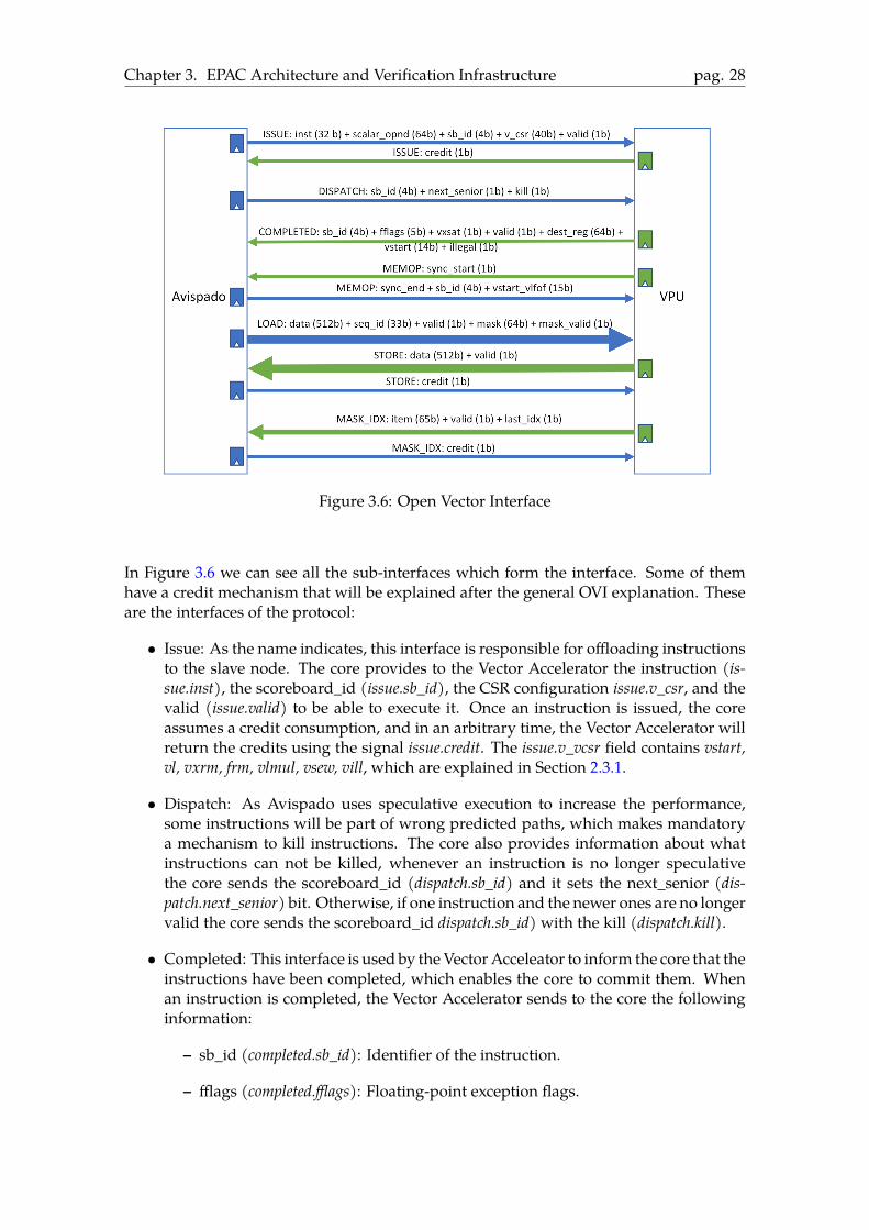
Figure 3.6: Open Vector Interface
In Figure 3.6 we can see all the sub-interfaces which form the interface. Some of themhave a credit mechanism that will be explained after the general OVI explanation. Theseare the interfaces of the protocol:
• Issue: As the name indicates, this interface is responsible for offloading instructionsto the slave node. The core provides to the Vector Accelerator the instruction (is-sue.inst), the scoreboard_id (issue.sb_id), the CSR configuration issue.v_csr, and thevalid (issue.valid) to be able to execute it. Once an instruction is issued, the coreassumes a credit consumption, and in an arbitrary time, the Vector Accelerator willreturn the credits using the signal issue.credit. The issue.v_vcsr field contains vstart,vl, vxrm, frm, vlmul, vsew, vill, which are explained in Section 2.3.1.
• Dispatch: As Avispado uses speculative execution to increase the performance,some instructions will be part of wrong predicted paths, which makes mandatorya mechanism to kill instructions. The core also provides information about whatinstructions can not be killed, whenever an instruction is no longer speculativethe core sends the scoreboard_id (dispatch.sb_id) and it sets the next_senior (dis-patch.next_senior) bit. Otherwise, if one instruction and the newer ones are no longervalid the core sends the scoreboard_id dispatch.sb_id) with the kill (dispatch.kill).
• Completed: This interface is used by theVectorAcceleator to inform the core that theinstructions have been completed, which enables the core to commit them. Whenan instruction is completed, the Vector Accelerator sends to the core the followinginformation:
– sb_id (completed.sb_id): Identifier of the instruction.
– fflags (completed.fflags): Floating-point exception flags.

Chapter 3. EPAC Architecture and Verification Infrastructure pag. 29
– vxsat (completed.vxsat): Fixed-point saturation flag.
– vstart (completed.vstart): Vstart value, must be zero except in certain load cases.
– dest_reg (completed.dest_reg): Scalar value in case that the instruction writes onthe scalar registers.
– illegal (completed.illegal): Bit which indicates that the instruction was illegal.Two types of illegal instructions can be detected: invalid instruction encodingor an unsupported configuration, as for example LMUL ̸= 1 is unsupportedin this version of the Accelerator.
– valid (completed.valid): Bit which indicates valid data in the completed group.
• Memop: Simple interface which has three basic signals. Firstly, the sync_start(memop.sync_start) which is sent by the Vector Accelerator which acknowledgesthat it is ready to recieve or send the data. Secondly, the sync_end (memop.sync_end)which is sent by the core and flags the end of the operation. Thirdly, it has thevstart_vlfof (memop.vstart_vlfof ) which is in charge of expressing if a exception inthe core has happened.
• Load: Interface drived by the core which is in charge of containing all the datain the load instructions. The core sends the data (load.data) with the sequence_id(load.seq_id) , identifier which helps the Vector Accelerator to know the order of theinformation, and the valid (load.valid).
• Store: Interface driven by the Vector Accelerator which contains all the data in storeinstructions. The Vector Accelerator sends the data (store.data) and the valid signal(store.valid). As Avispado can store a limited amount of data it has a credit systemthat tells the Vector Accelerator when the core can receive more data.
• Mask_idx: Interface used in masked or indexed memory instructions. TheVector Accelerator first sends the masks or the indexes to the core. The VectorAccelerator sends the item (mask_idx.valid), valid (mask_idx.valid) and last_idx(mask_idx.last_idx). The core also has limited mask buffering, so this interface alsouses a credit system.
This explanation of all the interfaces has clarified that this protocol is not easy as manythings can happen. Also, some interfacesmust interact with others inmany cases, makingit harder to implement. Besides that, the specification [42] is well-defined and explained,which makes the work a little easier.
3.4 Verification Infrastructure
This section will explain, more in-depth, the developed infrastructure the verification ofthe Vector Accelerator made for the EPI project.
First, when we started this project, we planned the verification approach. We decided tostart with the Block Level as recommended, but we dropped it after some developmentdue to significant changes in the module interfaces, which would mean more effort. We
Chapter 3. EPAC Architecture and Verification Infrastructure pag. 30
decided to move to System Level verification and treat the DUT as a whole to avoid this.In this way, we should only focus on the OVI interface (specified in 3.3.1), which was notgoing to have major changes during the Verification process.
Figure 3.7: Verification Flow
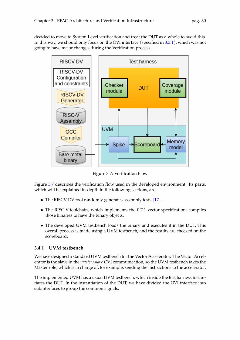
Figure 3.7 describes the verification flow used in the developed environment. Its parts,which will be explained in-depth in the following sections, are:
• The RISCV-DV tool randomly generates assembly tests [17].
• The RISC-V-toolchain, which implements the 0.7.1 vector specification, compilesthose binaries to have the binary objects.
• The developed UVM testbench loads the binary and executes it in the DUT. Thisoverall process is made using a UVM testbench, and the results are checked on thescoreboard.
3.4.1 UVM testbenchWehave designed a standardUVM testbench for the Vector Accelerator. The Vector Accel-erator is the slave in themaster/slaveOVI communication, so the UVM testbench takes theMaster role, which is in charge of, for example, sending the instructions to the accelerator.
The implemented UVM has a usual UVM testbench, which inside the test harness instan-tiates the DUT. In the instantiation of the DUT, we have divided the OVI interface intosubinterfaces to group the common signals.

Chapter 3. EPAC Architecture and Verification Infrastructure pag. 31
Figure 3.8: UVM diagram
Figure 3.8 illustrates the whole UVM structure, where the top test instantiates the UVMenvironment, and at the same time, this environment instantiates one agent per subinter-face defined in the OVI specification. As the UVM Cookbook [40] explains, each agenthas a sequencer, a driver, and a monitor connected to each of these subinterfaces.
We have implemented a virtual sequencer whose duty is not to send sequence items. Itis normally used in environments with multiple sequences and it has all the sequencers’instances to command the data generation.
This virtual sequencer, similar to the one in Figure 3.9, has a virtual sequence that is re-sponsible for the data generation of each one of the interfaces. This virtual sequence con-trols all the sequences’ states and connects them to their respective sequencers. This con-nection is made by changing the m_sequencer, which is the pointer to the sequencer thatcontains them. If the sequence wants to send the data to their sequencer, it will send it viathis m_sequencer handler.

Chapter 3. EPAC Architecture and Verification Infrastructure pag. 32
Figure 3.9: UVM Virtual sequence example [40]
The base of the UVM structure uses polymorphism to enable the test writer to developdifferent types of tests and sequences. In our environment, as the Issue_sequence is theone that provides the instructions, we use it as the one that should be extended to createdifferent types of tests. The extension classes of this sequence are the ones that providethe different instructions to feed the DUT.
This sequence is in charge of managing all the data and sending it to the correspondingsequences to emulate the core that commands the Vector Accelerator.
Instruction Flow
The base Issue sequence, which is the one in charge of providing the instructions for thewhole process, has a structure with all the pending instructions provided by some exten-sion Issue sequence.
We have extended this Issue sequence to use an Instruction Set Simulator (ISS), detailed inSection 4.1, which uses a binary not to write all the tests manually. Having this extendedsequence and using a test generator eased our life in terms of time spent writing tests.
The Issue sequence derivate class provides the instructions which arrive at the queues ofthe parent Issue sequence class, which, each cycle, will check if it can issue an instruction.Once it has the instructions, there are two primary states: issue a new instruction or not.
If the instruction can be issued, it is always pushed to the sequencer port, and dependingon the vector instruction type, several scenarios can happen. It will be sent to the Memopsequence if it is a memory instruction.
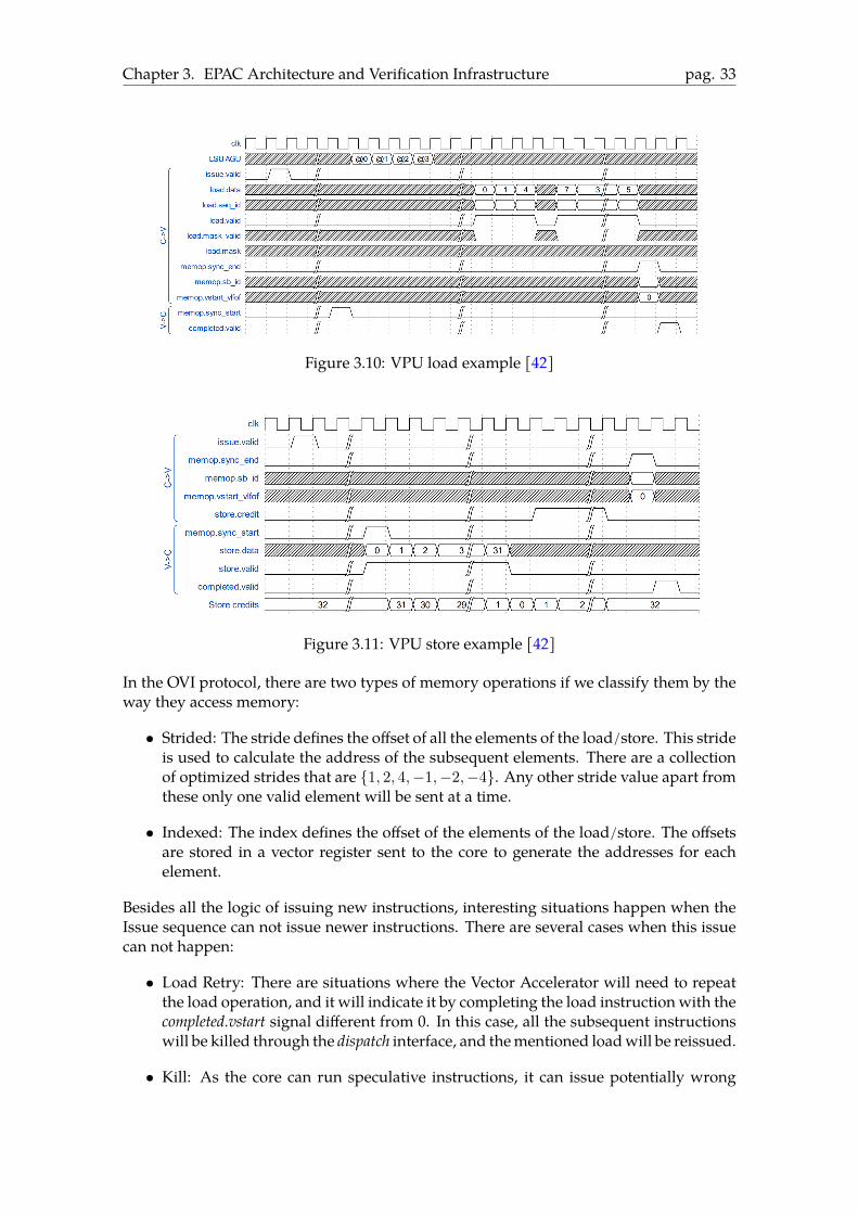
The memory operations use a protocol to specify how the information is sent. As we cansee in Figure 3.10 the communication starts with a memop.sync_start, which is raised bythe Vector Accelerator and indicates that it is ready to send/receive data. If it is a load, theUVMwill send the data through the load interface, and if it is a store, theVectorAcceleratorwill send the data through the store interface, as it is seen in Figure 3.11.
Chapter 3. EPAC Architecture and Verification Infrastructure pag. 33
Figure 3.10: VPU load example [42]
Figure 3.11: VPU store example [42]
In the OVI protocol, there are two types of memory operations if we classify them by theway they access memory:
• Strided: The stride defines the offset of all the elements of the load/store. This strideis used to calculate the address of the subsequent elements. There are a collectionof optimized strides that are {1, 2, 4,−1,−2,−4}. Any other stride value apart fromthese only one valid element will be sent at a time.
• Indexed: The index defines the offset of the elements of the load/store. The offsetsare stored in a vector register sent to the core to generate the addresses for eachelement.
Besides all the logic of issuing new instructions, interesting situations happen when theIssue sequence can not issue newer instructions. There are several cases when this issuecan not happen:
• Load Retry: There are situations where the Vector Accelerator will need to repeatthe load operation, and it will indicate it by completing the load instruction with thecompleted.vstart signal different from 0. In this case, all the subsequent instructionswill be killed through the dispatch interface, and thementioned loadwill be reissued.
• Kill: As the core can run speculative instructions, it can issue potentially wrong

Chapter 3. EPAC Architecture and Verification Infrastructure pag. 34
vector instructions. With this inmind, there is a need for a kill mechanism to discardthe wrong instructions. If an instruction must be killed, the core will send throughthe dispatch interface the dispatch.sb_id of the first mispredicted instruction and thekill bit activated, which will trigger the instruction discard on the VPU side.
• Memory exceptions: There will be situations where the core would have a memoryexception, which will notify the VPU by setting the memop.vstart_vlfof signal andrising the memop.sync_end before it would be expected.
• No issue credits: Each time the core issues an instruction, a credit consumption isimplied. If the core issues as many instructions as credits are in the system, theVector Accelerator would not be able to handle any other instruction. Therefore,the core will have to wait until the Vector Accelerator returns some of these creditsthrough the issue.credit signal.
Once the instruction is executed, the Vector Accelerator has to raise the completed.validwith the completed.sb_id to tell the core that it has finished. However, it has to wait untilthe core tells that the instruction will not be killed to be committed. The core will tell theVector Accelerator that the instruction can be committed by rising the dispatch.valid withthe dispatch.sb_id.
Once the instruction has been completed in theVectorAccelerator, theUVM testbenchwillsend it to the scoreboard to check if its results are correct. It will be done by comparingthe results of the Vector Accelerator registers with the ones in the reference model.
Instruction Generation
As we have described, the extension class of the issue sequence is in charge of providingthe instructions. Even if the normal UVM testbench generates the data with the randomi-sation of the sequence, it would be not easy to define a group of constraints that give uswhat we want.
Having this disadvantage in mind, we have looked for an open-source tool that allows usto:
• Generate a valid stream of instructions.
• Generate instructions with RISC-V vector 0.7.1 extension.
• Modify its generation easily.
The extension requirement is one of the most restrictive ones. We found RISCV-DV [17],which we adapted to our project to fulfil the generation of instructions.
3.4.2 RISCV-DV
RISCV-DV is an open-source instruction generator developed by Google. It has beenwrit-ten in SystemVerilog, and it uses the characteristics of UVM tomake the tests. It producesassembly tests which, after the generation, will be compiled by a riscv-toolchain. In ourcase, we were interested in generating vector instructions for our Vector Accelerator us-ing the specification 0.7.1, so as it was based in the 0.8 [23] specification we backported it

Chapter 3. EPAC Architecture and Verification Infrastructure pag. 35
to the 0.7.1 [22].
The tool was almost ready to be used as it generated binaries with instructions of thetargeted spec, butwehave changed some features in order tomake the testsmore complex:
• Memory initialisation pattern changes in order to support different initial values.
• Instruction blacklisting for the ones not implemented by our DUT.
• Instruction generation changes to generate vsetvli instruction during the test processand not only in the initialisation.
• Memory constraints in order to avoid memory exceptions.
• Registers initialisation changes in order to support vle.v instructions instead ofvmv.v.x.
• Sentinel instruction addition in the tohost routine, which enables the UVM testbenchto finalise the tests.
Moreover, the tool provides a wrapper in Python to enable non-experienced users to runit without knowing its internal process, which was also tuned to add options for the de-veloped features.
Also, therewere efforts tomake the toolworkwith the simulatorwewere using. Althoughit is an open-source tool, it requires a paid simulator to be used.
3.4.3 Coverage
Aswe have explained in Section 2.2, the coverage is essential to describe howwell stresseda DUT is. For that reason, coverage is developed or generated to decide if there is a needof doing more tests or the design is well verified.
In this project, we mainly had functional and code coverage. The functional coveragewas defined following the RISC-V vector extension and generated for each instruction.Moreover, depending on the type of each instruction, some coverpoints were enabled ornot. The most difficult coverpoints to generate were:
• Check that {vs1, vs2, vd} are stimulated in simulations and get the values:{v0, vX(others)}.
• Check that all the loads and stores types happended:
– Strided: Optimized values like {−4,−2,−1, 1, 2, 4} and other non optimized.
– Indexed: Negative indexes ([−∞, 0]) and positive ones [0,∞].
• SEW and VL configurations on all the instructions {8, 16, 32, 64}.
• For each instruction check if the masked variant has been executed.
Besides the functional coverage described in SystemVerilog, we have also generated the

Chapter 3. EPAC Architecture and Verification Infrastructure pag. 36
code coverage that helps to see how well the design is stressed. Almost all the EDA toolsgenerate a automatic coverage which includes branches, statements, toggles, conditions. As ithappens in software programming, instrumenting the code to obtain this kind of statisticsslows down the simulation by a factor of 2x, a fact that must be taken into account.
This coverage is reviewed by the verification team, which will investigate why some ex-pressions are not being executed. If this expression is correct, someone will write a testto stimulate that expression, and if its not a report will be sent to the design team to solvethe problem.
All these statistics are used to determine howmuch of the design is verified, which has tobe taken wisely as it is a metric done by the verification team, and it can also be meaning-less if it is not done correctly.

Chapter 4
Spike and Scoreboard
In this chapter, we will explain all the components wemodified and developed in order tohave an environment that checked the results of the Design Under Test. In Section 4.1 wewill go over the changes made to the reference model Spike, which was responsible forgiving us the correct results of the vector instructions. After that, details of the developedUVM components that made the checks will be presented in Sections 4.3 and 4.4.
4.1 SpikeSpike is a RISC-V Instruction Set Simulator (ISS) [25] developed by the RISC-V Founda-tion written in C++. It is widely used in the RISC-V community, and its primary purposeis to be able to run RISC-V software.
The oficial repository, which contains the up-to-date version of Spike, has already thefollowing features:
• Implements RV {32/64}IMAFDQCV extensions.
– Configurable ISA support during runtime.
– Configurable Vector Architecture.
– Updated functional model according to the new specifications.
• Multiple CPU support.
• Step-by-step execution, debug mode.
• Devices, mapped in memory, support.
Besides these features, it tries to model one or more hardware threads, which involveseven a more complex structure than just mimicking the functional behaviour. The Spikemimicking will match at the perfection with a RISC-V core execution. For example, it willhave the same program counter flow and the same appearance of exceptions/interrup-tions.
37

Chapter 4. Spike and Scoreboard pag. 38
Figure 4.1: Spike structure
In Figure 4.1 there is a scheme of the official Spike class structure. The sim_t class is themain class of the whole execution. It has the following items:
• Core: As its name explains, it is the class that emulates the functionality of a RISC-Vhardware thread. Each hardware thread has aMemory Management Unit (MMU).
– MMU: Inside a functional model of an L0 instruction cache, a TLB and aMemory-Mapped Input/Output unit.
– Processor: It has inside the state of the hardware thread, its hardware identifier,and a Vector Unit which will be in charge of executing the vector instructions.
• Clint: This Interrupt Controller is a functional model of the Core-local Interrupt Con-troller. It is in charge of notifying the corewhen an interruption happens, responsiblefor the system’s clock.
• Memories: This structure has all the memories shared between the cores, and theTLB will access it in the case of a miss.
• Boot room: The boot ROM describes the first instructions that the system will ex-ecute no matter what binary. In the case of Spike, as it is seen in Code 4.1, it setsthe mhartid of the main core and jumps unconditionally to the start_pc which is bydefault at the address 0x80000000.
• Devices: Collection of user-defined devices, which are mapped in memory, for thesimulation. It can be modelized using flags in the binary execution.
• Bus: It is the main connection between the devices and the cores. All the petitionsthat do not fit in the inner levels of the simulation are sent to the bus.

Chapter 4. Spike and Scoreboard pag. 39
1 uint32_t reset_vec[reset_vec_size] = {
2 0x297, // auipc t0,0x0
3 0x28593 + (reset_vec_size * 4 << 20), // addi a1, t0, &dtb
4 0xf1402573, // csrr a0, mhartid
5 get_core(0)->get_xlen() == 32 ?
6 0x0182a283u : // lw t0,24(t0)
7 0x0182b283u, // ld t0,24(t0)
8 0x28067, // jr t0
9 0,
10 (uint32_t) (start_pc & 0xffffffff),
(uint32_t) (start_pc >> 32)↪→
11 };
Code 4.1: Spike’s Boot Routine
End of Test
Spike detects the finalization of the tests using amemory position named tohost. To enableSpike to detect this memory position, we should include a symbol with this name in thesource of the binary. The symbols of the binary are read at the beginning and the positionof tohost is saved. In order to finish the execution, the binary must write in the tohostmemory position a non-zero value.
Setup
When Spike is executed, all the parameters are parsed to create the execution environ-ment. In Table 4.1we can see some of these parameters, whichwill define essential aspectsof the execution. All these parameters are parsed in themain function of Spike, which willcreate all the necessary structures to simulate the user requirements. To do so, the mem-ories are created with the given size, the devices are initialized, and the environmentalvariables like debug mode or log mode are set.
Argument Explanation-p<number> Number of cores–isa=<name> ISA string for all the cores
–varch=<name> varch string for all the VPUs-m<a:m,b:m,..> Memories and its size
Table 4.1: Relevant Spike arguments
Device Tree
Once all the system description is done, the device tree has to be generated and compiled.There are two main methods to discover hardware which are the ACPI protocol and thedevice tree blob, as Spike is not real hardware it takes the device tree blob approach inorder to allow systems like Linux to recognize where they are running in. Spike generatesthe string which specifies the device tree, named .dts, compiles it and later it copies theblob right after the boot_rom.
Chapter 4. Spike and Scoreboard pag. 40
Execution
Once all is ready, Spike dives into the simulation through two main functions, which areexecuted in an interleaved pattern using a context switching with the ucontext library. Thetwo functions are:
• sim main: Function in charge of the execution flow of the cores. It has two modesof operation, one which steps one instruction at a time to handle the debug mode,and the other which progress a bunch of steps for the other modes. Each time it hascompleted its instructions, it switches the context to the memory.
• mem main: Function in charge of the progression of the memory and devices. Itchecks if thememory position tohost has beenwritten, and it triggers the progressionof the devices instantiated in the simulation.
4.2 UVM IntegrationAs explained previously, we needed something to act as the core and something to actas a reference model. After some discussion and other options considered, like a RISC-VVirtual Machine, we adopted Spike as our ISA simulator for:
• Act as a core to provide uswith the instructions and all the derived data for the issuesequence.
• Act as a reference model to provide the execution results to the scoreboard to com-pare the actual results with the expected ones.
We needed to adapt the simulator structure, whichwas only compatible to run as a binary,to run as a library. Also, we needed to create an instance of the ISA simulator to call it inthe UVM testbench.
Wemodified Spike to run as a class instead of instantiating all the components in themainfunction and executing them straightforwardly. We have saved all the main components,like the sim_t object inside the class tomaintain the simulation object through the expectedcalls to the wrapper.
As we worked using theQuestasimHDL simulator, we wanted to import the Spike libraryinside it in order to make calls into it. After we adopted the Spike code to work as awrapper, the next step was integrating it with the aforementioned simulator.
To make the library possible, we changed the compilation flags of Spike to disable thebinary generation and make the shared object (.so). The compilation is almost the sameas the old one but the link phase, which has been disabled from the original Makefile.in.Instead of implementing our library compilation in the originalMakefile.in, we have madea compilation script to minimize the changes to their structure.
Without the linking phase, this script calls the original Makefile to obtain all the compiledobjects. After that, the main shared object is compiled with the flags -shared, to enable theshared object generation, and -static-libgcc -static-libstdc++ , which forces static linkingfor the standard C and C++ libraries. We used static linking for these libraries to avoidproblems in the case of moving the library to another machine.

Chapter 4. Spike and Scoreboard pag. 41
The script is also in charge of generating all the needed data for the compilation, whichincludes, for example, the configure step. It is also done automatically, as seen in Code 4.2because we need to force a more significant size on the vector registers to match the vlen16384. Also, as we had in mind to run the same binaries which the actual core would runwe also had enabled the misaligned memory acceses.
1 varch="vlen:16384,elen:64,slen:16384"
2 vlen=$(echo "$varch" | cut -d ',' -f 1 | cut -d ':' -f 2)
3 ../configure --with-varch=$varch --with-vlen=$vlen --enable-misaligned
Code 4.2: Compile script configure
4.2.1 Direct Programing InterfaceAfter we had all the things prepared on the C++ side, we needed tomake the functions toallow the SystemVerilog code call to Spike. We have used the Direct Programing InterfaceorDPI), which allows SystemVerilog to call foreign codewritten particularly in C or C++.The SystemVerilog types that are directly compatible with the C types are presented inTable 4.2, others like arrays may require the use of the DPI-defined types.
SV Type byte int longint shortint real shortreal chandle stringC Type char int long long short int double float void* char*
Table 4.2: DPI types table
In order to call a C function for the SystemVerilog code we must define it first in theVerilog side and import the library when simulating. As it is shown in codes 4.3 and 4.4the function must be defined as an extern function in the C++ code and import it in theSystemVerilog part.
1 //include the SystemVerilog DPI header file if a DPI-type is used
2 #include "svdpi.h"
3
4 // C function
5 int compute_example (int op1, int op2)
6
7 // C++ function
8 extern C int compute_example(int op1, int op2);
Code 4.3: DPI C++ Example
1 // SystemVerilog import function
2 import DPI-C function int compute_example(input int op1, input int op2);
Code 4.4: DPI SystemVerilog Example
It is also worth noting that this DPI-C interface can also be used in the other direction,calling SystemVerilog from C. Besides that, in the SystemVerilog part, the function dec-laration can also specify if the parameters will be passed by reference or by value, being
Chapter 4. Spike and Scoreboard pag. 42
by value the default. If the user specifies the keyword input in the parameter, this will bepassed by value, but if the keyword output/inout is used, it will be passed by reference.
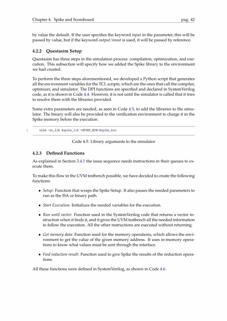
4.2.2 Questasim SetupQuestasim has three steps in the simulation process: compilation, optimization, and exe-cution. This subsection will specify how we added the Spike library to the environmentwe had created.
To perform the three steps aforementioned, we developed a Python script that generatesall the environment variables for the TCL scripts, which are the ones that call the compiler,optimizer, and simulator. The DPI functions are specified and declared in SystemVerilogcode, as it is shown in Code 4.4. However, it is not until the simulator is called that it triesto resolve them with the libraries provided.
Some extra parameters are needed, as seen in Code 4.5, to add the libraries to the simu-lator. The binary will also be provided to the verification environment to charge it in theSpike memory before the execution.
1 vsim -sv_lib $spike_lib +SPIKE_BIN=$spike_bin
Code 4.5: Library arguments to the simulator
4.2.3 Defined FunctionsAs explained in Section 3.4.1 the issue sequence needs instructions in their queues to ex-ecute them.
Tomake this flow in the UVM testbench possible, we have decided to create the followingfunctions:
• Setup: Function that wraps the Spike Setup. It also passes the needed parameters torun as the ISA or binary path.
• Start Execution: Initializes the needed variables for the execution.
• Run until vector: Function used in the SystemVerilog code that returns a vector in-structionwhen it finds it, and it gives the UVM testbench all the needed informationto follow the execution. All the other instructions are executed without returning.
• Get memory data: Function used for the memory operations, which allows the envi-ronment to get the value of the given memory address. It uses in-memory opera-tions to know what values must be sent through the interface.
• Feed reduction result: Function used to give Spike the results of the reduction opera-tions.
All these functions were defined in SystemVerilog, as shown in Code 4.6.

Chapter 4. Spike and Scoreboard pag. 43
1 extern "C" void setup(int argc, char* argv);
2 extern "C" void start_execution();
3 extern "C" int run_until_vector_ins(core_info_t* core_info);
4 extern "C" int get_memory_data(uint64_t* data, uint64_t direction);
5 extern "C" void feed_reduction_result(uint64_t vpu_result, uint32_t vdest);
Code 4.6: DPI defined functions
Run until vector
As it is the main function of the Spike execution wewill take a deeper look to explain howit works.
1 int run_until_vector() {
2 while(is_not_vector_instruction(ins))
3 if(is_centinel(ins))
4 return SUCCESS;
5 step_execution();
6 }
7 if (spike_trap_illegal())
8 return ILLEGAL;
9
10 if (spike_trap())
11 return INTERNAL_ERROR;
12
13 get_instruction_and_pc();
14 copy_vector_csrs();
15 copy_src_vector_registers();
16 copy_masks();
17 copy_destination_vector_registers();
18
19 copy_src_scalar_registers();
20 copy_destination_scalar_registers();
21
22 if(rs1_is_fp)
23 copy_fp_register();
24
25 return CONTINUE;
26 }
Code 4.7: Run Until Vector Function
The pseudocode in Code 4.7, will ease the explanation. Firstly in the run_until_vectorfunction, we want to get the next vector instruction in the whole execution of the binary.This forces us to skip the non-vector ones doing an instruction-by-instruction check.
With the changes wemade to the reference model, the tohostmechanismwas not workingproperly, so we decided to use a sentinel to notify the end of execution. In our UVM thesentinel was the 0xc00292f3 instruction which disassembles to csrrw t0, cycle,t0. If this

Chapter 4. Spike and Scoreboard pag. 44
instruction is detected, Spike will return an exit code corresponding to the end of the test.
After getting a valid vector instruction, we should copy all the needed data like sourceand destination vector registers, scalar destination registers if present, program counterand instruction, or current vector control registers (csrs). All this data will be retrievedfrom the SystemVerilog part as a struct named core_info. Apart from that, which will becopied for all the vector instructions, we have types of vector instructions that will requiremore data than those with a scalar or floating-point as a source register.
As we have also modified the instruction generator to fit our needs, we will also check ifthe executed instruction is not illegal to prevent some malfunctioning in the UVM.
All the gathered data in this function will be outputted in the UVM in a struct passed byreference named core_info.
4.3 UVMAs explained in Section 3.4.1, the issue sequence is the one in charge of issuing the in-structions, so to integrate Spike, we had to create a new test and a new sequence.
All the new tests in this UVM testbench should create a new sequence that extends fromthe issue_sequence, so we had to create the Spike sequence class with its Spike test.
The Spike test has the following functionalities:
• Changing and randomizing certain predefined behaviours on the interfaces.
• Enabling the scoreboard and aborting the simulation in case of mismatch.
• Override the issue_seq class with the spike_seq class using the override methods ofthe UVM.
• Enable the illegal check in the scoreboard.
• Setting memory exceptions probability.
4.3.1 Spike sequenceThis sequence aims to push the instructions received through the Direct ProgrammingInterface functions to the issue sequence queues. For this purpose, the base issue sequencehas a virtual method, named test_body, which is intended to be overridden by the classextension of the issue sequence.
As we can see in Code 4.8, we had to specify the functions that must be imported in sim-ulation time.
The text_body virtual method, which is the main task of the Spike sequence, has the fol-lowing structure:
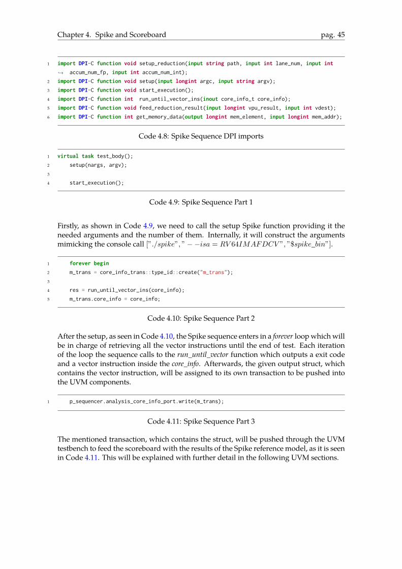
Chapter 4. Spike and Scoreboard pag. 45
1 import DPI-C function void setup_reduction(input string path, input int lane_num, input int
accum_num_fp, input int accum_num_int);↪→
2 import DPI-C function void setup(input longint argc, input string argv);
3 import DPI-C function void start_execution();
4 import DPI-C function int run_until_vector_ins(inout core_info_t core_info);
5 import DPI-C function void feed_reduction_result(input longint vpu_result, input int vdest);
6 import DPI-C function int get_memory_data(output longint mem_element, input longint mem_addr);
Code 4.8: Spike Sequence DPI imports
1 virtual task test_body();
2 setup(nargs, argv);
3
4 start_execution();
Code 4.9: Spike Sequence Part 1
Firstly, as shown in Code 4.9, we need to call the setup Spike function providing it theneeded arguments and the number of them. Internally, it will construct the argumentsmimicking the console call [”./spike”, ”−−isa = RV 64IMAFDCV ”, ”$spike_bin”].
1 forever begin
2 m_trans = core_info_trans::type_id::create("m_trans");
3
4 res = run_until_vector_ins(core_info);
5 m_trans.core_info = core_info;
Code 4.10: Spike Sequence Part 2
After the setup, as seen in Code 4.10, the Spike sequence enters in a forever loopwhichwillbe in charge of retrieving all the vector instructions until the end of test. Each iterationof the loop the sequence calls to the run_until_vector function which outputs a exit codeand a vector instruction inside the core_info. Afterwards, the given output struct, whichcontains the vector instruction, will be assigned to its own transaction to be pushed intothe UVM components.
1 p_sequencer.analysis_core_info_port.write(m_trans);
Code 4.11: Spike Sequence Part 3
The mentioned transaction, which contains the struct, will be pushed through the UVMtestbench to feed the scoreboard with the results of the Spike reference model, as it is seenin Code 4.11. This will be explained with further detail in the following UVM sections.
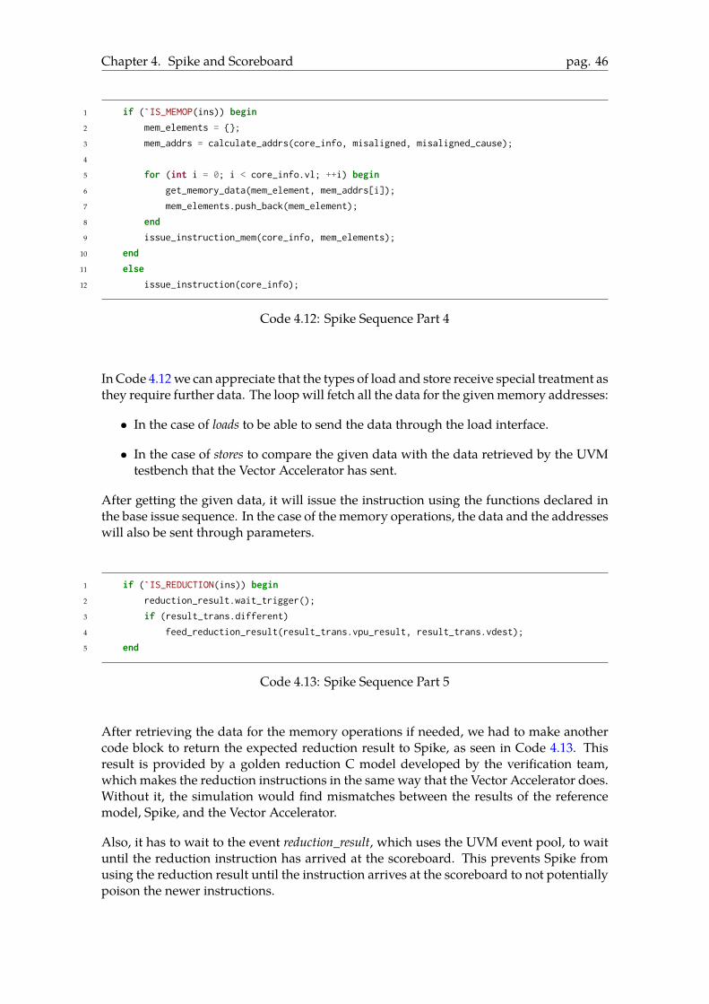
Chapter 4. Spike and Scoreboard pag. 46
1 if (`IS_MEMOP(ins)) begin
2 mem_elements = {};
3 mem_addrs = calculate_addrs(core_info, misaligned, misaligned_cause);
4
5 for (int i = 0; i < core_info.vl; ++i) begin
6 get_memory_data(mem_element, mem_addrs[i]);
7 mem_elements.push_back(mem_element);
8 end
9 issue_instruction_mem(core_info, mem_elements);
10 end
11 else
12 issue_instruction(core_info);
Code 4.12: Spike Sequence Part 4
In Code 4.12we can appreciate that the types of load and store receive special treatment asthey require further data. The loopwill fetch all the data for the givenmemory addresses:
• In the case of loads to be able to send the data through the load interface.
• In the case of stores to compare the given data with the data retrieved by the UVMtestbench that the Vector Accelerator has sent.
After getting the given data, it will issue the instruction using the functions declared inthe base issue sequence. In the case of the memory operations, the data and the addresseswill also be sent through parameters.
1 if (`IS_REDUCTION(ins)) begin
2 reduction_result.wait_trigger();
3 if (result_trans.different)
4 feed_reduction_result(result_trans.vpu_result, result_trans.vdest);
5 end
Code 4.13: Spike Sequence Part 5
After retrieving the data for the memory operations if needed, we had to make anothercode block to return the expected reduction result to Spike, as seen in Code 4.13. Thisresult is provided by a golden reduction C model developed by the verification team,which makes the reduction instructions in the same way that the Vector Accelerator does.Without it, the simulation would find mismatches between the results of the referencemodel, Spike, and the Vector Accelerator.
Also, it has to wait to the event reduction_result, which uses the UVM event pool, to waituntil the reduction instruction has arrived at the scoreboard. This prevents Spike fromusing the reduction result until the instruction arrives at the scoreboard to not potentiallypoison the newer instructions.

Chapter 4. Spike and Scoreboard pag. 47
4.3.2 Structure
TheUVMdescribes an architecturewhere some components do not have visibility of otherones. In our case, a struct containing the data by the core is generated in the issue se-quence. We needed support to send it through the UVM testbench to the scoreboard,which is the place where the mismatches between the reference model and the DUT arechecked.
UVM components typically define ports in the transactional layer to enable the connec-tion between them. Besides this, the data is generated in a sequence that can not have aport instantiated as it is not a UVM component. The sequence must call another UVMcomponent to send the data. In our case, the only component that was visible in the issuesequence was the issue sequencer, which was used to instantiate the mentioned port, asit is shown in Code 4.14.
1 class avispado_issue_sequencer extends uvm_sequencer #(avispado_issue_trans);
2 `uvm_component_utils(avispado_issue_sequencer)3
4 uvm_analysis_port #(core_info_trans) analysis_core_info_port;
5
6 function new(string name, uvm_component parent);
7 super.new(name, parent);
8 analysis_core_info_port = new("analysis_core_info_port",this);
9 endfunction : new
10
11 endclass : avispado_issue_sequencer
Code 4.14: UVM issue sequencer
With this method, we acomplished giving the sequence access to the port, enabling thesequence to push the transactions, which contain the results, to the port.
Figure 4.2: UVM ports connection

Chapter 4. Spike and Scoreboard pag. 48
Consequently, to enable this transaction to arrive at the UVM scoreboard, we designed theneeded ports around the UVM testbench. In Figure 4.2 we can see the mentioned ports.Starting at issue sequencer we have instantiated a TLM analysis port; each time the portis called with the write()method, all the components which have a connection to the portwill execute their write implementation of the port.
To connect the issue sequencer port to the scoreboard, we added an analysis_export tomakethe middle transition. It is connected from the sequencer to the UVM environment wherethe scoreboard is instantiated. As a result, this environment export will be connected tothe analysis_impl in the scoreboard, which will have the write function.
4.4 ScoreboardAs it is defined in the UVMCookbook [40], the scoreboard is the component that has oneof the most complex tasks, which is to determine if the DUT is behaving correctly or not.
In our case, the scoreboard will receive the results from our reference model, Spike, andthe results from the Vector Accelerator. All these results will be compared during the exe-cution. The scoreboard reports to the final user if the executed instructionswere correct orthe Vector Accelerator was doing erroneously. In the case of CPUs and Vector ProcessingUnits, there is no sense in continuing the execution if there is some incorrect result in theDesign Under Test. All the following instructions would be poisoned with incorrect data,which would also be incorrect.
If an incorrect instruction is found, the mission of the scoreboard is to report it in the sim-ulation transcript and abort the simulation. The simulation abortionwill be done throughthe uvm_fatalmethod, part of the UVMmacros header.

Chapter 4. Spike and Scoreboard pag. 49
1 `uvm_analysis_imp_decl(_completed)2 class vpu_scoreboard extends uvm_scoreboard;
3 `uvm_component_utils(vpu_scoreboard)4
5 // Variable: m_cfg
6 scoreboard_cfg m_cfg;
7
8 // Variable: vreg_if
9 virtual vpu_vreg_if vreg_if;
10
11 // Variable: clk_if
12 virtual vpu_clock_if clk_if;
13
14 // Variable: m_cfg
15 ascoreboard_cfg m_cfg;
16
17 // Variable: vpu_results
18 uvm_analysis_imp_completed #(completed_trans, vpu_scoreboard) vpu_completed;
19
20 // Variable: core_info_fifo
21 uvm_tlm_analysis_fifo #(core_info_trans) core_info_fifo;
22
23 // Variable: mem_model_fifo
24 uvm_tlm_analysis_fifo #(mem_model_trans) mem_model_fifo;
25
26 // Variable: mem_mask_fifo
27 uvm_tlm_analysis_fifo #(mem_mask_trans) mem_mask_fifo;
28
29 endclass : vpu_scoreboard
Code 4.15: Scoreboard declaration
The scoreboard is declared as shown in Code 4.15 and it receives the information to un-dertake its duty through many ports and interfaces:
• The vpu_completed_port is in charge of receiving the completed transactionsfrom the completed monitor. Each time the completed monitor observes a {com-pleted.valid} it will write into the port, which will trigger the write method in thescoreboard. The write function declared in the scoreboard will push the receivedtransaction into the queue of the pending transactions. It will also get the numberof the physical vector register that contains the result. The transaction sent throughthe port will contain the following values {scoreboard_id, flags, valid, vxsat, dst_reg,start, illegal}.
• The core_info_fifo which is the endpoint of all the transactions pushed from thespike_seq, explained in Section 4.3.1. This FIFO is connected to the port instantiatedin the environment and stores all the data until a vector instruction completes. Thetransactions in this FIFO are: {vector_dest_register, vector_src_registers, vector csrs, pc,inst}.

Chapter 4. Spike and Scoreboard pag. 50
• Themem_model_fifo is used to store the information coming from the storemonitorand the memory elements retrieved from Spike in the spike_seq. This one is alsoconnected in outer levels, more precisely in the environment, as the other FIFO. Wehave added this functionality because store operations do not reflect its results inthe vector registers. Instead, we check that all the information sent to the core iscorrect.
• Themem_mask_fifo, also connected in the env, which contains themasks or indexesgathered from the mask_idx interface, in the mask_idx_monitor, during the executionof a masked memory operation.
Following the UVM structure, we have made a UVM scoreboard configuration object, thescoreboard_cfg for the scoreboard to manipulate its behaviour. The configuration objecthas the following fields:
• Scoreboard Enable: Bit used to define if the scoreboard is defined in the test. Thescoreboard is only meant to be used when using the spike_tests. Otherwise, this bitshould be disabled to disable the scoreboard instantiation.
• Mismatch is Fatal: Bit used to define the behaviour when a mismatch happens. It isnot disabled commonly, as explained earlier, to prevent the simulation from beingpoisoned after a mismatch, but is useful for some debug tasks.
• Reduction rounding bits: These configurations quantify the number of mismatchbits that will be ignored from the less precise part of the reduction instructions. Itwas used previously developing the reduction reference model.
• Illegal ComparisonMode: This field will change the behaviour of comparing IllegalInstructions inside the scoreboard.
The scoreboard also declares two virtual interfaces:
• vpu_clock_if: Interfacewhich contains the clock and the clocking blocks associated.Clocking blocks are statements that force a group of signals to respect a given timing,they are normally used which enable the gate-level simulations.
• vpu_vreg_if: Interfacewhich contains the destination vector register of the last com-pleted instruction.
Functions
After all the information is transparently pushed to the FIFOs, it must be compared. Thiscomparison happens during the run_phase of the scoreboard, which starts a comparatortask.

Chapter 4. Spike and Scoreboard pag. 51
1 task comparator_task();
2 completed_trans m_completed_trans;
3
4 forever begin
5 clk_if.wait_cycles(1);
6 if (completed_instr.size()) begin
7 m_completed_trans = completed_trans::type_id::create("m_completed_trans");
8 m_completed_trans = completed_instr.pop_front();
9 comparator(m_completed_trans.dst_reg, m_completed_trans.sb_id,
m_completed_trans.vstart, m_completed_trans.fflags,
m_completed_trans.illegal, m_completed_trans.vxsat);
↪→
↪→
10 end
11 end
12 endtask : comparator_task
Code 4.16: Comparator task
In Code 4.16, we can see the main function of the scoreboard, which is called from the runphase run_phase of the scoreboard component. Every cycle checks if there is an instructionto compare its results; if that is the case, it gets it from the completed_queue. Once it haspopped the instruction, it calls the function to check its results.
This function will be in charge of two main functionalities:
• ISA checks: It will ensure that all the ISA specifications are being followed, as theresults, CSRs or illegal detection.
• OVI checks: It will ensure that the OVI protocol is correctly implemented and thedata-driven is valid, for example, the masks or store data.
1 if (vstart) begin
2 if(!core_info_fifo.try_peek(core_trans))
3 `uvm_fatal(get_type_name(), "No core_info element with a pending completed
instruction.")↪→
4 end
5 else if(!core_info_fifo.try_get(core_trans))
6 `uvm_fatal(get_type_name(), "No core_info element with a pending completed
instruction.")↪→
7
8 inst = core_trans.core_info.ins;
9 mnemo = rvv_utils::get_mnemo(inst);
10
11 csr = form_csr_value(core_info)
Code 4.17: Transaction retrieve
Firstly in the comparator function and as seen in Code 4.17, we need to pop the informa-tion that comes from Spike, stored in the core_info_fifo. Previously to invoke the try_getmethod we need to check the vstart of the completed instruction. If the start is different
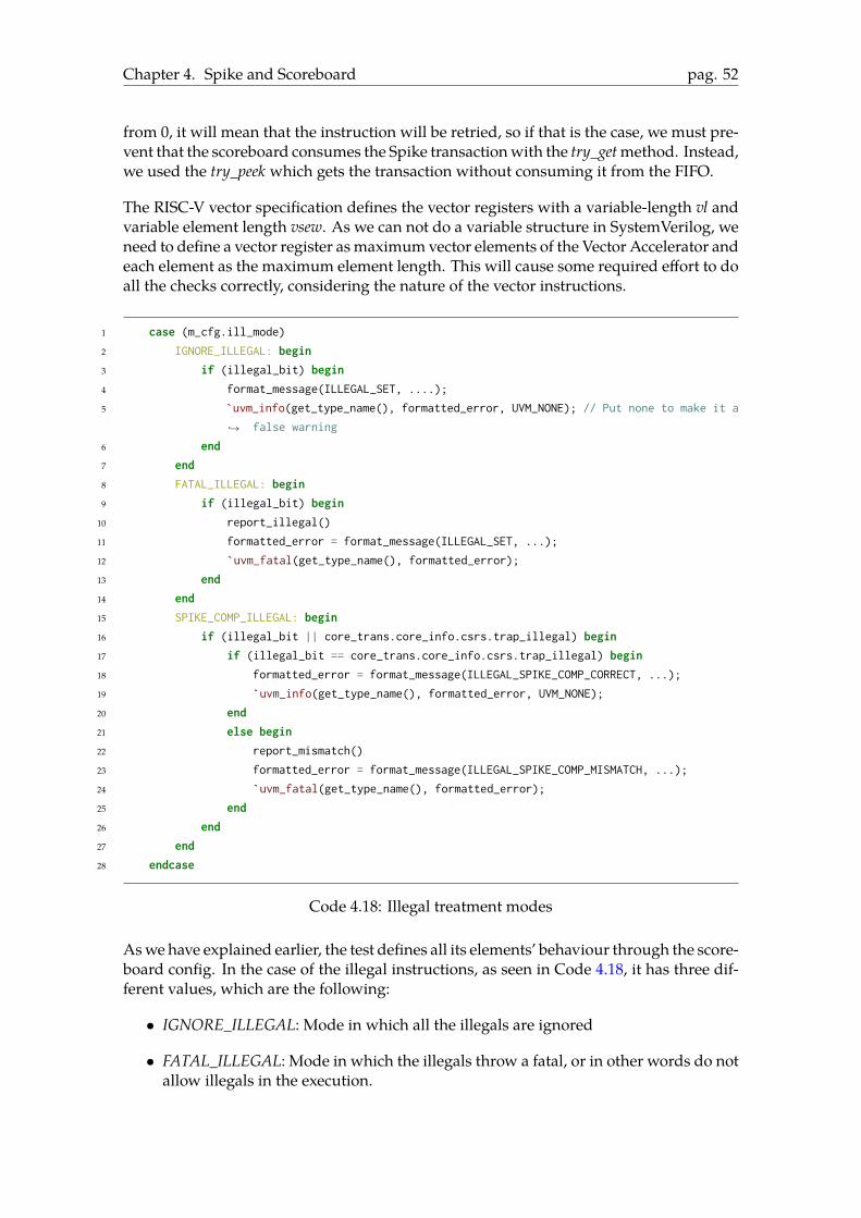
Chapter 4. Spike and Scoreboard pag. 52
from 0, it will mean that the instruction will be retried, so if that is the case, we must pre-vent that the scoreboard consumes the Spike transactionwith the try_getmethod. Instead,we used the try_peek which gets the transaction without consuming it from the FIFO.
The RISC-V vector specification defines the vector registers with a variable-length vl andvariable element length vsew. As we can not do a variable structure in SystemVerilog, weneed to define a vector register asmaximumvector elements of the Vector Accelerator andeach element as the maximum element length. This will cause some required effort to doall the checks correctly, considering the nature of the vector instructions.
1 case (m_cfg.ill_mode)
2 IGNORE_ILLEGAL: begin
3 if (illegal_bit) begin
4 format_message(ILLEGAL_SET, ....);
5 `uvm_info(get_type_name(), formatted_error, UVM_NONE); // Put none to make it a
false warning↪→
6 end
7 end
8 FATAL_ILLEGAL: begin
9 if (illegal_bit) begin
10 report_illegal()
11 formatted_error = format_message(ILLEGAL_SET, ...);
12 `uvm_fatal(get_type_name(), formatted_error);
13 end
14 end
15 SPIKE_COMP_ILLEGAL: begin
16 if (illegal_bit || core_trans.core_info.csrs.trap_illegal) begin
17 if (illegal_bit == core_trans.core_info.csrs.trap_illegal) begin
18 formatted_error = format_message(ILLEGAL_SPIKE_COMP_CORRECT, ...);
19 `uvm_info(get_type_name(), formatted_error, UVM_NONE);
20 end
21 else begin
22 report_mismatch()
23 formatted_error = format_message(ILLEGAL_SPIKE_COMP_MISMATCH, ...);
24 `uvm_fatal(get_type_name(), formatted_error);
25 end
26 end
27 end
28 endcase
Code 4.18: Illegal treatment modes
Aswe have explained earlier, the test defines all its elements’ behaviour through the score-board config. In the case of the illegal instructions, as seen in Code 4.18, it has three dif-ferent values, which are the following:
• IGNORE_ILLEGAL: Mode in which all the illegals are ignored
• FATAL_ILLEGAL: Mode in which the illegals throw a fatal, or in other words do notallow illegals in the execution.

Chapter 4. Spike and Scoreboard pag. 53
• SPIKE_COMP_ILLEGAL: The most commonmode where the illegal bit return fromthe Vector Accelerator is compared with the one coming from Spike. If the bitsmatch, the simulation continues if not throw a uvm fatal
Even if that is illegal, the instruction results will be validated to detect possible mistreat-ment. After the illegal bits comparison the scoreboard will start to check that the com-pleted instruction has a supported LMUL as the Vector Accelerator does not support anyLMUL different from 1. If it not the case, the instruction will be discarded and the execu-tion aborted as the UVM does not support it either.
ISA Checks
First, the scoreboard validates the vector CSRs {vxsat, fflags} which are passed throughthe completed interface when the instruction completes. These values indicate the fixedpoint saturation flag and the floating-point exception flags and are comparedwith Spike’sones.
After the CSR comparison, the result from the Vector Accelerator must be retrieved fromthe debug interface, which is done through a function named return_vpu_result. Firstly,in an older version, we had a virtual interface that allowed us to directly access the vectorregisters of all the lanes. That option had difficulties knowing the actual physical registerfor the logic register that we wanted to check. After some project process, the RTL teammade some changes to add a debug interface which was meant to drive the result of thevector instructions at the next cycle it marked the completed.valid.
A comparator function is called after getting the two results, one from the ISS and an-other from the VPU. This function, which is not as simple as a scalar one and namedresult_comparison, takes the next factors into account to perform the comparison:
• CSR values, as vl and vsew, will be compared to ensure that they have the sameconfiguration.
• Widening instructions have special treatment as they unify two elements in one oftwice the vsew.
Code 4.19, which is used mainly for error treatment, is a wrapper of the com-pare_vec_operands which is the one that performs the comparison.
1 function vec_mismatch_t result_comparison (vreg_elements_t vpu_result, vreg_elements_t
spike_result, int sew_control, int vl, int widening);↪→
2 mismatch = compare_vec_operands(vl, sew_control, widening, vpu_result, spike_result);
3
4 if (mismatch.error) begin
5 print_srcs(spike_result);
6 print_element_mismatch(mismatch.elem_index);
7 end
8 return mismatch;
9 endfunction
Code 4.19: Result Comparison function

Chapter 4. Spike and Scoreboard pag. 54
Besides the destination vector comparison, some instructions do not produce any visi-ble change in the vector registers but a scalar value as the vector scalar moves (vmv.v.s),or the vector mask population count (vmpopc.m). For the ones that write a scalar reg-ister, we needed to check that that scalar value retrieved from the completed interface{completed.dest_reg} is correct.
OVI Checks
Apart from the ISA verification, we also perform checks on the Open Vector Interfaceprotocol, mainly of masks, indexes, and data comparison for store operations.
To do all the checks, we needed to retrieve the data as follows:
• Firstly, if it is a masked or indexed memory operation, the scoreboard will needto wait until it can retrieve the mask elements from the mem_mask_fifo which aregenerated in the mask_idx_monitor.
• Secondly, if it is a store memory operation, the scoreboard will also need to wait forthe store data generated in the store_monitor.
After all the data is retrieved, the scoreboard will compare it with the referencemodel. For the indexed and masked comparison it will be done in a function namedmem_mask_comparison as shown in Code 4.20.
1 function vec_mismatch_t mem_mask_comparison (instr_type_t instr_type, int vl, int sew,
vreg_elements_t vpu_mask, vreg_elements_t spike_mask, vreg_elements_t vpu_indexes, vreg
vec_elements_t spike_indexes, int initial_vstart, int final_vstart);
↪→
↪→
2 if (IS_INDEXED(instr_type)) begin
3 index_mismatch = compare_vec_indexes(vpu_index, spike_index);
4 end
5 if (IS_MASKED(instr_type) begin
6 mask_mismatch = compare_mem_masks(vpu_mask, spike_mask);)
7 end
8
9 if (mask_mismatch.error)
10 print_element_mismatch(mask_mismatch.elem_index);
11
12 if (index_mismatch.error)
13 print_element_mismatch(mismatch.elem_index);
14 return mismatch;
15 endfunction : mem_mask_comparison
Code 4.20: Scoreboard memory mask comparison function
For the stores, the code is similar to the one in Code 4.19 but takes into account the masksto avoid the fatal mismatch in masked elements as the data from Spike will not containthose.
If all the mentioned steps were correct and no uvm_fatal is thrown, the UVM testbenchwill continue the simulation printing, depending on the verbosity, the data of the correctlychecked instruction.

Chapter 5
Continous Integration
5.1 Introduction
Continuous Integration or CI is a practice that Software Developers use to integrate thedeveloped changes into a shared repository frequently. This practicemakes the changes tothe main branch smaller, allowing it to detect errors quickly and debug them faster. Usu-ally, Continous Integration is associated with Continous Testing, Continous Deploymentand Continous Delivery, and we will use it as a whole when we talk about ContinuousIntegration.
This methodology is based on the source-code control version systems as it depends com-pletely on its existence to enable the merges. The software development world is unthink-able without Continous Integration as it also contributes to:
• Reduce the work for the developers.
• Secure code health previous to Deployment.
• Avoid human errors on the Deployment and Testing stages
Besides these advantages, these practices have forced new developers to do this particulartask, DevOps. Generally, all the businesses have DevOps groups merged with their ITgroups, which are in charge of developing this infrastructure to fulfil this task.
5.2 Verification Requirements
This chapter will provide an in-depth explanation of our journey in applying ContinousIntegration techniques to our Verification Environment. As the verification itself wouldbe similar to what testing is, we had two main objectives during the whole project:
• We wanted to extensively check our Design Under Test, the Vector Accelerator, toget the more bugs we could to report them to the Design Team.
• We wanted to check our environment health. This point was critical as the protocolto implement in the UVM testbench was difficult and could result in false positives
55
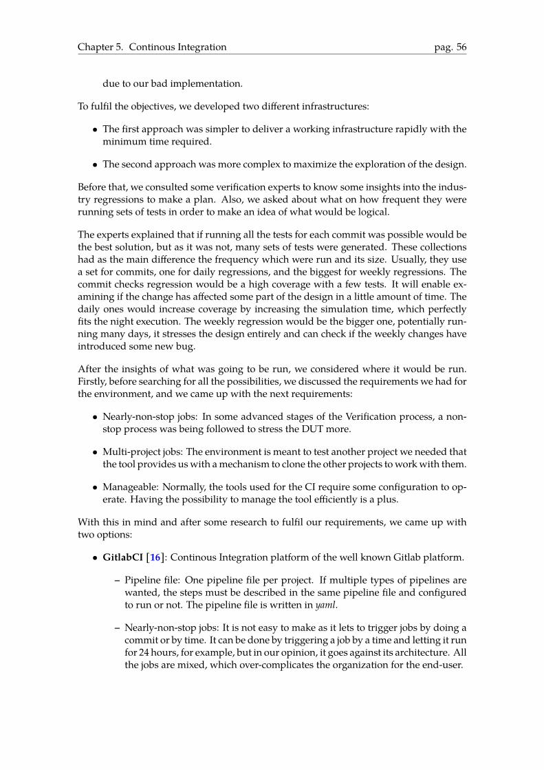
Chapter 5. Continous Integration pag. 56
due to our bad implementation.
To fulfil the objectives, we developed two different infrastructures:
• The first approach was simpler to deliver a working infrastructure rapidly with theminimum time required.
• The second approach was more complex to maximize the exploration of the design.
Before that, we consulted some verification experts to know some insights into the indus-try regressions to make a plan. Also, we asked about what on how frequent they wererunning sets of tests in order to make an idea of what would be logical.
The experts explained that if running all the tests for each commit was possible would bethe best solution, but as it was not, many sets of tests were generated. These collectionshad as the main difference the frequency which were run and its size. Usually, they usea set for commits, one for daily regressions, and the biggest for weekly regressions. Thecommit checks regression would be a high coverage with a few tests. It will enable ex-amining if the change has affected some part of the design in a little amount of time. Thedaily ones would increase coverage by increasing the simulation time, which perfectlyfits the night execution. The weekly regression would be the bigger one, potentially run-ning many days, it stresses the design entirely and can check if the weekly changes haveintroduced some new bug.
After the insights of what was going to be run, we considered where it would be run.Firstly, before searching for all the possibilities, we discussed the requirements we had forthe environment, and we came up with the next requirements:
• Nearly-non-stop jobs: In some advanced stages of the Verification process, a non-stop process was being followed to stress the DUT more.
• Multi-project jobs: The environment is meant to test another project we needed thatthe tool provides uswith amechanism to clone the other projects toworkwith them.
• Manageable: Normally, the tools used for the CI require some configuration to op-erate. Having the possibility to manage the tool efficiently is a plus.
With this in mind and after some research to fulfil our requirements, we came up withtwo options:
• GitlabCI [16]: Continous Integration platform of the well known Gitlab platform.
– Pipeline file: One pipeline file per project. If multiple types of pipelines arewanted, the steps must be described in the same pipeline file and configuredto run or not. The pipeline file is written in yaml.
– Nearly-non-stop jobs: It is not easy to make as it lets to trigger jobs by doing acommit or by time. It can be done by triggering a job by a time and letting it runfor 24 hours, for example, but in our opinion, it goes against its architecture. Allthe jobs are mixed, which over-complicates the organization for the end-user.

Chapter 5. Continous Integration pag. 57
– Multi-project jobs: Easy to perform. It clones the repository automaticallywhere the job is running, and the other ones must be done by cloning withssh keys or deploying keys.
– Manageable: No. It is hosted on the company’s servers, and we do not haveaccess to the administration pane.
• Jenkins [26]: We considered it because it is a well established CI tool with a decentamount of documentation.
– Pipeline file: The platform lets the user configure multiple pipelines, and eachpipeline has its pipeline file. The pipeline files can be described using the webinterface, but they can also be stored in a repository and configure the pipelineto retrieve it. The pipeline files are written in groovy.
– Nearly-non-stop jobs: Easy to make, as each pipeline has a separate web page,their jobs do not mix. It can be done as in GitLab with a trigger by time andallows a job that triggers itself.
– Multi-project jobs: Easy to perform. As the pipeline is agnostic to the project,it can clone multiple repositories if needed.
– Manageable: Yes, if we set up and host it in our project servers.
After comparing the two options and having internal discussions, we chose Jenkinsmainly for the modularity at the pipeline creation. We saw the GitLab pipeline file asa big drawback for the project. Consequently, we installed the Jenkins in a machinededicated to the project. This machine has:
• Intel(R) Xeon(R) Gold 5218
• 7.2 TB of storage
• Ubuntu 18.04
• 256 GB RAM
Likewise gitlabci, Jenkins pipelines can use the master node, where it is installed, or in achild node, to run a given pipeline. In favour of simplicity, we used the primary nodeJenkins. Jenkins has the functionality to use Docker [7] in the pipelines, which avoidsinstalling the tools in bare metal, so we decided to create a Docker image with all ourneeded tools for the executions.
5.3 Docker
To start doing the Docker image, we first thought about the needs during the executionto install it there. We came up with the following requirements:
• QuestaSIM [39]: The default tool we were using for the simulation.
• VCS [45]: Simulator used mainly to execute the RISCV-DV random instruction gen-

Chapter 5. Continous Integration pag. 58
erator.
• RISC-V GNU toolchain 0.7.1 [37]: GNU toolchain used to compile the binaries weproduce with RISCV-DV. We needed this specific version as it supported the 0.7.1vector specification.
• Verible [5]: Linter, property of ChipAlliance, to check the UVM code.
• Python Packages: Collection of packages with utils for the Python scripts developedin the project.
• Jenkins User: Jenkins by default adds to the docker command line its user id andgroup id for the execution to match their folder permissions. We needed the user toadd the ssh keys and other configs.
We wanted to do the images as a perfect environment to execute our infrastructure. Wehad to use as a base image CentOS [4], as it was the only system where the tools officiallygive support in case of bugs. This fact implied more efforts as CentOS is an enterprise-focused distribution that does not have the newer packages in the mainline repositoriesbut the stable ones.
To minimize the size of the images and the effort on the recompilation in case of a missingpackage we created a multistage image.
1 FROM centos:7 as rgt
2
3 ENV RISCV_VEC_TOOL /opt/riscv-vector-toolchain
4 ENV RISCV_VEC_TOOL_VER rvv-0.7.1
5
6 RUN yum install -y centos-release-scl && \
7 yum install -y devtoolset-7 && \
8 echo "source scl_source enable devtoolset-7" >> /etc/bashrc
9
10 RUN source /etc/bashrc
11
12 COPY store/rgt.tar.gz /tmp/
13
14 # Setup riscv-vector-toolchain
15 RUN tar xf /tmp/rgt.tar.gz && cd riscv-gnu-toolchain && \
16 ./configure --prefix=$RISCV_VEC_TOOL && \
17 make -j 2 && \
18 make install && \
19 cd $DOCK && rm -rf riscv-gnu-toolchain
Code 5.1: Tools installation image
Firstly, as we can see in Code 5.1, we made the image in charge of compiling the RISC-VGNU vector toolchain. As we would always want the same toolchain, it was done in aseparate image to avoid the over costs of recompiling it each time.

Chapter 5. Continous Integration pag. 59
1 FROM centos:7 as tools
2
3 RUN mkdir -p /eda/
4
5 COPY store/Mentor_Graphics.tar.gz /tmp/Mentor_Graphcis.tar.gz
6 COPY store/synopsys.tar.gz /tmp/synopsys.tar.gz
7
8 WORKDIR /tmp/
9 RUN tar xf /tmp/Mentor_Graphcis.tar.gz && tar xf /tmp/synopsys.tar.gz
10
11 RUN bash $MENTOR_INSTALLER_SCRIPT -d $MENTOR_OUTPUT
12 RUN bash $SYNOPSYS_INSTALLER_SCRIPT -d $MENTOR_OUTPUT
Code 5.2: Toolchain compilation image
Secondly, as we can see in Code 5.2, the image is in charge of installing the EDA tools forthe simulation. It mainly copies the generated files and executes the installers from thevendors.
1 FROM centos:7 as hw_base_image
2 COPY --from=tools /eda/ /eda/
3 COPY --from=rgt /opt/ /opt/
4
5 COPY packages.txt .
6 RUN yum update --nogpgcheck -y && \
7 xargs yum install --nogpgcheck -y <packages.txt && \
8 yum clean all
9
10 RUN yum install -y centos-release-scl && \
11 yum install -y devtoolset-7 && \
12 echo "source scl_source enable devtoolset-7" >> /etc/bashrc
13
14 RUN mkdir -p /root/.ssh && \
15 chmod 0700 /root/.ssh
16
17 WORKDIR /root
Code 5.3: Final base image
After the partial images are built, we created another one that extends from the samedistribution and has the same packages. That one copies the produced data by the othersinside it with the COPY commands as shown in Code 5.3. This practice allowed us toreduce the final image size by removing the temporal layers created while doing the othersteps as the COPY or RUN commands. It also has included an updated version of GCCas the default one was outdated and caused problems in compiling some of the projects.
The resulting image was named hw_base_image, and it was the base for all derivative im-ages that use the same tools as the ones included.

Chapter 5. Continous Integration pag. 60
Our image, which code is presented in Code 5.4, extends from the image explained above.Besides all the base tools, we have included the verification specific tools and path config-uration in the default PATH variable. We have mainly added verible and Python packagesthat were specifically needed for our scripts.
1 FROM hw_base_image
2 ENV DOCK /opt/docker
3 WORKDIR $DOCK
4
5 ARG USER_NAME=jenkins
6 ARG USER_ID=127
7 ARG GROUP_ID=133
8
9 COPY build_verible.sh /root/
10 RUN bash /root/build_verible.sh
11
12 COPY requirements.txt /root/
13 RUN pip3 install -r /root/requirements.txt
14
15 ENV TZ=Europe/Madrid
16 RUN ln -snf /usr/share/zoneinfo/$TZ /etc/localtime && echo $TZ > /etc/timezone
17
18 ENV MTI_HOME=/eda/mentor/2019-20/RHELx86/QUESTA-CORE-PRIME_2019.4/questasim
19 ENV QUESTA_HOME=/eda/mentor/2019-20/RHELx86/QUESTA-CORE-PRIME_2019.4/
20 ENV VCS_HOME=/eda/synopsys/2019-20/RHELx86/VCS_2019.06-SP2/
21
22 ENV PATH=$MTI_HOME/linux_x86_64:$PATH
23 ENV PATH=$PATH:/opt/riscv-vector-toolchain/bin/
24
25 RUN mkdir -p /root/.ssh && \
26 ssh-keyscan $gitlab_host1 >> /root/.ssh/known_hosts && \
27 ssh-keyscan $gitlab_host2 >> /root/.ssh/known_hosts
28
29 ENV USER root
30
31 RUN groupadd --gid $GROUP_ID jenkins && adduser --uid $USER_ID --gid $GROUP_ID $USER_NAME
32
33 RUN mkdir -p /home/jenkins/.ssh && \
34 ssh-keyscan $gitlab_host1 >> /home/jenkins/.ssh/known_hosts && \
35 ssh-keyscan $gitlab_host2 >> /home/jenkins/.ssh/known_hosts
36
37 RUN chown $USER_ID:$GROUP_ID /home/jenkins/.ssh/
Code 5.4: Verification Image
Furthermore, we added a user for the Jenkins with the same user id and group id as theinstallation to match permissions and avoid future problems. Also, we added for bothroot and Jenkins the public keys of the GitLab repositories we were using for the projectto the known_hosts file.
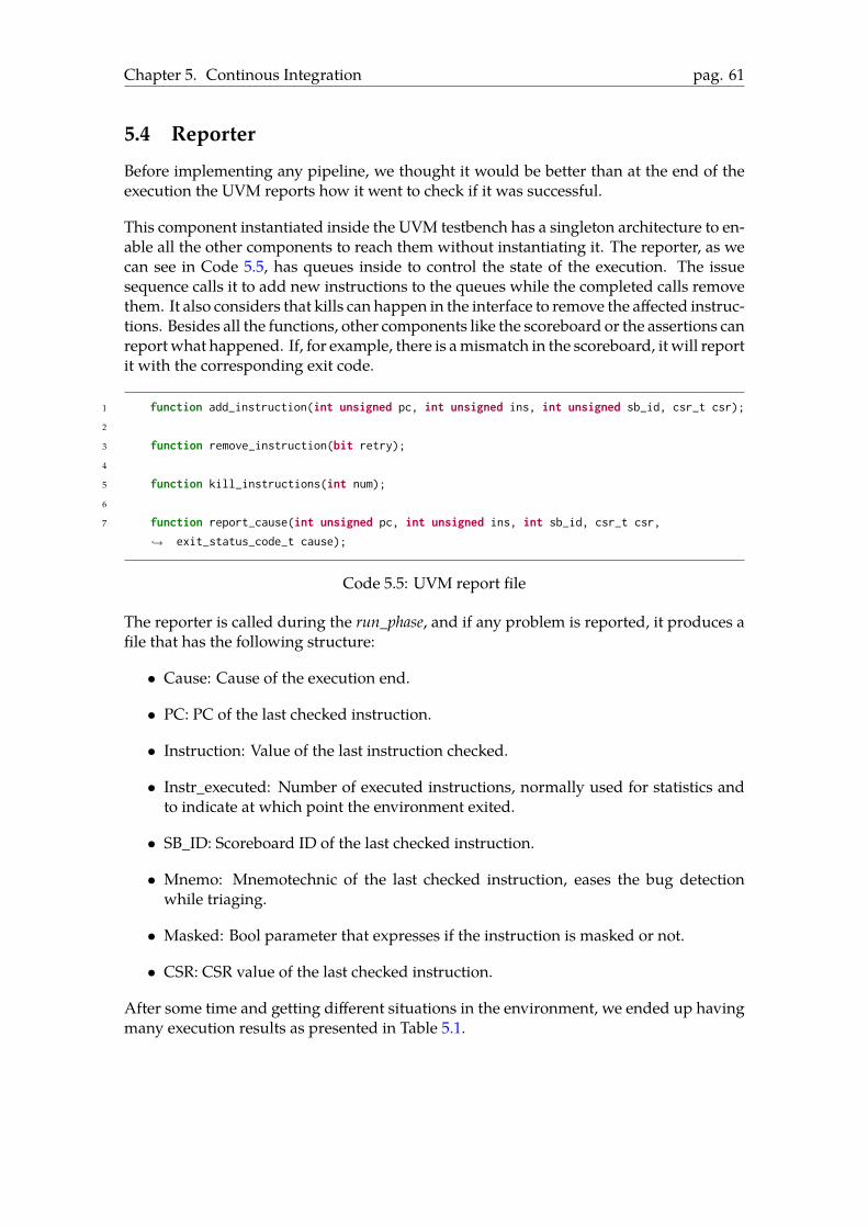
Chapter 5. Continous Integration pag. 61
5.4 ReporterBefore implementing any pipeline, we thought it would be better than at the end of theexecution the UVM reports how it went to check if it was successful.
This component instantiated inside the UVM testbench has a singleton architecture to en-able all the other components to reach them without instantiating it. The reporter, as wecan see in Code 5.5, has queues inside to control the state of the execution. The issuesequence calls it to add new instructions to the queues while the completed calls removethem. It also considers that kills can happen in the interface to remove the affected instruc-tions. Besides all the functions, other components like the scoreboard or the assertions canreportwhat happened. If, for example, there is amismatch in the scoreboard, it will reportit with the corresponding exit code.
1 function add_instruction(int unsigned pc, int unsigned ins, int unsigned sb_id, csr_t csr);
2
3 function remove_instruction(bit retry);
4
5 function kill_instructions(int num);
6
7 function report_cause(int unsigned pc, int unsigned ins, int sb_id, csr_t csr,
exit_status_code_t cause);↪→
Code 5.5: UVM report file
The reporter is called during the run_phase, and if any problem is reported, it produces afile that has the following structure:
• Cause: Cause of the execution end.
• PC: PC of the last checked instruction.
• Instruction: Value of the last instruction checked.
• Instr_executed: Number of executed instructions, normally used for statistics andto indicate at which point the environment exited.
• SB_ID: Scoreboard ID of the last checked instruction.
• Mnemo: Mnemotechnic of the last checked instruction, eases the bug detectionwhile triaging.
• Masked: Bool parameter that expresses if the instruction is masked or not.
• CSR: CSR value of the last checked instruction.
After some time and getting different situations in the environment, we ended up havingmany execution results as presented in Table 5.1.

Chapter 5. Continous Integration pag. 62
Cause Value Cause String0 SUCCESS1 TIMEOUT2 COMPILATION ERROR3 EXECUTION ERROR4 SPIKE ERROR5 ASSERTION ERROR6 BINARY ERROR7 ILLEGAL MISMATCH
Table 5.1: Possible environment exit codes
5.5 First ApproachAs presented below, we wanted to quickly develop an environment that automaticallycould report bugs to the Design Team. With this basic idea, we proposed, as seen inFigure 5.1.
• 5J pipeline: Pipeline triggered nightly, which was in charge of testing five selectedbinaries.
• Night random pipeline: Pipeline triggered many times in the night, which was incharge of generating a binary and executing it.
• Success pipeline: Pipeline triggered each night which ran a manually crafted se-lection of tests to check if the day no bug was introduced in the design. The testsselectionwasmade from randombinaries generated in theNight Randompipeline.
Figure 5.1: First Approach pipelines schemes
In the morning, after all the jobs from the Night random had been triggered, the pipelineNight Random results will be executed and generate a table summarizing the results, likethe one in Table 5.2. The table was published in our Gitlab platform, and the DesignTeam triaged the failing binaries. As Jenkins was outside the Gitlab, we needed to makescripts that used the Gitlab API to publish to its designated issues. Publishing the resultson Gitlab made the life of the Design Team way easier than making them look into the

Chapter 5. Continous Integration pag. 63
Jenkins. The tables had an extra columnwhich allowed the Design Team to add the statusof each particular test.
NUM CAUSE EXECUTION TIME INSTRUCTION MNEMOTECHNIC STATUS409 TIMEOUT 9530001 0x57802057 vmfirst.m410 TIMEOUT 8930001 0x5a60a157 vmsbf.m411 EXECUTION ERROR 12630000 0x834b8657 vsaddu.vv412 TIMEOUT 9530001 0x5a682257 viota.m
Table 5.2: Gitlab Issues table example
The tests executed in the night random pipeline have the coverage collection enabled bydefault, so each execution will produce a UCDB file. The UCDB or Unified CoverageDatabase is a database file specified by Mentor [1], which contains code coverage, func-tional coverage and other metrics in one place to unify its analysis. All the UCDB fileswere stored after executing each job in a shared folder in the host machine. After exe-cuting the tests, some the coverage files were ranked to retrieve which were the ones thatcontributed to the coverage. If a test did not contribute to the coverage, it would meanthat it did not stimulate the circuit more than the others.
Once the ranking process was done, if a test did not contribute to coverage, it was dis-carded, so we kept the ones that contributed to the coverage, and we made a set of teststhat were stored inside our repository and were run with the success pipeline. We did thisprocess of ranking and storing the ones that contribute to the coverage manually.
Almost all the pipelines followed the same structure, which was:
• Specify the pipeline configuration: when the pipeline should be triggered, timeout.
• Specify the plugin configuration: GitLab plugin. . .
• Specify the pipeline stages:
– Fetch the repositories: UVM, Vector Accelerator, Verification CI repository.
– Execute the UVM testbench.
– Custom post-execution script.
• Choose what artifacts to archive.
Furthermore, in the development world, the projects have tests that certify that the im-plemented functionality is well implemented. In the case of UVM, there are some frame-works like SVUnit [44].
Alternatively, wemade an empty test that extends from the base_test to have a basic checkfor the environment without much effort. It checked that the environment could compileand execute, as some errors appeared in the simulation. It had an empty sequence asdescribed in Code 5.6 which overrides the task body.
This empty test was used in the commit-checks pipeline, the first one configured withthe webhooks provided by the Gitlab platform to trigger external pipelines. This pipeline

Chapter 5. Continous Integration pag. 64
1 class empty_seq extends avispado_mod_issue_seq;
2 `uvm_object_utils(empty_seq)3
4 task body();
5 super.body();
6 endtask : body
7
8 virtual task test_body();
9 endtask: test_body
10
11 endclass : empty_seq
Code 5.6: Empty sequence
was triggered each commit of an opened merge request to master in the UVM testbenchrepository. Besides the run of the empty test, it also executed the linter verible to checkpossible bugs or coding style errors in the code. This pipeline saves the linting outputand the compile and simulation transcript for the artifacts.
5.6 Second approach
After many weeks with all the Night Runs clean without any bug, we decided to take adifferent approach to the same problem. We intended to do a similar organization asthe first approach but with a higher level of automation for the second approach. Wewanted a sophisticated mechanism that automatically and continuously generated teststo find new bugs and extract coverage. Also, we wanted to ensure that the current codein the develop branch is healthy and that no one could introduce new bugs. The overallarchitecture would have the objective of generating the next set of tests:
These new pipelines had the next features:
• Failing Set: Set of tests failing with the last RTL develop commit.
• Small Set: Set of the tests, a subset of the completed tests relevant to the coverage.
• Complete Set: Set of tests formed by all the tests ever executed that had a successfulend of execution in the environment.
We needed tools to orchestrate the flow that produced the sets mentioned above. Wediscussed implementing the tools ourselves or using a vendor solution for this purpose.Firstly we decided to develop tools to be agnostic to the simulator to avoid future prob-lems. However, after some weeks of developing these tools, we decided to switch to thevendor option.
The vendor toolwe used to do the flow is property ofMentorGraphics and is calledVRUN[41]. It eased the development of the infrastructure as it is functionally prepared to runregressions and triage the results. Moreover, it also had capabilities to collect coverage oftests and auto-merge the outputs that provide an accurate state of the stimulation of thedesign. It could also specify the number of processes that will be instantiated, allowing
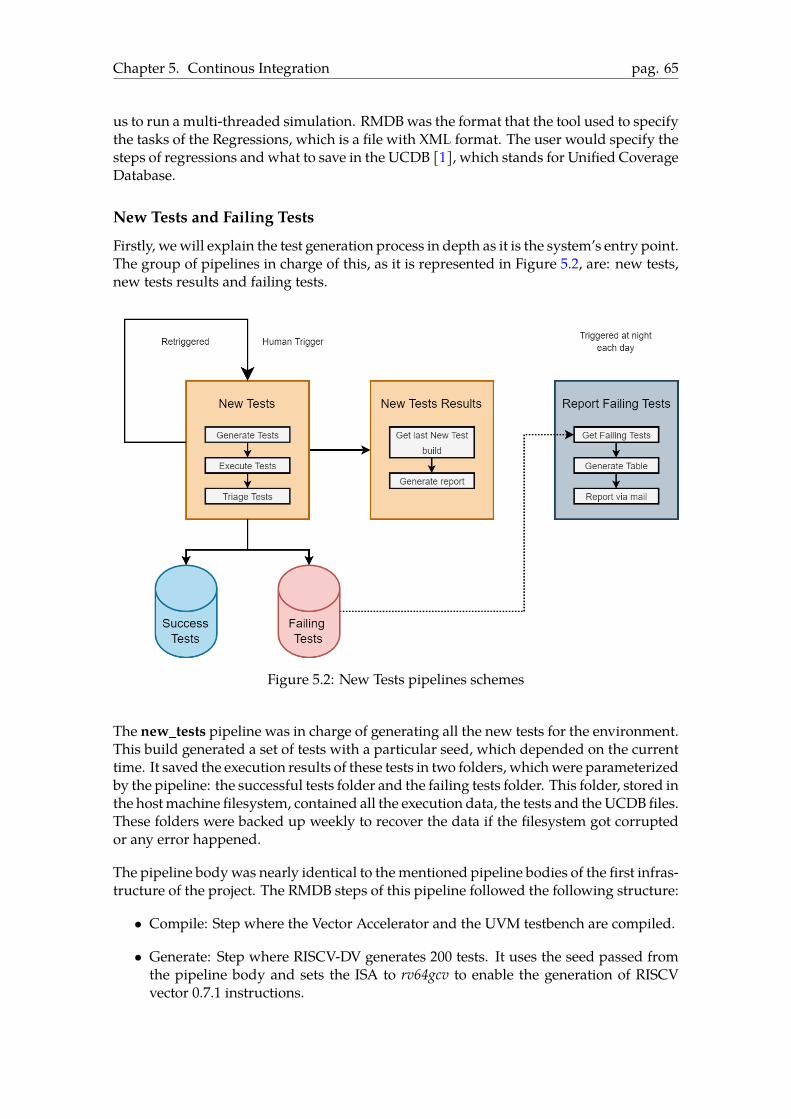
Chapter 5. Continous Integration pag. 65
us to run amulti-threaded simulation. RMDBwas the format that the tool used to specifythe tasks of the Regressions, which is a file with XML format. The user would specify thesteps of regressions andwhat to save in the UCDB [1], which stands for Unified CoverageDatabase.
New Tests and Failing Tests
Firstly, wewill explain the test generation process in depth as it is the system’s entry point.The group of pipelines in charge of this, as it is represented in Figure 5.2, are: new tests,new tests results and failing tests.
Figure 5.2: New Tests pipelines schemes
The new_tests pipeline was in charge of generating all the new tests for the environment.This build generated a set of tests with a particular seed, which depended on the currenttime. It saved the execution results of these tests in two folders, whichwere parameterizedby the pipeline: the successful tests folder and the failing tests folder. This folder, stored inthe hostmachine filesystem, contained all the execution data, the tests and theUCDBfiles.These folders were backed up weekly to recover the data if the filesystem got corruptedor any error happened.
The pipeline bodywas nearly identical to thementioned pipeline bodies of the first infras-tructure of the project. The RMDB steps of this pipeline followed the following structure:
• Compile: Step where the Vector Accelerator and the UVM testbench are compiled.
• Generate: Step where RISCV-DV generates 200 tests. It uses the seed passed fromthe pipeline body and sets the ISA to rv64gcv to enable the generation of RISCVvector 0.7.1 instructions.
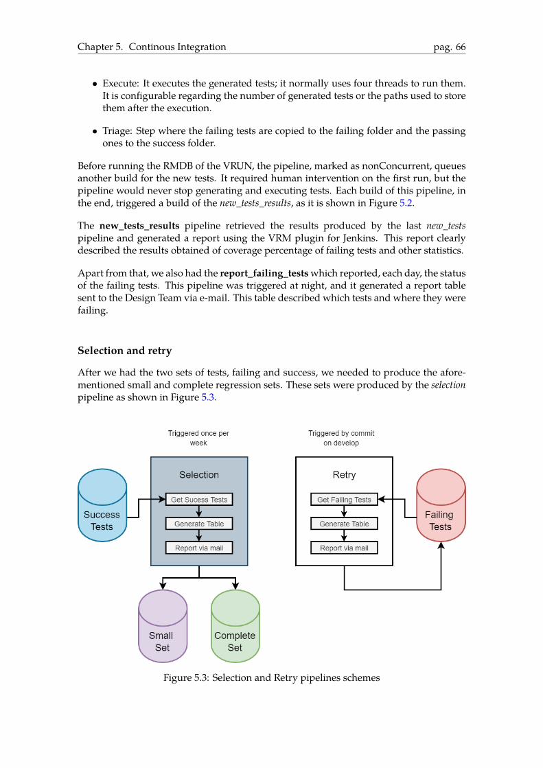
Chapter 5. Continous Integration pag. 66
• Execute: It executes the generated tests; it normally uses four threads to run them.It is configurable regarding the number of generated tests or the paths used to storethem after the execution.
• Triage: Step where the failing tests are copied to the failing folder and the passingones to the success folder.
Before running the RMDB of the VRUN, the pipeline, marked as nonConcurrent, queuesanother build for the new tests. It required human intervention on the first run, but thepipeline would never stop generating and executing tests. Each build of this pipeline, inthe end, triggered a build of the new_tests_results, as it is shown in Figure 5.2.
The new_tests_results pipeline retrieved the results produced by the last new_testspipeline and generated a report using the VRM plugin for Jenkins. This report clearlydescribed the results obtained of coverage percentage of failing tests and other statistics.
Apart from that, we also had the report_failing_testswhich reported, each day, the statusof the failing tests. This pipeline was triggered at night, and it generated a report tablesent to the Design Team via e-mail. This table described which tests and where they werefailing.
Selection and retry
After we had the two sets of tests, failing and success, we needed to produce the afore-mentioned small and complete regression sets. These sets were produced by the selectionpipeline as shown in Figure 5.3.
Figure 5.3: Selection and Retry pipelines schemes

Chapter 5. Continous Integration pag. 67
The selection pipeline’s first step was to block all the other pipelines which used the suc-cess, small and complete sets with a resource lock mechanism. The throttling was doneto preserve the consistency between sets and avoid more than one pipeline touching thesame sets. After that, it copied the current successful tests and the previous complete set toa temporary directory. If the number of gathered tests was higher than some threshold, itcopied the tests UCDBs in the success folder and ranked them. The tool also provided thisranking process, which generated a list of the tests that contribute to the coverage. Thecontributing ones were gathered and formed the complete regression set. The N mostsignificant items from that list formed the small regression, being N a pipeline parameter.
The retry pipeline was in charge of re-executing the failing set of tests each time a mergerequest is pushed to the develop branch. The pipeline aimed to delete the fixed tests withthe new changes introduced to the develop branch.
Small Regression and Complete RegressionThe pipelines running the previous tests were the small and complete regressionpipelines. The overall flow of these pipelines are represented in Figure 5.4.
Figure 5.4: Regression pipeline schemes
The small regression pipeline was in charge of executing the small regression set. Thisset of tests was a tradeoff between high coverage and the number of tests, and it is exe-cuted in each commit of every merge request opened to the develop branch of the designrepository. Using it, we ensured that the Design Team did not introduce any changes thatproduced a bug on previously successful tests.
The complete regression pipeline, which executed the complete regression, was executedonce per week as its execution required much time to execute because of the number oftests. Also, this regression ranwith coverage options, andwhen all the tests were finished,it merged the UCDBs and generated a coverage report published on anNginx server [33].
We wanted to do something more sophisticated to check that we did not break anythingfor the second approach.

Chapter 5. Continous Integration pag. 68
Figure 5.5: UVM Regressions pipeline scheme
We prepared the small regression set for the Vector Accelerator as we opted for a quickand efficient approach. We created a pipeline that used this small set and ran it in ourenvironment.
As it is seen in Figure 5.5, the pipeline UVM regressionswas designed to be run in everymerge request of our repository when the changes were ready to be merged. It was trig-gered by a fixed command that started the pipeline’s build. Even though it is not a goodpractice to check a project with another one, we decided that it was the less effort, higheroutcome approach.
Figure 5.6: Spike build pipeline scheme
Spike is added to the simulation, adding a shared object (spike.so) to the simulation scripts.The shared object during the first approach was updated manually as it was part of therepository. That manual process was not a good practice as the binaries are not optimallytracked in repositories.

Chapter 5. Continous Integration pag. 69
For the second approach, we decided to compile it in a pipeline, as seen in Figure 5.6.Each time we pushed a commit to master, the pipeline was triggered, saving the sharedobject as an artifact. This allowed a Python script in the verification repository to updateit transparently to the final user. The versions are done with the master commit hash, so ifthe script detects that the user has a different version from the last stable build will forcethe update and download the latest version.
Chapter 6
Evaluation
After all the contributions have been explained in the previous sections, the project resultswill be presented. In the following two sections, two topics will be evaluated.
In Section 6.1, we will present the Verification results obtained in the process, mainlycoverage and bugs. And in Section 6.2, we will evaluate the contributions made in thisthesis.
6.1 Verification Results
Verification, independently of the results, is a process that takes a high amount of time. Atthe start of these processes, when the design is almost not explored, many bugs are foundwithout much effort, but as time starts ticking, it becomesmore difficult to find them. TheVerification Team fights to find all the bugs during the whole process, but it would be animpossible task in almost all designs.
Besides having much bigger Verification Teams than the Design teams, many industrial-grade designs have many bugs post tape-out. If any is detected and depending on thetype of error [9], it will probably be fixed at physical or software level depending on itsseverity [6].
Despite this, the Verification Teams have always given all they have to report the mostsignificant ones to the Design Team.
Coverage and the number of executed tests are the most used metrics when results mustbe reported. In the end, the functional coverage values are produced by code developedby the verification team, and if it is not well-developed, it can lead tomisleading numbers.If it is the case, it can give a false feeling of exploration, which is why coverage implemen-tations should be reviewed periodically.
Anothermarker to explore howwell the verification has done is to see the number of bugsreported to the Design Team.
Taking this into account, we will explore two topics in this section; firstly, we will explorethe absolute numbers of the executed tests, and secondly, we will explore the logged cov-
70
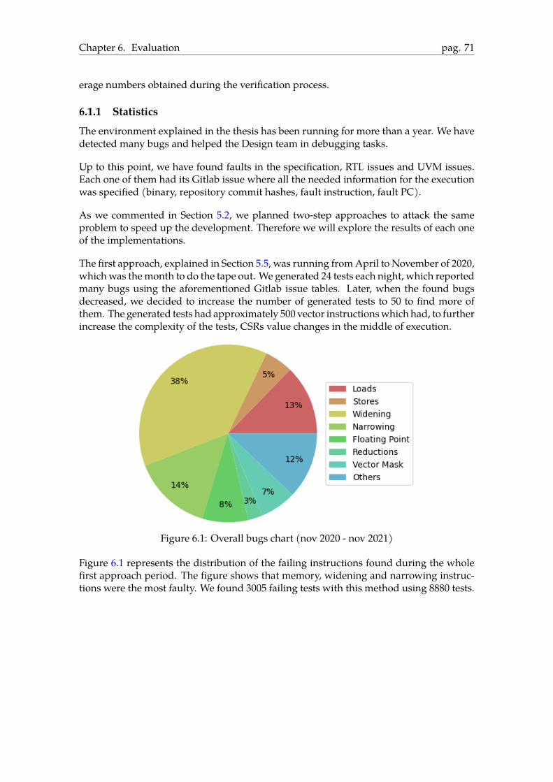
Chapter 6. Evaluation pag. 71
erage numbers obtained during the verification process.
6.1.1 StatisticsThe environment explained in the thesis has been running for more than a year. We havedetected many bugs and helped the Design team in debugging tasks.
Up to this point, we have found faults in the specification, RTL issues and UVM issues.Each one of them had its Gitlab issue where all the needed information for the executionwas specified (binary, repository commit hashes, fault instruction, fault PC).
As we commented in Section 5.2, we planned two-step approaches to attack the sameproblem to speed up the development. Therefore we will explore the results of each oneof the implementations.
The first approach, explained in Section 5.5, was running fromApril to November of 2020,whichwas themonth to do the tape out. We generated 24 tests each night, which reportedmany bugs using the aforementioned Gitlab issue tables. Later, when the found bugsdecreased, we decided to increase the number of generated tests to 50 to find more ofthem. The generated tests had approximately 500 vector instructionswhich had, to furtherincrease the complexity of the tests, CSRs value changes in the middle of execution.
Figure 6.1: Overall bugs chart (nov 2020 - nov 2021)
Figure 6.1 represents the distribution of the failing instructions found during the wholefirst approach period. The figure shows that memory, widening and narrowing instruc-tions were the most faulty. We found 3005 failing tests with this method using 8880 tests.
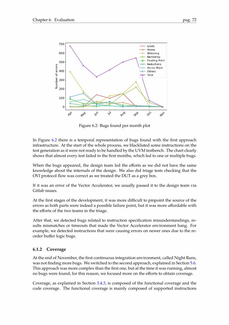
Chapter 6. Evaluation pag. 72
Figure 6.2: Bugs found per month plot
In Figure 6.2 there is a temporal representation of bugs found with the first approachinfrastructure. At the start of the whole process, we blacklisted some instructions on thetest generation as it were not ready to be handled by the UVM testbench. The chart clearlyshows that almost every test failed in the first months, which led to one or multiple bugs.
When the bugs appeared, the design team led the efforts as we did not have the sameknowledge about the internals of the design. We also did triage tests checking that theOVI protocol flow was correct as we treated the DUT as a grey box.
If it was an error of the Vector Accelerator, we usually passed it to the design team viaGitlab issues.
At the first stages of the development, it was more difficult to pinpoint the source of theerrors as both parts were indeed a possible failure point, but it was more affordable withthe efforts of the two teams in the triage.
After that, we detected bugs related to instruction specification misunderstandings, re-sults mismatches or timeouts that made the Vector Accelerator environment hang. Forexample, we detected instructions that were causing errors on newer ones due to the re-order buffer logic bugs.
6.1.2 Coverage
At the end of November, the first continuous integration environment, called Night Runs,was not findingmore bugs. We switched to the second approach, explained in Section 5.6.This approach wasmore complex than the first one, but at the time it was running, almostno bugs were found; for this reason, we focused more on the efforts to obtain coverage.
Coverage, as explained in Section 3.4.3, is composed of the functional coverage and thecode coverage. The functional coverage is mainly composed of supported instructions

Chapter 6. Evaluation pag. 73
coverage, which mainly checks what instruction test cases have been executed in the de-sign, and the code coverage, which is an automatic coverage made by the tool that ex-presses how much of the code has been stimulated.
Design Unit Coverage Design Unit CoverageOVI/Pre-issue Queue 91.95% Data Reorder Buffer 88.09%Instruction Unpacker 100.00% Ctrl FSM 92.64%Instruction Renaming 100.00% Functional Units 100.00%Instruction Queue 100.00% Vector Register File 92.37%Store Management 87.50% Inter-lane Ring 99.18%Load Management 100.00% Vector Lane 93.61%Item Management 100.00% Total 95.79%
Table 6.1: Functional coverage per design unit
Table 6.1 shows the summary of the functional coverage achieved in the project. The totalrow shows we have a total of 95.79% which is a high number, although it means that wehave not stimulated the whole design. Further explorations of the coverage will be doneto try to maximize the total coverage numbers.
Also, we need to consider that the tests are always generated by the same entity, RISCV-DV, which can bias the generated tests, which would affect the coverage results. It hasto be said that these coverage numbers result from many efforts, including specificationand exploration, to see which cases are not being triggered. Furthermore, the currentenvironment has some limitations of the OVI, as a protocol implementation can also leadto gaps in the coverage as some cases could not be handled.
It has to be considered that these functional coverage numbers are pretty high consideringthe overall project environment and our experience in verification. Even that, the resultsmust not be treated as certain as they will need to be reviewed by many teams to ensurethey are correct.
Type Bins Hits Misses CoverageBranches 135279 106251 29028 78.54%Conditions 17908 10353 7555 57.81%Expressions 95290 52349 42941 54.93%FSM States 186 170 16 91.39%
FSM Transitions 335 285 50 85.07%Statements 227695 206982 20713 90.90%Toggles 2526053 1258760 1267293 49.83%Total 72.64%
Table 6.2: Code coverage for the whole VPU
Table 6.2 refers to the code coverage obtained by the project, which statements were au-tomatically generated by the tool at the compilation. As it has zero cost on developing, itis interesting to check the behaviour of the developed RTL. Despite this, it adds overheadin the execution times, which must be considered. The code coverage overall numbersare lower than the functional coverage as it has 72.64%. Even being a coverage number,these results have a different meaning than the functional coverage ones. The code cover-
Chapter 6. Evaluation pag. 74
age describes how well the design is programmed, and how many of the described casesare observed. A Design’s code can be functional and correct but have many unused state-ments or oversized signals, leading to useless gates in the physical design. These numberswere less reviewed than the functional coverage, so some iterations need to be done withthe Design Team to refine them. Much effort is needed for this review task as usually thecode is not trivial enough or documented to see which statements produce holes in thecode coverage.
The coverage plan has been frequently reviewed in our project to secure we made it cor-rectly. Also, it has been reexplored to look with design parts that have not been stim-ulated correctly, in the end, which cases were not happening. After each reexploration,many efforts were made tomake themissing cases happen, from changing the code of thegeneration to doing some specific tests.
Even today, we are trying to push these numbers even higher with the help of the RTLteam by exploring non-executed cases or units with low numbers.
6.2 Contributions evaluationThe presented work was essential for significantly reducing the bugs in the environment.Even though it was not perfect and some parts could be criticised. Although we were ayoung team without any experience in verification, we have researched and developed awhole environment for a complex design.
In Continous Integration, we decided to use the vendor tool tomake all the infrastructure,which was a wrong decision in hindsight. If we want to use the same infrastructure withtools of another vendor, it would require a complete re-implementation. Taking the pathof writing our tool would require more time to be developed and debugged but would bemore beneficial in matters of reusability of other projects and maintenance.
As seen in Figure 6.3, during the early stages of the project, we published tables. One tablelike in the figure was published each night, which helped track what tests and why werefailing. The tables had the number of the failing tests, which had a hyperlink to make thereproduction of the execution almost effortless to the Design Team. These tables were thebasis of triaging as the RTL team edited these to complete the column of status to indicatethe reason for failure, which enabled them to categorise the tests by the causing bug, mak-ing it possible that more than one test failed for the same reason. The provided metadaalso helped to identify possible related bugs, for example in the figure all the failing testswith mnemotechnic vrsrl.wx probably failed because of the same bug. Moreover, to ar-rive to the failing point the number of executed instructions and the CSR vsew should beconsidered as both alter the execution times.

Chapter 6. Evaluation pag. 75
Figure 6.3: Gitlab Night Report
Figure 6.4: Jenkins New Tests Report
In Figure 6.4, we can appreciate the web page of Jenkins of the New Tests Results pipeline.It represents in charts the results of recent builds of the New Tests using the Questa VRMplugin [31]. Getting the results of the last builds, it makes charts with the success ratesand coverage numbers, which eases the global perspective of how is theNewTests pipelinegoing.
Furthermore, In Figure 6.5, we can see an example of the state of the Spike pipeline, whichproduced the shared library that the UVM will automatically downloads. In the figure,we can observe that one pipeline has failed due to compilation errors marked in red, an-other one that has succeeded but is marked as unstable not to save the library and, the first

Chapter 6. Evaluation pag. 76
Figure 6.5: Jenkins Spike pipeline
one, which has everything green, will produce the shared library. The pipeline was trig-gered in merge requests and in pushes to master, but only in the master ones must deliverthe shared object. To only provide stable releases of the ISS, we marked the non-mastercommit checks as unstable to prevent the tool from downloading those shared objects.With it, many errors of versioning have been avoided as they use the SHA1 [15] of Gitversion of the library, and it is displayed each time the UVM is executed.
Even if it was not commented in depth in the thesis, some decisions caused problemsduring the development of the environment. For example, initially, we were saving tem-porally the waves to enable the Design Team to look at the simulation without rerunningthe executions, which caused many performance and storage issues, so this feature wassoon disabled. In the end, it was disabled because approximately each of the waves sizedmany gigabytes, making it impossible to save when many tests were failing. Also, we didnot develop this structure standalone; it resulted frommany first thoughts andmany teststo seek which option was the best performing and best fitting.
Furthermore, even though Continous Integration was a complex field to work on as wehad no experience, we managed to deliver a functional Continous Integration Infrastruc-ture which was the basis of the results presented in the thesis. It helped us achieve thecurrent verification status and automatised many hours of manual work, which is what itis used for.
In terms of theUVM, even though itwas not covered in this thesis, we felt that even thoughit worked well, it had performance issues intrinsic to its structure that only a completerefactor could solve. The complex structure of the UVMmade the code toomuch complexand more challenging to read, and as we added features, it got worse.
Even if the environment does not findmany bugs nowadays, it continues fulfilling its dutyby securing the design team’s develop branch and collecting coverage. It does not allowto merge anything that could break any previously regression tests. However, when new

Chapter 6. Evaluation pag. 77
features are added to the design or the UVM, it can potentially find new bugs.
To conclude, evenwith all the self-criticismswe have for our environment, wewere proudof what we achieved and the utility we have provided to the Design Team. It has beenhandy to detect many bugs that the Design Team easily debugged as we provided thepoint where it failed.

Chapter 7
Conclusions and Future Work
7.1 ConclusionsThis thesis presents the verification efforts applied to theVectorAccelerator during the EPIproject, which was a long journey for a young team. Firstly, we have presented the effortsto modify an existing reference model to fit our needs, which was an essential aspect ofdeveloping a fully functional environment. Secondly, we have presented the ContinousIntegration efforts, which was crucial to the verification level.
Also, it must be mentioned that the work presented could not have been possible withoutthe efforts made by the group as the environment is the result of many people.
We have adapted an existing ISS, Spike, to do an instruction-by-instruction comparisonalongside a UVM testbench for the functional verification part. Moreover, we developedan auxiliary structure to provide the scoreboardwith the correct results of the instructionswe were executing in the UVM testbench.
Regarding Continous Integration, we have developed a huge infrastructure, alongsideJenkins and Docker, capable of finding bugs automatically. Also, it has been vital to re-trieve the coverage results we currently have.
Finally, we have proved that verifying complex designs involves much effort of many en-gineers just to be done, and evenmore if it is wanted to be done in the right way. We neverstated that what we presented in this thesis was done in the best way, but it was surelydone with the best will of achieving our goal. Furthermore, it ended up being tapeoutand working well on a real chip. Also, we had to learn many new things and try to guessthe right path to arrive at the point we were and give the results we gave.
7.2 Future WorkEven with all the presented work, there is always room to do better; there are alwaysthings that could have been different.
The existence of a Verification Plan is vital in a Verification Process. For example, in ourcase, even having and considering them, we started to add new features to the environ-
78

Chapter 7. Conclusions and Future Work pag. 79
ment as they were requested, which resulted in patches, making the environment morecomplex. A better initial plan or more frequent reviews would have reduced the projectcomplexity making the environment easier to modify.
There was work to do in the Block Level Verification in the most critical inner modules ofthe design. We understood the whole design as a System Level because it was more feasi-ble to do for the people we had than the other way. However, more efforts are needed if anindustrial-grade tape out is wanted, which translates to more UVM testbenches neededto explore the code better. This is only possible if the teams are big enough to assign somepeople to the Block Level and others to the System Level.
There was work in reviewing the existing Coverage Plans as it is the principal metric topresent the current Verification state of the design. This is crucial in Verification as the firstthought is never the best, and there is much room to do better in many aspects, especiallyin the coverage. Moreover, further exploration of the coverage usually implies severalchanges in the coverage statements on the design.
Currently, the next generation of the environment is being developed. It takes a radicalchange of approach on the same OVI interface but without complicating the developmentwith different agents. We have plans for this new environment currently under develop-ment to take the seat of his predecessor in a transparent way to the Design Team.
Finally, the Verification Infrastructure is a crucial topic when we refer to stimulating aDUT, as almost all the results presented in the thesis were accomplished using the devel-oped infrastructure. Even though the presented one was good enough, we could havemade many improvements to make it better and transparent for many projects. After allthe efforts, we are confident that the more agnostic the infrastructure to the environmentis, the more maintainable and reusable it will be, which is crucial for development.
Also, we consider that many of the current software techniques used nowadays can beapplied in some way to Verification, making the flow fancier. Furthermore, even someMachine Learning techniques have been appearing in Verification [19] for bug triagingand random stimulus generation, which could also be interesting to apply in the currentin-develop environments. TheseMachine Learning could open a new perspective on howthe Verification must be done or how it can be more efficient.

Bibliography
[1] Accellera.Unified Coverage Interoperability Standard (UCIS). 2021. url: https://www.accellera.org/images/downloads/standards/ucis/UCIS_Version_1.0_Final_June-2012.pdf.
[2] John Hauser AndrewWaterman Krste Asanovic. The RISC-V Instruction Set ManualVolume II: Privileged Architecture. 2021. url: https://github.com/riscv/riscv-isa-manual/releases/download/Ratified-IMAFDQC/riscv-spec-20191213.pdf(visited on 12/02/2021).
[3] Krste Asanovic Andrew Waterman. The RISC-V Instruction Set Manual Volume I:Unprivileged ISA. 2021. url: https : / / github . com / riscv / riscv - isa - manual /releases/download/Priv- v1.12/riscv- privileged- 20211203.pdf (visited on12/02/2021).
[4] CentOS. CentOS. 2021. url: https://www.centos.org/.[5] ChipsAlliance. Verible. 2021. url: https://github.com/chipsalliance/verible.[6] Kypros Constantinides, Onur Mutlu, and Todd Austin. “Online Design Bug Detec-
tion: RTL Analysis, Flexible Mechanisms, and Evaluation”. In: Nov. 2008, pp. 282–293. doi: 10.1109/MICRO.2008.4771798.
[7] Docker. Docker. 2021. url: https://www.docker.com/.[8] Symbiotic EDA. RISCV Formal Interface. 2021. url: https : / / github . com /
SymbioticEDA/riscv-formal/blob/master/docs/rvfi.md.[9] Chris Edwards. Early tape-out: smart verification or expensive mistake? url: https :
//www.techdesignforums.com/practice/technique/tape- out- verification-shift-left/ (visited on 12/05/2021).
[10] EPI. Automotive Project. 2021. url: https://www.european-processor-initiative.eu/automotive/.
[11] EPI. eFPGA Project. 2021. url: https://www.european-processor-initiative.eu/general-purpose-processor/.
[12] EPI. EPAC Project. 2021. url: https://www.european-processor-initiative.eu/accelerator/.
[13] EPI. EPAC Test Chip. 2021. url: https://www.european-processor-initiative.eu/epi-epac1-0-risc-v-test-chip-taped-out/.
[14] Òscar Palomar Perez Francesco Minervini. “Vitruvius: An Area-Efficient Decou-pled Vector Accelerator for High Performance Computing”. In: RISC-V Summit2021, San Francisco (2021).
[15] Git. GIT Internals. 2021. url: https://git-scm.com/book/en/v2/Git-Internals-Git-Objects/.
[16] GitlabCI. GitlabCI. 2021. url: https://docs.gitlab.com/ee/ci/.
80
Bibliography pag. 81
[17] Google. Riscv-dv. 2020. url: https://github.com/google/riscv-dv (visited on10/02/2021).
[18] Hannibal Height. A practical guide to adopting the universal verification methodology(UVM). Lulu. com, 2010.
[19] William Hughes et al. “Optimizing Design Verification using Machine Learning:Doing better than Random”. In: arXiv preprint arXiv:1909.13168 (2019).
[20] Imperas. Imperas Instruction Set Simulator. 2021. url: https://www.imperas.com/.[21] Intel. Instruction Set Extensions. 2021. url: https://www.intel.com/content/www/
us/en/support/articles/000005779/processors.html.[22] RISC-V International. RISC-V "V" Vector Extension, Version 0.7.1. 2019. url: https:
//github.com/riscv/riscv-v-spec/releases/download/0.7.1/riscv-v-spec-0.7.1.pdf (visited on 12/02/2021).
[23] RISC-V International. RISC-V "V" Vector Extension, Version 0.8. 2019. url: https://github.com/riscv/riscv-v-spec/releases/download/0.8/riscv-v-spec-0.8.pdf (visited on 12/02/2021).
[24] RISC-V International. RISC-V "V" Vector Extension, Version 1.0. 2020. url: https://github.com/riscv/riscv-v-spec/releases/download/v1.0/riscv-v-spec-1.0.pdf (visited on 12/02/2021).
[25] RISC-V International. Spike RISC-V ISA Simulator. 2020. url: https://github.com/riscv-software-src/riscv-isa-sim (visited on 10/02/2021).
[26] Jenkins. Jenkins. 2021. url: https://www.jenkins.io/.[27] Yuji Kukimoto. Introduction to Formal Verification. 1996. url: https : / / ptolemy .
berkeley.edu/projects/embedded/research/vis/doc/VisUser/vis_user/node4.html (visited on 12/05/2021).
[28] LowRISC. Ibex Core. 2021. url: https://github.com/lowRISC/ibex.[29] lowRISC. Opentitan project. 2019. url: https : / / opentitan . org/ (visited on
09/19/2021).[30] Ashok B Mehta. SystemVerilog Assertions and Functional Coverage. Springer, 2020.[31] Mentor. Questa VRM plugin. 2021. url: https://plugins.jenkins.io/mentor-
questa-vrm/.[32] Metrics. Metrics. 2021. url: https://metrics.ca/.[33] nginx. Nginx Web Server. 2021. url: https://www.nginx.com/.[34] Mauro Olivieri. “EPI: Accelerator Tile”. In: HiPEAC 2020, Bologna) (2020).[35] OpenHW. OpenHW Github. 2021. url: https://github.com/openhwgroup.[36] DavidA. Patterson and John L. Hennessy.Computer Organization andDesign RISC-V
Edition: The Hardware Software Interface. 1st. San Francisco, CA, USA: Morgan Kauf-mann Publishers Inc., 2017. isbn: 0128122757.
[37] RISC-V. RISC-V GNU toolchain. 2021. url: https://github.com/riscv- collab/riscv-gnu-toolchain.
[38] semianalysis.com. TSMCWants To Make Intel Dependent On External Manufacturing.2021. url: https://semianalysis.com/tsmc-intel-wafersupply/.
[39] Siemens. Questa Advanced Simulator. 2021. url: https://eda.sw.siemens.com/en-US/ic/questa/simulation/advanced-simulator/ (visited on 10/02/2021).
[40] Siemens. UVM Cookbook. 2021. url: https://verificationacademy.com/cookbook/uvm.
[41] Siemens. Verification Management. 2021. url: https://eda.sw.siemens.com/en-US/ic/questa/simulation/verification-management/.

Bibliography pag. 82
[42] SemiDynamics Technology Services SL. AVISPADO - VPU Interface (OVI Specifica-tions). 2019. url: https://github.com/semidynamics/OpenVectorInterface/blob/master/open_vector_interface_spec.pdf (visited on 09/20/2021).
[43] SemiDynamics Technology Services SL. Semidynamics: silicon design and verifi-cation services. 2021. url: https : / / semidynamics . com / technology (visited on09/20/2021).
[44] SVUnit. SVUnit. 2021. url: https://github.com/svunit/svunit.[45] Synopsys. Synopsys. 2021. url: https://www.synopsys.com/.[46] Andrew Waterman et al. “The risc-v instruction set manual, volume i: Base
user-level isa”. In: EECS Department, UC Berkeley, Tech. Rep. UCB/EECS-2011-62116 (2011).
[47] Bruce Wile, John Goss, andWolfgang Roesner. Comprehensive functional verification:The complete industry cycle. Morgan Kaufmann, 2005.


