Embed Size (px)
Citation preview
Reference Manual for Steam and Compressed Air Systems Professional Level Elective Module of Singapore Certified Energy Manager (SCEM) Programme
Acknowledgements The reference manual Steam and Compressed Air Systems for the Professional Level elective module of the Singapore Certified Energy Manager Programme was developed for the National Environment Agency. The material was prepared by LJ Energy Pte Ltd. We wish to thank the following organisations for providing various diagrams, photographs and reference data for this manual: Bry-Air Cleaver Brooks Ingersoll Rand Spirax Sarco © Copyright is jointly owned by National Environment Agency and LJ Energy Pte Ltd. No part of this publication may be reproduced or distributed in any form or by any means without the prior written permission of the copyright owners. June 2019 For National Environment Agency Singapore By LJ Energy Pte Ltd Singapore
SCEM Reference Manual for Steam & Compressed Air Systems
i
Table of Contents
1.0 STEAM PROPERTIES ........................................................................................ 1 1.1 Introduction ................................................................................................................. 1
1.2 Saturation temperature .............................................................................................. 2
1.3 Sensible and latent heat .............................................................................................. 5
1.4 Steam quality ............................................................................................................... 7
1.5 Superheated steam ..................................................................................................... 8
1.6 Steam pressure vs volume........................................................................................... 8
1.7 Enthalpy ..................................................................................................................... 11
1.8 Steam pressure vs enthalpy of evaporation .............................................................. 13
1.9 Entropy ...................................................................................................................... 14
1.10 Condensate and flash steam ................................................................................... 14
1.11 Use of steam tables ................................................................................................. 15
2.0 BOILERS........................................................................................................... 18 2.1 Introduction to boilers............................................................................................... 19
2.2 Main components of a boiler .................................................................................... 23
2.3 Boiler operation ......................................................................................................... 27
2.4 Boiler efficiency ......................................................................................................... 28
3.0 APPLICATIONS OF STEAM ............................................................................. 39 3.1 Steam distribution systems ....................................................................................... 40
3.2 Common applications of steam ................................................................................. 47
4.0 OPTIMISING STEAM SYSTEMS ...................................................................... 57 4.1 Improving combustion efficiency .............................................................................. 57
4.2 Reducing steam pressure .......................................................................................... 59
4.3 Optimising operation of auxiliary equipment ........................................................... 62
4.4 Standby losses ........................................................................................................... 65
4.5 Minimising conduction and radiation losses ............................................................. 66
4.6 Heat recovery from flue gas ...................................................................................... 67
4.7 Flash steam recovery ................................................................................................. 69
4.8 Automatic blowdown control .................................................................................... 70
4.9 Heat recovery from blowdown ................................................................................. 73
4.10 Condensate recovery ............................................................................................... 74
4.11 Faulty steam traps ................................................................................................... 76
4.12 Rectifying steam leaks ............................................................................................. 77
SCEM Reference Manual for Steam & Compressed Air Systems
ii
4.13 Feedwater tank........................................................................................................ 78
4.14 Fouling and scaling in boilers .................................................................................. 78
4.15 Fuel switching .......................................................................................................... 79
4.16 Using heat pumps .................................................................................................... 80
5.0 ENERGY AUDIT OF STEAM SYSTEMS........................................................... 83 5.1 Boiler overall efficiency ............................................................................................. 83
5.2 Boiler combustion efficiency ..................................................................................... 86
5.3 Condensate recovery ................................................................................................. 87
5.4 Blowdown rate .......................................................................................................... 87
5.5 Steam leaks ................................................................................................................ 88
5.6 Convective and radiative losses ................................................................................ 88
5.7 Case study of a boiler energy audit ........................................................................... 88
6.0 COMPRESSED AIR SYSTEMS ........................................................................ 92 6.1 Typical compressed air system components ............................................................. 94
6.2 Free Air Delivery ........................................................................................................ 95
6.3 Standard Conditions .................................................................................................. 96
6.4 Utilisation Factor ....................................................................................................... 99
6.5 Duty cycle ................................................................................................................ 100
6.6 Types of Compressors ............................................................................................. 100
7.0 AUXILIARY EQUIPMENT IN COMPRESSED AIR SYSTEMS ........................ 111 7.1 Dryers ...................................................................................................................... 111
7.2 Receiver tanks ......................................................................................................... 118
7.3 Filters ....................................................................................................................... 119
7.4 Aftercoolers ............................................................................................................. 120
7.5 Distribution systems ................................................................................................ 122
8.0 BASIC THEORY OF COMPRESSION ............................................................ 125 8.1 Compression process ............................................................................................... 125
8.2 Specific power ......................................................................................................... 129
8.3 Isothermal efficiency ............................................................................................... 130
8.4 Volumetric efficiency ............................................................................................... 131
9.0 COMPRESSOR CONTROLS .......................................................................... 133 9.1 On / Off control ....................................................................................................... 134
9.2 Load / unload ........................................................................................................... 135
9.3 Inlet modulation ...................................................................................................... 137
9.4 Variable displacement ............................................................................................. 139
SCEM Reference Manual for Steam & Compressed Air Systems
iii
9.5 Variable speed control ............................................................................................ 140
10.0 ENERGY SAVING MEASURES FOR COMPRESSED AIR SYSTEMS ......... 143 10.1 Rectifying leaks ...................................................................................................... 144
10.2 Use of receiver tanks ............................................................................................. 145
10.3 Reducing artificial demand .................................................................................... 146
10.4 Reducing inappropriate usage ............................................................................... 147
10.5 Reducing system pressure ..................................................................................... 148
10.6 Multistage and intercooling .................................................................................. 149
10.7 Heat recovery ........................................................................................................ 151
10.8 Intake temperature ............................................................................................... 152
11.0 ENERGY AUDIT OF COMPRESSED AIR SYSTEMS ................................... 154 11.1 Measurements ...................................................................................................... 155
11.2 Calculations ........................................................................................................... 156
11.3 Observations .......................................................................................................... 159
11.4 Case study of a compressed air system energy audit ........................................... 161
12.0 INTRODUCTION TO WASTE HEAT RECOVERY ........................................ 164 12.1 Waste heat recovery ............................................................................................. 164
12.2 Conduction ............................................................................................................ 166
12.3 Convection ............................................................................................................. 168
12.4 Radiation................................................................................................................ 173
12.4 Heat transfer through composite materials .......................................................... 174
12.5 Radial heat transfer ............................................................................................... 176
13.0 HEAT EXCHANGERS ................................................................................... 179 13.1 Parallel-flow heat exchangers ............................................................................... 179
13.2 Counterflow heat exchangers ............................................................................... 180
13.3 Cross-flow heat exchangers .................................................................................. 181
13.4 Performance of heat exchangers .......................................................................... 182
13.5 Extended surfaces ................................................................................................. 189
13.6 Heat exchanger effectiveness ............................................................................... 194
14.0 COMMERCIALLY AVAILABLE HEAT RECOVERY DEVICES ...................... 200 14.1 Shell and tube heat exchangers ............................................................................ 200
14.2 Plate type heat exchangers ................................................................................... 204
14.3 Rotary heat exchangers ......................................................................................... 208
14.4 Heat pipes .............................................................................................................. 210
14.5 Direct contact heat exchangers ............................................................................. 211

SCEM Reference Manual for Steam & Compressed Air Systems
iv
14.6 Fouling in heat exchangers .................................................................................... 213
14.7 Overall heat transfer coefficient values ................................................................ 215
15.0 ENERGY AUDIT OF HEAT RECOVERY SYSTEMS..................................... 217 15.1 Measurements ...................................................................................................... 217
15.2 Calculations ........................................................................................................... 218
15.3 Case study of a boiler heat recovery energy audit ................................................ 221
STEAM AND COMPRESSED AIR SYSTEMS ABRIDGED SYLLABUS ................ 223
REVIEW QUESTIONS .......................................................................................... 225
SCEM Reference Manual for Steam & Compressed Air Systems
v
PREFACE
The Singapore Certified Energy Manager (SCEM) programme offers a formal training
and certification system for energy managers in Singapore and is co-administered by
the National Environment Agency (NEA) and The Institution of Engineers, Singapore
(IES) since 2008. The programme equips facility managers, engineers, technicians
and others who intend to build their careers as energy professionals with the technical
skills and competencies needed to manage energy services within their organisations.
The Steam and Compressed Air Systems module is one of the elective modules in the
SCEM programme. This reference manual aims to help SCEM candidates with their
course work and serve as reference material for practising energy managers.
The reference manual contains fifteen chapters on different aspects of how to design
and operate typical steam, compressed air and heat recovery systems to be energy
efficient. Each chapter includes a brief introduction to assist readers who may not be
familiar with some of the basic concepts associated with each topic, and the expected
learning objectives.
Chapters 1 to 4 cover steam properties, boilers, steam applications and how to
optimise steam systems. Thereafter, Chapter 5 describes the main aspects of how to
conduct an energy audit of a steam system.
Chapters 6 to 9 provide an introduction to compressed air systems and include
auxiliary systems, theory of compression and compressor controls. This is followed by
Chapter 10 which describes common energy saving measures for compressed air
systems and Chapter 11 which outlines the main aspects of how to conduct an energy
audit of a compressed air system.
Chapter 12 provides an introduction to waste heat recovery while, Chapter 13 covers
heat exchangers and various heat transfer concepts associated with them. Chapter 14
describes some of the commercially available heat recovery systems followed by
Chapter 15, which provides an insight into the important aspects of an energy audit of
a heat recovery system.

SCEM Reference Manual for Steam & Compressed Air Systems
vi
I would like to take this opportunity to thank all those who have assisted in the
preparation of this reference manual by providing technical information, images and
case studies.
Dr Lal Jayamaha
LJ Energy Pte Ltd
SCEM Reference Manual for Steam & Compressed Air Systems
1
1.0 STEAM PROPERTIES
Water can exist as liquid, solid or gas. Steam is the gaseous phase of water. It is
produced by heating water in a boiler at constant pressure. The heat added to produce
steam can later be extracted from it by condensing it back to water. This enables
steam to be used for carrying large amounts of heat energy. In addition, steam is not
toxic, is easily transportable, can be generated relatively efficiently and is not very
costly to generate. Therefore, steam is the most common heating medium in industrial
facilities. Steam is also used for power generation and in various chemical reactions
and processes.
This chapter provides an introduction to some of the basic properties of steam, which
are useful in understanding how boilers and steam systems operate.
Learning Outcomes:
The main learning outcomes from this chapter are to understand:
1. The relationship between saturation temperature and pressure
2. Various properties of steam
3. How to use steam tables
1.1 Introduction
Water (H2O) is abundant on earth. Like many substances, it can exist in three physical
states, which are solid, liquid and gas. For H2O, the three states are called ice, water
and steam respectively.
The molecular arrangement and the degree of excitation of the molecules determine
the physical state of H2O. When in the state of ice, the molecules are locked together
and can only vibrate about a mean bonded position. If heat is added, the vibration
increases and when the heat added reaches a certain point, some of the molecules
break away from their bonds. At this stage, the solid starts to melt to a liquid state. At
atmospheric pressure, melting occurs at 0°C.
In the liquid phase, the molecules are free to move, but are still close to each other
due to mutual attraction. When heat is added, molecular agitation and collisions
increase. The temperature of the liquid also rises until it reaches the boiling
temperature when some molecules attain sufficient kinetic energy to allow them to
escape from the liquid. However, this is momentary and they fall back into the liquid.
SCEM Reference Manual for Steam & Compressed Air Systems
2
Further addition of heat causes the excitation to increase so that some molecules will
have sufficient energy to leave the liquid. When this happens, bubbles of steam will
rise and break through the surface. When the number of molecules leaving the liquid
surface is more than those re-entering, the water is freely vapourising into steam.
1.2 Saturation temperature
When water is heated to its boiling point or its saturation temperature, it is saturated
with heat energy. If more heat is added at this stage while maintaining the pressure
constant, the temperature of the water will not rise but it will result in the water forming
saturated steam. The temperature of both the boiling water and saturated steam will
be the same, but the heat energy (per unit mass) will be much greater in the steam
than the boiling water.
At atmospheric pressure, the boiling point or the saturation temperature of water is
100°C. However, if the pressure is increased, the saturation temperature will increase
(water temperature will need to be increased beyond 100oC for it to boil). Similarly, if
the pressure is reduced below atmospheric pressure, water will boil at a temperature
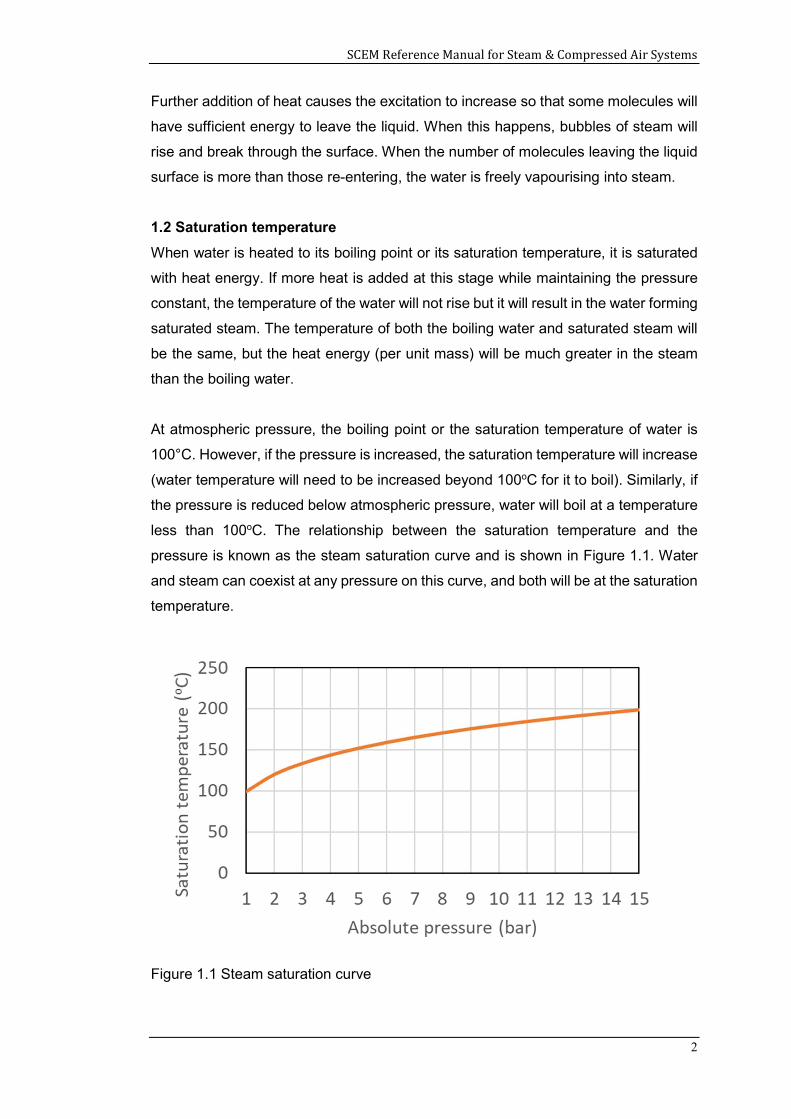
less than 100oC. The relationship between the saturation temperature and the
pressure is known as the steam saturation curve and is shown in Figure 1.1. Water
and steam can coexist at any pressure on this curve, and both will be at the saturation
temperature.
Figure 1.1 Steam saturation curve
SCEM Reference Manual for Steam & Compressed Air Systems
3
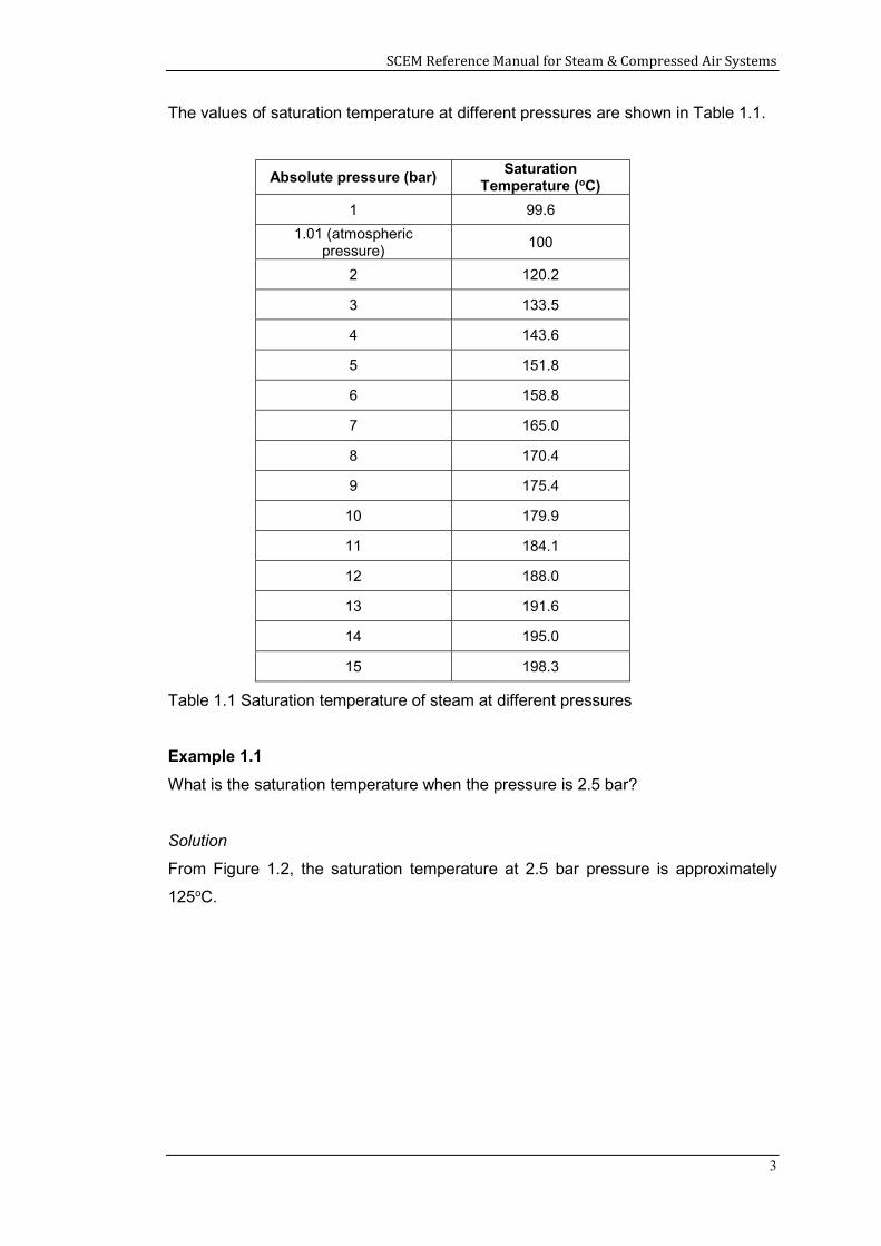
The values of saturation temperature at different pressures are shown in Table 1.1.
Absolute pressure (bar) Saturation
Temperature (oC)
1 99.6
1.01 (atmospheric pressure)
100
2 120.2
3 133.5
4 143.6
5 151.8
6 158.8
7 165.0
8 170.4
9 175.4
10 179.9
11 184.1
12 188.0
13 191.6
14 195.0
15 198.3
Table 1.1 Saturation temperature of steam at different pressures
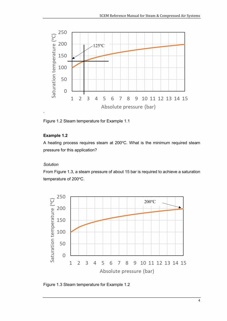
Example 1.1
What is the saturation temperature when the pressure is 2.5 bar?
Solution
From Figure 1.2, the saturation temperature at 2.5 bar pressure is approximately
125oC.
SCEM Reference Manual for Steam & Compressed Air Systems
4
`
Figure 1.2 Steam temperature for Example 1.1
Example 1.2
A heating process requires steam at 200oC. What is the minimum required steam
pressure for this application?
Solution
From Figure 1.3, a steam pressure of about 15 bar is required to achieve a saturation
temperature of 200oC.
Figure 1.3 Steam temperature for Example 1.2
125oC
200oC
SCEM Reference Manual for Steam & Compressed Air Systems
5
1.3 Sensible and latent heat
When water is heated by adding heat energy, the temperature of the water rises. Such
a process where adding heat leads to a corresponding increase in temperature is
called sensible heating and the heat added is called sensible heat.
Specific heat capacity is the amount of heat energy required to raise the temperature
per unit of mass of substance. In SI units, specific heat capacity is the amount of heat
in joules required to raise 1 kilogramme of a substance by 1 Kelvin. For water, the
specific heat capacity at atmospheric pressure is 4.19 kJ/kg.K.
For water, the amount of sensible heat required to increase the temperature of 1 kg
of water from 0oC to the boiling temperature is 419 kJ/kg (4.19 kJ/kg.K x 100 K). It is
also called the “liquid enthalpy” or enthalpy of water (explained later in this chapter).
When water is heated to its boiling point, further adding of heat does not increase the
temperature of water but only results in boiling of the water to form steam. Such
heating which does not result in an increase in the temperature of the substance that
is heated, but only results in a change in phase, is called latent heating. The heat
added during such a process is called latent heat.
Latent heat is energy absorbed during evaporation of a liquid (or released during
condensing of a vapour) that occurs without changing its temperature. The latent heat
in SI units is expressed in joules per unit mass in grams of the substance undergoing
a change of state. For water, the amount of heat required to evaporate 1 kg of water
at its boiling point is termed the “enthalpy of evaporation”. At atmospheric pressure,
the enthalpy of evaporation of water is 2257 kJ/kg.
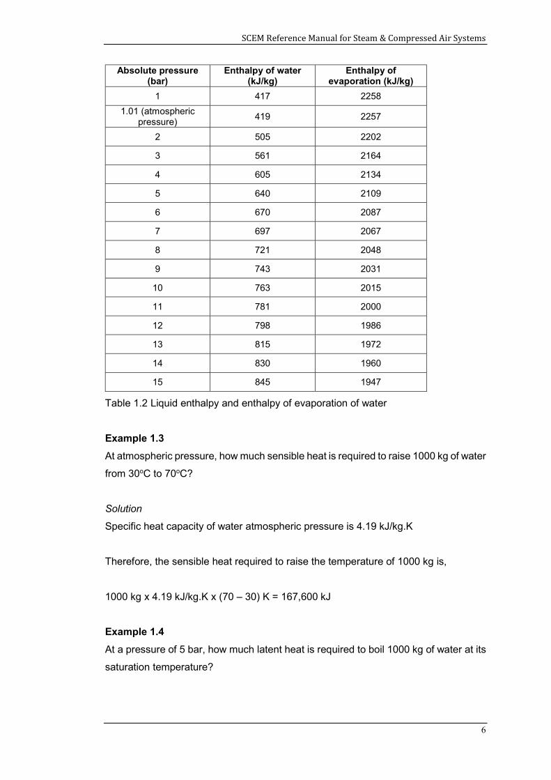
The liquid enthalpy and enthalpy of evaporation of water at different pressures is
shown in Table 1.2.
SCEM Reference Manual for Steam & Compressed Air Systems
6
Absolute pressure (bar)
Enthalpy of water (kJ/kg)
Enthalpy of evaporation (kJ/kg)
1 417 2258
1.01 (atmospheric pressure)
419 2257
2 505 2202
3 561 2164
4 605 2134
5 640 2109
6 670 2087
7 697 2067
8 721 2048
9 743 2031
10 763 2015
11 781 2000
12 798 1986
13 815 1972
14 830 1960
15 845 1947
Table 1.2 Liquid enthalpy and enthalpy of evaporation of water
Example 1.3
At atmospheric pressure, how much sensible heat is required to raise 1000 kg of water
from 30oC to 70oC?
Solution
Specific heat capacity of water atmospheric pressure is 4.19 kJ/kg.K
Therefore, the sensible heat required to raise the temperature of 1000 kg is,
1000 kg x 4.19 kJ/kg.K x (70 – 30) K = 167,600 kJ
Example 1.4
At a pressure of 5 bar, how much latent heat is required to boil 1000 kg of water at its
saturation temperature?
SCEM Reference Manual for Steam & Compressed Air Systems
7
Solution
Enthalpy of evaporation at 5 bar pressure (from Table 1.2) is 2109 kJ/kg
Therefore, the total heat required to boil 1000 kg of water at 5 bar is,
1000 kg x 2109 kJ/kg = 2,109,000 kJ
1.4 Steam quality
In an industrial type boiler, where heat is supplied only to the water, it is not possible
to produce dry steam. Due to turbulence and splashing in the boiler when bubbles of
steam are released from the water surface, the steam contains some water droplets.
Typically, steam produced by a shell-type boiler will contain about 5% water.
If the water content of the steam is say 4% by mass, then the steam is said to be 96%
dry.
Steam quality or dryness fraction of steam is defined as the ratio of the mass of actual
dry steam to the total mass of wet steam and can be expressed as:
x = mg / mg + mf (1.1)
x = mg / m
where,
x = steam quality (dryness fraction)
mg = mass of dry steam
mf = mass of water in mixture
m = mass of wet steam = mg + mf
Example 1.5
1000 kg of steam contains 50 kg of water. Compute the steam quality.
Solution
Steam quality, x = mg / mg + mf
= (1000 – 50) / 1000
= 0.95
SCEM Reference Manual for Steam & Compressed Air Systems
8
1.5 Superheated steam
When saturated steam is further heated so that the temperature of the steam exceeds
the saturation temperature at a particular pressure, the steam is superheated.
Superheating produces steam that has a higher temperature and lower density than
saturated steam at the same pressure.
For instance, steam at 5 bar is at a saturation temperature of 159oC. Now if this steam
is heated to 179oC, the steam will have a superheat of 20oC at 5 bar.
Superheating steam ensures that the steam is completely dry. Superheating is used
in steam driven equipment such as turbines to avoid a drop in performance due to the
presence of condensate and to prevent erosion and corrosion. However, superheated
steam is normally not used in pure heating applications where the latent heat of
condensation is the primary source of heating. When using superheated steam, first
it needs to be cooled to its saturation temperature before it can condense. As a result,
a larger heat transfer area will be required when using superheated steam compared
to saturated steam for the same application.
Example 1.6
Steam at 10 bar is at a temperature of 210oC. What is the degree of superheat of the
steam?
Solution
Saturation temperature of steam at 10 bar (from Table 1.1) is approximately 180oC.
Therefore, the degree of superheat is (210 – 180)oC = 30oC
1.6 Steam pressure vs volume
The specific volume is the total volume of steam divided by the total mass of steam
(volume per unit mass). It has units of cubic metre per kilogramme (m3/kg). The
density of steam is the reciprocal of its specific volume.
ρ = m/V = 1/ν
where,
ρ = density (kg/m3)
SCEM Reference Manual for Steam & Compressed Air Systems
9
m = mass of steam (kg)
V = volume of steam (m3)
v = specific volume (m3/kg)
As steam pressure increases, the density of steam also increases. Since the specific
volume is inversely related to the density, the specific volume decreases with
increased pressure.
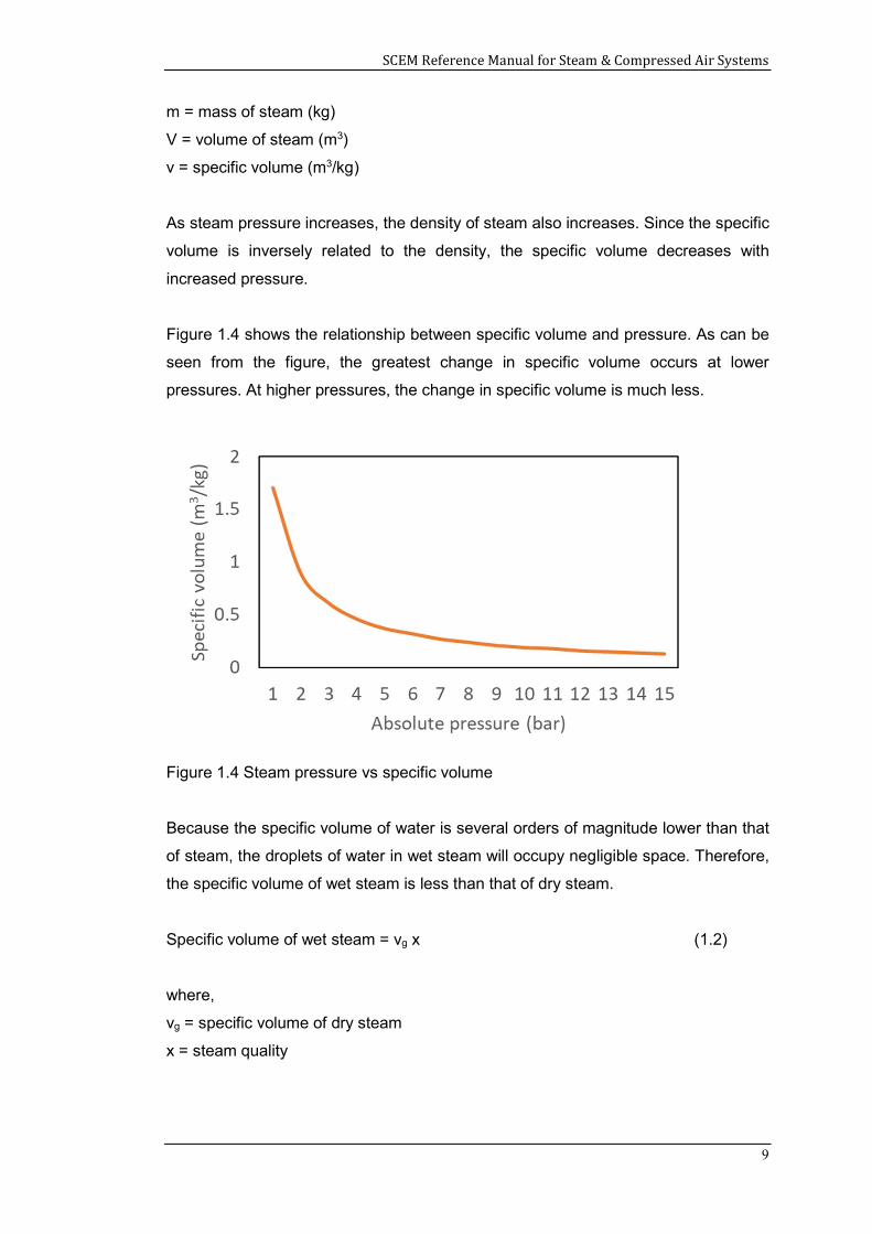
Figure 1.4 shows the relationship between specific volume and pressure. As can be
seen from the figure, the greatest change in specific volume occurs at lower
pressures. At higher pressures, the change in specific volume is much less.
Figure 1.4 Steam pressure vs specific volume
Because the specific volume of water is several orders of magnitude lower than that
of steam, the droplets of water in wet steam will occupy negligible space. Therefore,
the specific volume of wet steam is less than that of dry steam.
Specific volume of wet steam = vg x (1.2)
where,
vg = specific volume of dry steam
x = steam quality
SCEM Reference Manual for Steam & Compressed Air Systems
10
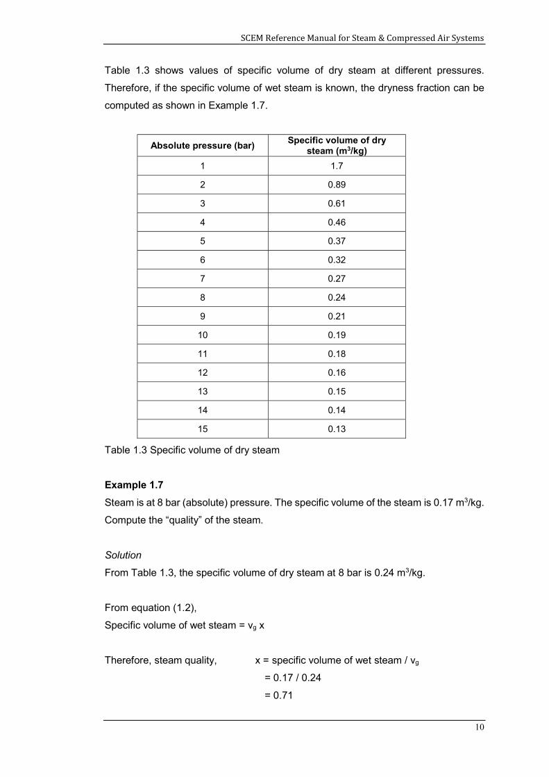
Table 1.3 shows values of specific volume of dry steam at different pressures.
Therefore, if the specific volume of wet steam is known, the dryness fraction can be
computed as shown in Example 1.7.
Absolute pressure (bar) Specific volume of dry
steam (m3/kg)
1 1.7
2 0.89
3 0.61
4 0.46
5 0.37
6 0.32
7 0.27
8 0.24
9 0.21
10 0.19
11 0.18
12 0.16
13 0.15
14 0.14
15 0.13
Table 1.3 Specific volume of dry steam
Example 1.7
Steam is at 8 bar (absolute) pressure. The specific volume of the steam is 0.17 m3/kg.
Compute the “quality” of the steam.
Solution
From Table 1.3, the specific volume of dry steam at 8 bar is 0.24 m3/kg.
From equation (1.2),
Specific volume of wet steam = vg x
Therefore, steam quality, x = specific volume of wet steam / vg
= 0.17 / 0.24
= 0.71
SCEM Reference Manual for Steam & Compressed Air Systems
11
1.7 Enthalpy
Specific enthalpy is a measure of the energy content of a single unit of mass of a
substance. The SI units of specific enthalpy are kJ/kg. For simplicity, specific enthalpy
will be referred to as enthalpy in this reference manual.
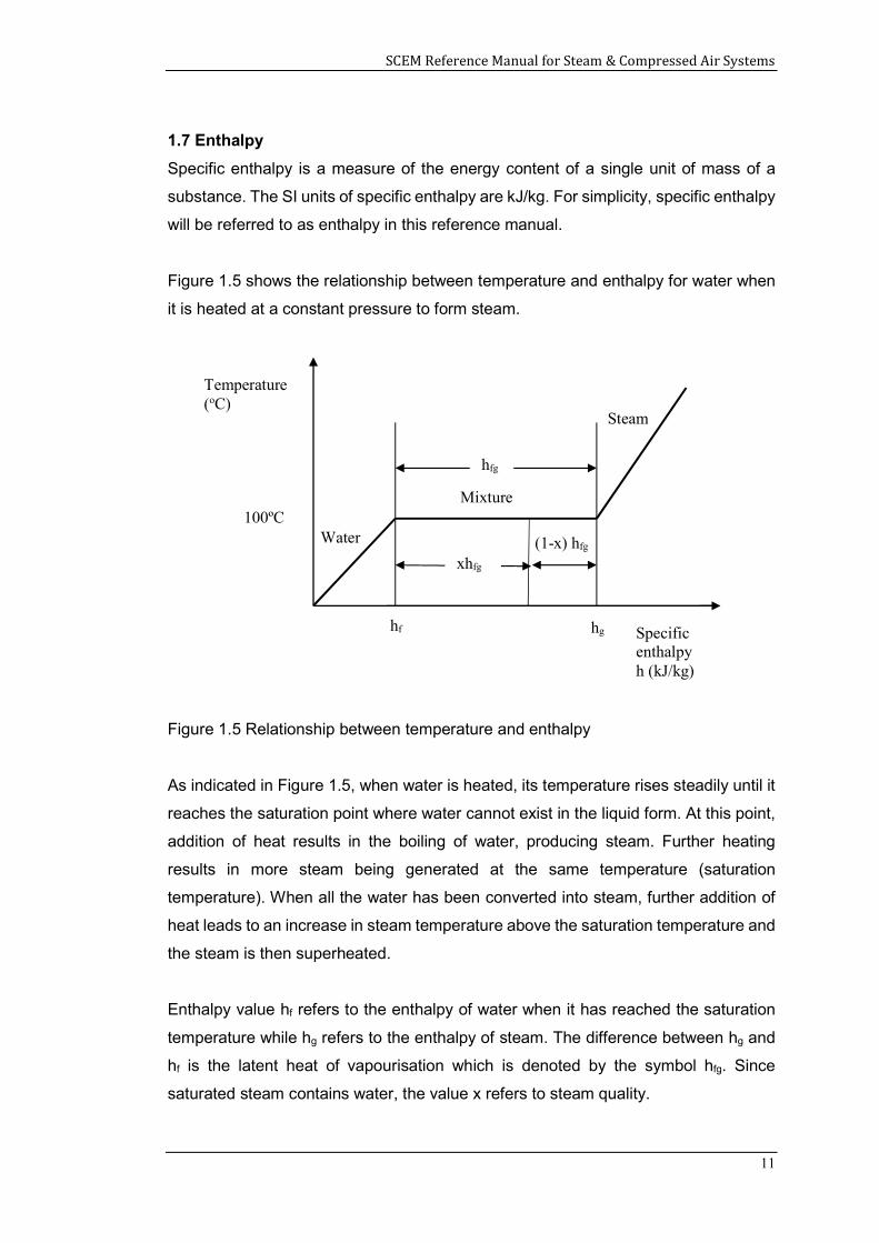
Figure 1.5 shows the relationship between temperature and enthalpy for water when
it is heated at a constant pressure to form steam.
Figure 1.5 Relationship between temperature and enthalpy
As indicated in Figure 1.5, when water is heated, its temperature rises steadily until it
reaches the saturation point where water cannot exist in the liquid form. At this point,
addition of heat results in the boiling of water, producing steam. Further heating
results in more steam being generated at the same temperature (saturation
temperature). When all the water has been converted into steam, further addition of
heat leads to an increase in steam temperature above the saturation temperature and
the steam is then superheated.
Enthalpy value hf refers to the enthalpy of water when it has reached the saturation
temperature while hg refers to the enthalpy of steam. The difference between hg and
hf is the latent heat of vapourisation which is denoted by the symbol hfg. Since
saturated steam contains water, the value x refers to steam quality.
Steam
Water
Mixture
hfg
xhfg
(1-x) hfg
100ºC
Specific enthalpy h (kJ/kg)
Temperature (oC)
hf hg
SCEM Reference Manual for Steam & Compressed Air Systems
12
Therefore,
Enthalpy of wet steam hg = hf + x hfg (1.3)
Enthalpy of dry steam hg = hf + hfg (1.4)
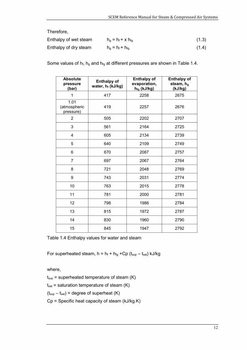
Some values of hf, hg and hfg at different pressures are shown in Table 1.4.
Absolute pressure
(bar)
Enthalpy of water, hf (kJ/kg)
Enthalpy of evaporation,
hfg (kJ/kg)
Enthalpy of steam, hg
(kJ/kg)
1 417 2258 2675
1.01 (atmospheric
pressure) 419 2257 2676
2 505 2202 2707
3 561 2164 2725
4 605 2134 2739
5 640 2109 2749
6 670 2087 2757
7 697 2067 2764
8 721 2048 2769
9 743 2031 2774
10 763 2015 2778
11 781 2000 2781
12 798 1986 2784
13 815 1972 2787
14 830 1960 2790
15 845 1947 2792
Table 1.4 Enthalpy values for water and steam
For superheated steam, h = hf + hfg +Cp (tsup – tsat) kJ/kg
where,
tsup = superheated temperature of steam (K)
tsat = saturation temperature of steam (K)
(tsup – tsat) = degree of superheat (K)
Cp = Specific heat capacity of steam (kJ/kg.K)
SCEM Reference Manual for Steam & Compressed Air Systems
13
Example 1.8
A boiler is supplied with feedwater at a temperature of 70ºC. The boiler produces
steam at a pressure of 8 bar (abs.) and a temperature of 190ºC.
Determine the quantity of heat supplied per kg of steam generation (excluding losses).
Take the specific heat capacity (Cp) of superheated steam to be 2.76 kJ/kg.K.
Solution
From Tables 1.1 and 1.4, the following enthalpy values at 8 bar pressure can be
obtained
hf = 721 kJ/kg
hfg = 2048 kJ/kg
tsat = 170.4ºC
Since steam is produced at 190oC, the steam is superheated.
The enthalpy of superheated steam,
hsup = hf + hfg + Cp (tsup – tsat)
= 721 + 2048 + 2.76 (190 – 170.4)
= 2823.1 kJ/kg
Enthalpy of feedwater at 70ºC is 293 kJ/kg (70oC x 4.19 kJ/kg)
Therefore, heat added = (2823.1 – 293) kJ/kg = 2530.1 kJ/kg
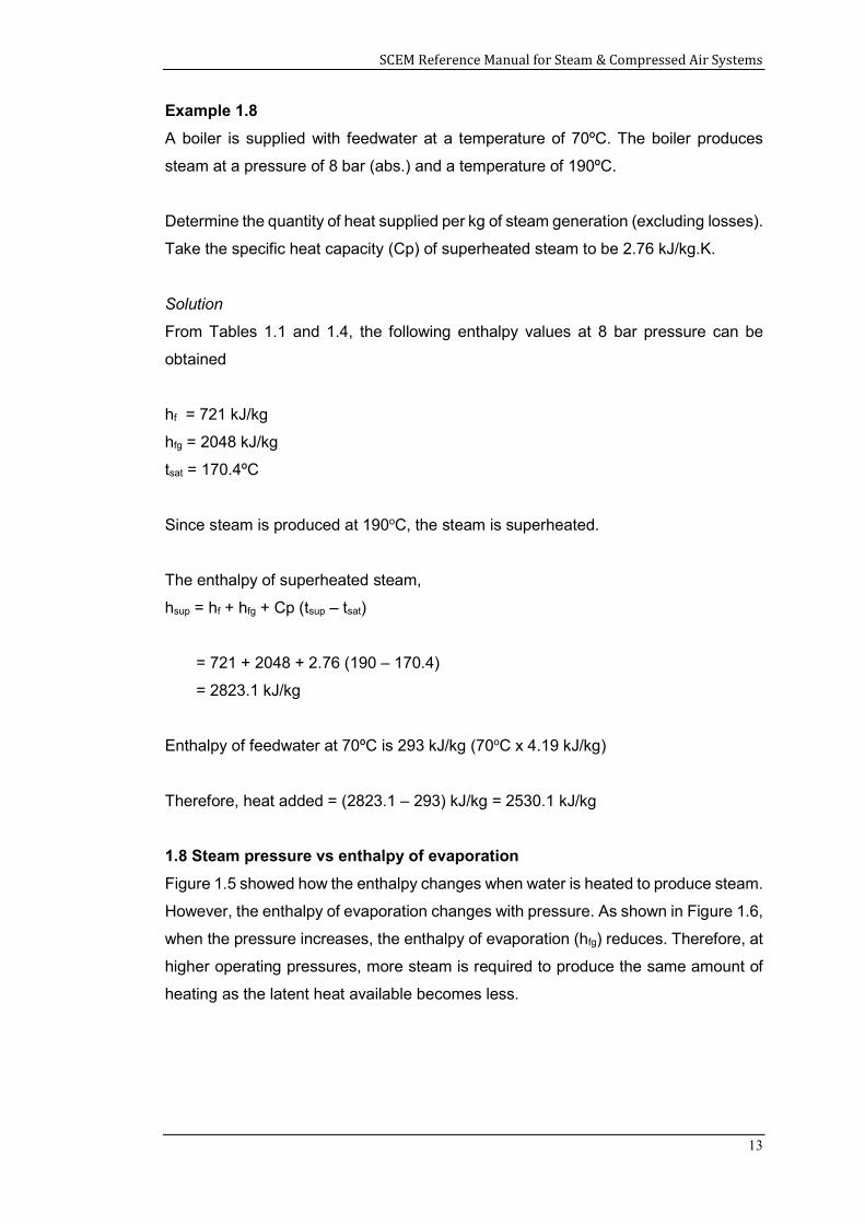
1.8 Steam pressure vs enthalpy of evaporation
Figure 1.5 showed how the enthalpy changes when water is heated to produce steam.
However, the enthalpy of evaporation changes with pressure. As shown in Figure 1.6,
when the pressure increases, the enthalpy of evaporation (hfg) reduces. Therefore, at
higher operating pressures, more steam is required to produce the same amount of
heating as the latent heat available becomes less.
SCEM Reference Manual for Steam & Compressed Air Systems
14
Figure 1.6 Enthalpy of evaporation at different pressures
1.9 Entropy
Entropy, is a thermodynamic measure of thermal energy per unit temperature of a
system that is unavailable for doing useful mechanical work. Since work is obtained
from orderly molecular motion, the amount of entropy is also a measure of the
molecular disorder, or randomness, of a system.
Specific entropy usually denoted by symbol “s”, is the entropy per unit mass of a
system. The units of entropy are kJ/K, and for specific entropy are kJ/kg.K.
From Table 1.4, at atmospheric pressure, 2,257 kJ (2,676 – 419) is required to convert
one kg of liquid water at 100oC to steam at 100oC. Since temperature remains
constant, the change in specific entropy is 2,257 / 373 = 6.059 kJ/kg.K. Hence, by
converting one kg of water to steam, the specific entropy has increased by 6.059
kJ/kg.K.
Values of specific entropy are usually provided in steam tables.
1.10 Condensate and flash steam
When high-pressure steam is condensed, the condensate will be at the saturation
temperature of the steam. Later, when the condensate is returned to the feedwater
tank, the pressure is reduced to atmospheric pressure. When this happens, the
enthalpy of the condensate has to reduce from the value at the higher pressure to the
value at atmospheric pressure.
SCEM Reference Manual for Steam & Compressed Air Systems
15
For example, condensate at 8 bar pressure (absolute) will have an enthalpy of 721
kJ/kg (from Table 1.4). However, when this condensate pressure is reduced to
atmospheric pressure, the enthalpy becomes 419 kJ/kg. The difference between the
enthalpy values of 302 kJ/kg (721 – 419) is released by evaporating part of the
condensate. The steam formed during such a pressure reduction is called flash
steam.
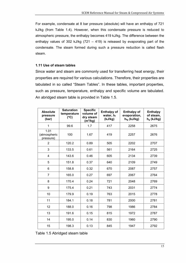
1.11 Use of steam tables
Since water and steam are commonly used for transferring heat energy, their
properties are required for various calculations. Therefore, their properties are
tabulated in so called “Steam Tables”. In these tables, important properties,
such as pressure, temperature, enthalpy and specific volume are tabulated.
An abridged steam table is provided in Table 1.5.
Absolute pressure
(bar)
Saturation temperature
(oC)
Specific volume of dry steam
(m3/kg)
Enthalpy of water, hf (kJ/kg)
Enthalpy of evaporation,
hfg (kJ/kg)
Enthalpy of steam, hg (kJ/kg)
1 99.6 1.7 417 2258 2675
1.01 (atmospheric
pressure) 100 1.67 419 2257 2676
2 120.2 0.89 505 2202 2707
3 133.5 0.61 561 2164 2725
4 143.6 0.46 605 2134 2739
5 151.8 0.37 640 2109 2749
6 158.8 0.32 670 2087 2757
7 165.0 0.27 697 2067 2764
8 170.4 0.24 721 2048 2769
9 175.4 0.21 743 2031 2774
10 179.9 0.19 763 2015 2778
11 184.1 0.18 781 2000 2781
12 188.0 0.16 798 1986 2784
13 191.6 0.15 815 1972 2787
14 195.0 0.14 830 1960 2790
15 198.3 0.13 845 1947 2792
Table 1.5 Abridged steam table
SCEM Reference Manual for Steam & Compressed Air Systems
16
Example 1.9
Determine the quantity of heat required to produce 1 kg of steam at pressure of 7 bar
(absolute) using water at a temperature of 90ºC, under the following conditions:
a) When the steam is wet and having a dryness fraction of 0.8
b) When the steam is dry saturated
c) When the steam is superheated at a constant pressure to 240oC (assume the
specific heat capacity of superheated steam to be 3.68 kJ/kg K)
Solution
From Table 1.5, at 7 bar
hf = 697 kJ/kg
hfg = 2067 kJ/kg
tsat = 165ºC
a) When the steam is wet
h = hf + x. hfg
h = 697 + 0.8 x 2067
h = 2350 kJ/kg
Enthalpy of water at 90ºC = 377 kJ/kg
Therefore, actual heat required
h = 2350 – 377
h = 1973 kJ/kg
b) When the steam is dry saturated
h = hf + hfg
h = 697 + 2067
h = 2764 kJ/kg
h = 2764 – 377 = 2387 kJ/kg
c) When the steam is superheated
h = hf + hfg + Cp (tsup – tsat)
h = 697 + 2067 + 3.68 (240 -165)
h = 3040 kJ/kg
h = 3040 – 377 = 2663 kJ/kg
SCEM Reference Manual for Steam & Compressed Air Systems
17
Often, the known parameter is between two values listed in the steam table. In such
instances, the required steam property can be derived by linear interpolation as
illustrated in Example 1.10.
Example 1.10
Determine the enthalpy of water at 6.3 bar (absolute pressure).
Solution
From Table 1.5, at 6 bar, hf = 670 kJ/kg and at 7 bar, hf = 697 kJ/kg
Therefore, using linear interpolation,
(hf @ 6.3 bar − hf @ 6 bar)
(hf @ 7 bar − hf @ 6 bar)=
(6.3 − 6)
(7 − 6)
From the above relationship, [email protected] bar = 678.1 kJ/kg
Summary
This chapter provided an introduction to some of the basic properties of steam, which
are useful in understanding how boilers and steam systems operate. The relationship
between saturation temperature and pressure, various properties of steam and the
use of steam tables were illustrated using worked examples.
References
1. Jayamaha, Lal, Energy-Efficient Industrial Systems, Evaluation and
Implementation, McGraw-Hill, New York, 2016.
2. Rogers, G.F.C. and Mayhew, Y.R., Thermodynamic and Transport Properties of
Fluids, Oxford, 2014.
3. The Steam and Condensate Loop, Spirax Sarco Limited, England 2008.
SCEM Reference Manual for Steam & Compressed Air Systems
18
2.0 BOILERS
Steam is vapour of water and is used in many industrial applications as the working
fluid for heating and as the carrier of energy. Steam is widely used in industry because
usually there is easy access to water required for steam generation, the ability to
convert water to steam using boilers, the high heat carrying capacity of steam and the
simplicity in transferring and distributing heat energy through a piping network.
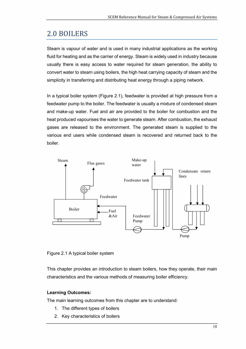
In a typical boiler system (Figure 2.1), feedwater is provided at high pressure from a
feedwater pump to the boiler. The feedwater is usually a mixture of condensed steam
and make-up water. Fuel and air are provided to the boiler for combustion and the
heat produced vapourises the water to generate steam. After combustion, the exhaust
gases are released to the environment. The generated steam is supplied to the
various end users while condensed steam is recovered and returned back to the
boiler.
Figure 2.1 A typical boiler system
This chapter provides an introduction to steam boilers, how they operate, their main
characteristics and the various methods of measuring boiler efficiency.
Learning Outcomes:
The main learning outcomes from this chapter are to understand:
1. The different types of boilers
2. Key characteristics of boilers
Feedwater tank
Feedwater Pump
Flue gases Steam
Pump
Condensate return lines
Feedwater
Fuel &Air
Make-up water
Boiler
SCEM Reference Manual for Steam & Compressed Air Systems
19
3. Parameters that affect boiler performance
4. How to assess boiler efficiency
2.1 Introduction to boilers
Boilers are used to produce steam by adding heat to water. A boiler generally consists
of a combustion chamber that can burn fuel in the form of solid, liquid or gas to
produce hot combustion gases, and a tubular heat exchanger, to transfer heat from
the combustion gases to the water. They are pressure vessels into which liquid water
is pumped at the operating pressure. After the heat energy from the fuel source has
vapourised the liquid water, the resulting steam is directly provided for use or is
passed through a superheater.
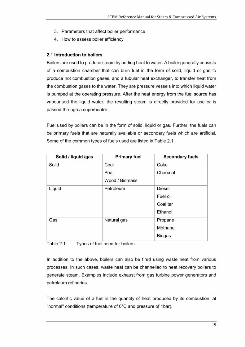
Fuel used by boilers can be in the form of solid, liquid or gas. Further, the fuels can
be primary fuels that are naturally available or secondary fuels which are artificial.
Some of the common types of fuels used are listed in Table 2.1.
Solid / liquid /gas Primary fuel Secondary fuels
Solid Coal
Peat
Wood / Biomass
Coke
Charcoal
Liquid Petroleum Diesel
Fuel oil
Coal tar
Ethanol
Gas Natural gas Propane
Methane
Biogas
Table 2.1 Types of fuel used for boilers
In addition to the above, boilers can also be fired using waste heat from various
processes. In such cases, waste heat can be channelled to heat recovery boilers to
generate steam. Examples include exhaust from gas turbine power generators and
petroleum refineries.
The calorific value of a fuel is the quantity of heat produced by its combustion, at
"normal" conditions (temperature of 0°C and pressure of 1bar).
SCEM Reference Manual for Steam & Compressed Air Systems
20
Gross Calorific Value assumes that the water produced during combustion is entirely
condensed and the heat contained in the water vapour is recovered. Net Calorific
Value assumes that the water vapour and the heat in the water vapour is not
recovered. Therefore, the gross calorific value is higher than the net calorific value.
Gross calorific value of common fuels used in boilers is provided in Table 2.2.
Fuel Calorific value (MJ/kg)
Natural gas 55
No. 2 oil (light oil) 46
No. 4 oil (heavy oil) 45
No. 6 oil (heavy oil) 44
Coal 32
Wood (dry) 16
Table 2.2 Calorific value of fuels
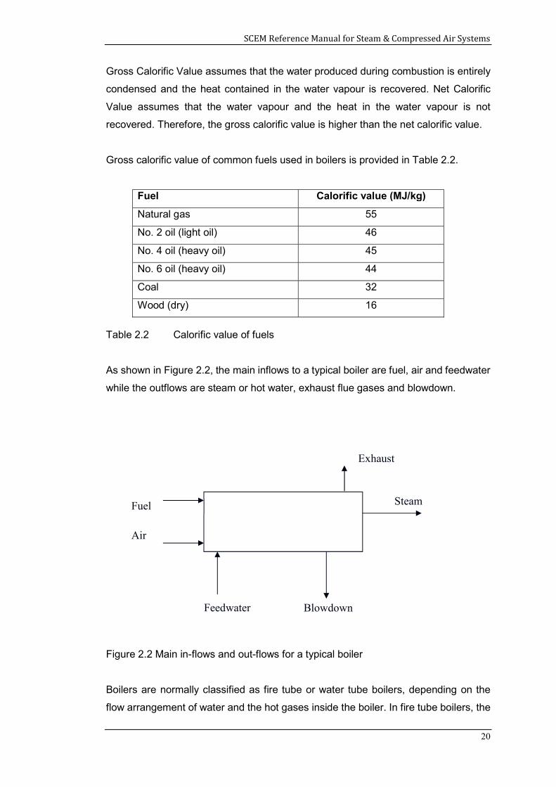
As shown in Figure 2.2, the main inflows to a typical boiler are fuel, air and feedwater
while the outflows are steam or hot water, exhaust flue gases and blowdown.
Figure 2.2 Main in-flows and out-flows for a typical boiler
Boilers are normally classified as fire tube or water tube boilers, depending on the
flow arrangement of water and the hot gases inside the boiler. In fire tube boilers, the
Fuel
Exhaust
Steam
Feedwater
Air
Blowdown
SCEM Reference Manual for Steam & Compressed Air Systems
21
hot gases pass through the boiler tubes that are immersed in the water being heated,
while in water tube boilers, water is contained in the tubes that are surrounded by the
hot combustion gases.
Fire tube boilers are used for general applications. However, since water is contained
in the circular boiler shell in fire tube boilers, increase in pressure requires increase in
thickness of the boiler shell, which becomes impractical at high pressures. Therefore,
water tube boilers, where water is circulated inside tubes (the relatively smaller
diameter of the tubes compared to the shell diameter in fire tube boilers require less
wall thickness), are used for high pressure applications. Fire tube boilers are usually
used for producing steam for process heating and other low pressure applications, up
to about 15 bar. For high pressure applications like in power plants where steam
pressure could be in the range of 150 bar, water tube boilers are used.
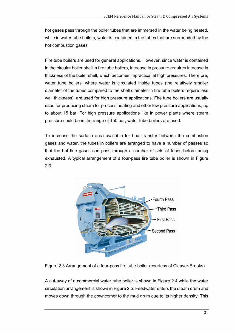
To increase the surface area available for heat transfer between the combustion
gases and water, the tubes in boilers are arranged to have a number of passes so
that the hot flue gases can pass through a number of sets of tubes before being
exhausted. A typical arrangement of a four-pass fire tube boiler is shown in Figure
2.3.
Figure 2.3 Arrangement of a four-pass fire tube boiler (courtesy of Cleaver-Brooks)
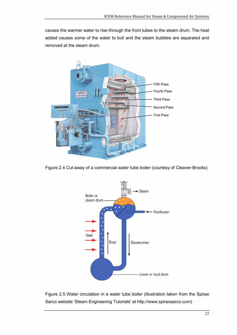
A cut-away of a commercial water tube boiler is shown in Figure 2.4 while the water
circulation arrangement is shown in Figure 2.5. Feedwater enters the steam drum and
moves down through the downcomer to the mud drum due to its higher density. This
SCEM Reference Manual for Steam & Compressed Air Systems
22
causes the warmer water to rise through the front tubes to the steam drum. The heat
added causes some of the water to boil and the steam bubbles are separated and
removed at the steam drum.
Figure 2.4 Cut-away of a commercial water tube boiler (courtesy of Cleaver-Brooks)
Figure 2.5 Water circulation in a water tube boiler (illustration taken from the Spirax
Sarco website 'Steam Engineering Tutorials' at http://www.spiraxsarco.com)
SCEM Reference Manual for Steam & Compressed Air Systems
23
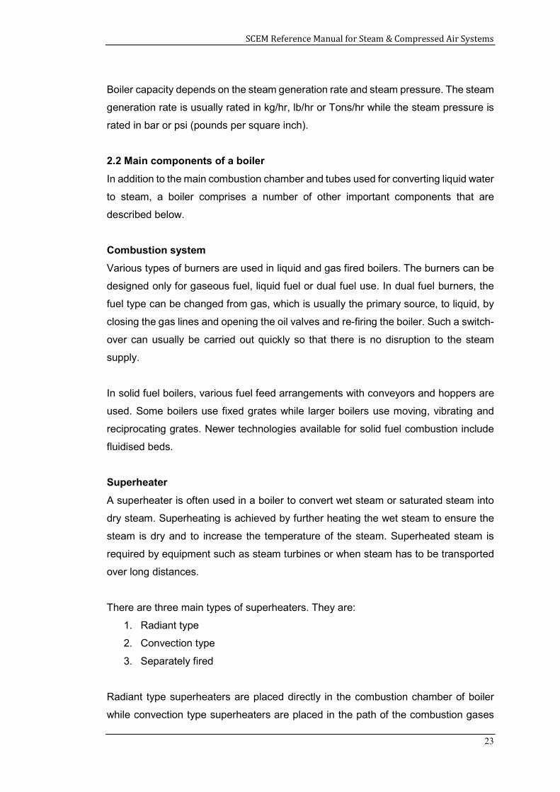
Boiler capacity depends on the steam generation rate and steam pressure. The steam
generation rate is usually rated in kg/hr, lb/hr or Tons/hr while the steam pressure is
rated in bar or psi (pounds per square inch).
2.2 Main components of a boiler
In addition to the main combustion chamber and tubes used for converting liquid water
to steam, a boiler comprises a number of other important components that are
described below.
Combustion system
Various types of burners are used in liquid and gas fired boilers. The burners can be
designed only for gaseous fuel, liquid fuel or dual fuel use. In dual fuel burners, the
fuel type can be changed from gas, which is usually the primary source, to liquid, by
closing the gas lines and opening the oil valves and re-firing the boiler. Such a switch-
over can usually be carried out quickly so that there is no disruption to the steam
supply.
In solid fuel boilers, various fuel feed arrangements with conveyors and hoppers are
used. Some boilers use fixed grates while larger boilers use moving, vibrating and
reciprocating grates. Newer technologies available for solid fuel combustion include
fluidised beds.
Superheater
A superheater is often used in a boiler to convert wet steam or saturated steam into
dry steam. Superheating is achieved by further heating the wet steam to ensure the
steam is dry and to increase the temperature of the steam. Superheated steam is
required by equipment such as steam turbines or when steam has to be transported
over long distances.
There are three main types of superheaters. They are:
1. Radiant type
2. Convection type
3. Separately fired
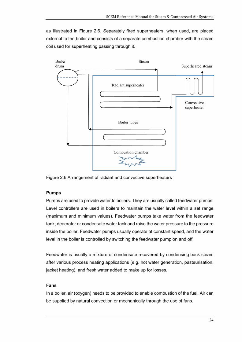
Radiant type superheaters are placed directly in the combustion chamber of boiler
while convection type superheaters are placed in the path of the combustion gases
SCEM Reference Manual for Steam & Compressed Air Systems
24
as illustrated in Figure 2.6. Separately fired superheaters, when used, are placed
external to the boiler and consists of a separate combustion chamber with the steam
coil used for superheating passing through it.
Figure 2.6 Arrangement of radiant and convective superheaters
Pumps
Pumps are used to provide water to boilers. They are usually called feedwater pumps.
Level controllers are used in boilers to maintain the water level within a set range
(maximum and minimum values). Feedwater pumps take water from the feedwater
tank, deaerator or condensate water tank and raise the water pressure to the pressure
inside the boiler. Feedwater pumps usually operate at constant speed, and the water
level in the boiler is controlled by switching the feedwater pump on and off.
Feedwater is usually a mixture of condensate recovered by condensing back steam
after various process heating applications (e.g. hot water generation, pasteurisation,
jacket heating), and fresh water added to make up for losses.
Fans
In a boiler, air (oxygen) needs to be provided to enable combustion of the fuel. Air can
be supplied by natural convection or mechanically through the use of fans.
Boiler drum
Radiant superheater
Boiler tubes
Convective superheater
Steam Superheated steam
Combustion chamber
SCEM Reference Manual for Steam & Compressed Air Systems
25
In boilers relying on natural convection, when the hot flue gases rise through the
chimney due to their lower density and are exhausted, surrounding air that has a
higher density enters the combustion chamber. This creates a natural draught and
provides the air required for combustion.
Since the natural draft created depends on factors such as the temperature of the
outside air, temperature of the flue gases and the height of the chimney, it is difficult
to control combustion in natural draught boilers.
Modern boilers rely on mechanical draught to provide air for combustion. In such
boilers, air for combustion is provided using a fan. There are three main arrangements
of mechanical draught, which are:
1. Induced draught where a fan is installed at the exit of the boiler to pull out the
exhaust gases;
2. Forced draught where a fan is installed at the air intake to push in the air for
combustion; and
3. Balanced draught where both induced draught and forced draught fans are
used.
Balanced draught arrangements are common in large boilers where the combustion
gases have to travel a long distance and over a number of heat exchanger passes
within the boiler, resulting in high pressure losses.
The airflow in mechanical draught systems is controlled using damper arrangements
and by adjusting the fan speed.
Deaerator
A deaerator is a device used external to the boiler to remove oxygen and other
dissolved gases from the feedwater. If a deaerator is not used, oxygen and other
dissolved gases can cause corrosion or form oxides on the boiler surfaces in contact
with water, leading to damage and component failure.
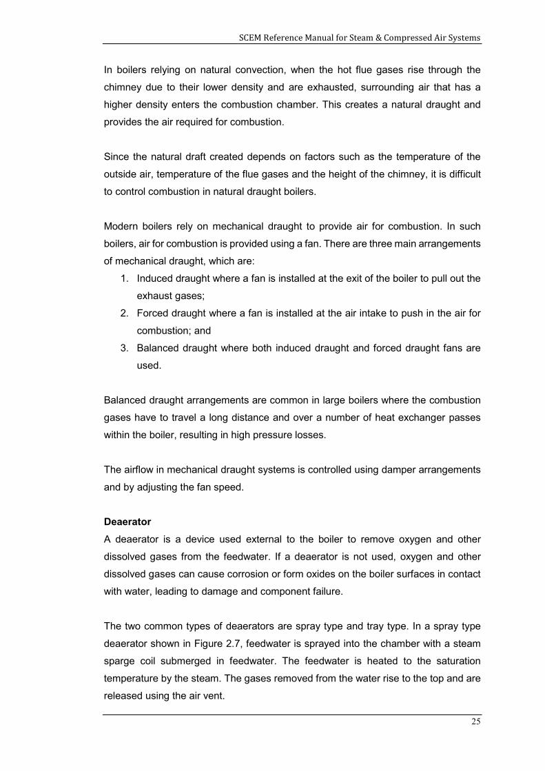
The two common types of deaerators are spray type and tray type. In a spray type
deaerator shown in Figure 2.7, feedwater is sprayed into the chamber with a steam
sparge coil submerged in feedwater. The feedwater is heated to the saturation
temperature by the steam. The gases removed from the water rise to the top and are
released using the air vent.
SCEM Reference Manual for Steam & Compressed Air Systems
26
Figure 2.7 Arrangement of a spray type deaerator
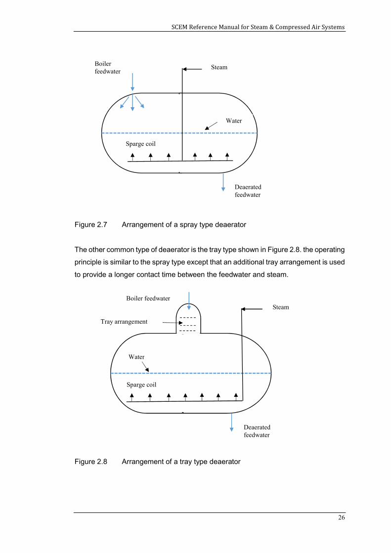
The other common type of deaerator is the tray type shown in Figure 2.8. the operating
principle is similar to the spray type except that an additional tray arrangement is used
to provide a longer contact time between the feedwater and steam.
Figure 2.8 Arrangement of a tray type deaerator
Boiler feedwater Steam
Deaerated feedwater
Water
Tray arrangement
Sparge coil
Boiler feedwater
Deaerated feedwater
Steam
Sparge coil
Water
SCEM Reference Manual for Steam & Compressed Air Systems
27
2.3 Boiler operation
Some of the key operating requirements of boilers are listed below.
Air to fuel ratio
Air is required for combustion of the fuel. If the quantity of air that is supplied is greater
than what is required for complete combustion of fuel, then the excess air provided
will remove part of the heat from the combustion chamber which otherwise would
have contributed to producing steam.
If insufficient air is provided, then some of the fuel will be unused in the combustion
process. This results in energy wastage as part of the fuel is discharged without being
used. In addition, it can lead to unsafe operation as the unburnt fuel can ignite while
passing through the boiler. Unburnt fuel also leads to soot formation on heat transfer
surfaces leading to poor heat transfer.
Therefore, the air to fuel ratio has to be optimum for the efficient and safe operation
of a boiler. A suitable control system has to be used to ensure that the air to fuel ratio
is maintained to provide sufficient air for combustion while not being significantly
excessive, to prevent unnecessary heat loss from the boiler. Recommended excess
air values for common fuels are provided in Table 2.4.
Blowdown
Makeup water used for boilers contains various impurities. As water is converted to
steam, the concentration of the impurities that remain in the boiler increases. If this
concentration is allowed to increase, it will lead to accelerated corrosion, scaling, and
fouling of the heat transfer surfaces of the boiler. Therefore, it is necessary to remove
part of the concentrated water from the boiler and replace it with fresh water.
Boiler blowdown is carried out as part of the water treatment process and involves
removal of sludge and solids from the boiler to maintain the concentration of solids
within an acceptable range.
The blowdown rate is normally determined based on the total dissolved solids (TDS)
in the boiler water. The acceptable TDS value to be maintained depends on many
factors like boiler design, boiler capacity, water level and load characteristics. For
typical two-pass and three-pass fire tube boilers, the allowable TDS level is 3000 to
SCEM Reference Manual for Steam & Compressed Air Systems
28
3500 ppm (parts per million) while for water tube boilers, the allowable level is about
1500 ppm.
Blowdown can be manual where a fixed volume of water is drained from the boiler
periodically, or continuous where a small amount of water is removed continuously in
order to maintain the quality of water within acceptable limits.
Water softening
Make-up water used for boilers usually contains minerals such as calcium and
magnesium which can cause scaling and damage to the boiler. Scale deposits form
a layer on the water side of the boiler heat transfer surfaces and act as a resistance
to heat transfer which reduces boiler efficiency.
A water softening plant removes positively charged ions like magnesium, calcium and
iron using negatively charged resin beads. As the water goes through the resin tank,
the minerals are chemically attracted to the negative charge of the resin beads. This
process removes the majority of “hard” minerals from the water, creating so-called
“soft” water.
2.4 Boiler efficiency
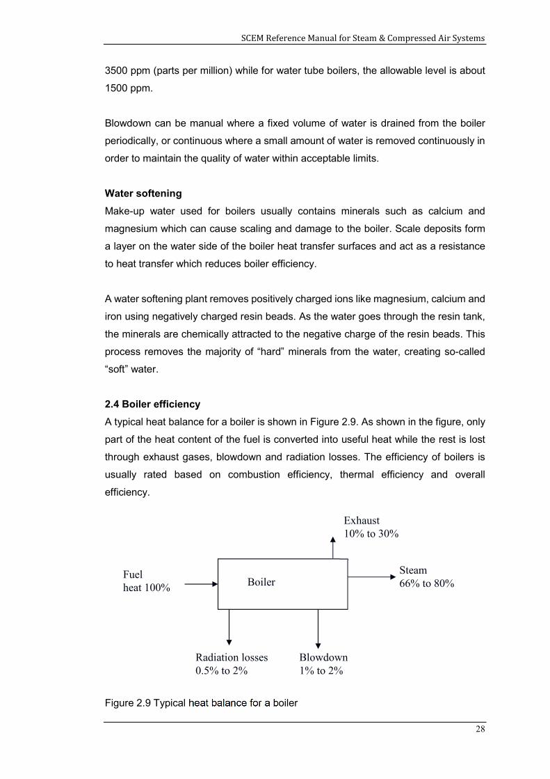
A typical heat balance for a boiler is shown in Figure 2.9. As shown in the figure, only
part of the heat content of the fuel is converted into useful heat while the rest is lost
through exhaust gases, blowdown and radiation losses. The efficiency of boilers is
usually rated based on combustion efficiency, thermal efficiency and overall
efficiency.
Figure 2.9 Typical heat balance for a boiler
Fuel heat 100%
Exhaust 10% to 30%
Steam 66% to 80%
Radiation losses 0.5% to 2%
Blowdown 1% to 2%
Boiler
SCEM Reference Manual for Steam & Compressed Air Systems
29
Combustion efficiency
One of the most common measures of boiler efficiency is combustion efficiency, which
indicates the ability of the combustion process to burn the fuel completely.
A typical combustion process in boilers involves the burning of fuels containing carbon
(oil, gas, coal) with oxygen to generate heat. Oxygen required for combustion is
normally taken from air supplied to the burner of the boiler. The amount of air needed
for combustion depends on the type of fuel used. To ensure complete combustion of
fuel, more air than required (excess air) for combustion is provided to ensure that the
fuel is completely burnt. Since excess air leads to lower boiler efficiency (due to
removal of heat by the excess air as it passes through the boiler), the objective is to
ensure that the minimum amount of excess air is provided.
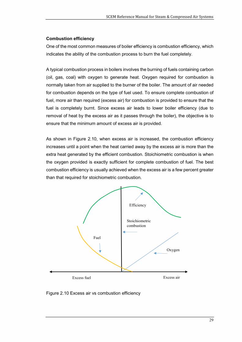
As shown in Figure 2.10, when excess air is increased, the combustion efficiency
increases until a point when the heat carried away by the excess air is more than the
extra heat generated by the efficient combustion. Stoichiometric combustion is when
the oxygen provided is exactly sufficient for complete combustion of fuel. The best
combustion efficiency is usually achieved when the excess air is a few percent greater
than that required for stoichiometric combustion.
Figure 2.10 Excess air vs combustion efficiency
Efficiency
Oxygen
Fuel
Excess air Excess fuel
Stoichiometric combustion
SCEM Reference Manual for Steam & Compressed Air Systems
30
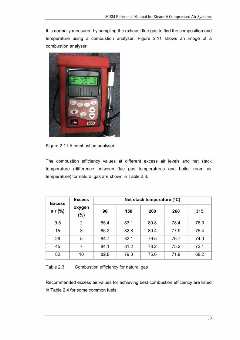
It is normally measured by sampling the exhaust flue gas to find the composition and
temperature using a combustion analyser. Figure 2.11 shows an image of a
combustion analyser.
Figure 2.11 A combustion analyser
The combustion efficiency values at different excess air levels and net stack
temperature (difference between flue gas temperatures and boiler room air
temperature) for natural gas are shown in Table 2.3.
Excess
air (%)
Excess
oxygen
(%)
Net stack temperature (oC)
90 150 200 260 315
9.5 2 85.4 83.1 80.8 78.4 76.0
15 3 85.2 82.8 80.4 77.9 75.4
28 5 84.7 82.1 79.5 76.7 74.0
45 7 84.1 81.2 78.2 75.2 72.1
82 10 82.8 79.3 75.6 71.9 68.2
Table 2.3 Combustion efficiency for natural gas
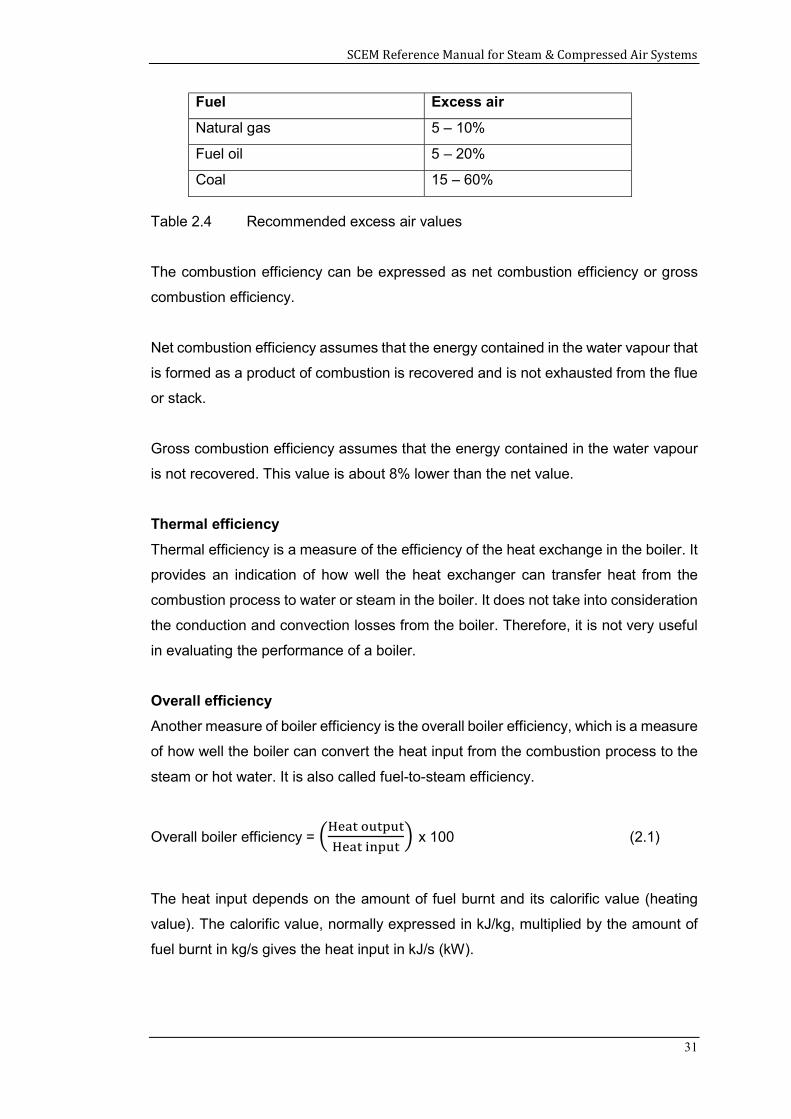
Recommended excess air values for achieving best combustion efficiency are listed
in Table 2.4 for some common fuels.
SCEM Reference Manual for Steam & Compressed Air Systems
31
Fuel Excess air
Natural gas 5 – 10%
Fuel oil 5 – 20%
Coal 15 – 60%
Table 2.4 Recommended excess air values
The combustion efficiency can be expressed as net combustion efficiency or gross
combustion efficiency.
Net combustion efficiency assumes that the energy contained in the water vapour that
is formed as a product of combustion is recovered and is not exhausted from the flue
or stack.
Gross combustion efficiency assumes that the energy contained in the water vapour
is not recovered. This value is about 8% lower than the net value.
Thermal efficiency
Thermal efficiency is a measure of the efficiency of the heat exchange in the boiler. It
provides an indication of how well the heat exchanger can transfer heat from the
combustion process to water or steam in the boiler. It does not take into consideration
the conduction and convection losses from the boiler. Therefore, it is not very useful
in evaluating the performance of a boiler.
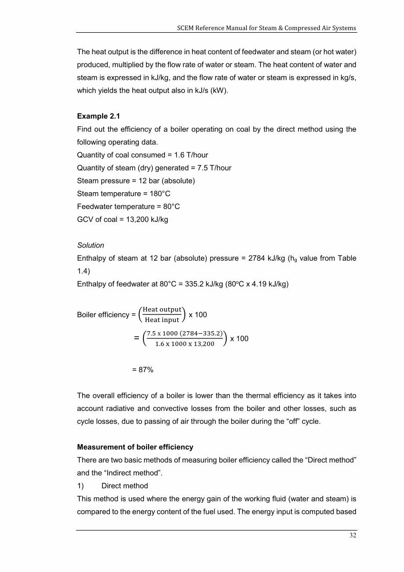
Overall efficiency
Another measure of boiler efficiency is the overall boiler efficiency, which is a measure
of how well the boiler can convert the heat input from the combustion process to the
steam or hot water. It is also called fuel-to-steam efficiency.
Overall boiler efficiency =
x 100 (2.1)
The heat input depends on the amount of fuel burnt and its calorific value (heating
value). The calorific value, normally expressed in kJ/kg, multiplied by the amount of
fuel burnt in kg/s gives the heat input in kJ/s (kW).
SCEM Reference Manual for Steam & Compressed Air Systems
32
The heat output is the difference in heat content of feedwater and steam (or hot water)
produced, multiplied by the flow rate of water or steam. The heat content of water and
steam is expressed in kJ/kg, and the flow rate of water or steam is expressed in kg/s,
which yields the heat output also in kJ/s (kW).
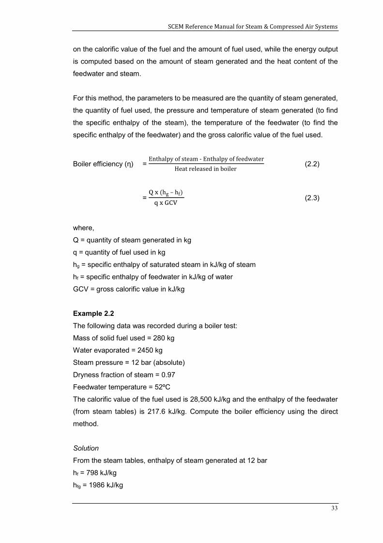
Example 2.1
Find out the efficiency of a boiler operating on coal by the direct method using the
following operating data.
Quantity of coal consumed = 1.6 T/hour
Quantity of steam (dry) generated = 7.5 T/hour
Steam pressure = 12 bar (absolute)
Steam temperature = 180°C
Feedwater temperature = 80°C
GCV of coal = 13,200 kJ/kg
Solution
Enthalpy of steam at 12 bar (absolute) pressure = 2784 kJ/kg (hg value from Table
1.4)
Enthalpy of feedwater at 80°C = 335.2 kJ/kg (80oC x 4.19 kJ/kg)
Boiler efficiency =
x 100
= . x ( . )
. , x 100
= 87%
The overall efficiency of a boiler is lower than the thermal efficiency as it takes into
account radiative and convective losses from the boiler and other losses, such as
cycle losses, due to passing of air through the boiler during the “off” cycle.
Measurement of boiler efficiency
There are two basic methods of measuring boiler efficiency called the “Direct method”
and the “Indirect method”.
1) Direct method
This method is used where the energy gain of the working fluid (water and steam) is
compared to the energy content of the fuel used. The energy input is computed based
SCEM Reference Manual for Steam & Compressed Air Systems
33
on the calorific value of the fuel and the amount of fuel used, while the energy output
is computed based on the amount of steam generated and the heat content of the
feedwater and steam.
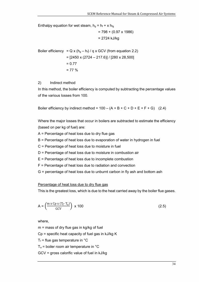
For this method, the parameters to be measured are the quantity of steam generated,
the quantity of fuel used, the pressure and temperature of steam generated (to find
the specific enthalpy of the steam), the temperature of the feedwater (to find the
specific enthalpy of the feedwater) and the gross calorific value of the fuel used.
Boiler efficiency (η) = Enthalpy of steam - Enthalpy of feedwater
Heat released in boiler (2.2)
= (hg – hf)
(2.3)
where,
Q = quantity of steam generated in kg
q = quantity of fuel used in kg
hg = specific enthalpy of saturated steam in kJ/kg of steam
hf = specific enthalpy of feedwater in kJ/kg of water
GCV = gross calorific value in kJ/kg
Example 2.2
The following data was recorded during a boiler test:
Mass of solid fuel used = 280 kg
Water evaporated = 2450 kg
Steam pressure = 12 bar (absolute)
Dryness fraction of steam = 0.97
Feedwater temperature = 52ºC
The calorific value of the fuel used is 28,500 kJ/kg and the enthalpy of the feedwater
(from steam tables) is 217.6 kJ/kg. Compute the boiler efficiency using the direct
method.
Solution
From the steam tables, enthalpy of steam generated at 12 bar
hf = 798 kJ/kg
hfg = 1986 kJ/kg
SCEM Reference Manual for Steam & Compressed Air Systems
34
Enthalpy equation for wet steam, hg = hf + x hfg
= 798 + (0.97 x 1986)
= 2724 kJ/kg
Boiler efficiency = Q x (hg – hf) / q x GCV (from equation 2.2)
= [2450 x (2724 – 217.6)] / [280 x 28,500]
= 0.77
= 77 %
2) Indirect method
In this method, the boiler efficiency is computed by subtracting the percentage values
of the various losses from 100.
Boiler efficiency by indirect method = 100 – (A + B + C + D + E + F + G) (2.4)
Where the major losses that occur in boilers are subtracted to estimate the efficiency
(based on per kg of fuel) are:
A = Percentage of heat loss due to dry flue gas
B = Percentage of heat loss due to evaporation of water in hydrogen in fuel
C = Percentage of heat loss due to moisture in fuel
D = Percentage of heat loss due to moisture in combustion air
E = Percentage of heat loss due to incomplete combustion
F = Percentage of heat loss due to radiation and convection
G = percentage of heat loss due to unburnt carbon in fly ash and bottom ash
Percentage of heat loss due to dry flue gas
This is the greatest loss, which is due to the heat carried away by the boiler flue gases.
A = m x Cp x (Tf- Ta)
GCV x 100 (2.5)
where,
m = mass of dry flue gas in kg/kg of fuel
Cp = specific heat capacity of fuel gas in kJ/kg K
Tf = flue gas temperature in °C
Ta = boiler room air temperature in °C
GCV = gross calorific value of fuel in kJ/kg
SCEM Reference Manual for Steam & Compressed Air Systems
35
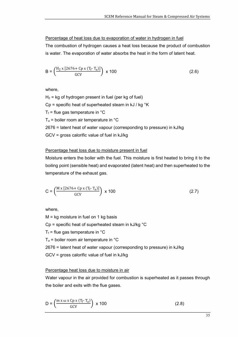
Percentage of heat loss due to evaporation of water in hydrogen in fuel
The combustion of hydrogen causes a heat loss because the product of combustion
is water. The evaporation of water absorbs the heat in the form of latent heat.
B = H2 x [2676+ Cp x (Tf- Ta)]
GCV x 100 (2.6)
where,
H2 = kg of hydrogen present in fuel (per kg of fuel)
Cp = specific heat of superheated steam in kJ / kg °K
Tf = flue gas temperature in °C
Ta = boiler room air temperature in °C
2676 = latent heat of water vapour (corresponding to pressure) in kJ/kg
GCV = gross calorific value of fuel in kJ/kg
Percentage heat loss due to moisture present in fuel
Moisture enters the boiler with the fuel. This moisture is first heated to bring it to the
boiling point (sensible heat) and evaporated (latent heat) and then superheated to the
temperature of the exhaust gas.
C = M x [2676+ Cp x (Tf- Ta)]
GCV x 100 (2.7)
where,
M = kg moisture in fuel on 1 kg basis
Cp = specific heat of superheated steam in kJ/kg °C
Tf = flue gas temperature in °C
Ta = boiler room air temperature in °C
2676 = latent heat of water vapour (corresponding to pressure) in kJ/kg
GCV = gross calorific value of fuel in kJ/kg
Percentage heat loss due to moisture in air
Water vapour in the air provided for combustion is superheated as it passes through
the boiler and exits with the flue gases.
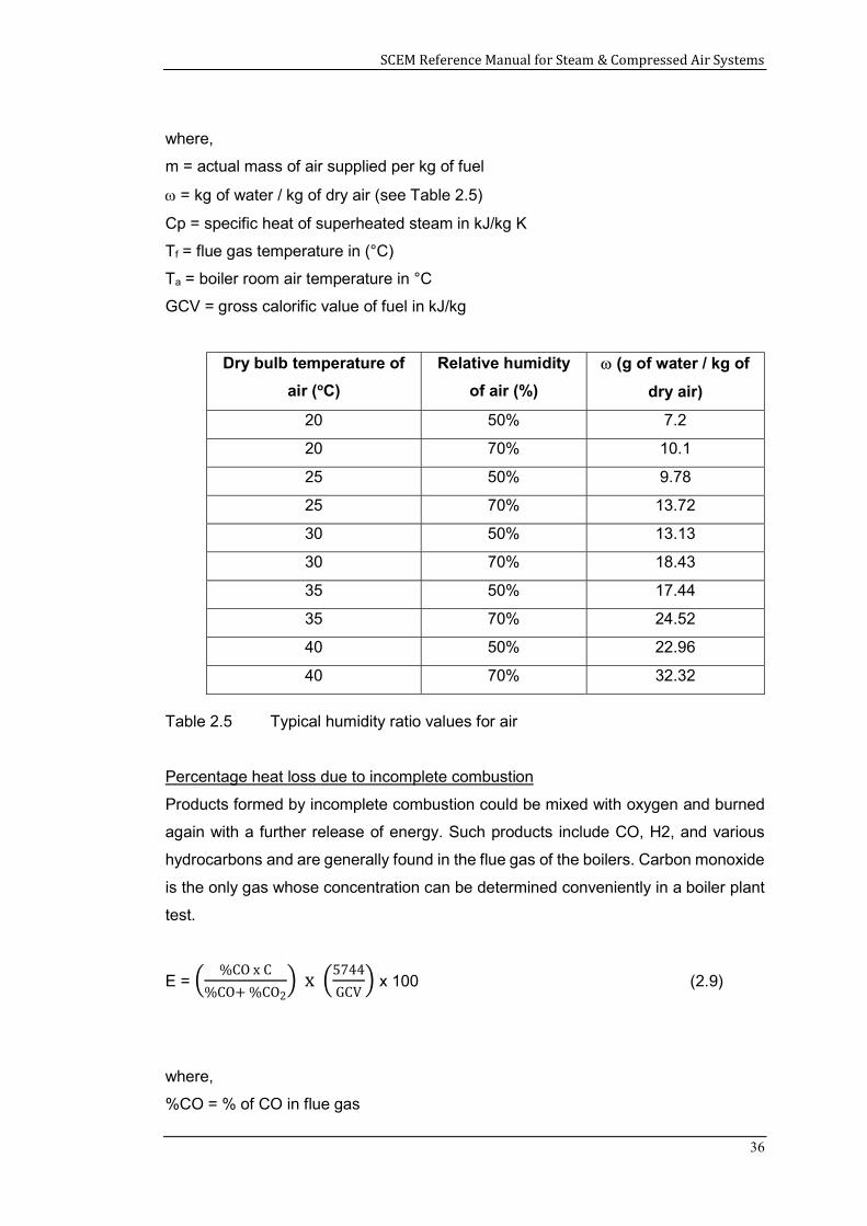
D = m x ω x Cp x (Tf- Ta)
GCV x 100 (2.8)
SCEM Reference Manual for Steam & Compressed Air Systems
36
where,
m = actual mass of air supplied per kg of fuel
= kg of water / kg of dry air (see Table 2.5)
Cp = specific heat of superheated steam in kJ/kg K
Tf = flue gas temperature in (°C)
Ta = boiler room air temperature in °C
GCV = gross calorific value of fuel in kJ/kg
Dry bulb temperature of
air (oC)
Relative humidity
of air (%)
(g of water / kg of
dry air)
20 50% 7.2
20 70% 10.1
25 50% 9.78
25 70% 13.72
30 50% 13.13
30 70% 18.43
35 50% 17.44
35 70% 24.52
40 50% 22.96
40 70% 32.32
Table 2.5 Typical humidity ratio values for air
Percentage heat loss due to incomplete combustion
Products formed by incomplete combustion could be mixed with oxygen and burned
again with a further release of energy. Such products include CO, H2, and various
hydrocarbons and are generally found in the flue gas of the boilers. Carbon monoxide
is the only gas whose concentration can be determined conveniently in a boiler plant
test.
E = %CO x C
%CO+ %CO2 x
5744
GCV x 100 (2.9)
where,
%CO = % of CO in flue gas
SCEM Reference Manual for Steam & Compressed Air Systems
37
%CO2 = % of CO2 in flue gas
C = carbon content kg/kg of fuel
5744 = heat loss due to partial combustion of carbon kJ/kg
GCV = gross calorific value of fuel in kJ/kg
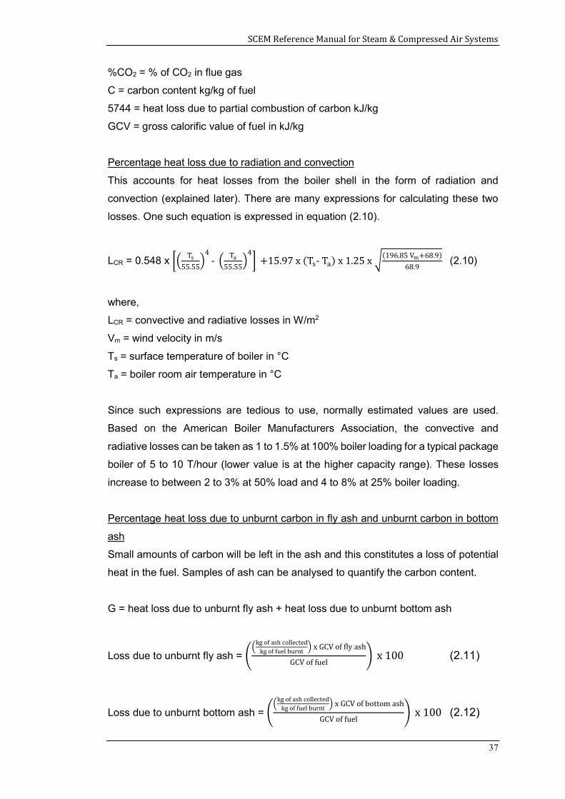
Percentage heat loss due to radiation and convection
This accounts for heat losses from the boiler shell in the form of radiation and
convection (explained later). There are many expressions for calculating these two
losses. One such equation is expressed in equation (2.10).
LCR = 0.548 x Ts
55.55
4-
Ta
55.55
4 +15.97 x (Ts- Ta) x 1.25 x
(196.85 Vm+68.9)
68.9 (2.10)
where,
LCR = convective and radiative losses in W/m2
Vm = wind velocity in m/s
Ts = surface temperature of boiler in °C
Ta = boiler room air temperature in °C
Since such expressions are tedious to use, normally estimated values are used.
Based on the American Boiler Manufacturers Association, the convective and
radiative losses can be taken as 1 to 1.5% at 100% boiler loading for a typical package
boiler of 5 to 10 T/hour (lower value is at the higher capacity range). These losses
increase to between 2 to 3% at 50% load and 4 to 8% at 25% boiler loading.
Percentage heat loss due to unburnt carbon in fly ash and unburnt carbon in bottom
ash
Small amounts of carbon will be left in the ash and this constitutes a loss of potential
heat in the fuel. Samples of ash can be analysed to quantify the carbon content.
G = heat loss due to unburnt fly ash + heat loss due to unburnt bottom ash
Loss due to unburnt fly ash = kg of ash collected
kg of fuel burnt x GCV of fly ash
GCV of fuel x 100 (2.11)
Loss due to unburnt bottom ash = kg of ash collected
kg of fuel burnt x GCV of bottom ash
GCV of fuel x 100 (2.12)
SCEM Reference Manual for Steam & Compressed Air Systems
38
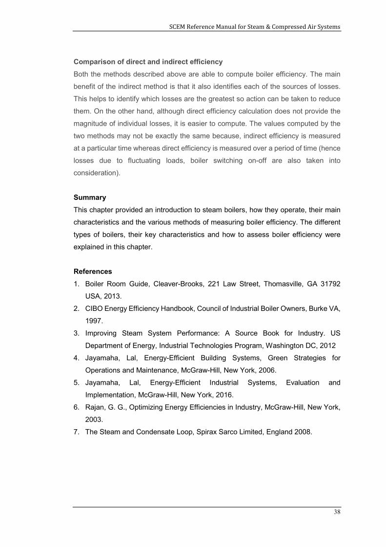
Comparison of direct and indirect efficiency
Both the methods described above are able to compute boiler efficiency. The main
benefit of the indirect method is that it also identifies each of the sources of losses.
This helps to identify which losses are the greatest so action can be taken to reduce
them. On the other hand, although direct efficiency calculation does not provide the
magnitude of individual losses, it is easier to compute. The values computed by the
two methods may not be exactly the same because, indirect efficiency is measured
at a particular time whereas direct efficiency is measured over a period of time (hence
losses due to fluctuating loads, boiler switching on-off are also taken into
consideration).
Summary
This chapter provided an introduction to steam boilers, how they operate, their main
characteristics and the various methods of measuring boiler efficiency. The different
types of boilers, their key characteristics and how to assess boiler efficiency were
explained in this chapter.
References
1. Boiler Room Guide, Cleaver-Brooks, 221 Law Street, Thomasville, GA 31792
USA, 2013.
2. CIBO Energy Efficiency Handbook, Council of Industrial Boiler Owners, Burke VA,
1997.
3. Improving Steam System Performance: A Source Book for Industry. US
Department of Energy, Industrial Technologies Program, Washington DC, 2012
4. Jayamaha, Lal, Energy-Efficient Building Systems, Green Strategies for
Operations and Maintenance, McGraw-Hill, New York, 2006.
5. Jayamaha, Lal, Energy-Efficient Industrial Systems, Evaluation and
Implementation, McGraw-Hill, New York, 2016.
6. Rajan, G. G., Optimizing Energy Efficiencies in Industry, McGraw-Hill, New York,
2003.
7. The Steam and Condensate Loop, Spirax Sarco Limited, England 2008.
SCEM Reference Manual for Steam & Compressed Air Systems
39
3.0 APPLICATIONS OF STEAM
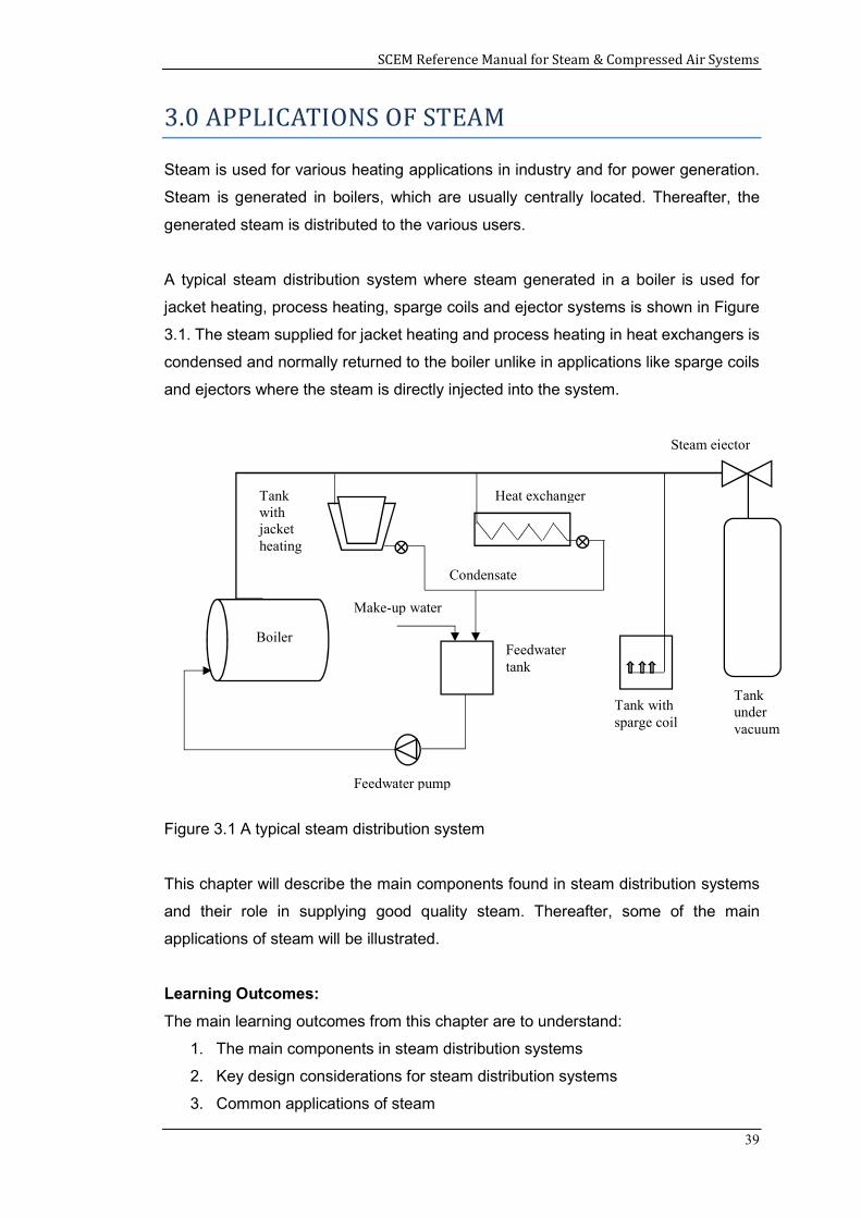
Steam is used for various heating applications in industry and for power generation.
Steam is generated in boilers, which are usually centrally located. Thereafter, the
generated steam is distributed to the various users.
A typical steam distribution system where steam generated in a boiler is used for
jacket heating, process heating, sparge coils and ejector systems is shown in Figure
3.1. The steam supplied for jacket heating and process heating in heat exchangers is
condensed and normally returned to the boiler unlike in applications like sparge coils
and ejectors where the steam is directly injected into the system.
Figure 3.1 A typical steam distribution system
This chapter will describe the main components found in steam distribution systems
and their role in supplying good quality steam. Thereafter, some of the main
applications of steam will be illustrated.
Learning Outcomes:
The main learning outcomes from this chapter are to understand:
1. The main components in steam distribution systems
2. Key design considerations for steam distribution systems
3. Common applications of steam
Tank with jacket heating
Steam ejector
Heat exchanger
Boiler
Condensate
Make-up water
Feedwater tank
Tank under vacuum
Tank with sparge coil
Feedwater pump
SCEM Reference Manual for Steam & Compressed Air Systems
40
3.1 Steam distribution systems
System pressure
When steam flows through the distribution system from the boiler to the users, the
pressure reduces due to losses caused by pipe and fitting resistance to the steam
flow. In addition, pressure losses occur in distribution systems due to condensing of
steam as a result of heat loss to the environment.
Since most steam users require a minimum pressure to be maintained, the system
pressure has to be set after accounting for the above losses. Often, the pressure is
set higher than the minimum requirements because at higher pressure, the specific
volume of steam is less (explained in section 1.6). Since steam occupies less volume
per unit mass at higher pressure, smaller diameter pipes and fittings can be used for
the distribution system.
However, as will be explained in section 4.2, the latent heat available reduces when
the steam pressure is increased, and this results in an increase in steam demand for
heating applications.
Pressure reducers
Since the system pressure is set based on the minimum pressure requirements of the
user needing the highest pressure and other considerations like sizing of distribution
piping and minimum operating pressure for the boiler, the steam supply pressure may
exceed the maximum allowable pressure for some users. In such cases, a pressure-
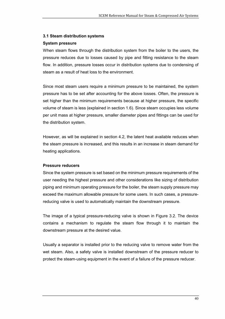
reducing valve is used to automatically maintain the downstream pressure.
The image of a typical pressure-reducing valve is shown in Figure 3.2. The device
contains a mechanism to regulate the steam flow through it to maintain the
downstream pressure at the desired value.
Usually a separator is installed prior to the reducing valve to remove water from the
wet steam. Also, a safety valve is installed downstream of the pressure reducer to
protect the steam-using equipment in the event of a failure of the pressure reducer.
SCEM Reference Manual for Steam & Compressed Air Systems
41
Figure 3.2 Image of a pressure-reducing valve (image taken from the Spirax Sarco
website 'Steam Engineering Tutorials' at http://www.spiraxsarco.com)
Separators
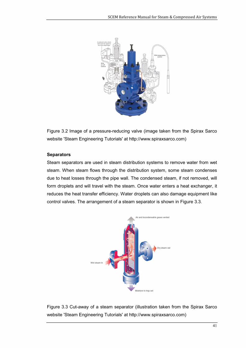
Steam separators are used in steam distribution systems to remove water from wet
steam. When steam flows through the distribution system, some steam condenses
due to heat losses through the pipe wall. The condensed steam, if not removed, will
form droplets and will travel with the steam. Once water enters a heat exchanger, it
reduces the heat transfer efficiency. Water droplets can also damage equipment like
control valves. The arrangement of a steam separator is shown in Figure 3.3.
Figure 3.3 Cut-away of a steam separator (illustration taken from the Spirax Sarco
website 'Steam Engineering Tutorials' at http://www.spiraxsarco.com)
SCEM Reference Manual for Steam & Compressed Air Systems
42
Air venting
Boiler feedwater can contain dissolved air. When the water is heated in the boiler, the
air is released and it will mix with steam. If air is not removed, it can form pockets in
heat transfer equipment and reduce the surface area available for heat exchange.
Also, when air is mixed in steam, the heat content of steam will be lower.
Air can also be present in equipment and distribution piping at start-up. When a steam
system is shut down, the steam inside it will condense and form a vacuum which then
can draw air inwards.
Some common signs of air in the systems are reduction in heating output of
equipment, air bubbles in the condensate and corrosion.
Deaerators (explained in section 2.2) are used in high pressure systems to remove
air from feedwater. However, air can still be present in steam systems and require
vents to remove it. Air vents are devices that can automatically remove air. They are
installed in locations where air tends to accumulate like the upper part of steam
jackets, the end of steam mains and the top level of closed vessels.
Drainage
Since some steam will condense in steam pipes due to heat losses, the distribution
system has to be designed to effectively remove condensate. Steam mains should be
designed to have a gradient downwards in the direction of steam flow as shown in
Figure 3.4. The gradient should be at least 100 mm for every 10 m in pipe length.
The gradient is designed to be downwards so that the condensate and steam will flow
in the same direction and condensate can be removed by creating suitable drain
points. If the gradient is set upwards, the condensate will tend to flow backwards while
the steam will drag it upwards.
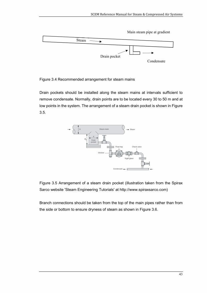
SCEM Reference Manual for Steam & Compressed Air Systems
43
Figure 3.4 Recommended arrangement for steam mains
Drain pockets should be installed along the steam mains at intervals sufficient to
remove condensate. Normally, drain points are to be located every 30 to 50 m and at
low points in the system. The arrangement of a steam drain pocket is shown in Figure
3.5.
Figure 3.5 Arrangement of a steam drain pocket (illustration taken from the Spirax
Sarco website 'Steam Engineering Tutorials' at http://www.spiraxsarco.com)
Branch connections should be taken from the top of the main pipes rather than from
the side or bottom to ensure dryness of steam as shown in Figure 3.6.
Main steam pipe at gradient
Drain pocket Condensate
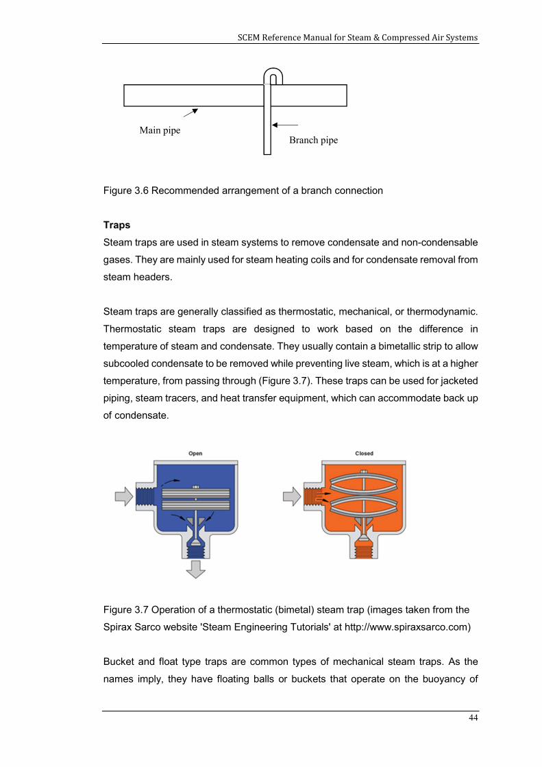
SCEM Reference Manual for Steam & Compressed Air Systems
44
Figure 3.6 Recommended arrangement of a branch connection
Traps
Steam traps are used in steam systems to remove condensate and non-condensable
gases. They are mainly used for steam heating coils and for condensate removal from
steam headers.
Steam traps are generally classified as thermostatic, mechanical, or thermodynamic.
Thermostatic steam traps are designed to work based on the difference in
temperature of steam and condensate. They usually contain a bimetallic strip to allow
subcooled condensate to be removed while preventing live steam, which is at a higher
temperature, from passing through (Figure 3.7). These traps can be used for jacketed
piping, steam tracers, and heat transfer equipment, which can accommodate back up
of condensate.
Figure 3.7 Operation of a thermostatic (bimetal) steam trap (images taken from the
Spirax Sarco website 'Steam Engineering Tutorials' at http://www.spiraxsarco.com)
Bucket and float type traps are common types of mechanical steam traps. As the
names imply, they have floating balls or buckets that operate on the buoyancy of
Branch pipe Main pipe
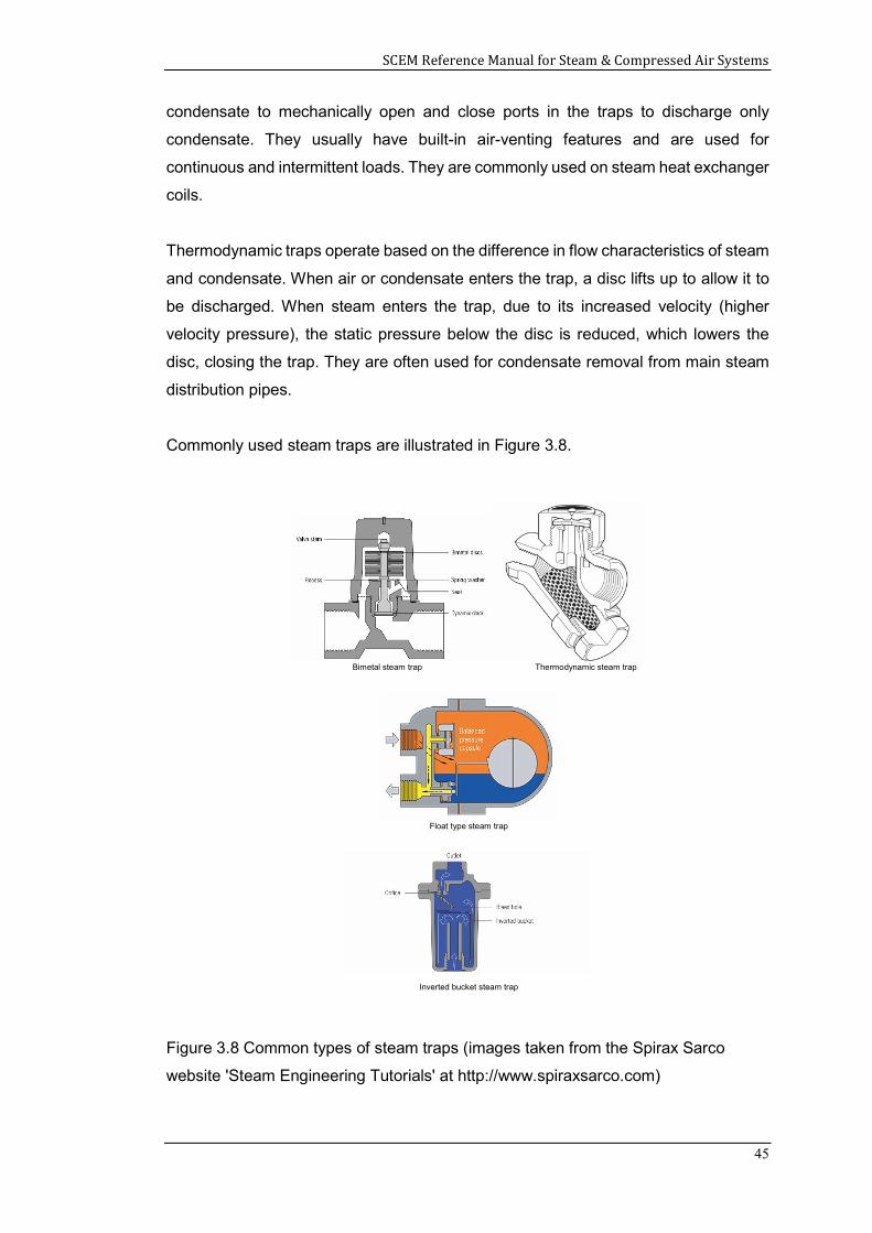
SCEM Reference Manual for Steam & Compressed Air Systems
45
condensate to mechanically open and close ports in the traps to discharge only
condensate. They usually have built-in air-venting features and are used for
continuous and intermittent loads. They are commonly used on steam heat exchanger
coils.
Thermodynamic traps operate based on the difference in flow characteristics of steam
and condensate. When air or condensate enters the trap, a disc lifts up to allow it to
be discharged. When steam enters the trap, due to its increased velocity (higher
velocity pressure), the static pressure below the disc is reduced, which lowers the
disc, closing the trap. They are often used for condensate removal from main steam
distribution pipes.
Commonly used steam traps are illustrated in Figure 3.8.
Figure 3.8 Common types of steam traps (images taken from the Spirax Sarco
website 'Steam Engineering Tutorials' at http://www.spiraxsarco.com)
Bimetal steam trap Thermodynamic steam trap
Float type steam trap
Inverted bucket steam trap
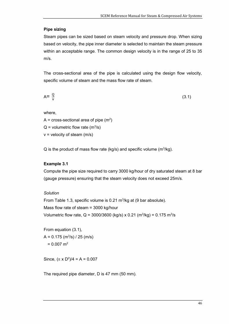
SCEM Reference Manual for Steam & Compressed Air Systems
46
Pipe sizing
Steam pipes can be sized based on steam velocity and pressure drop. When sizing
based on velocity, the pipe inner diameter is selected to maintain the steam pressure
within an acceptable range. The common design velocity is in the range of 25 to 35
m/s.
The cross-sectional area of the pipe is calculated using the design flow velocity,
specific volume of steam and the mass flow rate of steam.
A= Qv (3.1)
where,
A = cross-sectional area of pipe (m2)
Q = volumetric flow rate (m3/s)
v = velocity of steam (m/s)
Q is the product of mass flow rate (kg/s) and specific volume (m3/kg).
Example 3.1
Compute the pipe size required to carry 3000 kg/hour of dry saturated steam at 8 bar
(gauge pressure) ensuring that the steam velocity does not exceed 25m/s.
Solution
From Table 1.3, specific volume is 0.21 m3/kg at (9 bar absolute).
Mass flow rate of steam = 3000 kg/hour
Volumetric flow rate, Q = 3000/3600 (kg/s) x 0.21 (m3/kg) = 0.175 m3/s
From equation (3.1),
A = 0.175 (m3/s) / 25 (m/s)
= 0.007 m2
Since, ( x D2)/4 = A = 0.007
The required pipe diameter, D is 47 mm (50 mm).
SCEM Reference Manual for Steam & Compressed Air Systems
47
In some designs, it may be necessary to size piping based on pressure drop to ensure
that the pressure does not drop below a certain minimum value. In such cases,
reference charts that indicate the recommended pipe diameter for a set of steam
pressure, steam flow rate and pressure loss per unit length can be used.
3.2 Common applications of steam
Non-flow heating
Non-flow type heating is when a substance in a vessel is heated. The heating can be
through an internal steam coil or an external jacket. Heating in non-flow applications
serve two purposes, namely heating the material to the required temperature, and
maintaining the temperature while heat is lost to the surroundings.
The heat required at start-up to raise the temperature of the material being heated
can be computed using the following equation.
Q = m x Cp x T (3.2)
where,
Q = heat added (kW)
m = mass of the material being heated (kg)
Cp = specific heat capacity of material (kJ/kg.K)
T = rise in temperature of the material (K)
Example 3.2
Estimate the heat required to raise the temperature of 10,000 kg of oil having a
specific heat capacity of 2.2 kJ/kg.K from 30oC to 70oC.
Solution
Using equation (3.2),
Q = 10,000 (kg) x 2.2 (kJ/kg.K) x [70-30] (K)
= 880,000 kJ
The mean heating rate required is the amount of heat added divided by the time taken
to raise the temperature from the initial to the final temperature.
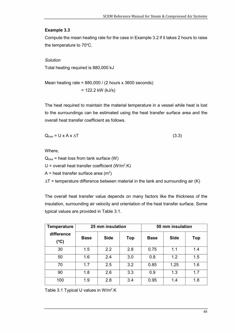
SCEM Reference Manual for Steam & Compressed Air Systems
48
Example 3.3
Compute the mean heating rate for the case in Example 3.2 if it takes 2 hours to raise
the temperature to 70oC.
Solution
Total heating required is 880,000 kJ
Mean heating rate = 880,000 / (2 hours x 3600 seconds)
= 122.2 kW (kJ/s)
The heat required to maintain the material temperature in a vessel while heat is lost
to the surroundings can be estimated using the heat transfer surface area and the
overall heat transfer coefficient as follows.
Qloss = U x A x T (3.3)
Where,
Qloss = heat loss from tank surface (W)
U = overall heat transfer coefficient (W/m2.K)
A = heat transfer surface area (m2)
T = temperature difference between material in the tank and surrounding air (K)
The overall heat transfer value depends on many factors like the thickness of the
insulation, surrounding air velocity and orientation of the heat transfer surface. Some
typical values are provided in Table 3.1.
Temperature
difference
(oC)
25 mm insulation 50 mm insulation
Base Side Top Base Side Top
30 1.5 2.2 2.8 0.75 1.1 1.4
50 1.6 2.4 3.0 0.8 1.2 1.5
70 1.7 2.5 3.2 0.85 1.25 1.6
90 1.8 2.6 3.3 0.9 1.3 1.7
100 1.9 2.8 3.4 0.95 1.4 1.8
Table 3.1 Typical U values in W/m2.K
SCEM Reference Manual for Steam & Compressed Air Systems
49
The values in Table 3.1 should be corrected for air movement by multiplying with the
factors in Table 3.2.
Air velocity
(m/s) 0 1 2 4 6 10
Multiplication
factor 1 1.4 1.7 2.4 3.0 4.1
Table 3.2 Correction factors for U value
Example 3.4
Estimate the heat loss from side walls of a tank having a surface area of 100 m2. The
material in the tank is maintained at 80oC. The tank has a 50 mm insulation. The
surrounding air is at 30oC and the average air velocity is 1 m/s.
Solution
A = 100 m2
T = (80 – 30) = 50oC
U = 1.2 W/m2.K (From Table 3.1, side wall with 50mm insulation and T of 50oC)
Correction factor for air movement of 1 m/s is 1.4 (Table 3.2)
From equation (3.3),
Qloss = (1.2 x 1.4) x 100 x 50 (W)
= 8.4 kW
Flow-type heating
Flow-type heating takes place when the material being heated flows over a heating
surface. Typical flow-type heating devices are shell and tube heat exchangers, plate
type heat exchangers and air heaters.
The relationship between the steam temperature and the increase in temperature of
the material being heated is illustrated in Figure 3.9. If the flow rate of the material
being heated is constant, the heat transfer rate is proportional to the temperature
difference between the two streams. This temperature difference is greatest at the
inlet and reduces at the outlet. The mean of these two values can be used to estimate
the instantaneous heating done. For most steam heating applications, since the steam
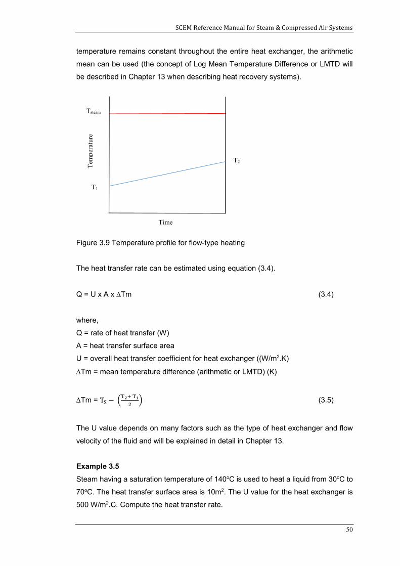
SCEM Reference Manual for Steam & Compressed Air Systems
50
temperature remains constant throughout the entire heat exchanger, the arithmetic
mean can be used (the concept of Log Mean Temperature Difference or LMTD will
be described in Chapter 13 when describing heat recovery systems).
Figure 3.9 Temperature profile for flow-type heating
The heat transfer rate can be estimated using equation (3.4).
Q = U x A x Tm (3.4)
where,
Q = rate of heat transfer (W)
A = heat transfer surface area
U = overall heat transfer coefficient for heat exchanger ((W/m2.K)
Tm = mean temperature difference (arithmetic or LMTD) (K)
Tm = T −
(3.5)
The U value depends on many factors such as the type of heat exchanger and flow
velocity of the fluid and will be explained in detail in Chapter 13.
Example 3.5
Steam having a saturation temperature of 140oC is used to heat a liquid from 30oC to
70oC. The heat transfer surface area is 10m2. The U value for the heat exchanger is
500 W/m2.C. Compute the heat transfer rate.
Tem
pera
ture
Tsteam
T2
T1
Time
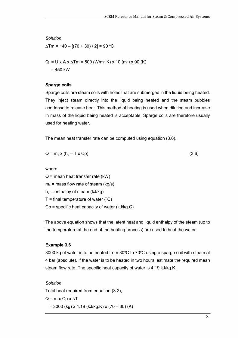
SCEM Reference Manual for Steam & Compressed Air Systems
51
Solution
Tm = 140 – [(70 + 30) / 2] = 90 oC
Q = U x A x Tm = 500 (W/m2.K) x 10 (m2) x 90 (K)
= 450 kW
Sparge coils
Sparge coils are steam coils with holes that are submerged in the liquid being heated.
They inject steam directly into the liquid being heated and the steam bubbles
condense to release heat. This method of heating is used when dilution and increase
in mass of the liquid being heated is acceptable. Sparge coils are therefore usually
used for heating water.
The mean heat transfer rate can be computed using equation (3.6).
Q = ms x (hg – T x Cp) (3.6)
where,
Q = mean heat transfer rate (kW)
ms = mass flow rate of steam (kg/s)
hg = enthalpy of steam (kJ/kg)
T = final temperature of water (oC)
Cp = specific heat capacity of water (kJ/kg.C)
The above equation shows that the latent heat and liquid enthalpy of the steam (up to
the temperature at the end of the heating process) are used to heat the water.
Example 3.6
3000 kg of water is to be heated from 30oC to 70oC using a sparge coil with steam at
4 bar (absolute). If the water is to be heated in two hours, estimate the required mean
steam flow rate. The specific heat capacity of water is 4.19 kJ/kg.K.
Solution
Total heat required from equation (3.2),
Q = m x Cp x T
= 3000 (kg) x 4.19 (kJ/kg.K) x (70 – 30) (K)
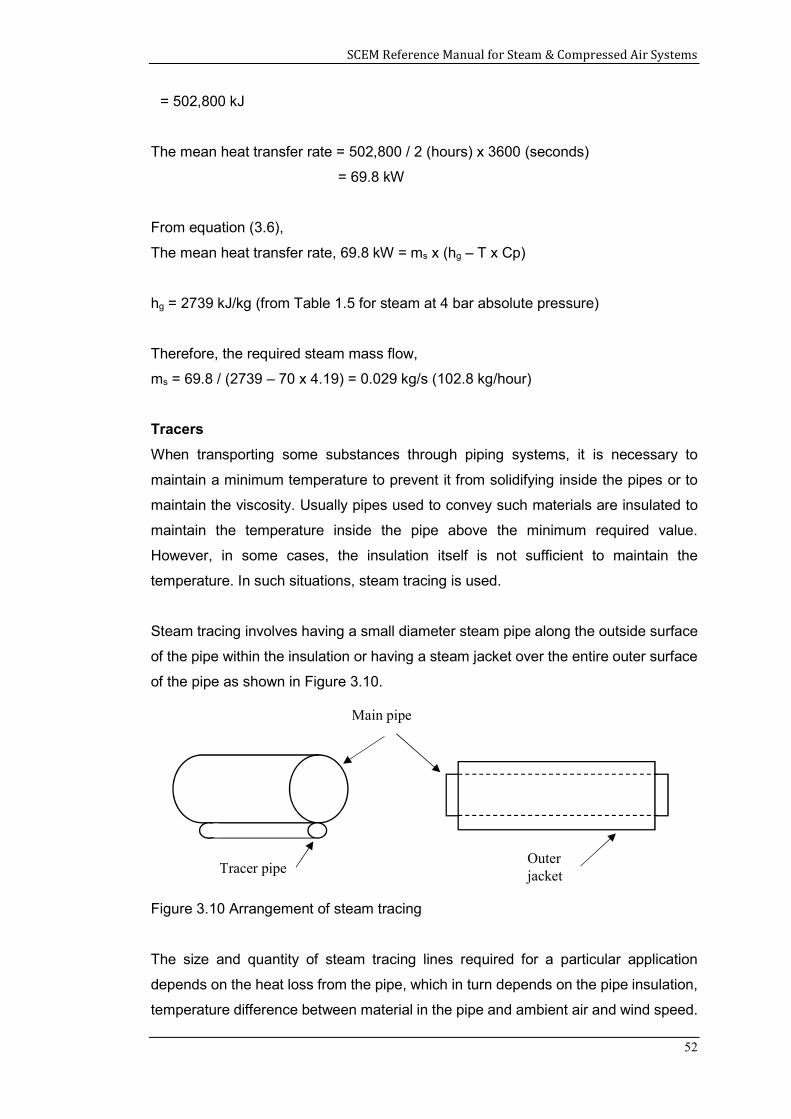
SCEM Reference Manual for Steam & Compressed Air Systems
52
= 502,800 kJ
The mean heat transfer rate = 502,800 / 2 (hours) x 3600 (seconds)
= 69.8 kW
From equation (3.6),
The mean heat transfer rate, 69.8 kW = ms x (hg – T x Cp)
hg = 2739 kJ/kg (from Table 1.5 for steam at 4 bar absolute pressure)
Therefore, the required steam mass flow,
ms = 69.8 / (2739 – 70 x 4.19) = 0.029 kg/s (102.8 kg/hour)
Tracers
When transporting some substances through piping systems, it is necessary to
maintain a minimum temperature to prevent it from solidifying inside the pipes or to
maintain the viscosity. Usually pipes used to convey such materials are insulated to
maintain the temperature inside the pipe above the minimum required value.
However, in some cases, the insulation itself is not sufficient to maintain the
temperature. In such situations, steam tracing is used.
Steam tracing involves having a small diameter steam pipe along the outside surface
of the pipe within the insulation or having a steam jacket over the entire outer surface
of the pipe as shown in Figure 3.10.
Figure 3.10 Arrangement of steam tracing
The size and quantity of steam tracing lines required for a particular application
depends on the heat loss from the pipe, which in turn depends on the pipe insulation,
temperature difference between material in the pipe and ambient air and wind speed.
Main pipe
Tracer pipe Outer jacket
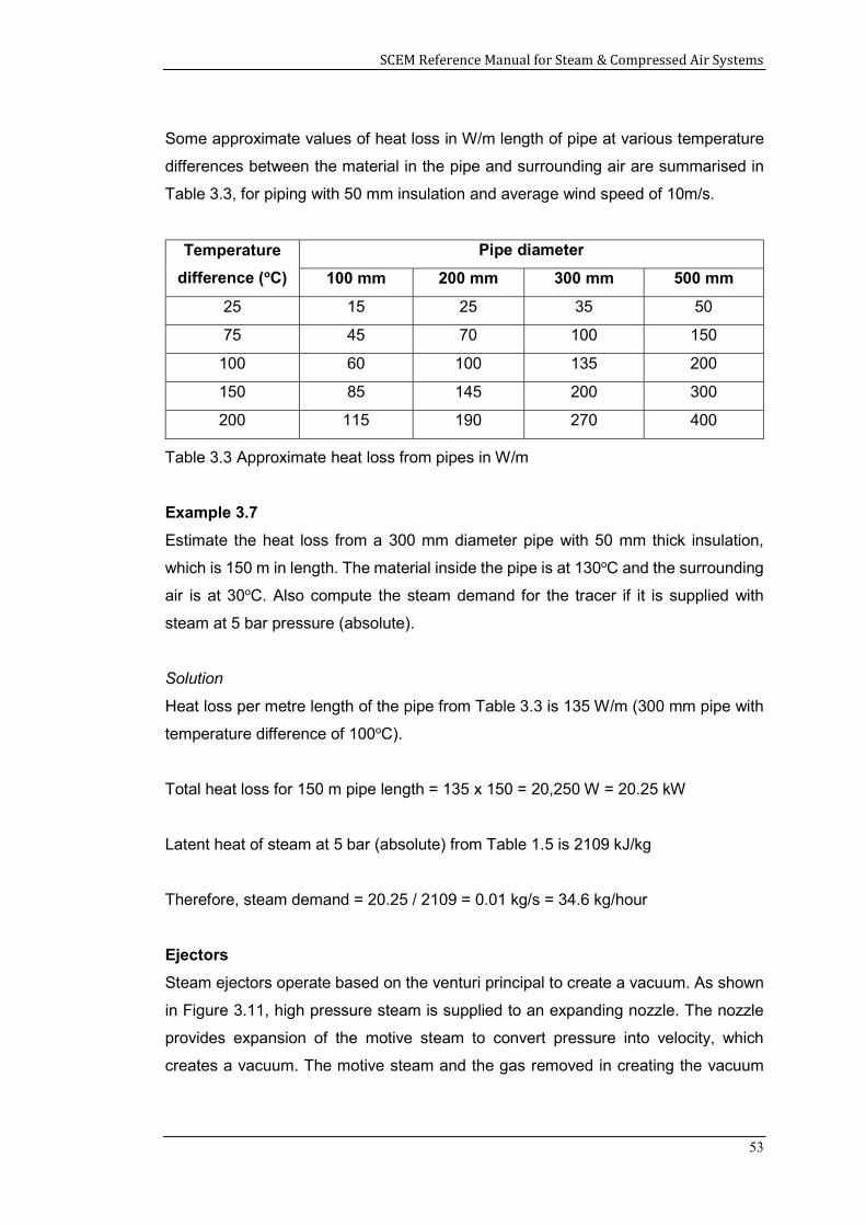
SCEM Reference Manual for Steam & Compressed Air Systems
53
Some approximate values of heat loss in W/m length of pipe at various temperature
differences between the material in the pipe and surrounding air are summarised in
Table 3.3, for piping with 50 mm insulation and average wind speed of 10m/s.
Temperature
difference (oC)
Pipe diameter
100 mm 200 mm 300 mm 500 mm
25 15 25 35 50
75 45 70 100 150
100 60 100 135 200
150 85 145 200 300
200 115 190 270 400
Table 3.3 Approximate heat loss from pipes in W/m
Example 3.7
Estimate the heat loss from a 300 mm diameter pipe with 50 mm thick insulation,
which is 150 m in length. The material inside the pipe is at 130oC and the surrounding
air is at 30oC. Also compute the steam demand for the tracer if it is supplied with
steam at 5 bar pressure (absolute).
Solution
Heat loss per metre length of the pipe from Table 3.3 is 135 W/m (300 mm pipe with
temperature difference of 100oC).
Total heat loss for 150 m pipe length = 135 x 150 = 20,250 W = 20.25 kW
Latent heat of steam at 5 bar (absolute) from Table 1.5 is 2109 kJ/kg
Therefore, steam demand = 20.25 / 2109 = 0.01 kg/s = 34.6 kg/hour
Ejectors
Steam ejectors operate based on the venturi principal to create a vacuum. As shown
in Figure 3.11, high pressure steam is supplied to an expanding nozzle. The nozzle
provides expansion of the motive steam to convert pressure into velocity, which
creates a vacuum. The motive steam and the gas removed in creating the vacuum
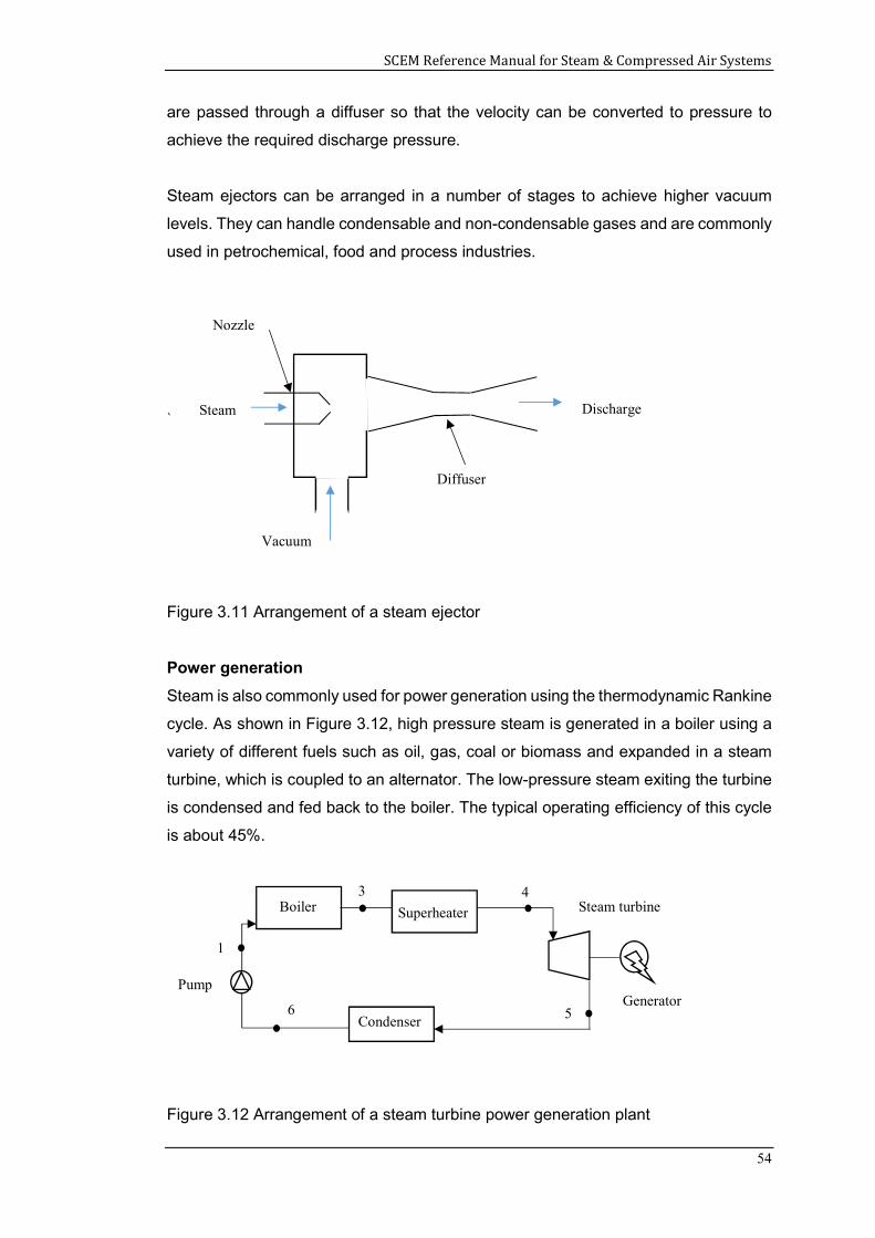
SCEM Reference Manual for Steam & Compressed Air Systems
54
are passed through a diffuser so that the velocity can be converted to pressure to
achieve the required discharge pressure.
Steam ejectors can be arranged in a number of stages to achieve higher vacuum
levels. They can handle condensable and non-condensable gases and are commonly
used in petrochemical, food and process industries.
`
Figure 3.11 Arrangement of a steam ejector
Power generation
Steam is also commonly used for power generation using the thermodynamic Rankine
cycle. As shown in Figure 3.12, high pressure steam is generated in a boiler using a
variety of different fuels such as oil, gas, coal or biomass and expanded in a steam
turbine, which is coupled to an alternator. The low-pressure steam exiting the turbine
is condensed and fed back to the boiler. The typical operating efficiency of this cycle
is about 45%.
Figure 3.12 Arrangement of a steam turbine power generation plant
Steam
Vacuum
Nozzle
Diffuser
Discharge
Boiler Steam turbine
Pump Generator
5 Condenser
Superheater
6
1
3 4
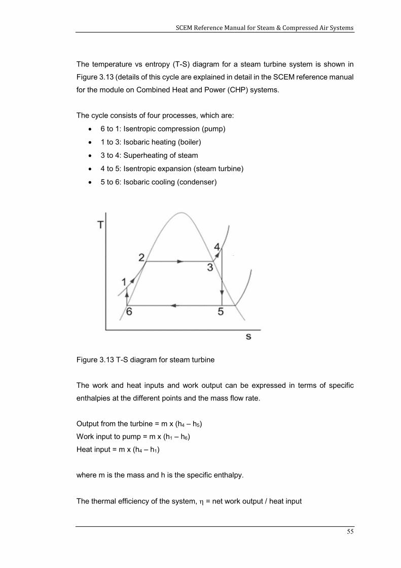
SCEM Reference Manual for Steam & Compressed Air Systems
55
The temperature vs entropy (T-S) diagram for a steam turbine system is shown in
Figure 3.13 (details of this cycle are explained in detail in the SCEM reference manual
for the module on Combined Heat and Power (CHP) systems.
The cycle consists of four processes, which are:
6 to 1: Isentropic compression (pump)
1 to 3: Isobaric heating (boiler)
3 to 4: Superheating of steam
4 to 5: Isentropic expansion (steam turbine)
5 to 6: Isobaric cooling (condenser)
Figure 3.13 T-S diagram for steam turbine
The work and heat inputs and work output can be expressed in terms of specific
enthalpies at the different points and the mass flow rate.
Output from the turbine = m x (h4 – h5)
Work input to pump = m x (h1 – h6)
Heat input = m x (h4 – h1)
where m is the mass and h is the specific enthalpy.
The thermal efficiency of the system, = net work output / heat input
SCEM Reference Manual for Steam & Compressed Air Systems
56
= [m (h4 – h5) – m (h1 – h6)] / m (h4 – h1)
= [(h4 – h5) – (h1 – h6)] / (h4 – h1) (3.7)
Summary
This chapter covered the main components found in steam distribution systems and
their role in supplying good quality steam. Thereafter, some of the main applications
of steam were described and examples were used to illustrate important design
aspects for these systems.
References
1. Improving Steam System Performance: A Source Book for Industry. US
Department of Energy, Industrial Technologies Program, Washington DC, 2012
2. Jayamaha, Lal, Energy-Efficient Industrial Systems, Evaluation and
Implementation, McGraw-Hill, New York, 2016.
3. The Steam and Condensate Loop, Spirax Sarco Limited, England 2008.
SCEM Reference Manual for Steam & Compressed Air Systems
57
4.0 OPTIMISING STEAM SYSTEMS
Boilers and steam systems are widely used in industrial facilities for various process
heating and power generation applications. Boilers use solid, liquid and gaseous fuel
and produce steam, hot water, hot oil or other thermic fluids. They account for a
significant portion of the energy consumption in many industrial plants.
This chapter describes in detail the most common energy-saving measures that can
be implemented to optimise the operation and energy efficiency of such boilers and
heating systems. Various examples will be used to illustrate the energy savings
achievable for each energy-saving measure.
Learning Outcomes:
The main learning outcomes from this chapter are to understand:
1. How to improve the operating efficiency of boilers
2. How to reduce losses and energy wastage in steam systems
3. How to optimise the operation of auxiliary systems used with boilers
4.1 Improving combustion efficiency
The major loss in any boiler is due to the hot gases discharged into the chimney. If
there is a lot of excess air, the increased quantity of exhaust gas will lead to extra flue
gas losses. Similarly, insufficient air for combustion results in wastage of fuel due to
incomplete combustion and reduces the heat transfer efficiency due to soot build-up
on heat transfer surfaces.
The amount of excess air required depends on the type of fuel and, in general, a
minimum of about 10 to 15% excess air is required for complete combustion. This
translates to about 2 to 3% excess oxygen.
As explained earlier, boiler combustion efficiency, which indicates the ability of the
combustion process to burn the fuel completely (with minimum excess air) can be
measured by sampling the exhaust flue gas to find its composition and temperature
using a combustion analyser. Most good combustion analysers are able to give a
direct reading of the combustion efficiency based on the fuel used. If this facility is not
available on the instrument used, a combustion efficiency versus oxygen (O2)
concentration chart (Figure 4.1) can be used to estimate the combustion efficiency.
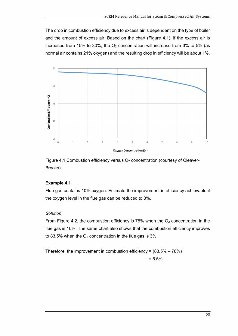
SCEM Reference Manual for Steam & Compressed Air Systems
58
The drop in combustion efficiency due to excess air is dependent on the type of boiler
and the amount of excess air. Based on the chart (Figure 4.1), if the excess air is
increased from 15% to 30%, the O2 concentration will increase from 3% to 5% (as
normal air contains 21% oxygen) and the resulting drop in efficiency will be about 1%.
Figure 4.1 Combustion efficiency versus O2 concentration (courtesy of Cleaver-
Brooks)
Example 4.1
Flue gas contains 10% oxygen. Estimate the improvement in efficiency achievable if
the oxygen level in the flue gas can be reduced to 3%.
Solution
From Figure 4.2, the combustion efficiency is 78% when the O2 concentration in the
flue gas is 10%. The same chart also shows that the combustion efficiency improves
to 83.5% when the O2 concentration in the flue gas is 3%.
Therefore, the improvement in combustion efficiency = (83.5% – 78%)
= 5.5%
65
70
75
80
85
0 1 2 3 4 5 6 7 8 9 10
Com
bust
ion
Effic
ienc
y (%
)
Oxygen Concentration (%)
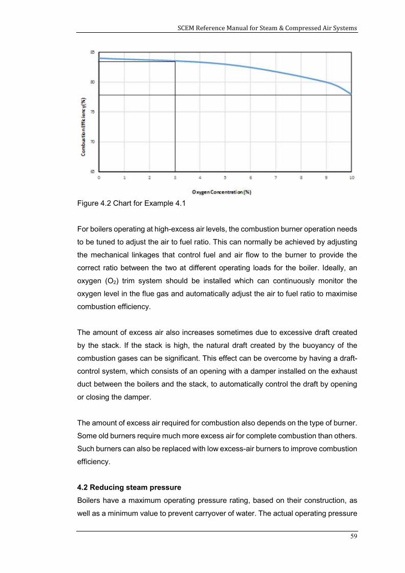
SCEM Reference Manual for Steam & Compressed Air Systems
59
Figure 4.2 Chart for Example 4.1
For boilers operating at high-excess air levels, the combustion burner operation needs
to be tuned to adjust the air to fuel ratio. This can normally be achieved by adjusting
the mechanical linkages that control fuel and air flow to the burner to provide the
correct ratio between the two at different operating loads for the boiler. Ideally, an
oxygen (O2) trim system should be installed which can continuously monitor the
oxygen level in the flue gas and automatically adjust the air to fuel ratio to maximise
combustion efficiency.
The amount of excess air also increases sometimes due to excessive draft created
by the stack. If the stack is high, the natural draft created by the buoyancy of the
combustion gases can be significant. This effect can be overcome by having a draft-
control system, which consists of an opening with a damper installed on the exhaust
duct between the boilers and the stack, to automatically control the draft by opening
or closing the damper.
The amount of excess air required for combustion also depends on the type of burner.
Some old burners require much more excess air for complete combustion than others.
Such burners can also be replaced with low excess-air burners to improve combustion
efficiency.
4.2 Reducing steam pressure
Boilers have a maximum operating pressure rating, based on their construction, as
well as a minimum value to prevent carryover of water. The actual operating pressure
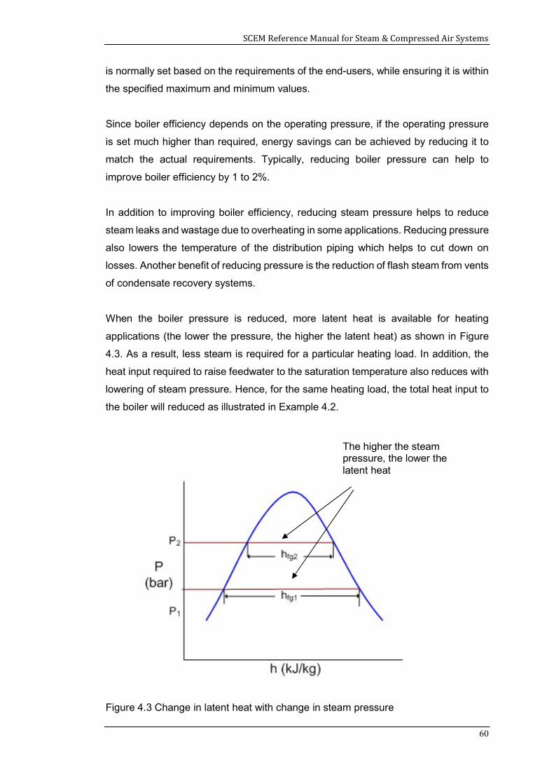
SCEM Reference Manual for Steam & Compressed Air Systems
60
is normally set based on the requirements of the end-users, while ensuring it is within
the specified maximum and minimum values.
Since boiler efficiency depends on the operating pressure, if the operating pressure
is set much higher than required, energy savings can be achieved by reducing it to
match the actual requirements. Typically, reducing boiler pressure can help to
improve boiler efficiency by 1 to 2%.
In addition to improving boiler efficiency, reducing steam pressure helps to reduce
steam leaks and wastage due to overheating in some applications. Reducing pressure
also lowers the temperature of the distribution piping which helps to cut down on
losses. Another benefit of reducing pressure is the reduction of flash steam from vents
of condensate recovery systems.
When the boiler pressure is reduced, more latent heat is available for heating
applications (the lower the pressure, the higher the latent heat) as shown in Figure
4.3. As a result, less steam is required for a particular heating load. In addition, the
heat input required to raise feedwater to the saturation temperature also reduces with
lowering of steam pressure. Hence, for the same heating load, the total heat input to
the boiler will reduced as illustrated in Example 4.2.
Figure 4.3 Change in latent heat with change in steam pressure
The higher the steam pressure, the lower the latent heat
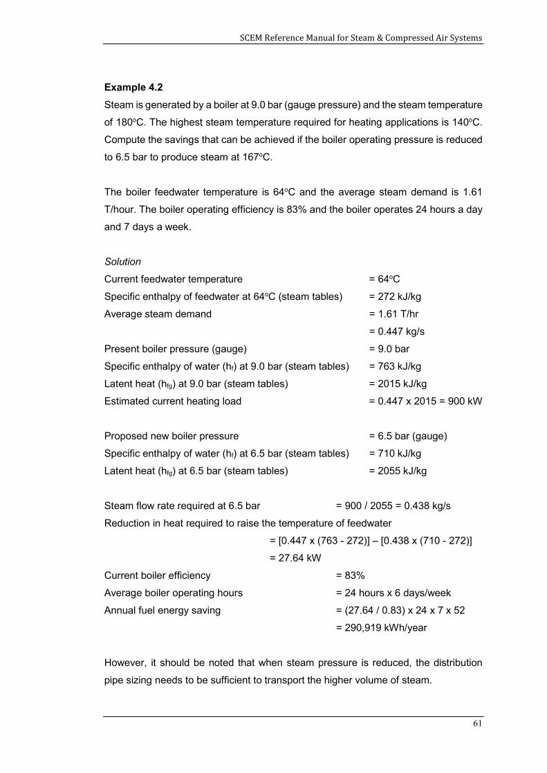
SCEM Reference Manual for Steam & Compressed Air Systems
61
Example 4.2
Steam is generated by a boiler at 9.0 bar (gauge pressure) and the steam temperature
of 180oC. The highest steam temperature required for heating applications is 140oC.
Compute the savings that can be achieved if the boiler operating pressure is reduced
to 6.5 bar to produce steam at 167oC.
The boiler feedwater temperature is 64oC and the average steam demand is 1.61
T/hour. The boiler operating efficiency is 83% and the boiler operates 24 hours a day
and 7 days a week.
Solution
Current feedwater temperature = 64oC
Specific enthalpy of feedwater at 64oC (steam tables) = 272 kJ/kg
Average steam demand = 1.61 T/hr
= 0.447 kg/s
Present boiler pressure (gauge) = 9.0 bar
Specific enthalpy of water (hf) at 9.0 bar (steam tables) = 763 kJ/kg
Latent heat (hfg) at 9.0 bar (steam tables) = 2015 kJ/kg
Estimated current heating load = 0.447 x 2015 = 900 kW
Proposed new boiler pressure = 6.5 bar (gauge)
Specific enthalpy of water (hf) at 6.5 bar (steam tables) = 710 kJ/kg
Latent heat (hfg) at 6.5 bar (steam tables) = 2055 kJ/kg
Steam flow rate required at 6.5 bar = 900 / 2055 = 0.438 kg/s
Reduction in heat required to raise the temperature of feedwater
= [0.447 x (763 - 272)] – [0.438 x (710 - 272)]
= 27.64 kW
Current boiler efficiency = 83%
Average boiler operating hours = 24 hours x 6 days/week
Annual fuel energy saving = (27.64 / 0.83) x 24 x 7 x 52
= 290,919 kWh/year
However, it should be noted that when steam pressure is reduced, the distribution
pipe sizing needs to be sufficient to transport the higher volume of steam.
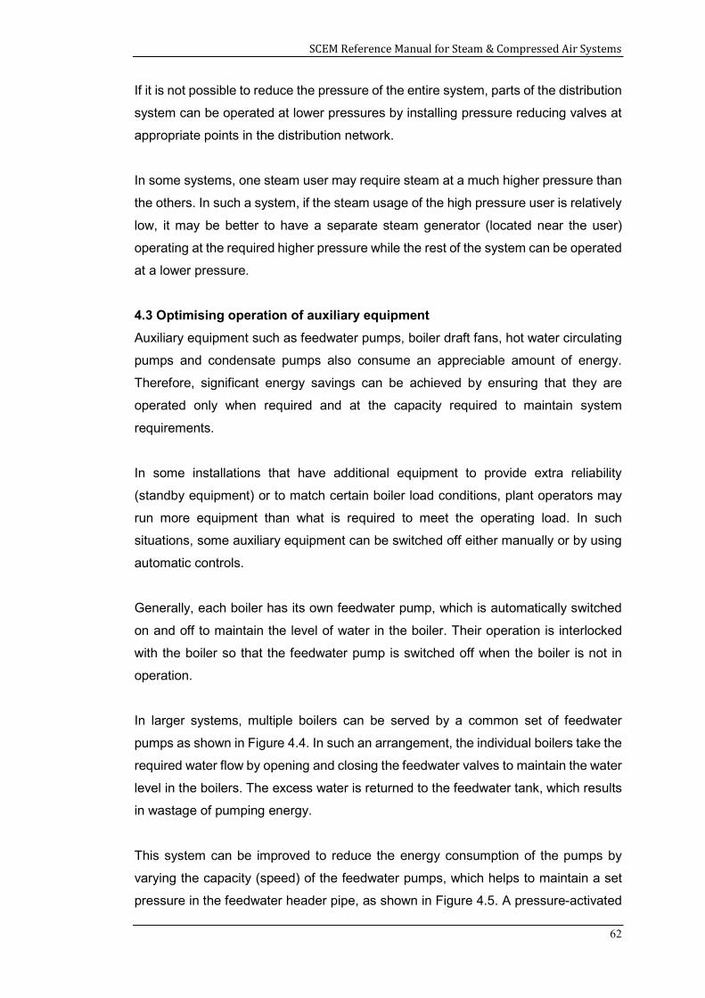
SCEM Reference Manual for Steam & Compressed Air Systems
62
If it is not possible to reduce the pressure of the entire system, parts of the distribution
system can be operated at lower pressures by installing pressure reducing valves at
appropriate points in the distribution network.
In some systems, one steam user may require steam at a much higher pressure than
the others. In such a system, if the steam usage of the high pressure user is relatively
low, it may be better to have a separate steam generator (located near the user)
operating at the required higher pressure while the rest of the system can be operated
at a lower pressure.
4.3 Optimising operation of auxiliary equipment
Auxiliary equipment such as feedwater pumps, boiler draft fans, hot water circulating
pumps and condensate pumps also consume an appreciable amount of energy.
Therefore, significant energy savings can be achieved by ensuring that they are
operated only when required and at the capacity required to maintain system
requirements.
In some installations that have additional equipment to provide extra reliability
(standby equipment) or to match certain boiler load conditions, plant operators may
run more equipment than what is required to meet the operating load. In such
situations, some auxiliary equipment can be switched off either manually or by using
automatic controls.
Generally, each boiler has its own feedwater pump, which is automatically switched
on and off to maintain the level of water in the boiler. Their operation is interlocked
with the boiler so that the feedwater pump is switched off when the boiler is not in
operation.
In larger systems, multiple boilers can be served by a common set of feedwater
pumps as shown in Figure 4.4. In such an arrangement, the individual boilers take the
required water flow by opening and closing the feedwater valves to maintain the water
level in the boilers. The excess water is returned to the feedwater tank, which results
in wastage of pumping energy.
This system can be improved to reduce the energy consumption of the pumps by
varying the capacity (speed) of the feedwater pumps, which helps to maintain a set
pressure in the feedwater header pipe, as shown in Figure 4.5. A pressure-activated
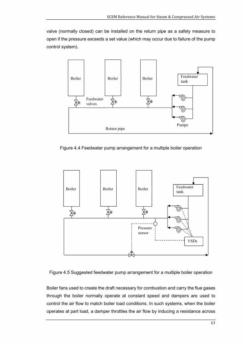
SCEM Reference Manual for Steam & Compressed Air Systems
63
valve (normally closed) can be installed on the return pipe as a safety measure to
open if the pressure exceeds a set value (which may occur due to failure of the pump
control system).
Figure 4.4 Feedwater pump arrangement for a multiple boiler operation
Figure 4.5 Suggested feedwater pump arrangement for a multiple boiler operation
Boiler fans used to create the draft necessary for combustion and carry the flue gases
through the boiler normally operate at constant speed and dampers are used to
control the air flow to match boiler load conditions. In such systems, when the boiler
operates at part load, a damper throttles the air flow by inducing a resistance across
Return pipe
Boiler Boiler Boiler Feedwater tank
Pumps
Feedwater valves
Pressure sensor
Boiler Boiler Boiler Feedwater tank
VSDs
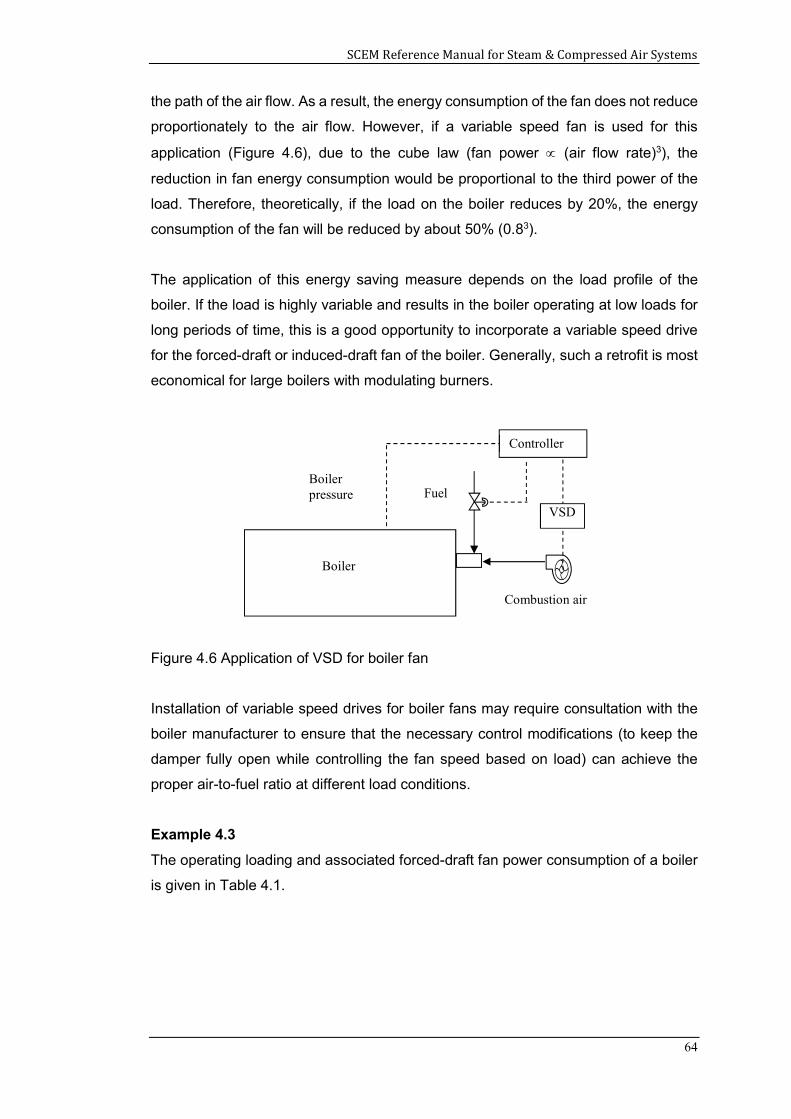
SCEM Reference Manual for Steam & Compressed Air Systems
64
the path of the air flow. As a result, the energy consumption of the fan does not reduce
proportionately to the air flow. However, if a variable speed fan is used for this
application (Figure 4.6), due to the cube law (fan power (air flow rate)3), the
reduction in fan energy consumption would be proportional to the third power of the
load. Therefore, theoretically, if the load on the boiler reduces by 20%, the energy
consumption of the fan will be reduced by about 50% (0.83).
The application of this energy saving measure depends on the load profile of the
boiler. If the load is highly variable and results in the boiler operating at low loads for
long periods of time, this is a good opportunity to incorporate a variable speed drive
for the forced-draft or induced-draft fan of the boiler. Generally, such a retrofit is most
economical for large boilers with modulating burners.
Figure 4.6 Application of VSD for boiler fan
Installation of variable speed drives for boiler fans may require consultation with the
boiler manufacturer to ensure that the necessary control modifications (to keep the
damper fully open while controlling the fan speed based on load) can achieve the
proper air-to-fuel ratio at different load conditions.
Example 4.3
The operating loading and associated forced-draft fan power consumption of a boiler
is given in Table 4.1.
Boiler
Combustion air
Fuel
Controller
Boiler pressure
VSD
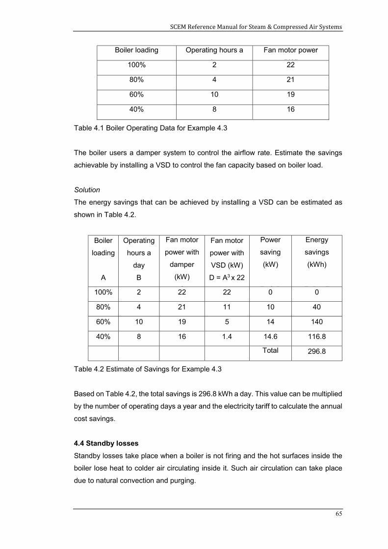
SCEM Reference Manual for Steam & Compressed Air Systems
65
Boiler loading Operating hours a
day
Fan motor power
(kW) 100% 2 22
80% 4 21
60% 10 19
40% 8 16
Table 4.1 Boiler Operating Data for Example 4.3
The boiler users a damper system to control the airflow rate. Estimate the savings
achievable by installing a VSD to control the fan capacity based on boiler load.
Solution
The energy savings that can be achieved by installing a VSD can be estimated as
shown in Table 4.2.
Boiler
loading
A
Operating
hours a
day
B
Fan motor
power with
damper
(kW)
C
Fan motor
power with
VSD (kW)
D = A3 x 22
Power
saving
(kW)
E=C-D
Energy
savings
(kWh)
F=B x E 100% 2 22 22 0 0
80% 4 21 11 10 40
60% 10 19 5 14 140
40% 8 16 1.4 14.6 116.8
Total 296.8
Table 4.2 Estimate of Savings for Example 4.3
Based on Table 4.2, the total savings is 296.8 kWh a day. This value can be multiplied
by the number of operating days a year and the electricity tariff to calculate the annual
cost savings.
4.4 Standby losses
Standby losses take place when a boiler is not firing and the hot surfaces inside the
boiler lose heat to colder air circulating inside it. Such air circulation can take place
due to natural convection and purging.
SCEM Reference Manual for Steam & Compressed Air Systems
66
Losses due to natural convection occur when the air in the boiler gets heated (by the
hot surfaces) making it lighter causing it to move up the stack, circulating cold air
through the boiler. This can be avoided if dampers are installed to prevent the
circulation of air when the boiler is not being fired.
Purging losses take place when the boiler combustion space is purged by the fan
before firing the burners to ensure that there is only air present (to prevent possible
explosions). Some burner systems also follow a purging cycle when firing stops.
Losses due to purging can be reduced by minimising the on-off cycle of the burner
system. This can be achieved by using burners that have a high turndown ratio (ratio
of maximum heat output to the minimum heat output of a burner) to enable the burner
to function at low loads without switching off the flame (compared to normal burners
which have to be switched off at low loads and later switched on back again).
4.5 Minimising conduction and radiation losses
When a steam system is in operation, the surface temperature of boilers, auxiliary
equipment and distribution piping become much hotter than the surrounding areas.
Therefore, they lose heat by radiation and conduction. The amount of heat lost
depends on the surface temperature of the hot surface, which in turn depends on the
insulation (thickness, thermal conductivity and condition). To minimise heat loss, all
hot surfaces should be insulated with material having sufficient resistance to heat
transfer. Further, the insulation should be of adequate thickness and should be in
good condition.
As stated earlier, a 10 T/hour boiler will have a loss of about 1% due to radiation and
convection when operating at full load. Since the radiation and convective losses
remain the same irrespective of boiler loading, 1% losses at full load can increase to
2% at 50% loading and 4.5% at 25% loading. Some typical values for radiation and
convection losses are shown in Table 4.3.
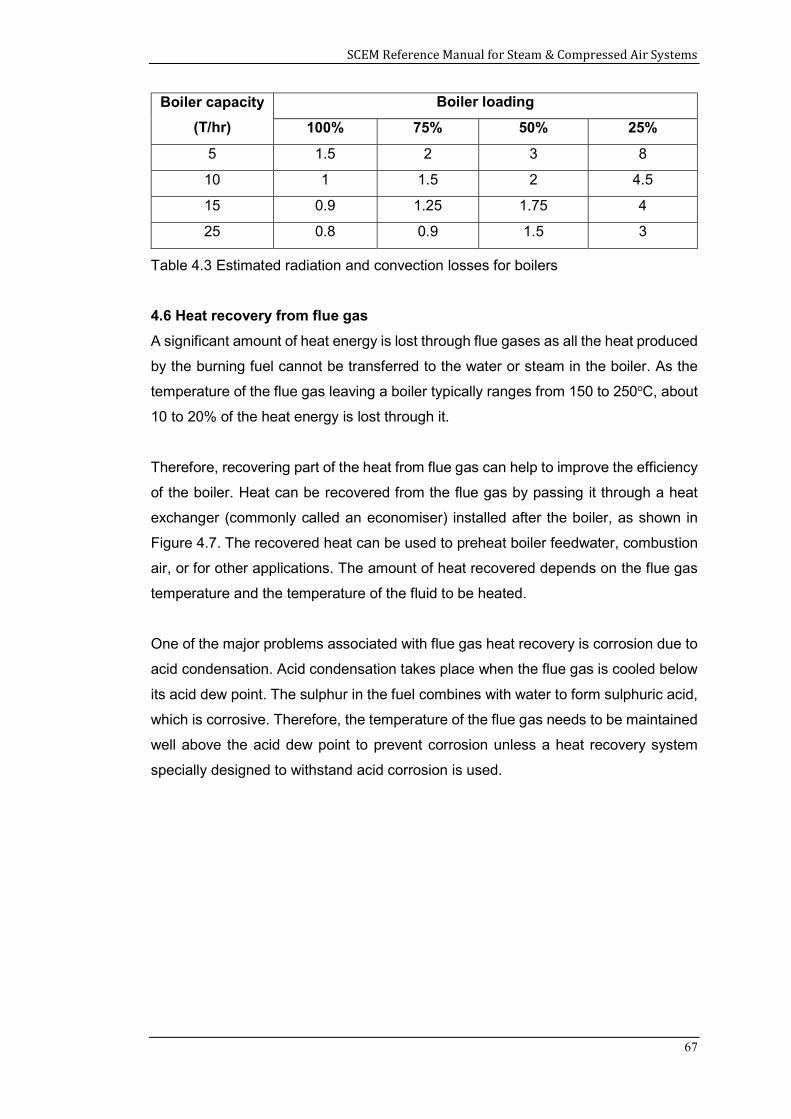
SCEM Reference Manual for Steam & Compressed Air Systems
67
Boiler capacity
(T/hr)
Boiler loading
100% 75% 50% 25%
5 1.5 2 3 8
10 1 1.5 2 4.5
15 0.9 1.25 1.75 4
25 0.8 0.9 1.5 3
Table 4.3 Estimated radiation and convection losses for boilers
4.6 Heat recovery from flue gas
A significant amount of heat energy is lost through flue gases as all the heat produced
by the burning fuel cannot be transferred to the water or steam in the boiler. As the
temperature of the flue gas leaving a boiler typically ranges from 150 to 250oC, about
10 to 20% of the heat energy is lost through it.
Therefore, recovering part of the heat from flue gas can help to improve the efficiency
of the boiler. Heat can be recovered from the flue gas by passing it through a heat
exchanger (commonly called an economiser) installed after the boiler, as shown in
Figure 4.7. The recovered heat can be used to preheat boiler feedwater, combustion
air, or for other applications. The amount of heat recovered depends on the flue gas
temperature and the temperature of the fluid to be heated.
One of the major problems associated with flue gas heat recovery is corrosion due to
acid condensation. Acid condensation takes place when the flue gas is cooled below
its acid dew point. The sulphur in the fuel combines with water to form sulphuric acid,
which is corrosive. Therefore, the temperature of the flue gas needs to be maintained
well above the acid dew point to prevent corrosion unless a heat recovery system
specially designed to withstand acid corrosion is used.
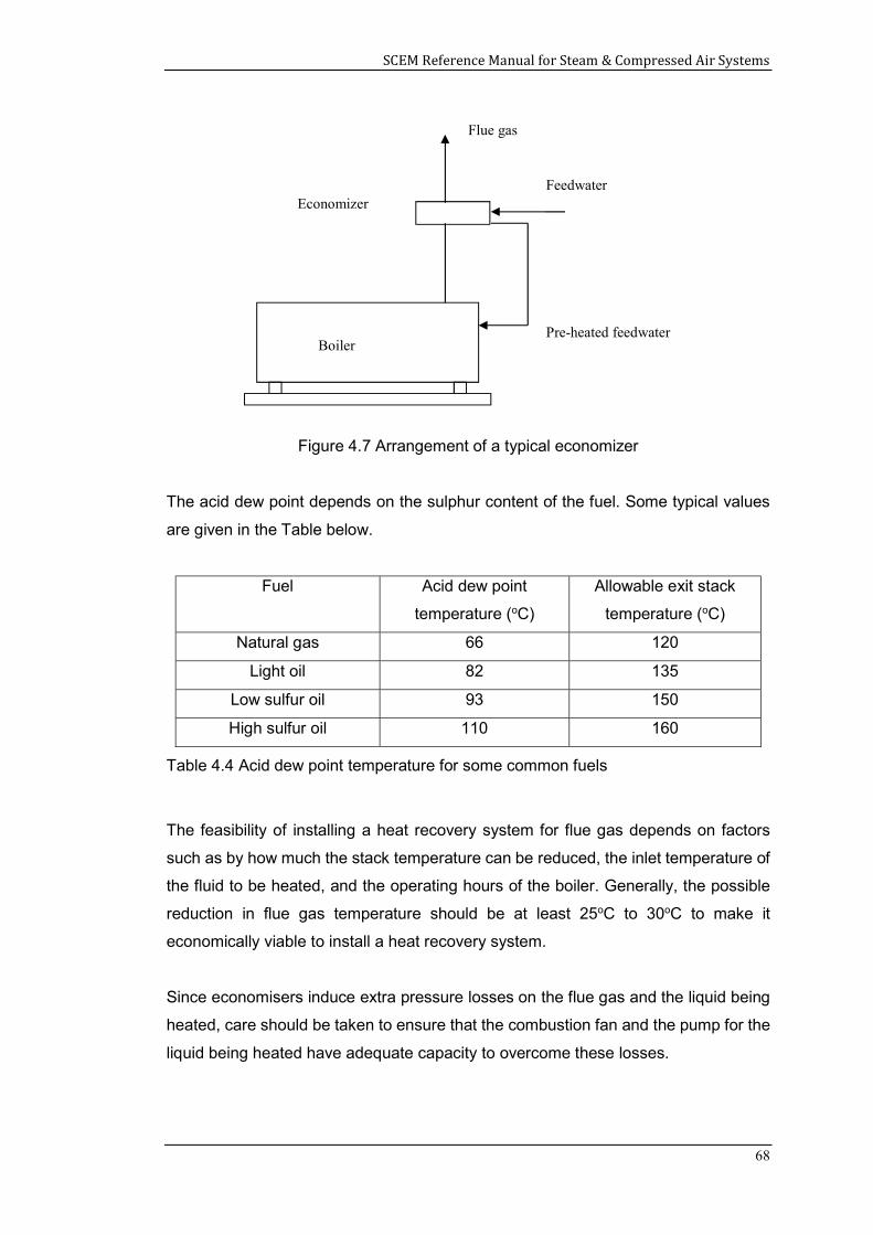
SCEM Reference Manual for Steam & Compressed Air Systems
68
Figure 4.7 Arrangement of a typical economizer
The acid dew point depends on the sulphur content of the fuel. Some typical values
are given in the Table below.
Fuel Acid dew point
temperature (oC)
Allowable exit stack
temperature (oC)
Natural gas 66 120
Light oil 82 135
Low sulfur oil 93 150
High sulfur oil 110 160
Table 4.4 Acid dew point temperature for some common fuels
The feasibility of installing a heat recovery system for flue gas depends on factors
such as by how much the stack temperature can be reduced, the inlet temperature of
the fluid to be heated, and the operating hours of the boiler. Generally, the possible
reduction in flue gas temperature should be at least 25oC to 30oC to make it
economically viable to install a heat recovery system.
Since economisers induce extra pressure losses on the flue gas and the liquid being
heated, care should be taken to ensure that the combustion fan and the pump for the
liquid being heated have adequate capacity to overcome these losses.
Boiler
Economizer
Flue gas
Pre-heated feedwater
Feedwater
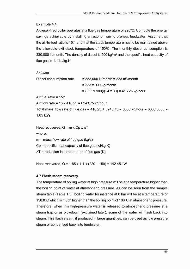
SCEM Reference Manual for Steam & Compressed Air Systems
69
Example 4.4
A diesel-fired boiler operates at a flue gas temperature of 220oC. Compute the energy
savings achievable by installing an economiser to preheat feedwater. Assume that
the air-to-fuel ratio is 15:1 and that the stack temperature has to be maintained above
the allowable exit stack temperature of 150oC. The monthly diesel consumption is
330,000 lit/month. The density of diesel is 900 kg/m3 and the specific heat capacity of
flue gas is 1.1 kJ/kg.K
Solution
Diesel consumption rate = 333,000 lit/month = 333 m3/month
= 333 x 900 kg/month
= (333 x 900)/(24 x 30) = 416.25 kg/hour
Air fuel ratio = 15:1
Air flow rate = 15 x 416.25 = 6243.75 kg/hour
Total mass flow rate of flue gas = 416.25 + 6243.75 = 6660 kg/hour = 6660/3600 =
1.85 kg/s
Heat recovered, Q = m x Cp x ∆T
where,
m = mass flow rate of flue gas (kg/s)
Cp = specific heat capacity of flue gas (kJ/kg.K)
∆T = reduction in temperature of flue gas (K)
Heat recovered, Q = 1.85 x 1.1 x (220 – 150) = 142.45 kW
4.7 Flash steam recovery
The temperature of boiling water at high pressure will be at a temperature higher than
the boiling point of water at atmospheric pressure. As can be seen from the sample
steam table (Table 1.5), boiling water for instance at 6 bar will be at a temperature of
158.8oC which is much higher than the boiling point of 100oC at atmospheric pressure.
Therefore, when this high-pressure water is released to atmospheric pressure at a
steam trap or as blowdown (explained later), some of the water will flash back into
steam. This flash steam, if produced in large quantities, can be used as low pressure
steam or condensed back into feedwater.
SCEM Reference Manual for Steam & Compressed Air Systems
70
Example 4.5
0.25 kg/s of condensate at 8 bar (absolute) is released through a steam trap. Compute
the percentage and amount of flash steam produced.
Solution
Enthalpy of water at 8 bar = 721 kJ/kg (from Table 1.5)
Enthalpy of water at atmospheric pressure = 419 kJ/kg
Excess energy = 721 – 419 = 302 kJ/kg
Enthalpy of evaporation at atmospheric pressure = 2257 kJ/kg
Percentage of flash steam produced = (excess energy / enthalpy of evaporation) x
100%
= (302 / 2257) x 100%
= 13%
Amount of flash steam produced = 0.25 x 0.13 = 0.0325 kg/s
4.8 Automatic blowdown control
Boiler blowdown is part of the water treatment process and involves removal of sludge
and solids from the boiler. Make-up water used for boilers contains various impurities.
As water is converted to steam, the concentration of the impurities that remain in the
boiler increases. If this concentration is allowed to increase, it will lead to accelerated
corrosion, scaling, and fouling of the heat-transfer surfaces of the boiler. Therefore, it
is necessary to remove part of the concentrated water from the boiler and replace it
with fresh water.
The quality of water in the boiler is normally assessed using the TDS (total dissolved
solids) level measured in ppm (parts per million). For typical two-pass and three-pass
fire tube boilers, the allowable TDS level is 3000 to 3500 ppm while for water tube
boilers the allowable level is about 1500 ppm.
The blowdown rate depends on the rate of steam production, TDS of the feedwater
and the allowable maximum TDS and can be expressed as follows:
Blowdown rate (kg/hr) = [S x FT ] / [MT – FT] (4.1)
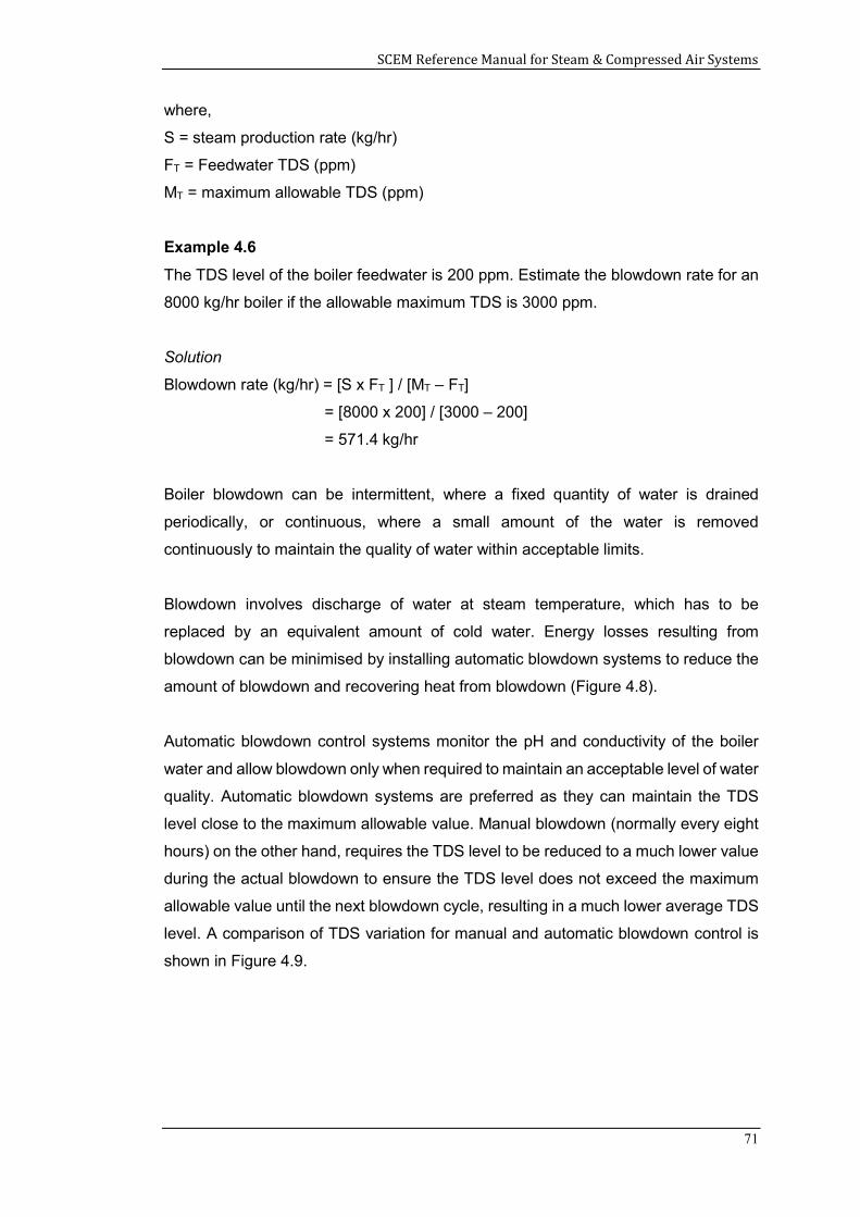
SCEM Reference Manual for Steam & Compressed Air Systems
71
where,
S = steam production rate (kg/hr)
FT = Feedwater TDS (ppm)
MT = maximum allowable TDS (ppm)
Example 4.6
The TDS level of the boiler feedwater is 200 ppm. Estimate the blowdown rate for an
8000 kg/hr boiler if the allowable maximum TDS is 3000 ppm.
Solution
Blowdown rate (kg/hr) = [S x FT ] / [MT – FT]
= [8000 x 200] / [3000 – 200]
= 571.4 kg/hr
Boiler blowdown can be intermittent, where a fixed quantity of water is drained
periodically, or continuous, where a small amount of the water is removed
continuously to maintain the quality of water within acceptable limits.
Blowdown involves discharge of water at steam temperature, which has to be
replaced by an equivalent amount of cold water. Energy losses resulting from
blowdown can be minimised by installing automatic blowdown systems to reduce the
amount of blowdown and recovering heat from blowdown (Figure 4.8).
Automatic blowdown control systems monitor the pH and conductivity of the boiler
water and allow blowdown only when required to maintain an acceptable level of water
quality. Automatic blowdown systems are preferred as they can maintain the TDS
level close to the maximum allowable value. Manual blowdown (normally every eight
hours) on the other hand, requires the TDS level to be reduced to a much lower value
during the actual blowdown to ensure the TDS level does not exceed the maximum
allowable value until the next blowdown cycle, resulting in a much lower average TDS
level. A comparison of TDS variation for manual and automatic blowdown control is
shown in Figure 4.9.
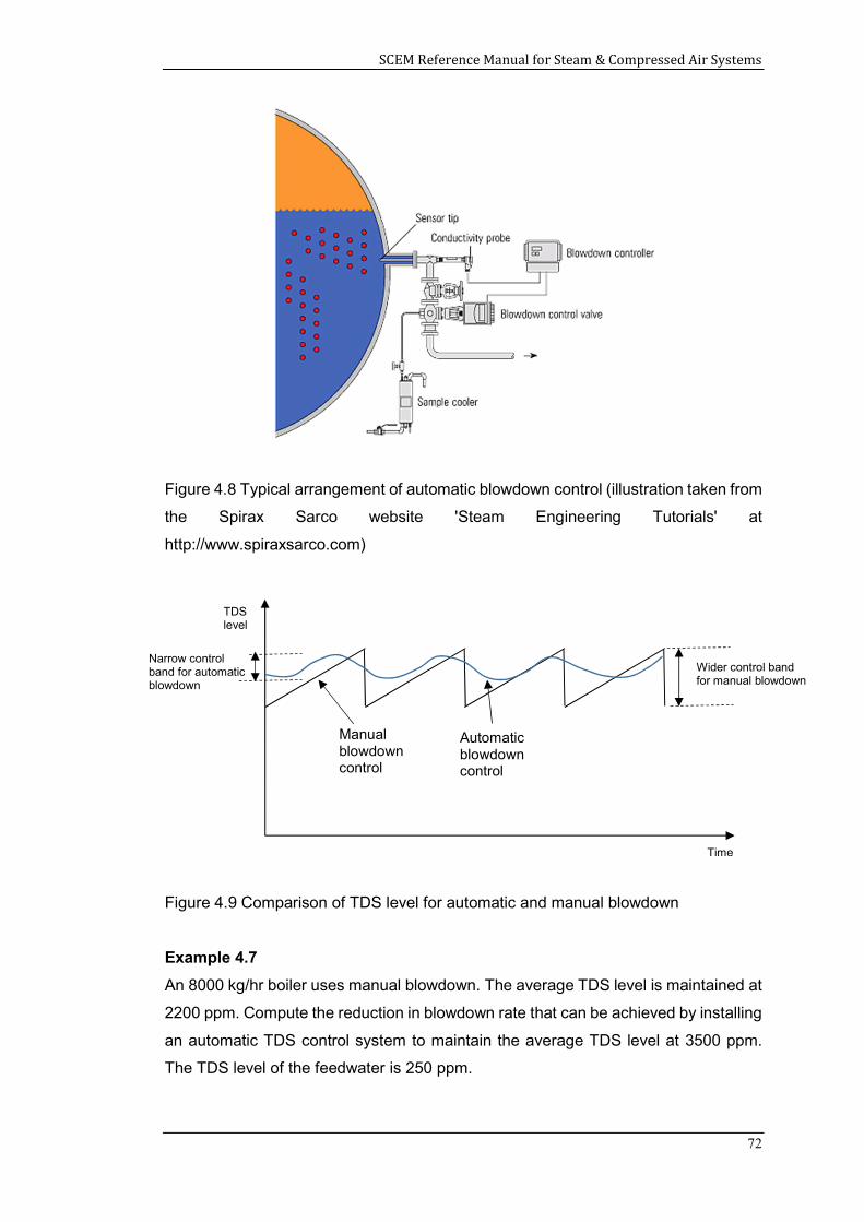
SCEM Reference Manual for Steam & Compressed Air Systems
72
Figure 4.8 Typical arrangement of automatic blowdown control (illustration taken from
the Spirax Sarco website 'Steam Engineering Tutorials' at
http://www.spiraxsarco.com)
Figure 4.9 Comparison of TDS level for automatic and manual blowdown
Example 4.7
An 8000 kg/hr boiler uses manual blowdown. The average TDS level is maintained at
2200 ppm. Compute the reduction in blowdown rate that can be achieved by installing
an automatic TDS control system to maintain the average TDS level at 3500 ppm.
The TDS level of the feedwater is 250 ppm.
Manual blowdown control
Wider control band for manual blowdown
Narrow control band for automatic blowdown
TDS level
Automatic blowdown control
Time
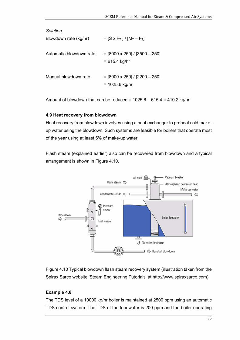
SCEM Reference Manual for Steam & Compressed Air Systems
73
Solution
Blowdown rate (kg/hr) = [S x FT ] / [MT – FT]
Automatic blowdown rate = [8000 x 250] / [3500 – 250]
= 615.4 kg/hr
Manual blowdown rate = [8000 x 250] / [2200 – 250]
= 1025.6 kg/hr
Amount of blowdown that can be reduced = 1025.6 – 615.4 = 410.2 kg/hr
4.9 Heat recovery from blowdown
Heat recovery from blowdown involves using a heat exchanger to preheat cold make-
up water using the blowdown. Such systems are feasible for boilers that operate most
of the year using at least 5% of make-up water.
Flash steam (explained earlier) also can be recovered from blowdown and a typical
arrangement is shown in Figure 4.10.
Figure 4.10 Typical blowdown flash steam recovery system (illustration taken from the
Spirax Sarco website 'Steam Engineering Tutorials' at http://www.spiraxsarco.com)
Example 4.8
The TDS level of a 10000 kg/hr boiler is maintained at 2500 ppm using an automatic
TDS control system. The TDS of the feedwater is 200 ppm and the boiler operating
SCEM Reference Manual for Steam & Compressed Air Systems
74
pressure is 10 bar (absolute). Compute the amount of heat energy in the blowdown
and the amount of flash steam that can be recovered from the blowdown.
Solution
Blowdown rate (kg/hr) = [S x FT ] / [MT – FT]
= [10000 x 200] / [2500 – 200]
= 869.6 kg/hr
= 0.24 kg/s
Enthalpy of blowdown at 10 bar, hf = 763 kJ/kg (Table 1.5)
Heat energy in the blowdown = 0.24 (kg/s) x 763 (kJ/kg) = 183 kW
Enthalpy of water at atmospheric pressure = 419 kJ/kg
Excess energy = 763 – 419 = 344 kJ/kg
Enthalpy of evaporation at atmospheric pressure = 2257 kJ/kg
Percentage of flash steam = (excess energy / enthalpy of evaporation) x 100%
= (344 / 2257) x 100%
= 15%
Amount of flash steam = 0.24 x 0.15 = 0.036 kg/s
4.10 Condensate recovery
In most steam systems, steam is used mainly for heating by extracting its latent heat
(hfg). The resulting condensate is at steam temperature and still contains a
considerable amount of heat energy (hf). From Table 1.5, if steam is used at 8 bar
(absolute), then the condensate enthalpy (hf) will be 721 kJ/kg which is 26% of the
total enthalpy of steam (2769 kJ/kg) and will be lost if condensate is not returned to
the system. Therefore, returning condensate to the boiler feedwater tank will result in
significant fuel energy savings.
Since condensate is distilled water, it is ideal for use as boiler feedwater. Therefore,
condensate recovery helps to reduce water consumption (water cost), water
treatment cost, and blowdown.
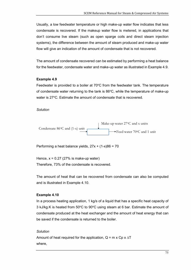
SCEM Reference Manual for Steam & Compressed Air Systems
75
Usually, a low feedwater temperature or high make-up water flow indicates that less
condensate is recovered. If the makeup water flow is metered, in applications that
don’t consume live steam (such as open sparge coils and direct steam injection
systems), the difference between the amount of steam produced and make-up water
flow will give an indication of the amount of condensate that is not recovered.
The amount of condensate recovered can be estimated by performing a heat balance
for the feedwater, condensate water and make-up water as illustrated in Example 4.9.
Example 4.9
Feedwater is provided to a boiler at 70oC from the feedwater tank. The temperature
of condensate water returning to the tank is 86oC, while the temperature of make-up
water is 27oC. Estimate the amount of condensate that is recovered.
Solution
Performing a heat balance yields, 27x + (1-x)86 = 70
Hence, x = 0.27 (27% is make-up water)
Therefore, 73% of the condensate is recovered.
The amount of heat that can be recovered from condensate can also be computed
and is illustrated in Example 4.10.
Example 4.10
In a process heating application, 1 kg/s of a liquid that has a specific heat capacity of
3 kJ/kg.K is heated from 50oC to 90oC using steam at 6 bar. Estimate the amount of
condensate produced at the heat exchanger and the amount of heat energy that can
be saved if the condensate is returned to the boiler.
Solution
Amount of heat required for the application, Q = m x Cp x ∆T
where,
Make-up water 27oC and x units
Feed water 70oC and 1 unitCondensate 86oC and (1-x) unit
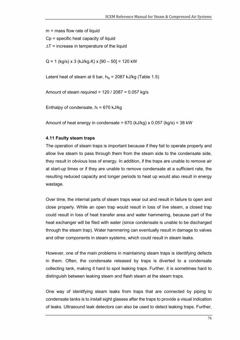
SCEM Reference Manual for Steam & Compressed Air Systems
76
m = mass flow rate of liquid
Cp = specific heat capacity of liquid
∆T = increase in temperature of the liquid
Q = 1 (kg/s) x 3 (kJ/kg.K) x [90 – 50] = 120 kW
Latent heat of steam at 6 bar, hfg = 2087 kJ/kg (Table 1.5)
Amount of steam required = 120 / 2087 = 0.057 kg/s
Enthalpy of condensate, hf = 670 kJ/kg
Amount of heat energy in condensate = 670 (kJ/kg) x 0.057 (kg/s) = 38 kW
4.11 Faulty steam traps
The operation of steam traps is important because if they fail to operate properly and
allow live steam to pass through them from the steam side to the condensate side,
they result in obvious loss of energy. In addition, if the traps are unable to remove air
at start-up times or if they are unable to remove condensate at a sufficient rate, the
resulting reduced capacity and longer periods to heat up would also result in energy
wastage.
Over time, the internal parts of steam traps wear out and result in failure to open and
close properly. While an open trap would result in loss of live steam, a closed trap
could result in loss of heat transfer area and water hammering, because part of the
heat exchanger will be filed with water (since condensate is unable to be discharged
through the steam trap). Water hammering can eventually result in damage to valves
and other components in steam systems, which could result in steam leaks.
However, one of the main problems in maintaining steam traps is identifying defects
in them. Often, the condensate released by traps is diverted to a condensate
collecting tank, making it hard to spot leaking traps. Further, it is sometimes hard to
distinguish between leaking steam and flash steam at the steam traps.
One way of identifying steam leaks from traps that are connected by piping to
condensate tanks is to install sight glasses after the traps to provide a visual indication
of leaks. Ultrasound leak detectors can also be used to detect leaking traps. Further,
SCEM Reference Manual for Steam & Compressed Air Systems
77
traps should be periodically inspected and repaired or replaced to ensure that they
are in good working condition. In addition, the correct type of steam trap should be
selected for each application.
4.12 Rectifying steam leaks
Steam leakage occurs from pipes, flanges, valves, connections, traps, and process
equipment and can be substantial for some steam distribution systems. The amount
of steam leaking from various openings depends on the size of the opening and the
system pressure. Figure 4.11 shows the approximate steam leak rates at different
operating pressures for various leaking hole sizes.
Figure 4.11 Steam losses through leaks (illustration taken from the Spirax Sarco
website 'Steam Engineering Tutorials' at http://www.spiraxsarco.com)
Once the leakage rate is known, the amount of energy lost can be computed using
the enthalpy data, while the amount of fuel wasted can be estimated using the boiler
efficiency as illustrated in Example 4.11.
Example 4.11
The total steam leak rate for a plant is estimated to be 100 kg/hr. If the steam pressure
is 7 bar (absolute), compute the amount of energy wasted due to the steam leaks. As
the fuel, the boiler uses natural gas which has a calorific value of 55,000 kJ/kg and
SCEM Reference Manual for Steam & Compressed Air Systems
78
the operating boiler efficiency is 88%. Estimate the reduction in fuel used by the boiler
that can be achieved if all the steam leaks in the plant are rectified.
Solution
Enthalpy of steam at 7 bar, hg = 2764 kJ/kg (Table 1.5)
Total steam leak rate = 100 kg/hr = 0.028 kg/s
Amount of heat energy wasted = 0.028 (kg/s) x 2764 (kJ/kg) = 77.4 kW
Amount of input heat energy wasted = 77.4 / 0.88 = 87.95 kW
Amount of fuel wasted = 87.95 (kW) / 55,000 (kJ/kg) = 0.0016 kg/s = 5.76 kg/hr
4.13 Feedwater tank
The feedwater tank is a very important part of any steam system. It provides a
reservoir of returned condensate and fresh make-up water for the boilers. The
feedwater tank gives a good indication of the system performance. Excessive
feedwater temperature may indicate that some traps may be passing live steam, while
a high make-up water flow may indicate that some condensate is not being returned
to the tank.
Feedwater is normally hot due to returned condensate and recovery of heat from other
sources. Therefore, the tank should be elevated to prevent hot water being flashed
off as steam at the feedwater pump inlet, in order to prevent cavitation.
Since the feedwater tank is hot, steps should be taken to minimise heat losses from
the tank. Other than insulating the tank, the top of the tank should be covered since a
great amount of losses usually take place at the water surface.
4.14 Fouling and scaling in boilers
Fouling, scaling, and soot build-up on heat transfer surfaces of boilers acts as an
insulator and leads to reduced heat transfer. This results in lower heat transfer to
water in the boiler and higher flue gas temperature. If at the same load conditions and
same excess air setting the flue gas temperature increases with time, this is a good
indication of increased resistance to heat transfer in the boiler. Data for energy
wastage due to scaling is shown in Table 4.5.
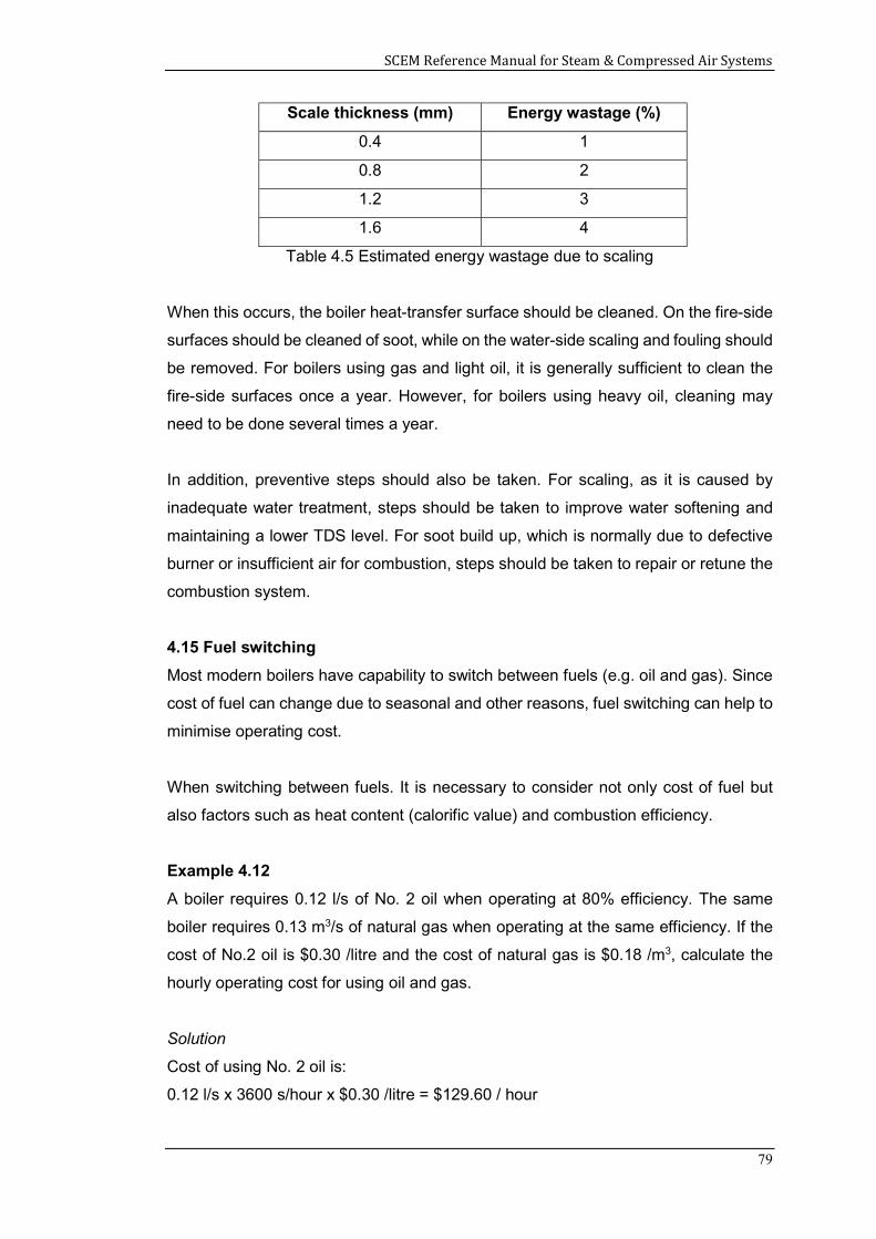
SCEM Reference Manual for Steam & Compressed Air Systems
79
Scale thickness (mm) Energy wastage (%)
0.4 1
0.8 2
1.2 3
1.6 4
Table 4.5 Estimated energy wastage due to scaling
When this occurs, the boiler heat-transfer surface should be cleaned. On the fire-side
surfaces should be cleaned of soot, while on the water-side scaling and fouling should
be removed. For boilers using gas and light oil, it is generally sufficient to clean the
fire-side surfaces once a year. However, for boilers using heavy oil, cleaning may
need to be done several times a year.
In addition, preventive steps should also be taken. For scaling, as it is caused by
inadequate water treatment, steps should be taken to improve water softening and
maintaining a lower TDS level. For soot build up, which is normally due to defective
burner or insufficient air for combustion, steps should be taken to repair or retune the
combustion system.
4.15 Fuel switching
Most modern boilers have capability to switch between fuels (e.g. oil and gas). Since
cost of fuel can change due to seasonal and other reasons, fuel switching can help to
minimise operating cost.
When switching between fuels. It is necessary to consider not only cost of fuel but
also factors such as heat content (calorific value) and combustion efficiency.
Example 4.12
A boiler requires 0.12 l/s of No. 2 oil when operating at 80% efficiency. The same
boiler requires 0.13 m3/s of natural gas when operating at the same efficiency. If the
cost of No.2 oil is $0.30 /litre and the cost of natural gas is $0.18 /m3, calculate the
hourly operating cost for using oil and gas.
Solution
Cost of using No. 2 oil is:
0.12 l/s x 3600 s/hour x $0.30 /litre = $129.60 / hour
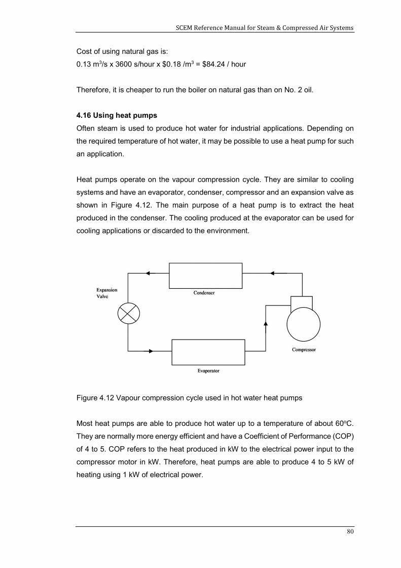
SCEM Reference Manual for Steam & Compressed Air Systems
80
Cost of using natural gas is:
0.13 m3/s x 3600 s/hour x $0.18 /m3 = $84.24 / hour
Therefore, it is cheaper to run the boiler on natural gas than on No. 2 oil.
4.16 Using heat pumps
Often steam is used to produce hot water for industrial applications. Depending on
the required temperature of hot water, it may be possible to use a heat pump for such
an application.
Heat pumps operate on the vapour compression cycle. They are similar to cooling
systems and have an evaporator, condenser, compressor and an expansion valve as
shown in Figure 4.12. The main purpose of a heat pump is to extract the heat
produced in the condenser. The cooling produced at the evaporator can be used for
cooling applications or discarded to the environment.
Figure 4.12 Vapour compression cycle used in hot water heat pumps
Most heat pumps are able to produce hot water up to a temperature of about 60oC.
They are normally more energy efficient and have a Coefficient of Performance (COP)
of 4 to 5. COP refers to the heat produced in kW to the electrical power input to the
compressor motor in kW. Therefore, heat pumps are able to produce 4 to 5 kW of
heating using 1 kW of electrical power.
SCEM Reference Manual for Steam & Compressed Air Systems
81
Example 4.13
A diesel fired boiler is used to produce hot water at 60oC. The average daily hot water
demand is 5,000 kWh. The boiler operates 365 days a year. The boiler efficiency is
80%.
Compute the reduction in energy consumption (kWh) that can be achieved if a heat
pump with a COP of 4.0 is used for the same application.
If the calorific value of diesel is 12 kWh/litre and the cost of diesel and electricity are
$1.5/litre and $0.10/kWh respectively, compute the annual cost savings that can be
achieved.
Solution
Daily energy usage for diesel = 5,000 / 0.8 = 6,250 kWh
Daily electrical energy usage for a heat pump with COP of 4.0
= 5,000 / 4.0 = 1,250 kWh
Reduction in energy usage = (6,250 – 1,250) kWh/day
= 5,000 kWh/day
= 5,000 x 365 kWh/year
= 1,825,000 kWh/year
Diesel usage = 6,250 / 12 litres/day
= 520.83 litres/day
= 520.83 x 365 litres/year
= 190,103 litres/year
Cost of diesel = 190,103 x $1.5
= $285,154 /year
Cost of electricity = 1,250 x $0.1 /day
= $125 /day
= $45,625 /year
Cost savings = $(285,154 – 45,625)
= $239,529 /year
SCEM Reference Manual for Steam & Compressed Air Systems
82
Summary
This chapter described the most common energy saving measures that can be
implemented to optimise the operation and energy efficiency of boilers and hot water
systems. Various examples were used to illustrate the energy savings achievable for
each energy saving measure.
References
1. Improving Steam System Performance: A Source Book for Industry. US
Department of Energy, Industrial Technologies Program, Washington DC, 2012
2. Jayamaha, Lal, Energy-Efficient Building Systems, Green Strategies for
Operations and Maintenance, McGraw-Hill, New York, 2006.
3. Jayamaha, Lal, Energy-Efficient Industrial Systems, Evaluation and
Implementation, McGraw-Hill, New York, 2016.
4. The Steam and Condensate Loop, Spirax Sarco Limited, England 2008.
SCEM Reference Manual for Steam & Compressed Air Systems
83
5.0 ENERGY AUDIT OF STEAM SYSTEMS
Boilers and steam systems are significant energy users in various manufacturing
plants, ranging from petrochemical to food manufacturing. Normally, they account for
more than 80% of the energy consumed in such plants.
From the previous chapter of this reference manual, it is clear that many measures
are available to optimise the operation of boilers and steam systems to minimise
energy usage.
However, before optimising a boiler or steam system, it is necessary to first assess
its performance so that suitable improvements can be identified and implemented.
Such a system assessment is usually called an “Energy Audit”. This chapter describes
the key energy performance indicators (EnPIs) used for assessing the performance
of boilers and steam systems followed by how the required parameters are to be
obtained.
Learning Outcomes:
The main learning outcomes from this chapter are to understand:
1. The key EnPIs for boilers and steam systems
2. The parameters required
3. Measurements required
4. Case study of a boiler energy audit
The main EnPIs used for assessing the performance of boilers and steam systems
are explained in the subsequent sections of this chapter.
5.1 Boiler overall efficiency
The overall efficiency of the boiler accounts for all the losses, which include individual
losses due to combustion, blowdown, convection, radiation and exhaust.
Overall boiler efficiency =
x 100
The overall boiler efficiency can be measured using either the direct or indirect method
as explained in chapter 2. Since the direct method is easier to follow and provides a
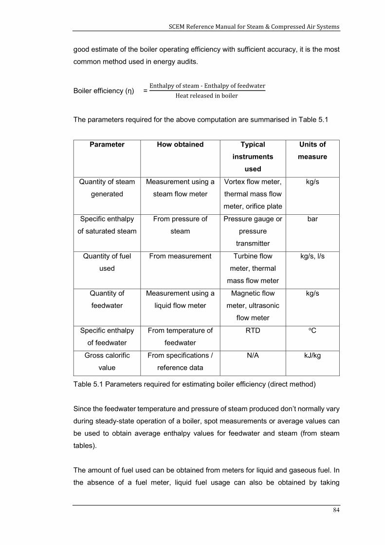
SCEM Reference Manual for Steam & Compressed Air Systems
84
good estimate of the boiler operating efficiency with sufficient accuracy, it is the most
common method used in energy audits.
Boiler efficiency (η) = Enthalpy of steam - Enthalpy of feedwater
Heat released in boiler
The parameters required for the above computation are summarised in Table 5.1
Parameter How obtained Typical
instruments
used
Units of
measure
Quantity of steam
generated
Measurement using a
steam flow meter
Vortex flow meter,
thermal mass flow
meter, orifice plate
kg/s
Specific enthalpy
of saturated steam
From pressure of
steam
Pressure gauge or
pressure
transmitter
bar
Quantity of fuel
used
From measurement Turbine flow
meter, thermal
mass flow meter
kg/s, l/s
Quantity of
feedwater
Measurement using a
liquid flow meter
Magnetic flow
meter, ultrasonic
flow meter
kg/s
Specific enthalpy
of feedwater
From temperature of
feedwater
RTD oC
Gross calorific
value
From specifications /
reference data
N/A kJ/kg
Table 5.1 Parameters required for estimating boiler efficiency (direct method)
Since the feedwater temperature and pressure of steam produced don’t normally vary
during steady-state operation of a boiler, spot measurements or average values can
be used to obtain average enthalpy values for feedwater and steam (from steam
tables).
The amount of fuel used can be obtained from meters for liquid and gaseous fuel. In
the absence of a fuel meter, liquid fuel usage can also be obtained by taking
SCEM Reference Manual for Steam & Compressed Air Systems
85
measurements of the tank level. When solid fuels are used, a weighing scale would
need to be used.
The calorific value of the fuel can be obtained from the specifications provided by the
supplier of the fuel, using reference data or laboratory measurement of a sample of
fuel.
Therefore, the main measurements required are for the quantities of steam output
and feedwater input. In some installations, instruments may be available to measure
both parameters and this would provide the most accurate estimation of the boiler
overall efficiency.
If only a steam flow meter is installed for the boiler, then an ultrasonic liquid flow meter
can be installed to measure the feedwater flow rate during the audit.
However, if a steam flow meter is not available, since it would not be practical to install
a temporary steam flow meter during the audit (flow meter installation will be
intrusive), a temporary liquid flow meter can be used for measuring only the
feedwater. In such a case, the steam output can be estimated by accounting for the
boiler blowdown and subtracting it from the feedwater flow rate as shown below.
Under steady-state operation of a boiler,
ms = mf – mbd (5.1)
where,
ms = steam mass flow rate
mf = feedwater mass flow rate
mbd = mass flow rate of blowdown
Since it is not practical to measure the mass flow rate of blowdown, it can be estimated
using measurements of total dissolved solids (TDS) levels of the feedwater and boiler
water as shown below.
B = [S x FT ] / [MT – FT] (5.2)
and
F = B + S (5.3)
SCEM Reference Manual for Steam & Compressed Air Systems
86
where,
B = blowdown mass flow rate (kg/hr)
S = steam production rate (kg/hr)
F = feedwater mass flow rate (kg/hr)
FT = Feedwater TDS (ppm)
MT = Boiler water TDS (ppm)
Rearranging equations (5.2) and (5.3), the steam flow rate can be expressed in terms
of feedwater flow rate and the TDS values as shown below.
S= F
FTMT-FT
+1 (5.4)
Therefore, if a steam flow meter is not available, the TDS values of the feedwater and
boiler water would need to be measured. Electrical conductivity of water is directly
related to the concentration of dissolved solids in the water. Since the ability for water
to conduct an electric current depends on the ions from the dissolved solids, TDS can
be measured using a conductivity meter. Conductivity provides an approximate value
of the TDS concentration, usually to within 10% accuracy.
5.2 Boiler combustion efficiency
As explained in chapter 2, combustion efficiency is an assessment of how close the
actual combustion is to Stoichiometric combustion, where the oxygen provided is
exactly sufficient for complete combustion of fuel.
It can be measured by sampling the exhaust flue gas to find the composition and
temperature using a combustion analyser. Ideally, the combustion efficiency should
be greater than 80%.
The flue gas temperature measured to assess the combustion efficiency can also be
used to evaluate the potential for heat recovery from exhaust flue gas (if an
economiser is not already installed). The measured exhaust temperature value can
be compared with the minimum stack temperature recommended for the particular
fuel in section 4.6. If there is sufficient potential to reduce the exhaust temperature
without reaching the minimum recommended value, then an economiser can be
considered.
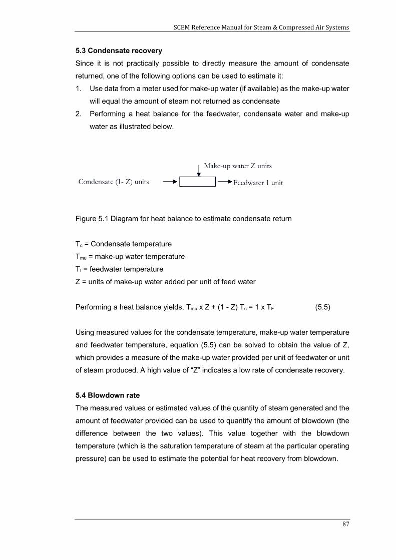
SCEM Reference Manual for Steam & Compressed Air Systems
87
5.3 Condensate recovery
Since it is not practically possible to directly measure the amount of condensate
returned, one of the following options can be used to estimate it:
1. Use data from a meter used for make-up water (if available) as the make-up water
will equal the amount of steam not returned as condensate
2. Performing a heat balance for the feedwater, condensate water and make-up
water as illustrated below.
Figure 5.1 Diagram for heat balance to estimate condensate return
Tc = Condensate temperature
Tmu = make-up water temperature
Tf = feedwater temperature
Z = units of make-up water added per unit of feed water
Performing a heat balance yields, Tmu x Z + (1 - Z) Tc = 1 x TF (5.5)
Using measured values for the condensate temperature, make-up water temperature
and feedwater temperature, equation (5.5) can be solved to obtain the value of Z,
which provides a measure of the make-up water provided per unit of feedwater or unit
of steam produced. A high value of “Z” indicates a low rate of condensate recovery.
5.4 Blowdown rate
The measured values or estimated values of the quantity of steam generated and the
amount of feedwater provided can be used to quantify the amount of blowdown (the
difference between the two values). This value together with the blowdown
temperature (which is the saturation temperature of steam at the particular operating
pressure) can be used to estimate the potential for heat recovery from blowdown.
Make-up water Z units
Feedwater 1 unit Condensate (1- Z) units
SCEM Reference Manual for Steam & Compressed Air Systems
88
5.5 Steam leaks
Visual inspection of steam distribution piping, valves, fittings and steam consuming
process systems can help to identify steam leaks. Since steam leaks cannot usually
be rectified during operation, leaks should be tagged so that they can be rectified
during a system shut-down.
Similarly, observation of steam traps can also help to identify leaks. If steam traps are
directly connected to condensate return piping, then it would not be possible to identify
leaking traps by observation. In such cases, ultrasonic leak detection systems can be
used to identify leaking steam traps.
5.6 Convective and radiative losses
During an energy audit, the surface temperature of the boiler outer surface at various
locations should be measured to check the adequacy of the boiler insulation. An
infrared temperature detector can be used for this purpose. Similarly, the surface
temperature of the feedwater tank, condensate return tank, deaerator, steam
headers, heat exchangers and other process equipment using steam should also be
measured.
5.7 Case study of a boiler energy audit
Information on the system
In a manufacturing plant, three boilers are usually in operation. Diesel is used as the
primary fuel for the boilers. The steam pressure is maintained between 8.9 to 9.0 bar.
Steam produced by the boilers is supplied to the production areas and is mainly used
for process heating. An economiser is installed to recover heat from the flue gas and
pre-heat the make-up water before going into the feedwater tank. In addition, a
condensate recovery system is used to recover condensate from the production
equipment and to return back to the feedwater tank. The feedwater temperature is
usually maintained at around 50 - 70 °C.
The boiler blowdown is manually performed by the operators based on the TDS
indicator on the boiler panel. It is conducted once every 2 hours, to maintain the boiler
TDS at 1700 ppm and below.
Data collection and analysis
The boiler efficiency was estimated using daily steam demand and fuel consumption
data. Cumulative daily figures for above mentioned parameters were recorded for a
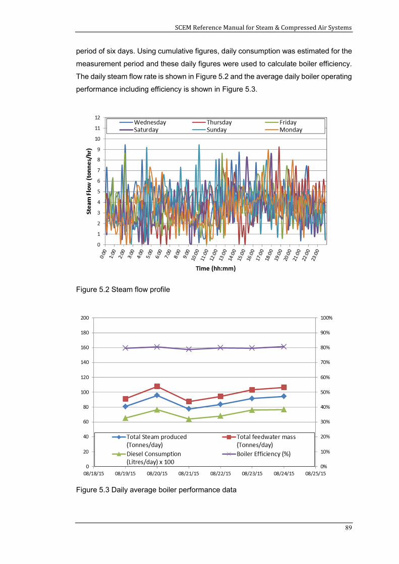
SCEM Reference Manual for Steam & Compressed Air Systems
89
period of six days. Using cumulative figures, daily consumption was estimated for the
measurement period and these daily figures were used to calculate boiler efficiency.
The daily steam flow rate is shown in Figure 5.2 and the average daily boiler operating
performance including efficiency is shown in Figure 5.3.
Figure 5.2 Steam flow profile
Figure 5.3 Daily average boiler performance data
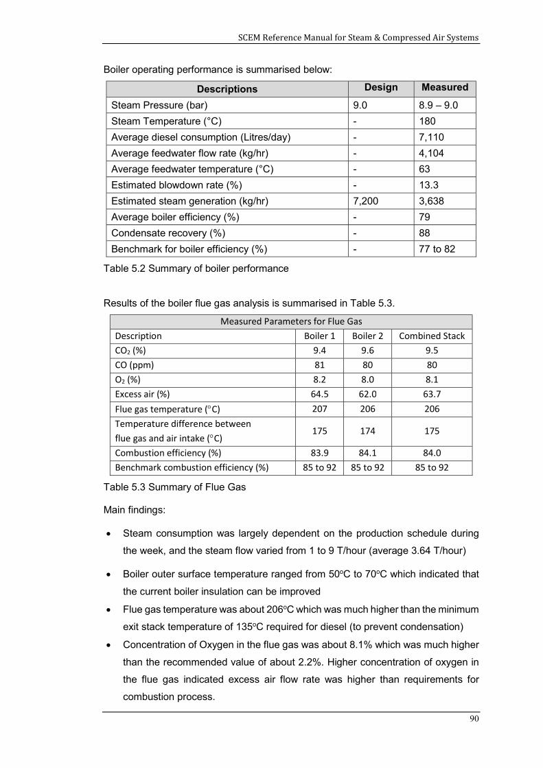
SCEM Reference Manual for Steam & Compressed Air Systems
90
Boiler operating performance is summarised below:
Descriptions Design Measured
Steam Pressure (bar) 9.0 8.9 – 9.0
Steam Temperature (°C) - 180
Average diesel consumption (Litres/day) - 7,110
Average feedwater flow rate (kg/hr) - 4,104
Average feedwater temperature (°C) - 63
Estimated blowdown rate (%) - 13.3
Estimated steam generation (kg/hr) 7,200 3,638
Average boiler efficiency (%) - 79
Condensate recovery (%) - 88
Benchmark for boiler efficiency (%) - 77 to 82
Table 5.2 Summary of boiler performance
Results of the boiler flue gas analysis is summarised in Table 5.3.
Measured Parameters for Flue Gas Description Boiler 1 Boiler 2 Combined Stack CO2 (%) 9.4 9.6 9.5 CO (ppm) 81 80 80 O2 (%) 8.2 8.0 8.1 Excess air (%) 64.5 62.0 63.7 Flue gas temperature (C) 207 206 206 Temperature difference between flue gas and air intake (C)
175 174 175
Combustion efficiency (%) 83.9 84.1 84.0 Benchmark combustion efficiency (%) 85 to 92 85 to 92 85 to 92
Table 5.3 Summary of Flue Gas
Main findings:
Steam consumption was largely dependent on the production schedule during
the week, and the steam flow varied from 1 to 9 T/hour (average 3.64 T/hour)
Boiler outer surface temperature ranged from 50oC to 70oC which indicated that
the current boiler insulation can be improved
Flue gas temperature was about 206oC which was much higher than the minimum
exit stack temperature of 135oC required for diesel (to prevent condensation)
Concentration of Oxygen in the flue gas was about 8.1% which was much higher
than the recommended value of about 2.2%. Higher concentration of oxygen in
the flue gas indicated excess air flow rate was higher than requirements for
combustion process.
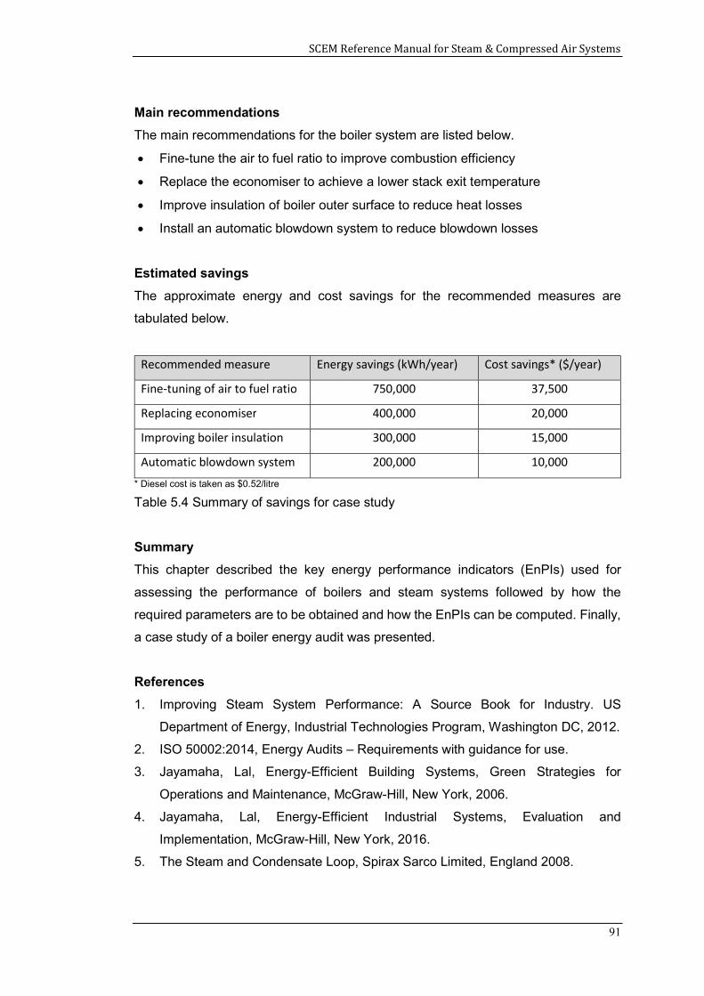
SCEM Reference Manual for Steam & Compressed Air Systems
91
Main recommendations
The main recommendations for the boiler system are listed below.
Fine-tune the air to fuel ratio to improve combustion efficiency
Replace the economiser to achieve a lower stack exit temperature
Improve insulation of boiler outer surface to reduce heat losses
Install an automatic blowdown system to reduce blowdown losses
Estimated savings
The approximate energy and cost savings for the recommended measures are
tabulated below.
Recommended measure Energy savings (kWh/year) Cost savings* ($/year)
Fine-tuning of air to fuel ratio 750,000 37,500
Replacing economiser 400,000 20,000
Improving boiler insulation 300,000 15,000
Automatic blowdown system 200,000 10,000
* Diesel cost is taken as $0.52/litre
Table 5.4 Summary of savings for case study
Summary
This chapter described the key energy performance indicators (EnPIs) used for
assessing the performance of boilers and steam systems followed by how the
required parameters are to be obtained and how the EnPIs can be computed. Finally,
a case study of a boiler energy audit was presented.
References
1. Improving Steam System Performance: A Source Book for Industry. US
Department of Energy, Industrial Technologies Program, Washington DC, 2012.
2. ISO 50002:2014, Energy Audits – Requirements with guidance for use.
3. Jayamaha, Lal, Energy-Efficient Building Systems, Green Strategies for
Operations and Maintenance, McGraw-Hill, New York, 2006.
4. Jayamaha, Lal, Energy-Efficient Industrial Systems, Evaluation and
Implementation, McGraw-Hill, New York, 2016.
5. The Steam and Condensate Loop, Spirax Sarco Limited, England 2008.
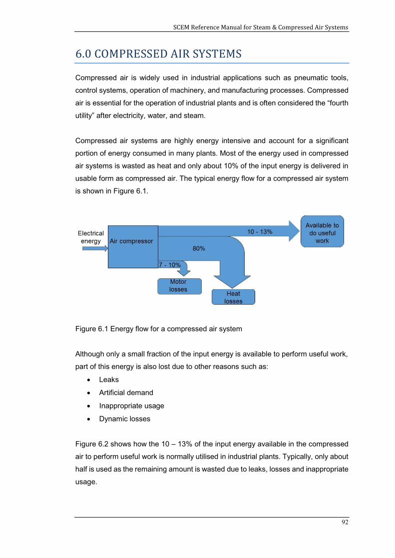
SCEM Reference Manual for Steam & Compressed Air Systems
92
6.0 COMPRESSED AIR SYSTEMS
Compressed air is widely used in industrial applications such as pneumatic tools,
control systems, operation of machinery, and manufacturing processes. Compressed
air is essential for the operation of industrial plants and is often considered the “fourth
utility” after electricity, water, and steam.
Compressed air systems are highly energy intensive and account for a significant
portion of energy consumed in many plants. Most of the energy used in compressed
air systems is wasted as heat and only about 10% of the input energy is delivered in
usable form as compressed air. The typical energy flow for a compressed air system
is shown in Figure 6.1.
Figure 6.1 Energy flow for a compressed air system
Although only a small fraction of the input energy is available to perform useful work,
part of this energy is also lost due to other reasons such as:
Leaks
Artificial demand
Inappropriate usage
Dynamic losses
Figure 6.2 shows how the 10 – 13% of the input energy available in the compressed
air to perform useful work is normally utilised in industrial plants. Typically, only about
half is used as the remaining amount is wasted due to leaks, losses and inappropriate
usage.
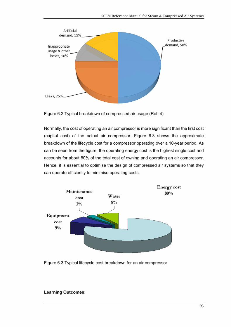
SCEM Reference Manual for Steam & Compressed Air Systems
93
Figure 6.2 Typical breakdown of compressed air usage (Ref. 4)
Normally, the cost of operating an air compressor is more significant than the first cost
(capital cost) of the actual air compressor. Figure 6.3 shows the approximate
breakdown of the lifecycle cost for a compressor operating over a 10-year period. As
can be seen from the figure, the operating energy cost is the highest single cost and
accounts for about 80% of the total cost of owning and operating an air compressor.
Hence, it is essential to optimise the design of compressed air systems so that they
can operate efficiently to minimise operating costs.
Figure 6.3 Typical lifecycle cost breakdown for an air compressor
Learning Outcomes:
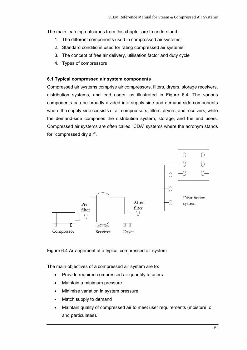
SCEM Reference Manual for Steam & Compressed Air Systems
94
The main learning outcomes from this chapter are to understand:
1. The different components used in compressed air systems
2. Standard conditions used for rating compressed air systems
3. The concept of free air delivery, utilisation factor and duty cycle
4. Types of compressors
6.1 Typical compressed air system components
Compressed air systems comprise air compressors, filters, dryers, storage receivers,
distribution systems, and end users, as illustrated in Figure 6.4. The various
components can be broadly divided into supply-side and demand-side components
where the supply-side consists of air compressors, filters, dryers, and receivers, while
the demand-side comprises the distribution system, storage, and the end users.
Compressed air systems are often called “CDA” systems where the acronym stands
for “compressed dry air”.
Figure 6.4 Arrangement of a typical compressed air system
The main objectives of a compressed air system are to:
Provide required compressed air quantity to users
Maintain a minimum pressure
Minimise variation in system pressure
Match supply to demand
Maintain quality of compressed air to meet user requirements (moisture, oil
and particulates).
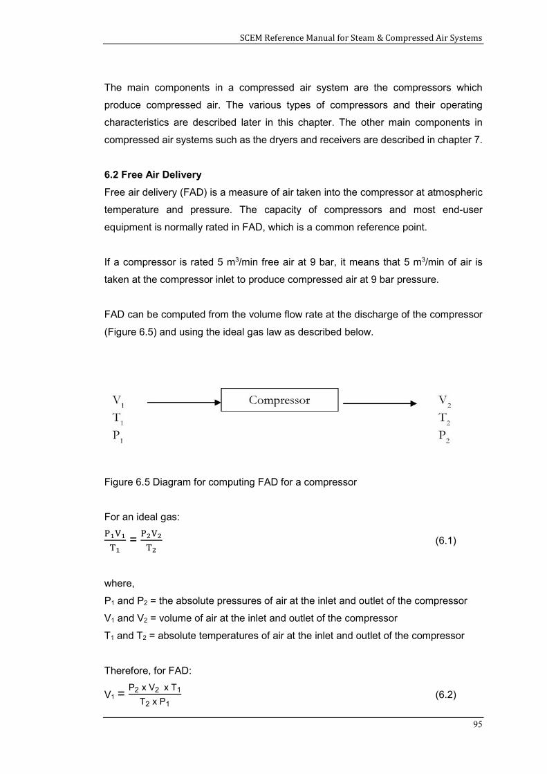
SCEM Reference Manual for Steam & Compressed Air Systems
95
The main components in a compressed air system are the compressors which
produce compressed air. The various types of compressors and their operating
characteristics are described later in this chapter. The other main components in
compressed air systems such as the dryers and receivers are described in chapter 7.
6.2 Free Air Delivery
Free air delivery (FAD) is a measure of air taken into the compressor at atmospheric
temperature and pressure. The capacity of compressors and most end-user
equipment is normally rated in FAD, which is a common reference point.
If a compressor is rated 5 m3/min free air at 9 bar, it means that 5 m3/min of air is
taken at the compressor inlet to produce compressed air at 9 bar pressure.
FAD can be computed from the volume flow rate at the discharge of the compressor
(Figure 6.5) and using the ideal gas law as described below.
Figure 6.5 Diagram for computing FAD for a compressor
For an ideal gas:
= (6.1)
where,
P1 and P2 = the absolute pressures of air at the inlet and outlet of the compressor
V1 and V2 = volume of air at the inlet and outlet of the compressor
T1 and T2 = absolute temperatures of air at the inlet and outlet of the compressor
Therefore, for FAD:
V1 = P2 x V2 x T1
T2 x P1 (6.2)
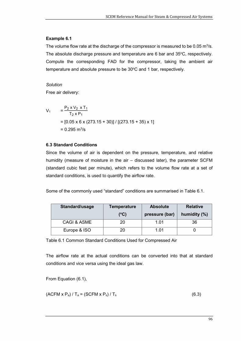
SCEM Reference Manual for Steam & Compressed Air Systems
96
Example 6.1
The volume flow rate at the discharge of the compressor is measured to be 0.05 m3/s.
The absolute discharge pressure and temperature are 6 bar and 35oC, respectively.
Compute the corresponding FAD for the compressor, taking the ambient air
temperature and absolute pressure to be 30oC and 1 bar, respectively.
Solution
Free air delivery:
V1 = P2 x V2 x T1
T2 x P1
= [0.05 x 6 x (273.15 + 30)] / [(273.15 + 35) x 1]
= 0.295 m3/s
6.3 Standard Conditions
Since the volume of air is dependent on the pressure, temperature, and relative
humidity (measure of moisture in the air – discussed later), the parameter SCFM
(standard cubic feet per minute), which refers to the volume flow rate at a set of
standard conditions, is used to quantify the airflow rate.
Some of the commonly used “standard” conditions are summarised in Table 6.1.
Standard/usage Temperature
(oC)
Absolute
pressure (bar)
Relative
humidity (%)
CAGI & ASME 20 1.01 36
Europe & ISO 20 1.01 0
Table 6.1 Common Standard Conditions Used for Compressed Air
The airflow rate at the actual conditions can be converted into that at standard
conditions and vice versa using the ideal gas law.
From Equation (6.1),
(ACFM x Pa) / Ta = (SCFM x Ps) / Ts (6.3)
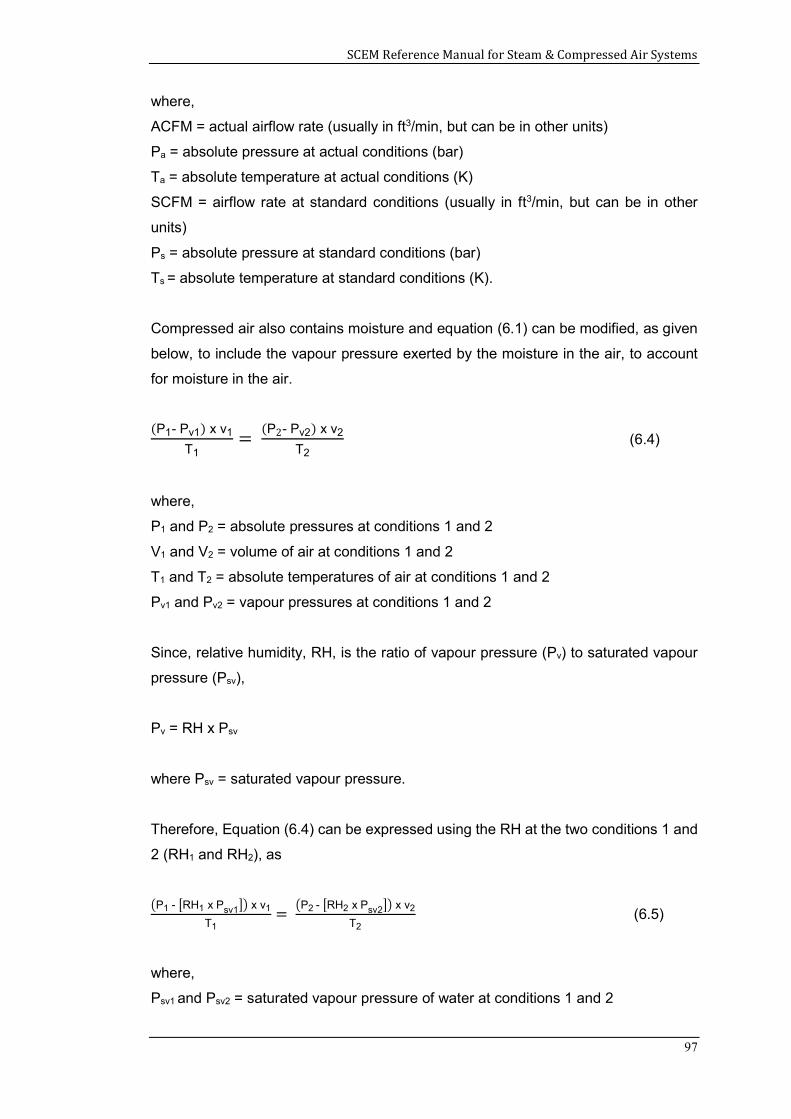
SCEM Reference Manual for Steam & Compressed Air Systems
97
where,
ACFM = actual airflow rate (usually in ft3/min, but can be in other units)
Pa = absolute pressure at actual conditions (bar)
Ta = absolute temperature at actual conditions (K)
SCFM = airflow rate at standard conditions (usually in ft3/min, but can be in other
units)
Ps = absolute pressure at standard conditions (bar)
Ts = absolute temperature at standard conditions (K).
Compressed air also contains moisture and equation (6.1) can be modified, as given
below, to include the vapour pressure exerted by the moisture in the air, to account
for moisture in the air.
(P1- Pv1) x v1
T1=
(P2- Pv2) x v2
T2 (6.4)
where,
P1 and P2 = absolute pressures at conditions 1 and 2
V1 and V2 = volume of air at conditions 1 and 2
T1 and T2 = absolute temperatures of air at conditions 1 and 2
Pv1 and Pv2 = vapour pressures at conditions 1 and 2
Since, relative humidity, RH, is the ratio of vapour pressure (Pv) to saturated vapour
pressure (Psv),
Pv = RH x Psv
where Psv = saturated vapour pressure.
Therefore, Equation (6.4) can be expressed using the RH at the two conditions 1 and
2 (RH1 and RH2), as
P1 - RH1 x Psv1 x v1
T1=
P2 - RH2 x Psv2 x v2
T2 (6.5)
where,
Psv1 and Psv2 = saturated vapour pressure of water at conditions 1 and 2
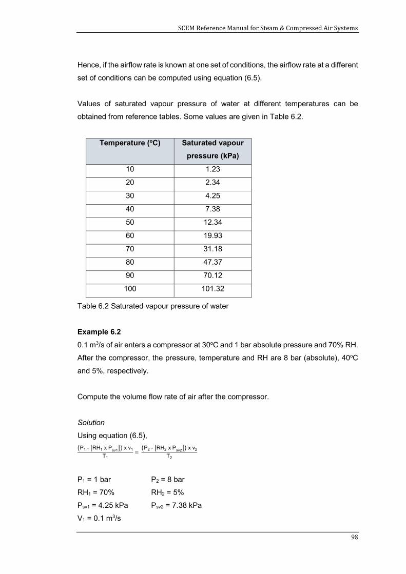
SCEM Reference Manual for Steam & Compressed Air Systems
98
Hence, if the airflow rate is known at one set of conditions, the airflow rate at a different
set of conditions can be computed using equation (6.5).
Values of saturated vapour pressure of water at different temperatures can be
obtained from reference tables. Some values are given in Table 6.2.
Temperature (oC) Saturated vapour
pressure (kPa)
10 1.23
20 2.34
30 4.25
40 7.38
50 12.34
60 19.93
70 31.18
80 47.37
90 70.12
100 101.32
Table 6.2 Saturated vapour pressure of water
Example 6.2
0.1 m3/s of air enters a compressor at 30oC and 1 bar absolute pressure and 70% RH.
After the compressor, the pressure, temperature and RH are 8 bar (absolute), 40oC
and 5%, respectively.
Compute the volume flow rate of air after the compressor.
Solution
Using equation (6.5),
P1 - RH1 x Psv1 x v1
T1=
P2 - RH2 x Psv2 x v2
T2
P1 = 1 bar P2 = 8 bar
RH1 = 70% RH2 = 5%
Psv1 = 4.25 kPa Psv2 = 7.38 kPa
V1 = 0.1 m3/s
SCEM Reference Manual for Steam & Compressed Air Systems
99
T1 = 303 K T2 = 308 K
Therefore, ( [ . x . ]) x .
= ( [ . x . ]) x v2
V2 = 0.012 m3/s
6.4 Utilisation Factor
The utilisation factor (also called the load factor) for a compressed air user is the ratio
of the actual compressed air consumption to the maximum continuous consumption.
Utilisation factor actual air consumption in 24 h
maximum continuous air consumption in 24 h (6.6)
Example 6.3
The rated compressed air usage by a machine is 0.01 m3/s. If the actual compressed
air usage by this machine is measured to be 260 m3/day, calculate the utilisation
factor.
Solution
Utilisation factor = 260 / (0.01 x 3600 x 24) = 0.3
Utilisation factor is used to estimate the total compressed air requirements when
designing a new plant. Although many industrial plants have a large number of
pneumatic tools and users, most of them may not operate simultaneously. Therefore,
to prevent oversizing of the system, utilisation factors for the various users can be
used to compute the approximate average total compressed air consumption, as
illustrated in Example 6.4.
Similarly, the utilisation factor for a compressor can be expressed as the ratio of the
actual compressed air output in a period of time to the output when operating at
maximum capacity for the same period of time.
Example 6.4
Compressed air requirements for a new system are summarised in Table 6.3.
Estimate the FAD for a suitable compressor for this application.
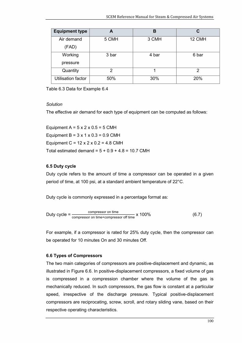
SCEM Reference Manual for Steam & Compressed Air Systems
100
Equipment type A B C
Air demand
(FAD)
5 CMH 3 CMH 12 CMH
Working
pressure
3 bar 4 bar 6 bar
Quantity 2 1 2
Utilisation factor 50% 30% 20%
Table 6.3 Data for Example 6.4
Solution
The effective air demand for each type of equipment can be computed as follows:
Equipment A = 5 x 2 x 0.5 = 5 CMH
Equipment B = 3 x 1 x 0.3 = 0.9 CMH
Equipment C = 12 x 2 x 0.2 = 4.8 CMH
Total estimated demand = 5 + 0.9 + 4.8 = 10.7 CMH
6.5 Duty cycle
Duty cycle refers to the amount of time a compressor can be operated in a given
period of time, at 100 psi, at a standard ambient temperature of 22°C.
Duty cycle is commonly expressed in a percentage format as:
Duty cycle = compressor on time
compressor on time+compressor off time x 100% (6.7)
For example, if a compressor is rated for 25% duty cycle, then the compressor can
be operated for 10 minutes On and 30 minutes Off.
6.6 Types of Compressors
The two main categories of compressors are positive-displacement and dynamic, as
illustrated in Figure 6.6. In positive-displacement compressors, a fixed volume of gas
is compressed in a compression chamber where the volume of the gas is
mechanically reduced. In such compressors, the gas flow is constant at a particular
speed, irrespective of the discharge pressure. Typical positive-displacement
compressors are reciprocating, screw, scroll, and rotary sliding vane, based on their
respective operating characteristics.
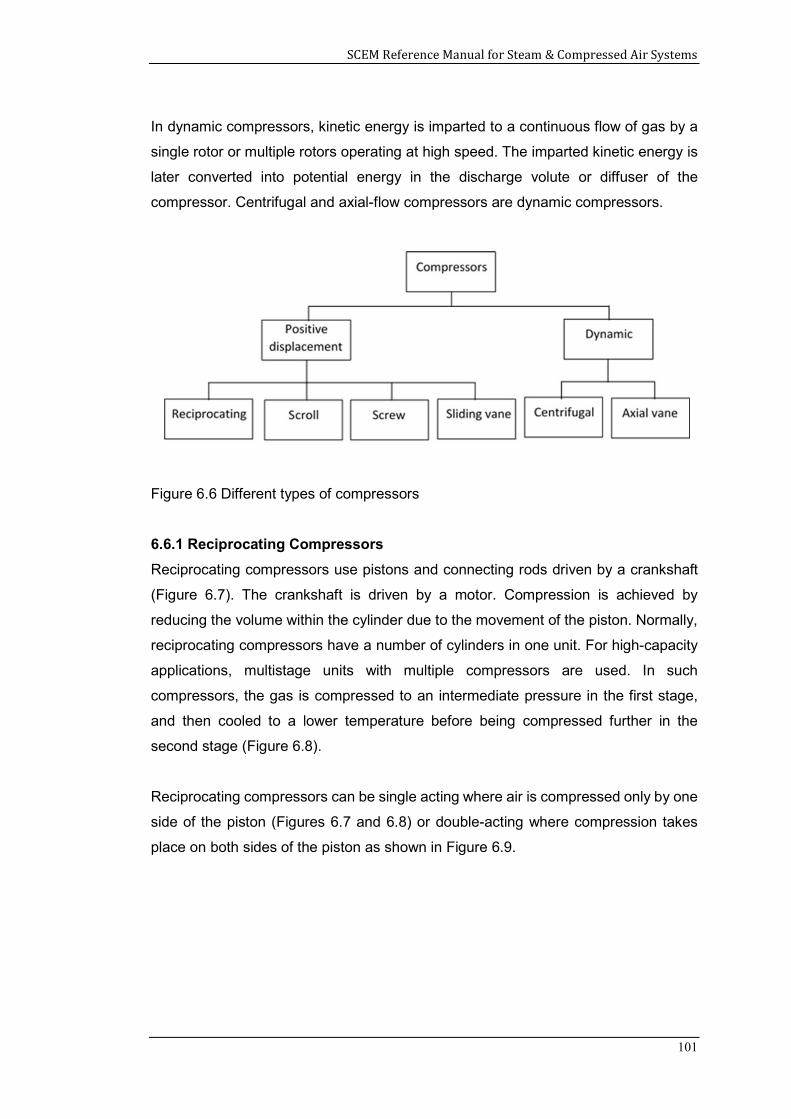
SCEM Reference Manual for Steam & Compressed Air Systems
101
In dynamic compressors, kinetic energy is imparted to a continuous flow of gas by a
single rotor or multiple rotors operating at high speed. The imparted kinetic energy is
later converted into potential energy in the discharge volute or diffuser of the
compressor. Centrifugal and axial-flow compressors are dynamic compressors.
Figure 6.6 Different types of compressors
6.6.1 Reciprocating Compressors
Reciprocating compressors use pistons and connecting rods driven by a crankshaft
(Figure 6.7). The crankshaft is driven by a motor. Compression is achieved by
reducing the volume within the cylinder due to the movement of the piston. Normally,
reciprocating compressors have a number of cylinders in one unit. For high-capacity
applications, multistage units with multiple compressors are used. In such
compressors, the gas is compressed to an intermediate pressure in the first stage,
and then cooled to a lower temperature before being compressed further in the
second stage (Figure 6.8).
Reciprocating compressors can be single acting where air is compressed only by one
side of the piston (Figures 6.7 and 6.8) or double-acting where compression takes
place on both sides of the piston as shown in Figure 6.9.
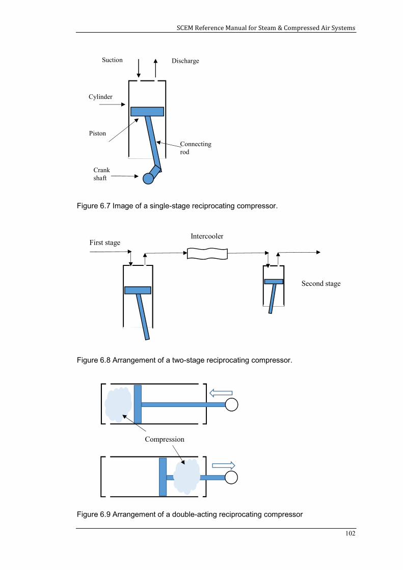
SCEM Reference Manual for Steam & Compressed Air Systems
102
Figure 6.7 Image of a single-stage reciprocating compressor.
Figure 6.8 Arrangement of a two-stage reciprocating compressor.
Figure 6.9 Arrangement of a double-acting reciprocating compressor
Suction Discharge
Cylinder
Piston
Crank shaft
Connecting rod
Intercooler
Second stage
First stage
V V
Compression
V V
V V
V V
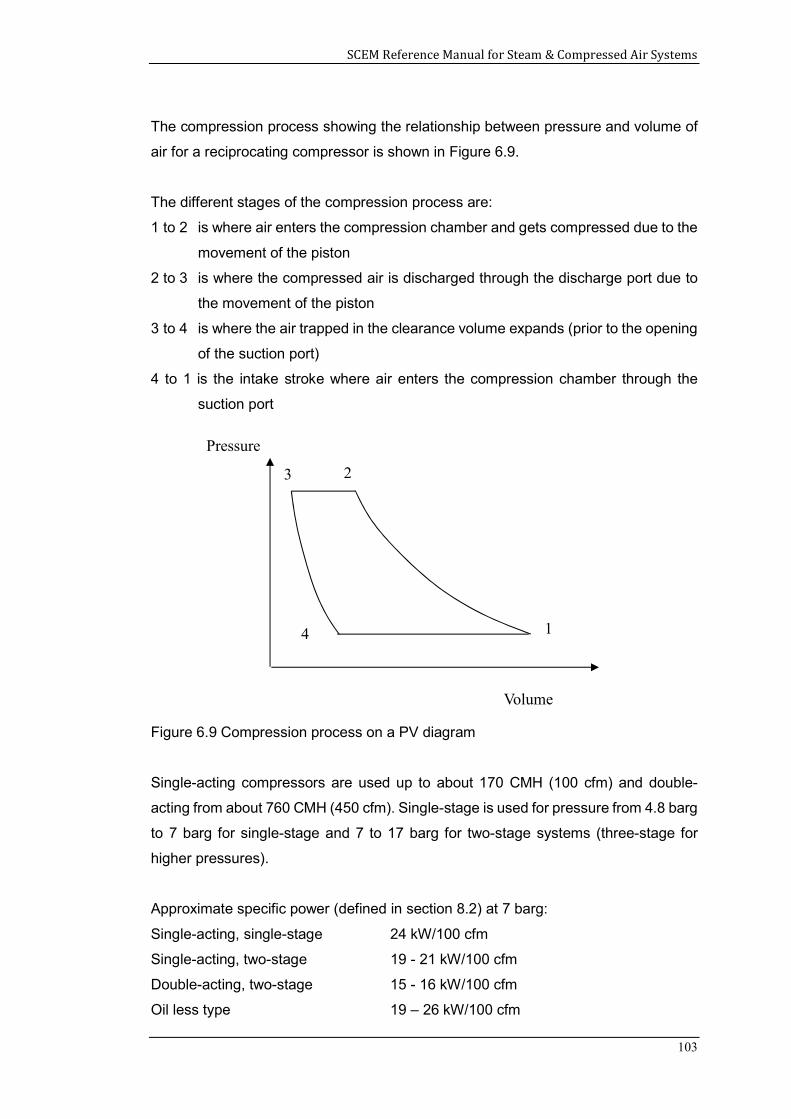
SCEM Reference Manual for Steam & Compressed Air Systems
103
The compression process showing the relationship between pressure and volume of
air for a reciprocating compressor is shown in Figure 6.9.
The different stages of the compression process are:
1 to 2 is where air enters the compression chamber and gets compressed due to the
movement of the piston
2 to 3 is where the compressed air is discharged through the discharge port due to
the movement of the piston
3 to 4 is where the air trapped in the clearance volume expands (prior to the opening
of the suction port)
4 to 1 is the intake stroke where air enters the compression chamber through the
suction port
Figure 6.9 Compression process on a PV diagram
Single-acting compressors are used up to about 170 CMH (100 cfm) and double-
acting from about 760 CMH (450 cfm). Single-stage is used for pressure from 4.8 barg
to 7 barg for single-stage and 7 to 17 barg for two-stage systems (three-stage for
higher pressures).
Approximate specific power (defined in section 8.2) at 7 barg:
Single-acting, single-stage 24 kW/100 cfm
Single-acting, two-stage 19 - 21 kW/100 cfm
Double-acting, two-stage 15 - 16 kW/100 cfm
Oil less type 19 – 26 kW/100 cfm
Pressure
VolumeVolume
1
2 3
4
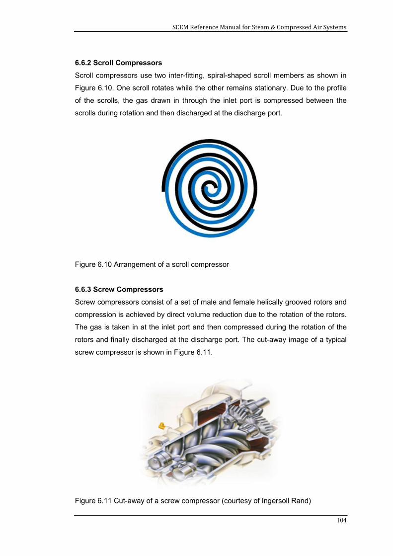
SCEM Reference Manual for Steam & Compressed Air Systems
104
6.6.2 Scroll Compressors
Scroll compressors use two inter-fitting, spiral-shaped scroll members as shown in
Figure 6.10. One scroll rotates while the other remains stationary. Due to the profile
of the scrolls, the gas drawn in through the inlet port is compressed between the
scrolls during rotation and then discharged at the discharge port.
Figure 6.10 Arrangement of a scroll compressor
6.6.3 Screw Compressors
Screw compressors consist of a set of male and female helically grooved rotors and
compression is achieved by direct volume reduction due to the rotation of the rotors.
The gas is taken in at the inlet port and then compressed during the rotation of the
rotors and finally discharged at the discharge port. The cut-away image of a typical
screw compressor is shown in Figure 6.11.
Figure 6.11 Cut-away of a screw compressor (courtesy of Ingersoll Rand)
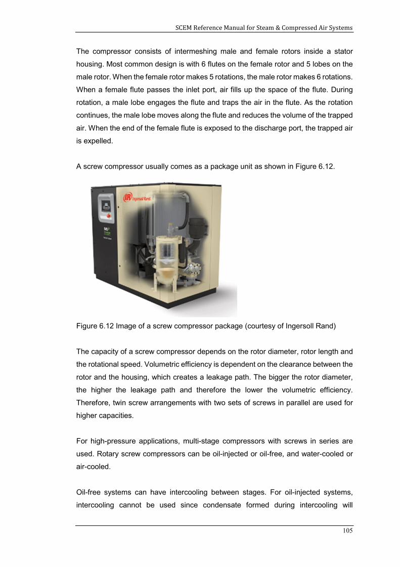
SCEM Reference Manual for Steam & Compressed Air Systems
105
The compressor consists of intermeshing male and female rotors inside a stator
housing. Most common design is with 6 flutes on the female rotor and 5 lobes on the
male rotor. When the female rotor makes 5 rotations, the male rotor makes 6 rotations.
When a female flute passes the inlet port, air fills up the space of the flute. During
rotation, a male lobe engages the flute and traps the air in the flute. As the rotation
continues, the male lobe moves along the flute and reduces the volume of the trapped
air. When the end of the female flute is exposed to the discharge port, the trapped air
is expelled.
A screw compressor usually comes as a package unit as shown in Figure 6.12.
Figure 6.12 Image of a screw compressor package (courtesy of Ingersoll Rand)
The capacity of a screw compressor depends on the rotor diameter, rotor length and
the rotational speed. Volumetric efficiency is dependent on the clearance between the
rotor and the housing, which creates a leakage path. The bigger the rotor diameter,
the higher the leakage path and therefore the lower the volumetric efficiency.
Therefore, twin screw arrangements with two sets of screws in parallel are used for
higher capacities.
For high-pressure applications, multi-stage compressors with screws in series are
used. Rotary screw compressors can be oil-injected or oil-free, and water-cooled or
air-cooled.
Oil-free systems can have intercooling between stages. For oil-injected systems,
intercooling cannot be used since condensate formed during intercooling will
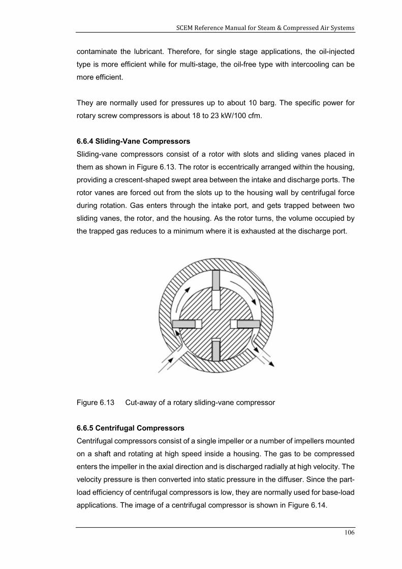
SCEM Reference Manual for Steam & Compressed Air Systems
106
contaminate the lubricant. Therefore, for single stage applications, the oil-injected
type is more efficient while for multi-stage, the oil-free type with intercooling can be
more efficient.
They are normally used for pressures up to about 10 barg. The specific power for
rotary screw compressors is about 18 to 23 kW/100 cfm.
6.6.4 Sliding-Vane Compressors
Sliding-vane compressors consist of a rotor with slots and sliding vanes placed in
them as shown in Figure 6.13. The rotor is eccentrically arranged within the housing,
providing a crescent-shaped swept area between the intake and discharge ports. The
rotor vanes are forced out from the slots up to the housing wall by centrifugal force
during rotation. Gas enters through the intake port, and gets trapped between two
sliding vanes, the rotor, and the housing. As the rotor turns, the volume occupied by
the trapped gas reduces to a minimum where it is exhausted at the discharge port.
Figure 6.13 Cut-away of a rotary sliding-vane compressor
6.6.5 Centrifugal Compressors
Centrifugal compressors consist of a single impeller or a number of impellers mounted
on a shaft and rotating at high speed inside a housing. The gas to be compressed
enters the impeller in the axial direction and is discharged radially at high velocity. The
velocity pressure is then converted into static pressure in the diffuser. Since the part-
load efficiency of centrifugal compressors is low, they are normally used for base-load
applications. The image of a centrifugal compressor is shown in Figure 6.14.
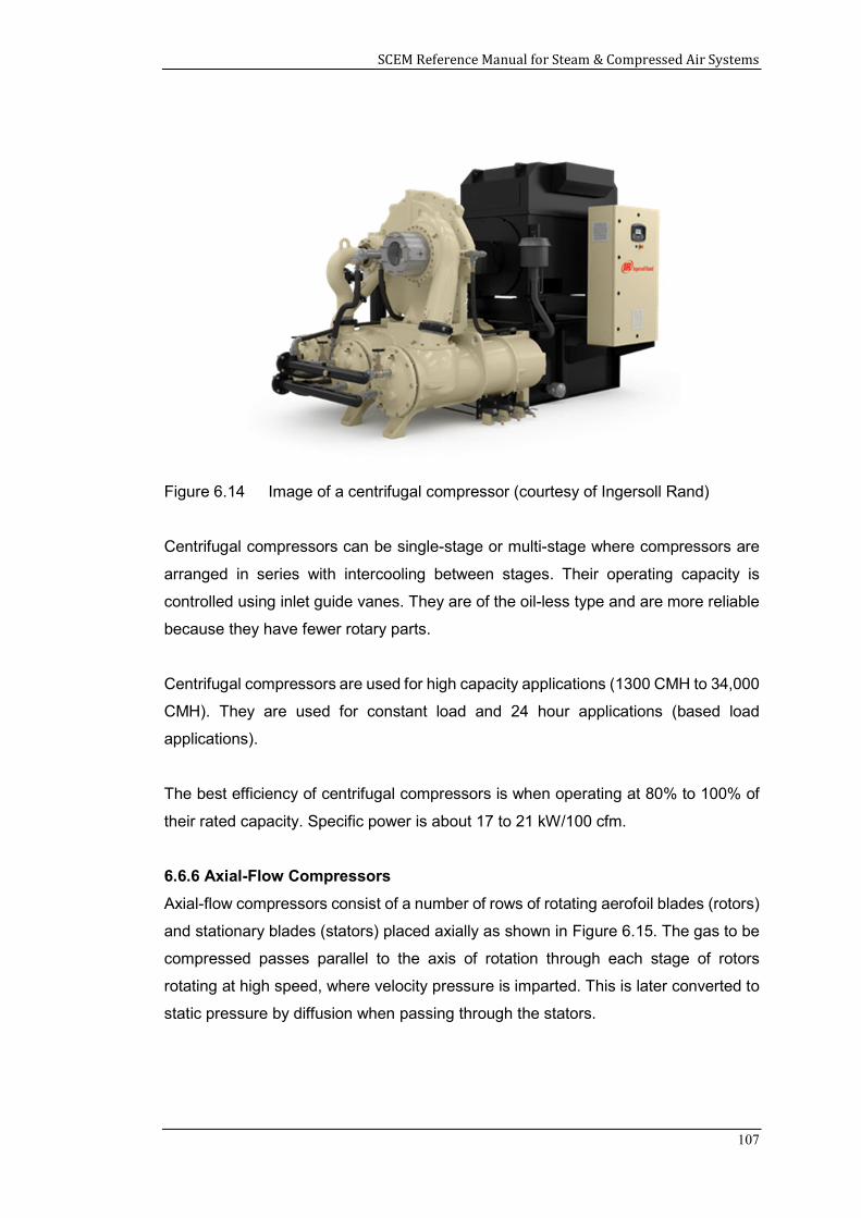
SCEM Reference Manual for Steam & Compressed Air Systems
107
Figure 6.14 Image of a centrifugal compressor (courtesy of Ingersoll Rand)
Centrifugal compressors can be single-stage or multi-stage where compressors are
arranged in series with intercooling between stages. Their operating capacity is
controlled using inlet guide vanes. They are of the oil-less type and are more reliable
because they have fewer rotary parts.
Centrifugal compressors are used for high capacity applications (1300 CMH to 34,000
CMH). They are used for constant load and 24 hour applications (based load
applications).
The best efficiency of centrifugal compressors is when operating at 80% to 100% of
their rated capacity. Specific power is about 17 to 21 kW/100 cfm.
6.6.6 Axial-Flow Compressors
Axial-flow compressors consist of a number of rows of rotating aerofoil blades (rotors)
and stationary blades (stators) placed axially as shown in Figure 6.15. The gas to be
compressed passes parallel to the axis of rotation through each stage of rotors
rotating at high speed, where velocity pressure is imparted. This is later converted to
static pressure by diffusion when passing through the stators.
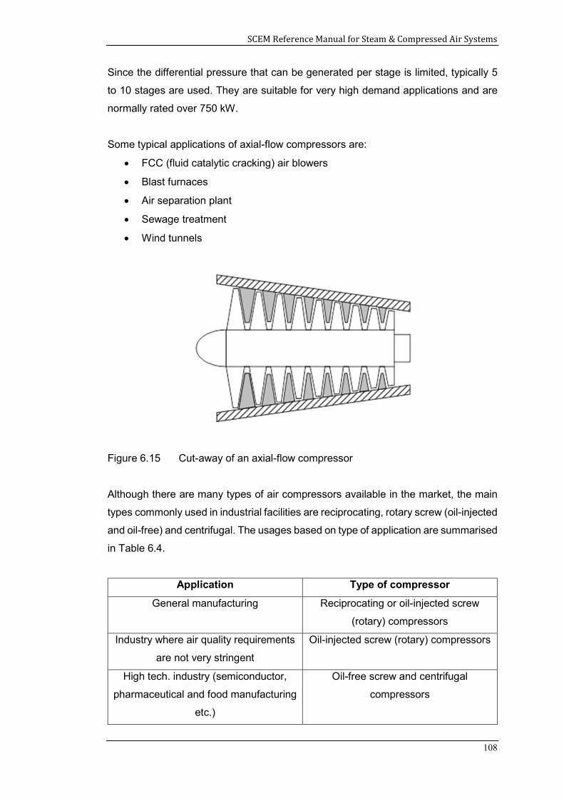
SCEM Reference Manual for Steam & Compressed Air Systems
108
Since the differential pressure that can be generated per stage is limited, typically 5
to 10 stages are used. They are suitable for very high demand applications and are
normally rated over 750 kW.
Some typical applications of axial-flow compressors are:
FCC (fluid catalytic cracking) air blowers
Blast furnaces
Air separation plant
Sewage treatment
Wind tunnels
Figure 6.15 Cut-away of an axial-flow compressor
Although there are many types of air compressors available in the market, the main
types commonly used in industrial facilities are reciprocating, rotary screw (oil-injected
and oil-free) and centrifugal. The usages based on type of application are summarised
in Table 6.4.
Application Type of compressor
General manufacturing Reciprocating or oil-injected screw
(rotary) compressors
Industry where air quality requirements
are not very stringent
Oil-injected screw (rotary) compressors
High tech. industry (semiconductor,
pharmaceutical and food manufacturing
etc.)
Oil-free screw and centrifugal
compressors
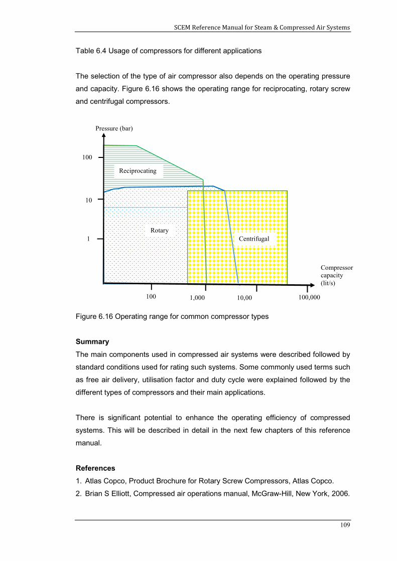
SCEM Reference Manual for Steam & Compressed Air Systems
109
Table 6.4 Usage of compressors for different applications
The selection of the type of air compressor also depends on the operating pressure
and capacity. Figure 6.16 shows the operating range for reciprocating, rotary screw
and centrifugal compressors.
Figure 6.16 Operating range for common compressor types
Summary
The main components used in compressed air systems were described followed by
standard conditions used for rating such systems. Some commonly used terms such
as free air delivery, utilisation factor and duty cycle were explained followed by the
different types of compressors and their main applications.
There is significant potential to enhance the operating efficiency of compressed
systems. This will be described in detail in the next few chapters of this reference
manual.
References
1. Atlas Copco, Product Brochure for Rotary Screw Compressors, Atlas Copco.
2. Brian S Elliott, Compressed air operations manual, McGraw-Hill, New York, 2006.
10
100
Pressure (bar)
Compressor capacity (lit/s)
1,000 10,000
100,000 100
1 Rotary
Reciprocating
Centrifugal
SCEM Reference Manual for Steam & Compressed Air Systems
110
3. Compressed Air Production (Compressors), Chapter 2, Compressed Air and Gas
Institute
4. Ed Attanasio, Compressed Air Best Practices, Advanced Air Leak Detection
Services (https://www.airbestpractices.com/system-assessments /leaks/
maintenance-saves-energy)
5. Good Practice Guide 241, “Energy savings in the selection, control and
maintenance of air compressors”, Department of the Environment, Transport and
the Regions, UK, 1998.
6. Improving compressed air system performance: A source book for industry, US
DOE, 2003.
7. Jayamaha, Lal, Energy-Efficient Industrial Systems, Evaluation and
Implementation, McGraw-Hill, New York, 2016.
SCEM Reference Manual for Steam & Compressed Air Systems
111
7.0 AUXILIARY EQUIPMENT IN COMPRESSED AIR SYSTEMS
The basic objectives of a compressed air system are to:
Provide the required compressed air quantity to users
Maintain a minimum pressure
Minimise variation in system pressure
Match supply to demand
Maintain quality of air to meet user requirements (moisture, oil etc.)
Therefore, in addition to the air compressors, a variety of other auxiliary equipment is
used in compressed air systems. Some of the main auxiliary equipment used in
compressed air systems are:
Dryers
Receiver tanks
Filters
After coolers
Distribution system
This chapter describes the main auxiliary equipment used in compressed air systems.
Learning Outcomes:
The main learning outcomes from this chapter are to understand:
1. The main types of auxiliary equipment used in compressed air systems
2. The various applications of auxiliary equipment based on the various
requirements of the end-users of compressed air
7.1 Dryers
Air contains moisture and when compressed, the same amount of moisture is then
contained in a lower volume of air. This results in condensation which needs to be
removed as otherwise it could damage equipment, cause corrosion and even affect
the performance of systems.
Moisture therefore needs to be removed from compressed air before being supplied
to most end users. The aftercooler that is used to cool the air after compression to
bring it down to a usable temperature removes a significant amount of moisture from
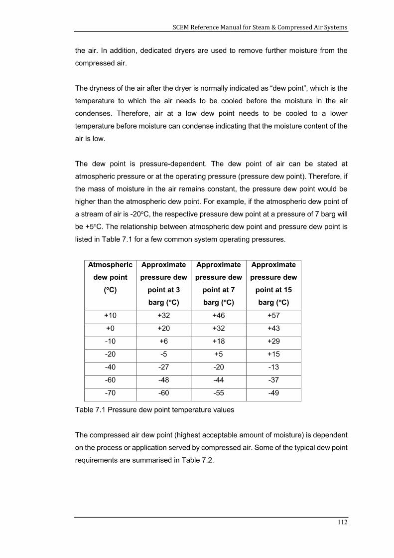
SCEM Reference Manual for Steam & Compressed Air Systems
112
the air. In addition, dedicated dryers are used to remove further moisture from the
compressed air.
The dryness of the air after the dryer is normally indicated as “dew point”, which is the
temperature to which the air needs to be cooled before the moisture in the air
condenses. Therefore, air at a low dew point needs to be cooled to a lower
temperature before moisture can condense indicating that the moisture content of the
air is low.
The dew point is pressure-dependent. The dew point of air can be stated at
atmospheric pressure or at the operating pressure (pressure dew point). Therefore, if
the mass of moisture in the air remains constant, the pressure dew point would be
higher than the atmospheric dew point. For example, if the atmospheric dew point of
a stream of air is -20oC, the respective pressure dew point at a pressure of 7 barg will
be +5oC. The relationship between atmospheric dew point and pressure dew point is
listed in Table 7.1 for a few common system operating pressures.
Atmospheric
dew point
(oC)
Approximate
pressure dew
point at 3
barg (oC)
Approximate
pressure dew
point at 7
barg (oC)
Approximate
pressure dew
point at 15
barg (oC)
+10 +32 +46 +57
+0 +20 +32 +43
-10 +6 +18 +29
-20 -5 +5 +15
-40 -27 -20 -13
-60 -48 -44 -37
-70 -60 -55 -49
Table 7.1 Pressure dew point temperature values
The compressed air dew point (highest acceptable amount of moisture) is dependent
on the process or application served by compressed air. Some of the typical dew point
requirements are summarised in Table 7.2.
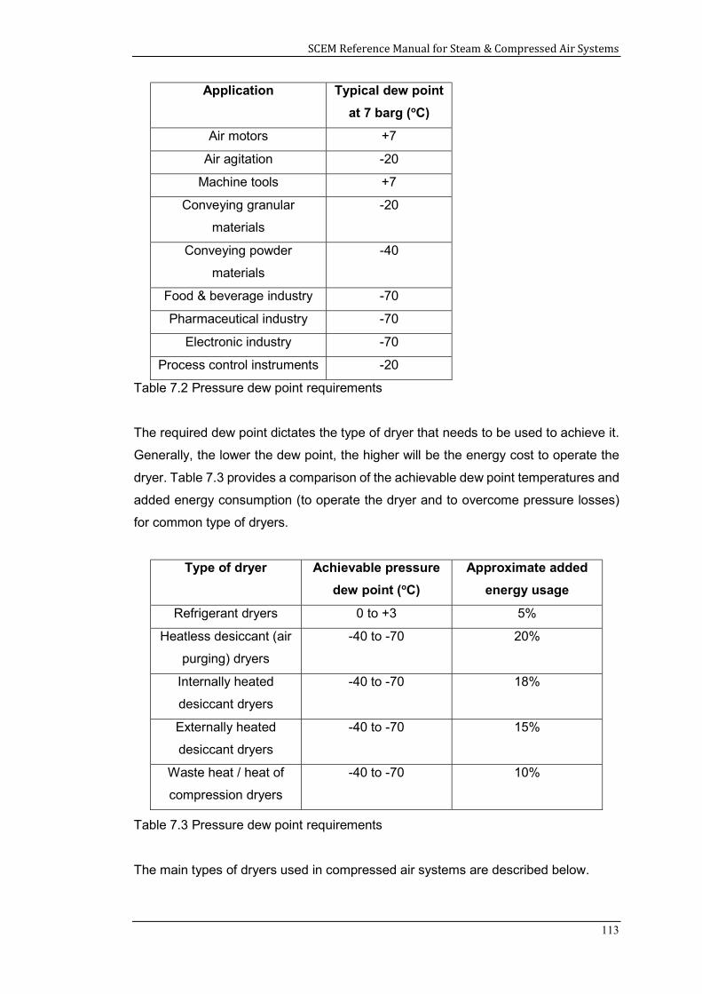
SCEM Reference Manual for Steam & Compressed Air Systems
113
Application Typical dew point
at 7 barg (oC)
Air motors +7
Air agitation -20
Machine tools +7
Conveying granular
materials
-20
Conveying powder
materials
-40
Food & beverage industry -70
Pharmaceutical industry -70
Electronic industry -70
Process control instruments -20
Table 7.2 Pressure dew point requirements
The required dew point dictates the type of dryer that needs to be used to achieve it.
Generally, the lower the dew point, the higher will be the energy cost to operate the
dryer. Table 7.3 provides a comparison of the achievable dew point temperatures and
added energy consumption (to operate the dryer and to overcome pressure losses)
for common type of dryers.
Type of dryer Achievable pressure
dew point (oC)
Approximate added
energy usage
Refrigerant dryers 0 to +3 5%
Heatless desiccant (air
purging) dryers
-40 to -70 20%
Internally heated
desiccant dryers
-40 to -70 18%
Externally heated
desiccant dryers
-40 to -70 15%
Waste heat / heat of
compression dryers
-40 to -70 10%
Table 7.3 Pressure dew point requirements
The main types of dryers used in compressed air systems are described below.
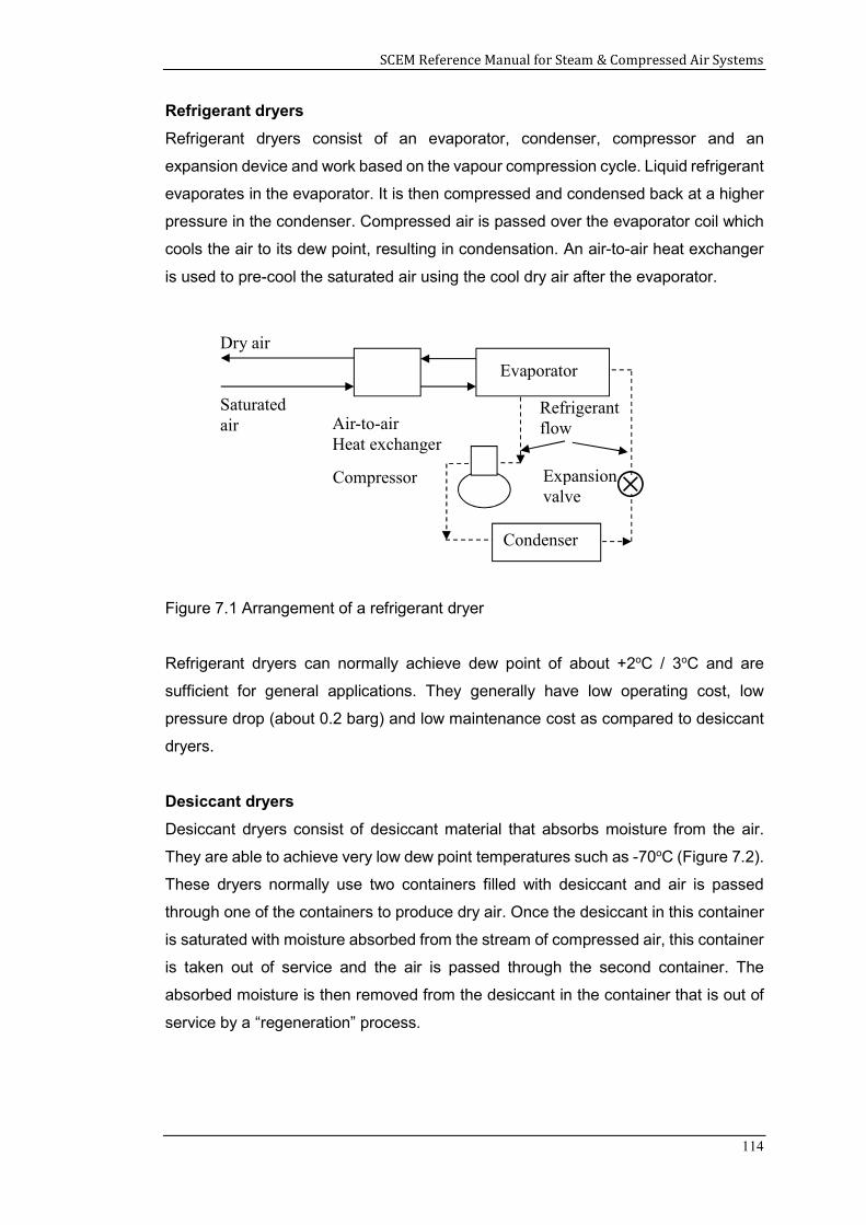
SCEM Reference Manual for Steam & Compressed Air Systems
114
Refrigerant dryers
Refrigerant dryers consist of an evaporator, condenser, compressor and an
expansion device and work based on the vapour compression cycle. Liquid refrigerant
evaporates in the evaporator. It is then compressed and condensed back at a higher
pressure in the condenser. Compressed air is passed over the evaporator coil which
cools the air to its dew point, resulting in condensation. An air-to-air heat exchanger
is used to pre-cool the saturated air using the cool dry air after the evaporator.
Figure 7.1 Arrangement of a refrigerant dryer
Refrigerant dryers can normally achieve dew point of about +2oC / 3oC and are
sufficient for general applications. They generally have low operating cost, low
pressure drop (about 0.2 barg) and low maintenance cost as compared to desiccant
dryers.
Desiccant dryers
Desiccant dryers consist of desiccant material that absorbs moisture from the air.
They are able to achieve very low dew point temperatures such as -70oC (Figure 7.2).
These dryers normally use two containers filled with desiccant and air is passed
through one of the containers to produce dry air. Once the desiccant in this container
is saturated with moisture absorbed from the stream of compressed air, this container
is taken out of service and the air is passed through the second container. The
absorbed moisture is then removed from the desiccant in the container that is out of
service by a “regeneration” process.
Air-to-air Heat exchanger
Evaporator coil
Saturated air
Dry air
Expansion valve
Compressor
Refrigerant flow
Condenser
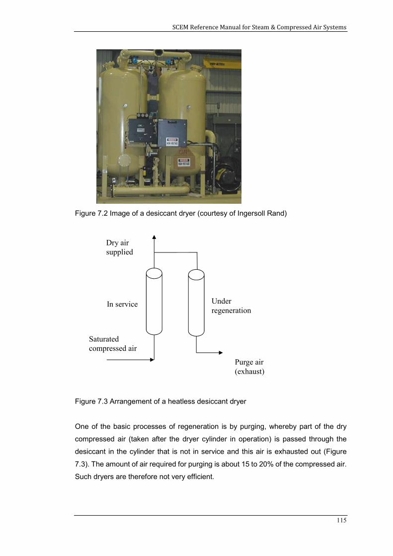
SCEM Reference Manual for Steam & Compressed Air Systems
115
Figure 7.2 Image of a desiccant dryer (courtesy of Ingersoll Rand)
Figure 7.3 Arrangement of a heatless desiccant dryer
One of the basic processes of regeneration is by purging, whereby part of the dry
compressed air (taken after the dryer cylinder in operation) is passed through the
desiccant in the cylinder that is not in service and this air is exhausted out (Figure
7.3). The amount of air required for purging is about 15 to 20% of the compressed air.
Such dryers are therefore not very efficient.
Saturated compressed air
In service Under regeneration
Dry air supplied
Purge air (exhaust)
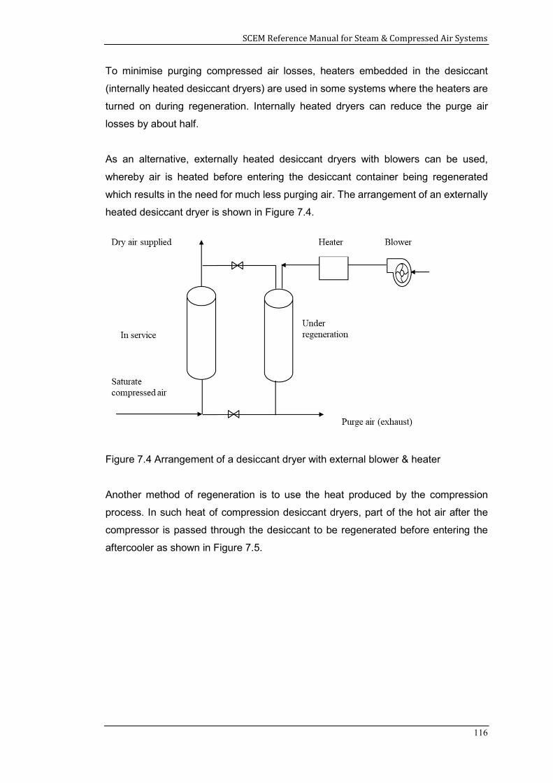
SCEM Reference Manual for Steam & Compressed Air Systems
116
To minimise purging compressed air losses, heaters embedded in the desiccant
(internally heated desiccant dryers) are used in some systems where the heaters are
turned on during regeneration. Internally heated dryers can reduce the purge air
losses by about half.
As an alternative, externally heated desiccant dryers with blowers can be used,
whereby air is heated before entering the desiccant container being regenerated
which results in the need for much less purging air. The arrangement of an externally
heated desiccant dryer is shown in Figure 7.4.
Figure 7.4 Arrangement of a desiccant dryer with external blower & heater
Another method of regeneration is to use the heat produced by the compression
process. In such heat of compression desiccant dryers, part of the hot air after the
compressor is passed through the desiccant to be regenerated before entering the
aftercooler as shown in Figure 7.5.
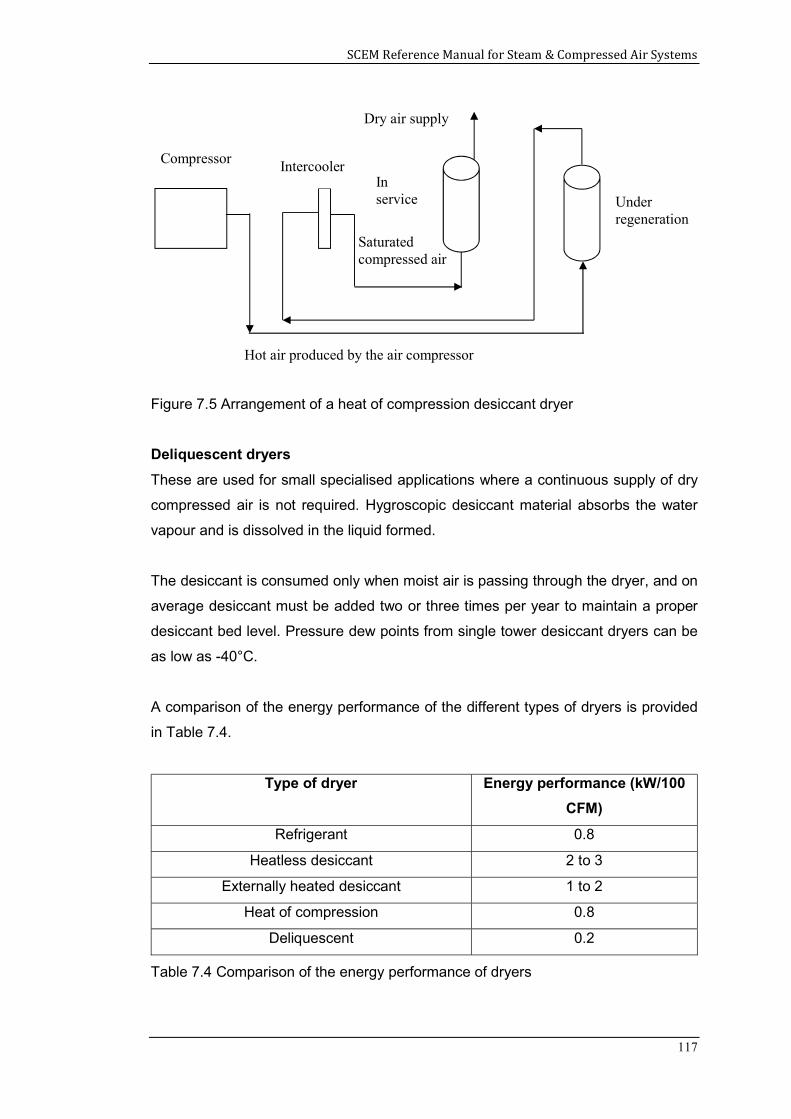
SCEM Reference Manual for Steam & Compressed Air Systems
117
Figure 7.5 Arrangement of a heat of compression desiccant dryer
Deliquescent dryers
These are used for small specialised applications where a continuous supply of dry
compressed air is not required. Hygroscopic desiccant material absorbs the water
vapour and is dissolved in the liquid formed.
The desiccant is consumed only when moist air is passing through the dryer, and on
average desiccant must be added two or three times per year to maintain a proper
desiccant bed level. Pressure dew points from single tower desiccant dryers can be
as low as -40°C.
A comparison of the energy performance of the different types of dryers is provided
in Table 7.4.
Type of dryer Energy performance (kW/100
CFM)
Refrigerant 0.8
Heatless desiccant 2 to 3
Externally heated desiccant 1 to 2
Heat of compression 0.8
Deliquescent 0.2
Table 7.4 Comparison of the energy performance of dryers
Saturated compressed air
In service Under
regeneration
Dry air supply
Hot air produced by the air compressor
Compressor Intercooler
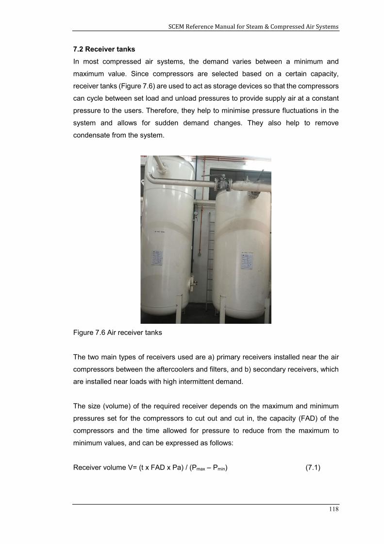
SCEM Reference Manual for Steam & Compressed Air Systems
118
7.2 Receiver tanks
In most compressed air systems, the demand varies between a minimum and
maximum value. Since compressors are selected based on a certain capacity,
receiver tanks (Figure 7.6) are used to act as storage devices so that the compressors
can cycle between set load and unload pressures to provide supply air at a constant
pressure to the users. Therefore, they help to minimise pressure fluctuations in the
system and allows for sudden demand changes. They also help to remove
condensate from the system.
Figure 7.6 Air receiver tanks
The two main types of receivers used are a) primary receivers installed near the air
compressors between the aftercoolers and filters, and b) secondary receivers, which
are installed near loads with high intermittent demand.
The size (volume) of the required receiver depends on the maximum and minimum
pressures set for the compressors to cut out and cut in, the capacity (FAD) of the
compressors and the time allowed for pressure to reduce from the maximum to
minimum values, and can be expressed as follows:
Receiver volume V= (t x FAD x Pa) / (Pmax – Pmin) (7.1)
SCEM Reference Manual for Steam & Compressed Air Systems
119
where,
V is in m3
t = time required (seconds) to increase receiver pressure from Pmin to Pmax
Pmax = maximum pressure at which the compressor cuts out (bar)
Pmin = maximum pressure at which the compressor cuts in (bar)
Pa = atmospheric pressure (bar)
FAD = free air delivery required (m3/s)
Since in most situations, the size of the receiver tank installed is known, the above
relationship can be used to estimate the FAD of the compressor by measuring the
time taken (t) for the receiver pressure to increase from Pmin to Pmax (with the discharge
valve after the receiver closed).
Example 7.1
Compute the FAD of an air compressor if it takes 30 seconds to increase the receiver
tank pressure from 7 bar to 9 bar (both absolute pressures). The receiver tank volume
is 1m3.
Solution
Using relationship (7.1),
Receiver volume V= (t x FAD x Pa) / (Pmax – Pmin)
Therefore, FAD = V x (Pmax – Pmin) / (t x Pa) = 1 x (9 – 7) / 30 x 1 = 0.067 m3/s
7.3 Filters
Dirt particles, liquid droplets and water vapour can enter compressed air systems
through the intake. In addition, other contaminants like oil droplets can be introduced
by the air compressor. Depending on user requirements, the contaminants may need
to be removed to achieve the acceptable level of air quality.
Therefore, various types of filters are used to remove these contaminants. The three
main types of filters used are called:
Particulate
Coalescing
Adsorbing
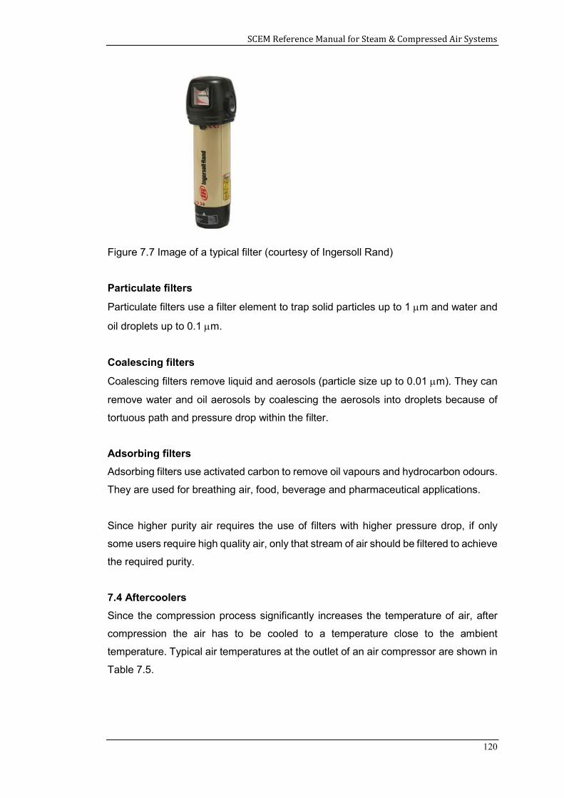
SCEM Reference Manual for Steam & Compressed Air Systems
120
Figure 7.7 Image of a typical filter (courtesy of Ingersoll Rand)
Particulate filters
Particulate filters use a filter element to trap solid particles up to 1 m and water and
oil droplets up to 0.1 m.
Coalescing filters
Coalescing filters remove liquid and aerosols (particle size up to 0.01 m). They can
remove water and oil aerosols by coalescing the aerosols into droplets because of
tortuous path and pressure drop within the filter.
Adsorbing filters
Adsorbing filters use activated carbon to remove oil vapours and hydrocarbon odours.
They are used for breathing air, food, beverage and pharmaceutical applications.
Since higher purity air requires the use of filters with higher pressure drop, if only
some users require high quality air, only that stream of air should be filtered to achieve
the required purity.
7.4 Aftercoolers
Since the compression process significantly increases the temperature of air, after
compression the air has to be cooled to a temperature close to the ambient
temperature. Typical air temperatures at the outlet of an air compressor are shown in
Table 7.5.
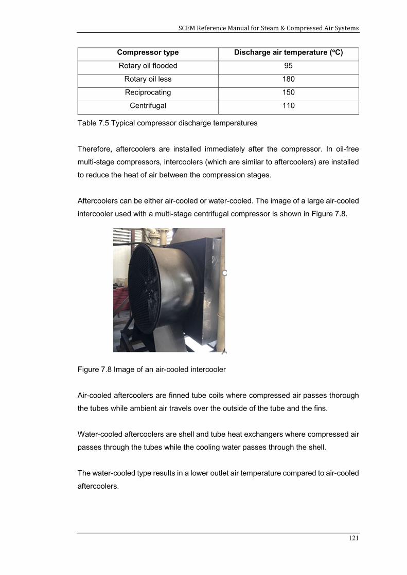
SCEM Reference Manual for Steam & Compressed Air Systems
121
Compressor type Discharge air temperature (oC)
Rotary oil flooded 95
Rotary oil less 180
Reciprocating 150
Centrifugal 110
Table 7.5 Typical compressor discharge temperatures
Therefore, aftercoolers are installed immediately after the compressor. In oil-free
multi-stage compressors, intercoolers (which are similar to aftercoolers) are installed
to reduce the heat of air between the compression stages.
Aftercoolers can be either air-cooled or water-cooled. The image of a large air-cooled
intercooler used with a multi-stage centrifugal compressor is shown in Figure 7.8.
Figure 7.8 Image of an air-cooled intercooler
Air-cooled aftercoolers are finned tube coils where compressed air passes thorough
the tubes while ambient air travels over the outside of the tube and the fins.
Water-cooled aftercoolers are shell and tube heat exchangers where compressed air
passes through the tubes while the cooling water passes through the shell.
The water-cooled type results in a lower outlet air temperature compared to air-cooled
aftercoolers.
SCEM Reference Manual for Steam & Compressed Air Systems
122
Aftercoolers are selected based on approach temperature (difference between the
temperature of air leaving the aftercooler and the cooling medium temperature).
Typical approach temperatures are 3 to 12oC. Water-cooled aftercoolers operate at
lower end of the range while air-cooled aftercoolers operate at the higher end of the
range. Other than reducing the temperature of air, they perform the function of
removing water and some oil vapour from the air.
7.5 Distribution systems
Distribution systems consisting of piping and fittings are used to transport the
compressed air from the compressors to the users. The main objectives of a
distribution system are to:
Transmit the required volume of air
Withstand the operating pressure
Minimise pressure losses
Pressure losses in distribution systems can be categorised as:
Friction losses
Dynamic losses
Friction losses
Friction losses can be computed using the Darcy-Weisbach relationship.
∆Pf= f . L . v2
2 . g . D (7.2)
where,
Pf = frictional pressure drop (m)
f = friction factor
L = length of pipe (m)
v = mean velocity (m/s)
g = acceleration due to gravity (m/s2)
D = inside pipe diameter (m)
By inspecting equation (7.2), it can be seen that friction losses can be reduced by
increasing pipe diameter D, which also lowers the velocity v, and by reducing the pipe
length L. Ideally, the total friction losses for the piping distribution system should not
be more than 0.1 bar.
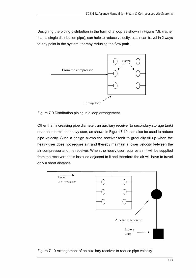
SCEM Reference Manual for Steam & Compressed Air Systems
123
Designing the piping distribution in the form of a loop as shown in Figure 7.9, (rather
than a single distribution pipe), can help to reduce velocity, as air can travel in 2 ways
to any point in the system, thereby reducing the flow path.
Figure 7.9 Distribution piping in a loop arrangement
Other than increasing pipe diameter, an auxiliary receiver (a secondary storage tank)
near an intermittent heavy user, as shown in Figure 7.10, can also be used to reduce
pipe velocity. Such a design allows the receiver tank to gradually fill up when the
heavy user does not require air, and thereby maintain a lower velocity between the
air compressor and the receiver. When the heavy user requires air, it will be supplied
from the receiver that is installed adjacent to it and therefore the air will have to travel
only a short distance.
Figure 7.10 Arrangement of an auxiliary receiver to reduce pipe velocity
From the compressor
Piping loop
Users
From compressor
Auxiliary receiver
Heavy user
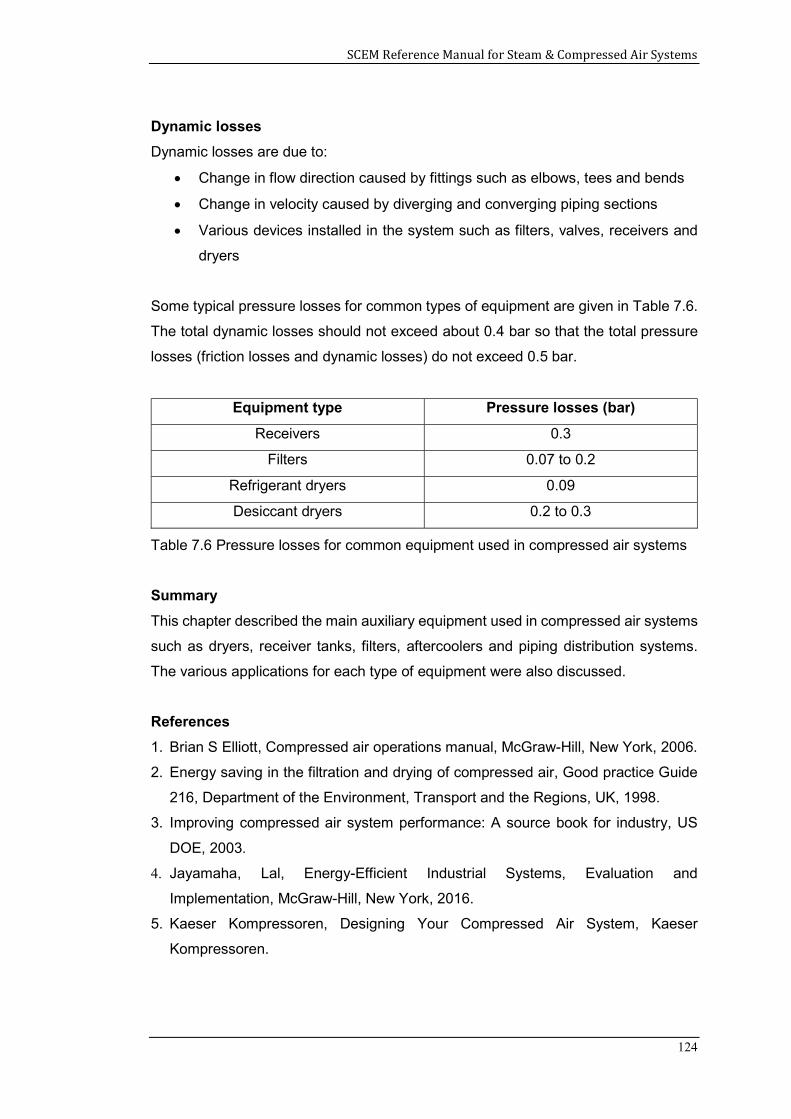
SCEM Reference Manual for Steam & Compressed Air Systems
124
Dynamic losses
Dynamic losses are due to:
Change in flow direction caused by fittings such as elbows, tees and bends
Change in velocity caused by diverging and converging piping sections
Various devices installed in the system such as filters, valves, receivers and
dryers
Some typical pressure losses for common types of equipment are given in Table 7.6.
The total dynamic losses should not exceed about 0.4 bar so that the total pressure
losses (friction losses and dynamic losses) do not exceed 0.5 bar.
Equipment type Pressure losses (bar)
Receivers 0.3
Filters 0.07 to 0.2
Refrigerant dryers 0.09
Desiccant dryers 0.2 to 0.3
Table 7.6 Pressure losses for common equipment used in compressed air systems
Summary
This chapter described the main auxiliary equipment used in compressed air systems
such as dryers, receiver tanks, filters, aftercoolers and piping distribution systems.
The various applications for each type of equipment were also discussed.
References
1. Brian S Elliott, Compressed air operations manual, McGraw-Hill, New York, 2006.
2. Energy saving in the filtration and drying of compressed air, Good practice Guide
216, Department of the Environment, Transport and the Regions, UK, 1998.
3. Improving compressed air system performance: A source book for industry, US
DOE, 2003.
4. Jayamaha, Lal, Energy-Efficient Industrial Systems, Evaluation and
Implementation, McGraw-Hill, New York, 2016.
5. Kaeser Kompressoren, Designing Your Compressed Air System, Kaeser
Kompressoren.
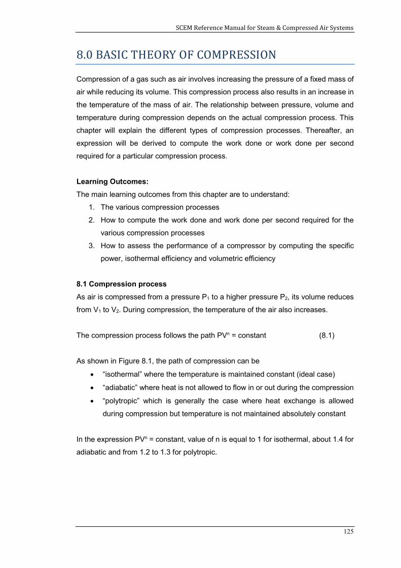
SCEM Reference Manual for Steam & Compressed Air Systems
125
8.0 BASIC THEORY OF COMPRESSION
Compression of a gas such as air involves increasing the pressure of a fixed mass of
air while reducing its volume. This compression process also results in an increase in
the temperature of the mass of air. The relationship between pressure, volume and
temperature during compression depends on the actual compression process. This
chapter will explain the different types of compression processes. Thereafter, an
expression will be derived to compute the work done or work done per second
required for a particular compression process.
Learning Outcomes:
The main learning outcomes from this chapter are to understand:
1. The various compression processes
2. How to compute the work done and work done per second required for the
various compression processes
3. How to assess the performance of a compressor by computing the specific
power, isothermal efficiency and volumetric efficiency
8.1 Compression process
As air is compressed from a pressure P1 to a higher pressure P2, its volume reduces
from V1 to V2. During compression, the temperature of the air also increases.
The compression process follows the path PVn = constant (8.1)
As shown in Figure 8.1, the path of compression can be
“isothermal” where the temperature is maintained constant (ideal case)
“adiabatic” where heat is not allowed to flow in or out during the compression
“polytropic” which is generally the case where heat exchange is allowed
during compression but temperature is not maintained absolutely constant
In the expression PVn = constant, value of n is equal to 1 for isothermal, about 1.4 for
adiabatic and from 1.2 to 1.3 for polytropic.
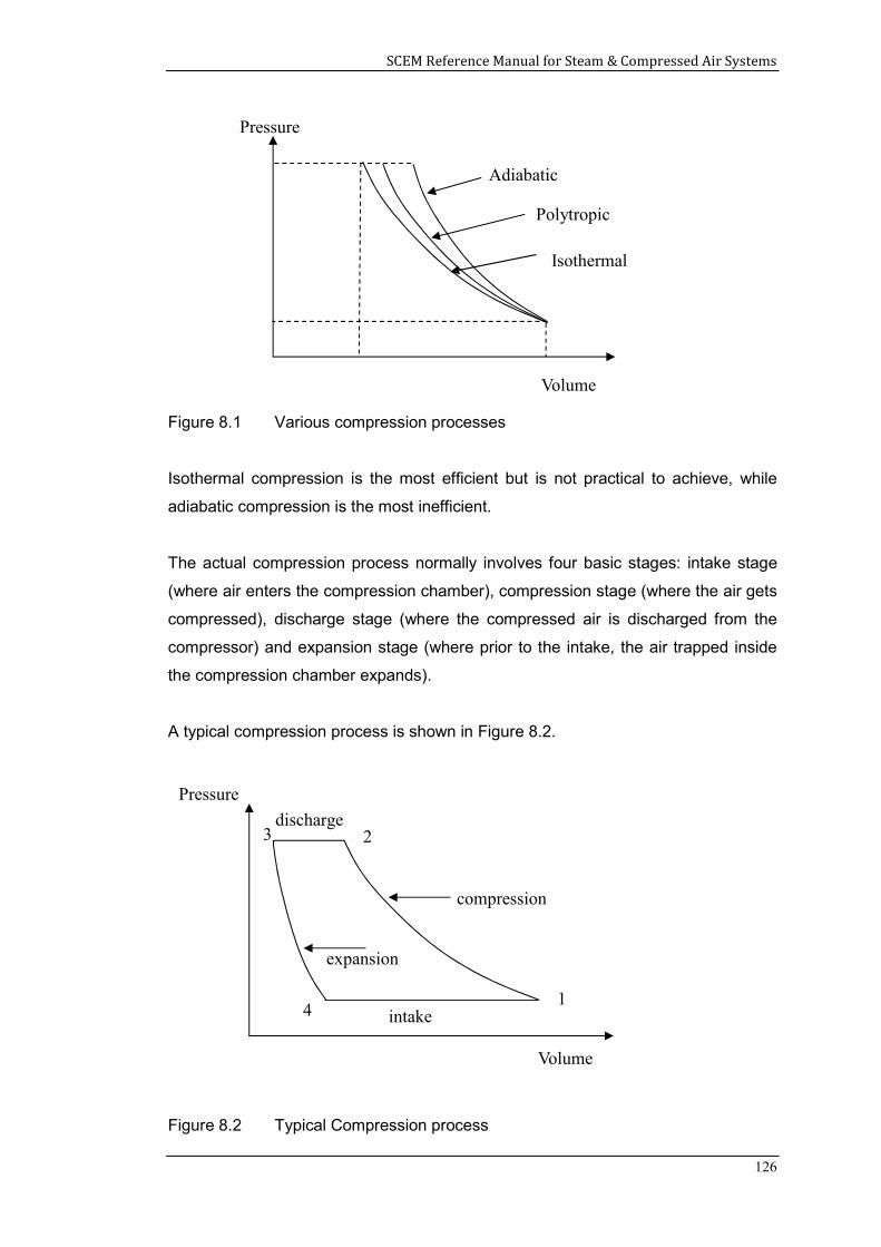
SCEM Reference Manual for Steam & Compressed Air Systems
126
Figure 8.1 Various compression processes
Isothermal compression is the most efficient but is not practical to achieve, while
adiabatic compression is the most inefficient.
The actual compression process normally involves four basic stages: intake stage
(where air enters the compression chamber), compression stage (where the air gets
compressed), discharge stage (where the compressed air is discharged from the
compressor) and expansion stage (where prior to the intake, the air trapped inside
the compression chamber expands).
A typical compression process is shown in Figure 8.2.
Figure 8.2 Typical Compression process
Pressure
Adiabatic
Polytropic
Volume
Isothermal
intake
discharge
Pressure
VolumeVolume
compression
expansion
2
1
3
4
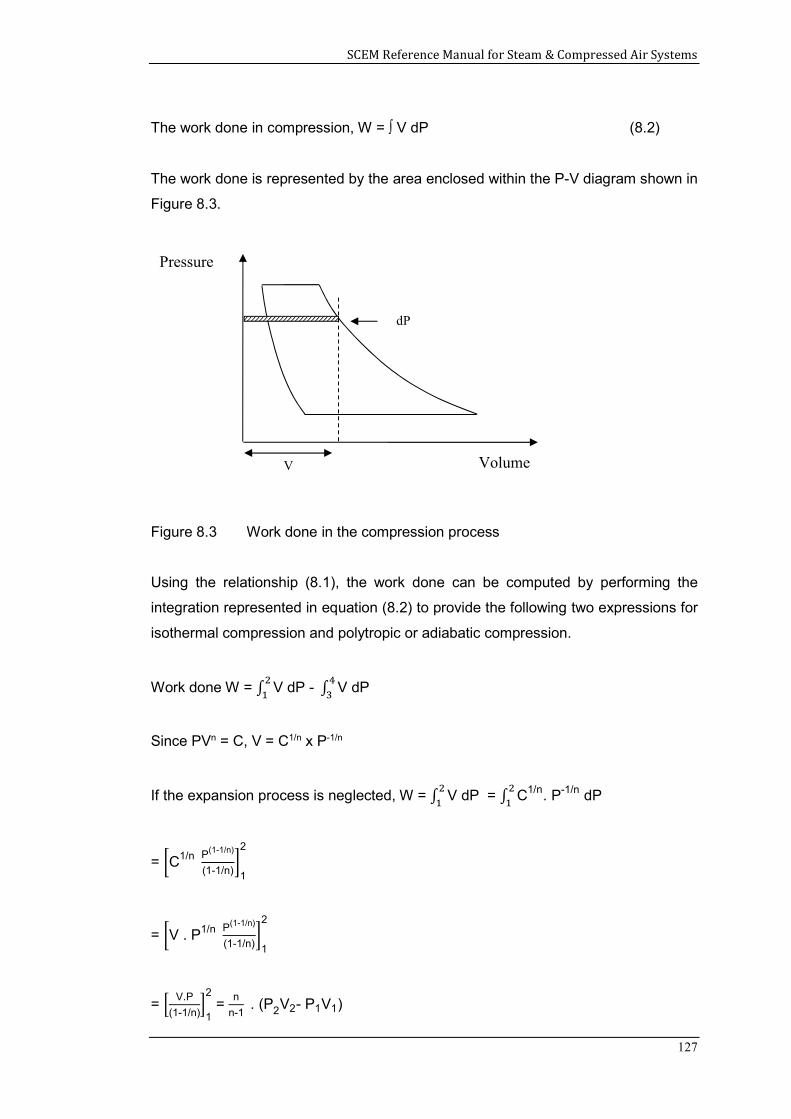
SCEM Reference Manual for Steam & Compressed Air Systems
127
The work done in compression, W = V dP (8.2)
The work done is represented by the area enclosed within the P-V diagram shown in
Figure 8.3.
Figure 8.3 Work done in the compression process
Using the relationship (8.1), the work done can be computed by performing the
integration represented in equation (8.2) to provide the following two expressions for
isothermal compression and polytropic or adiabatic compression.
Work done W = ∫ V dP - ∫ V dP
Since PVn = C, V = C1/n x P-1/n
If the expansion process is neglected, W = ∫ V dP = ∫ C1/n. P-1/n dP
= C1/n P(1-1/n)
(1-1/n) 1
2
= V . P1/n P(1-1/n)
(1-1/n) 1
2
= V.P
(1-1/n) 1
2 =
n
n-1 . (P2V2- P1V1)
Pressure
Volume
dP
V
SCEM Reference Manual for Steam & Compressed Air Systems
128
= n
n-1 . P1V1 (
P2V2
P1V1- 1)
Since from equation (8.1), V2
V1=
P2
P1
-1/n
W = n
n-1. P1V1
P2
P1.
P2
P1
-1n - 1 =
n
n-1 . P1V1
P2
P1
n-1n - 1
Since for an ideal gas PV = mRT, where R = ideal gas constant
W = n
n-1 . m R T1
P2
P1
n-1n - 1 (8.3)
For Isothermal compression, since n=1
W = ∫ V dP = ∫ C. P-1 dP 2
1 = PV [ln P ]1
2
Therefore,
(8.4)
where,
W = work done (Joules)
m = mass of air being compressed (kg)
R = specific gas constant for air (287 J/kg.K)
T1 = absolute temperature at the air compressor intake (K)
P2 / P1 = compression ratio in absolute pressure values
If the mass flow rate ṁ is used instead of mass, m, the expressions for work done per
second will be as follows:
for isothermal compression (8.5)
and, W=n
n-1 mRT1
P2
P1
n-1n - 1 for polytropic & adiabatic compression (8.6)
1
21 P
PlnmRTW
1
21
..
P
PlnRTmW
SCEM Reference Manual for Steam & Compressed Air Systems
129
where,
Ẇ = work done per seconds (Watts)
ṁ = mass flow rate (kg/s)
Example 8.1
Compute the mechanical power required to compress 1 m3/s of dry air at 30oC from 1
bar to 7.5 bar (both absolute pressures) for isothermal, polytropic (n=1.3) and
adiabatic (n=1.4) compression. Take the density of air to be 1.2 kg/m3 and specific
gas constant for air R to be 287 J/kg.K.
Solution
ṁ = 1 m3/s x 1.2 kg/m3 = 1.2 kg/s
Isothermal (from equation 8.5)
Ẇ = 1.2 x 287 x (273+30) x ln (7.5/1) Watts
= 210 kW
Adiabatic (from equation 8.6)
Ẇ = 1.2 x 287 x (273+30) x (1.4/0.4) x [(7.5/1)0.4/1.4 -1] Watts
= 284 kW
Polytropic (from equation 8.6)
Ẇ = 1.2 x 287 x (273+30) x (1.3/0.3) x [(7.5/1)0.3/1.3 -1] Watts
= 267 kW
8.2 Specific power
Specific power for compressors is a measure of how much power is used to compress
a specific quantity of air and is the ratio of power input to the compressor in kW to the
free air delivery in m3/s.
Example 8.2
Compute the specific power in kW per m3/s and kW per l/s for the three cases of
compression in example 8.1.
Solution
Isothermal
Specific power = 210 kW / 1 m3/s
SCEM Reference Manual for Steam & Compressed Air Systems
130
= 0.21 kW/(l/s)
Adiabatic
Specific power = 284 kW / 1 m3/s
= 0.28 kW/(l/s)
Polytropic
Specific power = 267 kW / 1 m3/s
= 0.27 kW/(l/s)
8.3 Isothermal efficiency
Isothermal efficiency is a measure of how close a particular process of compression
is to the ideal case of isothermal compression. It is defined as the ratio of isothermal
power to the actual power consumed.
Isothermal efficiency = Isothermal power
Actual power consumed (8.7)
Example 8.3
Compute the isothermal efficiency of an air compressor operating at 1 m3/s of dry air
at 30oC from 1 bar to 9 bar (both absolute pressures) where the measured power
consumption of the motor is 325 kW. The efficiency of the motor and transmission
drive between the motor and compressor is 85%. Take the density of air to be 1.2
kg/m3 and specific gas constant R to be 287 J/kg.K.
Solution
ṁ = 1 m3/s x 1.2 kg/m3 = 1.2 kg/s
Isothermal power (from equation 8.4)
Ẇ = 1.2 x 287 x (273+30) x ln (9/1) Watts
= 229.3 kW
Actual power drawn by the compressor shaft = 325 x 0.85 = 276.3 kW
From equation (8.7),
Isothermal efficiency = 229.3/276.3 = 0.83 = 83%
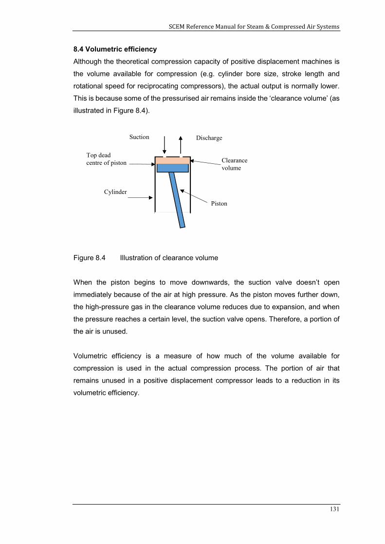
SCEM Reference Manual for Steam & Compressed Air Systems
131
8.4 Volumetric efficiency
Although the theoretical compression capacity of positive displacement machines is
the volume available for compression (e.g. cylinder bore size, stroke length and
rotational speed for reciprocating compressors), the actual output is normally lower.
This is because some of the pressurised air remains inside the ‘clearance volume’ (as
illustrated in Figure 8.4).
Figure 8.4 Illustration of clearance volume
When the piston begins to move downwards, the suction valve doesn’t open
immediately because of the air at high pressure. As the piston moves further down,
the high-pressure gas in the clearance volume reduces due to expansion, and when
the pressure reaches a certain level, the suction valve opens. Therefore, a portion of
the air is unused.
Volumetric efficiency is a measure of how much of the volume available for
compression is used in the actual compression process. The portion of air that
remains unused in a positive displacement compressor leads to a reduction in its
volumetric efficiency.
Suction Discharge
Cylinder
Piston
Top dead centre of piston Clearance
volume
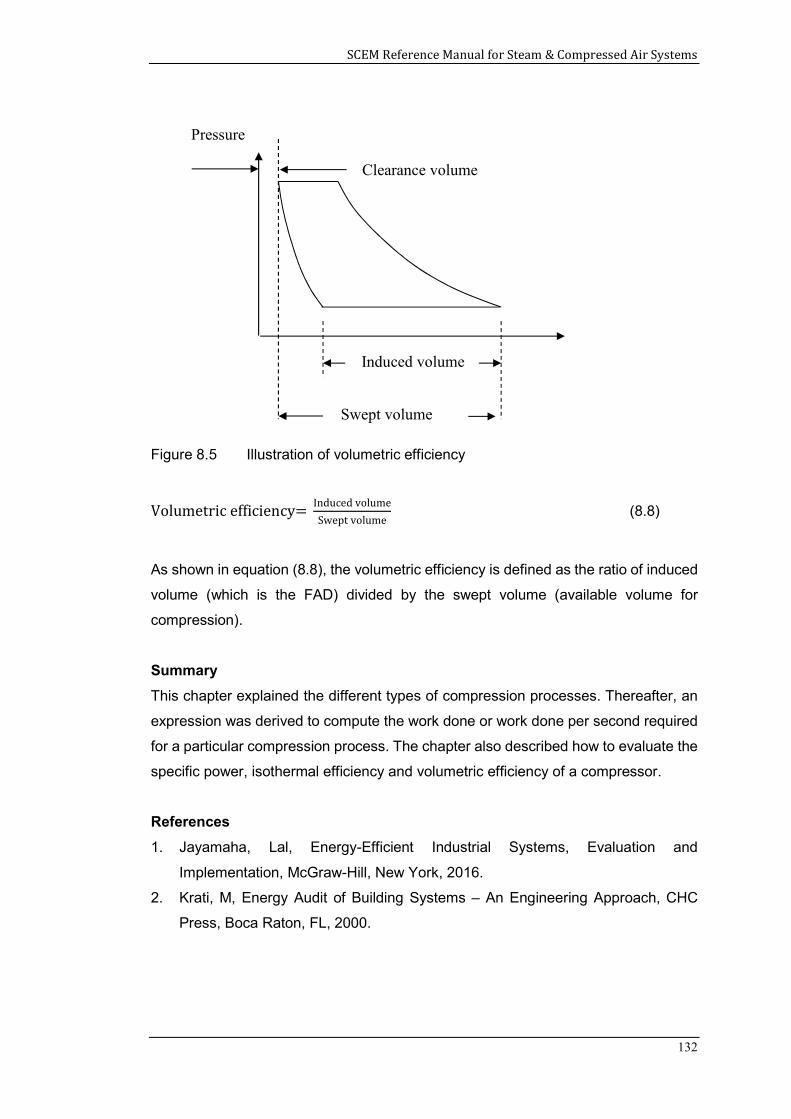
SCEM Reference Manual for Steam & Compressed Air Systems
132
Figure 8.5 Illustration of volumetric efficiency
Volumetric efficiency= Induced volume
Swept volume (8.8)
As shown in equation (8.8), the volumetric efficiency is defined as the ratio of induced
volume (which is the FAD) divided by the swept volume (available volume for
compression).
Summary
This chapter explained the different types of compression processes. Thereafter, an
expression was derived to compute the work done or work done per second required
for a particular compression process. The chapter also described how to evaluate the
specific power, isothermal efficiency and volumetric efficiency of a compressor.
References
1. Jayamaha, Lal, Energy-Efficient Industrial Systems, Evaluation and
Implementation, McGraw-Hill, New York, 2016.
2. Krati, M, Energy Audit of Building Systems – An Engineering Approach, CHC
Press, Boca Raton, FL, 2000.
Pressure
Induced volume
Clearance volume
Swept volume
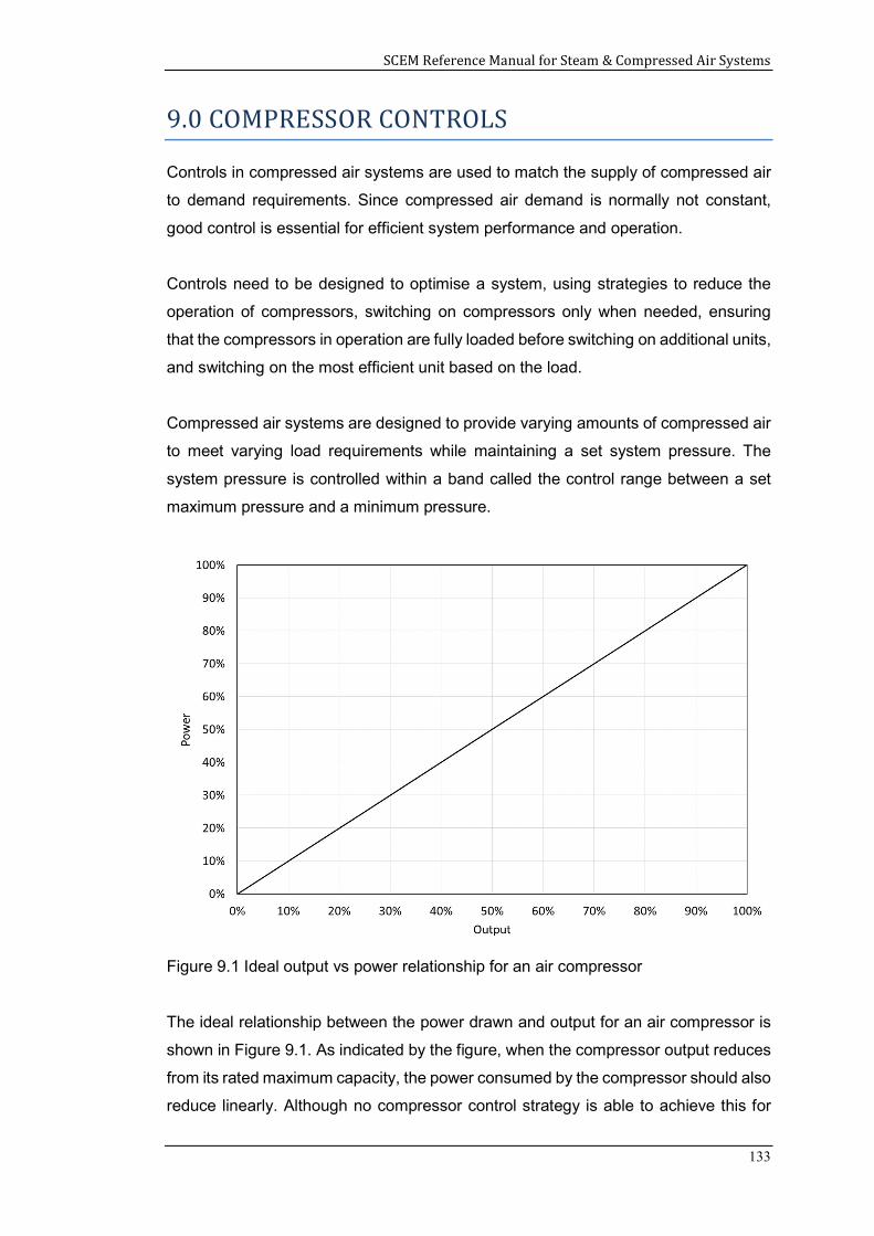
SCEM Reference Manual for Steam & Compressed Air Systems
133
9.0 COMPRESSOR CONTROLS
Controls in compressed air systems are used to match the supply of compressed air
to demand requirements. Since compressed air demand is normally not constant,
good control is essential for efficient system performance and operation.
Controls need to be designed to optimise a system, using strategies to reduce the
operation of compressors, switching on compressors only when needed, ensuring
that the compressors in operation are fully loaded before switching on additional units,
and switching on the most efficient unit based on the load.
Compressed air systems are designed to provide varying amounts of compressed air
to meet varying load requirements while maintaining a set system pressure. The
system pressure is controlled within a band called the control range between a set
maximum pressure and a minimum pressure.
Figure 9.1 Ideal output vs power relationship for an air compressor
The ideal relationship between the power drawn and output for an air compressor is
shown in Figure 9.1. As indicated by the figure, when the compressor output reduces
from its rated maximum capacity, the power consumed by the compressor should also
reduce linearly. Although no compressor control strategy is able to achieve this for
SCEM Reference Manual for Steam & Compressed Air Systems
134
the entire operating range from 0 to 100% capacity, some are able to achieve this at
some operating points. These will be described in detail in this chapter.
Learning Outcomes:
The main learning outcomes from this chapter are to understand the main air
compressor control strategies, which are:
1. On / Off
2. Load / Unload
3. Inlet modulation
4. Variable displacement
5. Variable speed control
9.1 On / Off control
This form of control involves switching on and off the compressor motor to control the
amount of compressed air produced to meet the load. This type of control is used only
for small compressors that have low duty cycles as otherwise, frequent cycling will
lead to overheating of the motor and excessive wear and tear of compressor parts.
The compressor operates under two modes, which are On and Off. These two
operating modes can be marked on the ideal relationship between compressor power
and output (explained earlier). As shown in Figure 9.2, the two operating modes match
the ideal requirements at 0% and 100% output. When the load is less than 100%
capacity of the compressor, it will go on and off, and the average value will move
along the ideal line. For example, if the load is 50% of the compressor capacity, it will
be on for 50% of the time and off during the balance 50% of the time, resulting in an
average compressor power of 50% of the power at 100% load.
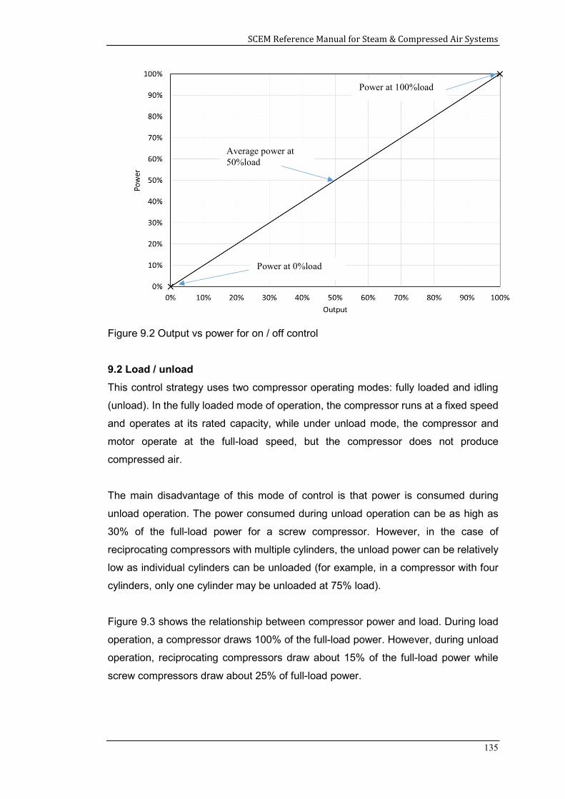
SCEM Reference Manual for Steam & Compressed Air Systems
135
Figure 9.2 Output vs power for on / off control
9.2 Load / unload
This control strategy uses two compressor operating modes: fully loaded and idling
(unload). In the fully loaded mode of operation, the compressor runs at a fixed speed
and operates at its rated capacity, while under unload mode, the compressor and
motor operate at the full-load speed, but the compressor does not produce
compressed air.
The main disadvantage of this mode of control is that power is consumed during
unload operation. The power consumed during unload operation can be as high as
30% of the full-load power for a screw compressor. However, in the case of
reciprocating compressors with multiple cylinders, the unload power can be relatively
low as individual cylinders can be unloaded (for example, in a compressor with four
cylinders, only one cylinder may be unloaded at 75% load).
Figure 9.3 shows the relationship between compressor power and load. During load
operation, a compressor draws 100% of the full-load power. However, during unload
operation, reciprocating compressors draw about 15% of the full-load power while
screw compressors draw about 25% of full-load power.
Power at 100%load
Power at 0%load
Average power at 50%load
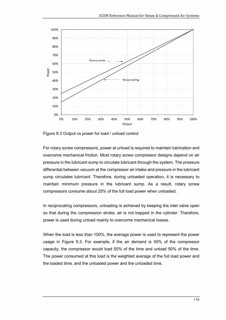
SCEM Reference Manual for Steam & Compressed Air Systems
136
Figure 9.3 Output vs power for load / unload control
For rotary screw compressors, power at unload is required to maintain lubrication and
overcome mechanical friction. Most rotary screw compressor designs depend on air
pressure in the lubricant sump to circulate lubricant through the system. The pressure
differential between vacuum at the compressor air intake and pressure in the lubricant
sump circulates lubricant. Therefore, during unloaded operation, it is necessary to
maintain minimum pressure in the lubricant sump. As a result, rotary screw
compressors consume about 25% of the full load power when unloaded.
In reciprocating compressors, unloading is achieved by keeping the inlet valve open
so that during the compression stroke, air is not trapped in the cylinder. Therefore,
power is used during unload mainly to overcome mechanical losses.
When the load is less than 100%, the average power is used to represent the power
usage in Figure 9.3. For example, if the air demand is 50% of the compressor
capacity, the compressor would load 50% of the time and unload 50% of the time.
The power consumed at this load is the weighted average of the full load power and
the loaded time, and the unloaded power and the unloaded time.
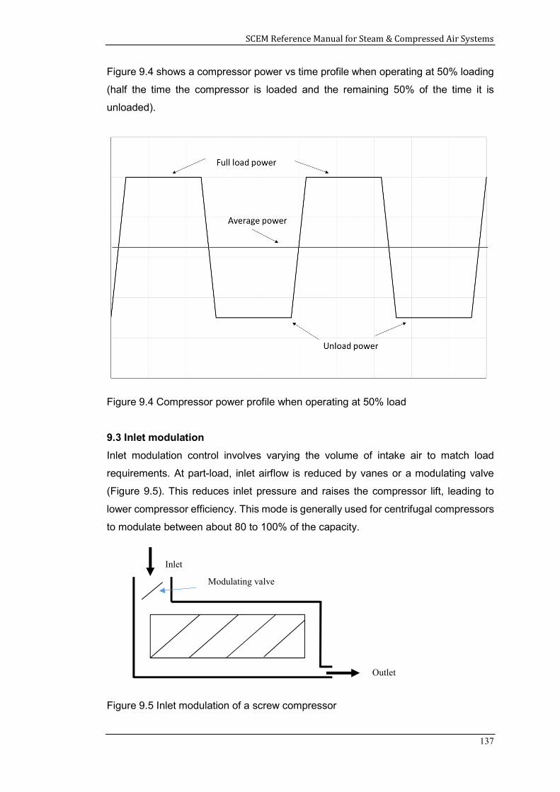
SCEM Reference Manual for Steam & Compressed Air Systems
137
Figure 9.4 shows a compressor power vs time profile when operating at 50% loading
(half the time the compressor is loaded and the remaining 50% of the time it is
unloaded).
Figure 9.4 Compressor power profile when operating at 50% load
9.3 Inlet modulation
Inlet modulation control involves varying the volume of intake air to match load
requirements. At part-load, inlet airflow is reduced by vanes or a modulating valve
(Figure 9.5). This reduces inlet pressure and raises the compressor lift, leading to
lower compressor efficiency. This mode is generally used for centrifugal compressors
to modulate between about 80 to 100% of the capacity.
Figure 9.5 Inlet modulation of a screw compressor
Inlet
Outlet
Modulating valve
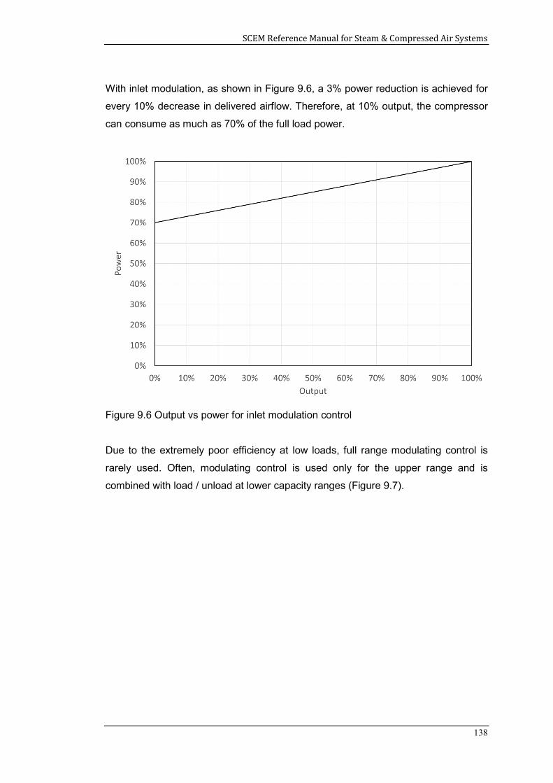
SCEM Reference Manual for Steam & Compressed Air Systems
138
With inlet modulation, as shown in Figure 9.6, a 3% power reduction is achieved for
every 10% decrease in delivered airflow. Therefore, at 10% output, the compressor
can consume as much as 70% of the full load power.
Figure 9.6 Output vs power for inlet modulation control
Due to the extremely poor efficiency at low loads, full range modulating control is
rarely used. Often, modulating control is used only for the upper range and is
combined with load / unload at lower capacity ranges (Figure 9.7).
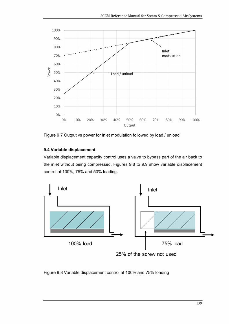
SCEM Reference Manual for Steam & Compressed Air Systems
139
Figure 9.7 Output vs power for inlet modulation followed by load / unload
9.4 Variable displacement
Variable displacement capacity control uses a valve to bypass part of the air back to
the inlet without being compressed. Figures 9.8 to 9.9 show variable displacement
control at 100%, 75% and 50% loading.
Figure 9.8 Variable displacement control at 100% and 75% loading
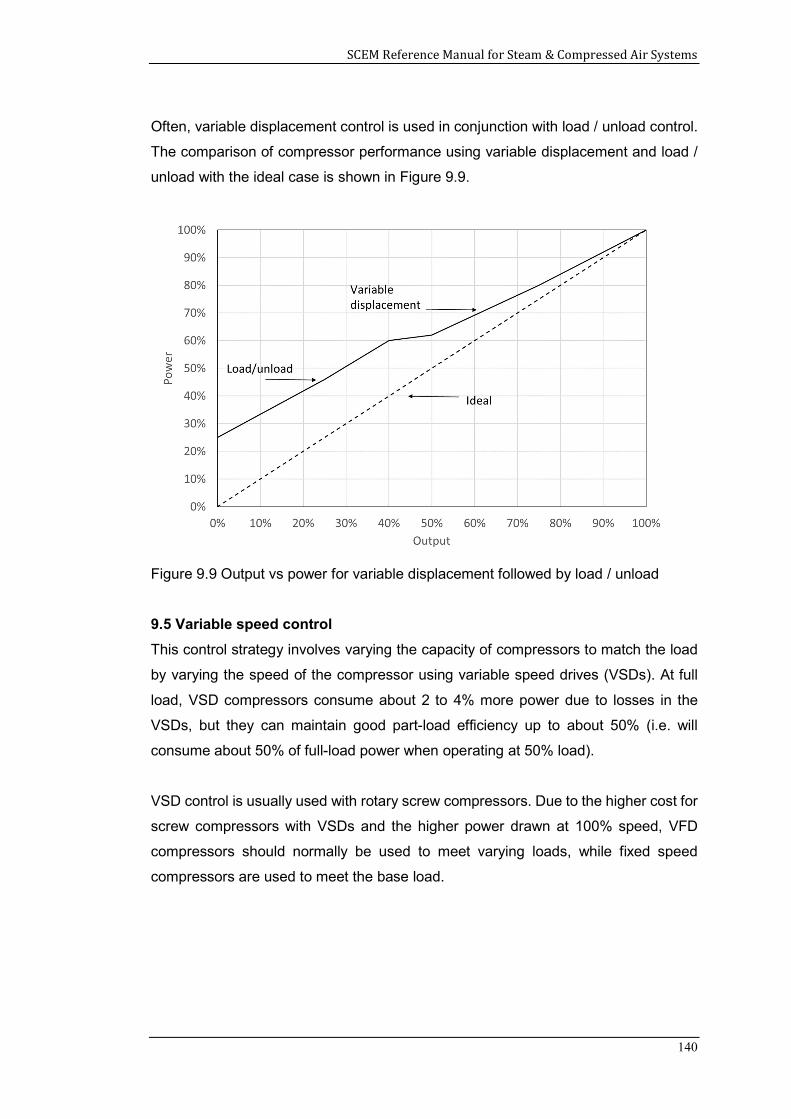
SCEM Reference Manual for Steam & Compressed Air Systems
140
Often, variable displacement control is used in conjunction with load / unload control.
The comparison of compressor performance using variable displacement and load /
unload with the ideal case is shown in Figure 9.9.
Figure 9.9 Output vs power for variable displacement followed by load / unload
9.5 Variable speed control
This control strategy involves varying the capacity of compressors to match the load
by varying the speed of the compressor using variable speed drives (VSDs). At full
load, VSD compressors consume about 2 to 4% more power due to losses in the
VSDs, but they can maintain good part-load efficiency up to about 50% (i.e. will
consume about 50% of full-load power when operating at 50% load).
VSD control is usually used with rotary screw compressors. Due to the higher cost for
screw compressors with VSDs and the higher power drawn at 100% speed, VFD
compressors should normally be used to meet varying loads, while fixed speed
compressors are used to meet the base load.
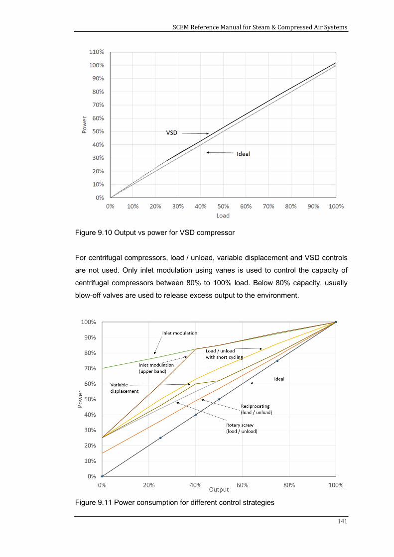
SCEM Reference Manual for Steam & Compressed Air Systems
141
Figure 9.10 Output vs power for VSD compressor
For centrifugal compressors, load / unload, variable displacement and VSD controls
are not used. Only inlet modulation using vanes is used to control the capacity of
centrifugal compressors between 80% to 100% load. Below 80% capacity, usually
blow-off valves are used to release excess output to the environment.
Figure 9.11 Power consumption for different control strategies
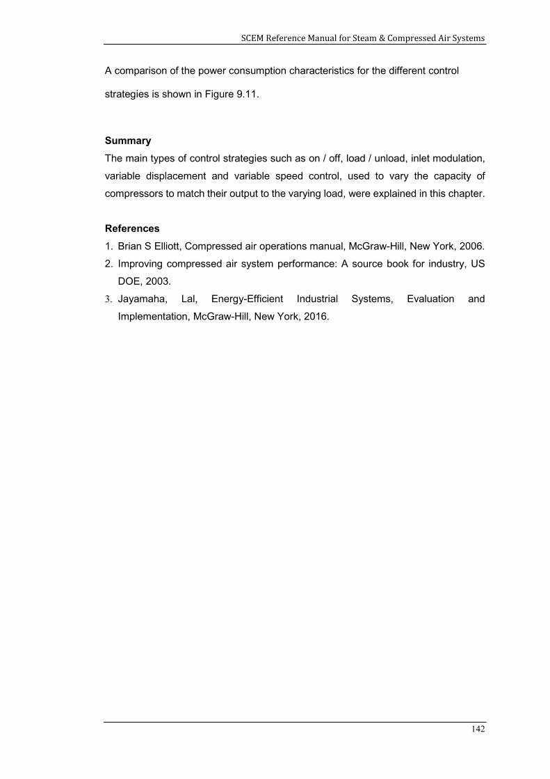
SCEM Reference Manual for Steam & Compressed Air Systems
142
A comparison of the power consumption characteristics for the different control
strategies is shown in Figure 9.11.
Summary
The main types of control strategies such as on / off, load / unload, inlet modulation,
variable displacement and variable speed control, used to vary the capacity of
compressors to match their output to the varying load, were explained in this chapter.
References
1. Brian S Elliott, Compressed air operations manual, McGraw-Hill, New York, 2006.
2. Improving compressed air system performance: A source book for industry, US
DOE, 2003.
3. Jayamaha, Lal, Energy-Efficient Industrial Systems, Evaluation and
Implementation, McGraw-Hill, New York, 2016.
SCEM Reference Manual for Steam & Compressed Air Systems
143
10.0 ENERGY SAVING MEASURES FOR COMPRESSED AIR SYSTEMS
As explained in the earlier chapters of this reference manual, compressed air systems
are highly energy intensive and account for a significant portion of energy consumed
in many plants. Most of the energy used in compressed air systems is wasted as heat,
and only about 10% of the input energy is delivered in usable form as compressed
air. Further, part of the generated compressed air is wasted due to leaks, artificial
demand and inappropriate usage.
However, there are a number of energy-saving measures that can be implemented to
reduce the energy usage of compressed air systems. These energy-saving measures
can be broadly categorised into those leading to reduction in demand and those
improving the compression process. Some of the common energy-saving measures
for each category are listed below.
Reduction in demand
Reducing leaks
Reducing artificial demand (due to high pressure)
Eliminating inappropriate usage
Improving compression process
Reducing pressure ratio
Multi-staging
Reducing intake temperature
This chapter describes some of the common energy saving measures that can be
implemented for compressed air systems.
Learning Outcomes:
The main learning outcomes from this chapter are to understand:
1. The main energy saving measures for compressed air systems
2. How to estimate the energy savings achievable for each measure
SCEM Reference Manual for Steam & Compressed Air Systems
144
10.1 Rectifying leaks
Since compressed air is produced, stored, distributed and used at a much higher
pressure than the surrounding air, compressed air will leak through even the smallest
openings, resulting in much energy wastage. In many compressed air systems, leaks
account for about 20% to 30% of the total compressor output.
Common sources of leaks are pipe fittings, flexible tubes, couplings, pressure
regulators, condensate traps, and pipe joints.
Compressed air leakage depends on the size of the opening, system pressure and
the shape of the opening (round or sharp).
Leakage rate can be estimated using Fliegner’s formula for flow through an orifice
m = (2/R) . C . A x P x T-1/2 (10.1)
where,
m is in kg/s
C = 0.65 for round holes
A = the orifice size in m2
P = the pressure in Pa
T = the absolute temperature in K
However, it is not convenient to use the above relationship as the orifice size is
normally not known. Therefore, the total leakage rate from a compressed air system
can be estimated by switching off all the equipment that uses compressed air,
operating the compressor to charge the system to the operating pressure, and
measuring the time taken for “load” and “unload” cycles of the compressor
continuously for about 10 cycles.
The following expression can be used to estimate the system leakage rate:
% of leakage = T / (T + t) x 100 (10.2)
and,
System leakage (m3/min) = (Q x T) / (T+ t) (10.3)
SCEM Reference Manual for Steam & Compressed Air Systems
145
where,
Q = compressor capacity (FAD in m3/min)
T = average load time (minutes)
t = average unload time (minutes)
Example 10.1
A leak test carried out on a compressed air system with all the compressed air
equipment switched off provided the following information :
Average load time = 3 minutes
Average unload time = 10 minutes
If the FAD of the compressor is 0.1 m3/s, compute the percentage and quantity of
leaks.
Taking the specific power for the compressor system to be 270 kW / m3/s, estimate
the energy wastage (in kWh per day) assuming the system operates 24 hours a day.
Solution
Load time = 3 minutes
Unload time = 10 minutes
FAD = 0.1 m3/s
% leakage = [3 / (3 + 10)] x 100 = 23%
Leakage rate = 0.1 m3/s x 0.23 = 0.023 m3/s
Power usage = 0.023 x 270 = 6.21 kW
Energy usage = 6.21 x 24 = 149 kWh / day
10.2 Use of receiver tanks
As explained earlier in chapter 7, receiver tanks are commonly used to store
compressed air. Primary receivers installed near the air compressors help to maintain
a steady output from the compressors, even when the demand is changing. When the
demand is low, the receiver tanks store the excess compressed air while when the
demand is high, part of the demand is met by releasing stored air from the tanks.
If receiver tanks are not installed in the system, when the compressed air demand
exceeds the capacity of the compressors, the system pressure will drop. To avoid the
system pressure dropping below the required minimum pressure at the end-users, the
operating pressure is often set at a much higher value than normally required. This
results in higher energy consumption by the compressor motor.
SCEM Reference Manual for Steam & Compressed Air Systems
146
Similarly, if there are intermittent high loads, a sudden flow of compressed air through
the piping system will result in higher pressure losses. Therefore, if secondary
receivers are installed near intermittent high loads, the storage tanks can gradually
fill-up when the equipment is not using air, and supply the high flow rate when
required, through a much shorter pipe resulting in a much lower pressure drop.
Therefore, installation of receiver tanks helps to operate compressed air systems at
the lowest possible pressure. Energy savings resulting from the use of receiver tanks
is usually due to the reduction in system pressure and can be estimated as explained
later in section 10.5.
10.3 Reducing artificial demand
Different types of equipment need compressed air at different pressures for their
operation. Usually the system pressure is set at a value to satisfy all the users. Often,
the system pressure is also set to be higher than required to ensure sufficient pressure
during sudden high demand, to minimise complaints from end users and to allow for
high pressure losses in the distribution system.
Operating the system at a higher than required system pressure not only reduces
compressor efficiency (will be explained later), it also results in extra usage called
artificial demand.
Compressed air usage by many users can be considered like air flowing through an
orifice where, when the upstream pressure increases, the flow through the orifice
increases.
Hence, pressure regulators should be installed at the point of use and set at the
optimum minimum pressure required for proper functioning. Pressure controllers can
also be installed for the distribution system (after the primary receiver) and set to
maintain an optimum pressure downstream.
In addition to reducing artificial demand, reducing system pressure will also help to
reduce leaks.
Other opportunities for reducing artificial demand are, replacing heatless desiccant
dryers (which use purge air for regeneration) with externally heated or refrigerant
SCEM Reference Manual for Steam & Compressed Air Systems
147
dryers, repairing faulty dryers that continuously purge and increasing the dew point
settings on heatless desiccant dryers.
10.4 Reducing inappropriate usage
Often compressed air is used for applications that can be served by other means.
Some such examples are:
Electrically driven vacuum pumps instead of air powered venturi vacuum
systems
Electric motors for air motors
Electric actuators for pneumatic actuators
Using vacuum cleaners for general cleaning
Using high pressure blowers for tank agitation
Using blowers for tank agitation
Often compressed air is used for tank agitation in applications such as plating to
provide movement of the solution in the tank. In such situations, the use of
compressed air can be replaced by installing blowers which are much more energy
efficient than air compressors.
The blowers should be selected to provide sufficient pressure and air flow rate. The
minimum pressure requirement is dependent on the liquid level in tank and can be
estimated using equation (10.4).
Minimum gauge pressure in bar = [( x g x h) / (1x10⁻⁵)] + 0.05 (10.4)
where,
= density of the fluid in the tank (kg/m3)
g = acceleration due to gravity (m/s2)
h = height of the liquid in the tank (m)
The air flow rate required for agitation can be expressed by equation (10.5.)
The air flow rate required for agitation in SCFM = A x F (10.5)
where,
A = tank surface area in m2
SCEM Reference Manual for Steam & Compressed Air Systems
148
F = agitation factor between 10 to 20 in SCFM/m2
Example 10.2
A tank contains a solution with a density of 1200 kg/m3. The liquid level in the tank is
1 m. The surface area of the tank is 2 m2. It is currently being served by an air
compressor having a specific power of 0.2 kW/SCFM.
Compute the required pressure and air flow rate for a suitable blower for this
application, taking the agitation factor to be 15 SCFM/m2. Estimate the reduction in
power if the specific power for the blower is 0.08 kW/CFM.
Solution
From equation (10.4),
Gauge pressure requirement = [(1200 x 9.81 x 1) / (1x10⁻⁵)] + 0.05 = 0.17 bar
The air flow rate required = 2 x 15 = 30 SCFM
Estimated reduction in power = 30 x (0.2 – 0.08) = 3.6 kW
10.5 Reducing system pressure
The system pressure, which is the pressure at which compressed air is supplied by
the compressors, depends on factors such as the pressure requirements of the end
users, pressure losses in the system, storage capacity and variation in demand.
Power consumed by compressors depends on the discharge pressure as expressed
by the following relationship (which was derived earlier in chapter 8).
(10.6)
Therefore, a higher discharge pressure results in a higher compressor power (as the
compressor has to work against a higher back pressure). The rule of thumb used in
industry is a 7 to 8% increase in compressor power for every 1 bar increase in
compressor discharge pressure.
1P
P
1-n
nRTmW
n
1n
1
21
..
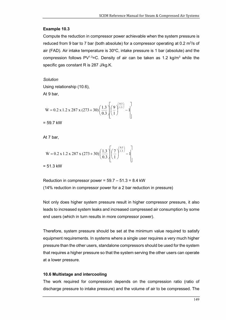
SCEM Reference Manual for Steam & Compressed Air Systems
149
Example 10.3
Compute the reduction in compressor power achievable when the system pressure is
reduced from 9 bar to 7 bar (both absolute) for a compressor operating at 0.2 m3/s of
air (FAD). Air intake temperature is 30oC, intake pressure is 1 bar (absolute) and the
compression follows PV1.3=C. Density of air can be taken as 1.2 kg/m3 while the
specific gas constant R is 287 J/kg.K.
Solution
Using relationship (10.6),
At 9 bar,
= 59.7 kW
At 7 bar,
= 51.3 kW
Reduction in compressor power = 59.7 – 51.3 = 8.4 kW
(14% reduction in compressor power for a 2 bar reduction in pressure)
Not only does higher system pressure result in higher compressor pressure, it also
leads to increased system leaks and increased compressed air consumption by some
end users (which in turn results in more compressor power).
Therefore, system pressure should be set at the minimum value required to satisfy
equipment requirements. In systems where a single user requires a very much higher
pressure than the other users, standalone compressors should be used for the system
that requires a higher pressure so that the system serving the other users can operate
at a lower pressure.
10.6 Multistage and intercooling
The work required for compression depends on the compression ratio (ratio of
discharge pressure to intake pressure) and the volume of air to be compressed. The
11
7
0.3
1.3 30) (273 x 287 x 1.2 x 2.0W
1.3
0.3.
11
9
0.3
1.3 30) (273 x 287 x 1.2 x 2.0W
1.3
0.3.
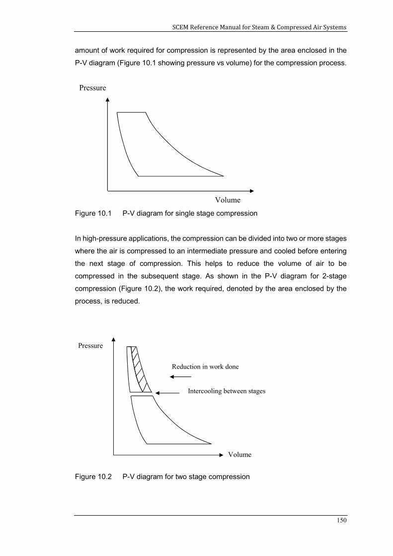
SCEM Reference Manual for Steam & Compressed Air Systems
150
amount of work required for compression is represented by the area enclosed in the
P-V diagram (Figure 10.1 showing pressure vs volume) for the compression process.
Figure 10.1 P-V diagram for single stage compression
In high-pressure applications, the compression can be divided into two or more stages
where the air is compressed to an intermediate pressure and cooled before entering
the next stage of compression. This helps to reduce the volume of air to be
compressed in the subsequent stage. As shown in the P-V diagram for 2-stage
compression (Figure 10.2), the work required, denoted by the area enclosed by the
process, is reduced.
Figure 10.2 P-V diagram for two stage compression
Pressure
Volume
Pressure
Intercooling between stages
Reduction in work done
Volume
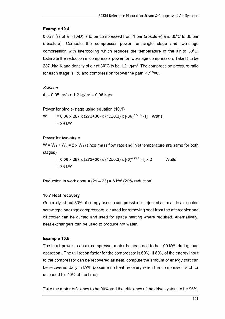
SCEM Reference Manual for Steam & Compressed Air Systems
151
Example 10.4
0.05 m3/s of air (FAD) is to be compressed from 1 bar (absolute) and 30oC to 36 bar
(absolute). Compute the compressor power for single stage and two-stage
compression with intercooling which reduces the temperature of the air to 30oC.
Estimate the reduction in compressor power for two-stage compression. Take R to be
287 J/kg.K and density of air at 30oC to be 1.2 kg/m3. The compression pressure ratio
for each stage is 1:6 and compression follows the path PV1.3=C.
Solution
ṁ = 0.05 m3/s x 1.2 kg/m3 = 0.06 kg/s
Power for single-stage using equation (10.1)
Ẇ = 0.06 x 287 x (273+30) x (1.3/0.3) x [(36)0.3/1.3 -1] Watts
= 29 kW
Power for two-stage
Ẇ = Ẇ1 + Ẇ2 = 2 x Ẇ1 (since mass flow rate and inlet temperature are same for both
stages)
= 0.06 x 287 x (273+30) x (1.3/0.3) x [(6)0.3/1.3 -1] x 2 Watts
= 23 kW
Reduction in work done = (29 – 23) = 6 kW (20% reduction)
10.7 Heat recovery
Generally, about 80% of energy used in compression is rejected as heat. In air-cooled
screw type package compressors, air used for removing heat from the aftercooler and
oil cooler can be ducted and used for space heating where required. Alternatively,
heat exchangers can be used to produce hot water.
Example 10.5
The input power to an air compressor motor is measured to be 100 kW (during load
operation). The utilisation factor for the compressor is 60%. If 80% of the energy input
to the compressor can be recovered as heat, compute the amount of energy that can
be recovered daily in kWh (assume no heat recovery when the compressor is off or
unloaded for 40% of the time).
Take the motor efficiency to be 90% and the efficiency of the drive system to be 95%.
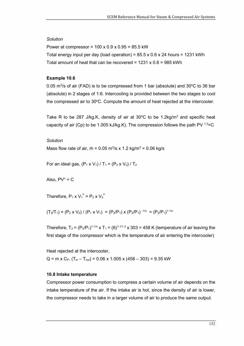
SCEM Reference Manual for Steam & Compressed Air Systems
152
Solution
Power at compressor = 100 x 0.9 x 0.95 = 85.5 kW
Total energy input per day (load operation) = 85.5 x 0.6 x 24 hours = 1231 kWh
Total amount of heat that can be recovered = 1231 x 0.8 = 985 kWh
Example 10.6
0.05 m3/s of air (FAD) is to be compressed from 1 bar (absolute) and 30oC to 36 bar
(absolute) in 2 stages of 1:6. Intercooling is provided between the two stages to cool
the compressed air to 30oC. Compute the amount of heat rejected at the intercooler.
Take R to be 287 J/kg.K, density of air at 30oC to be 1.2kg/m3 and specific heat
capacity of air (Cp) to be 1.005 kJ/kg.K). The compression follows the path PV 1.3=C
Solution
Mass flow rate of air, ṁ = 0.05 m3/s x 1.2 kg/m3 = 0.06 kg/s
For an ideal gas, (P1 x V1) / T1 = (P2 x V2) / T2
Also, PVn = C
Therefore, P1 x V1n = P2 x V2
n
(T2/T1) = (P2 x V2) / (P1 x V1) = (P2/P1) x (P2/P1) -1/n = (P2/P1)1-1/n
Therefore, T2 = (P2/P1)1-1/n x T1 = (6)1-1/1.3 x 303 = 458 K (temperature of air leaving the
first stage of the compressor which is the temperature of air entering the intercooler)
Heat rejected at the intercooler,
Q = m x CP. (Tin – Tout) = 0.06 x 1.005 x (458 – 303) = 9.35 kW
10.8 Intake temperature
Compressor power consumption to compress a certain volume of air depends on the
intake temperature of the air. If the intake air is hot, since the density of air is lower,
the compressor needs to take in a larger volume of air to produce the same output.
SCEM Reference Manual for Steam & Compressed Air Systems
153
Therefore, it is essential to provide adequate ventilation for compressor rooms to
minimise the intake air temperature. Ventilation can be provided by natural means or
by forced ventilation using fans and ducting systems.
Generally, a 5oC reduction in intake temperature of air results in a 1.5% reduction in
compressor power.
Summary
This chapter described some of the common energy saving measures that can be
implemented for compressed air systems to reduce the usage of compressed air and
to improve the efficiency of the compression process. Various examples were used
to illustrate the energy savings achievable for the saving measures.
References
1. Druckluft Effizient, Fraunhifer ISI, Karlsruhe, Germany, 2003.
2. Fuji Electric Applications, Tank Agitation, www.fujiblowers.com.
3. Improving Compressed Air System Performance: A source book for industry,
Compressed Air Challenge and US Department of Energy, 2003.
4. Jayamaha, Lal, Energy-Efficient Industrial Systems, Evaluation and
Implementation, McGraw-Hill, New York, 2016.
5. Kaeser Kompressoren, Energy Savings In Compressed Air Systems, Kaeser
Kompressoren.
SCEM Reference Manual for Steam & Compressed Air Systems
154
11.0 ENERGY AUDIT OF COMPRESSED AIR SYSTEMS
The main objectives of a compressed air system audit are to:
Assess system performance
Establish the energy baseline
Identify opportunities for improvement
The audit should cover the air compressors, dryers, distribution system and the end
users. The audit will usually consist of two parts, which are the measurements and
site observations. The main aspects of the measurements and observations are listed
below.
Measurements
Compressed air demand (FAD)
Pressure profile
Compressed air temperature and dew point
Compressor power
Dryer power
Site observations
Leak observation
Pressure drop along distribution piping
Identifying inappropriate usage
Identifying wastage
Identifying areas for improving maintenance
Assessing potential for heat recovery
Learning Outcomes:
The main learning outcomes from this chapter are to understand:
1. The parameters to be measured in a compressed air system audit
2. How to compute key performance indicators
3. How to identify potential improvement measures
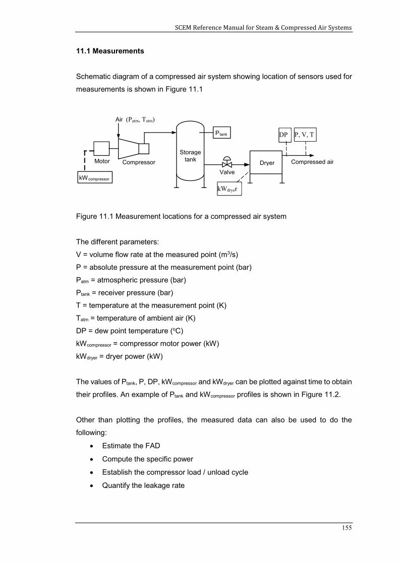
SCEM Reference Manual for Steam & Compressed Air Systems
155
11.1 Measurements
Schematic diagram of a compressed air system showing location of sensors used for
measurements is shown in Figure 11.1
Figure 11.1 Measurement locations for a compressed air system
The different parameters:
V = volume flow rate at the measured point (m3/s)
P = absolute pressure at the measurement point (bar)
Patm = atmospheric pressure (bar)
Ptank = receiver pressure (bar)
T = temperature at the measurement point (K)
Tatm = temperature of ambient air (K)
DP = dew point temperature (oC)
kWcompressor = compressor motor power (kW)
kWdryer = dryer power (kW)
The values of Ptank, P, DP, kWcompressor and kWdryer can be plotted against time to obtain
their profiles. An example of Ptank and kWcompressor profiles is shown in Figure 11.2.
Other than plotting the profiles, the measured data can also be used to do the
following:
Estimate the FAD
Compute the specific power
Establish the compressor load / unload cycle
Quantify the leakage rate
Compressor
Storage tankMotor
kWcompressor
Air
Valve
Dryer Compressed air
P tank
(Patm, Tatm)
kWdryer
P, V, T DP
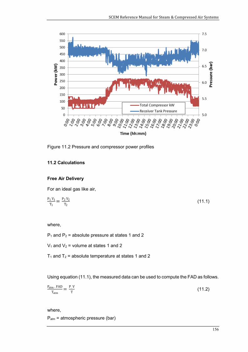
SCEM Reference Manual for Steam & Compressed Air Systems
156
Figure 11.2 Pressure and compressor power profiles
11.2 Calculations
Free Air Delivery
For an ideal gas like air,
P1 V1
T1=
P2 V2
T2 (11.1)
where,
P1 and P2 = absolute pressure at states 1 and 2
V1 and V2 = volume at states 1 and 2
T1 and T2 = absolute temperature at states 1 and 2
Using equation (11.1), the measured data can be used to compute the FAD as follows.
Patm . FAD
Tatm=
P . V
T (11.2)
where,
Patm = atmospheric pressure (bar)
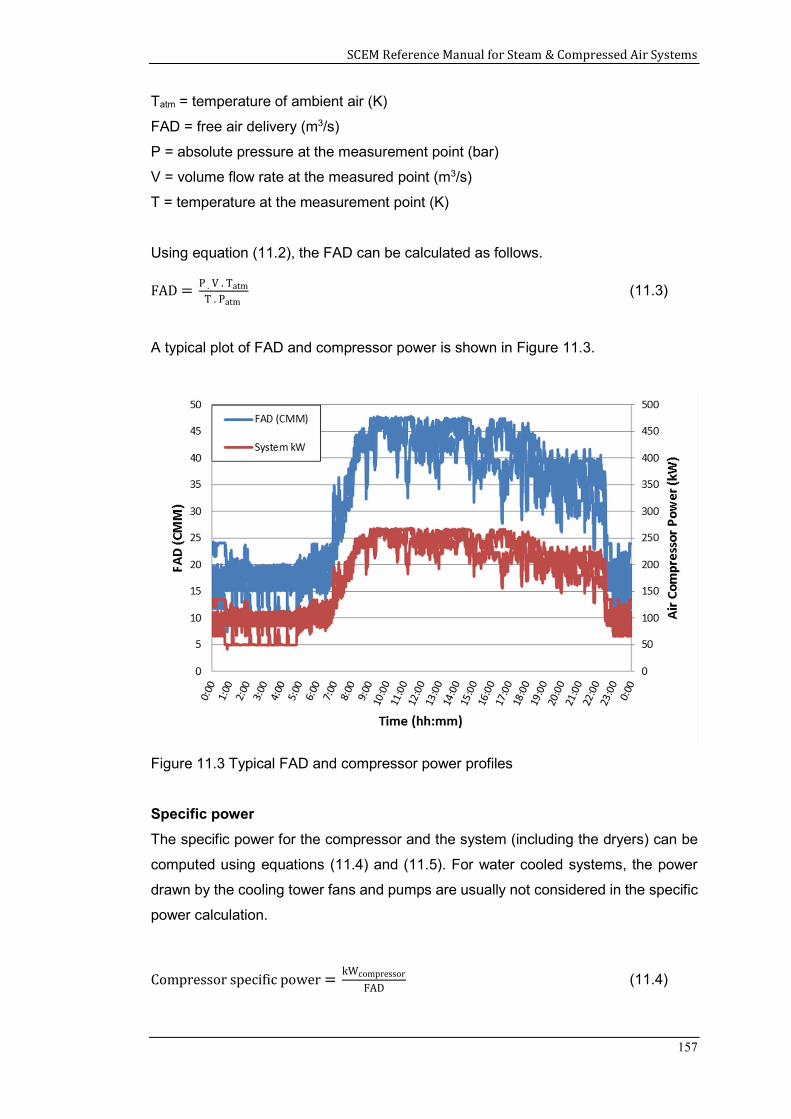
SCEM Reference Manual for Steam & Compressed Air Systems
157
Tatm = temperature of ambient air (K)
FAD = free air delivery (m3/s)
P = absolute pressure at the measurement point (bar)
V = volume flow rate at the measured point (m3/s)
T = temperature at the measurement point (K)
Using equation (11.2), the FAD can be calculated as follows.
FAD = P . V . Tatm
T . Patm (11.3)
A typical plot of FAD and compressor power is shown in Figure 11.3.
Figure 11.3 Typical FAD and compressor power profiles
Specific power
The specific power for the compressor and the system (including the dryers) can be
computed using equations (11.4) and (11.5). For water cooled systems, the power
drawn by the cooling tower fans and pumps are usually not considered in the specific
power calculation.
Compressor specific power = kWcompressor
FAD (11.4)
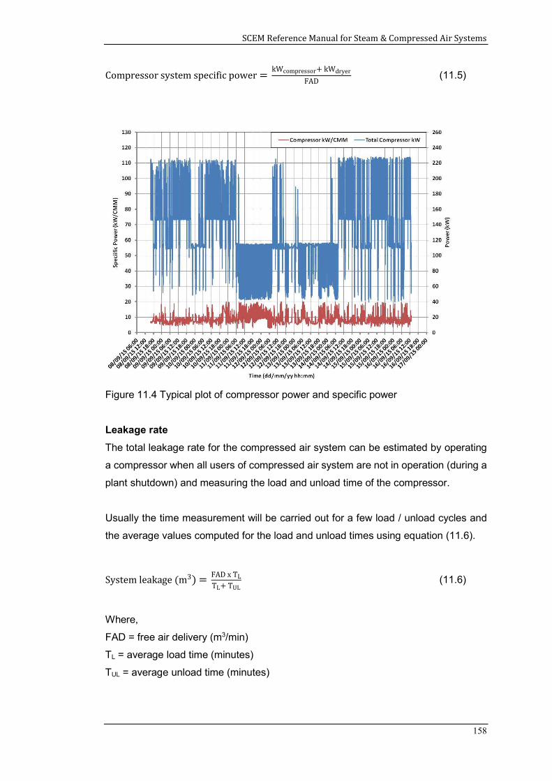
SCEM Reference Manual for Steam & Compressed Air Systems
158
Compressor system specific power = kWcompressor+ kWdryer
FAD (11.5)
Figure 11.4 Typical plot of compressor power and specific power
Leakage rate
The total leakage rate for the compressed air system can be estimated by operating
a compressor when all users of compressed air system are not in operation (during a
plant shutdown) and measuring the load and unload time of the compressor.
Usually the time measurement will be carried out for a few load / unload cycles and
the average values computed for the load and unload times using equation (11.6).
System leakage (m3) = FAD x TL
TL+ TUL (11.6)
Where,
FAD = free air delivery (m3/min)
TL = average load time (minutes)
TUL = average unload time (minutes)
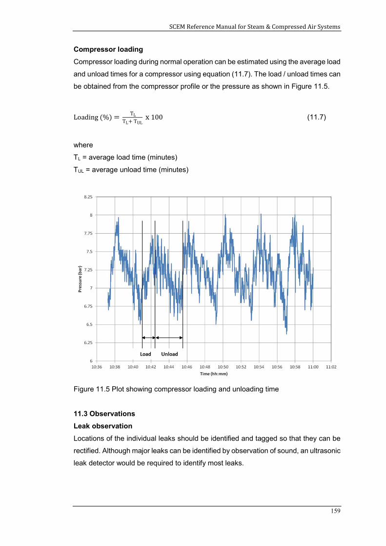
SCEM Reference Manual for Steam & Compressed Air Systems
159
Compressor loading
Compressor loading during normal operation can be estimated using the average load
and unload times for a compressor using equation (11.7). The load / unload times can
be obtained from the compressor profile or the pressure as shown in Figure 11.5.
Loading (%) = TL
TL+ TUL x 100 (11.7)
where
TL = average load time (minutes)
TUL = average unload time (minutes)
Figure 11.5 Plot showing compressor loading and unloading time
11.3 Observations
Leak observation
Locations of the individual leaks should be identified and tagged so that they can be
rectified. Although major leaks can be identified by observation of sound, an ultrasonic
leak detector would be required to identify most leaks.
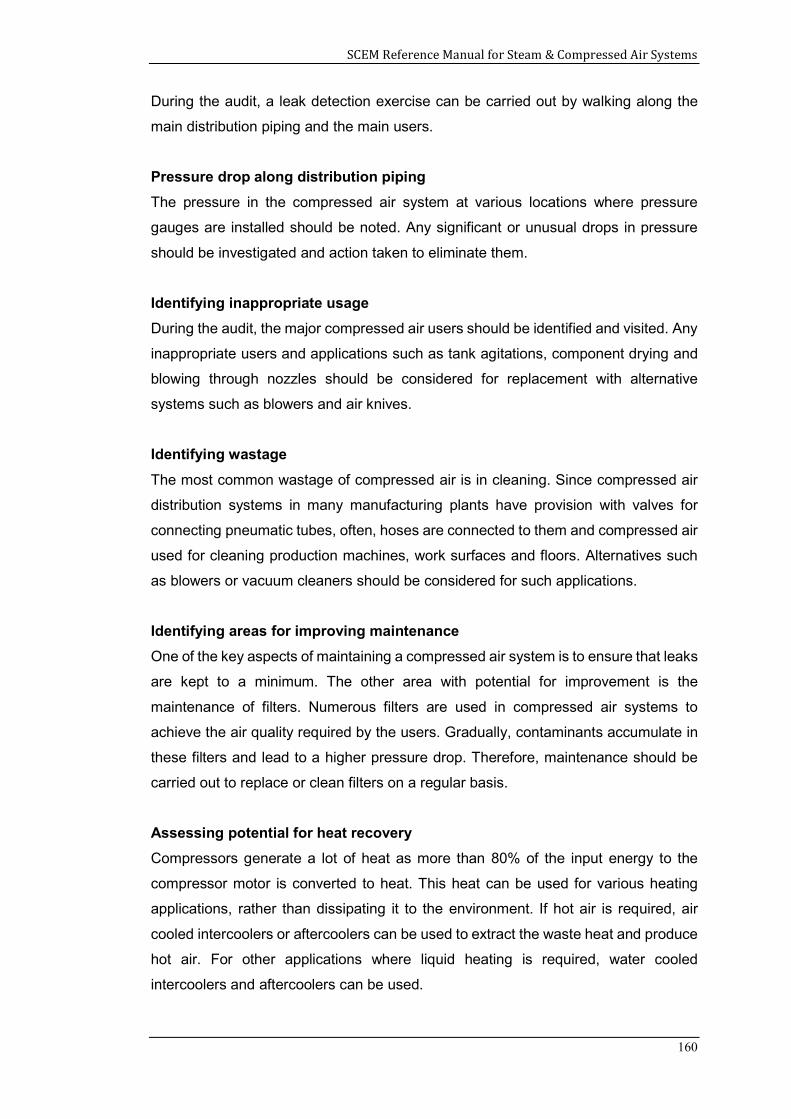
SCEM Reference Manual for Steam & Compressed Air Systems
160
During the audit, a leak detection exercise can be carried out by walking along the
main distribution piping and the main users.
Pressure drop along distribution piping
The pressure in the compressed air system at various locations where pressure
gauges are installed should be noted. Any significant or unusual drops in pressure
should be investigated and action taken to eliminate them.
Identifying inappropriate usage
During the audit, the major compressed air users should be identified and visited. Any
inappropriate users and applications such as tank agitations, component drying and
blowing through nozzles should be considered for replacement with alternative
systems such as blowers and air knives.
Identifying wastage
The most common wastage of compressed air is in cleaning. Since compressed air
distribution systems in many manufacturing plants have provision with valves for
connecting pneumatic tubes, often, hoses are connected to them and compressed air
used for cleaning production machines, work surfaces and floors. Alternatives such
as blowers or vacuum cleaners should be considered for such applications.
Identifying areas for improving maintenance
One of the key aspects of maintaining a compressed air system is to ensure that leaks
are kept to a minimum. The other area with potential for improvement is the
maintenance of filters. Numerous filters are used in compressed air systems to
achieve the air quality required by the users. Gradually, contaminants accumulate in
these filters and lead to a higher pressure drop. Therefore, maintenance should be
carried out to replace or clean filters on a regular basis.
Assessing potential for heat recovery
Compressors generate a lot of heat as more than 80% of the input energy to the
compressor motor is converted to heat. This heat can be used for various heating
applications, rather than dissipating it to the environment. If hot air is required, air
cooled intercoolers or aftercoolers can be used to extract the waste heat and produce
hot air. For other applications where liquid heating is required, water cooled
intercoolers and aftercoolers can be used.
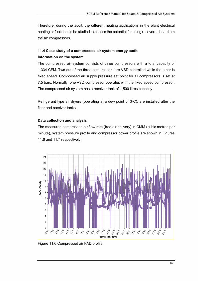
SCEM Reference Manual for Steam & Compressed Air Systems
161
Therefore, during the audit, the different heating applications in the plant electrical
heating or fuel should be studied to assess the potential for using recovered heat from
the air compressors.
11.4 Case study of a compressed air system energy audit
Information on the system
The compressed air system consists of three compressors with a total capacity of
1,334 CFM. Two out of the three compressors are VSD controlled while the other is
fixed speed. Compressed air supply pressure set point for all compressors is set at
7.5 bars. Normally, one VSD compressor operates with the fixed speed compressor.
The compressed air system has a receiver tank of 1,500 litres capacity.
Refrigerant type air dryers (operating at a dew point of 30C), are installed after the
filter and receiver tanks.
Data collection and analysis
The measured compressed air flow rate (free air delivery) in CMM (cubic metres per
minute), system pressure profile and compressor power profile are shown in Figures
11.6 and 11.7 respectively.
Figure 11.6 Compressed air FAD profile
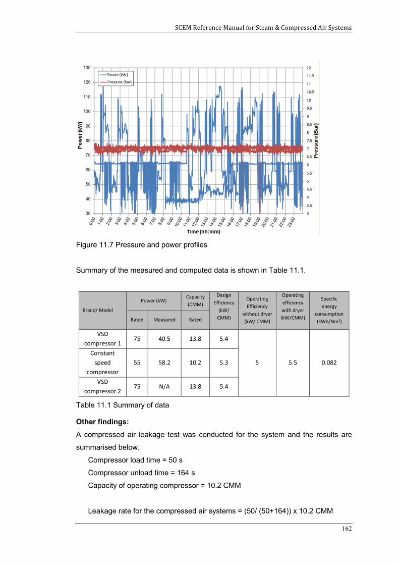
SCEM Reference Manual for Steam & Compressed Air Systems
162
Figure 11.7 Pressure and power profiles
Summary of the measured and computed data is shown in Table 11.1.
Brand/ Model
Power (kW) Capacity (CMM)
Design Efficiency
(kW/ CMM)
Operating Efficiency
without dryer (kW/ CMM)
Operating efficiency with dryer (kW/CMM)
Specific energy
consumption (kWh/Nm3) Rated Measured Rated
VSD compressor 1
75 40.5 13.8 5.4
5 5.5 0.082 Constant
speed compressor
55 58.2 10.2 5.3
VSD compressor 2
75 N/A 13.8 5.4
Table 11.1 Summary of data
Other findings:
A compressed air leakage test was conducted for the system and the results are
summarised below.
Compressor load time = 50 s
Compressor unload time = 164 s
Capacity of operating compressor = 10.2 CMM
Leakage rate for the compressed air systems = (50/ (50+164)) x 10.2 CMM
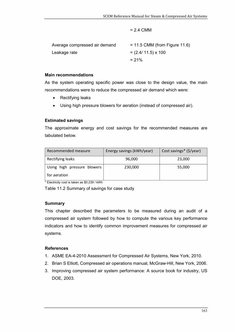
SCEM Reference Manual for Steam & Compressed Air Systems
163
= 2.4 CMM
Average compressed air demand = 11.5 CMM (from Figure 11.6)
Leakage rate = (2.4/ 11.5) x 100
= 21%
Main recommendations
As the system operating specific power was close to the design value, the main
recommendations were to reduce the compressed air demand which were:
Rectifying leaks
Using high pressure blowers for aeration (instead of compressed air).
Estimated savings
The approximate energy and cost savings for the recommended measures are
tabulated below.
Recommended measure Energy savings (kWh/year) Cost savings* ($/year)
Rectifying leaks 96,000 23,000
Using high pressure blowers
for aeration
230,000 55,000
* Electricity cost is taken as $0.239 / kWh
Table 11.2 Summary of savings for case study
Summary
This chapter described the parameters to be measured during an audit of a
compressed air system followed by how to compute the various key performance
indicators and how to identify common improvement measures for compressed air
systems.
References
1. ASME EA-4-2010 Assessment for Compressed Air Systems, New York, 2010.
2. Brian S Elliott, Compressed air operations manual, McGraw-Hill, New York, 2006.
3. Improving compressed air system performance: A source book for industry, US
DOE, 2003.
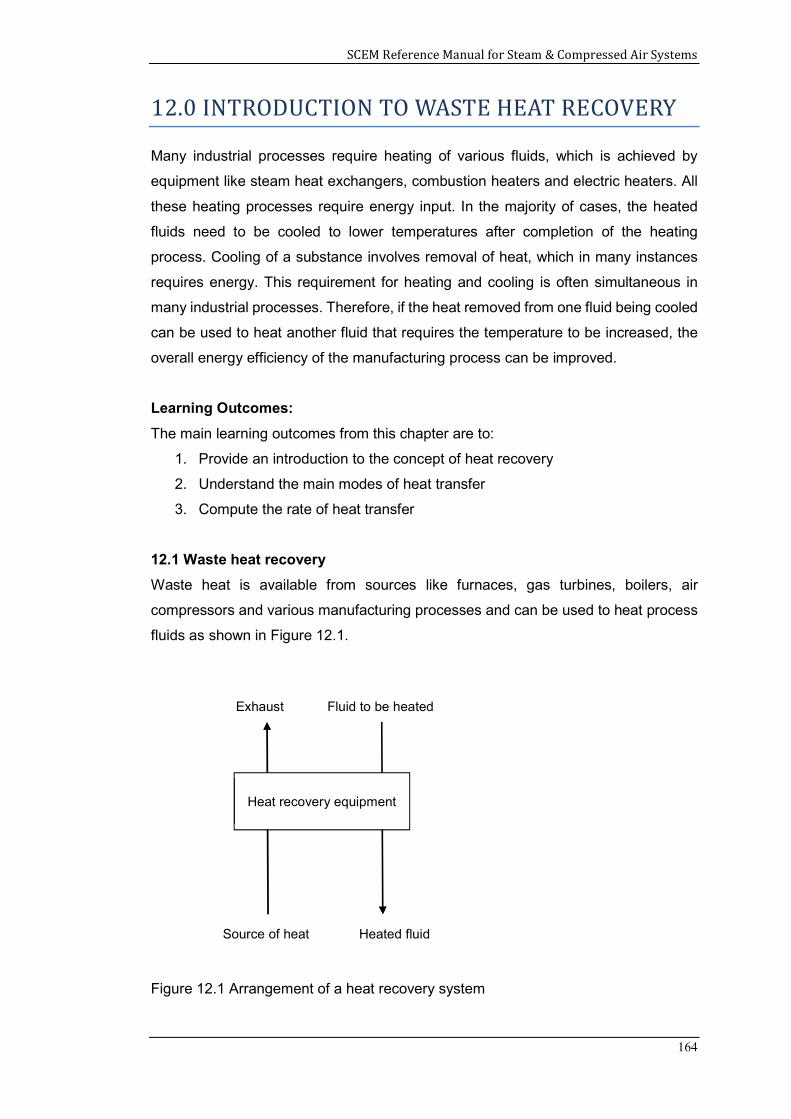
SCEM Reference Manual for Steam & Compressed Air Systems
164
12.0 INTRODUCTION TO WASTE HEAT RECOVERY
Many industrial processes require heating of various fluids, which is achieved by
equipment like steam heat exchangers, combustion heaters and electric heaters. All
these heating processes require energy input. In the majority of cases, the heated
fluids need to be cooled to lower temperatures after completion of the heating
process. Cooling of a substance involves removal of heat, which in many instances
requires energy. This requirement for heating and cooling is often simultaneous in
many industrial processes. Therefore, if the heat removed from one fluid being cooled
can be used to heat another fluid that requires the temperature to be increased, the
overall energy efficiency of the manufacturing process can be improved.
Learning Outcomes:
The main learning outcomes from this chapter are to:
1. Provide an introduction to the concept of heat recovery
2. Understand the main modes of heat transfer
3. Compute the rate of heat transfer
12.1 Waste heat recovery
Waste heat is available from sources like furnaces, gas turbines, boilers, air
compressors and various manufacturing processes and can be used to heat process
fluids as shown in Figure 12.1.
Figure 12.1 Arrangement of a heat recovery system
Exhaust Fluid to be heated
Source of heat
Heat recovery equipment
Heated fluid
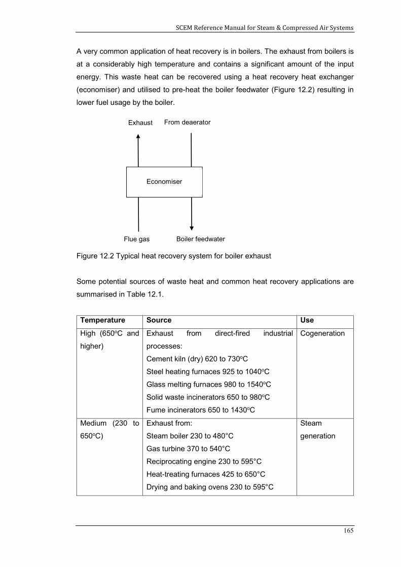
SCEM Reference Manual for Steam & Compressed Air Systems
165
A very common application of heat recovery is in boilers. The exhaust from boilers is
at a considerably high temperature and contains a significant amount of the input
energy. This waste heat can be recovered using a heat recovery heat exchanger
(economiser) and utilised to pre-heat the boiler feedwater (Figure 12.2) resulting in
lower fuel usage by the boiler.
Figure 12.2 Typical heat recovery system for boiler exhaust
Some potential sources of waste heat and common heat recovery applications are
summarised in Table 12.1.
Temperature Source Use
High (650oC and
higher)
Exhaust from direct-fired industrial
processes:
Cement kiln (dry) 620 to 730oC
Steel heating furnaces 925 to 1040oC
Glass melting furnaces 980 to 1540oC
Solid waste incinerators 650 to 980oC
Fume incinerators 650 to 1430oC
Cogeneration
Medium (230 to
650oC)
Exhaust from:
Steam boiler 230 to 480°C
Gas turbine 370 to 540°C
Reciprocating engine 230 to 595°C
Heat-treating furnaces 425 to 650°C
Drying and baking ovens 230 to 595°C
Steam
generation
Exhaust From deaerator
Boiler feedwater Flue gas
Economiser
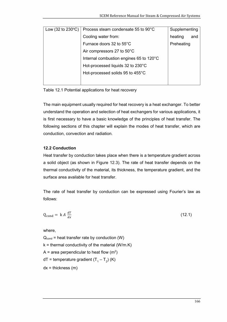
SCEM Reference Manual for Steam & Compressed Air Systems
166
Low (32 to 230oC) Process steam condensate 55 to 90°C
Cooling water from:
Furnace doors 32 to 55°C
Air compressors 27 to 50°C
Internal combustion engines 65 to 120°C
Hot-processed liquids 32 to 230°C
Hot-processed solids 95 to 455°C
Supplementing
heating and
Preheating
Table 12.1 Potential applications for heat recovery
The main equipment usually required for heat recovery is a heat exchanger. To better
understand the operation and selection of heat exchangers for various applications, it
is first necessary to have a basic knowledge of the principles of heat transfer. The
following sections of this chapter will explain the modes of heat transfer, which are
conduction, convection and radiation.
12.2 Conduction
Heat transfer by conduction takes place when there is a temperature gradient across
a solid object (as shown in Figure 12.3). The rate of heat transfer depends on the
thermal conductivity of the material, its thickness, the temperature gradient, and the
surface area available for heat transfer.
The rate of heat transfer by conduction can be expressed using Fourier’s law as
follows:
Q = k 𝐴 (12.1)
where,
Qcond = heat transfer rate by conduction (W)
k = thermal conductivity of the material (W/m.K)
A = area perpendicular to heat flow (m2)
dT = temperature gradient (T1 – T
2) (K)
dx = thickness (m)
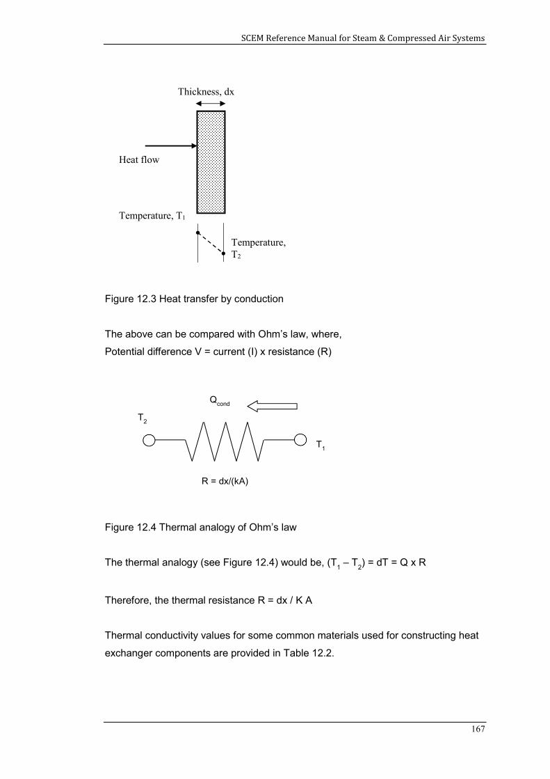
SCEM Reference Manual for Steam & Compressed Air Systems
167
Figure 12.3 Heat transfer by conduction
The above can be compared with Ohm’s law, where,
Potential difference V = current (I) x resistance (R)
Figure 12.4 Thermal analogy of Ohm’s law
The thermal analogy (see Figure 12.4) would be, (T1 – T
2) = dT = Q x R
Therefore, the thermal resistance R = dx / K A
Thermal conductivity values for some common materials used for constructing heat
exchanger components are provided in Table 12.2.
Thickness, dx
Heat flow
Temperature, T1
Temperature, T2
T1
T2
Qcond
R = dx/(kA)
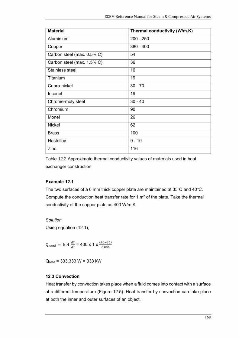
SCEM Reference Manual for Steam & Compressed Air Systems
168
Material Thermal conductivity (W/m.K)
Aluminium 200 - 250
Copper 380 - 400
Carbon steel (max. 0.5% C) 54
Carbon steel (max. 1.5% C) 36
Stainless steel 16
Titanium 19
Cupro-nickel 30 - 70
Inconel 19
Chrome-moly steel 30 - 40
Chromium 90
Monel 26
Nickel 62
Brass 100
Hastelloy 9 - 10
Zinc 116
Table 12.2 Approximate thermal conductivity values of materials used in heat
exchanger construction
Example 12.1
The two surfaces of a 6 mm thick copper plate are maintained at 35oC and 40oC.
Compute the conduction heat transfer rate for 1 m2 of the plate. Take the thermal
conductivity of the copper plate as 400 W/m.K
Solution
Using equation (12.1),
Q = k 𝐴 = 400 x 1 x ( )
.
Qcond = 333,333 W = 333 kW
12.3 Convection
Heat transfer by convection takes place when a fluid comes into contact with a surface
at a different temperature (Figure 12.5). Heat transfer by convection can take place
at both the inner and outer surfaces of an object.
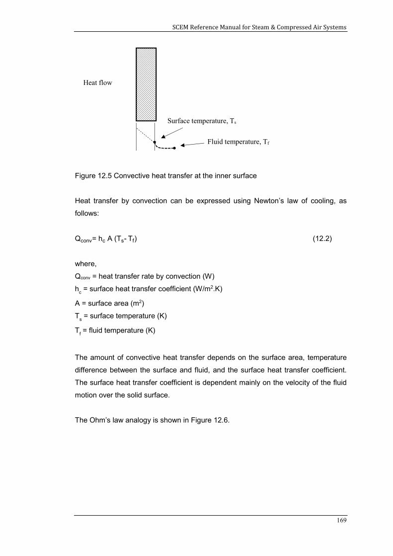
SCEM Reference Manual for Steam & Compressed Air Systems
169
Figure 12.5 Convective heat transfer at the inner surface
Heat transfer by convection can be expressed using Newton’s law of cooling, as
follows:
Qconv= hc A (Ts- Tf) (12.2)
where,
Qconv = heat transfer rate by convection (W)
hc = surface heat transfer coefficient (W/m2.K)
A = surface area (m2)
Ts = surface temperature (K)
Tf = fluid temperature (K)
The amount of convective heat transfer depends on the surface area, temperature
difference between the surface and fluid, and the surface heat transfer coefficient.
The surface heat transfer coefficient is dependent mainly on the velocity of the fluid
motion over the solid surface.
The Ohm’s law analogy is shown in Figure 12.6.
Heat flow
Surface temperature, Ts
Fluid temperature, Tf
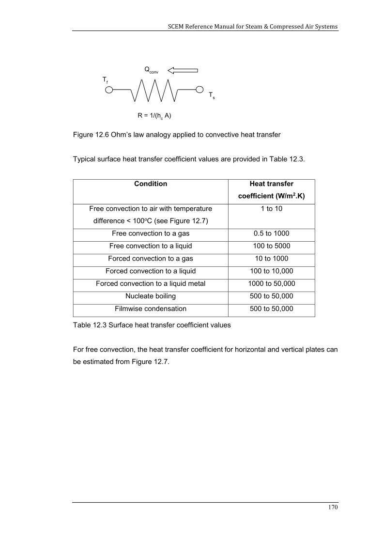
SCEM Reference Manual for Steam & Compressed Air Systems
170
Figure 12.6 Ohm’s law analogy applied to convective heat transfer
Typical surface heat transfer coefficient values are provided in Table 12.3.
Condition Heat transfer
coefficient (W/m2.K)
Free convection to air with temperature
difference < 100oC (see Figure 12.7)
1 to 10
Free convection to a gas 0.5 to 1000
Free convection to a liquid 100 to 5000
Forced convection to a gas 10 to 1000
Forced convection to a liquid 100 to 10,000
Forced convection to a liquid metal 1000 to 50,000
Nucleate boiling 500 to 50,000
Filmwise condensation 500 to 50,000
Table 12.3 Surface heat transfer coefficient values
For free convection, the heat transfer coefficient for horizontal and vertical plates can
be estimated from Figure 12.7.
Ts
Tf
Qconv
R = 1/(hc A)
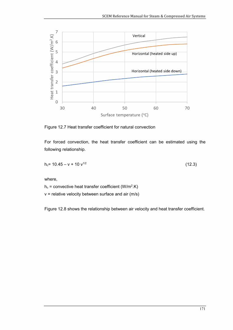
SCEM Reference Manual for Steam & Compressed Air Systems
171
Figure 12.7 Heat transfer coefficient for natural convection
For forced convection, the heat transfer coefficient can be estimated using the
following relationship.
hc= 10.45 – v + 10 v1/2 (12.3)
where,
hc = convective heat transfer coefficient (W/m2.K)
v = relative velocity between surface and air (m/s)
Figure 12.8 shows the relationship between air velocity and heat transfer coefficient.
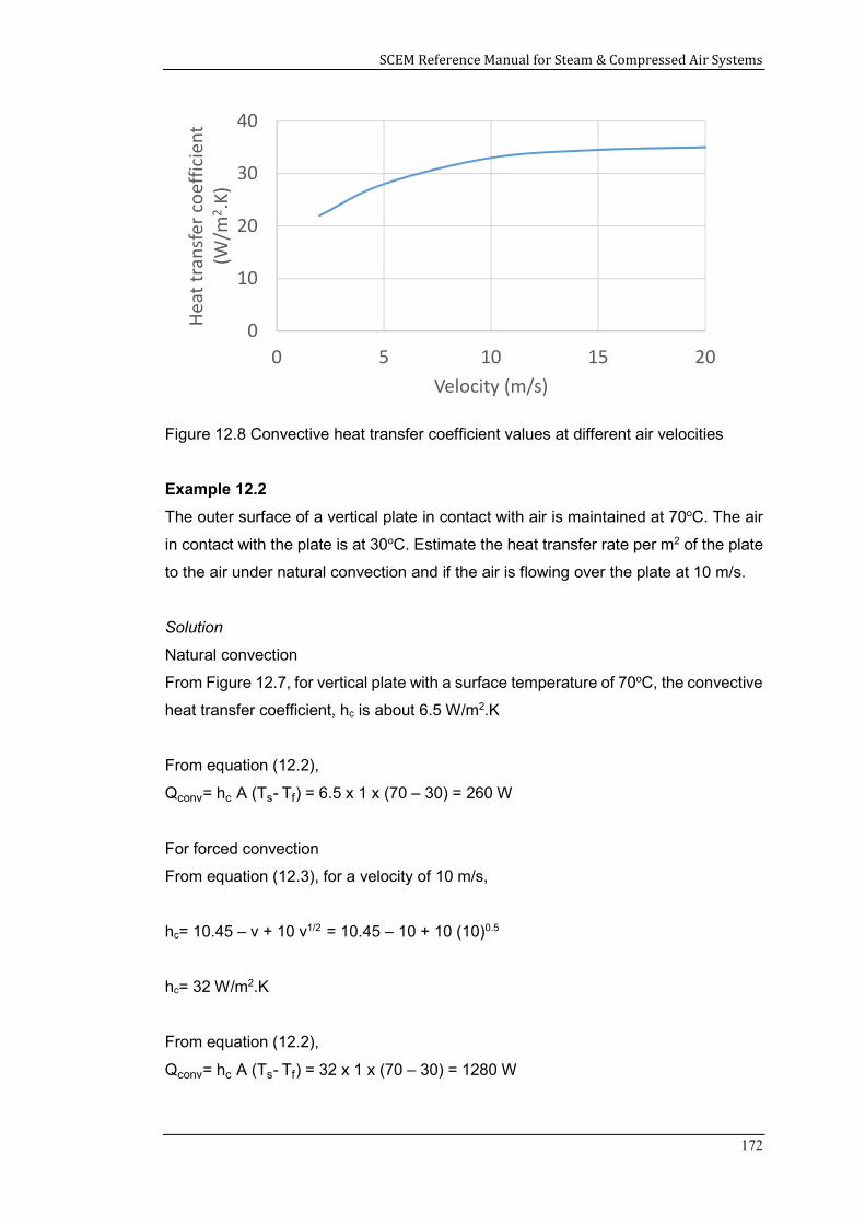
SCEM Reference Manual for Steam & Compressed Air Systems
172
Figure 12.8 Convective heat transfer coefficient values at different air velocities
Example 12.2
The outer surface of a vertical plate in contact with air is maintained at 70oC. The air
in contact with the plate is at 30oC. Estimate the heat transfer rate per m2 of the plate
to the air under natural convection and if the air is flowing over the plate at 10 m/s.
Solution
Natural convection
From Figure 12.7, for vertical plate with a surface temperature of 70oC, the convective
heat transfer coefficient, hc is about 6.5 W/m2.K
From equation (12.2),
Qconv= hc A (Ts- Tf) = 6.5 x 1 x (70 – 30) = 260 W
For forced convection
From equation (12.3), for a velocity of 10 m/s,
hc= 10.45 – v + 10 v1/2 = 10.45 – 10 + 10 (10)0.5
hc= 32 W/m2.K
From equation (12.2),
Qconv= hc A (Ts- Tf) = 32 x 1 x (70 – 30) = 1280 W
0
10
20
30
40
0 5 10 15 20
Hea
t tra
nsfe
r coe
ffici
ent
(W/m
2 .K)
Velocity (m/s)
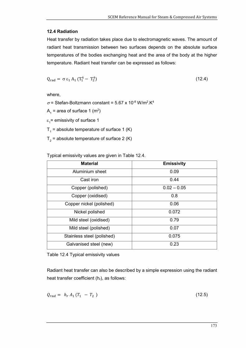
SCEM Reference Manual for Steam & Compressed Air Systems
173
12.4 Radiation
Heat transfer by radiation takes place due to electromagnetic waves. The amount of
radiant heat transmission between two surfaces depends on the absolute surface
temperatures of the bodies exchanging heat and the area of the body at the higher
temperature. Radiant heat transfer can be expressed as follows:
Q = A (T − T ) (12.4)
where,
= Stefan-Boltzmann constant = 5.67 x 10⁻⁸ W/m2.K4
A1 = area of surface 1 (m2)
1= emissivity of surface 1
T1 = absolute temperature of surface 1 (K)
T2 = absolute temperature of surface 2 (K)
Typical emissivity values are given in Table 12.4.
Material Emissivity
Aluminium sheet 0.09
Cast iron 0.44
Copper (polished) 0.02 – 0.05
Copper (oxidised) 0.8
Copper nickel (polished) 0.06
Nickel polished 0.072
Mild steel (oxidised) 0.79
Mild steel (polished) 0.07
Stainless steel (polished) 0.075
Galvanised steel (new) 0.23
Table 12.4 Typical emissivity values
Radiant heat transfer can also be described by a simple expression using the radiant
heat transfer coefficient (hr), as follows:
𝑄 = ℎ 𝐴 (𝑇 − 𝑇 ) (12.5)
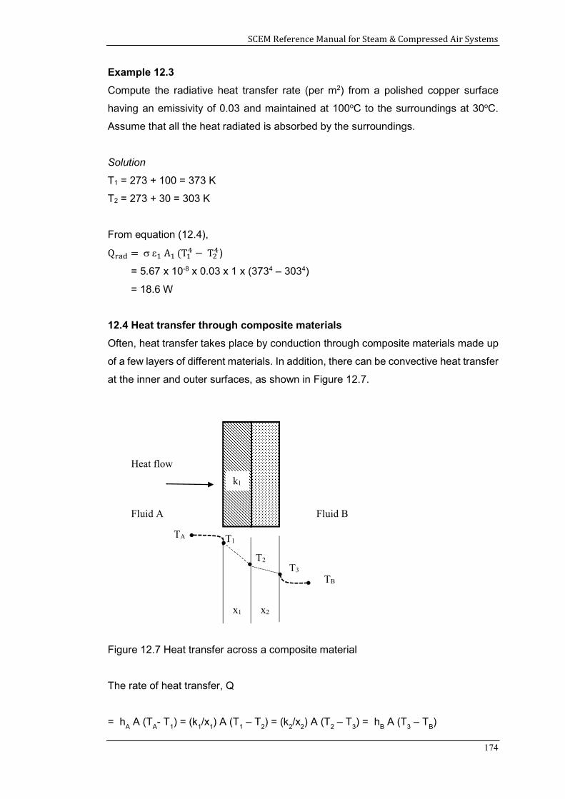
SCEM Reference Manual for Steam & Compressed Air Systems
174
Example 12.3
Compute the radiative heat transfer rate (per m2) from a polished copper surface
having an emissivity of 0.03 and maintained at 100oC to the surroundings at 30oC.
Assume that all the heat radiated is absorbed by the surroundings.
Solution
T1 = 273 + 100 = 373 K
T2 = 273 + 30 = 303 K
From equation (12.4),
Q = A (T − T )
= 5.67 x 10-8 x 0.03 x 1 x (3734 – 3034)
= 18.6 W
12.4 Heat transfer through composite materials
Often, heat transfer takes place by conduction through composite materials made up
of a few layers of different materials. In addition, there can be convective heat transfer
at the inner and outer surfaces, as shown in Figure 12.7.
Figure 12.7 Heat transfer across a composite material
The rate of heat transfer, Q
= hA A (T
A- T
1) = (k
1/x
1) A (T
1 – T
2) = (k
2/x
2) A (T
2 – T
3) = h
B A (T
3 – T
B)
Heat flow
Fluid A
TA
Fluid B
T1
T2 T3
TB
x1 x2
k1
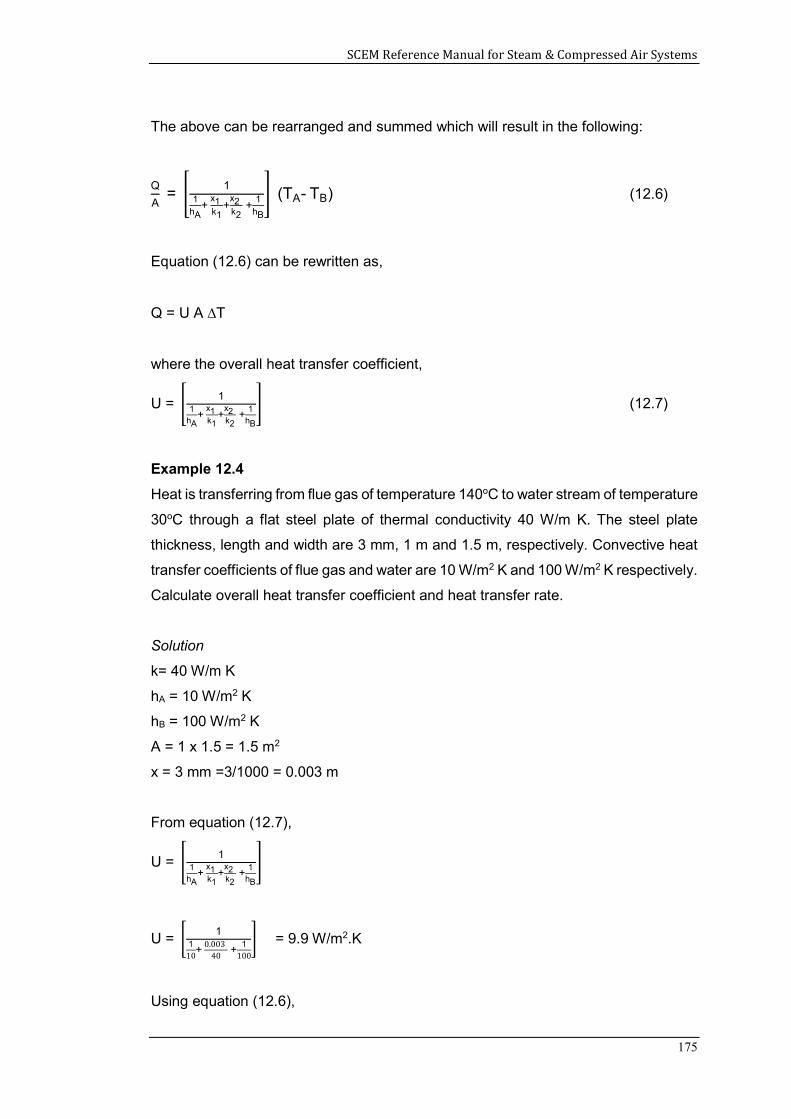
SCEM Reference Manual for Steam & Compressed Air Systems
175
The above can be rearranged and summed which will result in the following:
Q
A =
11
hA+
x1
k1+
x2
k2 +
1hB
(TA- TB) (12.6)
Equation (12.6) can be rewritten as,
Q = U A T
where the overall heat transfer coefficient,
U = 1
1hA
+ x1
k1+
x2
k2 +
1hB
(12.7)
Example 12.4
Heat is transferring from flue gas of temperature 140oC to water stream of temperature
30oC through a flat steel plate of thermal conductivity 40 W/m K. The steel plate
thickness, length and width are 3 mm, 1 m and 1.5 m, respectively. Convective heat
transfer coefficients of flue gas and water are 10 W/m2 K and 100 W/m2 K respectively.
Calculate overall heat transfer coefficient and heat transfer rate.
Solution
k= 40 W/m K
hA = 10 W/m2 K
hB = 100 W/m2 K
A = 1 x 1.5 = 1.5 m2
x = 3 mm =3/1000 = 0.003 m
From equation (12.7),
U = 1
1hA
+ x1
k1+
x2
k2 +
1hB
U = 1
110
+ 0.003
40 +
1100
= 9.9 W/m2.K
Using equation (12.6),
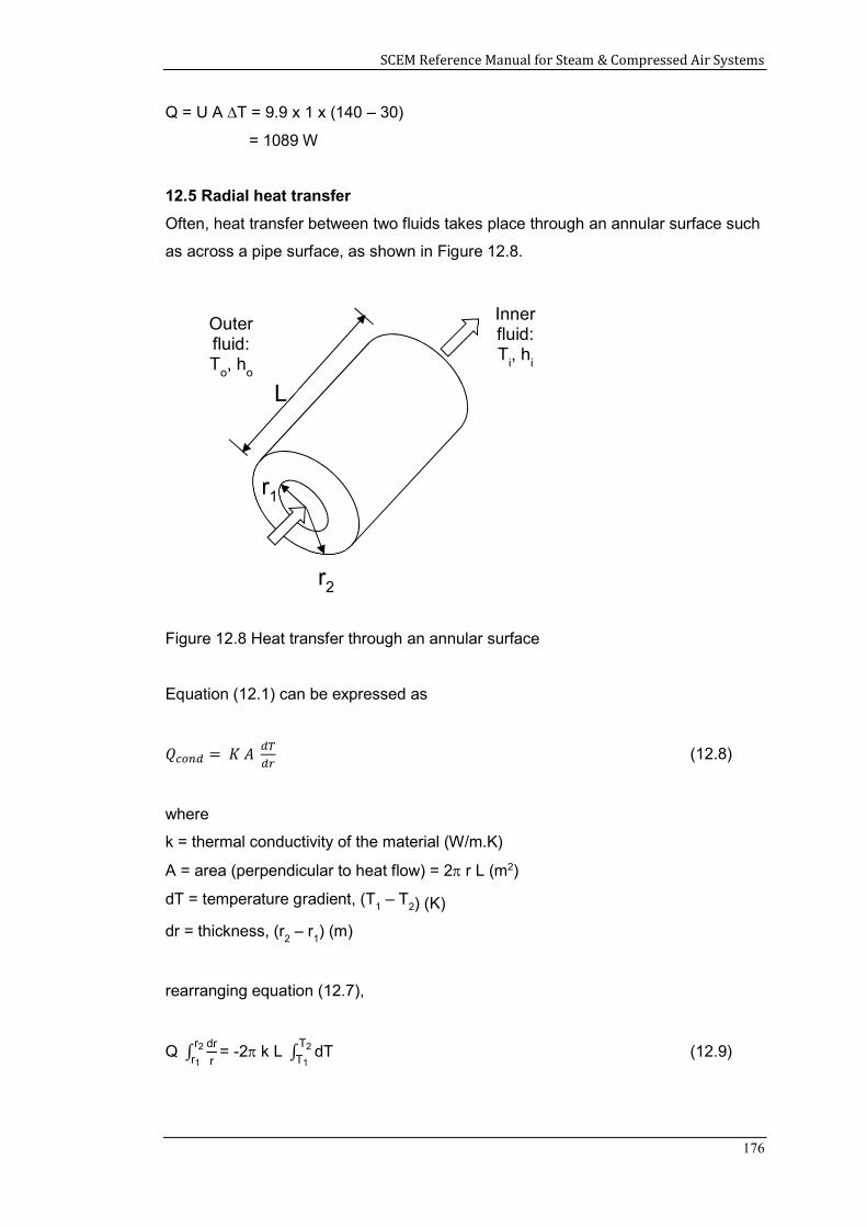
SCEM Reference Manual for Steam & Compressed Air Systems
176
Q = U A T = 9.9 x 1 x (140 – 30)
= 1089 W
12.5 Radial heat transfer
Often, heat transfer between two fluids takes place through an annular surface such
as across a pipe surface, as shown in Figure 12.8.
Figure 12.8 Heat transfer through an annular surface
Equation (12.1) can be expressed as
𝑄 = 𝐾 𝐴 (12.8)
where
k = thermal conductivity of the material (W/m.K)
A = area (perpendicular to heat flow) = 2 r L (m2)
dT = temperature gradient, (T1 – T
2) (K)
dr = thickness, (r2 – r
1) (m)
rearranging equation (12.7),
Q ∫dr
r
r2r1
= -2 k L ∫ dTT2
T1 (12.9)
r1
r2
L
Outer fluid: T
o, h
o
Inner fluid: T
i, h
i
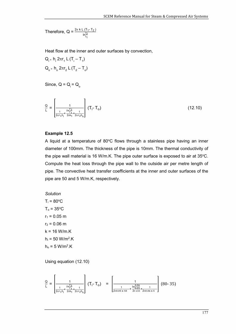
SCEM Reference Manual for Steam & Compressed Air Systems
177
Therefore, Q = 2 k L (T1- T2 )
lnr2r1
Heat flow at the inner and outer surfaces by convection,
Qi = hi
2r1 L (Ti
– T1)
Qo = ho
2r2 L (T2
– To)
Since, Q = Qi = Q
o
Q
L =
1
12 hi
+
2k1+
12 ho
(Ti- To) (12.10)
Example 12.5
A liquid at a temperature of 80oC flows through a stainless pipe having an inner
diameter of 100mm. The thickness of the pipe is 10mm. The thermal conductivity of
the pipe wall material is 16 W/m.K. The pipe outer surface is exposed to air at 35oC.
Compute the heat loss through the pipe wall to the outside air per metre length of
pipe. The convective heat transfer coefficients at the inner and outer surfaces of the
pipe are 50 and 5 W/m.K, respectively.
Solution
Ti = 80oC
To = 35oC
r1 = 0.05 m
r2 = 0.06 m
k = 16 W/m.K
hi = 50 W/m2.K
ho = 5 W/m2.K
Using equation (12.10)
Q
L =
1
12 hi
+
2k1+
12 ho
(Ti- To) = 1
12 .
+
.
.
2 x16+
12 .
(80- 35)
SCEM Reference Manual for Steam & Compressed Air Systems
178
= 378 W/m
Summary
The various modes of heat transfer were explained in this chapter. The key
parameters that control heat transfer were identified and the heat transfer rate was
computed for different situations. The application of these concepts in heat recovery
systems will be discussed in the subsequent chapters of this reference manual.
References
1. Arora, C P, Heat and Mass Transfer, Khanna Publishers, Delhi, 1986.
2. ASHRAE Handbook: Fundamentals, American Society of Heating, Refrigerating
and Air-Conditioning Engineers Inc., Atlanta, GA, 2017.
3. Bergman, Lavine, Incropera, and DeWitt, Fundamentals of Heat Transfer, 7th
edition, John Wiley & Sons, New York, 2011.
4. Cornwell, K, The Flow of Heat, ELBS and Van Nostrand Reinhold Company Ltd,
London, 1977.
5. Jayamaha, Lal, Energy-Efficient Industrial Systems, Evaluation and
Implementation, McGraw-Hill, New York, 2016.
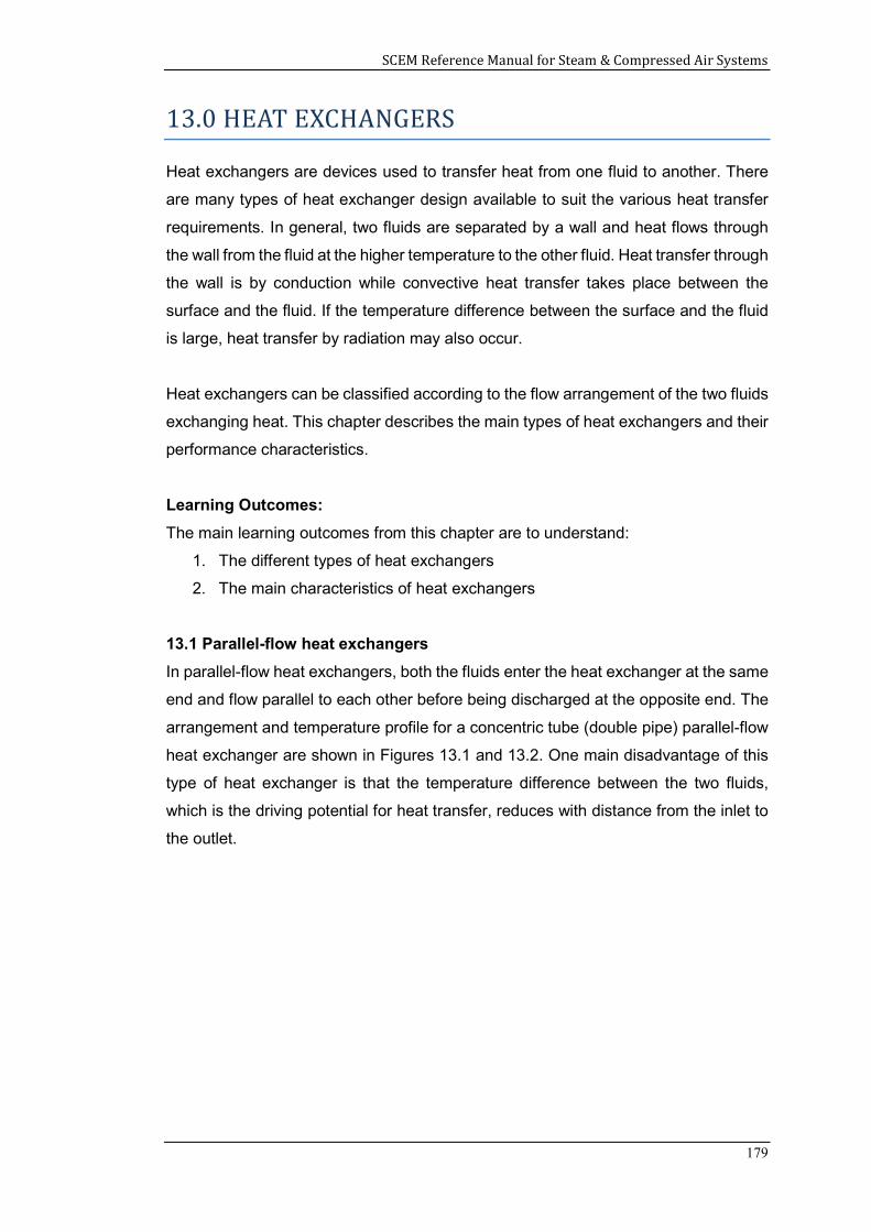
SCEM Reference Manual for Steam & Compressed Air Systems
179
13.0 HEAT EXCHANGERS
Heat exchangers are devices used to transfer heat from one fluid to another. There
are many types of heat exchanger design available to suit the various heat transfer
requirements. In general, two fluids are separated by a wall and heat flows through
the wall from the fluid at the higher temperature to the other fluid. Heat transfer through
the wall is by conduction while convective heat transfer takes place between the
surface and the fluid. If the temperature difference between the surface and the fluid
is large, heat transfer by radiation may also occur.
Heat exchangers can be classified according to the flow arrangement of the two fluids
exchanging heat. This chapter describes the main types of heat exchangers and their
performance characteristics.
Learning Outcomes:
The main learning outcomes from this chapter are to understand:
1. The different types of heat exchangers
2. The main characteristics of heat exchangers
13.1 Parallel-flow heat exchangers
In parallel-flow heat exchangers, both the fluids enter the heat exchanger at the same
end and flow parallel to each other before being discharged at the opposite end. The
arrangement and temperature profile for a concentric tube (double pipe) parallel-flow
heat exchanger are shown in Figures 13.1 and 13.2. One main disadvantage of this
type of heat exchanger is that the temperature difference between the two fluids,
which is the driving potential for heat transfer, reduces with distance from the inlet to
the outlet.
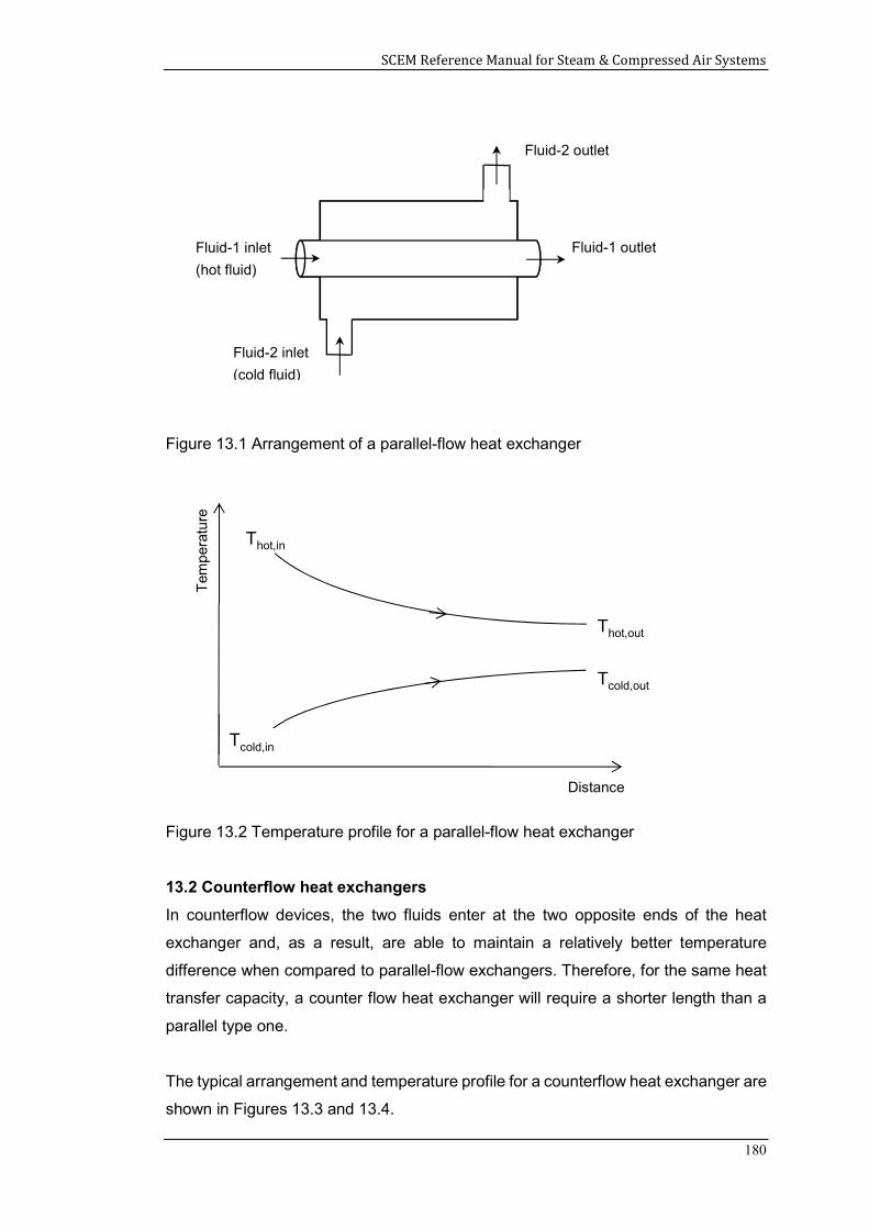
SCEM Reference Manual for Steam & Compressed Air Systems
180
Figure 13.1 Arrangement of a parallel-flow heat exchanger
Figure 13.2 Temperature profile for a parallel-flow heat exchanger
13.2 Counterflow heat exchangers
In counterflow devices, the two fluids enter at the two opposite ends of the heat
exchanger and, as a result, are able to maintain a relatively better temperature
difference when compared to parallel-flow exchangers. Therefore, for the same heat
transfer capacity, a counter flow heat exchanger will require a shorter length than a
parallel type one.
The typical arrangement and temperature profile for a counterflow heat exchanger are
shown in Figures 13.3 and 13.4.
Fluid-1 inlet
(hot fluid) Fluid-1 outlet
Fluid-2 inlet
(cold fluid)
Fluid-2 outlet
Thot,in
Tem
per
atu
re
Thot,out
Tcold,out
Tcold,in
Distance
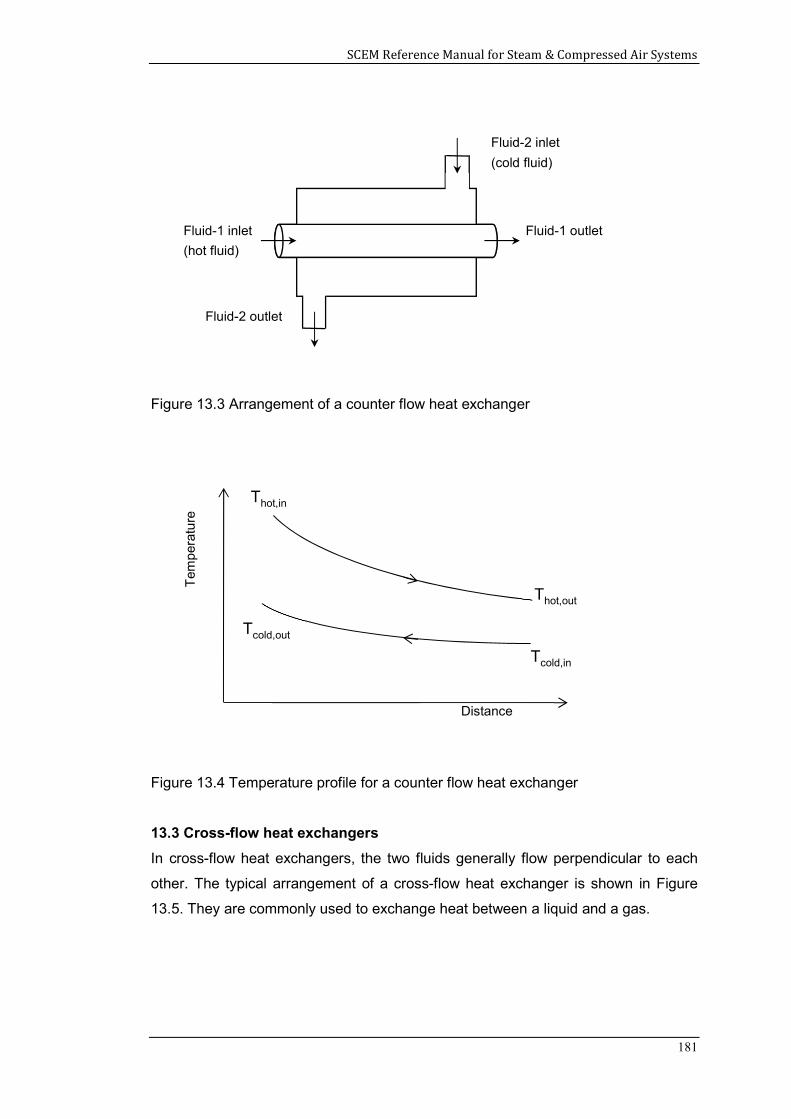
SCEM Reference Manual for Steam & Compressed Air Systems
181
Figure 13.3 Arrangement of a counter flow heat exchanger
Figure 13.4 Temperature profile for a counter flow heat exchanger
13.3 Cross-flow heat exchangers
In cross-flow heat exchangers, the two fluids generally flow perpendicular to each
other. The typical arrangement of a cross-flow heat exchanger is shown in Figure
13.5. They are commonly used to exchange heat between a liquid and a gas.
Fluid-1 inlet
(hot fluid) Fluid-1 outlet
Fluid-2 outlet
Fluid-2 inlet
(cold fluid)
Distance
Tem
per
atu
re
Thot,in
Tcold,in
Thot,out
Tcold,out
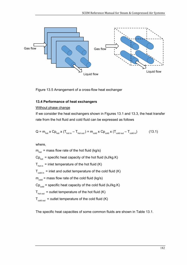
SCEM Reference Manual for Steam & Compressed Air Systems
182
Figure 13.5 Arrangement of a cross-flow heat exchanger
13.4 Performance of heat exchangers
Without phase change
If we consider the heat exchangers shown in Figures 13.1 and 13.3, the heat transfer
rate from the hot fluid and cold fluid can be expressed as follows
Q = mhot
x Cphot
x (Thot in
– Thot out
) = mcold
x Cpcold
x (Tcold out
– Tcold in
) (13.1)
where,
mhot
= mass flow rate of the hot fluid (kg/s)
Cphot
= specific heat capacity of the hot fluid (kJ/kg.K)
Thot in = inlet temperature of the hot fluid (K)
Tcold in = inlet and outlet temperature of the cold fluid (K)
mcold
= mass flow rate of the cold fluid (kg/s)
Cpcold
= specific heat capacity of the cold fluid (kJ/kg.K)
Thot out
= outlet temperature of the hot fluid (K)
Tcold out
= outlet temperature of the cold fluid (K)
The specific heat capacities of some common fluids are shown in Table 13.1.
Gas flow
Liquid flow
Gas flow
Liquid flow
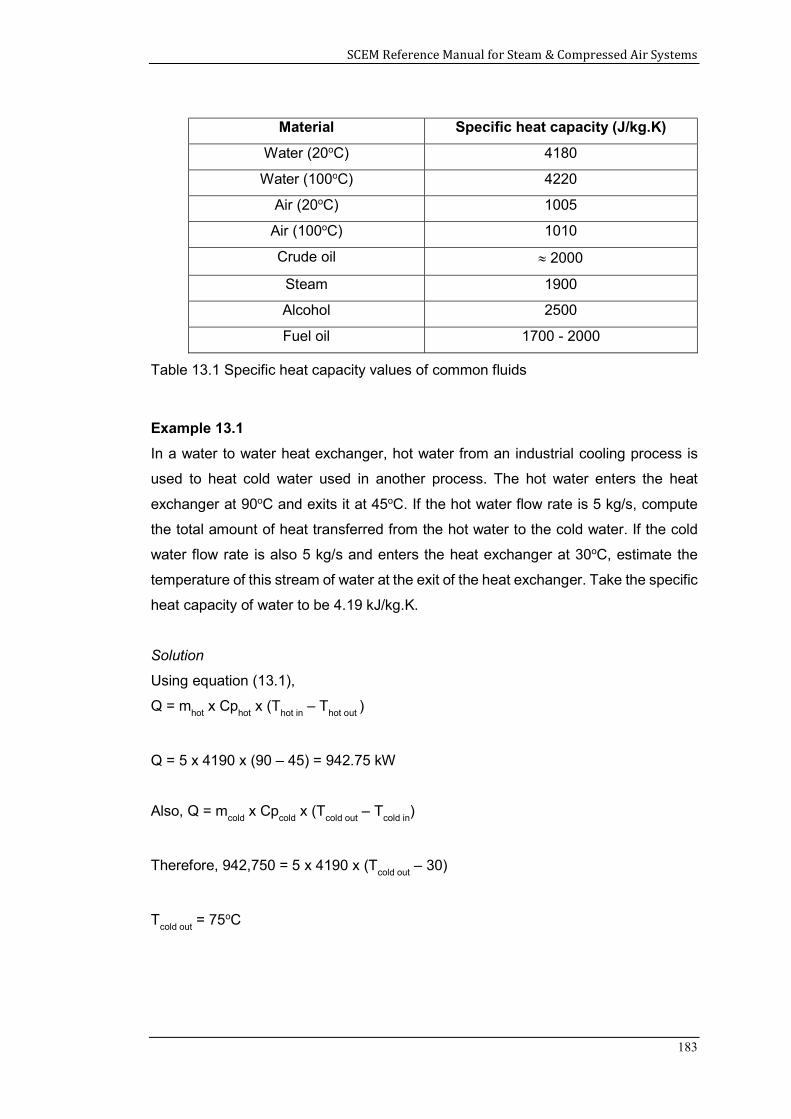
SCEM Reference Manual for Steam & Compressed Air Systems
183
Material Specific heat capacity (J/kg.K)
Water (20oC) 4180
Water (100oC) 4220
Air (20oC) 1005
Air (100oC) 1010
Crude oil 2000
Steam 1900
Alcohol 2500
Fuel oil 1700 - 2000
Table 13.1 Specific heat capacity values of common fluids
Example 13.1
In a water to water heat exchanger, hot water from an industrial cooling process is
used to heat cold water used in another process. The hot water enters the heat
exchanger at 90oC and exits it at 45oC. If the hot water flow rate is 5 kg/s, compute
the total amount of heat transferred from the hot water to the cold water. If the cold
water flow rate is also 5 kg/s and enters the heat exchanger at 30oC, estimate the
temperature of this stream of water at the exit of the heat exchanger. Take the specific
heat capacity of water to be 4.19 kJ/kg.K.
Solution
Using equation (13.1),
Q = mhot
x Cphot
x (Thot in
– Thot out
)
Q = 5 x 4190 x (90 – 45) = 942.75 kW
Also, Q = mcold
x Cpcold
x (Tcold out
– Tcold in
)
Therefore, 942,750 = 5 x 4190 x (Tcold out
– 30)
Tcold out
= 75oC
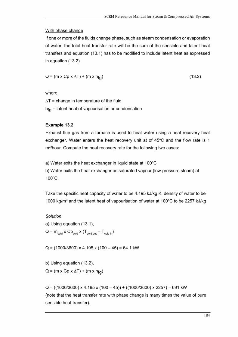
SCEM Reference Manual for Steam & Compressed Air Systems
184
With phase change
If one or more of the fluids change phase, such as steam condensation or evaporation
of water, the total heat transfer rate will be the sum of the sensible and latent heat
transfers and equation (13.1) has to be modified to include latent heat as expressed
in equation (13.2).
Q = (m x Cp x T) + (m x hfg) (13.2)
where,
T = change in temperature of the fluid
hfg = latent heat of vapourisation or condensation
Example 13.2
Exhaust flue gas from a furnace is used to heat water using a heat recovery heat
exchanger. Water enters the heat recovery unit at of 45oC and the flow rate is 1
m3/hour. Compute the heat recovery rate for the following two cases:
a) Water exits the heat exchanger in liquid state at 100oC
b) Water exits the heat exchanger as saturated vapour (low-pressure steam) at
100oC.
Take the specific heat capacity of water to be 4.195 kJ/kg.K, density of water to be
1000 kg/m3 and the latent heat of vapourisation of water at 100oC to be 2257 kJ/kg
Solution
a) Using equation (13.1),
Q = mcold
x Cpcold
x (Tcold out
– Tcold in
)
Q = (1000/3600) x 4.195 x (100 – 45) = 64.1 kW
b) Using equation (13.2),
Q = (m x Cp x T) + (m x hfg)
Q = ((1000/3600) x 4.195 x (100 – 45)) + ((1000/3600) x 2257) = 691 kW
(note that the heat transfer rate with phase change is many times the value of pure
sensible heat transfer).
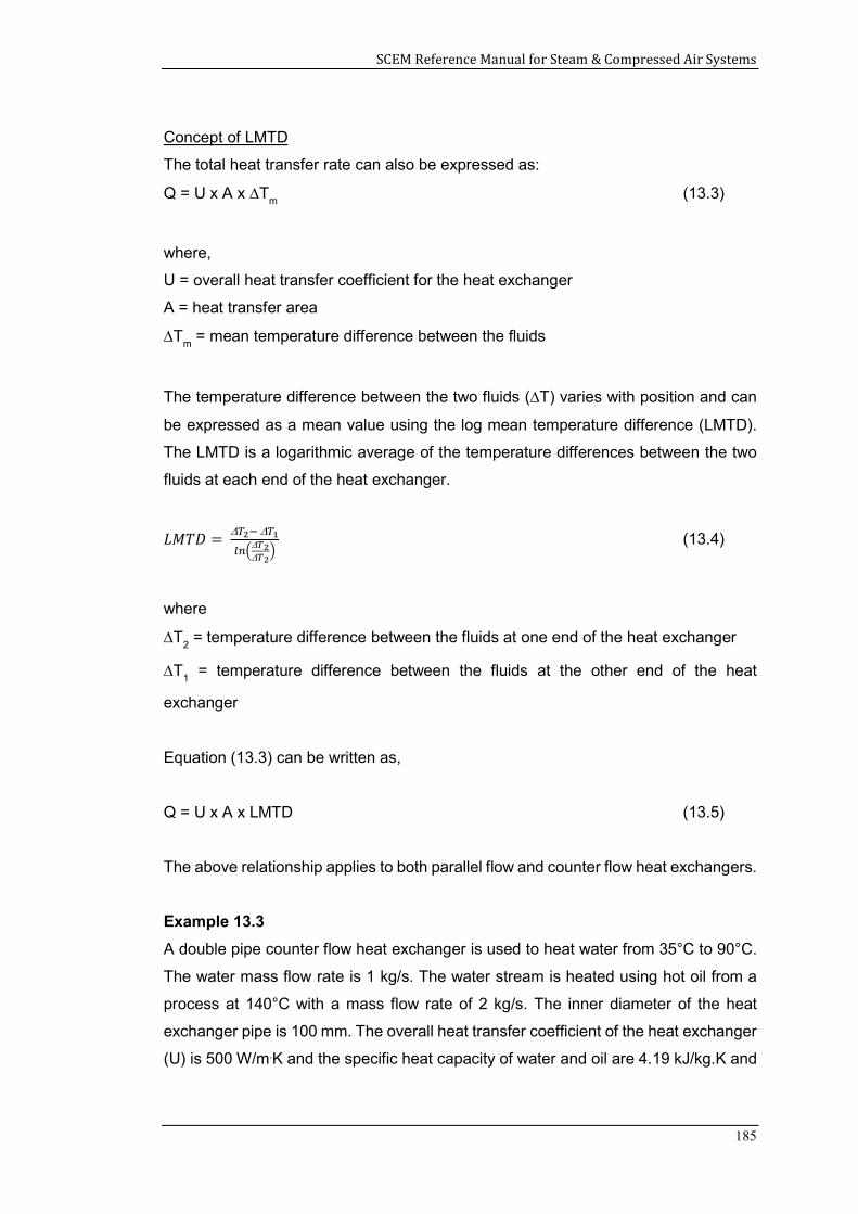
SCEM Reference Manual for Steam & Compressed Air Systems
185
Concept of LMTD
The total heat transfer rate can also be expressed as:
Q = U x A x Tm (13.3)
where,
U = overall heat transfer coefficient for the heat exchanger
A = heat transfer area
Tm = mean temperature difference between the fluids
The temperature difference between the two fluids (T) varies with position and can
be expressed as a mean value using the log mean temperature difference (LMTD).
The LMTD is a logarithmic average of the temperature differences between the two
fluids at each end of the heat exchanger.
𝐿𝑀𝑇𝐷 =
(13.4)
where
T2 = temperature difference between the fluids at one end of the heat exchanger
T1 = temperature difference between the fluids at the other end of the heat
exchanger
Equation (13.3) can be written as,
Q = U x A x LMTD (13.5)
The above relationship applies to both parallel flow and counter flow heat exchangers.
Example 13.3
A double pipe counter flow heat exchanger is used to heat water from 35°C to 90°C.
The water mass flow rate is 1 kg/s. The water stream is heated using hot oil from a
process at 140°C with a mass flow rate of 2 kg/s. The inner diameter of the heat
exchanger pipe is 100 mm. The overall heat transfer coefficient of the heat exchanger
(U) is 500 W/m.K and the specific heat capacity of water and oil are 4.19 kJ/kg.K and
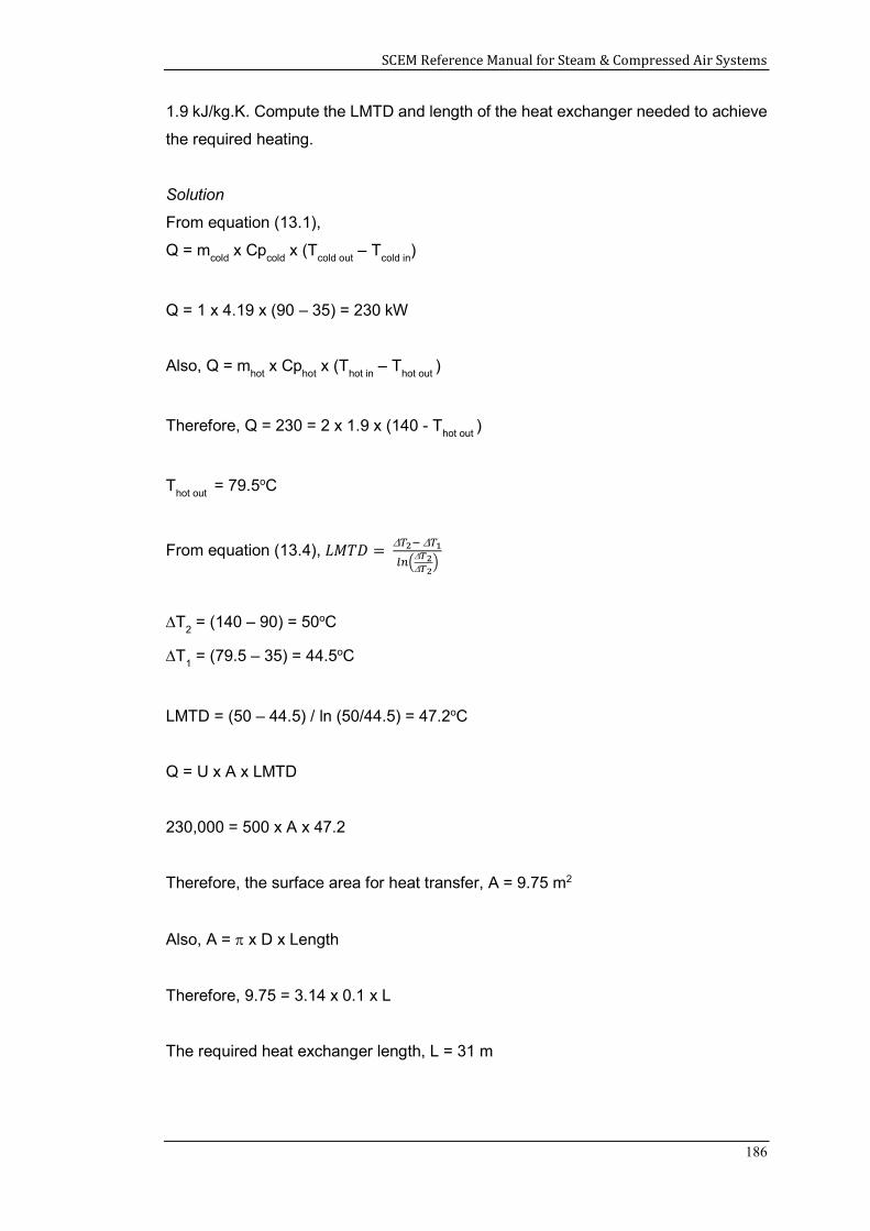
SCEM Reference Manual for Steam & Compressed Air Systems
186
1.9 kJ/kg.K. Compute the LMTD and length of the heat exchanger needed to achieve
the required heating.
Solution
From equation (13.1),
Q = mcold
x Cpcold
x (Tcold out
– Tcold in
)
Q = 1 x 4.19 x (90 – 35) = 230 kW
Also, Q = mhot
x Cphot
x (Thot in
– Thot out
)
Therefore, Q = 230 = 2 x 1.9 x (140 - Thot out
)
Thot out
= 79.5oC
From equation (13.4), 𝐿𝑀𝑇𝐷 =
T2 = (140 – 90) = 50oC
T1 = (79.5 – 35) = 44.5oC
LMTD = (50 – 44.5) / ln (50/44.5) = 47.2oC
Q = U x A x LMTD
230,000 = 500 x A x 47.2
Therefore, the surface area for heat transfer, A = 9.75 m2
Also, A = x D x Length
Therefore, 9.75 = 3.14 x 0.1 x L
The required heat exchanger length, L = 31 m
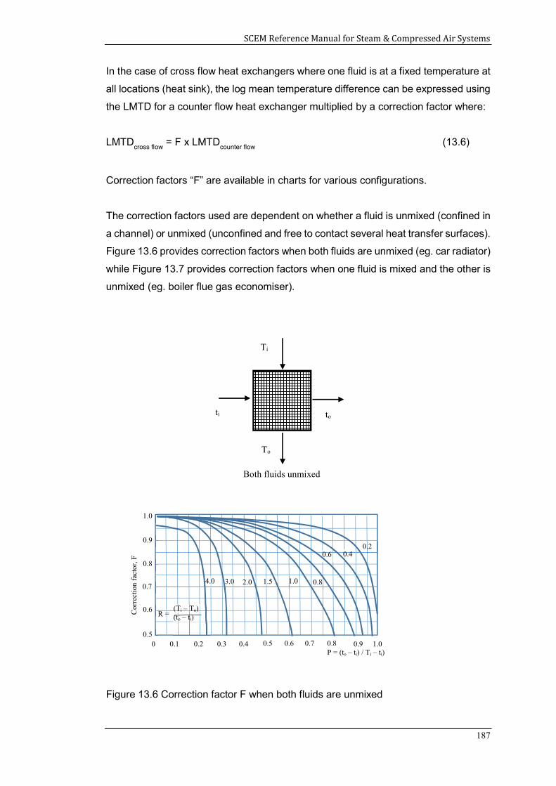
SCEM Reference Manual for Steam & Compressed Air Systems
187
In the case of cross flow heat exchangers where one fluid is at a fixed temperature at
all locations (heat sink), the log mean temperature difference can be expressed using
the LMTD for a counter flow heat exchanger multiplied by a correction factor where:
LMTDcross flow
= F x LMTDcounter flow
(13.6)
Correction factors “F” are available in charts for various configurations.
The correction factors used are dependent on whether a fluid is unmixed (confined in
a channel) or unmixed (unconfined and free to contact several heat transfer surfaces).
Figure 13.6 provides correction factors when both fluids are unmixed (eg. car radiator)
while Figure 13.7 provides correction factors when one fluid is mixed and the other is
unmixed (eg. boiler flue gas economiser).
Figure 13.6 Correction factor F when both fluids are unmixed
Ti
to ti
To
Both fluids unmixed
1.0
0.9
0.8
0.7
0.6
0.5 0 0.1
Cor
rect
ion
fact
or, F
0.2 0.3 1.0 0.4 0.5
0.2 0.4 0.6
0.8 1.0 1.5 2.0 3.0 4.0
0.6 0.7
(Ti – To) (to – ti)
0.8 0.9 P = (to – ti) / Ti – ti)
R =
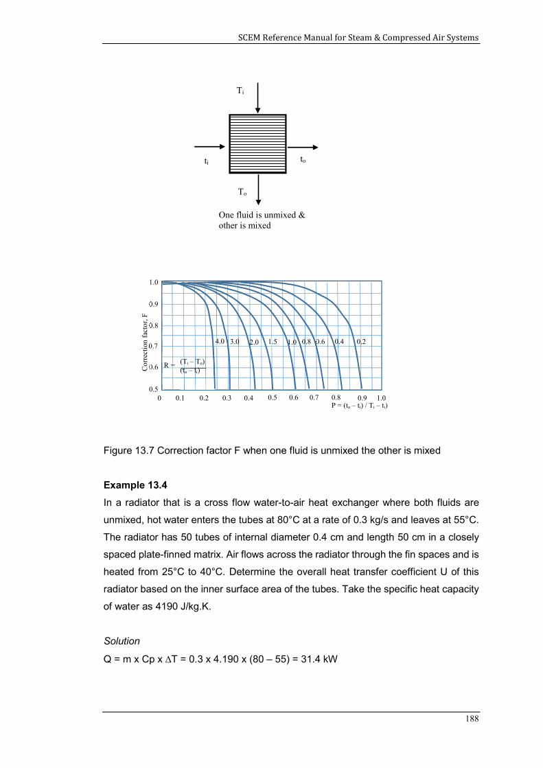
SCEM Reference Manual for Steam & Compressed Air Systems
188
Figure 13.7 Correction factor F when one fluid is unmixed the other is mixed
Example 13.4
In a radiator that is a cross flow water-to-air heat exchanger where both fluids are
unmixed, hot water enters the tubes at 80°C at a rate of 0.3 kg/s and leaves at 55°C.
The radiator has 50 tubes of internal diameter 0.4 cm and length 50 cm in a closely
spaced plate-finned matrix. Air flows across the radiator through the fin spaces and is
heated from 25°C to 40°C. Determine the overall heat transfer coefficient U of this
radiator based on the inner surface area of the tubes. Take the specific heat capacity
of water as 4190 J/kg.K.
Solution
Q = m x Cp x T = 0.3 x 4.190 x (80 – 55) = 31.4 kW
Ti
to ti
One fluid is unmixed & other is mixed
To
1.0
0.9
0.8
0.7
0.6
0.5 0 0.1 0.2 0.3
Cor
rect
ion
fact
or, F
1.0 0.4 0.5 0.6 0.7 0.8
0.2 0.4 0.6 0.8 1.0 1.5 2.0 3.0 4.0
0.9 P = (to – ti) / Ti – ti)
(Ti – To) (to – ti)
R =
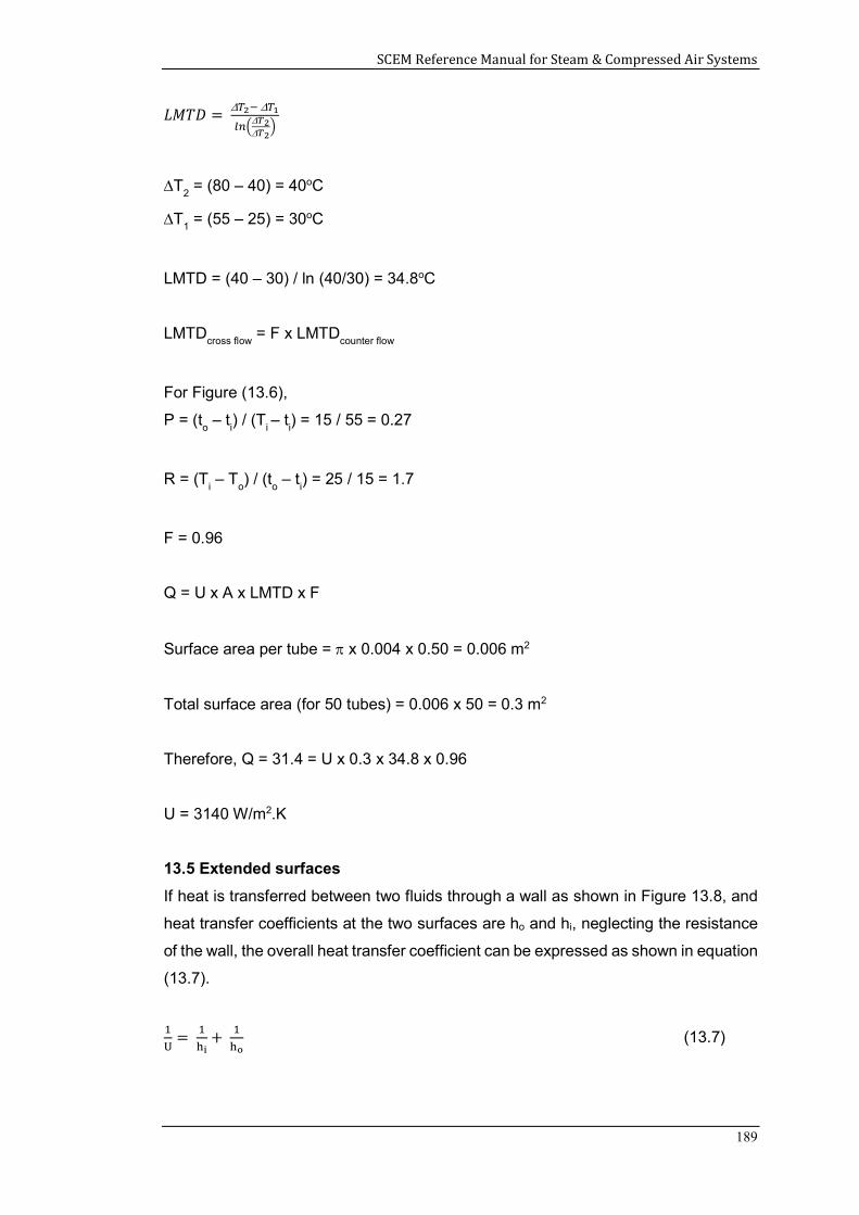
SCEM Reference Manual for Steam & Compressed Air Systems
189
𝐿𝑀𝑇𝐷 =
T2 = (80 – 40) = 40oC
T1 = (55 – 25) = 30oC
LMTD = (40 – 30) / ln (40/30) = 34.8oC
LMTDcross flow
= F x LMTDcounter flow
For Figure (13.6),
P = (to – t
i) / (T
i – t
i) = 15 / 55 = 0.27
R = (Ti – T
o) / (t
o – t
i) = 25 / 15 = 1.7
F = 0.96
Q = U x A x LMTD x F
Surface area per tube = x 0.004 x 0.50 = 0.006 m2
Total surface area (for 50 tubes) = 0.006 x 50 = 0.3 m2
Therefore, Q = 31.4 = U x 0.3 x 34.8 x 0.96
U = 3140 W/m2.K
13.5 Extended surfaces
If heat is transferred between two fluids through a wall as shown in Figure 13.8, and
heat transfer coefficients at the two surfaces are ho and hi, neglecting the resistance
of the wall, the overall heat transfer coefficient can be expressed as shown in equation
(13.7).
= + (13.7)
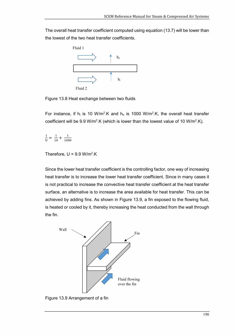
SCEM Reference Manual for Steam & Compressed Air Systems
190
The overall heat transfer coefficient computed using equation (13.7) will be lower than
the lowest of the two heat transfer coefficients.
Figure 13.8 Heat exchange between two fluids
For instance, if hi is 10 W/m2.K and ho is 1000 W/m2.K, the overall heat transfer
coefficient will be 9.9 W/m2.K (which is lower than the lowest value of 10 W/m2.K).
= +
Therefore, U = 9.9 W/m2.K
Since the lower heat transfer coefficient is the controlling factor, one way of increasing
heat transfer is to increase the lower heat transfer coefficient. Since in many cases it
is not practical to increase the convective heat transfer coefficient at the heat transfer
surface, an alternative is to increase the area available for heat transfer. This can be
achieved by adding fins. As shown in Figure 13.9, a fin exposed to the flowing fluid,
is heated or cooled by it, thereby increasing the heat conducted from the wall through
the fin.
Figure 13.9 Arrangement of a fin
Wall Fin
Fluid flowing over the fin
Fluid 1
Fluid 2
ho
hi
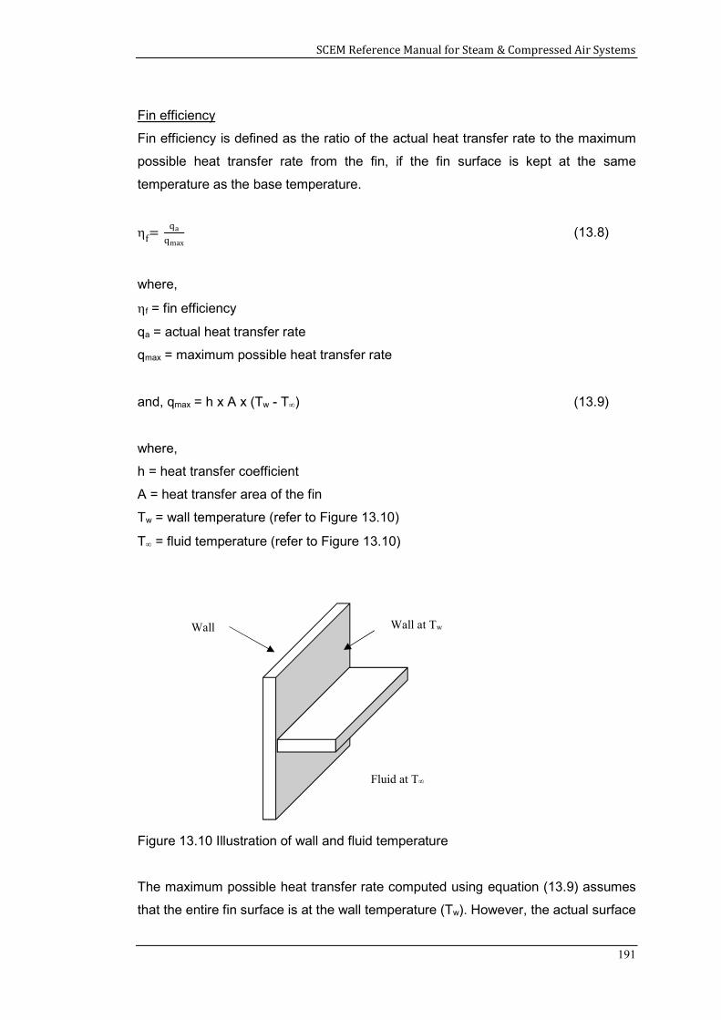
SCEM Reference Manual for Steam & Compressed Air Systems
191
Fin efficiency
Fin efficiency is defined as the ratio of the actual heat transfer rate to the maximum
possible heat transfer rate from the fin, if the fin surface is kept at the same
temperature as the base temperature.
f= qa
qmax (13.8)
where,
f = fin efficiency
qa = actual heat transfer rate
qmax = maximum possible heat transfer rate
and, qmax = h x A x (Tw - T) (13.9)
where,
h = heat transfer coefficient
A = heat transfer area of the fin
Tw = wall temperature (refer to Figure 13.10)
T = fluid temperature (refer to Figure 13.10)
Figure 13.10 Illustration of wall and fluid temperature
The maximum possible heat transfer rate computed using equation (13.9) assumes
that the entire fin surface is at the wall temperature (Tw). However, the actual surface
Wall Wall at Tw
Fluid at T
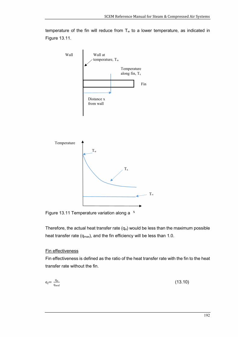
SCEM Reference Manual for Steam & Compressed Air Systems
192
temperature of the fin will reduce from Tw to a lower temperature, as indicated in
Figure 13.11.
Figure 13.11 Temperature variation along a fin
Therefore, the actual heat transfer rate (qa) would be less than the maximum possible
heat transfer rate (qmax), and the fin efficiency will be less than 1.0.
Fin effectiveness
Fin effectiveness is defined as the ratio of the heat transfer rate with the fin to the heat
transfer rate without the fin.
ϵf= qa
qwof (13.10)
Wall Wall at temperature, Tw
Temperature along fin, Tx
Fin
Distance x from wall
x
Temperature
Tw
Tx
T
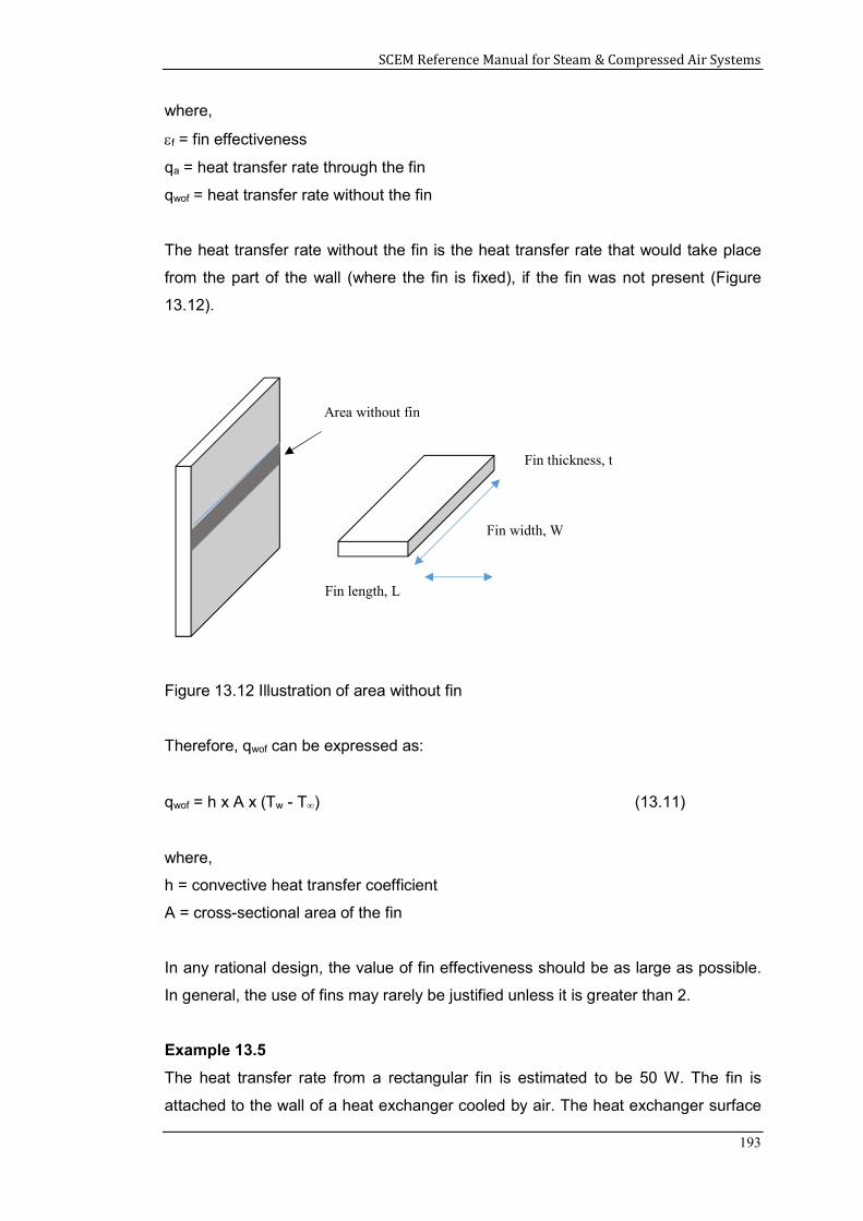
SCEM Reference Manual for Steam & Compressed Air Systems
193
where,
f = fin effectiveness
qa = heat transfer rate through the fin
qwof = heat transfer rate without the fin
The heat transfer rate without the fin is the heat transfer rate that would take place
from the part of the wall (where the fin is fixed), if the fin was not present (Figure
13.12).
Figure 13.12 Illustration of area without fin
Therefore, qwof can be expressed as:
qwof = h x A x (Tw - T) (13.11)
where,
h = convective heat transfer coefficient
A = cross-sectional area of the fin
In any rational design, the value of fin effectiveness should be as large as possible.
In general, the use of fins may rarely be justified unless it is greater than 2.
Example 13.5
The heat transfer rate from a rectangular fin is estimated to be 50 W. The fin is
attached to the wall of a heat exchanger cooled by air. The heat exchanger surface
Area without fin
Fin thickness, t
Fin length, L
Fin width, W
SCEM Reference Manual for Steam & Compressed Air Systems
194
temperature is maintained at 150°C and the ambient air temperature is 30°C. The
width and thickness of the fin are 250 mm and 3 mm, respectively. The convective
heat transfer coefficient is 10 W/m2 K and the fin efficiency is 70%.
Compute the length of the fin and the effectiveness of the fin.
Solution
The surface area of the fin, taking the fin length to be L,
= (2 x 0.25 x L) + (0.003 x (2L + 0.25))
= 0.506 L + 0.00075 (the second term can be neglected)
Therefore,
Fin length calculation
qmax = h x A x (Tw - T)
= 10 x 0.506 x L x (150 - 30) = 607 L
f= qa
qmax = 0.7
Since qa = 50 W,
qmax = 50 / 0.7 = 71.4 W = 607 x L
Hence, L = 0.118 m (118 mm)
qwof = h x A x (Tw - T)
= 10 x 0.003 x 0.05 x (150 – 30)
= 0.18 W
Fin effectiveness calculation,
ϵf= qa
qwof=
.= 277.8
13.6 Heat exchanger effectiveness
Similar to fins, the effectiveness of a heat exchanger can also be defined as the ratio
of the actual heat transfer rate to the maximum possible heat transfer rate.
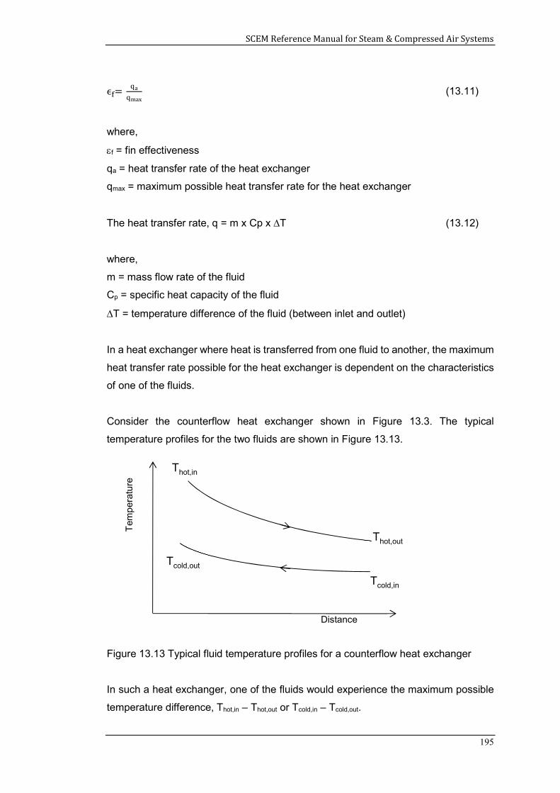
SCEM Reference Manual for Steam & Compressed Air Systems
195
ϵ = qa
qmax (13.11)
where,
f = fin effectiveness
qa = heat transfer rate of the heat exchanger
qmax = maximum possible heat transfer rate for the heat exchanger
The heat transfer rate, q = m x Cp x T (13.12)
where,
m = mass flow rate of the fluid
Cp = specific heat capacity of the fluid
T = temperature difference of the fluid (between inlet and outlet)
In a heat exchanger where heat is transferred from one fluid to another, the maximum
heat transfer rate possible for the heat exchanger is dependent on the characteristics
of one of the fluids.
Consider the counterflow heat exchanger shown in Figure 13.3. The typical
temperature profiles for the two fluids are shown in Figure 13.13.
Figure 13.13 Typical fluid temperature profiles for a counterflow heat exchanger
In such a heat exchanger, one of the fluids would experience the maximum possible
temperature difference, Thot,in – Thot,out or Tcold,in – Tcold,out.
Distance
Tem
per
atu
re
Thot,in
Tcold,in
Thot,out
Tcold,out
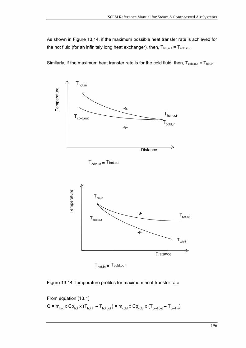
SCEM Reference Manual for Steam & Compressed Air Systems
196
As shown in Figure 13.14, if the maximum possible heat transfer rate is achieved for
the hot fluid (for an infinitely long heat exchanger), then, Thot,out = Tcold,in.
Similarly, if the maximum heat transfer rate is for the cold fluid, then, Tcold,out = Thot,in.
Figure 13.14 Temperature profiles for maximum heat transfer rate
From equation (13.1)
Q = mhot
x Cphot
x (Thot in
– Thot out
) = mcold
x Cpcold
x (Tcold out
– Tcold in
)
Thot,in
Tem
per
atur
e
Thot,out Tcold,out Tcold,in
Distance
Tcold,in = Thot,out
Thot,in
Tem
per
atu
re
Thot,out
Tcold,in
Distance
Tcold,out
Thot,in = Tcold,out
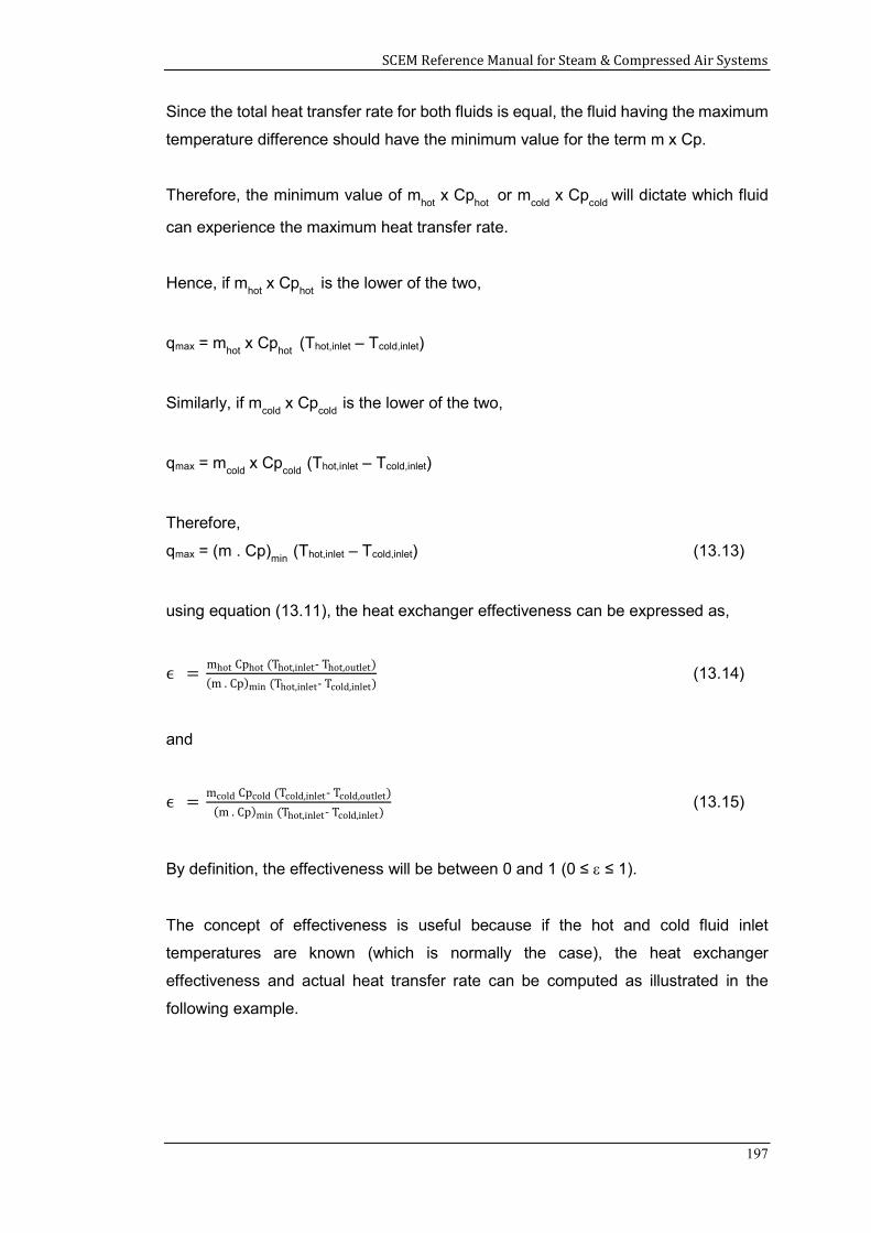
SCEM Reference Manual for Steam & Compressed Air Systems
197
Since the total heat transfer rate for both fluids is equal, the fluid having the maximum
temperature difference should have the minimum value for the term m x Cp.
Therefore, the minimum value of mhot
x Cphot or mcold
x Cpcold
will dictate which fluid
can experience the maximum heat transfer rate.
Hence, if mhot
x Cphot is the lower of the two,
qmax = mhot
x Cphot (Thot,inlet – Tcold,inlet)
Similarly, if mcold
x Cpcold
is the lower of the two,
qmax = mcold
x Cpcold
(Thot,inlet – Tcold,inlet)
Therefore,
qmax = (m . Cp)min
(Thot,inlet – Tcold,inlet) (13.13)
using equation (13.11), the heat exchanger effectiveness can be expressed as,
ϵ = mhot Cphot (Thot,inlet- Thot,outlet)
(m . Cp)min (Thot,inlet- Tcold,inlet) (13.14)
and
ϵ = mcold Cpcold (Tcold,inlet- Tcold,outlet)
(m . Cp)min (Thot,inlet- Tcold,inlet) (13.15)
By definition, the effectiveness will be between 0 and 1 (0 ≤ ≤ 1).
The concept of effectiveness is useful because if the hot and cold fluid inlet
temperatures are known (which is normally the case), the heat exchanger
effectiveness and actual heat transfer rate can be computed as illustrated in the
following example.
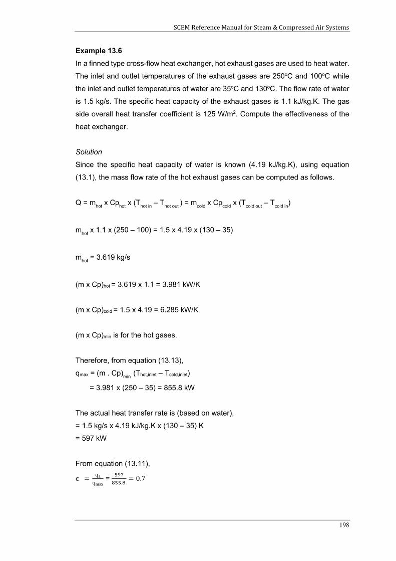
SCEM Reference Manual for Steam & Compressed Air Systems
198
Example 13.6
In a finned type cross-flow heat exchanger, hot exhaust gases are used to heat water.
The inlet and outlet temperatures of the exhaust gases are 250oC and 100oC while
the inlet and outlet temperatures of water are 35oC and 130oC. The flow rate of water
is 1.5 kg/s. The specific heat capacity of the exhaust gases is 1.1 kJ/kg.K. The gas
side overall heat transfer coefficient is 125 W/m2. Compute the effectiveness of the
heat exchanger.
Solution
Since the specific heat capacity of water is known (4.19 kJ/kg.K), using equation
(13.1), the mass flow rate of the hot exhaust gases can be computed as follows.
Q = mhot
x Cphot
x (Thot in
– Thot out
) = mcold
x Cpcold
x (Tcold out
– Tcold in
)
mhot
x 1.1 x (250 – 100) = 1.5 x 4.19 x (130 – 35)
mhot
= 3.619 kg/s
(m x Cp)hot = 3.619 x 1.1 = 3.981 kW/K
(m x Cp)cold = 1.5 x 4.19 = 6.285 kW/K
(m x Cp)min is for the hot gases.
Therefore, from equation (13.13),
qmax = (m . Cp)min
(Thot,inlet – Tcold,inlet)
= 3.981 x (250 – 35) = 855.8 kW
The actual heat transfer rate is (based on water),
= 1.5 kg/s x 4.19 kJ/kg.K x (130 – 35) K
= 597 kW
From equation (13.11),
ϵ = qa
qmax =
. = 0.7
SCEM Reference Manual for Steam & Compressed Air Systems
199
Summary
This chapter described the main types of heat exchangers such as parallel-flow,
counterflow and cross flow. Their characteristics and performance evaluation
methods were explained and illustrated using examples.
References
1. Arora, C P, Heat and Mass Transfer, Khanna Publishers, Delhi, 1986.
2. Bergman, Lavine, Incropera, and DeWitt, Fundamentals of Heat Transfer, 7th
edition, John Wiley & Sons, New York, 2011.
3. Cornwell, K, The Flow of Heat, ELBS and Van Nostrand Reinhold Company Ltd,
London, 1977.
4. Jayamaha, Lal, Energy-Efficient Industrial Systems, Evaluation and
Implementation, McGraw-Hill, New York, 2016.
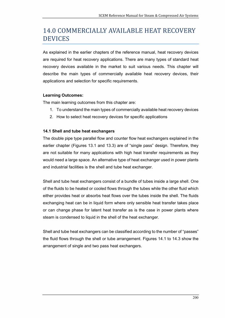
SCEM Reference Manual for Steam & Compressed Air Systems
200
14.0 COMMERCIALLY AVAILABLE HEAT RECOVERY DEVICES
As explained in the earlier chapters of the reference manual, heat recovery devices
are required for heat recovery applications. There are many types of standard heat
recovery devices available in the market to suit various needs. This chapter will
describe the main types of commercially available heat recovery devices, their
applications and selection for specific requirements.
Learning Outcomes:
The main learning outcomes from this chapter are:
1. To understand the main types of commercially available heat recovery devices
2. How to select heat recovery devices for specific applications
14.1 Shell and tube heat exchangers
The double pipe type parallel flow and counter flow heat exchangers explained in the
earlier chapter (Figures 13.1 and 13.3) are of “single pass” design. Therefore, they
are not suitable for many applications with high heat transfer requirements as they
would need a large space. An alternative type of heat exchanger used in power plants
and industrial facilities is the shell and tube heat exchanger.
Shell and tube heat exchangers consist of a bundle of tubes inside a large shell. One
of the fluids to be heated or cooled flows through the tubes while the other fluid which
either provides heat or absorbs heat flows over the tubes inside the shell. The fluids
exchanging heat can be in liquid form where only sensible heat transfer takes place
or can change phase for latent heat transfer as is the case in power plants where
steam is condensed to liquid in the shell of the heat exchanger.
Shell and tube heat exchangers can be classified according to the number of “passes”
the fluid flows through the shell or tube arrangement. Figures 14.1 to 14.3 show the
arrangement of single and two pass heat exchangers.
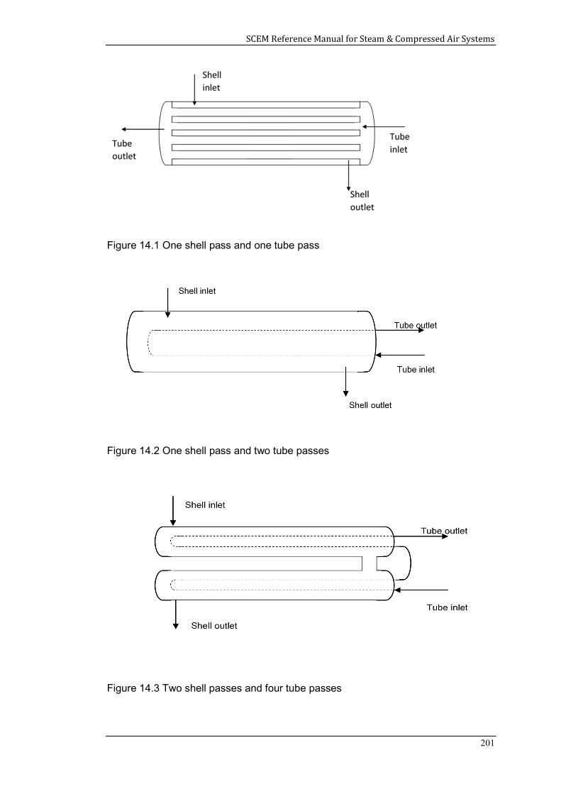
SCEM Reference Manual for Steam & Compressed Air Systems
201
Figure 14.1 One shell pass and one tube pass
Figure 14.2 One shell pass and two tube passes
Figure 14.3 Two shell passes and four tube passes
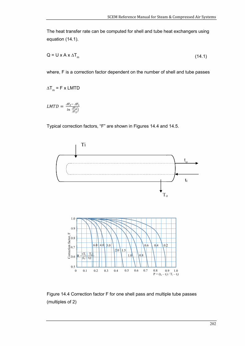
SCEM Reference Manual for Steam & Compressed Air Systems
202
The heat transfer rate can be computed for shell and tube heat exchangers using
equation (14.1).
Q = U x A x Tm (14.1)
where, F is a correction factor dependent on the number of shell and tube passes
Tm = F x LMTD
𝐿𝑀𝑇𝐷 =
Typical correction factors, “F” are shown in Figures 14.4 and 14.5.
Figure 14.4 Correction factor F for one shell pass and multiple tube passes
(multiples of 2)
1.0
0.9
0.8
0.7
0.6
0.5 0 0.1 0.2 0.3
Cor
rect
ion
fact
or, F
1.0 0.4 0.5 0.6 0.7 0.8
0.2 0.4 0.6
0.8 1.0
1.5 2.0
3.0 4.0
0.9 P = (to – ti) / Ti – ti)
(Ti – To) (to – ti)
R =
6.0
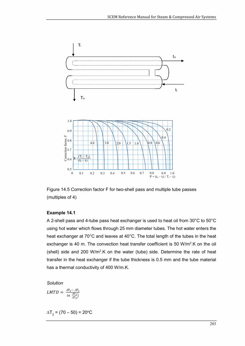
SCEM Reference Manual for Steam & Compressed Air Systems
203
Figure 14.5 Correction factor F for two-shell pass and multiple tube passes
(multiples of 4)
Example 14.1
A 2-shell pass and 4-tube pass heat exchanger is used to heat oil from 30°C to 50°C
using hot water which flows through 25 mm diameter tubes. The hot water enters the
heat exchanger at 70°C and leaves at 40°C. The total length of the tubes in the heat
exchanger is 40 m. The convection heat transfer coefficient is 50 W/m2.K on the oil
(shell) side and 200 W/m2.K on the water (tube) side. Determine the rate of heat
transfer in the heat exchanger if the tube thickness is 0.5 mm and the tube material
has a thermal conductivity of 400 W/m.K.
Solution
𝐿𝑀𝑇𝐷 =
T2 = (70 – 50) = 20oC
1.0
0.9
0.8
0.7
0.6
0.5 0 0.1 0.2 0.3
Cor
rect
ion
fact
or, F
1.0 0.4 0.5 0.6 0.7 0.8
0.2
0.4
0.6 0.8 1.0 1.5 2.0 3.0 4.0
0.9 P = (to – ti) / Ti – ti)
(Ti – To) (to – ti)
R =
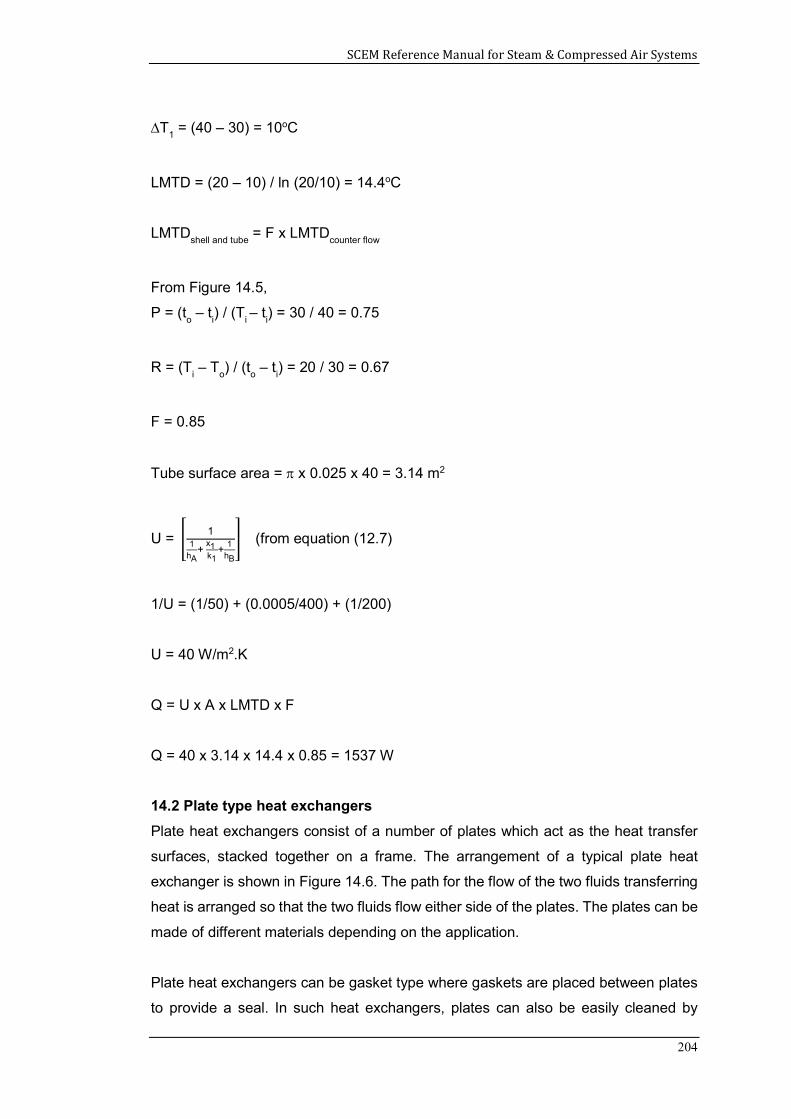
SCEM Reference Manual for Steam & Compressed Air Systems
204
T1 = (40 – 30) = 10oC
LMTD = (20 – 10) / ln (20/10) = 14.4oC
LMTDshell and tube
= F x LMTDcounter flow
From Figure 14.5,
P = (to – t
i) / (T
i – t
i) = 30 / 40 = 0.75
R = (Ti – T
o) / (t
o – t
i) = 20 / 30 = 0.67
F = 0.85
Tube surface area = x 0.025 x 40 = 3.14 m2
U = 1
1hA
+ x1
k1+
1hB
(from equation (12.7)
1/U = (1/50) + (0.0005/400) + (1/200)
U = 40 W/m2.K
Q = U x A x LMTD x F
Q = 40 x 3.14 x 14.4 x 0.85 = 1537 W
14.2 Plate type heat exchangers
Plate heat exchangers consist of a number of plates which act as the heat transfer
surfaces, stacked together on a frame. The arrangement of a typical plate heat
exchanger is shown in Figure 14.6. The path for the flow of the two fluids transferring
heat is arranged so that the two fluids flow either side of the plates. The plates can be
made of different materials depending on the application.
Plate heat exchangers can be gasket type where gaskets are placed between plates
to provide a seal. In such heat exchangers, plates can also be easily cleaned by
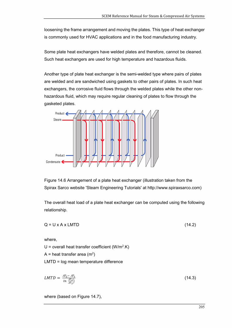
SCEM Reference Manual for Steam & Compressed Air Systems
205
loosening the frame arrangement and moving the plates. This type of heat exchanger
is commonly used for HVAC applications and in the food manufacturing industry.
Some plate heat exchangers have welded plates and therefore, cannot be cleaned.
Such heat exchangers are used for high temperature and hazardous fluids.
Another type of plate heat exchanger is the semi-welded type where pairs of plates
are welded and are sandwiched using gaskets to other pairs of plates. In such heat
exchangers, the corrosive fluid flows through the welded plates while the other non-
hazardous fluid, which may require regular cleaning of plates to flow through the
gasketed plates.
Figure 14.6 Arrangement of a plate heat exchanger (illustration taken from the
Spirax Sarco website 'Steam Engineering Tutorials' at http://www.spiraxsarco.com)
The overall heat load of a plate heat exchanger can be computed using the following
relationship.
Q = U x A x LMTD (14.2)
where,
U = overall heat transfer coefficient (W/m2.K)
A = heat transfer area (m2)
LMTD = log mean temperature difference
𝐿𝑀𝑇𝐷 =
(14.3)
where (based on Figure 14.7),
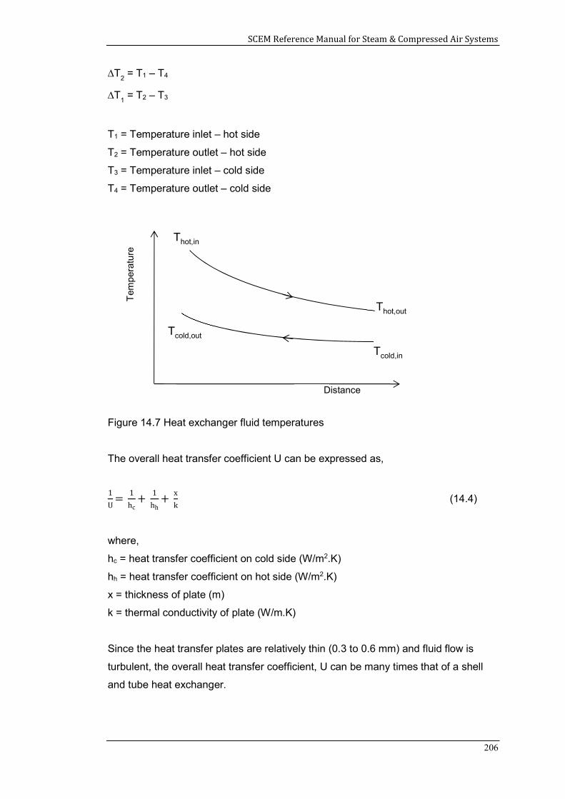
SCEM Reference Manual for Steam & Compressed Air Systems
206
T2 = T1 – T4
T1 = T2 – T3
T1 = Temperature inlet – hot side
T2 = Temperature outlet – hot side
T3 = Temperature inlet – cold side
T4 = Temperature outlet – cold side
Figure 14.7 Heat exchanger fluid temperatures
The overall heat transfer coefficient U can be expressed as,
1
U=
1
hc+
1
hh+
x
k (14.4)
where,
hc = heat transfer coefficient on cold side (W/m2.K)
hh = heat transfer coefficient on hot side (W/m2.K)
x = thickness of plate (m)
k = thermal conductivity of plate (W/m.K)
Since the heat transfer plates are relatively thin (0.3 to 0.6 mm) and fluid flow is
turbulent, the overall heat transfer coefficient, U can be many times that of a shell
and tube heat exchanger.
Distance
Tem
per
atu
re
Thot,in
Tcold,in
Thot,out
Tcold,out
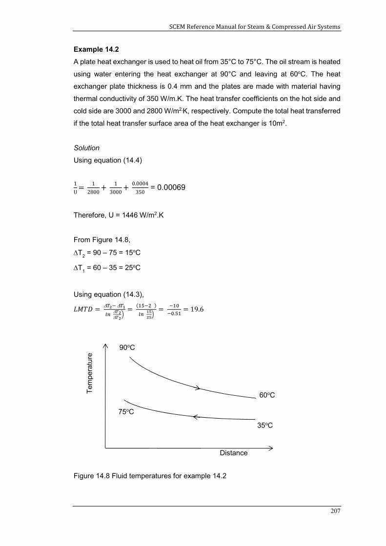
SCEM Reference Manual for Steam & Compressed Air Systems
207
Example 14.2
A plate heat exchanger is used to heat oil from 35°C to 75°C. The oil stream is heated
using water entering the heat exchanger at 90°C and leaving at 60oC. The heat
exchanger plate thickness is 0.4 mm and the plates are made with material having
thermal conductivity of 350 W/m.K. The heat transfer coefficients on the hot side and
cold side are 3000 and 2800 W/m2.K, respectively. Compute the total heat transferred
if the total heat transfer surface area of the heat exchanger is 10m2.
Solution
Using equation (14.4)
1
U=
1
2800+
1
3000+
0.0004
350 = 0.00069
Therefore, U = 1446 W/m2.K
From Figure 14.8,
T2 = 90 – 75 = 15oC
T1 = 60 – 35 = 25oC
Using equation (14.3),
𝐿𝑀𝑇𝐷 =
= ( )
= .
= 19.6
Figure 14.8 Fluid temperatures for example 14.2
Distance
Tem
pera
ture
90oC
35oC
60oC
75oC
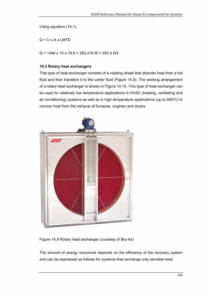
SCEM Reference Manual for Steam & Compressed Air Systems
208
Using equation (14.1),
Q = U x A x LMTD
Q = 1446 x 10 x 19.6 = 283,416 W = 283.4 kW
14.3 Rotary heat exchangers
This type of heat exchanger consists of a rotating wheel that absorbs heat from a hot
fluid and then transfers it to the colder fluid (Figure 14.9). The working arrangement
of a rotary heat exchanger is shown in Figure 14.10. This type of heat exchanger can
be used for relatively low temperature applications in HVAC (heating, ventilating and
air conditioning) systems as well as in high temperature applications (up to 500oC) to
recover heat from the exhaust of furnaces, engines and dryers.
Figure 14.9 Rotary heat exchanger (courtesy of Bry-Air)
The amount of energy recovered depends on the efficiency of the recovery system
and can be expressed as follows for systems that exchange only sensible heat.
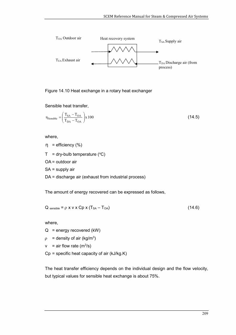
SCEM Reference Manual for Steam & Compressed Air Systems
209
Figure 14.10 Heat exchange in a rotary heat exchanger
Sensible heat transfer,
(14.5)
where,
= efficiency (%)
T = dry-bulb temperature (oC)
OA = outdoor air
SA = supply air
DA = discharge air (exhaust from industrial process)
The amount of energy recovered can be expressed as follows,
Q sensible = x v x Cp x (TSA – TOA) (14.6)
where,
Q = energy recovered (kW)
= density of air (kg/m3)
v = air flow rate (m3/s)
Cp = specific heat capacity of air (kJ/kg.K)
The heat transfer efficiency depends on the individual design and the flow velocity,
but typical values for sensible heat exchange is about 75%.
100 x TT
TTη
OADA
OASASensible
η
TDA Discharge air (from process)
TSA Supply air TOA Outdoor air
TEA Exhaust air
Heat recovery system
SCEM Reference Manual for Steam & Compressed Air Systems
210
Example 14.3
Consider the case where 1.2 m3/s of outdoor air is provided to an industrial dryer to
make up for an equal amount of air removed by the exhaust system. If the outdoor air
temperature is 32oC and the dryer discharge air temperature is 300oC, find the supply
air temperature that can be achieved using an energy recovery system that can only
transfer sensible heat and has an efficiency of 75%. Also, calculate the total amount
of pre-heating done to the outdoor air. Take the density of air to be 0.9 kg/m3 and the
specific heat capacity of air as 1002 J/kg.K.
Solution
Using equation (14.5),
= 32 + (300 – 32) x 0.75
= 233oC
Sensible heat added,
Q sensible = x v x Cp x (TSA – TOA)
= 0.9 x 1.2 x 1002 x (233 – 32)
= 217.5 kW
14.4 Heat pipes
A heat pipe is a heat exchange device which transfers heat through the phase change
of a substance. The typical arrangement of a heat pipe is shown in Figure 14.11. The
heat pipe consists of a hot side and a cold side. The liquid at the hot end absorbs heat
from the outer surrounding area through the thermally conductive tube wall. The liquid
then vapourises and the vapour travels to the cold side of the tube. When the vapour
reaches the cold side, it is cooled by the tube wall, which is exposed to the cold
medium, and the vapour condenses. The condensed vapour then flows back to the
hot side by gravity or through capillary action to continue the cycle.
SensibleOADAOASA η x )T(T TT
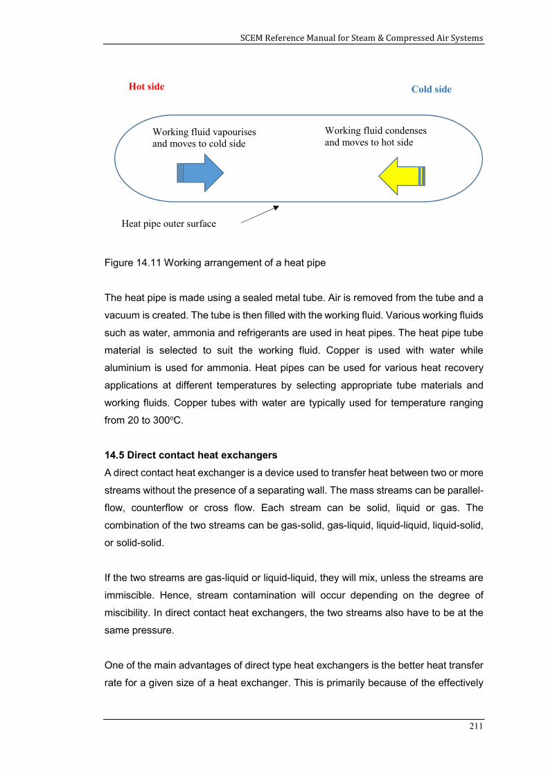
SCEM Reference Manual for Steam & Compressed Air Systems
211
Figure 14.11 Working arrangement of a heat pipe
The heat pipe is made using a sealed metal tube. Air is removed from the tube and a
vacuum is created. The tube is then filled with the working fluid. Various working fluids
such as water, ammonia and refrigerants are used in heat pipes. The heat pipe tube
material is selected to suit the working fluid. Copper is used with water while
aluminium is used for ammonia. Heat pipes can be used for various heat recovery
applications at different temperatures by selecting appropriate tube materials and
working fluids. Copper tubes with water are typically used for temperature ranging
from 20 to 300oC.
14.5 Direct contact heat exchangers
A direct contact heat exchanger is a device used to transfer heat between two or more
streams without the presence of a separating wall. The mass streams can be parallel-
flow, counterflow or cross flow. Each stream can be solid, liquid or gas. The
combination of the two streams can be gas-solid, gas-liquid, liquid-liquid, liquid-solid,
or solid-solid.
If the two streams are gas-liquid or liquid-liquid, they will mix, unless the streams are
immiscible. Hence, stream contamination will occur depending on the degree of
miscibility. In direct contact heat exchangers, the two streams also have to be at the
same pressure.
One of the main advantages of direct type heat exchangers is the better heat transfer
rate for a given size of a heat exchanger. This is primarily because of the effectively
Hot side Cold side
Working fluid vapourises and moves to cold side
Working fluid condenses and moves to hot side
Heat pipe outer surface
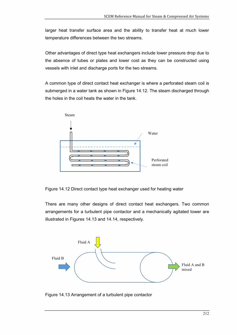
SCEM Reference Manual for Steam & Compressed Air Systems
212
larger heat transfer surface area and the ability to transfer heat at much lower
temperature differences between the two streams.
Other advantages of direct type heat exchangers include lower pressure drop due to
the absence of tubes or plates and lower cost as they can be constructed using
vessels with inlet and discharge ports for the two streams.
A common type of direct contact heat exchanger is where a perforated steam coil is
submerged in a water tank as shown in Figure 14.12. The steam discharged through
the holes in the coil heats the water in the tank.
Figure 14.12 Direct contact type heat exchanger used for heating water
There are many other designs of direct contact heat exchangers. Two common
arrangements for a turbulent pipe contactor and a mechanically agitated tower are
illustrated in Figures 14.13 and 14.14, respectively.
Figure 14.13 Arrangement of a turbulent pipe contactor
Steam
Water
Perforated steam coil
Fluid A
Fluid B
Fluid A and B mixed
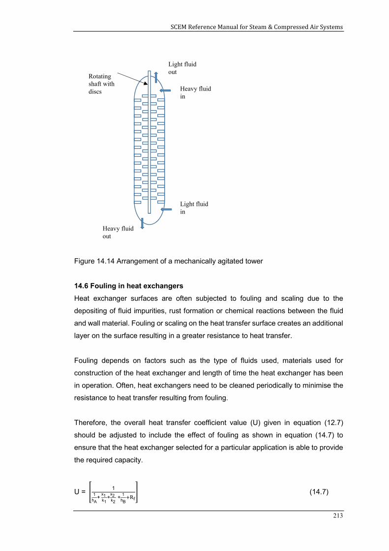
SCEM Reference Manual for Steam & Compressed Air Systems
213
Figure 14.14 Arrangement of a mechanically agitated tower
14.6 Fouling in heat exchangers
Heat exchanger surfaces are often subjected to fouling and scaling due to the
depositing of fluid impurities, rust formation or chemical reactions between the fluid
and wall material. Fouling or scaling on the heat transfer surface creates an additional
layer on the surface resulting in a greater resistance to heat transfer.
Fouling depends on factors such as the type of fluids used, materials used for
construction of the heat exchanger and length of time the heat exchanger has been
in operation. Often, heat exchangers need to be cleaned periodically to minimise the
resistance to heat transfer resulting from fouling.
Therefore, the overall heat transfer coefficient value (U) given in equation (12.7)
should be adjusted to include the effect of fouling as shown in equation (14.7) to
ensure that the heat exchanger selected for a particular application is able to provide
the required capacity.
U = 1
1hA
+ x1
k1+
x2
k2 +
1hB
(14.7)
Heavy fluid out
Light fluid in
Heavy fluid in
Light fluid out
Rotating shaft with discs
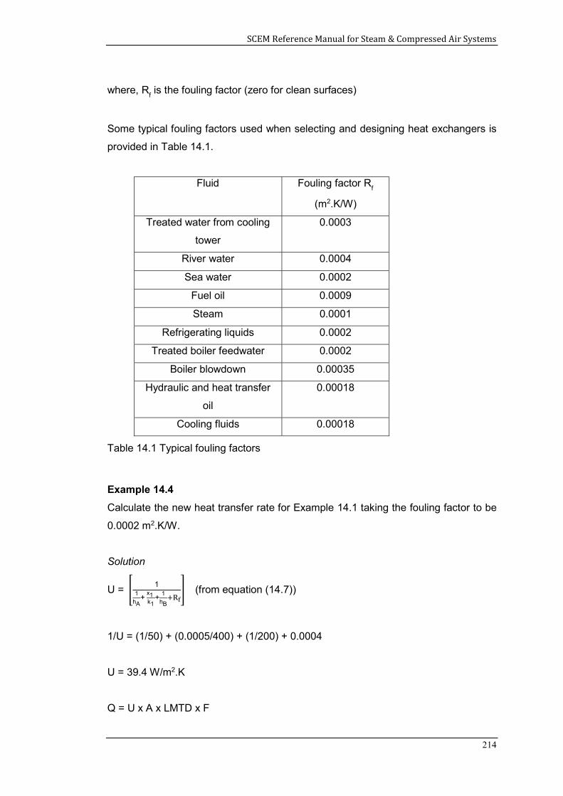
SCEM Reference Manual for Steam & Compressed Air Systems
214
where, Rf is the fouling factor (zero for clean surfaces)
Some typical fouling factors used when selecting and designing heat exchangers is
provided in Table 14.1.
Fluid Fouling factor Rf
(m2.K/W)
Treated water from cooling
tower
0.0003
River water 0.0004
Sea water 0.0002
Fuel oil 0.0009
Steam 0.0001
Refrigerating liquids 0.0002
Treated boiler feedwater 0.0002
Boiler blowdown 0.00035
Hydraulic and heat transfer
oil
0.00018
Cooling fluids 0.00018
Table 14.1 Typical fouling factors
Example 14.4
Calculate the new heat transfer rate for Example 14.1 taking the fouling factor to be
0.0002 m2.K/W.
Solution
U = 1
1hA
+ x1
k1+
1hB
(from equation (14.7))
1/U = (1/50) + (0.0005/400) + (1/200) + 0.0004
U = 39.4 W/m2.K
Q = U x A x LMTD x F
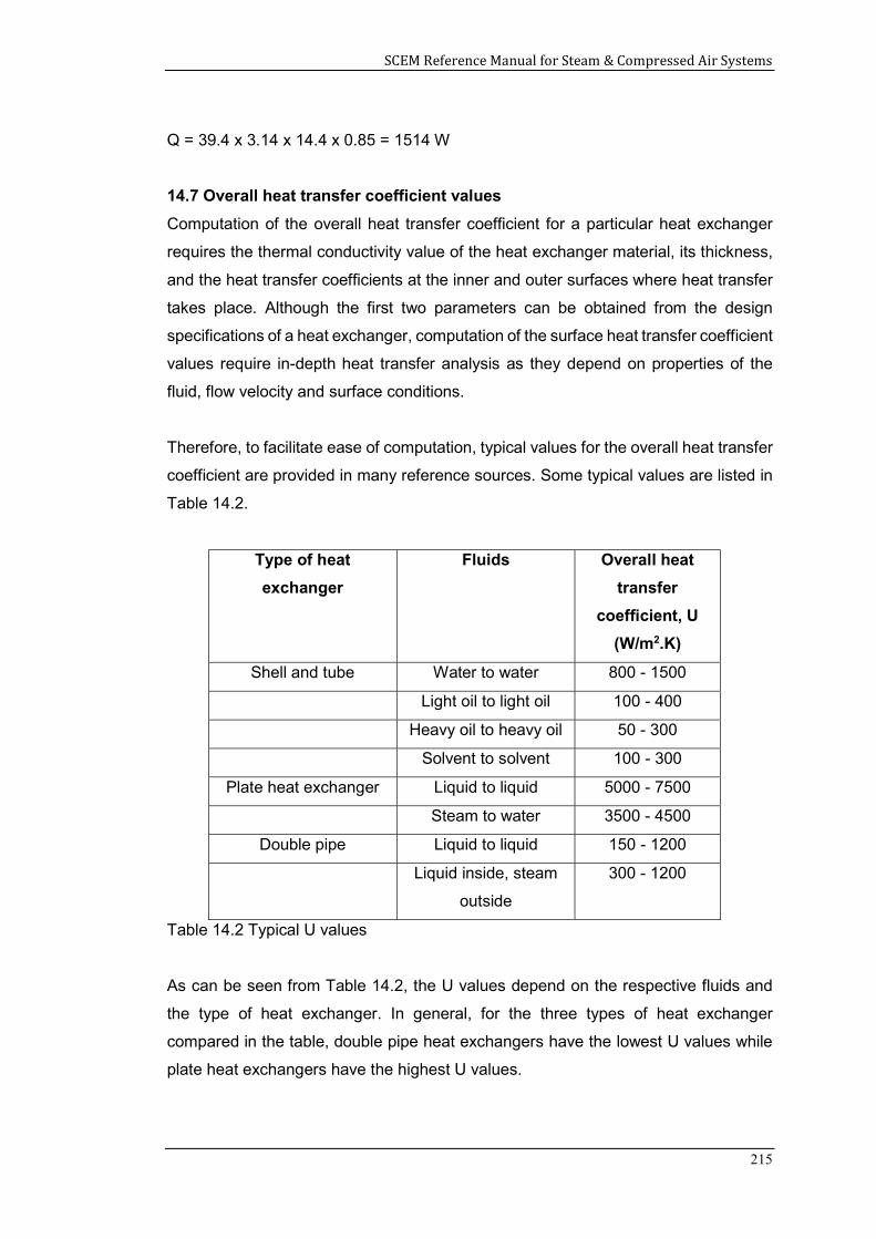
SCEM Reference Manual for Steam & Compressed Air Systems
215
Q = 39.4 x 3.14 x 14.4 x 0.85 = 1514 W
14.7 Overall heat transfer coefficient values
Computation of the overall heat transfer coefficient for a particular heat exchanger
requires the thermal conductivity value of the heat exchanger material, its thickness,
and the heat transfer coefficients at the inner and outer surfaces where heat transfer
takes place. Although the first two parameters can be obtained from the design
specifications of a heat exchanger, computation of the surface heat transfer coefficient
values require in-depth heat transfer analysis as they depend on properties of the
fluid, flow velocity and surface conditions.
Therefore, to facilitate ease of computation, typical values for the overall heat transfer
coefficient are provided in many reference sources. Some typical values are listed in
Table 14.2.
Type of heat
exchanger
Fluids Overall heat
transfer
coefficient, U
(W/m2.K)
Shell and tube Water to water 800 - 1500
Light oil to light oil 100 - 400
Heavy oil to heavy oil 50 - 300
Solvent to solvent 100 - 300
Plate heat exchanger Liquid to liquid 5000 - 7500
Steam to water 3500 - 4500
Double pipe Liquid to liquid 150 - 1200
Liquid inside, steam
outside
300 - 1200
Table 14.2 Typical U values
As can be seen from Table 14.2, the U values depend on the respective fluids and
the type of heat exchanger. In general, for the three types of heat exchanger
compared in the table, double pipe heat exchangers have the lowest U values while
plate heat exchangers have the highest U values.
SCEM Reference Manual for Steam & Compressed Air Systems
216
Summary
This chapter described the main types of commercially available heat recovery
devices such as shell and tube heat exchangers, plate type heat exchangers, rotary
heat exchangers, heat pipes and direct contact type heat exchangers. The application
of the various types of heat recovery devices was illustrated using examples.
References
1. Arora, C P, Heat and Mass Transfer, Khanna Publishers, Delhi, 1986.
2. Bergman, Lavine, Incropera, and DeWitt, Fundamentals of Heat Transfer, 7th
edition, John Wiley & Sons, New York, 2011.
3. Cornwell, K, The Flow of Heat, ELBS and Van Nostrand Reinhold Company Ltd,
London, 1977.
4. Jayamaha, Lal, Energy-Efficient Industrial Systems, Evaluation and
Implementation, McGraw-Hill, New York, 2016.
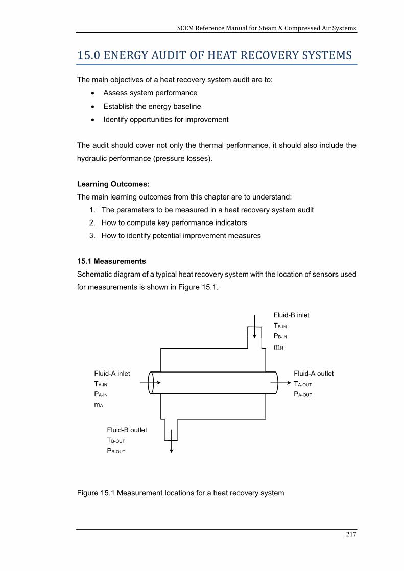
SCEM Reference Manual for Steam & Compressed Air Systems
217
15.0 ENERGY AUDIT OF HEAT RECOVERY SYSTEMS
The main objectives of a heat recovery system audit are to:
Assess system performance
Establish the energy baseline
Identify opportunities for improvement
The audit should cover not only the thermal performance, it should also include the
hydraulic performance (pressure losses).
Learning Outcomes:
The main learning outcomes from this chapter are to understand:
1. The parameters to be measured in a heat recovery system audit
2. How to compute key performance indicators
3. How to identify potential improvement measures
15.1 Measurements
Schematic diagram of a typical heat recovery system with the location of sensors used
for measurements is shown in Figure 15.1.
Figure 15.1 Measurement locations for a heat recovery system
Fluid-A inlet
TA-IN
PA-IN
mA
Fluid-A outlet
TA-OUT
PA-OUT
Fluid-B outlet
TB-OUT
PB-OUT
Fluid-B inlet
TB-IN
PB-IN
mB
SCEM Reference Manual for Steam & Compressed Air Systems
218
The different parameters:
mA = mass flow rate of fluid A
mB = mass flow rate of fluid B
PA-In = inlet pressure of fluid A
PA-out = outlet pressure of fluid A
PB-In = inlet pressure of fluid B
PB-out = outlet pressure of fluid B
TA-In = inlet temperature of fluid A
TA-out = outlet temperature of fluid A
TB-In = inlet temperature of fluid B
TB-out = outlet temperature of fluid B
15.2 Calculations
Heat transfer rate
The heat transfer rate Q, can be calculated as follows.
For the hot fluid
Q = mA x Cp
A x (T
A-IN – T
A-OUT ) (15.1)
For the cold fluid
Q = mB x Cp
B x (T
B-OUT – T
B-IN) (15.2)
where,
CpA = specific heat capacity of fluid A
CpB = specific heat capacity of fluid B
Log mean temperature difference (LMTD)
The log mean temperature difference can be calculated as follows.
𝐿𝑀𝑇𝐷 =
(15.3)
where
T2 = temperature difference between the fluids at one end of the heat exchanger (eg.
TA-IN – TB-OUT)
SCEM Reference Manual for Steam & Compressed Air Systems
219
T1 = temperature difference between the fluids at the other end of the heat
exchanger (eg. TB-IN – TA-OUT)
Overall heat transfer coefficient
The overall heat transfer coefficient U can be calculated as follows.
U = Q / (A x LMTD) (15.4)
where
A = heat transfer area of the heat recovery unit
Heat exchanger effectiveness
The heat exchanger effectiveness , can be can be computed as follows.
ϵ = mhot Cphot (Thot,inlet- Thot,outlet)
(m . Cp)min (Thot,inlet- Tcold,inlet) (15.5)
or
ϵ = mcold Cpcold (Tcold,inlet- Tcold,outlet)
(m . Cp)min (Thot,inlet- Tcold,inlet) (15.6)
where
mhot and mcold = mass flow rates of the hot and cold fluids, respectively
Cphot and Cpcold = specific heat capacities of the hot and cold fluids, respectively
T = temperature of the cold and hot fluid at the inlet and outlet of the heat recovery
unit
m.Cp = the lowest value of the product of the mass flow rate and specific heat capacity
of the two fluids
Heat exchanger approach temperature
This term refers to the temperature difference between the leaving process fluid and
the entering service fluid. If air is cooled from 60oC to 40oC using 30oC cooling water,
the air temperature approaches the water by 10oC (40 – 30 = 10).
As the approach temperature diminishes, the size (and cost) of the heat exchanger
will eventually increase exponentially.
SCEM Reference Manual for Steam & Compressed Air Systems
220
Fouling of heat exchangers
The following ratio can be computed to assess the need for cleaning of the heat
exchanger due to internal scaling and fouling.
(Tcold,out- Tcold,in)
(Thot,in- Tcold,in) (15.7)
where
Tcold-In = inlet temperature of cold fluid
Tcold-out = outlet temperature of cold fluid
Thot-In = inlet temperature of fluid being cooled
As the heat exchanger fouls, the cooling fluid temperature in and out will become
closer as less heat is transferred from the heat exchanger to the fluid. If the flow rates
remain the same, then the denominator of the ratio will remain the same. Thus, a
reducing number divided by a static number gives a lower value for the ratio.
Pressure losses
The pressure losses across the heat recovery unit can be computed for both fluid
streams using the following relationships.
PA = PA-IN – PA-Out (15.8)
and
PB = PB-IN – PB-Out (15.9)
where
PA-In = inlet pressure of fluid A
PA-out = outlet pressure of fluid A
PB-In = inlet pressure of fluid B
PB-out = outlet pressure of fluid B
Surface heat loss
Heat can be lost to the environment from the surface of the heat recovery system. For
heating applications, this can result in energy wastage. The surface temperature of
the heat recovery unit can be estimated using an infrared temperature sensor. The
measurements can be used to assess whether it is necessary to improve the
insulation.
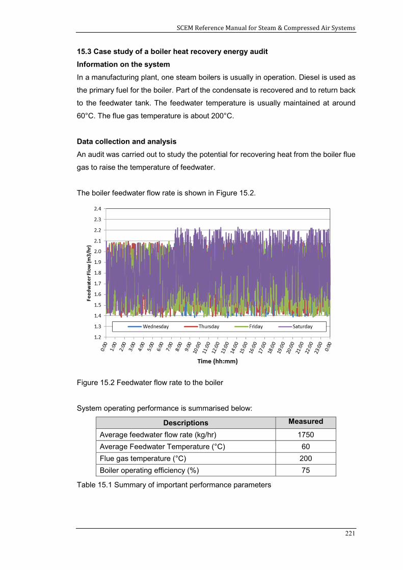
SCEM Reference Manual for Steam & Compressed Air Systems
221
15.3 Case study of a boiler heat recovery energy audit
Information on the system
In a manufacturing plant, one steam boilers is usually in operation. Diesel is used as
the primary fuel for the boiler. Part of the condensate is recovered and to return back
to the feedwater tank. The feedwater temperature is usually maintained at around
60°C. The flue gas temperature is about 200°C.
Data collection and analysis
An audit was carried out to study the potential for recovering heat from the boiler flue
gas to raise the temperature of feedwater.
The boiler feedwater flow rate is shown in Figure 15.2.
Figure 15.2 Feedwater flow rate to the boiler
System operating performance is summarised below:
Descriptions Measured
Average feedwater flow rate (kg/hr) 1750
Average Feedwater Temperature (°C) 60
Flue gas temperature (°C) 200
Boiler operating efficiency (%) 75
Table 15.1 Summary of important performance parameters
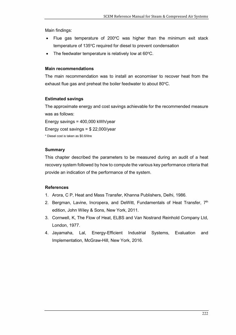
SCEM Reference Manual for Steam & Compressed Air Systems
222
Main findings:
Flue gas temperature of 200oC was higher than the minimum exit stack
temperature of 135oC required for diesel to prevent condensation
The feedwater temperature is relatively low at 60oC.
Main recommendations
The main recommendation was to install an economiser to recover heat from the
exhaust flue gas and preheat the boiler feedwater to about 80oC.
Estimated savings
The approximate energy and cost savings achievable for the recommended measure
was as follows:
Energy savings = 400,000 kWh/year
Energy cost savings = $ 22,000/year
* Diesel cost is taken as $0.6/litre
Summary
This chapter described the parameters to be measured during an audit of a heat
recovery system followed by how to compute the various key performance criteria that
provide an indication of the performance of the system.
References
1. Arora, C P, Heat and Mass Transfer, Khanna Publishers, Delhi, 1986.
2. Bergman, Lavine, Incropera, and DeWitt, Fundamentals of Heat Transfer, 7th
edition, John Wiley & Sons, New York, 2011.
3. Cornwell, K, The Flow of Heat, ELBS and Van Nostrand Reinhold Company Ltd,
London, 1977.
4. Jayamaha, Lal, Energy-Efficient Industrial Systems, Evaluation and
Implementation, McGraw-Hill, New York, 2016.
SCEM Reference Manual for Steam & Compressed Air Systems
223
STEAM AND COMPRESSED AIR SYSTEMS ABRIDGED SYLLABUS
Compressed Air Systems General introduction Components of compressed air system Definitions parameters such as standard pressure and temperature, standard
flow rate, dew point, free air delivery, utilisation factor, specific power. Types of compressors (positive displacement, dynamic) Selection of compressors for different industries Basic theory of compression (isothermal, adiabatic, polytropic)
Design considerations Power consumption calculation Comparison of specific power Efficiency (isothermal, volumetric) Single stage, multi-stage, intercooling Heat recovery potential Different types of dryers, requirements, comparison of energy consumption
Energy saving measures Receiver sizing System pressure losses Compressed air leaks, quantification Compressor intake temperature Compressor controls strategies
Steam Systems General introduction Steam generation processes Types of steam Properties of steam Steam tables Calculation of steam properties
Boilers Introduction to boilers Basic boiler operation Fuels Boiler blow down & draught Air fuel ratio, effect of excess air Combustion efficiency Calculation of boiler overall efficiency • Quick estimation of boiler efficiency
Optimising steam systems • Steam pressure
• Fuel switching • Boiler blow down • Auxiliary equipment
SCEM Reference Manual for Steam & Compressed Air Systems
224
• Heat recovery from flue gas • Condensate recovery
• Steam leaks • Steam traps • Other measures
Waste Heat Recovery System General introduction
• What is waste heat? • Benefits of waste heat recovery • Sources and use of waste heat
• Calculation involving waste heat recovery • Parameters controlling waste heat recovery
Modes of heat transfer • Conduction, Convection and Radiation
• Heat transfer through composite materials and radial heat transfer Heat exchangers
• Parallel flow • Counter flow
• Cross flow • Performance of heat exchangers • Log mean temperature difference
• Correction factors for cross flow heat exchangers • Shell and tube heat exchangers • Correction factors for shell and tube heat exchangers
• Plate type heat exchangers • Extended surfaces (fins) • Fouling of heat exchangers
• Overall heat transfer coefficient of heat exchangers • Typical values of overall heat transfer coefficient
Commercially available waste heat recovery devices • Shell & Tube Heat Exchanger • Heat Pipes
• Heat Wheels
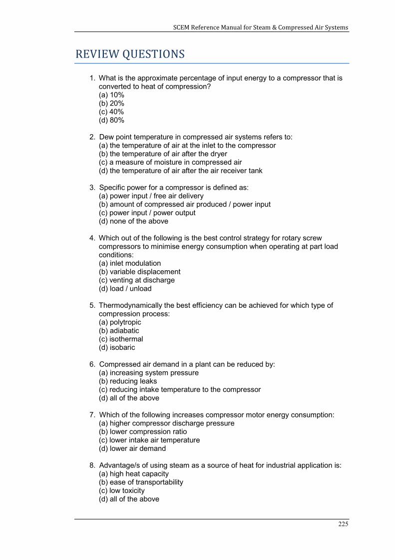
SCEM Reference Manual for Steam & Compressed Air Systems
225
REVIEW QUESTIONS
1. What is the approximate percentage of input energy to a compressor that is converted to heat of compression? (a) 10% (b) 20% (c) 40% (d) 80%
2. Dew point temperature in compressed air systems refers to:
(a) the temperature of air at the inlet to the compressor (b) the temperature of air after the dryer (c) a measure of moisture in compressed air (d) the temperature of air after the air receiver tank
3. Specific power for a compressor is defined as:
(a) power input / free air delivery (b) amount of compressed air produced / power input (c) power input / power output (d) none of the above
4. Which out of the following is the best control strategy for rotary screw
compressors to minimise energy consumption when operating at part load conditions: (a) inlet modulation (b) variable displacement (c) venting at discharge (d) load / unload
5. Thermodynamically the best efficiency can be achieved for which type of
compression process: (a) polytropic (b) adiabatic (c) isothermal (d) isobaric
6. Compressed air demand in a plant can be reduced by:
(a) increasing system pressure (b) reducing leaks (c) reducing intake temperature to the compressor (d) all of the above
7. Which of the following increases compressor motor energy consumption:
(a) higher compressor discharge pressure (b) lower compression ratio (c) lower intake air temperature (d) lower air demand
8. Advantage/s of using steam as a source of heat for industrial application is:
(a) high heat capacity (b) ease of transportability (c) low toxicity (d) all of the above
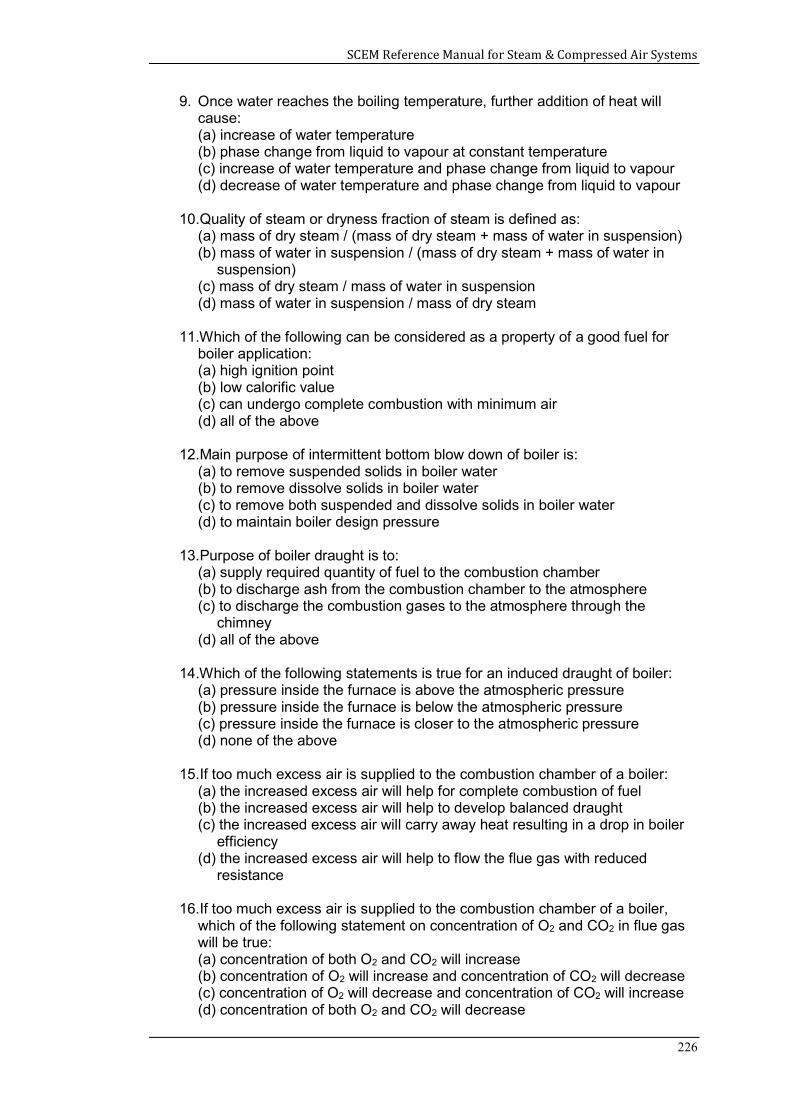
SCEM Reference Manual for Steam & Compressed Air Systems
226
9. Once water reaches the boiling temperature, further addition of heat will cause: (a) increase of water temperature (b) phase change from liquid to vapour at constant temperature (c) increase of water temperature and phase change from liquid to vapour (d) decrease of water temperature and phase change from liquid to vapour
10.Quality of steam or dryness fraction of steam is defined as:
(a) mass of dry steam / (mass of dry steam + mass of water in suspension) (b) mass of water in suspension / (mass of dry steam + mass of water in
suspension) (c) mass of dry steam / mass of water in suspension (d) mass of water in suspension / mass of dry steam
11.Which of the following can be considered as a property of a good fuel for
boiler application: (a) high ignition point (b) low calorific value (c) can undergo complete combustion with minimum air (d) all of the above
12.Main purpose of intermittent bottom blow down of boiler is:
(a) to remove suspended solids in boiler water (b) to remove dissolve solids in boiler water (c) to remove both suspended and dissolve solids in boiler water (d) to maintain boiler design pressure
13.Purpose of boiler draught is to:
(a) supply required quantity of fuel to the combustion chamber (b) to discharge ash from the combustion chamber to the atmosphere (c) to discharge the combustion gases to the atmosphere through the
chimney (d) all of the above
14.Which of the following statements is true for an induced draught of boiler:
(a) pressure inside the furnace is above the atmospheric pressure (b) pressure inside the furnace is below the atmospheric pressure (c) pressure inside the furnace is closer to the atmospheric pressure (d) none of the above
15.If too much excess air is supplied to the combustion chamber of a boiler:
(a) the increased excess air will help for complete combustion of fuel (b) the increased excess air will help to develop balanced draught (c) the increased excess air will carry away heat resulting in a drop in boiler
efficiency (d) the increased excess air will help to flow the flue gas with reduced
resistance 16.If too much excess air is supplied to the combustion chamber of a boiler,
which of the following statement on concentration of O2 and CO2 in flue gas will be true: (a) concentration of both O2 and CO2 will increase (b) concentration of O2 will increase and concentration of CO2 will decrease (c) concentration of O2 will decrease and concentration of CO2 will increase (d) concentration of both O2 and CO2 will decrease
SCEM Reference Manual for Steam & Compressed Air Systems
227
17.For effective heat transfer from a liquid to a gaseous fluid, fins should be
added: (a) on heat exchanger surface over which gaseous fluid flows as heat
transfer coefficient of gaseous fluid is relatively low (b) on heat exchanger surface over which gaseous fluid flows as heat
transfer coefficient of gaseous fluid is relatively high (c) on heat exchanger surface over which liquid fluid flows as heat transfer
coefficient of gaseous fluid is relatively low (d) on heat exchanger surface over which liquid fluid flows as heat transfer
coefficient of gaseous fluid is relatively high 18.For the same heat flow rate (under same inlet and outlet temperatures),
required heat transfer surface area for: (a) counter flow heat exchanger is less than parallel flow (b) counter flow heat exchanger is more than parallel flow (c) both counter and parallel flow heat exchangers are equal (d) none of the above
19. FAD in compressed air systems refer to conditions at:
(a) compressor intake (b) compressor discharge (c) at STP conditions (d) none of the above
20. Which of the following parameters is not required for computing the volumetric efficiency: (a) free air delivery (FAD) (b) power (c) stroke length (d) cylinder bore diameter