48

Chapter 3

Roots finding of equations

3.1 Introduction:

In this chapter we will discuss one of the most basic problems in

numerical analysis. The problem is called a root-finding problem

and consists of finding values of the variable x (real) that satisfy

the equation f(x) = 0, for a given function f. Let f be a real-value

function of a real variable. Any real number for which f () = 0

is called a root of that equation or a zero of function. We shall

confine our discussion to locating only the real roots of f(x), that is,

locating non-real complex roots of f(x) = 0 will not be discussed.

This is one of the oldest numerical approximation problems. The

procedures we will discuss range from the classical Newton-

Raphson method developed primarily by Isaac Newton over 300

years ago to methods that were established in the recent past.

Myriads of methods are available for locating zeros of functions

and in first section we discuss bisection methods and fixed point

method. In the second section, Chord Method for finding roots

will be discussed. More specifically, we will take up regula-falsi

method (or method of false position), Newton-Raphson method,

and secant method. In section 3, we will discuss error analysis for

iterative methods or convergence analysis of iterative method.

49

We shall consider the problem of numerical computation of the

real roots of a given equation .

which may be algebraic or transcendental. It will be assumed that

the function is continuously differentiable a sufficient

number of times. Mostly, we shall confine to simple roots and

indicate the iteration function for multiple roots in case of Newton

Raphson method.

All the methods for numerical solution of equations discussed here

will consist of two steps. First step is about the location of the

roots, that is, rough approximate value of the roots is obtained as

initial approximation to a root. Second step consists of methods,

which improve the rough value of each root.

A method for improvement of the value of a root at a second step

usually involves a process of successive approximation of iteration.

In such a process of successive approximation a sequence {Xn} n =

0, 1, 2, … is generated by the method used starting with the initial

approximation xo of the root obtained in the first step such that

the sequence {Xn} converges to as n . This xn is called the

nth approximation of nth iterate and it gives a sufficiently accurate

value of the root .

For the first step we need the following theorem:

50

Theorem 1: If f(x) is continuous in the closed internal [a, b] and

f(a) are of opposite signs, then there is at least one real root of

the equation f(x) = 0 such that a << b.

If further f(x) is differentiable in the open interval (a, b) and either

f’(x) < 0 or f’(x) > 0 in (a, b) then f(x) is strictly monotonic in [a,

b] and the root is unique.

3.2 The Methods of roots finding of equations

Simple iteration Method

Newton-Raphson Method

Modified Newton-Raphson Method

Modified Newton-Raphson Method for multiple roots

Secant Method

Bisection Method

3.2.1 Simple iteration Method

Suppose we have to find the roots of the equation . We

express it in the form and the iterative scheme is given

as

Where xn denotes the nth

iterated value which is known and

denotes (n + 1) the approximated value which is to be computed.

However, f(x) = 0 can be expressed in the form in

many ways but the corresponding iterative may not converge in all

51

cases to the true value, rather it may diverge start giving absurd

values. It can be proved that necessary and sufficient condition for

convergence of the scheme is that the modulus of the first

derivative of i.e. ́ at the exact root should be less than 1

i.e. if is the exact root then| ́ | . But since we do not

know the exact root which is to be computed we test the condition

for convergence at the initial approximation i.e.| ́ | .

Hence, it is necessary that the initial approximation should be

taken quite close to the exact root and test the condition before

starting the iteration. This method is also known as ‘fixed point’

method since the mapping maps the root to itself

since i.e. remains unchanged (fixed) under the

mapping .

Algorithm

1- Expressed in the form .

2- Choose the starting points by finding the approximate

location of the root, we try to evaluate the function values at

different x and tabulate as follows:

X A B

f(x) +

52

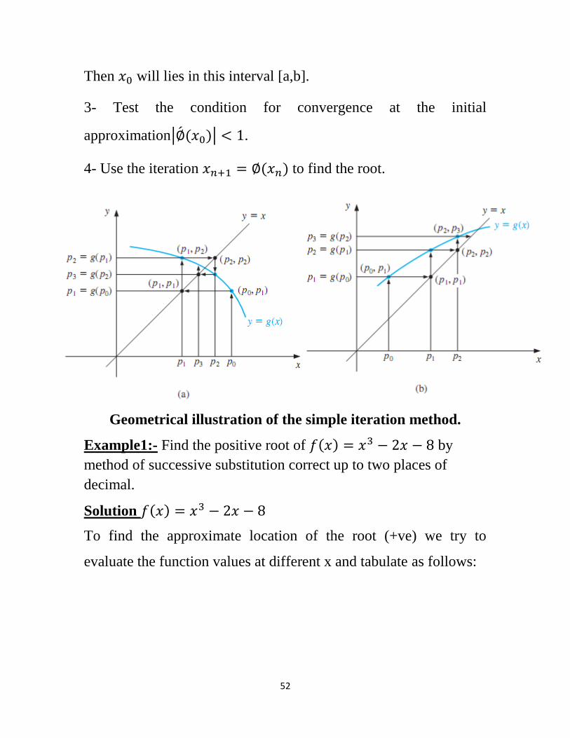
Then will lies in this interval [a,b].

3- Test the condition for convergence at the initial

approximation| ́ | .

4- Use the iteration to find the root.

Geometrical illustration of the simple iteration method.

Example1:- Find the positive root of by

method of successive substitution correct up to two places of

decimal.

Solution

To find the approximate location of the root (+ve) we try to

evaluate the function values at different x and tabulate as follows:

53

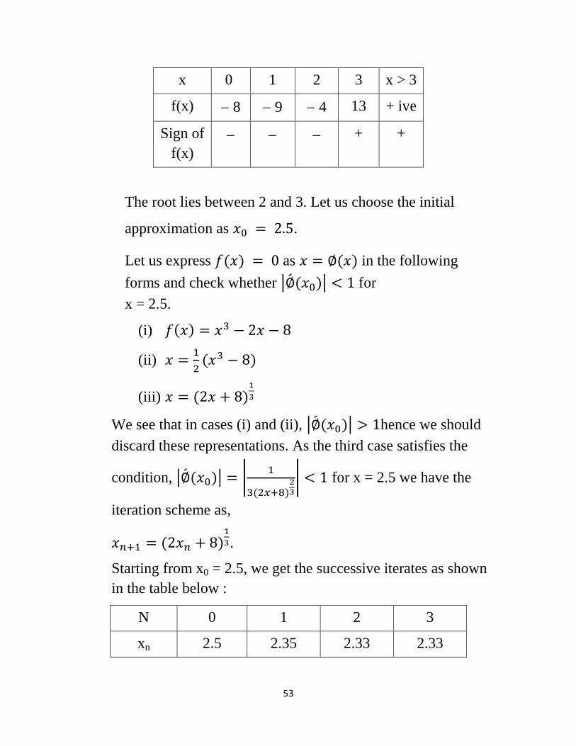
x 0 1 2 3 x > 3

f(x) 8 9 4 13 + ive

Sign of

f(x)

+ +

The root lies between 2 and 3. Let us choose the initial

approximation as .

Let us express as in the following

forms and check whether | ́ | for

x = 2.5.

(i)

(ii)

(iii)

We see that in cases (i) and (ii), | ́ | hence we should

discard these representations. As the third case satisfies the

condition, | ́ | |

| for x = 2.5 we have the

iteration scheme as,

.

Starting from x0 = 2.5, we get the successive iterates as shown

in the table below :

N 0 1 2 3

xn 2.5 2.35 2.33 2.33

54

Example2:- Find the roots of 032)( 2 xxxf .

It is easy to show the two roots at and .

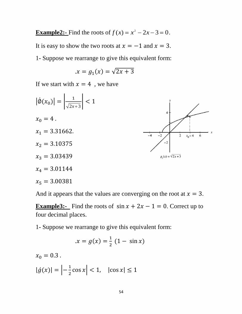
1- Suppose we rearrange to give this equivalent form:

. √

If we start with , we have

| ́ | |

32 x|

And it appears that the values are converging on the root at .

Example3:- Find the roots of . Correct up to

four decimal places.

1- Suppose we rearrange to give this equivalent form:

.

| ́ | |

| | |

55

The root is .

Example4:- Find the roots of

. Correct up to

four decimal places.

1- Suppose we rearrange to give this equivalent form:

.

| ́ | | | | ́ | | |

| ́ | |

√

| | ́ |

56

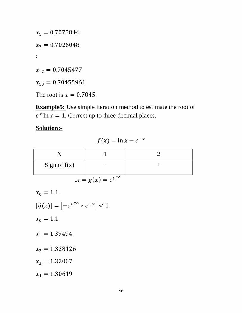
The root is .

Example5: Use simple iteration method to estimate the root of

. Correct up to three decimal places.

Solution:-

X 1 2

Sign of f(x) +

.

| ́ | | |

57

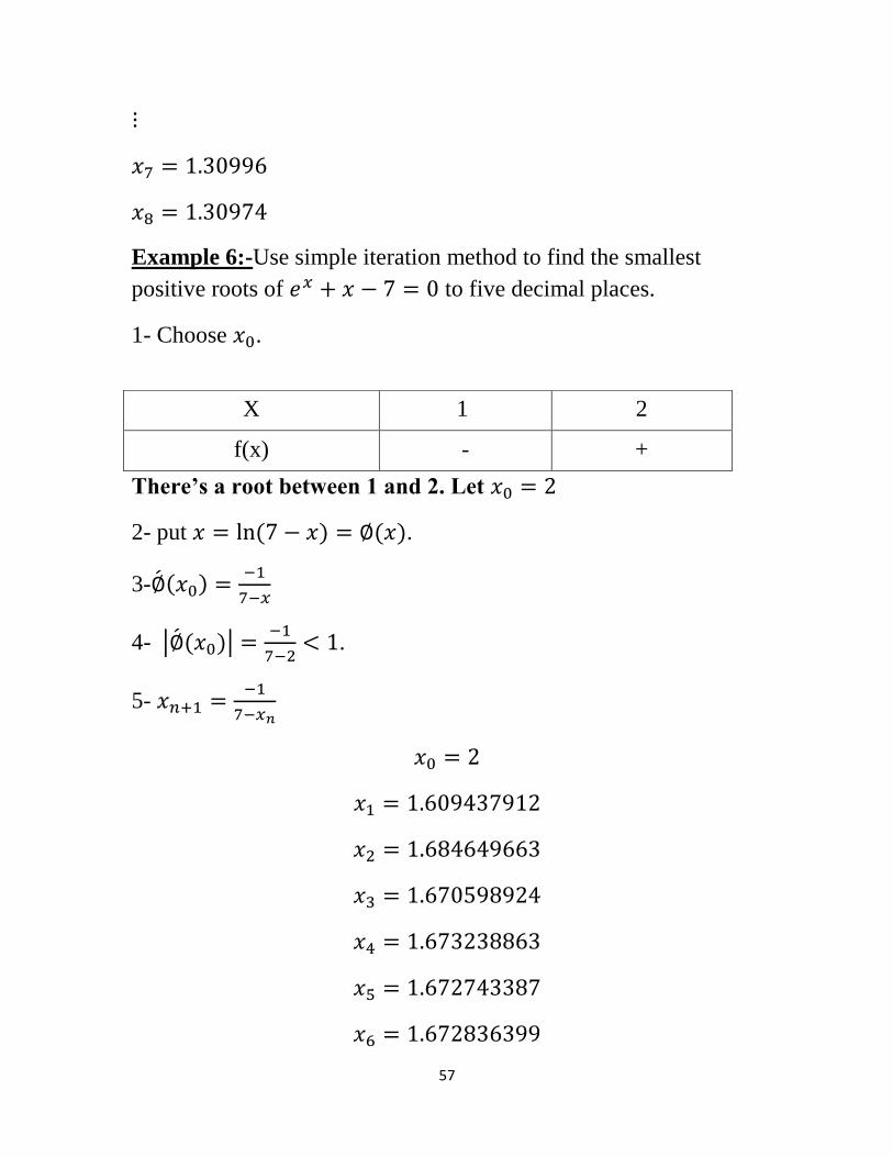
Example 6:-Use simple iteration method to find the smallest

positive roots of to five decimal places.

1- Choose .

There’s a root between 1 and 2. Let

2- put .

3- ́

4- | ́ |

.

5-

X 1 2

f(x) - +

58

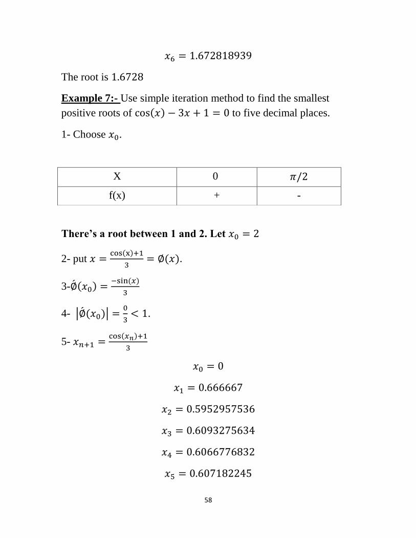
The root is

Example 7:- Use simple iteration method to find the smallest

positive roots of to five decimal places.

1- Choose .

There’s a root between 1 and 2. Let

2- put

.

3- ́

4- | ́ |

.

5-

X 0

f(x) + -

59

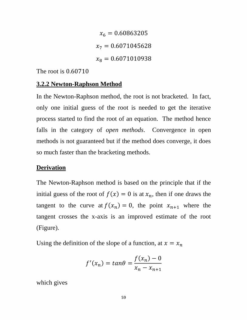
The root is

3.2.2 Newton-Raphson Method

In the Newton-Raphson method, the root is not bracketed. In fact,

only one initial guess of the root is needed to get the iterative

process started to find the root of an equation. The method hence

falls in the category of open methods. Convergence in open

methods is not guaranteed but if the method does converge, it does

so much faster than the bracketing methods.

Derivation

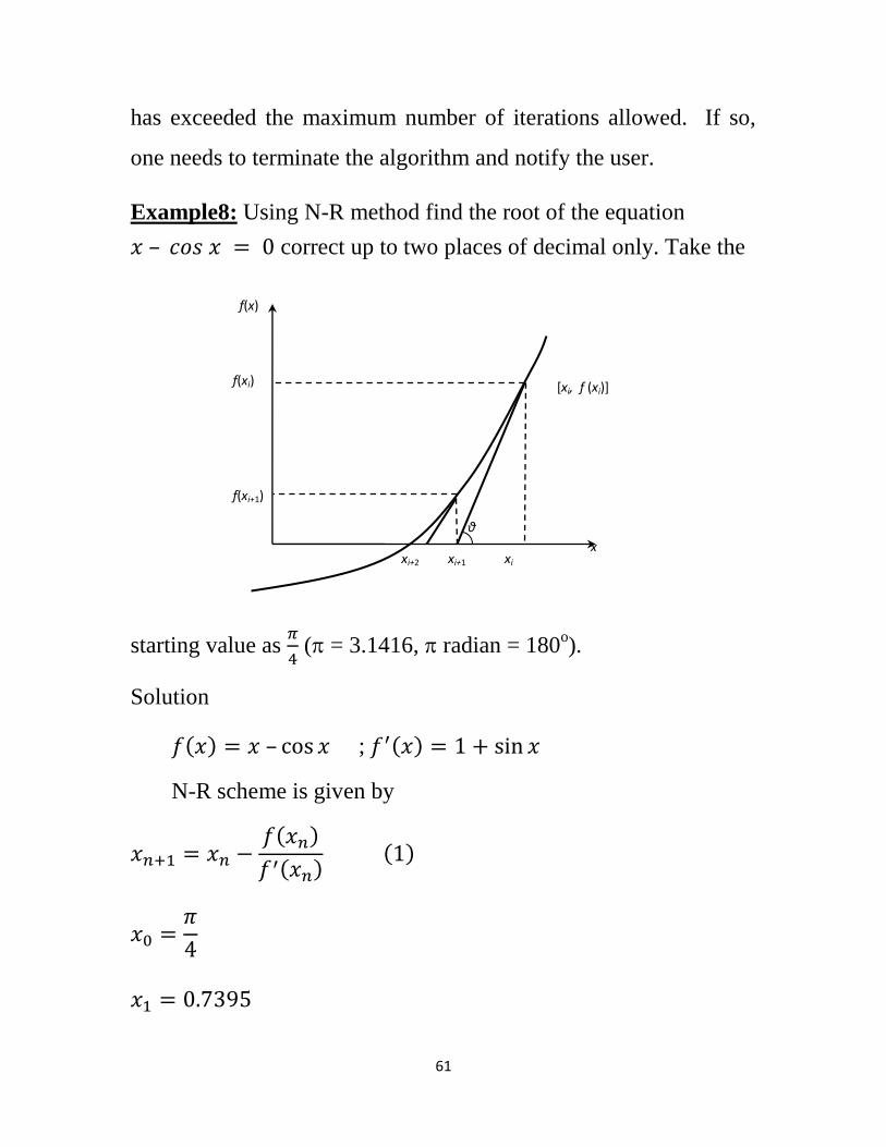
The Newton-Raphson method is based on the principle that if the

initial guess of the root of is at , then if one draws the

tangent to the curve at , the point where the

tangent crosses the x-axis is an improved estimate of the root

(Figure).

Using the definition of the slope of a function, at

which gives

60

Equation (1) is called the Newton-Raphson formula for solving

nonlinear equations of the form . So starting with an

initial guess, , one can find the next guess, , by using

Equation (1). One can repeat this process until one finds the root

within a desirable tolerance.

Algorithm

The steps of the Newton-Raphson method to find the root of an

equation are

1- Evaluate symbolically

2- Use an initial guess of the root, ix to estimate the new value of

the root, as

3- Find the absolute relative approximate error | | as

| | |

|

Compare the absolute relative approximate error with the pre-

specified relative error tolerance, . If | | , then go to Step

2, else stop the algorithm. Also, check if the number of iterations

61

has exceeded the maximum number of iterations allowed. If so,

one needs to terminate the algorithm and notify the user.

Example8: Using N-R method find the root of the equation

– correct up to two places of decimal only. Take the

starting value as

( = 3.1416, radian = 180

o).

Solution

– ;

N-R scheme is given by

f(x)

f(xi)

f(xi+1)

xi+2 xi+1 xi x

θ

[xi, f (xi)]