On ®nding dissimilar paths

Vedat Akg�un a, Erhan Erkut b,*, Rajan Batta a

a Department of Industrial Engineering, State University of New York at Bu�alo, Bu�alo, NY 14260-2050, USAb Department of Finance and Management Science, Faculty of Business, University of Alberta, Edmonton, Alb., Canada T6G 2R6

Abstract

Given a transportation network, this paper considers the problem of ®nding a number of spatially dissimilar paths

between an origin and a destination. A number of dissimilar paths can be useful in solving capacitated ¯ow problems or

in selecting routes for hazardous materials. A critical discussion of three existing methods for the generation of spatially

dissimilar paths is o�ered, and computational experience using these methods is reported. As an alternative method, the

generation of a large set of candidate paths, and the selection of a subset using a dispersion model which maximizes the

minimum dissimilarity in the selected subset is proposed. Computational results with this method are encourag-

ing. Ó 2000 Elsevier Science B.V. All rights reserved.

Keywords: Transportation planning; Path selection; Dangerous goods; Heuristics; Risk management

1. Introduction

In many single objective route-planning prob-lems, it may be adequate to select a single ``best''path from an origin to a destination. In contrast, inmulti-objective routing problems, it is usually nec-essary to generate a set of paths and evaluate themunder the relevant criteria. In addition to the multi-objective scenario, there may be instances where adecision maker is interested in developing backuproutes for a daily shipment in case the best routebecomes infeasible due to road construction or asnowstorm. To do this, one may wish to generate all

paths with lengths that are within 10% of the lengthof the shortest path. It is possible to accomplish thisvia a k-shortest path algorithm (e.g., see Yen, 1971)by selecting a su�ciently large k. However, many ofthe k-shortest paths generated by such algorithmshave the property that they are spatially very similarto one another. In some instances, this similaritybetween the generated paths may be acceptable.However, there are other instances where excessivesimilarity between the generated paths may be un-desirable, and it may be preferable to generatespatially dissimilar paths. This is the central focusof our paper; we seek dissimilar (but not necessarilydisjoint) paths from an origin to a destination on atransportation network.

Several speci®c examples to motivate thegeneration of spatially dissimilar paths are nowpresented. The ®rst example provided the primary

European Journal of Operational Research 121 (2000) 232±246www.elsevier.com/locate/orms

* Corresponding author. Tel.: 001-780-492-3068; fax: 001-

780-492-3325.

E-mail address: erhan.erkut@ualberta.ca (E. Erkut).

0377-2217/00/$ - see front matter Ó 2000 Elsevier Science B.V. All rights reserved.

PII: S 0 3 7 7 - 2 2 1 7 ( 9 9 ) 0 0 2 1 4 - 3

motivation for Kuby et al. (1997). When workingwith a large, capacitated, multi-commodity net-work ¯ow model, one may not be able to use arcvariables (due to the sheer size of the model),and may be forced to use path variables instead.To reformulate the problem using path variables,the requirement is to select a small number ofalternative paths between each origin±destinationpair. If two of these alternative paths use thesame bottleneck link, then one of them is uselessfor many solutions. The smaller the number ofcommon links between the paths, the higher thetotal potential capacity between the origin anddestination. As well, paths of excessive length areundesirable. Hence, the task is to generate asmall number of paths (say 10) with acceptablelengths which have as few common links aspossible.

Lombard and Church (1993) suggest a corridorlocation application for the same problem. Whenplanning a pipeline between an origin and desti-nation, it is desirable for the pipeline to be short,but there are many other concerns, such as to-pography and proximity to population centers.Suppose that the shortest path is infeasible, orundesirable due to these other concerns. A paththat is only marginally di�erent from the shortestpath may su�er from the same infeasibility orundesirability. Hence, it is desirable to generate anumber of paths that are not very similar topo-logically.

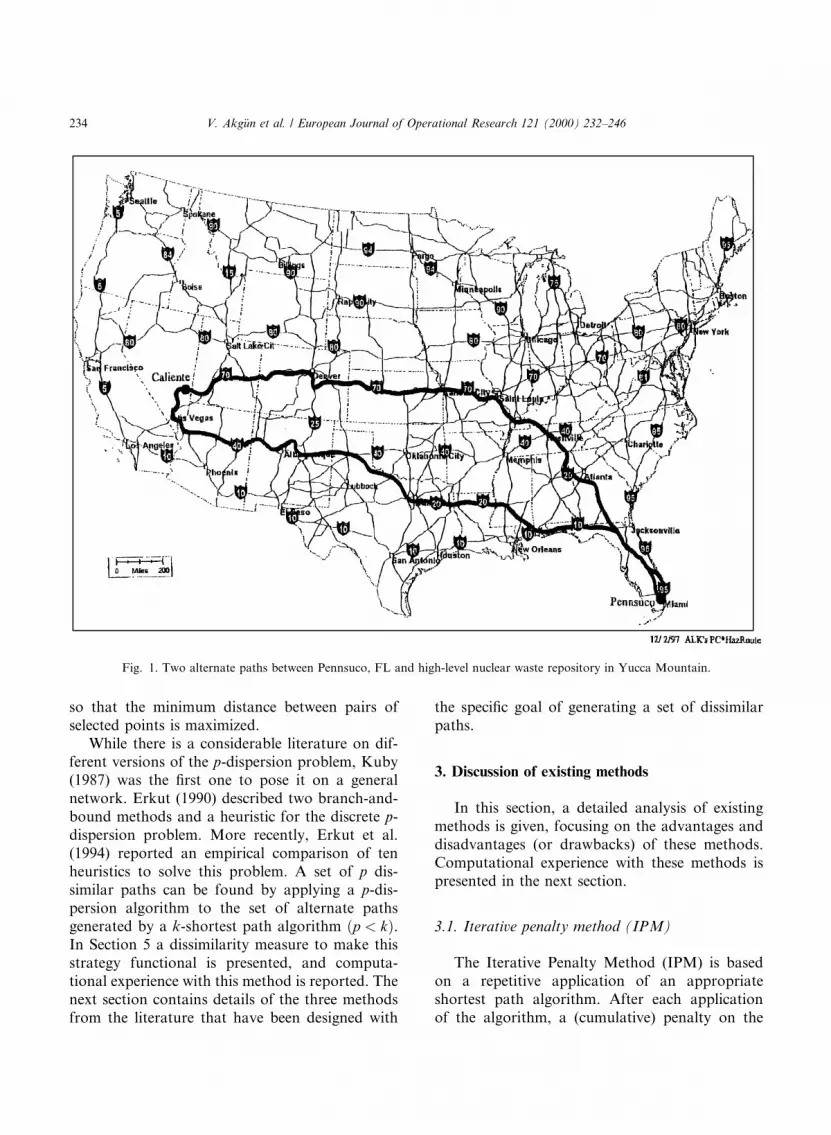
The third example is the primary reason westarted studying this problem: routing for haz-ardous materials. There are at least two reasonswhy dissimilar paths may be desirable in hazard-ous materials route planning. The ®rst reason is inrecognition of the fact that accident probabilitiescan increase considerably in the case of adverseweather conditions, in which case it is desirable tohave several dissimilar paths to increase theprobability of being able to select a path that isnot impacted by a weather system. A set of dis-similar paths is also needed to ensure spatial riskequity for multiple shipments of hazardous ma-terials. One way to ``spread'' the risk is by usingmore than one path for the shipments, and en-suring that the alternate paths are quite dissimilar.As an example, Fig. 1 displays two routes between

Pennsuco, FL and the proposed high-level nuclearwaste repository in Yucca Mountain, NV. Theseroutes are within 2.4% of one another in terms oflength, yet they are quite dissimilar.

The remainder of this paper is organized asfollows. In Section 2, we review the directly relatedliterature. In Section 3, we o�er a critical discus-sion of the three existing methods. In Section 4, wedesign a computational test to compare the e�-ciency and e�ectiveness of the existing methodsand summarize our computational results. Wedescribe a solution technique, derived by posingthis problem as a p-dispersion problem, in Section5. The p-dispersion problem, which is related tothe clique and independent set problems in graphtheory, is a facility location model designed tomaximize the separation (minimum distance) be-tween selected facilities. Finally, in Section 6, weprovide our concluding remarks.

2. Related literature

The problem of ®nding the shortest path be-tween an origin and a destination is one of the bestknown applications of operations research totransport planning. There exist a number of al-gorithms to solve this problem (Ahuja et al., 1993).As an extension of the shortest path problem, anumber of researchers have studied the problem of®nding the second-shortest path, the third-shortestpath, and so on. These e�orts gave rise to anumber of k-shortest path algorithms (Yen, 1971;Shier, 1979; Katoh et al., 1982; Skiscim andGolden, 1987; Miaou and Chin, 1991).

Obviously, the k-shortest path algorithms arecapable of generating a large number of alternativepaths, which can be useful in a number of trans-port planning instances. However, many of thesealternative paths are likely to share a large numberof edges. If one can de®ne a measure of dissimi-larity between these paths (similar to a distancemetric), then a subset of these paths can be selectedso that the minimum dissimilarity is maximized.In fact, this is an application of the ``discretep-dispersion'' model, a facility location modelwhich considers the problem of selecting a dis-persed subset of a given set of points in some space

V. Akg�un et al. / European Journal of Operational Research 121 (2000) 232±246 233

so that the minimum distance between pairs ofselected points is maximized.

While there is a considerable literature on dif-ferent versions of the p-dispersion problem, Kuby(1987) was the ®rst one to pose it on a generalnetwork. Erkut (1990) described two branch-and-bound methods and a heuristic for the discrete p-dispersion problem. More recently, Erkut et al.(1994) reported an empirical comparison of tenheuristics to solve this problem. A set of p dis-similar paths can be found by applying a p-dis-persion algorithm to the set of alternate pathsgenerated by a k-shortest path algorithm �p < k�.In Section 5 a dissimilarity measure to make thisstrategy functional is presented, and computa-tional experience with this method is reported. Thenext section contains details of the three methodsfrom the literature that have been designed with

the speci®c goal of generating a set of dissimilarpaths.

3. Discussion of existing methods

In this section, a detailed analysis of existingmethods is given, focusing on the advantages anddisadvantages (or drawbacks) of these methods.Computational experience with these methods ispresented in the next section.

3.1. Iterative penalty method (IPM)

The Iterative Penalty Method (IPM) is basedon a repetitive application of an appropriateshortest path algorithm. After each applicationof the algorithm, a (cumulative) penalty on the

Fig. 1. Two alternate paths between Pennsuco, FL and high-level nuclear waste repository in Yucca Mountain.

234 V. Akg�un et al. / European Journal of Operational Research 121 (2000) 232±246

impedance of all links in the resulting shortest pathis imposed. Hence, repeated selection of the sameset of links is discouraged, and dissimilar paths aregenerated as a result. This method was suggestedin the context of hazardous materials routing byJohnson et al. (1992), and used by Ruphail et al.(1995), in a decision support system to generateeconomically di�erent paths over a networkcharacterized by time-dependent link travel times.There are several dimensions in the implementa-tion of the penalty mechanism:· Penalized units: Penalties can be applied to the

links, or nodes, or both.· Penalty structure: An additive penalty (i.e. add-

ing a ®xed positive amount to the impedance),or a multiplicative penalty structure (i.e. multi-plying the current impedance by a factor greaterthan one) can be used. If one uses a multiplica-tive penalty formula, the new impedance can bebased on the current impedance (which mayhave been penalized before), or on the originalimpedance.

· Penalty magnitude: If a relatively large penalty ischosen, then links that appear in generatedpaths are discouraged more heavily. Smallerpenalties, on the other hand allow for more fre-quent appearances of links in generated paths.

· Penalized paths: Penalties can be applied to themost-recently found path only, or to all pathsfound so far.Clearly, the primary advantage of this method

is its simplicity. To implement the method, all thatis needed is a shortest path subroutine and apenalty mechanism. However, the ad hoc nature ofthis method is a drawback. The method has noway of evaluating the quality of the set of the pathsit generates in terms of the spatial di�erences andthe lengths of the paths. Additionally, to opera-tionalize this method, it is necessary to make an(arbitrary) decision about every one of the fourdimensions discussed above, and the results willdepend on these decisions. For example, a smallpenalty may not achieve the goal of dissimilarity,while a large penalty may eliminate a great manyviable paths from consideration. While it is pos-sible to experiment with di�erent penalty mecha-nisms and magnitudes, this search procedurewould be somewhat arbitrary without developing

an evaluation scheme for the generated set. Fur-thermore, the selected (®ne-tuned) settings for thepenalty strategy would be strictly problem-depen-dent (and not portable). Finally, there is some riskof numerical instability (e.g., division by zero),particularly if one uses a multiplicative penaltywith a large penalty factor and penalizes based onthe current impedance.

3.2. Gateway shortest paths (GSPs)

The second method, GSP, is based on a con-strained shortest path problem; this was proposedby Lombard and Church (1993). For a given ori-gin and a destination, a ``gateway shortest path'' isthe shortest path between the origin and the des-tination that is constrained to go through a spec-i®ed node, called a ``gateway''. It is possible togenerate a large number of such paths by forcingthem through di�erent gateways. To evaluate thesimilarity between two paths, a concept of ``areaunder a path'' is used. It is assumed that the net-work is embedded on a plane, and there exists acoordinate system on the plane. The ``area'' undera given path is the physical area between the pathand the x-axis of the coordinate system. The sim-ilarity between two paths is the absolute di�erencebetween their ``area-under-the-path'' ®gures.

The greatest appeal of this method is the gen-eration of a large number of alternative paths byusing a shortest path algorithm twice. It also yieldsan e�cient set of paths in terms of their pathlengths and their dissimilarity from the shortestpath. However, there are some critical shortcom-ings of this method which we summarize in pointform. These drawbacks are demonstrated via nu-merical examples in Akg�un et al. (1997).· Some of the gateway paths may contain loops,

and in most routing applications looping pathsare undesirable.

· It may be impossible to identify some (rather de-sirable) dissimilar paths as GSPs.

· A desirable GSP may be identi®ed as a dominat-ed path and eliminated in the ®nal phase ofGSP.

· GSP can generate two paths that are very simi-lar to one another because it focuses on the

V. Akg�un et al. / European Journal of Operational Research 121 (2000) 232±246 235

similarity of the candidate paths to the shortestpath only, and not to the other GSPs.

· The area di�erence between a path and theshortest path, is computed recursively (as partof the shortest path algorithm), and particularattention must be paid to prevent double-count-ing.Given these drawbacks, it is suggested that GSP

be used with caution, if at all, to generate a set of(mutually) dissimilar paths between an origin anda destination.

3.3. Minimax method

This third method has been proposed recentlyby Kuby et al. (1997). It aims to generate a set of``di�erentiated'' paths by selecting a subset of alarge set of paths. Attention is paid to the simi-larity between the selected paths and to theirlengths so that the ®nal set is mutually dissimilarand includes relatively short paths. The algorithmstarts by generating k-shortest paths between theorigin and the destination using a k-shortest pathalgorithm. These k paths are then processed and adissimilar subset (DS) is constructed iteratively.An index is de®ned to measure the desirability of acandidate path for inclusion in DS.

The ®rst path included is the shortest path.Suppose P1 is the shortest path, and d(P1) is itslength. Also suppose that we wish to ®nd asecond path according to two criteria: minimizelength, minimize similarity with P1. Consider anarbitrary path, say Pj. Denote the length of theshared portion by P1 and Pj by ds�Pj; P1�, andthe length of Pj not shared by P1 by dn�Pj; P1�.Hence, the length of Pj is ds�Pj; P1� � dn�Pj; P1�.The minimization of this is the ®rst objective.The similarity between P1 and Pj can be mini-mized by minimizing ds�Pj; P1�. These two ob-jectives can be combined using the weightingmethod (thereby establishing a linear tradeo�).Using a weight of b for the second objective, andscaling the weighted objective by d(P1) (which isa constant), we have:

�1� b�ds�Pj; P1� � dn�Pj; P1�d�P1� ; bP 0: �1�

Minimization of this index with respect to j yieldsa relatively short path that is also dissimilar to theshortest path. Of course, the selected path willdepend on the value of the weight b. The secondobjective can be emphasized by using a large b,whereas the ®rst one can be emphasized by using asmall b. Kuby et al. (1997) use b� 1 in their nu-merical examples. The third path is selected tominimize the maximum (hence the ``minimax''name) of the indices between the candidates andthe ®rst two paths. The procedure continues in thisfashion until the desired number of paths havebeen selected. By de®ning the index

M�Pj; Pi� � �1� b�ds�Pj; Pi� � dn�Pj; Pi�d�P1� �2�

the model is equivalent to

Minj 62DS

Maxi2DSfM�Pj; Pi�g

� �:

Among the existing three methods, this is theonly one that explicitly compares pairs of paths forsimilarity. While this is a clear advantage, thismethod has several drawbacks. The ®rst drawbackis algorithmic. If we de®ne

M 0�Pj; Pi� � K ÿM�Pj; Pi�;where K is a su�ciently large number, then themaximization of the minimum of M 0�Pj; Pi� valuesis equivalent to the minimization of the maximumof the M�Pj; Pi� values. Hence, the underlyingproblem is, in fact, a p-dispersion problem, and thealgorithm proposed by Kuby et al. (1997) amountsto a simple greedy construction heuristic for the p-dispersion problem. However, there are exact al-gorithms and e�cient heuristics available for thep-dispersion problem, and the Kuby et al. (1997)algorithm may not be the best way to solve thisproblem.

The second drawback is associated with thede®nition of the ``distance not shared'' betweentwo paths. This value, dn�Pj; Pi�, is de®ned as thelength of Pj not common to Pi. This de®nitionimplies that if Pi 6�Pj, then dn�Pj; Pi� 6� dn�Pi; Pj�unless L(Pi)�L(Pj). Therefore, this measure is notsymmetrical, and the ®nal DS set may depend on

236 V. Akg�un et al. / European Journal of Operational Research 121 (2000) 232±246

the order of selection of its members as demon-strated in the following numerical example.

Assume that we want to choose 3 dissimilarpaths from a set of 4 paths. Table 1 summarizes allrelevant data.

Let Q and C be the sets for the selected pathsand candidate paths, respectively, and let the valueof b be 1. First, the shortest path, P1, is selected.The second path to be selected will be the one thatminimizes M�Pj; P1� for j � 2; 3; 4. There is a tiebetween P2 and P4 for the minimum. If P2 is se-lected, the third path will be found by

Minj�3;4

Maxi�1;2�M�Pj; Pi��

� �;

which is P3. Therefore the solution is Q�{P1, P2, P3}. However, the solution would be Q�{P1, P2, P4} by

Mini�2;3

Maxi�1;4�M�Pj; Pi��

� �if P4 was selected as the second path. Hence, thetie-breaking decision plays a critical role in thegeneration of the ®nal solution due to the asym-metry of the measure.

Finally, the de®nition of the index M(Pj, Pi)o�ers a complication to potential users of thismethod. As detailed above, b serves as the``weight'' for the dissimilarity criterion. While thisde®nition allows the ¯exibility to emphasize one ofthe two objectives, one may have to experimentwith di�erent values of b before deciding on itsvalue. For example, with b� 1 (as in Kuby et al.,1997) in the above numerical example, P2 is se-lected in the second iteration although it is quitesimilar to P1. To generate a dissimilar set, one hasto use a larger value of b.

4. Computational experience

In our computational experiments, we com-pared the performance of the three algorithmsmentioned above. As an example network, we usedthe provincial highway road network of Alberta,Canada, which has 305 nodes and 854 arcs. Elevenrepresentative origin±destination pairs on thisnetwork were chosen for consideration. Theshortest distances between the OD pairs range from230 to 566 km. Our experience with the 11 pairs issummarized, but we focus on one typical OD pairfor detailed examples due to space limitations. Themethods were coded in C+ and the programs exe-cuted on a Pentium 200 MMX machine.

Three important measures to judge the qualityof a set of dissimilar paths were focused on: theaverage path length, the average dissimilarity be-tween pairs of paths, and the minimum dissimi-larity in the set. To measure the spatial(dis)similarity between any pair of paths, a simi-larity index de®ned in Erkut and Verter (forth-coming) was used, namely

S�Pi; Pj� � �L�Pi \ Pj�=L�Pi�� L�Pi \ Pj�=L�Pj��=2;

�3�

where L��� denotes the length of a path. A corre-sponding dissimilarity index is de®ned as

D�Pi; Pj� � 1ÿ S�Pi; Pj�: �4�For convenience, the indexes are multiplied by 100and we refer to them as percentages.

4.1. Gateway shortest path (GSP) method

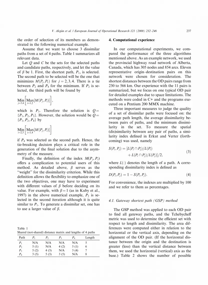
The GSP method was applied to each OD pairto ®nd all gateway paths, and the Tchebyche�metric was used to determine the e�cient set withrespect to length and dissimilarity. The area dif-ferences were computed either in relation to thehorizontal or the vertical axis, depending on thealignment of the OD pair. (If the horizontal dis-tance between the origin and the destination isgreater (less) than the vertical distance betweenthem, we used the horizontal (vertical) axis as thebase.) Table 2 shows the number of possible

Table 1

Shared (not-shared) distance matrix and lengths of 4 paths

Path P1 P2 P3 P4 Length

P1 N/A N/A N/A N/A 5

P2 5 (1) N/A 4 (2) 5 (1) 6

P3 5 (2) 4 (3) N/A 3 (4) 7

P4 3 (5) 5 (3) 3 (5) N/A 8

V. Akg�un et al. / European Journal of Operational Research 121 (2000) 232±246 237

gateway paths, number of loopless paths, numberof disjoint paths and the number of paths in thee�cient set.

Note that, for each OD pair, there are manypaths with loops and a large number of the loop-less paths are identical. Also, the number of pathsin the e�cient set is small when compared to thenumber of possible gateway paths.

GSP does not do well on the three measures ofinterest; it is prone to ®nding long and similarpaths. When generating the e�cient set, many longgateway paths and some similar paths are ex-cluded. Nevertheless, the average length of thee�cient paths is considerably longer than thelength of the shortest path. As well, there are manysimilar paths in the e�cient set since GSP com-pares each path only with the shortest path forsimilarity. For example, the minimum dissimilarityfor OD Pair 7 is only 0.3%, implying that at leasttwo of the e�cient paths are almost identical.

It is important to note that GSP was designedto solve a corridor location problem in which thearea under study was divided into grid cells andthe center of each grid cell was considered as anode. This network does not have the character-istics of a general road network. As well, theoriginal goal of GSP is not to generate a set ofmutually dissimilar paths, but to generate alter-natives to the shortest path. Our experience withGSP on a road network showed that GSP is not asuitable method for our problem. It failed togenerate a large number of alternate paths, elimi-nated some good candidates, and selected somespatially similar paths.

It is possible to improve GSPÕs performance byincreasing the number of loopless gateway pathsgenerated. If a gateway path has a loop, then acertain number of k-shortest paths can be found

from the origin to the gateway node and from thegateway node to the destination. It may be possi-ble to construct a number of loopless OD pathsthrough that gateway node by combining di�erentpairs of these subpaths. In fact, this procedure canalso be used for gateway paths without loops inorder to generate more than one path passingthrough a gateway node. Once a large number ofalternate paths are found, a p-dispersion algorithmcan be used to select a dissimilar set of paths asdiscussed in Section 5.

4.2. Iterative penalty method (IPM)

IPM was applied to ®nd r alternative paths foreach OD pair, where r � 3; . . . ; 25. As mentionedin Section 3, there are several dimensions in theimplementation of the penalty mechanism. In ourexperiment, we assigned penalties to the links (asopposed to the nodes). A multiplicative penaltymechanism was used and penalties were computedin two di�erent ways: (i) based on the currentimpedance (CI) (which may include past penal-ties), (ii) based on the original impedance (OI).Both small and large penalty magnitudes wereconsidered. The IPM method was tested withpenalty factors from 1% to 10% of the impedancewith 1% increments, and from 10% to 100% of theimpedance with 10% increments. At each iteration,penalties were assigned only to the links on themost-recently found path.

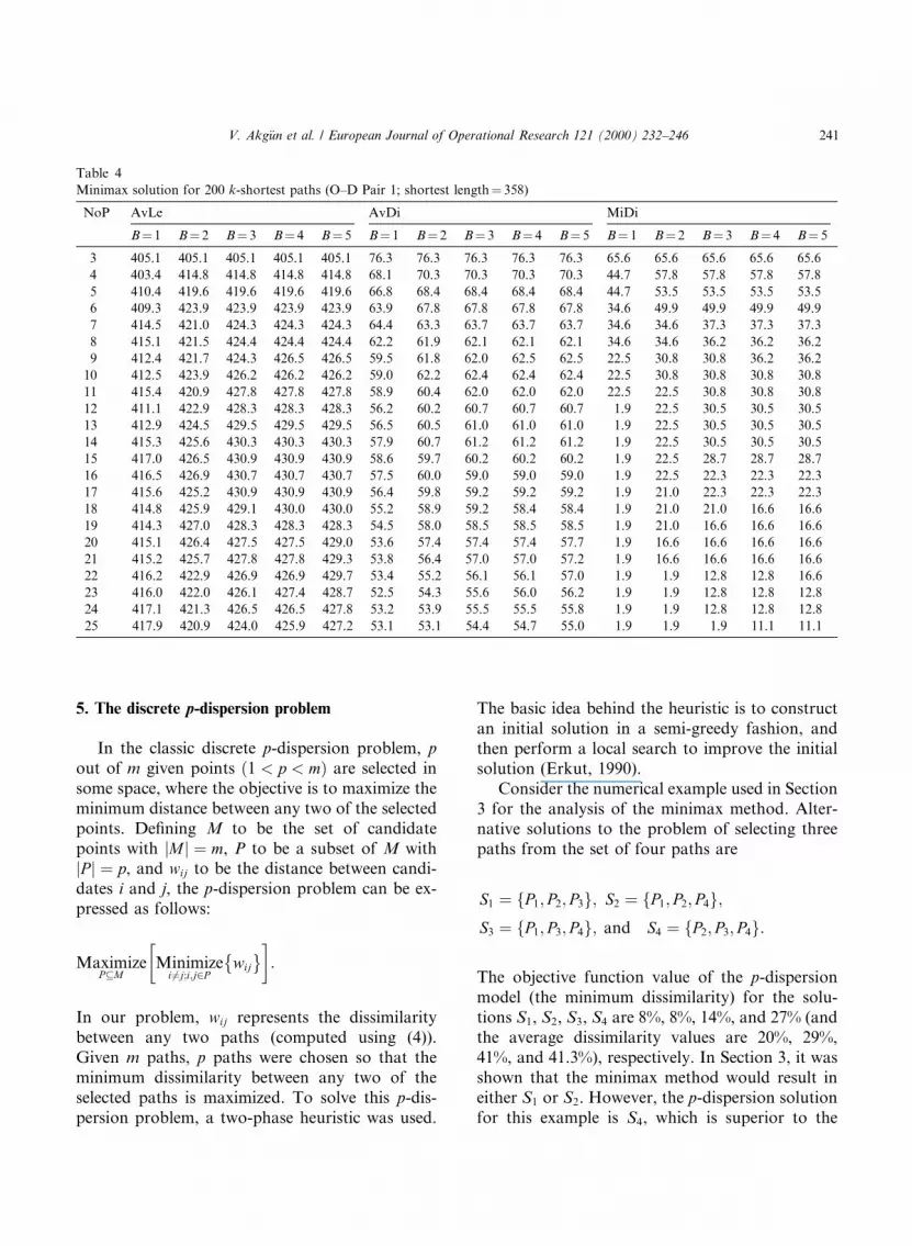
In our implementation of IPM, we rejected re-peated paths. If a repeat shortest path is found atan iteration, penalties are applied to the links onthis path although the path is rejected. Fig. 2shows the number of rejected paths generatedwhen attempting to ®nd 20 distinct paths with OI

Table 2

Number of candidate gateway paths and number of paths in the e�cient set

Origin±destination pair

1 2 3 4 5 6 7 8 9 10 11

Gateway paths 292 290 271 287 293 292 279 294 286 287 283

Loopless paths 116 130 142 119 119 141 144 85 137 85 144

Distinct paths 72 79 70 65 60 77 78 54 66 52 68

E�cient paths 10 16 18 15 18 13 24 16 23 15 25

238 V. Akg�un et al. / European Journal of Operational Research 121 (2000) 232±246

for OD Pair 1. As one would expect, higher pen-alty factors result is smaller rejected paths sincethey alter the relative impedances more severelythan lower penalty factors. For penalty factorsabove 20%, the number of rejected paths is quitelow, and seems independent of the exact value ofthe penalty factor. It was observed that with pen-alty factors above 10%, the number of rejectedpaths was approximately the same for OI and CI,while for smaller factors, OI resulted in a highernumber of rejects than CI. These general patternswere observed for all OD pairs.

As expected, the average path length increasesgradually as the number of paths generated in-creases. The rate of increase in the average pathlength is almost constant when the penalty factoris varied between 1% and 10%. However, the av-erage path length increases faster when the penaltyfactor is increased from 10% to 100%.

The values of the average path length (AvLe),the average dissimilarity between pairs of paths(AvDi) and the minimum dissimilarity (MiDi) forOD Pair 1 are summarized in Table 3 for the OIalternative.

Generally speaking, AvLe increases with thepenalty factor and with the number of paths re-quired (as one would expect). However, there arecertain exceptions. For example, with a 1% penaltyfactor, AvLe for 11 paths is lower than the AvLefor 10 paths for OD Pair 1. As another example,when generating 4 paths for OD pair 1, a penalty

factor of 70% results in a smaller AvLe than afactor of 40%. However, as the number of pathsincrease, the occurrence of these counter-intuitivecases becomes rare.

High penalty factors (40% and higher) result inhigher MiDi values than low penalty factors. Forexample, a factor of 100% generates the 10 maxi-mally dissimilar paths for OD Pair 1. However, forgenerating 20 dissimilar paths a factor of 70%works better than 100%. Hence, there are nogeneral rules for selecting an ``ideal'' penalty factorfor maximal dissimilarity.

Comparing brie¯y the results produced by CIand OI, in general CI results in higher MiDi valuesthan OI does. Although the di�erence in AvDivalues between OI and CI is insigni®cant, withhigh penalty factors, AvLe for CI can be consid-erably higher than for OI.

Although we used only one network in ourexperiment, we believe that the performance of acertain set of algorithm parameters will depend onthe underlying network. For example, a low pen-alty factor may succeed in generating more dis-similar paths on a dense network than on a sparsenetwork.

We conclude that IPM is a suitable algorithmto generate a set of alternative paths e�ciently, butthe selected paths may not be very desirable withrespect to one of the two relevant criteria. How-ever, a large number of alternative paths can begenerated easily using IPM, and a subset of this setselected in a second phase (see Section 5.2).

It may be possible to re®ne IPM via a selectivepenalty mechanism using di�erent penalty factorsfor di�erent links on the path. For example, in ahazmat transport context, links passing throughdensely populated areas may be penalized moreheavily than links that pass through areas withsparse populations.

4.3. Minimax method

To initialize this method, between 100 and 200k-shortest paths for each OD pair were found.Then, the minimax method of Kuby et al. (1997)was used to select anywhere from 3 to 25 paths foreach OD pair. It was observed that the time and

Fig. 2. Number of rejected paths as a function of the penalty

factor.

V. Akg�un et al. / European Journal of Operational Research 121 (2000) 232±246 239

storage requirements of ®nding k-shortest pathsincrease quickly with k. For example, when k wasincreased from 100 to 200, the computational timequadrupled (increasing from 0.7 hours to 2.5hours).

Since the k-shortest path algorithm ®nds manypaths that are small variations of the shortest path,the lengths of the 100th (and the 200th) shortestpaths are between 1.8% (2.2%) and 35.4% (38.5%)higher than the length of the shortest paths for the11 OD pairs in the experiment.

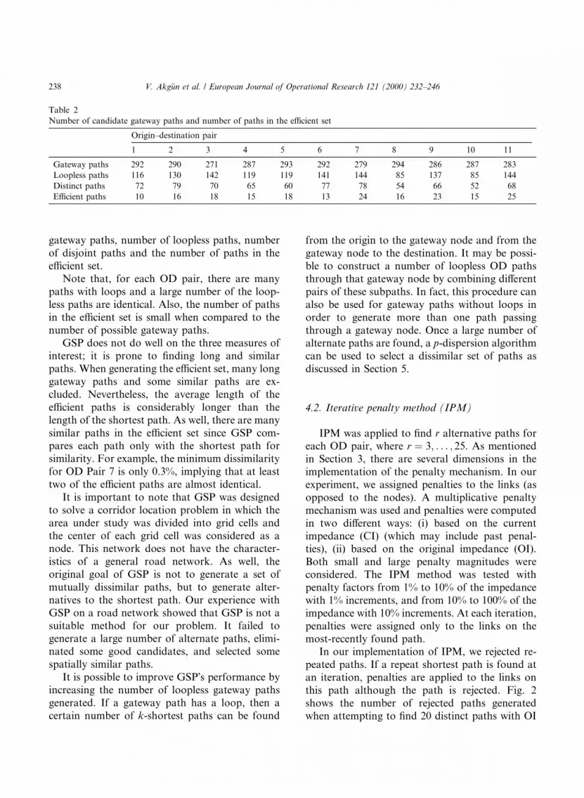
The minimax method was analyzed from dif-ferent angles. As discussed in Section 3, a param-eter (b) determines the weight of the similarityobjective in the model. Intuitively, an increase inthe value of b would improve the average andminimum dissimilarity values while the averagelength of the paths would increase. In order toanalyze the e�ect of b, we applied the minimaxmethod for a range of b values (b � 1; 2; . . . ; 5)with 100 and 200 paths. Table 4 summarizes theresults for OD Pair 1 with 200 paths.

The average length (AvLe) increases slightly asthe number of selected paths and the value of bincrease. The average dissimilarity (AvDi) value isquite insensitive to increases in b, while the mini-mum dissimilarity (MiDi) value is improved forlarger values of b. In general, the values of AvDiand MiDi do not change for b > 3.

If the length of the 200th path is close to thelength of the shortest path, then the averagesimilarity and the minimum similarity values forthe selected path set might be very low. For ex-ample, for OD Pair 7, the 200th shortest path isonly 4.9% longer than the shortest path. Even ifwe ®nd only three dissimilar paths (out of 200) forthis pair using the minimax method, the minimumdissimilarity for these three paths is merely 43%.We would need a much larger set of k-shortestpaths to ®nd a better result for this OD pair. Ingeneral, the number of k-shortest paths needed to®nd a good solution with the minimax methoddepends on the type of network and the locationof the OD pair.

Table 3

IPM solution by using penalty assignment with original impedance (OI) (O±D Pair 1; shortest length� 358)

No. AvLe AvDi MiDi

1% 10% 40% 70% 100% 1% 10% 40% 70% 100% 1% 10% 40% 70% 100%

3 389.1 389.1 422.1 422.1 422.1 65.3 65.3 94.2 94.2 94.2 44.7 44.7 85.4 85.4 85.4

4 394.9 406.5 453.2 429.9 453.2 58.7 76.5 93.7 88.1 93.7 4.8 44.7 82.1 67.1 82.1

5 407.5 415.3 445.4 449.4 461.5 67.7 78.8 88.4 89.2 91.7 4.8 44.7 56.9 67.1 77.8

6 416.0 422.4 453.4 456.9 453.6 67.1 76.6 87.9 88.5 87.9 4.4 4.4 56.9 67.1 56.9

7 420.9 427.6 455.2 447.6 474.3 72.4 76.2 85.3 84.4 88.1 4.4 4.4 13.0 22.5 56.9

8 426.5 435.1 448.3 456.1 496.8 70.9 76.8 83.8 84.6 88.6 4.4 4.4 13.0 22.5 56.9

9 430.1 432.6 453.4 461.3 512.6 72.8 74.9 83.4 84.3 88.2 4.4 4.4 13.0 22.5 56.9

10 435.9 438.7 469.5 480.6 518.4 73.1 76.5 84.7 85.5 87.6 4.4 4.4 13.0 22.5 39.0

11 432.6 446.7 468.5 486.2 513.6 73.0 78.8 83.7 85.2 86.2 1.7 4.4 13.0 22.5 13.0

12 435.4 442.8 469.6 494.0 529.5 71.4 77.8 83.3 85.2 86.6 1.7 1.7 13.0 22.5 13.0

13 439.9 441.4 464.7 491.2 536.9 73.5 77.8 82.5 84.3 86.6 1.7 1.7 13.0 22.5 13.0

14 446.0 441.7 470.3 503.9 528.0 74.7 77.0 82.6 84.8 86.0 1.7 1.7 13.0 22.5 13.0

15 446.9 449.4 476.1 503.0 523.8 73.5 78.5 82.9 84.5 85.4 1.7 1.7 13.0 22.5 13.0

16 450.6 451.5 474.9 496.6 525.5 73.4 78.5 82.5 84.0 85.2 1.7 1.7 13.0 22.5 13.0

17 456.2 452.0 486.4 497.0 526.9 74.4 77.9 83.2 83.9 85.0 1.7 1.7 13.0 22.5 13.0

18 453.9 451.5 484.9 508.2 543.4 74.5 77.6 82.8 84.3 85.4 1.7 1.7 13.0 22.5 13.0

19 453.5 456.7 483.7 510.3 540.2 75.1 78.2 82.4 84.2 84.9 1.7 1.7 13.0 22.5 13.0

20 455.1 453.9 494.4 507.3 535.7 74.4 78.1 82.9 83.8 84.7 1.7 1.7 13.0 22.5 13.0

21 455.4 454.5 495.9 519.2 544.5 73.2 77.6 82.9 84.2 84.8 1.7 1.7 13.0 22.5 13.0

22 458.1 452.6 498.1 513.7 542.1 73.0 77.5 82.8 83.7 84.5 1.7 1.7 13.0 22.5 13.0

23 455.8 454.7 494.4 516.1 540.2 74.0 77.7 82.5 83.7 84.3 1.7 1.7 13.0 17.1 13.0

24 459.8 459.5 495.3 515.4 540.0 74.5 78.3 82.3 83.6 84.2 1.7 1.7 13.0 17.1 13.0

25 463.7 460.5 491.5 511.2 538.1 74.8 77.9 82.0 83.1 84.0 1.7 1.7 13.0 17.1 13.0

240 V. Akg�un et al. / European Journal of Operational Research 121 (2000) 232±246

5. The discrete p-dispersion problem

In the classic discrete p-dispersion problem, pout of m given points �1 < p < m� are selected insome space, where the objective is to maximize theminimum distance between any two of the selectedpoints. De®ning M to be the set of candidatepoints with jM j � m, P to be a subset of M withjP j � p, and wij to be the distance between candi-dates i and j, the p-dispersion problem can be ex-pressed as follows:

MaximizeP�M

Minimizei6�j;i;j2P

wij

� � �:

In our problem, wij represents the dissimilaritybetween any two paths (computed using (4)).Given m paths, p paths were chosen so that theminimum dissimilarity between any two of theselected paths is maximized. To solve this p-dis-persion problem, a two-phase heuristic was used.

The basic idea behind the heuristic is to constructan initial solution in a semi-greedy fashion, andthen perform a local search to improve the initialsolution (Erkut, 1990).

Consider the numerical example used in Section3 for the analysis of the minimax method. Alter-native solutions to the problem of selecting threepaths from the set of four paths are

S1 � fP1; P2; P3g; S2 � fP1; P2; P4g;S3 � fP1; P3; P4g; and S4 � fP2; P3; P4g:

The objective function value of the p-dispersionmodel (the minimum dissimilarity) for the solu-tions S1, S2, S3, S4 are 8%, 8%, 14%, and 27% (andthe average dissimilarity values are 20%, 29%,41%, and 41.3%), respectively. In Section 3, it wasshown that the minimax method would result ineither S1 or S2. However, the p-dispersion solutionfor this example is S4, which is superior to the

Table 4

Minimax solution for 200 k-shortest paths (O±D Pair 1; shortest length� 358)

NoP AvLe AvDi MiDi

B� 1 B� 2 B� 3 B� 4 B� 5 B� 1 B� 2 B� 3 B� 4 B� 5 B� 1 B� 2 B� 3 B� 4 B� 5

3 405.1 405.1 405.1 405.1 405.1 76.3 76.3 76.3 76.3 76.3 65.6 65.6 65.6 65.6 65.6

4 403.4 414.8 414.8 414.8 414.8 68.1 70.3 70.3 70.3 70.3 44.7 57.8 57.8 57.8 57.8

5 410.4 419.6 419.6 419.6 419.6 66.8 68.4 68.4 68.4 68.4 44.7 53.5 53.5 53.5 53.5

6 409.3 423.9 423.9 423.9 423.9 63.9 67.8 67.8 67.8 67.8 34.6 49.9 49.9 49.9 49.9

7 414.5 421.0 424.3 424.3 424.3 64.4 63.3 63.7 63.7 63.7 34.6 34.6 37.3 37.3 37.3

8 415.1 421.5 424.4 424.4 424.4 62.2 61.9 62.1 62.1 62.1 34.6 34.6 36.2 36.2 36.2

9 412.4 421.7 424.3 426.5 426.5 59.5 61.8 62.0 62.5 62.5 22.5 30.8 30.8 36.2 36.2

10 412.5 423.9 426.2 426.2 426.2 59.0 62.2 62.4 62.4 62.4 22.5 30.8 30.8 30.8 30.8

11 415.4 420.9 427.8 427.8 427.8 58.9 60.4 62.0 62.0 62.0 22.5 22.5 30.8 30.8 30.8

12 411.1 422.9 428.3 428.3 428.3 56.2 60.2 60.7 60.7 60.7 1.9 22.5 30.5 30.5 30.5

13 412.9 424.5 429.5 429.5 429.5 56.5 60.5 61.0 61.0 61.0 1.9 22.5 30.5 30.5 30.5

14 415.3 425.6 430.3 430.3 430.3 57.9 60.7 61.2 61.2 61.2 1.9 22.5 30.5 30.5 30.5

15 417.0 426.5 430.9 430.9 430.9 58.6 59.7 60.2 60.2 60.2 1.9 22.5 28.7 28.7 28.7

16 416.5 426.9 430.7 430.7 430.7 57.5 60.0 59.0 59.0 59.0 1.9 22.5 22.3 22.3 22.3

17 415.6 425.2 430.9 430.9 430.9 56.4 59.8 59.2 59.2 59.2 1.9 21.0 22.3 22.3 22.3

18 414.8 425.9 429.1 430.0 430.0 55.2 58.9 59.2 58.4 58.4 1.9 21.0 21.0 16.6 16.6

19 414.3 427.0 428.3 428.3 428.3 54.5 58.0 58.5 58.5 58.5 1.9 21.0 16.6 16.6 16.6

20 415.1 426.4 427.5 427.5 429.0 53.6 57.4 57.4 57.4 57.7 1.9 16.6 16.6 16.6 16.6

21 415.2 425.7 427.8 427.8 429.3 53.8 56.4 57.0 57.0 57.2 1.9 16.6 16.6 16.6 16.6

22 416.2 422.9 426.9 426.9 429.7 53.4 55.2 56.1 56.1 57.0 1.9 1.9 12.8 12.8 16.6

23 416.0 422.0 426.1 427.4 428.7 52.5 54.3 55.6 56.0 56.2 1.9 1.9 12.8 12.8 12.8

24 417.1 421.3 426.5 426.5 427.8 53.2 53.9 55.5 55.5 55.8 1.9 1.9 12.8 12.8 12.8

25 417.9 420.9 424.0 425.9 427.2 53.1 53.1 54.4 54.7 55.0 1.9 1.9 1.9 11.1 11.1

V. Akg�un et al. / European Journal of Operational Research 121 (2000) 232±246 241

other solutions in terms of dissimilarity. Note thatthe optimal solution to this p-dispersion problemdoes not contain the shortest path; we note thatthis is quite likely to happen for very small p. Thethree other methods discussed earlier always in-clude the shortest path in the ®nal set. This can beviewed as another drawback of the existingmethods.

The candidate set M for the p-dispersionproblem can be constructed in many di�erentways. We experimented with two di�erent meth-ods: k-shortest paths, and IPM. The k-shortestpath algorithm ®nds the shortest possible mshortest paths for set M. However, usually there isa considerable amount of similarity between manyof these paths. On the other hand, it is possible togenerate a relatively dissimilar candidate set usingIPM by experimenting with the penalty mecha-nisms. Yet the average path length in such a can-didate set will be higher than the average pathlength in a set generated via the k-shortest path

algorithm. (We note that, from a purely compu-tational perspective, IPM is much faster than thek-shortest path algorithm.)

5.1. Constructing the candidate set m using k-shortest paths

The candidate set M was constructed withm� 100, and then with m� 200, using the k-shortest paths algorithm, and the p-dispersionproblem was then solved for p � 3; 4; . . . ; 25, forall OD pairs. Table 5 compares the p-dispersionsolution with the minimax solution with the same200 k-shortest paths for OD Pair 1.

The average length of paths (AvLe) is slightlyhigher in the p-dispersion solution than in theminimax solution since the p-dispersion model fo-cuses on dissimilarity, while the minimax methodconsiders dissimilarity as well as length. The aver-age dissimilarity value (AvDi) of the p-dispersion

Table 5

p-dispersion solution and its comparison with minimax method for 200 k-shortest paths (O±D Pair 1; shortest length� 358)

NoP p-dispersion solution for 200 paths Minimax solution for 2000 paths

AvLe AvDi MiDi AvLe AvDi MiDi

B� 2 B� 5 B� 2 B� 5 B� 2 B� 5

3 446.0 78.1 70.5 405.1 405.1 76.3 76.3 65.6 65.6

4 441.9 74.0 70.1 414.8 414.8 70.3 70.3 57.8 57.8

5 435.1 70.7 62.9 419.6 419.6 68.4 68.4 53.5 53.5

6 442.6 70.1 58.6 423.9 423.9 67.8 67.8 49.9 49.9

7 443.1 66.9 51.8 421.0 424.3 63.3 63.7 34.6 37.3

8 441.3 66.9 50.5 421.5 424.4 61.9 62.1 34.6 36.2

9 435.0 63.7 46.2 421.7 426.5 61.8 62.5 30.8 36.2

10 438.6 63.1 44.1 423.9 426.2 62.2 62.4 30.8 30.8

11 438.5 62.6 42.4 420.9 427.8 60.4 62.0 22.5 30.8

12 431.6 60.7 41.6 422.9 428.3 60.2 60.7 22.5 30.5

13 436.0 61.1 37.8 424.5 429.5 60.5 61.0 22.5 30.5

14 437.2 61.5 36.6 425.6 430.3 60.7 61.2 22.5 30.5

15 435.3 59.7 34.8 426.5 430.9 59.7 60.2 22.5 28.7

16 436.4 60.0 34.4 426.9 430.7 60.0 59.0 22.5 22.3

17 436.6 59.5 32.7 425.2 430.9 59.8 59.2 21.0 22.3

18 438.9 59.5 30.4 425.9 430.0 58.9 58.4 21.0 16.6

19 436.0 58.0 30.1 427.0 428.3 58.0 58.5 21.0 16.6

20 436.5 58.5 29.9 426.4 429.0 57.4 57.7 16.6 16.6

21 437.4 59.4 29.1 425.7 429.3 56.4 57.2 16.6 16.6

22 434.8 57.9 28.2 422.9 429.7 55.2 57.0 1.9 16.6

23 439.1 58.8 27.5 422.0 428.7 54.3 56.2 1.9 12.8

24 436.6 57.5 27.4 421.3 427.8 53.9 55.8 1.9 12.8

25 436.2 57.1 25.8 420.9 427.2 53.1 55.0 1.9 11.1

242 V. Akg�un et al. / European Journal of Operational Research 121 (2000) 232±246

solution is slightly better (higher) than that of theminimax solution. Finally, the minimum dissimi-larity value (MiDi) of the p-dispersion solution(which is optimized by the p-dispersion model) isconsiderably better than those of the minimaxmethod for both lower and higher values of b.

The superiority of the p-dispersion solutions tothe minimax solutions is most pronounced whenthe number of desired paths is large. For example,for p � 25, the MiDi of the minimax solutions forb� 1, 2, or 3 is 1.9% whereas the MiDi of the p-dispersion solution is 23.6%. We believe that thesolutions found using the two-stage greedy heu-ristic for the p-dispersion problem are superior tothe solutions generated by the minimax model forone obvious reason: the minimax algorithm is asingle-phase construction heuristic with no mech-anism to avoid painting itself into a corner.

5.2. Constructing the candidate set m using IPM

We found 500 distinct paths with IPM for allOD pairs by using a low penalty factor (1%) andthe original link impedance to determine the newimpedance of a link. The paths were then post-processed by the p-dispersion algorithm forp � 3; 4; . . . ; 25 paths for each OD pair. Theshortest path algorithm was used at most 7538times for OD Pair 10 to ®nd 500 distinct paths.Yet, the total amount of computation time re-quired to ®nd 500 distinct paths for all OD pairswas only around 0.3 hours.

The average dissimilarity (AvDi) values for the500 distinct paths are around 80% for all ODpairs. As expected, the application of the p-dis-persion algorithm to these 500 distinct paths re-sulted in very dissimilar solutions. However, the

selected sets contained some very long paths (up totwice as long as the shortest path). This may beunacceptable depending on the particular appli-cation. To prevent the selection of unreasonablylong paths, it was decided to eliminate from M allpaths that were above a certain threshold. Threethresholds for path lengths was experimented with:30%, 40% and 50% longer than the shortest path.In Table 6, the number of IPM-generated pathsthat satisfy these length constraints is stated. Ingeneral, if the dissimilarity is the only critical issue,then a very large m can be used to ®nd the dis-similar set. However, if the length is an importantfactor, then a fairly tight constraint (such as 10%above the length of the shortest path) on the lengthof paths could be used.

Table 6 provides some interesting informationon the characteristics of the OD pairs. For exam-ple, for OD Pair 6, there are only 46, 20 and 9paths for OD Pair 6, that are at most 50%, 40%and 30% longer than the shortest path, respec-tively. These numbers imply that there may not bemany dissimilar and relatively short paths for thispair. In contrast, for OD Pair 11, 432 of the 500IPM paths are at most 30% longer than theshortest path. Hence, this table makes it clear thatthe quality (dissimilarity) of the selected set willstrongly depend on the OD pair (and the network),regardless of which algorithm is used for selection.

Table 7 shows the results of the application ofthe p-dispersion algorithm to the IPM paths forOD Pair 9. It also gives the p-dispersion solutionfor the same pair with 200-shortest paths forcomparison. We observed that if the 200th shortestpath is considerably longer than the shortest path,then the p-dispersion solution based on IPM pathsis at least as good as the solution based onk-shortest paths in terms of dissimilarity. For pairs

Table 6

Classi®cation of IPM paths into di�erent groups by length

NoP O±D pair

1 2 3 4 5 6 7 8 9 10 11

All 500 500 500 500 500 500 500 500 500 500 500

6 1.5 ´ SL 212 270 421 355 275 46 404 123 457 127 464

6 1.4 ´ SL 116 233 408 317 255 20 352 118 439 110 451

6 1.3 ´ SL 57 167 364 213 171 9 316 67 411 99 432

V. Akg�un et al. / European Journal of Operational Research 121 (2000) 232±246 243

where the 200th shortest path is close to theshortest path in length, the IPM-based solution ismuch better than the solution based on the k-shortest paths. The OD Pair 9 is an example forthe latter case.

As the constraint on the path length is tight-ened, the average dissimilarity (AvDi) and theminimum dissimilarity (MiDi) values go down.The average length in the IPM-based solution withthe 30% threshold is approximately 10% morethan the average length in the k-shortest pathbased solution. However, the AvDi and MiDivalues in this IPM-based solution are considerablybetter than those for the k-shortest path basedsolution.

We conclude that the application of the p-dis-persion model to a large number of alternatepaths provides good solutions for the dissimilarpath problem. Generating a large number ofcandidate paths with IPM for the p-dispersionmodel seems to be a good alternative. However, it

is not suggested that IPM-based p-dispersion willalways result in a more dissimilar solution than k-shortest path-based p-dispersion. Suppose we areonly interested in paths with lengths that are be-low a given threshold. If we are able to generateall feasible paths using a k-shortest path algo-rithm, then applying the p-dispersion algorithm tothis set will produce results that are no worse thanthe results produced by the IPM-based p-disper-sion method. This is because IPM is able to gen-erate only a subset of all feasible paths. Forexample, the length of the 200th path for OD Pair6 is 38.5% more than the length of the shortestpath, and it is possible to select 25 paths with anaverage dissimilarity of 66.4% and a minimumdissimilarity of 29.5% by using these 200 paths asthe candidate set. However, IPM could only ®nd20 paths that are at most 40% longer than theshortest path with the penalty mechanism used.The average and the minimum dissimilarity ofthese 20 paths are 66.5% and 2.6%, respectively.

Table 7

p-dispersion solution for the paths found by IPM (O±D Pair 9; shortest length� 384.2)

NoP p-dispersion solution for IPM

AvLe AvDi MiDi

All 50% 40% 30% k-SP All 50% 40% 30% k-SP All 50% 40% 30% k-SP

3 624.6 529.7 498.3 453.6 396.7 99.4 99.5 97.2 94.8 79.0 98.7 98.9 94.6 93.5 73.3

4 599.1 507.7 478.6 450.0 399.3 94.8 95.7 92.6 91.4 73.2 87.8 89.2 87.7 86.1 50.6

5 534.0 494.4 473.4 449.5 398.5 94.4 94.8 92.1 90.6 66.6 76.7 87.7 86.2 82.6 37.1

6 624.3 492.7 464.8 450.3 400.3 95.2 93.9 89.1 88.6 68.4 75.4 84.3 80.4 81.0 36.6

7 514.2 474.9 462.8 447.5 400.7 89.1 89.2 85.5 86.9 65.5 71.1 77.1 76.4 75.7 33.3

8 570.1 469.4 446.6 441.0 399.6 91.6 87.9 85.2 84.0 64.2 73.1 74.4 72.2 71.2 31.8

9 559.0 465.8 450.5 447.1 400.7 90.7 86.1 83.8 83.7 63.1 68.1 72.0 70.2 71.3 28.3

10 566.8 459.6 450.2 443.5 400.5 90.3 83.4 81.4 81.5 61.0 71.3 68.1 64.1 64.4 23.2

11 554.5 469.2 445.1 444.5 400.8 88.8 85.0 81.5 79.8 62.7 63.8 63.9 62.8 60.9 21.7

12 542.1 467.5 451.3 442.6 400.8 88.3 83.3 82.1 80.6 61.5 55.9 63.3 61.3 59.9 19.7

13 555.0 455.3 449.7 443.3 401.7 88.8 83.0 81.6 79.2 60.5 56.8 59.6 58.4 57.9 17.2

14 535.5 460.1 443.2 436.9 400.6 86.3 82.9 79.4 79.4 61.6 51.8 59.4 59.1 57.5 14.7

15 548.5 459.7 441.2 441.6 400.0 87.8 82.3 79.5 78.4 61.7 51.6 58.2 57.3 55.0 14.6

16 508.8 455.1 447.8 440.4 400.4 85.4 81.7 79.5 78.0 61.1 54.2 58.2 54.9 56.7 12.0

17 535.3 457.6 440.1 437.7 400.5 86.7 82.0 77.2 78.4 60.3 52.0 57.6 53.7 50.9 11.5

18 514.7 459.0 445.9 438.8 400.5 85.6 81.6 78.2 77.7 59.2 49.7 49.8 50.6 50.4 11.2

19 526.3 456.4 449.1 438.6 400.0 85.5 81.3 77.0 77.0 59.0 44.0 50.4 50.4 49.6 11.0

20 516.1 456.3 441.0 439.7 400.1 85.8 80.7 77.4 77.2 58.1 45.3 50.1 46.8 47.9 10.9

21 523.7 459.4 445.1 437.6 400.2 85.0 80.1 77.9 76.6 58.3 47.0 49.6 46.4 45.5 10.5

22 527.8 455.3 440.9 438.4 400.3 84.0 80.1 76.8 76.8 57.9 39.1 49.5 45.8 46.1 10.5

23 512.1 452.0 446.0 437.1 399.8 83.9 79.8 77.3 76.0 57.7 37.1 47.3 45.0 42.6 8.2

24 512.3 454.9 443.7 440.8 400.7 84.4 79.5 78.1 75.5 58.8 44.2 45.0 42.5 41.7 8.2

25 495.3 456.9 443.6 437.7 400.3 82.4 80.2 76.6 74.8 58.5 44.0 43.6 43.8 41.9 8.0

244 V. Akg�un et al. / European Journal of Operational Research 121 (2000) 232±246

In this case, the k-shortest path-based approachproved to be superior.

6. Concluding remarks

In this paper, a detailed analysis of three ex-isting methods to generate a set of dissimilar pathsis provided and computational experience with themethods is reported. It is concluded that each ofthese three methods has a number of drawbacks.An alternative solution technique is proposed byposing the problem as a p-dispersion problem. If alarge number of suitable candidate paths can begenerated, then the application of the p-dispersionmodel is an e�ective way to solve the problem.

We now discuss a possible extension of ourproblem. Throughout this paper, links shared bytwo paths were considered in computing our sim-ilarity index. Hence, we may identify two paths as``dissimilar'' that have long portions which runparallel to one another, and are separated by ashort distance, such as one mile. In the context ofhazmat transport, these two paths might not bejudged as dissimilar. A weather system that im-pacts one will probably impact the other one aswell. Also, since these two paths will impose sim-ilar risks on residents living in areas located be-tween these two paths, the spatial risk equity in thesystem cannot be improved by alternating ship-ments between these two paths. Hence, in thehazmat context, a di�erent de®nition of similarityappears to be needed. We can de®ne a bu�er zonearound a path, where the width of the zone isdetermined according to the intended application.When computing the similarity between two paths,the area of the intersection of the two bu�er zonescan be used. (If we are concerned about popula-tion exposure, the number of people living in theintersection, as opposed to the area of the inter-section, in computing similarity can be used.)Given this new de®nition of similarity, all algo-rithms discussed in this paper still apply. The dif-®culty in implementing this extension is in thecomputation of the area of (or the population in)the intersection between pairs of paths. This taskcan be simpli®ed by using a geographic informa-tion system (GIS). Furthermore, using a GIS one

could test di�erent road networks, as there isconsiderable variability both in topological anddistance structure across the spectrum of all net-works.

Acknowledgements

This research has been supported in part bygrants from the Natural Sciences and EngineeringResearch Council of Canada (OGP 25481, CPG18134). We appreciate the support of ALK Asso-ciates by allowing us to use a copy of PC*Haz-Route for empirical analysis. Finally, thecomments of the anonymous referees are sincerelyappreciated.

References

Ahuja, R.K., Magnanti, T.L., Orlin, J.B., 1993. Network

Flows: Theory, Algorithms and Applications. Prentice-Hall,

Englewood Cli�s, NJ.

Akg�un, V., Erkut, E., Batta, R., 1997. On ®nding dissimilar

paths. Research report 97/3. Faculty of Business, University

of Alberta, Edmonton.

Erkut, E., 1990. The discrete p-dispersion problem. European

Journal of Operational Research 46, 48±60.

Erkut, E., �Ulk�usal, Y., Yenicßerio�glu, O., 1994. A comparison of

p-dispersion heuristics. Computers Operations Research 21

(10), 1103±1113.

Erkut, E., Verter, V., forthcoming. Modeling of transport risk

for hazardous materials. Operations Research.

Johnson, P.E., Joy, D.S., Clarke, D.B., Jacobi, J.M., 1992.

HIGHWAY 3.01, An Enhanced Highway Routing Model:

Program, Description, Methodology, and Revised UserÕsManual. Oak Ridge National Laboratory, ORNL/TM-

12124, Oak Ridge, TN.

Katoh, N., Ibaraki, T., Mine, H., 1982. An e�cient algorithm

for K shortest simple paths. Networks 12, 411±427.

Kuby, M.J., 1987. Programming models for facility dispersion:

The p-dispersion and maximum dispersion problems. Geo-

graphical Analysis 19 (4), 315±329.

Kuby, M., Zhongyi, X., Xiaodong, X., 1997. A minimax

method for ®nding the k best di�erentiated paths. Geo-

graphical Analysis 29 (4), 298±313.

Lombard, K., Church, R.L., 1993. The gateway shortest path

problem: Generating alternative routes for a corridor

location problem. Geographical Systems 1, 25±45.

Miaou, S.P., Chin, S.M., 1991. Computing k-shortest path for

nuclear spent fuel highway transportation. European Jour-

nal of Operational Research 53, 64±80.

Ruphail, N.M., Ranjithan, S.R., ElDessouki, W., Smith, T.,

Brill, E.D., 1995. A decision support system for dynamic

V. Akg�un et al. / European Journal of Operational Research 121 (2000) 232±246 245

pre-trip route planning. Applications of advanced technol-

ogies. In: Transportation Engineering: Proceedings of The

Fourth International Conference, pp. 325±329.

Shier, D.R., 1979. On algorithms for ®nding the k shortest

paths in a network. Networks 9, 195±214.

Skiscim, C.C., Golden, B.L., 1987. Computing k-shortest path

lengths in Euclidean networks. Networks 17, 341±352.

Yen, J.Y., 1971. Finding the K shortest loopless paths in a

network. Management Science 17 (11), 712±716.

246 V. Akg�un et al. / European Journal of Operational Research 121 (2000) 232±246