Calibrations on ${\\bf R}\\sp 8$

$Page 1: Calibrations on ${\\bf R}\\sp 8$$
TRANSACTIONS OF THEAMERICAN MATHEMATICAL SOCIETYVolume 307, Number 1, May 1988

CALIBRATIONS ON R8

J. DADOK, R. HARVEY AND F. MORGAN

ABSTRACT. Calibrations are a powerful tool for constructing minimal sur-

faces. In this paper we are concerned with 4-manifolds M C R8. If a dif-

ferential form <p € /\ R8 calibrates all tangent planes of M then M is area

minimizing. For <p in one of several large subspaces of /\ R8 we compute

its comass, that is the maximal value of <p on the Grassmannian of oriented

4-planes. We then determine the set G(<p) C G(4, R8) on which this maximum

is attained. These are the planes calibrated by <p, the possible tangent planes

to a manifold calibrated by <p. The families of calibrations obtained include

the well-known examples: special Lagrangian, Kahler, and Cayley.

Chapter l. Introduction

Let Mn be a Riemannian manifold. A calibration <p on Mn is a closed differential

fc-form with the property that |<p(£)| < 1 for every oriented tangent fc-plane £ of

unit volume, and <p(£) = 1 for some £. The planes £ for which <p(£) = 1 are

said to be calibrated by <p. The principal source of interest in calibrations is the

fact that any compact oriented fc-manifold Nk C Mn, all of whose tangent planes

are calibrated by ip, is automatically homologically area minimizing. For this and

other basic facts about calibrations, as well as a collection of very interesting and

fundamental examples, we refer to the foundational paper of Harvey and Lawson

[7] and to [6].The first case that comes to mind—the case of constant coefficient calibrations

on Rn—is already quite difficult to analyze and of considerable significance. It

serves as a model for local behavior of the general calibrated manifold near a singu-

larity, such as self-intersection (see Chapter 6). Also, the investigation of invariant

calibrations on symmetric spaces (cf. [19]) leads naturally to parallel calibrations

on Rn. Finally, many examples of calibrations that give rise to rich geometries of

minimal manifolds (e.g. complex, special Lagrangian, associative, and Cayley) have

constant coefficients (see [7 and 6]).

Identifying the constant coefficient calibrations <p E f\ R"* (a /\ R" via the

standard inner product) amounts to computing the comass of <p,

\]<p]\* or |M|=sup{b(0|:£eG(fc,R")},

where G(k, Rn) C f\ Rn is the Grassmannian of oriented unit fc-planes in R". The

next thing one wants to know, assuming \]ip\\ = 1, is what planes f are calibrated

by <p; i.e., what is the face G(<p) of the Grassmannian corresponding to <p,

J_ G(<p) = {£E G(k, R"): p(0 - 1}.Received by the editors April 9, 1986 and, in revised form, March 2, 1987.

1980 Mathematics Subject Classification (1985 Revision). Primary 49F10, 15A75; Secondary

49F20, 58A10, 22C05.Authors supported partially by NSF grants MCS 81-01635, MCS 81-04235, and DMS 85-04029.

©1988 American Mathematical Society0002-9947/88 $1.00 + $.25 per page

1License or copyright restrictions may apply to redistribution; see http://www.ams.org/journal-terms-of-use

2 J. DADOK, R. HARVEY AND F. MORGAN

The third basic question is what fc-manifolds (currents) in R™ are calibrated by tp.

Often, these are going to be unions of fc-planes, but even that case is of interest.

A fourth question, asks for a condition on the union of two (or more) oriented fc-

planes intersecting at the origin to be area minimizing. Clearly, if the planes can be

simultaneously calibrated they will be area minimizing. Morgan's conjecture ([13];

see also [1, problem 5.8]) gives such a condition, and in Chapter 6 we prove that

for a pair of 4-planes the condition is necessary for the planes to be simultaneously

calibrated (see [1, §6]). Very recently G. Lawlor [18] and D. Nance [16] proved

Morgan's conjecture [added in proof].

Answers to the first three questions are more or less classical for fc = 1,2,

n - l,n - 2 (see also [14]). The cases of /\ R6 and of f\ R7 have satisfactory

answers in [2, 8, 9, 12 and 13]. The case of /\ R8 is the subject of the present

paper.

The Grassmannian G(4,R8) is a 16-dimensional submanifold of the unit sphere

in the 70-dimensional space f\ R8. Its convex hull is called the mass ball. The

dual convex body, the comass ball, has the set of calibrations as its boundary. Both

of these balls are invariant under the natural action of SOs, and we may use this

group to reduce the number of variables in the problems. Thus to compute the

comass ball it is sufficient to determine the face of ei234 (= ey A e2 A e^ A t/y, {eSf

orthonormal), which is defined by

^(ei234) = {<P- IMI = 1 and p(ei234) = !}•

This is still too complicated. We have to restrict <p to proper subspaces of f\ R8 to

be able to compute its comass, and thus be able to proceed with the identification

of the face G(<p) and of the manifolds calibrated by tp. The subspaces we treat—

the complex line forms, self-dual forms, and torus forms—include calibrations with

large and interesting geometries. A description of our results follows.

Complex line forms. In Cn ~ R2™ let Zy,...,z„ be the standard coordinates.

The Zj axis is, as usual, the set given by the equations z% =0, i ^ j. A complex

coordinate axis 2p-plane w E G(2p,R2n) c A PR2" is the complex linear span

of p coordinate axes with either orientation. Let C be the convex hull of all the

complex coordinate axes' planes, and V be their linear span. Elements of V are

called complex line forms. In Chapter 2 (Theorem 2.2) we show that the comass

ball intersects V in the convex dual of C, which, of course, is a polyhedron. We

are able to describe the combinatorial structure (under inclusion) of all the faces

G(tp), tp E V, and in the case n = 4, p = 2 we also give a detailed description

of each possible G(<p) (Proposition 2.3, and Theorem 2.7). In one of the more

interesting cases (#XII) the face turns out to be a complex projective quadric with

an isolated singularity (a "cone"). This gives the first example of a face which is

not a finite union of smooth submanifolds.

Self-dual forms. Under the action of SO$ the space /\ R8 decomposes into the

self-dual forms /\+ R8 = {tp: tp = *tp (the Hodge star of tp)} and the anti-self-

dual forms. In Chapter 3 we compute the comass, the face G(tp), and the manifolds

calibrated by tp E /\+ R8. These forms include the Cayley, the special Lagrangian,

and the complex calibrations already mentioned. A prominent role is played here

by the Cayley calibrations. These forms are invariant under a Spin7 C SOs- Their

50g orbit is an isometrically imbedded RF7 c A+ R8 The comass ball then is seen

License or copyright restrictions may apply to redistribution; see http://www.ams.org/journal-terms-of-use

CALIBRATIONS ON R* 3

to intersect /\+ R8 in the convex hull of RP7 U -RF7. More precisely we show that

any self-dual calibration tp is SOg-equivalent to the convex linear combination of

four (fixed) Cayley calibrations ojy,..., W4 E RP7, and four "—Cayley" calibrations

r)y,... ,r]4 E {-RF7}. Moreover the face G(tp) is the intersection of those G(uij)

and G(r)i) that correspond to nonzero coefficients in the above-mentioned convex

combination. The various possible faces and ensuing geometries are described in

Theorem 3.7. The complete analysis of the self-dual calibrations is possible because

one can find a very nice seven-dimensional cross-section of all the SOs orbits in

A+ R8 which dramatically reduces the complexity of the problem. Of course one

immediately gets a similar description of anti-self-dual calibrations, and can, by

convex combinations, obtain many calibrations in the full space /\ R8.

Torus forms. The Grassmannian G(n, R2n) contains a flat, totally geodesic n-

torus T™, which is unique up to SO^ equivalence. It is an orbit of the diagonal

matrices in Un C S02n ■ Its linear span in /\n R2", denoted by Ts i is the space

of torus forms. In Chapter 4 we give a new proof of Morgan's torus lemma, which

states that a torus form attains its maximum on the torus; that is, in the case at

hand, to compute the comass of any four-form tp e Ts, it suffices to maximize a

trigonometric polynomial of degree four in four variables. In [2, 9, 12, and 13] the

analysis of the trigonometric polynomials (in three variables) yielded the descrip-

tions of the entire comass ball in A R6> since any three-form is 506-equivalent to a

torus form. For n > 4 this is no longer true; a complete analysis of torus forms gives

only a partial description of the comass ball. In Chapter 5 we focus on the torus

forms that correspond to large faces G(tp). More specifically, Theorem 5.2 describes

the calibrations whose faces include at least the CF1 of planes £ = ey A e2 A n,

where r\ is a complex line in the span of {ez,eA,ei,e^} with the complex structure

Jez = e\, and Je-j = e§. Unlike complex line forms and self-dual forms, these torus

forms are not convex combinations of finitely many distinguished calibrations. The

set of torus calibrations is "curved", i.e. contains infinitely many Ss-inequivalent

extreme points, and this makes the analysis technically very difficult. Theorems

5.3 and 5.4 then go on to identify the faces of these torus calibrations.

Chapter 2. Complex line forms

This chapter presents a nice class of calibrations in f\v R2n* generated by com-

plex lines (Theorem 2.2). The faces of the Grassmannian G(2p, R2") exposed by

such calibrations are classified for p = 1 (classical case, Corollary 2.4) and for

p = 2, n = 4 (Theorem 2.6). Thirteen types of faces of the Grassmannian G(4, R8)

are thus identified, including the first example of a face which is not a finite union

of compact submanifolds of the Grassmannian.

Lemmas of the following type have proved fundamental in the study of calibra-

tions and faces of the Grassmannian. (See Morgan [15, Lemma 5.1].)

LEMMA 2.1. Forn>k>2,lettpE/\h Rn* be of the form

<p = e* Af* AiP + x,

for e, f orthonormal vectors, and V,X forms in the orthogonal complement of

span{e,/}. Then ]\p\]* = max{|^||*, ||x||*}.



Assume \]tp\\* = 1, and let t; EG(tp). Then for some r) EG (k-2, span{e, f}^),

orthornormal vectors v,w orthogonal to e, f, and 0 < a < tt/2, £ is of the form

(*) £ = (cos a e + sin a v) A (cos a f + sin a vj) A n.

Moreover, at least one of the following holds:

(i) (^*AfA^=l,

(ii) <£,X> = 1,

(iii) (r],ip) = (vAwAr),x) = i-

REMARK. For fc = 2, n = ±l.

PROOF. We may assume ]\tp\\* = 1. Let £ E G(tp). Choose a unit vector uy =

cos q e + sin a v in £, with v orthogonal to e and 0 < a < tt/2, to maximize cos a.

Choose an orthogonal unit vector u2 = cos /? / + sin f3 w in £, with w orthogonal to

/ and 0 < 0 < it/2, to maximize cos/?. Let n = tf,\_(uy A u2)*, so that

£ = (cosae + sinav) A (cos/?/ + sin/?w) An.

By choice of uy, e is orthogonal to v,w, and n. By choice of u2, / is orthogonal to

w and r/. Since wi and u2 are orthogonal to ry, so are tj and iv. (We will verify other

orthogonality conditions later.) Because of the special form of tp, the expansion of

(£, <p) has only two terms:

(tl, tp) = cos a cos P(n, tp) + sin a sin (3(v A w A rj, x)

<max{|Mr, llxll*} cos(a-/?)

<max{|Mr,- llxll*}-with equality if and only if /? = a and one of the following holds:

(1) a = 0 and (n,^) = H\\* > \\X\\*,

(2) a = tt/2 and (v A w An,x) = llxll* > U\]S

(3) 0<a<?r/2 and (n,tp) = (v A w A n,x) = llxll* = IIV'H*-

Therefore max{||x||*, H^H*} = IMI* = 1- in case U)i where a = 0, the remaining

orthogonality conditions may be arranged trivially. Next we claim that in cases (2)

and (3), v is orthogonal to /. If not, replacing v by its component orthogonal to /

leaves (£,<p) unchanged, shortens £, and thus contradicts the choice of £ E G(tp).

Since uy is orthogonal to u2, it now follows that v is orthogonal to w.

Alternatives (l)-(3) imply alternatives (i)-(iii), respectively. □

The following theorem presents the class of complex line forms tp generated by

complex lines Uj. An alternative proof is given by Morgan [15, Lemma 5.2].

THEOREM 2.2. COMPLEX LINE FORMS. For n>2, identify R2n = C", with

real orthonormal basis {ej,iej\ 1 < j < n}. Letuij = e*A(iej)*. For 1 < p < n—1,

for a multi-index J with 1 < Jy < ■ ■ ■ < Jp < n, let wj = ujl A- ■ -Aujp E /\ p R2"*,

and let <p = Yô-J^J- Then comass (tp) = sup{|aj|}.

PROOF. This theorem follows from the first statement of Lemma 2.1, by induc-

tion. □

The following proposition gives precise information about containments and in-

tersections of faces of the Grassmannian.



PROPOSITION 2.3. For 1 < p < n, suppose <p,ip E /\2pR2n* are complex line

forms tp = âjLJj, ip = J^bjuj (cf. Theorem 2.2) with ]]<p]\* = sup{|oj|} =

|MI* = 8up{|M} = i.(1) If tlEG(tp) and ]aK] < 1, then (£,wk) =0.

(2) The face G(<p) equals the face G(tp') where <p' = ^2 a'jWj and

i i aj *f lajl = *'aj ~ I 0 if \aj\ < 1.

(3) Moreover G(<p) fl G(ip) = G(x), where x — J2CJU'J and

( aj if aj =bj = ±1,CJ — \

I 0 otherwise.

In particular, if whenever bj = ±1, aj = bj, then G(<p) D G(ip).

PROOF. To prove (1), note that by Theorem 2.2, for \t\ < l-\aK\, ]\<p+tojK]\* =

1. Therefore

Conclusions (2) and (3) follow immediately. As a corollary, we have a complete

classification of the faces of the Grassmannian G(2, Rm) for all m.

COROLLARY 2.4. For m>2, suppose tp e A Rm* is a degree 2 calibration on

Rm. Then for some 2(k + 1)-dimensional subspace E o/Rm, and some orthogonal

complex structure on E, the face G(<p) is the CPk of complex lines in E.

REMARK. It is a standard consequence of Wirtinger's inequality (Federer [4,

1.8.2]) that every such CFfc is the face exposed by the relevant Kahler form.

PROOF. Let tp E /\2Rm* with |M|* = 1. By standard linear algebra, there

are orthonormal vectors ey,iey,... ,en,ien in Rm such that tp takes the form tp =

5I?=i ctjUj of Theorem 2.2, with ay > a2 > • • ■ > an > 0. By Theorem 2.2, ay = 1.

By Proposition 2.3, we may assume tp = ujy -\-hm+i is the Kahler form on the

complex span E of {ey,..., ejt+i}. Now G(tp) is the CF* of complex lines in Cfc+1.

The following proposition addresses the question of whether the product of cali-

brations in orthogonal subspaces of R^ is a calibration. This result is a special case

of Theorem 5.1 in Morgan [12]. The question remains open in general dimensions

and codimensions.

PROPOSITION 2.6. For m > 2, n > I > 1, let tp e /\2 Rm* and tp E A' Rn* be

calibrations. Then ip A ip E A + Rm+n* is a calibration and the face G(<p A ip) =

G(p)AG(iP).

PROOF. The result is easy if tp or ip is simple (cf. [7, Proposition 7.10]). We will

deduce the general case as a corollary of Lemma 2.1. As in the proof of Corollary

2.4, we may assume that tp = £,=1 Ojujj, with 1 = ay > a2 > • • • > a^ > 0. Then

k

tp A ip = e*y A ie*y A ip + Yj ajUJj A ip.

3=2



By Lemma 2.1,

r k *i]]tp A ip]]* = max < ||e* Aie*y A ip\\*, ^ÔjOJj Aip \<1

{ J = 2 Jby induction.

Clearly G(tp A ip) D G(tp) A G(ip). On the other hand, let £ E G(tp A ip). Incase (i) of Lemma 2.1, £ E ey A iey A G(ip) C G(tp) A G(ip). In case (ii), by

induction £ E G(J2j=2 aju)j) A G(ip) C G(<p) A G(ip). In case (iii), £ = c A n with

n E G(ip) C R™, so that 1 = (c Arj,tp Atp) = (c,tp)(n,ip) = ($,<p). Therefore

c E G(tp) and £ E G(tp) A G(ip). We conclude that G(<p Aip) = G(tp) A G(ip). UThe following theorem gives a classification of the faces of the Grassmannian

G(4,R8) exposed by forms of the kind described by Theorem 2.2. Type XII gives

the first example in any dimension of a face which is not a finite union of compact

submanifolds of the Grassmannian.

THEOREM 2.7. The faces of the Grassmannian G(4,R8) exposed by nonzero

complex line forms tp = âjuij (cf. Theorem 2.2) are classified as follows. The

face G(ip) or —G(tp) is equivalent by some isometry of R8 to the face exposed by

one of the following thirteen forms:

I. SINGLETON. If <p = W12, then G(<p) is the dual singleton.

II. DOUBLETON. Iftp = wi2+w34, then G(tp) is the doubleton G(wi2)UG(w34).

III. CF1. If<p = wy2 + uyZ, then G(<p) is the CF1 G(uy) AG(w2 + w3).

IV. DOUBLE CF1. Iftp = u)12+ujy3 + u)24, then

G(tp) = G(iOy2 + W13) U G(uJy2 + OJ24)

is the union of two CF1 's, which intersect in the singleton G(wi2).

V. CF2. Iftp = uiy2+u!y3+ojy4, then G(tp) istheCP2G(ojy)AG(oj2+oj3+Lj4).

VI. CF2. //p = W12 + W13 + w23 = KW1+W2+W3)2, thenG(tp) is the CP2 of

complex planes in the complex span of {ey, e2, e^}.

VII. DOUBLE CF2. Ify A (w2 + UJ3)) = CF1.

VIII. CF1 x CF1. If p = (ujy + w2) A (w3 + Lo4), then G(tp) = G(uy + w2) A

G{to3 + uj4) = CP1 xCF1.

IX. Quadruple CF1. If<p = wi3 + wi4 + w23 - w24, then

G(tp) = G(oj13 + wi4) U G(wi3 + W23) U G(wi4 - w24) U G(w23 - w24)

is the union of four CF1 's, each of which intersects each of two others in a singleton.

X. Quadruple CF2. // <p = wi2 + wi3 + w1A + w23 - w24, then

G(tp) = G(ujy A (w2 +uj3 + U4)) U G(w2 A (wi + W3 - W4))

U G(-%{-Uy +w2-|-W4)2)UG(i(wi +lo2 +LO3)2)

is the union of four CP2 's, each of which intersects each of two others in a CF1;

all four intersect in a singleton.

XI. G(2,C4). Iftp = \(uy +u>2 +UJ3 + 104)2, thenG(tp) is the real 8-dimensional

submanifold of complex 2-dimensional planes in R8 = C4.



XII. If ip = W12 + W13 4- Wj4 + o;23 + w24 = tpxl - UJ34, then G(tp) = {£ E

G(2,C4): (£,w34) = 0} zs a 6-dimensional smooth submanifold except for the sin-

gular point w*2.

XIII. If 24 - U34, then G(<p) = G(tpy) U G(<p2),

where py = tp — ujy2 and —<p2 = —tp — W34 are of type XII, and

G(<py) D G(tp2) = G((ojy + oj2) A (w3 + w4)) = CF1 x CF1.

PROOF. First we check that for every nonzero complex line form tp = X)aJwJi

the face G(tp) or —G(<p) is equivalent by some isometry of R8 to one of the thirteen

listed. By Proposition 2.3, we may assume that {aj} C {1,-1,0}. As an example,

we treat the case that card{aj : |aj| = 1} = 6; the other cases are similar or easier.

In this case,

tp = ±Uly2 ± W13 ± W14 ± OJ23 ± W24 ± W34.

By using isometries which switch the signs of wi,W2, w3, and W4, we may assume

tp = W12 + Wl3 + ^14 ± ^23 ± W24 ± W34.

The case of no minus signs is type XI. In the case of 1 minus sign, by using isometries

which permute W2,oj3, and 0J4, we may reduce tp to type XIII. Similarly, in the case

of 2 minus signs, we may assume

<P = W12 + Wi3 + W14 + CJ23 - W24 - W34.

Now switching the sign of 0J4 followed by transposing uy and 0J3 reduces tp to type

XIII. Finally, in the case of 3 minus signs, switching the sign of wi reduces — <p to

type XI.

Second, all assertions about containments and intersections of faces follow from

Proposition 2.3.

Finally we will verify that the faces G(<p) are contained in the sets asserted.

I. SINGLETON. For any £ € G(4, R8), (£,wi2) < |£| ||wi2|| = 1, and equality

implies that £ is the 4-vector w*2.

II. DOUBLETON. Let £ E G(tp), and apply Lemma 2.1 with e = ey, f = iey.

In case (i), {£} is the singleton G(wi2). In case (ii), {£} = G(w34). Case (iii) is

impossible.

III. CF1. Proposition 2.6 implies that G(tp) = G(ujy) A G(w2 +w3). Note that

w2 + L03 is the Kahler form on the complex span of {e2,e3}, so that G(w2 + w3) is

the CF1 of complex lines (cf. Corollary 2.4).

IV. DOUBLE CF1. Let £ e G(tp, and apply Lemma 2.1 with e = ey, f = iey. In

case (i), £ E G(coy2 + W13). In case (ii) £ E G(w24) C G(wi2 + w24). In case (iii),

first n E G(u>2 + w3), whence it follows that n lies in the complex span of {e2, e3}.

Now

1 = (v A w A n,uJ24) = (v A w,ujS) (11,^2)-,

so that 77 = e2 A ie2- Therefore (£, W13) = 0 and £ E G(uiy2 + ^24)-

V. CF2. Proposition 2.6 implies that G(<p) = G(uy) A G(w2 + w3 + oj4). Note

that w2 + 0J3 + UJ4 is the Kahler form on the complex span of {e2,63,64}, so that

G(w2 + w3 + U4) is the CF2 of complex lines (cf. Corollary 2.4).

VI. CF2. This standard fact about powers of the Kahler form follows from

Wirtinger's inequality [4, 1.8.2].



VII. DOUBLE CF2. Let £ 6 G(tp), and apply Lemma 2.1 with e = e4,f = ie4.

Incase (i), £ G G(wi4) C G(wi A (w2+w3 + w4)). In (ii), £G G(\(ojy + w2 +0J3) )■

In case (iii), n = ey A iey and hence £ E G(uy A (0J2 + w3 + W4)).

VIII. CF1 x CF1. Proposition 2.6 applies.

IX. QUADRUPLE CF1. Let £ E G(<p), and apply Lemma 2.1 with e = ey, f =iey. In case (i), £ E G(wi3 + W14). In case (ii), £ € G(w23 - W24). In case (iii), n

lies in the complex span of {e3,64}. Hence

1 = (uAwA n, w23 - 0J24) = (v A w,w2)(^,w3 - w4).

Consequently n belongs to G(±(w3 — W4)) as well as G(u>3 + W4). Therefore 77 is

w* = e3 A ze3 or w* = e4 A ie4. If n = w3, then £ E G(wi3 + W23). If r/ = w*, then

£€G(w14 - W24).

X. QUADRUPLE CF2. Let £ E G(tp), and apply Lemma 2.1 with e = e3, / =

ie3. In case (i), £ E G(uj13 + w23) C G(^(uy + w2 + w3)2). In case (ii), £ E

G( — ̂(—uy + u>2 + W4)2). In case (iii), v Aw E G(n Jx). Moreover, since n lies in

the complex span of {ei, e3}, tp' = n J x is of the form

f' = VJiX = ^4 AV' + x'-

(Hence t// S [—1,1].) Now we reapply Lemma 2.1, using primes to distinguish

the notation, with e' = e4,f = ie4, £' = v A w. In cases (i)' and (iii)', ip' =

±1, ±e4 Ai'e4 G G(r/Jx), and ±»y G G(e4 Aie4 Jx) = G(wi — (^2). Since under the

original alternative (iii) also n E G(tjjy +w2), ry is either w* or w* and £ belongs

either to G(wi A (w2 + 0J3 + 0J4)) or to G(w2 A (t*Jy + w3 — U4)). In case (ii)', v Aw

and hence £ lie in the complex span of {ei,e2,e3}, and £ G G(^(u>y + u;2 +W3)2).

XI. G(2, C4). This standard fact about powers of the Kahler form follows from

Wirtinger's inequality [4, 1.8.2].

XII. By Proposition 2.3 G(<p) = {£ G G(2,C4): (£,w34) = 0}. Let S C

A2C4\{0} be the set of simple vectors S = {u A v / 0: u,v E C4}. Let

ir: (A2 C4\{0}) —» CF5 be the natural projection onto the space of lines in A C4.

Thus w(S) = G(2,C4). In homogeneous coordinates G(2,C4) is the quadric given

byZ12Z34 + X13X24 + Z14Z23 = 0,

where zi2 corresponds to the coefficient of ey Ae2, etc. The subset G(tp) C G(2,C4)

is given by the equation 134 = 0. The equation 134 = 0 alone defines a CF4 C CF5.

As a subset of this CF4, G(tp) is the quadric

(t) Z13Z24+Z14Z23 =0.

In the affine coordinates (setting ii2 = 1), (\) is seen to be a cone with a

singularity at the origin, which corresponds to the point ey Aiey Ae2 Aie2 G G(<p).

This is the only singularity of G(tp).

XIII. It suffices to show that for £ G G(<p), (£,^12) = 0 or (£,cj34) = 0. Assume

that (£,Wi2), (£,0134) 7^ 0. Applying Lemma 2.1 with e = ey,f = iey we conclude

that

£ = (ciei + syv) A (c2iei + s2w) A n.

Since <p is invariant under the unitary motions in the complex span of {e3,e4}, we

may move n into the complex span of {e2, e3}. Then v A w = ±e4 A ie4\ otherwise



(^34! £) = 0. We thus have

1 = (<P, 0 = cic2[(w2, n) + (w3,n)] ± sis2[(w2, v) ~ ("3, <?)],

and so (w2,ry) + (w3,»7) = 1, (w2,ry) - (w3,r/) = ±1. We conclude that either

(oj2,v) = 0 or (w3,/y) = 0, implying (£,wi2) = 0 or (£,w34) = 0, which gives a

contradiction.

REMARK. The methods of this chapter apply more generally. For example,

consider

tp = 0Jy2 + UJy4 + w3 A e*. A e*y.

We show that G(ip) = G(wi2+Wi4)U{e2Ae3Aie3Ae4} is the disjoint union of a CF1

and a singleton. It is easy to show that G(tp) D G(ujy2 + wia) U {e2 A e3 A «e3 A 64}.

Let £ G G(tp), and apply Lemma 2.1 with e = e3 and / = ie3. In case (i),

£ = e% A e3 A ze3 A 64. In case (ii), £ G G(wi2 + W14). In case (iii), n = e2 A e4 and

hence (v A w A n,uy2 + wu) = 0, a contradiction.

Chapter 3. Self-dual calibrations

In this chapter we determine all self-dual calibrations tp E A+ R8i and describe

their associated geometries. We accomplish this by exploiting the fact that the orbit

structure of the SOg action on A+ R8 is very well understood (as described in §§1

and 2 below). In this regard the case of self-dual calibrations R8 is theoretically

no more complicated than the classical case of calibrations <p E /\ Rn, though

the actual calculations are lengthier. Unfortunately, there is no other linear space

of calibrations on Rn where the methods of this chapter would apply without the

injection of substantially new ideas.

1. Generalities on polar representations. Let G be a compact connected

Lie group acting by orthogonal transformations on a real vectorspace V. By q we

denote the Lie algebra of G. If v E V is a vector whose G orbit is of maximal

dimension then the subspace c C V, c = (g- v)-1 (i.e. the orthocomplement of the

tangent space to this orbit at v) meets all the G orbits [3]. If in addition c meets

all the G orbits orthogonally then we say the action of G on V is polar. The polar

representations were classified in [3], where it was shown that their orbit structure

can be analyzed via the structure theory of symmetric spaces. The polar actions

have many nice geometric properties and we shall exploit these, for the action of

SOs on the self-dual four forms A+ R8 1S polar (see §2). Let us list some of these

properties whose validity for representations arising directly from symmetric spaces

was known for quite some time [11, 10] and for general polar representations follows

from [3].

Properties of polar representations.

3.1. If W = Nq(c)/Zo(c) (normalizer of c in G modulo the centralizer) then the

action of W on c is a finite reflection group with the property that (G-v)Hc = W -v

for all v Ec.

3.2. If v,e E c then

max(u,(/ • e) = max(i), w • e),g€G w&V

and the orthogonal projection of the orbit G • e on c is the convex hull of {w • e | w E

W}.



3.3. Let Gv be the connected component of the isotropy subgroup at v, and

assume that maxg€G(v, g ■ e) = (v,e). Then the maximum of the function g ■ e —►

(v,g ■ e) on the manifold G • e is achieved precisely at Gv ■ e.

For our purposes it is really sufficient to understand the following example:

Let G = SOs and V be the space of 8 x 8 traceless symmetric matrices. The

action of G on V is by matrix conjugation (preserving the inner product (u,v) =

Tr(uv)), and it is polar, with the nicest choice for c being the seven-dimensional

space of diagonal matrices. The group W = S% is the symmetric group permuting

the eigenvalues of elements in c. We set e = diag(l, 1,1,1, —1, —1, —1, —1), w, =

diag(0,..., 0,1,0,..., 0), where "1" appears in the ith position. Also let Wj be the

orthogonal projection of Wj onto c and note that (tjji, g ■ e) = (u>i,g ■ e).

Using the properties 3.2-3.3 we see for example that the maximum of (uy, g ■ e)

on the orbit G • e is one and is achieved on 5O7 • e, where 5O7 = GWl.

Suppose now that we are interested in F*(e), the face dual to e, that is

F*(e) = I v E V : 1 = max(u, g ■ e) = (v,e)\ .

Since maxgeG(v:9 • e) = niax^gê,g ■ v) it is clear from 3.3 that F*(e) = 5O4 x

504 • (F*(e) n c) where SO4 x 504 = Ge. Thus it remains to determine F*(e) n c.

Now wi, u>2,U3,u>4 as well as ny = — W5, r\2 = —^>6, V3 — ~u>7 and r\4 = — uig are

in F*(e)nc.

LEMMA 3.4. F*(e)(~lc is the convex hull of {wy,... ,0J4,ny,... ,r]4).

PROOF. Clearly F*(e)Dc contains the convex hull. On the other hand, suppose

v = J2 o-ifSi E F* (e) n c. Then

4 8

(v, e) - yâ, - y^q, = 1.i=l i=5

Moreover, since (v, e) = maxwew (w • v, e)

ai > aj for all 1 0 if 1 0 if 5 y,... ,uj4, — u5,..., —uj%},

as desired. D

Next we wish to explore the faces

G(p) = {g-e:gE SOs, (<p,g ■ e) = 1, <p E F*(e) n c}.

From 3.3 we know that G(tp) = G^ ■ e. Of course it may happen that G^ C Ge,

in which case G(tp) = {e}. We are mostly interested in those tp for which G(<p)



is of positive dimension. We may use the action of 54 x 54 C 5s to put tp in the

canonical form

p = diag(Ai, A2,... ,A8), A, > Xl+1, i = 1,...,7.

Then we have

~SOni I

, \SO4\O_] , r ° \S0^\ °Ge~ [ 0 I 504J and G^~

[SG~t

and so it is only at most one SOnj block in Gv that is significant for the computation

of G(tp). All other blocks are subgroups of Ge. We can describe then all the

significant blocks by a pair of integers (fc, I), 0 < fc, / < 3,..., as follows:

~h\_ 0"SOg-i-k _ j

0 ~JZ

where Ik is the fc x fc identity matrix. It is also apparent that if G^ contains a

block of type (fc,/) it is a strict convex combination of the first fc w's and the last

/ 77's. We say such a tp is of type (fc, /). If <p is of type (fc, /) then the largest possible

G^ is SOk x SOs-k-i x SO[, and in this case <p is on the line segment joining the

centroid of uy,..., ujk with the centroid of r/4,773,..., r)4-i+1, and

G^j = GW1 n • ■ • n Gwt n Gni n ■ • ■ n G7)4_,+1.

We can now list the G(tp) for tp of type (fc, /) as homogeneous spaces. We list

only the types where k > I, since G(p), where tp is of type (fc, /), can be moved

by 50s onto -G(ip) where ip is of type (/, fc). (Recall rn = —^4+,.) We shall

see later (Lemma 3.6 and Theorem 3.7) that the faces corresponding to self-dual

calibrations double cover the G(<p) in Table T. Therefore they are isometric to real

Grassmannians.

Table T

Type G(p)

(1,0) S07/S(04x03)

(2,0) S06/S(04x02)

(3.0) S05/S(04xOy)(1.1) S06/S(05 x Oy)

(2.1) 505/5(03 x 02)

(2.2) 504/5(02x02)

(3.1) 504/5(03 x Oi)

(3.2) S03/S(02xOy)

(3.3) 502/(±J)

2. The self-dual forms A+ R8- Let Spin8 be the double cover of 50g. Let 7r2

be the representation of 50s (and therefore of Spin8) on the traceless symmetric

2-tensors on R8, i.e. symmetric traceless 8x8 matrices. Let 7r4 be the representa-

tion of SOg (and also of Spin8) on the self-dual skew symmetric 4-tensors on R8,



i.e. A+ R8- The group Spin8 has an outer automorphism of order two p, such that

7T2 o p = ir4 as Spin8 representation. (This can be shown by a short computation

using the theorem of the highest weight.) This means that the orbit structure of

the action of SOs on V in §1 and on A+ R8 are identical. Thus we can find a

7-dimensional subspace c C A+ R8 that intersects all 508 orbits orthogonally and

an action of the Weyl group W = 58 on c that identifies the intersections of an

orbit with c. One can do this without explicitly finding an intertwining operator

between 7r2 o p and 7r4 as follows: The representation 7r4 is polar and so c can be

found directly as an orthocomplement to the tangent space to a generic orbit (all

choices of c are conjugate under the action of SOs). We take

c = spanR{e1234, e1256, e1278, e1357, e1467, e1368, e1458},

where ei234 = ey A e2 A e3 A e4, e1234 = ei234 + *ei234, etc. To get oriented inside

c we first discuss complex and quaternionic structures compatible with c.

Recall that a complex structure J E SOs on R8 determines a subgroup U4 C

SOs and a "Kahler" form rj E [\ R8. For brevity we will write down a complex

structure in the following form:

(1 3 5 7\

\2 4 6 %)'

This means Jey = e2, Je2 = —ey, Je3 = e4, Je4 = —e3 etc. In this example

tj = ey A e2 + e3 A e4 + e5 A e§ + e7 A e8. The form

lTj = e1234 + e1256 + e1278

is a self-dual and we shall call it the Kahler 4-form corresponding to J. A Kahler

4-form determines the complex structure up to a sign (i.e. {±J} is determined).

Since the Lie algebra U4 cz so q © so 2 we see that the Kahler 4-forms in c are of

type (2,0) as discussed in §1. Therefore we know that there are (8) = 28 Kahler

4-forms in c. Consider the following seven complex structures parameterized by

sending ey —* e/-, fc = 2,3,..., 8,

(1 3 5 7\ (1 2 5 6\ (1 2 5 6\ (l 2 3 4\

^2 4 6 8)'' x3 4 7 8/' ^438 7)' v5 6 7 8,1'

( ' fl 2 3 4\ fl 2 3 4\ /l 2 3 4\\6 5 8 7J' \7 8 5 6^' \8 7 6 b)'

Each of these complex structures gives four pairs {± J} by changing an even number

of signs on the bottom line of its matrix. The corresponding 28 Kahler 4-forms all

lie in c.

Recall [7] that each complex structure determines a circle of special Lagrangian

calibrations (an orbit of the center of r/4). For each complex structure J above we

single out one of these as follows. For example if

J=(l 2 5 6)

J \3 4 7 8)

we set

a j = Re(ei + ie3) A (e2 + ie4) A (e5 + ie7) A (e6 + Je8)

_ e1256 _ g1278 _|_ g1467 _ g1458



With this choice all oj E c. We note that each oj itself determines J up to a sign.

Moreover —o~j = exp(^J)-aj. The element exp(jj) E SOs also maps c into itself,

and fixes pointwise the orthocomplement of oj in c. These reflections exp(^ J) ] c

generate the Weyl group W = Ss (they correspond to the simple transpositions in

Sg). Recall that [3] the calibrations in c are 508-conjugate if and only if they are

W-conjugate.

Two complex structure I,JE SOs with commutation relations IJ = —JI =

K determine a quaternionic structure on R8, i.e., define a left multiplication by

quaternions H on R8: If q E H is q = ay + q2i + a3J + 04k and v E R8, then

q ■ v = ayv + a2I(v) + 03J(v) + a4K(v).

The unit quaternions 5pi = {q E H: ]\q\\ = 1} form the compact symplectic group,

and the above formula defines a representation of 5pi on R8, whose image in 508

we denote by 5pi corresponding to / and J. The subgroup of SOs consisting of

elements commuting with /, J (and K) is the compact symplectic group 5p2. It is of

course the intersection of the two unitary groups corresponding to the conjugations

/ and J. We note that Spy n Sp2 = {±1}.

REMARK 3.5. The action of 5pi on R8 decomposes R8 = R4 © R4 into

invariant subspaces. Choosing a unit vector in each R4 and identifying it with

1 E H enables us to write R8 = H © H = H2. (This is equivalent to choosing a

"conjugation".) For example if

/l 3 5 7\ fl 2 5 6 \

\2 4 6 8/ ' \3 -4 7 -8)

then R8 can be turned into H2 by identifying (ay,...,a&) E R8 with (ai + a2i +

C3J + 0.4k, a^ + a§i + a-jj + agk) E H2. Now on H2 we have the quaternion-valued

form

B(p,q) =Piq~i +P292-

We define the group 5p2 as the group of linear transformations preserving B. One

can write each g E 5p2 as a 2 x 2 quaternionic matrix acting on the right:

(P1P2) - (PiPa) (^ l2), B(a,a)=B(b,b) = l, B(a,b)=0.

We shall call the subgroup 5pi x5pi C Sp2 that preserves this splitting R8 = H®H

the "diagonal" 5pi x 5pi.

Next consider the self-dual 5p2-invariant form (cf. [17, §6])

P=1e(rf+r2j+T2K).

It is easy to check that <p is also 5pi-invariant (the 5pi corresponding to /, J).

It is clear that <p(£) = 1 if and only if £ is a complex 2-plane in both complex

structures /, J, and therefore if and only if £ is stable under left multiplication by

quaternions. Thus G(<p) = 5p2/5pi x 5pi is the quaternionic projective space.

We are now in a position to describe the geometries associated with each tp Ec.

First we write down the eight forms wi, w2, w3,w4, -ny, —ry2, —773, -774 of type (1,0)

in c. From §1 we know that these are characterized by having so-j as their Lie

isotropy subalgebra and thus they are Cayley calibrations [7] with Gv = Spin7

(there are no 507 fixed calibrations in A+ R8)i since the 5O7 representation on



A+ R8 is equivalent to the 507 representation on /\3R7). These are of the form

\t2 ± a j where {±J} runs through the four pairs of complex structures obtained

from any of the complex structures (1) by an even number of sign changes in the

second row. Each is seen to be a linear combination of the axes planes in c with

coefficients ±1.

e1234 £1256 e121S e1357 e1467 e1368 e1458

UJy + + + + ---

U>2 + + + - + + +

0J3 +-- + + - +

UJ4 +---- + -

ny +- + + + + -

m + + - - - +m + + - + - + +r/4 + + -- + --

Before writing down the list of various types we need

LEMMA 3.6. If p E F*(e1234) flc and G(<p) ^ {ei234,e5678} then G(tp) =

Gv ■ ei234 is connected, and double covers G^ ■ e1234.

PROOF. It is clear that £ G G(<p) if and only if

¥?(£ + *£)= max p(r + *r).t€G(4,R8) V ;

From 3.3 we known that (£ + *£) G Gv ■ e1234. Therefore G(<p) = G^ • e1234 U

G) > 0. The G^ for the types (fc,/), 1 < k, I < 3, all include Gôf type (3,3) and when we discuss type (3,3) below (2) is easy to check.

We now summarize our results and describe all geometries arising from calibra-

tions in A+ R8

THEOREM 3.7. Every form tp e f\+ R8 is SOg-conjugate to an element of c.

If tp is a calibration in c then it is W = Ss-conjugate to an element of

F*(ei234) flc = cohull{u;i,...,W4,771,...,j?4}.

If p E F*(ey234) n c calibrates more than {e1234,es678} then it is We = S4 x 5j

conjugate to a form of type (fc, /) discussed below.

Type (1,0). The Cayley geometry.REPRESENTATIVE, tp = UJy.

Gp = Spin7, G(<p) a Spin7/(5C/2 x SU2 x SU2/Z2) = G(3,R7).

For a detailed description see [7].

Type (2,0). The complex geometry.

REPRESENTATIVE, tp = \(uiy + w2) is the Kahler 4-form corresponding to

I = (Hll).Gv = U4, G(<p)Û4/(U2xU2) = G(2,R6).



Note that any pair of the Cayley calibrations wi,w2,..., -r/4 determines a pair

{±J} of complex structures, since the Weyl group W = 58 is transitive on pairs.

Of course we get again the (8) = 28 pairs of complex structures described earlier.

Type (3,0). The quaternionic geometry.

REPRESENTATIVE, tp = |(wi + uj2 + oj3) = y\(r] +t2j + t^) where / is as above,

K = I J, and J = (3 _24 ̂ _fg). This form was discussed earlier.

G„ = Sp2 x 5p2/Z2,

G(p) = Sp2/Spy x Spy ~ G(1,R5) ~ 54.

There are no nonlinear manifolds in this geometry. To see this recall that such

a manifold would have to be complex in both complex structures /, J. Writing

it as a graph over the plane ei234 and applying Cauchy-Riemann equations yields

the desired result. Note that any three Cayley calibrations determine three pairs of

complex structures {±/}, {± J} and {±rV} and therefore 24 quaternionic structures,

each of course determining the same 5p2 •

Type (1,1). Special Lagrangian geometry. See [7] for details.

REPRESENTATIVE, tp = \(uJy + 1)4) = <?J with J = (g23;4)-

GP = SU4, G(p) = SU4/S04^G(3,R6).

Type (2,1). Complex Lagrangian geometry.

REPRESENTATIVES, tp = \uy + \uj2 + \r]4 = \aj + \rf, p = \uy + \uj2 +

\r)4 = \oj + âK,ip = |(î +UJ2 +Tji)- The three Cayley calibrations uiy,LO2, —1)4

determine 24 quaternionic structures {I,J,K}, and we pick

fl 3 5 7\ fl 2 3 4\ fl 2 3 4 \\2 4 6 8y' \8 7 6 bj' \7 -8 5 -6J '

(The others differ only by different ordering and an even number of sign changes,

e.g. {-J,I,-K}.)

Cip = Sp2 determined by {/, J, K},

£^=6^ = Sp2 x 50(2)/Z2, where S02 = {expOI: 6 E R},

G(p) = G(p) = G(iP) = SP2/U2 = G(2,R5).

Each surface in this geometry is locally a graph of a closed holomorphic 1-form

(gradient) in the complex structure /. To see this write the surface as a graph

over the ei234 plane as 23 = /(î,22), z4 = g(zy,Z2), where zy = ey + ze2, 22 =

63 + ie4, Z3 = e$ + ie§, and Z4 = e7 + ie$. Since this geometry is contained in

the complex geometry determined by /, / and g must be holomorphic. Now the

tangent planes to our surface also have to be special Lagrangian with respect to aj.

The Lagrangian condition implies that the surface is locally a graph of a gradient

which in our case is easily calculated to imply df/dzy = dg/dz2 and so /dz2+gdzy

is a closed holomorphic 1-form. Finally, since our surface is complex it is minimal

and so we invoke [7, 2.17] which states that any minimal Lagrangian surface is

special Lagrangian. Note that from the expression for p above it follows that this

surface is also special Lagrangian with respect to o~k■



Type (2,2).

Representative.

f = \(ui + U2 + r)4 + m) = \t] + \t2 = \oK + \aL

= c1234 + e1256 = (e12 + e78)A(e34 + C56)

where

, fl 3 5 7\ fl 3 5 7\^2 4 6 8)' ^2 -4 -6 8/'

fl 2 3 4\ / 1 2 3 4\\8 7 6 h)' \~7 8 5 -6)'

G^ = U2 x U2 corresponding to the complex structures J = (23) and J =

(3g) onspanR(ei,e2,e7,e8) and spanR(e3,e4,e5,e6) respectively.

G(<p) = (U2/Uy x Uy) x (U2/Uy x Uy) = CF1 x CF1 S< G(2,R4).

The 4-folds in this geometry are products of holomorphic curves (in the complex

structures J and J). Note that from the second expression for tp these manifolds

are also special Lagrangian with respect to both ok and cr^.

Types (3,1), (3,2), and (3,3).

Representatives .

tP= |(wi +w2 +^3 + 7,4) type (3,1),

ip = l(toy + <jj2 + 0J3 + m + V4) type (3,2),

p = ±(uy + oj2 + 0J3 + m + V3 + V4) type (3,3).

G^ = 5pi x Spy x 5pi/Z2,

G^ = Spy X Spy X SO2/Z2,

GM = Spy x S02 x 5Pl/Z2.

To identify Gv, for example, one can proceed as follows. The first factor 5pi is

the same as in type (3,0), i.e., it also fixes $ = |(wi + w2 + w3). The remainder,

5pi x 5pi, is a subgroup of the 5p2 fixing $ that we now describe. We choose the

identification R8 ~ H2 as described in Remark 3.5. The Lie algebra sp: ©sp y then

is

(3) I ( pPp? ) : RpiRq are rignt multiplications by p,q E ImH > ,

as can be easily verified.

Now the planes calibrated by $ were previously described as H linear subspaces

of H2 (under left multiplication). These can be seen also as graphs of Rq, q E Bf,

over the plane ei234 union the singleton {e567s}- Since we already know that

G(<p) D Spy x Spy ■ ej234 we can easily deduce from (3) that

G(tp) D {e5678} U {£: a graph of Rq, qE ImH, over ei234}.

(Note e5678 is in the closure of the last set above.)



Similar calculation yields

G(ip) D {e5678}U{£: a graph of F,, q = aj + bk;a,b E R},

G(p) D {e5678} U {£: a graph of Rq, q = ak; aE R}.

Now observe that e5678 € G(p) as claimed in Lemma 3.6. The same lemma now

shows that the above containments are in fact equalities. Geometrically, of course,

G(tp) = G(1,R4) = 53, G(<p) = G(1,R3) = 52 and G(p) = G(1,R2) = 51. Since

these geometries are subgeometries of the (3,0) geometry the only 4-folds calibrated

by them are linear.

3. Anti-self-dual calibrations. /\_R8. Let g E Os be the element that

sends e8 —► -e8 and ej —> ej, j = 1,2,..., 7. Then if tp E A+ R8, gp E f\_ R8

and GgH> = gGvg~l. Thus from the description of self-dual calibrations we can

right away read off a description of anti-self-dual calibrations. Moreover, from the

fact that

co hull |(F*(e1234) n f\+ R8) U (F*(ei234) n f\_ R8)| C F*(e1234)

we can read off many other calibrations. For example, since g preserves F*(ei234),

the form tp = ^(wy +g-u>y) = tpAes E F*(ey234). Here Gp is the exceptional group

G2, and tp is just an associative calibration on

R7 = span{ei, e2,..., e7 }

(see [7]).

Chapter 4. The Torus Lemma

The Torus Lemma of Morgan [13, Lemma 4] has had numerous applications to

the study of calibrations. It will be used in Chapter 5 to study torus forms. Here

we deduce the Torus Lemma from a more basic new Lemma 4.1, which itself is

required in Chapter 5.

Lemma 4.1 ([15, Lemma 5.1]). Let p e A1 R2 ® AfcRn C A1+fcR2+n be

viewed as a function on the Grassmannian G(l + k,R2+n). Let £ be a maximum

point. Then either (1) £ is of the form v Ac for some v E R2, c E G(k, Rn), or (2)

there is some factor rj E G(k — l,Rn) of £ such that for any unit vector v in R2

there is a unit vector w in Rn perpendicular to n such that v Aw An is a maximum

point.

PROOF. Let M = \\tp\\ = max{<p(£): £ G G(l+k,R2+k)}. It is not hard to show

[7, Lemma II.7.5] that there are orthonormal bases ei, e2 for R2 and fy,..., fn for

Rn and angles 0y,62 E [0,7r/2) such that £ takes the form

£ = (costfiei -|-sm0i/i) A(cos02e2 +sin#2 /2) A /3 A • • • A fk+1.

Since ¥?G f\1R2®/\kRn,

<p(£) = a cos dy sin 62 + b sin dy cos 62

< \Jo? cos2 By + b2 sin2 dy < max{|o|, |6|} < M,



(where a = (ey A /2 A • ■ • A fk+1,p), b = (fy Ae2 A ■ ■ ■ A fk-y,<p)). Hence, equality

holds. Unless a = b = M, it follows that {#i,02} = {0,7r/2}, £ has as a factor ey

or e2, and thus conclusion (1) holds. Now assume a = b = M. By the first cousin

principle [12, 2.4],

(ey A/i A ■■■ Afk+y,p>) = (e2 A /2 A ••• Afk+y,<p) =0.

Therefore, for any 0,

((cosflei + sin<9e2) A(-sin0/i + cos9 f2) A /3 A • ■ ■ A fk+y,<p)

= M cos2 6 + M sin2 0 + 0 + 0 = M.

Therefore conclusion (2) holds.

The following Torus Lemma of Morgan has had numerous applications to the

study of calibrations. (See [13, Lemma 4], [12, Lemma 2.2], [15, Lemma 5.1], and

[9, Theorem 2.3].)

4.2. THE TORUS LEMMA. Consider R2m = Cm with orthonormal basis ey,

iey,... ,em,iem. Let p be a torus form, i.e.,

m / i \

p E T*s s (g) ( f\ spanje,, ie,} ) C /\m R2m.

(1) Then as a function on the Grassmannian G(m,R2m), p has a maximum

point on the torus T = {el6ley A • • ■ Ael6mem}.

(2) Furthermore, if'tp has only finitely many maxima inT, then all of its maxima

lie in T.

PROOF. The lemma follows immediately from Lemma 2.2 by induction.

4.3. REMARK. The following example shows that the Torus Lemma does not

generalize to /\m R3m* (or hence to Am Rkm* for fc > 3). Consider R9 = R3 x R3

with orthonormal basis ey, fy, gy,..., e3, /3, g3. Let tp E f\ R9* be the torus form

<P = e*y A f* A 33 + fl Ag*2Ae*3 + g*x A e*. A /*

- ff* A fi Ae*- /* A e*2 A g*3 - e* A g*2 A /J.

If £ G G(3, R9) is of torus form

£ = (anei + qi2/i + a13gy) A (a2ye2 + 022/2 + ^2302) A (a3ie3 + a32/3 + 033^3),

then tp(£) = det(q,j) < 1. However, if

ey + e2 + e3 fy + f2 + f3 h gi + 92 + 93

e= v^ A v/3 A v^ '

then ^(£) = 6/3%/3 = 2/sJZ > 1.

Chapter 5. Torus forms

This chapter studies the nice space T*. of torus forms in A R8* and gives a

classification of the associated faces of the Grassmannian G(4,R8) which contain

aCF1.



5.1. DEFINITIONS. Identify R8 = C4, with real orthonormal basis {ey, e2, e3, e4,

e5 = iey, e6 = ie2, e7 = ie3, e8 = ie4}. Each point £(f?) G G(4, R8) of the form

£(0) = (cos #i ex + sin 0y e5) A (cos #2 e2 + sin 02 e6)

(1) A (cos#3 e3 +sinf?3 e7) A (cos #464 +sinf?4 e8)

= e'"'eiAe,92e2Ae,93e3Ae,84e4

is called a torus point. Let T denote the set of torus points in G(4,R8) C A R8-

The span of T is a 16-dimensional subspace of A R8- The corresponding dual

space in A (R8)* is denoted TJ and called the torus span. That is, TJ consists of

all tp E A4(R8)* of the form

tp = p(X, a, a, b) = A0e*234 + aie*,234 + a2e*634 + Q3e*274 + Q4e1238

(2) + Ai2e*278 + Ai3e*638 + Ai4e*674 + A34e*,634 + A24e*,274

+ ^2365238 + ale1678 + a2e5278 + a3e*.638 + a4e*.674 + be*,67g.

Such forms are called torus forms.

The dual face F*(ey234) of the singleton {ei234} consists of those forms p E

A4(R8)* of comass 1 with £>(e1234) = 1. If p> E F*(ei234) n TJ then, by the first

cousin principle [12, 2.4], tp = tp(X,a,b) is of the form

,--, f — e*234 + -î2e1278 + î3e*638 + -î4e1674 + A34e5634 + A24e*274

+ ^23e*238 + ale1678 + a2e*,278 + a3e*,638 + a4e*.674 + fee5678-

Consider the form tp = e*234+e*278 G A (R8)*- It has comass one. The contact

set or face G(tp) = {£ G G(4,R8): £>(£) = 1} is given by

(4) G(e'234 + e*278) = e12 A CF1 = {e12 A £: £ G CF1 C G(2,R4)}

where R4 = span{e3, e4, e7, e8} has complex structure J defined by Je3 = e4, Je7 =

e8. This specific subset ei2 A CF1 of G(4, R8) plays a key role in our development

and will be noted CFj and referred to as the standard CF1 in G(4, R8). Moreover,

_, CFq1 f)T = {ei2 A (cos0e3 + sin0e7) A (cosf?e4 + sin0e8)}(5

= {t(8):0i = 02=O and 03 = M

will be denoted Sr) and referred to as the standard circle in CFq1.

Our first objective is to compute F*(CFo) fl TJ, i.e. to find all forms ip E Tg c

A (R8)* in the torus span which are of comass one and such that CFq1 C G(<p).

Second, for each such tp E F*(CPq) n TJ we will describe the contact set G(tp).

THEOREM 5.2 (THE DUAL FACE OF A CF1 AMONG TORUS FORMS). The

set F*(CF!) n Tg (i.e. all forms <p in the torus span TJ which are of comass one

and which equal one on the standard CF1) consists of those forms

,r.s P — ei234 + ei278 + AHei638 ~ ei674i + A2(e5238 — e5274) + A3(e5634 + e5678)

+ //(e5638 ~~ e5674i + a(e5638 + e5674j + /^(e5634 _ e5678i

with

(7) |Ai|<l, |A2| < 1 and A + B<C,



where

(8) A=^flTW, B = yJ(\3 + Xy\2)2 + p2, C = .y/(1-\2)(1-X2)

PROOF OF (6). As noted ((3) above), the first cousin principle implies that, for

tp E F*(ey234) n TJ certain coefficients of tp must vanish, namely, the coefficient of

eijki whenever eî is first cousin of ei234 (e.g. ei23s)- If V G F*(CFo) n TJ, then

tp attains its maximum value of one on each point £(#) on the standard circle Sr) =

CPr) DT in CFq1. Therefore, by the first cousin principle, each tp E F*(CPr)) nTJ

(which must be of the form (3)) must satisfy

Ai2 = 1, ai = a2 = 0, Ai3-|-Ai4=0, and A23 + A24 = 0.

That is, tp E F^CFq1) n TJ must be of the form

/q-, <P — e1234 + e1278 + ^13(^1638 _ e1674) + ^23(e*,238 - e*,274) + A34e*,634

"+" 0e5678 "+" a3e5638 "+" a4e5674'

The changes of variables

Ai = A13, A2 = A23, A3 = 2(A34 + b), p= 2(03-04),

a = ±(03 + 04), and /3=i(A34-6)

turns (9) into (6).

REMARK. This change of variables (10) is motivated by the proof of the inequal-

ity A + B < C in (7). This inequality is the key technical result of the chapter. Its

proof is postponed until after the statement of Theorem 5.3, the main result of the

chapter.

Theorem 5.3 (Classification) . Suppose p e F*(CF01)nTj is a torus form

in the dual face of the standard CF1 as described in Theorem b.2. The various

possibilities for the contact sets G(tp) are classified as follows. We assume that

A + B = C except in the second half of the final case IX.

I. Special Lagrangian. If A = p = 0 and (Ai,A2,A3) = (±i,±i,±i), with

an odd number of minus signs, then G(tp) is a ^-dimensional manifold of special

Lagrangian planes in R8.

II.A. Special Lagrangian. If A = p = o, precisely one o/Ai,A2 liesin { —1,-1-1}, and A3 = — AiA2, then G(tp) is the product of ey or e$ with a 5-

dimensional manifold of special Lagrangian 3-planes in span {ey,e$}^-.

H.B. CF1 x CF1. If A = p = 0, A3 = ±1, and A2 = -A3Ai g {-1,1}, then

G(<p) is the product of 2 CF1 's of 2-planes:

G(p)=G(e*12±e*5&)AG(e*34 + e*7S).

III. DOUBLE CF1. If A = 0 and eyAeie*e2AG h +^2 (e*34 + e78) + g(e38 - e74) ,

wheren ,_iAi-r-A2A3 ,_iA2 + AiA30y = cot -, 02 = cot -.

p p

See Figure 1.



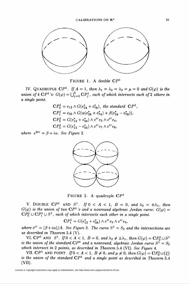
FIGURE 1. A double CF1

IV. QUADRUPLE CF1. If A = l, then Xy = A2 = A3 = p = 0 and G(tp) is the

union of 4 CF1 's: G(p) = (J.^CP1, each of which intersects each of 2 others in

a single point.

CPr) = ei2 A G(e34 + e78), the standard CP1,

CF/ = e56 A G(a(e*38 + e74) + 0(e*34 - e78)),

CF21=G(e*2 + e*6)Aeê3Ae"e4,

CF31=G(e*2-e;6)Ae"e7Ae"e8,

where e2lT = (3 + ia. See Figure 2.

FIGURE 2. A quadruple CF1

V. DOUBLE CF1 AND 51. If 0 < A < I, B = 0, and X2 = ±\y, thenG(p>) is the union of two CP1 's and a nonround algebraic Jordan curve: G(p) =

CFg1 U CPy U 51, each of which intersects each other in a single point.

CP1y=G(e*y2 + e*56)AelTe3Ae"e4,

where e" = (0 + ia)/A. See Figure 3. The curve 51 = 52 and the intersections are

as described in Theorem 5.4 (V).

VI. CF1 AND 51. IfO<A< 1, B = 0, andX27±±Xi, then G(pj) = CPr) U51is the union of the standard CP1 and a nonround, algebraic Jordan curve 51 = 52

which intersect in 2 points, as described in Theorem 5.4 (VI). See Figure 4.

VII. CF1 AND POINT. 7/0 < A < 1, B ^ 0, and p ^ 0, then G(tp) = CPr) U{£}is the union of the standard CP1 and a single point as described in Theorem 5.4

(VII).



FIGURE 3. Double CF1 and nonround 51

FIGURE 4. CF1 and nonround 51

VIII. DOUBLE CF1. 7/0 < A < 1, B ^ 0, p = 0, Ai = eA2 (e = ±1), and-e(A3 + XyX2) > 0, then G(<p) = CPr) U CF1 is the union of 2 CF^s, which meet

in a point. Here

CF1 = G(e*2 - ee*56) A eiTe3 A e"e4,

where e2lT = -e(/3 + ia)/A. CFq1 n CF/ = {e12 A eire3 A elTe4}.

IX. CF1. IfO<A<l, FÔ, p = 0, but not case VIII, or if A + B < C, thenG(tp) = CPr) is just the standard CF1.

Before giving the proofs of the descriptions of the contact sets G(tp) contained

in the main theorem, Theorem 5.3, it is convenient to focus attention on the torus

part, T f)G(p), oi the contact set.

THEOREM 5.4. Suppose tp e F*(CPq) fl TJ (as described in Theorem b.2).

Either G(tp) nT = Sq, the standard circle defined by (5), or p belongs to one of

the cases listed below.

If A = 0, as in Cases I, II, and III below, then p must be of the form

,,.s f — e1234 + e1278 + "Me1638 - e1674)

+ ^2(e5238 — e5274) + ^3(e5678) + Me5638 ~ e5674)-

Case I. A = 0, p = 0, Ai = ±1, A2 = ±1, A3 = ±1 with an odd number of

minus signs. In each of these four possibilities T D G(tp) is a 3-torus. For example,



if Xy = X2 = A3 = -1 then

(12) G(tp) n T = {£(0) :0y+02-03-r04 = 2ir}.

Case II. A = 0, p = 0 and exactly one Xi = ±1. T/n's forces Xj = ±Xk. G(tp)

is independent of the value chosen for \Xj\ < 1. (Hence one might wish to set

Xj =Xk= 0.)

For example, if Xy = 1 then

_ * . * . * *'P = e1234 + e1278 ' e1638 — e1674

+ He5238 ~ e5274 — e5634 — e5678J Wt^'1 KI < I'

and

(13) G(tp) n T = {£(6>): 0y = 0 and 02 + 03 - 04 = 0}

is the same 2-torus for all \t\ < 1.

Case III. A = 0, p / 0. Tfcen

1 — Aj — A2 — A3 — 2AiA2A3 = p ,

G(tp) D T = 5i U 52, w/iere 5r} = {£(0): 0y = 02 = 0 and 03 = 04} is the standard

circle and S2 is the circle defined by

cosî _ Ai + A2A3 cos02 _ A2 + AiA3 cos(04 - 03) _ A3 + AjA2

sin#i p sinf?2 p sin(f?4 — 03) p

with 9y,02,04 — 03 required to be in (0,n) if p > 0 and in (—7r,0) if p < 0.

Case IV. Ai = A2 = A3 = p = 0, A = Va2 + /?2 = 1.

T/jen £> is 0/ </ie /orm

V — e1234 + e1278 + Q(e5638 + e5674i + P(e5634 — e5678)-

Here G(<p) f) T = Sr) U 5/ U S2 U 53 is £/ie union of four intersecting circles.

Sr): 0y = 02 = 0, and 03 = 04 is the standard circle.

Sl:0y=02=n/2; sin(6»3 + 04) = a, cos(03 + 04) = {3.

S}:9y=02', 03Ô3, sin(03 + 04) = a, cos(03 + 04) = P-

53 : 0y + 02 = tt; 6>3 = f?4 + tt, sin(03 + 04) = a, cos(03 + 04) = P-

For example, if a = 0, /? = 1 </ien

V3 — e1234 + e1278 + e5634 ~ e5678»

and

S0: e12 A elSe3 A eiee4, 5j: e56 A eiee3 A e~iee4,

52: eieey A eiee2 A e34, 53: eiflei A e_ee2 A e78.

See Figure 5.



FIGURE 5

Case V. B = 0, 0 < A = C < 1, and Xy = eX2 = X, with s = ±1.

Then tp is of the form

f — e1234 + e1278 + -Me1638 ~~ e1674) + £A(e5238 — e5274)

— £* (e5634 + e5678) + a(e5638 + e5674) + /?(e5634 — e5678i

with 1 > A = a2 + P2 = (1 - A2) > 0.

The cases e = ±1 are interchangeable (replace e$ by — es, a by —a and P by

—p). Hence we assume e = — 1.

G(tp) fl T = So U 5i U 52 where S0 = {£(0): 0y = 02 = 0 and 03 = 04} is the

standard circle; Sy is a flat circle defined by 0y = 02, 03 = 04, e2l°3 = (/? + ia)/A;

and 52 is a twisted circle defined by

0y+02 = n, e'^3+e4) = (p + ia)/A, and

X2 sin2 0y - cos2 0y(15) sin(04-03) =—20 ,2 . 2o .\10) cos-2 0i + X2 sm 01

A2 sin 0! - cos2 0icos(04 - 03) = — . 3 •

cos'' 0i -I- AJ sin 0i

5o and Sy intersect at ey A e2 A e*ee3 A et9e4 where e2t9 = (P + ia)/A.

So and 52 intersect at ey A e2 A etfle3 A el6e4 where e2t6 = —(p + ia)/A.

Sy and 52 intersect at es Ae$ Aet9e3 Ae!"e4 where e2%6 = (P + ia)/A. See Figure

6.

Case VI. fl = 0, 0 < A = C < 1, and Xf ̂ A2,.Then p is of the form

f — e1234 + e1278 + ^1 (e1638 — e1674) + -^2(e5238 — e5274)

— AiA2(e5634 + e5678) -I- «(e5638 + e5674) + /?(e5634 — e5678),

with a2 + p2 = (1 - A2)(l - X22) > 0.License or copyright restrictions may apply to redistribution; see http://www.ams.org/journal-terms-of-use


FIGURE 6

G(tp) n T = So U 5i where S0 = {£(0): 0i = 02 = 0 and 03 = 04} is the standard

circle and Sy is a twisted circle parametrized by tp = 04 — 03, described by

sin 0! sin 02 > 0,

A sin i/> cos 0i - (Ai(l - X\) + A2AcosV')sin01 = 0,

Asin?/)cos02 - (A2(l - A2) + AiAcosV,)sin02 = 0,

ei(e3+e4) = ip + ia)/A.

The circles So and Sy intersect at the two points ey A e2 A el6e3 A el6e4 with

e™ = ±(p + ia)/A.Case VII. A ^ 0, p ^ 0, and A + B = C. Then tp is of the form (6) and

G(p) fl T = 5o U {£(0)} where So is the standard circle and the singleton £(0) is

defined by

cos01 _ A2(A3 + AtA2)A + (Ai + A2A3)F

sin 0i pC

cos02 _ Ai(A3 + AiA2)A + (A2 + AiA3)F

(17\ sin 02 pC

la a \ ^3 + -^1^2 ■ ,Q a ■, Pcos(04 - 03) =-, sm(04 - 03) = —,

cos(03 + 04) = |, sin(03 + 04) = j,

where, if p > 0 then 0i,02 G (0,7r), and if p < 0 then 0i,02 G (-7r,0).

Case VIII. Let e = ±1. Assume Xy = eX2, —e(X3 + AiA2) > 0, p = 0 and A =

1 + eX3 > 0 (hence A + B = C). Then p is of the form (6) and G(tp) nT = 50 U5i

where So is the standard circle and Sy is the circle defined by

0i=02, 03=04 ife = -l,

0y+02 = ^^4-03 = ir ife = +1,

cos(03 + 04) = (PIA) sin(03 + 04) = a/A for e = ±1.

Now we proceed with the proofs of Theorem 5.2, Theorem 5.4, and Theorem 5.3

in that order.License or copyright restrictions may apply to redistribution; see http://www.ams.org/journal-terms-of-use


The Torus Lemma 4.2 states that each form tp G TJ attains its maximum value

at some torus point £(0). Thus tp, defined by (9) above, has comass one if and only

if the function

p(t](0)) = CyC2C3C4 + CyC2S3S4

(18) 4- Ai3(cis2c3s4 - cis2s3c4) + A23(sic2c3s4 - sic2s3c4)

+ sis2(A34C3C4 + 03C3S4 -I- q4s3c4 + bs3s4)

has maximum value 1.

Consider the change of variables

(19) 01=01, 0~2=02, 03=04-03, 04 = 03 + 04.

Then the expression (18) for p(tf;(0)), as a function of 0, is given by

f(0) = C1C2C3 + A13cis2s3 + A23sic2s3

(20) + |(A34 + 6)s!S2c3 + ^(q3 - q4)sis2s3

+ [5(^34 - b)c4 + |(o3 + q4)s3] sy§2.

Under the change of variables (10), f(8) assumes the simpler form

,„., /(0) = cic2c3 + A1c1s2s3 + A2sic2s3 + A3si§2c3

+ pSyS~2S~3 + (01S4 + PC4)SyS2-

Thus we have proved

LEMMA 5.5. Each p of the form (6) of Theorem b.2 is of comass one if and

only if f(0) given by (21) has maximum value one.

If A = \Ja2 + P2 = 0 then this function f(0) was completely analyzed in Dadok

and Harvey [2].

By the results of [2], all portions of Theorems 5.2 and 5.4 with A = 0 follow

immediately. In the remainder of the proof we assume A > 0.

Since adding tt to any pair of the four angles 0i,02,03,04 does not change the

torus point £(0), we may assume that 0y, 02 G [0,tt). Then s"i,s2 > 0. Conse-

quently, choosing 04 with:

(22) sin 04 = a/A, cos04 = P/A,

we may replace f(0) by F(0) in Lemma 5.5, where

(23) F(0) = CyC2C3 + XyCyS2§3 + A2S"iC2S3 + A3SiS2C3 + pSyS~2S~3 + Asy§2-

LEMMA 5.6. Each <p of the form (6) is of comass one if and only if F(0),

defined by (23), has maximum value one.

The key to the proof of the theorems is an analysis of the critical points 0 of the

function F(0).

Suppose 0 is a critical point for F with critical value equal to one. Then

(1) CyC2C3 + XyCyS2S3 + X2SyC2S3 + X3SyS2C3 + pSyS2S3 + AsyS2 = 1,

,„.x (!) ~ SyC2C3 - XySy§2§3 +X2CyC2S3 +X3CyS2C3 +pCyS2S3+A5yS2 =0,(24)

(2) - cis2c3 + AiCic2c3 - A2sis2s3 + A3sic2c3 + psic2s3 + AsyC2 = 0,

(3) - cic2s3 + AiCiS2c3 + A2sic2c3 - A3sTs2s3 + p§y§2C3 — 0.



These equations imply

(a) Ci = C2C3 4 XyS2S3,

(b) c2 =cic3 + A2sis3,

, . (c) C3 = CiC2 4- (A3 + AC3)syS2,

(a1) sy = X2C2S3 4 X3S2C3 4 ps2S3 4 As2,

(W) S2 = AiCiS3 + A3S1C3 + pSyS2 +A§y,

(c') s3 = AiCi§2 4 A2sic2 4- pSys~2 4 As~is2s3.

For example, ci times equation (I) minus Si times equation (1) yields equation (a).

REMARK. If sis2s3 ^ 0 then (a), (b), (c) plus one of (a'), (b'), (c') imply (I),

(1), (2) and (3).

Let E = 1 - c\ - c\ - c\ 4 2ciC2c3. Since E = (1 - c2)(l - c2) - (ck - CiCj)2 for

all {i,j, k} = {1,2,3}, equations (a), (b), and (c) imply

(l)(l-A2)s-2s-2=F,

(26) (2) (1 - A2)s"2s1 = E,

(■i)(l-(X3+Ac3)2)s2s22 = E.

Note that equation (I), minus ci times equation (a), minus C2 times equation

(b), minus C3 times equation (c) yields:

(27) (^4As3)sis2s3=F.

Also note that

(C2 - CiC3)(c3 - Cy52) 4 (Ci - C2C3)s\ = CyE.

Now using (a), (b), and (c) yields (i) below.

(i) (A2(A3 4 Ac3) 4 Ai)sfs2s3 = CyE,

(28) (ii) (Xy(X3 + Ac3) + X2)syS22S3 = C2E,

(iii) (AiA2 4 A3 4 Ac3)sis2S3 = c3E.

Equations (ii) and (iii) are proved similarly.

Certain special cases must be considered separately. First, we consider the

generic case.

(29) Assume sis2s3 ^0, A2 ± 1 and X\±l.

Using (27) and (28) (iii) we conclude that

(30) c3p = (X3 + XyX2)s3.

If in addition we assume

(31) p ± 0

then

(32) c3/s3 = (A34A1A2)/p.

Let B = v/(A34AiA2)24p2. Then

(33) c3 = rj(AiA2 4 A3)/F and s3 = o(p/B)

where either CT=lorrj = —1.



Consequently,

(34) p + As3 = (p/B)(B 4 a A)

and

(35) A3 4 AjA2 4 Ac3 = ((A3 4 XyX2)/B)(B + aA).

Just as in the derivation of (30), using equation (27) with (28) (i) or (ii) yields

,oa, cy A2A3 + Ai+ A2Ac3(36) — =-tz-,

si p4As3

or

(37] £2 = A1A3 4 A2 + XyAc3

s2 p 4 As3

Substitution of (34), (35) into (36) and (37) yields:

, , 5y_ _ (Xy 4 A2A3)F. 4 crA2(AiA2 4 A3)A

1 ' sy p(B + uA)

, , £2 = (Aa 4 AiA3)F 4 aAi(AiA2 4 A3)A

1 j s"2 p(B + aA)

Equations (26) (1) and (26) (2) imply

(l-A2)(l-A2)s-2s-2s-4 = F2.

Equation (27) implies

(p4As3)2s2s2s4 = s2F2.

Equation (28) (iii) implies

(A3 4 AjA2 4 Ac3)2s2ys224 = c\E2.

Therefore,

(40) (p 4 As2)2 4 (A3 4 A, A2 4 Ac3)2 = (1 - X2)(l - A2).

Substitution of (34) and (35) into (40) yields

(41) (B4aA)2 = (l-A2)(l-A2).

Thus either

(42) B4a-A = v/(1-A2)(l-A2)

or

(43) B + CTA = -^(1-A2)(1-A2).

This completes our analysis of the critical equations (24) for the moment. We

shall return to these equations later.

LEMMA 5.7. det Hess F(0) at 0 = 0 is given by

1 " A? - X22 - X\ - 2AjA2A3 - 2(A3 4 AiA2)A - A2.

PROOF. Direct calculation.



COROLLARY 5.8. detHess(F(0))\ s=0 < 0 if A + B < C.

PROOF. Let H = l-Af-A|-A§-2AiA2A3 and note that (A34AiA2)24# = C2.

Now

det HessF(0)| -e=0 = A2 - 2(X3 + XyX2)A - H.

This quadratic function of A, denoted Q(A), vanishes at

A3 4 A,A2 ± v/(A3+AiA2)24Jr7 = A3 4 AiA2 ± G.

Thus Q is negative on the interval A3 4 A1A2 - C < A < A3 4 AiA2 4 C. IfA + B <C then -(A3 4 AXA2) 0} the

function C — A — B is strictly radially decreasing.

PROOF. Let

D = C-A-B = V/(1-A2)(l-A2) - V(A3 + AiA2)24p2 - y/ofl + p.

Since p ■ 3D/dp, a ■ 3D/da, and /? • 3D'/dp < 0 it suffices to show that

1 3D 1 3D 1 3D~2Xl3X[~2X2W2'2X3'3Xz

(44) _ A2 4 A2 - 2A2A2 (A34A1A2)(A34 2A1A2)

v/(l - A2)(l - A2) V(A3 + AiA2)24p2

is positive.

If (A3 4AiA2)(A34 2AiA2) > 0 then (44) is positive on |Ai| < 1, |A2| < 1. Hence

we may assume that (A3 4 A1A2HA3 4 2AiA2) < 0. Now (44) is increasing in p2,

and hence we may set p = 0. We may assume the product A1A2 < 0 and A3 > 0

since interchanging the signs of both Aj and A3 or both A2 and A3 does not change

(44).Then, since A3 4 Ai A2 and A3 4 2AXA2 are of opposite signs, A3 4 A1A2 > 0 and

A3 = 2A1A2 < 0, i.e. |AiA21 < A3 < 2|AiA2|. Therefore (44) is minimized when

A3 = |AiA2| = —AiA2 and this minimum is

\2 1 ^2 _ o\2 \2Ay -I- Ar, 4AyA2

^(i-xt)(i-xb+XlX>-

It remains to show that

ff(Ai, A2) = A2 4 A2 - 2A2A2 4 Aâ^/fl - A2)(l - A2) > 0.

Since

A J*L - X ^- (Aj-A2)(2-AiA2)ldXy 2dx2 va-Aâ-A2)'

the critical points of g are on the lines Ai ± A2 =0. Now it follows easily that 0 > 0

on |Ax| < 1, |A2| < 1.

REMARK 5.10. It follows easily from this lemma that

{<p: |Ai|<l,|A2|<l,A4F<G}

is the closure of {tp: |Ai| < 1, |A2| < 1 and A + B < C}.



Proposition 5.11. The set

(45) R = {p-\Xy\<l, ]X2\<1, A + B<C}

is contained in F*(CFo); i.e., each tp E R has comass 1.

PROOF. By the above remark we may assume |Ai| < 1, |A2| < 1 and A + B < C.

Since F*(CF01) n TJ is a convex set it suffices to show that, after we increase A

and p2 slightly (maintaining A + B < G), the form p has comass one. That is, we

may assume A > 0 and p ^ 0.

Note that \Xy\ < 1, |A2| < 1 and B < C imply that |A3| < 1, since G2 - B2 <

(l-X2)(l-X2)-(X2 + XyX3)2.

Let tpt denote the form obtained from p by replacing a by ta and p by tp,

i.e. py = tp. If \\tp\]* > 1 then for some t either

Case 1. —det Hess Ft (0)| ^=0 fails to be positive, so we cannot be certain that

0 = 0 remains a local maximum for Ft (0), or

Case 2. v?*(£(0)) has a critical point £(0), with critical value one, which is not

on the standard circle Sr).

Lemma 5.7 rules out Case 1. The calculations made above (see equations (24)

through (43)) can be used to rule out Case 2. These calculations assumed that

|Aa| < 1, |A2| < 1, A > 0, p / 0 and sys2s3 ^ 0. All of these assumptions except

S1S2S3 7^ 0 are automatically valid for pt with t < 1 fixed.

If Sis2s~3 = 0 there are several cases to consider. First, suppose s~i = 0. Then, by

(26) (2), E = 0. Therefore by (26) (1) either s2 = 0 or s3 = 0. If Sy = s2 = 0 then by

(25)(c') s3 = 0, while if sy = s3 = 0 then by (25)(b') s2 = 0. Thus s~i = s2 = s3 = 0

and hence, by (24)(I), cic2c3 = 1. Similarly, if s2 = 0 then c"iC2C3 = 1.

Now, suppose s3 = 0, but Sy ̂ 0, s2 ^ 0; then by (26)(2) and (3) A34Ac3 = ±1.

Thus A3 = ±1 ± A. Since B < C, (1 - A?)(l - A§) > (A2 4 A1A3)2 4 G2 - B2 > 0.

Thus |A3| < 1. Consequently, either A3 = 1 - A > 0 or A3 = -(1 - A) < 0.

Suppose A3 = 1 — A > 0. Then A + B > C. To prove this, we might as well

assume p = 0. A 4 B = 1 — A3 4 |A3 4 AiA2| is piecewise linear in A3.

At each of the points A3 = 0, A3 = — A1A2, and A3 = 1, we have A 4 B >

1 - |AiA2|. Hence A + B > 1 - ]XyX2] on 0 < A3 < 1. Now 1 - |A,A2| >

^(1-A2)(1-A2) = G.The proof for A3 = — (1 — A) < 0 is the same.

Therefore, with |Ai | < 1, |A2| < 1, A > 0 and p ^ 0 it follows that sis2s3 ^ 0.

Now equations (24) through (43) are valid.

In particular, either (42) or (43) must be true, i.e. B±A = ±C. Now A+B = -C

is impossible, and in the other three cases A + B >C. This rules out Case 2 above,

and completes the proof of Proposition 5.11.

COMPLETION OF THE PROOF OF THEOREM 5.2. Let F = F*(CFrj) Cl TJ

and R be defined by (45). By Proposition 5.11, R C F. By Lemma 5.9, R is

star-shaped with respect to the origin. Hence it suffices to show that 3R c 3F

(because F is also star-shaped).

If tp G 3R and A = 0 then tp E 3F by [2]. If p E 3R, A > 0 and p = 0 thentp is the limit of points tp E 3R with A > 0 and p ^ 0. Therefore, we need only

show that if tp E 3R, with A > 0 and /i^0 then p> E 3F. Defining 0i,02,03,04by equations (33), (38), and (39), with a = 1, and by (22), we obtain a point £(0)

which is not on the standard circle Sr) but with £>(£(0)) = 1. Hence tp e 3F.



This proves R = F and completes the proof of Theorem 5.2.

Now we complete the proof of Theorem 5.4, describing the contact sets G(^)(~lTJ

for each tp E R. As noted earlier, cases I, II, and III of Theorem 5.4 follow from [2].

Thus we assume A > 0. Also, unless p E 3R, G(p) fl T = Sr). Thus we assume

A + B = C.PROOF OF THEOREM 5.4. Case IV. In this case, A = 1, the function F(0)

defined by (23) reduces to

(46) F(0) = c,c2c34siS2.

The function F is equal to one exactly as described in Theorem 5.4, Case IV. The

details are omitted.

LEMMA 5.12. Suppose A > 0, B > 0, A + B = G, and X2 ̂ A2. Then any

point 0 satisfying the critical equations (24) must have s"is2s3 ^ 0 unless sy = s2 =

s3 = 0.

PROOF. As we have noted before, s~is2 ̂ 0. Suppose S3 = 0. Then, by (26)(2)

and (3), A3±A = ±1. Since B < C, (1-Af)(l-A§) > (A24A,A3)24C2-B2 > 0.Thus |A3| < 1. Consequently, either

(47) A3 = 1 - A > 0

or

(48) A3 = -(1-A)<0.

Consider the case A3 = 1 - A > 0. Now

A 4 B = 1 - A3 4 v/(A34A!A2)24m2 > o(A3) = 1 - A3 4 |A3 4 AXA2|.

Note o(A3) is piecewise linear on 0 < A3 < 1. Moreover, o(0) = l4|AiA2|,o(—AiA2)

= 1 - A3 = 1 - |AiA2|, and o(l) = 1 4 A,A2. Therefore, A 4 B > 1 - \XyX2]with equality if and only if AiA2 < 0 and A3 4 AiA2 > 0. Now 1 — |AiA2| >

<J(1 - Xj)(l - X'2,) = C with equality if and only if A? = X22. Therefore A 4 B > Cand equality holds if and only if Ai = —A2, A3 > A2, p = 0, and A = 1 — A3 > 0.

Similarly, in case A3 = -(1 - A) < 0 we get A + B > C with equality if and only

if Ai = A2, A3 < A2, p = 0, and A = 1 4 A3.

PROOF OF THEOREM 5.4. Case VII. Suppose A > 0, p ^ 0, and A 4 B = C,

i.e. p belongs to Case VII of Theorem 5.4. Then by Lemma 5.12 there are no

solutions of the critical equations (24) with s~is2s3 = 0 other than 0y=02 = 03= 0.

Hence we may assume s~is2s3 7^ 0. Now the calculations (29) through (43) given

above are valid. Since A + B = C, equations (42) and (43) imply that a = 1.

Case VII of Theorem 5.4 can be read off from equations (38), (39), (33), and

(31).PROOF OF THEOREM 5.4. Case VI. Suppose B = 0, A = C > 0, and X\ / X2,;

that is, p = 0, A3 = —AiA2, and A = C > 0. Since A2 7^ 1 and A2 ̂ 1, equation

(26) eliminates the possibility sys2 = 0 unless s~i = s2 = s3 = 0.

We must deal with the case s3 = 0, s~is2 / 0. By (26) A3 4 AC3 = ±1 or

A3 ± A = ±1. Since A3 = -A1A2, |A3| < 1. Therefore, there are only two cases:

(49) A3 = 1 - A > 0, and c3 = 1,



or

(50) A3 = -(1 - A) < 0, and c3 = -1.

In the first case (49), where c3 = 1, we derive from (25)

(51) A2 = -A!, A3 = Aj\ and A = 1 - X\.

In the second case (50) where C3 = —1,

(52) A2 = Ai, X3 = -X\, and A = l-X\.

In both cases A2 = A2. Hence we may assume sis~2S3 ̂ 0. Now equations (36)

and (37) are valid. Substitution of A3 = -A1A2 into (36) and (37) yields all but the

last equation el^3+e^ = (P + ia)/A in (17). This last equation is just (22). This

completes Case VI.

PROOF OF THEOREM 5.4. Case V. Assume e = -1 (i.e. A2 = -Ai). First,

suppose syS2S3 ^ 0. Then s"i = s2 by (26)(1) and (2). Hence either 0i = 02 or

0! 4 02 = TT. Note 1 - ASyS2 = 1 - (1 - A2)s2 =c\+ X2s\.

Now the equation 03 = 04, if 0i = 02, and equation (15), if 0i 4 02 = 7r, follow

from (25)(c') and (25)(c). Using (22) again, this completes the proof of Case V

unless S3 = 0. If S3 = 0 then direct examination of the critical equations (24)

yields the solutions described in Case V of Theorem 5.4.

PROOF OF THEOREM 5.4. Case VIII. We consider the case e = -1; the case

e = +1 is similar. Then with Ai = A, A2 = -A, A3 4 AiA2 = A3 - A2 > 0, p = 0

and A = 1 - X3 > 0.

Hence

F(0) = cic2c3 4 Acis2s3 - Asic2s3 4 A3sis2c3 4(1- A3)s~is2.

Note that c3 = 1, 0i = 02 is a solution. Using the critical equations one can

check that these are all the solutions.

To complete the proof of Theorem 5.4 we must show that all cases have been

considered. First, all cases with A = 0 were discussed in I III. Hence we may

assume A > 0. By Case VII we may assume p = 0. By Lemma 5.12 and equation

(33) it remains to consider the cases where either B = 0 or A2 = A2. Case V is

where both B = 0 and A? = A?,. Case VI is where B = 0 but X\ =£ X2,. Case VIII

is where B > 0 but X\ = A2. This completes the proof of Theorem 5.4.

PROOF OF THEOREM 5.3. Now we give the proof of the main theorem, 5.3,

classifying the faces or contact set G(tp) for all tp E F*(CFo) n TJ. Each such p>

can be expressed as

(53) V = ^*12 + ^^ A ^4 + 6*78> + ÂlC^6 + X2€*52 + ^^

A (e*38 - e*4) 4 e*56 A (P(e*34 - e78) 4 a(e^8 4 e74)),

with IAxI < 1, |A2| < 1, and A + B < C, where

A = s/a2 + p2, B = ^(X3 + XyX2)2 + p2 and C = y/(l - X2)(l - A2).

(This is just a restatement of Theorem 5.2.)

The classification of faces G(<p) follows Theorem 5.4 case by case. The new case

IX corresponds to the trivial case of Theorem 5.4 when the torus face is just the

standard circle 5q.



I. SPECIAL LAGRANGIAN. The standard special Lagrangian form (cf. [7]) is

given by

******* . *e1234 — e5634 — e5274 — e5238 — e1674 — e1638 ~ e1278 "+" e5678-

The 4 forms of Case I result from switching the signs on {ey, e3}, {ey, e4}, {es}, and

{e7}, respectively.

II.A. Special Lagrangian. First suppose Xy = ±1. Let A2 = t, X3 =+t, tp = tpt. Then tp0 = e* A tp, where

tp = e*234 4 e*,78 ± e*,38 + e*,74 = Re((e2 4 iei) A (e3 ± ier) A (e4 T ieD)

is a special Lagrangian form on span{ei,es}-L. Consequently (cf. [7, Proposition

7.10]), G(tpo) = ex A G(ip) as asserted. For any -1< t < 1, for any £ G G(4,R8),

<Pt(0 = -2~<Pi(0 + -^-£>-i(£) < -y- + ~y~ = X'

with equality if and only if £>i(£) = <P-i(£) = !• Hence G(p*) = G(tpy) UG(tp-y)

is independent of t, i.e., G(pt) = G(po)-By symmetry the case A2 = ±1 is similar.

II.B. CF1 x CF1. Here A3 = ±1. Let Ai =t, X2 = -t, <p = <pt. Then

tpo = (e*12 ± e*56) A (e34 4 e78),

and G(tpo) is as asserted (cf. Theorem 1.7(VIII)). For any -1 < t < 1, any £ G

G(4,R8),

,„, l + t _, 14* ,„ ^ l + t 1-t ,<pt(Z) = —pi(0 + —<p-i(S) < — + — = i,

with equality if and only if <py(£) = £>-i(£) = 1. Hence G(tpt) = G(tpy) n G(p>-y)

is independent of t, i.e., G(p>t) = G(p>o).

III. DOUBLE CF1. Let 0X,02 be as defined in Theorem 5.4(111). Direct compu-

tation shows that

tf = (el9lei A eê2) jp = ^^(e*, 4 e*8) 4 |e*.8(e74).

Therefore, with CF/ = eieie, A el92e2 A G(tp),

G(tp) n T c CFq1 U CF/ c G(>p).

Since 0i ^ 0, CFq1 n CF/ = 0. To see that CF/ is a CF1, note that tpis a Kahler form on C2 = span{e3,e4,e7,e8} because (A3 4 AiA2)2 4-p2 = F2.

(Whenever a2 +b2 = 1, then

a(e34 4 e*-8) 4 b(e*38 - e*74) = (ae*3 - be*7) A e\ + (ae*. 4 6e3) A eg

is a Kahler form.)

To complete the proof, we suppose £ G G(p) -T and deduce that £ G CFq1 UCF/.

Since £ £ T, for some j, £ must fail to have a factor of the form ene3. By the

Torus Lemma 4.2(2) and Theorem 5.4, j must be 3 or 4. Suppose £ has no factor

of the form etle4. Then by Lemma 4.1, there are a unit 2-vector factor n of £ and

unit vectors y, z such that

tp(n A y A e4) = tp(r) A z A e8) = 1.



The torus maxima oi e4 _\tp are ei23 and el9ley A eld2e2 A et93e3, as described by

Theorem 5.4(111). By the Torus Lemma 4.2(2), nAy = eX23 or ei6iey AeiS2e2Aeie3e3.

Similarly, by Theorem 5.4(111), the torus maxima of e8 Jp are ei27 and ±eldley A

el$2e2 A el$3e7. Again by Lemma 4.1, n A z = ei27 or ±el$1ey A e^2e2 A e^3e7.

Comparison of these expressions for nAy and n A z shows that n = ±ei2 or

±e'e'ei A el62e2. Replacing n by -n if necessary, we may assume n = e12 or

el9ley A etB2e2- If n = ei2, then n Jtp = e*34 - e78 and £ G G(e*234 4 e*278) = CFq1.

If n = ei6leyAeie2e2, then £ G eifllei Aei(?2e2AG(nJp) = CF/, as desired. The proof

in the alternative case when £ has no factor of the form elle3 is almost identical.

IV. QUADRUPLE CF1. Choose r G [0,7r) such that elT = p + ia. Direct

computation shows that

tpo=ey2Jp = e34 4e78,

tfi = e56 J<p = P(e*34 -e78)4a(e384e*-4),

tp2 = (e"e3 A elTe4)_lp = e*12 + e*56,

ip3 = (ejre7 A etTe8) Jp = e*2 - e*5e.

Comparison with Theorem 5.4(IV) now shows that Sj C CF1. Therefore, G(ip) fl

TcU-=0CF/cG(p).As in the proof of III, each CF1 is indeed a CF1. It is also easy to check that

CFq1 n CF/ = 0, CFq1 n CP2l = e12 A e"e3 A e"e4,

CFq1 n CF31 = eia A etTe7 A e"e8,

CF/ n CF/ = e56 A e"e3 A etTe4,

CF/ n CF^ = -e56 A elTe7 A e"e8, CF/ n CFg1 = 0.

To complete the proof, we suppose £ G G(tp)-T and deduce that £ G Ui=o CF1.

Since £ ^ T, for some k, £ must fail to have a factor of the form ellek.

Case k = 1. £ has no factor of the form e'êi. Let py,P2 be distinct angles

strictly between 0 and 7r/2. By Lemma 4.1, there are a unit 2-vector factor n at £

and unit vectors Wy and iu2 such that tp(elp'ey AWj An) = 1.

By Theorem 5.4(IV), the torus maxima of —elpjey J tp are e%p>e2 A e"e3 A e%Te4

and —e~lp>e2 A eJTe7 A etTes. By the Torus Lemma 4.2(2),

Wj A rj = elple2 A elTe3 A elTe4 or - e~%Ple2 A elTe7 A e*Te8.

Since py ^ P2, V = ±e"e3 A elTe4 or ±eJTe7 A e1Te8. Consequently £ belongs to

G(ip2) A e'Te3 A e"e4 = CP2X or to G(tp3) A elTe7 A elTe8 = CP3S

Case k = 2 is almost identical to case fc = 1.

Case k = 3. £ has no factor of the form elle3. Let py,P2 be angles such that

py,P2,r are distinct modulo 7r/2. By Lemma 4.1, there are a unit 2-vector factor n

of £ and unit vectors itfi,W2 such that <p(n Aeipê3 Awj) = 1. By Theorem 5.4(IV),

the torus maxima of -e,p>e3 Jtp are ei2 Aetpê4 and e56 Aet'2T~pê4. By the Torus

Lemma 4.2(2),

w3An = e12 Ae%p'e4 or e56 A ej(2r_Pj)e4.

Since py 7^ p2, n = ±eia or ±es6- Consequently £ belongs to CFj or to CF/.

Case fc = 4 is almost identical to case fc = 3.



V. DOUBLE CF1 AND 51. Choose r G [0,7r) such that e" = (P + ia)/A. Direct

computation shows that X3 + A = 1 and

tP = (e"e3 A eiTe4) J p = e*2 4 e*56.

Comparison with Theorem 5.4(V) now shows that 5i C CF/. Therefore,

G(ip) Cl T c CFq1 U CF/ U 51 C G(p).

Note that CF/ is indeed a CF1. It is also easy to check that

CFq1 n CF/ = {e12 A eITe3 A e""e4}, CFq1 n 51 = {e12 A e"e7 A elTes},

and

CF/ n 51 = {e56 A e'Te3 A eSTe4}.

To complete the proof, we suppose that £ G G(>p) — T and deduce that £ G

CFq1 U CF/. Since £ ^ T, for some fc, £ must fail to have a factor of the form ellek.

Case fc = 1. £ has no factor of the form enei. Let py,p2 be distinct angles

strictly between 0 and 7r/2, such that <7i ̂ <r2 where

. „ 2Ai cosp, sinp, „ A? sin p,■— cos2 p,sin2<J> = a /i2 ■ 2 - cos*>i = 2 1x2-2 .

cos-' pj 4 Aj sm pj cos'' pj + Xf sm pj

0 < a j < tt/2. By Lemma 4.1, there are a 2-vector factor n of £ and unit vectors

wy, W2 such that p>(eip>ey A Wj An) = 1. By Theorem 5.4(V), the torus maxima of

-eip'ey }p> are eJê2 A e"e3 Ae'Te4 and -e~ipê2 A ex^-°ê3 Ae'(r+<7')e4. By the

Torus Lemma 4.2(2),

Wj An = eipje2 A e"e3 A elTe4

or

-eip'e2Ael(T-°')e3Ael(T+a')e4.

Since py ^ pa and rji ^02, n = ±elTe3 A elTe4. Consequently £ belongs to

G(V)AeiTe3AetTe4 = CF/.


Case fc = 3. £ has no factor of the form el~le3. Let pi,pa be angles such that

Pi,P2,r are distinct modulo 7r and px — P2,2r are distinct modulo ir. By Lemma

4.1, there are a unit 2-vector factor n of £ and unit 2-vectors wy,W2 such that

<p(n A eip>e3 A Wj) = 1. By Theorem 5.4(V) the torus maxima of —elp>e3 Jp are

ei2 A eiPje4 and possibly points from 51 = 52 of the form —elS>ey A e~lS>e2 A

e^2T_pj'e4, where

. ,r. „ , 2Aj cos (5, sin (5, . „ , A? sin 8,— cos2 <5,sm(2r - 2pj) = —-±-J--f-, cos(2r - 2pj) = -=--^—-5-^.

cos2 Sj 4 A2 sin <5j cos2 6j — X2 sin 6j

Since everything is invariant under 83 —* 8j+tt, we may assume —7r/2 < 83 < tt/2.

Since the trigonometric functions are strictly increasing on this domain, there is at

most one solution 6j. Since pi ^ p2 (mod7r), 6y ^82-

By the Torus Lemma 4.2(2),

Wj An = ey2Aeip'e4 or - e6'ey Ae~lS'e2 Ael{2T'p')e4.



Since py ^ P2, 6y ^ 82, and pi 4 P2 7^ 2r (mod7r), n = ±ei2. Consequently £

belongs to ei2 A G(ei2 Jp) = CFq1.


VI. CF1 AND 51. Comparison with Theorem 5.4(VI) shows that G(p) nT C

CFq1 U 51 C G(tp). To complete the proof, we suppose that £ G G(tp) - T and

deduce that £ G CFq1. Since £ ^ T, for some fc, £ must fail to have a factor of the

form e%1ek.

Case k = 1. £ has no factor of the form el~>ey. By Lemma 2.2, there are a 2-

vector factor n of £ and unit vectors y, z such that <p(ey Ay An) = tp(e$AzAn) = 1.

For — 1 < t < 1, consider the forms

'Pt = ^1234 + e1278 + He1638 ~~ e1674J-

By Theorem 5.2, ]\pt\\* = 1. For any -1 < t < 1, for any £ G G(4,R8),

l + t ,,, 1-t _, 14* 1-t<Pt(Z) = — ¥>i(0 + — *>-i(0 < -5- + — = !.

with equality if and only if pi(£) = P-i(£) = 1. Hence G(p>t) = G(pi) fl G(p_i)

is independent of t E (—1,1). In particular

G(e*y A (ey Jp)) = G(pXi) = G(tp0) = CFq1.

Therefore, y A n E e2 A G(e34 4 e78).

The torus maxima et92e2 A et03e3 A el04e4 of es Jp are described by Theorem

5.4(VI). First note that there are only finitely many; otherwise, by real analyticity

every point of 51 = 5i would have es as a factor.

Therefore by the Torus Lemma 4.2(2), z An is of the form ejfl2e2 Ael03e3 Ael04e4.

Second, we claim that e1*2 ̂ ±1. Suppose sin02 = 0. Then by (16), sin^ = 0,

Ai(l- A2s)±A2A = 0, and

A2(l - A2)2 = A2A2 = A2G2 = A2(l - A2)(l - A2).

Since |A2| < 1, A2(l - A^) = A2(l - A2) and A2 = ±Ai, in contradiction to the

hypotheses of case VI.

Now since y A n E ea A G(e34 4 e78) and z An = el62e2 A el63e3 A e%9ie4 with

ei&2 ^ ±1, therefore n = ±el63e3 A eld4e4 and n E ±G(e34 4 e78). Consequently

tp = 04 — 03 = 0 (mod7r) and sin^ = 0, which leads to a contradiction as in the

preceding paragraph. Therefore the case fc = 1 never occurs.

Case fc = 2 is almost identical to the case fc = 1.

Case k = 3. £ has no factor of the form et7e3. Let r G [0,7r) be defined by

e2%T = (p 4 ia)/A. By Lemma 4.1, there are a 2-vector factor n of £ and unit

vectors y, z such that

<p(rj A e"e3 Ay) = p(n A el^T+7r/4)e3 A z) = 1.

By Theorem 5.4(VI), the torus maxima of -e,Te3 Jp are ei2 A e,Te4 and el01ey A

ei02e2 Aeire4. Similarly, the torus maxima of -e_^T+'r/'4ê3 Jp are ei2 Ae^T+v^4ê4

and e!CTlei A e,cr2e2 A et'T_7r/4'e4. The torus maxima of -e,Te3 Jp are ei2 A e!Te4

and el01ey A e^2e2 A etTe4 as described by Theorem 5.4(VI). In particular, tp =

0, sin0i = sin02 = 0, and eie'ei A eae2ea = ±eia- Now by the Torus Lemma

4.2(2), i] Ay = ±e12 A etTe4. Similarly, the torus maxima of -e^T+7r/4ê3 J p are

e12 Ae'('-'/4>e4 and e'ê, Ae*«2 A ei(r+7r/4)e4, tp = rr/2, sin<5, /0, sin,52^0,



and n A z = ey2 A e^T+7r/4)e4 or elSley A elS2e2 A e,(T-*'/4)e4. Comparing these

expressions for n A y and n Az shows that r\ = ±ei2- Therefore £ G CFq1.


VII. CF1 AND POINT. Comparison with Theorem 5.4(VII) shows that

G(p) nle CFq1 U {ei0iey A el02e2 A ex03e3 A ei0*e4} C G(tp),

with 0i,02,03,04 as in (25). To complete the proof, we suppose that £ G G(tp) - T

and deduce that £ G CFq1. Since £ £ T, for some fc, £ must fail to have a maximum

of the form eêfe.

Case fc = 1. £ has no factor of the form e'êi. Let p be an angle distinct from

0 and 0i modulo ir. By Lemma 4.1, there are a 2-vector factor n of £ and a unit

vector w such that tp(eipey AwArj) = 1. By the Torus Lemma 4.2, eipey Jtp attains

the value 1 on the torus, in contradiction to Theorem 5.4(VII). Hence this case does

not occur.

Case fc = 2 is almost the same as the case fc = 1.

Case fc = 3. £ has no factor of the form e'ês. Let pi,P2 be angles such that

Pi,P2,03 are distinct modulo 7r. By Lemma 4.1, there are a 2-vector factor n of £

and unit vectors wy, ti»2 such that tp(n A eiPje3 A Wj) = 1. By Theorem 5.4(VII),

the only torus maximum of — e%p>e3 Jtp is ei2 Ae1''^. By the Torus Lemma 4.2(2),

n Awj = ei2 A elp'e4. Therefore n = ±ei2 and £ G CFq1, as desired.

Case k = 4 is almost identical to the case fc = 3.

VIII. DOUBLE CF1. Direct computation shows that

tp = (eiTe3 A elTe4)jp> = e12 4 (A3 - eA)e*6 = e*2 - ee*56.

Comparison with Theorem 5.4(VIII) now shows that G(tp) fl T C CFq1 U CF/ C

G(p>). To complete the proof, we suppose that £ G G(tp) — T and deduce that

£ G CFq1 U CF/. Since £ £ T, for some fc, £ must fail to have a maximum of the

form ellek.

Case fc = 1. £ has no factor of the form e'êi. Let pi,P2 be distinct angles

strictly between 0 and 7r/2. By Lemma 4.1, there are a unit 2-vector factor n of £

and unit vectors wy, W2 such that p(eip>ei A Wj Ar/) = 1. By Theorem 5.4(VIII),

the only torus maximum of —etp'ey J tp is e~£xp'e2 A elTe3 A etTe4. By the Torus

Lemma 4.2,

Wj An = e~£lp>e2 A e"' e3 A e"e4.

Therefore, n = ±e"e3 A elTe4, and £ belongs to G(tp) A etTe3 A etTe4 = CF/.

Case fc = 2 is almost identical to case fc( = 1.

Case fc = 3. £ has no factor of the form elle3. Let pi,P2 be distinct angles

strictly between 0 and 7r/2. By Lemma 4.1, there are a unit 2-vector factor n of £

and unit vectors wy, w2 such that p(n A eip'e3 A Wj) = 1. By Theorem 5.4(VIII),

the only torus maximum of —eip>e3Jp is ei2 AetpJe4. By the Torus Lemma 4.2(2),

Wj An = e12 A elpJe4.

Hence n = ±ey2 and £ belongs to CFq1.


IX. CF1. Comparison with Theorem 5.4 shows that G(tp) DT c CPr) c G(<p).

On the other hand, suppose £ G G(tp) — T so that, for some fc, £ fails to have a

maximum of the form enek.



Case fc = 1. Let 0 < p < tt. By Lemma 4.1, there are a 2-vector factor n of £

and a unit vector w such that p(eipey Aw An) = 1. By the Torus Lemma 4.2(2),

eipey Jp attains the value 1 on the torus, which contradicts G(tp) fl T C CFq1.

Hence this case does not occur.


Case fc = 3. Let pi, P2 be distinct modulo tt. By Lemma 4.1, there are a 2-vector

factor n of £ and unit vectors wy, W2 such that tp(n Aetp'e3 Awj) = 1. By Theorem

5.4, the only torus maximum of — elp>e3 Jtp is ei2 Aeip>e4. Therefore n = ±ei2 and

£ G CFq1 as desired.


Chapter 6. On the angle conjecture

A basic question in the study of singularities in area-minimizing surfaces asks

when the sum (i.e., union) of two fc-dimensional planes £+,£- in R" is area-

minimizing (see [13] and [1, #5.8]). A sufficient (perhaps equivalent) condition

is that the two planes lie in a common face of the Grassmannian. The conjecture is

that two planes lie in a common face of the Grassmannian if and only if the angles

71,... ,7k which characterize their geometric relationship (cf. Lemma 6.1) satisfy

the inequality 7fc < 71 4 ■ • • 4 7fc-i- This conjecture has been proved for fc < 3 (cf.

[12, 1.2] or [2, Corollary 9]). Theorem 6.3 proves half the conjecture for fc = 4.

DEFINITIONS. Let {e3,ie3} be an orthonormal basis for R2/c = Ck. For a =

(ai,...,afc), define £(a)GAfcR2fc by

£(a) = exp(iai)ei A exp(ia2)e2 A • • • A exp(iafc)efc.

LEMMA 6.1 (Canonical form for two fc-planes (cf. [12, Lemma 2.3], or [7,

Lemma II.7.5])). Given two k-planes £+,£_ G G(fc,R2fc), there is an orthonormal

basis for R2k such that £± = £(±7/2), with 0 < 71 < • • • < 7fc-i < tt/2, 7^-1 <

7/t < 7r — 7fc_i. The 7j are unique. Another sum of planes £+ 4 £!_ is related to

£+ 4 £- by an isometry of R2k if and only if 7' = 7.

LEMMA 6.2. For 1 < k < n, p > 1, let p be a calibration in f\ Rn* and

let Cy,..., cp be k-vectors in /\ Rn satisfying ]\Cj]\ = <p($j). Then the mass of any

nonnegative linear combination c = CyCy + ■ ■ ■ + cpcP (cj > 0) satisfies \\c]\ = p(c).

REMARK. This lemma is just a renormalization of the geometric fact that a face

of the unit mass ball is convex.

PROOF. First notice that tp(c) < ||p|| ||c|| = ||c||. On the other hand,

Ikll < l|ciCi||4---4||cpCp|| =p(ci?i)4---- + p(cKi)=p(c).

THEOREM 6.3. Let £+, £_ be 4-dimensional planes through 0 in Rn with char-

acterizing angles 0 < 71 < 72 < 73 < 74- #74 > 71 4 72 4 73, then £+ and £_ do

not lie on a common face of the Grassmannian G(4,R"). In fact, the mass

£+ + £- _ 74 - (71 + 72 473)

2 C0S 2

is strictly less than 1.

REMARK. It is proved that an inadmissible pair £+, £_ do not lie on a common

face by showing that their average (£+ 4£-)/2 lies underneath a special Lagrangian

face.



PROOF. By Lemma 6.2, it suffices to prove the formula for the mass. By

Lemma 6.1, we may assume that £± = £(±a), with 0 < a3■ = 7j/2 < 7r/2. By a

limit argument, we may assume that 0 < a3< tt/2.

We will make use of the following general formula for £(<5), 0 < 83 < tt/2. First

note that if $ is the "special Lagrangian" calibration (cf. Harvey and Lawson [7])

$ = Re(a\zi A dz2 A dz3 A dz4),

then

(£(r5), <!>)) = Re(exp(-i(5i) exp(-io2) exp(-iS3) exp(i<54))

(1) =Re(exp(i]84-(8y+62 + 83))))

= cos(84 - (8y 4 82 4 83)).

Second, direct computation shows that

(2) --/ t c-T=ei234+ J2 tan 6j tan 6ke(j,k)2 COS by COS 02 COS 63 COS 84 k<4

4 tan<5i tan<52 tan 63 tan<54(iei) A (ie2) A (ies) A (ie4),

where e(l, 2) = (iei) A (ie2) A e3 A e4, etc.

For parameter A > 1, define aj < Pj < tt/2 by tan Pj = Atanctj . Consider

the function /(A) = p4 - (Py + P2 + Ps)- Since /(l) > 0 and limôo /(A) =

7r/2 — 37r/2 < 0, we may choose A such that /(A) = 0. It follows by formula (1)

that ($, £(±/?)> = 1 and hence {£(/?), £(-/?)} C G($). Also

{ei A e2 A e3 A e4, -(iey) A (ie2) A (ies) A (^4)} C G($).

But (£(q) 4 £(-q))/2 is a nonnegative linear combination of £(/?),£(-/?), ei234,

and -(iei) A (ie2) A (ies) A (ie4). Indeed, by formula (2) and the fact that tan/?, =

A tan aj,

*(<*) + £(-<*) _ A-2 gp) + a-p)2 COS tti cos 0:2 cos a3 cos 04 2 COS Py COS /?2 COS /33 COS /?4

= [l — A-2] ei234 4 VJ tana3 tanak]l — X~2X2]e(j,k)

l<j<k<4

4 tanai tana2 tanQ3 tan«4[l — A_2A4](iei) A (ie2) A (ie3) A (ie4).

Therefore by Lemma 6.2,

||(£(a) 4 £(-a))/2|| = ((£(a) 4 £(-a))/2, *) = cos(a4 - (ay + a2 + a3))

by formula (1). Since a = 7/2, the theorem is proved.

References

1. J. Brothers, Some open problems in geometric measure theory and its applications, Geometric

Measure Theory and the Calculus of Variations, W. K. Allard, F. J. Almgren, Jr. (eds.),

Proc. Sympos. Pure Math., vol. 44, Amer. Math. Soc, Providence, R. I., 1986.

2. Jiri Dadok and Reese Harvey, Calibrations on R6, Duke Math. J. 50 (1983), 1231-1243.

3. Jiri Dadok, Polar coordinates induced by actions of compact Lie groups, Trans. Amer. Math.

Soc. 288 (1985), 125-137.

4. Herbert Federer, Geometric measure theory, Springer-Verlag, New York, 1969.



5. Hermann Gluck, Frank Morgan, and Wolfgang Ziller, Calibrated geometries and minimal sur-

faces in Grassmann manifolds, preprint.

6. Reese Harvey, Calibrated geometries, Proc. Internat. Congress Math. 1983, PWN, Warsaw;

North-Holland, Amsterdam and New York, 1984, pp. 797-808.

7. Reese Harvey and H. Blaine Lawson, Jr., Calibrated geometries, Acta Math. 148 (1982),

47-157.

8. Reese Harvey and Frank Morgan, The faces of the Grassmannian of three-planes in R7, Invent.

Math. 83 (1986), 191-228.

9. _, The comass ball in /\3(R6)*, Indiana Math. J. 35 (1986), 145-156.10. G. J. Heckman, Projections of orbits and asymptotic behavior of multiplicities for compact con-

nected Lie groups, Invent. Math. 67 (1982), 333-356.

11. B. Kostant, On convexity, the Weyl group, and the Iwasawa decomposition, Ann. Sci. Ecole

Norm. Sup. 6 (1973), 413-455.Ak

Rn and area minimization, Linear Algebra Appl. 66

(1985), 1-28.13. _, On the singular structure of three-dimensiaonl area minimizing surfaces, Trans. Amer.

Math. Soc. 276 (1983), 137-143.14. _, On the singular structure of two-dimensional area minimizing surfaces in Rn, Math. Ann.

261 (1982), 101-110.

15. _, Examples of unoriented area minimizing surfaces, Trans. Amer. Math. Soc. 283 (1984),

225-237.16. Dana Nance, Sufficient conditions for a pair of planes to be area minimizing, Math. Ann. (to

appear).

17. M. Berger, Quelques problemes de geometrie Riemannienne ou deux variations sur les espaces

symmetriques compacts de rang un, Enseign. Math. 16 (1970), 73-96.

18. Gary Lawlor, The angle criterion, preprint.

19. F. Morgan, Area minimizing surfaces, faces of Grassmannians, and calibrations, Amer. Math.

Monthly (to appear).

20. _, Least-volume representatives of homology classes in G(2, C ), preprint.

Department of Mathematics, Indiana University, Bloomington, Indiana

47405

Department of Mathematics, Rice University, Houston, Texas 77251

Department of Mathematics, Williams College, Williamstown, Massachu-setts 01267

Documents

Calibrations on ${\\bf R}\\sp 8$