Gemini Planet Imager Observational Calibrations II:Detector Performance and Calibration

Patrick Ingrahamab, Marshall D. Perrinc, Naru Sadakunid, Jean-Baptiste Ruffioef, JeromeMaireg, Jeff Chilcoteh, James Larkinh, Franck Marchise, Raphael Galicheri, Jason Weissh

aKavli Institute for Particle Astrophysics and Cosmology, Stanford University, Stanford, CA94305, USA

bDepartment de Physique, Universite de Montreal, Montreal QC H3C 3J7, CanadacSpace Telescope Science Institute, 3700 San Martin Drive, Baltimore MD 21218 USA

dGemini Observatory, Casilla 603, La Serena, ChileeSETI Institute, Carl Sagan Center, 189 Bernardo Avenue, Mountain View, CA 94043, USA

fInstitute Superieur de l’Aeronautique et de l’Espace, Toulouse, FrancegDunlap Institute for Astrophysics, University of Toronto, 50 St. George St, Toronto ON M5S

3H4, CanadahUniveristy of California Los Angeles, Los Angeles California, USA

iLESIA, CNRS, Observatoire de Paris, Univ. Paris Diderot, UPMC, 5 place Jules Janssen,92190 Meudon, France

ABSTRACT

The Gemini Planet Imager is a newly commissioned facility instrument designed to measure the near-infraredspectra of young extrasolar planets in the solar neighborhood and obtain imaging polarimetry of circumstellardisks. GPI’s science instrument is an integral field spectrograph that utilizes a HAWAII-2RG detector with aSIDECAR ASIC readout system. This paper describes the detector characterization and calibrations performedby the GPI Data Reduction Pipeline to compensate for effects including bad/hot/cold pixels, persistence, non-linearity, vibration induced microphonics and correlated read noise.

Keywords: High Contrast Imaging, Integral field spectrograph, Extrasolar planets, Infrared Detectors

1. INTRODUCTION

The Gemini Planet Imager12 is a newly commissioned instrument at Gemini South Observatory that combines anextreme adaptive optics system, an advanced coronagraph, and an integral field spectrograph (IFS) to measurethe near-infrared spectra of young extrasolar planets orbiting stars in the stellar neighborhood (<100 pc), andconduct related observations such as imaging polarimetry of circumstellar disks. The science detector in itsinfrared IFS34 is a 2048×2048 pixel HgCdTe HAWAII-2RG (H2RG) with an 18 µm pixel pitch.5 The readoutelectronics feature an on-chip SIDECAR ASIC that enables cryogenic operations with low power and low readnoise.6

In this paper, we discuss the properties and noise characteristics of the GPI H2RG detector, includingits readnoise, dark current, and bad pixels. We report our preliminary efforts to characterize and implementcorrections for both the detector persistence and non-linearity. We present a novel method to remove thecorrelated noise from dark frames and in GPI science frames, where the correlated noise becomes significantlymore challenging to extract due to the presence of the complicated intensity pattern resulting from the thousandsof lenslet spectra. We also present a method to measure and remove microphonics from individual science imagesvia Fourier filtering. All of these corrections are performed using the GPI Data Reduction Pipeline7 (DRP),an open source software package written in IDL to reduce GPI data from raw files into science-ready calibrateddatacubes. The implementation and algorithms for the detector calibrations in the GPI DRP are discussed here,with additional details available in the pipeline documentation online.

Further author information: contact Patrick Ingraham E-mail: patricki@stanford.edu

arX

iv:1

407.

2302

v1 [

astr

o-ph

.IM

] 9

Jul

201

4

2. BASIC PROPERTIES AND OPERATION

For the specific detector used in GPI, the HgCdTe semiconductor band gap is tuned to extend the wavelengthcoverage over 0.9-2.5 µm, with a measured cutoff wavelength of 2.56 µm∗. The quantum efficiency ranges from79%-92% over that wavelength range, as measured by Teledyne. The CdZnTe detector substrate (used to hold theHgCdTe during its deposition) is removed to boost the quantum efficiency (QE) at short wavelengths and greatlyreduce cosmic ray count rates. The GPI detector has excellent cosmetic performance with <0.5% inoperablepixels, no large clusters of contiguous bad pixels, low dark current and interpixel capacitance.

GPI operates the detector using 32 readout channels in the up-the-ramp (UTR) mode for all observations,which rejects (kTC ) noise and reduces other noise sources. Pixels are clocked out at 100 kHz, resulting in areadout time of 1.45479 s per full frame readout; all exposure times are quantized to be multiples of this, sothe possible exposure times are ∼1.45 s, 2.91 s, 4.35 s, and so on. Overhead from resetting the array beforean exposure is 1 readout time, plus typically half of a readout time waiting for the start of a readout timeboundary before initiating the reset, plus 1 readout time for the initial read of the UTR sequence, for a totalintrinsic overhead of 2.5 readout times (∼3.75 s) for UTR exposure. To this is added software overheads forcommanding, setup and file writing, resulting in a total overhead of order 15 s per exposure written to disk. Forgreater efficiency with short exposures, multiple readouts can be coadded together before output, which incursonly the reset+read overhead of 3 s per coadd. The hardware supports subarray readouts but at a significantoverhead penalty, so this capability has not yet been commissioned. Correlated double sampling (CDS) andMultiple Correlated Double Sampling (Fowler Sampling) are also supported but are not generally used as theUTR mode delivers higher S/N per unit time.

The entire GPI IFS cryostat is cooled by two Sunpower Stirling cycle cryocoolers to bring the detector to atemperature of ∼80 K. Vibrations induced by the cryocoolers can at times couple into the detector to producemeasurable microphonics noise. Several other well-known correlated noise patterns are also known to exist, suchas the 1/f noise and the bias offsets between the individual channels8.9 These are discussed further below.

GPI FITS files are written out as standard Gemini Multi-Extension FITS files. The primary header containskeywords recording the overall GPI and observatory status. An image extension “SCI” contains the scienceimage as a 2048×2048 floating point array, and an image extension “DQ” provides data quality flags for eachpixel†. The IFS instrument software performs in real time the UTR slope fitting process using a memory-efficientalgorithm based on precomputed weights for each read, and in normal operation only the resulting slope valueis written for each pixel. This is written out scaled by the total exposure time such that the units of output filesare total counts, rather than counts/second, but we emphasize that the values output are based on the entireseries of detector reads. There is also a write-all mode that writes every read of the sequence to disk. Thisis particularly useful when a high-frequency (time) sampling is desired, a capability we have used to measuredetector properties such as non-linearity and persistence.

HAWAII-2RG detectors have a 4-pixel-wide ring of non-photosensitive reference pixels around the outer edgeof the field of view. The reference pixels at the top and bottom of the detector‡ are used to measure and removethe bias offsets between the readout channels. This is done by the IFS instrument software in real time as partof the slope fitting process just described, so the FITS files written out have already had vertical reference pixelcorrection applied. The reference pixels in the first four and last four columns are not used for horizontal striperemoval, since that correction is better made by the destriping steps discussed below (§4).

3. DARKS

Like all infrared (IR) detectors, or any detector based on the photoelectric effect, the HAWAII-2RG detectorin GPI has nonzero dark current. For GPI, dark files are used to subtract dark current, the detector bias, andother background (e.g. light leaks) from science and calibration observations. Dark frames are taken by settingthe IFS’s Lyot stop to “Blank” (an opaque mask) and taking multiple exposures which are combined to increase

∗As measured on a process evaluation chip, based on data provided by the vendor†See http://docs.planetimager.org/pipeline/ifs/dataformats.html for details of the DQ logical flags byte format.‡I.e. the reference pixels in the first four rows and the last four rows read out in each channel.

Figure 1. GPI dark image. Very long exposure, high SNR dark frames demonstrate a very low-level light leak at arate of ∼0.02 counts/sec/pixel near three of the corners. This has zero effect on science images which are generally lessthan 60-120 seconds. Hot pixels are scattered across the array. The dark count rate for normal pixels is negligible andmeasured to be ∼0.006 counts/sec/pixel.

signal to noise ratio§. Typical pixels have dark current much less than 1 count per second per pixel, which isnegligible for essentially all GPI observations. However, some “hot” pixels have higher dark rates and necessitatedark subtraction.

The “Combine 2D Dark Images” Data Reduction Pipeline primitive¶ merges the individual darks into amaster dark using a 3-sigma-clipped resistant mean to remove any possible cosmic ray events. While dark andhot pixel count rates are for the most part linear, because of the possible presence of various nonlinear detectoreffects (saturated hot pixels, reset anomaly, etc), it is generally considered better to use a reference dark thatis similar in integration time to the science frame. The standard set of facility darks taken by Gemini includesexposure times increasing by steps of 2-3× from 1.45 s to 120 s, obtained with multiple coadds and exposuresto ensure the S/N surpasses the levels obtained during science observations. These allow dark subtraction ofarbitrary exposure times with scaling factors always less than 2. The differential measurement techniques usedin GPI (e.g. PSF subtraction by angular differential imaging) typically will automatically reject any residual hotpixels, but careful dark subtraction is beneficial for measurements that occur prior to PSF subtraction (such aslocalization of satellite spots) and for observations that do not use PSF subtraction such as solar system resolvedbodies.

Periodic dark observations demonstrate that the detector’s complement of hot pixels evolves slightly butnoticeably on approximately week to week timescales as lattice defects within the crystal migrate stochastically.Using darks that differ in time by more than a week or two from science data results in visibly more residualhot pixels in the final datacubes. We have recommended weekly cadence for obtaining facility dark calibrationsat Gemini.

The detector readout exhibits a nonzero bias, even after subtraction of the initial read during the UTR slopefit. This is dominated by the “reset anomaly” effect settling in the first readout or two of the UTR series, which

§In practice it is also important to not schedule dark observations immediately after brightly illuminated observationsthat will cause persistence, for instance the very bright GCAL flat field lamps.¶We assume the reader is familiar with the basic operation of the GPI pipeline and key concepts such as reduction

recipes and primitives. For description of these see7

leads to a significant slope in the background across the first ∼ 100 rows of the image and an approximatelyuniform bias level elsewhere. This effect is very repeatable and is well subtracted by exposure-time-matched darkframes. Its apparent magnitude scales with 1/

√Nreads so it has the greatest impact for short exposure times.

The destriping process discussed below will remove any residual bias offset remaining after dark subtraction.

The GPI IFS is well baffled but exhibits a very low level light leak visible in long duration dark exposuresas a diffuse pattern in three corners of the detector (see Figure 1). This is believed to be scattered light leakingaround a small gap in the detector housing between the detector itself and the field flattening lens. Its peakmagnitude is about 0.02 counts/sec/pixel, comparable to the intrinsic dark current of typical pixels. While thisis visible on high signal-to-noise ratio (SNR) long exposure darks, in practice it has negligible impact on science.

4. CORRELATED NOISE REMOVAL

Beyond the Gaussian read noise, the GPI detector is subject to three known independent sources of correlatednoise. These are most easily identified in a 1.5 second dark frame (Figure 2 left), but are more difficult to observein a longer closed-loop science image (Figure 2 right). The three components are vertical striping, horizontalstriping, and microphonics noise. The GPI pipeline includes primitives that derive noise models based on non-illuminated pixels and use them to attenuate all three sources of noise in both dark and science frames. Theestimation method is dependent upon the amount of flux in the image. For a dark frame, no flux is present, andtherefore the pipeline primitive, “Destripe for Darks Only” utilizes the entire image to derives a high-fidelitynoise model. For the more complicated case of science exposures which have complex patterns of microspectraor polarization spots over much of the detector, the illuminated pixels must be masked out such that only theun-illuminated pixels are used to derive the correlated noise model. This is accomplished using the pipelineprimitive, “Destripe science image.” With the exception of the masking, the algorithms to determine the noisemodel are similar between the dark and science image cases.

Figure 2. Left: A 1.5 second GPI dark frame shows the three independent sources of correlated noise. The red circlesindicate sections of the detector heavily affected by the microphonic noise. The purple dashed lines indicate regions ofhorizontal detector striping and the green dashed lines indicate example of the vertical striping. Right: 10 coadds of a1.5 second short exposure coronagraphic image exhibits similar features, but are much harder to identify. This image isheavily stretched to make them visible.

The vertical striping, indicated by the green-dashed lines in Figure 2 (left) are a result of residual biasoffsets in each of the 32 individual detector channels that are not corrected by the IFS server software usingthe reference pixels. Such residuals typically occur when the bias level of a given channel changes non-linearlyduring an exposure so it is not well fit using only the top and bottom reference pixel rows. The noise model

for this component is derived by taking the median value of the un-illuminated pixels but future versions willemploy low-order polynomial fitting.

The horizontal striping, indicated by the purple dotted lines in Figure 2 (left), is due to the well known issueof 1/f noise in the readout electronics, primarily the SIDECAR ASIC8.9 Although the striping appears to bebroad stripes across the entire detector, in fact the stripes are repeated in every detector channel alternating indirection due to the H2RG readout pattern. This repetition across channels is key to deriving the noise model.The algorithm folds then stacks the 32 channels, then performs a median of the stack to derive the noise model.Any missing pixels are modeled as the median value of the line of pixels. The user is able to set a threshold toensure that if too many missing pixels are present, the destriping routine is aborted.

The third source of noise is microphonics noise, indicated by the solid red circles in Figure 2 (left), thatresults from vibrations from the cryo-coolers.3 GPI has two identical Sunpower cryocoolers which oscillate at∼60 Hz. During integration and test, science verification, and the first two instrument commissioning observingruns, the two motors would beat in and out of phase and the pattern was observed to oscillate in intensity. AfterJanuary 2014 a controller upgrade has synchronized the coolers to run always at 180◦out of phase, which hassignificantly reduced the microphonics noise but not eliminated it. The microphonics noise occurs in specificregions of the detector and with characteristic spatial frequencies that facilitate its filtering in Fourier space.Figure 3 demonstrates the efficiency of our algorithms in removing this pattern noise. However, if there is alarge amount of structure in the image, such as for flat fields or arc-lamp images that have microspectra fillingthe entire detector, those can contribute power on the same spatial frequencies. Then the microphonics do notoccupy a unique frequency/phase space and cannot be removed cleanly; however for bright flat or arc lampexposures the S/N is generally sufficiently high that microphonics noise can be neglected.

Figure 3. Left: A quicklook reduced cube consisting of 10 coadds of a 1.5 second image which has heavily stretched toshow the result of the correlated noise in reduced science images. Right: The same cube after running the destripingprimitive (same image stretch).

Since the impact of the above correlated noise terms decreases as 1/√Nreads, for moderately long exposure

images (>30 seconds) the striping averages down to levels that often make destriping unnecessary. However, forshort exposure images the destriping offers a significant reduction in the noise.

5. BAD PIXELS

The H2RG detector housed in the GPI IFS has approximately 99.5% of its pixels having a normal response.This does not include the 4-pixel wide rim of reference pixels around the outer edge of the detector which makeup 0.78% of the total pixels, but are non-photosensitive by design. The remaining “bad” pixels are classified

as either hot, cold or non-linear, and are scattered relatively uniformly over the array, but with slight higherconcentrations in the top right corner and a small region near the central of the array.

As noted above, a typical pixel on the GPI detector has a dark current of less than 0.02 electrons per second.A pixel is considered “hot” when it exhibits a highly elevated dark current. Maps of hot (high dark current)pixels are generated in the DRP using the “Generate Hot Bad Pixel Map from Darks” recipe. The input filesshould be a set of 10 or more identical long (t > 100 s) dark exposures. The algorithm measures the read noisefrom the standard deviation between frames and then locates pixels with high count rates significantly above thislevel. Specifically, the criteria for being considered a hot pixel is having a dark current greater than 1 electronper second, measured with greater than 5σ confidence. A normal dark frame has ∼15,000 hot pixels.

A pixel is classified as being “cold”, if its photo-sentivitity (response) is significantly below the average. Mapsof cold (non-photo-sensitive) pixels are generated using the recipe “Generate Cold Bad Pixel Map from Flats.”Finding such pixels for GPI is more complicated than for typical instruments: Because of the fixed lenslet array,it is not possible to illuminate the detector evenly with any kind of flat illumination pattern. Regardless of theinput, the light will always be focused by the microlenses creating a spatially variable illumination pattern withalternating illuminated and dark regions. However, by adding together many flat field exposures taken usingseveral different filters it is possible to illuminate (albeit non-simultaneously) all of the pixels on the detector.This illumination pattern is very structured and not a uniform illumination, therefore we refer to this as a“multi-filter pseudo-flat”. We then take advantage of the translational symmetries inherent in the lenslet arrayto build up a reference image that retains the spectral structure from the illumination pattern but is smoothedover several detector pixels. By comparing individual pixels to this reference image, we can identify those thatlack sensitivity. The selection criterion to flag cold pixels is any pixel having a less than 15% normalized response,as measured from the multi-filter pseudo-flat. The GPI detector has ∼2500 cold pixels.

A third class of bad pixels is those which show strongly nonlinear behavior. Of course, every pixel showssome non-linearity (see section 7), however the pixels we are referring to here exhibit very significant non-linearbehaviour at any level of exposure (without being strictly hot or cold). The software to measure these is not yetincorporated into the pipeline but exists as standalone code running outside of the pipeline. The non-linear pixelscan be detected using a series of flat-fields taken while the detector was in “write-all” mode. This engineeringmode requires special intervention to enable but then causes each individual detector read in up-the-ramp modeto be written to disk. Examining the pixel response in each individual read allows identification of the non-linearpixels. This non-linear bad-pixel map is currently being supplied as a pre-created calibration file by the GPIinstrument team to other users. The number of non-linear pixels is ∼1,000 and is not a significant contributionto the total number of bad-pixels.

An overall bad pixel map is generated by combining all three bad pixel types into a single boolean (1 or 0)image. During science reductions, the DRP can handle bad pixels by interpolating their values from surroundingpixels, using the primitive, “Interpolate bad pixels in 2D frame.” The method for interpolating is dependentupon the observing mode. For polarimetry mode, where each microlens forms a single Gaussian-like PSF, theinterpolation is performed using all 8 surrounding pixels. In the case of spectral mode, each microlens formsa single long illumination pattern, so the interpolation utilizes only the vertical pixels. Certain pipeline tasksinstead simply weight the bad pixels to zero, for instance the forward modeling wavelength calibration code,10

and the functions that derive and fit the high-resolution microlens PSF models.11 The pipeline records whichpixels have been interpolated in the data quality (DQ) FITS extension to make this record available to subsequentprocessing tasks.

Future work includes implementing as part of the pipeline the code for detection of the non-linear pixels, aswell as a correction for the interpixel capacitance, as is done for the Wide Field Camera 3 on the Hubble SpaceTelescope.12

6. READ NOISE

The detector readnoise for a single 1.5 s full-frame CDS exposure as produced by the detector electronics is22 electrons RMS, with bad pixels given zero weight. After running the destriping algorithm, the readnoise isdecreased to 17 electrons RMS. The variation over the field is small, with the exception of the areas that include

the microphonics. To test how the readnoise averages down with multiple exposures, 250-1.5 s exposures weretaken and averaged to make a single 1.5 s dark frame. This dark frame was subtracted from each exposure. Thereadnoise was then measured as a function of the number of images used in the average in a typical noise regionand a microphonics noise region, both before and after destriping. Figure 4 shows the readnoise behaviour overtime for both sections. The black solid lines indicate the readnoise for the raw detector images, whereas the bluedashed lines indicate measurements on the destriped images. The dotted red line is a 1/

√Nframes falloff with

the intercept set to 22 electrons.

Figure 4. Left: The readnoise as a function of the number of averaged images in a region unaffected by microphonics.Right: The same analysis in a region of strong microphonics. The black line indicates the noise in the raw detectorimages, whereas the blue dashed lines indicate the measurement in destriped images. The dotted red line indicates theexpected 1/

√Nframes behavior.

The noise properties of the detector and readout electronics are very well behaved and average down as ex-pected. The destriping routine does not impact this behaviour and therefore provides a significant improvement.

7. LINEARITY

The non-linear response for GPIs H2RG, as it approaches full-well, (116,000 electrons according to the vendorreport), was measured as part of early detector characterization studies‖. Upon putting the detector in it’s“write-all” mode, individual reads of an up-the-ramp sequence were stored and used in the analysis. Thefollowing measurements of the linearity were performed on the central 500×500 pixel section of the array, usingonly the brightest pixel from each individual microspectrum. The H2RG is intrinsically non-linear due to thesource follower architecture, but non-linearity is evident only near saturation, therefore, the intensity of the lampwas determined by fitting a slope to the measured intensity as a function of time for count levels between 2,000and 10,000 ADU, where the detector response is expected to be very close to linear (the detector gain is 3.04electrons/ADU). The very low count levels shown in figure 5 are believed to be contaminated by persistence ofprevious images and detector noise artifacts, therefore they are not included in the analysis. The residuals∗∗ ofthe incident intensity, based on the measurement of the source flux minus the measured intensity, are shown asthe black curve in Figure 5. The analysis indicates that the detected flux exhibits an ∼3% error at half-well(∼19,000 ADU). This motivated all GPI observations thus far to keep the total count level for an individual frameto be below ∼16,000 ADU. It should be noted that this count level is only reached during science observationsin polarimetry mode, or for bright targets in spectral mode. In general, the field rotation dictates the maximumexposure time. If longer exposures are possible without blending due to field rotation, then it has been thus farrecommended to use coadditions to minimize observing overheads.

In order to explore the possibility of exposing to greater filled well depths, a correction was derived tocompensate for the non-linearity. A simple quadratic function (ADU ′ = a0 + a1 ∗ADU + a2 ∗ADU2) was used

‖This study was performed while the detector electronics were tuned to mildly different settings than what is usedtoday, therefore prior to implementing any of the corrections described below, a re-measurement will be performed.∗∗The plotted residuals are Incident intensity−Detected intensity

Incident intensity× 100

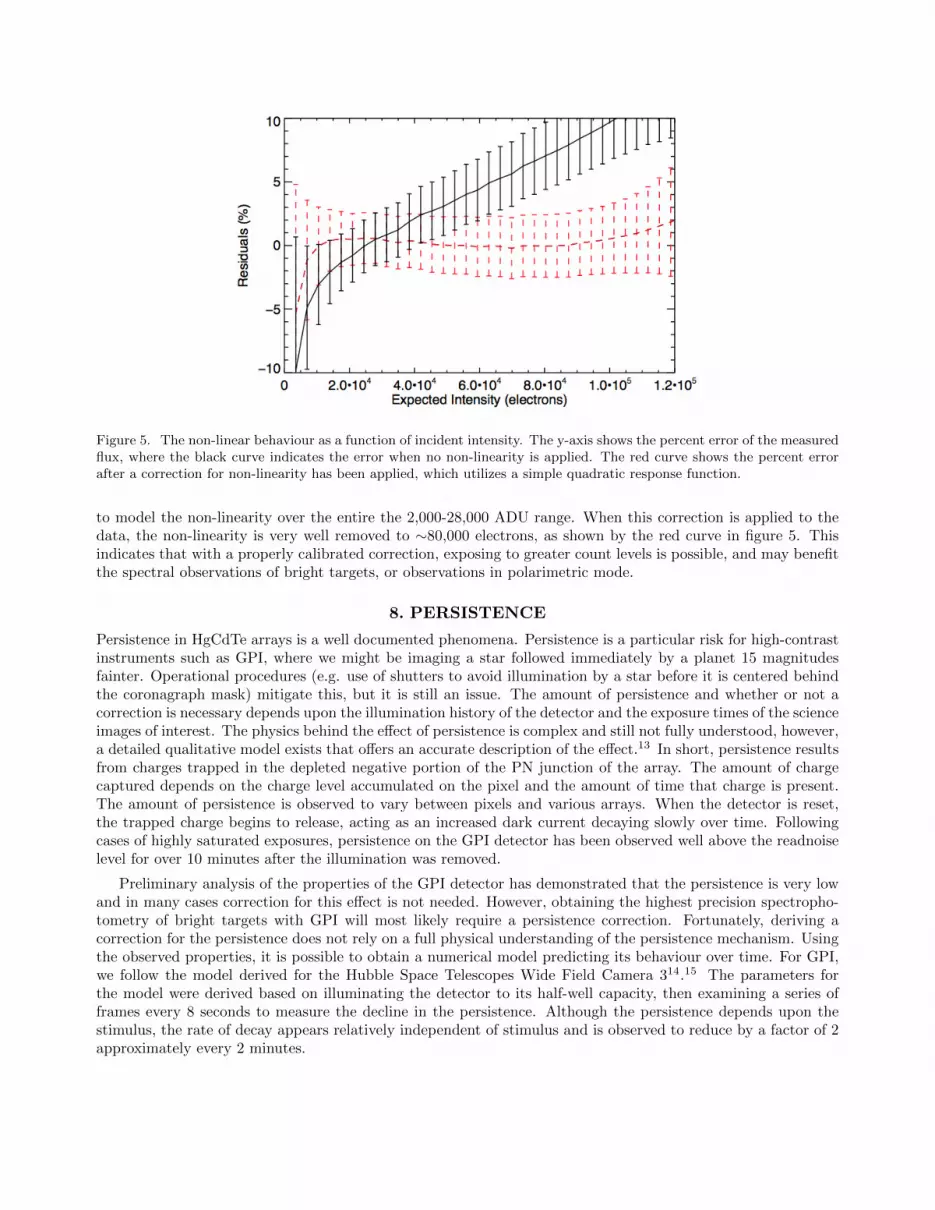
Figure 5. The non-linear behaviour as a function of incident intensity. The y-axis shows the percent error of the measuredflux, where the black curve indicates the error when no non-linearity is applied. The red curve shows the percent errorafter a correction for non-linearity has been applied, which utilizes a simple quadratic response function.

to model the non-linearity over the entire the 2,000-28,000 ADU range. When this correction is applied to thedata, the non-linearity is very well removed to ∼80,000 electrons, as shown by the red curve in figure 5. Thisindicates that with a properly calibrated correction, exposing to greater count levels is possible, and may benefitthe spectral observations of bright targets, or observations in polarimetric mode.

8. PERSISTENCE

Persistence in HgCdTe arrays is a well documented phenomena. Persistence is a particular risk for high-contrastinstruments such as GPI, where we might be imaging a star followed immediately by a planet 15 magnitudesfainter. Operational procedures (e.g. use of shutters to avoid illumination by a star before it is centered behindthe coronagraph mask) mitigate this, but it is still an issue. The amount of persistence and whether or not acorrection is necessary depends upon the illumination history of the detector and the exposure times of the scienceimages of interest. The physics behind the effect of persistence is complex and still not fully understood, however,a detailed qualitative model exists that offers an accurate description of the effect.13 In short, persistence resultsfrom charges trapped in the depleted negative portion of the PN junction of the array. The amount of chargecaptured depends on the charge level accumulated on the pixel and the amount of time that charge is present.The amount of persistence is observed to vary between pixels and various arrays. When the detector is reset,the trapped charge begins to release, acting as an increased dark current decaying slowly over time. Followingcases of highly saturated exposures, persistence on the GPI detector has been observed well above the readnoiselevel for over 10 minutes after the illumination was removed.

Preliminary analysis of the properties of the GPI detector has demonstrated that the persistence is very lowand in many cases correction for this effect is not needed. However, obtaining the highest precision spectropho-tometry of bright targets with GPI will most likely require a persistence correction. Fortunately, deriving acorrection for the persistence does not rely on a full physical understanding of the persistence mechanism. Usingthe observed properties, it is possible to obtain a numerical model predicting its behaviour over time. For GPI,we follow the model derived for the Hubble Space Telescopes Wide Field Camera 314.15 The parameters forthe model were derived based on illuminating the detector to its half-well capacity, then examining a series offrames every 8 seconds to measure the decline in the persistence. Although the persistence depends upon thestimulus, the rate of decay appears relatively independent of stimulus and is observed to reduce by a factor of 2approximately every 2 minutes.

The pipeline primitive, “Remove Persistence from Previous Images,” uses this model to estimate and subtractpersistence in any given science image, given the series of exposures preceeding that image. Figure 6 shows currenteffectiveness of the model to remove the persistence.

Figure 6. Left: The central portion of a 60 second (42 up-the-ramp read) Y -band sky frame showing persistence fromthe previous coronagraphic image taken 5 minutes before. Right: The same sky image after correction for the persistenceusing the GPI DRP.

Current performance of the persistence removal is limited by the data used to derive the model. The 8second sampling does not provide adequate coverage to enable precise measurements of the exponential falloff.Because data was only taken in a single band, a large portion of the array was never illuminated, and thereforewe were forced to spatially bin the model to 64x64 pixel boxes. This results in an over- or under-subtraction inmany parts of the array where the persistence properties of the detector change on small spatial scales. Anotherlimitation is that users will never have a full record of the illumination history of the array, since the array isnot read out after every detector reset.

Future work will extend persistence calibration to the entire array and further explore the amount of persis-tence as a function of varying fluence, or stimulus. Lastly, we will obtain test data with increased time samplingto better sample the exponential decay.

9. DISCUSSION

While the HAWAII-2RG detector is state of the art, it is still subject to many imperfections and systematics. ForGPI, depending on the details and science goals of any particular observations, some of these systematics maybe ignored without adverse impact but in other situations they must be attended to. For instance, the impact ofa handful of uncorrected bad pixels is generally very minor for a long exposure ADI sequence as part of a planetsearch: the PSF subtraction naturally subtracts out any residual that is fixed in the detector frame, while thesignal from a planet will be spectrally dispersed across many pixels and will move across even more differentdetector pixels as the sky rotates. In contrast for observations of a resolved solar system object, uncorrected badpixels directly reduce cosmetic quality and S/N for measurement of surface features, and no PSF subtractionis performed. In polarization mode, the non-common-path offset between the orthogonal polarization channelsis dominated by detector artifacts such as cold pixels that affect one polarization but not the other. Users ofGPI should apply their own scientific judgement when determining which correction steps are needed in theirparticular reduction recipes.

Some aspects of detector calibration for GPI are relatively mature, simply needing ongoing monitoring forthe long term, for instance the routine acquisition of darks. Other aspects have more substantial analysis workyet to be done, for instance the planned improvements to persistence calibration mentioned above, and betternonlinearity correction. We currently neglect the detection and correction of cosmic rays. The observed rate of

cosmic ray induced electrons is quite low for GPI, given its substrate removed detector, but it is not zero andoccasionally cosmic rays are visible particularly in longer exposures. Interpixel capacitance is not accounted for,nor intrapixel QE variations (with the exception that these latter are implicitly included when deriving highresolution microlens PSF models, although not explicitly considered in any reduction step). In some cases weplan to adapt algorithms developed for HST and JWST detector calibration for use with GPI data.

A particular challenge is detector flat fielding. Detector flat fields cannot be directly measured now; as notedabove given the lenslet array there is no way to evenly illuminate the detector. The multi-filter pseudo-flattechnique described above works to locate grossly low QE pixels but is not precise enough to measure smallerQE variations between good pixels. Given the presence of flexure continuously changing the registration betweenlenslets and the detector it is not sufficient to take day calibration flats while the telescope is parked at zenith,since slightly different sets of pixels will be illuminated at night. Improved calibration methods to deal with thissituation are under investigation.

10. ACKNOWLEDGMENTS

We would like to thank the staff of the Gemini Observatory for their assistance in the characterization of thedetector. The Gemini Observatory is operated by the Association of Universities for Research in Astronomy,Inc., under a cooperative agreement with the NSF on behalf of the Gemini partnership: the National ScienceFoundation (United States), the National Research Council (Canada), CONICYT (Chile), the Australian Re-search Council (Australia), Ministerio da Ciencia, Tecnologia e Inovacao (Brazil), and Ministerio de Ciencia,Tecnologıa e Innovacion Productiva (Argentina).

REFERENCES

[1] Macintosh, B., Graham, J. R., Ingraham, P., Konopacky, Q., Marois, C., Perrin, M., Poyneer, L., Bauman,B., Barman, T., Burrows, A. S., Cardwell, A., Chilcote, J., De Rosa, R. J., Dillon, D., Doyon, R., Dunn, J.,Erikson, D., Fitzgerald, M. P., Gavel, D., Goodsell, S., Hartung, M., Hibon, P., Kalas, P., Larkin, J., Maire,J., Marchis, F., Marley, M. S., McBride, J., Millar-Blanchaer, M., Morzinski, K., Norton, A., Oppenheimer,B. R., Palmer, D., Patience, J., Pueyo, L., Rantakyro, F., Sadakuni, N., Saddlemyer, L., Savransky, D.,Serio, A., Soummer, R., Sivaramakrishnan, A., Song, I., Thomas, S., Wallace, J. K., Wiktorowicz, S., andWolff, S., “First light of the gemini planet imager,” Proceedings of the National Academy of Sciences (2014).

[2] Macintosh, B., Graham, J. R., Ingraham, P., Konopacky, Q., Marois, C., Perrin, M., Poyneer, L., Bauman,B., Barman, T., Burrows, A. S., Cardwell, A., Chilcote, J., De Rosa, R. J., Dillon, D., Doyon, R., Dunn, J.,Erikson, D., Fitzgerald, M. P., Gavel, D., Goodsell, S., Hartung, M., Hibon, P., Kalas, P., Larkin, J., Maire,J., Marchis, F., Marley, M. S., McBride, J., Millar-Blanchaer, M., Morzinski, K., Norton, A., Oppenheimer,B. R., Palmer, D., Patience, J., Pueyo, L., Rantakyro, F., Sadakuni, N., Saddlemyer, L., Savransky, D., Serio,A., Soummer, R., Sivaramakrishnan, A., Song, I., Thomas, S., Wallace, J. K., Wiktorowicz, S., and Wolff,S., “The gemini planet imager: first light and commissioning,” Society of Photo-Optical InstrumentationEngineers (SPIE) Conference Series 9148 (2014).

[3] Chilcote, J. K., Larkin, J. E., Maire, J., Perrin, M. D., Fitzgerald, M. P., Doyon, R., Thibault, S., Bauman,B., Macintosh, B. A., Graham, J. R., and Saddlemyer, L., “Performance of the integral field spectrographfor the Gemini Planet Imager,” in [Society of Photo-Optical Instrumentation Engineers (SPIE) ConferenceSeries ], Society of Photo-Optical Instrumentation Engineers (SPIE) Conference Series 8446 (Sept. 2012).

[4] Larkin, J. E., Chilcote, J. K., Aliado, T., Bauman, B. J., Brims, G., Canfield, J. M., Cardwell, A., Dillon, D.,Doyon, R., Dunn, J., Fitzgerald, M. P., Graham, J. R., Goodsell, S., Hartung, M., Hibon, P., Ingraham, P.,Johnson, C. A., Kress, E., Konopacky, Q. M., Macintosh, B. A., Magnone, K. G., Maire, J., McLean, I. S.,Palmer, D., Perrin, M. D., Quiroz, C., Rantakyr, F., Sadakuni, N., Saddlemyer, L., Serio, A., Thibault, S.,Thomas, S. J., Vallee, P., and Weiss, J. L., “The Integral Field Spectrograph for the Gemini Planet Imager,”Society of Photo-Optical Instrumentation Engineers (SPIE) Conference Series 9147 (2014).

[5] Beletic, J. W., Blank, R., Gulbransen, D., Lee, D., Loose, M., Piquette, E. C., Sprafke, T., Tennant, W. E.,Zandian, M., and Zino, J., “Teledyne Imaging Sensors: infrared imaging technologies for astronomy andcivil space,” in [Society of Photo-Optical Instrumentation Engineers (SPIE) Conference Series ], Society ofPhoto-Optical Instrumentation Engineers (SPIE) Conference Series 7021 (Aug. 2008).

[6] Loose, M., Beletic, J., Garnett, J., and Xu, M., “High-performance focal plane arrays based on the HAWAII-2RG/4G and the SIDECAR ASIC,” in [Society of Photo-Optical Instrumentation Engineers (SPIE) Con-ference Series ], Society of Photo-Optical Instrumentation Engineers (SPIE) Conference Series 6690 (Sept.2007).

[7] Perrin, M., Maire, J., Ingraham, P. J., Savransky, D., Millar-Blanchaer, M., Wolff, S. G., Ruffio, J.-B.,Wang, J. J., Draper, Z. H., Sadakuni, N., Marois, C., Fitzgerald, M. P., Macintosh, B., Graham, J. R.,Doyon, R., Larkin, J. E., Chilcote, J. K., Goodsell, S. J., Palmer, D. W., Labrie, K., Beaulieau, M., Rosa,R. J. D., Greenbaum, A. Z., Hartung, M., Hibon, P., Konopacky, Q. M., Lafreniere, D., Lavigne, J.-F.,Marchis, F., Patience, J., Pueyo, L. A., Soummer, R., Thomas, S. J., Ward-Duong, K., and Wiktorowicz,S., “Gemini planet imager observational calibrations i: overview of the gpi data reduction pipeline,” Societyof Photo-Optical Instrumentation Engineers (SPIE) Conference Series 9147 (2014).

[8] Loose, M., “Application of the SIDECAR ASIC as the Detector Controller for ACS and the JWST Near-IRInstruments,” in [Hubble after SM4. Preparing JWST ], (July 2010).

[9] Grogin, N. A., Lim, P., Hook, R. N., Maybhate, A., and Loose, M., “ACS After SM4: Characterization AndMitigation Of WFC Bias Striping,” in [American Astronomical Society Meeting Abstracts #215 ], Bulletinof the American Astronomical Society 42, #462.06 (Jan. 2010).

[10] Wolff, S. G., Perrin, M., Maire, J., Ingraham, P. J., Rantakyro, F. T., and Hibon, P., “Gemini planetimager observational calibrations iv: Wavelength calibration and flexure correction for the integral fieldspectrograph,” Society of Photo-Optical Instrumentation Engineers (SPIE) Conference Series 9147 (2014).

[11] Ingraham, P. J., Ruffio, J.-B., Perrin, M. D., Wolff, S., Draper, Z., Maire, J., Marchis, F., and Fesquet,V., “Gemini planet imager observational calibrations iii: Empirical measurement methods and applicationsof high-resolution microlens psfs,” Society of Photo-Optical Instrumentation Engineers (SPIE) ConferenceSeries 9147 (2014).

[12] Hilbert, B. and McCullough, P., “Interpixel Capacitance in the IR Channel: Measurements Made On Orbit,”tech. rep., Space Telescope Science Institute, Baltimore, Maryland (Apr. 2011).

[13] Smith, R. M., Zavodny, M., Rahmer, G., and Bonati, M., “A theory for image persistence in HgCdTephotodiodes,” in [Society of Photo-Optical Instrumentation Engineers (SPIE) Conference Series ], Societyof Photo-Optical Instrumentation Engineers (SPIE) Conference Series 7021 (Aug. 2008).

[14] Rajan, A. and et al., [WFC3 Data Handbook v. 2.1 ] (May 2011).

[15] Long, S. L., Baggett, S. M., and W., M. J., “Characterizing Persistence in the WFC3 IR Channel: FiniteTrapping Times,” tech. rep., Space Telescope Science Institute, Baltimore, Maryland (June 2013).