arX

iv:h

ep-t

h/98

0418

5v1

28

Apr

199

8

CGPG-98/4-4

Discrete Space-Time Volume for

3-Dimensional BF Theory and Quantum Gravity

Laurent Freidel∗1,2 and Kirill Krasnov†1

1. Center for Gravitational Physics and Geometry

Department of Physics, The Pennsylvania State University

University Park, PA 16802, USA

2. Laboratoire de Physique Theorique ENSLAPP

Ecole Normale Superieure de Lyon

46, allee d’Italie, 69364 Lyon Cedex 07, France

Abstract

The Turaev-Viro state sum invariant is known to give the transition ampli-

tude for the three dimensional BF theory with cosmological term, and its de-

formation parameter h is related with the cosmological constant via h =√

Λ.

This suggests a way to find the expectation value of the spacetime volume

by differentiating the Turaev-Viro amplitude with respect to the cosmological

constant. Using this idea, we find an explicit expression for the spacetime

volume in BF theory. According to our results, each labelled triangulation

carries a volume that depends on the labelling spins. This volume is explicitly

discrete. We also show how the Turaev-Viro model can be used to obtain the

spacetime volume for (2+1) dimensional quantum gravity.

Typeset using REVTEX

∗E-mail address: freidel@phys.psu.edu

†E-mail address: krasnov@phys.psu.edu

1

The loop approach to quantum gravity [1] leads to a fascinating picture in which thestructure of geometry at the Planck scale is fundamentally different from that of the usualRiemannian geometry. The elementary excitations of the quantum geometry which arisesare one-dimensional, “loop-like”, rather than particle-like. The spectra of operators corre-sponding to such geometrical quantities as length, area and volume become quantized [2].The “size” of the corresponding quanta of geometry is proportional to the Planck length.

However, so far, almost all the progress that has been made within this approach concernsspace rather than spacetime aspects of quantum geometry. In this paper we propose a newset of ideas that can be used to study the spacetime quantum geometry. More precisely,using the path integral techniques, we propose a way to define the spacetime volume in thequantum theory. We do this in the context of BF theory and Euclidean quantum gravityin three spacetime dimensions. The simplicity of these (classically) closely related theoriesallows us to obtain an explicit expression for the spacetime volume.

There exists many ways to quantize 3-dimensional gravity (for a review see [3]). Inthis paper we concentrate on the approach pioneered by Ponzano and Regge [4]. Thisapproach is intimately related with the loop quantum gravity approach. Indeed, using theideas described by Baez [5] (see also [6]), one can think of the Ponzano-Regge model as acovariant (spacetime) version of loop quantum gravity in (2+1) dimensions. The Ponzano-Regge approach, as we explain below, is very close in spirit to the usual path integralapproach, and, thus, is best suited for a study of spacetime aspects of the theory.

Although the Ponzano-Regge model gives a quantization of BF theory, not gravity, thetwo are closely related in three dimensions, at least as classical theories. Thus, one can hopeto use BF theory to study certain aspects of 3-d quantum gravity. We will first derive anexpression for the spacetime volume in BF theory, and comment on how BF theory can beused to obtain the spacetime volume for gravity. Let us describe the Ponzano-Regge model(or, more precisely, its generalization proposed by Turaev and Viro, see e.g. [7]) in moredetails. Let us consider the theory whose action is given by

SΛ[A, E] = −∫

MTr(

E ∧ F +Λ

12E ∧ E ∧ E

)

, (1)

where M is assumed to be a three-dimensional orientable manifold. The action is a func-tional of an SU(2) connection A, whose curvature form is denoted by F , and a 1-form E,which takes values in the Lie algebra of SU(2). Thus, the action (1) is that of BF theory in3d, with E field playing the role of B, and with an additional “cosmological term” addedto the usual BF action. The relation to gravity in 3d is as follows. Having the one-form E,one can construct from it a real metric of Euclidean signature

gab = −1

2Tr(EaEb). (2)

For our conventions on indices and others see the Appendix. Thus, the E field in (1) hasthe interpretation of the triad field. One of the equations of motion that follows from (1)states that A is the spin connection compatible with the triad E. Taking the triad E tobe non-degenerate and “right-handed”, i.e., giving a nowhere zero positive volume form(A1), and substituting into (1) the spin connection instead of A, one gets the EuclideanEinstein-Hilbert action

2

1

2

∫

Md3x

√g (R − 2Λ). (3)

We use units in which 8πG = 1. The coefficient in front of (1) is chosen to yield preciselythe Einstein-Hilbert action after the elimination of A. Thus, on configurations of E fieldthat are non-degenerate and right-handed, (1) is equivalent to Einstein-Hilbert action, andΛ in (1) is precisely the cosmological constant. This means that all solutions of Einstein’sequations can be obtained from the solutions of BF theory. However, BF theory has moresolutions than gravity. For example, in BF theory one can have configurations of E field thatgive negative or zero value of the volume form at some points in spacetime. This does notcause any problems classically, for one can always restrict oneself to the sector where metricis non-degenerate and the volume form is positive. However, as we shall see below, thisdoes cause problems in the quantum theory: the amplitudes of configurations with positivevolume form interfere with the amplitudes of negative volume configurations. Thus, as weshall see, the quantum models corresponding to BF theory and gravity are rather different.

Let us first consider the quantization of BF theory. The Turaev-Viro model gives a wayto calculate the vacuum-vacuum transition amplitude of this theory, i.e., the path integral

Z(Λ,M) =∫

DE DA eiSΛ[A,E]. (4)

Note that we consider the transition amplitude of BF theory, not the partition function,which would be given by (4) without the i in the exponential. As we shall see below, thisis the transition amplitude that is related to the Turaev-Viro state sum invariant. In thispaper we consider only vacuum-vacuum amplitudes. Although the Turaev-Viro model canbe used to calculate more general amplitudes between non-trivial initial and final states, wewill not use this aspect of the model here. We consider the version of the model formulatedon a triangulated manifold. Thus, let us fix a triangulation ∆ of M. Let us label the edges,for which we will employ the notation e, by irreducible representations of the quantum group(SU(2))q, where q is a root of unity

q = e2πik ≡ eih. (5)

Later we will relate the parameter h with the cosmological constant Λ. The irreduciblerepresentations of (SU(2))q are labelled by half-integers (spins) j satisfying j ≤ (k − 2)/2.Thus, we associate a spin je to each edge e. The vacuum-vacuum transition amplitude ofthe theory is then given by the following expression (see, e.g. [7]):

TV(q, ∆) = κV∑

je

∏

e

dimq(je)∏

t

(6j)q, (6)

where κ and dimq(j) are defined by (A2),(A3) correspondingly, and V is the number ofvertices in ∆. The last product in (6) is taken over tetrahedra t of ∆, and (6j)q is thenormalized quantum (6j)-symbol constructed from the 6 spins labelling the edges of t. Itturns out that (6) is independent of the triangulation ∆ and gives a topological invariant ofM: TV(q, ∆) = TV(q,M).

The construction that interprets the Turaev-Viro invariant (6) as the vacuum-vacuumtransition amplitude of the theory defined by (1) is as follows. It has been proved (see

3

e.g. [8] and the works cited therein) that (6) is equal to the squared absolute value of theChern-Simons amplitude

TV(q,M) = |CS(k,M)|2, (7)

with the level of Chern-Simons theory being equal to k from (5). It is known, however, thatthe action (1) can be written as a difference of two copies of Chern-Simons action

SCS(A) =k

4π

∫

MTr(

A ∧ dA +2

3A ∧ A ∧ A

)

. (8)

Indeed, note that

S(A + λE) − S(A − λE) =kλ

π

∫

MTr

(

E ∧ F +λ2

3E ∧ E ∧ E

)

, (9)

where λ is a real parameter. Thus, (9) is equal to (1) if

λ = −√

Λ/2, k =2π√Λ

, or h =√

Λ. (10)

This relates the deformation parameter q of the Turaev-Viro model to the cosmological con-stant Λ, in the case of positive Λ, and proves that the Turaev-Viro amplitude is proportionalto the vacuum-vacuum transition amplitude of the theory defined by (1):

TV(q,M) ∼ Z(Λ,M). (11)

Let us now discuss the relation between quantum BF theory and gravity. We note that,although classically BF theory and gravity are equivalent (they lead to the same equations ofmotion), the transition amplitude of BF theory (4) is not the transition amplitude for gravity.Indeed, in the case of gravity one has to perform the path integral of the exponentiated actiononly over non-degenerate metric configurations that define a positive spacetime volume:

Zgr(Λ,M) =∫

Vol(E)>0DE DA eiSΛ[A,E]. (12)

However, the path integral in (4) is taken over all configurations of E field, even those that aredegenerate or define a negative volume. To see this, let us note that if the field E defines aneverywhere positive volume, then −E gives a negative volume, and both are summed over inthe path integral (4). Thus, the path integral includes contributions from both configurationsof E field that give an everywhere positive and the ones that given an everywhere negativevolume. Moreover, the path integral (4) takes into account also degenerate configurations ofE in which the volume form is negative at some points in spacetime and positive at other.As we further discuss below, these are these degenerate configurations that may cause thequantum BF theory to be drastically different from gravity, if it turns out that they dominatethe path integral. To further illustrate the difference between the quantum BF theory andgravity, let us write a heuristic expressions for the path integrals corresponding to the twotheories. For the transition amplitude in gravity one can formally write:

4

∫

Dg∏

x∈M

eiLgr(x), (13)

where the path integral is taken over non-degenerate configurations of metric g and Lgr(x)is the Lagrangian of gravity. In the path integral of the quantum BF theory, one takes intoaccount all, even highly degenerate configurations of the E field. Thus, heuristically, itstransition amplitude is given by

∫

Vol(E)≥0DEDA

∏

x∈M

cos(LBF (x)) =∫

Dg∏

x∈M

cos(iLgr(x)). (14)

Here the integral is taken over configurations of E field that give a non-negative volume, andthe presence of cos accounts for the fact that one sums at each point both over positive andnegative volumes. The presence of cos here is also reminiscent of the fact (see [4]) that thePonzano-Regge amplitude, which is given by the product of (6j)-symbols (see (22) below),in the limit of large spins je has the asymptotics of the cosine of the Regge calculus versionof the Einstein-Hilbert action. Thus, to summarize, the quantum BF theory may well bedrastically different from gravity because it takes into account highly degenerate, classicallyforbidden field configurations. However, the two theories would be related if there exists aphase of the quantum BF theory in which the path integral is dominated by non-degenerateconfigurations of E field, that is, configurations that have everywhere positive or negativevolume. In this phase one would effectively have to consider only everywhere positive oreverywhere negative volume configurations. In the transformation E → −E the BF action(1) changes its sign. Thus, in this phase

Z(Λ,M) = Zgr(Λ,M) + Zgr(Λ,M), (15)

where overline denotes complex conjugation. In this phase there exists a relation betweenthe spacetime volume in BF theory and gravity. We shall discuss this after we obtain anexpression for the volume in the quantum BF theory.

Let us now study the spacetime volume in BF theory. Note that the expectation valueof the volume is given simply by the derivative of the amplitude (4) with respect to (−iΛ)

〈Vol〉 =

∫ DEDA Vol(M)eiS

∫ DEDA eiS= i

∂ ln Z(Λ)

∂Λ, (16)

Vol(M) =∫

M

1

12εabcTr(EaEbEc).

Thus, the expectation value of the volume of M in BF theory can be obtained by differen-tiating the Turaev-Viro amplitude with respect to Λ. Here we calculate this derivative andfind an explicit expression for the spacetime volume. For simplicity, we will study only thevolume in the quantum theory with zero cosmological constant. This can be obtained byfirst differentiating (6) with respect to Λ, and then evaluating the result at Λ = 0. Thus,interestingly, the deformation parameter of the Turaev-Viro model q (related with Λ via(10)) serves as the quantity conjugate to the spacetime volume.

Since the Turaev-Viro amplitude is explicitly real, and, to find the volume, we differenti-ate its logarithm with respect to iΛ, the expectation value of the volume is purely imaginary.

5

This is, at the first sight, surprising, but can be easily understood by taking into accountthe fact that both positive and negative volume configurations are summed over in (4), andthat the action (1) changes its sign when E → −E.

Let us now find this volume. An important subtlety arises, however, if one follows theprocedure (16). To find the derivative (16) at Λ = 0 we have to find the first order termin Λ in the expansion of (6). It is not hard to show, however, that (6) has the followingasymptotic expansion in h

(

h3

4π

)V

PR(∆)(

1 − h2i〈Vol〉)

, (17)

where PR is the amplitude of the Ponzano-Regge model

PR(∆) =∑

je

∏

e

dim(je)∏

t

(6j), (18)

V is the number of vertices in ∆, and i〈Vol〉 is a real quantity independent of h. Thus,apparently there is no term proportional to h2 in this expansion. The resolution of this is thatthe deformation level k of the Turaev-Viro model plays two distinct roles in the theory. First,it serves as a regulator for the Ponzano-Regge model. Indeed, the amplitude (18) diverges.It is only the combination (h3V PR), defined as the limit of (TV) as h → 0, that is finite.Second, the parameter k (and the related to it q) also serves as a deformation parameter ofthe Ponzano-Regge model. The terms of the order O(h2) in (17) are the ones that appearas the result of this deformation. To derive an expression for the spacetime volume we mustbe concerned only with these terms, for they describe the “deformation” of the vacuum-vacuum transition amplitude occuring due to the introduction of the cosmological constantterm into the action functional. Thus, the expectation value of the spacetime volume iswhat is denoted by 〈Vol〉 in (17).

There is another, equivalent way to justify the absence of terms proportional to h2

in the decomposition (17). As we have mentioned above, the Turaev-Viro amplitude (6)is proportional to the transition amplitude (4). However, the proportionality coefficientdepends on h. Indeed, the integration over (A+λE), (A−λE), which is carried out to obtain|CS(k,M)|2 in (7) and thus the Turaev-Viro amplitude, is different from the integration overA, E one has to perform to obtain (4). The difference in the integration measures is a powerof h. Thus, the amplitude (4) and the squared absolute value of the amplitude of the Chern-Simons theory are proportional to each other with the coefficient of proportionality being apower of h. In the discretized version of the theory, given by the Turaev-Viro model, thispower of h is replaced by h3V . Thus, this is the (divergent) Ponzano-Regge amplitude (18)that gives the amplitude for BF theory without the cosmological constant. Turaev-Viroamplitude, in the limit of small cosmological constant, differs from the BF amplitude by apower of h.

These remarks being made, it is straightforward to write down an expression for theexpectation value of the volume:

i〈Vol〉∆ = − ∂

∂Λ

(

TV(Λ, ∆)

PR(∆)(h3/4π)V

)

Λ=0

=

6

1

PR(∆)

∑

je

iVol(∆, j)

(

∏

e

dim(je)∏

t

(6j)

)

, (19)

where the function Vol(∆, j) of the triangulation ∆ and the labels j = {je} is given by

iVol(∆, j) =∑

v

(

− ∂

∂Λ

(

κ

(h3/4π)

))

Λ=0

+∑

e

(

−∂ ln(dimq(je))

∂Λ

)

Λ=0

+

∑

t

(

−∂ ln((6j)q)

∂Λ

)

Λ=0

. (20)

Here v stands for vertices of ∆, e stands for edges and t stands for tetrahedra. We inten-tionally wrote the expectation value of the volume in the form (19) to introduce the volumeVol(∆, j) of a labelled triangulation, which is our main object of interest. Indeed, (19) hasthe form

∑

jeiVol(∆, j)Amplitude(∆, j)∑

jeAmplitude(∆, j)

, (21)

where

Amplitude(∆, j) =∏

e

dim(je)∏

t

(6j) (22)

is the amplitude of Ponzano-Regge model. This shows that Vol(∆, j) indeed has the inter-pretation of the volume of a labelled triangulation.

The volume (20) has three types of contributions: (i) from vertices; (ii) from edges; (iii)from tetrahedra. It is not hard to calculate the first two types of them. One finds that eachvertex contributes exactly 1/12, and each edge contributes je(je + 1)/6, where je is the spinthat labels the edge e. It is much more complicated to find the tetrahedron contribution tothe volume, that is, the derivative of ln((6j)q) with respect to Λ. Here we simply give theresult of this calculation. The details will appear elsewhere [9]. The simplest way to describethe result is graphical. First, let us, for each tetrahedron t, introduce a special graph Γ livingon the boundary of t. The boundary of t is a triangulated 2-manifold with the topology of asphere, and we define the graph Γ to be the one dual to that triangulation. The graph Γ hasfour vertices and six edges, and, as a piecewise linear complex, it is a tetrahedron. Let uslabell the edges of this graph, which are dual to the edges of the original graph, by the samespins as those labelling the edges of t. Let us then construct the spin network correspondingto the labelled Γ (for more details on spin networks, see e.g. [10]). Recall that a spin networkcorresponding to a labelled graph is a function on a certain number of copies of the gaugegroup – GE, where E is the number of edges in the graph – which is constructed by takingthe matrix elements of the group elements in the representations labelling the correspondingedges, and contracting these matrix elements with each other at vertices using intertwiners.In our case of Γ being a tetrahedron, all vertices are trivalent, that is, there are exactlythree edges meeting at each vertex. In this case intertwiners are unique (up to an overallmultiplicative constant), and given by the usual Clebsch-Gordan coefficients. We choose thenormalized intertwiners; then the evaluation of the spin network on all group elements equal

7

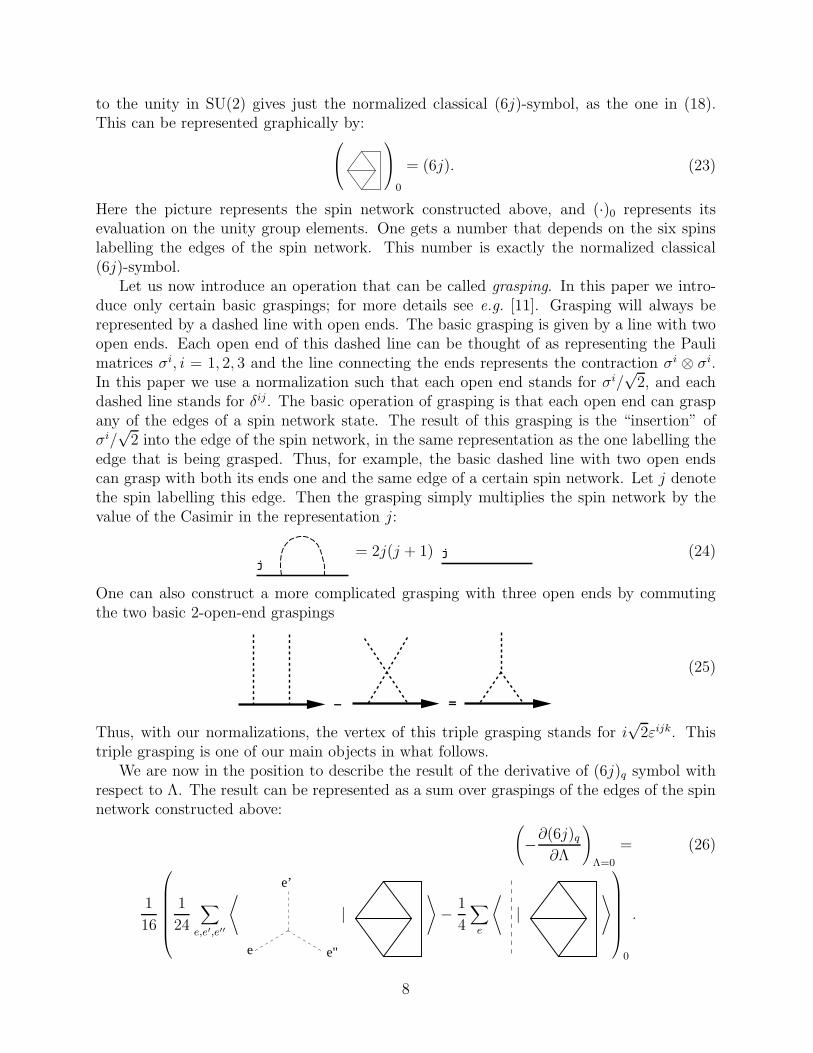
to the unity in SU(2) gives just the normalized classical (6j)-symbol, as the one in (18).This can be represented graphically by:

0

= (6j). (23)

Here the picture represents the spin network constructed above, and (·)0 represents itsevaluation on the unity group elements. One gets a number that depends on the six spinslabelling the edges of the spin network. This number is exactly the normalized classical(6j)-symbol.

Let us now introduce an operation that can be called grasping. In this paper we intro-duce only certain basic graspings; for more details see e.g. [11]. Grasping will always berepresented by a dashed line with open ends. The basic grasping is given by a line with twoopen ends. Each open end of this dashed line can be thought of as representing the Paulimatrices σi, i = 1, 2, 3 and the line connecting the ends represents the contraction σi ⊗ σi.In this paper we use a normalization such that each open end stands for σi/

√2, and each

dashed line stands for δij. The basic operation of grasping is that each open end can graspany of the edges of a spin network state. The result of this grasping is the “insertion” ofσi/

√2 into the edge of the spin network, in the same representation as the one labelling the

edge that is being grasped. Thus, for example, the basic dashed line with two open endscan grasp with both its ends one and the same edge of a certain spin network. Let j denotethe spin labelling this edge. Then the grasping simply multiplies the spin network by thevalue of the Casimir in the representation j:

j= 2j(j + 1) j (24)

One can also construct a more complicated grasping with three open ends by commutingthe two basic 2-open-end graspings

− =

(25)

Thus, with our normalizations, the vertex of this triple grasping stands for i√

2εijk. Thistriple grasping is one of our main objects in what follows.

We are now in the position to describe the result of the derivative of (6j)q symbol withrespect to Λ. The result can be represented as a sum over graspings of the edges of the spinnetwork constructed above:

(

−∂(6j)q

∂Λ

)

Λ=0

= (26)

1

16

1

24

∑

e,e′,e′′

⟨

e’

e"e

|⟩

− 1

4

∑

e

⟨

|⟩

0

.

8

Here the first sum is taken over all the graspings of the triples of distinct edges of thetetrahedron t (there are 20 different graspings of this type, but only 16 of them are non-zero), and the second sum is over all graspings of the edges of t (there are 6 graspings of thistype – equal to the number of edges of t). The result of this graspings is then evaluated onthe unity group elements to get a number. The derivative (26) is a real number dependingonly on the spins labelling the edges of t.

Thus, the final result for the spacetime volume in BF theory is

iVol(∆, j) =∑

v

1

12+∑

e

je(je + 1)

6+

∑

t

1

16

1

1

24

∑

e,e′,e”

⟨

e’

e"e

|⟩

− 1

4

∑

e

⟨

|⟩

0

. (27)

Here stands for the classical (6j)-symbol.It is interesting to note that not only tetrahedra t of ∆ contribute to the volume, but

also the edges e and the vertices v. The contribution from the vertices is somewhat trivial –it is constant for each vertex. Nevertheless, when thinking about the triangulated manifoldM one is forced to assign the spacetime volume to every vertex. The contribution fromedges depends on the spins labelling the edges. Again, this implies that each edge of thetriangulation ∆ carries an intrinsic volume that depends on its spin. The contribution fromtetrahedra is more complicated. It is given by a function that depends on the spins labellingthe edges of each tetrahedron. It is interesting that this picture of the spacetime volumebeing split into contributions from vertices, edges and tetrahedra can be understood in termsof Heegard splitting of M. Recall, that Heegard splitting of a three-dimensional manifoldM decomposes M into three dimensional manifolds with boundaries. Then the originalmanifold can be obtained by gluing these manifolds along the boundaries. For the caseof a triangulated manifold M, as we have now, the Heegard splitting proceeds as follows.First, one constructs balls centered at the vertices of ∆. Then one connects these ballswith cylinders, whose axes of cylindrical symmetry coincide with the edges of ∆. Removingfrom M the obtained balls and cylinders, one obtains a three-dimensional manifold witha complicated boundary. One has to further cut this manifold along the faces of ∆. Oneobtains three types of “building blocks” that are needed to reconstruct the original manifold:(i) balls; (ii) cylinders; (iii) spheres with four discs removed. Each of this manifolds carriesa part of the original volume of M. Our result (27) provides one with exactly the samepicture: the volume of M is concentrated in vertices (balls of the Heegard splitting), edges(cylinders), and tetrahedra (4-holed spheres).

The volume of each labelled triangulation is explicitly discrete, and is given by the func-tion (27) of the labelling spins. This gives an important insight as to the nature of quantumspacetime geometry. Indeed, one of the results of the canonical approach to quantum gravityin three spacetime dimensions is that lengths of curves and areas of regions are quantized.Our results also imply that the spacetime volume is quantized.

An important drawback of the present approach is that the spacetime volume we haveobtained is that of BF theory, not gravity. In particular, this is the reason why the spacetime

9

volume turns out to be purely imaginary. Let us now discuss a relation of the obtainedspacetime volume of BF theory with the volume in gravity. As we have discussed above, thequantum BF theory may develop a phase in which non-degenerate configurations of E fielddominate the path integral. In this phase it is possible to obtain some information about thespacetime volume in gravity from the quantum BF theory. As we described above, in sucha phase the BF theory transition amplitude is related to that in gravity according to (15).One can obtain a similar relation between the expectation value of the volume in the twotheories. Thus, if BF theory is in the phase in which non-degenerate solutions dominate,one has:

〈Vol〉gr =ReZgr(Λ,M)

iImZgr(Λ,M)〈Vol〉. (28)

To get this relation we have assumed that the expectation value 〈Vol〉gr of the volume ingravity is real. Thus, even in this phase, to relate the volume in gravity with the one in BFtheory one has to know the imaginary part of the gravity amplitude. Unfortunately, it is notpossible to extract this information from the Turaev-Viro model, which knows only aboutthe real part of Zgr. Thus, one cannot extract the expectation value of spacetime volume of3d gravity from BF theory. However, it turns out to be possible to extract the expectationvalue of the volume squared. Indeed, using the same arguments as in (15), and assumingthat the BF theory is in the non-degenerate phase, one can write

〈Vol2〉Z(Λ,M) = 〈Vol2〉grZgr(Λ,M) + 〈Vol2〉grZgr(Λ,M). (29)

Thus, assuming that 〈Vol2〉gr is a real quantity, we obtain

〈Vol2〉gr = 〈Vol2〉. (30)

In other words, when non-degenerate fields E dominate the path integral (4), the expectationvalue of the volume squared in Turaev-Viro model is the same as in gravity. Thus, it canbe obtained by the methods of this paper by differentiating the Turaev-Viro amplitude withrespect to Λ:

〈Vol2〉∆ = − ∂2

∂Λ2

(

TV(∆)

PR(∆)(h3/4π)V

)

Λ=0

. (31)

This also allows one to obtain an expression for the squared volume of a labelled triangula-tion. The results of this paper indicate that this squared volume will also be discrete, anddepend only on the spins labelling the triangulation. Thus, if there indeed exist a phaseof the quantum BF theory in which non-degenerate E fields dominate, then one can gainsome control over the spacetime volume in (2+1) quantum gravity using the results fromBF theory. If, on the other hand, the path integral of BF theory is always dominated byhighly degenerate solutions, as may well be the case, then the two theories have very littleto do with each other, and the spacetime volume of BF theory is not the same as the volumein gravity. At the present stage of our understanding of quantum gravity it is hard to tellwhich of this two possibilities is realized.

10

Let us conclude by pointing out a possible application of the results of this paper. One ofthe main conceptual problems of quantum gravity is the absence of time in the correspond-ing quantum theory. In fact, this comes about not just for gravity, but for any generallycovariant theory, as is, for example, BF theory discussed above. In the canonical theory thismanifests itself in the fact that the Hamiltonian becomes a constraint; in the path integralapproach a manifestation of this is that the path integral gives not the transition amplitudebetween states at different times, but the matrix element of the projection operator on thesubspace of solutions of the Hamiltonian constraint. In the path integral approach this arisesbecause one is summing over all spacetime geometries that can be put between the initialand final hypersurfaces. This is the basic reason why one loses track of the time: one issumming amplitudes of all spacetime geometries, even those which give a different propertime separation between the initial and final hypersurfaces. However, a possible alternativeto this arises if one constructs the path integral as a sum over labelled triangulations, aswe did above for the case of BF theory in three dimensions. In this case, as we found, eachlabelled triangulation can be assigned the spacetime volume carried by it. Thus, instead ofsumming over all triangulations, one can consider only the sum over triangulations havinga fixed spacetime volume contained between the initial and final hypersurfaces. The sumover amplitudes of such triangulations would depend on the fixed spacetime volume. Onecan interprete this spacetime volume as a measure of the time elapsed between the initialand final hypersurfaces. Thus, an expression for spacetime volume, as, for example, the oneobtained in this paper, allows one to introduce a natural time in the quantum theory.

Acknowledgements: We are grateful to John Baez for discussions and for carefulreading of the early versions of this paper. L. F. was supported by CNRS (France) and bya NATO grant. K. K. was supported in part by the NSF grant PHY95-14240, by Braddockfellowship from Penn State and by the Eberly research funds of Penn State.

APPENDIX A:

All the traces we use in this paper are traces in the fundamental representation. Lowercase latin letters stand for spacetime indices: a, b, ... = 1, 2, 3. The E field we use is assumedto be anti-hermitian. This explains the minus sign in (2). Note the factor of 1/2 in (2). Thisis not the standard choice in the gravity literature, but turns out to be very convenient in3d, for it allows one to get rid of the ugly factors of

√2 in some formulas. In case E has an

interpretation of the triad field, the volume form is given by

1

12εabcTr(EaEbEc). (A1)

Note that the volume form defined by E can be both positive and negative, and only aconfiguration of E giving the positive volume is a triad field of gravity.

The quantity κ in (6) that, in the limit of h → 0, serves as a regulator of the Ponzano-Regge model, is defined by:

κ = −(q1/2 − q−1/2)2

2k. (A2)

11

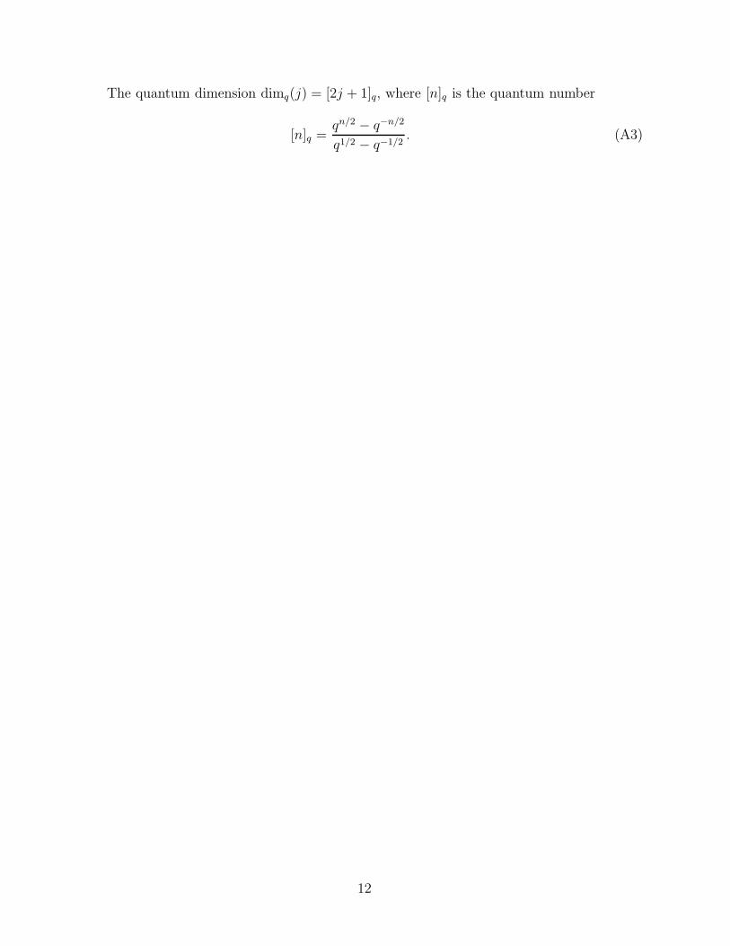
The quantum dimension dimq(j) = [2j + 1]q, where [n]q is the quantum number

[n]q =qn/2 − q−n/2

q1/2 − q−1/2. (A3)

12

REFERENCES

[1] C. Rovelli, Loop quantum gravity, available as gr-qc/9710008.[2] C. Rovelli and L. Smolin, Discreteness of area and volume in quantum gravity, Nucl.

Phys. B442, 593 (1995); Erratum: Nucl. Phys. B456, 734 (1995).A. Ashtekar and J. Lewandowski, Quantum theory of geometry I: Area operators, Class.Quant. Grav. 14, A55-A81 (1997).A. Ashtekar and J. Lewandowski, Quantum theory of geometry II: Volume Operators,Adv. Theo. Math. Phys. 1, 388-429 (1997).T. Thiemann, A length operator for canonical quantum gravity, gr-qc/9606092.R. Loll, Spectrum of the volume operator in quantum gravity, Nucl. Phys. B460 143-154 (1996).

[3] S. Carlip, Lectures in (2+1)-dimensional gravity, available as gr-qc/9503024.[4] G. Ponzano and T. Regge, Semiclassical limits of Racach coefficients, In Spectroscopic

and theoretical methods in physics, ed. F. Block, North-Holland Amsterdam, 1968.[5] J. Baez, Spin foam models, available as gr-qc/9709052.[6] C. Rovelli, The basis of the Ponzano-Regge-Turaev-Viro-Ooguri quantum gravity model

is the loop representation basis, Phys. Rev. D48, 2702-2707 (1993).[7] N. Reshetikhin and V. G. Turaev, Invariants of three manifolds via link polynomials

and quantum groups, Invent. Math. 103, 547-597 (1991).[8] J. Roberts, Skein theory and Turaev-Viro invariants, Topology 34, 771-787 (1995).[9] L. Freidel, manuscript in preparation.

[10] J. Baez, Spin networks in non-perturbative quantum gravity, in The Interface of Knotsand Physics, ed. Louis Kauffman, A.M.S., Providence, 1996, pp. 167-203.

[11] D. Ban-Natan, On the Vassiliev knot invariants, Topology 34, 423-472 (1995).

13