arX

iv:h

ep-t

h/01

1127

3v1

29

Nov

200

1

PAR-LPTHE 01-65LYCEN 2001-78UFES-DF-OP2001/2November 2001

On the Symmetries of BF Models

and Their Relation with Gravity

Clisthenis P. Constantinidis∗,∗∗,1, Francois Gieres∗∗∗,1,

Olivier Piguet∗∗,1 and Marcelo S. Sarandy∗∗∗∗,1

∗ LPTHE, Universite Pierre et Marie Curie, Boite 126, Tour 16, 1er etage, 4 PlaceJussieu, F - 75252 - Paris CEDEX 05 (France).

∗∗ Universidade Federal do Espırito Santo (UFES), CCE, Departamento de Fısica,Campus Universitario de Goiabeiras, BR-29060-900 - Vitoria - ES (Brasil).

∗∗∗ Institut de Physique Nucleaire, Universite Claude Bernard (Lyon 1),43, boulevard du 11 novembre 1918, F - 69622 - Villeurbanne (France).

∗∗∗∗ Centro Brasileiro de Pesquisas Fısicas (CBPF), Coordenacao de Teoria de Cam-pos e Partıculas (CCP), Rua Dr. Xavier Sigaud, BR-150-22290-180 - Rio de Janeiro- RJ (Brasil).

E-mails: clisthen@cce.ufes.br, gieres@ipnl.in2p3.fr,

piguet@cce.ufes.br, sarandy@cbpf.br

Abstract The perturbative finiteness of various topological models (e.g. BF models)

has its origin in an extra symmetry of the gauge-fixed action, the so-called vector su-

persymmetry. Since an invariance of this type also exists for gravity and since gravity

is closely related to certain BF models, vector supersymmetry should also be useful for

tackling various aspects of quantum gravity. With this motivation and goal in mind, we

first extend vector supersymmetry of BF models to generic manifolds by incorporating it

into the BRST symmetry within the Batalin-Vilkovisky framework. Thereafter, we ad-

dress the relationship between gravity and BF models, in particular for three-dimensional

space-time.

1Supported in part by the Conselho Nacional de Desenvolvimento Cientıfico e Tecnologico(CNPq – Brazil).

1 Introduction

1.1 Motivation

As was realized in recent years, there exists a close relationship between BF modelsand gravity in three dimensions [1] as well as in higher dimensions [2]. (For a reviewof BF models [1, 3] and other topological field theories [4, 5], see reference [6].) Theperturbative finiteness of BF models can be traced back to the invariance of thegauge-fixed action under vector supersymmetry (VSUSY) [7]-[10]. Since a symmetryof this type also exists for gravity [11], it should impose some constraints on thequantum theory of gravitation and thereby prove to be useful for its formulation.

Before presenting an outline of the present paper, we first review the resultswhich are known for the three-dimensional case.

1.1.1 Local VSUSY of the 3d BF model

Let G be a matrix Lie group and let G denote the associated Lie algebra. Thebasic variables of the 3d BF model with symmetry group G are a connection 1-form A and a 1-form potential B, both taking their values in G. More explicitly,A = Aµdxµ = Aa

µTadxµ (similarly for B) where the matrices Ta belong to G andsatisfy the relations

[Ta, Tb] = fabcTc , Tr (TaTb) = δab . (1.1)

The arena of the model is a smooth manifold M3 of dimension 3. The actionfunctional is given by

SBF (A, B) = −∫

M3

Tr (BF ) , (1.2)

where F = dA+ 12[A, A] = dA+A2 denotes the curvature (field strength) of A. This

functional is invariant under local gauge transformations of A and B parametrizedat the infinitesimal level by G-valued fields c and φ, respectively1. In the standardBRST framework, these parameters are turned into ghost fields and the symmetrytransformations are described by the BRST operator s. All fields are then character-ized by a total degree which is the sum of their form degree and their ghost-numberand all commutators are assumed to be graded with respect to this degree2. Thes-variations of the basic fields and ghosts read as

sA = −DAc , sc = −c2

sB = −DAφ − [c, B] , sφ = −[c, φ] , (1.3)1Strictly speaking, these transformations only leave the action invariant if the manifold is com-

pact without boundary or if the symmetry parameters vanish on the boundary [1].2See appendix for further details.

2

where DAc ≡ dc + [A, c] denotes the Yang-Mills covariant derivative.

After performing the gauge-fixing in a Landau-type gauge [8, 9, 10, 12] (or innon-covariant versions of the latter [13]), the gauge-fixed action is invariant un-der VSUSY-transformations. At the infinitesimal level, these transformations aredescribed by an operator δτ where τ ≡ τµ∂µ is a s-invariant vector field of ghost-number zero. The variation δτ acts as an antiderivation (odd operator) which lowersthe ghost-number by one unit and which anticommutes with d. Its action on theghost fields c and φ is given by [8]

δτ c = iτA , δτφ = iτB , (1.4)

where iτ denotes the interior product with respect to the vector field τ (see appendixfor technical details concerning operators, vector fields and differential forms). Theoperators s and δτ satisfy a graded algebra of Wess-Zumino type,

[s, δτ ] = Lτ + equations of motion , (1.5)

where Lτ denotes the Lie derivative (see (A.9)) with respect to the vector field τ .

To be more precise, we should note two points. First, invariance under VSUSYwas shown to exist solely on manifolds admitting vector fields that are covariantlyconstant with respect to some background metric, the vector field τ being any oneof these [14]. VSUSY therefore represents a rigid symmetry. This restriction has itsorigin in a particular way of implementing the gauge-fixing and introducing VSUSY-transformations. As we shall see in the present paper, VSUSY can hold as a trulylocal symmetry on a generic manifold if it is implemented in a different way.

Second, VSUSY only holds as an exact invariance as long as one does not incor-porate external sources (coupling to the non-linear s-variations of the fields). Oncethe latter are included into the action, VSUSY is expressed by a broken Ward iden-tity, the breaking term being linear in the quantum fields and thus unproblematicin quantum theory.

1.1.2 3d gravity

The basic variables of 3d gravity are the dreibein 1-forms (ei)i=1,2,3 and the Lorentzconnection 1-form ω = (ωij)i,j=1,2,3 which takes its values in the Lie algebra so(3) orso(1, 2), i.e. ωij = −ωji. The action functional [15]

Sgrav (e, ω) = −∫

M3

εijkeiRjk , (1.6)

in which R = dω + ω2 denotes the curvature 2-form, is invariant under diffeomor-phisms (general coordinate transformations) and under local Lorentz transforma-tions. At the infinitesimal level, these symmetries are parametrized, respectively, by

3

a vector field ξ = ξµ∂µ and an antisymmetric matrix Ω. In the BRST formalism,the latter parameters represent ghost fields and the s-variations have the form [16]

sω = −DωΩ + Lξω , sΩ = −Ω2 + LξΩ

se = −Ωe + Lξe , sξ =1

2[ξ, ξ] .

(1.7)

Here, DωΩ = dΩ + [ω, Ω] denotes the Lorentz covariant derivative, Lξ = iξd − diξrepresents the Lie derivative with respect to the ghost vector field ξ and the vectorfield [ξ, ξ] is the graded Lie bracket of ξ with itself: [ξ, ξ]µ = 2ξν∂νξ

µ.

The action (1.6) can be gauge-fixed by considering a background metric and bychoosing the Landau gauge. The gauge-fixed action is then invariant under VSUSY-transformations parametrized by a Killing vector field τ = τµ∂µ [11]: the latter onlyact non-trivially on the ghost field ξ according to

δτξ = τ (1.8)

and they satisfy the algebra (1.5).

1.1.3 Relation between 3d gravity and BF models

We now describe the correspondence between 3d gravity and BF models [1] (seealso [17]). As symmetry group of the BF model, one chooses G = SO(3) or G =SO(1, 2) as in the last subsection. Then, the connection 1-form A = (Aij)i,j=1,2,3

and the 1-form potential B = (Bij)i,j=1,2,3 both represent antisymmetric matricesof 1-forms. The correspondence between the degrees of freedom involved in boththeories can be made more precise by writing

Bjk = εijkei , Ajk = ωjk (hence Fjk = Rjk)

φjk = iξBjk , c = Ω + iξω ,(1.9)

where εijk denotes the components of the totally antisymmetric tensor. The action(1.6) then goes over into the action (1.2):

SBF (A, B) = −1

2

∫

M3

BjkFjk . (1.10)

Furthermore, the VSUSY-variations (1.8) imply the variations (1.4). The transfor-mation laws of ω and ei as given by (1.7) become

sA = −DAc + iξF

sB = −DAφ − [c, B] + iξDAB .

If the equations of motion F = 0 = DAB of the BF model are taken into account, thelatter transformation laws coincide with those given in eqs.(1.3). In summary, the

4

actions of both models coincide exactly and the symmetry transformations coincideon-shell.

Some comments concerning these results are in order. First, we note that thereparametrization (c, φ) → (Ω, ξ) considered in eqs.(1.9) represents a field-dependentchange of the generators of the BRST differential algebra: this explains the appear-ance of the equations of motion upon passage from one model to the other one.Second, we remark that there is a problem of invertibility with the change of gen-erators ξµ → φ = iξB ≡ ξµBµ since one cannot express ξµ in terms of φ, unlessthe 3-bein ei

µ = 12εi

jkBjkµ represents a nonsingular matrix in whole space-time. As a

matter of fact, this invertibility problem reappears in the perturbative approach toquantum theory, since the BF model is perturbed around the configuration B = 0whereas the corresponding configuration in gravity, i.e. ei = 0, represents a singularmetric. (For a general discussion, see references [18] and the remarks made in [5].)

1.2 Program

The results we just summarized suggest the following line of investigation:

1. to generalize the results concerning VSUSY of BF models (in three and, moregenerally, in higher dimensions) to generic manifolds, not just those admittingcovariantly constant vector fields,

2. to promote the three-dimensional on-shell results to off-shell results,

3. to extend this correspondence to the higher-dimensional case and to exploitits consequences.

In the present paper, we will discuss VSUSY on generic 3- and 4-manifolds forBF models which, in addition, involve a cosmological term in their action. (Thehigher-dimensional case is analogous to the 4-dimensional one in that it involves thephenomenon of “ghosts for ghosts” which does not occur in the 3-dimensional case.)Moreover, some results concerning the relationship between gravity and BF modelswill be presented.

At different stages of the discussion, the equations of motion of the modelsappear in the transformation laws of fields and therefore we will follow the Batalin-Vilkovisky (BV) approach [19] to the description of symmetries. Henceforth, anti-fields are to be introduced into the formalism from the beginning on. They play therole of external sources coupled to the BRST-variations of the basic fields. In a finalstep, the antifields are redefined according to the Batalin-Vilkovisky prescription inorder to implement the gauge-fixing. This procedure of gauge-fixing does not to in-terfere with vector supersymmetry thanks to the fact that the latter is incorporateddirectly into the BRST operator.

5

2 3d BF model with cosmological term

2.1 The model and its symmetries

To start with, we consider an arbitrary gauge group which will be specialized toSO(3) or SO(1, 2) when discussing gravity. The notation is the one introduced insubsection 1.1.1.

The action for a BF model with “cosmological constant” α on a 3-manifold M3

reads

Sinv (A, B) = −∫

M3

Tr(

BF +α

3B3)

, (2.1)

where α represents a real dimensionless parameter. The equations of motion of thismodel are given by

F + αB2 = 0 , DB = 0 , (2.2)

where D denotes the covariant derivative: D· = d · +[A, ·].

The symmetries of the action (2.1) can be expressed in terms of horizontalityconditions [20, 21] which have the form

F = F − α[B, φ] − αφ2

DB = DB , (2.3)

where the “tilded” quantities are defined by

A ≡ A + c , F ≡ dA + A2 , d ≡ d + s (2.4)

B ≡ B + φ , D· ≡ d · +[A, · ] .

Relations (2.3) yield the BRST transformations

sA = −Dc − α[φ, B]

sB = −[c, B] − Dφ

sc = −c2 − αφ2

sφ = −[c, φ] , (2.5)

where the ghosts c and φ parametrize local gauge transformations of the potentialsA and B, respectively.

Following the lines of the BV-formalism, we now include antifields A∗, B∗ andc∗, φ∗ associated to the basic fields A, B and to the ghosts c, φ. It is convenient to

6

introduce the complete ladders (generalized fields or extended forms [22])

A = c + A + B∗ + φ∗

B = φ + B + A∗ + c∗ , (2.6)

as well as the extended differential

δ = d + s . (2.7)

As usual, the exterior derivative d is assumed to anticommute with the BRST op-erator3 s. The generalized field strengths associated to A and B are defined by

F ≡ δA + A2 , DB ≡ δB + [A,B] . (2.8)

The action of the BRST operator s is again defined in terms of horizontality condi-tions, namely the “zero curvature” conditions [22, 23, 12]

F + αB2 = 0 , DB = 0 , (2.9)

which imply the nilpotency of the extended operator δ and thus of s. These hori-zontality conditions have the same form as the equations of motion (2.2), with Aand B substituted by A and B, and they are equivalent to4

sA = −(dA + A2 + αB2) , sB = −(dB + [A,B]) . (2.10)

The action of the nilpotent BRST operator s on the fields and antifields is found byexpanding relations (2.10) with respect to the ghost-number. In doing so, we obtain

sc = −c2 − αφ2

sA = −Dc − α [φ, B]

sB∗ = −(F + αB2) − [c, B∗] − α [φ, A∗]

sφ∗ = −DB∗ − [c, φ∗] − α ([φ, c∗] + [B, A∗])

(2.11)

andsφ = − [c, φ]

sB = −Dφ − [c, B]

sA∗ = −DB − [c, A∗] − [B∗, φ]

sc∗ = −DA∗ − [c, c∗] − [B∗, B] − [φ∗, φ] .

(2.12)

3Unlike the BRST differential considered up to now, the operator s introduced in (2.7) will acton the antifields as well. It will turn out to be the “linearized Slavnov-Taylor operator” which willbe defined later on. For simplicity, we shall keep the notation s for this operator and refer to thecorresponding variations of fields and antifields as “BRST-transformations”.

4We note that, up to field redefinitions, these equations are the most general ones which arecompatible with conservation of the total degree, provided one imposes the discrete symmetryA → A ,B → −B.

7

If all antifields are set to zero, we recover the BRST-transformations (2.5) whichhave been deduced from the horizontality conditions (2.3). However, in addition,we also get the field equations (2.2).

The BRST operator s defined by (2.9) or by (2.11) and (2.12) can be interpretedas the “linearized Slavnov-Taylor operator” [10] SS associated to a certain actionS(A, B, c, φ, A∗, B∗, c∗, φ∗): the latter operator has the form

SSX ≡ (S, X) =∑

ϕ

∫

(

δS

δϕ∗

δX

δϕ+

δS

δϕ

δX

δϕ∗

)

with ϕ ∈ A, B, c, φ ,(2.13)

where (·, ·) denotes the Batalin-Vilkovisky (BV) bracket whose properties are de-picted in the appendix, see eq.(A.18). Indeed, given the s-variations (2.11) and(2.12), we can find an action S solving the functional differential equations (see(A.19))

SSϕ ≡δS

δϕ∗= sϕ , SSϕ∗ ≡

δS

δϕ= sϕ∗ . (2.14)

The solution is given by the BF -like action

S = −∫

M3

Tr(

B(dA + A2) +α

3B3)∣

∣

∣

∣

3, (2.15)

where the integral is performed over all contributions of form degree 3 [22]. Whenexpanded into components, this action takes the familiar form

S = −∫

M3

Tr(

BF +α

3B3)

+∑

ϕ

∫

M3

Tr (ϕ∗sϕ) ≡ Sinv(A, B) + Santifields(ϕ, ϕ∗) .

(2.16)Moreover, the action S which solves the differential equations (2.14) obeys the (non-linear) Slavnov-Taylor identity or BV master equation

S(S) ≡1

2(S, S) =

∑

ϕ

∫

δS

δϕ∗

δS

δϕ= 0 . (2.17)

This follows from the nilpotency of s, which implies the nilpotency of the operatorSS defined by (2.13) and (2.14), and from the following identity that results from(A.25):

SXS(S) + (SS)2X = 0 for any functional X(ϕ, ϕ∗) . (2.18)

Indeed, by applying (2.18) to X = ϕ or X = ϕ∗ and by using SS2 = 0, we find

δS(S)

δϕ∗= 0 =

δS(S)

δϕ, (2.19)

i.e. S(S) does not depend on the fields and antifields, hence it vanishes.

8

2.2 Including diffeomorphisms and VSUSY

2.2.1 Diffeomorphisms as dynamical symmetry or as external symmetry

Diffeomorphism (or general coordinate) invariance is already present, as a dynam-ical symmetry of the model, in the gauge invariances as defined by the BRST-transformations (2.5) or (2.11)(2.12). This can be seen [1, 17] by rewriting theghosts c and φ as (c.f. (1.9))

c = iξA , φ = iξB , (2.20)

where ξ denotes a vector field of ghost-number one. In fact, by substituting expres-sions (2.20) in the gauge transformations of A and B as given by (2.5), we obtainthe infinitesimal transformations

δξA = LξA − iξ (F + αB2)

δξB = LξB − iξDB .(2.21)

Up to terms involving equations of motion, these variations represent the action ofdiffeomorphisms generated by the vector field ξ. This shows that diffeomorphismsconstitute a subgroup of the group of gauge transformations of the theory.

Nevertheless, it turns out to be useful to introduce diffeomorphisms in an inde-pendent and explicit way, i.e. as “external” (non-dynamical) symmetries generatedby the vector field5 ξ. They will act by virtue of the Lie derivative Lξ on all fields in-cluding ghosts and antifields. The ghost vector field ξ itself transforms non-triviallyunder BRST-variations, but to start with, its transformation law will not be speci-fied.

2.2.2 Vector supersymmetry

Let us recall some facts concerning vector supersymmetry [9, 10, 12] viewed as an ex-tra symmetry besides BRST invariance. The VSUSY-transformations parametrizedby a vector field τ are given by [12]

δτA = iτA , δτB = iτB , (2.22)

5We note that our procedure is reminiscent of four-dimensional topological Yang-Mills theories[24] where the generic shifts of the gauge field A given by δA = ψ involve, as a special case,infinitesimal gauge transformations corresponding to ψ = −Dc. Nevertheless, both the shift andgauge symmetries are included into the BRST operator.

9

which relations are equivalent to

δτ c = iτA , δτφ = iτB

δτA = iτB∗ , δτB = iτA

∗

δτB∗ = iτφ

∗ , δτA∗ = iτc

∗

δτφ∗ = 0 , δτ c

∗ = 0 .

(2.23)

These variations represent a generalization (involving antifields) of the transforma-tion laws (1.4). From eqs.(2.10)(2.22) and the commutation relations [d, δτ ] = 0 =[s, iτ ], it follows that the algebra [δτ , s] = Lτ is satisfied on the extended forms Aand B and thereby on all fields ϕ and antifields ϕ∗.

The functional (2.15) or (2.16) is invariant under the VSUSY-transformations(2.22) or (2.23) up to terms which are linear in the quantum fields [12] and thuscontrollable in the quantized theory. This result also holds after performing thegauge-fixing using the BRST operation (2.10), provided specific gauge conditionsare considered and provided the manifold M3 admits covariantly constant vectorfields τ , as emphasized in subsection 1.1.1.

2.2.3 “Diffeomorphisms imply VSUSY”

Let us now show how local VSUSY appears in a natural way, within the BRST sym-metry, as soon as (external) diffeomorphism invariance is included in the latter. Aconvenient way to incorporate external diffeomorphisms is to consider the extendedforms

A = c + A + B∗ + φ∗ , B = φ + B + A∗ + c∗

defined by [16, 25]A = e−iξA , B = e−iξB , (2.24)

with the extended forms A and B given by (2.6). More explicitly:

φ∗ = φ∗ , c∗ = c∗

B∗ = B∗ − iξφ∗ , A∗ = A∗ − iξc

∗

A = A − iξB∗ + 1

2i2ξφ

∗ , B = B − iξA∗ + 1

2i2ξc

∗

c = c − iξA + 12i2ξB

∗ − 16i3ξφ

∗ , φ = φ − iξB + 12i2ξA

∗ − 16i3ξc

∗ .

(2.25)

By applying the operator e−iξ to the horizontality conditions (2.9) and using thelast of relations (A.11), we obtain

0 = e−iξ (δA + A2 + αB2) = (s + d − Lξ + iv) A + A2 + αB2

0 = e−iξ (δB + [A,B]) = (s + d − Lξ + iv) B +[

A, B]

,(2.26)

10

where we have introduced the even (ghost-number 2) vector field

v ≡ sξ − ξ2 with ξ2 ≡1

2[ξ, ξ] . (2.27)

Equations (2.26) can be rewritten as

F + αB2 = 0 , DB = 0 , (2.28)

whereF ≡ δA + A2 , DB ≡ δB + [A, B] , (2.29)

with [25]δ ≡ e−iξ δ eiξ = d + s − Lξ + iv . (2.30)

Hence, they again have the same form as the equations of motion or as the hori-zontality conditions (2.9). They determine the action of the BRST operator on theextended forms A and B:

sA = −(

dA + A2 + αB2 − LξA + ivA)

sB = −(

dB +[

A, B]

− LξB + ivB)

.(2.31)

Thus, they also provide the variations of all component fields,

sc = −c2 − αφ2 + Lξc − ivA

sA = −Dc − α[

φ, B]

+ LξA − ivB∗

sB∗ = −(F + αB2) −[

c, B∗]

− α[

φ, A∗]

+ LξB∗ − ivφ

∗

sφ∗ = −DB∗ −[

c, φ∗]

− α([

φ, c∗]

+[

B, A∗])

+ Lξφ∗

sφ = −[

c, φ]

+ Lξφ − ivB

sB = −Dφ −[

c, B]

+ LξB − ivA∗

sA∗ = −DB −[

c, A∗]

−[

B∗, φ]

+ LξA∗ − iv c

∗

sc∗ = −DA∗ − [c, c∗] −[

B∗, B]

−[

φ∗, φ]

+ Lξc∗ ,

(2.32)

where F ≡ dA+A2 and D· ≡ d·+ [A, · ]. Note that the s-operator can be decomposedaccording to

s = sg + sξ + sv , (2.33)

where the action of sg and sv have the form (2.11)(2.12) and (2.23), respectively,while the action of sξ is given by the Lie derivative Lξ.

So far, the vector field v ≡ sξ − ξ2 determining the s-variation of ξ was not yetspecified. By requiring the nilpotency of s on A, B as well as on ξ, we do not obtainany constraint on v, except that it must transform according to

sv = [ξ, v] . (2.34)

11

Henceforth, we conclude that (2.27) (with v subject to the transformation law (2.34))can be interpreted as the most general BRST-transformation of the diffeomorphismghost ξ which is compatible with nilpotency:

sξ = ξ2 + v . (2.35)

We thus see how the local VSUSY-transformations (2.23) appear in the BRST op-erator once the diffeomorphisms have been incorporated: they are nothing but thesymmetry transformations of the fields ϕ and ϕ∗ whose corresponding ghost is theeven vector field v of ghost-number 2.

To simplify the notation, we will drop the symbol ˆ on fields and extended formsin the remainder of this subsection. An action S which is invariant under the BRSTsymmetry defined by the transformations (2.32)-(2.35) can be constructed alongthe lines followed at the end of subsection 2.1. The Slavnov-Taylor identity to besatisfied by the action S now takes the extended form6

S(S) ≡1

2(S, S) + ∆S = 0 , (2.36)

where the BV antibracket (·, ·) is given by (A.18) and where the operator ∆ isdefined by

∆ ≡∫

d3x

(

sξµ δ

δξµ+ svµ δ

δvµ

)

with ∆2 = 0 . (2.37)

The corresponding linearized Slavnov-Taylor operator reads

SS · ≡ (S, ·) + ∆ · , (2.38)

and we have the following identities resulting from (A.20) and (A.25):

∆S(S) = −SS∆S , SSS(S) = 0

(X,S(S)) + (SS)2X = 0 for any functional X(ϕ, ϕ∗, ξ, v) .(2.39)

Following the arguments of subsection 2.1, an action obeying the Slavnov-Tayloridentity (2.36) is found by solving the functional differential equations

SSϕ ≡δS

δϕ∗= sϕ , SSϕ∗ ≡

δS

δϕ= sϕ∗ , (2.40)

where the BRST operator s is now given by (2.32)-(2.35). The solution representsan extension of expression (2.15),

S = −∫

M3

Tr(

B(

dA + A2)

+α

3B3 − B(LξA− ivA)

)∣

∣

∣

∣

3, (2.41)

6As a matter of fact, a similar Slavnov-Taylor identity incorporating all of the symmetries hadinitially been considered for 3d Chern-Simons theory in flat space, see the second of references [7].

12

or, in components,

S = −∫

Tr(

BF +α

3B3)

+∑

ϕ

∫

Tr (ϕ∗sϕ) −∫

Tr (φ∗ivB + c∗ivA + A∗ivB∗)

≡ Sinv(A, B) + Santifields(ϕ, ϕ∗) .(2.42)

Here, sϕ denotes the BRST-variations (2.32) taken at v = 0, i.e. without vectorsupersymmetry, the effect of the latter appearing explicitly in the third integral.

We note that the action involves a contribution that is quadratic in the antifields.This term reflects the fact that the algebra of gauge symmetries, diffeomorphismsand vector supersymmetry only closes on-shell, i.e. by virtue of the equations ofmotion [7, 14].

To verify that the Slavnov-Taylor identity (2.36) is satisfied, we again proceedas in subsection 2.1, by applying the last of the identities (2.39) and using SS

2 = 0.As before, this implies that S(S) is independent of the fields and antifields ϕ, ϕ∗.Hence S(S) can only depend on the variables ξ and v,

S(S) = F (ξ, v) =∫

d3x aµξµ , (2.43)

where we used the fact that the functional F has to be linear in ξ, as well as indepen-dent of v due to ghost-number conservation (the coefficient aµ is field independent).The second of the identities (2.39) then yields the consistency condition ∆F = 0whose solution is aµ = 0.

The main conclusions of the present section are the following. First, by incorpo-rating diffeomorphisms into the BRST operator, we have shown that the presenceof VSUSY as a local symmetry is natural in the sense that it belongs to the mostgeneral BRST algebra (compatible with nilpotency) for the present set of fields. Sec-ond, the inclusion of VSUSY-transformations into the s-variations allows for theirdiscussion on generic manifolds.

2.3 Correspondence between 3d gravity and BF models

2.3.1 Action and BRST symmetry

We now choose so(3) or so(1, 2) as symmetry algebra in order to establish therelationship between the associated BF models and 3d gravity, extending off-shellthe on-shell result presented in subsection 1.1.3. The correspondence appeared therevia the substitution (1.9), in particular via the reparametrization φ = iξB of theghost φ in terms of the diffeomorphism ghost ξ. In view of relations (2.25), we inferthat the off-shell extension of the former equation reads

φ = 0 , i.e. φ = iξB −1

2i2ξA

∗ +1

6i3ξc

∗ . (2.44)

13

From the transformation law of φ as given in (2.32), we see that the necessary andsufficient condition for setting φ to zero consistently is to set v to zero – whichcondition for its part is compatible with the transformation law of v, see eq.(2.34).Thus, it is necessary to keep VSUSY out of the BRST operator.

For φ = 0 = v, the s-variations (2.32) and (2.35) reduce to

sA = −Dc + LξA , sA∗ = −DB −[

c, A∗]

+ LξA∗

sB = −[

c, B]

+ LξB , sB∗ = −(F + αB2) −[

c, B∗]

+ LξB∗

sc = −c2 + Lξ c , sc∗ = −DA∗ − [c, c∗] −[

B∗, B]

+ Lξc∗

sξ = ξ2 .

(2.45)

Furthermore, the action (2.42) reduces to

S = −∫

Tr(

BF +α

3B3)

+∑

ϕ=A,B,c

∫

Tr (ϕ∗sϕ) , (2.46)

with sϕ given by the previous set of equations.

With notation (1.9) for the Lorentz connection and the 3-bein,

Ajk = ωjk , cjk = Ωjk , Bjk = εijkei , (2.47)

the s-variations (2.45) become the BRST-transformations of gravity, i.e. eqs.(1.7)and the action (2.46) becomes the action for gravity involving a cosmological term,i.e. the action based on the invariant functional

Sinv (e, ω) = −∫

εijk

(

eiRjk +α

3eiejek

)

. (2.48)

Since diffeomorphisms now represent a dynamical symmetry – the vector fieldξ being a dynamical Faddeev-Popov field – one has to introduce an antifield7 ξ∗

coupled to the BRST-variation of ξ, i.e. add the term∫

ξ∗µsξµ to the action (2.46).

BRST invariance is then expressed by the Slavnov-Taylor identity (2.17) in whichϕ now takes the values A, e, Ω and ξ.

These results generalize the relations found in references [1, 17] where the anti-fields have not been taken into account.

2.3.2 Vector supersymmetry

Since we could not include VSUSY-variations into the BRST-transformations whenconsidering the gravity theory variables, we now have to deal with this symmetry sep-arately, i.e. as an extra symmetry expressed by a separate Ward identity. Thus, we

7The s-variation of ξ∗µ

is determined by sξ∗µ≡ δS/δξµ.

14

consider the s-variations (2.32)-(2.35) with v = 0 and the VSUSY-transformations(2.22) with an even vector field τ as parameter. Moreover, we assume that φ = 0as in the last section, since this truncation can be performed in a consistent way forv = 0.

Before evaluating the action of the operator [δτ , s] on A and B, we have tospecify the VSUSY-variation of ξ: in view of the v-dependent contribution to sξ(see eq.(2.35)), we postulate

δτξ = kτ , (2.49)

where k denotes a constant. It follows that [δτ , iξ] = kiτ and thereby

[

δτ , e−iξ]

= −kiτe−iξ . (2.50)

By virtue of the definition (2.24), we have

δτA = δτ (e−iξA)

= [δτ , e−iξ ]A + e−iξ iτA

= [δτ , e−iξ ]A + [e−iξ , iτ ]A + iτ A .

(2.51)

Since the second commutator in the last line vanishes, we obtain

δτA = (1 − k)iτ A , (2.52)

an analogous result holding for B. From this relation and eqs.(2.31), (A.10), wereadily find

[δτ , s] A = LτA − (1 − k) i[ξ,τ ]A (2.53)

and analogously for B. Choosing k = 1, we get the δτ -variations

δτξ = τ , δτ A = 0 , δτ B = 0 , (2.54)

which satisfy the algebra

[δτ , s] = Lτ , s2 = 0 , [δτ1 , δτ2 ] = 0 . (2.55)

If we pass over from the BF model to gravity by virtue of the identifications (2.47),we recover the VSUSY-variations (1.8) of gravity, i.e. the result of reference [11],now generalized by the presence of the antifields.

As we already noted at the end of subsection 1.1.3, the relation between bothversions of 3d gravity, namely the topological (i.e. BF) version and the conventionalone, as expressed by eq.(2.44), is not one-to-one unless the 3-bein coefficients (orthe metric) represent a nonsingular matrix.

15

2.4 Gauge-fixing

As usual [10], the theory is gauge-fixed by introducing pairs of antighosts and La-grange multipliers associated to each of the gauge invariances. We will consider theBF version of the theory. Since the gauge transformations of A and B represent irre-ducible symmetries in three dimensions, it suffices to consider one pair of antighostsand multipliers for each of them. These pairs of 0-forms are denoted by c, π andφ, λ, respectively and we have the BRST-transformation laws

sc = π , sπ = 0

sφ = λ , sλ = 0 .(2.56)

In the remainder of this subsection, we will again omit the hats on fields and an-tifields in order to simplify the notation. Following the Batalin-Vilkovisky proce-dure [19], we first complete the set of antifields by introducing antifields associatedto the new fields, namely the 3-forms c ∗, π∗, φ∗ and λ∗. The latter admit thetransformation laws [12]

sc ∗ = 0 , sπ∗ = c ∗

sφ∗ = 0 , sλ∗ = φ∗ (2.57)

and enter the so-called non-minimal action

Snm(ϕ, π, λ, ϕ∗, c ∗, φ∗) = S(ϕ, ϕ∗) +∫

Tr(

c ∗π + φ∗λ)

, (2.58)

where S is the action (2.42) or (2.41). This non-minimal action solves the sameSlavnov-Taylor identity (2.36) as S, the summation in (2.13) now including the newfields.

Next, we consider the “gauge fermion” functional for a Landau gauge,

Ψ(A, B, c, φ) =∫

Tr(

c d ⋆ A + φ d ⋆ B)

, (2.59)

where the Hodge duality operator ⋆ is given by eq.(A.5). The fields ϕ, c, φ, π, λ areto be denoted collectively by Φ and the corresponding antifields by Φ∗. We redefinethe antifields according to

Φ∗ = Φ∗ +δΨ

δΦ, (2.60)

where Φ∗ is to be viewed as the external source associated to the BRST variation ofthe field Φ. The non-trivial reparametrizations read as

A∗ = A∗ + ⋆ dc , ˇc ∗ = c ∗ + d ⋆A

B∗ = B∗ + ⋆ dφ , ˇφ∗ = φ∗ + d ⋆B .(2.61)

16

According to the BV prescription, the gauge-fixed action is given by the non-minimal action (2.58) in which the antifields are reparametrized in terms of thesources Φ∗ by virtue of eq.(2.60):

Sgauge−fixed(Φ, Φ∗) = Snm(Φ, Φ∗ = Φ∗ −δΨ

δΦ) . (2.62)

Thus, we obtainSgauge−fixed = Sinv + Sgf + Sext + Squadr , (2.63)

with

Sgf = −∫

Tr(

π d ⋆A + λ d ⋆B − c d ⋆sA − φ d ⋆sB − (⋆ dc) iv(⋆ dφ))

Sext =∑

Φ

∫

Tr(

Φ∗sΦ)

−∫

Tr(

φ∗ivB + c∗ivA + B∗iv(⋆ dc) + A∗iv(⋆ dφ))

Squadr = −∫

Tr(

A∗ivB∗)

,

where s is the BRST operator (2.32) taken at v = 0. This action obviously fulfillsthe same Slavnov-Taylor identity as the non-minimal action.

We note that VSUSY continues to hold as a local invariance of the gauge-fixedtheory. This is in contrast to the results obtained by alternative implementations ofthe gauge-fixing procedure [14] for which VSUSY only holds as a rigid invariance,the possible vector fields v being covariantly constant (assuming that such vectorfields exist on the manifold under consideration). The more general validity ofVSUSY invariance in our approach is due to its inclusion in the Slavnov-Tayloridentity whereas it is left outside in the other schemes. As for the usual gravitationalformulation discussed in section 2.3, one is precisely in the latter situation since wewere forced to keep VSUSY outside of the BRST operator: VSUSY then represents arigid symmetry, v being a Killing vector field with respect to a background metric [11](assuming again that the manifold under consideration admits such vector fields atall).

2.5 Summary

Let us briefly summarize our approach and results.

• BF model without diffeomorphisms: As is well known, the gauge transfor-mations of the BF model can be obtained from the horizontality conditionsF + αB2 = 0 = DB which are equivalent to the s-variations of A and B givenby eqs.(2.10).

17

• Local VSUSY of the BF model on a generic manifold (or inclusion of dif-feomorphisms and VSUSY): By applying the operator e−iξ to the previoushorizontality conditions and defining v ≡ sξ − ξ2 (i.e. sξ = ξ2 + v), one canderive the s-variations of the reparametrized fields A ≡ e−iξA, B ≡ e−iξB, seeeqs.(2.31), which include diffeomorphisms and local VSUSY.

• From the BF model to 3d gravity: We set v = 0 (in order to eliminate VSUSYfrom the s-variations) and φ = 0 (in order to express the gauge transforma-tion of the 1-form potential B in terms of diffeomorphisms). By virtue of theidentification (2.47), the invariant action of the BF model and its local sym-metries then yield those of gravity. The VSUSY-transformations of gravityare recovered directly from the VSUSY-variations of the BF model as givenby eqs.(2.22), by virtue of the reparametrization A ≡ e−iξA, B ≡ e−iξB, theidentification (2.47) and the postulate δτξ = τ .

• Gauge-fixing: Applying the Batalin-Vilkovisky gauge-fixing procedure to theBF theory, with VSUSY included into the BRST-transformations, we haveseen that this symmetry holds as a local invariance of the action. Yet, this re-sult is no longer valid if VSUSY is kept out of the BRST operator, as expectedfor the conventional formulation of 3d gravity.

3 4d BF model with cosmological term

3.1 The model and its symmetries

The model is now defined on a 4-manifold M4 and the potential B represents a2−form. The action reads

Sinv (A, B) = −∫

M4

Tr

(

BF +λ

2B2

)

, (3.1)

where the real dimensionless parameter λ is again referred to as cosmological con-stant. The equations of motion of this model have the form

F + λB = 0 , DB = 0 . (3.2)

In this case, we consider the generalized fields

A = c + A + B∗ + B∗

1 + B∗

0 ( with B∗

i ≡ (Bi)∗ )

B = B0 + B1 + B + A∗ + c∗ , (3.3)

where B1 denotes the ghost parametrizing the local gauge symmetry of B while B0

represents the “ghost for the ghost” B1.

18

The horizontality conditions have the same form as the equations of motion,

F + λB = 0 , DB = 0 (3.4)

and define a nilpotent BRST operator. Expansion with respect to the ghost-numberyields the BRST-transformations of fields and antifields:

sc = −c2 − λB0

sA = −Dc − λB1

sB∗ = −(F + λB) − [c, B∗]

sB∗

1 = −DB∗ − [c, B∗

1 ] − λA∗

sB∗

0 = −DB∗

1 − (B∗)2 − [c, B∗

0 ] − λc∗ (3.5)

and

sB0 = − [c, B0]

sB1 = −DB0 − [c, B1]

sB = −DB1 − [c, B] + [B∗, B0]

sA∗ = −DB − [c, A∗] − [B∗, B1] + [B∗

1 , B0]

sc∗ = −DA∗ − [c, c∗] − [B∗, B] − [B∗

1 , B1] − [B∗

0 , B0] . (3.6)

If the antifields are set to zero, we recover the BRST-transformations of A, B andof their ghosts, as well as their equations of motion.

3.2 Diffeomorphisms and vector supersymmetry

Proceeding along the lines of the three dimensional theory, one introduces newgeneralized fields A = e−iξA and B = e−iξB as in eqs.(2.24), which define new fieldsϕ and antifields ϕ∗.

Applying the operator e−iξ to the horizontality conditions (3.4), we obtain thes-variations of the new fields:

sc = −c2 − λB0 + Lξc − ivA

sA = −Dc − λB1 + LξA − ivB∗

sB∗ = −(F + λB) − [c, B∗] + LξB∗ − ivB

∗

1

19

sB∗

1 = −DB∗ − [c, B∗

1 ] − λA∗ + LξB∗

1 − ivB∗

0

sB∗

0 = −DB∗

1 −[

c, B∗

0

]

− (B∗)2 − λc∗ + LξB∗

0

and

sB0 = −[

c, B0

]

+ LξB0 − ivB1

sB1 = −DB0 −[

c, B1

]

+ LξB1 − ivB

sB = −DB1 −[

c, B]

−[

B∗, B0

]

+ LξB − ivA∗

sA∗ = −DB −[

c, A∗]

−[

B∗, B1

]

−[

B∗

1 , B0

]

+ LξA∗ − iv c

∗

sc∗ = −DA∗ − [c, c∗] −[

B∗, B]

−[

B∗

1 , B1

]

−[

B∗

0 , B0

]

+ Lξc∗ ,

where F = dA + A2 and D· = d · +[A, ·]. The BRST-transformations of the diffeo-morphism and supersymmetry ghosts again have the form

sξ = ξ2 + v , sv = [ξ, v] ,

where the latter relation follows by requiring nilpotency of s on ξ.

Slavnov-Taylor identity:

In the following, we will again omit the hats on fields and antifields. An actionwhich is invariant under the latter BRST-transformations that involve VSUSY canbe constructed along the lines of section 2: this action satisfies the Slavnov-Tayloridentity (2.36) in which the integration is now performed over the 4-manifold M4

and it is explicitly given by

S = −∫

M4Tr(

BF + λ2B2)

+∑

ϕ

∫

M4Tr (ϕ∗sϕ)

−∫

M4Tr (A∗ivB

∗ + (B∗)2B0) ,(3.7)

where sϕ is the part of sϕ that does not depend on antifields. The antifield-dependent part of sϕ is taken into account by the third integral containing termsthat are quadratic in the antifields. As we can see, a quadratic term of the form(B∗)2B0 is present even if VSUSY is excluded from the BRST operator, as usual forBF models in dimensions greater than three [12].

3.3 Gauge-fixed action

We shall introduce the gauge-fixing term in the action following the Batalin-Vilko-visky (BV) procedure as in section 2. By constructing the BV pyramid [19, 6, 9], it

20

can easily be seen that it is necessary to introduce a set of Lagrange multipliers (π01,

π−10 , π1

0) and antighosts (c−11 , c−2

0 , c 00 ) ≡ (c1, γ, φ) for the reducible gauge symmetry

of B. We also have to introduce a Lagrange multiplier π and an antighost c for thegauge symmetry of A. These fields transform as

sc = π , sc1 = π01 , sγ = π−1

0 , sφ = π10 , (3.8)

all Lagrange multipliers being s-inert. As before, an antifield is introduced for eachLagrange multiplier and each antighost. Moreover, all fields are collectively denotedby Φ and the corresponding antifields by Φ∗.

The non-minimal action reads

Snm(Φ, Φ∗) = S(ϕ, ϕ∗) +∫

M4

Tr(

c ∗π + c ∗

1 π01 + γ∗π−1

0 + φ∗π10

)

(3.9)

and as “gauge fermion” we choose the functional [9, 12]

Ψ(Φ) =∫

M4

Tr(

(dc) ⋆ A + (dc1) ⋆ B + (dγ) ⋆ B1 + (dφ) ⋆ c1

)

. (3.10)

An external source is associated to each field Φ by virtue of the reparametriza-tion (2.60) and the gauge-fixed action is obtained from the non-minimal action byvirtue of the prescription (2.62). The result again has the form (2.63) and explicitexpressions for all contributions can readily be obtained from (3.9) and (3.10).

The generalization to any dimension d ≥ 5 can be achieved in a straightforwardway by introducing the appropriate ghosts for ghosts, antighosts and Lagrange mul-tipliers.

4 Conclusions

Our first two conclusions concern VSUSY of BF models. First, we are naturallyled to the existence of a local vector supersymmetry for BF models within the BVframework if we use the formalism of extended differential forms and if we includediffeomorphism symmetry into the BRST-transformations. Second, VSUSY intro-duced in this way is valid on generic manifolds and still holds exactly as a localinvariance after carrying out the gauge-fixing procedure. These results which wediscussed in 3 and 4 space-time dimensions obviously extend to BF models in higherdimensions. They generalize in a substantial way the previous results [7, 14] usingan approach for which VSUSY only holds, after gauge-fixing, as a rigid symme-try generated by covariantly constant vector fields. In fact, the latter approach isrestricted to manifolds admitting such covariantly constant vectors.

Our further conclusions concerning 3d field theories are as follows. For threedimensions and specific gauge groups, the BF model can be related directly to

21

gravity. Thus, we could show that VSUSY still holds, as expected [11], withinthe gravity framework. However, VSUSY then turns out to be excluded from theBRST symmetry corresponding to the invariances with respect to diffeomorphismsand local Lorentz transformations. Together with the BRST operator s, it stillobeys the usual [7, 14, 11] algebra (2.55). As a consequence, after carrying out thegauge-fixing procedure, VSUSY can only hold as a rigid symmetry generated by aKilling vector field, as shown in reference [11]. Thus, for 3d gravity, VSUSY canonly be included into the BRST operator if the theory is described in the topologicalframework, i.e. to a BF model. Of course, this conclusion only applies in the 3dcase, since higher dimensional gravity is not topological. Rather it is related to aconstrained BF model whose investigation deserves a separate study [26].

Appendix: Notation and Useful Formulas

All fields that we consider are vector fields or Lie algebra-valued p-forms on a d-dimensional manifold Md (see the beginning of subsection 1.1.1). In the sequel, wewill summarize our notation concerning all of these fields and functionals thereof.

Differential forms and grading

The total degree of a Lie algebra-valued p-form ωgp of ghost-number g is defined by

[ωgp ] = p + g . (A.1)

If the total degree is even (odd), the form is said to be even (odd) and its gradingfunction

Grading (X) = (−1)[X] (A.2)

then takes the values +1 and −1, respectively. For instance, the gauge connectionA is odd, since it is a 1-form with ghost-number 0 and the Faddeev-Popov ghost cis odd too, since it is a 0-form with ghost-number 1.

The commutator of Lie algebra-valued forms is graded by the total degree, i.e.

[X, Y ] = XY − (−1)[X][Y ]Y X . (A.3)

Thus, the graded commutator of X and Y amounts to an anticommutator if bothquantities are odd and to a commutator otherwise.

The exterior derivative d, which acts as an antiderivation increasing the formdegree by one unit, is defined in local coordinates by

d = dxµ∂µ . (A.4)

22

E.g. for the Faddeev-Popov ghost c (which is of ghost-number 1), we have dc =dxµ∂µc = −∂µc dxµ.

The BRST differential s also acts as an antiderivation which increases the ghost-number (and thus the total degree) by one unit. A linear operator acting on productslike a derivation (antiderivation) is called an even (odd) operator. The commutatorof two such operators is always assumed to be graded according to (A.3), e.g. [s, d] =sd + ds.

The Hodge dual of a p-form ω is the (d − p)-form ⋆ ω defined by [21]

⋆ ω =1

(d − p)!ωµ1...µd−p

dxµ1 ...dxµd−p

where ωµ1...µd−p=

1

p!εµ1...µd

ωµd−p+1...µd .(A.5)

Here and elsewhere in the text, the wedge product symbol has been omitted. More-over, a background metric (gµν) has been used on Md, as well as the totally anti-symmetric tensor of Levi-Civita:

εµ1...µd= gµ1ν1

· · · gµdνdεν1...νd , ε1...d = 1 , ε1...d = det (gµν) . (A.6)

The following formulas are quite useful [27]:

⋆ ⋆ωgp = (−1)p(d−p) det (gµν) ωg

p , Tr(

ωgp ⋆ φh

p

)

= (−1)(p+d)(g+h)+gh Tr(

φhp ⋆ ωg

p

)

.

(A.7)Since the Hodge star operator maps a form of total degree p + g to a form of totaldegree (d−p)+ g, it represents an even operator if the space-time dimension is evenand an odd operator otherwise.

Vector fields, inner product and Lie derivative

For a vector field w = wµ∂µ on Md, the total degree is given by its ghost-numberg. It is said to be even (odd) if g is even (odd).

The Lie bracket [u, v] of two vector fields u and v is again a vector field: thisbracket is assumed to be graded according to (A.3) so that its components are givenby

[u, v]µ = uν∂νvµ − (−1)[u][v]vν∂νu

µ .

The interior product iw with respect to the vector field w = wµ∂µ is defined inlocal coordinates by

iwϕ = 0 for 0-forms ϕ , iw(dxµ) = wµ . (A.8)

23

If w is even, the operator iw acts as an antiderivation (odd operator), otherwise itacts as a derivation (even operator).

The Lie derivative Lw with respect to w acts on differential forms according to

Lw ≡ [iw, d] = iwd + (−1)[w]diw (A.9)

and we have the graded commutation relations

[Lu, iv] = i[u,v] , [Lu,Lv] = L[u,v] . (A.10)

In the main body of the text, the quantity ξ = ξµ∂µ always denotes a vectorfield of ghost-number 1 (representing the ghost for diffeomorphisms). We then havethe following identities involving the vector fields ξ and ξ2 ≡ 1

2[ξ, ξ] as well as the

previously introduced operators:

eiξ(X Y ) = (eiξX) (eiξY )

e−iξdeiξ = d −Lξ − iξ2

[s, eiξ ] = isξ eiξ , [s, e−iξ ] = −isξ e−iξ .

(A.11)

Functional calculus with differential forms

The functional derivative δF/δω of a functional F depending on differential formsω,... is defined as a left derivative by

δF =∫

δωδF

δω, (A.12)

where δF is the variation of F induced by the variation δω. In particular, for ap-form ωp, we have

δωp(x)

δωp(y)= δd−p,p(y, x) , (A.13)

where the right-hand side is a Dirac-type distribution defined by∫

y∈Md

ωp(y)δd−p,p(y, x) = ωp(x) . (A.14)

In order to discuss the grading of δF/δω, we first recall that the integral of ad-form over Md is defined by

∫

Md

ωgd =

1

d!

∫

Md

ddx εµ1...µdωgµ1...µd

, (A.15)

where the right-hand side represents the integral written in local coordinates. Thus,for an odd dimension d, this prescription changes the grading of the integrand. For

24

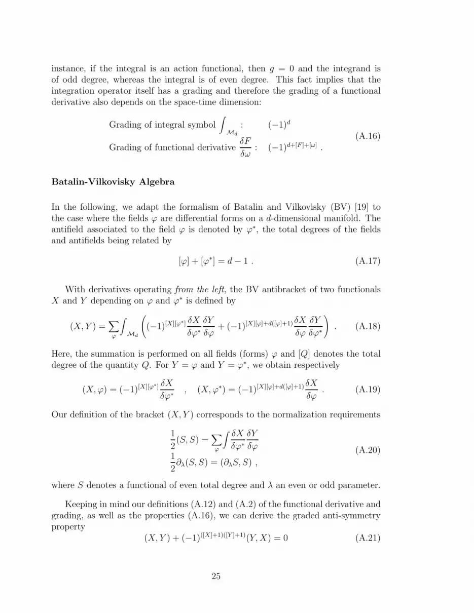
instance, if the integral is an action functional, then g = 0 and the integrand isof odd degree, whereas the integral is of even degree. This fact implies that theintegration operator itself has a grading and therefore the grading of a functionalderivative also depends on the space-time dimension:

Grading of integral symbol∫

Md

: (−1)d

Grading of functional derivativeδF

δω: (−1)d+[F ]+[ω] .

(A.16)

Batalin-Vilkovisky Algebra

In the following, we adapt the formalism of Batalin and Vilkovisky (BV) [19] tothe case where the fields ϕ are differential forms on a d-dimensional manifold. Theantifield associated to the field ϕ is denoted by ϕ∗, the total degrees of the fieldsand antifields being related by

[ϕ] + [ϕ∗] = d − 1 . (A.17)

With derivatives operating from the left, the BV antibracket of two functionalsX and Y depending on ϕ and ϕ∗ is defined by

(X, Y ) =∑

ϕ

∫

Md

(

(−1)[X][ϕ∗] δX

δϕ∗

δY

δϕ+ (−1)[X][ϕ]+d([ϕ]+1)δX

δϕ

δY

δϕ∗

)

. (A.18)

Here, the summation is performed on all fields (forms) ϕ and [Q] denotes the totaldegree of the quantity Q. For Y = ϕ and Y = ϕ∗, we obtain respectively

(X, ϕ) = (−1)[X][ϕ∗] δX

δϕ∗, (X, ϕ∗) = (−1)[X][ϕ]+d([ϕ]+1)δX

δϕ. (A.19)

Our definition of the bracket (X, Y ) corresponds to the normalization requirements

1

2(S, S) =

∑

ϕ

∫

δX

δϕ∗

δY

δϕ1

2∂λ(S, S) = (∂λS, S) ,

(A.20)

where S denotes a functional of even total degree and λ an even or odd parameter.

Keeping in mind our definitions (A.12) and (A.2) of the functional derivative andgrading, as well as the properties (A.16), we can derive the graded anti-symmetryproperty

(X, Y ) + (−1)([X]+1)([Y ]+1)(Y, X) = 0 (A.21)

25

and the graded Jacobi identity

(X, (Y, Z)) + (−1)([X]+1)([Y ]+[Z])(Y, (Z, X)) + (−1)([Z]+1)([X]+[Y ])(Z, (X, Y )) = 0 .(A.22)

The latter results from the following simple identity which is valid for any functionalS of even total degree:

(S, (S, S)) = 0 . (A.23)

Indeed, it suffices to consider S = xX+yY +zZ where the gradings of the coefficientsx, y and z are equal to those of X, Y and Z, respectively, then to differentiate with∂3/∂x ∂y ∂z at x = y = z = 0 while using the differentiation formula

∂λ(X, Y ) = (∂λX, Y ) + (−1)[λ]([X]+1)(X, ∂λY ) . (A.24)

A useful special case of the Jacobi identity is

(X, (S, S)) + 2 (S, (S, X)) = 0 , (A.25)

where the total degree of X is arbitrary.

References

[1] G.T. Horowitz, “Exactly soluble diffeomorphism invariant theories”, Com-mun.Math.Phys. 125 (1989) 417;

[2] L. Freidel, K. Krasnov and R. Puzio, “BF description of higher-dimensionalgravity theories”, Adv.Theor.Math.Phys. 3 (1999) 1289, hep-th/9901069;

[3] M. Blau and G. Thompson, “Topological gauge theories of antisymmetric tensorfields”, Ann.Phys. 205 (1991) 130;

A. Karlhede and M. Rocek, “Topological quantum field theories in arbitrarydimensions”, Phys.Lett. B224 (1989) 58;

[4] E. Witten, “Topological quantum field theory”,Commun. Math. Phys. 117 (1988) 353;

[5] E. Witten, “2+1 dimensional gravity as an exactly soluble system”, Nucl.Phys.B311 (1988/89) 46;

[6] D. Birmingham, M. Blau, M. Rakowski and G. Thompson, “Topological fieldtheory”, Phys. Rep. 209 (1991) 129;

[7] D. Birmingham, M. Rakowski and G. Thompson, “Renormalization of topolog-ical field theory”, Nucl.Phys. B329 (1990) 83;

F. Delduc, F. Gieres and S. P. Sorella, “Supersymmetry of the d = 3 Chern-Simons action in the Landau gauge”, Phys.Lett. B225 (1989) 367;

26

F. Delduc, C. Lucchesi, O. Piguet and S.P. Sorella, “Exact scale invariance ofthe Chern-Simons theory in the Landau gauge”, Nucl. Phys. B346 (1990) 313;

A. Blasi, O. Piguet and S.P. Sorella, “Landau gauge and finiteness”, Nucl.Phys. B356 (1991) 154;

[8] E. Guadagnini, N. Maggiore and S.P. Sorella, “Supersymmetric structure offour-dimensional antisymmetric tensor fields”, Phys.Lett. B255 (1991) 65;

N. Maggiore and S.P. Sorella, “Finiteness of the topological models in the Lan-dau gauge”, Nucl.Phys. B377 (1992) 236;

N. Maggiore and S.P. Sorella, “Perturbation theory for antisymmetric tensorfields in four-dimensions”, Int. J. Mod. Phys. A8 (1993) 929, hep-th/9204044;

[9] C. Lucchesi, O. Piguet and S.P. Sorella, “Renormalization and finiteness oftopological BF theories”, Nucl. Phys. B395 (1993) 325, hep-th/9208047;

[10] O. Piguet and S.P. Sorella, “Algebraic Renormalization”, Lecture Notes inPhysics m28, (Springer-Verlag, Berlin 1995);

[11] O. Piguet, “Ghost equations and diffeomorphism invariant theories,” Class.Quantum Grav. 17 (2000) 3799, hep-th/0005011;

[12] F. Gieres, J.M. Grimstrup, H. Nieder, T. Pisar and M. Schweda, “Symmetriesof topological field theories in the BV-framework”, hep-th/0111258;

[13] A. Boresch, S. Emery, O. Moritsch, M. Schweda, T. Sommer and H. Zerrouki,“Applications of Noncovariant Gauges in the Algebraic Renormalization Proce-dure” (World Scientific, Singapore 1998);

[14] C. Lucchesi and O. Piguet, “Local supersymmetry of the Chern-Simons theoryand finiteness”, Nucl. Phys. B381 (1992) 281;

[15] P. Peldan, “Actions for gravity, with generalizations: a review”, Class. Quan-tum Grav. 11 (1994) 1087, gr-qc/9305011;

[16] F. Langouche, T. Schucker and R. Stora, “Gravitational anomalies of the Adler-Bardeen type”, Phys. Lett. B145 (1984) 342;

L. Baulieu and J. Thierry-Mieg, “Algebraic structure of quantum gravity andthe classification of the gravitational anomalies”, Phys.Lett. B145 (1984) 53;

[17] K. Ezawa, “Ashtekar’s formulation for N = 1, 2 supergravities as ”constrained”BF theories”, Prog.Theor.Phys. 95 (1996) 863, hep-th/9511047;

[18] H.J. Matschull, “On the relation between 2+1 Einstein gravity and Chern-Simons theory”, Class.Quant.Grav. 16 (1999) 2599, gr-qc/9903040;

L. Freidel and K. Krasnov, “Discrete space-time volume for 3-dimensional BFtheory and quantum gravity”,Class.Quant.Grav. 16 (1999) 351, hep-th/9804185;

27

[19] I.A. Batalin and G.A. Vilkovisky, “Gauge algebra and quantization”, Phys.Lett. B102 (1981) 27,

I.A. Batalin and G.A. Vilkovisky, “Quantization of gauge theories with linearlydependent generators”, Phys. Rev. D28 (1983) 2567;

J. Gomis, J. Paris and S. Samuel, “Antibracket, antifields and gauge theoryquantization”, Phys.Rept. 259 (1995) 1, hep-th/9412228;

[20] J. Thierry-Mieg, “Geometrical reinterpretation of Faddeev-Popov ghost parti-cles and BRS transformations”, J.Math.Phys. 21 (1980) 2834;

L. Bonora and M. Tonin, “Superfield formulation of extended BRS symmetry”,Phys.Lett. 98B (1981) 48;

R. Stora, in “New Developments in Quantum Field Theory and StatisticalMechanics”, Cargese 1976, M. Levy and P. Mitter, eds., NATO ASI Ser. B,Vol. 26 (Plenum Press, 1977);

R. Stora, in “Progress in Gauge Field Theory”, Cargese 1983, G. ’t Hooft et al.eds., NATO ASI Ser. B, Vol. 115 (Plenum Press, 1984);

L. Baulieu and J. Thierry-Mieg, “The principle of BRS symmetry: An alterna-tive approach to Yang-Mills theories”, Nucl.Phys. B197 (1982) 477;

[21] R. A. Bertlmann, Anomalies in quantum field theory (Clarendon Press, Oxford1996);

[22] H. Ikemori, “Extended form method of antifield BRST formalism for BF theo-ries,” Mod.Phys.Lett. A7 (1992) 3397, hep-th/9205111;

H. Ikemori, “Extended form method of antifield BRST formalism for topologicalquantum field theories”, Class.Quant.Grav. 10 (1993) 233, hep-th/9206061;

L. Baulieu, “B-V quantization and field-anti-field duality for p-form gauge fields,topological field theories and 2-D gravity”, Nucl. Phys. B478 (1996) 431;

J.C. Wallet, “Algebraic setup for the gauge fixing of BF and super BF systems”,Phys. Lett. B235 (1990) 71;

[23] M. Carvalho, L. C. Vilar, C. A. Sasaki and S. P. Sorella, “BRS cohomology ofzero curvature systems I. The complete ladder case”, J.Math.Phys. 37 (1996)5310, hep-th/9509047;

[24] S. Ouvry, R. Stora, and P. van Baal, “On the algebraic characterization ofWitten’s topological Yang-Mills theory”, Phys.Lett. B220 (1989) 159;

L. Baulieu and I. M. Singer, “Topological Yang-Mills symmetry”,Nucl.Phys.B(Proc.Suppl.) 5B (1988) 12;

[25] L. Baulieu and M. Bellon, “p forms and supergravity: gauge symmetries incurved space”, Nucl.Phys. B266 (1986) 75;

28

[26] C.P. Constantinides, F. Gieres, O. Piguet and M.S. Sarandy, work in progress;

[27] F. Gieres, J.M. Grimstrup, T. Pisar and M. Schweda, “Vector supersymmetryin topological field theories”, JHEP 06 (2000) 18, hep-th/0002167.

29