Embed Size (px)
Citation preview
Volume 1

Calculus Volume 1
SENIOR CONTRIBUTING AUTHORS EDWIN "JED" HERMAN, UNIVERSITY OF WISCONSIN-STEVENS POINT GILBERT STRANG, MASSACHUSETTS INSTITUTE OF TECHNOLOGY
OpenStax Rice University 6100 Main Street MS-375 Houston, Texas 77005 To learn more about OpenStax, visit https://openstax.org. Individual print copies and bulk orders can be purchased through our website. ©2018 Rice University. Textbook content produced by OpenStax is licensed under a Creative Commons Attribution Non-Commercial ShareAlike 4.0 International License (CC BY-NC-SA 4.0). Under this license, any user of this textbook or the textbook contents herein can share, remix, and build upon the content for noncommercial purposes only. Any adaptations must be shared under the same type of license. In any case of sharing the original or adapted material, whether in whole or in part, the user must provide proper attribution as follows:
- If you noncommercially redistribute this textbook in a digital format (including but not limited to PDF and HTML), then you must retain on every page the following attribution: “Download for free at https://openstax.org/details/books/calculus-volume-1.”
- If you noncommercially redistribute this textbook in a print format, then you must include on every physical page the following attribution: “Download for free at https://openstax.org/details/books/calculus-volume-1.”
- If you noncommercially redistribute part of this textbook, then you must retain in every digital format page view (including but not limited to PDF and HTML) and on every physical printed page the following attribution: “Download for free at https://openstax.org/details/books/calculus-volume-1.”
- If you use this textbook as a bibliographic reference, please include https://openstax.org/details/books/calculus-volume-1 in your citation.
For questions regarding this licensing, please contact [email protected]. Trademarks The OpenStax name, OpenStax logo, OpenStax book covers, OpenStax CNX name, OpenStax CNX logo, OpenStax Tutor name, Openstax Tutor logo, Connexions name, Connexions logo, Rice University name, and Rice University logo are not subject to the license and may not be reproduced without the prior and express written consent of Rice University.
PRINT BOOK ISBN-10 1-938168-02-X PRINT BOOK ISBN-13 978-1-938168-02-4
PDF VERSION ISBN-10 1-947172-13-1
PDF VERSION ISBN-13 978-1-947172-13-5
Revision Number C1-2016-003(03/18)-MJ Original Publication Year 2016

OPENSTAX OpenStax provides free, peer-reviewed, openly licensed textbooks for introductory college and Advanced Placement® courses and low-cost, personalized courseware that helps students learn. A nonprofit ed tech initiative based at Rice University, we’re committed to helping students access the tools they need to complete their courses and meet their educational goals.
RICE UNIVERSITY OpenStax, OpenStax CNX, and OpenStax Tutor are initiatives of Rice University. As a leading research university with a distinctive commitment to undergraduate education, Rice University aspires to path-breaking research, unsurpassed teaching, and contributions to the betterment of our world. It seeks to fulfill this mission by cultivating a diverse community of learning and discovery that produces leaders across the spectrum of human endeavor.
FOUNDATION SUPPORT OpenStax is grateful for the tremendous support of our sponsors. Without their strong engagement, the goal of free access to high-quality textbooks would remain just a dream.
Laura and John Arnold Foundation (LJAF) actively seeks opportunities to invest in organizations and thought leaders that have a sincere interest in implementing fundamental changes that not only yield immediate gains, but also repair broken systems for future generations. LJAF currently focuses its strategic investments on education, criminal justice, research integrity, and public accountability.
The William and Flora Hewlett Foundation has been making grants since 1967 to help solve social and environmental problems at home and around the world. The Foundation concentrates its resources on activities in education, the environment, global development and population, performing arts, and philanthropy, and makes grants to support disadvantaged communities in the San Francisco Bay Area. Calvin K. Kazanjian was the founder and president of Peter Paul (Almond Joy), Inc. He firmly believed that the more people understood about basic economics the happier and more prosperous they would be. Accordingly, he established the Calvin K. Kazanjian Economics Foundation Inc, in 1949 as a philanthropic, nonpolitical educational organization to support efforts that enhanced economic understanding.
Guided by the belief that every life has equal value, the Bill & Melinda Gates Foundation works to help all people lead healthy, productive lives. In developing countries, it focuses on improving people’s health with vaccines and other life-saving tools and giving them the chance to lift themselves out of hunger and extreme poverty. In the United States, it seeks to significantly improve education so that all young people have the opportunity to reach their full potential. Based in Seattle, Washington, the foundation is led by CEO Jeff Raikes and Co-chair William H. Gates Sr., under the direction of Bill and Melinda Gates and Warren Buffett. The Maxfield Foundation supports projects with potential for high impact in science, education, sustainability, and other areas of social importance.
Our mission at The Michelson 20MM Foundation is to grow access and success by eliminating unnecessary hurdles to affordability. We support the creation, sharing, and proliferation of more effective, more affordable educational content by leveraging disruptive technologies, open educational resources, and new models for collaboration between for-profit, nonprofit, and public entities. The Bill and Stephanie Sick Fund supports innovative projects in the areas of Education, Art, Science and Engineering.

Access. The future of education.
OpenStax.org
I like free textbooks and I cannot lie.
Give $5 or more to OpenStax and we’ll send you a sticker! OpenStax is a nonprofit initiative, which means that that every dollar you give helps us maintain and grow our library of free textbooks.
If you have a few dollars to spare, visit OpenStax.org/give to donate. We’ll send you an OpenStax sticker to thank you for your support!
Table of ContentsPreface . . . . . . . . . . . . . . . . . . . . . . . . . . . . . . . . . . . . . . . . . . . . . . . . . . . 1Chapter 1: Functions and Graphs . . . . . . . . . . . . . . . . . . . . . . . . . . . . . . . . . . . . 7
1.1 Review of Functions . . . . . . . . . . . . . . . . . . . . . . . . . . . . . . . . . . . . . . . 81.2 Basic Classes of Functions . . . . . . . . . . . . . . . . . . . . . . . . . . . . . . . . . . 361.3 Trigonometric Functions . . . . . . . . . . . . . . . . . . . . . . . . . . . . . . . . . . . . 621.4 Inverse Functions . . . . . . . . . . . . . . . . . . . . . . . . . . . . . . . . . . . . . . . 781.5 Exponential and Logarithmic Functions . . . . . . . . . . . . . . . . . . . . . . . . . . . . 96
Chapter 2: Limits . . . . . . . . . . . . . . . . . . . . . . . . . . . . . . . . . . . . . . . . . . . . 1232.1 A Preview of Calculus . . . . . . . . . . . . . . . . . . . . . . . . . . . . . . . . . . . . . 1242.2 The Limit of a Function . . . . . . . . . . . . . . . . . . . . . . . . . . . . . . . . . . . . . 1352.3 The Limit Laws . . . . . . . . . . . . . . . . . . . . . . . . . . . . . . . . . . . . . . . . . 1602.4 Continuity . . . . . . . . . . . . . . . . . . . . . . . . . . . . . . . . . . . . . . . . . . . 1792.5 The Precise Definition of a Limit . . . . . . . . . . . . . . . . . . . . . . . . . . . . . . . . 194
Chapter 3: Derivatives . . . . . . . . . . . . . . . . . . . . . . . . . . . . . . . . . . . . . . . . . 2133.1 Defining the Derivative . . . . . . . . . . . . . . . . . . . . . . . . . . . . . . . . . . . . . 2143.2 The Derivative as a Function . . . . . . . . . . . . . . . . . . . . . . . . . . . . . . . . . . 2323.3 Differentiation Rules . . . . . . . . . . . . . . . . . . . . . . . . . . . . . . . . . . . . . . 2473.4 Derivatives as Rates of Change . . . . . . . . . . . . . . . . . . . . . . . . . . . . . . . . 2663.5 Derivatives of Trigonometric Functions . . . . . . . . . . . . . . . . . . . . . . . . . . . . 2773.6 The Chain Rule . . . . . . . . . . . . . . . . . . . . . . . . . . . . . . . . . . . . . . . . 2873.7 Derivatives of Inverse Functions . . . . . . . . . . . . . . . . . . . . . . . . . . . . . . . . 2993.8 Implicit Differentiation . . . . . . . . . . . . . . . . . . . . . . . . . . . . . . . . . . . . . 3093.9 Derivatives of Exponential and Logarithmic Functions . . . . . . . . . . . . . . . . . . . . . 319
Chapter 4: Applications of Derivatives . . . . . . . . . . . . . . . . . . . . . . . . . . . . . . . . 3414.1 Related Rates . . . . . . . . . . . . . . . . . . . . . . . . . . . . . . . . . . . . . . . . . 3424.2 Linear Approximations and Differentials . . . . . . . . . . . . . . . . . . . . . . . . . . . . 3544.3 Maxima and Minima . . . . . . . . . . . . . . . . . . . . . . . . . . . . . . . . . . . . . . 3664.4 The Mean Value Theorem . . . . . . . . . . . . . . . . . . . . . . . . . . . . . . . . . . . 3794.5 Derivatives and the Shape of a Graph . . . . . . . . . . . . . . . . . . . . . . . . . . . . . 3904.6 Limits at Infinity and Asymptotes . . . . . . . . . . . . . . . . . . . . . . . . . . . . . . . . 4074.7 Applied Optimization Problems . . . . . . . . . . . . . . . . . . . . . . . . . . . . . . . . 4394.8 L’Hôpital’s Rule . . . . . . . . . . . . . . . . . . . . . . . . . . . . . . . . . . . . . . . . . 4544.9 Newton’s Method . . . . . . . . . . . . . . . . . . . . . . . . . . . . . . . . . . . . . . . . 4724.10 Antiderivatives . . . . . . . . . . . . . . . . . . . . . . . . . . . . . . . . . . . . . . . . 485
Chapter 5: Integration . . . . . . . . . . . . . . . . . . . . . . . . . . . . . . . . . . . . . . . . . 5075.1 Approximating Areas . . . . . . . . . . . . . . . . . . . . . . . . . . . . . . . . . . . . . . 5085.2 The Definite Integral . . . . . . . . . . . . . . . . . . . . . . . . . . . . . . . . . . . . . . 5295.3 The Fundamental Theorem of Calculus . . . . . . . . . . . . . . . . . . . . . . . . . . . . 5495.4 Integration Formulas and the Net Change Theorem . . . . . . . . . . . . . . . . . . . . . . 5665.5 Substitution . . . . . . . . . . . . . . . . . . . . . . . . . . . . . . . . . . . . . . . . . . . 5845.6 Integrals Involving Exponential and Logarithmic Functions . . . . . . . . . . . . . . . . . . 5955.7 Integrals Resulting in Inverse Trigonometric Functions . . . . . . . . . . . . . . . . . . . . 608
Chapter 6: Applications of Integration . . . . . . . . . . . . . . . . . . . . . . . . . . . . . . . . 6236.1 Areas between Curves . . . . . . . . . . . . . . . . . . . . . . . . . . . . . . . . . . . . . 6246.2 Determining Volumes by Slicing . . . . . . . . . . . . . . . . . . . . . . . . . . . . . . . . 6366.3 Volumes of Revolution: Cylindrical Shells . . . . . . . . . . . . . . . . . . . . . . . . . . . 6566.4 Arc Length of a Curve and Surface Area . . . . . . . . . . . . . . . . . . . . . . . . . . . 6716.5 Physical Applications . . . . . . . . . . . . . . . . . . . . . . . . . . . . . . . . . . . . . . 6856.6 Moments and Centers of Mass . . . . . . . . . . . . . . . . . . . . . . . . . . . . . . . . 7036.7 Integrals, Exponential Functions, and Logarithms . . . . . . . . . . . . . . . . . . . . . . . 7216.8 Exponential Growth and Decay . . . . . . . . . . . . . . . . . . . . . . . . . . . . . . . . 7346.9 Calculus of the Hyperbolic Functions . . . . . . . . . . . . . . . . . . . . . . . . . . . . . 745
Appendix A: Table of Integrals . . . . . . . . . . . . . . . . . . . . . . . . . . . . . . . . . . . . . 763Appendix B: Table of Derivatives . . . . . . . . . . . . . . . . . . . . . . . . . . . . . . . . . . . 769Appendix C: Review of Pre-Calculus . . . . . . . . . . . . . . . . . . . . . . . . . . . . . . . . . 771Index . . . . . . . . . . . . . . . . . . . . . . . . . . . . . . . . . . . . . . . . . . . . . . . . . . . 863

This OpenStax book is available for free at http://cnx.org/content/col11964/1.2

PREFACE
Welcome to Calculus Volume 1, an OpenStax resource. This textbook was written to increase student access to high-qualitylearning materials, maintaining highest standards of academic rigor at little to no cost.
About OpenStaxOpenStax is a nonprofit based at Rice University, and it’s our mission to improve student access to education. Our firstopenly licensed college textbook was published in 2012, and our library has since scaled to over 25 books for collegeand AP® courses used by hundreds of thousands of students. OpenStax Tutor, our low-cost personalized learning tool, isbeing used in college courses throughout the country. Through our partnerships with philanthropic foundations and ouralliance with other educational resource organizations, OpenStax is breaking down the most common barriers to learningand empowering students and instructors to succeed.
About OpenStax's resourcesCustomization
Calculus Volume 1 is licensed under a Creative Commons Attribution 4.0 International (CC BY) license, which meansthat you can distribute, remix, and build upon the content, as long as you provide attribution to OpenStax and its contentcontributors.
Because our books are openly licensed, you are free to use the entire book or pick and choose the sections that are mostrelevant to the needs of your course. Feel free to remix the content by assigning your students certain chapters and sectionsin your syllabus, in the order that you prefer. You can even provide a direct link in your syllabus to the sections in the webview of your book.
Instructors also have the option of creating a customized version of their OpenStax book. The custom version can be madeavailable to students in low-cost print or digital form through their campus bookstore. Visit your book page on OpenStax.orgfor more information.
Errata
All OpenStax textbooks undergo a rigorous review process. However, like any professional-grade textbook, errorssometimes occur. Since our books are web based, we can make updates periodically when deemed pedagogically necessary.If you have a correction to suggest, submit it through the link on your book page on OpenStax.org. Subject matter expertsreview all errata suggestions. OpenStax is committed to remaining transparent about all updates, so you will also find a listof past errata changes on your book page on OpenStax.org.
Format
You can access this textbook for free in web view or PDF through OpenStax.org, and for a low cost in print.
About Calculus Volume 1Calculus is designed for the typical two- or three-semester general calculus course, incorporating innovative features toenhance student learning. The book guides students through the core concepts of calculus and helps them understandhow those concepts apply to their lives and the world around them. Due to the comprehensive nature of the material, weare offering the book in three volumes for flexibility and efficiency. Volume 1 covers functions, limits, derivatives, andintegration.
Coverage and scope
Our Calculus Volume 1 textbook adheres to the scope and sequence of most general calculus courses nationwide. We haveworked to make calculus interesting and accessible to students while maintaining the mathematical rigor inherent in thesubject. With this objective in mind, the content of the three volumes of Calculus have been developed and arranged toprovide a logical progression from fundamental to more advanced concepts, building upon what students have alreadylearned and emphasizing connections between topics and between theory and applications. The goal of each section is toenable students not just to recognize concepts, but work with them in ways that will be useful in later courses and futurecareers. The organization and pedagogical features were developed and vetted with feedback from mathematics educatorsdedicated to the project.
Volume 1
Preface 1
Chapter 1: Functions and Graphs
Chapter 2: Limits
Chapter 3: Derivatives
Chapter 4: Applications of Derivatives
Chapter 5: Integration
Chapter 6: Applications of Integration
Volume 2Chapter 1: Integration
Chapter 2: Applications of Integration
Chapter 3: Techniques of Integration
Chapter 4: Introduction to Differential Equations
Chapter 5: Sequences and Series
Chapter 6: Power Series
Chapter 7: Parametric Equations and Polar Coordinates
Volume 3Chapter 1: Parametric Equations and Polar Coordinates
Chapter 2: Vectors in Space
Chapter 3: Vector-Valued Functions
Chapter 4: Differentiation of Functions of Several Variables
Chapter 5: Multiple Integration
Chapter 6: Vector Calculus
Chapter 7: Second-Order Differential Equations
Pedagogical foundation
Throughout Calculus Volume 1 you will find examples and exercises that present classical ideas and techniques as well asmodern applications and methods. Derivations and explanations are based on years of classroom experience on the partof long-time calculus professors, striving for a balance of clarity and rigor that has proven successful with their students.Motivational applications cover important topics in probability, biology, ecology, business, and economics, as well as areasof physics, chemistry, engineering, and computer science. Student Projects in each chapter give students opportunities toexplore interesting sidelights in pure and applied mathematics, from determining a safe distance between the grandstand andthe track at a Formula One racetrack, to calculating the center of mass of the Grand Canyon Skywalk or the terminal speedof a skydiver. Chapter Opening Applications pose problems that are solved later in the chapter, using the ideas covered inthat chapter. Problems include the hydraulic force against the Hoover Dam, and the comparison of relative intensity of twoearthquakes. Definitions, Rules, and Theorems are highlighted throughout the text, including over 60 Proofs of theorems.
Assessments that reinforce key concepts
In-chapter Examples walk students through problems by posing a question, stepping out a solution, and then asking studentsto practice the skill with a “Checkpoint” question. The book also includes assessments at the end of each chapter sostudents can apply what they’ve learned through practice problems. Many exercises are marked with a [T] to indicate theyare suitable for solution by technology, including calculators or Computer Algebra Systems (CAS). Answers for selectedexercises are available in the Answer Key at the back of the book. The book also includes assessments at the end of eachchapter so students can apply what they’ve learned through practice problems.
Early or late transcendentals
Calculus Volume 1 is designed to accommodate both Early and Late Transcendental approaches to calculus. Exponentialand logarithmic functions are introduced informally in Chapter 1 and presented in more rigorous terms in Chapter 6.Differentiation and integration of these functions is covered in Chapters 3–5 for instructors who want to include them withother types of functions. These discussions, however, are in separate sections that can be skipped for instructors who preferto wait until the integral definitions are given before teaching the calculus derivations of exponentials and logarithms.
Comprehensive art program
Our art program is designed to enhance students’ understanding of concepts through clear and effective illustrations,
2 Preface
This OpenStax book is available for free at http://cnx.org/content/col11964/1.2
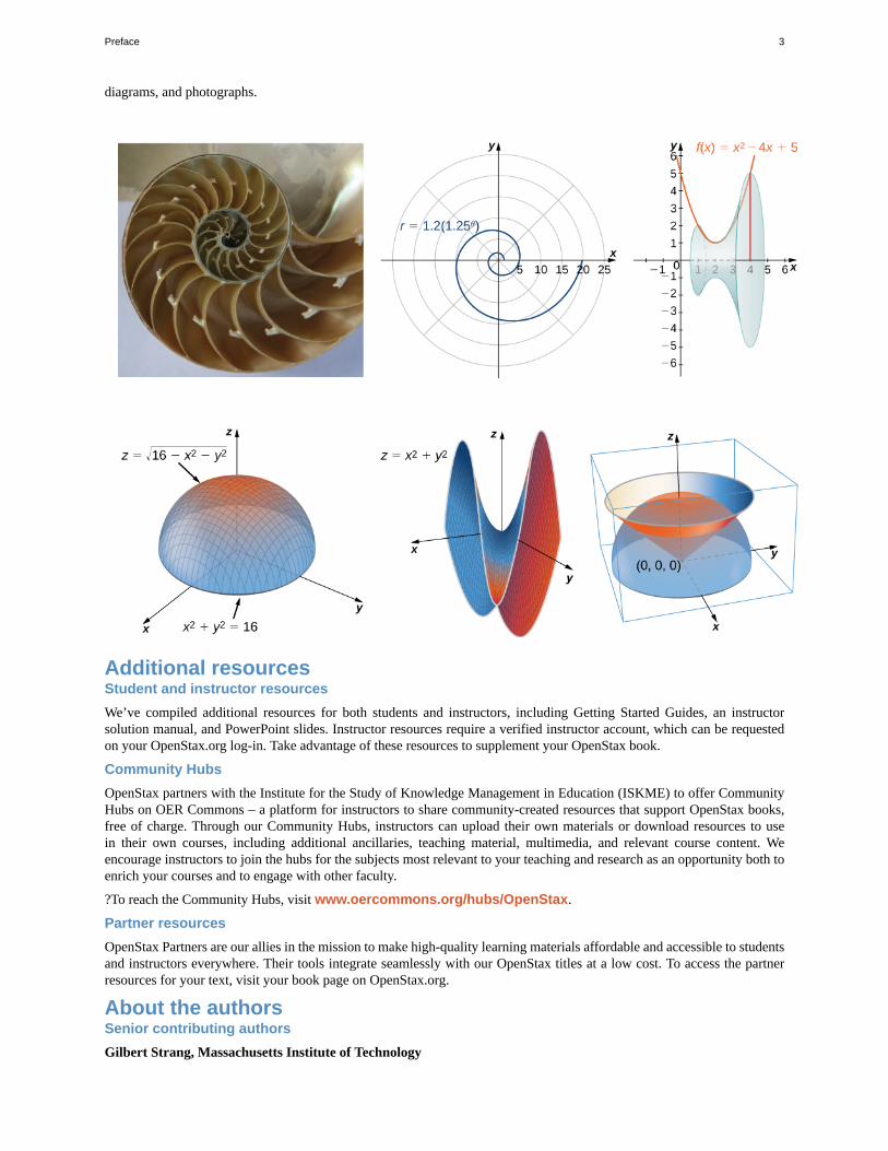
diagrams, and photographs.
Additional resourcesStudent and instructor resources
We’ve compiled additional resources for both students and instructors, including Getting Started Guides, an instructorsolution manual, and PowerPoint slides. Instructor resources require a verified instructor account, which can be requestedon your OpenStax.org log-in. Take advantage of these resources to supplement your OpenStax book.
Community Hubs
OpenStax partners with the Institute for the Study of Knowledge Management in Education (ISKME) to offer CommunityHubs on OER Commons – a platform for instructors to share community-created resources that support OpenStax books,free of charge. Through our Community Hubs, instructors can upload their own materials or download resources to usein their own courses, including additional ancillaries, teaching material, multimedia, and relevant course content. Weencourage instructors to join the hubs for the subjects most relevant to your teaching and research as an opportunity both toenrich your courses and to engage with other faculty.
?To reach the Community Hubs, visit www.oercommons.org/hubs/OpenStax.
Partner resources
OpenStax Partners are our allies in the mission to make high-quality learning materials affordable and accessible to studentsand instructors everywhere. Their tools integrate seamlessly with our OpenStax titles at a low cost. To access the partnerresources for your text, visit your book page on OpenStax.org.
About the authorsSenior contributing authors
Gilbert Strang, Massachusetts Institute of Technology
Preface 3

Dr. Strang received his PhD from UCLA in 1959 and has been teaching mathematics at MIT ever since. His Calculus onlinetextbook is one of eleven that he has published and is the basis from which our final product has been derived and updatedfor today’s student. Strang is a decorated mathematician and past Rhodes Scholar at Oxford University.
Edwin “Jed” Herman, University of Wisconsin-Stevens PointDr. Herman earned a BS in Mathematics from Harvey Mudd College in 1985, an MA in Mathematics from UCLA in1987, and a PhD in Mathematics from the University of Oregon in 1997. He is currently a Professor at the University ofWisconsin-Stevens Point. He has more than 20 years of experience teaching college mathematics, is a student researchmentor, is experienced in course development/design, and is also an avid board game designer and player.
Contributing authors
Catherine Abbott, Keuka CollegeNicoleta Virginia Bila, Fayetteville State UniversitySheri J. Boyd, Rollins CollegeJoyati Debnath, Winona State UniversityValeree Falduto, Palm Beach State CollegeJoseph Lakey, New Mexico State UniversityJulie Levandosky, Framingham State UniversityDavid McCune, William Jewell CollegeMichelle Merriweather, Bronxville High SchoolKirsten R. Messer, Colorado State University - PuebloAlfred K. Mulzet, Florida State College at JacksonvilleWilliam Radulovich (retired), Florida State College at JacksonvilleErica M. Rutter, Arizona State UniversityDavid Smith, University of the Virgin IslandsElaine A. Terry, Saint Joseph’s UniversityDavid Torain, Hampton University
Reviewers
Marwan A. Abu-Sawwa, Florida State College at JacksonvilleKenneth J. Bernard, Virginia State UniversityJohn Beyers, University of MarylandCharles Buehrle, Franklin & Marshall CollegeMatthew Cathey, Wofford CollegeMichael Cohen, Hofstra UniversityWilliam DeSalazar, Broward County School SystemMurray Eisenberg, University of Massachusetts AmherstKristyanna Erickson, Cecil CollegeTiernan Fogarty, Oregon Institute of TechnologyDavid French, Tidewater Community CollegeMarilyn Gloyer, Virginia Commonwealth UniversityShawna Haider, Salt Lake Community CollegeLance Hemlow, Raritan Valley Community CollegeJerry Jared, The Blue Ridge SchoolPeter Jipsen, Chapman UniversityDavid Johnson, Lehigh UniversityM.R. Khadivi, Jackson State UniversityRobert J. Krueger, Concordia UniversityTor A. Kwembe, Jackson State UniversityJean-Marie Magnier, Springfield Technical Community CollegeCheryl Chute Miller, SUNY PotsdamBagisa Mukherjee, Penn State University, Worthington Scranton CampusKasso Okoudjou, University of Maryland College ParkPeter Olszewski, Penn State Erie, The Behrend CollegeSteven Purtee, Valencia CollegeAlice Ramos, Bethel CollegeDoug Shaw, University of Northern IowaHussain Elalaoui-Talibi, Tuskegee UniversityJeffrey Taub, Maine Maritime AcademyWilliam Thistleton, SUNY Polytechnic Institute
4 Preface
This OpenStax book is available for free at http://cnx.org/content/col11964/1.2
A. David Trubatch, Montclair State UniversityCarmen Wright, Jackson State UniversityZhenbu Zhang, Jackson State University
Preface 5

Preface
This OpenStax book is available for free at http://cnx.org/content/col11964/1.2
1 | FUNCTIONS ANDGRAPHS
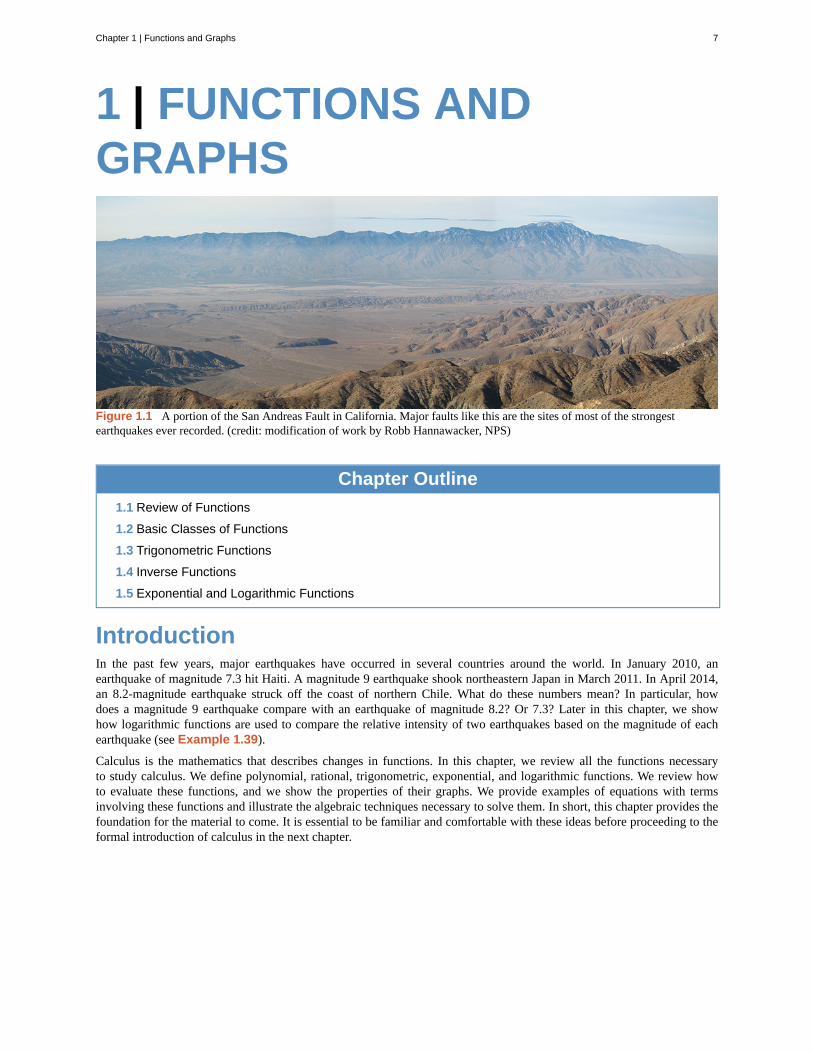
Figure 1.1 A portion of the San Andreas Fault in California. Major faults like this are the sites of most of the strongestearthquakes ever recorded. (credit: modification of work by Robb Hannawacker, NPS)
Chapter Outline
1.1 Review of Functions
1.2 Basic Classes of Functions
1.3 Trigonometric Functions
1.4 Inverse Functions
1.5 Exponential and Logarithmic Functions
IntroductionIn the past few years, major earthquakes have occurred in several countries around the world. In January 2010, anearthquake of magnitude 7.3 hit Haiti. A magnitude 9 earthquake shook northeastern Japan in March 2011. In April 2014,an 8.2-magnitude earthquake struck off the coast of northern Chile. What do these numbers mean? In particular, howdoes a magnitude 9 earthquake compare with an earthquake of magnitude 8.2? Or 7.3? Later in this chapter, we showhow logarithmic functions are used to compare the relative intensity of two earthquakes based on the magnitude of eachearthquake (see Example 1.39).
Calculus is the mathematics that describes changes in functions. In this chapter, we review all the functions necessaryto study calculus. We define polynomial, rational, trigonometric, exponential, and logarithmic functions. We review howto evaluate these functions, and we show the properties of their graphs. We provide examples of equations with termsinvolving these functions and illustrate the algebraic techniques necessary to solve them. In short, this chapter provides thefoundation for the material to come. It is essential to be familiar and comfortable with these ideas before proceeding to theformal introduction of calculus in the next chapter.
Chapter 1 | Functions and Graphs 7
1.1 | Review of Functions
Learning Objectives1.1.1 Use functional notation to evaluate a function.
1.1.2 Determine the domain and range of a function.
1.1.3 Draw the graph of a function.
1.1.4 Find the zeros of a function.
1.1.5 Recognize a function from a table of values.
1.1.6 Make new functions from two or more given functions.
1.1.7 Describe the symmetry properties of a function.
In this section, we provide a formal definition of a function and examine several ways in which functions arerepresented—namely, through tables, formulas, and graphs. We study formal notation and terms related to functions. Wealso define composition of functions and symmetry properties. Most of this material will be a review for you, but it servesas a handy reference to remind you of some of the algebraic techniques useful for working with functions.
FunctionsGiven two sets A and B, a set with elements that are ordered pairs (x, y), where x is an element of A and y is an
element of B, is a relation from A to B. A relation from A to B defines a relationship between those two sets. A
function is a special type of relation in which each element of the first set is related to exactly one element of the secondset. The element of the first set is called the input; the element of the second set is called the output. Functions are used allthe time in mathematics to describe relationships between two sets. For any function, when we know the input, the output isdetermined, so we say that the output is a function of the input. For example, the area of a square is determined by its sidelength, so we say that the area (the output) is a function of its side length (the input). The velocity of a ball thrown in theair can be described as a function of the amount of time the ball is in the air. The cost of mailing a package is a function ofthe weight of the package. Since functions have so many uses, it is important to have precise definitions and terminology tostudy them.
Definition
A function f consists of a set of inputs, a set of outputs, and a rule for assigning each input to exactly one output. The
set of inputs is called the domain of the function. The set of outputs is called the range of the function.
For example, consider the function f , where the domain is the set of all real numbers and the rule is to square the input.
Then, the input x = 3 is assigned to the output 32 = 9. Since every nonnegative real number has a real-value square root,
every nonnegative number is an element of the range of this function. Since there is no real number with a square that isnegative, the negative real numbers are not elements of the range. We conclude that the range is the set of nonnegative realnumbers.
For a general function f with domain D, we often use x to denote the input and y to denote the output associated with
x. When doing so, we refer to x as the independent variable and y as the dependent variable, because it depends on x.Using function notation, we write y = f (x), and we read this equation as “y equals f of x.” For the squaring function
described earlier, we write f (x) = x2.
The concept of a function can be visualized using Figure 1.2, Figure 1.3, and Figure 1.4.
8 Chapter 1 | Functions and Graphs
This OpenStax book is available for free at http://cnx.org/content/col11964/1.2
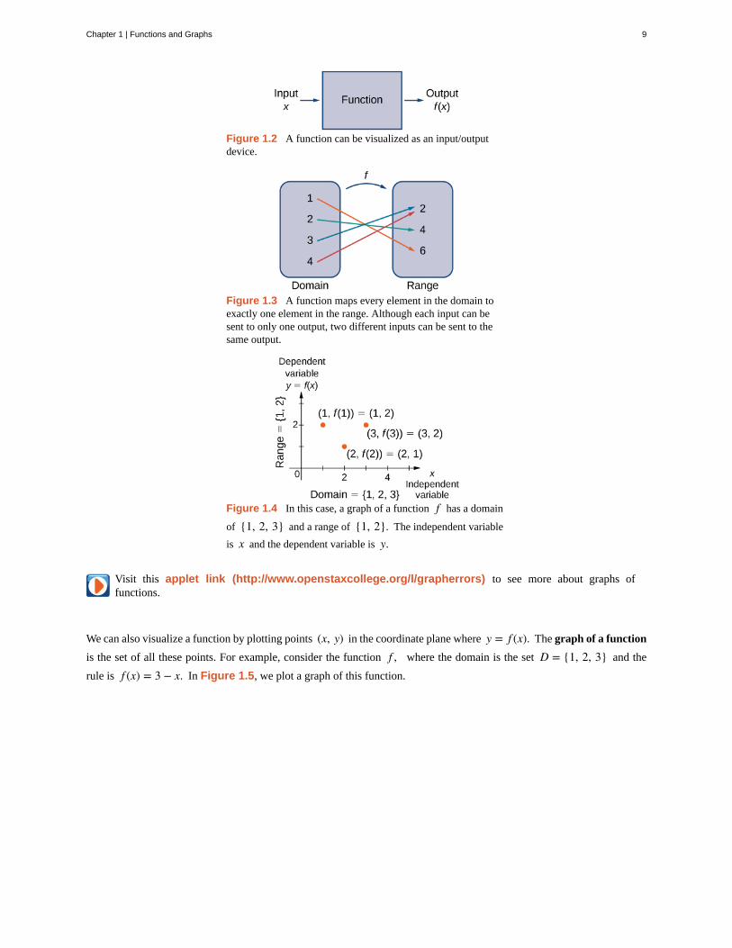
Figure 1.2 A function can be visualized as an input/outputdevice.
Figure 1.3 A function maps every element in the domain toexactly one element in the range. Although each input can besent to only one output, two different inputs can be sent to thesame output.
Figure 1.4 In this case, a graph of a function f has a domain
of {1, 2, 3} and a range of {1, 2}. The independent variable
is x and the dependent variable is y.
Visit this applet link (http://www.openstaxcollege.org/l/grapherrors) to see more about graphs offunctions.
We can also visualize a function by plotting points (x, y) in the coordinate plane where y = f (x). The graph of a function
is the set of all these points. For example, consider the function f , where the domain is the set D = {1, 2, 3} and the
rule is f (x) = 3 − x. In Figure 1.5, we plot a graph of this function.
Chapter 1 | Functions and Graphs 9
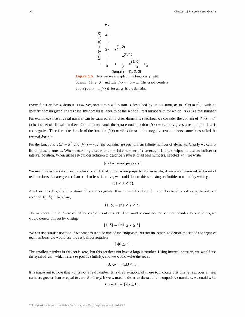
Figure 1.5 Here we see a graph of the function f with
domain {1, 2, 3} and rule f (x) = 3 − x. The graph consists
of the points (x, f (x)) for all x in the domain.
Every function has a domain. However, sometimes a function is described by an equation, as in f (x) = x2, with no
specific domain given. In this case, the domain is taken to be the set of all real numbers x for which f (x) is a real number.
For example, since any real number can be squared, if no other domain is specified, we consider the domain of f (x) = x2
to be the set of all real numbers. On the other hand, the square root function f (x) = x only gives a real output if x is
nonnegative. Therefore, the domain of the function f (x) = x is the set of nonnegative real numbers, sometimes called the
natural domain.
For the functions f (x) = x2 and f (x) = x, the domains are sets with an infinite number of elements. Clearly we cannot
list all these elements. When describing a set with an infinite number of elements, it is often helpful to use set-builder orinterval notation. When using set-builder notation to describe a subset of all real numbers, denoted ℝ, we write
⎧
⎩⎨x|x has some property⎫
⎭⎬.
We read this as the set of real numbers x such that x has some property. For example, if we were interested in the set of
real numbers that are greater than one but less than five, we could denote this set using set-builder notation by writing
{x|1 < x < 5}.
A set such as this, which contains all numbers greater than a and less than b, can also be denoted using the interval
notation (a, b). Therefore,
(1, 5) = ⎧
⎩⎨x|1 < x < 5⎫
⎭⎬.
The numbers 1 and 5 are called the endpoints of this set. If we want to consider the set that includes the endpoints, we
would denote this set by writing
[1, 5] = {x|1 ≤ x ≤ 5}.
We can use similar notation if we want to include one of the endpoints, but not the other. To denote the set of nonnegativereal numbers, we would use the set-builder notation
{x|0 ≤ x}.
The smallest number in this set is zero, but this set does not have a largest number. Using interval notation, we would usethe symbol ∞, which refers to positive infinity, and we would write the set as
[0, ∞) = {x|0 ≤ x}.
It is important to note that ∞ is not a real number. It is used symbolically here to indicate that this set includes all real
numbers greater than or equal to zero. Similarly, if we wanted to describe the set of all nonpositive numbers, we could write
(−∞, 0] = {x|x ≤ 0}.
10 Chapter 1 | Functions and Graphs
This OpenStax book is available for free at http://cnx.org/content/col11964/1.2
1.1
Here, the notation −∞ refers to negative infinity, and it indicates that we are including all numbers less than or equal to
zero, no matter how small. The set
(−∞, ∞) = ⎧
⎩⎨x|x is any real number⎫
⎭⎬
refers to the set of all real numbers.
Some functions are defined using different equations for different parts of their domain. These types of functions are knownas piecewise-defined functions. For example, suppose we want to define a function f with a domain that is the set of all
real numbers such that f (x) = 3x + 1 for x ≥ 2 and f (x) = x2 for x < 2. We denote this function by writing
f (x) =⎧
⎩⎨3x + 1 x ≥ 2x2 x < 2
.
When evaluating this function for an input x, the equation to use depends on whether x ≥ 2 or x < 2. For example,
since 5 > 2, we use the fact that f (x) = 3x + 1 for x ≥ 2 and see that f (5) = 3(5) + 1 = 16. On the other hand, for
x = −1, we use the fact that f (x) = x2 for x < 2 and see that f (−1) = 1.
Example 1.1
Evaluating Functions
For the function f (x) = 3x2 + 2x − 1, evaluate
a. f (−2)
b. f ( 2)
c. f (a + h)
Solution
Substitute the given value for x in the formula for f (x).
a. f (−2) = 3(−2)2 + 2(−2) − 1 = 12 − 4 − 1 = 7
b. f ( 2) = 3( 2)2 + 2 2 − 1 = 6 + 2 2 − 1 = 5 + 2 2
c.f (a + h) = 3(a + h)2 + 2(a + h) − 1 = 3⎛
⎝a2 + 2ah + h2⎞⎠ + 2a + 2h − 1
= 3a2 + 6ah + 3h2 + 2a + 2h − 1
For f (x) = x2 − 3x + 5, evaluate f (1) and f (a + h).
Example 1.2
Finding Domain and Range
For each of the following functions, determine the i. domain and ii. range.
Chapter 1 | Functions and Graphs 11
a. f (x) = (x − 4)2 + 5
b. f (x) = 3x + 2 − 1
c. f (x) = 3x − 2
Solution
a. Consider f (x) = (x − 4)2 + 5.
i. Since f (x) = (x − 4)2 + 5 is a real number for any real number x, the domain of f is the
interval (−∞, ∞).
ii. Since (x − 4)2 ≥ 0, we know f (x) = (x − 4)2 + 5 ≥ 5. Therefore, the range must be a subset
of ⎧
⎩⎨y|y ≥ 5⎫
⎭⎬. To show that every element in this set is in the range, we need to show that for a
given y in that set, there is a real number x such that f (x) = (x − 4)2 + 5 = y. Solving this
equation for x, we see that we need x such that
(x − 4)2 = y − 5.
This equation is satisfied as long as there exists a real number x such that
x − 4 = ± y − 5.
Since y ≥ 5, the square root is well-defined. We conclude that for x = 4 ± y − 5, f (x) = y,and therefore the range is ⎧
⎩⎨y|y ≥ 5⎫
⎭⎬.
b. Consider f (x) = 3x + 2 − 1.
i. To find the domain of f , we need the expression 3x + 2 ≥ 0. Solving this inequality, we
conclude that the domain is {x|x ≥ −2/3}.
ii. To find the range of f , we note that since 3x + 2 ≥ 0, f (x) = 3x + 2 − 1 ≥ −1. Therefore,
the range of f must be a subset of the set ⎧
⎩⎨y|y ≥ −1⎫
⎭⎬. To show that every element in this set is
in the range of f , we need to show that for all y in this set, there exists a real number x in the
domain such that f (x) = y. Let y ≥ −1. Then, f (x) = y if and only if
3x + 2 − 1 = y.
Solving this equation for x, we see that x must solve the equation
3x + 2 = y + 1.
Since y ≥ −1, such an x could exist. Squaring both sides of this equation, we have
3x + 2 = (y + 1)2.Therefore, we need
3x = (y + 1)2 − 2,
12 Chapter 1 | Functions and Graphs
This OpenStax book is available for free at http://cnx.org/content/col11964/1.2
1.2
which implies
x = 13
⎛⎝y + 1⎞
⎠2 − 2
3.
We just need to verify that x is in the domain of f . Since the domain of f consists of all real
numbers greater than or equal to −2/3, and
13
⎛⎝y + 1⎞
⎠2 − 2
3 ≥ − 23,
there does exist an x in the domain of f . We conclude that the range of f is ⎧
⎩⎨y|y ≥ −1⎫
⎭⎬.
c. Consider f (x) = 3/(x − 2).
i. Since 3/(x − 2) is defined when the denominator is nonzero, the domain is {x|x ≠ 2}.
ii. To find the range of f , we need to find the values of y such that there exists a real number xin the domain with the property that
3x − 2 = y.
Solving this equation for x, we find that
x = 3y + 2.
Therefore, as long as y ≠ 0, there exists a real number x in the domain such that f (x) = y.Thus, the range is ⎧
⎩⎨y|y ≠ 0⎫
⎭⎬.
Find the domain and range for f (x) = 4 − 2x + 5.
Representing FunctionsTypically, a function is represented using one or more of the following tools:
• A table
• A graph
• A formula
We can identify a function in each form, but we can also use them together. For instance, we can plot on a graph the valuesfrom a table or create a table from a formula.
Tables
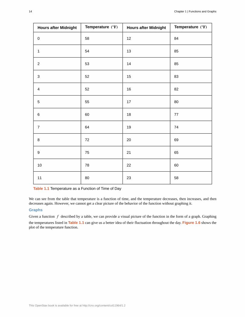
Functions described using a table of values arise frequently in real-world applications. Consider the following simpleexample. We can describe temperature on a given day as a function of time of day. Suppose we record the temperature everyhour for a 24-hour period starting at midnight. We let our input variable x be the time after midnight, measured in hours,
and the output variable y be the temperature x hours after midnight, measured in degrees Fahrenheit. We record our data
in Table 1.1.
Chapter 1 | Functions and Graphs 13
Hours after Midnight Temperature (°F) Hours after Midnight Temperature (°F)
0 58 12 84
1 54 13 85
2 53 14 85
3 52 15 83
4 52 16 82
5 55 17 80
6 60 18 77
7 64 19 74
8 72 20 69
9 75 21 65
10 78 22 60
11 80 23 58
Table 1.1 Temperature as a Function of Time of Day
We can see from the table that temperature is a function of time, and the temperature decreases, then increases, and thendecreases again. However, we cannot get a clear picture of the behavior of the function without graphing it.
Graphs
Given a function f described by a table, we can provide a visual picture of the function in the form of a graph. Graphing
the temperatures listed in Table 1.1 can give us a better idea of their fluctuation throughout the day. Figure 1.6 shows theplot of the temperature function.
14 Chapter 1 | Functions and Graphs
This OpenStax book is available for free at http://cnx.org/content/col11964/1.2
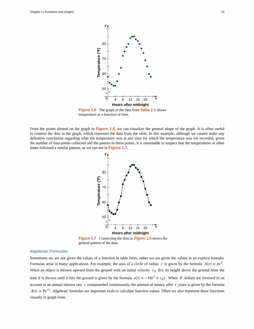
Figure 1.6 The graph of the data from Table 1.1 showstemperature as a function of time.
From the points plotted on the graph in Figure 1.6, we can visualize the general shape of the graph. It is often usefulto connect the dots in the graph, which represent the data from the table. In this example, although we cannot make anydefinitive conclusion regarding what the temperature was at any time for which the temperature was not recorded, giventhe number of data points collected and the pattern in these points, it is reasonable to suspect that the temperatures at othertimes followed a similar pattern, as we can see in Figure 1.7.
Figure 1.7 Connecting the dots in Figure 1.6 shows thegeneral pattern of the data.
Algebraic Formulas
Sometimes we are not given the values of a function in table form, rather we are given the values in an explicit formula.
Formulas arise in many applications. For example, the area of a circle of radius r is given by the formula A(r) = πr2.When an object is thrown upward from the ground with an initial velocity v0 ft/s, its height above the ground from the
time it is thrown until it hits the ground is given by the formula s(t) = −16t2 + v0 t. When P dollars are invested in an
account at an annual interest rate r compounded continuously, the amount of money after t years is given by the formula
A(t) = Pert. Algebraic formulas are important tools to calculate function values. Often we also represent these functions
visually in graph form.
Chapter 1 | Functions and Graphs 15
Given an algebraic formula for a function f , the graph of f is the set of points ⎛⎝x, f (x)⎞
⎠, where x is in the domain of
f and f (x) is in the range. To graph a function given by a formula, it is helpful to begin by using the formula to create
a table of inputs and outputs. If the domain of f consists of an infinite number of values, we cannot list all of them, but
because listing some of the inputs and outputs can be very useful, it is often a good way to begin.
When creating a table of inputs and outputs, we typically check to determine whether zero is an output. Those values of
x where f (x) = 0 are called the zeros of a function. For example, the zeros of f (x) = x2 − 4 are x = ± 2. The zeros
determine where the graph of f intersects the x -axis, which gives us more information about the shape of the graph of
the function. The graph of a function may never intersect the x-axis, or it may intersect multiple (or even infinitely many)times.
Another point of interest is the y -intercept, if it exists. The y -intercept is given by ⎛⎝0, f (0)⎞
⎠.
Since a function has exactly one output for each input, the graph of a function can have, at most, one y -intercept. If x = 0is in the domain of a function f , then f has exactly one y -intercept. If x = 0 is not in the domain of f , then f has
no y -intercept. Similarly, for any real number c, if c is in the domain of f , there is exactly one output f (c), and the
line x = c intersects the graph of f exactly once. On the other hand, if c is not in the domain of f , f (c) is not defined
and the line x = c does not intersect the graph of f . This property is summarized in the vertical line test.
Rule: Vertical Line Test
Given a function f , every vertical line that may be drawn intersects the graph of f no more than once. If any vertical
line intersects a set of points more than once, the set of points does not represent a function.
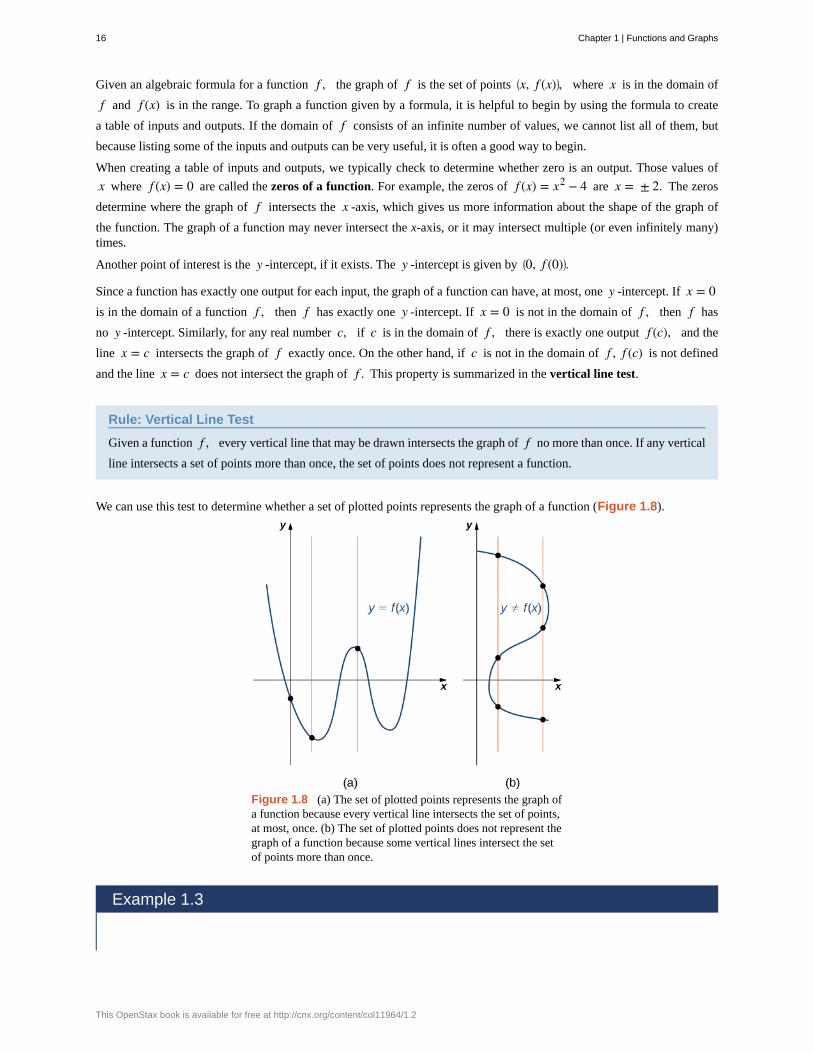
We can use this test to determine whether a set of plotted points represents the graph of a function (Figure 1.8).
Figure 1.8 (a) The set of plotted points represents the graph ofa function because every vertical line intersects the set of points,at most, once. (b) The set of plotted points does not represent thegraph of a function because some vertical lines intersect the setof points more than once.
Example 1.3
16 Chapter 1 | Functions and Graphs
This OpenStax book is available for free at http://cnx.org/content/col11964/1.2
Finding Zeros and y -Intercepts of a Function
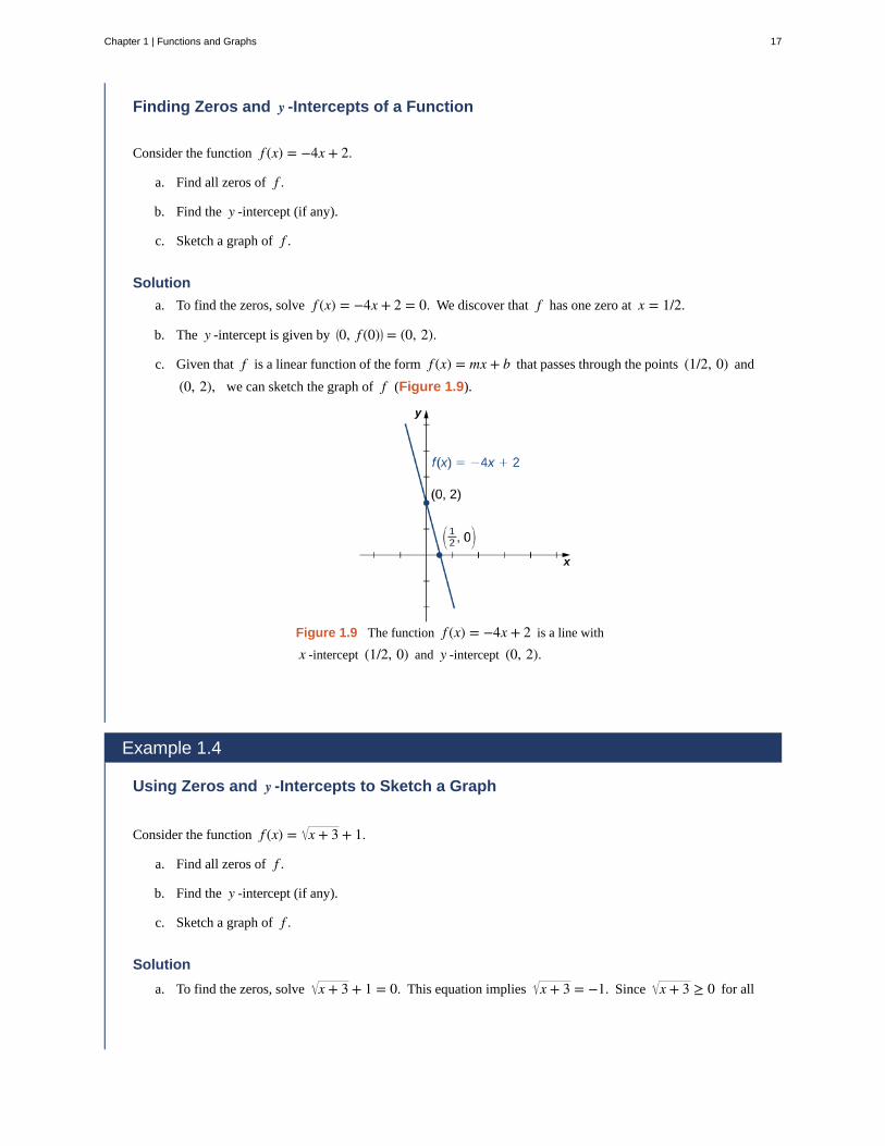
Consider the function f (x) = −4x + 2.
a. Find all zeros of f .
b. Find the y -intercept (if any).
c. Sketch a graph of f .
Solution
a. To find the zeros, solve f (x) = −4x + 2 = 0. We discover that f has one zero at x = 1/2.
b. The y -intercept is given by ⎛⎝0, f (0)⎞
⎠ = (0, 2).
c. Given that f is a linear function of the form f (x) = mx + b that passes through the points (1/2, 0) and
(0, 2), we can sketch the graph of f (Figure 1.9).
Figure 1.9 The function f (x) = −4x + 2 is a line with
x -intercept (1/2, 0) and y -intercept (0, 2).
Example 1.4
Using Zeros and y -Intercepts to Sketch a Graph
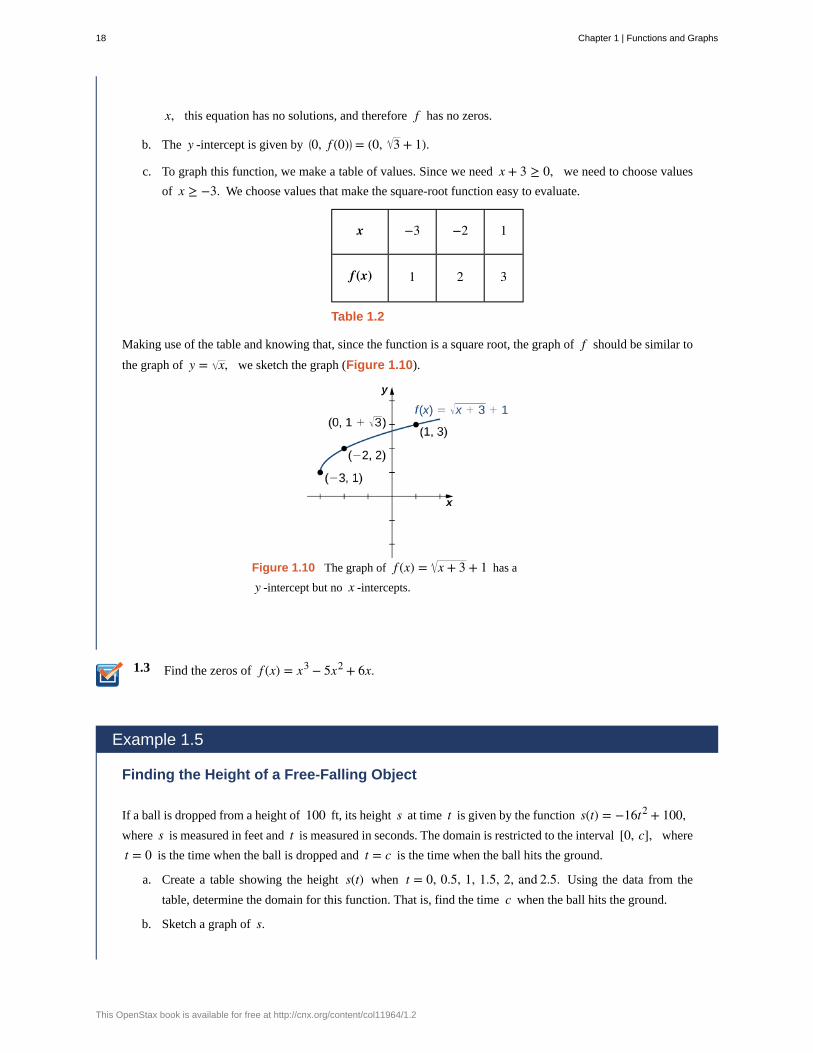
Consider the function f (x) = x + 3 + 1.
a. Find all zeros of f .
b. Find the y -intercept (if any).
c. Sketch a graph of f .
Solution
a. To find the zeros, solve x + 3 + 1 = 0. This equation implies x + 3 = −1. Since x + 3 ≥ 0 for all
Chapter 1 | Functions and Graphs 17
1.3
x, this equation has no solutions, and therefore f has no zeros.
b. The y -intercept is given by ⎛⎝0, f (0)⎞
⎠ = (0, 3 + 1).
c. To graph this function, we make a table of values. Since we need x + 3 ≥ 0, we need to choose values
of x ≥ −3. We choose values that make the square-root function easy to evaluate.
x −3 −2 1
f (x) 1 2 3
Table 1.2
Making use of the table and knowing that, since the function is a square root, the graph of f should be similar to
the graph of y = x, we sketch the graph (Figure 1.10).
Figure 1.10 The graph of f (x) = x + 3 + 1 has a
y -intercept but no x -intercepts.
Find the zeros of f (x) = x3 − 5x2 + 6x.
Example 1.5
Finding the Height of a Free-Falling Object
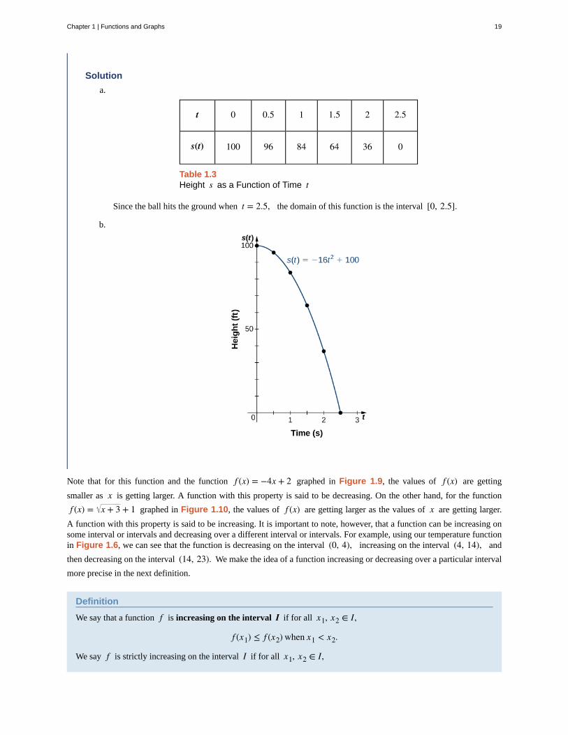
If a ball is dropped from a height of 100 ft, its height s at time t is given by the function s(t) = −16t2 + 100,where s is measured in feet and t is measured in seconds. The domain is restricted to the interval [0, c], where
t = 0 is the time when the ball is dropped and t = c is the time when the ball hits the ground.
a. Create a table showing the height s(t) when t = 0, 0.5, 1, 1.5, 2, and 2.5. Using the data from the
table, determine the domain for this function. That is, find the time c when the ball hits the ground.
b. Sketch a graph of s.
18 Chapter 1 | Functions and Graphs
This OpenStax book is available for free at http://cnx.org/content/col11964/1.2
Solution
a.
t 0 0.5 1 1.5 2 2.5
s(t) 100 96 84 64 36 0
Table 1.3Height s as a Function of Time t
Since the ball hits the ground when t = 2.5, the domain of this function is the interval [0, 2.5].
b.
Note that for this function and the function f (x) = −4x + 2 graphed in Figure 1.9, the values of f (x) are getting
smaller as x is getting larger. A function with this property is said to be decreasing. On the other hand, for the function
f (x) = x + 3 + 1 graphed in Figure 1.10, the values of f (x) are getting larger as the values of x are getting larger.
A function with this property is said to be increasing. It is important to note, however, that a function can be increasing onsome interval or intervals and decreasing over a different interval or intervals. For example, using our temperature functionin Figure 1.6, we can see that the function is decreasing on the interval (0, 4), increasing on the interval (4, 14), and
then decreasing on the interval (14, 23). We make the idea of a function increasing or decreasing over a particular interval
more precise in the next definition.
Definition
We say that a function f is increasing on the interval I if for all x1, x2 ∈ I,
f (x1) ≤ f (x2) when x1 < x2.
We say f is strictly increasing on the interval I if for all x1, x2 ∈ I,
Chapter 1 | Functions and Graphs 19
f (x1) < f (x2) when x1 < x2.
We say that a function f is decreasing on the interval I if for all x1, x2 ∈ I,
f (x1) ≥ f (x2) if x1 < x2.
We say that a function f is strictly decreasing on the interval I if for all x1, x2 ∈ I,
f (x1) > f (x2) if x1 < x2.
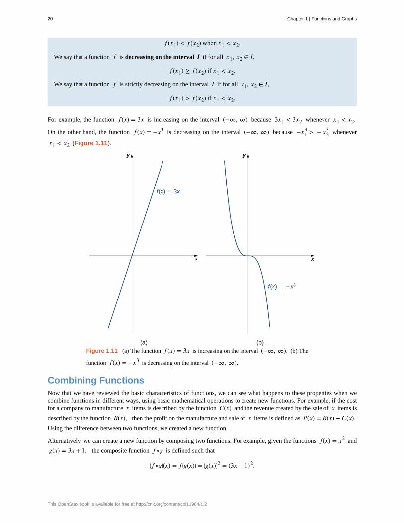
For example, the function f (x) = 3x is increasing on the interval (−∞, ∞) because 3x1 < 3x2 whenever x1 < x2.
On the other hand, the function f (x) = −x3 is decreasing on the interval (−∞, ∞) because −x13 > − x2
3 whenever
x1 < x2 (Figure 1.11).
Figure 1.11 (a) The function f (x) = 3x is increasing on the interval (−∞, ∞). (b) The
function f (x) = −x3 is decreasing on the interval (−∞, ∞).
Combining FunctionsNow that we have reviewed the basic characteristics of functions, we can see what happens to these properties when wecombine functions in different ways, using basic mathematical operations to create new functions. For example, if the costfor a company to manufacture x items is described by the function C(x) and the revenue created by the sale of x items is
described by the function R(x), then the profit on the manufacture and sale of x items is defined as P(x) = R(x) − C(x).Using the difference between two functions, we created a new function.
Alternatively, we can create a new function by composing two functions. For example, given the functions f (x) = x2 and
g(x) = 3x + 1, the composite function f ∘g is defined such that
⎛⎝ f ∘g⎞
⎠(x) = f ⎛⎝g(x)⎞
⎠ = ⎛⎝g(x)⎞
⎠2 = (3x + 1)2.
20 Chapter 1 | Functions and Graphs
This OpenStax book is available for free at http://cnx.org/content/col11964/1.2
1.4
The composite function g ∘ f is defined such that
⎛⎝g ∘ f ⎞
⎠(x) = g⎛⎝ f (x)⎞
⎠ = 3 f (x) + 1 = 3x2 + 1.
Note that these two new functions are different from each other.
Combining Functions with Mathematical Operators
To combine functions using mathematical operators, we simply write the functions with the operator and simplify. Giventwo functions f and g, we can define four new functions:
⎛⎝ f + g⎞
⎠(x) = f (x) + g(x) Sum⎛⎝ f − g⎞
⎠(x) = f (x) − g(x) Diffe ence⎛⎝ f · g⎞
⎠(x) = f (x)g(x) Product⎛⎝
fg
⎞⎠(x) = f (x)
g(x) for g(x) ≠ 0 Quotient
Example 1.6
Combining Functions Using Mathematical Operations
Given the functions f (x) = 2x − 3 and g(x) = x2 − 1, find each of the following functions and state its
domain.
a. ( f + g)(x)
b. ( f − g)(x)
c. ( f · g)(x)
d.⎛⎝
fg
⎞⎠(x)
Solution
a. ⎛⎝ f + g⎞
⎠(x) = (2x − 3) + (x2 − 1) = x2 + 2x − 4. The domain of this function is the interval (−∞, ∞).
b. ⎛⎝ f − g⎞
⎠(x) = (2x − 3) − (x2 − 1) = −x2 + 2x − 2. The domain of this function is the interval
(−∞, ∞).
c. ⎛⎝ f · g⎞
⎠(x) = (2x − 3)(x2 − 1) = 2x3 − 3x2 − 2x + 3. The domain of this function is the interval
(−∞, ∞).
d.⎛⎝
fg
⎞⎠(x) = 2x − 3
x2 − 1. The domain of this function is {x|x ≠ ±1}.
For f (x) = x2 + 3 and g(x) = 2x − 5, find ⎛⎝ f /g⎞
⎠(x) and state its domain.
Function Composition
When we compose functions, we take a function of a function. For example, suppose the temperature T on a given day is
described as a function of time t (measured in hours after midnight) as in Table 1.1. Suppose the cost C, to heat or cool
a building for 1 hour, can be described as a function of the temperature T . Combining these two functions, we can describe
Chapter 1 | Functions and Graphs 21
the cost of heating or cooling a building as a function of time by evaluating C⎛⎝T(t)⎞
⎠. We have defined a new function,
denoted C ∘T , which is defined such that (C ∘T)(t) = C(T(t)) for all t in the domain of T . This new function is called
a composite function. We note that since cost is a function of temperature and temperature is a function of time, it makessense to define this new function (C ∘T)(t). It does not make sense to consider (T ∘C)(t), because temperature is not a
function of cost.
Definition
Consider the function f with domain A and range B, and the function g with domain D and range E. If B is a
subset of D, then the composite function (g ∘ f )(x) is the function with domain A such that
(1.1)⎛⎝g ∘ f ⎞
⎠(x) = g⎛⎝ f (x)⎞
⎠.
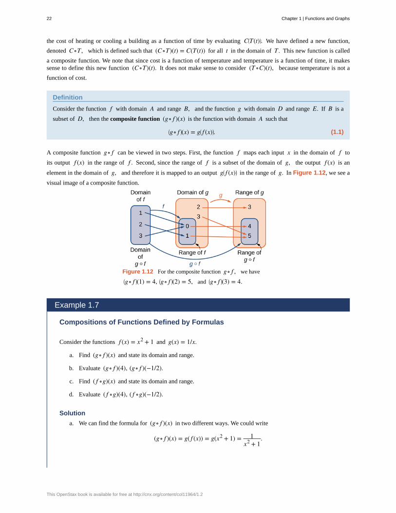
A composite function g ∘ f can be viewed in two steps. First, the function f maps each input x in the domain of f to
its output f (x) in the range of f . Second, since the range of f is a subset of the domain of g, the output f (x) is an
element in the domain of g, and therefore it is mapped to an output g⎛⎝ f (x)⎞
⎠ in the range of g. In Figure 1.12, we see a
visual image of a composite function.
Figure 1.12 For the composite function g ∘ f , we have⎛⎝g ∘ f ⎞
⎠(1) = 4, ⎛⎝g ∘ f ⎞
⎠(2) = 5, and ⎛⎝g ∘ f ⎞
⎠(3) = 4.
Example 1.7
Compositions of Functions Defined by Formulas
Consider the functions f (x) = x2 + 1 and g(x) = 1/x.
a. Find (g ∘ f )(x) and state its domain and range.
b. Evaluate (g ∘ f )(4), (g ∘ f )(−1/2).
c. Find ( f ∘g)(x) and state its domain and range.
d. Evaluate ( f ∘g)(4), ( f ∘g)(−1/2).
Solution
a. We can find the formula for (g ∘ f )(x) in two different ways. We could write
(g ∘ f )(x) = g( f (x)) = g(x2 + 1) = 1x2 + 1
.
22 Chapter 1 | Functions and Graphs
This OpenStax book is available for free at http://cnx.org/content/col11964/1.2
Alternatively, we could write
(g ∘ f )(x) = g⎛⎝ f (x)⎞
⎠ = 1f (x) = 1
x2 + 1.
Since x2 + 1 ≠ 0 for all real numbers x, the domain of (g ∘ f )(x) is the set of all real numbers. Since
0 < 1/(x2 + 1) ≤ 1, the range is, at most, the interval (0, 1]. To show that the range is this entire
interval, we let y = 1/(x2 + 1) and solve this equation for x to show that for all y in the interval
(0, 1], there exists a real number x such that y = 1/(x2 + 1). Solving this equation for x, we see
that x2 + 1 = 1/y, which implies that
x = ± 1y − 1.
If y is in the interval (0, 1], the expression under the radical is nonnegative, and therefore there exists
a real number x such that 1/(x2 + 1) = y. We conclude that the range of g ∘ f is the interval (0, 1].
b. (g ∘ f )(4) = g( f (4)) = g(42 + 1) = g(17) = 117
(g ∘ f )⎛⎝−
12
⎞⎠ = g⎛
⎝ f ⎛⎝−
12
⎞⎠⎞⎠ = g
⎛
⎝⎜⎛⎝−
12
⎞⎠2
+ 1⎞
⎠⎟ = g⎛
⎝54
⎞⎠ = 4
5
c. We can find a formula for ( f ∘g)(x) in two ways. First, we could write
( f ∘g)(x) = f (g(x)) = f ⎛⎝1x
⎞⎠ = ⎛
⎝1x
⎞⎠2
+ 1.
Alternatively, we could write
( f ∘g)(x) = f (g(x)) = (g(x))2 + 1 = ⎛⎝1x
⎞⎠2
+ 1.
The domain of f ∘g is the set of all real numbers x such that x ≠ 0. To find the range of f , we need
to find all values y for which there exists a real number x ≠ 0 such that
⎛⎝1x
⎞⎠2
+ 1 = y.
Solving this equation for x, we see that we need x to satisfy
⎛⎝1x
⎞⎠2
= y − 1,
which simplifies to
1x = ± y − 1.
Finally, we obtain
Chapter 1 | Functions and Graphs 23
1.5
x = ± 1y − 1
.
Since 1/ y − 1 is a real number if and only if y > 1, the range of f is the set ⎧
⎩⎨y|y ≥ 1⎫
⎭⎬.
d. ( f ∘g)(4) = f (g(4)) = f ⎛⎝14
⎞⎠ = ⎛
⎝14
⎞⎠2
+ 1 = 1716
( f ∘g)⎛⎝−
12
⎞⎠ = f ⎛
⎝g⎛⎝−
12
⎞⎠⎞⎠ = f (−2) = (−2)2 + 1 = 5
In Example 1.7, we can see that ⎛⎝ f ∘g⎞
⎠(x) ≠ ⎛⎝g ∘ f ⎞
⎠(x). This tells us, in general terms, that the order in which we compose
functions matters.
Let f (x) = 2 − 5x. Let g(x) = x. Find ⎛⎝ f ∘g⎞
⎠(x).
Example 1.8
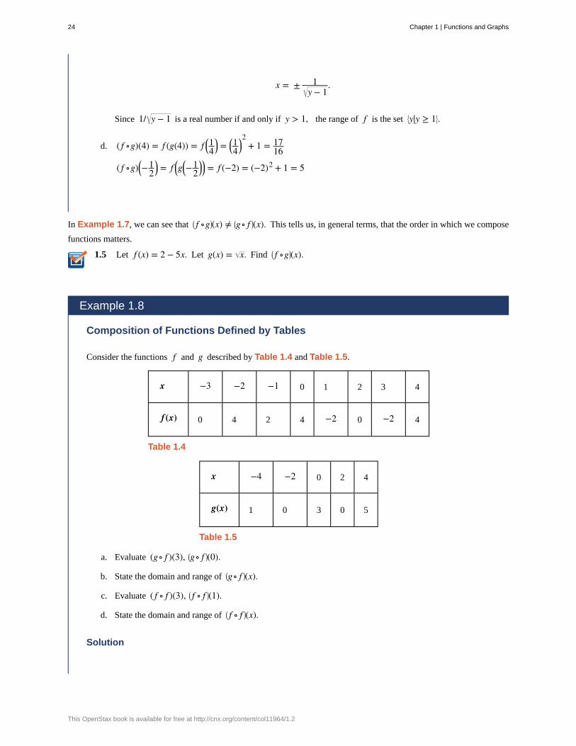
Composition of Functions Defined by Tables
Consider the functions f and g described by Table 1.4 and Table 1.5.
x −3 −2 −1 0 1 2 3 4
f (x) 0 4 2 4 −2 0 −2 4
Table 1.4
x −4 −2 0 2 4
g(x) 1 0 3 0 5
Table 1.5
a. Evaluate (g ∘ f )(3), ⎛⎝g ∘ f ⎞
⎠(0).
b. State the domain and range of ⎛⎝g ∘ f ⎞
⎠(x).
c. Evaluate ( f ∘ f )(3), ⎛⎝ f ∘ f ⎞
⎠(1).
d. State the domain and range of ⎛⎝ f ∘ f ⎞
⎠(x).
Solution
24 Chapter 1 | Functions and Graphs
This OpenStax book is available for free at http://cnx.org/content/col11964/1.2
1.6
a. ⎛⎝g ∘ f ⎞
⎠(3) = g⎛⎝ f (3)⎞
⎠ = g(−2) = 0(g ∘ f )(0) = g(4) = 5
b. The domain of g ∘ f is the set {−3, −2, −1, 0, 1, 2, 3, 4}. Since the range of f is the set
{−2, 0, 2, 4}, the range of g ∘ f is the set {0, 3, 5}.
c. ⎛⎝ f ∘ f ⎞
⎠(3) = f ⎛⎝ f (3)⎞
⎠ = f (−2) = 4( f ∘ f )(1) = f ( f (1)) = f (−2) = 4
d. The domain of f ∘ f is the set {−3, −2, −1, 0, 1, 2, 3, 4}. Since the range of f is the set
{−2, 0, 2, 4}, the range of f ∘ f is the set {0, 4}.
Example 1.9
Application Involving a Composite Function
A store is advertising a sale of 20% off all merchandise. Caroline has a coupon that entitles her to an additional
15% off any item, including sale merchandise. If Caroline decides to purchase an item with an original price of
x dollars, how much will she end up paying if she applies her coupon to the sale price? Solve this problem by
using a composite function.
Solution
Since the sale price is 20% off the original price, if an item is x dollars, its sale price is given by f (x) = 0.80x.Since the coupon entitles an individual to 15% off the price of any item, if an item is y dollars, the price, after
applying the coupon, is given by g(y) = 0.85y. Therefore, if the price is originally x dollars, its sale price will
be f (x) = 0.80x and then its final price after the coupon will be g( f (x)) = 0.85(0.80x) = 0.68x.
If items are on sale for 10% off their original price, and a customer has a coupon for an additional 30%off, what will be the final price for an item that is originally x dollars, after applying the coupon to the sale
price?
Symmetry of FunctionsThe graphs of certain functions have symmetry properties that help us understand the function and the shape of its graph.
For example, consider the function f (x) = x4 − 2x2 − 3 shown in Figure 1.13(a). If we take the part of the curve that
lies to the right of the y-axis and flip it over the y-axis, it lays exactly on top of the curve to the left of the y-axis. In this
case, we say the function has symmetry about the y-axis. On the other hand, consider the function f (x) = x3 − 4x shown
in Figure 1.13(b). If we take the graph and rotate it 180° about the origin, the new graph will look exactly the same. In
this case, we say the function has symmetry about the origin.
Chapter 1 | Functions and Graphs 25
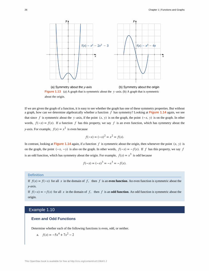
Figure 1.13 (a) A graph that is symmetric about the y -axis. (b) A graph that is symmetric
about the origin.
If we are given the graph of a function, it is easy to see whether the graph has one of these symmetry properties. But withouta graph, how can we determine algebraically whether a function f has symmetry? Looking at Figure 1.14 again, we see
that since f is symmetric about the y -axis, if the point (x, y) is on the graph, the point (−x, y) is on the graph. In other
words, f (−x) = f (x). If a function f has this property, we say f is an even function, which has symmetry about the
y-axis. For example, f (x) = x2 is even because
f (−x) = (−x)2 = x2 = f (x).
In contrast, looking at Figure 1.14 again, if a function f is symmetric about the origin, then whenever the point (x, y) is
on the graph, the point (−x, −y) is also on the graph. In other words, f (−x) = − f (x). If f has this property, we say f
is an odd function, which has symmetry about the origin. For example, f (x) = x3 is odd because
f (−x) = (−x)3 = −x3 = − f (x).
Definition
If f (x) = f (−x) for all x in the domain of f , then f is an even function. An even function is symmetric about the
y-axis.
If f (−x) = − f (x) for all x in the domain of f , then f is an odd function. An odd function is symmetric about the
origin.
Example 1.10
Even and Odd Functions
Determine whether each of the following functions is even, odd, or neither.
a. f (x) = −5x4 + 7x2 − 2
26 Chapter 1 | Functions and Graphs
This OpenStax book is available for free at http://cnx.org/content/col11964/1.2
1.7
b. f (x) = 2x5 − 4x + 5
c. f (x) = 3xx2 + 1
Solution
To determine whether a function is even or odd, we evaluate f (−x) and compare it to f(x) and − f (x).
a. f (−x) = −5(−x)4 + 7(−x)2 − 2 = −5x4 + 7x2 − 2 = f (x). Therefore, f is even.
b. f (−x) = 2(−x)5 − 4(−x) + 5 = −2x5 + 4x + 5. Now, f (−x) ≠ f (x). Furthermore, noting that
− f (x) = −2x5 + 4x − 5, we see that f (−x) ≠ − f (x). Therefore, f is neither even nor odd.
c. f (−x) = 3(−x)/((−x)2 + 1} = −3x/(x2 + 1) = −[3x/(x2 + 1)] = − f (x). Therefore, f is odd.
Determine whether f (x) = 4x3 − 5x is even, odd, or neither.
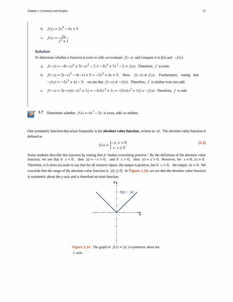
One symmetric function that arises frequently is the absolute value function, written as |x|. The absolute value function is
defined as
(1.2)f (x) =⎧
⎩⎨−x, x < 0x, x ≥ 0
.
Some students describe this function by stating that it “makes everything positive.” By the definition of the absolute valuefunction, we see that if x < 0, then |x| = −x > 0, and if x > 0, then |x| = x > 0. However, for x = 0, |x| = 0.Therefore, it is more accurate to say that for all nonzero inputs, the output is positive, but if x = 0, the output |x| = 0. We
conclude that the range of the absolute value function is ⎧
⎩⎨y|y ≥ 0⎫
⎭⎬. In Figure 1.14, we see that the absolute value function
is symmetric about the y-axis and is therefore an even function.
Figure 1.14 The graph of f (x) = |x| is symmetric about the
y -axis.
Chapter 1 | Functions and Graphs 27
1.8
Example 1.11
Working with the Absolute Value Function
Find the domain and range of the function f (x) = 2|x − 3| + 4.
Solution
Since the absolute value function is defined for all real numbers, the domain of this function is (−∞, ∞). Since
|x − 3| ≥ 0 for all x, the function f (x) = 2|x − 3| + 4 ≥ 4. Therefore, the range is, at most, the set ⎧
⎩⎨y|y ≥ 4⎫
⎭⎬.
To see that the range is, in fact, this whole set, we need to show that for y ≥ 4 there exists a real number x such
that
2|x − 3| + 4 = y.
A real number x satisfies this equation as long as
|x − 3| = 12(y − 4).
Since y ≥ 4, we know y − 4 ≥ 0, and thus the right-hand side of the equation is nonnegative, so it is possible
that there is a solution. Furthermore,
|x − 3| =⎧
⎩⎨−(x − 3) if x < 3x − 3 if x ≥ 3
.
Therefore, we see there are two solutions:
x = ± 12(y − 4) + 3.
The range of this function is ⎧
⎩⎨y|y ≥ 4⎫
⎭⎬.
For the function f (x) = |x + 2| − 4, find the domain and range.
28 Chapter 1 | Functions and Graphs
This OpenStax book is available for free at http://cnx.org/content/col11964/1.2
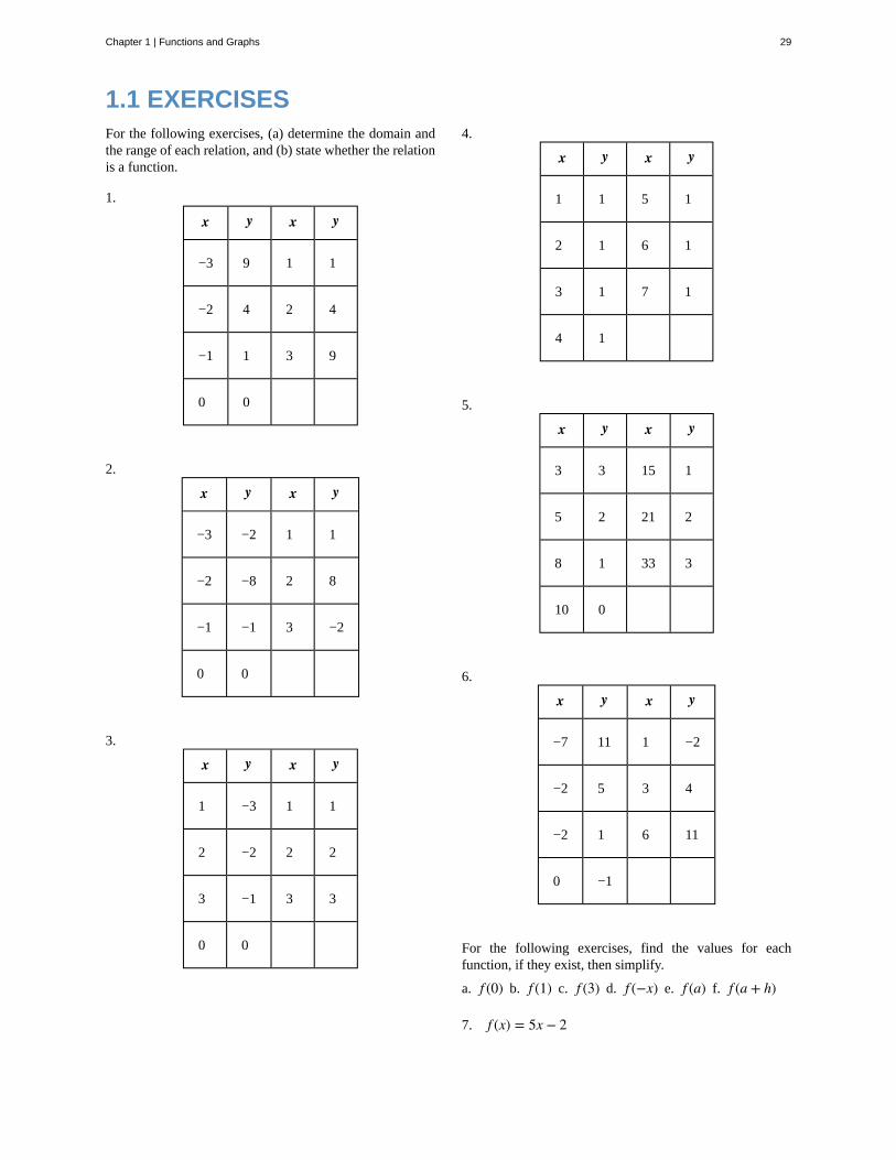
1.1 EXERCISESFor the following exercises, (a) determine the domain andthe range of each relation, and (b) state whether the relationis a function.
1.
x y x y
−3 9 1 1
−2 4 2 4
−1 1 3 9
0 0
2.
x y x y
−3 −2 1 1
−2 −8 2 8
−1 −1 3 −2
0 0
3.
x y x y
1 −3 1 1
2 −2 2 2
3 −1 3 3
0 0
4.
x y x y
1 1 5 1
2 1 6 1
3 1 7 1
4 1
5.
x y x y
3 3 15 1
5 2 21 2
8 1 33 3
10 0
6.
x y x y
−7 11 1 −2
−2 5 3 4
−2 1 6 11
0 −1
For the following exercises, find the values for eachfunction, if they exist, then simplify.
a. f (0) b. f (1) c. f (3) d. f (−x) e. f (a) f. f (a + h)
7. f (x) = 5x − 2
Chapter 1 | Functions and Graphs 29
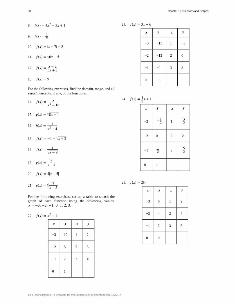
8. f (x) = 4x2 − 3x + 1
9. f (x) = 2x
10. f (x) = |x − 7| + 8
11. f (x) = 6x + 5
12. f (x) = x − 23x + 7
13. f (x) = 9
For the following exercises, find the domain, range, and allzeros/intercepts, if any, of the functions.
14. f (x) = xx2 − 16
15. g(x) = 8x − 1
16. h(x) = 3x2 + 4
17. f (x) = −1 + x + 2
18. f (x) = 1x − 9
19. g(x) = 3x − 4
20. f (x) = 4|x + 5|
21. g(x) = 7x − 5
For the following exercises, set up a table to sketch thegraph of each function using the following values:x = −3, −2, −1, 0, 1, 2, 3.
22. f (x) = x2 + 1
x y x y
−3 10 1 2
−2 5 2 5
−1 2 3 10
0 1
23. f (x) = 3x − 6
x y x y
−3 −15 1 −3
−2 −12 2 0
−1 −9 3 3
0 −6
24. f (x) = 12x + 1
x y x y
−3 −12 1
32
−2 0 2 2
−112 3
52
0 1
25. f (x) = 2|x|
x y x y
−3 6 1 2
−2 4 2 4
−1 2 3 6
0 0
30 Chapter 1 | Functions and Graphs
This OpenStax book is available for free at http://cnx.org/content/col11964/1.2
26. f (x) = −x2
x y x y
−3 −9 1 −1
−2 −4 2 −4
−1 −1 3 −9
0 0
27. f (x) = x3
x y x y
−3 −27 1 1
−2 −8 2 8
−1 −1 3 27
0 0
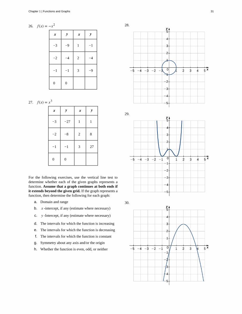
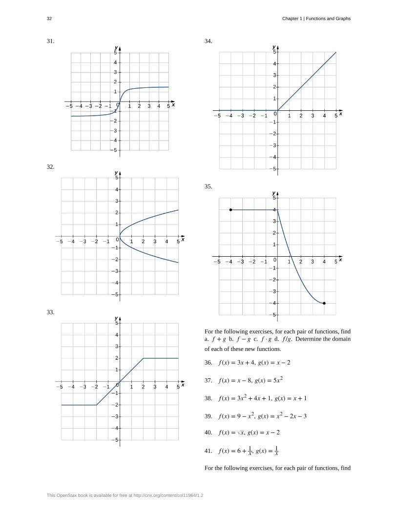
For the following exercises, use the vertical line test todetermine whether each of the given graphs represents afunction. Assume that a graph continues at both ends ifit extends beyond the given grid. If the graph represents afunction, then determine the following for each graph:
a. Domain and range
b. x -intercept, if any (estimate where necessary)
c. y -Intercept, if any (estimate where necessary)
d. The intervals for which the function is increasing
e. The intervals for which the function is decreasing
f. The intervals for which the function is constant
g. Symmetry about any axis and/or the origin
h. Whether the function is even, odd, or neither
28.
29.
30.
Chapter 1 | Functions and Graphs 31
31.
32.
33.
34.
35.
For the following exercises, for each pair of functions, finda. f + g b. f − g c. f · g d. f /g. Determine the domain
of each of these new functions.
36. f (x) = 3x + 4, g(x) = x − 2
37. f (x) = x − 8, g(x) = 5x2
38. f (x) = 3x2 + 4x + 1, g(x) = x + 1
39. f (x) = 9 − x2, g(x) = x2 − 2x − 3
40. f (x) = x, g(x) = x − 2
41. f (x) = 6 + 1x , g(x) = 1
x
For the following exercises, for each pair of functions, find
32 Chapter 1 | Functions and Graphs
This OpenStax book is available for free at http://cnx.org/content/col11964/1.2
a. ⎛⎝ f ∘g⎞
⎠(x) and b. ⎛⎝g ∘ f ⎞
⎠(x) Simplify the results. Find the
domain of each of the results.
42. f (x) = 3x, g(x) = x + 5
43. f (x) = x + 4, g(x) = 4x − 1
44. f (x) = 2x + 4, g(x) = x2 − 2
45. f (x) = x2 + 7, g(x) = x2 − 3
46. f (x) = x, g(x) = x + 9
47. f (x) = 32x + 1, g(x) = 2
x
48. f (x) = |x + 1|, g(x) = x2 + x − 4
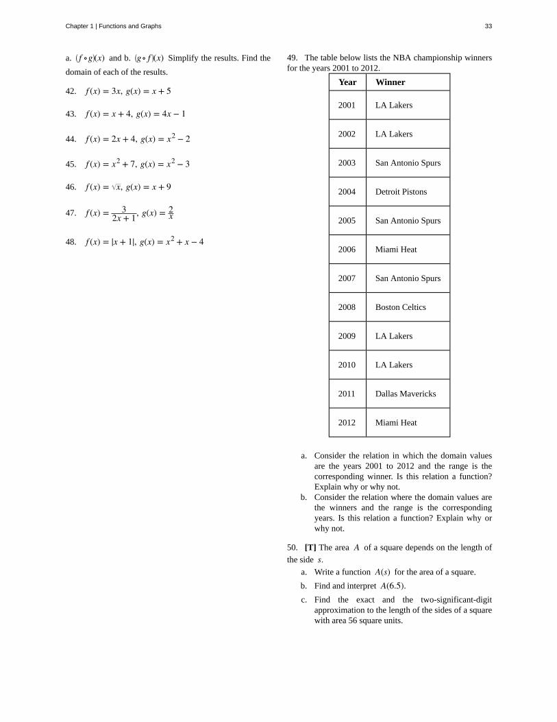
49. The table below lists the NBA championship winnersfor the years 2001 to 2012.
Year Winner
2001 LA Lakers
2002 LA Lakers
2003 San Antonio Spurs
2004 Detroit Pistons
2005 San Antonio Spurs
2006 Miami Heat
2007 San Antonio Spurs
2008 Boston Celtics
2009 LA Lakers
2010 LA Lakers
2011 Dallas Mavericks
2012 Miami Heat
a. Consider the relation in which the domain valuesare the years 2001 to 2012 and the range is thecorresponding winner. Is this relation a function?Explain why or why not.
b. Consider the relation where the domain values arethe winners and the range is the correspondingyears. Is this relation a function? Explain why orwhy not.
50. [T] The area A of a square depends on the length of
the side s.a. Write a function A(s) for the area of a square.
b. Find and interpret A(6.5).c. Find the exact and the two-significant-digit
approximation to the length of the sides of a squarewith area 56 square units.
Chapter 1 | Functions and Graphs 33
51. [T] The volume of a cube depends on the length of thesides s.
a. Write a function V(s) for the area of a square.
b. Find and interpret V(11.8).
52. [T] A rental car company rents cars for a flat fee of$20 and an hourly charge of $10.25. Therefore, the totalcost C to rent a car is a function of the hours t the car is
rented plus the flat fee.a. Write the formula for the function that models this
situation.b. Find the total cost to rent a car for 2 days and 7
hours.c. Determine how long the car was rented if the bill is
$432.73.
53. [T] A vehicle has a 20-gal tank and gets 15 mpg.The number of miles N that can be driven depends on theamount of gas x in the tank.
a. Write a formula that models this situation.b. Determine the number of miles the vehicle can
travel on (i) a full tank of gas and (ii) 3/4 of a tankof gas.
c. Determine the domain and range of the function.d. Determine how many times the driver had to stop
for gas if she has driven a total of 578 mi.
54. [T] The volume V of a sphere depends on the length of
its radius as V = (4/3)πr3. Because Earth is not a perfect
sphere, we can use the mean radius when measuring fromthe center to its surface. The mean radius is the averagedistance from the physical center to the surface, based ona large number of samples. Find the volume of Earth with
mean radius 6.371 × 10⁶ m.
55. [T] A certain bacterium grows in culture in a circularregion. The radius of the circle, measured in centimeters,
is given by r(t) = 6 − ⎡⎣5/⎛
⎝t2 + 1⎞⎠⎤⎦, where t is time
measured in hours since a circle of a 1-cm radius of thebacterium was put into the culture.
a. Express the area of the bacteria as a function oftime.
b. Find the exact and approximate area of the bacterialculture in 3 hours.
c. Express the circumference of the bacteria as afunction of time.
d. Find the exact and approximate circumference ofthe bacteria in 3 hours.
56. [T] An American tourist visits Paris and must convertU.S. dollars to Euros, which can be done using the functionE(x) = 0.79x, where x is the number of U.S. dollars and
E(x) is the equivalent number of Euros. Since conversion
rates fluctuate, when the tourist returns to the United States2 weeks later, the conversion from Euros to U.S. dollarsis D(x) = 1.245x, where x is the number of Euros and
D(x) is the equivalent number of U.S. dollars.
a. Find the composite function that converts directlyfrom U.S. dollars to U.S. dollars via Euros. Did thistourist lose value in the conversion process?
b. Use (a) to determine how many U.S. dollars thetourist would get back at the end of her trip if sheconverted an extra $200 when she arrived in Paris.
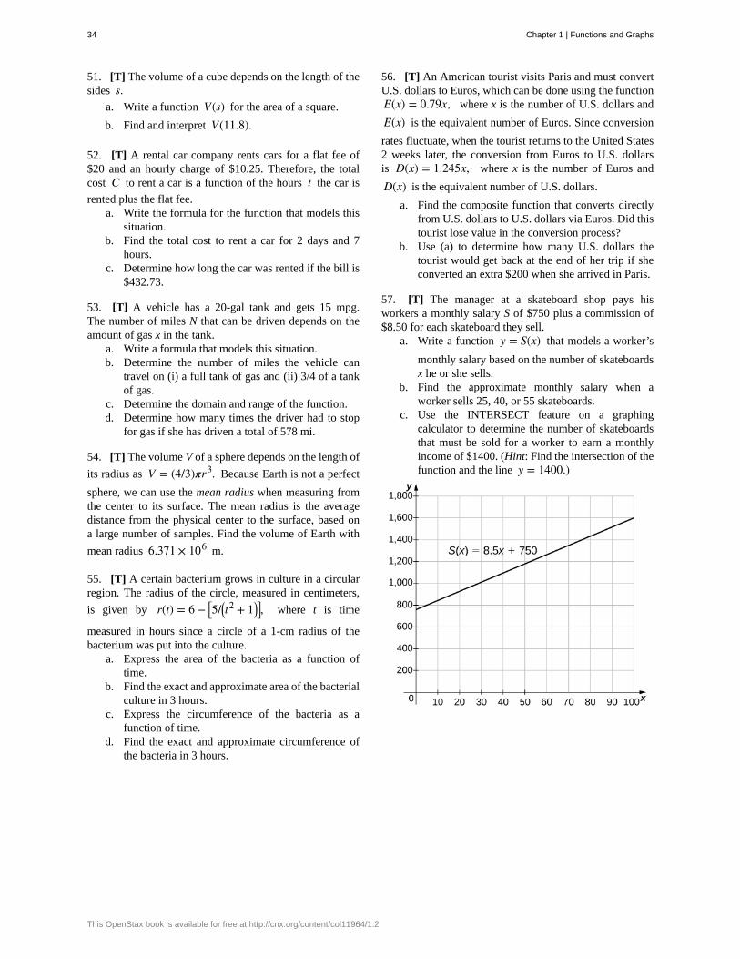
57. [T] The manager at a skateboard shop pays hisworkers a monthly salary S of $750 plus a commission of$8.50 for each skateboard they sell.
a. Write a function y = S(x) that models a worker’s
monthly salary based on the number of skateboardsx he or she sells.
b. Find the approximate monthly salary when aworker sells 25, 40, or 55 skateboards.
c. Use the INTERSECT feature on a graphingcalculator to determine the number of skateboardsthat must be sold for a worker to earn a monthlyincome of $1400. (Hint: Find the intersection of thefunction and the line y = 1400.)
34 Chapter 1 | Functions and Graphs
This OpenStax book is available for free at http://cnx.org/content/col11964/1.2
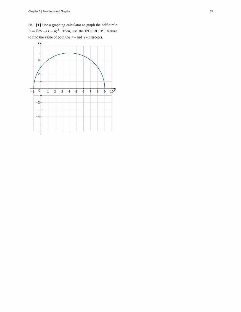
58. [T] Use a graphing calculator to graph the half-circle
y = 25 − (x − 4)2. Then, use the INTERCEPT feature
to find the value of both the x - and y -intercepts.
Chapter 1 | Functions and Graphs 35
1.2 | Basic Classes of Functions
Learning Objectives1.2.1 Calculate the slope of a linear function and interpret its meaning.
1.2.2 Recognize the degree of a polynomial.
1.2.3 Find the roots of a quadratic polynomial.
1.2.4 Describe the graphs of basic odd and even polynomial functions.
1.2.5 Identify a rational function.
1.2.6 Describe the graphs of power and root functions.
1.2.7 Explain the difference between algebraic and transcendental functions.
1.2.8 Graph a piecewise-defined function.
1.2.9 Sketch the graph of a function that has been shifted, stretched, or reflected from its initialgraph position.
We have studied the general characteristics of functions, so now let’s examine some specific classes of functions. Webegin by reviewing the basic properties of linear and quadratic functions, and then generalize to include higher-degreepolynomials. By combining root functions with polynomials, we can define general algebraic functions and distinguishthem from the transcendental functions we examine later in this chapter. We finish the section with examples of piecewise-defined functions and take a look at how to sketch the graph of a function that has been shifted, stretched, or reflected fromits initial form.
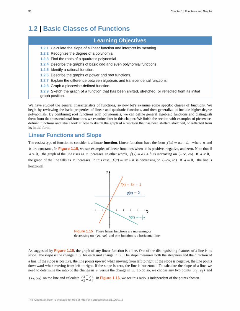
Linear Functions and SlopeThe easiest type of function to consider is a linear function. Linear functions have the form f (x) = ax + b, where a and
b are constants. In Figure 1.15, we see examples of linear functions when a is positive, negative, and zero. Note that if
a > 0, the graph of the line rises as x increases. In other words, f (x) = ax + b is increasing on (−∞, ∞). If a < 0,the graph of the line falls as x increases. In this case, f (x) = ax + b is decreasing on (−∞, ∞). If a = 0, the line is
horizontal.
Figure 1.15 These linear functions are increasing ordecreasing on (∞, ∞) and one function is a horizontal line.
As suggested by Figure 1.15, the graph of any linear function is a line. One of the distinguishing features of a line is itsslope. The slope is the change in y for each unit change in x. The slope measures both the steepness and the direction of
a line. If the slope is positive, the line points upward when moving from left to right. If the slope is negative, the line pointsdownward when moving from left to right. If the slope is zero, the line is horizontal. To calculate the slope of a line, weneed to determine the ratio of the change in y versus the change in x. To do so, we choose any two points (x1, y1) and
(x2, y2) on the line and calculatey2 − y1x2 − x1
. In Figure 1.16, we see this ratio is independent of the points chosen.
36 Chapter 1 | Functions and Graphs
This OpenStax book is available for free at http://cnx.org/content/col11964/1.2
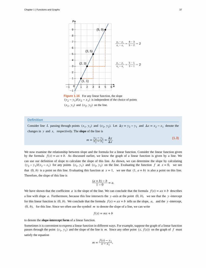
Figure 1.16 For any linear function, the slope(y2 − y1)/(x2 − x1) is independent of the choice of points
(x1, y1) and (x2, y2) on the line.
Definition
Consider line L passing through points (x1, y1) and (x2, y2). Let Δy = y2 − y1 and Δx = x2 − x1 denote the
changes in y and x, respectively. The slope of the line is
(1.3)m = y2 − y1x2 − x1
= ΔyΔx.
We now examine the relationship between slope and the formula for a linear function. Consider the linear function givenby the formula f (x) = ax + b. As discussed earlier, we know the graph of a linear function is given by a line. We
can use our definition of slope to calculate the slope of this line. As shown, we can determine the slope by calculating(y2 − y1)/(x2 − x1) for any points (x1, y1) and (x2, y2) on the line. Evaluating the function f at x = 0, we see
that (0, b) is a point on this line. Evaluating this function at x = 1, we see that (1, a + b) is also a point on this line.
Therefore, the slope of this line is
(a + b) − b1 − 0 = a.
We have shown that the coefficient a is the slope of the line. We can conclude that the formula f (x) = ax + b describes
a line with slope a. Furthermore, because this line intersects the y -axis at the point (0, b), we see that the y -intercept
for this linear function is (0, b). We conclude that the formula f (x) = ax + b tells us the slope, a, and the y -intercept,
(0, b), for this line. Since we often use the symbol m to denote the slope of a line, we can write
f (x) = mx + b
to denote the slope-intercept form of a linear function.
Sometimes it is convenient to express a linear function in different ways. For example, suppose the graph of a linear functionpasses through the point (x1, y1) and the slope of the line is m. Since any other point (x, f (x)) on the graph of f must
satisfy the equation
m = f (x) − y1x − x1
,
Chapter 1 | Functions and Graphs 37
this linear function can be expressed by writing
f (x) − y1 = m(x − x1).
We call this equation the point-slope equation for that linear function.
Since every nonvertical line is the graph of a linear function, the points on a nonvertical line can be described using theslope-intercept or point-slope equations. However, a vertical line does not represent the graph of a function and cannot beexpressed in either of these forms. Instead, a vertical line is described by the equation x = k for some constant k. Since
neither the slope-intercept form nor the point-slope form allows for vertical lines, we use the notation
ax + by = c,
where a, b are both not zero, to denote the standard form of a line.
Definition
Consider a line passing through the point (x1, y1) with slope m. The equation
(1.4)y − y1 = m(x − x1)
is the point-slope equation for that line.
Consider a line with slope m and y -intercept (0, b). The equation
(1.5)y = mx + b
is an equation for that line in slope-intercept form.
The standard form of a line is given by the equation
(1.6)ax + by = c,
where a and b are both not zero. This form is more general because it allows for a vertical line, x = k.
Example 1.12
Finding the Slope and Equations of Lines
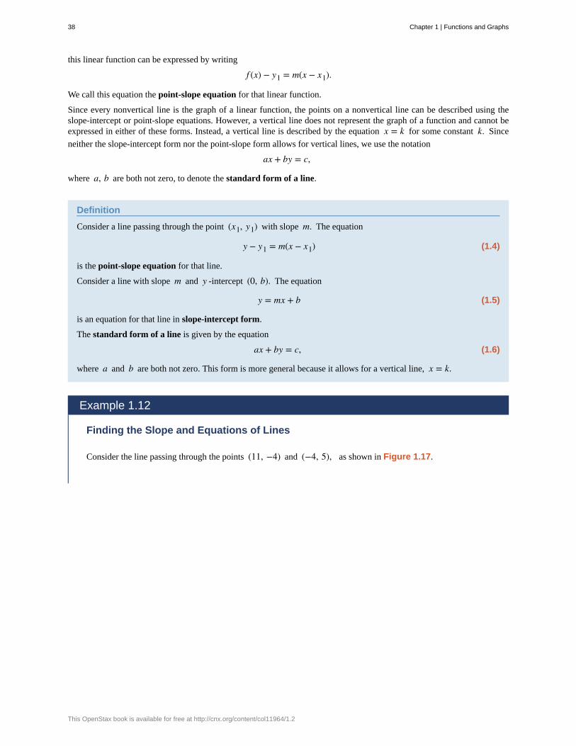
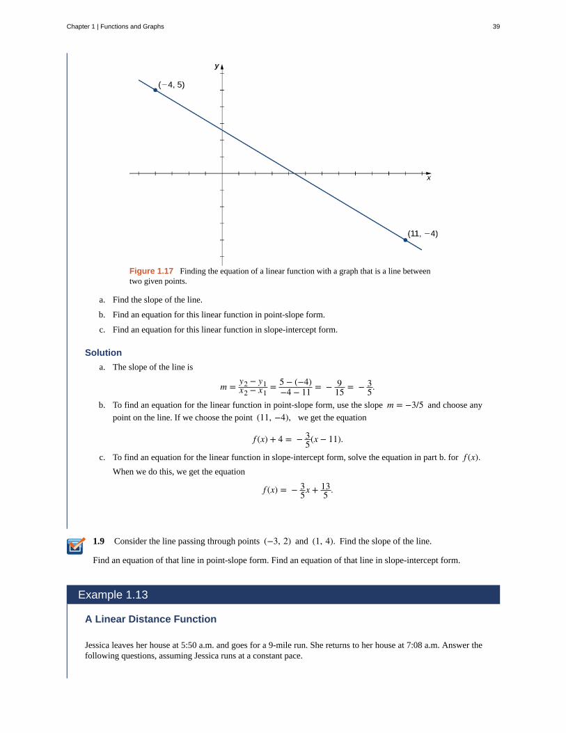
Consider the line passing through the points (11, −4) and (−4, 5), as shown in Figure 1.17.
38 Chapter 1 | Functions and Graphs
This OpenStax book is available for free at http://cnx.org/content/col11964/1.2
1.9
Figure 1.17 Finding the equation of a linear function with a graph that is a line betweentwo given points.
a. Find the slope of the line.
b. Find an equation for this linear function in point-slope form.
c. Find an equation for this linear function in slope-intercept form.
Solution
a. The slope of the line is
m = y2 − y1x2 − x1
= 5 − (−4)−4 − 11 = − 9
15 = − 35.
b. To find an equation for the linear function in point-slope form, use the slope m = −3/5 and choose any
point on the line. If we choose the point (11, −4), we get the equation
f (x) + 4 = − 35(x − 11).
c. To find an equation for the linear function in slope-intercept form, solve the equation in part b. for f (x).When we do this, we get the equation
f (x) = − 35x + 13
5 .
Consider the line passing through points (−3, 2) and (1, 4). Find the slope of the line.
Find an equation of that line in point-slope form. Find an equation of that line in slope-intercept form.
Example 1.13
A Linear Distance Function
Jessica leaves her house at 5:50 a.m. and goes for a 9-mile run. She returns to her house at 7:08 a.m. Answer thefollowing questions, assuming Jessica runs at a constant pace.
Chapter 1 | Functions and Graphs 39
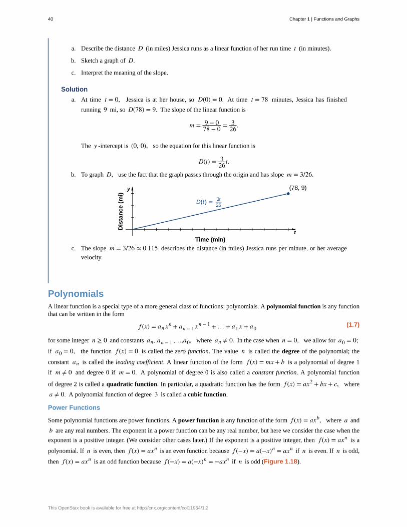
a. Describe the distance D (in miles) Jessica runs as a linear function of her run time t (in minutes).
b. Sketch a graph of D.
c. Interpret the meaning of the slope.
Solution
a. At time t = 0, Jessica is at her house, so D(0) = 0. At time t = 78 minutes, Jessica has finished
running 9 mi, so D(78) = 9. The slope of the linear function is
m = 9 − 078 − 0 = 3
26.
The y -intercept is (0, 0), so the equation for this linear function is
D(t) = 326t.
b. To graph D, use the fact that the graph passes through the origin and has slope m = 3/26.
c. The slope m = 3/26 ≈ 0.115 describes the distance (in miles) Jessica runs per minute, or her average
velocity.
PolynomialsA linear function is a special type of a more general class of functions: polynomials. A polynomial function is any functionthat can be written in the form
(1.7)f (x) = an xn + an − 1 xn − 1 + … + a1 x + a0
for some integer n ≥ 0 and constants an, an − 1 ,…,a0, where an ≠ 0. In the case when n = 0, we allow for a0 = 0;if a0 = 0, the function f (x) = 0 is called the zero function. The value n is called the degree of the polynomial; the
constant an is called the leading coefficient. A linear function of the form f (x) = mx + b is a polynomial of degree 1
if m ≠ 0 and degree 0 if m = 0. A polynomial of degree 0 is also called a constant function. A polynomial function
of degree 2 is called a quadratic function. In particular, a quadratic function has the form f (x) = ax2 + bx + c, where
a ≠ 0. A polynomial function of degree 3 is called a cubic function.
Power Functions
Some polynomial functions are power functions. A power function is any function of the form f (x) = axb, where a and
b are any real numbers. The exponent in a power function can be any real number, but here we consider the case when the
exponent is a positive integer. (We consider other cases later.) If the exponent is a positive integer, then f (x) = axn is a
polynomial. If n is even, then f (x) = axn is an even function because f (−x) = a(−x)n = axn if n is even. If n is odd,
then f (x) = axn is an odd function because f (−x) = a(−x)n = −axn if n is odd (Figure 1.18).
40 Chapter 1 | Functions and Graphs
This OpenStax book is available for free at http://cnx.org/content/col11964/1.2
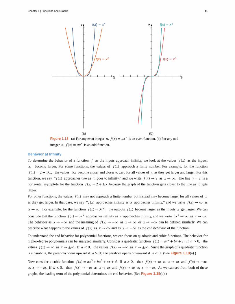
Figure 1.18 (a) For any even integer n, f (x) = axn is an even function. (b) For any odd
integer n, f (x) = axn is an odd function.
Behavior at Infinity
To determine the behavior of a function f as the inputs approach infinity, we look at the values f (x) as the inputs,
x, become larger. For some functions, the values of f (x) approach a finite number. For example, for the function
f (x) = 2 + 1/x, the values 1/x become closer and closer to zero for all values of x as they get larger and larger. For this
function, we say “ f (x) approaches two as x goes to infinity,” and we write f (x) → 2 as x → ∞. The line y = 2 is a
horizontal asymptote for the function f (x) = 2 + 1/x because the graph of the function gets closer to the line as x gets
larger.
For other functions, the values f (x) may not approach a finite number but instead may become larger for all values of xas they get larger. In that case, we say “ f (x) approaches infinity as x approaches infinity,” and we write f (x) → ∞ as
x → ∞. For example, for the function f (x) = 3x2, the outputs f (x) become larger as the inputs x get larger. We can
conclude that the function f (x) = 3x2 approaches infinity as x approaches infinity, and we write 3x2 → ∞ as x → ∞.The behavior as x → −∞ and the meaning of f (x) → −∞ as x → ∞ or x → −∞ can be defined similarly. We can
describe what happens to the values of f (x) as x → ∞ and as x → −∞ as the end behavior of the function.
To understand the end behavior for polynomial functions, we can focus on quadratic and cubic functions. The behavior for
higher-degree polynomials can be analyzed similarly. Consider a quadratic function f (x) = ax2 + bx + c. If a > 0, the
values f (x) → ∞ as x → ±∞. If a < 0, the values f (x) → −∞ as x → ±∞. Since the graph of a quadratic function
is a parabola, the parabola opens upward if a > 0; the parabola opens downward if a < 0. (See Figure 1.19(a).)
Now consider a cubic function f (x) = ax3 + bx2 + cx + d. If a > 0, then f (x) → ∞ as x → ∞ and f (x) → −∞as x → −∞. If a < 0, then f (x) → −∞ as x → ∞ and f (x) → ∞ as x → −∞. As we can see from both of these
graphs, the leading term of the polynomial determines the end behavior. (See Figure 1.19(b).)
Chapter 1 | Functions and Graphs 41
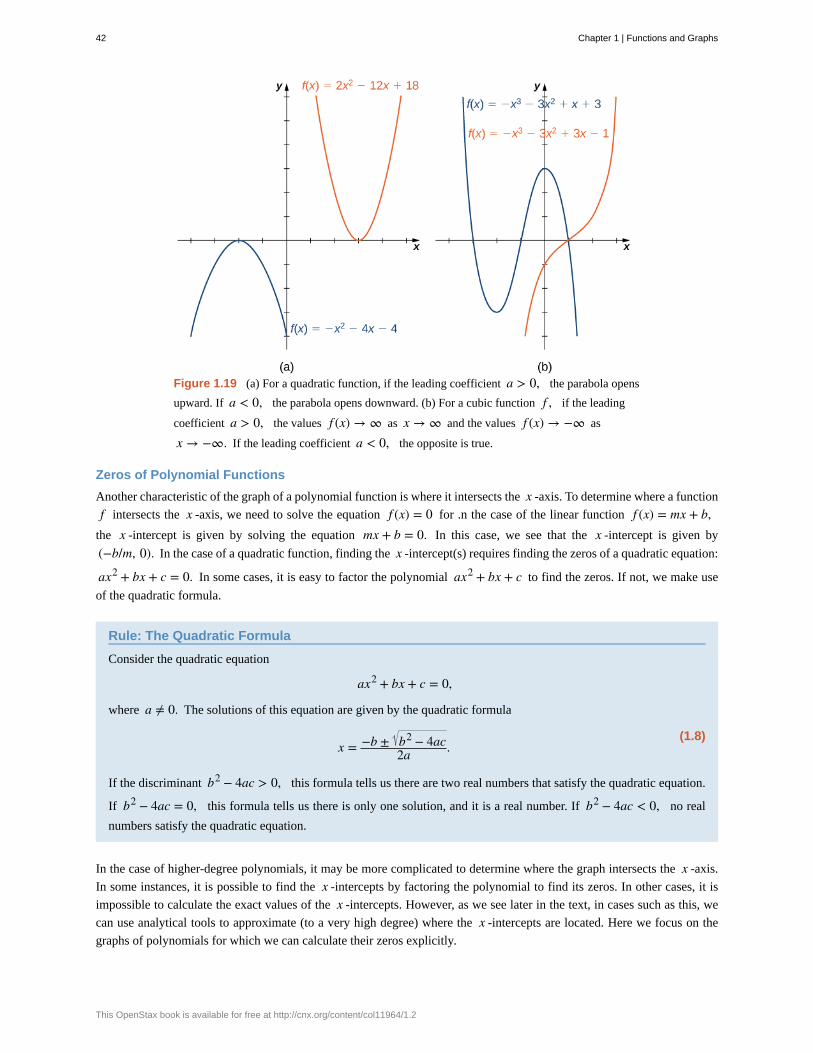
Figure 1.19 (a) For a quadratic function, if the leading coefficient a > 0, the parabola opens
upward. If a < 0, the parabola opens downward. (b) For a cubic function f , if the leading
coefficient a > 0, the values f (x) → ∞ as x → ∞ and the values f (x) → −∞ as
x → −∞. If the leading coefficient a < 0, the opposite is true.
Zeros of Polynomial Functions
Another characteristic of the graph of a polynomial function is where it intersects the x -axis. To determine where a function
f intersects the x -axis, we need to solve the equation f (x) = 0 for .n the case of the linear function f (x) = mx + b,the x -intercept is given by solving the equation mx + b = 0. In this case, we see that the x -intercept is given by
(−b/m, 0). In the case of a quadratic function, finding the x -intercept(s) requires finding the zeros of a quadratic equation:
ax2 + bx + c = 0. In some cases, it is easy to factor the polynomial ax2 + bx + c to find the zeros. If not, we make use
of the quadratic formula.
Rule: The Quadratic Formula
Consider the quadratic equation
ax2 + bx + c = 0,
where a ≠ 0. The solutions of this equation are given by the quadratic formula
(1.8)x = −b ± b2 − 4ac
2a .
If the discriminant b2 − 4ac > 0, this formula tells us there are two real numbers that satisfy the quadratic equation.
If b2 − 4ac = 0, this formula tells us there is only one solution, and it is a real number. If b2 − 4ac < 0, no real
numbers satisfy the quadratic equation.
In the case of higher-degree polynomials, it may be more complicated to determine where the graph intersects the x -axis.
In some instances, it is possible to find the x -intercepts by factoring the polynomial to find its zeros. In other cases, it is
impossible to calculate the exact values of the x -intercepts. However, as we see later in the text, in cases such as this, we
can use analytical tools to approximate (to a very high degree) where the x -intercepts are located. Here we focus on the
graphs of polynomials for which we can calculate their zeros explicitly.
42 Chapter 1 | Functions and Graphs
This OpenStax book is available for free at http://cnx.org/content/col11964/1.2
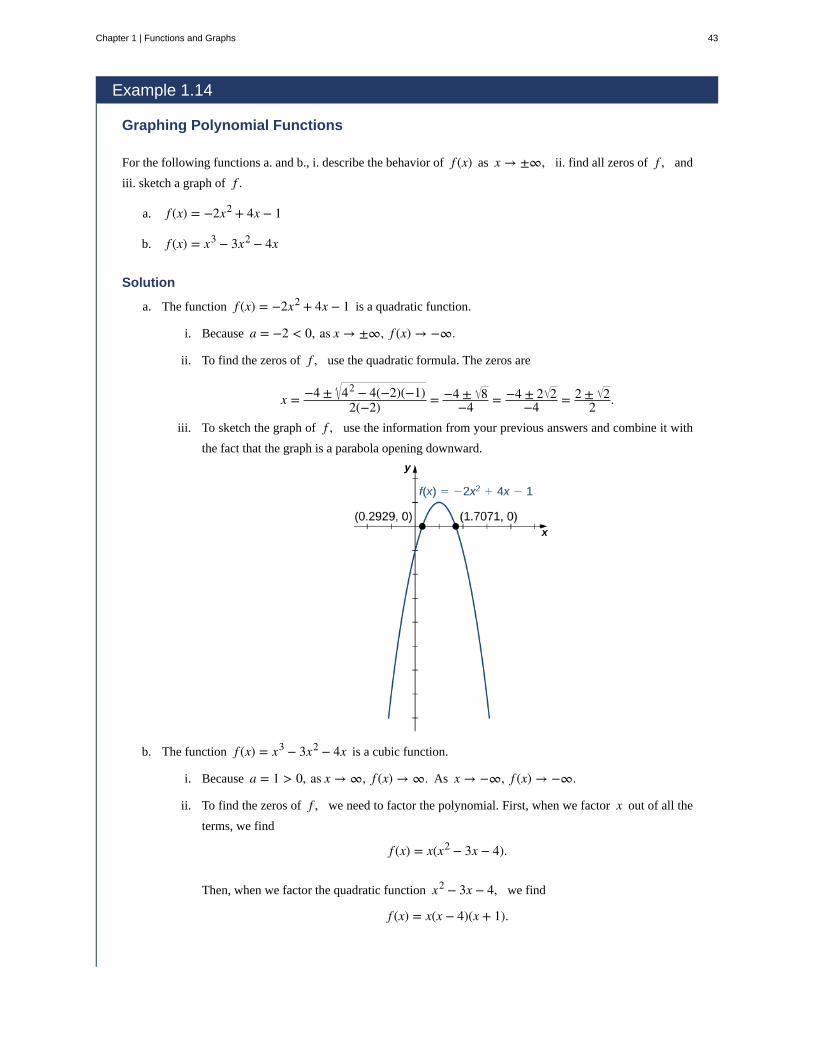
Example 1.14
Graphing Polynomial Functions
For the following functions a. and b., i. describe the behavior of f (x) as x → ±∞, ii. find all zeros of f , and
iii. sketch a graph of f .
a. f (x) = −2x2 + 4x − 1
b. f (x) = x3 − 3x2 − 4x
Solution
a. The function f (x) = −2x2 + 4x − 1 is a quadratic function.
i. Because a = −2 < 0, as x → ±∞, f (x) → −∞.
ii. To find the zeros of f , use the quadratic formula. The zeros are
x = −4 ± 42 − 4(−2)(−1)2(−2) = −4 ± 8
−4 = −4 ± 2 2−4 = 2 ± 2
2 .
iii. To sketch the graph of f , use the information from your previous answers and combine it with
the fact that the graph is a parabola opening downward.
b. The function f (x) = x3 − 3x2 − 4x is a cubic function.
i. Because a = 1 > 0, as x → ∞, f (x) → ∞. As x → −∞, f (x) → −∞.
ii. To find the zeros of f , we need to factor the polynomial. First, when we factor x out of all the
terms, we find
f (x) = x(x2 − 3x − 4).
Then, when we factor the quadratic function x2 − 3x − 4, we find
f (x) = x(x − 4)(x + 1).
Chapter 1 | Functions and Graphs 43
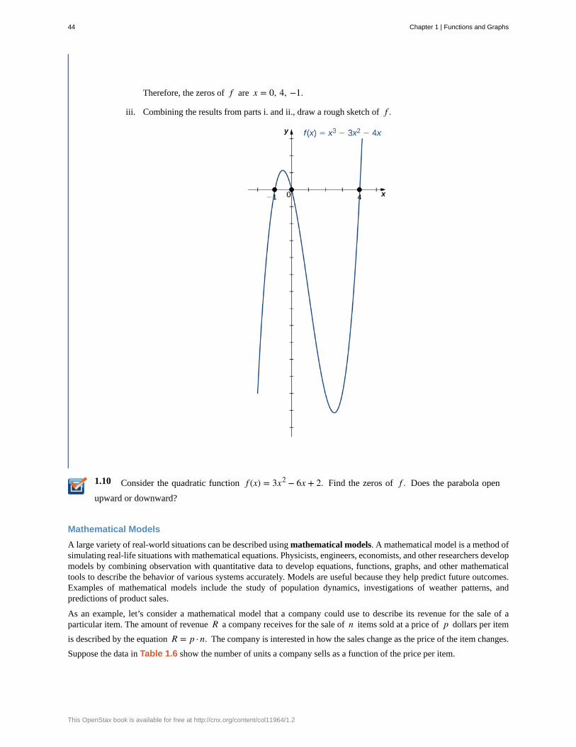
1.10
Therefore, the zeros of f are x = 0, 4, −1.
iii. Combining the results from parts i. and ii., draw a rough sketch of f .
Consider the quadratic function f (x) = 3x2 − 6x + 2. Find the zeros of f . Does the parabola open
upward or downward?
Mathematical Models
A large variety of real-world situations can be described using mathematical models. A mathematical model is a method ofsimulating real-life situations with mathematical equations. Physicists, engineers, economists, and other researchers developmodels by combining observation with quantitative data to develop equations, functions, graphs, and other mathematicaltools to describe the behavior of various systems accurately. Models are useful because they help predict future outcomes.Examples of mathematical models include the study of population dynamics, investigations of weather patterns, andpredictions of product sales.
As an example, let’s consider a mathematical model that a company could use to describe its revenue for the sale of aparticular item. The amount of revenue R a company receives for the sale of n items sold at a price of p dollars per item
is described by the equation R = p · n. The company is interested in how the sales change as the price of the item changes.
Suppose the data in Table 1.6 show the number of units a company sells as a function of the price per item.
44 Chapter 1 | Functions and Graphs
This OpenStax book is available for free at http://cnx.org/content/col11964/1.2
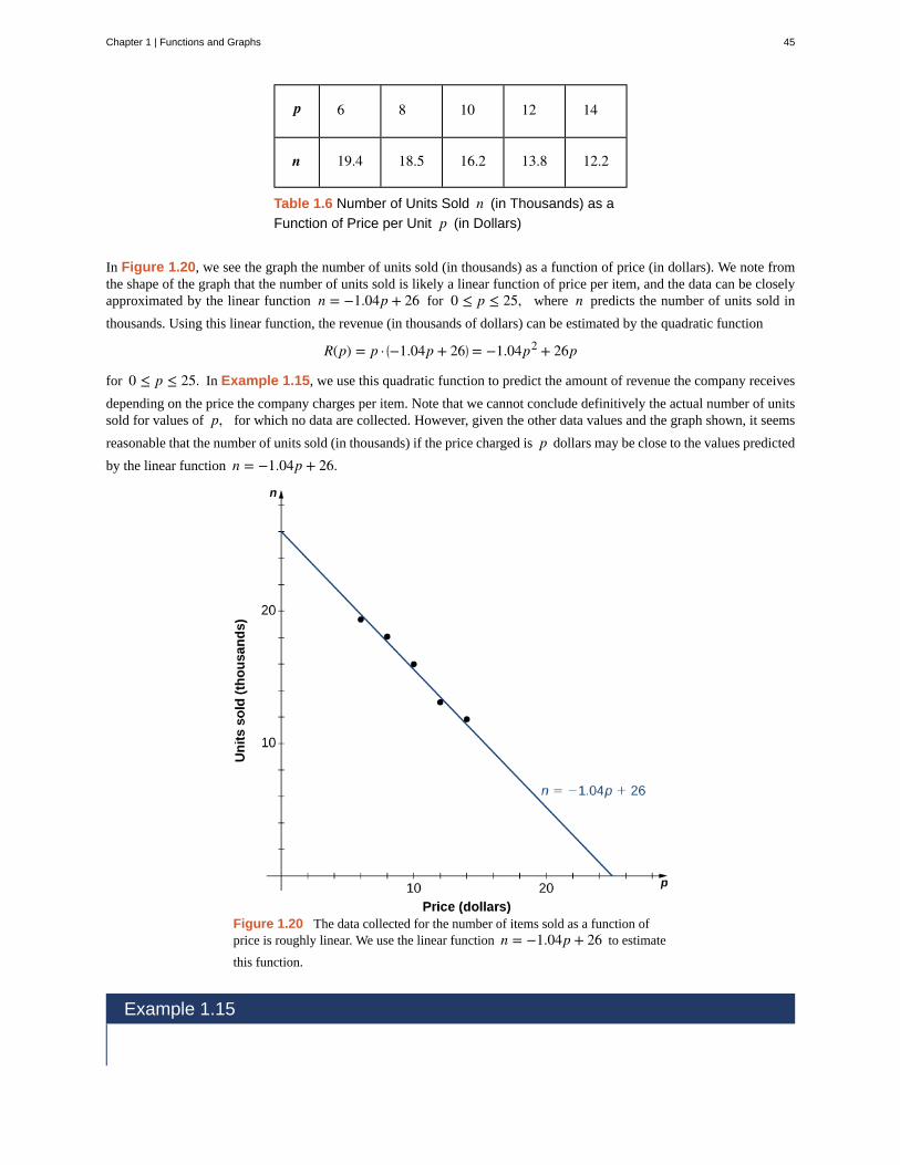
p 6 8 10 12 14
n 19.4 18.5 16.2 13.8 12.2
Table 1.6 Number of Units Sold n (in Thousands) as a
Function of Price per Unit p (in Dollars)
In Figure 1.20, we see the graph the number of units sold (in thousands) as a function of price (in dollars). We note fromthe shape of the graph that the number of units sold is likely a linear function of price per item, and the data can be closelyapproximated by the linear function n = −1.04p + 26 for 0 ≤ p ≤ 25, where n predicts the number of units sold in
thousands. Using this linear function, the revenue (in thousands of dollars) can be estimated by the quadratic function
R(p) = p · ⎛⎝−1.04p + 26⎞
⎠ = −1.04p2 + 26p
for 0 ≤ p ≤ 25. In Example 1.15, we use this quadratic function to predict the amount of revenue the company receives
depending on the price the company charges per item. Note that we cannot conclude definitively the actual number of unitssold for values of p, for which no data are collected. However, given the other data values and the graph shown, it seems
reasonable that the number of units sold (in thousands) if the price charged is p dollars may be close to the values predicted
by the linear function n = −1.04p + 26.
Figure 1.20 The data collected for the number of items sold as a function ofprice is roughly linear. We use the linear function n = −1.04p + 26 to estimate
this function.
Example 1.15
Chapter 1 | Functions and Graphs 45
Maximizing Revenue
A company is interested in predicting the amount of revenue it will receive depending on the price it charges for aparticular item. Using the data from Table 1.6, the company arrives at the following quadratic function to modelrevenue R as a function of price per item p:
R(p) = p · ⎛⎝−1.04p + 26⎞
⎠ = −1.04p2 + 26p
for 0 ≤ p ≤ 25.
a. Predict the revenue if the company sells the item at a price of p = $5 and p = $17.
b. Find the zeros of this function and interpret the meaning of the zeros.
c. Sketch a graph of R.
d. Use the graph to determine the value of p that maximizes revenue. Find the maximum revenue.
Solution
a. Evaluating the revenue function at p = 5 and p = 17, we can conclude that
R(5) = −1.04(5)2 + 26(5) = 104, so revenue = $104,000;R(17) = −1.04(17)2 + 26(17) = 141.44, so revenue = $144,440.
b. The zeros of this function can be found by solving the equation −1.04p2 + 26p = 0. When we factor
the quadratic expression, we get p⎛⎝−1.04p + 26⎞
⎠ = 0. The solutions to this equation are given by
p = 0, 25. For these values of p, the revenue is zero. When p = $0, the revenue is zero because the
company is giving away its merchandise for free. When p = $25, the revenue is zero because the price
is too high, and no one will buy any items.
c. Knowing the fact that the function is quadratic, we also know the graph is a parabola. Since theleading coefficient is negative, the parabola opens downward. One property of parabolas is that they aresymmetric about the axis, so since the zeros are at p = 0 and p = 25, the parabola must be symmetric
about the line halfway between them, or p = 12.5.
46 Chapter 1 | Functions and Graphs
This OpenStax book is available for free at http://cnx.org/content/col11964/1.2
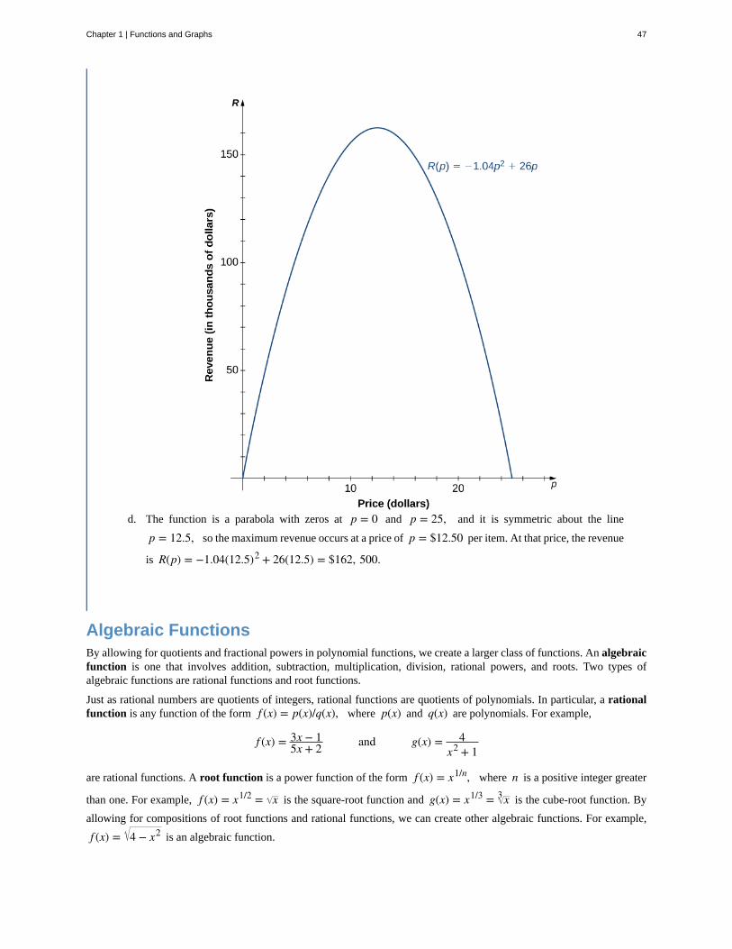
d. The function is a parabola with zeros at p = 0 and p = 25, and it is symmetric about the line
p = 12.5, so the maximum revenue occurs at a price of p = $12.50 per item. At that price, the revenue
is R(p) = −1.04(12.5)2 + 26(12.5) = $162, 500.
Algebraic FunctionsBy allowing for quotients and fractional powers in polynomial functions, we create a larger class of functions. An algebraicfunction is one that involves addition, subtraction, multiplication, division, rational powers, and roots. Two types ofalgebraic functions are rational functions and root functions.
Just as rational numbers are quotients of integers, rational functions are quotients of polynomials. In particular, a rationalfunction is any function of the form f (x) = p(x)/q(x), where p(x) and q(x) are polynomials. For example,
f (x) = 3x − 15x + 2 and g(x) = 4
x2 + 1
are rational functions. A root function is a power function of the form f (x) = x1/n, where n is a positive integer greater
than one. For example, f (x) = x1/2 = x is the square-root function and g(x) = x1/3 = x3 is the cube-root function. By
allowing for compositions of root functions and rational functions, we can create other algebraic functions. For example,
f (x) = 4 − x2 is an algebraic function.
Chapter 1 | Functions and Graphs 47
1.11
Example 1.16
Finding Domain and Range for Algebraic Functions
For each of the following functions, find the domain and range.
a. f (x) = 3x − 15x + 2
b. f (x) = 4 − x2
Solution
a. It is not possible to divide by zero, so the domain is the set of real numbers x such that x ≠ −2/5. To
find the range, we need to find the values y for which there exists a real number x such that
y = 3x − 15x + 2.
When we multiply both sides of this equation by 5x + 2, we see that x must satisfy the equation
5xy + 2y = 3x − 1.
From this equation, we can see that x must satisfy
2y + 1 = x(3 − 5y).
If y = 3/5, this equation has no solution. On the other hand, as long as y ≠ 3/5,
x = 2y + 13 − 5y
satisfies this equation. We can conclude that the range of f is ⎧
⎩⎨y|y ≠ 3/5⎫
⎭⎬.
b. To find the domain of f , we need 4 − x2 ≥ 0. When we factor, we write
4 − x2 = (2 − x)(2 + x) ≥ 0. This inequality holds if and only if both terms are positive or both terms
are negative. For both terms to be positive, we need to find x such that
2 − x ≥ 0 and 2 + x ≥ 0.
These two inequalities reduce to 2 ≥ x and x ≥ −2. Therefore, the set {x| − 2 ≤ x ≤ 2} must be part
of the domain. For both terms to be negative, we need
2 − x ≤ 0 and 2 + x ≥ 0.
These two inequalities also reduce to 2 ≤ x and x ≥ −2. There are no values of x that satisfy both of
these inequalities. Thus, we can conclude the domain of this function is {x| − 2 ≤ x ≤ 2}.
If −2 ≤ x ≤ 2, then 0 ≤ 4 − x2 ≤ 4. Therefore, 0 ≤ 4 − x2 ≤ 2, and the range of f is⎧
⎩⎨y|0 ≤ y ≤ 2⎫
⎭⎬.
Find the domain and range for the function f (x) = (5x + 2)/(2x − 1).
48 Chapter 1 | Functions and Graphs
This OpenStax book is available for free at http://cnx.org/content/col11964/1.2
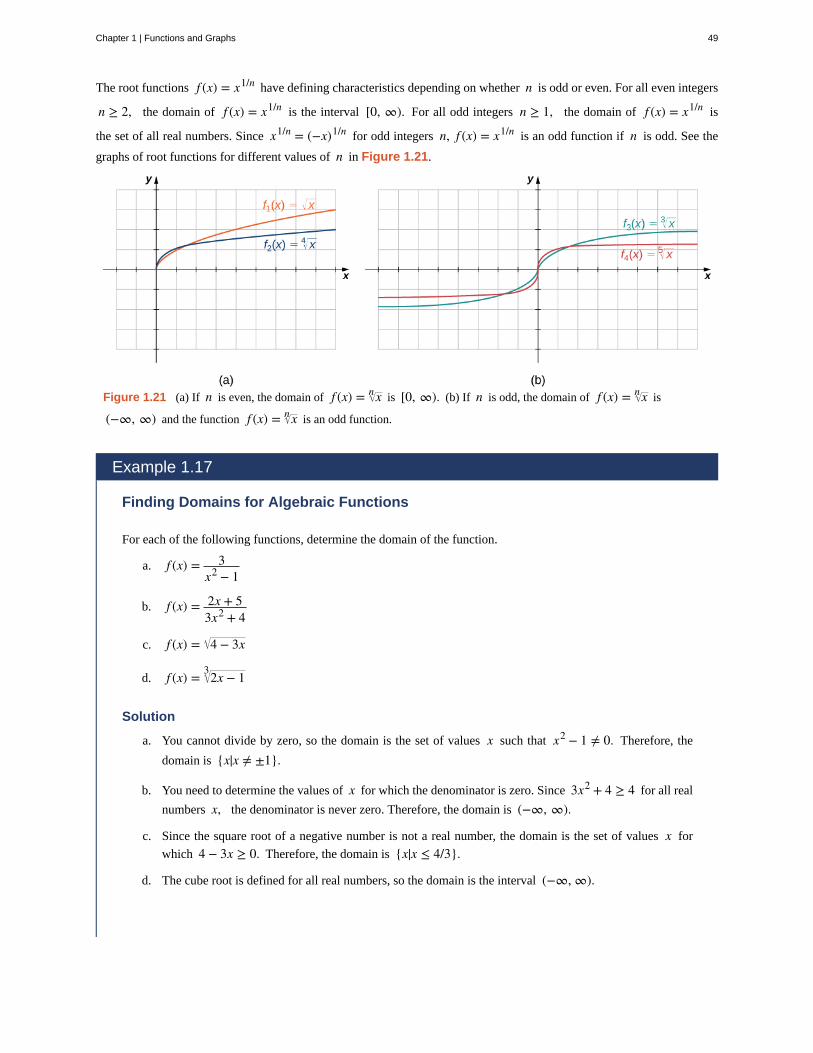
The root functions f (x) = x1/n have defining characteristics depending on whether n is odd or even. For all even integers
n ≥ 2, the domain of f (x) = x1/n is the interval [0, ∞). For all odd integers n ≥ 1, the domain of f (x) = x1/n is
the set of all real numbers. Since x1/n = (−x)1/n for odd integers n, f (x) = x1/n is an odd function if n is odd. See the
graphs of root functions for different values of n in Figure 1.21.
Figure 1.21 (a) If n is even, the domain of f (x) = xn is [0, ∞). (b) If n is odd, the domain of f (x) = xn is
(−∞, ∞) and the function f (x) = xn is an odd function.
Example 1.17
Finding Domains for Algebraic Functions
For each of the following functions, determine the domain of the function.
a. f (x) = 3x2 − 1
b. f (x) = 2x + 53x2 + 4
c. f (x) = 4 − 3x
d. f (x) = 2x − 13
Solution
a. You cannot divide by zero, so the domain is the set of values x such that x2 − 1 ≠ 0. Therefore, the
domain is {x|x ≠ ±1}.
b. You need to determine the values of x for which the denominator is zero. Since 3x2 + 4 ≥ 4 for all real
numbers x, the denominator is never zero. Therefore, the domain is (−∞, ∞).
c. Since the square root of a negative number is not a real number, the domain is the set of values x for
which 4 − 3x ≥ 0. Therefore, the domain is {x|x ≤ 4/3}.
d. The cube root is defined for all real numbers, so the domain is the interval (−∞, ∞).
Chapter 1 | Functions and Graphs 49
1.12
1.13
Find the domain for each of the following functions: f (x) = (5 − 2x)/(x2 + 2) and g(x) = 5x − 1.
Transcendental FunctionsThus far, we have discussed algebraic functions. Some functions, however, cannot be described by basic algebraicoperations. These functions are known as transcendental functions because they are said to “transcend,” or go beyond,algebra. The most common transcendental functions are trigonometric, exponential, and logarithmic functions. Atrigonometric function relates the ratios of two sides of a right triangle. They are sinx, cosx, tanx, cotx, secx, and cscx.(We discuss trigonometric functions later in the chapter.) An exponential function is a function of the form f (x) = bx,where the base b > 0, b ≠ 1. A logarithmic function is a function of the form f (x) = logb(x) for some constant
b > 0, b ≠ 1, where logb (x) = y if and only if by = x. (We also discuss exponential and logarithmic functions later in
the chapter.)
Example 1.18
Classifying Algebraic and Transcendental Functions
Classify each of the following functions, a. through c., as algebraic or transcendental.
a. f (x) = x3 + 14x + 2
b. f (x) = 2x2
c. f (x) = sin(2x)
Solution
a. Since this function involves basic algebraic operations only, it is an algebraic function.
b. This function cannot be written as a formula that involves only basic algebraic operations, so it istranscendental. (Note that algebraic functions can only have powers that are rational numbers.)
c. As in part b., this function cannot be written using a formula involving basic algebraic operations only;therefore, this function is transcendental.
Is f (x) = x/2 an algebraic or a transcendental function?
Piecewise-Defined FunctionsSometimes a function is defined by different formulas on different parts of its domain. A function with this property isknown as a piecewise-defined function. The absolute value function is an example of a piecewise-defined function becausethe formula changes with the sign of x:
f (x) =⎧
⎩⎨−x, x < 0x, x ≥ 0
.
Other piecewise-defined functions may be represented by completely different formulas, depending on the part of thedomain in which a point falls. To graph a piecewise-defined function, we graph each part of the function in its respectivedomain, on the same coordinate system. If the formula for a function is different for x < a and x > a, we need to pay
special attention to what happens at x = a when we graph the function. Sometimes the graph needs to include an open or
50 Chapter 1 | Functions and Graphs
This OpenStax book is available for free at http://cnx.org/content/col11964/1.2
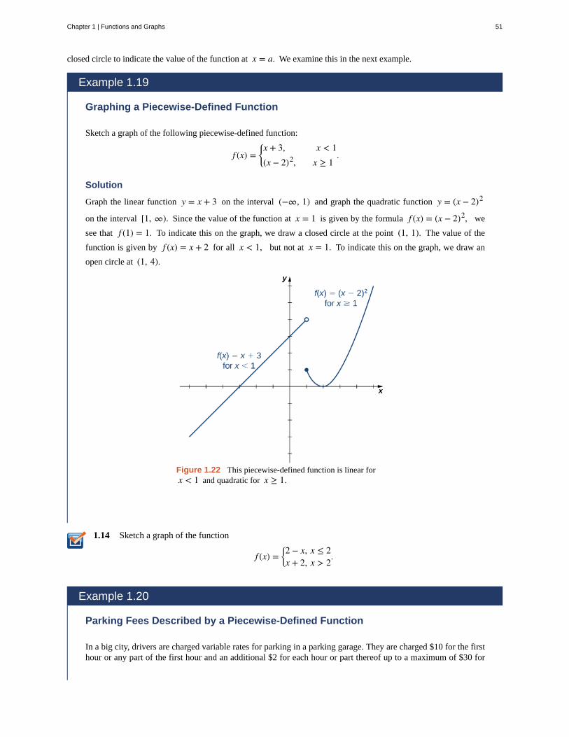
1.14
closed circle to indicate the value of the function at x = a. We examine this in the next example.
Example 1.19
Graphing a Piecewise-Defined Function
Sketch a graph of the following piecewise-defined function:
f (x) =⎧
⎩⎨
x + 3, x < 1(x − 2)2, x ≥ 1
.
Solution
Graph the linear function y = x + 3 on the interval (−∞, 1) and graph the quadratic function y = (x − 2)2
on the interval [1, ∞). Since the value of the function at x = 1 is given by the formula f (x) = (x − 2)2, we
see that f (1) = 1. To indicate this on the graph, we draw a closed circle at the point (1, 1). The value of the
function is given by f (x) = x + 2 for all x < 1, but not at x = 1. To indicate this on the graph, we draw an
open circle at (1, 4).
Figure 1.22 This piecewise-defined function is linear forx < 1 and quadratic for x ≥ 1.
Sketch a graph of the function
f (x) =⎧
⎩⎨2 − x, x ≤ 2x + 2, x > 2
.
Example 1.20
Parking Fees Described by a Piecewise-Defined Function
In a big city, drivers are charged variable rates for parking in a parking garage. They are charged $10 for the firsthour or any part of the first hour and an additional $2 for each hour or part thereof up to a maximum of $30 for
Chapter 1 | Functions and Graphs 51
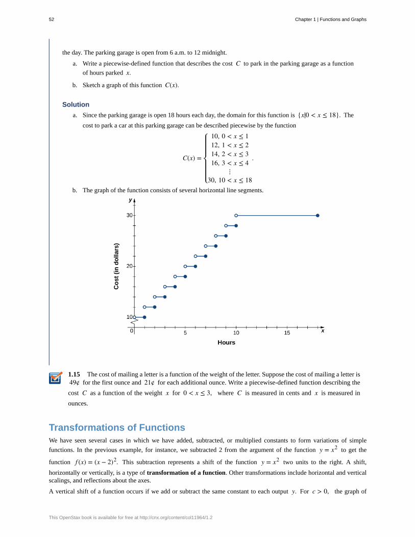
1.15
the day. The parking garage is open from 6 a.m. to 12 midnight.
a. Write a piecewise-defined function that describes the cost C to park in the parking garage as a function
of hours parked x.
b. Sketch a graph of this function C(x).
Solution
a. Since the parking garage is open 18 hours each day, the domain for this function is {x|0 < x ≤ 18}. The
cost to park a car at this parking garage can be described piecewise by the function
C(x) =
⎧
⎩
⎨⎪⎪
⎪⎪
10, 0 < x ≤ 112, 1 < x ≤ 214, 2 < x ≤ 316, 3 < x ≤ 4
⋮30, 10 < x ≤ 18
.
b. The graph of the function consists of several horizontal line segments.
The cost of mailing a letter is a function of the weight of the letter. Suppose the cost of mailing a letter is49¢ for the first ounce and 21¢ for each additional ounce. Write a piecewise-defined function describing the
cost C as a function of the weight x for 0 < x ≤ 3, where C is measured in cents and x is measured in
ounces.
Transformations of FunctionsWe have seen several cases in which we have added, subtracted, or multiplied constants to form variations of simple
functions. In the previous example, for instance, we subtracted 2 from the argument of the function y = x2 to get the
function f (x) = (x − 2)2. This subtraction represents a shift of the function y = x2 two units to the right. A shift,
horizontally or vertically, is a type of transformation of a function. Other transformations include horizontal and verticalscalings, and reflections about the axes.
A vertical shift of a function occurs if we add or subtract the same constant to each output y. For c > 0, the graph of
52 Chapter 1 | Functions and Graphs
This OpenStax book is available for free at http://cnx.org/content/col11964/1.2
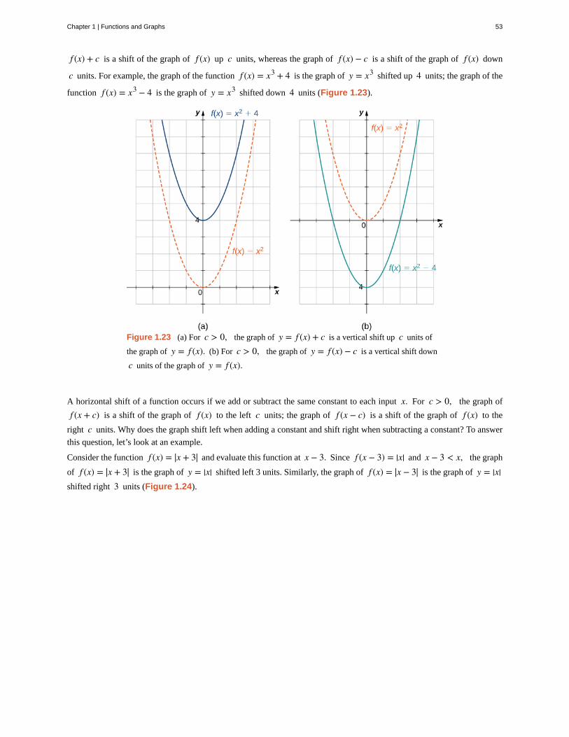
f (x) + c is a shift of the graph of f (x) up c units, whereas the graph of f (x) − c is a shift of the graph of f (x) down
c units. For example, the graph of the function f (x) = x3 + 4 is the graph of y = x3 shifted up 4 units; the graph of the
function f (x) = x3 − 4 is the graph of y = x3 shifted down 4 units (Figure 1.23).
Figure 1.23 (a) For c > 0, the graph of y = f (x) + c is a vertical shift up c units of
the graph of y = f (x). (b) For c > 0, the graph of y = f (x) − c is a vertical shift down
c units of the graph of y = f (x).
A horizontal shift of a function occurs if we add or subtract the same constant to each input x. For c > 0, the graph of
f (x + c) is a shift of the graph of f (x) to the left c units; the graph of f (x − c) is a shift of the graph of f (x) to the
right c units. Why does the graph shift left when adding a constant and shift right when subtracting a constant? To answer
this question, let’s look at an example.
Consider the function f (x) = |x + 3| and evaluate this function at x − 3. Since f (x − 3) = |x| and x − 3 < x, the graph
of f (x) = |x + 3| is the graph of y = |x| shifted left 3 units. Similarly, the graph of f (x) = |x − 3| is the graph of y = |x|shifted right 3 units (Figure 1.24).
Chapter 1 | Functions and Graphs 53
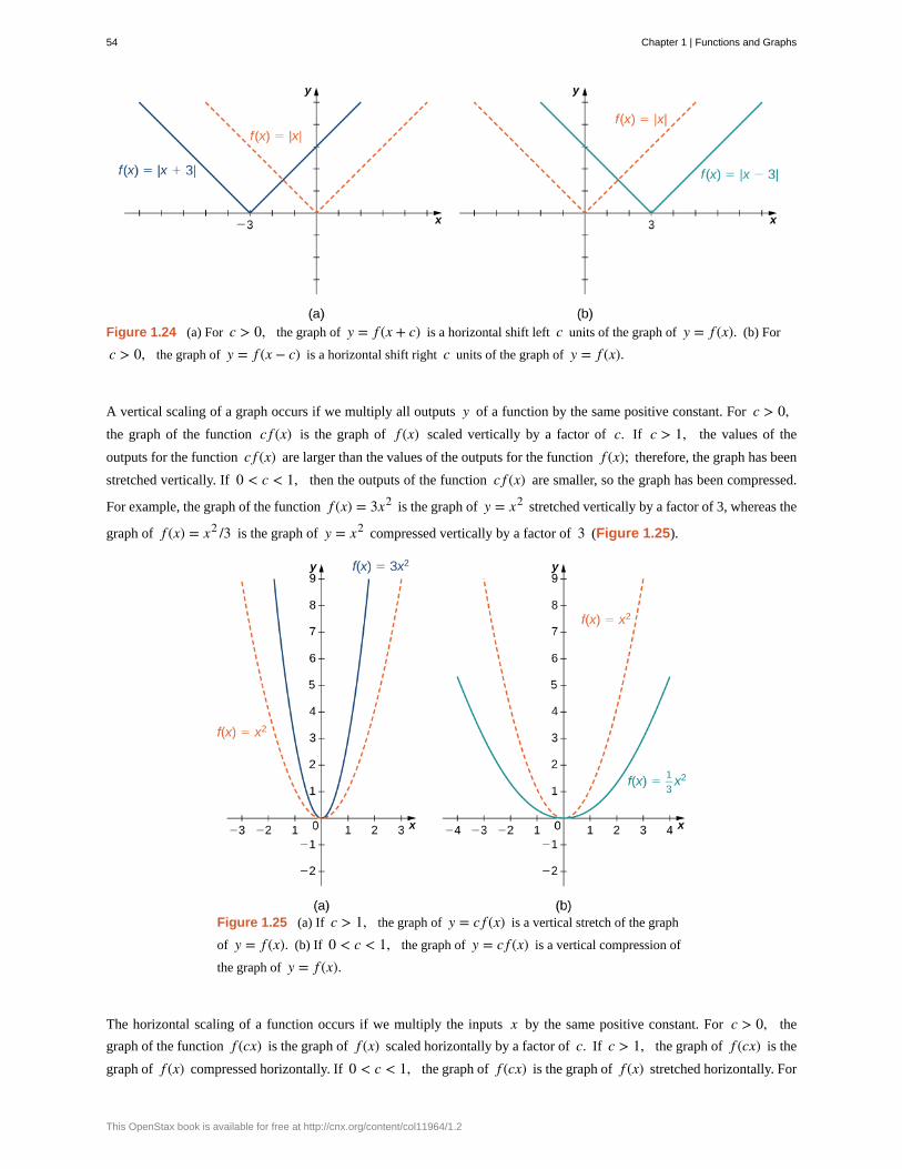
Figure 1.24 (a) For c > 0, the graph of y = f (x + c) is a horizontal shift left c units of the graph of y = f (x). (b) For
c > 0, the graph of y = f (x − c) is a horizontal shift right c units of the graph of y = f (x).
A vertical scaling of a graph occurs if we multiply all outputs y of a function by the same positive constant. For c > 0,the graph of the function c f (x) is the graph of f (x) scaled vertically by a factor of c. If c > 1, the values of the
outputs for the function c f (x) are larger than the values of the outputs for the function f (x); therefore, the graph has been
stretched vertically. If 0 < c < 1, then the outputs of the function c f (x) are smaller, so the graph has been compressed.
For example, the graph of the function f (x) = 3x2 is the graph of y = x2 stretched vertically by a factor of 3, whereas the
graph of f (x) = x2 /3 is the graph of y = x2 compressed vertically by a factor of 3 (Figure 1.25).
Figure 1.25 (a) If c > 1, the graph of y = c f (x) is a vertical stretch of the graph
of y = f (x). (b) If 0 < c < 1, the graph of y = c f (x) is a vertical compression of
the graph of y = f (x).
The horizontal scaling of a function occurs if we multiply the inputs x by the same positive constant. For c > 0, the
graph of the function f (cx) is the graph of f (x) scaled horizontally by a factor of c. If c > 1, the graph of f (cx) is the
graph of f (x) compressed horizontally. If 0 < c < 1, the graph of f (cx) is the graph of f (x) stretched horizontally. For
54 Chapter 1 | Functions and Graphs
This OpenStax book is available for free at http://cnx.org/content/col11964/1.2
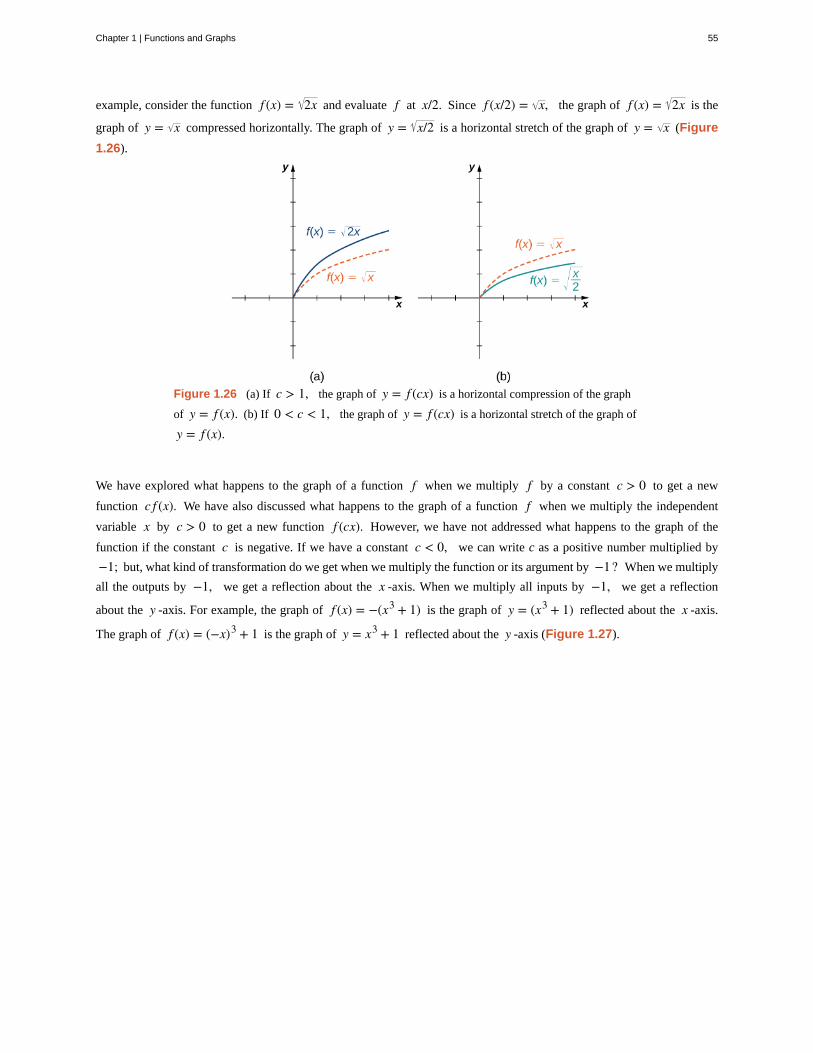
example, consider the function f (x) = 2x and evaluate f at x/2. Since f (x/2) = x, the graph of f (x) = 2x is the
graph of y = x compressed horizontally. The graph of y = x/2 is a horizontal stretch of the graph of y = x (Figure
1.26).
Figure 1.26 (a) If c > 1, the graph of y = f (cx) is a horizontal compression of the graph
of y = f (x). (b) If 0 < c < 1, the graph of y = f (cx) is a horizontal stretch of the graph of
y = f (x).
We have explored what happens to the graph of a function f when we multiply f by a constant c > 0 to get a new
function c f (x). We have also discussed what happens to the graph of a function f when we multiply the independent
variable x by c > 0 to get a new function f (cx). However, we have not addressed what happens to the graph of the
function if the constant c is negative. If we have a constant c < 0, we can write c as a positive number multiplied by
−1; but, what kind of transformation do we get when we multiply the function or its argument by −1? When we multiply
all the outputs by −1, we get a reflection about the x -axis. When we multiply all inputs by −1, we get a reflection
about the y -axis. For example, the graph of f (x) = −(x3 + 1) is the graph of y = (x3 + 1) reflected about the x -axis.
The graph of f (x) = (−x)3 + 1 is the graph of y = x3 + 1 reflected about the y -axis (Figure 1.27).
Chapter 1 | Functions and Graphs 55
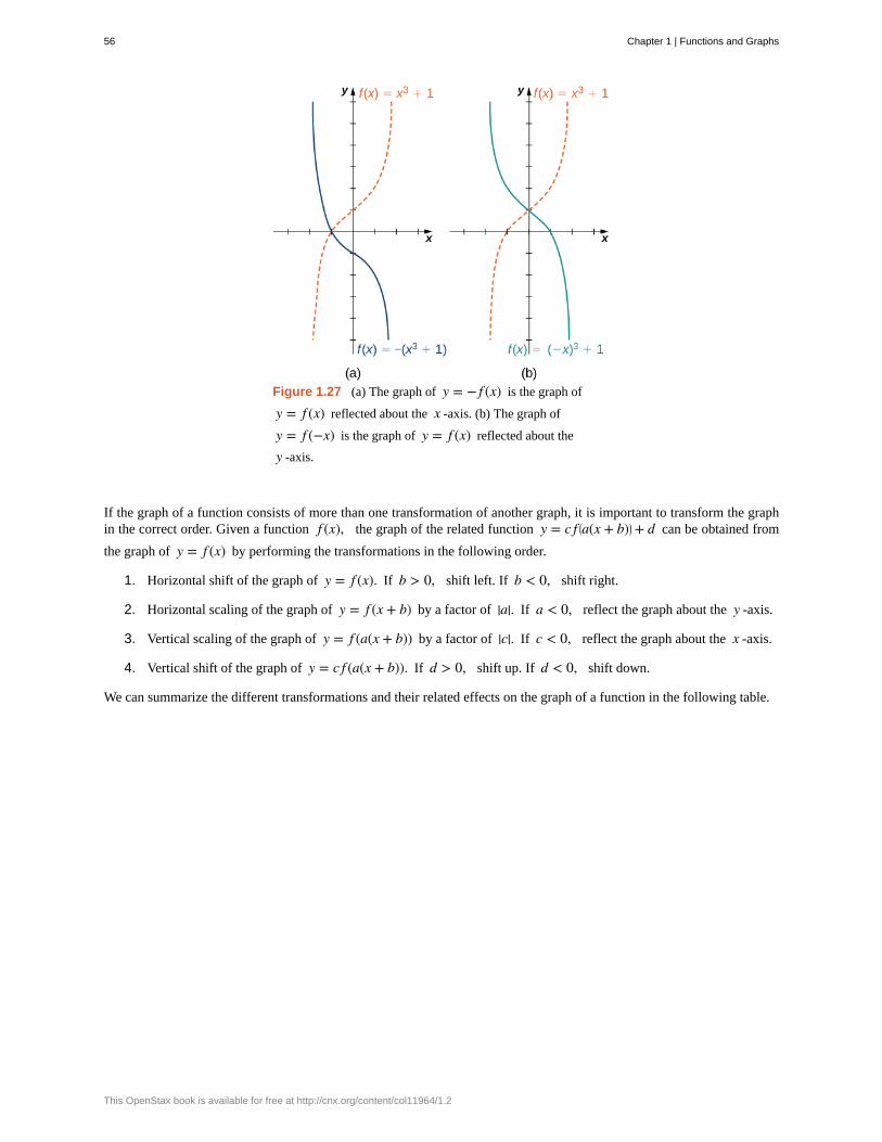
Figure 1.27 (a) The graph of y = − f (x) is the graph of
y = f (x) reflected about the x -axis. (b) The graph of
y = f (−x) is the graph of y = f (x) reflected about the
y -axis.
If the graph of a function consists of more than one transformation of another graph, it is important to transform the graphin the correct order. Given a function f (x), the graph of the related function y = c f ⎛
⎝a(x + b)⎞⎠ + d can be obtained from
the graph of y = f (x) by performing the transformations in the following order.
1. Horizontal shift of the graph of y = f (x). If b > 0, shift left. If b < 0, shift right.
2. Horizontal scaling of the graph of y = f (x + b) by a factor of |a|. If a < 0, reflect the graph about the y -axis.
3. Vertical scaling of the graph of y = f (a(x + b)) by a factor of |c|. If c < 0, reflect the graph about the x -axis.
4. Vertical shift of the graph of y = c f (a(x + b)). If d > 0, shift up. If d < 0, shift down.
We can summarize the different transformations and their related effects on the graph of a function in the following table.
56 Chapter 1 | Functions and Graphs
This OpenStax book is available for free at http://cnx.org/content/col11964/1.2
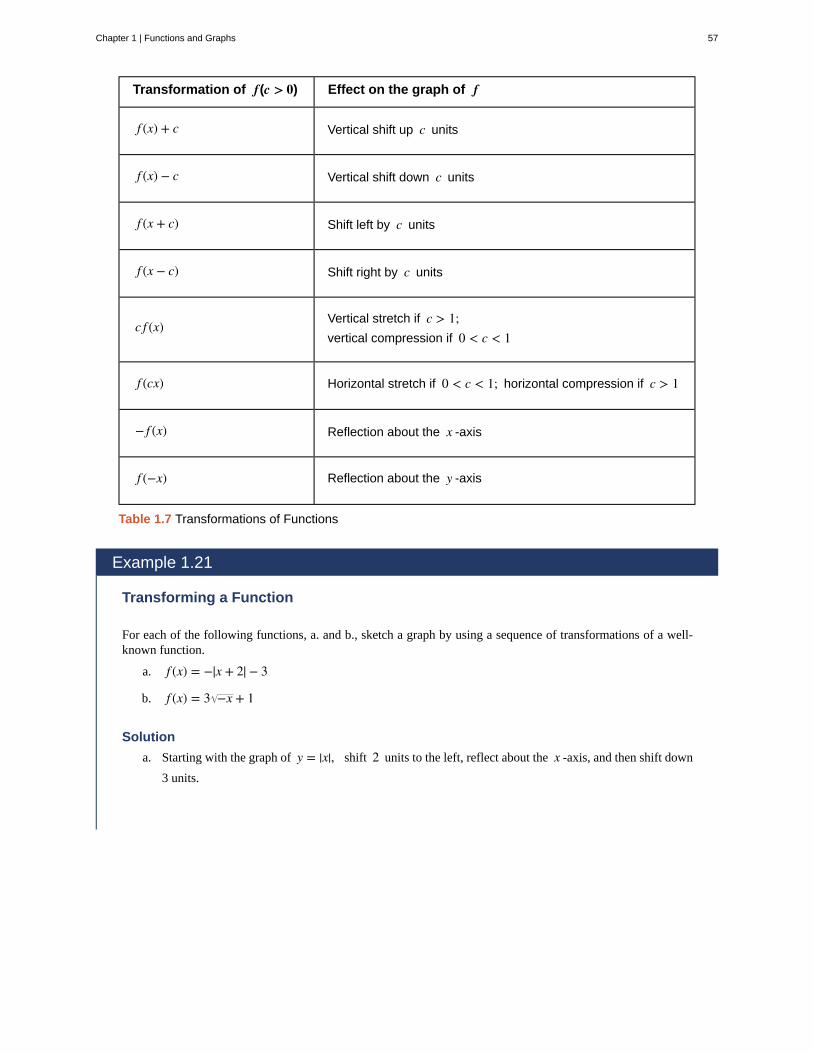
Transformation of f(c > 0) Effect on the graph of f
f (x) + c Vertical shift up c units
f (x) − c Vertical shift down c units
f (x + c) Shift left by c units
f (x − c) Shift right by c units
c f (x) Vertical stretch if c > 1;vertical compression if 0 < c < 1
f (cx) Horizontal stretch if 0 < c < 1; horizontal compression if c > 1
− f (x) Reflection about the x -axis
f (−x) Reflection about the y -axis
Table 1.7 Transformations of Functions
Example 1.21
Transforming a Function
For each of the following functions, a. and b., sketch a graph by using a sequence of transformations of a well-known function.
a. f (x) = −|x + 2| − 3
b. f (x) = 3 −x + 1
Solution
a. Starting with the graph of y = |x|, shift 2 units to the left, reflect about the x -axis, and then shift down
3 units.
Chapter 1 | Functions and Graphs 57
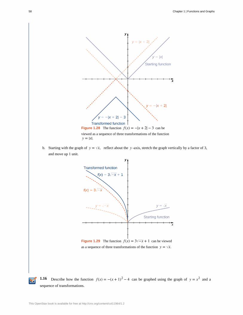
1.16
Figure 1.28 The function f (x) = −|x + 2| − 3 can be
viewed as a sequence of three transformations of the functiony = |x|.
b. Starting with the graph of y = x, reflect about the y -axis, stretch the graph vertically by a factor of 3,
and move up 1 unit.
Figure 1.29 The function f (x) = 3 −x + 1 can be viewed
as a sequence of three transformations of the function y = x.
Describe how the function f (x) = −(x + 1)2 − 4 can be graphed using the graph of y = x2 and a
sequence of transformations.
58 Chapter 1 | Functions and Graphs
This OpenStax book is available for free at http://cnx.org/content/col11964/1.2
1.2 EXERCISESFor the following exercises, for each pair of points, a.find the slope of the line passing through the points andb. indicate whether the line is increasing, decreasing,horizontal, or vertical.
59. (−2, 4) and (1, 1)
60. (−1, 4) and (3, −1)
61. (3, 5) and (−1, 2)
62. (6, 4) and (4, −3)
63. (2, 3) and (5, 7)
64. (1, 9) and (−8, 5)
65. (2, 4) and (1, 4)
66. (1, 4) and (1, 0)
For the following exercises, write the equation of the linesatisfying the given conditions in slope-intercept form.
67. Slope = −6, passes through (1, 3)
68. Slope = 3, passes through (−3, 2)
69. Slope = 13, passes through (0, 4)
70. Slope = 25, x -intercept = 8
71. Passing through (2, 1) and (−2, −1)
72. Passing through (−3, 7) and (1, 2)
73. x -intercept = 5 and y -intercept = −3
74. x -intercept = −6 and y -intercept = 9
For the following exercises, for each linear equation, a. givethe slope m and y -intercept b, if any, and b. graph the line.
75. y = 2x − 3
76. y = − 17x + 1
77. f (x) = −6x
78. f (x) = −5x + 4
79. 4y + 24 = 0
80. 8x − 4 = 0
81. 2x + 3y = 6
82. 6x − 5y + 15 = 0
For the following exercises, for each polynomial, a. find thedegree; b. find the zeros, if any; c. find the y -intercept(s),
if any; d. use the leading coefficient to determine thegraph’s end behavior; and e. determine algebraicallywhether the polynomial is even, odd, or neither.
83. f (x) = 2x2 − 3x − 5
84. f (x) = −3x2 + 6x
85. f (x) = 12x2 − 1
86. f (x) = x3 + 3x2 − x − 3
87. f (x) = 3x − x3
For the following exercises, use the graph of f (x) = x2 to
graph each transformed function g.
88. g(x) = x2 − 1
89. g(x) = (x + 3)2 + 1
For the following exercises, use the graph of f (x) = x to
graph each transformed function g.
90. g(x) = x + 2
91. g(x) = − x − 1
For the following exercises, use the graph of y = f (x) to
graph each transformed function g.
Chapter 1 | Functions and Graphs 59
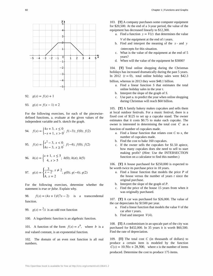
92. g(x) = f (x) + 1
93. g(x) = f (x − 1) + 2
For the following exercises, for each of the piecewise-defined functions, a. evaluate at the given values of theindependent variable and b. sketch the graph.
94. f (x) =⎧
⎩⎨
4x + 3, x ≤ 0−x + 1, x > 0
; f (−3); f (0); f (2)
95. f (x) =⎧
⎩⎨x2 − 3, x < 04x − 3, x ≥ 0
; f (−4); f (0); f (2)
96. h(x) =⎧
⎩⎨x + 1, x ≤ 5
4, x > 5; h(0); h(π); h(5)
97. g(x) =⎧
⎩⎨
3x − 2, x ≠ 2
4, x = 2; g(0); g(−4); g(2)
For the following exercises, determine whether thestatement is true or false. Explain why.
98. f (x) = (4x + 1)/(7x − 2) is a transcendental
function.
99. g(x) = x3 is an odd root function
100. A logarithmic function is an algebraic function.
101. A function of the form f (x) = xb, where b is a
real valued constant, is an exponential function.
102. The domain of an even root function is all realnumbers.
103. [T] A company purchases some computer equipmentfor $20,500. At the end of a 3-year period, the value of theequipment has decreased linearly to $12,300.
a. Find a function y = V(t) that determines the value
V of the equipment at the end of t years.b. Find and interpret the meaning of the x - and y
-intercepts for this situation.c. What is the value of the equipment at the end of 5
years?d. When will the value of the equipment be $3000?
104. [T] Total online shopping during the Christmasholidays has increased dramatically during the past 5 years.In 2012 (t = 0), total online holiday sales were $42.3
billion, whereas in 2013 they were $48.1 billion.a. Find a linear function S that estimates the total
online holiday sales in the year t.b. Interpret the slope of the graph of S.c. Use part a. to predict the year when online shopping
during Christmas will reach $60 billion.
105. [T] A family bakery makes cupcakes and sells themat local outdoor festivals. For a music festival, there is afixed cost of $125 to set up a cupcake stand. The ownerestimates that it costs $0.75 to make each cupcake. Theowner is interested in determining the total cost C as a
function of number of cupcakes made.a. Find a linear function that relates cost C to x, the
number of cupcakes made.b. Find the cost to bake 160 cupcakes.c. If the owner sells the cupcakes for $1.50 apiece,
how many cupcakes does she need to sell to startmaking profit? (Hint: Use the INTERSECTIONfunction on a calculator to find this number.)
106. [T] A house purchased for $250,000 is expected tobe worth twice its purchase price in 18 years.
a. Find a linear function that models the price P ofthe house versus the number of years t since theoriginal purchase.
b. Interpret the slope of the graph of P.c. Find the price of the house 15 years from when it
was originally purchased.
107. [T] A car was purchased for $26,000. The value ofthe car depreciates by $1500 per year.
a. Find a linear function that models the value V of thecar after t years.
b. Find and interpret V(4).
108. [T] A condominium in an upscale part of the city waspurchased for $432,000. In 35 years it is worth $60,500.Find the rate of depreciation.
109. [T] The total cost C (in thousands of dollars) toproduce a certain item is modeled by the functionC(x) = 10.50x + 28,500, where x is the number of items
produced. Determine the cost to produce 175 items.
60 Chapter 1 | Functions and Graphs
This OpenStax book is available for free at http://cnx.org/content/col11964/1.2
110. [T] A professor asks her class to report the amountof time t they spent writing two assignments. Most studentsreport that it takes them about 45 minutes to type a four-page assignment and about 1.5 hours to type a nine-pageassignment.
a. Find the linear function y = N(t) that models this
situation, where N is the number of pages typed
and t is the time in minutes.b. Use part a. to determine how many pages can be
typed in 2 hours.c. Use part a. to determine how long it takes to type a
20-page assignment.
111. [T] The output (as a percent of total capacity) ofnuclear power plants in the United States can be modeledby the function P(t) = 1.8576t + 68.052, where t is time
in years and t = 0 corresponds to the beginning of 2000.
Use the model to predict the percentage output in 2015.
112. [T] The admissions office at a public universityestimates that 65% of the students offered admission to theclass of 2019 will actually enroll.
a. Find the linear function y = N(x), where N is
the number of students that actually enroll and x is
the number of all students offered admission to theclass of 2019.
b. If the university wants the 2019 freshman class sizeto be 1350, determine how many students should beadmitted.
Chapter 1 | Functions and Graphs 61
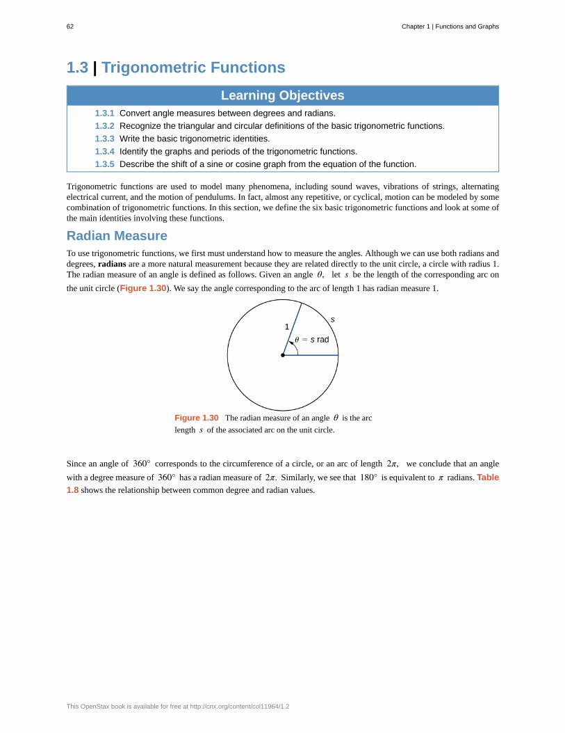
1.3 | Trigonometric Functions
Learning Objectives1.3.1 Convert angle measures between degrees and radians.
1.3.2 Recognize the triangular and circular definitions of the basic trigonometric functions.
1.3.3 Write the basic trigonometric identities.
1.3.4 Identify the graphs and periods of the trigonometric functions.
1.3.5 Describe the shift of a sine or cosine graph from the equation of the function.
Trigonometric functions are used to model many phenomena, including sound waves, vibrations of strings, alternatingelectrical current, and the motion of pendulums. In fact, almost any repetitive, or cyclical, motion can be modeled by somecombination of trigonometric functions. In this section, we define the six basic trigonometric functions and look at some ofthe main identities involving these functions.
Radian MeasureTo use trigonometric functions, we first must understand how to measure the angles. Although we can use both radians anddegrees, radians are a more natural measurement because they are related directly to the unit circle, a circle with radius 1.The radian measure of an angle is defined as follows. Given an angle θ, let s be the length of the corresponding arc on
the unit circle (Figure 1.30). We say the angle corresponding to the arc of length 1 has radian measure 1.
Figure 1.30 The radian measure of an angle θ is the arc
length s of the associated arc on the unit circle.
Since an angle of 360° corresponds to the circumference of a circle, or an arc of length 2π, we conclude that an angle
with a degree measure of 360° has a radian measure of 2π. Similarly, we see that 180° is equivalent to π radians. Table
1.8 shows the relationship between common degree and radian values.
62 Chapter 1 | Functions and Graphs
This OpenStax book is available for free at http://cnx.org/content/col11964/1.2
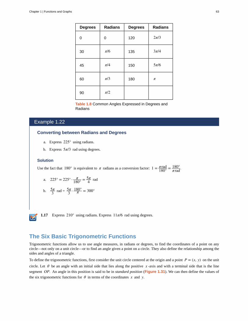
1.17
Degrees Radians Degrees Radians
0 0 120 2π/3
30 π/6 135 3π/4
45 π/4 150 5π/6
60 π/3 180 π
90 π/2
Table 1.8 Common Angles Expressed in Degrees andRadians
Example 1.22
Converting between Radians and Degrees
a. Express 225° using radians.
b. Express 5π/3 rad using degrees.
Solution
Use the fact that 180° is equivalent to π radians as a conversion factor: 1 = π rad180° = 180°
π rad.
a. 225° = 225° · π180° = 5π
4 rad
b. 5π3 rad = 5π
3 · 180°π = 300°
Express 210° using radians. Express 11π/6 rad using degrees.
The Six Basic Trigonometric FunctionsTrigonometric functions allow us to use angle measures, in radians or degrees, to find the coordinates of a point on anycircle—not only on a unit circle—or to find an angle given a point on a circle. They also define the relationship among thesides and angles of a triangle.
To define the trigonometric functions, first consider the unit circle centered at the origin and a point P = (x, y) on the unit
circle. Let θ be an angle with an initial side that lies along the positive x -axis and with a terminal side that is the line
segment OP. An angle in this position is said to be in standard position (Figure 1.31). We can then define the values of
the six trigonometric functions for θ in terms of the coordinates x and y.
Chapter 1 | Functions and Graphs 63
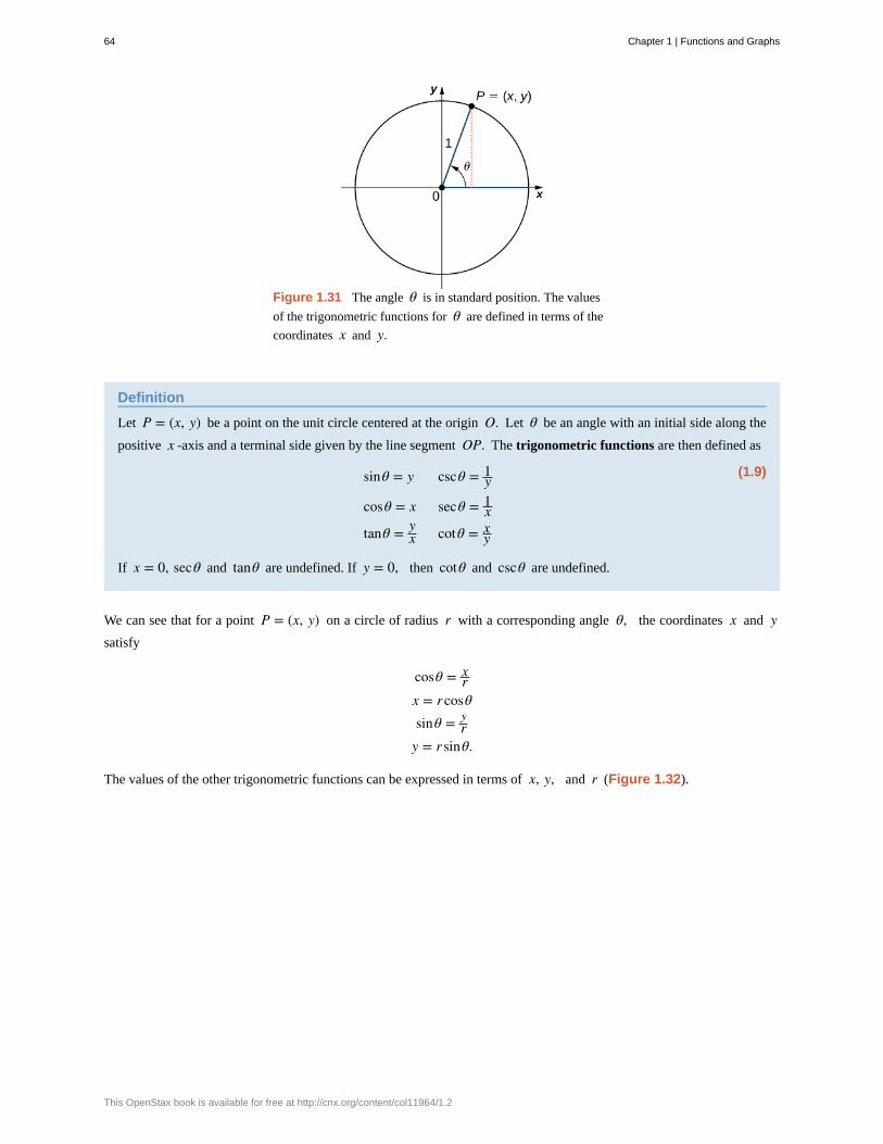
Figure 1.31 The angle θ is in standard position. The values
of the trigonometric functions for θ are defined in terms of the
coordinates x and y.
Definition
Let P = (x, y) be a point on the unit circle centered at the origin O. Let θ be an angle with an initial side along the
positive x -axis and a terminal side given by the line segment OP. The trigonometric functions are then defined as
(1.9)sinθ = y cscθ = 1y
cosθ = x secθ = 1x
tanθ = yx cotθ = x
y
If x = 0, secθ and tanθ are undefined. If y = 0, then cotθ and cscθ are undefined.
We can see that for a point P = (x, y) on a circle of radius r with a corresponding angle θ, the coordinates x and ysatisfy
cosθ = xr
x = rcosθsinθ = y
ry = r sinθ.
The values of the other trigonometric functions can be expressed in terms of x, y, and r (Figure 1.32).
64 Chapter 1 | Functions and Graphs
This OpenStax book is available for free at http://cnx.org/content/col11964/1.2
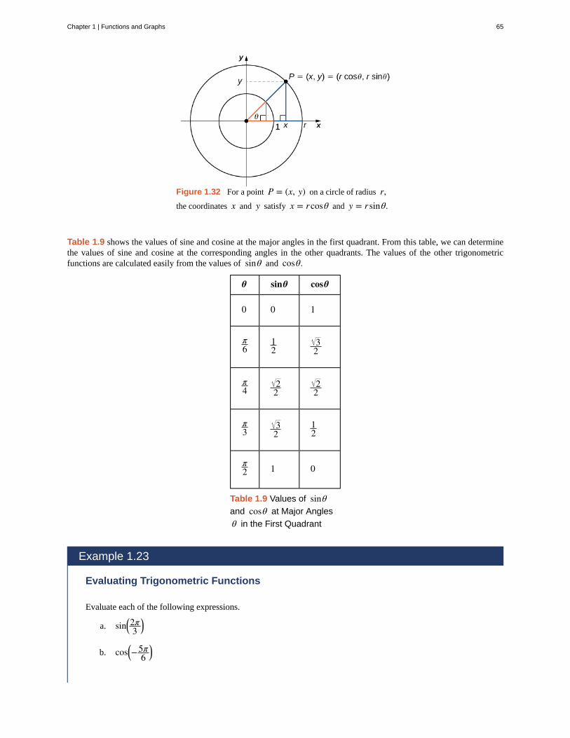
Figure 1.32 For a point P = (x, y) on a circle of radius r,the coordinates x and y satisfy x = rcosθ and y = r sinθ.
Table 1.9 shows the values of sine and cosine at the major angles in the first quadrant. From this table, we can determinethe values of sine and cosine at the corresponding angles in the other quadrants. The values of the other trigonometricfunctions are calculated easily from the values of sinθ and cosθ.
θ sinθ cosθ
0 0 1
π6
12
32
π4
22
22
π3
32
12
π2 1 0
Table 1.9 Values of sinθand cosθ at Major Angles
θ in the First Quadrant
Example 1.23
Evaluating Trigonometric Functions
Evaluate each of the following expressions.
a. sin⎛⎝2π3
⎞⎠
b. cos⎛⎝−
5π6
⎞⎠
Chapter 1 | Functions and Graphs 65
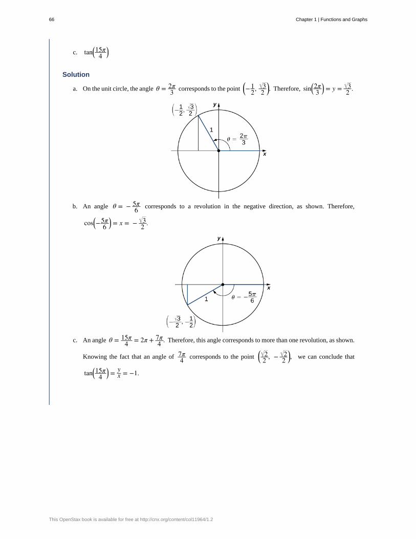
c. tan⎛⎝15π
4⎞⎠
Solution
a. On the unit circle, the angle θ = 2π3 corresponds to the point
⎛⎝−1
2, 32
⎞⎠. Therefore, sin⎛
⎝2π3
⎞⎠ = y = 3
2 .
b. An angle θ = − 5π6 corresponds to a revolution in the negative direction, as shown. Therefore,
cos⎛⎝−
5π6
⎞⎠ = x = − 3
2 .
c. An angle θ = 15π4 = 2π + 7π
4 . Therefore, this angle corresponds to more than one revolution, as shown.
Knowing the fact that an angle of 7π4 corresponds to the point
⎛⎝
22 , − 2
2⎞⎠, we can conclude that
tan⎛⎝15π
4⎞⎠ = y
x = −1.
66 Chapter 1 | Functions and Graphs
This OpenStax book is available for free at http://cnx.org/content/col11964/1.2
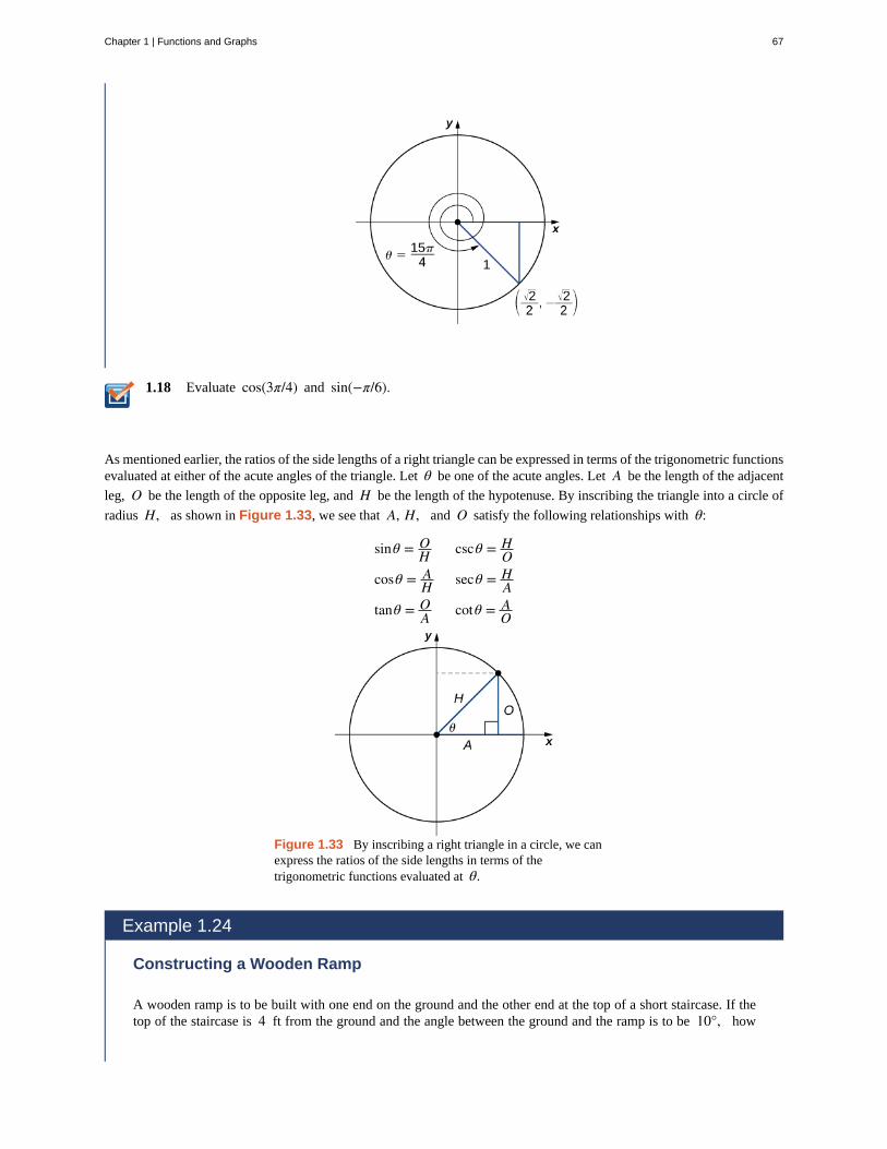
1.18 Evaluate cos(3π/4) and sin(−π/6).
As mentioned earlier, the ratios of the side lengths of a right triangle can be expressed in terms of the trigonometric functionsevaluated at either of the acute angles of the triangle. Let θ be one of the acute angles. Let A be the length of the adjacent
leg, O be the length of the opposite leg, and H be the length of the hypotenuse. By inscribing the triangle into a circle of
radius H, as shown in Figure 1.33, we see that A, H, and O satisfy the following relationships with θ:
sinθ = OH cscθ = H
Ocosθ = A
H secθ = HA
tanθ = OA cotθ = A
O
Figure 1.33 By inscribing a right triangle in a circle, we canexpress the ratios of the side lengths in terms of thetrigonometric functions evaluated at θ.
Example 1.24
Constructing a Wooden Ramp
A wooden ramp is to be built with one end on the ground and the other end at the top of a short staircase. If thetop of the staircase is 4 ft from the ground and the angle between the ground and the ramp is to be 10°, how
Chapter 1 | Functions and Graphs 67
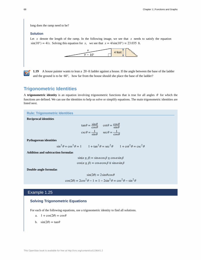
1.19
long does the ramp need to be?
Solution
Let x denote the length of the ramp. In the following image, we see that x needs to satisfy the equation
sin(10°) = 4/x. Solving this equation for x, we see that x = 4/sin(10°) ≈ 23.035 ft.
A house painter wants to lean a 20 -ft ladder against a house. If the angle between the base of the ladder
and the ground is to be 60°, how far from the house should she place the base of the ladder?
Trigonometric IdentitiesA trigonometric identity is an equation involving trigonometric functions that is true for all angles θ for which the
functions are defined. We can use the identities to help us solve or simplify equations. The main trigonometric identities arelisted next.
Rule: Trigonometric Identities
Reciprocal identities
tanθ = sinθcosθ cotθ = cosθ
sinθcscθ = 1
sinθ secθ = 1cosθ
Pythagorean identities
sin2 θ + cos2 θ = 1 1 + tan2 θ = sec2 θ 1 + cot2 θ = csc2 θ
Addition and subtraction formulas
sin⎛⎝α ± β⎞
⎠ = sinαcos β ± cosαsin βcos(α ± β) = cosαcos β ∓ sinαsin β
Double-angle formulas
sin(2θ) = 2sinθcosθ
cos(2θ) = 2cos2 θ − 1 = 1 − 2sin2 θ = cos2 θ − sin2 θ
Example 1.25
Solving Trigonometric Equations
For each of the following equations, use a trigonometric identity to find all solutions.
a. 1 + cos(2θ) = cosθ
b. sin(2θ) = tanθ
68 Chapter 1 | Functions and Graphs
This OpenStax book is available for free at http://cnx.org/content/col11964/1.2
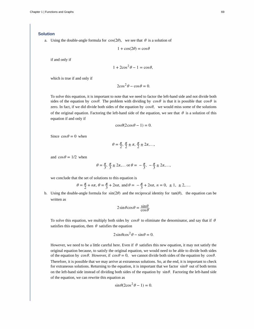
Solution
a. Using the double-angle formula for cos(2θ), we see that θ is a solution of
1 + cos(2θ) = cosθ
if and only if
1 + 2cos2 θ − 1 = cosθ,
which is true if and only if
2cos2 θ − cosθ = 0.
To solve this equation, it is important to note that we need to factor the left-hand side and not divide bothsides of the equation by cosθ. The problem with dividing by cosθ is that it is possible that cosθ is
zero. In fact, if we did divide both sides of the equation by cosθ, we would miss some of the solutions
of the original equation. Factoring the left-hand side of the equation, we see that θ is a solution of this
equation if and only if
cosθ(2cosθ − 1) = 0.
Since cosθ = 0 when
θ = π2, π
2 ± π, π2 ± 2π,…,
and cosθ = 1/2 when
θ = π3, π
3 ± 2π,… or θ = − π3, − π
3 ± 2π,…,
we conclude that the set of solutions to this equation is
θ = π2 + nπ, θ = π
3 + 2nπ, and θ = − π3 + 2nπ, n = 0, ± 1, ± 2,….
b. Using the double-angle formula for sin(2θ) and the reciprocal identity for tan(θ), the equation can be
written as
2sinθcosθ = sinθcosθ .
To solve this equation, we multiply both sides by cosθ to eliminate the denominator, and say that if θsatisfies this equation, then θ satisfies the equation
2sinθcos2 θ − sinθ = 0.
However, we need to be a little careful here. Even if θ satisfies this new equation, it may not satisfy the
original equation because, to satisfy the original equation, we would need to be able to divide both sidesof the equation by cosθ. However, if cosθ = 0, we cannot divide both sides of the equation by cosθ.Therefore, it is possible that we may arrive at extraneous solutions. So, at the end, it is important to checkfor extraneous solutions. Returning to the equation, it is important that we factor sinθ out of both terms
on the left-hand side instead of dividing both sides of the equation by sinθ. Factoring the left-hand side
of the equation, we can rewrite this equation as
sinθ(2cos2 θ − 1) = 0.
Chapter 1 | Functions and Graphs 69
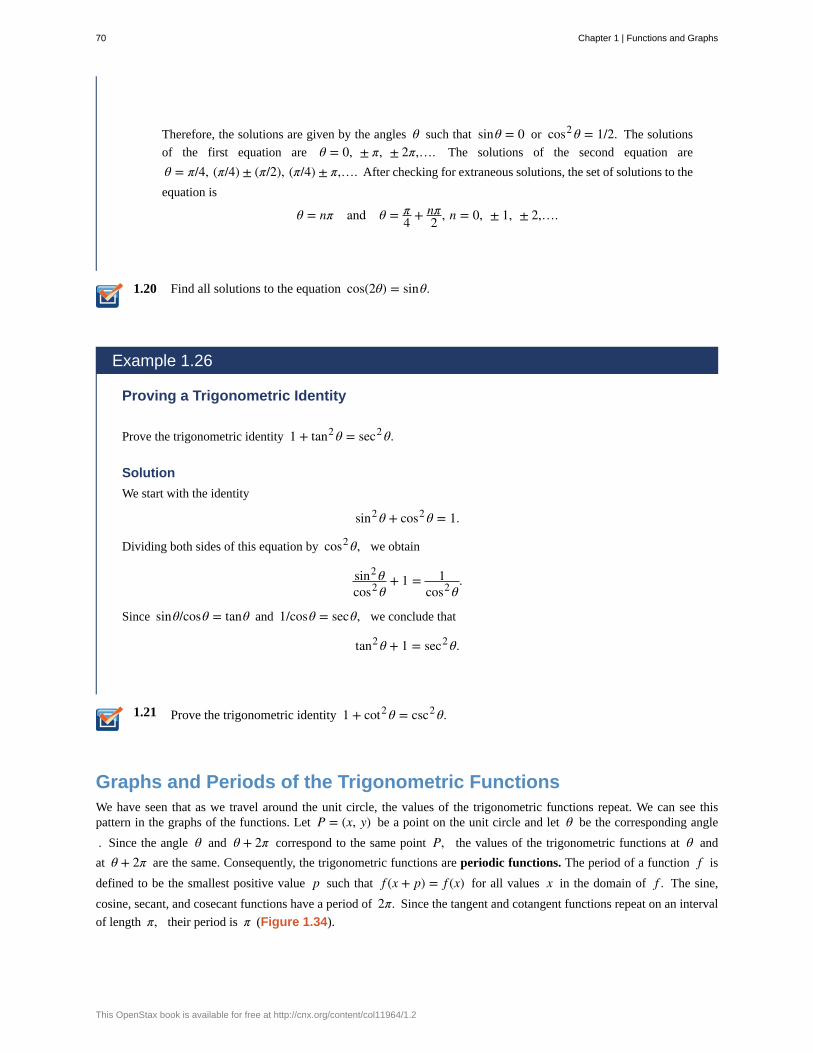
1.20
1.21
Therefore, the solutions are given by the angles θ such that sinθ = 0 or cos2 θ = 1/2. The solutions
of the first equation are θ = 0, ± π, ± 2π,…. The solutions of the second equation are
θ = π/4, (π/4) ± (π/2), (π/4) ± π,…. After checking for extraneous solutions, the set of solutions to the
equation is
θ = nπ and θ = π4 + nπ
2 , n = 0, ± 1, ± 2,….
Find all solutions to the equation cos(2θ) = sinθ.
Example 1.26
Proving a Trigonometric Identity
Prove the trigonometric identity 1 + tan2 θ = sec2 θ.
Solution
We start with the identity
sin2 θ + cos2 θ = 1.
Dividing both sides of this equation by cos2 θ, we obtain
sin2 θcos2 θ
+ 1 = 1cos2 θ
.
Since sinθ/cosθ = tanθ and 1/cosθ = secθ, we conclude that
tan2 θ + 1 = sec2 θ.
Prove the trigonometric identity 1 + cot2 θ = csc2 θ.
Graphs and Periods of the Trigonometric FunctionsWe have seen that as we travel around the unit circle, the values of the trigonometric functions repeat. We can see thispattern in the graphs of the functions. Let P = (x, y) be a point on the unit circle and let θ be the corresponding angle
. Since the angle θ and θ + 2π correspond to the same point P, the values of the trigonometric functions at θ and
at θ + 2π are the same. Consequently, the trigonometric functions are periodic functions. The period of a function f is
defined to be the smallest positive value p such that f (x + p) = f (x) for all values x in the domain of f . The sine,
cosine, secant, and cosecant functions have a period of 2π. Since the tangent and cotangent functions repeat on an interval
of length π, their period is π (Figure 1.34).
70 Chapter 1 | Functions and Graphs
This OpenStax book is available for free at http://cnx.org/content/col11964/1.2
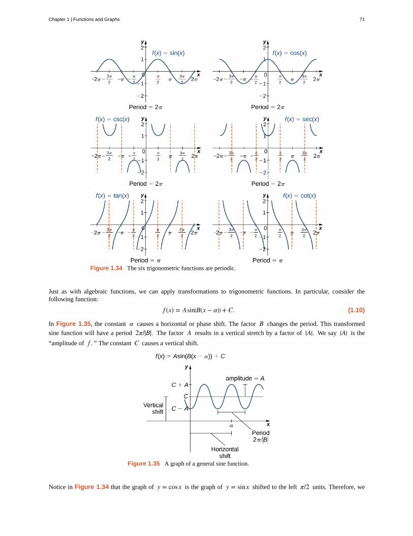
Figure 1.34 The six trigonometric functions are periodic.
Just as with algebraic functions, we can apply transformations to trigonometric functions. In particular, consider thefollowing function:
(1.10)f (x) = Asin⎛⎝B(x − α)⎞
⎠ + C.
In Figure 1.35, the constant α causes a horizontal or phase shift. The factor B changes the period. This transformed
sine function will have a period 2π/|B|. The factor A results in a vertical stretch by a factor of |A|. We say |A| is the
“amplitude of f . ” The constant C causes a vertical shift.
Figure 1.35 A graph of a general sine function.
Notice in Figure 1.34 that the graph of y = cosx is the graph of y = sinx shifted to the left π/2 units. Therefore, we
Chapter 1 | Functions and Graphs 71
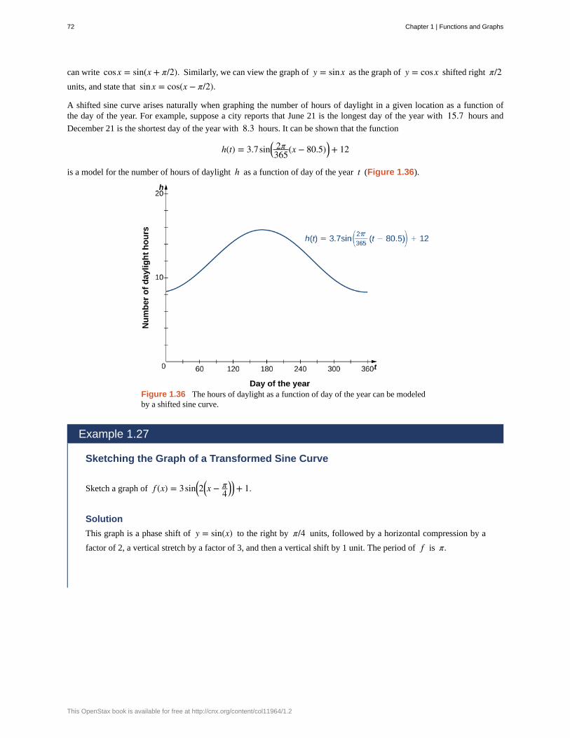
can write cosx = sin(x + π/2). Similarly, we can view the graph of y = sinx as the graph of y = cosx shifted right π/2units, and state that sinx = cos(x − π/2).
A shifted sine curve arises naturally when graphing the number of hours of daylight in a given location as a function ofthe day of the year. For example, suppose a city reports that June 21 is the longest day of the year with 15.7 hours and
December 21 is the shortest day of the year with 8.3 hours. It can be shown that the function
h(t) = 3.7sin⎛⎝
2π365(x − 80.5)⎞⎠ + 12
is a model for the number of hours of daylight h as a function of day of the year t (Figure 1.36).
Figure 1.36 The hours of daylight as a function of day of the year can be modeledby a shifted sine curve.
Example 1.27
Sketching the Graph of a Transformed Sine Curve
Sketch a graph of f (x) = 3sin⎛⎝2
⎛⎝x − π
4⎞⎠⎞⎠ + 1.
Solution
This graph is a phase shift of y = sin(x) to the right by π/4 units, followed by a horizontal compression by a
factor of 2, a vertical stretch by a factor of 3, and then a vertical shift by 1 unit. The period of f is π.
72 Chapter 1 | Functions and Graphs
This OpenStax book is available for free at http://cnx.org/content/col11964/1.2
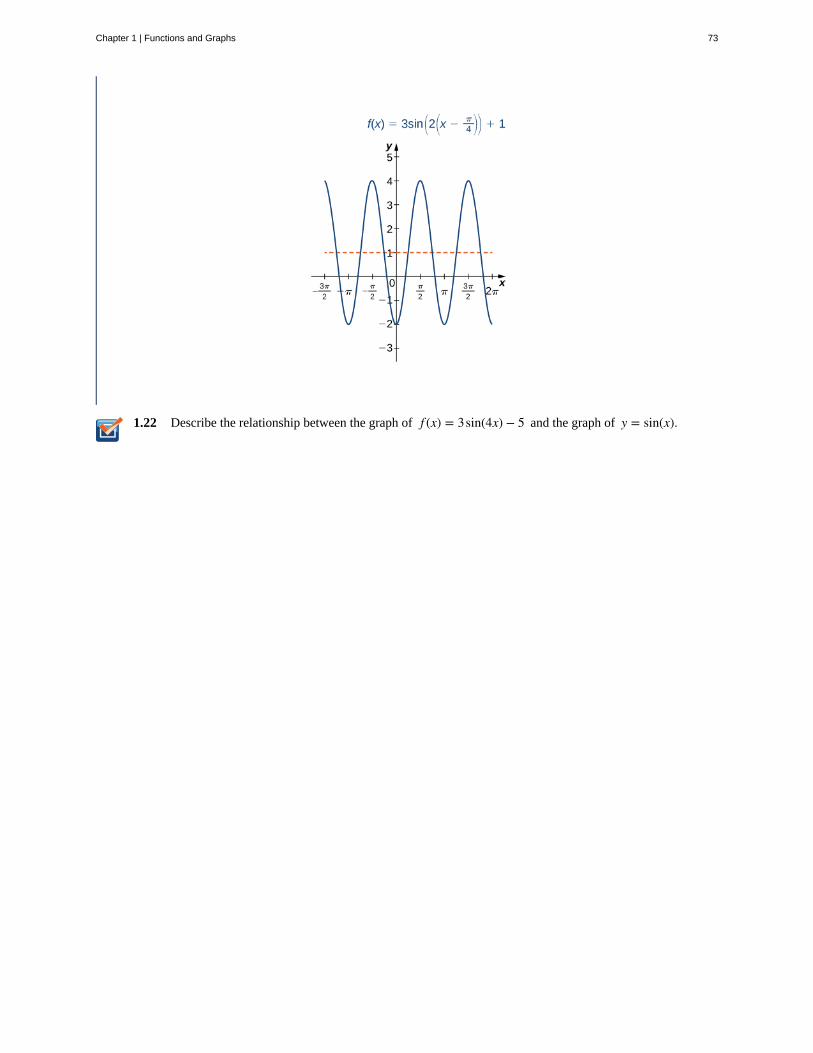
1.22 Describe the relationship between the graph of f (x) = 3sin(4x) − 5 and the graph of y = sin(x).
Chapter 1 | Functions and Graphs 73
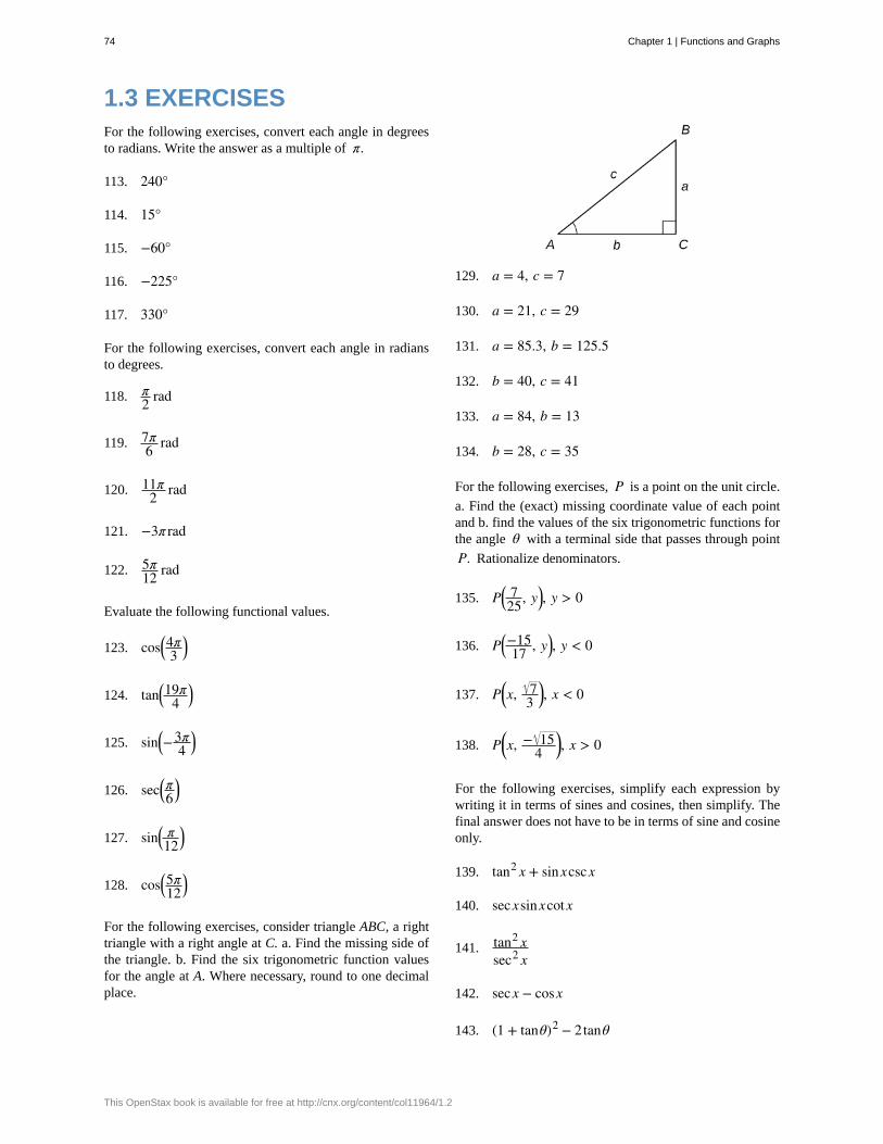
1.3 EXERCISESFor the following exercises, convert each angle in degreesto radians. Write the answer as a multiple of π.
113. 240°
114. 15°
115. −60°
116. −225°
117. 330°
For the following exercises, convert each angle in radiansto degrees.
118. π2 rad
119. 7π6 rad
120. 11π2 rad
121. −3π rad
122. 5π12 rad
Evaluate the following functional values.
123. cos⎛⎝4π3
⎞⎠
124. tan⎛⎝19π
4⎞⎠
125. sin⎛⎝−
3π4
⎞⎠
126. sec⎛⎝π6
⎞⎠
127. sin⎛⎝
π12
⎞⎠
128. cos⎛⎝5π12
⎞⎠
For the following exercises, consider triangle ABC, a righttriangle with a right angle at C. a. Find the missing side ofthe triangle. b. Find the six trigonometric function valuesfor the angle at A. Where necessary, round to one decimalplace.
129. a = 4, c = 7
130. a = 21, c = 29
131. a = 85.3, b = 125.5
132. b = 40, c = 41
133. a = 84, b = 13
134. b = 28, c = 35
For the following exercises, P is a point on the unit circle.
a. Find the (exact) missing coordinate value of each pointand b. find the values of the six trigonometric functions forthe angle θ with a terminal side that passes through point
P. Rationalize denominators.
135. P⎛⎝
725, y⎞
⎠, y > 0
136. P⎛⎝−1517 , y⎞
⎠, y < 0
137. P⎛⎝x, 7
3⎞⎠, x < 0
138. P⎛⎝x, − 15
4⎞⎠, x > 0
For the following exercises, simplify each expression bywriting it in terms of sines and cosines, then simplify. Thefinal answer does not have to be in terms of sine and cosineonly.
139. tan2 x + sinxcscx
140. secxsinxcot x
141. tan2 xsec2 x
142. secx − cosx
143. (1 + tanθ)2 − 2tanθ
74 Chapter 1 | Functions and Graphs
This OpenStax book is available for free at http://cnx.org/content/col11964/1.2
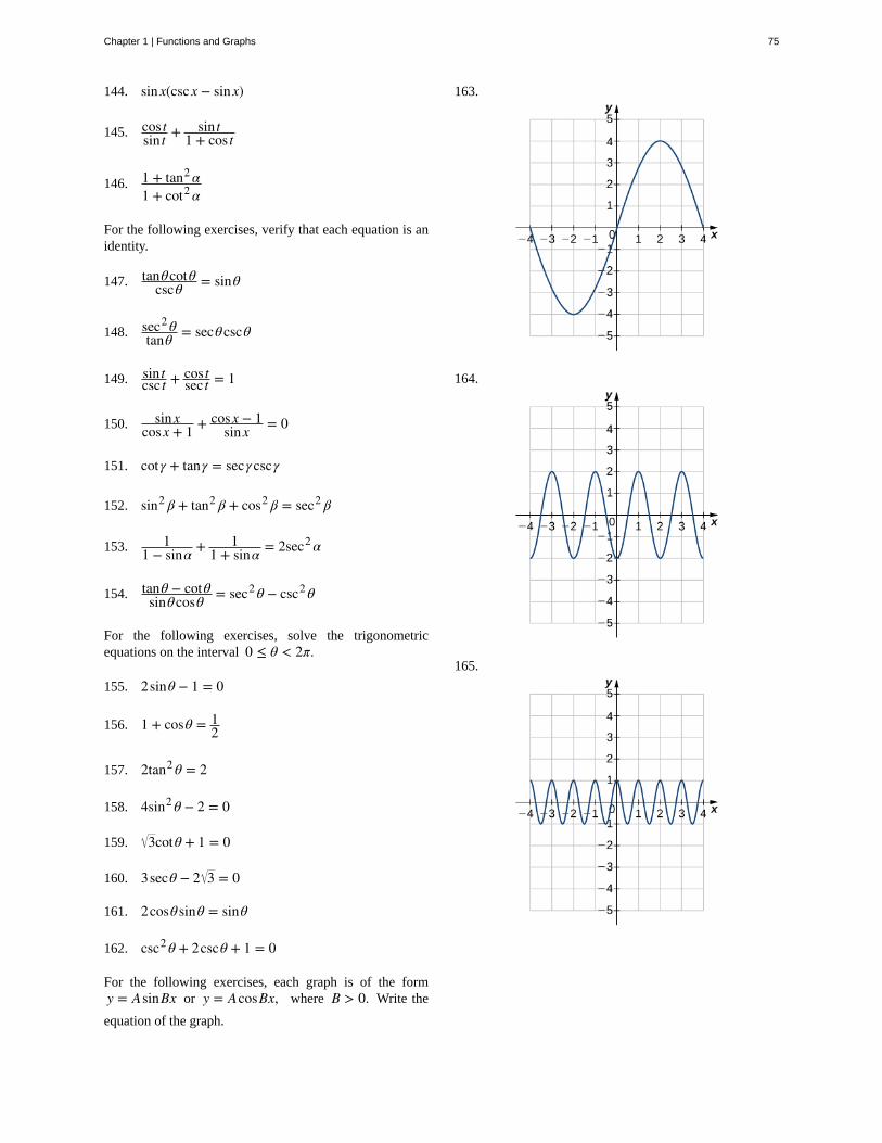
144. sinx(cscx − sinx)
145. cos tsin t + sin t
1 + cos t
146. 1 + tan2 α1 + cot2 α
For the following exercises, verify that each equation is anidentity.
147. tanθcotθcscθ = sinθ
148. sec2 θtanθ = secθcscθ
149. sin tcsc t + cos t
sec t = 1
150. sinxcosx + 1 + cosx − 1
sinx = 0
151. cotγ + tanγ = secγ cscγ
152. sin2 β + tan2 β + cos2 β = sec2 β
153. 11 − sinα + 1
1 + sinα = 2sec2 α
154. tanθ − cotθsinθcosθ = sec2 θ − csc2 θ
For the following exercises, solve the trigonometricequations on the interval 0 ≤ θ < 2π.
155. 2sinθ − 1 = 0
156. 1 + cosθ = 12
157. 2tan2 θ = 2
158. 4sin2 θ − 2 = 0
159. 3cotθ + 1 = 0
160. 3secθ − 2 3 = 0
161. 2cosθsinθ = sinθ
162. csc2 θ + 2cscθ + 1 = 0
For the following exercises, each graph is of the formy = AsinBx or y = AcosBx, where B > 0. Write the
equation of the graph.
163.
164.
165.
Chapter 1 | Functions and Graphs 75
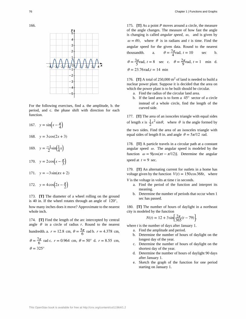
166.
For the following exercises, find a. the amplitude, b. theperiod, and c. the phase shift with direction for eachfunction.
167. y = sin⎛⎝x − π
4⎞⎠
168. y = 3cos(2x + 3)
169. y = −12 sin⎛
⎝14x⎞
⎠
170. y = 2cos⎛⎝x − π
3⎞⎠
171. y = −3sin(πx + 2)
172. y = 4cos⎛⎝2x − π
2⎞⎠
173. [T] The diameter of a wheel rolling on the groundis 40 in. If the wheel rotates through an angle of 120°,how many inches does it move? Approximate to the nearestwhole inch.
174. [T] Find the length of the arc intercepted by centralangle θ in a circle of radius r. Round to the nearest
hundredth. a. r = 12.8 cm, θ = 5π6 rad b. r = 4.378 cm,
θ = 7π6 rad c. r = 0.964 cm, θ = 50° d. r = 8.55 cm,
θ = 325°
175. [T] As a point P moves around a circle, the measureof the angle changes. The measure of how fast the angleis changing is called angular speed, ω, and is given by
ω = θ/t, where θ is in radians and t is time. Find the
angular speed for the given data. Round to the nearest
thousandth. a. θ = 7π4 rad, t = 10 sec b.
θ = 3π5 rad, t = 8 sec c. θ = 2π
9 rad, t = 1 min d.
θ = 23.76rad,t = 14 min
176. [T] A total of 250,000 m2 of land is needed to build anuclear power plant. Suppose it is decided that the area onwhich the power plant is to be built should be circular.
a. Find the radius of the circular land area.b. If the land area is to form a 45° sector of a circle
instead of a whole circle, find the length of thecurved side.
177. [T] The area of an isosceles triangle with equal sides
of length x is 12x2 sinθ, where θ is the angle formed by
the two sides. Find the area of an isosceles triangle withequal sides of length 8 in. and angle θ = 5π/12 rad.
178. [T] A particle travels in a circular path at a constantangular speed ω. The angular speed is modeled by the
function ω = 9|cos(πt − π/12)|. Determine the angular
speed at t = 9 sec.
179. [T] An alternating current for outlets in a home hasvoltage given by the function V(t) = 150cos368t, where
V is the voltage in volts at time t in seconds.a. Find the period of the function and interpret its
meaning.b. Determine the number of periods that occur when 1
sec has passed.
180. [T] The number of hours of daylight in a northeastcity is modeled by the function
N(t) = 12 + 3sin⎡⎣
2π365(t − 79)⎤⎦,
where t is the number of days after January 1.a. Find the amplitude and period.b. Determine the number of hours of daylight on the
longest day of the year.c. Determine the number of hours of daylight on the
shortest day of the year.d. Determine the number of hours of daylight 90 days
after January 1.e. Sketch the graph of the function for one period
starting on January 1.
76 Chapter 1 | Functions and Graphs
This OpenStax book is available for free at http://cnx.org/content/col11964/1.2
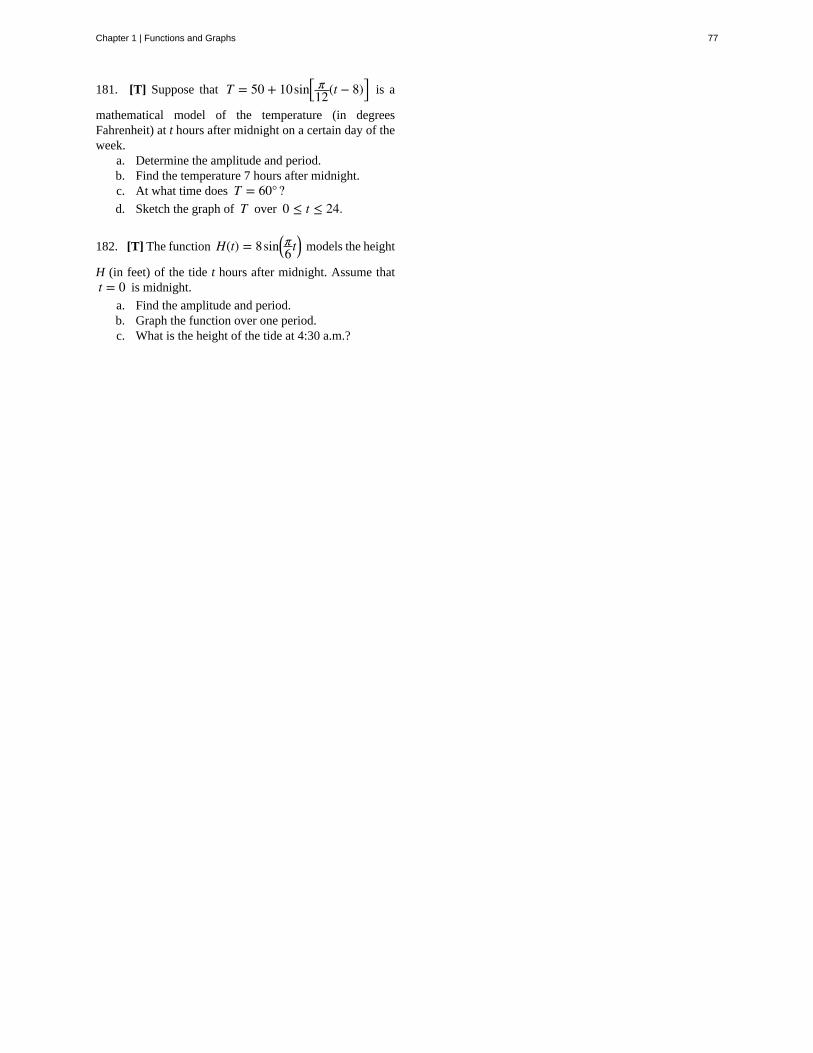
181. [T] Suppose that T = 50 + 10sin⎡⎣
π12(t − 8)⎤
⎦ is a
mathematical model of the temperature (in degreesFahrenheit) at t hours after midnight on a certain day of theweek.
a. Determine the amplitude and period.b. Find the temperature 7 hours after midnight.c. At what time does T = 60°?d. Sketch the graph of T over 0 ≤ t ≤ 24.
182. [T] The function H(t) = 8sin⎛⎝π6 t⎞⎠ models the height
H (in feet) of the tide t hours after midnight. Assume thatt = 0 is midnight.
a. Find the amplitude and period.b. Graph the function over one period.c. What is the height of the tide at 4:30 a.m.?
Chapter 1 | Functions and Graphs 77
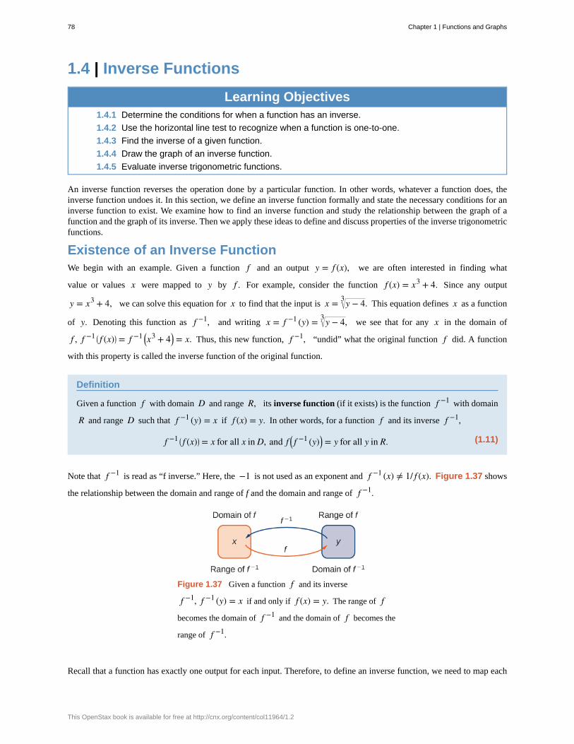
1.4 | Inverse Functions
Learning Objectives1.4.1 Determine the conditions for when a function has an inverse.
1.4.2 Use the horizontal line test to recognize when a function is one-to-one.
1.4.3 Find the inverse of a given function.
1.4.4 Draw the graph of an inverse function.
1.4.5 Evaluate inverse trigonometric functions.
An inverse function reverses the operation done by a particular function. In other words, whatever a function does, theinverse function undoes it. In this section, we define an inverse function formally and state the necessary conditions for aninverse function to exist. We examine how to find an inverse function and study the relationship between the graph of afunction and the graph of its inverse. Then we apply these ideas to define and discuss properties of the inverse trigonometricfunctions.
Existence of an Inverse FunctionWe begin with an example. Given a function f and an output y = f (x), we are often interested in finding what
value or values x were mapped to y by f . For example, consider the function f (x) = x3 + 4. Since any output
y = x3 + 4, we can solve this equation for x to find that the input is x = y − 43 . This equation defines x as a function
of y. Denoting this function as f −1, and writing x = f −1 (y) = y − 43 , we see that for any x in the domain of
f , f −1 ⎛⎝ f (x)⎞
⎠ = f −1 ⎛⎝x
3 + 4⎞⎠ = x. Thus, this new function, f −1, “undid” what the original function f did. A function
with this property is called the inverse function of the original function.
Definition
Given a function f with domain D and range R, its inverse function (if it exists) is the function f −1 with domain
R and range D such that f −1 (y) = x if f (x) = y. In other words, for a function f and its inverse f −1,
(1.11)f −1 ⎛⎝ f (x)⎞
⎠ = x for all x in D, and f ⎛⎝ f −1 (y)⎞
⎠ = y for all y in R.
Note that f −1 is read as “f inverse.” Here, the −1 is not used as an exponent and f −1 (x) ≠ 1/ f (x). Figure 1.37 shows
the relationship between the domain and range of f and the domain and range of f −1.
Figure 1.37 Given a function f and its inverse
f −1, f −1 (y) = x if and only if f (x) = y. The range of f
becomes the domain of f −1 and the domain of f becomes the
range of f −1.
Recall that a function has exactly one output for each input. Therefore, to define an inverse function, we need to map each
78 Chapter 1 | Functions and Graphs
This OpenStax book is available for free at http://cnx.org/content/col11964/1.2
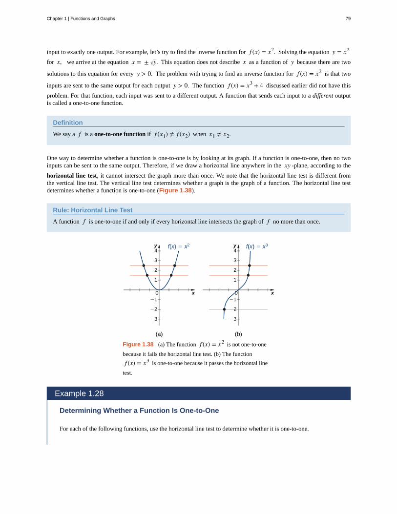
input to exactly one output. For example, let’s try to find the inverse function for f (x) = x2. Solving the equation y = x2
for x, we arrive at the equation x = ± y. This equation does not describe x as a function of y because there are two
solutions to this equation for every y > 0. The problem with trying to find an inverse function for f (x) = x2 is that two
inputs are sent to the same output for each output y > 0. The function f (x) = x3 + 4 discussed earlier did not have this
problem. For that function, each input was sent to a different output. A function that sends each input to a different outputis called a one-to-one function.
Definition
We say a f is a one-to-one function if f (x1) ≠ f (x2) when x1 ≠ x2.
One way to determine whether a function is one-to-one is by looking at its graph. If a function is one-to-one, then no twoinputs can be sent to the same output. Therefore, if we draw a horizontal line anywhere in the xy -plane, according to the
horizontal line test, it cannot intersect the graph more than once. We note that the horizontal line test is different fromthe vertical line test. The vertical line test determines whether a graph is the graph of a function. The horizontal line testdetermines whether a function is one-to-one (Figure 1.38).
Rule: Horizontal Line Test
A function f is one-to-one if and only if every horizontal line intersects the graph of f no more than once.
Figure 1.38 (a) The function f (x) = x2 is not one-to-one
because it fails the horizontal line test. (b) The function
f (x) = x3 is one-to-one because it passes the horizontal line
test.
Example 1.28
Determining Whether a Function Is One-to-One
For each of the following functions, use the horizontal line test to determine whether it is one-to-one.
Chapter 1 | Functions and Graphs 79
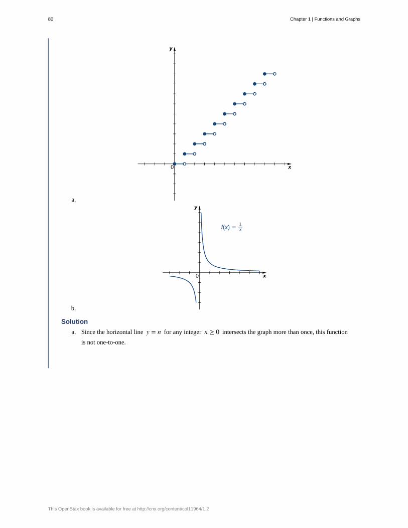
a.
b.
Solution
a. Since the horizontal line y = n for any integer n ≥ 0 intersects the graph more than once, this function
is not one-to-one.
80 Chapter 1 | Functions and Graphs
This OpenStax book is available for free at http://cnx.org/content/col11964/1.2
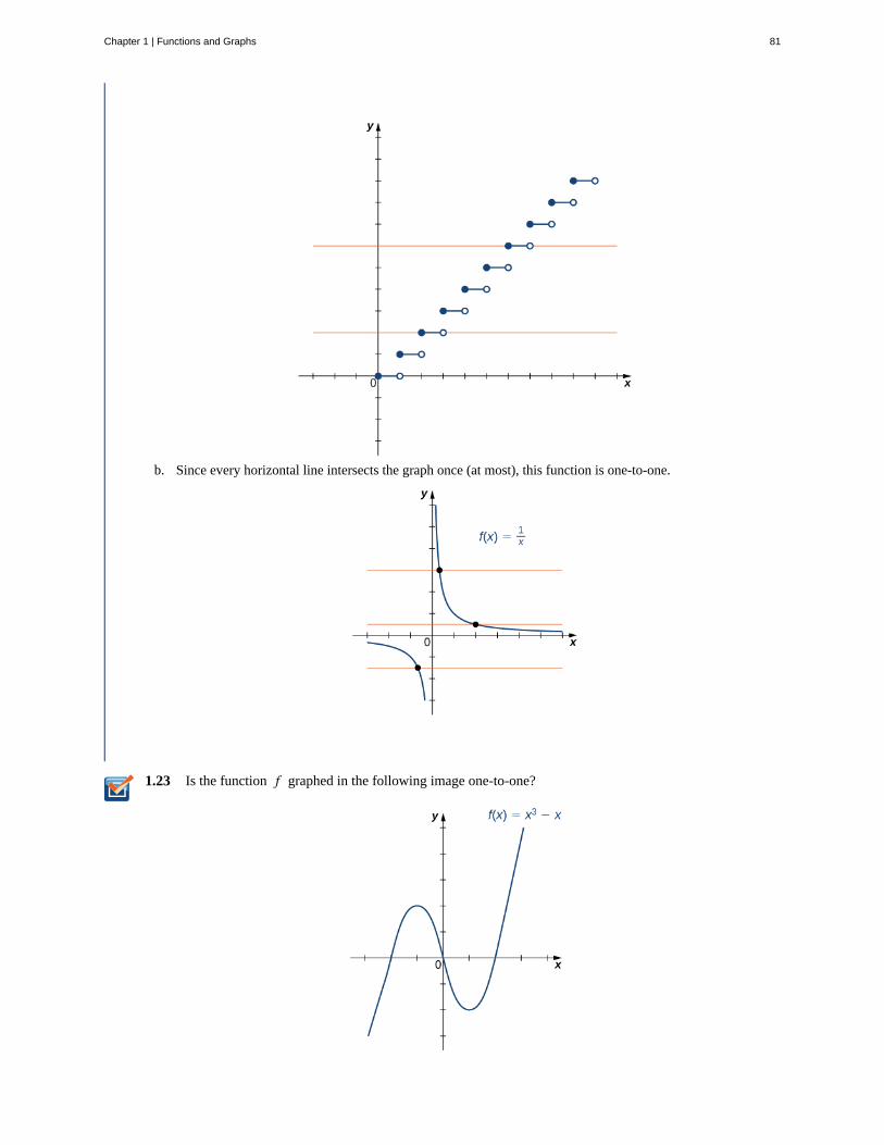
1.23
b. Since every horizontal line intersects the graph once (at most), this function is one-to-one.
Is the function f graphed in the following image one-to-one?
Chapter 1 | Functions and Graphs 81
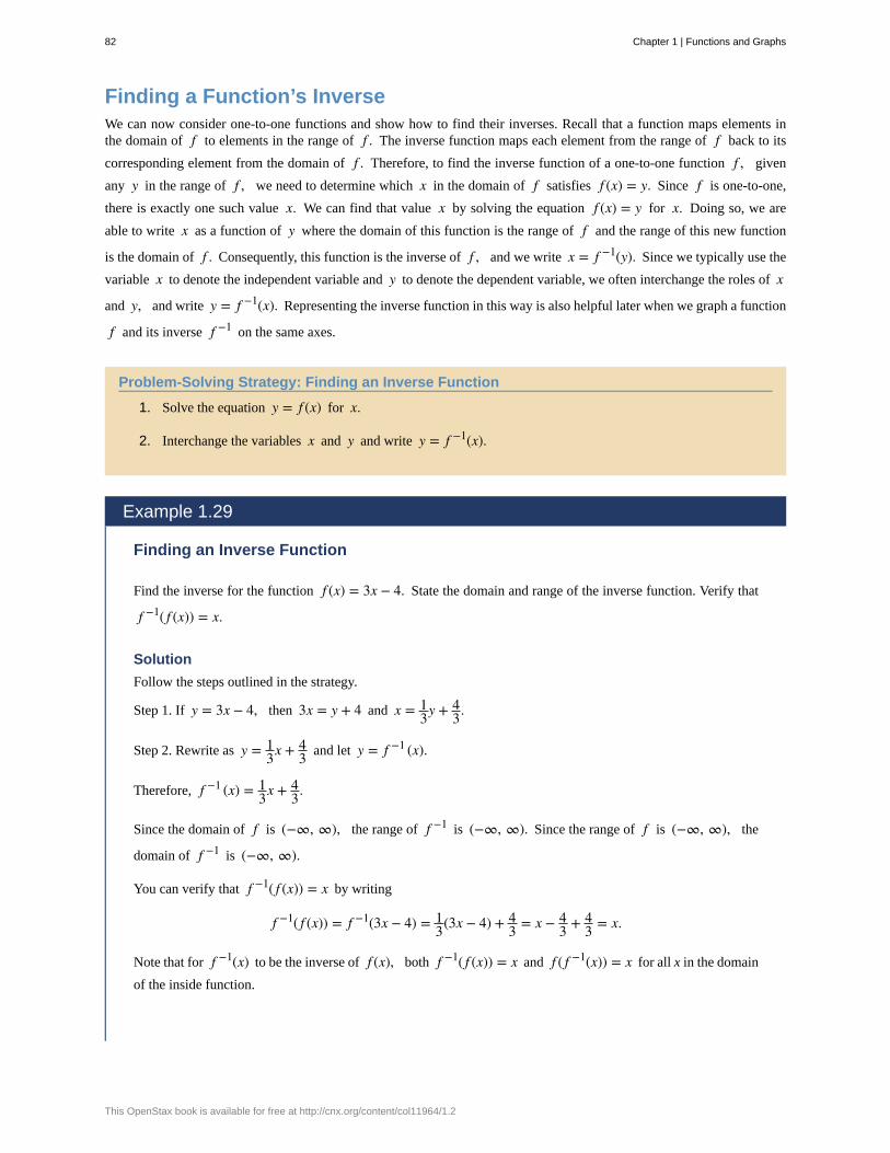
Finding a Function’s InverseWe can now consider one-to-one functions and show how to find their inverses. Recall that a function maps elements inthe domain of f to elements in the range of f . The inverse function maps each element from the range of f back to its
corresponding element from the domain of f . Therefore, to find the inverse function of a one-to-one function f , given
any y in the range of f , we need to determine which x in the domain of f satisfies f (x) = y. Since f is one-to-one,
there is exactly one such value x. We can find that value x by solving the equation f (x) = y for x. Doing so, we are
able to write x as a function of y where the domain of this function is the range of f and the range of this new function
is the domain of f . Consequently, this function is the inverse of f , and we write x = f −1(y). Since we typically use the
variable x to denote the independent variable and y to denote the dependent variable, we often interchange the roles of x
and y, and write y = f −1(x). Representing the inverse function in this way is also helpful later when we graph a function
f and its inverse f −1 on the same axes.
Problem-Solving Strategy: Finding an Inverse Function
1. Solve the equation y = f (x) for x.
2. Interchange the variables x and y and write y = f −1(x).
Example 1.29
Finding an Inverse Function
Find the inverse for the function f (x) = 3x − 4. State the domain and range of the inverse function. Verify that
f −1( f (x)) = x.
Solution
Follow the steps outlined in the strategy.
Step 1. If y = 3x − 4, then 3x = y + 4 and x = 13y + 4
3.
Step 2. Rewrite as y = 13x + 4
3 and let y = f −1 (x).
Therefore, f −1 (x) = 13x + 4
3.
Since the domain of f is (−∞, ∞), the range of f −1 is (−∞, ∞). Since the range of f is (−∞, ∞), the
domain of f −1 is (−∞, ∞).
You can verify that f −1( f (x)) = x by writing
f −1( f (x)) = f −1(3x − 4) = 13(3x − 4) + 4
3 = x − 43 + 4
3 = x.
Note that for f −1(x) to be the inverse of f (x), both f −1( f (x)) = x and f ( f −1(x)) = x for all x in the domain
of the inside function.
82 Chapter 1 | Functions and Graphs
This OpenStax book is available for free at http://cnx.org/content/col11964/1.2
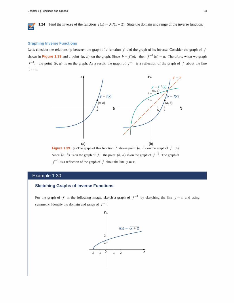
1.24 Find the inverse of the function f (x) = 3x/(x − 2). State the domain and range of the inverse function.
Graphing Inverse Functions
Let’s consider the relationship between the graph of a function f and the graph of its inverse. Consider the graph of f
shown in Figure 1.39 and a point (a, b) on the graph. Since b = f (a), then f −1 (b) = a. Therefore, when we graph
f −1, the point (b, a) is on the graph. As a result, the graph of f −1 is a reflection of the graph of f about the line
y = x.
Figure 1.39 (a) The graph of this function f shows point (a, b) on the graph of f . (b)
Since (a, b) is on the graph of f , the point (b, a) is on the graph of f −1. The graph of
f −1 is a reflection of the graph of f about the line y = x.
Example 1.30
Sketching Graphs of Inverse Functions
For the graph of f in the following image, sketch a graph of f −1 by sketching the line y = x and using
symmetry. Identify the domain and range of f −1.
Chapter 1 | Functions and Graphs 83
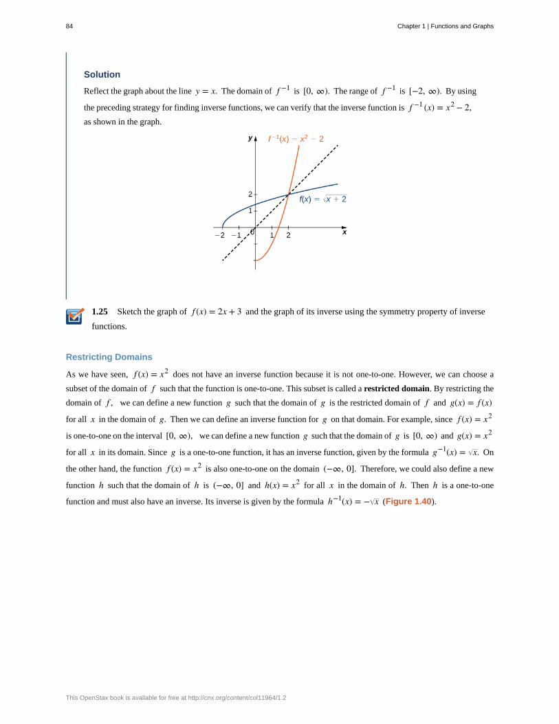
1.25
Solution
Reflect the graph about the line y = x. The domain of f −1 is [0, ∞). The range of f −1 is [−2, ∞). By using
the preceding strategy for finding inverse functions, we can verify that the inverse function is f −1 (x) = x2 − 2,as shown in the graph.
Sketch the graph of f (x) = 2x + 3 and the graph of its inverse using the symmetry property of inverse
functions.
Restricting Domains
As we have seen, f (x) = x2 does not have an inverse function because it is not one-to-one. However, we can choose a
subset of the domain of f such that the function is one-to-one. This subset is called a restricted domain. By restricting the
domain of f , we can define a new function g such that the domain of g is the restricted domain of f and g(x) = f (x)
for all x in the domain of g. Then we can define an inverse function for g on that domain. For example, since f (x) = x2
is one-to-one on the interval [0, ∞), we can define a new function g such that the domain of g is [0, ∞) and g(x) = x2
for all x in its domain. Since g is a one-to-one function, it has an inverse function, given by the formula g−1(x) = x. On
the other hand, the function f (x) = x2 is also one-to-one on the domain (−∞, 0]. Therefore, we could also define a new
function h such that the domain of h is (−∞, 0] and h(x) = x2 for all x in the domain of h. Then h is a one-to-one
function and must also have an inverse. Its inverse is given by the formula h−1(x) = − x (Figure 1.40).
84 Chapter 1 | Functions and Graphs
This OpenStax book is available for free at http://cnx.org/content/col11964/1.2
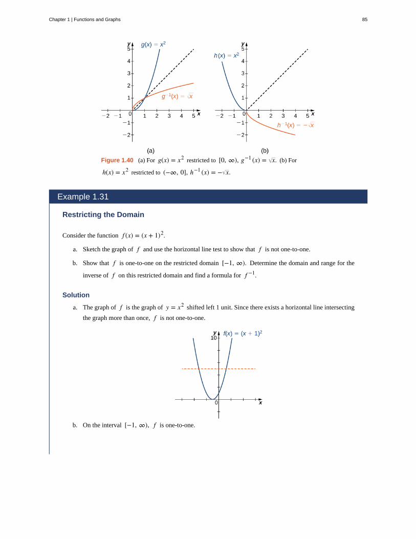
Figure 1.40 (a) For g(x) = x2 restricted to [0, ∞), g−1 (x) = x. (b) For
h(x) = x2 restricted to (−∞, 0], h−1 (x) = − x.
Example 1.31
Restricting the Domain
Consider the function f (x) = (x + 1)2.
a. Sketch the graph of f and use the horizontal line test to show that f is not one-to-one.
b. Show that f is one-to-one on the restricted domain [−1, ∞). Determine the domain and range for the
inverse of f on this restricted domain and find a formula for f −1.
Solution
a. The graph of f is the graph of y = x2 shifted left 1 unit. Since there exists a horizontal line intersecting
the graph more than once, f is not one-to-one.
b. On the interval [−1, ∞), f is one-to-one.
Chapter 1 | Functions and Graphs 85
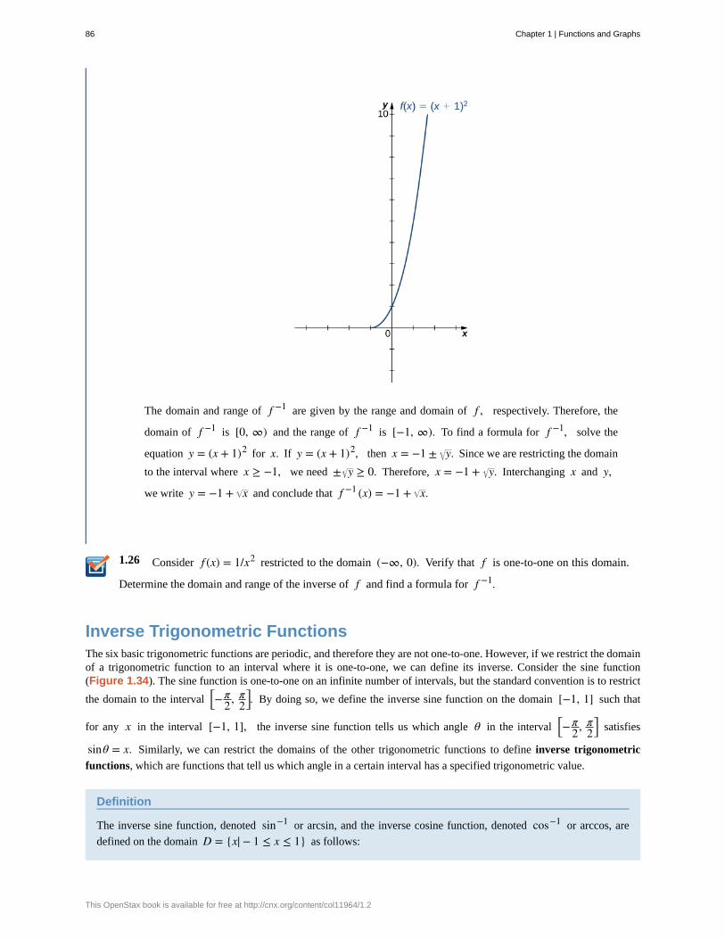
1.26
The domain and range of f −1 are given by the range and domain of f , respectively. Therefore, the
domain of f −1 is [0, ∞) and the range of f −1 is [−1, ∞). To find a formula for f −1, solve the
equation y = (x + 1)2 for x. If y = (x + 1)2, then x = −1 ± y. Since we are restricting the domain
to the interval where x ≥ −1, we need ± y ≥ 0. Therefore, x = −1 + y. Interchanging x and y,
we write y = −1 + x and conclude that f −1 (x) = −1 + x.
Consider f (x) = 1/x2 restricted to the domain (−∞, 0). Verify that f is one-to-one on this domain.
Determine the domain and range of the inverse of f and find a formula for f −1.
Inverse Trigonometric FunctionsThe six basic trigonometric functions are periodic, and therefore they are not one-to-one. However, if we restrict the domainof a trigonometric function to an interval where it is one-to-one, we can define its inverse. Consider the sine function(Figure 1.34). The sine function is one-to-one on an infinite number of intervals, but the standard convention is to restrict
the domain to the interval⎡⎣−
π2, π
2⎤⎦. By doing so, we define the inverse sine function on the domain [−1, 1] such that
for any x in the interval [−1, 1], the inverse sine function tells us which angle θ in the interval⎡⎣−
π2, π
2⎤⎦ satisfies
sinθ = x. Similarly, we can restrict the domains of the other trigonometric functions to define inverse trigonometric
functions, which are functions that tell us which angle in a certain interval has a specified trigonometric value.
Definition
The inverse sine function, denoted sin−1 or arcsin, and the inverse cosine function, denoted cos−1 or arccos, are
defined on the domain D = {x| − 1 ≤ x ≤ 1} as follows:
86 Chapter 1 | Functions and Graphs
This OpenStax book is available for free at http://cnx.org/content/col11964/1.2
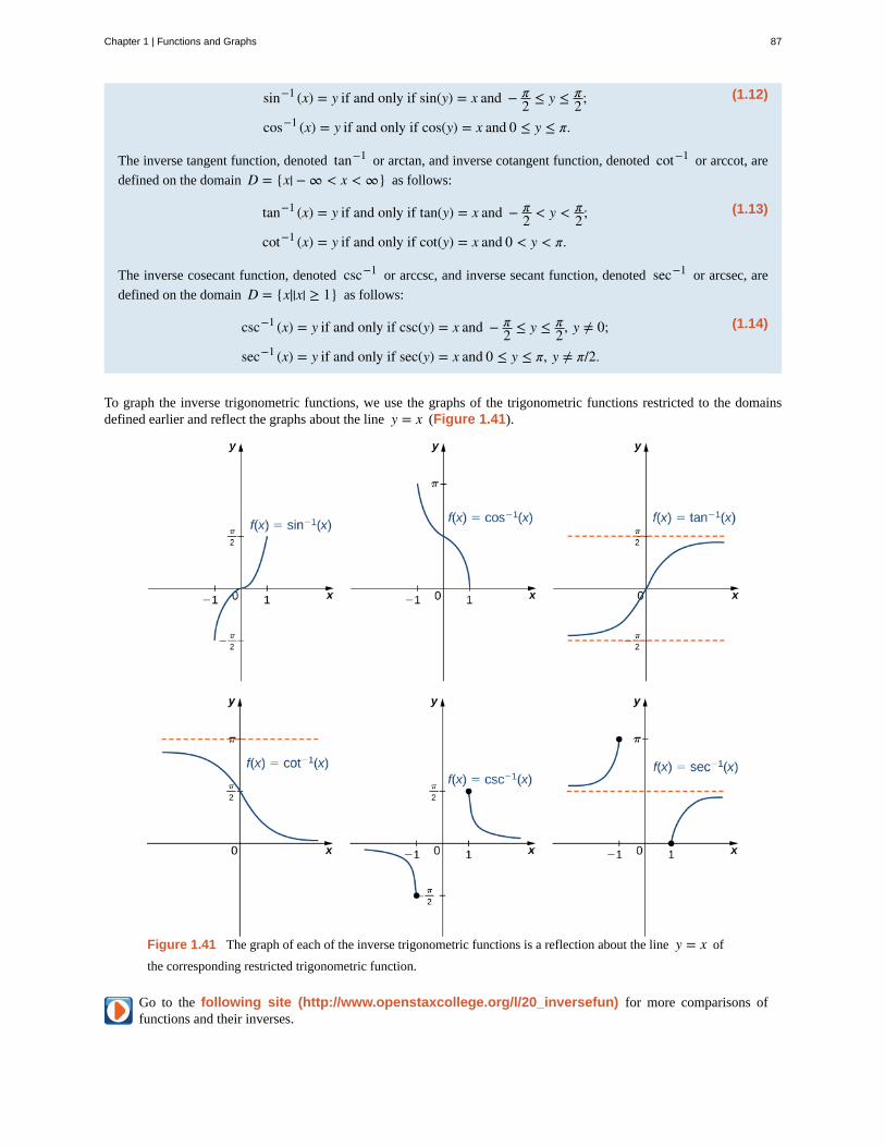
(1.12)sin−1 (x) = y if and only if sin(y) = x and − π2 ≤ y ≤ π
2;
cos−1 (x) = y if and only if cos(y) = x and 0 ≤ y ≤ π.
The inverse tangent function, denoted tan−1 or arctan, and inverse cotangent function, denoted cot−1 or arccot, are
defined on the domain D = {x| − ∞ < x < ∞} as follows:
(1.13)tan−1 (x) = y if and only if tan(y) = x and − π2 < y < π
2;
cot−1 (x) = y if and only if cot(y) = x and 0 < y < π.
The inverse cosecant function, denoted csc−1 or arccsc, and inverse secant function, denoted sec−1 or arcsec, are
defined on the domain D = {x||x| ≥ 1} as follows:
(1.14)csc−1 (x) = y if and only if csc(y) = x and − π2 ≤ y ≤ π
2, y ≠ 0;
sec−1 (x) = y if and only if sec(y) = x and 0 ≤ y ≤ π, y ≠ π/2.
To graph the inverse trigonometric functions, we use the graphs of the trigonometric functions restricted to the domainsdefined earlier and reflect the graphs about the line y = x (Figure 1.41).
Figure 1.41 The graph of each of the inverse trigonometric functions is a reflection about the line y = x of
the corresponding restricted trigonometric function.
Go to the following site (http://www.openstaxcollege.org/l/20_inversefun) for more comparisons offunctions and their inverses.
Chapter 1 | Functions and Graphs 87
When evaluating an inverse trigonometric function, the output is an angle. For example, to evaluate cos−1 ⎛⎝12
⎞⎠, we need to
find an angle θ such that cosθ = 12. Clearly, many angles have this property. However, given the definition of cos−1, we
need the angle θ that not only solves this equation, but also lies in the interval [0, π]. We conclude that cos−1 ⎛⎝12
⎞⎠ = π
3.
We now consider a composition of a trigonometric function and its inverse. For example, consider the two expressions
sin⎛⎝sin−1 ⎛
⎝22
⎞⎠⎞⎠ and sin−1(sin(π)). For the first one, we simplify as follows:
sin⎛⎝sin−1 ⎛
⎝22
⎞⎠⎞⎠ = sin⎛
⎝π4
⎞⎠ = 2
2 .
For the second one, we have
sin−1 ⎛⎝sin(π)⎞
⎠ = sin−1 (0) = 0.
The inverse function is supposed to “undo” the original function, so why isn’t sin−1 ⎛⎝sin(π)⎞
⎠ = π ? Recalling our definition
of inverse functions, a function f and its inverse f −1 satisfy the conditions f ⎛⎝ f −1 (y)⎞
⎠ = y for all y in the domain of
f −1 and f −1 ⎛⎝ f (x)⎞
⎠ = x for all x in the domain of f , so what happened here? The issue is that the inverse sine function,
sin−1, is the inverse of the restricted sine function defined on the domain⎡⎣−
π2, π
2⎤⎦. Therefore, for x in the interval
⎡⎣−
π2, π
2⎤⎦, it is true that sin−1 (sinx) = x. However, for values of x outside this interval, the equation does not hold, even
though sin−1(sinx) is defined for all real numbers x.
What about sin(sin−1 y)? Does that have a similar issue? The answer is no. Since the domain of sin−1 is the interval
[−1, 1], we conclude that sin(sin−1 y) = y if −1 ≤ y ≤ 1 and the expression is not defined for other values of y. To
summarize,
sin(sin−1 y) = y if −1 ≤ y ≤ 1
and
sin−1 (sinx) = x if − π2 ≤ x ≤ π
2.
Similarly, for the cosine function,
cos(cos−1 y) = y if −1 ≤ y ≤ 1
and
cos−1 (cosx) = x if 0 ≤ x ≤ π.
Similar properties hold for the other trigonometric functions and their inverses.
Example 1.32
Evaluating Expressions Involving Inverse Trigonometric Functions
Evaluate each of the following expressions.
a. sin−1 ⎛⎝− 3
2⎞⎠
b. tan⎛⎝tan−1 ⎛
⎝− 13
⎞⎠⎞⎠
88 Chapter 1 | Functions and Graphs
This OpenStax book is available for free at http://cnx.org/content/col11964/1.2
c. cos−1 ⎛⎝cos⎛
⎝5π4
⎞⎠⎞⎠
d. sin−1 ⎛⎝cos⎛
⎝2π3
⎞⎠⎞⎠
Solution
a. Evaluating sin−1 ⎛⎝− 3/2⎞
⎠ is equivalent to finding the angle θ such that sinθ = − 3/2 and
−π/2 ≤ θ ≤ π/2. The angle θ = −π/3 satisfies these two conditions. Therefore,
sin−1 ⎛⎝− 3/2⎞
⎠ = −π/3.
b. First we use the fact that tan−1 ⎛⎝−1/ 3⎞
⎠ = −π/6. Then tan(π/6) = −1/ 3. Therefore,
tan⎛⎝tan−1 ⎛
⎝−1/ 3⎞⎠⎞⎠ = −1/ 3.
c. To evaluate cos−1 ⎛⎝cos(5π/4)⎞
⎠, first use the fact that cos(5π/4) = − 2/2. Then we need to find the
angle θ such that cos(θ) = − 2/2 and 0 ≤ θ ≤ π. Since 3π/4 satisfies both these conditions, we have
cos⎛⎝cos−1 (5π/4)⎞
⎠ = cos⎛⎝cos−1 ⎛
⎝− 2/2⎞⎠⎞⎠ = 3π/4.
d. Since cos(2π/3) = −1/2, we need to evaluate sin−1 (−1/2). That is, we need to find the angle θ such
that sin(θ) = −1/2 and −π/2 ≤ θ ≤ π/2. Since −π/6 satisfies both these conditions, we can conclude
that sin−1 (cos(2π/3)) = sin−1 (−1/2) = −π/6.
Chapter 1 | Functions and Graphs 89
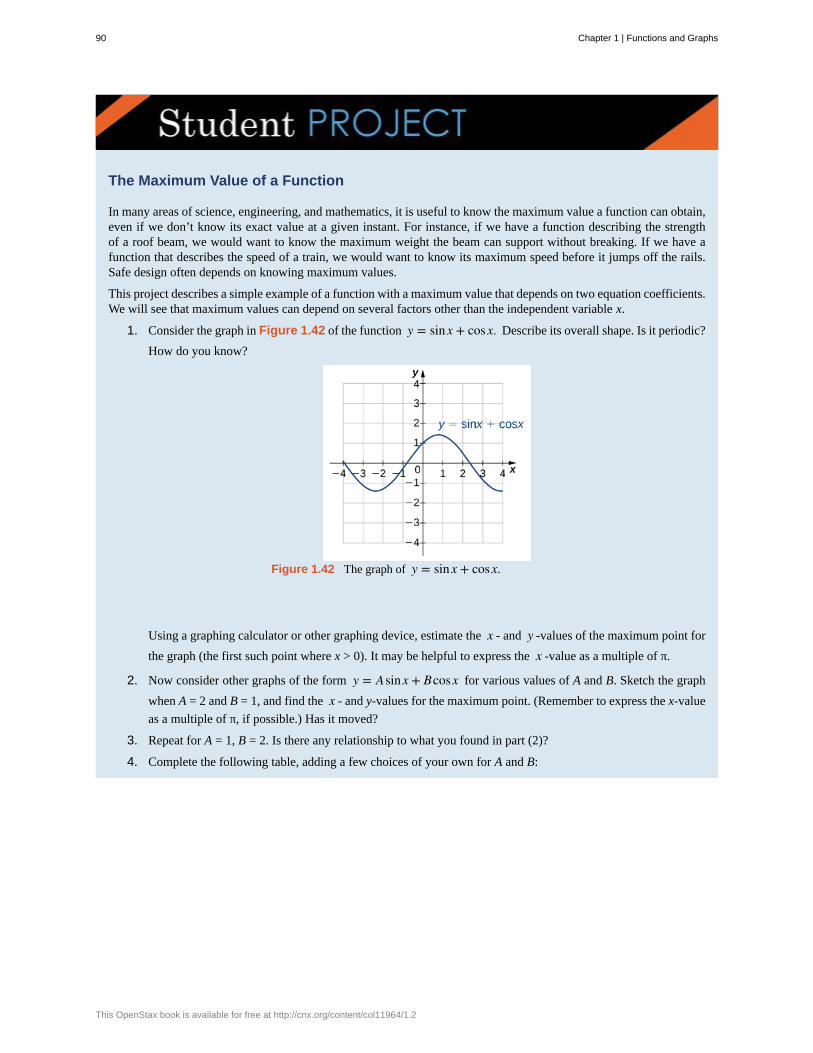
The Maximum Value of a Function
In many areas of science, engineering, and mathematics, it is useful to know the maximum value a function can obtain,even if we don’t know its exact value at a given instant. For instance, if we have a function describing the strengthof a roof beam, we would want to know the maximum weight the beam can support without breaking. If we have afunction that describes the speed of a train, we would want to know its maximum speed before it jumps off the rails.Safe design often depends on knowing maximum values.
This project describes a simple example of a function with a maximum value that depends on two equation coefficients.We will see that maximum values can depend on several factors other than the independent variable x.
1. Consider the graph in Figure 1.42 of the function y = sinx + cosx. Describe its overall shape. Is it periodic?
How do you know?
Figure 1.42 The graph of y = sinx + cosx.
Using a graphing calculator or other graphing device, estimate the x - and y -values of the maximum point for
the graph (the first such point where x > 0). It may be helpful to express the x -value as a multiple of π.
2. Now consider other graphs of the form y = Asinx + Bcosx for various values of A and B. Sketch the graph
when A = 2 and B = 1, and find the x - and y-values for the maximum point. (Remember to express the x-value
as a multiple of π, if possible.) Has it moved?
3. Repeat for A = 1, B = 2. Is there any relationship to what you found in part (2)?
4. Complete the following table, adding a few choices of your own for A and B:
90 Chapter 1 | Functions and Graphs
This OpenStax book is available for free at http://cnx.org/content/col11964/1.2
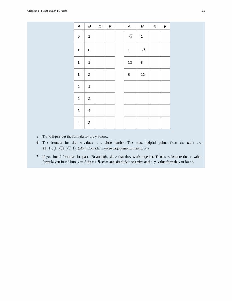
A B x y A B x y
0 1 3 1
1 0 1 3
1 1 12 5
1 2 5 12
2 1
2 2
3 4
4 3
5. Try to figure out the formula for the y-values.
6. The formula for the x -values is a little harder. The most helpful points from the table are
(1, 1), ⎛⎝1, 3⎞
⎠, ⎛⎝ 3, 1⎞
⎠. (Hint: Consider inverse trigonometric functions.)
7. If you found formulas for parts (5) and (6), show that they work together. That is, substitute the x -value
formula you found into y = Asinx + Bcosx and simplify it to arrive at the y -value formula you found.
Chapter 1 | Functions and Graphs 91
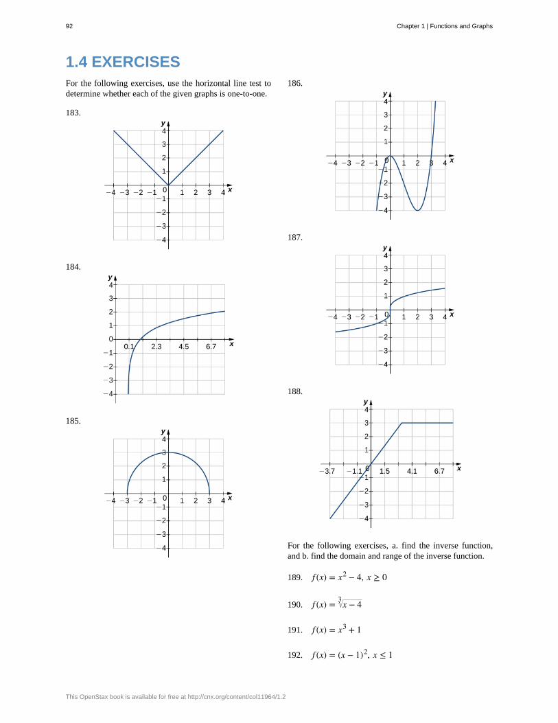
1.4 EXERCISESFor the following exercises, use the horizontal line test todetermine whether each of the given graphs is one-to-one.
183.
184.
185.
186.
187.
188.
For the following exercises, a. find the inverse function,and b. find the domain and range of the inverse function.
189. f (x) = x2 − 4, x ≥ 0
190. f (x) = x − 43
191. f (x) = x3 + 1
192. f (x) = (x − 1)2, x ≤ 1
92 Chapter 1 | Functions and Graphs
This OpenStax book is available for free at http://cnx.org/content/col11964/1.2
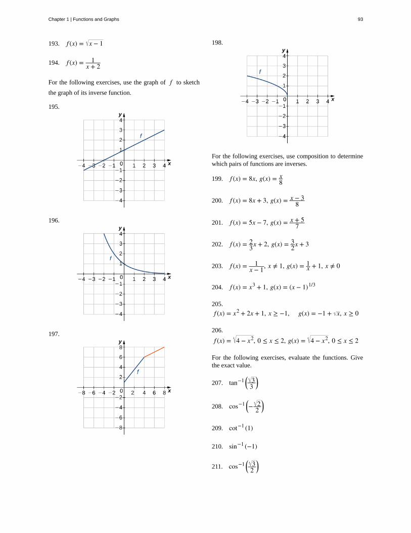
193. f (x) = x − 1
194. f (x) = 1x + 2
For the following exercises, use the graph of f to sketch
the graph of its inverse function.
195.
196.
197.
198.
For the following exercises, use composition to determinewhich pairs of functions are inverses.
199. f (x) = 8x, g(x) = x8
200. f (x) = 8x + 3, g(x) = x − 38
201. f (x) = 5x − 7, g(x) = x + 57
202. f (x) = 23x + 2, g(x) = 3
2x + 3
203. f (x) = 1x − 1, x ≠ 1, g(x) = 1
x + 1, x ≠ 0
204. f (x) = x3 + 1, g(x) = (x − 1)1/3
205.
f (x) = x2 + 2x + 1, x ≥ −1, g(x) = −1 + x, x ≥ 0
206.
f (x) = 4 − x2, 0 ≤ x ≤ 2, g(x) = 4 − x2, 0 ≤ x ≤ 2
For the following exercises, evaluate the functions. Givethe exact value.
207. tan−1 ⎛⎝
33
⎞⎠
208. cos−1 ⎛⎝− 2
2⎞⎠
209. cot−1 (1)
210. sin−1 (−1)
211. cos−1 ⎛⎝
32
⎞⎠
Chapter 1 | Functions and Graphs 93
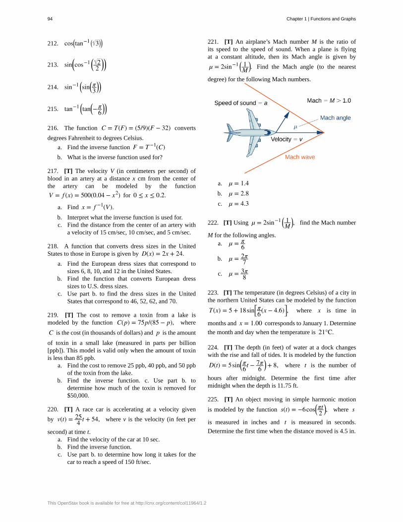
212. cos⎛⎝tan−1 ⎛
⎝ 3⎞⎠⎞⎠
213. sin⎛⎝cos−1 ⎛
⎝22
⎞⎠⎞⎠
214. sin−1 ⎛⎝sin⎛
⎝π3
⎞⎠⎞⎠
215. tan−1 ⎛⎝tan⎛
⎝−π6
⎞⎠⎞⎠
216. The function C = T(F) = (5/9)(F − 32) converts
degrees Fahrenheit to degrees Celsius.
a. Find the inverse function F = T −1(C)b. What is the inverse function used for?
217. [T] The velocity V (in centimeters per second) ofblood in an artery at a distance x cm from the center ofthe artery can be modeled by the function
V = f (x) = 500(0.04 − x2) for 0 ≤ x ≤ 0.2.
a. Find x = f −1(V).b. Interpret what the inverse function is used for.c. Find the distance from the center of an artery with
a velocity of 15 cm/sec, 10 cm/sec, and 5 cm/sec.
218. A function that converts dress sizes in the UnitedStates to those in Europe is given by D(x) = 2x + 24.
a. Find the European dress sizes that correspond tosizes 6, 8, 10, and 12 in the United States.
b. Find the function that converts European dresssizes to U.S. dress sizes.
c. Use part b. to find the dress sizes in the UnitedStates that correspond to 46, 52, 62, and 70.
219. [T] The cost to remove a toxin from a lake ismodeled by the function C(p) = 75p/(85 − p), where
C is the cost (in thousands of dollars) and p is the amount
of toxin in a small lake (measured in parts per billion[ppb]). This model is valid only when the amount of toxinis less than 85 ppb.
a. Find the cost to remove 25 ppb, 40 ppb, and 50 ppbof the toxin from the lake.
b. Find the inverse function. c. Use part b. todetermine how much of the toxin is removed for$50,000.
220. [T] A race car is accelerating at a velocity given
by v(t) = 254 t + 54, where v is the velocity (in feet per
second) at time t.a. Find the velocity of the car at 10 sec.b. Find the inverse function.c. Use part b. to determine how long it takes for the
car to reach a speed of 150 ft/sec.
221. [T] An airplane’s Mach number M is the ratio ofits speed to the speed of sound. When a plane is flyingat a constant altitude, then its Mach angle is given by
µ = 2sin−1 ⎛⎝
1M
⎞⎠. Find the Mach angle (to the nearest
degree) for the following Mach numbers.
a. µ = 1.4b. µ = 2.8c. µ = 4.3
222. [T] Using µ = 2sin−1 ⎛⎝
1M
⎞⎠, find the Mach number
M for the following angles.a. µ = π
6
b. µ = 2π7
c. µ = 3π8
223. [T] The temperature (in degrees Celsius) of a city inthe northern United States can be modeled by the function
T(x) = 5 + 18sin⎡⎣π6(x − 4.6)⎤⎦, where x is time in
months and x = 1.00 corresponds to January 1. Determine
the month and day when the temperature is 21°C.
224. [T] The depth (in feet) of water at a dock changeswith the rise and fall of tides. It is modeled by the function
D(t) = 5sin⎛⎝π6 t − 7π
6⎞⎠ + 8, where t is the number of
hours after midnight. Determine the first time aftermidnight when the depth is 11.75 ft.
225. [T] An object moving in simple harmonic motion
is modeled by the function s(t) = −6cos⎛⎝πt2
⎞⎠, where s
is measured in inches and t is measured in seconds.
Determine the first time when the distance moved is 4.5 in.
94 Chapter 1 | Functions and Graphs
This OpenStax book is available for free at http://cnx.org/content/col11964/1.2
226. [T] A local art gallery has a portrait 3 ft in heightthat is hung 2.5 ft above the eye level of an average person.The viewing angle θ can be modeled by the function
θ = tan−1 5.5x − tan−1 2.5
x , where x is the distance (in
feet) from the portrait. Find the viewing angle when aperson is 4 ft from the portrait.
227. [T] Use a calculator to evaluate tan−1 (tan(2.1)) and
cos−1 (cos(2.1)). Explain the results of each.
228. [T] Use a calculator to evaluate sin(sin−1(−2)) and
tan(tan−1(−2)). Explain the results of each.
Chapter 1 | Functions and Graphs 95
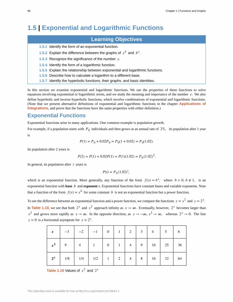
1.5 | Exponential and Logarithmic Functions
Learning Objectives1.5.1 Identify the form of an exponential function.
1.5.2 Explain the difference between the graphs of xb and bx.1.5.3 Recognize the significance of the number e.1.5.4 Identify the form of a logarithmic function.
1.5.5 Explain the relationship between exponential and logarithmic functions.
1.5.6 Describe how to calculate a logarithm to a different base.
1.5.7 Identify the hyperbolic functions, their graphs, and basic identities.
In this section we examine exponential and logarithmic functions. We use the properties of these functions to solveequations involving exponential or logarithmic terms, and we study the meaning and importance of the number e. We also
define hyperbolic and inverse hyperbolic functions, which involve combinations of exponential and logarithmic functions.(Note that we present alternative definitions of exponential and logarithmic functions in the chapter Applications ofIntegrations, and prove that the functions have the same properties with either definition.)
Exponential FunctionsExponential functions arise in many applications. One common example is population growth.
For example, if a population starts with P0 individuals and then grows at an annual rate of 2%, its population after 1 year
is
P(1) = P0 + 0.02P0 = P0(1 + 0.02) = P0(1.02).
Its population after 2 years is
P(2) = P(1) + 0.02P(1) = P(1)(1.02) = P0 (1.02)2.
In general, its population after t years is
P(t) = P0 (1.02)t,
which is an exponential function. More generally, any function of the form f (x) = bx, where b > 0, b ≠ 1, is an
exponential function with base b and exponent x. Exponential functions have constant bases and variable exponents. Note
that a function of the form f (x) = xb for some constant b is not an exponential function but a power function.
To see the difference between an exponential function and a power function, we compare the functions y = x2 and y = 2x.
In Table 1.10, we see that both 2x and x2 approach infinity as x → ∞. Eventually, however, 2x becomes larger than
x2 and grows more rapidly as x → ∞. In the opposite direction, as x → −∞, x2 → ∞, whereas 2x → 0. The line
y = 0 is a horizontal asymptote for y = 2x.
x −3 −2 −1 0 1 2 3 4 5 6
x2 9 4 1 0 1 4 9 16 25 36
2x 1/8 1/4 1/2 1 2 4 8 16 32 64
Table 1.10 Values of x2 and 2x
96 Chapter 1 | Functions and Graphs
This OpenStax book is available for free at http://cnx.org/content/col11964/1.2
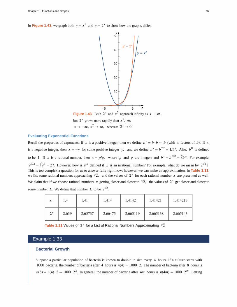
In Figure 1.43, we graph both y = x2 and y = 2x to show how the graphs differ.
Figure 1.43 Both 2x and x2 approach infinity as x → ∞,
but 2x grows more rapidly than x2. As
x → −∞, x2 → ∞, whereas 2x → 0.
Evaluating Exponential Functions
Recall the properties of exponents: If x is a positive integer, then we define bx = b · b ⋯ b (with x factors of b). If x
is a negative integer, then x = −y for some positive integer y, and we define bx = b−y = 1/by. Also, b0 is defined
to be 1. If x is a rational number, then x = p/q, where p and q are integers and bx = b p/q = b pq. For example,
93/2 = 93 = 27. However, how is bx defined if x is an irrational number? For example, what do we mean by 2 2?This is too complex a question for us to answer fully right now; however, we can make an approximation. In Table 1.11,we list some rational numbers approaching 2, and the values of 2x for each rational number x are presented as well.
We claim that if we choose rational numbers x getting closer and closer to 2, the values of 2x get closer and closer to
some number L. We define that number L to be 2 2.
x 1.4 1.41 1.414 1.4142 1.41421 1.414213
2x 2.639 2.65737 2.66475 2.665119 2.665138 2.665143
Table 1.11 Values of 2x for a List of Rational Numbers Approximating 2
Example 1.33
Bacterial Growth
Suppose a particular population of bacteria is known to double in size every 4 hours. If a culture starts with
1000 bacteria, the number of bacteria after 4 hours is n(4) = 1000 · 2. The number of bacteria after 8 hours is
n(8) = n(4) · 2 = 1000 · 22. In general, the number of bacteria after 4m hours is n(4m) = 1000 · 2m. Letting
Chapter 1 | Functions and Graphs 97
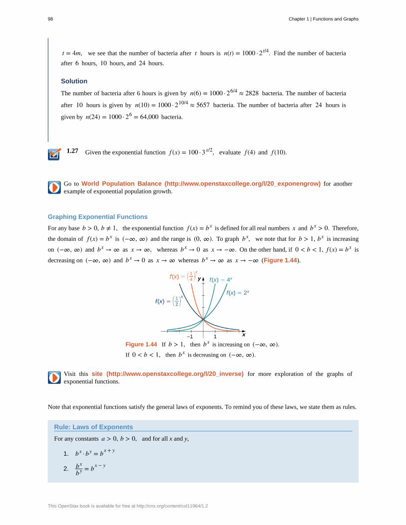
1.27
t = 4m, we see that the number of bacteria after t hours is n(t) = 1000 · 2t/4. Find the number of bacteria
after 6 hours, 10 hours, and 24 hours.
Solution
The number of bacteria after 6 hours is given by n(6) = 1000 · 26/4 ≈ 2828 bacteria. The number of bacteria
after 10 hours is given by n(10) = 1000 · 210/4 ≈ 5657 bacteria. The number of bacteria after 24 hours is
given by n(24) = 1000 · 26 = 64,000 bacteria.
Given the exponential function f (x) = 100 · 3x/2, evaluate f (4) and f (10).
Go to World Population Balance (http://www.openstaxcollege.org/l/20_exponengrow) for anotherexample of exponential population growth.
Graphing Exponential Functions
For any base b > 0, b ≠ 1, the exponential function f (x) = bx is defined for all real numbers x and bx > 0. Therefore,
the domain of f (x) = bx is (−∞, ∞) and the range is (0, ∞). To graph bx, we note that for b > 1, bx is increasing
on (−∞, ∞) and bx → ∞ as x → ∞, whereas bx → 0 as x → −∞. On the other hand, if 0 < b < 1, f (x) = bx is
decreasing on (−∞, ∞) and bx → 0 as x → ∞ whereas bx → ∞ as x → −∞ (Figure 1.44).
Figure 1.44 If b > 1, then bx is increasing on (−∞, ∞).If 0 < b < 1, then bx is decreasing on (−∞, ∞).
Visit this site (http://www.openstaxcollege.org/l/20_inverse) for more exploration of the graphs ofexponential functions.
Note that exponential functions satisfy the general laws of exponents. To remind you of these laws, we state them as rules.
Rule: Laws of Exponents
For any constants a > 0, b > 0, and for all x and y,
1. bx · by = bx + y
2. bx
by = bx − y
98 Chapter 1 | Functions and Graphs
This OpenStax book is available for free at http://cnx.org/content/col11964/1.2
1.28
3. (bx)y = bxy
4. (ab)x = ax bx
5. ax
bx = ⎛⎝ab
⎞⎠
x
Example 1.34
Using the Laws of Exponents
Use the laws of exponents to simplify each of the following expressions.
a.⎛⎝2x2/3⎞
⎠3
⎛⎝4x−1/3⎞
⎠2
b.⎛⎝x
3 y−1⎞⎠2
⎛⎝xy2⎞
⎠−2
Solution
a. We can simplify as follows:
⎛⎝2x2/3⎞
⎠3
⎛⎝4x−1/3⎞
⎠2 =
23 ⎛⎝x
2/3⎞⎠3
42 ⎛⎝x
−1/3⎞⎠2 = 8x2
16x−2/3 = x2 x2/3
2 = x8/3
2 .
b. We can simplify as follows:
⎛⎝x
3 y−1⎞⎠2
⎛⎝xy2⎞
⎠−2 =
⎛⎝x
3⎞⎠2 ⎛
⎝y−1⎞⎠2
x−2 ⎛⎝y2⎞
⎠−2 = x6 y−2
x−2 y−4 = x6 x2 y−2 y4 = x8 y2.
Use the laws of exponents to simplify ⎛⎝6x−3 y2⎞
⎠/⎛⎝12x−4 y5⎞
⎠.
The Number eA special type of exponential function appears frequently in real-world applications. To describe it, consider the followingexample of exponential growth, which arises from compounding interest in a savings account. Suppose a person invests Pdollars in a savings account with an annual interest rate r, compounded annually. The amount of money after 1 year is
A(1) = P + rP = P(1 + r).
The amount of money after 2 years is
A(2) = A(1) + rA(1) = P(1 + r) + rP(1 + r) = P(1 + r)2.
More generally, the amount after t years is
A(t) = P(1 + r)t.
Chapter 1 | Functions and Graphs 99
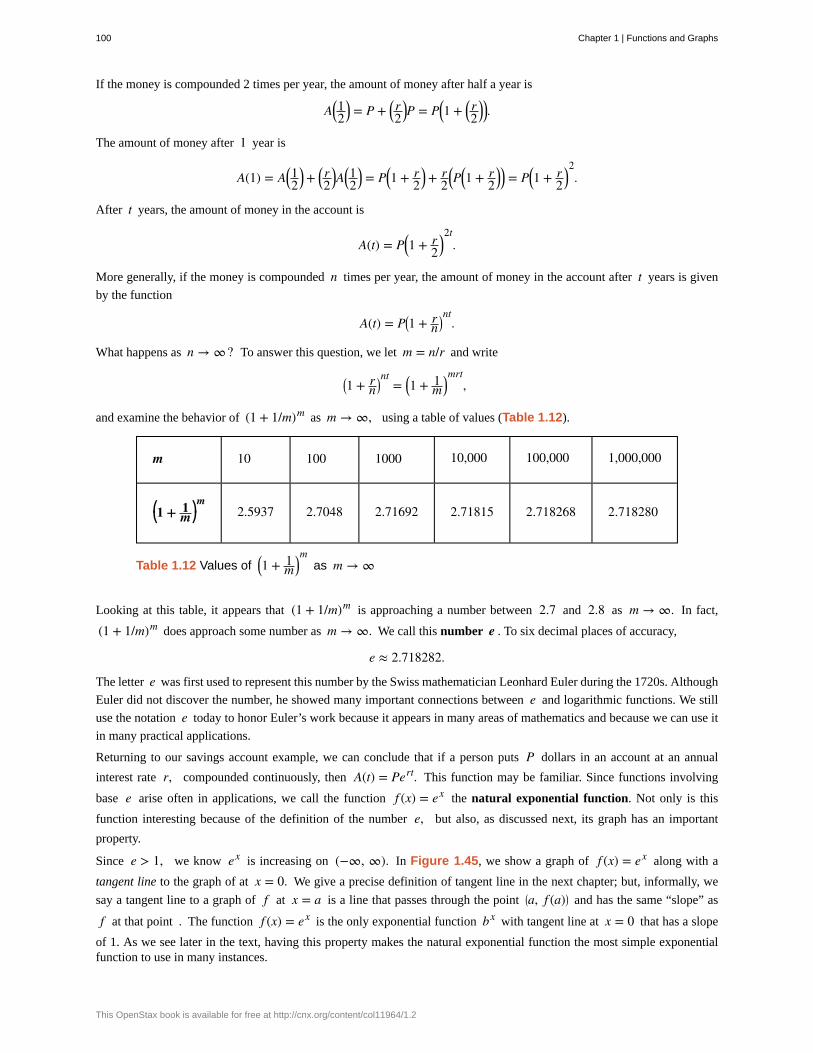
If the money is compounded 2 times per year, the amount of money after half a year is
A⎛⎝12
⎞⎠ = P + ⎛
⎝r2
⎞⎠P = P⎛
⎝1 + ⎛⎝r2
⎞⎠⎞⎠.
The amount of money after 1 year is
A(1) = A⎛⎝12
⎞⎠ + ⎛
⎝r2
⎞⎠A⎛
⎝12
⎞⎠ = P⎛
⎝1 + r2
⎞⎠ + r
2⎛⎝P
⎛⎝1 + r
2⎞⎠⎞⎠ = P⎛
⎝1 + r2
⎞⎠2.
After t years, the amount of money in the account is
A(t) = P⎛⎝1 + r
2⎞⎠2t
.
More generally, if the money is compounded n times per year, the amount of money in the account after t years is given
by the function
A(t) = P⎛⎝1 + r
n⎞⎠nt
.
What happens as n → ∞? To answer this question, we let m = n/r and write
⎛⎝1 + r
n⎞⎠nt
= ⎛⎝1 + 1
m⎞⎠mrt
,
and examine the behavior of (1 + 1/m)m as m → ∞, using a table of values (Table 1.12).
m 10 100 1000 10,000 100,000 1,000,000
⎛⎝1 + 1
m⎞⎠m
2.5937 2.7048 2.71692 2.71815 2.718268 2.718280
Table 1.12 Values of ⎛⎝1 + 1
m⎞⎠m
as m → ∞
Looking at this table, it appears that (1 + 1/m)m is approaching a number between 2.7 and 2.8 as m → ∞. In fact,
(1 + 1/m)m does approach some number as m → ∞. We call this number e . To six decimal places of accuracy,
e ≈ 2.718282.
The letter e was first used to represent this number by the Swiss mathematician Leonhard Euler during the 1720s. Although
Euler did not discover the number, he showed many important connections between e and logarithmic functions. We still
use the notation e today to honor Euler’s work because it appears in many areas of mathematics and because we can use it
in many practical applications.
Returning to our savings account example, we can conclude that if a person puts P dollars in an account at an annual
interest rate r, compounded continuously, then A(t) = Pert. This function may be familiar. Since functions involving
base e arise often in applications, we call the function f (x) = ex the natural exponential function. Not only is this
function interesting because of the definition of the number e, but also, as discussed next, its graph has an important
property.
Since e > 1, we know ex is increasing on (−∞, ∞). In Figure 1.45, we show a graph of f (x) = ex along with a
tangent line to the graph of at x = 0. We give a precise definition of tangent line in the next chapter; but, informally, we
say a tangent line to a graph of f at x = a is a line that passes through the point ⎛⎝a, f (a)⎞
⎠ and has the same “slope” as
f at that point . The function f (x) = ex is the only exponential function bx with tangent line at x = 0 that has a slope
of 1. As we see later in the text, having this property makes the natural exponential function the most simple exponentialfunction to use in many instances.
100 Chapter 1 | Functions and Graphs
This OpenStax book is available for free at http://cnx.org/content/col11964/1.2
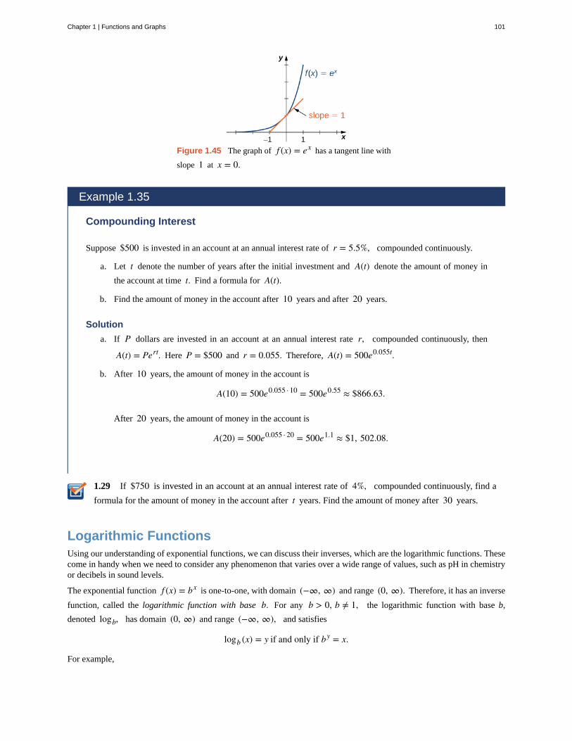
1.29
Figure 1.45 The graph of f (x) = ex has a tangent line with
slope 1 at x = 0.
Example 1.35
Compounding Interest
Suppose $500 is invested in an account at an annual interest rate of r = 5.5%, compounded continuously.
a. Let t denote the number of years after the initial investment and A(t) denote the amount of money in
the account at time t. Find a formula for A(t).
b. Find the amount of money in the account after 10 years and after 20 years.
Solution
a. If P dollars are invested in an account at an annual interest rate r, compounded continuously, then
A(t) = Pert. Here P = $500 and r = 0.055. Therefore, A(t) = 500e0.055t.
b. After 10 years, the amount of money in the account is
A(10) = 500e0.055 · 10 = 500e0.55 ≈ $866.63.
After 20 years, the amount of money in the account is
A(20) = 500e0.055 · 20 = 500e1.1 ≈ $1, 502.08.
If $750 is invested in an account at an annual interest rate of 4%, compounded continuously, find a
formula for the amount of money in the account after t years. Find the amount of money after 30 years.
Logarithmic FunctionsUsing our understanding of exponential functions, we can discuss their inverses, which are the logarithmic functions. Thesecome in handy when we need to consider any phenomenon that varies over a wide range of values, such as pH in chemistryor decibels in sound levels.
The exponential function f (x) = bx is one-to-one, with domain (−∞, ∞) and range (0, ∞). Therefore, it has an inverse
function, called the logarithmic function with base b. For any b > 0, b ≠ 1, the logarithmic function with base b,
denoted logb, has domain (0, ∞) and range (−∞, ∞), and satisfies
logb (x) = y if and only if by = x.
For example,
Chapter 1 | Functions and Graphs 101
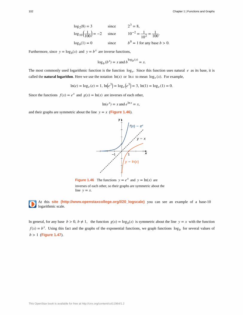
log2(8) = 3 since 23 = 8,
log10⎛⎝
1100
⎞⎠ = −2 since 10−2 = 1
102 = 1100,
logb(1) = 0 since b0 = 1 for any base b > 0.
Furthermore, since y = logb(x) and y = bx are inverse functions,
logb (bx) = x and blogb (x)
= x.
The most commonly used logarithmic function is the function loge. Since this function uses natural e as its base, it is
called the natural logarithm. Here we use the notation ln(x) or lnx to mean loge (x). For example,
ln(e) = loge (e) = 1, ln⎛⎝e
3⎞⎠ = loge
⎛⎝e
3⎞⎠ = 3, ln(1) = loge (1) = 0.
Since the functions f (x) = ex and g(x) = ln(x) are inverses of each other,
ln(ex) = x and elnx = x,
and their graphs are symmetric about the line y = x (Figure 1.46).
Figure 1.46 The functions y = ex and y = ln(x) are
inverses of each other, so their graphs are symmetric about theline y = x.
At this site (http://www.openstaxcollege.org/l/20_logscale) you can see an example of a base-10logarithmic scale.
In general, for any base b > 0, b ≠ 1, the function g(x) = logb(x) is symmetric about the line y = x with the function
f (x) = bx. Using this fact and the graphs of the exponential functions, we graph functions logb for several values of
b > 1 (Figure 1.47).
102 Chapter 1 | Functions and Graphs
This OpenStax book is available for free at http://cnx.org/content/col11964/1.2
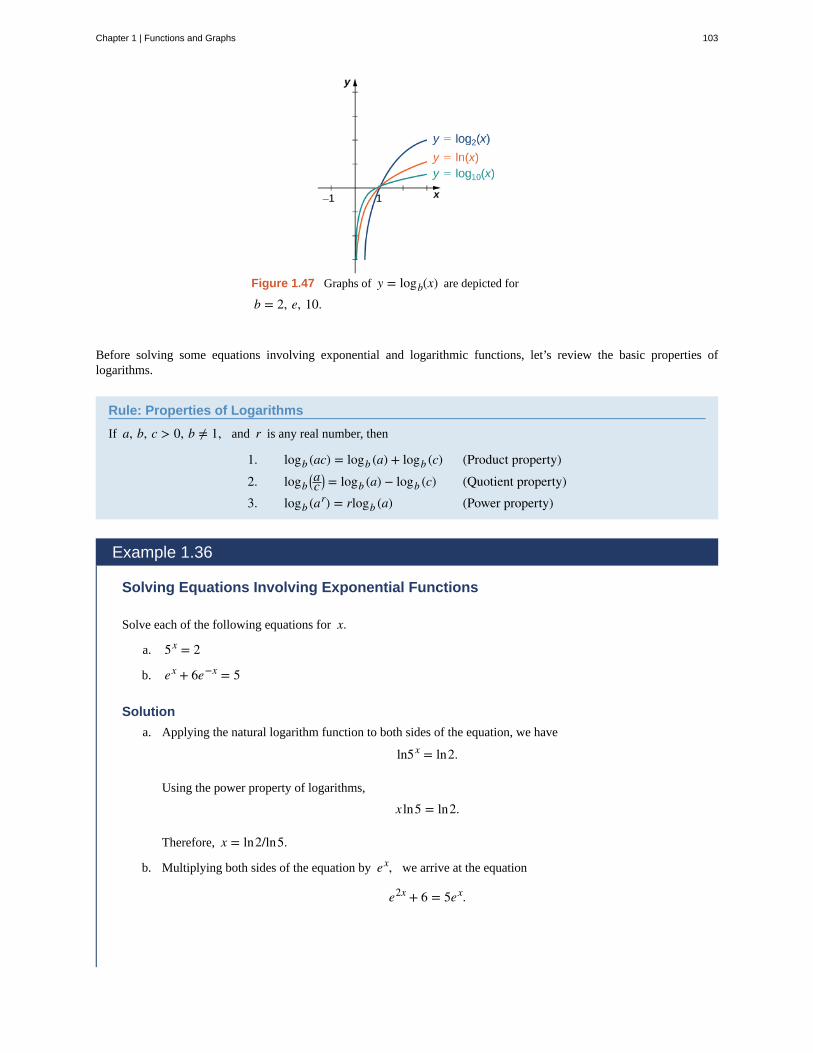
Figure 1.47 Graphs of y = logb(x) are depicted for
b = 2, e, 10.
Before solving some equations involving exponential and logarithmic functions, let’s review the basic properties oflogarithms.
Rule: Properties of Logarithms
If a, b, c > 0, b ≠ 1, and r is any real number, then
1. logb (ac) = logb (a) + logb (c) (Product property)2. logb
⎛⎝ac
⎞⎠ = logb (a) − logb (c) (Quotient property)
3. logb (ar) = rlogb (a) (Power property)
Example 1.36
Solving Equations Involving Exponential Functions
Solve each of the following equations for x.
a. 5x = 2
b. ex + 6e−x = 5
Solution
a. Applying the natural logarithm function to both sides of the equation, we have
ln5x = ln2.
Using the power property of logarithms,
x ln5 = ln2.
Therefore, x = ln2/ln5.
b. Multiplying both sides of the equation by ex, we arrive at the equation
e2x + 6 = 5ex.
Chapter 1 | Functions and Graphs 103
1.30
Rewriting this equation as
e2x − 5ex + 6 = 0,
we can then rewrite it as a quadratic equation in ex :
(ex)2 − 5(ex) + 6 = 0.
Now we can solve the quadratic equation. Factoring this equation, we obtain
(ex − 3)(ex − 2) = 0.
Therefore, the solutions satisfy ex = 3 and ex = 2. Taking the natural logarithm of both sides gives us
the solutions x = ln3, ln2.
Solve e2x /(3 + e2x) = 1/2.
Example 1.37
Solving Equations Involving Logarithmic Functions
Solve each of the following equations for x.
a. ln⎛⎝1x
⎞⎠ = 4
b. log10 x + log10 x = 2
c. ln(2x) − 3ln⎛⎝x2⎞
⎠ = 0
Solution
a. By the definition of the natural logarithm function,
ln⎛⎝1x
⎞⎠ = 4 if and only if e4 = 1
x .
Therefore, the solution is x = 1/e4.
b. Using the product and power properties of logarithmic functions, rewrite the left-hand side of the equationas
log10 x + log10 x = log10 x x = log10 x3/2 = 32log10 x.
Therefore, the equation can be rewritten as
32log10 x = 2 or log10 x = 4
3.
104 Chapter 1 | Functions and Graphs
This OpenStax book is available for free at http://cnx.org/content/col11964/1.2
1.31
The solution is x = 104/3 = 10 103 .
c. Using the power property of logarithmic functions, we can rewrite the equation as ln(2x) − ln⎛⎝x
6⎞⎠ = 0.
Using the quotient property, this becomes
ln⎛⎝
2x5
⎞⎠ = 0.
Therefore, 2/x5 = 1, which implies x = 25 . We should then check for any extraneous solutions.
Solve ln⎛⎝x
3⎞⎠ − 4ln(x) = 1.
When evaluating a logarithmic function with a calculator, you may have noticed that the only options are log10 or log,
called the common logarithm, or ln, which is the natural logarithm. However, exponential functions and logarithm functionscan be expressed in terms of any desired base b. If you need to use a calculator to evaluate an expression with a different
base, you can apply the change-of-base formulas first. Using this change of base, we typically write a given exponential orlogarithmic function in terms of the natural exponential and natural logarithmic functions.
Rule: Change-of-Base Formulas
Let a > 0, b > 0, and a ≠ 1, b ≠ 1.
1. ax = bxlogb a
for any real number x.
If b = e, this equation reduces to ax = exloge a = ex lna.
2. loga x = logb xlogb a for any real number x > 0.
If b = e, this equation reduces to loga x = lnxlna.
Proof
For the first change-of-base formula, we begin by making use of the power property of logarithmic functions. We know thatfor any base b > 0, b ≠ 1, logb(ax) = xlogb a. Therefore,
blogb(ax)
= bxlogb a
.
In addition, we know that bx and logb(x) are inverse functions. Therefore,
blogb(ax)
= ax.
Combining these last two equalities, we conclude that ax = bxlogb a
.
To prove the second property, we show that
(logb a) · (loga x) = logb x.
Let u = logb a, v = loga x, and w = logb x. We will show that u · v = w. By the definition of logarithmic functions, we
Chapter 1 | Functions and Graphs 105
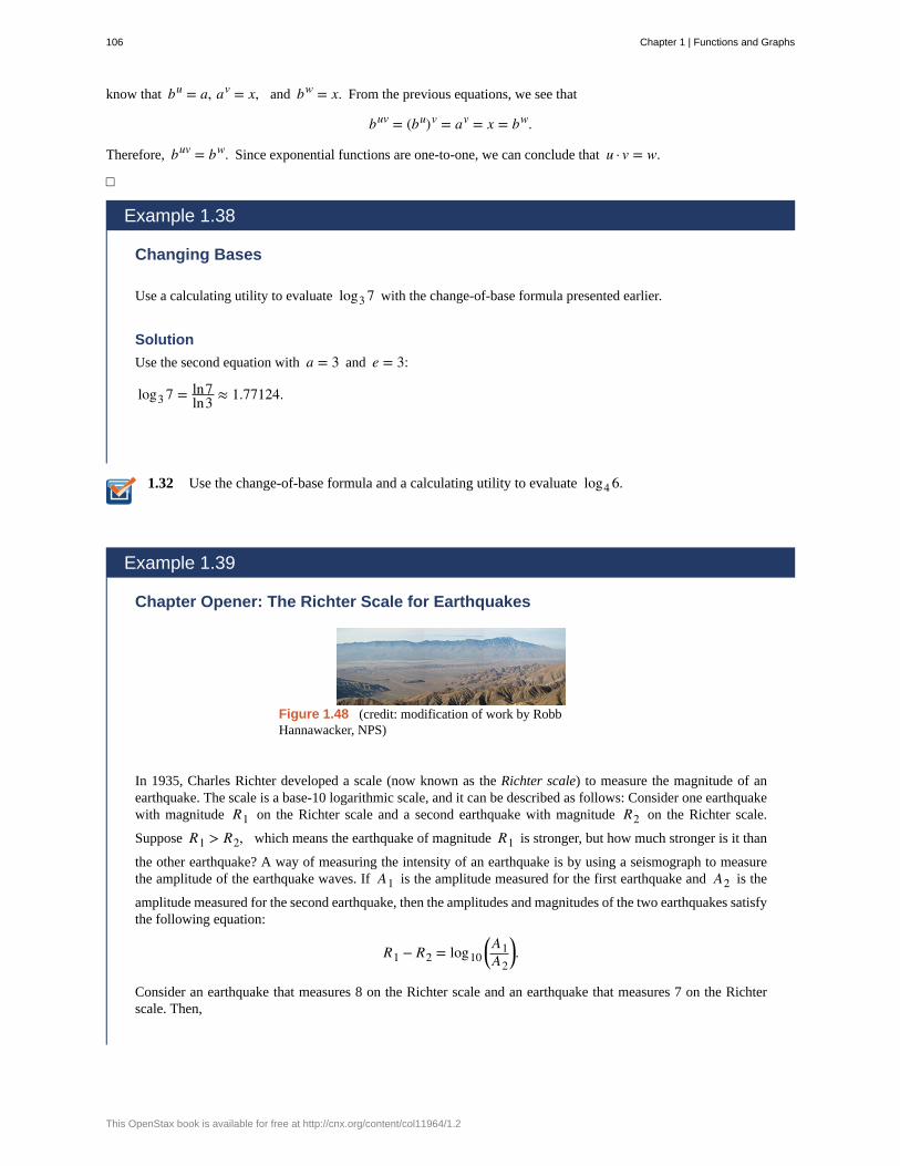
1.32
know that bu = a, av = x, and bw = x. From the previous equations, we see that
buv = (bu)v = av = x = bw.
Therefore, buv = bw. Since exponential functions are one-to-one, we can conclude that u · v = w.
□
Example 1.38
Changing Bases
Use a calculating utility to evaluate log3 7 with the change-of-base formula presented earlier.
Solution
Use the second equation with a = 3 and e = 3:
log3 7 = ln7ln3 ≈ 1.77124.
Use the change-of-base formula and a calculating utility to evaluate log4 6.
Example 1.39
Chapter Opener: The Richter Scale for Earthquakes
Figure 1.48 (credit: modification of work by RobbHannawacker, NPS)
In 1935, Charles Richter developed a scale (now known as the Richter scale) to measure the magnitude of anearthquake. The scale is a base-10 logarithmic scale, and it can be described as follows: Consider one earthquakewith magnitude R1 on the Richter scale and a second earthquake with magnitude R2 on the Richter scale.
Suppose R1 > R2, which means the earthquake of magnitude R1 is stronger, but how much stronger is it than
the other earthquake? A way of measuring the intensity of an earthquake is by using a seismograph to measurethe amplitude of the earthquake waves. If A1 is the amplitude measured for the first earthquake and A2 is the
amplitude measured for the second earthquake, then the amplitudes and magnitudes of the two earthquakes satisfythe following equation:
R1 − R2 = log10⎛⎝
A1A2
⎞⎠.
Consider an earthquake that measures 8 on the Richter scale and an earthquake that measures 7 on the Richterscale. Then,
106 Chapter 1 | Functions and Graphs
This OpenStax book is available for free at http://cnx.org/content/col11964/1.2
1.33
8 − 7 = log10⎛⎝
A1A2
⎞⎠.
Therefore,
log10⎛⎝
A1A2
⎞⎠ = 1,
which implies A1 /A2 = 10 or A1 = 10A2. Since A1 is 10 times the size of A2, we say that the first
earthquake is 10 times as intense as the second earthquake. On the other hand, if one earthquake measures 8 onthe Richter scale and another measures 6, then the relative intensity of the two earthquakes satisfies the equation
log10⎛⎝
A1A2
⎞⎠ = 8 − 6 = 2.
Therefore, A1 = 100A2. That is, the first earthquake is 100 times more intense than the second earthquake.
How can we use logarithmic functions to compare the relative severity of the magnitude 9 earthquake in Japan in2011 with the magnitude 7.3 earthquake in Haiti in 2010?
Solution
To compare the Japan and Haiti earthquakes, we can use an equation presented earlier:
9 − 7.3 = log10⎛⎝
A1A2
⎞⎠.
Therefore, A1 /A2 = 101.7, and we conclude that the earthquake in Japan was approximately 50 times more
intense than the earthquake in Haiti.
Compare the relative severity of a magnitude 8.4 earthquake with a magnitude 7.4 earthquake.
Hyperbolic FunctionsThe hyperbolic functions are defined in terms of certain combinations of ex and e−x. These functions arise naturally
in various engineering and physics applications, including the study of water waves and vibrations of elastic membranes.Another common use for a hyperbolic function is the representation of a hanging chain or cable, also known as a catenary(Figure 1.49). If we introduce a coordinate system so that the low point of the chain lies along the y -axis, we can describe
the height of the chain in terms of a hyperbolic function. First, we define the hyperbolic functions.
Chapter 1 | Functions and Graphs 107
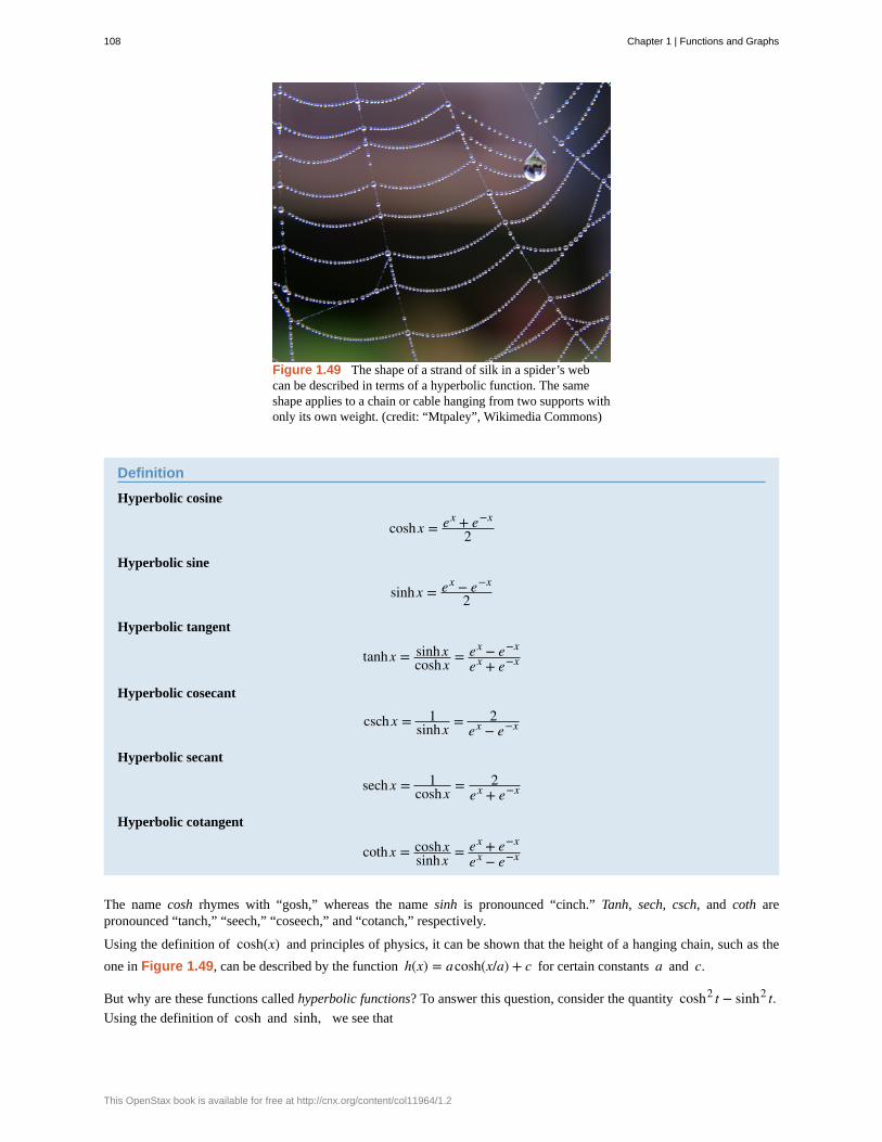
Figure 1.49 The shape of a strand of silk in a spider’s webcan be described in terms of a hyperbolic function. The sameshape applies to a chain or cable hanging from two supports withonly its own weight. (credit: “Mtpaley”, Wikimedia Commons)
Definition
Hyperbolic cosine
coshx = ex + e−x
2
Hyperbolic sine
sinhx = ex − e−x
2
Hyperbolic tangent
tanhx = sinhxcoshx = ex − e−x
ex + e−x
Hyperbolic cosecant
csch x = 1sinhx = 2
ex − e−x
Hyperbolic secant
sech x = 1coshx = 2
ex + e−x
Hyperbolic cotangent
cothx = coshxsinhx = ex + e−x
ex − e−x
The name cosh rhymes with “gosh,” whereas the name sinh is pronounced “cinch.” Tanh, sech, csch, and coth arepronounced “tanch,” “seech,” “coseech,” and “cotanch,” respectively.
Using the definition of cosh(x) and principles of physics, it can be shown that the height of a hanging chain, such as the
one in Figure 1.49, can be described by the function h(x) = acosh(x/a) + c for certain constants a and c.
But why are these functions called hyperbolic functions? To answer this question, consider the quantity cosh2 t − sinh2 t.Using the definition of cosh and sinh, we see that
108 Chapter 1 | Functions and Graphs
This OpenStax book is available for free at http://cnx.org/content/col11964/1.2
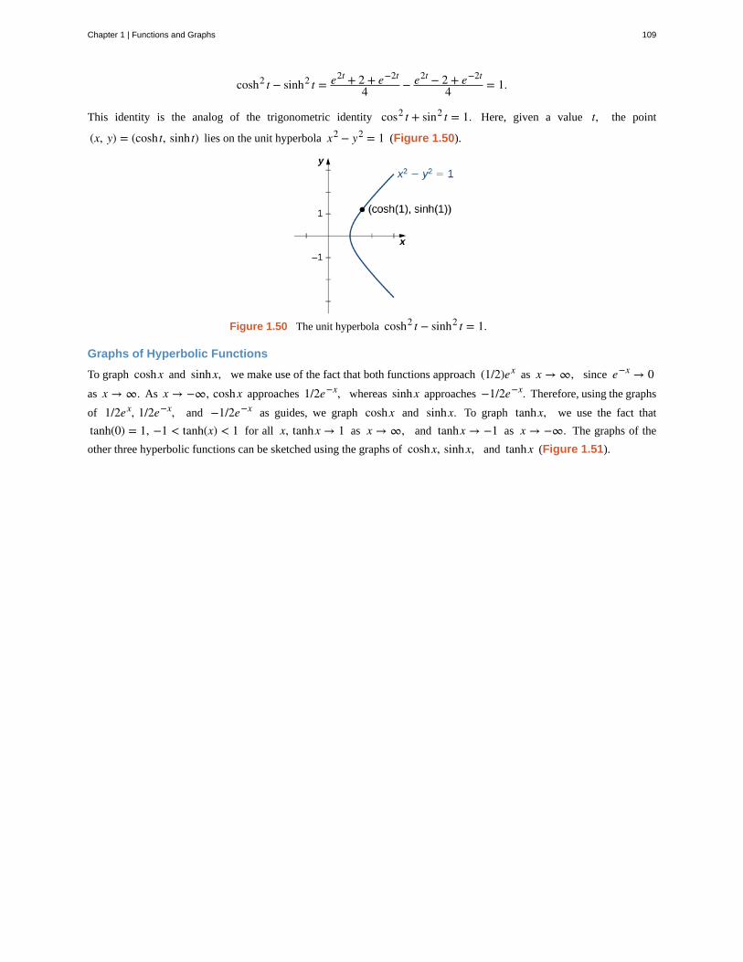
cosh2 t − sinh2 t = e2t + 2 + e−2t
4 − e2t − 2 + e−2t
4 = 1.
This identity is the analog of the trigonometric identity cos2 t + sin2 t = 1. Here, given a value t, the point
(x, y) = (cosh t, sinh t) lies on the unit hyperbola x2 − y2 = 1 (Figure 1.50).
Figure 1.50 The unit hyperbola cosh2 t − sinh2 t = 1.
Graphs of Hyperbolic Functions
To graph coshx and sinhx, we make use of the fact that both functions approach (1/2)ex as x → ∞, since e−x → 0as x → ∞. As x → −∞, coshx approaches 1/2e−x, whereas sinhx approaches −1/2e−x. Therefore, using the graphs
of 1/2ex, 1/2e−x, and −1/2e−x as guides, we graph coshx and sinhx. To graph tanhx, we use the fact that
tanh(0) = 1, −1 < tanh(x) < 1 for all x, tanhx → 1 as x → ∞, and tanhx → −1 as x → −∞. The graphs of the
other three hyperbolic functions can be sketched using the graphs of coshx, sinhx, and tanhx (Figure 1.51).
Chapter 1 | Functions and Graphs 109
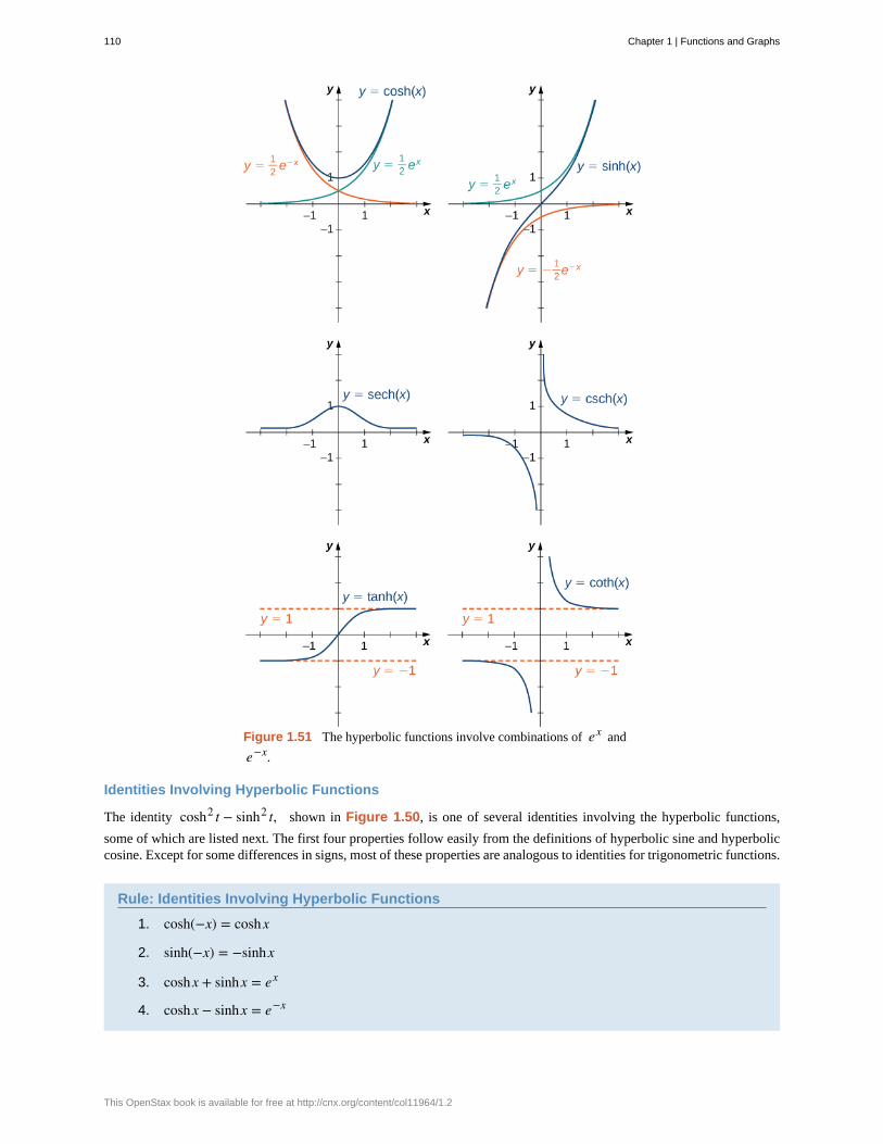
Figure 1.51 The hyperbolic functions involve combinations of ex and
e−x.
Identities Involving Hyperbolic Functions
The identity cosh2 t − sinh2 t, shown in Figure 1.50, is one of several identities involving the hyperbolic functions,
some of which are listed next. The first four properties follow easily from the definitions of hyperbolic sine and hyperboliccosine. Except for some differences in signs, most of these properties are analogous to identities for trigonometric functions.
Rule: Identities Involving Hyperbolic Functions
1. cosh(−x) = coshx
2. sinh(−x) = −sinhx
3. coshx + sinhx = ex
4. coshx − sinhx = e−x
110 Chapter 1 | Functions and Graphs
This OpenStax book is available for free at http://cnx.org/content/col11964/1.2
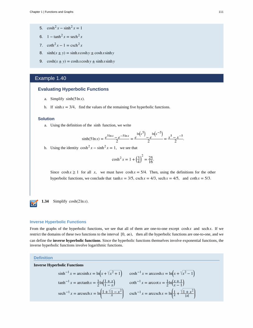
1.34
5. cosh2 x − sinh2 x = 1
6. 1 − tanh2 x = sech2 x
7. coth2 x − 1 = csch2 x
8. sinh(x ± y) = sinhxcoshy ± coshxsinhy
9. cosh(x ± y) = coshxcoshy ± sinhxsinhy
Example 1.40
Evaluating Hyperbolic Functions
a. Simplify sinh(5lnx).
b. If sinhx = 3/4, find the values of the remaining five hyperbolic functions.
Solution
a. Using the definition of the sinh function, we write
sinh(5lnx) = e5lnx − e−5lnx
2 = eln⎛
⎝x5⎞
⎠ − eln⎛
⎝x−5⎞
⎠
2 = x5 − x−5
2 .
b. Using the identity cosh2 x − sinh2 x = 1, we see that
cosh2 x = 1 + ⎛⎝34
⎞⎠2
= 2516.
Since coshx ≥ 1 for all x, we must have coshx = 5/4. Then, using the definitions for the other
hyperbolic functions, we conclude that tanhx = 3/5, csch x = 4/3, sech x = 4/5, and cothx = 5/3.
Simplify cosh(2lnx).
Inverse Hyperbolic Functions
From the graphs of the hyperbolic functions, we see that all of them are one-to-one except coshx and sech x. If we
restrict the domains of these two functions to the interval [0, ∞), then all the hyperbolic functions are one-to-one, and we
can define the inverse hyperbolic functions. Since the hyperbolic functions themselves involve exponential functions, theinverse hyperbolic functions involve logarithmic functions.
Definition
Inverse Hyperbolic Functions
sinh−1 x = arcsinhx = ln⎛⎝x + x2 + 1⎞
⎠ cosh−1 x = arccoshx = ln⎛⎝x + x2 − 1⎞
⎠
tanh−1 x = arctanhx = 12ln⎛
⎝1 + x1 − x
⎞⎠ coth−1 x = arccot x = 1
2ln⎛⎝x + 1x − 1
⎞⎠
sech−1 x = arcsech x = ln⎛
⎝⎜1 + 1 − x2
x⎞
⎠⎟ csch−1 x = arccsch x = ln
⎛
⎝⎜1x + 1 + x2
|x|⎞
⎠⎟
Chapter 1 | Functions and Graphs 111
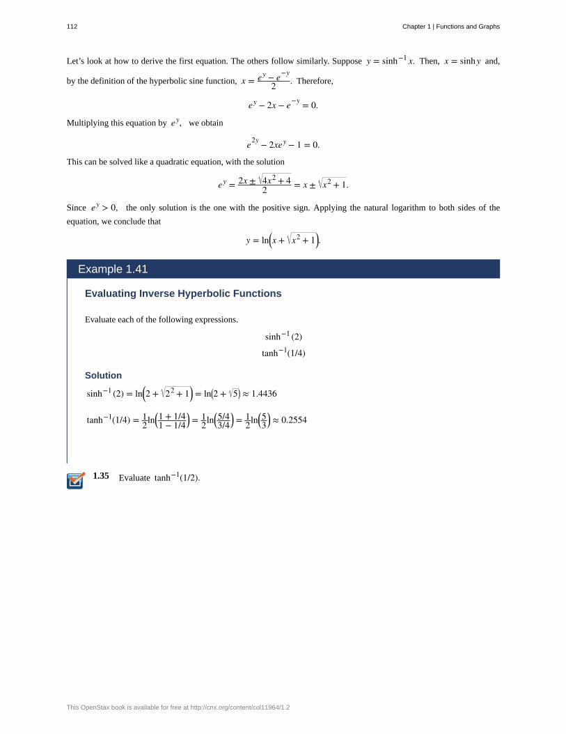
1.35
Let’s look at how to derive the first equation. The others follow similarly. Suppose y = sinh−1 x. Then, x = sinhy and,
by the definition of the hyperbolic sine function, x = ey − e−y
2 . Therefore,
ey − 2x − e−y = 0.
Multiplying this equation by ey, we obtain
e2y − 2xey − 1 = 0.
This can be solved like a quadratic equation, with the solution
ey = 2x ± 4x2 + 42 = x ± x2 + 1.
Since ey > 0, the only solution is the one with the positive sign. Applying the natural logarithm to both sides of the
equation, we conclude that
y = ln⎛⎝x + x2 + 1⎞
⎠.
Example 1.41
Evaluating Inverse Hyperbolic Functions
Evaluate each of the following expressions.
sinh−1 (2)
tanh−1(1/4)
Solution
sinh−1 (2) = ln⎛⎝2 + 22 + 1⎞
⎠ = ln⎛⎝2 + 5⎞
⎠ ≈ 1.4436
tanh−1(1/4) = 12ln⎛
⎝1 + 1/41 − 1/4
⎞⎠ = 1
2ln⎛⎝5/43/4
⎞⎠ = 1
2ln⎛⎝53
⎞⎠ ≈ 0.2554
Evaluate tanh−1(1/2).
112 Chapter 1 | Functions and Graphs
This OpenStax book is available for free at http://cnx.org/content/col11964/1.2
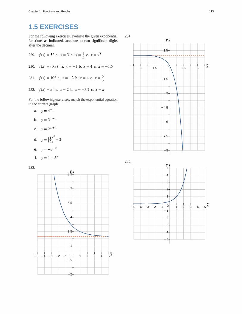
1.5 EXERCISESFor the following exercises, evaluate the given exponentialfunctions as indicated, accurate to two significant digitsafter the decimal.
229. f (x) = 5x a. x = 3 b. x = 12 c. x = 2
230. f (x) = (0.3)x a. x = −1 b. x = 4 c. x = −1.5
231. f (x) = 10x a. x = −2 b. x = 4 c. x = 53
232. f (x) = ex a. x = 2 b. x = −3.2 c. x = π
For the following exercises, match the exponential equationto the correct graph.
a. y = 4−x
b. y = 3x − 1
c. y = 2x + 1
d. y = ⎛⎝12
⎞⎠
x+ 2
e. y = −3−x
f. y = 1 − 5x
233.
234.
235.
Chapter 1 | Functions and Graphs 113
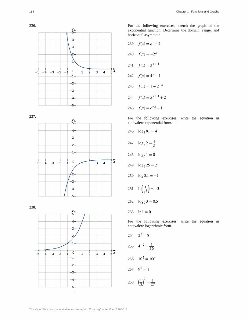
236.
237.
238.
For the following exercises, sketch the graph of theexponential function. Determine the domain, range, andhorizontal asymptote.
239. f (x) = ex + 2
240. f (x) = −2x
241. f (x) = 3x + 1
242. f (x) = 4x − 1
243. f (x) = 1 − 2−x
244. f (x) = 5x + 1 + 2
245. f (x) = e−x − 1
For the following exercises, write the equation inequivalent exponential form.
246. log3 81 = 4
247. log8 2 = 13
248. log5 1 = 0
249. log5 25 = 2
250. log0.1 = −1
251. ln⎛⎝
1e3
⎞⎠ = −3
252. log9 3 = 0.5
253. ln1 = 0
For the following exercises, write the equation inequivalent logarithmic form.
254. 23 = 8
255. 4−2 = 116
256. 102 = 100
257. 90 = 1
258. ⎛⎝13
⎞⎠
3= 1
27
114 Chapter 1 | Functions and Graphs
This OpenStax book is available for free at http://cnx.org/content/col11964/1.2
259. 643 = 4
260. ex = y
261. 9y = 150
262. b3 = 45
263. 4−3/2 = 0.125
For the following exercises, sketch the graph of thelogarithmic function. Determine the domain, range, andvertical asymptote.
264. f (x) = 3 + lnx
265. f (x) = ln(x − 1)
266. f (x) = ln(−x)
267. f (x) = 1 − lnx
268. f (x) = logx − 1
269. f (x) = ln(x + 1)
For the following exercises, use properties of logarithms towrite the expressions as a sum, difference, and/or productof logarithms.
270. logx4 y
271. log39a3
b
272. lna b3
273. log5 125xy3
274. log4xy3
64
275. ln⎛
⎝⎜ 6
e3
⎞
⎠⎟
For the following exercises, solve the exponential equationexactly.
276. 5x = 125
277. e3x − 15 = 0
278. 8x = 4
279. 4x + 1 − 32 = 0
280. 3x/14 = 110
281. 10x = 7.21
282. 4 · 23x − 20 = 0
283. 73x − 2 = 11
For the following exercises, solve the logarithmic equationexactly, if possible.
284. log3 x = 0
285. log5 x = −2
286. log4 (x + 5) = 0
287. log(2x − 7) = 0
288. ln x + 3 = 2
289. log6 (x + 9) + log6 x = 2
290. log4 (x + 2) − log4 (x − 1) = 0
291. lnx + ln(x − 2) = ln4
For the following exercises, use the change-of-baseformula and either base 10 or base e to evaluate the givenexpressions. Answer in exact form and in approximateform, rounding to four decimal places.
292. log5 47
293. log7 82
294. log6 103
295. log0.5 211
296. log2 π
297. log0.2 0.452
298. Rewrite the following expressions in terms ofexponentials and simplify. a. 2cosh(lnx) b.
cosh4x + sinh4x c. cosh2x − sinh2x d.
ln(coshx + sinhx) + ln(coshx − sinhx)
Chapter 1 | Functions and Graphs 115
299. [T] The number of bacteria N in a culture after t days
can be modeled by the function N(t) = 1300 · (2)t/4. Find
the number of bacteria present after 15 days.
300. [T] The demand D (in millions of barrels) for oilin an oil-rich country is given by the function
D(p) = 150 · (2.7)−0.25p, where p is the price (in dollars)
of a barrel of oil. Find the amount of oil demanded (to thenearest million barrels) when the price is between $15 and$20.
301. [T] The amount A of a $100,000 investment payingcontinuously and compounded for t years is given by
A(t) = 100,000 · e0.055t. Find the amount A accumulated
in 5 years.
302. [T] An investment is compounded monthly,quarterly, or yearly and is given by the function
A = P⎛⎝1 + j
n⎞⎠
nt, where A is the value of the investment
at time t, P is the initial principle that was invested, jis the annual interest rate, and n is the number of time
the interest is compounded per year. Given a yearly interestrate of 3.5% and an initial principle of $100,000, find theamount A accumulated in 5 years for interest that is
compounded a. daily, b., monthly, c. quarterly, and d.yearly.
303. [T] The concentration of hydrogen ions in a
substance is denoted by ⎡⎣H+ ⎤
⎦, measured in moles per
liter. The pH of a substance is defined by the logarithmic
function pH = −log⎡⎣H+ ⎤
⎦. This function is used to
measure the acidity of a substance. The pH of water is 7. Asubstance with a pH less than 7 is an acid, whereas one thathas a pH of more than 7 is a base.
a. Find the pH of the following substances. Roundanswers to one digit.
b. Determine whether the substance is an acid or abase.
i. Eggs: ⎡⎣H+ ⎤
⎦ = 1.6 × 10⁻⁸ mol/L
ii. Beer: ⎡⎣H+ ⎤
⎦ = 3.16 × 10⁻³ mol/L
iii. Tomato Juice: ⎡⎣H+ ⎤
⎦ = 7.94 × 10⁻⁵ mol/L
304. [T] Iodine-131 is a radioactive substance that decays
according to the function Q(t) = Q0 · e−0.08664t, where
Q0 is the initial quantity of a sample of the substance and t
is in days. Determine how long it takes (to the nearest day)for 95% of a quantity to decay.
305. [T] According to the World Bank, at the end of2013 ( t = 0 ) the U.S. population was 316 million and
was increasing according to the following model:
P(t) = 316e0.0074t, where P is measured in millions of
people and t is measured in years after 2013.a. Based on this model, what will be the population of
the United States in 2020?b. Determine when the U.S. population will be twice
what it is in 2013.
306. [T] The amount A accumulated after 1000 dollars isinvested for t years at an interest rate of 4% is modeled bythe function A(t) = 1000(1.04)t.
a. Find the amount accumulated after 5 years and 10years.
b. Determine how long it takes for the originalinvestment to triple.
307. [T] A bacterial colony grown in a lab is known todouble in number in 12 hours. Suppose, initially, there are1000 bacteria present.
a. Use the exponential function Q = Q0 ekt to
determine the value k, which is the growth rate of
the bacteria. Round to four decimal places.b. Determine approximately how long it takes for
200,000 bacteria to grow.
308. [T] The rabbit population on a game reserve doublesevery 6 months. Suppose there were 120 rabbits initially.
a. Use the exponential function P = P0 at to
determine the growth rate constant a. Round to
four decimal places.b. Use the function in part a. to determine
approximately how long it takes for the rabbitpopulation to reach 3500.
309. [T] The 1906 earthquake in San Francisco had amagnitude of 8.3 on the Richter scale. At the same time,in Japan, an earthquake with magnitude 4.9 caused onlyminor damage. Approximately how much more energy wasreleased by the San Francisco earthquake than by theJapanese earthquake?
116 Chapter 1 | Functions and Graphs
This OpenStax book is available for free at http://cnx.org/content/col11964/1.2
absolute value function
algebraic function
base
composite function
cubic function
decreasing on the interval I
degree
dependent variable
domain
even function
exponent
function
graph of a function
horizontal line test
hyperbolic functions
increasing on the interval I
independent variable
inverse function
inverse hyperbolic functions
inverse trigonometric functions
linear function
logarithmic function
mathematical model
natural exponential function
CHAPTER 1 REVIEW
KEY TERMS
f (x) =⎧
⎩⎨−x, x < 0x, x ≥ 0
a function involving any combination of only the basic operations of addition, subtraction,multiplication, division, powers, and roots applied to an input variable x
the number b in the exponential function f (x) = bx and the logarithmic function f (x) = logb x
given two functions f and g, a new function, denoted g ∘ f , such that ⎛⎝g ∘ f ⎞
⎠(x) = g⎛⎝ f (x)⎞
⎠
a polynomial of degree 3; that is, a function of the form f (x) = ax3 + bx2 + cx + d, where a ≠ 0
a function decreasing on the interval I if, for all x1, x2 ∈ I, f (x1) ≥ f (x2) if
x1 < x2
for a polynomial function, the value of the largest exponent of any term
the output variable for a function
the set of inputs for a function
a function is even if f (−x) = f (x) for all x in the domain of f
the value x in the expression bx
a set of inputs, a set of outputs, and a rule for mapping each input to exactly one output
the set of points (x, y) such that x is in the domain of f and y = f (x)
a function f is one-to-one if and only if every horizontal line intersects the graph of f , at most,
once
the functions denoted sinh, cosh, tanh, csch, sech, and coth, which involve certain
combinations of ex and e−x
a function increasing on the interval I if for all x1, x2 ∈ I, f (x1) ≤ f (x2) if x1 < x2
the input variable for a function
for a function f , the inverse function f −1 satisfies f −1 (y) = x if f (x) = y
the inverses of the hyperbolic functions where cosh and sech are restricted to the
domain [0, ∞); each of these functions can be expressed in terms of a composition of the natural logarithm function
and an algebraic function
the inverses of the trigonometric functions are defined on restricted domains wherethey are one-to-one functions
a function that can be written in the form f (x) = mx + b
a function of the form f (x) = logb (x) for some base b > 0, b ≠ 1 such that y = logb(x) if
and only if by = x
A method of simulating real-life situations with mathematical equations
the function f (x) = ex
Chapter 1 | Functions and Graphs 117
natural logarithm
number e
odd function
one-to-one function
periodic function
piecewise-defined function
point-slope equation
polynomial function
power function
quadratic function
radians
range
rational function
restricted domain
root function
slope
slope-intercept form
symmetry about the origin
symmetry about the y-axis
table of values
transcendental function
transformation of a function
trigonometric functions
trigonometric identity
vertical line test
zeros of a function
the function lnx = loge x
as m gets larger, the quantity (1 + (1/m)m gets closer to some real number; we define that real number to be
e; the value of e is approximately 2.718282
a function is odd if f (−x) = − f (x) for all x in the domain of f
a function f is one-to-one if f (x1) ≠ f (x2) if x1 ≠ x2
a function is periodic if it has a repeating pattern as the values of x move from left to right
a function that is defined differently on different parts of its domain
equation of a linear function indicating its slope and a point on the graph of the function
a function of the form f (x) = an xn + an − 1 xn − 1 + … + a1 x + a0
a function of the form f (x) = xn for any positive integer n ≥ 1
a polynomial of degree 2; that is, a function of the form f (x) = ax2 + bx + c where a ≠ 0
for a circular arc of length s on a circle of radius 1, the radian measure of the associated angle θ is s
the set of outputs for a function
a function of the form f (x) = p(x)/q(x), where p(x) and q(x) are polynomials
a subset of the domain of a function f
a function of the form f (x) = x1/n for any integer n ≥ 2
the change in y for each unit change in x
equation of a linear function indicating its slope and y-intercept
the graph of a function f is symmetric about the origin if (−x, −y) is on the graph of fwhenever (x, y) is on the graph
the graph of a function f is symmetric about the y -axis if (−x, y) is on the graph of fwhenever (x, y) is on the graph
a table containing a list of inputs and their corresponding outputs
a function that cannot be expressed by a combination of basic arithmetic operations
a shift, scaling, or reflection of a function
functions of an angle defined as ratios of the lengths of the sides of a right triangle
an equation involving trigonometric functions that is true for all angles θ for which the
functions in the equation are defined
given the graph of a function, every vertical line intersects the graph, at most, once
when a real number x is a zero of a function f , f (x) = 0
KEY EQUATIONS• Composition of two functions
⎛⎝g ∘ f ⎞
⎠(x) = g⎛⎝ f (x)⎞
⎠
• Absolute value function
f (x) =⎧
⎩⎨−x, x < 0x, x ≥ 0
118 Chapter 1 | Functions and Graphs
This OpenStax book is available for free at http://cnx.org/content/col11964/1.2
• Point-slope equation of a liney − y1 = m(x − x1)
• Slope-intercept form of a liney = mx + b
• Standard form of a lineax + by = c
• Polynomial function
f (x) = an xn + an − 1 xn − 1 + ⋯ + a1 x + a0
• Generalized sine functionf (x) = Asin⎛
⎝B(x − α)⎞⎠ + C
• Inverse functions
f −1 ⎛⎝ f (x)⎞
⎠ = x for all x in D, and f ⎛⎝ f −1 (y)⎞
⎠ = y for all y in R.
KEY CONCEPTS
1.1 Review of Functions
• A function is a mapping from a set of inputs to a set of outputs with exactly one output for each input.
• If no domain is stated for a function y = f (x), the domain is considered to be the set of all real numbers x for
which the function is defined.
• When sketching the graph of a function f , each vertical line may intersect the graph, at most, once.
• A function may have any number of zeros, but it has, at most, one y-intercept.
• To define the composition g ∘ f , the range of f must be contained in the domain of g.
• Even functions are symmetric about the y -axis whereas odd functions are symmetric about the origin.
1.2 Basic Classes of Functions
• The power function f (x) = xn is an even function if n is even and n ≠ 0, and it is an odd function if n is odd.
• The root function f (x) = x1/n has the domain [0, ∞) if n is even and the domain (−∞, ∞) if n is odd. If n
is odd, then f (x) = x1/n is an odd function.
• The domain of the rational function f (x) = p(x)/q(x), where p(x) and q(x) are polynomial functions, is the set
of x such that q(x) ≠ 0.
• Functions that involve the basic operations of addition, subtraction, multiplication, division, and powers arealgebraic functions. All other functions are transcendental. Trigonometric, exponential, and logarithmic functionsare examples of transcendental functions.
• A polynomial function f with degree n ≥ 1 satisfies f (x) → ±∞ as x → ±∞. The sign of the output as
x → ∞ depends on the sign of the leading coefficient only and on whether n is even or odd.
• Vertical and horizontal shifts, vertical and horizontal scalings, and reflections about the x - and y -axes are
examples of transformations of functions.
1.3 Trigonometric Functions
• Radian measure is defined such that the angle associated with the arc of length 1 on the unit circle has radianmeasure 1. An angle with a degree measure of 180° has a radian measure of π rad.
Chapter 1 | Functions and Graphs 119
• For acute angles θ, the values of the trigonometric functions are defined as ratios of two sides of a right triangle
in which one of the acute angles is θ.
• For a general angle θ, let (x, y) be a point on a circle of radius r corresponding to this angle θ. The
trigonometric functions can be written as ratios involving x, y, and r.
• The trigonometric functions are periodic. The sine, cosine, secant, and cosecant functions have period 2π. The
tangent and cotangent functions have period π.
1.4 Inverse Functions
• For a function to have an inverse, the function must be one-to-one. Given the graph of a function, we can determinewhether the function is one-to-one by using the horizontal line test.
• If a function is not one-to-one, we can restrict the domain to a smaller domain where the function is one-to-one andthen define the inverse of the function on the smaller domain.
• For a function f and its inverse f −1, f ⎛⎝ f −1 (x)⎞
⎠ = x for all x in the domain of f −1 and f −1 ⎛⎝ f (x)⎞
⎠ = x for all
x in the domain of f .
• Since the trigonometric functions are periodic, we need to restrict their domains to define the inverse trigonometricfunctions.
• The graph of a function f and its inverse f −1 are symmetric about the line y = x.
1.5 Exponential and Logarithmic Functions
• The exponential function y = bx is increasing if b > 1 and decreasing if 0 < b < 1. Its domain is (−∞, ∞)and its range is (0, ∞).
• The logarithmic function y = logb(x) is the inverse of y = bx. Its domain is (0, ∞) and its range is (−∞, ∞).
• The natural exponential function is y = ex and the natural logarithmic function is y = lnx = loge x.
• Given an exponential function or logarithmic function in base a, we can make a change of base to convert this
function to any base b > 0, b ≠ 1. We typically convert to base e.
• The hyperbolic functions involve combinations of the exponential functions ex and e−x. As a result, the inverse
hyperbolic functions involve the natural logarithm.
CHAPTER 1 REVIEW EXERCISESTrue or False? Justify your answer with a proof or acounterexample.
310. A function is always one-to-one.
311. f ∘g = g ∘ f , assuming f and g are functions.
312. A relation that passes the horizontal and vertical linetests is a one-to-one function.
313. A relation passing the horizontal line test is afunction.
For the following problems, state the domain and range ofthe given functions:
f = x2 + 2x − 3, g = ln(x − 5), h = 1x + 4
314. h
315. g
316. h ∘ f
317. g ∘ f
Find the degree, y-intercept, and zeros for the followingpolynomial functions.
318. f (x) = 2x2 + 9x − 5
120 Chapter 1 | Functions and Graphs
This OpenStax book is available for free at http://cnx.org/content/col11964/1.2
319. f (x) = x3 + 2x2 − 2x
Simplify the following trigonometric expressions.
320. tan2 xsec2 x
+ cos2 x
321. cos(2x) = sin2 x
Solve the following trigonometric equations on the intervalθ = [−2π, 2π] exactly.
322. 6cos2 x − 3 = 0
323. sec2 x − 2secx + 1 = 0
Solve the following logarithmic equations.
324. 5x = 16
325. log2(x + 4) = 3
Are the following functions one-to-one over their domainof existence? Does the function have an inverse? If so, find
the inverse f −1(x) of the function. Justify your answer.
326. f (x) = x2 + 2x + 1
327. f (x) = 1x
For the following problems, determine the largest domainon which the function is one-to-one and find the inverse onthat domain.
328. f (x) = 9 − x
329. f (x) = x2 + 3x + 4
330. A car is racing along a circular track with diameter of1 mi. A trainer standing in the center of the circle marks hisprogress every 5 sec. After 5 sec, the trainer has to turn 55°to keep up with the car. How fast is the car traveling?
For the following problems, consider a restaurant ownerwho wants to sell T-shirts advertising his brand. He recallsthat there is a fixed cost and variable cost, although he doesnot remember the values. He does know that the T-shirtprinting company charges $440 for 20 shirts and $1000 for100 shirts.
331. a. Find the equation C = f (x) that describes the
total cost as a function of number of shirts and b. determinehow many shirts he must sell to break even if he sells theshirts for $10 each.
332. a. Find the inverse function x = f −1(C) and
describe the meaning of this function. b. Determine howmany shirts the owner can buy if he has $8000 to spend.
For the following problems, consider the population ofOcean City, New Jersey, which is cyclical by season.
333. The population can be modeled byP(t) = 82.5 − 67.5cos⎡
⎣(π/6)t⎤⎦, where t is time in
months (t = 0 represents January 1) and P is population
(in thousands). During a year, in what intervals is thepopulation less than 20,000? During what intervals is thepopulation more than 140,000?
334. In reality, the overall population is most likelyincreasing or decreasing throughout each year. Let’sreformulate the model asP(t) = 82.5 − 67.5cos⎡
⎣(π/6)t⎤⎦ + t, where t is time in
months ( t = 0 represents January 1) and P is population
(in thousands). When is the first time the populationreaches 200,000?
For the following problems, consider radioactive dating. Ahuman skeleton is found in an archeological dig. Carbondating is implemented to determine how old the skeleton isby using the equation y = ert, where y is the percentage
of radiocarbon still present in the material, t is the number
of years passed, and r = −0.0001210 is the decay rate of
radiocarbon.
335. If the skeleton is expected to be 2000 years old, whatpercentage of radiocarbon should be present?
336. Find the inverse of the carbon-dating equation. Whatdoes it mean? If there is 25% radiocarbon, how old is theskeleton?
Chapter 1 | Functions and Graphs 121

122 Chapter 1 | Functions and Graphs
This OpenStax book is available for free at http://cnx.org/content/col11964/1.2
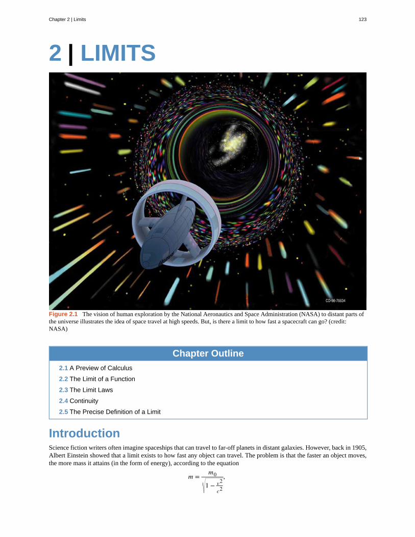
2 | LIMITS
Figure 2.1 The vision of human exploration by the National Aeronautics and Space Administration (NASA) to distant parts ofthe universe illustrates the idea of space travel at high speeds. But, is there a limit to how fast a spacecraft can go? (credit:NASA)
Chapter Outline
2.1 A Preview of Calculus
2.2 The Limit of a Function
2.3 The Limit Laws
2.4 Continuity
2.5 The Precise Definition of a Limit
IntroductionScience fiction writers often imagine spaceships that can travel to far-off planets in distant galaxies. However, back in 1905,Albert Einstein showed that a limit exists to how fast any object can travel. The problem is that the faster an object moves,the more mass it attains (in the form of energy), according to the equation
m = m0
1 − v2
c2
,
Chapter 2 | Limits 123
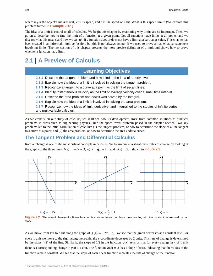
where m0 is the object’s mass at rest, v is its speed, and c is the speed of light. What is this speed limit? (We explore thisproblem further in Example 2.12.)
The idea of a limit is central to all of calculus. We begin this chapter by examining why limits are so important. Then, wego on to describe how to find the limit of a function at a given point. Not all functions have limits at all points, and wediscuss what this means and how we can tell if a function does or does not have a limit at a particular value. This chapter hasbeen created in an informal, intuitive fashion, but this is not always enough if we need to prove a mathematical statementinvolving limits. The last section of this chapter presents the more precise definition of a limit and shows how to provewhether a function has a limit.
2.1 | A Preview of Calculus
Learning Objectives2.1.1 Describe the tangent problem and how it led to the idea of a derivative.
2.1.2 Explain how the idea of a limit is involved in solving the tangent problem.
2.1.3 Recognize a tangent to a curve at a point as the limit of secant lines.
2.1.4 Identify instantaneous velocity as the limit of average velocity over a small time interval.
2.1.5 Describe the area problem and how it was solved by the integral.
2.1.6 Explain how the idea of a limit is involved in solving the area problem.
2.1.7 Recognize how the ideas of limit, derivative, and integral led to the studies of infinite seriesand multivariable calculus.
As we embark on our study of calculus, we shall see how its development arose from common solutions to practicalproblems in areas such as engineering physics—like the space travel problem posed in the chapter opener. Two keyproblems led to the initial formulation of calculus: (1) the tangent problem, or how to determine the slope of a line tangentto a curve at a point; and (2) the area problem, or how to determine the area under a curve.
The Tangent Problem and Differential CalculusRate of change is one of the most critical concepts in calculus. We begin our investigation of rates of change by looking at
the graphs of the three lines f (x) = −2x − 3, g(x) = 12x + 1, and h(x) = 2, shown in Figure 2.2.
Figure 2.2 The rate of change of a linear function is constant in each of these three graphs, with the constant determined by theslope.
As we move from left to right along the graph of f (x) = −2x − 3, we see that the graph decreases at a constant rate. For
every 1 unit we move to the right along the x-axis, the y-coordinate decreases by 2 units. This rate of change is determinedby the slope (−2) of the line. Similarly, the slope of 1/2 in the function g(x) tells us that for every change in x of 1 unit
there is a corresponding change in y of 1/2 unit. The function h(x) = 2 has a slope of zero, indicating that the values of the
function remain constant. We see that the slope of each linear function indicates the rate of change of the function.
124 Chapter 2 | Limits
This OpenStax book is available for free at http://cnx.org/content/col11964/1.2
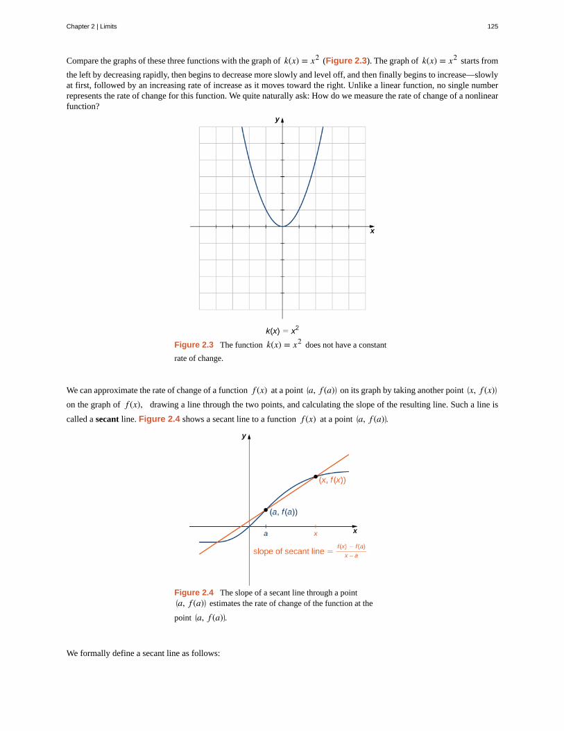
Compare the graphs of these three functions with the graph of k(x) = x2 (Figure 2.3). The graph of k(x) = x2 starts from
the left by decreasing rapidly, then begins to decrease more slowly and level off, and then finally begins to increase—slowlyat first, followed by an increasing rate of increase as it moves toward the right. Unlike a linear function, no single numberrepresents the rate of change for this function. We quite naturally ask: How do we measure the rate of change of a nonlinearfunction?
Figure 2.3 The function k(x) = x2 does not have a constant
rate of change.
We can approximate the rate of change of a function f (x) at a point ⎛⎝a, f (a)⎞
⎠ on its graph by taking another point ⎛⎝x, f (x)⎞
⎠
on the graph of f (x), drawing a line through the two points, and calculating the slope of the resulting line. Such a line is
called a secant line. Figure 2.4 shows a secant line to a function f (x) at a point ⎛⎝a, f (a)⎞
⎠.
Figure 2.4 The slope of a secant line through a point⎛⎝a, f (a)⎞
⎠ estimates the rate of change of the function at the
point ⎛⎝a, f (a)⎞
⎠.
We formally define a secant line as follows:
Chapter 2 | Limits 125
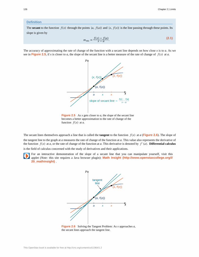
Definition
The secant to the function f (x) through the points ⎛⎝a, f (a)⎞
⎠ and ⎛⎝x, f (x)⎞
⎠ is the line passing through these points. Its
slope is given by
(2.1)msec = f (x) − f (a)x − a .
The accuracy of approximating the rate of change of the function with a secant line depends on how close x is to a. As wesee in Figure 2.5, if x is closer to a, the slope of the secant line is a better measure of the rate of change of f (x) at a.
Figure 2.5 As x gets closer to a, the slope of the secant linebecomes a better approximation to the rate of change of thefunction f (x) at a.
The secant lines themselves approach a line that is called the tangent to the function f (x) at a (Figure 2.6). The slope of
the tangent line to the graph at a measures the rate of change of the function at a. This value also represents the derivative ofthe function f (x) at a, or the rate of change of the function at a. This derivative is denoted by f ′ (a). Differential calculus
is the field of calculus concerned with the study of derivatives and their applications.
For an interactive demonstration of the slope of a secant line that you can manipulate yourself, visit thisapplet (Note: this site requires a Java browser plugin): Math Insight (http://www.openstaxcollege.org/l/20_mathinsight) .
Figure 2.6 Solving the Tangent Problem: As x approaches a,the secant lines approach the tangent line.
126 Chapter 2 | Limits
This OpenStax book is available for free at http://cnx.org/content/col11964/1.2
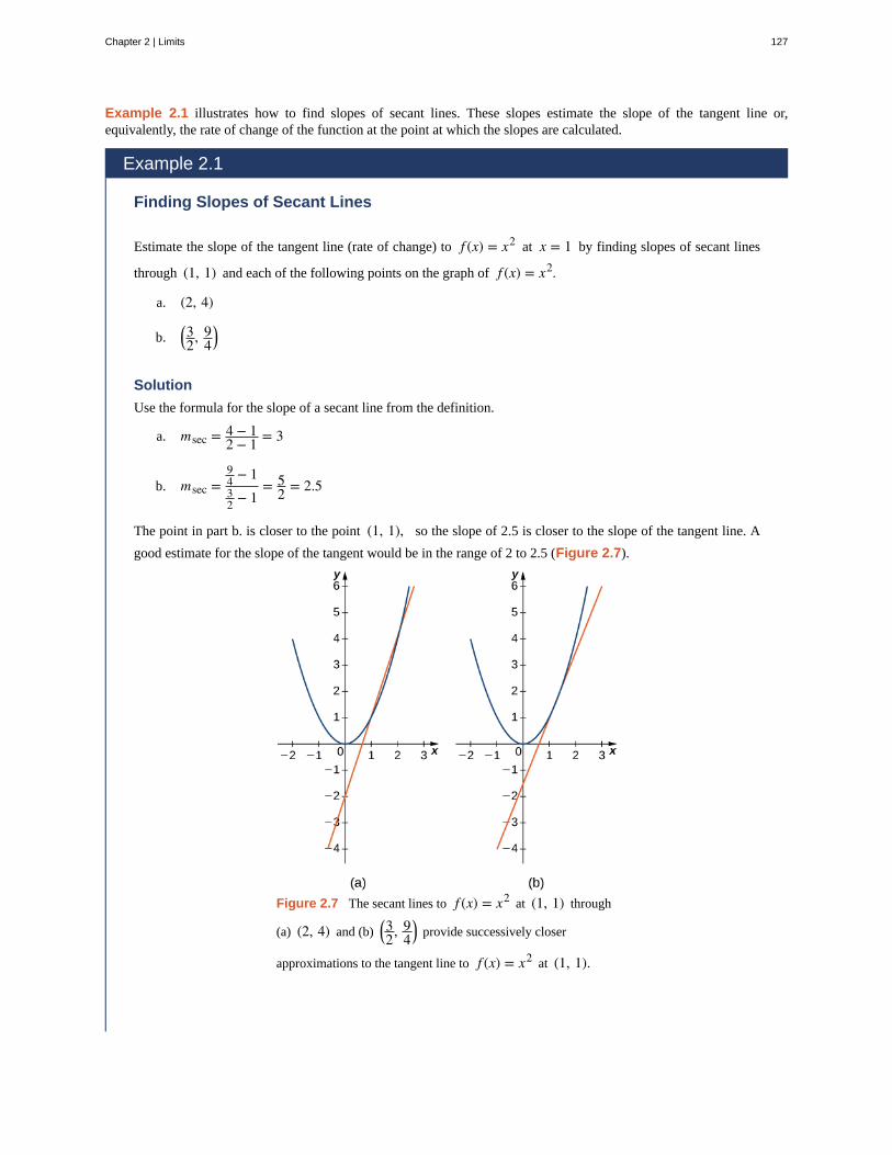
Example 2.1 illustrates how to find slopes of secant lines. These slopes estimate the slope of the tangent line or,equivalently, the rate of change of the function at the point at which the slopes are calculated.
Example 2.1
Finding Slopes of Secant Lines
Estimate the slope of the tangent line (rate of change) to f (x) = x2 at x = 1 by finding slopes of secant lines
through (1, 1) and each of the following points on the graph of f (x) = x2.
a. (2, 4)
b. ⎛⎝32, 9
4⎞⎠
Solution
Use the formula for the slope of a secant line from the definition.
a. msec = 4 − 12 − 1 = 3
b. msec =94 − 132 − 1
= 52 = 2.5
The point in part b. is closer to the point (1, 1), so the slope of 2.5 is closer to the slope of the tangent line. A
good estimate for the slope of the tangent would be in the range of 2 to 2.5 (Figure 2.7).
Figure 2.7 The secant lines to f (x) = x2 at (1, 1) through
(a) (2, 4) and (b)⎛⎝32, 9
4⎞⎠ provide successively closer
approximations to the tangent line to f (x) = x2 at (1, 1).
Chapter 2 | Limits 127
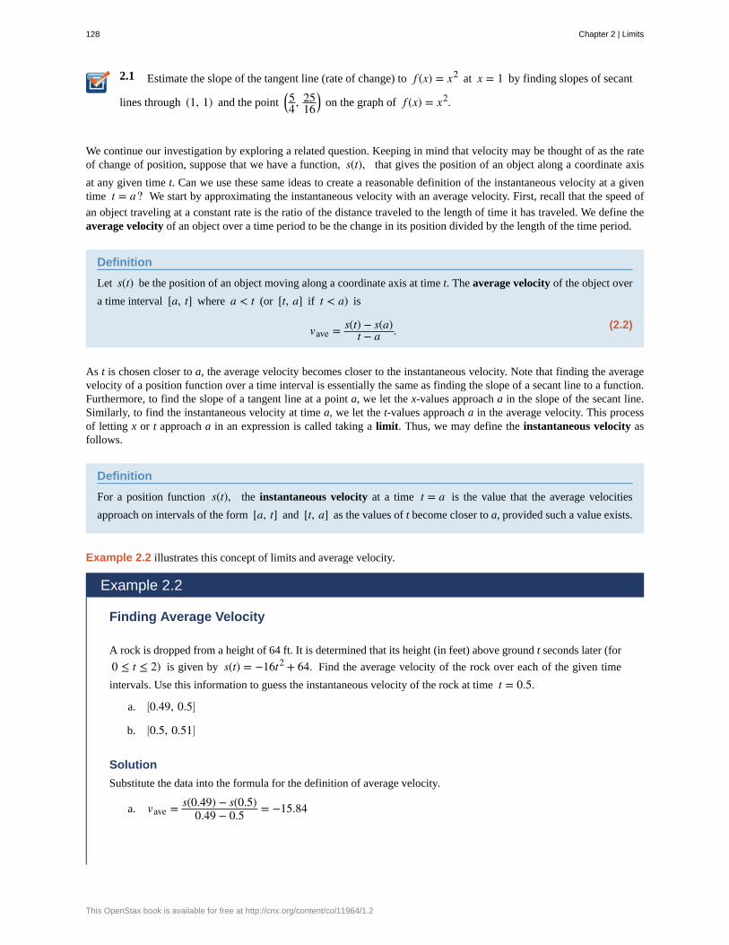
2.1 Estimate the slope of the tangent line (rate of change) to f (x) = x2 at x = 1 by finding slopes of secant
lines through (1, 1) and the point ⎛⎝54, 25
16⎞⎠ on the graph of f (x) = x2.
We continue our investigation by exploring a related question. Keeping in mind that velocity may be thought of as the rateof change of position, suppose that we have a function, s(t), that gives the position of an object along a coordinate axis
at any given time t. Can we use these same ideas to create a reasonable definition of the instantaneous velocity at a giventime t = a? We start by approximating the instantaneous velocity with an average velocity. First, recall that the speed of
an object traveling at a constant rate is the ratio of the distance traveled to the length of time it has traveled. We define theaverage velocity of an object over a time period to be the change in its position divided by the length of the time period.
Definition
Let s(t) be the position of an object moving along a coordinate axis at time t. The average velocity of the object over
a time interval [a, t] where a < t (or [t, a] if t < a) is
(2.2)vave = s(t) − s(a)t − a .
As t is chosen closer to a, the average velocity becomes closer to the instantaneous velocity. Note that finding the averagevelocity of a position function over a time interval is essentially the same as finding the slope of a secant line to a function.Furthermore, to find the slope of a tangent line at a point a, we let the x-values approach a in the slope of the secant line.Similarly, to find the instantaneous velocity at time a, we let the t-values approach a in the average velocity. This processof letting x or t approach a in an expression is called taking a limit. Thus, we may define the instantaneous velocity asfollows.
Definition
For a position function s(t), the instantaneous velocity at a time t = a is the value that the average velocities
approach on intervals of the form [a, t] and [t, a] as the values of t become closer to a, provided such a value exists.
Example 2.2 illustrates this concept of limits and average velocity.
Example 2.2
Finding Average Velocity
A rock is dropped from a height of 64 ft. It is determined that its height (in feet) above ground t seconds later (for
0 ≤ t ≤ 2) is given by s(t) = −16t2 + 64. Find the average velocity of the rock over each of the given time
intervals. Use this information to guess the instantaneous velocity of the rock at time t = 0.5.
a. ⎡⎣0.49, 0.5⎤
⎦
b. ⎡⎣0.5, 0.51⎤
⎦
Solution
Substitute the data into the formula for the definition of average velocity.
a. vave = s(0.49) − s(0.5)0.49 − 0.5 = −15.84
128 Chapter 2 | Limits
This OpenStax book is available for free at http://cnx.org/content/col11964/1.2
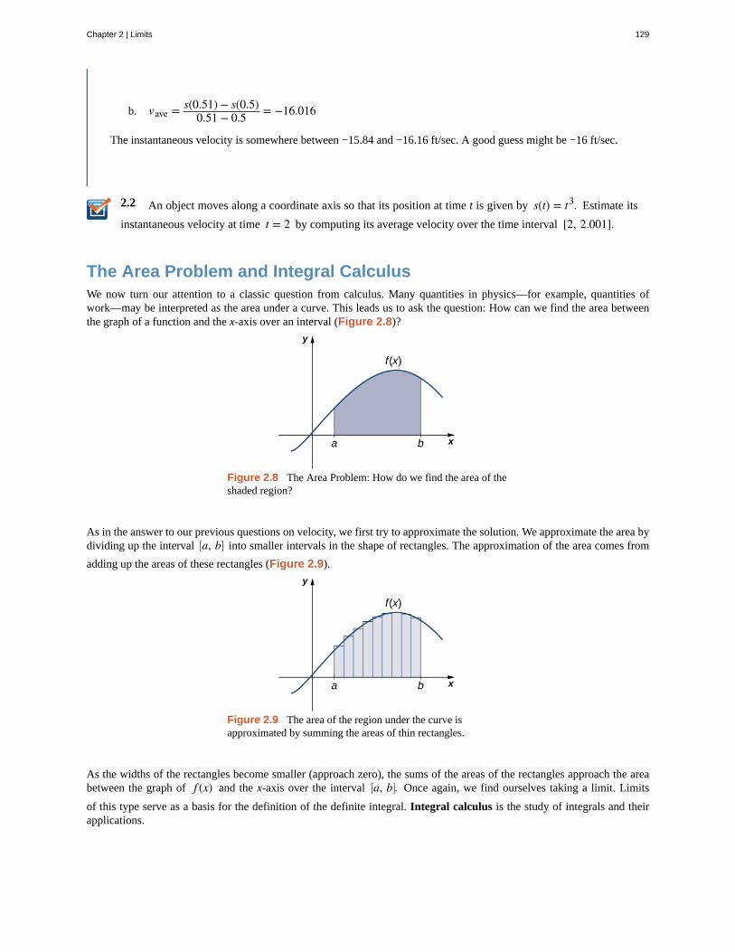
2.2
b. vave = s(0.51) − s(0.5)0.51 − 0.5 = −16.016
The instantaneous velocity is somewhere between −15.84 and −16.16 ft/sec. A good guess might be −16 ft/sec.
An object moves along a coordinate axis so that its position at time t is given by s(t) = t3. Estimate its
instantaneous velocity at time t = 2 by computing its average velocity over the time interval [2, 2.001].
The Area Problem and Integral CalculusWe now turn our attention to a classic question from calculus. Many quantities in physics—for example, quantities ofwork—may be interpreted as the area under a curve. This leads us to ask the question: How can we find the area betweenthe graph of a function and the x-axis over an interval (Figure 2.8)?
Figure 2.8 The Area Problem: How do we find the area of theshaded region?
As in the answer to our previous questions on velocity, we first try to approximate the solution. We approximate the area bydividing up the interval ⎡
⎣a, b⎤⎦ into smaller intervals in the shape of rectangles. The approximation of the area comes from
adding up the areas of these rectangles (Figure 2.9).
Figure 2.9 The area of the region under the curve isapproximated by summing the areas of thin rectangles.
As the widths of the rectangles become smaller (approach zero), the sums of the areas of the rectangles approach the areabetween the graph of f (x) and the x-axis over the interval ⎡
⎣a, b⎤⎦. Once again, we find ourselves taking a limit. Limits
of this type serve as a basis for the definition of the definite integral. Integral calculus is the study of integrals and theirapplications.
Chapter 2 | Limits 129
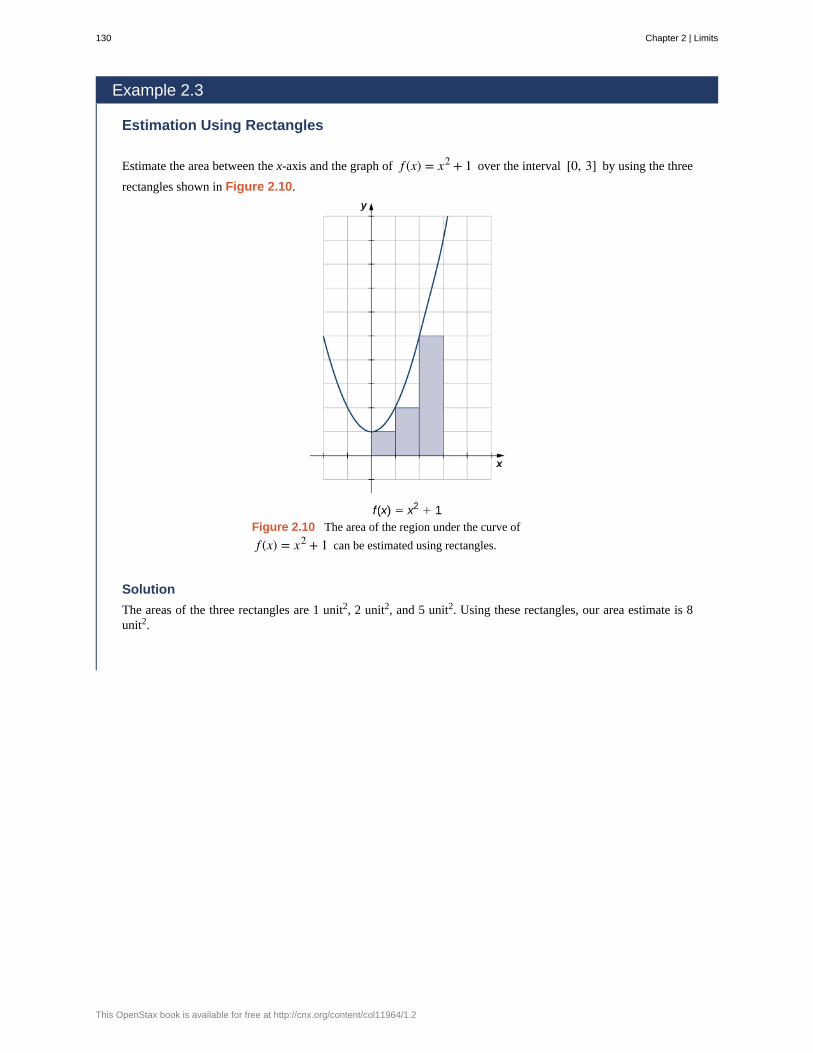
Example 2.3
Estimation Using Rectangles
Estimate the area between the x-axis and the graph of f (x) = x2 + 1 over the interval [0, 3] by using the three
rectangles shown in Figure 2.10.
Figure 2.10 The area of the region under the curve of
f (x) = x2 + 1 can be estimated using rectangles.
Solution
The areas of the three rectangles are 1 unit2, 2 unit2, and 5 unit2. Using these rectangles, our area estimate is 8unit2.
130 Chapter 2 | Limits
This OpenStax book is available for free at http://cnx.org/content/col11964/1.2
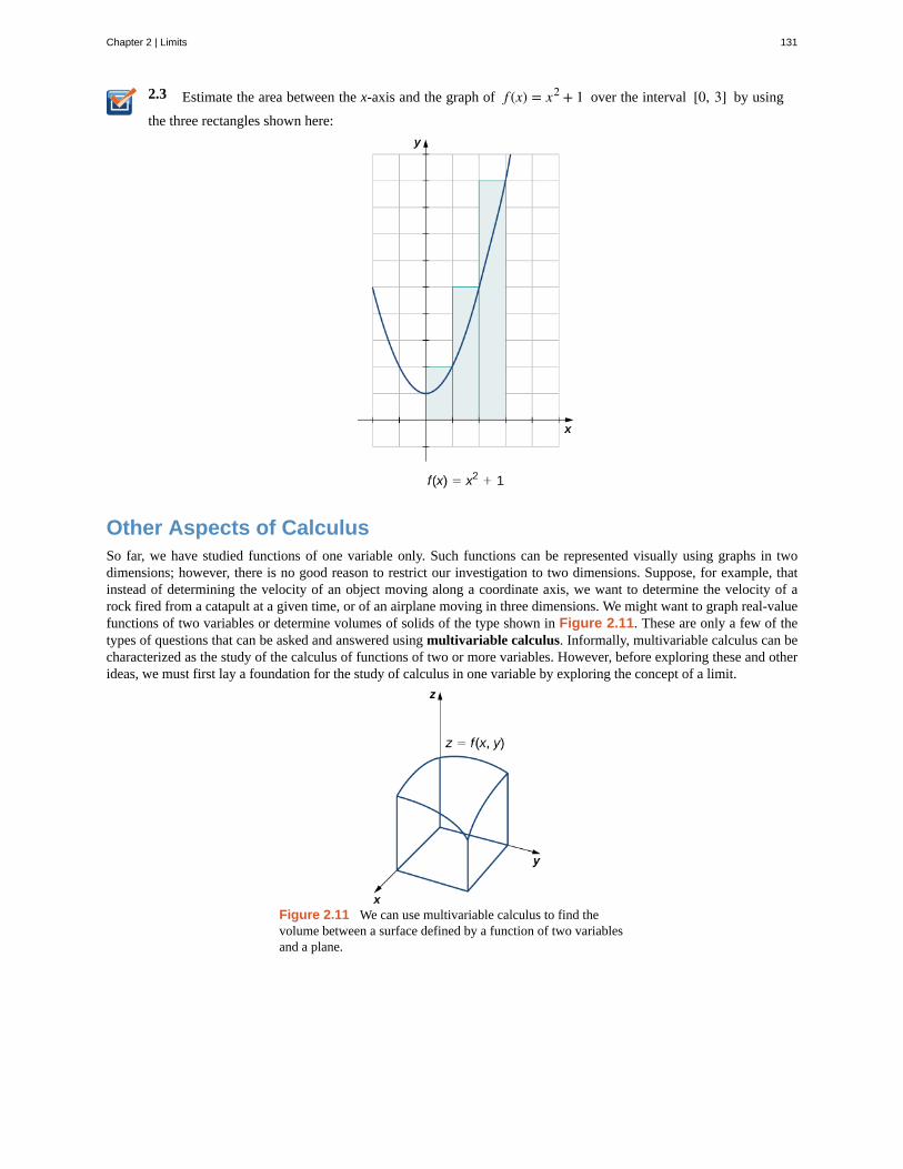
2.3 Estimate the area between the x-axis and the graph of f (x) = x2 + 1 over the interval [0, 3] by using
the three rectangles shown here:
Other Aspects of CalculusSo far, we have studied functions of one variable only. Such functions can be represented visually using graphs in twodimensions; however, there is no good reason to restrict our investigation to two dimensions. Suppose, for example, thatinstead of determining the velocity of an object moving along a coordinate axis, we want to determine the velocity of arock fired from a catapult at a given time, or of an airplane moving in three dimensions. We might want to graph real-valuefunctions of two variables or determine volumes of solids of the type shown in Figure 2.11. These are only a few of thetypes of questions that can be asked and answered using multivariable calculus. Informally, multivariable calculus can becharacterized as the study of the calculus of functions of two or more variables. However, before exploring these and otherideas, we must first lay a foundation for the study of calculus in one variable by exploring the concept of a limit.
Figure 2.11 We can use multivariable calculus to find thevolume between a surface defined by a function of two variablesand a plane.
Chapter 2 | Limits 131
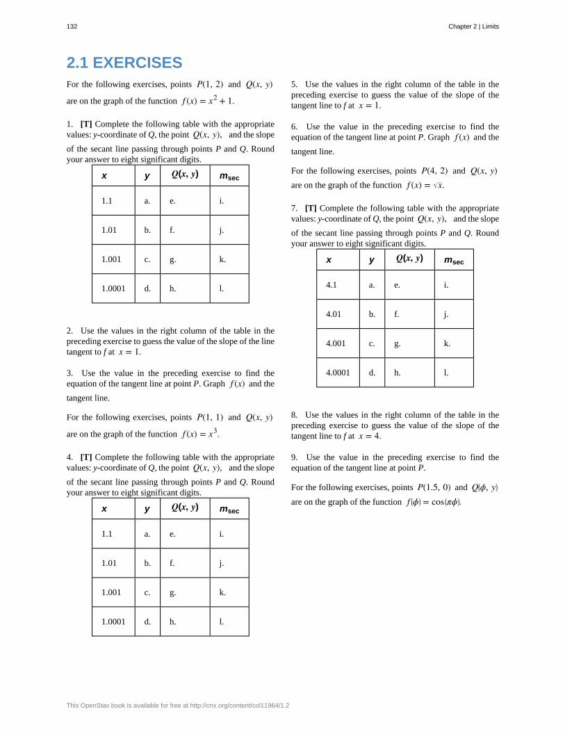
2.1 EXERCISESFor the following exercises, points P(1, 2) and Q(x, y)
are on the graph of the function f (x) = x2 + 1.
1. [T] Complete the following table with the appropriatevalues: y-coordinate of Q, the point Q(x, y), and the slope
of the secant line passing through points P and Q. Roundyour answer to eight significant digits.
x y Q(x, y) msec
1.1 a. e. i.
1.01 b. f. j.
1.001 c. g. k.
1.0001 d. h. l.
2. Use the values in the right column of the table in thepreceding exercise to guess the value of the slope of the linetangent to f at x = 1.
3. Use the value in the preceding exercise to find theequation of the tangent line at point P. Graph f (x) and the
tangent line.
For the following exercises, points P(1, 1) and Q(x, y)
are on the graph of the function f (x) = x3.
4. [T] Complete the following table with the appropriatevalues: y-coordinate of Q, the point Q(x, y), and the slope
of the secant line passing through points P and Q. Roundyour answer to eight significant digits.
x y Q(x, y) msec
1.1 a. e. i.
1.01 b. f. j.
1.001 c. g. k.
1.0001 d. h. l.
5. Use the values in the right column of the table in thepreceding exercise to guess the value of the slope of thetangent line to f at x = 1.
6. Use the value in the preceding exercise to find theequation of the tangent line at point P. Graph f (x) and the
tangent line.
For the following exercises, points P(4, 2) and Q(x, y)are on the graph of the function f (x) = x.
7. [T] Complete the following table with the appropriatevalues: y-coordinate of Q, the point Q(x, y), and the slope
of the secant line passing through points P and Q. Roundyour answer to eight significant digits.
x y Q(x, y) msec
4.1 a. e. i.
4.01 b. f. j.
4.001 c. g. k.
4.0001 d. h. l.
8. Use the values in the right column of the table in thepreceding exercise to guess the value of the slope of thetangent line to f at x = 4.
9. Use the value in the preceding exercise to find theequation of the tangent line at point P.
For the following exercises, points P(1.5, 0) and Q⎛⎝ϕ, y⎞
⎠
are on the graph of the function f ⎛⎝ϕ⎞
⎠ = cos ⎛⎝πϕ⎞
⎠.
132 Chapter 2 | Limits
This OpenStax book is available for free at http://cnx.org/content/col11964/1.2
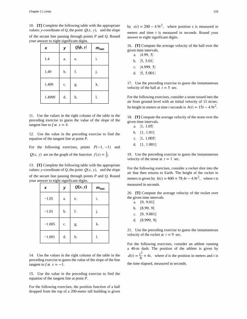
10. [T] Complete the following table with the appropriatevalues: y-coordinate of Q, the point Q(x, y), and the slope
of the secant line passing through points P and Q. Roundyour answer to eight significant digits.
x y Q⎛⎝ϕ, y⎞
⎠ msec
1.4 a. e. i.
1.49 b. f. j.
1.499 c. g. k.
1.4999 d. h. l.
11. Use the values in the right column of the table in thepreceding exercise to guess the value of the slope of thetangent line to f at x = 4.
12. Use the value in the preceding exercise to find theequation of the tangent line at point P.
For the following exercises, points P(−1, −1) and
Q(x, y) are on the graph of the function f (x) = 1x .
13. [T] Complete the following table with the appropriatevalues: y-coordinate of Q, the point Q(x, y), and the slope
of the secant line passing through points P and Q. Roundyour answer to eight significant digits.
x y Q(x, y) msec
−1.05 a. e. i.
−1.01 b. f. j.
−1.005 c. g. k.
−1.001 d. h. l.
14. Use the values in the right column of the table in thepreceding exercise to guess the value of the slope of the linetangent to f at x = −1.
15. Use the value in the preceding exercise to find theequation of the tangent line at point P.
For the following exercises, the position function of a balldropped from the top of a 200-meter tall building is given
by s(t) = 200 − 4.9t2, where position s is measured in
meters and time t is measured in seconds. Round youranswer to eight significant digits.
16. [T] Compute the average velocity of the ball over thegiven time intervals.
a. ⎡⎣4.99, 5⎤
⎦
b. ⎡⎣5, 5.01⎤
⎦
c. ⎡⎣4.999, 5⎤
⎦
d. ⎡⎣5, 5.001⎤
⎦
17. Use the preceding exercise to guess the instantaneousvelocity of the ball at t = 5 sec.
For the following exercises, consider a stone tossed into theair from ground level with an initial velocity of 15 m/sec.
Its height in meters at time t seconds is h(t) = 15t − 4.9t2.
18. [T] Compute the average velocity of the stone over thegiven time intervals.
a. ⎡⎣1, 1.05⎤
⎦
b. [1, 1.01]c. ⎡
⎣1, 1.005⎤⎦
d. [1, 1.001]
19. Use the preceding exercise to guess the instantaneousvelocity of the stone at t = 1 sec.
For the following exercises, consider a rocket shot into theair that then returns to Earth. The height of the rocket in
meters is given by h(t) = 600 + 78.4t − 4.9t2, where t is
measured in seconds.
20. [T] Compute the average velocity of the rocket overthe given time intervals.
a. [9, 9.01]b. [8.99, 9]c. [9, 9.001]d. [8.999, 9]
21. Use the preceding exercise to guess the instantaneousvelocity of the rocket at t = 9 sec.
For the following exercises, consider an athlete runninga 40-m dash. The position of the athlete is given by
d(t) = t3
6 + 4t, where d is the position in meters and t is
the time elapsed, measured in seconds.
Chapter 2 | Limits 133
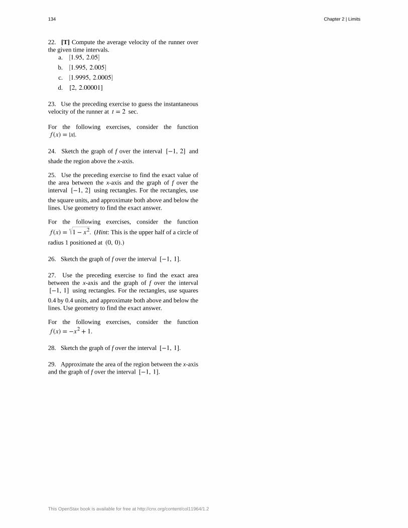
22. [T] Compute the average velocity of the runner overthe given time intervals.
a. ⎡⎣1.95, 2.05⎤
⎦
b. ⎡⎣1.995, 2.005⎤
⎦
c. ⎡⎣1.9995, 2.0005⎤
⎦
d. [2, 2.00001]
23. Use the preceding exercise to guess the instantaneousvelocity of the runner at t = 2 sec.
For the following exercises, consider the functionf (x) = |x|.
24. Sketch the graph of f over the interval [−1, 2] and
shade the region above the x-axis.
25. Use the preceding exercise to find the exact value ofthe area between the x-axis and the graph of f over theinterval [−1, 2] using rectangles. For the rectangles, use
the square units, and approximate both above and below thelines. Use geometry to find the exact answer.
For the following exercises, consider the function
f (x) = 1 − x2. (Hint: This is the upper half of a circle of
radius 1 positioned at (0, 0).)
26. Sketch the graph of f over the interval [−1, 1].
27. Use the preceding exercise to find the exact areabetween the x-axis and the graph of f over the interval[−1, 1] using rectangles. For the rectangles, use squares
0.4 by 0.4 units, and approximate both above and below thelines. Use geometry to find the exact answer.
For the following exercises, consider the function
f (x) = −x2 + 1.
28. Sketch the graph of f over the interval [−1, 1].
29. Approximate the area of the region between the x-axisand the graph of f over the interval [−1, 1].
134 Chapter 2 | Limits
This OpenStax book is available for free at http://cnx.org/content/col11964/1.2
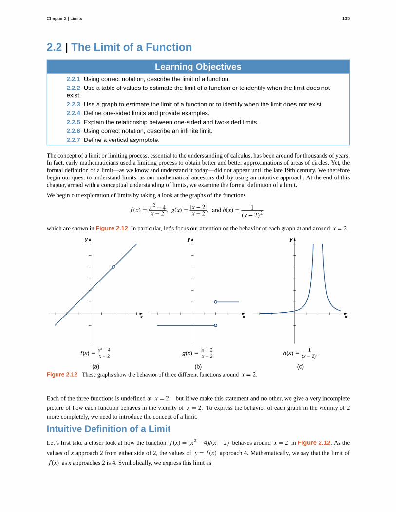
2.2 | The Limit of a Function
Learning Objectives2.2.1 Using correct notation, describe the limit of a function.
2.2.2 Use a table of values to estimate the limit of a function or to identify when the limit does notexist.
2.2.3 Use a graph to estimate the limit of a function or to identify when the limit does not exist.
2.2.4 Define one-sided limits and provide examples.
2.2.5 Explain the relationship between one-sided and two-sided limits.
2.2.6 Using correct notation, describe an infinite limit.
2.2.7 Define a vertical asymptote.
The concept of a limit or limiting process, essential to the understanding of calculus, has been around for thousands of years.In fact, early mathematicians used a limiting process to obtain better and better approximations of areas of circles. Yet, theformal definition of a limit—as we know and understand it today—did not appear until the late 19th century. We thereforebegin our quest to understand limits, as our mathematical ancestors did, by using an intuitive approach. At the end of thischapter, armed with a conceptual understanding of limits, we examine the formal definition of a limit.
We begin our exploration of limits by taking a look at the graphs of the functions
f (x) = x2 − 4x − 2 , g(x) = |x − 2|
x − 2 , and h(x) = 1(x − 2)2,
which are shown in Figure 2.12. In particular, let’s focus our attention on the behavior of each graph at and around x = 2.
Figure 2.12 These graphs show the behavior of three different functions around x = 2.
Each of the three functions is undefined at x = 2, but if we make this statement and no other, we give a very incomplete
picture of how each function behaves in the vicinity of x = 2. To express the behavior of each graph in the vicinity of 2
more completely, we need to introduce the concept of a limit.
Intuitive Definition of a LimitLet’s first take a closer look at how the function f (x) = (x2 − 4)/(x − 2) behaves around x = 2 in Figure 2.12. As the
values of x approach 2 from either side of 2, the values of y = f (x) approach 4. Mathematically, we say that the limit of
f (x) as x approaches 2 is 4. Symbolically, we express this limit as
Chapter 2 | Limits 135
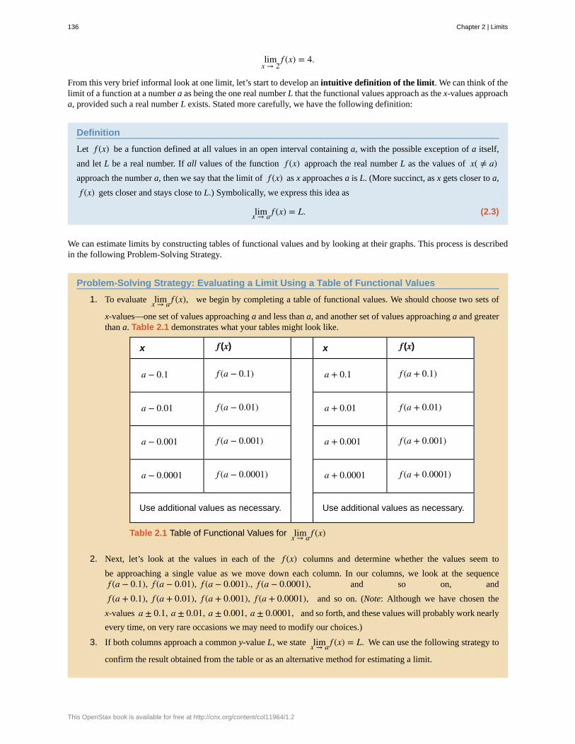
limx → 2
f (x) = 4.
From this very brief informal look at one limit, let’s start to develop an intuitive definition of the limit. We can think of thelimit of a function at a number a as being the one real number L that the functional values approach as the x-values approacha, provided such a real number L exists. Stated more carefully, we have the following definition:
Definition
Let f (x) be a function defined at all values in an open interval containing a, with the possible exception of a itself,
and let L be a real number. If all values of the function f (x) approach the real number L as the values of x( ≠ a)approach the number a, then we say that the limit of f (x) as x approaches a is L. (More succinct, as x gets closer to a,
f (x) gets closer and stays close to L.) Symbolically, we express this idea as
(2.3)limx → a f (x) = L.
We can estimate limits by constructing tables of functional values and by looking at their graphs. This process is describedin the following Problem-Solving Strategy.
Problem-Solving Strategy: Evaluating a Limit Using a Table of Functional Values
1. To evaluate limx → a f (x), we begin by completing a table of functional values. We should choose two sets of
x-values—one set of values approaching a and less than a, and another set of values approaching a and greaterthan a. Table 2.1 demonstrates what your tables might look like.
x f(x) x f(x)
a − 0.1 f (a − 0.1) a + 0.1 f (a + 0.1)
a − 0.01 f (a − 0.01) a + 0.01 f (a + 0.01)
a − 0.001 f (a − 0.001) a + 0.001 f (a + 0.001)
a − 0.0001 f (a − 0.0001) a + 0.0001 f (a + 0.0001)
Use additional values as necessary. Use additional values as necessary.
Table 2.1 Table of Functional Values for limx → a f (x)
2. Next, let’s look at the values in each of the f (x) columns and determine whether the values seem to
be approaching a single value as we move down each column. In our columns, we look at the sequencef (a − 0.1), f (a − 0.01), f (a − 0.001)., f (a − 0.0001), and so on, and
f (a + 0.1), f (a + 0.01), f (a + 0.001), f (a + 0.0001), and so on. (Note: Although we have chosen the
x-values a ± 0.1, a ± 0.01, a ± 0.001, a ± 0.0001, and so forth, and these values will probably work nearly
every time, on very rare occasions we may need to modify our choices.)
3. If both columns approach a common y-value L, we state limx → a f (x) = L. We can use the following strategy to
confirm the result obtained from the table or as an alternative method for estimating a limit.
136 Chapter 2 | Limits
This OpenStax book is available for free at http://cnx.org/content/col11964/1.2
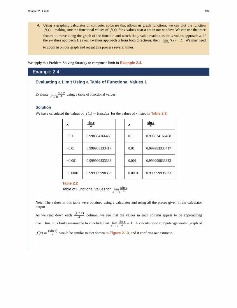
4. Using a graphing calculator or computer software that allows us graph functions, we can plot the functionf (x), making sure the functional values of f (x) for x-values near a are in our window. We can use the trace
feature to move along the graph of the function and watch the y-value readout as the x-values approach a. Ifthe y-values approach L as our x-values approach a from both directions, then limx → a f (x) = L. We may need
to zoom in on our graph and repeat this process several times.
We apply this Problem-Solving Strategy to compute a limit in Example 2.4.
Example 2.4
Evaluating a Limit Using a Table of Functional Values 1
Evaluate limx → 0
sinxx using a table of functional values.
Solution
We have calculated the values of f (x) = (sinx)/x for the values of x listed in Table 2.2.
x sinxx x sinx
x
−0.1 0.998334166468 0.1 0.998334166468
−0.01 0.999983333417 0.01 0.999983333417
−0.001 0.999999833333 0.001 0.999999833333
−0.0001 0.999999998333 0.0001 0.999999998333
Table 2.2
Table of Functional Values for limx → 0
sinxx
Note: The values in this table were obtained using a calculator and using all the places given in the calculatoroutput.
As we read down each(sinx)
x column, we see that the values in each column appear to be approaching
one. Thus, it is fairly reasonable to conclude that limx → 0
sinxx = 1. A calculator-or computer-generated graph of
f (x) = (sinx)x would be similar to that shown in Figure 2.13, and it confirms our estimate.
Chapter 2 | Limits 137
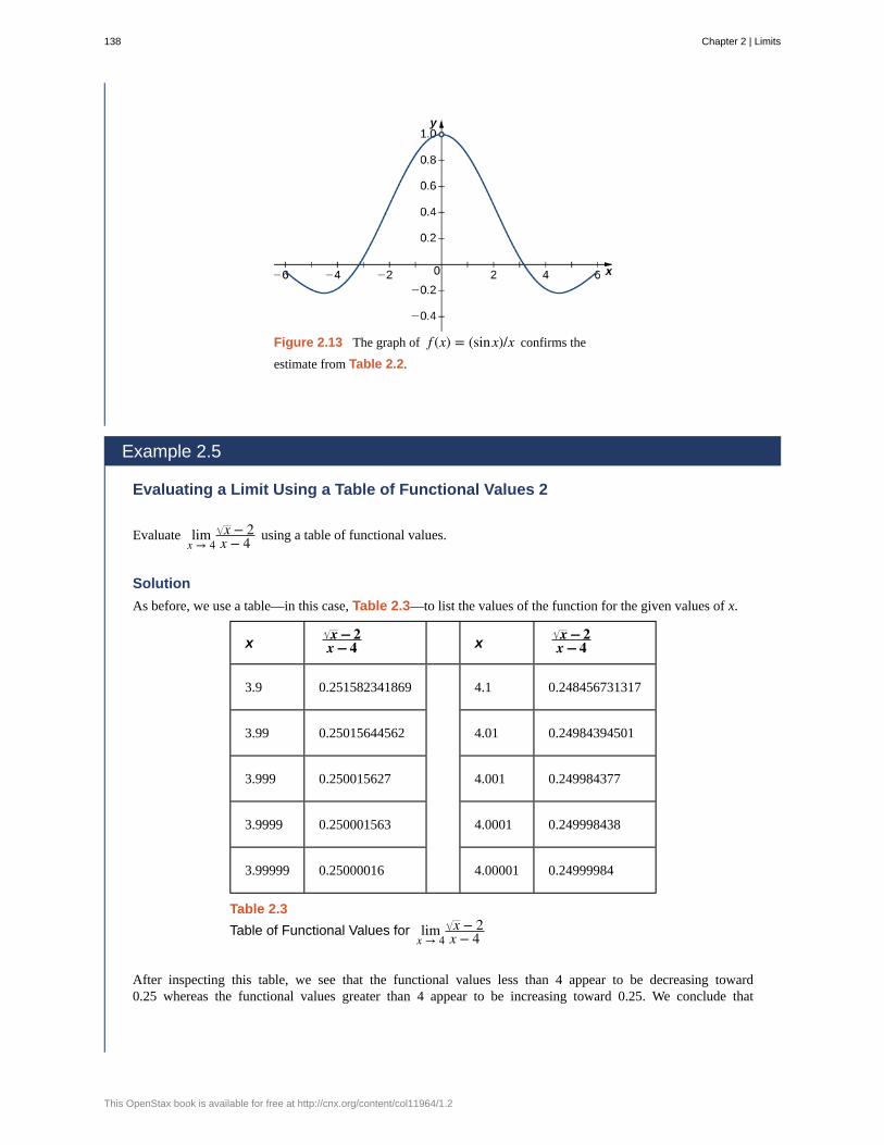
Figure 2.13 The graph of f (x) = (sinx)/x confirms the
estimate from Table 2.2.
Example 2.5
Evaluating a Limit Using a Table of Functional Values 2
Evaluate limx → 4
x − 2x − 4 using a table of functional values.
Solution
As before, we use a table—in this case, Table 2.3—to list the values of the function for the given values of x.
xx − 2
x − 4 xx − 2x − 4
3.9 0.251582341869 4.1 0.248456731317
3.99 0.25015644562 4.01 0.24984394501
3.999 0.250015627 4.001 0.249984377
3.9999 0.250001563 4.0001 0.249998438
3.99999 0.25000016 4.00001 0.24999984
Table 2.3
Table of Functional Values for limx → 4
x − 2x − 4
After inspecting this table, we see that the functional values less than 4 appear to be decreasing toward0.25 whereas the functional values greater than 4 appear to be increasing toward 0.25. We conclude that
138 Chapter 2 | Limits
This OpenStax book is available for free at http://cnx.org/content/col11964/1.2
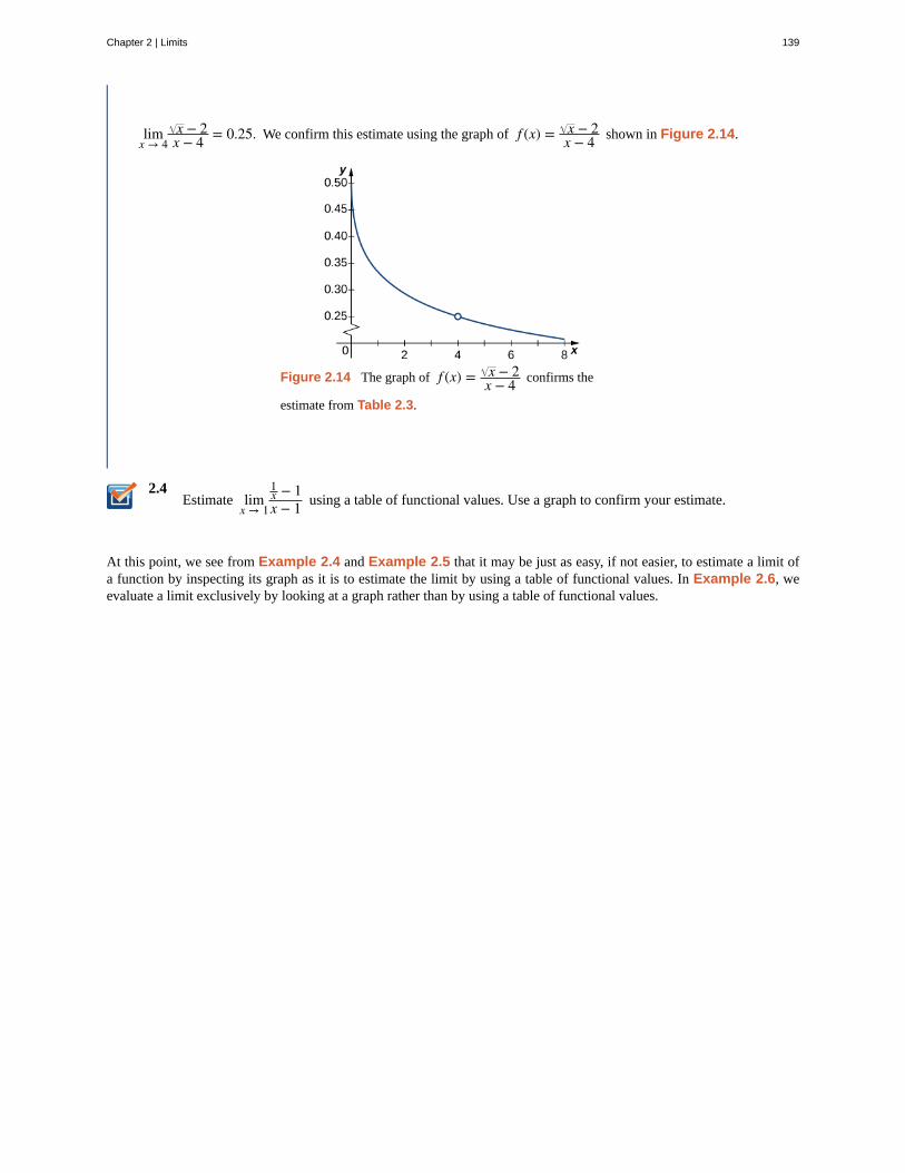
2.4
limx → 4
x − 2x − 4 = 0.25. We confirm this estimate using the graph of f (x) = x − 2
x − 4 shown in Figure 2.14.
Figure 2.14 The graph of f (x) = x − 2x − 4 confirms the
estimate from Table 2.3.
Estimate limx → 1
1x − 1x − 1 using a table of functional values. Use a graph to confirm your estimate.
At this point, we see from Example 2.4 and Example 2.5 that it may be just as easy, if not easier, to estimate a limit ofa function by inspecting its graph as it is to estimate the limit by using a table of functional values. In Example 2.6, weevaluate a limit exclusively by looking at a graph rather than by using a table of functional values.
Chapter 2 | Limits 139
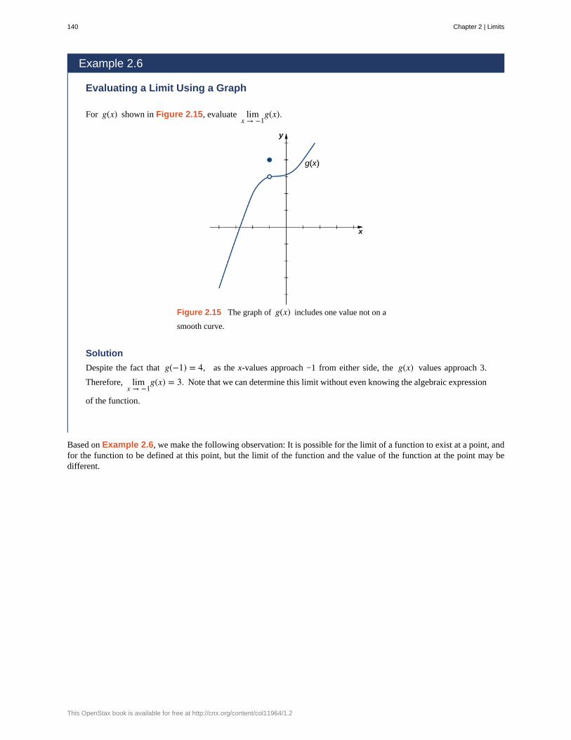
Example 2.6
Evaluating a Limit Using a Graph
For g(x) shown in Figure 2.15, evaluate limx → −1
g(x).
Figure 2.15 The graph of g(x) includes one value not on a
smooth curve.
Solution
Despite the fact that g(−1) = 4, as the x-values approach −1 from either side, the g(x) values approach 3.
Therefore, limx → −1
g(x) = 3. Note that we can determine this limit without even knowing the algebraic expression
of the function.
Based on Example 2.6, we make the following observation: It is possible for the limit of a function to exist at a point, andfor the function to be defined at this point, but the limit of the function and the value of the function at the point may bedifferent.
140 Chapter 2 | Limits
This OpenStax book is available for free at http://cnx.org/content/col11964/1.2
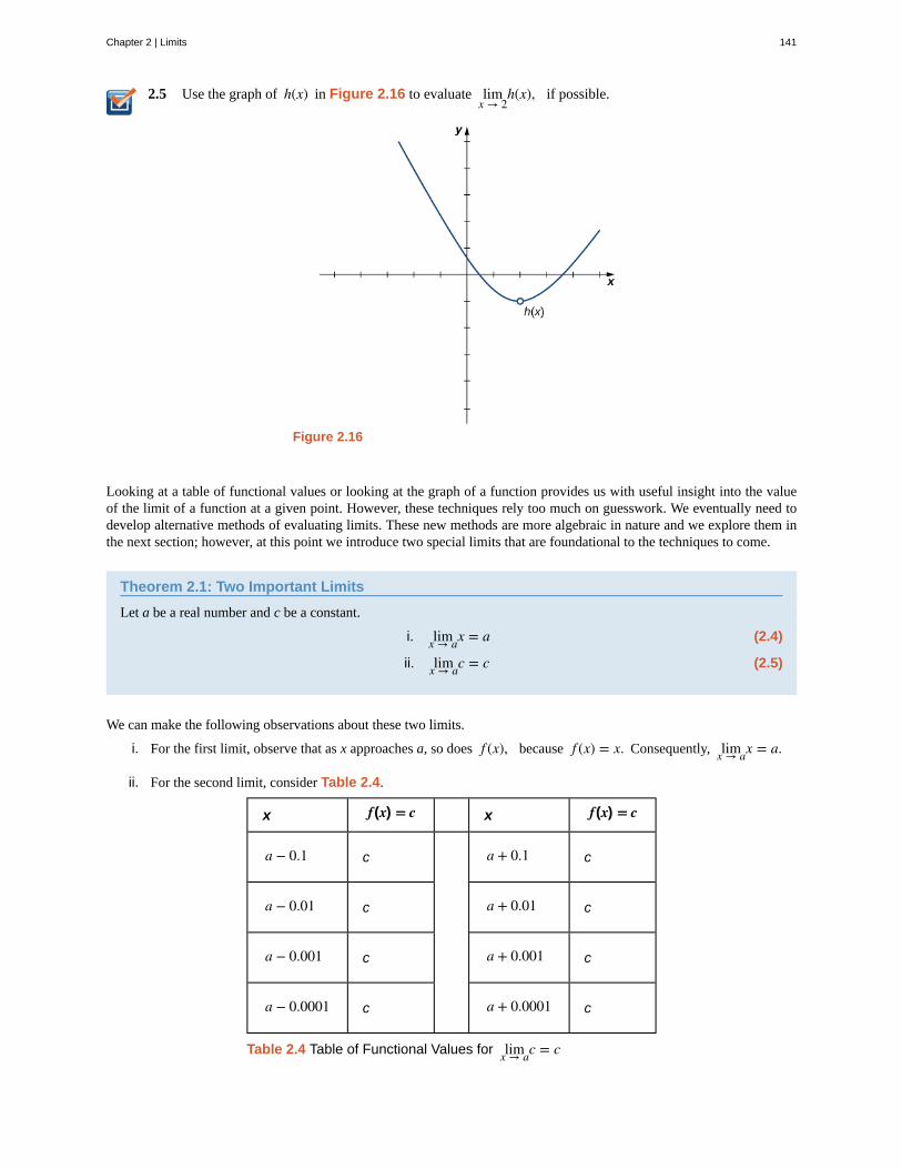
2.5 Use the graph of h(x) in Figure 2.16 to evaluate limx → 2
h(x), if possible.
Figure 2.16
Looking at a table of functional values or looking at the graph of a function provides us with useful insight into the valueof the limit of a function at a given point. However, these techniques rely too much on guesswork. We eventually need todevelop alternative methods of evaluating limits. These new methods are more algebraic in nature and we explore them inthe next section; however, at this point we introduce two special limits that are foundational to the techniques to come.
Theorem 2.1: Two Important Limits
Let a be a real number and c be a constant.
i. (2.4)limx → ax = a
ii. (2.5)limx → ac = c
We can make the following observations about these two limits.
i. For the first limit, observe that as x approaches a, so does f (x), because f (x) = x. Consequently, limx → ax = a.
ii. For the second limit, consider Table 2.4.
x f(x) = c x f(x) = c
a − 0.1 c a + 0.1 c
a − 0.01 c a + 0.01 c
a − 0.001 c a + 0.001 c
a − 0.0001 c a + 0.0001 c
Table 2.4 Table of Functional Values for limx → ac = c
Chapter 2 | Limits 141
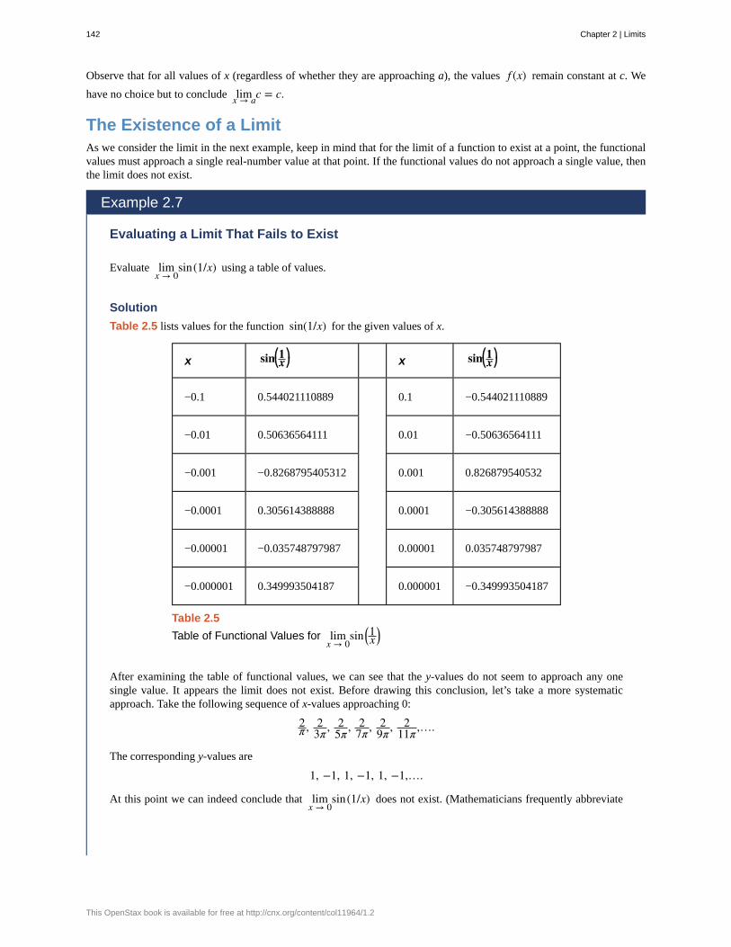
Observe that for all values of x (regardless of whether they are approaching a), the values f (x) remain constant at c. We
have no choice but to conclude limx → ac = c.
The Existence of a LimitAs we consider the limit in the next example, keep in mind that for the limit of a function to exist at a point, the functionalvalues must approach a single real-number value at that point. If the functional values do not approach a single value, thenthe limit does not exist.
Example 2.7
Evaluating a Limit That Fails to Exist
Evaluate limx → 0
sin(1/x) using a table of values.
Solution
Table 2.5 lists values for the function sin(1/x) for the given values of x.
x sin⎛⎝1x⎞⎠ x sin⎛⎝1x
⎞⎠
−0.1 0.544021110889 0.1 −0.544021110889
−0.01 0.50636564111 0.01 −0.50636564111
−0.001 −0.8268795405312 0.001 0.826879540532
−0.0001 0.305614388888 0.0001 −0.305614388888
−0.00001 −0.035748797987 0.00001 0.035748797987
−0.000001 0.349993504187 0.000001 −0.349993504187
Table 2.5
Table of Functional Values for limx → 0
sin⎛⎝1x
⎞⎠
After examining the table of functional values, we can see that the y-values do not seem to approach any onesingle value. It appears the limit does not exist. Before drawing this conclusion, let’s take a more systematicapproach. Take the following sequence of x-values approaching 0:
2π , 2
3π , 25π , 2
7π , 29π , 2
11π ,….
The corresponding y-values are
1, −1, 1, −1, 1, −1,….
At this point we can indeed conclude that limx → 0
sin(1/x) does not exist. (Mathematicians frequently abbreviate
142 Chapter 2 | Limits
This OpenStax book is available for free at http://cnx.org/content/col11964/1.2
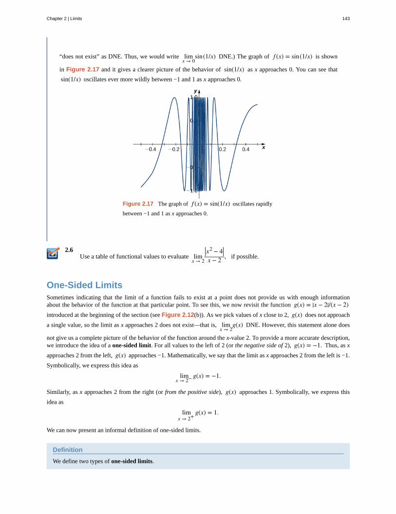
2.6
“does not exist” as DNE. Thus, we would write limx → 0
sin(1/x) DNE.) The graph of f (x) = sin(1/x) is shown
in Figure 2.17 and it gives a clearer picture of the behavior of sin(1/x) as x approaches 0. You can see that
sin(1/x) oscillates ever more wildly between −1 and 1 as x approaches 0.
Figure 2.17 The graph of f (x) = sin(1/x) oscillates rapidly
between −1 and 1 as x approaches 0.
Use a table of functional values to evaluate limx → 2
|x2 − 4|x − 2 , if possible.
One-Sided LimitsSometimes indicating that the limit of a function fails to exist at a point does not provide us with enough informationabout the behavior of the function at that particular point. To see this, we now revisit the function g(x) = |x − 2|/(x − 2)introduced at the beginning of the section (see Figure 2.12(b)). As we pick values of x close to 2, g(x) does not approach
a single value, so the limit as x approaches 2 does not exist—that is, limx → 2
g(x) DNE. However, this statement alone does
not give us a complete picture of the behavior of the function around the x-value 2. To provide a more accurate description,we introduce the idea of a one-sided limit. For all values to the left of 2 (or the negative side of 2), g(x) = −1. Thus, as x
approaches 2 from the left, g(x) approaches −1. Mathematically, we say that the limit as x approaches 2 from the left is −1.
Symbolically, we express this idea as
limx → 2− g(x) = −1.
Similarly, as x approaches 2 from the right (or from the positive side), g(x) approaches 1. Symbolically, we express this
idea as
limx → 2+
g(x) = 1.
We can now present an informal definition of one-sided limits.
Definition
We define two types of one-sided limits.
Chapter 2 | Limits 143
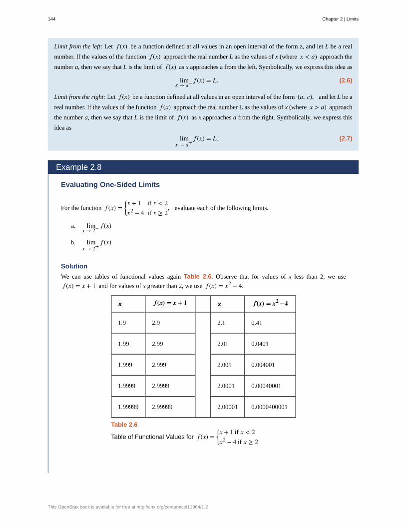
Limit from the left: Let f (x) be a function defined at all values in an open interval of the form z, and let L be a real
number. If the values of the function f (x) approach the real number L as the values of x (where x < a) approach the
number a, then we say that L is the limit of f (x) as x approaches a from the left. Symbolically, we express this idea as
(2.6)limx → a− f (x) = L.
Limit from the right: Let f (x) be a function defined at all values in an open interval of the form (a, c), and let L be a
real number. If the values of the function f (x) approach the real number L as the values of x (where x > a) approach
the number a, then we say that L is the limit of f (x) as x approaches a from the right. Symbolically, we express this
idea as
(2.7)limx → a+
f (x) = L.
Example 2.8
Evaluating One-Sided Limits
For the function f (x) =⎧
⎩⎨x + 1 if x < 2x2 − 4 if x ≥ 2
, evaluate each of the following limits.
a. limx → 2− f (x)
b. limx → 2+
f (x)
Solution
We can use tables of functional values again Table 2.6. Observe that for values of x less than 2, we use
f (x) = x + 1 and for values of x greater than 2, we use f (x) = x2 − 4.
x f(x) = x + 1 x f(x) = x2 −4
1.9 2.9 2.1 0.41
1.99 2.99 2.01 0.0401
1.999 2.999 2.001 0.004001
1.9999 2.9999 2.0001 0.00040001
1.99999 2.99999 2.00001 0.0000400001
Table 2.6
Table of Functional Values for f (x) =⎧
⎩⎨x + 1 if x < 2x2 − 4 if x ≥ 2
144 Chapter 2 | Limits
This OpenStax book is available for free at http://cnx.org/content/col11964/1.2
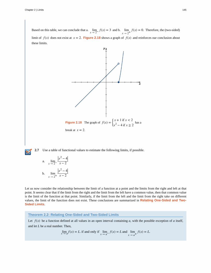
2.7
Based on this table, we can conclude that a. limx → 2− f (x) = 3 and b. lim
x → 2+f (x) = 0. Therefore, the (two-sided)
limit of f (x) does not exist at x = 2. Figure 2.18 shows a graph of f (x) and reinforces our conclusion about
these limits.
Figure 2.18 The graph of f (x) =⎧
⎩⎨
x + 1 if x < 2x2 − 4 if x ≥ 2
has a
break at x = 2.
Use a table of functional values to estimate the following limits, if possible.
a. limx → 2−
|x2 − 4|x − 2
b. limx → 2+
|x2 − 4|x − 2
Let us now consider the relationship between the limit of a function at a point and the limits from the right and left at thatpoint. It seems clear that if the limit from the right and the limit from the left have a common value, then that common valueis the limit of the function at that point. Similarly, if the limit from the left and the limit from the right take on differentvalues, the limit of the function does not exist. These conclusions are summarized in Relating One-Sided and Two-Sided Limits.
Theorem 2.2: Relating One-Sided and Two-Sided Limits
Let f (x) be a function defined at all values in an open interval containing a, with the possible exception of a itself,
and let L be a real number. Then,
limx → a f (x) = L. if and only if limx → a− f (x) = L and lim
x → a+f (x) = L.
Chapter 2 | Limits 145
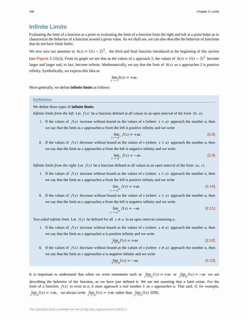
Infinite LimitsEvaluating the limit of a function at a point or evaluating the limit of a function from the right and left at a point helps us tocharacterize the behavior of a function around a given value. As we shall see, we can also describe the behavior of functionsthat do not have finite limits.
We now turn our attention to h(x) = 1/(x − 2)2, the third and final function introduced at the beginning of this section
(see Figure 2.12(c)). From its graph we see that as the values of x approach 2, the values of h(x) = 1/(x − 2)2 become
larger and larger and, in fact, become infinite. Mathematically, we say that the limit of h(x) as x approaches 2 is positive
infinity. Symbolically, we express this idea as
limx → 2
h(x) = +∞.
More generally, we define infinite limits as follows:
Definition
We define three types of infinite limits.
Infinite limits from the left: Let f (x) be a function defined at all values in an open interval of the form (b, a).
i. If the values of f (x) increase without bound as the values of x (where x < a) approach the number a, then
we say that the limit as x approaches a from the left is positive infinity and we write
(2.8)limx → a− f (x) = +∞.
ii. If the values of f (x) decrease without bound as the values of x (where x < a) approach the number a, then
we say that the limit as x approaches a from the left is negative infinity and we write
(2.9)limx → a− f (x) = −∞.
Infinite limits from the right: Let f (x) be a function defined at all values in an open interval of the form (a, c).
i. If the values of f (x) increase without bound as the values of x (where x > a) approach the number a, then
we say that the limit as x approaches a from the left is positive infinity and we write
(2.10)limx → a+
f (x) = +∞.
ii. If the values of f (x) decrease without bound as the values of x (where x > a) approach the number a, then
we say that the limit as x approaches a from the left is negative infinity and we write
(2.11)limx → a+
f (x) = −∞.
Two-sided infinite limit: Let f (x) be defined for all x ≠ a in an open interval containing a.
i. If the values of f (x) increase without bound as the values of x (where x ≠ a) approach the number a, then
we say that the limit as x approaches a is positive infinity and we write
(2.12)limx → a f (x) = +∞.
ii. If the values of f (x) decrease without bound as the values of x (where x ≠ a) approach the number a, then
we say that the limit as x approaches a is negative infinity and we write
(2.13)limx → a f (x) = −∞.
It is important to understand that when we write statements such as limx → a f (x) = +∞ or limx → a f (x) = −∞ we are
describing the behavior of the function, as we have just defined it. We are not asserting that a limit exists. For thelimit of a function f (x) to exist at a, it must approach a real number L as x approaches a. That said, if, for example,
limx → a f (x) = +∞, we always write limx → a f (x) = +∞ rather than limx → a f (x) DNE.
146 Chapter 2 | Limits
This OpenStax book is available for free at http://cnx.org/content/col11964/1.2
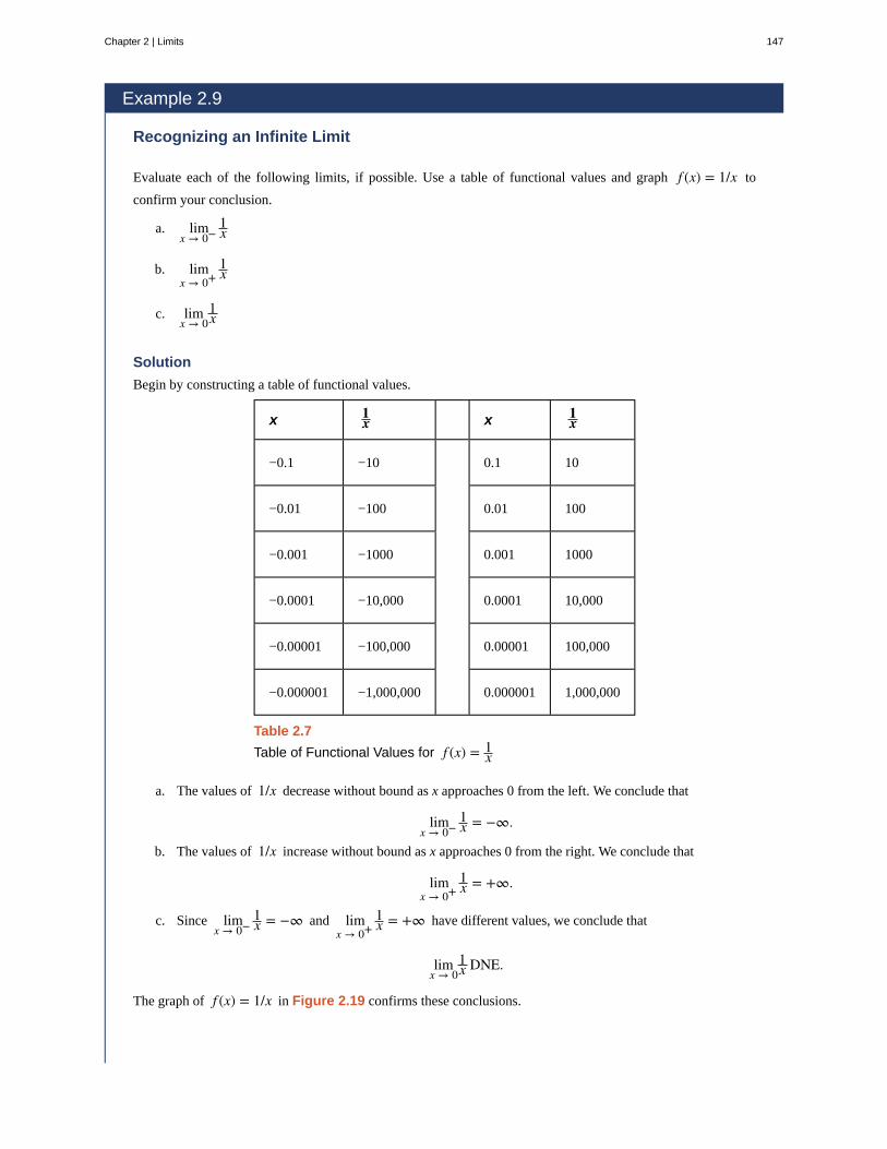
Example 2.9
Recognizing an Infinite Limit
Evaluate each of the following limits, if possible. Use a table of functional values and graph f (x) = 1/x to
confirm your conclusion.
a. limx → 0−
1x
b. limx → 0+
1x
c. limx → 0
1x
Solution
Begin by constructing a table of functional values.
x 1x x 1
x
−0.1 −10 0.1 10
−0.01 −100 0.01 100
−0.001 −1000 0.001 1000
−0.0001 −10,000 0.0001 10,000
−0.00001 −100,000 0.00001 100,000
−0.000001 −1,000,000 0.000001 1,000,000
Table 2.7
Table of Functional Values for f (x) = 1x
a. The values of 1/x decrease without bound as x approaches 0 from the left. We conclude that
limx → 0−
1x = −∞.
b. The values of 1/x increase without bound as x approaches 0 from the right. We conclude that
limx → 0+
1x = +∞.
c. Since limx → 0−
1x = −∞ and lim
x → 0+1x = +∞ have different values, we conclude that
limx → 0
1x DNE.
The graph of f (x) = 1/x in Figure 2.19 confirms these conclusions.
Chapter 2 | Limits 147
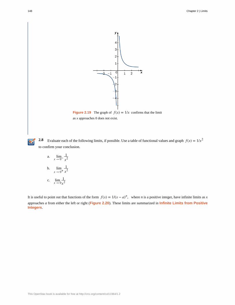
2.8
Figure 2.19 The graph of f (x) = 1/x confirms that the limit
as x approaches 0 does not exist.
Evaluate each of the following limits, if possible. Use a table of functional values and graph f (x) = 1/x2
to confirm your conclusion.
a. limx → 0−
1x2
b. limx → 0+
1x2
c. limx → 0
1x2
It is useful to point out that functions of the form f (x) = 1/(x − a)n, where n is a positive integer, have infinite limits as x
approaches a from either the left or right (Figure 2.20). These limits are summarized in Infinite Limits from PositiveIntegers.
148 Chapter 2 | Limits
This OpenStax book is available for free at http://cnx.org/content/col11964/1.2
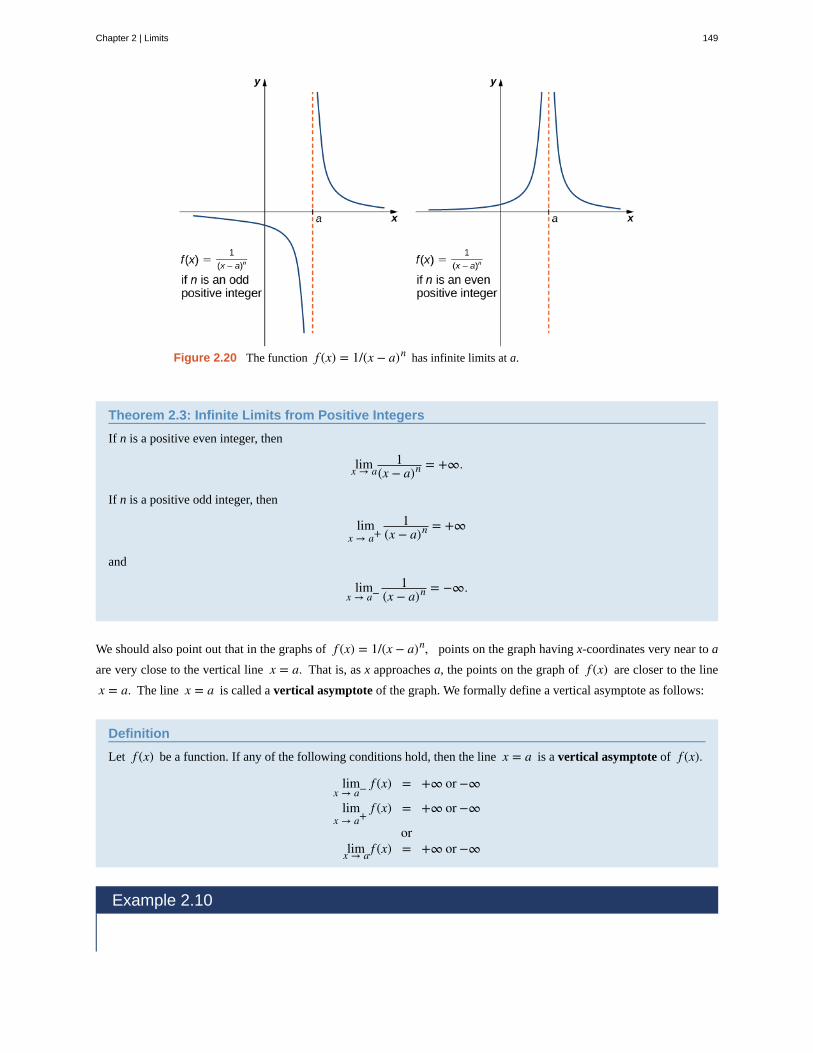
Figure 2.20 The function f (x) = 1/(x − a)n has infinite limits at a.
Theorem 2.3: Infinite Limits from Positive Integers
If n is a positive even integer, then
limx → a1
(x − a)n = +∞.
If n is a positive odd integer, then
limx → a+
1(x − a)n = +∞
and
limx → a−
1(x − a)n = −∞.
We should also point out that in the graphs of f (x) = 1/(x − a)n, points on the graph having x-coordinates very near to a
are very close to the vertical line x = a. That is, as x approaches a, the points on the graph of f (x) are closer to the line
x = a. The line x = a is called a vertical asymptote of the graph. We formally define a vertical asymptote as follows:
Definition
Let f (x) be a function. If any of the following conditions hold, then the line x = a is a vertical asymptote of f (x).
limx → a− f (x) = +∞ or −∞
limx → a+
f (x) = +∞ or −∞
orlimx → a f (x) = +∞ or −∞
Example 2.10
Chapter 2 | Limits 149
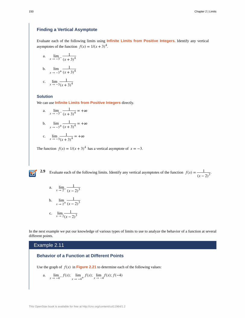
2.9
Finding a Vertical Asymptote
Evaluate each of the following limits using Infinite Limits from Positive Integers. Identify any vertical
asymptotes of the function f (x) = 1/(x + 3)4.
a. limx → −3−
1(x + 3)4
b. limx → −3+
1(x + 3)4
c. limx → −3
1(x + 3)4
Solution
We can use Infinite Limits from Positive Integers directly.
a. limx → −3−
1(x + 3)4 = +∞
b. limx → −3+
1(x + 3)4 = +∞
c. limx → −3
1(x + 3)4 = +∞
The function f (x) = 1/(x + 3)4 has a vertical asymptote of x = −3.
Evaluate each of the following limits. Identify any vertical asymptotes of the function f (x) = 1(x − 2)3.
a. limx → 2−
1(x − 2)3
b. limx → 2+
1(x − 2)3
c. limx → 2
1(x − 2)3
In the next example we put our knowledge of various types of limits to use to analyze the behavior of a function at severaldifferent points.
Example 2.11
Behavior of a Function at Different Points
Use the graph of f (x) in Figure 2.21 to determine each of the following values:
a. limx → −4− f (x); lim
x → −4+f (x); lim
x → −4f (x); f (−4)
150 Chapter 2 | Limits
This OpenStax book is available for free at http://cnx.org/content/col11964/1.2
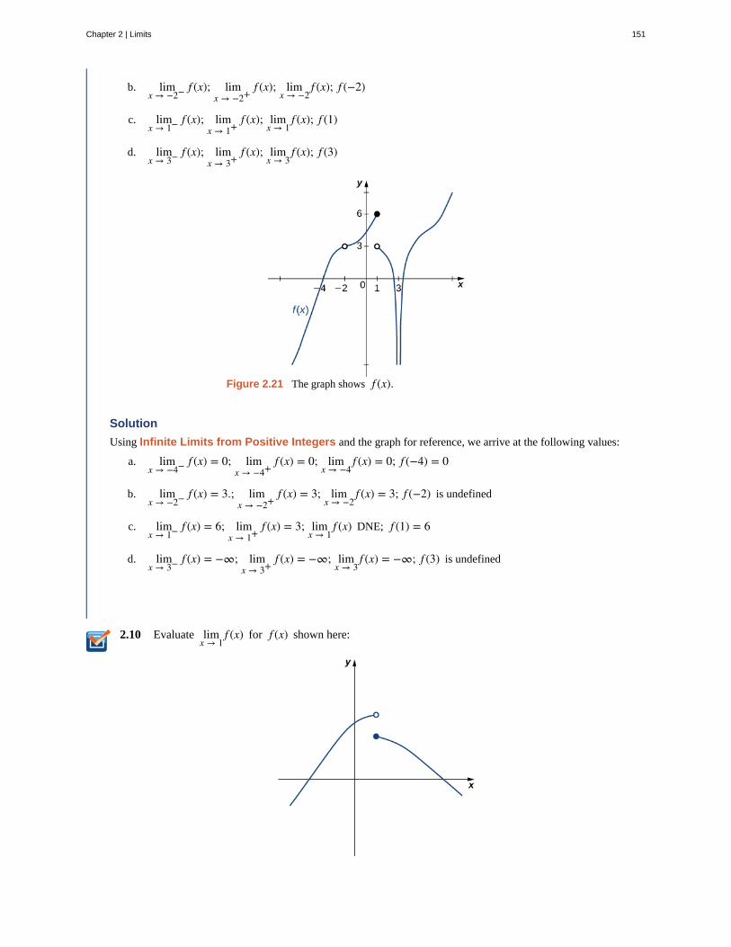
2.10
b. limx → −2− f (x); lim
x → −2+f (x); lim
x → −2f (x); f (−2)
c. limx → 1− f (x); lim
x → 1+f (x); lim
x → 1f (x); f (1)
d. limx → 3− f (x); lim
x → 3+f (x); lim
x → 3f (x); f (3)
Figure 2.21 The graph shows f (x).
Solution
Using Infinite Limits from Positive Integers and the graph for reference, we arrive at the following values:
a. limx → −4− f (x) = 0; lim
x → −4+f (x) = 0; lim
x → −4f (x) = 0; f (−4) = 0
b. limx → −2− f (x) = 3.; lim
x → −2+f (x) = 3; lim
x → −2f (x) = 3; f (−2) is undefined
c. limx → 1− f (x) = 6; lim
x → 1+f (x) = 3; lim
x → 1f (x) DNE; f (1) = 6
d. limx → 3− f (x) = −∞; lim
x → 3+f (x) = −∞; lim
x → 3f (x) = −∞; f (3) is undefined
Evaluate limx → 1
f (x) for f (x) shown here:
Chapter 2 | Limits 151
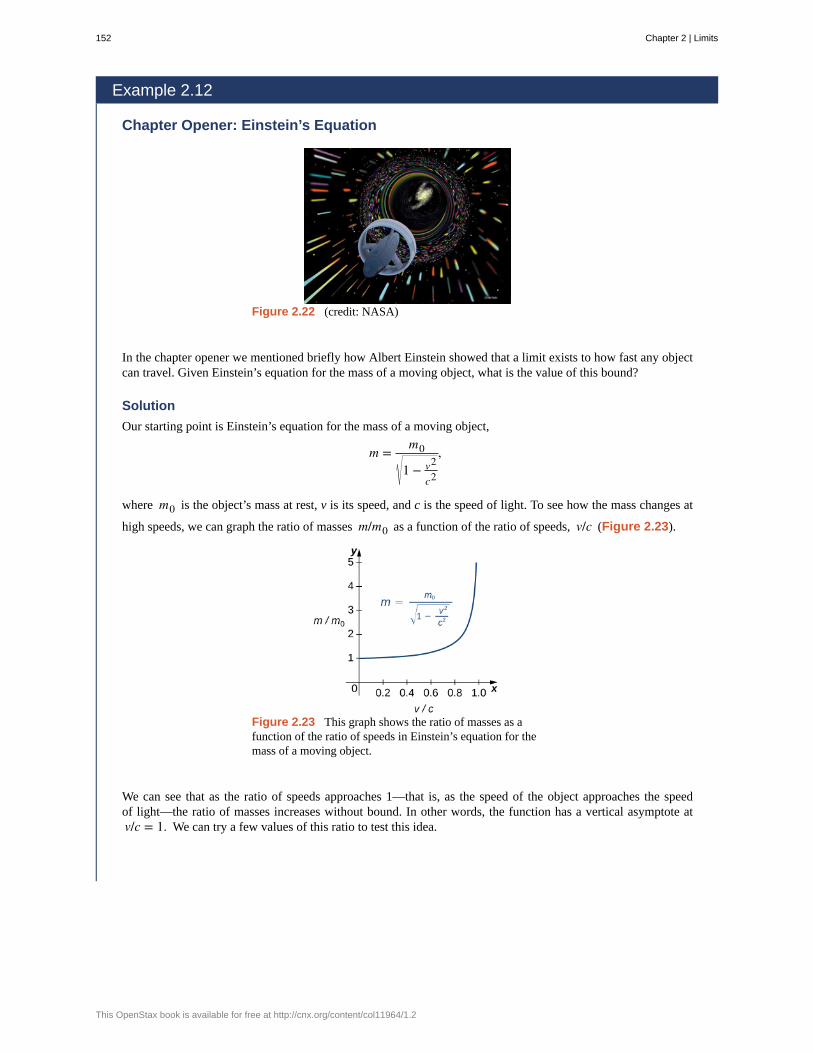
Example 2.12
Chapter Opener: Einstein’s Equation
Figure 2.22 (credit: NASA)
In the chapter opener we mentioned briefly how Albert Einstein showed that a limit exists to how fast any objectcan travel. Given Einstein’s equation for the mass of a moving object, what is the value of this bound?
Solution
Our starting point is Einstein’s equation for the mass of a moving object,
m = m0
1 − v2
c2
,
where m0 is the object’s mass at rest, v is its speed, and c is the speed of light. To see how the mass changes at
high speeds, we can graph the ratio of masses m/m0 as a function of the ratio of speeds, v/c (Figure 2.23).
Figure 2.23 This graph shows the ratio of masses as afunction of the ratio of speeds in Einstein’s equation for themass of a moving object.
We can see that as the ratio of speeds approaches 1—that is, as the speed of the object approaches the speedof light—the ratio of masses increases without bound. In other words, the function has a vertical asymptote atv/c = 1. We can try a few values of this ratio to test this idea.
152 Chapter 2 | Limits
This OpenStax book is available for free at http://cnx.org/content/col11964/1.2
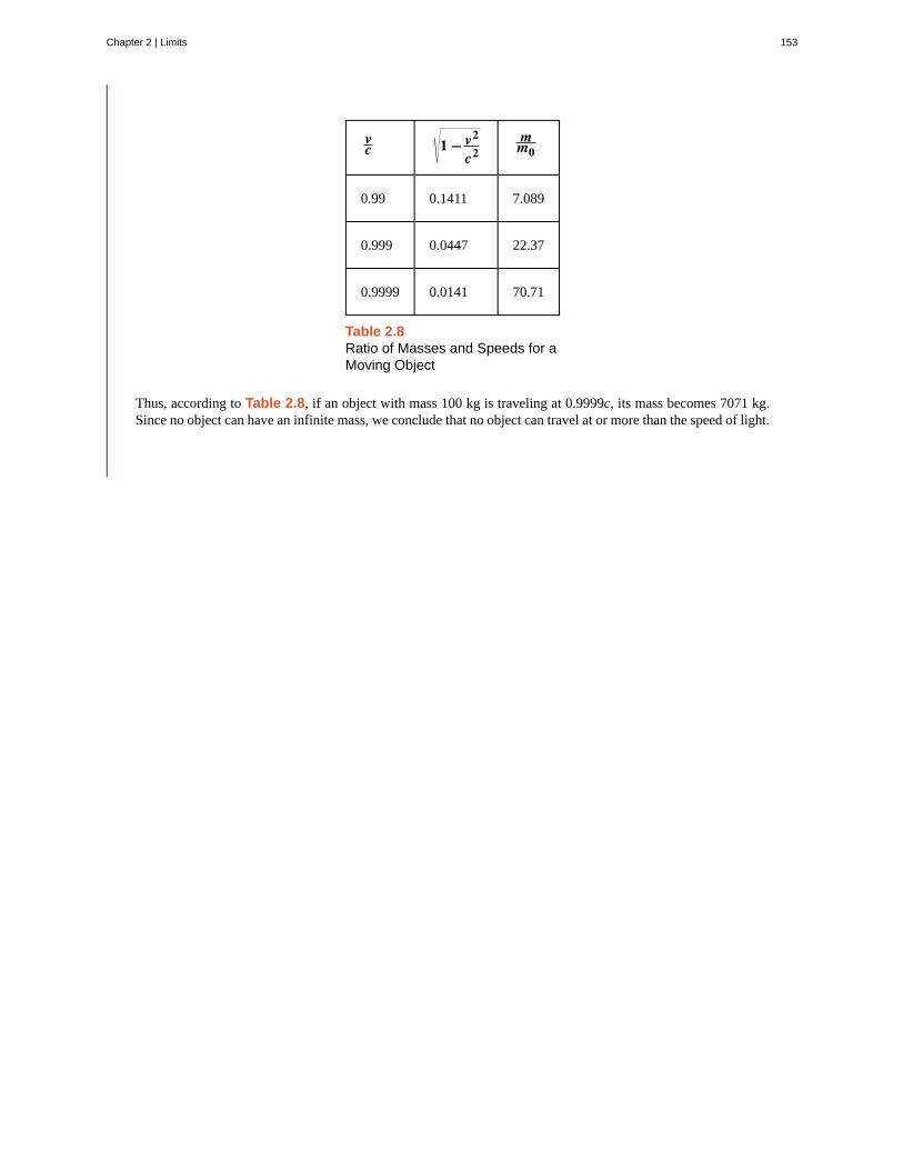
vc 1 − v2
c2mm0
0.99 0.1411 7.089
0.999 0.0447 22.37
0.9999 0.0141 70.71
Table 2.8Ratio of Masses and Speeds for aMoving Object
Thus, according to Table 2.8, if an object with mass 100 kg is traveling at 0.9999c, its mass becomes 7071 kg.Since no object can have an infinite mass, we conclude that no object can travel at or more than the speed of light.
Chapter 2 | Limits 153
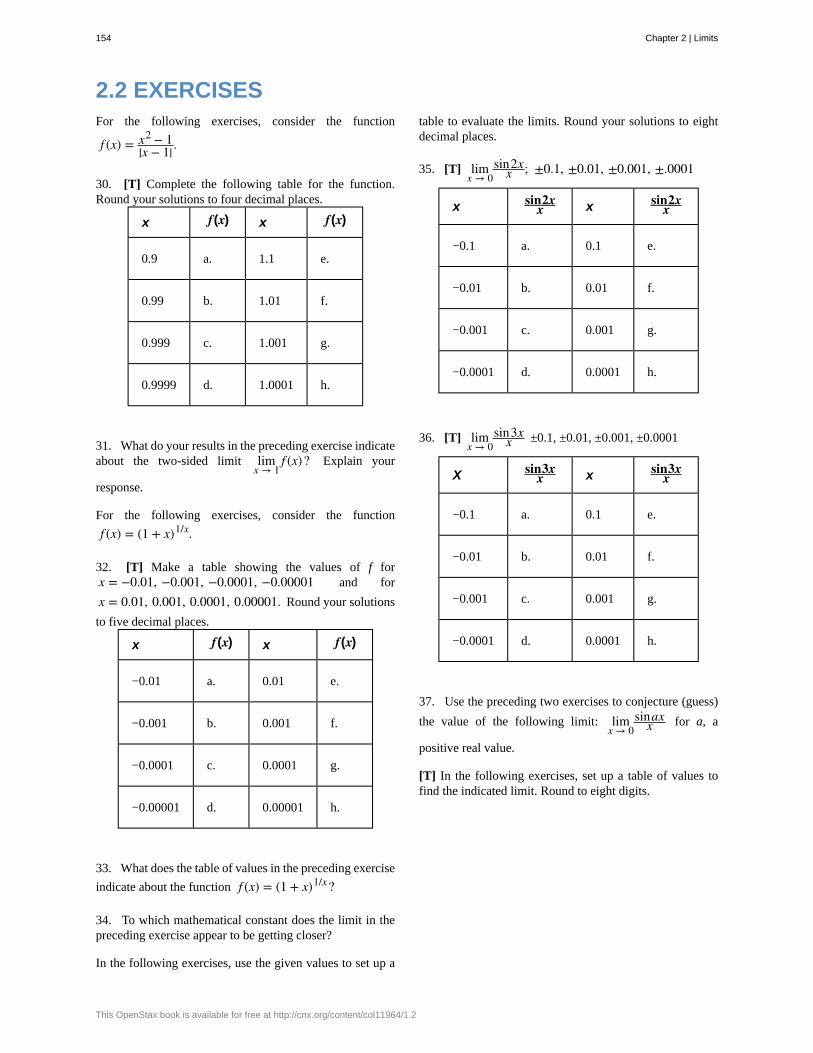
2.2 EXERCISESFor the following exercises, consider the function
f (x) = x2 − 1|x − 1| .
30. [T] Complete the following table for the function.Round your solutions to four decimal places.
x f(x) x f(x)
0.9 a. 1.1 e.
0.99 b. 1.01 f.
0.999 c. 1.001 g.
0.9999 d. 1.0001 h.
31. What do your results in the preceding exercise indicateabout the two-sided limit lim
x → 1f (x)? Explain your
response.
For the following exercises, consider the function
f (x) = (1 + x)1/x.
32. [T] Make a table showing the values of f forx = −0.01, −0.001, −0.0001, −0.00001 and for
x = 0.01, 0.001, 0.0001, 0.00001. Round your solutions
to five decimal places.
x f(x) x f(x)
−0.01 a. 0.01 e.
−0.001 b. 0.001 f.
−0.0001 c. 0.0001 g.
−0.00001 d. 0.00001 h.
33. What does the table of values in the preceding exercise
indicate about the function f (x) = (1 + x)1/x ?
34. To which mathematical constant does the limit in thepreceding exercise appear to be getting closer?
In the following exercises, use the given values to set up a
table to evaluate the limits. Round your solutions to eightdecimal places.
35. [T] limx → 0
sin2xx ; ±0.1, ±0.01, ±0.001, ±.0001
x sin2xx x sin2x
x
−0.1 a. 0.1 e.
−0.01 b. 0.01 f.
−0.001 c. 0.001 g.
−0.0001 d. 0.0001 h.
36. [T] limx → 0
sin3xx ±0.1, ±0.01, ±0.001, ±0.0001
X sin3xx x sin3x
x
−0.1 a. 0.1 e.
−0.01 b. 0.01 f.
−0.001 c. 0.001 g.
−0.0001 d. 0.0001 h.
37. Use the preceding two exercises to conjecture (guess)
the value of the following limit: limx → 0
sinaxx for a, a
positive real value.
[T] In the following exercises, set up a table of values tofind the indicated limit. Round to eight digits.
154 Chapter 2 | Limits
This OpenStax book is available for free at http://cnx.org/content/col11964/1.2
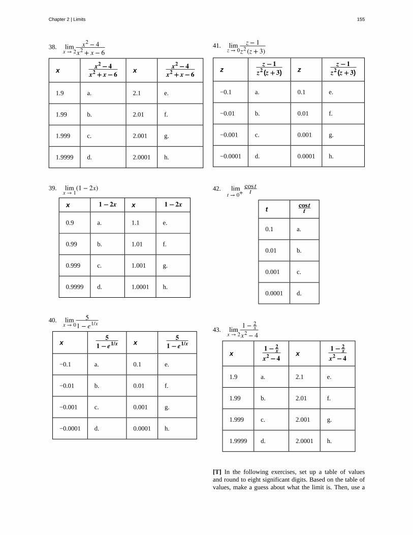
38. limx → 2
x2 − 4x2 + x − 6
xx2 − 4
x2 + x − 6 xx2 − 4
x2 + x − 6
1.9 a. 2.1 e.
1.99 b. 2.01 f.
1.999 c. 2.001 g.
1.9999 d. 2.0001 h.
39. limx → 1
(1 − 2x)
x 1 − 2x x 1 − 2x
0.9 a. 1.1 e.
0.99 b. 1.01 f.
0.999 c. 1.001 g.
0.9999 d. 1.0001 h.
40. limx → 0
51 − e1/x
x5
1 − e1/x x5
1 − e1/x
−0.1 a. 0.1 e.
−0.01 b. 0.01 f.
−0.001 c. 0.001 g.
−0.0001 d. 0.0001 h.
41. limz → 0
z − 1z2 (z + 3)
zz − 1
z2 (z + 3) zz − 1
z2 (z + 3)
−0.1 a. 0.1 e.
−0.01 b. 0.01 f.
−0.001 c. 0.001 g.
−0.0001 d. 0.0001 h.
42. limt → 0+
cos tt
tcos t
t
0.1 a.
0.01 b.
0.001 c.
0.0001 d.
43. limx → 2
1 − 2x
x2 − 4
x1 − 2
xx2 − 4
x1 − 2
xx2 − 4
1.9 a. 2.1 e.
1.99 b. 2.01 f.
1.999 c. 2.001 g.
1.9999 d. 2.0001 h.
[T] In the following exercises, set up a table of valuesand round to eight significant digits. Based on the table ofvalues, make a guess about what the limit is. Then, use a
Chapter 2 | Limits 155
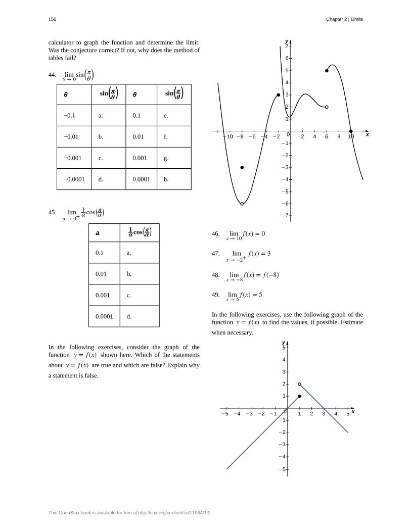
calculator to graph the function and determine the limit.Was the conjecture correct? If not, why does the method oftables fail?
44. limθ → 0
sin⎛⎝πθ
⎞⎠
θ sin⎛⎝πθ⎞⎠ θ sin⎛⎝
πθ⎞⎠
−0.1 a. 0.1 e.
−0.01 b. 0.01 f.
−0.001 c. 0.001 g.
−0.0001 d. 0.0001 h.
45. limα → 0+
1α cos ⎛
⎝πα
⎞⎠
a 1α cos ⎛⎝πα
⎞⎠
0.1 a.
0.01 b.
0.001 c.
0.0001 d.
In the following exercises, consider the graph of thefunction y = f (x) shown here. Which of the statements
about y = f (x) are true and which are false? Explain why
a statement is false.
46. limx → 10
f (x) = 0
47. limx → −2+
f (x) = 3
48. limx → −8
f (x) = f (−8)
49. limx → 6
f (x) = 5
In the following exercises, use the following graph of thefunction y = f (x) to find the values, if possible. Estimate
when necessary.
156 Chapter 2 | Limits
This OpenStax book is available for free at http://cnx.org/content/col11964/1.2
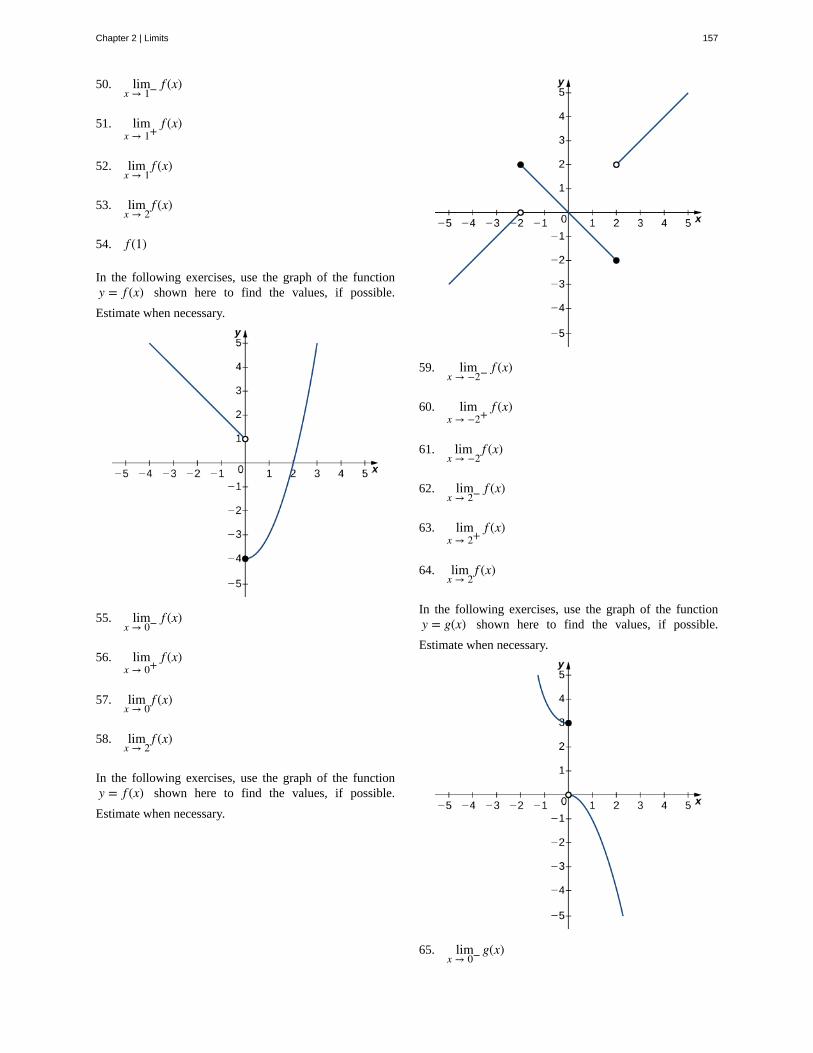
50. limx → 1− f (x)
51. limx → 1+
f (x)
52. limx → 1
f (x)
53. limx → 2
f (x)
54. f (1)
In the following exercises, use the graph of the functiony = f (x) shown here to find the values, if possible.
Estimate when necessary.
55. limx → 0− f (x)
56. limx → 0+
f (x)
57. limx → 0
f (x)
58. limx → 2
f (x)
In the following exercises, use the graph of the functiony = f (x) shown here to find the values, if possible.
Estimate when necessary.
59. limx → −2− f (x)
60. limx → −2+
f (x)
61. limx → −2
f (x)
62. limx → 2− f (x)
63. limx → 2+
f (x)
64. limx → 2
f (x)
In the following exercises, use the graph of the functiony = g(x) shown here to find the values, if possible.
Estimate when necessary.
65. limx → 0− g(x)
Chapter 2 | Limits 157
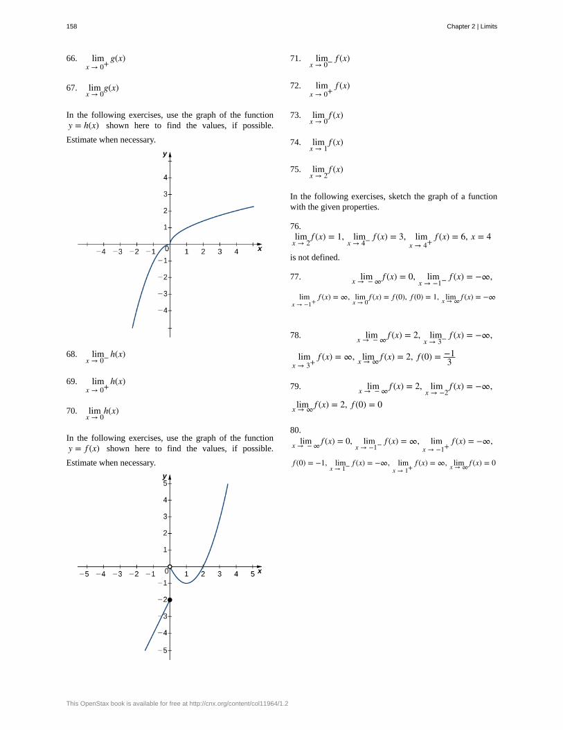
66. limx → 0+
g(x)
67. limx → 0
g(x)
In the following exercises, use the graph of the functiony = h(x) shown here to find the values, if possible.
Estimate when necessary.
68. limx → 0− h(x)
69. limx → 0+
h(x)
70. limx → 0
h(x)
In the following exercises, use the graph of the functiony = f (x) shown here to find the values, if possible.
Estimate when necessary.
71. limx → 0− f (x)
72. limx → 0+
f (x)
73. limx → 0
f (x)
74. limx → 1
f (x)
75. limx → 2
f (x)
In the following exercises, sketch the graph of a functionwith the given properties.
76.lim
x → 2f (x) = 1, lim
x → 4− f (x) = 3, limx → 4+
f (x) = 6, x = 4
is not defined.
77. limx → − ∞ f (x) = 0, limx → −1− f (x) = −∞,
limx → −1+
f (x) = ∞, limx → 0
f (x) = f (0), f (0) = 1, limx → ∞ f (x) = −∞
78. limx → − ∞ f (x) = 2, limx → 3− f (x) = −∞,
limx → 3+
f (x) = ∞, limx → ∞ f (x) = 2, f (0) = −13
79. limx → − ∞ f (x) = 2, limx → −2
f (x) = −∞,
limx → ∞ f (x) = 2, f (0) = 0
80.limx → − ∞ f (x) = 0, lim
x → −1− f (x) = ∞, limx → −1+
f (x) = −∞,
f (0) = −1, limx → 1− f (x) = −∞, lim
x → 1+f (x) = ∞, limx → ∞ f (x) = 0
158 Chapter 2 | Limits
This OpenStax book is available for free at http://cnx.org/content/col11964/1.2
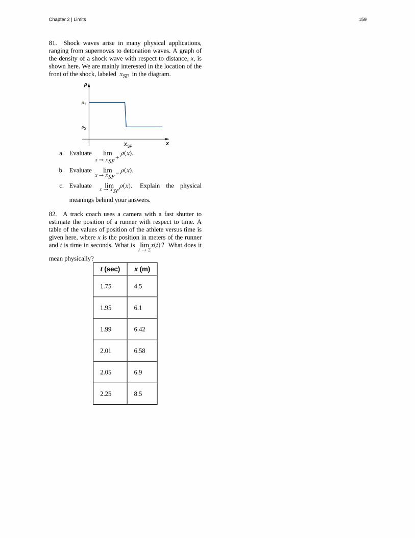
81. Shock waves arise in many physical applications,ranging from supernovas to detonation waves. A graph ofthe density of a shock wave with respect to distance, x, isshown here. We are mainly interested in the location of thefront of the shock, labeled xSF in the diagram.
a. Evaluate limx → xSF
+ρ(x).
b. Evaluate limx → xSF
− ρ(x).
c. Evaluate limx → xSFρ(x). Explain the physical
meanings behind your answers.
82. A track coach uses a camera with a fast shutter toestimate the position of a runner with respect to time. Atable of the values of position of the athlete versus time isgiven here, where x is the position in meters of the runnerand t is time in seconds. What is lim
t → 2x(t)? What does it
mean physically?
t (sec) x (m)
1.75 4.5
1.95 6.1
1.99 6.42
2.01 6.58
2.05 6.9
2.25 8.5
Chapter 2 | Limits 159
2.3 | The Limit Laws
Learning Objectives2.3.1 Recognize the basic limit laws.
2.3.2 Use the limit laws to evaluate the limit of a function.
2.3.3 Evaluate the limit of a function by factoring.
2.3.4 Use the limit laws to evaluate the limit of a polynomial or rational function.
2.3.5 Evaluate the limit of a function by factoring or by using conjugates.
2.3.6 Evaluate the limit of a function by using the squeeze theorem.
In the previous section, we evaluated limits by looking at graphs or by constructing a table of values. In this section, weestablish laws for calculating limits and learn how to apply these laws. In the Student Project at the end of this section, youhave the opportunity to apply these limit laws to derive the formula for the area of a circle by adapting a method devised bythe Greek mathematician Archimedes. We begin by restating two useful limit results from the previous section. These tworesults, together with the limit laws, serve as a foundation for calculating many limits.
Evaluating Limits with the Limit LawsThe first two limit laws were stated in Two Important Limits and we repeat them here. These basic results, together withthe other limit laws, allow us to evaluate limits of many algebraic functions.
Theorem 2.4: Basic Limit Results
For any real number a and any constant c,
i. (2.14)limx → ax = a
ii. (2.15)limx → ac = c
Example 2.13
Evaluating a Basic Limit
Evaluate each of the following limits using Basic Limit Results.
a. limx → 2
x
b. limx → 2
5
Solution
a. The limit of x as x approaches a is a: limx → 2
x = 2.
b. The limit of a constant is that constant: limx → 2
5 = 5.
We now take a look at the limit laws, the individual properties of limits. The proofs that these laws hold are omitted here.
160 Chapter 2 | Limits
This OpenStax book is available for free at http://cnx.org/content/col11964/1.2
Theorem 2.5: Limit Laws
Let f (x) and g(x) be defined for all x ≠ a over some open interval containing a. Assume that L and M are real
numbers such that limx → a f (x) = L and limx → ag(x) = M. Let c be a constant. Then, each of the following statements
holds:
Sum law for limits: limx → a⎛⎝ f (x) + g(x)⎞
⎠ = limx → a f (x) + limx → ag(x) = L + M
Difference law for limits: limx → a⎛⎝ f (x) − g(x)⎞
⎠ = limx → a f (x) − limx → ag(x) = L − M
Constant multiple law for limits: limx → ac f (x) = c · limx → a f (x) = cL
Product law for limits: limx → a⎛⎝ f (x) · g(x)⎞
⎠ = limx → a f (x) · limx → ag(x) = L · M
Quotient law for limits: limx → af (x)g(x) =
limx → a f (x)limx → ag(x) = L
M for M ≠ 0
Power law for limits: limx → a⎛⎝ f (x)⎞
⎠n = ⎛
⎝ limx → a f (x)⎞⎠n
= Ln for every positive integer n.
Root law for limits: limx → a f (x)n = limx → a f (x)n = Lnfor all L if n is odd and for L ≥ 0 if n is even.
We now practice applying these limit laws to evaluate a limit.
Example 2.14
Evaluating a Limit Using Limit Laws
Use the limit laws to evaluate limx → −3
(4x + 2).
Solution
Let’s apply the limit laws one step at a time to be sure we understand how they work. We need to keep in mindthe requirement that, at each application of a limit law, the new limits must exist for the limit law to be applied.
limx → −3
(4x + 2) = limx → −3
4x + limx → −3
2 Apply the sum law.
= 4 · limx → −3
x + limx → −3
2 Apply the constant multiple law.
= 4 · (−3) + 2 = −10. Apply the basic limit results and simplify.
Example 2.15
Using Limit Laws Repeatedly
Use the limit laws to evaluate limx → 2
2x2 − 3x + 1x3 + 4
.
Solution
Chapter 2 | Limits 161
2.11
To find this limit, we need to apply the limit laws several times. Again, we need to keep in mind that as we rewritethe limit in terms of other limits, each new limit must exist for the limit law to be applied.
limx → 2
2x2 − 3x + 1x3 + 4
=lim
x → 2⎛⎝2x2 − 3x + 1⎞
⎠
limx → 2
⎛⎝x
3 + 4⎞⎠
Apply the quotient law, making sure that. (2)3 + 4 ≠ 0
=2 · lim
x → 2x2 − 3 · lim
x → 2x + lim
x → 21
limx → 2
x3 + limx → 2
4Apply the sum law and constant multiple law.
=2 · ⎛
⎝ limx → 2
x⎞⎠
2− 3 · lim
x → 2x + lim
x → 21
⎛⎝ limx → 2
x⎞⎠
3+ lim
x → 24
Apply the power law.
= 2(4) − 3(2) + 1(2)3 + 4
= 14. Apply the basic limit laws and simplify.
Use the limit laws to evaluate limx → 6
(2x − 1) x + 4. In each step, indicate the limit law applied.
Limits of Polynomial and Rational FunctionsBy now you have probably noticed that, in each of the previous examples, it has been the case that limx → a f (x) = f (a). This
is not always true, but it does hold for all polynomials for any choice of a and for all rational functions at all values of a forwhich the rational function is defined.
Theorem 2.6: Limits of Polynomial and Rational Functions
Let p(x) and q(x) be polynomial functions. Let a be a real number. Then,
limx → ap(x) = p(a)
limx → ap(x)q(x) = p(a)
q(a) when q(a) ≠ 0.
To see that this theorem holds, consider the polynomial p(x) = cn xn + cn − 1 xn − 1 + ⋯ + c1 x + c0. By applying the
sum, constant multiple, and power laws, we end up with
limx → ap(x) = limx → a⎛⎝cn xn + cn − 1 xn − 1 + ⋯ + c1 x + c0
⎞⎠
= cn⎛⎝ limx → ax⎞
⎠n
+ cn − 1⎛⎝ limx → ax⎞
⎠n − 1
+ ⋯ + c1⎛⎝ limx → ax⎞
⎠ + limx → ac0
= cn an + cn − 1 an − 1 + ⋯ + c1 a + c0= p(a).
It now follows from the quotient law that if p(x) and q(x) are polynomials for which q(a) ≠ 0, then
limx → ap(x)q(x) = p(a)
q(a) .
Example 2.16 applies this result.
162 Chapter 2 | Limits
This OpenStax book is available for free at http://cnx.org/content/col11964/1.2
2.12
Example 2.16
Evaluating a Limit of a Rational Function
Evaluate the limx → 3
2x2 − 3x + 15x + 4 .
Solution
Since 3 is in the domain of the rational function f (x) = 2x2 − 3x + 15x + 4 , we can calculate the limit by substituting
3 for x into the function. Thus,
limx → 3
2x2 − 3x + 15x + 4 = 10
19.
Evaluate limx → −2
⎛⎝3x3 − 2x + 7⎞
⎠.
Additional Limit Evaluation TechniquesAs we have seen, we may evaluate easily the limits of polynomials and limits of some (but not all) rational functions bydirect substitution. However, as we saw in the introductory section on limits, it is certainly possible for limx → a f (x) to exist
when f (a) is undefined. The following observation allows us to evaluate many limits of this type:
If for all x ≠ a, f (x) = g(x) over some open interval containing a, then limx → a f (x) = limx → ag(x).
To understand this idea better, consider the limit limx → 1
x2 − 1x − 1 .
The function
f (x) = x2 − 1x − 1
= (x − 1)(x + 1)x − 1
and the function g(x) = x + 1 are identical for all values of x ≠ 1. The graphs of these two functions are shown in Figure
2.24.
Chapter 2 | Limits 163
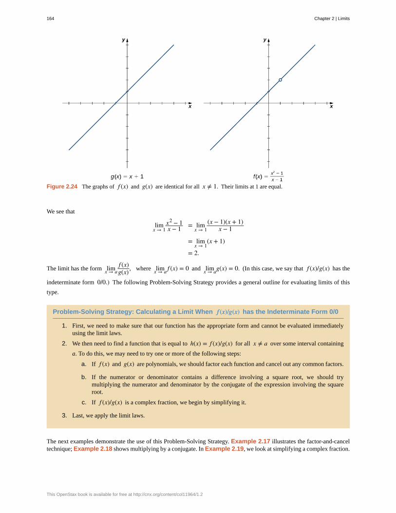
Figure 2.24 The graphs of f (x) and g(x) are identical for all x ≠ 1. Their limits at 1 are equal.
We see that
limx → 1
x2 − 1x − 1 = lim
x → 1(x − 1)(x + 1)
x − 1
= limx → 1
(x + 1)
= 2.
The limit has the form limx → af (x)g(x) , where limx → a f (x) = 0 and limx → ag(x) = 0. (In this case, we say that f (x)/g(x) has the
indeterminate form 0/0.) The following Problem-Solving Strategy provides a general outline for evaluating limits of this
type.
Problem-Solving Strategy: Calculating a Limit When f(x)/g(x) has the Indeterminate Form 0/0
1. First, we need to make sure that our function has the appropriate form and cannot be evaluated immediatelyusing the limit laws.
2. We then need to find a function that is equal to h(x) = f (x)/g(x) for all x ≠ a over some interval containing
a. To do this, we may need to try one or more of the following steps:
a. If f (x) and g(x) are polynomials, we should factor each function and cancel out any common factors.
b. If the numerator or denominator contains a difference involving a square root, we should trymultiplying the numerator and denominator by the conjugate of the expression involving the squareroot.
c. If f (x)/g(x) is a complex fraction, we begin by simplifying it.
3. Last, we apply the limit laws.
The next examples demonstrate the use of this Problem-Solving Strategy. Example 2.17 illustrates the factor-and-canceltechnique; Example 2.18 shows multiplying by a conjugate. In Example 2.19, we look at simplifying a complex fraction.
164 Chapter 2 | Limits
This OpenStax book is available for free at http://cnx.org/content/col11964/1.2
2.13
Example 2.17
Evaluating a Limit by Factoring and Canceling
Evaluate limx → 3
x2 − 3x2x2 − 5x − 3
.
Solution
Step 1. The function f (x) = x2 − 3x2x2 − 5x − 3
is undefined for x = 3. In fact, if we substitute 3 into the function
we get 0/0, which is undefined. Factoring and canceling is a good strategy:
limx → 3
x2 − 3x2x2 − 5x − 3
= limx → 3
x(x − 3)(x − 3)(2x + 1)
Step 2. For all x ≠ 3, x2 − 3x2x2 − 5x − 3
= x2x + 1. Therefore,
limx → 3
x(x − 3)(x − 3)(2x + 1) = lim
x → 3x
2x + 1.
Step 3. Evaluate using the limit laws:
limx → 3
x2x + 1 = 3
7.
Evaluate limx → −3
x2 + 4x + 3x2 − 9
.
Example 2.18
Evaluating a Limit by Multiplying by a Conjugate
Evaluate limx → −1
x + 2 − 1x + 1 .
Solution
Step 1. x + 2 − 1x + 1 has the form 0/0 at −1. Let’s begin by multiplying by x + 2 + 1, the conjugate of
x + 2 − 1, on the numerator and denominator:
limx → −1
x + 2 − 1x + 1 = lim
x → −1x + 2 − 1
x + 1 · x + 2 + 1x + 2 + 1
.
Step 2. We then multiply out the numerator. We don’t multiply out the denominator because we are hoping thatthe (x + 1) in the denominator cancels out in the end:
= limx → −1
x + 1(x + 1)⎛
⎝ x + 2 + 1⎞⎠.
Chapter 2 | Limits 165
2.14
Step 3. Then we cancel:
= limx → −1
1x + 2 + 1
.
Step 4. Last, we apply the limit laws:
limx → −1
1x + 2 + 1
= 12.
Evaluate limx → 5
x − 1 − 2x − 5 .
Example 2.19
Evaluating a Limit by Simplifying a Complex Fraction
Evaluate limx → 1
1x + 1 − 1
2x − 1 .
Solution
Step 1.1
x + 1 − 12
x − 1 has the form 0/0 at 1. We simplify the algebraic fraction by multiplying by
2(x + 1)/2(x + 1) :
limx → 1
1x + 1 − 1
2x − 1 = lim
x → 1
1x + 1 − 1
2x − 1 · 2(x + 1)
2(x + 1).
Step 2. Next, we multiply through the numerators. Do not multiply the denominators because we want to be ableto cancel the factor (x − 1):
= limx → 1
2 − (x + 1)2(x − 1)(x + 1).
Step 3. Then, we simplify the numerator:
= limx → 1
−x + 12(x − 1)(x + 1).
Step 4. Now we factor out −1 from the numerator:
= limx → 1
−(x − 1)2(x − 1)(x + 1).
Step 5. Then, we cancel the common factors of (x − 1):
= limx → 1
−12(x + 1).
Step 6. Last, we evaluate using the limit laws:
limx → 1
−12(x + 1) = − 1
4.
166 Chapter 2 | Limits
This OpenStax book is available for free at http://cnx.org/content/col11964/1.2
2.15
2.16
Evaluate limx → −3
1x + 2 + 1
x + 3 .
Example 2.20 does not fall neatly into any of the patterns established in the previous examples. However, with a littlecreativity, we can still use these same techniques.
Example 2.20
Evaluating a Limit When the Limit Laws Do Not Apply
Evaluate limx → 0
⎛⎝1x + 5
x(x − 5)⎞⎠.
Solution
Both 1/x and 5/x(x − 5) fail to have a limit at zero. Since neither of the two functions has a limit at zero, we
cannot apply the sum law for limits; we must use a different strategy. In this case, we find the limit by performingaddition and then applying one of our previous strategies. Observe that
1x + 5
x(x − 5) = x − 5 + 5x(x − 5)
= xx(x − 5).
Thus,
limx → 0
⎛⎝1x + 5
x(x − 5)⎞⎠ = lim
x → 0x
x(x − 5)
= limx → 0
1x − 5
= − 15.
Evaluate limx → 3
⎛⎝
1x − 3 − 4
x2 − 2x − 3⎞⎠.
Let’s now revisit one-sided limits. Simple modifications in the limit laws allow us to apply them to one-sided limits. Forexample, to apply the limit laws to a limit of the form lim
x → a− h(x), we require the function h(x) to be defined over an
open interval of the form (b, a); for a limit of the form limx → a+
h(x), we require the function h(x) to be defined over an
open interval of the form (a, c). Example 2.21 illustrates this point.
Example 2.21
Evaluating a One-Sided Limit Using the Limit Laws
Evaluate each of the following limits, if possible.
a. limx → 3− x − 3
Chapter 2 | Limits 167
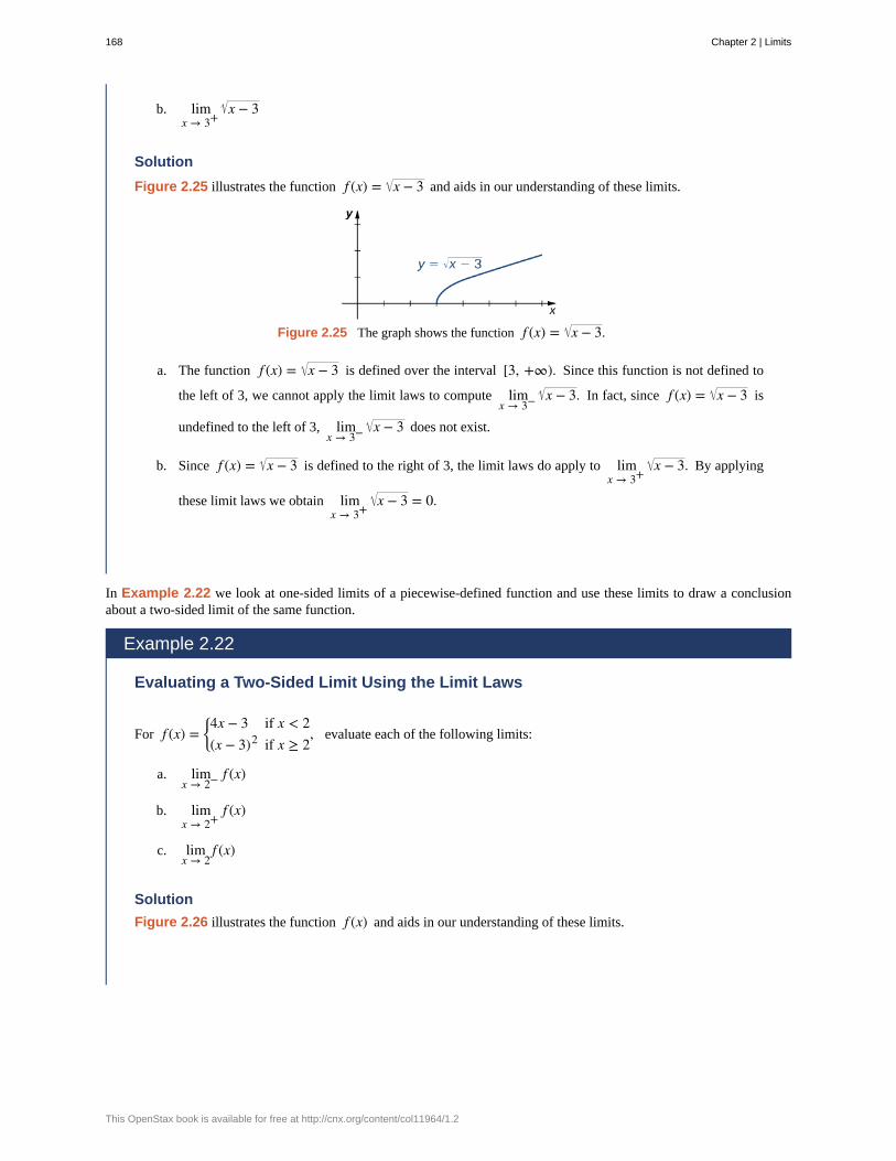
b. limx → 3+
x − 3
Solution
Figure 2.25 illustrates the function f (x) = x − 3 and aids in our understanding of these limits.
Figure 2.25 The graph shows the function f (x) = x − 3.
a. The function f (x) = x − 3 is defined over the interval [3, +∞). Since this function is not defined to
the left of 3, we cannot apply the limit laws to compute limx → 3− x − 3. In fact, since f (x) = x − 3 is
undefined to the left of 3, limx → 3− x − 3 does not exist.
b. Since f (x) = x − 3 is defined to the right of 3, the limit laws do apply to limx → 3+
x − 3. By applying
these limit laws we obtain limx → 3+
x − 3 = 0.
In Example 2.22 we look at one-sided limits of a piecewise-defined function and use these limits to draw a conclusionabout a two-sided limit of the same function.
Example 2.22
Evaluating a Two-Sided Limit Using the Limit Laws
For f (x) =⎧
⎩⎨4x − 3 if x < 2(x − 3)2 if x ≥ 2
, evaluate each of the following limits:
a. limx → 2− f (x)
b. limx → 2+
f (x)
c. limx → 2
f (x)
Solution
Figure 2.26 illustrates the function f (x) and aids in our understanding of these limits.
168 Chapter 2 | Limits
This OpenStax book is available for free at http://cnx.org/content/col11964/1.2
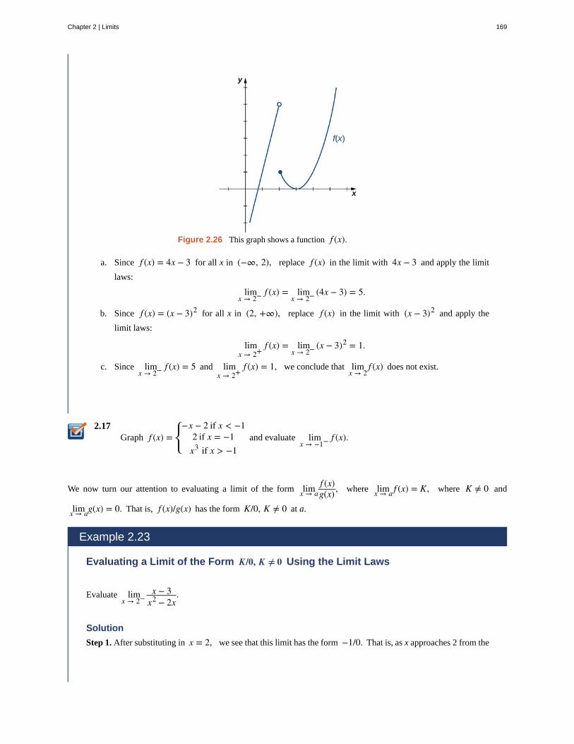
2.17
Figure 2.26 This graph shows a function f (x).
a. Since f (x) = 4x − 3 for all x in (−∞, 2), replace f (x) in the limit with 4x − 3 and apply the limit
laws:
limx → 2− f (x) = lim
x → 2− (4x − 3) = 5.
b. Since f (x) = (x − 3)2 for all x in (2, +∞), replace f (x) in the limit with (x − 3)2 and apply the
limit laws:
limx → 2+
f (x) = limx → 2− (x − 3)2 = 1.
c. Since limx → 2− f (x) = 5 and lim
x → 2+f (x) = 1, we conclude that lim
x → 2f (x) does not exist.
Graph f (x) =⎧
⎩⎨
−x − 2 if x < −12 if x = −1
x3 if x > −1and evaluate lim
x → −1− f (x).
We now turn our attention to evaluating a limit of the form limx → af (x)g(x) , where limx → a f (x) = K, where K ≠ 0 and
limx → ag(x) = 0. That is, f (x)/g(x) has the form K/0, K ≠ 0 at a.
Example 2.23
Evaluating a Limit of the Form K/0, K ≠ 0 Using the Limit Laws
Evaluate limx → 2−
x − 3x2 − 2x
.
Solution
Step 1. After substituting in x = 2, we see that this limit has the form −1/0. That is, as x approaches 2 from the
Chapter 2 | Limits 169
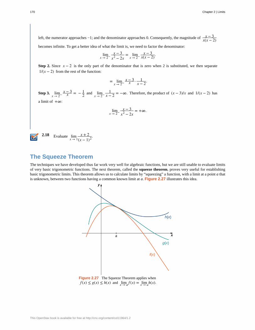
2.18
left, the numerator approaches −1; and the denominator approaches 0. Consequently, the magnitude of x − 3x(x − 2)
becomes infinite. To get a better idea of what the limit is, we need to factor the denominator:
limx → 2−
x − 3x2 − 2x
= limx → 2−
x − 3x(x − 2).
Step 2. Since x − 2 is the only part of the denominator that is zero when 2 is substituted, we then separate
1/(x − 2) from the rest of the function:
= limx → 2−
x − 3x · 1
x − 2.
Step 3. limx → 2−
x − 3x = − 1
2 and limx → 2−
1x − 2 = −∞. Therefore, the product of (x − 3)/x and 1/(x − 2) has
a limit of +∞:
limx → 2−
x − 3x2 − 2x
= +∞.
Evaluate limx → 1
x + 2(x − 1)2.
The Squeeze TheoremThe techniques we have developed thus far work very well for algebraic functions, but we are still unable to evaluate limitsof very basic trigonometric functions. The next theorem, called the squeeze theorem, proves very useful for establishingbasic trigonometric limits. This theorem allows us to calculate limits by “squeezing” a function, with a limit at a point a thatis unknown, between two functions having a common known limit at a. Figure 2.27 illustrates this idea.
Figure 2.27 The Squeeze Theorem applies whenf (x) ≤ g(x) ≤ h(x) and limx → a f (x) = limx → ah(x).
170 Chapter 2 | Limits
This OpenStax book is available for free at http://cnx.org/content/col11964/1.2
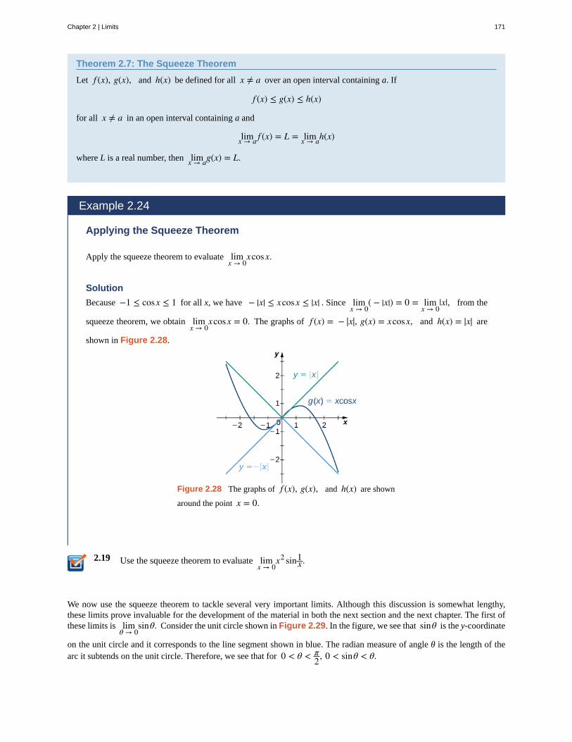
2.19
Theorem 2.7: The Squeeze Theorem
Let f (x), g(x), and h(x) be defined for all x ≠ a over an open interval containing a. If
f (x) ≤ g(x) ≤ h(x)
for all x ≠ a in an open interval containing a and
limx → a f (x) = L = limx → ah(x)
where L is a real number, then limx → ag(x) = L.
Example 2.24
Applying the Squeeze Theorem
Apply the squeeze theorem to evaluate limx → 0
xcosx.
Solution
Because −1 ≤ cosx ≤ 1 for all x, we have − |x| ≤ xcosx ≤ |x| . Since limx → 0
( − |x|) = 0 = limx → 0
|x|, from the
squeeze theorem, we obtain limx → 0
xcosx = 0. The graphs of f (x) = − |x|, g(x) = xcosx, and h(x) = |x| are
shown in Figure 2.28.
Figure 2.28 The graphs of f (x), g(x), and h(x) are shown
around the point x = 0.
Use the squeeze theorem to evaluate limx → 0
x2 sin1x .
We now use the squeeze theorem to tackle several very important limits. Although this discussion is somewhat lengthy,these limits prove invaluable for the development of the material in both the next section and the next chapter. The first ofthese limits is lim
θ → 0sinθ. Consider the unit circle shown in Figure 2.29. In the figure, we see that sinθ is the y-coordinate
on the unit circle and it corresponds to the line segment shown in blue. The radian measure of angle θ is the length of thearc it subtends on the unit circle. Therefore, we see that for 0 < θ < π
2, 0 < sinθ < θ.
Chapter 2 | Limits 171
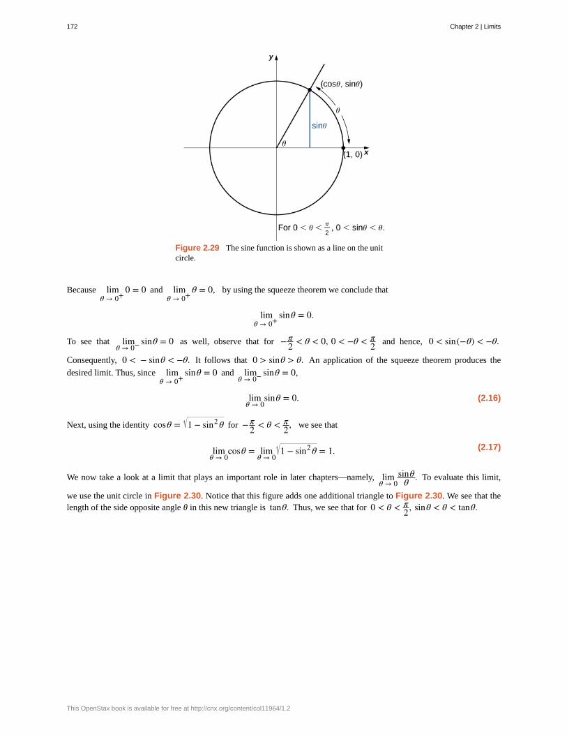
Figure 2.29 The sine function is shown as a line on the unitcircle.
Because limθ → 0+
0 = 0 and limθ → 0+
θ = 0, by using the squeeze theorem we conclude that
limθ → 0+
sinθ = 0.
To see that limθ → 0− sinθ = 0 as well, observe that for −π
2 < θ < 0, 0 < −θ < π2 and hence, 0 < sin(−θ) < −θ.
Consequently, 0 < − sinθ < −θ. It follows that 0 > sinθ > θ. An application of the squeeze theorem produces the
desired limit. Thus, since limθ → 0+
sinθ = 0 and limθ → 0− sinθ = 0,
(2.16)limθ → 0
sinθ = 0.
Next, using the identity cosθ = 1 − sin2 θ for −π2 < θ < π
2, we see that
(2.17)limθ → 0
cosθ = limθ → 0
1 − sin2 θ = 1.
We now take a look at a limit that plays an important role in later chapters—namely, limθ → 0
sinθθ . To evaluate this limit,
we use the unit circle in Figure 2.30. Notice that this figure adds one additional triangle to Figure 2.30. We see that thelength of the side opposite angle θ in this new triangle is tanθ. Thus, we see that for 0 < θ < π
2, sinθ < θ < tanθ.
172 Chapter 2 | Limits
This OpenStax book is available for free at http://cnx.org/content/col11964/1.2
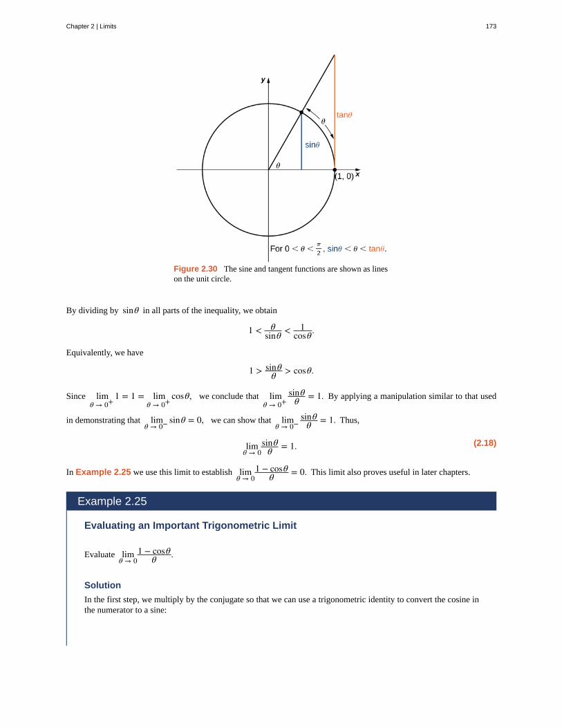
Figure 2.30 The sine and tangent functions are shown as lineson the unit circle.
By dividing by sinθ in all parts of the inequality, we obtain
1 < θsinθ < 1
cosθ .
Equivalently, we have
1 > sinθθ > cosθ.
Since limθ → 0+
1 = 1 = limθ → 0+
cosθ, we conclude that limθ → 0+
sinθθ = 1. By applying a manipulation similar to that used
in demonstrating that limθ → 0− sinθ = 0, we can show that lim
θ → 0−sinθ
θ = 1. Thus,
(2.18)limθ → 0
sinθθ = 1.
In Example 2.25 we use this limit to establish limθ → 0
1 − cosθθ = 0. This limit also proves useful in later chapters.
Example 2.25
Evaluating an Important Trigonometric Limit
Evaluate limθ → 0
1 − cosθθ .
Solution
In the first step, we multiply by the conjugate so that we can use a trigonometric identity to convert the cosine inthe numerator to a sine:
Chapter 2 | Limits 173
(2.19)
2.20
limθ → 0
1 − cosθθ = lim
θ → 01 − cosθ
θ · 1 + cosθ1 + cosθ
= limθ → 0
1 − cos2 θθ(1 + cosθ)
= limθ → 0
sin2 θθ(1 + cosθ)
= limθ → 0
sinθθ · sinθ
1 + cosθ= 1 · 0
2 = 0.
Therefore,
limθ → 0
1 − cosθθ = 0.
Evaluate limθ → 0
1 − cosθsinθ .
174 Chapter 2 | Limits
This OpenStax book is available for free at http://cnx.org/content/col11964/1.2
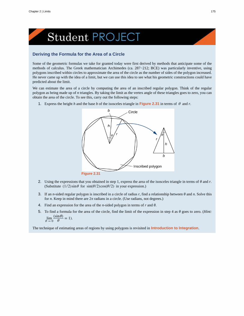
Deriving the Formula for the Area of a Circle
Some of the geometric formulas we take for granted today were first derived by methods that anticipate some of themethods of calculus. The Greek mathematician Archimedes (ca. 287−212; BCE) was particularly inventive, usingpolygons inscribed within circles to approximate the area of the circle as the number of sides of the polygon increased.He never came up with the idea of a limit, but we can use this idea to see what his geometric constructions could havepredicted about the limit.
We can estimate the area of a circle by computing the area of an inscribed regular polygon. Think of the regularpolygon as being made up of n triangles. By taking the limit as the vertex angle of these triangles goes to zero, you canobtain the area of the circle. To see this, carry out the following steps:
1. Express the height h and the base b of the isosceles triangle in Figure 2.31 in terms of θ and r.
Figure 2.31
2. Using the expressions that you obtained in step 1, express the area of the isosceles triangle in terms of θ and r.(Substitute (1 /2)sinθ for sin(θ /2)cos(θ /2) in your expression.)
3. If an n-sided regular polygon is inscribed in a circle of radius r, find a relationship between θ and n. Solve thisfor n. Keep in mind there are 2π radians in a circle. (Use radians, not degrees.)
4. Find an expression for the area of the n-sided polygon in terms of r and θ.
5. To find a formula for the area of the circle, find the limit of the expression in step 4 as θ goes to zero. (Hint:
limθ → 0
(sinθ)θ = 1).
The technique of estimating areas of regions by using polygons is revisited in Introduction to Integration.
Chapter 2 | Limits 175
2.3 EXERCISESIn the following exercises, use the limit laws to evaluateeach limit. Justify each step by indicating the appropriatelimit law(s).
83. limx → 0
⎛⎝4x2 − 2x + 3⎞
⎠
84. limx → 1
x3 + 3x2 + 54 − 7x
85. limx → −2
x2 − 6x + 3
86. limx → −1
(9x + 1)2
In the following exercises, use direct substitution toevaluate each limit.
87. limx → 7
x2
88. limx → −2
⎛⎝4x2 − 1⎞
⎠
89. limx → 0
11 + sinx
90. limx → 2
e2x − x2
91. limx → 1
2 − 7xx + 6
92. limx → 3
lne3x
In the following exercises, use direct substitution to showthat each limit leads to the indeterminate form 0/0. Then,
evaluate the limit.
93. limx → 4
x2 − 16x − 4
94. limx → 2
x − 2x2 − 2x
95. limx → 6
3x − 182x − 12
96. limh → 0
(1 + h)2 − 1h
97. limt → 9
t − 9t − 3
98. limh → 0
1a + h − 1
ah , where a is a real-valued constant
99. limθ → π
sinθtanθ
100. limx → 1
x3 − 1x2 − 1
101. limx → 1/2
2x2 + 3x − 22x − 1
102. limx → −3
x + 4 − 1x + 3
In the following exercises, use direct substitution to obtainan undefined expression. Then, use the method ofExample 2.23 to simplify the function to help determinethe limit.
103. limx → −2−
2x2 + 7x − 4x2 + x − 2
104. limx → −2+
2x2 + 7x − 4x2 + x − 2
105. limx → 1−
2x2 + 7x − 4x2 + x − 2
106. limx → 1+
2x2 + 7x − 4x2 + x − 2
In the following exercises, assume thatlim
x → 6f (x) = 4, lim
x → 6g(x) = 9, and lim
x → 6h(x) = 6. Use
these three facts and the limit laws to evaluate each limit.
107. limx → 6
2 f (x)g(x)
108. limx → 6
g(x) − 1f (x)
109. limx → 6
⎛⎝ f (x) + 1
3g(x)⎞⎠
110. limx → 6
⎛⎝h(x)⎞
⎠3
2
111. limx → 6
g(x) − f (x)
112. limx → 6
x · h(x)
176 Chapter 2 | Limits
This OpenStax book is available for free at http://cnx.org/content/col11964/1.2
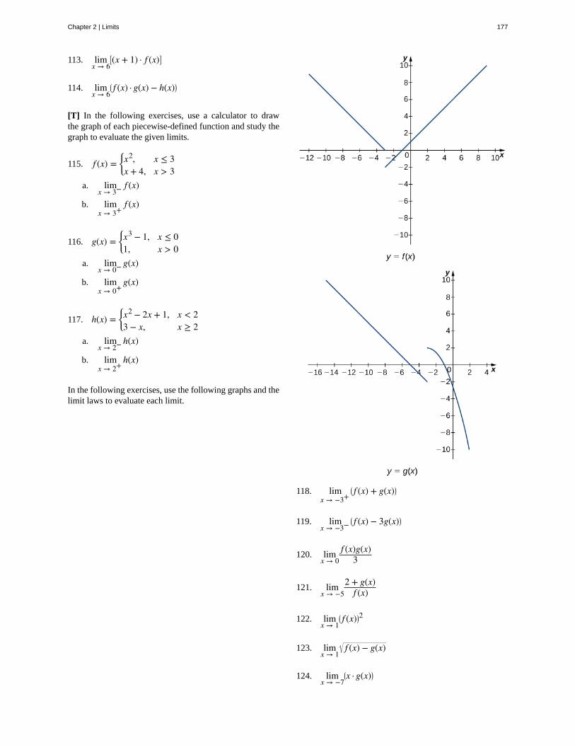
113. limx → 6
⎡⎣(x + 1) · f (x)⎤
⎦
114. limx → 6
⎛⎝ f (x) · g(x) − h(x)⎞
⎠
[T] In the following exercises, use a calculator to drawthe graph of each piecewise-defined function and study thegraph to evaluate the given limits.
115. f (x) =⎧
⎩⎨x2, x ≤ 3
x + 4, x > 3a. lim
x → 3− f (x)
b. limx → 3+
f (x)
116. g(x) =⎧
⎩⎨x3 − 1, x ≤ 01, x > 0
a. limx → 0− g(x)
b. limx → 0+
g(x)
117. h(x) =⎧
⎩⎨x2 − 2x + 1, x < 23 − x, x ≥ 2
a. limx → 2− h(x)
b. limx → 2+
h(x)
In the following exercises, use the following graphs and thelimit laws to evaluate each limit.
118. limx → −3+
⎛⎝ f (x) + g(x)⎞
⎠
119. limx → −3−
⎛⎝ f (x) − 3g(x)⎞
⎠
120. limx → 0
f (x)g(x)3
121. limx → −5
2 + g(x)f (x)
122. limx → 1
⎛⎝ f (x)⎞
⎠2
123. limx → 1
f (x) − g(x)
124. limx → −7
⎛⎝x · g(x)⎞
⎠
Chapter 2 | Limits 177
125. limx → −9
⎡⎣x · f (x) + 2 · g(x)⎤
⎦
For the following problems, evaluate the limit using thesqueeze theorem. Use a calculator to graph the functionsf (x), g(x), and h(x) when possible.
126. [T] True or False? If
2x − 1 ≤ g(x) ≤ x2 − 2x + 3, then limx → 2
g(x) = 0.
127. [T] limθ → 0
θ2 cos⎛⎝1θ
⎞⎠
128. limx → 0
f (x), where f (x) =⎧
⎩⎨0, x rationalx2, x irrrational
129. [T] In physics, the magnitude of an electric fieldgenerated by a point charge at a distance r in vacuum
is governed by Coulomb’s law: E(r) = q4πε0 r2, where
E represents the magnitude of the electric field, q is thecharge of the particle, r is the distance between the particle
and where the strength of the field is measured, and 14πε0
is Coulomb’s constant: 8.988 × 10⁹ N · m2 /C2.a. Use a graphing calculator to graph E(r) given that
the charge of the particle is q = 10−10.b. Evaluate lim
r → 0+E(r). What is the physical
meaning of this quantity? Is it physically relevant?Why are you evaluating from the right?
130. [T] The density of an object is given by its massdivided by its volume: ρ = m/V .
a. Use a calculator to plot the volume as a function ofdensity ⎛
⎝V = m/ρ⎞⎠, assuming you are examining
something of mass 8 kg ( m = 8).b. Evaluate lim
ρ → 0+V(ρ) and explain the physical
meaning.
178 Chapter 2 | Limits
This OpenStax book is available for free at http://cnx.org/content/col11964/1.2
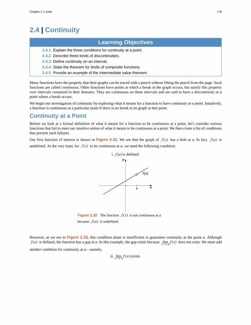
2.4 | Continuity
Learning Objectives2.4.1 Explain the three conditions for continuity at a point.
2.4.2 Describe three kinds of discontinuities.
2.4.3 Define continuity on an interval.
2.4.4 State the theorem for limits of composite functions.
2.4.5 Provide an example of the intermediate value theorem.
Many functions have the property that their graphs can be traced with a pencil without lifting the pencil from the page. Suchfunctions are called continuous. Other functions have points at which a break in the graph occurs, but satisfy this propertyover intervals contained in their domains. They are continuous on these intervals and are said to have a discontinuity at apoint where a break occurs.
We begin our investigation of continuity by exploring what it means for a function to have continuity at a point. Intuitively,a function is continuous at a particular point if there is no break in its graph at that point.
Continuity at a PointBefore we look at a formal definition of what it means for a function to be continuous at a point, let’s consider variousfunctions that fail to meet our intuitive notion of what it means to be continuous at a point. We then create a list of conditionsthat prevent such failures.
Our first function of interest is shown in Figure 2.32. We see that the graph of f (x) has a hole at a. In fact, f (a) is
undefined. At the very least, for f (x) to be continuous at a, we need the following condition:
i. f (a) is defined
Figure 2.32 The function f (x) is not continuous at a
because f (a) is undefined.
However, as we see in Figure 2.33, this condition alone is insufficient to guarantee continuity at the point a. Althoughf (a) is defined, the function has a gap at a. In this example, the gap exists because limx → a f (x) does not exist. We must add
another condition for continuity at a—namely,
ii. limx → a f (x) exists.
Chapter 2 | Limits 179
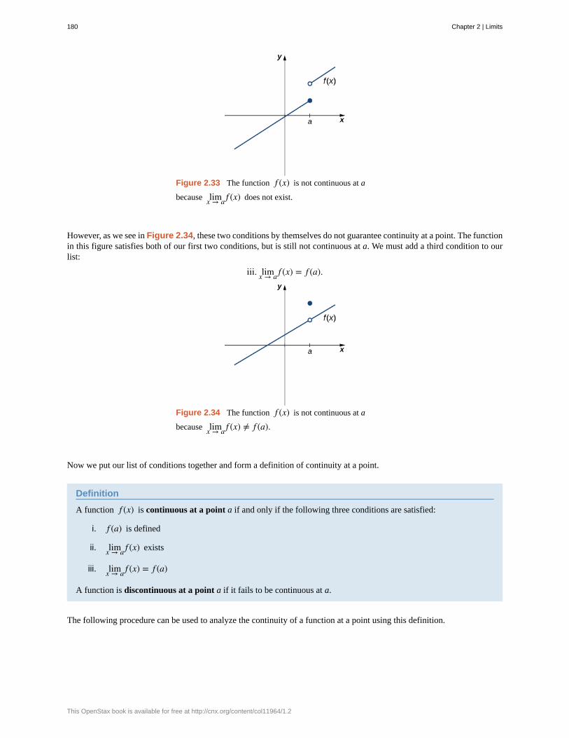
Figure 2.33 The function f (x) is not continuous at a
because limx → a f (x) does not exist.
However, as we see in Figure 2.34, these two conditions by themselves do not guarantee continuity at a point. The functionin this figure satisfies both of our first two conditions, but is still not continuous at a. We must add a third condition to ourlist:
iii. limx → a f (x) = f (a).
Figure 2.34 The function f (x) is not continuous at a
because limx → a f (x) ≠ f (a).
Now we put our list of conditions together and form a definition of continuity at a point.
Definition
A function f (x) is continuous at a point a if and only if the following three conditions are satisfied:
i. f (a) is defined
ii. limx → a f (x) exists
iii. limx → a f (x) = f (a)
A function is discontinuous at a point a if it fails to be continuous at a.
The following procedure can be used to analyze the continuity of a function at a point using this definition.
180 Chapter 2 | Limits
This OpenStax book is available for free at http://cnx.org/content/col11964/1.2
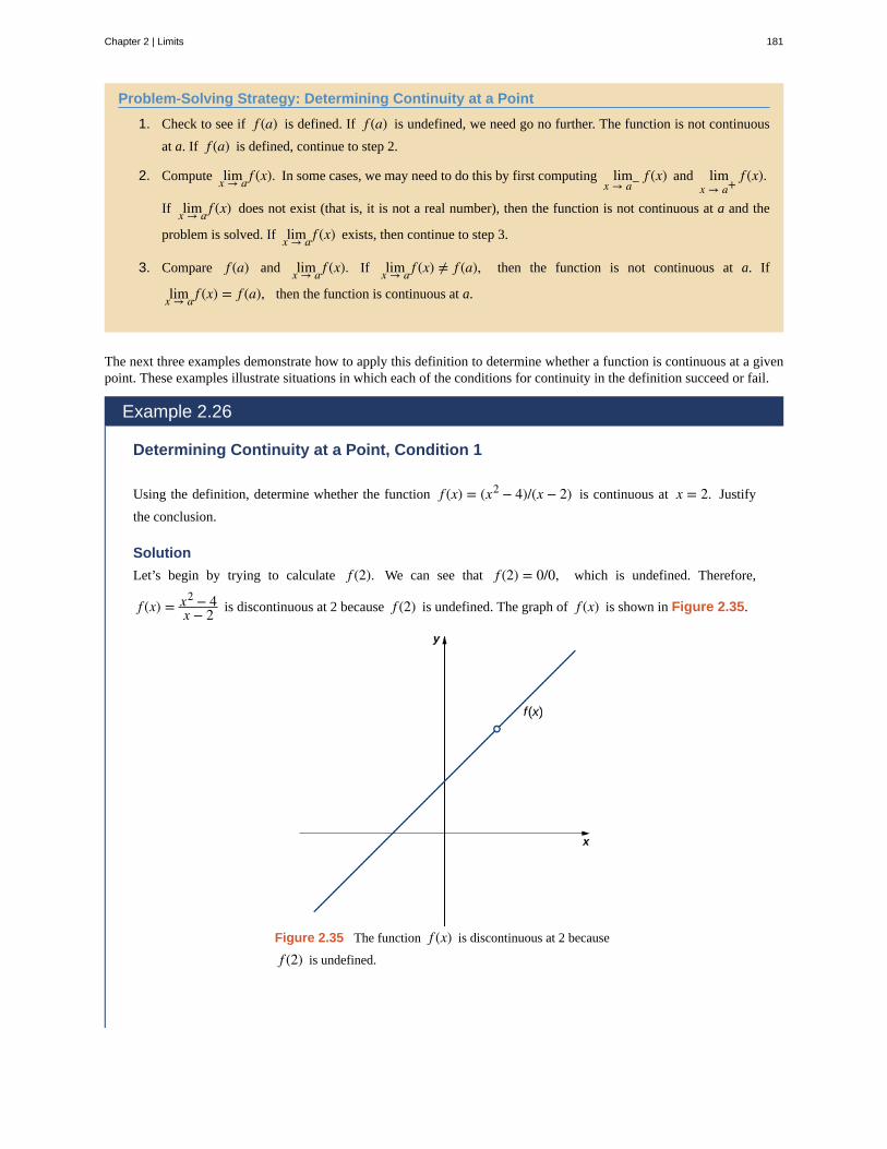
Problem-Solving Strategy: Determining Continuity at a Point
1. Check to see if f (a) is defined. If f (a) is undefined, we need go no further. The function is not continuous
at a. If f (a) is defined, continue to step 2.
2. Compute limx → a f (x). In some cases, we may need to do this by first computing limx → a− f (x) and lim
x → a+f (x).
If limx → a f (x) does not exist (that is, it is not a real number), then the function is not continuous at a and the
problem is solved. If limx → a f (x) exists, then continue to step 3.
3. Compare f (a) and limx → a f (x). If limx → a f (x) ≠ f (a), then the function is not continuous at a. If
limx → a f (x) = f (a), then the function is continuous at a.
The next three examples demonstrate how to apply this definition to determine whether a function is continuous at a givenpoint. These examples illustrate situations in which each of the conditions for continuity in the definition succeed or fail.
Example 2.26
Determining Continuity at a Point, Condition 1
Using the definition, determine whether the function f (x) = (x2 − 4)/(x − 2) is continuous at x = 2. Justify
the conclusion.
Solution
Let’s begin by trying to calculate f (2). We can see that f (2) = 0/0, which is undefined. Therefore,
f (x) = x2 − 4x − 2 is discontinuous at 2 because f (2) is undefined. The graph of f (x) is shown in Figure 2.35.
Figure 2.35 The function f (x) is discontinuous at 2 because
f (2) is undefined.
Chapter 2 | Limits 181
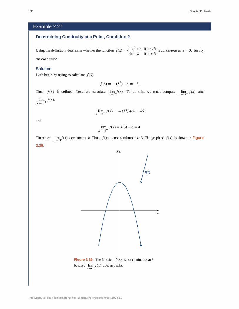
Example 2.27
Determining Continuity at a Point, Condition 2
Using the definition, determine whether the function f (x) =⎧
⎩⎨−x2 + 4 if x ≤ 34x − 8 if x > 3
is continuous at x = 3. Justify
the conclusion.
Solution
Let’s begin by trying to calculate f (3).
f (3) = − (32) + 4 = −5.
Thus, f (3) is defined. Next, we calculate limx → 3
f (x). To do this, we must compute limx → 3− f (x) and
limx → 3+
f (x):
limx → 3− f (x) = − (32) + 4 = −5
and
limx → 3+
f (x) = 4(3) − 8 = 4.
Therefore, limx → 3
f (x) does not exist. Thus, f (x) is not continuous at 3. The graph of f (x) is shown in Figure
2.36.
Figure 2.36 The function f (x) is not continuous at 3
because limx → 3
f (x) does not exist.
182 Chapter 2 | Limits
This OpenStax book is available for free at http://cnx.org/content/col11964/1.2
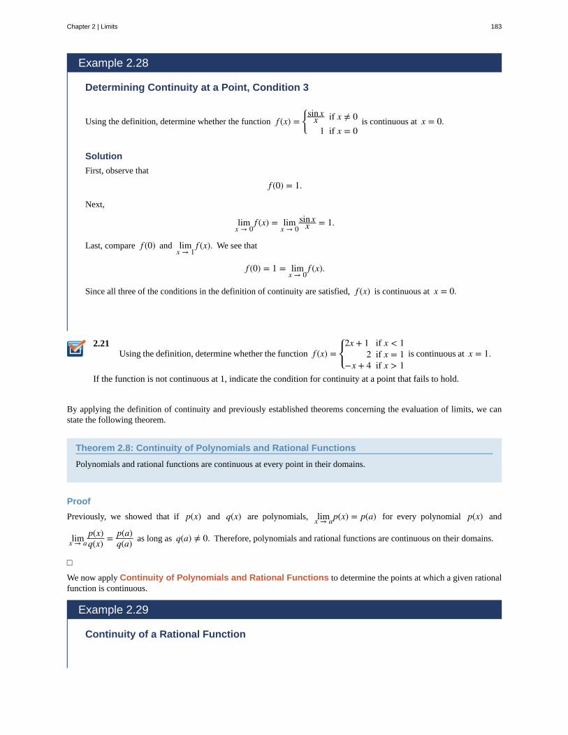
2.21
Example 2.28
Determining Continuity at a Point, Condition 3
Using the definition, determine whether the function f (x) =⎧
⎩⎨
sinxx if x ≠ 0
1 if x = 0is continuous at x = 0.
Solution
First, observe that
f (0) = 1.
Next,
limx → 0
f (x) = limx → 0
sinxx = 1.
Last, compare f (0) and limx → 1
f (x). We see that
f (0) = 1 = limx → 0
f (x).
Since all three of the conditions in the definition of continuity are satisfied, f (x) is continuous at x = 0.
Using the definition, determine whether the function f (x) =⎧
⎩⎨
2x + 1 if x < 12 if x = 1
−x + 4 if x > 1is continuous at x = 1.
If the function is not continuous at 1, indicate the condition for continuity at a point that fails to hold.
By applying the definition of continuity and previously established theorems concerning the evaluation of limits, we canstate the following theorem.
Theorem 2.8: Continuity of Polynomials and Rational Functions
Polynomials and rational functions are continuous at every point in their domains.
Proof
Previously, we showed that if p(x) and q(x) are polynomials, limx → ap(x) = p(a) for every polynomial p(x) and
limx → ap(x)q(x) = p(a)
q(a) as long as q(a) ≠ 0. Therefore, polynomials and rational functions are continuous on their domains.
□
We now apply Continuity of Polynomials and Rational Functions to determine the points at which a given rationalfunction is continuous.
Example 2.29
Continuity of a Rational Function
Chapter 2 | Limits 183
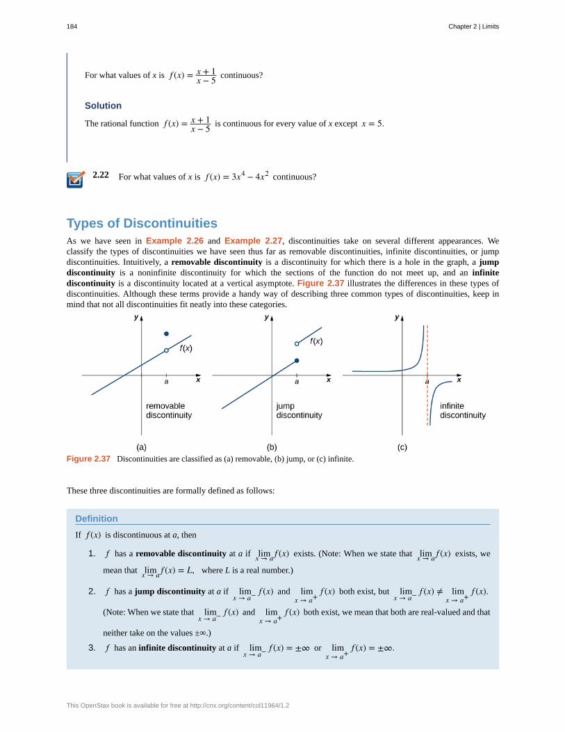
2.22
For what values of x is f (x) = x + 1x − 5 continuous?
Solution
The rational function f (x) = x + 1x − 5 is continuous for every value of x except x = 5.
For what values of x is f (x) = 3x4 − 4x2 continuous?
Types of DiscontinuitiesAs we have seen in Example 2.26 and Example 2.27, discontinuities take on several different appearances. Weclassify the types of discontinuities we have seen thus far as removable discontinuities, infinite discontinuities, or jumpdiscontinuities. Intuitively, a removable discontinuity is a discontinuity for which there is a hole in the graph, a jumpdiscontinuity is a noninfinite discontinuity for which the sections of the function do not meet up, and an infinitediscontinuity is a discontinuity located at a vertical asymptote. Figure 2.37 illustrates the differences in these types ofdiscontinuities. Although these terms provide a handy way of describing three common types of discontinuities, keep inmind that not all discontinuities fit neatly into these categories.
Figure 2.37 Discontinuities are classified as (a) removable, (b) jump, or (c) infinite.
These three discontinuities are formally defined as follows:
Definition
If f (x) is discontinuous at a, then
1. f has a removable discontinuity at a if limx → a f (x) exists. (Note: When we state that limx → a f (x) exists, we
mean that limx → a f (x) = L, where L is a real number.)
2. f has a jump discontinuity at a if limx → a− f (x) and lim
x → a+f (x) both exist, but lim
x → a− f (x) ≠ limx → a+
f (x).
(Note: When we state that limx → a− f (x) and lim
x → a+f (x) both exist, we mean that both are real-valued and that
neither take on the values ±∞.)
3. f has an infinite discontinuity at a if limx → a− f (x) = ±∞ or lim
x → a+f (x) = ±∞.
184 Chapter 2 | Limits
This OpenStax book is available for free at http://cnx.org/content/col11964/1.2
Example 2.30
Classifying a Discontinuity
In Example 2.26, we showed that f (x) = x2 − 4x − 2 is discontinuous at x = 2. Classify this discontinuity as
removable, jump, or infinite.
Solution
To classify the discontinuity at 2 we must evaluate limx → 2
f (x):
limx → 2
f (x) = limx → 2
x2 − 4x − 2
= limx → 2
(x − 2)(x + 2)x − 2
= limx → 2
(x + 2)
= 4.
Since f is discontinuous at 2 and limx → 2
f (x) exists, f has a removable discontinuity at x = 2.
Example 2.31
Classifying a Discontinuity
In Example 2.27, we showed that f (x) =⎧
⎩⎨−x2 + 4 if x ≤ 3
4x − 8 if x > 3is discontinuous at x = 3. Classify this
discontinuity as removable, jump, or infinite.
Solution
Earlier, we showed that f is discontinuous at 3 because limx → 3
f (x) does not exist. However, since
limx → 3− f (x) = −5 and lim
x → 3− f (x) = 4 both exist, we conclude that the function has a jump discontinuity at 3.
Example 2.32
Classifying a Discontinuity
Determine whether f (x) = x + 2x + 1 is continuous at −1. If the function is discontinuous at −1, classify the
discontinuity as removable, jump, or infinite.
Solution
The function value f (−1) is undefined. Therefore, the function is not continuous at −1. To determine the type of
Chapter 2 | Limits 185
2.23
discontinuity, we must determine the limit at −1. We see that limx → −1−
x + 2x + 1 = −∞ and lim
x → −1+x + 2x + 1 = +∞.
Therefore, the function has an infinite discontinuity at −1.
For f (x) =⎧
⎩⎨x2 if x ≠ 1
3 if x = 1, decide whether f is continuous at 1. If f is not continuous at 1, classify the
discontinuity as removable, jump, or infinite.
Continuity over an IntervalNow that we have explored the concept of continuity at a point, we extend that idea to continuity over an interval. Aswe develop this idea for different types of intervals, it may be useful to keep in mind the intuitive idea that a function iscontinuous over an interval if we can use a pencil to trace the function between any two points in the interval without liftingthe pencil from the paper. In preparation for defining continuity on an interval, we begin by looking at the definition of whatit means for a function to be continuous from the right at a point and continuous from the left at a point.
Continuity from the Right and from the Left
A function f (x) is said to be continuous from the right at a if limx → a+
f (x) = f (a).
A function f (x) is said to be continuous from the left at a if limx → a− f (x) = f (a).
A function is continuous over an open interval if it is continuous at every point in the interval. A function f (x) is continuous
over a closed interval of the form ⎡⎣a, b⎤
⎦ if it is continuous at every point in (a, b) and is continuous from the right at a
and is continuous from the left at b. Analogously, a function f (x) is continuous over an interval of the form (a, b⎤⎦ if it is
continuous over (a, b) and is continuous from the left at b. Continuity over other types of intervals are defined in a similar
fashion.
Requiring that limx → a+
f (x) = f (a) and limx → b− f (x) = f (b) ensures that we can trace the graph of the function from the
point ⎛⎝a, f (a)⎞
⎠ to the point ⎛⎝b, f (b)⎞
⎠ without lifting the pencil. If, for example, limx → a+
f (x) ≠ f (a), we would need to lift
our pencil to jump from f (a) to the graph of the rest of the function over (a, b⎤⎦.
Example 2.33
Continuity on an Interval
State the interval(s) over which the function f (x) = x − 1x2 + 2x
is continuous.
Solution
Since f (x) = x − 1x2 + 2x
is a rational function, it is continuous at every point in its domain. The domain of
f (x) is the set (−∞, −2) ∪ (−2, 0) ∪ (0, +∞). Thus, f (x) is continuous over each of the intervals
186 Chapter 2 | Limits
This OpenStax book is available for free at http://cnx.org/content/col11964/1.2
2.24
(−∞, −2), (−2, 0), and (0, +∞).
Example 2.34
Continuity over an Interval
State the interval(s) over which the function f (x) = 4 − x2 is continuous.
Solution
From the limit laws, we know that limx → a 4 − x2 = 4 − a2 for all values of a in (−2, 2). We also know that
limx → −2+
4 − x2 = 0 exists and limx → 2− 4 − x2 = 0 exists. Therefore, f (x) is continuous over the interval
[−2, 2].
State the interval(s) over which the function f (x) = x + 3 is continuous.
The Composite Function Theorem allows us to expand our ability to compute limits. In particular, this theoremultimately allows us to demonstrate that trigonometric functions are continuous over their domains.
Theorem 2.9: Composite Function Theorem
If f (x) is continuous at L and limx → ag(x) = L, then
limx → a f ⎛⎝g(x)⎞
⎠ = f ⎛⎝ limx → ag(x)⎞
⎠ = f (L).
Before we move on to Example 2.35, recall that earlier, in the section on limit laws, we showed limx → 0
cosx = 1 = cos(0).
Consequently, we know that f (x) = cosx is continuous at 0. In Example 2.35 we see how to combine this result with the
composite function theorem.
Example 2.35
Limit of a Composite Cosine Function
Evaluate limx → π/2
cos⎛⎝x − π
2⎞⎠.
Solution
Chapter 2 | Limits 187
2.25
The given function is a composite of cosx and x − π2. Since lim
x → π/2⎛⎝x − π
2⎞⎠ = 0 and cosx is continuous at 0,
we may apply the composite function theorem. Thus,
limx → π/2
cos⎛⎝x − π
2⎞⎠ = cos⎛
⎝ limx → π/2
⎛⎝x − π
2⎞⎠⎞⎠ = cos(0) = 1.
Evaluate limx → πsin(x − π).
The proof of the next theorem uses the composite function theorem as well as the continuity of f (x) = sinx and
g(x) = cosx at the point 0 to show that trigonometric functions are continuous over their entire domains.
Theorem 2.10: Continuity of Trigonometric Functions
Trigonometric functions are continuous over their entire domains.
ProofWe begin by demonstrating that cosx is continuous at every real number. To do this, we must show that limx → acosx = cosa
for all values of a.
limx → acosx = limx → acos((x − a) + a) rewrite x = x − a + a
= limx → a⎛⎝cos(x − a)cosa − sin(x − a)sina⎞
⎠ apply the identity for the cosine of the sum of two angles
= cos⎛⎝ limx → a(x − a)⎞
⎠cosa − sin⎛⎝ limx → a(x − a)⎞
⎠sina limx → a(x − a) = 0, and sinx and cosx are continuous at 0= cos(0)cosa − sin(0)sina evaluate cos(0) and sin(0) and simplify= 1 · cosa − 0 · sina = cosa.
The proof that sinx is continuous at every real number is analogous. Because the remaining trigonometric functions may
be expressed in terms of sinx and cosx, their continuity follows from the quotient limit law.
□
As you can see, the composite function theorem is invaluable in demonstrating the continuity of trigonometric functions.As we continue our study of calculus, we revisit this theorem many times.
The Intermediate Value TheoremFunctions that are continuous over intervals of the form ⎡
⎣a, b⎤⎦, where a and b are real numbers, exhibit many useful
properties. Throughout our study of calculus, we will encounter many powerful theorems concerning such functions. Thefirst of these theorems is the Intermediate Value Theorem.
Theorem 2.11: The Intermediate Value Theorem
Let f be continuous over a closed, bounded interval ⎡⎣a, b⎤
⎦. If z is any real number between f (a) and f (b), then there
is a number c in ⎡⎣a, b⎤
⎦ satisfying f (c) = z in Figure 2.38.
188 Chapter 2 | Limits
This OpenStax book is available for free at http://cnx.org/content/col11964/1.2
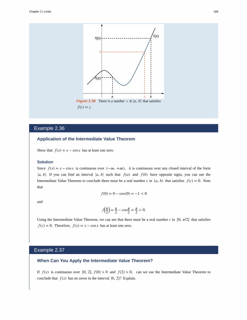
Figure 2.38 There is a number c ∈ ⎡⎣a, b⎤
⎦ that satisfies
f (c) = z.
Example 2.36
Application of the Intermediate Value Theorem
Show that f (x) = x − cosx has at least one zero.
Solution
Since f (x) = x − cosx is continuous over (−∞, +∞), it is continuous over any closed interval of the form⎡⎣a, b⎤
⎦. If you can find an interval ⎡⎣a, b⎤
⎦ such that f (a) and f (b) have opposite signs, you can use the
Intermediate Value Theorem to conclude there must be a real number c in (a, b) that satisfies f (c) = 0. Note
that
f (0) = 0 − cos(0) = −1 < 0
and
f ⎛⎝π2
⎞⎠ = π
2 − cosπ2 = π
2 > 0.
Using the Intermediate Value Theorem, we can see that there must be a real number c in [0, π/2] that satisfies
f (c) = 0. Therefore, f (x) = x − cosx has at least one zero.
Example 2.37
When Can You Apply the Intermediate Value Theorem?
If f (x) is continuous over [0, 2], f (0) > 0 and f (2) > 0, can we use the Intermediate Value Theorem to
conclude that f (x) has no zeros in the interval ⎡⎣0, 2]? Explain.
Chapter 2 | Limits 189
2.26
Solution
No. The Intermediate Value Theorem only allows us to conclude that we can find a value between f (0) and
f (2); it doesn’t allow us to conclude that we can’t find other values. To see this more clearly, consider the
function f (x) = (x − 1)2. It satisfies f (0) = 1 > 0, f (2) = 1 > 0, and f (1) = 0.
Example 2.38
When Can You Apply the Intermediate Value Theorem?
For f (x) = 1/x, f (−1) = −1 < 0 and f (1) = 1 > 0. Can we conclude that f (x) has a zero in the interval
[−1, 1]?
Solution
No. The function is not continuous over [−1, 1]. The Intermediate Value Theorem does not apply here.
Show that f (x) = x3 − x2 − 3x + 1 has a zero over the interval [0, 1].
190 Chapter 2 | Limits
This OpenStax book is available for free at http://cnx.org/content/col11964/1.2
2.4 EXERCISESFor the following exercises, determine the point(s), if any,at which each function is discontinuous. Classify anydiscontinuity as jump, removable, infinite, or other.
131. f (x) = 1x
132. f (x) = 2x2 + 1
133. f (x) = xx2 − x
134. g(t) = t−1 + 1
135. f (x) = 5ex − 2
136. f (x) = |x − 2|x − 2
137. H(x) = tan2x
138. f (t) = t + 3t2 + 5t + 6
For the following exercises, decide if the functioncontinuous at the given point. If it is discontinuous, whattype of discontinuity is it?
139. 2x2 − 5x + 3x − 1 at x = 1
140. h(θ) = sinθ − cosθtanθ at θ = π
141. g(u) =
⎧
⎩
⎨⎪
⎪
6u2 + u − 22u − 1 if u ≠ 1
272 if u = 1
2
, at u = 12
142. f (y) = sin(πy)tan(πy), at y = 1
143. f (x) =⎧
⎩⎨x2 − ex if x < 0x − 1 if x ≥ 0
, at x = 0
144. f (x) =⎧
⎩⎨xsin(x) if x ≤ πx tan(x) if x > π
, at x = π
In the following exercises, find the value(s) of k that makeseach function continuous over the given interval.
145. f (x) =⎧
⎩⎨3x + 2, x < k2x − 3, k ≤ x ≤ 8
146. f (θ) =⎧
⎩⎨
sinθ, 0 ≤ θ < π2
cos(θ + k), π2 ≤ θ ≤ π
147. f (x) =⎧
⎩⎨
x2 + 3x + 2x + 2 , x ≠ − 2
k, x = −2
148. f (x) =⎧
⎩⎨ ekx, 0 ≤ x < 4
x + 3, 4 ≤ x ≤ 8
149. f (x) =⎧
⎩⎨ kx, 0 ≤ x ≤ 3x + 1, 3 < x ≤ 10
In the following exercises, use the Intermediate ValueTheorem (IVT).
150. Let h(x) =⎧
⎩⎨3x2 − 4, x ≤ 25 + 4x, x > 2
Over the interval
[0, 4], there is no value of x such that h(x) = 10,although h(0) < 10 and h(4) > 10. Explain why this
does not contradict the IVT.
151. A particle moving along a line has at each time ta position function s(t), which is continuous. Assume
s(2) = 5 and s(5) = 2. Another particle moves such that
its position is given by h(t) = s(t) − t. Explain why there
must be a value c for 2 < c < 5 such that h(c) = 0.
152. [T] Use the statement “The cosine of t is equal to tcubed.”
a. Write a mathematical equation of the statement.b. Prove that the equation in part a. has at least one
real solution.c. Use a calculator to find an interval of length 0.01
that contains a solution.
153. Apply the IVT to determine whether 2x = x3 has
a solution in one of the intervals ⎡⎣1.25, 1.375⎤
⎦ or⎡⎣1.375, 1.5⎤
⎦. Briefly explain your response for each
interval.
Chapter 2 | Limits 191
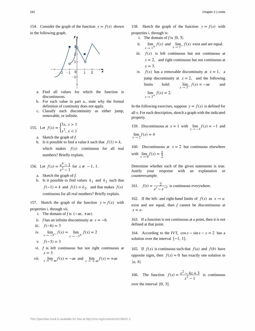
154. Consider the graph of the function y = f (x) shown
in the following graph.
a. Find all values for which the function isdiscontinuous.
b. For each value in part a., state why the formaldefinition of continuity does not apply.
c. Classify each discontinuity as either jump,removable, or infinite.
155. Let f (x) =⎧
⎩⎨3x, x > 1x3, x < 1
.
a. Sketch the graph of f.b. Is it possible to find a value k such that f (1) = k,
which makes f (x) continuous for all real
numbers? Briefly explain.
156. Let f (x) = x4 − 1x2 − 1
for x ≠ − 1, 1.
a. Sketch the graph of f.b. Is it possible to find values k1 and k2 such that
f (−1) = k and f (1) = k2, and that makes f (x)continuous for all real numbers? Briefly explain.
157. Sketch the graph of the function y = f (x) with
properties i. through vii.i. The domain of f is (−∞, +∞).
ii. f has an infinite discontinuity at x = −6.iii. f (−6) = 3iv. lim
x → −3− f (x) = limx → −3+
f (x) = 2
v. f (−3) = 3vi. f is left continuous but not right continuous at
x = 3.vii. limx → − ∞ f (x) = −∞ and lim
x → + ∞f (x) = +∞
158. Sketch the graph of the function y = f (x) with
properties i. through iv.i. The domain of f is ⎡
⎣0, 5⎤⎦.
ii. limx → 1+
f (x) and limx → 1− f (x) exist and are equal.
iii. f (x) is left continuous but not continuous at
x = 2, and right continuous but not continuous at
x = 3.iv. f (x) has a removable discontinuity at x = 1, a
jump discontinuity at x = 2, and the following
limits hold: limx → 3− f (x) = −∞ and
limx → 3+
f (x) = 2.
In the following exercises, suppose y = f (x) is defined for
all x. For each description, sketch a graph with the indicatedproperty.
159. Discontinuous at x = 1 with limx → −1
f (x) = −1 and
limx → 2
f (x) = 4
160. Discontinuous at x = 2 but continuous elsewhere
with limx → 0
f (x) = 12
Determine whether each of the given statements is true.Justify your response with an explanation orcounterexample.
161. f (t) = 2et − e−t is continuous everywhere.
162. If the left- and right-hand limits of f (x) as x → aexist and are equal, then f cannot be discontinuous atx = a.
163. If a function is not continuous at a point, then it is notdefined at that point.
164. According to the IVT, cosx − sinx − x = 2 has a
solution over the interval [−1, 1].
165. If f (x) is continuous such that f (a) and f (b) have
opposite signs, then f (x) = 0 has exactly one solution in⎡⎣a, b⎤
⎦.
166. The function f (x) = x2 − 4x + 3x2 − 1
is continuous
over the interval [0, 3].
192 Chapter 2 | Limits
This OpenStax book is available for free at http://cnx.org/content/col11964/1.2
167. If f (x) is continuous everywhere and
f (a), f (b) > 0, then there is no root of f (x) in the
interval ⎡⎣a, b⎤
⎦.
[T] The following problems consider the scalar form ofCoulomb’s law, which describes the electrostatic forcebetween two point charges, such as electrons. It is given by
the equation F(r) = ke|q1 q2|
r2 , where ke is Coulomb’s
constant, qi are the magnitudes of the charges of the two
particles, and r is the distance between the two particles.
168. To simplify the calculation of a model with manyinteracting particles, after some threshold value r = R,we approximate F as zero.
a. Explain the physical reasoning behind thisassumption.
b. What is the force equation?c. Evaluate the force F using both Coulomb’s law
and our approximation, assuming two protons witha charge magnitude of
1.6022 × 10⁻¹⁹ coulombs (C), and the
Coulomb constant ke = 8.988 × 10⁹ Nm2/C2 are
1 m apart. Also, assume R < 1 m. How much
inaccuracy does our approximation generate? Is ourapproximation reasonable?
d. Is there any finite value of R for which this systemremains continuous at R?
169. Instead of making the force 0 at R, instead we letthe force be 10−20 for r ≥ R. Assume two protons, which
have a magnitude of charge 1.6022 × 10⁻¹⁹ C, and the
Coulomb constant ke = 8.988 × 10⁹ Nm2/C2. Is there a
value R that can make this system continuous? If so, findit.
Recall the discussion on spacecraft from the chapteropener. The following problems consider a rocket launchfrom Earth’s surface. The force of gravity on the rocket is
given by F(d) = − mk/d2, where m is the mass of the
rocket, d is the distance of the rocket from the center ofEarth, and k is a constant.
170. [T] Determine the value and units of k given thatthe mass of the rocket on Earth is 3 million kg. (Hint: Thedistance from the center of Earth to its surface is 6378 km.)
171. [T] After a certain distance D has passed, thegravitational effect of Earth becomes quite negligible, sowe can approximate the force function by
F(d) =⎧
⎩⎨
−mkd2 if d < D
10,000 if d ≥ D. Find the necessary condition
D such that the force function remains continuous.
172. As the rocket travels away from Earth’s surface, thereis a distance D where the rocket sheds some of its mass,since it no longer needs the excess fuel storage. We can
write this function as F(d) =
⎧
⎩
⎨⎪
⎪
−m1 kd2 if d < D
−m2 kd2 if d ≥ D
. Is there
a D value such that this function is continuous, assumingm1 ≠ m2?
Prove the following functions are continuous everywhere
173. f (θ) = sinθ
174. g(x) = |x|
175. Where is f (x) =⎧
⎩⎨0 if x is irrational1 if x is rational
continuous?
Chapter 2 | Limits 193
2.5 | The Precise Definition of a Limit
Learning Objectives2.5.1 Describe the epsilon-delta definition of a limit.
2.5.2 Apply the epsilon-delta definition to find the limit of a function.
2.5.3 Describe the epsilon-delta definitions of one-sided limits and infinite limits.
2.5.4 Use the epsilon-delta definition to prove the limit laws.
By now you have progressed from the very informal definition of a limit in the introduction of this chapter to the intuitiveunderstanding of a limit. At this point, you should have a very strong intuitive sense of what the limit of a function meansand how you can find it. In this section, we convert this intuitive idea of a limit into a formal definition using precisemathematical language. The formal definition of a limit is quite possibly one of the most challenging definitions you willencounter early in your study of calculus; however, it is well worth any effort you make to reconcile it with your intuitivenotion of a limit. Understanding this definition is the key that opens the door to a better understanding of calculus.
Quantifying ClosenessBefore stating the formal definition of a limit, we must introduce a few preliminary ideas. Recall that the distance betweentwo points a and b on a number line is given by |a − b|.
• The statement | f (x) − L| < ε may be interpreted as: The distance between f (x) and L is less than ε.
• The statement 0 < |x − a| < δ may be interpreted as: x ≠ a and the distance between x and a is less than δ.
It is also important to look at the following equivalences for absolute value:
• The statement | f (x) − L| < ε is equivalent to the statement L − ε < f (x) < L + ε.
• The statement 0 < |x − a| < δ is equivalent to the statement a − δ < x < a + δ and x ≠ a.
With these clarifications, we can state the formal epsilon-delta definition of the limit.
Definition
Let f (x) be defined for all x ≠ a over an open interval containing a. Let L be a real number. Then
limx → a f (x) = L
if, for every ε > 0, there exists a δ > 0, such that if 0 < |x − a| < δ, then | f (x) − L| < ε.
This definition may seem rather complex from a mathematical point of view, but it becomes easier to understand if webreak it down phrase by phrase. The statement itself involves something called a universal quantifier (for every ε > 0), an
existential quantifier (there exists a δ > 0), and, last, a conditional statement (if 0 < |x − a| < δ, then | f (x) − L| < ε).Let’s take a look at Table 2.9, which breaks down the definition and translates each part.
194 Chapter 2 | Limits
This OpenStax book is available for free at http://cnx.org/content/col11964/1.2
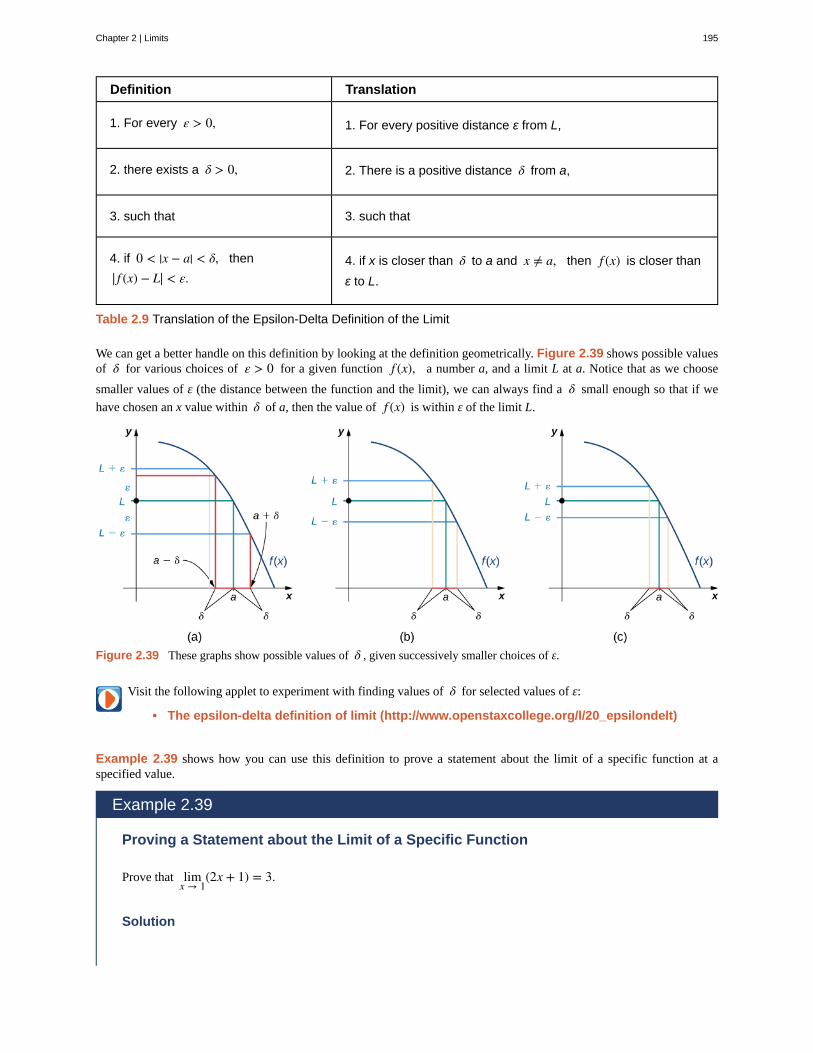
Definition Translation
1. For every ε > 0, 1. For every positive distance ε from L,
2. there exists a δ > 0, 2. There is a positive distance δ from a,
3. such that 3. such that
4. if 0 < |x − a| < δ, then
| f (x) − L| < ε.4. if x is closer than δ to a and x ≠ a, then f (x) is closer than
ε to L.
Table 2.9 Translation of the Epsilon-Delta Definition of the Limit
We can get a better handle on this definition by looking at the definition geometrically. Figure 2.39 shows possible valuesof δ for various choices of ε > 0 for a given function f (x), a number a, and a limit L at a. Notice that as we choose
smaller values of ε (the distance between the function and the limit), we can always find a δ small enough so that if we
have chosen an x value within δ of a, then the value of f (x) is within ε of the limit L.
Figure 2.39 These graphs show possible values of δ , given successively smaller choices of ε.
Visit the following applet to experiment with finding values of δ for selected values of ε:
• The epsilon-delta definition of limit (http://www.openstaxcollege.org/l/20_epsilondelt)
Example 2.39 shows how you can use this definition to prove a statement about the limit of a specific function at aspecified value.
Example 2.39
Proving a Statement about the Limit of a Specific Function
Prove that limx → 1
(2x + 1) = 3.
Solution
Chapter 2 | Limits 195
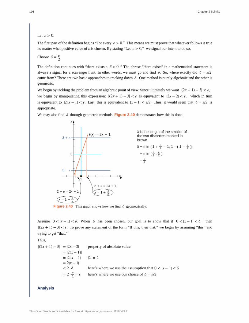
Let ε > 0.
The first part of the definition begins “For every ε > 0.” This means we must prove that whatever follows is true
no matter what positive value of ε is chosen. By stating “Let ε > 0,” we signal our intent to do so.
Choose δ = ε2.
The definition continues with “there exists a δ > 0. ” The phrase “there exists” in a mathematical statement is
always a signal for a scavenger hunt. In other words, we must go and find δ. So, where exactly did δ = ε/2come from? There are two basic approaches to tracking down δ. One method is purely algebraic and the other is
geometric.
We begin by tackling the problem from an algebraic point of view. Since ultimately we want |(2x + 1) − 3| < ε,we begin by manipulating this expression: |(2x + 1) − 3| < ε is equivalent to |2x − 2| < ε, which in turn
is equivalent to |2||x − 1| < ε. Last, this is equivalent to |x − 1| < ε/2. Thus, it would seem that δ = ε/2 is
appropriate.
We may also find δ through geometric methods. Figure 2.40 demonstrates how this is done.
Figure 2.40 This graph shows how we find δ geometrically.
Assume 0 < |x − 1| < δ. When δ has been chosen, our goal is to show that if 0 < |x − 1| < δ, then
|(2x + 1) − 3| < ε. To prove any statement of the form “If this, then that,” we begin by assuming “this” and
trying to get “that.”
Thus,
|(2x + 1) − 3| = |2x − 2| property of absolute value= |2(x − 1)|= |2||x − 1| |2| = 2= 2|x − 1|< 2 · δ here’s where we use the assumption that 0 < |x − 1| < δ= 2 · ε
2 = ε here’s where we use our choice of δ = ε/2
Analysis
196 Chapter 2 | Limits
This OpenStax book is available for free at http://cnx.org/content/col11964/1.2
In this part of the proof, we started with |(2x + 1) − 3| and used our assumption 0 < |x − 1| < δ in a key part
of the chain of inequalities to get |(2x + 1) − 3| to be less than ε. We could just as easily have manipulated the
assumed inequality 0 < |x − 1| < δ to arrive at |(2x + 1) − 3| < ε as follows:
0 < |x − 1| < δ ⇒ |x − 1| < δ⇒ − δ < x − 1 < δ⇒ − ε
2 < x − 1 < ε2
⇒ − ε < 2x − 2 < ε⇒ − ε < 2x − 2 < ε⇒ |2x − 2| < ε⇒ |(2x + 1) − 3| < ε.
Therefore, limx → 1
(2x + 1) = 3. (Having completed the proof, we state what we have accomplished.)
After removing all the remarks, here is a final version of the proof:
Let ε > 0.
Choose δ = ε/2.
Assume 0 < |x − 1| < δ.
Thus,
|(2x + 1) − 3| = |2x − 2|= |2(x − 1)|= |2||x − 1|= 2|x − 1|< 2 · δ= 2 · ε
2= ε.
Therefore, limx → 1
(2x + 1) = 3.
The following Problem-Solving Strategy summarizes the type of proof we worked out in Example 2.39.
Problem-Solving Strategy: Proving That limx → a f(x) = L for a Specific Function f(x)
1. Let’s begin the proof with the following statement: Let ε > 0.
2. Next, we need to obtain a value for δ. After we have obtained this value, we make the following statement,
filling in the blank with our choice of δ : Choose δ = _______.
3. The next statement in the proof should be (at this point, we fill in our given value for a):Assume 0 < |x − a| < δ.
4. Next, based on this assumption, we need to show that | f (x) − L| < ε, where f (x) and L are our function
f (x) and our limit L. At some point, we need to use 0 < |x − a| < δ.
5. We conclude our proof with the statement: Therefore, limx → a f (x) = L.
Chapter 2 | Limits 197
2.27
Example 2.40
Proving a Statement about a Limit
Complete the proof that limx → −1
(4x + 1) = −3 by filling in the blanks.
Let _____.
Choose δ = _______.
Assume 0 < |x − _______| < δ.
Thus, |________ − ________| = _____________________________________ε.
Solution
We begin by filling in the blanks where the choices are specified by the definition. Thus, we have
Let ε > 0.
Choose δ = _______.
Assume 0 < |x − (−1)| < δ. (or equivalently, 0 < |x + 1| < δ.)
Thus, |(4x + 1) − (−3)| = |4x + 4| = |4||x + 1| < 4δ_______ε.
Focusing on the final line of the proof, we see that we should choose δ = ε4.
We now complete the final write-up of the proof:
Let ε > 0.
Choose δ = ε4.
Assume 0 < |x − (−1)| < δ (or equivalently, 0 < |x + 1| < δ.)
Thus, |(4x + 1) − (−3)| = |4x + 4| = |4||x + 1| < 4δ = 4(ε/4) = ε.
Complete the proof that limx → 2
(3x − 2) = 4 by filling in the blanks.
Let _______.
Choose δ = _______.
Assume 0 < |x − ____| < ____.
Thus,
|_______ − ____| = ______________________________ε.
Therefore, limx → 2
(3x − 2) = 4.
In Example 2.39 and Example 2.40, the proofs were fairly straightforward, since the functions with which we wereworking were linear. In Example 2.41, we see how to modify the proof to accommodate a nonlinear function.
Example 2.41
198 Chapter 2 | Limits
This OpenStax book is available for free at http://cnx.org/content/col11964/1.2
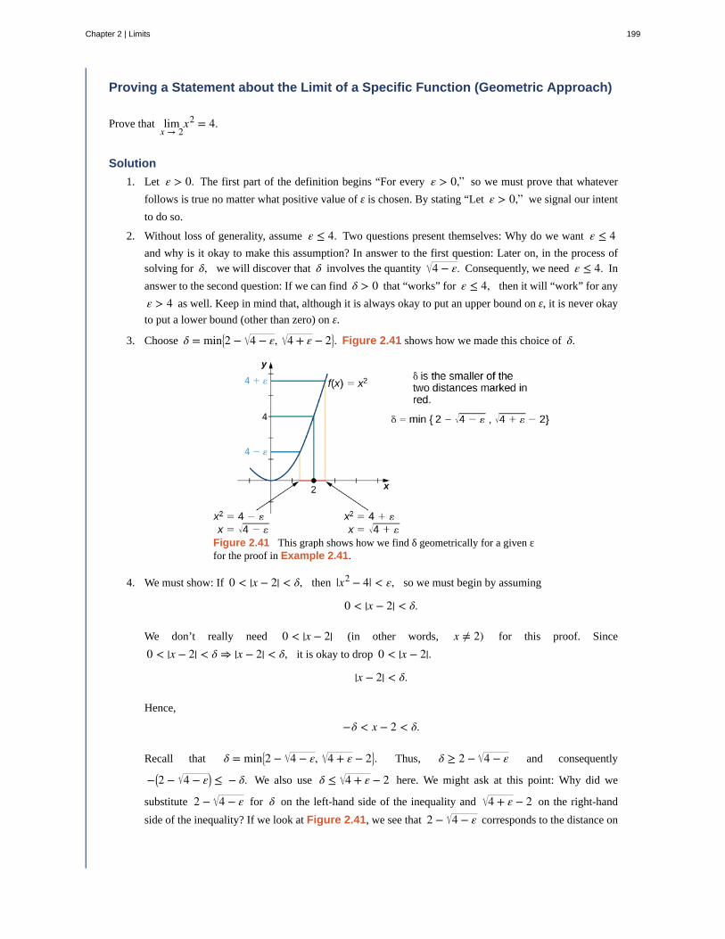
Proving a Statement about the Limit of a Specific Function (Geometric Approach)
Prove that limx → 2
x2 = 4.
Solution
1. Let ε > 0. The first part of the definition begins “For every ε > 0,” so we must prove that whatever
follows is true no matter what positive value of ε is chosen. By stating “Let ε > 0,” we signal our intent
to do so.
2. Without loss of generality, assume ε ≤ 4. Two questions present themselves: Why do we want ε ≤ 4and why is it okay to make this assumption? In answer to the first question: Later on, in the process ofsolving for δ, we will discover that δ involves the quantity 4 − ε. Consequently, we need ε ≤ 4. In
answer to the second question: If we can find δ > 0 that “works” for ε ≤ 4, then it will “work” for any
ε > 4 as well. Keep in mind that, although it is always okay to put an upper bound on ε, it is never okay
to put a lower bound (other than zero) on ε.
3. Choose δ = min⎧
⎩⎨2 − 4 − ε, 4 + ε − 2⎫
⎭⎬. Figure 2.41 shows how we made this choice of δ.
Figure 2.41 This graph shows how we find δ geometrically for a given εfor the proof in Example 2.41.
4. We must show: If 0 < |x − 2| < δ, then |x2 − 4| < ε, so we must begin by assuming
0 < |x − 2| < δ.
We don’t really need 0 < |x − 2| (in other words, x ≠ 2) for this proof. Since
0 < |x − 2| < δ ⇒ |x − 2| < δ, it is okay to drop 0 < |x − 2|.
|x − 2| < δ.
Hence,
−δ < x − 2 < δ.
Recall that δ = min⎧
⎩⎨2 − 4 − ε, 4 + ε − 2⎫
⎭⎬. Thus, δ ≥ 2 − 4 − ε and consequently
−⎛⎝2 − 4 − ε⎞
⎠ ≤ − δ. We also use δ ≤ 4 + ε − 2 here. We might ask at this point: Why did we
substitute 2 − 4 − ε for δ on the left-hand side of the inequality and 4 + ε − 2 on the right-hand
side of the inequality? If we look at Figure 2.41, we see that 2 − 4 − ε corresponds to the distance on
Chapter 2 | Limits 199
2.28
the left of 2 on the x-axis and 4 + ε − 2 corresponds to the distance on the right. Thus,
−⎛⎝2 − 4 − ε⎞
⎠ ≤ − δ < x − 2 < δ ≤ 4 + ε − 2.
We simplify the expression on the left:
−2 + 4 − ε < x − 2 < 4 + ε − 2.
Then, we add 2 to all parts of the inequality:
4 − ε < x < 4 + ε.
We square all parts of the inequality. It is okay to do so, since all parts of the inequality are positive:
4 − ε < x2 < 4 + ε.
We subtract 4 from all parts of the inequality:
−ε < x2 − 4 < ε.
Last,
|x2 − 4| < ε.5. Therefore,
limx → 2
x2 = 4.
Find δ corresponding to ε > 0 for a proof that limx → 9
x = 3.
The geometric approach to proving that the limit of a function takes on a specific value works quite well for some functions.Also, the insight into the formal definition of the limit that this method provides is invaluable. However, we may alsoapproach limit proofs from a purely algebraic point of view. In many cases, an algebraic approach may not only provideus with additional insight into the definition, it may prove to be simpler as well. Furthermore, an algebraic approach is theprimary tool used in proofs of statements about limits. For Example 2.42, we take on a purely algebraic approach.
Example 2.42
Proving a Statement about the Limit of a Specific Function (Algebraic Approach)
Prove that limx → −1
⎛⎝x2 − 2x + 3⎞
⎠ = 6.
Solution
Let’s use our outline from the Problem-Solving Strategy:
1. Let ε > 0.
2. Choose δ = min{1, ε/5}. This choice of δ may appear odd at first glance, but it was obtained by
200 Chapter 2 | Limits
This OpenStax book is available for free at http://cnx.org/content/col11964/1.2
2.29
taking a look at our ultimate desired inequality: |⎛⎝x2 − 2x + 3⎞⎠ − 6| < ε. This inequality is equivalent
to |x + 1| · |x − 3| < ε. At this point, the temptation simply to choose δ = εx − 3 is very strong.
Unfortunately, our choice of δ must depend on ε only and no other variable. If we can replace |x − 3| by
a numerical value, our problem can be resolved. This is the place where assuming δ ≤ 1 comes into play.
The choice of δ ≤ 1 here is arbitrary. We could have just as easily used any other positive number. In
some proofs, greater care in this choice may be necessary. Now, since δ ≤ 1 and |x + 1| < δ ≤ 1, we
are able to show that |x − 3| < 5. Consequently, |x + 1| · |x − 3| < |x + 1| · 5. At this point we realize
that we also need δ ≤ ε/5. Thus, we choose δ = min{1, ε/5}.
3. Assume 0 < |x + 1| < δ. Thus,
|x + 1| < 1 and |x + 1| < ε5.
Since |x + 1| < 1, we may conclude that −1 < x + 1 < 1. Thus, by subtracting 4 from all parts of the
inequality, we obtain −5 < x − 3 < −1. Consequently, |x − 3| < 5. This gives us
|⎛⎝x2 − 2x + 3⎞⎠ − 6| = |x + 1| · |x − 3| < ε
5 · 5 = ε.
Therefore,
limx → −1
⎛⎝x2 − 2x + 3⎞
⎠ = 6.
Complete the proof that limx → 1
x2 = 1.
Let ε > 0; choose δ = min{1, ε/3}; assume 0 < |x − 1| < δ.
Since |x − 1| < 1, we may conclude that −1 < x − 1 < 1. Thus, 1 < x + 1 < 3. Hence, |x + 1| < 3.
You will find that, in general, the more complex a function, the more likely it is that the algebraic approach is the easiest toapply. The algebraic approach is also more useful in proving statements about limits.
Proving Limit LawsWe now demonstrate how to use the epsilon-delta definition of a limit to construct a rigorous proof of one of the limit laws.The triangle inequality is used at a key point of the proof, so we first review this key property of absolute value.
Definition
The triangle inequality states that if a and b are any real numbers, then |a + b| ≤ |a| + |b|.
Proof
We prove the following limit law: If limx → a f (x) = L and limx → ag(x) = M, then limx → a⎛⎝ f (x) + g(x)⎞
⎠ = L + M.
Let ε > 0.
Choose δ1 > 0 so that if 0 < |x − a| < δ1, then | f (x) − L| < ε/2.
Choose δ2 > 0 so that if 0 < |x − a| < δ2, then |g(x) − M| < ε/2.
Chapter 2 | Limits 201
Choose δ = min⎧
⎩⎨δ1, δ2
⎫
⎭⎬.
Assume 0 < |x − a| < δ.
Thus,
0 < |x − a| < δ1 and 0 < |x − a| < δ2.
Hence,
|⎛⎝ f (x) + g(x)⎞⎠ − (L + M)| = |⎛⎝ f (x) − L⎞
⎠ + ⎛⎝g(x) − M⎞
⎠|≤ | f (x) − L| + |g(x) − M|< ε
2 + ε2 = ε.
□
We now explore what it means for a limit not to exist. The limit limx → a f (x) does not exist if there is no real number L for
which limx → a f (x) = L. Thus, for all real numbers L, limx → a f (x) ≠ L. To understand what this means, we look at each part
of the definition of limx → a f (x) = L together with its opposite. A translation of the definition is given in Table 2.10.
Definition Opposite
1. For every ε > 0, 1. There exists ε > 0 so that
2. there exists a δ > 0, so that 2. for every δ > 0,
3. if 0 < |x − a| < δ, then
| f (x) − L| < ε.3. There is an x satisfying 0 < |x − a| < δ so that
| f (x) − L| ≥ ε.
Table 2.10 Translation of the Definition of limx → a f (x) = L and its Opposite
Finally, we may state what it means for a limit not to exist. The limit limx → a f (x) does not exist if for every real number L,
there exists a real number ε > 0 so that for all δ > 0, there is an x satisfying 0 < |x − a| < δ, so that | f (x) − L| ≥ ε.Let’s apply this in Example 2.43 to show that a limit does not exist.
Example 2.43
Showing That a Limit Does Not Exist
Show that limx → 0
|x|x does not exist. The graph of f (x) = |x|/x is shown here:
202 Chapter 2 | Limits
This OpenStax book is available for free at http://cnx.org/content/col11964/1.2
Solution
Suppose that L is a candidate for a limit. Choose ε = 1/2.
Let δ > 0. Either L ≥ 0 or L < 0. If L ≥ 0, then let x = − δ/2. Thus,
|x − 0| = |− δ2 − 0| = δ
2 < δ
and
| |− δ2 |
− δ2
− L| = |−1 − L| = L + 1 ≥ 1 > 12 = ε.
On the other hand, if L < 0, then let x = δ/2. Thus,
|x − 0| = |δ2 − 0| = δ2 < δ
and
| |δ2 |δ2
− L| = |1 − L| = |L| + 1 ≥ 1 > 12 = ε.
Thus, for any value of L, limx → 0
|x|x ≠ L.
One-Sided and Infinite LimitsJust as we first gained an intuitive understanding of limits and then moved on to a more rigorous definition of a limit,we now revisit one-sided limits. To do this, we modify the epsilon-delta definition of a limit to give formal epsilon-deltadefinitions for limits from the right and left at a point. These definitions only require slight modifications from the definitionof the limit. In the definition of the limit from the right, the inequality 0 < x − a < δ replaces 0 < |x − a| < δ, which
ensures that we only consider values of x that are greater than (to the right of) a. Similarly, in the definition of the limit fromthe left, the inequality −δ < x − a < 0 replaces 0 < |x − a| < δ, which ensures that we only consider values of x that
are less than (to the left of) a.
Definition
Limit from the Right: Let f (x) be defined over an open interval of the form (a, b) where a < b. Then,
Chapter 2 | Limits 203
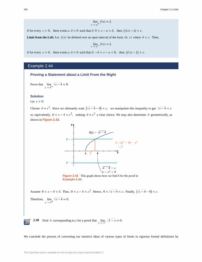
2.30
limx → a+
f (x) = L
if for every ε > 0, there exists a δ > 0 such that if 0 < x − a < δ, then | f (x) − L| < ε.
Limit from the Left: Let f (x) be defined over an open interval of the form (b, c) where b < c. Then,
limx → a− f (x) = L
if for every ε > 0, there exists a δ > 0 such that if −δ < x − a < 0, then | f (x) − L| < ε.
Example 2.44
Proving a Statement about a Limit From the Right
Prove that limx → 4+
x − 4 = 0.
Solution
Let ε > 0.
Choose δ = ε2. Since we ultimately want | x − 4 − 0| < ε, we manipulate this inequality to get x − 4 < ε
or, equivalently, 0 < x − 4 < ε2, making δ = ε2 a clear choice. We may also determine δ geometrically, as
shown in Figure 2.42.
Figure 2.42 This graph shows how we find δ for the proof inExample 2.44.
Assume 0 < x − 4 < δ. Thus, 0 < x − 4 < ε2. Hence, 0 < x − 4 < ε. Finally, | x − 4 − 0| < ε.
Therefore, limx → 4+
x − 4 = 0.
Find δ corresponding to ε for a proof that limx → 1− 1 − x = 0.
We conclude the process of converting our intuitive ideas of various types of limits to rigorous formal definitions by
204 Chapter 2 | Limits
This OpenStax book is available for free at http://cnx.org/content/col11964/1.2
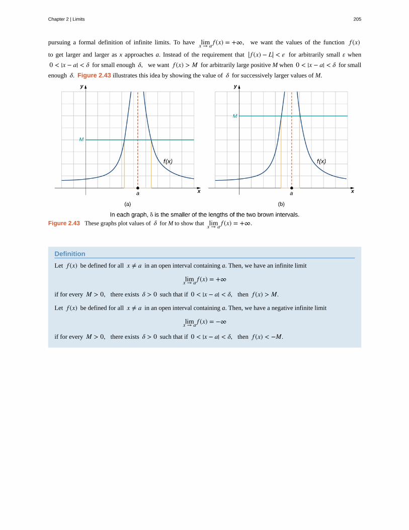
pursuing a formal definition of infinite limits. To have limx → a f (x) = +∞, we want the values of the function f (x)
to get larger and larger as x approaches a. Instead of the requirement that | f (x) − L| < ε for arbitrarily small ε when
0 < |x − a| < δ for small enough δ, we want f (x) > M for arbitrarily large positive M when 0 < |x − a| < δ for small
enough δ. Figure 2.43 illustrates this idea by showing the value of δ for successively larger values of M.
Figure 2.43 These graphs plot values of δ for M to show that limx → a f (x) = +∞.
Definition
Let f (x) be defined for all x ≠ a in an open interval containing a. Then, we have an infinite limit
limx → a f (x) = +∞
if for every M > 0, there exists δ > 0 such that if 0 < |x − a| < δ, then f (x) > M.
Let f (x) be defined for all x ≠ a in an open interval containing a. Then, we have a negative infinite limit
limx → a f (x) = −∞
if for every M > 0, there exists δ > 0 such that if 0 < |x − a| < δ, then f (x) < −M.
Chapter 2 | Limits 205
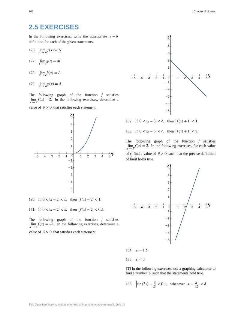
2.5 EXERCISESIn the following exercises, write the appropriate ε − δdefinition for each of the given statements.
176. limx → a f (x) = N
177. limt → b
g(t) = M
178. limx → ch(x) = L
179. limx → aφ(x) = A
The following graph of the function f satisfieslim
x → 2f (x) = 2. In the following exercises, determine a
value of δ > 0 that satisfies each statement.
180. If 0 < |x − 2| < δ, then | f (x) − 2| < 1.
181. If 0 < |x − 2| < δ, then | f (x) − 2| < 0.5.
The following graph of the function f satisfieslim
x → 3f (x) = −1. In the following exercises, determine a
value of δ > 0 that satisfies each statement.
182. If 0 < |x − 3| < δ, then | f (x) + 1| < 1.
183. If 0 < |x − 3| < δ, then | f (x) + 1| < 2.
The following graph of the function f satisfieslim
x → 3f (x) = 2. In the following exercises, for each value
of ε, find a value of δ > 0 such that the precise definition
of limit holds true.
184. ε = 1.5
185. ε = 3
[T] In the following exercises, use a graphing calculator tofind a number δ such that the statements hold true.
186. |sin(2x) − 12| < 0.1, whenever |x − π
12| < δ
206 Chapter 2 | Limits
This OpenStax book is available for free at http://cnx.org/content/col11964/1.2
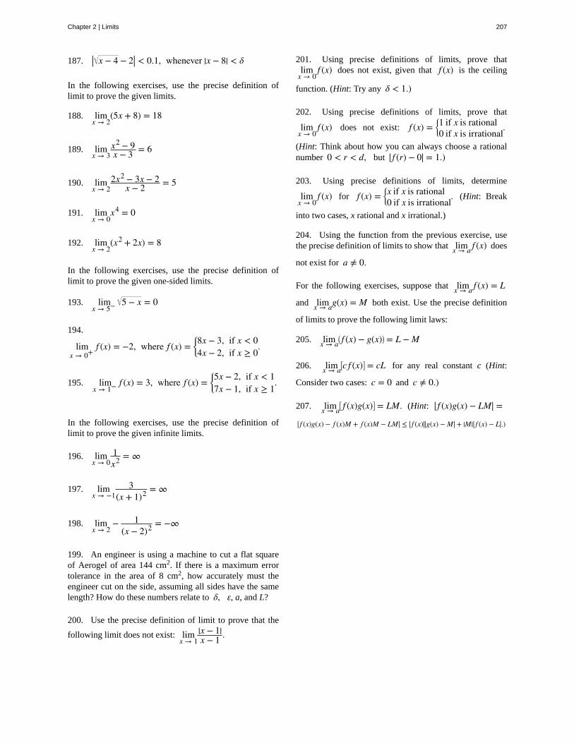
187. | x − 4 − 2| < 0.1, whenever |x − 8| < δ
In the following exercises, use the precise definition oflimit to prove the given limits.
188. limx → 2
(5x + 8) = 18
189. limx → 3
x2 − 9x − 3 = 6
190. limx → 2
2x2 − 3x − 2x − 2 = 5
191. limx → 0
x4 = 0
192. limx → 2
(x2 + 2x) = 8
In the following exercises, use the precise definition oflimit to prove the given one-sided limits.
193. limx → 5− 5 − x = 0
194.
limx → 0+
f (x) = −2, where f (x) =⎧
⎩⎨8x − 3, if x < 04x − 2, if x ≥ 0
.
195. limx → 1− f (x) = 3, where f (x) =
⎧
⎩⎨5x − 2, if x < 17x − 1, if x ≥ 1
.
In the following exercises, use the precise definition oflimit to prove the given infinite limits.
196. limx → 0
1x2 = ∞
197. limx → −1
3(x + 1)2 = ∞
198. limx → 2
− 1(x − 2)2 = −∞
199. An engineer is using a machine to cut a flat squareof Aerogel of area 144 cm2. If there is a maximum errortolerance in the area of 8 cm2, how accurately must theengineer cut on the side, assuming all sides have the samelength? How do these numbers relate to δ, ε, a, and L?
200. Use the precise definition of limit to prove that the
following limit does not exist: limx → 1
|x − 1|x − 1 .
201. Using precise definitions of limits, prove thatlim
x → 0f (x) does not exist, given that f (x) is the ceiling
function. (Hint: Try any δ < 1.)
202. Using precise definitions of limits, prove that
limx → 0
f (x) does not exist: f (x) =⎧
⎩⎨1 if x is rational0 if x is irrational
.
(Hint: Think about how you can always choose a rationalnumber 0 < r < d, but | f (r) − 0| = 1.)
203. Using precise definitions of limits, determine
limx → 0
f (x) for f (x) =⎧
⎩⎨x if x is rational0 if x is irrational
. (Hint: Break
into two cases, x rational and x irrational.)
204. Using the function from the previous exercise, usethe precise definition of limits to show that limx → a f (x) does
not exist for a ≠ 0.
For the following exercises, suppose that limx → a f (x) = L
and limx → ag(x) = M both exist. Use the precise definition
of limits to prove the following limit laws:
205. limx → a⎛⎝ f (x) − g(x)⎞
⎠ = L − M
206. limx → a⎡⎣c f (x)⎤
⎦ = cL for any real constant c (Hint:
Consider two cases: c = 0 and c ≠ 0.)
207. limx → a⎡⎣ f (x)g(x)⎤
⎦ = LM. (Hint: | f (x)g(x) − LM| =
| f (x)g(x) − f (x)M + f (x)M − LM| ≤ | f (x)||g(x) − M| + |M|| f (x) − L|.)
Chapter 2 | Limits 207
average velocity
constant multiple law for limits
continuity at a point
continuity from the left
continuity from the right
continuity over an interval
difference law for limits
differential calculus
discontinuity at a point
epsilon-delta definition of the limit
infinite discontinuity
infinite limit
instantaneous velocity
integral calculus
Intermediate Value Theorem
intuitive definition of the limit
jump discontinuity
limit
CHAPTER 2 REVIEW
KEY TERMSthe change in an object’s position divided by the length of a time period; the average velocity of an
object over a time interval [t, a] (if t < a or [a, t] if t > a) , with a position given by s(t), that is
vave = s(t) − s(a)t − a
the limit law limx → ac f (x) = c · limx → a f (x) = cL
A function f (x) is continuous at a point a if and only if the following three conditions are
satisfied: (1) f (a) is defined, (2) limx → a f (x) exists, and (3) limx → a f (x) = f (a)
A function is continuous from the left at b if limx → b− f (x) = f (b)
A function is continuous from the right at a if limx → a+
f (x) = f (a)
a function that can be traced with a pencil without lifting the pencil; a function iscontinuous over an open interval if it is continuous at every point in the interval; a function f (x) is continuous over a
closed interval of the form ⎡⎣a, b⎤
⎦ if it is continuous at every point in (a, b), and it is continuous from the right at a
and from the left at b
the limit law limx → a⎛⎝ f (x) − g(x)⎞
⎠ = limx → a f (x) − limx → ag(x) = L − M
the field of calculus concerned with the study of derivatives and their applications
A function is discontinuous at a point or has a discontinuity at a point if it is not continuous atthe point
limx → a f (x) = L if for every ε > 0, there exists a δ > 0 such that if
0 < |x − a| < δ, then | f (x) − L| < ε
An infinite discontinuity occurs at a point a if limx → a− f (x) = ±∞ or lim
x → a+f (x) = ±∞
A function has an infinite limit at a point a if it either increases or decreases without bound as it approachesa
The instantaneous velocity of an object with a position function that is given by s(t) is the
value that the average velocities on intervals of the form [t, a] and [a, t] approach as the values of t move closer to
a, provided such a value exists
the study of integrals and their applications
Let f be continuous over a closed bounded interval ⎡⎣a, b⎤
⎦; if z is any real number
between f (a) and f (b), then there is a number c in ⎡⎣a, b⎤
⎦ satisfying f (c) = z
If all values of the function f (x) approach the real number L as the values of x( ≠ a)approach a, f (x) approaches L
A jump discontinuity occurs at a point a if limx → a− f (x) and lim
x → a+f (x) both exist, but
limx → a− f (x) ≠ lim
x → a+f (x)
the process of letting x or t approach a in an expression; the limit of a function f (x) as x approaches a is the value
208 Chapter 2 | Limits
This OpenStax book is available for free at http://cnx.org/content/col11964/1.2
limit laws
multivariable calculus
one-sided limit
power law for limits
product law for limits
quotient law for limits
removable discontinuity
root law for limits
secant
squeeze theorem
sum law for limits
tangent
triangle inequality
vertical asymptote
that f (x) approaches as x approaches a
the individual properties of limits; for each of the individual laws, let f (x) and g(x) be defined for all x ≠ aover some open interval containing a; assume that L and M are real numbers so that limx → a f (x) = L and
limx → ag(x) = M; let c be a constant
the study of the calculus of functions of two or more variables
A one-sided limit of a function is a limit taken from either the left or the right
the limit law limx → a⎛⎝ f (x)⎞
⎠n = ⎛
⎝ limx → a f (x)⎞⎠n
= Ln for every positive integer n
the limit law limx → a⎛⎝ f (x) · g(x)⎞
⎠ = limx → a f (x) · limx → ag(x) = L · M
the limit law limx → af (x)g(x) =
limx → a f (x)limx → ag(x) = L
M for M ≠ 0
A removable discontinuity occurs at a point a if f (x) is discontinuous at a, but limx → a f (x)
exists
the limit law limx → a f (x)n = limx → a f (x)n = Lnfor all L if n is odd and for L ≥ 0 if n is even
A secant line to a function f (x) at a is a line through the point ⎛⎝a, f (a)⎞
⎠ and another point on the function; the
slope of the secant line is given by msec = f (x) − f (a)x − a
states that if f (x) ≤ g(x) ≤ h(x) for all x ≠ a over an open interval containing a and
limx → a f (x) = L = limx → ah(x) where L is a real number, then limx → ag(x) = L
The limit law limx → a⎛⎝ f (x) + g(x)⎞
⎠ = limx → a f (x) + limx → ag(x) = L + M
A tangent line to the graph of a function at a point ⎛⎝a, f (a)⎞
⎠ is the line that secant lines through ⎛⎝a, f (a)⎞
⎠
approach as they are taken through points on the function with x-values that approach a; the slope of the tangent lineto a graph at a measures the rate of change of the function at a
If a and b are any real numbers, then |a + b| ≤ |a| + |b|A function has a vertical asymptote at x = a if the limit as x approaches a from the right or left is
infinite
KEY EQUATIONS• Slope of a Secant Line
msec = f (x) − f (a)x − a
• Average Velocity over Interval [a, t]
vave = s(t) − s(a)t − a
• Intuitive Definition of the Limitlimx → a f (x) = L
• Two Important Limitslimx → ax = a limx → ac = c
• One-Sided Limits
Chapter 2 | Limits 209
limx → a− f (x) = L lim
x → a+f (x) = L
• Infinite Limits from the Leftlim
x → a− f (x) = +∞ limx → a− f (x) = −∞
• Infinite Limits from the Rightlim
x → a+f (x) = +∞ lim
x → a+f (x) = −∞
• Two-Sided Infinite Limitslimx → a f (x) = +∞ : lim
x → a− f (x) = +∞ and limx → a+
f (x) = +∞
limx → a f (x) = −∞ : limx → a− f (x) = −∞ and lim
x → a+f (x) = −∞
• Basic Limit Resultslimx → ax = a limx → ac = c
• Important Limitslim
θ → 0sinθ = 0
limθ → 0
cosθ = 1
limθ → 0
sinθθ = 1
limθ → 0
1 − cosθθ = 0
KEY CONCEPTS
2.1 A Preview of Calculus
• Differential calculus arose from trying to solve the problem of determining the slope of a line tangent to a curve at apoint. The slope of the tangent line indicates the rate of change of the function, also called the derivative. Calculatinga derivative requires finding a limit.
• Integral calculus arose from trying to solve the problem of finding the area of a region between the graph of afunction and the x-axis. We can approximate the area by dividing it into thin rectangles and summing the areas ofthese rectangles. This summation leads to the value of a function called the integral. The integral is also calculatedby finding a limit and, in fact, is related to the derivative of a function.
• Multivariable calculus enables us to solve problems in three-dimensional space, including determining motion inspace and finding volumes of solids.
2.2 The Limit of a Function
• A table of values or graph may be used to estimate a limit.
• If the limit of a function at a point does not exist, it is still possible that the limits from the left and right at that pointmay exist.
• If the limits of a function from the left and right exist and are equal, then the limit of the function is that commonvalue.
• We may use limits to describe infinite behavior of a function at a point.
2.3 The Limit Laws
• The limit laws allow us to evaluate limits of functions without having to go through step-by-step processes eachtime.
• For polynomials and rational functions, limx → a f (x) = f (a).
210 Chapter 2 | Limits
This OpenStax book is available for free at http://cnx.org/content/col11964/1.2
• You can evaluate the limit of a function by factoring and canceling, by multiplying by a conjugate, or by simplifyinga complex fraction.
• The squeeze theorem allows you to find the limit of a function if the function is always greater than one functionand less than another function with limits that are known.
2.4 Continuity
• For a function to be continuous at a point, it must be defined at that point, its limit must exist at the point, and thevalue of the function at that point must equal the value of the limit at that point.
• Discontinuities may be classified as removable, jump, or infinite.
• A function is continuous over an open interval if it is continuous at every point in the interval. It is continuous overa closed interval if it is continuous at every point in its interior and is continuous at its endpoints.
• The composite function theorem states: If f (x) is continuous at L and limx → ag(x) = L, then
limx → a f ⎛⎝g(x)⎞
⎠ = f ⎛⎝ limx → ag(x)⎞
⎠ = f (L).
• The Intermediate Value Theorem guarantees that if a function is continuous over a closed interval, then the functiontakes on every value between the values at its endpoints.
2.5 The Precise Definition of a Limit
• The intuitive notion of a limit may be converted into a rigorous mathematical definition known as the epsilon-deltadefinition of the limit.
• The epsilon-delta definition may be used to prove statements about limits.
• The epsilon-delta definition of a limit may be modified to define one-sided limits.
CHAPTER 2 REVIEW EXERCISESTrue or False. In the following exercises, justify youranswer with a proof or a counterexample.
208. A function has to be continuous at x = a if the
limx → a f (x) exists.
209. You can use the quotient rule to evaluate limx → 0
sinxx .
210. If there is a vertical asymptote at x = a for the
function f (x), then f is undefined at the point x = a.
211. If limx → a f (x) does not exist, then f is undefined at the
point x = a.
212. Using the graph, find each limit or explain why thelimit does not exist.
a. limx → −1
f (x)
b. limx → 1
f (x)
c. limx → 0+
f (x)
d. limx → 2
f (x)
In the following exercises, evaluate the limit algebraicallyor explain why the limit does not exist.
213. limx → 2
2x2 − 3x − 2x − 2
Chapter 2 | Limits 211
214. limx → 0
3x2 − 2x + 4
215. limx → 3
x3 − 2x2 − 13x − 2
216. limx → π/2
cot xcosx
217. limx → −5
x2 + 25x + 5
218. limx → 2
3x2 − 2x − 8x2 − 4
219. limx → 1
x2 − 1x3 − 1
220. limx → 1
x2 − 1x − 1
221. limx → 4
4 − xx − 2
222. limx → 4
1x − 2
In the following exercises, use the squeeze theorem toprove the limit.
223. limx → 0
x2 cos(2πx) = 0
224. limx → 0
x3 sin ⎛⎝πx
⎞⎠ = 0
225. Determine the domain such that the functionf (x) = x − 2 + xex is continuous over its domain.
In the following exercises, determine the value of c suchthat the function remains continuous. Draw your resultingfunction to ensure it is continuous.
226. f (x) =⎧
⎩⎨x2 + 1, x > c2x, x ≤ c
227. f (x) =⎧
⎩⎨
x + 1, x > −1x2 + c, x ≤ − 1
In the following exercises, use the precise definition oflimit to prove the limit.
228. limx → 1
(8x + 16) = 24
229. limx → 0
x3 = 0
230. A ball is thrown into the air and the vertical position
is given by x(t) = −4.9t2 + 25t + 5. Use the Intermediate
Value Theorem to show that the ball must land on theground sometime between 5 sec and 6 sec after the throw.
231. A particle moving along a line has a displacement
according to the function x(t) = t2 − 2t + 4, where x is
measured in meters and t is measured in seconds. Find theaverage velocity over the time period t = [0, 2].
232. From the previous exercises, estimate theinstantaneous velocity at t = 2 by checking the average
velocity within t = 0.01 sec.
212 Chapter 2 | Limits
This OpenStax book is available for free at http://cnx.org/content/col11964/1.2
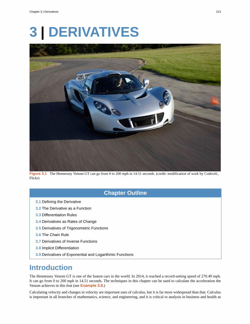
3 | DERIVATIVES
Figure 3.1 The Hennessey Venom GT can go from 0 to 200 mph in 14.51 seconds. (credit: modification of work by Codex41,Flickr)
Chapter Outline
3.1 Defining the Derivative
3.2 The Derivative as a Function
3.3 Differentiation Rules
3.4 Derivatives as Rates of Change
3.5 Derivatives of Trigonometric Functions
3.6 The Chain Rule
3.7 Derivatives of Inverse Functions
3.8 Implicit Differentiation
3.9 Derivatives of Exponential and Logarithmic Functions
IntroductionThe Hennessey Venom GT is one of the fastest cars in the world. In 2014, it reached a record-setting speed of 270.49 mph.It can go from 0 to 200 mph in 14.51 seconds. The techniques in this chapter can be used to calculate the acceleration theVenom achieves in this feat (see Example 3.8.)
Calculating velocity and changes in velocity are important uses of calculus, but it is far more widespread than that. Calculusis important in all branches of mathematics, science, and engineering, and it is critical to analysis in business and health as
Chapter 3 | Derivatives 213
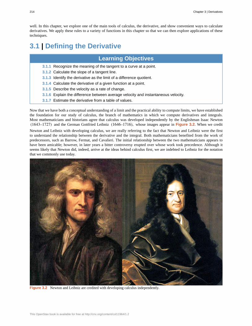
well. In this chapter, we explore one of the main tools of calculus, the derivative, and show convenient ways to calculatederivatives. We apply these rules to a variety of functions in this chapter so that we can then explore applications of thesetechniques.
3.1 | Defining the Derivative
Learning Objectives3.1.1 Recognize the meaning of the tangent to a curve at a point.
3.1.2 Calculate the slope of a tangent line.
3.1.3 Identify the derivative as the limit of a difference quotient.
3.1.4 Calculate the derivative of a given function at a point.
3.1.5 Describe the velocity as a rate of change.
3.1.6 Explain the difference between average velocity and instantaneous velocity.
3.1.7 Estimate the derivative from a table of values.
Now that we have both a conceptual understanding of a limit and the practical ability to compute limits, we have establishedthe foundation for our study of calculus, the branch of mathematics in which we compute derivatives and integrals.Most mathematicians and historians agree that calculus was developed independently by the Englishman Isaac Newton(1643–1727) and the German Gottfried Leibniz (1646–1716), whose images appear in Figure 3.2. When we credit
Newton and Leibniz with developing calculus, we are really referring to the fact that Newton and Leibniz were the firstto understand the relationship between the derivative and the integral. Both mathematicians benefited from the work ofpredecessors, such as Barrow, Fermat, and Cavalieri. The initial relationship between the two mathematicians appears tohave been amicable; however, in later years a bitter controversy erupted over whose work took precedence. Although itseems likely that Newton did, indeed, arrive at the ideas behind calculus first, we are indebted to Leibniz for the notationthat we commonly use today.
Figure 3.2 Newton and Leibniz are credited with developing calculus independently.
214 Chapter 3 | Derivatives
This OpenStax book is available for free at http://cnx.org/content/col11964/1.2
Tangent LinesWe begin our study of calculus by revisiting the notion of secant lines and tangent lines. Recall that we used the slope ofa secant line to a function at a point (a, f (a)) to estimate the rate of change, or the rate at which one variable changes in
relation to another variable. We can obtain the slope of the secant by choosing a value of x near a and drawing a line
through the points (a, f (a)) and ⎛⎝x, f (x)⎞
⎠, as shown in Figure 3.3. The slope of this line is given by an equation in the
form of a difference quotient:
msec = f (x) − f (a)x − a .
We can also calculate the slope of a secant line to a function at a value a by using this equation and replacing x with
a + h, where h is a value close to 0. We can then calculate the slope of the line through the points (a, f (a)) and
(a + h, f (a + h)). In this case, we find the secant line has a slope given by the following difference quotient with
increment h:
msec = f (a + h) − f (a)a + h − a = f (a + h) − f (a)
h .
Definition
Let f be a function defined on an interval I containing a. If x ≠ a is in I, then
(3.1)Q = f (x) − f (a)x − a
is a difference quotient.
Also, if h ≠ 0 is chosen so that a + h is in I, then
(3.2)Q = f (a + h) − f (a)h
is a difference quotient with increment h.
View the development of the derivative (http://www.openstaxcollege.org/l/20_calcapplets) with thisapplet.
These two expressions for calculating the slope of a secant line are illustrated in Figure 3.3. We will see that each of thesetwo methods for finding the slope of a secant line is of value. Depending on the setting, we can choose one or the other. Theprimary consideration in our choice usually depends on ease of calculation.
Chapter 3 | Derivatives 215
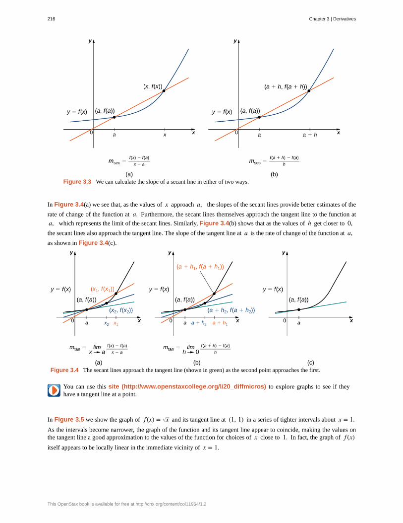
Figure 3.3 We can calculate the slope of a secant line in either of two ways.
In Figure 3.4(a) we see that, as the values of x approach a, the slopes of the secant lines provide better estimates of the
rate of change of the function at a. Furthermore, the secant lines themselves approach the tangent line to the function at
a, which represents the limit of the secant lines. Similarly, Figure 3.4(b) shows that as the values of h get closer to 0,the secant lines also approach the tangent line. The slope of the tangent line at a is the rate of change of the function at a,as shown in Figure 3.4(c).
Figure 3.4 The secant lines approach the tangent line (shown in green) as the second point approaches the first.
You can use this site (http://www.openstaxcollege.org/l/20_diffmicros) to explore graphs to see if theyhave a tangent line at a point.
In Figure 3.5 we show the graph of f (x) = x and its tangent line at (1, 1) in a series of tighter intervals about x = 1.As the intervals become narrower, the graph of the function and its tangent line appear to coincide, making the values onthe tangent line a good approximation to the values of the function for choices of x close to 1. In fact, the graph of f (x)itself appears to be locally linear in the immediate vicinity of x = 1.
216 Chapter 3 | Derivatives
This OpenStax book is available for free at http://cnx.org/content/col11964/1.2
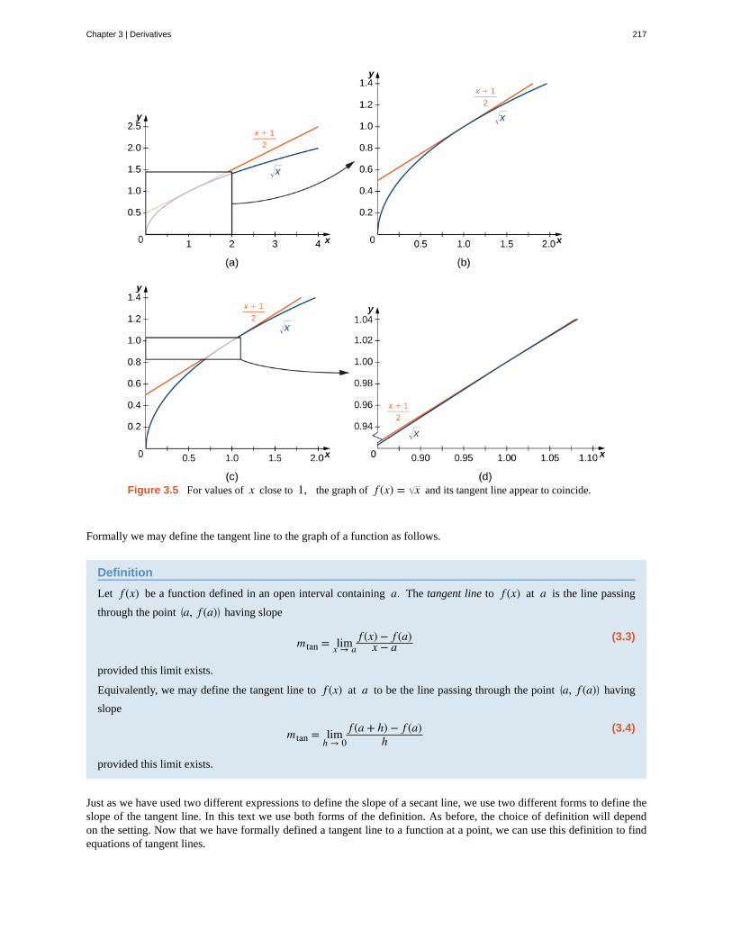
Figure 3.5 For values of x close to 1, the graph of f (x) = x and its tangent line appear to coincide.
Formally we may define the tangent line to the graph of a function as follows.
Definition
Let f (x) be a function defined in an open interval containing a. The tangent line to f (x) at a is the line passing
through the point ⎛⎝a, f (a)⎞
⎠ having slope
(3.3)mtan = limx → af (x) − f (a)
x − a
provided this limit exists.
Equivalently, we may define the tangent line to f (x) at a to be the line passing through the point ⎛⎝a, f (a)⎞
⎠ having
slope
(3.4)mtan = limh → 0
f (a + h) − f (a)h
provided this limit exists.
Just as we have used two different expressions to define the slope of a secant line, we use two different forms to define theslope of the tangent line. In this text we use both forms of the definition. As before, the choice of definition will dependon the setting. Now that we have formally defined a tangent line to a function at a point, we can use this definition to findequations of tangent lines.
Chapter 3 | Derivatives 217
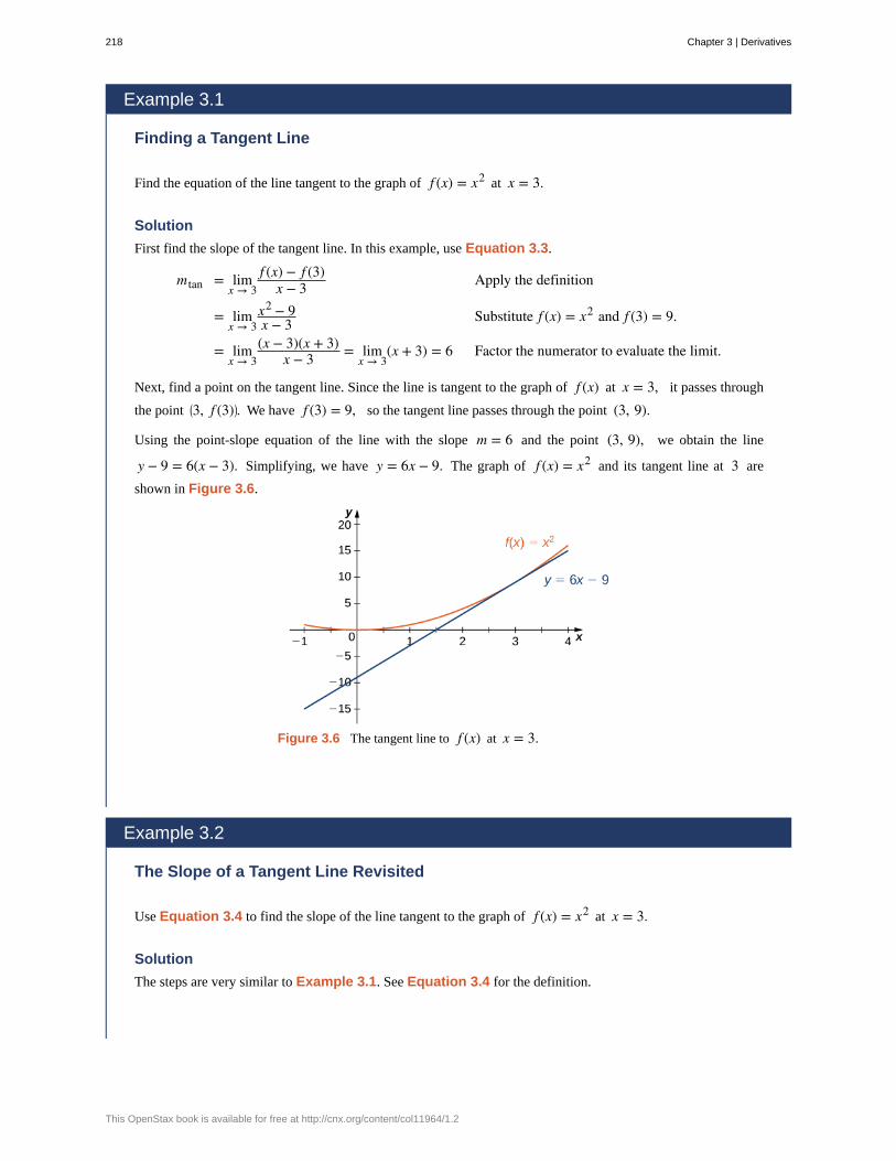
Example 3.1
Finding a Tangent Line
Find the equation of the line tangent to the graph of f (x) = x2 at x = 3.
Solution
First find the slope of the tangent line. In this example, use Equation 3.3.
mtan = limx → 3
f (x) − f (3)x − 3 Apply the definition
= limx → 3
x2 − 9x − 3 Substitute f (x) = x2 and f (3) = 9.
= limx → 3
(x − 3)(x + 3)x − 3 = lim
x → 3(x + 3) = 6 Factor the numerator to evaluate the limit.
Next, find a point on the tangent line. Since the line is tangent to the graph of f (x) at x = 3, it passes through
the point ⎛⎝3, f (3)⎞
⎠. We have f (3) = 9, so the tangent line passes through the point (3, 9).
Using the point-slope equation of the line with the slope m = 6 and the point (3, 9), we obtain the line
y − 9 = 6(x − 3). Simplifying, we have y = 6x − 9. The graph of f (x) = x2 and its tangent line at 3 are
shown in Figure 3.6.
Figure 3.6 The tangent line to f (x) at x = 3.
Example 3.2
The Slope of a Tangent Line Revisited
Use Equation 3.4 to find the slope of the line tangent to the graph of f (x) = x2 at x = 3.
Solution
The steps are very similar to Example 3.1. See Equation 3.4 for the definition.
218 Chapter 3 | Derivatives
This OpenStax book is available for free at http://cnx.org/content/col11964/1.2
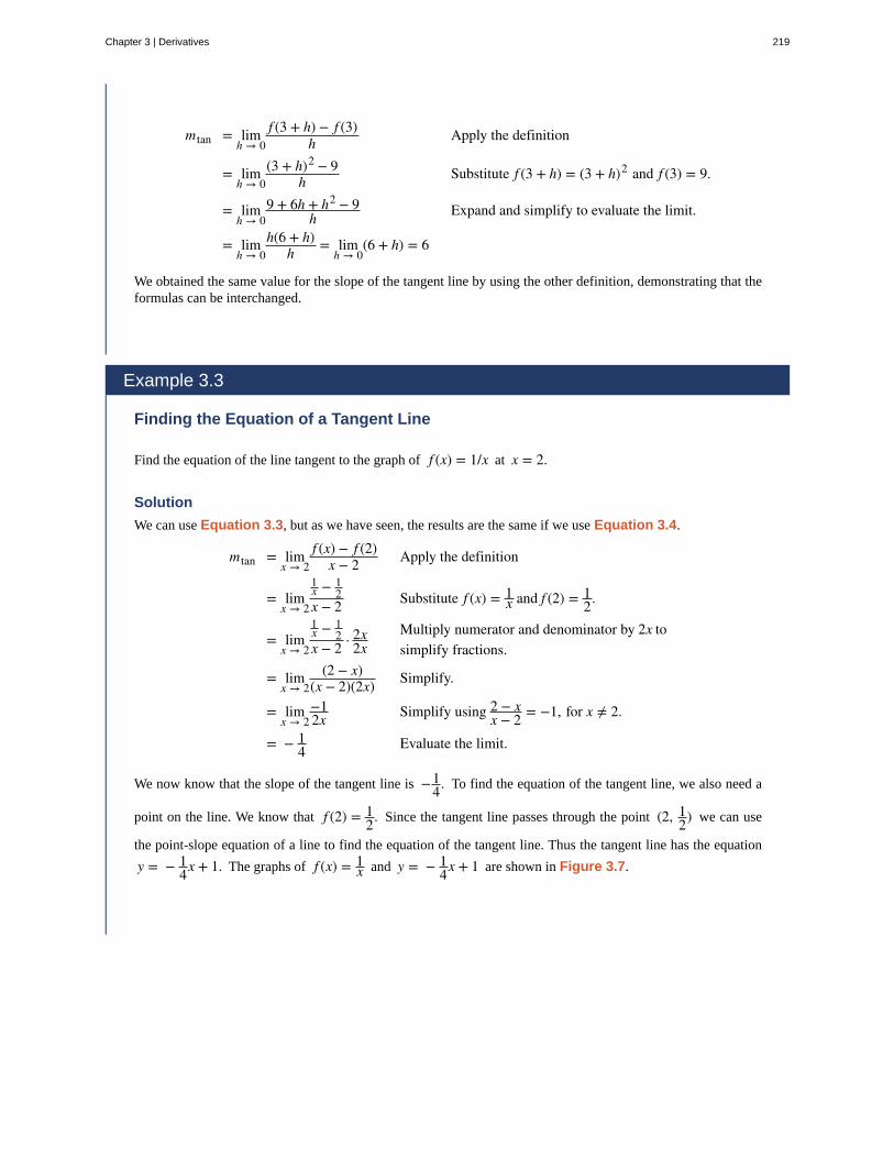
mtan = limh → 0
f (3 + h) − f (3)h Apply the definition
= limh → 0
(3 + h)2 − 9h Substitute f (3 + h) = (3 + h)2 and f (3) = 9.
= limh → 0
9 + 6h + h2 − 9h Expand and simplify to evaluate the limit.
= limh → 0
h(6 + h)h = lim
h → 0(6 + h) = 6
We obtained the same value for the slope of the tangent line by using the other definition, demonstrating that theformulas can be interchanged.
Example 3.3
Finding the Equation of a Tangent Line
Find the equation of the line tangent to the graph of f (x) = 1/x at x = 2.
Solution
We can use Equation 3.3, but as we have seen, the results are the same if we use Equation 3.4.
mtan = limx → 2
f (x) − f (2)x − 2 Apply the definition
= limx → 2
1x − 1
2x − 2 Substitute f (x) = 1
x and f (2) = 12.
= limx → 2
1x − 1
2x − 2 · 2x
2xMultiply numerator and denominator by 2x tosimplify fractions.
= limx → 2
(2 − x)(x − 2)(2x) Simplify.
= limx → 2
−12x Simplify using 2 − x
x − 2 = −1, for x ≠ 2.
= − 14 Evaluate the limit.
We now know that the slope of the tangent line is −14. To find the equation of the tangent line, we also need a
point on the line. We know that f (2) = 12. Since the tangent line passes through the point (2, 1
2) we can use
the point-slope equation of a line to find the equation of the tangent line. Thus the tangent line has the equation
y = − 14x + 1. The graphs of f (x) = 1
x and y = − 14x + 1 are shown in Figure 3.7.
Chapter 3 | Derivatives 219
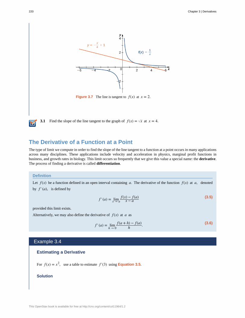
3.1
Figure 3.7 The line is tangent to f (x) at x = 2.
Find the slope of the line tangent to the graph of f (x) = x at x = 4.
The Derivative of a Function at a PointThe type of limit we compute in order to find the slope of the line tangent to a function at a point occurs in many applicationsacross many disciplines. These applications include velocity and acceleration in physics, marginal profit functions inbusiness, and growth rates in biology. This limit occurs so frequently that we give this value a special name: the derivative.The process of finding a derivative is called differentiation.
Definition
Let f (x) be a function defined in an open interval containing a. The derivative of the function f (x) at a, denoted
by f ′ (a), is defined by
(3.5)f ′ (a) = limx → af (x) − f (a)
x − a
provided this limit exists.
Alternatively, we may also define the derivative of f (x) at a as
(3.6)f ′ (a) = limh → 0
f (a + h) − f (a)h .
Example 3.4
Estimating a Derivative
For f (x) = x2, use a table to estimate f ′(3) using Equation 3.5.
Solution
220 Chapter 3 | Derivatives
This OpenStax book is available for free at http://cnx.org/content/col11964/1.2
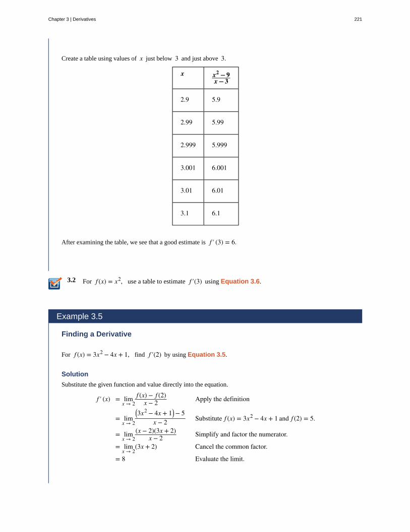
3.2
Create a table using values of x just below 3 and just above 3.
x x2 − 9x − 3
2.9 5.9
2.99 5.99
2.999 5.999
3.001 6.001
3.01 6.01
3.1 6.1
After examining the table, we see that a good estimate is f ′ (3) = 6.
For f (x) = x2, use a table to estimate f ′(3) using Equation 3.6.
Example 3.5
Finding a Derivative
For f (x) = 3x2 − 4x + 1, find f ′(2) by using Equation 3.5.
Solution
Substitute the given function and value directly into the equation.
f ′ (x) = limx → 2
f (x) − f (2)x − 2 Apply the definition
= limx → 2
⎛⎝3x2 − 4x + 1⎞
⎠ − 5x − 2 Substitute f (x) = 3x2 − 4x + 1 and f (2) = 5.
= limx → 2
(x − 2)(3x + 2)x − 2 Simplify and factor the numerator.
= limx → 2
(3x + 2) Cancel the common factor.
= 8 Evaluate the limit.
Chapter 3 | Derivatives 221
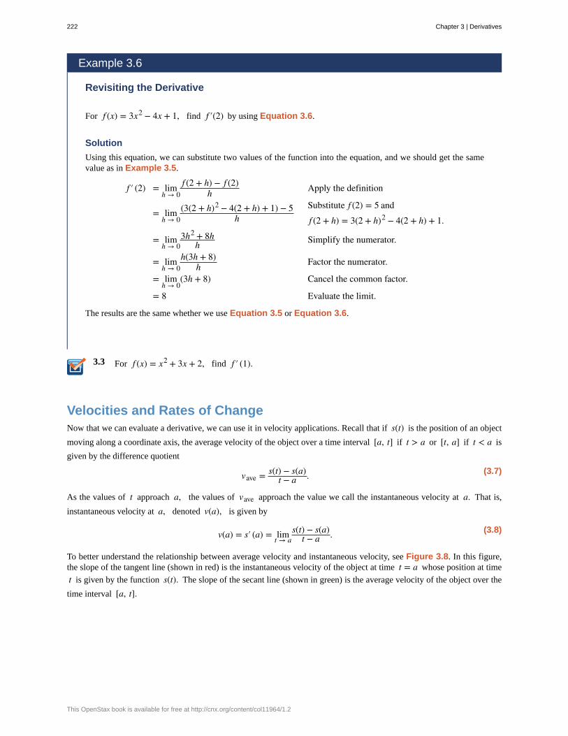
3.3
Example 3.6
Revisiting the Derivative
For f (x) = 3x2 − 4x + 1, find f ′(2) by using Equation 3.6.
Solution
Using this equation, we can substitute two values of the function into the equation, and we should get the samevalue as in Example 3.5.
f ′ (2) = limh → 0
f (2 + h) − f (2)h Apply the definition
= limh → 0
(3(2 + h)2 − 4(2 + h) + 1) − 5h
Substitute f (2) = 5 and
f (2 + h) = 3(2 + h)2 − 4(2 + h) + 1.
= limh → 0
3h2 + 8hh Simplify the numerator.
= limh → 0
h(3h + 8)h Factor the numerator.
= limh → 0
(3h + 8) Cancel the common factor.
= 8 Evaluate the limit.
The results are the same whether we use Equation 3.5 or Equation 3.6.
For f (x) = x2 + 3x + 2, find f ′ (1).
Velocities and Rates of ChangeNow that we can evaluate a derivative, we can use it in velocity applications. Recall that if s(t) is the position of an object
moving along a coordinate axis, the average velocity of the object over a time interval [a, t] if t > a or [t, a] if t < a is
given by the difference quotient
(3.7)vave = s(t) − s(a)t − a .
As the values of t approach a, the values of vave approach the value we call the instantaneous velocity at a. That is,
instantaneous velocity at a, denoted v(a), is given by
(3.8)v(a) = s′ (a) = limt → a
s(t) − s(a)t − a .
To better understand the relationship between average velocity and instantaneous velocity, see Figure 3.8. In this figure,the slope of the tangent line (shown in red) is the instantaneous velocity of the object at time t = a whose position at time
t is given by the function s(t). The slope of the secant line (shown in green) is the average velocity of the object over the
time interval [a, t].
222 Chapter 3 | Derivatives
This OpenStax book is available for free at http://cnx.org/content/col11964/1.2
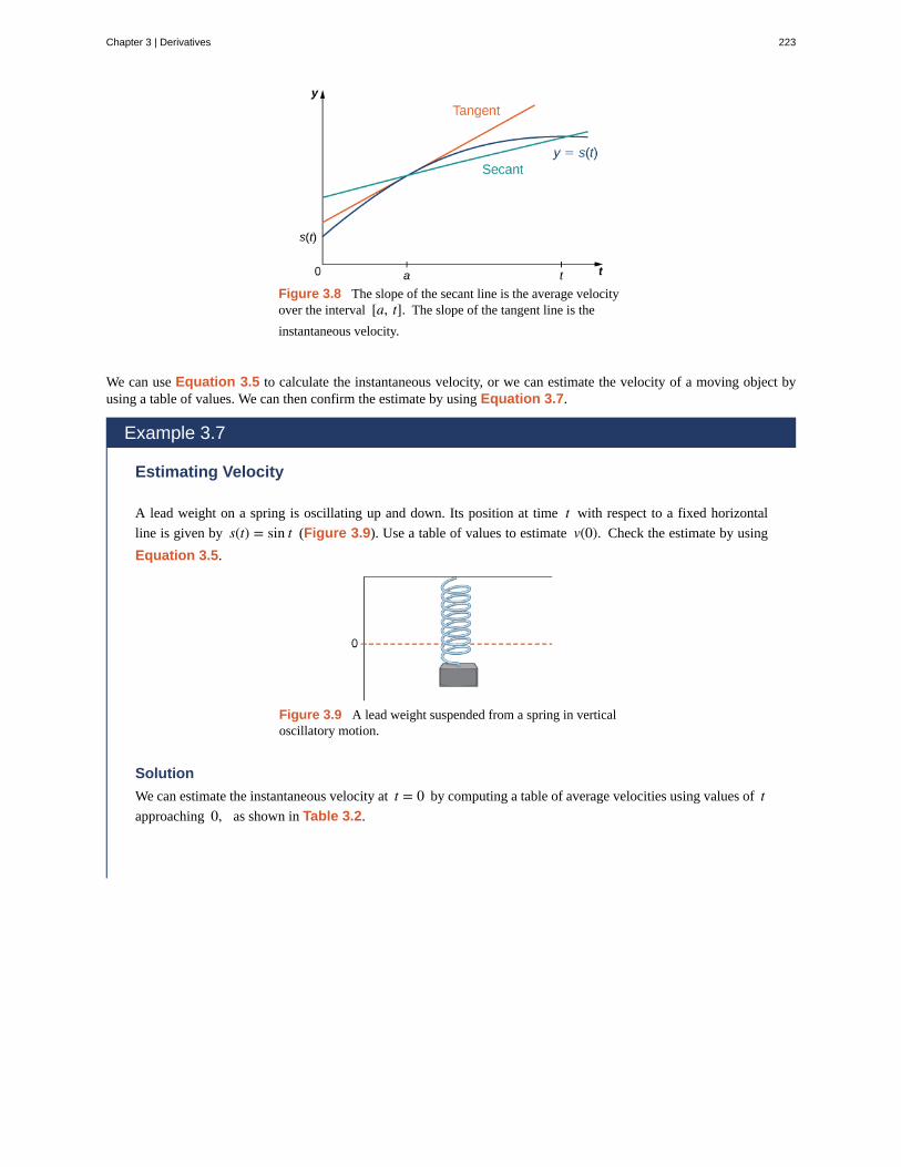
Figure 3.8 The slope of the secant line is the average velocityover the interval [a, t]. The slope of the tangent line is the
instantaneous velocity.
We can use Equation 3.5 to calculate the instantaneous velocity, or we can estimate the velocity of a moving object byusing a table of values. We can then confirm the estimate by using Equation 3.7.
Example 3.7
Estimating Velocity
A lead weight on a spring is oscillating up and down. Its position at time t with respect to a fixed horizontal
line is given by s(t) = sin t (Figure 3.9). Use a table of values to estimate v(0). Check the estimate by using
Equation 3.5.
Figure 3.9 A lead weight suspended from a spring in verticaloscillatory motion.
Solution
We can estimate the instantaneous velocity at t = 0 by computing a table of average velocities using values of tapproaching 0, as shown in Table 3.2.
Chapter 3 | Derivatives 223
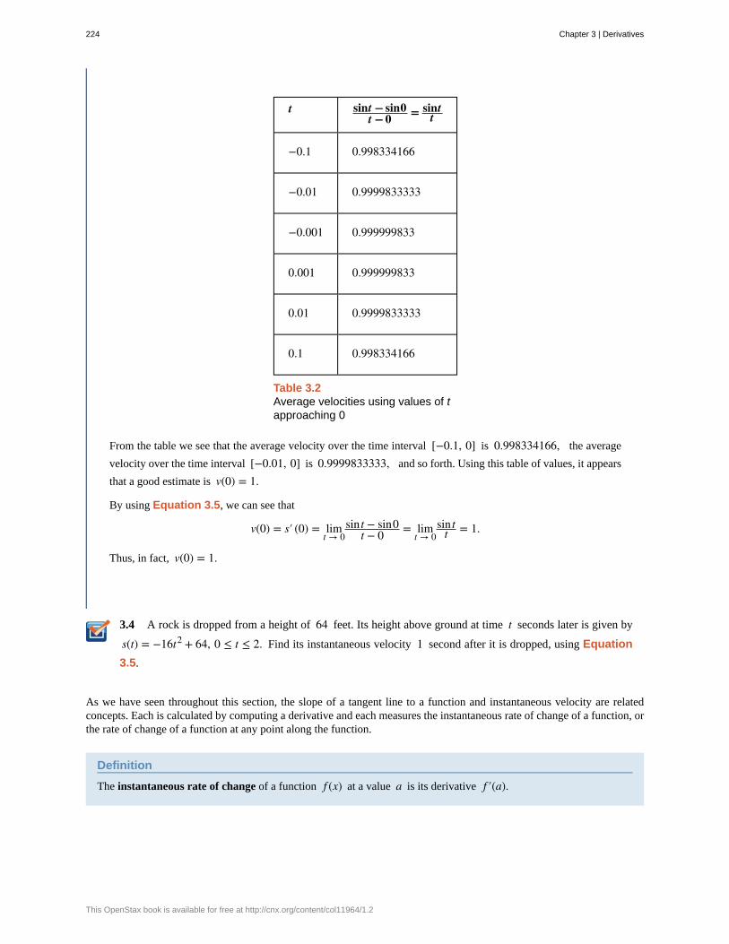
3.4
t sint − sin0t − 0 = sint
t
−0.1 0.998334166
−0.01 0.9999833333
−0.001 0.999999833
0.001 0.999999833
0.01 0.9999833333
0.1 0.998334166
Table 3.2Average velocities using values of tapproaching 0
From the table we see that the average velocity over the time interval [−0.1, 0] is 0.998334166, the average
velocity over the time interval [−0.01, 0] is 0.9999833333, and so forth. Using this table of values, it appears
that a good estimate is v(0) = 1.
By using Equation 3.5, we can see that
v(0) = s′ (0) = limt → 0
sin t − sin0t − 0 = lim
t → 0sin t
t = 1.
Thus, in fact, v(0) = 1.
A rock is dropped from a height of 64 feet. Its height above ground at time t seconds later is given by
s(t) = −16t2 + 64, 0 ≤ t ≤ 2. Find its instantaneous velocity 1 second after it is dropped, using Equation
3.5.
As we have seen throughout this section, the slope of a tangent line to a function and instantaneous velocity are relatedconcepts. Each is calculated by computing a derivative and each measures the instantaneous rate of change of a function, orthe rate of change of a function at any point along the function.
Definition
The instantaneous rate of change of a function f (x) at a value a is its derivative f ′(a).
224 Chapter 3 | Derivatives
This OpenStax book is available for free at http://cnx.org/content/col11964/1.2
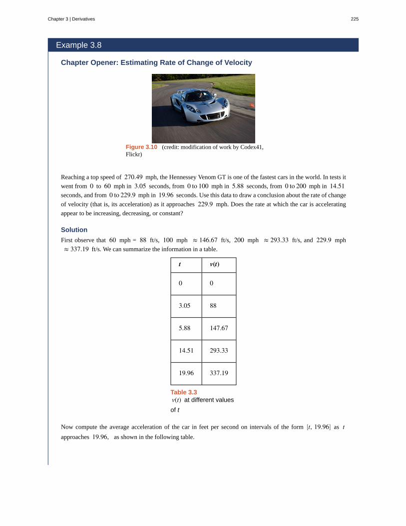
Example 3.8
Chapter Opener: Estimating Rate of Change of Velocity
Figure 3.10 (credit: modification of work by Codex41,Flickr)
Reaching a top speed of 270.49 mph, the Hennessey Venom GT is one of the fastest cars in the world. In tests it
went from 0 to 60 mph in 3.05 seconds, from 0 to 100 mph in 5.88 seconds, from 0 to 200 mph in 14.51seconds, and from 0 to 229.9 mph in 19.96 seconds. Use this data to draw a conclusion about the rate of change
of velocity (that is, its acceleration) as it approaches 229.9 mph. Does the rate at which the car is accelerating
appear to be increasing, decreasing, or constant?
Solution
First observe that 60 mph = 88 ft/s, 100 mph ≈ 146.67 ft/s, 200 mph ≈ 293.33 ft/s, and 229.9 mph
≈ 337.19 ft/s. We can summarize the information in a table.
t v(t)
0 0
3.05 88
5.88 147.67
14.51 293.33
19.96 337.19
Table 3.3v(t) at different values
of t
Now compute the average acceleration of the car in feet per second on intervals of the form ⎡⎣t, 19.96⎤
⎦ as tapproaches 19.96, as shown in the following table.
Chapter 3 | Derivatives 225
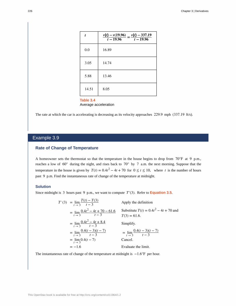
t v(t) − v(19.96)t − 19.96 = v(t) − 337.19
t − 19.96
0.0 16.89
3.05 14.74
5.88 13.46
14.51 8.05
Table 3.4Average acceleration
The rate at which the car is accelerating is decreasing as its velocity approaches 229.9 mph (337.19 ft/s).
Example 3.9
Rate of Change of Temperature
A homeowner sets the thermostat so that the temperature in the house begins to drop from 70°F at 9 p.m.,
reaches a low of 60° during the night, and rises back to 70° by 7 a.m. the next morning. Suppose that the
temperature in the house is given by T(t) = 0.4t2 − 4t + 70 for 0 ≤ t ≤ 10, where t is the number of hours
past 9 p.m. Find the instantaneous rate of change of the temperature at midnight.
Solution
Since midnight is 3 hours past 9 p.m., we want to compute T′(3). Refer to Equation 3.5.
T′ (3) = limt → 3
T(t) − T(3)t − 3 Apply the definition
= limt → 3
0.4t2 − 4t + 70 − 61.6t − 3
Substitute T(t) = 0.4t2 − 4t + 70 andT(3) = 61.6.
= limt → 3
0.4t2 − 4t + 8.4t − 3 Simplify.
= limt → 3
0.4(t − 3)(t − 7)t − 3 = lim
t → 30.4(t − 3)(t − 7)
t − 3= lim
t → 30.4(t − 7) Cancel.
= −1.6 Evaluate the limit.
The instantaneous rate of change of the temperature at midnight is −1.6°F per hour.
226 Chapter 3 | Derivatives
This OpenStax book is available for free at http://cnx.org/content/col11964/1.2
3.5
Example 3.10
Rate of Change of Profit
A toy company can sell x electronic gaming systems at a price of p = −0.01x + 400 dollars per gaming
system. The cost of manufacturing x systems is given by C(x) = 100x + 10,000 dollars. Find the rate of change
of profit when 10,000 games are produced. Should the toy company increase or decrease production?
Solution
The profit P(x) earned by producing x gaming systems is R(x) − C(x), where R(x) is the revenue obtained
from the sale of x games. Since the company can sell x games at p = −0.01x + 400 per game,
R(x) = xp = x(−0.01x + 400) = −0.01x2 + 400x.
Consequently,
P(x) = −0.01x2 + 300x − 10,000.
Therefore, evaluating the rate of change of profit gives
P′ (10000) = limx → 10000
P(x) − P(10000)x − 10000
= limx → 10000
−0.01x2 + 300x − 10000 − 1990000x − 10000
= limx → 10000
−0.01x2 + 300x − 2000000x − 10000
= 100.
Since the rate of change of profit P′ (10,000) > 0 and P(10,000) > 0, the company should increase
production.
A coffee shop determines that the daily profit on scones obtained by charging s dollars per scone is
P(s) = −20s2 + 150s − 10. The coffee shop currently charges $3.25 per scone. Find P′(3.25), the rate of
change of profit when the price is $3.25 and decide whether or not the coffee shop should consider raising or
lowering its prices on scones.
Chapter 3 | Derivatives 227
3.1 EXERCISESFor the following exercises, use Equation 3.3 to find theslope of the secant line between the values x1 and x2 for
each function y = f (x).
1. f (x) = 4x + 7; x1 = 2, x2 = 5
2. f (x) = 8x − 3; x1 = −1, x2 = 3
3. f (x) = x2 + 2x + 1; x1 = 3, x2 = 3.5
4. f (x) = −x2 + x + 2; x1 = 0.5, x2 = 1.5
5. f (x) = 43x − 1; x1 = 1, x2 = 3
6. f (x) = x − 72x + 1; x1 = −2, x2 = 0
7. f (x) = x; x1 = 1, x2 = 16
8. f (x) = x − 9; x1 = 10, x2 = 13
9. f (x) = x1/3 + 1; x1 = 0, x2 = 8
10. f (x) = 6x2/3 + 2x1/3; x1 = 1, x2 = 27
For the following functions,
a. use Equation 3.4 to find the slope of the tangentline mtan = f ′ (a), and
b. find the equation of the tangent line to f at x = a.
11. f (x) = 3 − 4x, a = 2
12. f (x) = x5 + 6, a = −1
13. f (x) = x2 + x, a = 1
14. f (x) = 1 − x − x2, a = 0
15. f (x) = 7x , a = 3
16. f (x) = x + 8, a = 1
17. f (x) = 2 − 3x2, a = −2
18. f (x) = −3x − 1, a = 4
19. f (x) = 2x + 3, a = −4
20. f (x) = 3x2, a = 3
For the following functions y = f (x), find f ′ (a) using
Equation 3.3.
21. f (x) = 5x + 4, a = −1
22. f (x) = −7x + 1, a = 3
23. f (x) = x2 + 9x, a = 2
24. f (x) = 3x2 − x + 2, a = 1
25. f (x) = x, a = 4
26. f (x) = x − 2, a = 6
27. f (x) = 1x , a = 2
28. f (x) = 1x − 3, a = −1
29. f (x) = 1x3, a = 1
30. f (x) = 1x, a = 4
For the following exercises, given the function y = f (x),
a. find the slope of the secant line PQ for each point
Q⎛⎝x, f (x)⎞
⎠ with x value given in the table.
b. Use the answers from a. to estimate the value of theslope of the tangent line at P.
c. Use the answer from b. to find the equation of thetangent line to f at point P.
228 Chapter 3 | Derivatives
This OpenStax book is available for free at http://cnx.org/content/col11964/1.2
31. [T] f (x) = x2 + 3x + 4, P(1, 8) (Round to 6decimal places.)
x SlopemPQ
x SlopemPQ
1.1 (i) 0.9 (vii)
1.01 (ii) 0.99 (viii)
1.001 (iii) 0.999 (ix)
1.0001 (iv) 0.9999 (x)
1.00001 (v) 0.99999 (xi)
1.000001 (vi) 0.999999 (xii)
32. [T] f (x) = x + 1x2 − 1
, P(0, −1)
x SlopemPQ
x SlopemPQ
0.1 (i) −0.1 (vii)
0.01 (ii) −0.01 (viii)
0.001 (iii) −0.001 (ix)
0.0001 (iv) −0.0001 (x)
0.00001 (v) −0.00001 (xi)
0.000001 (vi) −0.000001 (xii)
33. [T] f (x) = 10e0.5x, P(0, 10) (Round to 4 decimal
places.)
x Slope mPQ
−0.1 (i)
−0.01 (ii)
−0.001 (iii)
−0.0001 (iv)
−0.00001 (v)
−0.000001 (vi)
34. [T] f (x) = tan(x), P(π, 0)
x Slope mPQ
3.1 (i)
3.14 (ii)
3.141 (iii)
3.1415 (iv)
3.14159 (v)
3.141592 (vi)
[T] For the following position functions y = s(t), an
object is moving along a straight line, where t is in seconds
and s is in meters. Find
a. the simplified expression for the average velocityfrom t = 2 to t = 2 + h;
b. the average velocity between t = 2 and
t = 2 + h, where (i) h = 0.1, (ii) h = 0.01,(iii) h = 0.001, and (iv) h = 0.0001; and
c. use the answer from a. to estimate the instantaneous
Chapter 3 | Derivatives 229
velocity at t = 2 second.
35. s(t) = 13t + 5
36. s(t) = t2 − 2t
37. s(t) = 2t3 + 3
38. s(t) = 16t2 − 4
t
39. Use the following graph to evaluate a. f ′ (1) and b.
f ′ (6).
40. Use the following graph to evaluate a. f ′ (−3) and b.
f ′ (1.5).
For the following exercises, use the limit definition ofderivative to show that the derivative does not exist atx = a for each of the given functions.
41. f (x) = x1/3, x = 0
42. f (x) = x2/3, x = 0
43. f (x) =⎧
⎩⎨1, x < 1x, x ≥ 1
, x = 1
44. f (x) = |x|x , x = 0
45. [T] The position in feet of a race car along a straighttrack after t seconds is modeled by the function
s(t) = 8t2 − 116t3.
a. Find the average velocity of the vehicle over thefollowing time intervals to four decimal places:
i. [4, 4.1]ii. [4, 4.01]
iii. [4, 4.001]iv. [4, 4.0001]
b. Use a. to draw a conclusion about the instantaneousvelocity of the vehicle at t = 4 seconds.
46. [T] The distance in feet that a ball rolls down an
incline is modeled by the function s(t) = 14t2, where t is
seconds after the ball begins rolling.a. Find the average velocity of the ball over the
following time intervals:i. [5, 5.1]
ii. [5, 5.01]iii. [5, 5.001]iv. [5, 5.0001]
b. Use the answers from a. to draw a conclusion aboutthe instantaneous velocity of the ball at t = 5seconds.
47. Two vehicles start out traveling side by side alonga straight road. Their position functions, shown in thefollowing graph, are given by s = f (t) and s = g(t),where s is measured in feet and t is measured in seconds.
a. Which vehicle has traveled farther at t = 2seconds?
b. What is the approximate velocity of each vehicle att = 3 seconds?
c. Which vehicle is traveling faster at t = 4 seconds?
d. What is true about the positions of the vehicles att = 4 seconds?
230 Chapter 3 | Derivatives
This OpenStax book is available for free at http://cnx.org/content/col11964/1.2
48. [T] The total cost C(x), in hundreds of dollars,
to produce x jars of mayonnaise is given by
C(x) = 0.000003x3 + 4x + 300.a. Calculate the average cost per jar over the
following intervals:i. [100, 100.1]
ii. [100, 100.01]iii. [100, 100.001]iv. [100, 100.0001]
b. Use the answers from a. to estimate the averagecost to produce 100 jars of mayonnaise.
49. [T] For the function f (x) = x3 − 2x2 − 11x + 12,do the following.
a. Use a graphing calculator to graph f in anappropriate viewing window.
b. Use the ZOOM feature on the calculator toapproximate the two values of x = a for which
mtan = f ′ (a) = 0.
50. [T] For the function f (x) = x1 + x2, do the
following.a. Use a graphing calculator to graph f in an
appropriate viewing window.b. Use the ZOOM feature on the calculator to
approximate the values of x = a for which
mtan = f ′ (a) = 0.
51. Suppose that N(x) computes the number of gallons
of gas used by a vehicle traveling x miles. Suppose the
vehicle gets 30 mpg.
a. Find a mathematical expression for N(x).b. What is N(100)? Explain the physical meaning.
c. What is N′(100)? Explain the physical meaning.
52. [T] For the function f (x) = x4 − 5x2 + 4, do the
following.a. Use a graphing calculator to graph f in an
appropriate viewing window.b. Use the nDeriv function, which numerically finds
the derivative, on a graphing calculator to estimatef ′ (−2), f ′(−0.5), f ′(1.7), and f ′(2.718).
53. [T] For the function f (x) = x2
x2 + 1, do the
following.a. Use a graphing calculator to graph f in an
appropriate viewing window.b. Use the nDeriv function on a graphing calculator
to find f ′ (−4), f ′(−2), f ′(2), and f ′(4).
Chapter 3 | Derivatives 231
3.2 | The Derivative as a Function
Learning Objectives3.2.1 Define the derivative function of a given function.
3.2.2 Graph a derivative function from the graph of a given function.
3.2.3 State the connection between derivatives and continuity.
3.2.4 Describe three conditions for when a function does not have a derivative.
3.2.5 Explain the meaning of a higher-order derivative.
As we have seen, the derivative of a function at a given point gives us the rate of change or slope of the tangent line to thefunction at that point. If we differentiate a position function at a given time, we obtain the velocity at that time. It seemsreasonable to conclude that knowing the derivative of the function at every point would produce valuable information aboutthe behavior of the function. However, the process of finding the derivative at even a handful of values using the techniquesof the preceding section would quickly become quite tedious. In this section we define the derivative function and learn aprocess for finding it.
Derivative FunctionsThe derivative function gives the derivative of a function at each point in the domain of the original function for which thederivative is defined. We can formally define a derivative function as follows.
Definition
Let f be a function. The derivative function, denoted by f ′, is the function whose domain consists of those values
of x such that the following limit exists:
(3.9)f ′ (x) = limh → 0
f (x + h) − f (x)h .
A function f (x) is said to be differentiable at a if f ′(a) exists. More generally, a function is said to be differentiable
on S if it is differentiable at every point in an open set S, and a differentiable function is one in which f ′(x) exists on
its domain.
In the next few examples we use Equation 3.9 to find the derivative of a function.
Example 3.11
Finding the Derivative of a Square-Root Function
Find the derivative of f (x) = x.
Solution
Start directly with the definition of the derivative function. Use Equation 3.1.
232 Chapter 3 | Derivatives
This OpenStax book is available for free at http://cnx.org/content/col11964/1.2
3.6
f ′ (x) = limh → 0
x + h − xh
Substitute f (x + h) = x + h and f (x) = x
into f ′ (x) = limh → 0
f (x + h) − f (x)h .
= limh → 0
x + h − xh · x + h + x
x + h + x
Multiply numerator and denominator byx + h + x without distributing in the
denominator.= lim
h → 0h
h( x + h + x)Multiply the numerators and simplify.
= limh → 0
1( x + h + x)
Cancel the h.
= 12 x Evaluate the limit.
Example 3.12
Finding the Derivative of a Quadratic Function
Find the derivative of the function f (x) = x2 − 2x.
Solution
Follow the same procedure here, but without having to multiply by the conjugate.
f ′ (x) = limh → 0
((x + h)2 − 2(x + h)) − (x2 − 2x)h
Substitute f (x + h) = (x + h)2 − 2(x + h) and
f (x) = x2 − 2x into
f ′ (x) = limh → 0
f (x + h) − f (x)h .
= limh → 0
x2 + 2xh + h2 − 2x − 2h − x2 + 2xh Expand (x + h)2 − 2(x + h).
= limh → 0
2xh − 2h + h2
h Simplify.
= limh → 0
h(2x − 2 + h)h Factor out h from the numerator.
= limh → 0
(2x − 2 + h) Cancel the common factor of h.
= 2x − 2 Evaluate the limit.
Find the derivative of f (x) = x2.
We use a variety of different notations to express the derivative of a function. In Example 3.12 we showed that if
f (x) = x2 − 2x, then f ′ (x) = 2x − 2. If we had expressed this function in the form y = x2 − 2x, we could have
expressed the derivative as y′ = 2x − 2 ordydx = 2x − 2. We could have conveyed the same information by writing
ddx
⎛⎝x2 − 2x⎞
⎠ = 2x − 2. Thus, for the function y = f (x), each of the following notations represents the derivative of
f (x):
Chapter 3 | Derivatives 233
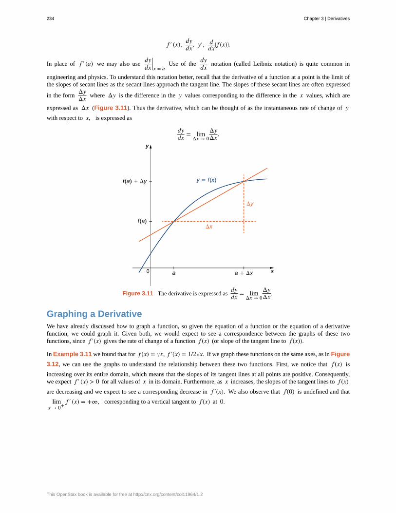
f ′ (x), dydx, y′, d
dx⎛⎝ f (x)⎞
⎠.
In place of f ′ (a) we may also usedydx |x = a
Use of thedydx notation (called Leibniz notation) is quite common in
engineering and physics. To understand this notation better, recall that the derivative of a function at a point is the limit ofthe slopes of secant lines as the secant lines approach the tangent line. The slopes of these secant lines are often expressed
in the formΔyΔx where Δy is the difference in the y values corresponding to the difference in the x values, which are
expressed as Δx (Figure 3.11). Thus the derivative, which can be thought of as the instantaneous rate of change of ywith respect to x, is expressed as
dydx = lim
Δx → 0ΔyΔx.
Figure 3.11 The derivative is expressed asdydx = lim
Δx → 0ΔyΔx.
Graphing a DerivativeWe have already discussed how to graph a function, so given the equation of a function or the equation of a derivativefunction, we could graph it. Given both, we would expect to see a correspondence between the graphs of these twofunctions, since f ′(x) gives the rate of change of a function f (x) (or slope of the tangent line to f (x)).
In Example 3.11 we found that for f (x) = x, f ′(x) = 1/2 x. If we graph these functions on the same axes, as in Figure
3.12, we can use the graphs to understand the relationship between these two functions. First, we notice that f (x) is
increasing over its entire domain, which means that the slopes of its tangent lines at all points are positive. Consequently,we expect f ′ (x) > 0 for all values of x in its domain. Furthermore, as x increases, the slopes of the tangent lines to f (x)are decreasing and we expect to see a corresponding decrease in f ′(x). We also observe that f (0) is undefined and that
limx → 0+
f ′ (x) = +∞, corresponding to a vertical tangent to f (x) at 0.
234 Chapter 3 | Derivatives
This OpenStax book is available for free at http://cnx.org/content/col11964/1.2
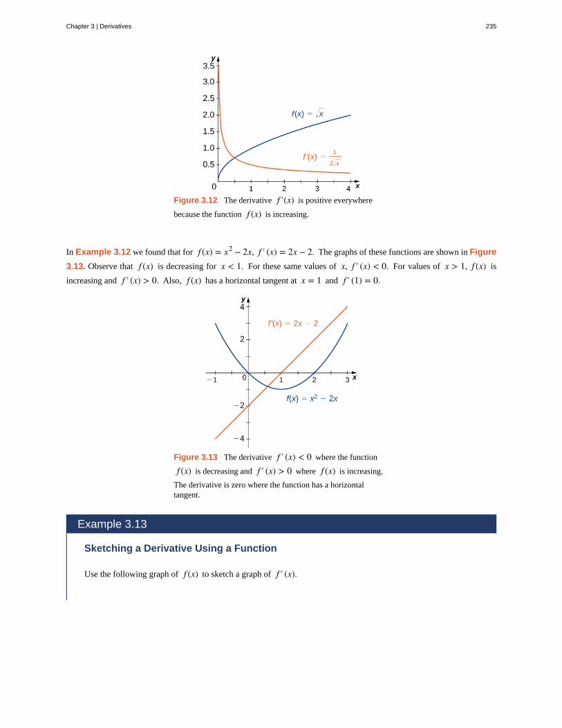
Figure 3.12 The derivative f ′(x) is positive everywhere
because the function f (x) is increasing.
In Example 3.12 we found that for f (x) = x2 − 2x, f ′ (x) = 2x − 2. The graphs of these functions are shown in Figure
3.13. Observe that f (x) is decreasing for x < 1. For these same values of x, f ′ (x) < 0. For values of x > 1, f (x) is
increasing and f ′ (x) > 0. Also, f (x) has a horizontal tangent at x = 1 and f ′ (1) = 0.
Figure 3.13 The derivative f ′ (x) < 0 where the function
f (x) is decreasing and f ′ (x) > 0 where f (x) is increasing.
The derivative is zero where the function has a horizontaltangent.
Example 3.13
Sketching a Derivative Using a Function
Use the following graph of f (x) to sketch a graph of f ′ (x).
Chapter 3 | Derivatives 235
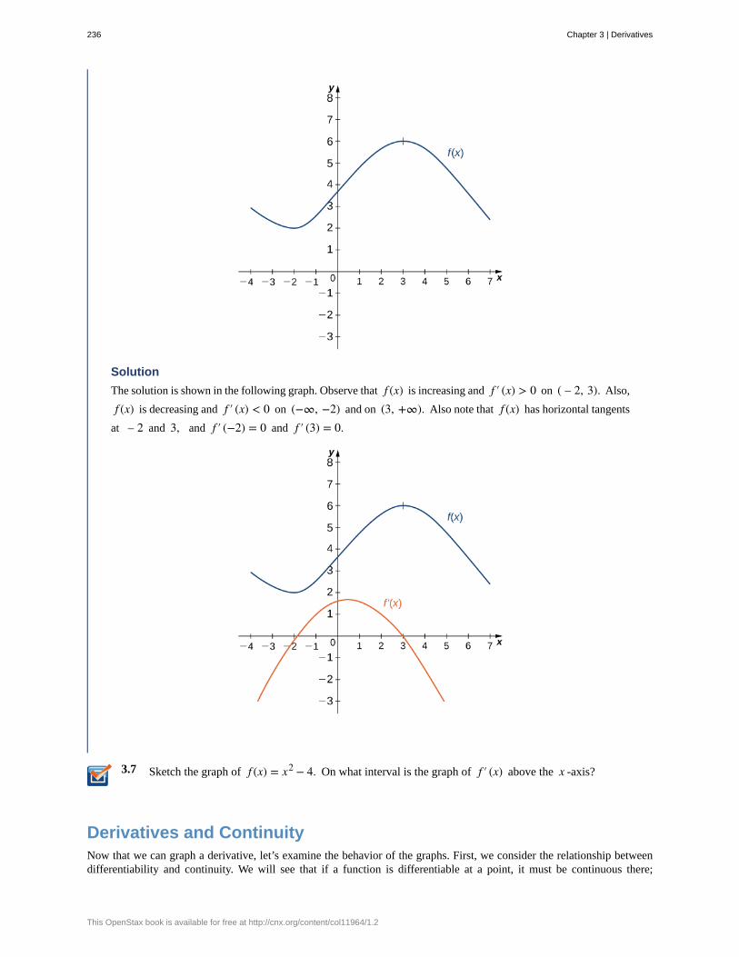
3.7
Solution
The solution is shown in the following graph. Observe that f (x) is increasing and f ′ (x) > 0 on ( – 2, 3). Also,
f (x) is decreasing and f ′ (x) < 0 on (−∞, −2) and on (3, +∞). Also note that f (x) has horizontal tangents
at – 2 and 3, and f ′ (−2) = 0 and f ′ (3) = 0.
Sketch the graph of f (x) = x2 − 4. On what interval is the graph of f ′ (x) above the x -axis?
Derivatives and ContinuityNow that we can graph a derivative, let’s examine the behavior of the graphs. First, we consider the relationship betweendifferentiability and continuity. We will see that if a function is differentiable at a point, it must be continuous there;
236 Chapter 3 | Derivatives
This OpenStax book is available for free at http://cnx.org/content/col11964/1.2
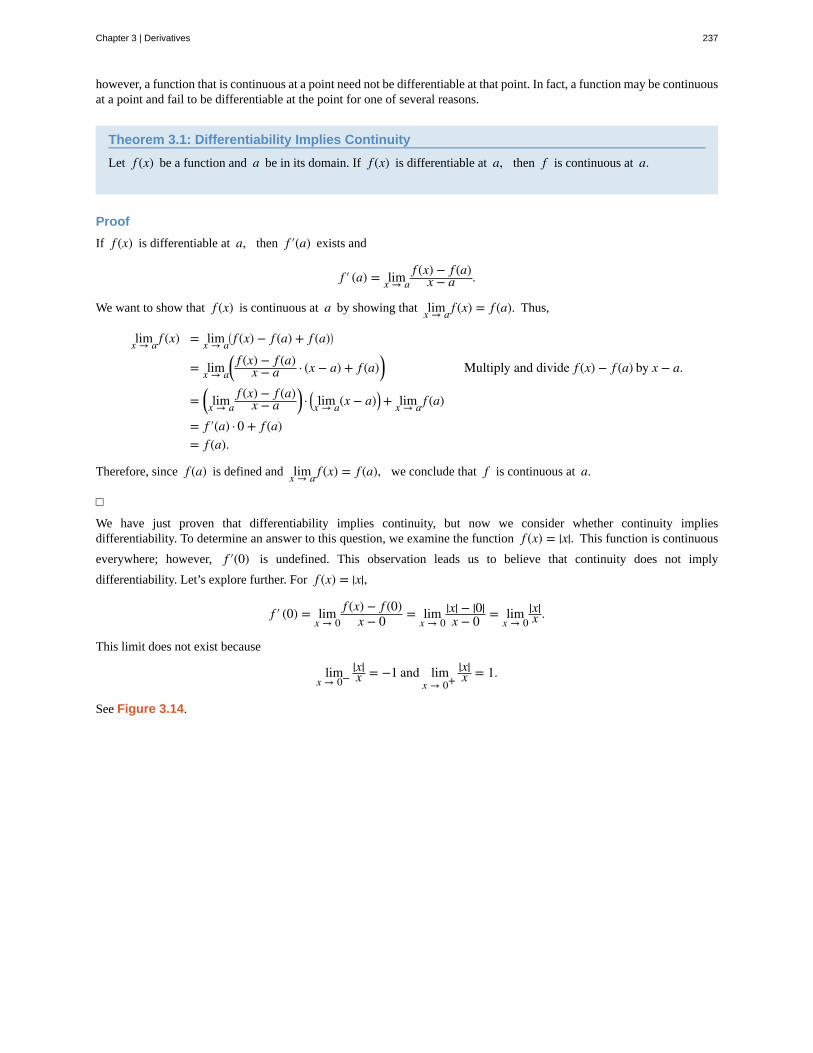
however, a function that is continuous at a point need not be differentiable at that point. In fact, a function may be continuousat a point and fail to be differentiable at the point for one of several reasons.
Theorem 3.1: Differentiability Implies Continuity
Let f (x) be a function and a be in its domain. If f (x) is differentiable at a, then f is continuous at a.
Proof
If f (x) is differentiable at a, then f ′(a) exists and
f ′ (a) = limx → af (x) − f (a)
x − a .
We want to show that f (x) is continuous at a by showing that limx → a f (x) = f (a). Thus,
limx → a f (x) = limx → a⎛⎝ f (x) − f (a) + f (a)⎞
⎠
= limx → a⎛⎝
f (x) − f (a)x − a · (x − a) + f (a)⎞⎠ Multiply and divide f (x) − f (a) by x − a.
= ⎛⎝ limx → a
f (x) − f (a)x − a
⎞⎠ · ⎛
⎝ limx → a(x − a)⎞⎠ + limx → a f (a)
= f ′(a) · 0 + f (a)= f (a).
Therefore, since f (a) is defined and limx → a f (x) = f (a), we conclude that f is continuous at a.
□
We have just proven that differentiability implies continuity, but now we consider whether continuity impliesdifferentiability. To determine an answer to this question, we examine the function f (x) = |x|. This function is continuous
everywhere; however, f ′(0) is undefined. This observation leads us to believe that continuity does not imply
differentiability. Let’s explore further. For f (x) = |x|,
f ′ (0) = limx → 0
f (x) − f (0)x − 0 = lim
x → 0|x| − |0|x − 0 = lim
x → 0|x|x .
This limit does not exist because
limx → 0−
|x|x = −1 and lim
x → 0+|x|x = 1.
See Figure 3.14.
Chapter 3 | Derivatives 237
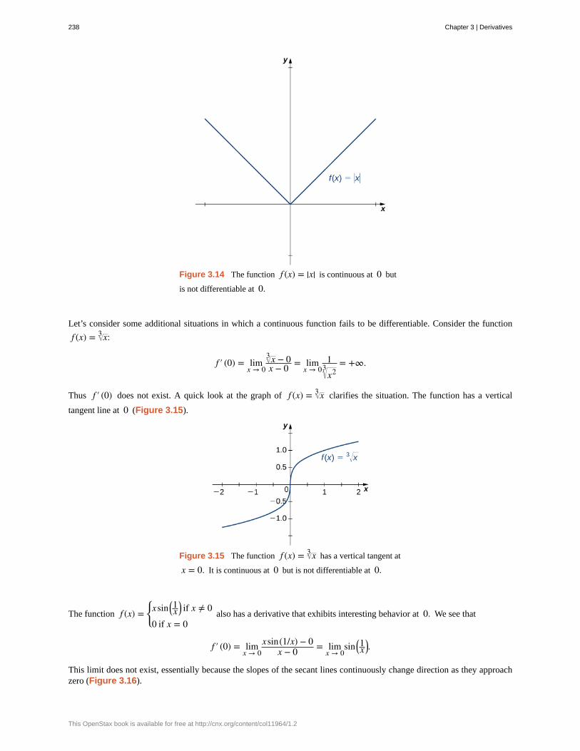
Figure 3.14 The function f (x) = |x| is continuous at 0 but
is not differentiable at 0.
Let’s consider some additional situations in which a continuous function fails to be differentiable. Consider the function
f (x) = x3 :
f ′ (0) = limx → 0
x3 − 0x − 0 = lim
x → 01x23 = +∞.
Thus f ′ (0) does not exist. A quick look at the graph of f (x) = x3 clarifies the situation. The function has a vertical
tangent line at 0 (Figure 3.15).
Figure 3.15 The function f (x) = x3 has a vertical tangent at
x = 0. It is continuous at 0 but is not differentiable at 0.
The function f (x) =⎧
⎩⎨xsin⎛
⎝1x
⎞⎠ if x ≠ 0
0 if x = 0also has a derivative that exhibits interesting behavior at 0. We see that
f ′ (0) = limx → 0
xsin(1/x) − 0x − 0 = lim
x → 0sin⎛
⎝1x
⎞⎠.
This limit does not exist, essentially because the slopes of the secant lines continuously change direction as they approachzero (Figure 3.16).
238 Chapter 3 | Derivatives
This OpenStax book is available for free at http://cnx.org/content/col11964/1.2
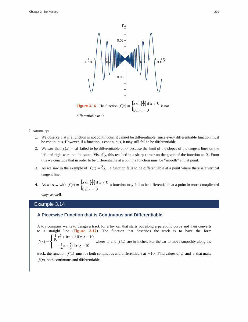
Figure 3.16 The function f (x) =⎧
⎩⎨xsin⎛
⎝1x
⎞⎠ if x ≠ 0
0 if x = 0is not
differentiable at 0.
In summary:
1. We observe that if a function is not continuous, it cannot be differentiable, since every differentiable function mustbe continuous. However, if a function is continuous, it may still fail to be differentiable.
2. We saw that f (x) = |x| failed to be differentiable at 0 because the limit of the slopes of the tangent lines on the
left and right were not the same. Visually, this resulted in a sharp corner on the graph of the function at 0. From
this we conclude that in order to be differentiable at a point, a function must be “smooth” at that point.
3. As we saw in the example of f (x) = x3 , a function fails to be differentiable at a point where there is a vertical
tangent line.
4. As we saw with f (x) =⎧
⎩⎨xsin⎛
⎝1x
⎞⎠ if x ≠ 0
0 if x = 0a function may fail to be differentiable at a point in more complicated
ways as well.
Example 3.14
A Piecewise Function that is Continuous and Differentiable
A toy company wants to design a track for a toy car that starts out along a parabolic curve and then convertsto a straight line (Figure 3.17). The function that describes the track is to have the form
f (x) =⎧
⎩⎨
110x2 + bx + c if x < −10
−14x + 5
2 if x ≥ −10where x and f (x) are in inches. For the car to move smoothly along the
track, the function f (x) must be both continuous and differentiable at −10. Find values of b and c that make
f (x) both continuous and differentiable.
Chapter 3 | Derivatives 239
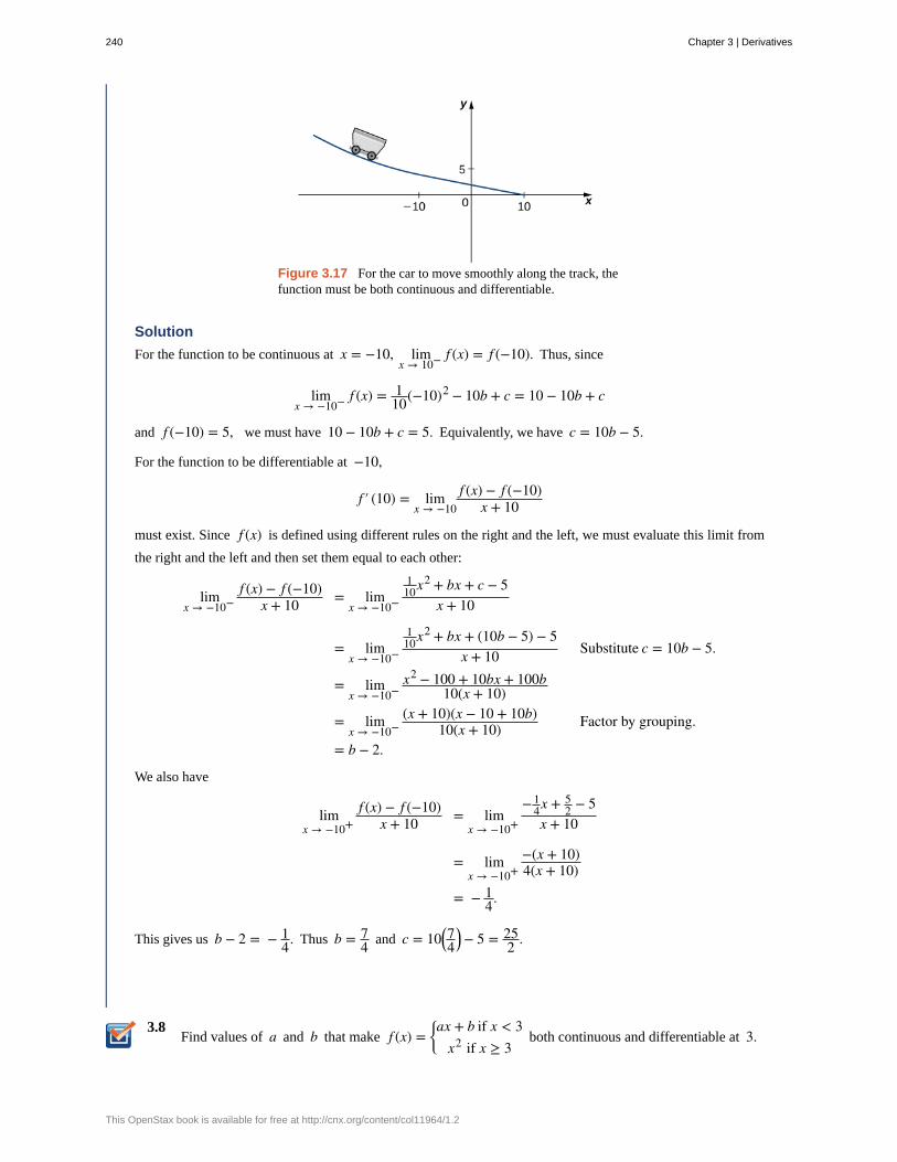
3.8
Figure 3.17 For the car to move smoothly along the track, thefunction must be both continuous and differentiable.
Solution
For the function to be continuous at x = −10, limx → 10− f (x) = f (−10). Thus, since
limx → −10− f (x) = 1
10(−10)2 − 10b + c = 10 − 10b + c
and f (−10) = 5, we must have 10 − 10b + c = 5. Equivalently, we have c = 10b − 5.
For the function to be differentiable at −10,
f ′ (10) = limx → −10
f (x) − f (−10)x + 10
must exist. Since f (x) is defined using different rules on the right and the left, we must evaluate this limit from
the right and the left and then set them equal to each other:
limx → −10−
f (x) − f (−10)x + 10 = lim
x → −10−
110x2 + bx + c − 5
x + 10
= limx → −10−
110x2 + bx + (10b − 5) − 5
x + 10 Substitute c = 10b − 5.
= limx → −10−
x2 − 100 + 10bx + 100b10(x + 10)
= limx → −10−
(x + 10)(x − 10 + 10b)10(x + 10) Factor by grouping.
= b − 2.
We also have
limx → −10+
f (x) − f (−10)x + 10 = lim
x → −10+
− 14x + 5
2 − 5x + 10
= limx → −10+
−(x + 10)4(x + 10)
= − 14.
This gives us b − 2 = − 14. Thus b = 7
4 and c = 10⎛⎝74
⎞⎠ − 5 = 25
2 .
Find values of a and b that make f (x) =⎧
⎩⎨ax + b if x < 3
x2 if x ≥ 3both continuous and differentiable at 3.
240 Chapter 3 | Derivatives
This OpenStax book is available for free at http://cnx.org/content/col11964/1.2
Higher-Order DerivativesThe derivative of a function is itself a function, so we can find the derivative of a derivative. For example, the derivativeof a position function is the rate of change of position, or velocity. The derivative of velocity is the rate of change ofvelocity, which is acceleration. The new function obtained by differentiating the derivative is called the second derivative.Furthermore, we can continue to take derivatives to obtain the third derivative, fourth derivative, and so on. Collectively,these are referred to as higher-order derivatives. The notation for the higher-order derivatives of y = f (x) can be
expressed in any of the following forms:
f ″(x), f ‴(x), f (4) (x),…, f (n) (x)
y″(x), y‴(x), y(4) (x),…, y(n) (x)
d2 ydx2 , d3 y
dy3 , d4 ydy4 ,…, dn y
dyn .
It is interesting to note that the notation ford2 ydx2 may be viewed as an attempt to express d
dx⎛⎝dydx
⎞⎠ more compactly.
Analogously, ddx
⎛⎝
ddx
⎛⎝dydx
⎞⎠⎞⎠ = d
dx⎛
⎝⎜ d2 y
dx2
⎞
⎠⎟ = d3 y
dx3 .
Example 3.15
Finding a Second Derivative
For f (x) = 2x2 − 3x + 1, find f ″(x).
Solution
First find f ′(x).
f ′ (x) = limh → 0
⎛⎝2(x + h)2 − 3(x + h) + 1⎞
⎠ − (2x2 − 3x + 1)h
Substitute f (x) = 2x2 − 3x + 1andf (x + h) = 2(x + h)2 − 3(x + h) + 1
into f ′ (x) = limh → 0
f (x + h) − f (x)h .
= limh → 0
4xh + h2 − 3hh Simplify the numerator.
= limh → 0
(4x + h − 3)Factor out the h in the numeratorand cancel with the h in thedenominator.
= 4x − 3 Take the limit.
Next, find f ″(x) by taking the derivative of f ′ (x) = 4x − 3.
f ″(x) = limh → 0
f ′ (x + h) − f ′(x)h
Use f ′ (x) = limh → 0
f (x + h) − f (x)h with f ′(x) in
place of f (x).
= limh → 0
⎛⎝4(x + h) − 3⎞
⎠ − (4x − 3)h
Substitute f ′ (x + h) = 4(x + h) − 3 andf ′ (x) = 4x − 3.
= limh → 0
4 Simplify.
= 4 Take the limit.
Chapter 3 | Derivatives 241
3.9
3.10
Find f ″(x) for f (x) = x2.
Example 3.16
Finding Acceleration
The position of a particle along a coordinate axis at time t (in seconds) is given by s(t) = 3t2 − 4t + 1 (in
meters). Find the function that describes its acceleration at time t.
Solution
Since v(t) = s′(t) and a(t) = v′ (t) = s″(t), we begin by finding the derivative of s(t) :
s′ (t) = limh → 0
s(t + h) − s(t)h
= limh → 0
3(t + h)2 − 4(t + h) + 1 − ⎛⎝3t2 − 4t + 1⎞
⎠h
= 6t − 4.
Next,
s″(t) = limh → 0
s′ (t + h) − s′(t)h
= limh → 0
6(t + h) − 4 − (6t − 4)h
= 6.
Thus, a = 6 m/s2.
For s(t) = t3, find a(t).
242 Chapter 3 | Derivatives
This OpenStax book is available for free at http://cnx.org/content/col11964/1.2
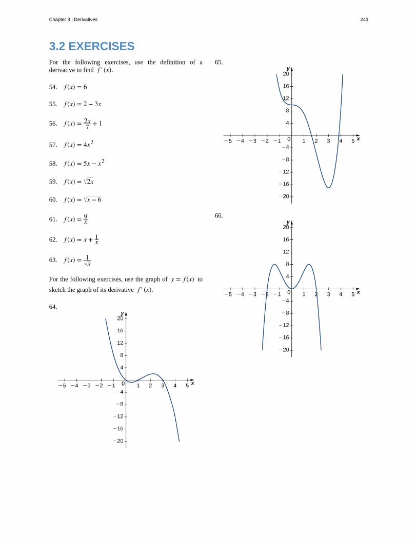
3.2 EXERCISESFor the following exercises, use the definition of aderivative to find f ′ (x).
54. f (x) = 6
55. f (x) = 2 − 3x
56. f (x) = 2x7 + 1
57. f (x) = 4x2
58. f (x) = 5x − x2
59. f (x) = 2x
60. f (x) = x − 6
61. f (x) = 9x
62. f (x) = x + 1x
63. f (x) = 1x
For the following exercises, use the graph of y = f (x) to
sketch the graph of its derivative f ′ (x).
64.
65.
66.
Chapter 3 | Derivatives 243
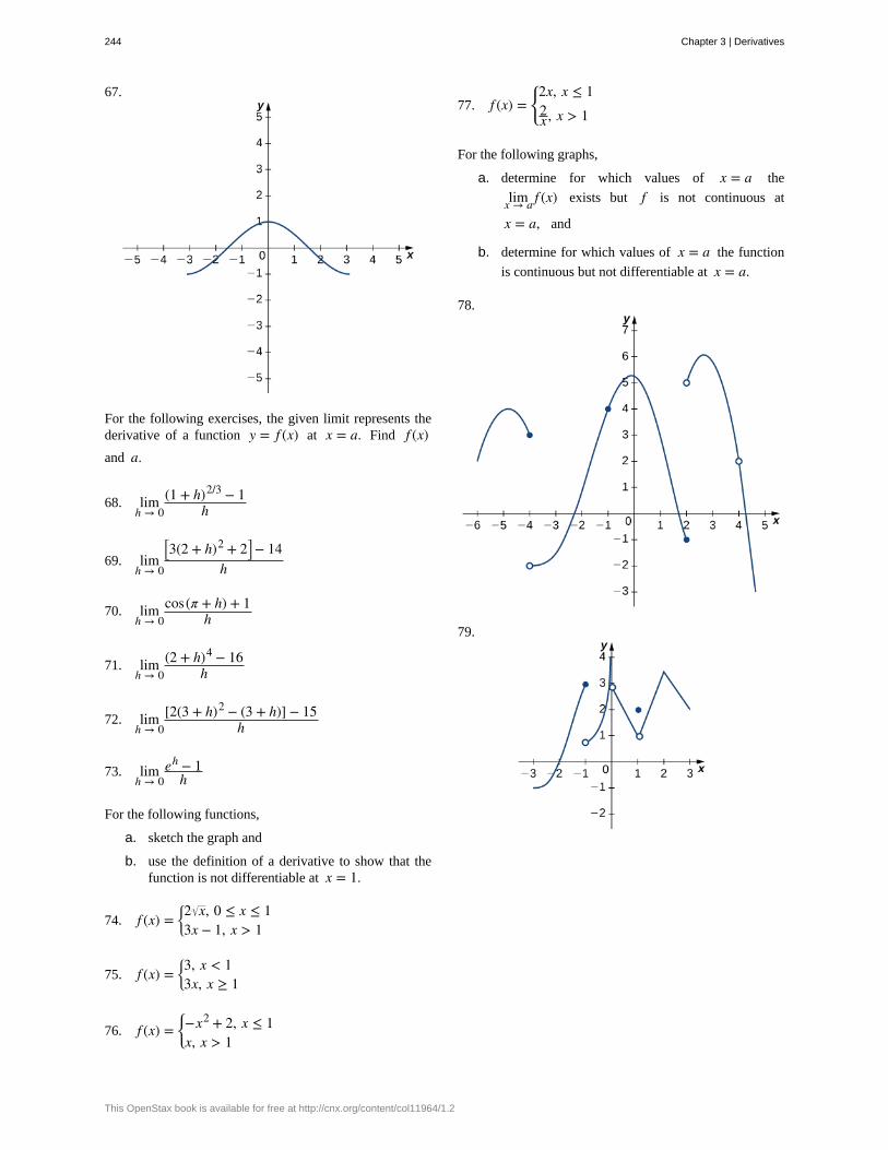
67.
For the following exercises, the given limit represents thederivative of a function y = f (x) at x = a. Find f (x)and a.
68. limh → 0
(1 + h)2/3 − 1h
69. limh → 0
⎡⎣3(2 + h)2 + 2⎤
⎦ − 14h
70. limh → 0
cos(π + h) + 1h
71. limh → 0
(2 + h)4 − 16h
72. limh → 0
[2(3 + h)2 − (3 + h)] − 15h
73. limh → 0
eh − 1h
For the following functions,
a. sketch the graph and
b. use the definition of a derivative to show that thefunction is not differentiable at x = 1.
74. f (x) =⎧
⎩⎨2 x, 0 ≤ x ≤ 13x − 1, x > 1
75. f (x) =⎧
⎩⎨3, x < 13x, x ≥ 1
76. f (x) =⎧
⎩⎨−x2 + 2, x ≤ 1
x, x > 1
77. f (x) =⎧
⎩⎨
2x, x ≤ 12x , x > 1
For the following graphs,
a. determine for which values of x = a the
limx → a f (x) exists but f is not continuous at
x = a, and
b. determine for which values of x = a the function
is continuous but not differentiable at x = a.
78.
79.
244 Chapter 3 | Derivatives
This OpenStax book is available for free at http://cnx.org/content/col11964/1.2
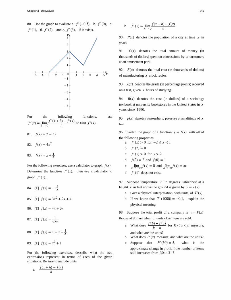
80. Use the graph to evaluate a. f ′ (−0.5), b. f ′ (0), c.
f ′ (1), d. f ′ (2), and e. f ′ (3), if it exists.
For the following functions, use
f ″(x) = limh → 0
f ′ (x + h) − f ′(x)h to find f ″(x).
81. f (x) = 2 − 3x
82. f (x) = 4x2
83. f (x) = x + 1x
For the following exercises, use a calculator to graph f (x).Determine the function f ′ (x), then use a calculator to
graph f ′ (x).
84. [T] f (x) = − 5x
85. [T] f (x) = 3x2 + 2x + 4.
86. [T] f (x) = x + 3x
87. [T] f (x) = 12x
88. [T] f (x) = 1 + x + 1x
89. [T] f (x) = x3 + 1
For the following exercises, describe what the twoexpressions represent in terms of each of the givensituations. Be sure to include units.
a.f (x + h) − f (x)
h
b. f ′ (x) = limh → 0
f (x + h) − f (x)h
90. P(x) denotes the population of a city at time x in
years.
91. C(x) denotes the total amount of money (in
thousands of dollars) spent on concessions by x customers
at an amusement park.
92. R(x) denotes the total cost (in thousands of dollars)
of manufacturing x clock radios.
93. g(x) denotes the grade (in percentage points) received
on a test, given x hours of studying.
94. B(x) denotes the cost (in dollars) of a sociology
textbook at university bookstores in the United States in xyears since 1990.
95. p(x) denotes atmospheric pressure at an altitude of xfeet.
96. Sketch the graph of a function y = f (x) with all of
the following properties:a. f ′ (x) > 0 for −2 ≤ x < 1b. f ′ (2) = 0c. f ′ (x) > 0 for x > 2d. f (2) = 2 and f (0) = 1e. limx → −∞ f (x) = 0 and limx → ∞ f (x) = ∞
f. f ′ (1) does not exist.
97. Suppose temperature T in degrees Fahrenheit at a
height x in feet above the ground is given by y = T(x).a. Give a physical interpretation, with units, of T′(x).b. If we know that T′ (1000) = −0.1, explain the
physical meaning.
98. Suppose the total profit of a company is y = P(x)thousand dollars when x units of an item are sold.
a. What doesP(b) − P(a)
b − a for 0 < a < b measure,
and what are the units?b. What does P′(x) measure, and what are the units?
c. Suppose that P′ (30) = 5, what is the
approximate change in profit if the number of itemssold increases from 30 to 31?
Chapter 3 | Derivatives 245
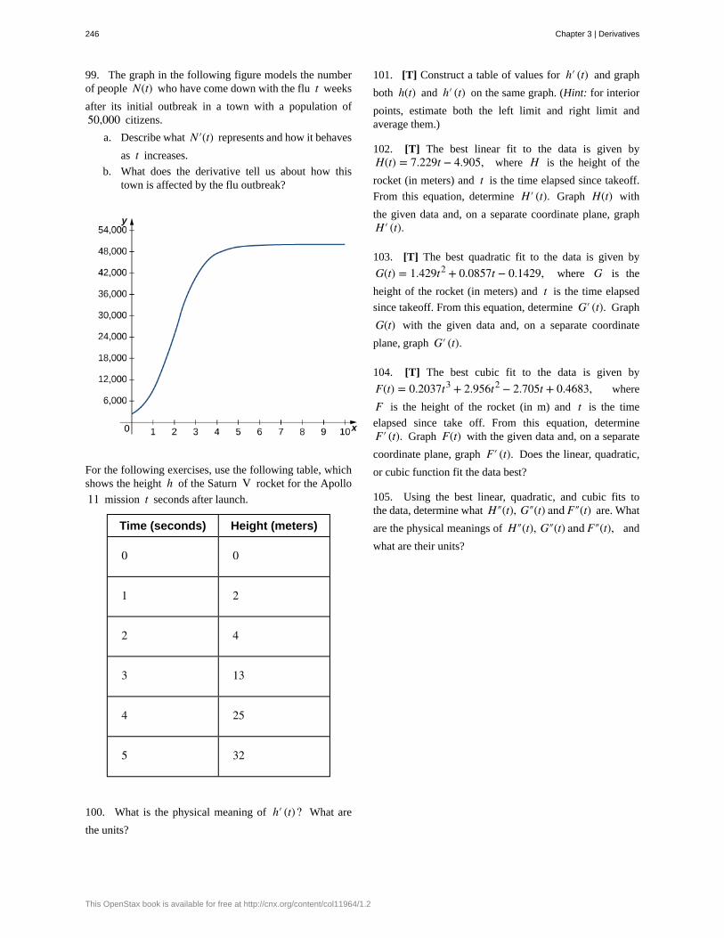
99. The graph in the following figure models the numberof people N(t) who have come down with the flu t weeks
after its initial outbreak in a town with a population of50,000 citizens.
a. Describe what N′(t) represents and how it behaves
as t increases.
b. What does the derivative tell us about how thistown is affected by the flu outbreak?
For the following exercises, use the following table, whichshows the height h of the Saturn V rocket for the Apollo
11 mission t seconds after launch.
Time (seconds) Height (meters)
0 0
1 2
2 4
3 13
4 25
5 32
100. What is the physical meaning of h′ (t)? What are
the units?
101. [T] Construct a table of values for h′ (t) and graph
both h(t) and h′ (t) on the same graph. (Hint: for interior
points, estimate both the left limit and right limit andaverage them.)
102. [T] The best linear fit to the data is given byH(t) = 7.229t − 4.905, where H is the height of the
rocket (in meters) and t is the time elapsed since takeoff.
From this equation, determine H′ (t). Graph H(t) with
the given data and, on a separate coordinate plane, graphH′ (t).
103. [T] The best quadratic fit to the data is given by
G(t) = 1.429t2 + 0.0857t − 0.1429, where G is the
height of the rocket (in meters) and t is the time elapsed
since takeoff. From this equation, determine G′ (t). Graph
G(t) with the given data and, on a separate coordinate
plane, graph G′ (t).
104. [T] The best cubic fit to the data is given by
F(t) = 0.2037t3 + 2.956t2 − 2.705t + 0.4683, where
F is the height of the rocket (in m) and t is the time
elapsed since take off. From this equation, determineF′ (t). Graph F(t) with the given data and, on a separate
coordinate plane, graph F′ (t). Does the linear, quadratic,
or cubic function fit the data best?
105. Using the best linear, quadratic, and cubic fits tothe data, determine what H″(t), G″(t) and F″(t) are. What
are the physical meanings of H″(t), G″(t) and F″(t), and
what are their units?
246 Chapter 3 | Derivatives
This OpenStax book is available for free at http://cnx.org/content/col11964/1.2
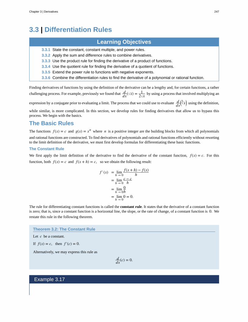
3.3 | Differentiation Rules
Learning Objectives3.3.1 State the constant, constant multiple, and power rules.
3.3.2 Apply the sum and difference rules to combine derivatives.
3.3.3 Use the product rule for finding the derivative of a product of functions.
3.3.4 Use the quotient rule for finding the derivative of a quotient of functions.
3.3.5 Extend the power rule to functions with negative exponents.
3.3.6 Combine the differentiation rules to find the derivative of a polynomial or rational function.
Finding derivatives of functions by using the definition of the derivative can be a lengthy and, for certain functions, a rather
challenging process. For example, previously we found that ddx( x) = 1
2 x by using a process that involved multiplying an
expression by a conjugate prior to evaluating a limit. The process that we could use to evaluate ddx
⎛⎝ x3 ⎞
⎠ using the definition,
while similar, is more complicated. In this section, we develop rules for finding derivatives that allow us to bypass thisprocess. We begin with the basics.
The Basic RulesThe functions f (x) = c and g(x) = xn where n is a positive integer are the building blocks from which all polynomials
and rational functions are constructed. To find derivatives of polynomials and rational functions efficiently without resortingto the limit definition of the derivative, we must first develop formulas for differentiating these basic functions.
The Constant Rule
We first apply the limit definition of the derivative to find the derivative of the constant function, f (x) = c. For this
function, both f (x) = c and f (x + h) = c, so we obtain the following result:
f ′ (x) = limh → 0
f (x + h) − f (x)h
= limh → 0
c − ch
= limh → 0
0h
= limh → 0
0 = 0.
The rule for differentiating constant functions is called the constant rule. It states that the derivative of a constant functionis zero; that is, since a constant function is a horizontal line, the slope, or the rate of change, of a constant function is 0. We
restate this rule in the following theorem.
Theorem 3.2: The Constant Rule
Let c be a constant.
If f (x) = c, then f ′(c) = 0.
Alternatively, we may express this rule as
ddx(c) = 0.
Example 3.17
Chapter 3 | Derivatives 247
3.11
Applying the Constant Rule
Find the derivative of f (x) = 8.
Solution
This is just a one-step application of the rule:
f ′(8) = 0.
Find the derivative of g(x) = −3.
The Power RuleWe have shown that
ddx
⎛⎝x2⎞
⎠ = 2x and ddx
⎛⎝x
1/2⎞⎠ = 1
2x−1/2.
At this point, you might see a pattern beginning to develop for derivatives of the form ddx(xn). We continue our
examination of derivative formulas by differentiating power functions of the form f (x) = xn where n is a positive integer.
We develop formulas for derivatives of this type of function in stages, beginning with positive integer powers. Before stating
and proving the general rule for derivatives of functions of this form, we take a look at a specific case, ddx(x3). As we go
through this derivation, pay special attention to the portion of the expression in boldface, as the technique used in this caseis essentially the same as the technique used to prove the general case.
Example 3.18
Differentiating x3
Find ddx
⎛⎝x
3⎞⎠.
Solution
248 Chapter 3 | Derivatives
This OpenStax book is available for free at http://cnx.org/content/col11964/1.2
3.12
ddx
⎛⎝x
3⎞⎠ = lim
h → 0(x + h)3 − x3
h
= limh → 0
x3 + 3x2 h + 3xh2 + h3 − x3
h
Notice that the fir t term in the expansion of
(x + h)3 is x3 and the second term is 3x2 h. Allother terms contain powers of h that are two orgreater.
= limh → 0
3x2 h + 3xh2 + h3
hIn this step the x3 terms have been cancelled,leaving only terms containing h.
= limh → 0
h(3x2 + 3xh + h2)h Factor out the common factor of h.
= limh → 0
(3x2 + 3xh + h2)After cancelling the common factor of h, the
only term not containing h is 3x2.
= 3x2 Let h go to 0.
Find ddx
⎛⎝x4⎞
⎠.
As we shall see, the procedure for finding the derivative of the general form f (x) = xn is very similar. Although it is often
unwise to draw general conclusions from specific examples, we note that when we differentiate f (x) = x3, the power on
x becomes the coefficient of x2 in the derivative and the power on x in the derivative decreases by 1. The following
theorem states that the power rule holds for all positive integer powers of x. We will eventually extend this result to
negative integer powers. Later, we will see that this rule may also be extended first to rational powers of x and then to
arbitrary powers of x. Be aware, however, that this rule does not apply to functions in which a constant is raised to a
variable power, such as f (x) = 3x.
Theorem 3.3: The Power Rule
Let n be a positive integer. If f (x) = xn, then
f ′ (x) = nxn − 1.
Alternatively, we may express this rule as
ddxxn = nxn − 1.
Proof
For f (x) = xn where n is a positive integer, we have
f ′ (x) = limh → 0
(x + h)n − xn
h .
Since (x + h)n = xn + nxn − 1 h + ⎛⎝n2
⎞⎠ xn − 2 h2 + ⎛
⎝n3
⎞⎠ xn − 3 h3 + … + nxhn − 1 + hn,
we see that
Chapter 3 | Derivatives 249
3.13
(x + h)n − xn = nxn − 1 h + ⎛⎝n2
⎞⎠ xn − 2 h2 + ⎛
⎝n3
⎞⎠ xn − 3 h3 + … + nxhn − 1 + hn.
Next, divide both sides by h:
(x + h)n − xn
h =nxn − 1 h + ⎛
⎝n2
⎞⎠ xn − 2 h2 + ⎛
⎝n3
⎞⎠ xn − 3 h3 + … + nxhn − 1 + hn
h .
Thus,
(x + h)n − xn
h = nxn − 1 + ⎛⎝n2
⎞⎠ xn − 2 h + ⎛
⎝n3
⎞⎠ xn − 3 h2 + … + nxhn − 2 + hn − 1.
Finally,
f ′ (x) = limh → 0
⎛⎝nxn − 1 + ⎛
⎝n2
⎞⎠ xn − 2 h + ⎛
⎝n3
⎞⎠ xn − 3 h2 + … + nxhn − 1 + hn⎞
⎠
= nxn − 1.
□
Example 3.19
Applying the Power Rule
Find the derivative of the function f (x) = x10 by applying the power rule.
Solution
Using the power rule with n = 10, we obtain
f ′(x) = 10x10 − 1 = 10x9.
Find the derivative of f (x) = x7.
The Sum, Difference, and Constant Multiple RulesWe find our next differentiation rules by looking at derivatives of sums, differences, and constant multiples of functions.Just as when we work with functions, there are rules that make it easier to find derivatives of functions that we add, subtract,or multiply by a constant. These rules are summarized in the following theorem.
Theorem 3.4: Sum, Difference, and Constant Multiple Rules
Let f (x) and g(x) be differentiable functions and k be a constant. Then each of the following equations holds.
Sum Rule. The derivative of the sum of a function f and a function g is the same as the sum of the derivative of fand the derivative of g.
ddx
⎛⎝ f (x) + g(x)⎞
⎠ = ddx
⎛⎝ f (x)⎞
⎠ + ddx
⎛⎝g(x)⎞
⎠;
that is,
for j(x) = f (x) + g(x), j′ (x) = f ′ (x) + g′(x).
Difference Rule. The derivative of the difference of a function f and a function g is the same as the difference of the
250 Chapter 3 | Derivatives
This OpenStax book is available for free at http://cnx.org/content/col11964/1.2
derivative of f and the derivative of g:
ddx
⎛⎝ f (x) − g(x)⎞
⎠ = ddx
⎛⎝ f (x)⎞
⎠ − ddx
⎛⎝g(x)⎞
⎠;
that is,
for j(x) = f (x) − g(x), j′ (x) = f ′ (x) − g′(x).
Constant Multiple Rule. The derivative of a constant k multiplied by a function f is the same as the constant multipliedby the derivative:
ddx
⎛⎝k f (x)⎞
⎠ = k ddx
⎛⎝ f (x)⎞
⎠;
that is,
for j(x) = k f (x), j′ (x) = k f ′(x).
Proof
We provide only the proof of the sum rule here. The rest follow in a similar manner.
For differentiable functions f (x) and g(x), we set j(x) = f (x) + g(x). Using the limit definition of the derivative we
have
j′ (x) = limh → 0
j(x + h) − j(x)h .
By substituting j(x + h) = f (x + h) + g(x + h) and j(x) = f (x) + g(x), we obtain
j′(x) = limh → 0
⎛⎝ f (x + h) + g(x + h)⎞
⎠ − ⎛⎝ f (x) + g(x)⎞
⎠
h .
Rearranging and regrouping the terms, we have
j′(x) = limh → 0
⎛⎝
f (x + h) − f (x)h + g(x + h) − g(x)
h⎞⎠.
We now apply the sum law for limits and the definition of the derivative to obtain
j′(x) = limh → 0
⎛⎝
f (x + h) − f (x)h
⎞⎠ + lim
h → 0⎛⎝g(x + h) − g(x)
h⎞⎠ = f ′ (x) + g′ (x).
□
Example 3.20
Applying the Constant Multiple Rule
Find the derivative of g(x) = 3x2 and compare it to the derivative of f (x) = x2.
Solution
We use the power rule directly:
g′ (x) = ddx
⎛⎝3x2⎞
⎠ = 3 ddx
⎛⎝x2⎞
⎠ = 3(2x) = 6x.
Since f (x) = x2 has derivative f ′ (x) = 2x, we see that the derivative of g(x) is 3 times the derivative of
Chapter 3 | Derivatives 251
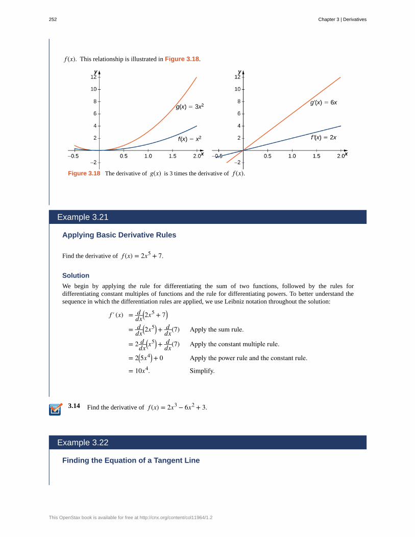
3.14
f (x). This relationship is illustrated in Figure 3.18.
Figure 3.18 The derivative of g(x) is 3 times the derivative of f (x).
Example 3.21
Applying Basic Derivative Rules
Find the derivative of f (x) = 2x5 + 7.
Solution
We begin by applying the rule for differentiating the sum of two functions, followed by the rules fordifferentiating constant multiples of functions and the rule for differentiating powers. To better understand thesequence in which the differentiation rules are applied, we use Leibniz notation throughout the solution:
f ′ (x) = ddx
⎛⎝2x5 + 7⎞
⎠
= ddx
⎛⎝2x5⎞
⎠ + ddx(7) Apply the sum rule.
= 2 ddx
⎛⎝x
5⎞⎠ + d
dx(7) Apply the constant multiple rule.
= 2⎛⎝5x4⎞
⎠ + 0 Apply the power rule and the constant rule.
= 10x4. Simplify.
Find the derivative of f (x) = 2x3 − 6x2 + 3.
Example 3.22
Finding the Equation of a Tangent Line
252 Chapter 3 | Derivatives
This OpenStax book is available for free at http://cnx.org/content/col11964/1.2
3.15
Find the equation of the line tangent to the graph of f (x) = x2 − 4x + 6 at x = 1.
Solution
To find the equation of the tangent line, we need a point and a slope. To find the point, compute
f (1) = 12 − 4(1) + 6 = 3.
This gives us the point (1, 3). Since the slope of the tangent line at 1 is f ′ (1), we must first find f ′ (x). Using
the definition of a derivative, we have
f ′ (x) = 2x − 4
so the slope of the tangent line is f ′ (1) = −2. Using the point-slope formula, we see that the equation of the
tangent line is
y − 3 = −2(x − 1).
Putting the equation of the line in slope-intercept form, we obtain
y = −2x + 5.
Find the equation of the line tangent to the graph of f (x) = 3x2 − 11 at x = 2. Use the point-slope
form.
The Product RuleNow that we have examined the basic rules, we can begin looking at some of the more advanced rules. The first oneexamines the derivative of the product of two functions. Although it might be tempting to assume that the derivative ofthe product is the product of the derivatives, similar to the sum and difference rules, the product rule does not follow this
pattern. To see why we cannot use this pattern, consider the function f (x) = x2, whose derivative is f ′ (x) = 2x and not
ddx(x) · d
dx(x) = 1 · 1 = 1.
Theorem 3.5: Product Rule
Let f (x) and g(x) be differentiable functions. Then
ddx
⎛⎝ f (x)g(x)⎞
⎠ = ddx
⎛⎝ f (x)⎞
⎠ · g(x) + ddx
⎛⎝g(x)⎞
⎠ · f (x).
That is,
if j(x) = f (x)g(x), then j′ (x) = f ′ (x)g(x) + g′ (x) f (x).
This means that the derivative of a product of two functions is the derivative of the first function times the secondfunction plus the derivative of the second function times the first function.
Proof
We begin by assuming that f (x) and g(x) are differentiable functions. At a key point in this proof we need to use the
fact that, since g(x) is differentiable, it is also continuous. In particular, we use the fact that since g(x) is continuous,
limh → 0
g(x + h) = g(x).
Chapter 3 | Derivatives 253
By applying the limit definition of the derivative to j(x) = f (x)g(x), we obtain
j′ (x) = limh → 0
f (x + h)g(x + h) − f (x)g(x)h .
By adding and subtracting f (x)g(x + h) in the numerator, we have
j′ (x) = limh → 0
f (x + h)g(x + h) − f (x)g(x + h) + f (x)g(x + h) − f (x)g(x)h .
After breaking apart this quotient and applying the sum law for limits, the derivative becomes
j′ (x) = limh → 0
⎛⎝
f (x + h)g(x + h) − f (x)g(x + h)h
⎞⎠ + lim
h → 0⎛⎝
f (x)g(x + h) − f (x)g(x)h
⎞⎠.
Rearranging, we obtain
j′ (x) = limh → 0
⎛⎝
f (x + h) − f (x)h · g(x + h)⎞⎠ + lim
h → 0⎛⎝g(x + h) − g(x)
h · f (x)⎞⎠.
By using the continuity of g(x), the definition of the derivatives of f (x) and g(x), and applying the limit laws, we arrive
at the product rule,
j′ (x) = f ′ (x)g(x) + g′ (x) f (x).
□
Example 3.23
Applying the Product Rule to Functions at a Point
For j(x) = f (x)g(x), use the product rule to find j′(2) if f (2) = 3, f ′ (2) = −4, g(2) = 1, and g′ (2) = 6.
Solution
Since j(x) = f (x)g(x), j′ (x) = f ′ (x)g(x) + g′ (x) f (x), and hence
j′ (2) = f ′ (2)g(2) + g′ (2) f (2) = (−4)(1) + (6)(3) = 14.
Example 3.24
Applying the Product Rule to Binomials
For j(x) = (x2 + 2)(3x3 − 5x), find j′(x) by applying the product rule. Check the result by first finding the
product and then differentiating.
Solution
If we set f (x) = x2 + 2 and g(x) = 3x3 − 5x, then f ′ (x) = 2x and g′ (x) = 9x2 − 5. Thus,
j′ (x) = f ′ (x)g(x) + g′ (x) f (x) = (2x)⎛⎝3x3 − 5x⎞
⎠ + (9x2 − 5)(x2 + 2).
Simplifying, we have
j′ (x) = 15x4 + 3x2 − 10.
254 Chapter 3 | Derivatives
This OpenStax book is available for free at http://cnx.org/content/col11964/1.2
3.16
To check, we see that j(x) = 3x5 + x3 − 10x and, consequently, j′ (x) = 15x4 + 3x2 − 10.
Use the product rule to obtain the derivative of j(x) = 2x5 ⎛⎝4x2 + x⎞
⎠.
The Quotient RuleHaving developed and practiced the product rule, we now consider differentiating quotients of functions. As we see in thefollowing theorem, the derivative of the quotient is not the quotient of the derivatives; rather, it is the derivative of thefunction in the numerator times the function in the denominator minus the derivative of the function in the denominatortimes the function in the numerator, all divided by the square of the function in the denominator. In order to better graspwhy we cannot simply take the quotient of the derivatives, keep in mind that
ddx
⎛⎝x2⎞
⎠ = 2x, notddx
⎛⎝x
3⎞⎠
ddx(x)
= 3x2
1 = 3x2.
Theorem 3.6: The Quotient Rule
Let f (x) and g(x) be differentiable functions. Then
ddx
⎛⎝
f (x)g(x)
⎞⎠ =
ddx( f (x)) · g(x) − d
dx(g(x)) · f (x)
(g(x))2 .
That is,
if j(x) = f (x)g(x) , then j′ (x) = f ′ (x)g(x) − g′ (x) f (x)
(g(x))2 .
The proof of the quotient rule is very similar to the proof of the product rule, so it is omitted here. Instead, we apply thisnew rule for finding derivatives in the next example.
Example 3.25
Applying the Quotient Rule
Use the quotient rule to find the derivative of k(x) = 5x2
4x + 3.
Solution
Let f (x) = 5x2 and g(x) = 4x + 3. Thus, f ′ (x) = 10x and g′ (x) = 4. Substituting into the quotient rule, we
have
k′ (x) = f ′ (x)g(x) − g′ (x) f (x)(g(x))2 = 10x(4x + 3) − 4(5x2)
(4x + 3)2 .
Chapter 3 | Derivatives 255
3.17
Simplifying, we obtain
k′ (x) = 20x2 + 30x(4x + 3)2 .
Find the derivative of h(x) = 3x + 14x − 3.
It is now possible to use the quotient rule to extend the power rule to find derivatives of functions of the form xk where kis a negative integer.
Theorem 3.7: Extended Power Rule
If k is a negative integer, then
ddx
⎛⎝xk⎞
⎠ = kxk − 1.
Proof
If k is a negative integer, we may set n = −k, so that n is a positive integer with k = −n. Since for each positive integer
n, x−n = 1xn, we may now apply the quotient rule by setting f (x) = 1 and g(x) = xn. In this case, f ′ (x) = 0 and
g′ (x) = nxn − 1. Thus,
dd(x−n) =
0(xn) − 1⎛⎝nxn − 1⎞
⎠
(xn)2 .
Simplifying, we see that
dd(x−n) = −nxn − 1
x2n = −nx(n − 1) − 2n = −nx−n − 1.
Finally, observe that since k = −n, by substituting we have
ddx
⎛⎝xk⎞
⎠ = kxk − 1.
□
Example 3.26
Using the Extended Power Rule
Find ddx
⎛⎝x−4⎞
⎠.
Solution
By applying the extended power rule with k = −4, we obtain
256 Chapter 3 | Derivatives
This OpenStax book is available for free at http://cnx.org/content/col11964/1.2
3.18
ddx
⎛⎝x−4⎞
⎠ = −4x−4 − 1 = −4x−5.
Example 3.27
Using the Extended Power Rule and the Constant Multiple Rule
Use the extended power rule and the constant multiple rule to find f (x) = 6x2.
Solution
It may seem tempting to use the quotient rule to find this derivative, and it would certainly not be incorrect to do
so. However, it is far easier to differentiate this function by first rewriting it as f (x) = 6x−2.
f ′ (x) = ddx
⎛⎝
6x2
⎞⎠ = d
dx⎛⎝6x−2⎞
⎠ Rewrite 6x2 as 6x−2.
= 6 ddx(x−2) Apply the constant multiple rule.
= 6(−2x−3) Use the extended power rule to diffe entiate x−2.
= −12x−3 Simplify.
Find the derivative of g(x) = 1x7 using the extended power rule.
Combining Differentiation RulesAs we have seen throughout the examples in this section, it seldom happens that we are called on to apply just onedifferentiation rule to find the derivative of a given function. At this point, by combining the differentiation rules, we mayfind the derivatives of any polynomial or rational function. Later on we will encounter more complex combinations ofdifferentiation rules. A good rule of thumb to use when applying several rules is to apply the rules in reverse of the order inwhich we would evaluate the function.
Example 3.28
Combining Differentiation Rules
For k(x) = 3h(x) + x2 g(x), find k′(x).
Solution
Finding this derivative requires the sum rule, the constant multiple rule, and the product rule.
Chapter 3 | Derivatives 257
k′ (x) = ddx
⎛⎝3h(x) + x2 g(x)⎞
⎠ = ddx
⎛⎝3h(x)⎞
⎠ + ddx
⎛⎝x2 g(x)⎞
⎠ Apply the sum rule.
= 3 ddx
⎛⎝h(x)⎞
⎠ + ⎛⎝
ddx
⎛⎝x2⎞
⎠g(x) + ddx
⎛⎝g(x)⎞
⎠x2⎞⎠
Apply the constant multiple rule todiffe entiate 3h(x) and the product
rule to diffe entiate x2 g(x).
= 3h′ (x) + 2xg(x) + g′(x)x2
Example 3.29
Extending the Product Rule
For k(x) = f (x)g(x)h(x), express k′ (x) in terms of f (x), g(x), h(x), and their derivatives.
Solution
We can think of the function k(x) as the product of the function f (x)g(x) and the function h(x). That is,
k(x) = ⎛⎝ f (x)g(x)⎞
⎠ · h(x). Thus,
k′(x) = ddx
⎛⎝ f (x)g(x)⎞
⎠ · h(x) + ddx
⎛⎝h(x)⎞
⎠ · ⎛⎝ f (x)g(x)⎞
⎠Apply the product rule to the productof f (x)g(x) and h(x).
= ⎛⎝ f ′ (x)g(x) + g′ (x) f (x)h⎞
⎠(x) + h′ (x) f (x)g(x) Apply the product rule to f (x)g(x).= f ′ (x)g(x)h(x) + f (x)g′ (x)h(x) + f (x)g(x)h′ (x). Simplify.
Example 3.30
Combining the Quotient Rule and the Product Rule
For h(x) = 2x3 k(x)3x + 2 , find h′(x).
Solution
This procedure is typical for finding the derivative of a rational function.
h′ (x) =ddx
⎛⎝2x3 k(x)⎞
⎠ · (3x + 2) − ddx(3x + 2) · ⎛
⎝2x3 k(x)⎞⎠
(3x + 2)2 Apply the quotient rule.
=⎛⎝6x2 k(x) + k′ (x) · 2x3⎞
⎠(3x + 2) − 3⎛⎝2x3 k(x)⎞
⎠
(3x + 2)2
Apply the product rule to finddx
⎛⎝2x3 k(x)⎞
⎠. Use ddx(3x + 2) = 3.
= −6x3 k(x) + 18x3 k(x) + 12x2 k(x) + 6x4 k′ (x) + 4x3 k′ (x)(3x + 2)2 Simplify.
258 Chapter 3 | Derivatives
This OpenStax book is available for free at http://cnx.org/content/col11964/1.2
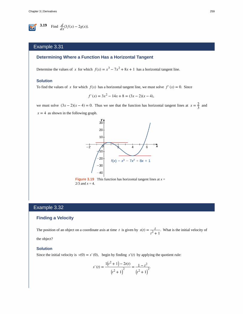
3.19 Find ddx
⎛⎝3 f (x) − 2g(x)⎞
⎠.
Example 3.31
Determining Where a Function Has a Horizontal Tangent
Determine the values of x for which f (x) = x3 − 7x2 + 8x + 1 has a horizontal tangent line.
Solution
To find the values of x for which f (x) has a horizontal tangent line, we must solve f ′ (x) = 0. Since
f ′ (x) = 3x2 − 14x + 8 = (3x − 2)(x − 4),
we must solve (3x − 2)(x − 4) = 0. Thus we see that the function has horizontal tangent lines at x = 23 and
x = 4 as shown in the following graph.
Figure 3.19 This function has horizontal tangent lines at x =2/3 and x = 4.
Example 3.32
Finding a Velocity
The position of an object on a coordinate axis at time t is given by s(t) = tt2 + 1
. What is the initial velocity of
the object?
Solution
Since the initial velocity is v(0) = s′ (0), begin by finding s′(t) by applying the quotient rule:
s′ (t) =1⎛
⎝t2 + 1⎞⎠ − 2t(t)
⎛⎝t2 + 1⎞
⎠2 = 1 − t2
⎛⎝t2 + 1⎞
⎠2.
Chapter 3 | Derivatives 259
3.20
After evaluating, we see that v(0) = 1.
Find the values of x for which the line tangent to the graph of f (x) = 4x2 − 3x + 2 has a tangent line
parallel to the line y = 2x + 3.
260 Chapter 3 | Derivatives
This OpenStax book is available for free at http://cnx.org/content/col11964/1.2
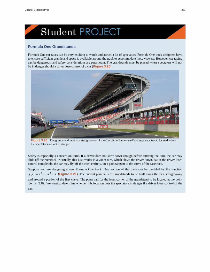
Formula One Grandstands
Formula One car races can be very exciting to watch and attract a lot of spectators. Formula One track designers haveto ensure sufficient grandstand space is available around the track to accommodate these viewers. However, car racingcan be dangerous, and safety considerations are paramount. The grandstands must be placed where spectators will notbe in danger should a driver lose control of a car (Figure 3.20).
Figure 3.20 The grandstand next to a straightaway of the Circuit de Barcelona-Catalunya race track, located wherethe spectators are not in danger.
Safety is especially a concern on turns. If a driver does not slow down enough before entering the turn, the car mayslide off the racetrack. Normally, this just results in a wider turn, which slows the driver down. But if the driver losescontrol completely, the car may fly off the track entirely, on a path tangent to the curve of the racetrack.
Suppose you are designing a new Formula One track. One section of the track can be modeled by the function
f (x) = x3 + 3x2 + x (Figure 3.21). The current plan calls for grandstands to be built along the first straightaway
and around a portion of the first curve. The plans call for the front corner of the grandstand to be located at the point(−1.9, 2.8). We want to determine whether this location puts the spectators in danger if a driver loses control of the
car.
Chapter 3 | Derivatives 261
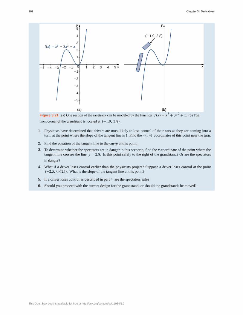
Figure 3.21 (a) One section of the racetrack can be modeled by the function f (x) = x3 + 3x2 + x. (b) The
front corner of the grandstand is located at (−1.9, 2.8).
1. Physicists have determined that drivers are most likely to lose control of their cars as they are coming into aturn, at the point where the slope of the tangent line is 1. Find the (x, y) coordinates of this point near the turn.
2. Find the equation of the tangent line to the curve at this point.
3. To determine whether the spectators are in danger in this scenario, find the x-coordinate of the point where thetangent line crosses the line y = 2.8. Is this point safely to the right of the grandstand? Or are the spectators
in danger?
4. What if a driver loses control earlier than the physicists project? Suppose a driver loses control at the point(−2.5, 0.625). What is the slope of the tangent line at this point?
5. If a driver loses control as described in part 4, are the spectators safe?
6. Should you proceed with the current design for the grandstand, or should the grandstands be moved?
262 Chapter 3 | Derivatives
This OpenStax book is available for free at http://cnx.org/content/col11964/1.2
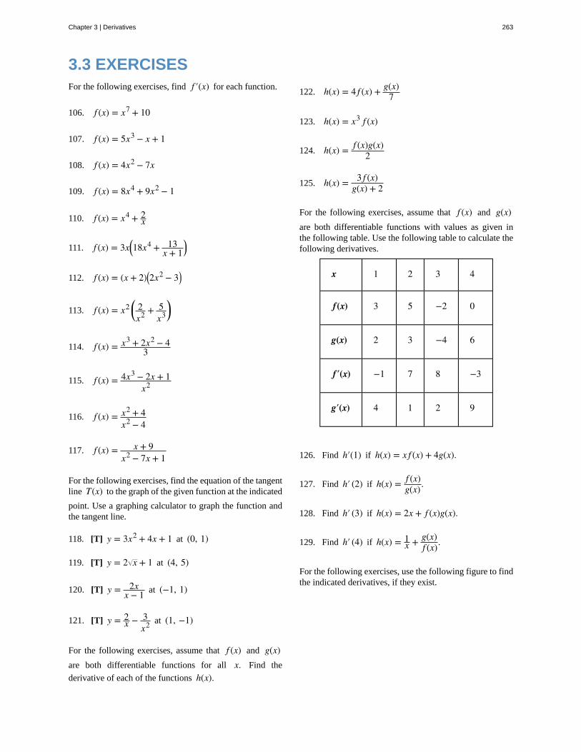
3.3 EXERCISESFor the following exercises, find f ′(x) for each function.
106. f (x) = x7 + 10
107. f (x) = 5x3 − x + 1
108. f (x) = 4x2 − 7x
109. f (x) = 8x4 + 9x2 − 1
110. f (x) = x4 + 2x
111. f (x) = 3x⎛⎝18x4 + 13
x + 1⎞⎠
112. f (x) = (x + 2)⎛⎝2x2 − 3⎞
⎠
113. f (x) = x2 ⎛⎝
2x2 + 5
x3⎞⎠
114. f (x) = x3 + 2x2 − 43
115. f (x) = 4x3 − 2x + 1x2
116. f (x) = x2 + 4x2 − 4
117. f (x) = x + 9x2 − 7x + 1
For the following exercises, find the equation of the tangentline T(x) to the graph of the given function at the indicated
point. Use a graphing calculator to graph the function andthe tangent line.
118. [T] y = 3x2 + 4x + 1 at (0, 1)
119. [T] y = 2 x + 1 at (4, 5)
120. [T] y = 2xx − 1 at (−1, 1)
121. [T] y = 2x − 3
x2 at (1, −1)
For the following exercises, assume that f (x) and g(x)are both differentiable functions for all x. Find the
derivative of each of the functions h(x).
122. h(x) = 4 f (x) + g(x)7
123. h(x) = x3 f (x)
124. h(x) = f (x)g(x)2
125. h(x) = 3 f (x)g(x) + 2
For the following exercises, assume that f (x) and g(x)are both differentiable functions with values as given inthe following table. Use the following table to calculate thefollowing derivatives.
x 1 2 3 4
f(x) 3 5 −2 0
g(x) 2 3 −4 6
f′(x) −1 7 8 −3
g′(x) 4 1 2 9
126. Find h′(1) if h(x) = x f (x) + 4g(x).
127. Find h′ (2) if h(x) = f (x)g(x) .
128. Find h′ (3) if h(x) = 2x + f (x)g(x).
129. Find h′ (4) if h(x) = 1x + g(x)
f (x).
For the following exercises, use the following figure to findthe indicated derivatives, if they exist.
Chapter 3 | Derivatives 263
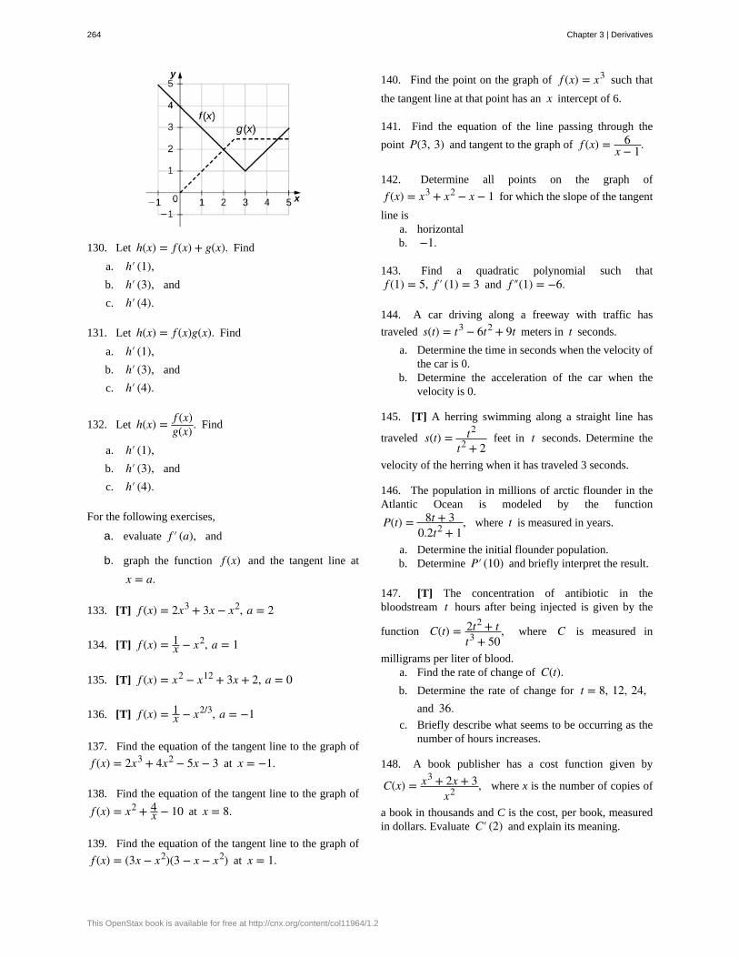
130. Let h(x) = f (x) + g(x). Find
a. h′ (1),b. h′ (3), and
c. h′ (4).
131. Let h(x) = f (x)g(x). Find
a. h′ (1),b. h′ (3), and
c. h′ (4).
132. Let h(x) = f (x)g(x) . Find
a. h′ (1),b. h′ (3), and
c. h′ (4).
For the following exercises,
a. evaluate f ′ (a), and
b. graph the function f (x) and the tangent line at
x = a.
133. [T] f (x) = 2x3 + 3x − x2, a = 2
134. [T] f (x) = 1x − x2, a = 1
135. [T] f (x) = x2 − x12 + 3x + 2, a = 0
136. [T] f (x) = 1x − x2/3, a = −1
137. Find the equation of the tangent line to the graph of
f (x) = 2x3 + 4x2 − 5x − 3 at x = −1.
138. Find the equation of the tangent line to the graph of
f (x) = x2 + 4x − 10 at x = 8.
139. Find the equation of the tangent line to the graph of
f (x) = (3x − x2)(3 − x − x2) at x = 1.
140. Find the point on the graph of f (x) = x3 such that
the tangent line at that point has an x intercept of 6.
141. Find the equation of the line passing through the
point P(3, 3) and tangent to the graph of f (x) = 6x − 1.
142. Determine all points on the graph of
f (x) = x3 + x2 − x − 1 for which the slope of the tangent
line isa. horizontalb. −1.
143. Find a quadratic polynomial such thatf (1) = 5, f ′ (1) = 3 and f ″(1) = −6.
144. A car driving along a freeway with traffic has
traveled s(t) = t3 − 6t2 + 9t meters in t seconds.
a. Determine the time in seconds when the velocity ofthe car is 0.
b. Determine the acceleration of the car when thevelocity is 0.
145. [T] A herring swimming along a straight line has
traveled s(t) = t2
t2 + 2feet in t seconds. Determine the
velocity of the herring when it has traveled 3 seconds.
146. The population in millions of arctic flounder in theAtlantic Ocean is modeled by the function
P(t) = 8t + 30.2t2 + 1
, where t is measured in years.
a. Determine the initial flounder population.b. Determine P′ (10) and briefly interpret the result.
147. [T] The concentration of antibiotic in thebloodstream t hours after being injected is given by the
function C(t) = 2t2 + tt3 + 50
, where C is measured in
milligrams per liter of blood.a. Find the rate of change of C(t).b. Determine the rate of change for t = 8, 12, 24,
and 36.c. Briefly describe what seems to be occurring as the
number of hours increases.
148. A book publisher has a cost function given by
C(x) = x3 + 2x + 3x2 , where x is the number of copies of
a book in thousands and C is the cost, per book, measuredin dollars. Evaluate C′ (2) and explain its meaning.
264 Chapter 3 | Derivatives
This OpenStax book is available for free at http://cnx.org/content/col11964/1.2
149. [T] According to Newton’s law of universalgravitation, the force F between two bodies of constant
mass m1 and m2 is given by the formula F = Gm1 m2d2 ,
where G is the gravitational constant and d is the distance
between the bodies.a. Suppose that G, m1, and m2 are constants. Find
the rate of change of force F with respect to
distance d.b. Find the rate of change of force F with
gravitational constant G = 6.67 × 10⁻¹¹
Nm2 /kg2, on two bodies 10 meters apart, each
with a mass of 1000 kilograms.
Chapter 3 | Derivatives 265
3.4 | Derivatives as Rates of Change
Learning Objectives3.4.1 Determine a new value of a quantity from the old value and the amount of change.
3.4.2 Calculate the average rate of change and explain how it differs from the instantaneous rateof change.
3.4.3 Apply rates of change to displacement, velocity, and acceleration of an object moving alonga straight line.
3.4.4 Predict the future population from the present value and the population growth rate.
3.4.5 Use derivatives to calculate marginal cost and revenue in a business situation.
In this section we look at some applications of the derivative by focusing on the interpretation of the derivative as the rate ofchange of a function. These applications include acceleration and velocity in physics, population growth rates in biology,and marginal functions in economics.
Amount of Change FormulaOne application for derivatives is to estimate an unknown value of a function at a point by using a known value of afunction at some given point together with its rate of change at the given point. If f (x) is a function defined on an interval⎡⎣a, a + h⎤
⎦, then the amount of change of f (x) over the interval is the change in the y values of the function over that
interval and is given by
f (a + h) − f (a).
The average rate of change of the function f over that same interval is the ratio of the amount of change over that interval
to the corresponding change in the x values. It is given by
f (a + h) − f (a)h .
As we already know, the instantaneous rate of change of f (x) at a is its derivative
f ′ (a) = limh → 0
f (a + h) − f (a)h .
For small enough values of h, f ′ (a) ≈ f (a + h) − f (a)h . We can then solve for f (a + h) to get the amount of change
formula:
(3.10)f (a + h) ≈ f (a) + f ′(a)h.
We can use this formula if we know only f (a) and f ′(a) and wish to estimate the value of f (a + h). For example, we
may use the current population of a city and the rate at which it is growing to estimate its population in the near future. Aswe can see in Figure 3.22, we are approximating f (a + h) by the y coordinate at a + h on the line tangent to f (x) at
x = a. Observe that the accuracy of this estimate depends on the value of h as well as the value of f ′ (a).
266 Chapter 3 | Derivatives
This OpenStax book is available for free at http://cnx.org/content/col11964/1.2
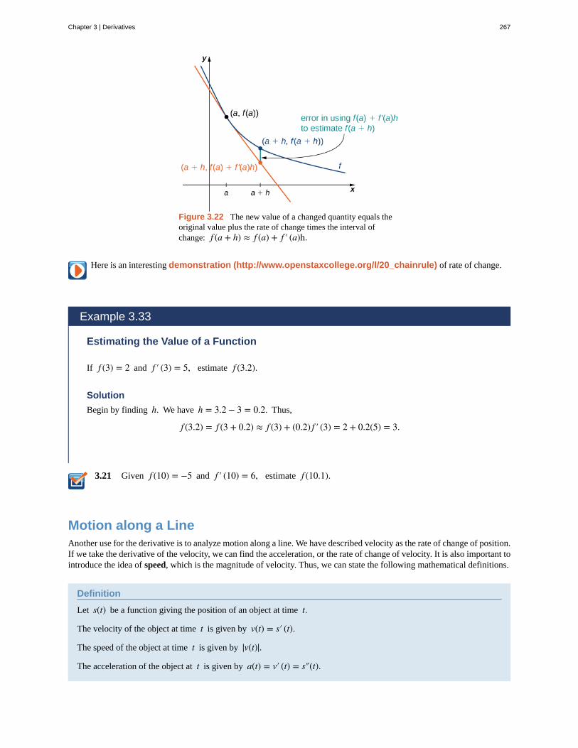
3.21
Figure 3.22 The new value of a changed quantity equals theoriginal value plus the rate of change times the interval ofchange: f (a + h) ≈ f (a) + f ′ (a)h.
Here is an interesting demonstration (http://www.openstaxcollege.org/l/20_chainrule) of rate of change.
Example 3.33
Estimating the Value of a Function
If f (3) = 2 and f ′ (3) = 5, estimate f (3.2).
Solution
Begin by finding h. We have h = 3.2 − 3 = 0.2. Thus,
f (3.2) = f (3 + 0.2) ≈ f (3) + (0.2) f ′ (3) = 2 + 0.2(5) = 3.
Given f (10) = −5 and f ′ (10) = 6, estimate f (10.1).
Motion along a LineAnother use for the derivative is to analyze motion along a line. We have described velocity as the rate of change of position.If we take the derivative of the velocity, we can find the acceleration, or the rate of change of velocity. It is also important tointroduce the idea of speed, which is the magnitude of velocity. Thus, we can state the following mathematical definitions.
Definition
Let s(t) be a function giving the position of an object at time t.
The velocity of the object at time t is given by v(t) = s′ (t).
The speed of the object at time t is given by |v(t)|.The acceleration of the object at t is given by a(t) = v′ (t) = s″(t).
Chapter 3 | Derivatives 267
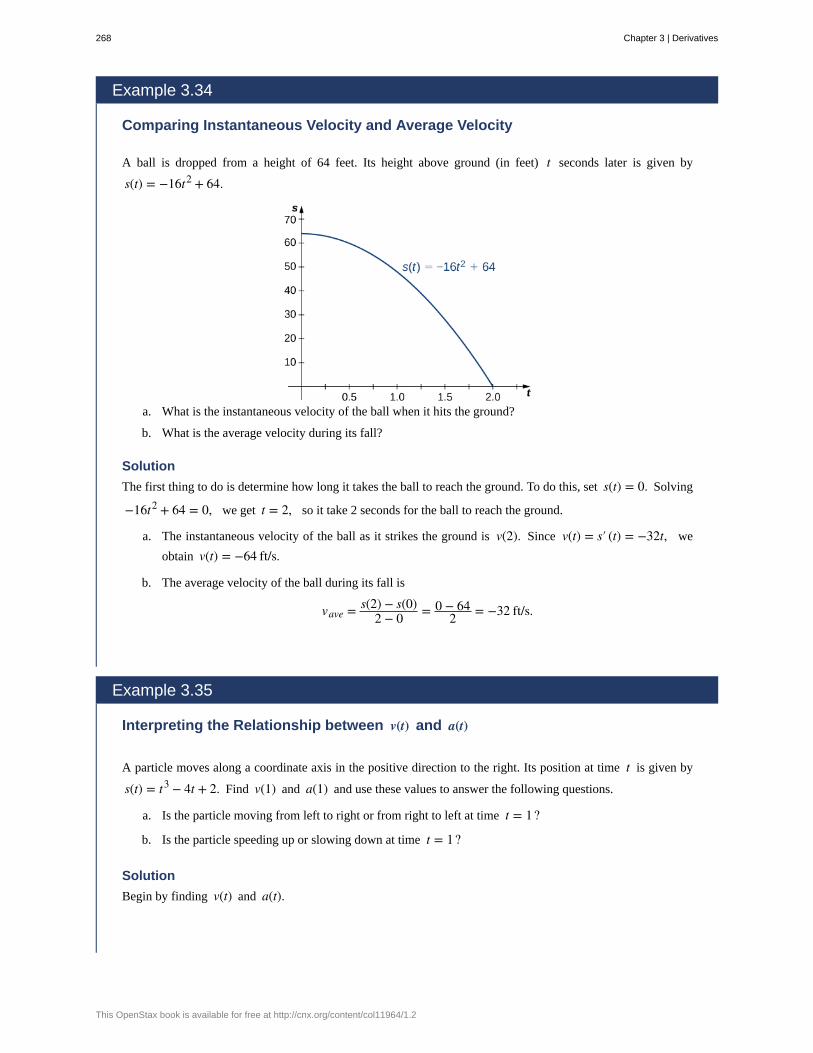
Example 3.34
Comparing Instantaneous Velocity and Average Velocity
A ball is dropped from a height of 64 feet. Its height above ground (in feet) t seconds later is given by
s(t) = −16t2 + 64.
a. What is the instantaneous velocity of the ball when it hits the ground?
b. What is the average velocity during its fall?
Solution
The first thing to do is determine how long it takes the ball to reach the ground. To do this, set s(t) = 0. Solving
−16t2 + 64 = 0, we get t = 2, so it take 2 seconds for the ball to reach the ground.
a. The instantaneous velocity of the ball as it strikes the ground is v(2). Since v(t) = s′ (t) = −32t, we
obtain v(t) = −64 ft/s.
b. The average velocity of the ball during its fall is
vave = s(2) − s(0)2 − 0 = 0 − 64
2 = −32 ft/s.
Example 3.35
Interpreting the Relationship between v(t) and a(t)
A particle moves along a coordinate axis in the positive direction to the right. Its position at time t is given by
s(t) = t3 − 4t + 2. Find v(1) and a(1) and use these values to answer the following questions.
a. Is the particle moving from left to right or from right to left at time t = 1?
b. Is the particle speeding up or slowing down at time t = 1?
Solution
Begin by finding v(t) and a(t).
268 Chapter 3 | Derivatives
This OpenStax book is available for free at http://cnx.org/content/col11964/1.2
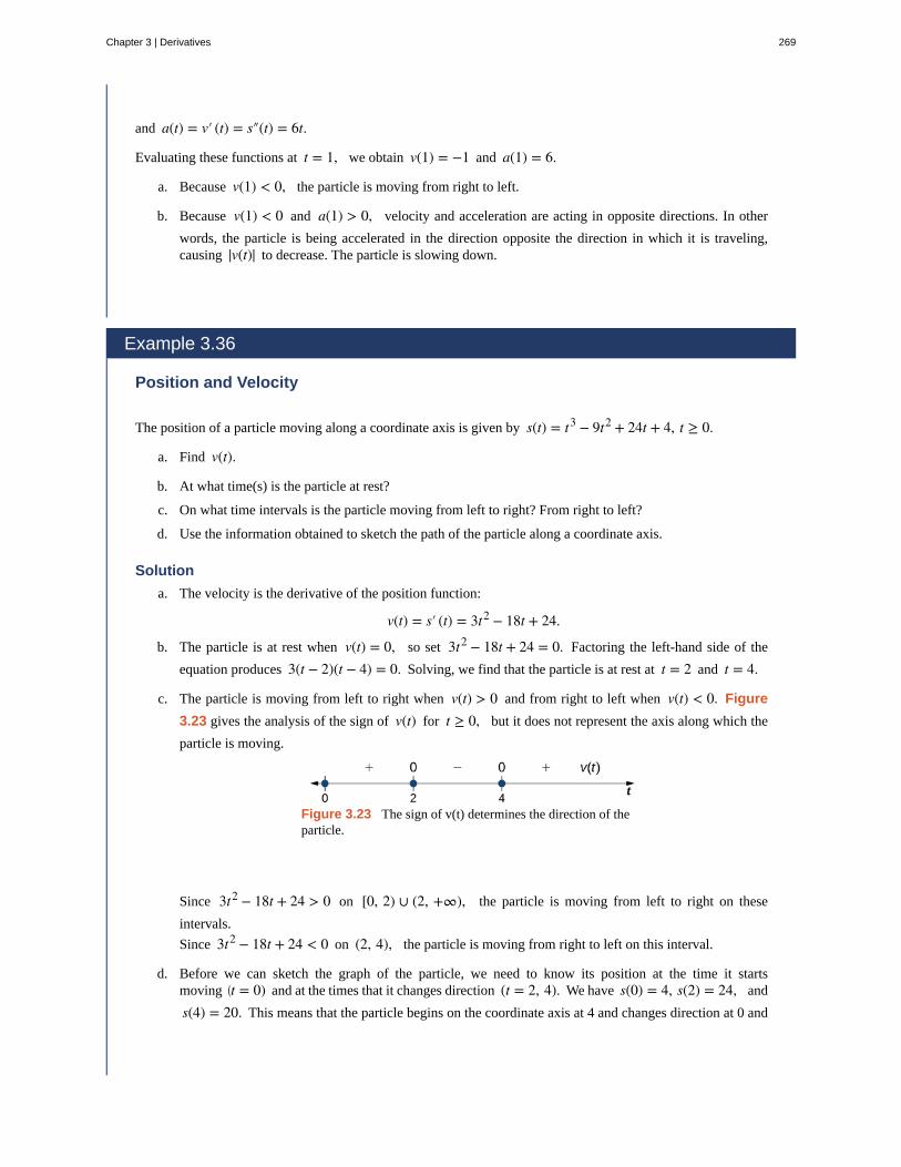
and a(t) = v′ (t) = s″(t) = 6t.
Evaluating these functions at t = 1, we obtain v(1) = −1 and a(1) = 6.
a. Because v(1) < 0, the particle is moving from right to left.
b. Because v(1) < 0 and a(1) > 0, velocity and acceleration are acting in opposite directions. In other
words, the particle is being accelerated in the direction opposite the direction in which it is traveling,causing |v(t)| to decrease. The particle is slowing down.
Example 3.36
Position and Velocity
The position of a particle moving along a coordinate axis is given by s(t) = t3 − 9t2 + 24t + 4, t ≥ 0.
a. Find v(t).
b. At what time(s) is the particle at rest?
c. On what time intervals is the particle moving from left to right? From right to left?
d. Use the information obtained to sketch the path of the particle along a coordinate axis.
Solution
a. The velocity is the derivative of the position function:
v(t) = s′ (t) = 3t2 − 18t + 24.
b. The particle is at rest when v(t) = 0, so set 3t2 − 18t + 24 = 0. Factoring the left-hand side of the
equation produces 3(t − 2)(t − 4) = 0. Solving, we find that the particle is at rest at t = 2 and t = 4.
c. The particle is moving from left to right when v(t) > 0 and from right to left when v(t) < 0. Figure
3.23 gives the analysis of the sign of v(t) for t ≥ 0, but it does not represent the axis along which the
particle is moving.
Figure 3.23 The sign of v(t) determines the direction of theparticle.
Since 3t2 − 18t + 24 > 0 on [0, 2) ∪ (2, +∞), the particle is moving from left to right on these
intervals.
Since 3t2 − 18t + 24 < 0 on (2, 4), the particle is moving from right to left on this interval.
d. Before we can sketch the graph of the particle, we need to know its position at the time it startsmoving ⎛
⎝t = 0) and at the times that it changes direction (t = 2, 4). We have s(0) = 4, s(2) = 24, and
s(4) = 20. This means that the particle begins on the coordinate axis at 4 and changes direction at 0 and
Chapter 3 | Derivatives 269
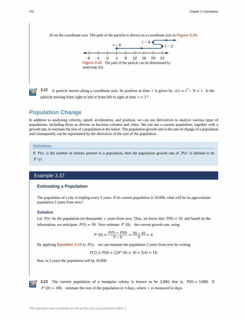
3.22
3.23
20 on the coordinate axis. The path of the particle is shown on a coordinate axis in Figure 3.24.
Figure 3.24 The path of the particle can be determined byanalyzing v(t).
A particle moves along a coordinate axis. Its position at time t is given by s(t) = t2 − 5t + 1. Is the
particle moving from right to left or from left to right at time t = 3?
Population ChangeIn addition to analyzing velocity, speed, acceleration, and position, we can use derivatives to analyze various types ofpopulations, including those as diverse as bacteria colonies and cities. We can use a current population, together with agrowth rate, to estimate the size of a population in the future. The population growth rate is the rate of change of a populationand consequently can be represented by the derivative of the size of the population.
Definition
If P(t) is the number of entities present in a population, then the population growth rate of P(t) is defined to be
P′ (t).
Example 3.37
Estimating a Population
The population of a city is tripling every 5 years. If its current population is 10,000, what will be its approximatepopulation 2 years from now?
Solution
Let P(t) be the population (in thousands) t years from now. Thus, we know that P(0) = 10 and based on the
information, we anticipate P(5) = 30. Now estimate P′ (0), the current growth rate, using
P′ (0) ≈ P(5) − P(0)5 − 0 = 30 − 10
5 = 4.
By applying Equation 3.10 to P(t), we can estimate the population 2 years from now by writing
P(2) ≈ P(0) + (2)P′ (0) ≈ 10 + 2(4) = 18;
thus, in 2 years the population will be 18,000.
The current population of a mosquito colony is known to be 3,000; that is, P(0) = 3,000. If
P′ (0) = 100, estimate the size of the population in 3 days, where t is measured in days.
270 Chapter 3 | Derivatives
This OpenStax book is available for free at http://cnx.org/content/col11964/1.2
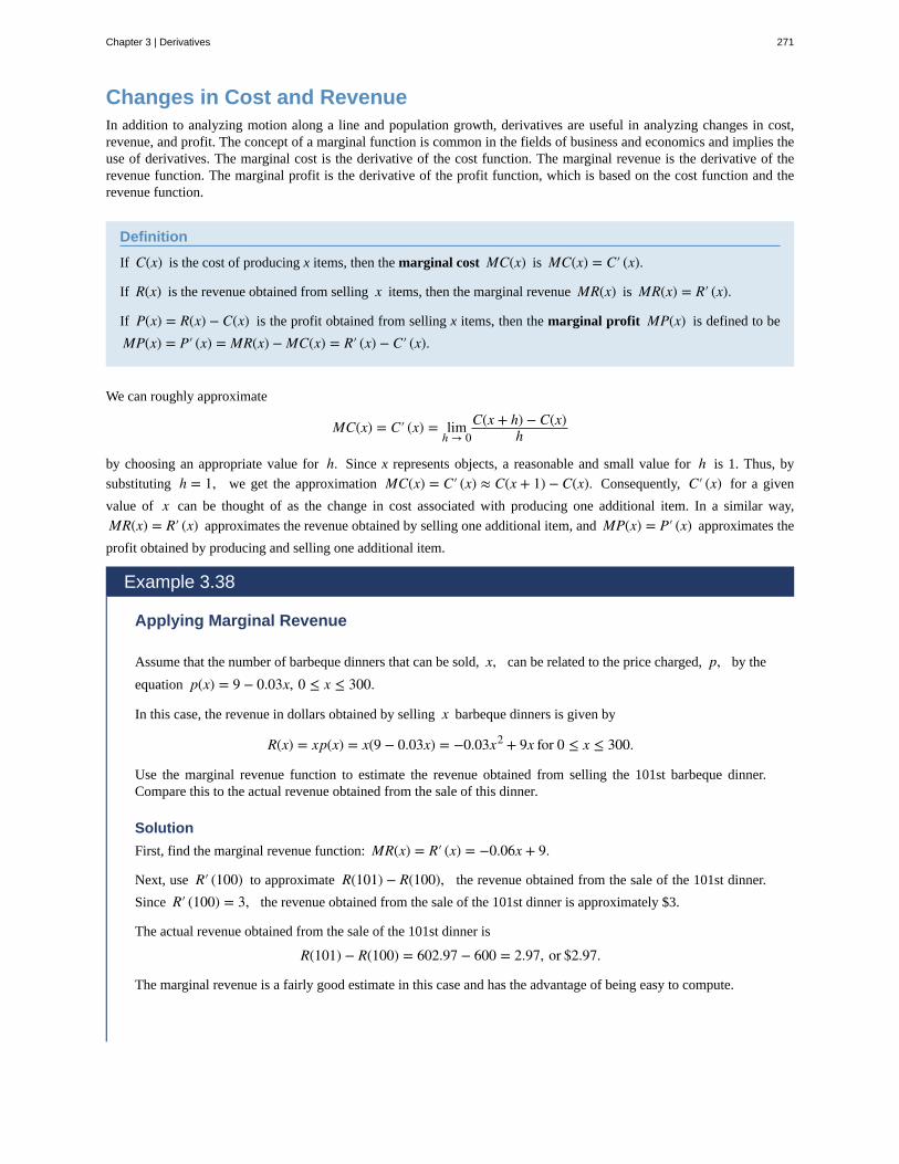
Changes in Cost and RevenueIn addition to analyzing motion along a line and population growth, derivatives are useful in analyzing changes in cost,revenue, and profit. The concept of a marginal function is common in the fields of business and economics and implies theuse of derivatives. The marginal cost is the derivative of the cost function. The marginal revenue is the derivative of therevenue function. The marginal profit is the derivative of the profit function, which is based on the cost function and therevenue function.
Definition
If C(x) is the cost of producing x items, then the marginal cost MC(x) is MC(x) = C′ (x).
If R(x) is the revenue obtained from selling x items, then the marginal revenue MR(x) is MR(x) = R′ (x).
If P(x) = R(x) − C(x) is the profit obtained from selling x items, then the marginal profit MP(x) is defined to be
MP(x) = P′ (x) = MR(x) − MC(x) = R′ (x) − C′ (x).
We can roughly approximate
MC(x) = C′ (x) = limh → 0
C(x + h) − C(x)h
by choosing an appropriate value for h. Since x represents objects, a reasonable and small value for h is 1. Thus, by
substituting h = 1, we get the approximation MC(x) = C′ (x) ≈ C(x + 1) − C(x). Consequently, C′ (x) for a given
value of x can be thought of as the change in cost associated with producing one additional item. In a similar way,
MR(x) = R′ (x) approximates the revenue obtained by selling one additional item, and MP(x) = P′ (x) approximates the
profit obtained by producing and selling one additional item.
Example 3.38
Applying Marginal Revenue
Assume that the number of barbeque dinners that can be sold, x, can be related to the price charged, p, by the
equation p(x) = 9 − 0.03x, 0 ≤ x ≤ 300.
In this case, the revenue in dollars obtained by selling x barbeque dinners is given by
R(x) = xp(x) = x(9 − 0.03x) = −0.03x2 + 9x for 0 ≤ x ≤ 300.
Use the marginal revenue function to estimate the revenue obtained from selling the 101st barbeque dinner.Compare this to the actual revenue obtained from the sale of this dinner.
Solution
First, find the marginal revenue function: MR(x) = R′ (x) = −0.06x + 9.
Next, use R′ (100) to approximate R(101) − R(100), the revenue obtained from the sale of the 101st dinner.
Since R′ (100) = 3, the revenue obtained from the sale of the 101st dinner is approximately $3.
The actual revenue obtained from the sale of the 101st dinner is
R(101) − R(100) = 602.97 − 600 = 2.97, or $2.97.
The marginal revenue is a fairly good estimate in this case and has the advantage of being easy to compute.
Chapter 3 | Derivatives 271
3.24 Suppose that the profit obtained from the sale of x fish-fry dinners is given by
P(x) = −0.03x2 + 8x − 50. Use the marginal profit function to estimate the profit from the sale of the 101st
fish-fry dinner.
272 Chapter 3 | Derivatives
This OpenStax book is available for free at http://cnx.org/content/col11964/1.2
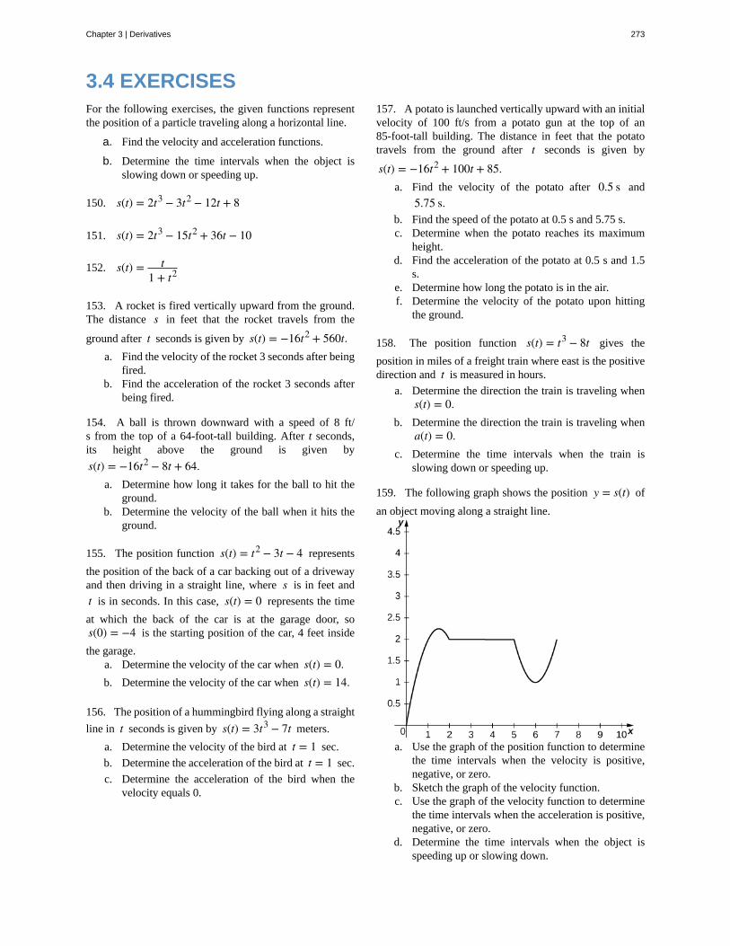
3.4 EXERCISESFor the following exercises, the given functions representthe position of a particle traveling along a horizontal line.
a. Find the velocity and acceleration functions.
b. Determine the time intervals when the object isslowing down or speeding up.
150. s(t) = 2t3 − 3t2 − 12t + 8
151. s(t) = 2t3 − 15t2 + 36t − 10
152. s(t) = t1 + t2
153. A rocket is fired vertically upward from the ground.The distance s in feet that the rocket travels from the
ground after t seconds is given by s(t) = −16t2 + 560t.a. Find the velocity of the rocket 3 seconds after being
fired.b. Find the acceleration of the rocket 3 seconds after
being fired.
154. A ball is thrown downward with a speed of 8 ft/s from the top of a 64-foot-tall building. After t seconds,its height above the ground is given by
s(t) = −16t2 − 8t + 64.a. Determine how long it takes for the ball to hit the
ground.b. Determine the velocity of the ball when it hits the
ground.
155. The position function s(t) = t2 − 3t − 4 represents
the position of the back of a car backing out of a drivewayand then driving in a straight line, where s is in feet and
t is in seconds. In this case, s(t) = 0 represents the time
at which the back of the car is at the garage door, sos(0) = −4 is the starting position of the car, 4 feet inside
the garage.a. Determine the velocity of the car when s(t) = 0.b. Determine the velocity of the car when s(t) = 14.
156. The position of a hummingbird flying along a straight
line in t seconds is given by s(t) = 3t3 − 7t meters.
a. Determine the velocity of the bird at t = 1 sec.
b. Determine the acceleration of the bird at t = 1 sec.
c. Determine the acceleration of the bird when thevelocity equals 0.
157. A potato is launched vertically upward with an initialvelocity of 100 ft/s from a potato gun at the top of an85-foot-tall building. The distance in feet that the potatotravels from the ground after t seconds is given by
s(t) = −16t2 + 100t + 85.a. Find the velocity of the potato after 0.5 s and
5.75 s.b. Find the speed of the potato at 0.5 s and 5.75 s.c. Determine when the potato reaches its maximum
height.d. Find the acceleration of the potato at 0.5 s and 1.5
s.e. Determine how long the potato is in the air.f. Determine the velocity of the potato upon hitting
the ground.
158. The position function s(t) = t3 − 8t gives the
position in miles of a freight train where east is the positivedirection and t is measured in hours.
a. Determine the direction the train is traveling whens(t) = 0.
b. Determine the direction the train is traveling whena(t) = 0.
c. Determine the time intervals when the train isslowing down or speeding up.
159. The following graph shows the position y = s(t) of
an object moving along a straight line.
a. Use the graph of the position function to determinethe time intervals when the velocity is positive,negative, or zero.
b. Sketch the graph of the velocity function.c. Use the graph of the velocity function to determine
the time intervals when the acceleration is positive,negative, or zero.
d. Determine the time intervals when the object isspeeding up or slowing down.
Chapter 3 | Derivatives 273
160. The cost function, in dollars, of a company thatmanufactures food processors is given by
C(x) = 200 + 7x + x2
7 , where x is the number of food
processors manufactured.a. Find the marginal cost function.b. Find the marginal cost of manufacturing 12 food
processors.c. Find the actual cost of manufacturing the thirteenth
food processor.
161. The price p (in dollars) and the demand x for a
certain digital clock radio is given by the price–demandfunction p = 10 − 0.001x.
a. Find the revenue function R(x).b. Find the marginal revenue function.c. Find the marginal revenue at x = 2000 and 5000.
162. [T] A profit is earned when revenue exceeds cost.Suppose the profit function for a skateboard manufacturer
is given by P(x) = 30x − 0.3x2 − 250, where x is the
number of skateboards sold.a. Find the exact profit from the sale of the thirtieth
skateboard.b. Find the marginal profit function and use it to
estimate the profit from the sale of the thirtiethskateboard.
163. [T] In general, the profit function is the differencebetween the revenue and cost functions:P(x) = R(x) − C(x). Suppose the price-demand and cost
functions for the production of cordless drills is givenrespectively by p = 143 − 0.03x and
C(x) = 75,000 + 65x, where x is the number of
cordless drills that are sold at a price of p dollars per drill
and C(x) is the cost of producing x cordless drills.
a. Find the marginal cost function.b. Find the revenue and marginal revenue functions.c. Find R′(1000) and R′(4000). Interpret the
results.d. Find the profit and marginal profit functions.e. Find P′(1000) and P′(4000). Interpret the
results.
164. A small town in Ohio commissioned an actuarialfirm to conduct a study that modeled the rate of changeof the town’s population. The study found that the town’spopulation (measured in thousands of people) can be
modeled by the function P(t) = − 13t3 + 64t + 3000,
where t is measured in years.
a. Find the rate of change function P′ (t) of the
population function.b. Find P′ (1), P′ (2), P′ (3), and P′ (4). Interpret
what the results mean for the town.c. Find P″(1), P″(2), P″(3), and P″(4). Interpret
what the results mean for the town’s population.
165. [T] A culture of bacteria grows in number according
to the function N(t) = 3000⎛⎝1 + 4t
t2 + 100⎞⎠, where t is
measured in hours.a. Find the rate of change of the number of bacteria.b. Find N′ (0), N′ (10), N′ (20), and N′ (30).c. Interpret the results in (b).d. Find N″(0), N″(10), N″(20), and N″(30).
Interpret what the answers imply about the bacteriapopulation growth.
166. The centripetal force of an object of mass m is given
by F(r) = mv2r , where v is the speed of rotation and r
is the distance from the center of rotation.a. Find the rate of change of centripetal force with
respect to the distance from the center of rotation.b. Find the rate of change of centripetal force of an
object with mass 1000 kilograms, velocity of 13.89m/s, and a distance from the center of rotation of200 meters.
The following questions concern the population (inmillions) of London by decade in the 19th century, which islisted in the following table.
274 Chapter 3 | Derivatives
This OpenStax book is available for free at http://cnx.org/content/col11964/1.2
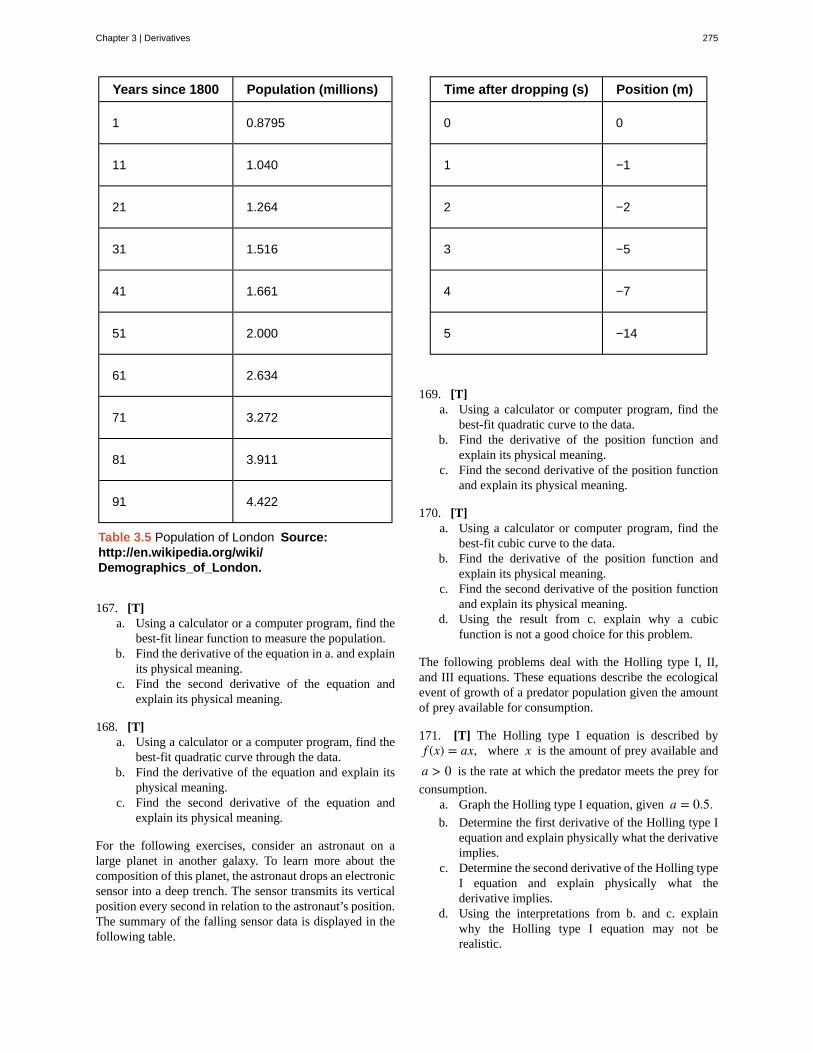
Years since 1800 Population (millions)
1 0.8795
11 1.040
21 1.264
31 1.516
41 1.661
51 2.000
61 2.634
71 3.272
81 3.911
91 4.422
Table 3.5 Population of London Source:http://en.wikipedia.org/wiki/Demographics_of_London.
167. [T]a. Using a calculator or a computer program, find the
best-fit linear function to measure the population.b. Find the derivative of the equation in a. and explain
its physical meaning.c. Find the second derivative of the equation and
explain its physical meaning.
168. [T]a. Using a calculator or a computer program, find the
best-fit quadratic curve through the data.b. Find the derivative of the equation and explain its
physical meaning.c. Find the second derivative of the equation and
explain its physical meaning.
For the following exercises, consider an astronaut on alarge planet in another galaxy. To learn more about thecomposition of this planet, the astronaut drops an electronicsensor into a deep trench. The sensor transmits its verticalposition every second in relation to the astronaut’s position.The summary of the falling sensor data is displayed in thefollowing table.
Time after dropping (s) Position (m)
0 0
1 −1
2 −2
3 −5
4 −7
5 −14
169. [T]a. Using a calculator or computer program, find the
best-fit quadratic curve to the data.b. Find the derivative of the position function and
explain its physical meaning.c. Find the second derivative of the position function
and explain its physical meaning.
170. [T]a. Using a calculator or computer program, find the
best-fit cubic curve to the data.b. Find the derivative of the position function and
explain its physical meaning.c. Find the second derivative of the position function
and explain its physical meaning.d. Using the result from c. explain why a cubic
function is not a good choice for this problem.
The following problems deal with the Holling type I, II,and III equations. These equations describe the ecologicalevent of growth of a predator population given the amountof prey available for consumption.
171. [T] The Holling type I equation is described byf (x) = ax, where x is the amount of prey available and
a > 0 is the rate at which the predator meets the prey for
consumption.a. Graph the Holling type I equation, given a = 0.5.b. Determine the first derivative of the Holling type I
equation and explain physically what the derivativeimplies.
c. Determine the second derivative of the Holling typeI equation and explain physically what thederivative implies.
d. Using the interpretations from b. and c. explainwhy the Holling type I equation may not berealistic.
Chapter 3 | Derivatives 275
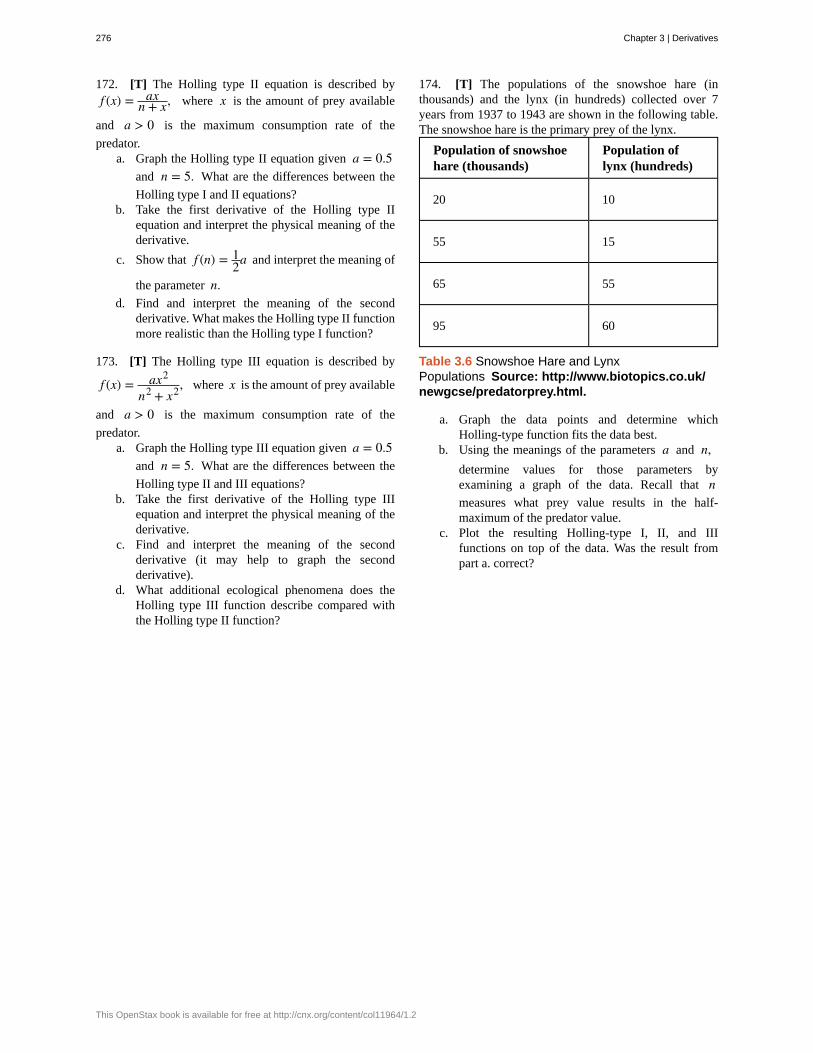
172. [T] The Holling type II equation is described byf (x) = ax
n + x, where x is the amount of prey available
and a > 0 is the maximum consumption rate of the
predator.a. Graph the Holling type II equation given a = 0.5
and n = 5. What are the differences between the
Holling type I and II equations?b. Take the first derivative of the Holling type II
equation and interpret the physical meaning of thederivative.
c. Show that f (n) = 12a and interpret the meaning of
the parameter n.d. Find and interpret the meaning of the second
derivative. What makes the Holling type II functionmore realistic than the Holling type I function?
173. [T] The Holling type III equation is described by
f (x) = ax2
n2 + x2, where x is the amount of prey available
and a > 0 is the maximum consumption rate of the
predator.a. Graph the Holling type III equation given a = 0.5
and n = 5. What are the differences between the
Holling type II and III equations?b. Take the first derivative of the Holling type III
equation and interpret the physical meaning of thederivative.
c. Find and interpret the meaning of the secondderivative (it may help to graph the secondderivative).
d. What additional ecological phenomena does theHolling type III function describe compared withthe Holling type II function?
174. [T] The populations of the snowshoe hare (inthousands) and the lynx (in hundreds) collected over 7years from 1937 to 1943 are shown in the following table.The snowshoe hare is the primary prey of the lynx.
Population of snowshoehare (thousands)
Population oflynx (hundreds)
20 10
55 15
65 55
95 60
Table 3.6 Snowshoe Hare and LynxPopulations Source: http://www.biotopics.co.uk/newgcse/predatorprey.html.
a. Graph the data points and determine whichHolling-type function fits the data best.
b. Using the meanings of the parameters a and n,determine values for those parameters byexamining a graph of the data. Recall that nmeasures what prey value results in the half-maximum of the predator value.
c. Plot the resulting Holling-type I, II, and IIIfunctions on top of the data. Was the result frompart a. correct?
276 Chapter 3 | Derivatives
This OpenStax book is available for free at http://cnx.org/content/col11964/1.2
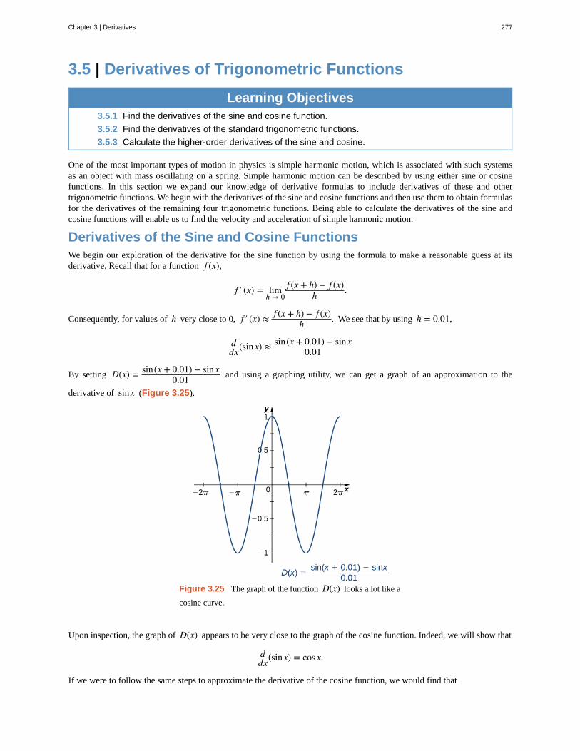
3.5 | Derivatives of Trigonometric Functions
Learning Objectives3.5.1 Find the derivatives of the sine and cosine function.
3.5.2 Find the derivatives of the standard trigonometric functions.
3.5.3 Calculate the higher-order derivatives of the sine and cosine.
One of the most important types of motion in physics is simple harmonic motion, which is associated with such systemsas an object with mass oscillating on a spring. Simple harmonic motion can be described by using either sine or cosinefunctions. In this section we expand our knowledge of derivative formulas to include derivatives of these and othertrigonometric functions. We begin with the derivatives of the sine and cosine functions and then use them to obtain formulasfor the derivatives of the remaining four trigonometric functions. Being able to calculate the derivatives of the sine andcosine functions will enable us to find the velocity and acceleration of simple harmonic motion.
Derivatives of the Sine and Cosine FunctionsWe begin our exploration of the derivative for the sine function by using the formula to make a reasonable guess at itsderivative. Recall that for a function f (x),
f ′ (x) = limh → 0
f (x + h) − f (x)h .
Consequently, for values of h very close to 0, f ′ (x) ≈ f (x + h) − f (x)h . We see that by using h = 0.01,
ddx(sinx) ≈ sin(x + 0.01) − sinx
0.01
By setting D(x) = sin(x + 0.01) − sinx0.01 and using a graphing utility, we can get a graph of an approximation to the
derivative of sinx (Figure 3.25).
Figure 3.25 The graph of the function D(x) looks a lot like a
cosine curve.
Upon inspection, the graph of D(x) appears to be very close to the graph of the cosine function. Indeed, we will show that
ddx(sinx) = cosx.
If we were to follow the same steps to approximate the derivative of the cosine function, we would find that
Chapter 3 | Derivatives 277
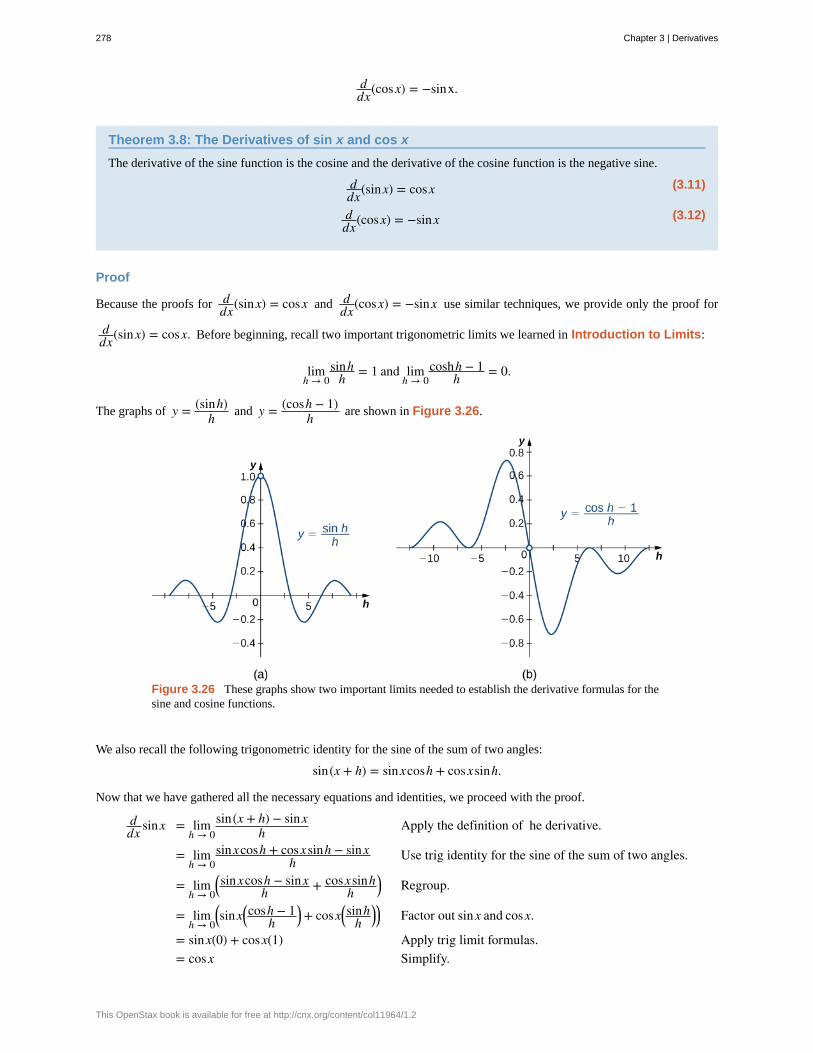
ddx(cosx) = −sinx.
Theorem 3.8: The Derivatives of sin x and cos x
The derivative of the sine function is the cosine and the derivative of the cosine function is the negative sine.
(3.11)ddx(sinx) = cosx
(3.12)ddx(cosx) = −sinx
Proof
Because the proofs for ddx(sinx) = cosx and d
dx(cosx) = −sinx use similar techniques, we provide only the proof for
ddx(sinx) = cosx. Before beginning, recall two important trigonometric limits we learned in Introduction to Limits:
limh → 0
sinhh = 1 and lim
h → 0coshh − 1
h = 0.
The graphs of y = (sinh)h and y = (cosh − 1)
h are shown in Figure 3.26.
Figure 3.26 These graphs show two important limits needed to establish the derivative formulas for thesine and cosine functions.
We also recall the following trigonometric identity for the sine of the sum of two angles:
sin(x + h) = sinxcosh + cosxsinh.
Now that we have gathered all the necessary equations and identities, we proceed with the proof.
ddx sinx = lim
h → 0sin(x + h) − sinx
h Apply the definition of he derivative.
= limh → 0
sinxcosh + cosxsinh − sinxh Use trig identity for the sine of the sum of two angles.
= limh → 0
⎛⎝sinxcosh − sinx
h + cosxsinhh
⎞⎠ Regroup.
= limh → 0
⎛⎝sinx⎛
⎝cosh − 1
h⎞⎠ + cosx⎛
⎝sinh
h⎞⎠⎞⎠ Factor out sinx and cosx.
= sinx(0) + cosx(1) Apply trig limit formulas.= cosx Simplify.
278 Chapter 3 | Derivatives
This OpenStax book is available for free at http://cnx.org/content/col11964/1.2
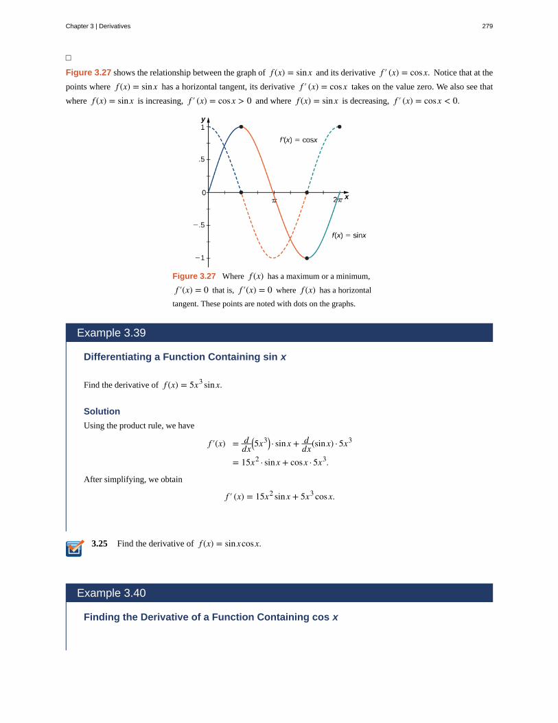
3.25
□
Figure 3.27 shows the relationship between the graph of f (x) = sinx and its derivative f ′ (x) = cosx. Notice that at the
points where f (x) = sinx has a horizontal tangent, its derivative f ′ (x) = cosx takes on the value zero. We also see that
where f (x) = sinx is increasing, f ′ (x) = cosx > 0 and where f (x) = sinx is decreasing, f ′ (x) = cosx < 0.
Figure 3.27 Where f (x) has a maximum or a minimum,
f ′(x) = 0 that is, f ′(x) = 0 where f (x) has a horizontal
tangent. These points are noted with dots on the graphs.
Example 3.39
Differentiating a Function Containing sin x
Find the derivative of f (x) = 5x3 sinx.
Solution
Using the product rule, we have
f ′(x) = ddx
⎛⎝5x3⎞
⎠ · sinx + ddx(sinx) · 5x3
= 15x2 · sinx + cosx · 5x3.
After simplifying, we obtain
f ′ (x) = 15x2 sinx + 5x3 cosx.
Find the derivative of f (x) = sinxcosx.
Example 3.40
Finding the Derivative of a Function Containing cos x
Chapter 3 | Derivatives 279
3.26
3.27
Find the derivative of g(x) = cosx4x2 .
Solution
By applying the quotient rule, we have
g′ (x) = (−sinx)4x2 − 8x(cosx)⎛⎝4x2⎞
⎠2 .
Simplifying, we obtain
g′ (x) = −4x2 sinx − 8xcosx16x4
= −xsinx − 2cosx4x3 .
Find the derivative of f (x) = xcosx.
Example 3.41
An Application to Velocity
A particle moves along a coordinate axis in such a way that its position at time t is given by s(t) = 2sin t − tfor 0 ≤ t ≤ 2π. At what times is the particle at rest?
Solution
To determine when the particle is at rest, set s′ (t) = v(t) = 0. Begin by finding s′ (t). We obtain
s′ (t) = 2cos t − 1,
so we must solve
2cos t − 1 = 0 for 0 ≤ t ≤ 2π.
The solutions to this equation are t = π3 and t = 5π
3 . Thus the particle is at rest at times t = π3 and t = 5π
3 .
A particle moves along a coordinate axis. Its position at time t is given by s(t) = 3t + 2cos t for
0 ≤ t ≤ 2π. At what times is the particle at rest?
Derivatives of Other Trigonometric FunctionsSince the remaining four trigonometric functions may be expressed as quotients involving sine, cosine, or both, we can usethe quotient rule to find formulas for their derivatives.
280 Chapter 3 | Derivatives
This OpenStax book is available for free at http://cnx.org/content/col11964/1.2
3.28
Example 3.42
The Derivative of the Tangent Function
Find the derivative of f (x) = tanx.
Solution
Start by expressing tanx as the quotient of sinx and cosx :
f (x) = tanx = sinxcosx.
Now apply the quotient rule to obtain
f ′ (x) = cosxcosx − (−sinx)sinx(cosx)2 .
Simplifying, we obtain
f ′ (x) = cos2 x + sin2 xcos2 x
.
Recognizing that cos2 x + sin2 x = 1, by the Pythagorean theorem, we now have
f ′ (x) = 1cos2 x
.
Finally, use the identity secx = 1cosx to obtain
f ′ (x) = sec2 x.
Find the derivative of f (x) = cot x.
The derivatives of the remaining trigonometric functions may be obtained by using similar techniques. We provide theseformulas in the following theorem.
Theorem 3.9: Derivatives of tanx, cotx, secx, and cscx
The derivatives of the remaining trigonometric functions are as follows:
(3.13)ddx(tanx) = sec2 x
(3.14)ddx(cot x) = −csc2 x
(3.15)ddx(secx) = secx tanx
(3.16)ddx(cscx) = −cscxcotx.
Example 3.43
Chapter 3 | Derivatives 281
3.29
Finding the Equation of a Tangent Line
Find the equation of a line tangent to the graph of f (x) = cot x at x = π4.
Solution
To find the equation of the tangent line, we need a point and a slope at that point. To find the point, compute
f ⎛⎝π4
⎞⎠ = cot π
4 = 1.
Thus the tangent line passes through the point ⎛⎝π4, 1⎞
⎠. Next, find the slope by finding the derivative of
f (x) = cot x and evaluating it at π4:
f ′ (x) = −csc2 x and f ′ ⎛⎝π4
⎞⎠ = −csc2 ⎛
⎝π4
⎞⎠ = −2.
Using the point-slope equation of the line, we obtain
y − 1 = −2⎛⎝x − π
4⎞⎠
or equivalently,
y = −2x + 1 + π2.
Example 3.44
Finding the Derivative of Trigonometric Functions
Find the derivative of f (x) = cscx + x tanx.
Solution
To find this derivative, we must use both the sum rule and the product rule. Using the sum rule, we find
f ′ (x) = ddx(cscx) + d
dx(x tanx).
In the first term, ddx(cscx) = −cscxcot x, and by applying the product rule to the second term we obtain
ddx(x tanx) = (1)(tanx) + (sec2 x)(x).
Therefore, we have
f ′ (x) = −cscxcot x + tanx + xsec2 x.
Find the derivative of f (x) = 2tanx − 3cot x.
282 Chapter 3 | Derivatives
This OpenStax book is available for free at http://cnx.org/content/col11964/1.2
3.30
3.31
Find the slope of the line tangent to the graph of f (x) = tanx at x = π6.
Higher-Order DerivativesThe higher-order derivatives of sinx and cosx follow a repeating pattern. By following the pattern, we can find any
higher-order derivative of sinx and cosx.
Example 3.45
Finding Higher-Order Derivatives of y = sinx
Find the first four derivatives of y = sinx.
Solution
Each step in the chain is straightforward:
y = sinxdydx = cosx
d2 ydx2 = −sinx
d3 ydx3 = −cosx
d4 ydx4 = sinx.
AnalysisOnce we recognize the pattern of derivatives, we can find any higher-order derivative by determining the step inthe pattern to which it corresponds. For example, every fourth derivative of sin x equals sin x, so
d4
dx4(sinx) = d8
dx8(sinx) = d12
dx12(sinx) = … = d4n
dx4n(sinx) = sinx
d5
dx5(sinx) = d9
dx9(sinx) = d13
dx13(sinx) = … = d4n + 1
dx4n + 1(sinx) = cosx.
For y = cosx, findd4 ydx4 .
Example 3.46
Using the Pattern for Higher-Order Derivatives of y = sinx
Find d74
dx74(sinx).
Chapter 3 | Derivatives 283
3.32
3.33
Solution
We can see right away that for the 74th derivative of sinx, 74 = 4(18) + 2, so
d74
dx74(sinx) = d72 + 2
dx72 + 2(sinx) = d2
dx2(sinx) = −sinx.
For y = sinx, find d59
dx59(sinx).
Example 3.47
An Application to Acceleration
A particle moves along a coordinate axis in such a way that its position at time t is given by s(t) = 2 − sin t.Find v(π/4) and a(π/4). Compare these values and decide whether the particle is speeding up or slowing down.
Solution
First find v(t) = s′ (t):
v(t) = s′ (t) = −cos t.
Thus,
v⎛⎝π4
⎞⎠ = − 1
2.
Next, find a(t) = v′(t). Thus, a(t) = v′ (t) = sin t and we have
a⎛⎝π4
⎞⎠ = 1
2.
Since v⎛⎝π4
⎞⎠ = − 1
2< 0 and a⎛
⎝π4
⎞⎠ = 1
2> 0, we see that velocity and acceleration are acting in opposite
directions; that is, the object is being accelerated in the direction opposite to the direction in which it is travelling.Consequently, the particle is slowing down.
A block attached to a spring is moving vertically. Its position at time t is given by s(t) = 2sin t. Find
v⎛⎝5π6
⎞⎠ and a⎛
⎝5π6
⎞⎠. Compare these values and decide whether the block is speeding up or slowing down.
284 Chapter 3 | Derivatives
This OpenStax book is available for free at http://cnx.org/content/col11964/1.2
3.5 EXERCISES
For the following exercises, finddydx for the given
functions.
175. y = x2 − secx + 1
176. y = 3cscx + 5x
177. y = x2 cot x
178. y = x − x3 sinx
179. y = secxx
180. y = sinx tanx
181. y = (x + cosx)(1 − sinx)
182. y = tanx1 − secx
183. y = 1 − cot x1 + cot x
184. y = cosx(1 + cscx)
For the following exercises, find the equation of the tangentline to each of the given functions at the indicated valuesof x. Then use a calculator to graph both the function and
the tangent line to ensure the equation for the tangent lineis correct.
185. [T] f (x) = −sinx, x = 0
186. [T] f (x) = cscx, x = π2
187. [T] f (x) = 1 + cosx, x = 3π2
188. [T] f (x) = secx, x = π4
189. [T] f (x) = x2 − tanx x = 0
190. [T] f (x) = 5cot x x = π4
For the following exercises, findd2 ydx2 for the given
functions.
191. y = xsinx − cosx
192. y = sinxcosx
193. y = x − 12 sinx
194. y = 1x + tanx
195. y = 2cscx
196. y = sec2 x
197. Find all x values on the graph of
f (x) = −3sinxcosx where the tangent line is horizontal.
198. Find all x values on the graph of f (x) = x − 2cosxfor 0 < x < 2π where the tangent line has slope 2.
199. Let f (x) = cot x. Determine the points on the graph
of f for 0 < x < 2π where the tangent line(s) is (are)
parallel to the line y = −2x.
200. [T] A mass on a spring bounces up and down insimple harmonic motion, modeled by the functions(t) = −6cos t where s is measured in inches and t is
measured in seconds. Find the rate at which the spring isoscillating at t = 5 s.
201. Let the position of a swinging pendulum in simpleharmonic motion be given by s(t) = acos t + bsin t. Find
the constants a and b such that when the velocity is 3 cm/
s, s = 0 and t = 0.
202. After a diver jumps off a diving board, the edge ofthe board oscillates with position given by s(t) = −5cos tcm at t seconds after the jump.
a. Sketch one period of the position function fort ≥ 0.
b. Find the velocity function.c. Sketch one period of the velocity function for
t ≥ 0.d. Determine the times when the velocity is 0 over one
period.e. Find the acceleration function.f. Sketch one period of the acceleration function for
t ≥ 0.
Chapter 3 | Derivatives 285
203. The number of hamburgers sold at a fast-foodrestaurant in Pasadena, California, is given byy = 10 + 5sinx where y is the number of hamburgers
sold and x represents the number of hours after the
restaurant opened at 11 a.m. until 11 p.m., when the storecloses. Find y′ and determine the intervals where the
number of burgers being sold is increasing.
204. [T] The amount of rainfall per month in Phoenix,Arizona, can be approximated by y(t) = 0.5 + 0.3cos t,where t is months since January. Find y′ and use a
calculator to determine the intervals where the amount ofrain falling is decreasing.
For the following exercises, use the quotient rule to derivethe given equations.
205. ddx(cot x) = −csc2 x
206. ddx(secx) = secx tanx
207. ddx(cscx) = −cscxcot x
208. Use the definition of derivative and the identitycos(x + h) = cosxcosh − sinxsinh to prove that
d(cosx)dx = −sinx.
For the following exercises, find the requested higher-orderderivative for the given functions.
209.d3 ydx3 of y = 3cosx
210.d2 ydx2 of y = 3sinx + x2 cosx
211.d4 ydx4 of y = 5cosx
212.d2 ydx2 of y = secx + cot x
213.d3 ydx3 of y = x10 − secx
286 Chapter 3 | Derivatives
This OpenStax book is available for free at http://cnx.org/content/col11964/1.2
3.6 | The Chain Rule
Learning Objectives3.6.1 State the chain rule for the composition of two functions.
3.6.2 Apply the chain rule together with the power rule.
3.6.3 Apply the chain rule and the product/quotient rules correctly in combination when both arenecessary.
3.6.4 Recognize the chain rule for a composition of three or more functions.
3.6.5 Describe the proof of the chain rule.
We have seen the techniques for differentiating basic functions (xn, sinx, cosx, etc.) as well as sums, differences,
products, quotients, and constant multiples of these functions. However, these techniques do not allow us to differentiate
compositions of functions, such as h(x) = sin⎛⎝x
3⎞⎠ or k(x) = 3x2 + 1. In this section, we study the rule for finding the
derivative of the composition of two or more functions.
Deriving the Chain RuleWhen we have a function that is a composition of two or more functions, we could use all of the techniques we have alreadylearned to differentiate it. However, using all of those techniques to break down a function into simpler parts that we areable to differentiate can get cumbersome. Instead, we use the chain rule, which states that the derivative of a compositefunction is the derivative of the outer function evaluated at the inner function times the derivative of the inner function.
To put this rule into context, let’s take a look at an example: h(x) = sin ⎛⎝x
3⎞⎠. We can think of the derivative of this function
with respect to x as the rate of change of sin⎛⎝x
3⎞⎠ relative to the change in x. Consequently, we want to know how sin⎛
⎝x3⎞
⎠
changes as x changes. We can think of this event as a chain reaction: As x changes, x3 changes, which leads to a change
in sin ⎛⎝x
3⎞⎠. This chain reaction gives us hints as to what is involved in computing the derivative of sin⎛
⎝x3⎞
⎠. First of all, a
change in x forcing a change in x3 suggests that somehow the derivative of x3 is involved. In addition, the change in x3
forcing a change in sin⎛⎝x
3⎞⎠ suggests that the derivative of sin(u) with respect to u, where u = x3, is also part of the
final derivative.
We can take a more formal look at the derivative of h(x) = sin ⎛⎝x
3⎞⎠ by setting up the limit that would give us the derivative
at a specific value a in the domain of h(x) = sin ⎛⎝x
3⎞⎠.
h′ (a) = limx → asin ⎛
⎝x3⎞
⎠ − sin⎛⎝a
3⎞⎠
x − a .
This expression does not seem particularly helpful; however, we can modify it by multiplying and dividing by the
expression x3 − a3 to obtain
h′ (a) = limx → asin ⎛
⎝x3⎞
⎠ − sin⎛⎝a
3⎞⎠
x3 − a3 · x3 − a3x − a .
From the definition of the derivative, we can see that the second factor is the derivative of x3 at x = a. That is,
limx → ax3 − a3x − a = d
dx⎛⎝x
3⎞⎠ = 3a2.
However, it might be a little more challenging to recognize that the first term is also a derivative. We can see this by letting
u = x3 and observing that as x → a, u → a3 :
Chapter 3 | Derivatives 287
limx → asin ⎛
⎝x3⎞
⎠ − sin ⎛⎝a
3⎞⎠
x3 − a3 = limu → a3
sinu − sin ⎛⎝a
3⎞⎠
u − a3
= ddu(sinu)u = a3
= cos ⎛⎝a
3).
Thus, h′ (a) = cos⎛⎝a
3⎞⎠ · 3a2.
In other words, if h(x) = sin ⎛⎝x
3⎞⎠, then h′ (x) = cos ⎛
⎝x3⎞
⎠ · 3x2. Thus, if we think of h(x) = sin⎛⎝x
3⎞⎠ as the composition
⎛⎝ f ∘g⎞
⎠(x) = f ⎛⎝g(x)⎞
⎠ where f (x) = sin x and g(x) = x3, then the derivative of h(x) = sin⎛⎝x
3⎞⎠ is the product of the
derivative of g(x) = x3 and the derivative of the function f (x) = sinx evaluated at the function g(x) = x3. At this point,
we anticipate that for h(x) = sin ⎛⎝g(x)⎞
⎠, it is quite likely that h′(x) = cos(g(x))g′(x). As we determined above, this is the
case for h(x) = sin ⎛⎝x
3⎞⎠.
Now that we have derived a special case of the chain rule, we state the general case and then apply it in a general form toother composite functions. An informal proof is provided at the end of the section.
Rule: The Chain Rule
Let f and g be functions. For all x in the domain of g for which g is differentiable at x and f is differentiable at
g(x), the derivative of the composite function
h(x) = ⎛⎝ f ∘g⎞
⎠(x) = f ⎛⎝g(x)⎞
⎠
is given by
(3.17)h′ (x) = f ′ ⎛⎝g(x)⎞
⎠g′ (x).
Alternatively, if y is a function of u, and u is a function of x, then
dydx = dy
du · dudx .
Watch an animation (http://www.openstaxcollege.org/l/20_chainrule2) of the chain rule.
Problem-Solving Strategy: Applying the Chain Rule
1. To differentiate h(x) = f ⎛⎝g(x)⎞
⎠, begin by identifying f (x) and g(x).
2. Find f ′(x) and evaluate it at g(x) to obtain f ′ ⎛⎝g(x)⎞
⎠.
3. Find g′(x).
4. Write h′ (x) = f ′ ⎛⎝g(x)⎞
⎠ · g′ (x).
Note: When applying the chain rule to the composition of two or more functions, keep in mind that we work our wayfrom the outside function in. It is also useful to remember that the derivative of the composition of two functions canbe thought of as having two parts; the derivative of the composition of three functions has three parts; and so on. Also,remember that we never evaluate a derivative at a derivative.
288 Chapter 3 | Derivatives
This OpenStax book is available for free at http://cnx.org/content/col11964/1.2
3.34
The Chain and Power Rules CombinedWe can now apply the chain rule to composite functions, but note that we often need to use it with other rules. For example,to find derivatives of functions of the form h(x) = (g(x))n, we need to use the chain rule combined with the power rule. To
do so, we can think of h(x) = ⎛⎝g(x)⎞
⎠n as f ⎛
⎝g(x)⎞⎠ where f (x) = xn. Then f ′ (x) = nxn − 1. Thus, f ′ ⎛
⎝g(x)⎞⎠ = n⎛
⎝g(x)⎞⎠n − 1.
This leads us to the derivative of a power function using the chain rule,
h′ (x) = n⎛⎝g(x)⎞
⎠n − 1 g′ (x)
Rule: Power Rule for Composition of Functions
For all values of x for which the derivative is defined, if
h(x) = ⎛⎝g(x)⎞
⎠n.
Then
(3.18)h′ (x) = n⎛⎝g(x)⎞
⎠n − 1 g′ (x).
Example 3.48
Using the Chain and Power Rules
Find the derivative of h(x) = 1⎛⎝3x2 + 1⎞
⎠2.
Solution
First, rewrite h(x) = 1⎛⎝3x2 + 1⎞
⎠2 = ⎛
⎝3x2 + 1⎞⎠−2
.
Applying the power rule with g(x) = 3x2 + 1, we have
h′ (x) = −2⎛⎝3x2 + 1⎞
⎠−3
(6x).
Rewriting back to the original form gives us
h′ (x) = −12x(3x2 + 1)3.
Find the derivative of h(x) = ⎛⎝2x3 + 2x − 1⎞
⎠4.
Example 3.49
Using the Chain and Power Rules with a Trigonometric Function
Find the derivative of h(x) = sin3 x.
Chapter 3 | Derivatives 289
3.35
Solution
First recall that sin3 x = (sinx)3, so we can rewrite h(x) = sin3 x as h(x) = (sinx)3.
Applying the power rule with g(x) = sinx, we obtain
h′ (x) = 3(sinx)2 cosx = 3sin2 xcosx.
Example 3.50
Finding the Equation of a Tangent Line
Find the equation of a line tangent to the graph of h(x) = 1(3x − 5)2 at x = 2.
Solution
Because we are finding an equation of a line, we need a point. The x-coordinate of the point is 2. To find the
y-coordinate, substitute 2 into h(x). Since h(2) = 1⎛⎝3(2) − 5⎞
⎠2 = 1, the point is (2, 1).
For the slope, we need h′(2). To find h′(x), first we rewrite h(x) = (3x − 5)−2 and apply the power rule to
obtain
h′ (x) = −2(3x − 5)−3 (3) = −6(3x − 5)−3.
By substituting, we have h′ (2) = −6⎛⎝3(2) − 5⎞
⎠−3 = −6. Therefore, the line has equation y − 1 = −6(x − 2).
Rewriting, the equation of the line is y = −6x + 13.
Find the equation of the line tangent to the graph of f (x) = ⎛⎝x2 − 2⎞
⎠3
at x = −2.
Combining the Chain Rule with Other RulesNow that we can combine the chain rule and the power rule, we examine how to combine the chain rule with the other ruleswe have learned. In particular, we can use it with the formulas for the derivatives of trigonometric functions or with theproduct rule.
Example 3.51
Using the Chain Rule on a General Cosine Function
Find the derivative of h(x) = cos ⎛⎝g(x)⎞
⎠.
Solution
290 Chapter 3 | Derivatives
This OpenStax book is available for free at http://cnx.org/content/col11964/1.2
3.36
Think of h(x) = cos(g(x)) as f ⎛⎝g(x)⎞
⎠ where f (x) = cosx. Since f ′ (x) = −sinx. we have
f ′ ⎛⎝g(x)⎞
⎠ = −sin ⎛⎝g(x)⎞
⎠. Then we do the following calculation.
h′ (x) = f ′ ⎛⎝g(x)⎞
⎠g′ (x) Apply the chain rule.= −sin ⎛
⎝g(x)⎞⎠g′ (x) Substitute f ′ ⎛
⎝g(x)⎞⎠ = −sin ⎛
⎝g(x)⎞⎠.
Thus, the derivative of h(x) = cos ⎛⎝g(x)⎞
⎠ is given by h′ (x) = −sin ⎛⎝g(x)⎞
⎠g′ (x).
In the following example we apply the rule that we have just derived.
Example 3.52
Using the Chain Rule on a Cosine Function
Find the derivative of h(x) = cos ⎛⎝5x2⎞
⎠.
Solution
Let g(x) = 5x2. Then g′ (x) = 10x. Using the result from the previous example,
h′ (x) = −sin ⎛⎝5x2⎞
⎠ · 10x
= −10xsin ⎛⎝5x2⎞
⎠.
Example 3.53
Using the Chain Rule on Another Trigonometric Function
Find the derivative of h(x) = sec⎛⎝4x5 + 2x⎞
⎠.
Solution
Apply the chain rule to h(x) = sec ⎛⎝g(x)⎞
⎠ to obtain
h′ (x) = sec(g(x) tan ⎛⎝g(x)⎞
⎠g′ (x).
In this problem, g(x) = 4x5 + 2x, so we have g′ (x) = 20x4 + 2. Therefore, we obtain
h′ (x) = sec⎛⎝4x5 + 2x⎞
⎠tan⎛⎝4x5 + 2x⎞
⎠⎛⎝20x4 + 2⎞
⎠
= (20x4 + 2)sec⎛⎝4x5 + 2x⎞
⎠tan⎛⎝4x5 + 2x⎞
⎠.
Find the derivative of h(x) = sin(7x + 2).
Chapter 3 | Derivatives 291
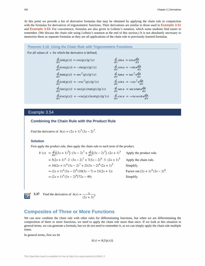
3.37
At this point we provide a list of derivative formulas that may be obtained by applying the chain rule in conjunctionwith the formulas for derivatives of trigonometric functions. Their derivations are similar to those used in Example 3.51and Example 3.53. For convenience, formulas are also given in Leibniz’s notation, which some students find easier toremember. (We discuss the chain rule using Leibniz’s notation at the end of this section.) It is not absolutely necessary tomemorize these as separate formulas as they are all applications of the chain rule to previously learned formulas.
Theorem 3.10: Using the Chain Rule with Trigonometric Functions
For all values of x for which the derivative is defined,
ddx
⎛⎝sin(g(x)⎞
⎠ = cos ⎛⎝g(x)⎞
⎠g′(x) ddx sinu = cosudu
dxddx
⎛⎝cos(g(x)⎞
⎠ = −sin ⎛⎝g(x)⎞
⎠g′(x) ddx cosu = −sinudu
dxddx
⎛⎝tan(g(x)⎞
⎠ = sec2 ⎛⎝g(x)⎞
⎠g′(x) ddx tanu = sec2 udu
dxddx
⎛⎝cot(g(x)⎞
⎠ = −csc2 ⎛⎝g(x)⎞
⎠g′(x) ddx cotu = −csc2 udu
dxddx
⎛⎝sec(g(x)⎞
⎠ = sec(g(x) tan ⎛⎝g(x)⎞
⎠g′(x) ddx secu = secu tanudu
dxddx
⎛⎝csc(g(x)⎞
⎠ = −csc(g(x))cot ⎛⎝g(x)⎞
⎠g′(x) ddx cscu = −cscucotudu
dx .
Example 3.54
Combining the Chain Rule with the Product Rule
Find the derivative of h(x) = (2x + 1)5 (3x − 2)7.
Solution
First apply the product rule, then apply the chain rule to each term of the product.
h′ (x) = ddx
⎛⎝(2x + 1)5⎞
⎠ · (3x − 2)7 + ddx
⎛⎝(3x − 2)7⎞
⎠ · (2x + 1)5 Apply the product rule.
= 5(2x + 1)4 · 2 · (3x − 2)7 + 7(3x − 2)6 · 3 · (2x + 1)5 Apply the chain rule.
= 10(2x + 1)4 (3x − 2)7 + 21(3x − 2)6 (2x + 1)5 Simplify.
= (2x + 1)4 (3x − 2)6 (10(3x − 7) + 21(2x + 1)) Factor out (2x + 1)4 (3x − 2)6.= (2x + 1)4 (3x − 2)6(72x − 49) Simplify.
Find the derivative of h(x) = x(2x + 3)3.
Composites of Three or More FunctionsWe can now combine the chain rule with other rules for differentiating functions, but when we are differentiating thecomposition of three or more functions, we need to apply the chain rule more than once. If we look at this situation ingeneral terms, we can generate a formula, but we do not need to remember it, as we can simply apply the chain rule multipletimes.
In general terms, first we let
k(x) = h⎛⎝ f ⎛
⎝g(x)⎞⎠⎞⎠.
292 Chapter 3 | Derivatives
This OpenStax book is available for free at http://cnx.org/content/col11964/1.2
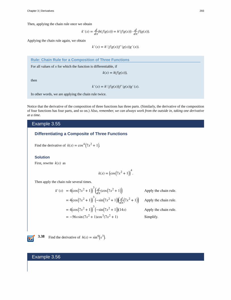
3.38
Then, applying the chain rule once we obtain
k′ (x) = ddx
⎛⎝h( f ⎛
⎝g(x)⎞⎠⎞⎠ = h′⎛
⎝ f ⎛⎝g(x)⎞
⎠⎞⎠ · d
dx f ⎛⎝⎛⎝g(x)⎞
⎠⎞⎠.
Applying the chain rule again, we obtain
k′ (x) = h′ ⎛⎝ f ⎛
⎝g(x)⎞⎠ f ′ ⎛
⎝g(x)⎞⎠g′ (x)⎞
⎠.
Rule: Chain Rule for a Composition of Three Functions
For all values of x for which the function is differentiable, if
k(x) = h⎛⎝ f ⎛
⎝g(x)⎞⎠⎞⎠,
then
k′ (x) = h′ ⎛⎝ f ⎛
⎝g(x)⎞⎠⎞⎠ f ′ ⎛
⎝g(x)⎞⎠g′ (x).
In other words, we are applying the chain rule twice.
Notice that the derivative of the composition of three functions has three parts. (Similarly, the derivative of the compositionof four functions has four parts, and so on.) Also, remember, we can always work from the outside in, taking one derivativeat a time.
Example 3.55
Differentiating a Composite of Three Functions
Find the derivative of k(x) = cos4 ⎛⎝7x2 + 1⎞
⎠.
Solution
First, rewrite k(x) as
k(x) = ⎛⎝cos ⎛
⎝7x2 + 1⎞⎠⎞⎠4.
Then apply the chain rule several times.
k′ (x) = 4⎛⎝cos ⎛
⎝7x2 + 1⎞⎠⎞⎠3 ⎛
⎝ddx(cos ⎛
⎝7x2 + 1⎞⎠⎞⎠ Apply the chain rule.
= 4⎛⎝cos ⎛
⎝7x2 + 1⎞⎠⎞⎠3 ⎛
⎝−sin ⎛⎝7x2 + 1⎞
⎠⎞⎠⎛⎝
ddx
⎛⎝7x2 + 1⎞
⎠⎞⎠ Apply the chain rule.
= 4⎛⎝cos ⎛
⎝7x2 + 1⎞⎠⎞⎠3 ⎛
⎝−sin ⎛⎝7x2 + 1⎞
⎠⎞⎠(14x) Apply the chain rule.
= −56xsin(7x2 + 1)cos3(7x2 + 1) Simplify.
Find the derivative of h(x) = sin6⎛⎝x
3⎞⎠.
Example 3.56
Chapter 3 | Derivatives 293
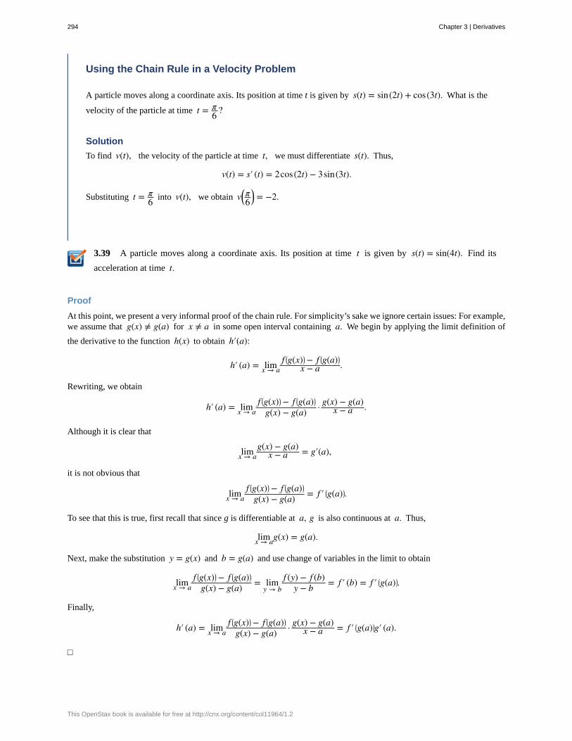
3.39
Using the Chain Rule in a Velocity Problem
A particle moves along a coordinate axis. Its position at time t is given by s(t) = sin(2t) + cos(3t). What is the
velocity of the particle at time t = π6 ?
Solution
To find v(t), the velocity of the particle at time t, we must differentiate s(t). Thus,
v(t) = s′ (t) = 2cos(2t) − 3sin(3t).
Substituting t = π6 into v(t), we obtain v⎛
⎝π6
⎞⎠ = −2.
A particle moves along a coordinate axis. Its position at time t is given by s(t) = sin(4t). Find its
acceleration at time t.
Proof
At this point, we present a very informal proof of the chain rule. For simplicity’s sake we ignore certain issues: For example,we assume that g(x) ≠ g(a) for x ≠ a in some open interval containing a. We begin by applying the limit definition of
the derivative to the function h(x) to obtain h′(a):
h′ (a) = limx → af ⎛
⎝g(x)⎞⎠ − f ⎛
⎝g(a)⎞⎠
x − a .
Rewriting, we obtain
h′ (a) = limx → af ⎛
⎝g(x)⎞⎠ − f ⎛
⎝g(a)⎞⎠
g(x) − g(a) · g(x) − g(a)x − a .
Although it is clear that
limx → ag(x) − g(a)
x − a = g′(a),
it is not obvious that
limx → af ⎛
⎝g(x)⎞⎠ − f ⎛
⎝g(a)⎞⎠
g(x) − g(a) = f ′ ⎛⎝g(a)⎞
⎠.
To see that this is true, first recall that since g is differentiable at a, g is also continuous at a. Thus,
limx → ag(x) = g(a).
Next, make the substitution y = g(x) and b = g(a) and use change of variables in the limit to obtain
limx → af ⎛
⎝g(x)⎞⎠ − f ⎛
⎝g(a)⎞⎠
g(x) − g(a) = limy → b
f (y) − f (b)y − b = f ′ (b) = f ′ ⎛
⎝g(a)⎞⎠.
Finally,
h′ (a) = limx → af ⎛
⎝g(x)⎞⎠ − f ⎛
⎝g(a)⎞⎠
g(x) − g(a) · g(x) − g(a)x − a = f ′ ⎛
⎝g(a)⎞⎠g′ (a).
□
294 Chapter 3 | Derivatives
This OpenStax book is available for free at http://cnx.org/content/col11964/1.2
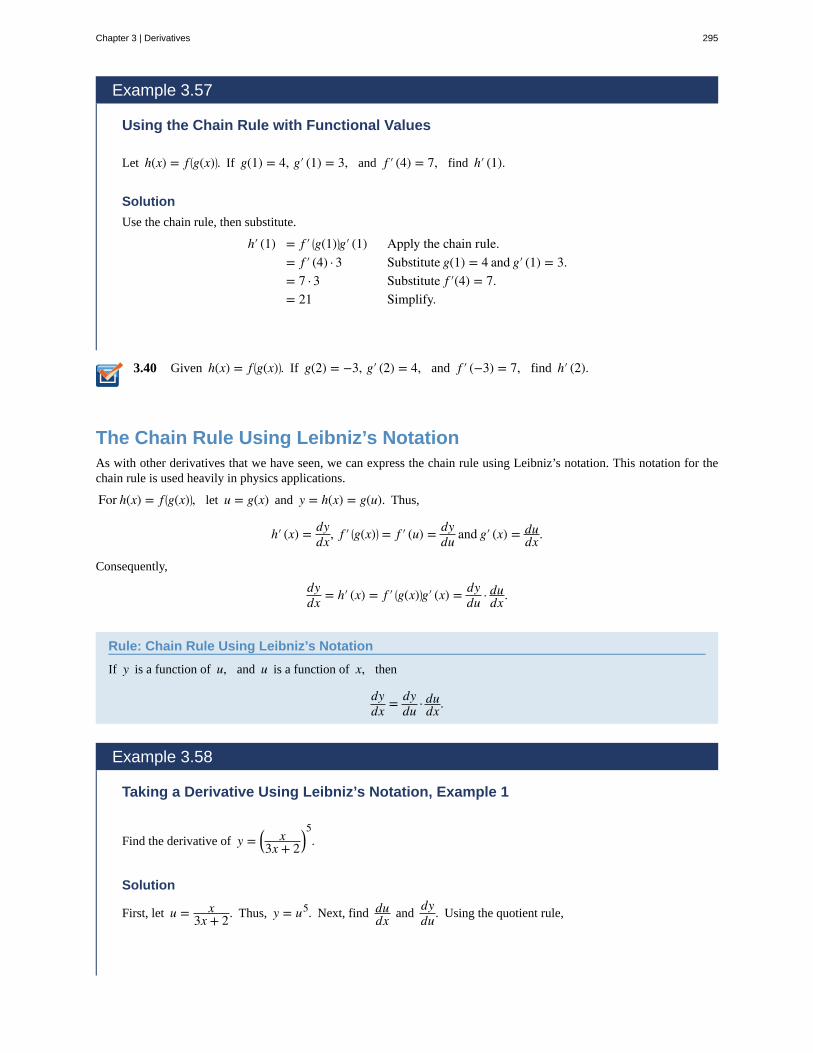
3.40
Example 3.57
Using the Chain Rule with Functional Values
Let h(x) = f ⎛⎝g(x)⎞
⎠. If g(1) = 4, g′ (1) = 3, and f ′ (4) = 7, find h′ (1).
Solution
Use the chain rule, then substitute.
h′ (1) = f ′ ⎛⎝g(1)⎞
⎠g′ (1) Apply the chain rule.= f ′ (4) · 3 Substitute g(1) = 4 and g′ (1) = 3.= 7 · 3 Substitute f ′(4) = 7.= 21 Simplify.
Given h(x) = f ⎛⎝g(x)⎞
⎠. If g(2) = −3, g′ (2) = 4, and f ′ (−3) = 7, find h′ (2).
The Chain Rule Using Leibniz’s NotationAs with other derivatives that we have seen, we can express the chain rule using Leibniz’s notation. This notation for thechain rule is used heavily in physics applications.
For h(x) = f ⎛⎝g(x)⎞
⎠, let u = g(x) and y = h(x) = g(u). Thus,
h′ (x) = dydx, f ′ ⎛
⎝g(x)⎞⎠ = f ′ (u) = dy
du and g′ (x) = dudx .
Consequently,
dydx = h′ (x) = f ′ ⎛
⎝g(x)⎞⎠g′ (x) = dy
du · dudx .
Rule: Chain Rule Using Leibniz’s Notation
If y is a function of u, and u is a function of x, then
dydx = dy
du · dudx .
Example 3.58
Taking a Derivative Using Leibniz’s Notation, Example 1
Find the derivative of y = ⎛⎝
x3x + 2
⎞⎠
5.
Solution
First, let u = x3x + 2. Thus, y = u5. Next, find du
dx anddydu. Using the quotient rule,
Chapter 3 | Derivatives 295
3.41
dudx = 2
(3x + 2)2
and
dydu = 5u4.
Finally, we put it all together.
dydx = dy
du · dudx Apply the chain rule.
= 5u4 · 2(3x + 2)2 Substitute dy
du = 5u4 and dudx = 2
(3x + 2)2.
= 5⎛⎝
x3x + 2
⎞⎠
4· 2(3x + 2)2 Substitute u = x
3x + 2.
= 10x4
(3x + 2)6 Simplify.
It is important to remember that, when using the Leibniz form of the chain rule, the final answer must beexpressed entirely in terms of the original variable given in the problem.
Example 3.59
Taking a Derivative Using Leibniz’s Notation, Example 2
Find the derivative of y = tan⎛⎝4x2 − 3x + 1⎞
⎠.
Solution
First, let u = 4x2 − 3x + 1. Then y = tanu. Next, find dudx and
dydu:
dudx = 8x − 3 and dy
du = sec2 u.
Finally, we put it all together.
dydx = dy
du · dudx Apply the chain rule.
= sec2 u · (8x − 3) Use dudx = 8x − 3 and dy
du = sec2 u.
= sec2(4x2 − 3x + 1) · (8x − 3) Substitute u = 4x2 − 3x + 1.
Use Leibniz’s notation to find the derivative of y = cos ⎛⎝x
3⎞⎠. Make sure that the final answer is
expressed entirely in terms of the variable x.
296 Chapter 3 | Derivatives
This OpenStax book is available for free at http://cnx.org/content/col11964/1.2
3.6 EXERCISESFor the following exercises, given y = f (u) and
u = g(x), finddydx by using Leibniz’s notation for the
chain rule:dydx = dy
dududx .
214. y = 3u − 6, u = 2x2
215. y = 6u3, u = 7x − 4
216. y = sinu, u = 5x − 1
217. y = cosu, u = −x8
218. y = tanu, u = 9x + 2
219. y = 4u + 3, u = x2 − 6x
For each of the following exercises,
a. decompose each function in the form y = f (u)and u = g(x), and
b. finddydx as a function of x.
220. y = (3x − 2)6
221. y = ⎛⎝3x2 + 1⎞
⎠3
222. y = sin5 (x)
223. y = ⎛⎝x7 + 7
x⎞⎠7
224. y = tan(secx)
225. y = csc(πx + 1)
226. y = cot2 x
227. y = −6sin−3 x
For the following exercises, finddydx for each function.
228. y = ⎛⎝3x2 + 3x − 1⎞
⎠4
229. y = (5 − 2x)−2
230. y = cos3 (πx)
231. y = ⎛⎝2x3 − x2 + 6x + 1⎞
⎠3
232. y = 1sin2(x)
233. y = (tanx + sinx)−3
234. y = x2 cos4 x
235. y = sin(cos7x)
236. y = 6 + secπx2
237. y = cot3 (4x + 1)
238. Let y = ⎡⎣ f (x)⎤
⎦3 and suppose that f ′ (1) = 4 and
dydx = 10 for x = 1. Find f (1).
239. Let y = ⎛⎝ f (x) + 5x2⎞
⎠4
and suppose that
f (−1) = −4 anddydx = 3 when x = −1. Find f ′ (−1)
240. Let y = ⎛⎝ f (u) + 3x⎞
⎠2 and u = x3 − 2x. If
f (4) = 6 anddydx = 18 when x = 2, find f ′ (4).
241. [T] Find the equation of the tangent line to
y = −sin⎛⎝x2
⎞⎠ at the origin. Use a calculator to graph the
function and the tangent line together.
242. [T] Find the equation of the tangent line to
y = ⎛⎝3x + 1
x⎞⎠2
at the point (1, 16). Use a calculator to
graph the function and the tangent line together.
243. Find the x -coordinates at which the tangent line to
y = ⎛⎝x − 6
x⎞⎠8
is horizontal.
244. [T] Find an equation of the line that is normal to
g(θ) = sin2 (πθ) at the point ⎛⎝14, 1
2⎞⎠. Use a calculator to
graph the function and the normal line together.
For the following exercises, use the information in thefollowing table to find h′(a) at the given value for a.
Chapter 3 | Derivatives 297
x f(x) f′(x) g(x) g′(x)
0 2 5 0 2
1 1 −2 3 0
2 4 4 1 −1
3 3 −3 2 3
245. h(x) = f ⎛⎝g(x)⎞
⎠; a = 0
246. h(x) = g⎛⎝ f (x)⎞
⎠; a = 0
247. h(x) = ⎛⎝x4 + g(x)⎞
⎠−2
; a = 1
248. h(x) = ⎛⎝
f (x)g(x)
⎞⎠
2; a = 3
249. h(x) = f ⎛⎝x + f (x)⎞
⎠; a = 1
250. h(x) = ⎛⎝1 + g(x)⎞
⎠3; a = 2
251. h(x) = g⎛⎝2 + f ⎛
⎝x2⎞⎠⎞⎠; a = 1
252. h(x) = f ⎛⎝g(sinx)⎞
⎠; a = 0
253. [T] The position function of a freight train is given by
s(t) = 100(t + 1)−2, with s in meters and t in seconds.
At time t = 6 s, find the train’s
a. velocity andb. acceleration.c. Using a. and b. is the train speeding up or slowing
down?
254. [T] A mass hanging from a vertical spring is insimple harmonic motion as given by the following positionfunction, where t is measured in seconds and s is in
inches: s(t) = −3cos⎛⎝πt + π
4⎞⎠.
a. Determine the position of the spring at t = 1.5 s.
b. Find the velocity of the spring at t = 1.5 s.
255. [T] The total cost to produce x boxes of Thin Mint
Girl Scout cookies is C dollars, where
C = 0.0001x3 − 0.02x2 + 3x + 300. In t weeks
production is estimated to be x = 1600 + 100t boxes.
a. Find the marginal cost C′ (x).b. Use Leibniz’s notation for the chain rule,
dCdt = dC
dx · dxdt , to find the rate with respect to
time t that the cost is changing.
c. Use b. to determine how fast costs are increasingwhen t = 2 weeks. Include units with the answer.
256. [T] The formula for the area of a circle is A = πr2,where r is the radius of the circle. Suppose a circle is
expanding, meaning that both the area A and the radius r(in inches) are expanding.
a. Suppose r = 2 − 100(t + 7)2 where t is time in
seconds. Use the chain rule dAdt = dA
dr · drdt to find
the rate at which the area is expanding.b. Use a. to find the rate at which the area is
expanding at t = 4 s.
257. [T] The formula for the volume of a sphere is
S = 43πr3, where r (in feet) is the radius of the sphere.
Suppose a spherical snowball is melting in the sun.
a. Suppose r = 1(t + 1)2 − 1
12 where t is time in
minutes. Use the chain rule dSdt = dS
dr · drdt to find
the rate at which the snowball is melting.b. Use a. to find the rate at which the volume is
changing at t = 1 min.
258. [T] The daily temperature in degrees Fahrenheit ofPhoenix in the summer can be modeled by the function
T(x) = 94 − 10cos⎡⎣
π12(x − 2)⎤
⎦, where x is hours after
midnight. Find the rate at which the temperature ischanging at 4 p.m.
259. [T] The depth (in feet) of water at a dock changeswith the rise and fall of tides. The depth is modeled by
the function D(t) = 5sin⎛⎝π6 t − 7π
6⎞⎠ + 8, where t is the
number of hours after midnight. Find the rate at which thedepth is changing at 6 a.m.
298 Chapter 3 | Derivatives
This OpenStax book is available for free at http://cnx.org/content/col11964/1.2
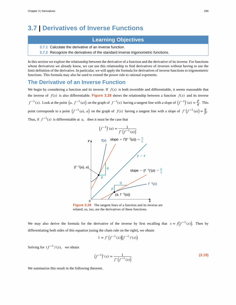
3.7 | Derivatives of Inverse Functions
Learning Objectives3.7.1 Calculate the derivative of an inverse function.
3.7.2 Recognize the derivatives of the standard inverse trigonometric functions.
In this section we explore the relationship between the derivative of a function and the derivative of its inverse. For functionswhose derivatives we already know, we can use this relationship to find derivatives of inverses without having to use thelimit definition of the derivative. In particular, we will apply the formula for derivatives of inverse functions to trigonometricfunctions. This formula may also be used to extend the power rule to rational exponents.
The Derivative of an Inverse FunctionWe begin by considering a function and its inverse. If f (x) is both invertible and differentiable, it seems reasonable that
the inverse of f (x) is also differentiable. Figure 3.28 shows the relationship between a function f (x) and its inverse
f −1 (x). Look at the point ⎛⎝a, f −1 (a)⎞
⎠ on the graph of f −1(x) having a tangent line with a slope of ⎛⎝ f −1⎞
⎠′ (a) = pq . This
point corresponds to a point ⎛⎝ f −1 (a), a⎞
⎠ on the graph of f (x) having a tangent line with a slope of f ′ ⎛⎝ f −1 (a)⎞
⎠ = qp.
Thus, if f −1(x) is differentiable at a, then it must be the case that
⎛⎝ f −1⎞
⎠′ (a) = 1f ′ ⎛
⎝ f −1 (a)⎞⎠.
Figure 3.28 The tangent lines of a function and its inverse arerelated; so, too, are the derivatives of these functions.
We may also derive the formula for the derivative of the inverse by first recalling that x = f ⎛⎝ f −1 (x)⎞
⎠. Then by
differentiating both sides of this equation (using the chain rule on the right), we obtain
1 = f ′ ⎛⎝ f −1 (x)⎞
⎠⎛⎝ f −1 )′(x)⎞
⎠.
Solving for ( f −1 )′(x), we obtain
(3.19)⎛⎝ f −1⎞
⎠′ (x) = 1f ′ ⎛
⎝ f −1 (x)⎞⎠.
We summarize this result in the following theorem.
Chapter 3 | Derivatives 299
3.42
Theorem 3.11: Inverse Function Theorem
Let f (x) be a function that is both invertible and differentiable. Let y = f −1 (x) be the inverse of f (x). For all x
satisfying f ′ ⎛⎝ f −1 (x)⎞
⎠ ≠ 0,
dydx = d
dx⎛⎝ f −1(x)⎞
⎠ = ⎛⎝ f −1⎞
⎠′ (x) = 1f ′ ⎛
⎝ f −1 (x)⎞⎠.
Alternatively, if y = g(x) is the inverse of f (x), then
g(x) = 1f ′ ⎛
⎝g(x)⎞⎠.
Example 3.60
Applying the Inverse Function Theorem
Use the inverse function theorem to find the derivative of g(x) = x + 2x . Compare the resulting derivative to that
obtained by differentiating the function directly.
Solution
The inverse of g(x) = x + 2x is f (x) = 2
x − 1. Since g′ (x) = 1f ′ ⎛
⎝g(x)⎞⎠, begin by finding f ′ (x). Thus,
f ′ (x) = −2(x − 1)2 and f ′ ⎛
⎝g(x)⎞⎠ = −2
⎛⎝g(x) − 1⎞
⎠2 = −2
⎛⎝x + 2
x − 1⎞⎠2 = − x2
2 .
Finally,
g′ (x) = 1f ′ ⎛
⎝g(x)⎞⎠
= − 2x2.
We can verify that this is the correct derivative by applying the quotient rule to g(x) to obtain
g′ (x) = − 2x2.
Use the inverse function theorem to find the derivative of g(x) = 1x + 2. Compare the result obtained
by differentiating g(x) directly.
Example 3.61
Applying the Inverse Function Theorem
Use the inverse function theorem to find the derivative of g(x) = x3 .
300 Chapter 3 | Derivatives
This OpenStax book is available for free at http://cnx.org/content/col11964/1.2
3.43
Solution
The function g(x) = x3 is the inverse of the function f (x) = x3. Since g′ (x) = 1f ′ ⎛
⎝g(x)⎞⎠, begin by finding
f ′ (x). Thus,
f ′ (x) = 3x3 and f ′ ⎛⎝g(x)⎞
⎠ = 3⎛⎝ x3 ⎞
⎠2
= 3x2/3.
Finally,
g′ (x) = 13x2/3 = 1
3x−2/3.
Find the derivative of g(x) = x5 by applying the inverse function theorem.
From the previous example, we see that we can use the inverse function theorem to extend the power rule to exponents of
the form 1n, where n is a positive integer. This extension will ultimately allow us to differentiate xq, where q is any
rational number.
Theorem 3.12: Extending the Power Rule to Rational Exponents
The power rule may be extended to rational exponents. That is, if n is a positive integer, then
(3.20)ddx
⎛⎝x
1/n⎞⎠ = 1
nx(1/n) − 1.
Also, if n is a positive integer and m is an arbitrary integer, then
(3.21)ddx
⎛⎝x
m/n⎞⎠ = m
n x(m/n) − 1.
Proof
The function g(x) = x1/n is the inverse of the function f (x) = xn. Since g′ (x) = 1f ′ ⎛
⎝g(x)⎞⎠, begin by finding f ′ (x).
Thus,
f ′ (x) = nxn − 1 and f ′ ⎛⎝g(x)⎞
⎠ = n(x1/n)n − 1 = nx(n − 1)/n.
Finally,
g′ (x) = 1nx(n − 1)/n = 1
nx(1 − n)/n = 1nx(1/n) − 1.
To differentiate xm/n we must rewrite it as ⎛⎝x
1/n⎞⎠m
and apply the chain rule. Thus,
ddx
⎛⎝x
m/n⎞⎠ = d
dx⎛⎝
⎛⎝x
1/n⎞⎠m⎞
⎠ = m⎛⎝x
1/n⎞⎠m − 1
· 1nx(1/n) − 1 = m
n x(m/n) − 1.
□
Chapter 3 | Derivatives 301
3.44
Example 3.62
Applying the Power Rule to a Rational Power
Find the equation of the line tangent to the graph of y = x2/3 at x = 8.
Solution
First finddydx and evaluate it at x = 8. Since
dydx = 2
3x−1/3 and dydx |x = 8
= 13
the slope of the tangent line to the graph at x = 8 is 13.
Substituting x = 8 into the original function, we obtain y = 4. Thus, the tangent line passes through the point
(8, 4). Substituting into the point-slope formula for a line, we obtain the tangent line
y = 13x + 4
3.
Find the derivative of s(t) = 2t + 1.
Derivatives of Inverse Trigonometric FunctionsWe now turn our attention to finding derivatives of inverse trigonometric functions. These derivatives will prove invaluablein the study of integration later in this text. The derivatives of inverse trigonometric functions are quite surprising in thattheir derivatives are actually algebraic functions. Previously, derivatives of algebraic functions have proven to be algebraicfunctions and derivatives of trigonometric functions have been shown to be trigonometric functions. Here, for the first time,we see that the derivative of a function need not be of the same type as the original function.
Example 3.63
Derivative of the Inverse Sine Function
Use the inverse function theorem to find the derivative of g(x) = sin−1 x.
Solution
Since for x in the interval⎡⎣−
π2, π
2⎤⎦, f (x) = sinx is the inverse of g(x) = sin−1 x, begin by finding f ′(x).
Since
f ′ (x) = cosx and f ′ ⎛⎝g(x)⎞
⎠ = cos ⎛⎝sin−1 x⎞
⎠ = 1 − x2,
we see that
g′ (x) = ddx
⎛⎝sin−1 x⎞
⎠ = 1f ′ ⎛
⎝g(x)⎞⎠
= 11 − x2
.
302 Chapter 3 | Derivatives
This OpenStax book is available for free at http://cnx.org/content/col11964/1.2
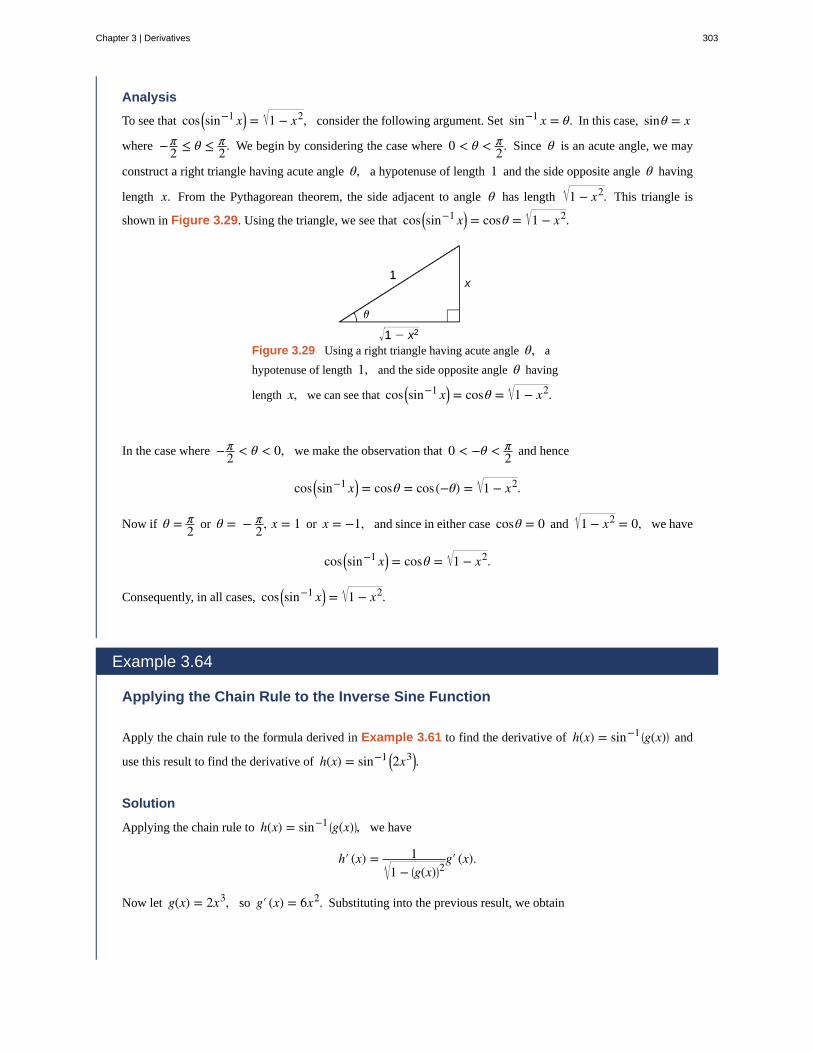
Analysis
To see that cos ⎛⎝sin−1 x⎞
⎠ = 1 − x2, consider the following argument. Set sin−1 x = θ. In this case, sinθ = x
where −π2 ≤ θ ≤ π
2. We begin by considering the case where 0 < θ < π2. Since θ is an acute angle, we may
construct a right triangle having acute angle θ, a hypotenuse of length 1 and the side opposite angle θ having
length x. From the Pythagorean theorem, the side adjacent to angle θ has length 1 − x2. This triangle is
shown in Figure 3.29. Using the triangle, we see that cos ⎛⎝sin−1 x⎞
⎠ = cosθ = 1 − x2.
Figure 3.29 Using a right triangle having acute angle θ, a
hypotenuse of length 1, and the side opposite angle θ having
length x, we can see that cos ⎛⎝sin−1 x⎞
⎠ = cosθ = 1 − x2.
In the case where −π2 < θ < 0, we make the observation that 0 < −θ < π
2 and hence
cos ⎛⎝sin−1 x⎞
⎠ = cosθ = cos(−θ) = 1 − x2.
Now if θ = π2 or θ = − π
2, x = 1 or x = −1, and since in either case cosθ = 0 and 1 − x2 = 0, we have
cos ⎛⎝sin−1 x⎞
⎠ = cosθ = 1 − x2.
Consequently, in all cases, cos ⎛⎝sin−1 x⎞
⎠ = 1 − x2.
Example 3.64
Applying the Chain Rule to the Inverse Sine Function
Apply the chain rule to the formula derived in Example 3.61 to find the derivative of h(x) = sin−1 ⎛⎝g(x)⎞
⎠ and
use this result to find the derivative of h(x) = sin−1 ⎛⎝2x3⎞
⎠.
Solution
Applying the chain rule to h(x) = sin−1 ⎛⎝g(x)⎞
⎠, we have
h′ (x) = 11 − ⎛
⎝g(x)⎞⎠2g′ (x).
Now let g(x) = 2x3, so g′ (x) = 6x2. Substituting into the previous result, we obtain
Chapter 3 | Derivatives 303
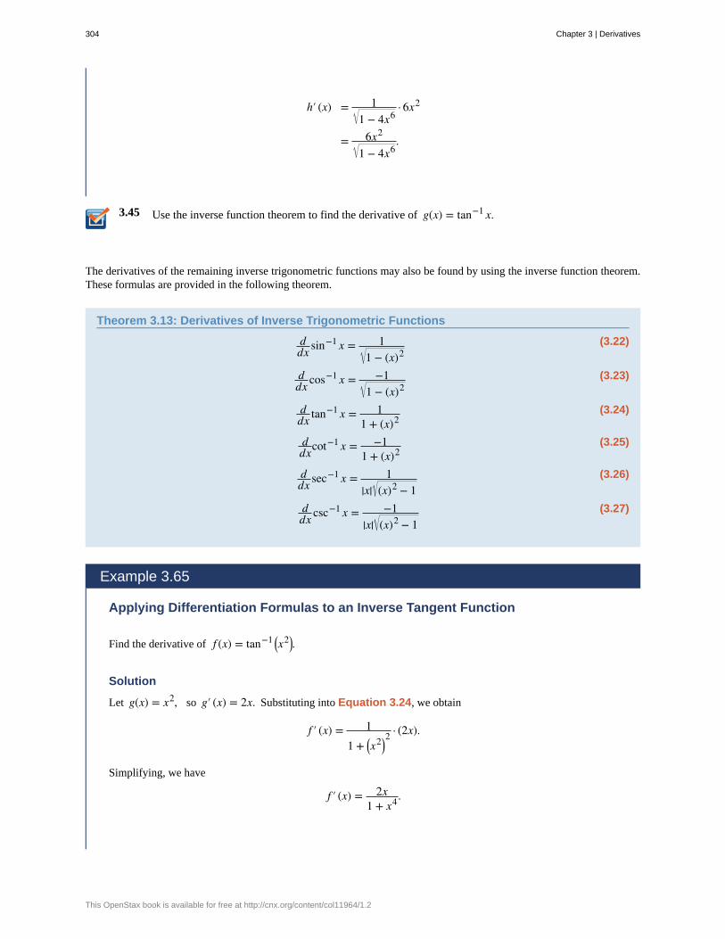
3.45
h′ (x) = 11 − 4x6
· 6x2
= 6x2
1 − 4x6.
Use the inverse function theorem to find the derivative of g(x) = tan−1 x.
The derivatives of the remaining inverse trigonometric functions may also be found by using the inverse function theorem.These formulas are provided in the following theorem.
Theorem 3.13: Derivatives of Inverse Trigonometric Functions
(3.22)ddx sin−1 x = 1
1 − (x)2
(3.23)ddx cos−1 x = −1
1 − (x)2
(3.24)ddx tan−1 x = 1
1 + (x)2
(3.25)ddxcot−1 x = −1
1 + (x)2
(3.26)ddx sec−1 x = 1
|x| (x)2 − 1(3.27)d
dx csc−1 x = −1|x| (x)2 − 1
Example 3.65
Applying Differentiation Formulas to an Inverse Tangent Function
Find the derivative of f (x) = tan−1 ⎛⎝x2⎞
⎠.
Solution
Let g(x) = x2, so g′ (x) = 2x. Substituting into Equation 3.24, we obtain
f ′ (x) = 1
1 + ⎛⎝x2⎞
⎠2 · (2x).
Simplifying, we have
f ′ (x) = 2x1 + x4.
304 Chapter 3 | Derivatives
This OpenStax book is available for free at http://cnx.org/content/col11964/1.2
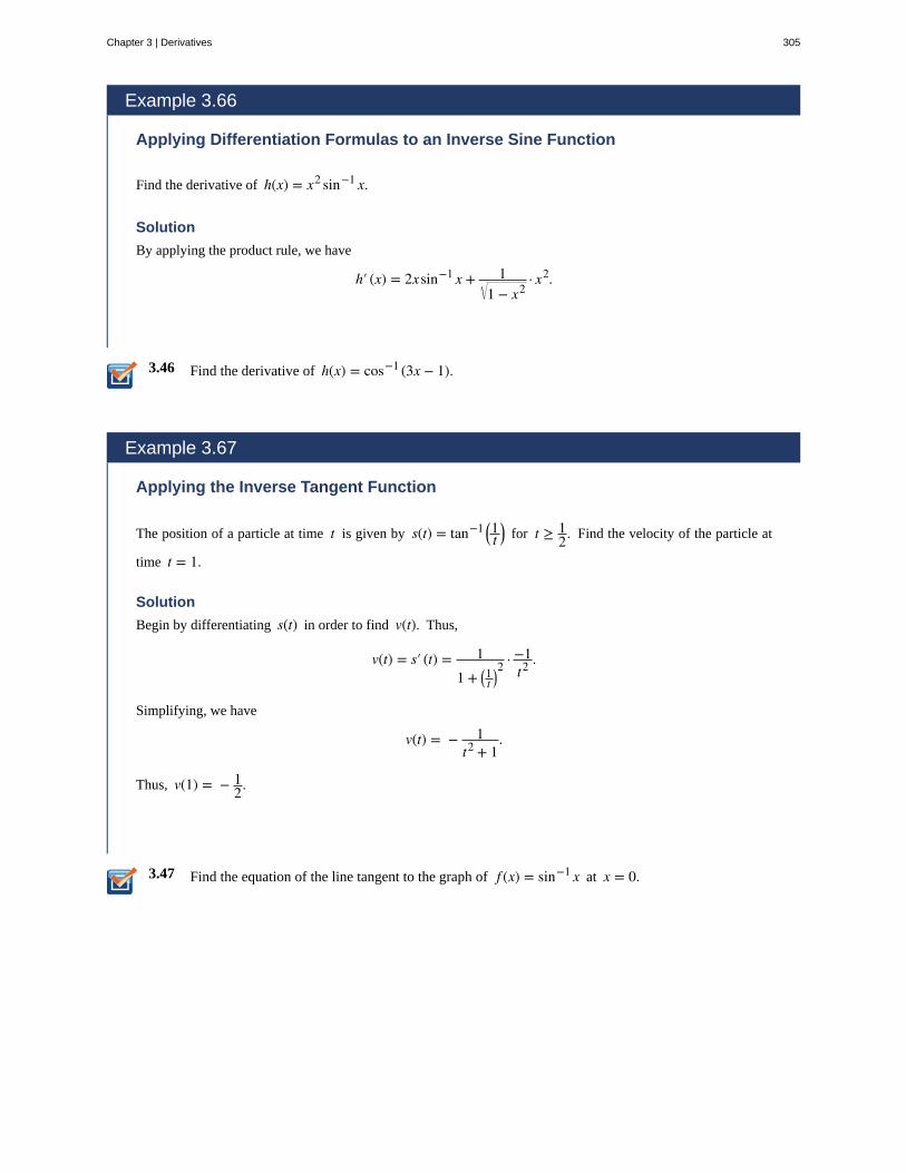
3.46
3.47
Example 3.66
Applying Differentiation Formulas to an Inverse Sine Function
Find the derivative of h(x) = x2 sin−1 x.
Solution
By applying the product rule, we have
h′ (x) = 2xsin−1 x + 11 − x2
· x2.
Find the derivative of h(x) = cos−1 (3x − 1).
Example 3.67
Applying the Inverse Tangent Function
The position of a particle at time t is given by s(t) = tan−1 ⎛⎝1t
⎞⎠ for t ≥ 1
2. Find the velocity of the particle at
time t = 1.
Solution
Begin by differentiating s(t) in order to find v(t). Thus,
v(t) = s′ (t) = 11 + ⎛
⎝1t
⎞⎠2 · −1
t2 .
Simplifying, we have
v(t) = − 1t2 + 1
.
Thus, v(1) = − 12.
Find the equation of the line tangent to the graph of f (x) = sin−1 x at x = 0.
Chapter 3 | Derivatives 305
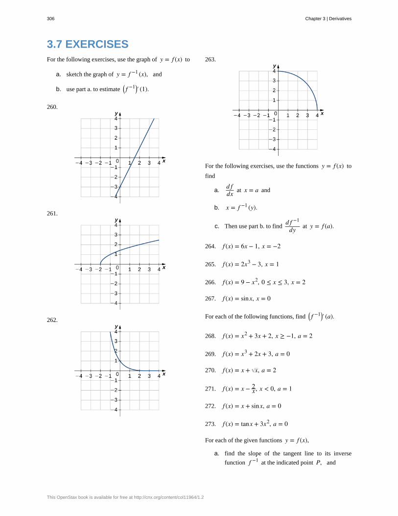
3.7 EXERCISESFor the following exercises, use the graph of y = f (x) to
a. sketch the graph of y = f −1 (x), and
b. use part a. to estimate ⎛⎝ f −1⎞
⎠′ (1).
260.
261.
262.
263.
For the following exercises, use the functions y = f (x) to
find
a.d fdx at x = a and
b. x = f −1 (y).
c. Then use part b. to findd f −1
dy at y = f (a).
264. f (x) = 6x − 1, x = −2
265. f (x) = 2x3 − 3, x = 1
266. f (x) = 9 − x2, 0 ≤ x ≤ 3, x = 2
267. f (x) = sinx, x = 0
For each of the following functions, find ⎛⎝ f −1⎞
⎠′ (a).
268. f (x) = x2 + 3x + 2, x ≥ −1, a = 2
269. f (x) = x3 + 2x + 3, a = 0
270. f (x) = x + x, a = 2
271. f (x) = x − 2x , x < 0, a = 1
272. f (x) = x + sinx, a = 0
273. f (x) = tanx + 3x2, a = 0
For each of the given functions y = f (x),
a. find the slope of the tangent line to its inverse
function f −1 at the indicated point P, and
306 Chapter 3 | Derivatives
This OpenStax book is available for free at http://cnx.org/content/col11964/1.2
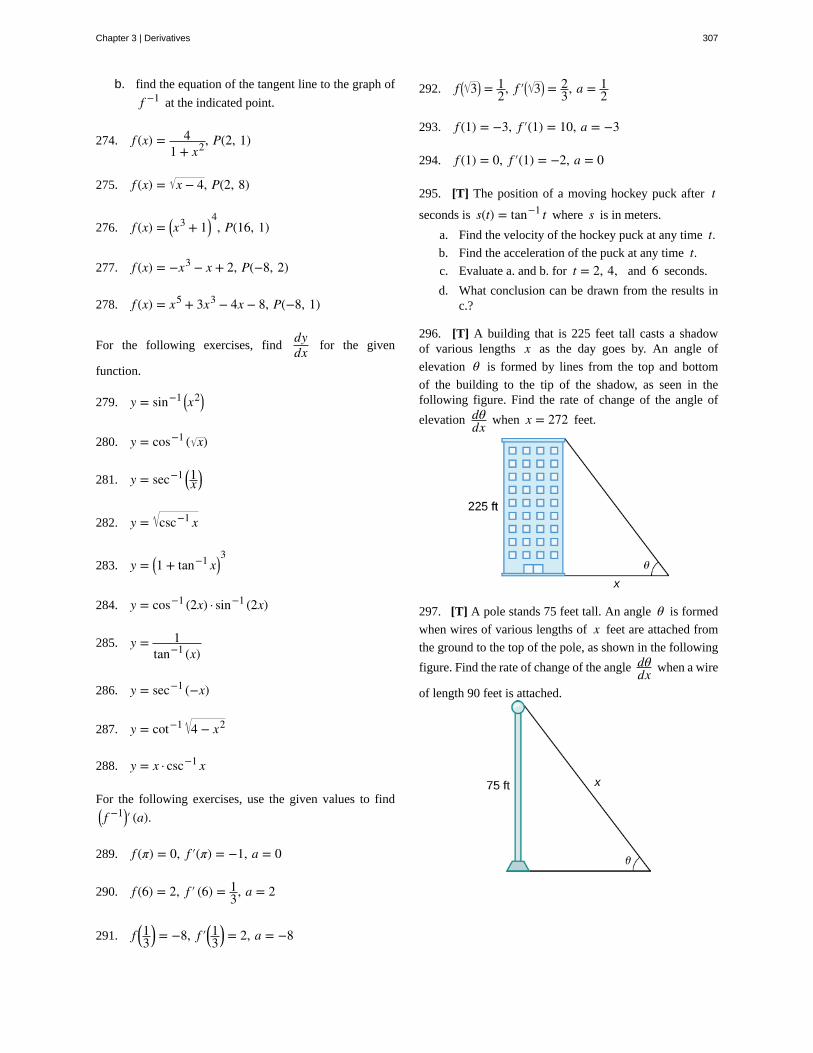
b. find the equation of the tangent line to the graph of
f −1 at the indicated point.
274. f (x) = 41 + x2, P(2, 1)
275. f (x) = x − 4, P(2, 8)
276. f (x) = ⎛⎝x
3 + 1⎞⎠4, P(16, 1)
277. f (x) = −x3 − x + 2, P(−8, 2)
278. f (x) = x5 + 3x3 − 4x − 8, P(−8, 1)
For the following exercises, finddydx for the given
function.
279. y = sin−1 ⎛⎝x2⎞
⎠
280. y = cos−1 ( x)
281. y = sec−1 ⎛⎝1x
⎞⎠
282. y = csc−1 x
283. y = ⎛⎝1 + tan−1 x⎞
⎠3
284. y = cos−1 (2x) · sin−1 (2x)
285. y = 1tan−1 (x)
286. y = sec−1 (−x)
287. y = cot−1 4 − x2
288. y = x · csc−1 x
For the following exercises, use the given values to find⎛⎝ f −1⎞
⎠′ (a).
289. f (π) = 0, f ′(π) = −1, a = 0
290. f (6) = 2, f ′ (6) = 13, a = 2
291. f ⎛⎝13
⎞⎠ = −8, f ′⎛⎝
13
⎞⎠ = 2, a = −8
292. f ⎛⎝ 3⎞
⎠ = 12, f ′⎛
⎝ 3⎞⎠ = 2
3, a = 12
293. f (1) = −3, f ′(1) = 10, a = −3
294. f (1) = 0, f ′(1) = −2, a = 0
295. [T] The position of a moving hockey puck after tseconds is s(t) = tan−1 t where s is in meters.
a. Find the velocity of the hockey puck at any time t.b. Find the acceleration of the puck at any time t.c. Evaluate a. and b. for t = 2, 4, and 6 seconds.
d. What conclusion can be drawn from the results inc.?
296. [T] A building that is 225 feet tall casts a shadowof various lengths x as the day goes by. An angle of
elevation θ is formed by lines from the top and bottom
of the building to the tip of the shadow, as seen in thefollowing figure. Find the rate of change of the angle of
elevation dθdx when x = 272 feet.
297. [T] A pole stands 75 feet tall. An angle θ is formed
when wires of various lengths of x feet are attached from
the ground to the top of the pole, as shown in the following
figure. Find the rate of change of the angle dθdx when a wire
of length 90 feet is attached.
Chapter 3 | Derivatives 307
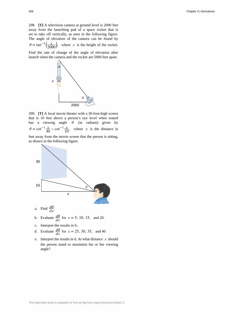
298. [T] A television camera at ground level is 2000 feetaway from the launching pad of a space rocket that isset to take off vertically, as seen in the following figure.The angle of elevation of the camera can be found by
θ = tan−1 ⎛⎝
x2000
⎞⎠, where x is the height of the rocket.
Find the rate of change of the angle of elevation afterlaunch when the camera and the rocket are 5000 feet apart.
299. [T] A local movie theater with a 30-foot-high screenthat is 10 feet above a person’s eye level when seatedhas a viewing angle θ (in radians) given by
θ = cot−1 x40 − cot−1 x
10, where x is the distance in
feet away from the movie screen that the person is sitting,as shown in the following figure.
a. Find dθdx .
b. Evaluate dθdx for x = 5, 10, 15, and 20.
c. Interpret the results in b..
d. Evaluate dθdx for x = 25, 30, 35, and 40
e. Interpret the results in d. At what distance x should
the person stand to maximize his or her viewingangle?
308 Chapter 3 | Derivatives
This OpenStax book is available for free at http://cnx.org/content/col11964/1.2
3.8 | Implicit Differentiation
Learning Objectives3.8.1 Find the derivative of a complicated function by using implicit differentiation.
3.8.2 Use implicit differentiation to determine the equation of a tangent line.
We have already studied how to find equations of tangent lines to functions and the rate of change of a function at a specificpoint. In all these cases we had the explicit equation for the function and differentiated these functions explicitly. Supposeinstead that we want to determine the equation of a tangent line to an arbitrary curve or the rate of change of an arbitrarycurve at a point. In this section, we solve these problems by finding the derivatives of functions that define y implicitly in
terms of x.
Implicit DifferentiationIn most discussions of math, if the dependent variable y is a function of the independent variable x, we express y in terms
of x. If this is the case, we say that y is an explicit function of x. For example, when we write the equation y = x2 + 1,we are defining y explicitly in terms of x. On the other hand, if the relationship between the function y and the variable xis expressed by an equation where y is not expressed entirely in terms of x, we say that the equation defines y implicitly
in terms of x. For example, the equation y − x2 = 1 defines the function y = x2 + 1 implicitly.
Implicit differentiation allows us to find slopes of tangents to curves that are clearly not functions (they fail the vertical linetest). We are using the idea that portions of y are functions that satisfy the given equation, but that y is not actually a
function of x.
In general, an equation defines a function implicitly if the function satisfies that equation. An equation may define manydifferent functions implicitly. For example, the functions
y = 25 − x2 and y =⎧
⎩⎨ 25 − x2 if − 25 ≤ x < 0
− 25 − x2 if 0 ≤ x ≤ 25, which are illustrated in Figure 3.30, are just three of the many
functions defined implicitly by the equation x2 + y2 = 25.
Chapter 3 | Derivatives 309
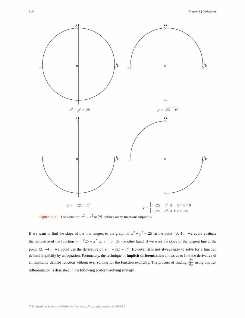
Figure 3.30 The equation x2 + y2 = 25 defines many functions implicitly.
If we want to find the slope of the line tangent to the graph of x2 + y2 = 25 at the point (3, 4), we could evaluate
the derivative of the function y = 25 − x2 at x = 3. On the other hand, if we want the slope of the tangent line at the
point (3, −4), we could use the derivative of y = − 25 − x2. However, it is not always easy to solve for a function
defined implicitly by an equation. Fortunately, the technique of implicit differentiation allows us to find the derivative of
an implicitly defined function without ever solving for the function explicitly. The process of findingdydx using implicit
differentiation is described in the following problem-solving strategy.
310 Chapter 3 | Derivatives
This OpenStax book is available for free at http://cnx.org/content/col11964/1.2
Problem-Solving Strategy: Implicit Differentiation
To perform implicit differentiation on an equation that defines a function y implicitly in terms of a variable x, use
the following steps:
1. Take the derivative of both sides of the equation. Keep in mind that y is a function of x. Consequently, whereas
ddx(sinx) = cosx, d
dx(siny) = cosydydx because we must use the chain rule to differentiate siny with respect
to x.
2. Rewrite the equation so that all terms containingdydx are on the left and all terms that do not contain
dydx are
on the right.
3. Factor outdydx on the left.
4. Solve fordydx by dividing both sides of the equation by an appropriate algebraic expression.
Example 3.68
Using Implicit Differentiation
Assuming that y is defined implicitly by the equation x2 + y2 = 25, finddydx.
Solution
Follow the steps in the problem-solving strategy.
ddx
⎛⎝x2 + y2⎞
⎠ = ddx(25) Step 1. Diffe entiate both sides of the equation.
ddx
⎛⎝x2⎞
⎠ + ddx
⎛⎝y2⎞
⎠ = 0Step 1.1. Use the sum rule on the left.
On the right ddx(25) = 0.
2x + 2ydydx = 0
Step 1.2. Take the derivatives, so ddx
⎛⎝x2⎞
⎠ = 2x
and ddx
⎛⎝y2⎞
⎠ = 2ydydx.
2ydydx = −2x Step 2. Keep the terms with dy
dx on the left.
Move the remaining terms to the right.dydx = − x
yStep 4. Divide both sides of the equation by2y. (Step 3 does not apply in this case.)
Analysis
Note that the resulting expression fordydx is in terms of both the independent variable x and the dependent
variable y. Although in some cases it may be possible to expressdydx in terms of x only, it is generally not
possible to do so.
Chapter 3 | Derivatives 311
Example 3.69
Using Implicit Differentiation and the Product Rule
Assuming that y is defined implicitly by the equation x3 siny + y = 4x + 3, finddydx.
Solution
ddx
⎛⎝x
3 siny + y⎞⎠ = d
dx(4x + 3) Step 1: Diffe entiate both sides of the equation.
ddx
⎛⎝x
3 siny⎞⎠ + d
dx(y) = 4Step 1.1: Apply the sum rule on the left.
On the right, ddx(4x + 3) = 4.
⎛⎝
ddx
⎛⎝x
3⎞⎠ · siny + d
dx⎛⎝siny⎞
⎠ · x3⎞⎠ + dy
dx = 4Step 1.2: Use the product rule to finddx
⎛⎝x
3 siny⎞⎠. Observe that d
dx(y) = dydx.
3x2 siny + ⎛⎝cosydy
dx⎞⎠ · x3 + dy
dx = 4Step 1.3: We know d
dx⎛⎝x
3⎞⎠ = 3x2. Use the
chain rule to obtain ddx
⎛⎝siny⎞
⎠ = cosydydx.
x3 cosydydx + dy
dx = 4 − 3x2 siny Step 2: Keep all terms containing dydx on the
left. Move all other terms to the right.dydx
⎛⎝x3 cosy + 1⎞
⎠ = 4 − 3x2 siny Step 3: Factor out dydx on the left.
dydx = 4 − 3x2 siny
x3 cosy + 1Step 4: Solve for dy
dx by dividing both sides of
the equation by x3 cosy + 1.
Example 3.70
Using Implicit Differentiation to Find a Second Derivative
Findd2 ydx2 if x2 + y2 = 25.
Solution
In Example 3.68, we showed thatdydx = − x
y. We can take the derivative of both sides of this equation to find
d2 ydx2 .
312 Chapter 3 | Derivatives
This OpenStax book is available for free at http://cnx.org/content/col11964/1.2
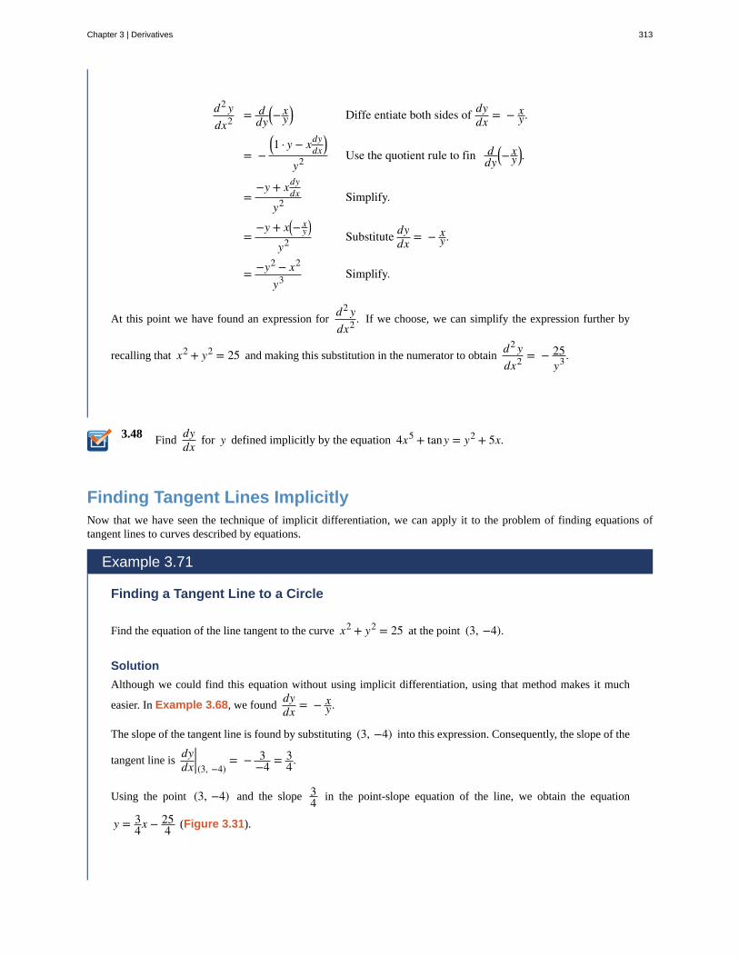
3.48
d2 ydx2 = d
dy⎛⎝−
xy
⎞⎠ Diffe entiate both sides of dy
dx = − xy.
= −⎛⎝1 · y − xdy
dx⎞⎠
y2 Use the quotient rule to fin ddy
⎛⎝−
xy
⎞⎠.
=−y + xdy
dxy2 Simplify.
=−y + x⎛
⎝− xy
⎞⎠
y2 Substitute dydx = − x
y.
= −y2 − x2
y3 Simplify.
At this point we have found an expression ford2 ydx2 . If we choose, we can simplify the expression further by
recalling that x2 + y2 = 25 and making this substitution in the numerator to obtaind2 ydx2 = − 25
y3 .
Finddydx for y defined implicitly by the equation 4x5 + tany = y2 + 5x.
Finding Tangent Lines ImplicitlyNow that we have seen the technique of implicit differentiation, we can apply it to the problem of finding equations oftangent lines to curves described by equations.
Example 3.71
Finding a Tangent Line to a Circle
Find the equation of the line tangent to the curve x2 + y2 = 25 at the point (3, −4).
Solution
Although we could find this equation without using implicit differentiation, using that method makes it much
easier. In Example 3.68, we founddydx = − x
y.
The slope of the tangent line is found by substituting (3, −4) into this expression. Consequently, the slope of the
tangent line isdydx |(3, −4)
= − 3−4 = 3
4.
Using the point (3, −4) and the slope 34 in the point-slope equation of the line, we obtain the equation
y = 34x − 25
4 (Figure 3.31).
Chapter 3 | Derivatives 313
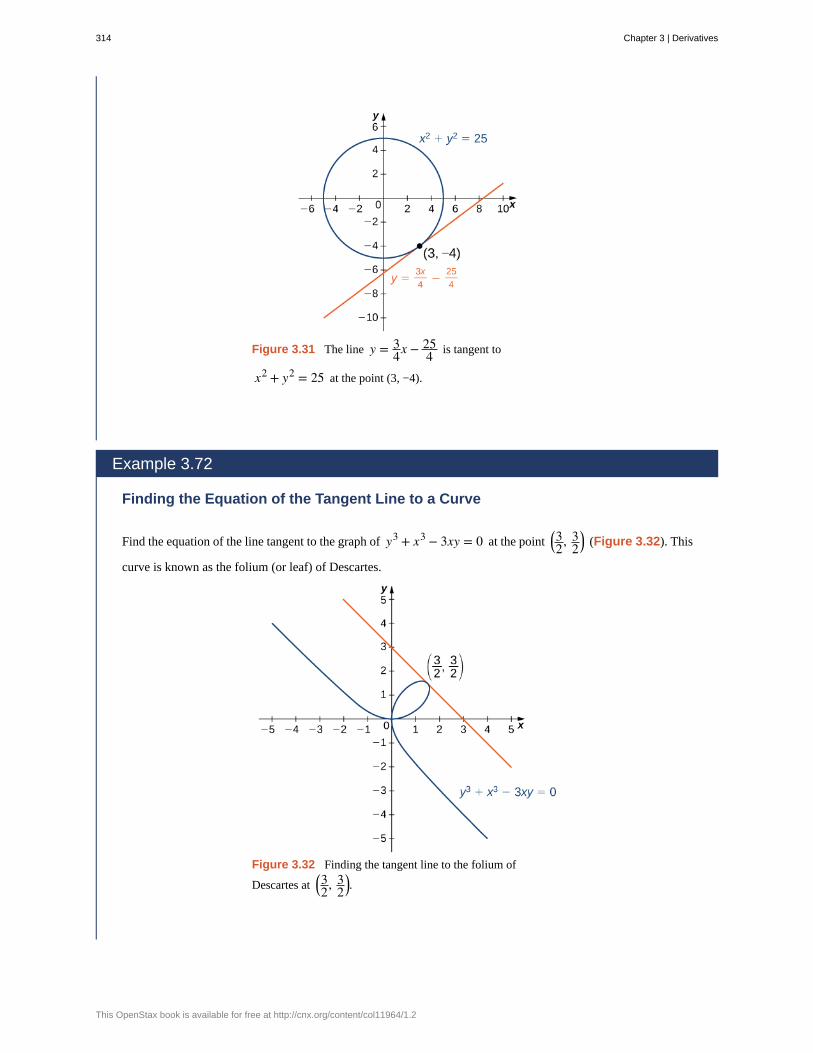
Figure 3.31 The line y = 34x − 25
4 is tangent to
x2 + y2 = 25 at the point (3, −4).
Example 3.72
Finding the Equation of the Tangent Line to a Curve
Find the equation of the line tangent to the graph of y3 + x3 − 3xy = 0 at the point ⎛⎝32, 3
2⎞⎠ (Figure 3.32). This
curve is known as the folium (or leaf) of Descartes.
Figure 3.32 Finding the tangent line to the folium of
Descartes at⎛⎝32, 3
2⎞⎠.
314 Chapter 3 | Derivatives
This OpenStax book is available for free at http://cnx.org/content/col11964/1.2
Solution
Begin by findingdydx.
ddx
⎛⎝y
3 + x3 − 3xy⎞⎠ = d
dx(0)
3y2 dydx + 3x2 − ⎛
⎝3y + dydx3x⎞
⎠ = 0
dydx = 3y − 3x2
3y2 − 3x.
Next, substitute ⎛⎝32, 3
2⎞⎠ into
dydx = 3y − 3x2
3y2 − 3xto find the slope of the tangent line:
dydx |⎛⎝3
2, 32
⎞⎠
= −1.
Finally, substitute into the point-slope equation of the line to obtain
y = −x + 3.
Example 3.73
Applying Implicit Differentiation
In a simple video game, a rocket travels in an elliptical orbit whose path is described by the equation
4x2 + 25y2 = 100. The rocket can fire missiles along lines tangent to its path. The object of the game is to
destroy an incoming asteroid traveling along the positive x-axis toward (0, 0). If the rocket fires a missile when
it is located at ⎛⎝3, 8
3⎞⎠, where will it intersect the x-axis?
Solution
To solve this problem, we must determine where the line tangent to the graph of
4x2 + 25y2 = 100 at ⎛⎝3, 8
3⎞⎠ intersects the x-axis. Begin by finding
dydx implicitly.
Differentiating, we have
8x + 50ydydx = 0.
Solving fordydx, we have
dydx = − 4x
25y.
The slope of the tangent line isdydx |⎛⎝3, 8
3⎞⎠
= − 950. The equation of the tangent line is y = − 9
50x + 183200. To
Chapter 3 | Derivatives 315
3.49
determine where the line intersects the x-axis, solve 0 = − 950x + 183
200. The solution is x = 613 . The missile
intersects the x-axis at the point ⎛⎝613 , 0⎞
⎠.
Find the equation of the line tangent to the hyperbola x2 − y2 = 16 at the point (5, 3).
316 Chapter 3 | Derivatives
This OpenStax book is available for free at http://cnx.org/content/col11964/1.2
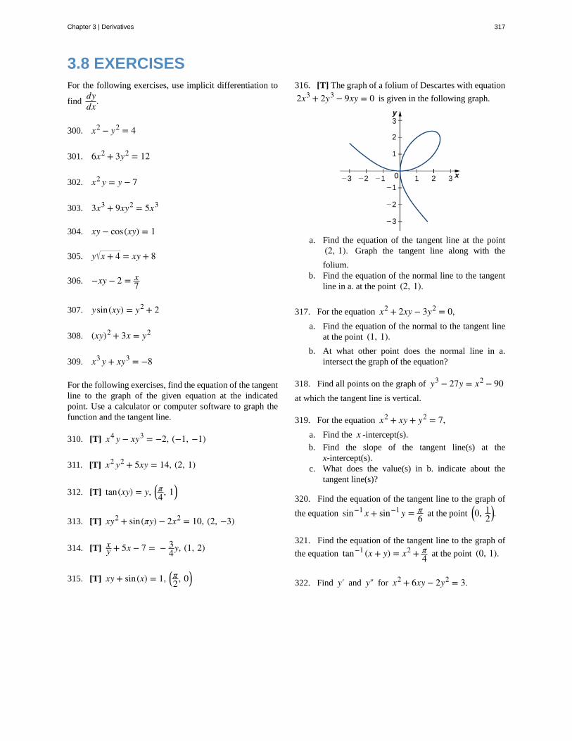
3.8 EXERCISESFor the following exercises, use implicit differentiation to
finddydx.
300. x2 − y2 = 4
301. 6x2 + 3y2 = 12
302. x2 y = y − 7
303. 3x3 + 9xy2 = 5x3
304. xy − cos(xy) = 1
305. y x + 4 = xy + 8
306. −xy − 2 = x7
307. ysin(xy) = y2 + 2
308. (xy)2 + 3x = y2
309. x3 y + xy3 = −8
For the following exercises, find the equation of the tangentline to the graph of the given equation at the indicatedpoint. Use a calculator or computer software to graph thefunction and the tangent line.
310. [T] x4 y − xy3 = −2, (−1, −1)
311. [T] x2 y2 + 5xy = 14, (2, 1)
312. [T] tan(xy) = y, ⎛⎝π4, 1⎞
⎠
313. [T] xy2 + sin(πy) − 2x2 = 10, (2, −3)
314. [T] xy + 5x − 7 = − 3
4y, (1, 2)
315. [T] xy + sin(x) = 1, ⎛⎝π2, 0⎞
⎠
316. [T] The graph of a folium of Descartes with equation
2x3 + 2y3 − 9xy = 0 is given in the following graph.
a. Find the equation of the tangent line at the point(2, 1). Graph the tangent line along with the
folium.b. Find the equation of the normal line to the tangent
line in a. at the point (2, 1).
317. For the equation x2 + 2xy − 3y2 = 0,a. Find the equation of the normal to the tangent line
at the point (1, 1).b. At what other point does the normal line in a.
intersect the graph of the equation?
318. Find all points on the graph of y3 − 27y = x2 − 90at which the tangent line is vertical.
319. For the equation x2 + xy + y2 = 7,a. Find the x -intercept(s).
b. Find the slope of the tangent line(s) at thex-intercept(s).
c. What does the value(s) in b. indicate about thetangent line(s)?
320. Find the equation of the tangent line to the graph of
the equation sin−1 x + sin−1 y = π6 at the point ⎛
⎝0, 12
⎞⎠.
321. Find the equation of the tangent line to the graph of
the equation tan−1 (x + y) = x2 + π4 at the point (0, 1).
322. Find y′ and y″ for x2 + 6xy − 2y2 = 3.
Chapter 3 | Derivatives 317
323. [T] The number of cell phones produced when xdollars is spent on labor and y dollars is spent on capital
invested by a manufacturer can be modeled by the equation
60x3/4 y1/4 = 3240.
a. Finddydx and evaluate at the point (81, 16).
b. Interpret the result of a.
324. [T] The number of cars produced when x dollars is
spent on labor and y dollars is spent on capital invested
by a manufacturer can be modeled by the equation
30x1/3 y2/3 = 360. (Both x and y are measured in
thousands of dollars.)
a. Finddydx and evaluate at the point (27, 8).
b. Interpret the result of a.
325. The volume of a right circular cone of radius x
and height y is given by V = 13πx2 y. Suppose that the
volume of the cone is 85π cm3. Finddydx when x = 4 and
y = 16.
For the following exercises, consider a closed rectangularbox with a square base with side x and height y.
326. Find an equation for the surface area of therectangular box, S(x, y).
327. If the surface area of the rectangular box is 78 square
feet, finddydx when x = 3 feet and y = 5 feet.
For the following exercises, use implicit differentiation todetermine y′. Does the answer agree with the formulas we
have previously determined?
328. x = siny
329. x = cosy
330. x = tany
318 Chapter 3 | Derivatives
This OpenStax book is available for free at http://cnx.org/content/col11964/1.2
3.9 | Derivatives of Exponential and Logarithmic
Functions
Learning Objectives3.9.1 Find the derivative of exponential functions.
3.9.2 Find the derivative of logarithmic functions.
3.9.3 Use logarithmic differentiation to determine the derivative of a function.
So far, we have learned how to differentiate a variety of functions, including trigonometric, inverse, and implicit functions.In this section, we explore derivatives of exponential and logarithmic functions. As we discussed in Introduction toFunctions and Graphs, exponential functions play an important role in modeling population growth and the decayof radioactive materials. Logarithmic functions can help rescale large quantities and are particularly helpful for rewritingcomplicated expressions.
Derivative of the Exponential FunctionJust as when we found the derivatives of other functions, we can find the derivatives of exponential and logarithmicfunctions using formulas. As we develop these formulas, we need to make certain basic assumptions. The proofs that theseassumptions hold are beyond the scope of this course.
First of all, we begin with the assumption that the function B(x) = bx, b > 0, is defined for every real number and is
continuous. In previous courses, the values of exponential functions for all rational numbers were defined—beginningwith the definition of bn, where n is a positive integer—as the product of b multiplied by itself n times. Later,
we defined b0 = 1, b−n = 1bn, for a positive integer n, and bs/t = ( bt )s for positive integers s and t. These
definitions leave open the question of the value of br where r is an arbitrary real number. By assuming the continuity of
B(x) = bx, b > 0, we may interpret br as limx → rbx where the values of x as we take the limit are rational. For example,
we may view 4π as the number satisfying
43 < 4π < 44, 43.1 < 4π < 43.2, 43.14 < 4π < 43.15,43.141 < 4π < 43.142, 43.1415 < 4π < 43.1416 ,….
As we see in the following table, 4π ≈ 77.88.
Chapter 3 | Derivatives 319
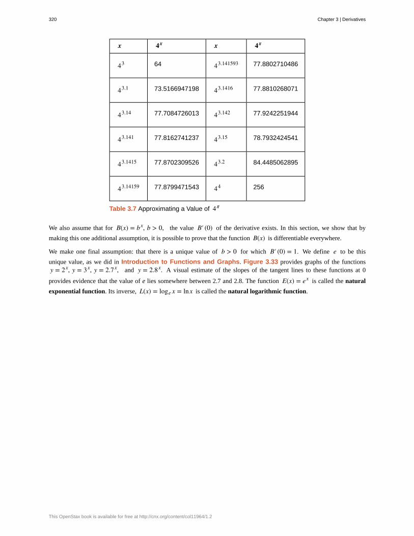
x 4x x 4x
43 64 43.141593 77.8802710486
43.1 73.5166947198 43.1416 77.8810268071
43.14 77.7084726013 43.142 77.9242251944
43.141 77.8162741237 43.15 78.7932424541
43.1415 77.8702309526 43.2 84.4485062895
43.14159 77.8799471543 44 256
Table 3.7 Approximating a Value of 4π
We also assume that for B(x) = bx, b > 0, the value B′ (0) of the derivative exists. In this section, we show that by
making this one additional assumption, it is possible to prove that the function B(x) is differentiable everywhere.
We make one final assumption: that there is a unique value of b > 0 for which B′ (0) = 1. We define e to be this
unique value, as we did in Introduction to Functions and Graphs. Figure 3.33 provides graphs of the functionsy = 2x, y = 3x, y = 2.7x, and y = 2.8x. A visual estimate of the slopes of the tangent lines to these functions at 0
provides evidence that the value of e lies somewhere between 2.7 and 2.8. The function E(x) = ex is called the natural
exponential function. Its inverse, L(x) = loge x = lnx is called the natural logarithmic function.
320 Chapter 3 | Derivatives
This OpenStax book is available for free at http://cnx.org/content/col11964/1.2
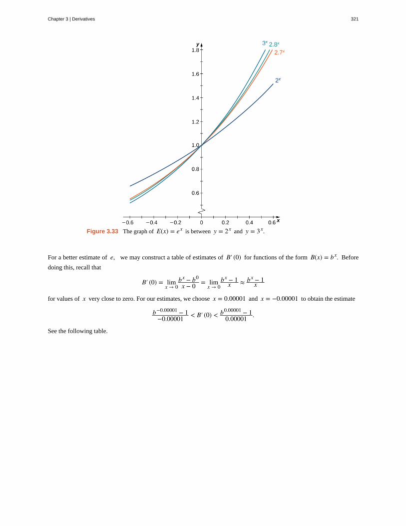
Figure 3.33 The graph of E(x) = ex is between y = 2x and y = 3x.
For a better estimate of e, we may construct a table of estimates of B′ (0) for functions of the form B(x) = bx. Before
doing this, recall that
B′ (0) = limx → 0
bx − b0
x − 0 = limx → 0
bx − 1x ≈ bx − 1
x
for values of x very close to zero. For our estimates, we choose x = 0.00001 and x = −0.00001 to obtain the estimate
b−0.00001 − 1−0.00001 < B′ (0) < b0.00001 − 1
0.00001 .
See the following table.
Chapter 3 | Derivatives 321
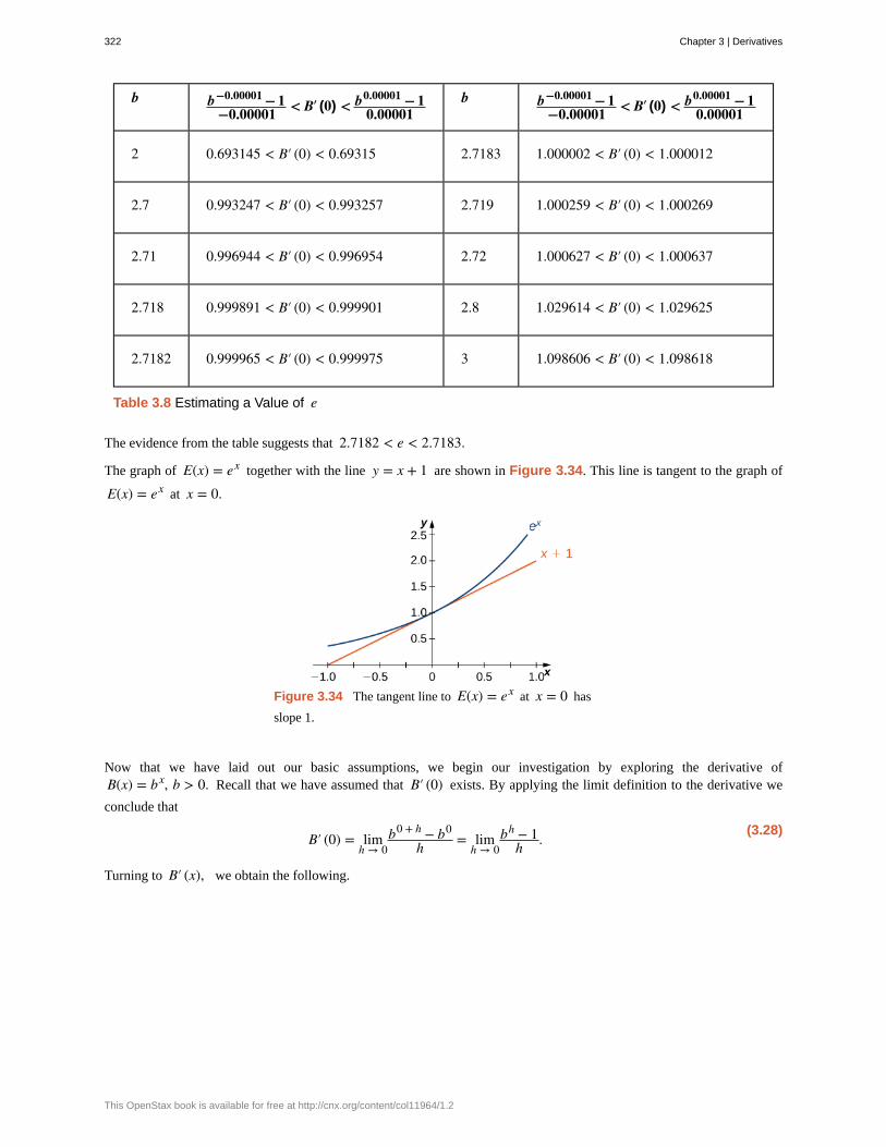
b b−0.00001 − 1−0.00001 < B′ (0) < b0.00001 − 1
0.00001b b−0.00001 − 1
−0.00001 < B′ (0) < b0.00001 − 10.00001
2 0.693145 < B′ (0) < 0.69315 2.7183 1.000002 < B′ (0) < 1.000012
2.7 0.993247 < B′ (0) < 0.993257 2.719 1.000259 < B′ (0) < 1.000269
2.71 0.996944 < B′ (0) < 0.996954 2.72 1.000627 < B′ (0) < 1.000637
2.718 0.999891 < B′ (0) < 0.999901 2.8 1.029614 < B′ (0) < 1.029625
2.7182 0.999965 < B′ (0) < 0.999975 3 1.098606 < B′ (0) < 1.098618
Table 3.8 Estimating a Value of e
The evidence from the table suggests that 2.7182 < e < 2.7183.
The graph of E(x) = ex together with the line y = x + 1 are shown in Figure 3.34. This line is tangent to the graph of
E(x) = ex at x = 0.
Figure 3.34 The tangent line to E(x) = ex at x = 0 has
slope 1.
Now that we have laid out our basic assumptions, we begin our investigation by exploring the derivative ofB(x) = bx, b > 0. Recall that we have assumed that B′ (0) exists. By applying the limit definition to the derivative we
conclude that
(3.28)B′ (0) = lim
h → 0b0 + h − b0
h = limh → 0
bh − 1h .
Turning to B′ (x), we obtain the following.
322 Chapter 3 | Derivatives
This OpenStax book is available for free at http://cnx.org/content/col11964/1.2
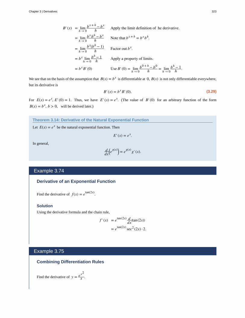
B′ (x) = limh → 0
bx + h − bx
h Apply the limit definition of he derivative.
= limh → 0
bx bh − bx
h Note that bx + h = bx bh.
= limh → 0
bx(bh − 1)h Factor out bx.
= bx limh → 0
bh − 1h Apply a property of limits.
= bx B′ (0) Use B′ (0) = limh → 0
b0 + h − b0
h = limh → 0
bh − 1h .
We see that on the basis of the assumption that B(x) = bx is differentiable at 0, B(x) is not only differentiable everywhere,
but its derivative is
(3.29)B′ (x) = bx B′ (0).
For E(x) = ex, E′ (0) = 1. Thus, we have E′ (x) = ex. (The value of B′ (0) for an arbitrary function of the form
B(x) = bx, b > 0, will be derived later.)
Theorem 3.14: Derivative of the Natural Exponential Function
Let E(x) = ex be the natural exponential function. Then
E′ (x) = ex.
In general,
ddx
⎛⎝e
g(x)⎞⎠ = eg(x) g′ (x).
Example 3.74
Derivative of an Exponential Function
Find the derivative of f (x) = etan(2x).
Solution
Using the derivative formula and the chain rule,
f ′ (x) = etan(2x) ddx
⎛⎝tan(2x)⎞
⎠
= etan(2x) sec2 (2x) · 2.
Example 3.75
Combining Differentiation Rules
Find the derivative of y = ex2
x .
Chapter 3 | Derivatives 323
3.50
3.51
Solution
Use the derivative of the natural exponential function, the quotient rule, and the chain rule.
y′ =
⎛⎝ex2
· 2⎞⎠x · x − 1 · ex2
x2 Apply the quotient rule.
=ex2 ⎛
⎝2x2 − 1⎞⎠
x2 Simplify.
Find the derivative of h(x) = xe2x.
Example 3.76
Applying the Natural Exponential Function
A colony of mosquitoes has an initial population of 1000. After t days, the population is given by
A(t) = 1000e0.3t. Show that the ratio of the rate of change of the population, A′ (t), to the population, A(t) is
constant.
Solution
First find A′ (t). By using the chain rule, we have A′ (t) = 300e0.3t. Thus, the ratio of the rate of change of the
population to the population is given by
A′ (t) = 300e0.3t
1000e0.3t = 0.3.
The ratio of the rate of change of the population to the population is the constant 0.3.
If A(t) = 1000e0.3t describes the mosquito population after t days, as in the preceding example, what
is the rate of change of A(t) after 4 days?
Derivative of the Logarithmic FunctionNow that we have the derivative of the natural exponential function, we can use implicit differentiation to find the derivativeof its inverse, the natural logarithmic function.
Theorem 3.15: The Derivative of the Natural Logarithmic Function
If x > 0 and y = lnx, then
(3.30)dydx = 1
x .
More generally, let g(x) be a differentiable function. For all values of x for which g′ (x) > 0, the derivative of
324 Chapter 3 | Derivatives
This OpenStax book is available for free at http://cnx.org/content/col11964/1.2
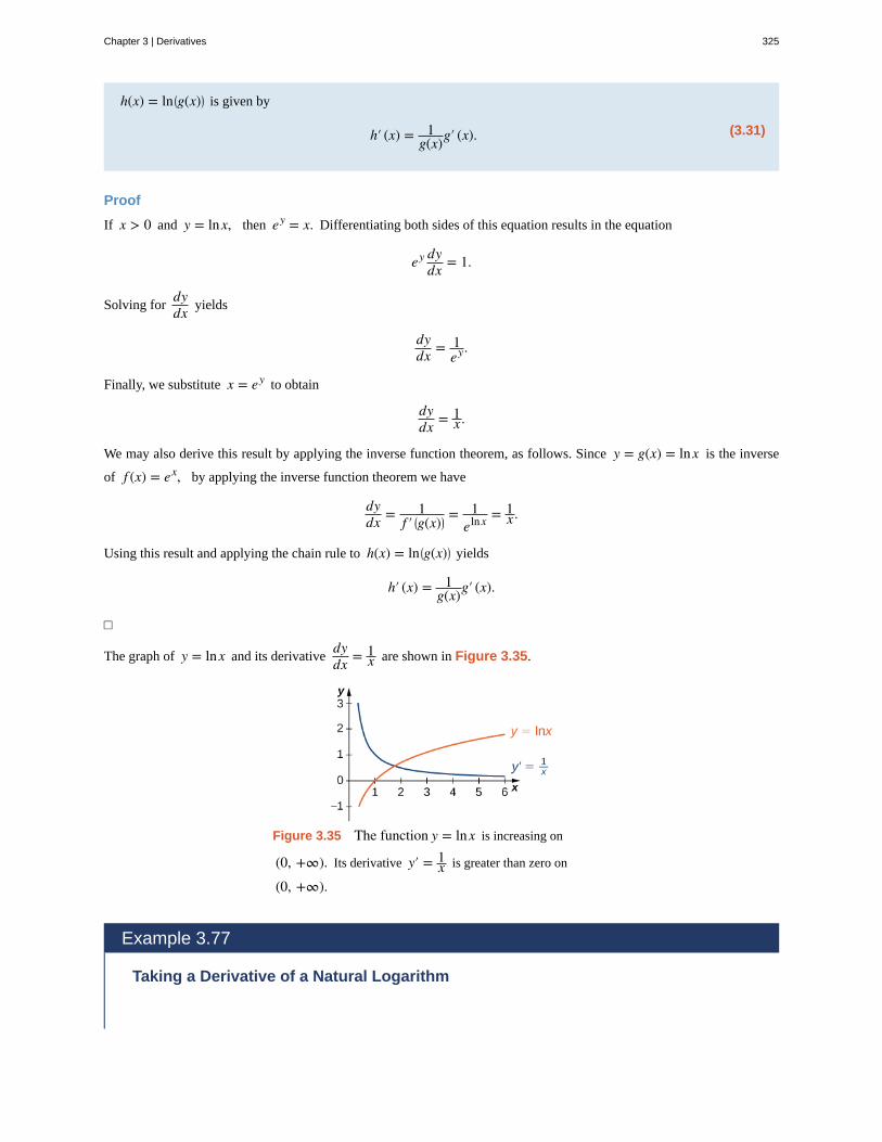
h(x) = ln ⎛⎝g(x)⎞
⎠ is given by
(3.31)h′ (x) = 1g(x)g′ (x).
Proof
If x > 0 and y = lnx, then ey = x. Differentiating both sides of this equation results in the equation
ey dydx = 1.
Solving fordydx yields
dydx = 1
ey.
Finally, we substitute x = ey to obtain
dydx = 1
x .
We may also derive this result by applying the inverse function theorem, as follows. Since y = g(x) = lnx is the inverse
of f (x) = ex, by applying the inverse function theorem we have
dydx = 1
f ′ ⎛⎝g(x)⎞
⎠= 1
elnx = 1x .
Using this result and applying the chain rule to h(x) = ln ⎛⎝g(x)⎞
⎠ yields
h′ (x) = 1g(x)g′ (x).
□
The graph of y = lnx and its derivativedydx = 1
x are shown in Figure 3.35.
Figure 3.35 The function y = lnx is increasing on
(0, +∞). Its derivative y′ = 1x is greater than zero on
(0, +∞).
Example 3.77
Taking a Derivative of a Natural Logarithm
Chapter 3 | Derivatives 325
3.52
Find the derivative of f (x) = ln ⎛⎝x
3 + 3x − 4⎞⎠.
Solution
Use Equation 3.31 directly.
f ′ (x) = 1x3 + 3x − 4
· ⎛⎝3x2 + 3⎞
⎠ Use g(x) = x3 + 3x − 4 in h′ (x) = 1g(x)g′ (x).
= 3x2 + 3x3 + 3x − 4
Rewrite.
Example 3.78
Using Properties of Logarithms in a Derivative
Find the derivative of f (x) = ln⎛⎝
x2 sinx2x + 1
⎞⎠.
Solution
At first glance, taking this derivative appears rather complicated. However, by using the properties of logarithmsprior to finding the derivative, we can make the problem much simpler.
f (x) = ln⎛⎝
x2 sinx2x + 1
⎞⎠ = 2lnx + ln(sinx) − ln(2x + 1) Apply properties of logarithms.
f ′ (x) = 2x + cot x − 2
2x + 1 Apply sum rule and h′ (x) = 1g(x)g′ (x).
Differentiate: f (x) = ln(3x + 2)5.
Now that we can differentiate the natural logarithmic function, we can use this result to find the derivatives of y = logb x
and y = bx for b > 0, b ≠ 1.
Theorem 3.16: Derivatives of General Exponential and Logarithmic Functions
Let b > 0, b ≠ 1, and let g(x) be a differentiable function.
i. If, y = logb x, then
(3.32)dydx = 1
x lnb.
More generally, if h(x) = logb⎛⎝g(x)⎞
⎠, then for all values of x for which g(x) > 0,
(3.33)h′ (x) = g′ (x)g(x) lnb.
ii. If y = bx, then
326 Chapter 3 | Derivatives
This OpenStax book is available for free at http://cnx.org/content/col11964/1.2
(3.34)dydx = bx lnb.
More generally, if h(x) = bg(x), then
(3.35)h′ (x) = bg(x) g″(x) lnb.
Proof
If y = logb x, then by = x. It follows that ln(by) = ln x. Thus y ln b = ln x. Solving for y, we have y = lnxlnb.
Differentiating and keeping in mind that lnb is a constant, we see that
dydx = 1
x lnb.
The derivative in Equation 3.33 now follows from the chain rule.
If y = bx, then ln y = x lnb. Using implicit differentiation, again keeping in mind that lnb is constant, it follows that
1y
dydx = lnb. Solving for
dydx and substituting y = bx, we see that
dydx = y lnb = bx lnb.
The more general derivative (Equation 3.35) follows from the chain rule.
□
Example 3.79
Applying Derivative Formulas
Find the derivative of h(x) = 3x
3x + 2.
Solution
Use the quotient rule and Derivatives of General Exponential and Logarithmic Functions.
h′ (x) = 3x ln3(3x + 2) − 3x ln3(3x)(3x + 2)2 Apply the quotient rule.
= 2 · 3x ln3(3x + 2)2 Simplify.
Example 3.80
Finding the Slope of a Tangent Line
Find the slope of the line tangent to the graph of y = log2 (3x + 1) at x = 1.
Solution
Chapter 3 | Derivatives 327
3.53
To find the slope, we must evaluatedydx at x = 1. Using Equation 3.33, we see that
dydx = 3
ln2(3x + 1).
By evaluating the derivative at x = 1, we see that the tangent line has slope
dydx |x = 1
= 34ln2 = 3
ln16.
Find the slope for the line tangent to y = 3x at x = 2.
Logarithmic DifferentiationAt this point, we can take derivatives of functions of the form y = ⎛
⎝g(x)⎞⎠n for certain values of n, as well as functions
of the form y = bg(x), where b > 0 and b ≠ 1. Unfortunately, we still do not know the derivatives of functions such as
y = xx or y = xπ. These functions require a technique called logarithmic differentiation, which allows us to differentiate
any function of the form h(x) = g(x) f (x). It can also be used to convert a very complex differentiation problem into a
simpler one, such as finding the derivative of y = x 2x + 1ex sin3 x
. We outline this technique in the following problem-solving
strategy.
Problem-Solving Strategy: Using Logarithmic Differentiation
1. To differentiate y = h(x) using logarithmic differentiation, take the natural logarithm of both sides of the
equation to obtain ln y = ln ⎛⎝h(x)⎞
⎠.
2. Use properties of logarithms to expand ln ⎛⎝h(x)⎞
⎠ as much as possible.
3. Differentiate both sides of the equation. On the left we will have 1y
dydx.
4. Multiply both sides of the equation by y to solve fordydx.
5. Replace y by h(x).
Example 3.81
Using Logarithmic Differentiation
Find the derivative of y = ⎛⎝2x4 + 1⎞
⎠tanx
.
328 Chapter 3 | Derivatives
This OpenStax book is available for free at http://cnx.org/content/col11964/1.2
Solution
Use logarithmic differentiation to find this derivative.
lny = ln⎛⎝2x4 + 1⎞
⎠tanx
Step 1. Take the natural logarithm of both sides.
lny = tanx ln ⎛⎝2x4 + 1⎞
⎠ Step 2. Expand using properties of logarithms.
1y
dydx = sec2 x ln ⎛
⎝2x4 + 1⎞⎠ + 8x3
2x4 + 1· tanx
Step 3. Diffe entiate both sides. Use theproduct rule on the right.
dydx = y · ⎛⎝sec2 x ln ⎛
⎝2x4 + 1⎞⎠ + 8x3
2x4 + 1· tanx⎞
⎠ Step 4. Multiply by y on both sides.
dydx = ⎛
⎝2x4 + 1⎞⎠tanx ⎛
⎝sec2 x ln ⎛⎝2x4 + 1⎞
⎠ + 8x3
2x4 + 1· tanx⎞
⎠ Step 5. Substitute y = ⎛⎝2x4 + 1⎞
⎠tanx
.
Example 3.82
Using Logarithmic Differentiation
Find the derivative of y = x 2x + 1ex sin3 x
.
Solution
This problem really makes use of the properties of logarithms and the differentiation rules given in this chapter.
lny = ln x 2x + 1ex sin3 x
Step 1. Take the natural logarithm of both sides.
lny = lnx + 12 ln(2x + 1) − x lne − 3lnsinx Step 2. Expand using properties of logarithms.
1y
dydx = 1
x + 12x + 1 − 1 − 3cosx
sinx Step 3. Diffe entiate both sides.
dydx = y⎛
⎝1x + 1
2x + 1 − 1 − 3cot x⎞⎠ Step 4. Multiply by y on both sides.
dydx = x 2x + 1
ex sin3 x⎛⎝1x + 1
2x + 1 − 1 − 3cot x⎞⎠ Step 5. Substitute y = x 2x + 1
ex sin3 x.
Example 3.83
Extending the Power Rule
Find the derivative of y = xr where r is an arbitrary real number.
Solution
The process is the same as in Example 3.82, though with fewer complications.
Chapter 3 | Derivatives 329
3.54
3.55
lny = lnxr Step 1. Take the natural logarithm of both sides.lny = r lnx Step 2. Expand using properties of logarithms.
1y
dydx = r1
x Step 3. Diffe entiate both sides.
dydx = yr
x Step 4. Multiply by y on both sides.
dydx = xr r
x Step 5. Substitute y = xr.
dydx = rxr − 1 Simplify.
Use logarithmic differentiation to find the derivative of y = xx.
Find the derivative of y = (tanx)π.
330 Chapter 3 | Derivatives
This OpenStax book is available for free at http://cnx.org/content/col11964/1.2
3.9 EXERCISESFor the following exercises, find f ′ (x) for each function.
331. f (x) = x2 ex
332. f (x) = e−xx
333. f (x) = ex3 lnx
334. f (x) = e2x + 2x
335. f (x) = ex − e−x
ex + e−x
336. f (x) = 10x
ln10
337. f (x) = 24x + 4x2
338. f (x) = 3sin3x
339. f (x) = xπ · π x
340. f (x) = ln ⎛⎝4x3 + x⎞
⎠
341. f (x) = ln 5x − 7
342. f (x) = x2 ln9x
343. f (x) = log(secx)
344. f (x) = log7⎛⎝6x4 + 3⎞
⎠5
345. f (x) = 2x · log3 7x2 − 4
For the following exercises, use logarithmic differentiation
to finddydx.
346. y = x x
347. y = (sin2x)4x
348. y = (lnx)lnx
349. y = xlog2 x
350. y = ⎛⎝x2 − 1⎞
⎠lnx
351. y = xcot x
352. y = x + 11
x2 − 43
353. y = x−1/2 ⎛⎝x2 + 3⎞
⎠2/3
(3x − 4)4
354. [T] Find an equation of the tangent line to the graph
of f (x) = 4xe⎛⎝x
2 − 1⎞⎠
at the point where x = −1. Graph
both the function and the tangent line.
355. [T] Find the equation of the line that is normal to thegraph of f (x) = x · 5x at the point where x = 1. Graph
both the function and the normal line.
356. [T] Find the equation of the tangent line to the graph
of x3 − x lny + y3 = 2x + 5 at the point where x = 2.
(Hint: Use implicit differentiation to finddydx.) Graph both
the curve and the tangent line.
357. Consider the function y = x1/x for x > 0.a. Determine the points on the graph where the
tangent line is horizontal.b. Determine the points on the graph where y′ > 0
and those where y′ < 0.
Chapter 3 | Derivatives 331
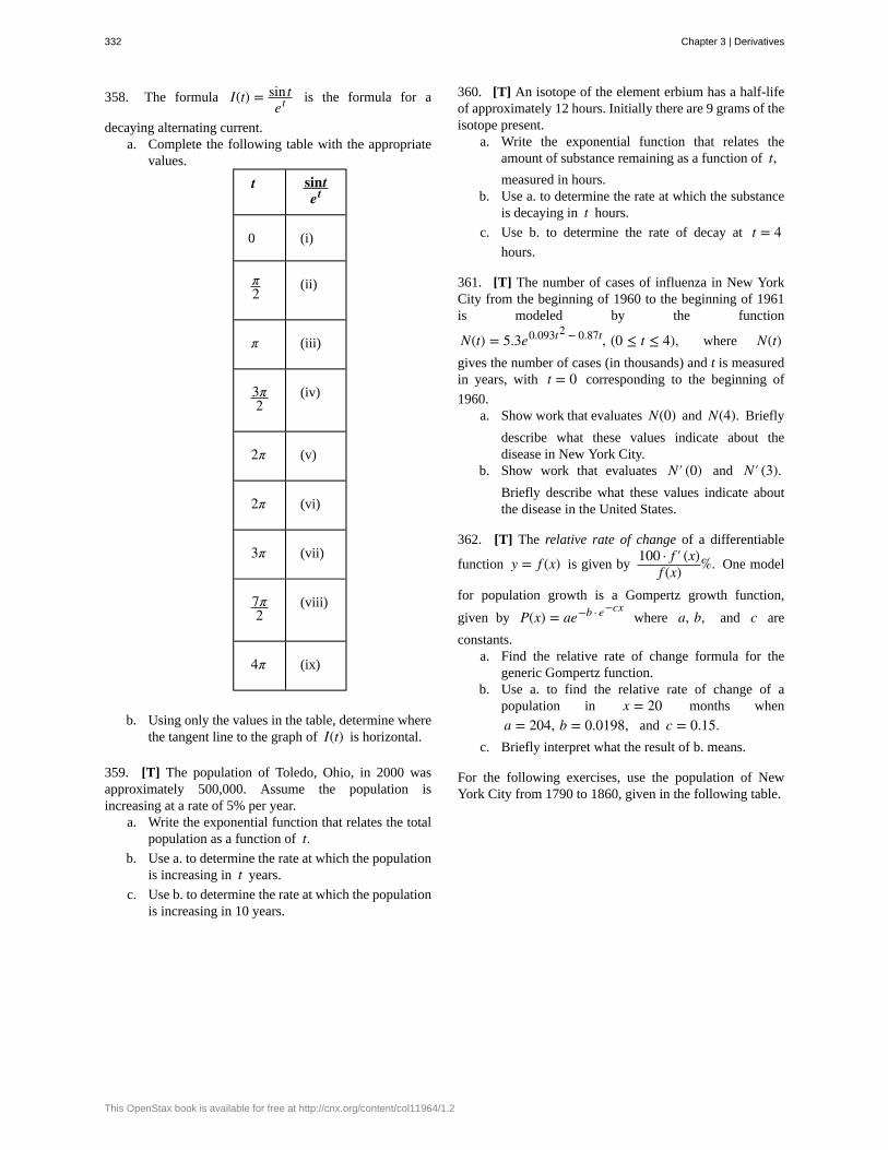
358. The formula I(t) = sin tet is the formula for a
decaying alternating current.a. Complete the following table with the appropriate
values.
t sintet
0 (i)
π2
(ii)
π (iii)
3π2
(iv)
2π (v)
2π (vi)
3π (vii)
7π2
(viii)
4π (ix)
b. Using only the values in the table, determine wherethe tangent line to the graph of I(t) is horizontal.
359. [T] The population of Toledo, Ohio, in 2000 wasapproximately 500,000. Assume the population isincreasing at a rate of 5% per year.
a. Write the exponential function that relates the totalpopulation as a function of t.
b. Use a. to determine the rate at which the populationis increasing in t years.
c. Use b. to determine the rate at which the populationis increasing in 10 years.
360. [T] An isotope of the element erbium has a half-lifeof approximately 12 hours. Initially there are 9 grams of theisotope present.
a. Write the exponential function that relates theamount of substance remaining as a function of t,measured in hours.
b. Use a. to determine the rate at which the substanceis decaying in t hours.
c. Use b. to determine the rate of decay at t = 4hours.
361. [T] The number of cases of influenza in New YorkCity from the beginning of 1960 to the beginning of 1961is modeled by the function
N(t) = 5.3e0.093t2 − 0.87t, (0 ≤ t ≤ 4), where N(t)gives the number of cases (in thousands) and t is measuredin years, with t = 0 corresponding to the beginning of
1960.a. Show work that evaluates N(0) and N(4). Briefly
describe what these values indicate about thedisease in New York City.
b. Show work that evaluates N′ (0) and N′ (3).Briefly describe what these values indicate aboutthe disease in the United States.
362. [T] The relative rate of change of a differentiable
function y = f (x) is given by100 · f ′ (x)
f (x) %. One model
for population growth is a Gompertz growth function,
given by P(x) = ae−b · e−cxwhere a, b, and c are
constants.a. Find the relative rate of change formula for the
generic Gompertz function.b. Use a. to find the relative rate of change of a
population in x = 20 months when
a = 204, b = 0.0198, and c = 0.15.c. Briefly interpret what the result of b. means.
For the following exercises, use the population of NewYork City from 1790 to 1860, given in the following table.
332 Chapter 3 | Derivatives
This OpenStax book is available for free at http://cnx.org/content/col11964/1.2
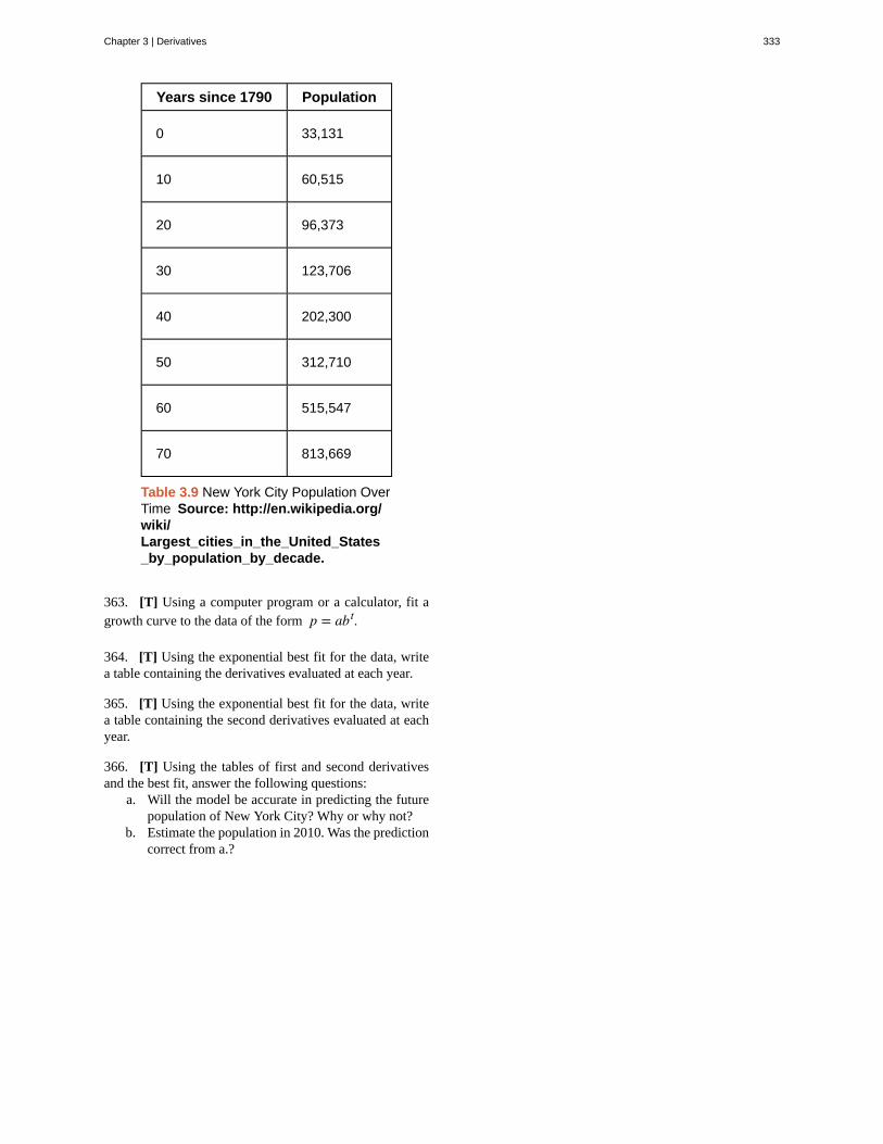
Years since 1790 Population
0 33,131
10 60,515
20 96,373
30 123,706
40 202,300
50 312,710
60 515,547
70 813,669
Table 3.9 New York City Population OverTime Source: http://en.wikipedia.org/wiki/Largest_cities_in_the_United_States_by_population_by_decade.
363. [T] Using a computer program or a calculator, fit agrowth curve to the data of the form p = abt.
364. [T] Using the exponential best fit for the data, writea table containing the derivatives evaluated at each year.
365. [T] Using the exponential best fit for the data, writea table containing the second derivatives evaluated at eachyear.
366. [T] Using the tables of first and second derivativesand the best fit, answer the following questions:
a. Will the model be accurate in predicting the futurepopulation of New York City? Why or why not?
b. Estimate the population in 2010. Was the predictioncorrect from a.?
Chapter 3 | Derivatives 333
acceleration
amount of change
average rate of change
chain rule
constant multiple rule
constant rule
derivative
derivative function
difference quotient
difference rule
differentiable at a
differentiable function
differentiable on S
differentiation
higher-order derivative
implicit differentiation
instantaneous rate of change
logarithmic differentiation
marginal cost
marginal profit
marginal revenue
CHAPTER 3 REVIEW
KEY TERMSis the rate of change of the velocity, that is, the derivative of velocity
the amount of a function f (x) over an interval ⎡⎣x, x + h⎤
⎦ is f (x + h) − f (x)
is a function f (x) over an interval ⎡⎣x, x + h⎤
⎦ isf (x + h) − f (a)
b − a
the chain rule defines the derivative of a composite function as the derivative of the outer function evaluatedat the inner function times the derivative of the inner function
the derivative of a constant c multiplied by a function f is the same as the constant multiplied by
the derivative: ddx
⎛⎝c f (x)⎞
⎠ = c f ′ (x)
the derivative of a constant function is zero: ddx(c) = 0, where c is a constant
the slope of the tangent line to a function at a point, calculated by taking the limit of the difference quotient, isthe derivative
gives the derivative of a function at each point in the domain of the original function for which thederivative is defined
of a function f (x) at a is given by
f (a + h) − f (a)h or f (x) − f (a)
x − a
the derivative of the difference of a function f and a function g is the same as the difference of the
derivative of f and the derivative of g: ddx
⎛⎝ f (x) − g(x)⎞
⎠ = f ′ (x) − g′ (x)
a function for which f ′(a) exists is differentiable at a
a function for which f ′(x) exists is a differentiable function
a function for which f ′(x) exists for each x in the open set S is differentiable on S
the process of taking a derivative
a derivative of a derivative, from the second derivative to the nth derivative, is called a higher-order derivative
is a technique for computingdydx for a function defined by an equation, accomplished by
differentiating both sides of the equation (remembering to treat the variable y as a function) and solving fordydx
the rate of change of a function at any point along the function a, also called f ′(a),or the derivative of the function at a
is a technique that allows us to differentiate a function by first taking the natural logarithmof both sides of an equation, applying properties of logarithms to simplify the equation, and differentiating implicitly
is the derivative of the cost function, or the approximate cost of producing one more item
is the derivative of the profit function, or the approximate profit obtained by producing and selling onemore item
is the derivative of the revenue function, or the approximate revenue obtained by selling one moreitem
334 Chapter 3 | Derivatives
This OpenStax book is available for free at http://cnx.org/content/col11964/1.2
population growth rate
power rule
product rule
quotient rule
speed
sum rule
is the derivative of the population with respect to time
the derivative of a power function is a function in which the power on x becomes the coefficient of the term
and the power on x in the derivative decreases by 1: If n is an integer, then ddxxn = nxn − 1
the derivative of a product of two functions is the derivative of the first function times the second function
plus the derivative of the second function times the first function: ddx
⎛⎝ f (x)g(x)⎞
⎠ = f ′ (x)g(x) + g′ (x) f (x)
the derivative of the quotient of two functions is the derivative of the first function times the secondfunction minus the derivative of the second function times the first function, all divided by the square of the second
function: ddx
⎛⎝
f (x)g(x)
⎞⎠ = f ′ (x)g(x) − g′ (x) f (x)
⎛⎝g(x)⎞
⎠2
is the absolute value of velocity, that is, |v(t)| is the speed of an object at time t whose velocity is given by v(t)
the derivative of the sum of a function f and a function g is the same as the sum of the derivative of f and the
derivative of g: ddx
⎛⎝ f (x) + g(x)⎞
⎠ = f ′ (x) + g′ (x)
KEY EQUATIONS• Difference quotient
Q = f (x) − f (a)x − a
• Difference quotient with increment h
Q = f (a + h) − f (a)a + h − a = f (a + h) − f (a)
h
• Slope of tangent line
mtan = limx → af (x) − f (a)
x − a
mtan = limh → 0
f (a + h) − f (a)h
• Derivative of f (x) at a
f ′ (a) = limx → af (x) − f (a)
x − a
f ′(a) = limh → 0
f (a + h) − f (a)h
• Average velocity
vave = s(t) − s(a)t − a
• Instantaneous velocity
v(a) = s′ (a) = limt → a
s(t) − s(a)t − a
• The derivative function
f ′ (x) = limh → 0
f (x + h) − f (x)h
• Derivative of sine functionddx(sinx) = cosx
• Derivative of cosine functionddx(cosx) = −sinx
• Derivative of tangent function
Chapter 3 | Derivatives 335
ddx(tanx) = sec2 x
• Derivative of cotangent functionddx(cot x) = −csc2 x
• Derivative of secant functionddx(secx) = secx tanx
• Derivative of cosecant functionddx(cscx) = −cscxcot x
• The chain ruleh′ (x) = f ′ ⎛
⎝g(x)⎞⎠g′ (x)
• The power rule for functions
h′ (x) = n⎛⎝g(x)⎞
⎠n − 1 g′ (x)
• Inverse function theorem⎛⎝ f −1⎞
⎠′ (x) = 1f ′ ⎛
⎝ f −1 (x)⎞⎠
whenever f ′ ⎛⎝ f −1 (x)⎞
⎠ ≠ 0 and f (x) is differentiable.
• Power rule with rational exponentsddx
⎛⎝x
m/n⎞⎠ = m
n x(m/n) − 1.
• Derivative of inverse sine functionddx sin−1 x = 1
1 − (x)2
• Derivative of inverse cosine functionddx cos−1 x = −1
1 − (x)2
• Derivative of inverse tangent functionddx tan−1 x = 1
1 + (x)2
• Derivative of inverse cotangent functionddx cot−1 x = −1
1 + (x)2
• Derivative of inverse secant functionddx sec−1 x = 1
|x| (x)2 − 1
• Derivative of inverse cosecant functionddx csc−1 x = −1
|x| (x)2 − 1
• Derivative of the natural exponential functionddx
⎛⎝e
g(x)⎞⎠ = eg(x) g′ (x)
• Derivative of the natural logarithmic functionddx
⎛⎝lng(x)⎞
⎠ = 1g(x)g′ (x)
• Derivative of the general exponential function
336 Chapter 3 | Derivatives
This OpenStax book is available for free at http://cnx.org/content/col11964/1.2
ddx
⎛⎝b
g(x)⎞⎠ = bg(x) g′ (x) lnb
• Derivative of the general logarithmic function
ddx
⎛⎝logb g(x)⎞
⎠ = g′ (x)g(x) lnb
KEY CONCEPTS
3.1 Defining the Derivative
• The slope of the tangent line to a curve measures the instantaneous rate of change of a curve. We can calculate it byfinding the limit of the difference quotient or the difference quotient with increment h.
• The derivative of a function f (x) at a value a is found using either of the definitions for the slope of the tangent
line.
• Velocity is the rate of change of position. As such, the velocity v(t) at time t is the derivative of the position s(t)at time t. Average velocity is given by
vave = s(t) − s(a)t − a .
Instantaneous velocity is given by
v(a) = s′ (a) = limt → a
s(t) − s(a)t − a .
• We may estimate a derivative by using a table of values.
3.2 The Derivative as a Function
• The derivative of a function f (x) is the function whose value at x is f ′(x).
• The graph of a derivative of a function f (x) is related to the graph of f (x). Where f (x) has a tangent line with
positive slope, f ′ (x) > 0. Where f (x) has a tangent line with negative slope, f ′ (x) < 0. Where f (x) has a
horizontal tangent line, f ′ (x) = 0.
• If a function is differentiable at a point, then it is continuous at that point. A function is not differentiable at a pointif it is not continuous at the point, if it has a vertical tangent line at the point, or if the graph has a sharp corner orcusp.
• Higher-order derivatives are derivatives of derivatives, from the second derivative to the nth derivative.
3.3 Differentiation Rules
• The derivative of a constant function is zero.
• The derivative of a power function is a function in which the power on x becomes the coefficient of the term and
the power on x in the derivative decreases by 1.
• The derivative of a constant c multiplied by a function f is the same as the constant multiplied by the derivative.
• The derivative of the sum of a function f and a function g is the same as the sum of the derivative of f and thederivative of g.
• The derivative of the difference of a function f and a function g is the same as the difference of the derivative of fand the derivative of g.
• The derivative of a product of two functions is the derivative of the first function times the second function plus thederivative of the second function times the first function.
• The derivative of the quotient of two functions is the derivative of the first function times the second function minus
Chapter 3 | Derivatives 337
the derivative of the second function times the first function, all divided by the square of the second function.
• We used the limit definition of the derivative to develop formulas that allow us to find derivatives without resortingto the definition of the derivative. These formulas can be used singly or in combination with each other.
3.4 Derivatives as Rates of Change
• Using f (a + h) ≈ f (a) + f ′ (a)h, it is possible to estimate f (a + h) given f ′ (a) and f (a).
• The rate of change of position is velocity, and the rate of change of velocity is acceleration. Speed is the absolutevalue, or magnitude, of velocity.
• The population growth rate and the present population can be used to predict the size of a future population.
• Marginal cost, marginal revenue, and marginal profit functions can be used to predict, respectively, the cost ofproducing one more item, the revenue obtained by selling one more item, and the profit obtained by producing andselling one more item.
3.5 Derivatives of Trigonometric Functions
• We can find the derivatives of sin x and cos x by using the definition of derivative and the limit formulas foundearlier. The results are
ddx sinx = cosx d
dx cosx = −sinx.
• With these two formulas, we can determine the derivatives of all six basic trigonometric functions.
3.6 The Chain Rule
• The chain rule allows us to differentiate compositions of two or more functions. It states that for h(x) = f ⎛⎝g(x)⎞
⎠,
h′ (x) = f ′ ⎛⎝g(x)⎞
⎠g′ (x).
In Leibniz’s notation this rule takes the form
dydx = dy
du · dudx .
• We can use the chain rule with other rules that we have learned, and we can derive formulas for some of them.
• The chain rule combines with the power rule to form a new rule:
If h(x) = ⎛⎝g(x)⎞
⎠n, then h′ (x) = n⎛
⎝g(x)⎞⎠n − 1 g′ (x).
• When applied to the composition of three functions, the chain rule can be expressed as follows: Ifh(x) = f ⎛
⎝g⎛⎝k(x)⎞
⎠⎞⎠, then h′ (x) = f ′(g⎛
⎝k(x)⎞⎠g′ ⎛
⎝k(x)⎞⎠k′ (x).
3.7 Derivatives of Inverse Functions
• The inverse function theorem allows us to compute derivatives of inverse functions without using the limitdefinition of the derivative.
• We can use the inverse function theorem to develop differentiation formulas for the inverse trigonometric functions.
3.8 Implicit Differentiation
• We use implicit differentiation to find derivatives of implicitly defined functions (functions defined by equations).
• By using implicit differentiation, we can find the equation of a tangent line to the graph of a curve.
3.9 Derivatives of Exponential and Logarithmic Functions
• On the basis of the assumption that the exponential function y = bx, b > 0 is continuous everywhere and
338 Chapter 3 | Derivatives
This OpenStax book is available for free at http://cnx.org/content/col11964/1.2
differentiable at 0, this function is differentiable everywhere and there is a formula for its derivative.
• We can use a formula to find the derivative of y = lnx, and the relationship logb x = lnxlnb allows us to extend
our differentiation formulas to include logarithms with arbitrary bases.
• Logarithmic differentiation allows us to differentiate functions of the form y = g(x) f (x)or very complex functions
by taking the natural logarithm of both sides and exploiting the properties of logarithms before differentiating.
CHAPTER 3 REVIEW EXERCISESTrue or False? Justify the answer with a proof or acounterexample.
367. Every function has a derivative.
368. A continuous function has a continuous derivative.
369. A continuous function has a derivative.
370. If a function is differentiable, it is continuous.
Use the limit definition of the derivative to exactly evaluatethe derivative.
371. f (x) = x + 4
372. f (x) = 3x
Find the derivatives of the following functions.
373. f (x) = 3x3 − 4x2
374. f (x) = ⎛⎝4 − x2⎞
⎠3
375. f (x) = esinx
376. f (x) = ln(x + 2)
377. f (x) = x2 cosx + x tan(x)
378. f (x) = 3x2 + 2
379. f (x) = x4 sin−1 (x)
380. x2 y = ⎛⎝y + 2⎞
⎠ + xysin(x)
Find the following derivatives of various orders.
381. First derivative of y = x ln(x)cosx
382. Third derivative of y = (3x + 2)2
383. Second derivative of y = 4x + x2 sin(x)
Find the equation of the tangent line to the followingequations at the specified point.
384. y = cos−1 (x) + x at x = 0
385. y = x + ex − 1x at x = 1
Draw the derivative for the following graphs.
386.
387.
The following questions concern the water level in OceanCity, New Jersey, in January, which can be approximated
by w(t) = 1.9 + 2.9cos⎛⎝π6 t⎞⎠, where t is measured in
hours after midnight, and the height is measured in feet.
388. Find and graph the derivative. What is the physicalmeaning?
Chapter 3 | Derivatives 339
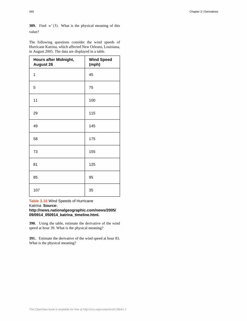
389. Find w′ (3). What is the physical meaning of this
value?
The following questions consider the wind speeds ofHurricane Katrina, which affected New Orleans, Louisiana,in August 2005. The data are displayed in a table.
Hours after Midnight,August 26
Wind Speed(mph)
1 45
5 75
11 100
29 115
49 145
58 175
73 155
81 125
85 95
107 35
Table 3.10 Wind Speeds of HurricaneKatrina Source:http://news.nationalgeographic.com/news/2005/09/0914_050914_katrina_timeline.html.
390. Using the table, estimate the derivative of the windspeed at hour 39. What is the physical meaning?
391. Estimate the derivative of the wind speed at hour 83.What is the physical meaning?
340 Chapter 3 | Derivatives
This OpenStax book is available for free at http://cnx.org/content/col11964/1.2
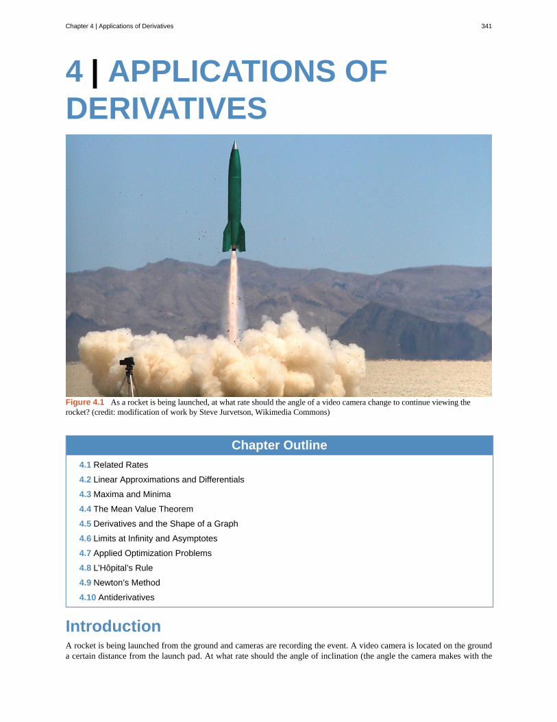
4 | APPLICATIONS OFDERIVATIVES
Figure 4.1 As a rocket is being launched, at what rate should the angle of a video camera change to continue viewing therocket? (credit: modification of work by Steve Jurvetson, Wikimedia Commons)
Chapter Outline
4.1 Related Rates
4.2 Linear Approximations and Differentials
4.3 Maxima and Minima
4.4 The Mean Value Theorem
4.5 Derivatives and the Shape of a Graph
4.6 Limits at Infinity and Asymptotes
4.7 Applied Optimization Problems
4.8 L’Hôpital’s Rule
4.9 Newton’s Method
4.10 Antiderivatives
IntroductionA rocket is being launched from the ground and cameras are recording the event. A video camera is located on the grounda certain distance from the launch pad. At what rate should the angle of inclination (the angle the camera makes with the
Chapter 4 | Applications of Derivatives 341
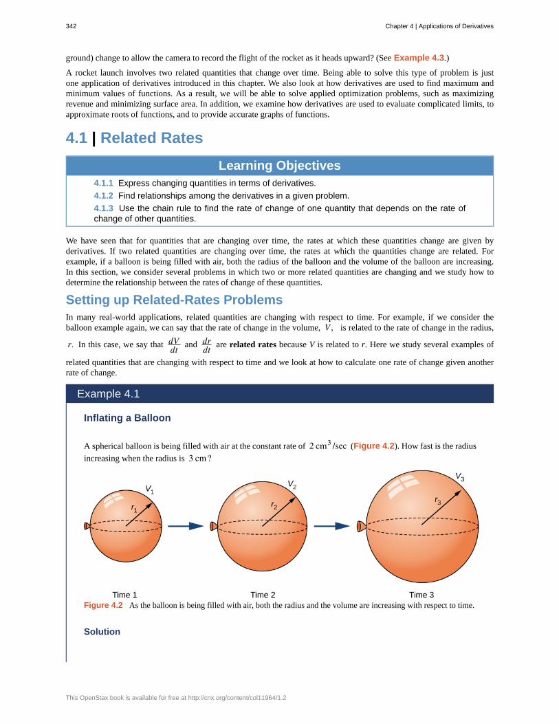
ground) change to allow the camera to record the flight of the rocket as it heads upward? (See Example 4.3.)
A rocket launch involves two related quantities that change over time. Being able to solve this type of problem is justone application of derivatives introduced in this chapter. We also look at how derivatives are used to find maximum andminimum values of functions. As a result, we will be able to solve applied optimization problems, such as maximizingrevenue and minimizing surface area. In addition, we examine how derivatives are used to evaluate complicated limits, toapproximate roots of functions, and to provide accurate graphs of functions.
4.1 | Related Rates
Learning Objectives4.1.1 Express changing quantities in terms of derivatives.
4.1.2 Find relationships among the derivatives in a given problem.
4.1.3 Use the chain rule to find the rate of change of one quantity that depends on the rate ofchange of other quantities.
We have seen that for quantities that are changing over time, the rates at which these quantities change are given byderivatives. If two related quantities are changing over time, the rates at which the quantities change are related. Forexample, if a balloon is being filled with air, both the radius of the balloon and the volume of the balloon are increasing.In this section, we consider several problems in which two or more related quantities are changing and we study how todetermine the relationship between the rates of change of these quantities.
Setting up Related-Rates ProblemsIn many real-world applications, related quantities are changing with respect to time. For example, if we consider theballoon example again, we can say that the rate of change in the volume, V , is related to the rate of change in the radius,
r. In this case, we say that dVdt and dr
dt are related rates because V is related to r. Here we study several examples of
related quantities that are changing with respect to time and we look at how to calculate one rate of change given anotherrate of change.
Example 4.1
Inflating a Balloon
A spherical balloon is being filled with air at the constant rate of 2 cm3 /sec (Figure 4.2). How fast is the radius
increasing when the radius is 3 cm?
Figure 4.2 As the balloon is being filled with air, both the radius and the volume are increasing with respect to time.
Solution
342 Chapter 4 | Applications of Derivatives
This OpenStax book is available for free at http://cnx.org/content/col11964/1.2
4.1
The volume of a sphere of radius r centimeters is
V = 43πr3 cm3.
Since the balloon is being filled with air, both the volume and the radius are functions of time. Therefore, tseconds after beginning to fill the balloon with air, the volume of air in the balloon is
V(t) = 43π[r(t)]3 cm3.
Differentiating both sides of this equation with respect to time and applying the chain rule, we see that the rate ofchange in the volume is related to the rate of change in the radius by the equation
V′(t) = 4π⎡⎣r(t)⎤
⎦2 r′ (t).
The balloon is being filled with air at the constant rate of 2 cm3/sec, so V′(t) = 2 cm3 /sec. Therefore,
2cm3 /sec = ⎛⎝4π⎡
⎣r(t)⎤⎦2 cm2⎞
⎠ · ⎛⎝r′(t)cm/s⎞
⎠,
which implies
r′(t) = 12π⎡
⎣r(t)⎤⎦2 cm/sec.
When the radius r = 3 cm,
r′(t) = 118π cm/sec.
What is the instantaneous rate of change of the radius when r = 6 cm?
Before looking at other examples, let’s outline the problem-solving strategy we will be using to solve related-rates problems.
Problem-Solving Strategy: Solving a Related-Rates Problem
1. Assign symbols to all variables involved in the problem. Draw a figure if applicable.
2. State, in terms of the variables, the information that is given and the rate to be determined.
3. Find an equation relating the variables introduced in step 1.
4. Using the chain rule, differentiate both sides of the equation found in step 3 with respect to the independentvariable. This new equation will relate the derivatives.
5. Substitute all known values into the equation from step 4, then solve for the unknown rate of change.
Note that when solving a related-rates problem, it is crucial not to substitute known values too soon. For example, if thevalue for a changing quantity is substituted into an equation before both sides of the equation are differentiated, then thatquantity will behave as a constant and its derivative will not appear in the new equation found in step 4. We examine thispotential error in the following example.
Examples of the ProcessLet’s now implement the strategy just described to solve several related-rates problems. The first example involves a planeflying overhead. The relationship we are studying is between the speed of the plane and the rate at which the distancebetween the plane and a person on the ground is changing.
Chapter 4 | Applications of Derivatives 343
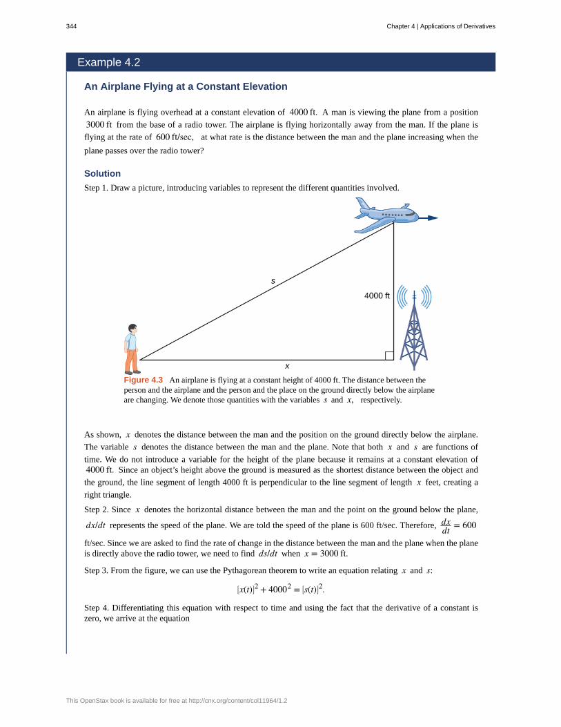
Example 4.2
An Airplane Flying at a Constant Elevation
An airplane is flying overhead at a constant elevation of 4000 ft. A man is viewing the plane from a position
3000 ft from the base of a radio tower. The airplane is flying horizontally away from the man. If the plane is
flying at the rate of 600 ft/sec, at what rate is the distance between the man and the plane increasing when the
plane passes over the radio tower?
Solution
Step 1. Draw a picture, introducing variables to represent the different quantities involved.
Figure 4.3 An airplane is flying at a constant height of 4000 ft. The distance between theperson and the airplane and the person and the place on the ground directly below the airplaneare changing. We denote those quantities with the variables s and x, respectively.
As shown, x denotes the distance between the man and the position on the ground directly below the airplane.
The variable s denotes the distance between the man and the plane. Note that both x and s are functions of
time. We do not introduce a variable for the height of the plane because it remains at a constant elevation of4000 ft. Since an object’s height above the ground is measured as the shortest distance between the object and
the ground, the line segment of length 4000 ft is perpendicular to the line segment of length x feet, creating a
right triangle.
Step 2. Since x denotes the horizontal distance between the man and the point on the ground below the plane,
dx/dt represents the speed of the plane. We are told the speed of the plane is 600 ft/sec. Therefore, dxdt = 600
ft/sec. Since we are asked to find the rate of change in the distance between the man and the plane when the planeis directly above the radio tower, we need to find ds/dt when x = 3000 ft.
Step 3. From the figure, we can use the Pythagorean theorem to write an equation relating x and s:
⎡⎣x(t)⎤
⎦2 + 40002 = ⎡
⎣s(t)⎤⎦2.
Step 4. Differentiating this equation with respect to time and using the fact that the derivative of a constant iszero, we arrive at the equation
344 Chapter 4 | Applications of Derivatives
This OpenStax book is available for free at http://cnx.org/content/col11964/1.2
4.2
xdxdt = sds
dt .
Step 5. Find the rate at which the distance between the man and the plane is increasing when the plane is directly
over the radio tower. That is, find dsdt when x = 3000 ft. Since the speed of the plane is 600 ft/sec, we know
that dxdt = 600 ft/sec. We are not given an explicit value for s; however, since we are trying to find ds
dt when
x = 3000 ft, we can use the Pythagorean theorem to determine the distance s when x = 3000 and the height
is 4000 ft. Solving the equation
30002 + 40002 = s2
for s, we have s = 5000 ft at the time of interest. Using these values, we conclude that ds/dt is a solution of
the equation
(3000)(600) = (5000) · dsdt .
Therefore,
dsdt = 3000 · 600
5000 = 360 ft/sec.
Note: When solving related-rates problems, it is important not to substitute values for the variables too soon. Forexample, in step 3, we related the variable quantities x(t) and s(t) by the equation
⎡⎣x(t)⎤
⎦2 + 40002 = ⎡
⎣s(t)⎤⎦2.
Since the plane remains at a constant height, it is not necessary to introduce a variable for the height, and we areallowed to use the constant 4000 to denote that quantity. However, the other two quantities are changing. If wemistakenly substituted x(t) = 3000 into the equation before differentiating, our equation would have been
30002 + 40002 = ⎡⎣s(t)⎤
⎦2.
After differentiating, our equation would become
0 = s(t)dsdt .
As a result, we would incorrectly conclude that dsdt = 0.
What is the speed of the plane if the distance between the person and the plane is increasing at the rate of300 ft/sec?
We now return to the problem involving the rocket launch from the beginning of the chapter.
Example 4.3
Chapter Opener: A Rocket Launch
Chapter 4 | Applications of Derivatives 345
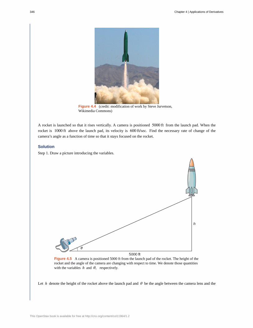
Figure 4.4 (credit: modification of work by Steve Jurvetson,Wikimedia Commons)
A rocket is launched so that it rises vertically. A camera is positioned 5000 ft from the launch pad. When the
rocket is 1000 ft above the launch pad, its velocity is 600 ft/sec. Find the necessary rate of change of the
camera’s angle as a function of time so that it stays focused on the rocket.
Solution
Step 1. Draw a picture introducing the variables.
Figure 4.5 A camera is positioned 5000 ft from the launch pad of the rocket. The height of therocket and the angle of the camera are changing with respect to time. We denote those quantitieswith the variables h and θ, respectively.
Let h denote the height of the rocket above the launch pad and θ be the angle between the camera lens and the
346 Chapter 4 | Applications of Derivatives
This OpenStax book is available for free at http://cnx.org/content/col11964/1.2
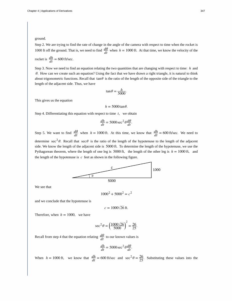
ground.
Step 2. We are trying to find the rate of change in the angle of the camera with respect to time when the rocket is
1000 ft off the ground. That is, we need to find dθdt when h = 1000 ft. At that time, we know the velocity of the
rocket is dhdt = 600 ft/sec.
Step 3. Now we need to find an equation relating the two quantities that are changing with respect to time: h and
θ. How can we create such an equation? Using the fact that we have drawn a right triangle, it is natural to think
about trigonometric functions. Recall that tanθ is the ratio of the length of the opposite side of the triangle to the
length of the adjacent side. Thus, we have
tanθ = h5000.
This gives us the equation
h = 5000tanθ.
Step 4. Differentiating this equation with respect to time t, we obtain
dhdt = 5000sec2 θ dθ
dt .
Step 5. We want to find dθdt when h = 1000 ft. At this time, we know that dh
dt = 600 ft/sec. We need to
determine sec2 θ. Recall that secθ is the ratio of the length of the hypotenuse to the length of the adjacent
side. We know the length of the adjacent side is 5000 ft. To determine the length of the hypotenuse, we use the
Pythagorean theorem, where the length of one leg is 5000 ft, the length of the other leg is h = 1000 ft, and
the length of the hypotenuse is c feet as shown in the following figure.
We see that
10002 + 50002 = c2
and we conclude that the hypotenuse is
c = 1000 26 ft.
Therefore, when h = 1000, we have
sec2 θ = ⎛⎝1000 26
5000⎞⎠
2= 26
25.
Recall from step 4 that the equation relating dθdt to our known values is
dhdt = 5000sec2 θ dθ
dt .
When h = 1000 ft, we know that dhdt = 600 ft/sec and sec2 θ = 26
25. Substituting these values into the
Chapter 4 | Applications of Derivatives 347
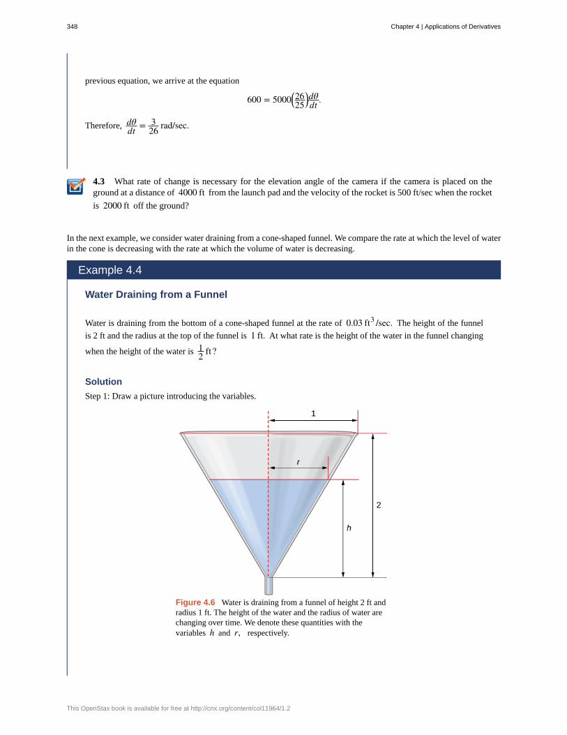
4.3
previous equation, we arrive at the equation
600 = 5000⎛⎝2625
⎞⎠dθdt .
Therefore, dθdt = 3
26 rad/sec.
What rate of change is necessary for the elevation angle of the camera if the camera is placed on theground at a distance of 4000 ft from the launch pad and the velocity of the rocket is 500 ft/sec when the rocket
is 2000 ft off the ground?
In the next example, we consider water draining from a cone-shaped funnel. We compare the rate at which the level of waterin the cone is decreasing with the rate at which the volume of water is decreasing.
Example 4.4
Water Draining from a Funnel
Water is draining from the bottom of a cone-shaped funnel at the rate of 0.03 ft3 /sec. The height of the funnel
is 2 ft and the radius at the top of the funnel is 1 ft. At what rate is the height of the water in the funnel changing
when the height of the water is 12 ft?
Solution
Step 1: Draw a picture introducing the variables.
Figure 4.6 Water is draining from a funnel of height 2 ft andradius 1 ft. The height of the water and the radius of water arechanging over time. We denote these quantities with thevariables h and r, respectively.
348 Chapter 4 | Applications of Derivatives
This OpenStax book is available for free at http://cnx.org/content/col11964/1.2
4.4
Let h denote the height of the water in the funnel, r denote the radius of the water at its surface, and V denote
the volume of the water.
Step 2: We need to determine dhdt when h = 1
2 ft. We know that dVdt = −0.03 ft/sec.
Step 3: The volume of water in the cone is
V = 13πr2 h.
From the figure, we see that we have similar triangles. Therefore, the ratio of the sides in the two triangles is the
same. Therefore, rh = 1
2 or r = h2. Using this fact, the equation for volume can be simplified to
V = 13π⎛
⎝h2
⎞⎠2
h = π12 h3.
Step 4: Applying the chain rule while differentiating both sides of this equation with respect to time t, we obtain
dVdt = π
4 h2 dhdt .
Step 5: We want to find dhdt when h = 1
2 ft. Since water is leaving at the rate of 0.03 ft3 /sec, we know that
dVdt = −0.03 ft3 /sec. Therefore,
−0.03 = π4
⎛⎝12
⎞⎠2 dh
dt ,
which implies
−0.03 = π16
dhdt .
It follows that
dhdt = − 0.48
π = −0.153 ft/sec.
At what rate is the height of the water changing when the height of the water is 14 ft?
Chapter 4 | Applications of Derivatives 349
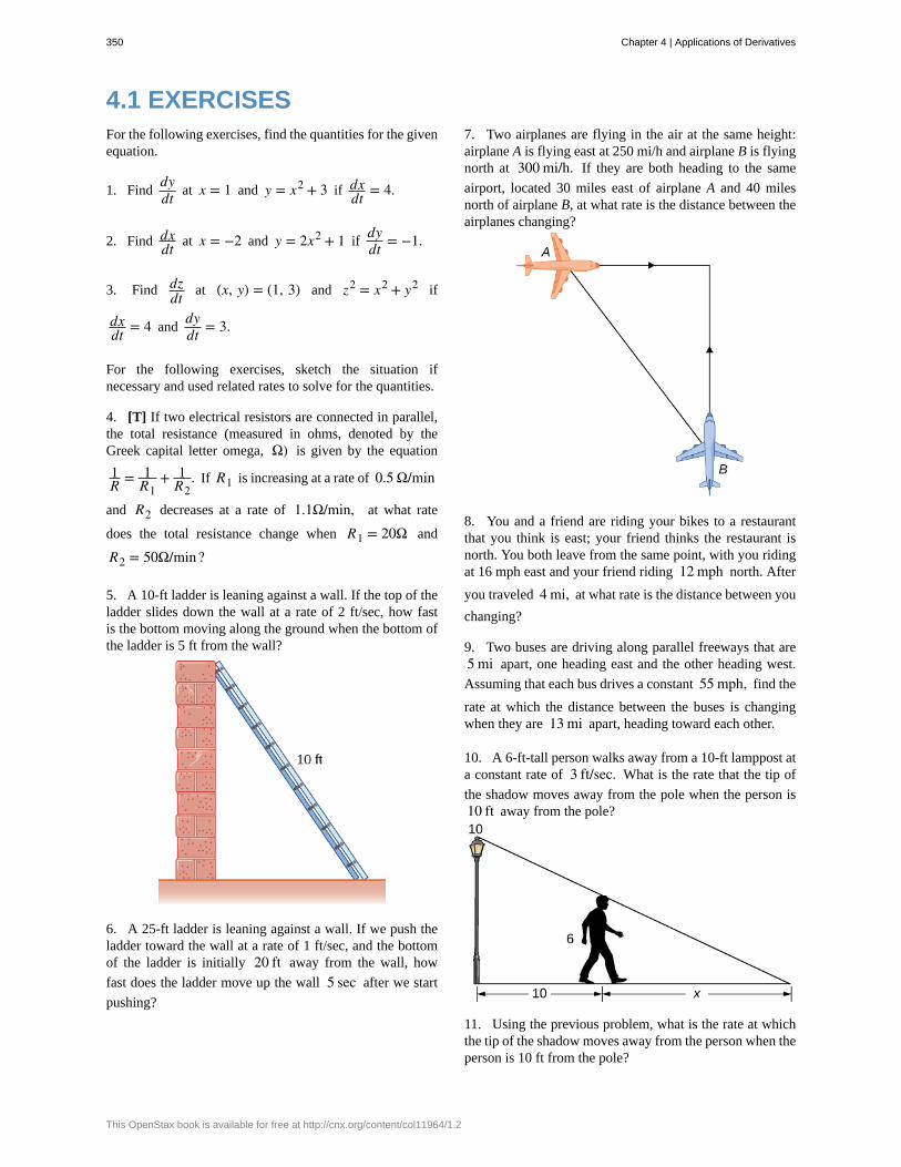
4.1 EXERCISESFor the following exercises, find the quantities for the givenequation.
1. Finddydt at x = 1 and y = x2 + 3 if dx
dt = 4.
2. Find dxdt at x = −2 and y = 2x2 + 1 if
dydt = −1.
3. Find dzdt at (x, y) = (1, 3) and z2 = x2 + y2 if
dxdt = 4 and
dydt = 3.
For the following exercises, sketch the situation ifnecessary and used related rates to solve for the quantities.
4. [T] If two electrical resistors are connected in parallel,the total resistance (measured in ohms, denoted by theGreek capital letter omega, Ω) is given by the equation
1R = 1
R1+ 1
R2. If R1 is increasing at a rate of 0.5 Ω/min
and R2 decreases at a rate of 1.1Ω/min, at what rate
does the total resistance change when R1 = 20Ω and
R2 = 50Ω/min?
5. A 10-ft ladder is leaning against a wall. If the top of theladder slides down the wall at a rate of 2 ft/sec, how fastis the bottom moving along the ground when the bottom ofthe ladder is 5 ft from the wall?
6. A 25-ft ladder is leaning against a wall. If we push theladder toward the wall at a rate of 1 ft/sec, and the bottomof the ladder is initially 20 ft away from the wall, how
fast does the ladder move up the wall 5 sec after we start
pushing?
7. Two airplanes are flying in the air at the same height:airplane A is flying east at 250 mi/h and airplane B is flyingnorth at 300 mi/h. If they are both heading to the same
airport, located 30 miles east of airplane A and 40 milesnorth of airplane B, at what rate is the distance between theairplanes changing?
8. You and a friend are riding your bikes to a restaurantthat you think is east; your friend thinks the restaurant isnorth. You both leave from the same point, with you ridingat 16 mph east and your friend riding 12 mph north. After
you traveled 4 mi, at what rate is the distance between you
changing?
9. Two buses are driving along parallel freeways that are5 mi apart, one heading east and the other heading west.
Assuming that each bus drives a constant 55 mph, find the
rate at which the distance between the buses is changingwhen they are 13 mi apart, heading toward each other.
10. A 6-ft-tall person walks away from a 10-ft lamppost ata constant rate of 3 ft/sec. What is the rate that the tip of
the shadow moves away from the pole when the person is10 ft away from the pole?
11. Using the previous problem, what is the rate at whichthe tip of the shadow moves away from the person when theperson is 10 ft from the pole?
350 Chapter 4 | Applications of Derivatives
This OpenStax book is available for free at http://cnx.org/content/col11964/1.2
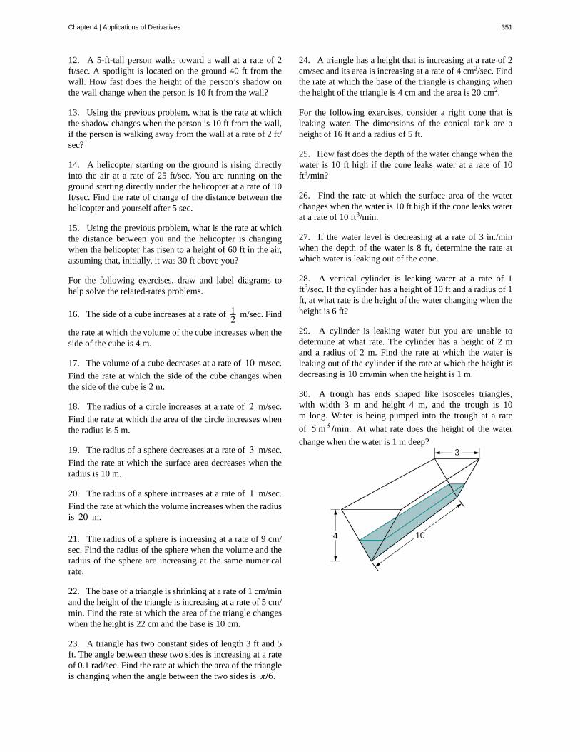
12. A 5-ft-tall person walks toward a wall at a rate of 2ft/sec. A spotlight is located on the ground 40 ft from thewall. How fast does the height of the person’s shadow onthe wall change when the person is 10 ft from the wall?
13. Using the previous problem, what is the rate at whichthe shadow changes when the person is 10 ft from the wall,if the person is walking away from the wall at a rate of 2 ft/sec?
14. A helicopter starting on the ground is rising directlyinto the air at a rate of 25 ft/sec. You are running on theground starting directly under the helicopter at a rate of 10ft/sec. Find the rate of change of the distance between thehelicopter and yourself after 5 sec.
15. Using the previous problem, what is the rate at whichthe distance between you and the helicopter is changingwhen the helicopter has risen to a height of 60 ft in the air,assuming that, initially, it was 30 ft above you?
For the following exercises, draw and label diagrams tohelp solve the related-rates problems.
16. The side of a cube increases at a rate of 12 m/sec. Find
the rate at which the volume of the cube increases when theside of the cube is 4 m.
17. The volume of a cube decreases at a rate of 10 m/sec.
Find the rate at which the side of the cube changes whenthe side of the cube is 2 m.
18. The radius of a circle increases at a rate of 2 m/sec.
Find the rate at which the area of the circle increases whenthe radius is 5 m.
19. The radius of a sphere decreases at a rate of 3 m/sec.
Find the rate at which the surface area decreases when theradius is 10 m.
20. The radius of a sphere increases at a rate of 1 m/sec.
Find the rate at which the volume increases when the radiusis 20 m.
21. The radius of a sphere is increasing at a rate of 9 cm/sec. Find the radius of the sphere when the volume and theradius of the sphere are increasing at the same numericalrate.
22. The base of a triangle is shrinking at a rate of 1 cm/minand the height of the triangle is increasing at a rate of 5 cm/min. Find the rate at which the area of the triangle changeswhen the height is 22 cm and the base is 10 cm.
23. A triangle has two constant sides of length 3 ft and 5ft. The angle between these two sides is increasing at a rateof 0.1 rad/sec. Find the rate at which the area of the triangleis changing when the angle between the two sides is π/6.
24. A triangle has a height that is increasing at a rate of 2cm/sec and its area is increasing at a rate of 4 cm2/sec. Findthe rate at which the base of the triangle is changing whenthe height of the triangle is 4 cm and the area is 20 cm2.
For the following exercises, consider a right cone that isleaking water. The dimensions of the conical tank are aheight of 16 ft and a radius of 5 ft.
25. How fast does the depth of the water change when thewater is 10 ft high if the cone leaks water at a rate of 10ft3/min?
26. Find the rate at which the surface area of the waterchanges when the water is 10 ft high if the cone leaks waterat a rate of 10 ft3/min.
27. If the water level is decreasing at a rate of 3 in./minwhen the depth of the water is 8 ft, determine the rate atwhich water is leaking out of the cone.
28. A vertical cylinder is leaking water at a rate of 1ft3/sec. If the cylinder has a height of 10 ft and a radius of 1ft, at what rate is the height of the water changing when theheight is 6 ft?
29. A cylinder is leaking water but you are unable todetermine at what rate. The cylinder has a height of 2 mand a radius of 2 m. Find the rate at which the water isleaking out of the cylinder if the rate at which the height isdecreasing is 10 cm/min when the height is 1 m.
30. A trough has ends shaped like isosceles triangles,with width 3 m and height 4 m, and the trough is 10m long. Water is being pumped into the trough at a rate
of 5 m3 /min. At what rate does the height of the water
change when the water is 1 m deep?
Chapter 4 | Applications of Derivatives 351
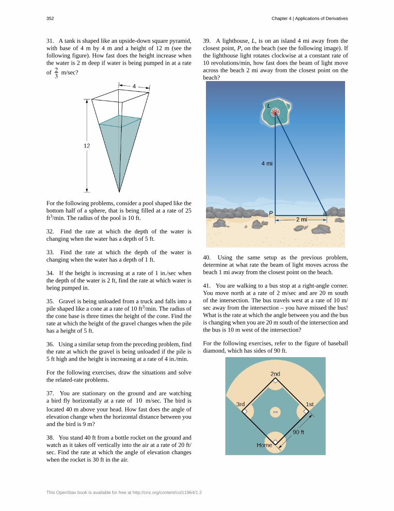
31. A tank is shaped like an upside-down square pyramid,with base of 4 m by 4 m and a height of 12 m (see thefollowing figure). How fast does the height increase whenthe water is 2 m deep if water is being pumped in at a rate
of 23 m/sec?
For the following problems, consider a pool shaped like thebottom half of a sphere, that is being filled at a rate of 25ft3/min. The radius of the pool is 10 ft.
32. Find the rate at which the depth of the water ischanging when the water has a depth of 5 ft.
33. Find the rate at which the depth of the water ischanging when the water has a depth of 1 ft.
34. If the height is increasing at a rate of 1 in./sec whenthe depth of the water is 2 ft, find the rate at which water isbeing pumped in.
35. Gravel is being unloaded from a truck and falls into apile shaped like a cone at a rate of 10 ft3/min. The radius ofthe cone base is three times the height of the cone. Find therate at which the height of the gravel changes when the pilehas a height of 5 ft.
36. Using a similar setup from the preceding problem, findthe rate at which the gravel is being unloaded if the pile is5 ft high and the height is increasing at a rate of 4 in./min.
For the following exercises, draw the situations and solvethe related-rate problems.
37. You are stationary on the ground and are watchinga bird fly horizontally at a rate of 10 m/sec. The bird is
located 40 m above your head. How fast does the angle ofelevation change when the horizontal distance between youand the bird is 9 m?
38. You stand 40 ft from a bottle rocket on the ground andwatch as it takes off vertically into the air at a rate of 20 ft/sec. Find the rate at which the angle of elevation changeswhen the rocket is 30 ft in the air.
39. A lighthouse, L, is on an island 4 mi away from theclosest point, P, on the beach (see the following image). Ifthe lighthouse light rotates clockwise at a constant rate of10 revolutions/min, how fast does the beam of light moveacross the beach 2 mi away from the closest point on thebeach?
40. Using the same setup as the previous problem,determine at what rate the beam of light moves across thebeach 1 mi away from the closest point on the beach.
41. You are walking to a bus stop at a right-angle corner.You move north at a rate of 2 m/sec and are 20 m southof the intersection. The bus travels west at a rate of 10 m/sec away from the intersection – you have missed the bus!What is the rate at which the angle between you and the busis changing when you are 20 m south of the intersection andthe bus is 10 m west of the intersection?
For the following exercises, refer to the figure of baseballdiamond, which has sides of 90 ft.
352 Chapter 4 | Applications of Derivatives
This OpenStax book is available for free at http://cnx.org/content/col11964/1.2
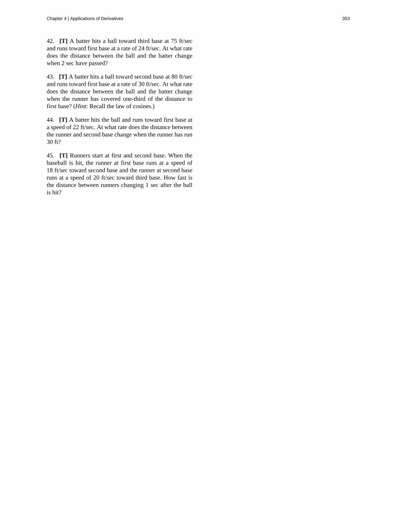
42. [T] A batter hits a ball toward third base at 75 ft/secand runs toward first base at a rate of 24 ft/sec. At what ratedoes the distance between the ball and the batter changewhen 2 sec have passed?
43. [T] A batter hits a ball toward second base at 80 ft/secand runs toward first base at a rate of 30 ft/sec. At what ratedoes the distance between the ball and the batter changewhen the runner has covered one-third of the distance tofirst base? (Hint: Recall the law of cosines.)
44. [T] A batter hits the ball and runs toward first base ata speed of 22 ft/sec. At what rate does the distance betweenthe runner and second base change when the runner has run30 ft?
45. [T] Runners start at first and second base. When thebaseball is hit, the runner at first base runs at a speed of18 ft/sec toward second base and the runner at second baseruns at a speed of 20 ft/sec toward third base. How fast isthe distance between runners changing 1 sec after the ballis hit?
Chapter 4 | Applications of Derivatives 353
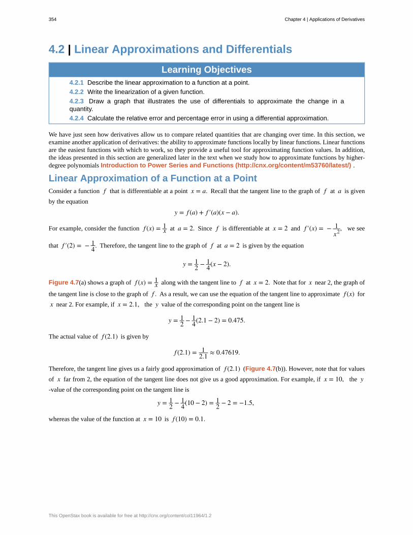
4.2 | Linear Approximations and Differentials
Learning Objectives4.2.1 Describe the linear approximation to a function at a point.
4.2.2 Write the linearization of a given function.
4.2.3 Draw a graph that illustrates the use of differentials to approximate the change in aquantity.
4.2.4 Calculate the relative error and percentage error in using a differential approximation.
We have just seen how derivatives allow us to compare related quantities that are changing over time. In this section, weexamine another application of derivatives: the ability to approximate functions locally by linear functions. Linear functionsare the easiest functions with which to work, so they provide a useful tool for approximating function values. In addition,the ideas presented in this section are generalized later in the text when we study how to approximate functions by higher-degree polynomials Introduction to Power Series and Functions (http://cnx.org/content/m53760/latest/) .
Linear Approximation of a Function at a PointConsider a function f that is differentiable at a point x = a. Recall that the tangent line to the graph of f at a is given
by the equation
y = f (a) + f ′(a)(x − a).
For example, consider the function f (x) = 1x at a = 2. Since f is differentiable at x = 2 and f ′(x) = − 1
x2, we see
that f ′(2) = − 14. Therefore, the tangent line to the graph of f at a = 2 is given by the equation
y = 12 − 1
4(x − 2).
Figure 4.7(a) shows a graph of f (x) = 1x along with the tangent line to f at x = 2. Note that for x near 2, the graph of
the tangent line is close to the graph of f . As a result, we can use the equation of the tangent line to approximate f (x) for
x near 2. For example, if x = 2.1, the y value of the corresponding point on the tangent line is
y = 12 − 1
4(2.1 − 2) = 0.475.
The actual value of f (2.1) is given by
f (2.1) = 12.1 ≈ 0.47619.
Therefore, the tangent line gives us a fairly good approximation of f (2.1) (Figure 4.7(b)). However, note that for values
of x far from 2, the equation of the tangent line does not give us a good approximation. For example, if x = 10, the y-value of the corresponding point on the tangent line is
y = 12 − 1
4(10 − 2) = 12 − 2 = −1.5,
whereas the value of the function at x = 10 is f (10) = 0.1.
354 Chapter 4 | Applications of Derivatives
This OpenStax book is available for free at http://cnx.org/content/col11964/1.2
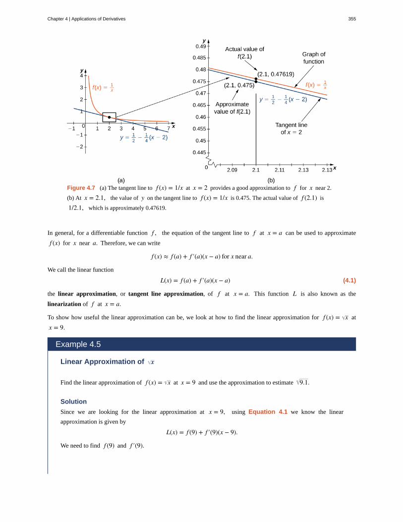
Figure 4.7 (a) The tangent line to f (x) = 1/x at x = 2 provides a good approximation to f for x near 2.
(b) At x = 2.1, the value of y on the tangent line to f (x) = 1/x is 0.475. The actual value of f (2.1) is
1/2.1, which is approximately 0.47619.
In general, for a differentiable function f , the equation of the tangent line to f at x = a can be used to approximate
f (x) for x near a. Therefore, we can write
f (x) ≈ f (a) + f ′(a)(x − a) for x near a.
We call the linear function
(4.1)L(x) = f (a) + f ′(a)(x − a)
the linear approximation, or tangent line approximation, of f at x = a. This function L is also known as the
linearization of f at x = a.
To show how useful the linear approximation can be, we look at how to find the linear approximation for f (x) = x at
x = 9.
Example 4.5
Linear Approximation of x
Find the linear approximation of f (x) = x at x = 9 and use the approximation to estimate 9.1.
Solution
Since we are looking for the linear approximation at x = 9, using Equation 4.1 we know the linear
approximation is given by
L(x) = f (9) + f ′(9)(x − 9).
We need to find f (9) and f ′(9).
Chapter 4 | Applications of Derivatives 355
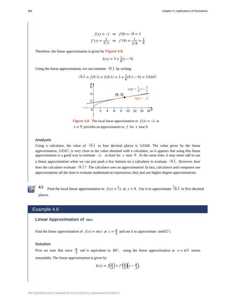
4.5
f (x) = x ⇒ f (9) = 9 = 3
f ′(x) = 12 x ⇒ f ′(9) = 1
2 9= 1
6
Therefore, the linear approximation is given by Figure 4.8.
L(x) = 3 + 16(x − 9)
Using the linear approximation, we can estimate 9.1 by writing
9.1 = f (9.1) ≈ L(9.1) = 3 + 16(9.1 − 9) ≈ 3.0167.
Figure 4.8 The local linear approximation to f (x) = x at
x = 9 provides an approximation to f for x near 9.
Analysis
Using a calculator, the value of 9.1 to four decimal places is 3.0166. The value given by the linear
approximation, 3.0167, is very close to the value obtained with a calculator, so it appears that using this linearapproximation is a good way to estimate x, at least for x near 9. At the same time, it may seem odd to use
a linear approximation when we can just push a few buttons on a calculator to evaluate 9.1. However, how
does the calculator evaluate 9.1? The calculator uses an approximation! In fact, calculators and computers use
approximations all the time to evaluate mathematical expressions; they just use higher-degree approximations.
Find the local linear approximation to f (x) = x3 at x = 8. Use it to approximate 8.13to five decimal
places.
Example 4.6
Linear Approximation of sinx
Find the linear approximation of f (x) = sinx at x = π3 and use it to approximate sin(62°).
Solution
First we note that since π3 rad is equivalent to 60°, using the linear approximation at x = π/3 seems
reasonable. The linear approximation is given by
L(x) = f ⎛⎝π3
⎞⎠ + f ′⎛⎝
π3
⎞⎠⎛⎝x − π
3⎞⎠.
356 Chapter 4 | Applications of Derivatives
This OpenStax book is available for free at http://cnx.org/content/col11964/1.2
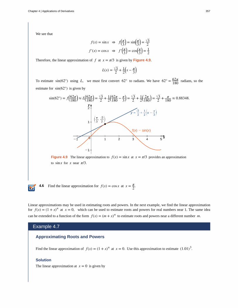
4.6
We see that
f (x) = sinx ⇒ f ⎛⎝π3
⎞⎠ = sin⎛
⎝π3
⎞⎠ = 3
2f ′(x) = cosx ⇒ f ′⎛⎝
π3
⎞⎠ = cos⎛
⎝π3
⎞⎠ = 1
2
Therefore, the linear approximation of f at x = π/3 is given by Figure 4.9.
L(x) = 32 + 1
2⎛⎝x − π
3⎞⎠
To estimate sin(62°) using L, we must first convert 62° to radians. We have 62° = 62π180 radians, so the
estimate for sin(62°) is given by
sin(62°) = f ⎛⎝62π180
⎞⎠ ≈ L⎛
⎝62π180
⎞⎠ = 3
2 + 12
⎛⎝62π180 − π
3⎞⎠ = 3
2 + 12
⎛⎝
2π180
⎞⎠ = 3
2 + π180 ≈ 0.88348.
Figure 4.9 The linear approximation to f (x) = sinx at x = π/3 provides an approximation
to sinx for x near π/3.
Find the linear approximation for f (x) = cosx at x = π2.
Linear approximations may be used in estimating roots and powers. In the next example, we find the linear approximationfor f (x) = (1 + x)n at x = 0, which can be used to estimate roots and powers for real numbers near 1. The same idea
can be extended to a function of the form f (x) = (m + x)n to estimate roots and powers near a different number m.
Example 4.7
Approximating Roots and Powers
Find the linear approximation of f (x) = (1 + x)n at x = 0. Use this approximation to estimate (1.01)3.
Solution
The linear approximation at x = 0 is given by
Chapter 4 | Applications of Derivatives 357
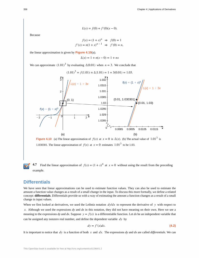
4.7
L(x) = f (0) + f ′(0)(x − 0).
Because
f (x) = (1 + x)n ⇒ f (0) = 1f ′(x) = n(1 + x)n − 1 ⇒ f ′(0) = n,
the linear approximation is given by Figure 4.10(a).
L(x) = 1 + n(x − 0) = 1 + nx
We can approximate (1.01)3 by evaluating L(0.01) when n = 3. We conclude that
(1.01)3 = f (1.01) ≈ L(1.01) = 1 + 3(0.01) = 1.03.
Figure 4.10 (a) The linear approximation of f (x) at x = 0 is L(x). (b) The actual value of 1.013 is
1.030301. The linear approximation of f (x) at x = 0 estimates 1.013 to be 1.03.
Find the linear approximation of f (x) = (1 + x)4 at x = 0 without using the result from the preceding
example.
DifferentialsWe have seen that linear approximations can be used to estimate function values. They can also be used to estimate theamount a function value changes as a result of a small change in the input. To discuss this more formally, we define a relatedconcept: differentials. Differentials provide us with a way of estimating the amount a function changes as a result of a smallchange in input values.
When we first looked at derivatives, we used the Leibniz notation dy/dx to represent the derivative of y with respect to
x. Although we used the expressions dy and dx in this notation, they did not have meaning on their own. Here we see a
meaning to the expressions dy and dx. Suppose y = f (x) is a differentiable function. Let dx be an independent variable that
can be assigned any nonzero real number, and define the dependent variable dy by
(4.2)dy = f ′(x)dx.
It is important to notice that dy is a function of both x and dx. The expressions dy and dx are called differentials. We can
358 Chapter 4 | Applications of Derivatives
This OpenStax book is available for free at http://cnx.org/content/col11964/1.2
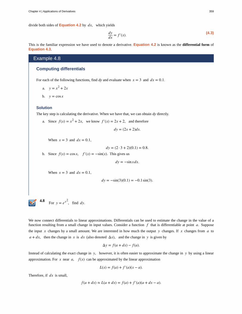
4.8
divide both sides of Equation 4.2 by dx, which yields
(4.3)dydx = f ′(x).
This is the familiar expression we have used to denote a derivative. Equation 4.2 is known as the differential form ofEquation 4.3.
Example 4.8
Computing differentials
For each of the following functions, find dy and evaluate when x = 3 and dx = 0.1.
a. y = x2 + 2x
b. y = cosx
Solution
The key step is calculating the derivative. When we have that, we can obtain dy directly.
a. Since f (x) = x2 + 2x, we know f ′(x) = 2x + 2, and therefore
dy = (2x + 2)dx.
When x = 3 and dx = 0.1,
dy = (2 · 3 + 2)(0.1) = 0.8.b. Since f (x) = cosx, f ′(x) = −sin(x). This gives us
dy = −sinxdx.
When x = 3 and dx = 0.1,
dy = −sin(3)(0.1) = −0.1sin(3).
For y = ex2, find dy.
We now connect differentials to linear approximations. Differentials can be used to estimate the change in the value of afunction resulting from a small change in input values. Consider a function f that is differentiable at point a. Suppose
the input x changes by a small amount. We are interested in how much the output y changes. If x changes from a to
a + dx, then the change in x is dx (also denoted Δx), and the change in y is given by
Δy = f (a + dx) − f (a).
Instead of calculating the exact change in y, however, it is often easier to approximate the change in y by using a linear
approximation. For x near a, f (x) can be approximated by the linear approximation
L(x) = f (a) + f ′(a)(x − a).
Therefore, if dx is small,
f (a + dx) ≈ L(a + dx) = f (a) + f ′(a)(a + dx − a).
Chapter 4 | Applications of Derivatives 359
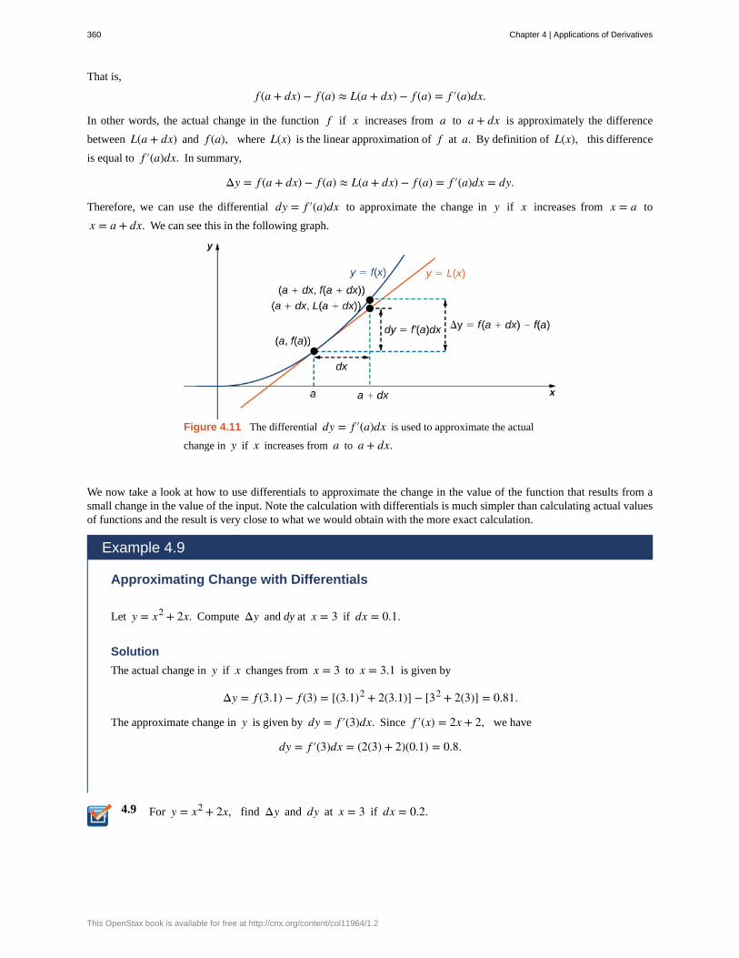
4.9
That is,
f (a + dx) − f (a) ≈ L(a + dx) − f (a) = f ′(a)dx.
In other words, the actual change in the function f if x increases from a to a + dx is approximately the difference
between L(a + dx) and f (a), where L(x) is the linear approximation of f at a. By definition of L(x), this difference
is equal to f ′(a)dx. In summary,
Δy = f (a + dx) − f (a) ≈ L(a + dx) − f (a) = f ′(a)dx = dy.
Therefore, we can use the differential dy = f ′(a)dx to approximate the change in y if x increases from x = a to
x = a + dx. We can see this in the following graph.
Figure 4.11 The differential dy = f ′(a)dx is used to approximate the actual
change in y if x increases from a to a + dx.
We now take a look at how to use differentials to approximate the change in the value of the function that results from asmall change in the value of the input. Note the calculation with differentials is much simpler than calculating actual valuesof functions and the result is very close to what we would obtain with the more exact calculation.
Example 4.9
Approximating Change with Differentials
Let y = x2 + 2x. Compute Δy and dy at x = 3 if dx = 0.1.
Solution
The actual change in y if x changes from x = 3 to x = 3.1 is given by
Δy = f (3.1) − f (3) = [(3.1)2 + 2(3.1)] − [32 + 2(3)] = 0.81.
The approximate change in y is given by dy = f ′(3)dx. Since f ′(x) = 2x + 2, we have
dy = f ′(3)dx = (2(3) + 2)(0.1) = 0.8.
For y = x2 + 2x, find Δy and dy at x = 3 if dx = 0.2.
360 Chapter 4 | Applications of Derivatives
This OpenStax book is available for free at http://cnx.org/content/col11964/1.2
Calculating the Amount of ErrorAny type of measurement is prone to a certain amount of error. In many applications, certain quantities are calculated basedon measurements. For example, the area of a circle is calculated by measuring the radius of the circle. An error in themeasurement of the radius leads to an error in the computed value of the area. Here we examine this type of error and studyhow differentials can be used to estimate the error.
Consider a function f with an input that is a measured quantity. Suppose the exact value of the measured quantity is a,but the measured value is a + dx. We say the measurement error is dx (or Δx). As a result, an error occurs in the calculated
quantity f (x). This type of error is known as a propagated error and is given by
Δy = f (a + dx) − f (a).
Since all measurements are prone to some degree of error, we do not know the exact value of a measured quantity, so wecannot calculate the propagated error exactly. However, given an estimate of the accuracy of a measurement, we can usedifferentials to approximate the propagated error Δy. Specifically, if f is a differentiable function at a, the propagated
error is
Δy ≈ dy = f ′(a)dx.
Unfortunately, we do not know the exact value a. However, we can use the measured value a + dx, and estimate
Δy ≈ dy ≈ f ′(a + dx)dx.
In the next example, we look at how differentials can be used to estimate the error in calculating the volume of a box if weassume the measurement of the side length is made with a certain amount of accuracy.
Example 4.10
Volume of a Cube
Suppose the side length of a cube is measured to be 5 cm with an accuracy of 0.1 cm.
a. Use differentials to estimate the error in the computed volume of the cube.
b. Compute the volume of the cube if the side length is (i) 4.9 cm and (ii) 5.1 cm to compare the estimatederror with the actual potential error.
Solution
a. The measurement of the side length is accurate to within ±0.1 cm. Therefore,
−0.1 ≤ dx ≤ 0.1.
The volume of a cube is given by V = x3, which leads to
dV = 3x2 dx.
Using the measured side length of 5 cm, we can estimate that
−3(5)2(0.1) ≤ dV ≤ 3(5)2(0.1).
Therefore,
−7.5 ≤ dV ≤ 7.5.b. If the side length is actually 4.9 cm, then the volume of the cube is
V(4.9) = (4.9)3 = 117.649 cm3.
Chapter 4 | Applications of Derivatives 361
4.10
If the side length is actually 5.1 cm, then the volume of the cube is
V(5.1) = (5.1)3 = 132.651 cm3.
Therefore, the actual volume of the cube is between 117.649 and 132.651. Since the side length is
measured to be 5 cm, the computed volume is V(5) = 53 = 125. Therefore, the error in the computed
volume is
117.649 − 125 ≤ ΔV ≤ 132.651 − 125.
That is,
−7.351 ≤ ΔV ≤ 7.651.
We see the estimated error dV is relatively close to the actual potential error in the computed volume.
Estimate the error in the computed volume of a cube if the side length is measured to be 6 cm with anaccuracy of 0.2 cm.
The measurement error dx (=Δx) and the propagated error Δy are absolute errors. We are typically interested in the size
of an error relative to the size of the quantity being measured or calculated. Given an absolute error Δq for a particular
quantity, we define the relative error asΔqq , where q is the actual value of the quantity. The percentage error is the
relative error expressed as a percentage. For example, if we measure the height of a ladder to be 63 in. when the actual
height is 62 in., the absolute error is 1 in. but the relative error is 162 = 0.016, or 1.6%. By comparison, if we measure the
width of a piece of cardboard to be 8.25 in. when the actual width is 8 in., our absolute error is 14 in., whereas the relative
error is 0.258 = 1
32, or 3.1%. Therefore, the percentage error in the measurement of the cardboard is larger, even though
0.25 in. is less than 1 in.
Example 4.11
Relative and Percentage Error
An astronaut using a camera measures the radius of Earth as 4000 mi with an error of ±80 mi. Let’s use
differentials to estimate the relative and percentage error of using this radius measurement to calculate the volumeof Earth, assuming the planet is a perfect sphere.
Solution
If the measurement of the radius is accurate to within ±80, we have
−80 ≤ dr ≤ 80.
Since the volume of a sphere is given by V = ⎛⎝43
⎞⎠πr3, we have
362 Chapter 4 | Applications of Derivatives
This OpenStax book is available for free at http://cnx.org/content/col11964/1.2
4.11
dV = 4πr2 dr.
Using the measured radius of 4000 mi, we can estimate
−4π(4000)2(80) ≤ dV ≤ 4π(4000)2(80).
To estimate the relative error, consider dVV . Since we do not know the exact value of the volume V , use the
measured radius r = 4000 mi to estimate V . We obtain V ≈ ⎛⎝43
⎞⎠π(4000)3. Therefore the relative error satisfies
−4π(4000)2(80)4π(4000)3 /3
≤ dVV ≤ 4π(4000)2(80)
4π(4000)3 /3,
which simplifies to
−0.06 ≤ dVV ≤ 0.06.
The relative error is 0.06 and the percentage error is 6%.
Determine the percentage error if the radius of Earth is measured to be 3950 mi with an error of ±100mi.
Chapter 4 | Applications of Derivatives 363
4.2 EXERCISES46. What is the linear approximation for any generic linearfunction y = mx + b?
47. Determine the necessary conditions such that thelinear approximation function is constant. Use a graph toprove your result.
48. Explain why the linear approximation becomes lessaccurate as you increase the distance between x and a.Use a graph to prove your argument.
49. When is the linear approximation exact?
For the following exercises, find the linear approximationL(x) to y = f (x) near x = a for the function.
50. [T] f (x) = x + x4, a = 0
51. [T] f (x) = 1x , a = 2
52. [T] f (x) = tanx, a = π4
53. [T] f (x) = sinx, a = π2
54. [T] f (x) = xsinx, a = 2π
55. [T] f (x) = sin2 x, a = 0
For the following exercises, compute the values givenwithin 0.01 by deciding on the appropriate f (x) and a,and evaluating L(x) = f (a) + f ′(a)(x − a). Check your
answer using a calculator.
56. [T] (2.001)6
57. [T] sin(0.02)
58. [T] cos(0.03)
59. [T] (15.99)1/4
60. [T] 10.98
61. [T] sin(3.14)
For the following exercises, determine the appropriatef (x) and a, and evaluate L(x) = f (a) + f ′ (a)(x − a).
Calculate the numerical error in the linear approximationsthat follow.
62. (1.01)3
63. cos(0.01)
64. ⎛⎝sin(0.01)⎞
⎠2
65. (1.01)−3
66. ⎛⎝1 + 1
10⎞⎠
10
67. 8.99
For the following exercises, find the differential of thefunction.
68. y = 3x4 + x2 − 2x + 1
69. y = xcosx
70. y = 1 + x
71. y = x2 + 2x − 1
For the following exercises, find the differential andevaluate for the given x and dx.
72. y = 3x2 − x + 6, x = 2, dx = 0.1
73. y = 1x + 1, x = 1, dx = 0.25
74. y = tanx, x = 0, dx = π10
75. y = 3x2 + 2x + 1
, x = 0, dx = 0.1
76. y = sin(2x)x , x = π, dx = 0.25
77. y = x3 + 2x + 1x , x = 1, dx = 0.05
For the following exercises, find the change in volume dVor in surface area dA.
78. dV if the sides of a cube change from 10 to 10.1.
79. dA if the sides of a cube change from x to x + dx.
80. dA if the radius of a sphere changes from r by dr.
364 Chapter 4 | Applications of Derivatives
This OpenStax book is available for free at http://cnx.org/content/col11964/1.2
81. dV if the radius of a sphere changes from r by dr.
82. dV if a circular cylinder with r = 2 changes height
from 3 cm to 3.05 cm.
83. dV if a circular cylinder of height 3 changes from
r = 2 to r = 1.9 cm.
For the following exercises, use differentials to estimate themaximum and relative error when computing the surfacearea or volume.
84. A spherical golf ball is measured to have a radius of5 mm, with a possible measurement error of 0.1 mm.What is the possible change in volume?
85. A pool has a rectangular base of 10 ft by 20 ft and adepth of 6 ft. What is the change in volume if you only fillit up to 5.5 ft?
86. An ice cream cone has height 4 in. and radius 1 in. Ifthe cone is 0.1 in. thick, what is the difference between thevolume of the cone, including the shell, and the volume ofthe ice cream you can fit inside the shell?
For the following exercises, confirm the approximations byusing the linear approximation at x = 0.
87. 1 − x ≈ 1 − 12x
88. 11 − x2
≈ 1
89. c2 + x2 ≈ c
Chapter 4 | Applications of Derivatives 365
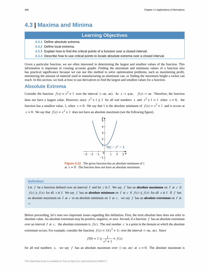
4.3 | Maxima and Minima
Learning Objectives4.3.1 Define absolute extrema.
4.3.2 Define local extrema.
4.3.3 Explain how to find the critical points of a function over a closed interval.
4.3.4 Describe how to use critical points to locate absolute extrema over a closed interval.
Given a particular function, we are often interested in determining the largest and smallest values of the function. Thisinformation is important in creating accurate graphs. Finding the maximum and minimum values of a function alsohas practical significance because we can use this method to solve optimization problems, such as maximizing profit,minimizing the amount of material used in manufacturing an aluminum can, or finding the maximum height a rocket canreach. In this section, we look at how to use derivatives to find the largest and smallest values for a function.
Absolute ExtremaConsider the function f (x) = x2 + 1 over the interval (−∞, ∞). As x → ±∞, f (x) → ∞. Therefore, the function
does not have a largest value. However, since x2 + 1 ≥ 1 for all real numbers x and x2 + 1 = 1 when x = 0, the
function has a smallest value, 1, when x = 0. We say that 1 is the absolute minimum of f (x) = x2 + 1 and it occurs at
x = 0. We say that f (x) = x2 + 1 does not have an absolute maximum (see the following figure).
Figure 4.12 The given function has an absolute minimum of 1at x = 0. The function does not have an absolute maximum.
Definition
Let f be a function defined over an interval I and let c ∈ I. We say f has an absolute maximum on I at c if
f (c) ≥ f (x) for all x ∈ I. We say f has an absolute minimum on I at c if f (c) ≤ f (x) for all x ∈ I. If f has
an absolute maximum on I at c or an absolute minimum on I at c, we say f has an absolute extremum on I at
c.
Before proceeding, let’s note two important issues regarding this definition. First, the term absolute here does not refer toabsolute value. An absolute extremum may be positive, negative, or zero. Second, if a function f has an absolute extremum
over an interval I at c, the absolute extremum is f (c). The real number c is a point in the domain at which the absolute
extremum occurs. For example, consider the function f (x) = 1/(x2 + 1) over the interval (−∞, ∞). Since
f (0) = 1 ≥ 1x2 + 1
= f (x)
for all real numbers x, we say f has an absolute maximum over (−∞, ∞) at x = 0. The absolute maximum is
366 Chapter 4 | Applications of Derivatives
This OpenStax book is available for free at http://cnx.org/content/col11964/1.2
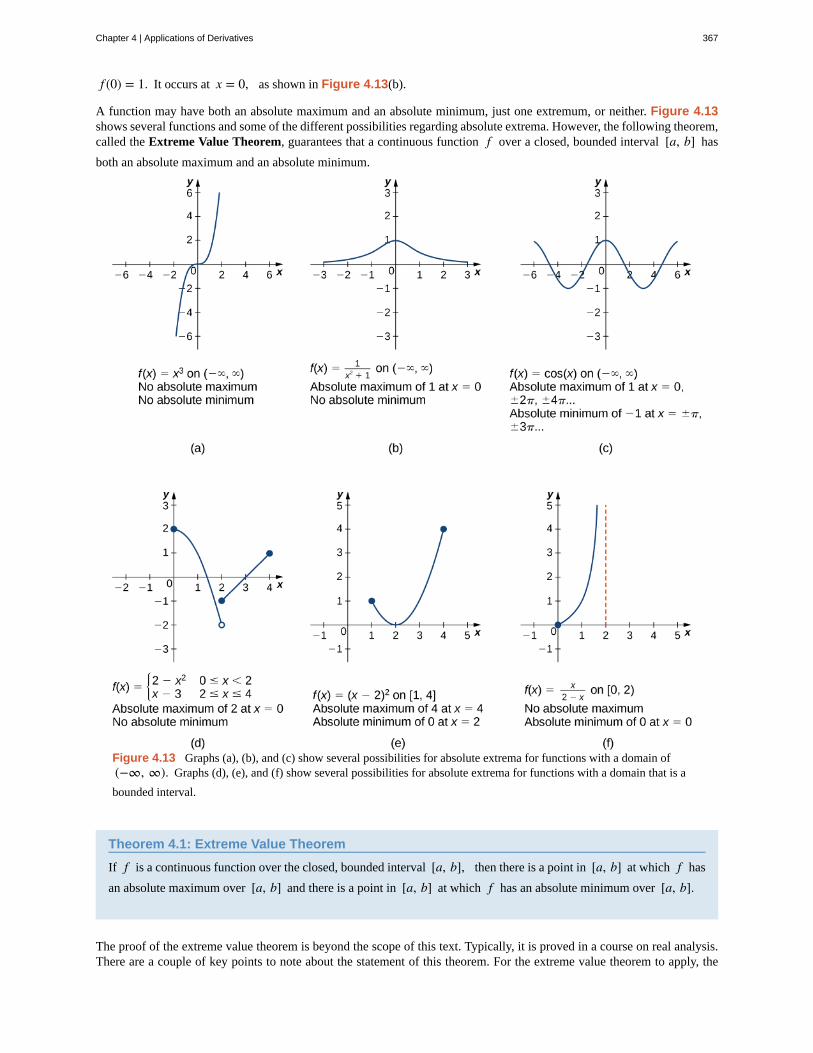
f (0) = 1. It occurs at x = 0, as shown in Figure 4.13(b).
A function may have both an absolute maximum and an absolute minimum, just one extremum, or neither. Figure 4.13shows several functions and some of the different possibilities regarding absolute extrema. However, the following theorem,called the Extreme Value Theorem, guarantees that a continuous function f over a closed, bounded interval [a, b] has
both an absolute maximum and an absolute minimum.
Figure 4.13 Graphs (a), (b), and (c) show several possibilities for absolute extrema for functions with a domain of(−∞, ∞). Graphs (d), (e), and (f) show several possibilities for absolute extrema for functions with a domain that is a
bounded interval.
Theorem 4.1: Extreme Value Theorem
If f is a continuous function over the closed, bounded interval [a, b], then there is a point in [a, b] at which f has
an absolute maximum over [a, b] and there is a point in [a, b] at which f has an absolute minimum over [a, b].
The proof of the extreme value theorem is beyond the scope of this text. Typically, it is proved in a course on real analysis.There are a couple of key points to note about the statement of this theorem. For the extreme value theorem to apply, the
Chapter 4 | Applications of Derivatives 367
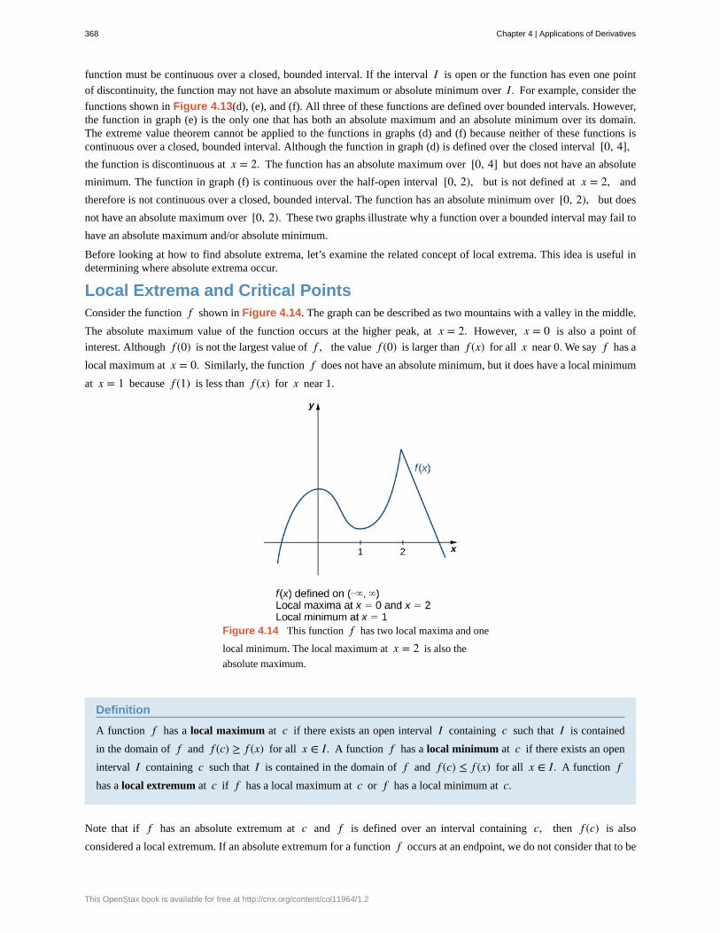
function must be continuous over a closed, bounded interval. If the interval I is open or the function has even one point
of discontinuity, the function may not have an absolute maximum or absolute minimum over I. For example, consider the
functions shown in Figure 4.13(d), (e), and (f). All three of these functions are defined over bounded intervals. However,the function in graph (e) is the only one that has both an absolute maximum and an absolute minimum over its domain.The extreme value theorem cannot be applied to the functions in graphs (d) and (f) because neither of these functions iscontinuous over a closed, bounded interval. Although the function in graph (d) is defined over the closed interval [0, 4],the function is discontinuous at x = 2. The function has an absolute maximum over [0, 4] but does not have an absolute
minimum. The function in graph (f) is continuous over the half-open interval [0, 2), but is not defined at x = 2, and
therefore is not continuous over a closed, bounded interval. The function has an absolute minimum over [0, 2), but does
not have an absolute maximum over [0, 2). These two graphs illustrate why a function over a bounded interval may fail to
have an absolute maximum and/or absolute minimum.
Before looking at how to find absolute extrema, let’s examine the related concept of local extrema. This idea is useful indetermining where absolute extrema occur.
Local Extrema and Critical PointsConsider the function f shown in Figure 4.14. The graph can be described as two mountains with a valley in the middle.
The absolute maximum value of the function occurs at the higher peak, at x = 2. However, x = 0 is also a point of
interest. Although f (0) is not the largest value of f , the value f (0) is larger than f (x) for all x near 0. We say f has a
local maximum at x = 0. Similarly, the function f does not have an absolute minimum, but it does have a local minimum
at x = 1 because f (1) is less than f (x) for x near 1.
Figure 4.14 This function f has two local maxima and one
local minimum. The local maximum at x = 2 is also the
absolute maximum.
Definition
A function f has a local maximum at c if there exists an open interval I containing c such that I is contained
in the domain of f and f (c) ≥ f (x) for all x ∈ I. A function f has a local minimum at c if there exists an open
interval I containing c such that I is contained in the domain of f and f (c) ≤ f (x) for all x ∈ I. A function fhas a local extremum at c if f has a local maximum at c or f has a local minimum at c.
Note that if f has an absolute extremum at c and f is defined over an interval containing c, then f (c) is also
considered a local extremum. If an absolute extremum for a function f occurs at an endpoint, we do not consider that to be
368 Chapter 4 | Applications of Derivatives
This OpenStax book is available for free at http://cnx.org/content/col11964/1.2
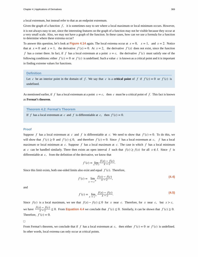
a local extremum, but instead refer to that as an endpoint extremum.
Given the graph of a function f , it is sometimes easy to see where a local maximum or local minimum occurs. However,
it is not always easy to see, since the interesting features on the graph of a function may not be visible because they occur ata very small scale. Also, we may not have a graph of the function. In these cases, how can we use a formula for a functionto determine where these extrema occur?
To answer this question, let’s look at Figure 4.14 again. The local extrema occur at x = 0, x = 1, and x = 2. Notice
that at x = 0 and x = 1, the derivative f ′(x) = 0. At x = 2, the derivative f ′(x) does not exist, since the function
f has a corner there. In fact, if f has a local extremum at a point x = c, the derivative f ′(c) must satisfy one of the
following conditions: either f ′(c) = 0 or f ′(c) is undefined. Such a value c is known as a critical point and it is important
in finding extreme values for functions.
Definition
Let c be an interior point in the domain of f . We say that c is a critical point of f if f ′(c) = 0 or f ′(c) is
undefined.
As mentioned earlier, if f has a local extremum at a point x = c, then c must be a critical point of f . This fact is known
as Fermat’s theorem.
Theorem 4.2: Fermat’s Theorem
If f has a local extremum at c and f is differentiable at c, then f ′(c) = 0.
Proof
Suppose f has a local extremum at c and f is differentiable at c. We need to show that f ′(c) = 0. To do this, we
will show that f ′(c) ≥ 0 and f ′(c) ≤ 0, and therefore f ′(c) = 0. Since f has a local extremum at c, f has a local
maximum or local minimum at c. Suppose f has a local maximum at c. The case in which f has a local minimum
at c can be handled similarly. There then exists an open interval I such that f (c) ≥ f (x) for all x ∈ I. Since f is
differentiable at c, from the definition of the derivative, we know that
f ′(c) = limx → cf (x) − f (c)
x − c .
Since this limit exists, both one-sided limits also exist and equal f ′(c). Therefore,
(4.4)f ′(c) = limx → c+
f (x) − f (c)x − c ,
and
(4.5)f ′(c) = limx → c−
f (x) − f (c)x − c .
Since f (c) is a local maximum, we see that f (x) − f (c) ≤ 0 for x near c. Therefore, for x near c, but x > c,
we havef (x) − f (c)
x − c ≤ 0. From Equation 4.4 we conclude that f ′(c) ≤ 0. Similarly, it can be shown that f ′(c) ≥ 0.
Therefore, f ′(c) = 0.
□
From Fermat’s theorem, we conclude that if f has a local extremum at c, then either f ′(c) = 0 or f ′(c) is undefined.
In other words, local extrema can only occur at critical points.
Chapter 4 | Applications of Derivatives 369
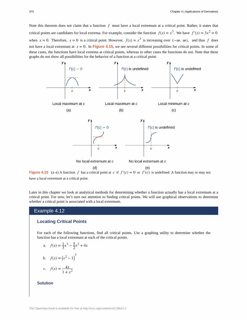
Note this theorem does not claim that a function f must have a local extremum at a critical point. Rather, it states that
critical points are candidates for local extrema. For example, consider the function f (x) = x3. We have f ′(x) = 3x2 = 0
when x = 0. Therefore, x = 0 is a critical point. However, f (x) = x3 is increasing over (−∞, ∞), and thus f does
not have a local extremum at x = 0. In Figure 4.15, we see several different possibilities for critical points. In some of
these cases, the functions have local extrema at critical points, whereas in other cases the functions do not. Note that thesegraphs do not show all possibilities for the behavior of a function at a critical point.
Figure 4.15 (a–e) A function f has a critical point at c if f ′(c) = 0 or f ′(c) is undefined. A function may or may not
have a local extremum at a critical point.
Later in this chapter we look at analytical methods for determining whether a function actually has a local extremum at acritical point. For now, let’s turn our attention to finding critical points. We will use graphical observations to determinewhether a critical point is associated with a local extremum.
Example 4.12
Locating Critical Points
For each of the following functions, find all critical points. Use a graphing utility to determine whether thefunction has a local extremum at each of the critical points.
a. f (x) = 13x3 − 5
2x2 + 4x
b. f (x) = ⎛⎝x2 − 1⎞
⎠3
c. f (x) = 4x1 + x2
Solution
370 Chapter 4 | Applications of Derivatives
This OpenStax book is available for free at http://cnx.org/content/col11964/1.2
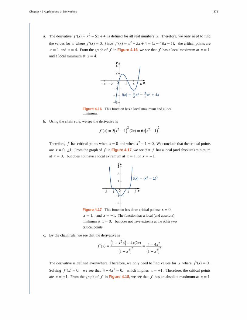
a. The derivative f ′(x) = x2 − 5x + 4 is defined for all real numbers x. Therefore, we only need to find
the values for x where f ′(x) = 0. Since f ′(x) = x2 − 5x + 4 = (x − 4)(x − 1), the critical points are
x = 1 and x = 4. From the graph of f in Figure 4.16, we see that f has a local maximum at x = 1and a local minimum at x = 4.
Figure 4.16 This function has a local maximum and a localminimum.
b. Using the chain rule, we see the derivative is
f ′(x) = 3⎛⎝x2 − 1⎞
⎠2
(2x) = 6x⎛⎝x2 − 1⎞
⎠2.
Therefore, f has critical points when x = 0 and when x2 − 1 = 0. We conclude that the critical points
are x = 0, ±1. From the graph of f in Figure 4.17, we see that f has a local (and absolute) minimum
at x = 0, but does not have a local extremum at x = 1 or x = −1.
Figure 4.17 This function has three critical points: x = 0,x = 1, and x = −1. The function has a local (and absolute)
minimum at x = 0, but does not have extrema at the other two
critical points.
c. By the chain rule, we see that the derivative is
f ′(x) =⎛⎝1 + x2 4⎞
⎠ − 4x(2x)⎛⎝1 + x2⎞
⎠2 = 4 − 4x2
⎛⎝1 + x2⎞
⎠2.
The derivative is defined everywhere. Therefore, we only need to find values for x where f ′(x) = 0.
Solving f ′(x) = 0, we see that 4 − 4x2 = 0, which implies x = ±1. Therefore, the critical points
are x = ±1. From the graph of f in Figure 4.18, we see that f has an absolute maximum at x = 1
Chapter 4 | Applications of Derivatives 371
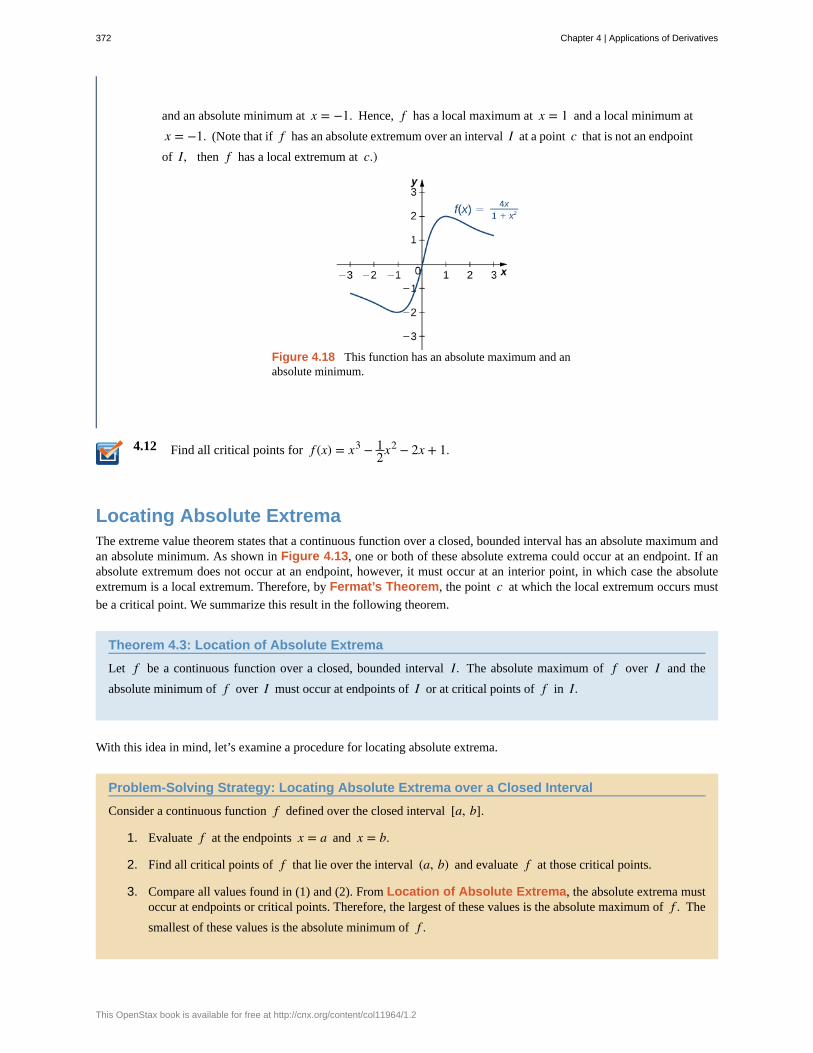
4.12
and an absolute minimum at x = −1. Hence, f has a local maximum at x = 1 and a local minimum at
x = −1. (Note that if f has an absolute extremum over an interval I at a point c that is not an endpoint
of I, then f has a local extremum at c.)
Figure 4.18 This function has an absolute maximum and anabsolute minimum.
Find all critical points for f (x) = x3 − 12x2 − 2x + 1.
Locating Absolute ExtremaThe extreme value theorem states that a continuous function over a closed, bounded interval has an absolute maximum andan absolute minimum. As shown in Figure 4.13, one or both of these absolute extrema could occur at an endpoint. If anabsolute extremum does not occur at an endpoint, however, it must occur at an interior point, in which case the absoluteextremum is a local extremum. Therefore, by Fermat’s Theorem, the point c at which the local extremum occurs must
be a critical point. We summarize this result in the following theorem.
Theorem 4.3: Location of Absolute Extrema
Let f be a continuous function over a closed, bounded interval I. The absolute maximum of f over I and the
absolute minimum of f over I must occur at endpoints of I or at critical points of f in I.
With this idea in mind, let’s examine a procedure for locating absolute extrema.
Problem-Solving Strategy: Locating Absolute Extrema over a Closed Interval
Consider a continuous function f defined over the closed interval [a, b].
1. Evaluate f at the endpoints x = a and x = b.
2. Find all critical points of f that lie over the interval (a, b) and evaluate f at those critical points.
3. Compare all values found in (1) and (2). From Location of Absolute Extrema, the absolute extrema mustoccur at endpoints or critical points. Therefore, the largest of these values is the absolute maximum of f . The
smallest of these values is the absolute minimum of f .
372 Chapter 4 | Applications of Derivatives
This OpenStax book is available for free at http://cnx.org/content/col11964/1.2
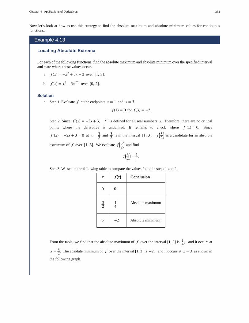
Now let’s look at how to use this strategy to find the absolute maximum and absolute minimum values for continuousfunctions.
Example 4.13
Locating Absolute Extrema
For each of the following functions, find the absolute maximum and absolute minimum over the specified intervaland state where those values occur.
a. f (x) = −x2 + 3x − 2 over [1, 3].
b. f (x) = x2 − 3x2/3 over [0, 2].
Solution
a. Step 1. Evaluate f at the endpoints x = 1 and x = 3.
f (1) = 0 and f (3) = −2
Step 2. Since f ′(x) = −2x + 3, f ′ is defined for all real numbers x. Therefore, there are no critical
points where the derivative is undefined. It remains to check where f ′(x) = 0. Since
f ′(x) = −2x + 3 = 0 at x = 32 and 3
2 is in the interval [1, 3], f ⎛⎝32
⎞⎠ is a candidate for an absolute
extremum of f over [1, 3]. We evaluate f ⎛⎝32
⎞⎠ and find
f ⎛⎝32
⎞⎠ = 1
4.
Step 3. We set up the following table to compare the values found in steps 1 and 2.
x f(x) Conclusion
0 0
32
14
Absolute maximum
3 −2 Absolute minimum
From the table, we find that the absolute maximum of f over the interval [1, 3] is 14, and it occurs at
x = 32. The absolute minimum of f over the interval [1, 3] is −2, and it occurs at x = 3 as shown in
the following graph.
Chapter 4 | Applications of Derivatives 373
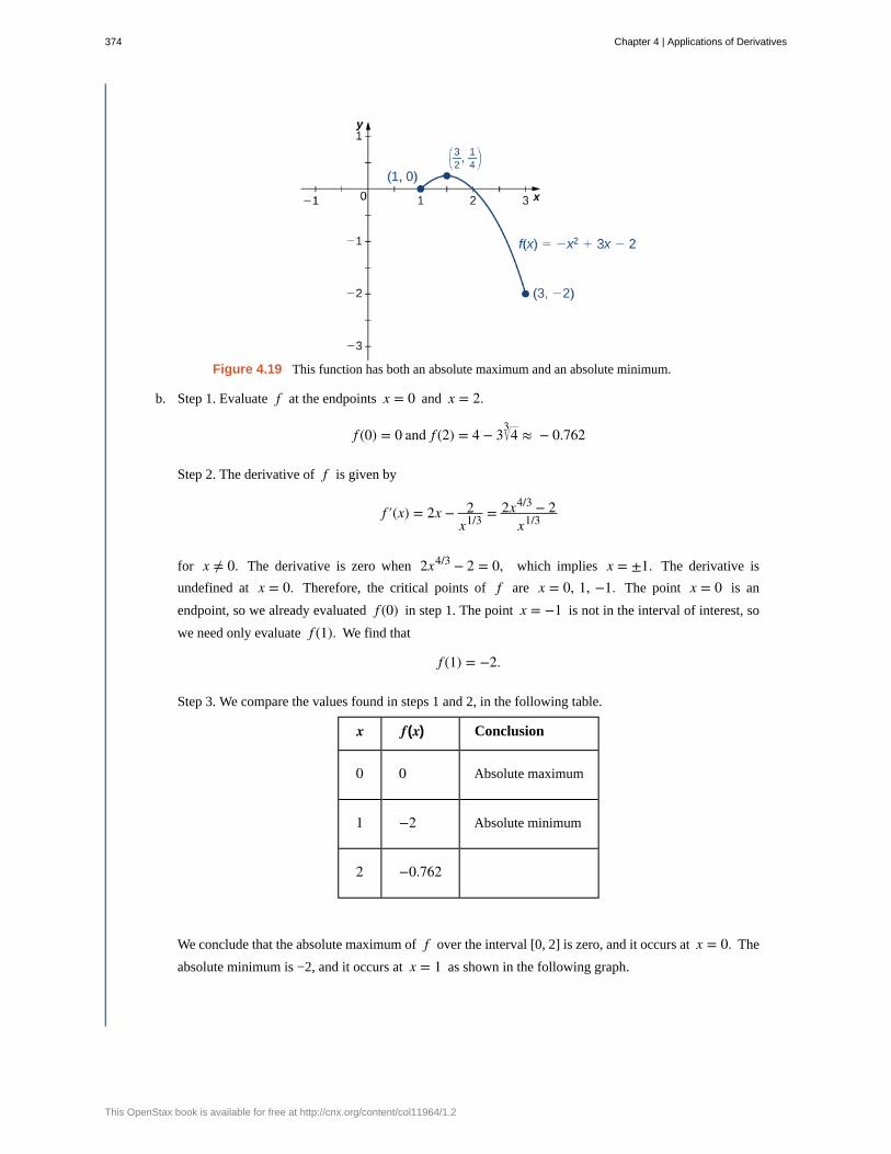
Figure 4.19 This function has both an absolute maximum and an absolute minimum.
b. Step 1. Evaluate f at the endpoints x = 0 and x = 2.
f (0) = 0 and f (2) = 4 − 3 43 ≈ − 0.762
Step 2. The derivative of f is given by
f ′(x) = 2x − 2x1/3 = 2x4/3 − 2
x1/3
for x ≠ 0. The derivative is zero when 2x4/3 − 2 = 0, which implies x = ±1. The derivative is
undefined at x = 0. Therefore, the critical points of f are x = 0, 1, −1. The point x = 0 is an
endpoint, so we already evaluated f (0) in step 1. The point x = −1 is not in the interval of interest, so
we need only evaluate f (1). We find that
f (1) = −2.
Step 3. We compare the values found in steps 1 and 2, in the following table.
x f(x) Conclusion
0 0 Absolute maximum
1 −2 Absolute minimum
2 −0.762
We conclude that the absolute maximum of f over the interval [0, 2] is zero, and it occurs at x = 0. The
absolute minimum is −2, and it occurs at x = 1 as shown in the following graph.
374 Chapter 4 | Applications of Derivatives
This OpenStax book is available for free at http://cnx.org/content/col11964/1.2
4.13
Figure 4.20 This function has an absolute maximum at anendpoint of the interval.
Find the absolute maximum and absolute minimum of f (x) = x2 − 4x + 3 over the interval [1, 4].
At this point, we know how to locate absolute extrema for continuous functions over closed intervals. We have also definedlocal extrema and determined that if a function f has a local extremum at a point c, then c must be a critical point of f .However, c being a critical point is not a sufficient condition for f to have a local extremum at c. Later in this chapter,
we show how to determine whether a function actually has a local extremum at a critical point. First, however, we need tointroduce the Mean Value Theorem, which will help as we analyze the behavior of the graph of a function.
Chapter 4 | Applications of Derivatives 375
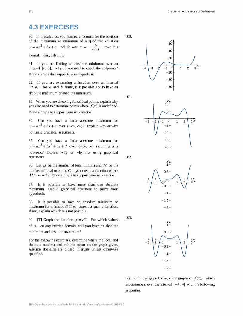
4.3 EXERCISES90. In precalculus, you learned a formula for the positionof the maximum or minimum of a quadratic equation
y = ax2 + bx + c, which was m = − b(2a). Prove this
formula using calculus.
91. If you are finding an absolute minimum over aninterval [a, b], why do you need to check the endpoints?
Draw a graph that supports your hypothesis.
92. If you are examining a function over an interval(a, b), for a and b finite, is it possible not to have an
absolute maximum or absolute minimum?
93. When you are checking for critical points, explain whyyou also need to determine points where f (x) is undefined.
Draw a graph to support your explanation.
94. Can you have a finite absolute maximum for
y = ax2 + bx + c over (−∞, ∞)? Explain why or why
not using graphical arguments.
95. Can you have a finite absolute maximum for
y = ax3 + bx2 + cx + d over (−∞, ∞) assuming a is
non-zero? Explain why or why not using graphicalarguments.
96. Let m be the number of local minima and M be the
number of local maxima. Can you create a function whereM > m + 2? Draw a graph to support your explanation.
97. Is it possible to have more than one absolutemaximum? Use a graphical argument to prove yourhypothesis.
98. Is it possible to have no absolute minimum ormaximum for a function? If so, construct such a function.If not, explain why this is not possible.
99. [T] Graph the function y = eax. For which values
of a, on any infinite domain, will you have an absolute
minimum and absolute maximum?
For the following exercises, determine where the local andabsolute maxima and minima occur on the graph given.Assume domains are closed intervals unless otherwisespecified.
100.
101.
102.
103.
For the following problems, draw graphs of f (x), which
is continuous, over the interval [−4, 4] with the following
properties:
376 Chapter 4 | Applications of Derivatives
This OpenStax book is available for free at http://cnx.org/content/col11964/1.2
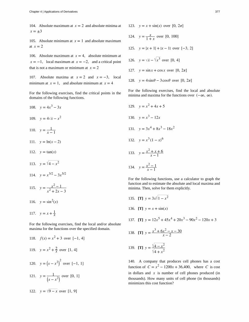
104. Absolute maximum at x = 2 and absolute minima at
x = ±3
105. Absolute minimum at x = 1 and absolute maximum
at x = 2
106. Absolute maximum at x = 4, absolute minimum at
x = −1, local maximum at x = −2, and a critical point
that is not a maximum or minimum at x = 2
107. Absolute maxima at x = 2 and x = −3, local
minimum at x = 1, and absolute minimum at x = 4
For the following exercises, find the critical points in thedomains of the following functions.
108. y = 4x3 − 3x
109. y = 4 x − x2
110. y = 1x − 1
111. y = ln(x − 2)
112. y = tan(x)
113. y = 4 − x2
114. y = x3/2 − 3x5/2
115. y = x2 − 1x2 + 2x − 3
116. y = sin2(x)
117. y = x + 1x
For the following exercises, find the local and/or absolutemaxima for the functions over the specified domain.
118. f (x) = x2 + 3 over [−1, 4]
119. y = x2 + 2x over [1, 4]
120. y = ⎛⎝x − x2⎞
⎠2
over [−1, 1]
121. y = 1⎛⎝x − x2⎞
⎠over [0, 1]
122. y = 9 − x over [1, 9]
123. y = x + sin(x) over [0, 2π]
124. y = x1 + x over [0, 100]
125. y = |x + 1| + |x − 1| over [−3, 2]
126. y = x − x3 over [0, 4]
127. y = sinx + cosx over [0, 2π]
128. y = 4sinθ − 3cosθ over [0, 2π]
For the following exercises, find the local and absoluteminima and maxima for the functions over (−∞, ∞).
129. y = x2 + 4x + 5
130. y = x3 − 12x
131. y = 3x4 + 8x3 − 18x2
132. y = x3 (1 − x)6
133. y = x2 + x + 6x − 1
134. y = x2 − 1x − 1
For the following functions, use a calculator to graph thefunction and to estimate the absolute and local maxima andminima. Then, solve for them explicitly.
135. [T] y = 3x 1 − x2
136. [T] y = x + sin(x)
137. [T] y = 12x5 + 45x4 + 20x3 − 90x2 − 120x + 3
138. [T] y = x3 + 6x2 − x − 30x − 2
139. [T] y = 4 − x2
4 + x2
140. A company that produces cell phones has a cost
function of C = x2 − 1200x + 36,400, where C is cost
in dollars and x is number of cell phones produced (in
thousands). How many units of cell phone (in thousands)minimizes this cost function?
Chapter 4 | Applications of Derivatives 377
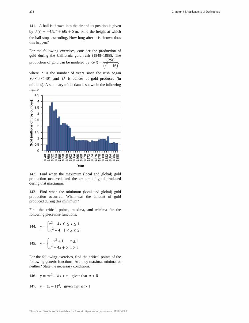
141. A ball is thrown into the air and its position is given
by h(t) = −4.9t2 + 60t + 5 m. Find the height at which
the ball stops ascending. How long after it is thrown doesthis happen?
For the following exercises, consider the production ofgold during the California gold rush (1848–1888). The
production of gold can be modeled by G(t) = (25t)⎛⎝t2 + 16⎞
⎠,
where t is the number of years since the rush began
(0 ≤ t ≤ 40) and G is ounces of gold produced (in
millions). A summary of the data is shown in the followingfigure.
142. Find when the maximum (local and global) goldproduction occurred, and the amount of gold producedduring that maximum.
143. Find when the minimum (local and global) goldproduction occurred. What was the amount of goldproduced during this minimum?
Find the critical points, maxima, and minima for thefollowing piecewise functions.
144. y =⎧
⎩⎨x2 − 4x 0 ≤ x ≤ 1
x2 − 4 1 < x ≤ 2
145. y =⎧
⎩⎨ x2 + 1 x ≤ 1
x2 − 4x + 5 x > 1
For the following exercises, find the critical points of thefollowing generic functions. Are they maxima, minima, orneither? State the necessary conditions.
146. y = ax2 + bx + c, given that a > 0
147. y = (x − 1)a, given that a > 1
378 Chapter 4 | Applications of Derivatives
This OpenStax book is available for free at http://cnx.org/content/col11964/1.2
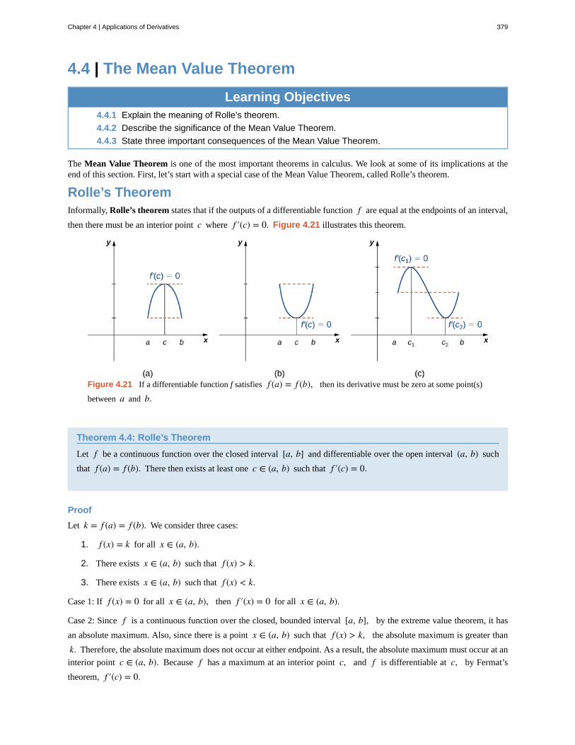
4.4 | The Mean Value Theorem
Learning Objectives4.4.1 Explain the meaning of Rolle’s theorem.
4.4.2 Describe the significance of the Mean Value Theorem.
4.4.3 State three important consequences of the Mean Value Theorem.
The Mean Value Theorem is one of the most important theorems in calculus. We look at some of its implications at theend of this section. First, let’s start with a special case of the Mean Value Theorem, called Rolle’s theorem.
Rolle’s TheoremInformally, Rolle’s theorem states that if the outputs of a differentiable function f are equal at the endpoints of an interval,
then there must be an interior point c where f ′(c) = 0. Figure 4.21 illustrates this theorem.
Figure 4.21 If a differentiable function f satisfies f (a) = f (b), then its derivative must be zero at some point(s)
between a and b.
Theorem 4.4: Rolle’s Theorem
Let f be a continuous function over the closed interval [a, b] and differentiable over the open interval (a, b) such
that f (a) = f (b). There then exists at least one c ∈ (a, b) such that f ′(c) = 0.
Proof
Let k = f (a) = f (b). We consider three cases:
1. f (x) = k for all x ∈ (a, b).
2. There exists x ∈ (a, b) such that f (x) > k.
3. There exists x ∈ (a, b) such that f (x) < k.
Case 1: If f (x) = 0 for all x ∈ (a, b), then f ′(x) = 0 for all x ∈ (a, b).
Case 2: Since f is a continuous function over the closed, bounded interval [a, b], by the extreme value theorem, it has
an absolute maximum. Also, since there is a point x ∈ (a, b) such that f (x) > k, the absolute maximum is greater than
k. Therefore, the absolute maximum does not occur at either endpoint. As a result, the absolute maximum must occur at an
interior point c ∈ (a, b). Because f has a maximum at an interior point c, and f is differentiable at c, by Fermat’s
theorem, f ′(c) = 0.
Chapter 4 | Applications of Derivatives 379
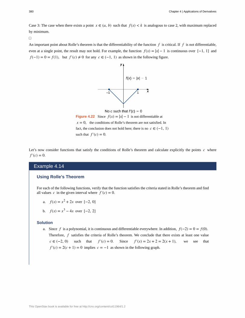
Case 3: The case when there exists a point x ∈ (a, b) such that f (x) < k is analogous to case 2, with maximum replaced
by minimum.
□
An important point about Rolle’s theorem is that the differentiability of the function f is critical. If f is not differentiable,
even at a single point, the result may not hold. For example, the function f (x) = |x| − 1 is continuous over [−1, 1] and
f (−1) = 0 = f (1), but f ′(c) ≠ 0 for any c ∈ (−1, 1) as shown in the following figure.
Figure 4.22 Since f (x) = |x| − 1 is not differentiable at
x = 0, the conditions of Rolle’s theorem are not satisfied. In
fact, the conclusion does not hold here; there is no c ∈ (−1, 1)such that f ′(c) = 0.
Let’s now consider functions that satisfy the conditions of Rolle’s theorem and calculate explicitly the points c where
f ′(c) = 0.
Example 4.14
Using Rolle’s Theorem
For each of the following functions, verify that the function satisfies the criteria stated in Rolle’s theorem and findall values c in the given interval where f ′(c) = 0.
a. f (x) = x2 + 2x over [−2, 0]
b. f (x) = x3 − 4x over [−2, 2]
Solution
a. Since f is a polynomial, it is continuous and differentiable everywhere. In addition, f (−2) = 0 = f (0).Therefore, f satisfies the criteria of Rolle’s theorem. We conclude that there exists at least one value
c ∈ (−2, 0) such that f ′(c) = 0. Since f ′(x) = 2x + 2 = 2(x + 1), we see that
f ′(c) = 2(c + 1) = 0 implies c = −1 as shown in the following graph.
380 Chapter 4 | Applications of Derivatives
This OpenStax book is available for free at http://cnx.org/content/col11964/1.2
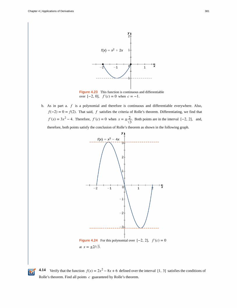
4.14
Figure 4.23 This function is continuous and differentiableover [−2, 0], f ′(c) = 0 when c = −1.
b. As in part a. f is a polynomial and therefore is continuous and differentiable everywhere. Also,
f (−2) = 0 = f (2). That said, f satisfies the criteria of Rolle’s theorem. Differentiating, we find that
f ′(x) = 3x2 − 4. Therefore, f ′(c) = 0 when x = ± 23
. Both points are in the interval [−2, 2], and,
therefore, both points satisfy the conclusion of Rolle’s theorem as shown in the following graph.
Figure 4.24 For this polynomial over [−2, 2], f ′(c) = 0
at x = ±2/ 3.
Verify that the function f (x) = 2x2 − 8x + 6 defined over the interval [1, 3] satisfies the conditions of
Rolle’s theorem. Find all points c guaranteed by Rolle’s theorem.
Chapter 4 | Applications of Derivatives 381
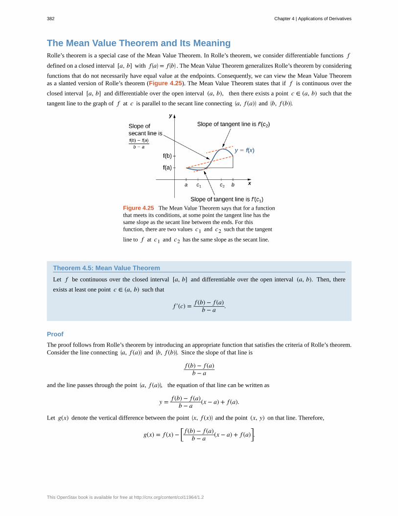
The Mean Value Theorem and Its MeaningRolle’s theorem is a special case of the Mean Value Theorem. In Rolle’s theorem, we consider differentiable functions fdefined on a closed interval [a, b] with f ⎛
⎝a⎞⎠ = f ⎛
⎝b⎞⎠ . The Mean Value Theorem generalizes Rolle’s theorem by considering
functions that do not necessarily have equal value at the endpoints. Consequently, we can view the Mean Value Theoremas a slanted version of Rolle’s theorem (Figure 4.25). The Mean Value Theorem states that if f is continuous over the
closed interval [a, b] and differentiable over the open interval (a, b), then there exists a point c ∈ (a, b) such that the
tangent line to the graph of f at c is parallel to the secant line connecting ⎛⎝a, f (a)⎞
⎠ and ⎛⎝b, f (b)⎞
⎠.
Figure 4.25 The Mean Value Theorem says that for a functionthat meets its conditions, at some point the tangent line has thesame slope as the secant line between the ends. For thisfunction, there are two values c1 and c2 such that the tangent
line to f at c1 and c2 has the same slope as the secant line.
Theorem 4.5: Mean Value Theorem
Let f be continuous over the closed interval [a, b] and differentiable over the open interval (a, b). Then, there
exists at least one point c ∈ (a, b) such that
f ′(c) = f (b) − f (a)b − a .
Proof
The proof follows from Rolle’s theorem by introducing an appropriate function that satisfies the criteria of Rolle’s theorem.Consider the line connecting ⎛
⎝a, f (a)⎞⎠ and ⎛
⎝b, f (b)⎞⎠. Since the slope of that line is
f (b) − f (a)b − a
and the line passes through the point ⎛⎝a, f (a)⎞
⎠, the equation of that line can be written as
y = f (b) − f (a)b − a (x − a) + f (a).
Let g(x) denote the vertical difference between the point ⎛⎝x, f (x)⎞
⎠ and the point (x, y) on that line. Therefore,
g(x) = f (x) − ⎡⎣
f (b) − f (a)b − a (x − a) + f (a)⎤⎦.
382 Chapter 4 | Applications of Derivatives
This OpenStax book is available for free at http://cnx.org/content/col11964/1.2
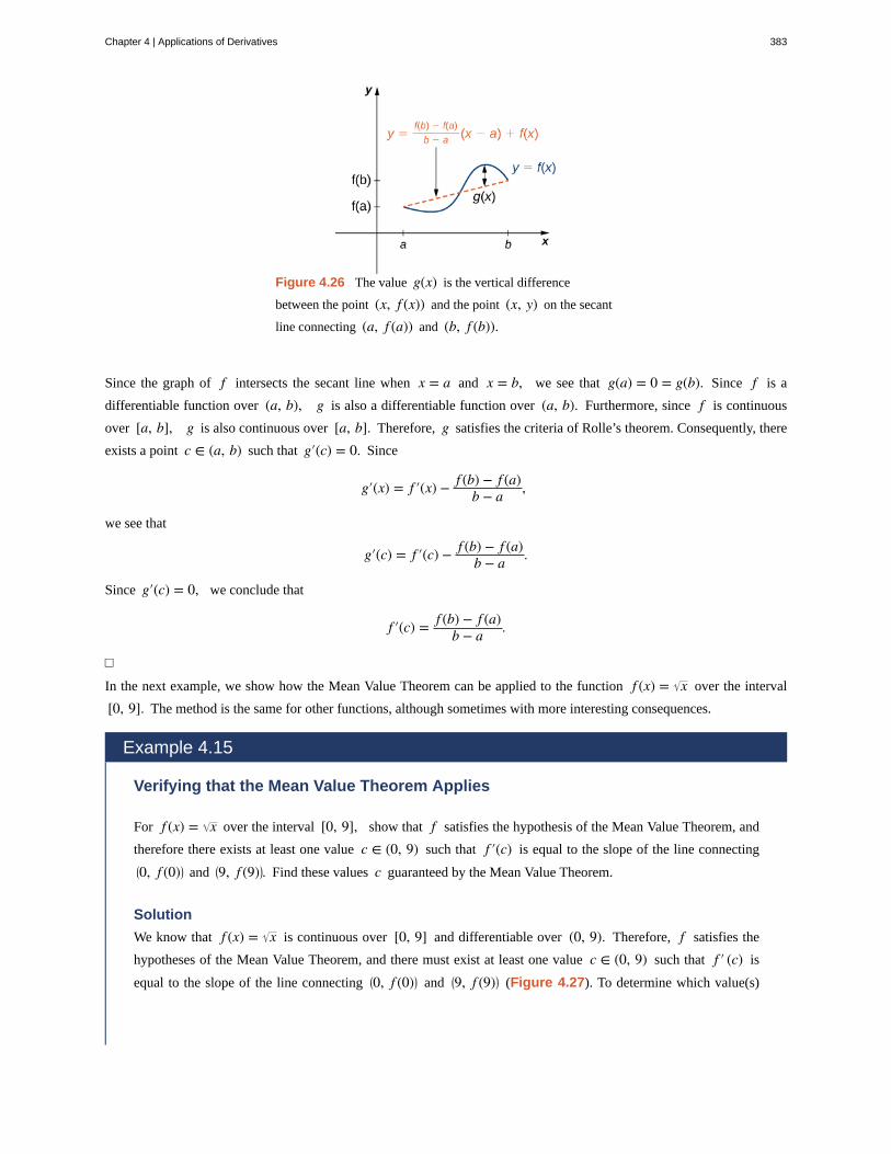
Figure 4.26 The value g(x) is the vertical difference
between the point (x, f (x)) and the point (x, y) on the secant
line connecting (a, f (a)) and (b, f (b)).
Since the graph of f intersects the secant line when x = a and x = b, we see that g(a) = 0 = g(b). Since f is a
differentiable function over (a, b), g is also a differentiable function over (a, b). Furthermore, since f is continuous
over [a, b], g is also continuous over [a, b]. Therefore, g satisfies the criteria of Rolle’s theorem. Consequently, there
exists a point c ∈ (a, b) such that g′(c) = 0. Since
g′(x) = f ′(x) − f (b) − f (a)b − a ,
we see that
g′(c) = f ′(c) − f (b) − f (a)b − a .
Since g′(c) = 0, we conclude that
f ′(c) = f (b) − f (a)b − a .
□
In the next example, we show how the Mean Value Theorem can be applied to the function f (x) = x over the interval
[0, 9]. The method is the same for other functions, although sometimes with more interesting consequences.
Example 4.15
Verifying that the Mean Value Theorem Applies
For f (x) = x over the interval [0, 9], show that f satisfies the hypothesis of the Mean Value Theorem, and
therefore there exists at least one value c ∈ (0, 9) such that f ′(c) is equal to the slope of the line connecting⎛⎝0, f (0)⎞
⎠ and ⎛⎝9, f (9)⎞
⎠. Find these values c guaranteed by the Mean Value Theorem.
Solution
We know that f (x) = x is continuous over [0, 9] and differentiable over (0, 9). Therefore, f satisfies the
hypotheses of the Mean Value Theorem, and there must exist at least one value c ∈ (0, 9) such that f ′ (c) is
equal to the slope of the line connecting ⎛⎝0, f (0)⎞
⎠ and ⎛⎝9, f (9)⎞
⎠ (Figure 4.27). To determine which value(s)
Chapter 4 | Applications of Derivatives 383
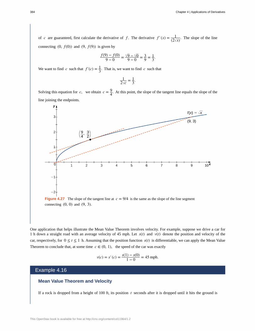
of c are guaranteed, first calculate the derivative of f . The derivative f ′ (x) = 1(2 x). The slope of the line
connecting (0, f (0)) and (9, f (9)) is given by
f (9) − f (0)9 − 0 = 9 − 0
9 − 0 = 39 = 1
3.
We want to find c such that f ′(c) = 13. That is, we want to find c such that
12 c = 1
3.
Solving this equation for c, we obtain c = 94. At this point, the slope of the tangent line equals the slope of the
line joining the endpoints.
Figure 4.27 The slope of the tangent line at c = 9/4 is the same as the slope of the line segment
connecting (0, 0) and (9, 3).
One application that helps illustrate the Mean Value Theorem involves velocity. For example, suppose we drive a car for1 h down a straight road with an average velocity of 45 mph. Let s(t) and v(t) denote the position and velocity of the
car, respectively, for 0 ≤ t ≤ 1 h. Assuming that the position function s(t) is differentiable, we can apply the Mean Value
Theorem to conclude that, at some time c ∈ (0, 1), the speed of the car was exactly
v(c) = s′ (c) = s(1) − s(0)1 − 0 = 45 mph.
Example 4.16
Mean Value Theorem and Velocity
If a rock is dropped from a height of 100 ft, its position t seconds after it is dropped until it hits the ground is
384 Chapter 4 | Applications of Derivatives
This OpenStax book is available for free at http://cnx.org/content/col11964/1.2
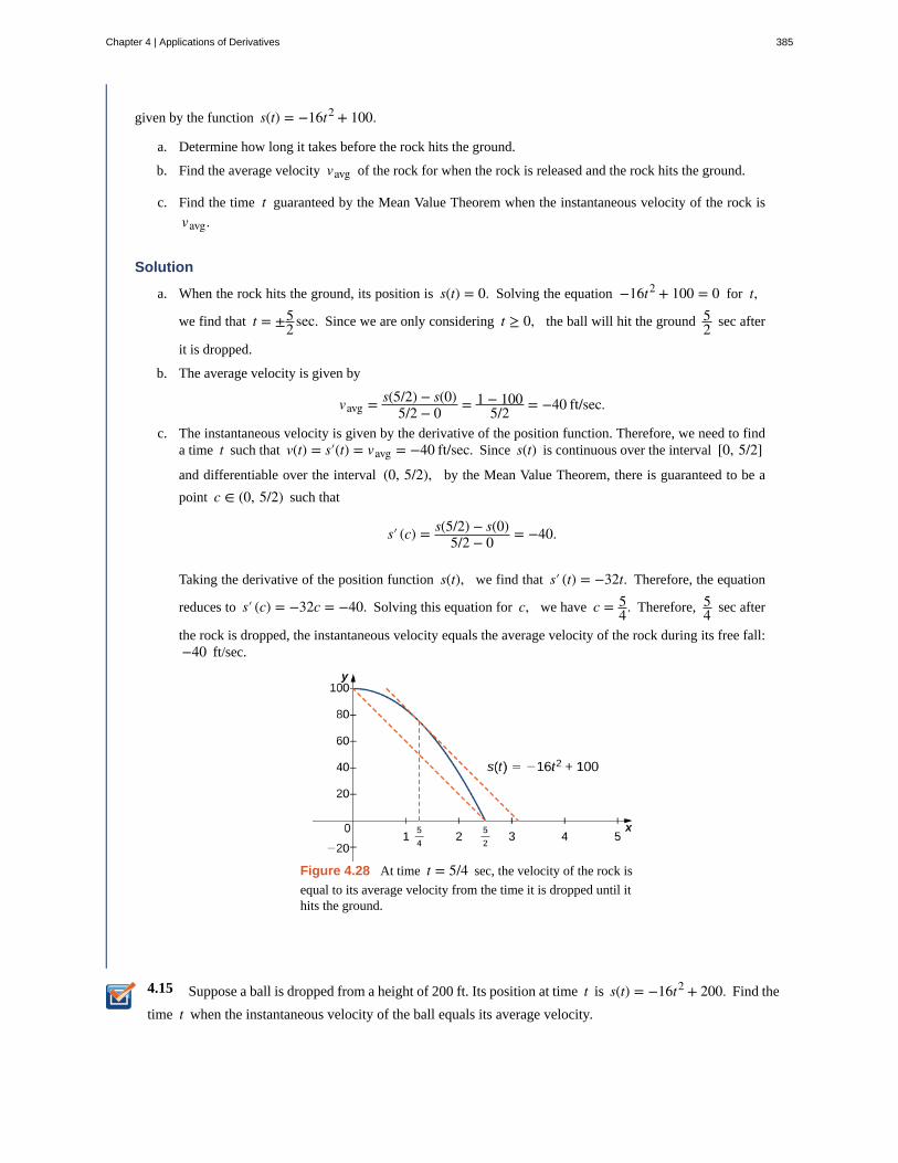
4.15
given by the function s(t) = −16t2 + 100.
a. Determine how long it takes before the rock hits the ground.
b. Find the average velocity vavg of the rock for when the rock is released and the rock hits the ground.
c. Find the time t guaranteed by the Mean Value Theorem when the instantaneous velocity of the rock is
vavg.
Solution
a. When the rock hits the ground, its position is s(t) = 0. Solving the equation −16t2 + 100 = 0 for t,
we find that t = ±52 sec. Since we are only considering t ≥ 0, the ball will hit the ground 5
2 sec after
it is dropped.
b. The average velocity is given by
vavg = s(5/2) − s(0)5/2 − 0 = 1 − 100
5/2 = −40 ft/sec.
c. The instantaneous velocity is given by the derivative of the position function. Therefore, we need to finda time t such that v(t) = s′(t) = vavg = −40 ft/sec. Since s(t) is continuous over the interval [0, 5/2]
and differentiable over the interval (0, 5/2), by the Mean Value Theorem, there is guaranteed to be a
point c ∈ (0, 5/2) such that
s′ (c) = s(5/2) − s(0)5/2 − 0 = −40.
Taking the derivative of the position function s(t), we find that s′ (t) = −32t. Therefore, the equation
reduces to s′ (c) = −32c = −40. Solving this equation for c, we have c = 54. Therefore, 5
4 sec after
the rock is dropped, the instantaneous velocity equals the average velocity of the rock during its free fall:−40 ft/sec.
Figure 4.28 At time t = 5/4 sec, the velocity of the rock is
equal to its average velocity from the time it is dropped until ithits the ground.
Suppose a ball is dropped from a height of 200 ft. Its position at time t is s(t) = −16t2 + 200. Find the
time t when the instantaneous velocity of the ball equals its average velocity.
Chapter 4 | Applications of Derivatives 385
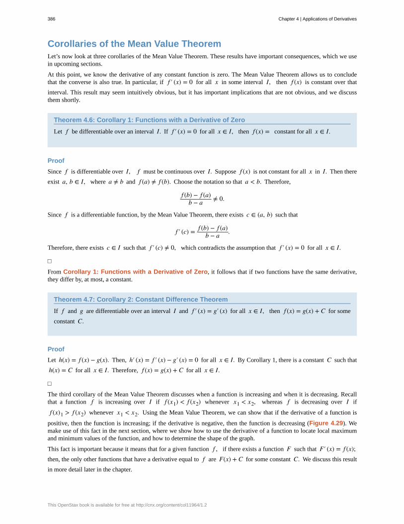
Corollaries of the Mean Value TheoremLet’s now look at three corollaries of the Mean Value Theorem. These results have important consequences, which we usein upcoming sections.
At this point, we know the derivative of any constant function is zero. The Mean Value Theorem allows us to concludethat the converse is also true. In particular, if f ′ (x) = 0 for all x in some interval I, then f (x) is constant over that
interval. This result may seem intuitively obvious, but it has important implications that are not obvious, and we discussthem shortly.
Theorem 4.6: Corollary 1: Functions with a Derivative of Zero
Let f be differentiable over an interval I. If f ′ (x) = 0 for all x ∈ I, then f (x) = constant for all x ∈ I.
Proof
Since f is differentiable over I, f must be continuous over I. Suppose f (x) is not constant for all x in I. Then there
exist a, b ∈ I, where a ≠ b and f (a) ≠ f (b). Choose the notation so that a < b. Therefore,
f (b) − f (a)b − a ≠ 0.
Since f is a differentiable function, by the Mean Value Theorem, there exists c ∈ (a, b) such that
f ′ (c) = f (b) − f (a)b − a .
Therefore, there exists c ∈ I such that f ′ (c) ≠ 0, which contradicts the assumption that f ′ (x) = 0 for all x ∈ I.
□
From Corollary 1: Functions with a Derivative of Zero, it follows that if two functions have the same derivative,they differ by, at most, a constant.
Theorem 4.7: Corollary 2: Constant Difference Theorem
If f and g are differentiable over an interval I and f ′ (x) = g′ (x) for all x ∈ I, then f (x) = g(x) + C for some
constant C.
Proof
Let h(x) = f (x) − g(x). Then, h′ (x) = f ′ (x) − g′ (x) = 0 for all x ∈ I. By Corollary 1, there is a constant C such that
h(x) = C for all x ∈ I. Therefore, f (x) = g(x) + C for all x ∈ I.
□
The third corollary of the Mean Value Theorem discusses when a function is increasing and when it is decreasing. Recallthat a function f is increasing over I if f (x1) < f (x2) whenever x1 < x2, whereas f is decreasing over I if
f (x)1 > f (x2) whenever x1 < x2. Using the Mean Value Theorem, we can show that if the derivative of a function is
positive, then the function is increasing; if the derivative is negative, then the function is decreasing (Figure 4.29). Wemake use of this fact in the next section, where we show how to use the derivative of a function to locate local maximumand minimum values of the function, and how to determine the shape of the graph.
This fact is important because it means that for a given function f , if there exists a function F such that F′ (x) = f (x);then, the only other functions that have a derivative equal to f are F(x) + C for some constant C. We discuss this result
in more detail later in the chapter.
386 Chapter 4 | Applications of Derivatives
This OpenStax book is available for free at http://cnx.org/content/col11964/1.2
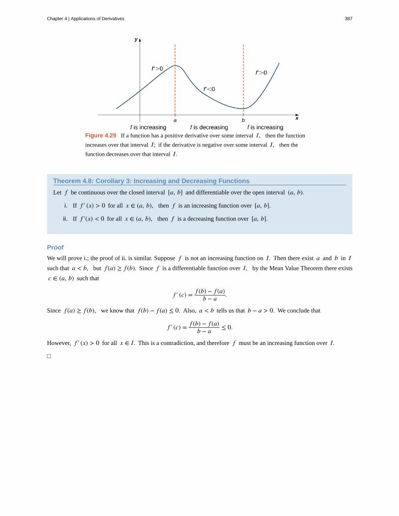
Figure 4.29 If a function has a positive derivative over some interval I, then the function
increases over that interval I; if the derivative is negative over some interval I, then the
function decreases over that interval I.
Theorem 4.8: Corollary 3: Increasing and Decreasing Functions
Let f be continuous over the closed interval [a, b] and differentiable over the open interval (a, b).
i. If f ′ (x) > 0 for all x ∈ (a, b), then f is an increasing function over [a, b].
ii. If f ′(x) < 0 for all x ∈ (a, b), then f is a decreasing function over [a, b].
Proof
We will prove i.; the proof of ii. is similar. Suppose f is not an increasing function on I. Then there exist a and b in Isuch that a < b, but f (a) ≥ f (b). Since f is a differentiable function over I, by the Mean Value Theorem there exists
c ∈ (a, b) such that
f ′ (c) = f (b) − f (a)b − a .
Since f (a) ≥ f (b), we know that f (b) − f (a) ≤ 0. Also, a < b tells us that b − a > 0. We conclude that
f ′ (c) = f (b) − f (a)b − a ≤ 0.
However, f ′ (x) > 0 for all x ∈ I. This is a contradiction, and therefore f must be an increasing function over I.
□
Chapter 4 | Applications of Derivatives 387
4.4 EXERCISES148. Why do you need continuity to apply the Mean ValueTheorem? Construct a counterexample.
149. Why do you need differentiability to apply the MeanValue Theorem? Find a counterexample.
150. When are Rolle’s theorem and the Mean ValueTheorem equivalent?
151. If you have a function with a discontinuity, is it stillpossible to have f ′ (c)(b − a) = f (b) − f (a)? Draw such
an example or prove why not.
For the following exercises, determine over what intervals(if any) the Mean Value Theorem applies. Justify youranswer.
152. y = sin(πx)
153. y = 1x3
154. y = 4 − x2
155. y = x2 − 4
156. y = ln(3x − 5)
For the following exercises, graph the functions on acalculator and draw the secant line that connects theendpoints. Estimate the number of points c such that
f ′(c)(b − a) = f (b) − f (a).
157. [T] y = 3x3 + 2x + 1 over [−1, 1]
158. [T] y = tan⎛⎝π4x⎞
⎠ over⎡⎣−
32, 3
2⎤⎦
159. [T] y = x2 cos(πx) over [−2, 2]
160. [T]
y = x6 − 34x5 − 9
8x4 + 1516x3 + 3
32x2 + 316x + 1
32 over
[−1, 1]
For the following exercises, use the Mean Value Theoremand find all points 0 < c < 2 such that
f (2) − f (0) = f ′ (c)(2 − 0).
161. f (x) = x3
162. f (x) = sin(πx)
163. f (x) = cos(2πx)
164. f (x) = 1 + x + x2
165. f (x) = (x − 1)10
166. f (x) = (x − 1)9
For the following exercises, show there is no c such that
f (1) − f (−1) = f ′ (c)(2). Explain why the Mean Value
Theorem does not apply over the interval [−1, 1].
167. f (x) = |x − 12|
168. f (x) = 1x2
169. f (x) = |x|
170. f (x) = ⌊x⌋ (Hint: This is called the floor function
and it is defined so that f (x) is the largest integer less than
or equal to x.)
For the following exercises, determine whether the MeanValue Theorem applies for the functions over the giveninterval [a, b]. Justify your answer.
171. y = ex over [0, 1]
172. y = ln(2x + 3) over⎡⎣−
32, 0⎤
⎦
173. f (x) = tan(2πx) over [0, 2]
174. y = 9 − x2 over [−3, 3]
175. y = 1|x + 1| over [0, 3]
176. y = x3 + 2x + 1 over [0, 6]
177. y = x2 + 3x + 2x over [−1, 1]
178. y = xsin(πx) + 1 over [0, 1]
179. y = ln(x + 1) over [0, e − 1]
180. y = xsin(πx) over [0, 2]
388 Chapter 4 | Applications of Derivatives
This OpenStax book is available for free at http://cnx.org/content/col11964/1.2
181. y = 5 + |x| over [−1, 1]
For the following exercises, consider the roots of theequation.
182. Show that the equation y = x3 + 3x2 + 16 has
exactly one real root. What is it?
183. Find the conditions for exactly one root (double root)
for the equation y = x2 + bx + c
184. Find the conditions for y = ex − b to have one root.
Is it possible to have more than one root?
For the following exercises, use a calculator to graph thefunction over the interval [a, b] and graph the secant line
from a to b. Use the calculator to estimate all values of cas guaranteed by the Mean Value Theorem. Then, find theexact value of c, if possible, or write the final equation
and use a calculator to estimate to four digits.
185. [T] y = tan(πx) over⎡⎣−
14, 1
4⎤⎦
186. [T] y = 1x + 1
over [0, 3]
187. [T] y = |x2 + 2x − 4| over [−4, 0]
188. [T] y = x + 1x over
⎡⎣12, 4⎤
⎦
189. [T] y = x + 1 + 1x2 over [3, 8]
190. At 10:17 a.m., you pass a police car at 55 mph thatis stopped on the freeway. You pass a second police car at55 mph at 10:53 a.m., which is located 39 mi from the firstpolice car. If the speed limit is 60 mph, can the police citeyou for speeding?
191. Two cars drive from one spotlight to the next, leavingat the same time and arriving at the same time. Is thereever a time when they are going the same speed? Prove ordisprove.
192. Show that y = sec2 x and y = tan2 x have the same
derivative. What can you say about y = sec2 x − tan2 x?
193. Show that y = csc2 x and y = cot2 x have the same
derivative. What can you say about y = csc2 x − cot2 x?
Chapter 4 | Applications of Derivatives 389
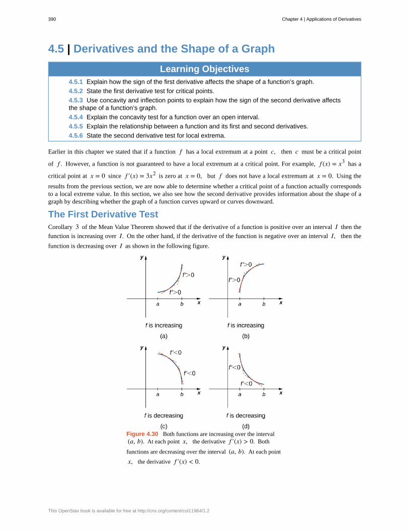
4.5 | Derivatives and the Shape of a Graph
Learning Objectives4.5.1 Explain how the sign of the first derivative affects the shape of a function’s graph.
4.5.2 State the first derivative test for critical points.
4.5.3 Use concavity and inflection points to explain how the sign of the second derivative affectsthe shape of a function’s graph.
4.5.4 Explain the concavity test for a function over an open interval.
4.5.5 Explain the relationship between a function and its first and second derivatives.
4.5.6 State the second derivative test for local extrema.
Earlier in this chapter we stated that if a function f has a local extremum at a point c, then c must be a critical point
of f . However, a function is not guaranteed to have a local extremum at a critical point. For example, f (x) = x3 has a
critical point at x = 0 since f ′(x) = 3x2 is zero at x = 0, but f does not have a local extremum at x = 0. Using the
results from the previous section, we are now able to determine whether a critical point of a function actually correspondsto a local extreme value. In this section, we also see how the second derivative provides information about the shape of agraph by describing whether the graph of a function curves upward or curves downward.
The First Derivative TestCorollary 3 of the Mean Value Theorem showed that if the derivative of a function is positive over an interval I then the
function is increasing over I. On the other hand, if the derivative of the function is negative over an interval I, then the
function is decreasing over I as shown in the following figure.
Figure 4.30 Both functions are increasing over the interval(a, b). At each point x, the derivative f ′(x) > 0. Both
functions are decreasing over the interval (a, b). At each point
x, the derivative f ′(x) < 0.
390 Chapter 4 | Applications of Derivatives
This OpenStax book is available for free at http://cnx.org/content/col11964/1.2
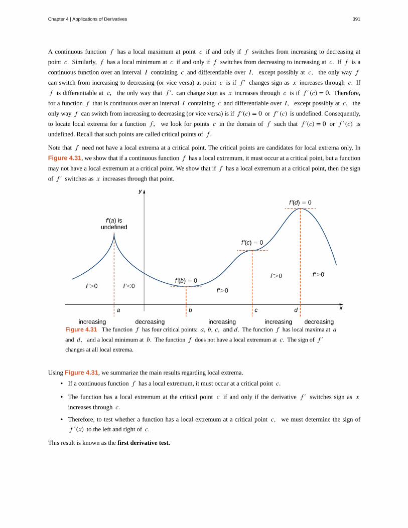
A continuous function f has a local maximum at point c if and only if f switches from increasing to decreasing at
point c. Similarly, f has a local minimum at c if and only if f switches from decreasing to increasing at c. If f is a
continuous function over an interval I containing c and differentiable over I, except possibly at c, the only way fcan switch from increasing to decreasing (or vice versa) at point c is if f ′ changes sign as x increases through c. If
f is differentiable at c, the only way that f ′. can change sign as x increases through c is if f ′ (c) = 0. Therefore,
for a function f that is continuous over an interval I containing c and differentiable over I, except possibly at c, the
only way f can switch from increasing to decreasing (or vice versa) is if f ′(c) = 0 or f ′ (c) is undefined. Consequently,
to locate local extrema for a function f , we look for points c in the domain of f such that f ′(c) = 0 or f ′ (c) is
undefined. Recall that such points are called critical points of f .
Note that f need not have a local extrema at a critical point. The critical points are candidates for local extrema only. In
Figure 4.31, we show that if a continuous function f has a local extremum, it must occur at a critical point, but a function
may not have a local extremum at a critical point. We show that if f has a local extremum at a critical point, then the sign
of f ′ switches as x increases through that point.
Figure 4.31 The function f has four critical points: a, b, c, and d. The function f has local maxima at aand d, and a local minimum at b. The function f does not have a local extremum at c. The sign of f ′changes at all local extrema.
Using Figure 4.31, we summarize the main results regarding local extrema.
• If a continuous function f has a local extremum, it must occur at a critical point c.
• The function has a local extremum at the critical point c if and only if the derivative f ′ switches sign as xincreases through c.
• Therefore, to test whether a function has a local extremum at a critical point c, we must determine the sign of
f ′ (x) to the left and right of c.
This result is known as the first derivative test.
Chapter 4 | Applications of Derivatives 391
Theorem 4.9: First Derivative Test
Suppose that f is a continuous function over an interval I containing a critical point c. If f is differentiable over
I, except possibly at point c, then f (c) satisfies one of the following descriptions:
i. If f ′ changes sign from positive when x < c to negative when x > c, then f (c) is a local maximum of f .
ii. If f ′ changes sign from negative when x < c to positive when x > c, then f (c) is a local minimum of f .
iii. If f ′ has the same sign for x < c and x > c, then f (c) is neither a local maximum nor a local minimum of
f .
We can summarize the first derivative test as a strategy for locating local extrema.
Problem-Solving Strategy: Using the First Derivative Test
Consider a function f that is continuous over an interval I.
1. Find all critical points of f and divide the interval I into smaller intervals using the critical points as
endpoints.
2. Analyze the sign of f ′ in each of the subintervals. If f ′ is continuous over a given subinterval (which is
typically the case), then the sign of f ′ in that subinterval does not change and, therefore, can be determined
by choosing an arbitrary test point x in that subinterval and by evaluating the sign of f ′ at that test point. Use
the sign analysis to determine whether f is increasing or decreasing over that interval.
3. Use First Derivative Test and the results of step 2 to determine whether f has a local maximum, a local
minimum, or neither at each of the critical points.
Now let’s look at how to use this strategy to locate all local extrema for particular functions.
Example 4.17
Using the First Derivative Test to Find Local Extrema
Use the first derivative test to find the location of all local extrema for f (x) = x3 − 3x2 − 9x − 1. Use a
graphing utility to confirm your results.
Solution
Step 1. The derivative is f ′ (x) = 3x2 − 6x − 9. To find the critical points, we need to find where f ′ (x) = 0.Factoring the polynomial, we conclude that the critical points must satisfy
3(x2 − 2x − 3) = 3(x − 3)(x + 1) = 0.
Therefore, the critical points are x = 3, −1. Now divide the interval (−∞, ∞) into the smaller intervals
(−∞, −1), (−1, 3) and (3, ∞).
Step 2. Since f ′ is a continuous function, to determine the sign of f ′ (x) over each subinterval, it suffices to
choose a point over each of the intervals (−∞, −1), (−1, 3) and (3, ∞) and determine the sign of f ′ at each
392 Chapter 4 | Applications of Derivatives
This OpenStax book is available for free at http://cnx.org/content/col11964/1.2
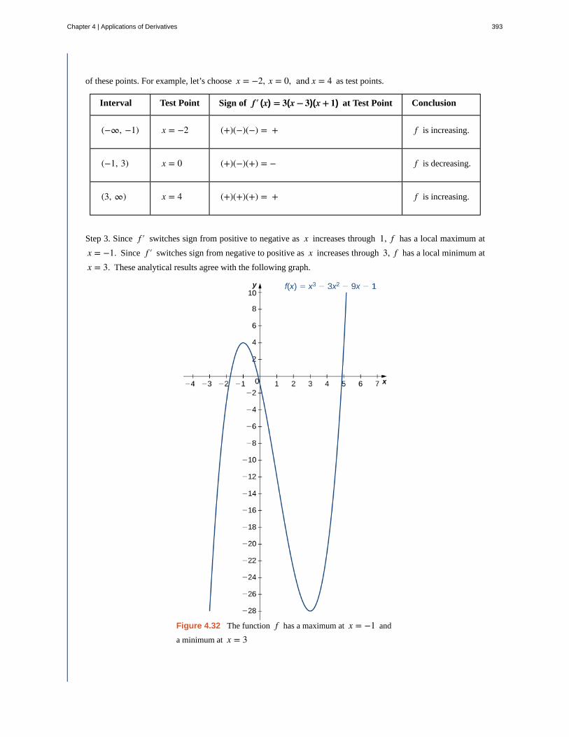
of these points. For example, let’s choose x = −2, x = 0, and x = 4 as test points.
Interval Test Point Sign of f′ (x) = 3(x − 3)(x + 1) at Test Point Conclusion
(−∞, −1) x = −2 (+)(−)(−) = + f is increasing.
(−1, 3) x = 0 (+)(−)(+) = − f is decreasing.
(3, ∞) x = 4 (+)(+)(+) = + f is increasing.
Step 3. Since f ′ switches sign from positive to negative as x increases through 1, f has a local maximum at
x = −1. Since f ′ switches sign from negative to positive as x increases through 3, f has a local minimum at
x = 3. These analytical results agree with the following graph.
Figure 4.32 The function f has a maximum at x = −1 and
a minimum at x = 3
Chapter 4 | Applications of Derivatives 393
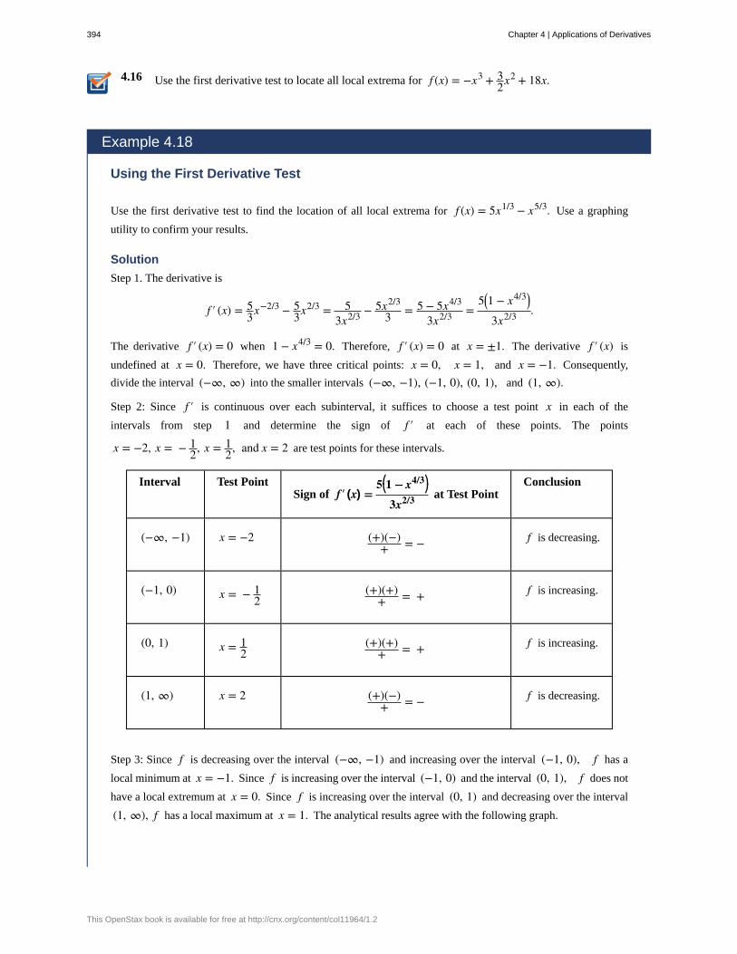
4.16 Use the first derivative test to locate all local extrema for f (x) = −x3 + 32x2 + 18x.
Example 4.18
Using the First Derivative Test
Use the first derivative test to find the location of all local extrema for f (x) = 5x1/3 − x5/3. Use a graphing
utility to confirm your results.
Solution
Step 1. The derivative is
f ′ (x) = 53x−2/3 − 5
3x2/3 = 53x2/3 − 5x2/3
3 = 5 − 5x4/3
3x2/3 =5⎛
⎝1 − x4/3⎞⎠
3x2/3 .
The derivative f ′ (x) = 0 when 1 − x4/3 = 0. Therefore, f ′ (x) = 0 at x = ±1. The derivative f ′ (x) is
undefined at x = 0. Therefore, we have three critical points: x = 0, x = 1, and x = −1. Consequently,
divide the interval (−∞, ∞) into the smaller intervals (−∞, −1), (−1, 0), (0, 1), and (1, ∞).
Step 2: Since f ′ is continuous over each subinterval, it suffices to choose a test point x in each of the
intervals from step 1 and determine the sign of f ′ at each of these points. The points
x = −2, x = − 12, x = 1
2, and x = 2 are test points for these intervals.
Interval Test PointSign of f′ (x) =
5⎛⎝1 − x4/3⎞⎠
3x2/3 at Test PointConclusion
(−∞, −1) x = −2 (+)(−)+ = − f is decreasing.
(−1, 0) x = − 12
(+)(+)+ = + f is increasing.
(0, 1) x = 12
(+)(+)+ = + f is increasing.
(1, ∞) x = 2 (+)(−)+ = − f is decreasing.
Step 3: Since f is decreasing over the interval (−∞, −1) and increasing over the interval (−1, 0), f has a
local minimum at x = −1. Since f is increasing over the interval (−1, 0) and the interval (0, 1), f does not
have a local extremum at x = 0. Since f is increasing over the interval (0, 1) and decreasing over the interval
(1, ∞), f has a local maximum at x = 1. The analytical results agree with the following graph.
394 Chapter 4 | Applications of Derivatives
This OpenStax book is available for free at http://cnx.org/content/col11964/1.2
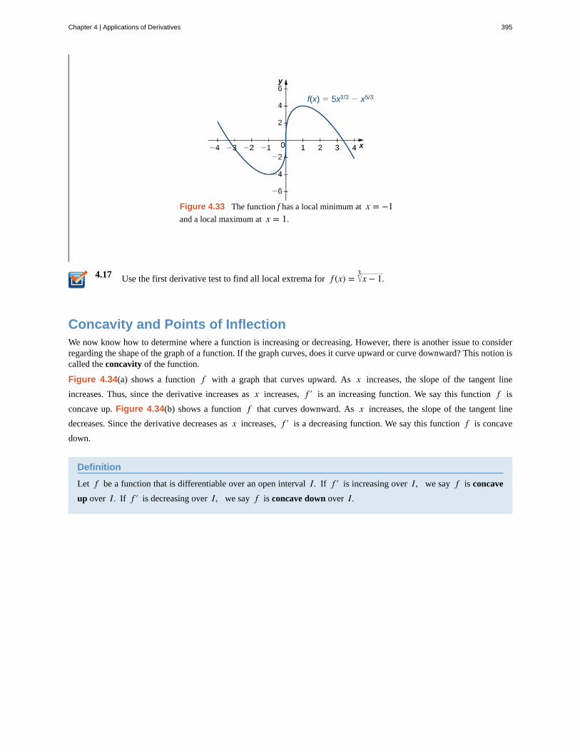
4.17
Figure 4.33 The function f has a local minimum at x = −1and a local maximum at x = 1.
Use the first derivative test to find all local extrema for f (x) = x − 13 .
Concavity and Points of InflectionWe now know how to determine where a function is increasing or decreasing. However, there is another issue to considerregarding the shape of the graph of a function. If the graph curves, does it curve upward or curve downward? This notion iscalled the concavity of the function.
Figure 4.34(a) shows a function f with a graph that curves upward. As x increases, the slope of the tangent line
increases. Thus, since the derivative increases as x increases, f ′ is an increasing function. We say this function f is
concave up. Figure 4.34(b) shows a function f that curves downward. As x increases, the slope of the tangent line
decreases. Since the derivative decreases as x increases, f ′ is a decreasing function. We say this function f is concave
down.
Definition
Let f be a function that is differentiable over an open interval I. If f ′ is increasing over I, we say f is concave
up over I. If f ′ is decreasing over I, we say f is concave down over I.
Chapter 4 | Applications of Derivatives 395
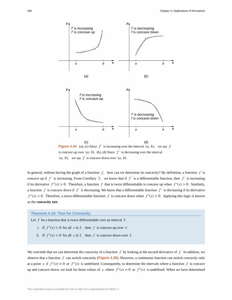
Figure 4.34 (a), (c) Since f ′ is increasing over the interval (a, b), we say fis concave up over (a, b). (b), (d) Since f ′ is decreasing over the interval
(a, b), we say f is concave down over (a, b).
In general, without having the graph of a function f , how can we determine its concavity? By definition, a function f is
concave up if f ′ is increasing. From Corollary 3, we know that if f ′ is a differentiable function, then f ′ is increasing
if its derivative f ″(x) > 0. Therefore, a function f that is twice differentiable is concave up when f ″(x) > 0. Similarly,
a function f is concave down if f ′ is decreasing. We know that a differentiable function f ′ is decreasing if its derivative
f ″(x) < 0. Therefore, a twice-differentiable function f is concave down when f ″(x) < 0. Applying this logic is known
as the concavity test.
Theorem 4.10: Test for Concavity
Let f be a function that is twice differentiable over an interval I.
i. If f ″(x) > 0 for all x ∈ I, then f is concave up over I.
ii. If f ″(x) < 0 for all x ∈ I, then f is concave down over I.
We conclude that we can determine the concavity of a function f by looking at the second derivative of f . In addition, we
observe that a function f can switch concavity (Figure 4.35). However, a continuous function can switch concavity only
at a point x if f ″(x) = 0 or f ″(x) is undefined. Consequently, to determine the intervals where a function f is concave
up and concave down, we look for those values of x where f ″(x) = 0 or f ″(x) is undefined. When we have determined
396 Chapter 4 | Applications of Derivatives
This OpenStax book is available for free at http://cnx.org/content/col11964/1.2
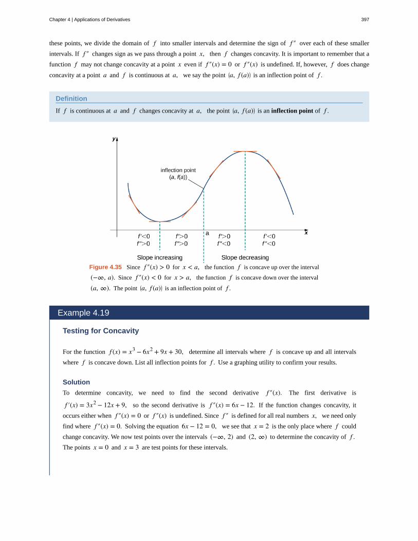
these points, we divide the domain of f into smaller intervals and determine the sign of f ″ over each of these smaller
intervals. If f ″ changes sign as we pass through a point x, then f changes concavity. It is important to remember that a
function f may not change concavity at a point x even if f ″(x) = 0 or f ″(x) is undefined. If, however, f does change
concavity at a point a and f is continuous at a, we say the point ⎛⎝a, f (a)⎞
⎠ is an inflection point of f .
Definition
If f is continuous at a and f changes concavity at a, the point ⎛⎝a, f (a)⎞
⎠ is an inflection point of f .
Figure 4.35 Since f ″(x) > 0 for x < a, the function f is concave up over the interval
(−∞, a). Since f ″(x) < 0 for x > a, the function f is concave down over the interval
(a, ∞). The point ⎛⎝a, f (a)⎞
⎠ is an inflection point of f .
Example 4.19
Testing for Concavity
For the function f (x) = x3 − 6x2 + 9x + 30, determine all intervals where f is concave up and all intervals
where f is concave down. List all inflection points for f . Use a graphing utility to confirm your results.
Solution
To determine concavity, we need to find the second derivative f ″(x). The first derivative is
f ′(x) = 3x2 − 12x + 9, so the second derivative is f ″(x) = 6x − 12. If the function changes concavity, it
occurs either when f ″(x) = 0 or f ″(x) is undefined. Since f ″ is defined for all real numbers x, we need only
find where f ″(x) = 0. Solving the equation 6x − 12 = 0, we see that x = 2 is the only place where f could
change concavity. We now test points over the intervals (−∞, 2) and (2, ∞) to determine the concavity of f .The points x = 0 and x = 3 are test points for these intervals.
Chapter 4 | Applications of Derivatives 397
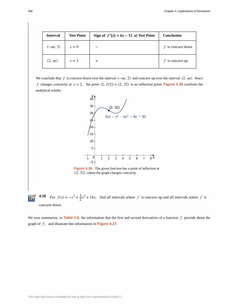
4.18
Interval Test Point Sign of f″(x) = 6x − 12 at Test Point Conclusion
(−∞, 2) x = 0 − f is concave down
(2, ∞) x = 3 + f is concave up.
We conclude that f is concave down over the interval (−∞, 2) and concave up over the interval (2, ∞). Since
f changes concavity at x = 2, the point ⎛⎝2, f (2)⎞
⎠ = (2, 32) is an inflection point. Figure 4.36 confirms the
analytical results.
Figure 4.36 The given function has a point of inflection at(2, 32) where the graph changes concavity.
For f (x) = −x3 + 32x2 + 18x, find all intervals where f is concave up and all intervals where f is
concave down.
We now summarize, in Table 4.6, the information that the first and second derivatives of a function f provide about the
graph of f , and illustrate this information in Figure 4.37.
398 Chapter 4 | Applications of Derivatives
This OpenStax book is available for free at http://cnx.org/content/col11964/1.2
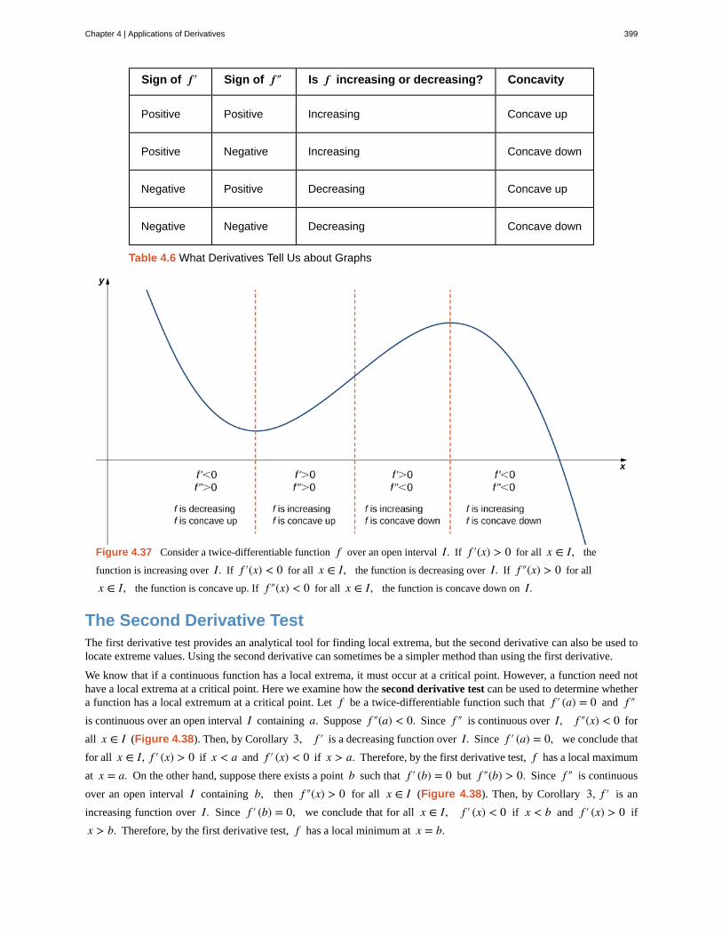
Sign of f′ Sign of f″ Is f increasing or decreasing? Concavity
Positive Positive Increasing Concave up
Positive Negative Increasing Concave down
Negative Positive Decreasing Concave up
Negative Negative Decreasing Concave down
Table 4.6 What Derivatives Tell Us about Graphs
Figure 4.37 Consider a twice-differentiable function f over an open interval I. If f ′(x) > 0 for all x ∈ I, the
function is increasing over I. If f ′(x) < 0 for all x ∈ I, the function is decreasing over I. If f ″(x) > 0 for all
x ∈ I, the function is concave up. If f ″(x) < 0 for all x ∈ I, the function is concave down on I.
The Second Derivative TestThe first derivative test provides an analytical tool for finding local extrema, but the second derivative can also be used tolocate extreme values. Using the second derivative can sometimes be a simpler method than using the first derivative.
We know that if a continuous function has a local extrema, it must occur at a critical point. However, a function need nothave a local extrema at a critical point. Here we examine how the second derivative test can be used to determine whethera function has a local extremum at a critical point. Let f be a twice-differentiable function such that f ′ (a) = 0 and f ″is continuous over an open interval I containing a. Suppose f ″(a) < 0. Since f ″ is continuous over I, f ″(x) < 0 for
all x ∈ I (Figure 4.38). Then, by Corollary 3, f ′ is a decreasing function over I. Since f ′ (a) = 0, we conclude that
for all x ∈ I, f ′ (x) > 0 if x < a and f ′ (x) < 0 if x > a. Therefore, by the first derivative test, f has a local maximum
at x = a. On the other hand, suppose there exists a point b such that f ′ (b) = 0 but f ″(b) > 0. Since f ″ is continuous
over an open interval I containing b, then f ″(x) > 0 for all x ∈ I (Figure 4.38). Then, by Corollary 3, f ′ is an
increasing function over I. Since f ′ (b) = 0, we conclude that for all x ∈ I, f ′ (x) < 0 if x < b and f ′ (x) > 0 if
x > b. Therefore, by the first derivative test, f has a local minimum at x = b.
Chapter 4 | Applications of Derivatives 399
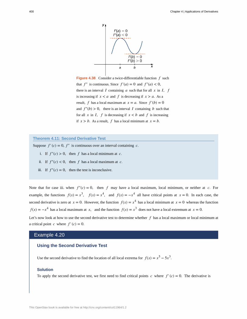
Figure 4.38 Consider a twice-differentiable function f such
that f ″ is continuous. Since f ′(a) = 0 and f ″(a) < 0,there is an interval I containing a such that for all x in I, fis increasing if x < a and f is decreasing if x > a. As a
result, f has a local maximum at x = a. Since f ′(b) = 0and f ″(b) > 0, there is an interval I containing b such that
for all x in I, f is decreasing if x < b and f is increasing
if x > b. As a result, f has a local minimum at x = b.
Theorem 4.11: Second Derivative Test
Suppose f ′ (c) = 0, f ″ is continuous over an interval containing c.
i. If f ″(c) > 0, then f has a local minimum at c.
ii. If f ″(c) < 0, then f has a local maximum at c.
iii. If f ″(c) = 0, then the test is inconclusive.
Note that for case iii. when f ″(c) = 0, then f may have a local maximum, local minimum, or neither at c. For
example, the functions f (x) = x3, f (x) = x4, and f (x) = −x4 all have critical points at x = 0. In each case, the
second derivative is zero at x = 0. However, the function f (x) = x4 has a local minimum at x = 0 whereas the function
f (x) = −x4 has a local maximum at x, and the function f (x) = x3 does not have a local extremum at x = 0.
Let’s now look at how to use the second derivative test to determine whether f has a local maximum or local minimum at
a critical point c where f ′ (c) = 0.
Example 4.20
Using the Second Derivative Test
Use the second derivative to find the location of all local extrema for f (x) = x5 − 5x3.
Solution
To apply the second derivative test, we first need to find critical points c where f ′ (c) = 0. The derivative is
400 Chapter 4 | Applications of Derivatives
This OpenStax book is available for free at http://cnx.org/content/col11964/1.2
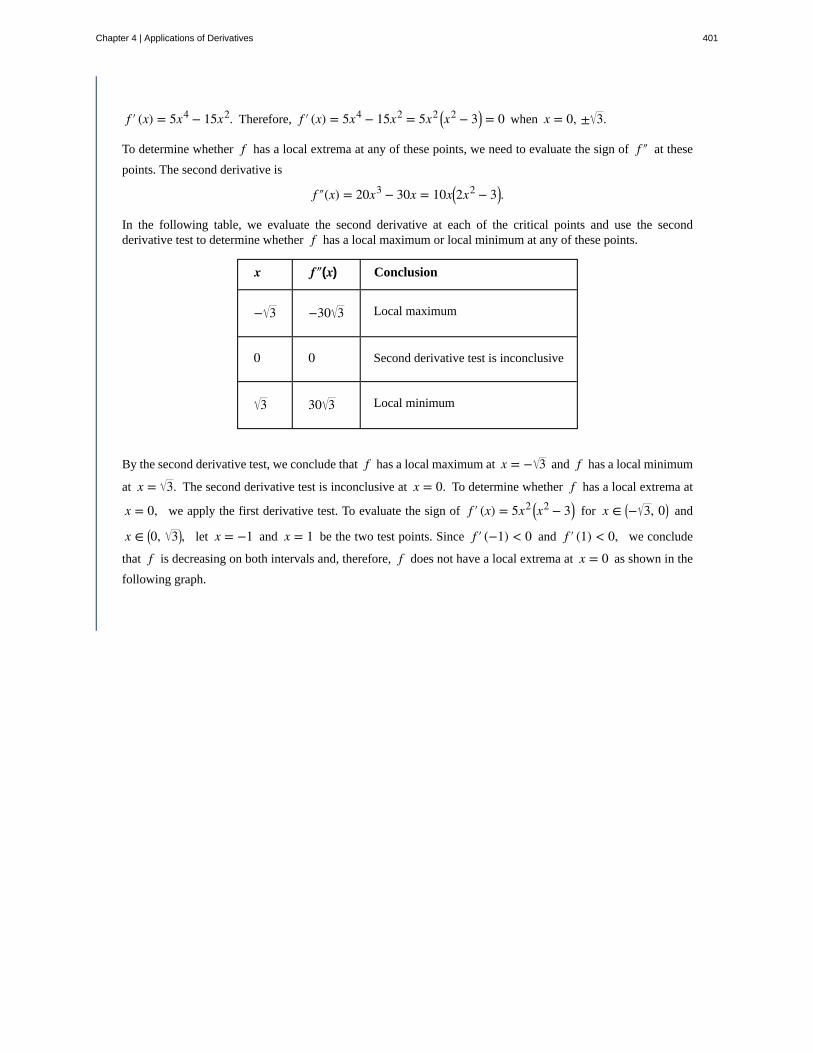
f ′ (x) = 5x4 − 15x2. Therefore, f ′ (x) = 5x4 − 15x2 = 5x2 ⎛⎝x2 − 3⎞
⎠ = 0 when x = 0, ± 3.
To determine whether f has a local extrema at any of these points, we need to evaluate the sign of f ″ at these
points. The second derivative is
f ″(x) = 20x3 − 30x = 10x⎛⎝2x2 − 3⎞
⎠.
In the following table, we evaluate the second derivative at each of the critical points and use the secondderivative test to determine whether f has a local maximum or local minimum at any of these points.
x f″(x) Conclusion
− 3 −30 3 Local maximum
0 0 Second derivative test is inconclusive
3 30 3 Local minimum
By the second derivative test, we conclude that f has a local maximum at x = − 3 and f has a local minimum
at x = 3. The second derivative test is inconclusive at x = 0. To determine whether f has a local extrema at
x = 0, we apply the first derivative test. To evaluate the sign of f ′ (x) = 5x2 ⎛⎝x2 − 3⎞
⎠ for x ∈ ⎛⎝− 3, 0⎞
⎠ and
x ∈ ⎛⎝0, 3⎞
⎠, let x = −1 and x = 1 be the two test points. Since f ′ (−1) < 0 and f ′ (1) < 0, we conclude
that f is decreasing on both intervals and, therefore, f does not have a local extrema at x = 0 as shown in the
following graph.
Chapter 4 | Applications of Derivatives 401
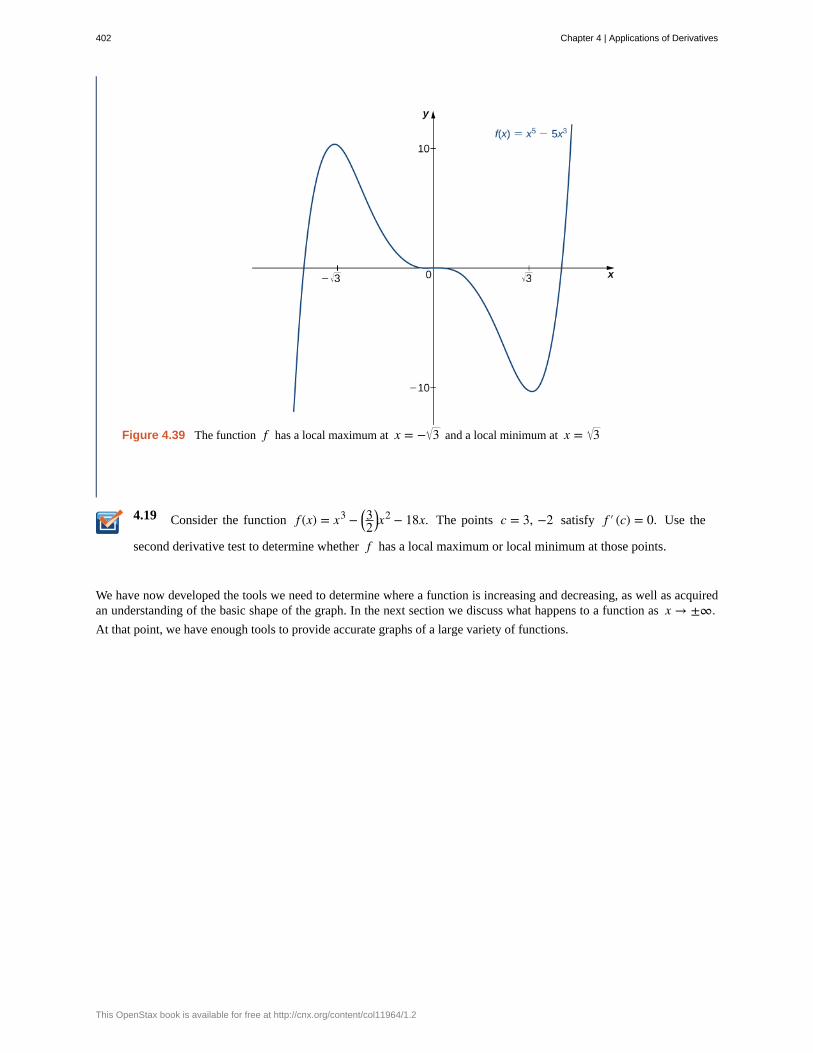
4.19
Figure 4.39 The function f has a local maximum at x = − 3 and a local minimum at x = 3
Consider the function f (x) = x3 − ⎛⎝32
⎞⎠x
2 − 18x. The points c = 3, −2 satisfy f ′ (c) = 0. Use the
second derivative test to determine whether f has a local maximum or local minimum at those points.
We have now developed the tools we need to determine where a function is increasing and decreasing, as well as acquiredan understanding of the basic shape of the graph. In the next section we discuss what happens to a function as x → ±∞.At that point, we have enough tools to provide accurate graphs of a large variety of functions.
402 Chapter 4 | Applications of Derivatives
This OpenStax book is available for free at http://cnx.org/content/col11964/1.2

4.5 EXERCISES194. If c is a critical point of f (x), when is there no
local maximum or minimum at c? Explain.
195. For the function y = x3, is x = 0 both an
inflection point and a local maximum/minimum?
196. For the function y = x3, is x = 0 an inflection
point?
197. Is it possible for a point c to be both an inflection
point and a local extrema of a twice differentiablefunction?
198. Why do you need continuity for the first derivativetest? Come up with an example.
199. Explain whether a concave-down function has tocross y = 0 for some value of x.
200. Explain whether a polynomial of degree 2 can have
an inflection point.
For the following exercises, analyze the graphs of f ′,then list all intervals where f is increasing or decreasing.
201.
202.
203.
204.
Chapter 4 | Applications of Derivatives 403
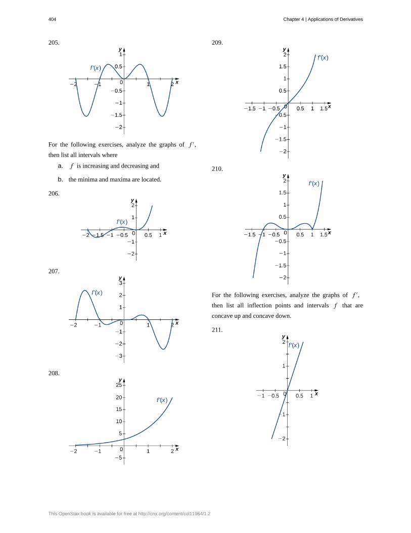
205.
For the following exercises, analyze the graphs of f ′,then list all intervals where
a. f is increasing and decreasing and
b. the minima and maxima are located.
206.
207.
208.
209.
210.
For the following exercises, analyze the graphs of f ′,then list all inflection points and intervals f that are
concave up and concave down.
211.
404 Chapter 4 | Applications of Derivatives
This OpenStax book is available for free at http://cnx.org/content/col11964/1.2
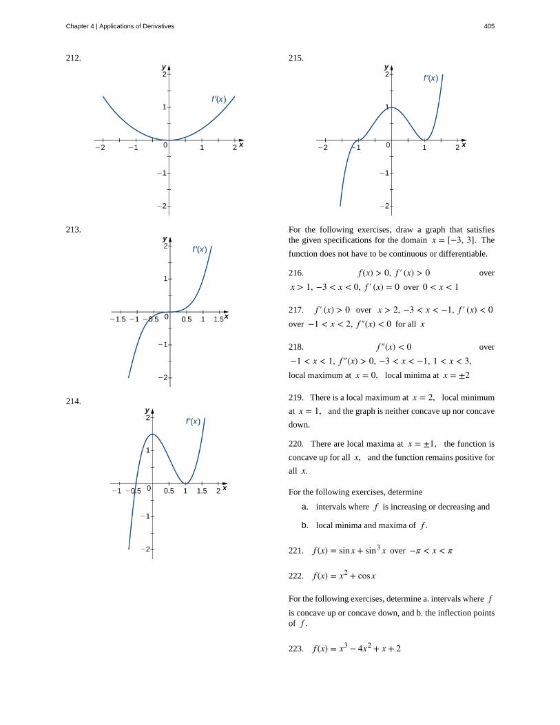
212.
213.
214.
215.
For the following exercises, draw a graph that satisfiesthe given specifications for the domain x = [−3, 3]. The
function does not have to be continuous or differentiable.
216. f (x) > 0, f ′ (x) > 0 over
x > 1, −3 < x < 0, f ′ (x) = 0 over 0 < x < 1
217. f ′ (x) > 0 over x > 2, −3 < x < −1, f ′ (x) < 0over −1 < x < 2, f ″(x) < 0 for all x
218. f ″(x) < 0 over
−1 < x < 1, f ″(x) > 0, −3 < x < −1, 1 < x < 3,local maximum at x = 0, local minima at x = ±2
219. There is a local maximum at x = 2, local minimum
at x = 1, and the graph is neither concave up nor concave
down.
220. There are local maxima at x = ±1, the function is
concave up for all x, and the function remains positive for
all x.
For the following exercises, determine
a. intervals where f is increasing or decreasing and
b. local minima and maxima of f .
221. f (x) = sinx + sin3 x over −π < x < π
222. f (x) = x2 + cosx
For the following exercises, determine a. intervals where fis concave up or concave down, and b. the inflection pointsof f .
223. f (x) = x3 − 4x2 + x + 2
Chapter 4 | Applications of Derivatives 405
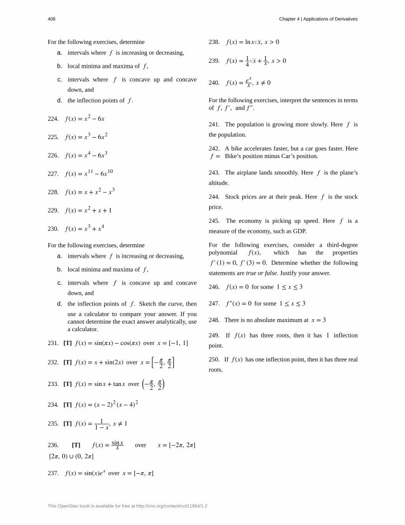
For the following exercises, determine
a. intervals where f is increasing or decreasing,
b. local minima and maxima of f ,
c. intervals where f is concave up and concave
down, and
d. the inflection points of f .
224. f (x) = x2 − 6x
225. f (x) = x3 − 6x2
226. f (x) = x4 − 6x3
227. f (x) = x11 − 6x10
228. f (x) = x + x2 − x3
229. f (x) = x2 + x + 1
230. f (x) = x3 + x4
For the following exercises, determine
a. intervals where f is increasing or decreasing,
b. local minima and maxima of f ,
c. intervals where f is concave up and concave
down, and
d. the inflection points of f . Sketch the curve, then
use a calculator to compare your answer. If youcannot determine the exact answer analytically, usea calculator.
231. [T] f (x) = sin(πx) − cos(πx) over x = [−1, 1]
232. [T] f (x) = x + sin(2x) over x = ⎡⎣−
π2, π
2⎤⎦
233. [T] f (x) = sinx + tanx over ⎛⎝−
π2, π
2⎞⎠
234. [T] f (x) = (x − 2)2 (x − 4)2
235. [T] f (x) = 11 − x, x ≠ 1
236. [T] f (x) = sinxx over x = [−2π, 2π]
[2π, 0) ∪ (0, 2π]
237. f (x) = sin(x)ex over x = [−π, π]
238. f (x) = lnx x, x > 0
239. f (x) = 14 x + 1
x , x > 0
240. f (x) = exx , x ≠ 0
For the following exercises, interpret the sentences in termsof f , f ′, and f ″.
241. The population is growing more slowly. Here f is
the population.
242. A bike accelerates faster, but a car goes faster. Heref = Bike’s position minus Car’s position.
243. The airplane lands smoothly. Here f is the plane’s
altitude.
244. Stock prices are at their peak. Here f is the stock
price.
245. The economy is picking up speed. Here f is a
measure of the economy, such as GDP.
For the following exercises, consider a third-degreepolynomial f (x), which has the properties
f ′ (1) = 0, f ′ (3) = 0. Determine whether the following
statements are true or false. Justify your answer.
246. f (x) = 0 for some 1 ≤ x ≤ 3
247. f ″(x) = 0 for some 1 ≤ x ≤ 3
248. There is no absolute maximum at x = 3
249. If f (x) has three roots, then it has 1 inflection
point.
250. If f (x) has one inflection point, then it has three real
roots.
406 Chapter 4 | Applications of Derivatives
This OpenStax book is available for free at http://cnx.org/content/col11964/1.2
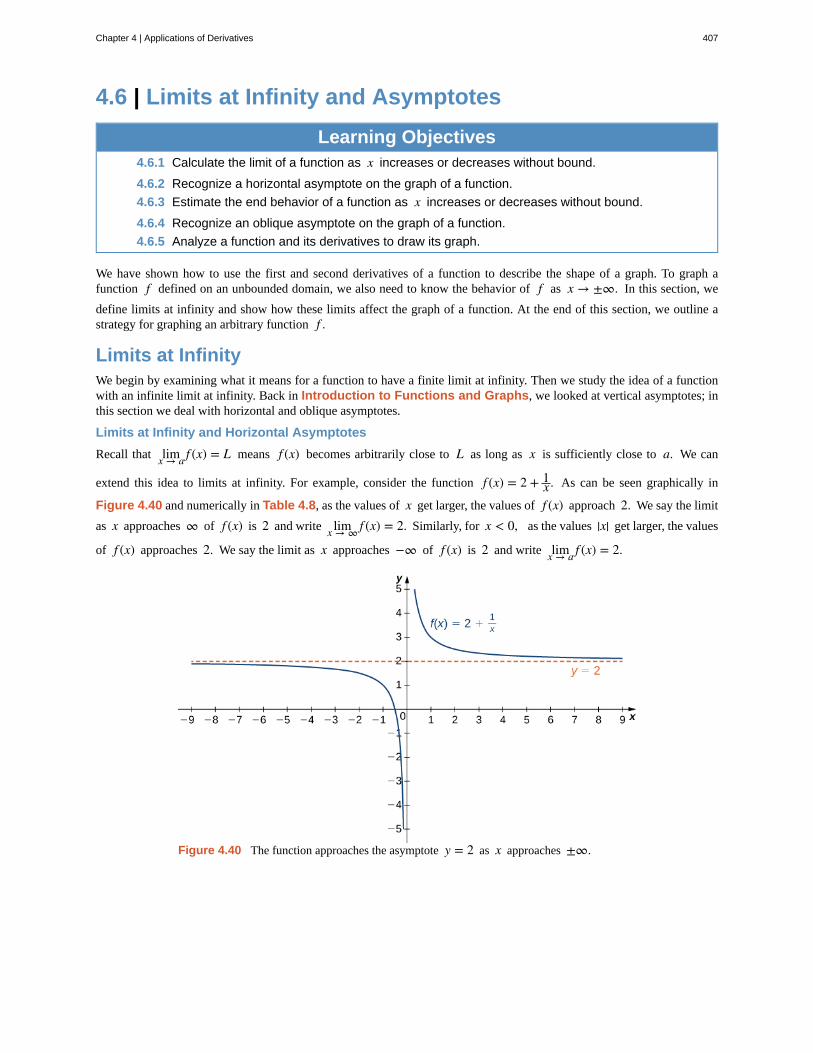
4.6 | Limits at Infinity and Asymptotes
Learning Objectives4.6.1 Calculate the limit of a function as x increases or decreases without bound.
4.6.2 Recognize a horizontal asymptote on the graph of a function.
4.6.3 Estimate the end behavior of a function as x increases or decreases without bound.
4.6.4 Recognize an oblique asymptote on the graph of a function.
4.6.5 Analyze a function and its derivatives to draw its graph.
We have shown how to use the first and second derivatives of a function to describe the shape of a graph. To graph afunction f defined on an unbounded domain, we also need to know the behavior of f as x → ±∞. In this section, we
define limits at infinity and show how these limits affect the graph of a function. At the end of this section, we outline astrategy for graphing an arbitrary function f .
Limits at InfinityWe begin by examining what it means for a function to have a finite limit at infinity. Then we study the idea of a functionwith an infinite limit at infinity. Back in Introduction to Functions and Graphs, we looked at vertical asymptotes; inthis section we deal with horizontal and oblique asymptotes.
Limits at Infinity and Horizontal Asymptotes
Recall that limx → a f (x) = L means f (x) becomes arbitrarily close to L as long as x is sufficiently close to a. We can
extend this idea to limits at infinity. For example, consider the function f (x) = 2 + 1x . As can be seen graphically in
Figure 4.40 and numerically in Table 4.8, as the values of x get larger, the values of f (x) approach 2. We say the limit
as x approaches ∞ of f (x) is 2 and write limx → ∞ f (x) = 2. Similarly, for x < 0, as the values |x| get larger, the values
of f (x) approaches 2. We say the limit as x approaches −∞ of f (x) is 2 and write limx → a f (x) = 2.
Figure 4.40 The function approaches the asymptote y = 2 as x approaches ±∞.
Chapter 4 | Applications of Derivatives 407
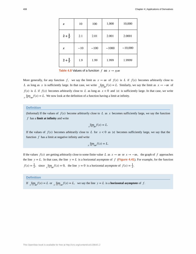
x 10 100 1,000 10,000
2 + 1x 2.1 2.01 2.001 2.0001
x −10 −100 −1000 −10,000
2 + 1x 1.9 1.99 1.999 1.9999
Table 4.8 Values of a function f as x → ±∞
More generally, for any function f , we say the limit as x → ∞ of f (x) is L if f (x) becomes arbitrarily close to
L as long as x is sufficiently large. In that case, we write limx → ∞ f (x) = L. Similarly, we say the limit as x → −∞ of
f (x) is L if f (x) becomes arbitrarily close to L as long as x < 0 and |x| is sufficiently large. In that case, we write
limx → −∞ f (x) = L. We now look at the definition of a function having a limit at infinity.
Definition
(Informal) If the values of f (x) become arbitrarily close to L as x becomes sufficiently large, we say the function
f has a limit at infinity and write
limx → ∞ f (x) = L.
If the values of f (x) becomes arbitrarily close to L for x < 0 as |x| becomes sufficiently large, we say that the
function f has a limit at negative infinity and write
limx → –∞ f (x) = L.
If the values f (x) are getting arbitrarily close to some finite value L as x → ∞ or x → −∞, the graph of f approaches
the line y = L. In that case, the line y = L is a horizontal asymptote of f (Figure 4.41). For example, for the function
f (x) = 1x , since limx → ∞ f (x) = 0, the line y = 0 is a horizontal asymptote of f (x) = 1
x .
Definition
If limx → ∞ f (x) = L or limx → −∞ f (x) = L, we say the line y = L is a horizontal asymptote of f .
408 Chapter 4 | Applications of Derivatives
This OpenStax book is available for free at http://cnx.org/content/col11964/1.2
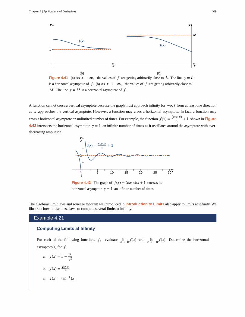
Figure 4.41 (a) As x → ∞, the values of f are getting arbitrarily close to L. The line y = Lis a horizontal asymptote of f . (b) As x → −∞, the values of f are getting arbitrarily close to
M. The line y = M is a horizontal asymptote of f .
A function cannot cross a vertical asymptote because the graph must approach infinity (or −∞) from at least one direction
as x approaches the vertical asymptote. However, a function may cross a horizontal asymptote. In fact, a function may
cross a horizontal asymptote an unlimited number of times. For example, the function f (x) = (cosx)x + 1 shown in Figure
4.42 intersects the horizontal asymptote y = 1 an infinite number of times as it oscillates around the asymptote with ever-
decreasing amplitude.
Figure 4.42 The graph of f (x) = (cosx)/x + 1 crosses its
horizontal asymptote y = 1 an infinite number of times.
The algebraic limit laws and squeeze theorem we introduced in Introduction to Limits also apply to limits at infinity. Weillustrate how to use these laws to compute several limits at infinity.
Example 4.21
Computing Limits at Infinity
For each of the following functions f , evaluate limx → ∞ f (x) and limx → −∞ f (x). Determine the horizontal
asymptote(s) for f .
a. f (x) = 5 − 2x2
b. f (x) = sinxx
c. f (x) = tan−1 (x)
Chapter 4 | Applications of Derivatives 409
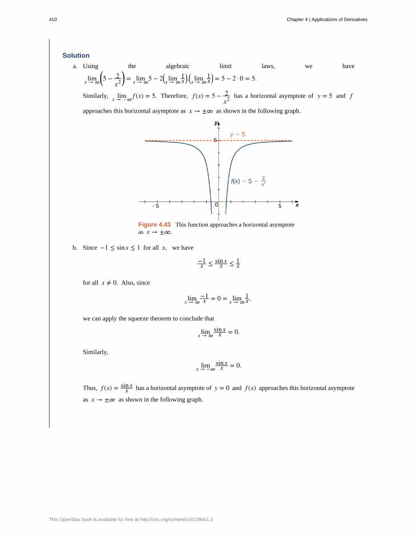
Solution
a. Using the algebraic limit laws, we have
limx → ∞⎛⎝5 − 2
x2⎞⎠ = limx → ∞5 − 2⎛
⎝ limx → ∞1x
⎞⎠.
⎛⎝ limx → ∞
1x
⎞⎠ = 5 − 2 · 0 = 5.
Similarly, limx → - ∞ f (x) = 5. Therefore, f (x) = 5 − 2x2 has a horizontal asymptote of y = 5 and f
approaches this horizontal asymptote as x → ±∞ as shown in the following graph.
Figure 4.43 This function approaches a horizontal asymptoteas x → ±∞.
b. Since −1 ≤ sinx ≤ 1 for all x, we have
−1x ≤ sinx
x ≤ 1x
for all x ≠ 0. Also, since
limx → ∞−1x = 0 = limx → ∞
1x ,
we can apply the squeeze theorem to conclude that
limx → ∞sinx
x = 0.
Similarly,
limx → −∞sinx
x = 0.
Thus, f (x) = sinxx has a horizontal asymptote of y = 0 and f (x) approaches this horizontal asymptote
as x → ±∞ as shown in the following graph.
410 Chapter 4 | Applications of Derivatives
This OpenStax book is available for free at http://cnx.org/content/col11964/1.2
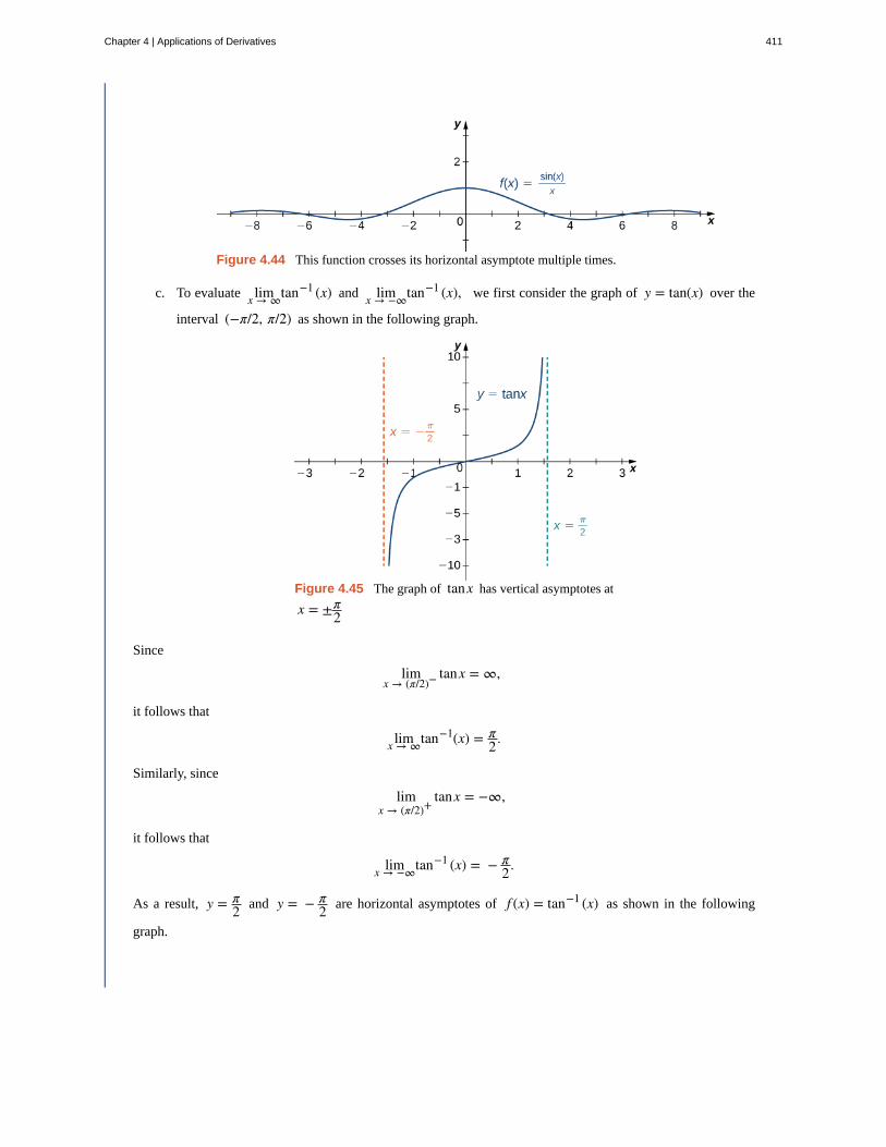
Figure 4.44 This function crosses its horizontal asymptote multiple times.
c. To evaluate limx → ∞tan−1 (x) and limx → −∞tan−1 (x), we first consider the graph of y = tan(x) over the
interval (−π/2, π/2) as shown in the following graph.
Figure 4.45 The graph of tanx has vertical asymptotes at
x = ±π2
Since
limx → (π/2)−
tanx = ∞,
it follows that
limx → ∞tan−1(x) = π2.
Similarly, since
limx → (π/2)+
tanx = −∞,
it follows that
limx → −∞tan−1 (x) = − π2.
As a result, y = π2 and y = − π
2 are horizontal asymptotes of f (x) = tan−1 (x) as shown in the following
graph.
Chapter 4 | Applications of Derivatives 411
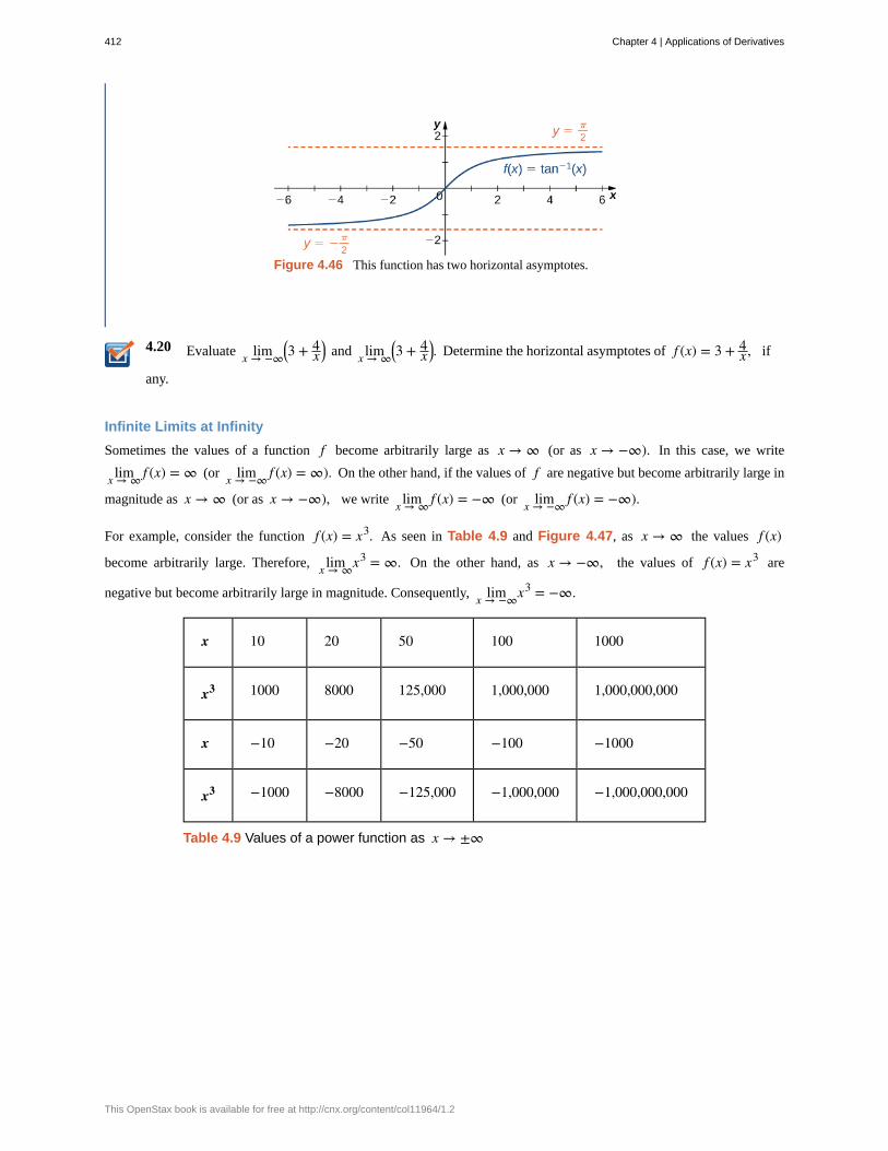
4.20
Figure 4.46 This function has two horizontal asymptotes.
Evaluate limx → −∞⎛⎝3 + 4
x⎞⎠ and limx → ∞
⎛⎝3 + 4
x⎞⎠. Determine the horizontal asymptotes of f (x) = 3 + 4
x , if
any.
Infinite Limits at Infinity
Sometimes the values of a function f become arbitrarily large as x → ∞ (or as x → −∞). In this case, we write
limx → ∞ f (x) = ∞ (or limx → −∞ f (x) = ∞). On the other hand, if the values of f are negative but become arbitrarily large in
magnitude as x → ∞ (or as x → −∞), we write limx → ∞ f (x) = −∞ (or limx → −∞ f (x) = −∞).
For example, consider the function f (x) = x3. As seen in Table 4.9 and Figure 4.47, as x → ∞ the values f (x)
become arbitrarily large. Therefore, limx → ∞x3 = ∞. On the other hand, as x → −∞, the values of f (x) = x3 are
negative but become arbitrarily large in magnitude. Consequently, limx → −∞x3 = −∞.
x 10 20 50 100 1000
x3 1000 8000 125,000 1,000,000 1,000,000,000
x −10 −20 −50 −100 −1000
x3 −1000 −8000 −125,000 −1,000,000 −1,000,000,000
Table 4.9 Values of a power function as x → ±∞
412 Chapter 4 | Applications of Derivatives
This OpenStax book is available for free at http://cnx.org/content/col11964/1.2
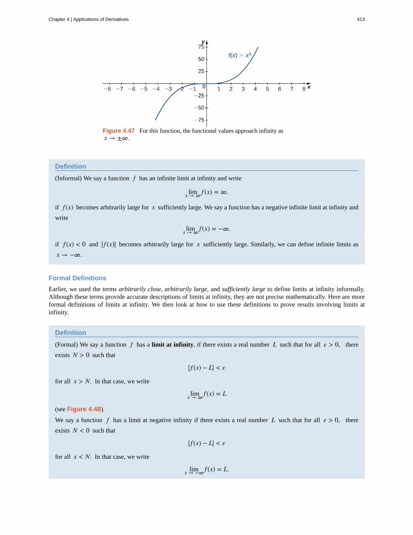
Figure 4.47 For this function, the functional values approach infinity asx → ±∞.
Definition
(Informal) We say a function f has an infinite limit at infinity and write
limx → ∞ f (x) = ∞.
if f (x) becomes arbitrarily large for x sufficiently large. We say a function has a negative infinite limit at infinity and
write
limx → ∞ f (x) = −∞.
if f (x) < 0 and | f (x)| becomes arbitrarily large for x sufficiently large. Similarly, we can define infinite limits as
x → −∞.
Formal Definitions
Earlier, we used the terms arbitrarily close, arbitrarily large, and sufficiently large to define limits at infinity informally.Although these terms provide accurate descriptions of limits at infinity, they are not precise mathematically. Here are moreformal definitions of limits at infinity. We then look at how to use these definitions to prove results involving limits atinfinity.
Definition
(Formal) We say a function f has a limit at infinity, if there exists a real number L such that for all ε > 0, there
exists N > 0 such that
| f (x) − L| < ε
for all x > N. In that case, we write
limx → ∞ f (x) = L
(see Figure 4.48).
We say a function f has a limit at negative infinity if there exists a real number L such that for all ε > 0, there
exists N < 0 such that
| f (x) − L| < ε
for all x < N. In that case, we write
limx → −∞ f (x) = L.
Chapter 4 | Applications of Derivatives 413
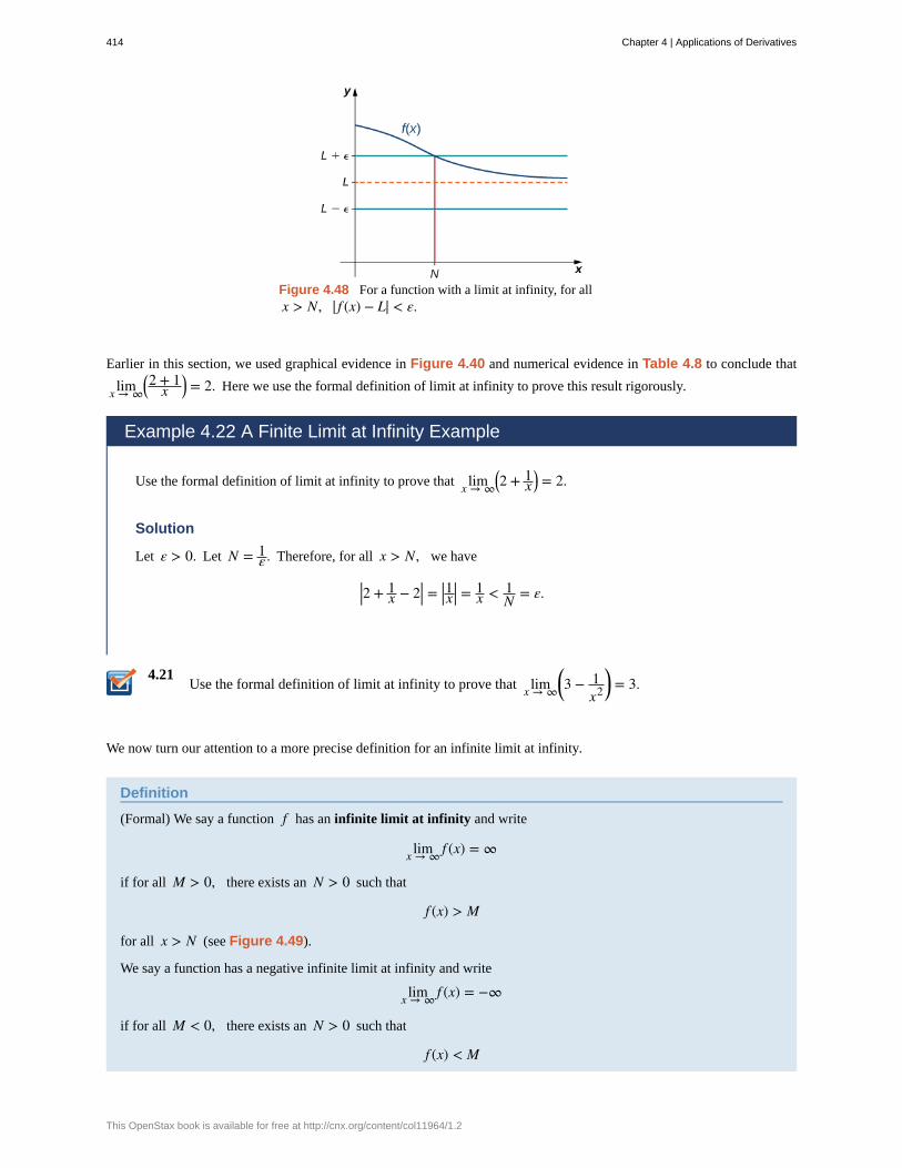
4.21
Figure 4.48 For a function with a limit at infinity, for allx > N, | f (x) − L| < ε.
Earlier in this section, we used graphical evidence in Figure 4.40 and numerical evidence in Table 4.8 to conclude that
limx → ∞⎛⎝2 + 1
x⎞⎠ = 2. Here we use the formal definition of limit at infinity to prove this result rigorously.
Example 4.22 A Finite Limit at Infinity Example
Use the formal definition of limit at infinity to prove that limx → ∞⎛⎝2 + 1
x⎞⎠ = 2.
Solution
Let ε > 0. Let N = 1ε . Therefore, for all x > N, we have
|2 + 1x − 2| = |1x | = 1
x < 1N = ε.
Use the formal definition of limit at infinity to prove that limx → ∞⎛⎝3 − 1
x2⎞⎠ = 3.
We now turn our attention to a more precise definition for an infinite limit at infinity.
Definition
(Formal) We say a function f has an infinite limit at infinity and write
limx → ∞ f (x) = ∞
if for all M > 0, there exists an N > 0 such that
f (x) > M
for all x > N (see Figure 4.49).
We say a function has a negative infinite limit at infinity and write
limx → ∞ f (x) = −∞
if for all M < 0, there exists an N > 0 such that
f (x) < M
414 Chapter 4 | Applications of Derivatives
This OpenStax book is available for free at http://cnx.org/content/col11964/1.2
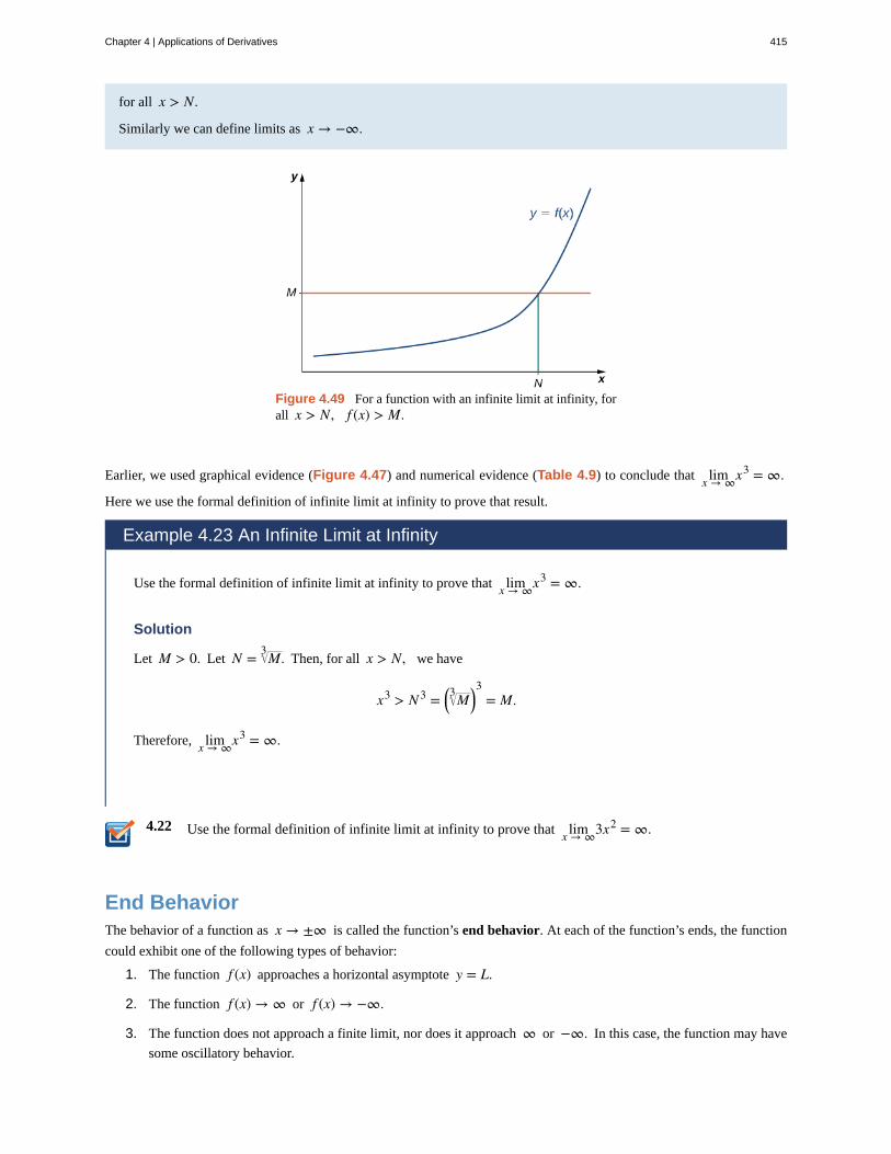
4.22
for all x > N.
Similarly we can define limits as x → −∞.
Figure 4.49 For a function with an infinite limit at infinity, forall x > N, f (x) > M.
Earlier, we used graphical evidence (Figure 4.47) and numerical evidence (Table 4.9) to conclude that limx → ∞x3 = ∞.
Here we use the formal definition of infinite limit at infinity to prove that result.
Example 4.23 An Infinite Limit at Infinity
Use the formal definition of infinite limit at infinity to prove that limx → ∞x3 = ∞.
Solution
Let M > 0. Let N = M3 . Then, for all x > N, we have
x3 > N 3 = ⎛⎝ M3 ⎞
⎠3
= M.
Therefore, limx → ∞x3 = ∞.
Use the formal definition of infinite limit at infinity to prove that limx → ∞3x2 = ∞.
End BehaviorThe behavior of a function as x → ±∞ is called the function’s end behavior. At each of the function’s ends, the function
could exhibit one of the following types of behavior:
1. The function f (x) approaches a horizontal asymptote y = L.
2. The function f (x) → ∞ or f (x) → −∞.
3. The function does not approach a finite limit, nor does it approach ∞ or −∞. In this case, the function may have
some oscillatory behavior.
Chapter 4 | Applications of Derivatives 415
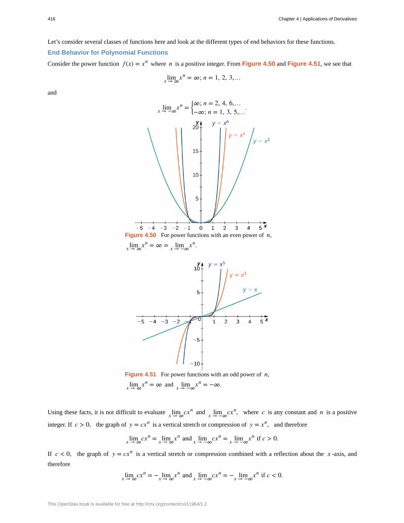
Let’s consider several classes of functions here and look at the different types of end behaviors for these functions.
End Behavior for Polynomial Functions
Consider the power function f (x) = xn where n is a positive integer. From Figure 4.50 and Figure 4.51, we see that
limx → ∞xn = ∞; n = 1, 2, 3,…
and
limx → −∞xn =⎧
⎩⎨∞; n = 2, 4, 6,…−∞; n = 1, 3, 5,…
.
Figure 4.50 For power functions with an even power of n,limx → ∞xn = ∞ = limx → −∞xn.
Figure 4.51 For power functions with an odd power of n,limx → ∞xn = ∞ and limx → −∞xn = −∞.
Using these facts, it is not difficult to evaluate limx → ∞cxn and limx → −∞cxn, where c is any constant and n is a positive
integer. If c > 0, the graph of y = cxn is a vertical stretch or compression of y = xn, and therefore
limx → ∞cxn = limx → ∞xn and limx → −∞cxn = limx → −∞xn if c > 0.
If c < 0, the graph of y = cxn is a vertical stretch or compression combined with a reflection about the x -axis, and
therefore
limx → ∞cxn = − limx → ∞xn and limx → −∞cxn = − limx → −∞xn if c < 0.
416 Chapter 4 | Applications of Derivatives
This OpenStax book is available for free at http://cnx.org/content/col11964/1.2
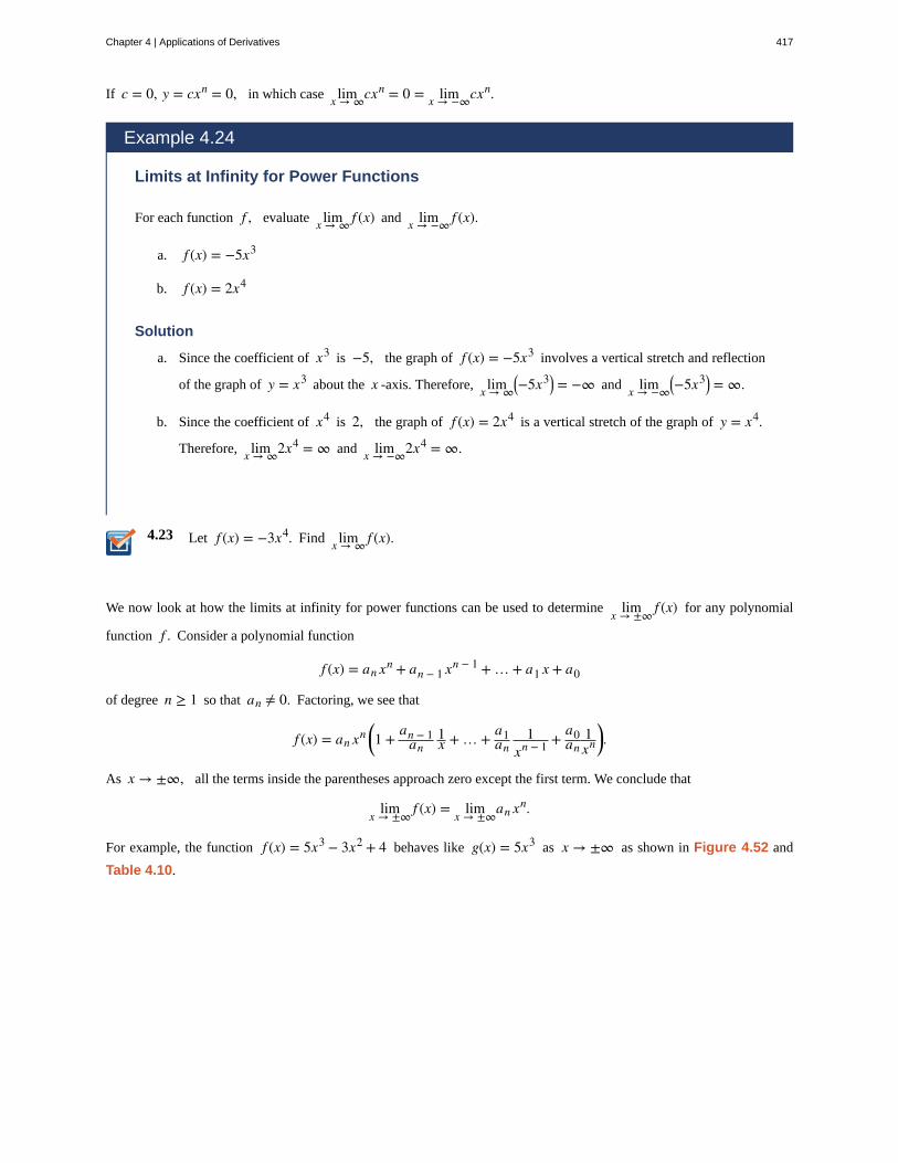
4.23
If c = 0, y = cxn = 0, in which case limx → ∞cxn = 0 = limx → −∞cxn.
Example 4.24
Limits at Infinity for Power Functions
For each function f , evaluate limx → ∞ f (x) and limx → −∞ f (x).
a. f (x) = −5x3
b. f (x) = 2x4
Solution
a. Since the coefficient of x3 is −5, the graph of f (x) = −5x3 involves a vertical stretch and reflection
of the graph of y = x3 about the x -axis. Therefore, limx → ∞⎛⎝−5x3⎞
⎠ = −∞ and limx → −∞⎛⎝−5x3⎞
⎠ = ∞.
b. Since the coefficient of x4 is 2, the graph of f (x) = 2x4 is a vertical stretch of the graph of y = x4.
Therefore, limx → ∞2x4 = ∞ and limx → −∞2x4 = ∞.
Let f (x) = −3x4. Find limx → ∞ f (x).
We now look at how the limits at infinity for power functions can be used to determine limx → ±∞ f (x) for any polynomial
function f . Consider a polynomial function
f (x) = an xn + an − 1 xn − 1 + … + a1 x + a0
of degree n ≥ 1 so that an ≠ 0. Factoring, we see that
f (x) = an xn ⎛⎝1 + an − 1
an1x + … + a1
an1
xn − 1 + a0an
1xn
⎞⎠.
As x → ±∞, all the terms inside the parentheses approach zero except the first term. We conclude that
limx → ±∞ f (x) = limx → ±∞an xn.
For example, the function f (x) = 5x3 − 3x2 + 4 behaves like g(x) = 5x3 as x → ±∞ as shown in Figure 4.52 and
Table 4.10.
Chapter 4 | Applications of Derivatives 417
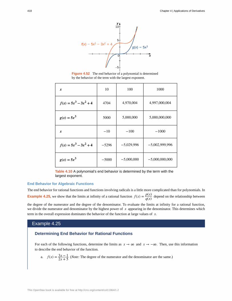
Figure 4.52 The end behavior of a polynomial is determinedby the behavior of the term with the largest exponent.
x 10 100 1000
f(x) = 5x3 − 3x2 + 4 4704 4,970,004 4,997,000,004
g(x) = 5x3 5000 5,000,000 5,000,000,000
x −10 −100 −1000
f(x) = 5x3 − 3x2 + 4 −5296 −5,029,996 −5,002,999,996
g(x) = 5x3 −5000 −5,000,000 −5,000,000,000
Table 4.10 A polynomial’s end behavior is determined by the term with thelargest exponent.
End Behavior for Algebraic Functions
The end behavior for rational functions and functions involving radicals is a little more complicated than for polynomials. In
Example 4.25, we show that the limits at infinity of a rational function f (x) = p(x)q(x) depend on the relationship between
the degree of the numerator and the degree of the denominator. To evaluate the limits at infinity for a rational function,we divide the numerator and denominator by the highest power of x appearing in the denominator. This determines which
term in the overall expression dominates the behavior of the function at large values of x.
Example 4.25
Determining End Behavior for Rational Functions
For each of the following functions, determine the limits as x → ∞ and x → −∞. Then, use this information
to describe the end behavior of the function.
a. f (x) = 3x − 12x + 5 (Note: The degree of the numerator and the denominator are the same.)
418 Chapter 4 | Applications of Derivatives
This OpenStax book is available for free at http://cnx.org/content/col11964/1.2
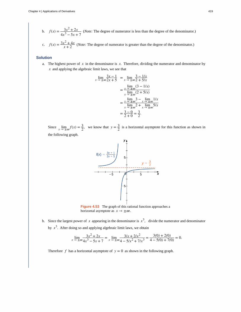
b. f (x) = 3x2 + 2x4x3 − 5x + 7
(Note: The degree of numerator is less than the degree of the denominator.)
c. f (x) = 3x2 + 4xx + 2 (Note: The degree of numerator is greater than the degree of the denominator.)
Solution
a. The highest power of x in the denominator is x. Therefore, dividing the numerator and denominator by
x and applying the algebraic limit laws, we see that
limx → ±∞3x − 12x + 5 = limx → ±∞
3 − 1/x2 + 5/x
=limx → ±∞(3 − 1/x)limx → ±∞(2 + 5/x)
=limx → ±∞3 − limx → ±∞1/xlimx → ±∞2 + limx → ±∞5/x
= 3 − 02 + 0 = 3
2.
Since limx → ±∞ f (x) = 32, we know that y = 3
2 is a horizontal asymptote for this function as shown in
the following graph.
Figure 4.53 The graph of this rational function approaches ahorizontal asymptote as x → ±∞.
b. Since the largest power of x appearing in the denominator is x3, divide the numerator and denominator
by x3. After doing so and applying algebraic limit laws, we obtain
limx → ±∞3x2 + 2x
4x3 − 5x + 7= limx → ±∞
3/x + 2/x2
4 − 5/x2 + 7/x3 = 3(0) + 2(0)4 − 5(0) + 7(0) = 0.
Therefore f has a horizontal asymptote of y = 0 as shown in the following graph.
Chapter 4 | Applications of Derivatives 419
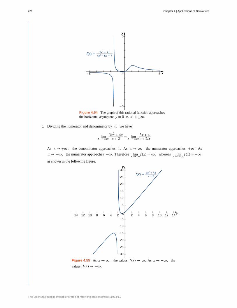
Figure 4.54 The graph of this rational function approachesthe horizontal asymptote y = 0 as x → ±∞.
c. Dividing the numerator and denominator by x, we have
limx → ±∞3x2 + 4x
x + 2 = limx → ±∞3x + 41 + 2/x.
As x → ±∞, the denominator approaches 1. As x → ∞, the numerator approaches +∞. As
x → −∞, the numerator approaches −∞. Therefore limx → ∞ f (x) = ∞, whereas limx → −∞ f (x) = −∞
as shown in the following figure.
Figure 4.55 As x → ∞, the values f (x) → ∞. As x → −∞, the
values f (x) → −∞.
420 Chapter 4 | Applications of Derivatives
This OpenStax book is available for free at http://cnx.org/content/col11964/1.2
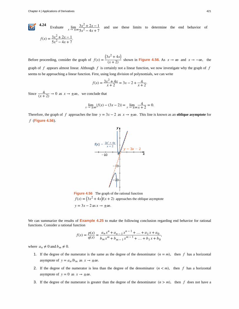
4.24Evaluate limx → ±∞
3x2 + 2x − 15x2 − 4x + 7
and use these limits to determine the end behavior of
f (x) = 3x2 + 2x − 15x2 − 4x + 7
.
Before proceeding, consider the graph of f (x) =⎛⎝3x2 + 4x⎞
⎠(x + 2) shown in Figure 4.56. As x → ∞ and x → −∞, the
graph of f appears almost linear. Although f is certainly not a linear function, we now investigate why the graph of fseems to be approaching a linear function. First, using long division of polynomials, we can write
f (x) = 3x2 + 4xx + 2 = 3x − 2 + 4
x + 2.
Since 4(x + 2) → 0 as x → ±∞, we conclude that
limx → ±∞⎛⎝ f (x) − (3x − 2)⎞
⎠ = limx → ±∞4
x + 2 = 0.
Therefore, the graph of f approaches the line y = 3x − 2 as x → ±∞. This line is known as an oblique asymptote for
f (Figure 4.56).
Figure 4.56 The graph of the rational function
f (x) = ⎛⎝3x2 + 4x⎞
⎠/(x + 2) approaches the oblique asymptote
y = 3x − 2 as x → ±∞.
We can summarize the results of Example 4.25 to make the following conclusion regarding end behavior for rationalfunctions. Consider a rational function
f (x) = p(x)q(x) = an xn + an − 1 xn − 1 + … + a1 x + a0
bm xm + bm − 1 xm − 1 + … + b1 x + b0,
where an ≠ 0 and bm ≠ 0.
1. If the degree of the numerator is the same as the degree of the denominator (n = m), then f has a horizontal
asymptote of y = an /bm as x → ±∞.
2. If the degree of the numerator is less than the degree of the denominator (n < m), then f has a horizontal
asymptote of y = 0 as x → ±∞.
3. If the degree of the numerator is greater than the degree of the denominator (n > m), then f does not have a
Chapter 4 | Applications of Derivatives 421
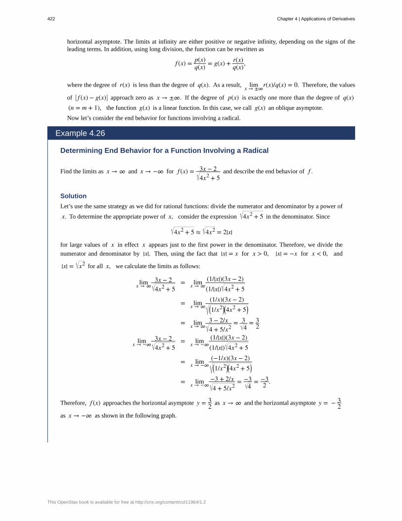
horizontal asymptote. The limits at infinity are either positive or negative infinity, depending on the signs of theleading terms. In addition, using long division, the function can be rewritten as
f (x) = p(x)q(x) = g(x) + r(x)
q(x),
where the degree of r(x) is less than the degree of q(x). As a result, limx → ±∞r(x)/q(x) = 0. Therefore, the values
of ⎡⎣ f (x) − g(x)⎤
⎦ approach zero as x → ±∞. If the degree of p(x) is exactly one more than the degree of q(x)(n = m + 1), the function g(x) is a linear function. In this case, we call g(x) an oblique asymptote.
Now let’s consider the end behavior for functions involving a radical.
Example 4.26
Determining End Behavior for a Function Involving a Radical
Find the limits as x → ∞ and x → −∞ for f (x) = 3x − 24x2 + 5
and describe the end behavior of f .
Solution
Let’s use the same strategy as we did for rational functions: divide the numerator and denominator by a power of
x. To determine the appropriate power of x, consider the expression 4x2 + 5 in the denominator. Since
4x2 + 5 ≈ 4x2 = 2|x|
for large values of x in effect x appears just to the first power in the denominator. Therefore, we divide the
numerator and denominator by |x|. Then, using the fact that |x| = x for x > 0, |x| = −x for x < 0, and
|x| = x2 for all x, we calculate the limits as follows:
limx → ∞3x − 24x2 + 5
= limx → ∞(1/|x|)(3x − 2)(1/|x|) 4x2 + 5
= limx → ∞(1/x)(3x − 2)⎛⎝1/x2⎞
⎠⎛⎝4x2 + 5⎞
⎠
= limx → ∞3 − 2/x4 + 5/x2
= 34
= 32
limx → −∞3x − 24x2 + 5
= limx → −∞(1/|x|)(3x − 2)(1/|x|) 4x2 + 5
= limx → −∞(−1/x)(3x − 2)⎛⎝1/x2⎞
⎠⎛⎝4x2 + 5⎞
⎠
= limx → −∞−3 + 2/x4 + 5/x2
= −34
= −32 .
Therefore, f (x) approaches the horizontal asymptote y = 32 as x → ∞ and the horizontal asymptote y = − 3
2as x → −∞ as shown in the following graph.
422 Chapter 4 | Applications of Derivatives
This OpenStax book is available for free at http://cnx.org/content/col11964/1.2
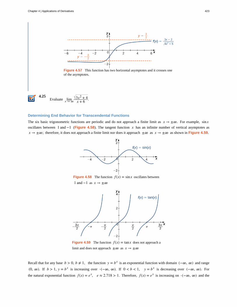
4.25
Figure 4.57 This function has two horizontal asymptotes and it crosses oneof the asymptotes.
Evaluate limx → ∞3x2 + 4x + 6 .
Determining End Behavior for Transcendental Functions
The six basic trigonometric functions are periodic and do not approach a finite limit as x → ±∞. For example, sinxoscillates between 1 and −1 (Figure 4.58). The tangent function x has an infinite number of vertical asymptotes as
x → ±∞; therefore, it does not approach a finite limit nor does it approach ±∞ as x → ±∞ as shown in Figure 4.59.
Figure 4.58 The function f (x) = sinx oscillates between
1 and −1 as x → ±∞
Figure 4.59 The function f (x) = tanx does not approach a
limit and does not approach ±∞ as x → ±∞
Recall that for any base b > 0, b ≠ 1, the function y = bx is an exponential function with domain (−∞, ∞) and range
(0, ∞). If b > 1, y = bx is increasing over `(−∞, ∞). If 0 < b < 1, y = bx is decreasing over (−∞, ∞). For
the natural exponential function f (x) = ex, e ≈ 2.718 > 1. Therefore, f (x) = ex is increasing on `(−∞, ∞) and the
Chapter 4 | Applications of Derivatives 423
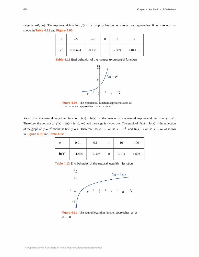
range is `(0, ∞). The exponential function f (x) = ex approaches ∞ as x → ∞ and approaches 0 as x → −∞ as
shown in Table 4.11 and Figure 4.60.
x −5 −2 0 2 5
ex 0.00674 0.135 1 7.389 148.413
Table 4.11 End behavior of the natural exponential function
Figure 4.60 The exponential function approaches zero asx → −∞ and approaches ∞ as x → ∞.
Recall that the natural logarithm function f (x) = ln(x) is the inverse of the natural exponential function y = ex.Therefore, the domain of f (x) = ln(x) is (0, ∞) and the range is (−∞, ∞). The graph of f (x) = ln(x) is the reflection
of the graph of y = ex about the line y = x. Therefore, ln(x) → −∞ as x → 0+ and ln(x) → ∞ as x → ∞ as shown
in Figure 4.61 and Table 4.12.
x 0.01 0.1 1 10 100
ln(x) −4.605 −2.303 0 2.303 4.605
Table 4.12 End behavior of the natural logarithm function
Figure 4.61 The natural logarithm function approaches ∞ as
x → ∞.
424 Chapter 4 | Applications of Derivatives
This OpenStax book is available for free at http://cnx.org/content/col11964/1.2
4.26
Example 4.27
Determining End Behavior for a Transcendental Function
Find the limits as x → ∞ and x → −∞ for f (x) = (2 + 3ex)(7 − 5ex) and describe the end behavior of f .
Solution
To find the limit as x → ∞, divide the numerator and denominator by ex :
limx → ∞ f (x) = limx → ∞2 + 3ex
7 − 5ex
= limx → ∞(2/ex) + 3(7/ex) − 5
.
As shown in Figure 4.60, ex → ∞ as x → ∞. Therefore,
limx → ∞2ex = 0 = limx → ∞
7ex.
We conclude that limx → ∞ f (x) = − 35, and the graph of f approaches the horizontal asymptote y = − 3
5as x → ∞. To find the limit as x → −∞, use the fact that ex → 0 as x → −∞ to conclude that
limx → ∞ f (x) = 27, and therefore the graph of approaches the horizontal asymptote y = 2
7 as x → −∞.
Find the limits as x → ∞ and x → −∞ for f (x) = (3ex − 4)(5ex + 2).
Guidelines for Drawing the Graph of a FunctionWe now have enough analytical tools to draw graphs of a wide variety of algebraic and transcendental functions. Beforeshowing how to graph specific functions, let’s look at a general strategy to use when graphing any function.
Problem-Solving Strategy: Drawing the Graph of a Function
Given a function f , use the following steps to sketch a graph of f :
1. Determine the domain of the function.
2. Locate the x - and y -intercepts.
3. Evaluate limx → ∞ f (x) and limx → −∞ f (x) to determine the end behavior. If either of these limits is a finite number
L, then y = L is a horizontal asymptote. If either of these limits is ∞ or −∞, determine whether f has
an oblique asymptote. If f is a rational function such that f (x) = p(x)q(x) , where the degree of the numerator
is greater than the degree of the denominator, then f can be written as
f (x) = p(x)q(x) = g(x) + r(x)
q(x),
where the degree of r(x) is less than the degree of q(x). The values of f (x) approach the values of g(x) as
Chapter 4 | Applications of Derivatives 425
x → ±∞. If g(x) is a linear function, it is known as an oblique asymptote.
4. Determine whether f has any vertical asymptotes.
5. Calculate f ′. Find all critical points and determine the intervals where f is increasing and where f is
decreasing. Determine whether f has any local extrema.
6. Calculate f ″. Determine the intervals where f is concave up and where f is concave down. Use this
information to determine whether f has any inflection points. The second derivative can also be used as an
alternate means to determine or verify that f has a local extremum at a critical point.
Now let’s use this strategy to graph several different functions. We start by graphing a polynomial function.
Example 4.28
Sketching a Graph of a Polynomial
Sketch a graph of f (x) = (x − 1)2 (x + 2).
Solution
Step 1. Since f is a polynomial, the domain is the set of all real numbers.
Step 2. When x = 0, f (x) = 2. Therefore, the y -intercept is (0, 2). To find the x -intercepts, we need to solve
the equation (x − 1)2 (x + 2) = 0, gives us the x -intercepts (1, 0) and (−2, 0)
Step 3. We need to evaluate the end behavior of f . As x → ∞, (x − 1)2 → ∞ and (x + 2) → ∞. Therefore,
limx → ∞ f (x) = ∞. As x → −∞, (x − 1)2 → ∞ and (x + 2) → −∞. Therefore, limx → −∞ f (x) = −∞. To get
even more information about the end behavior of f , we can multiply the factors of f . When doing so, we see
that
f (x) = (x − 1)2 (x + 2) = x3 − 3x + 2.
Since the leading term of f is x3, we conclude that f behaves like y = x3 as x → ±∞.
Step 4. Since f is a polynomial function, it does not have any vertical asymptotes.
Step 5. The first derivative of f is
f ′ (x) = 3x2 − 3.
Therefore, f has two critical points: x = 1, −1. Divide the interval (−∞, ∞) into the three smaller intervals:
(−∞, −1), (−1, 1), and (1, ∞). Then, choose test points x = −2, x = 0, and x = 2 from these
intervals and evaluate the sign of f ′ (x) at each of these test points, as shown in the following table.
426 Chapter 4 | Applications of Derivatives
This OpenStax book is available for free at http://cnx.org/content/col11964/1.2
Interval TestPoint
Sign of Derivative
f′(x) = 3x2 − 3 = 3(x − 1)(x + 1)
Conclusion
(−∞, −1) x = −2 (+)(−)(−) = + f is
increasing.
(−1, 1) x = 0 (+)(−)(+) = − f is
decreasing.
(1, ∞) x = 2 (+)(+)(+) = + f is
increasing.
From the table, we see that f has a local maximum at x = −1 and a local minimum at x = 1. Evaluating
f (x) at those two points, we find that the local maximum value is f (−1) = 4 and the local minimum value is
f (1) = 0.
Step 6. The second derivative of f is
f ″(x) = 6x.
The second derivative is zero at x = 0. Therefore, to determine the concavity of f , divide the interval
(−∞, ∞) into the smaller intervals (−∞, 0) and (0, ∞), and choose test points x = −1 and x = 1 to
determine the concavity of f on each of these smaller intervals as shown in the following table.
Interval Test Point Sign of f″(x) = 6x Conclusion
(−∞, 0) x = −1 − f is concave down.
(0, ∞) x = 1 + f is concave up.
We note that the information in the preceding table confirms the fact, found in step 5, that f has a local
maximum at x = −1 and a local minimum at x = 1. In addition, the information found in step 5 —namely, fhas a local maximum at x = −1 and a local minimum at x = 1, and f ′ (x) = 0 at those points—combined
with the fact that f ″ changes sign only at x = 0 confirms the results found in step 6 on the concavity of f .
Combining this information, we arrive at the graph of f (x) = (x − 1)2 (x + 2) shown in the following graph.
Chapter 4 | Applications of Derivatives 427
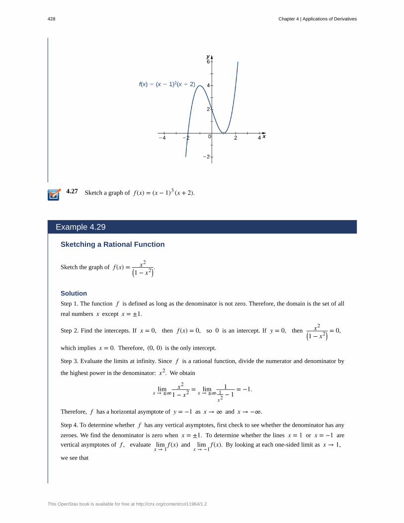
4.27 Sketch a graph of f (x) = (x − 1)3 (x + 2).
Example 4.29
Sketching a Rational Function
Sketch the graph of f (x) = x2⎛⎝1 − x2⎞
⎠.
Solution
Step 1. The function f is defined as long as the denominator is not zero. Therefore, the domain is the set of all
real numbers x except x = ±1.
Step 2. Find the intercepts. If x = 0, then f (x) = 0, so 0 is an intercept. If y = 0, then x2⎛⎝1 − x2⎞
⎠= 0,
which implies x = 0. Therefore, (0, 0) is the only intercept.
Step 3. Evaluate the limits at infinity. Since f is a rational function, divide the numerator and denominator by
the highest power in the denominator: x2. We obtain
limx → ±∞x2
1 − x2 = limx → ±∞1
1x2 − 1
= −1.
Therefore, f has a horizontal asymptote of y = −1 as x → ∞ and x → −∞.
Step 4. To determine whether f has any vertical asymptotes, first check to see whether the denominator has any
zeroes. We find the denominator is zero when x = ±1. To determine whether the lines x = 1 or x = −1 are
vertical asymptotes of f , evaluate limx → 1
f (x) and limx → −1
f (x). By looking at each one-sided limit as x → 1,
we see that
428 Chapter 4 | Applications of Derivatives
This OpenStax book is available for free at http://cnx.org/content/col11964/1.2
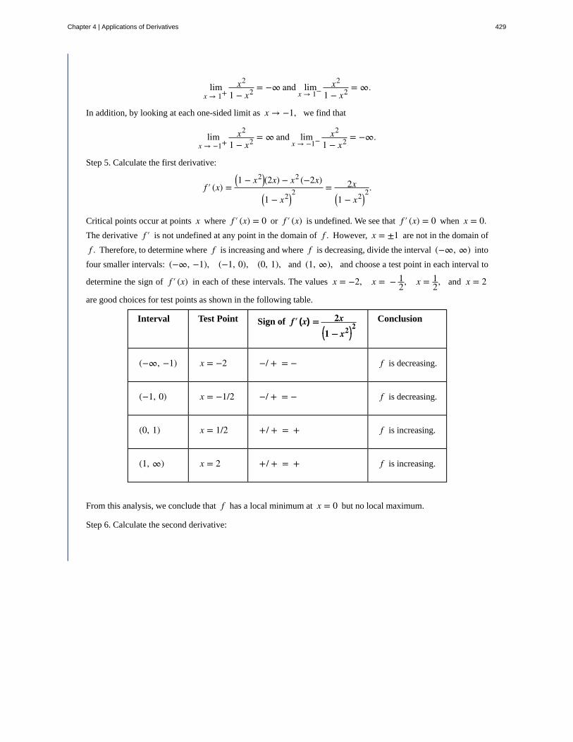
limx → 1+
x2
1 − x2 = −∞ and limx → 1−
x2
1 − x2 = ∞.
In addition, by looking at each one-sided limit as x → −1, we find that
limx → −1+
x2
1 − x2 = ∞ and limx → −1−
x2
1 − x2 = −∞.
Step 5. Calculate the first derivative:
f ′ (x) =⎛⎝1 − x2⎞
⎠(2x) − x2 (−2x)⎛⎝1 − x2⎞
⎠2 = 2x
⎛⎝1 − x2⎞
⎠2.
Critical points occur at points x where f ′ (x) = 0 or f ′ (x) is undefined. We see that f ′ (x) = 0 when x = 0.The derivative f ′ is not undefined at any point in the domain of f . However, x = ±1 are not in the domain of
f . Therefore, to determine where f is increasing and where f is decreasing, divide the interval (−∞, ∞) into
four smaller intervals: (−∞, −1), (−1, 0), (0, 1), and (1, ∞), and choose a test point in each interval to
determine the sign of f ′ (x) in each of these intervals. The values x = −2, x = − 12, x = 1
2, and x = 2
are good choices for test points as shown in the following table.
Interval Test Point Sign of f′ (x) = 2x⎛⎝1 − x2⎞
⎠2
Conclusion
(−∞, −1) x = −2 −/ + = − f is decreasing.
(−1, 0) x = −1/2 −/ + = − f is decreasing.
(0, 1) x = 1/2 +/ + = + f is increasing.
(1, ∞) x = 2 +/ + = + f is increasing.
From this analysis, we conclude that f has a local minimum at x = 0 but no local maximum.
Step 6. Calculate the second derivative:
Chapter 4 | Applications of Derivatives 429
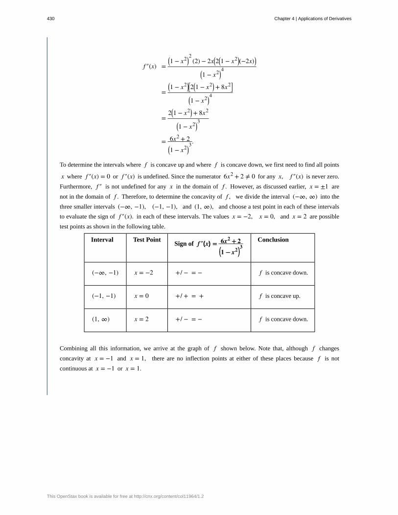
f ″(x) =⎛⎝1 − x2⎞
⎠2
(2) − 2x⎛⎝2
⎛⎝1 − x2⎞
⎠(−2x)⎞⎠
⎛⎝1 − x2⎞
⎠4
=⎛⎝1 − x2⎞
⎠⎡⎣2
⎛⎝1 − x2⎞
⎠ + 8x2⎤⎦
⎛⎝1 − x2⎞
⎠4
=2⎛
⎝1 − x2⎞⎠ + 8x2
⎛⎝1 − x2⎞
⎠3
= 6x2 + 2⎛⎝1 − x2⎞
⎠3.
To determine the intervals where f is concave up and where f is concave down, we first need to find all points
x where f ″(x) = 0 or f ″(x) is undefined. Since the numerator 6x2 + 2 ≠ 0 for any x, f ″(x) is never zero.
Furthermore, f ″ is not undefined for any x in the domain of f . However, as discussed earlier, x = ±1 are
not in the domain of f . Therefore, to determine the concavity of f , we divide the interval (−∞, ∞) into the
three smaller intervals (−∞, −1), (−1, −1), and (1, ∞), and choose a test point in each of these intervals
to evaluate the sign of f ″(x). in each of these intervals. The values x = −2, x = 0, and x = 2 are possible
test points as shown in the following table.
Interval Test PointSign of f″(x) = 6x2 + 2
⎛⎝1 − x2⎞
⎠3
Conclusion
(−∞, −1) x = −2 +/ − = − f is concave down.
(−1, −1) x = 0 +/ + = + f is concave up.
(1, ∞) x = 2 +/ − = − f is concave down.
Combining all this information, we arrive at the graph of f shown below. Note that, although f changes
concavity at x = −1 and x = 1, there are no inflection points at either of these places because f is not
continuous at x = −1 or x = 1.
430 Chapter 4 | Applications of Derivatives
This OpenStax book is available for free at http://cnx.org/content/col11964/1.2
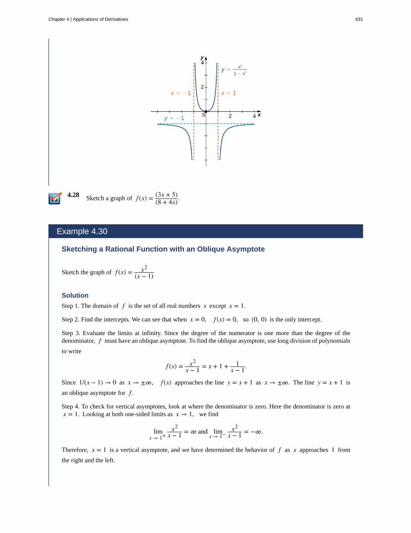
4.28 Sketch a graph of f (x) = (3x + 5)(8 + 4x).
Example 4.30
Sketching a Rational Function with an Oblique Asymptote
Sketch the graph of f (x) = x2
(x − 1)
Solution
Step 1. The domain of f is the set of all real numbers x except x = 1.
Step 2. Find the intercepts. We can see that when x = 0, f (x) = 0, so (0, 0) is the only intercept.
Step 3. Evaluate the limits at infinity. Since the degree of the numerator is one more than the degree of thedenominator, f must have an oblique asymptote. To find the oblique asymptote, use long division of polynomials
to write
f (x) = x2
x − 1 = x + 1 + 1x − 1.
Since 1/(x − 1) → 0 as x → ±∞, f (x) approaches the line y = x + 1 as x → ±∞. The line y = x + 1 is
an oblique asymptote for f .
Step 4. To check for vertical asymptotes, look at where the denominator is zero. Here the denominator is zero atx = 1. Looking at both one-sided limits as x → 1, we find
limx → 1+
x2
x − 1 = ∞ and limx → 1−
x2
x − 1 = −∞.
Therefore, x = 1 is a vertical asymptote, and we have determined the behavior of f as x approaches 1 from
the right and the left.
Chapter 4 | Applications of Derivatives 431
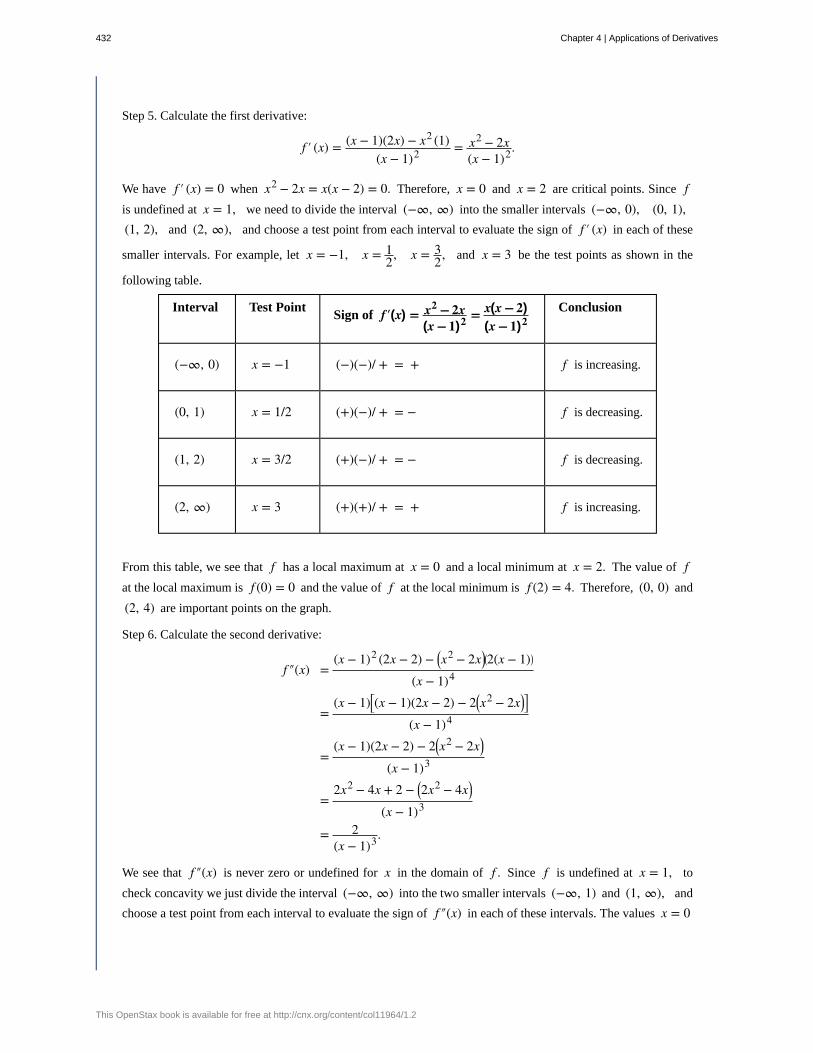
Step 5. Calculate the first derivative:
f ′ (x) = (x − 1)(2x) − x2 (1)(x − 1)2 = x2 − 2x
(x − 1)2.
We have f ′ (x) = 0 when x2 − 2x = x(x − 2) = 0. Therefore, x = 0 and x = 2 are critical points. Since fis undefined at x = 1, we need to divide the interval (−∞, ∞) into the smaller intervals (−∞, 0), (0, 1),(1, 2), and (2, ∞), and choose a test point from each interval to evaluate the sign of f ′ (x) in each of these
smaller intervals. For example, let x = −1, x = 12, x = 3
2, and x = 3 be the test points as shown in the
following table.
Interval Test PointSign of f′(x) = x2 − 2x
(x − 1)2 = x(x − 2)(x − 1)2
Conclusion
(−∞, 0) x = −1 (−)(−)/ + = + f is increasing.
(0, 1) x = 1/2 (+)(−)/ + = − f is decreasing.
(1, 2) x = 3/2 (+)(−)/ + = − f is decreasing.
(2, ∞) x = 3 (+)(+)/ + = + f is increasing.
From this table, we see that f has a local maximum at x = 0 and a local minimum at x = 2. The value of fat the local maximum is f (0) = 0 and the value of f at the local minimum is f (2) = 4. Therefore, (0, 0) and
(2, 4) are important points on the graph.
Step 6. Calculate the second derivative:
f ″(x) =(x − 1)2 (2x − 2) − ⎛
⎝x2 − 2x⎞⎠
⎛⎝2(x − 1)⎞
⎠
(x − 1)4
=(x − 1)⎡
⎣(x − 1)(2x − 2) − 2⎛⎝x2 − 2x⎞
⎠⎤⎦
(x − 1)4
=(x − 1)(2x − 2) − 2⎛
⎝x2 − 2x⎞⎠
(x − 1)3
=2x2 − 4x + 2 − ⎛
⎝2x2 − 4x⎞⎠
(x − 1)3
= 2(x − 1)3.
We see that f ″(x) is never zero or undefined for x in the domain of f . Since f is undefined at x = 1, to
check concavity we just divide the interval (−∞, ∞) into the two smaller intervals (−∞, 1) and (1, ∞), and
choose a test point from each interval to evaluate the sign of f ″(x) in each of these intervals. The values x = 0
432 Chapter 4 | Applications of Derivatives
This OpenStax book is available for free at http://cnx.org/content/col11964/1.2
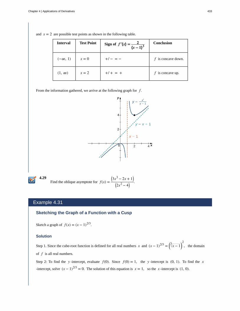
4.29
and x = 2 are possible test points as shown in the following table.
Interval Test Point Sign of f″(x) = 2(x − 1)3
Conclusion
(−∞, 1) x = 0 +/ − = − f is concave down.
(1, ∞) x = 2 +/ + = + f is concave up.
From the information gathered, we arrive at the following graph for f .
Find the oblique asymptote for f (x) =⎛⎝3x3 − 2x + 1⎞
⎠⎛⎝2x2 − 4⎞
⎠.
Example 4.31
Sketching the Graph of a Function with a Cusp
Sketch a graph of f (x) = (x − 1)2/3.
Solution
Step 1. Since the cube-root function is defined for all real numbers x and (x − 1)2/3 = ⎛⎝ x − 13 ⎞
⎠2, the domain
of f is all real numbers.
Step 2: To find the y -intercept, evaluate f (0). Since f (0) = 1, the y -intercept is (0, 1). To find the x
-intercept, solve (x − 1)2/3 = 0. The solution of this equation is x = 1, so the x -intercept is (1, 0).
Chapter 4 | Applications of Derivatives 433
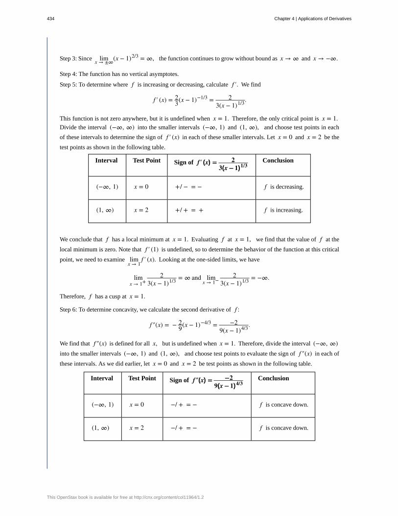
Step 3: Since limx → ±∞(x − 1)2/3 = ∞, the function continues to grow without bound as x → ∞ and x → −∞.
Step 4: The function has no vertical asymptotes.
Step 5: To determine where f is increasing or decreasing, calculate f ′. We find
f ′ (x) = 23(x − 1)−1/3 = 2
3(x − 1)1/3.
This function is not zero anywhere, but it is undefined when x = 1. Therefore, the only critical point is x = 1.Divide the interval (−∞, ∞) into the smaller intervals (−∞, 1) and (1, ∞), and choose test points in each
of these intervals to determine the sign of f ′ (x) in each of these smaller intervals. Let x = 0 and x = 2 be the
test points as shown in the following table.
Interval Test Point Sign of f′ (x) = 23(x − 1)1/3
Conclusion
(−∞, 1) x = 0 +/ − = − f is decreasing.
(1, ∞) x = 2 +/ + = + f is increasing.
We conclude that f has a local minimum at x = 1. Evaluating f at x = 1, we find that the value of f at the
local minimum is zero. Note that f ′ (1) is undefined, so to determine the behavior of the function at this critical
point, we need to examine limx → 1
f ′ (x). Looking at the one-sided limits, we have
limx → 1+
23(x − 1)1/3 = ∞ and lim
x → 1−2
3(x − 1)1/3 = −∞.
Therefore, f has a cusp at x = 1.
Step 6: To determine concavity, we calculate the second derivative of f :
f ″(x) = − 29(x − 1)−4/3 = −2
9(x − 1)4/3.
We find that f ″(x) is defined for all x, but is undefined when x = 1. Therefore, divide the interval (−∞, ∞)into the smaller intervals (−∞, 1) and (1, ∞), and choose test points to evaluate the sign of f ″(x) in each of
these intervals. As we did earlier, let x = 0 and x = 2 be test points as shown in the following table.
Interval Test Point Sign of f″(x) = −29(x − 1)4/3
Conclusion
(−∞, 1) x = 0 −/ + = − f is concave down.
(1, ∞) x = 2 −/ + = − f is concave down.
434 Chapter 4 | Applications of Derivatives
This OpenStax book is available for free at http://cnx.org/content/col11964/1.2
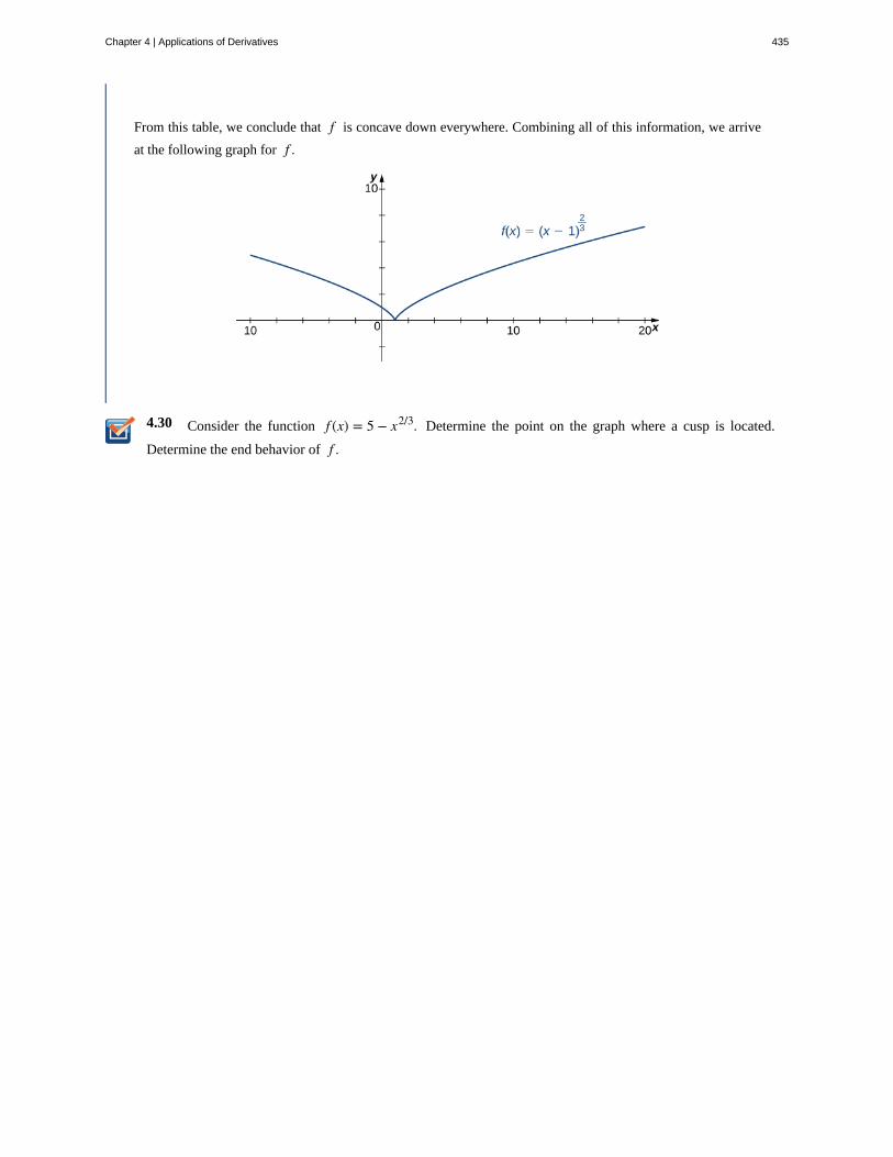
4.30
From this table, we conclude that f is concave down everywhere. Combining all of this information, we arrive
at the following graph for f .
Consider the function f (x) = 5 − x2/3. Determine the point on the graph where a cusp is located.
Determine the end behavior of f .
Chapter 4 | Applications of Derivatives 435
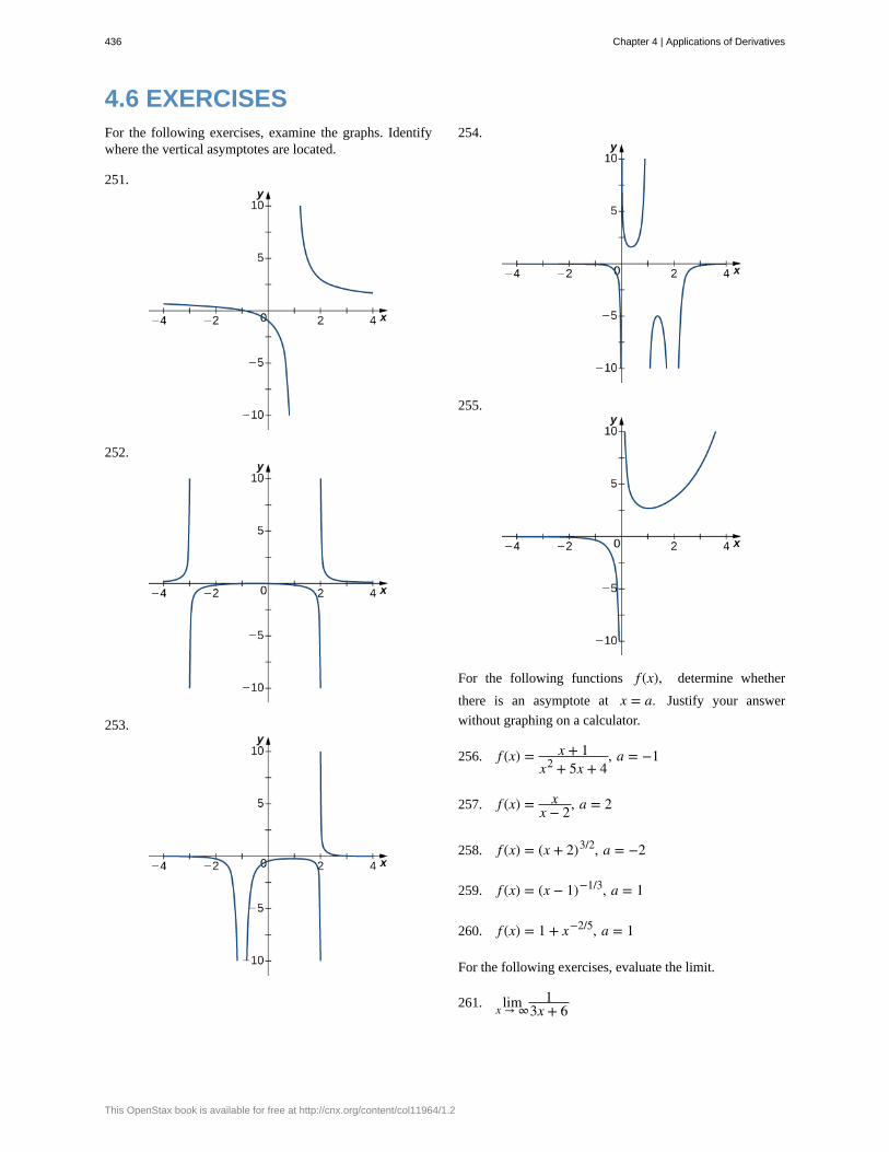
4.6 EXERCISESFor the following exercises, examine the graphs. Identifywhere the vertical asymptotes are located.
251.
252.
253.
254.
255.
For the following functions f (x), determine whether
there is an asymptote at x = a. Justify your answer
without graphing on a calculator.
256. f (x) = x + 1x2 + 5x + 4
, a = −1
257. f (x) = xx − 2, a = 2
258. f (x) = (x + 2)3/2, a = −2
259. f (x) = (x − 1)−1/3, a = 1
260. f (x) = 1 + x−2/5, a = 1
For the following exercises, evaluate the limit.
261. limx → ∞1
3x + 6
436 Chapter 4 | Applications of Derivatives
This OpenStax book is available for free at http://cnx.org/content/col11964/1.2
262. limx → ∞2x − 5
4x
263. limx → ∞x2 − 2x + 5
x + 2
264. limx → −∞3x3 − 2x
x2 + 2x + 8
265. limx → −∞x4 − 4x3 + 1
2 − 2x2 − 7x4
266. limx → ∞3x
x2 + 1
267. limx → −∞4x2 − 1x + 2
268. limx → ∞4x
x2 − 1
269. limx → −∞4x
x2 − 1
270. limx → ∞2 x
x − x + 1
For the following exercises, find the horizontal and verticalasymptotes.
271. f (x) = x − 9x
272. f (x) = 11 − x2
273. f (x) = x3
4 − x2
274. f (x) = x2 + 3x2 + 1
275. f (x) = sin(x)sin(2x)
276. f (x) = cosx + cos(3x) + cos(5x)
277. f (x) = xsin(x)x2 − 1
278. f (x) = xsin(x)
279. f (x) = 1x3 + x2
280. f (x) = 1x − 1 − 2x
281. f (x) = x3 + 1x3 − 1
282. f (x) = sinx + cosxsinx − cosx
283. f (x) = x − sinx
284. f (x) = 1x − x
For the following exercises, construct a function f (x) that
has the given asymptotes.
285. x = 1 and y = 2
286. x = 1 and y = 0
287. y = 4, x = −1
288. x = 0
For the following exercises, graph the function on agraphing calculator on the window x = ⎡
⎣−5, 5⎤⎦ and
estimate the horizontal asymptote or limit. Then, calculatethe actual horizontal asymptote or limit.
289. [T] f (x) = 1x + 10
290. [T] f (x) = x + 1x2 + 7x + 6
291. [T] limx → −∞x2 + 10x + 25
292. [T] limx → −∞x + 2
x2 + 7x + 6
293. [T] limx → ∞3x + 2x + 5
For the following exercises, draw a graph of the functionswithout using a calculator. Be sure to notice all importantfeatures of the graph: local maxima and minima, inflectionpoints, and asymptotic behavior.
294. y = 3x2 + 2x + 4
295. y = x3 − 3x2 + 4
296. y = 2x + 1x2 + 6x + 5
297. y = x3 + 4x2 + 3x3x + 9
Chapter 4 | Applications of Derivatives 437
298. y = x2 + x − 2x2 − 3x − 4
299. y = x2 − 5x + 4
300. y = 2x 16 − x2
301. y = cosxx , on x = [−2π, 2π]
302. y = ex − x3
303. y = x tanx, x = [−π, π]
304. y = x ln(x), x > 0
305. y = x2 sin(x), x = [−2π, 2π]
306. For f (x) = P(x)Q(x) to have an asymptote at y = 2
then the polynomials P(x) and Q(x) must have what
relation?
307. For f (x) = P(x)Q(x) to have an asymptote at x = 0,
then the polynomials P(x) and Q(x). must have what
relation?
308. If f ′ (x) has asymptotes at y = 3 and x = 1, then
f (x) has what asymptotes?
309. Both f (x) = 1(x − 1) and g(x) = 1
(x − 1)2 have
asymptotes at x = 1 and y = 0. What is the most obvious
difference between these two functions?
310. True or false: Every ratio of polynomials has verticalasymptotes.
438 Chapter 4 | Applications of Derivatives
This OpenStax book is available for free at http://cnx.org/content/col11964/1.2
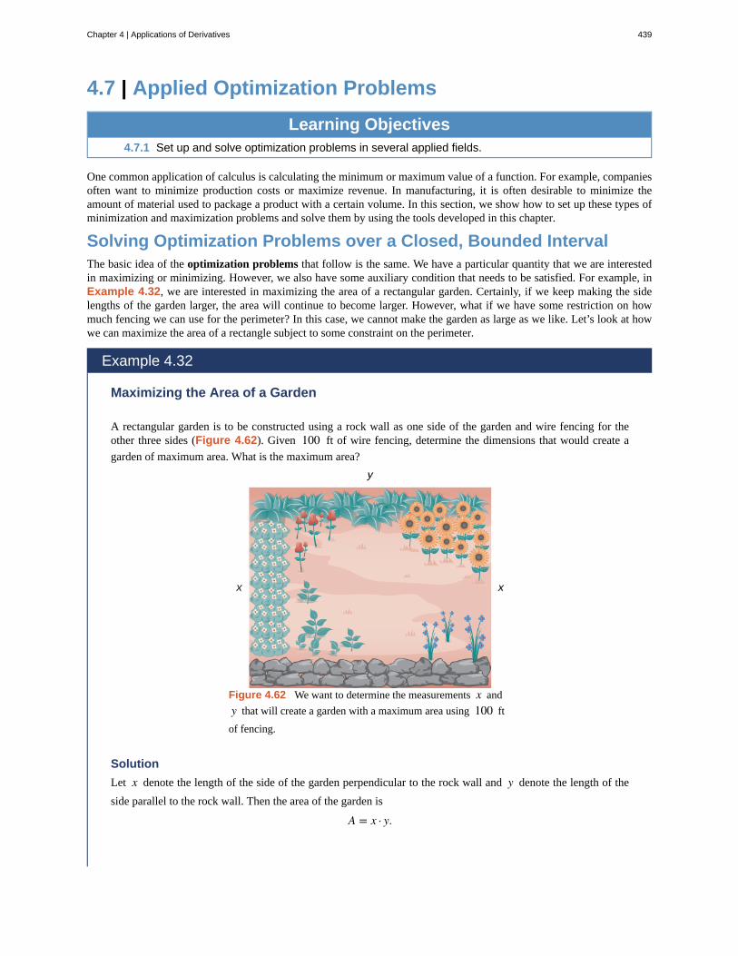
4.7 | Applied Optimization Problems
Learning Objectives4.7.1 Set up and solve optimization problems in several applied fields.
One common application of calculus is calculating the minimum or maximum value of a function. For example, companiesoften want to minimize production costs or maximize revenue. In manufacturing, it is often desirable to minimize theamount of material used to package a product with a certain volume. In this section, we show how to set up these types ofminimization and maximization problems and solve them by using the tools developed in this chapter.
Solving Optimization Problems over a Closed, Bounded IntervalThe basic idea of the optimization problems that follow is the same. We have a particular quantity that we are interestedin maximizing or minimizing. However, we also have some auxiliary condition that needs to be satisfied. For example, inExample 4.32, we are interested in maximizing the area of a rectangular garden. Certainly, if we keep making the sidelengths of the garden larger, the area will continue to become larger. However, what if we have some restriction on howmuch fencing we can use for the perimeter? In this case, we cannot make the garden as large as we like. Let’s look at howwe can maximize the area of a rectangle subject to some constraint on the perimeter.
Example 4.32
Maximizing the Area of a Garden
A rectangular garden is to be constructed using a rock wall as one side of the garden and wire fencing for theother three sides (Figure 4.62). Given 100 ft of wire fencing, determine the dimensions that would create a
garden of maximum area. What is the maximum area?
Figure 4.62 We want to determine the measurements x and
y that will create a garden with a maximum area using 100 ft
of fencing.
Solution
Let x denote the length of the side of the garden perpendicular to the rock wall and y denote the length of the
side parallel to the rock wall. Then the area of the garden is
A = x · y.
Chapter 4 | Applications of Derivatives 439
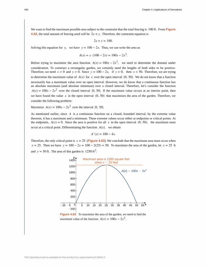
We want to find the maximum possible area subject to the constraint that the total fencing is 100 ft. From Figure
4.62, the total amount of fencing used will be 2x + y. Therefore, the constraint equation is
2x + y = 100.
Solving this equation for y, we have y = 100 − 2x. Thus, we can write the area as
A(x) = x · (100 − 2x) = 100x − 2x2.
Before trying to maximize the area function A(x) = 100x − 2x2, we need to determine the domain under
consideration. To construct a rectangular garden, we certainly need the lengths of both sides to be positive.Therefore, we need x > 0 and y > 0. Since y = 100 − 2x, if y > 0, then x < 50. Therefore, we are trying
to determine the maximum value of A(x) for x over the open interval (0, 50). We do not know that a function
necessarily has a maximum value over an open interval. However, we do know that a continuous function hasan absolute maximum (and absolute minimum) over a closed interval. Therefore, let’s consider the function
A(x) = 100x − 2x2 over the closed interval ⎡⎣0, 50⎤
⎦. If the maximum value occurs at an interior point, then
we have found the value x in the open interval (0, 50) that maximizes the area of the garden. Therefore, we
consider the following problem:
Maximize A(x) = 100x − 2x2 over the interval ⎡⎣0, 50⎤
⎦.
As mentioned earlier, since A is a continuous function on a closed, bounded interval, by the extreme value
theorem, it has a maximum and a minimum. These extreme values occur either at endpoints or critical points. Atthe endpoints, A(x) = 0. Since the area is positive for all x in the open interval (0, 50), the maximum must
occur at a critical point. Differentiating the function A(x), we obtain
A′ (x) = 100 − 4x.
Therefore, the only critical point is x = 25 (Figure 4.63). We conclude that the maximum area must occur when
x = 25. Then we have y = 100 − 2x = 100 − 2(25) = 50. To maximize the area of the garden, let x = 25 ft
and y = 50 ft. The area of this garden is 1250 ft2.
Figure 4.63 To maximize the area of the garden, we need to find the
maximum value of the function A(x) = 100x − 2x2.
440 Chapter 4 | Applications of Derivatives
This OpenStax book is available for free at http://cnx.org/content/col11964/1.2
4.31 Determine the maximum area if we want to make the same rectangular garden as in Figure 4.63, butwe have 200 ft of fencing.
Now let’s look at a general strategy for solving optimization problems similar to Example 4.32.
Problem-Solving Strategy: Solving Optimization Problems
1. Introduce all variables. If applicable, draw a figure and label all variables.
2. Determine which quantity is to be maximized or minimized, and for what range of values of the other variables(if this can be determined at this time).
3. Write a formula for the quantity to be maximized or minimized in terms of the variables. This formula mayinvolve more than one variable.
4. Write any equations relating the independent variables in the formula from step 3. Use these equations to
write the quantity to be maximized or minimized as a function of one variable.
5. Identify the domain of consideration for the function in step 4 based on the physical problem to be solved.
6. Locate the maximum or minimum value of the function from step 4. This step typically involves looking for
critical points and evaluating a function at endpoints.
Now let’s apply this strategy to maximize the volume of an open-top box given a constraint on the amount of material to beused.
Example 4.33
Maximizing the Volume of a Box
An open-top box is to be made from a 24 in. by 36 in. piece of cardboard by removing a square from each
corner of the box and folding up the flaps on each side. What size square should be cut out of each corner to geta box with the maximum volume?
Solution
Step 1: Let x be the side length of the square to be removed from each corner (Figure 4.64). Then, the
remaining four flaps can be folded up to form an open-top box. Let V be the volume of the resulting box.
Chapter 4 | Applications of Derivatives 441
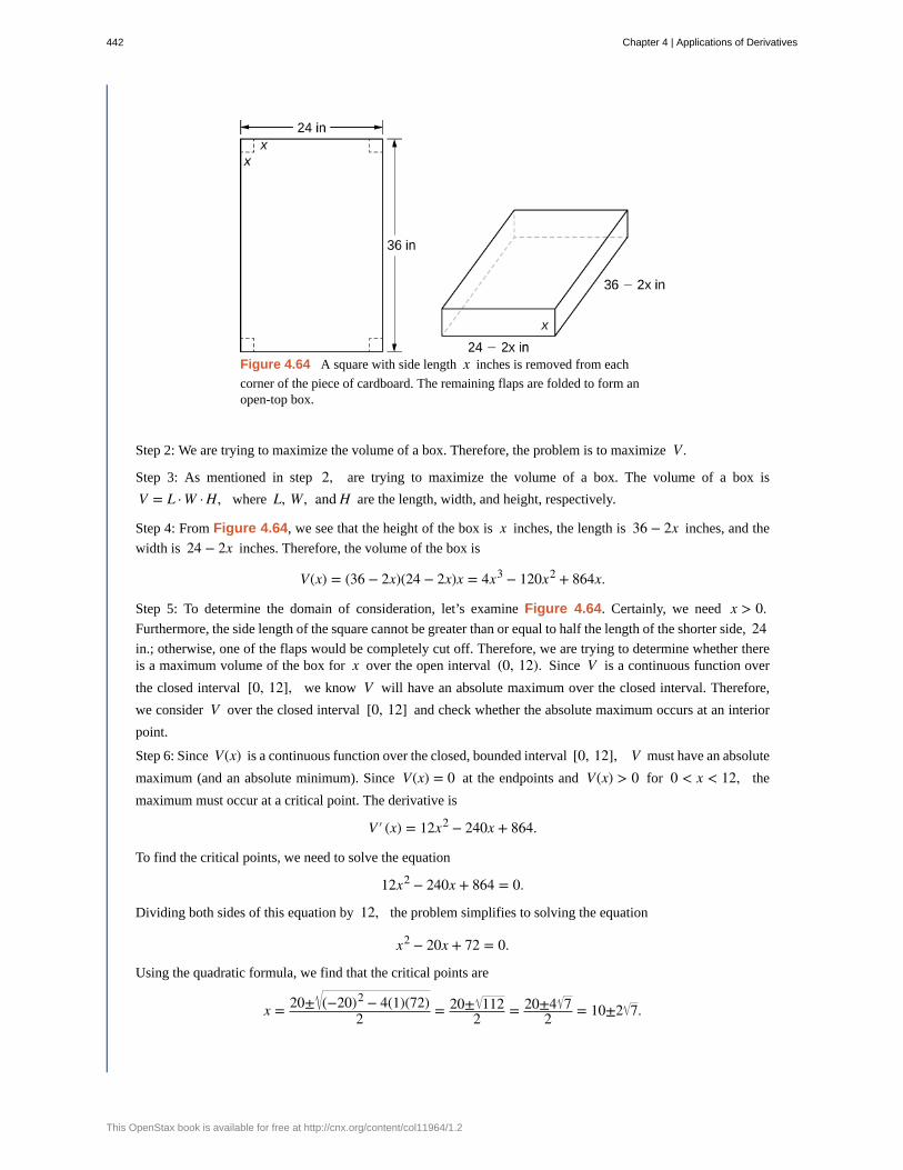
Figure 4.64 A square with side length x inches is removed from each
corner of the piece of cardboard. The remaining flaps are folded to form anopen-top box.
Step 2: We are trying to maximize the volume of a box. Therefore, the problem is to maximize V .
Step 3: As mentioned in step 2, are trying to maximize the volume of a box. The volume of a box is
V = L · W · H, where L, W, and H are the length, width, and height, respectively.
Step 4: From Figure 4.64, we see that the height of the box is x inches, the length is 36 − 2x inches, and the
width is 24 − 2x inches. Therefore, the volume of the box is
V(x) = (36 − 2x)(24 − 2x)x = 4x3 − 120x2 + 864x.
Step 5: To determine the domain of consideration, let’s examine Figure 4.64. Certainly, we need x > 0.Furthermore, the side length of the square cannot be greater than or equal to half the length of the shorter side, 24in.; otherwise, one of the flaps would be completely cut off. Therefore, we are trying to determine whether thereis a maximum volume of the box for x over the open interval (0, 12). Since V is a continuous function over
the closed interval [0, 12], we know V will have an absolute maximum over the closed interval. Therefore,
we consider V over the closed interval [0, 12] and check whether the absolute maximum occurs at an interior
point.
Step 6: Since V(x) is a continuous function over the closed, bounded interval [0, 12], V must have an absolute
maximum (and an absolute minimum). Since V(x) = 0 at the endpoints and V(x) > 0 for 0 < x < 12, the
maximum must occur at a critical point. The derivative is
V′ (x) = 12x2 − 240x + 864.
To find the critical points, we need to solve the equation
12x2 − 240x + 864 = 0.
Dividing both sides of this equation by 12, the problem simplifies to solving the equation
x2 − 20x + 72 = 0.
Using the quadratic formula, we find that the critical points are
x = 20± (−20)2 − 4(1)(72)2 = 20± 112
2 = 20±4 72 = 10±2 7.
442 Chapter 4 | Applications of Derivatives
This OpenStax book is available for free at http://cnx.org/content/col11964/1.2
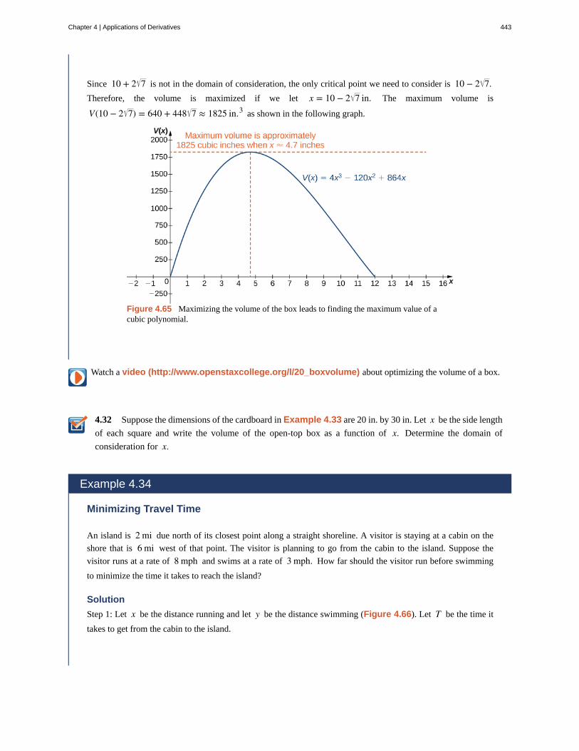
4.32
Since 10 + 2 7 is not in the domain of consideration, the only critical point we need to consider is 10 − 2 7.Therefore, the volume is maximized if we let x = 10 − 2 7 in. The maximum volume is
V(10 − 2 7) = 640 + 448 7 ≈ 1825 in.3 as shown in the following graph.
Figure 4.65 Maximizing the volume of the box leads to finding the maximum value of acubic polynomial.
Watch a video (http://www.openstaxcollege.org/l/20_boxvolume) about optimizing the volume of a box.
Suppose the dimensions of the cardboard in Example 4.33 are 20 in. by 30 in. Let x be the side length
of each square and write the volume of the open-top box as a function of x. Determine the domain of
consideration for x.
Example 4.34
Minimizing Travel Time
An island is 2 mi due north of its closest point along a straight shoreline. A visitor is staying at a cabin on the
shore that is 6 mi west of that point. The visitor is planning to go from the cabin to the island. Suppose the
visitor runs at a rate of 8 mph and swims at a rate of 3 mph. How far should the visitor run before swimming
to minimize the time it takes to reach the island?
Solution
Step 1: Let x be the distance running and let y be the distance swimming (Figure 4.66). Let T be the time it
takes to get from the cabin to the island.
Chapter 4 | Applications of Derivatives 443
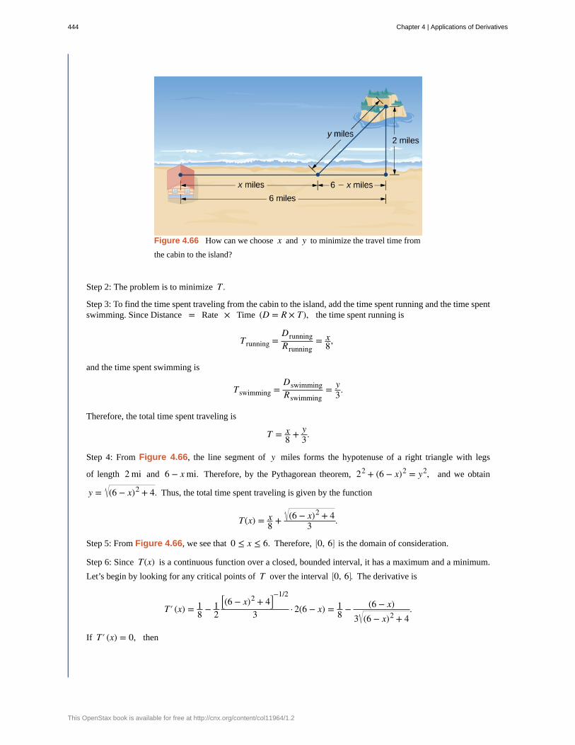
Figure 4.66 How can we choose x and y to minimize the travel time from
the cabin to the island?
Step 2: The problem is to minimize T .
Step 3: To find the time spent traveling from the cabin to the island, add the time spent running and the time spentswimming. Since Distance = Rate × Time (D = R × T), the time spent running is
Trunning =DrunningRrunning
= x8,
and the time spent swimming is
Tswimming =DswimmingRswimming
= y3.
Therefore, the total time spent traveling is
T = x8 + y
3.
Step 4: From Figure 4.66, the line segment of y miles forms the hypotenuse of a right triangle with legs
of length 2 mi and 6 − x mi. Therefore, by the Pythagorean theorem, 22 + (6 − x)2 = y2, and we obtain
y = (6 − x)2 + 4. Thus, the total time spent traveling is given by the function
T(x) = x8 + (6 − x)2 + 4
3 .
Step 5: From Figure 4.66, we see that 0 ≤ x ≤ 6. Therefore, ⎡⎣0, 6⎤
⎦ is the domain of consideration.
Step 6: Since T(x) is a continuous function over a closed, bounded interval, it has a maximum and a minimum.
Let’s begin by looking for any critical points of T over the interval ⎡⎣0, 6⎤
⎦. The derivative is
T′ (x) = 18 − 1
2
⎡⎣(6 − x)2 + 4⎤
⎦−1/2
3 · 2(6 − x) = 18 − (6 − x)
3 (6 − x)2 + 4.
If T′ (x) = 0, then
444 Chapter 4 | Applications of Derivatives
This OpenStax book is available for free at http://cnx.org/content/col11964/1.2
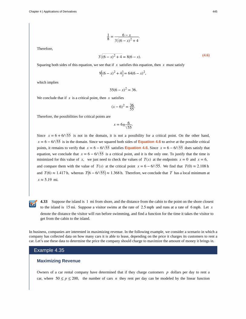
(4.6)
4.33
18 = 6 − x
3 (6 − x)2 + 4.
Therefore,
3 (6 − x)2 + 4 = 8(6 − x).
Squaring both sides of this equation, we see that if x satisfies this equation, then x must satisfy
9⎡⎣(6 − x)2 + 4⎤
⎦ = 64(6 − x)2,
which implies
55(6 − x)2 = 36.
We conclude that if x is a critical point, then x satisfies
(x − 6)2 = 3655.
Therefore, the possibilities for critical points are
x = 6± 655
.
Since x = 6 + 6/ 55 is not in the domain, it is not a possibility for a critical point. On the other hand,
x = 6 − 6/ 55 is in the domain. Since we squared both sides of Equation 4.6 to arrive at the possible critical
points, it remains to verify that x = 6 − 6/ 55 satisfies Equation 4.6. Since x = 6 − 6/ 55 does satisfy that
equation, we conclude that x = 6 − 6/ 55 is a critical point, and it is the only one. To justify that the time is
minimized for this value of x, we just need to check the values of T(x) at the endpoints x = 0 and x = 6,
and compare them with the value of T(x) at the critical point x = 6 − 6/ 55. We find that T(0) ≈ 2.108 h
and T(6) ≈ 1.417 h, whereas T⎛⎝6 − 6/ 55⎞
⎠ ≈ 1.368 h. Therefore, we conclude that T has a local minimum at
x ≈ 5.19 mi.
Suppose the island is 1 mi from shore, and the distance from the cabin to the point on the shore closest
to the island is 15 mi. Suppose a visitor swims at the rate of 2.5 mph and runs at a rate of 6 mph. Let xdenote the distance the visitor will run before swimming, and find a function for the time it takes the visitor toget from the cabin to the island.
In business, companies are interested in maximizing revenue. In the following example, we consider a scenario in which acompany has collected data on how many cars it is able to lease, depending on the price it charges its customers to rent acar. Let’s use these data to determine the price the company should charge to maximize the amount of money it brings in.
Example 4.35
Maximizing Revenue
Owners of a car rental company have determined that if they charge customers p dollars per day to rent a
car, where 50 ≤ p ≤ 200, the number of cars n they rent per day can be modeled by the linear function
Chapter 4 | Applications of Derivatives 445
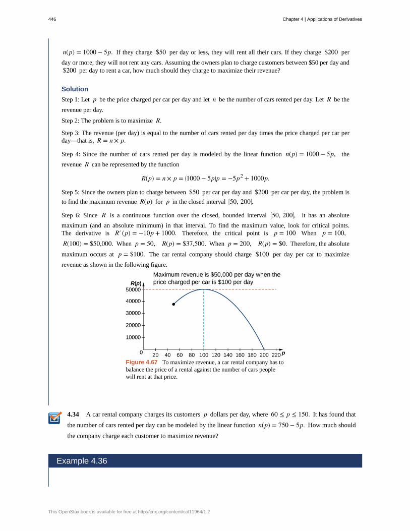
4.34
n(p) = 1000 − 5p. If they charge $50 per day or less, they will rent all their cars. If they charge $200 per
day or more, they will not rent any cars. Assuming the owners plan to charge customers between $50 per day and$200 per day to rent a car, how much should they charge to maximize their revenue?
Solution
Step 1: Let p be the price charged per car per day and let n be the number of cars rented per day. Let R be the
revenue per day.
Step 2: The problem is to maximize R.
Step 3: The revenue (per day) is equal to the number of cars rented per day times the price charged per car perday—that is, R = n × p.
Step 4: Since the number of cars rented per day is modeled by the linear function n(p) = 1000 − 5p, the
revenue R can be represented by the function
R(p) = n × p = ⎛⎝1000 − 5p⎞
⎠p = −5p2 + 1000p.
Step 5: Since the owners plan to charge between $50 per car per day and $200 per car per day, the problem is
to find the maximum revenue R(p) for p in the closed interval ⎡⎣50, 200⎤
⎦.
Step 6: Since R is a continuous function over the closed, bounded interval ⎡⎣50, 200⎤
⎦, it has an absolute
maximum (and an absolute minimum) in that interval. To find the maximum value, look for critical points.The derivative is R′ (p) = −10p + 1000. Therefore, the critical point is p = 100 When p = 100,R(100) = $50,000. When p = 50, R(p) = $37,500. When p = 200, R(p) = $0. Therefore, the absolute
maximum occurs at p = $100. The car rental company should charge $100 per day per car to maximize
revenue as shown in the following figure.
Figure 4.67 To maximize revenue, a car rental company has tobalance the price of a rental against the number of cars peoplewill rent at that price.
A car rental company charges its customers p dollars per day, where 60 ≤ p ≤ 150. It has found that
the number of cars rented per day can be modeled by the linear function n(p) = 750 − 5p. How much should
the company charge each customer to maximize revenue?
Example 4.36
446 Chapter 4 | Applications of Derivatives
This OpenStax book is available for free at http://cnx.org/content/col11964/1.2
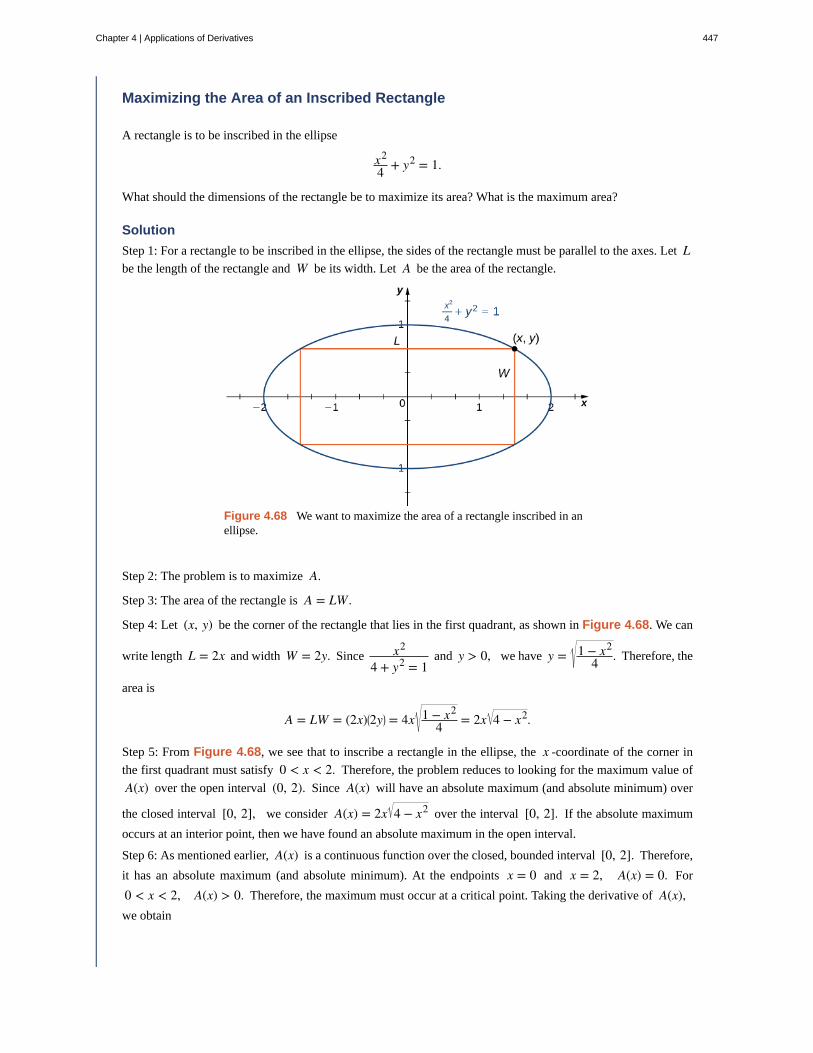
Maximizing the Area of an Inscribed Rectangle
A rectangle is to be inscribed in the ellipse
x2
4 + y2 = 1.
What should the dimensions of the rectangle be to maximize its area? What is the maximum area?
Solution
Step 1: For a rectangle to be inscribed in the ellipse, the sides of the rectangle must be parallel to the axes. Let Lbe the length of the rectangle and W be its width. Let A be the area of the rectangle.
Figure 4.68 We want to maximize the area of a rectangle inscribed in anellipse.
Step 2: The problem is to maximize A.
Step 3: The area of the rectangle is A = LW.
Step 4: Let (x, y) be the corner of the rectangle that lies in the first quadrant, as shown in Figure 4.68. We can
write length L = 2x and width W = 2y. Since x2
4 + y2 = 1and y > 0, we have y = 1 − x2
4 . Therefore, the
area is
A = LW = (2x)⎛⎝2y⎞
⎠ = 4x 1 − x2
4 = 2x 4 − x2.
Step 5: From Figure 4.68, we see that to inscribe a rectangle in the ellipse, the x -coordinate of the corner in
the first quadrant must satisfy 0 < x < 2. Therefore, the problem reduces to looking for the maximum value of
A(x) over the open interval (0, 2). Since A(x) will have an absolute maximum (and absolute minimum) over
the closed interval [0, 2], we consider A(x) = 2x 4 − x2 over the interval [0, 2]. If the absolute maximum
occurs at an interior point, then we have found an absolute maximum in the open interval.
Step 6: As mentioned earlier, A(x) is a continuous function over the closed, bounded interval [0, 2]. Therefore,
it has an absolute maximum (and absolute minimum). At the endpoints x = 0 and x = 2, A(x) = 0. For
0 < x < 2, A(x) > 0. Therefore, the maximum must occur at a critical point. Taking the derivative of A(x),we obtain
Chapter 4 | Applications of Derivatives 447
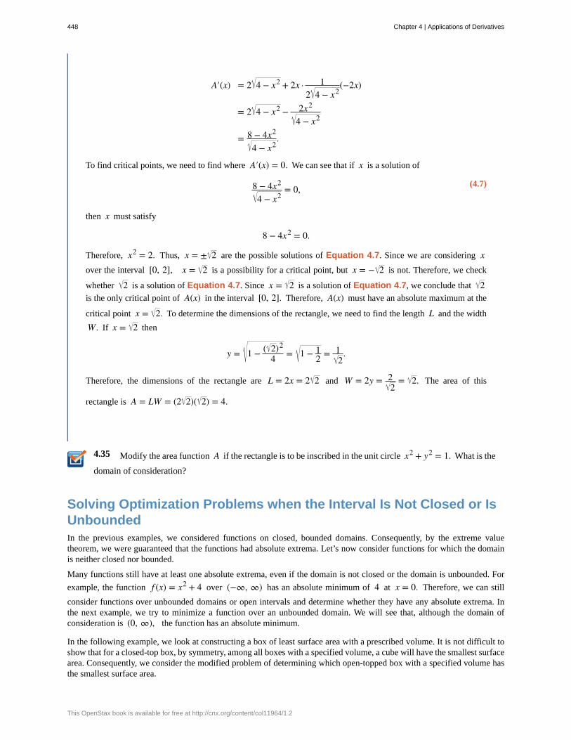
(4.7)
4.35
A′(x) = 2 4 − x2 + 2x · 12 4 − x2
(−2x)
= 2 4 − x2 − 2x2
4 − x2
= 8 − 4x2
4 − x2.
To find critical points, we need to find where A′(x) = 0. We can see that if x is a solution of
8 − 4x2
4 − x2= 0,
then x must satisfy
8 − 4x2 = 0.
Therefore, x2 = 2. Thus, x = ± 2 are the possible solutions of Equation 4.7. Since we are considering xover the interval [0, 2], x = 2 is a possibility for a critical point, but x = − 2 is not. Therefore, we check
whether 2 is a solution of Equation 4.7. Since x = 2 is a solution of Equation 4.7, we conclude that 2is the only critical point of A(x) in the interval [0, 2]. Therefore, A(x) must have an absolute maximum at the
critical point x = 2. To determine the dimensions of the rectangle, we need to find the length L and the width
W. If x = 2 then
y = 1 − ( 2)2
4 = 1 − 12 = 1
2.
Therefore, the dimensions of the rectangle are L = 2x = 2 2 and W = 2y = 22
= 2. The area of this
rectangle is A = LW = (2 2)( 2) = 4.
Modify the area function A if the rectangle is to be inscribed in the unit circle x2 + y2 = 1. What is the
domain of consideration?
Solving Optimization Problems when the Interval Is Not Closed or IsUnboundedIn the previous examples, we considered functions on closed, bounded domains. Consequently, by the extreme valuetheorem, we were guaranteed that the functions had absolute extrema. Let’s now consider functions for which the domainis neither closed nor bounded.
Many functions still have at least one absolute extrema, even if the domain is not closed or the domain is unbounded. For
example, the function f (x) = x2 + 4 over (−∞, ∞) has an absolute minimum of 4 at x = 0. Therefore, we can still
consider functions over unbounded domains or open intervals and determine whether they have any absolute extrema. Inthe next example, we try to minimize a function over an unbounded domain. We will see that, although the domain ofconsideration is (0, ∞), the function has an absolute minimum.
In the following example, we look at constructing a box of least surface area with a prescribed volume. It is not difficult toshow that for a closed-top box, by symmetry, among all boxes with a specified volume, a cube will have the smallest surfacearea. Consequently, we consider the modified problem of determining which open-topped box with a specified volume hasthe smallest surface area.
448 Chapter 4 | Applications of Derivatives
This OpenStax book is available for free at http://cnx.org/content/col11964/1.2
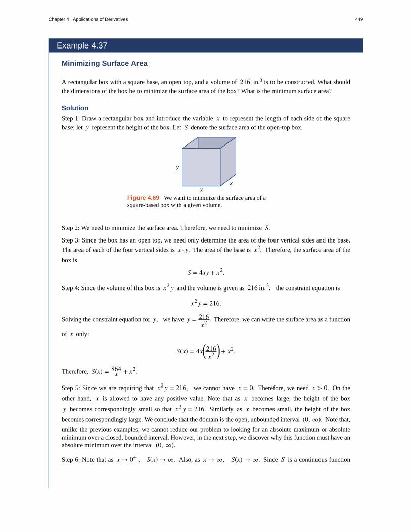
Example 4.37
Minimizing Surface Area
A rectangular box with a square base, an open top, and a volume of 216 in.3 is to be constructed. What should
the dimensions of the box be to minimize the surface area of the box? What is the minimum surface area?
Solution
Step 1: Draw a rectangular box and introduce the variable x to represent the length of each side of the square
base; let y represent the height of the box. Let S denote the surface area of the open-top box.
Figure 4.69 We want to minimize the surface area of asquare-based box with a given volume.
Step 2: We need to minimize the surface area. Therefore, we need to minimize S.
Step 3: Since the box has an open top, we need only determine the area of the four vertical sides and the base.
The area of each of the four vertical sides is x · y. The area of the base is x2. Therefore, the surface area of the
box is
S = 4xy + x2.
Step 4: Since the volume of this box is x2 y and the volume is given as 216 in.3, the constraint equation is
x2 y = 216.
Solving the constraint equation for y, we have y = 216x2 . Therefore, we can write the surface area as a function
of x only:
S(x) = 4x⎛⎝
216x2
⎞⎠ + x2.
Therefore, S(x) = 864x + x2.
Step 5: Since we are requiring that x2 y = 216, we cannot have x = 0. Therefore, we need x > 0. On the
other hand, x is allowed to have any positive value. Note that as x becomes large, the height of the box
y becomes correspondingly small so that x2 y = 216. Similarly, as x becomes small, the height of the box
becomes correspondingly large. We conclude that the domain is the open, unbounded interval (0, ∞). Note that,
unlike the previous examples, we cannot reduce our problem to looking for an absolute maximum or absoluteminimum over a closed, bounded interval. However, in the next step, we discover why this function must have anabsolute minimum over the interval (0, ∞).
Step 6: Note that as x → 0+ , S(x) → ∞. Also, as x → ∞, S(x) → ∞. Since S is a continuous function
Chapter 4 | Applications of Derivatives 449
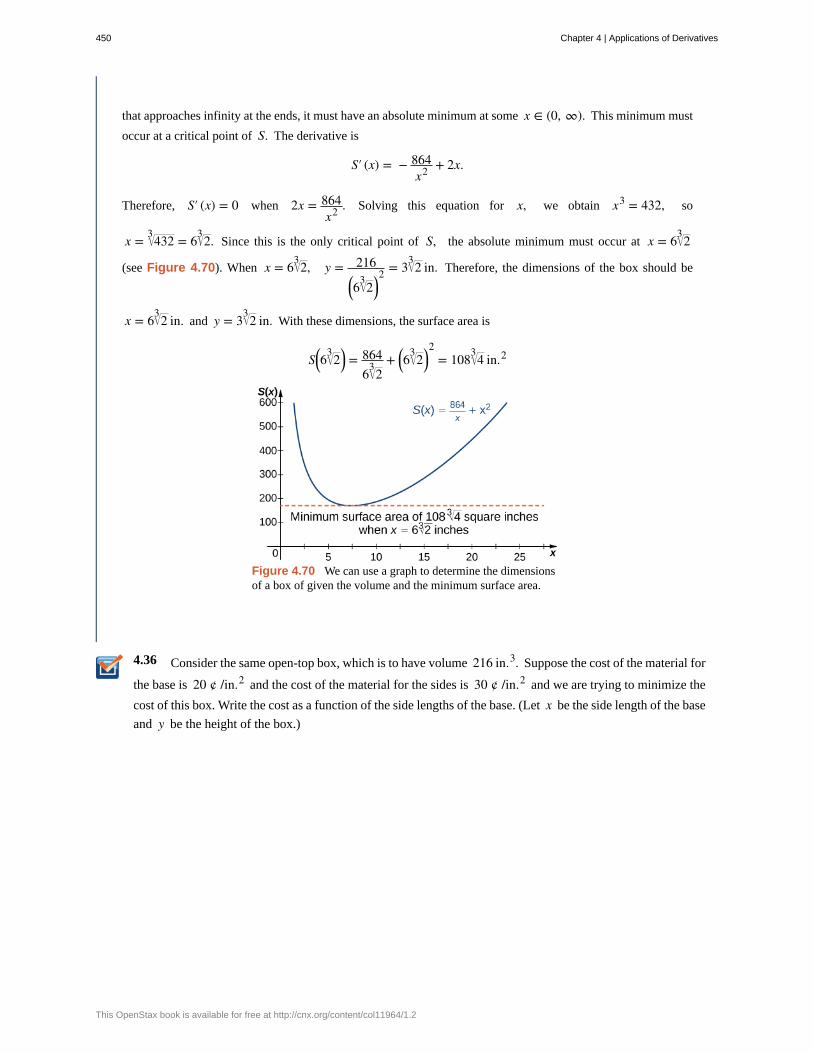
4.36
that approaches infinity at the ends, it must have an absolute minimum at some x ∈ (0, ∞). This minimum must
occur at a critical point of S. The derivative is
S′ (x) = − 864x2 + 2x.
Therefore, S′ (x) = 0 when 2x = 864x2 . Solving this equation for x, we obtain x3 = 432, so
x = 4323 = 6 23 . Since this is the only critical point of S, the absolute minimum must occur at x = 6 23
(see Figure 4.70). When x = 6 23 , y = 216⎛⎝6 23 ⎞
⎠2 = 3 23 in. Therefore, the dimensions of the box should be
x = 6 23 in. and y = 3 23 in. With these dimensions, the surface area is
S⎛⎝6 23 ⎞
⎠ = 8646 23 + ⎛
⎝6 23 ⎞⎠
2= 108 43 in.2
Figure 4.70 We can use a graph to determine the dimensionsof a box of given the volume and the minimum surface area.
Consider the same open-top box, which is to have volume 216 in.3. Suppose the cost of the material for
the base is 20 ¢ /in.2 and the cost of the material for the sides is 30 ¢ /in.2 and we are trying to minimize the
cost of this box. Write the cost as a function of the side lengths of the base. (Let x be the side length of the base
and y be the height of the box.)
450 Chapter 4 | Applications of Derivatives
This OpenStax book is available for free at http://cnx.org/content/col11964/1.2
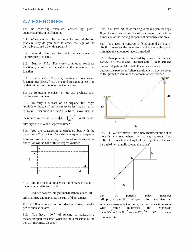
4.7 EXERCISESFor the following exercises, answer by proof,counterexample, or explanation.
311. When you find the maximum for an optimizationproblem, why do you need to check the sign of thederivative around the critical points?
312. Why do you need to check the endpoints foroptimization problems?
313. True or False. For every continuous nonlinearfunction, you can find the value x that maximizes the
function.
314. True or False. For every continuous nonconstantfunction on a closed, finite domain, there exists at least onex that minimizes or maximizes the function.
For the following exercises, set up and evaluate eachoptimization problem.
315. To carry a suitcase on an airplane, the length+width + height of the box must be less than or equal
to 62 in. Assuming the height is fixed, show that the
maximum volume is V = h⎛⎝31 − ⎛
⎝12
⎞⎠h⎞
⎠2. What height
allows you to have the largest volume?
316. You are constructing a cardboard box with thedimensions 2 m by 4 m. You then cut equal-size squares
from each corner so you may fold the edges. What are thedimensions of the box with the largest volume?
317. Find the positive integer that minimizes the sum ofthe number and its reciprocal.
318. Find two positive integers such that their sum is 10,and minimize and maximize the sum of their squares.
For the following exercises, consider the construction of apen to enclose an area.
319. You have 400 ft of fencing to construct a
rectangular pen for cattle. What are the dimensions of thepen that maximize the area?
320. You have 800 ft of fencing to make a pen for hogs.
If you have a river on one side of your property, what is thedimension of the rectangular pen that maximizes the area?
321. You need to construct a fence around an area of1600 ft. What are the dimensions of the rectangular pen to
minimize the amount of material needed?
322. Two poles are connected by a wire that is alsoconnected to the ground. The first pole is 20 ft tall and
the second pole is 10 ft tall. There is a distance of 30 ftbetween the two poles. Where should the wire be anchoredto the ground to minimize the amount of wire needed?
323. [T] You are moving into a new apartment and noticethere is a corner where the hallway narrows from8 ft to 6 ft. What is the length of the longest item that can
be carried horizontally around the corner?
324. A patient’s pulse measures70 bpm, 80 bpm, then 120 bpm. To determine an
accurate measurement of pulse, the doctor wants to knowwhat value minimizes the expression
(x − 70)2 + (x − 80)2 + (x − 120)2? What value
minimizes it?
Chapter 4 | Applications of Derivatives 451
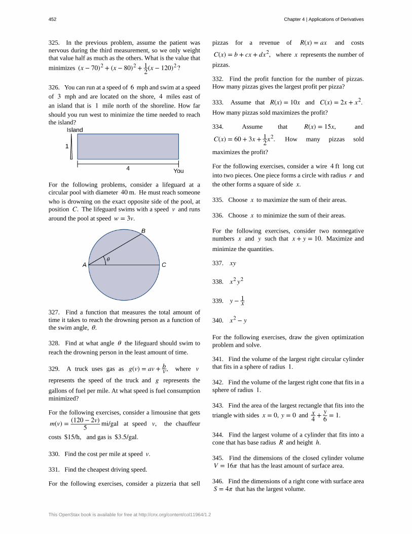
325. In the previous problem, assume the patient wasnervous during the third measurement, so we only weightthat value half as much as the others. What is the value that
minimizes (x − 70)2 + (x − 80)2 + 12(x − 120)2?
326. You can run at a speed of 6 mph and swim at a speed
of 3 mph and are located on the shore, 4 miles east of
an island that is 1 mile north of the shoreline. How far
should you run west to minimize the time needed to reachthe island?
For the following problems, consider a lifeguard at acircular pool with diameter 40 m. He must reach someone
who is drowning on the exact opposite side of the pool, atposition C. The lifeguard swims with a speed v and runs
around the pool at speed w = 3v.
327. Find a function that measures the total amount oftime it takes to reach the drowning person as a function ofthe swim angle, θ.
328. Find at what angle θ the lifeguard should swim to
reach the drowning person in the least amount of time.
329. A truck uses gas as g(v) = av + bv , where v
represents the speed of the truck and g represents the
gallons of fuel per mile. At what speed is fuel consumptionminimized?
For the following exercises, consider a limousine that gets
m(v) = (120 − 2v)5 mi/gal at speed v, the chauffeur
costs $15/h, and gas is $3.5/gal.
330. Find the cost per mile at speed v.
331. Find the cheapest driving speed.
For the following exercises, consider a pizzeria that sell
pizzas for a revenue of R(x) = ax and costs
C(x) = b + cx + dx2, where x represents the number of
pizzas.
332. Find the profit function for the number of pizzas.How many pizzas gives the largest profit per pizza?
333. Assume that R(x) = 10x and C(x) = 2x + x2.How many pizzas sold maximizes the profit?
334. Assume that R(x) = 15x, and
C(x) = 60 + 3x + 12x2. How many pizzas sold
maximizes the profit?
For the following exercises, consider a wire 4 ft long cut
into two pieces. One piece forms a circle with radius r and
the other forms a square of side x.
335. Choose x to maximize the sum of their areas.
336. Choose x to minimize the sum of their areas.
For the following exercises, consider two nonnegativenumbers x and y such that x + y = 10. Maximize and
minimize the quantities.
337. xy
338. x2 y2
339. y − 1x
340. x2 − y
For the following exercises, draw the given optimizationproblem and solve.
341. Find the volume of the largest right circular cylinderthat fits in a sphere of radius 1.
342. Find the volume of the largest right cone that fits in asphere of radius 1.
343. Find the area of the largest rectangle that fits into the
triangle with sides x = 0, y = 0 and x4 + y
6 = 1.
344. Find the largest volume of a cylinder that fits into acone that has base radius R and height h.
345. Find the dimensions of the closed cylinder volumeV = 16π that has the least amount of surface area.
346. Find the dimensions of a right cone with surface areaS = 4π that has the largest volume.
452 Chapter 4 | Applications of Derivatives
This OpenStax book is available for free at http://cnx.org/content/col11964/1.2
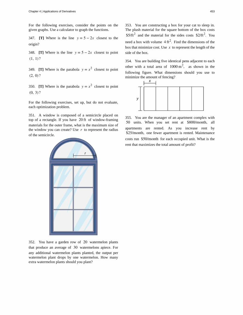
For the following exercises, consider the points on thegiven graphs. Use a calculator to graph the functions.
347. [T] Where is the line y = 5 − 2x closest to the
origin?
348. [T] Where is the line y = 5 − 2x closest to point
(1, 1)?
349. [T] Where is the parabola y = x2 closest to point
(2, 0)?
350. [T] Where is the parabola y = x2 closest to point
(0, 3)?
For the following exercises, set up, but do not evaluate,each optimization problem.
351. A window is composed of a semicircle placed ontop of a rectangle. If you have 20 ft of window-framing
materials for the outer frame, what is the maximum size ofthe window you can create? Use r to represent the radius
of the semicircle.
352. You have a garden row of 20 watermelon plants
that produce an average of 30 watermelons apiece. For
any additional watermelon plants planted, the output perwatermelon plant drops by one watermelon. How manyextra watermelon plants should you plant?
353. You are constructing a box for your cat to sleep in.The plush material for the square bottom of the box costs
$5/ft2 and the material for the sides costs $2/ft2. You
need a box with volume 4 ft2. Find the dimensions of the
box that minimize cost. Use x to represent the length of the
side of the box.
354. You are building five identical pens adjacent to each
other with a total area of 1000 m2, as shown in the
following figure. What dimensions should you use tominimize the amount of fencing?
355. You are the manager of an apartment complex with50 units. When you set rent at $800/month, all
apartments are rented. As you increase rent by$25/month, one fewer apartment is rented. Maintenance
costs run $50/month for each occupied unit. What is the
rent that maximizes the total amount of profit?
Chapter 4 | Applications of Derivatives 453
4.8 | L’Hôpital’s Rule
Learning Objectives4.8.1 Recognize when to apply L’Hôpital’s rule.
4.8.2 Identify indeterminate forms produced by quotients, products, subtractions, and powers,and apply L’Hôpital’s rule in each case.
4.8.3 Describe the relative growth rates of functions.
In this section, we examine a powerful tool for evaluating limits. This tool, known as L’Hôpital’s rule, uses derivatives tocalculate limits. With this rule, we will be able to evaluate many limits we have not yet been able to determine. Instead ofrelying on numerical evidence to conjecture that a limit exists, we will be able to show definitively that a limit exists and todetermine its exact value.
Applying L’Hôpital’s RuleL’Hôpital’s rule can be used to evaluate limits involving the quotient of two functions. Consider
limx → af (x)g(x) .
If limx → a f (x) = L1 and limx → ag(x) = L2 ≠ 0, then
limx → af (x)g(x) = L1
L2.
However, what happens if limx → a f (x) = 0 and limx → ag(x) = 0? We call this one of the indeterminate forms, of type 00.
This is considered an indeterminate form because we cannot determine the exact behavior off (x)g(x) as x → a without
further analysis. We have seen examples of this earlier in the text. For example, consider
limx → 2
x2 − 4x − 2 and lim
x → 0sinx
x .
For the first of these examples, we can evaluate the limit by factoring the numerator and writing
limx → 2
x2 − 4x − 2 = lim
x → 2(x + 2)(x − 2)
x − 2 = limx → 2
(x + 2) = 2 + 2 = 4.
For limx → 0
sinxx we were able to show, using a geometric argument, that
limx → 0
sinxx = 1.
Here we use a different technique for evaluating limits such as these. Not only does this technique provide an easier way toevaluate these limits, but also, and more important, it provides us with a way to evaluate many other limits that we couldnot calculate previously.
The idea behind L’Hôpital’s rule can be explained using local linear approximations. Consider two differentiable functionsf and g such that limx → a f (x) = 0 = limx → ag(x) and such that g′ (a) ≠ 0 For x near a, we can write
f (x) ≈ f (a) + f ′ (a)(x − a)
and
g(x) ≈ g(a) + g′ (a)(x − a).
Therefore,
f (x)g(x) ≈ f (a) + f ′ (a)(x − a)
g(a) + g′ (a)(x − a) .
454 Chapter 4 | Applications of Derivatives
This OpenStax book is available for free at http://cnx.org/content/col11964/1.2
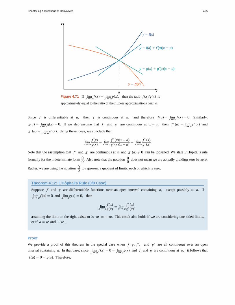
Figure 4.71 If limx → a f (x) = limx → ag(x), then the ratio f (x)/g(x) is
approximately equal to the ratio of their linear approximations near a.
Since f is differentiable at a, then f is continuous at a, and therefore f (a) = limx → a f (x) = 0. Similarly,
g(a) = limx → ag(x) = 0. If we also assume that f ′ and g′ are continuous at x = a, then f ′ (a) = limx → a f ′ (x) and
g′ (a) = limx → ag′ (x). Using these ideas, we conclude that
limx → af (x)g(x) = limx → a
f ′ (x)(x − a)g′ (x)(x − a) = limx → a
f ′ (x)g′ (x) .
Note that the assumption that f ′ and g′ are continuous at a and g′ (a) ≠ 0 can be loosened. We state L’Hôpital’s rule
formally for the indeterminate form 00. Also note that the notation 0
0 does not mean we are actually dividing zero by zero.
Rather, we are using the notation 00 to represent a quotient of limits, each of which is zero.
Theorem 4.12: L’Hôpital’s Rule (0/0 Case)
Suppose f and g are differentiable functions over an open interval containing a, except possibly at a. If
limx → a f (x) = 0 and limx → ag(x) = 0, then
limx → af (x)g(x) = limx → a
f ′ (x)g′ (x) ,
assuming the limit on the right exists or is ∞ or −∞. This result also holds if we are considering one-sided limits,
or if a = ∞ and − ∞.
Proof
We provide a proof of this theorem in the special case when f , g, f ′, and g′ are all continuous over an open
interval containing a. In that case, since limx → a f (x) = 0 = limx → ag(x) and f and g are continuous at a, it follows that
f (a) = 0 = g(a). Therefore,
Chapter 4 | Applications of Derivatives 455
limx → af (x)g(x) = limx → a
f (x) − f (a)g(x) − g(a) since f (a) = 0 = g(a)
= limx → a
f (x) − f (a)x − a
g(x) − g(a)x − a
algebra
=limx → a
f (x) − f (a)x − a
limx → ag(x) − g(a)
x − alimit of a quotient
= f ′ (a)g′ (a) definition of he derivative
=limx → a f ′ (x)limx → ag′ (x) continuity of f ′ and g′
= limx → af ′ (x)g′ (x) . limit of a quotient
Note that L’Hôpital’s rule states we can calculate the limit of a quotientfg by considering the limit of the quotient of the
derivativesf ′g′ . It is important to realize that we are not calculating the derivative of the quotient
fg .
□
Example 4.38
Applying L’Hôpital’s Rule (0/0 Case)
Evaluate each of the following limits by applying L’Hôpital’s rule.
a. limx → 0
1 − cosxx
b. limx → 1
sin(πx)lnx
c. limx → ∞e1/x − 1
1/x
d. limx → 0
sinx − xx2
Solution
a. Since the numerator 1 − cosx → 0 and the denominator x → 0, we can apply L’Hôpital’s rule to
evaluate this limit. We have
limx → 0
1 − cosxx = lim
x → 0
ddx(1 − cosx)
ddx(x)
= limx → 0
sinx1
=lim
x → 0(sinx)
limx → 0
(1)
= 01 = 0.
456 Chapter 4 | Applications of Derivatives
This OpenStax book is available for free at http://cnx.org/content/col11964/1.2
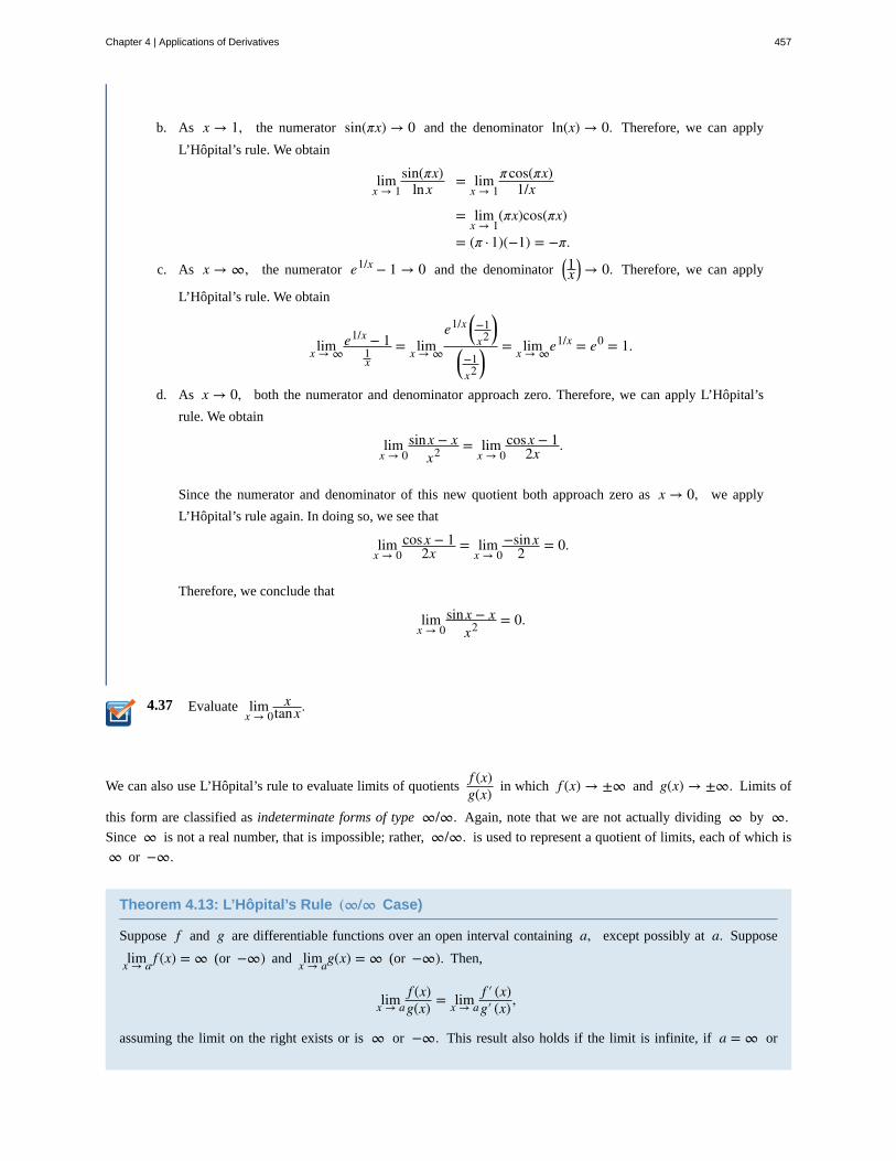
4.37
b. As x → 1, the numerator sin(πx) → 0 and the denominator ln(x) → 0. Therefore, we can apply
L’Hôpital’s rule. We obtain
limx → 1
sin(πx)lnx = lim
x → 1π cos(πx)
1/x
= limx → 1
(πx)cos(πx)
= (π · 1)(−1) = −π.
c. As x → ∞, the numerator e1/x − 1 → 0 and the denominator ⎛⎝1x
⎞⎠ → 0. Therefore, we can apply
L’Hôpital’s rule. We obtain
limx → ∞e1/x − 1
1x
= limx → ∞
e1/x ⎛⎝
−1x2
⎞⎠
⎛⎝
−1x2
⎞⎠
= limx → ∞e1/x = e0 = 1.
d. As x → 0, both the numerator and denominator approach zero. Therefore, we can apply L’Hôpital’s
rule. We obtain
limx → 0
sinx − xx2 = lim
x → 0cosx − 1
2x .
Since the numerator and denominator of this new quotient both approach zero as x → 0, we apply
L’Hôpital’s rule again. In doing so, we see that
limx → 0
cosx − 12x = lim
x → 0−sinx
2 = 0.
Therefore, we conclude that
limx → 0
sinx − xx2 = 0.
Evaluate limx → 0
xtanx.
We can also use L’Hôpital’s rule to evaluate limits of quotientsf (x)g(x) in which f (x) → ±∞ and g(x) → ±∞. Limits of
this form are classified as indeterminate forms of type ∞/∞. Again, note that we are not actually dividing ∞ by ∞.Since ∞ is not a real number, that is impossible; rather, ∞/∞. is used to represent a quotient of limits, each of which is
∞ or −∞.
Theorem 4.13: L’Hôpital’s Rule (∞/∞ Case)
Suppose f and g are differentiable functions over an open interval containing a, except possibly at a. Suppose
limx → a f (x) = ∞ (or −∞) and limx → ag(x) = ∞ (or −∞). Then,
limx → af (x)g(x) = limx → a
f ′ (x)g′ (x) ,
assuming the limit on the right exists or is ∞ or −∞. This result also holds if the limit is infinite, if a = ∞ or
Chapter 4 | Applications of Derivatives 457
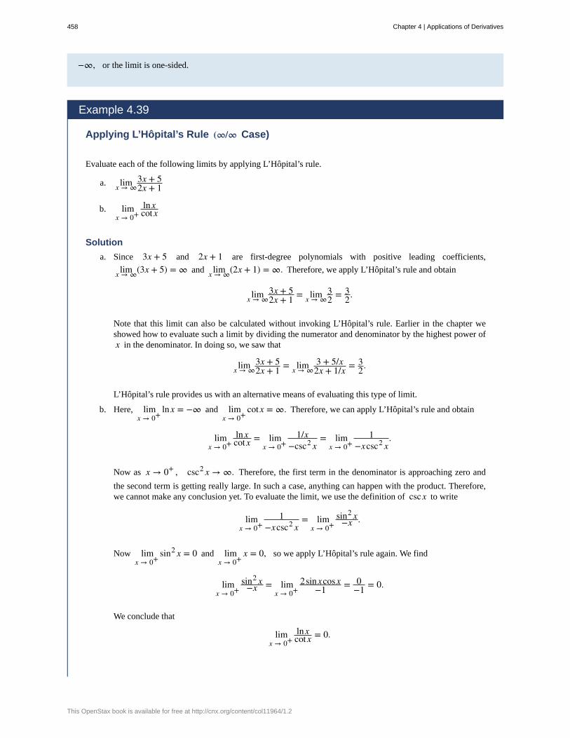
−∞, or the limit is one-sided.
Example 4.39
Applying L’Hôpital’s Rule (∞/∞ Case)
Evaluate each of the following limits by applying L’Hôpital’s rule.
a. limx → ∞3x + 52x + 1
b. limx → 0+
lnxcot x
Solution
a. Since 3x + 5 and 2x + 1 are first-degree polynomials with positive leading coefficients,
limx → ∞(3x + 5) = ∞ and limx → ∞(2x + 1) = ∞. Therefore, we apply L’Hôpital’s rule and obtain
limx → ∞3x + 52x + 1 = limx → ∞
32 = 3
2.
Note that this limit can also be calculated without invoking L’Hôpital’s rule. Earlier in the chapter weshowed how to evaluate such a limit by dividing the numerator and denominator by the highest power ofx in the denominator. In doing so, we saw that
limx → ∞3x + 52x + 1 = limx → ∞
3 + 5/x2x + 1/x = 3
2.
L’Hôpital’s rule provides us with an alternative means of evaluating this type of limit.
b. Here, limx → 0+
lnx = −∞ and limx → 0+
cot x = ∞. Therefore, we can apply L’Hôpital’s rule and obtain
limx → 0+
lnxcot x = lim
x → 0+1/x
−csc2 x= lim
x → 0+1
−xcsc2 x.
Now as x → 0+ , csc2 x → ∞. Therefore, the first term in the denominator is approaching zero and
the second term is getting really large. In such a case, anything can happen with the product. Therefore,we cannot make any conclusion yet. To evaluate the limit, we use the definition of cscx to write
limx → 0+
1−xcsc2 x
= limx → 0+
sin2 x−x .
Now limx → 0+
sin2 x = 0 and limx → 0+
x = 0, so we apply L’Hôpital’s rule again. We find
limx → 0+
sin2 x−x = lim
x → 0+2sinxcosx
−1 = 0−1 = 0.
We conclude that
limx → 0+
lnxcot x = 0.
458 Chapter 4 | Applications of Derivatives
This OpenStax book is available for free at http://cnx.org/content/col11964/1.2
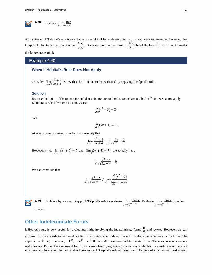
4.38
4.39
Evaluate limx → ∞lnx5x .
As mentioned, L’Hôpital’s rule is an extremely useful tool for evaluating limits. It is important to remember, however, that
to apply L’Hôpital’s rule to a quotientf (x)g(x) , it is essential that the limit of
f (x)g(x) be of the form 0
0 or ∞/∞. Consider
the following example.
Example 4.40
When L’Hôpital’s Rule Does Not Apply
Consider limx → 1
x2 + 53x + 4. Show that the limit cannot be evaluated by applying L’Hôpital’s rule.
Solution
Because the limits of the numerator and denominator are not both zero and are not both infinite, we cannot applyL’Hôpital’s rule. If we try to do so, we get
ddx
⎛⎝x2 + 5⎞
⎠ = 2x
and
ddx(3x + 4) = 3.
At which point we would conclude erroneously that
limx → 1
x2 + 53x + 4 = lim
x → 12x3 = 2
3.
However, since limx → 1
⎛⎝x2 + 5⎞
⎠ = 6 and limx → 1
(3x + 4) = 7, we actually have
limx → 1
x2 + 53x + 4 = 6
7.
We can conclude that
limx → 1
x2 + 53x + 4 ≠ lim
x → 1
ddx
⎛⎝x2 + 5⎞
⎠ddx(3x + 4)
.
Explain why we cannot apply L’Hôpital’s rule to evaluate limx → 0+
cosxx . Evaluate lim
x → 0+cosx
x by other
means.
Other Indeterminate Forms
L’Hôpital’s rule is very useful for evaluating limits involving the indeterminate forms 00 and ∞/∞. However, we can
also use L’Hôpital’s rule to help evaluate limits involving other indeterminate forms that arise when evaluating limits. The
expressions 0 · ∞, ∞ − ∞, 1∞, ∞0, and 00 are all considered indeterminate forms. These expressions are not
real numbers. Rather, they represent forms that arise when trying to evaluate certain limits. Next we realize why these areindeterminate forms and then understand how to use L’Hôpital’s rule in these cases. The key idea is that we must rewrite
Chapter 4 | Applications of Derivatives 459
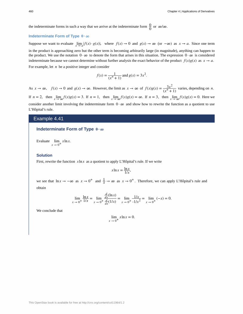
the indeterminate forms in such a way that we arrive at the indeterminate form 00 or ∞/∞.
Indeterminate Form of Type 0 · ∞
Suppose we want to evaluate limx → a⎛⎝ f (x) · g(x)⎞
⎠, where f (x) → 0 and g(x) → ∞ (or −∞) as x → a. Since one term
in the product is approaching zero but the other term is becoming arbitrarily large (in magnitude), anything can happen tothe product. We use the notation 0 · ∞ to denote the form that arises in this situation. The expression 0 · ∞ is considered
indeterminate because we cannot determine without further analysis the exact behavior of the product f (x)g(x) as x → a.For example, let n be a positive integer and consider
f (x) = 1(xn + 1) and g(x) = 3x2.
As x → ∞, f (x) → 0 and g(x) → ∞. However, the limit as x → ∞ of f (x)g(x) = 3x2
(xn + 1) varies, depending on n.
If n = 2, then limx → ∞ f (x)g(x) = 3. If n = 1, then limx → ∞ f (x)g(x) = ∞. If n = 3, then limx → ∞ f (x)g(x) = 0. Here we
consider another limit involving the indeterminate form 0 · ∞ and show how to rewrite the function as a quotient to use
L’Hôpital’s rule.
Example 4.41
Indeterminate Form of Type 0 · ∞
Evaluate limx → 0+
x lnx.
Solution
First, rewrite the function x lnx as a quotient to apply L’Hôpital’s rule. If we write
x lnx = lnx1/x ,
we see that lnx → −∞ as x → 0+ and 1x → ∞ as x → 0+ . Therefore, we can apply L’Hôpital’s rule and
obtain
limx → 0+
lnx1/x = lim
x → 0+
ddx(lnx)ddx(1/x)
= limx → 0+
1/x-1/x2 = lim
x → 0+(−x) = 0.
We conclude that
limx → 0+
x lnx = 0.
460 Chapter 4 | Applications of Derivatives
This OpenStax book is available for free at http://cnx.org/content/col11964/1.2
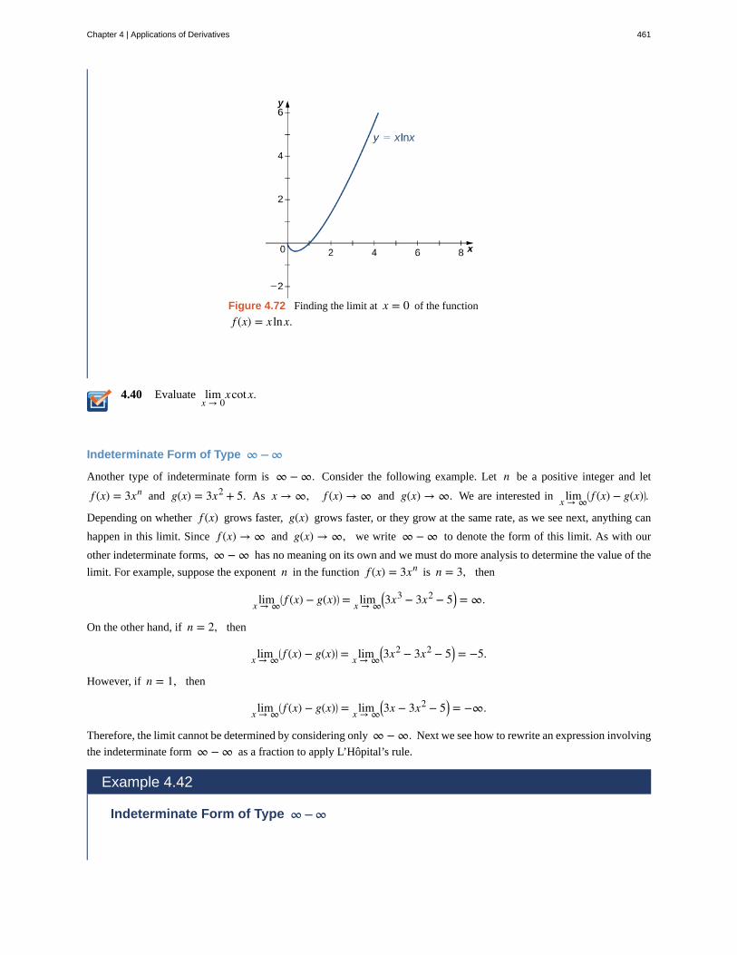
4.40
Figure 4.72 Finding the limit at x = 0 of the function
f (x) = x lnx.
Evaluate limx → 0
xcot x.
Indeterminate Form of Type ∞ − ∞
Another type of indeterminate form is ∞ − ∞. Consider the following example. Let n be a positive integer and let
f (x) = 3xn and g(x) = 3x2 + 5. As x → ∞, f (x) → ∞ and g(x) → ∞. We are interested in limx → ∞⎛⎝ f (x) − g(x)⎞
⎠.
Depending on whether f (x) grows faster, g(x) grows faster, or they grow at the same rate, as we see next, anything can
happen in this limit. Since f (x) → ∞ and g(x) → ∞, we write ∞ − ∞ to denote the form of this limit. As with our
other indeterminate forms, ∞ − ∞ has no meaning on its own and we must do more analysis to determine the value of the
limit. For example, suppose the exponent n in the function f (x) = 3xn is n = 3, then
limx → ∞⎛⎝ f (x) − g(x)⎞
⎠ = limx → ∞⎛⎝3x3 − 3x2 − 5⎞
⎠ = ∞.
On the other hand, if n = 2, then
limx → ∞⎛⎝ f (x) − g(x)⎞
⎠ = limx → ∞⎛⎝3x2 − 3x2 − 5⎞
⎠ = −5.
However, if n = 1, then
limx → ∞⎛⎝ f (x) − g(x)⎞
⎠ = limx → ∞⎛⎝3x − 3x2 − 5⎞
⎠ = −∞.
Therefore, the limit cannot be determined by considering only ∞ − ∞. Next we see how to rewrite an expression involving
the indeterminate form ∞ − ∞ as a fraction to apply L’Hôpital’s rule.
Example 4.42
Indeterminate Form of Type ∞ − ∞
Chapter 4 | Applications of Derivatives 461
4.41
Evaluate limx → 0+
⎛⎝
1x2 − 1
tanx⎞⎠.
Solution
By combining the fractions, we can write the function as a quotient. Since the least common denominator is
x2 tanx, we have
1x2 − 1
tanx = (tanx) − x2
x2 tanx.
As x → 0+ , the numerator tanx − x2 → 0 and the denominator x2 tanx → 0. Therefore, we can apply
L’Hôpital’s rule. Taking the derivatives of the numerator and the denominator, we have
limx → 0+
(tanx) − x2
x2 tanx= lim
x → 0+
⎛⎝sec2 x⎞
⎠ − 2x
x2 sec2 x + 2x tanx.
As x → 0+ , ⎛⎝sec2 x⎞
⎠ − 2x → 1 and x2 sec2 x + 2x tanx → 0. Since the denominator is positive as x
approaches zero from the right, we conclude that
limx → 0+
⎛⎝sec2 x⎞
⎠ − 2x
x2 sec2 x + 2x tanx= ∞.
Therefore,
limx → 0+
⎛⎝
1x2 − 1
tanx⎞⎠ = ∞.
Evaluate limx → 0+
⎛⎝1x − 1
sinx⎞⎠.
Another type of indeterminate form that arises when evaluating limits involves exponents. The expressions 00, ∞0, and
1∞ are all indeterminate forms. On their own, these expressions are meaningless because we cannot actually evaluate these
expressions as we would evaluate an expression involving real numbers. Rather, these expressions represent forms that arisewhen finding limits. Now we examine how L’Hôpital’s rule can be used to evaluate limits involving these indeterminateforms.
Since L’Hôpital’s rule applies to quotients, we use the natural logarithm function and its properties to reduce a problemevaluating a limit involving exponents to a related problem involving a limit of a quotient. For example, suppose we want
to evaluate limx → a f (x)g(x)and we arrive at the indeterminate form ∞0. (The indeterminate forms 00 and 1∞ can be
handled similarly.) We proceed as follows. Let
y = f (x)g(x).
Then,
lny = ln⎛⎝ f (x)g(x)⎞
⎠ = g(x)ln⎛⎝ f (x)⎞
⎠.
Therefore,
limx → a⎡⎣ln(y)⎤
⎦ = limx → a⎡⎣g(x)ln⎛
⎝ f (x)⎞⎠⎤⎦.
Since limx → a f (x) = ∞, we know that limx → aln⎛⎝ f (x)⎞
⎠ = ∞. Therefore, limx → ag(x)ln⎛⎝ f (x)⎞
⎠ is of the indeterminate form
462 Chapter 4 | Applications of Derivatives
This OpenStax book is available for free at http://cnx.org/content/col11964/1.2
4.42
0 · ∞, and we can use the techniques discussed earlier to rewrite the expression g(x)ln⎛⎝ f (x)⎞
⎠ in a form so that we can
apply L’Hôpital’s rule. Suppose limx → ag(x)ln⎛⎝ f (x)⎞
⎠ = L, where L may be ∞ or −∞. Then
limx → a⎡⎣ln(y)⎤
⎦ = L.
Since the natural logarithm function is continuous, we conclude that
ln⎛⎝ limx → ay⎞
⎠ = L,
which gives us
limx → ay = limx → a f (x)g(x) = eL.
Example 4.43
Indeterminate Form of Type ∞0
Evaluate limx → ∞x1/x.
Solution
Let y = x1/x. Then,
ln⎛⎝x
1/x⎞⎠ = 1
x lnx = lnxx .
We need to evaluate limx → ∞lnxx . Applying L’Hôpital’s rule, we obtain
limx → ∞lny = limx → ∞lnxx = limx → ∞
1/x1 = 0.
Therefore, limx → ∞lny = 0. Since the natural logarithm function is continuous, we conclude that
ln⎛⎝ limx → ∞y⎞
⎠ = 0,
which leads to
limx → ∞y = limx → ∞lnxx = e0 = 1.
Hence,
limx → ∞x1/x = 1.
Evaluate limx → ∞x1/ln(x).
Example 4.44
Indeterminate Form of Type 00
Chapter 4 | Applications of Derivatives 463
4.43
Evaluate limx → 0+
xsinx.
Solution
Let
y = xsinx.
Therefore,
lny = ln⎛⎝x
sinx⎞⎠ = sinx lnx.
We now evaluate limx → 0+
sinx lnx. Since limx → 0+
sinx = 0 and limx → 0+
lnx = −∞, we have the indeterminate
form 0 · ∞. To apply L’Hôpital’s rule, we need to rewrite sinx lnx as a fraction. We could write
sinx lnx = sinx1/ln x
or
sinx lnx = lnx1/sinx = lnx
cscx.
Let’s consider the first option. In this case, applying L’Hôpital’s rule, we would obtain
limx → 0+
sinx lnx = limx → 0+
sinx1/lnx = lim
x → 0+cosx
−1/⎛⎝x(lnx)2⎞
⎠= lim
x → 0+⎛⎝−x(lnx)2 cosx⎞
⎠.
Unfortunately, we not only have another expression involving the indeterminate form 0 · ∞, but the new limit
is even more complicated to evaluate than the one with which we started. Instead, we try the second option. Bywriting
sinx lnx = lnx1/sinx = lnx
cscx,
and applying L’Hôpital’s rule, we obtain
limx → 0+
sinx lnx = limx → 0+
lnxcscx = lim
x → 0+1/x
−cscxcot x = limx → 0+
−1xcscxcot x.
Using the fact that cscx = 1sinx and cot x = cosx
sinx , we can rewrite the expression on the right-hand side as
limx → 0+
−sin2 xxcosx = lim
x → 0+⎡⎣sinx
x · (−tanx)⎤⎦ = ⎛
⎝ limx → 0+
sinxx
⎞⎠ · ⎛⎝ lim
x → 0+(−tanx)⎞⎠ = 1 · 0 = 0.
We conclude that limx → 0+
lny = 0. Therefore, ln⎛⎝ lim
x → 0+y⎞⎠ = 0 and we have
limx → 0+
y = limx → 0+
xsinx = e0 = 1.
Hence,
limx → 0+
xsinx = 1.
Evaluate limx → 0+
xx.
464 Chapter 4 | Applications of Derivatives
This OpenStax book is available for free at http://cnx.org/content/col11964/1.2
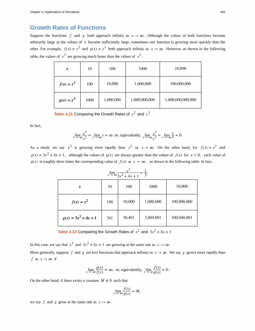
Growth Rates of FunctionsSuppose the functions f and g both approach infinity as x → ∞. Although the values of both functions become
arbitrarily large as the values of x become sufficiently large, sometimes one function is growing more quickly than the
other. For example, f (x) = x2 and g(x) = x3 both approach infinity as x → ∞. However, as shown in the following
table, the values of x3 are growing much faster than the values of x2.
x 10 100 1000 10,000
f(x) = x2 100 10,000 1,000,000 100,000,000
g(x) = x3 1000 1,000,000 1,000,000,000 1,000,000,000,000
Table 4.21 Comparing the Growth Rates of x2 and x3
In fact,
limx → ∞x3
x2 = limx → ∞x = ∞. or, equivalently, limx → ∞x2
x3 = limx → ∞1x = 0.
As a result, we say x3 is growing more rapidly than x2 as x → ∞. On the other hand, for f (x) = x2 and
g(x) = 3x2 + 4x + 1, although the values of g(x) are always greater than the values of f (x) for x > 0, each value of
g(x) is roughly three times the corresponding value of f (x) as x → ∞, as shown in the following table. In fact,
limx → ∞x2
3x2 + 4x + 1= 1
3.
x 10 100 1000 10,000
f(x) = x2 100 10,000 1,000,000 100,000,000
g(x) = 3x2 + 4x + 1 341 30,401 3,004,001 300,040,001
Table 4.22 Comparing the Growth Rates of x2 and 3x2 + 4x + 1
In this case, we say that x2 and 3x2 + 4x + 1 are growing at the same rate as x → ∞.
More generally, suppose f and g are two functions that approach infinity as x → ∞. We say g grows more rapidly than
f as x → ∞ if
limx → ∞g(x)f (x) = ∞; or, equivalently, limx → ∞
f (x)g(x) = 0.
On the other hand, if there exists a constant M ≠ 0 such that
limx → ∞f (x)g(x) = M,
we say f and g grow at the same rate as x → ∞.
Chapter 4 | Applications of Derivatives 465
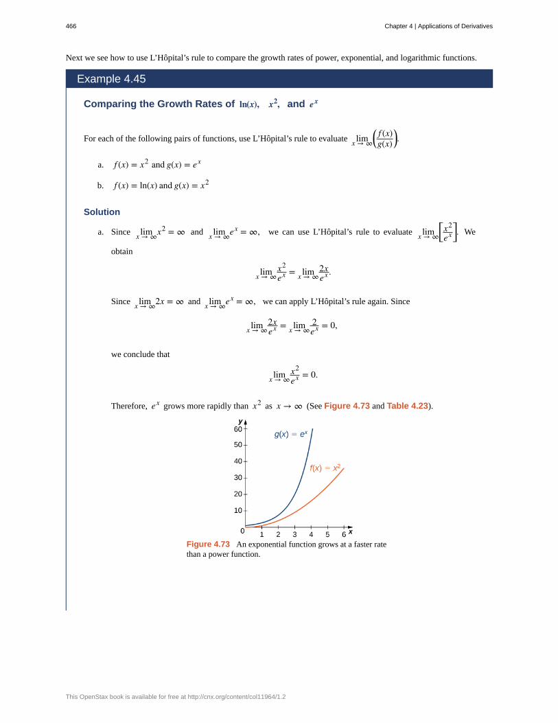
Next we see how to use L’Hôpital’s rule to compare the growth rates of power, exponential, and logarithmic functions.
Example 4.45
Comparing the Growth Rates of ln(x), x2, and ex
For each of the following pairs of functions, use L’Hôpital’s rule to evaluate limx → ∞⎛⎝
f (x)g(x)
⎞⎠.
a. f (x) = x2 and g(x) = ex
b. f (x) = ln(x) and g(x) = x2
Solution
a. Since limx → ∞x2 = ∞ and limx → ∞ex = ∞, we can use L’Hôpital’s rule to evaluate limx → ∞⎡⎣
x2
ex⎤⎦. We
obtain
limx → ∞x2
ex = limx → ∞2xex .
Since limx → ∞2x = ∞ and limx → ∞ex = ∞, we can apply L’Hôpital’s rule again. Since
limx → ∞2xex = limx → ∞
2ex = 0,
we conclude that
limx → ∞x2
ex = 0.
Therefore, ex grows more rapidly than x2 as x → ∞ (See Figure 4.73 and Table 4.23).
Figure 4.73 An exponential function grows at a faster ratethan a power function.
466 Chapter 4 | Applications of Derivatives
This OpenStax book is available for free at http://cnx.org/content/col11964/1.2
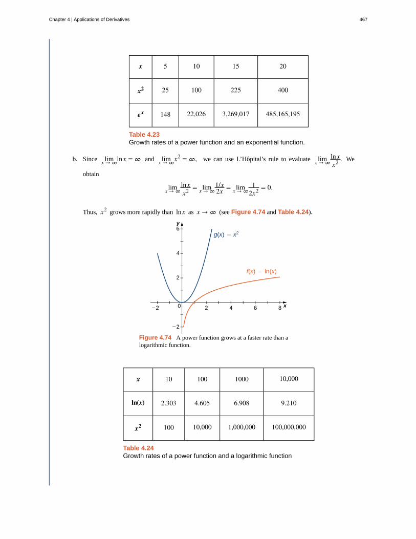
x 5 10 15 20
x2 25 100 225 400
ex 148 22,026 3,269,017 485,165,195
Table 4.23Growth rates of a power function and an exponential function.
b. Since limx → ∞lnx = ∞ and limx → ∞x2 = ∞, we can use L’Hôpital’s rule to evaluate limx → ∞lnxx2 . We
obtain
limx → ∞lnxx2 = limx → ∞
1/x2x = limx → ∞
12x2 = 0.
Thus, x2 grows more rapidly than lnx as x → ∞ (see Figure 4.74 and Table 4.24).
Figure 4.74 A power function grows at a faster rate than alogarithmic function.
x 10 100 1000 10,000
ln(x) 2.303 4.605 6.908 9.210
x2 100 10,000 1,000,000 100,000,000
Table 4.24Growth rates of a power function and a logarithmic function
Chapter 4 | Applications of Derivatives 467
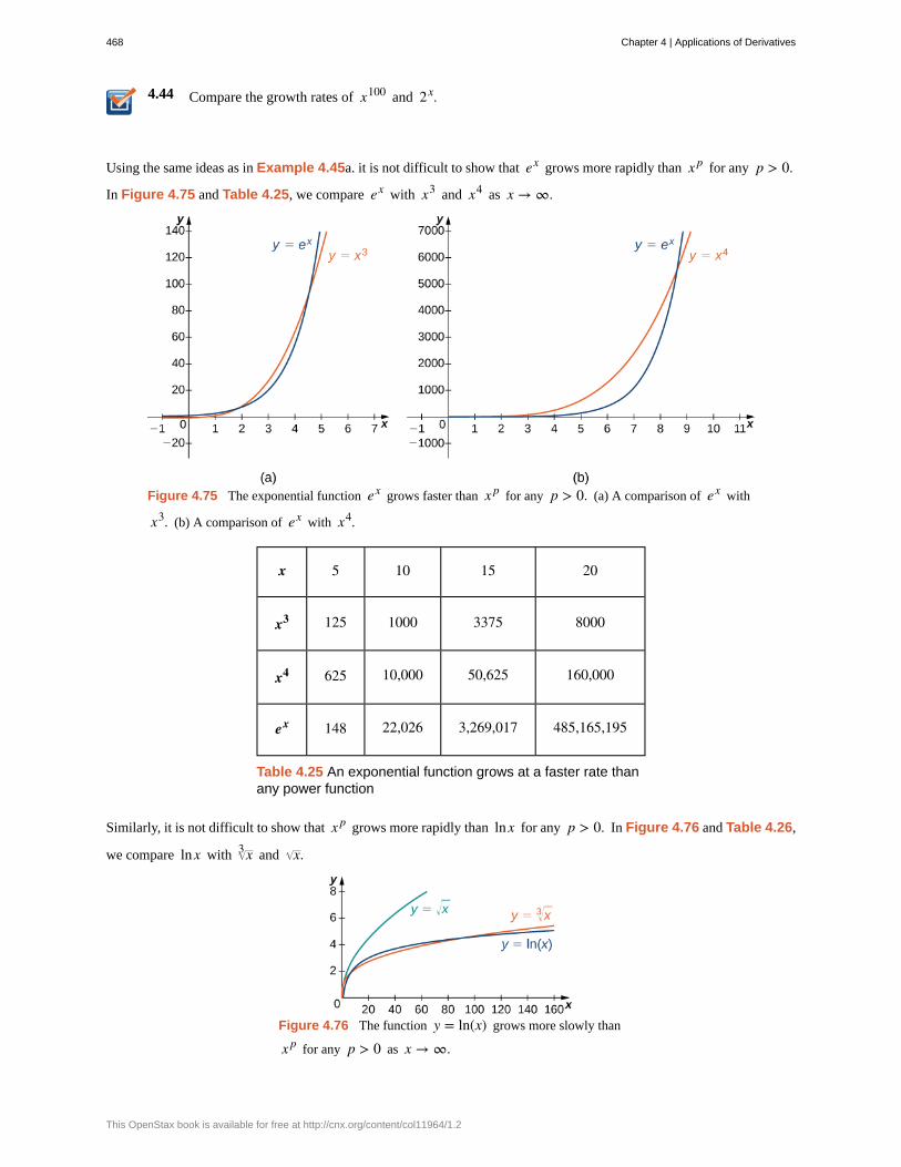
4.44 Compare the growth rates of x100 and 2x.
Using the same ideas as in Example 4.45a. it is not difficult to show that ex grows more rapidly than x p for any p > 0.
In Figure 4.75 and Table 4.25, we compare ex with x3 and x4 as x → ∞.
Figure 4.75 The exponential function ex grows faster than x p for any p > 0. (a) A comparison of ex with
x3. (b) A comparison of ex with x4.
x 5 10 15 20
x3 125 1000 3375 8000
x4 625 10,000 50,625 160,000
ex 148 22,026 3,269,017 485,165,195
Table 4.25 An exponential function grows at a faster rate thanany power function
Similarly, it is not difficult to show that x p grows more rapidly than lnx for any p > 0. In Figure 4.76 and Table 4.26,
we compare lnx with x3 and x.
Figure 4.76 The function y = ln(x) grows more slowly than
x p for any p > 0 as x → ∞.
468 Chapter 4 | Applications of Derivatives
This OpenStax book is available for free at http://cnx.org/content/col11964/1.2
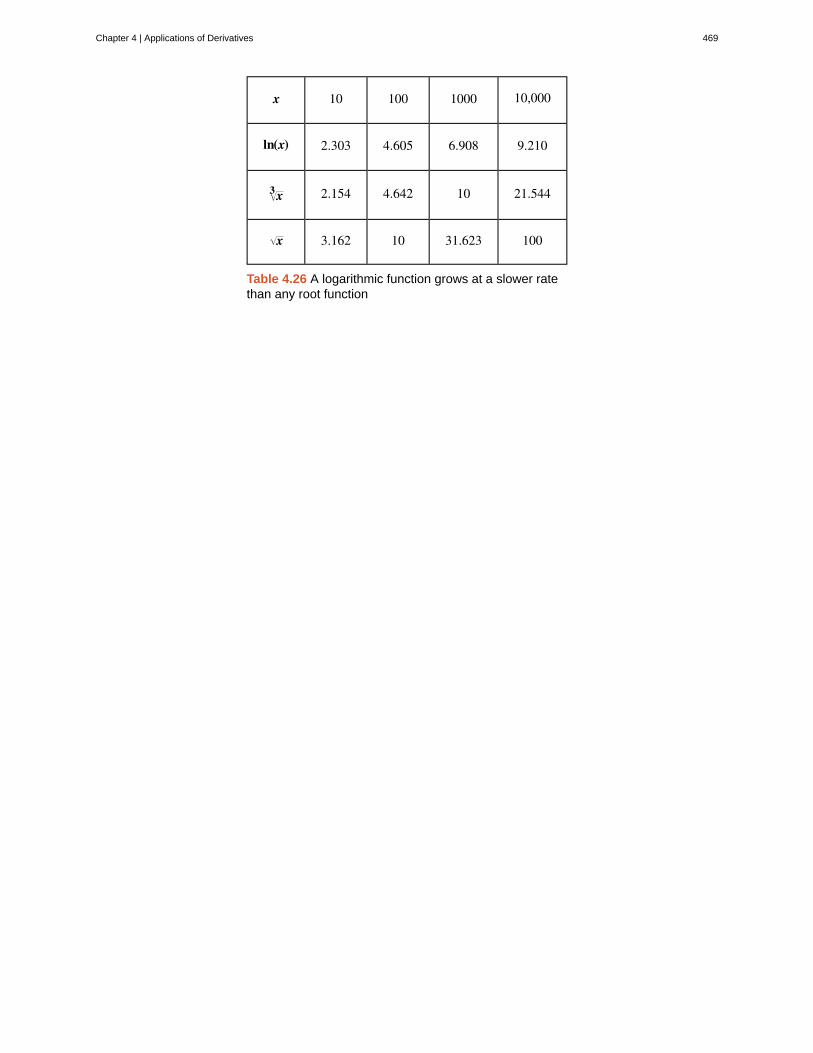
x 10 100 1000 10,000
ln(x) 2.303 4.605 6.908 9.210
x3 2.154 4.642 10 21.544
x 3.162 10 31.623 100
Table 4.26 A logarithmic function grows at a slower ratethan any root function
Chapter 4 | Applications of Derivatives 469
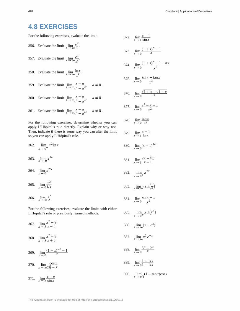
4.8 EXERCISESFor the following exercises, evaluate the limit.
356. Evaluate the limit limx → ∞exx .
357. Evaluate the limit limx → ∞ex
xk .
358. Evaluate the limit limx → ∞lnxxk .
359. Evaluate the limit limx → ax − a
x2 − a2, a ≠ 0 .
360. Evaluate the limit limx → ax − a
x3 − a3, a ≠ 0 .
361. Evaluate the limit limx → ax − a
xn − an, a ≠ 0 .
For the following exercises, determine whether you canapply L’Hôpital’s rule directly. Explain why or why not.Then, indicate if there is some way you can alter the limitso you can apply L’Hôpital’s rule.
362. limx → 0+
x2 lnx
363. limx → ∞x1/x
364. limx → 0
x2/x
365. limx → 0
x2
1/x
366. limx → ∞exx
For the following exercises, evaluate the limits with eitherL’Hôpital’s rule or previously learned methods.
367. limx → 3
x2 − 9x − 3
368. limx → 3
x2 − 9x + 3
369. limx → 0
(1 + x)−2 − 1x
370. limx → π/2
cosxπ2 − x
371. limx → πx − πsinx
372. limx → 1
x − 1sinx
373. limx → 0
(1 + x)n − 1x
374. limx → 0
(1 + x)n − 1 − nxx2
375. limx → 0
sinx − tanxx3
376. limx → 0
1 + x − 1 − xx
377. limx → 0
ex − x − 1x2
378. limx → 0
tanxx
379. limx → 1
x − 1lnx
380. limx → 0
(x + 1)1/x
381. limx → 1
x − x3
x − 1
382. limx → 0+
x2x
383. limx → ∞xsin⎛⎝1x
⎞⎠
384. limx → 0
sinx − xx2
385. limx → 0+
x ln⎛⎝x4⎞
⎠
386. limx → ∞(x − ex)
387. limx → ∞x2 e−x
388. limx → 0
3x − 2xx
389. limx → 0
1 + 1/x1 − 1/x
390. limx → π/4
(1 − tanx)cot x
470 Chapter 4 | Applications of Derivatives
This OpenStax book is available for free at http://cnx.org/content/col11964/1.2
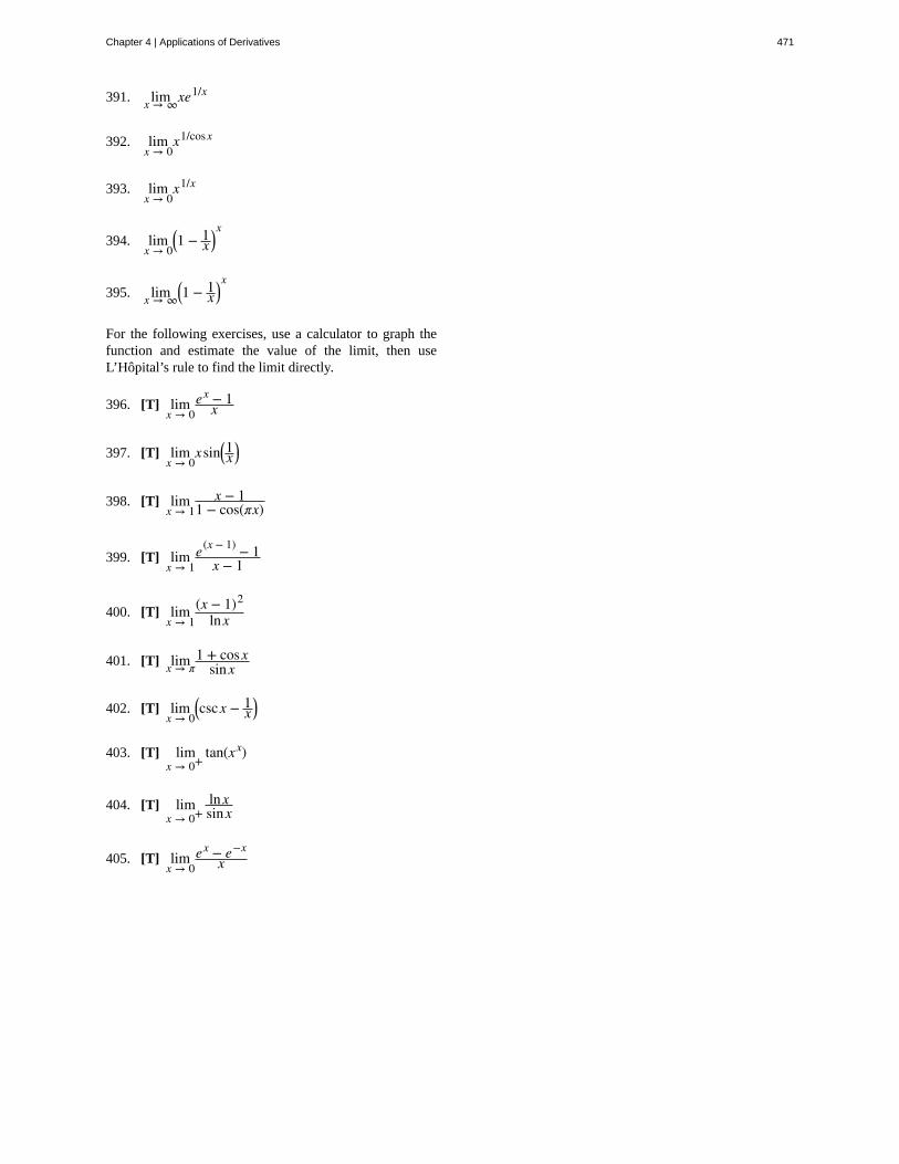
391. limx → ∞xe1/x
392. limx → 0
x1/cosx
393. limx → 0
x1/x
394. limx → 0
⎛⎝1 − 1
x⎞⎠x
395. limx → ∞⎛⎝1 − 1
x⎞⎠x
For the following exercises, use a calculator to graph thefunction and estimate the value of the limit, then useL’Hôpital’s rule to find the limit directly.
396. [T] limx → 0
ex − 1x
397. [T] limx → 0
xsin⎛⎝1x
⎞⎠
398. [T] limx → 1
x − 11 − cos(πx)
399. [T] limx → 1
e(x − 1) − 1x − 1
400. [T] limx → 1
(x − 1)2
lnx
401. [T] limx → π1 + cosx
sinx
402. [T] limx → 0
⎛⎝cscx − 1
x⎞⎠
403. [T] limx → 0+
tan(xx)
404. [T] limx → 0+
lnxsinx
405. [T] limx → 0
ex − e−xx
Chapter 4 | Applications of Derivatives 471
4.9 | Newton’s Method
Learning Objectives4.9.1 Describe the steps of Newton’s method.
4.9.2 Explain what an iterative process means.
4.9.3 Recognize when Newton’s method does not work.
4.9.4 Apply iterative processes to various situations.
In many areas of pure and applied mathematics, we are interested in finding solutions to an equation of the form f (x) = 0.For most functions, however, it is difficult—if not impossible—to calculate their zeroes explicitly. In this section, we takea look at a technique that provides a very efficient way of approximating the zeroes of functions. This technique makes useof tangent line approximations and is behind the method used often by calculators and computers to find zeroes.
Describing Newton’s MethodConsider the task of finding the solutions of f (x) = 0. If f is the first-degree polynomial f (x) = ax + b, then the
solution of f (x) = 0 is given by the formula x = − ba. If f is the second-degree polynomial f (x) = ax2 + bx + c,
the solutions of f (x) = 0 can be found by using the quadratic formula. However, for polynomials of degree 3 or more,
finding roots of f becomes more complicated. Although formulas exist for third- and fourth-degree polynomials, they are
quite complicated. Also, if f is a polynomial of degree 5 or greater, it is known that no such formulas exist. For example,
consider the function
f (x) = x5 + 8x4 + 4x3 − 2x − 7.
No formula exists that allows us to find the solutions of f (x) = 0. Similar difficulties exist for nonpolynomial functions.
For example, consider the task of finding solutions of tan(x) − x = 0. No simple formula exists for the solutions of this
equation. In cases such as these, we can use Newton’s method to approximate the roots.
Newton’s method makes use of the following idea to approximate the solutions of f (x) = 0. By sketching a graph of
f , we can estimate a root of f (x) = 0. Let’s call this estimate x0. We then draw the tangent line to f at x0. If
f ′ (x0) ≠ 0, this tangent line intersects the x -axis at some point ⎛⎝x1, 0⎞
⎠. Now let x1 be the next approximation to the
actual root. Typically, x1 is closer than x0 to an actual root. Next we draw the tangent line to f at x1. If f ′ (x1) ≠ 0,this tangent line also intersects the x -axis, producing another approximation, x2. We continue in this way, deriving a list
of approximations: x0, x1, x2 ,…. Typically, the numbers x0, x1, x2 ,… quickly approach an actual root x * , as shown
in the following figure.
472 Chapter 4 | Applications of Derivatives
This OpenStax book is available for free at http://cnx.org/content/col11964/1.2
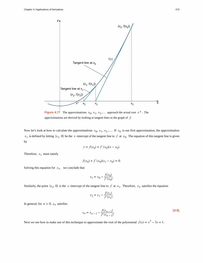
Figure 4.77 The approximations x0, x1, x2 ,… approach the actual root x * . The
approximations are derived by looking at tangent lines to the graph of f .
Now let’s look at how to calculate the approximations x0, x1, x2 ,…. If x0 is our first approximation, the approximation
x1 is defined by letting ⎛⎝x1, 0⎞
⎠ be the x -intercept of the tangent line to f at x0. The equation of this tangent line is given
by
y = f (x0) + f ′ (x0)(x − x0).
Therefore, x1 must satisfy
f (x0) + f ′ (x0)(x1 − x0) = 0.
Solving this equation for x1, we conclude that
x1 = x0 − f (x0)f ′(x0).
Similarly, the point ⎛⎝x2, 0⎞
⎠ is the x -intercept of the tangent line to f at x1. Therefore, x2 satisfies the equation
x2 = x1 − f (x1)f ′(x1).
In general, for n > 0, xn satisfies
(4.8)xn = xn − 1 − f (xn − 1)f ′(xn − 1).
Next we see how to make use of this technique to approximate the root of the polynomial f (x) = x3 − 3x + 1.
Chapter 4 | Applications of Derivatives 473
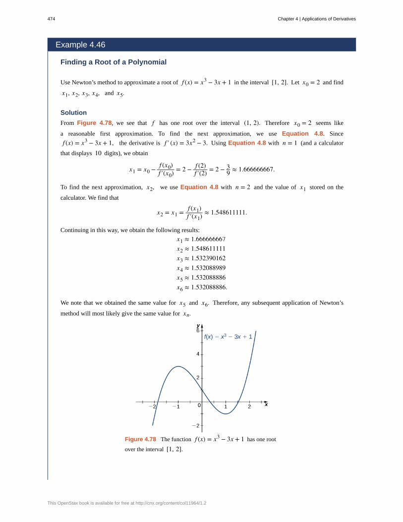
Example 4.46
Finding a Root of a Polynomial
Use Newton’s method to approximate a root of f (x) = x3 − 3x + 1 in the interval [1, 2]. Let x0 = 2 and find
x1, x2, x3, x4, and x5.
Solution
From Figure 4.78, we see that f has one root over the interval (1, 2). Therefore x0 = 2 seems like
a reasonable first approximation. To find the next approximation, we use Equation 4.8. Since
f (x) = x3 − 3x + 1, the derivative is f ′ (x) = 3x2 − 3. Using Equation 4.8 with n = 1 (and a calculator
that displays 10 digits), we obtain
x1 = x0 − f (x0)f ′(x0) = 2 − f (2)
f ′(2) = 2 − 39 ≈ 1.666666667.
To find the next approximation, x2, we use Equation 4.8 with n = 2 and the value of x1 stored on the
calculator. We find that
x2 = x1 = f (x1)f ′(x1) ≈ 1.548611111.
Continuing in this way, we obtain the following results:
x1 ≈ 1.666666667x2 ≈ 1.548611111x3 ≈ 1.532390162x4 ≈ 1.532088989x5 ≈ 1.532088886x6 ≈ 1.532088886.
We note that we obtained the same value for x5 and x6. Therefore, any subsequent application of Newton’s
method will most likely give the same value for xn.
Figure 4.78 The function f (x) = x3 − 3x + 1 has one root
over the interval [1, 2].
474 Chapter 4 | Applications of Derivatives
This OpenStax book is available for free at http://cnx.org/content/col11964/1.2
4.45 Letting x0 = 0, let’s use Newton’s method to approximate the root of f (x) = x3 − 3x + 1 over the
interval [0, 1] by calculating x1 and x2.
Newton’s method can also be used to approximate square roots. Here we show how to approximate 2. This method can
be modified to approximate the square root of any positive number.
Example 4.47
Finding a Square Root
Use Newton’s method to approximate 2 (Figure 4.79). Let f (x) = x2 − 2, let x0 = 2, and calculate
x1, x2, x3, x4, x5. (We note that since f (x) = x2 − 2 has a zero at 2, the initial value x0 = 2 is a
reasonable choice to approximate 2.)
Solution
For f (x) = x2 − 2, f ′ (x) = 2x. From Equation 4.8, we know that
xn = xn − 1 − f (xn − 1)f ′(xn − 1)
= xn − 1 −x2
n − 1 − 22xn − 1
= 12xn − 1 + 1
xn − 1
= 12
⎛⎝xn − 1 + 2
xn − 1⎞⎠.
Therefore,
x1 = 12
⎛⎝x0 + 2
x0⎞⎠ = 1
2⎛⎝2 + 2
2⎞⎠ = 1.5
x2 = 12
⎛⎝x1 + 2
x1⎞⎠ = 1
2⎛⎝1.5 + 2
1.5⎞⎠ ≈ 1.416666667.
Continuing in this way, we find that
x1 = 1.5x2 ≈ 1.416666667x3 ≈ 1.414215686x4 ≈ 1.414213562x5 ≈ 1.414213562.
Since we obtained the same value for x4 and x5, it is unlikely that the value xn will change on any subsequent
application of Newton’s method. We conclude that 2 ≈ 1.414213562.
Chapter 4 | Applications of Derivatives 475
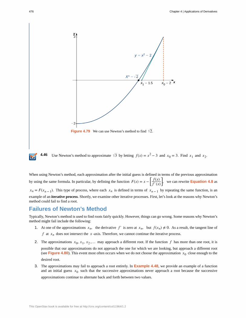
4.46
Figure 4.79 We can use Newton’s method to find 2.
Use Newton’s method to approximate 3 by letting f (x) = x2 − 3 and x0 = 3. Find x1 and x2.
When using Newton’s method, each approximation after the initial guess is defined in terms of the previous approximation
by using the same formula. In particular, by defining the function F(x) = x − ⎡⎣
f (x)f ′ (x)
⎤⎦, we can rewrite Equation 4.8 as
xn = F(xn − 1). This type of process, where each xn is defined in terms of xn − 1 by repeating the same function, is an
example of an iterative process. Shortly, we examine other iterative processes. First, let’s look at the reasons why Newton’smethod could fail to find a root.
Failures of Newton’s MethodTypically, Newton’s method is used to find roots fairly quickly. However, things can go wrong. Some reasons why Newton’smethod might fail include the following:
1. At one of the approximations xn, the derivative f ′ is zero at xn, but f (xn) ≠ 0. As a result, the tangent line of
f at xn does not intersect the x -axis. Therefore, we cannot continue the iterative process.
2. The approximations x0, x1, x2 ,… may approach a different root. If the function f has more than one root, it is
possible that our approximations do not approach the one for which we are looking, but approach a different root(see Figure 4.80). This event most often occurs when we do not choose the approximation x0 close enough to the
desired root.
3. The approximations may fail to approach a root entirely. In Example 4.48, we provide an example of a functionand an initial guess x0 such that the successive approximations never approach a root because the successive
approximations continue to alternate back and forth between two values.
476 Chapter 4 | Applications of Derivatives
This OpenStax book is available for free at http://cnx.org/content/col11964/1.2
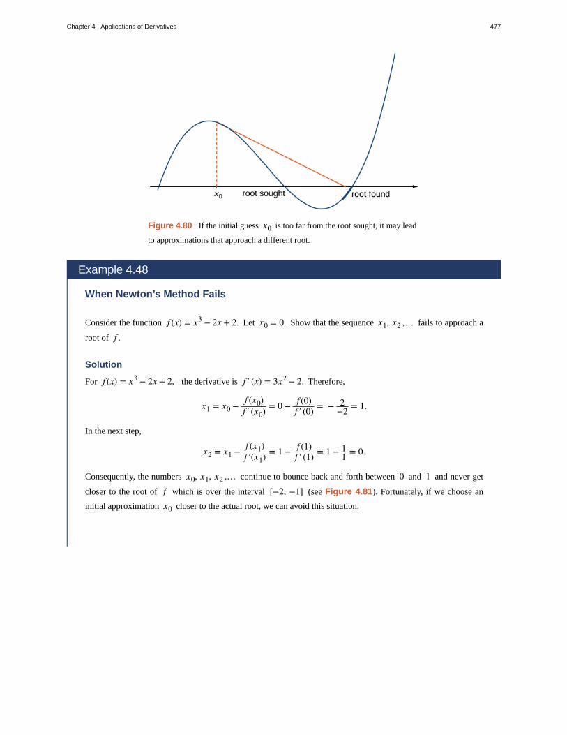
Figure 4.80 If the initial guess x0 is too far from the root sought, it may lead
to approximations that approach a different root.
Example 4.48
When Newton’s Method Fails
Consider the function f (x) = x3 − 2x + 2. Let x0 = 0. Show that the sequence x1, x2 ,… fails to approach a
root of f .
Solution
For f (x) = x3 − 2x + 2, the derivative is f ′ (x) = 3x2 − 2. Therefore,
x1 = x0 − f (x0)f ′ (x0) = 0 − f (0)
f ′ (0) = − 2−2 = 1.
In the next step,
x2 = x1 − f (x1)f ′(x1) = 1 − f (1)
f ′ (1) = 1 − 11 = 0.
Consequently, the numbers x0, x1, x2 ,… continue to bounce back and forth between 0 and 1 and never get
closer to the root of f which is over the interval [−2, −1] (see Figure 4.81). Fortunately, if we choose an
initial approximation x0 closer to the actual root, we can avoid this situation.
Chapter 4 | Applications of Derivatives 477
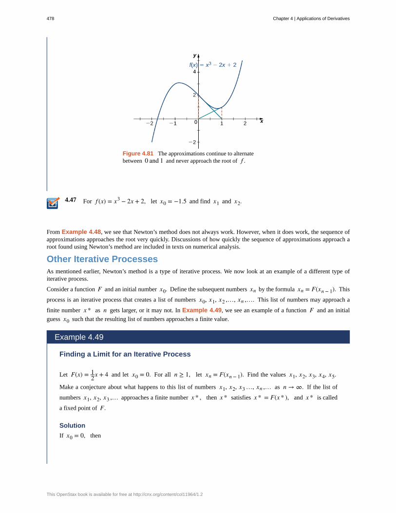
4.47
Figure 4.81 The approximations continue to alternatebetween 0 and 1 and never approach the root of f .
For f (x) = x3 − 2x + 2, let x0 = −1.5 and find x1 and x2.
From Example 4.48, we see that Newton’s method does not always work. However, when it does work, the sequence ofapproximations approaches the root very quickly. Discussions of how quickly the sequence of approximations approach aroot found using Newton’s method are included in texts on numerical analysis.
Other Iterative ProcessesAs mentioned earlier, Newton’s method is a type of iterative process. We now look at an example of a different type ofiterative process.
Consider a function F and an initial number x0. Define the subsequent numbers xn by the formula xn = F(xn − 1). This
process is an iterative process that creates a list of numbers x0, x1, x2 ,…, xn ,…. This list of numbers may approach a
finite number x * as n gets larger, or it may not. In Example 4.49, we see an example of a function F and an initial
guess x0 such that the resulting list of numbers approaches a finite value.
Example 4.49
Finding a Limit for an Iterative Process
Let F(x) = 12x + 4 and let x0 = 0. For all n ≥ 1, let xn = F(xn − 1). Find the values x1, x2, x3, x4, x5.
Make a conjecture about what happens to this list of numbers x1, x2, x3 …, xn ,… as n → ∞. If the list of
numbers x1, x2, x3 ,… approaches a finite number x * , then x * satisfies x * = F(x * ), and x * is called
a fixed point of F.
Solution
If x0 = 0, then
478 Chapter 4 | Applications of Derivatives
This OpenStax book is available for free at http://cnx.org/content/col11964/1.2
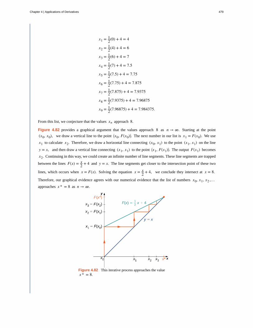
x1 = 12(0) + 4 = 4
x2 = 12(4) + 4 = 6
x3 = 12(6) + 4 = 7
x4 = 12(7) + 4 = 7.5
x5 = 12(7.5) + 4 = 7.75
x6 = 12(7.75) + 4 = 7.875
x7 = 12(7.875) + 4 = 7.9375
x8 = 12(7.9375) + 4 = 7.96875
x9 = 12(7.96875) + 4 = 7.984375.
From this list, we conjecture that the values xn approach 8.
Figure 4.82 provides a graphical argument that the values approach 8 as n → ∞. Starting at the point
(x0, x0), we draw a vertical line to the point ⎛⎝x0, F(x0)⎞
⎠. The next number in our list is x1 = F(x0). We use
x1 to calculate x2. Therefore, we draw a horizontal line connecting (x0, x1) to the point (x1, x1) on the line
y = x, and then draw a vertical line connecting (x1, x1) to the point ⎛⎝x1, F(x1)⎞
⎠. The output F(x1) becomes
x2. Continuing in this way, we could create an infinite number of line segments. These line segments are trapped
between the lines F(x) = x2 + 4 and y = x. The line segments get closer to the intersection point of these two
lines, which occurs when x = F(x). Solving the equation x = x2 + 4, we conclude they intersect at x = 8.
Therefore, our graphical evidence agrees with our numerical evidence that the list of numbers x0, x1, x2 ,…approaches x * = 8 as n → ∞.
Figure 4.82 This iterative process approaches the valuex * = 8.
Chapter 4 | Applications of Derivatives 479
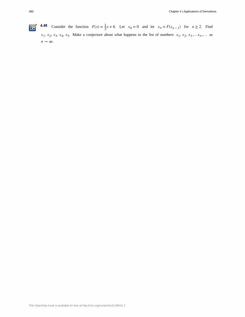
4.48 Consider the function F(x) = 13x + 6. Let x0 = 0 and let xn = F(xn − 1) for n ≥ 2. Find
x1, x2, x3, x4, x5. Make a conjecture about what happens to the list of numbers x1, x2, x3 ,…xn ,… as
n → ∞.
480 Chapter 4 | Applications of Derivatives
This OpenStax book is available for free at http://cnx.org/content/col11964/1.2
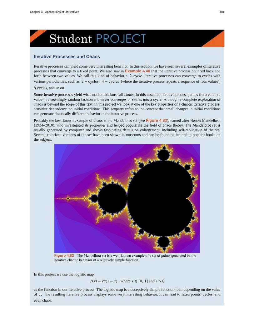
Iterative Processes and Chaos
Iterative processes can yield some very interesting behavior. In this section, we have seen several examples of iterativeprocesses that converge to a fixed point. We also saw in Example 4.48 that the iterative process bounced back andforth between two values. We call this kind of behavior a 2 -cycle. Iterative processes can converge to cycles with
various periodicities, such as 2 − cycles, 4 − cycles (where the iterative process repeats a sequence of four values),
8-cycles, and so on.
Some iterative processes yield what mathematicians call chaos. In this case, the iterative process jumps from value tovalue in a seemingly random fashion and never converges or settles into a cycle. Although a complete exploration ofchaos is beyond the scope of this text, in this project we look at one of the key properties of a chaotic iterative process:sensitive dependence on initial conditions. This property refers to the concept that small changes in initial conditionscan generate drastically different behavior in the iterative process.
Probably the best-known example of chaos is the Mandelbrot set (see Figure 4.83), named after Benoit Mandelbrot(1924–2010), who investigated its properties and helped popularize the field of chaos theory. The Mandelbrot set isusually generated by computer and shows fascinating details on enlargement, including self-replication of the set.Several colorized versions of the set have been shown in museums and can be found online and in popular books onthe subject.
Figure 4.83 The Mandelbrot set is a well-known example of a set of points generated by theiterative chaotic behavior of a relatively simple function.
In this project we use the logistic map
f (x) = rx(1 − x), where x ∈ [0, 1] and r > 0
as the function in our iterative process. The logistic map is a deceptively simple function; but, depending on the valueof r, the resulting iterative process displays some very interesting behavior. It can lead to fixed points, cycles, and
even chaos.
Chapter 4 | Applications of Derivatives 481
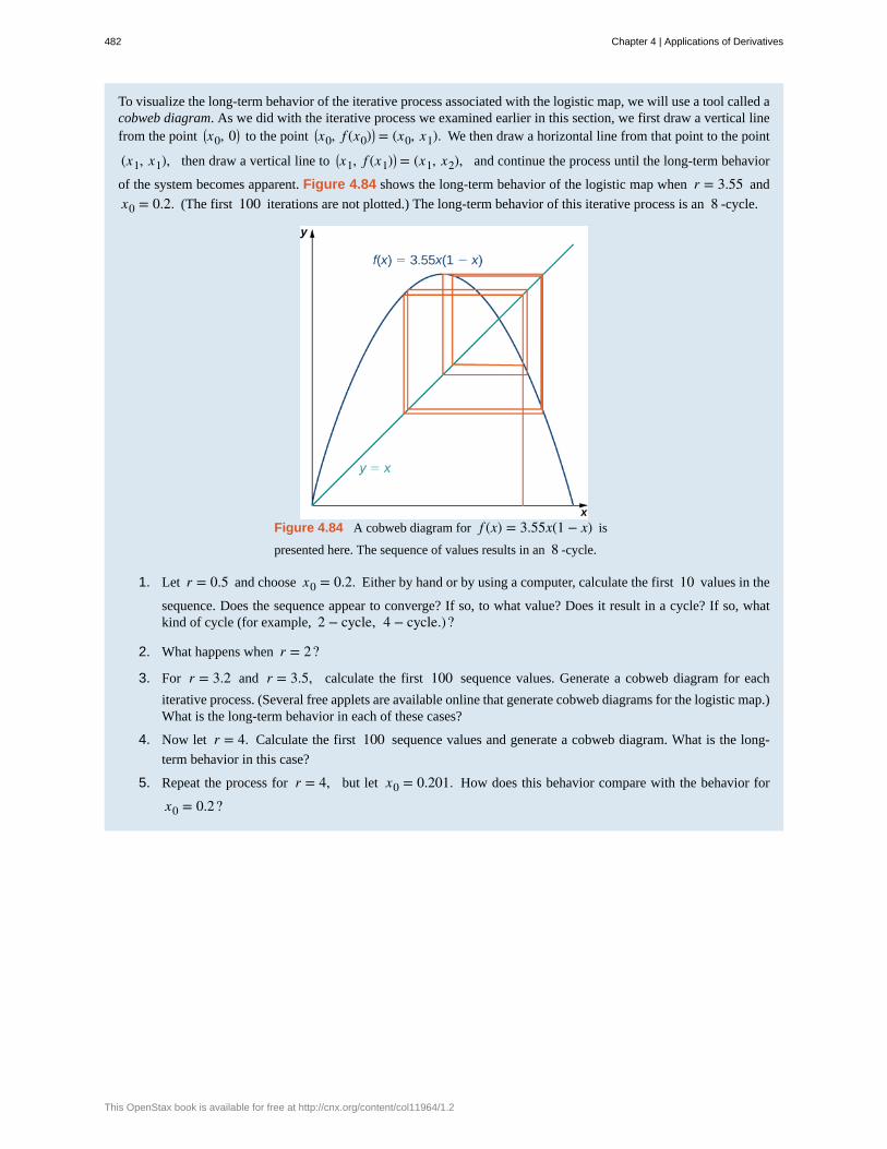
To visualize the long-term behavior of the iterative process associated with the logistic map, we will use a tool called acobweb diagram. As we did with the iterative process we examined earlier in this section, we first draw a vertical linefrom the point ⎛
⎝x0, 0⎞⎠ to the point ⎛
⎝x0, f (x0)⎞⎠ = (x0, x1). We then draw a horizontal line from that point to the point
(x1, x1), then draw a vertical line to ⎛⎝x1, f (x1)⎞
⎠ = (x1, x2), and continue the process until the long-term behavior
of the system becomes apparent. Figure 4.84 shows the long-term behavior of the logistic map when r = 3.55 and
x0 = 0.2. (The first 100 iterations are not plotted.) The long-term behavior of this iterative process is an 8 -cycle.
Figure 4.84 A cobweb diagram for f (x) = 3.55x(1 − x) is
presented here. The sequence of values results in an 8 -cycle.
1. Let r = 0.5 and choose x0 = 0.2. Either by hand or by using a computer, calculate the first 10 values in the
sequence. Does the sequence appear to converge? If so, to what value? Does it result in a cycle? If so, whatkind of cycle (for example, 2 − cycle, 4 − cycle.)?
2. What happens when r = 2?
3. For r = 3.2 and r = 3.5, calculate the first 100 sequence values. Generate a cobweb diagram for each
iterative process. (Several free applets are available online that generate cobweb diagrams for the logistic map.)What is the long-term behavior in each of these cases?
4. Now let r = 4. Calculate the first 100 sequence values and generate a cobweb diagram. What is the long-
term behavior in this case?
5. Repeat the process for r = 4, but let x0 = 0.201. How does this behavior compare with the behavior for
x0 = 0.2?
482 Chapter 4 | Applications of Derivatives
This OpenStax book is available for free at http://cnx.org/content/col11964/1.2
4.9 EXERCISESFor the following exercises, write Newton’s formula asxn + 1 = F(xn) for solving f (x) = 0.
406. f (x) = x2 + 1
407. f (x) = x3 + 2x + 1
408. f (x) = sinx
409. f (x) = ex
410. f (x) = x3 + 3xex
For the following exercises, solve f (x) = 0 using the
iteration xn + 1 = xn − c f (xn), which differs slightly
from Newton’s method. Find a c that works and a c that
fails to converge, with the exception of c = 0.
411. f (x) = x2 − 4, with x0 = 0
412. f (x) = x2 − 4x + 3, with x0 = 2
413. What is the value of “c” for Newton’s method?
For the following exercises, start at
a. x0 = 0.6 and
b. x0 = 2.
Compute x1 and x2 using the specified iterative method.
414. xn + 1 = xn2 − 1
2
415. xn + 1 = 2xn⎛⎝1 − xn
⎞⎠
416. xn + 1 = xn
417. xn + 1 = 1xn
418. xn + 1 = 3xn⎛⎝1 − xn
⎞⎠
419. xn + 1 = xn2 + xn − 2
420. xn + 1 = 12xn − 1
421. xn + 1 = |xn|
For the following exercises, solve to four decimal places
using Newton’s method and a computer or calculator.Choose any initial guess x0 that is not the exact root.
422. x2 − 10 = 0
423. x4 − 100 = 0
424. x2 − x = 0
425. x3 − x = 0
426. x + 5cos(x) = 0
427. x + tan(x) = 0, choose x0 ∈ ⎛⎝−
π2, π
2⎞⎠
428. 11 − x = 2
429. 1 + x + x2 + x3 + x4 = 2
430. x3 + (x + 1)3 = 103
431. x = sin2 (x)
For the following exercises, use Newton’s method to findthe fixed points of the function where f (x) = x; round to
three decimals.
432. sinx
433. tan(x) on x = ⎛⎝π2, 3π
2⎞⎠
434. ex − 2
435. ln(x) + 2
Newton’s method can be used to find maxima and minimaof functions in addition to the roots. In this case applyNewton’s method to the derivative function f ′ (x) to find
its roots, instead of the original function. For the followingexercises, consider the formulation of the method.
436. To find candidates for maxima and minima, we needto find the critical points f ′ (x) = 0. Show that to solve for
the critical points of a function f (x), Newton’s method is
given by xn + 1 = xn − f ′ (xn)f ″(xn).
437. What additional restrictions are necessary on thefunction f ?
Chapter 4 | Applications of Derivatives 483
For the following exercises, use Newton’s method to findthe location of the local minima and/or maxima of thefollowing functions; round to three decimals.
438. Minimum of f (x) = x2 + 2x + 4
439. Minimum of f (x) = 3x3 + 2x2 − 16
440. Minimum of f (x) = x2 ex
441. Maximum of f (x) = x + 1x
442. Maximum of f (x) = x3 + 10x2 + 15x − 2
443. Maximum of f (x) = x − x3x
444. Minimum of f (x) = x2 sinx, closest non-zero
minimum to x = 0
445. Minimum of f (x) = x4 + x3 + 3x2 + 12x + 6
For the following exercises, use the specified method tosolve the equation. If it does not work, explain why it doesnot work.
446. Newton’s method, x2 + 2 = 0
447. Newton’s method, 0 = ex
448. Newton’s method, 0 = 1 + x2 starting at x0 = 0
449. Solving xn + 1 = −xn3 starting at x0 = −1
For the following exercises, use the secant method, analternative iterative method to Newton’s method. Theformula is given by
xn = xn − 1 − f (xn − 1) xn − 1 − xn − 2f (xn − 1) − f (xn − 2).
450. Find a root to 0 = x2 − x − 3 accurate to three
decimal places.
451. Find a root to 0 = sinx + 3x accurate to four
decimal places.
452. Find a root to 0 = ex − 2 accurate to four decimal
places.
453. Find a root to ln(x + 2) = 12 accurate to four
decimal places.
454. Why would you use the secant method overNewton’s method? What are the necessary restrictions onf ?
For the following exercises, use both Newton’s methodand the secant method to calculate a root for the followingequations. Use a calculator or computer to calculate howmany iterations of each are needed to reach within threedecimal places of the exact answer. For the secant method,use the first guess from Newton’s method.
455. f (x) = x2 + 2x + 1, x0 = 1
456. f (x) = x2, x0 = 1
457. f (x) = sinx, x0 = 1
458. f (x) = ex − 1, x0 = 2
459. f (x) = x3 + 2x + 4, x0 = 0
In the following exercises, consider Kepler’s equationregarding planetary orbits, M = E − εsin(E), where Mis the mean anomaly, E is eccentric anomaly, and εmeasures eccentricity.
460. Use Newton’s method to solve for the eccentricanomaly E when the mean anomaly M = π
3 and the
eccentricity of the orbit ε = 0.25; round to three
decimals.
461. Use Newton’s method to solve for the eccentric
anomaly E when the mean anomaly M = 3π2 and the
eccentricity of the orbit ε = 0.8; round to three decimals.
The following two exercises consider a bank investment.The initial investment is $10,000. After 25 years, the
investment has tripled to $30,000.
462. Use Newton’s method to determine the interest rateif the interest was compounded annually.
463. Use Newton’s method to determine the interest rateif the interest was compounded continuously.
464. The cost for printing a book can be given by the
equation C(x) = 1000 + 12x + ⎛⎝12
⎞⎠x
2/3. Use Newton’s
method to find the break-even point if the printer sells eachbook for $20.
484 Chapter 4 | Applications of Derivatives
This OpenStax book is available for free at http://cnx.org/content/col11964/1.2
4.10 | Antiderivatives
Learning Objectives4.10.1 Find the general antiderivative of a given function.
4.10.2 Explain the terms and notation used for an indefinite integral.
4.10.3 State the power rule for integrals.
4.10.4 Use antidifferentiation to solve simple initial-value problems.
At this point, we have seen how to calculate derivatives of many functions and have been introduced to a variety of theirapplications. We now ask a question that turns this process around: Given a function f , how do we find a function with
the derivative f and why would we be interested in such a function?
We answer the first part of this question by defining antiderivatives. The antiderivative of a function f is a function with a
derivative f . Why are we interested in antiderivatives? The need for antiderivatives arises in many situations, and we look
at various examples throughout the remainder of the text. Here we examine one specific example that involves rectilinearmotion. In our examination in Derivatives of rectilinear motion, we showed that given a position function s(t) of an
object, then its velocity function v(t) is the derivative of s(t) —that is, v(t) = s′ (t). Furthermore, the acceleration a(t)is the derivative of the velocity v(t) —that is, a(t) = v′ (t) = s″(t). Now suppose we are given an acceleration function
a, but not the velocity function v or the position function s. Since a(t) = v′ (t), determining the velocity function
requires us to find an antiderivative of the acceleration function. Then, since v(t) = s′ (t), determining the position
function requires us to find an antiderivative of the velocity function. Rectilinear motion is just one case in which theneed for antiderivatives arises. We will see many more examples throughout the remainder of the text. For now, let’s lookat the terminology and notation for antiderivatives, and determine the antiderivatives for several types of functions. Weexamine various techniques for finding antiderivatives of more complicated functions later in the text (Introduction toTechniques of Integration (http://cnx.org/content/m53654/latest/) ).
The Reverse of DifferentiationAt this point, we know how to find derivatives of various functions. We now ask the opposite question. Given a functionf , how can we find a function with derivative f ? If we can find a function F derivative f , we call F an antiderivative
of f .
Definition
A function F is an antiderivative of the function f if
F′ (x) = f (x)
for all x in the domain of f .
Consider the function f (x) = 2x. Knowing the power rule of differentiation, we conclude that F(x) = x2 is an
antiderivative of f since F′ (x) = 2x. Are there any other antiderivatives of f ? Yes; since the derivative of any constant
C is zero, x2 + C is also an antiderivative of 2x. Therefore, x2 + 5 and x2 − 2 are also antiderivatives. Are there any
others that are not of the form x2 + C for some constant C ? The answer is no. From Corollary 2 of the Mean Value
Theorem, we know that if F and G are differentiable functions such that F′ (x) = G′ (x), then F(x) − G(x) = C for
some constant C. This fact leads to the following important theorem.
Chapter 4 | Applications of Derivatives 485
Theorem 4.14: General Form of an Antiderivative
Let F be an antiderivative of f over an interval I. Then,
i. for each constant C, the function F(x) + C is also an antiderivative of f over I;
ii. if G is an antiderivative of f over I, there is a constant C for which G(x) = F(x) + C over I.
In other words, the most general form of the antiderivative of f over I is F(x) + C.
We use this fact and our knowledge of derivatives to find all the antiderivatives for several functions.
Example 4.50
Finding Antiderivatives
For each of the following functions, find all antiderivatives.
a. f (x) = 3x2
b. f (x) = 1x
c. f (x) = cosx
d. f (x) = ex
Solution
a. Because
ddx
⎛⎝x
3⎞⎠ = 3x2
then F(x) = x3 is an antiderivative of 3x2. Therefore, every antiderivative of 3x2 is of the form
x3 + C for some constant C, and every function of the form x3 + C is an antiderivative of 3x2.
b. Let f (x) = ln|x|. For x > 0, f (x) = ln(x) and
ddx(lnx) = 1
x .
For x < 0, f (x) = ln(−x) and
ddx
⎛⎝ln(−x)⎞
⎠ = − 1−x = 1
x .
Therefore,
ddx(ln|x|) = 1
x .
Thus, F(x) = ln|x| is an antiderivative of 1x . Therefore, every antiderivative of 1
x is of the form
ln|x| + C for some constant C and every function of the form ln|x| + C is an antiderivative of 1x .
c. We have
486 Chapter 4 | Applications of Derivatives
This OpenStax book is available for free at http://cnx.org/content/col11964/1.2
4.49
ddx(sinx) = cosx,
so F(x) = sinx is an antiderivative of cosx. Therefore, every antiderivative of cosx is of the form
sinx + C for some constant C and every function of the form sinx + C is an antiderivative of cosx.
d. Since
ddx(ex) = ex,
then F(x) = ex is an antiderivative of ex. Therefore, every antiderivative of ex is of the form ex + Cfor some constant C and every function of the form ex + C is an antiderivative of ex.
Find all antiderivatives of f (x) = sinx.
Indefinite IntegralsWe now look at the formal notation used to represent antiderivatives and examine some of their properties. These properties
allow us to find antiderivatives of more complicated functions. Given a function f , we use the notation f ′ (x) ord fdx
to denote the derivative of f . Here we introduce notation for antiderivatives. If F is an antiderivative of f , we say that
F(x) + C is the most general antiderivative of f and write
∫ f (x)dx = F(x) + C.
The symbol ∫ is called an integral sign, and ∫ f (x)dx is called the indefinite integral of f .
Definition
Given a function f , the indefinite integral of f , denoted
∫ f (x)dx,
is the most general antiderivative of f . If F is an antiderivative of f , then
∫ f (x)dx = F(x) + C.
The expression f (x) is called the integrand and the variable x is the variable of integration.
Given the terminology introduced in this definition, the act of finding the antiderivatives of a function f is usually referred
to as integrating f .
For a function f and an antiderivative F, the functions F(x) + C, where C is any real number, is often referred to as
the family of antiderivatives of f . For example, since x2 is an antiderivative of 2x and any antiderivative of 2x is of the
form x2 + C, we write
Chapter 4 | Applications of Derivatives 487
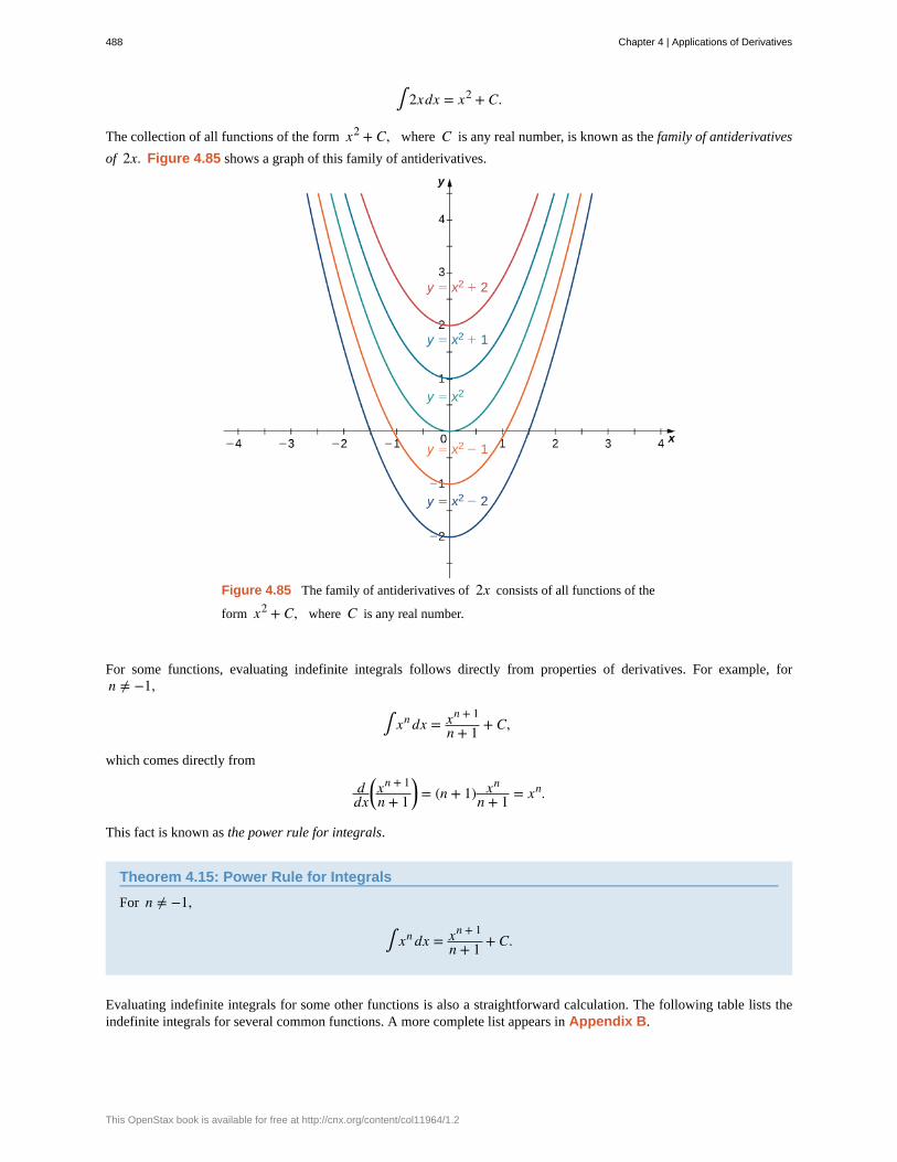
∫ 2xdx = x2 + C.
The collection of all functions of the form x2 + C, where C is any real number, is known as the family of antiderivatives
of 2x. Figure 4.85 shows a graph of this family of antiderivatives.
Figure 4.85 The family of antiderivatives of 2x consists of all functions of the
form x2 + C, where C is any real number.
For some functions, evaluating indefinite integrals follows directly from properties of derivatives. For example, forn ≠ −1,
∫ xn dx = xn + 1
n + 1 + C,
which comes directly from
ddx
⎛⎝
xn + 1
n + 1⎞⎠ = (n + 1) xn
n + 1 = xn.
This fact is known as the power rule for integrals.
Theorem 4.15: Power Rule for Integrals
For n ≠ −1,
∫ xn dx = xn + 1
n + 1 + C.
Evaluating indefinite integrals for some other functions is also a straightforward calculation. The following table lists theindefinite integrals for several common functions. A more complete list appears in Appendix B.
488 Chapter 4 | Applications of Derivatives
This OpenStax book is available for free at http://cnx.org/content/col11964/1.2
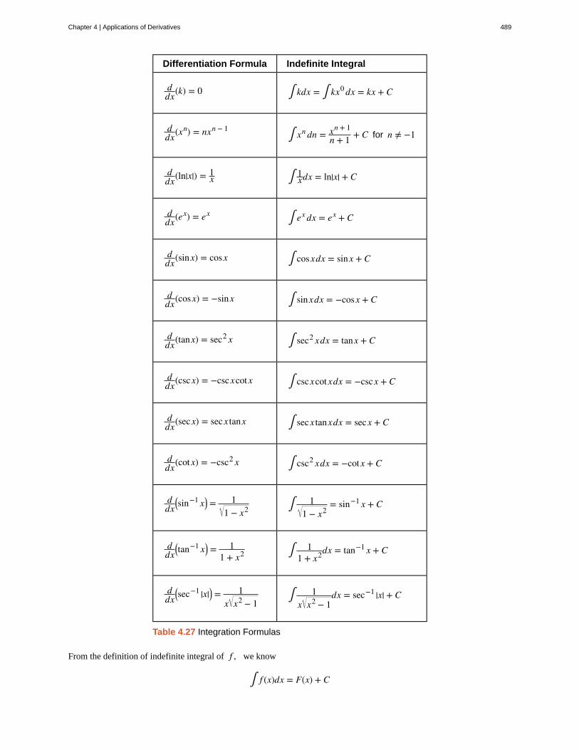
Differentiation Formula Indefinite Integral
ddx(k) = 0 ∫ kdx = ∫ kx0 dx = kx + C
ddx(xn) = nxn − 1 ∫ xn dn = xn + 1
n + 1 + C for n ≠ −1
ddx(ln|x|) = 1
x ∫ 1xdx = ln|x| + C
ddx(ex) = ex ∫ ex dx = ex + C
ddx(sinx) = cosx ∫ cosxdx = sinx + C
ddx(cosx) = −sinx ∫ sinxdx = −cosx + C
ddx(tanx) = sec2 x ∫ sec2 xdx = tanx + C
ddx(cscx) = −cscxcot x ∫ cscxcot xdx = −cscx + C
ddx(secx) = secx tanx ∫ secx tanxdx = secx + C
ddx(cot x) = −csc2 x ∫ csc2 xdx = −cot x + C
ddx
⎛⎝sin−1 x⎞
⎠ = 11 − x2 ∫ 1
1 − x2= sin−1 x + C
ddx
⎛⎝tan−1 x⎞
⎠ = 11 + x2 ∫ 1
1 + x2dx = tan−1 x + C
ddx
⎛⎝sec−1 |x|⎞⎠ = 1
x x2 − 1∫ 1
x x2 − 1dx = sec−1 |x| + C
Table 4.27 Integration Formulas
From the definition of indefinite integral of f , we know
∫ f (x)dx = F(x) + C
Chapter 4 | Applications of Derivatives 489
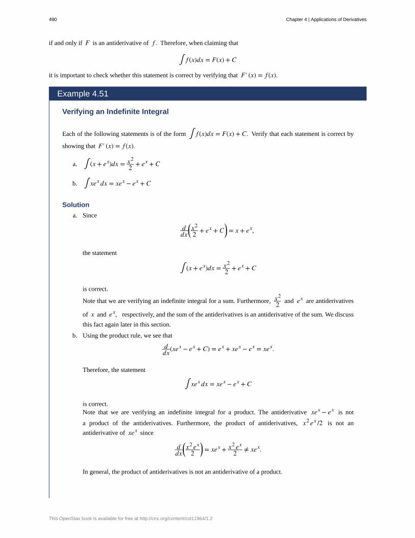
if and only if F is an antiderivative of f . Therefore, when claiming that
∫ f (x)dx = F(x) + C
it is important to check whether this statement is correct by verifying that F′ (x) = f (x).
Example 4.51
Verifying an Indefinite Integral
Each of the following statements is of the form ∫ f (x)dx = F(x) + C. Verify that each statement is correct by
showing that F′ (x) = f (x).
a. ∫ (x + ex)dx = x2
2 + ex + C
b. ∫ xex dx = xex − ex + C
Solution
a. Since
ddx
⎛⎝
x2
2 + ex + C⎞⎠ = x + ex,
the statement
∫ (x + ex)dx = x2
2 + ex + C
is correct.
Note that we are verifying an indefinite integral for a sum. Furthermore, x2
2 and ex are antiderivatives
of x and ex, respectively, and the sum of the antiderivatives is an antiderivative of the sum. We discuss
this fact again later in this section.
b. Using the product rule, we see that
ddx(xex − ex + C) = ex + xex − ex = xex.
Therefore, the statement
∫ xex dx = xex − ex + C
is correct.Note that we are verifying an indefinite integral for a product. The antiderivative xex − ex is not
a product of the antiderivatives. Furthermore, the product of antiderivatives, x2 ex /2 is not an
antiderivative of xex since
ddx
⎛⎝
x2 ex
2⎞⎠ = xex + x2 ex
2 ≠ xex.
In general, the product of antiderivatives is not an antiderivative of a product.
490 Chapter 4 | Applications of Derivatives
This OpenStax book is available for free at http://cnx.org/content/col11964/1.2
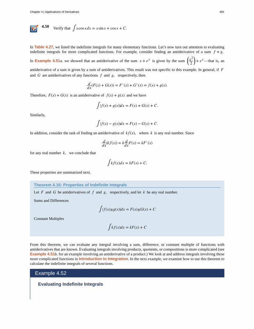
4.50 Verify that ∫ xcosxdx = xsinx + cosx + C.
In Table 4.27, we listed the indefinite integrals for many elementary functions. Let’s now turn our attention to evaluatingindefinite integrals for more complicated functions. For example, consider finding an antiderivative of a sum f + g.
In Example 4.51a. we showed that an antiderivative of the sum x + ex is given by the sum⎛⎝
x2
2⎞⎠ + ex —that is, an
antiderivative of a sum is given by a sum of antiderivatives. This result was not specific to this example. In general, if Fand G are antiderivatives of any functions f and g, respectively, then
ddx(F(x) + G(x)) = F′ (x) + G′ (x) = f (x) + g(x).
Therefore, F(x) + G(x) is an antiderivative of f (x) + g(x) and we have
∫ ⎛⎝ f (x) + g(x)⎞
⎠dx = F(x) + G(x) + C.
Similarly,
∫ ⎛⎝ f (x) − g(x)⎞
⎠dx = F(x) − G(x) + C.
In addition, consider the task of finding an antiderivative of k f (x), where k is any real number. Since
ddx
⎛⎝k f (x)⎞
⎠ = k ddxF(x) = kF′ (x)
for any real number k, we conclude that
∫ k f (x)dx = kF(x) + C.
These properties are summarized next.
Theorem 4.16: Properties of Indefinite Integrals
Let F and G be antiderivatives of f and g, respectively, and let k be any real number.
Sums and Differences
∫ ⎛⎝ f (x)±g(x)⎞
⎠dx = F(x)±G(x) + C
Constant Multiples
∫ k f (x)dx = kF(x) + C
From this theorem, we can evaluate any integral involving a sum, difference, or constant multiple of functions withantiderivatives that are known. Evaluating integrals involving products, quotients, or compositions is more complicated (seeExample 4.51b. for an example involving an antiderivative of a product.) We look at and address integrals involving thesemore complicated functions in Introduction to Integration. In the next example, we examine how to use this theorem tocalculate the indefinite integrals of several functions.
Example 4.52
Evaluating Indefinite Integrals
Chapter 4 | Applications of Derivatives 491
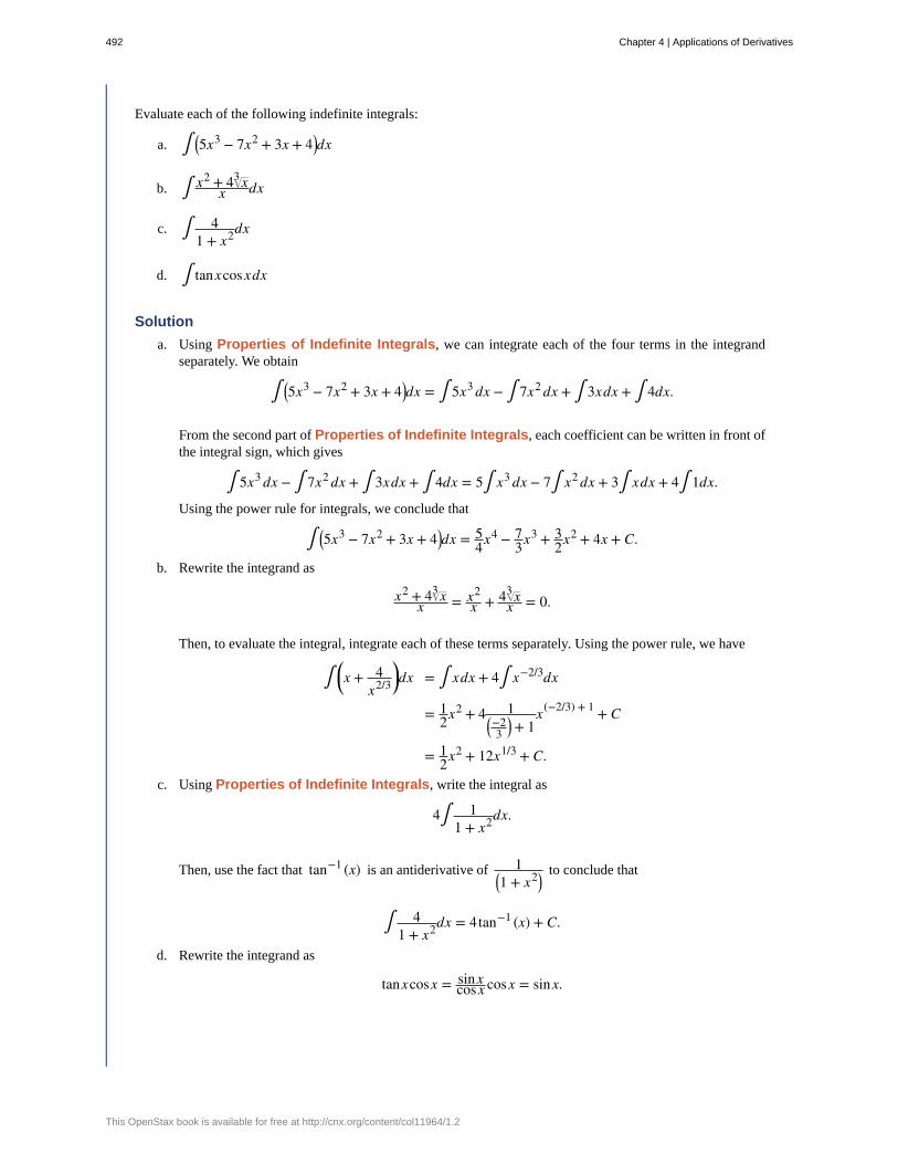
Evaluate each of the following indefinite integrals:
a. ∫ ⎛⎝5x3 − 7x2 + 3x + 4⎞
⎠dx
b. ∫ x2 + 4 x3x dx
c. ∫ 41 + x2dx
d. ∫ tanxcosxdx
Solution
a. Using Properties of Indefinite Integrals, we can integrate each of the four terms in the integrandseparately. We obtain
∫ ⎛⎝5x3 − 7x2 + 3x + 4⎞
⎠dx = ∫ 5x3 dx − ∫ 7x2 dx + ∫ 3xdx + ∫ 4dx.
From the second part of Properties of Indefinite Integrals, each coefficient can be written in front ofthe integral sign, which gives
∫ 5x3 dx − ∫ 7x2 dx + ∫ 3xdx + ∫ 4dx = 5∫ x3 dx − 7∫ x2 dx + 3∫ xdx + 4∫ 1dx.
Using the power rule for integrals, we conclude that
∫ ⎛⎝5x3 − 7x2 + 3x + 4⎞
⎠dx = 54x4 − 7
3x3 + 32x2 + 4x + C.
b. Rewrite the integrand as
x2 + 4 x3x = x2
x + 4 x3x = 0.
Then, to evaluate the integral, integrate each of these terms separately. Using the power rule, we have
∫ ⎛⎝x + 4
x2/3⎞⎠dx = ∫ xdx + 4∫ x−2/3dx
= 12x2 + 4 1
⎛⎝−23
⎞⎠ + 1
x(−2/3) + 1 + C
= 12x2 + 12x1/3 + C.
c. Using Properties of Indefinite Integrals, write the integral as
4∫ 11 + x2dx.
Then, use the fact that tan−1 (x) is an antiderivative of 1⎛⎝1 + x2⎞
⎠to conclude that
∫ 41 + x2dx = 4tan−1 (x) + C.
d. Rewrite the integrand as
tanxcosx = sinxcosx cosx = sinx.
492 Chapter 4 | Applications of Derivatives
This OpenStax book is available for free at http://cnx.org/content/col11964/1.2
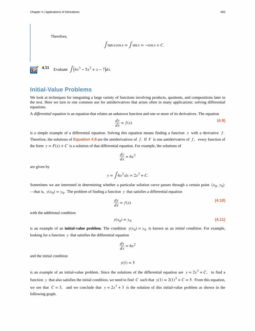
4.51
Therefore,
∫ tanxcosx = ∫ sinx = −cosx + C.
Evaluate ∫ ⎛⎝4x3 − 5x2 + x − 7⎞
⎠dx.
Initial-Value ProblemsWe look at techniques for integrating a large variety of functions involving products, quotients, and compositions later inthe text. Here we turn to one common use for antiderivatives that arises often in many applications: solving differentialequations.
A differential equation is an equation that relates an unknown function and one or more of its derivatives. The equation
(4.9)dydx = f (x)
is a simple example of a differential equation. Solving this equation means finding a function y with a derivative f .Therefore, the solutions of Equation 4.9 are the antiderivatives of f . If F is one antiderivative of f , every function of
the form y = F(x) + C is a solution of that differential equation. For example, the solutions of
dydx = 6x2
are given by
y = ∫ 6x2 dx = 2x3 + C.
Sometimes we are interested in determining whether a particular solution curve passes through a certain point (x0, y0)—that is, y(x0) = y0. The problem of finding a function y that satisfies a differential equation
(4.10)dydx = f (x)
with the additional condition
(4.11)y(x0) = y0
is an example of an initial-value problem. The condition y(x0) = y0 is known as an initial condition. For example,
looking for a function y that satisfies the differential equation
dydx = 6x2
and the initial condition
y(1) = 5
is an example of an initial-value problem. Since the solutions of the differential equation are y = 2x3 + C, to find a
function y that also satisfies the initial condition, we need to find C such that y(1) = 2(1)3 + C = 5. From this equation,
we see that C = 3, and we conclude that y = 2x3 + 3 is the solution of this initial-value problem as shown in the
following graph.
Chapter 4 | Applications of Derivatives 493
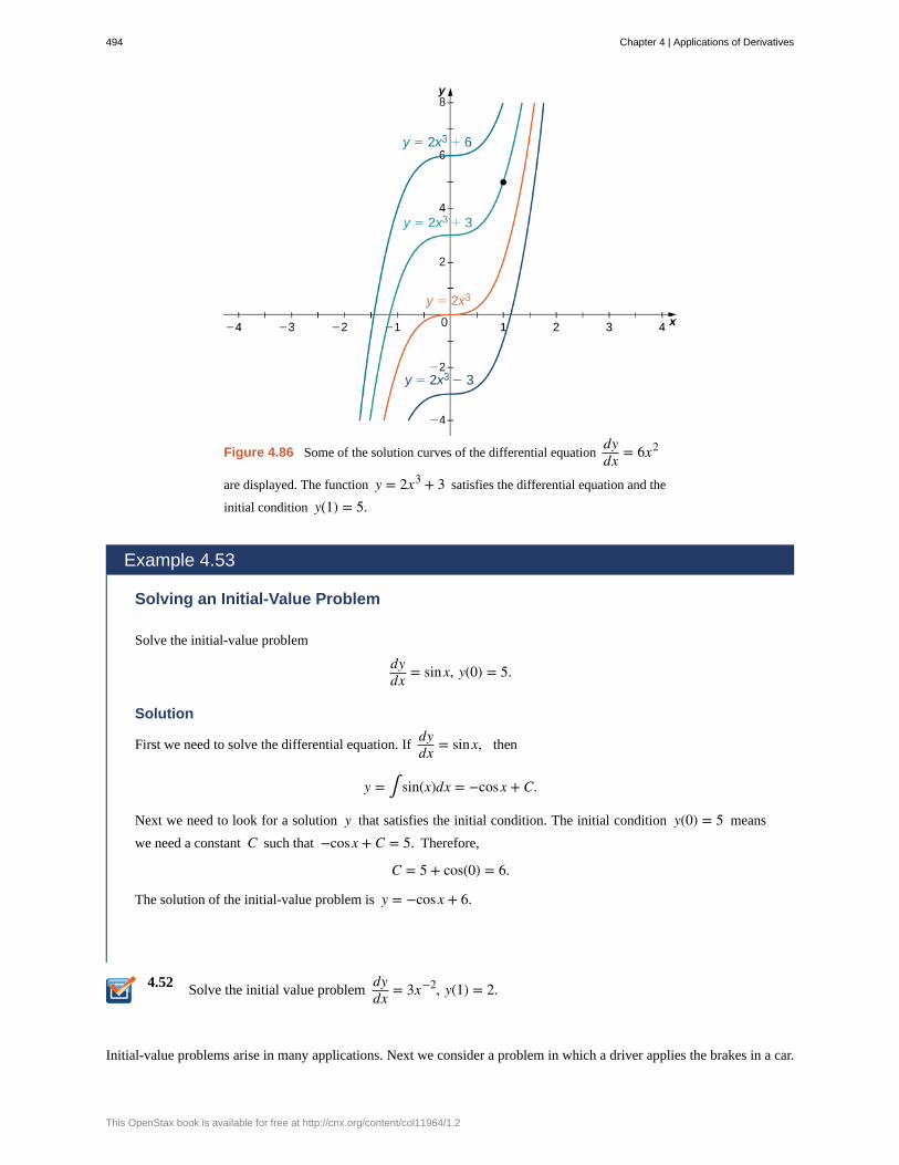
4.52
Figure 4.86 Some of the solution curves of the differential equationdydx = 6x2
are displayed. The function y = 2x3 + 3 satisfies the differential equation and the
initial condition y(1) = 5.
Example 4.53
Solving an Initial-Value Problem
Solve the initial-value problem
dydx = sinx, y(0) = 5.
Solution
First we need to solve the differential equation. Ifdydx = sinx, then
y = ∫ sin(x)dx = −cosx + C.
Next we need to look for a solution y that satisfies the initial condition. The initial condition y(0) = 5 means
we need a constant C such that −cosx + C = 5. Therefore,
C = 5 + cos(0) = 6.
The solution of the initial-value problem is y = −cosx + 6.
Solve the initial value problemdydx = 3x−2, y(1) = 2.
Initial-value problems arise in many applications. Next we consider a problem in which a driver applies the brakes in a car.
494 Chapter 4 | Applications of Derivatives
This OpenStax book is available for free at http://cnx.org/content/col11964/1.2
We are interested in how long it takes for the car to stop. Recall that the velocity function v(t) is the derivative of a position
function s(t), and the acceleration a(t) is the derivative of the velocity function. In earlier examples in the text, we could
calculate the velocity from the position and then compute the acceleration from the velocity. In the next example we workthe other way around. Given an acceleration function, we calculate the velocity function. We then use the velocity functionto determine the position function.
Example 4.54
Decelerating Car
A car is traveling at the rate of 88 ft/sec (60 mph) when the brakes are applied. The car begins decelerating at a
constant rate of 15 ft/sec2.
a. How many seconds elapse before the car stops?
b. How far does the car travel during that time?
Solution
a. First we introduce variables for this problem. Let t be the time (in seconds) after the brakes are first
applied. Let a(t) be the acceleration of the car (in feet per seconds squared) at time t. Let v(t) be the
velocity of the car (in feet per second) at time t. Let s(t) be the car’s position (in feet) beyond the point
where the brakes are applied at time t.The car is traveling at a rate of 88 ft/sec. Therefore, the initial velocity is v(0) = 88 ft/sec. Since the car
is decelerating, the acceleration is
a(t) = −15 ft/s2.
The acceleration is the derivative of the velocity,
v′ (t) = −15.
Therefore, we have an initial-value problem to solve:
v′ (t) = −15, v(0) = 88.
Integrating, we find that
v(t) = −15t + C.
Since v(0) = 88, C = 88. Thus, the velocity function is
v(t) = −15t + 88.
To find how long it takes for the car to stop, we need to find the time t such that the velocity is zero.
Solving −15t + 88 = 0, we obtain t = 8815 sec.
b. To find how far the car travels during this time, we need to find the position of the car after 8815 sec. We
know the velocity v(t) is the derivative of the position s(t). Consider the initial position to be s(0) = 0.Therefore, we need to solve the initial-value problem
s′ (t) = −15t + 88, s(0) = 0.
Chapter 4 | Applications of Derivatives 495
4.53
Integrating, we have
s(t) = − 152 t2 + 88t + C.
Since s(0) = 0, the constant is C = 0. Therefore, the position function is
s(t) = − 152 t2 + 88t.
After t = 8815 sec, the position is s⎛
⎝8815
⎞⎠ ≈ 258.133 ft.
Suppose the car is traveling at the rate of 44 ft/sec. How long does it take for the car to stop? How far
will the car travel?
496 Chapter 4 | Applications of Derivatives
This OpenStax book is available for free at http://cnx.org/content/col11964/1.2
4.10 EXERCISESFor the following exercises, show that F(x) are
antiderivatives of f (x).
465.
F(x) = 5x3 + 2x2 + 3x + 1, f (x) = 15x2 + 4x + 3
466. F(x) = x2 + 4x + 1, f (x) = 2x + 4
467. F(x) = x2 ex, f (x) = ex ⎛⎝x2 + 2x⎞
⎠
468. F(x) = cosx, f (x) = −sinx
469. F(x) = ex, f (x) = ex
For the following exercises, find the antiderivative of thefunction.
470. f (x) = 1x2 + x
471. f (x) = ex − 3x2 + sinx
472. f (x) = ex + 3x − x2
473. f (x) = x − 1 + 4sin(2x)
For the following exercises, find the antiderivative F(x) of
each function f (x).
474. f (x) = 5x4 + 4x5
475. f (x) = x + 12x2
476. f (x) = 1x
477. f (x) = ( x)3
478. f (x) = x1/3 + (2x)1/3
479. f (x) = x1/3
x2/3
480. f (x) = 2sin(x) + sin(2x)
481. f (x) = sec2 (x) + 1
482. f (x) = sinxcosx
483. f (x) = sin2 (x)cos(x)
484. f (x) = 0
485. f (x) = 12csc2 (x) + 1
x2
486. f (x) = cscxcot x + 3x
487. f (x) = 4cscxcot x − secx tanx
488. f (x) = 8secx(secx − 4tanx)
489. f (x) = 12e−4x + sinx
For the following exercises, evaluate the integral.
490. ∫ (−1)dx
491. ∫ sinxdx
492. ∫ (4x + x)dx
493. ∫ 3x2 + 2x2 dx
494. ∫ (secx tanx + 4x)dx
495. ∫ ⎛⎝4 x + x4 ⎞
⎠dx
496. ∫ ⎛⎝x
−1/3 − x2/3⎞⎠dx
497. ∫ 14x3 + 2x + 1x3 dx
498. ∫ (ex + e−x)dx
For the following exercises, solve the initial value problem.
499. f ′ (x) = x−3, f (1) = 1
500. f ′ (x) = x + x2, f (0) = 2
501. f ′ (x) = cosx + sec2 (x), f ⎛⎝π4
⎞⎠ = 2 + 2
2
502. f ′ (x) = x3 − 8x2 + 16x + 1, f (0) = 0
Chapter 4 | Applications of Derivatives 497
503. f ′ (x) = 2x2 − x2
2 , f (1) = 0
For the following exercises, find two possible functions fgiven the second- or third-order derivatives.
504. f ″(x) = x2 + 2
505. f ″(x) = e−x
506. f ″(x) = 1 + x
507. f ‴(x) = cosx
508. f ‴(x) = 8e−2x − sinx
509. A car is being driven at a rate of 40 mph when the
brakes are applied. The car decelerates at a constant rate of10 ft/sec2. How long before the car stops?
510. In the preceding problem, calculate how far the cartravels in the time it takes to stop.
511. You are merging onto the freeway, accelerating at aconstant rate of 12 ft/sec2. How long does it take you to
reach merging speed at 60 mph?
512. Based on the previous problem, how far does the cartravel to reach merging speed?
513. A car company wants to ensure its newest model canstop in 8 sec when traveling at 75 mph. If we assume
constant deceleration, find the value of deceleration thataccomplishes this.
514. A car company wants to ensure its newest model canstop in less than 450 ft when traveling at 60 mph. If we
assume constant deceleration, find the value of decelerationthat accomplishes this.
For the following exercises, find the antiderivative of thefunction, assuming F(0) = 0.
515. [T] f (x) = x2 + 2
516. [T] f (x) = 4x − x
517. [T] f (x) = sinx + 2x
518. [T] f (x) = ex
519. [T] f (x) = 1(x + 1)2
520. [T] f (x) = e−2x + 3x2
For the following exercises, determine whether thestatement is true or false. Either prove it is true or find acounterexample if it is false.
521. If f (x) is the antiderivative of v(x), then 2 f (x) is
the antiderivative of 2v(x).
522. If f (x) is the antiderivative of v(x), then f (2x) is
the antiderivative of v(2x).
523. If f (x) is the antiderivative of v(x), then f (x) + 1is the antiderivative of v(x) + 1.
524. If f (x) is the antiderivative of v(x), then ⎛⎝ f (x)⎞
⎠2
is the antiderivative of (v(x))2.
498 Chapter 4 | Applications of Derivatives
This OpenStax book is available for free at http://cnx.org/content/col11964/1.2
absolute extremum
absolute maximum
absolute minimum
antiderivative
concave down
concave up
concavity
concavity test
critical point
differential
differential form
end behavior
extreme value theorem
Fermat’s theorem
first derivative test
horizontal asymptote
indefinite integral
indeterminate forms
infinite limit at infinity
inflection point
CHAPTER 4 REVIEW
KEY TERMSif f has an absolute maximum or absolute minimum at c, we say f has an absolute extremum
at c
if f (c) ≥ f (x) for all x in the domain of f , we say f has an absolute maximum at c
if f (c) ≤ f (x) for all x in the domain of f , we say f has an absolute minimum at c
a function F such that F′ (x) = f (x) for all x in the domain of f is an antiderivative of f
if f is differentiable over an interval I and f ′ is decreasing over I, then f is concave down over
I
if f is differentiable over an interval I and f ′ is increasing over I, then f is concave up over I
the upward or downward curve of the graph of a function
suppose f is twice differentiable over an interval I; if f ″ > 0 over I, then f is concave up over I;if f ″ < 0 over I, then f is concave down over I
if f ′(c) = 0 or f ′(c) is undefined, we say that c is a critical point of f
the differential dx is an independent variable that can be assigned any nonzero real number; the differential
dy is defined to be dy = f ′(x)dx
given a differentiable function y = f ′(x), the equation dy = f ′(x)dx is the differential form of the
derivative of y with respect to x
the behavior of a function as x → ∞ and x → −∞
if f is a continuous function over a finite, closed interval, then f has an absolute maximum
and an absolute minimum
if f has a local extremum at c, then c is a critical point of f
let f be a continuous function over an interval I containing a critical point c such that f is
differentiable over I except possibly at c; if f ′ changes sign from positive to negative as x increases through c,then f has a local maximum at c; if f ′ changes sign from negative to positive as x increases through c, then fhas a local minimum at c; if f ′ does not change sign as x increases through c, then f does not have a local
extremum at c
if limx → ∞ f (x) = L or limx → −∞ f (x) = L, then y = L is a horizontal asymptote of f
the most general antiderivative of f (x) is the indefinite integral of f ; we use the notation
∫ f (x)dx to denote the indefinite integral of f
when evaluating a limit, the forms 00, ∞/∞, 0 · ∞, ∞ − ∞, 00, ∞0, and 1∞ are
considered indeterminate because further analysis is required to determine whether the limit exists and, if so, what itsvalue is
a function that becomes arbitrarily large as x becomes large
if f is continuous at c and f changes concavity at c, the point ⎛⎝c, f (c)⎞
⎠ is an inflection point of f
Chapter 4 | Applications of Derivatives 499
initial value problem
iterative process
limit at infinity
linear approximation
local extremum
local maximum
local minimum
L’Hôpital’s rule
mean value theorem
Newton’s method
oblique asymptote
optimization problems
percentage error
propagated error
related rates
relative error
rolle’s theorem
second derivative test
tangent line approximation (linearization)
a problem that requires finding a function y that satisfies the differential equationdydx = f (x)
together with the initial condition y(x0) = y0
process in which a list of numbers x0, x1, x2, x3 … is generated by starting with a number x0 and
defining xn = F(xn − 1) for n ≥ 1
the limiting value, if it exists, of a function as x → ∞ or x → −∞
the linear function L(x) = f (a) + f ′(a)(x − a) is the linear approximation of f at x = a
if f has a local maximum or local minimum at c, we say f has a local extremum at c
if there exists an interval I such that f (c) ≥ f (x) for all x ∈ I, we say f has a local maximum at
c
if there exists an interval I such that f (c) ≤ f (x) for all x ∈ I, we say f has a local minimum at c
if f and g are differentiable functions over an interval a, except possibly at a, and
limx → a f (x) = 0 = limx → ag(x) or limx → a f (x) and limx → ag(x) are infinite, then limx → af (x)g(x) = limx → a
f ′ (x)g′ (x) , assuming the
limit on the right exists or is ∞ or −∞
if f is continuous over [a, b] and differentiable over (a, b), then there exists c ∈ (a, b) such
that
f ′ (c) = f (b) − f (a)b − a
method for approximating roots of f (x) = 0; using an initial guess x0; each subsequent
approximation is defined by the equation xn = xn − 1 − f (xn − 1)f ′(xn − 1)
the line y = mx + b if f (x) approaches it as x → ∞ or x → −∞
problems that are solved by finding the maximum or minimum value of a function
the relative error expressed as a percentage
the error that results in a calculated quantity f (x) resulting from a measurement error dx
are rates of change associated with two or more related quantities that are changing over time
given an absolute error Δq for a particular quantity,Δqq is the relative error.
if f is continuous over [a, b] and differentiable over (a, b), and if f (a) = f (b), then there exists
c ∈ (a, b) such that f ′ (c) = 0
suppose f ′ (c) = 0 and f ″ is continuous over an interval containing c; if f ″(c) > 0, then
f has a local minimum at c; if f ″(c) < 0, then f has a local maximum at c; if f ″(c) = 0, then the test is
inconclusive
since the linear approximation of f at x = a is defined using the
equation of the tangent line, the linear approximation of f at x = a is also known as the tangent line approximation
to f at x = a
KEY EQUATIONS• Linear approximation
500 Chapter 4 | Applications of Derivatives
This OpenStax book is available for free at http://cnx.org/content/col11964/1.2
L(x) = f (a) + f ′(a)(x − a)
• A differentialdy = f ′(x)dx.
KEY CONCEPTS
4.1 Related Rates
• To solve a related rates problem, first draw a picture that illustrates the relationship between the two or more relatedquantities that are changing with respect to time.
• In terms of the quantities, state the information given and the rate to be found.
• Find an equation relating the quantities.
• Use differentiation, applying the chain rule as necessary, to find an equation that relates the rates.
• Be sure not to substitute a variable quantity for one of the variables until after finding an equation relating the rates.
4.2 Linear Approximations and Differentials
• A differentiable function y = f (x) can be approximated at a by the linear function
L(x) = f (a) + f ′(a)(x − a).• For a function y = f (x), if x changes from a to a + dx, then
dy = f ′(x)dx
is an approximation for the change in y. The actual change in y is
Δy = f (a + dx) − f (a).• A measurement error dx can lead to an error in a calculated quantity f (x). The error in the calculated quantity is
known as the propagated error. The propagated error can be estimated by
dy ≈ f ′(x)dx.
• To estimate the relative error of a particular quantity q, we estimateΔqq .
4.3 Maxima and Minima
• A function may have both an absolute maximum and an absolute minimum, have just one absolute extremum, orhave no absolute maximum or absolute minimum.
• If a function has a local extremum, the point at which it occurs must be a critical point. However, a function neednot have a local extremum at a critical point.
• A continuous function over a closed, bounded interval has an absolute maximum and an absolute minimum. Eachextremum occurs at a critical point or an endpoint.
4.4 The Mean Value Theorem
• If f is continuous over [a, b] and differentiable over (a, b) and f (a) = 0 = f (b), then there exists a point
c ∈ (a, b) such that f ′ (c) = 0. This is Rolle’s theorem.
• If f is continuous over [a, b] and differentiable over (a, b), then there exists a point c ∈ (a, b) such that
f ′(c) = f (b) − f (a)b − a .
Chapter 4 | Applications of Derivatives 501
This is the Mean Value Theorem.
• If f ′(x) = 0 over an interval I, then f is constant over I.
• If two differentiable functions f and g satisfy f ′(x) = g′(x) over I, then f (x) = g(x) + C for some constant
C.
• If f ′ (x) > 0 over an interval I, then f is increasing over I. If f ′(x) < 0 over I, then f is decreasing over
I.
4.5 Derivatives and the Shape of a Graph
• If c is a critical point of f and f ′ (x) > 0 for x < c and f ′ (x) < 0 for x > c, then f has a local maximum at
c.
• If c is a critical point of f and f ′ (x) < 0 for x < c and f ′ (x) > 0 for x > c, then f has a local minimum at
c.
• If f ″(x) > 0 over an interval I, then f is concave up over I.
• If f ″(x) < 0 over an interval I, then f is concave down over I.
• If f ′ (c) = 0 and f ″(c) > 0, then f has a local minimum at c.
• If f ′ (c) = 0 and f ″(c) < 0, then f has a local maximum at c.
• If f ′ (c) = 0 and f ″(c) = 0, then evaluate f ′ (x) at a test point x to the left of c and a test point x to the right
of c, to determine whether f has a local extremum at c.
4.6 Limits at Infinity and Asymptotes
• The limit of f (x) is L as x → ∞ (or as x → −∞) if the values f (x) become arbitrarily close to L as xbecomes sufficiently large.
• The limit of f (x) is ∞ as x → ∞ if f (x) becomes arbitrarily large as x becomes sufficiently large. The limit
of f (x) is −∞ as x → ∞ if f (x) < 0 and | f (x)| becomes arbitrarily large as x becomes sufficiently large. We
can define the limit of f (x) as x approaches −∞ similarly.
• For a polynomial function p(x) = an xn + an − 1 xn − 1 + … + a1 x + a0, where an ≠ 0, the end behavior is
determined by the leading term an xn. If n ≠ 0, p(x) approaches ∞ or −∞ at each end.
• For a rational function f (x) = p(x)q(x) , the end behavior is determined by the relationship between the degree of p
and the degree of q. If the degree of p is less than the degree of q, the line y = 0 is a horizontal asymptote for
f . If the degree of p is equal to the degree of q, then the line y = anbn
is a horizontal asymptote, where an and
bn are the leading coefficients of p and q, respectively. If the degree of p is greater than the degree of q, then
f approaches ∞ or −∞ at each end.
4.7 Applied Optimization Problems
• To solve an optimization problem, begin by drawing a picture and introducing variables.
• Find an equation relating the variables.
• Find a function of one variable to describe the quantity that is to be minimized or maximized.
502 Chapter 4 | Applications of Derivatives
This OpenStax book is available for free at http://cnx.org/content/col11964/1.2
• Look for critical points to locate local extrema.
4.8 L’Hôpital’s Rule
• L’Hôpital’s rule can be used to evaluate the limit of a quotient when the indeterminate form 00 or ∞/∞ arises.
• L’Hôpital’s rule can also be applied to other indeterminate forms if they can be rewritten in terms of a limit involving
a quotient that has the indeterminate form 00 or ∞/∞.
• The exponential function ex grows faster than any power function x p, p > 0.
• The logarithmic function lnx grows more slowly than any power function x p, p > 0.
4.9 Newton’s Method
• Newton’s method approximates roots of f (x) = 0 by starting with an initial approximation x0, then uses tangent
lines to the graph of f to create a sequence of approximations x1, x2, x3 ,….
• Typically, Newton’s method is an efficient method for finding a particular root. In certain cases, Newton’s methodfails to work because the list of numbers x0, x1, x2 ,… does not approach a finite value or it approaches a value
other than the root sought.
• Any process in which a list of numbers x0, x1, x2 ,… is generated by defining an initial number x0 and defining
the subsequent numbers by the equation xn = F(xn − 1) for some function F is an iterative process. Newton’s
method is an example of an iterative process, where the function F(x) = x − ⎡⎣
f (x)f ′ (x)
⎤⎦ for a given function f .
4.10 Antiderivatives
• If F is an antiderivative of f , then every antiderivative of f is of the form F(x) + C for some constant C.
• Solving the initial-value problem
dydx = f (x), y(x0) = y0
requires us first to find the set of antiderivatives of f and then to look for the particular antiderivative that also
satisfies the initial condition.
CHAPTER 4 REVIEW EXERCISESTrue or False? Justify your answer with a proof or acounterexample. Assume that f (x) is continuous and
differentiable unless stated otherwise.
525. If f (−1) = −6 and f (1) = 2, then there exists at
least one point x ∈ [−1, 1] such that f ′ (x) = 4.
526. If f ′ (c) = 0, there is a maximum or minimum at
x = c.
527. There is a function such that f (x) < 0, f ′ (x) > 0,and f ″(x) < 0. (A graphical “proof” is acceptable for this
answer.)
528. There is a function such that there is both aninflection point and a critical point for some value x = a.
Chapter 4 | Applications of Derivatives 503
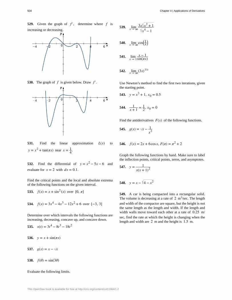
529. Given the graph of f ′, determine where f is
increasing or decreasing.
530. The graph of f is given below. Draw f ′.
531. Find the linear approximation L(x) to
y = x2 + tan(πx) near x = 14.
532. Find the differential of y = x2 − 5x − 6 and
evaluate for x = 2 with dx = 0.1.
Find the critical points and the local and absolute extremaof the following functions on the given interval.
533. f (x) = x + sin2 (x) over [0, π]
534. f (x) = 3x4 − 4x3 − 12x2 + 6 over [−3, 3]
Determine over which intervals the following functions areincreasing, decreasing, concave up, and concave down.
535. x(t) = 3t4 − 8t3 − 18t2
536. y = x + sin(πx)
537. g(x) = x − x
538. f (θ) = sin(3θ)
Evaluate the following limits.
539. limx → ∞3x x2 + 1
x4 − 1
540. limx → ∞cos⎛⎝1x
⎞⎠
541. limx → 1
x − 1sin(πx)
542. limx → ∞(3x)1/x
Use Newton’s method to find the first two iterations, giventhe starting point.
543. y = x3 + 1, x0 = 0.5
544. 1x + 1 = 1
2, x0 = 0
Find the antiderivatives F(x) of the following functions.
545. g(x) = x − 1x2
546. f (x) = 2x + 6cosx, F(π) = π2 + 2
Graph the following functions by hand. Make sure to labelthe inflection points, critical points, zeros, and asymptotes.
547. y = 1x(x + 1)2
548. y = x − 4 − x2
549. A car is being compacted into a rectangular solid.The volume is decreasing at a rate of 2 m3/sec. The length
and width of the compactor are square, but the height is notthe same length as the length and width. If the length andwidth walls move toward each other at a rate of 0.25 m/
sec, find the rate at which the height is changing when thelength and width are 2 m and the height is 1.5 m.
504 Chapter 4 | Applications of Derivatives
This OpenStax book is available for free at http://cnx.org/content/col11964/1.2
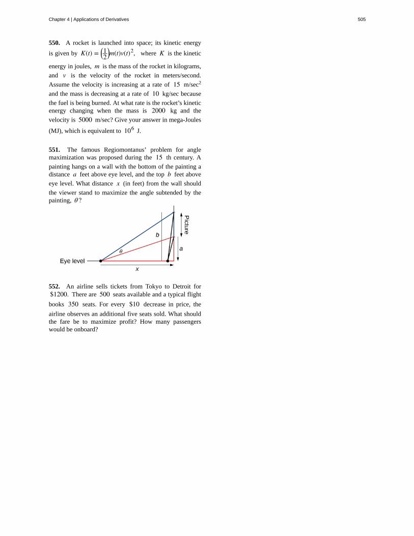
550. A rocket is launched into space; its kinetic energy
is given by K(t) = ⎛⎝12
⎞⎠m(t)v(t)2, where K is the kinetic
energy in joules, m is the mass of the rocket in kilograms,
and v is the velocity of the rocket in meters/second.
Assume the velocity is increasing at a rate of 15 m/sec2
and the mass is decreasing at a rate of 10 kg/sec because
the fuel is being burned. At what rate is the rocket’s kineticenergy changing when the mass is 2000 kg and the
velocity is 5000 m/sec? Give your answer in mega-Joules
(MJ), which is equivalent to 106 J.
551. The famous Regiomontanus’ problem for anglemaximization was proposed during the 15 th century. A
painting hangs on a wall with the bottom of the painting adistance a feet above eye level, and the top b feet above
eye level. What distance x (in feet) from the wall should
the viewer stand to maximize the angle subtended by thepainting, θ ?
552. An airline sells tickets from Tokyo to Detroit for$1200. There are 500 seats available and a typical flight
books 350 seats. For every $10 decrease in price, the
airline observes an additional five seats sold. What shouldthe fare be to maximize profit? How many passengerswould be onboard?
Chapter 4 | Applications of Derivatives 505

506 Chapter 4 | Applications of Derivatives
This OpenStax book is available for free at http://cnx.org/content/col11964/1.2
5 | INTEGRATION
Figure 5.1 Iceboating is a popular winter sport in parts of the northern United States and Europe. (credit: modification of workby Carter Brown, Flickr)
Chapter Outline
5.1 Approximating Areas
5.2 The Definite Integral
5.3 The Fundamental Theorem of Calculus
5.4 Integration Formulas and the Net Change Theorem
5.5 Substitution
5.6 Integrals Involving Exponential and Logarithmic Functions
5.7 Integrals Resulting in Inverse Trigonometric Functions
IntroductionIceboats are a common sight on the lakes of Wisconsin and Minnesota on winter weekends. Iceboats are similar to sailboats,but they are fitted with runners, or “skates,” and are designed to run over the ice, rather than on water. Iceboats can movevery quickly, and many ice boating enthusiasts are drawn to the sport because of the speed. Top iceboat racers can attain
Chapter 5 | Integration 507
speeds up to five times the wind speed. If we know how fast an iceboat is moving, we can use integration to determine howfar it travels. We revisit this question later in the chapter (see Example 5.27).
Determining distance from velocity is just one of many applications of integration. In fact, integrals are used in a widevariety of mechanical and physical applications. In this chapter, we first introduce the theory behind integration and useintegrals to calculate areas. From there, we develop the Fundamental Theorem of Calculus, which relates differentiation andintegration. We then study some basic integration techniques and briefly examine some applications.
5.1 | Approximating Areas
Learning Objectives5.1.1 Use sigma (summation) notation to calculate sums and powers of integers.
5.1.2 Use the sum of rectangular areas to approximate the area under a curve.
5.1.3 Use Riemann sums to approximate area.
Archimedes was fascinated with calculating the areas of various shapes—in other words, the amount of space enclosed bythe shape. He used a process that has come to be known as the method of exhaustion, which used smaller and smaller shapes,the areas of which could be calculated exactly, to fill an irregular region and thereby obtain closer and closer approximationsto the total area. In this process, an area bounded by curves is filled with rectangles, triangles, and shapes with exact areaformulas. These areas are then summed to approximate the area of the curved region.
In this section, we develop techniques to approximate the area between a curve, defined by a function f (x), and the x-axis
on a closed interval ⎡⎣a, b⎤
⎦. Like Archimedes, we first approximate the area under the curve using shapes of known area
(namely, rectangles). By using smaller and smaller rectangles, we get closer and closer approximations to the area. Takinga limit allows us to calculate the exact area under the curve.
Let’s start by introducing some notation to make the calculations easier. We then consider the case when f (x) is continuous
and nonnegative. Later in the chapter, we relax some of these restrictions and develop techniques that apply in more generalcases.
Sigma (Summation) NotationAs mentioned, we will use shapes of known area to approximate the area of an irregular region bounded by curves. Thisprocess often requires adding up long strings of numbers. To make it easier to write down these lengthy sums, we look atsome new notation here, called sigma notation (also known as summation notation). The Greek capital letter Σ, sigma,
is used to express long sums of values in a compact form. For example, if we want to add all the integers from 1 to 20without sigma notation, we have to write
1 + 2 + 3 + 4 + 5 + 6 + 7 + 8 + 9 + 10 + 11 + 12 + 13 + 14 + 15 + 16 + 17 + 18 + 19 + 20.
We could probably skip writing a couple of terms and write
1 + 2 + 3 + 4 + ⋯ + 19 + 20,
which is better, but still cumbersome. With sigma notation, we write this sum as
∑i = 1
20i,
which is much more compact.
Typically, sigma notation is presented in the form
∑i = 1
nai
where ai describes the terms to be added, and the i is called the index. Each term is evaluated, then we sum all the values,
beginning with the value when i = 1 and ending with the value when i = n. For example, an expression like ∑i = 2
7si is
508 Chapter 5 | Integration
This OpenStax book is available for free at http://cnx.org/content/col11964/1.2
5.1
interpreted as s2 + s3 + s4 + s5 + s6 + s7. Note that the index is used only to keep track of the terms to be added; it does
not factor into the calculation of the sum itself. The index is therefore called a dummy variable. We can use any letter welike for the index. Typically, mathematicians use i, j, k, m, and n for indices.
Let’s try a couple of examples of using sigma notation.
Example 5.1
Using Sigma Notation
a. Write in sigma notation and evaluate the sum of terms 3i for i = 1, 2, 3, 4, 5.
b. Write the sum in sigma notation:
1 + 14 + 1
9 + 116 + 1
25.
Solution
a. Write
∑i = 1
53i = 3 + 32 + 33 + 34 + 35
= 363.b. The denominator of each term is a perfect square. Using sigma notation, this sum can be written as
∑i = 1
51i2.
Write in sigma notation and evaluate the sum of terms 2i for i = 3, 4, 5, 6.
The properties associated with the summation process are given in the following rule.
Rule: Properties of Sigma Notation
Let a1, a2 ,…, an and b1, b2 ,…, bn represent two sequences of terms and let c be a constant. The following
properties hold for all positive integers n and for integers m, with 1 ≤ m ≤ n.
1.
(5.1)∑i = 1
nc = nc
2.
(5.2)∑i = 1
ncai = c ∑
i = 1
nai
3.
(5.3)∑i = 1
n⎛⎝ai + bi
⎞⎠ = ∑
i = 1
nai + ∑
i = 1
nbi
4.
(5.4)∑i = 1
n⎛⎝ai − bi
⎞⎠ = ∑
i = 1
nai − ∑
i = 1
nbi
Chapter 5 | Integration 509
5.
(5.5)∑i = 1
nai = ∑
i = 1
mai + ∑
i = m + 1
nai
Proof
We prove properties 2. and 3. here, and leave proof of the other properties to the Exercises.
2. We have
∑i = 1
ncai = ca1 + ca2 + ca3 + ⋯ + can
= c(a1 + a2 + a3 + ⋯ + an)
= c ∑i = 1
nai.
3. We have
∑i = 1
n⎛⎝ai + bi
⎞⎠ = ⎛
⎝a1 + b1⎞⎠ + ⎛
⎝a2 + b2⎞⎠ + ⎛
⎝a3 + b3⎞⎠ + ⋯ + ⎛
⎝an + bn⎞⎠
= (a1 + a2 + a3 + ⋯ + an) + ⎛⎝b1 + b2 + b3 + ⋯ + bn
⎞⎠
= ∑i = 1
nai + ∑
i = 1
nbi.
□
A few more formulas for frequently found functions simplify the summation process further. These are shown in the nextrule, for sums and powers of integers, and we use them in the next set of examples.
Rule: Sums and Powers of Integers
1. The sum of n integers is given by
∑i = 1
ni = 1 + 2 + ⋯ + n = n(n + 1)
2 .
2. The sum of consecutive integers squared is given by
∑i = 1
ni2 = 12 + 22 + ⋯ + n2 = n(n + 1)(2n + 1)
6 .
3. The sum of consecutive integers cubed is given by
∑i = 1
ni3 = 13 + 23 + ⋯ + n3 = n2 (n + 1)2
4 .
Example 5.2
Evaluation Using Sigma Notation
Write using sigma notation and evaluate:
a. The sum of the terms (i − 3)2 for i = 1, 2,…, 200.
510 Chapter 5 | Integration
This OpenStax book is available for free at http://cnx.org/content/col11964/1.2
5.2
b. The sum of the terms ⎛⎝i
3 − i2⎞⎠ for i = 1, 2, 3, 4, 5, 6.
Solution
a. Multiplying out (i − 3)2, we can break the expression into three terms.
∑i = 1
200(i − 3)2 = ∑
i = 1
200⎛⎝i2 − 6i + 9⎞
⎠
= ∑i = 1
200i2 − ∑
i = 1
2006i + ∑
i = 1
2009
= ∑i = 1
200i2 − 6 ∑
i = 1
200i + ∑
i = 1
2009
= 200(200 + 1)(400 + 1)6 − 6⎡
⎣200(200 + 1)
2⎤⎦ + 9(200)
= 2,686,700 − 120,600 + 1800= 2,567,900
b. Use sigma notation property iv. and the rules for the sum of squared terms and the sum of cubed terms.
∑i = 1
6⎛⎝i
3 − i2⎞⎠ = ∑
i = 1
6i3 − ∑
i = 1
6i2
= 62 (6 + 1)2
4 − 6(6 + 1)⎛⎝2(6) + 1⎞
⎠
6= 1764
4 − 5466
= 350
Find the sum of the values of 4 + 3i for i = 1, 2,…, 100.
Example 5.3
Finding the Sum of the Function Values
Find the sum of the values of f (x) = x3 over the integers 1, 2, 3,…, 10.
Solution
Using the formula, we have
∑i = 0
10i3 = (10)2 (10 + 1)2
4
= 100(121)4
= 3025.
Chapter 5 | Integration 511
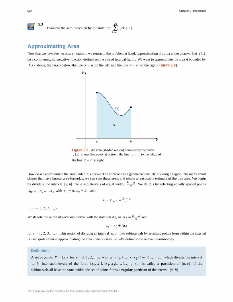
5.3Evaluate the sum indicated by the notation ∑
k = 1
20(2k + 1).
Approximating AreaNow that we have the necessary notation, we return to the problem at hand: approximating the area under a curve. Let f (x)be a continuous, nonnegative function defined on the closed interval ⎡
⎣a, b⎤⎦. We want to approximate the area A bounded by
f (x) above, the x-axis below, the line x = a on the left, and the line x = b on the right (Figure 5.2).
Figure 5.2 An area (shaded region) bounded by the curvef (x) at top, the x-axis at bottom, the line x = a to the left, and
the line x = b at right.
How do we approximate the area under this curve? The approach is a geometric one. By dividing a region into many smallshapes that have known area formulas, we can sum these areas and obtain a reasonable estimate of the true area. We begin
by dividing the interval ⎡⎣a, b⎤
⎦ into n subintervals of equal width, b − an . We do this by selecting equally spaced points
x0, x1, x2 ,…, xn with x0 = a, xn = b, and
xi − xi − 1 = b − an
for i = 1, 2, 3,…, n.
We denote the width of each subinterval with the notation Δx, so Δx = b − an and
xi = x0 + iΔx
for i = 1, 2, 3,…, n. This notion of dividing an interval ⎡⎣a, b⎤
⎦ into subintervals by selecting points from within the interval
is used quite often in approximating the area under a curve, so let’s define some relevant terminology.
Definition
A set of points P = {xi} for i = 0, 1, 2,…, n with a = x0 < x1 < x2 < ⋯ < xn = b, which divides the interval⎡⎣a, b⎤
⎦ into subintervals of the form [x0, x1], [x1, x2],…, [xn − 1, xn] is called a partition of ⎡⎣a, b⎤
⎦. If the
subintervals all have the same width, the set of points forms a regular partition of the interval ⎡⎣a, b⎤
⎦.
512 Chapter 5 | Integration
This OpenStax book is available for free at http://cnx.org/content/col11964/1.2
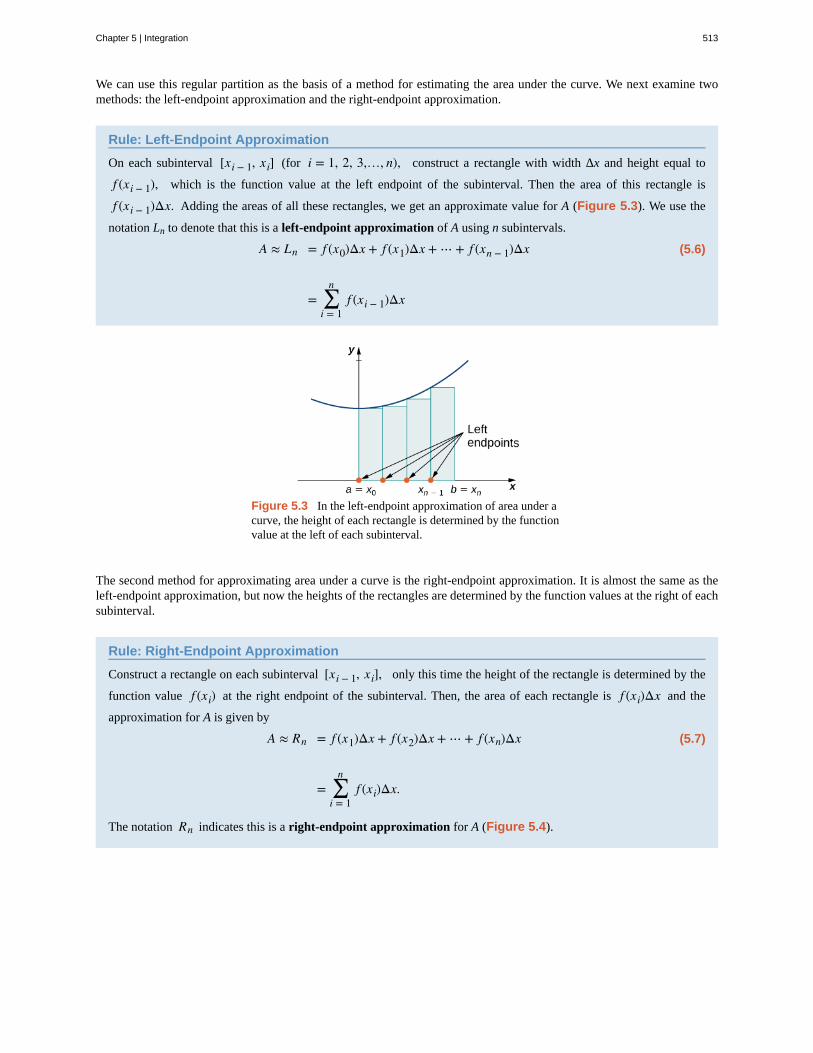
We can use this regular partition as the basis of a method for estimating the area under the curve. We next examine twomethods: the left-endpoint approximation and the right-endpoint approximation.
Rule: Left-Endpoint Approximation
On each subinterval [xi − 1, xi] (for i = 1, 2, 3,…, n), construct a rectangle with width Δx and height equal to
f (xi − 1), which is the function value at the left endpoint of the subinterval. Then the area of this rectangle is
f (xi − 1)Δx. Adding the areas of all these rectangles, we get an approximate value for A (Figure 5.3). We use the
notation Ln to denote that this is a left-endpoint approximation of A using n subintervals.
(5.6)A ≈ Ln = f (x0)Δx + f (x1)Δx + ⋯ + f (xn − 1)Δx
= ∑i = 1
nf (xi − 1)Δx
Figure 5.3 In the left-endpoint approximation of area under acurve, the height of each rectangle is determined by the functionvalue at the left of each subinterval.
The second method for approximating area under a curve is the right-endpoint approximation. It is almost the same as theleft-endpoint approximation, but now the heights of the rectangles are determined by the function values at the right of eachsubinterval.
Rule: Right-Endpoint Approximation
Construct a rectangle on each subinterval [xi − 1, xi], only this time the height of the rectangle is determined by the
function value f (xi) at the right endpoint of the subinterval. Then, the area of each rectangle is f (xi)Δx and the
approximation for A is given by
(5.7)A ≈ Rn = f (x1)Δx + f (x2)Δx + ⋯ + f (xn)Δx
= ∑i = 1
nf (xi)Δx.
The notation Rn indicates this is a right-endpoint approximation for A (Figure 5.4).
Chapter 5 | Integration 513
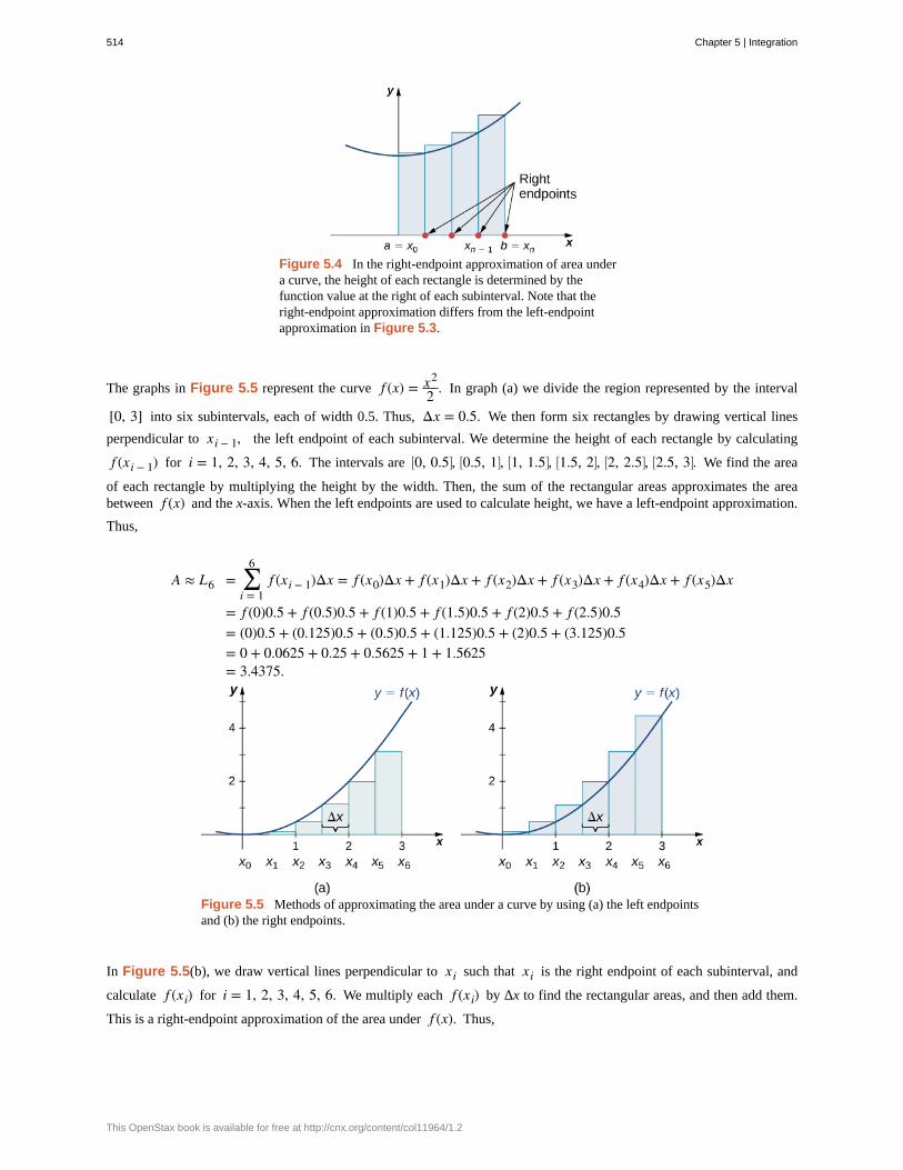
Figure 5.4 In the right-endpoint approximation of area undera curve, the height of each rectangle is determined by thefunction value at the right of each subinterval. Note that theright-endpoint approximation differs from the left-endpointapproximation in Figure 5.3.
The graphs in Figure 5.5 represent the curve f (x) = x2
2 . In graph (a) we divide the region represented by the interval
[0, 3] into six subintervals, each of width 0.5. Thus, Δx = 0.5. We then form six rectangles by drawing vertical lines
perpendicular to xi − 1, the left endpoint of each subinterval. We determine the height of each rectangle by calculating
f (xi − 1) for i = 1, 2, 3, 4, 5, 6. The intervals are ⎡⎣0, 0.5⎤
⎦, ⎡⎣0.5, 1⎤
⎦, ⎡⎣1, 1.5⎤
⎦, ⎡⎣1.5, 2⎤
⎦, ⎡⎣2, 2.5⎤
⎦, ⎡⎣2.5, 3⎤
⎦. We find the area
of each rectangle by multiplying the height by the width. Then, the sum of the rectangular areas approximates the areabetween f (x) and the x-axis. When the left endpoints are used to calculate height, we have a left-endpoint approximation.
Thus,
A ≈ L6 = ∑i = 1
6f (xi − 1)Δx = f (x0)Δx + f (x1)Δx + f (x2)Δx + f (x3)Δx + f (x4)Δx + f (x5)Δx
= f (0)0.5 + f (0.5)0.5 + f (1)0.5 + f (1.5)0.5 + f (2)0.5 + f (2.5)0.5= (0)0.5 + (0.125)0.5 + (0.5)0.5 + (1.125)0.5 + (2)0.5 + (3.125)0.5= 0 + 0.0625 + 0.25 + 0.5625 + 1 + 1.5625= 3.4375.
Figure 5.5 Methods of approximating the area under a curve by using (a) the left endpointsand (b) the right endpoints.
In Figure 5.5(b), we draw vertical lines perpendicular to xi such that xi is the right endpoint of each subinterval, and
calculate f (xi) for i = 1, 2, 3, 4, 5, 6. We multiply each f (xi) by Δx to find the rectangular areas, and then add them.
This is a right-endpoint approximation of the area under f (x). Thus,
514 Chapter 5 | Integration
This OpenStax book is available for free at http://cnx.org/content/col11964/1.2
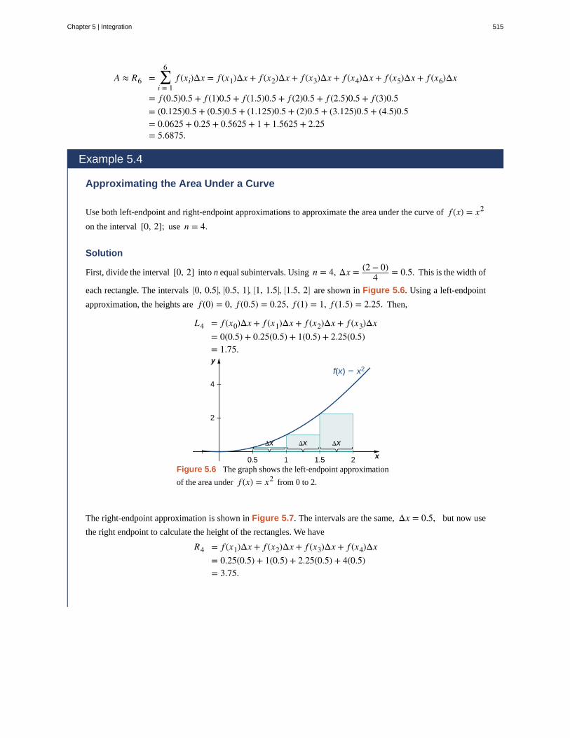
A ≈ R6 = ∑i = 1
6f (xi)Δx = f (x1)Δx + f (x2)Δx + f (x3)Δx + f (x4)Δx + f (x5)Δx + f (x6)Δx
= f (0.5)0.5 + f (1)0.5 + f (1.5)0.5 + f (2)0.5 + f (2.5)0.5 + f (3)0.5= (0.125)0.5 + (0.5)0.5 + (1.125)0.5 + (2)0.5 + (3.125)0.5 + (4.5)0.5= 0.0625 + 0.25 + 0.5625 + 1 + 1.5625 + 2.25= 5.6875.
Example 5.4
Approximating the Area Under a Curve
Use both left-endpoint and right-endpoint approximations to approximate the area under the curve of f (x) = x2
on the interval [0, 2]; use n = 4.
Solution
First, divide the interval [0, 2] into n equal subintervals. Using n = 4, Δx = (2 − 0)4 = 0.5. This is the width of
each rectangle. The intervals ⎡⎣0, 0.5⎤
⎦, ⎡⎣0.5, 1⎤
⎦, ⎡⎣1, 1.5⎤
⎦, ⎡⎣1.5, 2⎤
⎦ are shown in Figure 5.6. Using a left-endpoint
approximation, the heights are f (0) = 0, f (0.5) = 0.25, f (1) = 1, f (1.5) = 2.25. Then,
L4 = f (x0)Δx + f (x1)Δx + f (x2)Δx + f (x3)Δx= 0(0.5) + 0.25(0.5) + 1(0.5) + 2.25(0.5)= 1.75.
Figure 5.6 The graph shows the left-endpoint approximation
of the area under f (x) = x2 from 0 to 2.
The right-endpoint approximation is shown in Figure 5.7. The intervals are the same, Δx = 0.5, but now use
the right endpoint to calculate the height of the rectangles. We have
R4 = f (x1)Δx + f (x2)Δx + f (x3)Δx + f (x4)Δx= 0.25(0.5) + 1(0.5) + 2.25(0.5) + 4(0.5)= 3.75.
Chapter 5 | Integration 515
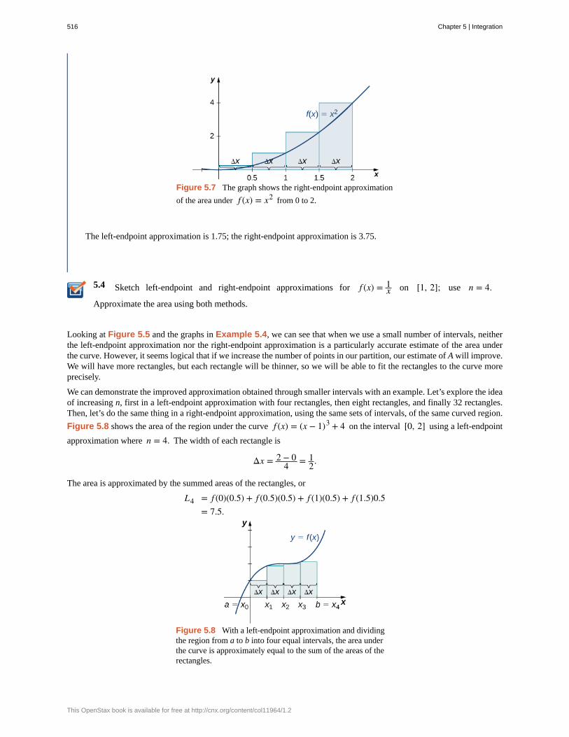
5.4
Figure 5.7 The graph shows the right-endpoint approximation
of the area under f (x) = x2 from 0 to 2.
The left-endpoint approximation is 1.75; the right-endpoint approximation is 3.75.
Sketch left-endpoint and right-endpoint approximations for f (x) = 1x on [1, 2]; use n = 4.
Approximate the area using both methods.
Looking at Figure 5.5 and the graphs in Example 5.4, we can see that when we use a small number of intervals, neitherthe left-endpoint approximation nor the right-endpoint approximation is a particularly accurate estimate of the area underthe curve. However, it seems logical that if we increase the number of points in our partition, our estimate of A will improve.We will have more rectangles, but each rectangle will be thinner, so we will be able to fit the rectangles to the curve moreprecisely.
We can demonstrate the improved approximation obtained through smaller intervals with an example. Let’s explore the ideaof increasing n, first in a left-endpoint approximation with four rectangles, then eight rectangles, and finally 32 rectangles.Then, let’s do the same thing in a right-endpoint approximation, using the same sets of intervals, of the same curved region.
Figure 5.8 shows the area of the region under the curve f (x) = (x − 1)3 + 4 on the interval [0, 2] using a left-endpoint
approximation where n = 4. The width of each rectangle is
Δx = 2 − 04 = 1
2.
The area is approximated by the summed areas of the rectangles, or
L4 = f (0)(0.5) + f (0.5)(0.5) + f (1)(0.5) + f (1.5)0.5= 7.5.
Figure 5.8 With a left-endpoint approximation and dividingthe region from a to b into four equal intervals, the area underthe curve is approximately equal to the sum of the areas of therectangles.
516 Chapter 5 | Integration
This OpenStax book is available for free at http://cnx.org/content/col11964/1.2
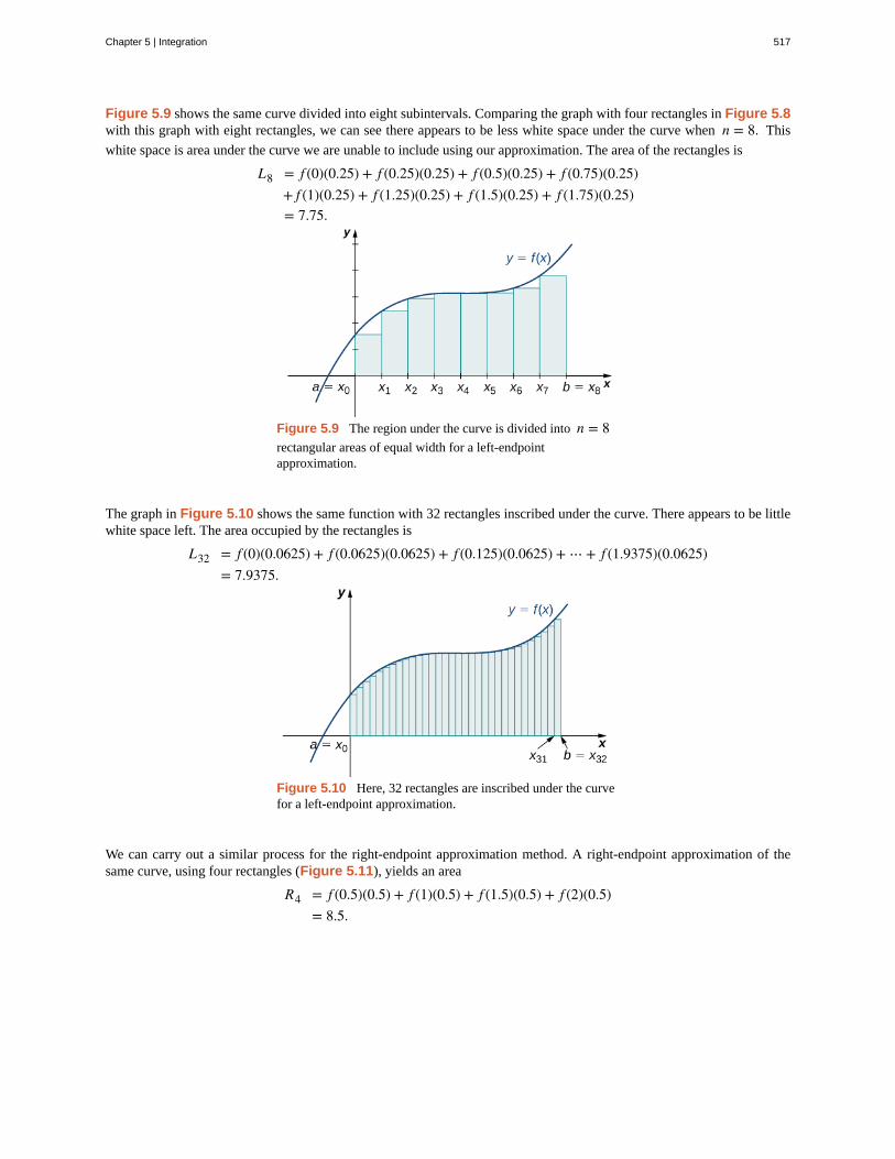
Figure 5.9 shows the same curve divided into eight subintervals. Comparing the graph with four rectangles in Figure 5.8with this graph with eight rectangles, we can see there appears to be less white space under the curve when n = 8. This
white space is area under the curve we are unable to include using our approximation. The area of the rectangles is
L8 = f (0)(0.25) + f (0.25)(0.25) + f (0.5)(0.25) + f (0.75)(0.25)+ f (1)(0.25) + f (1.25)(0.25) + f (1.5)(0.25) + f (1.75)(0.25)= 7.75.
Figure 5.9 The region under the curve is divided into n = 8rectangular areas of equal width for a left-endpointapproximation.
The graph in Figure 5.10 shows the same function with 32 rectangles inscribed under the curve. There appears to be littlewhite space left. The area occupied by the rectangles is
L32 = f (0)(0.0625) + f (0.0625)(0.0625) + f (0.125)(0.0625) + ⋯ + f (1.9375)(0.0625)= 7.9375.
Figure 5.10 Here, 32 rectangles are inscribed under the curvefor a left-endpoint approximation.
We can carry out a similar process for the right-endpoint approximation method. A right-endpoint approximation of thesame curve, using four rectangles (Figure 5.11), yields an area
R4 = f (0.5)(0.5) + f (1)(0.5) + f (1.5)(0.5) + f (2)(0.5)= 8.5.
Chapter 5 | Integration 517
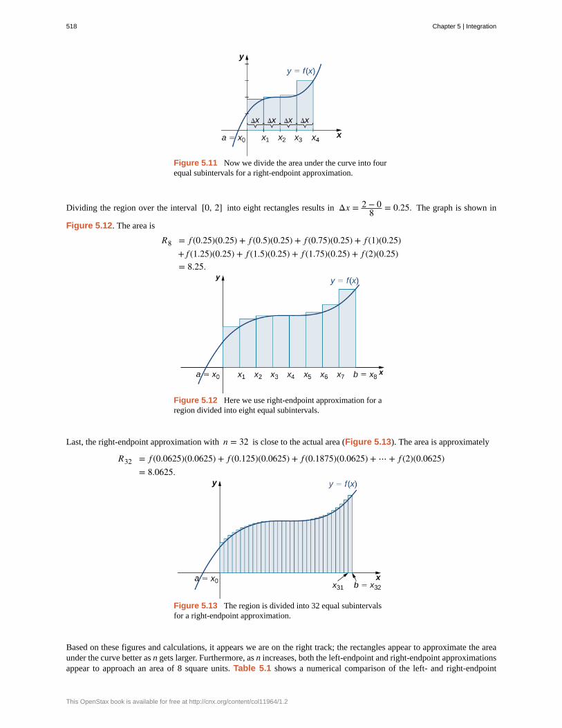
Figure 5.11 Now we divide the area under the curve into fourequal subintervals for a right-endpoint approximation.
Dividing the region over the interval [0, 2] into eight rectangles results in Δx = 2 − 08 = 0.25. The graph is shown in
Figure 5.12. The area is
R8 = f (0.25)(0.25) + f (0.5)(0.25) + f (0.75)(0.25) + f (1)(0.25)+ f (1.25)(0.25) + f (1.5)(0.25) + f (1.75)(0.25) + f (2)(0.25)= 8.25.
Figure 5.12 Here we use right-endpoint approximation for aregion divided into eight equal subintervals.
Last, the right-endpoint approximation with n = 32 is close to the actual area (Figure 5.13). The area is approximately
R32 = f (0.0625)(0.0625) + f (0.125)(0.0625) + f (0.1875)(0.0625) + ⋯ + f (2)(0.0625)= 8.0625.
Figure 5.13 The region is divided into 32 equal subintervalsfor a right-endpoint approximation.
Based on these figures and calculations, it appears we are on the right track; the rectangles appear to approximate the areaunder the curve better as n gets larger. Furthermore, as n increases, both the left-endpoint and right-endpoint approximationsappear to approach an area of 8 square units. Table 5.1 shows a numerical comparison of the left- and right-endpoint
518 Chapter 5 | Integration
This OpenStax book is available for free at http://cnx.org/content/col11964/1.2
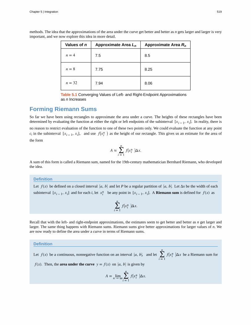
methods. The idea that the approximations of the area under the curve get better and better as n gets larger and larger is veryimportant, and we now explore this idea in more detail.
Values of n Approximate Area Ln Approximate Area Rn
n = 4 7.5 8.5
n = 8 7.75 8.25
n = 32 7.94 8.06
Table 5.1 Converging Values of Left- and Right-Endpoint Approximationsas n Increases
Forming Riemann SumsSo far we have been using rectangles to approximate the area under a curve. The heights of these rectangles have beendetermined by evaluating the function at either the right or left endpoints of the subinterval [xi − 1, xi]. In reality, there is
no reason to restrict evaluation of the function to one of these two points only. We could evaluate the function at any pointci in the subinterval [xi − 1, xi], and use f ⎛
⎝xi*⎞⎠ as the height of our rectangle. This gives us an estimate for the area of
the form
A ≈ ∑i = 1
nf ⎛
⎝xi*⎞⎠Δx.
A sum of this form is called a Riemann sum, named for the 19th-century mathematician Bernhard Riemann, who developedthe idea.
Definition
Let f (x) be defined on a closed interval ⎡⎣a, b⎤
⎦ and let P be a regular partition of ⎡⎣a, b⎤
⎦. Let Δx be the width of each
subinterval [xi − 1, xi] and for each i, let xi* be any point in [xi − 1, xi]. A Riemann sum is defined for f (x) as
∑i = 1
nf ⎛
⎝xi*⎞⎠Δx.
Recall that with the left- and right-endpoint approximations, the estimates seem to get better and better as n get larger andlarger. The same thing happens with Riemann sums. Riemann sums give better approximations for larger values of n. Weare now ready to define the area under a curve in terms of Riemann sums.
Definition
Let f (x) be a continuous, nonnegative function on an interval ⎡⎣a, b⎤
⎦, and let ∑i = 1
nf ⎛
⎝xi*⎞⎠Δx be a Riemann sum for
f (x). Then, the area under the curve y = f (x) on ⎡⎣a, b⎤
⎦ is given by
A = limn → ∞ ∑i = 1
nf ⎛
⎝xi*⎞⎠Δx.
Chapter 5 | Integration 519
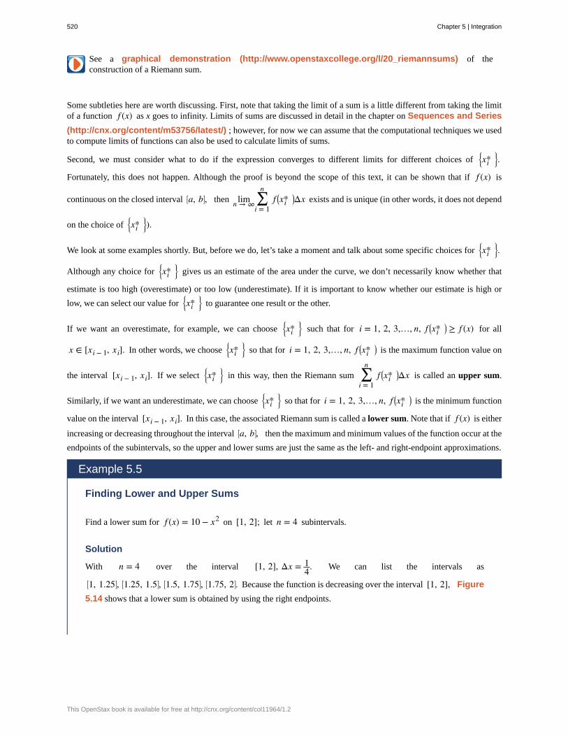
See a graphical demonstration (http://www.openstaxcollege.org/l/20_riemannsums) of theconstruction of a Riemann sum.
Some subtleties here are worth discussing. First, note that taking the limit of a sum is a little different from taking the limitof a function f (x) as x goes to infinity. Limits of sums are discussed in detail in the chapter on Sequences and Series
(http://cnx.org/content/m53756/latest/) ; however, for now we can assume that the computational techniques we usedto compute limits of functions can also be used to calculate limits of sums.
Second, we must consider what to do if the expression converges to different limits for different choices of⎧
⎩⎨xi*
⎫
⎭⎬.
Fortunately, this does not happen. Although the proof is beyond the scope of this text, it can be shown that if f (x) is
continuous on the closed interval ⎡⎣a, b⎤
⎦, then limn → ∞ ∑i = 1
nf ⎛
⎝xi*⎞⎠Δx exists and is unique (in other words, it does not depend
on the choice of⎧
⎩⎨xi*
⎫
⎭⎬).
We look at some examples shortly. But, before we do, let’s take a moment and talk about some specific choices for⎧
⎩⎨xi*
⎫
⎭⎬.
Although any choice for⎧
⎩⎨xi*
⎫
⎭⎬ gives us an estimate of the area under the curve, we don’t necessarily know whether that
estimate is too high (overestimate) or too low (underestimate). If it is important to know whether our estimate is high or
low, we can select our value for⎧
⎩⎨xi*
⎫
⎭⎬ to guarantee one result or the other.
If we want an overestimate, for example, we can choose⎧
⎩⎨xi*
⎫
⎭⎬ such that for i = 1, 2, 3,…, n, f ⎛
⎝xi*⎞⎠ ≥ f (x) for all
x ∈ [xi − 1, xi]. In other words, we choose⎧
⎩⎨xi*
⎫
⎭⎬ so that for i = 1, 2, 3,…, n, f ⎛
⎝xi*⎞⎠ is the maximum function value on
the interval [xi − 1, xi]. If we select⎧
⎩⎨xi*
⎫
⎭⎬ in this way, then the Riemann sum ∑
i = 1
nf ⎛
⎝xi*⎞⎠Δx is called an upper sum.
Similarly, if we want an underestimate, we can choose⎧
⎩⎨xi*
⎫
⎭⎬ so that for i = 1, 2, 3,…, n, f ⎛
⎝xi*⎞⎠ is the minimum function
value on the interval [xi − 1, xi]. In this case, the associated Riemann sum is called a lower sum. Note that if f (x) is either
increasing or decreasing throughout the interval ⎡⎣a, b⎤
⎦, then the maximum and minimum values of the function occur at the
endpoints of the subintervals, so the upper and lower sums are just the same as the left- and right-endpoint approximations.
Example 5.5
Finding Lower and Upper Sums
Find a lower sum for f (x) = 10 − x2 on [1, 2]; let n = 4 subintervals.
Solution
With n = 4 over the interval [1, 2], Δx = 14. We can list the intervals as
⎡⎣1, 1.25⎤
⎦, ⎡⎣1.25, 1.5⎤
⎦, ⎡⎣1.5, 1.75⎤
⎦, ⎡⎣1.75, 2⎤
⎦. Because the function is decreasing over the interval [1, 2], Figure
5.14 shows that a lower sum is obtained by using the right endpoints.
520 Chapter 5 | Integration
This OpenStax book is available for free at http://cnx.org/content/col11964/1.2
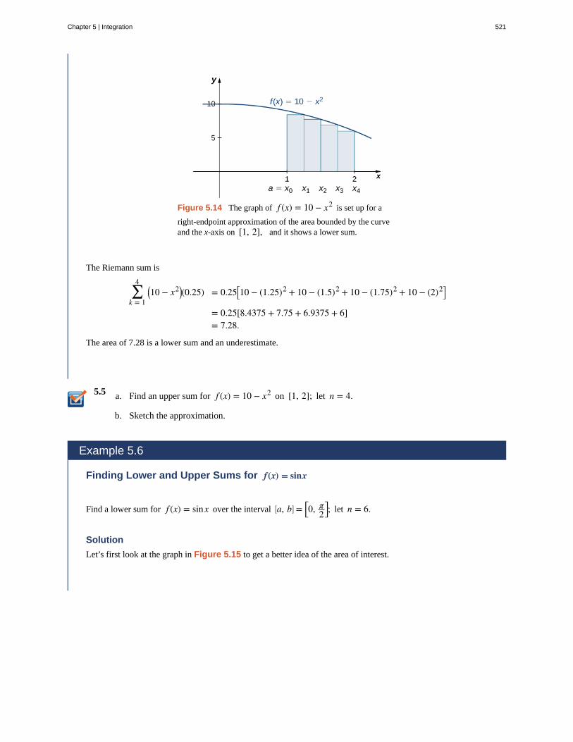
5.5
Figure 5.14 The graph of f (x) = 10 − x2 is set up for a
right-endpoint approximation of the area bounded by the curveand the x-axis on [1, 2], and it shows a lower sum.
The Riemann sum is
∑k = 1
4⎛⎝10 − x2⎞
⎠(0.25) = 0.25⎡⎣10 − (1.25)2 + 10 − (1.5)2 + 10 − (1.75)2 + 10 − (2)2⎤
⎦
= 0.25[8.4375 + 7.75 + 6.9375 + 6]= 7.28.
The area of 7.28 is a lower sum and an underestimate.
a. Find an upper sum for f (x) = 10 − x2 on [1, 2]; let n = 4.
b. Sketch the approximation.
Example 5.6
Finding Lower and Upper Sums for f(x) = sinx
Find a lower sum for f (x) = sinx over the interval ⎡⎣a, b⎤
⎦ = ⎡⎣0, π
2⎤⎦; let n = 6.
Solution
Let’s first look at the graph in Figure 5.15 to get a better idea of the area of interest.
Chapter 5 | Integration 521
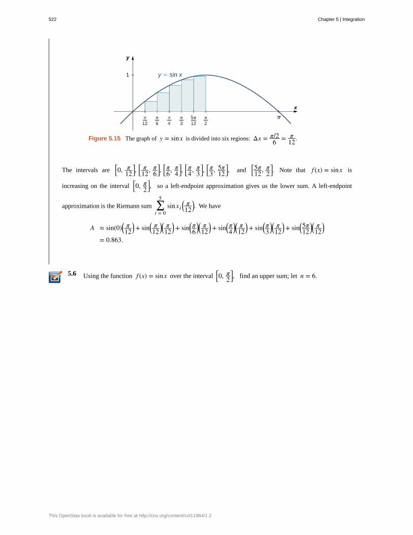
5.6
Figure 5.15 The graph of y = sinx is divided into six regions: Δx = π/26 = π
12.
The intervals are⎡⎣0, π
12⎤⎦,
⎡⎣
π12, π
6⎤⎦,
⎡⎣π6, π
4⎤⎦,
⎡⎣π4, π
3⎤⎦,
⎡⎣π3, 5π
12⎤⎦, and
⎡⎣5π12, π
2⎤⎦. Note that f (x) = sinx is
increasing on the interval⎡⎣0, π
2⎤⎦, so a left-endpoint approximation gives us the lower sum. A left-endpoint
approximation is the Riemann sum ∑i = 0
5sinxi
⎛⎝
π12
⎞⎠. We have
A ≈ sin(0)⎛⎝
π12
⎞⎠ + sin⎛
⎝π12
⎞⎠⎛⎝
π12
⎞⎠ + sin⎛
⎝π6
⎞⎠⎛⎝
π12
⎞⎠ + sin⎛
⎝π4
⎞⎠⎛⎝
π12
⎞⎠ + sin⎛
⎝π3
⎞⎠⎛⎝
π12
⎞⎠ + sin⎛
⎝5π12
⎞⎠⎛⎝
π12
⎞⎠
= 0.863.
Using the function f (x) = sinx over the interval ⎡⎣0, π
2⎤⎦, find an upper sum; let n = 6.
522 Chapter 5 | Integration
This OpenStax book is available for free at http://cnx.org/content/col11964/1.2
5.1 EXERCISES1. State whether the given sums are equal or unequal.
a. ∑i = 1
10i and ∑
k = 1
10k
b. ∑i = 1
10i and ∑
i = 6
15(i − 5)
c. ∑i = 1
10i(i − 1) and ∑
j = 0
9⎛⎝ j + 1⎞
⎠ j
d. ∑i = 1
10i(i − 1) and ∑
k = 1
10⎛⎝k2 − k⎞
⎠
In the following exercises, use the rules for sums of powersof integers to compute the sums.
2. ∑i = 5
10i
3. ∑i = 5
10i2
Suppose that ∑i = 1
100ai = 15 and ∑
i = 1
100bi = −12. In the
following exercises, compute the sums.
4. ∑i = 1
100⎛⎝ai + bi
⎞⎠
5. ∑i = 1
100⎛⎝ai − bi
⎞⎠
6. ∑i = 1
100⎛⎝3ai − 4bi
⎞⎠
7. ∑i = 1
100⎛⎝5ai + 4bi
⎞⎠
In the following exercises, use summation properties andformulas to rewrite and evaluate the sums.
8. ∑k = 1
20100⎛
⎝k2 − 5k + 1⎞⎠
9. ∑j = 1
50⎛⎝j2 − 2 j⎞⎠
10. ∑j = 11
20⎛⎝j2 − 10 j⎞⎠
11. ∑k = 1
25⎡⎣(2k)2 − 100k⎤
⎦
Let Ln denote the left-endpoint sum using n subintervals
and let Rn denote the corresponding right-endpoint sum.
In the following exercises, compute the indicated left andright sums for the given functions on the indicated interval.
12. L4 for f (x) = 1x − 1 on [2, 3]
13. R4 for g(x) = cos(πx) on [0, 1]
14. L6 for f (x) = 1x(x − 1) on ⎡
⎣2, 5⎤⎦
15. R6 for f (x) = 1x(x − 1) on ⎡
⎣2, 5⎤⎦
16. R4 for 1x2 + 1
on [−2, 2]
17. L4 for 1x2 + 1
on [−2, 2]
18. R4 for x2 − 2x + 1 on [0, 2]
19. L8 for x2 − 2x + 1 on [0, 2]
20. Compute the left and right Riemann sums—L4 and R4,respectively—for f (x) = (2 − |x|) on [−2, 2]. Compute
their average value and compare it with the area under thegraph of f.
21. Compute the left and right Riemann sums—L6 andR6, respectively—for f (x) = (3 − |3 − x|) on ⎡
⎣0, 6⎤⎦.
Compute their average value and compare it with the areaunder the graph of f.
22. Compute the left and right Riemann sums—L4 and
R4, respectively—for f (x) = 4 − x2 on [−2, 2] and
compare their values.
23. Compute the left and right Riemann sums—L6 and
R6, respectively—for f (x) = 9 − (x − 3)2 on ⎡⎣0, 6⎤
⎦ and
compare their values.
Express the following endpoint sums in sigma notation butdo not evaluate them.
Chapter 5 | Integration 523
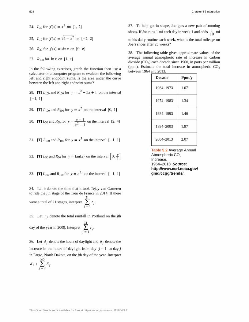
24. L30 for f (x) = x2 on [1, 2]
25. L10 for f (x) = 4 − x2 on [−2, 2]
26. R20 for f (x) = sinx on [0, π]
27. R100 for lnx on [1, e]
In the following exercises, graph the function then use acalculator or a computer program to evaluate the followingleft and right endpoint sums. Is the area under the curvebetween the left and right endpoint sums?
28. [T] L100 and R100 for y = x2 − 3x + 1 on the interval
[−1, 1]
29. [T] L100 and R100 for y = x2 on the interval [0, 1]
30. [T] L50 and R50 for y = x + 1x2 − 1
on the interval [2, 4]
31. [T] L100 and R100 for y = x3 on the interval [−1, 1]
32. [T] L50 and R50 for y = tan(x) on the interval⎡⎣0, π
4⎤⎦
33. [T] L100 and R100 for y = e2x on the interval [−1, 1]
34. Let tj denote the time that it took Tejay van Garterento ride the jth stage of the Tour de France in 2014. If there
were a total of 21 stages, interpret ∑j = 1
21t j.
35. Let r j denote the total rainfall in Portland on the jth
day of the year in 2009. Interpret ∑j = 1
31r j.
36. Let d j denote the hours of daylight and δ j denote the
increase in the hours of daylight from day j − 1 to day j
in Fargo, North Dakota, on the jth day of the year. Interpret
d1 + ∑j = 2
365δ j.
37. To help get in shape, Joe gets a new pair of running
shoes. If Joe runs 1 mi each day in week 1 and adds 110 mi
to his daily routine each week, what is the total mileage onJoe’s shoes after 25 weeks?
38. The following table gives approximate values of theaverage annual atmospheric rate of increase in carbondioxide (CO2) each decade since 1960, in parts per million(ppm). Estimate the total increase in atmospheric CO2between 1964 and 2013.
Decade Ppm/y
1964–1973 1.07
1974–1983 1.34
1984–1993 1.40
1994–2003 1.87
2004–2013 2.07
Table 5.2 Average AnnualAtmospheric CO2Increase,1964–2013 Source:http://www.esrl.noaa.gov/gmd/ccgg/trends/.
524 Chapter 5 | Integration
This OpenStax book is available for free at http://cnx.org/content/col11964/1.2
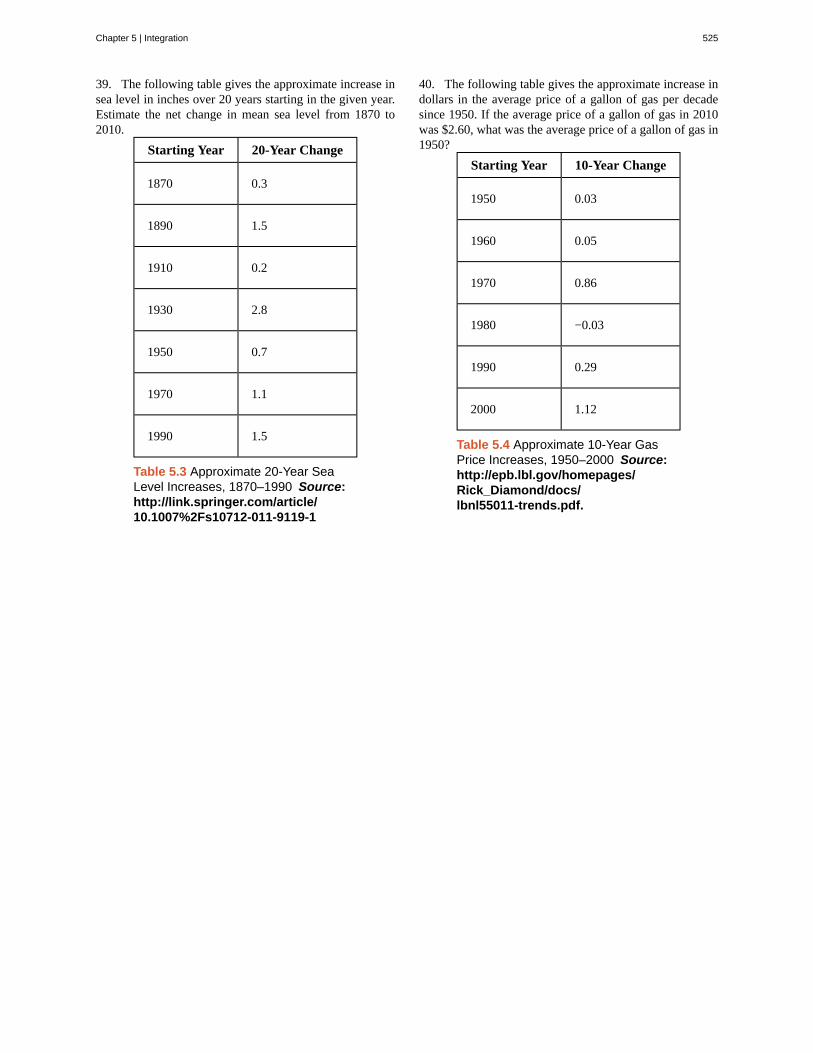
39. The following table gives the approximate increase insea level in inches over 20 years starting in the given year.Estimate the net change in mean sea level from 1870 to2010.
Starting Year 20-Year Change
1870 0.3
1890 1.5
1910 0.2
1930 2.8
1950 0.7
1970 1.1
1990 1.5
Table 5.3 Approximate 20-Year SeaLevel Increases, 1870–1990 Source:http://link.springer.com/article/10.1007%2Fs10712-011-9119-1
40. The following table gives the approximate increase indollars in the average price of a gallon of gas per decadesince 1950. If the average price of a gallon of gas in 2010was $2.60, what was the average price of a gallon of gas in1950?
Starting Year 10-Year Change
1950 0.03
1960 0.05
1970 0.86
1980 −0.03
1990 0.29
2000 1.12
Table 5.4 Approximate 10-Year GasPrice Increases, 1950–2000 Source:http://epb.lbl.gov/homepages/Rick_Diamond/docs/lbnl55011-trends.pdf.
Chapter 5 | Integration 525
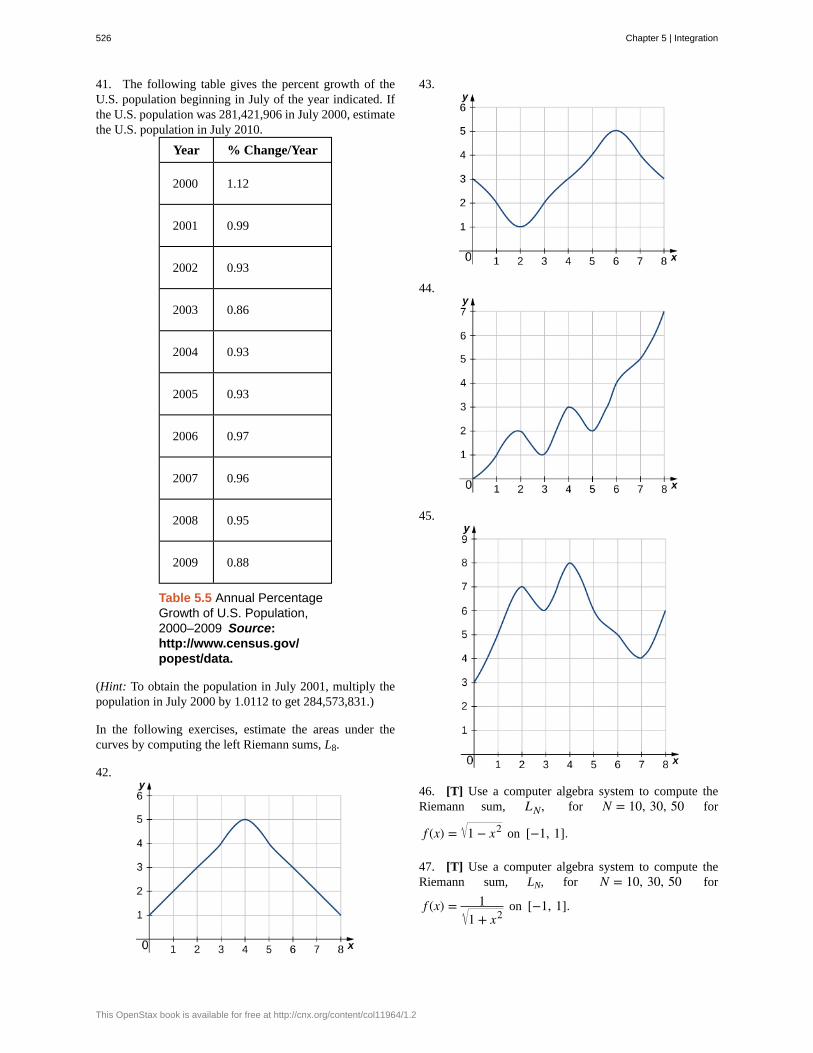
41. The following table gives the percent growth of theU.S. population beginning in July of the year indicated. Ifthe U.S. population was 281,421,906 in July 2000, estimatethe U.S. population in July 2010.
Year % Change/Year
2000 1.12
2001 0.99
2002 0.93
2003 0.86
2004 0.93
2005 0.93
2006 0.97
2007 0.96
2008 0.95
2009 0.88
Table 5.5 Annual PercentageGrowth of U.S. Population,2000–2009 Source:http://www.census.gov/popest/data.
(Hint: To obtain the population in July 2001, multiply thepopulation in July 2000 by 1.0112 to get 284,573,831.)
In the following exercises, estimate the areas under thecurves by computing the left Riemann sums, L8.
42.
43.
44.
45.
46. [T] Use a computer algebra system to compute theRiemann sum, LN, for N = 10, 30, 50 for
f (x) = 1 − x2 on [−1, 1].
47. [T] Use a computer algebra system to compute theRiemann sum, LN, for N = 10, 30, 50 for
f (x) = 11 + x2
on [−1, 1].
526 Chapter 5 | Integration
This OpenStax book is available for free at http://cnx.org/content/col11964/1.2
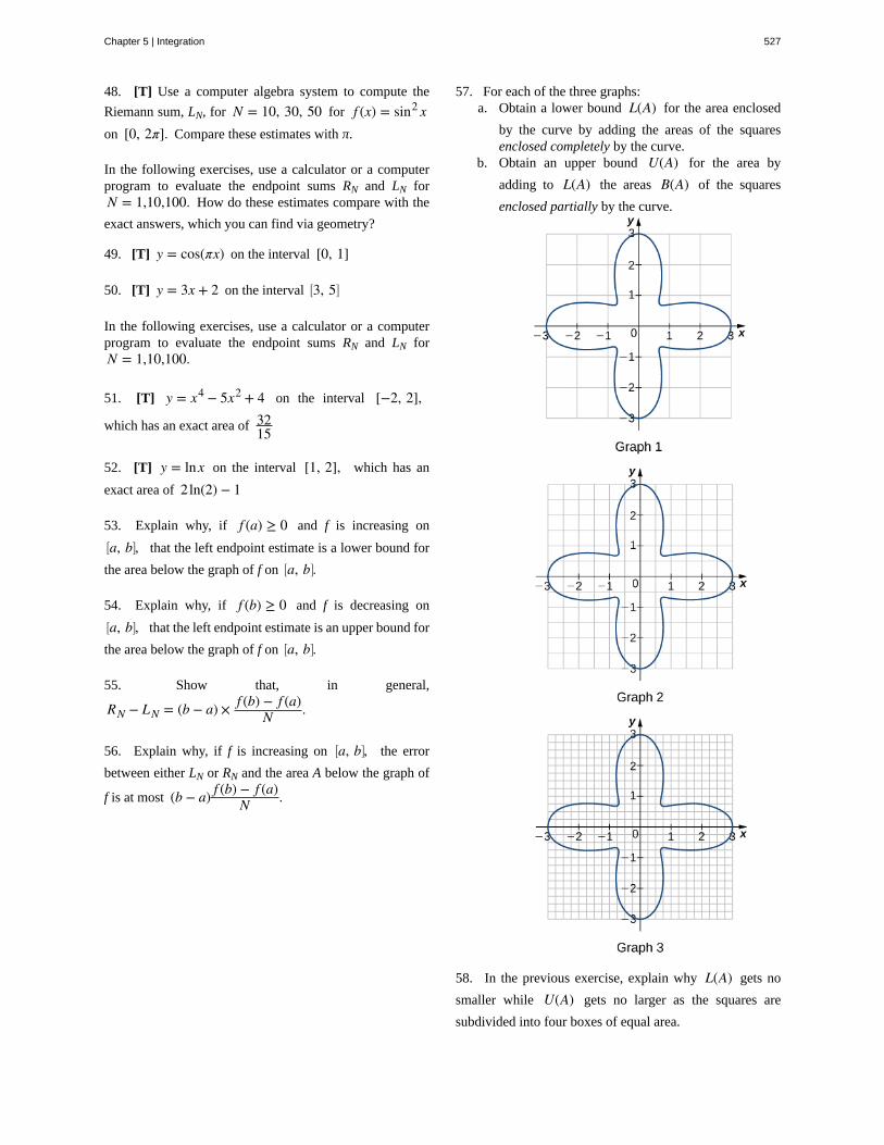
48. [T] Use a computer algebra system to compute the
Riemann sum, LN, for N = 10, 30, 50 for f (x) = sin2 xon [0, 2π]. Compare these estimates with π.
In the following exercises, use a calculator or a computerprogram to evaluate the endpoint sums RN and LN forN = 1,10,100. How do these estimates compare with the
exact answers, which you can find via geometry?
49. [T] y = cos(πx) on the interval [0, 1]
50. [T] y = 3x + 2 on the interval ⎡⎣3, 5⎤
⎦
In the following exercises, use a calculator or a computerprogram to evaluate the endpoint sums RN and LN forN = 1,10,100.
51. [T] y = x4 − 5x2 + 4 on the interval [−2, 2],
which has an exact area of 3215
52. [T] y = lnx on the interval [1, 2], which has an
exact area of 2ln(2) − 1
53. Explain why, if f (a) ≥ 0 and f is increasing on⎡⎣a, b⎤
⎦, that the left endpoint estimate is a lower bound for
the area below the graph of f on ⎡⎣a, b⎤
⎦.
54. Explain why, if f (b) ≥ 0 and f is decreasing on⎡⎣a, b⎤
⎦, that the left endpoint estimate is an upper bound for
the area below the graph of f on ⎡⎣a, b⎤
⎦.
55. Show that, in general,
RN − LN = (b − a) × f (b) − f (a)N .
56. Explain why, if f is increasing on ⎡⎣a, b⎤
⎦, the error
between either LN or RN and the area A below the graph of
f is at most (b − a) f (b) − f (a)N .
57. For each of the three graphs:a. Obtain a lower bound L(A) for the area enclosed
by the curve by adding the areas of the squaresenclosed completely by the curve.
b. Obtain an upper bound U(A) for the area by
adding to L(A) the areas B(A) of the squares
enclosed partially by the curve.
58. In the previous exercise, explain why L(A) gets no
smaller while U(A) gets no larger as the squares are
subdivided into four boxes of equal area.
Chapter 5 | Integration 527
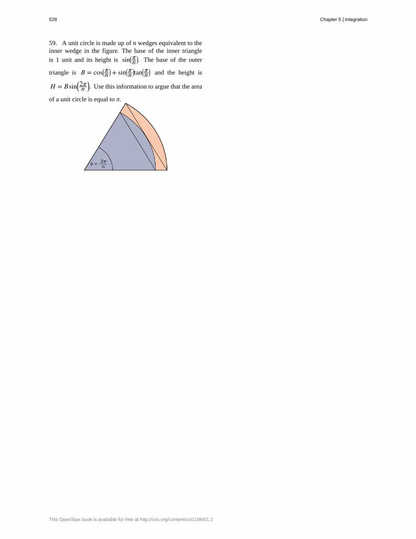
59. A unit circle is made up of n wedges equivalent to theinner wedge in the figure. The base of the inner triangle
is 1 unit and its height is sin⎛⎝πn
⎞⎠. The base of the outer
triangle is B = cos⎛⎝πn
⎞⎠ + sin⎛
⎝πn
⎞⎠tan⎛
⎝πn
⎞⎠ and the height is
H = Bsin⎛⎝2πn
⎞⎠. Use this information to argue that the area
of a unit circle is equal to π.
528 Chapter 5 | Integration
This OpenStax book is available for free at http://cnx.org/content/col11964/1.2
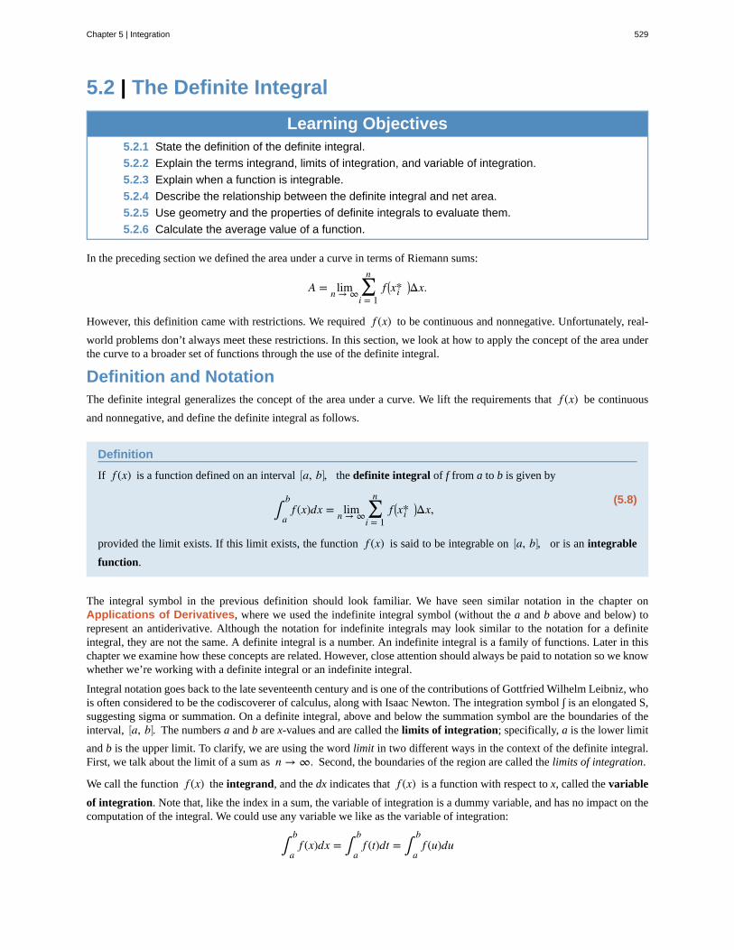
5.2 | The Definite Integral
Learning Objectives5.2.1 State the definition of the definite integral.
5.2.2 Explain the terms integrand, limits of integration, and variable of integration.
5.2.3 Explain when a function is integrable.
5.2.4 Describe the relationship between the definite integral and net area.
5.2.5 Use geometry and the properties of definite integrals to evaluate them.
5.2.6 Calculate the average value of a function.
In the preceding section we defined the area under a curve in terms of Riemann sums:
A = limn → ∞ ∑i = 1
nf ⎛
⎝xi*⎞⎠Δx.
However, this definition came with restrictions. We required f (x) to be continuous and nonnegative. Unfortunately, real-
world problems don’t always meet these restrictions. In this section, we look at how to apply the concept of the area underthe curve to a broader set of functions through the use of the definite integral.
Definition and NotationThe definite integral generalizes the concept of the area under a curve. We lift the requirements that f (x) be continuous
and nonnegative, and define the definite integral as follows.
Definition
If f (x) is a function defined on an interval ⎡⎣a, b⎤
⎦, the definite integral of f from a to b is given by
(5.8)∫
a
bf (x)dx = limn → ∞ ∑
i = 1
nf ⎛
⎝xi*⎞⎠Δx,
provided the limit exists. If this limit exists, the function f (x) is said to be integrable on ⎡⎣a, b⎤
⎦, or is an integrable
function.
The integral symbol in the previous definition should look familiar. We have seen similar notation in the chapter onApplications of Derivatives, where we used the indefinite integral symbol (without the a and b above and below) torepresent an antiderivative. Although the notation for indefinite integrals may look similar to the notation for a definiteintegral, they are not the same. A definite integral is a number. An indefinite integral is a family of functions. Later in thischapter we examine how these concepts are related. However, close attention should always be paid to notation so we knowwhether we’re working with a definite integral or an indefinite integral.
Integral notation goes back to the late seventeenth century and is one of the contributions of Gottfried Wilhelm Leibniz, whois often considered to be the codiscoverer of calculus, along with Isaac Newton. The integration symbol ∫ is an elongated S,suggesting sigma or summation. On a definite integral, above and below the summation symbol are the boundaries of theinterval, ⎡
⎣a, b⎤⎦. The numbers a and b are x-values and are called the limits of integration; specifically, a is the lower limit
and b is the upper limit. To clarify, we are using the word limit in two different ways in the context of the definite integral.First, we talk about the limit of a sum as n → ∞. Second, the boundaries of the region are called the limits of integration.
We call the function f (x) the integrand, and the dx indicates that f (x) is a function with respect to x, called the variable
of integration. Note that, like the index in a sum, the variable of integration is a dummy variable, and has no impact on thecomputation of the integral. We could use any variable we like as the variable of integration:
∫a
bf (x)dx = ∫
a
bf (t)dt = ∫
a
bf (u)du
Chapter 5 | Integration 529
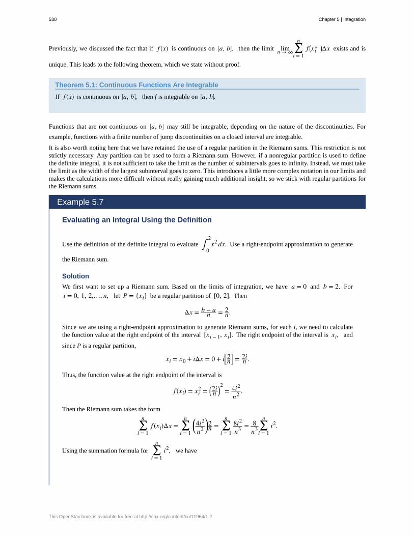
Previously, we discussed the fact that if f (x) is continuous on ⎡⎣a, b⎤
⎦, then the limit limn → ∞ ∑i = 1
nf ⎛
⎝xi*⎞⎠Δx exists and is
unique. This leads to the following theorem, which we state without proof.
Theorem 5.1: Continuous Functions Are Integrable
If f (x) is continuous on ⎡⎣a, b⎤
⎦, then f is integrable on ⎡⎣a, b⎤
⎦.
Functions that are not continuous on ⎡⎣a, b⎤
⎦ may still be integrable, depending on the nature of the discontinuities. For
example, functions with a finite number of jump discontinuities on a closed interval are integrable.
It is also worth noting here that we have retained the use of a regular partition in the Riemann sums. This restriction is notstrictly necessary. Any partition can be used to form a Riemann sum. However, if a nonregular partition is used to definethe definite integral, it is not sufficient to take the limit as the number of subintervals goes to infinity. Instead, we must takethe limit as the width of the largest subinterval goes to zero. This introduces a little more complex notation in our limits andmakes the calculations more difficult without really gaining much additional insight, so we stick with regular partitions forthe Riemann sums.
Example 5.7
Evaluating an Integral Using the Definition
Use the definition of the definite integral to evaluate ∫0
2x2 dx. Use a right-endpoint approximation to generate
the Riemann sum.
Solution
We first want to set up a Riemann sum. Based on the limits of integration, we have a = 0 and b = 2. For
i = 0, 1, 2,…, n, let P = {xi} be a regular partition of [0, 2]. Then
Δx = b − an = 2
n.
Since we are using a right-endpoint approximation to generate Riemann sums, for each i, we need to calculatethe function value at the right endpoint of the interval [xi − 1, xi]. The right endpoint of the interval is xi, and
since P is a regular partition,
xi = x0 + iΔx = 0 + i⎡⎣2n
⎤⎦ = 2i
n .
Thus, the function value at the right endpoint of the interval is
f (xi) = xi2 = ⎛
⎝2in
⎞⎠2
= 4i2
n2 .
Then the Riemann sum takes the form
∑i = 1
nf (xi)Δx = ∑
i = 1
n ⎛⎝
4i2
n2⎞⎠
2n = ∑
i = 1
n8i2
n3 = 8n3 ∑
i = 1
ni2.
Using the summation formula for ∑i = 1
ni2, we have
530 Chapter 5 | Integration
This OpenStax book is available for free at http://cnx.org/content/col11964/1.2
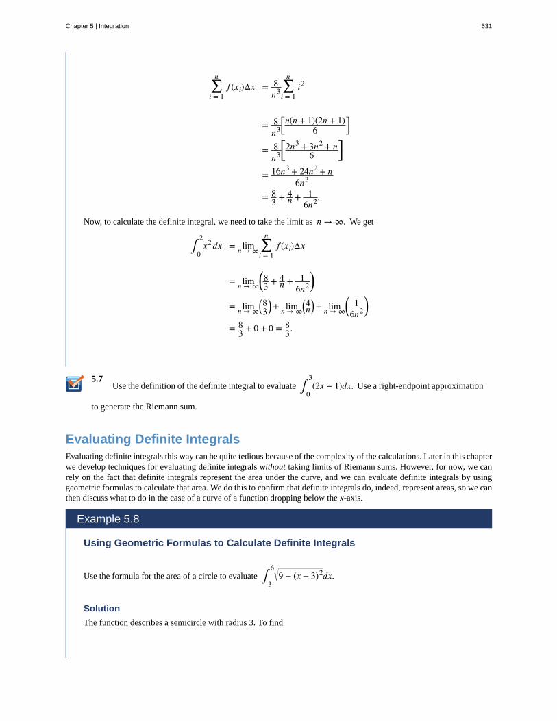
5.7
∑i = 1
nf (xi)Δx = 8
n3 ∑i = 1
ni2
= 8n3
⎡⎣n(n + 1)(2n + 1)
6⎤⎦
= 8n3
⎡⎣
2n3 + 3n2 + n6
⎤⎦
= 16n3 + 24n2 + n6n3
= 83 + 4
n + 16n2.
Now, to calculate the definite integral, we need to take the limit as n → ∞. We get
∫0
2x2 dx = limn → ∞ ∑
i = 1
nf (xi)Δx
= limn → ∞⎛⎝
83 + 4
n + 16n2
⎞⎠
= limn → ∞⎛⎝83
⎞⎠ + limn → ∞
⎛⎝4n
⎞⎠ + limn → ∞
⎛⎝
16n2
⎞⎠
= 83 + 0 + 0 = 8
3.
Use the definition of the definite integral to evaluate ∫0
3(2x − 1)dx. Use a right-endpoint approximation
to generate the Riemann sum.
Evaluating Definite IntegralsEvaluating definite integrals this way can be quite tedious because of the complexity of the calculations. Later in this chapterwe develop techniques for evaluating definite integrals without taking limits of Riemann sums. However, for now, we canrely on the fact that definite integrals represent the area under the curve, and we can evaluate definite integrals by usinggeometric formulas to calculate that area. We do this to confirm that definite integrals do, indeed, represent areas, so we canthen discuss what to do in the case of a curve of a function dropping below the x-axis.
Example 5.8
Using Geometric Formulas to Calculate Definite Integrals
Use the formula for the area of a circle to evaluate ∫3
69 − (x − 3)2dx.
Solution
The function describes a semicircle with radius 3. To find
Chapter 5 | Integration 531
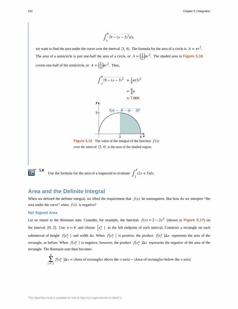
5.8
∫3
69 − (x − 3)2dx,
we want to find the area under the curve over the interval ⎡⎣3, 6⎤
⎦. The formula for the area of a circle is A = πr2.
The area of a semicircle is just one-half the area of a circle, or A = ⎛⎝12
⎞⎠πr2. The shaded area in Figure 5.16
covers one-half of the semicircle, or A = ⎛⎝14
⎞⎠πr2. Thus,
∫3
69 − (x − 3)2 = 1
4π(3)2
= 94π
≈ 7.069.
Figure 5.16 The value of the integral of the function f (x)over the interval ⎡
⎣3, 6⎤⎦ is the area of the shaded region.
Use the formula for the area of a trapezoid to evaluate ∫2
4(2x + 3)dx.
Area and the Definite IntegralWhen we defined the definite integral, we lifted the requirement that f (x) be nonnegative. But how do we interpret “the
area under the curve” when f (x) is negative?
Net Signed Area
Let us return to the Riemann sum. Consider, for example, the function f (x) = 2 − 2x2 (shown in Figure 5.17) on
the interval [0, 2]. Use n = 8 and choose⎧
⎩⎨xi* } as the left endpoint of each interval. Construct a rectangle on each
subinterval of height f ⎛⎝xi*
⎞⎠ and width Δx. When f ⎛
⎝xi*⎞⎠ is positive, the product f ⎛
⎝xi*⎞⎠Δx represents the area of the
rectangle, as before. When f ⎛⎝xi*
⎞⎠ is negative, however, the product f ⎛
⎝xi*⎞⎠Δx represents the negative of the area of the
rectangle. The Riemann sum then becomes
∑i = 1
8f ⎛
⎝xi*⎞⎠Δx = ⎛
⎝Area of rectangles above the x-axis⎞⎠ − ⎛
⎝Area of rectangles below the x-axis⎞⎠
532 Chapter 5 | Integration
This OpenStax book is available for free at http://cnx.org/content/col11964/1.2
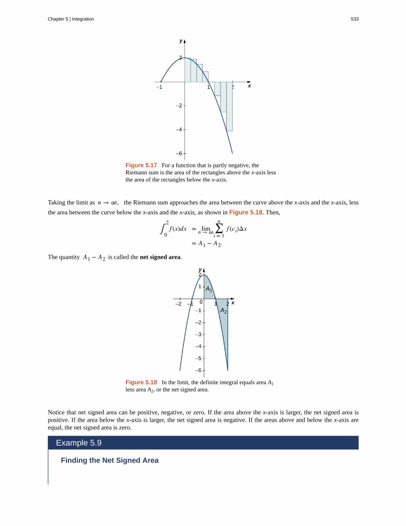
Figure 5.17 For a function that is partly negative, theRiemann sum is the area of the rectangles above the x-axis lessthe area of the rectangles below the x-axis.
Taking the limit as n → ∞, the Riemann sum approaches the area between the curve above the x-axis and the x-axis, less
the area between the curve below the x-axis and the x-axis, as shown in Figure 5.18. Then,
∫0
2f (x)dx = limn → ∞ ∑
i = 1
nf (ci)Δx
= A1 − A2.
The quantity A1 − A2 is called the net signed area.
Figure 5.18 In the limit, the definite integral equals area A1less area A2, or the net signed area.
Notice that net signed area can be positive, negative, or zero. If the area above the x-axis is larger, the net signed area ispositive. If the area below the x-axis is larger, the net signed area is negative. If the areas above and below the x-axis areequal, the net signed area is zero.
Example 5.9
Finding the Net Signed Area
Chapter 5 | Integration 533
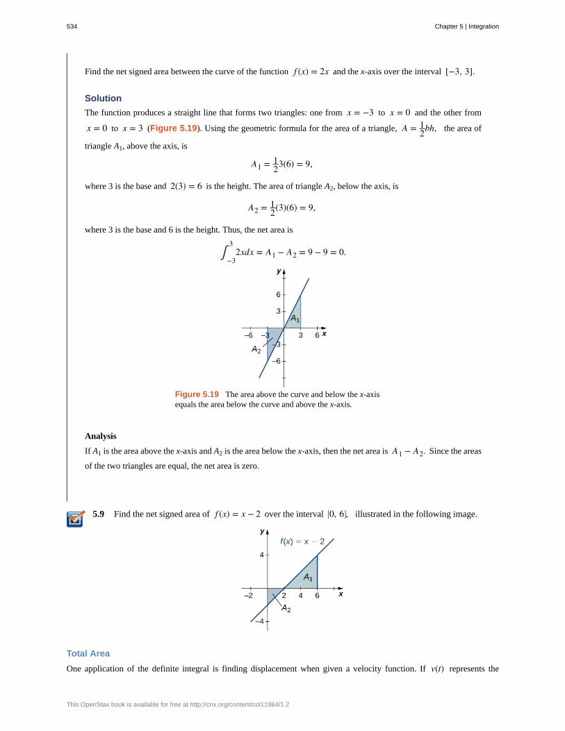
5.9
Find the net signed area between the curve of the function f (x) = 2x and the x-axis over the interval [−3, 3].
Solution
The function produces a straight line that forms two triangles: one from x = −3 to x = 0 and the other from
x = 0 to x = 3 (Figure 5.19). Using the geometric formula for the area of a triangle, A = 12bh, the area of
triangle A1, above the axis, is
A1 = 123(6) = 9,
where 3 is the base and 2(3) = 6 is the height. The area of triangle A2, below the axis, is
A2 = 12(3)(6) = 9,
where 3 is the base and 6 is the height. Thus, the net area is
∫−3
32xdx = A1 − A2 = 9 − 9 = 0.
Figure 5.19 The area above the curve and below the x-axisequals the area below the curve and above the x-axis.
Analysis
If A1 is the area above the x-axis and A2 is the area below the x-axis, then the net area is A1 − A2. Since the areas
of the two triangles are equal, the net area is zero.
Find the net signed area of f (x) = x − 2 over the interval ⎡⎣0, 6⎤
⎦, illustrated in the following image.
Total Area
One application of the definite integral is finding displacement when given a velocity function. If v(t) represents the
534 Chapter 5 | Integration
This OpenStax book is available for free at http://cnx.org/content/col11964/1.2
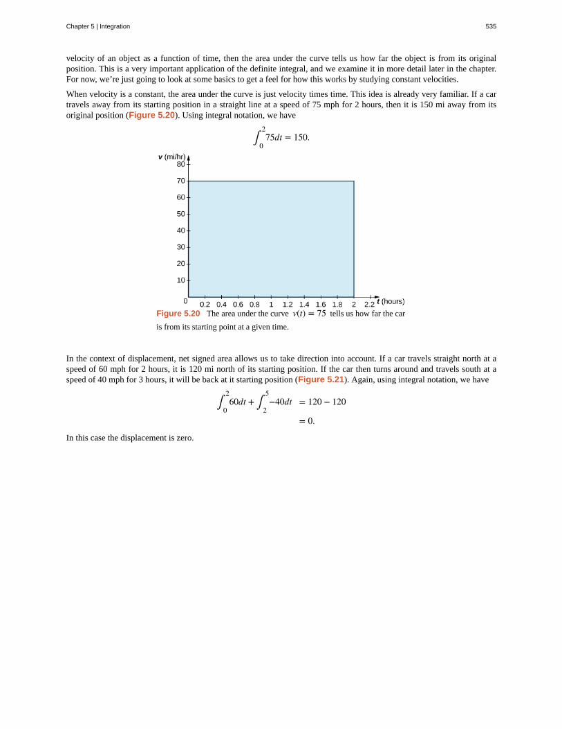
velocity of an object as a function of time, then the area under the curve tells us how far the object is from its originalposition. This is a very important application of the definite integral, and we examine it in more detail later in the chapter.For now, we’re just going to look at some basics to get a feel for how this works by studying constant velocities.
When velocity is a constant, the area under the curve is just velocity times time. This idea is already very familiar. If a cartravels away from its starting position in a straight line at a speed of 75 mph for 2 hours, then it is 150 mi away from itsoriginal position (Figure 5.20). Using integral notation, we have
∫0
275dt = 150.
Figure 5.20 The area under the curve v(t) = 75 tells us how far the car
is from its starting point at a given time.
In the context of displacement, net signed area allows us to take direction into account. If a car travels straight north at aspeed of 60 mph for 2 hours, it is 120 mi north of its starting position. If the car then turns around and travels south at aspeed of 40 mph for 3 hours, it will be back at it starting position (Figure 5.21). Again, using integral notation, we have
∫0
260dt + ∫
2
5−40dt = 120 − 120
= 0.
In this case the displacement is zero.
Chapter 5 | Integration 535
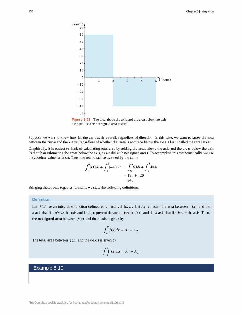
Figure 5.21 The area above the axis and the area below the axisare equal, so the net signed area is zero.
Suppose we want to know how far the car travels overall, regardless of direction. In this case, we want to know the areabetween the curve and the x-axis, regardless of whether that area is above or below the axis. This is called the total area.
Graphically, it is easiest to think of calculating total area by adding the areas above the axis and the areas below the axis(rather than subtracting the areas below the axis, as we did with net signed area). To accomplish this mathematically, we usethe absolute value function. Thus, the total distance traveled by the car is
∫0
2|60|dt + ∫
2
5|−40|dt = ∫
0
260dt + ∫
2
540dt
= 120 + 120= 240.
Bringing these ideas together formally, we state the following definitions.
Definition
Let f (x) be an integrable function defined on an interval ⎡⎣a, b⎤
⎦. Let A1 represent the area between f (x) and the
x-axis that lies above the axis and let A2 represent the area between f (x) and the x-axis that lies below the axis. Then,
the net signed area between f (x) and the x-axis is given by
∫a
bf (x)dx = A1 − A2.
The total area between f (x) and the x-axis is given by
∫a
b| f (x)|dx = A1 + A2.
Example 5.10
536 Chapter 5 | Integration
This OpenStax book is available for free at http://cnx.org/content/col11964/1.2
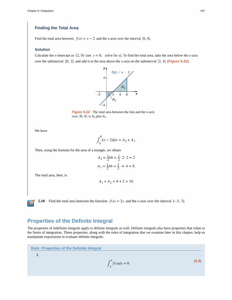
5.10
Finding the Total Area
Find the total area between f (x) = x − 2 and the x-axis over the interval ⎡⎣0, 6⎤
⎦.
Solution
Calculate the x-intercept as (2, 0) (set y = 0, solve for x). To find the total area, take the area below the x-axis
over the subinterval [0, 2] and add it to the area above the x-axis on the subinterval ⎡⎣2, 6⎤
⎦ (Figure 5.22).
Figure 5.22 The total area between the line and the x-axisover ⎡
⎣0, 6⎤⎦ is A2 plus A1.
We have
∫0
6|(x − 2)|dx = A2 + A1.
Then, using the formula for the area of a triangle, we obtain
A2 = 12bh = 1
2 · 2 · 2 = 2
A1 = 12bh = 1
2 · 4 · 4 = 8.
The total area, then, is
A1 + A2 = 8 + 2 = 10.
Find the total area between the function f (x) = 2x and the x-axis over the interval [−3, 3].
Properties of the Definite IntegralThe properties of indefinite integrals apply to definite integrals as well. Definite integrals also have properties that relate tothe limits of integration. These properties, along with the rules of integration that we examine later in this chapter, help usmanipulate expressions to evaluate definite integrals.
Rule: Properties of the Definite Integral
1.
(5.9)∫a
af (x)dx = 0
Chapter 5 | Integration 537
If the limits of integration are the same, the integral is just a line and contains no area.
2.
(5.10)∫b
af (x)dx = −∫
a
bf (x)dx
If the limits are reversed, then place a negative sign in front of the integral.
3.
(5.11)∫a
b⎡⎣ f (x) + g(x)⎤
⎦dx = ∫a
bf (x)dx + ∫
a
bg(x)dx
The integral of a sum is the sum of the integrals.
4.
(5.12)⌠⌡a
b⎡⎣ f (x) − g(x)⎤
⎦dx = ⌠⌡a
b
f (x)dx − ∫a
bg(x)dx
The integral of a difference is the difference of the integrals.
5.
(5.13)∫a
bc f (x)dx = c∫
a
bf (x)
for constant c. The integral of the product of a constant and a function is equal to the constant multiplied bythe integral of the function.
6.
(5.14)∫a
bf (x)dx = ∫
a
cf (x)dx + ∫
c
bf (x)dx
Although this formula normally applies when c is between a and b, the formula holds for all values of a, b, andc, provided f (x) is integrable on the largest interval.
Example 5.11
Using the Properties of the Definite Integral
Use the properties of the definite integral to express the definite integral of f (x) = −3x3 + 2x + 2 over the
interval [−2, 1] as the sum of three definite integrals.
Solution
Using integral notation, we have ∫−2
1 ⎛⎝−3x3 + 2x + 2⎞
⎠dx. We apply properties 3. and 5. to get
538 Chapter 5 | Integration
This OpenStax book is available for free at http://cnx.org/content/col11964/1.2
5.11
5.12
∫−2
1 ⎛⎝−3x3 + 2x + 2⎞
⎠dx = ∫−2
1−3x3 dx + ∫
−2
12xdx + ∫
−2
12dx
= −3∫−2
1x3 dx + 2∫
−2
1xdx + ∫
−2
12dx.
Use the properties of the definite integral to express the definite integral of f (x) = 6x3 − 4x2 + 2x − 3over the interval [1, 3] as the sum of four definite integrals.
Example 5.12
Using the Properties of the Definite Integral
If it is known that ∫0
8f (x)dx = 10 and ∫
0
5f (x)dx = 5, find the value of ∫
5
8f (x)dx.
Solution
By property 6.,
∫a
bf (x)dx = ∫
a
cf (x)dx + ∫
c
bf (x)dx.
Thus,
∫0
8f (x)dx = ∫
0
5f (x)dx + ∫
5
8f (x)dx
10 = 5 + ∫5
8f (x)dx
5 = ∫5
8f (x)dx.
If it is known that ∫1
5f (x)dx = −3 and ∫
2
5f (x)dx = 4, find the value of ∫
1
2f (x)dx.
Comparison Properties of Integrals
A picture can sometimes tell us more about a function than the results of computations. Comparing functions by their graphsas well as by their algebraic expressions can often give new insight into the process of integration. Intuitively, we might saythat if a function f (x) is above another function g(x), then the area between f (x) and the x-axis is greater than the area
between g(x) and the x-axis. This is true depending on the interval over which the comparison is made. The properties of
definite integrals are valid whether a < b, a = b, or a > b. The following properties, however, concern only the case
a ≤ b, and are used when we want to compare the sizes of integrals.
Chapter 5 | Integration 539
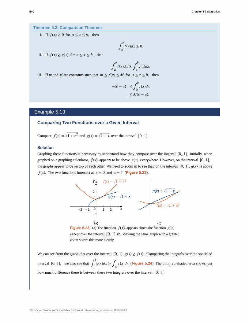
Theorem 5.2: Comparison Theorem
i. If f (x) ≥ 0 for a ≤ x ≤ b, then
∫a
bf (x)dx ≥ 0.
ii. If f (x) ≥ g(x) for a ≤ x ≤ b, then
∫a
bf (x)dx ≥ ∫
a
bg(x)dx.
iii. If m and M are constants such that m ≤ f (x) ≤ M for a ≤ x ≤ b, then
m(b − a) ≤ ∫a
bf (x)dx
≤ M(b − a).
Example 5.13
Comparing Two Functions over a Given Interval
Compare f (x) = 1 + x2 and g(x) = 1 + x over the interval [0, 1].
Solution
Graphing these functions is necessary to understand how they compare over the interval [0, 1]. Initially, when
graphed on a graphing calculator, f (x) appears to be above g(x) everywhere. However, on the interval [0, 1],the graphs appear to be on top of each other. We need to zoom in to see that, on the interval [0, 1], g(x) is above
f (x). The two functions intersect at x = 0 and x = 1 (Figure 5.23).
Figure 5.23 (a) The function f (x) appears above the function g(x)except over the interval [0, 1] (b) Viewing the same graph with a greater
zoom shows this more clearly.
We can see from the graph that over the interval [0, 1], g(x) ≥ f (x). Comparing the integrals over the specified
interval [0, 1], we also see that ∫0
1g(x)dx ≥ ∫
0
1f (x)dx (Figure 5.24). The thin, red-shaded area shows just
how much difference there is between these two integrals over the interval [0, 1].
540 Chapter 5 | Integration
This OpenStax book is available for free at http://cnx.org/content/col11964/1.2
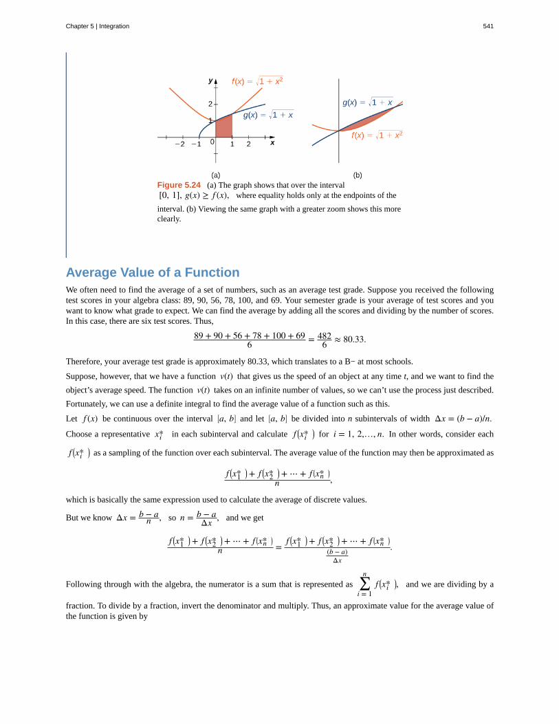
Figure 5.24 (a) The graph shows that over the interval[0, 1], g(x) ≥ f (x), where equality holds only at the endpoints of the
interval. (b) Viewing the same graph with a greater zoom shows this moreclearly.
Average Value of a FunctionWe often need to find the average of a set of numbers, such as an average test grade. Suppose you received the followingtest scores in your algebra class: 89, 90, 56, 78, 100, and 69. Your semester grade is your average of test scores and youwant to know what grade to expect. We can find the average by adding all the scores and dividing by the number of scores.In this case, there are six test scores. Thus,
89 + 90 + 56 + 78 + 100 + 696 = 482
6 ≈ 80.33.
Therefore, your average test grade is approximately 80.33, which translates to a B− at most schools.
Suppose, however, that we have a function v(t) that gives us the speed of an object at any time t, and we want to find the
object’s average speed. The function v(t) takes on an infinite number of values, so we can’t use the process just described.
Fortunately, we can use a definite integral to find the average value of a function such as this.
Let f (x) be continuous over the interval ⎡⎣a, b⎤
⎦ and let ⎡⎣a, b⎤
⎦ be divided into n subintervals of width Δx = (b − a)/n.
Choose a representative xi* in each subinterval and calculate f ⎛⎝xi*
⎞⎠ for i = 1, 2,…, n. In other words, consider each
f ⎛⎝xi*
⎞⎠ as a sampling of the function over each subinterval. The average value of the function may then be approximated as
f ⎛⎝x1*
⎞⎠ + f ⎛
⎝x2*⎞⎠ + ⋯ + f ⎛
⎝xn* ⎞⎠
n ,
which is basically the same expression used to calculate the average of discrete values.
But we know Δx = b − an , so n = b − a
Δx , and we get
f ⎛⎝x1*
⎞⎠ + f ⎛
⎝x2*⎞⎠ + ⋯ + f ⎛
⎝xn* ⎞⎠
n =f ⎛
⎝x1*⎞⎠ + f ⎛
⎝x2*⎞⎠ + ⋯ + f ⎛
⎝xn* ⎞⎠
(b − a)Δx
.
Following through with the algebra, the numerator is a sum that is represented as ∑i = 1
nf ⎛
⎝xi*⎞⎠, and we are dividing by a
fraction. To divide by a fraction, invert the denominator and multiply. Thus, an approximate value for the average value ofthe function is given by
Chapter 5 | Integration 541
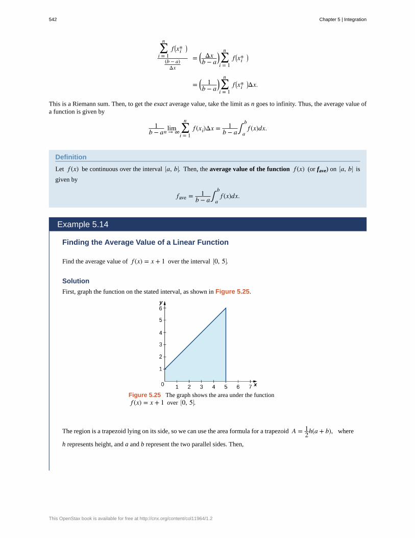
∑i = 1
nf ⎛
⎝xi*⎞⎠
(b − a)Δx
= ⎛⎝
Δxb − a
⎞⎠∑i = 1
nf ⎛
⎝xi*⎞⎠
= ⎛⎝
1b − a
⎞⎠∑i = 1
nf ⎛
⎝xi*⎞⎠Δx.
This is a Riemann sum. Then, to get the exact average value, take the limit as n goes to infinity. Thus, the average value ofa function is given by
1b − a limn → ∞ ∑
i = 1
nf (xi)Δx = 1
b − a∫a
bf (x)dx.
Definition
Let f (x) be continuous over the interval ⎡⎣a, b⎤
⎦. Then, the average value of the function f (x) (or fave) on ⎡⎣a, b⎤
⎦ is
given by
fave = 1b − a∫
a
bf (x)dx.
Example 5.14
Finding the Average Value of a Linear Function
Find the average value of f (x) = x + 1 over the interval ⎡⎣0, 5⎤
⎦.
Solution
First, graph the function on the stated interval, as shown in Figure 5.25.
Figure 5.25 The graph shows the area under the functionf (x) = x + 1 over ⎡
⎣0, 5⎤⎦.
The region is a trapezoid lying on its side, so we can use the area formula for a trapezoid A = 12h(a + b), where
h represents height, and a and b represent the two parallel sides. Then,
542 Chapter 5 | Integration
This OpenStax book is available for free at http://cnx.org/content/col11964/1.2
5.13
∫0
5x + 1dx = 1
2h(a + b)
= 12 · 5 · (1 + 6)
= 352 .
Thus the average value of the function is
15 − 0∫
0
5x + 1dx = 1
5 · 352 = 7
2.
Find the average value of f (x) = 6 − 2x over the interval [0, 3].
Chapter 5 | Integration 543
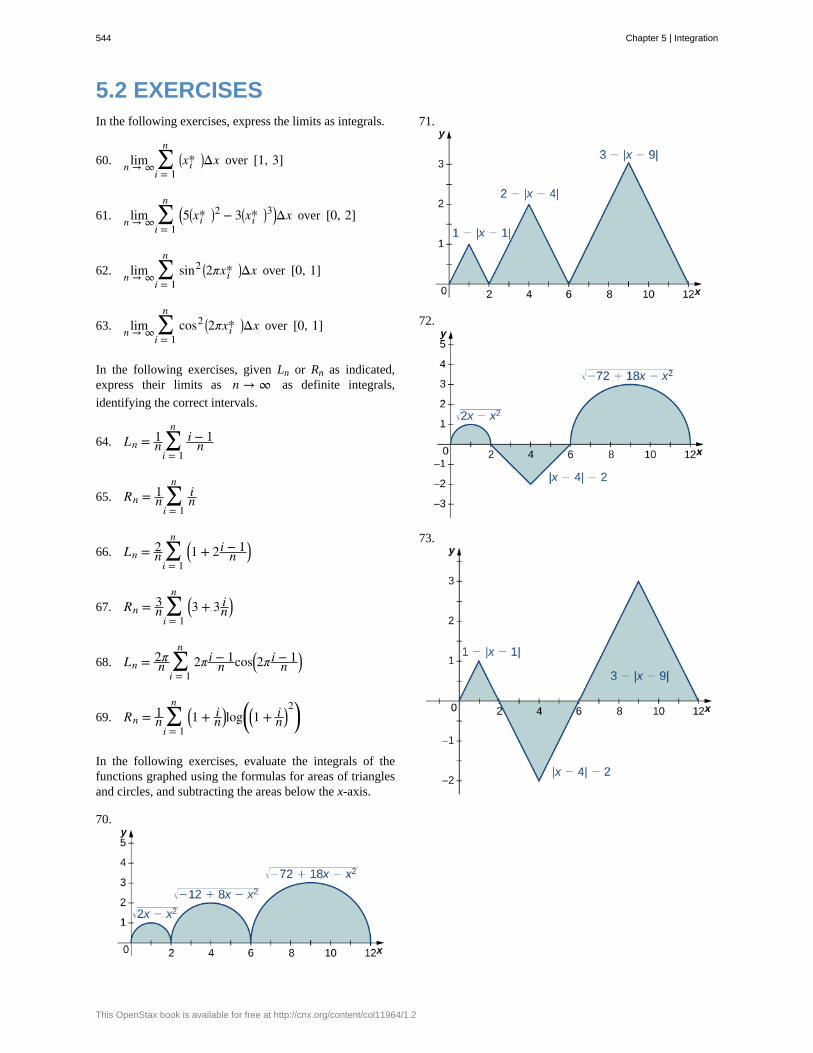
5.2 EXERCISESIn the following exercises, express the limits as integrals.
60. limn → ∞ ∑i = 1
n⎛⎝xi*
⎞⎠Δx over [1, 3]
61. limn → ∞ ∑i = 1
n⎛⎝5
⎛⎝xi*
⎞⎠2 − 3⎛
⎝xi*⎞⎠3⎞
⎠Δx over [0, 2]
62. limn → ∞ ∑i = 1
nsin2 ⎛
⎝2πxi*⎞⎠Δx over [0, 1]
63. limn → ∞ ∑i = 1
ncos2 ⎛
⎝2πxi*⎞⎠Δx over [0, 1]
In the following exercises, given Ln or Rn as indicated,express their limits as n → ∞ as definite integrals,
identifying the correct intervals.
64. Ln = 1n ∑
i = 1
ni − 1
n
65. Rn = 1n ∑
i = 1
nin
66. Ln = 2n ∑
i = 1
n⎛⎝1 + 2i − 1
n⎞⎠
67. Rn = 3n ∑
i = 1
n⎛⎝3 + 3 i
n⎞⎠
68. Ln = 2πn ∑
i = 1
n2πi − 1
n cos⎛⎝2πi − 1
n⎞⎠
69. Rn = 1n ∑
i = 1
n⎛⎝1 + i
n⎞⎠log⎛
⎝⎛⎝1 + i
n⎞⎠2⎞⎠
In the following exercises, evaluate the integrals of thefunctions graphed using the formulas for areas of trianglesand circles, and subtracting the areas below the x-axis.
70.
71.
72.
73.
544 Chapter 5 | Integration
This OpenStax book is available for free at http://cnx.org/content/col11964/1.2
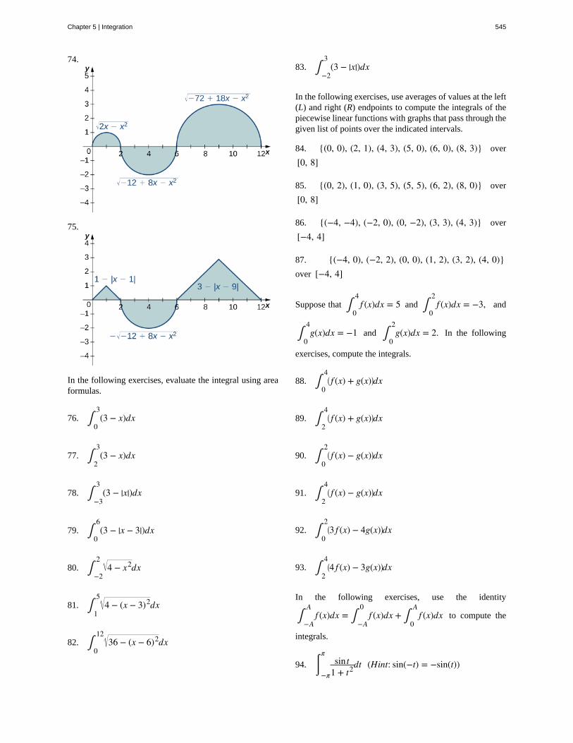
74.
75.
In the following exercises, evaluate the integral using areaformulas.
76. ∫0
3(3 − x)dx
77. ∫2
3(3 − x)dx
78. ∫−3
3(3 − |x|)dx
79. ∫0
6(3 − |x − 3|)dx
80. ∫−2
24 − x2dx
81. ∫1
54 − (x − 3)2dx
82. ∫0
1236 − (x − 6)2dx
83. ∫−2
3(3 − |x|)dx
In the following exercises, use averages of values at the left(L) and right (R) endpoints to compute the integrals of thepiecewise linear functions with graphs that pass through thegiven list of points over the indicated intervals.
84. {(0, 0), (2, 1), (4, 3), (5, 0), (6, 0), (8, 3)} over
[0, 8]
85. {(0, 2), (1, 0), (3, 5), (5, 5), (6, 2), (8, 0)} over
[0, 8]
86. {(−4, −4), (−2, 0), (0, −2), (3, 3), (4, 3)} over
[−4, 4]
87. {(−4, 0), (−2, 2), (0, 0), (1, 2), (3, 2), (4, 0)}over [−4, 4]
Suppose that ∫0
4f (x)dx = 5 and ∫
0
2f (x)dx = −3, and
∫0
4g(x)dx = −1 and ∫
0
2g(x)dx = 2. In the following
exercises, compute the integrals.
88. ∫0
4⎛⎝ f (x) + g(x)⎞
⎠dx
89. ∫2
4⎛⎝ f (x) + g(x)⎞
⎠dx
90. ∫0
2⎛⎝ f (x) − g(x)⎞
⎠dx
91. ∫2
4⎛⎝ f (x) − g(x)⎞
⎠dx
92. ∫0
2⎛⎝3 f (x) − 4g(x)⎞
⎠dx
93. ∫2
4⎛⎝4 f (x) − 3g(x)⎞
⎠dx
In the following exercises, use the identity
∫−A
Af (x)dx = ∫
−A
0f (x)dx + ∫
0
Af (x)dx to compute the
integrals.
94. ⌠⌡−π
πsin t
1 + t2dt (Hint: sin(−t) = −sin(t))
Chapter 5 | Integration 545
95. ∫− π
π t1 + cos tdt
96. ∫1
3(2 − x)dx (Hint: Look at the graph of f.)
97. ∫2
4(x − 3)3 dx (Hint: Look at the graph of f.)
In the following exercises, given that
∫0
1xdx = 1
2, ∫0
1x2 dx = 1
3, and ∫0
1x3 dx = 1
4,
compute the integrals.
98. ∫0
1⎛⎝1 + x + x2 + x3⎞
⎠dx
99. ∫0
1⎛⎝1 − x + x2 − x3⎞
⎠dx
100. ∫0
1(1 − x)2 dx
101. ∫0
1(1 − 2x)3 dx
102. ⌠⌡0
1⎛⎝6x − 4
3x2⎞⎠dx
103. ∫0
1⎛⎝7 − 5x3⎞
⎠dx
In the following exercises, use the comparisontheorem.
104. Show that ∫0
3⎛⎝x2 − 6x + 9⎞
⎠dx ≥ 0.
105. Show that ∫−2
3(x − 3)(x + 2)dx ≤ 0.
106. Show that ∫0
11 + x3dx ≤ ∫
0
11 + x2dx.
107. Show that ∫1
21 + xdx ≤ ∫
1
21 + x2dx.
108. Show that ∫0
π/2sin tdt ≥ π
4. (Hint: sin t ≥ 2tπ over
⎡⎣0, π
2⎤⎦)
109. Show that ∫−π/4
π/4cos tdt ≥ π 2/4.
In the following exercises, find the average value fave of fbetween a and b, and find a point c, where f (c) = fave.
110. f (x) = x2, a = −1, b = 1
111. f (x) = x5, a = −1, b = 1
112. f (x) = 4 − x2, a = 0, b = 2
113. f (x) = (3 − |x|), a = −3, b = 3
114. f (x) = sinx, a = 0, b = 2π
115. f (x) = cosx, a = 0, b = 2π
In the following exercises, approximate the average valueusing Riemann sums L100 and R100. How does your answercompare with the exact given answer?
116. [T] y = ln(x) over the interval [1, 4]; the exact
solution is ln(256)3 − 1.
117. [T] y = ex/2 over the interval [0, 1]; the exact
solution is 2( e − 1).
118. [T] y = tanx over the interval⎡⎣0, π
4⎤⎦; the exact
solution is 2ln(2)π .
119. [T] y = x + 14 − x2
over the interval [−1, 1]; the
exact solution is π6.
In the following exercises, compute the average value usingthe left Riemann sums LN for N = 1, 10, 100. How does
the accuracy compare with the given exact value?
120. [T] y = x2 − 4 over the interval [0, 2]; the exact
solution is −83.
121. [T] y = xex2over the interval [0, 2]; the exact
solution is 14
⎛⎝e4 − 1⎞
⎠.
546 Chapter 5 | Integration
This OpenStax book is available for free at http://cnx.org/content/col11964/1.2
122. [T] y = ⎛⎝12
⎞⎠
xover the interval [0, 4]; the exact
solution is 1564ln(2).
123. [T] y = xsin⎛⎝x2⎞
⎠ over the interval [−π, 0]; the
exact solution iscos⎛
⎝π2⎞⎠ − 1
2π .
124. Suppose that A = ∫0
2πsin2 tdt and
B = ∫0
2πcos2 tdt. Show that A + B = 2π and A = B.
125. Suppose that A = ∫−π/4
π/4sec2 tdt = π and
B = ∫−π/4
π/4tan2 tdt. Show that A − B = π
2.
126. Show that the average value of sin2 t over [0, 2π]is equal to 1/2 Without further calculation, determine
whether the average value of sin2 t over [0, π] is also
equal to 1/2.
127. Show that the average value of cos2 t over [0, 2π]is equal to 1/2. Without further calculation, determine
whether the average value of cos2 (t) over [0, π] is also
equal to 1/2.
128. Explain why the graphs of a quadratic function(parabola) p(x) and a linear function ℓ(x) can intersect
in at most two points. Suppose that p(a) = ℓ(a) and
p(b) = ℓ(b), and that ∫a
bp(t)dt > ∫
a
bℓ(t)dt. Explain
why ∫c
dp(t) > ∫
c
dℓ(t)dt whenever a ≤ c < d ≤ b.
129. Suppose that parabola p(x) = ax2 + bx + c opens
downward (a < 0) and has a vertex of y = −b2a > 0. For
which interval [A, B] is ∫A
B⎛⎝ax2 + bx + c⎞
⎠dx as large as
possible?
130. Suppose ⎡⎣a, b⎤
⎦ can be subdivided into subintervals
a = a0 < a1 < a2 < ⋯ < aN = b such that either
f ≥ 0 over [ai − 1, ai] or f ≤ 0 over [ai − 1, ai]. Set
Ai = ∫ai − 1
aif (t)dt.
a. Explain why ∫a
bf (t)dt = A1 + A2 + ⋯ + AN.
b. Then, explain why |∫a
bf (t)dt| ≤ ∫
a
b| f (t)|dt.
131. Suppose f and g are continuous functions such that
∫c
df (t)dt ≤ ∫
c
dg(t)dt for every subinterval ⎡
⎣c, d⎤⎦ of
⎡⎣a, b⎤
⎦. Explain why f (x) ≤ g(x) for all values of x.
132. Suppose the average value of f over ⎡⎣a, b⎤
⎦ is 1 and
the average value of f over ⎡⎣b, c⎤
⎦ is 1 where a < c < b.Show that the average value of f over [a, c] is also 1.
133. Suppose that ⎡⎣a, b⎤
⎦ can be partitioned. taking
a = a0 < a1 < ⋯ < aN = b such that the average value
of f over each subinterval [ai − 1, ai] = 1 is equal to 1 for
each i = 1,…, N. Explain why the average value of f over⎡⎣a, b⎤
⎦ is also equal to 1.
134. Suppose that for each i such that 1 ≤ i ≤ N one has
∫i − 1
if (t)dt = i. Show that ∫
0
Nf (t)dt = N(N + 1)
2 .
135. Suppose that for each i such that 1 ≤ i ≤ N one
has ∫i − 1
if (t)dt = i2. Show that
∫0
Nf (t)dt = N(N + 1)(2N + 1)
6 .
136. [T] Compute the left and right Riemann sums L10
and R10 and their averageL10 + R10
2 for f (t) = t2 over
[0, 1]. Given that ∫0
1t2 dt = 0.33
–, to how many
decimal places isL10 + R10
2 accurate?
Chapter 5 | Integration 547
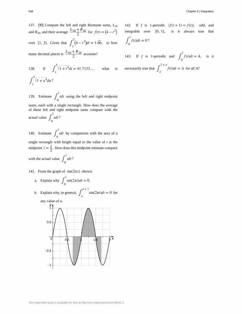
137. [T] Compute the left and right Riemann sums, L10
and R10, and their averageL10 + R10
2 for f (t) = ⎛⎝4 − t2⎞
⎠
over [1, 2]. Given that ∫1
2⎛⎝4 − t2⎞
⎠dt = 1.66–
, to how
many decimal places isL10 + R10
2 accurate?
138. If ∫1
51 + t4dt = 41.7133..., what is
∫1
51 + u4du?
139. Estimate ∫0
1tdt using the left and right endpoint
sums, each with a single rectangle. How does the averageof these left and right endpoint sums compare with the
actual value ∫0
1tdt ?
140. Estimate ∫0
1tdt by comparison with the area of a
single rectangle with height equal to the value of t at the
midpoint t = 12. How does this midpoint estimate compare
with the actual value ∫0
1tdt ?
141. From the graph of sin(2πx) shown:
a. Explain why ∫0
1sin(2πt)dt = 0.
b. Explain why, in general, ∫a
a + 1sin(2πt)dt = 0 for
any value of a.
142. If f is 1-periodic ⎛⎝ f (t + 1) = f (t)⎞
⎠, odd, and
integrable over [0, 1], is it always true that
∫0
1f (t)dt = 0?
143. If f is 1-periodic and ∫0
1f (t)dt = A, is it
necessarily true that ∫a
1 + af (t)dt = A for all A?
548 Chapter 5 | Integration
This OpenStax book is available for free at http://cnx.org/content/col11964/1.2
5.3 | The Fundamental Theorem of Calculus
Learning Objectives5.3.1 Describe the meaning of the Mean Value Theorem for Integrals.
5.3.2 State the meaning of the Fundamental Theorem of Calculus, Part 1.
5.3.3 Use the Fundamental Theorem of Calculus, Part 1, to evaluate derivatives of integrals.
5.3.4 State the meaning of the Fundamental Theorem of Calculus, Part 2.
5.3.5 Use the Fundamental Theorem of Calculus, Part 2, to evaluate definite integrals.
5.3.6 Explain the relationship between differentiation and integration.
In the previous two sections, we looked at the definite integral and its relationship to the area under the curve of a function.Unfortunately, so far, the only tools we have available to calculate the value of a definite integral are geometric areaformulas and limits of Riemann sums, and both approaches are extremely cumbersome. In this section we look at somemore powerful and useful techniques for evaluating definite integrals.
These new techniques rely on the relationship between differentiation and integration. This relationship was discovered andexplored by both Sir Isaac Newton and Gottfried Wilhelm Leibniz (among others) during the late 1600s and early 1700s,and it is codified in what we now call the Fundamental Theorem of Calculus, which has two parts that we examine in thissection. Its very name indicates how central this theorem is to the entire development of calculus.
Isaac Newton’s contributions to mathematics and physics changed the way we look at the world. The relationshipshe discovered, codified as Newton’s laws and the law of universal gravitation, are still taught as foundationalmaterial in physics today, and his calculus has spawned entire fields of mathematics. To learn more, read a briefbiography (http://www.openstaxcollege.org/l/20_newtonbio) of Newton with multimedia clips.
Before we get to this crucial theorem, however, let’s examine another important theorem, the Mean Value Theorem forIntegrals, which is needed to prove the Fundamental Theorem of Calculus.
The Mean Value Theorem for IntegralsThe Mean Value Theorem for Integrals states that a continuous function on a closed interval takes on its average value atthe same point in that interval. The theorem guarantees that if f (x) is continuous, a point c exists in an interval ⎡
⎣a, b⎤⎦ such
that the value of the function at c is equal to the average value of f (x) over ⎡⎣a, b⎤
⎦. We state this theorem mathematically
with the help of the formula for the average value of a function that we presented at the end of the preceding section.
Theorem 5.3: The Mean Value Theorem for Integrals
If f (x) is continuous over an interval ⎡⎣a, b⎤
⎦, then there is at least one point c ∈ ⎡⎣a, b⎤
⎦ such that
(5.15)f (c) = 1
b − a∫a
bf (x)dx.
This formula can also be stated as
∫a
bf (x)dx = f (c)(b − a).
Proof
Since f (x) is continuous on ⎡⎣a, b⎤
⎦, by the extreme value theorem (see Maxima and Minima), it assumes minimum and
maximum values—m and M, respectively—on ⎡⎣a, b⎤
⎦. Then, for all x in ⎡⎣a, b⎤
⎦, we have m ≤ f (x) ≤ M. Therefore, by
the comparison theorem (see The Definite Integral), we have
m(b − a) ≤ ∫a
bf (x)dx ≤ M(b − a).
Chapter 5 | Integration 549
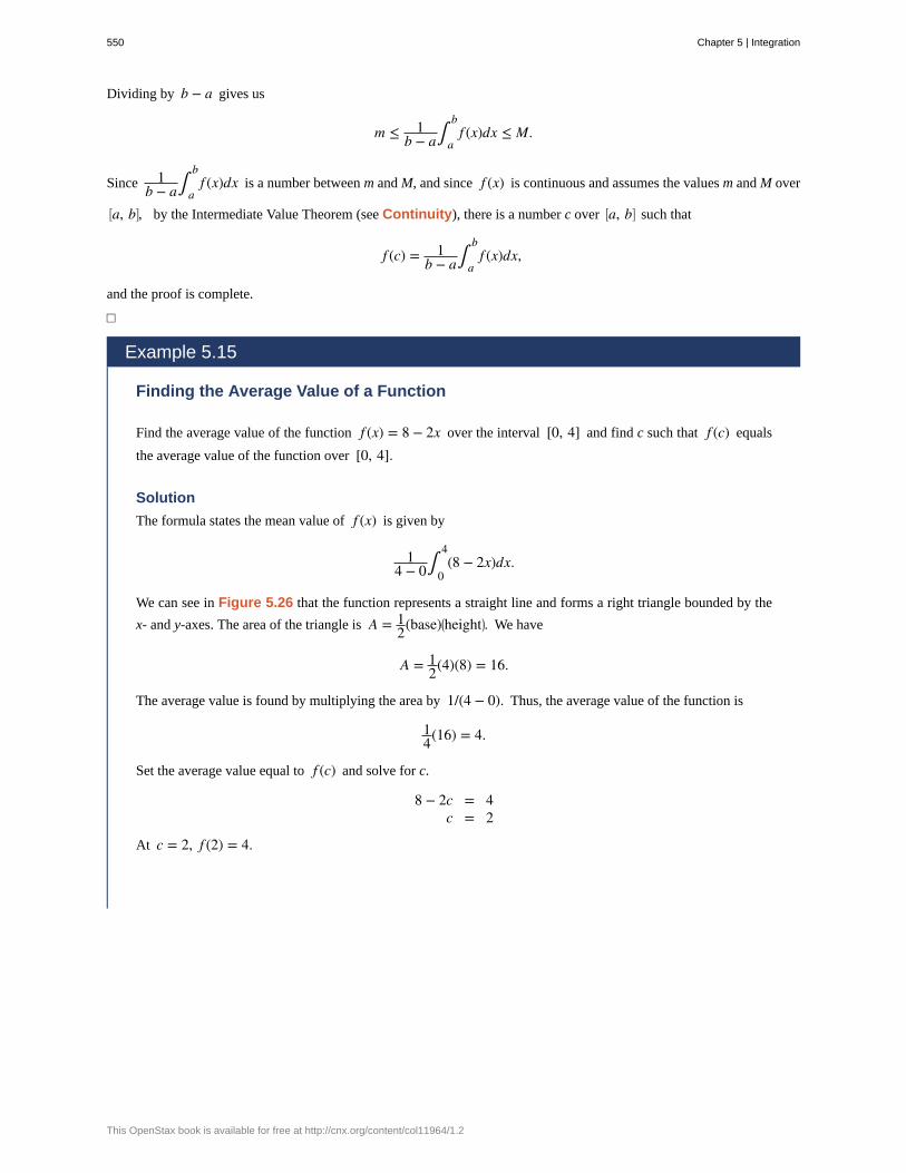
Dividing by b − a gives us
m ≤ 1b − a∫
a
bf (x)dx ≤ M.
Since 1b − a∫
a
bf (x)dx is a number between m and M, and since f (x) is continuous and assumes the values m and M over
⎡⎣a, b⎤
⎦, by the Intermediate Value Theorem (see Continuity), there is a number c over ⎡⎣a, b⎤
⎦ such that
f (c) = 1b − a∫
a
bf (x)dx,
and the proof is complete.
□
Example 5.15
Finding the Average Value of a Function
Find the average value of the function f (x) = 8 − 2x over the interval [0, 4] and find c such that f (c) equals
the average value of the function over [0, 4].
Solution
The formula states the mean value of f (x) is given by
14 − 0∫
0
4(8 − 2x)dx.
We can see in Figure 5.26 that the function represents a straight line and forms a right triangle bounded by the
x- and y-axes. The area of the triangle is A = 12(base)⎛
⎝height⎞⎠. We have
A = 12(4)(8) = 16.
The average value is found by multiplying the area by 1/(4 − 0). Thus, the average value of the function is
14(16) = 4.
Set the average value equal to f (c) and solve for c.
8 − 2c = 4c = 2
At c = 2, f (2) = 4.
550 Chapter 5 | Integration
This OpenStax book is available for free at http://cnx.org/content/col11964/1.2
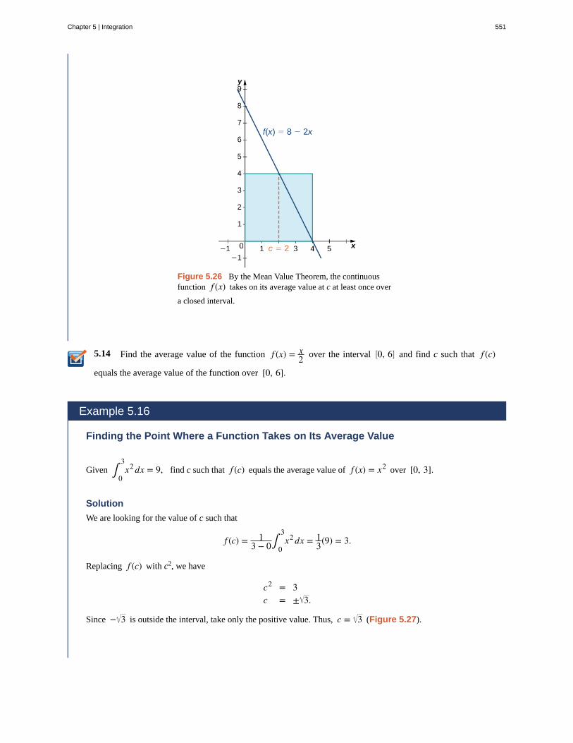
5.14
Figure 5.26 By the Mean Value Theorem, the continuousfunction f (x) takes on its average value at c at least once over
a closed interval.
Find the average value of the function f (x) = x2 over the interval ⎡
⎣0, 6⎤⎦ and find c such that f (c)
equals the average value of the function over [0, 6].
Example 5.16
Finding the Point Where a Function Takes on Its Average Value
Given ∫0
3x2 dx = 9, find c such that f (c) equals the average value of f (x) = x2 over [0, 3].
Solution
We are looking for the value of c such that
f (c) = 13 − 0∫
0
3x2 dx = 1
3(9) = 3.
Replacing f (c) with c2, we have
c2 = 3c = ± 3.
Since − 3 is outside the interval, take only the positive value. Thus, c = 3 (Figure 5.27).
Chapter 5 | Integration 551
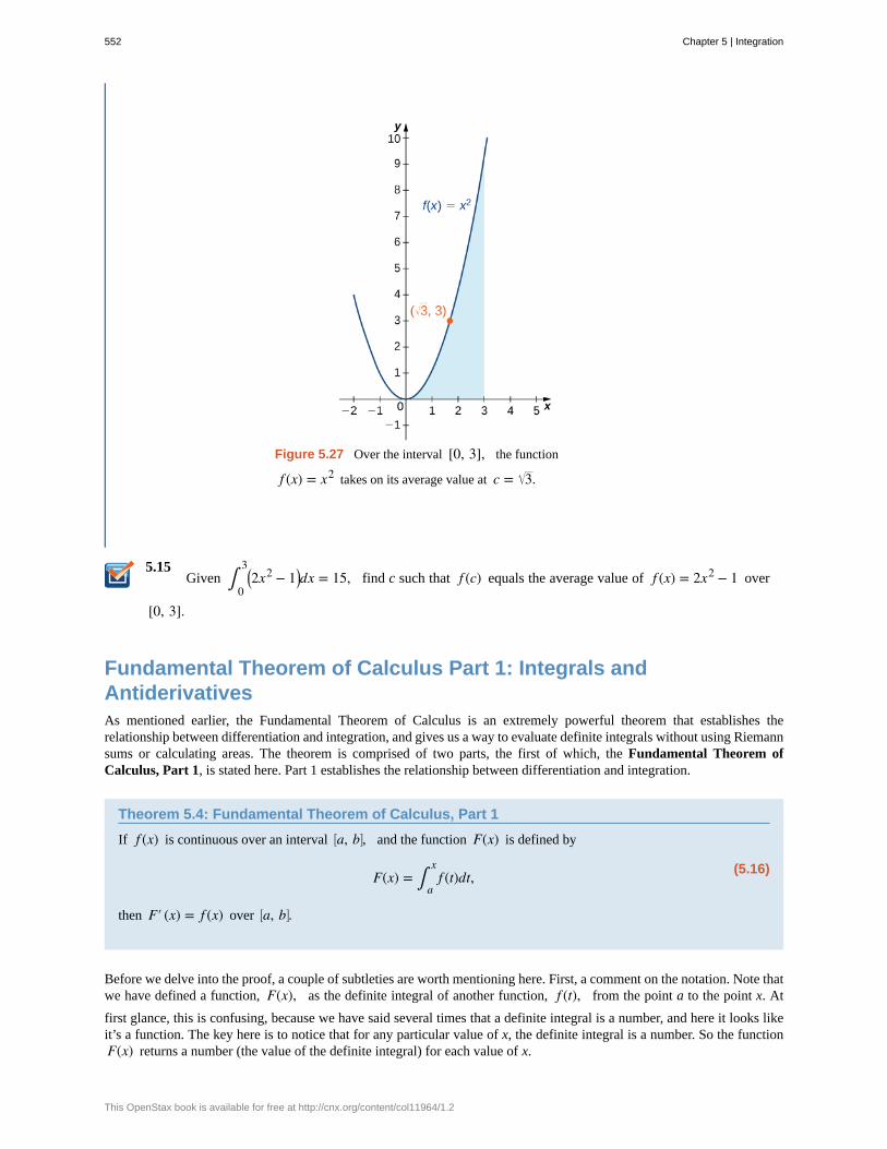
5.15
Figure 5.27 Over the interval [0, 3], the function
f (x) = x2 takes on its average value at c = 3.
Given ∫0
3⎛⎝2x2 − 1⎞
⎠dx = 15, find c such that f (c) equals the average value of f (x) = 2x2 − 1 over
[0, 3].
Fundamental Theorem of Calculus Part 1: Integrals andAntiderivativesAs mentioned earlier, the Fundamental Theorem of Calculus is an extremely powerful theorem that establishes therelationship between differentiation and integration, and gives us a way to evaluate definite integrals without using Riemannsums or calculating areas. The theorem is comprised of two parts, the first of which, the Fundamental Theorem ofCalculus, Part 1, is stated here. Part 1 establishes the relationship between differentiation and integration.
Theorem 5.4: Fundamental Theorem of Calculus, Part 1
If f (x) is continuous over an interval ⎡⎣a, b⎤
⎦, and the function F(x) is defined by
(5.16)F(x) = ∫a
xf (t)dt,
then F′ (x) = f (x) over ⎡⎣a, b⎤
⎦.
Before we delve into the proof, a couple of subtleties are worth mentioning here. First, a comment on the notation. Note thatwe have defined a function, F(x), as the definite integral of another function, f (t), from the point a to the point x. At
first glance, this is confusing, because we have said several times that a definite integral is a number, and here it looks likeit’s a function. The key here is to notice that for any particular value of x, the definite integral is a number. So the functionF(x) returns a number (the value of the definite integral) for each value of x.
552 Chapter 5 | Integration
This OpenStax book is available for free at http://cnx.org/content/col11964/1.2
Second, it is worth commenting on some of the key implications of this theorem. There is a reason it is called theFundamental Theorem of Calculus. Not only does it establish a relationship between integration and differentiation, butalso it guarantees that any integrable function has an antiderivative. Specifically, it guarantees that any continuous functionhas an antiderivative.
Proof
Applying the definition of the derivative, we have
F′ (x) = limh → 0
F(x + h) − F(x)h
= limh → 0
1h
⎡
⎣⎢∫
a
x + hf (t)dt − ∫
a
xf (t)dt
⎤
⎦⎥
= limh → 0
1h
⎡
⎣⎢∫
a
x + hf (t)dt + ∫
x
af (t)dt
⎤
⎦⎥
= limh → 0
1h∫
x
x + hf (t)dt.
Looking carefully at this last expression, we see 1h∫
x
x + hf (t)dt is just the average value of the function f (x) over the
interval ⎡⎣x, x + h⎤
⎦. Therefore, by The Mean Value Theorem for Integrals, there is some number c in ⎡⎣x, x + h⎤
⎦ such
that
1h∫
x
x + hf (x)dx = f (c).
In addition, since c is between x and x + h, c approaches x as h approaches zero. Also, since f (x) is continuous, we have
limh → 0
f (c) = limc → x f (c) = f (x). Putting all these pieces together, we have
F′ (x) = limh → 0
1h∫
x
x + hf (x)dx
= limh → 0
f (c)
= f (x),
and the proof is complete.
□
Example 5.17
Finding a Derivative with the Fundamental Theorem of Calculus
Use the Fundamental Theorem of Calculus, Part 1 to find the derivative of
g(x) = ⌠⌡1
x1
t3 + 1dt.
Solution
According to the Fundamental Theorem of Calculus, the derivative is given by
g′ (x) = 1x3 + 1
.
Chapter 5 | Integration 553
5.16
5.17
Use the Fundamental Theorem of Calculus, Part 1 to find the derivative of g(r) = ∫0
rx2 + 4dx.
Example 5.18
Using the Fundamental Theorem and the Chain Rule to Calculate Derivatives
Let F(x) = ∫1
xsin tdt. Find F′ (x).
Solution
Letting u(x) = x, we have F(x) = ∫1
u(x)sin tdt. Thus, by the Fundamental Theorem of Calculus and the chain
rule,
F′ (x) = sin⎛⎝u(x)⎞
⎠dudx
= sin(u(x)) · ⎛⎝12x−1/2⎞
⎠
= sin x2 x .
Let F(x) = ∫1
x3cos tdt. Find F′ (x).
Example 5.19
Using the Fundamental Theorem of Calculus with Two Variable Limits ofIntegration
Let F(x) = ∫x
2xt3 dt. Find F′ (x).
Solution
We have F(x) = ∫x
2xt3 dt. Both limits of integration are variable, so we need to split this into two integrals. We
get
F(x) = ∫x
2xt3 dt
= ∫x
0t3 dt + ∫
0
2xt3 dt
= −∫0
xt3 dt + ∫
0
2xt3 dt.
554 Chapter 5 | Integration
This OpenStax book is available for free at http://cnx.org/content/col11964/1.2
5.18
Differentiating the first term, we obtain
ddx
⎡⎣−∫
0
xt3 dt⎤⎦ = −x3.
Differentiating the second term, we first let u(x) = 2x. Then,
ddx
⎡
⎣⎢∫
0
2xt3 dt
⎤
⎦⎥ = d
dx⎡
⎣⎢∫
0
u(x)t3 dt
⎤
⎦⎥
= (u(x))3 dudx
= (2x)3 · 2= 16x3.
Thus,
F′ (x) = ddx
⎡⎣−∫
0
xt3 dt⎤⎦ + d
dx⎡
⎣⎢∫
0
2xt3 dt
⎤
⎦⎥
= −x3 + 16x3
= 15x3.
Let F(x) = ∫x
x2cos tdt. Find F′ (x).
Fundamental Theorem of Calculus, Part 2: The Evaluation TheoremThe Fundamental Theorem of Calculus, Part 2, is perhaps the most important theorem in calculus. After tireless effortsby mathematicians for approximately 500 years, new techniques emerged that provided scientists with the necessary toolsto explain many phenomena. Using calculus, astronomers could finally determine distances in space and map planetaryorbits. Everyday financial problems such as calculating marginal costs or predicting total profit could now be handled withsimplicity and accuracy. Engineers could calculate the bending strength of materials or the three-dimensional motion ofobjects. Our view of the world was forever changed with calculus.
After finding approximate areas by adding the areas of n rectangles, the application of this theorem is straightforward bycomparison. It almost seems too simple that the area of an entire curved region can be calculated by just evaluating anantiderivative at the first and last endpoints of an interval.
Theorem 5.5: The Fundamental Theorem of Calculus, Part 2
If f is continuous over the interval ⎡⎣a, b⎤
⎦ and F(x) is any antiderivative of f (x), then
(5.17)∫a
bf (x)dx = F(b) − F(a).
We often see the notation F(x)|ab to denote the expression F(b) − F(a). We use this vertical bar and associated limits a
and b to indicate that we should evaluate the function F(x) at the upper limit (in this case, b), and subtract the value of the
function F(x) evaluated at the lower limit (in this case, a).
The Fundamental Theorem of Calculus, Part 2 (also known as the evaluation theorem) states that if we can find an
Chapter 5 | Integration 555
antiderivative for the integrand, then we can evaluate the definite integral by evaluating the antiderivative at the endpointsof the interval and subtracting.
Proof
Let P = {xi}, i = 0, 1,…, n be a regular partition of ⎡⎣a, b⎤
⎦. Then, we can write
F(b) − F(a) = F(xn) − F(x0)= ⎡
⎣F(xn) − F(xn − 1)⎤⎦ + ⎡
⎣F(xn − 1) − F(xn − 2)⎤⎦ + … + ⎡
⎣F(x1) − F(x0)⎤⎦
= ∑i = 1
n⎡⎣F(xi) − F(xi − 1)⎤
⎦.
Now, we know F is an antiderivative of f over ⎡⎣a, b⎤
⎦, so by the Mean Value Theorem (see The Mean Value Theorem)
for i = 0, 1,…, n we can find ci in [xi − 1, xi] such that
F(xi) − F(xi − 1) = F′ (ci⎞⎠(xi − xi − 1) = f (ci)Δx.
Then, substituting into the previous equation, we have
F(b) − F(a) = ∑i = 1
nf (ci)Δx.
Taking the limit of both sides as n → ∞, we obtain
F(b) − F(a) = limn → ∞ ∑i = 1
nf (ci)Δx
= ∫a
bf (x)dx.
□
Example 5.20
Evaluating an Integral with the Fundamental Theorem of Calculus
Use The Fundamental Theorem of Calculus, Part 2 to evaluate
∫−2
2 ⎛⎝t2 − 4⎞
⎠dt.
Solution
Recall the power rule for Antiderivatives:
If y = xn, ∫ xn dx = xn + 1
n + 1 + C.
Use this rule to find the antiderivative of the function and then apply the theorem. We have
556 Chapter 5 | Integration
This OpenStax book is available for free at http://cnx.org/content/col11964/1.2
∫−2
2 ⎛⎝t2 − 4⎞
⎠dt = t3
3 − 4t|−22
= ⎡⎣
(2)3
3 − 4(2)⎤⎦ − ⎡⎣
(−2)3
3 − 4(−2)⎤⎦= ⎛
⎝83 − 8⎞
⎠ − ⎛⎝−
83 + 8⎞
⎠
= 83 − 8 + 8
3 − 8
= 163 − 16
= − 323 .
Analysis
Notice that we did not include the “+ C” term when we wrote the antiderivative. The reason is that, accordingto the Fundamental Theorem of Calculus, Part 2, any antiderivative works. So, for convenience, we chose theantiderivative with C = 0. If we had chosen another antiderivative, the constant term would have canceled out.
This always happens when evaluating a definite integral.
The region of the area we just calculated is depicted in Figure 5.28. Note that the region between the curveand the x-axis is all below the x-axis. Area is always positive, but a definite integral can still produce a negativenumber (a net signed area). For example, if this were a profit function, a negative number indicates the companyis operating at a loss over the given interval.
Figure 5.28 The evaluation of a definite integral can producea negative value, even though area is always positive.
Example 5.21
Evaluating a Definite Integral Using the Fundamental Theorem of Calculus, Part 2
Evaluate the following integral using the Fundamental Theorem of Calculus, Part 2:
∫1
9x − 1x dx.
Solution
Chapter 5 | Integration 557
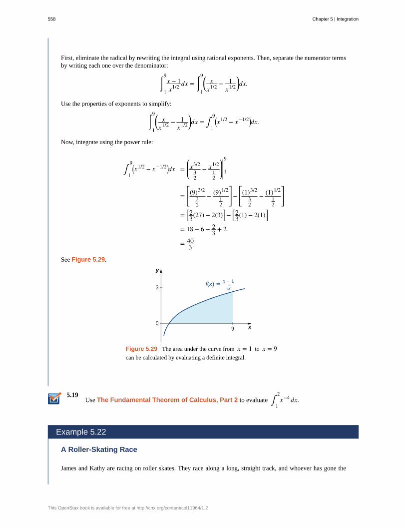
5.19
First, eliminate the radical by rewriting the integral using rational exponents. Then, separate the numerator termsby writing each one over the denominator:
⌠⌡1
9x − 1x1/2 dx = ⌠
⌡1
9⎛⎝
xx1/2 − 1
x1/2⎞⎠dx.
Use the properties of exponents to simplify:
⌠⌡1
9⎛⎝
xx1/2 − 1
x1/2⎞⎠dx = ∫
1
9⎛⎝x
1/2 − x−1/2⎞⎠dx.
Now, integrate using the power rule:
∫1
9⎛⎝x
1/2 − x−1/2⎞⎠dx =
⎛
⎝⎜x3/2
32
− x1/212
⎞
⎠⎟|19
=⎡
⎣⎢(9)3/2
32
− (9)1/2
12
⎤
⎦⎥ −
⎡
⎣⎢(1)3/2
32
− (1)1/2
12
⎤
⎦⎥
= ⎡⎣23(27) − 2(3)⎤⎦ − ⎡
⎣23(1) − 2(1)⎤⎦
= 18 − 6 − 23 + 2
= 403 .
See Figure 5.29.
Figure 5.29 The area under the curve from x = 1 to x = 9can be calculated by evaluating a definite integral.
Use The Fundamental Theorem of Calculus, Part 2 to evaluate ∫1
2x−4 dx.
Example 5.22
A Roller-Skating Race
James and Kathy are racing on roller skates. They race along a long, straight track, and whoever has gone the
558 Chapter 5 | Integration
This OpenStax book is available for free at http://cnx.org/content/col11964/1.2
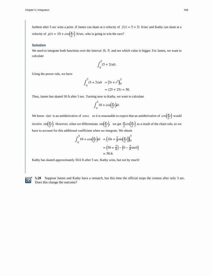
5.20
farthest after 5 sec wins a prize. If James can skate at a velocity of f (t) = 5 + 2t ft/sec and Kathy can skate at a
velocity of g(t) = 10 + cos⎛⎝π2 t⎞⎠ ft/sec, who is going to win the race?
Solution
We need to integrate both functions over the interval ⎡⎣0, 5⎤
⎦ and see which value is bigger. For James, we want to
calculate
∫0
5(5 + 2t)dt.
Using the power rule, we have
∫0
5(5 + 2t)dt = ⎛
⎝5t + t2⎞⎠|05
= (25 + 25) = 50.
Thus, James has skated 50 ft after 5 sec. Turning now to Kathy, we want to calculate
∫0
510 + cos⎛
⎝π2 t⎞⎠dt.
We know sin t is an antiderivative of cos t, so it is reasonable to expect that an antiderivative of cos⎛⎝π2 t⎞⎠ would
involve sin⎛⎝π2 t⎞⎠. However, when we differentiate sin⎛
⎝π2 t⎞⎠, we get π
2cos⎛⎝π2 t⎞⎠ as a result of the chain rule, so we
have to account for this additional coefficient when we integrate. We obtain
∫0
510 + cos⎛
⎝π2 t⎞⎠dt = ⎛
⎝10t + 2πsin⎛
⎝π2 t⎞⎠
⎞⎠|05
= ⎛⎝50 + 2
π⎞⎠ − ⎛
⎝0 − 2πsin0⎞
⎠
≈ 50.6.
Kathy has skated approximately 50.6 ft after 5 sec. Kathy wins, but not by much!
Suppose James and Kathy have a rematch, but this time the official stops the contest after only 3 sec.Does this change the outcome?
Chapter 5 | Integration 559
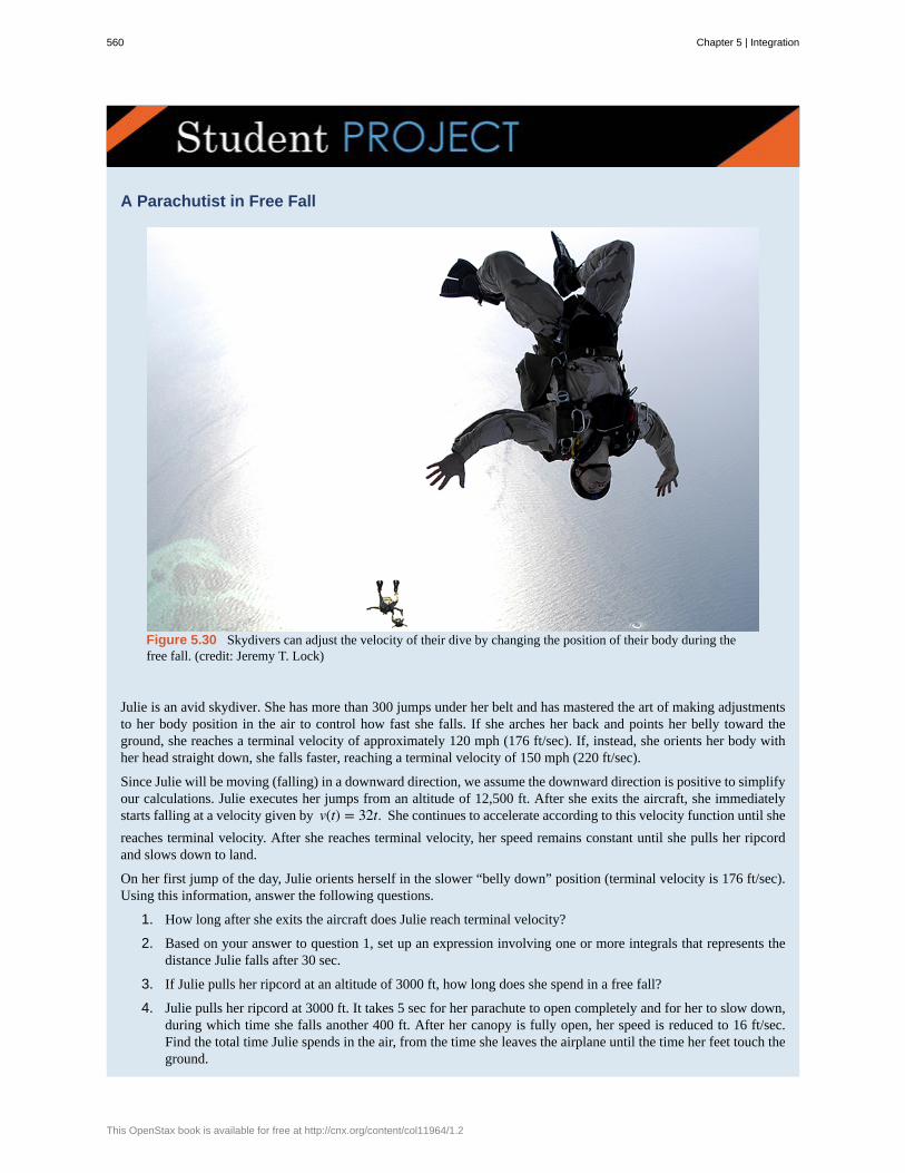
A Parachutist in Free Fall
Figure 5.30 Skydivers can adjust the velocity of their dive by changing the position of their body during thefree fall. (credit: Jeremy T. Lock)
Julie is an avid skydiver. She has more than 300 jumps under her belt and has mastered the art of making adjustmentsto her body position in the air to control how fast she falls. If she arches her back and points her belly toward theground, she reaches a terminal velocity of approximately 120 mph (176 ft/sec). If, instead, she orients her body withher head straight down, she falls faster, reaching a terminal velocity of 150 mph (220 ft/sec).
Since Julie will be moving (falling) in a downward direction, we assume the downward direction is positive to simplifyour calculations. Julie executes her jumps from an altitude of 12,500 ft. After she exits the aircraft, she immediatelystarts falling at a velocity given by v(t) = 32t. She continues to accelerate according to this velocity function until she
reaches terminal velocity. After she reaches terminal velocity, her speed remains constant until she pulls her ripcordand slows down to land.
On her first jump of the day, Julie orients herself in the slower “belly down” position (terminal velocity is 176 ft/sec).Using this information, answer the following questions.
1. How long after she exits the aircraft does Julie reach terminal velocity?
2. Based on your answer to question 1, set up an expression involving one or more integrals that represents thedistance Julie falls after 30 sec.
3. If Julie pulls her ripcord at an altitude of 3000 ft, how long does she spend in a free fall?
4. Julie pulls her ripcord at 3000 ft. It takes 5 sec for her parachute to open completely and for her to slow down,during which time she falls another 400 ft. After her canopy is fully open, her speed is reduced to 16 ft/sec.Find the total time Julie spends in the air, from the time she leaves the airplane until the time her feet touch theground.
560 Chapter 5 | Integration
This OpenStax book is available for free at http://cnx.org/content/col11964/1.2
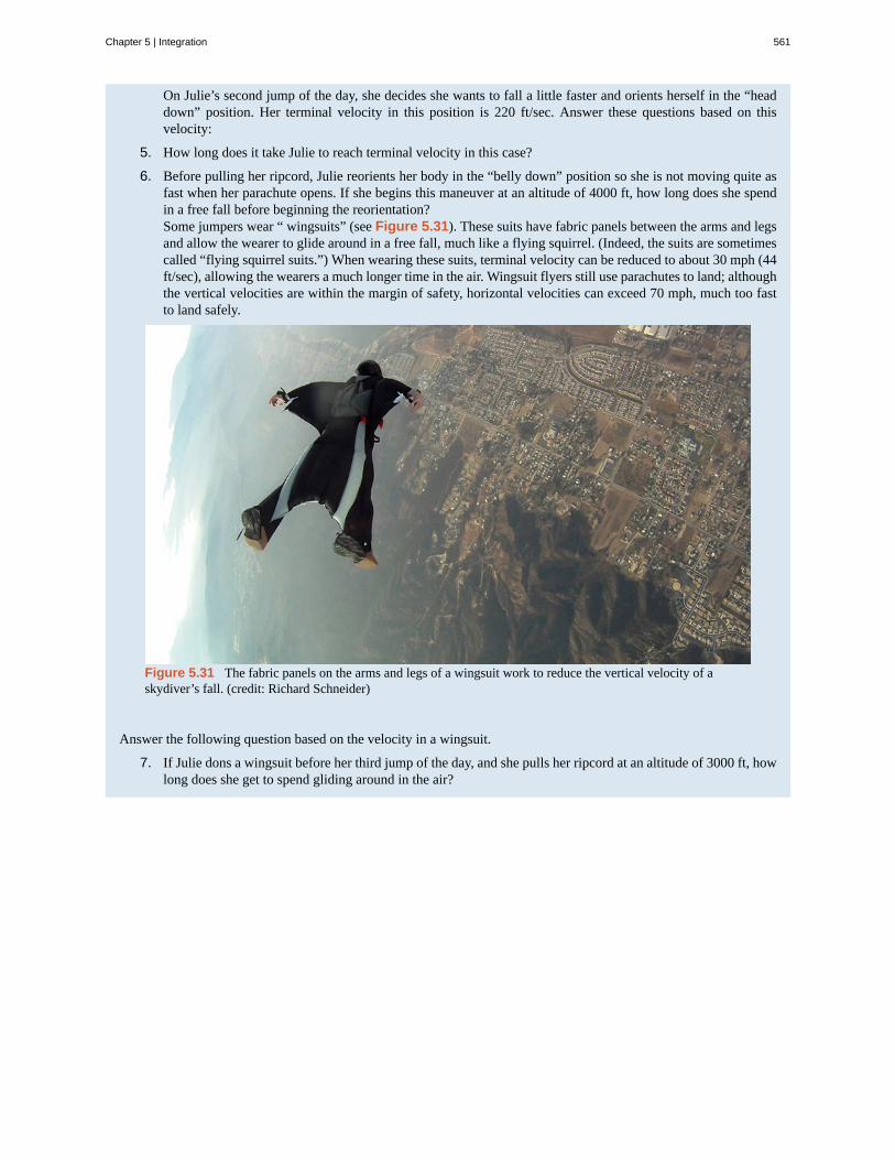
On Julie’s second jump of the day, she decides she wants to fall a little faster and orients herself in the “headdown” position. Her terminal velocity in this position is 220 ft/sec. Answer these questions based on thisvelocity:
5. How long does it take Julie to reach terminal velocity in this case?
6. Before pulling her ripcord, Julie reorients her body in the “belly down” position so she is not moving quite asfast when her parachute opens. If she begins this maneuver at an altitude of 4000 ft, how long does she spendin a free fall before beginning the reorientation?Some jumpers wear “ wingsuits” (see Figure 5.31). These suits have fabric panels between the arms and legsand allow the wearer to glide around in a free fall, much like a flying squirrel. (Indeed, the suits are sometimescalled “flying squirrel suits.”) When wearing these suits, terminal velocity can be reduced to about 30 mph (44ft/sec), allowing the wearers a much longer time in the air. Wingsuit flyers still use parachutes to land; althoughthe vertical velocities are within the margin of safety, horizontal velocities can exceed 70 mph, much too fastto land safely.
Figure 5.31 The fabric panels on the arms and legs of a wingsuit work to reduce the vertical velocity of askydiver’s fall. (credit: Richard Schneider)
Answer the following question based on the velocity in a wingsuit.
7. If Julie dons a wingsuit before her third jump of the day, and she pulls her ripcord at an altitude of 3000 ft, howlong does she get to spend gliding around in the air?
Chapter 5 | Integration 561
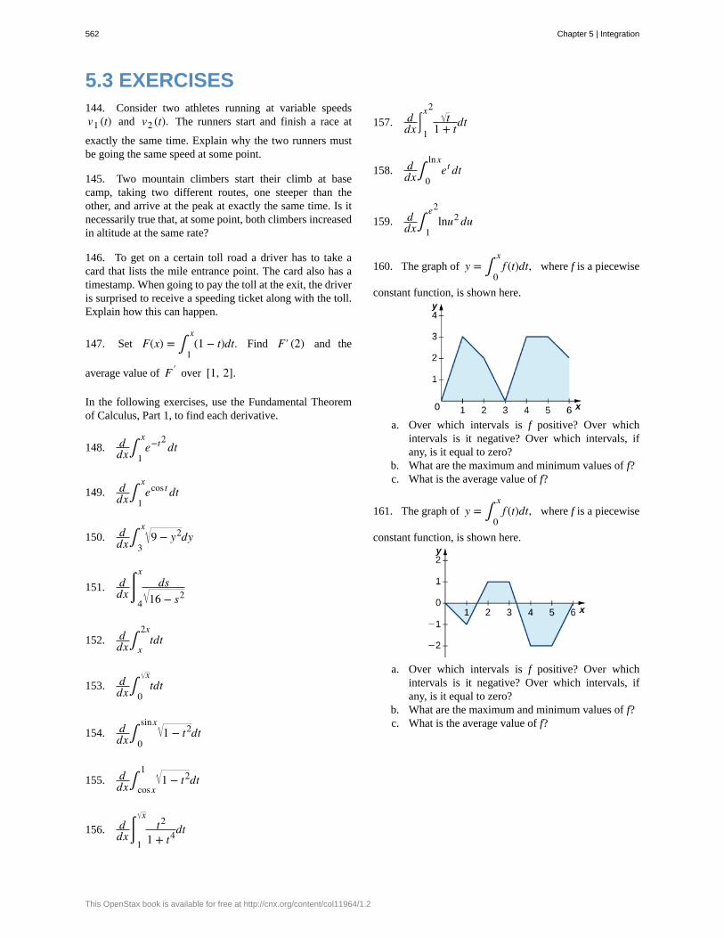
5.3 EXERCISES144. Consider two athletes running at variable speedsv1 (t) and v2 (t). The runners start and finish a race at
exactly the same time. Explain why the two runners mustbe going the same speed at some point.
145. Two mountain climbers start their climb at basecamp, taking two different routes, one steeper than theother, and arrive at the peak at exactly the same time. Is itnecessarily true that, at some point, both climbers increasedin altitude at the same rate?
146. To get on a certain toll road a driver has to take acard that lists the mile entrance point. The card also has atimestamp. When going to pay the toll at the exit, the driveris surprised to receive a speeding ticket along with the toll.Explain how this can happen.
147. Set F(x) = ∫1
x(1 − t)dt. Find F′ (2) and the
average value of F ′ over [1, 2].
In the following exercises, use the Fundamental Theoremof Calculus, Part 1, to find each derivative.
148. ddx∫
1
xe−t2
dt
149. ddx∫
1
xecos t dt
150. ddx∫
3
x9 − y2dy
151. ddx
⌠⌡4
xds
16 − s2
152. ddx∫
x
2xtdt
153. ddx∫
0
xtdt
154. ddx∫
0
sinx1 − t2dt
155. ddx∫
cosx
11 − t2dt
156. ddx
⌠⌡1
xt2
1 + t4dt
157. ddx
⌠⌡1
x2t
1 + tdt
158. ddx∫
0
lnxet dt
159. ddx∫
1
e2lnu2 du
160. The graph of y = ∫0
xf (t)dt, where f is a piecewise
constant function, is shown here.
a. Over which intervals is f positive? Over whichintervals is it negative? Over which intervals, ifany, is it equal to zero?
b. What are the maximum and minimum values of f?c. What is the average value of f?
161. The graph of y = ∫0
xf (t)dt, where f is a piecewise
constant function, is shown here.
a. Over which intervals is f positive? Over whichintervals is it negative? Over which intervals, ifany, is it equal to zero?
b. What are the maximum and minimum values of f?c. What is the average value of f?
562 Chapter 5 | Integration
This OpenStax book is available for free at http://cnx.org/content/col11964/1.2
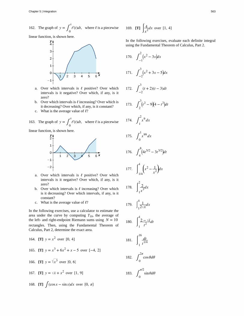
162. The graph of y = ∫0
xℓ(t)dt, where ℓ is a piecewise
linear function, is shown here.
a. Over which intervals is ℓ positive? Over whichintervals is it negative? Over which, if any, is itzero?
b. Over which intervals is ℓ increasing? Over which isit decreasing? Over which, if any, is it constant?
c. What is the average value of ℓ?
163. The graph of y = ∫0
xℓ(t)dt, where ℓ is a piecewise
linear function, is shown here.
a. Over which intervals is ℓ positive? Over whichintervals is it negative? Over which, if any, is itzero?
b. Over which intervals is ℓ increasing? Over whichis it decreasing? Over which intervals, if any, is itconstant?
c. What is the average value of ℓ?
In the following exercises, use a calculator to estimate thearea under the curve by computing T10, the average ofthe left- and right-endpoint Riemann sums using N = 10rectangles. Then, using the Fundamental Theorem ofCalculus, Part 2, determine the exact area.
164. [T] y = x2 over [0, 4]
165. [T] y = x3 + 6x2 + x − 5 over [−4, 2]
166. [T] y = x3 over ⎡⎣0, 6⎤
⎦
167. [T] y = x + x2 over [1, 9]
168. [T] ∫ (cosx − sinx)dx over [0, π]
169. [T] ⌠⌡
4x2dx over [1, 4]
In the following exercises, evaluate each definite integralusing the Fundamental Theorem of Calculus, Part 2.
170. ∫−1
2 ⎛⎝x2 − 3x⎞
⎠dx
171. ∫−2
3⎛⎝x2 + 3x − 5⎞
⎠dx
172. ∫−2
3(t + 2)(t − 3)dt
173. ∫2
3⎛⎝t2 − 9⎞
⎠⎛⎝4 − t2⎞
⎠dt
174. ∫1
2x9 dx
175. ∫0
1x99 dx
176. ∫4
8⎛⎝4t5/2 − 3t3/2⎞
⎠dt
177. ⌠⌡1/4
4 ⎛⎝x2 − 1
x2⎞⎠dx
178. ⌠⌡1
22x3dx
179. ⌠⌡1
4 12 xdx
180. ⌠⌡1
42 − t
t2 dt
181. ⌠⌡1
16dt
t1/4
182. ∫0
2πcosθdθ
183. ∫0
π/2sinθdθ
Chapter 5 | Integration 563
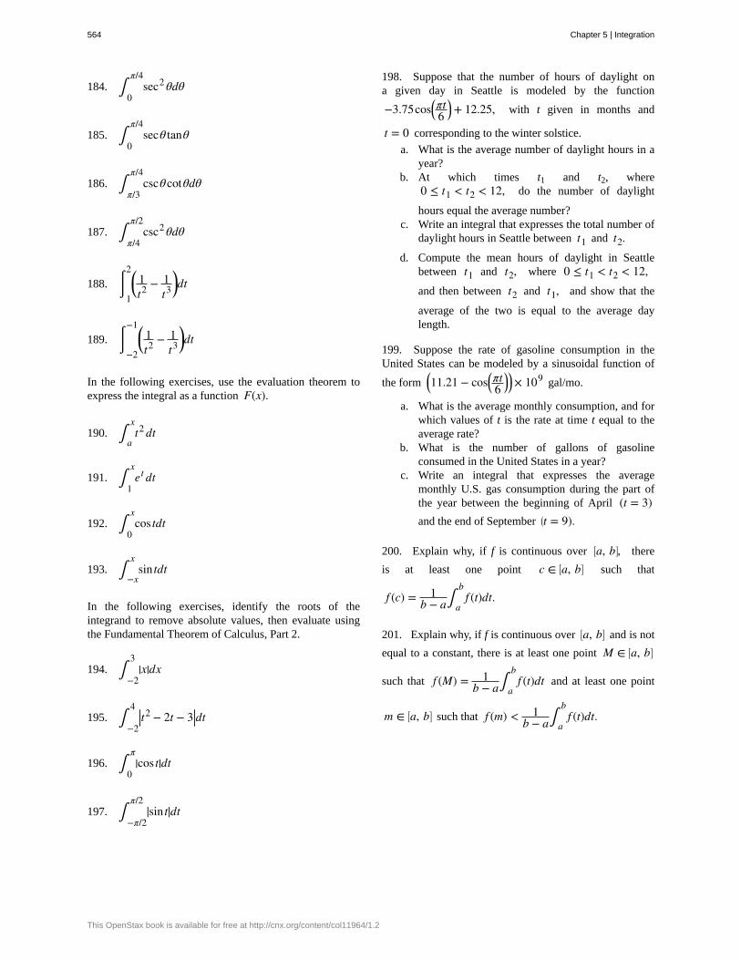
184. ∫0
π/4sec2 θdθ
185. ∫0
π/4secθ tanθ
186. ∫π/3
π/4cscθcotθdθ
187. ∫π/4
π/2csc2 θdθ
188. ⌠⌡1
2⎛⎝
1t2 − 1
t3⎞⎠dt
189. ⌠⌡−2
−1⎛⎝
1t2 − 1
t3⎞⎠dt
In the following exercises, use the evaluation theorem toexpress the integral as a function F(x).
190. ∫a
xt2 dt
191. ∫1
xet dt
192. ∫0
xcos tdt
193. ∫−x
xsin tdt
In the following exercises, identify the roots of theintegrand to remove absolute values, then evaluate usingthe Fundamental Theorem of Calculus, Part 2.
194. ∫−2
3|x|dx
195. ∫−2
4
|t2 − 2t − 3|dt
196. ∫0
π|cos t|dt
197. ∫−π/2
π/2|sin t|dt
198. Suppose that the number of hours of daylight ona given day in Seattle is modeled by the function
−3.75cos⎛⎝πt6
⎞⎠ + 12.25, with t given in months and
t = 0 corresponding to the winter solstice.
a. What is the average number of daylight hours in ayear?
b. At which times t1 and t2, where0 ≤ t1 < t2 < 12, do the number of daylight
hours equal the average number?c. Write an integral that expresses the total number of
daylight hours in Seattle between t1 and t2.d. Compute the mean hours of daylight in Seattle
between t1 and t2, where 0 ≤ t1 < t2 < 12,and then between t2 and t1, and show that the
average of the two is equal to the average daylength.
199. Suppose the rate of gasoline consumption in theUnited States can be modeled by a sinusoidal function of
the form ⎛⎝11.21 − cos⎛
⎝πt6
⎞⎠⎞⎠ × 109 gal/mo.
a. What is the average monthly consumption, and forwhich values of t is the rate at time t equal to theaverage rate?
b. What is the number of gallons of gasolineconsumed in the United States in a year?
c. Write an integral that expresses the averagemonthly U.S. gas consumption during the part ofthe year between the beginning of April (t = 3)and the end of September ⎛
⎝t = 9).
200. Explain why, if f is continuous over ⎡⎣a, b⎤
⎦, there
is at least one point c ∈ ⎡⎣a, b⎤
⎦ such that
f (c) = 1b − a∫
a
bf (t)dt.
201. Explain why, if f is continuous over ⎡⎣a, b⎤
⎦ and is not
equal to a constant, there is at least one point M ∈ ⎡⎣a, b⎤
⎦
such that f (M) = 1b − a∫
a
bf (t)dt and at least one point
m ∈ ⎡⎣a, b⎤
⎦ such that f (m) < 1b − a∫
a
bf (t)dt.
564 Chapter 5 | Integration
This OpenStax book is available for free at http://cnx.org/content/col11964/1.2
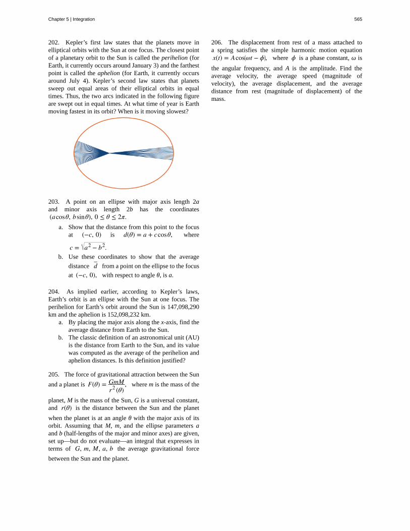
202. Kepler’s first law states that the planets move inelliptical orbits with the Sun at one focus. The closest pointof a planetary orbit to the Sun is called the perihelion (forEarth, it currently occurs around January 3) and the farthestpoint is called the aphelion (for Earth, it currently occursaround July 4). Kepler’s second law states that planetssweep out equal areas of their elliptical orbits in equaltimes. Thus, the two arcs indicated in the following figureare swept out in equal times. At what time of year is Earthmoving fastest in its orbit? When is it moving slowest?
203. A point on an ellipse with major axis length 2aand minor axis length 2b has the coordinates(acosθ, bsinθ), 0 ≤ θ ≤ 2π.
a. Show that the distance from this point to the focusat (−c, 0) is d(θ) = a + ccosθ, where
c = a2 − b2.b. Use these coordinates to show that the average
distance d–
from a point on the ellipse to the focus
at (−c, 0), with respect to angle θ, is a.
204. As implied earlier, according to Kepler’s laws,Earth’s orbit is an ellipse with the Sun at one focus. Theperihelion for Earth’s orbit around the Sun is 147,098,290km and the aphelion is 152,098,232 km.
a. By placing the major axis along the x-axis, find theaverage distance from Earth to the Sun.
b. The classic definition of an astronomical unit (AU)is the distance from Earth to the Sun, and its valuewas computed as the average of the perihelion andaphelion distances. Is this definition justified?
205. The force of gravitational attraction between the Sun
and a planet is F(θ) = GmMr2 (θ)
, where m is the mass of the
planet, M is the mass of the Sun, G is a universal constant,and r(θ) is the distance between the Sun and the planet
when the planet is at an angle θ with the major axis of itsorbit. Assuming that M, m, and the ellipse parameters aand b (half-lengths of the major and minor axes) are given,set up—but do not evaluate—an integral that expresses interms of G, m, M, a, b the average gravitational force
between the Sun and the planet.
206. The displacement from rest of a mass attached toa spring satisfies the simple harmonic motion equationx(t) = Acos⎛
⎝ωt − ϕ⎞⎠, where ϕ is a phase constant, ω is
the angular frequency, and A is the amplitude. Find theaverage velocity, the average speed (magnitude ofvelocity), the average displacement, and the averagedistance from rest (magnitude of displacement) of themass.
Chapter 5 | Integration 565
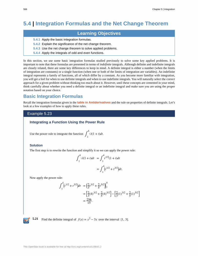
5.21
5.4 | Integration Formulas and the Net Change Theorem
Learning Objectives5.4.1 Apply the basic integration formulas.
5.4.2 Explain the significance of the net change theorem.
5.4.3 Use the net change theorem to solve applied problems.
5.4.4 Apply the integrals of odd and even functions.
In this section, we use some basic integration formulas studied previously to solve some key applied problems. It isimportant to note that these formulas are presented in terms of indefinite integrals. Although definite and indefinite integralsare closely related, there are some key differences to keep in mind. A definite integral is either a number (when the limitsof integration are constants) or a single function (when one or both of the limits of integration are variables). An indefiniteintegral represents a family of functions, all of which differ by a constant. As you become more familiar with integration,you will get a feel for when to use definite integrals and when to use indefinite integrals. You will naturally select the correctapproach for a given problem without thinking too much about it. However, until these concepts are cemented in your mind,think carefully about whether you need a definite integral or an indefinite integral and make sure you are using the propernotation based on your choice.
Basic Integration FormulasRecall the integration formulas given in the table in Antiderivatives and the rule on properties of definite integrals. Let’slook at a few examples of how to apply these rules.
Example 5.23
Integrating a Function Using the Power Rule
Use the power rule to integrate the function ∫1
4t(1 + t)dt.
Solution
The first step is to rewrite the function and simplify it so we can apply the power rule:
∫1
4t(1 + t)dt = ∫
1
4t1/2(1 + t)dt
= ∫1
4⎛⎝t
1/2 + t3/2⎞⎠dt.
Now apply the power rule:
∫1
4⎛⎝t
1/2 + t3/2⎞⎠dt = ⎛
⎝23t3/2 + 2
5t5/2⎞⎠|14
= ⎡⎣23(4)3/2 + 2
5(4)5/2⎤⎦ − ⎡
⎣23(1)3/2 + 2
5(1)5/2⎤⎦
= 25615 .
Find the definite integral of f (x) = x2 − 3x over the interval [1, 3].
566 Chapter 5 | Integration
This OpenStax book is available for free at http://cnx.org/content/col11964/1.2
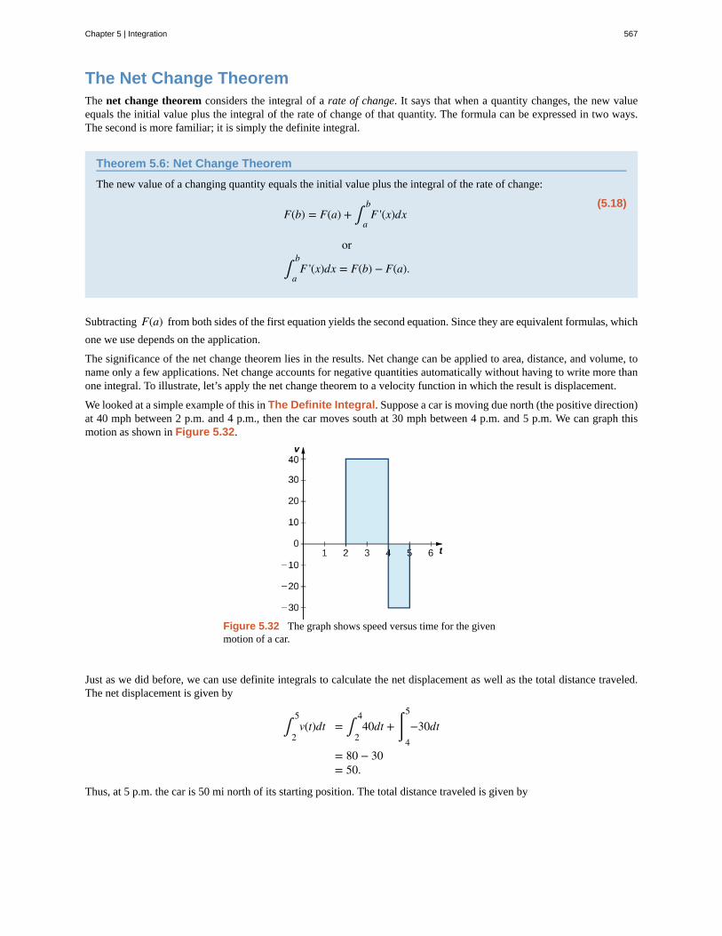
The Net Change TheoremThe net change theorem considers the integral of a rate of change. It says that when a quantity changes, the new valueequals the initial value plus the integral of the rate of change of that quantity. The formula can be expressed in two ways.The second is more familiar; it is simply the definite integral.
Theorem 5.6: Net Change Theorem
The new value of a changing quantity equals the initial value plus the integral of the rate of change:
(5.18)F(b) = F(a) + ∫
a
bF '(x)dx
or
∫a
bF '(x)dx = F(b) − F(a).
Subtracting F(a) from both sides of the first equation yields the second equation. Since they are equivalent formulas, which
one we use depends on the application.
The significance of the net change theorem lies in the results. Net change can be applied to area, distance, and volume, toname only a few applications. Net change accounts for negative quantities automatically without having to write more thanone integral. To illustrate, let’s apply the net change theorem to a velocity function in which the result is displacement.
We looked at a simple example of this in The Definite Integral. Suppose a car is moving due north (the positive direction)at 40 mph between 2 p.m. and 4 p.m., then the car moves south at 30 mph between 4 p.m. and 5 p.m. We can graph thismotion as shown in Figure 5.32.
Figure 5.32 The graph shows speed versus time for the givenmotion of a car.
Just as we did before, we can use definite integrals to calculate the net displacement as well as the total distance traveled.The net displacement is given by
∫2
5v(t)dt = ∫
2
440dt + ⌠
⌡4
5
−30dt
= 80 − 30= 50.
Thus, at 5 p.m. the car is 50 mi north of its starting position. The total distance traveled is given by
Chapter 5 | Integration 567
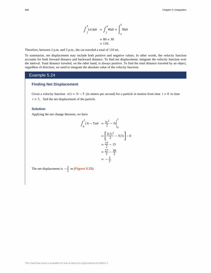
∫2
5|v(t)|dt = ∫
2
440dt + ⌠
⌡4
5
30dt
= 80 + 30= 110.
Therefore, between 2 p.m. and 5 p.m., the car traveled a total of 110 mi.
To summarize, net displacement may include both positive and negative values. In other words, the velocity functionaccounts for both forward distance and backward distance. To find net displacement, integrate the velocity function overthe interval. Total distance traveled, on the other hand, is always positive. To find the total distance traveled by an object,regardless of direction, we need to integrate the absolute value of the velocity function.
Example 5.24
Finding Net Displacement
Given a velocity function v(t) = 3t − 5 (in meters per second) for a particle in motion from time t = 0 to time
t = 3, find the net displacement of the particle.
Solution
Applying the net change theorem, we have
∫0
3(3t − 5)dt = 3t2
2 − 5t|03
= ⎡⎣
3(3)2
2 − 5(3)⎤⎦ − 0
= 272 − 15
= 272 − 30
2= − 3
2.
The net displacement is −32 m (Figure 5.33).
568 Chapter 5 | Integration
This OpenStax book is available for free at http://cnx.org/content/col11964/1.2
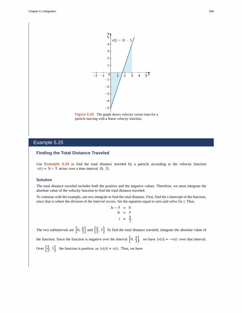
Figure 5.33 The graph shows velocity versus time for aparticle moving with a linear velocity function.
Example 5.25
Finding the Total Distance Traveled
Use Example 5.24 to find the total distance traveled by a particle according to the velocity functionv(t) = 3t − 5 m/sec over a time interval [0, 3].
Solution
The total distance traveled includes both the positive and the negative values. Therefore, we must integrate theabsolute value of the velocity function to find the total distance traveled.
To continue with the example, use two integrals to find the total distance. First, find the t-intercept of the function,since that is where the division of the interval occurs. Set the equation equal to zero and solve for t. Thus,
3t − 5 = 03t = 5t = 5
3.
The two subintervals are⎡⎣0, 5
3⎤⎦ and
⎡⎣53, 3⎤
⎦. To find the total distance traveled, integrate the absolute value of
the function. Since the function is negative over the interval⎡⎣0, 5
3⎤⎦, we have |v(t)| = −v(t) over that interval.
Over⎡⎣53, 3⎤
⎦, the function is positive, so |v(t)| = v(t). Thus, we have
Chapter 5 | Integration 569
5.22
∫0
3|v(t)|dt = ⌠
⌡0
5/3
−v(t)dt + ∫5/3
3v(t)dt
= ∫0
5/35 − 3tdt + ∫
5/3
33t − 5dt
= ⎛⎝5t − 3t2
2⎞⎠|05/3
+ ⎛⎝3t2
2 − 5t⎞⎠|5/3
3
= ⎡⎣5⎛
⎝53
⎞⎠ − 3(5/3)2
2⎤⎦ − 0 + ⎡
⎣272 − 15⎤
⎦ − ⎡⎣
3(5/3)2
2 − 253
⎤⎦
= 253 − 25
6 + 272 − 15 − 25
6 + 253
= 416 .
So, the total distance traveled is 146 m.
Find the net displacement and total distance traveled in meters given the velocity function
f (t) = 12et − 2 over the interval [0, 2].
Applying the Net Change TheoremThe net change theorem can be applied to the flow and consumption of fluids, as shown in Example 5.26.
Example 5.26
How Many Gallons of Gasoline Are Consumed?
If the motor on a motorboat is started at t = 0 and the boat consumes gasoline at the rate of 5 − t3 gal/hr, how
much gasoline is used in the first 2 hours?
Solution
Express the problem as a definite integral, integrate, and evaluate using the Fundamental Theorem of Calculus.The limits of integration are the endpoints of the interval [0, 2]. We have
∫0
2⎛⎝5 − t3⎞
⎠dt = ⎛⎝5t − t4
4⎞⎠|0
2
= ⎡⎣5(2) − (2)4
4⎤⎦ − 0
= 10 − 164
= 6.
570 Chapter 5 | Integration
This OpenStax book is available for free at http://cnx.org/content/col11964/1.2
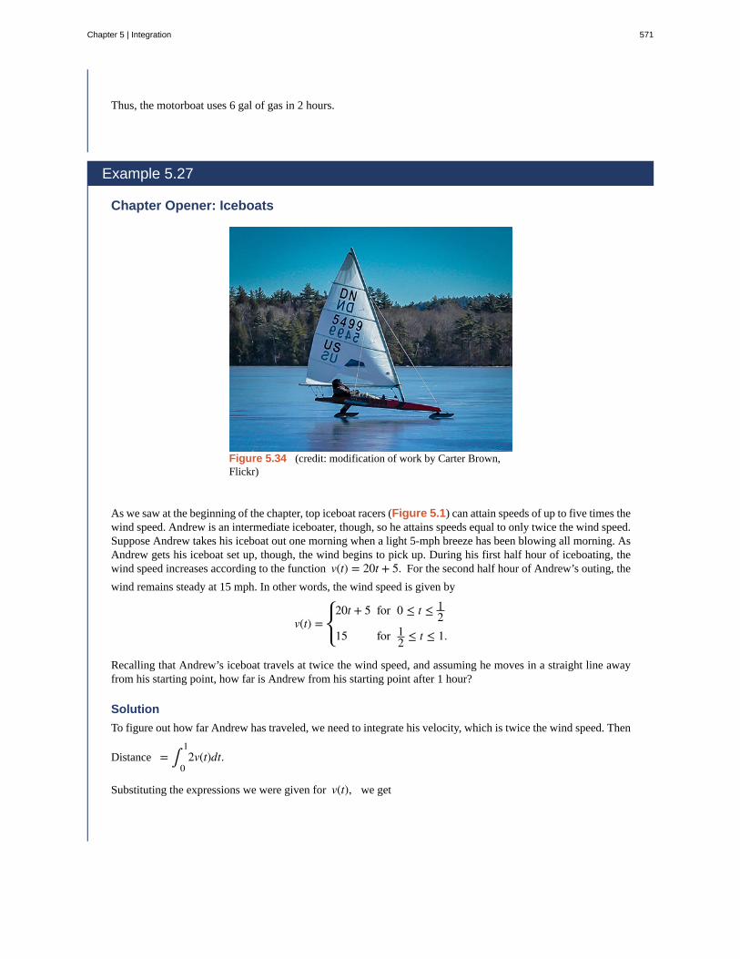
Thus, the motorboat uses 6 gal of gas in 2 hours.
Example 5.27
Chapter Opener: Iceboats
Figure 5.34 (credit: modification of work by Carter Brown,Flickr)
As we saw at the beginning of the chapter, top iceboat racers (Figure 5.1) can attain speeds of up to five times thewind speed. Andrew is an intermediate iceboater, though, so he attains speeds equal to only twice the wind speed.Suppose Andrew takes his iceboat out one morning when a light 5-mph breeze has been blowing all morning. AsAndrew gets his iceboat set up, though, the wind begins to pick up. During his first half hour of iceboating, thewind speed increases according to the function v(t) = 20t + 5. For the second half hour of Andrew’s outing, the
wind remains steady at 15 mph. In other words, the wind speed is given by
v(t) =⎧
⎩⎨
20t + 5 for 0 ≤ t ≤ 12
15 for 12 ≤ t ≤ 1.
Recalling that Andrew’s iceboat travels at twice the wind speed, and assuming he moves in a straight line awayfrom his starting point, how far is Andrew from his starting point after 1 hour?
Solution
To figure out how far Andrew has traveled, we need to integrate his velocity, which is twice the wind speed. Then
Distance = ∫0
12v(t)dt.
Substituting the expressions we were given for v(t), we get
Chapter 5 | Integration 571
5.23
∫0
12v(t)dt = ⌠
⌡0
1/2
2v(t)dt + ∫1/2
12v(t)dt
= ⌠⌡0
1/2
2(20t + 5)dt + ∫1/3
12(15)dt
= ⌠⌡0
1/2
(40t + 10)dt + ∫1/2
130dt
= ⎡⎣20t2 + 10t⎤
⎦|01/2 + [30t]|1/2
1
= ⎛⎝204 + 5⎞
⎠ − 0 + (30 − 15)
= 25.
Andrew is 25 mi from his starting point after 1 hour.
Suppose that, instead of remaining steady during the second half hour of Andrew’s outing, the windstarts to die down according to the function v(t) = −10t + 15. In other words, the wind speed is given by
v(t) =⎧
⎩⎨
20t + 5 for 0 ≤ t ≤ 12
−10t + 15 for 12 ≤ t ≤ 1.
Under these conditions, how far from his starting point is Andrew after 1 hour?
Integrating Even and Odd FunctionsWe saw in Functions and Graphs that an even function is a function in which f (−x) = f (x) for all x in the
domain—that is, the graph of the curve is unchanged when x is replaced with −x. The graphs of even functions aresymmetric about the y-axis. An odd function is one in which f (−x) = − f (x) for all x in the domain, and the graph of the
function is symmetric about the origin.
Integrals of even functions, when the limits of integration are from −a to a, involve two equal areas, because they aresymmetric about the y-axis. Integrals of odd functions, when the limits of integration are similarly [−a, a], evaluate to
zero because the areas above and below the x-axis are equal.
Rule: Integrals of Even and Odd Functions
For continuous even functions such that f (−x) = f (x),
⌠⌡−a
af (x)dx = 2∫
0
af (x)dx.
For continuous odd functions such that f (−x) = − f (x),
∫−a
af (x)dx = 0.
572 Chapter 5 | Integration
This OpenStax book is available for free at http://cnx.org/content/col11964/1.2
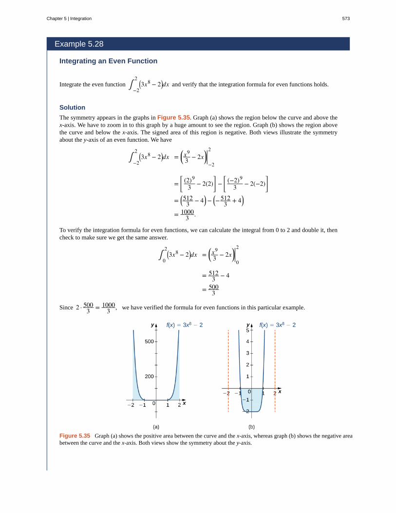
Example 5.28
Integrating an Even Function
Integrate the even function ∫−2
2 ⎛⎝3x8 − 2⎞
⎠dx and verify that the integration formula for even functions holds.
Solution
The symmetry appears in the graphs in Figure 5.35. Graph (a) shows the region below the curve and above thex-axis. We have to zoom in to this graph by a huge amount to see the region. Graph (b) shows the region abovethe curve and below the x-axis. The signed area of this region is negative. Both views illustrate the symmetryabout the y-axis of an even function. We have
∫−2
2 ⎛⎝3x8 − 2⎞
⎠dx = ⎛⎝
x9
3 − 2x⎞⎠|−2
2
=⎡
⎣⎢ (2)9
3 − 2(2)⎤
⎦⎥ −
⎡
⎣⎢ (−2)9
3 − 2(−2)⎤
⎦⎥
= ⎛⎝5123 − 4⎞
⎠ − ⎛⎝−
5123 + 4⎞
⎠
= 10003 .
To verify the integration formula for even functions, we can calculate the integral from 0 to 2 and double it, thencheck to make sure we get the same answer.
∫0
2⎛⎝3x8 − 2⎞
⎠dx = ⎛⎝
x9
3 − 2x⎞⎠|0
2
= 5123 − 4
= 5003
Since 2 · 5003 = 1000
3 , we have verified the formula for even functions in this particular example.
Figure 5.35 Graph (a) shows the positive area between the curve and the x-axis, whereas graph (b) shows the negative areabetween the curve and the x-axis. Both views show the symmetry about the y-axis.
Chapter 5 | Integration 573
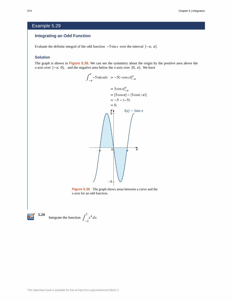
5.24
Example 5.29
Integrating an Odd Function
Evaluate the definite integral of the odd function −5sinx over the interval [−π, π].
Solution
The graph is shown in Figure 5.36. We can see the symmetry about the origin by the positive area above thex-axis over [−π, 0], and the negative area below the x-axis over [0, π]. We have
∫−π
π−5sinxdx = −5(−cosx)|−π
π
= 5cosx|−ππ
= [5cosπ] − ⎡⎣5cos(−π)⎤
⎦
= −5 − (−5)= 0.
Figure 5.36 The graph shows areas between a curve and thex-axis for an odd function.
Integrate the function ∫−2
2x4 dx.
574 Chapter 5 | Integration
This OpenStax book is available for free at http://cnx.org/content/col11964/1.2
5.4 EXERCISESUse basic integration formulas to compute the followingantiderivatives.
207. ∫ ⎛⎝ x − 1
x⎞⎠dx
208. ⌠⌡⎛⎝e
2x − 12ex/2⎞
⎠dx
209. ⌠⌡dx2x
210. ⌠⌡
x − 1x2 dx
211. ∫0
π(sinx − cosx)dx
212. ∫0
π/2(x − sinx)dx
213. Write an integral that expresses the increase in theperimeter P(s) of a square when its side length s increases
from 2 units to 4 units and evaluate the integral.
214. Write an integral that quantifies the change in the
area A(s) = s2 of a square when the side length doubles
from S units to 2S units and evaluate the integral.
215. A regular N-gon (an N-sided polygon with sides thathave equal length s, such as a pentagon or hexagon) hasperimeter Ns. Write an integral that expresses the increasein perimeter of a regular N-gon when the length of each sideincreases from 1 unit to 2 units and evaluate the integral.
216. The area of a regular pentagon with side length
a > 0 is pa2 with p = 14 5 + 5 + 2 5. The Pentagon in
Washington, DC, has inner sides of length 360 ft and outersides of length 920 ft. Write an integral to express the areaof the roof of the Pentagon according to these dimensionsand evaluate this area.
217. A dodecahedron is a Platonic solid with a surface thatconsists of 12 pentagons, each of equal area. By how muchdoes the surface area of a dodecahedron increase as the sidelength of each pentagon doubles from 1 unit to 2 units?
218. An icosahedron is a Platonic solid with a surface thatconsists of 20 equilateral triangles. By how much does thesurface area of an icosahedron increase as the side length ofeach triangle doubles from a unit to 2a units?
219. Write an integral that quantifies the change in thearea of the surface of a cube when its side length doublesfrom s unit to 2s units and evaluate the integral.
220. Write an integral that quantifies the increase in thevolume of a cube when the side length doubles from s unitto 2s units and evaluate the integral.
221. Write an integral that quantifies the increase in thesurface area of a sphere as its radius doubles from R unit to2R units and evaluate the integral.
222. Write an integral that quantifies the increase in thevolume of a sphere as its radius doubles from R unit to 2Runits and evaluate the integral.
223. Suppose that a particle moves along a straight linewith velocity v(t) = 4 − 2t, where 0 ≤ t ≤ 2 (in meters
per second). Find the displacement at time t and the totaldistance traveled up to t = 2.
224. Suppose that a particle moves along a straight line
with velocity defined by v(t) = t2 − 3t − 18, where
0 ≤ t ≤ 6 (in meters per second). Find the displacement at
time t and the total distance traveled up to t = 6.
225. Suppose that a particle moves along a straight linewith velocity defined by v(t) = |2t − 6|, where
0 ≤ t ≤ 6 (in meters per second). Find the displacement at
time t and the total distance traveled up to t = 6.
226. Suppose that a particle moves along a straight linewith acceleration defined by a(t) = t − 3, where
0 ≤ t ≤ 6 (in meters per second). Find the velocity and
displacement at time t and the total distance traveled up tot = 6 if v(0) = 3 and d(0) = 0.
227. A ball is thrown upward from a height of 1.5 m atan initial speed of 40 m/sec. Acceleration resulting fromgravity is −9.8 m/sec2. Neglecting air resistance, solve forthe velocity v(t) and the height h(t) of the ball t seconds
after it is thrown and before it returns to the ground.
228. A ball is thrown upward from a height of 3 m atan initial speed of 60 m/sec. Acceleration resulting fromgravity is −9.8 m/sec2. Neglecting air resistance, solve forthe velocity v(t) and the height h(t) of the ball t seconds
after it is thrown and before it returns to the ground.
229. The area A(t) of a circular shape is growing at a
constant rate. If the area increases from 4π units to 9π unitsbetween times t = 2 and t = 3, find the net change in the
radius during that time.
Chapter 5 | Integration 575
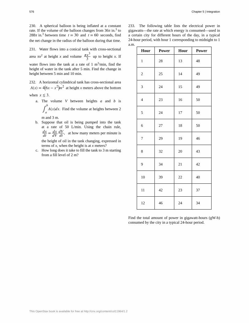
230. A spherical balloon is being inflated at a constantrate. If the volume of the balloon changes from 36π in.3 to288π in.3 between time t = 30 and t = 60 seconds, find
the net change in the radius of the balloon during that time.
231. Water flows into a conical tank with cross-sectional
area πx2 at height x and volume πx3
3 up to height x. If
water flows into the tank at a rate of 1 m3/min, find theheight of water in the tank after 5 min. Find the change inheight between 5 min and 10 min.
232. A horizontal cylindrical tank has cross-sectional area
A(x) = 4⎛⎝6x − x2⎞
⎠m2 at height x meters above the bottom
when x ≤ 3.a. The volume V between heights a and b is
∫a
bA(x)dx. Find the volume at heights between 2
m and 3 m.b. Suppose that oil is being pumped into the tank
at a rate of 50 L/min. Using the chain rule,dxdt = dx
dVdVdt , at how many meters per minute is
the height of oil in the tank changing, expressed interms of x, when the height is at x meters?
c. How long does it take to fill the tank to 3 m startingfrom a fill level of 2 m?
233. The following table lists the electrical power ingigawatts—the rate at which energy is consumed—used ina certain city for different hours of the day, in a typical24-hour period, with hour 1 corresponding to midnight to 1a.m.
Hour Power Hour Power
1 28 13 48
2 25 14 49
3 24 15 49
4 23 16 50
5 24 17 50
6 27 18 50
7 29 19 46
8 32 20 43
9 34 21 42
10 39 22 40
11 42 23 37
12 46 24 34
Find the total amount of power in gigawatt-hours (gW-h)consumed by the city in a typical 24-hour period.
576 Chapter 5 | Integration
This OpenStax book is available for free at http://cnx.org/content/col11964/1.2
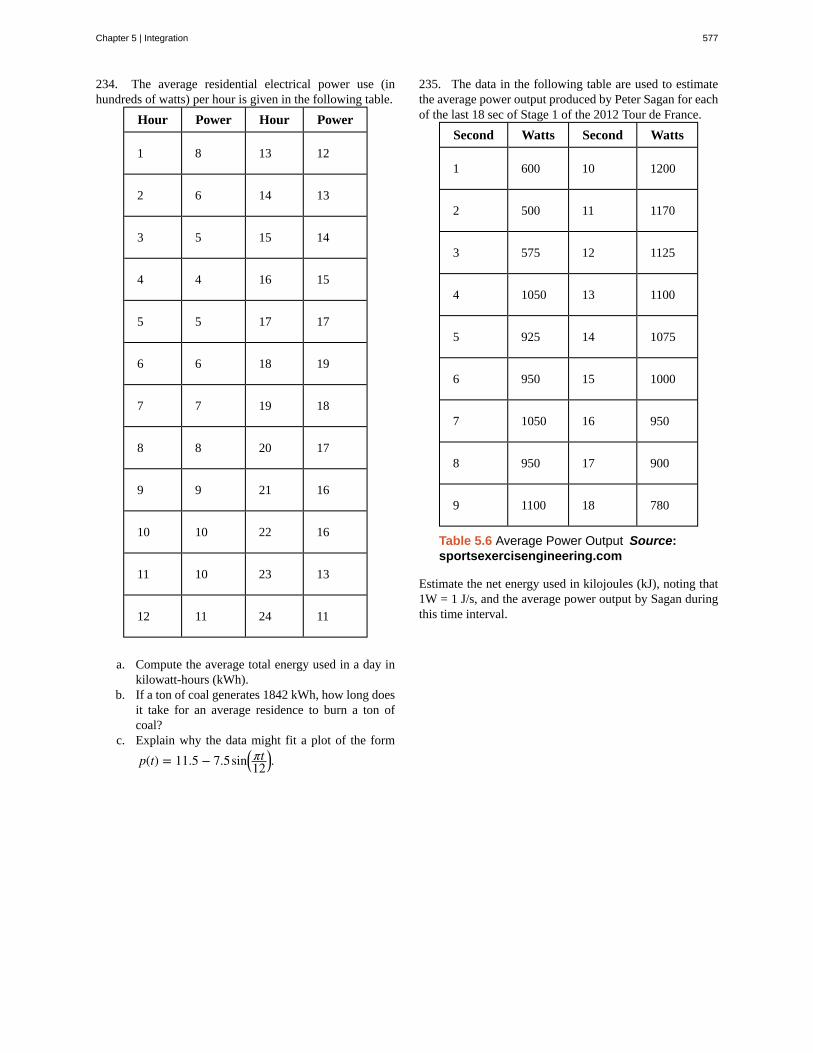
234. The average residential electrical power use (inhundreds of watts) per hour is given in the following table.
Hour Power Hour Power
1 8 13 12
2 6 14 13
3 5 15 14
4 4 16 15
5 5 17 17
6 6 18 19
7 7 19 18
8 8 20 17
9 9 21 16
10 10 22 16
11 10 23 13
12 11 24 11
a. Compute the average total energy used in a day inkilowatt-hours (kWh).
b. If a ton of coal generates 1842 kWh, how long doesit take for an average residence to burn a ton ofcoal?
c. Explain why the data might fit a plot of the form
p(t) = 11.5 − 7.5sin⎛⎝πt12
⎞⎠.
235. The data in the following table are used to estimatethe average power output produced by Peter Sagan for eachof the last 18 sec of Stage 1 of the 2012 Tour de France.
Second Watts Second Watts
1 600 10 1200
2 500 11 1170
3 575 12 1125
4 1050 13 1100
5 925 14 1075
6 950 15 1000
7 1050 16 950
8 950 17 900
9 1100 18 780
Table 5.6 Average Power Output Source:sportsexercisengineering.com
Estimate the net energy used in kilojoules (kJ), noting that1W = 1 J/s, and the average power output by Sagan duringthis time interval.
Chapter 5 | Integration 577
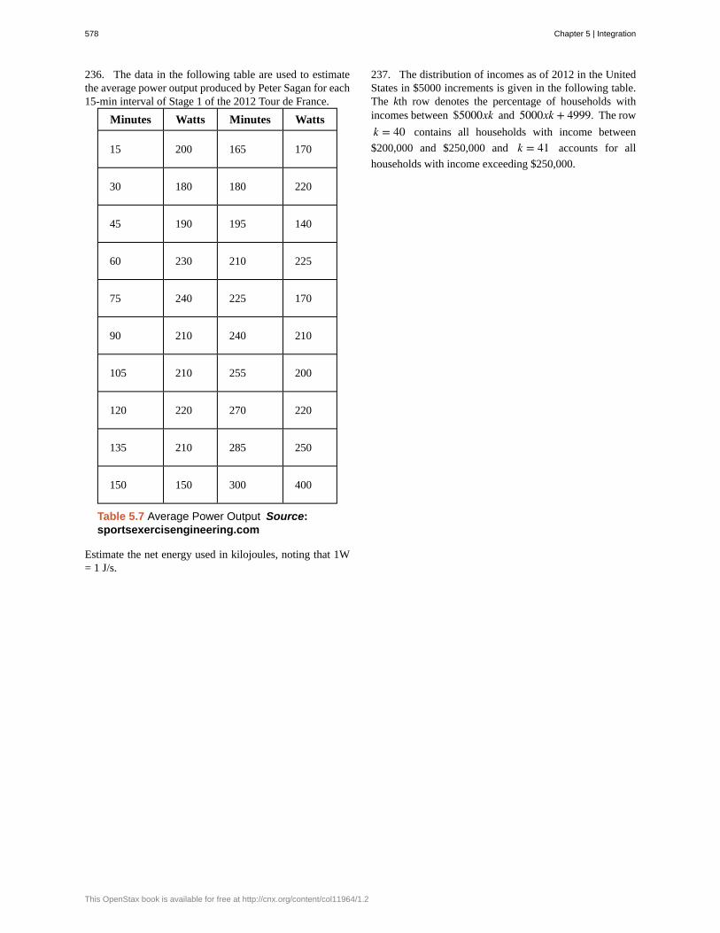
236. The data in the following table are used to estimatethe average power output produced by Peter Sagan for each15-min interval of Stage 1 of the 2012 Tour de France.
Minutes Watts Minutes Watts
15 200 165 170
30 180 180 220
45 190 195 140
60 230 210 225
75 240 225 170
90 210 240 210
105 210 255 200
120 220 270 220
135 210 285 250
150 150 300 400
Table 5.7 Average Power Output Source:sportsexercisengineering.com
Estimate the net energy used in kilojoules, noting that 1W= 1 J/s.
237. The distribution of incomes as of 2012 in the UnitedStates in $5000 increments is given in the following table.The kth row denotes the percentage of households withincomes between $5000xk and 5000xk + 4999. The row
k = 40 contains all households with income between
$200,000 and $250,000 and k = 41 accounts for all
households with income exceeding $250,000.
578 Chapter 5 | Integration
This OpenStax book is available for free at http://cnx.org/content/col11964/1.2
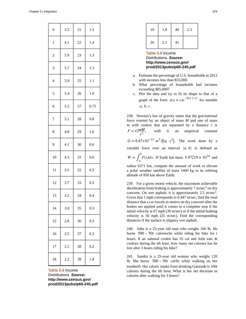
0 3.5 21 1.5
1 4.1 22 1.4
2 5.9 23 1.3
3 5.7 24 1.3
4 5.9 25 1.1
5 5.4 26 1.0
6 5.5 27 0.75
7 5.1 28 0.8
8 4.8 29 1.0
9 4.1 30 0.6
10 4.3 31 0.6
11 3.5 32 0.5
12 3.7 33 0.5
13 3.2 34 0.4
14 3.0 35 0.3
15 2.8 36 0.3
16 2.5 37 0.3
17 2.2 38 0.2
18 2.2 39 1.8
Table 5.8 IncomeDistributions Source:http://www.census.gov/prod/2013pubs/p60-245.pdf
19 1.8 40 2.3
20 2.1 41
Table 5.8 IncomeDistributions Source:http://www.census.gov/prod/2013pubs/p60-245.pdf
a. Estimate the percentage of U.S. households in 2012with incomes less than $55,000.
b. What percentage of households had incomesexceeding $85,000?
c. Plot the data and try to fit its shape to that of a
graph of the form a(x + c)e−b(x + e)for suitable
a, b, c.
238. Newton’s law of gravity states that the gravitationalforce exerted by an object of mass M and one of massm with centers that are separated by a distance r is
F = GmMr2 , with G an empirical constant
G = 6.67x10⁻¹¹ m3 /⎛⎝kg · s2⎞
⎠. The work done by a
variable force over an interval ⎡⎣a, b⎤
⎦ is defined as
W = ∫a
bF(x)dx. If Earth has mass 5.97219 × 1024 and
radius 6371 km, compute the amount of work to elevatea polar weather satellite of mass 1400 kg to its orbitingaltitude of 850 km above Earth.
239. For a given motor vehicle, the maximum achievabledeceleration from braking is approximately 7 m/sec2 on dryconcrete. On wet asphalt, it is approximately 2.5 m/sec2.Given that 1 mph corresponds to 0.447 m/sec, find the totaldistance that a car travels in meters on dry concrete after thebrakes are applied until it comes to a complete stop if theinitial velocity is 67 mph (30 m/sec) or if the initial brakingvelocity is 56 mph (25 m/sec). Find the correspondingdistances if the surface is slippery wet asphalt.
240. John is a 25-year old man who weighs 160 lb. Heburns 500 − 50t calories/hr while riding his bike for t
hours. If an oatmeal cookie has 55 cal and John eats 4tcookies during the tth hour, how many net calories has helost after 3 hours riding his bike?
241. Sandra is a 25-year old woman who weighs 120lb. She burns 300 − 50t cal/hr while walking on her
treadmill. Her caloric intake from drinking Gatorade is 100tcalories during the tth hour. What is her net decrease incalories after walking for 3 hours?
Chapter 5 | Integration 579
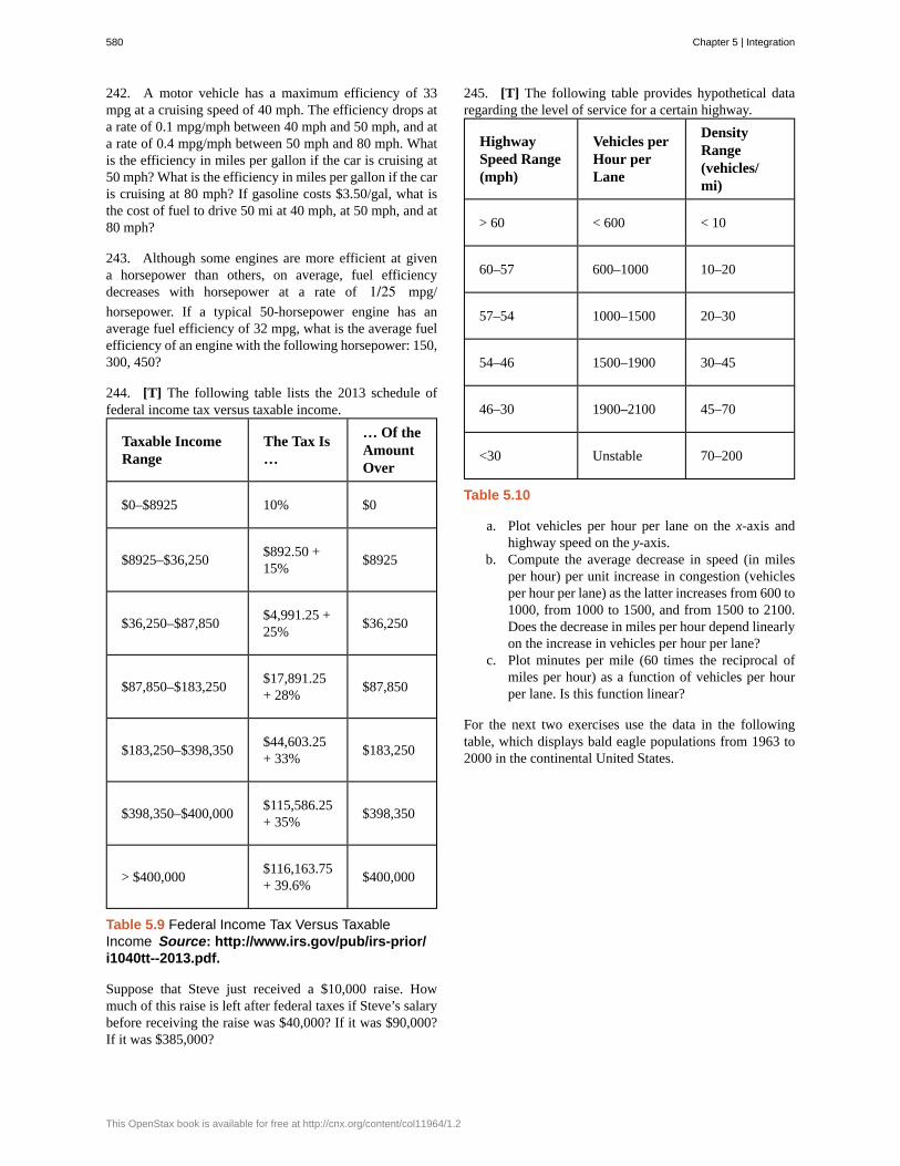
242. A motor vehicle has a maximum efficiency of 33mpg at a cruising speed of 40 mph. The efficiency drops ata rate of 0.1 mpg/mph between 40 mph and 50 mph, and ata rate of 0.4 mpg/mph between 50 mph and 80 mph. Whatis the efficiency in miles per gallon if the car is cruising at50 mph? What is the efficiency in miles per gallon if the caris cruising at 80 mph? If gasoline costs $3.50/gal, what isthe cost of fuel to drive 50 mi at 40 mph, at 50 mph, and at80 mph?
243. Although some engines are more efficient at givena horsepower than others, on average, fuel efficiencydecreases with horsepower at a rate of 1/25 mpg/
horsepower. If a typical 50-horsepower engine has anaverage fuel efficiency of 32 mpg, what is the average fuelefficiency of an engine with the following horsepower: 150,300, 450?
244. [T] The following table lists the 2013 schedule offederal income tax versus taxable income.
Taxable IncomeRange
The Tax Is…
… Of theAmountOver
$0–$8925 10% $0
$8925–$36,250$892.50 +15%
$8925
$36,250–$87,850$4,991.25 +25%
$36,250
$87,850–$183,250$17,891.25+ 28%
$87,850
$183,250–$398,350$44,603.25+ 33%
$183,250
$398,350–$400,000$115,586.25+ 35%
$398,350
> $400,000$116,163.75+ 39.6%
$400,000
Table 5.9 Federal Income Tax Versus TaxableIncome Source: http://www.irs.gov/pub/irs-prior/i1040tt--2013.pdf.
Suppose that Steve just received a $10,000 raise. Howmuch of this raise is left after federal taxes if Steve’s salarybefore receiving the raise was $40,000? If it was $90,000?If it was $385,000?
245. [T] The following table provides hypothetical dataregarding the level of service for a certain highway.
HighwaySpeed Range(mph)
Vehicles perHour perLane
DensityRange(vehicles/mi)
> 60 < 600 < 10
60–57 600–1000 10–20
57–54 1000–1500 20–30
54–46 1500–1900 30–45
46–30 1900–2100 45–70
<30 Unstable 70–200
Table 5.10
a. Plot vehicles per hour per lane on the x-axis andhighway speed on the y-axis.
b. Compute the average decrease in speed (in milesper hour) per unit increase in congestion (vehiclesper hour per lane) as the latter increases from 600 to1000, from 1000 to 1500, and from 1500 to 2100.Does the decrease in miles per hour depend linearlyon the increase in vehicles per hour per lane?
c. Plot minutes per mile (60 times the reciprocal ofmiles per hour) as a function of vehicles per hourper lane. Is this function linear?
For the next two exercises use the data in the followingtable, which displays bald eagle populations from 1963 to2000 in the continental United States.
580 Chapter 5 | Integration
This OpenStax book is available for free at http://cnx.org/content/col11964/1.2
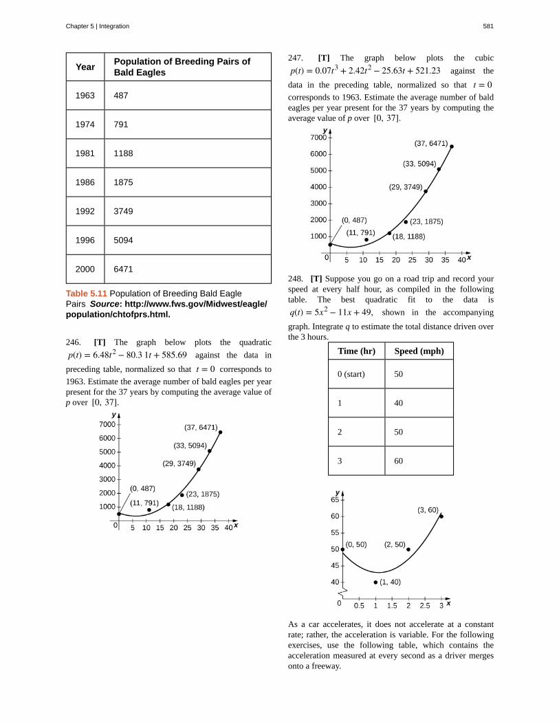
YearPopulation of Breeding Pairs ofBald Eagles
1963 487
1974 791
1981 1188
1986 1875
1992 3749
1996 5094
2000 6471
Table 5.11 Population of Breeding Bald EaglePairs Source: http://www.fws.gov/Midwest/eagle/population/chtofprs.html.
246. [T] The graph below plots the quadratic
p(t) = 6.48t2 − 80.3 1t + 585.69 against the data in
preceding table, normalized so that t = 0 corresponds to
1963. Estimate the average number of bald eagles per yearpresent for the 37 years by computing the average value ofp over [0, 37].
247. [T] The graph below plots the cubic
p(t) = 0.07t3 + 2.42t2 − 25.63t + 521.23 against the
data in the preceding table, normalized so that t = 0corresponds to 1963. Estimate the average number of baldeagles per year present for the 37 years by computing theaverage value of p over [0, 37].
248. [T] Suppose you go on a road trip and record yourspeed at every half hour, as compiled in the followingtable. The best quadratic fit to the data is
q(t) = 5x2 − 11x + 49, shown in the accompanying
graph. Integrate q to estimate the total distance driven overthe 3 hours.
Time (hr) Speed (mph)
0 (start) 50
1 40
2 50
3 60
As a car accelerates, it does not accelerate at a constantrate; rather, the acceleration is variable. For the followingexercises, use the following table, which contains theacceleration measured at every second as a driver mergesonto a freeway.
Chapter 5 | Integration 581
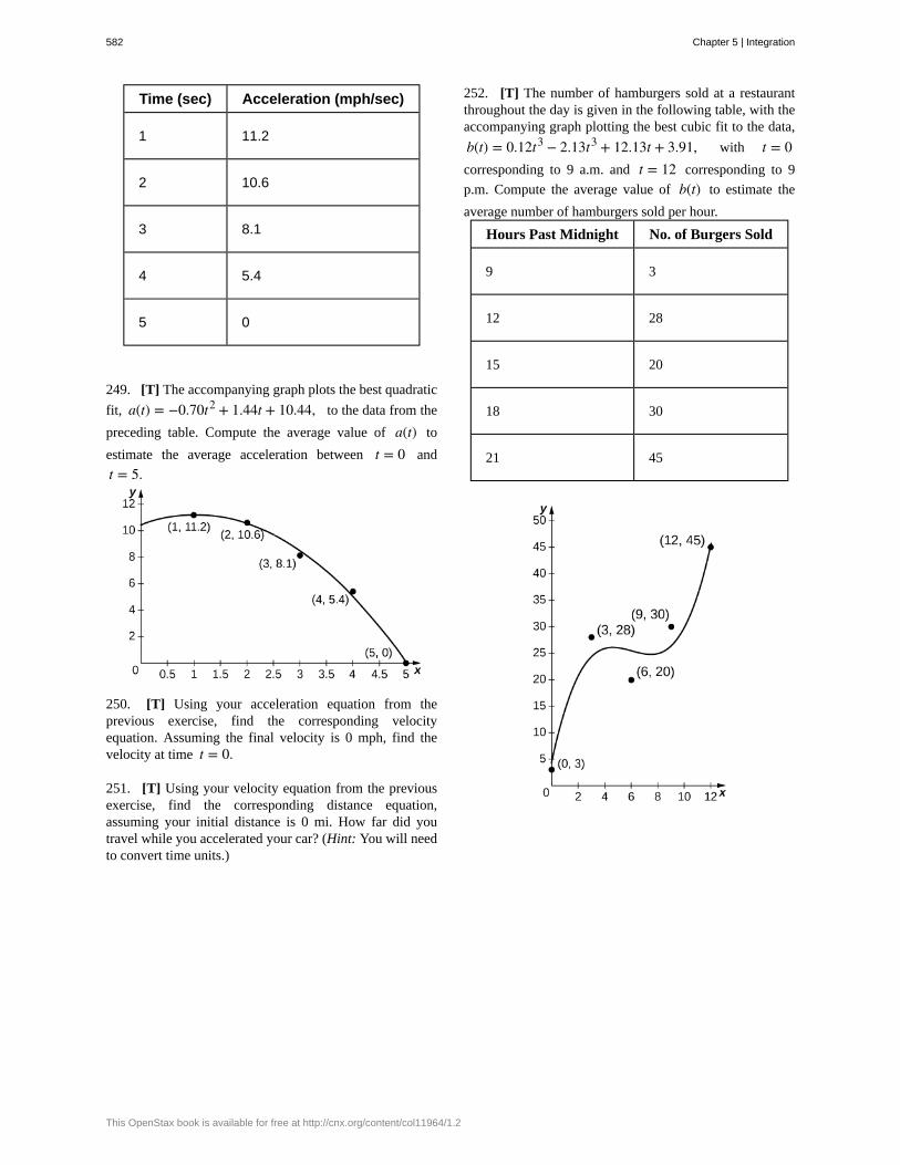
Time (sec) Acceleration (mph/sec)
1 11.2
2 10.6
3 8.1
4 5.4
5 0
249. [T] The accompanying graph plots the best quadratic
fit, a(t) = −0.70t2 + 1.44t + 10.44, to the data from the
preceding table. Compute the average value of a(t) to
estimate the average acceleration between t = 0 and
t = 5.
250. [T] Using your acceleration equation from theprevious exercise, find the corresponding velocityequation. Assuming the final velocity is 0 mph, find thevelocity at time t = 0.
251. [T] Using your velocity equation from the previousexercise, find the corresponding distance equation,assuming your initial distance is 0 mi. How far did youtravel while you accelerated your car? (Hint: You will needto convert time units.)
252. [T] The number of hamburgers sold at a restaurantthroughout the day is given in the following table, with theaccompanying graph plotting the best cubic fit to the data,
b(t) = 0.12t3 − 2.13t3 + 12.13t + 3.91, with t = 0corresponding to 9 a.m. and t = 12 corresponding to 9
p.m. Compute the average value of b(t) to estimate the
average number of hamburgers sold per hour.
Hours Past Midnight No. of Burgers Sold
9 3
12 28
15 20
18 30
21 45
582 Chapter 5 | Integration
This OpenStax book is available for free at http://cnx.org/content/col11964/1.2
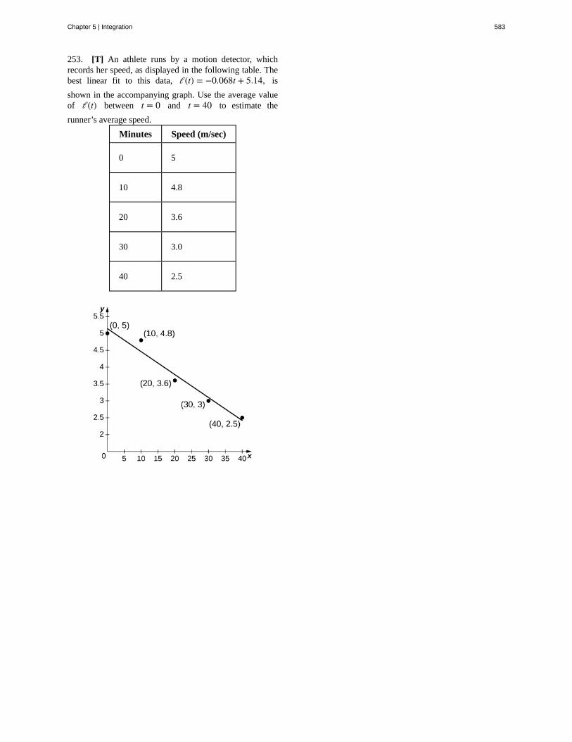
253. [T] An athlete runs by a motion detector, whichrecords her speed, as displayed in the following table. Thebest linear fit to this data, ℓ(t) = −0.068t + 5.14, is
shown in the accompanying graph. Use the average valueof ℓ(t) between t = 0 and t = 40 to estimate the
runner’s average speed.
Minutes Speed (m/sec)
0 5
10 4.8
20 3.6
30 3.0
40 2.5
Chapter 5 | Integration 583
5.5 | Substitution
Learning Objectives5.5.1 Use substitution to evaluate indefinite integrals.
5.5.2 Use substitution to evaluate definite integrals.
The Fundamental Theorem of Calculus gave us a method to evaluate integrals without using Riemann sums. The drawbackof this method, though, is that we must be able to find an antiderivative, and this is not always easy. In this section weexamine a technique, called integration by substitution, to help us find antiderivatives. Specifically, this method helps usfind antiderivatives when the integrand is the result of a chain-rule derivative.
At first, the approach to the substitution procedure may not appear very obvious. However, it is primarily a visual task—thatis, the integrand shows you what to do; it is a matter of recognizing the form of the function. So, what are we supposed to
see? We are looking for an integrand of the form f ⎡⎣g(x)⎤
⎦g′ (x)dx. For example, in the integral ⌠⌡
⎛⎝x2 − 3⎞
⎠3
2xdx, we have
f (x) = x3, g(x) = x2 − 3, and g '(x) = 2x. Then,
f ⎡⎣g(x)⎤
⎦g′ (x) = ⎛⎝x2 − 3⎞
⎠3
(2x),
and we see that our integrand is in the correct form.
The method is called substitution because we substitute part of the integrand with the variable u and part of the integrandwith du. It is also referred to as change of variables because we are changing variables to obtain an expression that is easierto work with for applying the integration rules.
Theorem 5.7: Substitution with Indefinite Integrals
Let u = g(x), , where g′ (x) is continuous over an interval, let f (x) be continuous over the corresponding range of
g, and let F(x) be an antiderivative of f (x). Then,
(5.19)∫ f ⎡⎣g(x)⎤
⎦g′ (x)dx = ∫ f (u)du
= F(u) + C= F⎛
⎝g(x)⎞⎠ + C.
ProofLet f, g, u, and F be as specified in the theorem. Then
ddxF(g(x)) = F′ (g(x)⎞
⎠g′ (x)
= f ⎡⎣g(x)⎤
⎦g′ (x).
Integrating both sides with respect to x, we see that
∫ f ⎡⎣g(x)⎤
⎦g′ (x)dx = F⎛⎝g(x)⎞
⎠ + C.
If we now substitute u = g(x), and du = g '(x)dx, we get
∫ f ⎡⎣g(x)⎤
⎦g′ (x)dx = ∫ f (u)du
= F(u) + C= F⎛
⎝g(x)⎞⎠ + C.
□
584 Chapter 5 | Integration
This OpenStax book is available for free at http://cnx.org/content/col11964/1.2
Returning to the problem we looked at originally, we let u = x2 − 3 and then du = 2xdx. Rewrite the integral in terms of
u:
⌠⌡
⎛⎝x2 − 3⎞
⎠⎫⎭ ⎬
u
3
(2xdx)⏟du
= ∫ u3 du.
Using the power rule for integrals, we have
⌠⌡
u3 du = u4
4 + C.
Substitute the original expression for x back into the solution:
u4
4 + C =⎛⎝x2 − 3⎞
⎠4
4 + C.
We can generalize the procedure in the following Problem-Solving Strategy.
Problem-Solving Strategy: Integration by Substitution
1. Look carefully at the integrand and select an expression g(x) within the integrand to set equal to u. Let’s select
g(x). such that g′ (x) is also part of the integrand.
2. Substitute u = g(x) and du = g′ (x)dx. into the integral.
3. We should now be able to evaluate the integral with respect to u. If the integral can’t be evaluated we need togo back and select a different expression to use as u.
4. Evaluate the integral in terms of u.
5. Write the result in terms of x and the expression g(x).
Example 5.30
Using Substitution to Find an Antiderivative
Use substitution to find the antiderivative of ⌠⌡
6x⎛⎝3x2 + 4⎞
⎠4
dx.
Solution
The first step is to choose an expression for u. We choose u = 3x2 + 4. because then du = 6xdx., and we
already have du in the integrand. Write the integral in terms of u:
⌠⌡
6x⎛⎝3x2 + 4⎞
⎠4
dx = ∫ u4 du.
Remember that du is the derivative of the expression chosen for u, regardless of what is inside the integrand. Nowwe can evaluate the integral with respect to u:
Chapter 5 | Integration 585
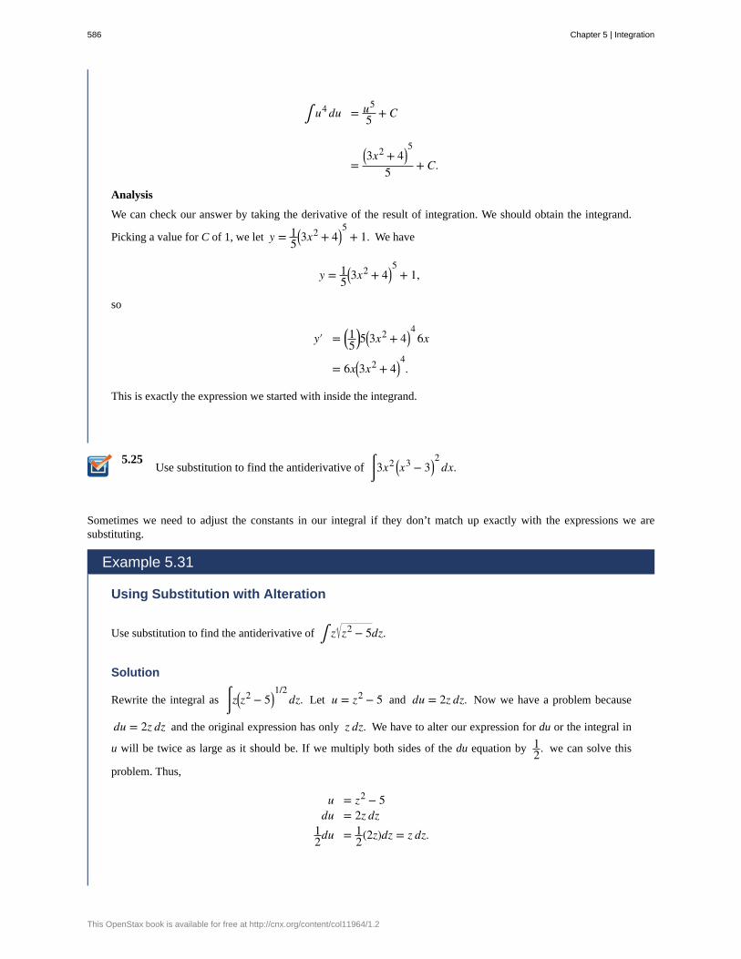
5.25
∫ u4 du = u5
5 + C
=⎛⎝3x2 + 4⎞
⎠5
5 + C.
Analysis
We can check our answer by taking the derivative of the result of integration. We should obtain the integrand.
Picking a value for C of 1, we let y = 15
⎛⎝3x2 + 4⎞
⎠5
+ 1. We have
y = 15
⎛⎝3x2 + 4⎞
⎠5
+ 1,
so
y′ = ⎛⎝15
⎞⎠5
⎛⎝3x2 + 4⎞
⎠4
6x
= 6x⎛⎝3x2 + 4⎞
⎠4.
This is exactly the expression we started with inside the integrand.
Use substitution to find the antiderivative of ⌠⌡
3x2 ⎛⎝x
3 − 3⎞⎠2
dx.
Sometimes we need to adjust the constants in our integral if they don’t match up exactly with the expressions we aresubstituting.
Example 5.31
Using Substitution with Alteration
Use substitution to find the antiderivative of ∫ z z2 − 5dz.
Solution
Rewrite the integral as ⌠⌡
z⎛⎝z2 − 5⎞
⎠1/2
dz. Let u = z2 − 5 and du = 2z dz. Now we have a problem because
du = 2z dz and the original expression has only z dz. We have to alter our expression for du or the integral in
u will be twice as large as it should be. If we multiply both sides of the du equation by 12. we can solve this
problem. Thus,
u = z2 − 5du = 2z dz
12du = 1
2(2z)dz = z dz.
586 Chapter 5 | Integration
This OpenStax book is available for free at http://cnx.org/content/col11964/1.2
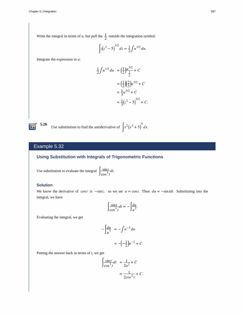
5.26
Write the integral in terms of u, but pull the 12 outside the integration symbol:
⌠⌡
z⎛⎝z2 − 5⎞
⎠1/2
dz = 12∫ u1/2 du.
Integrate the expression in u:
12∫ u1/2 du = ⎛
⎝12
⎞⎠u3/2
32
+ C
= ⎛⎝12
⎞⎠⎛⎝23
⎞⎠u
3/2 + C
= 13u3/2 + C
= 13
⎛⎝z2 − 5⎞
⎠3/2
+ C.
Use substitution to find the antiderivative of ⌠⌡
x2 ⎛⎝x
3 + 5⎞⎠9
dx.
Example 5.32
Using Substitution with Integrals of Trigonometric Functions
Use substitution to evaluate the integral ⌠⌡
sin tcos3 t
dt.
Solution
We know the derivative of cos t is −sin t, so we set u = cos t. Then du = −sin tdt. Substituting into the
integral, we have
⌠⌡
sin tcos3 t
dt = −⌠⌡
duu3 .
Evaluating the integral, we get
−⌠⌡
duu3 = −∫ u−3 du
= −⎛⎝−
12
⎞⎠u
−2 + C.
Putting the answer back in terms of t, we get
⌠⌡
sin tcos3 t
dt = 12u2 + C
= 12cos2 t
+ C.
Chapter 5 | Integration 587
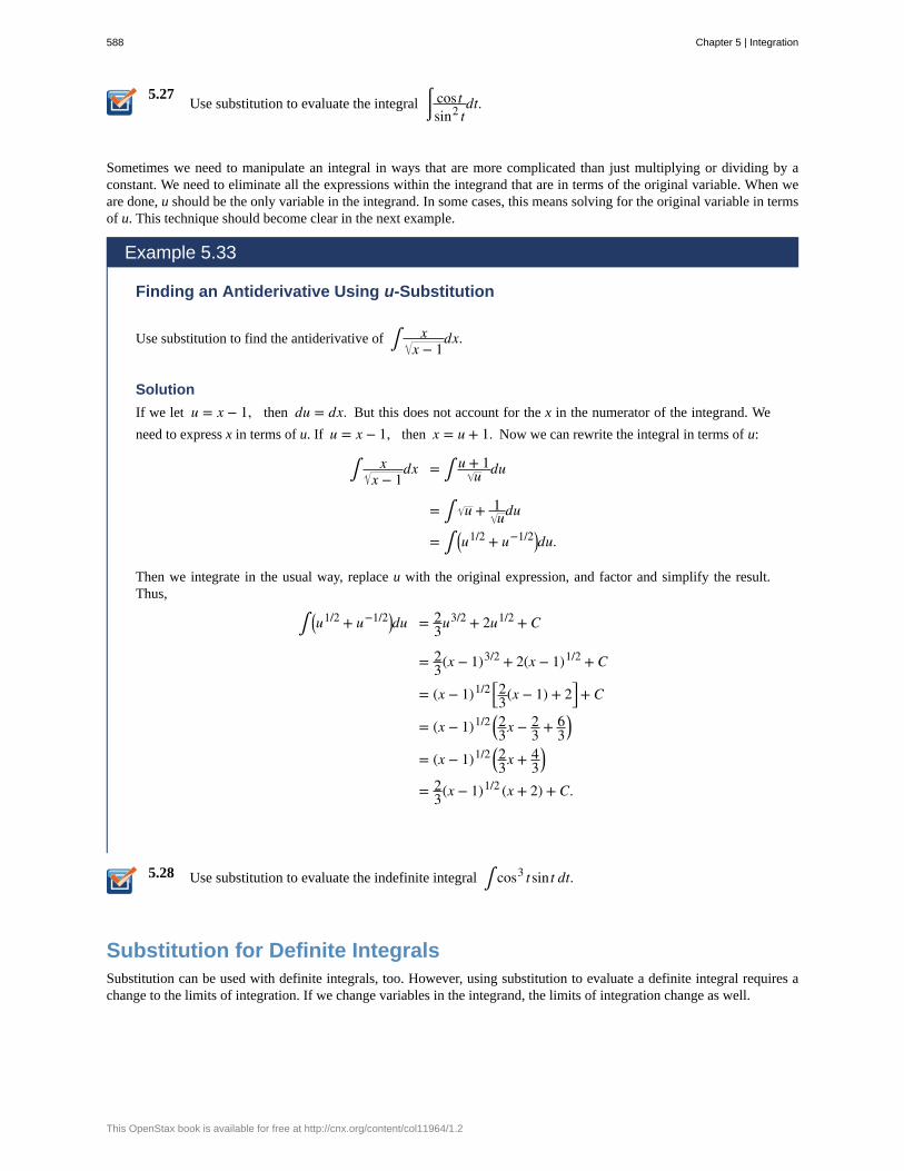
5.27
5.28
Use substitution to evaluate the integral ⌠⌡
cos tsin2 t
dt.
Sometimes we need to manipulate an integral in ways that are more complicated than just multiplying or dividing by aconstant. We need to eliminate all the expressions within the integrand that are in terms of the original variable. When weare done, u should be the only variable in the integrand. In some cases, this means solving for the original variable in termsof u. This technique should become clear in the next example.
Example 5.33
Finding an Antiderivative Using u-Substitution
Use substitution to find the antiderivative of ∫ xx − 1
dx.
Solution
If we let u = x − 1, then du = dx. But this does not account for the x in the numerator of the integrand. We
need to express x in terms of u. If u = x − 1, then x = u + 1. Now we can rewrite the integral in terms of u:
∫ xx − 1
dx = ∫ u + 1u du
= ∫ u + 1udu
= ∫ ⎛⎝u
1/2 + u−1/2⎞⎠du.
Then we integrate in the usual way, replace u with the original expression, and factor and simplify the result.Thus,
∫ ⎛⎝u
1/2 + u−1/2⎞⎠du = 2
3u3/2 + 2u1/2 + C
= 23(x − 1)3/2 + 2(x − 1)1/2 + C
= (x − 1)1/2 ⎡⎣23(x − 1) + 2⎤
⎦ + C
= (x − 1)1/2 ⎛⎝23x − 2
3 + 63
⎞⎠
= (x − 1)1/2 ⎛⎝23x + 4
3⎞⎠
= 23(x − 1)1/2 (x + 2) + C.
Use substitution to evaluate the indefinite integral ∫ cos3 t sin t dt.
Substitution for Definite IntegralsSubstitution can be used with definite integrals, too. However, using substitution to evaluate a definite integral requires achange to the limits of integration. If we change variables in the integrand, the limits of integration change as well.
588 Chapter 5 | Integration
This OpenStax book is available for free at http://cnx.org/content/col11964/1.2
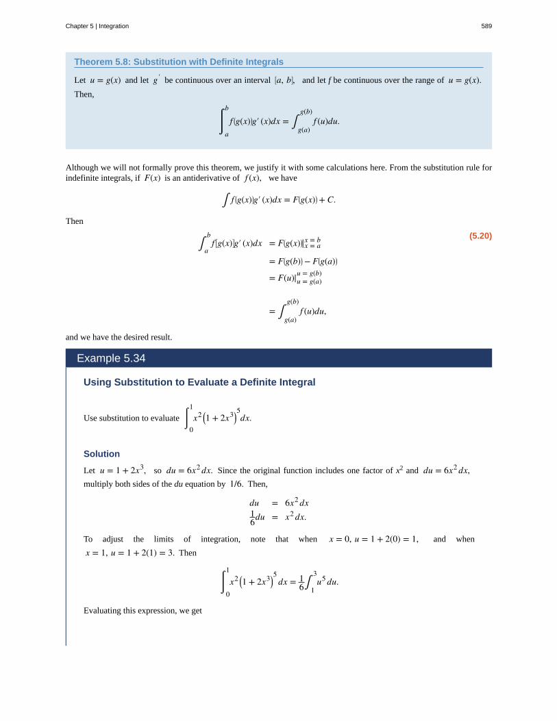
Theorem 5.8: Substitution with Definite Integrals
Let u = g(x) and let g′ be continuous over an interval ⎡⎣a, b⎤
⎦, and let f be continuous over the range of u = g(x).Then,
⌠⌡a
b
f ⎛⎝g(x)⎞
⎠g′ (x)dx = ∫g(a)
g(b)f (u)du.
Although we will not formally prove this theorem, we justify it with some calculations here. From the substitution rule forindefinite integrals, if F(x) is an antiderivative of f (x), we have
∫ f ⎛⎝g(x)⎞
⎠g′ (x)dx = F⎛⎝g(x)⎞
⎠ + C.
Then
(5.20)∫a
bf ⎡
⎣g(x)⎤⎦g′ (x)dx = F⎛
⎝g(x)⎞⎠|x = a
x = b
= F⎛⎝g(b)⎞
⎠ − F⎛⎝g(a)⎞
⎠
= F(u)|u = g(a)u = g(b)
= ∫g(a)
g(b)f (u)du,
and we have the desired result.
Example 5.34
Using Substitution to Evaluate a Definite Integral
Use substitution to evaluate ⌠⌡0
1x2 ⎛
⎝1 + 2x3⎞⎠5dx.
Solution
Let u = 1 + 2x3, so du = 6x2 dx. Since the original function includes one factor of x2 and du = 6x2 dx,multiply both sides of the du equation by 1/6. Then,
du = 6x2 dx16du = x2 dx.
To adjust the limits of integration, note that when x = 0, u = 1 + 2(0) = 1, and when
x = 1, u = 1 + 2(1) = 3. Then
⌠⌡0
1
x2 ⎛⎝1 + 2x3⎞
⎠5
dx = 16∫
1
3u5 du.
Evaluating this expression, we get
Chapter 5 | Integration 589
5.29
5.30
16∫
1
3u5 du = ⎛
⎝16
⎞⎠⎛⎝u6
6⎞⎠|1
3
= 136
⎡⎣(3)6 − (1)6⎤
⎦
= 1829 .
Use substitution to evaluate the definite integral ⌠⌡−1
0y⎛
⎝2y2 − 3⎞⎠5
dy.
Example 5.35
Using Substitution with an Exponential Function
Use substitution to evaluate ∫0
1xe4x2 + 3 dx.
Solution
Let u = 4x3 + 3. Then, du = 8xdx. To adjust the limits of integration, we note that when x = 0, u = 3, and
when x = 1, u = 7. So our substitution gives
∫0
1xe4x2 + 3 dx = 1
8∫3
7eu du
= 18eu |3
7
= e7 − e3
8≈ 134.568.
Use substitution to evaluate ⌠⌡0
1x2 cos⎛
⎝π2x3⎞
⎠dx.
Substitution may be only one of the techniques needed to evaluate a definite integral. All of the properties and rules ofintegration apply independently, and trigonometric functions may need to be rewritten using a trigonometric identity beforewe can apply substitution. Also, we have the option of replacing the original expression for u after we find the antiderivative,which means that we do not have to change the limits of integration. These two approaches are shown in Example 5.36.
Example 5.36
590 Chapter 5 | Integration
This OpenStax book is available for free at http://cnx.org/content/col11964/1.2
Using Substitution to Evaluate a Trigonometric Integral
Use substitution to evaluate ∫0
π/2cos2 θ dθ.
Solution
Let us first use a trigonometric identity to rewrite the integral. The trig identity cos2 θ = 1 + cos2θ2 allows us
to rewrite the integral as
∫0
π/2cos2 θdθ = ⌠
⌡0
π/21 + cos2θ2 dθ.
Then,
⌠⌡0
π/2⎛⎝1 + cos2θ
2⎞⎠dθ = ⌠
⌡0
π/2⎛⎝12 + 1
2cos2θ⎞⎠dθ
= 12∫
0
π/2dθ + ∫
0
π/2cos2θdθ.
We can evaluate the first integral as it is, but we need to make a substitution to evaluate the second integral. Let
u = 2θ. Then, du = 2dθ, or 12du = dθ. Also, when θ = 0, u = 0, and when θ = π/2, u = π. Expressing
the second integral in terms of u, we have
12
⌠⌡0
π/2
dθ + 12∫
0
π/2cos2θdθ = 1
2⌠⌡0
π/2dθ + 1
2⎛⎝12
⎞⎠∫
0
πcosudu
= θ2|θ = 0
θ = π/2+ 1
4sinu|u = 0
u = θ
= ⎛⎝π4 − 0⎞
⎠ + (0 − 0) = π4.
Chapter 5 | Integration 591
5.5 EXERCISES254. Why is u-substitution referred to as change ofvariable?
255. 2. If f = g ∘h, when reversing the chain rule,
ddx(g ∘h)(x) = g′ (h(x)⎞
⎠h′ (x), should you take u = g(x)
or u = h(x)?
In the following exercises, verify each identity usingdifferentiation. Then, using the indicated u-substitution,
identify f such that the integral takes the form ∫ f (u)du.
256.
∫ x x + 1dx = 215(x + 1)3/2 (3x − 2) + C; u = x + 1
257.
⌠⌡
x2
x − 1dx(x > 1) = 2
15 x − 1⎛⎝3x2 + 4x + 8⎞
⎠ + C; u = x − 1
258.
⌠⌡
x 4x2 + 9dx = 112
⎛⎝4x2 + 9⎞
⎠3/2
+ C; u = 4x2 + 9
259. ⌠⌡
x4x2 + 9
dx = 14 4x2 + 9 + C; u = 4x2 + 9
260. ⌠⌡
x(4x2 + 9)2dx = − 1
8(4x2 + 9); u = 4x2 + 9
In the following exercises, find the antiderivative using theindicated substitution.
261. ∫ (x + 1)4 dx; u = x + 1
262. ∫ (x − 1)5 dx; u = x − 1
263. ∫ (2x − 3)−7 dx; u = 2x − 3
264. ∫ (3x − 2)−11 dx; u = 3x − 2
265. ⌠⌡
xx2 + 1
dx; u = x2 + 1
266. ⌠⌡
x1 − x2
dx; u = 1 − x2
267. ⌠⌡
(x − 1)⎛⎝x2 − 2x⎞
⎠3
dx; u = x2 − 2x
268. ⌠⌡
⎛⎝x2 − 2x⎞
⎠⎛⎝x
3 − 3x2⎞⎠2
dx; u = x3 = 3x2
269. ∫ cos3 θdθ; u = sinθ (Hint: cos2 θ = 1 − sin2 θ)
270. ∫ sin3 θdθ; u = cosθ (Hint: sin2 θ = 1 − cos2 θ)
In the following exercises, use a suitable change ofvariables to determine the indefinite integral.
271. ∫ x(1 − x)99 dx
272. ⌠⌡
t⎛⎝1 − t2⎞
⎠10
dt
273. ∫ (11x − 7)−3 dx
274. ∫ (7x − 11)4 dx
275. ∫ cos3 θsinθdθ
276. ∫ sin7 θcosθdθ
277. ∫ cos2 (πt)sin(πt)dt
278. ∫ sin2 xcos3 xdx (Hint: sin2 x + cos2 x = 1)
279. ∫ t sin⎛⎝t2⎞
⎠cos⎛⎝t2⎞
⎠dt
280. ∫ t2cos2 ⎛⎝t
3⎞⎠sin⎛
⎝t3⎞
⎠dt
281.⌠
⌡⎮ x2
⎛⎝x
3 − 3⎞⎠2dx
282. ⌠⌡
x3
1 − x2dx
592 Chapter 5 | Integration
This OpenStax book is available for free at http://cnx.org/content/col11964/1.2
283.⌠
⌡⎮ y5
⎛⎝1 − y3⎞
⎠3/2dy
284. ∫ cosθ(1 − cosθ)99
sinθdθ
285. ∫ ⎛⎝1 − cos3 θ⎞
⎠10
cos2 θsinθdθ
286. ⌠⌡
(cosθ − 1)⎛⎝cos2 θ − 2cosθ⎞
⎠3
sinθdθ
287. ⌠⌡
⎛⎝sin2 θ − 2sinθ⎞
⎠⎛⎝sin3 θ − 3sin2 θ⎞
⎠3
cosθdθ
In the following exercises, use a calculator to estimate thearea under the curve using left Riemann sums with 50terms, then use substitution to solve for the exact answer.
288. [T] y = 3(1 − x)2 over [0, 2]
289. [T] y = x⎛⎝1 − x2⎞
⎠3
over [−1, 2]
290. [T] y = sinx(1 − cosx)2 over [0, π]
291. [T] y = x⎛⎝x2 + 1⎞
⎠2 over [−1, 1]
In the following exercises, use a change of variables toevaluate the definite integral.
292. ∫0
1x 1 − x2dx
293. ⌠⌡0
1x
1 + x2dx
294. ⌠⌡0
2t
5 + t2dt
295. ⌠⌡0
1t2
1 + t3dt
296. ∫0
π/4sec2 θ tanθdθ
297. ⌠⌡0
π/4sinθ
cos4 θdθ
In the following exercises, evaluate the indefinite integral
∫ f (x)dx with constant C = 0 using u-substitution.
Then, graph the function and the antiderivative over theindicated interval. If possible, estimate a value of C thatwould need to be added to the antiderivative to make it
equal to the definite integral F(x) = ∫a
xf (t)dt, with a the
left endpoint of the given interval.
298. [T] ∫ (2x + 1)ex2 + x − 6 dx over [−3, 2]
299. [T] ∫ cos⎛⎝ln(2x)⎞
⎠
x dx on [0, 2]
300. [T] ⌠⌡
3x2 + 2x + 1x3 + x2 + x + 4
dx over [−1, 2]
301. [T] ⌠⌡
sinxcos3 x
dx over⎡⎣−
π3, π
3⎤⎦
302. [T] ∫ (x + 2)e−x2 − 4x + 3 dx over ⎡⎣−5, 1⎤
⎦
303. [T] ∫ 3x2 2x3 + 1dx over [0, 1]
304. If h(a) = h(b) in ∫a
bg '⎛⎝h(x)⎞
⎠h(x)dx, what can you
say about the value of the integral?
305. Is the substitution u = 1 − x2 in the definite integral
⌠⌡0
2x
1 − x2dx okay? If not, why not?
In the following exercises, use a change of variables toshow that each definite integral is equal to zero.
306. ∫0
πcos2 (2θ)sin(2θ)dθ
307. ∫0
πtcos⎛
⎝t2⎞⎠sin⎛
⎝t2⎞⎠dt
308. ∫0
1(1 − 2t)dt
Chapter 5 | Integration 593
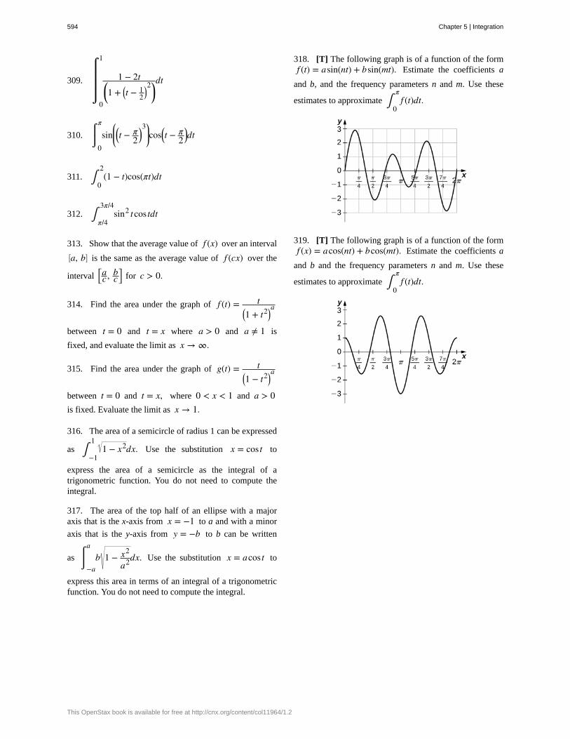
309.⌠
⌡⎮⎮
0
1
1 − 2t⎛⎝1 + ⎛
⎝t − 12
⎞⎠2⎞⎠
dt
310. ⌠⌡0
π
sin⎛
⎝⎜⎛⎝t − π
2⎞⎠3⎞
⎠⎟cos⎛
⎝t − π2
⎞⎠dt
311. ∫0
2(1 − t)cos(πt)dt
312. ∫π/4
3π/4sin2 tcos tdt
313. Show that the average value of f (x) over an interval⎡⎣a, b⎤
⎦ is the same as the average value of f (cx) over the
interval ⎡⎣ac , b
c⎤⎦ for c > 0.
314. Find the area under the graph of f (t) = t⎛⎝1 + t2⎞
⎠a
between t = 0 and t = x where a > 0 and a ≠ 1 is
fixed, and evaluate the limit as x → ∞.
315. Find the area under the graph of g(t) = t⎛⎝1 − t2⎞
⎠a
between t = 0 and t = x, where 0 < x < 1 and a > 0is fixed. Evaluate the limit as x → 1.
316. The area of a semicircle of radius 1 can be expressed
as ∫−1
11 − x2dx. Use the substitution x = cos t to
express the area of a semicircle as the integral of atrigonometric function. You do not need to compute theintegral.
317. The area of the top half of an ellipse with a majoraxis that is the x-axis from x = −1 to a and with a minor
axis that is the y-axis from y = −b to b can be written
as ⌠⌡−a
a
b 1 − x2
a2dx. Use the substitution x = acos t to
express this area in terms of an integral of a trigonometricfunction. You do not need to compute the integral.
318. [T] The following graph is of a function of the formf (t) = asin(nt) + bsin(mt). Estimate the coefficients a
and b, and the frequency parameters n and m. Use these
estimates to approximate ∫0
πf (t)dt.
319. [T] The following graph is of a function of the formf (x) = acos(nt) + bcos(mt). Estimate the coefficients a
and b and the frequency parameters n and m. Use these
estimates to approximate ∫0
πf (t)dt.
594 Chapter 5 | Integration
This OpenStax book is available for free at http://cnx.org/content/col11964/1.2
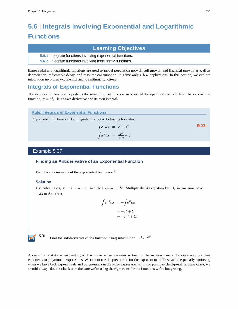
5.31
5.6 | Integrals Involving Exponential and Logarithmic
Functions
Learning Objectives5.6.1 Integrate functions involving exponential functions.
5.6.2 Integrate functions involving logarithmic functions.
Exponential and logarithmic functions are used to model population growth, cell growth, and financial growth, as well asdepreciation, radioactive decay, and resource consumption, to name only a few applications. In this section, we exploreintegration involving exponential and logarithmic functions.
Integrals of Exponential FunctionsThe exponential function is perhaps the most efficient function in terms of the operations of calculus. The exponentialfunction, y = ex, is its own derivative and its own integral.
Rule: Integrals of Exponential Functions
Exponential functions can be integrated using the following formulas.
(5.21)∫ ex dx = ex + C
∫ ax dx = ax
lna + C
Example 5.37
Finding an Antiderivative of an Exponential Function
Find the antiderivative of the exponential function e−x.
Solution
Use substitution, setting u = −x, and then du = −1dx. Multiply the du equation by −1, so you now have
−du = dx. Then,
∫ e−xdx = −∫ eu du
= −eu + C= −e−x + C.
Find the antiderivative of the function using substitution: x2 e−2x3.
A common mistake when dealing with exponential expressions is treating the exponent on e the same way we treatexponents in polynomial expressions. We cannot use the power rule for the exponent on e. This can be especially confusingwhen we have both exponentials and polynomials in the same expression, as in the previous checkpoint. In these cases, weshould always double-check to make sure we’re using the right rules for the functions we’re integrating.
Chapter 5 | Integration 595
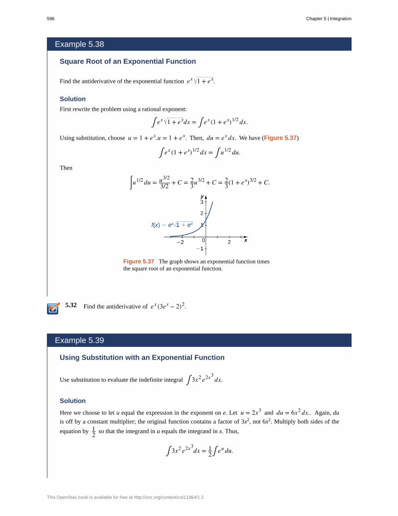
5.32
Example 5.38
Square Root of an Exponential Function
Find the antiderivative of the exponential function ex 1 + ex.
Solution
First rewrite the problem using a rational exponent:
∫ ex 1 + exdx = ∫ ex (1 + ex)1/2 dx.
Using substitution, choose u = 1 + ex.u = 1 + ex. Then, du = ex dx. We have (Figure 5.37)
∫ ex (1 + ex)1/2 dx = ∫ u1/2 du.
Then
⌠⌡
u1/2 du = u3/2
3/2 + C = 23u3/2 + C = 2
3(1 + ex)3/2 + C.
Figure 5.37 The graph shows an exponential function timesthe square root of an exponential function.
Find the antiderivative of ex (3ex − 2)2.
Example 5.39
Using Substitution with an Exponential Function
Use substitution to evaluate the indefinite integral ∫ 3x2 e2x3dx.
Solution
Here we choose to let u equal the expression in the exponent on e. Let u = 2x3 and du = 6x2 dx.. Again, du
is off by a constant multiplier; the original function contains a factor of 3x2, not 6x2. Multiply both sides of the
equation by 12 so that the integrand in u equals the integrand in x. Thus,
∫ 3x2 e2x3dx = 1
2∫ eu du.
596 Chapter 5 | Integration
This OpenStax book is available for free at http://cnx.org/content/col11964/1.2
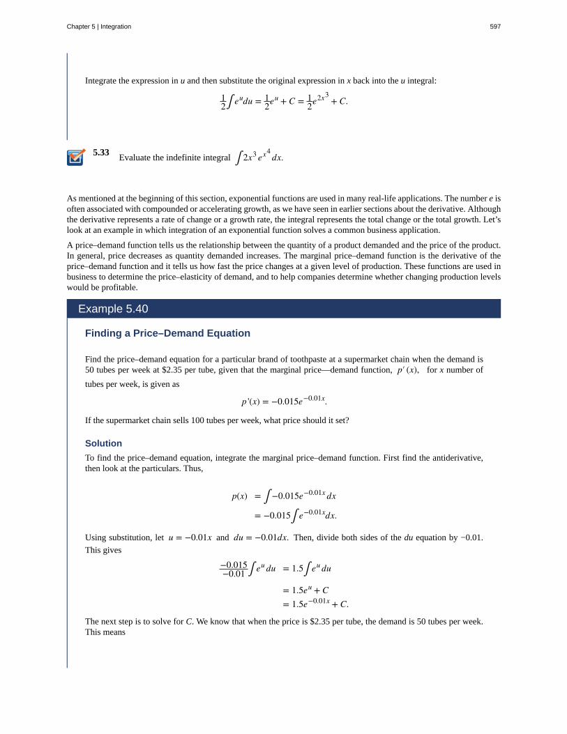
5.33
Integrate the expression in u and then substitute the original expression in x back into the u integral:
12∫ eudu = 1
2eu + C = 12e2x3
+ C.
Evaluate the indefinite integral ∫ 2x3 ex4dx.
As mentioned at the beginning of this section, exponential functions are used in many real-life applications. The number e isoften associated with compounded or accelerating growth, as we have seen in earlier sections about the derivative. Althoughthe derivative represents a rate of change or a growth rate, the integral represents the total change or the total growth. Let’slook at an example in which integration of an exponential function solves a common business application.
A price–demand function tells us the relationship between the quantity of a product demanded and the price of the product.In general, price decreases as quantity demanded increases. The marginal price–demand function is the derivative of theprice–demand function and it tells us how fast the price changes at a given level of production. These functions are used inbusiness to determine the price–elasticity of demand, and to help companies determine whether changing production levelswould be profitable.
Example 5.40
Finding a Price–Demand Equation
Find the price–demand equation for a particular brand of toothpaste at a supermarket chain when the demand is50 tubes per week at $2.35 per tube, given that the marginal price—demand function, p′ (x), for x number of
tubes per week, is given as
p '(x) = −0.015e−0.01x.
If the supermarket chain sells 100 tubes per week, what price should it set?
Solution
To find the price–demand equation, integrate the marginal price–demand function. First find the antiderivative,then look at the particulars. Thus,
p(x) = ∫ −0.015e−0.01x dx
= −0.015∫ e−0.01xdx.
Using substitution, let u = −0.01x and du = −0.01dx. Then, divide both sides of the du equation by −0.01.
This gives
−0.015−0.01 ∫ eu du = 1.5∫ eu du
= 1.5eu + C= 1.5e−0.01x + C.
The next step is to solve for C. We know that when the price is $2.35 per tube, the demand is 50 tubes per week.This means
Chapter 5 | Integration 597
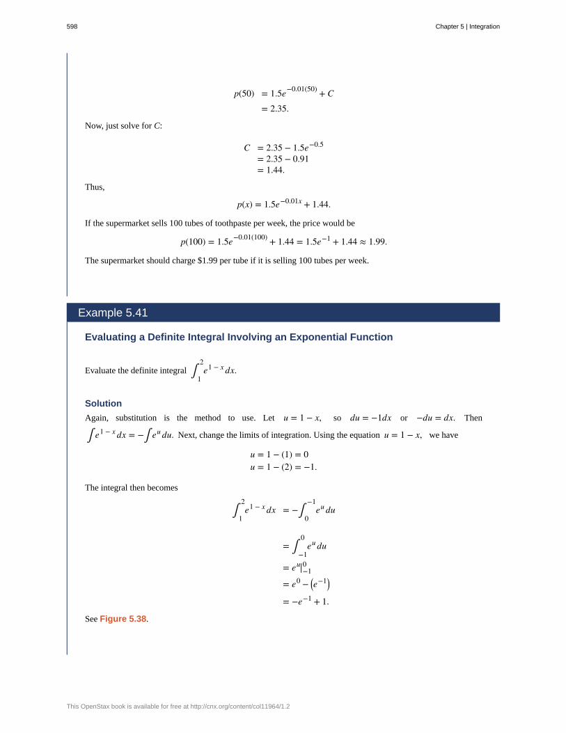
p(50) = 1.5e−0.01(50) + C
= 2.35.
Now, just solve for C:
C = 2.35 − 1.5e−0.5
= 2.35 − 0.91= 1.44.
Thus,
p(x) = 1.5e−0.01x + 1.44.
If the supermarket sells 100 tubes of toothpaste per week, the price would be
p(100) = 1.5e−0.01(100) + 1.44 = 1.5e−1 + 1.44 ≈ 1.99.
The supermarket should charge $1.99 per tube if it is selling 100 tubes per week.
Example 5.41
Evaluating a Definite Integral Involving an Exponential Function
Evaluate the definite integral ∫1
2e1 − x dx.
Solution
Again, substitution is the method to use. Let u = 1 − x, so du = −1dx or −du = dx. Then
∫ e1 − x dx = −∫ eu du. Next, change the limits of integration. Using the equation u = 1 − x, we have
u = 1 − (1) = 0u = 1 − (2) = −1.
The integral then becomes
∫1
2e1 − x dx = −∫
0
−1eu du
= ∫−1
0eu du
= eu|−10
= e0 − ⎛⎝e−1⎞
⎠
= −e−1 + 1.
See Figure 5.38.
598 Chapter 5 | Integration
This OpenStax book is available for free at http://cnx.org/content/col11964/1.2
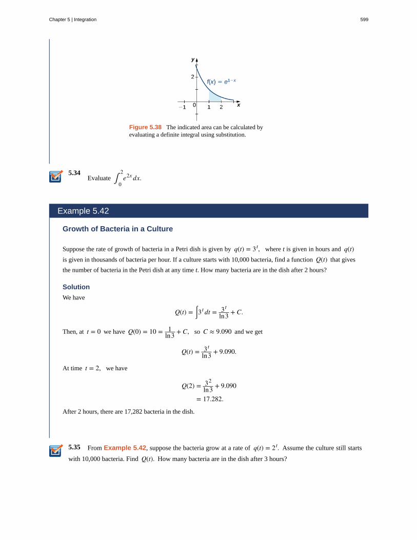
5.34
5.35
Figure 5.38 The indicated area can be calculated byevaluating a definite integral using substitution.
Evaluate ∫0
2e2x dx.
Example 5.42
Growth of Bacteria in a Culture
Suppose the rate of growth of bacteria in a Petri dish is given by q(t) = 3t, where t is given in hours and q(t)is given in thousands of bacteria per hour. If a culture starts with 10,000 bacteria, find a function Q(t) that gives
the number of bacteria in the Petri dish at any time t. How many bacteria are in the dish after 2 hours?
Solution
We have
Q(t) = ⌠⌡3t dt = 3t
ln3 + C.
Then, at t = 0 we have Q(0) = 10 = 1ln3 + C, so C ≈ 9.090 and we get
Q(t) = 3t
ln3 + 9.090.
At time t = 2, we have
Q(2) = 32
ln3 + 9.090
= 17.282.
After 2 hours, there are 17,282 bacteria in the dish.
From Example 5.42, suppose the bacteria grow at a rate of q(t) = 2t. Assume the culture still starts
with 10,000 bacteria. Find Q(t). How many bacteria are in the dish after 3 hours?
Chapter 5 | Integration 599
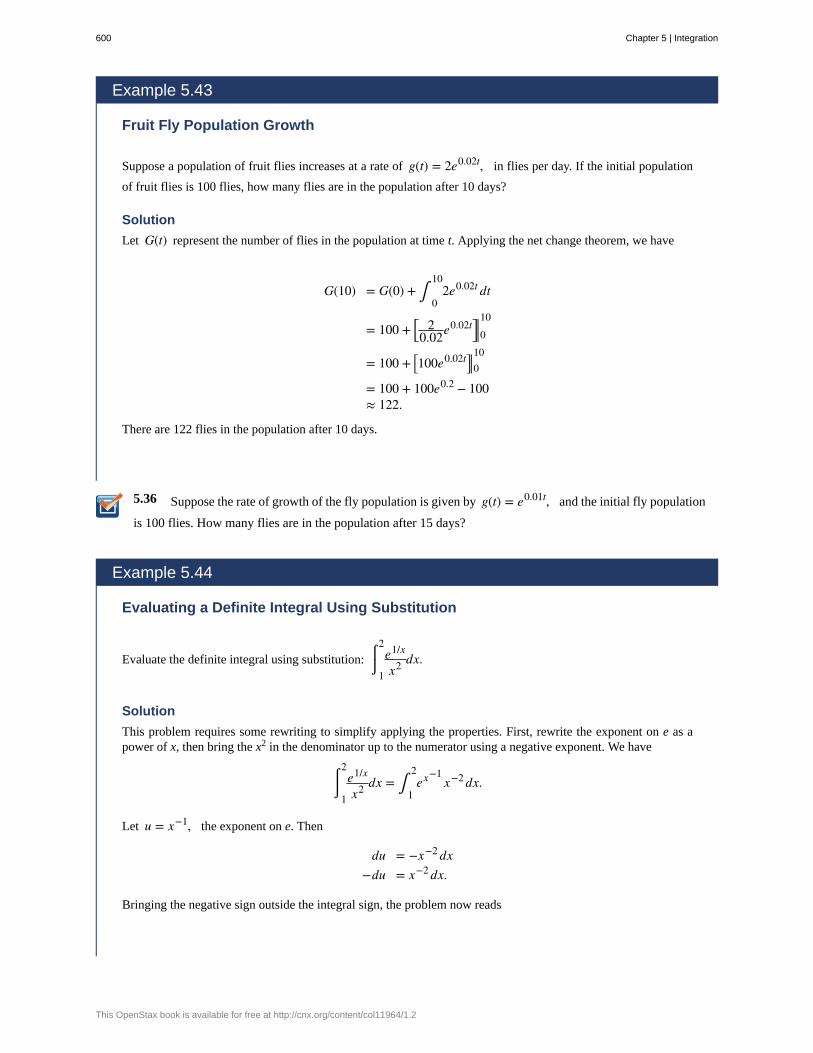
5.36
Example 5.43
Fruit Fly Population Growth
Suppose a population of fruit flies increases at a rate of g(t) = 2e0.02t, in flies per day. If the initial population
of fruit flies is 100 flies, how many flies are in the population after 10 days?
Solution
Let G(t) represent the number of flies in the population at time t. Applying the net change theorem, we have
G(10) = G(0) + ∫0
102e0.02t dt
= 100 + ⎡⎣
20.02e0.02t⎤
⎦|010
= 100 + ⎡⎣100e0.02t⎤
⎦|010
= 100 + 100e0.2 − 100≈ 122.
There are 122 flies in the population after 10 days.
Suppose the rate of growth of the fly population is given by g(t) = e0.01t, and the initial fly population
is 100 flies. How many flies are in the population after 15 days?
Example 5.44
Evaluating a Definite Integral Using Substitution
Evaluate the definite integral using substitution: ⌠⌡1
2e1/x
x2 dx.
Solution
This problem requires some rewriting to simplify applying the properties. First, rewrite the exponent on e as apower of x, then bring the x2 in the denominator up to the numerator using a negative exponent. We have
⌠⌡1
2e1/x
x2 dx = ∫1
2ex−1
x−2 dx.
Let u = x−1, the exponent on e. Then
du = −x−2 dx−du = x−2 dx.
Bringing the negative sign outside the integral sign, the problem now reads
600 Chapter 5 | Integration
This OpenStax book is available for free at http://cnx.org/content/col11964/1.2
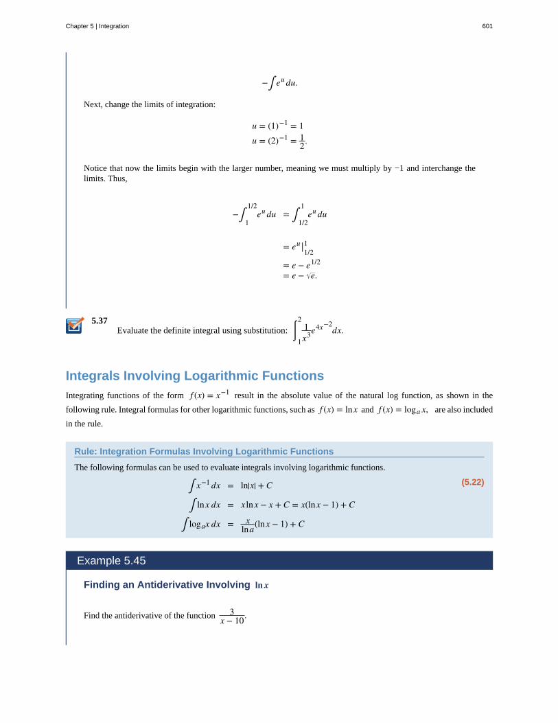
5.37
−∫ eu du.
Next, change the limits of integration:
u = (1)−1 = 1u = (2)−1 = 1
2.
Notice that now the limits begin with the larger number, meaning we must multiply by −1 and interchange thelimits. Thus,
−∫1
1/2eu du = ∫
1/2
1eu du
= eu |1/21
= e − e1/2
= e − e.
Evaluate the definite integral using substitution: ⌠⌡1
21x3e4x−2
dx.
Integrals Involving Logarithmic FunctionsIntegrating functions of the form f (x) = x−1 result in the absolute value of the natural log function, as shown in the
following rule. Integral formulas for other logarithmic functions, such as f (x) = lnx and f (x) = loga x, are also included
in the rule.
Rule: Integration Formulas Involving Logarithmic Functions
The following formulas can be used to evaluate integrals involving logarithmic functions.
(5.22)∫ x−1 dx = ln|x| + C
∫ lnx dx = x lnx − x + C = x(lnx − 1) + C
∫ logax dx = xlna(lnx − 1) + C
Example 5.45
Finding an Antiderivative Involving ln x
Find the antiderivative of the function 3x − 10.
Chapter 5 | Integration 601
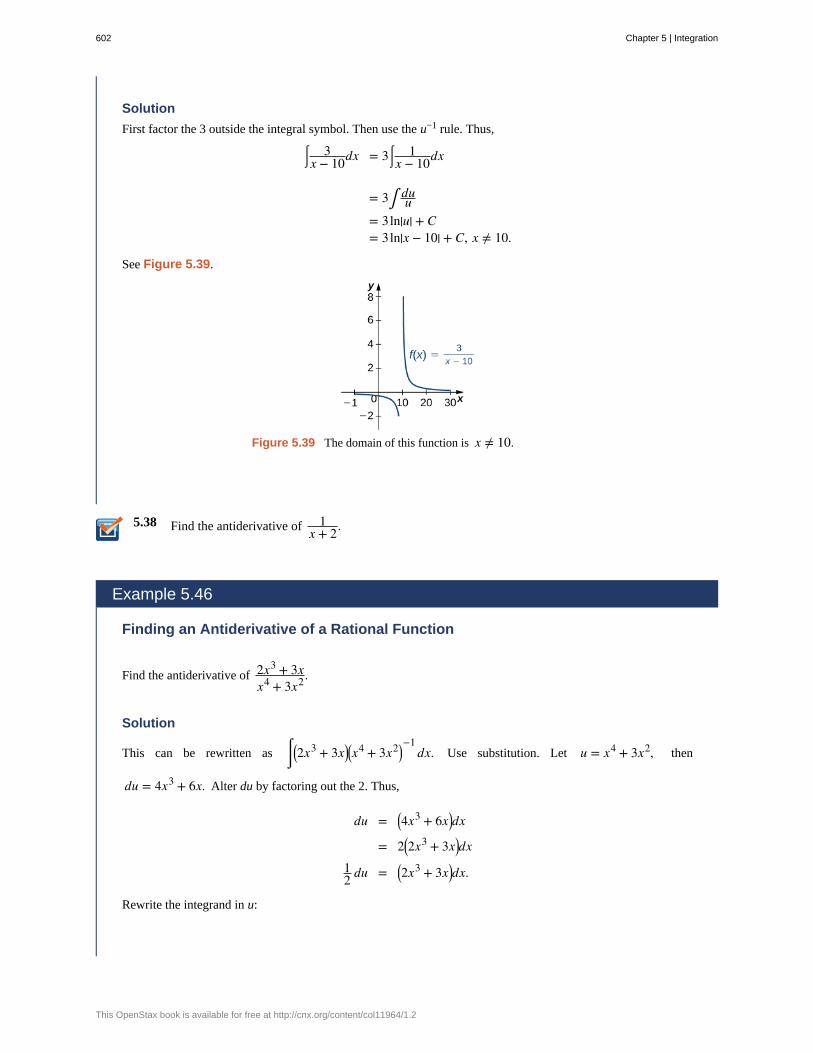
5.38
Solution
First factor the 3 outside the integral symbol. Then use the u−1 rule. Thus,
⌠⌡
3x − 10dx = 3⌠
⌡1
x − 10dx
= 3∫ duu
= 3ln|u| + C= 3ln|x − 10| + C, x ≠ 10.
See Figure 5.39.
Figure 5.39 The domain of this function is x ≠ 10.
Find the antiderivative of 1x + 2.
Example 5.46
Finding an Antiderivative of a Rational Function
Find the antiderivative of 2x3 + 3xx4 + 3x2 .
Solution
This can be rewritten as ⌠⌡
⎛⎝2x3 + 3x⎞
⎠⎛⎝x4 + 3x2⎞
⎠−1
dx. Use substitution. Let u = x4 + 3x2, then
du = 4x3 + 6x. Alter du by factoring out the 2. Thus,
du = ⎛⎝4x3 + 6x⎞
⎠dx
= 2⎛⎝2x3 + 3x⎞
⎠dx12 du = ⎛
⎝2x3 + 3x⎞⎠dx.
Rewrite the integrand in u:
602 Chapter 5 | Integration
This OpenStax book is available for free at http://cnx.org/content/col11964/1.2
5.39
⌠⌡
⎛⎝2x3 + 3x⎞
⎠⎛⎝x4 + 3x2⎞
⎠−1
dx = 12∫ u−1du.
Then we have
12∫ u−1 du = 1
2ln|u| + C
= 12ln|x4 + 3x2| + C.
Example 5.47
Finding an Antiderivative of a Logarithmic Function
Find the antiderivative of the log function log2 x.
Solution
Follow the format in the formula listed in the rule on integration formulas involving logarithmic functions. Basedon this format, we have
∫ log2 xdx = xln2(lnx − 1) + C.
Find the antiderivative of log3 x.
Example 5.48 is a definite integral of a trigonometric function. With trigonometric functions, we often have to apply atrigonometric property or an identity before we can move forward. Finding the right form of the integrand is usually the keyto a smooth integration.
Example 5.48
Evaluating a Definite Integral
Find the definite integral of ⌠⌡0
π/2sinx
1 + cosxdx.
Solution
We need substitution to evaluate this problem. Let u = 1 + cosx, , so du = −sinx dx. Rewrite the integral in
terms of u, changing the limits of integration as well. Thus,
u = 1 + cos(0) = 2u = 1 + cos⎛
⎝π2
⎞⎠ = 1.
Chapter 5 | Integration 603
Then
⌠⌡0
π/2sinx
1 + cosx = −∫2
1u−1 du
= ∫1
2u−1 du
= ln|u||12= [ln2 − ln1]= ln2.
604 Chapter 5 | Integration
This OpenStax book is available for free at http://cnx.org/content/col11964/1.2
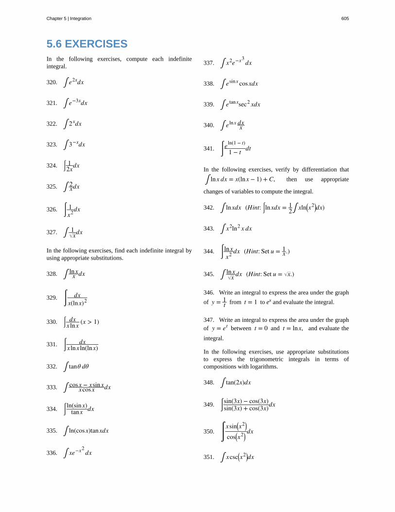
5.6 EXERCISESIn the following exercises, compute each indefiniteintegral.
320. ∫ e2xdx
321. ∫ e−3xdx
322. ∫ 2xdx
323. ∫ 3−xdx
324. ⌠⌡
12xdx
325. ∫ 2xdx
326. ⌠⌡
1x2dx
327. ∫ 1xdx
In the following exercises, find each indefinite integral byusing appropriate substitutions.
328. ∫ lnxx dx
329. ⌠⌡
dxx(lnx)2
330. ⌠⌡
dxx lnx (x > 1)
331. ⌠⌡
dxx lnx ln(lnx)
332. ∫ tanθ dθ
333. ∫ cosx − xsinxxcosx dx
334. ⌠⌡
ln(sinx)tanx dx
335. ∫ ln(cosx)tanxdx
336. ∫ xe−x2dx
337. ∫ x2e−x3dx
338. ∫ esinx cosxdx
339. ∫ etanxsec2 xdx
340. ∫ elnx dxx
341. ⌠⌡
eln(1 − t)
1 − t dt
In the following exercises, verify by differentiation that
∫ lnx dx = x(lnx − 1) + C, then use appropriate
changes of variables to compute the integral.
342. ∫ lnxdx (Hint: ⌠⌡lnxdx = 1
2∫ xln⎛⎝x2⎞
⎠dx)
343. ∫ x2ln2 x dx
344. ⌠⌡
lnxx2 dx (Hint: Set u = 1
x .)
345. ∫ lnxx dx (Hint: Set u = x.)
346. Write an integral to express the area under the graph
of y = 1t from t = 1 to ex and evaluate the integral.
347. Write an integral to express the area under the graphof y = et between t = 0 and t = lnx, and evaluate the
integral.
In the following exercises, use appropriate substitutionsto express the trigonometric integrals in terms ofcompositions with logarithms.
348. ∫ tan(2x)dx
349. ⌠⌡
sin(3x) − cos(3x)sin(3x) + cos(3x)dx
350. ⌠⌡
xsin⎛⎝x2⎞
⎠
cos⎛⎝x2⎞
⎠dx
351. ∫ xcsc⎛⎝x2⎞
⎠dx
Chapter 5 | Integration 605
352. ∫ ln(cosx)tanx dx
353. ∫ ln(cscx)cot xdx
354. ⌠⌡
ex − e−x
ex + e−xdx
In the following exercises, evaluate the definite integral.
355. ⌠⌡1
21 + 2x + x2
3x + 3x2 + x3dx
356. ∫0
π/4tanx dx
357. ⌠⌡0
π/3sinx − cosxsinx + cosxdx
358. ∫π/6
π/2cscxdx
359. ∫π/4
π/3cot xdx
In the following exercises, integrate using the indicatedsubstitution.
360. ∫ xx − 100dx; u = x − 100
361. ⌠⌡
y − 1y + 1dy; u = y + 1
362. ⌠⌡
1 − x2
3x − x3dx; u = 3x − x3
363. ⌠⌡sinx + cosxsinx − cosxdx; u = sinx − cosx
364. ∫ e2x 1 − e2xdx; u = e2x
365. ⌠⌡
ln(x) 1 − (lnx)2x dx; u = lnx
In the following exercises, does the right-endpointapproximation overestimate or underestimate the exactarea? Calculate the right endpoint estimate R50 and solvefor the exact area.
366. [T] y = ex over [0, 1]
367. [T] y = e−x over [0, 1]
368. [T] y = ln(x) over [1, 2]
369. [T] y = x + 1x2 + 2x + 6
over [0, 1]
370. [T] y = 2x over [−1, 0]
371. [T] y = −2−x over [0, 1]
In the following exercises, f (x) ≥ 0 for a ≤ x ≤ b. Find
the area under the graph of f (x) between the given values
a and b by integrating.
372. f (x) = log10 (x)x ; a = 10, b = 100
373. f (x) = log2 (x)x ; a = 32, b = 64
374. f (x) = 2−x; a = 1, b = 2
375. f (x) = 2−x; a = 3, b = 4
376. Find the area under the graph of the function
f (x) = xe−x2between x = 0 and x = 5.
377. Compute the integral of f (x) = xe−x2and find the
smallest value of N such that the area under the graph
f (x) = xe−x2between x = N and x = N + 10 is, at
most, 0.01.
378. Find the limit, as N tends to infinity, of the area under
the graph of f (x) = xe−x2between x = 0 and x = 5.
379. Show that ∫a
bdtt = ∫
1/b
1/adtt when 0 < a ≤ b.
380. Suppose that f (x) > 0 for all x and that f and g are
differentiable. Use the identity f g = eg ln fand the chain
rule to find the derivative of f g.
381. Use the previous exercise to find the antiderivative of
h(x) = xx (1 + lnx) and evaluate ∫2
3xx (1 + lnx)dx.
382. Show that if c > 0, then the integral of 1/x from
ac to bc (0 < a < b) is the same as the integral of 1/xfrom a to b.
The following exercises are intended to derive thefundamental properties of the natural log starting from the
606 Chapter 5 | Integration
This OpenStax book is available for free at http://cnx.org/content/col11964/1.2
definition ln(x) = ∫1
xdtt , using properties of the definite
integral and making no further assumptions.
383. Use the identity ln(x) = ∫1
xdtt to derive the identity
ln⎛⎝1x
⎞⎠ = −ln x.
384. Use a change of variable in the integral ∫1
xy1t dt to
show that lnxy = lnx + lny for x, y > 0.
385. Use the identity lnx = ∫1
xdtx to show that ln(x)
is an increasing function of x on [0, ∞), and use the
previous exercises to show that the range of ln(x) is
(−∞, ∞). Without any further assumptions, conclude that
ln(x) has an inverse function defined on (−∞, ∞).
386. Pretend, for the moment, that we do not know thatex is the inverse function of ln(x), but keep in mind
that ln(x) has an inverse function defined on (−∞, ∞).Call it E. Use the identity lnxy = lnx + lny to deduce that
E(a + b) = E(a)E(b) for any real numbers a, b.
387. Pretend, for the moment, that we do not know thatex is the inverse function of lnx, but keep in mind that
lnx has an inverse function defined on (−∞, ∞). Call it
E. Show that E '(t) = E(t).
388. The sine integral, defined as S(x) = ∫0
xsin tt dt is
an important quantity in engineering. Although it does nothave a simple closed formula, it is possible to estimateits behavior for large x. Show that for
k ≥ 1, |S(2πk) − S⎛⎝2π(k + 1)⎞
⎠| ≤ 1k(2k + 1)π .
(Hint: sin(t + π) = −sin t)
389. [T] The normal distribution in probability is given
by p(x) = 1σ 2π
e−(x − µ)2 /2σ2, where σ is the standard
deviation and μ is the average. The standard normaldistribution in probability, ps, corresponds to
µ = 0 and σ = 1. Compute the left endpoint estimates
R10 and R100 of ⌠⌡−1
112π
e−x2/2dx.
390. [T] Compute the right endpoint estimates
R50 and R100 of ⌠⌡−3
51
2 2πe−(x − 1)2 /8.
Chapter 5 | Integration 607
5.7 | Integrals Resulting in Inverse Trigonometric
Functions
Learning Objectives5.7.1 Integrate functions resulting in inverse trigonometric functions
In this section we focus on integrals that result in inverse trigonometric functions. We have worked with these functionsbefore. Recall from Functions and Graphs that trigonometric functions are not one-to-one unless the domains arerestricted. When working with inverses of trigonometric functions, we always need to be careful to take these restrictionsinto account. Also in Derivatives, we developed formulas for derivatives of inverse trigonometric functions. The formulasdeveloped there give rise directly to integration formulas involving inverse trigonometric functions.
Integrals that Result in Inverse Sine FunctionsLet us begin this last section of the chapter with the three formulas. Along with these formulas, we use substitution toevaluate the integrals. We prove the formula for the inverse sine integral.
Rule: Integration Formulas Resulting in Inverse Trigonometric Functions
The following integration formulas yield inverse trigonometric functions:
1.
(5.23)⌠⌡
dua2 − u2
= sin−1 ua + C
2.
(5.24)⌠⌡
dua2 + u2 = 1
a tan−1 ua + C
3.
(5.25)⌠⌡
duu u2 − a2
= 1asec−1 u
a + C
Proof
Let y = sin−1 xa. Then asiny = x. Now let’s use implicit differentiation. We obtain
ddx
⎛⎝asiny⎞
⎠ = ddx (x)
acosy dydx = 1
dydx = 1
acosy.
For −π2 ≤ y ≤ π
2, cosy ≥ 0. Thus, applying the Pythagorean identity sin2 y + cos2 y = 1, we have
cosy = 1 = sin2 y. This gives
608 Chapter 5 | Integration
This OpenStax book is available for free at http://cnx.org/content/col11964/1.2
5.40
1acosy = 1
a 1 − sin2 y
= 1a2 − a2 sin2 y
= 1a2 − x2
.
Then for −a ≤ x ≤ a, we have
⌠⌡
1a2 − u2
du = sin−1⎛⎝ua
⎞⎠ + C.
□
Example 5.49
Evaluating a Definite Integral Using Inverse Trigonometric Functions
Evaluate the definite integral ⌠⌡0
1dx
1 − x2.
Solution
We can go directly to the formula for the antiderivative in the rule on integration formulas resulting in inversetrigonometric functions, and then evaluate the definite integral. We have
⌠⌡0
1dx
1 − x2= sin−1 x|0
1
= sin−1 1 − sin−1 0= π
2 − 0
= π2.
Find the antiderivative of ⌠⌡
dx1 − 16x2
.
Example 5.50
Finding an Antiderivative Involving an Inverse Trigonometric Function
Evaluate the integral ⌠⌡
dx4 − 9x2
.
Solution
Chapter 5 | Integration 609
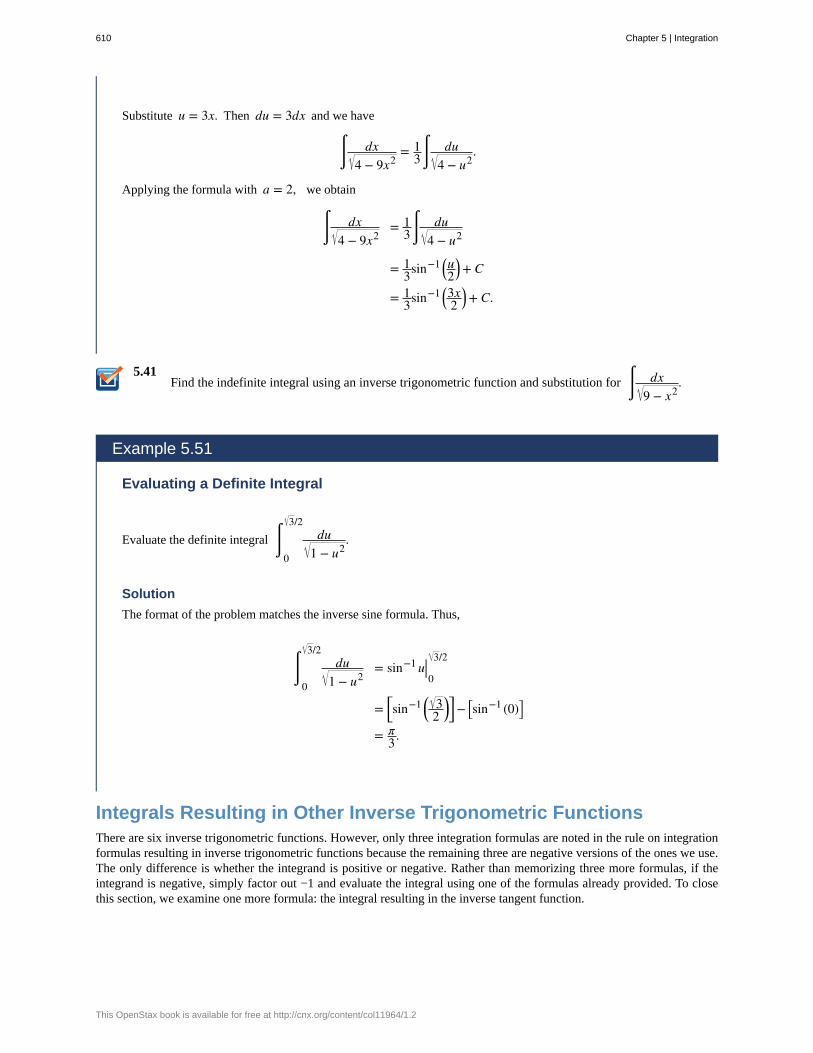
5.41
Substitute u = 3x. Then du = 3dx and we have
⌠⌡
dx4 − 9x2
= 13⌠⌡
du4 − u2
.
Applying the formula with a = 2, we obtain
⌠⌡
dx4 − 9x2
= 13⌠⌡
du4 − u2
= 13sin−1 ⎛
⎝u2
⎞⎠ + C
= 13sin−1 ⎛
⎝3x2
⎞⎠ + C.
Find the indefinite integral using an inverse trigonometric function and substitution for ⌠⌡
dx9 − x2
.
Example 5.51
Evaluating a Definite Integral
Evaluate the definite integral ⌠⌡0
3/2du
1 − u2.
Solution
The format of the problem matches the inverse sine formula. Thus,
⌠⌡0
3/2du
1 − u2= sin−1 u|0
3/2
= ⎡⎣sin−1 ⎛
⎝32
⎞⎠⎤⎦ − ⎡
⎣sin−1 (0)⎤⎦
= π3.
Integrals Resulting in Other Inverse Trigonometric FunctionsThere are six inverse trigonometric functions. However, only three integration formulas are noted in the rule on integrationformulas resulting in inverse trigonometric functions because the remaining three are negative versions of the ones we use.The only difference is whether the integrand is positive or negative. Rather than memorizing three more formulas, if theintegrand is negative, simply factor out −1 and evaluate the integral using one of the formulas already provided. To closethis section, we examine one more formula: the integral resulting in the inverse tangent function.
610 Chapter 5 | Integration
This OpenStax book is available for free at http://cnx.org/content/col11964/1.2
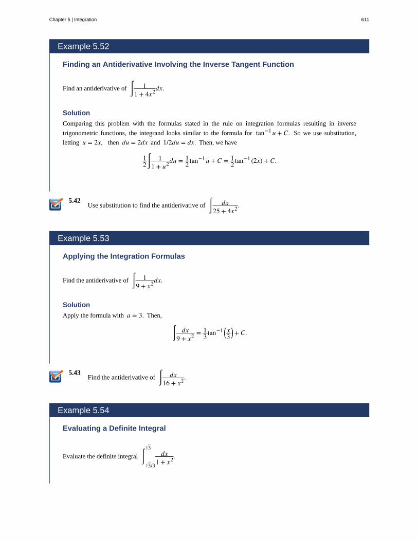
5.42
5.43
Example 5.52
Finding an Antiderivative Involving the Inverse Tangent Function
Find an antiderivative of ⌠⌡
11 + 4x2dx.
Solution
Comparing this problem with the formulas stated in the rule on integration formulas resulting in inverse
trigonometric functions, the integrand looks similar to the formula for tan−1 u + C. So we use substitution,
letting u = 2x, then du = 2dx and 1/2du = dx. Then, we have
12
⌠⌡
11 + u2du = 1
2tan−1 u + C = 12tan−1 (2x) + C.
Use substitution to find the antiderivative of ⌠⌡
dx25 + 4x2.
Example 5.53
Applying the Integration Formulas
Find the antiderivative of ⌠⌡
19 + x2dx.
Solution
Apply the formula with a = 3. Then,
⌠⌡
dx9 + x2 = 1
3tan−1 ⎛⎝x3
⎞⎠ + C.
Find the antiderivative of ⌠⌡
dx16 + x2.
Example 5.54
Evaluating a Definite Integral
Evaluate the definite integral ⌠⌡ 3/3
3dx
1 + x2.
Chapter 5 | Integration 611
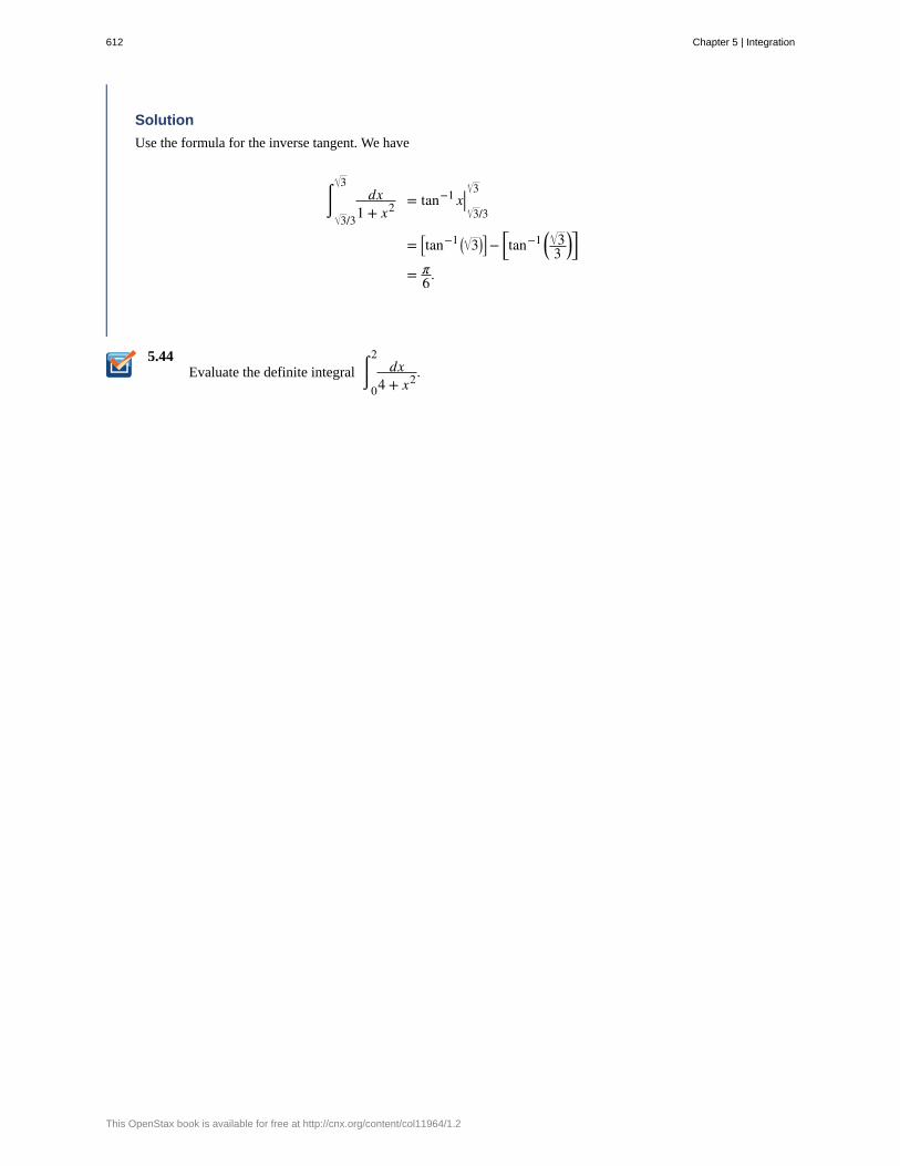
5.44
Solution
Use the formula for the inverse tangent. We have
⌠⌡ 3/3
3dx
1 + x2 = tan−1 x| 3/3
3
= ⎡⎣tan−1 ⎛
⎝ 3⎞⎠⎤⎦ − ⎡
⎣tan−1 ⎛⎝
33
⎞⎠⎤⎦
= π6.
Evaluate the definite integral ⌠⌡0
2dx
4 + x2.
612 Chapter 5 | Integration
This OpenStax book is available for free at http://cnx.org/content/col11964/1.2
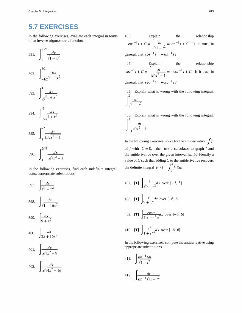
5.7 EXERCISESIn the following exercises, evaluate each integral in termsof an inverse trigonometric function.
391. ⌠⌡0
3/2dx
1 − x2
392. ⌠⌡−1/2
1/2dx
1 − x2
393. ⌠⌡ 3
1dx
1 + x2
394. ⌠⌡1/ 3
3dx
1 + x2
395. ⌠⌡1
2dx
|x| x2 − 1
396. ⌠⌡1
2/ 3dx
|x| x2 − 1
In the following exercises, find each indefinite integral,using appropriate substitutions.
397. ⌠⌡
dx9 − x2
398. ⌠⌡
dx1 − 16x2
399. ⌠⌡
dx9 + x2
400. ⌠⌡
dx25 + 16x2
401. ⌠⌡
dx|x| x2 − 9
402. ⌠⌡
dx|x| 4x2 − 16
403. Explain the relationship
−cos−1 t + C = ⌠⌡
dt1 − t2
= sin−1 t + C. Is it true, in
general, that cos−1 t = −sin−1 t ?
404. Explain the relationship
sec−1 t + C = ⌠⌡
dt|t| t2 − 1
= −csc−1 t + C. Is it true, in
general, that sec−1 t = −csc−1 t ?
405. Explain what is wrong with the following integral:
⌠⌡1
2dt
1 − t2.
406. Explain what is wrong with the following integral:
⌠⌡−1
1dt
|t| t2 − 1.
In the following exercises, solve for the antiderivative ∫ f
of f with C = 0, then use a calculator to graph f and
the antiderivative over the given interval ⎡⎣a, b⎤
⎦. Identify a
value of C such that adding C to the antiderivative recovers
the definite integral F(x) = ∫a
xf (t)dt.
407. [T] ⌠⌡
19 − x2
dx over [−3, 3]
408. [T] ⌠⌡
99 + x2dx over ⎡
⎣−6, 6⎤⎦
409. [T] ⌠⌡
cosx4 + sin2 x
dx over ⎡⎣−6, 6⎤
⎦
410. [T] ⌠⌡
ex
1 + e2xdx over ⎡⎣−6, 6⎤
⎦
In the following exercises, compute the antiderivative usingappropriate substitutions.
411. ⌠⌡
sin−1 tdt1 − t2
412. ⌠⌡
dtsin−1 t 1 − t2
Chapter 5 | Integration 613
413. ⌠⌡
tan−1 (2t)1 + 4t2 dt
414. ⌠⌡
ttan−1 ⎛⎝t2⎞
⎠
1 + t4 dt
415. ⌠⌡
sec−1 ⎛⎝
t2
⎞⎠
|t| t2 − 4dt
416. ⌠⌡
tsec−1 ⎛⎝t2⎞
⎠
t2 t4 − 1dt
In the following exercises, use a calculator to graph the
antiderivative ∫ f with C = 0 over the given interval
⎡⎣a, b⎤
⎦. Approximate a value of C, if possible, such that
adding C to the antiderivative gives the same value as the
definite integral F(x) = ∫a
xf (t)dt.
417. [T] ⌠⌡
1x x2 − 4
dx over ⎡⎣2, 6⎤
⎦
418. [T] ⌠⌡
1(2x + 2) xdx over ⎡
⎣0, 6⎤⎦
419. [T] ⌠⌡
(sinx + xcosx)1 + x2 sin2 x
dx over ⎡⎣−6, 6⎤
⎦
420. [T] ⌠⌡
2e−2x
1 − e−4xdx over [0, 2]
421. [T] ⌠⌡
1x + xln2 x
over [0, 2]
422. [T] ⌠⌡
sin−1 x1 − x2
over [−1, 1]
In the following exercises, compute each integral usingappropriate substitutions.
423. ⌠⌡
ex
1 − e2tdt
424. ⌠⌡
et
1 + e2tdt
425. ⌠⌡
dtt 1 − ln2 t
426. ⌠⌡
dtt⎛⎝1 + ln2 t⎞
⎠
427. ⌠⌡
cos−1 (2t)1 − 4t2
dt
428. ⌠⌡
et cos−1 ⎛⎝et⎞
⎠
1 − e2tdt
In the following exercises, compute each definite integral.
429. ⌠⌡0
1/2tan⎛
⎝sin−1 t⎞⎠
1 − t2dt
430. ⌠⌡1/4
1/2tan⎛
⎝cos−1 t⎞⎠
1 − t2dt
431. ⌠⌡0
1/2sin⎛
⎝tan−1 t⎞⎠
1 + t2 dt
432. ⌠⌡0
1/2cos⎛
⎝tan−1 t⎞⎠
1 + t2 dt
433. For A > 0, compute I(A) = ⌠⌡−A
Adt
1 + t2 and
evaluate lima → ∞I(A), the area under the graph of 11 + t2
on [−∞, ∞].
434. For 1 < B < ∞, compute I(B) = ⌠⌡1
Bdt
t t2 − 1and
evaluate limB → ∞
I(B), the area under the graph of
1t t2 − 1
over [1, ∞).
435. Use the substitution u = 2 cot x and the identity
1 + cot2 x = csc2 x to evaluate ⌠⌡
dx1 + cos2 x
. (Hint:
Multiply the top and bottom of the integrand by csc2 x.)
614 Chapter 5 | Integration
This OpenStax book is available for free at http://cnx.org/content/col11964/1.2
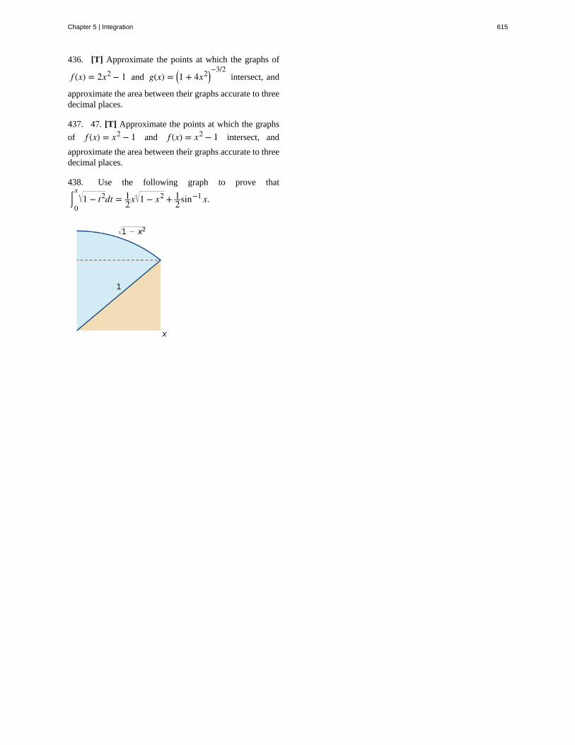
436. [T] Approximate the points at which the graphs of
f (x) = 2x2 − 1 and g(x) = ⎛⎝1 + 4x2⎞
⎠−3/2
intersect, and
approximate the area between their graphs accurate to threedecimal places.
437. 47. [T] Approximate the points at which the graphs
of f (x) = x2 − 1 and f (x) = x2 − 1 intersect, and
approximate the area between their graphs accurate to threedecimal places.
438. Use the following graph to prove that
⌠⌡0
x1 − t2dt = 1
2x 1 − x2 + 12sin−1 x.
Chapter 5 | Integration 615
average value of a function
change of variables
definite integral
fundamental theorem of calculus
fundamental theorem of calculus, part 1
fundamental theorem of calculus, part 2
integrable function
integrand
integration by substitution
left-endpoint approximation
limits of integration
lower sum
mean value theorem for integrals
net change theorem
net signed area
partition
regular partition
riemann sum
right-endpoint approximation
sigma notation
total area
upper sum
variable of integration
CHAPTER 5 REVIEW
KEY TERMS(or fave) the average value of a function on an interval can be found by calculating the
definite integral of the function and dividing that value by the length of the interval
the substitution of a variable, such as u, for an expression in the integrand
a primary operation of calculus; the area between the curve and the x-axis over a given interval is adefinite integral
the theorem, central to the entire development of calculus, that establishes therelationship between differentiation and integration
uses a definite integral to define an antiderivative of a function
(also, evaluation theorem) we can evaluate a definite integral byevaluating the antiderivative of the integrand at the endpoints of the interval and subtracting
a function is integrable if the limit defining the integral exists; in other words, if the limit of theRiemann sums as n goes to infinity exists
the function to the right of the integration symbol; the integrand includes the function being integrated
a technique for integration that allows integration of functions that are the result of achain-rule derivative
an approximation of the area under a curve computed by using the left endpoint of eachsubinterval to calculate the height of the vertical sides of each rectangle
these values appear near the top and bottom of the integral sign and define the interval over whichthe function should be integrated
a sum obtained by using the minimum value of f (x) on each subinterval
guarantees that a point c exists such that f (c) is equal to the average value of the
function
if we know the rate of change of a quantity, the net change theorem says the future quantity isequal to the initial quantity plus the integral of the rate of change of the quantity
the area between a function and the x-axis such that the area below the x-axis is subtracted from the areaabove the x-axis; the result is the same as the definite integral of the function
a set of points that divides an interval into subintervals
a partition in which the subintervals all have the same width
an estimate of the area under the curve of the form A ≈ ∑i = 1
nf (xi* )Δx
the right-endpoint approximation is an approximation of the area of the rectanglesunder a curve using the right endpoint of each subinterval to construct the vertical sides of each rectangle
(also, summation notation) the Greek letter sigma (Σ) indicates addition of the values; the values of theindex above and below the sigma indicate where to begin the summation and where to end it
total area between a function and the x-axis is calculated by adding the area above the x-axis and the areabelow the x-axis; the result is the same as the definite integral of the absolute value of the function
a sum obtained by using the maximum value of f (x) on each subinterval
indicates which variable you are integrating with respect to; if it is x, then the function in theintegrand is followed by dx
616 Chapter 5 | Integration
This OpenStax book is available for free at http://cnx.org/content/col11964/1.2
KEY EQUATIONS• Properties of Sigma Notation
∑i = 1
nc = nc
∑i = 1
ncai = c ∑
i = 1
nai
∑i = 1
n⎛⎝ai + bi
⎞⎠ = ∑
i = 1
nai + ∑
i = 1
nbi
∑i = 1
n⎛⎝ai − bi
⎞⎠ = ∑
i = 1
nai − ∑
i = 1
nbi
∑i = 1
nai = ∑
i = 1
mai + ∑
i = m + 1
nai
• Sums and Powers of Integers
∑i = 1
ni = 1 + 2 + ⋯ + n = n(n + 1)
2
∑i = 1
ni2 = 12 + 22 + ⋯ + n2 = n(n + 1)(2n + 1)
6
∑i = 0
ni3 = 13 + 23 + ⋯ + n3 = n2 (n + 1)2
4
• Left-Endpoint Approximation
A ≈ Ln = f (x0)Δx + f (x1)Δx + ⋯ + f (xn − 1)Δx = ∑i = 1
nf (xi − 1)Δx
• Right-Endpoint Approximation
A ≈ Rn = f (x1)Δx + f (x2)Δx + ⋯ + f (xn)Δx = ∑i = 1
nf (xi)Δx
• Definite Integral
∫a
bf (x)dx = limn → ∞ ∑
i = 1
nf ⎛
⎝xi*⎞⎠Δx
• Properties of the Definite Integral
∫a
af (x)dx = 0
∫b
af (x)dx = −∫
a
bf (x)dx
∫a
b⎡⎣ f (x) + g(x)⎤
⎦dx = ∫a
bf (x)dx + ∫
a
bg(x)dx
⌠⌡a
b⎡⎣ f (x) − g(x)⎤
⎦dx = ⌠⌡a
b
f (x)dx − ∫a
bg(x)dx
∫a
bc f (x)dx = c∫
a
bf (x) for constant c
∫a
bf (x)dx = ∫
a
cf (x)dx + ∫
c
bf (x)dx
• Mean Value Theorem for Integrals
Chapter 5 | Integration 617
If f (x) is continuous over an interval ⎡⎣a, b⎤
⎦, then there is at least one point c ∈ ⎡⎣a, b⎤
⎦ such that
f (c) = 1b − a∫
a
bf (x)dx.
• Fundamental Theorem of Calculus Part 1
If f (x) is continuous over an interval ⎡⎣a, b⎤
⎦, and the function F(x) is defined by F(x) = ∫a
xf (t)dt, then
F′ (x) = f (x).
• Fundamental Theorem of Calculus Part 2
If f is continuous over the interval ⎡⎣a, b⎤
⎦ and F(x) is any antiderivative of f (x), then ∫a
bf (x)dx = F(b) − F(a).
• Net Change Theorem
F(b) = F(a) + ∫a
bF '(x)dx or ∫
a
bF '(x)dx = F(b) − F(a)
• Substitution with Indefinite Integrals
∫ f ⎡⎣g(x)⎤
⎦g′ (x)dx = ∫ f (u)du = F(u) + C = F⎛⎝g(x)⎞
⎠ + C
• Substitution with Definite Integrals
⌠⌡a
b
f ⎛⎝g(x)⎞
⎠g '(x)dx = ∫g(a)
g(b)f (u)du
• Integrals of Exponential Functions
∫ ex dx = ex + C
⌠⌡ax dx = ax
lna + C
• Integration Formulas Involving Logarithmic Functions
∫ x−1 dx = ln|x| + C
∫ lnx dx = x lnx − x + C = x(lnx − 1) + C
∫ loga x dx = xlna(lnx − 1) + C
• Integrals That Produce Inverse Trigonometric Functions
⌠⌡
dua2 − u2
= sin−1 ⎛⎝ua
⎞⎠ + C
⌠⌡
dua2 + u2 = 1
a tan−1 ⎛⎝ua
⎞⎠ + C
⌠⌡
duu u2 − a2
= 1asec−1 ⎛
⎝ua
⎞⎠ + C
KEY CONCEPTS
5.1 Approximating Areas
• The use of sigma (summation) notation of the form ∑i = 1
nai is useful for expressing long sums of values in compact
form.
618 Chapter 5 | Integration
This OpenStax book is available for free at http://cnx.org/content/col11964/1.2
• For a continuous function defined over an interval ⎡⎣a, b⎤
⎦, the process of dividing the interval into n equal parts,
extending a rectangle to the graph of the function, calculating the areas of the series of rectangles, and then summingthe areas yields an approximation of the area of that region.
• The width of each rectangle is Δx = b − an .
• Riemann sums are expressions of the form ∑i = 1
nf ⎛
⎝xi*⎞⎠Δx, and can be used to estimate the area under the curve
y = f (x). Left- and right-endpoint approximations are special kinds of Riemann sums where the values of⎧
⎩⎨xi*
⎫
⎭⎬
are chosen to be the left or right endpoints of the subintervals, respectively.
• Riemann sums allow for much flexibility in choosing the set of points⎧
⎩⎨xi*
⎫
⎭⎬ at which the function is evaluated,
often with an eye to obtaining a lower sum or an upper sum.
5.2 The Definite Integral
• The definite integral can be used to calculate net signed area, which is the area above the x-axis less the area belowthe x-axis. Net signed area can be positive, negative, or zero.
• The component parts of the definite integral are the integrand, the variable of integration, and the limits ofintegration.
• Continuous functions on a closed interval are integrable. Functions that are not continuous may still be integrable,depending on the nature of the discontinuities.
• The properties of definite integrals can be used to evaluate integrals.
• The area under the curve of many functions can be calculated using geometric formulas.
• The average value of a function can be calculated using definite integrals.
5.3 The Fundamental Theorem of Calculus
• The Mean Value Theorem for Integrals states that for a continuous function over a closed interval, there is a value csuch that f (c) equals the average value of the function. See The Mean Value Theorem for Integrals.
• The Fundamental Theorem of Calculus, Part 1 shows the relationship between the derivative and the integral. SeeFundamental Theorem of Calculus, Part 1.
• The Fundamental Theorem of Calculus, Part 2 is a formula for evaluating a definite integral in terms of anantiderivative of its integrand. The total area under a curve can be found using this formula. See TheFundamental Theorem of Calculus, Part 2.
5.4 Integration Formulas and the Net Change Theorem
• The net change theorem states that when a quantity changes, the final value equals the initial value plus the integralof the rate of change. Net change can be a positive number, a negative number, or zero.
• The area under an even function over a symmetric interval can be calculated by doubling the area over the positivex-axis. For an odd function, the integral over a symmetric interval equals zero, because half the area is negative.
5.5 Substitution
• Substitution is a technique that simplifies the integration of functions that are the result of a chain-rule derivative.The term ‘substitution’ refers to changing variables or substituting the variable u and du for appropriate expressionsin the integrand.
• When using substitution for a definite integral, we also have to change the limits of integration.
Chapter 5 | Integration 619
5.6 Integrals Involving Exponential and Logarithmic Functions
• Exponential and logarithmic functions arise in many real-world applications, especially those involving growth anddecay.
• Substitution is often used to evaluate integrals involving exponential functions or logarithms.
5.7 Integrals Resulting in Inverse Trigonometric Functions
• Formulas for derivatives of inverse trigonometric functions developed in Derivatives of Exponential andLogarithmic Functions lead directly to integration formulas involving inverse trigonometric functions.
• Use the formulas listed in the rule on integration formulas resulting in inverse trigonometric functions to match upthe correct format and make alterations as necessary to solve the problem.
• Substitution is often required to put the integrand in the correct form.
CHAPTER 5 REVIEW EXERCISESTrue or False. Justify your answer with a proof or acounterexample. Assume all functions f and g are
continuous over their domains.
439. If f (x) > 0, f ′ (x) > 0 for all x, then the right-
hand rule underestimates the integral ∫a
bf (x). Use a graph
to justify your answer.
440. ∫a
bf (x)2 dx = ∫
a
bf (x)dx∫
a
bf (x)dx
441. If f (x) ≤ g(x) for all x ∈ ⎡⎣a, b⎤
⎦, then
∫a
bf (x) ≤ ∫
a
bg(x).
442. All continuous functions have an antiderivative.
Evaluate the Riemann sums L4 and R4 for the following
functions over the specified interval. Compare your answerwith the exact answer, when possible, or use a calculator todetermine the answer.
443. y = 3x2 − 2x + 1 over [−1, 1]
444. y = ln⎛⎝x2 + 1⎞
⎠ over [0, e]
445. y = x2 sinx over [0, π]
446. y = x + 1x over [1, 4]
Evaluate the following integrals.
447. ∫−1
1 ⎛⎝x
3 − 2x2 + 4x⎞⎠dx
448. ⌠⌡0
43t
1 + 6t2dt
449. ∫π/3
π/22sec(2θ)tan(2θ)dθ
450. ∫0
π/4ecos2 xsinxcosdx
Find the antiderivative.
451. ⌠⌡
dx(x + 4)3
452. ∫ x ln⎛⎝x2⎞
⎠dx
453. ⌠⌡
4x2
1 − x6dx
454. ⌠⌡
e2x
1 + e4xdx
Find the derivative.
455. ddt
⌠⌡0
tsinx1 + x2
dx
620 Chapter 5 | Integration
This OpenStax book is available for free at http://cnx.org/content/col11964/1.2
456. ddx∫
1
x34 − t2dt
457. ddx∫
1
ln(x)⎛⎝4t + et⎞
⎠dt
458. ddx∫
0
cosxet2
dt
The following problems consider the historic average costper gigabyte of RAM on a computer.
Year 5-Year Change ($)
1980 0
1985 −5,468,750
1990 −755,495
1995 −73,005
2000 −29,768
2005 −918
2010 −177
459. If the average cost per gigabyte of RAM in 2010 is$12, find the average cost per gigabyte of RAM in 1980.
460. The average cost per gigabyte of RAM can beapproximated by the functionC(t) = 8, 500, 000(0.65)t, where t is measured in years
since 1980, and C is cost in US$. Find the average cost per
gigabyte of RAM for 1980 to 2010.
461. Find the average cost of 1GB RAM for 2005 to2010.
462. The velocity of a bullet from a rifle can be
approximated by v(t) = 6400t2 − 6505t + 2686, where
t is seconds after the shot and v is the velocity measured
in feet per second. This equation only models the velocityfor the first half-second after the shot: 0 ≤ t ≤ 0.5. What
is the total distance the bullet travels in 0.5 sec?
463. What is the average velocity of the bullet for the firsthalf-second?
Chapter 5 | Integration 621

622 Chapter 5 | Integration
This OpenStax book is available for free at http://cnx.org/content/col11964/1.2
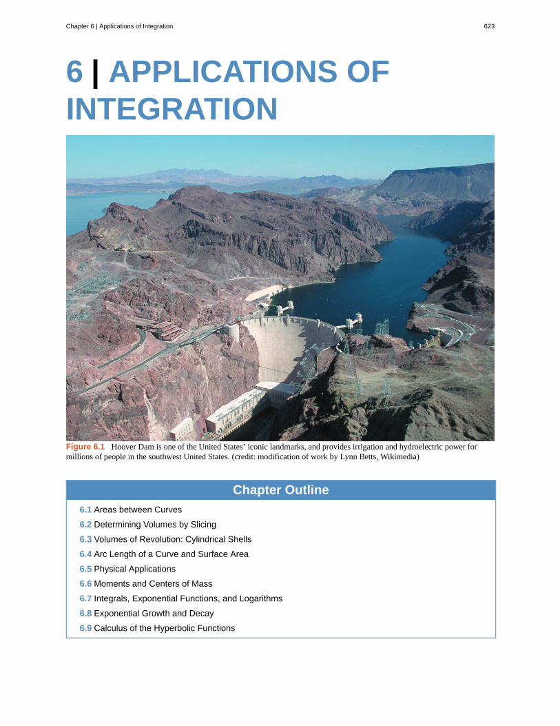
6 | APPLICATIONS OFINTEGRATION
Figure 6.1 Hoover Dam is one of the United States’ iconic landmarks, and provides irrigation and hydroelectric power formillions of people in the southwest United States. (credit: modification of work by Lynn Betts, Wikimedia)
Chapter Outline
6.1 Areas between Curves
6.2 Determining Volumes by Slicing
6.3 Volumes of Revolution: Cylindrical Shells
6.4 Arc Length of a Curve and Surface Area
6.5 Physical Applications
6.6 Moments and Centers of Mass
6.7 Integrals, Exponential Functions, and Logarithms
6.8 Exponential Growth and Decay
6.9 Calculus of the Hyperbolic Functions
Chapter 6 | Applications of Integration 623
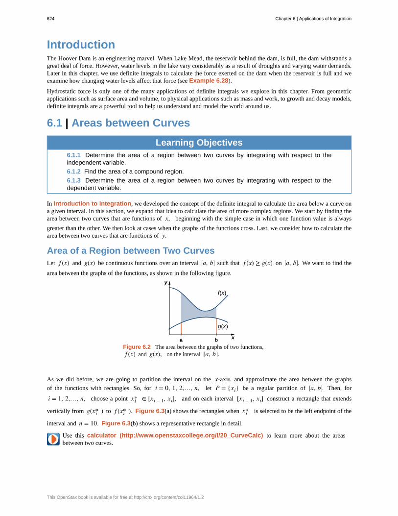
IntroductionThe Hoover Dam is an engineering marvel. When Lake Mead, the reservoir behind the dam, is full, the dam withstands agreat deal of force. However, water levels in the lake vary considerably as a result of droughts and varying water demands.Later in this chapter, we use definite integrals to calculate the force exerted on the dam when the reservoir is full and weexamine how changing water levels affect that force (see Example 6.28).
Hydrostatic force is only one of the many applications of definite integrals we explore in this chapter. From geometricapplications such as surface area and volume, to physical applications such as mass and work, to growth and decay models,definite integrals are a powerful tool to help us understand and model the world around us.
6.1 | Areas between Curves
Learning Objectives6.1.1 Determine the area of a region between two curves by integrating with respect to theindependent variable.
6.1.2 Find the area of a compound region.
6.1.3 Determine the area of a region between two curves by integrating with respect to thedependent variable.
In Introduction to Integration, we developed the concept of the definite integral to calculate the area below a curve ona given interval. In this section, we expand that idea to calculate the area of more complex regions. We start by finding thearea between two curves that are functions of x, beginning with the simple case in which one function value is always
greater than the other. We then look at cases when the graphs of the functions cross. Last, we consider how to calculate thearea between two curves that are functions of y.
Area of a Region between Two CurvesLet f (x) and g(x) be continuous functions over an interval ⎡
⎣a, b⎤⎦ such that f (x) ≥ g(x) on ⎡
⎣a, b⎤⎦. We want to find the
area between the graphs of the functions, as shown in the following figure.
Figure 6.2 The area between the graphs of two functions,f (x) and g(x), on the interval [a, b].
As we did before, we are going to partition the interval on the x-axis and approximate the area between the graphs
of the functions with rectangles. So, for i = 0, 1, 2,…, n, let P = {xi} be a regular partition of ⎡⎣a, b⎤
⎦. Then, for
i = 1, 2,…, n, choose a point xi* ∈ [xi − 1, xi], and on each interval [xi − 1, xi] construct a rectangle that extends
vertically from g(xi* ) to f (xi* ). Figure 6.3(a) shows the rectangles when xi* is selected to be the left endpoint of the
interval and n = 10. Figure 6.3(b) shows a representative rectangle in detail.
Use this calculator (http://www.openstaxcollege.org/l/20_CurveCalc) to learn more about the areasbetween two curves.
624 Chapter 6 | Applications of Integration
This OpenStax book is available for free at http://cnx.org/content/col11964/1.2
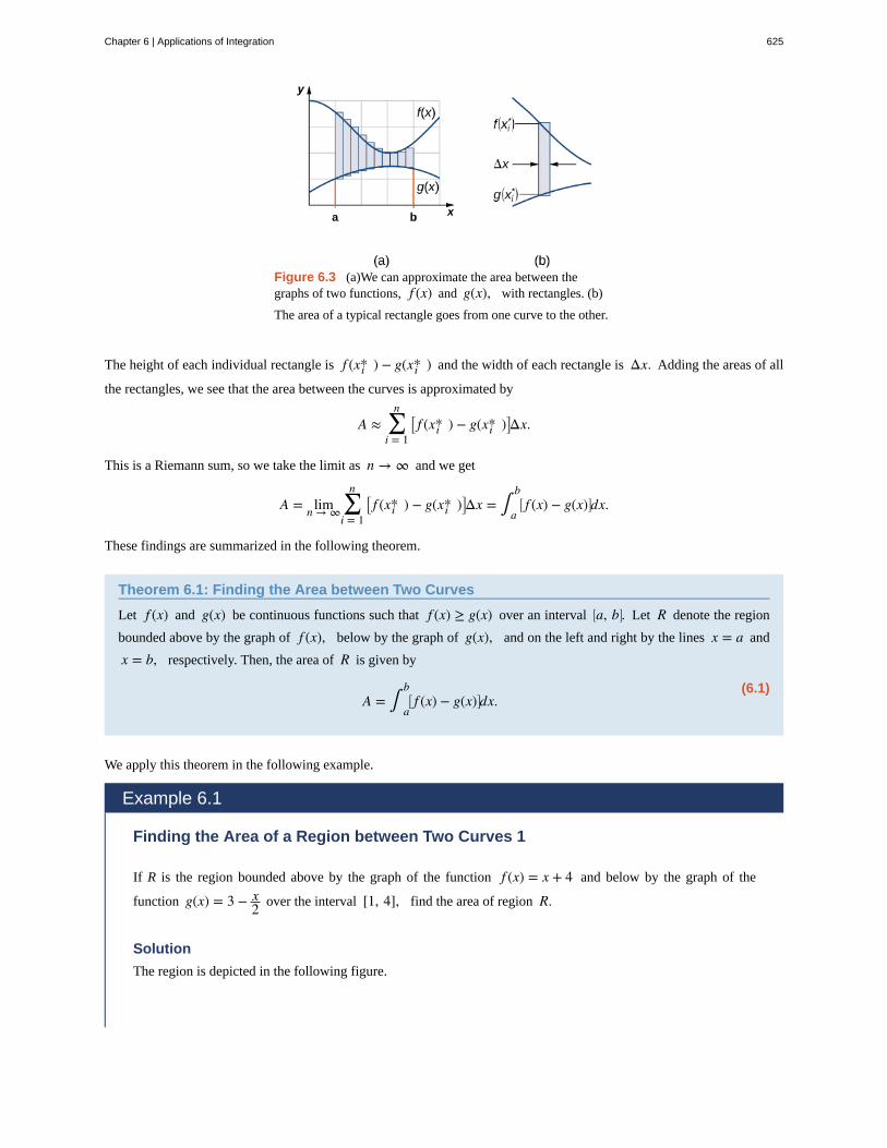
Figure 6.3 (a)We can approximate the area between thegraphs of two functions, f (x) and g(x), with rectangles. (b)
The area of a typical rectangle goes from one curve to the other.
The height of each individual rectangle is f (xi* ) − g(xi* ) and the width of each rectangle is Δx. Adding the areas of all
the rectangles, we see that the area between the curves is approximated by
A ≈ ∑i = 1
n⎡⎣ f (xi* ) − g(xi* )⎤
⎦Δx.
This is a Riemann sum, so we take the limit as n → ∞ and we get
A = limn → ∞ ∑i = 1
n⎡⎣ f (xi* ) − g(xi* )⎤
⎦Δx = ∫a
b⎡⎣ f (x) − g(x)⎤
⎦dx.
These findings are summarized in the following theorem.
Theorem 6.1: Finding the Area between Two Curves
Let f (x) and g(x) be continuous functions such that f (x) ≥ g(x) over an interval ⎡⎣a, b⎤
⎦. Let R denote the region
bounded above by the graph of f (x), below by the graph of g(x), and on the left and right by the lines x = a and
x = b, respectively. Then, the area of R is given by
(6.1)A = ∫
a
b⎡⎣ f (x) − g(x)⎤
⎦dx.
We apply this theorem in the following example.
Example 6.1
Finding the Area of a Region between Two Curves 1
If R is the region bounded above by the graph of the function f (x) = x + 4 and below by the graph of the
function g(x) = 3 − x2 over the interval [1, 4], find the area of region R.
Solution
The region is depicted in the following figure.
Chapter 6 | Applications of Integration 625
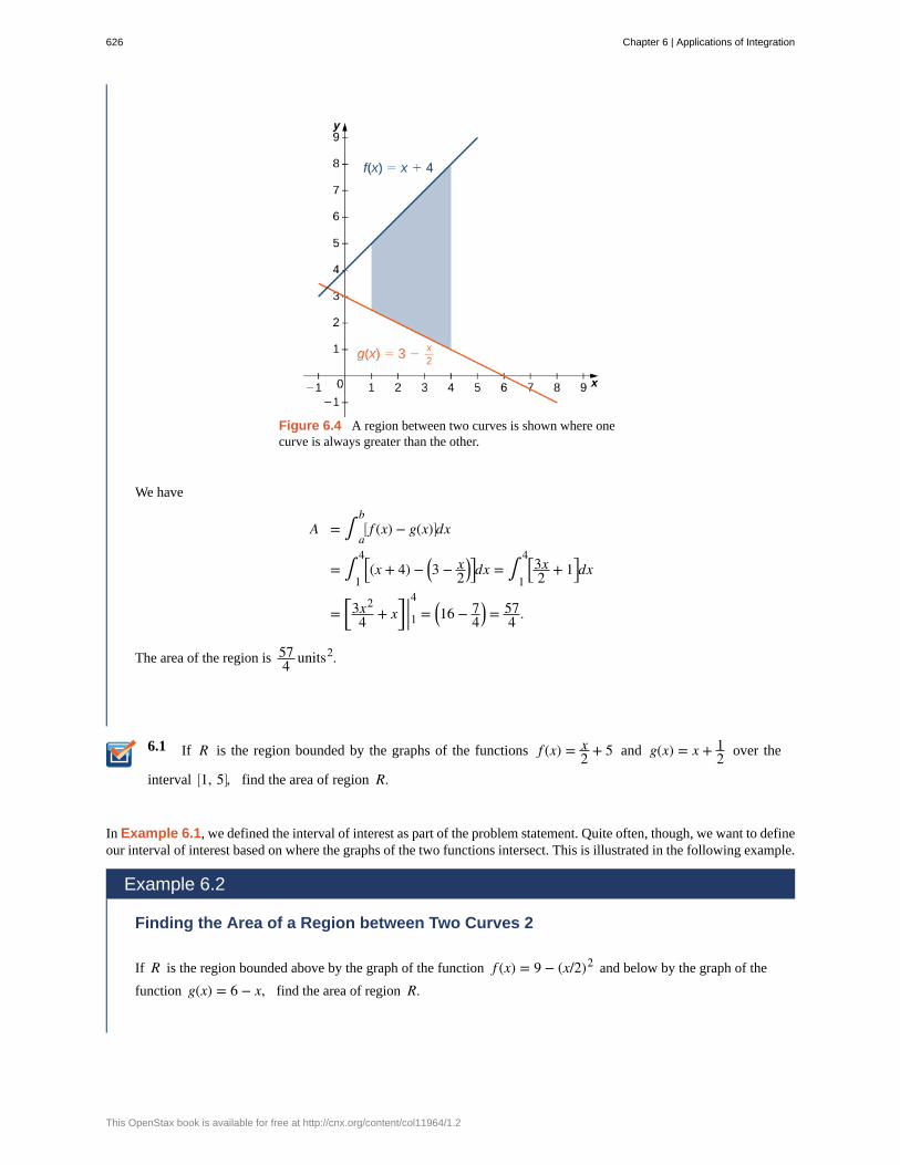
6.1
Figure 6.4 A region between two curves is shown where onecurve is always greater than the other.
We have
A = ∫a
b⎡⎣ f (x) − g(x)⎤
⎦dx
= ∫1
4⎡⎣(x + 4) − ⎛
⎝3 − x2
⎞⎠⎤⎦dx = ∫
1
4⎡⎣3x2 + 1⎤
⎦dx
= ⎡⎣
3x2
4 + x⎤⎦ |14 = ⎛
⎝16 − 74
⎞⎠ = 57
4 .
The area of the region is 574 units2.
If R is the region bounded by the graphs of the functions f (x) = x2 + 5 and g(x) = x + 1
2 over the
interval ⎡⎣1, 5⎤
⎦, find the area of region R.
In Example 6.1, we defined the interval of interest as part of the problem statement. Quite often, though, we want to defineour interval of interest based on where the graphs of the two functions intersect. This is illustrated in the following example.
Example 6.2
Finding the Area of a Region between Two Curves 2
If R is the region bounded above by the graph of the function f (x) = 9 − (x/2)2 and below by the graph of the
function g(x) = 6 − x, find the area of region R.
626 Chapter 6 | Applications of Integration
This OpenStax book is available for free at http://cnx.org/content/col11964/1.2
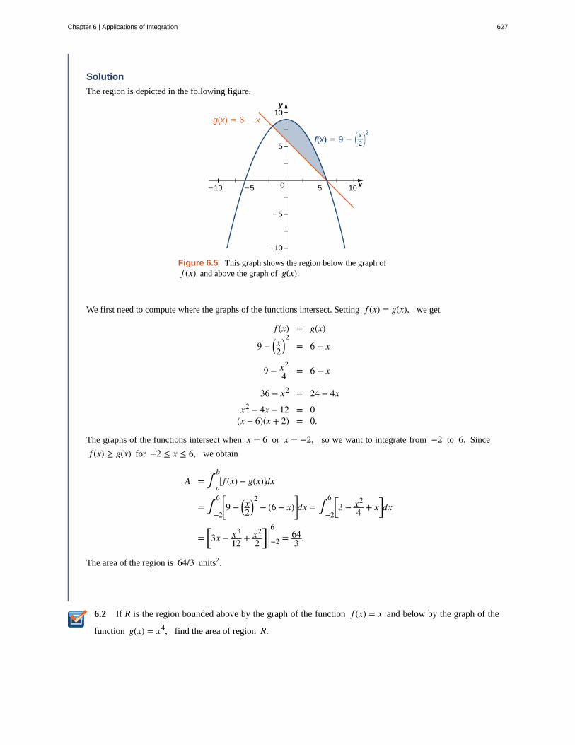
6.2
Solution
The region is depicted in the following figure.
Figure 6.5 This graph shows the region below the graph off (x) and above the graph of g(x).
We first need to compute where the graphs of the functions intersect. Setting f (x) = g(x), we get
f (x) = g(x)
9 − ⎛⎝x2
⎞⎠2
= 6 − x
9 − x2
4 = 6 − x
36 − x2 = 24 − 4x
x2 − 4x − 12 = 0(x − 6)(x + 2) = 0.
The graphs of the functions intersect when x = 6 or x = −2, so we want to integrate from −2 to 6. Since
f (x) ≥ g(x) for −2 ≤ x ≤ 6, we obtain
A = ∫a
b⎡⎣ f (x) − g(x)⎤
⎦dx
= ∫−2
6 ⎡
⎣⎢9 − ⎛
⎝x2
⎞⎠2
− (6 − x)⎤
⎦⎥dx = ∫
−2
6 ⎡⎣3 − x2
4 + x⎤⎦dx
= ⎡⎣3x − x3
12 + x2
2⎤⎦ |−2
6= 64
3 .
The area of the region is 64/3 units2.
If R is the region bounded above by the graph of the function f (x) = x and below by the graph of the
function g(x) = x4, find the area of region R.
Chapter 6 | Applications of Integration 627
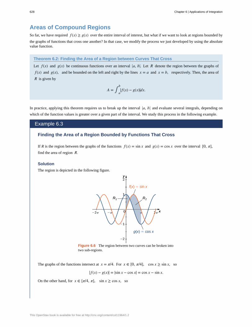
Areas of Compound RegionsSo far, we have required f (x) ≥ g(x) over the entire interval of interest, but what if we want to look at regions bounded by
the graphs of functions that cross one another? In that case, we modify the process we just developed by using the absolutevalue function.
Theorem 6.2: Finding the Area of a Region between Curves That Cross
Let f (x) and g(x) be continuous functions over an interval ⎡⎣a, b⎤
⎦. Let R denote the region between the graphs of
f (x) and g(x), and be bounded on the left and right by the lines x = a and x = b, respectively. Then, the area of
R is given by
A = ∫a
b| f (x) − g(x)|dx.
In practice, applying this theorem requires us to break up the interval ⎡⎣a, b⎤
⎦ and evaluate several integrals, depending on
which of the function values is greater over a given part of the interval. We study this process in the following example.
Example 6.3
Finding the Area of a Region Bounded by Functions That Cross
If R is the region between the graphs of the functions f (x) = sin x and g(x) = cos x over the interval [0, π],find the area of region R.
Solution
The region is depicted in the following figure.
Figure 6.6 The region between two curves can be broken intotwo sub-regions.
The graphs of the functions intersect at x = π/4. For x ∈ [0, π/4], cos x ≥ sin x, so
| f (x) − g(x)| = |sin x − cos x| = cos x − sin x.
On the other hand, for x ∈ [π/4, π], sin x ≥ cos x, so
628 Chapter 6 | Applications of Integration
This OpenStax book is available for free at http://cnx.org/content/col11964/1.2
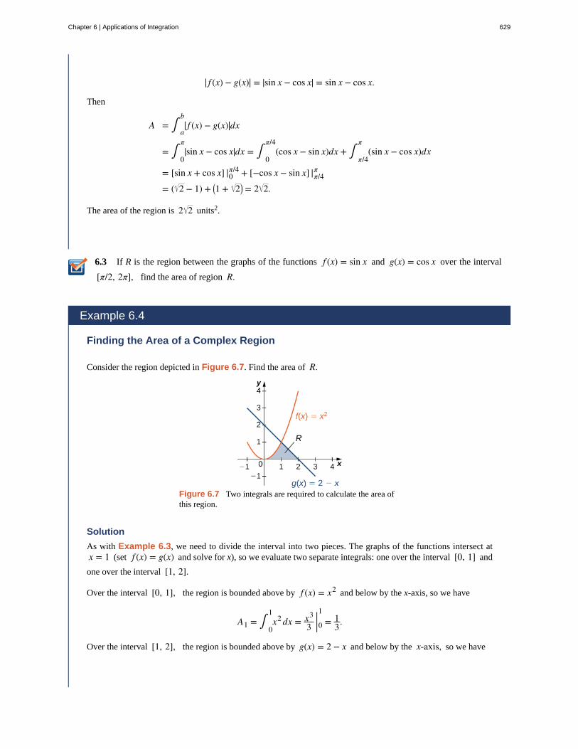
6.3
| f (x) − g(x)| = |sin x − cos x| = sin x − cos x.
Then
A = ∫a
b| f (x) − g(x)|dx
= ∫0
π|sin x − cos x|dx = ∫
0
π/4(cos x − sin x)dx + ∫
π/4
π(sin x − cos x)dx
= [sin x + cos x] |0π/4 + [−cos x − sin x] |π/4π
= ( 2 − 1) + ⎛⎝1 + 2⎞
⎠ = 2 2.
The area of the region is 2 2 units2.
If R is the region between the graphs of the functions f (x) = sin x and g(x) = cos x over the interval
[π/2, 2π], find the area of region R.
Example 6.4
Finding the Area of a Complex Region
Consider the region depicted in Figure 6.7. Find the area of R.
Figure 6.7 Two integrals are required to calculate the area ofthis region.
Solution
As with Example 6.3, we need to divide the interval into two pieces. The graphs of the functions intersect atx = 1 (set f (x) = g(x) and solve for x), so we evaluate two separate integrals: one over the interval [0, 1] and
one over the interval [1, 2].
Over the interval [0, 1], the region is bounded above by f (x) = x2 and below by the x-axis, so we have
A1 = ∫0
1x2 dx = x3
3 |01 = 13.
Over the interval [1, 2], the region is bounded above by g(x) = 2 − x and below by the x-axis, so we have
Chapter 6 | Applications of Integration 629
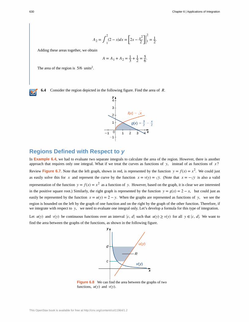
6.4
A2 = ∫1
2(2 − x)dx = ⎡
⎣2x − x2
2⎤⎦ |12 = 1
2.
Adding these areas together, we obtain
A = A1 + A2 = 13 + 1
2 = 56.
The area of the region is 5/6 units2.
Consider the region depicted in the following figure. Find the area of R.
Regions Defined with Respect to yIn Example 6.4, we had to evaluate two separate integrals to calculate the area of the region. However, there is anotherapproach that requires only one integral. What if we treat the curves as functions of y, instead of as functions of x?
Review Figure 6.7. Note that the left graph, shown in red, is represented by the function y = f (x) = x2. We could just
as easily solve this for x and represent the curve by the function x = v(y) = y. (Note that x = − y is also a valid
representation of the function y = f (x) = x2 as a function of y. However, based on the graph, it is clear we are interested
in the positive square root.) Similarly, the right graph is represented by the function y = g(x) = 2 − x, but could just as
easily be represented by the function x = u(y) = 2 − y. When the graphs are represented as functions of y, we see the
region is bounded on the left by the graph of one function and on the right by the graph of the other function. Therefore, ifwe integrate with respect to y, we need to evaluate one integral only. Let’s develop a formula for this type of integration.
Let u(y) and v(y) be continuous functions over an interval ⎡⎣c, d⎤
⎦ such that u(y) ≥ v(y) for all y ∈ ⎡⎣c, d⎤
⎦. We want to
find the area between the graphs of the functions, as shown in the following figure.
Figure 6.8 We can find the area between the graphs of twofunctions, u(y) and v(y).
630 Chapter 6 | Applications of Integration
This OpenStax book is available for free at http://cnx.org/content/col11964/1.2
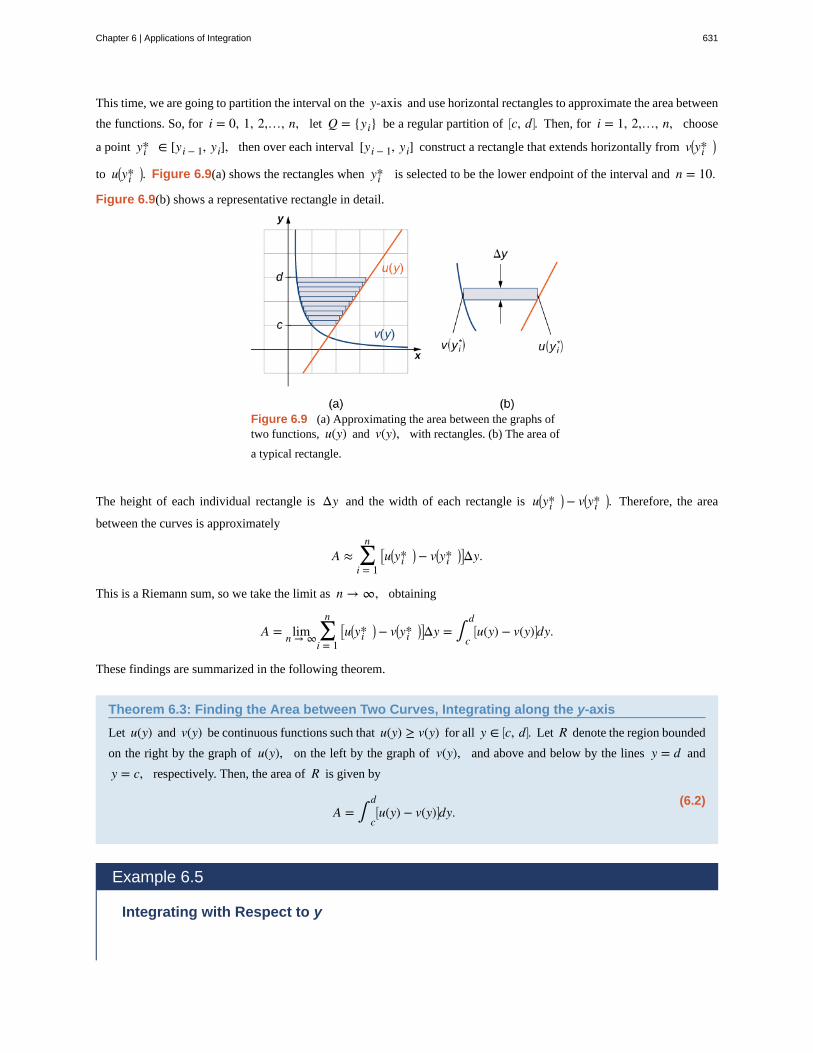
This time, we are going to partition the interval on the y-axis and use horizontal rectangles to approximate the area between
the functions. So, for i = 0, 1, 2,…, n, let Q = {yi} be a regular partition of ⎡⎣c, d⎤
⎦. Then, for i = 1, 2,…, n, choose
a point yi* ∈ [yi − 1, yi], then over each interval [yi − 1, yi] construct a rectangle that extends horizontally from v⎛⎝yi*
⎞⎠
to u⎛⎝yi*
⎞⎠. Figure 6.9(a) shows the rectangles when yi* is selected to be the lower endpoint of the interval and n = 10.
Figure 6.9(b) shows a representative rectangle in detail.
Figure 6.9 (a) Approximating the area between the graphs oftwo functions, u(y) and v(y), with rectangles. (b) The area of
a typical rectangle.
The height of each individual rectangle is Δy and the width of each rectangle is u⎛⎝yi*
⎞⎠ − v⎛
⎝yi*⎞⎠. Therefore, the area
between the curves is approximately
A ≈ ∑i = 1
n⎡⎣u⎛
⎝yi*⎞⎠ − v⎛
⎝yi*⎞⎠⎤⎦Δy.
This is a Riemann sum, so we take the limit as n → ∞, obtaining
A = limn → ∞ ∑i = 1
n⎡⎣u⎛
⎝yi*⎞⎠ − v⎛
⎝yi*⎞⎠⎤⎦Δy = ∫
c
d⎡⎣u(y) − v(y)⎤
⎦dy.
These findings are summarized in the following theorem.
Theorem 6.3: Finding the Area between Two Curves, Integrating along the y-axis
Let u(y) and v(y) be continuous functions such that u(y) ≥ v(y) for all y ∈ ⎡⎣c, d⎤
⎦. Let R denote the region bounded
on the right by the graph of u(y), on the left by the graph of v(y), and above and below by the lines y = d and
y = c, respectively. Then, the area of R is given by
(6.2)A = ∫
c
d⎡⎣u(y) − v(y)⎤
⎦dy.
Example 6.5
Integrating with Respect to y
Chapter 6 | Applications of Integration 631
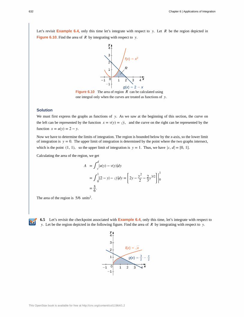
6.5
Let’s revisit Example 6.4, only this time let’s integrate with respect to y. Let R be the region depicted in
Figure 6.10. Find the area of R by integrating with respect to y.
Figure 6.10 The area of region R can be calculated using
one integral only when the curves are treated as functions of y.
Solution
We must first express the graphs as functions of y. As we saw at the beginning of this section, the curve on
the left can be represented by the function x = v(y) = y, and the curve on the right can be represented by the
function x = u(y) = 2 − y.
Now we have to determine the limits of integration. The region is bounded below by the x-axis, so the lower limitof integration is y = 0. The upper limit of integration is determined by the point where the two graphs intersect,
which is the point (1, 1), so the upper limit of integration is y = 1. Thus, we have ⎡⎣c, d⎤
⎦ = [0, 1].
Calculating the area of the region, we get
A = ∫c
d⎡⎣u(y) − v(y)⎤
⎦dy
= ∫0
1⎡⎣⎛⎝2 − y⎞
⎠ − y⎤⎦dy =
⎡
⎣⎢ 2y − y2
2 − 23y3/2⎤
⎦⎥ |01
= 56.
The area of the region is 5/6 units2.
Let’s revisit the checkpoint associated with Example 6.4, only this time, let’s integrate with respect toy. Let be the region depicted in the following figure. Find the area of R by integrating with respect to y.
632 Chapter 6 | Applications of Integration
This OpenStax book is available for free at http://cnx.org/content/col11964/1.2
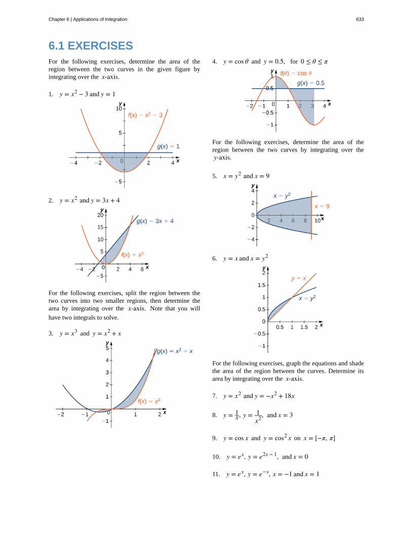
6.1 EXERCISESFor the following exercises, determine the area of theregion between the two curves in the given figure byintegrating over the x-axis.
1. y = x2 − 3 and y = 1
2. y = x2 and y = 3x + 4
For the following exercises, split the region between thetwo curves into two smaller regions, then determine thearea by integrating over the x-axis. Note that you will
have two integrals to solve.
3. y = x3 and y = x2 + x
4. y = cos θ and y = 0.5, for 0 ≤ θ ≤ π
For the following exercises, determine the area of theregion between the two curves by integrating over they-axis.
5. x = y2 and x = 9
6. y = x and x = y2
For the following exercises, graph the equations and shadethe area of the region between the curves. Determine itsarea by integrating over the x-axis.
7. y = x2 and y = −x2 + 18x
8. y = 1x , y = 1
x2, and x = 3
9. y = cos x and y = cos2 x on x = [−π, π]
10. y = ex, y = e2x − 1, and x = 0
11. y = ex, y = e−x, x = −1 and x = 1
Chapter 6 | Applications of Integration 633
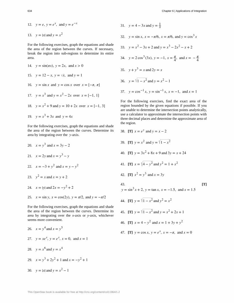
12. y = e, y = ex, and y = e−x
13. y = |x| and y = x2
For the following exercises, graph the equations and shadethe area of the region between the curves. If necessary,break the region into sub-regions to determine its entirearea.
14. y = sin(πx), y = 2x, and x > 0
15. y = 12 − x, y = x, and y = 1
16. y = sin x and y = cos x over x = [−π, π]
17. y = x3 and y = x2 − 2x over x = [−1, 1]
18. y = x2 + 9 and y = 10 + 2x over x = [−1, 3]
19. y = x3 + 3x and y = 4x
For the following exercises, graph the equations and shadethe area of the region between the curves. Determine itsarea by integrating over the y-axis.
20. x = y3 and x = 3y − 2
21. x = 2y and x = y3 − y
22. x = −3 + y2 and x = y − y2
23. y2 = x and x = y + 2
24. x = |y| and 2x = −y2 + 2
25. x = sin y, x = cos(2y), y = π/2, and y = −π/2
For the following exercises, graph the equations and shadethe area of the region between the curves. Determine itsarea by integrating over the x-axis or y-axis, whicheverseems more convenient.
26. x = y4 and x = y5
27. y = xex, y = ex, x = 0, and x = 1
28. y = x6 and y = x4
29. x = y3 + 2y2 + 1 and x = −y2 + 1
30. y = |x| and y = x2 − 1
31. y = 4 − 3x and y = 1x
32. y = sin x, x = −π/6, x = π/6, and y = cos3 x
33. y = x2 − 3x + 2 and y = x3 − 2x2 − x + 2
34. y = 2 cos3 (3x), y = −1, x = π4, and x = − π
4
35. y + y3 = x and 2y = x
36. y = 1 − x2 and y = x2 − 1
37. y = cos−1 x, y = sin−1 x, x = −1, and x = 1
For the following exercises, find the exact area of theregion bounded by the given equations if possible. If youare unable to determine the intersection points analytically,use a calculator to approximate the intersection points withthree decimal places and determine the approximate area ofthe region.
38. [T] x = ey and y = x − 2
39. [T] y = x2 and y = 1 − x2
40. [T] y = 3x2 + 8x + 9 and 3y = x + 24
41. [T] x = 4 − y2 and y2 = 1 + x2
42. [T] x2 = y3 and x = 3y
43. [T]
y = sin3 x + 2, y = tan x, x = −1.5, and x = 1.5
44. [T] y = 1 − x2 and y2 = x2
45. [T] y = 1 − x2 and y = x2 + 2x + 1
46. [T] x = 4 − y2 and x = 1 + 3y + y2
47. [T] y = cos x, y = ex, x = −π, and x = 0
634 Chapter 6 | Applications of Integration
This OpenStax book is available for free at http://cnx.org/content/col11964/1.2
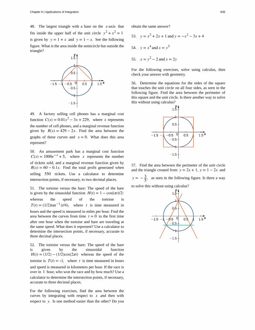
48. The largest triangle with a base on the x-axis that
fits inside the upper half of the unit circle y2 + x2 = 1is given by y = 1 + x and y = 1 − x. See the following
figure. What is the area inside the semicircle but outside thetriangle?
49. A factory selling cell phones has a marginal cost
function C(x) = 0.01x2 − 3x + 229, where x represents
the number of cell phones, and a marginal revenue functiongiven by R(x) = 429 − 2x. Find the area between the
graphs of these curves and x = 0. What does this area
represent?
50. An amusement park has a marginal cost functionC(x) = 1000e−x + 5, where x represents the number
of tickets sold, and a marginal revenue function given byR(x) = 60 − 0.1x. Find the total profit generated when
selling 550 tickets. Use a calculator to determine
intersection points, if necessary, to two decimal places.
51. The tortoise versus the hare: The speed of the hareis given by the sinusoidal function H(t) = 1 − cos⎛
⎝(πt)/2⎞⎠
whereas the speed of the tortoise is
T(t) = (1/2)tan−1 (t/4), where t is time measured in
hours and the speed is measured in miles per hour. Find thearea between the curves from time t = 0 to the first time
after one hour when the tortoise and hare are traveling atthe same speed. What does it represent? Use a calculator todetermine the intersection points, if necessary, accurate tothree decimal places.
52. The tortoise versus the hare: The speed of the hareis given by the sinusoidal functionH(t) = (1/2) − (1/2)cos(2πt) whereas the speed of the
tortoise is T(t) = t, where t is time measured in hours
and speed is measured in kilometers per hour. If the race isover in 1 hour, who won the race and by how much? Use a
calculator to determine the intersection points, if necessary,accurate to three decimal places.
For the following exercises, find the area between thecurves by integrating with respect to x and then with
respect to y. Is one method easier than the other? Do you
obtain the same answer?
53. y = x2 + 2x + 1 and y = −x2 − 3x + 4
54. y = x4 and x = y5
55. x = y2 − 2 and x = 2y
For the following exercises, solve using calculus, thencheck your answer with geometry.
56. Determine the equations for the sides of the squarethat touches the unit circle on all four sides, as seen in thefollowing figure. Find the area between the perimeter ofthis square and the unit circle. Is there another way to solvethis without using calculus?
57. Find the area between the perimeter of the unit circleand the triangle created from y = 2x + 1, y = 1 − 2x and
y = − 35, as seen in the following figure. Is there a way
to solve this without using calculus?
Chapter 6 | Applications of Integration 635
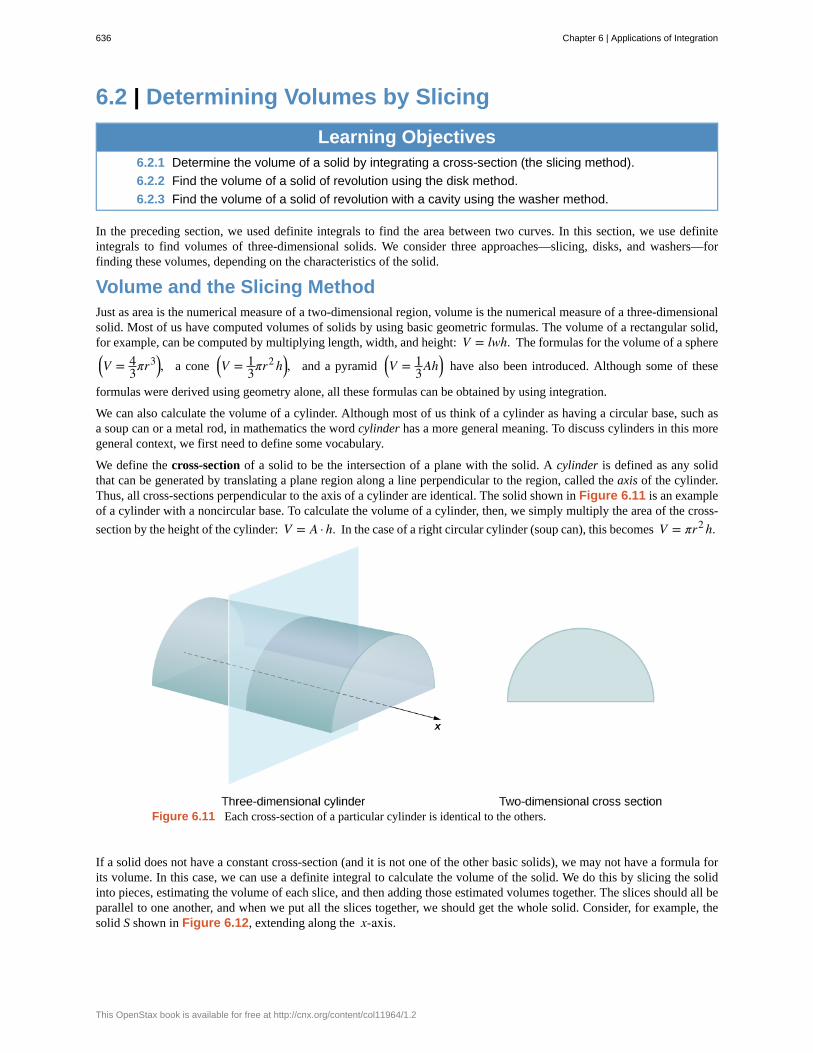
6.2 | Determining Volumes by Slicing
Learning Objectives6.2.1 Determine the volume of a solid by integrating a cross-section (the slicing method).
6.2.2 Find the volume of a solid of revolution using the disk method.
6.2.3 Find the volume of a solid of revolution with a cavity using the washer method.
In the preceding section, we used definite integrals to find the area between two curves. In this section, we use definiteintegrals to find volumes of three-dimensional solids. We consider three approaches—slicing, disks, and washers—forfinding these volumes, depending on the characteristics of the solid.
Volume and the Slicing MethodJust as area is the numerical measure of a two-dimensional region, volume is the numerical measure of a three-dimensionalsolid. Most of us have computed volumes of solids by using basic geometric formulas. The volume of a rectangular solid,for example, can be computed by multiplying length, width, and height: V = lwh. The formulas for the volume of a sphere⎛⎝V = 4
3πr3⎞⎠, a cone ⎛
⎝V = 13πr2 h⎞
⎠, and a pyramid ⎛⎝V = 1
3Ah⎞⎠ have also been introduced. Although some of these
formulas were derived using geometry alone, all these formulas can be obtained by using integration.
We can also calculate the volume of a cylinder. Although most of us think of a cylinder as having a circular base, such asa soup can or a metal rod, in mathematics the word cylinder has a more general meaning. To discuss cylinders in this moregeneral context, we first need to define some vocabulary.
We define the cross-section of a solid to be the intersection of a plane with the solid. A cylinder is defined as any solidthat can be generated by translating a plane region along a line perpendicular to the region, called the axis of the cylinder.Thus, all cross-sections perpendicular to the axis of a cylinder are identical. The solid shown in Figure 6.11 is an exampleof a cylinder with a noncircular base. To calculate the volume of a cylinder, then, we simply multiply the area of the cross-
section by the height of the cylinder: V = A · h. In the case of a right circular cylinder (soup can), this becomes V = πr2 h.
Figure 6.11 Each cross-section of a particular cylinder is identical to the others.
If a solid does not have a constant cross-section (and it is not one of the other basic solids), we may not have a formula forits volume. In this case, we can use a definite integral to calculate the volume of the solid. We do this by slicing the solidinto pieces, estimating the volume of each slice, and then adding those estimated volumes together. The slices should all beparallel to one another, and when we put all the slices together, we should get the whole solid. Consider, for example, thesolid S shown in Figure 6.12, extending along the x-axis.
636 Chapter 6 | Applications of Integration
This OpenStax book is available for free at http://cnx.org/content/col11964/1.2
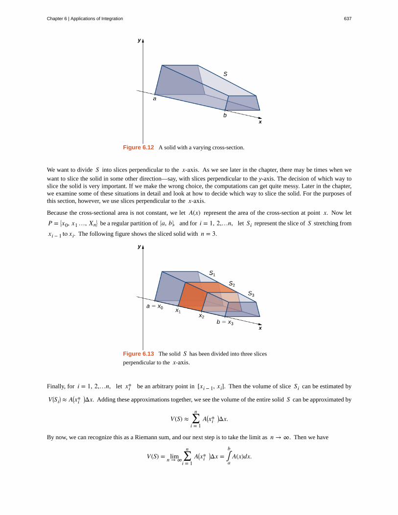
Figure 6.12 A solid with a varying cross-section.
We want to divide S into slices perpendicular to the x-axis. As we see later in the chapter, there may be times when we
want to slice the solid in some other direction—say, with slices perpendicular to the y-axis. The decision of which way toslice the solid is very important. If we make the wrong choice, the computations can get quite messy. Later in the chapter,we examine some of these situations in detail and look at how to decide which way to slice the solid. For the purposes ofthis section, however, we use slices perpendicular to the x-axis.
Because the cross-sectional area is not constant, we let A(x) represent the area of the cross-section at point x. Now let
P = ⎧
⎩⎨x0, x1 …, Xn
⎫
⎭⎬ be a regular partition of ⎡
⎣a, b⎤⎦, and for i = 1, 2,…n, let Si represent the slice of S stretching from
xi − 1 to xi. The following figure shows the sliced solid with n = 3.
Figure 6.13 The solid S has been divided into three slices
perpendicular to the x-axis.
Finally, for i = 1, 2,…n, let xi* be an arbitrary point in [xi − 1, xi]. Then the volume of slice Si can be estimated by
V ⎛⎝Si
⎞⎠ ≈ A⎛
⎝xi*⎞⎠Δx. Adding these approximations together, we see the volume of the entire solid S can be approximated by
V(S) ≈ ∑i = 1
nA⎛
⎝xi*⎞⎠Δx.
By now, we can recognize this as a Riemann sum, and our next step is to take the limit as n → ∞. Then we have
V(S) = limn → ∞ ∑i = 1
nA⎛
⎝xi*⎞⎠Δx = ∫
a
bA(x)dx.
Chapter 6 | Applications of Integration 637
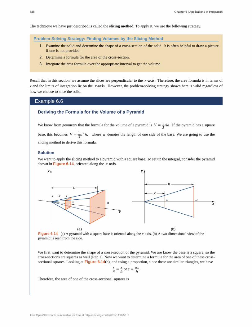
The technique we have just described is called the slicing method. To apply it, we use the following strategy.
Problem-Solving Strategy: Finding Volumes by the Slicing Method
1. Examine the solid and determine the shape of a cross-section of the solid. It is often helpful to draw a pictureif one is not provided.
2. Determine a formula for the area of the cross-section.
3. Integrate the area formula over the appropriate interval to get the volume.
Recall that in this section, we assume the slices are perpendicular to the x-axis. Therefore, the area formula is in terms of
x and the limits of integration lie on the x-axis. However, the problem-solving strategy shown here is valid regardless of
how we choose to slice the solid.
Example 6.6
Deriving the Formula for the Volume of a Pyramid
We know from geometry that the formula for the volume of a pyramid is V = 13Ah. If the pyramid has a square
base, this becomes V = 13a2 h, where a denotes the length of one side of the base. We are going to use the
slicing method to derive this formula.
Solution
We want to apply the slicing method to a pyramid with a square base. To set up the integral, consider the pyramidshown in Figure 6.14, oriented along the x-axis.
Figure 6.14 (a) A pyramid with a square base is oriented along the x-axis. (b) A two-dimensional view of thepyramid is seen from the side.
We first want to determine the shape of a cross-section of the pyramid. We are know the base is a square, so thecross-sections are squares as well (step 1). Now we want to determine a formula for the area of one of these cross-sectional squares. Looking at Figure 6.14(b), and using a proportion, since these are similar triangles, we have
sa = x
h or s = axh .
Therefore, the area of one of the cross-sectional squares is
638 Chapter 6 | Applications of Integration
This OpenStax book is available for free at http://cnx.org/content/col11964/1.2
6.6
A(x) = s2 = ⎛⎝axh
⎞⎠
2⎛⎝step 2⎞
⎠.
Then we find the volume of the pyramid by integrating from 0 to h (step 3):
V = ∫0
hA(x)dx
= ∫0
h⎛⎝axh
⎞⎠
2dx = a2
h2∫0
hx2dx
= ⎡⎣
a2
h2⎛⎝13x3⎞
⎠⎤⎦ |0h = 1
3a2 h.
This is the formula we were looking for.
Use the slicing method to derive the formula V = 13πr2 h for the volume of a circular cone.
Solids of RevolutionIf a region in a plane is revolved around a line in that plane, the resulting solid is called a solid of revolution, as shown inthe following figure.
Chapter 6 | Applications of Integration 639
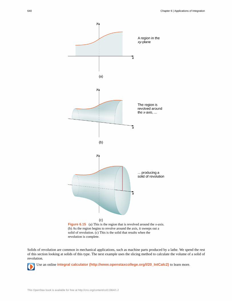
Figure 6.15 (a) This is the region that is revolved around the x-axis.(b) As the region begins to revolve around the axis, it sweeps out asolid of revolution. (c) This is the solid that results when therevolution is complete.
Solids of revolution are common in mechanical applications, such as machine parts produced by a lathe. We spend the restof this section looking at solids of this type. The next example uses the slicing method to calculate the volume of a solid ofrevolution.
Use an online integral calculator (http://www.openstaxcollege.org/l/20_IntCalc2) to learn more.
640 Chapter 6 | Applications of Integration
This OpenStax book is available for free at http://cnx.org/content/col11964/1.2
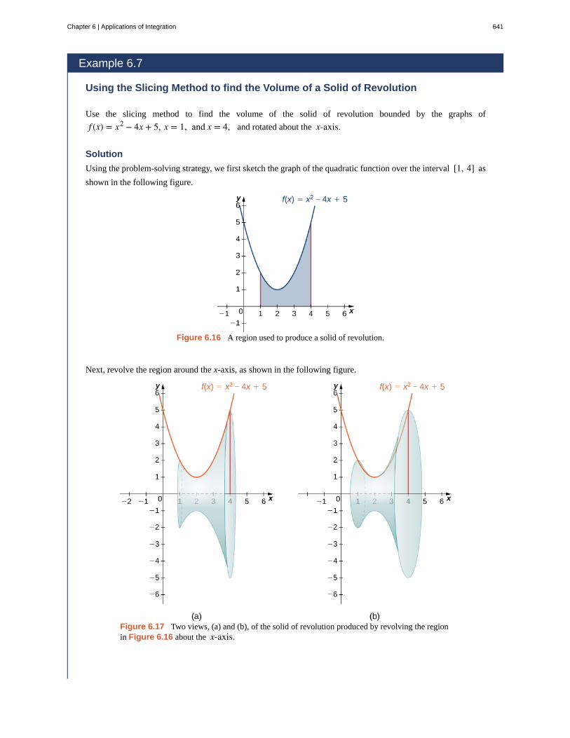
Example 6.7
Using the Slicing Method to find the Volume of a Solid of Revolution
Use the slicing method to find the volume of the solid of revolution bounded by the graphs of
f (x) = x2 − 4x + 5, x = 1, and x = 4, and rotated about the x-axis.
Solution
Using the problem-solving strategy, we first sketch the graph of the quadratic function over the interval [1, 4] as
shown in the following figure.
Figure 6.16 A region used to produce a solid of revolution.
Next, revolve the region around the x-axis, as shown in the following figure.
Figure 6.17 Two views, (a) and (b), of the solid of revolution produced by revolving the regionin Figure 6.16 about the x-axis.
Chapter 6 | Applications of Integration 641
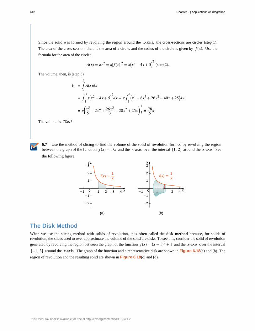
6.7
Since the solid was formed by revolving the region around the x-axis, the cross-sections are circles (step 1).
The area of the cross-section, then, is the area of a circle, and the radius of the circle is given by f (x). Use the
formula for the area of the circle:
A(x) = πr2 = π⎡⎣ f (x)⎤
⎦2 = π⎛
⎝x2 − 4x + 5⎞⎠2
(step 2).
The volume, then, is (step 3)
V = ∫a
hA(x)dx
= ∫1
4π⎛
⎝x2 − 4x + 5⎞⎠2dx = π∫
1
4⎛⎝x4 − 8x3 + 26x2 − 40x + 25⎞
⎠dx
= π⎛⎝
x5
5 − 2x4 + 26x3
3 − 20x2 + 25x⎞⎠|14 = 78
5 π.
The volume is 78π/5.
Use the method of slicing to find the volume of the solid of revolution formed by revolving the regionbetween the graph of the function f (x) = 1/x and the x-axis over the interval [1, 2] around the x-axis. See
the following figure.
The Disk MethodWhen we use the slicing method with solids of revolution, it is often called the disk method because, for solids ofrevolution, the slices used to over approximate the volume of the solid are disks. To see this, consider the solid of revolution
generated by revolving the region between the graph of the function f (x) = (x − 1)2 + 1 and the x-axis over the interval
[−1, 3] around the x-axis. The graph of the function and a representative disk are shown in Figure 6.18(a) and (b). The
region of revolution and the resulting solid are shown in Figure 6.18(c) and (d).
642 Chapter 6 | Applications of Integration
This OpenStax book is available for free at http://cnx.org/content/col11964/1.2
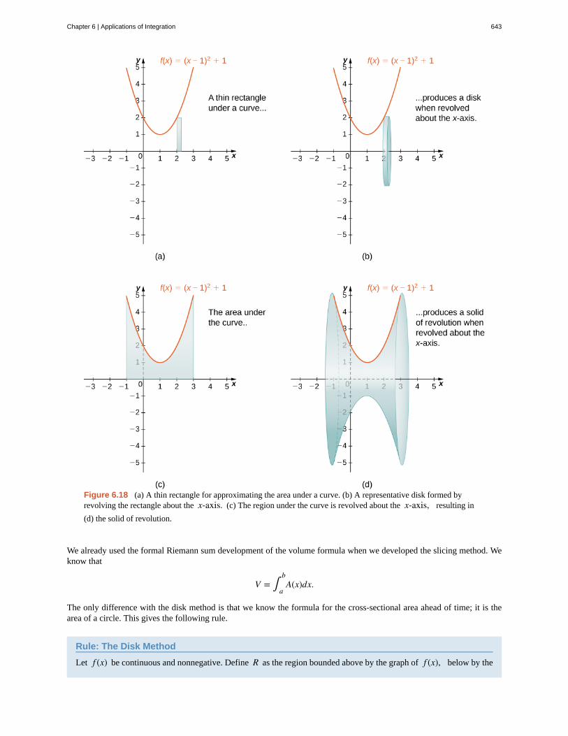
Figure 6.18 (a) A thin rectangle for approximating the area under a curve. (b) A representative disk formed byrevolving the rectangle about the x-axis. (c) The region under the curve is revolved about the x-axis, resulting in
(d) the solid of revolution.
We already used the formal Riemann sum development of the volume formula when we developed the slicing method. Weknow that
V = ∫a
bA(x)dx.
The only difference with the disk method is that we know the formula for the cross-sectional area ahead of time; it is thearea of a circle. This gives the following rule.
Rule: The Disk Method
Let f (x) be continuous and nonnegative. Define R as the region bounded above by the graph of f (x), below by the
Chapter 6 | Applications of Integration 643
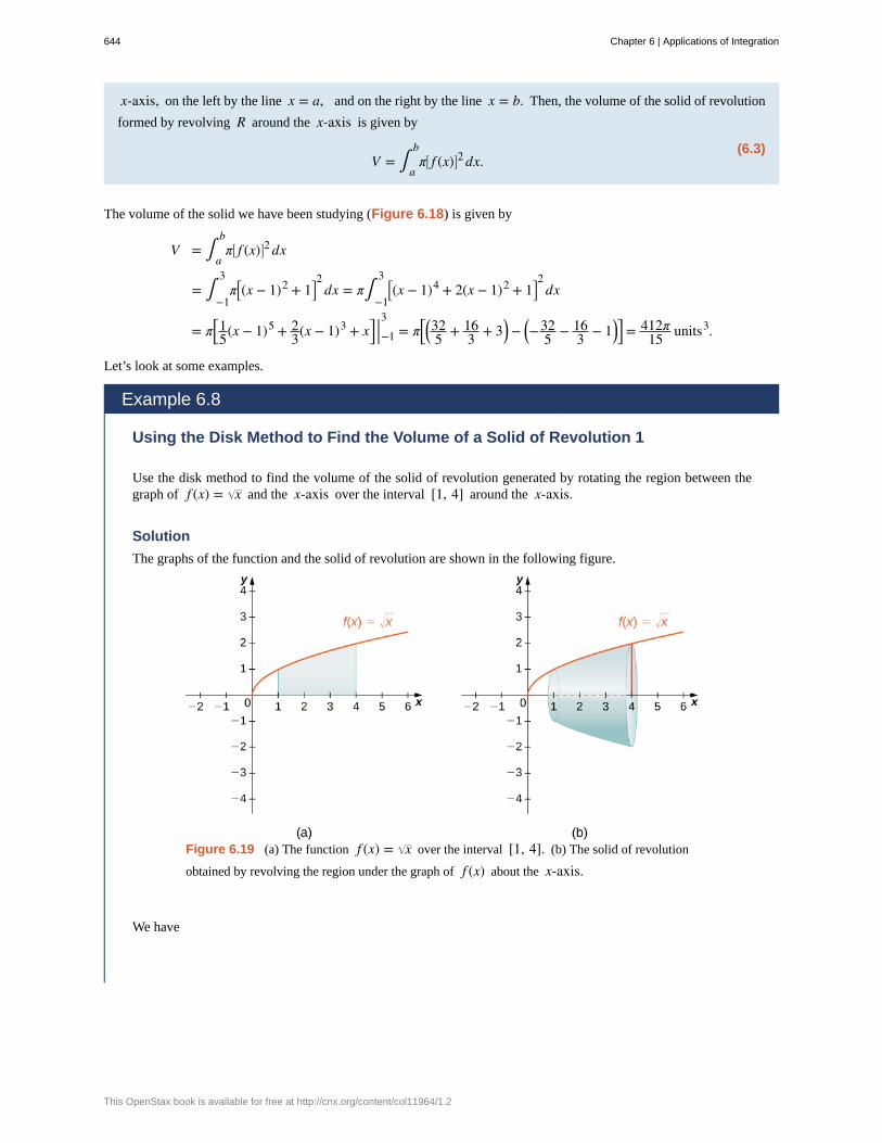
x-axis, on the left by the line x = a, and on the right by the line x = b. Then, the volume of the solid of revolution
formed by revolving R around the x-axis is given by
(6.3)V = ∫
a
bπ⎡
⎣ f (x)⎤⎦2 dx.
The volume of the solid we have been studying (Figure 6.18) is given by
V = ∫a
bπ⎡
⎣ f (x)⎤⎦2 dx
= ∫−1
3π⎡
⎣(x − 1)2 + 1⎤⎦2
dx = π∫−1
3⎡⎣(x − 1)4 + 2(x − 1)2 + 1⎤
⎦2
dx
= π⎡⎣15(x − 1)5 + 2
3(x − 1)3 + x⎤⎦ |−1
3= π⎡
⎣⎛⎝325 + 16
3 + 3⎞⎠ − ⎛
⎝−325 − 16
3 − 1⎞⎠⎤⎦ = 412π
15 units3.
Let’s look at some examples.
Example 6.8
Using the Disk Method to Find the Volume of a Solid of Revolution 1
Use the disk method to find the volume of the solid of revolution generated by rotating the region between thegraph of f (x) = x and the x-axis over the interval [1, 4] around the x-axis.
Solution
The graphs of the function and the solid of revolution are shown in the following figure.
Figure 6.19 (a) The function f (x) = x over the interval [1, 4]. (b) The solid of revolution
obtained by revolving the region under the graph of f (x) about the x-axis.
We have
644 Chapter 6 | Applications of Integration
This OpenStax book is available for free at http://cnx.org/content/col11964/1.2
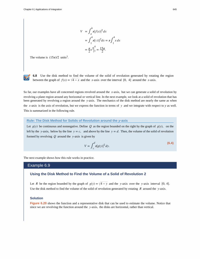
6.8
V = ∫a
bπ⎡
⎣ f (x)⎤⎦2 dx
= ∫1
4π[ x]2dx = π∫
1
4x dx
= π2x2|14 = 15π
2 .
The volume is (15π)/2 units3.
Use the disk method to find the volume of the solid of revolution generated by rotating the regionbetween the graph of f (x) = 4 − x and the x-axis over the interval [0, 4] around the x-axis.
So far, our examples have all concerned regions revolved around the x-axis, but we can generate a solid of revolution by
revolving a plane region around any horizontal or vertical line. In the next example, we look at a solid of revolution that hasbeen generated by revolving a region around the y-axis. The mechanics of the disk method are nearly the same as when
the x-axis is the axis of revolution, but we express the function in terms of y and we integrate with respect to y as well.
This is summarized in the following rule.
Rule: The Disk Method for Solids of Revolution around the y-axis
Let g(y) be continuous and nonnegative. Define Q as the region bounded on the right by the graph of g(y), on the
left by the y-axis, below by the line y = c, and above by the line y = d. Then, the volume of the solid of revolution
formed by revolving Q around the y-axis is given by
(6.4)V = ∫
c
dπ⎡
⎣g(y)⎤⎦2 dy.
The next example shows how this rule works in practice.
Example 6.9
Using the Disk Method to Find the Volume of a Solid of Revolution 2
Let R be the region bounded by the graph of g(y) = 4 − y and the y-axis over the y-axis interval [0, 4].Use the disk method to find the volume of the solid of revolution generated by rotating R around the y-axis.
Solution
Figure 6.20 shows the function and a representative disk that can be used to estimate the volume. Notice thatsince we are revolving the function around the y-axis, the disks are horizontal, rather than vertical.
Chapter 6 | Applications of Integration 645
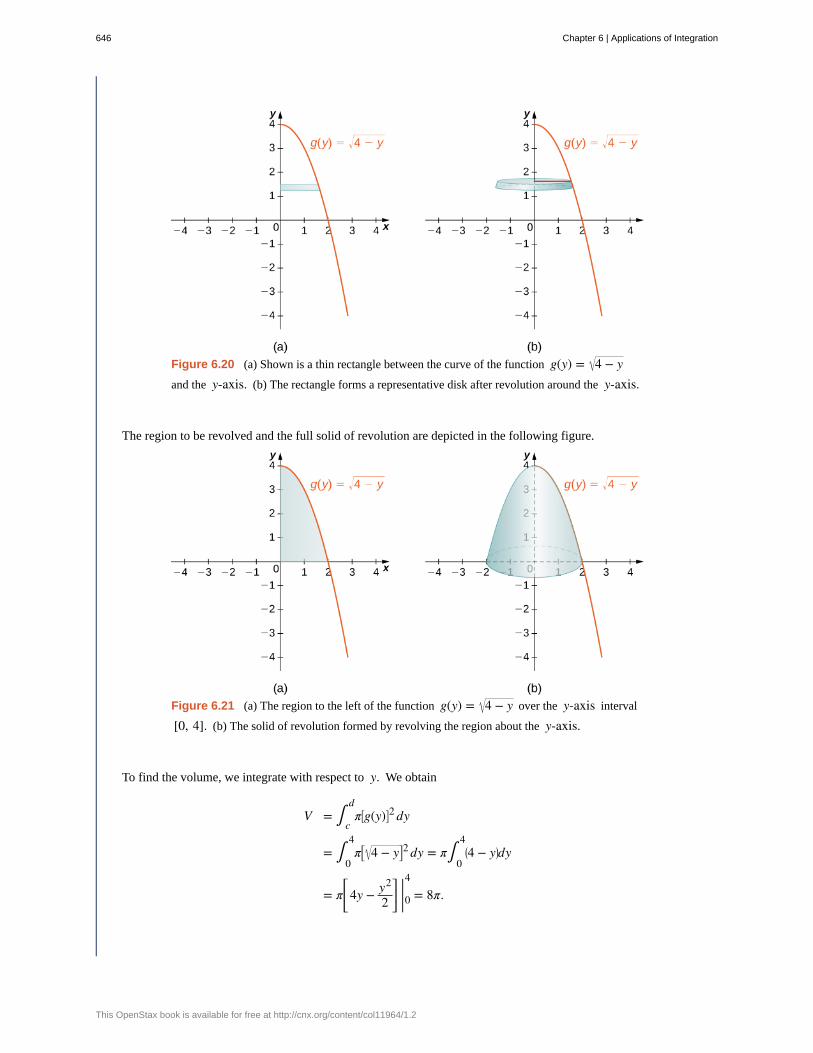
Figure 6.20 (a) Shown is a thin rectangle between the curve of the function g(y) = 4 − yand the y-axis. (b) The rectangle forms a representative disk after revolution around the y-axis.
The region to be revolved and the full solid of revolution are depicted in the following figure.
Figure 6.21 (a) The region to the left of the function g(y) = 4 − y over the y-axis interval
[0, 4]. (b) The solid of revolution formed by revolving the region about the y-axis.
To find the volume, we integrate with respect to y. We obtain
V = ∫c
dπ⎡
⎣g(y)⎤⎦2 dy
= ∫0
4π⎡
⎣ 4 − y⎤⎦2 dy = π∫
0
4⎛⎝4 − y⎞
⎠dy
= π⎡
⎣⎢ 4y − y2
2⎤
⎦⎥ |04 = 8π.
646 Chapter 6 | Applications of Integration
This OpenStax book is available for free at http://cnx.org/content/col11964/1.2
6.9
The volume is 8π units3.
Use the disk method to find the volume of the solid of revolution generated by rotating the regionbetween the graph of g(y) = y and the y-axis over the interval [1, 4] around the y-axis.
The Washer MethodSome solids of revolution have cavities in the middle; they are not solid all the way to the axis of revolution. Sometimes,this is just a result of the way the region of revolution is shaped with respect to the axis of revolution. In other cases, cavitiesarise when the region of revolution is defined as the region between the graphs of two functions. A third way this can happenis when an axis of revolution other than the x-axis or y-axis is selected.
When the solid of revolution has a cavity in the middle, the slices used to approximate the volume are not disks, but washers(disks with holes in the center). For example, consider the region bounded above by the graph of the function f (x) = xand below by the graph of the function g(x) = 1 over the interval [1, 4]. When this region is revolved around the x-axis,the result is a solid with a cavity in the middle, and the slices are washers. The graph of the function and a representativewasher are shown in Figure 6.22(a) and (b). The region of revolution and the resulting solid are shown in Figure 6.22(c)and (d).
Chapter 6 | Applications of Integration 647
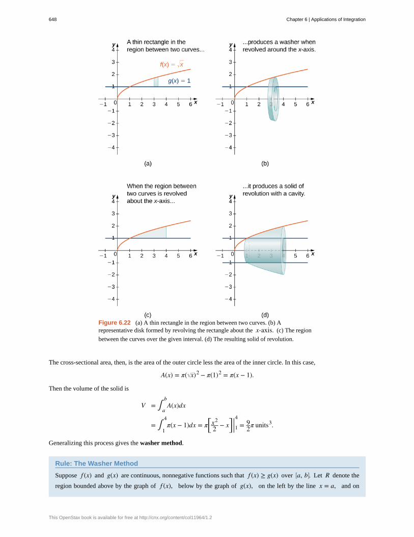
Figure 6.22 (a) A thin rectangle in the region between two curves. (b) Arepresentative disk formed by revolving the rectangle about the x-axis. (c) The region
between the curves over the given interval. (d) The resulting solid of revolution.
The cross-sectional area, then, is the area of the outer circle less the area of the inner circle. In this case,
A(x) = π( x)2 − π(1)2 = π(x − 1).
Then the volume of the solid is
V = ∫a
bA(x)dx
= ∫1
4π(x − 1)dx = π⎡
⎣x2
2 − x⎤⎦ |14 = 9
2π units3.
Generalizing this process gives the washer method.
Rule: The Washer Method
Suppose f (x) and g(x) are continuous, nonnegative functions such that f (x) ≥ g(x) over ⎡⎣a, b⎤
⎦. Let R denote the
region bounded above by the graph of f (x), below by the graph of g(x), on the left by the line x = a, and on
648 Chapter 6 | Applications of Integration
This OpenStax book is available for free at http://cnx.org/content/col11964/1.2
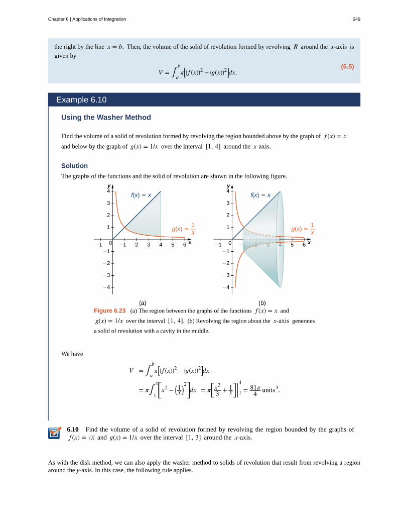
6.10
the right by the line x = b. Then, the volume of the solid of revolution formed by revolving R around the x-axis is
given by
(6.5)V = ∫
a
bπ⎡
⎣⎛⎝ f (x)⎞
⎠2 − ⎛
⎝g(x)⎞⎠2⎤
⎦dx.
Example 6.10
Using the Washer Method
Find the volume of a solid of revolution formed by revolving the region bounded above by the graph of f (x) = xand below by the graph of g(x) = 1/x over the interval [1, 4] around the x-axis.
Solution
The graphs of the functions and the solid of revolution are shown in the following figure.
Figure 6.23 (a) The region between the graphs of the functions f (x) = x and
g(x) = 1/x over the interval [1, 4]. (b) Revolving the region about the x-axis generates
a solid of revolution with a cavity in the middle.
We have
V = ∫a
bπ⎡
⎣⎛⎝ f (x)⎞
⎠2 − ⎛
⎝g(x)⎞⎠2⎤
⎦dx
= π∫1
4⎡⎣x2 − ⎛
⎝1x
⎞⎠2⎤⎦dx = π⎡
⎣x3
3 + 1x⎤⎦ |14 = 81π
4 units3.
Find the volume of a solid of revolution formed by revolving the region bounded by the graphs off (x) = x and g(x) = 1/x over the interval [1, 3] around the x-axis.
As with the disk method, we can also apply the washer method to solids of revolution that result from revolving a regionaround the y-axis. In this case, the following rule applies.
Chapter 6 | Applications of Integration 649
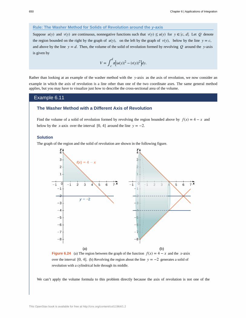
Rule: The Washer Method for Solids of Revolution around the y-axis
Suppose u(y) and v(y) are continuous, nonnegative functions such that v(y) ≤ u(y) for y ∈ ⎡⎣c, d⎤
⎦. Let Q denote
the region bounded on the right by the graph of u(y), on the left by the graph of v(y), below by the line y = c,and above by the line y = d. Then, the volume of the solid of revolution formed by revolving Q around the y-axisis given by
V = ∫c
dπ⎡
⎣⎛⎝u(y)⎞
⎠2 − ⎛
⎝v(y)⎞⎠2⎤
⎦dy.
Rather than looking at an example of the washer method with the y-axis as the axis of revolution, we now consider an
example in which the axis of revolution is a line other than one of the two coordinate axes. The same general methodapplies, but you may have to visualize just how to describe the cross-sectional area of the volume.
Example 6.11
The Washer Method with a Different Axis of Revolution
Find the volume of a solid of revolution formed by revolving the region bounded above by f (x) = 4 − x and
below by the x-axis over the interval [0, 4] around the line y = −2.
Solution
The graph of the region and the solid of revolution are shown in the following figure.
Figure 6.24 (a) The region between the graph of the function f (x) = 4 − x and the x-axisover the interval [0, 4]. (b) Revolving the region about the line y = −2 generates a solid of
revolution with a cylindrical hole through its middle.
We can’t apply the volume formula to this problem directly because the axis of revolution is not one of the
650 Chapter 6 | Applications of Integration
This OpenStax book is available for free at http://cnx.org/content/col11964/1.2
6.11
coordinate axes. However, we still know that the area of the cross-section is the area of the outer circle less thearea of the inner circle. Looking at the graph of the function, we see the radius of the outer circle is given byf (x) + 2, which simplifies to
f (x) + 2 = (4 − x) + 2 = 6 − x.
The radius of the inner circle is g(x) = 2. Therefore, we have
V = ∫0
4π⎡
⎣(6 − x)2 − (2)2⎤⎦dx
= π∫0
4⎛⎝x2 − 12x + 32⎞
⎠dx = π⎡⎣
x3
3 − 6x2 + 32x⎤⎦ |04 = 160π
3 units3.
Find the volume of a solid of revolution formed by revolving the region bounded above by the graph off (x) = x + 2 and below by the x-axis over the interval [0, 3] around the line y = −1.
Chapter 6 | Applications of Integration 651
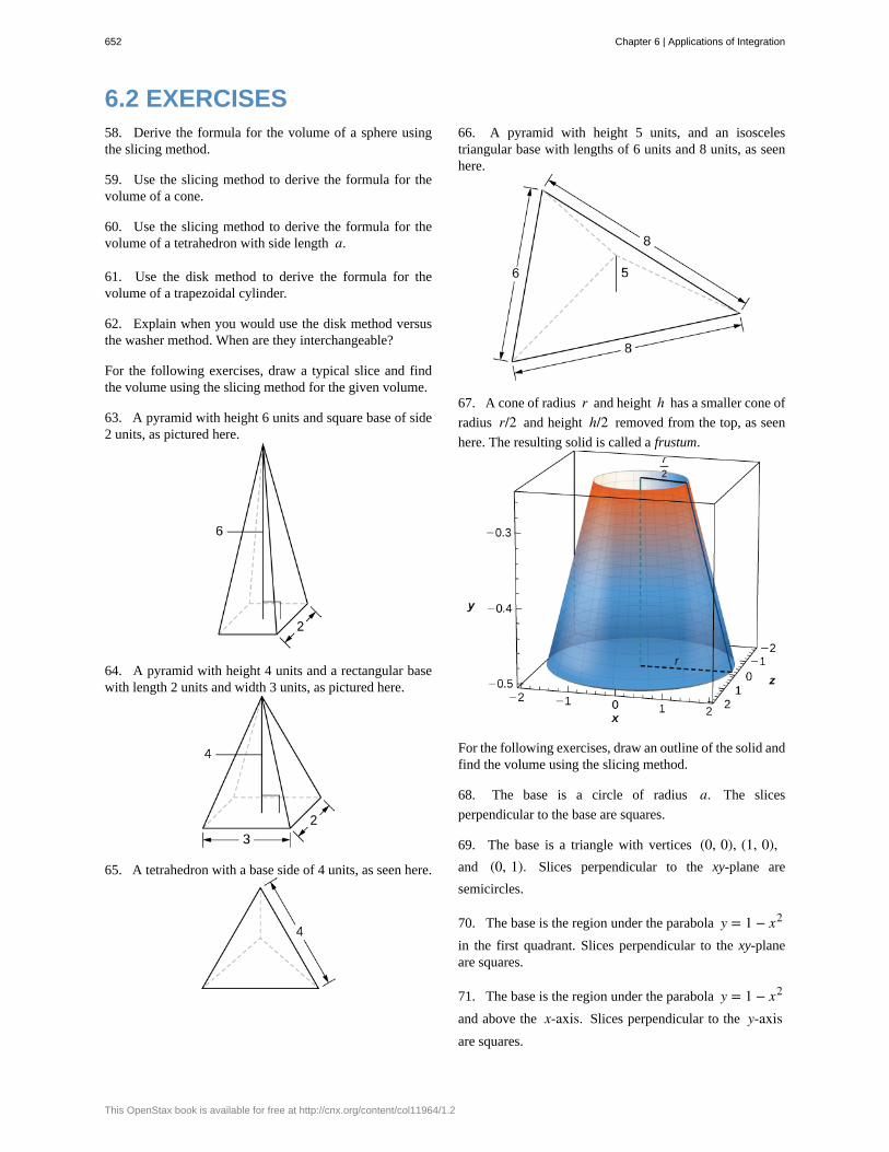
6.2 EXERCISES58. Derive the formula for the volume of a sphere usingthe slicing method.
59. Use the slicing method to derive the formula for thevolume of a cone.
60. Use the slicing method to derive the formula for thevolume of a tetrahedron with side length a.
61. Use the disk method to derive the formula for thevolume of a trapezoidal cylinder.
62. Explain when you would use the disk method versusthe washer method. When are they interchangeable?
For the following exercises, draw a typical slice and findthe volume using the slicing method for the given volume.
63. A pyramid with height 6 units and square base of side2 units, as pictured here.
64. A pyramid with height 4 units and a rectangular basewith length 2 units and width 3 units, as pictured here.
65. A tetrahedron with a base side of 4 units, as seen here.
66. A pyramid with height 5 units, and an isoscelestriangular base with lengths of 6 units and 8 units, as seenhere.
67. A cone of radius r and height h has a smaller cone of
radius r/2 and height h/2 removed from the top, as seen
here. The resulting solid is called a frustum.
For the following exercises, draw an outline of the solid andfind the volume using the slicing method.
68. The base is a circle of radius a. The slices
perpendicular to the base are squares.
69. The base is a triangle with vertices (0, 0), (1, 0),and (0, 1). Slices perpendicular to the xy-plane are
semicircles.
70. The base is the region under the parabola y = 1 − x2
in the first quadrant. Slices perpendicular to the xy-planeare squares.
71. The base is the region under the parabola y = 1 − x2
and above the x-axis. Slices perpendicular to the y-axisare squares.
652 Chapter 6 | Applications of Integration
This OpenStax book is available for free at http://cnx.org/content/col11964/1.2
72. The base is the region enclosed by y = x2 and
y = 9. Slices perpendicular to the x-axis are right isosceles
triangles.
73. The base is the area between y = x and y = x2.Slices perpendicular to the x-axis are semicircles.
For the following exercises, draw the region bounded bythe curves. Then, use the disk method to find the volumewhen the region is rotated around the x-axis.
74. x + y = 8, x = 0, and y = 0
75. y = 2x2, x = 0, x = 4, and y = 0
76. y = ex + 1, x = 0, x = 1, and y = 0
77. y = x4, x = 0, and y = 1
78. y = x, x = 0, x = 4, and y = 0
79. y = sin x, y = cos x, and x = 0
80. y = 1x , x = 2, and y = 3
81. x2 − y2 = 9 and x + y = 9, y = 0 and x = 0
For the following exercises, draw the region bounded bythe curves. Then, find the volume when the region isrotated around the y-axis.
82. y = 4 − 12x, x = 0, and y = 0
83. y = 2x3, x = 0, x = 1, and y = 0
84. y = 3x2, x = 0, and y = 3
85. y = 4 − x2, y = 0, and x = 0
86. y = 1x + 1
, x = 0, and x = 3
87. x = sec(y) and y = π4, y = 0 and x = 0
88. y = 1x + 1, x = 0, and x = 2
89. y = 4 − x, y = x, and x = 0
For the following exercises, draw the region bounded bythe curves. Then, find the volume when the region isrotated around the x-axis.
90. y = x + 2, y = x + 6, x = 0, and x = 5
91. y = x2 and y = x + 2
92. x2 = y3 and x3 = y2
93. y = 4 − x2 and y = 2 − x
94. [T] y = cos x, y = e−x, x = 0, and x = 1.2927
95. y = x and y = x2
96. y = sin x, y = 5 sin x, x = 0 and x = π
97. y = 1 + x2 and y = 4 − x2
For the following exercises, draw the region bounded bythe curves. Then, use the washer method to find the volumewhen the region is revolved around the y-axis.
98. y = x, x = 4, and y = 0
99. y = x + 2, y = 2x − 1, and x = 0
100. y = x3 and y = x3
101. x = e2y, x = y2, y = 0, and y = ln(2)
102. x = 9 − y2, x = e−y, y = 0, and y = 3
Chapter 6 | Applications of Integration 653
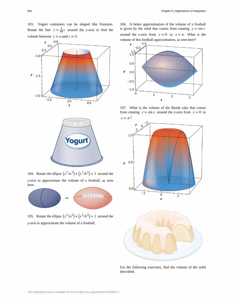
103. Yogurt containers can be shaped like frustums.
Rotate the line y = 1mx around the y-axis to find the
volume between y = a and y = b.
104. Rotate the ellipse ⎛⎝x2 /a2⎞
⎠ + ⎛⎝y2 /b2⎞
⎠ = 1 around the
x-axis to approximate the volume of a football, as seenhere.
105. Rotate the ellipse ⎛⎝x2 /a2⎞
⎠ + ⎛⎝y2 /b2⎞
⎠ = 1 around the
y-axis to approximate the volume of a football.
106. A better approximation of the volume of a footballis given by the solid that comes from rotating y = sin xaround the x-axis from x = 0 to x = π. What is the
volume of this football approximation, as seen here?
107. What is the volume of the Bundt cake that comesfrom rotating y = sin x around the y-axis from x = 0 to
x = π ?
For the following exercises, find the volume of the soliddescribed.
654 Chapter 6 | Applications of Integration
This OpenStax book is available for free at http://cnx.org/content/col11964/1.2
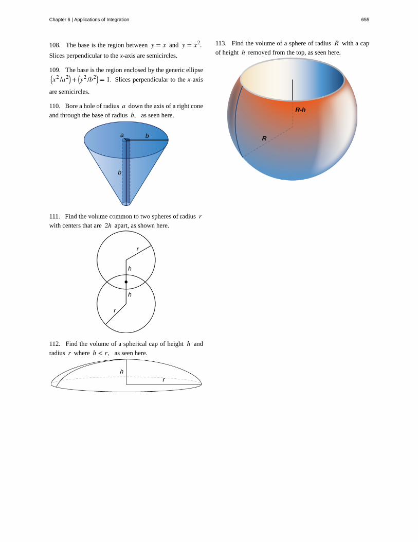
108. The base is the region between y = x and y = x2.Slices perpendicular to the x-axis are semicircles.
109. The base is the region enclosed by the generic ellipse⎛⎝x2 /a2⎞
⎠ + ⎛⎝y2 /b2⎞
⎠ = 1. Slices perpendicular to the x-axis
are semicircles.
110. Bore a hole of radius a down the axis of a right cone
and through the base of radius b, as seen here.
111. Find the volume common to two spheres of radius rwith centers that are 2h apart, as shown here.
112. Find the volume of a spherical cap of height h and
radius r where h < r, as seen here.
113. Find the volume of a sphere of radius R with a cap
of height h removed from the top, as seen here.
Chapter 6 | Applications of Integration 655
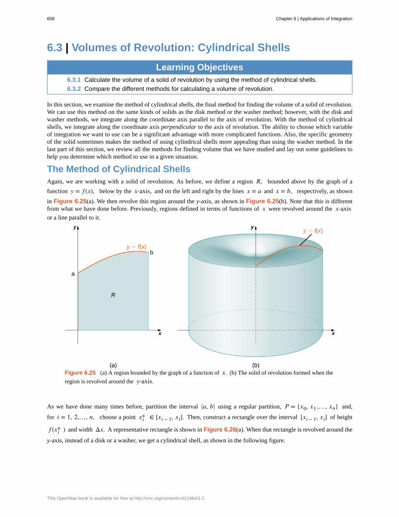
6.3 | Volumes of Revolution: Cylindrical Shells
Learning Objectives6.3.1 Calculate the volume of a solid of revolution by using the method of cylindrical shells.
6.3.2 Compare the different methods for calculating a volume of revolution.
In this section, we examine the method of cylindrical shells, the final method for finding the volume of a solid of revolution.We can use this method on the same kinds of solids as the disk method or the washer method; however, with the disk andwasher methods, we integrate along the coordinate axis parallel to the axis of revolution. With the method of cylindricalshells, we integrate along the coordinate axis perpendicular to the axis of revolution. The ability to choose which variableof integration we want to use can be a significant advantage with more complicated functions. Also, the specific geometryof the solid sometimes makes the method of using cylindrical shells more appealing than using the washer method. In thelast part of this section, we review all the methods for finding volume that we have studied and lay out some guidelines tohelp you determine which method to use in a given situation.
The Method of Cylindrical ShellsAgain, we are working with a solid of revolution. As before, we define a region R, bounded above by the graph of a
function y = f (x), below by the x-axis, and on the left and right by the lines x = a and x = b, respectively, as shown
in Figure 6.25(a). We then revolve this region around the y-axis, as shown in Figure 6.25(b). Note that this is differentfrom what we have done before. Previously, regions defined in terms of functions of x were revolved around the x-axisor a line parallel to it.
Figure 6.25 (a) A region bounded by the graph of a function of x. (b) The solid of revolution formed when the
region is revolved around the y-axis.
As we have done many times before, partition the interval ⎡⎣a, b⎤
⎦ using a regular partition, P = {x0, x1 ,…, xn} and,
for i = 1, 2,…, n, choose a point xi* ∈ [xi − 1, xi]. Then, construct a rectangle over the interval [xi − 1, xi] of height
f (xi* ) and width Δx. A representative rectangle is shown in Figure 6.26(a). When that rectangle is revolved around the
y-axis, instead of a disk or a washer, we get a cylindrical shell, as shown in the following figure.
656 Chapter 6 | Applications of Integration
This OpenStax book is available for free at http://cnx.org/content/col11964/1.2
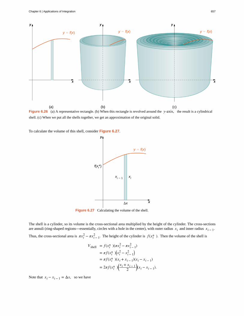
Figure 6.26 (a) A representative rectangle. (b) When this rectangle is revolved around the y-axis, the result is a cylindrical
shell. (c) When we put all the shells together, we get an approximation of the original solid.
To calculate the volume of this shell, consider Figure 6.27.
Figure 6.27 Calculating the volume of the shell.
The shell is a cylinder, so its volume is the cross-sectional area multiplied by the height of the cylinder. The cross-sectionsare annuli (ring-shaped regions—essentially, circles with a hole in the center), with outer radius xi and inner radius xi − 1.
Thus, the cross-sectional area is πxi2 − πxi − 1
2 . The height of the cylinder is f (xi* ). Then the volume of the shell is
Vshell = f (xi* )(πxi2 − πxi − 1
2 )
= π f (xi* )⎛⎝xi
2 − xi − 12 ⎞
⎠
= π f (xi* )(xi + xi − 1)(xi − xi − 1)
= 2π f (xi* )⎛⎝xi + xi − 1
2⎞⎠(xi − xi − 1).
Note that xi − xi − 1 = Δx, so we have
Chapter 6 | Applications of Integration 657
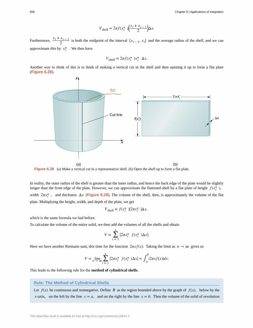
Vshell = 2π f (xi* )⎛⎝xi + xi − 1
2⎞⎠Δx.
Furthermore,xi + xi − 1
2 is both the midpoint of the interval [xi − 1, xi] and the average radius of the shell, and we can
approximate this by xi* . We then have
Vshell ≈ 2π f (xi* )xi* Δx.
Another way to think of this is to think of making a vertical cut in the shell and then opening it up to form a flat plate(Figure 6.28).
Figure 6.28 (a) Make a vertical cut in a representative shell. (b) Open the shell up to form a flat plate.
In reality, the outer radius of the shell is greater than the inner radius, and hence the back edge of the plate would be slightlylonger than the front edge of the plate. However, we can approximate the flattened shell by a flat plate of height f (xi* ),
width 2πxi* , and thickness Δx (Figure 6.28). The volume of the shell, then, is approximately the volume of the flat
plate. Multiplying the height, width, and depth of the plate, we get
Vshell ≈ f (xi* )⎛⎝2πxi*
⎞⎠Δx,
which is the same formula we had before.
To calculate the volume of the entire solid, we then add the volumes of all the shells and obtain
V ≈ ∑i = 1
n⎛⎝2πxi* f (xi* )Δx⎞
⎠.
Here we have another Riemann sum, this time for the function 2πx f (x). Taking the limit as n → ∞ gives us
V = limn → ∞ ∑i = 1
n⎛⎝2πxi* f (xi* )Δx⎞
⎠ = ∫a
b⎛⎝2πx f (x)⎞
⎠dx.
This leads to the following rule for the method of cylindrical shells.
Rule: The Method of Cylindrical Shells
Let f (x) be continuous and nonnegative. Define R as the region bounded above by the graph of f (x), below by the
x-axis, on the left by the line x = a, and on the right by the line x = b. Then the volume of the solid of revolution
658 Chapter 6 | Applications of Integration
This OpenStax book is available for free at http://cnx.org/content/col11964/1.2
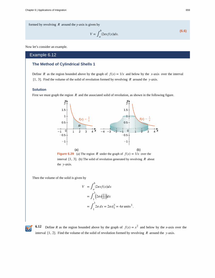
6.12
formed by revolving R around the y-axis is given by
(6.6)V = ∫
a
b⎛⎝2πx f (x)⎞
⎠dx.
Now let’s consider an example.
Example 6.12
The Method of Cylindrical Shells 1
Define R as the region bounded above by the graph of f (x) = 1/x and below by the x-axis over the interval
[1, 3]. Find the volume of the solid of revolution formed by revolving R around the y-axis.
Solution
First we must graph the region R and the associated solid of revolution, as shown in the following figure.
Figure 6.29 (a) The region R under the graph of f (x) = 1/x over the
interval [1, 3]. (b) The solid of revolution generated by revolving R about
the y-axis.
Then the volume of the solid is given by
V = ∫a
b⎛⎝2πx f (x)⎞
⎠dx
= ∫1
3⎛⎝2πx⎛
⎝1x
⎞⎠⎞⎠dx
= ∫1
32π dx = 2πx|13 = 4π units3 .
Define R as the region bounded above by the graph of f (x) = x2 and below by the x-axis over the
interval [1, 2]. Find the volume of the solid of revolution formed by revolving R around the y-axis.
Chapter 6 | Applications of Integration 659
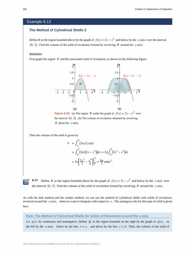
6.13
Example 6.13
The Method of Cylindrical Shells 2
Define R as the region bounded above by the graph of f (x) = 2x − x2 and below by the x-axis over the interval
[0, 2]. Find the volume of the solid of revolution formed by revolving R around the y-axis.
Solution
First graph the region R and the associated solid of revolution, as shown in the following figure.
Figure 6.30 (a) The region R under the graph of f (x) = 2x − x2 over
the interval [0, 2]. (b) The volume of revolution obtained by revolving
R about the y-axis.
Then the volume of the solid is given by
V = ∫a
b⎛⎝2πx f (x)⎞
⎠dx
= ∫0
2⎛⎝2πx⎛
⎝2x − x2⎞⎠⎞⎠dx = 2π∫
0
2⎛⎝2x2 − x3⎞
⎠dx
= 2π⎡⎣
2x3
3 − x4
4⎤⎦ |02 = 8π
3 units3 .
Define R as the region bounded above by the graph of f (x) = 3x − x2 and below by the x-axis over
the interval [0, 2]. Find the volume of the solid of revolution formed by revolving R around the y-axis.
As with the disk method and the washer method, we can use the method of cylindrical shells with solids of revolution,revolved around the x-axis, when we want to integrate with respect to y. The analogous rule for this type of solid is given
here.
Rule: The Method of Cylindrical Shells for Solids of Revolution around the x-axis
Let g(y) be continuous and nonnegative. Define Q as the region bounded on the right by the graph of g(y), on
the left by the y-axis, below by the line y = c, and above by the line y = d. Then, the volume of the solid of
660 Chapter 6 | Applications of Integration
This OpenStax book is available for free at http://cnx.org/content/col11964/1.2
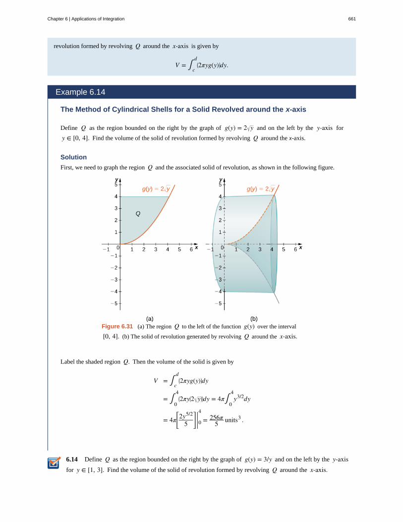
6.14
revolution formed by revolving Q around the x-axis is given by
V = ∫c
d⎛⎝2πyg(y)⎞
⎠dy.
Example 6.14
The Method of Cylindrical Shells for a Solid Revolved around the x-axis
Define Q as the region bounded on the right by the graph of g(y) = 2 y and on the left by the y-axis for
y ∈ [0, 4]. Find the volume of the solid of revolution formed by revolving Q around the x-axis.
Solution
First, we need to graph the region Q and the associated solid of revolution, as shown in the following figure.
Figure 6.31 (a) The region Q to the left of the function g(y) over the interval
[0, 4]. (b) The solid of revolution generated by revolving Q around the x-axis.
Label the shaded region Q. Then the volume of the solid is given by
V = ∫c
d⎛⎝2πyg(y)⎞
⎠dy
= ∫0
4⎛⎝2πy⎛
⎝2 y⎞⎠⎞⎠dy = 4π∫
0
4y3/2dy
= 4π⎡
⎣⎢2y5/2
5⎤
⎦⎥ |04 = 256π
5 units3 .
Define Q as the region bounded on the right by the graph of g(y) = 3/y and on the left by the y-axisfor y ∈ [1, 3]. Find the volume of the solid of revolution formed by revolving Q around the x-axis.
Chapter 6 | Applications of Integration 661
For the next example, we look at a solid of revolution for which the graph of a function is revolved around a line other thanone of the two coordinate axes. To set this up, we need to revisit the development of the method of cylindrical shells. Recallthat we found the volume of one of the shells to be given by
Vshell = f (xi* )(πxi2 − πxi − 1
2 )
= π f (xi* )⎛⎝xi
2 − xi − 12 ⎞
⎠
= π f (xi* )(xi + xi − 1)(xi − xi − 1)
= 2π f (xi* )⎛⎝xi + xi − 1
2⎞⎠(xi − xi − 1).
This was based on a shell with an outer radius of xi and an inner radius of xi − 1. If, however, we rotate the region around
a line other than the y-axis, we have a different outer and inner radius. Suppose, for example, that we rotate the region
around the line x = −k, where k is some positive constant. Then, the outer radius of the shell is xi + k and the inner
radius of the shell is xi − 1 + k. Substituting these terms into the expression for volume, we see that when a plane region is
rotated around the line x = −k, the volume of a shell is given by
Vshell = 2π f (xi* )⎛⎝⎛⎝xi + k⎞
⎠ + ⎛⎝xi − 1 + k⎞
⎠
2⎞⎠
⎛⎝⎛⎝xi + k⎞
⎠ − ⎛⎝xi − 1 + k⎞
⎠⎞⎠
= 2π f (xi* )⎛⎝⎛⎝xi + xi − 2
2⎞⎠ + k⎞
⎠Δx.
As before, we notice thatxi + xi − 1
2 is the midpoint of the interval [xi − 1, xi] and can be approximated by xi* . Then,
the approximate volume of the shell is
Vshell ≈ 2π⎛⎝xi* + k⎞
⎠ f (xi* )Δx.
The remainder of the development proceeds as before, and we see that
V = ∫a
b⎛⎝2π(x + k) f (x)⎞
⎠dx.
We could also rotate the region around other horizontal or vertical lines, such as a vertical line in the right half plane. Ineach case, the volume formula must be adjusted accordingly. Specifically, the x-term in the integral must be replaced with
an expression representing the radius of a shell. To see how this works, consider the following example.
Example 6.15
A Region of Revolution Revolved around a Line
Define R as the region bounded above by the graph of f (x) = x and below by the x-axis over the interval
[1, 2]. Find the volume of the solid of revolution formed by revolving R around the line x = −1.
Solution
First, graph the region R and the associated solid of revolution, as shown in the following figure.
662 Chapter 6 | Applications of Integration
This OpenStax book is available for free at http://cnx.org/content/col11964/1.2
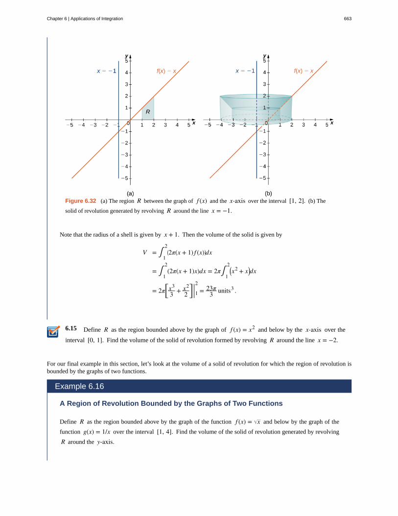
6.15
Figure 6.32 (a) The region R between the graph of f (x) and the x-axis over the interval [1, 2]. (b) The
solid of revolution generated by revolving R around the line x = −1.
Note that the radius of a shell is given by x + 1. Then the volume of the solid is given by
V = ∫1
2⎛⎝2π(x + 1) f (x)⎞
⎠dx
= ∫1
2(2π(x + 1)x)dx = 2π∫
1
2⎛⎝x2 + x⎞
⎠dx
= 2π⎡⎣
x3
3 + x2
2⎤⎦ |12 = 23π
3 units3 .
Define R as the region bounded above by the graph of f (x) = x2 and below by the x-axis over the
interval [0, 1]. Find the volume of the solid of revolution formed by revolving R around the line x = −2.
For our final example in this section, let’s look at the volume of a solid of revolution for which the region of revolution isbounded by the graphs of two functions.
Example 6.16
A Region of Revolution Bounded by the Graphs of Two Functions
Define R as the region bounded above by the graph of the function f (x) = x and below by the graph of the
function g(x) = 1/x over the interval [1, 4]. Find the volume of the solid of revolution generated by revolving
R around the y-axis.
Chapter 6 | Applications of Integration 663
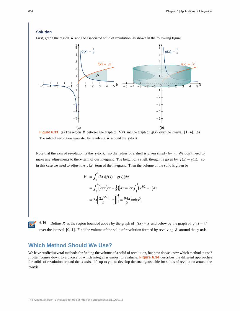
6.16
Solution
First, graph the region R and the associated solid of revolution, as shown in the following figure.
Figure 6.33 (a) The region R between the graph of f (x) and the graph of g(x) over the interval [1, 4]. (b)
The solid of revolution generated by revolving R around the y-axis.
Note that the axis of revolution is the y-axis, so the radius of a shell is given simply by x. We don’t need to
make any adjustments to the x-term of our integrand. The height of a shell, though, is given by f (x) − g(x), so
in this case we need to adjust the f (x) term of the integrand. Then the volume of the solid is given by
V = ∫1
4⎛⎝2πx⎛
⎝ f (x) − g(x)⎞⎠⎞⎠dx
= ∫1
4⎛⎝2πx⎛
⎝ x − 1x
⎞⎠⎞⎠dx = 2π∫
1
4⎛⎝x
3/2 − 1⎞⎠dx
= 2π⎡⎣
2x5/2
5 − x⎤⎦ |14 = 94π
5 units3.
Define R as the region bounded above by the graph of f (x) = x and below by the graph of g(x) = x2
over the interval [0, 1]. Find the volume of the solid of revolution formed by revolving R around the y-axis.
Which Method Should We Use?We have studied several methods for finding the volume of a solid of revolution, but how do we know which method to use?It often comes down to a choice of which integral is easiest to evaluate. Figure 6.34 describes the different approachesfor solids of revolution around the x-axis. It’s up to you to develop the analogous table for solids of revolution around the
y-axis.
664 Chapter 6 | Applications of Integration
This OpenStax book is available for free at http://cnx.org/content/col11964/1.2
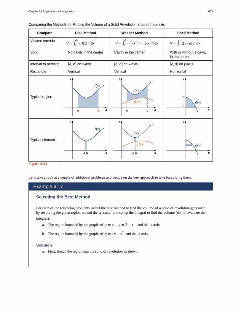
Figure 6.34
Let’s take a look at a couple of additional problems and decide on the best approach to take for solving them.
Example 6.17
Selecting the Best Method
For each of the following problems, select the best method to find the volume of a solid of revolution generatedby revolving the given region around the x-axis, and set up the integral to find the volume (do not evaluate the
integral).
a. The region bounded by the graphs of y = x, y = 2 − x, and the x-axis.
b. The region bounded by the graphs of y = 4x − x2 and the x-axis.
Solution
a. First, sketch the region and the solid of revolution as shown.
Chapter 6 | Applications of Integration 665
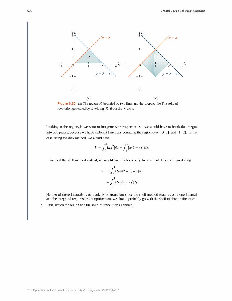
Figure 6.35 (a) The region R bounded by two lines and the x-axis. (b) The solid of
revolution generated by revolving R about the x-axis.
Looking at the region, if we want to integrate with respect to x, we would have to break the integral
into two pieces, because we have different functions bounding the region over [0, 1] and [1, 2]. In this
case, using the disk method, we would have
V = ∫0
1⎛⎝πx2⎞
⎠dx + ∫1
2⎛⎝π(2 − x)2⎞
⎠dx.
If we used the shell method instead, we would use functions of y to represent the curves, producing
V = ∫0
1⎛⎝2πy⎡
⎣⎛⎝2 − y⎞
⎠ − y⎤⎦⎞⎠dy
= ∫0
1⎛⎝2πy⎡
⎣2 − 2y⎤⎦⎞⎠dy.
Neither of these integrals is particularly onerous, but since the shell method requires only one integral,and the integrand requires less simplification, we should probably go with the shell method in this case.
b. First, sketch the region and the solid of revolution as shown.
666 Chapter 6 | Applications of Integration
This OpenStax book is available for free at http://cnx.org/content/col11964/1.2
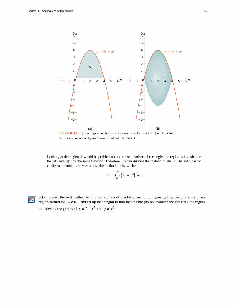
6.17
Figure 6.36 (a) The region R between the curve and the x-axis. (b) The solid of
revolution generated by revolving R about the x-axis.
Looking at the region, it would be problematic to define a horizontal rectangle; the region is bounded onthe left and right by the same function. Therefore, we can dismiss the method of shells. The solid has nocavity in the middle, so we can use the method of disks. Then
V = ∫0
4π⎛
⎝4x − x2⎞⎠2
dx.
Select the best method to find the volume of a solid of revolution generated by revolving the givenregion around the x-axis, and set up the integral to find the volume (do not evaluate the integral): the region
bounded by the graphs of y = 2 − x2 and y = x2.
Chapter 6 | Applications of Integration 667
6.3 EXERCISESFor the following exercise, find the volume generated whenthe region between the two curves is rotated around thegiven axis. Use both the shell method and the washermethod. Use technology to graph the functions and draw atypical slice by hand.
114. [T] Over the curve of y = 3x, x = 0, and y = 3rotated around the y-axis.
115. [T] Under the curve of y = 3x, x = 0, and x = 3rotated around the y-axis.
116. [T] Over the curve of y = 3x, x = 0, and y = 3rotated around the x-axis.
117. [T] Under the curve of y = 3x, x = 0, and x = 3rotated around the x-axis.
118. [T] Under the curve of y = 2x3, x = 0, and x = 2rotated around the y-axis.
119. [T] Under the curve of y = 2x3, x = 0, and x = 2rotated around the x-axis.
For the following exercises, use shells to find the volumesof the given solids. Note that the rotated regions lie betweenthe curve and the x-axis and are rotated around the
y-axis.
120. y = 1 − x2, x = 0, and x = 1
121. y = 5x3, x = 0, and x = 1
122. y = 1x , x = 1, and x = 100
123. y = 1 − x2, x = 0, and x = 1
124. y = 11 + x2, x = 0, and x = 3
125. y = sinx2, x = 0, and x = π
126. y = 11 − x2
, x = 0, and x = 12
127. y = x, x = 0, and x = 1
128. y = ⎛⎝1 + x2⎞
⎠3, x = 0, and x = 1
129. y = 5x3 − 2x4, x = 0, and x = 2
For the following exercises, use shells to find the volumegenerated by rotating the regions between the given curveand y = 0 around the x-axis.
130. y = 1 − x2, x = 0, and x = 1
131. y = x2, x = 0, and x = 2
132. y = ex, x = 0, and x = 1
133. y = ln(x), x = 1, and x = e
134. x = 11 + y2, y = 1, and y = 4
135. x = 1 + y2y , y = 0, and y = 2
136. x = cos y, y = 0, and y = π
137. x = y3 − 4y2, x = −1, and x = 2
138. x = yey , x = −1, and x = 2
139. x = cos yey, x = 0, and x = π
For the following exercises, find the volume generatedwhen the region between the curves is rotated around thegiven axis.
140. y = 3 − x, y = 0, x = 0, and x = 2 rotated around
the y-axis.
141. y = x3, y = 0, and y = 8 rotated around the
y-axis.
142. y = x2, y = x, rotated around the y-axis.
143. y = x, x = 0, and x = 1 rotated around the line
x = 2.
144. y = 14 − x, x = 1, and x = 2 rotated around the
line x = 4.
145. y = x and y = x2 rotated around the y-axis.
146. y = x and y = x2 rotated around the line x = 2.
668 Chapter 6 | Applications of Integration
This OpenStax book is available for free at http://cnx.org/content/col11964/1.2
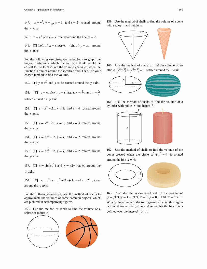
147. x = y3, y = 1x , x = 1, and y = 2 rotated around
the x-axis.
148. x = y2 and y = x rotated around the line y = 2.
149. [T] Left of x = sin(πy), right of y = x, around
the y-axis.
For the following exercises, use technology to graph theregion. Determine which method you think would beeasiest to use to calculate the volume generated when thefunction is rotated around the specified axis. Then, use yourchosen method to find the volume.
150. [T] y = x2 and y = 4x rotated around the y-axis.
151. [T] y = cos(πx), y = sin(πx), x = 14, and x = 5
4rotated around the y-axis.
152. [T] y = x2 − 2x, x = 2, and x = 4 rotated around
the y-axis.
153. [T] y = x2 − 2x, x = 2, and x = 4 rotated around
the x-axis.
154. [T] y = 3x3 − 2, y = x, and x = 2 rotated around
the x-axis.
155. [T] y = 3x3 − 2, y = x, and x = 2 rotated around
the y-axis.
156. [T] x = sin⎛⎝πy2⎞
⎠ and x = 2y rotated around the
x-axis.
157. [T] x = y2, x = y2 − 2y + 1, and x = 2 rotated
around the y-axis.
For the following exercises, use the method of shells toapproximate the volumes of some common objects, whichare pictured in accompanying figures.
158. Use the method of shells to find the volume of asphere of radius r.
159. Use the method of shells to find the volume of a conewith radius r and height h.
160. Use the method of shells to find the volume of an
ellipse ⎛⎝x2/a2⎞
⎠ + ⎛⎝y2/b2⎞
⎠ = 1 rotated around the x-axis.
161. Use the method of shells to find the volume of acylinder with radius r and height h.
162. Use the method of shells to find the volume of the
donut created when the circle x2 + y2 = 4 is rotated
around the line x = 4.
163. Consider the region enclosed by the graphs ofy = f (x), y = 1 + f (x), x = 0, y = 0, and x = a > 0.What is the volume of the solid generated when this regionis rotated around the y-axis? Assume that the function is
defined over the interval [0, a].
Chapter 6 | Applications of Integration 669
164. Consider the function y = f (x), which decreases
from f (0) = b to f (1) = 0. Set up the integrals for
determining the volume, using both the shell method andthe disk method, of the solid generated when this region,with x = 0 and y = 0, is rotated around the y-axis.Prove that both methods approximate the same volume.Which method is easier to apply? (Hint: Since f (x) is one-
to-one, there exists an inverse f −1(y).)
670 Chapter 6 | Applications of Integration
This OpenStax book is available for free at http://cnx.org/content/col11964/1.2
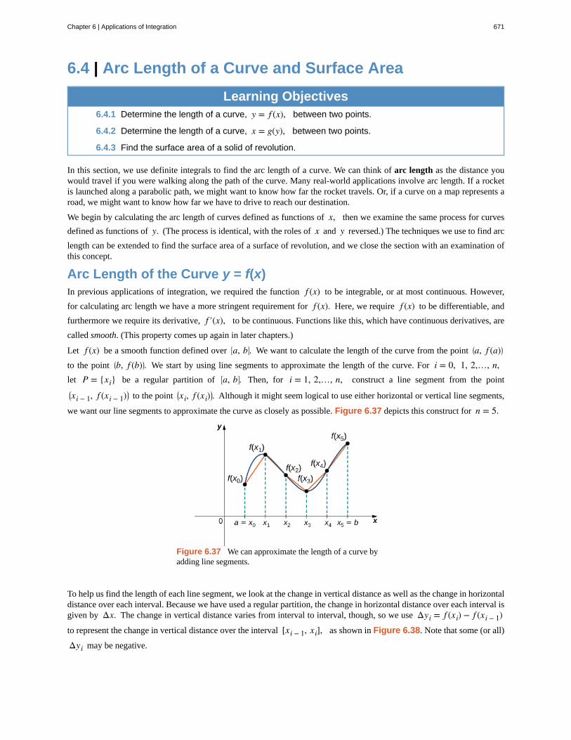
6.4 | Arc Length of a Curve and Surface Area
Learning Objectives6.4.1 Determine the length of a curve, y = f (x), between two points.
6.4.2 Determine the length of a curve, x = g(y), between two points.
6.4.3 Find the surface area of a solid of revolution.
In this section, we use definite integrals to find the arc length of a curve. We can think of arc length as the distance youwould travel if you were walking along the path of the curve. Many real-world applications involve arc length. If a rocketis launched along a parabolic path, we might want to know how far the rocket travels. Or, if a curve on a map represents aroad, we might want to know how far we have to drive to reach our destination.
We begin by calculating the arc length of curves defined as functions of x, then we examine the same process for curves
defined as functions of y. (The process is identical, with the roles of x and y reversed.) The techniques we use to find arc
length can be extended to find the surface area of a surface of revolution, and we close the section with an examination ofthis concept.
Arc Length of the Curve y = f(x)In previous applications of integration, we required the function f (x) to be integrable, or at most continuous. However,
for calculating arc length we have a more stringent requirement for f (x). Here, we require f (x) to be differentiable, and
furthermore we require its derivative, f ′(x), to be continuous. Functions like this, which have continuous derivatives, are
called smooth. (This property comes up again in later chapters.)
Let f (x) be a smooth function defined over ⎡⎣a, b⎤
⎦. We want to calculate the length of the curve from the point ⎛⎝a, f (a)⎞
⎠
to the point ⎛⎝b, f (b)⎞
⎠. We start by using line segments to approximate the length of the curve. For i = 0, 1, 2,…, n,let P = {xi} be a regular partition of ⎡
⎣a, b⎤⎦. Then, for i = 1, 2,…, n, construct a line segment from the point
⎛⎝xi − 1, f (xi − 1)⎞
⎠ to the point ⎛⎝xi, f (xi)
⎞⎠. Although it might seem logical to use either horizontal or vertical line segments,
we want our line segments to approximate the curve as closely as possible. Figure 6.37 depicts this construct for n = 5.
Figure 6.37 We can approximate the length of a curve byadding line segments.
To help us find the length of each line segment, we look at the change in vertical distance as well as the change in horizontaldistance over each interval. Because we have used a regular partition, the change in horizontal distance over each interval isgiven by Δx. The change in vertical distance varies from interval to interval, though, so we use Δyi = f (xi) − f (xi − 1)to represent the change in vertical distance over the interval [xi − 1, xi], as shown in Figure 6.38. Note that some (or all)
Δyi may be negative.
Chapter 6 | Applications of Integration 671
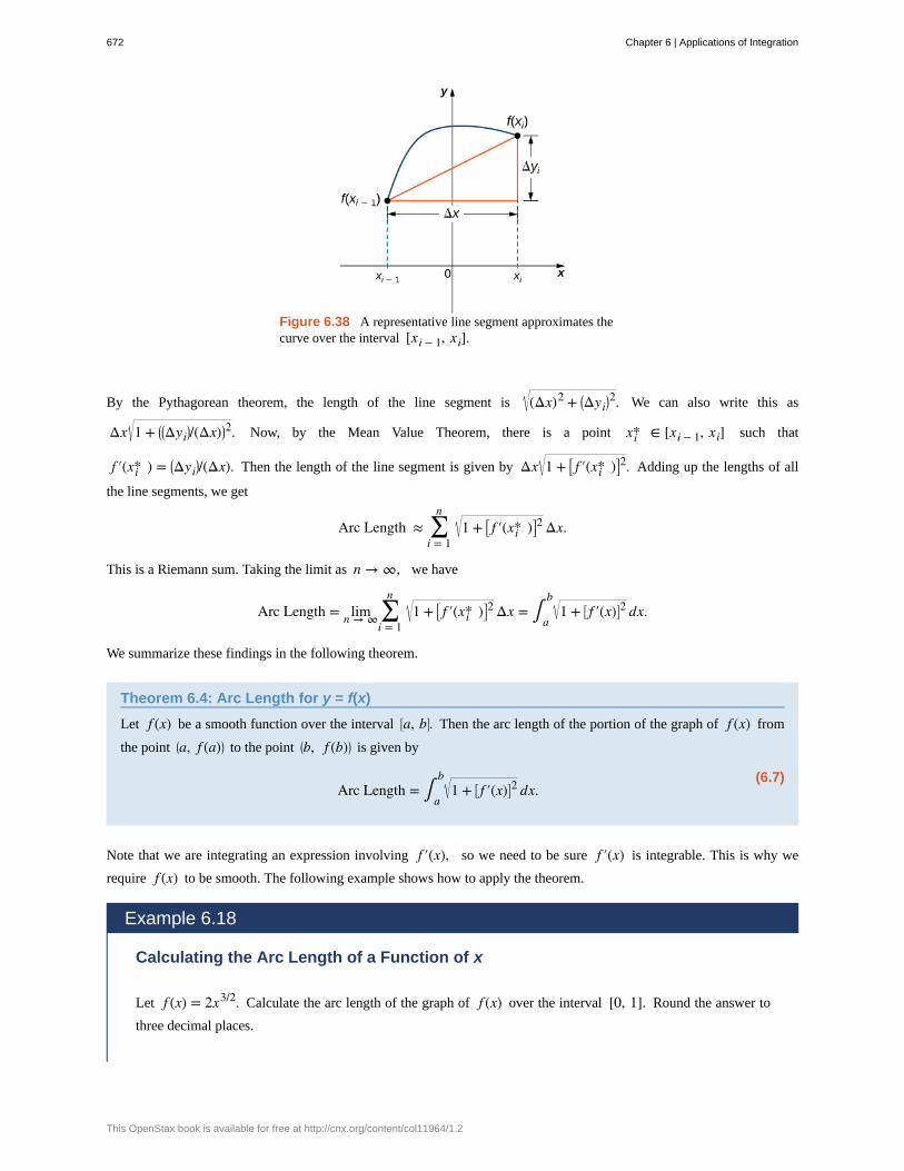
Figure 6.38 A representative line segment approximates thecurve over the interval [xi − 1, xi].
By the Pythagorean theorem, the length of the line segment is (Δx)2 + ⎛⎝Δyi
⎞⎠2. We can also write this as
Δx 1 + ⎛⎝⎛⎝Δyi
⎞⎠/(Δx)⎞
⎠2. Now, by the Mean Value Theorem, there is a point xi* ∈ [xi − 1, xi] such that
f ′(xi* ) = ⎛⎝Δyi
⎞⎠/(Δx). Then the length of the line segment is given by Δx 1 + ⎡
⎣ f ′(xi* )⎤⎦2. Adding up the lengths of all
the line segments, we get
Arc Length ≈ ∑i = 1
n1 + ⎡
⎣ f ′(xi* )⎤⎦2 Δx.
This is a Riemann sum. Taking the limit as n → ∞, we have
Arc Length = limn → ∞ ∑i = 1
n1 + ⎡
⎣ f ′(xi* )⎤⎦2 Δx = ∫
a
b1 + ⎡
⎣ f ′(x)⎤⎦2 dx.
We summarize these findings in the following theorem.
Theorem 6.4: Arc Length for y = f(x)
Let f (x) be a smooth function over the interval ⎡⎣a, b⎤
⎦. Then the arc length of the portion of the graph of f (x) from
the point ⎛⎝a, f (a)⎞
⎠ to the point ⎛⎝b, f (b)⎞
⎠ is given by
(6.7)Arc Length = ∫
a
b1 + ⎡
⎣ f ′(x)⎤⎦2 dx.
Note that we are integrating an expression involving f ′(x), so we need to be sure f ′(x) is integrable. This is why we
require f (x) to be smooth. The following example shows how to apply the theorem.
Example 6.18
Calculating the Arc Length of a Function of x
Let f (x) = 2x3/2. Calculate the arc length of the graph of f (x) over the interval [0, 1]. Round the answer to
three decimal places.
672 Chapter 6 | Applications of Integration
This OpenStax book is available for free at http://cnx.org/content/col11964/1.2
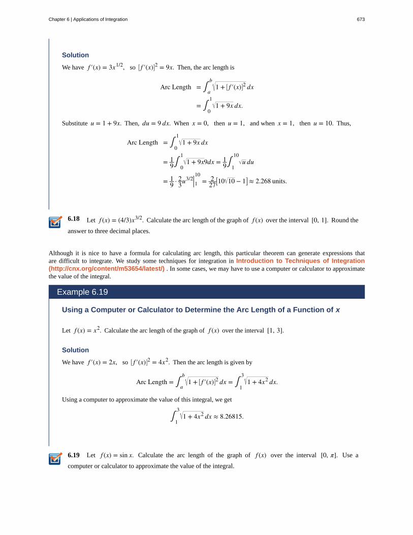
6.18
6.19
Solution
We have f ′(x) = 3x1/2, so ⎡⎣ f ′(x)⎤
⎦2 = 9x. Then, the arc length is
Arc Length = ∫a
b1 + ⎡
⎣ f ′(x)⎤⎦2 dx
= ∫0
11 + 9x dx.
Substitute u = 1 + 9x. Then, du = 9 dx. When x = 0, then u = 1, and when x = 1, then u = 10. Thus,
Arc Length = ∫0
11 + 9x dx
= 19∫
0
11 + 9x9dx = 1
9∫1
10u du
= 19 · 2
3u3/2|110= 2
27⎡⎣10 10 − 1⎤
⎦ ≈ 2.268 units.
Let f (x) = (4/3)x3/2. Calculate the arc length of the graph of f (x) over the interval [0, 1]. Round the
answer to three decimal places.
Although it is nice to have a formula for calculating arc length, this particular theorem can generate expressions thatare difficult to integrate. We study some techniques for integration in Introduction to Techniques of Integration(http://cnx.org/content/m53654/latest/) . In some cases, we may have to use a computer or calculator to approximatethe value of the integral.
Example 6.19
Using a Computer or Calculator to Determine the Arc Length of a Function of x
Let f (x) = x2. Calculate the arc length of the graph of f (x) over the interval [1, 3].
Solution
We have f ′(x) = 2x, so ⎡⎣ f ′(x)⎤
⎦2 = 4x2. Then the arc length is given by
Arc Length = ∫a
b1 + ⎡
⎣ f ′(x)⎤⎦2 dx = ∫
1
31 + 4x2 dx.
Using a computer to approximate the value of this integral, we get
∫1
31 + 4x2 dx ≈ 8.26815.
Let f (x) = sin x. Calculate the arc length of the graph of f (x) over the interval [0, π]. Use a
computer or calculator to approximate the value of the integral.
Chapter 6 | Applications of Integration 673
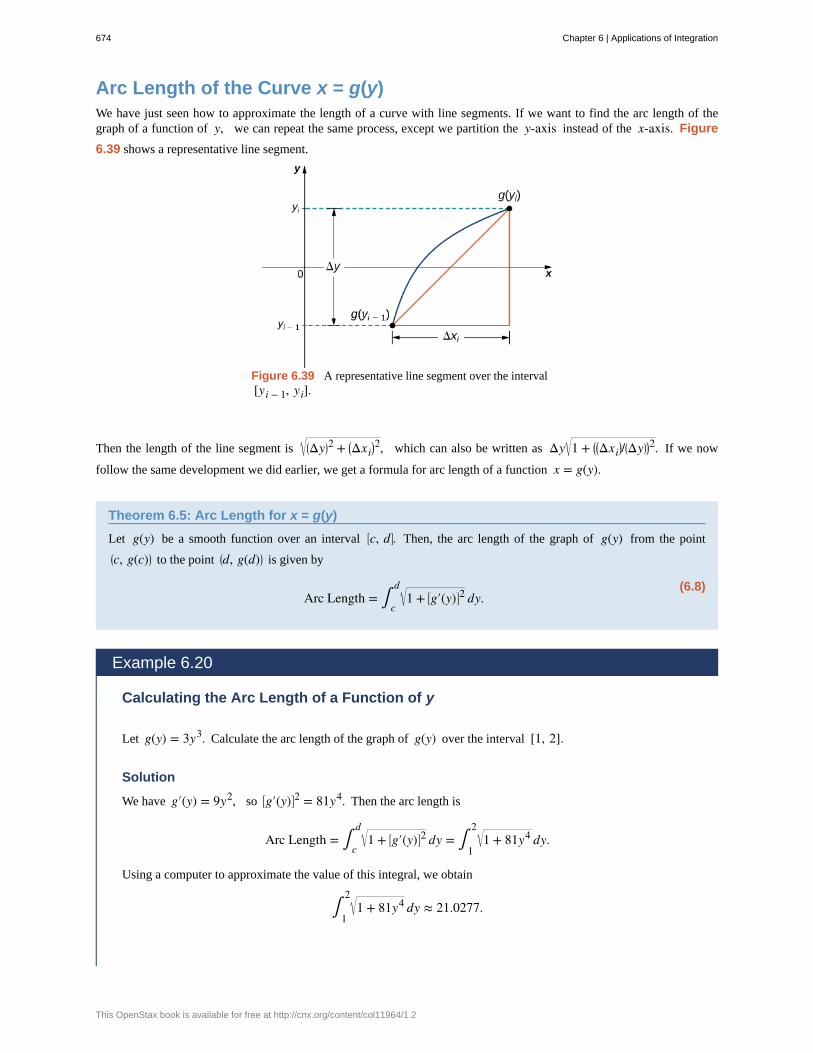
Arc Length of the Curve x = g(y)We have just seen how to approximate the length of a curve with line segments. If we want to find the arc length of thegraph of a function of y, we can repeat the same process, except we partition the y-axis instead of the x-axis. Figure
6.39 shows a representative line segment.
Figure 6.39 A representative line segment over the interval[yi − 1, yi].
Then the length of the line segment is ⎛⎝Δy⎞
⎠2 + ⎛
⎝Δxi⎞⎠2, which can also be written as Δy 1 + ⎛
⎝⎛⎝Δxi
⎞⎠/⎛
⎝Δy⎞⎠⎞⎠2. If we now
follow the same development we did earlier, we get a formula for arc length of a function x = g(y).
Theorem 6.5: Arc Length for x = g(y)
Let g(y) be a smooth function over an interval ⎡⎣c, d⎤
⎦. Then, the arc length of the graph of g(y) from the point⎛⎝c, g(c)⎞
⎠ to the point ⎛⎝d, g(d)⎞
⎠ is given by
(6.8)Arc Length = ∫
c
d1 + ⎡
⎣g′(y)⎤⎦2 dy.
Example 6.20
Calculating the Arc Length of a Function of y
Let g(y) = 3y3. Calculate the arc length of the graph of g(y) over the interval [1, 2].
Solution
We have g′(y) = 9y2, so ⎡⎣g′(y)⎤
⎦2 = 81y4. Then the arc length is
Arc Length = ∫c
d1 + ⎡
⎣g′(y)⎤⎦2 dy = ∫
1
21 + 81y4 dy.
Using a computer to approximate the value of this integral, we obtain
∫1
21 + 81y4 dy ≈ 21.0277.
674 Chapter 6 | Applications of Integration
This OpenStax book is available for free at http://cnx.org/content/col11964/1.2
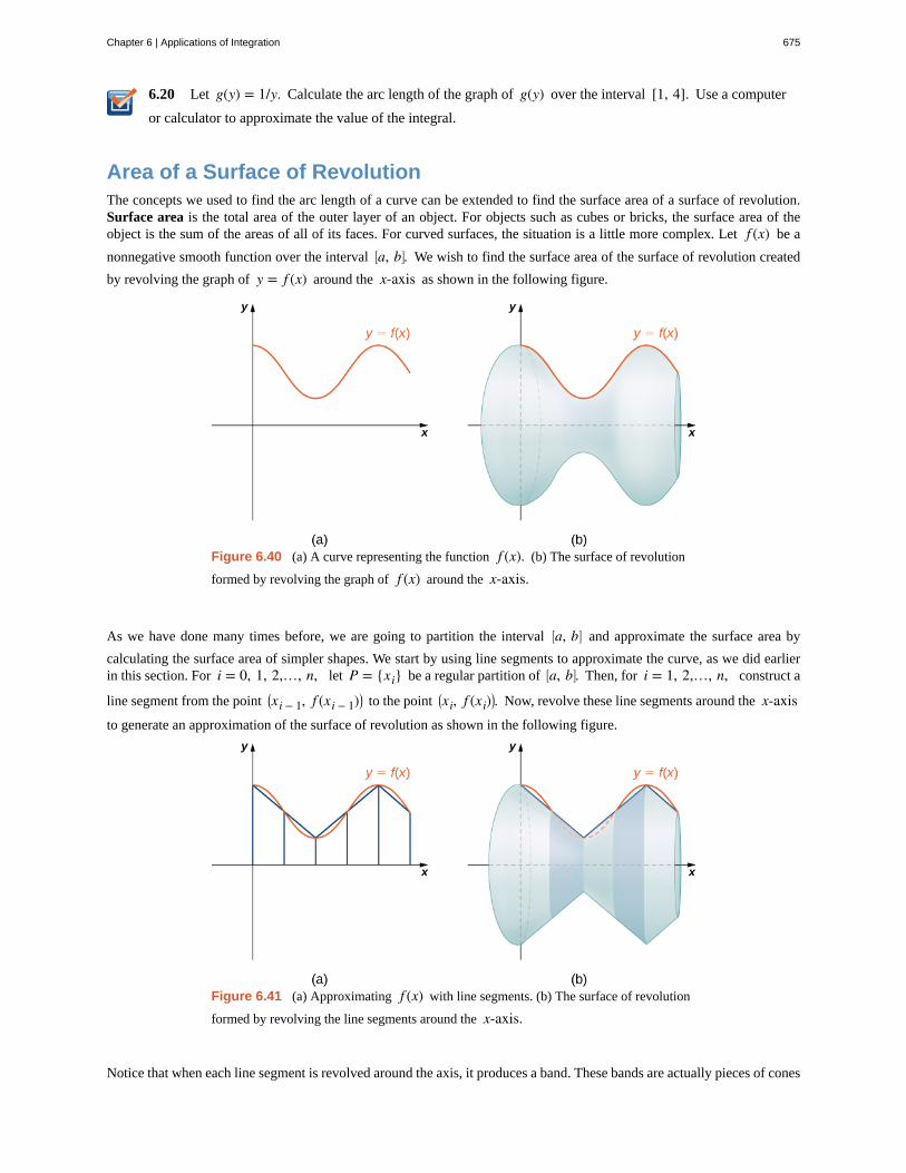
6.20 Let g(y) = 1/y. Calculate the arc length of the graph of g(y) over the interval [1, 4]. Use a computer
or calculator to approximate the value of the integral.
Area of a Surface of RevolutionThe concepts we used to find the arc length of a curve can be extended to find the surface area of a surface of revolution.Surface area is the total area of the outer layer of an object. For objects such as cubes or bricks, the surface area of theobject is the sum of the areas of all of its faces. For curved surfaces, the situation is a little more complex. Let f (x) be a
nonnegative smooth function over the interval ⎡⎣a, b⎤
⎦. We wish to find the surface area of the surface of revolution created
by revolving the graph of y = f (x) around the x-axis as shown in the following figure.
Figure 6.40 (a) A curve representing the function f (x). (b) The surface of revolution
formed by revolving the graph of f (x) around the x-axis.
As we have done many times before, we are going to partition the interval ⎡⎣a, b⎤
⎦ and approximate the surface area by
calculating the surface area of simpler shapes. We start by using line segments to approximate the curve, as we did earlierin this section. For i = 0, 1, 2,…, n, let P = {xi} be a regular partition of ⎡
⎣a, b⎤⎦. Then, for i = 1, 2,…, n, construct a
line segment from the point ⎛⎝xi − 1, f (xi − 1)⎞
⎠ to the point ⎛⎝xi, f (xi)
⎞⎠. Now, revolve these line segments around the x-axis
to generate an approximation of the surface of revolution as shown in the following figure.
Figure 6.41 (a) Approximating f (x) with line segments. (b) The surface of revolution
formed by revolving the line segments around the x-axis.
Notice that when each line segment is revolved around the axis, it produces a band. These bands are actually pieces of cones
Chapter 6 | Applications of Integration 675
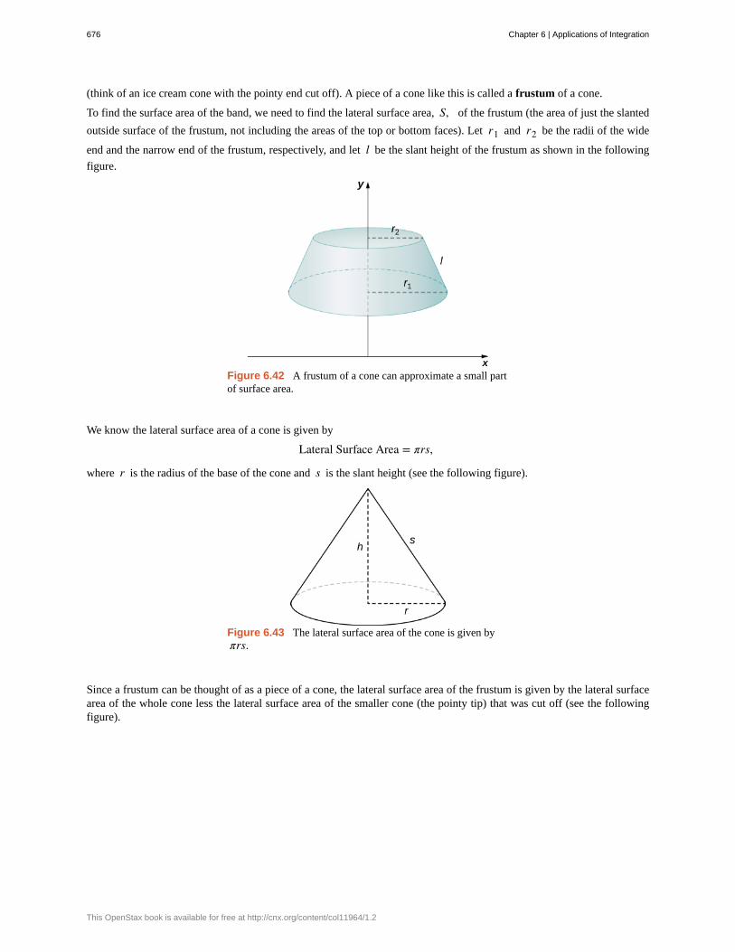
(think of an ice cream cone with the pointy end cut off). A piece of a cone like this is called a frustum of a cone.
To find the surface area of the band, we need to find the lateral surface area, S, of the frustum (the area of just the slanted
outside surface of the frustum, not including the areas of the top or bottom faces). Let r1 and r2 be the radii of the wide
end and the narrow end of the frustum, respectively, and let l be the slant height of the frustum as shown in the following
figure.
Figure 6.42 A frustum of a cone can approximate a small partof surface area.
We know the lateral surface area of a cone is given by
Lateral Surface Area = πrs,
where r is the radius of the base of the cone and s is the slant height (see the following figure).
Figure 6.43 The lateral surface area of the cone is given byπrs.
Since a frustum can be thought of as a piece of a cone, the lateral surface area of the frustum is given by the lateral surfacearea of the whole cone less the lateral surface area of the smaller cone (the pointy tip) that was cut off (see the followingfigure).
676 Chapter 6 | Applications of Integration
This OpenStax book is available for free at http://cnx.org/content/col11964/1.2
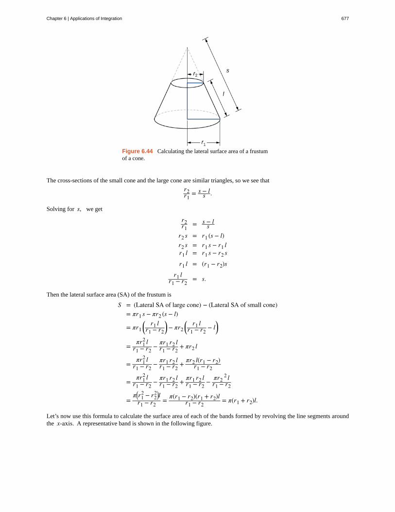
Figure 6.44 Calculating the lateral surface area of a frustumof a cone.
The cross-sections of the small cone and the large cone are similar triangles, so we see that
r2r1
= s − ls .
Solving for s, we get
r2r1
= s − ls
r2 s = r1 (s − l)r2 s = r1 s − r1 lr1 l = r1 s − r2 s
r1 l = (r1 − r2)s
r1 lr1 − r2
= s.
Then the lateral surface area (SA) of the frustum is
S = (Lateral SA of large cone) − (Lateral SA of small cone)= πr1 s − πr2 (s − l)
= πr1⎛⎝
r1 lr1 − r2
⎞⎠ − πr2
⎛⎝
r1 lr1 − r2
− l⎞⎠
=πr1
2 lr1 − r2
− πr1 r2 lr1 − r2
+ πr2 l
=πr1
2 lr1 − r2
− πr1 r2 lr1 − r2
+ πr2 l(r1 − r2)r1 − r2
=πr1
2 lr1 − r2
− πr1 r2 lr1 − r2
+ πr1 r2 lr1 − r2
− πr22 l
r1 − r2
=π⎛
⎝r12 − r2
2⎞⎠l
r1 − r2= π(r1 − r2)(r1 + r2)l
r1 − r2= π(r1 + r2)l.
Let’s now use this formula to calculate the surface area of each of the bands formed by revolving the line segments aroundthe x-axis. A representative band is shown in the following figure.
Chapter 6 | Applications of Integration 677
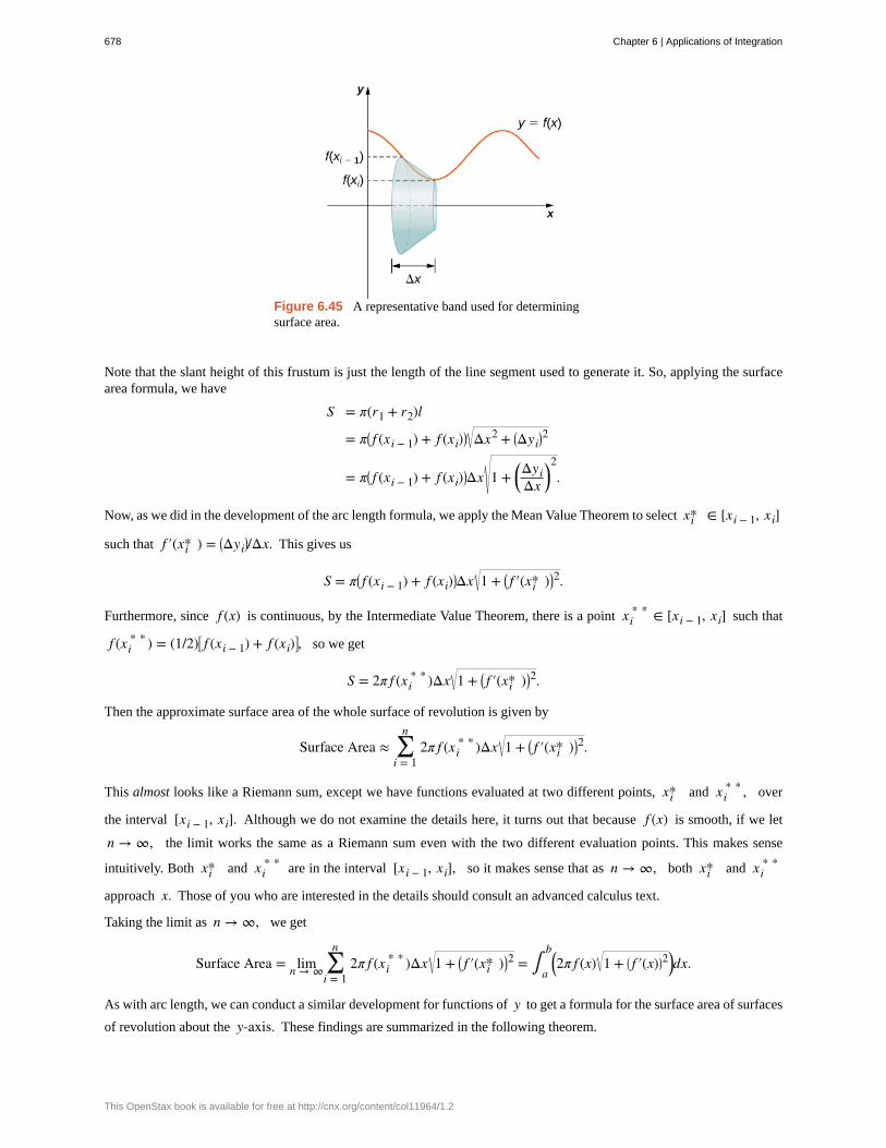
Figure 6.45 A representative band used for determiningsurface area.
Note that the slant height of this frustum is just the length of the line segment used to generate it. So, applying the surfacearea formula, we have
S = π(r1 + r2)l
= π⎛⎝ f (xi − 1) + f (xi)
⎞⎠ Δx2 + ⎛
⎝Δyi⎞⎠2
= π⎛⎝ f (xi − 1) + f (xi)
⎞⎠Δx 1 + ⎛
⎝ΔyiΔx
⎞⎠
2.
Now, as we did in the development of the arc length formula, we apply the Mean Value Theorem to select xi* ∈ [xi − 1, xi]
such that f ′(xi* ) = ⎛⎝Δyi
⎞⎠/Δx. This gives us
S = π⎛⎝ f (xi − 1) + f (xi)
⎞⎠Δx 1 + ⎛
⎝ f ′(xi* )⎞⎠2.
Furthermore, since f (x) is continuous, by the Intermediate Value Theorem, there is a point xi* * ∈ [xi − 1, xi] such that
f (xi* * ) = (1/2)⎡
⎣ f (xi − 1) + f (xi)⎤⎦, so we get
S = 2π f (xi* * )Δx 1 + ⎛
⎝ f ′(xi* )⎞⎠2.
Then the approximate surface area of the whole surface of revolution is given by
Surface Area ≈ ∑i = 1
n2π f (xi
* * )Δx 1 + ⎛⎝ f ′(xi* )⎞
⎠2.
This almost looks like a Riemann sum, except we have functions evaluated at two different points, xi* and xi* * , over
the interval [xi − 1, xi]. Although we do not examine the details here, it turns out that because f (x) is smooth, if we let
n → ∞, the limit works the same as a Riemann sum even with the two different evaluation points. This makes sense
intuitively. Both xi* and xi* * are in the interval [xi − 1, xi], so it makes sense that as n → ∞, both xi* and xi
* *
approach x. Those of you who are interested in the details should consult an advanced calculus text.
Taking the limit as n → ∞, we get
Surface Area = limn → ∞ ∑i = 1
n2π f (xi
* * )Δx 1 + ⎛⎝ f ′(xi* )⎞
⎠2 = ∫
a
b⎛⎝2π f (x) 1 + ⎛
⎝ f ′(x)⎞⎠2⎞⎠dx.
As with arc length, we can conduct a similar development for functions of y to get a formula for the surface area of surfaces
of revolution about the y-axis. These findings are summarized in the following theorem.
678 Chapter 6 | Applications of Integration
This OpenStax book is available for free at http://cnx.org/content/col11964/1.2
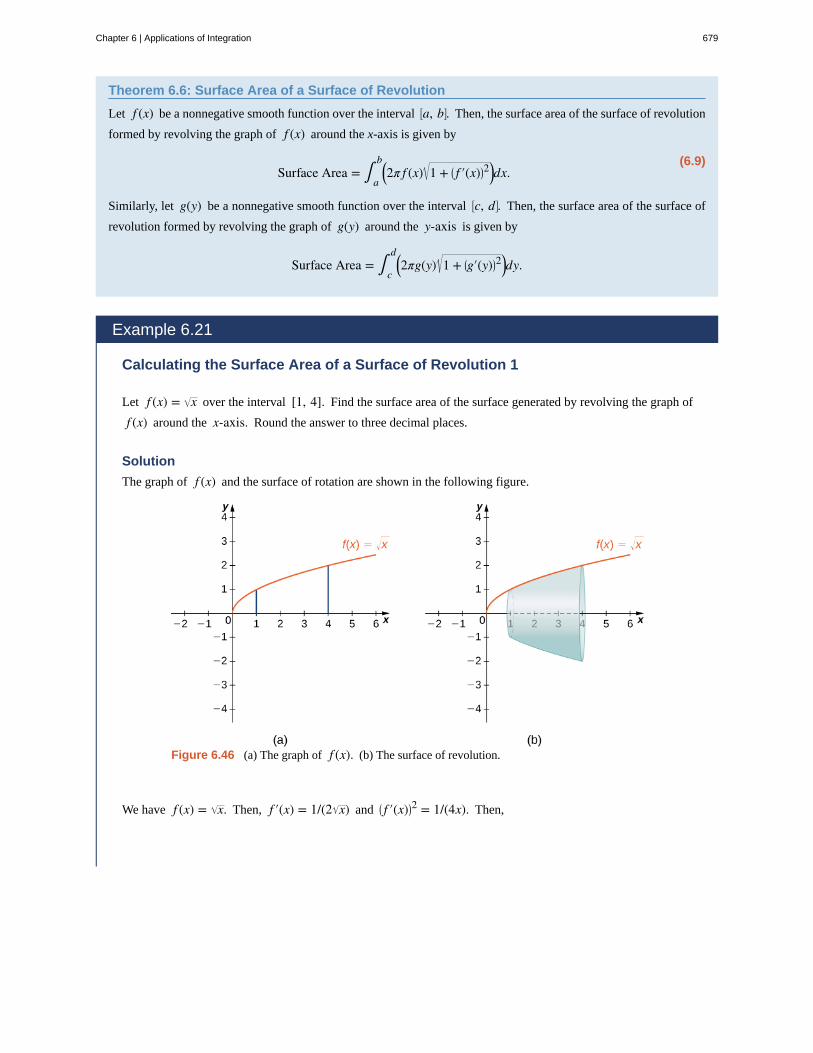
Theorem 6.6: Surface Area of a Surface of Revolution
Let f (x) be a nonnegative smooth function over the interval ⎡⎣a, b⎤
⎦. Then, the surface area of the surface of revolution
formed by revolving the graph of f (x) around the x-axis is given by
(6.9)Surface Area = ∫
a
b⎛⎝2π f (x) 1 + ⎛
⎝ f ′(x)⎞⎠2⎞⎠dx.
Similarly, let g(y) be a nonnegative smooth function over the interval ⎡⎣c, d⎤
⎦. Then, the surface area of the surface of
revolution formed by revolving the graph of g(y) around the y-axis is given by
Surface Area = ∫c
d⎛⎝2πg(y) 1 + ⎛
⎝g′(y)⎞⎠2⎞⎠dy.
Example 6.21
Calculating the Surface Area of a Surface of Revolution 1
Let f (x) = x over the interval [1, 4]. Find the surface area of the surface generated by revolving the graph of
f (x) around the x-axis. Round the answer to three decimal places.
Solution
The graph of f (x) and the surface of rotation are shown in the following figure.
Figure 6.46 (a) The graph of f (x). (b) The surface of revolution.
We have f (x) = x. Then, f ′(x) = 1/(2 x) and ⎛⎝ f ′(x)⎞
⎠2 = 1/(4x). Then,
Chapter 6 | Applications of Integration 679
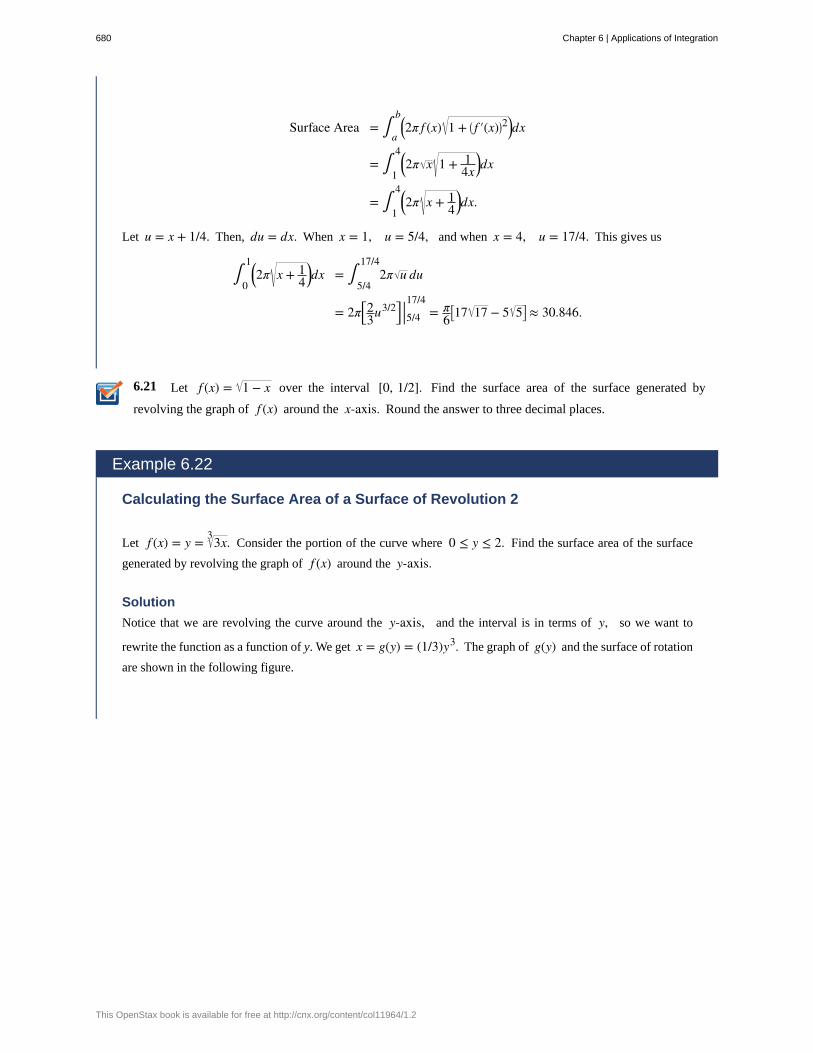
6.21
Surface Area = ∫a
b⎛⎝2π f (x) 1 + ⎛
⎝ f ′(x)⎞⎠2⎞⎠dx
= ∫1
4⎛⎝2π x 1 + 1
4x⎞⎠dx
= ∫1
4⎛⎝2π x + 1
4⎞⎠dx.
Let u = x + 1/4. Then, du = dx. When x = 1, u = 5/4, and when x = 4, u = 17/4. This gives us
∫0
1⎛⎝2π x + 1
4⎞⎠dx = ∫
5/4
17/42π u du
= 2π⎡⎣23u3/2⎤
⎦ |5/4
17/4= π
6⎡⎣17 17 − 5 5⎤
⎦ ≈ 30.846.
Let f (x) = 1 − x over the interval [0, 1/2]. Find the surface area of the surface generated by
revolving the graph of f (x) around the x-axis. Round the answer to three decimal places.
Example 6.22
Calculating the Surface Area of a Surface of Revolution 2
Let f (x) = y = 3x3 . Consider the portion of the curve where 0 ≤ y ≤ 2. Find the surface area of the surface
generated by revolving the graph of f (x) around the y-axis.
Solution
Notice that we are revolving the curve around the y-axis, and the interval is in terms of y, so we want to
rewrite the function as a function of y. We get x = g(y) = (1/3)y3. The graph of g(y) and the surface of rotation
are shown in the following figure.
680 Chapter 6 | Applications of Integration
This OpenStax book is available for free at http://cnx.org/content/col11964/1.2
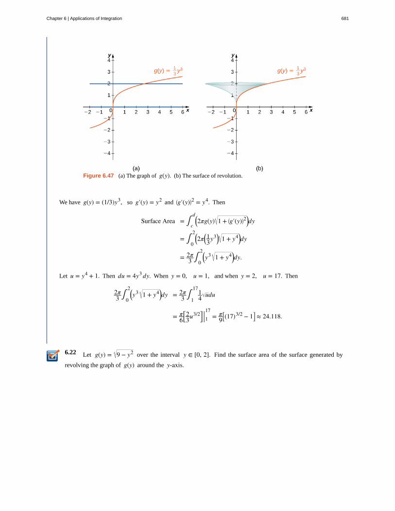
6.22
Figure 6.47 (a) The graph of g(y). (b) The surface of revolution.
We have g(y) = (1/3)y3, so g′(y) = y2 and ⎛⎝g′(y)⎞
⎠2 = y4. Then
Surface Area = ∫c
d⎛⎝2πg(y) 1 + ⎛
⎝g′(y)⎞⎠2⎞⎠dy
= ∫0
2⎛⎝2π⎛
⎝13y3⎞
⎠ 1 + y4⎞⎠dy
= 2π3 ∫
0
2⎛⎝y
3 1 + y4⎞⎠dy.
Let u = y4 + 1. Then du = 4y3 dy. When y = 0, u = 1, and when y = 2, u = 17. Then
2π3 ∫
0
2⎛⎝y
3 1 + y4⎞⎠dy = 2π
3 ∫1
1714 udu
= π6
⎡⎣23u3/2⎤
⎦ |117= π
9⎡⎣(17)3/2 − 1⎤
⎦ ≈ 24.118.
Let g(y) = 9 − y2 over the interval y ∈ [0, 2]. Find the surface area of the surface generated by
revolving the graph of g(y) around the y-axis.
Chapter 6 | Applications of Integration 681
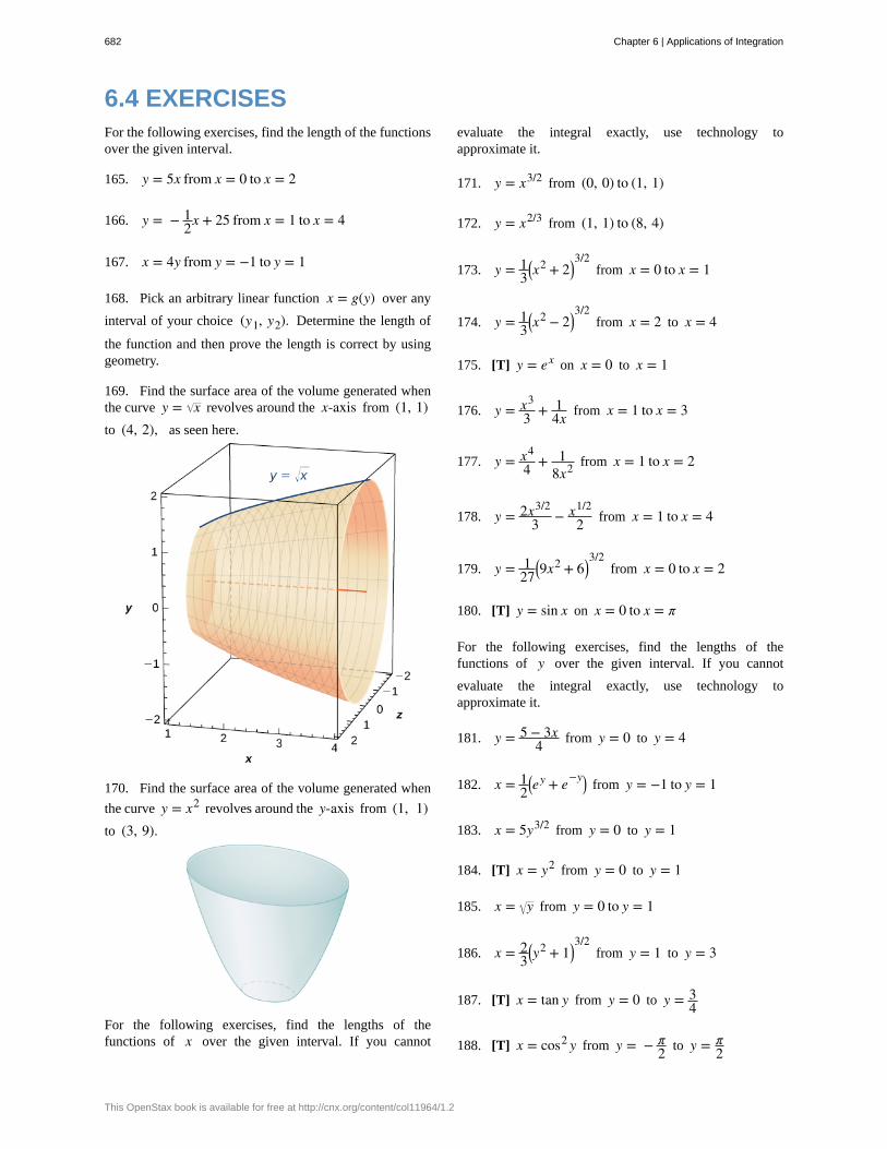
6.4 EXERCISESFor the following exercises, find the length of the functionsover the given interval.
165. y = 5x from x = 0 to x = 2
166. y = − 12x + 25 from x = 1 to x = 4
167. x = 4y from y = −1 to y = 1
168. Pick an arbitrary linear function x = g(y) over any
interval of your choice (y1, y2). Determine the length of
the function and then prove the length is correct by usinggeometry.
169. Find the surface area of the volume generated whenthe curve y = x revolves around the x-axis from (1, 1)to (4, 2), as seen here.
170. Find the surface area of the volume generated when
the curve y = x2 revolves around the y-axis from (1, 1)to (3, 9).
For the following exercises, find the lengths of thefunctions of x over the given interval. If you cannot
evaluate the integral exactly, use technology toapproximate it.
171. y = x3/2 from (0, 0) to (1, 1)
172. y = x2/3 from (1, 1) to (8, 4)
173. y = 13
⎛⎝x2 + 2⎞
⎠3/2
from x = 0 to x = 1
174. y = 13
⎛⎝x2 − 2⎞
⎠3/2
from x = 2 to x = 4
175. [T] y = ex on x = 0 to x = 1
176. y = x3
3 + 14x from x = 1 to x = 3
177. y = x4
4 + 18x2 from x = 1 to x = 2
178. y = 2x3/2
3 − x1/2
2 from x = 1 to x = 4
179. y = 127
⎛⎝9x2 + 6⎞
⎠3/2
from x = 0 to x = 2
180. [T] y = sin x on x = 0 to x = π
For the following exercises, find the lengths of thefunctions of y over the given interval. If you cannot
evaluate the integral exactly, use technology toapproximate it.
181. y = 5 − 3x4 from y = 0 to y = 4
182. x = 12
⎛⎝ey + e−y⎞
⎠ from y = −1 to y = 1
183. x = 5y3/2 from y = 0 to y = 1
184. [T] x = y2 from y = 0 to y = 1
185. x = y from y = 0 to y = 1
186. x = 23
⎛⎝y2 + 1⎞
⎠3/2
from y = 1 to y = 3
187. [T] x = tan y from y = 0 to y = 34
188. [T] x = cos2 y from y = − π2 to y = π
2
682 Chapter 6 | Applications of Integration
This OpenStax book is available for free at http://cnx.org/content/col11964/1.2
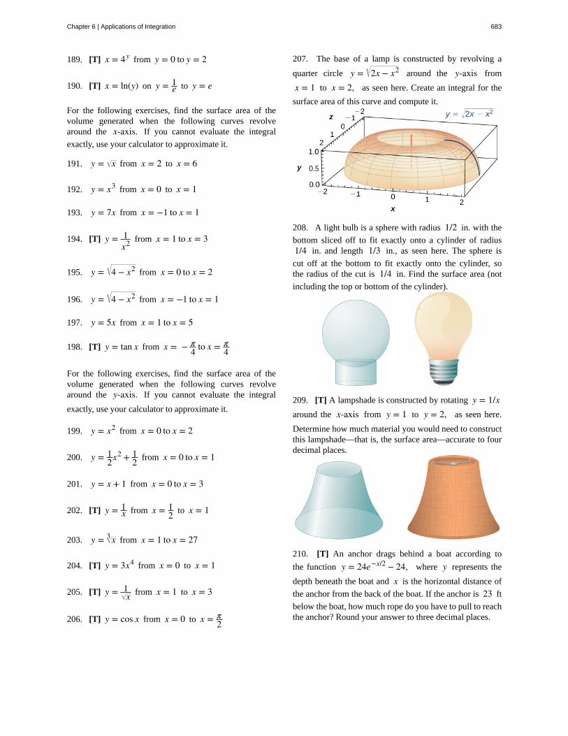
189. [T] x = 4y from y = 0 to y = 2
190. [T] x = ln(y) on y = 1e to y = e
For the following exercises, find the surface area of thevolume generated when the following curves revolvearound the x-axis. If you cannot evaluate the integral
exactly, use your calculator to approximate it.
191. y = x from x = 2 to x = 6
192. y = x3 from x = 0 to x = 1
193. y = 7x from x = −1 to x = 1
194. [T] y = 1x2 from x = 1 to x = 3
195. y = 4 − x2 from x = 0 to x = 2
196. y = 4 − x2 from x = −1 to x = 1
197. y = 5x from x = 1 to x = 5
198. [T] y = tan x from x = − π4 to x = π
4
For the following exercises, find the surface area of thevolume generated when the following curves revolvearound the y-axis. If you cannot evaluate the integral
exactly, use your calculator to approximate it.
199. y = x2 from x = 0 to x = 2
200. y = 12x2 + 1
2 from x = 0 to x = 1
201. y = x + 1 from x = 0 to x = 3
202. [T] y = 1x from x = 1
2 to x = 1
203. y = x3 from x = 1 to x = 27
204. [T] y = 3x4 from x = 0 to x = 1
205. [T] y = 1x from x = 1 to x = 3
206. [T] y = cos x from x = 0 to x = π2
207. The base of a lamp is constructed by revolving a
quarter circle y = 2x − x2 around the y-axis from
x = 1 to x = 2, as seen here. Create an integral for the
surface area of this curve and compute it.
208. A light bulb is a sphere with radius 1/2 in. with the
bottom sliced off to fit exactly onto a cylinder of radius1/4 in. and length 1/3 in., as seen here. The sphere is
cut off at the bottom to fit exactly onto the cylinder, sothe radius of the cut is 1/4 in. Find the surface area (not
including the top or bottom of the cylinder).
209. [T] A lampshade is constructed by rotating y = 1/xaround the x-axis from y = 1 to y = 2, as seen here.
Determine how much material you would need to constructthis lampshade—that is, the surface area—accurate to fourdecimal places.
210. [T] An anchor drags behind a boat according to
the function y = 24e−x/2 − 24, where y represents the
depth beneath the boat and x is the horizontal distance of
the anchor from the back of the boat. If the anchor is 23 ft
below the boat, how much rope do you have to pull to reachthe anchor? Round your answer to three decimal places.
Chapter 6 | Applications of Integration 683
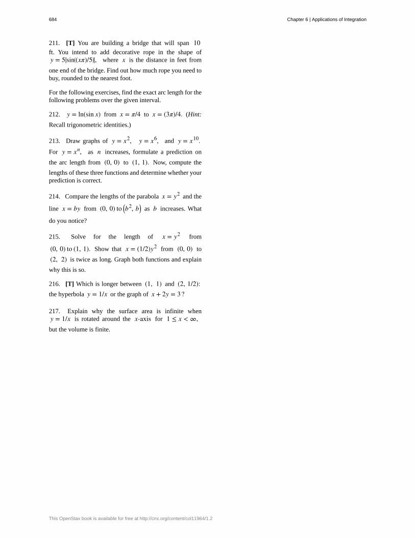
211. [T] You are building a bridge that will span 10ft. You intend to add decorative rope in the shape ofy = 5|sin⎛
⎝(xπ)/5⎞⎠|, where x is the distance in feet from
one end of the bridge. Find out how much rope you need tobuy, rounded to the nearest foot.
For the following exercises, find the exact arc length for thefollowing problems over the given interval.
212. y = ln(sin x) from x = π/4 to x = (3π)/4. (Hint:
Recall trigonometric identities.)
213. Draw graphs of y = x2, y = x6, and y = x10.For y = xn, as n increases, formulate a prediction on
the arc length from (0, 0) to (1, 1). Now, compute the
lengths of these three functions and determine whether yourprediction is correct.
214. Compare the lengths of the parabola x = y2 and the
line x = by from (0, 0) to ⎛⎝b2, b⎞
⎠ as b increases. What
do you notice?
215. Solve for the length of x = y2 from
(0, 0) to (1, 1). Show that x = (1/2)y2 from (0, 0) to
(2, 2) is twice as long. Graph both functions and explain
why this is so.
216. [T] Which is longer between (1, 1) and (2, 1/2):the hyperbola y = 1/x or the graph of x + 2y = 3?
217. Explain why the surface area is infinite wheny = 1/x is rotated around the x-axis for 1 ≤ x < ∞,but the volume is finite.
684 Chapter 6 | Applications of Integration
This OpenStax book is available for free at http://cnx.org/content/col11964/1.2
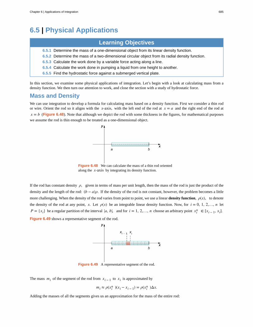
6.5 | Physical Applications
Learning Objectives6.5.1 Determine the mass of a one-dimensional object from its linear density function.
6.5.2 Determine the mass of a two-dimensional circular object from its radial density function.
6.5.3 Calculate the work done by a variable force acting along a line.
6.5.4 Calculate the work done in pumping a liquid from one height to another.
6.5.5 Find the hydrostatic force against a submerged vertical plate.
In this section, we examine some physical applications of integration. Let’s begin with a look at calculating mass from adensity function. We then turn our attention to work, and close the section with a study of hydrostatic force.
Mass and DensityWe can use integration to develop a formula for calculating mass based on a density function. First we consider a thin rodor wire. Orient the rod so it aligns with the x-axis, with the left end of the rod at x = a and the right end of the rod at
x = b (Figure 6.48). Note that although we depict the rod with some thickness in the figures, for mathematical purposes
we assume the rod is thin enough to be treated as a one-dimensional object.
Figure 6.48 We can calculate the mass of a thin rod orientedalong the x-axis by integrating its density function.
If the rod has constant density ρ, given in terms of mass per unit length, then the mass of the rod is just the product of the
density and the length of the rod: (b − a)ρ. If the density of the rod is not constant, however, the problem becomes a little
more challenging. When the density of the rod varies from point to point, we use a linear density function, ρ(x), to denote
the density of the rod at any point, x. Let ρ(x) be an integrable linear density function. Now, for i = 0, 1, 2,…, n let
P = {xi} be a regular partition of the interval ⎡⎣a, b⎤
⎦, and for i = 1, 2,…, n choose an arbitrary point xi* ∈ [xi − 1, xi].
Figure 6.49 shows a representative segment of the rod.
Figure 6.49 A representative segment of the rod.
The mass mi of the segment of the rod from xi − 1 to xi is approximated by
mi ≈ ρ(xi* )(xi − xi − 1) = ρ(xi* )Δx.
Adding the masses of all the segments gives us an approximation for the mass of the entire rod:
Chapter 6 | Applications of Integration 685
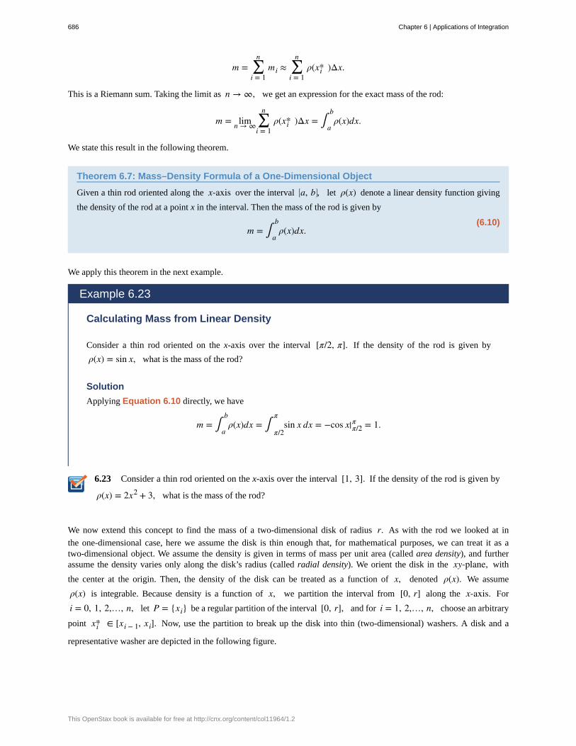
6.23
m = ∑i = 1
nmi ≈ ∑
i = 1
nρ(xi* )Δx.
This is a Riemann sum. Taking the limit as n → ∞, we get an expression for the exact mass of the rod:
m = limn → ∞ ∑i = 1
nρ(xi* )Δx = ∫
a
bρ(x)dx.
We state this result in the following theorem.
Theorem 6.7: Mass–Density Formula of a One-Dimensional Object
Given a thin rod oriented along the x-axis over the interval ⎡⎣a, b⎤
⎦, let ρ(x) denote a linear density function giving
the density of the rod at a point x in the interval. Then the mass of the rod is given by
(6.10)m = ∫
a
bρ(x)dx.
We apply this theorem in the next example.
Example 6.23
Calculating Mass from Linear Density
Consider a thin rod oriented on the x-axis over the interval [π/2, π]. If the density of the rod is given by
ρ(x) = sin x, what is the mass of the rod?
Solution
Applying Equation 6.10 directly, we have
m = ∫a
bρ(x)dx = ∫
π/2
πsin x dx = −cos x|π/2
π = 1.
Consider a thin rod oriented on the x-axis over the interval [1, 3]. If the density of the rod is given by
ρ(x) = 2x2 + 3, what is the mass of the rod?
We now extend this concept to find the mass of a two-dimensional disk of radius r. As with the rod we looked at in
the one-dimensional case, here we assume the disk is thin enough that, for mathematical purposes, we can treat it as atwo-dimensional object. We assume the density is given in terms of mass per unit area (called area density), and furtherassume the density varies only along the disk’s radius (called radial density). We orient the disk in the xy-plane, with
the center at the origin. Then, the density of the disk can be treated as a function of x, denoted ρ(x). We assume
ρ(x) is integrable. Because density is a function of x, we partition the interval from [0, r] along the x-axis. For
i = 0, 1, 2,…, n, let P = {xi} be a regular partition of the interval [0, r], and for i = 1, 2,…, n, choose an arbitrary
point xi* ∈ [xi − 1, xi]. Now, use the partition to break up the disk into thin (two-dimensional) washers. A disk and a
representative washer are depicted in the following figure.
686 Chapter 6 | Applications of Integration
This OpenStax book is available for free at http://cnx.org/content/col11964/1.2
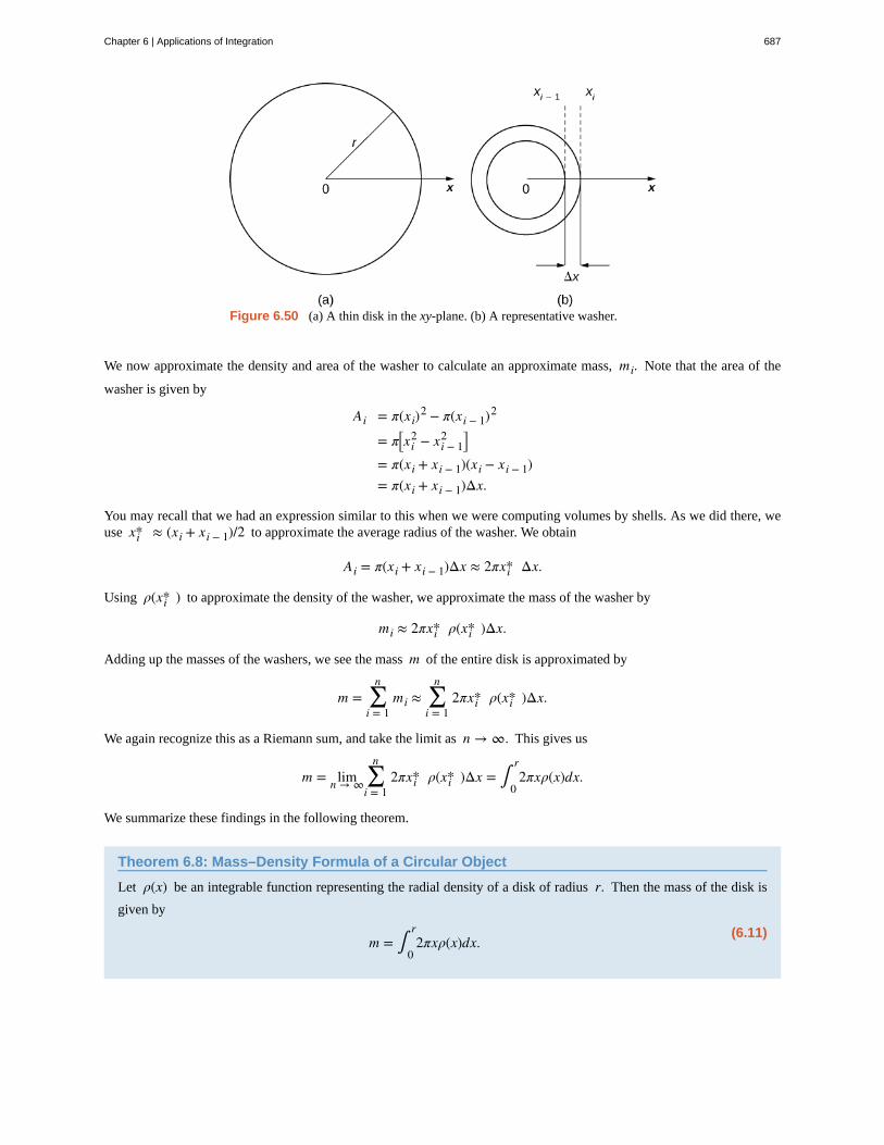
Figure 6.50 (a) A thin disk in the xy-plane. (b) A representative washer.
We now approximate the density and area of the washer to calculate an approximate mass, mi. Note that the area of the
washer is given by
Ai = π(xi)2 − π(xi − 1)2
= π⎡⎣xi
2 − xi − 12 ⎤
⎦
= π(xi + xi − 1)(xi − xi − 1)= π(xi + xi − 1)Δx.
You may recall that we had an expression similar to this when we were computing volumes by shells. As we did there, weuse xi* ≈ (xi + xi − 1)/2 to approximate the average radius of the washer. We obtain
Ai = π(xi + xi − 1)Δx ≈ 2πxi* Δx.
Using ρ(xi* ) to approximate the density of the washer, we approximate the mass of the washer by
mi ≈ 2πxi* ρ(xi* )Δx.
Adding up the masses of the washers, we see the mass m of the entire disk is approximated by
m = ∑i = 1
nmi ≈ ∑
i = 1
n2πxi* ρ(xi* )Δx.
We again recognize this as a Riemann sum, and take the limit as n → ∞. This gives us
m = limn → ∞ ∑i = 1
n2πxi* ρ(xi* )Δx = ∫
0
r2πxρ(x)dx.
We summarize these findings in the following theorem.
Theorem 6.8: Mass–Density Formula of a Circular Object
Let ρ(x) be an integrable function representing the radial density of a disk of radius r. Then the mass of the disk is
given by
(6.11)m = ∫
0
r2πxρ(x)dx.
Chapter 6 | Applications of Integration 687
6.24
Example 6.24
Calculating Mass from Radial Density
Let ρ(x) = x represent the radial density of a disk. Calculate the mass of a disk of radius 4.
Solution
Applying the formula, we find
m = ∫0
r2πxρ(x)dx
= ∫0
42πx xdx = 2π∫
0
4x3/2dx
= 2π25x5/2|04 = 4π
5 [32] = 128π5 .
Let ρ(x) = 3x + 2 represent the radial density of a disk. Calculate the mass of a disk of radius 2.
Work Done by a ForceWe now consider work. In physics, work is related to force, which is often intuitively defined as a push or pull on an object.When a force moves an object, we say the force does work on the object. In other words, work can be thought of as theamount of energy it takes to move an object. According to physics, when we have a constant force, work can be expressedas the product of force and distance.
In the English system, the unit of force is the pound and the unit of distance is the foot, so work is given in foot-pounds. Inthe metric system, kilograms and meters are used. One newton is the force needed to accelerate 1 kilogram of mass at the
rate of 1 m/sec2. Thus, the most common unit of work is the newton-meter. This same unit is also called the joule. Both
are defined as kilograms times meters squared over seconds squared ⎛⎝kg · m2/s2⎞
⎠.
When we have a constant force, things are pretty easy. It is rare, however, for a force to be constant. The work done tocompress (or elongate) a spring, for example, varies depending on how far the spring has already been compressed (orstretched). We look at springs in more detail later in this section.
Suppose we have a variable force F(x) that moves an object in a positive direction along the x-axis from point a to point
b. To calculate the work done, we partition the interval ⎡⎣a, b⎤
⎦ and estimate the work done over each subinterval. So, for
i = 0, 1, 2,…, n, let P = {xi} be a regular partition of the interval ⎡⎣a, b⎤
⎦, and for i = 1, 2,…, n, choose an arbitrary
point xi* ∈ [xi − 1, xi]. To calculate the work done to move an object from point xi − 1 to point xi, we assume the
force is roughly constant over the interval, and use F(xi* ) to approximate the force. The work done over the interval
[xi − 1, xi], then, is given by
Wi ≈ F(xi* )(xi − xi − 1) = F(xi* )Δx.
Therefore, the work done over the interval ⎡⎣a, b⎤
⎦ is approximately
W = ∑i = 1
nWi ≈ ∑
i = 1
nF(xi* )Δx.
Taking the limit of this expression as n → ∞ gives us the exact value for work:
688 Chapter 6 | Applications of Integration
This OpenStax book is available for free at http://cnx.org/content/col11964/1.2
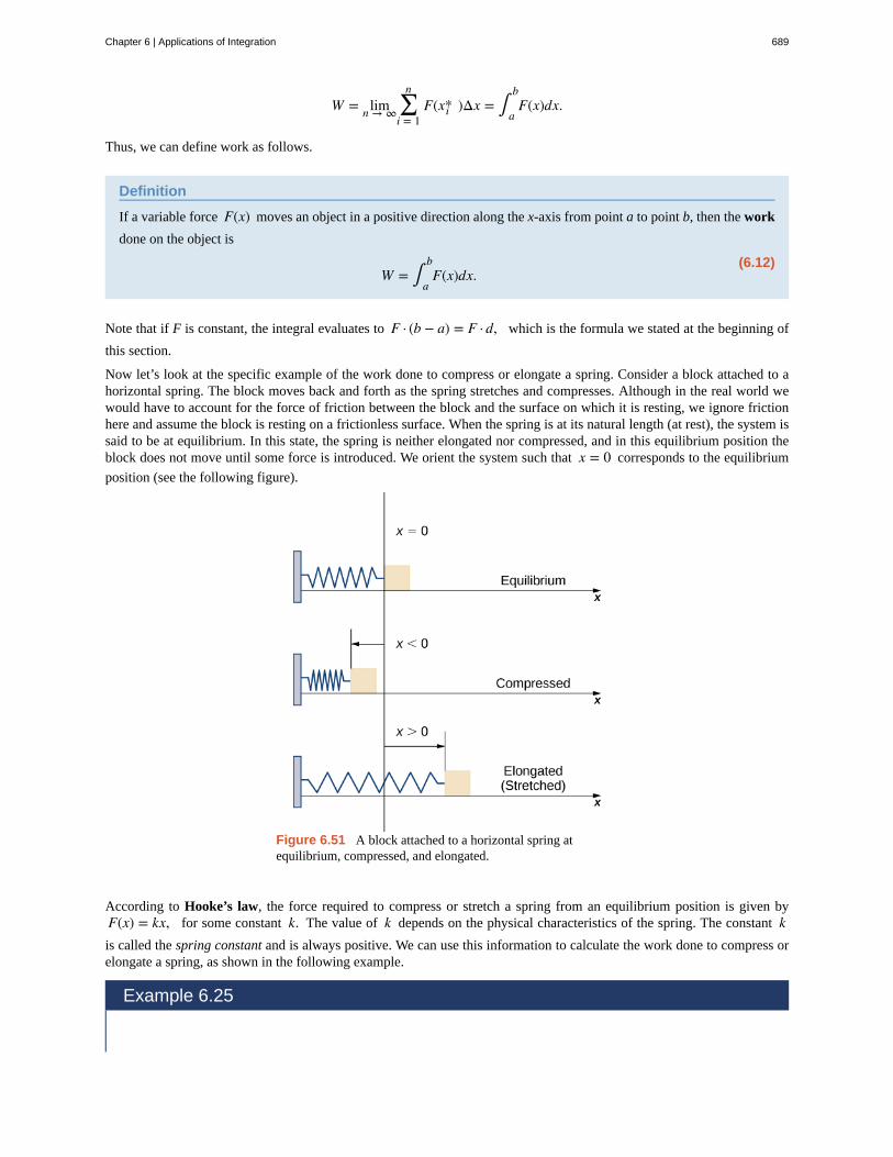
W = limn → ∞ ∑i = 1
nF(xi* )Δx = ∫
a
bF(x)dx.
Thus, we can define work as follows.
Definition
If a variable force F(x) moves an object in a positive direction along the x-axis from point a to point b, then the work
done on the object is
(6.12)W = ∫
a
bF(x)dx.
Note that if F is constant, the integral evaluates to F · (b − a) = F · d, which is the formula we stated at the beginning of
this section.
Now let’s look at the specific example of the work done to compress or elongate a spring. Consider a block attached to ahorizontal spring. The block moves back and forth as the spring stretches and compresses. Although in the real world wewould have to account for the force of friction between the block and the surface on which it is resting, we ignore frictionhere and assume the block is resting on a frictionless surface. When the spring is at its natural length (at rest), the system issaid to be at equilibrium. In this state, the spring is neither elongated nor compressed, and in this equilibrium position theblock does not move until some force is introduced. We orient the system such that x = 0 corresponds to the equilibrium
position (see the following figure).
Figure 6.51 A block attached to a horizontal spring atequilibrium, compressed, and elongated.
According to Hooke’s law, the force required to compress or stretch a spring from an equilibrium position is given byF(x) = kx, for some constant k. The value of k depends on the physical characteristics of the spring. The constant kis called the spring constant and is always positive. We can use this information to calculate the work done to compress orelongate a spring, as shown in the following example.
Example 6.25
Chapter 6 | Applications of Integration 689
6.25
The Work Required to Stretch or Compress a Spring
Suppose it takes a force of 10 N (in the negative direction) to compress a spring 0.2 m from the equilibrium
position. How much work is done to stretch the spring 0.5 m from the equilibrium position?
Solution
First find the spring constant, k. When x = −0.2, we know F(x) = −10, so
F(x) = kx−10 = k(−0.2)
k = 50
and F(x) = 50x. Then, to calculate work, we integrate the force function, obtaining
W = ∫a
bF(x)dx = ∫
0
0.550x dx = 25x2|00.5
= 6.25.
The work done to stretch the spring is 6.25 J.
Suppose it takes a force of 8 lb to stretch a spring 6 in. from the equilibrium position. How much work
is done to stretch the spring 1 ft from the equilibrium position?
Work Done in PumpingConsider the work done to pump water (or some other liquid) out of a tank. Pumping problems are a little more complicatedthan spring problems because many of the calculations depend on the shape and size of the tank. In addition, instead ofbeing concerned about the work done to move a single mass, we are looking at the work done to move a volume of water,and it takes more work to move the water from the bottom of the tank than it does to move the water from the top of thetank.
We examine the process in the context of a cylindrical tank, then look at a couple of examples using tanks of differentshapes. Assume a cylindrical tank of radius 4 m and height 10 m is filled to a depth of 8 m. How much work does it take
to pump all the water over the top edge of the tank?
The first thing we need to do is define a frame of reference. We let x represent the vertical distance below the top of the
tank. That is, we orient the x-axis vertically, with the origin at the top of the tank and the downward direction being positive
(see the following figure).
690 Chapter 6 | Applications of Integration
This OpenStax book is available for free at http://cnx.org/content/col11964/1.2
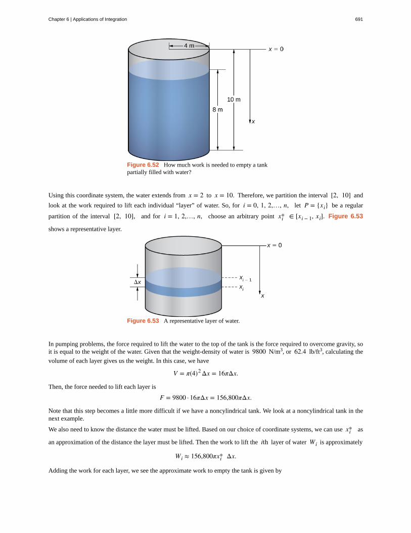
Figure 6.52 How much work is needed to empty a tankpartially filled with water?
Using this coordinate system, the water extends from x = 2 to x = 10. Therefore, we partition the interval [2, 10] and
look at the work required to lift each individual “layer” of water. So, for i = 0, 1, 2,…, n, let P = {xi} be a regular
partition of the interval [2, 10], and for i = 1, 2,…, n, choose an arbitrary point xi* ∈ [xi − 1, xi]. Figure 6.53
shows a representative layer.
Figure 6.53 A representative layer of water.
In pumping problems, the force required to lift the water to the top of the tank is the force required to overcome gravity, soit is equal to the weight of the water. Given that the weight-density of water is 9800 N/m3, or 62.4 lb/ft3, calculating the
volume of each layer gives us the weight. In this case, we have
V = π(4)2 Δx = 16πΔx.
Then, the force needed to lift each layer is
F = 9800 · 16πΔx = 156,800πΔx.
Note that this step becomes a little more difficult if we have a noncylindrical tank. We look at a noncylindrical tank in thenext example.
We also need to know the distance the water must be lifted. Based on our choice of coordinate systems, we can use xi* as
an approximation of the distance the layer must be lifted. Then the work to lift the ith layer of water Wi is approximately
Wi ≈ 156,800πxi* Δx.
Adding the work for each layer, we see the approximate work to empty the tank is given by
Chapter 6 | Applications of Integration 691
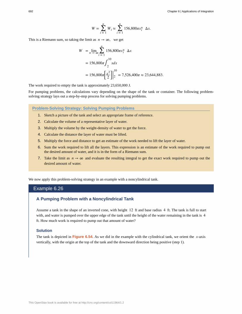
W = ∑i = 1
nWi ≈ ∑
i = 1
n156,800πxi* Δx.
This is a Riemann sum, so taking the limit as n → ∞, we get
W = limn → ∞ ∑i = 1
n156,800πxi* Δx
= 156,800π∫2
10xdx
= 156,800π⎡⎣
x2
2⎤⎦ |210
= 7,526,400π ≈ 23,644,883.
The work required to empty the tank is approximately 23,650,000 J.
For pumping problems, the calculations vary depending on the shape of the tank or container. The following problem-solving strategy lays out a step-by-step process for solving pumping problems.
Problem-Solving Strategy: Solving Pumping Problems
1. Sketch a picture of the tank and select an appropriate frame of reference.
2. Calculate the volume of a representative layer of water.
3. Multiply the volume by the weight-density of water to get the force.
4. Calculate the distance the layer of water must be lifted.
5. Multiply the force and distance to get an estimate of the work needed to lift the layer of water.
6. Sum the work required to lift all the layers. This expression is an estimate of the work required to pump outthe desired amount of water, and it is in the form of a Riemann sum.
7. Take the limit as n → ∞ and evaluate the resulting integral to get the exact work required to pump out the
desired amount of water.
We now apply this problem-solving strategy in an example with a noncylindrical tank.
Example 6.26
A Pumping Problem with a Noncylindrical Tank
Assume a tank in the shape of an inverted cone, with height 12 ft and base radius 4 ft. The tank is full to start
with, and water is pumped over the upper edge of the tank until the height of the water remaining in the tank is 4ft. How much work is required to pump out that amount of water?
Solution
The tank is depicted in Figure 6.54. As we did in the example with the cylindrical tank, we orient the x-axisvertically, with the origin at the top of the tank and the downward direction being positive (step 1).
692 Chapter 6 | Applications of Integration
This OpenStax book is available for free at http://cnx.org/content/col11964/1.2
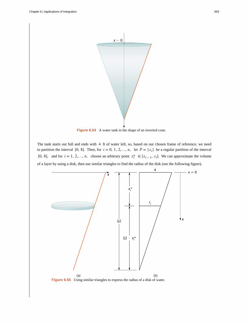
Figure 6.54 A water tank in the shape of an inverted cone.
The tank starts out full and ends with 4 ft of water left, so, based on our chosen frame of reference, we need
to partition the interval [0, 8]. Then, for i = 0, 1, 2,…, n, let P = {xi} be a regular partition of the interval
[0, 8], and for i = 1, 2,…, n, choose an arbitrary point xi* ∈ [xi − 1, xi]. We can approximate the volume
of a layer by using a disk, then use similar triangles to find the radius of the disk (see the following figure).
Figure 6.55 Using similar triangles to express the radius of a disk of water.
Chapter 6 | Applications of Integration 693
6.26
From properties of similar triangles, we have
ri12 − xi*
= 412 = 1
33ri = 12 − xi*
ri =12 − xi*
3
= 4 −xi*3 .
Then the volume of the disk is
Vi = π⎛⎝4 −
xi*3
⎞⎠
2Δx (step 2).
The weight-density of water is 62.4 lb/ft3, so the force needed to lift each layer is approximately
Fi ≈ 62.4π⎛⎝4 −
xi*3
⎞⎠
2Δx (step 3).
Based on the diagram, the distance the water must be lifted is approximately xi* feet (step 4), so the approximate
work needed to lift the layer is
Wi ≈ 62.4πxi*⎛⎝4 −
xi*3
⎞⎠
2Δx (step 5).
Summing the work required to lift all the layers, we get an approximate value of the total work:
W = ∑i = 1
nWi ≈ ∑
i = 1
n62.4πxi*
⎛⎝4 −
xi*3
⎞⎠
2Δx (step 6).
Taking the limit as n → ∞, we obtain
W = limn → ∞ ∑i = 1
n62.4πxi*
⎛⎝4 −
xi*3
⎞⎠
2Δx
= ∫0
862.4πx⎛
⎝4 − x3
⎞⎠
2dx
= 62.4π∫0
8x⎛⎝16 − 8x
3 + x2
9⎞⎠dx = 62.4π∫
0
8⎛⎝16x − 8x2
3 + x3
9⎞⎠dx
= 62.4π⎡⎣8x2 − 8x3
9 + x4
36⎤⎦ |08 = 10,649.6π ≈ 33,456.7.
It takes approximately 33,450 ft-lb of work to empty the tank to the desired level.
A tank is in the shape of an inverted cone, with height 10 ft and base radius 6 ft. The tank is filled to a
depth of 8 ft to start with, and water is pumped over the upper edge of the tank until 3 ft of water remain in thetank. How much work is required to pump out that amount of water?
694 Chapter 6 | Applications of Integration
This OpenStax book is available for free at http://cnx.org/content/col11964/1.2
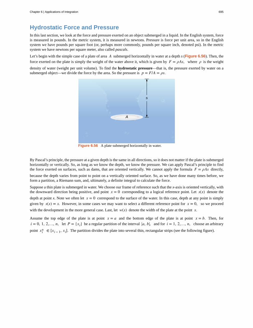
Hydrostatic Force and PressureIn this last section, we look at the force and pressure exerted on an object submerged in a liquid. In the English system, forceis measured in pounds. In the metric system, it is measured in newtons. Pressure is force per unit area, so in the Englishsystem we have pounds per square foot (or, perhaps more commonly, pounds per square inch, denoted psi). In the metricsystem we have newtons per square meter, also called pascals.
Let’s begin with the simple case of a plate of area A submerged horizontally in water at a depth s (Figure 6.56). Then, the
force exerted on the plate is simply the weight of the water above it, which is given by F = ρAs, where ρ is the weight
density of water (weight per unit volume). To find the hydrostatic pressure—that is, the pressure exerted by water on asubmerged object—we divide the force by the area. So the pressure is p = F/A = ρs.
Figure 6.56 A plate submerged horizontally in water.
By Pascal’s principle, the pressure at a given depth is the same in all directions, so it does not matter if the plate is submergedhorizontally or vertically. So, as long as we know the depth, we know the pressure. We can apply Pascal’s principle to findthe force exerted on surfaces, such as dams, that are oriented vertically. We cannot apply the formula F = ρAs directly,
because the depth varies from point to point on a vertically oriented surface. So, as we have done many times before, weform a partition, a Riemann sum, and, ultimately, a definite integral to calculate the force.
Suppose a thin plate is submerged in water. We choose our frame of reference such that the x-axis is oriented vertically, withthe downward direction being positive, and point x = 0 corresponding to a logical reference point. Let s(x) denote the
depth at point x. Note we often let x = 0 correspond to the surface of the water. In this case, depth at any point is simply
given by s(x) = x. However, in some cases we may want to select a different reference point for x = 0, so we proceed
with the development in the more general case. Last, let w(x) denote the width of the plate at the point x.
Assume the top edge of the plate is at point x = a and the bottom edge of the plate is at point x = b. Then, for
i = 0, 1, 2,…, n, let P = {xi} be a regular partition of the interval ⎡⎣a, b⎤
⎦, and for i = 1, 2,…, n, choose an arbitrary
point xi* ∈ [xi − 1, xi]. The partition divides the plate into several thin, rectangular strips (see the following figure).
Chapter 6 | Applications of Integration 695
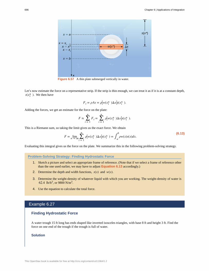
Figure 6.57 A thin plate submerged vertically in water.
Let’s now estimate the force on a representative strip. If the strip is thin enough, we can treat it as if it is at a constant depth,s(xi* ). We then have
Fi = ρAs = ρ⎡⎣w(xi* )Δx⎤
⎦s(xi* ).
Adding the forces, we get an estimate for the force on the plate:
F ≈ ∑i = 1
nFi = ∑
i = 1
nρ⎡
⎣w(xi* )Δx⎤⎦s(xi* ).
This is a Riemann sum, so taking the limit gives us the exact force. We obtain
(6.13)F = limn → ∞ ∑
i = 1
nρ⎡
⎣w(xi* )Δx⎤⎦s(xi* ) = ∫
a
bρw(x)s(x)dx.
Evaluating this integral gives us the force on the plate. We summarize this in the following problem-solving strategy.
Problem-Solving Strategy: Finding Hydrostatic Force
1. Sketch a picture and select an appropriate frame of reference. (Note that if we select a frame of reference otherthan the one used earlier, we may have to adjust Equation 6.13 accordingly.)
2. Determine the depth and width functions, s(x) and w(x).
3. Determine the weight-density of whatever liquid with which you are working. The weight-density of water is62.4 lb/ft3, or 9800 N/m3.
4. Use the equation to calculate the total force.
Example 6.27
Finding Hydrostatic Force
A water trough 15 ft long has ends shaped like inverted isosceles triangles, with base 8 ft and height 3 ft. Find theforce on one end of the trough if the trough is full of water.
Solution
696 Chapter 6 | Applications of Integration
This OpenStax book is available for free at http://cnx.org/content/col11964/1.2
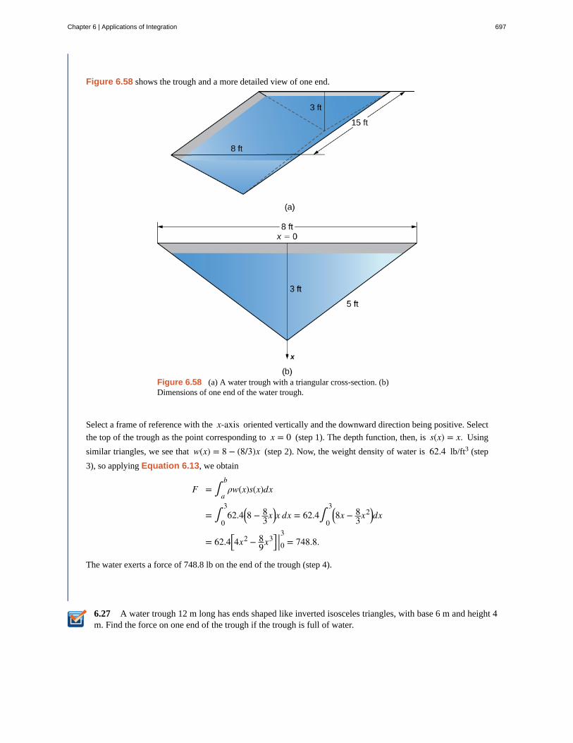
6.27
Figure 6.58 shows the trough and a more detailed view of one end.
Figure 6.58 (a) A water trough with a triangular cross-section. (b)Dimensions of one end of the water trough.
Select a frame of reference with the x-axis oriented vertically and the downward direction being positive. Select
the top of the trough as the point corresponding to x = 0 (step 1). The depth function, then, is s(x) = x. Using
similar triangles, we see that w(x) = 8 − (8/3)x (step 2). Now, the weight density of water is 62.4 lb/ft3 (step
3), so applying Equation 6.13, we obtain
F = ∫a
bρw(x)s(x)dx
= ∫0
362.4⎛
⎝8 − 83x⎞
⎠x dx = 62.4∫0
3⎛⎝8x − 8
3x2⎞⎠dx
= 62.4⎡⎣4x2 − 8
9x3⎤⎦ |03 = 748.8.
The water exerts a force of 748.8 lb on the end of the trough (step 4).
A water trough 12 m long has ends shaped like inverted isosceles triangles, with base 6 m and height 4m. Find the force on one end of the trough if the trough is full of water.
Chapter 6 | Applications of Integration 697
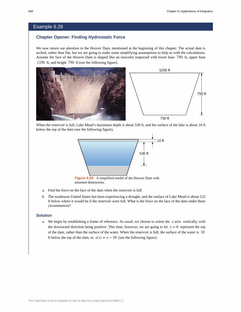
Example 6.28
Chapter Opener: Finding Hydrostatic Force
We now return our attention to the Hoover Dam, mentioned at the beginning of this chapter. The actual dam isarched, rather than flat, but we are going to make some simplifying assumptions to help us with the calculations.Assume the face of the Hoover Dam is shaped like an isosceles trapezoid with lower base 750 ft, upper base
1250 ft, and height 750 ft (see the following figure).
When the reservoir is full, Lake Mead’s maximum depth is about 530 ft, and the surface of the lake is about 10 ftbelow the top of the dam (see the following figure).
Figure 6.59 A simplified model of the Hoover Dam withassumed dimensions.
a. Find the force on the face of the dam when the reservoir is full.
b. The southwest United States has been experiencing a drought, and the surface of Lake Mead is about 125ft below where it would be if the reservoir were full. What is the force on the face of the dam under thesecircumstances?
Solution
a. We begin by establishing a frame of reference. As usual, we choose to orient the x-axis vertically, with
the downward direction being positive. This time, however, we are going to let x = 0 represent the top
of the dam, rather than the surface of the water. When the reservoir is full, the surface of the water is 10ft below the top of the dam, so s(x) = x − 10 (see the following figure).
698 Chapter 6 | Applications of Integration
This OpenStax book is available for free at http://cnx.org/content/col11964/1.2
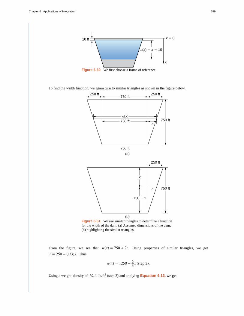
Figure 6.60 We first choose a frame of reference.
To find the width function, we again turn to similar triangles as shown in the figure below.
Figure 6.61 We use similar triangles to determine a functionfor the width of the dam. (a) Assumed dimensions of the dam;(b) highlighting the similar triangles.
From the figure, we see that w(x) = 750 + 2r. Using properties of similar triangles, we get
r = 250 − (1/3)x. Thus,
w(x) = 1250 − 23x (step 2).
Using a weight-density of 62.4 lb/ft3 (step 3) and applying Equation 6.13, we get
Chapter 6 | Applications of Integration 699
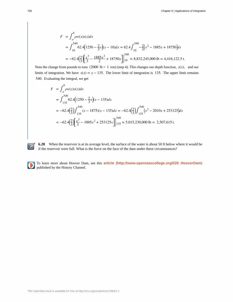
6.28
F = ∫a
bρw(x)s(x)dx
= ∫10
54062.4⎛
⎝1250 − 23x⎞
⎠(x − 10)dx = 62.4∫10
540−2
3⎡⎣x2 − 1885x + 18750⎤
⎦dx
= −62.4⎛⎝23
⎞⎠⎡⎣
x3
3 − 1885x2
2 + 18750x⎤⎦ |10
540≈ 8,832,245,000 lb = 4,416,122.5 t.
Note the change from pounds to tons (2000 lb = 1 ton) (step 4). This changes our depth function, s(x), and our
limits of integration. We have s(x) = x − 135. The lower limit of integration is 135. The upper limit remains
540. Evaluating the integral, we get
F = ∫a
bρw(x)s(x)dx
= ∫135
54062.4⎛
⎝1250 − 23x⎞
⎠(x − 135)dx
= −62.4⎛⎝23
⎞⎠∫135
540(x − 1875)(x − 135)dx = −62.4⎛
⎝23
⎞⎠∫135
540⎛⎝x2 − 2010x + 253125⎞
⎠dx
= −62.4⎛⎝23
⎞⎠⎡⎣
x3
3 − 1005x2 + 253125x⎤⎦ |135
540≈ 5,015,230,000 lb = 2,507,615 t.
When the reservoir is at its average level, the surface of the water is about 50 ft below where it would beif the reservoir were full. What is the force on the face of the dam under these circumstances?
To learn more about Hoover Dam, see this article (http://www.openstaxcollege.org/l/20_HooverDam)published by the History Channel.
700 Chapter 6 | Applications of Integration
This OpenStax book is available for free at http://cnx.org/content/col11964/1.2
6.5 EXERCISESFor the following exercises, find the work done.
218. Find the work done when a constant force F = 12lb moves a chair from x = 0.9 to x = 1.1 ft.
219. How much work is done when a person lifts a 50 lb
box of comics onto a truck that is 3 ft off the ground?
220. What is the work done lifting a 20 kg child from the
floor to a height of 2 m? (Note that 1 kg equates to 9.8N)
221. Find the work done when you push a box alongthe floor 2 m, when you apply a constant force of
F = 100 N.
222. Compute the work done for a force F = 12/x2 N
from x = 1 to x = 2 m.
223. What is the work done moving a particle from x = 0to x = 1 m if the force acting on it is F = 3x2 N?
For the following exercises, find the mass of the one-dimensional object.
224. A wire that is 2 ft long (starting at x = 0) and has
a density function of ρ(x) = x2 + 2x lb/ft
225. A car antenna that is 3 ft long (starting at x = 0)and has a density function of ρ(x) = 3x + 2 lb/ft
226. A metal rod that is 8 in. long (starting at x = 0) and
has a density function of ρ(x) = e1/2x lb/in.
227. A pencil that is 4 in. long (starting at x = 2) and
has a density function of ρ(x) = 5/x oz/in.
228. A ruler that is 12 in. long (starting at x = 5) and
has a density function of ρ(x) = ln(x) + (1/2)x2 oz/in.
For the following exercises, find the mass of the two-dimensional object that is centered at the origin.
229. An oversized hockey puck of radius 2 in. with
density function ρ(x) = x3 − 2x + 5
230. A frisbee of radius 6 in. with density function
ρ(x) = e−x
231. A plate of radius 10 in. with density function
ρ(x) = 1 + cos(πx)
232. A jar lid of radius 3 in. with density function
ρ(x) = ln(x + 1)
233. A disk of radius 5 cm with density function
ρ(x) = 3x
234. A 12 -in. spring is stretched to 15 in. by a force of
75 lb. What is the spring constant?
235. A spring has a natural length of 10 cm. It takes 2J to stretch the spring to 15 cm. How much work would it
take to stretch the spring from 15 cm to 20 cm?
236. A 1 -m spring requires 10 J to stretch the spring to
1.1 m. How much work would it take to stretch the spring
from 1 m to 1.2 m?
237. A spring requires 5 J to stretch the spring from 8cm to 12 cm, and an additional 4 J to stretch the spring
from 12 cm to 14 cm. What is the natural length of the
spring?
238. A shock absorber is compressed 1 in. by a weight of1 t. What is the spring constant?
239. A force of F = 20x − x3 N stretches a nonlinear
spring by x meters. What work is required to stretch the
spring from x = 0 to x = 2 m?
240. Find the work done by winding up a hanging cable oflength 100 ft and weight-density 5 lb/ft.
241. For the cable in the preceding exercise, how muchwork is done to lift the cable 50 ft?
242. For the cable in the preceding exercise, how muchadditional work is done by hanging a 200 lb weight at the
end of the cable?
243. [T] A pyramid of height 500 ft has a square base
800 ft by 800 ft. Find the area A at height h. If the
rock used to build the pyramid weighs approximately
w = 100 lb/ft3, how much work did it take to lift all the
rock?
Chapter 6 | Applications of Integration 701
244. [T] For the pyramid in the preceding exercise,assume there were 1000 workers each working 10 hours
a day, 5 days a week, 50 weeks a year. If the workers, on
average, lifted 10 100 lb rocks 2 ft/hr, how long did it take
to build the pyramid?
245. [T] The force of gravity on a mass m is
F = −⎛⎝(GMm)/x2⎞
⎠ newtons. For a rocket of mass
m = 1000 kg, compute the work to lift the rocket from
x = 6400 to x = 6500 km. (Note:
G = 6 × 10⁻¹⁷ N m2 /kg2 and M = 6 × 1024 kg.)
246. [T] For the rocket in the preceding exercise, find thework to lift the rocket from x = 6400 to x = ∞.
247. [T] A rectangular dam is 40 ft high and 60 ft wide.
Compute the total force F on the dam when
a. the surface of the water is at the top of the dam andb. the surface of the water is halfway down the dam.
248. [T] Find the work required to pump all the water outof a cylinder that has a circular base of radius 5 ft and
height 200 ft. Use the fact that the density of water is 62lb/ft3.
249. [T] Find the work required to pump all the water outof the cylinder in the preceding exercise if the cylinder isonly half full.
250. [T] How much work is required to pump out aswimming pool if the area of the base is 800 ft2, the water
is 4 ft deep, and the top is 1 ft above the water level?
Assume that the density of water is 62 lb/ft3.
251. A cylinder of depth H and cross-sectional area Astands full of water at density ρ. Compute the work to
pump all the water to the top.
252. For the cylinder in the preceding exercise, computethe work to pump all the water to the top if the cylinder isonly half full.
253. A cone-shaped tank has a cross-sectional area that
increases with its depth: A = ⎛⎝πr2 h2⎞
⎠/H 3. Show that the
work to empty it is half the work for a cylinder with thesame height and base.
702 Chapter 6 | Applications of Integration
This OpenStax book is available for free at http://cnx.org/content/col11964/1.2
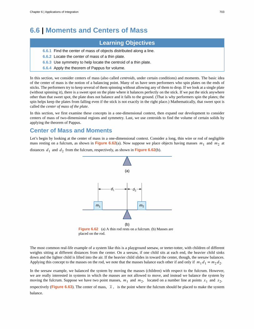
6.6 | Moments and Centers of Mass
Learning Objectives6.6.1 Find the center of mass of objects distributed along a line.
6.6.2 Locate the center of mass of a thin plate.
6.6.3 Use symmetry to help locate the centroid of a thin plate.
6.6.4 Apply the theorem of Pappus for volume.
In this section, we consider centers of mass (also called centroids, under certain conditions) and moments. The basic ideaof the center of mass is the notion of a balancing point. Many of us have seen performers who spin plates on the ends ofsticks. The performers try to keep several of them spinning without allowing any of them to drop. If we look at a single plate(without spinning it), there is a sweet spot on the plate where it balances perfectly on the stick. If we put the stick anywhereother than that sweet spot, the plate does not balance and it falls to the ground. (That is why performers spin the plates; thespin helps keep the plates from falling even if the stick is not exactly in the right place.) Mathematically, that sweet spot iscalled the center of mass of the plate.
In this section, we first examine these concepts in a one-dimensional context, then expand our development to considercenters of mass of two-dimensional regions and symmetry. Last, we use centroids to find the volume of certain solids byapplying the theorem of Pappus.
Center of Mass and MomentsLet’s begin by looking at the center of mass in a one-dimensional context. Consider a long, thin wire or rod of negligiblemass resting on a fulcrum, as shown in Figure 6.62(a). Now suppose we place objects having masses m1 and m2 at
distances d1 and d2 from the fulcrum, respectively, as shown in Figure 6.62(b).
Figure 6.62 (a) A thin rod rests on a fulcrum. (b) Masses areplaced on the rod.
The most common real-life example of a system like this is a playground seesaw, or teeter-totter, with children of differentweights sitting at different distances from the center. On a seesaw, if one child sits at each end, the heavier child sinksdown and the lighter child is lifted into the air. If the heavier child slides in toward the center, though, the seesaw balances.Applying this concept to the masses on the rod, we note that the masses balance each other if and only if m1 d1 = m2 d2.
In the seesaw example, we balanced the system by moving the masses (children) with respect to the fulcrum. However,we are really interested in systems in which the masses are not allowed to move, and instead we balance the system bymoving the fulcrum. Suppose we have two point masses, m1 and m2, located on a number line at points x1 and x2,respectively (Figure 6.63). The center of mass, x– , is the point where the fulcrum should be placed to make the system
balance.
Chapter 6 | Applications of Integration 703
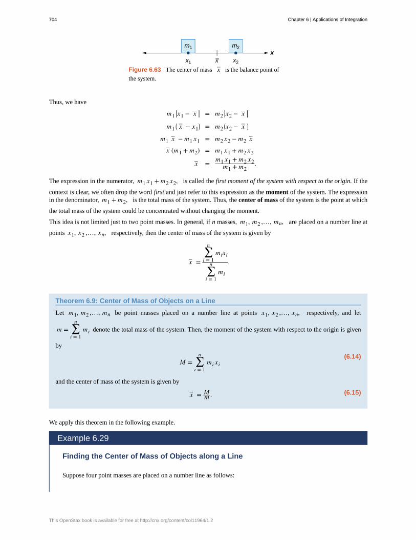
Figure 6.63 The center of mass x– is the balance point of
the system.
Thus, we have
m1 |x1 − x– | = m2 |x2 − x– |m1
⎛⎝ x– − x1
⎞⎠ = m2
⎛⎝x2 − x– ⎞
⎠
m1 x– − m1 x1 = m2 x2 − m2 x–
x– (m1 + m2) = m1 x1 + m2 x2
x– = m1 x1 + m2 x2m1 + m2
.
The expression in the numerator, m1 x1 + m2 x2, is called the first moment of the system with respect to the origin. If the
context is clear, we often drop the word first and just refer to this expression as the moment of the system. The expressionin the denominator, m1 + m2, is the total mass of the system. Thus, the center of mass of the system is the point at which
the total mass of the system could be concentrated without changing the moment.
This idea is not limited just to two point masses. In general, if n masses, m1, m2 ,…, mn, are placed on a number line at
points x1, x2 ,…, xn, respectively, then the center of mass of the system is given by
x– =∑i = 1
nmixi
∑i = 1
nmi
.
Theorem 6.9: Center of Mass of Objects on a Line
Let m1, m2 ,…, mn be point masses placed on a number line at points x1, x2 ,…, xn, respectively, and let
m = ∑i = 1
nmi denote the total mass of the system. Then, the moment of the system with respect to the origin is given
by
(6.14)M = ∑
i = 1
nmi xi
and the center of mass of the system is given by
(6.15)x– = Mm .
We apply this theorem in the following example.
Example 6.29
Finding the Center of Mass of Objects along a Line
Suppose four point masses are placed on a number line as follows:
704 Chapter 6 | Applications of Integration
This OpenStax book is available for free at http://cnx.org/content/col11964/1.2
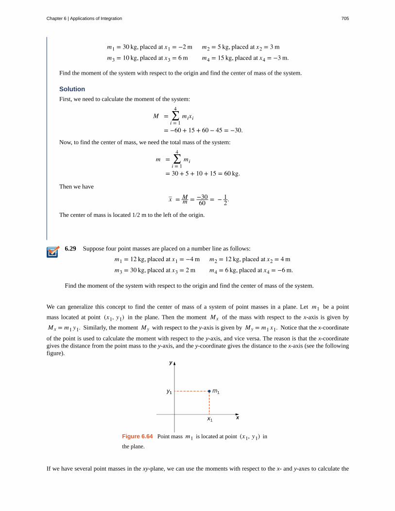
6.29
m1 = 30 kg, placed at x1 = −2 m m2 = 5 kg, placed at x2 = 3 m
m3 = 10 kg, placed at x3 = 6 m m4 = 15 kg, placed at x4 = −3 m.
Find the moment of the system with respect to the origin and find the center of mass of the system.
Solution
First, we need to calculate the moment of the system:
M = ∑i = 1
4mixi
= −60 + 15 + 60 − 45 = −30.
Now, to find the center of mass, we need the total mass of the system:
m = ∑i = 1
4mi
= 30 + 5 + 10 + 15 = 60 kg.
Then we have
x– = Mm = −30
60 = − 12.
The center of mass is located 1/2 m to the left of the origin.
Suppose four point masses are placed on a number line as follows:
m1 = 12 kg, placed at x1 = −4 m m2 = 12 kg, placed at x2 = 4 m
m3 = 30 kg, placed at x3 = 2 m m4 = 6 kg, placed at x4 = −6 m.
Find the moment of the system with respect to the origin and find the center of mass of the system.
We can generalize this concept to find the center of mass of a system of point masses in a plane. Let m1 be a point
mass located at point (x1, y1) in the plane. Then the moment Mx of the mass with respect to the x-axis is given by
Mx = m1 y1. Similarly, the moment My with respect to the y-axis is given by My = m1 x1. Notice that the x-coordinate
of the point is used to calculate the moment with respect to the y-axis, and vice versa. The reason is that the x-coordinategives the distance from the point mass to the y-axis, and the y-coordinate gives the distance to the x-axis (see the followingfigure).
Figure 6.64 Point mass m1 is located at point (x1, y1) in
the plane.
If we have several point masses in the xy-plane, we can use the moments with respect to the x- and y-axes to calculate the
Chapter 6 | Applications of Integration 705
x- and y-coordinates of the center of mass of the system.
Theorem 6.10: Center of Mass of Objects in a Plane
Let m1, m2 ,…, mn be point masses located in the xy-plane at points (x1, y1), (x2, y2),…, (xn, yn), respectively,
and let m = ∑i = 1
nmi denote the total mass of the system. Then the moments Mx and My of the system with respect
to the x- and y-axes, respectively, are given by
(6.16)Mx = ∑
i = 1
nmi yi and My = ∑
i = 1
nmi xi.
Also, the coordinates of the center of mass ⎛⎝ x– , y– ⎞
⎠ of the system are
(6.17)x– =Mym and y– = Mx
m .
The next example demonstrates how to apply this theorem.
Example 6.30
Finding the Center of Mass of Objects in a Plane
Suppose three point masses are placed in the xy-plane as follows (assume coordinates are given in meters):
m1 = 2 kg, placed at (−1, 3),m2 = 6 kg, placed at (1, 1),m3 = 4 kg, placed at (2, −2).
Find the center of mass of the system.
Solution
First we calculate the total mass of the system:
m = ∑i = 1
3mi = 2 + 6 + 4 = 12 kg.
Next we find the moments with respect to the x- and y-axes:
My = ∑i = 1
3mixi = −2 + 6 + 8 = 12,
Mx = ∑i = 1
3miyi = 6 + 6 − 8 = 4.
Then we have
x– =Mym = 12
12 = 1 and y– = Mxm = 4
12 = 13.
The center of mass of the system is (1, 1/3), in meters.
706 Chapter 6 | Applications of Integration
This OpenStax book is available for free at http://cnx.org/content/col11964/1.2
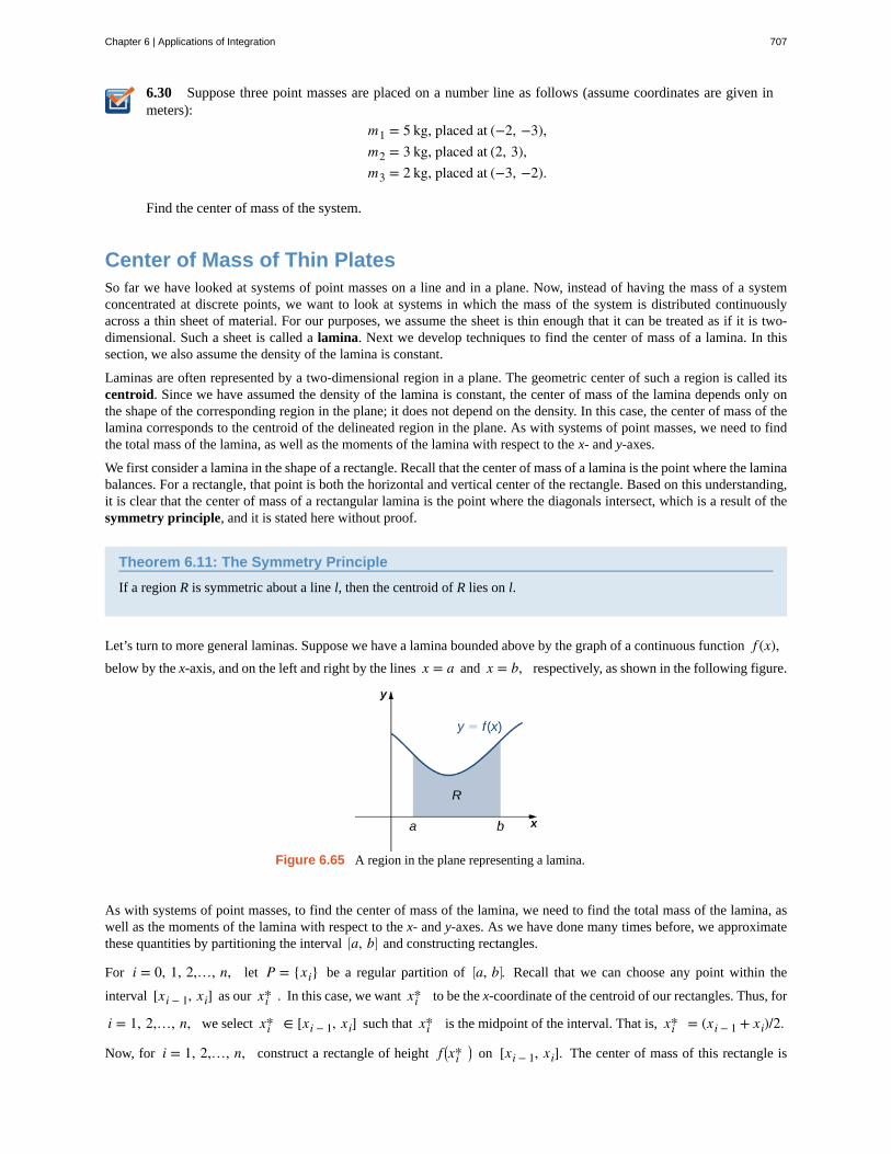
6.30 Suppose three point masses are placed on a number line as follows (assume coordinates are given inmeters):
m1 = 5 kg, placed at (−2, −3),m2 = 3 kg, placed at (2, 3),m3 = 2 kg, placed at (−3, −2).
Find the center of mass of the system.
Center of Mass of Thin PlatesSo far we have looked at systems of point masses on a line and in a plane. Now, instead of having the mass of a systemconcentrated at discrete points, we want to look at systems in which the mass of the system is distributed continuouslyacross a thin sheet of material. For our purposes, we assume the sheet is thin enough that it can be treated as if it is two-dimensional. Such a sheet is called a lamina. Next we develop techniques to find the center of mass of a lamina. In thissection, we also assume the density of the lamina is constant.
Laminas are often represented by a two-dimensional region in a plane. The geometric center of such a region is called itscentroid. Since we have assumed the density of the lamina is constant, the center of mass of the lamina depends only onthe shape of the corresponding region in the plane; it does not depend on the density. In this case, the center of mass of thelamina corresponds to the centroid of the delineated region in the plane. As with systems of point masses, we need to findthe total mass of the lamina, as well as the moments of the lamina with respect to the x- and y-axes.
We first consider a lamina in the shape of a rectangle. Recall that the center of mass of a lamina is the point where the laminabalances. For a rectangle, that point is both the horizontal and vertical center of the rectangle. Based on this understanding,it is clear that the center of mass of a rectangular lamina is the point where the diagonals intersect, which is a result of thesymmetry principle, and it is stated here without proof.
Theorem 6.11: The Symmetry Principle
If a region R is symmetric about a line l, then the centroid of R lies on l.
Let’s turn to more general laminas. Suppose we have a lamina bounded above by the graph of a continuous function f (x),below by the x-axis, and on the left and right by the lines x = a and x = b, respectively, as shown in the following figure.
Figure 6.65 A region in the plane representing a lamina.
As with systems of point masses, to find the center of mass of the lamina, we need to find the total mass of the lamina, aswell as the moments of the lamina with respect to the x- and y-axes. As we have done many times before, we approximatethese quantities by partitioning the interval ⎡
⎣a, b⎤⎦ and constructing rectangles.
For i = 0, 1, 2,…, n, let P = {xi} be a regular partition of ⎡⎣a, b⎤
⎦. Recall that we can choose any point within the
interval [xi − 1, xi] as our xi* . In this case, we want xi* to be the x-coordinate of the centroid of our rectangles. Thus, for
i = 1, 2,…, n, we select xi* ∈ [xi − 1, xi] such that xi* is the midpoint of the interval. That is, xi* = (xi − 1 + xi)/2.
Now, for i = 1, 2,…, n, construct a rectangle of height f ⎛⎝xi*
⎞⎠ on [xi − 1, xi]. The center of mass of this rectangle is
Chapter 6 | Applications of Integration 707
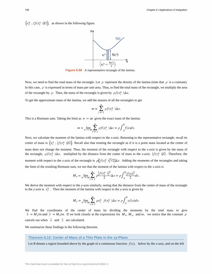
⎛⎝xi* , ⎛
⎝ f (xi* )⎞⎠/2⎞
⎠, as shown in the following figure.
Figure 6.66 A representative rectangle of the lamina.
Next, we need to find the total mass of the rectangle. Let ρ represent the density of the lamina (note that ρ is a constant).
In this case, ρ is expressed in terms of mass per unit area. Thus, to find the total mass of the rectangle, we multiply the area
of the rectangle by ρ. Then, the mass of the rectangle is given by ρ f (xi* )Δx.
To get the approximate mass of the lamina, we add the masses of all the rectangles to get
m ≈ ∑i = 1
nρ f (xi* )Δx.
This is a Riemann sum. Taking the limit as n → ∞ gives the exact mass of the lamina:
m = limn → ∞ ∑i = 1
nρ f (xi* )Δx = ρ∫
a
bf (x)dx.
Next, we calculate the moment of the lamina with respect to the x-axis. Returning to the representative rectangle, recall its
center of mass is ⎛⎝xi* , ⎛
⎝ f (xi* )⎞⎠/2⎞
⎠. Recall also that treating the rectangle as if it is a point mass located at the center of
mass does not change the moment. Thus, the moment of the rectangle with respect to the x-axis is given by the mass ofthe rectangle, ρ f (xi* )Δx, multiplied by the distance from the center of mass to the x-axis: ⎛
⎝ f (xi* )⎞⎠/2. Therefore, the
moment with respect to the x-axis of the rectangle is ρ⎛⎝⎡⎣ f (xi* )⎤
⎦2/2⎞
⎠Δx. Adding the moments of the rectangles and taking
the limit of the resulting Riemann sum, we see that the moment of the lamina with respect to the x-axis is
Mx = limn → ∞ ∑i = 1
nρ
⎡⎣ f (xi* )⎤
⎦2
2 Δx = ρ∫a
b ⎡⎣ f (x)⎤
⎦2
2 dx.
We derive the moment with respect to the y-axis similarly, noting that the distance from the center of mass of the rectangleto the y-axis is xi* . Then the moment of the lamina with respect to the y-axis is given by
My = limn → ∞ ∑i = 1
nρxi* f (xi* )Δx = ρ∫
a
bx f (x)dx.
We find the coordinates of the center of mass by dividing the moments by the total mass to givex– = My/m and y– = Mx/m. If we look closely at the expressions for Mx, My, and m, we notice that the constant ρ
cancels out when x– and y– are calculated.
We summarize these findings in the following theorem.
Theorem 6.12: Center of Mass of a Thin Plate in the xy-Plane
Let R denote a region bounded above by the graph of a continuous function f (x), below by the x-axis, and on the left
708 Chapter 6 | Applications of Integration
This OpenStax book is available for free at http://cnx.org/content/col11964/1.2
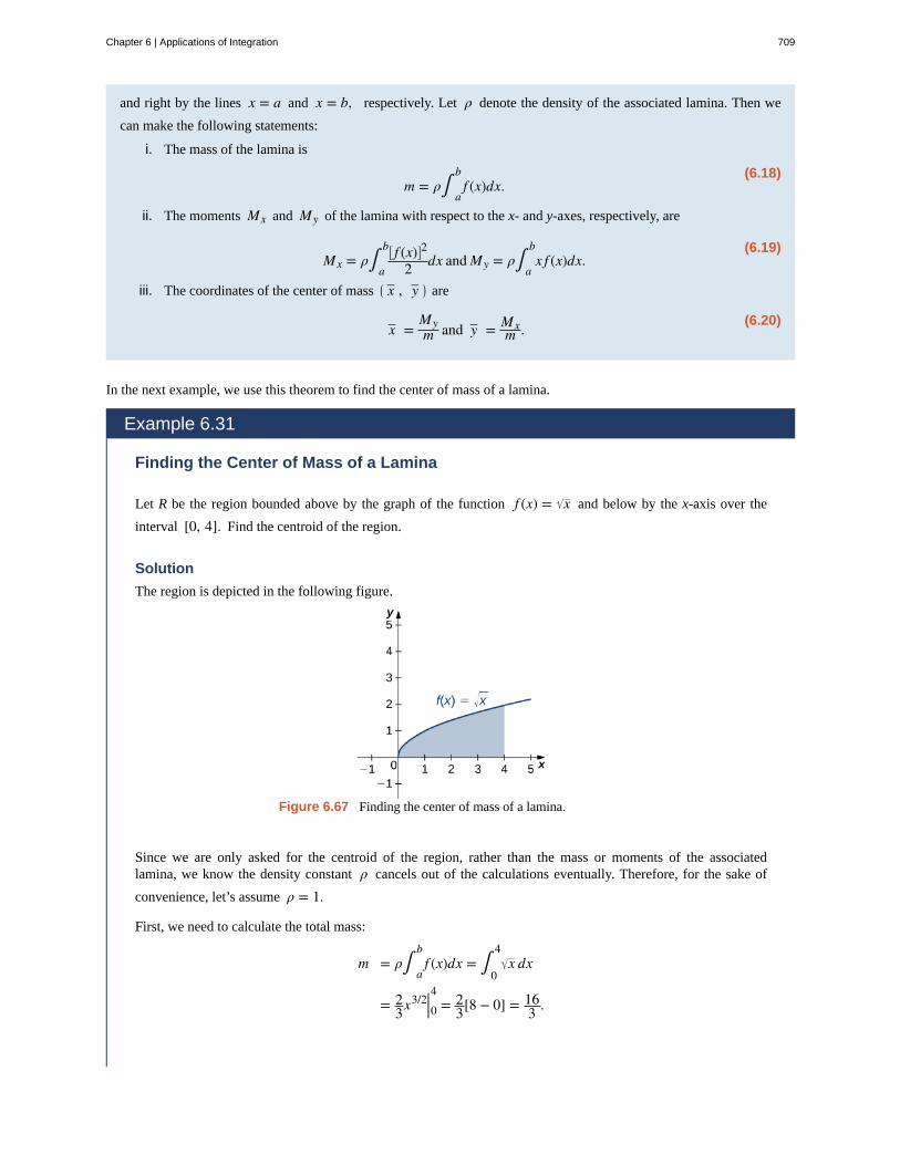
and right by the lines x = a and x = b, respectively. Let ρ denote the density of the associated lamina. Then we
can make the following statements:
i. The mass of the lamina is
(6.18)m = ρ∫
a
bf (x)dx.
ii. The moments Mx and My of the lamina with respect to the x- and y-axes, respectively, are
(6.19)Mx = ρ∫
a
b ⎡⎣ f (x)⎤
⎦2
2 dx and My = ρ∫a
bx f (x)dx.
iii. The coordinates of the center of mass ⎛⎝ x– , y– ⎞
⎠ are
(6.20)x– =Mym and y– = Mx
m .
In the next example, we use this theorem to find the center of mass of a lamina.
Example 6.31
Finding the Center of Mass of a Lamina
Let R be the region bounded above by the graph of the function f (x) = x and below by the x-axis over the
interval [0, 4]. Find the centroid of the region.
Solution
The region is depicted in the following figure.
Figure 6.67 Finding the center of mass of a lamina.
Since we are only asked for the centroid of the region, rather than the mass or moments of the associatedlamina, we know the density constant ρ cancels out of the calculations eventually. Therefore, for the sake of
convenience, let’s assume ρ = 1.
First, we need to calculate the total mass:
m = ρ∫a
bf (x)dx = ∫
0
4x dx
= 23x3/2|04 = 2
3[8 − 0] = 163 .
Chapter 6 | Applications of Integration 709
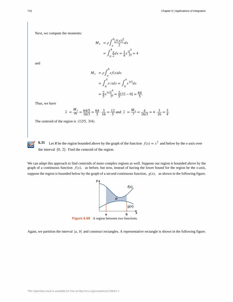
6.31
Next, we compute the moments:
Mx = ρ∫a
b ⎡⎣ f (x)⎤
⎦2
2 dx
= ∫0
4x2dx = 1
4x2|04 = 4
and
My = ρ∫a
bx f (x)dx
= ∫0
4x xdx = ∫
0
4x3/2dx
= 25x5/2|04 = 2
5[32 − 0] = 645 .
Thus, we have
x– =Mym = 64/5
16/3 = 645 · 3
16 = 125 and y– = Mx
y = 416/3 = 4 · 3
16 = 34.
The centroid of the region is (12/5, 3/4).
Let R be the region bounded above by the graph of the function f (x) = x2 and below by the x-axis over
the interval [0, 2]. Find the centroid of the region.
We can adapt this approach to find centroids of more complex regions as well. Suppose our region is bounded above by thegraph of a continuous function f (x), as before, but now, instead of having the lower bound for the region be the x-axis,
suppose the region is bounded below by the graph of a second continuous function, g(x), as shown in the following figure.
Figure 6.68 A region between two functions.
Again, we partition the interval ⎡⎣a, b⎤
⎦ and construct rectangles. A representative rectangle is shown in the following figure.
710 Chapter 6 | Applications of Integration
This OpenStax book is available for free at http://cnx.org/content/col11964/1.2
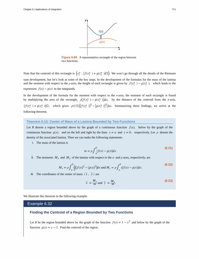
Figure 6.69 A representative rectangle of the region betweentwo functions.
Note that the centroid of this rectangle is ⎛⎝xi* , ⎛
⎝ f (xi* ) + g(xi* )⎞⎠/2⎞
⎠. We won’t go through all the details of the Riemann
sum development, but let’s look at some of the key steps. In the development of the formulas for the mass of the laminaand the moment with respect to the y-axis, the height of each rectangle is given by f (xi* ) − g(xi* ), which leads to the
expression f (x) − g(x) in the integrands.
In the development of the formula for the moment with respect to the x-axis, the moment of each rectangle is foundby multiplying the area of the rectangle, ρ⎡
⎣ f (xi* ) − g(xi* )⎤⎦Δx, by the distance of the centroid from the x-axis,
⎛⎝ f (xi* ) + g(xi* )⎞
⎠/2, which gives ρ(1/2)⎧
⎩⎨⎡⎣ f (xi* )⎤
⎦2 − ⎡
⎣g(xi* )⎤⎦2⎫
⎭⎬Δx. Summarizing these findings, we arrive at the
following theorem.
Theorem 6.13: Center of Mass of a Lamina Bounded by Two Functions
Let R denote a region bounded above by the graph of a continuous function f (x), below by the graph of the
continuous function g(x), and on the left and right by the lines x = a and x = b, respectively. Let ρ denote the
density of the associated lamina. Then we can make the following statements:
i. The mass of the lamina is
(6.21)m = ρ∫
a
b⎡⎣ f (x) − g(x)⎤
⎦dx.
ii. The moments Mx and My of the lamina with respect to the x- and y-axes, respectively, are
(6.22)Mx = ρ∫
a
b12
⎛⎝
⎡⎣ f (x)⎤
⎦2 − ⎡
⎣g(x)⎤⎦2⎞
⎠dx and My = ρ∫a
bx⎡
⎣ f (x) − g(x)⎤⎦dx.
iii. The coordinates of the center of mass ⎛⎝ x– , y– ⎞
⎠ are
(6.23)x– =Mym and y– = Mx
m .
We illustrate this theorem in the following example.
Example 6.32
Finding the Centroid of a Region Bounded by Two Functions
Let R be the region bounded above by the graph of the function f (x) = 1 − x2 and below by the graph of the
function g(x) = x − 1. Find the centroid of the region.
Chapter 6 | Applications of Integration 711
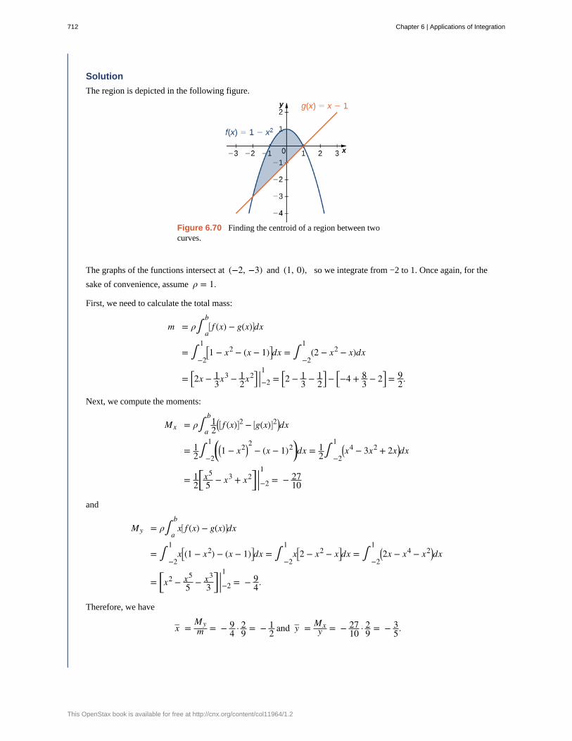
Solution
The region is depicted in the following figure.
Figure 6.70 Finding the centroid of a region between twocurves.
The graphs of the functions intersect at (−2, −3) and (1, 0), so we integrate from −2 to 1. Once again, for the
sake of convenience, assume ρ = 1.
First, we need to calculate the total mass:
m = ρ∫a
b⎡⎣ f (x) − g(x)⎤
⎦dx
= ∫−2
1⎡⎣1 − x2 − (x − 1)⎤
⎦dx = ∫−2
1(2 − x2 − x)dx
= ⎡⎣2x − 1
3x3 − 12x2⎤
⎦ |−21
= ⎡⎣2 − 1
3 − 12
⎤⎦ − ⎡
⎣−4 + 83 − 2⎤
⎦ = 92.
Next, we compute the moments:
Mx = ρ∫a
b12
⎛⎝
⎡⎣ f (x)⎤
⎦2 − ⎡
⎣g(x)⎤⎦2⎞
⎠dx
= 12∫
−2
1 ⎛⎝
⎛⎝1 − x2⎞
⎠2
− (x − 1)2⎞⎠dx = 1
2∫−2
1⎛⎝x4 − 3x2 + 2x⎞
⎠dx
= 12
⎡⎣
x5
5 − x3 + x2⎤⎦ |−2
1= − 27
10
and
My = ρ∫a
bx⎡
⎣ f (x) − g(x)⎤⎦dx
= ∫−2
1x⎡
⎣(1 − x2) − (x − 1)⎤⎦dx = ∫
−2
1x⎡
⎣2 − x2 − x⎤⎦dx = ∫
−2
1⎛⎝2x − x4 − x2⎞
⎠dx
= ⎡⎣x2 − x5
5 − x3
3⎤⎦ |−2
1= − 9
4.
Therefore, we have
x– =Mym = − 9
4 · 29 = − 1
2 and y– = Mxy = − 27
10 · 29 = − 3
5.
712 Chapter 6 | Applications of Integration
This OpenStax book is available for free at http://cnx.org/content/col11964/1.2
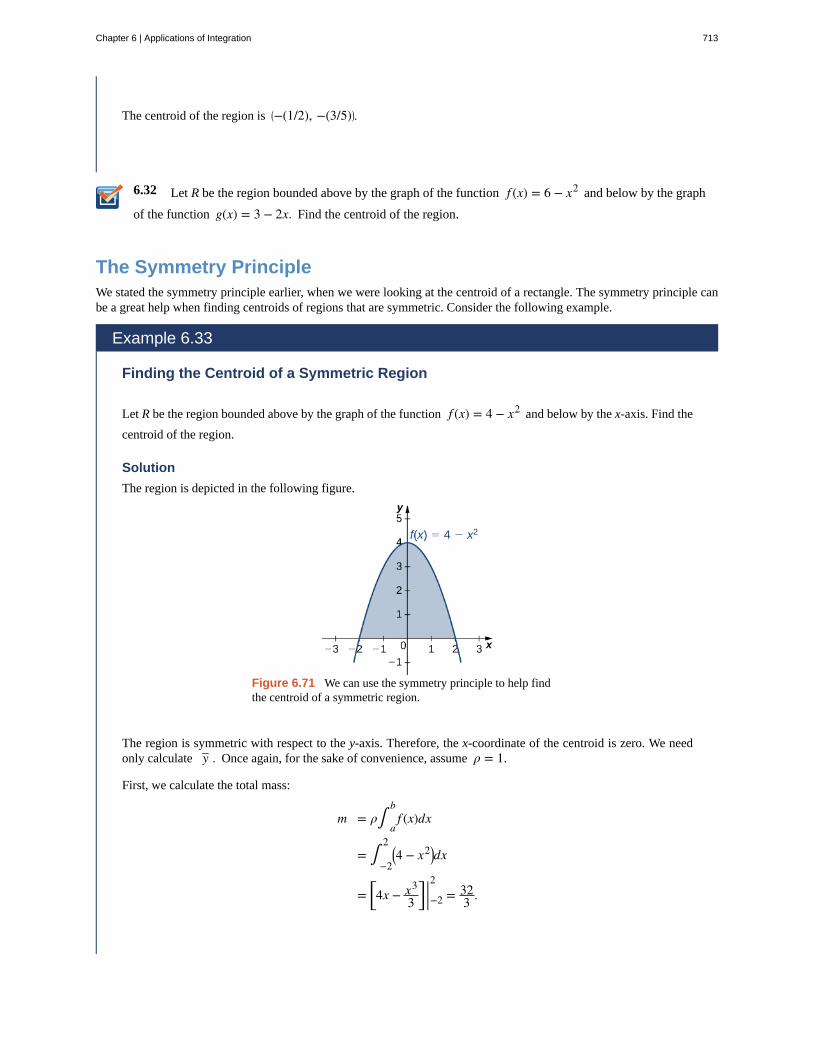
6.32
The centroid of the region is ⎛⎝−(1/2), −(3/5)⎞
⎠.
Let R be the region bounded above by the graph of the function f (x) = 6 − x2 and below by the graph
of the function g(x) = 3 − 2x. Find the centroid of the region.
The Symmetry PrincipleWe stated the symmetry principle earlier, when we were looking at the centroid of a rectangle. The symmetry principle canbe a great help when finding centroids of regions that are symmetric. Consider the following example.
Example 6.33
Finding the Centroid of a Symmetric Region
Let R be the region bounded above by the graph of the function f (x) = 4 − x2 and below by the x-axis. Find the
centroid of the region.
Solution
The region is depicted in the following figure.
Figure 6.71 We can use the symmetry principle to help findthe centroid of a symmetric region.
The region is symmetric with respect to the y-axis. Therefore, the x-coordinate of the centroid is zero. We needonly calculate y– . Once again, for the sake of convenience, assume ρ = 1.
First, we calculate the total mass:
m = ρ∫a
bf (x)dx
= ∫−2
2⎛⎝4 − x2⎞
⎠dx
= ⎡⎣4x − x3
3⎤⎦ |−2
2= 32
3 .
Chapter 6 | Applications of Integration 713
6.33
Next, we calculate the moments. We only need Mx :
Mx = ρ∫a
b ⎡⎣ f (x)⎤
⎦2
2 dx
= 12∫
−2
2⎡⎣4 − x2⎤
⎦2
dx = 12∫
−2
2⎛⎝16 − 8x2 + x4⎞
⎠dx
= 12
⎡⎣
x5
5 − 8x3
3 + 16x⎤⎦ |−2
2= 256
15 .
Then we have
y– = Mxy = 256
15 · 332 = 8
5.
The centroid of the region is (0, 8/5).
Let R be the region bounded above by the graph of the function f (x) = 1 − x2 and below by x-axis.
Find the centroid of the region.
714 Chapter 6 | Applications of Integration
This OpenStax book is available for free at http://cnx.org/content/col11964/1.2
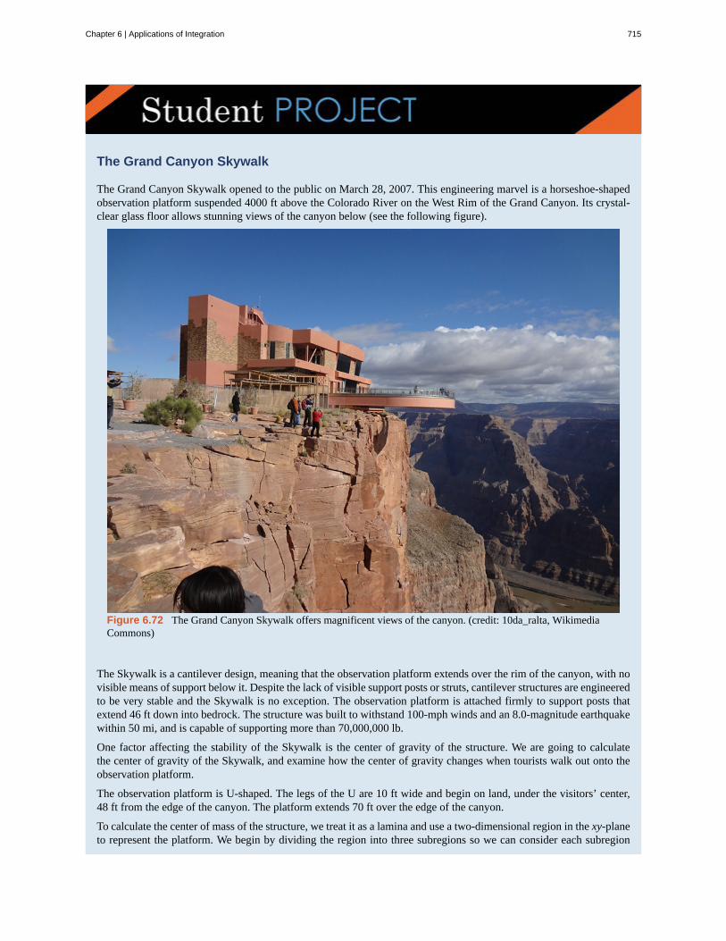
The Grand Canyon Skywalk
The Grand Canyon Skywalk opened to the public on March 28, 2007. This engineering marvel is a horseshoe-shapedobservation platform suspended 4000 ft above the Colorado River on the West Rim of the Grand Canyon. Its crystal-clear glass floor allows stunning views of the canyon below (see the following figure).
Figure 6.72 The Grand Canyon Skywalk offers magnificent views of the canyon. (credit: 10da_ralta, WikimediaCommons)
The Skywalk is a cantilever design, meaning that the observation platform extends over the rim of the canyon, with novisible means of support below it. Despite the lack of visible support posts or struts, cantilever structures are engineeredto be very stable and the Skywalk is no exception. The observation platform is attached firmly to support posts thatextend 46 ft down into bedrock. The structure was built to withstand 100-mph winds and an 8.0-magnitude earthquakewithin 50 mi, and is capable of supporting more than 70,000,000 lb.
One factor affecting the stability of the Skywalk is the center of gravity of the structure. We are going to calculatethe center of gravity of the Skywalk, and examine how the center of gravity changes when tourists walk out onto theobservation platform.
The observation platform is U-shaped. The legs of the U are 10 ft wide and begin on land, under the visitors’ center,48 ft from the edge of the canyon. The platform extends 70 ft over the edge of the canyon.
To calculate the center of mass of the structure, we treat it as a lamina and use a two-dimensional region in the xy-planeto represent the platform. We begin by dividing the region into three subregions so we can consider each subregion
Chapter 6 | Applications of Integration 715
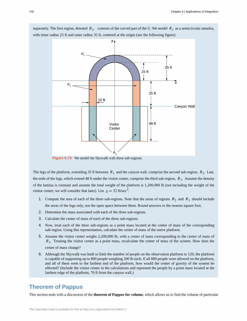
separately. The first region, denoted R1, consists of the curved part of the U. We model R1 as a semicircular annulus,
with inner radius 25 ft and outer radius 35 ft, centered at the origin (see the following figure).
Figure 6.73 We model the Skywalk with three sub-regions.
The legs of the platform, extending 35 ft between R1 and the canyon wall, comprise the second sub-region, R2. Last,
the ends of the legs, which extend 48 ft under the visitor center, comprise the third sub-region, R3. Assume the density
of the lamina is constant and assume the total weight of the platform is 1,200,000 lb (not including the weight of the
visitor center; we will consider that later). Use g = 32 ft/sec2.
1. Compute the area of each of the three sub-regions. Note that the areas of regions R2 and R3 should include
the areas of the legs only, not the open space between them. Round answers to the nearest square foot.
2. Determine the mass associated with each of the three sub-regions.
3. Calculate the center of mass of each of the three sub-regions.
4. Now, treat each of the three sub-regions as a point mass located at the center of mass of the correspondingsub-region. Using this representation, calculate the center of mass of the entire platform.
5. Assume the visitor center weighs 2,200,000 lb, with a center of mass corresponding to the center of mass ofR3. Treating the visitor center as a point mass, recalculate the center of mass of the system. How does the
center of mass change?
6. Although the Skywalk was built to limit the number of people on the observation platform to 120, the platformis capable of supporting up to 800 people weighing 200 lb each. If all 800 people were allowed on the platform,and all of them went to the farthest end of the platform, how would the center of gravity of the system beaffected? (Include the visitor center in the calculations and represent the people by a point mass located at thefarthest edge of the platform, 70 ft from the canyon wall.)
Theorem of PappusThis section ends with a discussion of the theorem of Pappus for volume, which allows us to find the volume of particular
716 Chapter 6 | Applications of Integration
This OpenStax book is available for free at http://cnx.org/content/col11964/1.2
kinds of solids by using the centroid. (There is also a theorem of Pappus for surface area, but it is much less useful than thetheorem for volume.)
Theorem 6.14: Theorem of Pappus for Volume
Let R be a region in the plane and let l be a line in the plane that does not intersect R. Then the volume of the solid ofrevolution formed by revolving R around l is equal to the area of R multiplied by the distance d traveled by the centroidof R.
Proof
We can prove the case when the region is bounded above by the graph of a function f (x) and below by the graph of a
function g(x) over an interval ⎡⎣a, b⎤
⎦, and for which the axis of revolution is the y-axis. In this case, the area of the region is
A = ∫a
b⎡⎣ f (x) − g(x)⎤
⎦dx. Since the axis of rotation is the y-axis, the distance traveled by the centroid of the region depends
only on the x-coordinate of the centroid, x– , which is
x– =Mym ,
where
m = ρ∫a
b⎡⎣ f (x) − g(x)⎤
⎦dx and My = ρ∫a
bx⎡
⎣ f (x) − g(x)⎤⎦dx.
Then,
d = 2πρ∫
a
bx⎡
⎣ f (x) − g(x)⎤⎦dx
ρ∫a
b⎡⎣ f (x) − g(x)⎤
⎦dx
and thus
d · A = 2π∫a
bx⎡
⎣ f (x) − g(x)⎤⎦dx.
However, using the method of cylindrical shells, we have
V = 2π∫a
bx⎡
⎣ f (x) − g(x)⎤⎦dx.
So,
V = d · A
and the proof is complete.
□
Example 6.34
Using the Theorem of Pappus for Volume
Let R be a circle of radius 2 centered at (4, 0). Use the theorem of Pappus for volume to find the volume of the
torus generated by revolving R around the y-axis.
Chapter 6 | Applications of Integration 717
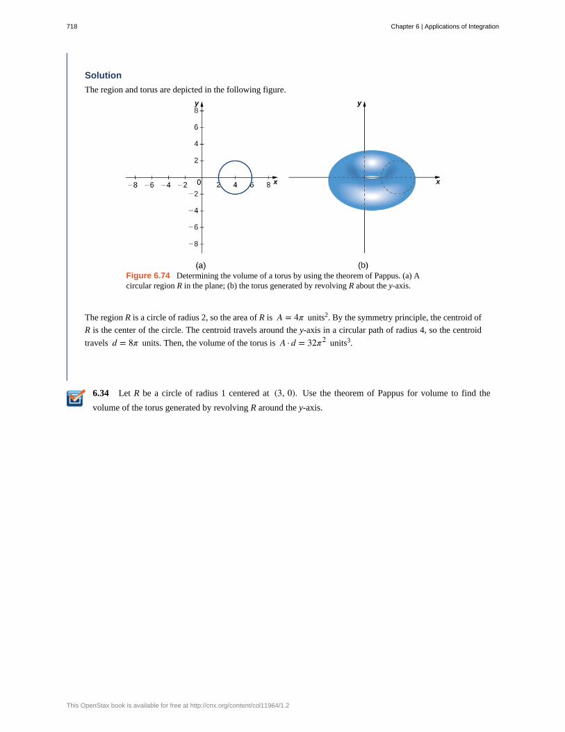
6.34
Solution
The region and torus are depicted in the following figure.
Figure 6.74 Determining the volume of a torus by using the theorem of Pappus. (a) Acircular region R in the plane; (b) the torus generated by revolving R about the y-axis.
The region R is a circle of radius 2, so the area of R is A = 4π units2. By the symmetry principle, the centroid of
R is the center of the circle. The centroid travels around the y-axis in a circular path of radius 4, so the centroid
travels d = 8π units. Then, the volume of the torus is A · d = 32π2 units3.
Let R be a circle of radius 1 centered at (3, 0). Use the theorem of Pappus for volume to find the
volume of the torus generated by revolving R around the y-axis.
718 Chapter 6 | Applications of Integration
This OpenStax book is available for free at http://cnx.org/content/col11964/1.2
6.6 EXERCISESFor the following exercises, calculate the center of mass forthe collection of masses given.
254. m1 = 2 at x1 = 1 and m2 = 4 at x2 = 2
255. m1 = 1 at x1 = −1 and m2 = 3 at x2 = 2
256. m = 3 at x = 0, 1, 2, 6
257. Unit masses at (x, y) = (1, 0), (0, 1), (1, 1)
258. m1 = 1 at (1, 0) and m2 = 4 at (0, 1)
259. m1 = 1 at (1, 0) and m2 = 3 at (2, 2)
For the following exercises, compute the center of massx– .
260. ρ = 1 for x ∈ (−1, 3)
261. ρ = x2 for x ∈ (0, L)
262. ρ = 1 for x ∈ (0, 1) and ρ = 2 for x ∈ (1, 2)
263. ρ = sin x for x ∈ (0, π)
264. ρ = cos x for x ∈ ⎛⎝0, π
2⎞⎠
265. ρ = ex for x ∈ (0, 2)
266. ρ = x3 + xe−x for x ∈ (0, 1)
267. ρ = x sin x for x ∈ (0, π)
268. ρ = x for x ∈ (1, 4)
269. ρ = ln x for x ∈ (1, e)
For the following exercises, compute the center of mass⎛⎝ x– , y– ⎞
⎠. Use symmetry to help locate the center of mass
whenever possible.
270. ρ = 7 in the square 0 ≤ x ≤ 1, 0 ≤ y ≤ 1
271. ρ = 3 in the triangle with vertices (0, 0), (a, 0),and (0, b)
272. ρ = 2 for the region bounded by y = cos(x),
y = −cos(x), x = − π2, and x = π
2
For the following exercises, use a calculator to draw theregion, then compute the center of mass ⎛
⎝ x– , y– ⎞⎠. Use
symmetry to help locate the center of mass wheneverpossible.
273. [T] The region bounded by y = cos(2x),
x = − π4, and x = π
4
274. [T] The region between y = 2x2, y = 0, x = 0,and x = 1
275. [T] The region between y = 54x2 and y = 5
276. [T] Region between y = x, y = ln(x), x = 1,and x = 4
277. [T] The region bounded by y = 0, x2
4 + y2
9 = 1
278. [T] The region bounded by y = 0, x = 0, and
x2
4 + y2
9 = 1
279. [T] The region bounded by y = x2 and y = x4 in
the first quadrant
For the following exercises, use the theorem of Pappus todetermine the volume of the shape.
280. Rotating y = mx around the x -axis between x = 0and x = 1
281. Rotating y = mx around the y -axis between x = 0and x = 1
282. A general cone created by rotating a triangle withvertices (0, 0), (a, 0), and (0, b) around the y -axis.
Does your answer agree with the volume of a cone?
283. A general cylinder created by rotating a rectanglewith vertices (0, 0), (a, 0), (0, b), and (a, b) around
the y -axis. Does your answer agree with the volume of a
cylinder?
284. A sphere created by rotating a semicircle with radiusa around the y -axis. Does your answer agree with the
volume of a sphere?
For the following exercises, use a calculator to draw theregion enclosed by the curve. Find the area M and the
Chapter 6 | Applications of Integration 719
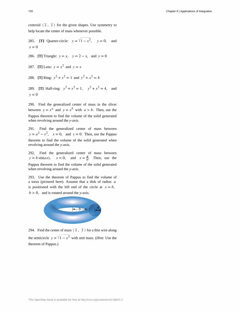
centroid ⎛⎝ x– , y– ⎞
⎠ for the given shapes. Use symmetry to
help locate the center of mass whenever possible.
285. [T] Quarter-circle: y = 1 − x2, y = 0, and
x = 0
286. [T] Triangle: y = x, y = 2 − x, and y = 0
287. [T] Lens: y = x2 and y = x
288. [T] Ring: y2 + x2 = 1 and y2 + x2 = 4
289. [T] Half-ring: y2 + x2 = 1, y2 + x2 = 4, and
y = 0
290. Find the generalized center of mass in the sliver
between y = xa and y = xb with a > b. Then, use the
Pappus theorem to find the volume of the solid generatedwhen revolving around the y-axis.
291. Find the generalized center of mass between
y = a2 − x2, x = 0, and y = 0. Then, use the Pappus
theorem to find the volume of the solid generated whenrevolving around the y-axis.
292. Find the generalized center of mass betweeny = b sin(ax), x = 0, and x = π
a . Then, use the
Pappus theorem to find the volume of the solid generatedwhen revolving around the y-axis.
293. Use the theorem of Pappus to find the volume ofa torus (pictured here). Assume that a disk of radius ais positioned with the left end of the circle at x = b,b > 0, and is rotated around the y-axis.
294. Find the center of mass ⎛⎝ x– , y– ⎞
⎠ for a thin wire along
the semicircle y = 1 − x2 with unit mass. (Hint: Use the
theorem of Pappus.)
720 Chapter 6 | Applications of Integration
This OpenStax book is available for free at http://cnx.org/content/col11964/1.2
6.7 | Integrals, Exponential Functions, and Logarithms
Learning Objectives6.7.1 Write the definition of the natural logarithm as an integral.
6.7.2 Recognize the derivative of the natural logarithm.
6.7.3 Integrate functions involving the natural logarithmic function.
6.7.4 Define the number e through an integral.
6.7.5 Recognize the derivative and integral of the exponential function.
6.7.6 Prove properties of logarithms and exponential functions using integrals.
6.7.7 Express general logarithmic and exponential functions in terms of natural logarithms andexponentials.
We already examined exponential functions and logarithms in earlier chapters. However, we glossed over some key detailsin the previous discussions. For example, we did not study how to treat exponential functions with exponents that areirrational. The definition of the number e is another area where the previous development was somewhat incomplete. Wenow have the tools to deal with these concepts in a more mathematically rigorous way, and we do so in this section.
For purposes of this section, assume we have not yet defined the natural logarithm, the number e, or any of the integrationand differentiation formulas associated with these functions. By the end of the section, we will have studied these conceptsin a mathematically rigorous way (and we will see they are consistent with the concepts we learned earlier).
We begin the section by defining the natural logarithm in terms of an integral. This definition forms the foundation forthe section. From this definition, we derive differentiation formulas, define the number e, and expand these concepts to
logarithms and exponential functions of any base.
The Natural Logarithm as an IntegralRecall the power rule for integrals:
∫ xn dx = xn + 1
n + 1 + C, n ≠ −1.
Clearly, this does not work when n = −1, as it would force us to divide by zero. So, what do we do with ∫ 1xdx? Recall
from the Fundamental Theorem of Calculus that ∫1
x1t dt is an antiderivative of 1/x. Therefore, we can make the following
definition.
Definition
For x > 0, define the natural logarithm function by
(6.24)ln x = ∫
1
x1t dt.
For x > 1, this is just the area under the curve y = 1/t from 1 to x. For x < 1, we have ∫1
x1t dt = −∫
x
11t dt, so in
this case it is the negative of the area under the curve from x to 1 (see the following figure).
Chapter 6 | Applications of Integration 721
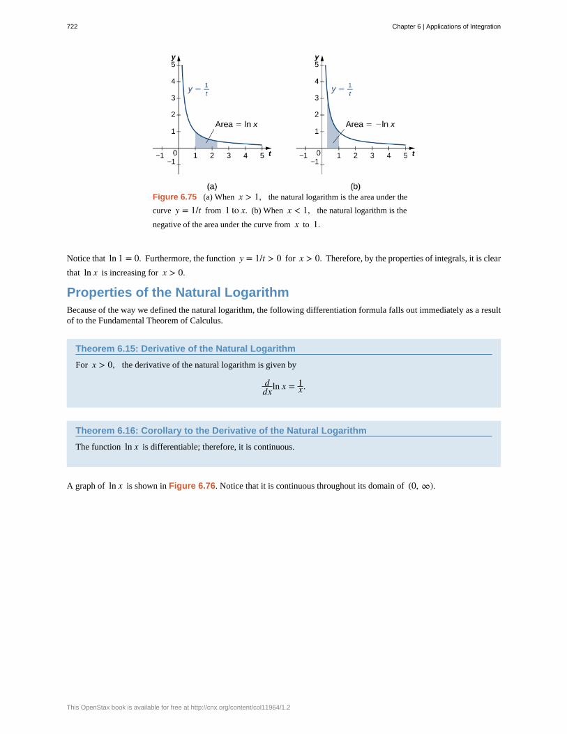
Figure 6.75 (a) When x > 1, the natural logarithm is the area under the
curve y = 1/t from 1 to x. (b) When x < 1, the natural logarithm is the
negative of the area under the curve from x to 1.
Notice that ln 1 = 0. Furthermore, the function y = 1/t > 0 for x > 0. Therefore, by the properties of integrals, it is clear
that ln x is increasing for x > 0.
Properties of the Natural LogarithmBecause of the way we defined the natural logarithm, the following differentiation formula falls out immediately as a resultof to the Fundamental Theorem of Calculus.
Theorem 6.15: Derivative of the Natural Logarithm
For x > 0, the derivative of the natural logarithm is given by
ddxln x = 1
x .
Theorem 6.16: Corollary to the Derivative of the Natural Logarithm
The function ln x is differentiable; therefore, it is continuous.
A graph of ln x is shown in Figure 6.76. Notice that it is continuous throughout its domain of (0, ∞).
722 Chapter 6 | Applications of Integration
This OpenStax book is available for free at http://cnx.org/content/col11964/1.2
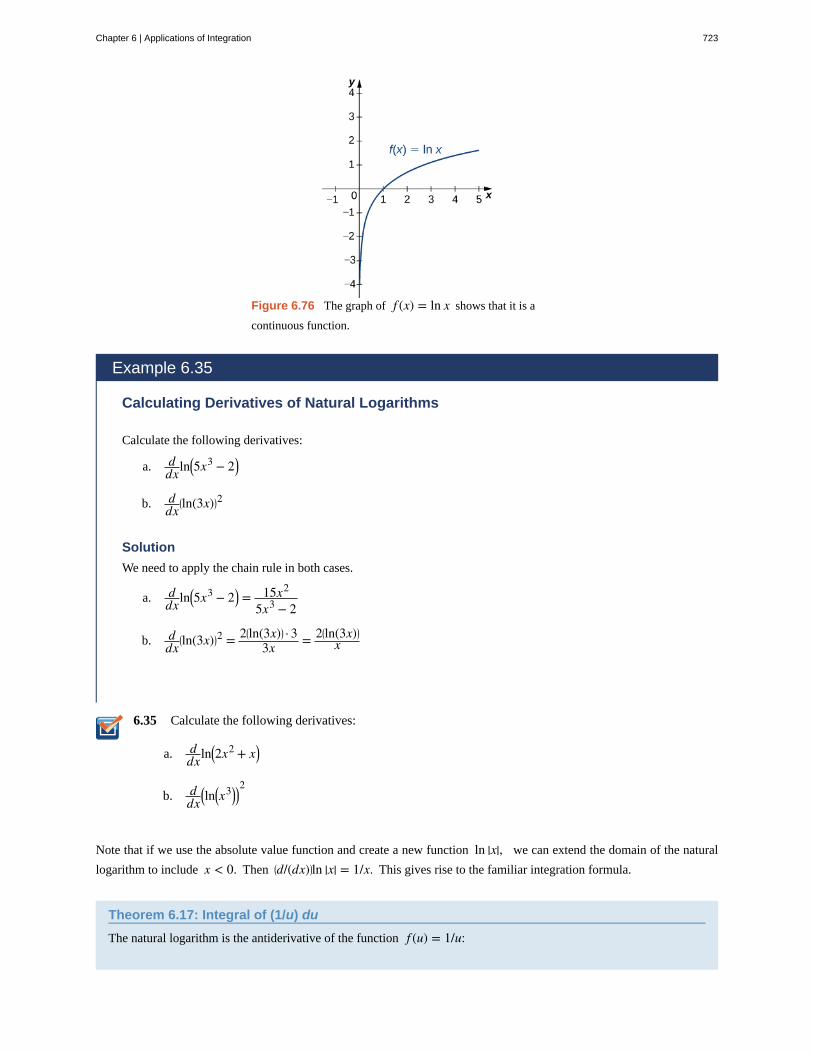
6.35
Figure 6.76 The graph of f (x) = ln x shows that it is a
continuous function.
Example 6.35
Calculating Derivatives of Natural Logarithms
Calculate the following derivatives:
a. ddxln⎛
⎝5x3 − 2⎞⎠
b. ddx
⎛⎝ln(3x)⎞
⎠2
Solution
We need to apply the chain rule in both cases.
a. ddxln⎛
⎝5x3 − 2⎞⎠ = 15x2
5x3 − 2
b. ddx
⎛⎝ln(3x)⎞
⎠2 = 2⎛
⎝ln(3x)⎞⎠ · 3
3x = 2⎛⎝ln(3x)⎞
⎠
x
Calculate the following derivatives:
a. ddxln⎛
⎝2x2 + x⎞⎠
b. ddx
⎛⎝ln
⎛⎝x
3⎞⎠⎞⎠2
Note that if we use the absolute value function and create a new function ln |x|, we can extend the domain of the natural
logarithm to include x < 0. Then ⎛⎝d/(dx)⎞
⎠ln |x| = 1/x. This gives rise to the familiar integration formula.
Theorem 6.17: Integral of (1/u) du
The natural logarithm is the antiderivative of the function f (u) = 1/u:
Chapter 6 | Applications of Integration 723
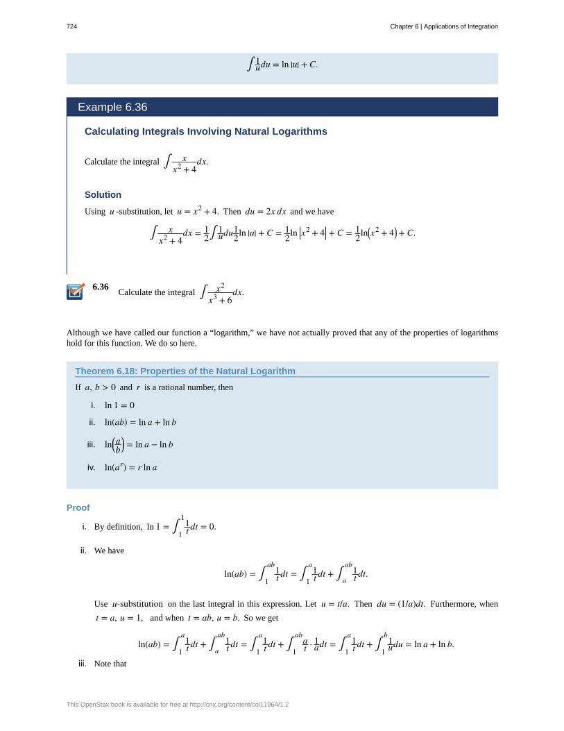
6.36
∫ 1udu = ln |u| + C.
Example 6.36
Calculating Integrals Involving Natural Logarithms
Calculate the integral ∫ xx2 + 4
dx.
Solution
Using u -substitution, let u = x2 + 4. Then du = 2x dx and we have
∫ xx2 + 4
dx = 12∫ 1
udu12ln |u| + C = 1
2ln |x2 + 4| + C = 12ln⎛
⎝x2 + 4⎞⎠ + C.
Calculate the integral ∫ x2
x3 + 6dx.
Although we have called our function a “logarithm,” we have not actually proved that any of the properties of logarithmshold for this function. We do so here.
Theorem 6.18: Properties of the Natural Logarithm
If a, b > 0 and r is a rational number, then
i. ln 1 = 0
ii. ln(ab) = ln a + ln b
iii. ln⎛⎝ab
⎞⎠ = ln a − ln b
iv. ln(ar) = r ln a
Proof
i. By definition, ln 1 = ∫1
11t dt = 0.
ii. We have
ln(ab) = ∫1
ab1t dt = ∫
1
a1t dt + ∫
a
ab1t dt.
Use u-substitution on the last integral in this expression. Let u = t/a. Then du = (1/a)dt. Furthermore, when
t = a, u = 1, and when t = ab, u = b. So we get
ln(ab) = ∫1
a1t dt + ∫
a
ab1t dt = ∫
1
a1t dt + ∫
1
abat · 1
adt = ∫1
a1t dt + ∫
1
b1udu = ln a + ln b.
iii. Note that
724 Chapter 6 | Applications of Integration
This OpenStax book is available for free at http://cnx.org/content/col11964/1.2
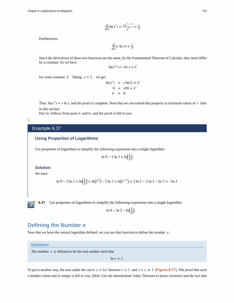
6.37
ddxln(xr) = rxr − 1
xr = rx.
Furthermore,
ddx(r ln x) = r
x.
Since the derivatives of these two functions are the same, by the Fundamental Theorem of Calculus, they must differby a constant. So we have
ln(xr) = r ln x + C
for some constant C. Taking x = 1, we get
ln(1r) = r ln(1) + C0 = r(0) + CC = 0.
Thus ln(xr) = r ln x and the proof is complete. Note that we can extend this property to irrational values of r later
in this section.Part iii. follows from parts ii. and iv. and the proof is left to you.
□
Example 6.37
Using Properties of Logarithms
Use properties of logarithms to simplify the following expression into a single logarithm:
ln 9 − 2 ln 3 + ln⎛⎝13
⎞⎠.
Solution
We have
ln 9 − 2 ln 3 + ln⎛⎝13
⎞⎠ = ln⎛
⎝32⎞⎠ − 2 ln 3 + ln⎛
⎝3−1⎞⎠ = 2 ln 3 − 2 ln 3 − ln 3 = −ln 3.
Use properties of logarithms to simplify the following expression into a single logarithm:
ln 8 − ln 2 − ln⎛⎝14
⎞⎠.
Defining the Number eNow that we have the natural logarithm defined, we can use that function to define the number e.
Definition
The number e is defined to be the real number such that
ln e = 1.
To put it another way, the area under the curve y = 1/t between t = 1 and t = e is 1 (Figure 6.77). The proof that such
a number exists and is unique is left to you. (Hint: Use the Intermediate Value Theorem to prove existence and the fact that
Chapter 6 | Applications of Integration 725
ln x is increasing to prove uniqueness.)
Figure 6.77 The area under the curve from 1 to e is equal
to one.
The number e can be shown to be irrational, although we won’t do so here (see the Student Project in Taylor and
Maclaurin Series (http://cnx.org/content/m53817/latest/) ). Its approximate value is given by
e ≈ 2.71828182846.
The Exponential FunctionWe now turn our attention to the function ex. Note that the natural logarithm is one-to-one and therefore has an inverse
function. For now, we denote this inverse function by exp x. Then,
exp(ln x) = x for x > 0 and ln(exp x) = x for all x.
The following figure shows the graphs of exp x and ln x.
Figure 6.78 The graphs of ln x and exp x.
We hypothesize that exp x = ex. For rational values of x, this is easy to show. If x is rational, then we have
ln(ex) = x ln e = x. Thus, when x is rational, ex = exp x. For irrational values of x, we simply define ex as the
inverse function of ln x.
726 Chapter 6 | Applications of Integration
This OpenStax book is available for free at http://cnx.org/content/col11964/1.2
Definition
For any real number x, define y = ex to be the number for which
(6.25)ln y = ln(ex) = x.
Then we have ex = exp(x) for all x, and thus
(6.26)eln x = x for x > 0 and ln(ex) = x
for all x.
Properties of the Exponential FunctionSince the exponential function was defined in terms of an inverse function, and not in terms of a power of e, we must
verify that the usual laws of exponents hold for the function ex.
Theorem 6.19: Properties of the Exponential Function
If p and q are any real numbers and r is a rational number, then
i. e p eq = e p + q
ii. e p
eq = e p − q
iii. (e p)r = e pr
Proof
Note that if p and q are rational, the properties hold. However, if p or q are irrational, we must apply the inverse
function definition of ex and verify the properties. Only the first property is verified here; the other two are left to you. We
have
ln(e p eq) = ln(e p) + ln(eq) = p + q = ln⎛⎝e
p + q⎞⎠.
Since ln x is one-to-one, then
e p eq = e p + q.
□
As with part iv. of the logarithm properties, we can extend property iii. to irrational values of r, and we do so by the end
of the section.
We also want to verify the differentiation formula for the function y = ex. To do this, we need to use implicit
differentiation. Let y = ex. Then
ln y = xddxln y = d
dxx
1y
dydx = 1
dydx = y.
Thus, we see
Chapter 6 | Applications of Integration 727
6.38
ddxex = ex
as desired, which leads immediately to the integration formula
∫ ex dx = ex + C.
We apply these formulas in the following examples.
Example 6.38
Using Properties of Exponential Functions
Evaluate the following derivatives:
a. ddte
3t et2
b. ddxe3x2
Solution
We apply the chain rule as necessary.
a. ddte
3t et2= d
dte3t + t2
= e3t + t2(3 + 2t)
b. ddxe3x2
= e3x26x
Evaluate the following derivatives:
a. ddx
⎛
⎝⎜ex2
e5x
⎞
⎠⎟
b. ddt
⎛⎝e2t⎞
⎠3
Example 6.39
Using Properties of Exponential Functions
Evaluate the following integral: ∫ 2xe−x2dx.
Solution
Using u -substitution, let u = −x2. Then du = −2x dx, and we have
∫ 2xe−x2dx = −∫ eu du = −eu + C = −e−x2
+ C.
728 Chapter 6 | Applications of Integration
This OpenStax book is available for free at http://cnx.org/content/col11964/1.2
6.39 Evaluate the following integral: ∫ 4e3xdx.
General Logarithmic and Exponential FunctionsWe close this section by looking at exponential functions and logarithms with bases other than e. Exponential functions
are functions of the form f (x) = ax. Note that unless a = e, we still do not have a mathematically rigorous definition
of these functions for irrational exponents. Let’s rectify that here by defining the function f (x) = ax in terms of the
exponential function ex. We then examine logarithms with bases other than e as inverse functions of exponential
functions.
Definition
For any a > 0, and for any real number x, define y = ax as follows:
y = ax = ex ln a.
Now ax is defined rigorously for all values of x. This definition also allows us to generalize property iv. of logarithms and
property iii. of exponential functions to apply to both rational and irrational values of r. It is straightforward to show that
properties of exponents hold for general exponential functions defined in this way.
Let’s now apply this definition to calculate a differentiation formula for ax. We have
ddxax = d
dxex ln a = ex ln a ln a = ax ln a.
The corresponding integration formula follows immediately.
Theorem 6.20: Derivatives and Integrals Involving General Exponential Functions
Let a > 0. Then,
ddxax = ax ln a
and
∫ ax dx = 1ln aax + C.
If a ≠ 1, then the function ax is one-to-one and has a well-defined inverse. Its inverse is denoted by loga x. Then,
y = loga x if and only if x = ay.
Note that general logarithm functions can be written in terms of the natural logarithm. Let y = loga x. Then, x = ay.Taking the natural logarithm of both sides of this second equation, we get
ln x = ln(ay)ln x = y ln a
y = ln xln a
log x = ln xln a.
Thus, we see that all logarithmic functions are constant multiples of one another. Next, we use this formula to find adifferentiation formula for a logarithm with base a. Again, let y = loga x. Then,
Chapter 6 | Applications of Integration 729
6.40
dydx = d
dx⎛⎝loga x⎞
⎠
= ddx
⎛⎝ln xln a
⎞⎠
= ⎛⎝
1ln a
⎞⎠
ddx(ln x)
= 1ln a · 1
x
= 1x ln a.
Theorem 6.21: Derivatives of General Logarithm Functions
Let a > 0. Then,
ddxloga x = 1
x ln a.
Example 6.40
Calculating Derivatives of General Exponential and Logarithm Functions
Evaluate the following derivatives:
a. ddt
⎛⎝4t · 2t2⎞
⎠
b. ddxlog8
⎛⎝7x2 + 4⎞
⎠
Solution
We need to apply the chain rule as necessary.
a. ddt
⎛⎝4t · 2t2⎞
⎠ = ddt
⎛⎝22t · 2t2⎞
⎠ = ddt
⎛⎝22t + t2⎞
⎠ = 22t + t2ln(2)(2 + 2t)
b. ddxlog8
⎛⎝7x2 + 4⎞
⎠ = 1⎛⎝7x2 + 4⎞
⎠(ln 8)(14x)
Evaluate the following derivatives:
a. ddt 4t4
b. ddxlog3
⎛⎝ x2 + 1⎞
⎠
Example 6.41
Integrating General Exponential Functions
730 Chapter 6 | Applications of Integration
This OpenStax book is available for free at http://cnx.org/content/col11964/1.2
6.41
Evaluate the following integral: ∫ 323xdx.
Solution
Use u-substitution and let u = −3x. Then du = −3dx and we have
∫ 323xdx = ∫ 3 · 2−3xdx = −∫ 2u du = − 1
ln 22u + C = − 1ln 22−3x + C.
Evaluate the following integral: ∫ x2 2x3dx.
Chapter 6 | Applications of Integration 731
6.7 EXERCISES
For the following exercises, find the derivativedydx.
295. y = ln(2x)
296. y = ln(2x + 1)
297. y = 1ln x
For the following exercises, find the indefinite integral.
298. ∫ dt3t
299. ∫ dx1 + x
For the following exercises, find the derivative dy/dx.(You can use a calculator to plot the function and thederivative to confirm that it is correct.)
300. [T] y = ln(x)x
301. [T] y = x ln(x)
302. [T] y = log10 x
303. [T] y = ln(sin x)
304. [T] y = ln(ln x)
305. [T] y = 7 ln(4x)
306. [T] y = ln⎛⎝(4x)7⎞
⎠
307. [T] y = ln(tan x)
308. [T] y = ln(tan(3x))
309. [T] y = ln⎛⎝cos2 x⎞
⎠
For the following exercises, find the definite or indefiniteintegral.
310. ∫0
1dx
3 + x
311. ∫0
1dt
3 + 2t
312. ∫0
2x dx
x2 + 1
313. ∫0
2x3 dxx2 + 1
314. ∫2
edx
x ln x
315. ∫2
edx
⎛⎝x ln(x)⎞
⎠2
316. ∫ cos x dxsin x
317. ∫0
π/4tan x dx
318. ∫ cot(3x)dx
319. ∫ (ln x)2 dxx
For the following exercises, compute dy/dx by
differentiating ln y.
320. y = x2 + 1
321. y = x2 + 1 x2 − 1
322. y = esin x
323. y = x−1/x
324. y = e(ex)
325. y = xe
326. y = x(ex)
327. y = x x3 x6
328. y = x−1/ln x
329. y = e−ln x
For the following exercises, evaluate by any method.
732 Chapter 6 | Applications of Integration
This OpenStax book is available for free at http://cnx.org/content/col11964/1.2
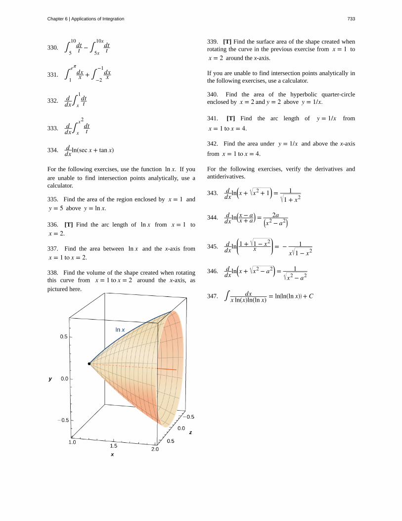
330. ∫5
10dtt − ∫
5x
10xdtt
331. ∫1
eπdxx + ∫
−2
−1dxx
332. ddx∫
x
1dtt
333. ddx∫
x
x2dtt
334. ddxln(sec x + tan x)
For the following exercises, use the function ln x. If you
are unable to find intersection points analytically, use acalculator.
335. Find the area of the region enclosed by x = 1 and
y = 5 above y = ln x.
336. [T] Find the arc length of ln x from x = 1 to
x = 2.
337. Find the area between ln x and the x-axis from
x = 1 to x = 2.
338. Find the volume of the shape created when rotatingthis curve from x = 1 to x = 2 around the x-axis, as
pictured here.
339. [T] Find the surface area of the shape created whenrotating the curve in the previous exercise from x = 1 to
x = 2 around the x-axis.
If you are unable to find intersection points analytically inthe following exercises, use a calculator.
340. Find the area of the hyperbolic quarter-circleenclosed by x = 2 and y = 2 above y = 1/x.
341. [T] Find the arc length of y = 1/x from
x = 1 to x = 4.
342. Find the area under y = 1/x and above the x-axis
from x = 1 to x = 4.
For the following exercises, verify the derivatives andantiderivatives.
343. ddxln⎛
⎝x + x2 + 1⎞⎠ = 1
1 + x2
344. ddxln⎛
⎝x − ax + a
⎞⎠ = 2a
⎛⎝x2 − a2⎞
⎠
345. ddxln
⎛
⎝⎜1 + 1 − x2
x⎞
⎠⎟ = − 1
x 1 − x2
346. ddxln⎛
⎝x + x2 − a2⎞⎠ = 1
x2 − a2
347. ∫ dxx ln(x)ln(ln x) = ln⎛
⎝ln(ln x)⎞⎠ + C
Chapter 6 | Applications of Integration 733
6.8 | Exponential Growth and Decay
Learning Objectives6.8.1 Use the exponential growth model in applications, including population growth andcompound interest.
6.8.2 Explain the concept of doubling time.
6.8.3 Use the exponential decay model in applications, including radioactive decay and Newton’slaw of cooling.
6.8.4 Explain the concept of half-life.
One of the most prevalent applications of exponential functions involves growth and decay models. Exponential growthand decay show up in a host of natural applications. From population growth and continuously compounded interest toradioactive decay and Newton’s law of cooling, exponential functions are ubiquitous in nature. In this section, we examineexponential growth and decay in the context of some of these applications.
Exponential Growth Model
Many systems exhibit exponential growth. These systems follow a model of the form y = y0 ekt, where y0 represents
the initial state of the system and k is a positive constant, called the growth constant. Notice that in an exponential growth
model, we have
(6.27)y′ = ky0 ekt = ky.
That is, the rate of growth is proportional to the current function value. This is a key feature of exponential growth.Equation 6.27 involves derivatives and is called a differential equation. We learn more about differential equations inIntroduction to Differential Equations (http://cnx.org/content/m53696/latest/) .
Rule: Exponential Growth Model
Systems that exhibit exponential growth increase according to the mathematical model
y = y0 ekt,
where y0 represents the initial state of the system and k > 0 is a constant, called the growth constant.
Population growth is a common example of exponential growth. Consider a population of bacteria, for instance. It seemsplausible that the rate of population growth would be proportional to the size of the population. After all, the more bacteriathere are to reproduce, the faster the population grows. Figure 6.79 and Table 6.1 represent the growth of a populationof bacteria with an initial population of 200 bacteria and a growth constant of 0.02. Notice that after only 2 hours (120minutes), the population is 10 times its original size!
734 Chapter 6 | Applications of Integration
This OpenStax book is available for free at http://cnx.org/content/col11964/1.2
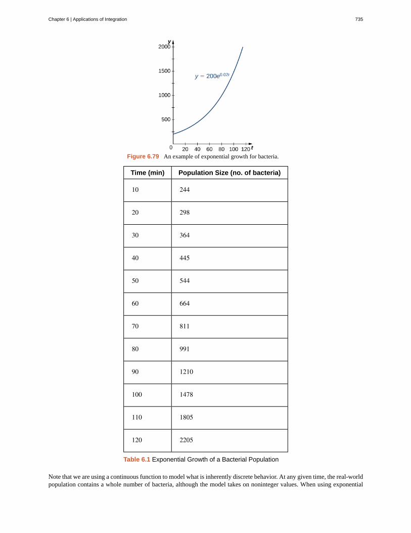
Figure 6.79 An example of exponential growth for bacteria.
Time (min) Population Size (no. of bacteria)
10 244
20 298
30 364
40 445
50 544
60 664
70 811
80 991
90 1210
100 1478
110 1805
120 2205
Table 6.1 Exponential Growth of a Bacterial Population
Note that we are using a continuous function to model what is inherently discrete behavior. At any given time, the real-worldpopulation contains a whole number of bacteria, although the model takes on noninteger values. When using exponential
Chapter 6 | Applications of Integration 735
6.42
growth models, we must always be careful to interpret the function values in the context of the phenomenon we aremodeling.
Example 6.42
Population Growth
Consider the population of bacteria described earlier. This population grows according to the function
f (t) = 200e0.02t, where t is measured in minutes. How many bacteria are present in the population after 5hours (300 minutes)? When does the population reach 100,000 bacteria?
Solution
We have f (t) = 200e0.02t. Then
f (300) = 200e0.02(300) ≈ 80,686.
There are 80,686 bacteria in the population after 5 hours.
To find when the population reaches 100,000 bacteria, we solve the equation
100,000 = 200e0.02t
500 = e0.02t
ln 500 = 0.02tt = ln 500
0.02 ≈ 310.73.
The population reaches 100,000 bacteria after 310.73 minutes.
Consider a population of bacteria that grows according to the function f (t) = 500e0.05t, where t is
measured in minutes. How many bacteria are present in the population after 4 hours? When does the populationreach 100 million bacteria?
Let’s now turn our attention to a financial application: compound interest. Interest that is not compounded is called simpleinterest. Simple interest is paid once, at the end of the specified time period (usually 1 year). So, if we put $1000 in a
savings account earning 2% simple interest per year, then at the end of the year we have
1000(1 + 0.02) = $1020.
Compound interest is paid multiple times per year, depending on the compounding period. Therefore, if the bankcompounds the interest every 6 months, it credits half of the year’s interest to the account after 6 months. During the
second half of the year, the account earns interest not only on the initial $1000, but also on the interest earned during the
first half of the year. Mathematically speaking, at the end of the year, we have
1000⎛⎝1 + 0.02
2⎞⎠2
= $1020.10.
Similarly, if the interest is compounded every 4 months, we have
1000⎛⎝1 + 0.02
3⎞⎠
3= $1020.13,
and if the interest is compounded daily (365 times per year), we have $1020.20. If we extend this concept, so that the
interest is compounded continuously, after t years we have
736 Chapter 6 | Applications of Integration
This OpenStax book is available for free at http://cnx.org/content/col11964/1.2
6.43
1000 limn → ∞⎛⎝1 + 0.02
n⎞⎠nt
.
Now let’s manipulate this expression so that we have an exponential growth function. Recall that the number e can be
expressed as a limit:
e = limm → ∞⎛⎝1 + 1
m⎞⎠m
.
Based on this, we want the expression inside the parentheses to have the form (1 + 1/m). Let n = 0.02m. Note that as
n → ∞, m → ∞ as well. Then we get
1000 limn → ∞⎛⎝1 + 0.02
n⎞⎠nt
= 1000 limm → ∞⎛⎝1 + 0.02
0.02m⎞⎠
0.02mt= 1000⎡
⎣ limm → ∞⎛⎝1 + 1
m⎞⎠m⎤
⎦0.02t
.
We recognize the limit inside the brackets as the number e. So, the balance in our bank account after t years is given by
1000e0.02t. Generalizing this concept, we see that if a bank account with an initial balance of $P earns interest at a rate
of r%, compounded continuously, then the balance of the account after t years is
Balance = Pert.
Example 6.43
Compound Interest
A 25-year-old student is offered an opportunity to invest some money in a retirement account that pays 5%annual interest compounded continuously. How much does the student need to invest today to have $1 million
when she retires at age 65? What if she could earn 6% annual interest compounded continuously instead?
Solution
We have
1,000,000 = Pe0.05(40)
P = 135,335.28.
She must invest $135,335.28 at 5% interest.
If, instead, she is able to earn 6%, then the equation becomes
1,000,000 = Pe0.06(40)
P = 90,717.95.
In this case, she needs to invest only $90,717.95. This is roughly two-thirds the amount she needs to invest at
5%. The fact that the interest is compounded continuously greatly magnifies the effect of the 1% increase in
interest rate.
Suppose instead of investing at age 25 b2 − 4ac, the student waits until age 35. How much would
she have to invest at 5%? At 6%?
If a quantity grows exponentially, the time it takes for the quantity to double remains constant. In other words, it takes thesame amount of time for a population of bacteria to grow from 100 to 200 bacteria as it does to grow from 10,000 to
20,000 bacteria. This time is called the doubling time. To calculate the doubling time, we want to know when the quantity
Chapter 6 | Applications of Integration 737
6.44
reaches twice its original size. So we have
2y0 = y0 ekt
2 = ekt
ln 2 = ktt = ln 2
k .
Definition
If a quantity grows exponentially, the doubling time is the amount of time it takes the quantity to double. It is givenby
Doubling time = ln 2k .
Example 6.44
Using the Doubling Time
Assume a population of fish grows exponentially. A pond is stocked initially with 500 fish. After 6 months,
there are 1000 fish in the pond. The owner will allow his friends and neighbors to fish on his pond after the fish
population reaches 10,000. When will the owner’s friends be allowed to fish?
Solution
We know it takes the population of fish 6 months to double in size. So, if t represents time in months,
by the doubling-time formula, we have 6 = (ln 2)/k. Then, k = (ln 2)/6. Thus, the population is given by
y = 500e⎛⎝(ln 2)/6⎞
⎠t. To figure out when the population reaches 10,000 fish, we must solve the following
equation:
10,000 = 500e(ln 2/6)t
20 = e(ln 2/6)t
ln 20 = ⎛⎝ln 26
⎞⎠t
t = 6(ln 20)ln 2 ≈ 25.93.
The owner’s friends have to wait 25.93 months (a little more than 2 years) to fish in the pond.
Suppose it takes 9 months for the fish population in Example 6.44 to reach 1000 fish. Under these
circumstances, how long do the owner’s friends have to wait?
Exponential Decay ModelExponential functions can also be used to model populations that shrink (from disease, for example), or chemicalcompounds that break down over time. We say that such systems exhibit exponential decay, rather than exponential growth.The model is nearly the same, except there is a negative sign in the exponent. Thus, for some positive constant k, we have
y = y0 e−kt.
As with exponential growth, there is a differential equation associated with exponential decay. We have
738 Chapter 6 | Applications of Integration
This OpenStax book is available for free at http://cnx.org/content/col11964/1.2
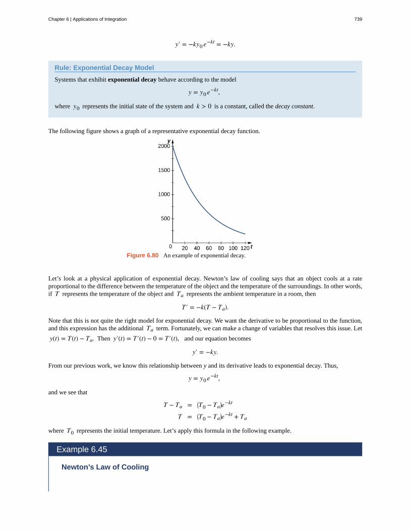
y′ = −ky0 e−kt = −ky.
Rule: Exponential Decay Model
Systems that exhibit exponential decay behave according to the model
y = y0 e−kt,
where y0 represents the initial state of the system and k > 0 is a constant, called the decay constant.
The following figure shows a graph of a representative exponential decay function.
Figure 6.80 An example of exponential decay.
Let’s look at a physical application of exponential decay. Newton’s law of cooling says that an object cools at a rateproportional to the difference between the temperature of the object and the temperature of the surroundings. In other words,if T represents the temperature of the object and Ta represents the ambient temperature in a room, then
T′ = −k(T − Ta).
Note that this is not quite the right model for exponential decay. We want the derivative to be proportional to the function,and this expression has the additional Ta term. Fortunately, we can make a change of variables that resolves this issue. Let
y(t) = T(t) − Ta. Then y′(t) = T′(t) − 0 = T′(t), and our equation becomes
y′ = −ky.
From our previous work, we know this relationship between y and its derivative leads to exponential decay. Thus,
y = y0 e−kt,
and we see that
T − Ta = ⎛⎝T0 − Ta
⎞⎠e−kt
T = ⎛⎝T0 − Ta
⎞⎠e−kt + Ta
where T0 represents the initial temperature. Let’s apply this formula in the following example.
Example 6.45
Newton’s Law of Cooling
Chapter 6 | Applications of Integration 739
6.45
According to experienced baristas, the optimal temperature to serve coffee is between 155°F and 175°F.Suppose coffee is poured at a temperature of 200°F, and after 2 minutes in a 70°F room it has cooled to
180°F. When is the coffee first cool enough to serve? When is the coffee too cold to serve? Round answers to
the nearest half minute.
Solution
We have
T = ⎛⎝T0 − Ta
⎞⎠e−kt + Ta
180 = (200 − 70)e−k(2) + 70110 = 130e−2k
1113 = e−2k
ln 1113 = −2k
ln 11 − ln 13 = −2kk = ln 13 − ln 11
2 .
Then, the model is
T = 130e(ln 11 − ln 13/2)t + 70.
The coffee reaches 175°F when
175 = 130e(ln 11 − ln 13/2)t + 70105 = 130e(ln 11 − ln 13/2)t
2126 = e(ln 11 − ln 13/2)t
ln 2126 = ln 11 − ln 13
2 t
ln 21 − ln 26 = ln 11 − ln 132 t
t = 2(ln 21 − ln 26)ln 11 − ln 13 ≈ 2.56.
The coffee can be served about 2.5 minutes after it is poured. The coffee reaches 155°F at
155 = 130e(ln 11 − ln 13/2)t + 7085 = 130e(ln 11 − ln 13)t
1726 = e(ln 11 − ln 13)t
ln 17 − ln 26 = ⎛⎝ln 11 − ln 13
2⎞⎠t
t = 2(ln 17 − ln 26)ln 11 − ln 13 ≈ 5.09.
The coffee is too cold to be served about 5 minutes after it is poured.
Suppose the room is warmer (75°F) and, after 2 minutes, the coffee has cooled only to 185°F. When
is the coffee first cool enough to serve? When is the coffee be too cold to serve? Round answers to the nearesthalf minute.
740 Chapter 6 | Applications of Integration
This OpenStax book is available for free at http://cnx.org/content/col11964/1.2
Just as systems exhibiting exponential growth have a constant doubling time, systems exhibiting exponential decay have aconstant half-life. To calculate the half-life, we want to know when the quantity reaches half its original size. Therefore, wehave
y02 = y0 e−kt
12 = e−kt
−ln 2 = −kt
t = ln 2k .
Note: This is the same expression we came up with for doubling time.
Definition
If a quantity decays exponentially, the half-life is the amount of time it takes the quantity to be reduced by half. It isgiven by
Half-life = ln 2k .
Example 6.46
Radiocarbon Dating
One of the most common applications of an exponential decay model is carbon dating. Carbon-14 decays (emits
a radioactive particle) at a regular and consistent exponential rate. Therefore, if we know how much carbon wasoriginally present in an object and how much carbon remains, we can determine the age of the object. The half-life of carbon-14 is approximately 5730 years—meaning, after that many years, half the material has converted
from the original carbon-14 to the new nonradioactive nitrogen-14. If we have 100 g carbon-14 today, how
much is left in 50 years? If an artifact that originally contained 100 g of carbon now contains 10 g of carbon,
how old is it? Round the answer to the nearest hundred years.
Solution
We have
5730 = ln 2k
k = ln 25730.
So, the model says
y = 100e−(ln 2/5730)t.
In 50 years, we have
y = 100e−(ln 2/5730)(50)
≈ 99.40.
Therefore, in 50 years, 99.40 g of carbon-14 remains.
To determine the age of the artifact, we must solve
Chapter 6 | Applications of Integration 741
6.46
10 = 100e−(ln 2/5730)t
110 = e−(ln 2/5730)t
t ≈ 19035.
The artifact is about 19,000 years old.
If we have 100 g of carbon-14, how much is left after. years? If an artifact that originally contained
100 g of carbon now contains 20g of carbon, how old is it? Round the answer to the nearest hundred years.
742 Chapter 6 | Applications of Integration
This OpenStax book is available for free at http://cnx.org/content/col11964/1.2
6.8 EXERCISESTrue or False? If true, prove it. If false, find the true answer.
348. The doubling time for y = ect is ⎛⎝ln (2)⎞
⎠/⎛⎝ln (c)⎞
⎠.
349. If you invest $500, an annual rate of interest of
3% yields more money in the first year than a 2.5%continuous rate of interest.
350. If you leave a 100°C pot of tea at room temperature
(25°C) and an identical pot in the refrigerator (5°C),with k = 0.02, the tea in the refrigerator reaches a
drinkable temperature (70°C) more than 5 minutes
before the tea at room temperature.
351. If given a half-life of t years, the constant k for
y = ekt is calculated by k = ln (1/2)/t.
For the following exercises, use y = y0 ekt.
352. If a culture of bacteria doubles in 3 hours, how many
hours does it take to multiply by 10?
353. If bacteria increase by a factor of 10 in 10 hours,
how many hours does it take to increase by 100?
354. How old is a skull that contains one-fifth as muchradiocarbon as a modern skull? Note that the half-life ofradiocarbon is 5730 years.
355. If a relic contains 90% as much radiocarbon as
new material, can it have come from the time of Christ(approximately 2000 years ago)? Note that the half-life of
radiocarbon is 5730 years.
356. The population of Cairo grew from 5 million to
10 million in 20 years. Use an exponential model to find
when the population was 8 million.
357. The populations of New York and Los Angeles aregrowing at 1% and 1.4% a year, respectively. Starting
from 8 million (New York) and 6 million (Los Angeles),
when are the populations equal?
358. Suppose the value of $1 in Japanese yen decreases
at 2% per year. Starting from $1 = ¥250, when will
$1 = ¥1?
359. The effect of advertising decays exponentially. If40% of the population remembers a new product after 3days, how long will 20% remember it?
360. If y = 1000 at t = 3 and y = 3000 at t = 4,what was y0 at t = 0?
361. If y = 100 at t = 4 and y = 10 at t = 8, when
does y = 1?
362. If a bank offers annual interest of 7.5% or
continuous interest of 7.25%, which has a better annual
yield?
363. What continuous interest rate has the same yield asan annual rate of 9%?
364. If you deposit $5000 at 8% annual interest, how
many years can you withdraw $500 (starting after the first
year) without running out of money?
365. You are trying to save $50,000 in 20 years for
college tuition for your child. If interest is a continuous10%, how much do you need to invest initially?
366. You are cooling a turkey that was taken out of theoven with an internal temperature of 165°F. After 10minutes of resting the turkey in a 70°F apartment, the
temperature has reached 155°F. What is the temperature
of the turkey 20 minutes after taking it out of the oven?
367. You are trying to thaw some vegetables that areat a temperature of 1°F. To thaw vegetables safely, you
must put them in the refrigerator, which has an ambienttemperature of 44°F. You check on your vegetables 2hours after putting them in the refrigerator to find that theyare now 12°F. Plot the resulting temperature curve and use
it to determine when the vegetables reach 33°F.
368. You are an archaeologist and are given a bone that isclaimed to be from a Tyrannosaurus Rex. You know thesedinosaurs lived during the Cretaceous Era (146 million
years to 65 million years ago), and you find by
radiocarbon dating that there is 0.000001% the amount of
radiocarbon. Is this bone from the Cretaceous?
369. The spent fuel of a nuclear reactor containsplutonium-239, which has a half-life of 24,000 years. If 1barrel containing 10 kg of plutonium-239 is sealed, how
many years must pass until only 10g of plutonium-239 is
left?
For the next set of exercises, use the following table, whichfeatures the world population by decade.
Chapter 6 | Applications of Integration 743
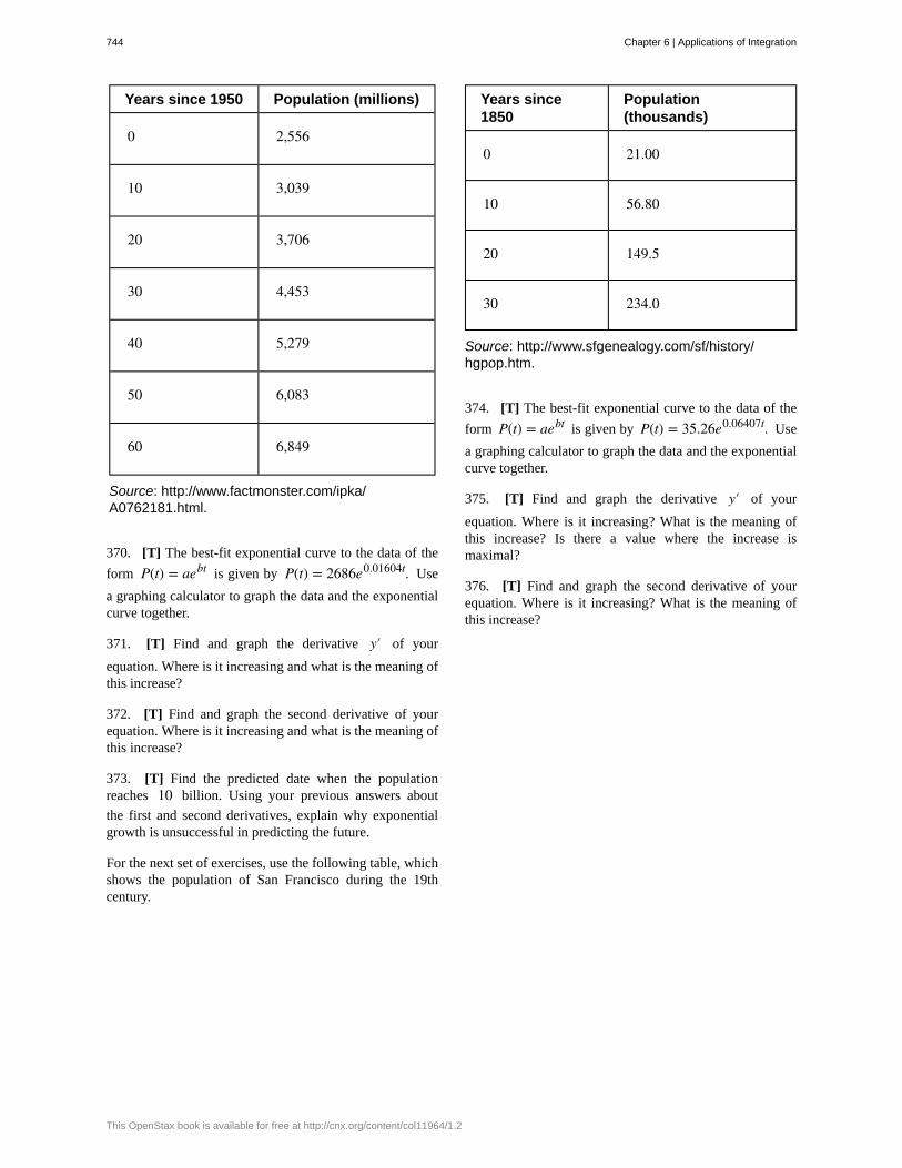
Years since 1950 Population (millions)
0 2,556
10 3,039
20 3,706
30 4,453
40 5,279
50 6,083
60 6,849
Source: http://www.factmonster.com/ipka/A0762181.html.
370. [T] The best-fit exponential curve to the data of the
form P(t) = aebt is given by P(t) = 2686e0.01604t. Use
a graphing calculator to graph the data and the exponentialcurve together.
371. [T] Find and graph the derivative y′ of your
equation. Where is it increasing and what is the meaning ofthis increase?
372. [T] Find and graph the second derivative of yourequation. Where is it increasing and what is the meaning ofthis increase?
373. [T] Find the predicted date when the populationreaches 10 billion. Using your previous answers about
the first and second derivatives, explain why exponentialgrowth is unsuccessful in predicting the future.
For the next set of exercises, use the following table, whichshows the population of San Francisco during the 19thcentury.
Years since1850
Population(thousands)
0 21.00
10 56.80
20 149.5
30 234.0
Source: http://www.sfgenealogy.com/sf/history/hgpop.htm.
374. [T] The best-fit exponential curve to the data of the
form P(t) = aebt is given by P(t) = 35.26e0.06407t. Use
a graphing calculator to graph the data and the exponentialcurve together.
375. [T] Find and graph the derivative y′ of your
equation. Where is it increasing? What is the meaning ofthis increase? Is there a value where the increase ismaximal?
376. [T] Find and graph the second derivative of yourequation. Where is it increasing? What is the meaning ofthis increase?
744 Chapter 6 | Applications of Integration
This OpenStax book is available for free at http://cnx.org/content/col11964/1.2
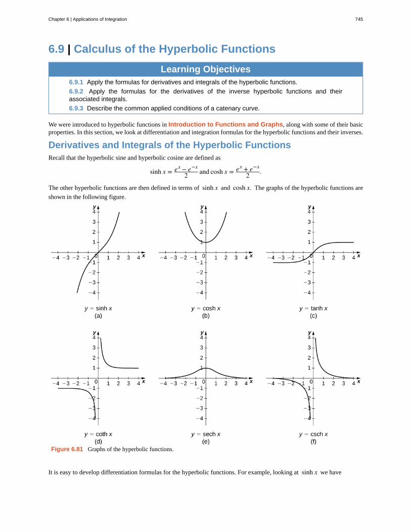
6.9 | Calculus of the Hyperbolic Functions
Learning Objectives6.9.1 Apply the formulas for derivatives and integrals of the hyperbolic functions.
6.9.2 Apply the formulas for the derivatives of the inverse hyperbolic functions and theirassociated integrals.
6.9.3 Describe the common applied conditions of a catenary curve.
We were introduced to hyperbolic functions in Introduction to Functions and Graphs, along with some of their basicproperties. In this section, we look at differentiation and integration formulas for the hyperbolic functions and their inverses.
Derivatives and Integrals of the Hyperbolic FunctionsRecall that the hyperbolic sine and hyperbolic cosine are defined as
sinh x = ex − e−x
2 and cosh x = ex + e−x
2 .
The other hyperbolic functions are then defined in terms of sinh x and cosh x. The graphs of the hyperbolic functions are
shown in the following figure.
Figure 6.81 Graphs of the hyperbolic functions.
It is easy to develop differentiation formulas for the hyperbolic functions. For example, looking at sinh x we have
Chapter 6 | Applications of Integration 745
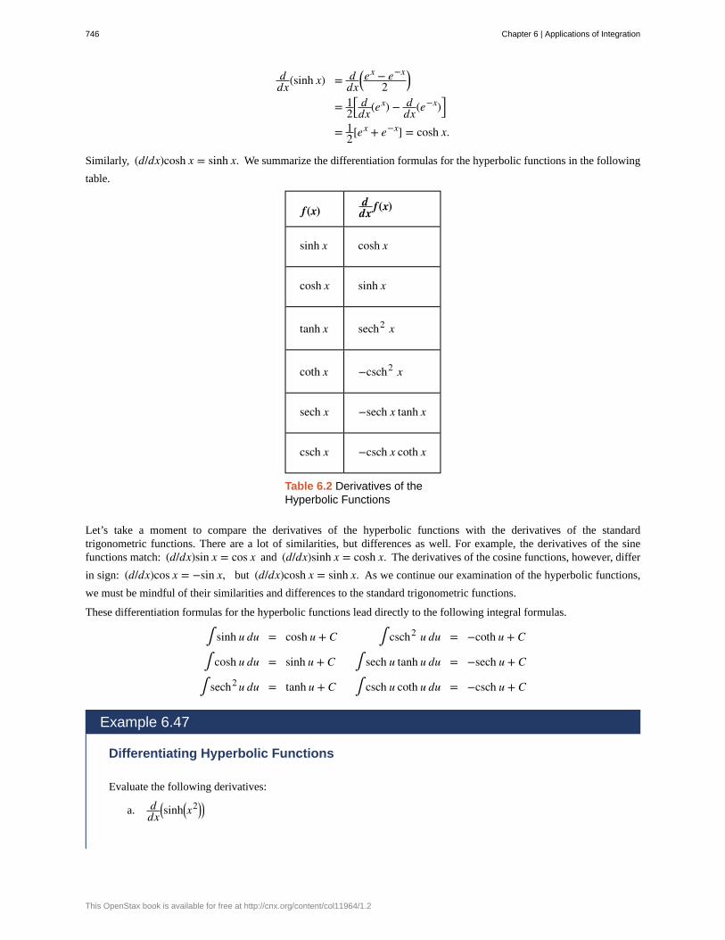
ddx(sinh x) = d
dx⎛⎝ex − e−x
2⎞⎠
= 12
⎡⎣
ddx(ex) − d
dx(e−x)⎤⎦
= 12[ex + e−x] = cosh x.
Similarly, (d/dx)cosh x = sinh x. We summarize the differentiation formulas for the hyperbolic functions in the following
table.
f(x)ddx f(x)
sinh x cosh x
cosh x sinh x
tanh x sech2 x
coth x −csch2 x
sech x −sech x tanh x
csch x −csch x coth x
Table 6.2 Derivatives of theHyperbolic Functions
Let’s take a moment to compare the derivatives of the hyperbolic functions with the derivatives of the standardtrigonometric functions. There are a lot of similarities, but differences as well. For example, the derivatives of the sinefunctions match: (d/dx)sin x = cos x and (d/dx)sinh x = cosh x. The derivatives of the cosine functions, however, differ
in sign: (d/dx)cos x = −sin x, but (d/dx)cosh x = sinh x. As we continue our examination of the hyperbolic functions,
we must be mindful of their similarities and differences to the standard trigonometric functions.
These differentiation formulas for the hyperbolic functions lead directly to the following integral formulas.
∫ sinh u du = cosh u + C ∫ csch2 u du = −coth u + C
∫ cosh u du = sinh u + C ∫ sech u tanh u du = −sech u + C
∫ sech2 u du = tanh u + C ∫ csch u coth u du = −csch u + C
Example 6.47
Differentiating Hyperbolic Functions
Evaluate the following derivatives:
a. ddx
⎛⎝sinh⎛
⎝x2⎞⎠⎞⎠
746 Chapter 6 | Applications of Integration
This OpenStax book is available for free at http://cnx.org/content/col11964/1.2
6.47
b. ddx(cosh x)2
Solution
Using the formulas in Table 6.2 and the chain rule, we get
a. ddx
⎛⎝sinh⎛
⎝x2⎞⎠⎞⎠ = cosh⎛
⎝x2⎞⎠ · 2x
b. ddx(cosh x)2 = 2 cosh x sinh x
Evaluate the following derivatives:
a. ddx
⎛⎝tanh⎛
⎝x2 + 3x⎞⎠⎞⎠
b. ddx
⎛
⎝⎜ 1(sinh x)2
⎞
⎠⎟
Example 6.48
Integrals Involving Hyperbolic Functions
Evaluate the following integrals:
a. ∫ x cosh⎛⎝x2⎞
⎠dx
b. ∫ tanh x dx
Solution
We can use u-substitution in both cases.
a. Let u = x2. Then, du = 2x dx and
∫ x cosh⎛⎝x2⎞
⎠dx = ∫ 12cosh u du = 1
2sinh u + C = 12sinh⎛
⎝x2⎞⎠ + C.
b. Let u = cosh x. Then, du = sinh x dx and
∫ tanh x dx = ∫ sinh xcosh xdx = ∫ 1
udu = ln|u| + C = ln|cosh x| + C.
Note that cosh x > 0 for all x, so we can eliminate the absolute value signs and obtain
∫ tanh x dx = ln(cosh x) + C.
Chapter 6 | Applications of Integration 747
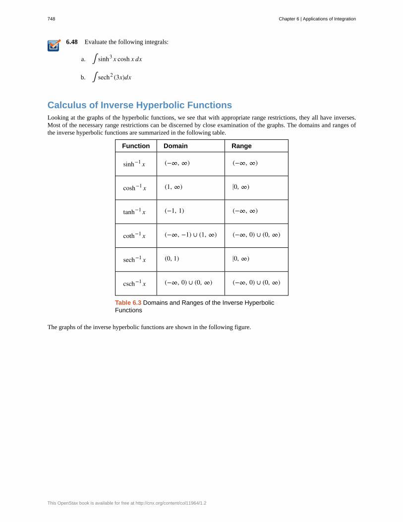
6.48 Evaluate the following integrals:
a. ∫ sinh3 x cosh x dx
b. ∫ sech2 (3x)dx
Calculus of Inverse Hyperbolic FunctionsLooking at the graphs of the hyperbolic functions, we see that with appropriate range restrictions, they all have inverses.Most of the necessary range restrictions can be discerned by close examination of the graphs. The domains and ranges ofthe inverse hyperbolic functions are summarized in the following table.
Function Domain Range
sinh−1 x (−∞, ∞) (−∞, ∞)
cosh−1 x (1, ∞) ⎡⎣0, ∞)
tanh−1 x (−1, 1) (−∞, ∞)
coth−1 x (−∞, −1) ∪ (1, ∞) (−∞, 0) ∪ (0, ∞)
sech−1 x (0, 1) ⎡⎣0, ∞)
csch−1 x (−∞, 0) ∪ (0, ∞) (−∞, 0) ∪ (0, ∞)
Table 6.3 Domains and Ranges of the Inverse HyperbolicFunctions
The graphs of the inverse hyperbolic functions are shown in the following figure.
748 Chapter 6 | Applications of Integration
This OpenStax book is available for free at http://cnx.org/content/col11964/1.2
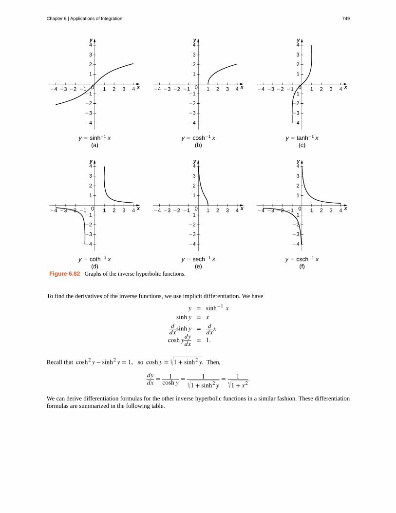
Figure 6.82 Graphs of the inverse hyperbolic functions.
To find the derivatives of the inverse functions, we use implicit differentiation. We have
y = sinh−1 xsinh y = x
ddxsinh y = d
dxx
cosh ydydx = 1.
Recall that cosh2 y − sinh2 y = 1, so cosh y = 1 + sinh2 y. Then,
dydx = 1
cosh y = 11 + sinh2 y
= 11 + x2
.
We can derive differentiation formulas for the other inverse hyperbolic functions in a similar fashion. These differentiationformulas are summarized in the following table.
Chapter 6 | Applications of Integration 749
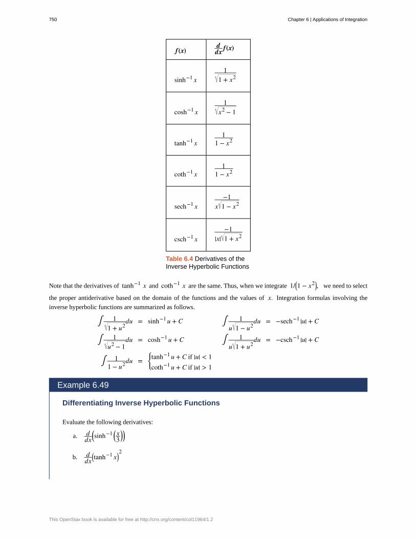
f(x)ddx f(x)
sinh−1 x1
1 + x2
cosh−1 x1
x2 − 1
tanh−1 x1
1 − x2
coth−1 x1
1 − x2
sech−1 x−1
x 1 − x2
csch−1 x−1
|x| 1 + x2
Table 6.4 Derivatives of theInverse Hyperbolic Functions
Note that the derivatives of tanh−1 x and coth−1 x are the same. Thus, when we integrate 1/⎛⎝1 − x2⎞
⎠, we need to select
the proper antiderivative based on the domain of the functions and the values of x. Integration formulas involving the
inverse hyperbolic functions are summarized as follows.
∫ 11 + u2
du = sinh−1 u + C ∫ 1u 1 − u2
du = −sech−1 |u| + C
∫ 1u2 − 1
du = cosh−1 u + C ∫ 1u 1 + u2
du = −csch−1 |u| + C
∫ 11 − u2du =
⎧
⎩⎨tanh−1 u + C if |u| < 1
coth−1 u + C if |u| > 1
Example 6.49
Differentiating Inverse Hyperbolic Functions
Evaluate the following derivatives:
a. ddx
⎛⎝sinh−1 ⎛
⎝x3
⎞⎠⎞⎠
b. ddx
⎛⎝tanh−1 x⎞
⎠2
750 Chapter 6 | Applications of Integration
This OpenStax book is available for free at http://cnx.org/content/col11964/1.2
6.49
6.50
Solution
Using the formulas in Table 6.4 and the chain rule, we obtain the following results:
a. ddx
⎛⎝sinh−1 ⎛
⎝x3
⎞⎠⎞⎠ = 1
3 1 + x29
= 19 + x2
b. ddx
⎛⎝tanh−1 x⎞
⎠2
=2⎛
⎝tanh−1 x⎞⎠
1 − x2
Evaluate the following derivatives:
a. ddx
⎛⎝cosh−1 (3x)⎞
⎠
b. ddx
⎛⎝coth−1 x⎞
⎠3
Example 6.50
Integrals Involving Inverse Hyperbolic Functions
Evaluate the following integrals:
a. ∫ 14x2 − 1
dx
b. ∫ 12x 1 − 9x2
dx
Solution
We can use u-substitution in both cases.
a. Let u = 2x. Then, du = 2dx and we have
∫ 14x2 − 1
dx = ∫ 12 u2 − 1
du = 12cosh−1 u + C = 1
2cosh−1 (2x) + C.
b. Let u = 3x. Then, du = 3dx and we obtain
∫ 12x 1 − 9x2
dx = 12∫ 1
u 1 − u2du = − 1
2sech−1 |u| + C = − 12sech−1 |3x| + C.
Evaluate the following integrals:
a. ∫ 1x2 − 4
dx, x > 2
b. ∫ 11 − e2x
dx
Chapter 6 | Applications of Integration 751
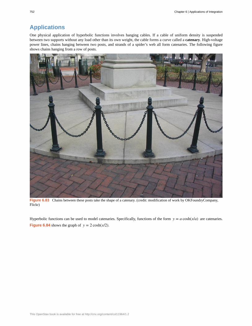
ApplicationsOne physical application of hyperbolic functions involves hanging cables. If a cable of uniform density is suspendedbetween two supports without any load other than its own weight, the cable forms a curve called a catenary. High-voltagepower lines, chains hanging between two posts, and strands of a spider’s web all form catenaries. The following figureshows chains hanging from a row of posts.
Figure 6.83 Chains between these posts take the shape of a catenary. (credit: modification of work by OKFoundryCompany,Flickr)
Hyperbolic functions can be used to model catenaries. Specifically, functions of the form y = a cosh(x/a) are catenaries.
Figure 6.84 shows the graph of y = 2 cosh(x/2).
752 Chapter 6 | Applications of Integration
This OpenStax book is available for free at http://cnx.org/content/col11964/1.2
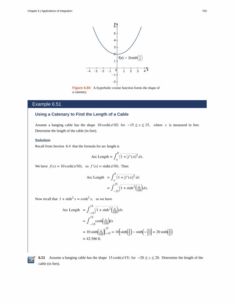
6.51
Figure 6.84 A hyperbolic cosine function forms the shape ofa catenary.
Example 6.51
Using a Catenary to Find the Length of a Cable
Assume a hanging cable has the shape 10 cosh(x/10) for −15 ≤ x ≤ 15, where x is measured in feet.
Determine the length of the cable (in feet).
Solution
Recall from Section 6.4 that the formula for arc length is
Arc Length = ∫a
b1 + ⎡
⎣ f ′(x)⎤⎦2 dx.
We have f (x) = 10 cosh(x/10), so f ′(x) = sinh(x/10). Then
Arc Length = ∫a
b1 + ⎡
⎣ f ′(x)⎤⎦2 dx
= ∫−15
151 + sinh2 ⎛
⎝x
10⎞⎠ dx.
Now recall that 1 + sinh2 x = cosh2 x, so we have
Arc Length = ∫−15
151 + sinh2 ⎛
⎝x
10⎞⎠ dx
= ∫−15
15cosh⎛
⎝x
10⎞⎠dx
= 10 sinh⎛⎝
x10
⎞⎠|−15
15= 10⎡
⎣sinh⎛⎝32
⎞⎠ − sinh⎛
⎝−32
⎞⎠⎤⎦ = 20 sinh⎛
⎝32
⎞⎠
≈ 42.586 ft.
Assume a hanging cable has the shape 15 cosh(x/15) for −20 ≤ x ≤ 20. Determine the length of the
cable (in feet).
Chapter 6 | Applications of Integration 753
6.9 EXERCISES377. [T] Find expressions for cosh x + sinh x and
cosh x − sinh x. Use a calculator to graph these functions
and ensure your expression is correct.
378. From the definitions of cosh(x) and sinh(x), find
their antiderivatives.
379. Show that cosh(x) and sinh(x) satisfy y″ = y.
380. Use the quotient rule to verify that
tanh(x)′ = sech2 (x).
381. Derive cosh2 (x) + sinh2 (x) = cosh(2x) from the
definition.
382. Take the derivative of the previous expression to findan expression for sinh(2x).
383. Provesinh(x + y) = sinh(x)cosh(y) + cosh(x)sinh(y) by
changing the expression to exponentials.
384. Take the derivative of the previous expression to findan expression for cosh(x + y).
For the following exercises, find the derivatives of thegiven functions and graph along with the function to ensureyour answer is correct.
385. [T] cosh(3x + 1)
386. [T] sinh⎛⎝x2⎞
⎠
387. [T] 1cosh(x)
388. [T] sinh⎛⎝ln(x)⎞
⎠
389. [T] cosh2 (x) + sinh2 (x)
390. [T] cosh2 (x) − sinh2 (x)
391. [T] tanh⎛⎝ x2 + 1⎞
⎠
392. [T] 1 + tanh(x)1 − tanh(x)
393. [T] sinh6 (x)
394. [T] ln⎛⎝sech(x) + tanh(x)⎞
⎠
For the following exercises, find the antiderivatives for thegiven functions.
395. cosh(2x + 1)
396. tanh(3x + 2)
397. x cosh⎛⎝x2⎞
⎠
398. 3x3 tanh⎛⎝x4⎞
⎠
399. cosh2 (x)sinh(x)
400. tanh2 (x)sech2 (x)
401. sinh(x)1 + cosh(x)
402. coth(x)
403. cosh(x) + sinh(x)
404. ⎛⎝cosh(x) + sinh(x)⎞
⎠n
For the following exercises, find the derivatives for thefunctions.
405. tanh−1 (4x)
406. sinh−1 ⎛⎝x2⎞
⎠
407. sinh−1 ⎛⎝cosh(x)⎞
⎠
408. cosh−1 ⎛⎝x
3⎞⎠
409. tanh−1 (cos(x))
410. esinh−1 (x)
411. ln⎛⎝tanh−1 (x)⎞
⎠
For the following exercises, find the antiderivatives for thefunctions.
412. ∫ dx4 − x2
413. ∫ dxa2 − x2
754 Chapter 6 | Applications of Integration
This OpenStax book is available for free at http://cnx.org/content/col11964/1.2
414. ∫ dxx2 + 1
415. ∫ x dxx2 + 1
416. ∫ − dxx 1 − x2
417. ∫ ex
e2x − 1
418. ∫ − 2xx4 − 1
For the following exercises, use the fact that a falling bodywith friction equal to velocity squared obeys the equation
dv/dt = g − v2.
419. Show that v(t) = g tanh⎛⎝ gt⎞
⎠ satisfies this
equation.
420. Derive the previous expression for v(t) by
integrating dvg − v2 = dt.
421. [T] Estimate how far a body has fallen in 12 seconds
by finding the area underneath the curve of v(t).
For the following exercises, use this scenario: A cablehanging under its own weight has a slope S = dy/dx that
satisfies dS/dx = c 1 + S2. The constant c is the ratio of
cable density to tension.
422. Show that S = sinh(cx) satisfies this equation.
423. Integrate dy/dx = sinh(cx) to find the cable height
y(x) if y(0) = 1/c.
424. Sketch the cable and determine how far down it sagsat x = 0.
For the following exercises, solve each problem.
425. [T] A chain hangs from two posts 2 m apart to form
a catenary described by the equation y = 2 cosh(x/2) − 1.Find the slope of the catenary at the left fence post.
426. [T] A chain hangs from two posts four meters apartto form a catenary described by the equationy = 4 cosh(x/4) − 3. Find the total length of the catenary
(arc length).
427. [T] A high-voltage power line is a catenary describedby y = 10 cosh(x/10). Find the ratio of the area under the
catenary to its arc length. What do you notice?
428. A telephone line is a catenary described byy = a cosh(x/a). Find the ratio of the area under the
catenary to its arc length. Does this confirm your answerfor the previous question?
429. Prove the formula for the derivative of
y = sinh−1(x) by differentiating x = sinh(y). (Hint: Use
hyperbolic trigonometric identities.)
430. Prove the formula for the derivative of
y = cosh−1(x) by differentiating x = cosh(y). (Hint:
Use hyperbolic trigonometric identities.)
431. Prove the formula for the derivative of
y = sech−1(x) by differentiating x = sech(y). (Hint: Use
hyperbolic trigonometric identities.)
432. Prove that⎛⎝cosh(x) + sinh(x)⎞
⎠n = cosh(nx) + sinh(nx).
433. Prove the expression for sinh−1 (x). Multiply
x = sinh(y) = (1/2)⎛⎝ey − e−y⎞
⎠ by 2ey and solve for y.
Does your expression match the textbook?
434. Prove the expression for cosh−1 (x). Multiply
x = cosh(y) = (1/2)⎛⎝ey − e−y⎞
⎠ by 2ey and solve for y.
Does your expression match the textbook?
Chapter 6 | Applications of Integration 755
arc length
catenary
center of mass
centroid
cross-section
density function
disk method
doubling time
exponential decay
exponential growth
frustum
half-life
Hooke’s law
hydrostatic pressure
lamina
method of cylindrical shells
moment
slicing method
solid of revolution
CHAPTER 6 REVIEW
KEY TERMSthe arc length of a curve can be thought of as the distance a person would travel along the path of the curve
a curve in the shape of the function y = a cosh(x/a) is a catenary; a cable of uniform density suspended
between two supports assumes the shape of a catenary
the point at which the total mass of the system could be concentrated without changing the moment
the centroid of a region is the geometric center of the region; laminas are often represented by regions in theplane; if the lamina has a constant density, the center of mass of the lamina depends only on the shape of thecorresponding planar region; in this case, the center of mass of the lamina corresponds to the centroid of therepresentative region
the intersection of a plane and a solid object
a density function describes how mass is distributed throughout an object; it can be a linear density,expressed in terms of mass per unit length; an area density, expressed in terms of mass per unit area; or a volumedensity, expressed in terms of mass per unit volume; weight-density is also used to describe weight (rather than mass)per unit volume
a special case of the slicing method used with solids of revolution when the slices are disks
if a quantity grows exponentially, the doubling time is the amount of time it takes the quantity to double,and is given by (ln 2)/k
systems that exhibit exponential decay follow a model of the form y = y0 e−kt
systems that exhibit exponential growth follow a model of the form y = y0 ekt
a portion of a cone; a frustum is constructed by cutting the cone with a plane parallel to the base
if a quantity decays exponentially, the half-life is the amount of time it takes the quantity to be reduced by half. Itis given by (ln 2)/k
this law states that the force required to compress (or elongate) a spring is proportional to the distance thespring has been compressed (or stretched) from equilibrium; in other words, F = kx, where k is a constant
the pressure exerted by water on a submerged object
a thin sheet of material; laminas are thin enough that, for mathematical purposes, they can be treated as if they aretwo-dimensional
a method of calculating the volume of a solid of revolution by dividing the solid intonested cylindrical shells; this method is different from the methods of disks or washers in that we integrate withrespect to the opposite variable
if n masses are arranged on a number line, the moment of the system with respect to the origin is given by
M = ∑i = 1
nmi xi; if, instead, we consider a region in the plane, bounded above by a function f (x) over an interval
⎡⎣a, b⎤
⎦, then the moments of the region with respect to the x- and y-axes are given by Mx = ρ∫a
b ⎡⎣ f (x)⎤
⎦2
2 dx and
My = ρ∫a
bx f (x)dx, respectively
a method of calculating the volume of a solid that involves cutting the solid into pieces, estimating thevolume of each piece, then adding these estimates to arrive at an estimate of the total volume; as the number of slicesgoes to infinity, this estimate becomes an integral that gives the exact value of the volume
a solid generated by revolving a region in a plane around a line in that plane
756 Chapter 6 | Applications of Integration
This OpenStax book is available for free at http://cnx.org/content/col11964/1.2
surface area
symmetry principle
theorem of Pappus for volume
washer method
work
the surface area of a solid is the total area of the outer layer of the object; for objects such as cubes orbricks, the surface area of the object is the sum of the areas of all of its faces
the symmetry principle states that if a region R is symmetric about a line l, then the centroid of Rlies on l
this theorem states that the volume of a solid of revolution formed by revolving aregion around an external axis is equal to the area of the region multiplied by the distance traveled by the centroid ofthe region
a special case of the slicing method used with solids of revolution when the slices are washers
the amount of energy it takes to move an object; in physics, when a force is constant, work is expressed as theproduct of force and distance
KEY EQUATIONS• Area between two curves, integrating on the x-axis
A = ∫a
b⎡⎣ f (x) − g(x)⎤
⎦dx
• Area between two curves, integrating on the y-axis
A = ∫c
d⎡⎣u(y) − v(y)⎤
⎦dy
• Disk Method along the x-axis
V = ∫a
bπ⎡
⎣ f (x)⎤⎦2 dx
• Disk Method along the y-axis
V = ∫c
dπ⎡
⎣g(y)⎤⎦2 dy
• Washer Method
V = ∫a
bπ⎡
⎣⎛⎝ f (x)⎞
⎠2 − ⎛
⎝g(x)⎞⎠2⎤
⎦dx
• Method of Cylindrical Shells
V = ∫a
b⎛⎝2πx f (x)⎞
⎠dx
• Arc Length of a Function of x
Arc Length = ∫a
b1 + ⎡
⎣ f ′(x)⎤⎦2 dx
• Arc Length of a Function of y
Arc Length = ∫c
d1 + ⎡
⎣g′(y)⎤⎦2 dy
• Surface Area of a Function of x
Surface Area = ∫a
b⎛⎝2π f (x) 1 + ⎛
⎝ f ′(x)⎞⎠2⎞⎠dx
• Mass of a one-dimensional object
m = ∫a
bρ(x)dx
• Mass of a circular object
m = ∫0
r2πxρ(x)dx
Chapter 6 | Applications of Integration 757
• Work done on an object
W = ∫a
bF(x)dx
• Hydrostatic force on a plate
F = ∫a
bρw(x)s(x)dx
• Mass of a lamina
m = ρ∫a
bf (x)dx
• Moments of a lamina
Mx = ρ∫a
b ⎡⎣ f (x)⎤
⎦2
2 dx and My = ρ∫a
bx f (x)dx
• Center of mass of a lamina
x– =Mym and y– = Mx
m
• Natural logarithm function
• ln x = ∫1
x1t dt Z
• Exponential function y = ex
• ln y = ln(ex) = x Z
KEY CONCEPTS
6.1 Areas between Curves
• Just as definite integrals can be used to find the area under a curve, they can also be used to find the area betweentwo curves.
• To find the area between two curves defined by functions, integrate the difference of the functions.
• If the graphs of the functions cross, or if the region is complex, use the absolute value of the difference of thefunctions. In this case, it may be necessary to evaluate two or more integrals and add the results to find the area ofthe region.
• Sometimes it can be easier to integrate with respect to y to find the area. The principles are the same regardless ofwhich variable is used as the variable of integration.
6.2 Determining Volumes by Slicing
• Definite integrals can be used to find the volumes of solids. Using the slicing method, we can find a volume byintegrating the cross-sectional area.
• For solids of revolution, the volume slices are often disks and the cross-sections are circles. The method of disksinvolves applying the method of slicing in the particular case in which the cross-sections are circles, and using theformula for the area of a circle.
• If a solid of revolution has a cavity in the center, the volume slices are washers. With the method of washers, thearea of the inner circle is subtracted from the area of the outer circle before integrating.
6.3 Volumes of Revolution: Cylindrical Shells
• The method of cylindrical shells is another method for using a definite integral to calculate the volume of a solid ofrevolution. This method is sometimes preferable to either the method of disks or the method of washers because weintegrate with respect to the other variable. In some cases, one integral is substantially more complicated than the
758 Chapter 6 | Applications of Integration
This OpenStax book is available for free at http://cnx.org/content/col11964/1.2
other.
• The geometry of the functions and the difficulty of the integration are the main factors in deciding which integrationmethod to use.
6.4 Arc Length of a Curve and Surface Area
• The arc length of a curve can be calculated using a definite integral.
• The arc length is first approximated using line segments, which generates a Riemann sum. Taking a limit then givesus the definite integral formula. The same process can be applied to functions of y.
• The concepts used to calculate the arc length can be generalized to find the surface area of a surface of revolution.
• The integrals generated by both the arc length and surface area formulas are often difficult to evaluate. It may benecessary to use a computer or calculator to approximate the values of the integrals.
6.5 Physical Applications
• Several physical applications of the definite integral are common in engineering and physics.
• Definite integrals can be used to determine the mass of an object if its density function is known.
• Work can also be calculated from integrating a force function, or when counteracting the force of gravity, as in apumping problem.
• Definite integrals can also be used to calculate the force exerted on an object submerged in a liquid.
6.6 Moments and Centers of Mass
• Mathematically, the center of mass of a system is the point at which the total mass of the system could beconcentrated without changing the moment. Loosely speaking, the center of mass can be thought of as the balancingpoint of the system.
• For point masses distributed along a number line, the moment of the system with respect to the origin is
M = ∑i = 1
nmi xi. For point masses distributed in a plane, the moments of the system with respect to the x- and
y-axes, respectively, are Mx = ∑i = 1
nmi yi and My = ∑
i = 1
nmi xi, respectively.
• For a lamina bounded above by a function f (x), the moments of the system with respect to the x- and y-axes,
respectively, are Mx = ρ∫a
b ⎡⎣ f (x)⎤
⎦2
2 dx and My = ρ∫a
bx f (x)dx.
• The x- and y-coordinates of the center of mass can be found by dividing the moments around the y-axis and aroundthe x-axis, respectively, by the total mass. The symmetry principle says that if a region is symmetric with respect toa line, then the centroid of the region lies on the line.
• The theorem of Pappus for volume says that if a region is revolved around an external axis, the volume of theresulting solid is equal to the area of the region multiplied by the distance traveled by the centroid of the region.
6.7 Integrals, Exponential Functions, and Logarithms
• The earlier treatment of logarithms and exponential functions did not define the functions precisely and formally.This section develops the concepts in a mathematically rigorous way.
• The cornerstone of the development is the definition of the natural logarithm in terms of an integral.
• The function ex is then defined as the inverse of the natural logarithm.
• General exponential functions are defined in terms of ex, and the corresponding inverse functions are general
logarithms.
Chapter 6 | Applications of Integration 759
• Familiar properties of logarithms and exponents still hold in this more rigorous context.
6.8 Exponential Growth and Decay
• Exponential growth and exponential decay are two of the most common applications of exponential functions.
• Systems that exhibit exponential growth follow a model of the form y = y0 ekt.
• In exponential growth, the rate of growth is proportional to the quantity present. In other words, y′ = ky.
• Systems that exhibit exponential growth have a constant doubling time, which is given by (ln 2)/k.
• Systems that exhibit exponential decay follow a model of the form y = y0 e−kt.
• Systems that exhibit exponential decay have a constant half-life, which is given by (ln 2)/k.
6.9 Calculus of the Hyperbolic Functions
• Hyperbolic functions are defined in terms of exponential functions.
• Term-by-term differentiation yields differentiation formulas for the hyperbolic functions. These differentiationformulas give rise, in turn, to integration formulas.
• With appropriate range restrictions, the hyperbolic functions all have inverses.
• Implicit differentiation yields differentiation formulas for the inverse hyperbolic functions, which in turn give riseto integration formulas.
• The most common physical applications of hyperbolic functions are calculations involving catenaries.
CHAPTER 6 REVIEW EXERCISESTrue or False? Justify your answer with a proof or acounterexample.
435. The amount of work to pump the water out of a half-full cylinder is half the amount of work to pump the waterout of the full cylinder.
436. If the force is constant, the amount of work to movean object from x = a to x = b is F(b − a).
437. The disk method can be used in any situation inwhich the washer method is successful at finding thevolume of a solid of revolution.
438. If the half-life of seaborgium-266 is 360 ms, then
k = ⎛⎝ln(2)⎞
⎠/360.
For the following exercises, use the requested method todetermine the volume of the solid.
439. The volume that has a base of the ellipse
x2/4 + y2/9 = 1 and cross-sections of an equilateral
triangle perpendicular to the y-axis. Use the method of
slicing.
440. y = x2 − x, from x = 1 to x = 4, rotated around
they-axis using the washer method
441. x = y2 and x = 3y rotated around the y-axis using
the washer method
442. x = 2y2 − y3, x = 0, and y = 0 rotated around the
x-axis using cylindrical shells
For the following exercises, find
a. the area of the region,
b. the volume of the solid when rotated around thex-axis, and
c. the volume of the solid when rotated around they-axis. Use whichever method seems mostappropriate to you.
443. y = x3, x = 0, y = 0, and x = 2
444. y = x2 − x and x = 0
445. [T] y = ln(x) + 2 and y = x
446. y = x2 and y = x
447. y = 5 + x, y = x2, x = 0, and x = 1
760 Chapter 6 | Applications of Integration
This OpenStax book is available for free at http://cnx.org/content/col11964/1.2
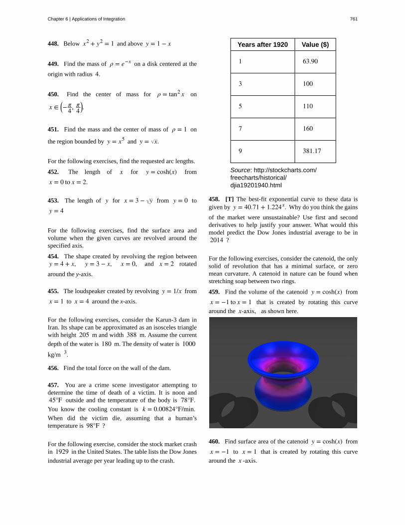
448. Below x2 + y2 = 1 and above y = 1 − x
449. Find the mass of ρ = e−x on a disk centered at the
origin with radius 4.
450. Find the center of mass for ρ = tan2 x on
x ∈ ⎛⎝−
π4, π
4⎞⎠.
451. Find the mass and the center of mass of ρ = 1 on
the region bounded by y = x5 and y = x.
For the following exercises, find the requested arc lengths.
452. The length of x for y = cosh(x) from
x = 0 to x = 2.
453. The length of y for x = 3 − y from y = 0 to
y = 4
For the following exercises, find the surface area andvolume when the given curves are revolved around thespecified axis.
454. The shape created by revolving the region betweeny = 4 + x, y = 3 − x, x = 0, and x = 2 rotated
around the y-axis.
455. The loudspeaker created by revolving y = 1/x from
x = 1 to x = 4 around the x-axis.
For the following exercises, consider the Karun-3 dam inIran. Its shape can be approximated as an isosceles trianglewith height 205 m and width 388 m. Assume the current
depth of the water is 180 m. The density of water is 1000kg/m 3.
456. Find the total force on the wall of the dam.
457. You are a crime scene investigator attempting todetermine the time of death of a victim. It is noon and45°F outside and the temperature of the body is 78°F.You know the cooling constant is k = 0.00824°F/min.When did the victim die, assuming that a human’stemperature is 98°F ?
For the following exercise, consider the stock market crashin 1929 in the United States. The table lists the Dow Jones
industrial average per year leading up to the crash.
Years after 1920 Value ($)
1 63.90
3 100
5 110
7 160
9 381.17
Source: http://stockcharts.com/freecharts/historical/djia19201940.html
458. [T] The best-fit exponential curve to these data isgiven by y = 40.71 + 1.224x. Why do you think the gains
of the market were unsustainable? Use first and secondderivatives to help justify your answer. What would thismodel predict the Dow Jones industrial average to be in2014 ?
For the following exercises, consider the catenoid, the onlysolid of revolution that has a minimal surface, or zeromean curvature. A catenoid in nature can be found whenstretching soap between two rings.
459. Find the volume of the catenoid y = cosh(x) from
x = −1 to x = 1 that is created by rotating this curve
around the x-axis, as shown here.
460. Find surface area of the catenoid y = cosh(x) from
x = −1 to x = 1 that is created by rotating this curve
around the x -axis.
Chapter 6 | Applications of Integration 761

762 Chapter 6 | Applications of Integration
This OpenStax book is available for free at http://cnx.org/content/col11964/1.2
APPENDIX A | TABLE OF
INTEGRALSBasic Integrals
1. ∫ un du = un + 1
n + 1 + C, n ≠ −1
2. ∫ duu = ln|u| + C
3. ∫ eu du = eu + C
4. ∫ au du = au
lna + C
5. ∫ sin u du = −cos u + C
6. ∫ cos u du = sin u + C
7. ∫ sec2 u du = tan u + C
8. ∫ csc2 u du = −cot u + C
9. ∫ sec u tan u du = sec u + C
10. ∫ csc u cot u du = −csc u + C
11. ∫ tan u du = ln|sec u| + C
12. ∫ cot u du = ln|sin u| + C
13. ∫ sec u du = ln|sec u + tan u| + C
14. ∫ csc u du = ln|csc u − cot u| + C
15. ∫ dua2 − u2
= sin−1 ua + C
16. ∫ dua2 + u2 = 1
atan−1 ua + C
17. ∫ duu u2 − a2
= 1asec−1 u
a + C
Trigonometric Integrals18. ∫ sin2 u du = 1
2u − 14sin 2u + C
Appendix A 763
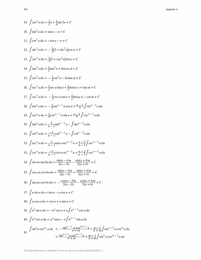
19. ∫ cos2 u du = 12u + 1
4sin 2u + C
20. ∫ tan2 u du = tan u − u + C
21. ∫ cot2 u du = −cot u − u + C
22. ∫ sin3 u du = − 13
⎛⎝2 + sin2 u⎞
⎠cos u + C
23. ∫ cos3 u du = 13
⎛⎝2 + cos2 u⎞
⎠sin u + C
24. ∫ tan3 u du = 12tan2 u + ln|cos u| + C
25. ∫ cot3 u du = − 12cot2 u − ln|sin u| + C
26. ∫ sec3 u du = 12sec u tan u + 1
2ln |sec u + tan u| + C
27. ∫ csc3 u du = − 12csc u cot u + 1
2ln |csc u − cot u| + C
28. ∫ sinn u du = − 1nsinn − 1 u cos u + n − 1
n ∫ sinn − 2 u du
29. ∫ cosn u du = 1ncosn − 1 u sin u + n − 1
n ∫ cosn − 2 u du
30. ∫ tann u du = 1n − 1tann − 1 u − ∫ tann − 2 u du
31. ∫ cotn u du = −1n − 1cotn − 1 u − ∫ cotn − 2 u du
32. ∫ secn u du = 1n − 1tan u secn − 2 u + n − 2
n − 1∫ secn − 2 u du
33. ∫ cscn u du = −1n − 1cot u cscn − 2 u + n − 2
n − 1∫ cscn − 2 u du
34. ∫ sin au sin bu du = sin(a − b)u2(a − b) − sin(a + b)u
2(a + b) + C
35. ∫ cos au cos bu du = sin(a − b)u2(a − b) + sin(a + b)u
2(a + b) + C
36. ∫ sin au cos bu du = − cos(a − b)u2(a − b) − cos(a + b)u
2(a + b) + C
37. ∫ u sin u du = sin u − u cos u + C
38. ∫ u cos u du = cos u + u sin u + C
39. ∫ un sin u du = −un cos u + n∫ un − 1 cos u du
40. ∫ un cos u du = un sin u − n∫ un − 1 sin u du
41.∫ sinnu cosm u du = − sinn − 1 u cosm + 1 u
n + m + n − 1n + m∫ sinn − 2 u cosm u du
= sinn + 1 u cosm − 1 un + m + m − 1
n + m∫ sinn u cosm − 2 u du
764 Appendix A
This OpenStax book is available for free at http://cnx.org/content/col11964/1.2
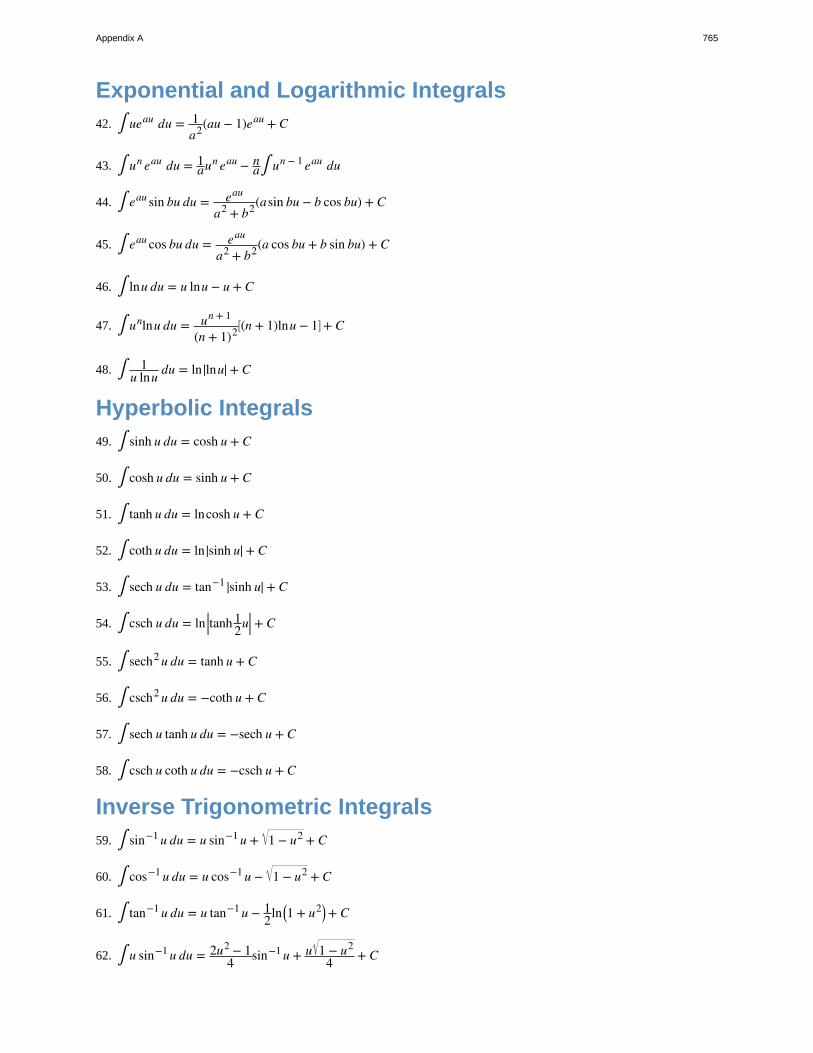
Exponential and Logarithmic Integrals42. ∫ ueau du = 1
a2(au − 1)eau + C
43. ∫ un eau du = 1aun eau − n
a∫ un − 1 eau du
44. ∫ eau sin bu du = eau
a2 + b2(asin bu − b cos bu) + C
45. ∫ eau cos bu du = eau
a2 + b2(a cos bu + b sin bu) + C
46. ∫ lnu du = u lnu − u + C
47. ∫ unlnu du = un + 1
(n + 1)2⎡⎣(n + 1)lnu − 1⎤
⎦ + C
48. ∫ 1u lnu du = ln|lnu| + C
Hyperbolic Integrals49. ∫ sinh u du = cosh u + C
50. ∫ cosh u du = sinh u + C
51. ∫ tanh u du = lncosh u + C
52. ∫ coth u du = ln|sinh u| + C
53. ∫ sech u du = tan−1 |sinh u| + C
54. ∫ csch u du = ln|tanh 12u| + C
55. ∫ sech2 u du = tanh u + C
56. ∫ csch2 u du = −coth u + C
57. ∫ sech u tanh u du = −sech u + C
58. ∫ csch u coth u du = −csch u + C
Inverse Trigonometric Integrals59. ∫ sin−1 u du = u sin−1 u + 1 − u2 + C
60. ∫ cos−1 u du = u cos−1 u − 1 − u2 + C
61. ∫ tan−1 u du = u tan−1 u − 12ln ⎛
⎝1 + u2⎞⎠ + C
62. ∫ u sin−1 u du = 2u2 − 14 sin−1 u + u 1 − u2
4 + C
Appendix A 765
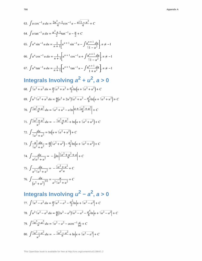
63. ∫ u cos−1 u du = 2u2 − 14 cos−1 u − u 1 − u2
4 + C
64. ∫ u tan−1 u du = u2 + 12 tan−1 u − u
2 + C
65. ∫ un sin−1 u du = 1n + 1
⎡
⎣⎢un + 1 sin−1 u − ∫ un + 1 du
1 − u2
⎤
⎦⎥, n ≠ −1
66. ∫ un cos−1 u du = 1n + 1
⎡
⎣⎢un + 1 cos−1 u + ∫ un + 1 du
1 − u2
⎤
⎦⎥, n ≠ −1
67. ∫ un tan−1 u du = 1n + 1
⎡⎣un + 1 tan−1 u − ∫ un + 1 du
1 + u2⎤⎦, n ≠ −1
Integrals Involving a2 + u2, a > 0
68. ∫ a2 + u2 du = u2 a2 + u2 + a2
2 ln⎛⎝u + a2 + u2⎞
⎠ + C
69. ∫ u2 a2 + u2 du = u8
⎛⎝a2 + 2u2⎞
⎠ a2 + u2 − a4
8 ln⎛⎝u + a2 + u2⎞
⎠ + C
70. ∫ a2 + u2u du = a2 + u2 − a ln |a + a2 + u2
u | + C
71. ∫ a2 + u2
u2 du = − a2 + u2u + ln⎛
⎝u + a2 + u2⎞⎠ + C
72. ∫ dua2 + u2
= ln⎛⎝u + a2 + u2⎞
⎠ + C
73. ∫ u2 dua2 + u2
= u2
⎛⎝ a2 + u2⎞
⎠ − a2
2 ln⎛⎝u + a2 + u2⎞
⎠ + C
74. ∫ duu a2 + u2
= − 1aln | a2 + u2 + a
u | + C
75. ∫ duu2 a2 + u2
= − a2 + u2
a2 u+ C
76. ∫ du⎛⎝a2 + u2⎞
⎠3/2 = u
a2 a2 + u2+ C
Integrals Involving u2 − a2, a > 0
77. ∫ u2 − a2 du = u2 u2 − a2 − a2
2 ln |u + u2 − a2| + C
78. ∫ u2 u2 − a2 du = u8
⎛⎝2u2 − a2⎞
⎠ u2 − a2 − a4
8 ln |u + u2 − a2| + C
79. ∫ u2 − a2u du = u2 − a2 − acos−1 a
|u| + C
80. ∫ u2 − a2
u2 du = − u2 − a2u + ln|u + u2 − a2| + C
766 Appendix A
This OpenStax book is available for free at http://cnx.org/content/col11964/1.2
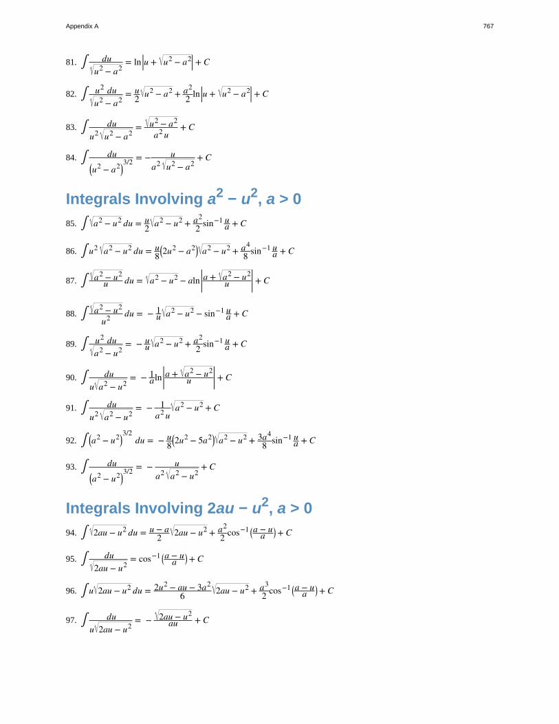
81. ∫ duu2 − a2
= ln|u + u2 − a2| + C
82. ∫ u2 duu2 − a2
= u2 u2 − a2 + a2
2 ln |u + u2 − a2| + C
83. ∫ duu2 u2 − a2
= u2 − a2
a2 u+ C
84. ∫ du⎛⎝u2 − a2⎞
⎠3/2 = − u
a2 u2 − a2+ C
Integrals Involving a2 − u2, a > 0
85. ∫ a2 − u2 du = u2 a2 − u2 + a2
2 sin−1 ua + C
86. ∫ u2 a2 − u2 du = u8
⎛⎝2u2 − a2⎞
⎠ a2 − u2 + a4
8 sin−1 ua + C
87. ∫ a2 − u2u du = a2 − u2 − aln |a + a2 − u2
u | + C
88. ∫ a2 − u2
u2 du = − 1u a2 − u2 − sin−1 u
a + C
89. ∫ u2 dua2 − u2
= − uu a2 − u2 + a2
2 sin−1 ua + C
90. ∫ duu a2 − u2
= − 1aln |a + a2 − u2
u | + C
91. ∫ duu2 a2 − u2
= − 1a2 u
a2 − u2 + C
92. ∫ ⎛⎝a2 − u2⎞
⎠3/2
du = − u8
⎛⎝2u2 − 5a2⎞
⎠ a2 − u2 + 3a4
8 sin−1 ua + C
93. ∫ du⎛⎝a2 − u2⎞
⎠3/2 = − u
a2 a2 − u2+ C
Integrals Involving 2au − u2, a > 0
94. ∫ 2au − u2 du = u − a2 2au − u2 + a2
2 cos−1 ⎛⎝a − u
a⎞⎠ + C
95. ∫ du2au − u2
= cos−1 ⎛⎝a − u
a⎞⎠ + C
96. ∫ u 2au − u2 du = 2u2 − au − 3a2
6 2au − u2 + a3
2 cos−1 ⎛⎝a − u
a⎞⎠ + C
97. ∫ duu 2au − u2
= − 2au − u2au + C
Appendix A 767
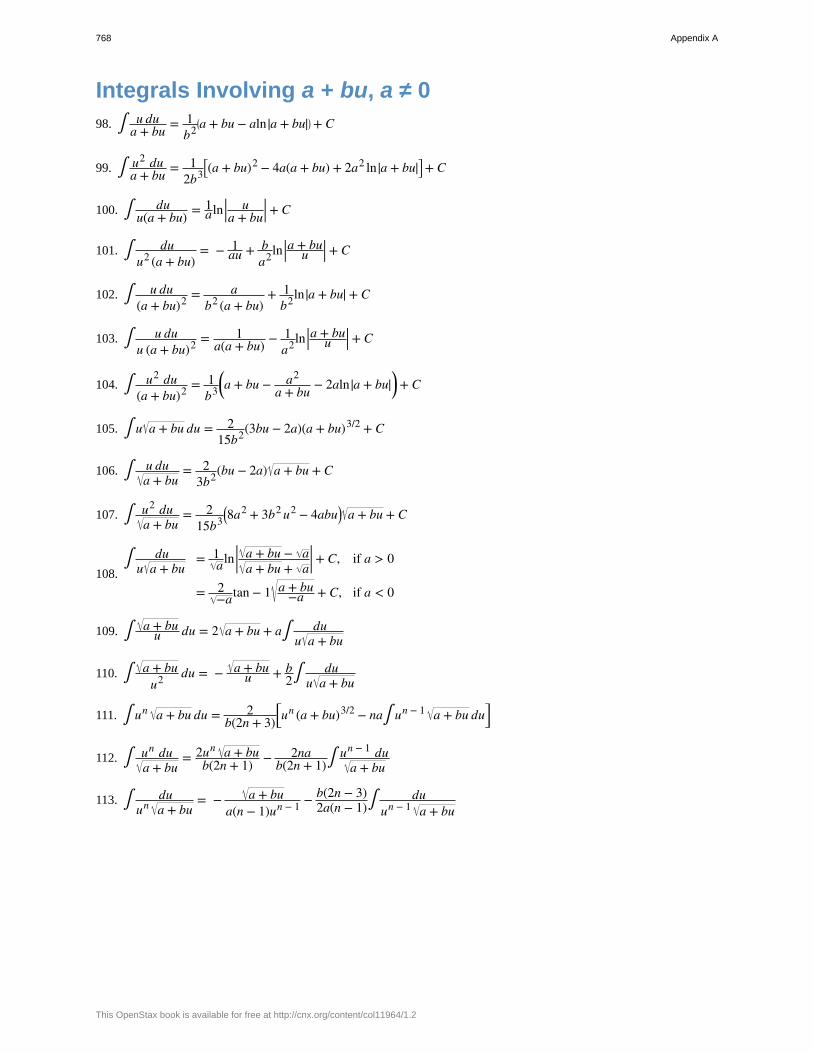
Integrals Involving a + bu, a ≠ 098. ∫ u du
a + bu = 1b2
⎛⎝a + bu − aln |a + bu|⎞
⎠ + C
99. ∫ u2 dua + bu = 1
2b3⎡⎣(a + bu)2 − 4a(a + bu) + 2a2 ln |a + bu|⎤⎦ + C
100. ∫ duu(a + bu) = 1
aln | ua + bu | + C
101. ∫ duu2 (a + bu)
= − 1au + b
a2ln |a + buu | + C
102. ∫ u du(a + bu)2 = a
b2 (a + bu)+ 1
b2ln |a + bu| + C
103. ∫ u duu (a + bu)2 = 1
a(a + bu) − 1a2ln |a + bu
u | + C
104. ∫ u2 du(a + bu)2 = 1
b3⎛⎝a + bu − a2
a + bu − 2aln |a + bu|⎞⎠ + C
105. ∫ u a + bu du = 215b2(3bu − 2a)(a + bu)3/2 + C
106. ∫ u dua + bu
= 23b2(bu − 2a) a + bu + C
107. ∫ u2 dua + bu
= 215b3
⎛⎝8a2 + 3b2 u2 − 4abu⎞
⎠ a + bu + C
108.∫ du
u a + bu= 1
aln | a + bu − aa + bu + a | + C, if a > 0
= 2−atan − 1 a + bu
−a + C, if a < 0
109. ∫ a + buu du = 2 a + bu + a∫ du
u a + bu
110. ∫ a + buu2 du = − a + bu
u + b2∫ du
u a + bu
111. ∫ un a + bu du = 2b(2n + 3)
⎡⎣un (a + bu)3/2 − na∫ un − 1 a + bu du⎤
⎦
112. ∫ un dua + bu
= 2un a + bub(2n + 1) − 2na
b(2n + 1)∫un − 1 du
a + bu
113. ∫ duun a + bu
= − a + bua(n − 1)un − 1 − b(2n − 3)
2a(n − 1)∫du
un − 1 a + bu
768 Appendix A
This OpenStax book is available for free at http://cnx.org/content/col11964/1.2
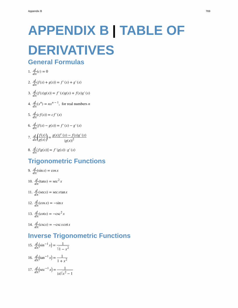
APPENDIX B | TABLE OF
DERIVATIVESGeneral Formulas1. d
dx(c) = 0
2. ddx
⎛⎝ f (x) + g(x)⎞
⎠ = f ′ (x) + g′ (x)
3. ddx
⎛⎝ f (x)g(x)⎞
⎠ = f ′ (x)g(x) + f (x)g′ (x)
4. ddx(xn) = nxn − 1, for real numbers n
5. ddx
⎛⎝c f (x)⎞
⎠ = c f ′ (x)
6. ddx
⎛⎝ f (x) − g(x)⎞
⎠ = f ′ (x) − g′ (x)
7. ddx
⎛⎝
f (x)g(x)
⎞⎠ = g(x) f ′ (x) − f (x)g′ (x)
⎛⎝g(x)⎞
⎠2
8. ddx
⎡⎣ f ⎛
⎝g(x)⎞⎠⎤⎦ = f ′ ⎛
⎝g(x)⎞⎠ · g′ (x)
Trigonometric Functions9. d
dx(sinx) = cosx
10. ddx(tanx) = sec2 x
11. ddx(secx) = secx tanx
12. ddx(cosx) = −sinx
13. ddx(cotx) = −csc2 x
14. ddx(cscx) = −cscxcot x
Inverse Trigonometric Functions15. d
dx⎛⎝sin−1 x⎞
⎠ = 11 − x2
16. ddx
⎛⎝tan−1 x⎞
⎠ = 11 + x2
17. ddx
⎛⎝sec−1 x⎞
⎠ = 1|x| x2 − 1
Appendix B 769
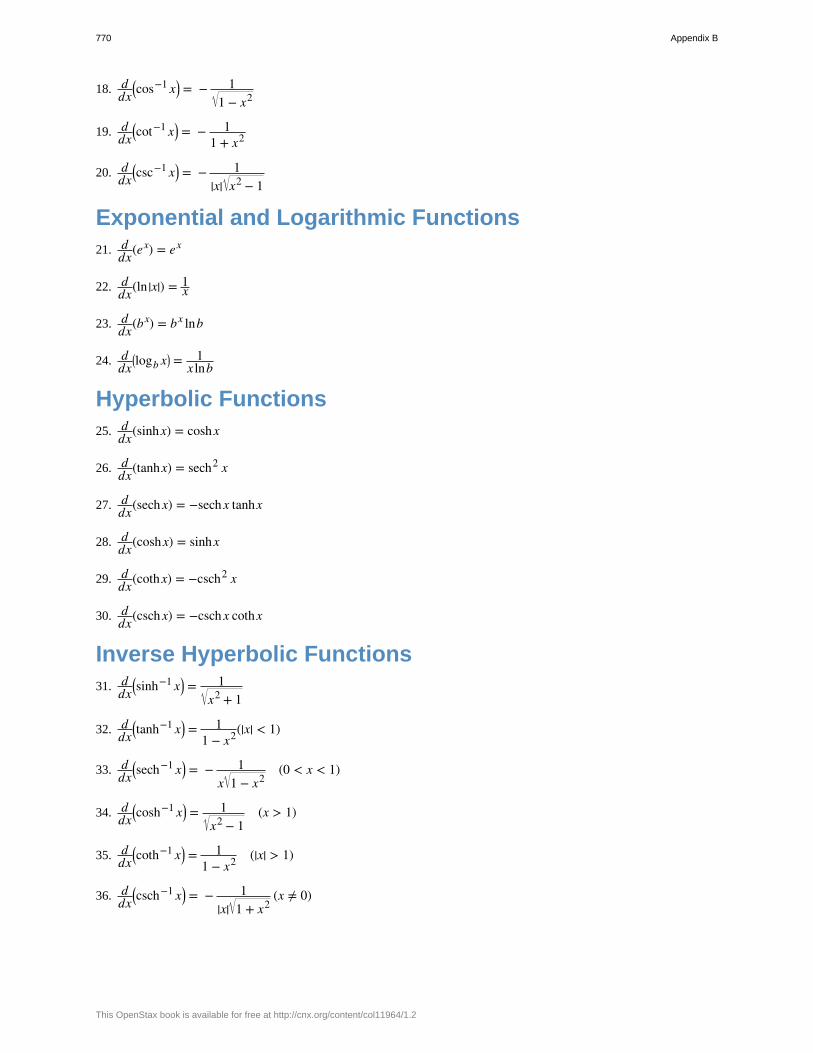
18. ddx
⎛⎝cos−1 x⎞
⎠ = − 11 − x2
19. ddx
⎛⎝cot−1 x⎞
⎠ = − 11 + x2
20. ddx
⎛⎝csc−1 x⎞
⎠ = − 1|x| x2 − 1
Exponential and Logarithmic Functions21. d
dx(ex) = ex
22. ddx(ln |x|) = 1
x
23. ddx(bx) = bx lnb
24. ddx
⎛⎝logb x⎞
⎠ = 1x lnb
Hyperbolic Functions25. d
dx(sinhx) = coshx
26. ddx(tanhx) = sech2 x
27. ddx(sech x) = −sech x tanhx
28. ddx(coshx) = sinhx
29. ddx(cothx) = −csch2 x
30. ddx(csch x) = −csch x cothx
Inverse Hyperbolic Functions31. d
dx⎛⎝sinh−1 x⎞
⎠ = 1x2 + 1
32. ddx
⎛⎝tanh−1 x⎞
⎠ = 11 − x2(|x| < 1)
33. ddx
⎛⎝sech−1 x⎞
⎠ = − 1x 1 − x2
(0 < x < 1)
34. ddx
⎛⎝cosh−1 x⎞
⎠ = 1x2 − 1
(x > 1)
35. ddx
⎛⎝coth−1 x⎞
⎠ = 11 − x2 (|x| > 1)
36. ddx
⎛⎝csch−1 x⎞
⎠ = − 1|x| 1 + x2
(x ≠ 0)
770 Appendix B
This OpenStax book is available for free at http://cnx.org/content/col11964/1.2
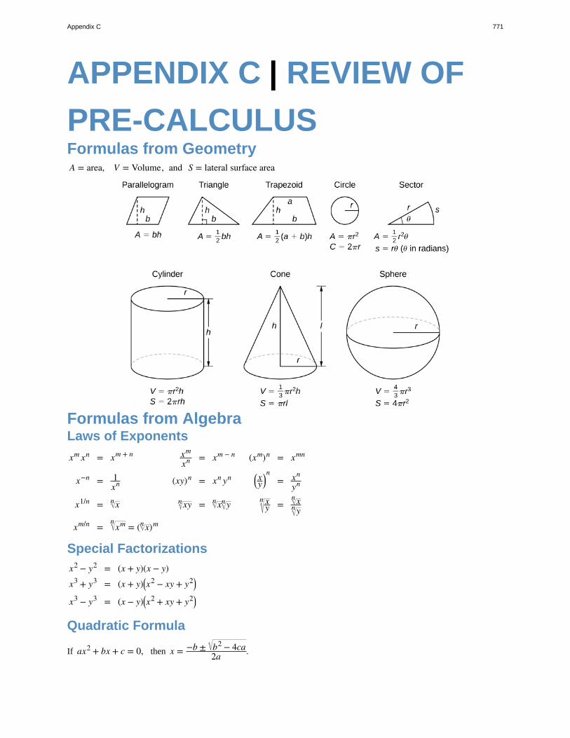
APPENDIX C | REVIEW OF
PRE-CALCULUSFormulas from GeometryA = area, V = Volume, and S = lateral surface area
Formulas from AlgebraLaws of Exponents
xm xn = xm + n xm
xn = xm − n (xm)n = xmn
x−n = 1xn (xy)n = xn yn ⎛
⎝xy
⎞⎠n
= xn
yn
x1/n = xn xyn = xn yn xy
n = xn
yn
xm/n = xmn= ( xn )m
Special Factorizationsx2 − y2 = (x + y)(x − y)
x3 + y3 = (x + y)⎛⎝x2 − xy + y2⎞
⎠
x3 − y3 = (x − y)⎛⎝x2 + xy + y2⎞
⎠
Quadratic Formula
If ax2 + bx + c = 0, then x = −b ± b2 − 4ca2a .
Appendix C 771
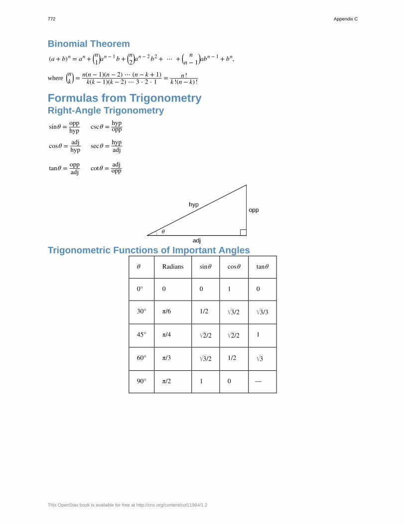
Binomial Theorem
(a + b)n = an + ⎛⎝n1
⎞⎠a
n − 1 b + ⎛⎝n2
⎞⎠a
n − 2 b2 + ⋯ + ⎛⎝
nn − 1
⎞⎠abn − 1 + bn,
where ⎛⎝nk
⎞⎠ = n(n − 1)(n − 2) ⋯ (n − k + 1)
k(k − 1)(k − 2) ⋯ 3 ⋅ 2 ⋅ 1 = n !k !(n − k) !
Formulas from TrigonometryRight-Angle Trigonometry
sinθ = opphyp cscθ = hyp
opp
cosθ = adjhyp secθ = hyp
adj
tanθ = oppadj cotθ = adj
opp
Trigonometric Functions of Important Angles
θ Radians sinθ cosθ tanθ
0° 0 0 1 0
30° π/6 1/2 3/2 3/3
45° π/4 2/2 2/2 1
60° π/3 3/2 1/2 3
90° π/2 1 0 —
772 Appendix C
This OpenStax book is available for free at http://cnx.org/content/col11964/1.2
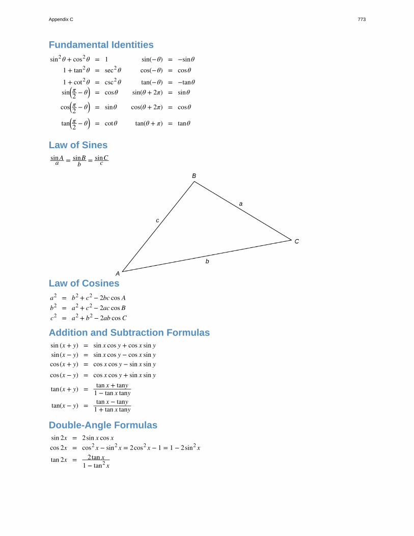
Fundamental Identitiessin2 θ + cos2 θ = 1 sin(−θ) = −sinθ
1 + tan2 θ = sec2 θ cos(−θ) = cosθ
1 + cot2 θ = csc2 θ tan(−θ) = −tanθsin⎛
⎝π2 − θ⎞
⎠ = cosθ sin(θ + 2π) = sinθ
cos⎛⎝π2 − θ⎞
⎠ = sinθ cos(θ + 2π) = cosθ
tan⎛⎝π2 − θ⎞
⎠ = cotθ tan(θ + π) = tanθ
Law of Sinessin A
a = sinBb = sinC
c
Law of Cosinesa2 = b2 + c2 − 2bc cos Ab2 = a2 + c2 − 2ac cos Bc2 = a2 + b2 − 2ab cos C
Addition and Subtraction Formulassin (x + y) = sin x cos y + cos x sin ysin(x − y) = sin x cos y − cos x sin ycos(x + y) = cos x cos y − sin x sin ycos(x − y) = cos x cos y + sin x sin y
tan(x + y) = tan x + tany1 − tan x tany
tan(x − y) = tan x − tany1 + tan x tany
Double-Angle Formulassin 2x = 2sin x cos xcos 2x = cos2 x − sin2 x = 2cos2 x − 1 = 1 − 2sin2 x
tan 2x = 2tan x1 − tan2 x
Appendix C 773
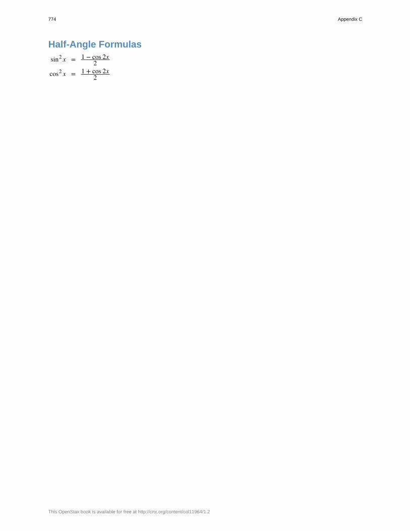
Half-Angle Formulas
sin2 x = 1 − cos 2x2
cos2 x = 1 + cos 2x2
774 Appendix C
This OpenStax book is available for free at http://cnx.org/content/col11964/1.2
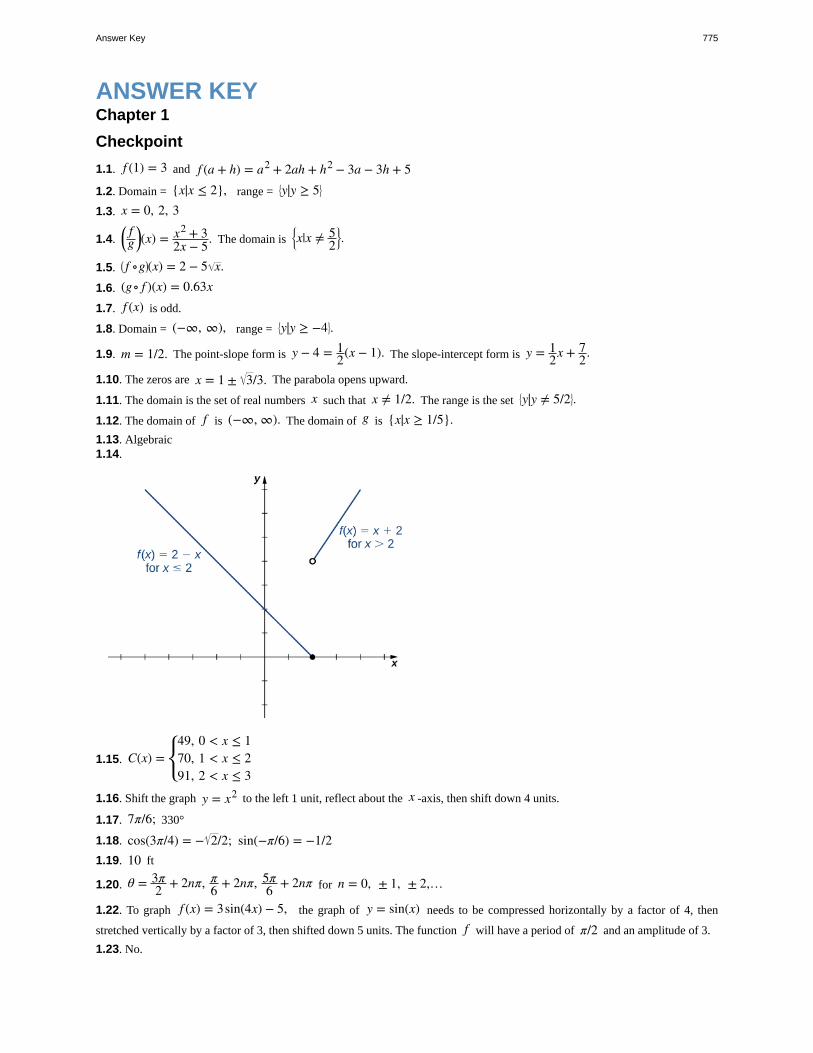
ANSWER KEYChapter 1
Checkpoint
1.1. f (1) = 3 and f (a + h) = a2 + 2ah + h2 − 3a − 3h + 51.2. Domain = {x|x ≤ 2}, range =
⎧
⎩⎨y|y ≥ 5⎫
⎭⎬
1.3. x = 0, 2, 3
1.4.⎛⎝
fg
⎞⎠(x) = x2 + 3
2x − 5. The domain is⎧
⎩⎨x|x ≠ 5
2⎫
⎭⎬.
1.5. ⎛⎝ f ∘g⎞
⎠(x) = 2 − 5 x.1.6. (g ∘ f )(x) = 0.63x1.7. f (x) is odd.
1.8. Domain = (−∞, ∞), range =⎧
⎩⎨y|y ≥ −4⎫
⎭⎬.
1.9. m = 1/2. The point-slope form is y − 4 = 12(x − 1). The slope-intercept form is y = 1
2x + 72.
1.10. The zeros are x = 1 ± 3/3. The parabola opens upward.
1.11. The domain is the set of real numbers x such that x ≠ 1/2. The range is the set⎧
⎩⎨y|y ≠ 5/2⎫
⎭⎬.
1.12. The domain of f is (−∞, ∞). The domain of g is {x|x ≥ 1/5}.1.13. Algebraic1.14.
1.15. C(x) =⎧
⎩⎨
49, 0 < x ≤ 170, 1 < x ≤ 291, 2 < x ≤ 3
1.16. Shift the graph y = x2 to the left 1 unit, reflect about the x -axis, then shift down 4 units.
1.17. 7π/6; 330°
1.18. cos(3π/4) = − 2/2; sin(−π/6) = −1/21.19. 10 ft
1.20. θ = 3π2 + 2nπ, π
6 + 2nπ, 5π6 + 2nπ for n = 0, ± 1, ± 2,…
1.22. To graph f (x) = 3sin(4x) − 5, the graph of y = sin(x) needs to be compressed horizontally by a factor of 4, then
stretched vertically by a factor of 3, then shifted down 5 units. The function f will have a period of π/2 and an amplitude of 3.
1.23. No.
Answer Key 775
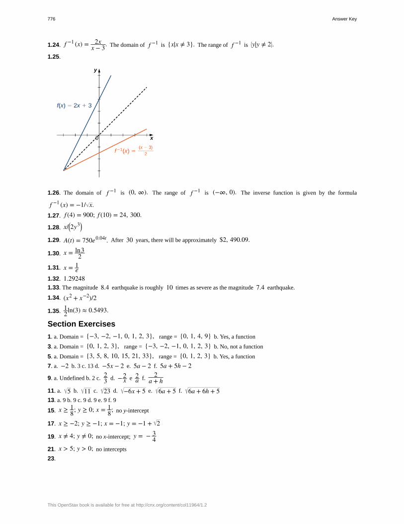
1.24. f −1 (x) = 2xx − 3. The domain of f −1 is {x|x ≠ 3}. The range of f −1 is
⎧
⎩⎨y|y ≠ 2⎫
⎭⎬.
1.25.
1.26. The domain of f −1 is (0, ∞). The range of f −1 is (−∞, 0). The inverse function is given by the formula
f −1 (x) = −1/ x.1.27. f (4) = 900; f (10) = 24, 300.
1.28. x/⎛⎝2y3⎞
⎠
1.29. A(t) = 750e0.04t. After 30 years, there will be approximately $2, 490.09.
1.30. x = ln32
1.31. x = 1e
1.32. 1.292481.33. The magnitude 8.4 earthquake is roughly 10 times as severe as the magnitude 7.4 earthquake.
1.34. (x2 + x−2)/2
1.35. 12ln(3) ≈ 0.5493.
Section Exercises
1. a. Domain = {−3, −2, −1, 0, 1, 2, 3}, range = {0, 1, 4, 9} b. Yes, a function
3. a. Domain = {0, 1, 2, 3}, range = {−3, −2, −1, 0, 1, 2, 3} b. No, not a function
5. a. Domain = {3, 5, 8, 10, 15, 21, 33}, range = {0, 1, 2, 3} b. Yes, a function
7. a. −2 b. 3 c. 13 d. −5x − 2 e. 5a − 2 f. 5a + 5h − 2
9. a. Undefined b. 2 c. 23 d. −2
x e 2a f. 2
a + h11. a. 5 b. 11 c. 23 d. −6x + 5 e. 6a + 5 f. 6a + 6h + 513. a. 9 b. 9 c. 9 d. 9 e. 9 f. 9
15. x ≥ 18; y ≥ 0; x = 1
8; no y-intercept
17. x ≥ −2; y ≥ −1; x = −1; y = −1 + 2
19. x ≠ 4; y ≠ 0; no x-intercept; y = − 34
21. x > 5; y > 0; no intercepts
23.
776 Answer Key
This OpenStax book is available for free at http://cnx.org/content/col11964/1.2
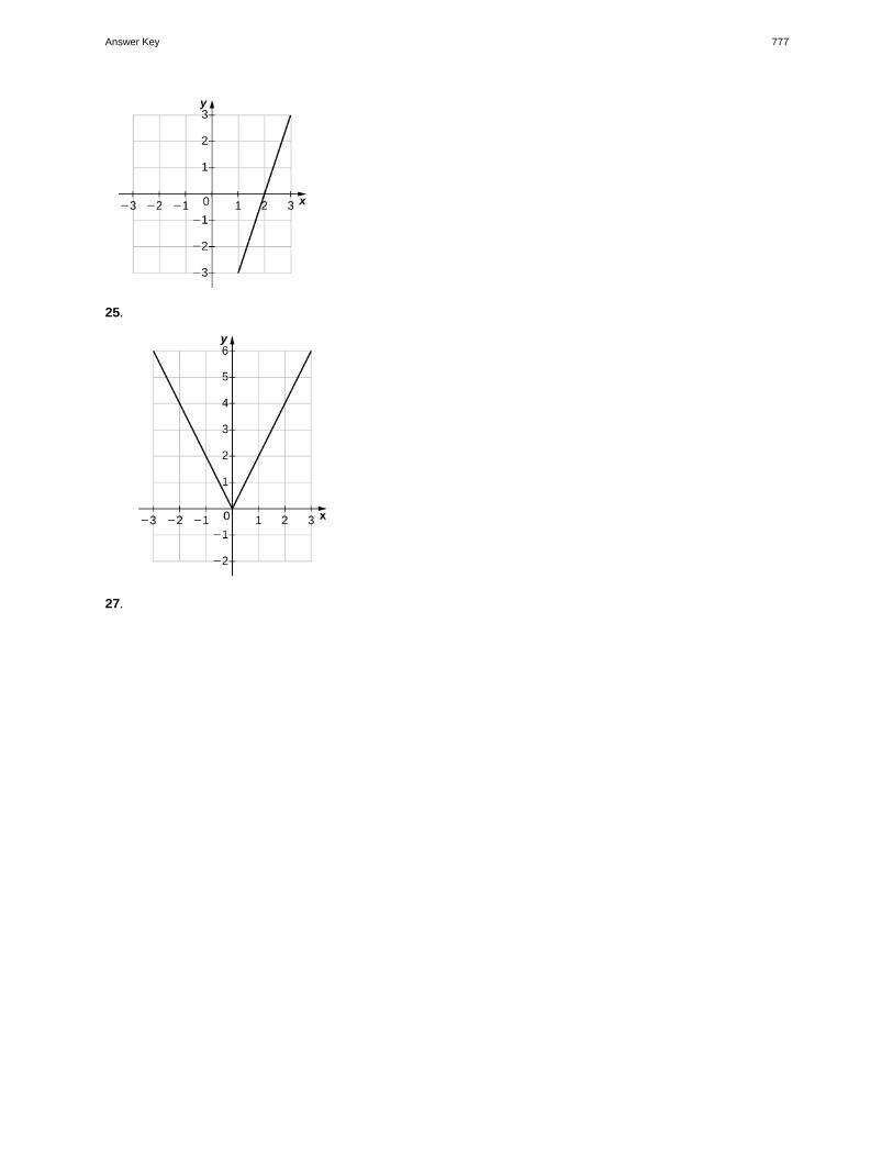
25.
27.
Answer Key 777
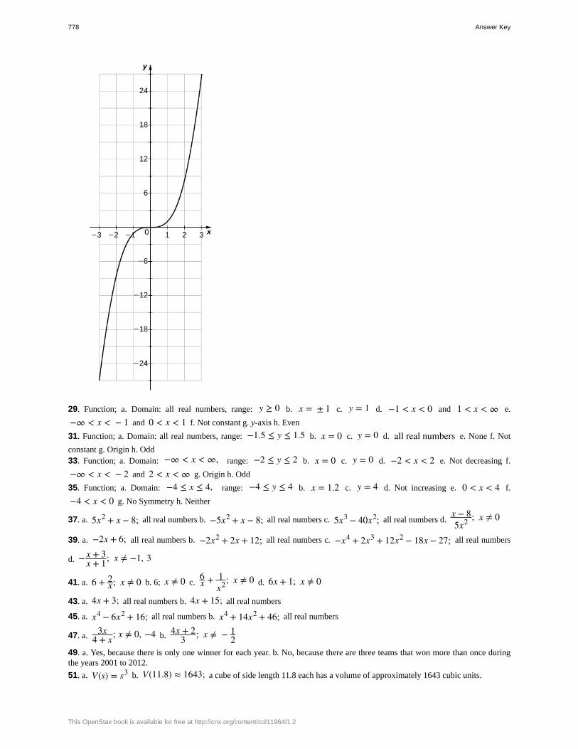
29. Function; a. Domain: all real numbers, range: y ≥ 0 b. x = ± 1 c. y = 1 d. −1 < x < 0 and 1 < x < ∞ e.
−∞ < x < − 1 and 0 < x < 1 f. Not constant g. y-axis h. Even
31. Function; a. Domain: all real numbers, range: −1.5 ≤ y ≤ 1.5 b. x = 0 c. y = 0 d. all real numbers e. None f. Not
constant g. Origin h. Odd33. Function; a. Domain: −∞ < x < ∞, range: −2 ≤ y ≤ 2 b. x = 0 c. y = 0 d. −2 < x < 2 e. Not decreasing f.
−∞ < x < − 2 and 2 < x < ∞ g. Origin h. Odd
35. Function; a. Domain: −4 ≤ x ≤ 4, range: −4 ≤ y ≤ 4 b. x = 1.2 c. y = 4 d. Not increasing e. 0 < x < 4 f.
−4 < x < 0 g. No Symmetry h. Neither
37. a. 5x2 + x − 8; all real numbers b. −5x2 + x − 8; all real numbers c. 5x3 − 40x2; all real numbers d.x − 85x2 ; x ≠ 0
39. a. −2x + 6; all real numbers b. −2x2 + 2x + 12; all real numbers c. −x4 + 2x3 + 12x2 − 18x − 27; all real numbers
d. − x + 3x + 1; x ≠ −1, 3
41. a. 6 + 2x; x ≠ 0 b. 6; x ≠ 0 c.
6x + 1
x2; x ≠ 0 d. 6x + 1; x ≠ 0
43. a. 4x + 3; all real numbers b. 4x + 15; all real numbers
45. a. x4 − 6x2 + 16; all real numbers b. x4 + 14x2 + 46; all real numbers
47. a. 3x4 + x; x ≠ 0, −4 b. 4x + 2
3 ; x ≠ − 12
49. a. Yes, because there is only one winner for each year. b. No, because there are three teams that won more than once duringthe years 2001 to 2012.
51. a. V(s) = s3 b. V(11.8) ≈ 1643; a cube of side length 11.8 each has a volume of approximately 1643 cubic units.
778 Answer Key
This OpenStax book is available for free at http://cnx.org/content/col11964/1.2
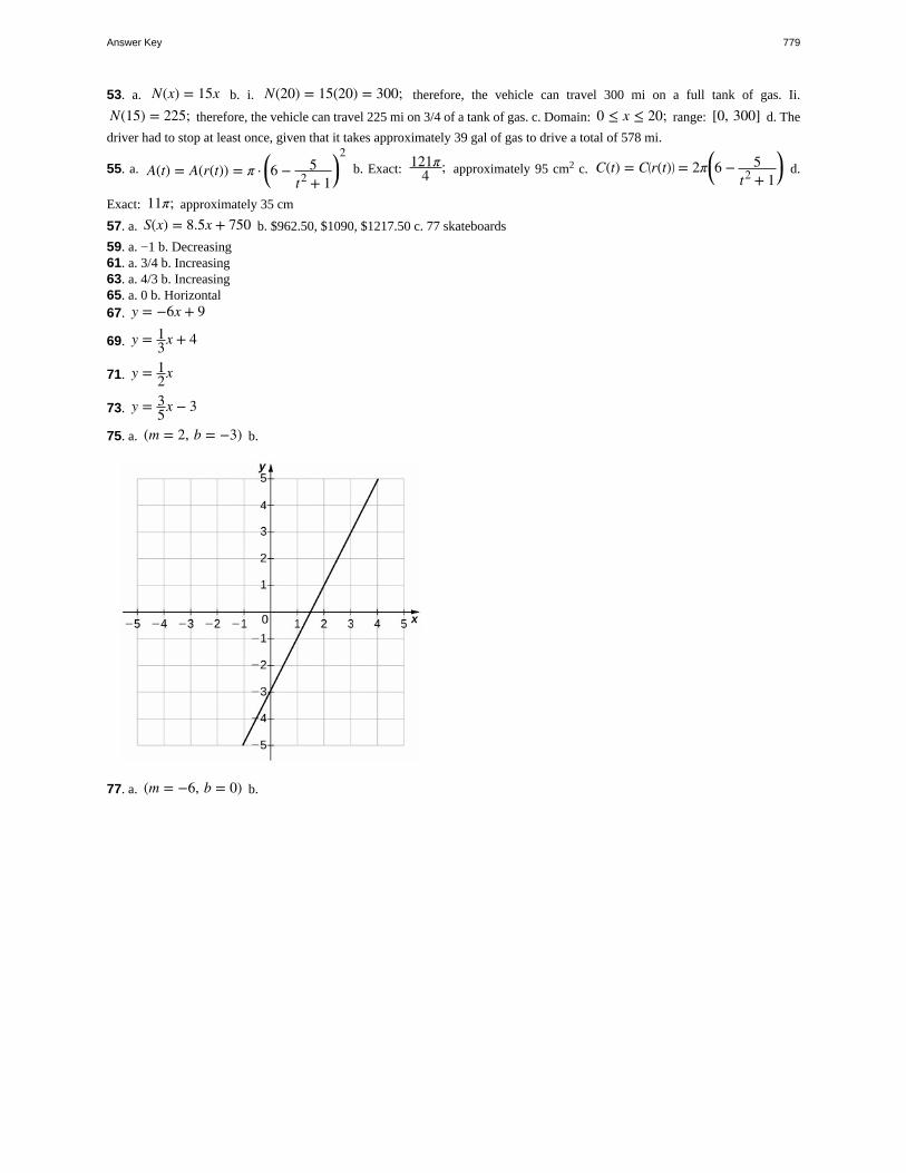
53. a. N(x) = 15x b. i. N(20) = 15(20) = 300; therefore, the vehicle can travel 300 mi on a full tank of gas. Ii.
N(15) = 225; therefore, the vehicle can travel 225 mi on 3/4 of a tank of gas. c. Domain: 0 ≤ x ≤ 20; range: [0, 300] d. The
driver had to stop at least once, given that it takes approximately 39 gal of gas to drive a total of 578 mi.
55. a. A(t) = A(r(t)) = π · ⎛⎝6 − 5t2 + 1
⎞⎠
2b. Exact: 121π
4 ; approximately 95 cm2 c. C(t) = C⎛⎝r(t)⎞
⎠ = 2π⎛⎝6 − 5
t2 + 1⎞⎠ d.
Exact: 11π; approximately 35 cm
57. a. S(x) = 8.5x + 750 b. $962.50, $1090, $1217.50 c. 77 skateboards
59. a. −1 b. Decreasing61. a. 3/4 b. Increasing63. a. 4/3 b. Increasing65. a. 0 b. Horizontal67. y = −6x + 9
69. y = 13x + 4
71. y = 12x
73. y = 35x − 3
75. a. (m = 2, b = −3) b.
77. a. (m = −6, b = 0) b.
Answer Key 779
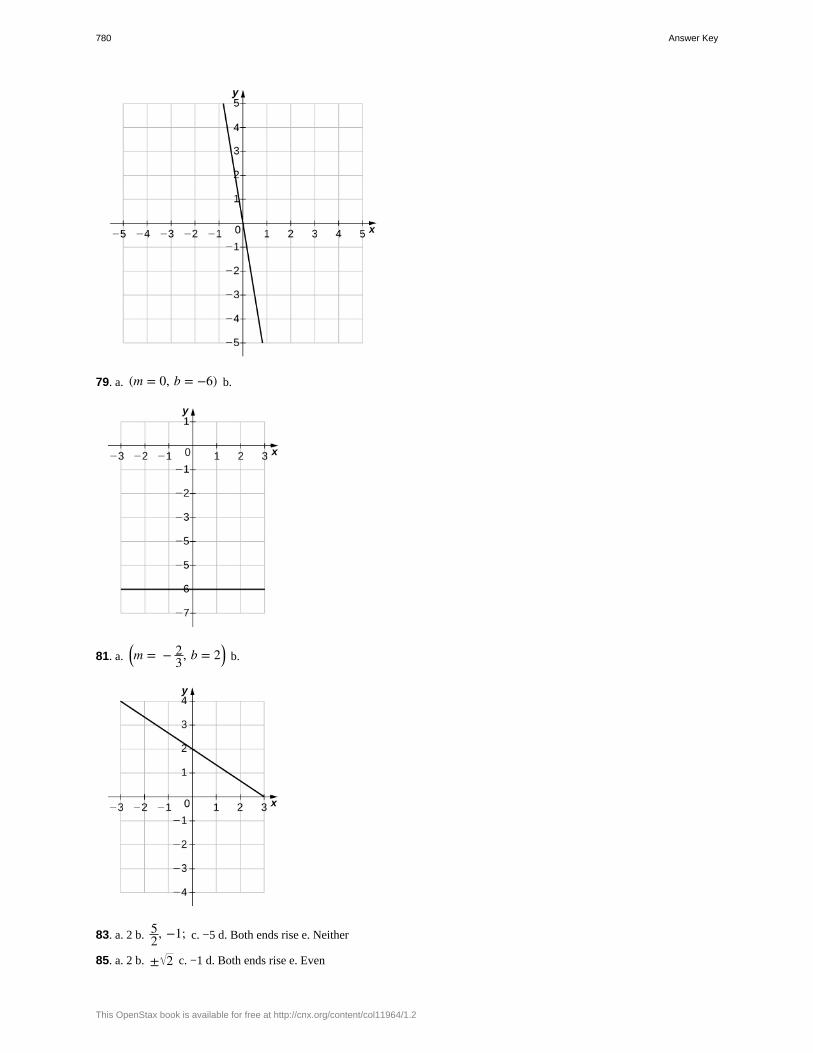
79. a. (m = 0, b = −6) b.
81. a.⎛⎝m = − 2
3, b = 2⎞⎠ b.
83. a. 2 b. 52, −1; c. −5 d. Both ends rise e. Neither
85. a. 2 b. ± 2 c. −1 d. Both ends rise e. Even
780 Answer Key
This OpenStax book is available for free at http://cnx.org/content/col11964/1.2
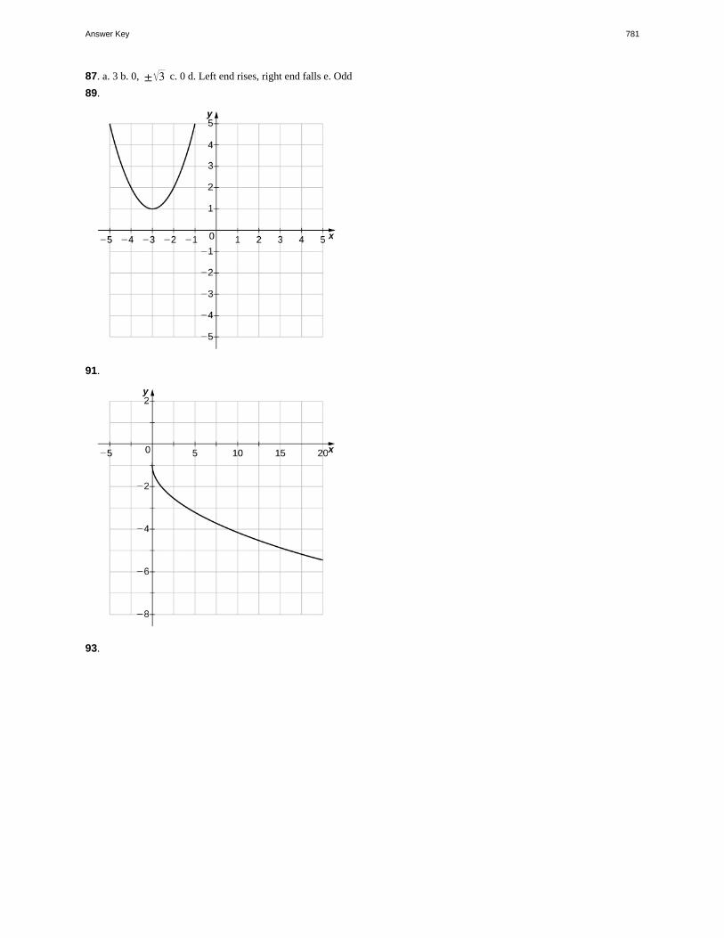
87. a. 3 b. 0, ± 3 c. 0 d. Left end rises, right end falls e. Odd
89.
91.
93.
Answer Key 781
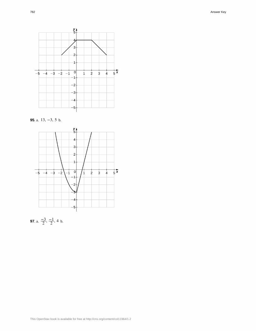
95. a. 13, −3, 5 b.
97. a. −32 , −1
2 , 4 b.
782 Answer Key
This OpenStax book is available for free at http://cnx.org/content/col11964/1.2
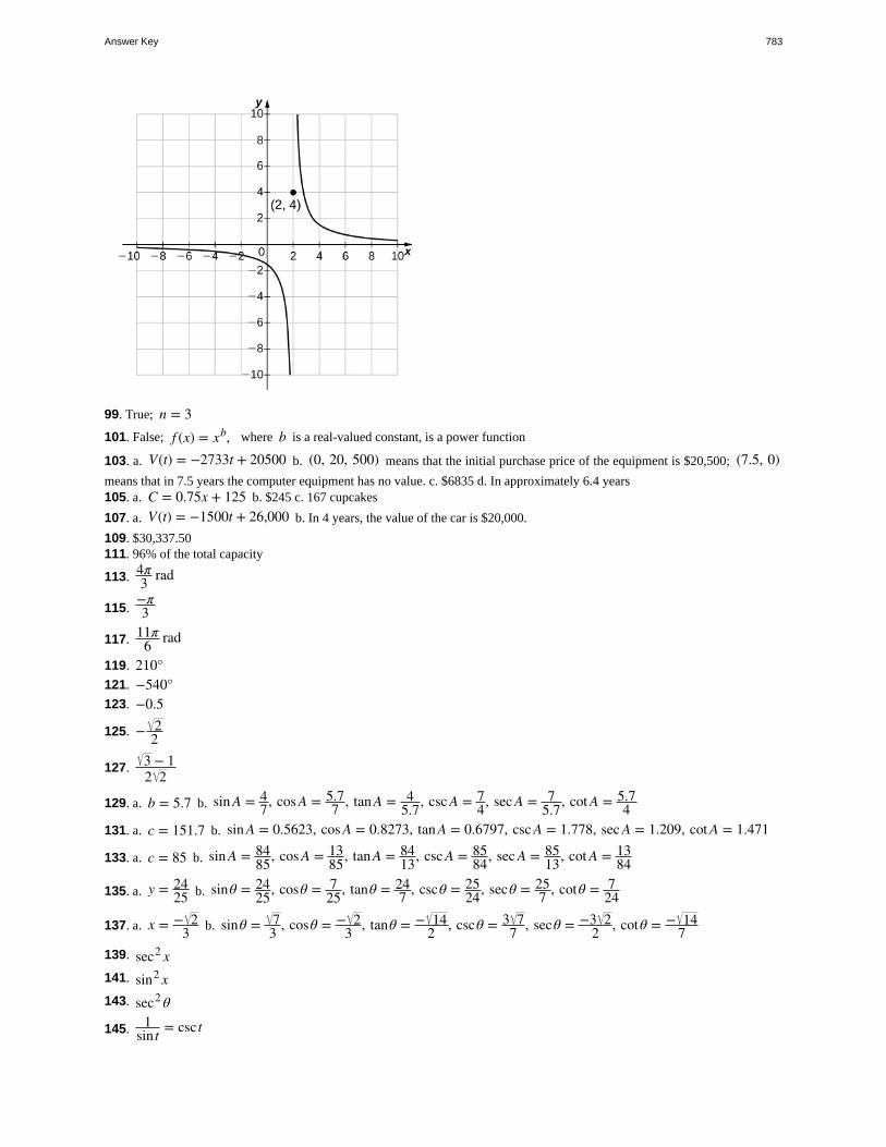
99. True; n = 3101. False; f (x) = xb, where b is a real-valued constant, is a power function
103. a. V(t) = −2733t + 20500 b. (0, 20, 500) means that the initial purchase price of the equipment is $20,500; (7.5, 0)means that in 7.5 years the computer equipment has no value. c. $6835 d. In approximately 6.4 years105. a. C = 0.75x + 125 b. $245 c. 167 cupcakes
107. a. V(t) = −1500t + 26,000 b. In 4 years, the value of the car is $20,000.
109. $30,337.50111. 96% of the total capacity
113. 4π3 rad
115.−π3
117. 11π6 rad
119. 210°121. −540°123. −0.5
125. − 22
127. 3 − 12 2
129. a. b = 5.7 b. sin A = 47, cos A = 5.7
7 , tan A = 45.7, csc A = 7
4, sec A = 75.7, cot A = 5.7
4131. a. c = 151.7 b. sin A = 0.5623, cos A = 0.8273, tan A = 0.6797, csc A = 1.778, sec A = 1.209, cot A = 1.471
133. a. c = 85 b. sin A = 8485, cos A = 13
85, tan A = 8413, csc A = 85
84, sec A = 8513, cot A = 13
84
135. a. y = 2425 b. sinθ = 24
25, cosθ = 725, tanθ = 24
7 , cscθ = 2524, secθ = 25
7 , cotθ = 724
137. a. x = − 23 b. sinθ = 7
3 , cosθ = − 23 , tanθ = − 14
2 , cscθ = 3 77 , secθ = −3 2
2 , cotθ = − 147
139. sec2 x141. sin2 x143. sec2 θ
145. 1sin t = csc t
Answer Key 783
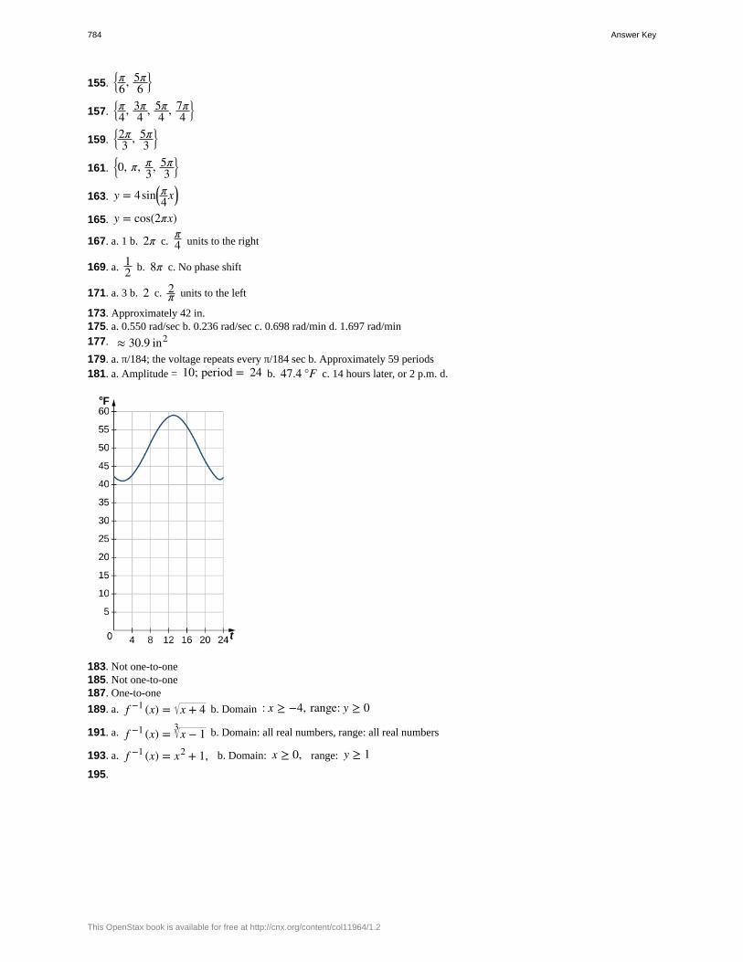
155.⎧
⎩⎨π6, 5π
6⎫
⎭⎬
157.⎧
⎩⎨π4, 3π
4 , 5π4 , 7π
4⎫
⎭⎬
159.⎧
⎩⎨2π
3 , 5π3
⎫
⎭⎬
161.⎧
⎩⎨0, π, π
3, 5π3
⎫
⎭⎬
163. y = 4sin⎛⎝π4x⎞
⎠
165. y = cos(2πx)
167. a. 1 b. 2π c.π4 units to the right
169. a. 12 b. 8π c. No phase shift
171. a. 3 b. 2 c. 2π units to the left
173. Approximately 42 in.175. a. 0.550 rad/sec b. 0.236 rad/sec c. 0.698 rad/min d. 1.697 rad/min177. ≈ 30.9 in2
179. a. π/184; the voltage repeats every π/184 sec b. Approximately 59 periods181. a. Amplitude = 10; period = 24 b. 47.4 °F c. 14 hours later, or 2 p.m. d.
183. Not one-to-one185. Not one-to-one187. One-to-one
189. a. f −1 (x) = x + 4 b. Domain : x ≥ −4, range: y ≥ 0
191. a. f −1 (x) = x − 13 b. Domain: all real numbers, range: all real numbers
193. a. f −1 (x) = x2 + 1, b. Domain: x ≥ 0, range: y ≥ 1195.
784 Answer Key
This OpenStax book is available for free at http://cnx.org/content/col11964/1.2
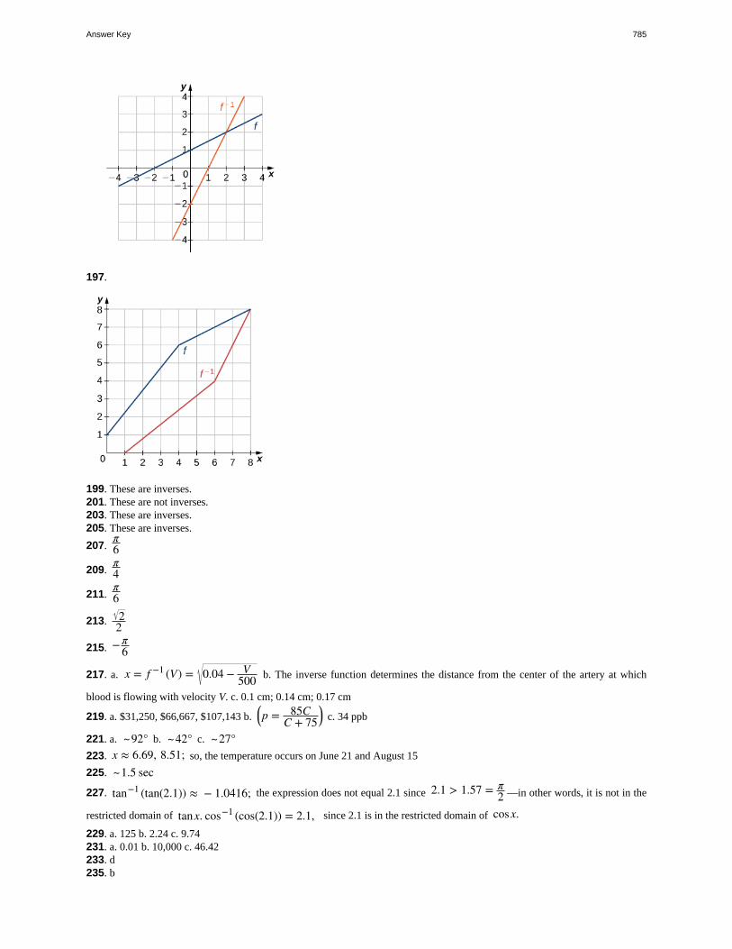
197.
199. These are inverses.201. These are not inverses.203. These are inverses.205. These are inverses.
207.π6
209.π4
211.π6
213. 22
215. −π6
217. a. x = f −1 (V) = 0.04 − V500 b. The inverse function determines the distance from the center of the artery at which
blood is flowing with velocity V. c. 0.1 cm; 0.14 cm; 0.17 cm
219. a. $31,250, $66,667, $107,143 b.⎛⎝p = 85C
C + 75⎞⎠ c. 34 ppb
221. a. ~92° b. ~42° c. ~27°223. x ≈ 6.69, 8.51; so, the temperature occurs on June 21 and August 15
225. ~1.5 sec
227. tan−1 (tan(2.1)) ≈ − 1.0416; the expression does not equal 2.1 since 2.1 > 1.57 = π2 —in other words, it is not in the
restricted domain of tanx. cos−1 (cos(2.1)) = 2.1, since 2.1 is in the restricted domain of cosx.229. a. 125 b. 2.24 c. 9.74231. a. 0.01 b. 10,000 c. 46.42233. d235. b
Answer Key 785
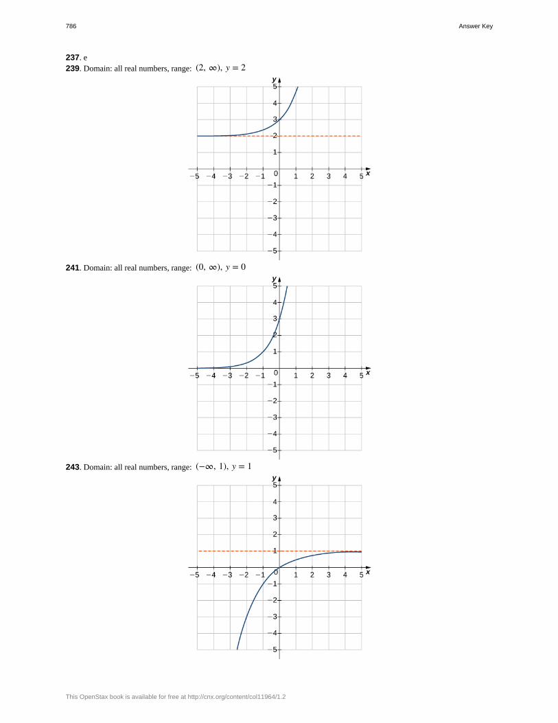
237. e239. Domain: all real numbers, range: (2, ∞), y = 2
241. Domain: all real numbers, range: (0, ∞), y = 0
243. Domain: all real numbers, range: (−∞, 1), y = 1
786 Answer Key
This OpenStax book is available for free at http://cnx.org/content/col11964/1.2
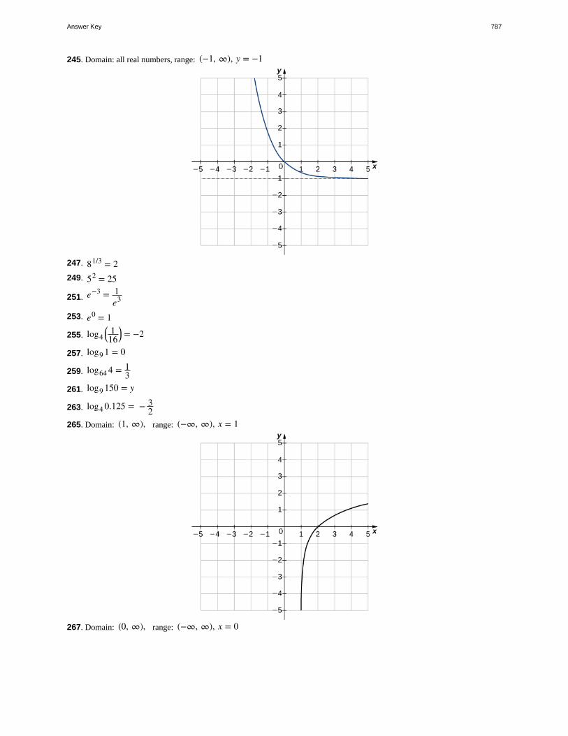
245. Domain: all real numbers, range: (−1, ∞), y = −1
247. 81/3 = 2249. 52 = 25
251. e−3 = 1e3
253. e0 = 1
255. log4⎛⎝
116
⎞⎠ = −2
257. log9 1 = 0
259. log64 4 = 13
261. log9 150 = y
263. log4 0.125 = − 32
265. Domain: (1, ∞), range: (−∞, ∞), x = 1
267. Domain: (0, ∞), range: (−∞, ∞), x = 0
Answer Key 787
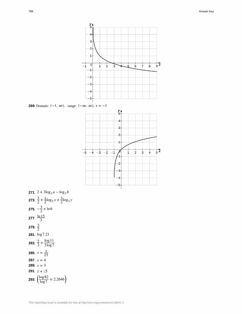
269. Domain: (−1, ∞), range: (−∞, ∞), x = −1
271. 2 + 3log3 a − log3 b
273. 32 + 1
2log5 x + 32log5 y
275. −32 + ln6
277. ln153
279. 32
281. log7.21
283. 23 + log11
3log7
285. x = 125
287. x = 4289. x = 3291. 1 + 5
293.⎛⎝log82log7 ≈ 2.2646⎞
⎠
788 Answer Key
This OpenStax book is available for free at http://cnx.org/content/col11964/1.2
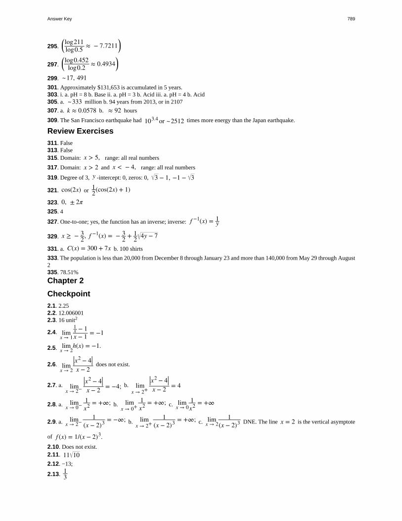
295.⎛⎝log211log0.5 ≈ − 7.7211⎞
⎠
297.⎛⎝log0.452log0.2 ≈ 0.4934⎞
⎠299. ~17, 491301. Approximately $131,653 is accumulated in 5 years.303. i. a. pH = 8 b. Base ii. a. pH = 3 b. Acid iii. a. pH = 4 b. Acid305. a. ~333 million b. 94 years from 2013, or in 2107
307. a. k ≈ 0.0578 b. ≈ 92 hours
309. The San Francisco earthquake had 103.4 or ~2512 times more energy than the Japan earthquake.
Review Exercises
311. False313. False315. Domain: x > 5, range: all real numbers
317. Domain: x > 2 and x < − 4, range: all real numbers
319. Degree of 3, y -intercept: 0, zeros: 0, 3 − 1, −1 − 3
321. cos(2x) or 12(cos(2x) + 1)
323. 0, ± 2π325. 4
327. One-to-one; yes, the function has an inverse; inverse: f −1(x) = 1y
329. x ≥ − 32, f −1(x) = − 3
2 + 12 4y − 7
331. a. C(x) = 300 + 7x b. 100 shirts
333. The population is less than 20,000 from December 8 through January 23 and more than 140,000 from May 29 through August2335. 78.51%
Chapter 2
Checkpoint
2.1. 2.252.2. 12.0060012.3. 16 unit2
2.4. limx → 1
1x − 1x − 1 = −1
2.5. limx → 2
h(x) = −1.
2.6. limx → 2
|x2 − 4|x − 2
does not exist.
2.7. a. limx → 2−
|x2 − 4|x − 2 = −4; b. lim
x → 2+|x2 − 4|x − 2 = 4
2.8. a. limx → 0−
1x2 = +∞; b. lim
x → 0+1x2 = +∞; c. lim
x → 01x2 = +∞
2.9. a. limx → 2−
1(x − 2)3 = −∞; b. lim
x → 2+1
(x − 2)3 = +∞; c. limx → 2
1(x − 2)3 DNE. The line x = 2 is the vertical asymptote
of f (x) = 1/(x − 2)3.2.10. Does not exist.2.11. 11 102.12. −13;
2.13. 13
Answer Key 789
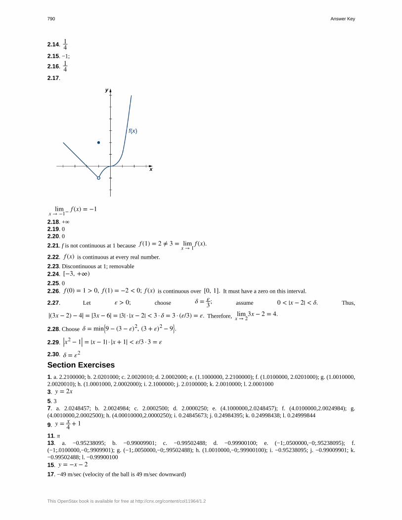
2.14. 14
2.15. −1;
2.16. 14
2.17.
limx → −1− f (x) = −1
2.18. +∞2.19. 02.20. 0
2.21. f is not continuous at 1 because f (1) = 2 ≠ 3 = limx → 1
f (x).
2.22. f (x) is continuous at every real number.
2.23. Discontinuous at 1; removable2.24. [−3, +∞)2.25. 02.26. f (0) = 1 > 0, f (1) = −2 < 0; f (x) is continuous over [0, 1]. It must have a zero on this interval.
2.27. Let ε > 0; choose δ = ε3; assume 0 < |x − 2| < δ. Thus,
|(3x − 2) − 4| = |3x − 6| = |3| · |x − 2| < 3 · δ = 3 · (ε/3) = ε. Therefore, limx → 2
3x − 2 = 4.
2.28. Choose δ = min⎧
⎩⎨9 − (3 − ε)2, (3 + ε)2 − 9⎫
⎭⎬.
2.29. |x2 − 1| = |x − 1| · |x + 1| < ε/3 · 3 = ε
2.30. δ = ε2
Section Exercises
1. a. 2.2100000; b. 2.0201000; c. 2.0020010; d. 2.0002000; e. (1.1000000, 2.2100000); f. (1.0100000, 2.0201000); g. (1.0010000,2.0020010); h. (1.0001000, 2.0002000); i. 2.1000000; j. 2.0100000; k. 2.0010000; l. 2.00010003. y = 2x5. 37. a. 2.0248457; b. 2.0024984; c. 2.0002500; d. 2.0000250; e. (4.1000000,2.0248457); f. (4.0100000,2.0024984); g.(4.0010000,2.0002500); h. (4.00010000,2.0000250); i. 0.24845673; j. 0.24984395; k. 0.24998438; l. 0.24999844
9. y = x4 + 1
11. π13. a. −0.95238095; b. −0.99009901; c. −0.99502488; d. −0.99900100; e. (−1;.0500000,−0;.95238095); f.(−1;.0100000,−0;.9909901); g. (−1;.0050000,−0;.99502488); h. (1.0010000,−0;.99900100); i. −0.95238095; j. −0.99009901; k.−0.99502488; l. −0.9990010015. y = −x − 217. −49 m/sec (velocity of the ball is 49 m/sec downward)
790 Answer Key
This OpenStax book is available for free at http://cnx.org/content/col11964/1.2
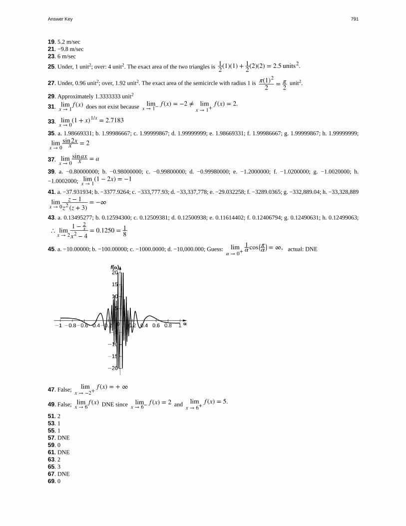
19. 5.2 m/sec21. −9.8 m/sec23. 6 m/sec
25. Under, 1 unit2; over: 4 unit2. The exact area of the two triangles is 12(1)(1) + 1
2(2)(2) = 2.5 units2.
27. Under, 0.96 unit2; over, 1.92 unit2. The exact area of the semicircle with radius 1 is π(1)2
2 = π2
unit2.
29. Approximately 1.3333333 unit2
31. limx → 1
f (x) does not exist because limx → 1− f (x) = −2 ≠ lim
x → 1+f (x) = 2.
33. limx → 0
(1 + x)1/x = 2.7183
35. a. 1.98669331; b. 1.99986667; c. 1.99999867; d. 1.99999999; e. 1.98669331; f. 1.99986667; g. 1.99999867; h. 1.99999999;
limx → 0
sin2xx = 2
37. limx → 0
sinaxx = a
39. a. −0.80000000; b. −0.98000000; c. −0.99800000; d. −0.99980000; e. −1.2000000; f. −1.0200000; g. −1.0020000; h.
−1.0002000; limx → 1
(1 − 2x) = −1
41. a. −37.931934; b. −3377.9264; c. −333,777.93; d. −33,337,778; e. −29.032258; f. −3289.0365; g. −332,889.04; h. −33,328,889
limx → 0
z − 1z2 (z + 3)
= −∞
43. a. 0.13495277; b. 0.12594300; c. 0.12509381; d. 0.12500938; e. 0.11614402; f. 0.12406794; g. 0.12490631; h. 0.12499063;
∴ limx → 2
1 − 2x
x2 − 4= 0.1250 = 1
8
45. a. −10.00000; b. −100.00000; c. −1000.0000; d. −10,000.000; Guess: limα → 0+
1α cos ⎛
⎝πα
⎞⎠ = ∞, actual: DNE
47. False; limx → −2+
f (x) = + ∞
49. False; limx → 6
f (x) DNE since limx → 6− f (x) = 2 and lim
x → 6+f (x) = 5.
51. 253. 155. 157. DNE59. 061. DNE63. 265. 367. DNE69. 0
Answer Key 791
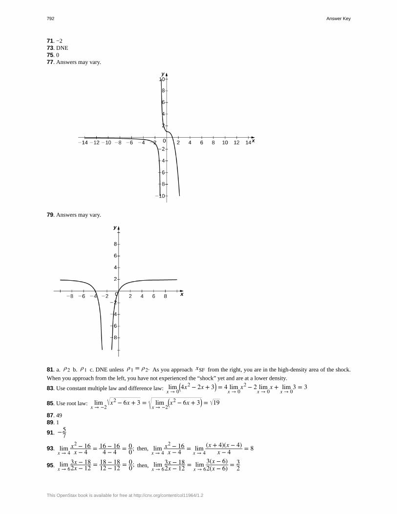
71. −273. DNE75. 077. Answers may vary.
79. Answers may vary.
81. a. ρ2 b. ρ1 c. DNE unless ρ1 = ρ2. As you approach xSF from the right, you are in the high-density area of the shock.
When you approach from the left, you have not experienced the “shock” yet and are at a lower density.
83. Use constant multiple law and difference law: limx → 0
⎛⎝4x2 − 2x + 3⎞
⎠ = 4 limx → 0
x2 − 2 limx → 0
x + limx → 0
3 = 3
85. Use root law: limx → −2
x2 − 6x + 3 = limx → −2
⎛⎝x2 − 6x + 3⎞
⎠ = 19
87. 4989. 1
91. −57
93. limx → 4
x2 − 16x − 4 = 16 − 16
4 − 4 = 00; then, lim
x → 4x2 − 16x − 4 = lim
x → 4(x + 4)(x − 4)
x − 4 = 8
95. limx → 6
3x − 182x − 12 = 18 − 18
12 − 12 = 00; then, lim
x → 63x − 182x − 12 = lim
x → 63(x − 6)2(x − 6) = 3
2
792 Answer Key
This OpenStax book is available for free at http://cnx.org/content/col11964/1.2
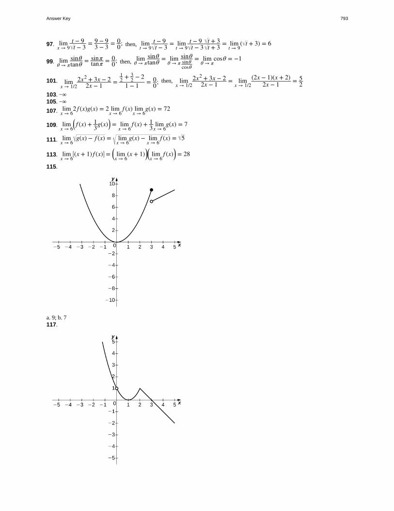
97. limx → 9
t − 9t − 3 = 9 − 9
3 − 3 = 00; then, lim
t → 9t − 9t − 3 = lim
t → 9t − 9t − 3
t + 3t + 3 = lim
t → 9( t + 3) = 6
99. limθ → π
sinθtanθ = sinπ
tanπ = 00; then, lim
θ → πsinθtanθ = lim
θ → πsinθsinθcosθ
= limθ → π
cosθ = −1
101. limx → 1/2
2x2 + 3x − 22x − 1 =
12 + 3
2 − 21 − 1 = 0
0; then, limx → 1/2
2x2 + 3x − 22x − 1 = lim
x → 1/2(2x − 1)(x + 2)
2x − 1 = 52
103. −∞105. −∞
107. limx → 6
2 f (x)g(x) = 2 limx → 6
f (x) limx → 6
g(x) = 72
109. limx → 6
⎛⎝ f (x) + 1
3g(x)⎞⎠ = limx → 6
f (x) + 13 lim
x → 6g(x) = 7
111. limx → 6
g(x) − f (x) = limx → 6
g(x) − limx → 6
f (x) = 5
113. limx → 6
⎡⎣(x + 1) f (x)⎤
⎦ = ⎛⎝ limx → 6
(x + 1)⎞⎠⎛⎝ limx → 6
f (x)⎞⎠ = 28
115.
a. 9; b. 7117.
Answer Key 793
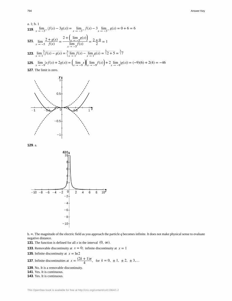
a. 1; b. 1
119. limx → −3−
⎛⎝ f (x) − 3g(x)⎞
⎠ = limx → −3− f (x) − 3 lim
x → −3− g(x) = 0 + 6 = 6
121. limx → −5
2 + g(x)f (x) =
2 + ⎛⎝ limx → −5
g(x)⎞⎠lim
x → −5f (x) = 2 + 0
2 = 1
123. limx → 1
f (x) − g(x)3 = limx → 1
f (x) − limx → 1
g(x)3 = 2 + 53 = 73
125. limx → −9
⎛⎝x f (x) + 2g(x)⎞
⎠ = ⎛⎝ limx → −9
x⎞⎠⎛⎝ limx → −9
f (x)⎞⎠ + 2 limx → −9
⎛⎝g(x)⎞
⎠ = (−9)(6) + 2(4) = −46
127. The limit is zero.
129. a.
b. ∞. The magnitude of the electric field as you approach the particle q becomes infinite. It does not make physical sense to evaluatenegative distance.131. The function is defined for all x in the interval (0, ∞).133. Removable discontinuity at x = 0; infinite discontinuity at x = 1135. Infinite discontinuity at x = ln2
137. Infinite discontinuities at x = (2k + 1)π4 , for k = 0, ± 1, ± 2, ± 3,…
139. No. It is a removable discontinuity.141. Yes. It is continuous.143. Yes. It is continuous.
794 Answer Key
This OpenStax book is available for free at http://cnx.org/content/col11964/1.2
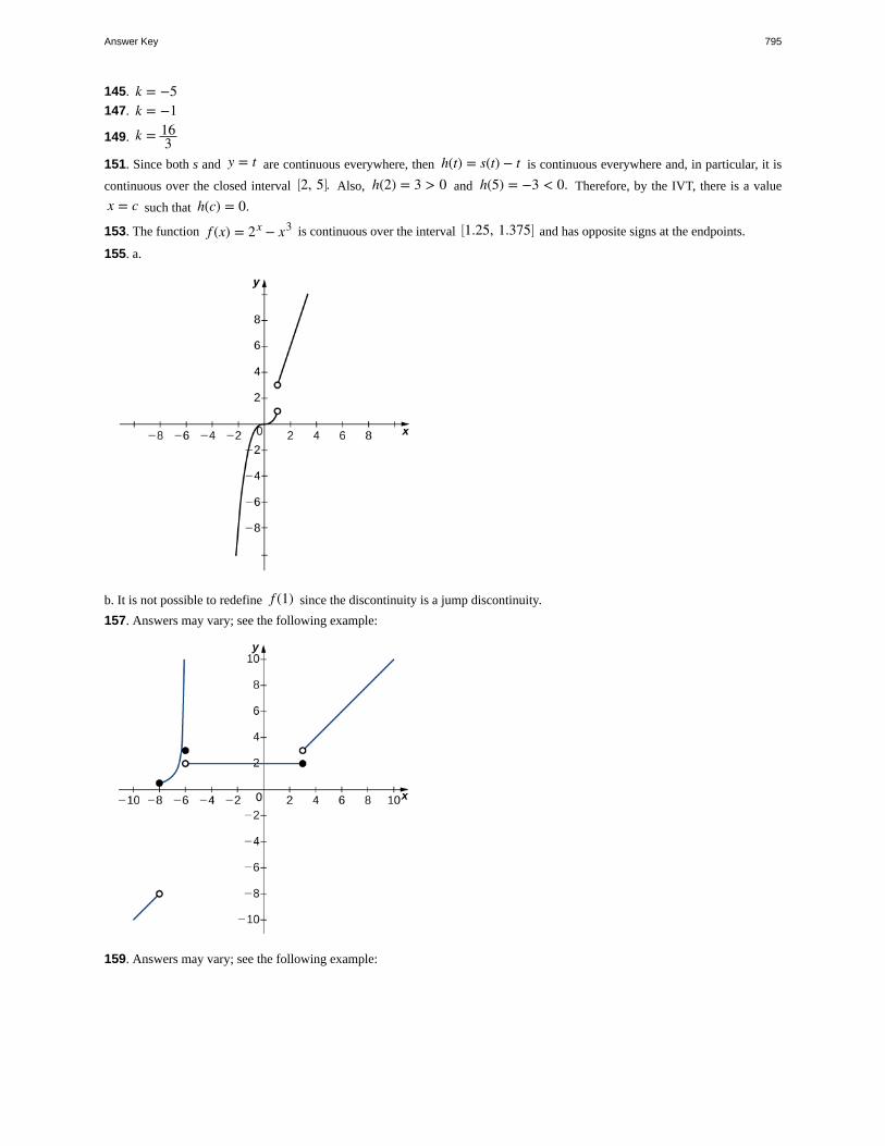
145. k = −5147. k = −1
149. k = 163
151. Since both s and y = t are continuous everywhere, then h(t) = s(t) − t is continuous everywhere and, in particular, it is
continuous over the closed interval ⎡⎣2, 5⎤
⎦. Also, h(2) = 3 > 0 and h(5) = −3 < 0. Therefore, by the IVT, there is a value
x = c such that h(c) = 0.
153. The function f (x) = 2x − x3 is continuous over the interval ⎡⎣1.25, 1.375⎤
⎦ and has opposite signs at the endpoints.
155. a.
b. It is not possible to redefine f (1) since the discontinuity is a jump discontinuity.
157. Answers may vary; see the following example:
159. Answers may vary; see the following example:
Answer Key 795
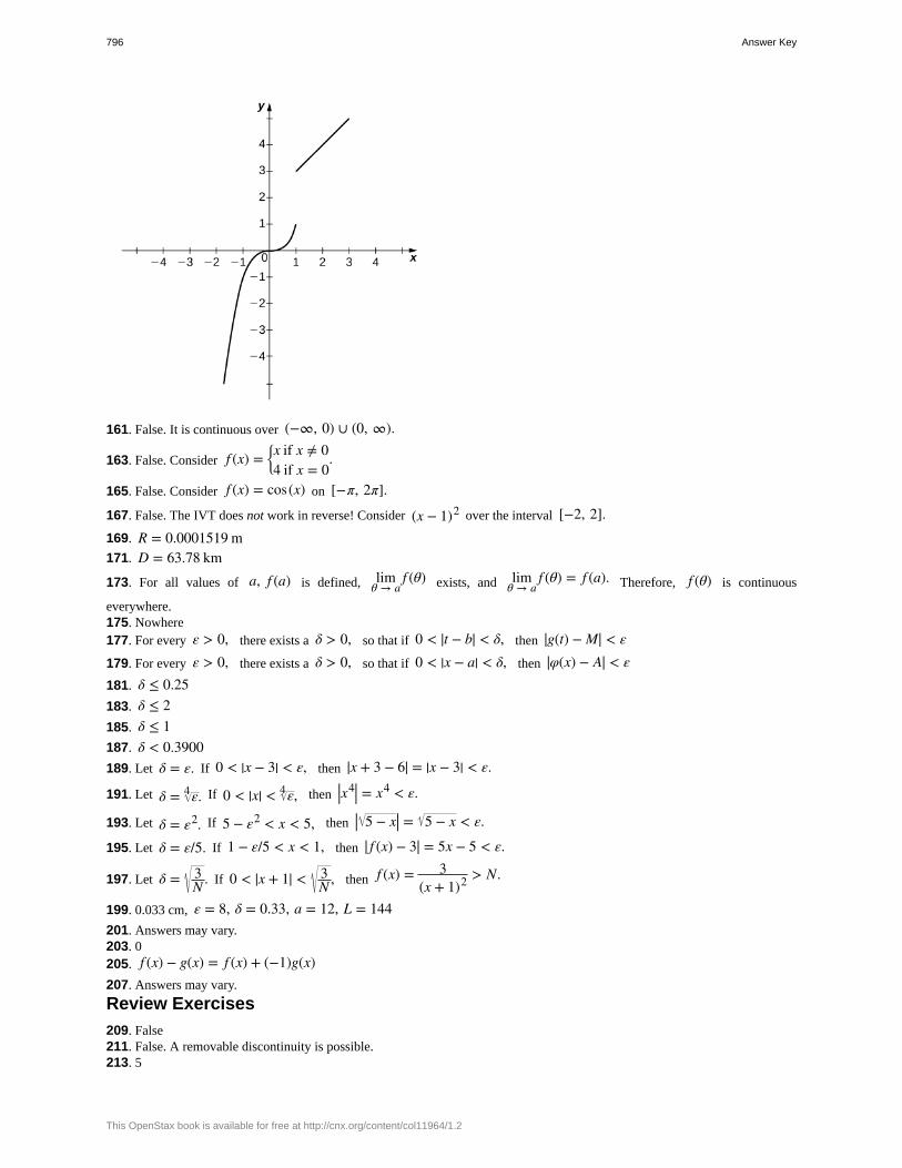
161. False. It is continuous over (−∞, 0) ∪ (0, ∞).
163. False. Consider f (x) =⎧
⎩⎨x if x ≠ 04 if x = 0
.
165. False. Consider f (x) = cos(x) on [−π, 2π].
167. False. The IVT does not work in reverse! Consider (x − 1)2 over the interval [−2, 2].169. R = 0.0001519 m171. D = 63.78 km173. For all values of a, f (a) is defined, lim
θ → af (θ) exists, and lim
θ → af (θ) = f (a). Therefore, f (θ) is continuous
everywhere.175. Nowhere177. For every ε > 0, there exists a δ > 0, so that if 0 < |t − b| < δ, then |g(t) − M| < ε179. For every ε > 0, there exists a δ > 0, so that if 0 < |x − a| < δ, then |φ(x) − A| < ε181. δ ≤ 0.25183. δ ≤ 2185. δ ≤ 1187. δ < 0.3900189. Let δ = ε. If 0 < |x − 3| < ε, then |x + 3 − 6| = |x − 3| < ε.
191. Let δ = ε4 . If 0 < |x| < ε4 , then |x4| = x4 < ε.
193. Let δ = ε2. If 5 − ε2 < x < 5, then | 5 − x| = 5 − x < ε.
195. Let δ = ε/5. If 1 − ε/5 < x < 1, then | f (x) − 3| = 5x − 5 < ε.
197. Let δ = 3N . If 0 < |x + 1| < 3
N , then f (x) = 3(x + 1)2 > N.
199. 0.033 cm, ε = 8, δ = 0.33, a = 12, L = 144201. Answers may vary.203. 0205. f (x) − g(x) = f (x) + (−1)g(x)207. Answers may vary.
Review Exercises
209. False211. False. A removable discontinuity is possible.213. 5
796 Answer Key
This OpenStax book is available for free at http://cnx.org/content/col11964/1.2
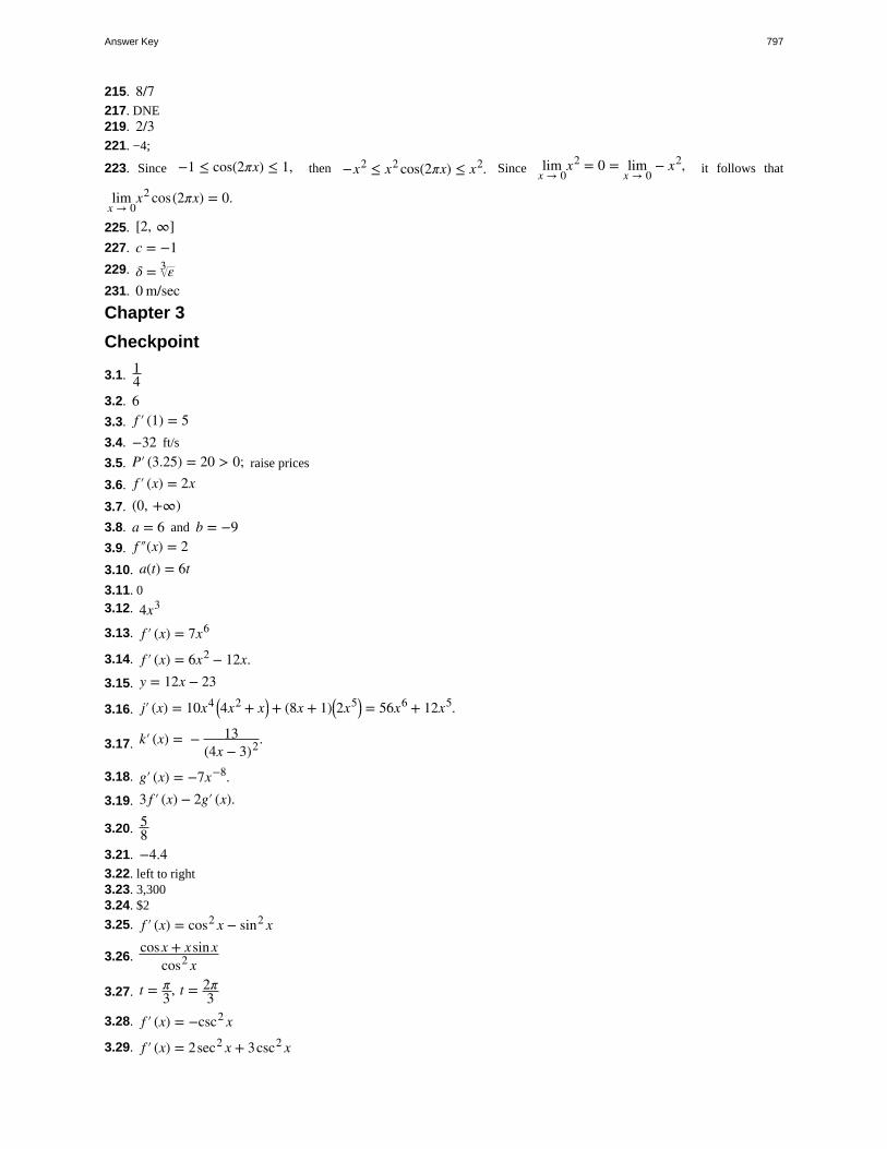
215. 8/7217. DNE219. 2/3221. −4;
223. Since −1 ≤ cos(2πx) ≤ 1, then −x2 ≤ x2 cos(2πx) ≤ x2. Since limx → 0
x2 = 0 = limx → 0
− x2, it follows that
limx → 0
x2 cos(2πx) = 0.
225. [2, ∞]227. c = −1229. δ = ε3
231. 0 m/secChapter 3
Checkpoint
3.1. 14
3.2. 63.3. f ′ (1) = 53.4. −32 ft/s
3.5. P′ (3.25) = 20 > 0; raise prices
3.6. f ′ (x) = 2x3.7. (0, +∞)3.8. a = 6 and b = −93.9. f ″(x) = 23.10. a(t) = 6t3.11. 03.12. 4x3
3.13. f ′ (x) = 7x6
3.14. f ′ (x) = 6x2 − 12x.3.15. y = 12x − 23
3.16. j′ (x) = 10x4 ⎛⎝4x2 + x⎞
⎠ + (8x + 1)⎛⎝2x5⎞
⎠ = 56x6 + 12x5.
3.17. k′ (x) = − 13(4x − 3)2.
3.18. g′ (x) = −7x−8.3.19. 3 f ′ (x) − 2g′ (x).
3.20. 58
3.21. −4.43.22. left to right3.23. 3,3003.24. $2
3.25. f ′ (x) = cos2 x − sin2 x
3.26.cosx + xsinx
cos2 x
3.27. t = π3, t = 2π
33.28. f ′ (x) = −csc2 x
3.29. f ′ (x) = 2sec2 x + 3csc2 x
Answer Key 797
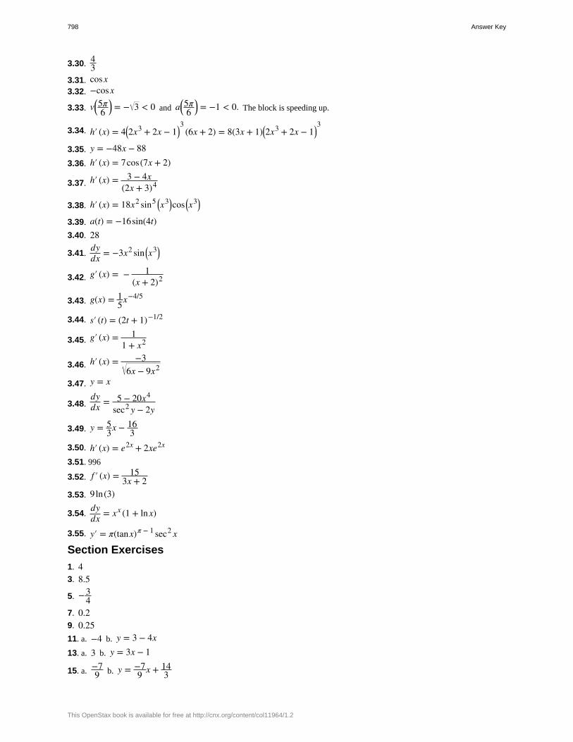
3.30. 43
3.31. cosx3.32. −cosx
3.33. v⎛⎝5π6
⎞⎠ = − 3 < 0 and a⎛
⎝5π6
⎞⎠ = −1 < 0. The block is speeding up.
3.34. h′ (x) = 4⎛⎝2x3 + 2x − 1⎞
⎠3
(6x + 2) = 8(3x + 1)⎛⎝2x3 + 2x − 1⎞
⎠3
3.35. y = −48x − 883.36. h′ (x) = 7cos(7x + 2)
3.37. h′ (x) = 3 − 4x(2x + 3)4
3.38. h′ (x) = 18x2 sin5 ⎛⎝x
3⎞⎠cos ⎛
⎝x3⎞
⎠
3.39. a(t) = −16sin(4t)3.40. 28
3.41.dydx = −3x2 sin ⎛
⎝x3⎞
⎠
3.42. g′ (x) = − 1(x + 2)2
3.43. g(x) = 15x−4/5
3.44. s′ (t) = (2t + 1)−1/2
3.45. g′ (x) = 11 + x2
3.46. h′ (x) = −36x − 9x2
3.47. y = x
3.48.dydx = 5 − 20x4
sec2 y − 2y
3.49. y = 53x − 16
33.50. h′ (x) = e2x + 2xe2x
3.51. 996
3.52. f ′ (x) = 153x + 2
3.53. 9ln(3)
3.54.dydx = xx (1 + lnx)
3.55. y′ = π(tanx)π − 1 sec2 x
Section Exercises
1. 43. 8.5
5. −34
7. 0.29. 0.2511. a. −4 b. y = 3 − 4x13. a. 3 b. y = 3x − 1
15. a. −79 b. y = −7
9 x + 143
798 Answer Key
This OpenStax book is available for free at http://cnx.org/content/col11964/1.2
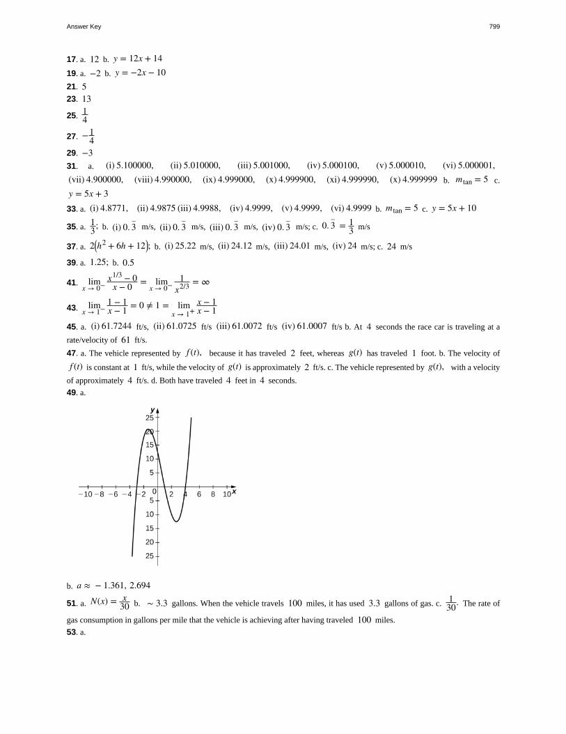
17. a. 12 b. y = 12x + 1419. a. −2 b. y = −2x − 1021. 523. 13
25. 14
27. −14
29. −331. a. (i) 5.100000, (ii) 5.010000, (iii) 5.001000, (iv) 5.000100, (v) 5.000010, (vi) 5.000001,(vii) 4.900000, (viii) 4.990000, (ix) 4.999000, (x) 4.999900, (xi) 4.999990, (x) 4.999999 b. mtan = 5 c.
y = 5x + 333. a. (i) 4.8771, (ii) 4.9875 (iii) 4.9988, (iv) 4.9999, (v) 4.9999, (vi) 4.9999 b. mtan = 5 c. y = 5x + 10
35. a. 13; b. (i) 0. 3
–m/s, (ii) 0. 3
–m/s, (iii) 0. 3
–m/s, (iv) 0. 3
–m/s; c. 0. 3
–= 1
3 m/s
37. a. 2⎛⎝h2 + 6h + 12⎞
⎠; b. (i) 25.22 m/s, (ii) 24.12 m/s, (iii) 24.01 m/s, (iv) 24 m/s; c. 24 m/s
39. a. 1.25; b. 0.5
41. limx → 0−
x1/3 − 0x − 0 = lim
x → 0−1
x2/3 = ∞
43. limx → 1−
1 − 1x − 1 = 0 ≠ 1 = lim
x → 1+x − 1x − 1
45. a. (i) 61.7244 ft/s, (ii) 61.0725 ft/s (iii) 61.0072 ft/s (iv) 61.0007 ft/s b. At 4 seconds the race car is traveling at a
rate/velocity of 61 ft/s.
47. a. The vehicle represented by f (t), because it has traveled 2 feet, whereas g(t) has traveled 1 foot. b. The velocity of
f (t) is constant at 1 ft/s, while the velocity of g(t) is approximately 2 ft/s. c. The vehicle represented by g(t), with a velocity
of approximately 4 ft/s. d. Both have traveled 4 feet in 4 seconds.
49. a.
b. a ≈ − 1.361, 2.694
51. a. N(x) = x30 b. ∼ 3.3 gallons. When the vehicle travels 100 miles, it has used 3.3 gallons of gas. c. 1
30. The rate of
gas consumption in gallons per mile that the vehicle is achieving after having traveled 100 miles.
53. a.
Answer Key 799
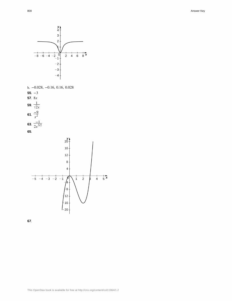
b. −0.028, −0.16, 0.16, 0.02855. −357. 8x
59.12x
61.−9x2
63.−1
2x3/2
65.
67.
800 Answer Key
This OpenStax book is available for free at http://cnx.org/content/col11964/1.2
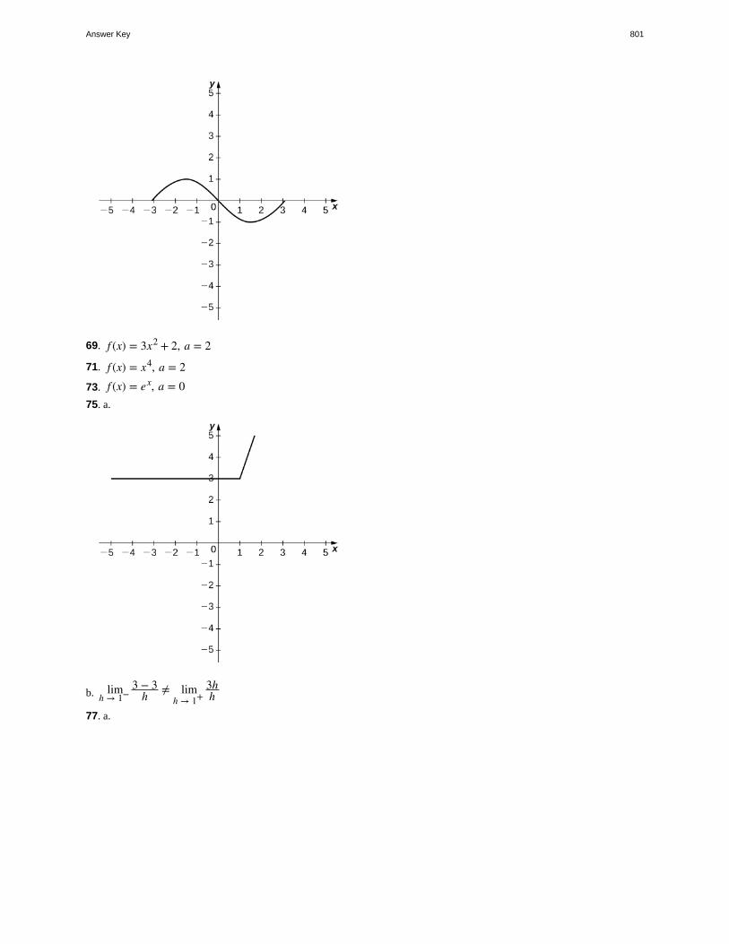
69. f (x) = 3x2 + 2, a = 2
71. f (x) = x4, a = 273. f (x) = ex, a = 075. a.
b. limh → 1−
3 − 3h ≠ lim
h → 1+3hh
77. a.
Answer Key 801
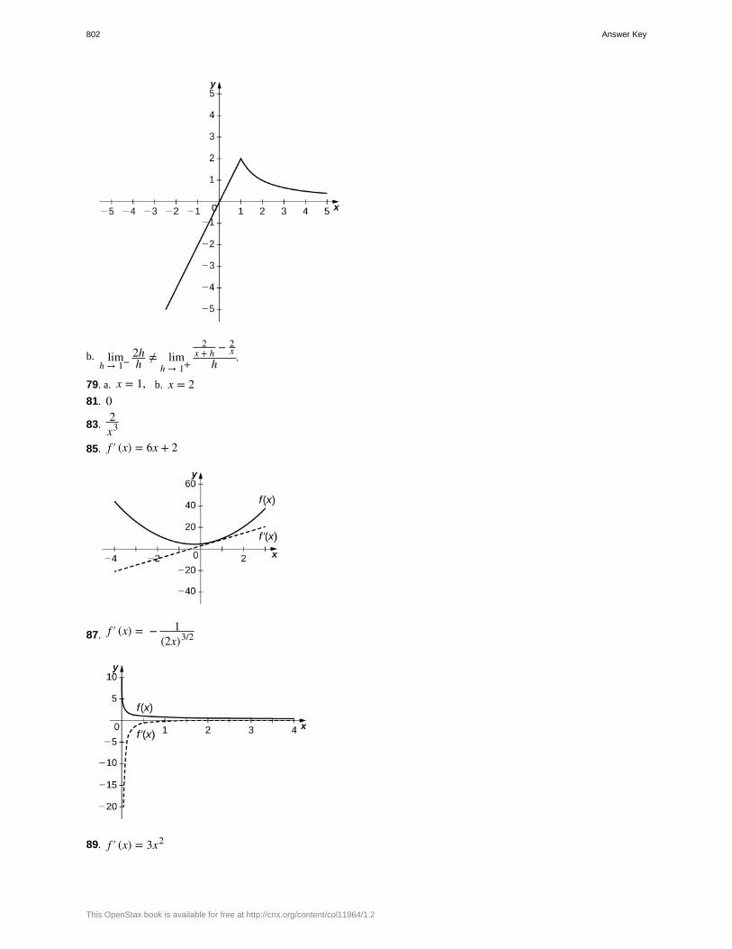
b. limh → 1−
2hh ≠ lim
h → 1+
2x + h − 2
xh .
79. a. x = 1, b. x = 281. 0
83.2x3
85. f ′ (x) = 6x + 2
87. f ′ (x) = − 1(2x)3/2
89. f ′ (x) = 3x2
802 Answer Key
This OpenStax book is available for free at http://cnx.org/content/col11964/1.2
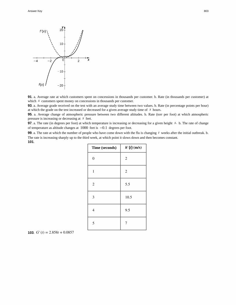
91. a. Average rate at which customers spent on concessions in thousands per customer. b. Rate (in thousands per customer) atwhich x customers spent money on concessions in thousands per customer.93. a. Average grade received on the test with an average study time between two values. b. Rate (in percentage points per hour)at which the grade on the test increased or decreased for a given average study time of x hours.95. a. Average change of atmospheric pressure between two different altitudes. b. Rate (torr per foot) at which atmosphericpressure is increasing or decreasing at x feet.97. a. The rate (in degrees per foot) at which temperature is increasing or decreasing for a given height x. b. The rate of changeof temperature as altitude changes at 1000 feet is −0.1 degrees per foot.
99. a. The rate at which the number of people who have come down with the flu is changing t weeks after the initial outbreak. b.The rate is increasing sharply up to the third week, at which point it slows down and then becomes constant.101.
Time (seconds) h′ (t) (m/s)
0 2
1 2
2 5.5
3 10.5
4 9.5
5 7
103. G′ (t) = 2.858t + 0.0857
Answer Key 803
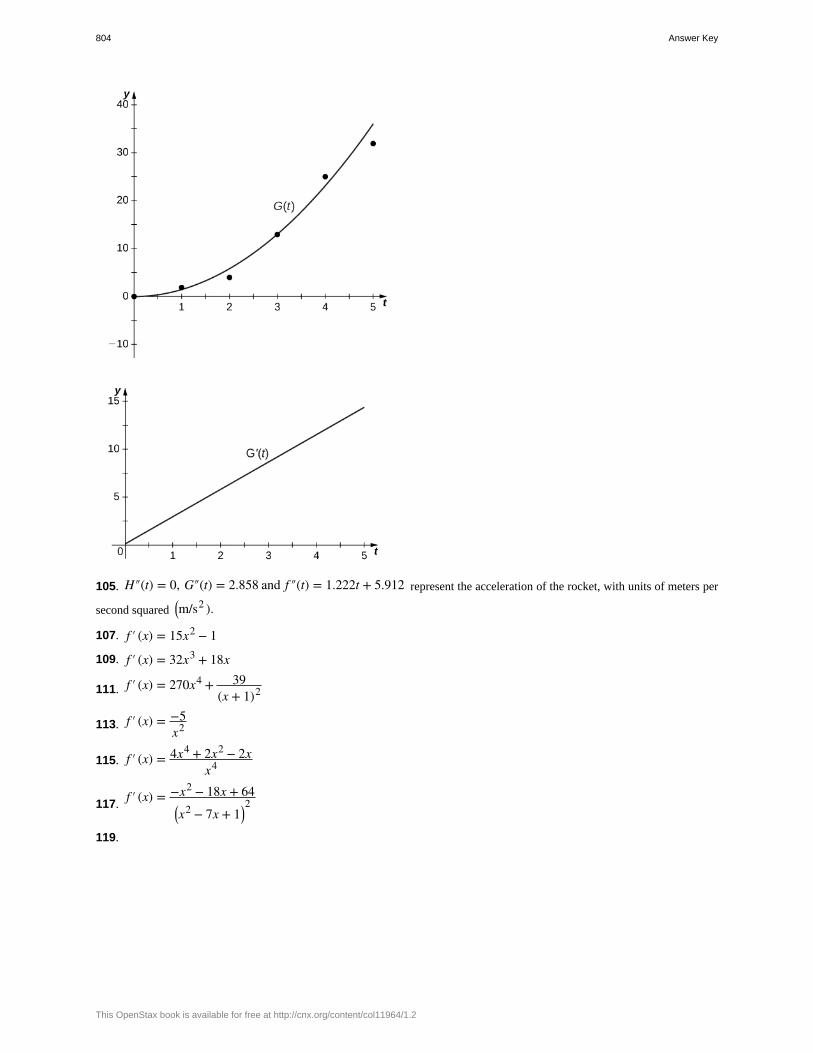
105. H″(t) = 0, G″(t) = 2.858 and f ″(t) = 1.222t + 5.912 represent the acceleration of the rocket, with units of meters per
second squared⎛⎝m/s2 ).
107. f ′ (x) = 15x2 − 1
109. f ′ (x) = 32x3 + 18x
111. f ′ (x) = 270x4 + 39(x + 1)2
113. f ′ (x) = −5x2
115. f ′ (x) = 4x4 + 2x2 − 2xx4
117.f ′ (x) = −x2 − 18x + 64
⎛⎝x2 − 7x + 1⎞
⎠2
119.
804 Answer Key
This OpenStax book is available for free at http://cnx.org/content/col11964/1.2
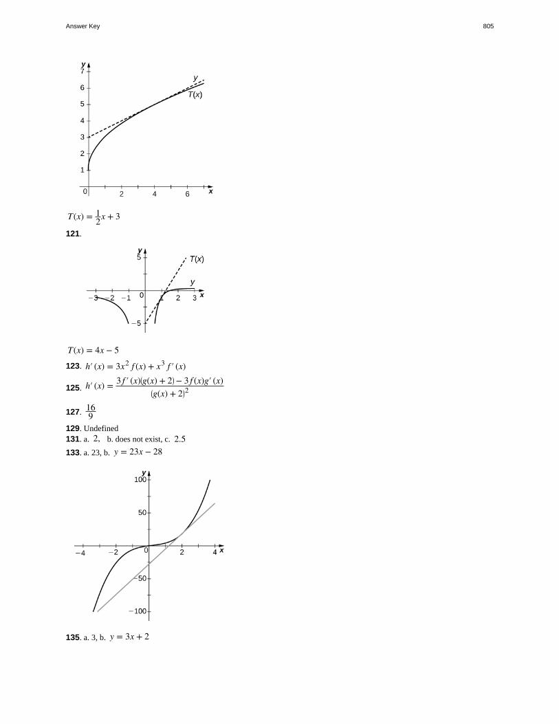
T(x) = 12x + 3
121.
T(x) = 4x − 5
123. h′ (x) = 3x2 f (x) + x3 f ′ (x)
125. h′ (x) = 3 f ′ (x)⎛⎝g(x) + 2⎞
⎠ − 3 f (x)g′ (x)⎛⎝g(x) + 2⎞
⎠2
127. 169
129. Undefined131. a. 2, b. does not exist, c. 2.5133. a. 23, b. y = 23x − 28
135. a. 3, b. y = 3x + 2
Answer Key 805
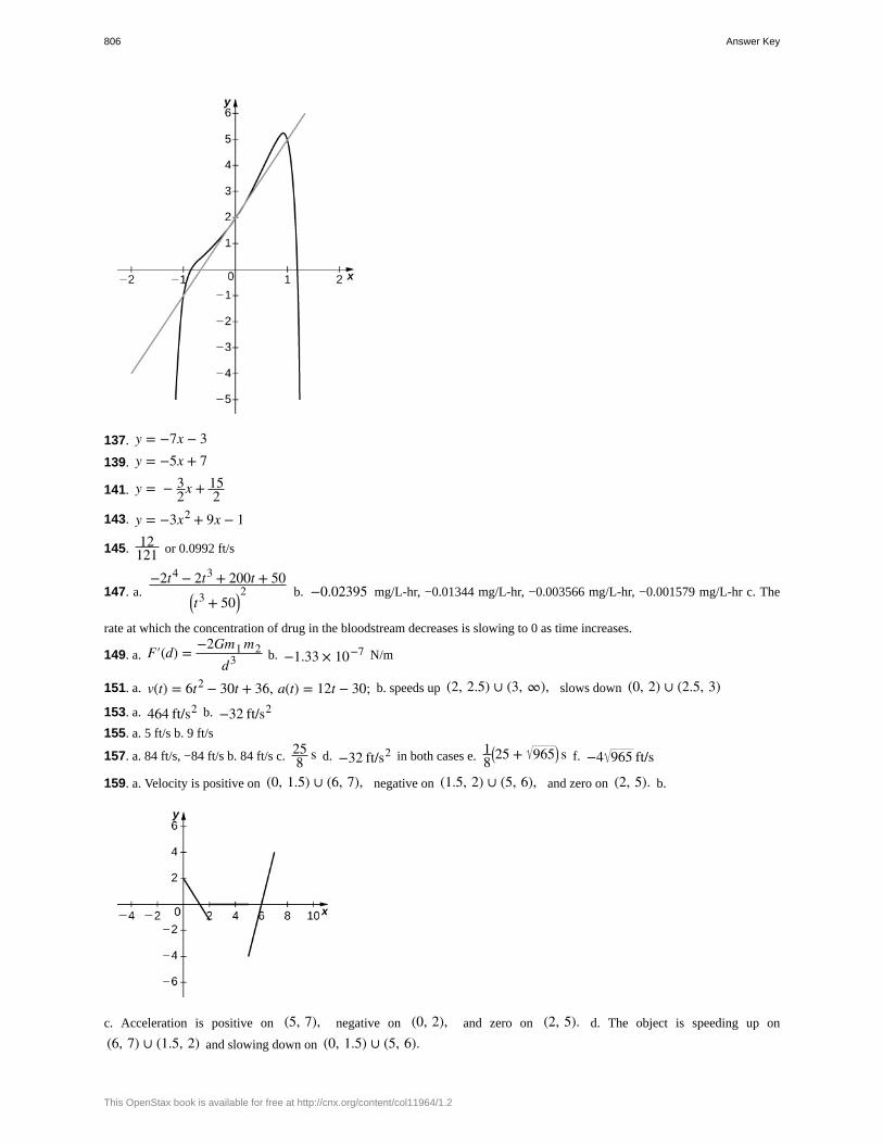
137. y = −7x − 3139. y = −5x + 7
141. y = − 32x + 15
2143. y = −3x2 + 9x − 1
145. 12121 or 0.0992 ft/s
147. a.−2t4 − 2t3 + 200t + 50
⎛⎝t
3 + 50⎞⎠2 b. −0.02395 mg/L-hr, −0.01344 mg/L-hr, −0.003566 mg/L-hr, −0.001579 mg/L-hr c. The
rate at which the concentration of drug in the bloodstream decreases is slowing to 0 as time increases.
149. a. F′(d) = −2Gm1 m2d3 b. −1.33 × 10⁻⁷ N/m
151. a. v(t) = 6t2 − 30t + 36, a(t) = 12t − 30; b. speeds up (2, 2.5) ∪ (3, ∞), slows down (0, 2) ∪ (2.5, 3)
153. a. 464 ft/s2 b. −32 ft/s2
155. a. 5 ft/s b. 9 ft/s
157. a. 84 ft/s, −84 ft/s b. 84 ft/s c. 258 s d. −32 ft/s2 in both cases e. 1
8⎛⎝25 + 965⎞
⎠ s f. −4 965 ft/s
159. a. Velocity is positive on (0, 1.5) ∪ (6, 7), negative on (1.5, 2) ∪ (5, 6), and zero on (2, 5). b.
c. Acceleration is positive on (5, 7), negative on (0, 2), and zero on (2, 5). d. The object is speeding up on
(6, 7) ∪ (1.5, 2) and slowing down on (0, 1.5) ∪ (5, 6).
806 Answer Key
This OpenStax book is available for free at http://cnx.org/content/col11964/1.2
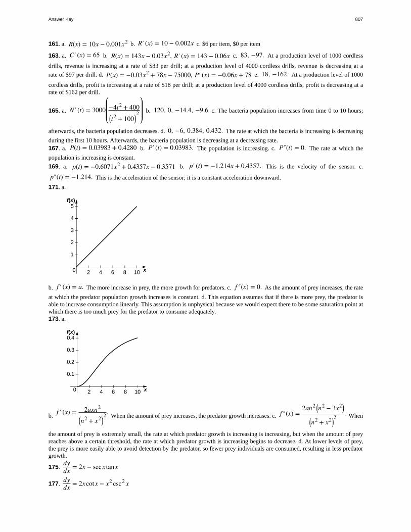
161. a. R(x) = 10x − 0.001x2 b. R′ (x) = 10 − 0.002x c. $6 per item, $0 per item
163. a. C′ (x) = 65 b. R(x) = 143x − 0.03x2, R′ (x) = 143 − 0.06x c. 83, −97. At a production level of 1000 cordless
drills, revenue is increasing at a rate of $83 per drill; at a production level of 4000 cordless drills, revenue is decreasing at a
rate of $97 per drill. d. P(x) = −0.03x2 + 78x − 75000, P′ (x) = −0.06x + 78 e. 18, −162. At a production level of 1000
cordless drills, profit is increasing at a rate of $18 per drill; at a production level of 4000 cordless drills, profit is decreasing at arate of $162 per drill.
165. a. N′ (t) = 3000⎛
⎝⎜⎜−4t2 + 400
⎛⎝t2 + 100⎞
⎠2
⎞
⎠⎟⎟
b. 120, 0, −14.4, −9.6 c. The bacteria population increases from time 0 to 10 hours;
afterwards, the bacteria population decreases. d. 0, −6, 0.384, 0.432. The rate at which the bacteria is increasing is decreasing
during the first 10 hours. Afterwards, the bacteria population is decreasing at a decreasing rate.167. a. P(t) = 0.03983 + 0.4280 b. P′ (t) = 0.03983. The population is increasing. c. P″(t) = 0. The rate at which the
population is increasing is constant.
169. a. p(t) = −0.6071x2 + 0.4357x − 0.3571 b. p′ (t) = −1.214x + 0.4357. This is the velocity of the sensor. c.
p″(t) = −1.214. This is the acceleration of the sensor; it is a constant acceleration downward.
171. a.
b. f ′ (x) = a. The more increase in prey, the more growth for predators. c. f ″(x) = 0. As the amount of prey increases, the rate
at which the predator population growth increases is constant. d. This equation assumes that if there is more prey, the predator isable to increase consumption linearly. This assumption is unphysical because we would expect there to be some saturation point atwhich there is too much prey for the predator to consume adequately.173. a.
b.f ′ (x) = 2axn2
⎛⎝n2 + x2⎞
⎠2.
When the amount of prey increases, the predator growth increases. c. f ″(x) =2an2 ⎛
⎝n2 − 3x2⎞⎠
⎛⎝n2 + x2⎞
⎠3 . When
the amount of prey is extremely small, the rate at which predator growth is increasing is increasing, but when the amount of preyreaches above a certain threshold, the rate at which predator growth is increasing begins to decrease. d. At lower levels of prey,the prey is more easily able to avoid detection by the predator, so fewer prey individuals are consumed, resulting in less predatorgrowth.
175.dydx = 2x − secx tanx
177.dydx = 2xcot x − x2 csc2 x
Answer Key 807
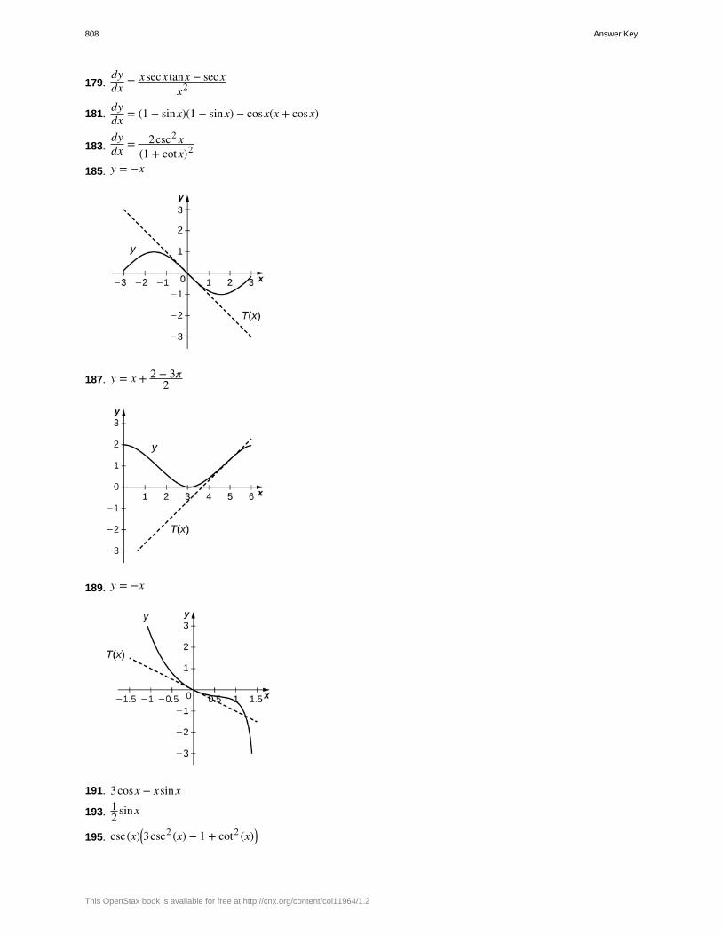
179.dydx = xsecx tanx − secx
x2
181.dydx = (1 − sinx)(1 − sinx) − cosx(x + cosx)
183.dydx = 2csc2 x
(1 + cot x)2
185. y = −x
187. y = x + 2 − 3π2
189. y = −x
191. 3cosx − xsinx
193. 12 sinx
195. csc(x)⎛⎝3csc2 (x) − 1 + cot2 (x)⎞
⎠
808 Answer Key
This OpenStax book is available for free at http://cnx.org/content/col11964/1.2
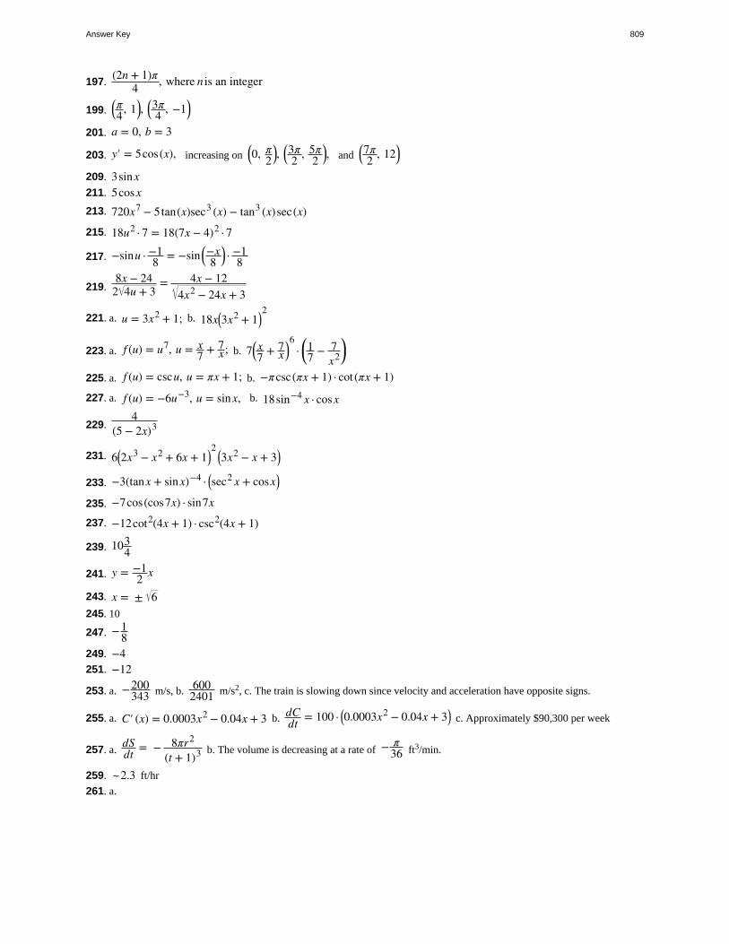
197.(2n + 1)π
4 , where n is an integer
199.⎛⎝π4, 1⎞
⎠,⎛⎝3π4 , −1⎞
⎠
201. a = 0, b = 3
203. y′ = 5cos(x), increasing on⎛⎝0, π
2⎞⎠,
⎛⎝3π2 , 5π
2⎞⎠, and
⎛⎝7π2 , 12⎞
⎠
209. 3sinx211. 5cosx213. 720x7 − 5tan(x)sec3 (x) − tan3 (x)sec(x)
215. 18u2 · 7 = 18(7x − 4)2 · 7
217. −sinu · −18 = −sin⎛
⎝−x8
⎞⎠ · −1
8
219.8x − 24
2 4u + 3= 4x − 12
4x2 − 24x + 3
221. a. u = 3x2 + 1; b. 18x⎛⎝3x2 + 1⎞
⎠2
223. a. f (u) = u7, u = x7 + 7
x; b. 7⎛⎝x7 + 7
x⎞⎠6
· ⎛⎝17 − 7
x2⎞⎠
225. a. f (u) = cscu, u = πx + 1; b. −π csc(πx + 1) · cot (πx + 1)
227. a. f (u) = −6u−3, u = sinx, b. 18sin−4 x · cosx
229.4
(5 − 2x)3
231. 6⎛⎝2x3 − x2 + 6x + 1⎞
⎠2 ⎛
⎝3x2 − x + 3⎞⎠
233. −3(tanx + sinx)−4 · ⎛⎝sec2 x + cosx⎞
⎠
235. −7cos(cos7x) · sin7x
237. −12cot2(4x + 1) · csc2(4x + 1)
239. 1034
241. y = −12 x
243. x = ± 6245. 10
247. −18
249. −4251. −12
253. a. −200343 m/s, b. 600
2401 m/s2, c. The train is slowing down since velocity and acceleration have opposite signs.
255. a. C′ (x) = 0.0003x2 − 0.04x + 3 b. dCdt = 100 · ⎛
⎝0.0003x2 − 0.04x + 3⎞⎠ c. Approximately $90,300 per week
257. a.dSdt = − 8πr2
(t + 1)3 b. The volume is decreasing at a rate of − π36 ft3/min.
259. ~2.3 ft/hr
261. a.
Answer Key 809
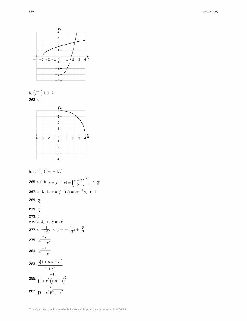
b.⎛⎝ f −1⎞
⎠′ (1)~2
263. a.
b.⎛⎝ f −1⎞
⎠′ (1)~ − 1/ 3
265. a. 6, b. x = f −1 (y) = ⎛⎝y + 3
2⎞⎠
1/3, c. 1
6
267. a. 1, b. x = f −1(y) = sin−1 y, c. 1
269. 15
271. 13
273. 1275. a. 4, b. y = 4x
277. a. − 196, b. y = − 1
13x + 1813
279.2x
1 − x4
281.−1
1 − x2
283. 3⎛⎝1 + tan−1 x⎞
⎠2
1 + x2
285.−1
⎛⎝1 + x2⎞
⎠⎛⎝tan−1 x⎞
⎠2
287.x
⎛⎝5 − x2⎞
⎠ 4 − x2
810 Answer Key
This OpenStax book is available for free at http://cnx.org/content/col11964/1.2
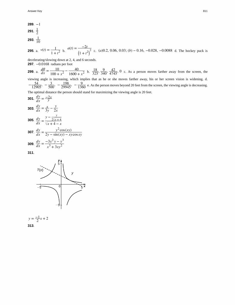
289. −1
291. 12
293. 110
295. a. v(t) = 11 + t2 b.
a(t) = −2t⎛⎝1 + t2⎞
⎠2 c. (a)0.2, 0.06, 0.03; (b) − 0.16, −0.028, −0.0088 d. The hockey puck is
decelerating/slowing down at 2, 4, and 6 seconds.297. −0.0168 radians per foot
299. a.dθdx = 10
100 + x2 − 401600 + x2 b. 18
325, 9340, 42
4745, 0 c. As a person moves farther away from the screen, the
viewing angle is increasing, which implies that as he or she moves farther away, his or her screen vision is widening. d.
− 5412905, − 3
500, − 19829945, − 9
1360 e. As the person moves beyond 20 feet from the screen, the viewing angle is decreasing.
The optimal distance the person should stand for maximizing the viewing angle is 20 feet.
301.dydx = −2x
y
303.dydx = x
3y − y2x
305. dydx =
y − y2 x + 4
x + 4 − x
307.dydx = y2 cos(xy)
2y − sin(xy) − xycosxy
309.dydx = −3x2 y − y3
x3 + 3xy2
311.
y = −12 x + 2
313.
Answer Key 811
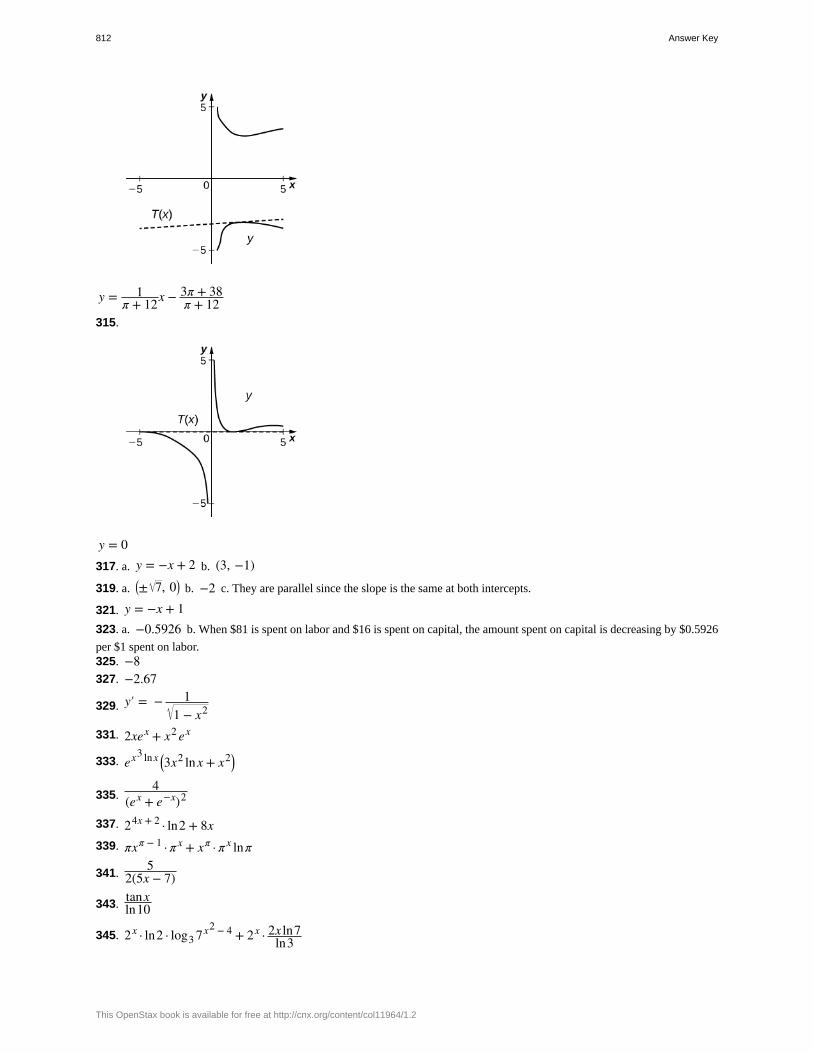
y = 1π + 12x − 3π + 38
π + 12315.
y = 0317. a. y = −x + 2 b. (3, −1)
319. a. ⎛⎝± 7, 0⎞
⎠ b. −2 c. They are parallel since the slope is the same at both intercepts.
321. y = −x + 1323. a. −0.5926 b. When $81 is spent on labor and $16 is spent on capital, the amount spent on capital is decreasing by $0.5926
per $1 spent on labor.325. −8327. −2.67
329. y′ = − 11 − x2
331. 2xex + x2 ex
333. ex3 lnx ⎛⎝3x2 lnx + x2⎞
⎠
335.4
(ex + e−x)2
337. 24x + 2 · ln2 + 8x339. πxπ − 1 · π x + xπ · π x lnπ
341.5
2(5x − 7)
343.tanxln10
345. 2x · ln2 · log3 7x2 − 4 + 2x · 2x ln7ln3
812 Answer Key
This OpenStax book is available for free at http://cnx.org/content/col11964/1.2
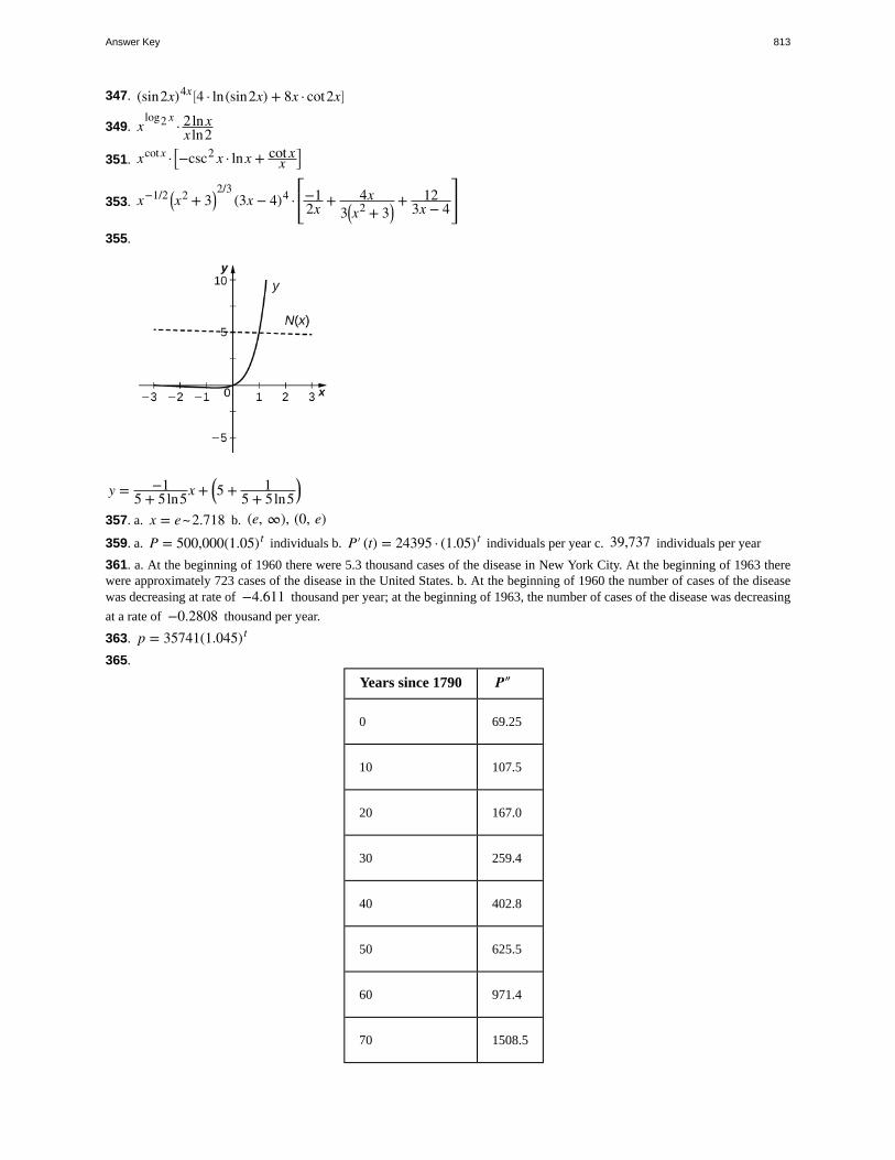
347. (sin2x)4x ⎡⎣4 · ln(sin2x) + 8x · cot2x⎤
⎦
349. xlog2 x
· 2 ln xx ln2
351. xcot x · ⎡⎣−csc2 x · lnx + cot x
x⎤⎦
353. x−1/2 ⎛⎝x2 + 3⎞
⎠2/3
(3x − 4)4 ·⎡
⎣⎢−1
2x + 4x3⎛
⎝x2 + 3⎞⎠
+ 123x − 4
⎤
⎦⎥
355.
y = −15 + 5ln5x + ⎛
⎝5 + 15 + 5ln5
⎞⎠
357. a. x = e~2.718 b. (e, ∞), (0, e)359. a. P = 500,000(1.05)t individuals b. P′ (t) = 24395 · (1.05)t individuals per year c. 39,737 individuals per year
361. a. At the beginning of 1960 there were 5.3 thousand cases of the disease in New York City. At the beginning of 1963 therewere approximately 723 cases of the disease in the United States. b. At the beginning of 1960 the number of cases of the diseasewas decreasing at rate of −4.611 thousand per year; at the beginning of 1963, the number of cases of the disease was decreasing
at a rate of −0.2808 thousand per year.
363. p = 35741(1.045)t
365.
Years since 1790 P″
0 69.25
10 107.5
20 167.0
30 259.4
40 402.8
50 625.5
60 971.4
70 1508.5
Answer Key 813
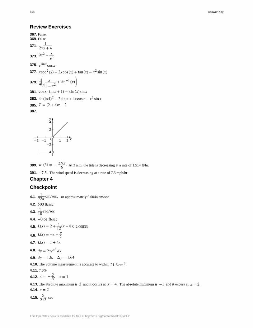
Review Exercises
367. False.369. False
371.1
2 x + 4
373. 9x2 + 8x3
375. esinx cosx377. xsec2 (x) + 2xcos(x) + tan(x) − x2 sin(x)
379. 14
⎛
⎝⎜ x
1 − x2+ sin−1 (x)
⎞
⎠⎟
381. cosx · (lnx + 1) − x ln(x)sinx
383. 4x (ln4)2 + 2sinx + 4xcosx − x2 sinx385. T = (2 + e)x − 2387.
389. w′ (3) = − 2.9π6 . At 3 a.m. the tide is decreasing at a rate of 1.514 ft/hr.
391. −7.5. The wind speed is decreasing at a rate of 7.5 mph/hr
Chapter 4
Checkpoint
4.1. 172π cm/sec, or approximately 0.0044 cm/sec
4.2. 500 ft/sec
4.3. 110 rad/sec
4.4. −0.61 ft/sec
4.5. L(x) = 2 + 112(x − 8); 2.00833
4.6. L(x) = −x + π2
4.7. L(x) = 1 + 4x
4.8. dy = 2xex2dx
4.9. dy = 1.6, Δy = 1.644.10. The volume measurement is accurate to within 21.6 cm3.4.11. 7.6%
4.12. x = − 23, x = 1
4.13. The absolute maximum is 3 and it occurs at x = 4. The absolute minimum is −1 and it occurs at x = 2.4.14. c = 2
4.15.5
2 2 sec
814 Answer Key
This OpenStax book is available for free at http://cnx.org/content/col11964/1.2
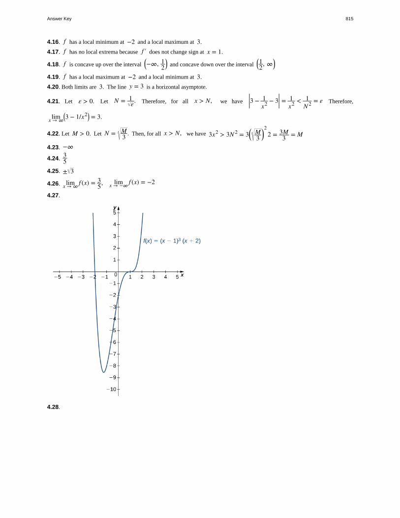
4.16. f has a local minimum at −2 and a local maximum at 3.4.17. f has no local extrema because f ′ does not change sign at x = 1.
4.18. f is concave up over the interval⎛⎝−∞, 1
2⎞⎠ and concave down over the interval
⎛⎝12, ∞⎞
⎠
4.19. f has a local maximum at −2 and a local minimum at 3.4.20. Both limits are 3. The line y = 3 is a horizontal asymptote.
4.21. Let ε > 0. Let N = 1ε. Therefore, for all x > N, we have |3 − 1
x2 − 3| = 1x2 < 1
N 2 = ε Therefore,
limx → ∞⎛⎝3 − 1/x2⎞
⎠ = 3.
4.22. Let M > 0. Let N = M3 . Then, for all x > N, we have 3x2 > 3N 2 = 3⎛
⎝M3
⎞⎠
22 = 3M
3 = M
4.23. −∞
4.24. 35
4.25. ± 3
4.26. limx → ∞ f (x) = 35, limx → −∞ f (x) = −2
4.27.
4.28.
Answer Key 815
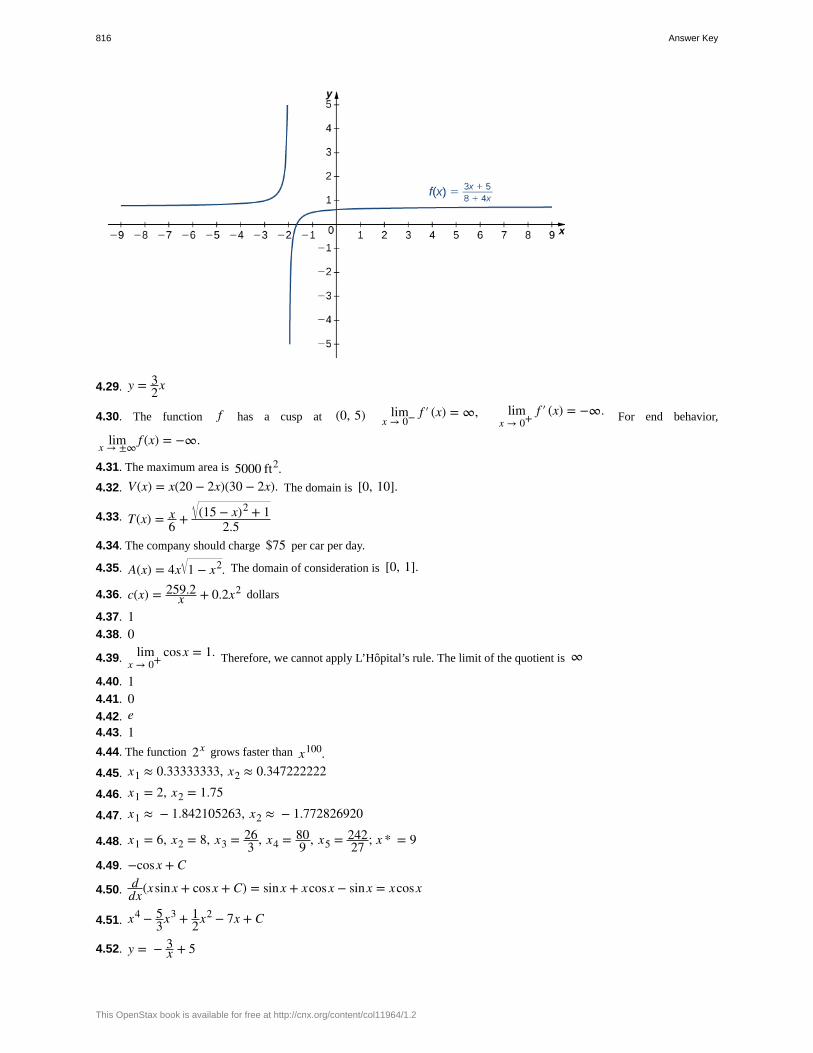
4.29. y = 32x
4.30. The function f has a cusp at (0, 5) limx → 0− f ′ (x) = ∞, lim
x → 0+f ′ (x) = −∞. For end behavior,
limx → ±∞ f (x) = −∞.
4.31. The maximum area is 5000 ft2.4.32. V(x) = x(20 − 2x)(30 − 2x). The domain is [0, 10].
4.33. T(x) = x6 + (15 − x)2 + 1
2.54.34. The company should charge $75 per car per day.
4.35. A(x) = 4x 1 − x2. The domain of consideration is [0, 1].
4.36. c(x) = 259.2x + 0.2x2 dollars
4.37. 14.38. 0
4.39. limx → 0+
cosx = 1. Therefore, we cannot apply L’Hôpital’s rule. The limit of the quotient is ∞
4.40. 14.41. 04.42. e4.43. 14.44. The function 2x grows faster than x100.4.45. x1 ≈ 0.33333333, x2 ≈ 0.347222222
4.46. x1 = 2, x2 = 1.75
4.47. x1 ≈ − 1.842105263, x2 ≈ − 1.772826920
4.48. x1 = 6, x2 = 8, x3 = 263 , x4 = 80
9 , x5 = 24227 ; x * = 9
4.49. −cosx + C
4.50. ddx(xsinx + cosx + C) = sinx + xcosx − sinx = xcosx
4.51. x4 − 53x3 + 1
2x2 − 7x + C
4.52. y = − 3x + 5
816 Answer Key
This OpenStax book is available for free at http://cnx.org/content/col11964/1.2
4.53. 2.93 sec, 64.5 ft
Section Exercises
1. 8
3.1310
5. 2 3 ft/sec
7. The distance is decreasing at 390 mi/h.
9. The distance between them shrinks at a rate of 132013 ≈ 101.5 mph.
11. 92 ft/sec
13. It grows at a rate 49 ft/sec
15. The distance is increasing at⎛⎝135 26⎞
⎠
26ft/sec
17. −56 m/sec
19. 240π m2/sec
21. 12 π cm
23. The area is increasing at a rate⎛⎝3 3⎞
⎠
8 ft /sec.
25. The depth of the water decreases at 128125π ft/min.
27. The volume is decreasing at a rate of(25π)
16 ft3 /min.
29. The water flows out at rate(2π)
5 m /min.
31. 32 m/sec
33. 2519π ft/min
35. 245π ft/min
37. The angle decreases at 4001681 rad/sec.
39. 100π/min
41. The angle is changing at a rate of 2125 rad/sec.
43. The distance is increasing at a rate of 62.50 ft/sec.
45. The distance is decreasing at a rate of 11.99 ft/sec.
47. f ′ (a) = 049. The linear approximation exact when y = f (x) is linear or constant.
51. L(x) = 12 − 1
4(x − 2)
53. L(x) = 155. L(x) = 057. 0.0259. 1.999687561. 0.00159363. 1; error, ~0.0000565. 0.97; error, ~0.0006
Answer Key 817
67. 3 − 1600; error, ~4.632 × 10⁻⁷
69. dy = (cosx − xsinx)dx
71. dy =⎛
⎝⎜x2 − 2x − 2
(x − 1)2
⎞
⎠⎟dx
73. dy = − 1(x + 1)2dx, − 1
16
75. dy = 9x2 + 12x − 22(x + 1)3/2 dx, −0.1
77. dy = ⎛⎝3x2 + 2 − 1
x2⎞⎠dx, 0.2
79. 12xdx81. 4πr2 dr83. −1.2π cm3
85. −100 ft3
91. Answers may vary93. Answers will vary95. No; answers will vary97. Since the absolute maximum is the function (output) value rather than the x value, the answer is no; answers will vary99. When a = 0101. Absolute minimum at 3; Absolute maximum at −2.2; local minima at −2, 1; local maxima at −1, 2103. Absolute minima at −2, 2; absolute maxima at −2.5, 2.5; local minimum at 0; local maxima at −1, 1105. Answers may vary.107. Answers may vary.109. x = 1111. None113. x = 0115. None117. x = −1, 1
119. Absolute maximum: x = 4, y = 332 ; absolute minimum: x = 1, y = 3
121. Absolute minimum: x = 12, y = 4
123. Absolute maximum: x = 2π, y = 2π; absolute minimum: x = 0, y = 0125. Absolute maximum: x = −3; absolute minimum: −1 ≤ x ≤ 1, y = 2
127. Absolute maximum: x = π4, y = 2; absolute minimum: x = 5π
4 , y = − 2
129. Absolute minimum: x = −2, y = 1131. Absolute minimum: x = −3, y = −135; local maximum: x = 0, y = 0; local minimum: x = 1, y = −7
133. Local maximum: x = 1 − 2 2, y = 3 − 4 2; local minimum: x = 1 + 2 2, y = 3 + 4 2
135. Absolute maximum: x = 22 , y = 3
2; absolute minimum: x = − 22 , y = − 3
2137. Local maximum: x = −2, y = 59; local minimum: x = 1, y = −130139. Absolute maximum: x = 0, y = 1; absolute minimum: x = −2, 2, y = 0
141. h = 924549 m, t = 300
49 s
143. The global minimum was in 1848, when no gold was produced.145. Absolute minima: x = 0, x = 2, y = 1; local maximum at x = 1, y = 2147. No maxima/minima if a is odd, minimum at x = 1 if a is even
149. One example is f (x) = |x| + 3, −2 ≤ x ≤ 2151. Yes, but the Mean Value Theorem still does not apply
818 Answer Key
This OpenStax book is available for free at http://cnx.org/content/col11964/1.2

153. (−∞, 0), (0, ∞)155. (−∞, −2), (2, ∞)157. 2 points159. 5 points
161. c = 2 33
163. c = 12, 1, 3
2165. c = 1167. Not differentiable169. Not differentiable171. Yes
173. The Mean Value Theorem does not apply since the function is discontinuous at x = 14, 3
4, 54, 7
4.
175. Yes177. The Mean Value Theorem does not apply; discontinuous at x = 0.179. Yes181. The Mean Value Theorem does not apply; not differentiable at x = 0.183. b = ±2 c
185. c = ±1πcos−1 ⎛
⎝π2
⎞⎠, c = ±0.1533
187. The Mean Value Theorem does not apply.
189.1
2 c + 1− 2
c3 = 5212880; c = 3.133, 5.867
191. Yes193. It is constant.195. It is not a local maximum/minimum because f ′ does not change sign
197. No199. False; for example, y = x.201. Increasing for −2 < x < −1 and x > 2; decreasing for x < −2 and −1 < x < 2203. Decreasing for x < 1, increasing for x > 1205. Decreasing for −2 < x < −1 and 1 < x < 2; increasing for −1 < x < 1 and x < −2 and x > 2207. a. Increasing over −2 < x < −1, 0 < x < 1, x > 2, decreasing over x < −2, −1 < x < 0, 1 < x < 2; b. maxima
at x = −1 and x = 1, minima at x = −2 and x = 0 and x = 2209. a. Increasing over x > 0, decreasing over x < 0; b. Minimum at x = 0211. Concave up on all x, no inflection points
213. Concave up on all x, no inflection points
215. Concave up for x < 0 and x > 1, concave down for 0 < x < 1, inflection points at x = 0 and x = 1217. Answers will vary219. Answers will vary
221. a. Increasing over −π2 < x < π
2, decreasing over x < − π2, x > π
2 b. Local maximum at x = π2; local minimum at
x = − π2
223. a. Concave up for x > 43, concave down for x < 4
3 b. Inflection point at x = 43
225. a. Increasing over x < 0 and x > 4, decreasing over 0 < x < 4 b. Maximum at x = 0, minimum at x = 4 c. Concave
up for x > 2, concave down for x < 2 d. Infection point at x = 2
227. a. Increasing over x < 0 and x > 6011, decreasing over 0 < x < 60
11 b. Minimum at x = 6011 c. Concave down for
x < 5411, concave up for x > 54
11 d. Inflection point at x = 5411
229. a. Increasing over x > − 12, decreasing over x < − 1
2 b. Minimum at x = − 12 c. Concave up for all x d. No inflection
points
Answer Key 819
231. a. Increases over −14 < x < 3
4, decreases over x > 34 and x < − 1
4 b. Minimum at x = − 14, maximum at x = 3
4
c. Concave up for −34 < x < 1
4, concave down for x < − 34 and x > 1
4 d. Inflection points at x = − 34, x = 1
4233. a. Increasing for all x b. No local minimum or maximum c. Concave up for x > 0, concave down for x < 0 d. Inflection
point at x = 0235. a. Increasing for all x where defined b. No local minima or maxima c. Concave up for x < 1; concave down for x > 1 d.
No inflection points in domain
237. a. Increasing over −π4 < x < 3π
4 , decreasing over x > 3π4 , x < − π
4 b. Minimum at x = − π4, maximum at x = 3π
4c. Concave up for −π
2 < x < π2, concave down for x < − π
2, x > π2 d. Infection points at x = ±π
2239. a. Increasing over x > 4, decreasing over 0 < x < 4 b. Minimum at x = 4 c. Concave up for 0 < x < 8 23 , concave
down for x > 8 23 d. Inflection point at x = 8 23
241. f > 0, f ′ > 0, f ″ < 0243. f > 0, f ′ < 0, f ″ < 0245. f > 0, f ′ > 0, f ″ > 0247. True, by the Mean Value Theorem249. True, examine derivative251. x = 1253. x = −1, x = 2255. x = 0257. Yes, there is a vertical asymptote259. Yes, there is vertical asymptote261. 0263. ∞
265. −17
267. −2269. −4271. Horizontal: none, vertical: x = 0273. Horizontal: none, vertical: x = ±2275. Horizontal: none, vertical: none277. Horizontal: y = 0, vertical: x = ±1279. Horizontal: y = 0, vertical: x = 0 and x = −1281. Horizontal: y = 1, vertical: x = 1283. Horizontal: none, vertical: none
285. Answers will vary, for example: y = 2xx − 1
287. Answers will vary, for example: y = 4xx + 1
289. y = 0291. ∞293. y = 3295.
820 Answer Key
This OpenStax book is available for free at http://cnx.org/content/col11964/1.2
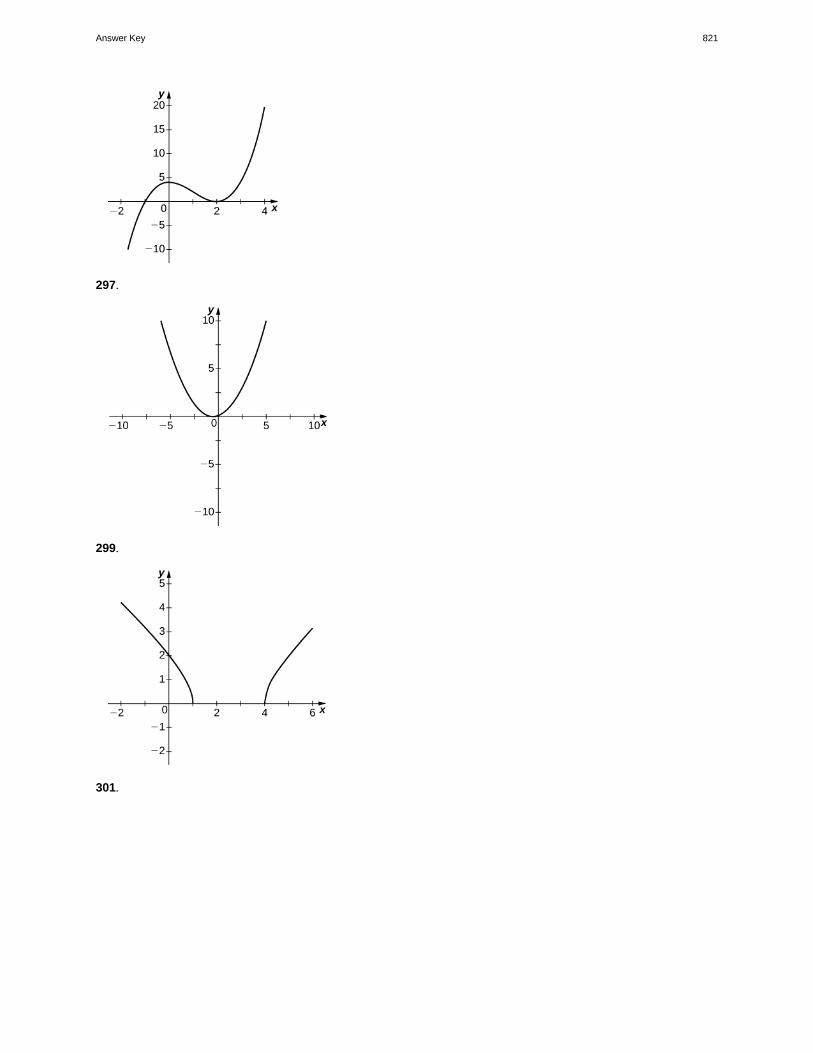
297.
299.
301.
Answer Key 821
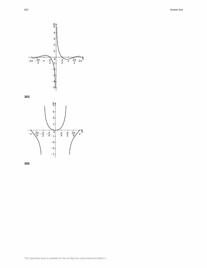
303.
305.
822 Answer Key
This OpenStax book is available for free at http://cnx.org/content/col11964/1.2
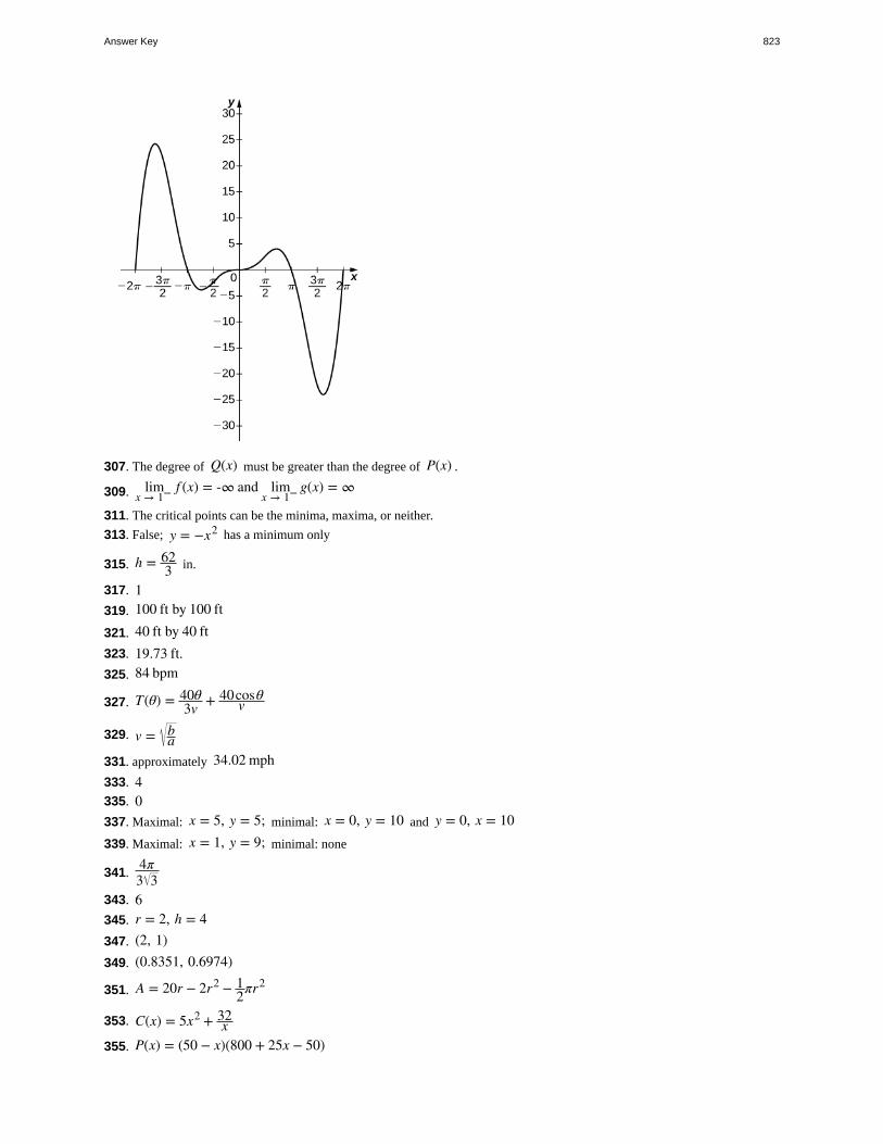
307. The degree of Q(x) must be greater than the degree of P(x) .
309. limx → 1− f (x) = -∞ and lim
x → 1− g(x) = ∞
311. The critical points can be the minima, maxima, or neither.
313. False; y = −x2 has a minimum only
315. h = 623 in.
317. 1319. 100 ft by 100 ft321. 40 ft by 40 ft323. 19.73 ft.325. 84 bpm
327. T(θ) = 40θ3v + 40cosθ
v
329. v = ba
331. approximately 34.02 mph333. 4335. 0337. Maximal: x = 5, y = 5; minimal: x = 0, y = 10 and y = 0, x = 10339. Maximal: x = 1, y = 9; minimal: none
341.4π3 3
343. 6345. r = 2, h = 4347. (2, 1)349. (0.8351, 0.6974)
351. A = 20r − 2r2 − 12πr2
353. C(x) = 5x2 + 32x
355. P(x) = (50 − x)(800 + 25x − 50)
Answer Key 823
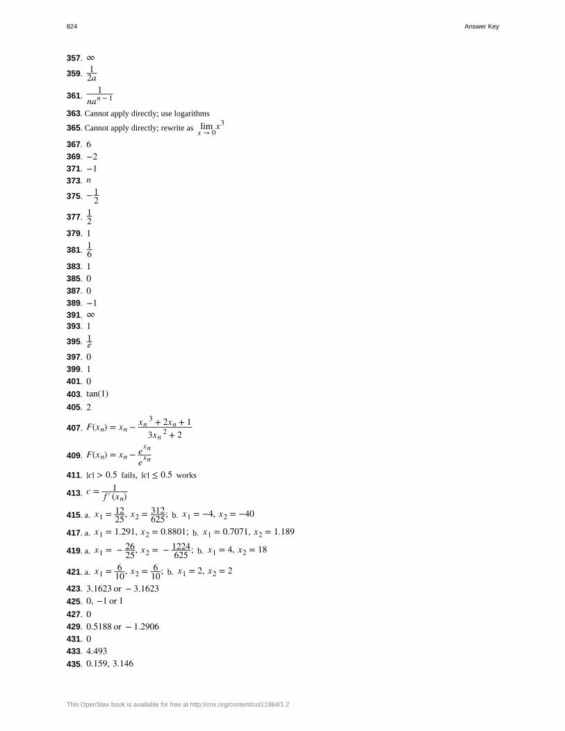
357. ∞
359. 12a
361.1
nan − 1
363. Cannot apply directly; use logarithms
365. Cannot apply directly; rewrite as limx → 0
x3
367. 6369. −2371. −1373. n
375. −12
377. 12
379. 1
381. 16
383. 1385. 0387. 0389. −1391. ∞393. 1395. 1
e397. 0399. 1401. 0403. tan(1)405. 2
407. F(xn) = xn − xn3 + 2xn + 13xn
2 + 2
409. F(xn) = xn − exn
exn
411. |c| > 0.5 fails, |c| ≤ 0.5 works
413. c = 1f ′ (xn)
415. a. x1 = 1225, x2 = 312
625; b. x1 = −4, x2 = −40
417. a. x1 = 1.291, x2 = 0.8801; b. x1 = 0.7071, x2 = 1.189
419. a. x1 = − 2625, x2 = − 1224
625 ; b. x1 = 4, x2 = 18
421. a. x1 = 610, x2 = 6
10; b. x1 = 2, x2 = 2
423. 3.1623 or − 3.1623425. 0, −1 or 1427. 0429. 0.5188 or − 1.2906431. 0433. 4.493435. 0.159, 3.146
824 Answer Key
This OpenStax book is available for free at http://cnx.org/content/col11964/1.2
437. We need f to be twice continuously differentiable.
439. x = 0441. x = −1443. x = 5.619445. x = −1.326447. There is no solution to the equation.449. It enters a cycle.451. 0453. −0.3513455. Newton: 11 iterations, secant: 16 iterations
457. Newton: three iterations, secant: six iterations459. Newton: five iterations, secant: eight iterations461. E = 4.071463. 4.394%465. F′ (x) = 15x2 + 4x + 3
467. F′ (x) = 2xex + x2 ex
469. F′ (x) = ex
471. F(x) = ex − x3 − cos(x) + C
473. F(x) = x2
2 − x − 2cos(2x) + C
475. F(x) = 12x2 + 4x3 + C
477. F(x) = 25( x)5 + C
479. F(x) = 32x2/3 + C
481. F(x) = x + tan(x) + C
483. F(x) = 13sin3 (x) + C
485. F(x) = − 12 cot(x) − 1
x + C
487. F(x) = −secx − 4cscx + C
489. F(x) = − 18e−4x − cosx + C
491. −cosx + C
493. 3x − 2x + C
495. 83x3/2 + 4
5x5/4 + C
497. 14x − 2x − 1
2x2 + C
499. f (x) = − 12x2 + 3
2
501. f (x) = sinx + tanx + 1
503. f (x) = − 16x3 − 2
x + 136
505. Answers may vary; one possible answer is f (x) = e−x
507. Answers may vary; one possible answer is f (x) = −sinx509. 5.867 sec
511. 7.333 sec
513. 13.75 ft/sec2
Answer Key 825
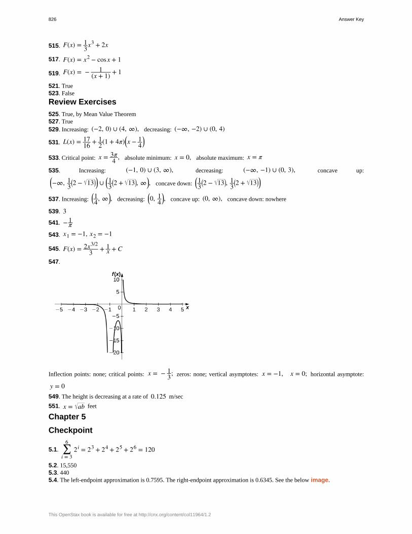
515. F(x) = 13x3 + 2x
517. F(x) = x2 − cosx + 1
519. F(x) = − 1(x + 1) + 1
521. True523. False
Review Exercises
525. True, by Mean Value Theorem527. True529. Increasing: (−2, 0) ∪ (4, ∞), decreasing: (−∞, −2) ∪ (0, 4)
531. L(x) = 1716 + 1
2(1 + 4π)⎛⎝x − 1
4⎞⎠
533. Critical point: x = 3π4 , absolute minimum: x = 0, absolute maximum: x = π
535. Increasing: (−1, 0) ∪ (3, ∞), decreasing: (−∞, −1) ∪ (0, 3), concave up:
⎛⎝−∞, 1
3⎛⎝2 − 13⎞
⎠⎞⎠ ∪ ⎛
⎝13
⎛⎝2 + 13⎞
⎠, ∞⎞⎠, concave down:
⎛⎝13
⎛⎝2 − 13⎞
⎠, 13
⎛⎝2 + 13⎞
⎠⎞⎠
537. Increasing:⎛⎝14, ∞⎞
⎠, decreasing:⎛⎝0, 1
4⎞⎠, concave up: (0, ∞), concave down: nowhere
539. 3
541. − 1π
543. x1 = −1, x2 = −1
545. F(x) = 2x3/2
3 + 1x + C
547.
Inflection points: none; critical points: x = − 13; zeros: none; vertical asymptotes: x = −1, x = 0; horizontal asymptote:
y = 0549. The height is decreasing at a rate of 0.125 m/sec
551. x = ab feet
Chapter 5
Checkpoint
5.1. ∑i = 3
62i = 23 + 24 + 25 + 26 = 120
5.2. 15,5505.3. 4405.4. The left-endpoint approximation is 0.7595. The right-endpoint approximation is 0.6345. See the below image.
826 Answer Key
This OpenStax book is available for free at http://cnx.org/content/col11964/1.2
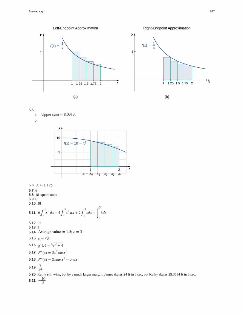
5.5.a. Upper sum = 8.0313.b.
5.6. A ≈ 1.1255.7. 65.8. 18 square units5.9. 65.10. 18
5.11. 6∫1
3x3 dx − 4∫
1
3x2 dx + 2∫
1
3xdx − ⌠
⌡1
3
3dx
5.12. −75.13. 35.14. Average value = 1.5; c = 35.15. c = 35.16. g′ (r) = r2 + 4
5.17. F′ (x) = 3x2 cosx3
5.18. F′ (x) = 2xcosx2 − cosx
5.19. 724
5.20. Kathy still wins, but by a much larger margin: James skates 24 ft in 3 sec, but Kathy skates 29.3634 ft in 3 sec.
5.21. −103
Answer Key 827
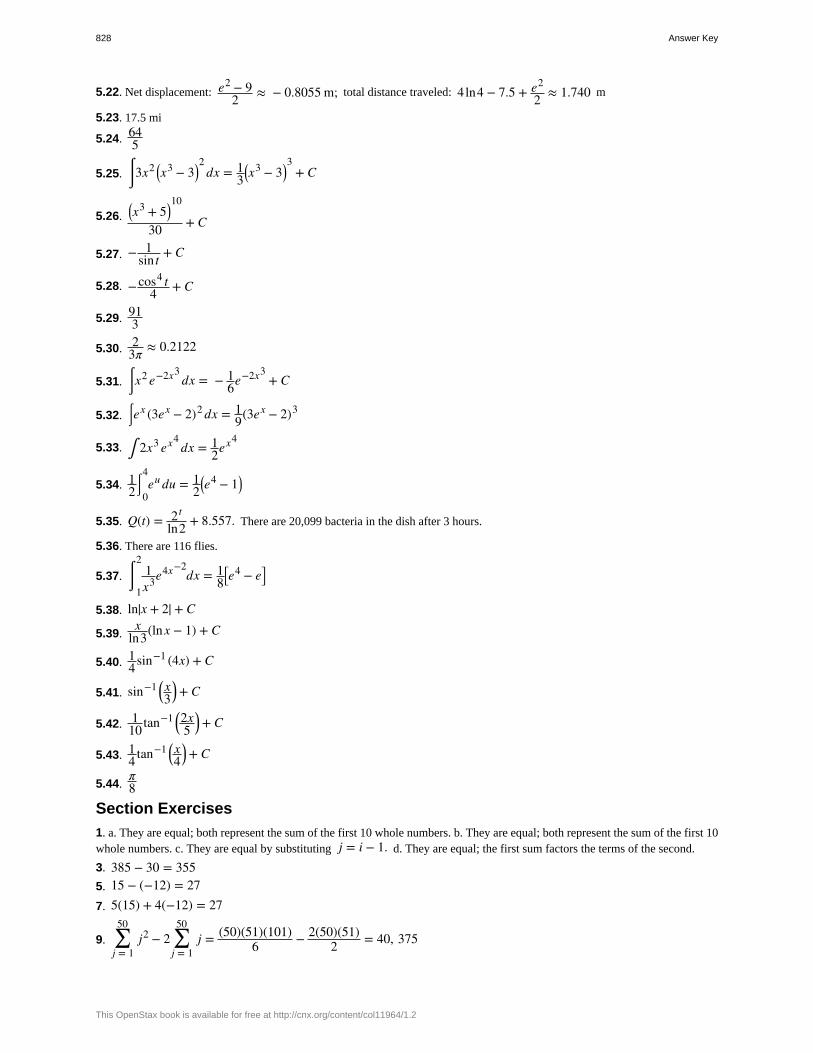
5.22. Net displacement: e2 − 92 ≈ − 0.8055 m; total distance traveled: 4ln4 − 7.5 + e2
2 ≈ 1.740 m
5.23. 17.5 mi
5.24. 645
5.25. ⌠⌡
3x2 ⎛⎝x
3 − 3⎞⎠2
dx = 13
⎛⎝x
3 − 3⎞⎠3
+ C
5.26.⎛⎝x
3 + 5⎞⎠10
30 + C
5.27. − 1sin t + C
5.28. −cos4 t4 + C
5.29. 913
5.30. 23π ≈ 0.2122
5.31. ⌠⌡
x2 e−2x3dx = − 1
6e−2x3+ C
5.32. ⌠⌡ex (3ex − 2)2 dx = 1
9(3ex − 2)3
5.33. ∫ 2x3 ex4dx = 1
2ex4
5.34. 12
⌠⌡0
4eu du = 1
2⎛⎝e4 − 1⎞
⎠
5.35. Q(t) = 2t
ln2 + 8.557. There are 20,099 bacteria in the dish after 3 hours.
5.36. There are 116 flies.
5.37. ⌠⌡1
21x3e4x−2
dx = 18
⎡⎣e4 − e⎤
⎦
5.38. ln|x + 2| + C
5.39.x
ln3(lnx − 1) + C
5.40. 14sin−1 (4x) + C
5.41. sin−1 ⎛⎝x3
⎞⎠ + C
5.42. 110tan−1 ⎛
⎝2x5
⎞⎠ + C
5.43. 14tan−1 ⎛
⎝x4
⎞⎠ + C
5.44.π8
Section Exercises
1. a. They are equal; both represent the sum of the first 10 whole numbers. b. They are equal; both represent the sum of the first 10whole numbers. c. They are equal by substituting j = i − 1. d. They are equal; the first sum factors the terms of the second.
3. 385 − 30 = 3555. 15 − (−12) = 277. 5(15) + 4(−12) = 27
9. ∑j = 1
50j2 − 2 ∑
j = 1
50j = (50)(51)(101)
6 − 2(50)(51)2 = 40, 375
828 Answer Key
This OpenStax book is available for free at http://cnx.org/content/col11964/1.2
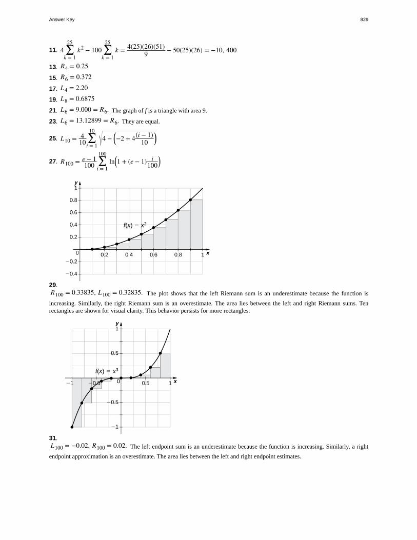
11. 4 ∑k = 1
25k2 − 100 ∑
k = 1
25k = 4(25)(26)(51)
9 − 50(25)(26) = −10, 400
13. R4 = 0.25
15. R6 = 0.372
17. L4 = 2.20
19. L8 = 0.6875
21. L6 = 9.000 = R6. The graph of f is a triangle with area 9.
23. L6 = 13.12899 = R6. They are equal.
25. L10 = 410 ∑
i = 1
104 − ⎛
⎝−2 + 4(i − 1)10
⎞⎠
27. R100 = e − 1100 ∑
i = 1
100ln⎛
⎝1 + (e − 1) i100
⎞⎠
29.R100 = 0.33835, L100 = 0.32835. The plot shows that the left Riemann sum is an underestimate because the function is
increasing. Similarly, the right Riemann sum is an overestimate. The area lies between the left and right Riemann sums. Tenrectangles are shown for visual clarity. This behavior persists for more rectangles.
31.L100 = −0.02, R100 = 0.02. The left endpoint sum is an underestimate because the function is increasing. Similarly, a right
endpoint approximation is an overestimate. The area lies between the left and right endpoint estimates.
Answer Key 829
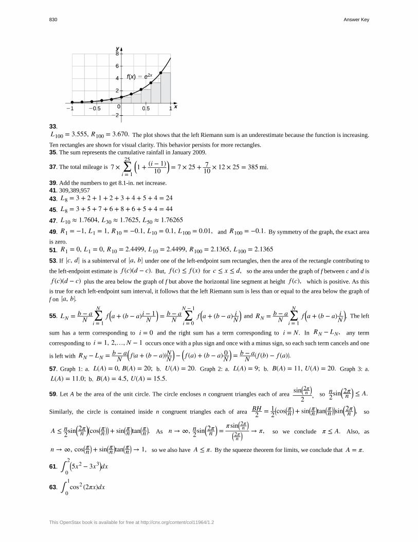
33.L100 = 3.555, R100 = 3.670. The plot shows that the left Riemann sum is an underestimate because the function is increasing.
Ten rectangles are shown for visual clarity. This behavior persists for more rectangles.35. The sum represents the cumulative rainfall in January 2009.
37. The total mileage is 7 × ∑i = 1
25 ⎛⎝1 + (i − 1)
10⎞⎠ = 7 × 25 + 7
10 × 12 × 25 = 385 mi.
39. Add the numbers to get 8.1-in. net increase.41. 309,389,95743. L8 = 3 + 2 + 1 + 2 + 3 + 4 + 5 + 4 = 24
45. L8 = 3 + 5 + 7 + 6 + 8 + 6 + 5 + 4 = 44
47. L10 ≈ 1.7604, L30 ≈ 1.7625, L50 ≈ 1.76265
49. R1 = −1, L1 = 1, R10 = −0.1, L10 = 0.1, L100 = 0.01, and R100 = −0.1. By symmetry of the graph, the exact area
is zero.51. R1 = 0, L1 = 0, R10 = 2.4499, L10 = 2.4499, R100 = 2.1365, L100 = 2.1365
53. If ⎡⎣c, d⎤
⎦ is a subinterval of ⎡⎣a, b⎤
⎦ under one of the left-endpoint sum rectangles, then the area of the rectangle contributing to
the left-endpoint estimate is f (c)(d − c). But, f (c) ≤ f (x) for c ≤ x ≤ d, so the area under the graph of f between c and d is
f (c)(d − c) plus the area below the graph of f but above the horizontal line segment at height f (c), which is positive. As this
is true for each left-endpoint sum interval, it follows that the left Riemann sum is less than or equal to the area below the graph off on ⎡
⎣a, b⎤⎦.
55. LN = b − aN ∑
i = 1
Nf ⎛
⎝a + (b − a)i − 1N
⎞⎠ = b − a
N ∑i = 0
N − 1f ⎛
⎝a + (b − a) iN
⎞⎠ and RN = b − a
N ∑i = 1
Nf ⎛
⎝a + (b − a) iN
⎞⎠. The left
sum has a term corresponding to i = 0 and the right sum has a term corresponding to i = N. In RN − LN, any term
corresponding to i = 1, 2,…, N − 1 occurs once with a plus sign and once with a minus sign, so each such term cancels and one
is left with RN − LN = b − aN
⎛⎝ f ⎛
⎝a + (b − a)⎞⎠NN
⎞⎠ − ⎛
⎝ f (a) + (b − a) 0N
⎞⎠ = b − a
N⎛⎝ f (b) − f (a)⎞
⎠.
57. Graph 1: a. L(A) = 0, B(A) = 20; b. U(A) = 20. Graph 2: a. L(A) = 9; b. B(A) = 11, U(A) = 20. Graph 3: a.
L(A) = 11.0; b. B(A) = 4.5, U(A) = 15.5.
59. Let A be the area of the unit circle. The circle encloses n congruent triangles each of areasin⎛
⎝2πn
⎞⎠
2 , so n2sin⎛
⎝2πn
⎞⎠ ≤ A.
Similarly, the circle is contained inside n congruent triangles each of area BH2 = 1
2⎛⎝cos⎛
⎝πn
⎞⎠ + sin⎛
⎝πn
⎞⎠tan⎛
⎝πn
⎞⎠⎞⎠sin⎛
⎝2πn
⎞⎠, so
A ≤ n2sin⎛
⎝2πn
⎞⎠
⎛⎝cos⎛
⎝πn
⎞⎠⎞⎠ + sin⎛
⎝πn
⎞⎠tan⎛
⎝πn
⎞⎠. As n → ∞, n
2sin⎛⎝2πn
⎞⎠ =
π sin⎛⎝2πn
⎞⎠
⎛⎝2πn
⎞⎠
→ π, so we conclude π ≤ A. Also, as
n → ∞, cos⎛⎝πn
⎞⎠ + sin⎛
⎝πn
⎞⎠tan⎛
⎝πn
⎞⎠ → 1, so we also have A ≤ π. By the squeeze theorem for limits, we conclude that A = π.
61. ∫0
2⎛⎝5x2 − 3x3⎞
⎠dx
63. ∫0
1cos2 (2πx)dx
830 Answer Key
This OpenStax book is available for free at http://cnx.org/content/col11964/1.2
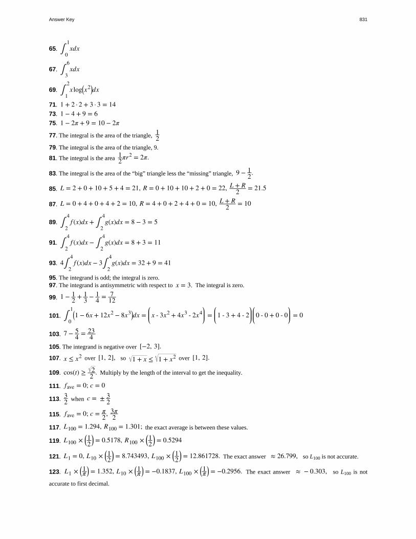
65. ∫0
1xdx
67. ∫3
6xdx
69. ∫1
2x log⎛
⎝x2⎞⎠dx
71. 1 + 2 · 2 + 3 · 3 = 1473. 1 − 4 + 9 = 675. 1 − 2π + 9 = 10 − 2π
77. The integral is the area of the triangle, 12
79. The integral is the area of the triangle, 9.
81. The integral is the area 12πr2 = 2π.
83. The integral is the area of the “big” triangle less the “missing” triangle, 9 − 12.
85. L = 2 + 0 + 10 + 5 + 4 = 21, R = 0 + 10 + 10 + 2 + 0 = 22, L + R2 = 21.5
87. L = 0 + 4 + 0 + 4 + 2 = 10, R = 4 + 0 + 2 + 4 + 0 = 10, L + R2 = 10
89. ∫2
4f (x)dx + ∫
2
4g(x)dx = 8 − 3 = 5
91. ∫2
4f (x)dx − ∫
2
4g(x)dx = 8 + 3 = 11
93. 4∫2
4f (x)dx − 3∫
2
4g(x)dx = 32 + 9 = 41
95. The integrand is odd; the integral is zero.97. The integrand is antisymmetric with respect to x = 3. The integral is zero.
99. 1 − 12 + 1
3 − 14 = 7
12
101. ∫0
1⎛⎝1 − 6x + 12x2 − 8x3⎞
⎠dx =⎛
⎝⎜ x - 3x2 + 4x3 - 2x4⎞
⎠⎟ =
⎛
⎝⎜ 1 - 3 + 4 - 2
⎞
⎠⎟
⎛
⎝⎜ 0 - 0 + 0 - 0
⎞
⎠⎟ = 0
103. 7 − 54 = 23
4105. The integrand is negative over [−2, 3].
107. x ≤ x2 over [1, 2], so 1 + x ≤ 1 + x2 over [1, 2].
109. cos(t) ≥ 22 . Multiply by the length of the interval to get the inequality.
111. fave = 0; c = 0
113. 32 when c = ± 3
2
115. fave = 0; c = π2, 3π
2117. L100 = 1.294, R100 = 1.301; the exact average is between these values.
119. L100 × ⎛⎝12
⎞⎠ = 0.5178, R100 × ⎛
⎝12
⎞⎠ = 0.5294
121. L1 = 0, L10 × ⎛⎝12
⎞⎠ = 8.743493, L100 × ⎛
⎝12
⎞⎠ = 12.861728. The exact answer ≈ 26.799, so L100 is not accurate.
123. L1 × ⎛⎝1π
⎞⎠ = 1.352, L10 × ⎛
⎝1π
⎞⎠ = −0.1837, L100 × ⎛
⎝1π
⎞⎠ = −0.2956. The exact answer ≈ − 0.303, so L100 is not
accurate to first decimal.
Answer Key 831
125. Use tan2 θ + 1 = sec2 θ. Then, B − A = ∫−π/4
π/41dx = π
2.
127. ∫0
2πcos2 tdt = π, so divide by the length 2π of the interval. cos2 t has period π, so yes, it is true.
129. The integral is maximized when one uses the largest interval on which p is nonnegative. Thus, A = −b − b2 − 4ac2a
and
B = −b + b2 − 4ac2a .
131. If f (t0) > g(t0) for some t0 ∈ ⎡⎣a, b⎤
⎦, then since f − g is continuous, there is an interval containing t0 such that
f (t) > g(t) over the interval ⎡⎣c, d⎤
⎦, and then ∫d
df (t)dt > ∫
c
dg(t)dt over this interval.
133. The integral of f over an interval is the same as the integral of the average of f over that interval. Thus,
∫a
bf (t)dt = ∫
a0
a1f (t)dt + ∫
a1
a2f (t)dt + ⋯ + ∫
aN + 1
aNf (t)dt = ∫
a0
a11dt + ∫
a1
a21dt + ⋯ + ∫
aN + 1
aN1dt
= (a1 − a0) + (a2 − a1) + ⋯ + (aN − aN − 1) = aN − a0 = b − a.Dividing through
by b − a gives the desired identity.
135. ∫0
Nf (t)dt = ∑
i = 1
N∫
i − 1
if (t)dt = ∑
i = 1
Ni2 = N(N + 1)(2N + 1)
6
137. L10 = 1.815, R10 = 1.515, L10 + R102 = 1.665, so the estimate is accurate to two decimal places.
139. The average is 1/2, which is equal to the integral in this case.
141. a. The graph is antisymmetric with respect to t = 12 over [0, 1], so the average value is zero. b. For any value of a, the
graph between [a, a + 1] is a shift of the graph over [0, 1], so the net areas above and below the axis do not change and the
average remains zero.143. Yes, the integral over any interval of length 1 is the same.145. Yes. It is implied by the Mean Value Theorem for Integrals.147. F′ (2) = −1; average value of F ′ over [1, 2] is −1/2.149. ecos t
151.1
16 − x2
153. x ddx x = 1
2
155. − 1 − cos2 x ddxcosx = |sinx|sinx
157. 2x |x|1 + x2
159. ln(e2x) ddxex = 2xex
161. a. f is positive over [1, 2] and ⎡⎣5, 6⎤
⎦, negative over [0, 1] and [3, 4], and zero over [2, 3] and ⎡⎣4, 5⎤
⎦. b. The
maximum value is 2 and the minimum is −3. c. The average value is 0.163. a. ℓ is positive over [0, 1] and ⎡
⎣3, 6⎤⎦, and negative over [1, 3]. b. It is increasing over [0, 1] and ⎡
⎣3, 5⎤⎦, and it is
constant over [1, 3] and ⎡⎣5, 6⎤
⎦. c. Its average value is 13.
165. T10 = 49.08, ∫−2
3x3 + 6x2 + x − 5dx = 48
167. T10 = 260.836, ∫1
9⎛⎝ x + x2⎞
⎠dx = 260
832 Answer Key
This OpenStax book is available for free at http://cnx.org/content/col11964/1.2
169. T10 = 3.058, ⌠⌡1
44x2dx = 3
171. F(x) = x3
3 + 3x2
2 − 5x, F(3) − F(−2) = − 356
173. F(x) = − t5
5 + 13t3
3 − 36t, F(3) − F(2) = 6215
175. F(x) = x100
100 , F(1) − F(0) = 1100
177. F(x) = x3
3 + 1x , F(4) − F⎛
⎝14
⎞⎠ = 1125
64179. F(x) = x, F(4) − F(1) = 1
181. F(x) = 43t3/4, F(16) − F(1) = 28
3
183. F(x) = −cosx, F⎛⎝π2
⎞⎠ − F(0) = 1
185. F(x) = secx, F⎛⎝π4
⎞⎠ − F(0) = 2 − 1
187. F(x) = −cot(x), F⎛⎝π2
⎞⎠ − F⎛
⎝π4
⎞⎠ = 1
189. F(x) = − 1x + 1
2x2, F(−1) − F(−2) = 78
191. F(x) = ex − e193. F(x) = 0
195. ∫−2
−1⎛⎝t2 − 2t − 3⎞
⎠dt − ∫−1
3⎛⎝t2 − 2t − 3⎞
⎠dt + ∫3
4⎛⎝t2 − 2t − 3⎞
⎠dt = 463
197. −⌠⌡−π/2
0
sin tdt + ∫0
π/2sin tdt = 2
199. a. The average is 11.21 × 10⁹ since cos⎛⎝πt6
⎞⎠ has period 12 and integral 0 over any period. Consumption is equal to
the average when cos⎛⎝πt6
⎞⎠ = 0, when t = 3, and when t = 9. b. Total consumption is the average rate times duration:
11.21 × 12 × 109 = 1.35 × 10¹¹ c. 109⎛
⎝⎜11.21 − 1
6⌠⌡3
9cos⎛
⎝πt6
⎞⎠dt
⎞
⎠⎟ = 109 ⎛
⎝11.21 + 2π
⎞⎠ = 11.84x10⁹
201. If f is not constant, then its average is strictly smaller than the maximum and larger than the minimum, which are attainedover ⎡
⎣a, b⎤⎦ by the extreme value theorem.
203. a. d2 θ = (acosθ + c)2 + b2 sin2 θ = a2 + c2 cos2 θ + 2accosθ = (a + ccosθ)2; b.
d–
= 12π∫
0
2π(a + 2ccosθ)dθ = a
205. Mean gravitational force = GmM2
⌠
⌡⎮⎮
0
2π
1⎛⎝a + 2 a2 − b2cosθ⎞
⎠2dθ.
207. ∫ ⎛⎝ x − 1
x⎞⎠dx = ∫ x1/2 dx − ∫ x−1/2 dx = 2
3x3/2 + C1 − 2x1/2 + C2 = 23x3/2 − 2x1/2 + C
209. ⌠⌡dx2x = 1
2ln|x| + C
211. ⌠⌡0
πsinxdx − ∫
0
πcosxdx = −cosx|0
π − (sinx)|0π = ⎛
⎝−(−1) + 1⎞⎠ − (0 − 0) = 2
Answer Key 833
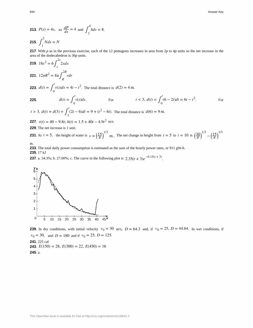
213. P(s) = 4s, so dPds = 4 and ∫
2
44ds = 8.
215. ∫1
2Nds = N
217. With p as in the previous exercise, each of the 12 pentagons increases in area from 2p to 4p units so the net increase in thearea of the dodecahedron is 36p units.
219. 18s2 = 6∫s
2s2xdx
221. 12πR2 = 8π∫R
2Rrdr
223. d(t) = ∫0
tv(s)ds = 4t − t2. The total distance is d(2) = 4 m.
225. d(t) = ∫0
tv(s)ds. For t < 3, d(t) = ∫
0
t(6 − 2t)dt = 6t − t2. For
t > 3, d(t) = d(3) + ∫3
t(2t − 6)dt = 9 + (t2 − 6t). The total distance is d(6) = 9 m.
227. v(t) = 40 − 9.8t; h(t) = 1.5 + 40t − 4.9t2 m/s
229. The net increase is 1 unit.
231. At t = 5, the height of water is x = ⎛⎝15π
⎞⎠1/3
m.. The net change in height from t = 5 to t = 10 is ⎛⎝30π
⎞⎠1/3
− ⎛⎝15π
⎞⎠1/3
m.233. The total daily power consumption is estimated as the sum of the hourly power rates, or 911 gW-h.235. 17 kJ
237. a. 54.3%; b. 27.00%; c. The curve in the following plot is 2.35(t + 3)e−0.15(t + 3).
239. In dry conditions, with initial velocity v0 = 30 m/s, D = 64.3 and, if v0 = 25, D = 44.64. In wet conditions, if
v0 = 30, and D = 180 and if v0 = 25, D = 125.241. 225 cal243. E(150) = 28, E(300) = 22, E(450) = 16245. a.
834 Answer Key
This OpenStax book is available for free at http://cnx.org/content/col11964/1.2
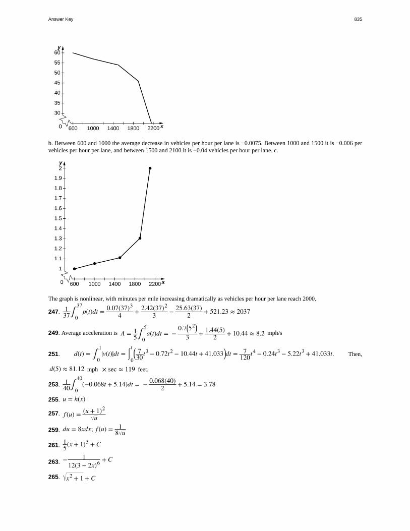
b. Between 600 and 1000 the average decrease in vehicles per hour per lane is −0.0075. Between 1000 and 1500 it is −0.006 pervehicles per hour per lane, and between 1500 and 2100 it is −0.04 vehicles per hour per lane. c.
The graph is nonlinear, with minutes per mile increasing dramatically as vehicles per hour per lane reach 2000.
247. 137∫
0
37p(t)dt = 0.07(37)3
4 + 2.42(37)2
3 − 25.63(37)2 + 521.23 ≈ 2037
249. Average acceleration is A = 15∫
0
5a(t)dt = −
0.7⎛⎝52⎞
⎠3 + 1.44(5)
2 + 10.44 ≈ 8.2 mph/s
251. d(t) = ∫0
1|v(t)|dt = ⌠
⌡0
t ⎛⎝
730t3 − 0.72t2 − 10.44t + 41.033⎞
⎠dt = 7120t4 − 0.24t3 − 5.22t3 + 41.033t. Then,
d(5) ≈ 81.12 mph × sec ≈ 119 feet.
253. 140∫
0
40(−0.068t + 5.14)dt = − 0.068(40)
2 + 5.14 = 3.78
255. u = h(x)
257. f (u) = (u + 1)2
u
259. du = 8xdx; f (u) = 18 u
261. 15(x + 1)5 + C
263. − 112(3 − 2x)6 + C
265. x2 + 1 + C
Answer Key 835
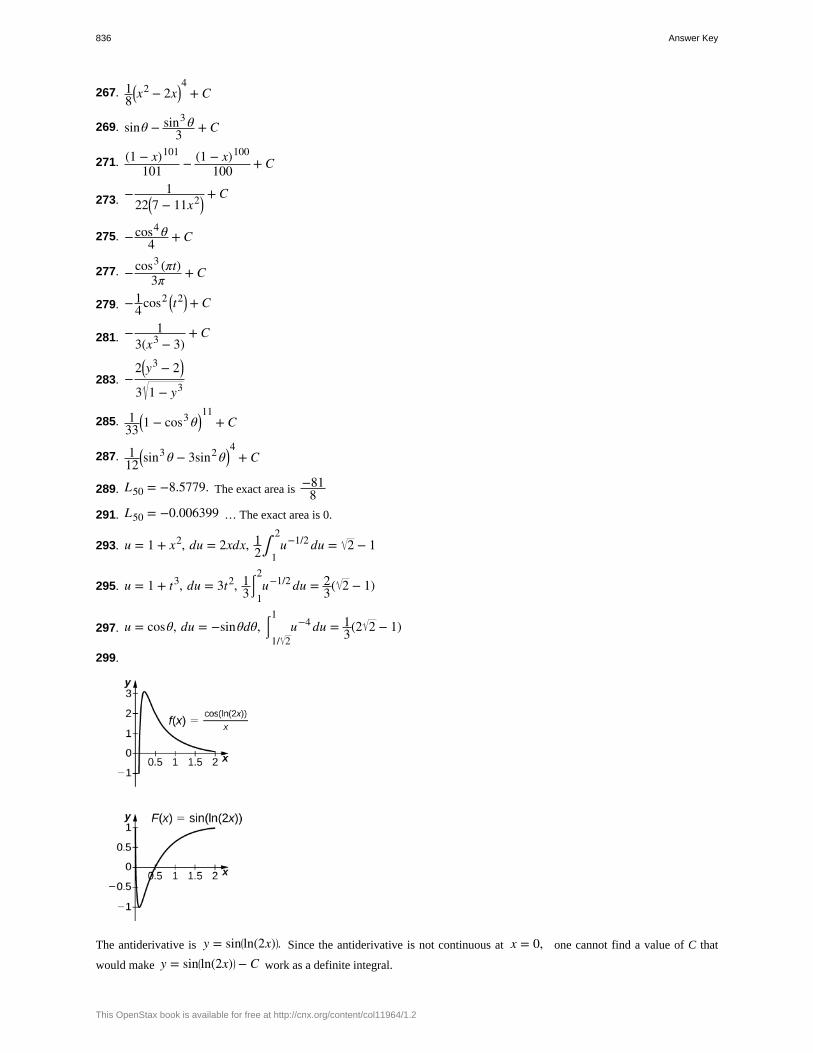
267. 18
⎛⎝x2 − 2x⎞
⎠4
+ C
269. sinθ − sin3 θ3 + C
271. (1 − x)101
101 − (1 − x)100
100 + C
273. − 122⎛
⎝7 − 11x2⎞⎠
+ C
275. −cos4 θ4 + C
277. −cos3 (πt)3π + C
279. −14cos2 ⎛
⎝t2⎞⎠ + C
281. − 13(x3 − 3)
+ C
283. −2⎛
⎝y3 − 2⎞
⎠
3 1 − y3
285. 133
⎛⎝1 − cos3 θ⎞
⎠11
+ C
287. 112
⎛⎝sin3 θ − 3sin2 θ⎞
⎠4
+ C
289. L50 = −8.5779. The exact area is −818
291. L50 = −0.006399 … The exact area is 0.
293. u = 1 + x2, du = 2xdx, 12∫
1
2u−1/2 du = 2 − 1
295. u = 1 + t3, du = 3t2, 13
⌠⌡1
2u−1/2 du = 2
3( 2 − 1)
297. u = cosθ, du = −sinθdθ, ⌠⌡1/ 2
1u−4 du = 1
3(2 2 − 1)
299.
The antiderivative is y = sin⎛⎝ln(2x)⎞
⎠. Since the antiderivative is not continuous at x = 0, one cannot find a value of C that
would make y = sin⎛⎝ln(2x)⎞
⎠ − C work as a definite integral.
836 Answer Key
This OpenStax book is available for free at http://cnx.org/content/col11964/1.2
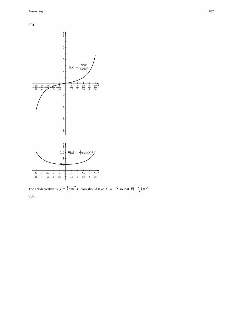
301.
The antiderivative is y = 12sec2 x. You should take C = −2 so that F⎛
⎝−π3
⎞⎠ = 0.
303.
Answer Key 837
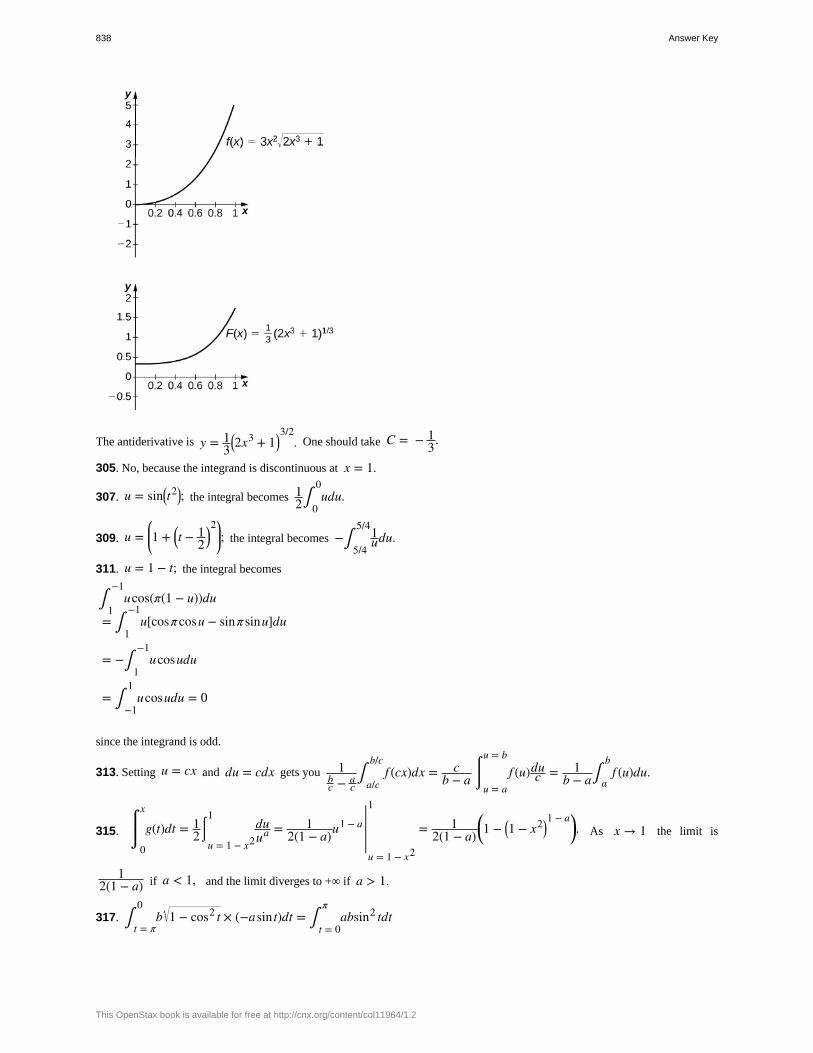
The antiderivative is y = 13
⎛⎝2x3 + 1⎞
⎠3/2
. One should take C = − 13.
305. No, because the integrand is discontinuous at x = 1.
307. u = sin⎛⎝t2⎞
⎠; the integral becomes 12∫
0
0udu.
309. u =⎛
⎝⎜1 + ⎛
⎝t − 12
⎞⎠2⎞
⎠⎟; the integral becomes −∫
5/4
5/41udu.
311. u = 1 − t; the integral becomes
∫1
−1ucos(π(1 − u))du
= ∫1
−1u[cosπ cosu − sinπ sinu]du
= −∫1
−1ucosudu
= ∫−1
1ucosudu = 0
since the integrand is odd.
313. Setting u = cx and du = cdx gets you 1bc − a
c∫
a/c
b/cf (cx)dx = c
b − a⌠⌡u = a
u = b
f (u)duc = 1
b − a∫a
bf (u)du.
315.⌠⌡0
x
g(t)dt = 12
⌠⌡
u = 1 − x2
1duua = 1
2(1 − a)u1 − a |u = 1 − x2
1
= 12(1 − a)
⎛⎝1 − ⎛
⎝1 − x2⎞⎠1 − a⎞
⎠. As x → 1 the limit is
12(1 − a) if a < 1, and the limit diverges to +∞ if a > 1.
317. ∫t = π
0b 1 − cos2 t × (−asin t)dt = ∫
t = 0
πabsin2 tdt
838 Answer Key
This OpenStax book is available for free at http://cnx.org/content/col11964/1.2
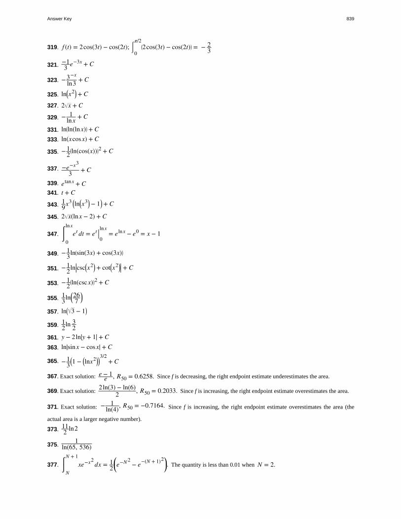
319. f (t) = 2cos(3t) − cos(2t); ⌠⌡0
π/2⎛⎝2cos(3t) − cos(2t)⎞
⎠ = − 23
321. −13 e−3x + C
323. −3−x
ln3 + C
325. ln⎛⎝x2⎞
⎠ + C
327. 2 x + C
329. − 1lnx + C
331. ln⎛⎝ln(lnx)⎞
⎠ + C333. ln(xcosx) + C
335. −12
⎛⎝ln(cos(x))⎞
⎠2 + C
337. −e−x3
3 + C
339. etanx + C341. t + C
343. 19x3 ⎛
⎝ln⎛⎝x
3⎞⎠ − 1⎞
⎠ + C
345. 2 x(lnx − 2) + C
347. ⌠⌡0
lnxet dt = et |0
lnx= elnx − e0 = x − 1
349. −13ln⎛
⎝sin(3x) + cos(3x)⎞⎠
351. −12ln|csc⎛
⎝x2⎞⎠ + cot⎛
⎝x2⎞⎠| + C
353. −12
⎛⎝ln(cscx)⎞
⎠2 + C
355. 13ln⎛
⎝267
⎞⎠
357. ln⎛⎝ 3 − 1⎞
⎠
359. 12ln 3
2361. y − 2ln|y + 1| + C363. ln|sinx − cosx| + C
365. −13
⎛⎝1 − ⎛
⎝lnx2⎞⎠⎞⎠3/2
+ C
367. Exact solution: e − 1e , R50 = 0.6258. Since f is decreasing, the right endpoint estimate underestimates the area.
369. Exact solution:2ln(3) − ln(6)
2 , R50 = 0.2033. Since f is increasing, the right endpoint estimate overestimates the area.
371. Exact solution: − 1ln(4), R50 = −0.7164. Since f is increasing, the right endpoint estimate overestimates the area (the
actual area is a larger negative number).
373. 112 ln2
375.1
ln(65, 536)
377. ⌠⌡N
N + 1xe−x2
dx = 12⎛⎝e−N 2
− e−(N + 1)2⎞⎠. The quantity is less than 0.01 when N = 2.
Answer Key 839
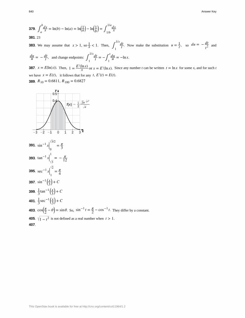
379. ∫a
bdxx = ln(b) − ln(a) = ln⎛
⎝1a
⎞⎠ − ln⎛
⎝1b
⎞⎠ = ∫
1/b
1/adxx
381. 23
383. We may assume that x > 1, so 1x < 1. Then, ∫
1
1/xdtt . Now make the substitution u = 1
t , so du = − dtt2 and
duu = − dt
t , and change endpoints: ∫1
1/xdtt = −∫
1
xduu = −lnx.
387. x = E⎛⎝ln(x)⎞
⎠. Then, 1 = E '(lnx)x or x = E '(lnx). Since any number t can be written t = lnx for some x, and for such t
we have x = E(t), it follows that for any t, E '(t) = E(t).389. R10 = 0.6811, R100 = 0.6827
391. sin−1 x|03/2
= π3
393. tan−1 x| 3
1= − π
12
395. sec−1 x|12
= π4
397. sin−1 ⎛⎝x3
⎞⎠ + C
399. 13tan−1 ⎛
⎝x3
⎞⎠ + C
401. 13sec−1 ⎛
⎝x3
⎞⎠ + C
403. cos⎛⎝π2 − θ⎞
⎠ = sinθ. So, sin−1 t = π2 − cos−1 t. They differ by a constant.
405. 1 − t2 is not defined as a real number when t > 1.407.
840 Answer Key
This OpenStax book is available for free at http://cnx.org/content/col11964/1.2
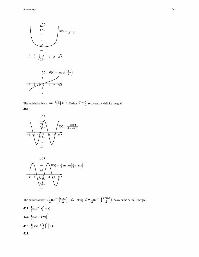
The antiderivative is sin−1 ⎛⎝x3
⎞⎠ + C. Taking C = π
2 recovers the definite integral.
409.
The antiderivative is 12tan−1 ⎛
⎝sinx
2⎞⎠ + C. Taking C = 1
2tan−1 ⎛⎝sin(6)
2⎞⎠ recovers the definite integral.
411. 12
⎛⎝sin−1 t⎞
⎠2
+ C
413. 14
⎛⎝tan−1 (2t)⎞
⎠2
415. 14
⎛
⎝⎜sec−1 ⎛
⎝t2
⎞⎠2⎞
⎠⎟ + C
417.
Answer Key 841
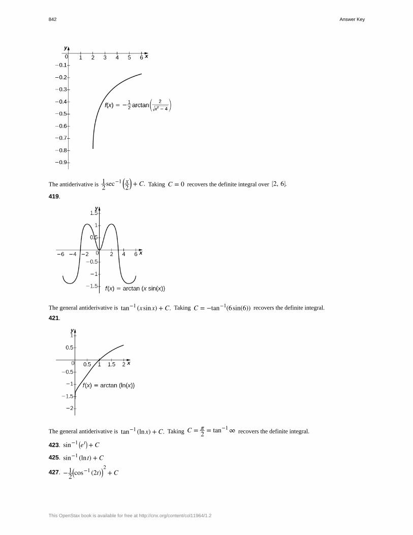
The antiderivative is 12sec−1 ⎛
⎝x2
⎞⎠ + C. Taking C = 0 recovers the definite integral over ⎡
⎣2, 6⎤⎦.
419.
The general antiderivative is tan−1 (xsinx) + C. Taking C = −tan−1(6sin(6)) recovers the definite integral.
421.
The general antiderivative is tan−1 (lnx) + C. Taking C = π2 = tan−1 ∞ recovers the definite integral.
423. sin−1 ⎛⎝et⎞
⎠ + C
425. sin−1 (ln t) + C
427. −12
⎛⎝cos−1 (2t)⎞
⎠2
+ C
842 Answer Key
This OpenStax book is available for free at http://cnx.org/content/col11964/1.2
429. 12ln⎛
⎝43
⎞⎠
431. 1 − 25
433. 2tan−1 (A) → π as A → ∞
435. Using the hint, one has ⌠⌡
csc2 xcsc2 x + cot2 x
dx = ⌠⌡
csc2 x1 + 2cot2 x
dx. Set u = 2cot x. Then, du = − 2csc2 x and the
integral is − 12
⌠⌡
du1 + u2 = − 1
2tan−1 u + C = 1
2tan−1 ⎛
⎝ 2cot x⎞⎠ + C. If one uses the identity tan−1 s + tan−1 ⎛
⎝1s
⎞⎠ = π
2,
then this can also be written 12
tan−1 ⎛⎝tanx
2⎞⎠ + C.
437. x ≈ ± 1.13525. The left endpoint estimate with N = 100 is 2.796 and these decimals persist for N = 500.Review Exercises
439. False441. True443. L4 = 5.25, R4 = 3.25, exact answer: 4
445. L4 = 5.364, R4 = 5.364, exact answer: 5.870
447. −43
449. 1
451. − 12(x + 4)2 + C
453. 43sin−1 ⎛
⎝x3⎞
⎠ + C
455.sin t1 + t2
457. 4lnxx + 1
459. $6,328,113461. $73.36
463. 1911712 ft/sec, or 1593 ft/sec
Chapter 6
Checkpoint
6.1. 12 units2
6.2. 310 unit2
6.3. 2 + 2 2 units2
6.4. 53 units2
6.5. 53 units2
6.7.π2
6.8. 8π units3
6.9. 21π units3
6.10. 10π3 units3
6.11. 60π units3
6.12. 15π2 units3
6.13. 8π units3
Answer Key 843
6.14. 12π units3
6.15. 11π6 units3
6.16.π6 units3
6.17. Use the method of washers; V = ∫−1
1π⎡⎣
⎛⎝2 − x2⎞
⎠2
− ⎛⎝x2⎞
⎠2⎤⎦dx
6.18. 16
⎛⎝5 5 − 1⎞
⎠ ≈ 1.697
6.19. Arc Length ≈ 3.82026.20. Arc Length = 3.15018
6.21.π6
⎛⎝5 5 − 3 3⎞
⎠ ≈ 3.133
6.22. 12π6.23. 70/36.24. 24π6.25. 8 ft-lb
6.26. Approximately 43,255.2 ft-lb
6.27. 156,800 N
6.28. Approximately 7,164,520,000 lb or 3,582,260 t
6.29. M = 24, x– = 25 m
6.30. (−1, −1) m
6.31. The centroid of the region is (3/2, 6/5).6.32. The centroid of the region is (1, 13/5).6.33. The centroid of the region is (0, 2/5).6.34. 6π2 units3
6.35.
a.ddxln⎛
⎝2x2 + x⎞⎠ = 4x + 1
2x2 + x
b. ddx
⎛⎝ln
⎛⎝x
3⎞⎠⎞⎠2
=6 ln⎛
⎝x3⎞
⎠x
6.36. ∫ x2
x3 + 6dx = 1
3ln |x3 + 6| + C
6.37. 4 ln 26.38.
a. ddx
⎛
⎝⎜ex2
e5x
⎞
⎠⎟ = ex2 − 5x (2x − 5)
b. ddt
⎛⎝e2t⎞
⎠3
= 6e6t
6.39. ∫ 4e3xdx = − 4
3e−3x + C
6.40.
a. ddt4
t4= 4t4
(ln 4)⎛⎝4t3⎞
⎠
b.ddxlog3
⎛⎝ x2 + 1⎞
⎠ = x(ln 3)⎛
⎝x2 + 1⎞⎠
6.41. ∫ x2 2x3dx = 1
3 ln 22x3+ C
6.42. There are 81,377,396 bacteria in the population after 4 hours. The population reaches 100 million bacteria after
844 Answer Key
This OpenStax book is available for free at http://cnx.org/content/col11964/1.2
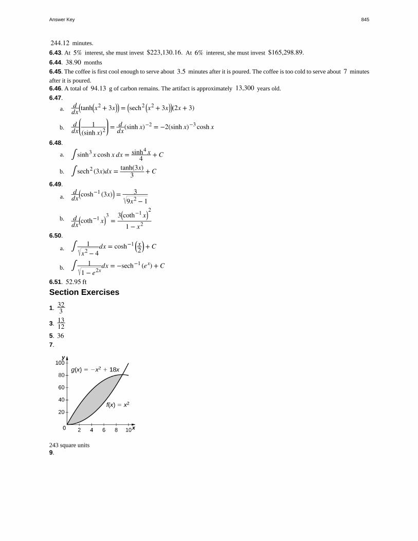
244.12 minutes.
6.43. At 5% interest, she must invest $223,130.16. At 6% interest, she must invest $165,298.89.6.44. 38.90 months
6.45. The coffee is first cool enough to serve about 3.5 minutes after it is poured. The coffee is too cold to serve about 7 minutes
after it is poured.6.46. A total of 94.13 g of carbon remains. The artifact is approximately 13,300 years old.
6.47.
a. ddx
⎛⎝tanh⎛
⎝x2 + 3x⎞⎠⎞⎠ = ⎛
⎝sech2 ⎛⎝x2 + 3x⎞
⎠⎞⎠(2x + 3)
b. ddx
⎛
⎝⎜ 1(sinh x)2
⎞
⎠⎟ = d
dx(sinh x)−2 = −2(sinh x)−3 cosh x
6.48.
a. ∫ sinh3 x cosh x dx = sinh4 x4 + C
b. ∫ sech2 (3x)dx = tanh(3x)3 + C
6.49.
a.ddx
⎛⎝cosh−1 (3x)⎞
⎠ = 39x2 − 1
b. ddx
⎛⎝coth−1 x⎞
⎠3
=3⎛
⎝coth−1 x⎞⎠2
1 − x2
6.50.
a. ∫ 1x2 − 4
dx = cosh−1 ⎛⎝x2
⎞⎠ + C
b. ∫ 11 − e2x
dx = −sech−1 (ex) + C
6.51. 52.95 ftSection Exercises
1. 323
3. 1312
5. 367.
243 square units9.
Answer Key 845
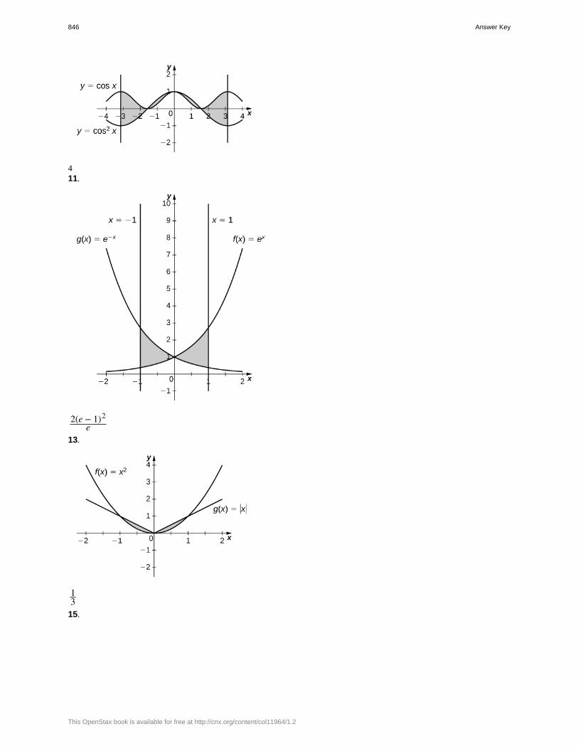
411.
2(e − 1)2e
13.
13
15.
846 Answer Key
This OpenStax book is available for free at http://cnx.org/content/col11964/1.2
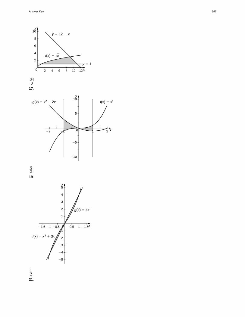
343
17.
52
19.
12
21.
Answer Key 847
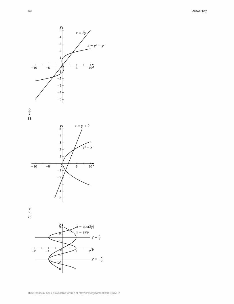
92
23.
92
25.
848 Answer Key
This OpenStax book is available for free at http://cnx.org/content/col11964/1.2
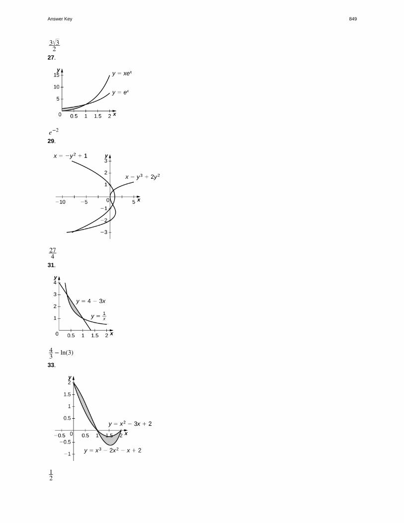
3 32
27.
e−2
29.
274
31.
43 − ln(3)
33.
12
Answer Key 849
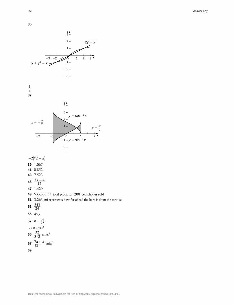
35.
12
37.
−2⎛⎝ 2 − π⎞
⎠
39. 1.06741. 0.85243. 7.523
45. 3π − 412
47. 1.42949. $33,333.33 total profit for 200 cell phones sold
51. 3.263 mi represents how far ahead the hare is from the tortoise
53. 34324
55. 4 3
57. π − 3225
63. 8 units3
65.323 2 units3
67. 7π12hr2
units3
69.
850 Answer Key
This OpenStax book is available for free at http://cnx.org/content/col11964/1.2
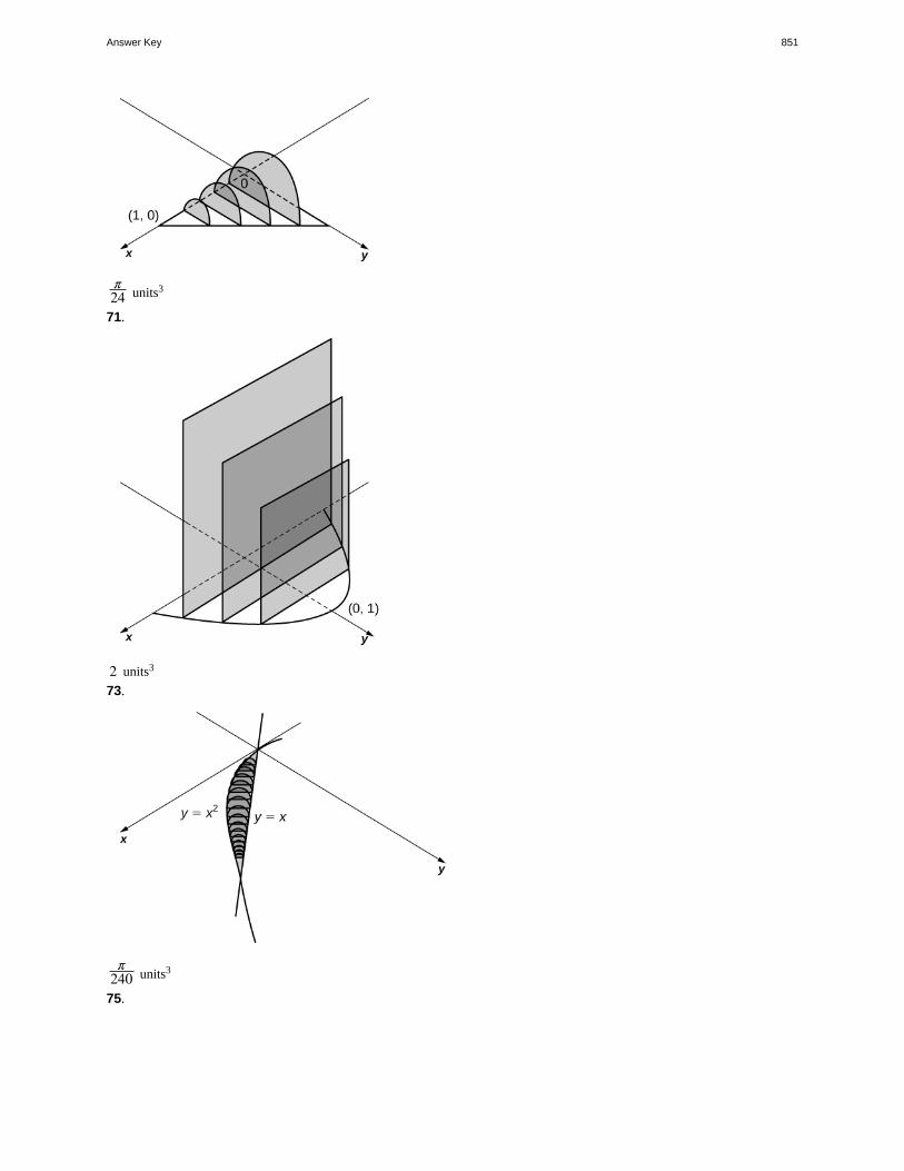
π24 units3
71.
2 units3
73.
π240 units3
75.
Answer Key 851
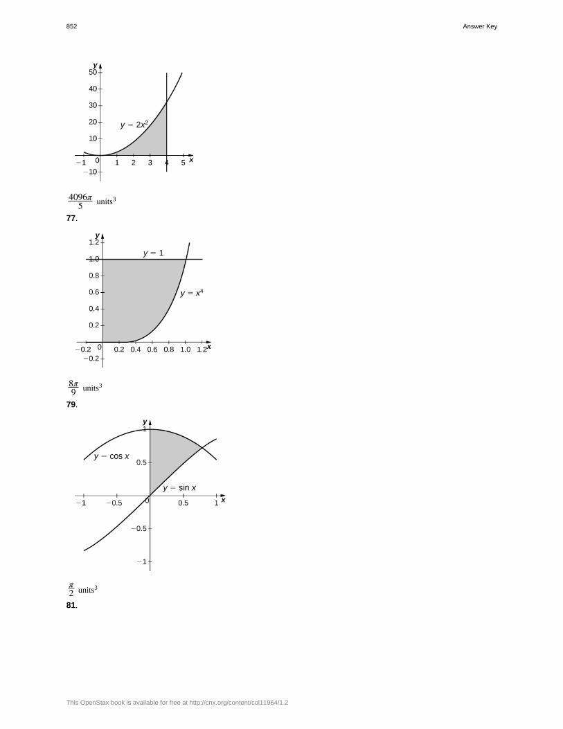
4096π5 units3
77.
8π9 units3
79.
π2 units3
81.
852 Answer Key
This OpenStax book is available for free at http://cnx.org/content/col11964/1.2
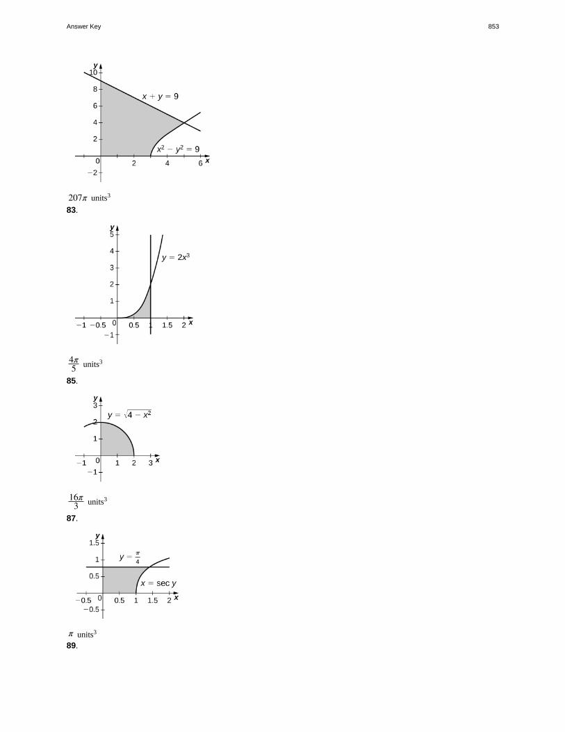
207π units3
83.
4π5 units3
85.
16π3 units3
87.
π units3
89.
Answer Key 853
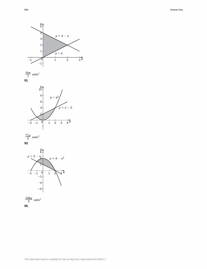
16π3 units3
91.
72π5 units3
93.
108π5 units3
95.
854 Answer Key
This OpenStax book is available for free at http://cnx.org/content/col11964/1.2
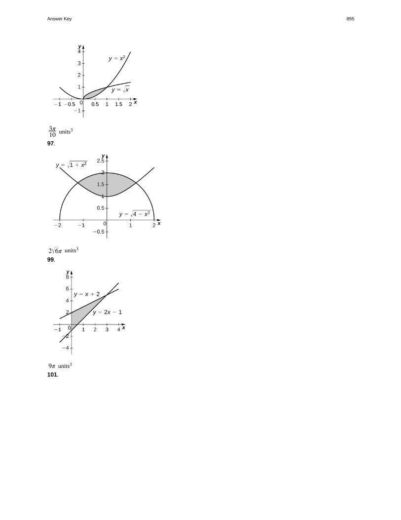
3π10 units3
97.
2 6π units3
99.
9π units3
101.
Answer Key 855
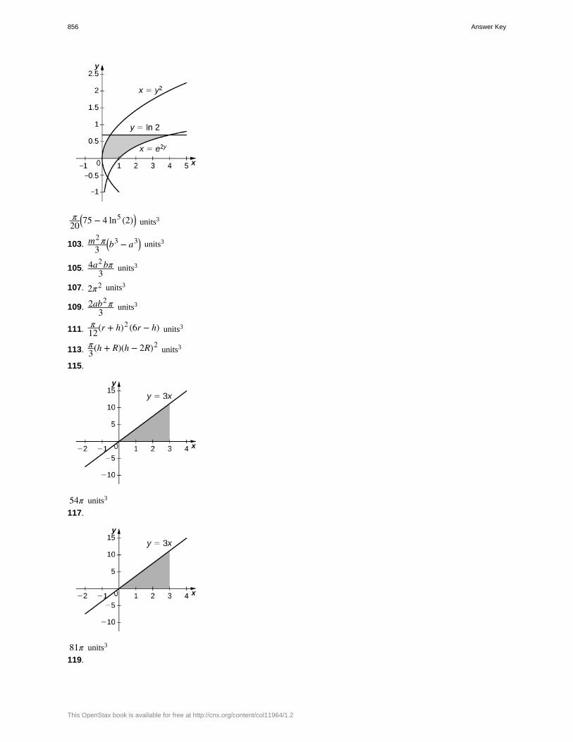
π20
⎛⎝75 − 4 ln5 (2)⎞
⎠ units3
103. m2 π3
⎛⎝b
3 − a3⎞⎠ units3
105. 4a2 bπ3 units3
107. 2π2 units3
109. 2ab2 π3 units3
111.π12(r + h)2 (6r − h) units3
113.π3(h + R)(h − 2R)2
units3
115.
54π units3
117.
81π units3
119.
856 Answer Key
This OpenStax book is available for free at http://cnx.org/content/col11964/1.2
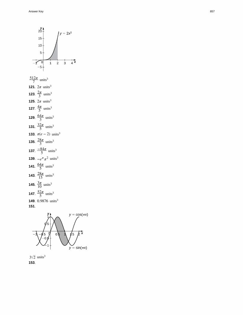
512π7 units3
121. 2π units3
123. 2π3 units3
125. 2π units3
127. 4π5 units3
129. 64π3 units3
131. 32π5 units3
133. π(e − 2) units3
135. 28π3 units3
137. −84π5 units3
139. −eπ π2 units3
141. 64π5 units3
143. 28π15 units3
145. 3π10 units3
147. 52π5 units3
149. 0.9876 units3
151.
3 2 units3
153.
Answer Key 857
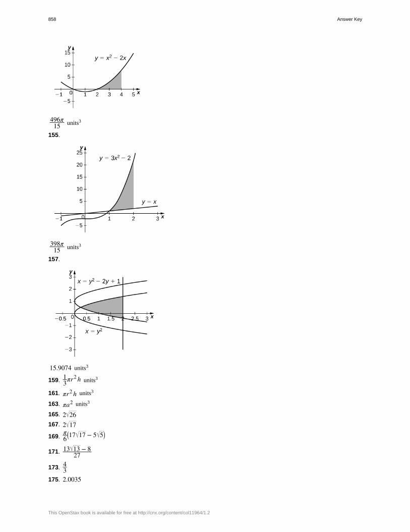
496π15 units3
155.
398π15 units3
157.
15.9074 units3
159. 13πr2 h units3
161. πr2 h units3
163. πa2 units3
165. 2 26167. 2 17
169.π6
⎛⎝17 17 − 5 5⎞
⎠
171. 13 13 − 827
173. 43
175. 2.0035
858 Answer Key
This OpenStax book is available for free at http://cnx.org/content/col11964/1.2
177. 12332
179. 10
181. 203
183. 1675
⎛⎝229 229 − 8⎞
⎠
185. 18
⎛⎝4 5 + ln⎛
⎝9 + 4 5⎞⎠⎞⎠
187. 1.201189. 15.2341
191. 49π3
193. 70π 2195. 8π197. 120π 26
199.π6(17 17 − 1)
201. 9 2π
203. 10 10π27
⎛⎝73 73 − 1⎞
⎠
205. 25.645207. 2π209. 10.5017211. 23 ft
213. 2215. Answers may vary217. For more information, look up Gabriel’s Horn.219. 150 ft-lb
221. 200 J223. 1 J
225. 392
227. ln(243)
229. 332π15
231. 100π233. 20π 15235. 6 J
237. 5 cm
239. 36 J
241. 18,750 ft-lb
243. 323 × 109 ft-lb
245. 8.65 × 10⁵ J247. a. 3,000,000 lb, b. 749,000 lb
249. 23.25π million ft-lb
251. AρH 2
2253. Answers may vary
255. 54
Answer Key 859
257.⎛⎝23, 2
3⎞⎠
259.⎛⎝74, 3
2⎞⎠
261. 3L4
263.π2
265. e2 + 1e2 − 1
267. π2 − 4π
269. 14
⎛⎝1 + e2⎞
⎠
271.⎛⎝a3, b
3⎞⎠
273.⎛⎝0, π
8⎞⎠
275. (0, 3)
277.⎛⎝0, 4
π⎞⎠
279.⎛⎝58, 1
3⎞⎠
281.mπ3
283. πa2 b
285.⎛⎝
43π , 4
3π⎞⎠
287.⎛⎝12, 2
5⎞⎠
289.⎛⎝0, 28
9π⎞⎠
291. Center of mass:⎛⎝a6, 4a2
5⎞⎠, volume: 2πa4
9293. Volume: 2π2 a2 (b + a)
295. 1x
297. − 1x(ln x)2
299. ln(x + 1) + C301. ln(x) + 1303. cot(x)
305. 7x
307. csc(x)sec x309. −2 tan x
311. 12ln⎛
⎝53
⎞⎠
313. 2 − 12ln(5)
315.1
ln(2) − 1
317. 12ln(2)
860 Answer Key
This OpenStax book is available for free at http://cnx.org/content/col11964/1.2
319. 13(ln x)3
321.2x3
x2 + 1 x2 − 1323. x−2 − (1/x) (ln x − 1)325. exe − 1
327. 1
329. − 1x2
331. π − ln(2)
333. 1x
335. e5 − 6 units2
337. ln(4) − 1 units2
339. 2.8656341. 3.1502349. True
351. False; k = ln (2)t
353. 20 hours
355. No. The relic is approximately 871 years old.
357. 71.92 years
359. 5 days 6 hours 27 minutes
361. 12363. 8.618%365. $6766.76367. 9 hours 13 minutes
369. 239,179 years
371. P′(t) = 43e0.01604t. The population is always increasing.
373. The population reaches 10 billion people in 2027.375. P′(t) = 2.259e0.06407t. The population is always increasing.
377. ex and e−x
379. Answers may vary381. Answers may vary383. Answers may vary385. 3 sinh(3x + 1)387. −tanh(x)sech(x)389. 4 cosh(x)sinh(x)
391.x sech2 ⎛
⎝ x2 + 1⎞⎠
x2 + 1393. 6 sinh5 (x)cosh(x)
395. 12sinh(2x + 1) + C
397. 12sinh2 ⎛
⎝x2⎞⎠ + C
399. 13cosh3 (x) + C
401. ln⎛⎝1 + cosh(x)⎞
⎠ + C403. cosh(x) + sinh(x) + C
Answer Key 861
405.4
1 − 16x2
407.sinh(x)
cosh2 (x) + 1409. −csc(x)
411. − 1⎛⎝x2 − 1⎞
⎠tanh−1 (x)
413. 1atanh−1 ⎛
⎝xa
⎞⎠ + C
415. x2 + 1 + C417. cosh−1 (ex) + C419. Answers may vary421. 37.30
423. y = 1ccosh(cx)
425. −0.521095427. 10Review Exercises
435. False437. False439. 32 3
441. 162π5
443. a. 4, b. 128π7 , c. 64π
5445. a. 1.949, b. 21.952, c. 17.099
447. a. 316 , b. 452π
15 , c. 31π6
449. 245.282
451. Mass: 12, center of mass:
⎛⎝1835, 9
11⎞⎠
453. 17 + 18ln(33 + 8 17)
455. Volume: 3π4 , surface area: π⎛
⎝ 2 − sinh−1(1) + sinh−1(16) − 25716
⎞⎠
457. 11:02 a.m.459. π(1 + sinh(1)cosh(1))
862 Answer Key
This OpenStax book is available for free at http://cnx.org/content/col11964/1.2
INDEXAabsolute extremum, 366, 499absolute maximum, 366, 499absolute minimum, 366, 499absolute value function, 27, 117acceleration, 225, 266, 334algebraic function, 47, 117amount of change, 266, 334antiderivative, 485, 499aphelion, 565arc length, 671, 756Archimedes, 175, 508area density, 686Area Problem, 129area under the curve, 519average rate of change, 266,334average value of a function, 616average value of the function,542average velocity, 128, 208, 222
Bbald eagle, 580base, 96, 117
Ccarbon dating, 741catenary, 752, 756center of mass, 704, 756centroid, 707, 756chain rule, 287, 334change of variables, 584, 616chaos, 481common logarithm, 105composite function, 22, 117compound interest, 736compounding interest, 99concave down, 395, 499concave up, 395, 499concavity, 395, 499concavity test, 396, 499conditional statement, 194constant function, 40Constant multiple law for limits,161constant multiple law for limits,208Constant Multiple Rule, 251constant multiple rule, 334constant rule, 247, 334continuity at a point, 208continuity from the left, 208continuity from the right, 208continuity over an interval, 186,
208continuous at a point, 180continuous from the left, 186continuous from the right, 186critical point, 369, 499cross-section, 636, 756cubic function, 40, 117
Ddeceleration, 579decreasing on the interval I ,
20, 117definite integral, 529, 616degree, 40, 117density function, 685, 756dependent variable, 8, 117derivative, 220, 334derivative function, 232, 334Difference law for limits, 161difference law for limits, 208difference quotient, 215, 334Difference Rule, 250difference rule, 334differentiable at a, 334differentiable at a , 232
differentiable function, 232, 334differentiable on S, 334differentiable on S , 232
differential, 499Differential calculus, 126differential calculus, 208differential form, 359, 499differentials, 358differentiation, 220, 334discontinuity at a point, 208discontinuous at a point, 180disk method, 642, 756displacement, 534, 567domain, 8, 117doubling time, 738, 756dummy variable, 509, 529
Eearthquake, 106end behavior, 41, 415, 499endpoints, 10epsilon-delta definition of thelimit, 194, 208evaluation theorem, 555even function, 26, 117, 572existential quantifier, 194exponent, 96, 117exponential decay, 739, 756exponential growth, 734, 756
Extreme Value Theorem, 367extreme value theorem, 499
Ffave, 542federal income tax, 580Fermat’s theorem, 369, 499first derivative test, 391, 499folium of Descartes, 314fruit flies, 600frustum, 676, 756function, 8, 117Fundamental Theorem ofCalculus, 549fundamental theorem ofcalculus, 616Fundamental Theorem ofCalculus, Part 1, 552fundamental theorem ofcalculus, part 1, 616Fundamental Theorem ofCalculus, Part 2, 555fundamental theorem ofcalculus, part 2, 616
Ggraph of a function, 9, 117growth of bacteria, 599
Hhalf-life, 741, 756hanging cables, 752higher-order derivative, 334higher-order derivatives, 241Holling type I equation, 275Hooke’s law, 689, 756Hoover Dam, 698horizontal asymptote, 408, 499horizontal line test, 79, 117hydrostatic pressure, 695, 756hyperbolic functions, 107, 117
Iiceboat, 571implicit differentiation, 310, 334increasing on the interval I , 19,
117indefinite integral, 487, 499independent variable, 8, 117indeterminate forms, 454, 499index, 508infinite discontinuity, 184, 208infinite limit, 208infinite limit at infinity, 414, 499infinite limits, 146
Index 863
inflection point, 397, 499initial value problem, 500initial-value problem, 493input, 8instantaneous rate of change,224, 334instantaneous velocity, 128,208, 222integrable function, 529, 616Integral calculus, 129integral calculus, 208integrand, 529, 616integration by substitution, 584,616Intermediate Value Theorem,188, 208interval notation, 10intuitive definition of the limit,136, 208inverse function, 78, 117inverse hyperbolic functions,111, 117inverse trigonometric functions,86, 117iterative process, 476, 500
Jjoule, 688jump discontinuity, 184, 208
Llamina, 707, 756leading coefficient, 40left-endpoint approximation,513, 616Leibniz, 214, 529limit, 128, 208limit at infinity, 408, 413, 500limit laws, 160, 209limits of integration, 529, 616linear approximation, 355, 500linear function, 36, 117linearization, 355local extremum, 368, 500local maximum, 368, 500local minimum, 368, 500logarithmic differentiation, 328,334logarithmic function, 50, 117lower sum, 520, 616L’Hôpital’s rule, 454, 500
MMandelbrot set, 481marginal cost, 271, 334marginal profit, 271, 334marginal revenue, 334
mathematical model, 117mathematical models, 44maximizing revenue, 445Mean Value Theorem, 379mean value theorem, 500Mean Value Theorem forIntegrals, 549mean value theorem forintegrals, 616method of cylindrical shells, 756method of cylindrical shells.,658method of exhaustion, 508moment, 704, 756multivariable calculus, 131, 209
Nnatural exponential function,100, 117, 320natural logarithm, 102, 118natural logarithmic function, 320net change theorem, 567, 616net signed area, 533, 616Newton, 214, 549Newton’s law of cooling, 739Newton’s method, 472, 500number e, 118number e , 100
Ooblique asymptote, 421, 500odd function, 26, 118, 572one-sided limit, 143, 209one-to-one function, 79, 118optimization problems, 439, 500output, 8
Ppartition, 512, 616pascals, 695Pascal’s principle, 695percentage error, 362, 500perihelion, 565periodic function, 118periodic functions., 70piecewise-defined function, 50,118piecewise-defined functions, 11point-slope equation, 38, 118polynomial function, 40, 118population growth, 96Population growth, 734population growth rate, 335population growth rates, 266power function, 40, 118Power law for limits, 161power law for limits, 209
power rule, 249, 335price–demand function, 597Product law for limits, 161product law for limits, 209product rule, 253, 335propagated error, 361, 500Pythagorean theorem, 344
Qquadratic function, 40, 118Quotient law for limits, 161quotient law for limits, 209quotient rule, 255, 335
Rradial density, 686radians, 62, 118range, 8, 118rate of change, 124, 567rational function, 47, 118Regiomontanus’ problem, 505regular partition, 512, 616related rates, 342, 500relative error, 362, 500removable discontinuity, 184,209restricted domain, 84, 118Richter scale, 106Riemann sum, 519riemann sum, 616right-endpoint approximation,513, 616Rolle’s theorem, 379rolle’s theorem, 500root function, 47, 118Root law for limits, 161root law for limits, 209
Ssecant, 125, 209secant method, 484second derivative test, 399, 500sigma notation, 508, 616simple interest, 736skydiver, 560slicing method, 638, 756slope, 36, 118slope-intercept form, 37, 118smooth, 671solid of revolution, 639, 756speed, 267, 335spring constant, 689squeeze theorem, 170, 209standard form of a line, 38Sum law for limits, 161sum law for limits, 209Sum Rule, 250
864 Index
This OpenStax book is available for free at http://cnx.org/content/col11964/1.2
sum rule, 335summation notation, 508sums and powers of integers,510Surface area, 675surface area, 757symmetry about the origin, 25,118symmetry about the y-axis, 25,118symmetry principle, 707, 757
Ttable of values, 13, 118tangent, 126, 209tangent line approximation, 355tangent line approximation(linearization), 500Tangent Problem, 126theorem of Pappus for volume,716, 757total area, 536, 616Tour de France, 577transcendental function, 118transcendental functions, 50transformation of a function, 52,118triangle inequality, 201, 209trigonometric functions, 64, 118trigonometric identity, 68, 118
Uuniversal quantifier, 194upper sum, 520, 616
Vvariable of integration, 529, 616velocity, 567vertical asymptote, 149, 209vertical line test, 16, 118
Wwasher method, 648, 757wingsuits, 561work, 689, 757
Zzeroes of functions, 472zeros of a function, 16, 118
Index 865