RC22683 Revised (W0305-138) May 29, 2003Computer Science

IBM Research Report

Blue Matter, An Application Framework for Molecular Simulation on Blue Gene

B. G. Fitcha, R. S. Germaina, M. Mendellc, J. Piterab, M. Pitmana, A. Rayshubskiya, Y. Shama, F. Suitsa, W. Swopeb, T. J. C. Warda,

Y. Zhestkova, R. Zhoua

aIBM Research DivisionThomas J. Watson Research Center

P.O. Box 218Yorktown Heights, NY 10598

bIBM Almaden Research Center650 Harry Road

San Jose, CA 95120-6099

cIBM Canada8200 Warden Avenue

Markham, ON L6G 1C7

Research DivisionAlmaden - Austin - Beijing - Haifa - India - T. J. Watson - Tokyo - Zurich

LIMITED DISTRIBUTION NOTICE: This report has been submitted for publication outside of IBM and will probably be copyrighted if accepted for publication. It has been issued as a ResearchReport for early dissemination of its contents. In view of the transfer of copyright to the outside publisher, its distribution outside of IBM prior to publication should be limited to peer communications and specificrequests. After outside publication, requests should be filled only by reprints or legally obtained copies of the article (e.g. , payment of royalties). Copies may be requested from IBM T. J. Watson Research Center , P.O. Box 218, Yorktown Heights, NY 10598 USA (email: reports@us.ibm.com). Some reports are available on the internet at http://domino.watson.ibm.com/library/CyberDig.nsf/home .

Blue Matter, An Application Framework for

Molecular Simulation on Blue Gene ?

B.G. Fitch a R.S. Germain a M. Mendell c J. Pitera b

M. Pitman a A. Rayshubskiy a Y. Sham a,?? F. Suits a

W. Swope b T.J.C. Ward a Y. Zhestkov a R. Zhou a

aIBM Thomas J. Watson Research Center

P.O. Box 218

Yorktown Heights, NY 10598

bIBM Almaden Research Center

650 Harry Road

San Jose, CA 95120-6099

cIBM Canada

8200 Warden Avenue

Markham, ON L6G 1C7

Abstract

In this paper we describe the context, architecture, and challenges of Blue Matter,

the application framework being developed in conjunction with the science effort

within IBM’s Blue Gene project. The study of the mechanisms behind protein fold-

ing and related topics can require long time simulations on systems with a wide

Preprint submitted to Elsevier Science April 14, 2003

range of sizes and the application supporting these studies must map efficiently

onto a large range of parallel partition sizes to optimize scientific throughput for a

particular study. The design goals for the Blue Matter architecture include separat-

ing the complexities of the parallel implementation on a particular machine from

those of the scientific simulation as well as minimizing system environmental depen-

dencies so that running an application within a low overhead kernel with minimal

services is possible. We describe some of the parallel decompositions currently being

explored that target the first member of the Blue Gene family, BG/L, and present

simple performance models for these decompositions that we are using to prioritize

our development work. Preliminary results indicate that the high performance net-

works on BG/L will allow us to use FFT-based techniques for periodic electrostatics

with reasonable speedups on 512-1024 node count partitions even for systems with

as few as 5000 atoms.

Key words:

PACS:

s

? The authors wish to acknowledge many useful discussions with Bruce J. Berne and Glenn J.

Martyna regarding molecular dynamics algorithms and members of the BG/L hardware and systems

software teams, particularly Alan Gara, Philip Heidelberger, Burkhard Steinmacher-Burow, and

Mark Giampapa, as well as the contributions of Huafeng Xu at the early stages of this project. We

also wish to thank the anonymous referees for their feedback on this paper.??Current address:

University of Minnesota

Supercomputing Institute for Digital Simulation and Advanced Computation

599 Walter Library

117 Pleasant Street S.E.

Minneapolis, MN 55455

2

1 Introduction

In December 1999, IBM announced the start of a five year effort to build a massively parallel

computer to be applied to the study of biomolecular phenomena such as protein folding.[1]

The project has two goals: advancing our understanding of the mechanisms behind biologi-

cally important phenomena such as protein folding via large scale simulation and exploring

novel ideas in massively parallel machine architecture and software. This project should en-

able biomolecular simulations that are orders of magnitude larger and longer than current

technology permits. The first member of the Blue Gene machine family is Blue Gene/L, for

which a 512 node prototype is projected to become available in the second half of 2003, with

a fully operational machine scheduled for the 2004-2005 time frame. The machine architec-

ture has evolved significantly since the inception of the project, but one aspect that has

remained constant is the use of a three dimensional mesh interconnect topology, a feature

that may require the application to be aware of the machine topology in order to achieve

optimal performance. This has not been the case for other recent large parallel machines

such as ASCI White. Another unusual feature of this machine is the availability of a second

high performance interconnect network to provide low-latency and high bandwidth global

broadcast and reduction capabilities. More details about the machine that are most relevant

to an application developer are provided in the body of this paper and additional informa-

tion can be found in a recent paper by the Blue Gene team[2]. The study of the mechanisms

behind protein folding and related topics can require long time simulations on systems with

a wide range of sizes and the application supporting these studies must map efficiently onto a

large range of parallel partition sizes to optimize scientific throughput for a particular study.

Typical system sizes of interest range from 5000 atoms (for a small peptide in water) through

30,000 atoms (for a folded 200-residue protein in water) up to 200,000 atoms or more (for a

protein-membrane system or large unfolded protein in water).

3

To support the goals of the Blue Gene project related to protein science and to explore novel

application programming approaches for massively parallel machine architectures in the con-

text of a concrete problem, we have been working on an application framework, Blue Matter,

which is currently focused on biomolecular simulation. It is hoped that the lessons learned

and even some of the components developed can be reused in other application domains. One

of the principal design goals for this framework is the effective logical separation of the com-

plexities of programming a massively parallel machine from the complexities of biomolecular

simulation through the definition of appropriate interfaces. Encapsulation of the semantics of

the biomolecular simulation methodologies means that the application can track the evolu-

tion of the machine architecture and explorations of various parallel decomposition schemes

can take place with minimal intervention from the domain experts on the team, who are also

the end users of the Blue Matter application. Furthermore, we have decomposed the applica-

tion into a core parallel engine with minimal system environmental requirements running on

BG/L and a set of support modules providing setup, monitoring, and analysis functionality

that can run on other host machines. Minimizing system environmental requirements for

the core parallel engine enables the use of non-pre-emptive low overhead parallel operating

system (OS) kernels[3] to enable scalability to thousands of nodes.

In order to prioritize our development efforts, we are exploring various mappings of the

Blue Matter application onto the BG/L platform via simple models. One area of interest

is the exploitation of the high performance networks available on Blue Gene/L in a way

that minimizes potential software overheads. If we can find parallel decompositions that

directly take advantage of the hardware communications facilities, we will reduce the software

overheads that may limit the maximum partition for a fixed size problem, thereby maximizing

throughput for a given molecular simulation.

4

1.1 Machine Overview

Blue Gene/L is a cellular architecture machine built of nodes containing a single application-

specific integrated circuit (ASIC) and additional off-chip memory. Each ASIC has two IBM

PowerPC processors with a projected clock speed of 700 MHz as well as cache memory

and communications logic. The target configuration contains a maximum of 65, 536 compute

nodes with several communications networks. The networks that are of primary interest

to application developers are the three-dimensional torus that connects each node to its six

nearest neighbors with a link bandwidth of 175 MB/s bidirectional (2 bits/cycle), a physically

separate global combining/broadcast tree with bandwidth of 350 MB/s (4 bits/cycle) and

a 1.5 microsecond one-way latency on a 64K node partition, and a global barrier/interrupt

network. BG/L can be electronically partitioned into multiple systems with a currently en-

visioned minimum size of 512 nodes, each of which has its own complete set of networks.

The target peak performance of the full 65, 536 node configuration of BG/L is 180/360 Ter-

aFLOPs, where the lower number corresponds to scenarios in which one processor exclusively

handles communication tasks, and the larger number assumes the application can take full

advantage of both processors for computation.

1.2 Blue Gene Science

Understanding the physical basis of protein function is a central objective of molecular bi-

ology. Proteins function through internal motion and interaction with their environment.

An understanding of protein motion at the atomic level has been pursued since the earliest

simulations of their dynamics [4]. When simulations can connect to experimental results, the

microscopic view of processes revealed by simulation acquire more credibility and the simu-

lation results can help interpret the experimental data [5]. Improvements in computational

5

power and simulation methods have led to important progress in studies of protein structure,

thermodynamics, and kinetics[4,6–8].

1.3 Methodological Implications for the Application

The validity of a molecular simulation depends strongly on the the quality of the force field,

including the representation of water, the treatment of long-range intermolecular interac-

tions, and the simulated environment of the protein. Validity comes at a cost, however,

both in the computational expense of the simulation and the complexity of the molecular

dynamics (MD) software.

Biological molecules are surrounded by water, so the representation of water in a simulation

has a critical effect on its quality. Explicit solvent simulations represent the atoms of each

of the water molecules around a protein, and calculate all of the intermolecular forces and

dynamics associated with those atoms. The expense of explicit water is significant since the

number of atoms contributed by the solvent can far exceed that of the protein itself. In order

to avoid boundary effects in explicit water simulations, it is typical to treat the simulated

system with periodic boundary conditions. Alternatively, implicit solvent models of various

levels of sophistication have been used which typically represent the water as a continuum

dielectric, optionally coupled with a cavity surface tension term to model the hydrophobic

effect. Although implicit solvent models have produced important results in some areas,

there are important cases where significant differences exist in the results obtained from an

implicit as opposed to an explicit treatment of water[9].

A major feature of molecular simulation that poses an implementation challenge is the treat-

ment of long-range interactions. For biological systems, this term arises from the long-ranged

Coulombic interaction between charged amino acids or ions. A simplification is to only in-

6

clude the interactions of atoms within a short cutoff radius of each other, which reduces the

computational burden, but in systems with charged groups or free charges this approach

can lead to unphysical artifacts[10]. The periodic representations used for explicit solvent

simulations can be treated correctly with the use of the Ewald summation technique[11] or

related methods[12] which typically require the use of Fourier transform techniques. These

techniques introduce global data dependencies and are correspondingly complex to paral-

lelize efficiently. Nonetheless, this addition to the MD code is important for the accuracy of

the results and these techniques, with their scalability consequences, are essential for large

scale simulations that can match experiment.

Another feature in molecular simulation that demands added complexity is the specific en-

semble being simulated, e.g. whether the simulated system is in a constant pressure or

constant volume environment, and whether or not it is coupled to a heat bath. Supporting

these capabilities requires additional code, communication, and added barriers to synchronize

the execution of parallel tasks. In particular, the calculation of the instantaneous internal

”pressure” inside the simulation cell requires a global reduction of all the interparticle forces

projected along their displacements from the origin.

2 Application Architecture

2.1 Overview

Blue Matter is a software framework for performing biomolecular simulations primarily tar-

geting parallel computing platforms containing thousands of nodes. At the highest level, the

Blue Matter architecture specifies a modular decomposition and has been implemented as

independent subprograms that cooperate via architected interfaces. By using concepts from

generic programming[13] and defining appropriate interfaces, we have been working towards

7

a separation of the complexity of molecular dynamics simulation from the complexity of

parallel programming with minimal impact on performance. The Blue Matter architecture

requires infrastructure to support extensive regression and validation because of the aggres-

sive and experimental nature of the computational platform we are targeting. As part of the

effort to separate the molecular dynamics domain from the implementation of the frame-

work, it is essential that functional correctness be established by validating the results of

test simulations rather than by examining code.

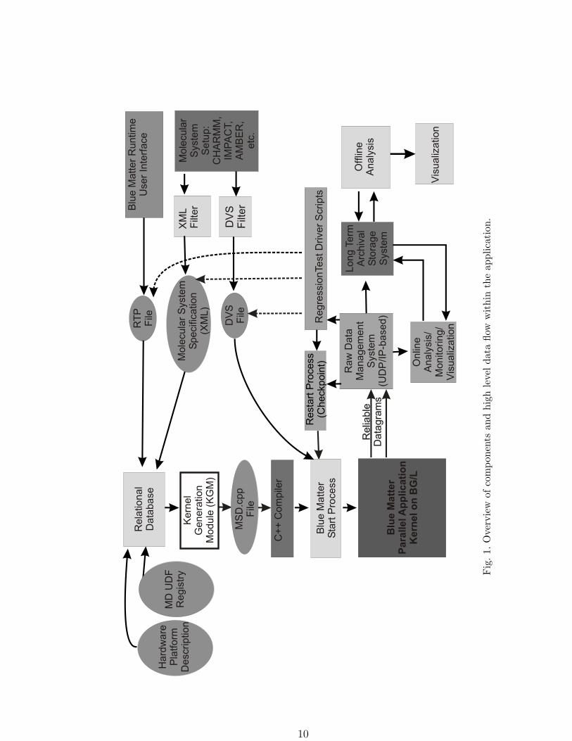
Figure 1 shows the relationship between the major modules in the Blue Matter framework.

A representation of the molecular system and its associated simulation parameters is created

in a relational database as part of the set up process. This representation forms part of the

experimental record which, along with information about specific simulation runs such as

hardware platform type and configuration, can be accessed during analyses of the simulation

data. A kernel generation module retrieves the data associated with a particular molecular

system from the database and creates a Molecular System Definition (MSD) file containing

C++ code which is then compiled and linked with framework source code libraries to produce

an executable. While running on a suitable platform, the executable sends data to a host

computer for consumption by analysis and monitoring modules via a raw datagram (RDG)

stream.

The Blue Matter framework has been architected to allow exploration of multiple application

decompositions with each implementation reusing the domain specific modules and seman-

tics. Currently, this framework is specialized by selecting force field functional forms and

simulation methods. Our strategy for separating MD complexity from parallel complexity

includes factoring as much domain specific knowledge as possible into the setup phase. The

framework is designed to manipulate domain function in very fine grained functional units,

embodied by call-back functions that we refer to as User Defined Functions (UDFs), that

encapsulate localized domain specific data transformations. The call-backs are resolved at

8

compile-time rather than run-time for performance reasons. Flexibly managing the granu-

larity of the domain decomposition is important because of the range of node count and

molecular system sizes we are targeting. Implementing a new parallel decomposition or com-

munications pattern in this framework does not involve changing the UDFs or restating the

simulation semantics. Using this generic infrastructure, we are able to support several force

fields and map them onto drivers suitable to the computational platform available.

2.2 Set-up

The set-up phase of Blue Matter collects all the non-dynamic information required for a

given simulation into a database and generates the source code specific to that run. First,

the user runs a commercially available simulation package (e.g. CHARMm[14], Impact[15],

AMBER[16], GROMOS[17]) to assign force field parameters for the molecular system. A

package-specific filter then transforms the output into an XML file that represents the molec-

ular system specification in a package-neutral form which is then loaded into a relational

database. Relational constraints within the database schema maintain internal consistency

of the molecular system where possible. The user then specifies simulation parameters that

are stored in the relational database. This phase of set-up associates identifiers with both

the inserted molecular system and the specific simulation parameters and allows us to main-

tain an audit path for our scientific and application development explorations including the

ability to execute ad hoc queries to find molecular systems and parameter sets that have

already been created.

Next, the kernel generation module (KGM) generates specialized source code for the simula-

tion using information stored in the database. Since the KGM must recognize a wide variety

of system specification parameters and create corresponding code, it must encapsulate the

molecular dynamics domain knowledge. The KGM generates a customized molecular system

9

Re

liab

leD

ata

gra

ms

Re

liab

leD

ata

gra

ms

Blu

e M

att

er

Ru

ntim

eU

se

r In

terf

ace

Mo

lecu

lar

Syst

em

Se

tup

:C

HA

RM

M,

IMP

AC

T,

AM

BE

R,

etc

.

XM

L F

ilte

rM

ole

cula

r S

yste

mS

pe

cific

atio

n(X

ML

)

RT

PF

ile

DV

SF

ileM

SD

.cp

pF

ile

Blu

e M

att

er

Sta

rt P

roce

ss

Blu

e M

att

er

Para

llel A

pp

licati

on

Kern

el o

n B

G/L

Ra

w D

ata

Ma

na

ge

me

nt

Syste

m(U

DP

/IP

-ba

se

d)

Re

sta

rt P

roce

ss

(Ch

eckp

oin

t)

Lo

ng

Te

rmA

rch

iva

lS

tora

ge

Syste

m

On

line

An

aly

sis

/M

on

ito

rin

g/

Vis

ua

liza

tio

n

Re

gre

ssio

nTe

st

Drive

r S

crip

ts

DV

SF

ilte

r

Off

line

An

aly

sis

Re

latio

na

lD

ata

ba

se

C+

+ C

om

pile

r

MD

UD

FR

eg

istr

y

Ha

rdw

are

Pla

tfo

rmD

escrip

tio

n

Vis

ua

liza

tio

n

Ke

rne

lG

en

era

tio

nM

od

ule

(K

GM

)

Fig

.1.

Ove

rvie

wof

com

pone

nts

and

high

leve

lda

taflo

ww

ithi

nth

eap

plic

atio

n.

10

definition (MSD) file containing parameters and C++ code containing only the desired code

paths in the parallel kernel. Minimizing the lines of source code allows more aggressive and

efficient optimization by the compiler. Although many parameters are built into the exe-

cutable, others are provided at runtime through the dynamic variable set (DVS) file, such

as positions and velocities.

2.3 Generic Molecular Dynamics Framework

Blue Matter encapsulates all molecular dynamics functions that transform data in User De-

fined Functions (UDFs). The term UDF comes from the database community where it refers

to an encapsulated data transformation added to the built-in functions that may be used

during a database query. Typically, these modules encapsulate domain specific knowledge

at the most fine grained level possible. An example is the standard coulomb UDF, which

operates on two charge sites and yields the force between them.

The UDF interface abstracts the calling context, allowing the framework flexibility in or-

ganizing access to parameters and dynamic variables. For example, this flexibility allows

the UDF driver implementation to tile the invocations, an established technique for improv-

ing data locality[18]. In addition, the interface enables the UDF function to be aggressively

inlined into the calling context.

UDF adapters and helpers are modules containing code that will be used by more than one

UDF. An adapter is a module that implements the framework UDF interface and also wraps

another UDF. A helper is a subroutine that is called by a UDF via standard C++ method

invocation interfaces and is passed values from the immediate UDF context. Adapters allow

generic code to be encapsulated. For example, the generation of a virial for pressure control

can be added to a standard UDF by means of an adapter. Adapters are written as C++

11

template classes taking an existing UDF as a parameter.

UDFs represent pure data transformations that may be invoked from several drivers. The

semantics of data movement are implemented in the selection of UDF drivers. For example,

drivers exist to perform pairwise N2 operations (NSQ) as well as to run lists of operands.

Drivers used for a given simulation are selected during kernel generation along with the

appropriate UDFs that appear as template parameters in the driver class. Different drivers

may be written for different hardware platforms and/or load balancing strategies.

UDF drivers may be implemented in several ways while preserving the same semantics. For

example, a set of drivers may support different NSQ parallel decompositions. The drivers

themselves may be inherently parallel with an instance on every node, each executing only

a fraction of the total number of UDF invocations. The implementation of the UDF driver

is where specific knowledge of the target architecture is used to improve performance. In

the case of the Cyclops architecture[1], which was the initial target hardware platform for

the Blue Gene project, the drivers had to be implemented to issue enough independent

work items to load 256 physical threads per chip. In the case of the BG/L architecture[2],

it is important to feed the processor instruction pipeline and to enable reuse of framework

recognizable intermediate values such as the distance between two atoms. Although these two

hardware architectures are quite different in their requirements, the design of Blue Matter

made it possible to adapt to both environments.

To facilitate early adoption of the experimental platforms which it targets, the Blue Matter

framework has been designed to have minimal dependency on system software. The modu-

larity of the framework allows much of the program to run on a stable server. To run the

parallel core in a new node environment requires a C++ compiler, a minimal C++ runtime,

the ability to send and receive datagrams to external machines, and a high performance

communications mechanism.

12

Blue Matter can target two primary communications interfaces for inter-node messaging:

MPI and active messaging. An explicit layer is most appropriate when the application is

operating in distinct phases with relatively large grained parallelism. For large node counts,

where scalability is bounded by the overhead of a very fine grained decomposition, we target a

simple active message interface. For currently available machine configurations, the selection

of communications library is handled at an interface layer by selecting either MPI or active

message based collectives. For BG/L, we are integrating the framework drivers more directly

with active messaging to enable lower overhead and the overlapping of communication and

computation phases.

2.3.1 Online Monitoring/Analysis

The traditional view of a computational simulation has scientific code running on a computer,

periodically dumping results to a file system for later analysis. Blue Matter breaks from this

standard model by avoiding direct file i/o and instead communicating all results via packets

over a reliable datagram connection to analysis tools listening on remote computers. The

resulting packet stream is the raw datagram output (RDG). Outputting a packet stream

offloads a great deal of the complexity of managing state and file formats from the kernel

to analysis tools that are less performance-critical. The parallel kernel may emit packets out

of sequence, and it is up is up to the host monitoring module to marshal a consistent set

of packets for each time step, indicating the code is operating correctly and allowing well-

defined parsing. Since the RDG stream is binary we retain the full precision of the results

for comparison and analysis.

Analyzing the RDG stream involves a combination of online processing of the arriving pack-

ets and selective storing of pre-processed data for efficient offline analysis. For molecular

simulations, the basic online analysis involves parsing the packet stream and determining

13

the value of the energy terms at each time step, while storing the full set of atom positions

and velocities at regular intervals. For each time step containing atom positions we calcu-

late, as a pre-processing task, such features as the presence of hydrogen bonds, the secondary

structure, radii of gyration, and more. The decision to calculate a term online and store the

result during the run depends on the expense of the calculation and the size of the stored

result.

The data stored during a computer simulation serve two distinct purposes:

(1) If the time evolution of the simulation is important, one must record periodic snapshots

of the simulation for later analysis since the final state of the simulation does not convey

the dynamic path, or ”trajectory,” taken from the initial state. These snapshots need not

include the full state of the system for later restart from that point, but should contain

all the information needed for anticipated trajectory analysis. In molecular simulations,

saving the trajectory is essential if the dynamic evolution of the system is central to the

experiment.

(2) Apart from the scientific needs of recording the system evolution there is also a practical

need to store the full system state for an exact restart of the simulation in case of

hardware or software error that either terminates the simulation or causes inaccuracy

in the output results. In general, the state needed for restart may be much larger than

the state relevant to analysis but, fortunately, molecular dynamics has relatively small

state even for large systems, dominated by the positions and velocities of all the atoms

(on the order of megabytes).

2.3.2 Post-Analysis and Data Management

Since Blue Matter relies on a database for the set up of each system to be run, the database

can serve not only to define the simulation, but to track the simulation runs of many scientists

14

because the stream contains a run identifier that directly binds to its full set of input data in

the database including: 1) the molecular system itself, 2) its compile-time parameters, and 3)

its initial configuration, i.e. atomic positions and velocities, plus other state variables. With

all the run information automatically tracked in the database without the need for human

input, powerful SQL queries across many independent runs become possible. The result is

a high-integrity single source of information in a database that serves as an experimental

record to track all the simulations, their parameters, and their results.

2.3.3 Regression/Validation Infrastructure and Strategy

A molecular dynamics simulation should be as fast as possible without compromising the

validity of the scientific results, and an important part of MD code development is a suite

of tools and test cases that provide this validation[19]. Blue Matter relies on a combination

of external regression tests that compare with other packages, internal regression tests that

track code changes, and validation tests that confirm the scientific correctness of specific

runs. To facilitate the specification and execution of these tests on a cluster of workstations

we use an environment that allows a concise specification of a set of related runs, which

makes it easier to create, modify, and run tests that vary many parameters, despite the need

to compile and build each executable corresponding to each run. A more detailed description

of these tests follows.

Since Blue Matter supports a variety of standard force fields and accepts input of molecular

systems created by other MD packages, it is essential to confirm that Blue Matter duplicates

the energy components and forces of those packages to a high degree of precision. Blue Matter

uses the molecular systems and their corresponding energy components and force results of

an extensive suite of blocked amino acids and peptides prepared with CHARMm, AMBER

and Impact (OPLS).[20] We use the set up phase of each MD package to create a system in

15

the corresponding force field, then use Blue Matter to compute the energy terms and confirm

the results agree with the external regression suite.

One of the main validation checks on the code is to verify the extent to which total energy

is conserved. Although the total energy is not strictly constant in time, the width of the

total energy distribution should vary quadratically with the time step size for dynamical

integrators based on simple Verlet-type algorithms and the total energy should not display

systematic drifts over time. This is a sensitive test of the correctness in the implementation

of the dynamics. The procedure involves running the same molecular system for the same

amount of simulation time, using a range of time step sizes, and calculating the root mean

square deviation (RMSD) of the total energy for each run. A correct implementation will show

RMSD’s that vary quadratically with time step to a fraction of a percent. Since accumulated

errors cause trajectories with different time steps to depart from one another in phase space,

we use short runs of a fraction of a picosecond. Other validation tests include checking the

density of water in a long constant pressure run with different water models, confirming the

equipartition theorem applies when constraints such as rigid bonds are in use, confirming

heat capacity estimates are consistent those implied by the slope of energy-temperature

curves from temperature-controlled simulations, and simpler checks of momentum and energy

conservation in long runs.

The internal regression tests provide immediate feedback on code development, but since Blue

Matter outputs results in a lossless binary form, differences can appear due to innocuous code

changes such as a reordering of terms in a summation. In order to be sensitive to the larger

changes in results that indicate a bug, while insensitive to benign changes, a per-system

tolerance is incorporated into the tests that scales with system size and the length of the

regression test. This helps automate the testing process since only errors above threshold

raise a flag that warrants inspection of the code.

16

3 Issues in Mapping the Application onto the Machine

3.1 Interconnect Topologies (Torus and Tree)

The replication unit for BG/L is a single “system-on-a-chip” application-specific integrated

circuit (ASIC) to which additional commodity DRAM chips are added to give 256 MB of

external memory per node. 512 of these replication units or “cells” will be be assembled

into an 8 × 8 × 8 cubic lattice “building block” as shown in Figure 2. The surfaces of this

“building block” (in effect, 6 sets of 8×8 wires) connect to simpler “link chips” that send and

receive signals over the relatively long distance to the next “building block”. A supervisory

computer can set up the links to partition the set of “building blocks” into the sizes of

lattice requested by the applications. The result is three dimensional torus wiring and the

ability to route around blocks that are out of service for maintenance. The ASICs also have

connections for a “tree” network. Each ASIC has a simple arithmetic-logic unit (ALU) for

the tree, enabling the tree to support “add reduction” (where each ASIC provides a vector of

numbers; the vectors being added element-wise to their partners at each node until a single

vector reaches the root; the vector is then broadcast back to all the ASICs). “max”, “or”,

“and”, and “broadcast” are also supported by the tree ALU.

For the internal (torus and tree) networks, there is hardware link-level error checking and

recovery; an application on the compute fabric is assured that a message sent from a node

will arrive intact and exactly once at its destination. All links carry data in both directions

at the same time. The torus links carry 2 bits per CPU clock cycle while the tree links carry

4 bits per CPU clock cycle. For both networks, data are forwarded as soon as possible, with

a per-node latency equivalent to the time required to send a few bytes, unless congestion

on the outgoing link (torus and tree) or a wait for partner data (tree reduction operations)

forces data to be buffered. There is no need for software intervention in any point-to-point

17

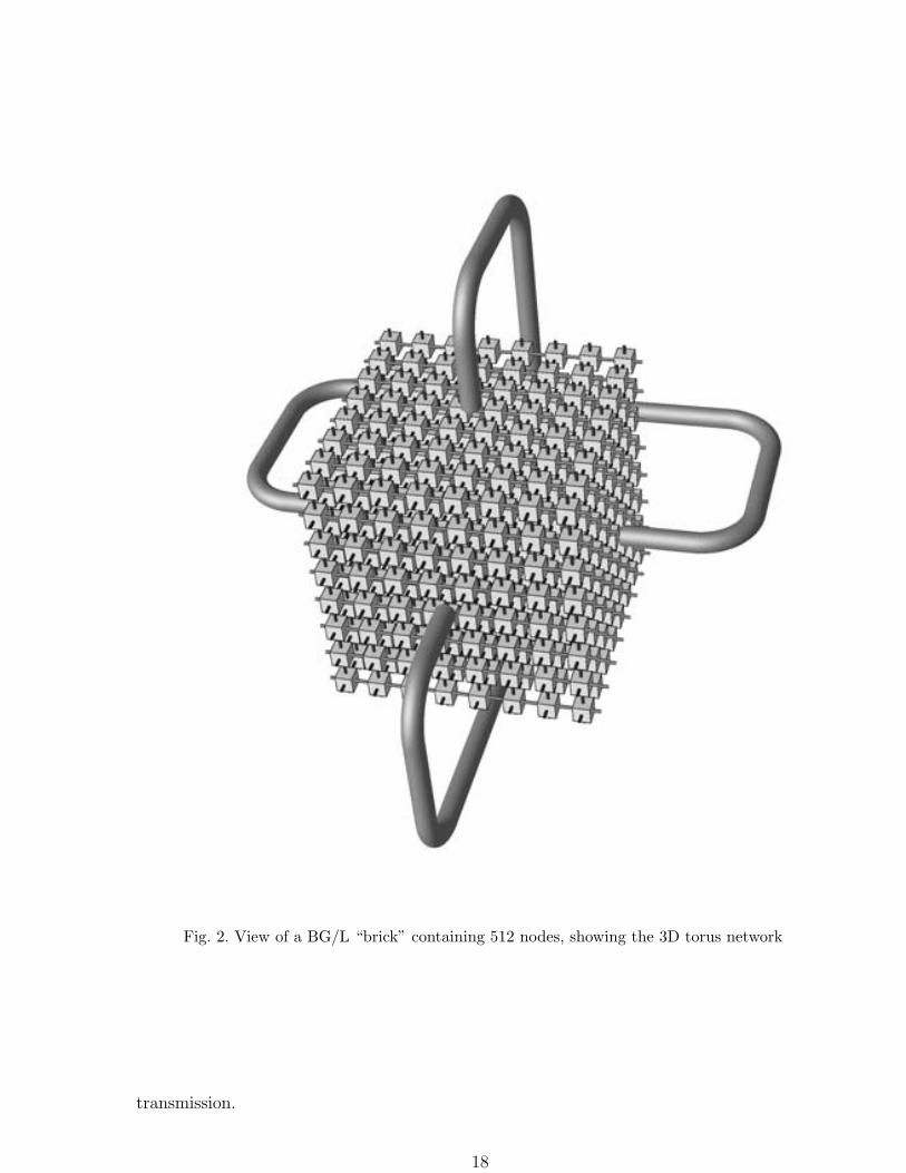
Fig. 2. View of a BG/L “brick” containing 512 nodes, showing the 3D torus network

transmission.

18

3.2 Efficient use of the Floating Point unit

The Blue Gene/L CPU belongs to the IBM PowerPC family, and we use the IBM VisualAge

compiler with a modified “back end” to generate code for it. Interaction with compiler devel-

opers has enabled better floating-point optimization for the current POWER3 architecture

as well as for Blue Gene/L, which has resulted in a 30% improvement in the performance of

Blue Matter when built to run on POWER3 machines.

On each ASIC there are 2 microprocessors. Each microprocessor is a PowerPC 440 microcon-

troller to which two copies of a PowerPC-type floating-point unit have been added. The CPU

can run the normal PowerPC floating-point instruction set and supports additional instruc-

tions that operate on data in both floating-point units concurrently. Each floating-point unit

has its own set of 32 registers at 64 bits wide. All floating-point instructions (except “divide”)

pass through a 5-cycle pipeline; provided there are no data dependencies, one floating-point

instruction can be dispatched per clock cycle. The PPC440 can dispatch 2 instructions per

clock cycle, thus peak floating-point performance would need 10 independent streams of data

to work on, and the program logic would require a “multiply-add” operation at every stage.

This would account for a “parallel multiply-add” instruction dispatched every clock cycle;

the other dispatch slot in the clock cycle would be used for a load, store, integer, or branch

op in support of the program logic to keep the floating-point pipeline busy and productive.

It is straightforward to achieve this for a polynomial function f(x) that needs evaluation

for 10 values of x, but for less regular code kernels, or poorly controlled vector lengths, the

fraction of peak achieved depends on the skill of the programmer. The unoptimized case

would dispatch only 1 instruction per clock cycle, not achieving any parallelization to use

the second floating-point unit, and not exploiting the fused ’multiply’ and ’add’; this would

run at 5% of peak. We have already implemented some computational kernels, such as vector

reciprocal square root, exponential, and inverse trigonometric functions, that have been set

19

up to exploit the double floating point unit by avoidance of conditional branches and other

strategies.

3.3 Memory Hierarchy

Each CPU has a 32 KByte instruction cache and a 32 kByte data cache. The L1 line size

is 32 bytes. There is no hardware support for keeping the L1 caches coherent between the

CPUs. Associated with each CPU is a prefetcher, known as L2, that fetches 128 bytes at a

time from L3. The ASIC contains 4 MBytes of DRAM as an L3 cache shared by both CPUs.

The L1 can read 3 cache lines from L2 every 16 CPU clock cycles, and concurrently write

1 cache line every 2 CPU clock cycles. The L3 can keep up with this bandwidth from both

CPUs.

The lack of coherency between the L1 data caches defines the ways in which both CPUs can

be used together. Those we foresee are

• Structured application coding, for example using single-writer-single-reader queues and

explicit memory synchronization points to move data between CPUs in a well-defined way

even though L1 is not made coherent by hardware.

• CPUs used independently, as if they were on separate nodes joined by a network.

• Second CPU used as a Direct Memory Access (DMA) controller. The first CPU would

perform all the computation, flush results as far as L3 cache, and set up DMA orders;

the second CPU would copy data between memory and the network FIFO interfaces. A

version of this mode would allow the second CPU to process active messages, where an

incoming torus packet contains a function pointer and data, and the reception routine calls

the function with the given data. Parallel loads/stores to registers in the double floating

point unit request 16 bytes to be moved between registers and the relevant level in the

20

memory hierarchy every clock cycle.

• Compiler-driven loop partitioning. A compiler would spot a computationally-intensive loop

(for example, ’evaluate the sine of each element of a vector’); assign part of the vector to

each CPU; ensure that the relevant source data was flushed as far as L3; post the second

processor to start work, then start work on its own portion; and synchronize with the

second processor at completion.

3.4 Identifying Concurrency in the Application

As a starting point for any discussion about how to map an application onto a particular

parallel architecture, it is essential to understand the fundamental limits to concurrency

present in the algorithm. Of course, such estimates depend on the granularity of computa-

tion that one is willing to distribute. One way to view the application execution is as the

materialization of a series of data structures that are transformed from one into the other by

computation and/or communication. During a phase of computation, the number of possible

data-independent operations determine the concurrency present during that phase of the ap-

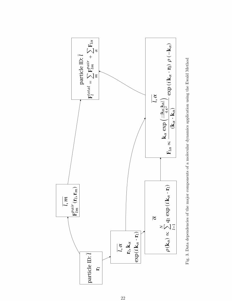
plication. A view of this sort representing the non-bonded force calculations in a molecular

dynamics application using the Ewald technique is shown in Figure 3.

Molecular Dynamics proceeds as a sequence of simulation time steps. At each time step, forces

on the atoms are computed; and then the equations of motion are integrated to update the

velocities and positions of the atoms. At the start, corresponding to the leftmost box in

Figure 3, the positions and velocities of all the particles are known and a data structure

indexed by the particle identifier l can be distributed using any “hashing” function of l with

the maximum possible number of hash slots equal to the number of particles, N . Both atom

and volume based decompositions are possible.

21

par

ticl

eID

:lr l

l,m

Fpair

lm(rl,

r m)

l,α

r l,kα

exp(i

kα·r

l)

α

ρ(kα)∝

N ∑ l=1

q lex

p(i

kα·r

l)

l,α

F lα∝

kα

exp( − (k

α·kα)

4κ

2

)(kα·k

α)

exp(i

kα·r

l)ρ(−

kα)

par

ticl

eID

:l

Ftotal

l=∑ m

Fpair

lm+∑ α

F lα

Fig

.3.

Dat

ade

pend

enci

esof

the

maj

orco

mpo

nent

sof

am

olec

ular

dyna

mic

sap

plic

atio

nus

ing

the

Ew

ald

Met

hod

22

Following the upper branch of data dependencies, the next phase involves computation of all

the pairwise forces between particles. This requires a data structure to be materialized that

contains all pairs of particle positions so that the computation of the pair forces can take

place. This structure can be indexed by a pair of particle identifiers l and m and indicates

that distribution over a much larger number of hash slots, N2, is possible although the finite

range cut-offs used for the pair potentials means that the actual number of non-vanishing

pair computations is much smaller than N2. This is the phase of the application where an

“interaction” decomposition is often used[21]. Next, a reduction is required to sum up the

pairwise forces on each particle so that a data structure containing the total force on each

particle, indexed by the particle identifier l can be created.

Along the lower branch of data dependencies, the calculation of the Ewald sum requires

exponentials that are functions of particle position and k-vector value. The k-vector values

are fixed and the number required is determined by the accuracy required in the Ewald sum.

The data structure containing these values is indexed by the particle identifier l and the

k-vector index α. Next, components of the Fourier transform of the charge density need to

be computed, which requires a reduction of the exponentials according to the k-vector index

α. The data structure containing the reciprocal space contributions to the force (indexed by

particle identifier l and k-vector index α) requires both the Fourier transform of the charge

density and the exponentials computed earlier. These contributions must also be added into

the total force on each particle. Finally, the data structure containing the total force on each

particle, indexed by l, can be used to propagate the dynamics and give new values for the

position and velocity of each particle.

The number of independent data items at each stage in this process is as follows:

• For stages that are partitionable by particle identifier, the number of independent data

items is N , the number of particles.

23

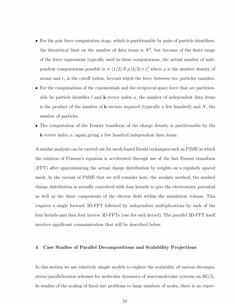
• For the pair force computation stage, which is partitionable by pairs of particle identifiers,

the theoretical limit on the number of data items is N2, but because of the finite range

of the force expressions typically used in these computations, the actual number of inde-

pendent computations possible is ≈ (1/2) N ρ (4/3) π r3c where ρ is the number density of

atoms and rc is the cutoff radius, beyond which the force between two particles vanishes.

• For the computations of the exponentials and the reciprocal space force that are partition-

able by particle identifier l and k-vector index α, the number of independent data items

is the product of the number of k-vectors required (typically a few hundred) and N , the

number of particles.

• The computation of the Fourier transform of the charge density is partitionable by the

k-vector index α, again giving a few hundred independent data items.

A similar analysis can be carried out for mesh-based Ewald techniques such as P3ME in which

the solution of Poisson’s equation is accelerated through use of the fast Fourier transform

(FFT) after approximating the actual charge distribution by weights on a regularly spaced

mesh. In the variant of P3ME that we will consider here, the analytic method, the meshed

charge distribution is actually convolved with four kernels to give the electrostatic potential

as well as the three components of the electric field within the simulation volume. This

requires a single forward 3D-FFT followed by independent multiplications by each of the

four kernels and then four inverse 3D-FFTs (one for each kernel). The parallel 3D-FFT itself

involves significant communication that will be described below.

4 Case Studies of Parallel Decompositions and Scalability Projections

In this section we use relatively simple models to explore the scalability of various decompo-

sition/parallelization schemes for molecular dynamics of macromolecular systems on BG/L.

In studies of the scaling of fixed size problems to large numbers of nodes, there is no expec-

24

tation that ideal scaling will be observed.[22] However, for a specified problem size, useful

parallel speed-ups should be achievable on a range of node counts with the upper limit on

node count being determined by the portion of the computation with the least favorable

scaling properties (Amdahl’s law). Our intent is to use these model calculations to assist in

making decisions about the relative viability of various approaches and to assess the balance

between computation and communication within these approaches, not to make absolute

performance predictions.

In the examples that follow, our focus is on communications patterns that map closely to

the hardware capabilities of the BG/L architecture because we want to keep the potential

for software overheads to a minimum. Some of the communications estimates used below are

derived from work on a network simulator developed by members of the BG/L team while

others, such as the capabilities of the tree network are taken directly from the designed

capabilities of the hardware.[2] Cycle count estimates for computational kernels are taken

from the output of the IBM C++ compiler that targets the BG/L architecture or from

estimates of the time required for memory accesses. The assumptions built into the examples

that follow are:

• System software overheads are neglected

• No overlap between computation and communication is utilized

• Only one CPU per node is available for computation

• Memory access times are neglected except where we have been able to identify them as

dominating the time for computation (only for integration of the equations of motion).

Since all of our work requires accounting correctly for the effects of the long range interactions

in the system, the first case study concerns the properties of a three-dimensional FFT on

the BG/L architecture. The two other case studies, which deal with different mappings

of molecular dynamics onto the BG/L hardware, both assume the same set of FFT-based

25

operations to support the P3ME method. Also, the projections made in these case studies

neglect the contributions of bonded force calculations to the total computational burden

since they represent relatively small fractions of the total and can be distributed well enough

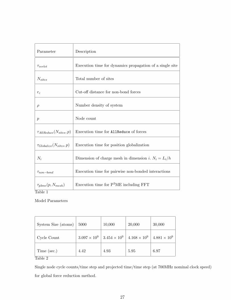
to keep their contribution to the per node computational burden small. The parameters used

in the models are defined in Table 1. Although the actual machine has hardware support for

partitioning down to a granularity of 512 nodes, we include smaller node counts in our model

for illustrative purposes. Occasional “anomalies” visible in in graphs of the performance are

due to the fact that since the machine is partitionable into multiples of eight nodes in each

dimension, many node counts will be comprised of non-cubical partitions which affect the

performance of the torus communications network.

In the model used to produce Figures 5 and 6, the contributions to τp3me(p, Nmesh) comprise

one forward and four inverse 3D real-valued FFTs to give the electrostatic potential and the

three components of the electric field using the analytic method as described in Section 3.4.

4.1 Three Dimensional Fast Fourier Transform

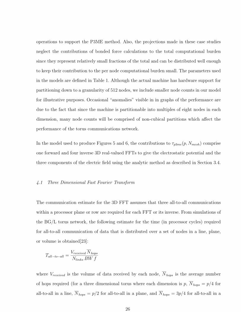
The communication estimate for the 3D FFT assumes that three all-to-all communications

within a processor plane or row are required for each FFT or its inverse. From simulations of

the BG/L torus network, the following estimate for the time (in processor cycles) required

for all-to-all communication of data that is distributed over a set of nodes in a line, plane,

or volume is obtained[23]:

Tall−to−all =Vreceived Nhops

Nlinks BW f

where Vreceived is the volume of data received by each node, Nhops is the average number

of hops required (for a three dimensional torus where each dimension is p, Nhops = p/4 for

all-to-all in a line, Nhops = p/2 for all-to-all in a plane, and Nhops = 3p/4 for all-to-all in a

26

Parameter Description

τverlet Execution time for dynamics propagation of a single site

Nsites Total number of sites

rc Cut-off distance for non-bond forces

ρ Number density of system

p Node count

τAllReduce(Nsites, p) Execution time for AllReduce of forces

τGlobalize(Nsites, p) Execution time for position globalization

Ni Dimension of charge mesh in dimension i. Ni = Li/h

τnon−bond Execution time for pairwise non-bonded interactions

τp3me(p, Nmesh) Execution time for P3ME including FFT

Table 1

Model Parameters

System Size (atoms) 5000 10,000 20,000 30,000

Cycle Count 3.097× 109 3.454× 109 4.168× 109 4.881× 109

Time (sec.) 4.42 4.93 5.95 6.97

Table 2

Single node cycle counts/time step and projected time/time step (at 700MHz nominal clock speed)

for global force reduction method.

27

volume), Nlinks is the number of links available to each node (2 for linear communication, 4

for planar communication, and 6 for volumetric communication), BW is the raw bandwidth

of the torus per link (2 bits per processor clock cycle), and f is the link utilization (assumed

to be 80%). Note that the time required for all-to-all communication is independent of the

dimensionality of the communication because of the compensating effects of the average hop

count and the number of links available for the communication.

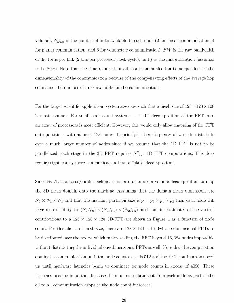
For the target scientific application, system sizes are such that a mesh size of 128×128×128

is most common. For small node count systems, a “slab” decomposition of the FFT onto

an array of processors is most efficient. However, this would only allow mapping of the FFT

onto partitions with at most 128 nodes. In principle, there is plenty of work to distribute

over a much larger number of nodes since if we assume that the 1D FFT is not to be

parallelized, each stage in the 3D FFT requires N2mesh 1D FFT computations. This does

require significantly more communication than a “slab” decomposition.

Since BG/L is a torus/mesh machine, it is natural to use a volume decomposition to map

the 3D mesh domain onto the machine. Assuming that the domain mesh dimensions are

N0 × N1 × N2 and that the machine partition size is p = p0 × p1 × p2 then each node will

have responsibility for (N0/p0) × (N1/p1) × (N2/p2) mesh points. Estimates of the various

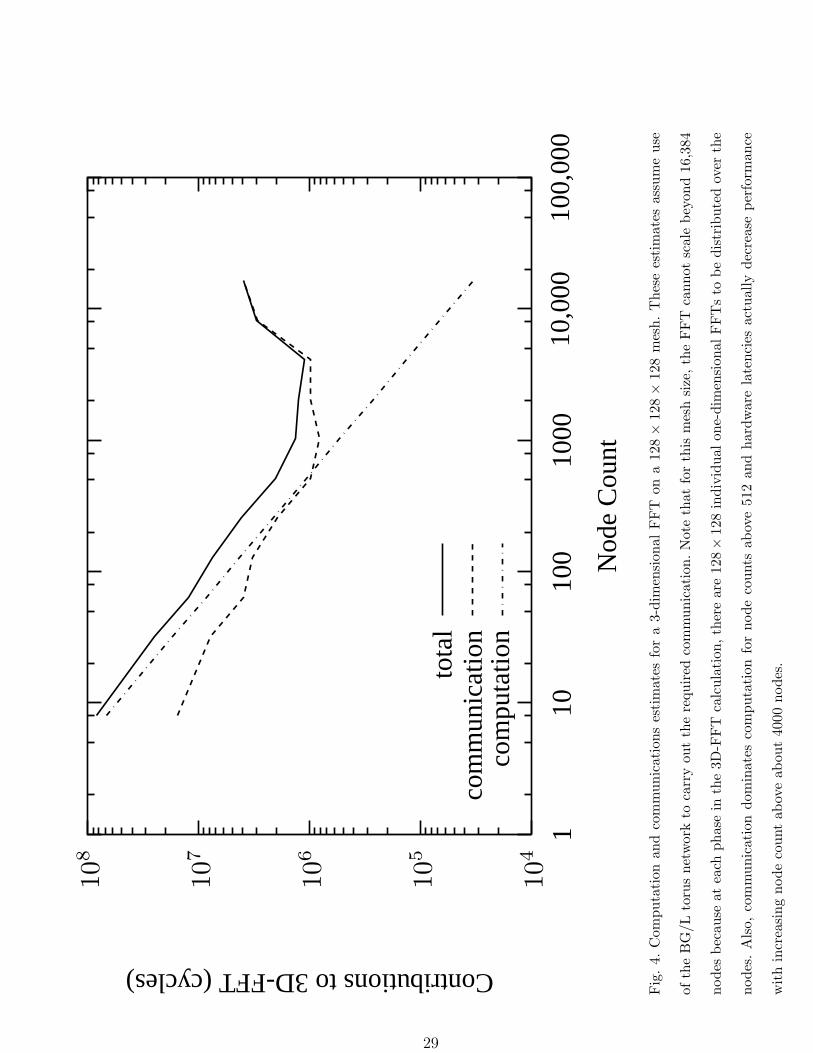
contributions to a 128 × 128 × 128 3D-FFT are shown in Figure 4 as a function of node

count. For this choice of mesh size, there are 128 × 128 = 16, 384 one-dimensional FFTs to

be distributed over the nodes, which makes scaling the FFT beyond 16, 384 nodes impossible

without distributing the individual one-dimensional FFTs as well. Note that the computation

dominates communication until the node count exceeds 512 and the FFT continues to speed

up until hardware latencies begin to dominate for node counts in excess of 4096. These

latencies become important because the amount of data sent from each node as part of the

all-to-all communication drops as the node count increases.

28

104

105

106

107

108

110

100

1000

10,0

0010

0,00

0

Contributionsto3D-FFT(cycles)

Nod

eC

ount

tota

lco

mm

unic

atio

nco

mpu

tatio

n

Fig

.4.

Com

puta

tion

and

com

mun

icat

ions

esti

mat

esfo

ra

3-di

men

sion

alFFT

ona

128×

128×

128

mes

h.T

hese

esti

mat

esas

sum

eus

e

ofth

eB

G/L

toru

sne

twor

kto

carr

you

tth

ere

quir

edco

mm

unic

atio

n.N

ote

that

for

this

mes

hsi

ze,th

eFFT

cann

otsc

ale

beyo

nd16

,384

node

sbe

caus

eat

each

phas

ein

the

3D-F

FT

calc

ulat

ion,

ther

ear

e12

8×

128

indi

vidu

alon

e-di

men

sion

alFFT

sto

bedi

stri

bute

dov

erth

e

node

s.A

lso,

com

mun

icat

ion

dom

inat

esco

mpu

tati

onfo

rno

deco

unts

abov

e51

2an

dha

rdw

are

late

ncie

sac

tual

lyde

crea

sepe

rfor

man

ce

wit

hin

crea

sing

node

coun

tab

ove

abou

t40

00no

des.

29

4.1.1 Global Force Reduction (GFR)

One simple parallel decomposition for real space molecular dynamics focuses on global force

reduction. This allows the pairwise interactions to be arbitrarily partitioned amongst nodes to

achieve load balance. Once per time step, all nodes participate in a summation all-reduction

implemented over the global tree network (equivalent to standard global reduce followed by a

broadcast) with each node contributing the results of its assigned interactions. Given access

to net force on each particle and the current positions and velocities of each particle, each

node can replicate the numerical integration of the equations of motion for each particle to

give every node a copy of the updated full configuration of the system. Since each node has

access to the full configuration of the system, this decomposition can work with versions of

the P3ME method that use only a subset of the nodes for the FFT computation.

GFR has the following advantages:

• Load balancing of the non-bonded force calculation is straightforward.

• Double computation of the non-bonded forces can be avoided.

• P3ME can be supported in a number of decompositions including using only a subset

of nodes for the P3ME portion of the computation since the computed forces are made

visible on all nodes.

Drawbacks to GFR are:

• The replication of the dynamics propagation on all nodes represents non-parallelizable

computation.

• The force reduction itself is non-scalable as implemented on the global tree.

• The implementation of a floating point reduction on the global tree network requires ad-

ditional software overhead. In our model, two reductions are required–the first establishes

a scale through a 16 bit/element comparison reduction while the second carries out a

30

summation reduction with scaled fixed point values (64 bits/element).

It is possible to reduce the replication of dynamics propagation by using some form of

volume decomposition and Verlet lists. Using these facilities, each node need only propagate

dynamics for atoms either homed on that node or within a cutoff distance (or within the

guard zone when using Verlet lists).

4.1.2 Global Position Broadcast Decomposition

Another possible decomposition that leverages the capabilities of the global tree network

on BG/L is based on a global position broadcast (GPB). Local force reductions will be

required, but their near neighbor communications burden will be neglected in this model. A

functional overview of the GPB class of decompositions is as follows. Once per time step the

atom position vector will be bit-OR all-reduced (OR reduce, then broadcast) via the global

tree network. However, for P3ME this method will also require near neighbor force reduction

since atoms will generate forces from FFT mesh points on nodes other than their home node.

Because of this, it is advantageous to maintain a 3D spatial mapping of atoms/fragment to

nodes in BG/L. An issue with using near neighbor point-to-point messages to bring in the

forces from the P3ME/FFT mesh points off node will be figuring out when all the forces have

been received. To handle this, for each fragment homed on a node, a deterministic algorithm

must yield an expectation of the exact number of forces to wait for. In this method, we

partition both the force generating operations as well as the integration parts of the loop -

each node only propagates dynamics for those sites/fragments that are locally homed.

In this initial version of the model for global position broadcast, double computing of forces

will be assumed as well as ideal load balancing of real-space non-bonded forces. The model

corresponding to these assumptions is

31

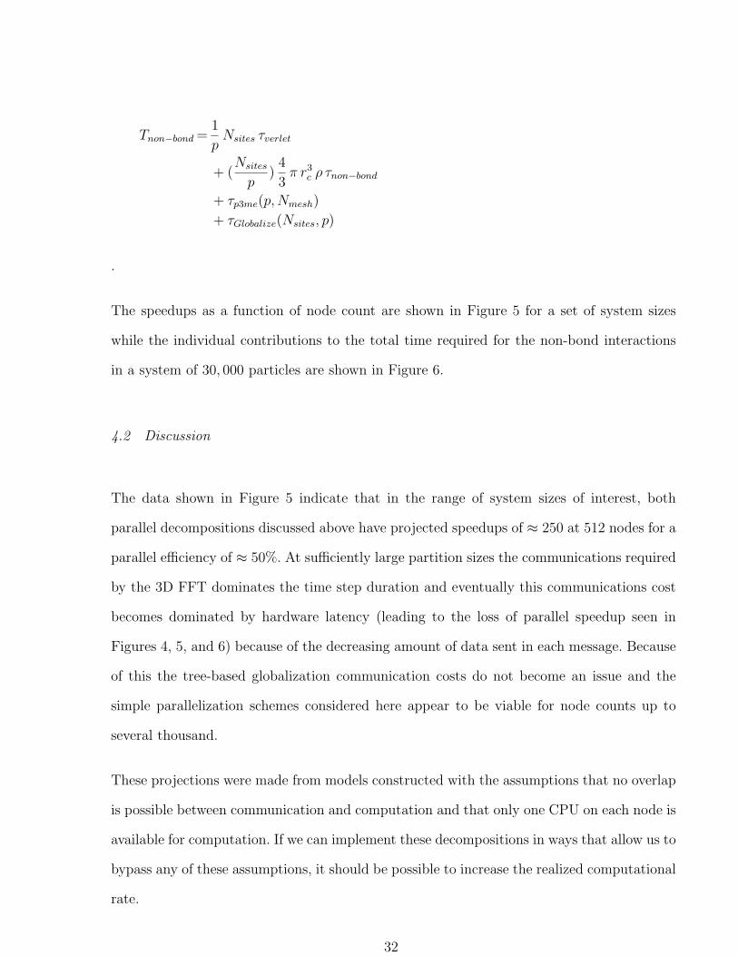
Tnon−bond =1

pNsites τverlet

+ (Nsites

p)4

3π r3

c ρ τnon−bond

+ τp3me(p, Nmesh)

+ τGlobalize(Nsites, p)

.

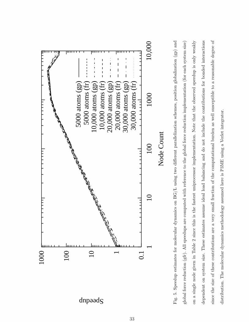
The speedups as a function of node count are shown in Figure 5 for a set of system sizes

while the individual contributions to the total time required for the non-bond interactions

in a system of 30, 000 particles are shown in Figure 6.

4.2 Discussion

The data shown in Figure 5 indicate that in the range of system sizes of interest, both

parallel decompositions discussed above have projected speedups of ≈ 250 at 512 nodes for a

parallel efficiency of ≈ 50%. At sufficiently large partition sizes the communications required

by the 3D FFT dominates the time step duration and eventually this communications cost

becomes dominated by hardware latency (leading to the loss of parallel speedup seen in

Figures 4, 5, and 6) because of the decreasing amount of data sent in each message. Because

of this the tree-based globalization communication costs do not become an issue and the

simple parallelization schemes considered here appear to be viable for node counts up to

several thousand.

These projections were made from models constructed with the assumptions that no overlap

is possible between communication and computation and that only one CPU on each node is

available for computation. If we can implement these decompositions in ways that allow us to

bypass any of these assumptions, it should be possible to increase the realized computational

rate.

32

0.1110100

1000

110

100

1000

10,0

00

Speedup

Nod

eC

ount

5000

atom

s(gp

)50

00at

oms(

fr)

10,0

00at

oms(

gp)

10,0

00at

oms(

fr)

20,0

00at

oms(

gp)

20,0

00at

oms(

fr)

30,0

00at

oms(

gp)

30,0

00at

oms(

fr)

Fig

.5.

Spee

dup

esti

mat

esfo

rm

olec

ular

dyna

mic

son

BG

/Lus

ing

two

diffe

rent

para

lleliz

atio

nsc

hem

es,po

siti

ongl

obal

izat

ion

(gp)

and

glob

alfo

rce

redu

ctio

n(g

fr).

All

spee

dups

are

com

pute

dw

ith

refe

renc

eto

the

glob

alfo

rce

redu

ctio

nim

plem

enta

tion

(for

each

syst

emsi

ze)

ona

sing

leno

degi

ven

inTab

le2

sinc

eth

isis

the

fast

est

unip

roce

ssor

impl

emen

tati

on.N

ote

that

the

obse

rved

spee

dup

ison

lyw

eakl

y

depe

nden

ton

syst

emsi

ze.

The

sees

tim

ates

assu

me

idea

llo

adba

lanc

ing

and

dono

tin

clud

eth

eco

ntri

buti

ons

for

bond

edin

tera

ctio

ns

sinc

eth

esi

zeof

thes

eco

ntri

buti

ons

are

ave

rysm

allfr

acti

onof

the

com

puta

tion

albu

rden

asw

ellsu

scep

tibl

eto

are

ason

able

degr

eeof

dist

ribu

tion

.T

hem

olec

ular

dyna

mic

sm

etho

dolo

gyas

sum

edhe

reis

P3M

Eus

ing

aV

erle

tin

tegr

ator

.

33

10

102

103

104

105

106

107

108

109

1 10 100 1000 10,000 100,000

Con

trib

utio

nsto

Tim

eS

tepD

urat

ion

(cyc

les)

NodeCount

PositionGlobalization

TotalVerlet

GlobalizationFFT

Realspacenon-bond

10

102

103

104

105

106

107

108

109

1 10 100 1000 10,000 100,000

Con

trib

utio

nsto

Tim

eS

tepD

urat

ion

(cyc

les)

NodeCount

GlobalForceReduction

TotalVerlet

ForceReductionFFT

Realspacenon-bond

Fig. 6. An estimate of the contributions of various computational and communications operations

to the total number of cycles required to carry out a time step on a 30, 000 atom system is shown as

a function of node count for two different parallelization schemes, position globalization (gp) and

global force reduction (gfr). At very large node counts, the performance of both schemes is limited

by the communications time required for the 3D FFT rather than the global position broadcast or

force reduction.

34

5 Areas for Exploration

5.1 Multiple Time Step Integration

Any methods that increase the ratio of simulation time to computational effort through

algorithmic means are extremely attractive candidates for investigation. The development of

methods to integrate the equations of motion in a way that takes account of the multiple time

scales present in a molecular dynamics simulation provides a means of reducing the number of

times that expensive long range force evaluations need to take place during a fixed amount of

simulation time.[24,25] Implementing these methods efficiently in the context of the parallel

decompositions discussed above may require some modifications to the implementation of

those decompositions, but the potential benefits in a parallel program are large[26] especially

when an appropriate decomposition of the electrostatic forces is used in combination with

an efficient algorithm for periodic electrostatics like P3ME.[25]

5.2 Alternatives for periodic electrostatics.

Several algorithms have been developed and extensively tested for efficient evaluation of

electrostatic forces, but improving already existing and developing new algorithms remains

an area of active research. These algorithms differ in the degree of implementation complexity,

scalability with the number of particles, and suitability for parallelization as defined by

scaling with the number of nodes used.

The particle-particle-particle-mesh (P3ME) method[12] uses FFT methods to speed up cal-

culation of the reciprocal space part. The P3ME method has good scalability with system

size since the computational cost grows as N log N , and this is currently the most popular

approach used in MD packages. Unfortunately, parallelization of the P3ME method is limited

35

by the properties of the FFT algorithm, which involves significant communications between

nodes.

Many algorithms can be classified as tree methods or multiple grid methods. Both approaches

are similar in that they hierarchically separate interactions based on their spatial separation.

The tree methods separate particles into clusters based on their relative distance, while the

multi-grid methods use grids of different coarseness to approximate the smooth part of the

potential between pairs of particles.

A well-known example of a tree method is the Fast Multipole Method[27], in which distant

particles are grouped in clusters and the effect of distant clusters is approximated using

multipole expansion. The scaling of this algorithm is O(N). A typical implementation of

this algorithm is usually rather expensive, and therefore it becomes faster than the P3ME

method only at relatively large system sizes.

Another method developed by Lekner[28] provides an alternative to Ewald summation and

related techniques for handling electrostatic interactions between particles in a periodic box.

The effect of all the periodic images is included in an effective pair-wise potential. The form

of this potential allows a product decomposition to be applied[29]. The rate of convergence of

the resulting series depends strongly on the ratio of the separation between particles in one of

the dimensions and the periodic box size. The hierarchy of scales in this method is achieved by

adding and subtracting images of charges to create periodic boundary conditions in a box of

half the spatial extent in one of the dimensions. Then the procedure is repeated for several

scales of box sizes. The scaling of this method with the particle number is O(N log N).

Studies of the efficiency of this method show promising results in comparison with other

methods in cases where the accuracy of the electrostatic interaction calculations is relatively

high[30].

36

6 Summary and Conclusions

We have described the architecture of the Blue Matter framework for biomolecular simulation

being developed as part of IBM’s Blue Gene project as well as some of the features of the

Blue Gene/L machine architecture that are relevant to application developers, particularly,

issues and approaches associated with achieving efficient utilization of the double floating

point unit. This work in collaboration with the IBM Toronto compiler team has not only

improved code generation for BG/L, but has also led to significant improvements, 30%

or more, in the performance of Blue Matter on the existing Power3 platform. In order to

guide our development efforts and algorithmic investigations, we have explored two parallel

decompositions that leverage the global tree interconnect on the BG/L platform as well as a

distributed implementation of a three-dimensional FFT (required for the most widely used

treatment of periodic electrostatics in molecular simulation) using the BG/L torus network

through modeling.

Our estimates indicate that a 3D-FFT on a 128 × 128 × 128 mesh remains computation

dominated up to a partition size of 512 nodes and that significant speed-ups are realizable

out to larger node counts. The two decompositions described here, position globalization

and global force reduction, both rely on reductions implemented via BG/L’s global tree.

Both schemes have projected parallel efficiencies of about 50% out to 512 nodes for system

sizes in the range of 5000 to 30,000 atoms and the time required to compute a single time

step becomes dominated by communications latency effects in the 3D-FFT implementation

for node counts above ≈ 4000. Given that the simulation experiments under consideration

require multiple independent or loosely coupled molecular simulations, we conclude that these

results indicate that FFT-based particle mesh techniques are a reasonable first approach to

implementing a molecular simulation application that targets BG/L. As hardware becomes

available, we will be able to validate our estimates, assess the impact of system software

37

overheads, explore whether some overlap of communication and computation is possible,

and assess the possibility of using both CPUs on a BG/L node for computation.

References

[1] F. Allen, et al., Blue Gene: a vision for protein science using a petaflop supercomputer, IBM

Systems Journal 40 (2) (2001) 310–327.

[2] N. Adiga, et al., An overview of the Blue Gene/L supercomputer, in: Supercomputing 2002

Proceedings, 2002, http://www.sc-2002.org/paperpdfs/pap.pap207.pdf.

[3] B. Fitch, M. Giampapa, The vulcan operating environment: a brief overview and status report,

in: G.-R. Hoffman, T. Kauranne (Eds.), Parallel Supercomputing in Atmospheric Science,

World Scientific, 1993, p. 130.

[4] M. Karplus, J. McCammon, Molecular dynamics simulations of biomolecules, Nature Structural

Biology 9 (9) (2002) 646–652.

[5] J. F. Nagle, S. Tristam-Nagle, Structure of lipid bilayers, Biochimica et Biophysica Acta 1469

(2000) 159–195.

[6] F. Sheinerman, C. Brooks III, Calculations on folding of segment b1 of streptococcal protein

g, J. Mol. Biol. 278 (1998) 439–456.

[7] Y. Duan, P. Kollman, Pathways to a protein folding intermediate observed in a 1-microsecond

simulation in aqueous solution, Science 282 (1998) 740.

[8] C. Snow, H. Nguyen, V. Pande, M. Gruebele, Absolute comparison of simulated and

experimental protein-folding dynamics, Nature 420 (6911) (2002) 102–106.

[9] R. Zhou, B. Berne, Can a continuum solvent model reproduce the free energy landscape of a

beta-hairpin folding in water?, Proc. Natl. Acad. Sci. USA 99 (20) (2002) 12777–12782.

38

[10] J. Bader, D. Chandler, Computer simulation study of the mean forces between ferrous and

ferric ions in water, The Journal of Physical Chemistry 96 (15).

[11] S. De Leeuw, J. Perram, E. Smith, Simulation of electrostatic systems in periodic boundary

conditions I. lattice sums and dielectric constants, Proc. Roy. Soc. Lond. A 373 (1980) 27–56,

and references therein.

[12] R. Hockney, J. Eastwood, Computer Simulation Using Particles, Institute of Physics Publishing,

1988.

[13] M. Austern, Generic Programming and the STL: using and extending the C++ standard

template library, Addison-Wesley, 1999.

[14] A. D. J. MacKerell, B. Brooks, C. L. Brooks III, L. Nilsson, B. Roux, Y. Won, M. Karplus,

Charmm: The energy function and its parameterization with an overview of the program, in:

P. v. R. Schleyer, et al. (Eds.), The Encyclopedia of Computational Chemistry, Vol. 1, John

Wiley & Sons, 1998, pp. 271–277.

[15] Impact, http://www.schrodinger.com.

[16] D. Case, D. Pearlman, J. Caldwell, T. Cheatham III, J. Wang, W. Ross, C. Simmerling,

T. Darden, K. Merz, R. Stanton, A. Cheng, J. Vincent, M. Crowley, V. Tsui, H. Gohlke,

R. Radmer, Y. Duan, J. Pitera, I. Massova, G. Seibel, U. Singh, P. Weiner, P. Kollman, AMBER

7, University of California, San Francisco (2002).

[17] W. van Gunsteren, S. Billeter, A. Eising, P. Hunenberger, P.H. Kruger, A. Mark, W. Scott,

I. Tironi, The GROMOS96 Manual and User Guide, ETH Zurich (1996).

[18] G. Rivera, C.-W. Tseng, Tiling optimizations for 3d scientific computations, in:

Supercomputing, 2000.

[19] W. van Gunsteren, A. Mark, Validation of molecular dynamics simulation, J. Chem. Phys.

108 (15) (1998) 6109–6116.

[20] C. Brooks III, D. Price, private communication.

39

[21] S. Plimpton, Fast parallel algorithms for short-range molecular dynamics, Journal of

Computational Physics 117 (1995) 1–19.

[22] V. Taylor, R. Stevens, K. Arnold, Parallel molecular dynamics: implications for massively

parallel machines, Journal of Parallel and Distributed Computing 45 (2) (1997) 166–175.

[23] A. Gara, P. Heidelberger, B. Steinmacher-burow, private communication.

[24] M. Tuckerman, B. Berne, G. Martyna, Reversible multiple time scale molecular dynamics, J.

Chem. Phys. 97 (3) (1992) 1990–2001.

[25] R. Zhou, E. Harder, H. Xu, B. Berne, Efficient multiple time step method for use with Ewald

and particle mesh Ewald for large biomolecular systems, Journal of Chemical Physics 115 (5)

(2001) 2348–2358.

[26] J. Phillips, G. Zheng, S. Kumar, L. Kale, NAMD: biomolecular simulation on thousands of

processors, in: Supercomputing 2002 Proceedings, 2002,

http://www.sc2002.org/paperpdfs/pap.pap277.pdf.

[27] L. Greengard, V. Rokhlin, A fast algorithm for particle simulations, Journal of Computational

Physics 73 (1987) 325–348.

[28] J. Lekner, Summation of coulomb fields in computer-simulated disordered systems, Physica A

176 (1991) 485–498.

[29] R. Sperb, An alternative to Ewald sums part 2: the coulomb potential in a periodic system,

Molecular Simulation 23 (1999) 199–212.

[30] R. Strebel, R. Sperb, An alternative to Ewald sums part 3: implementation and results,

Molecular Simulation 27 (2001) 61–74.

40