Blooming in a Nonlocal, Coupled Phytoplankton-Nutrient Model

Copyright © by SIAM. Unauthorized reproduction of this article is prohibited.

SIAM J. APPL. MATH. c© 2009 Society for Industrial and Applied MathematicsVol. 69, No. 4, pp. 1174–1204

BLOOMING IN A NONLOCAL, COUPLEDPHYTOPLANKTON-NUTRIENT MODEL∗

A. ZAGARIS† , A. DOELMAN†, N. N. PHAM THI‡ , AND B. P. SOMMEIJER§

Abstract. Recently, it has been discovered that the dynamics of phytoplankton concentrationsin an ocean exhibit a rich variety of patterns, ranging from trivial states to oscillating and evenchaotic behavior [J. Huisman, N. N. Pham Thi, D. M. Karl, and B. P. Sommeijer, Nature, 439(2006), pp. 322–325]. This paper is a first step towards understanding the bifurcational structureassociated with nonlocal coupled phytoplankton-nutrient models as studied in that paper. Its mainsubject is the linear stability analysis that governs the occurrence of the first nontrivial stationarypatterns, the deep chlorophyll maxima (DCMs) and the benthic layers (BLs). Since the model canbe scaled into a system with a natural singularly perturbed nature, and since the associated eigen-value problem decouples into a problem of Sturm–Liouville type, it is possible to obtain explicit(and rigorous) bounds on, and accurate approximations of, the eigenvalues. The analysis yieldsbifurcation-manifolds in parameter space, of which the existence, position, and nature are confirmedby numerical simulations. Moreover, it follows from the simulations and the results on the eigen-value problem that the asymptotic linear analysis may also serve as a foundation for the secondarybifurcations, such as the oscillating DCMs, exhibited by the model.

Key words. phytoplankton, singular perturbations, eigenvalue analysis, Sturm–Liouville, Airyfunctions, WKB

AMS subject classifications. 35B20, 35B32, 34B24, 34E20, 86A05, 92D40

DOI. 10.1137/070693692

1. Introduction. Phytoplankton forms the foundation of most aquatic ecosys-tems [16]. Since it transports significant amounts of atmospheric carbon dioxide intothe deep oceans, it may play a crucial role in climate dynamics [6]. Therefore, thedynamics of phytoplankton concentrations have been studied intensely and from vari-ous points of view (see, for instance, [7, 11, 15] and the references therein). Especiallyrelevant and interesting patterns exhibited by phytoplankton are the deep chlorophyllmaxima (DCMs), or phytoplankton blooms, in which the phytoplankton concentrationexhibits a maximum at a certain, well-defined depth of the ocean (or, in general, ofa vertical water column). Simple, one-dimensional, scalar—but nonlocal—models forthe influence of a depth-dependent light intensity on phytoplankton blooms have beenstudied since the early 1980s [14]. The nonlocality of these models is a consequenceof the influence of the accumulated plankton concentration on the light intensity ata certain depth z (see (1.2) below). Numerical simulations and various mathemat-ical approaches (see [5, 7, 8, 10, 12]) show that these models may, indeed, exhibitDCMs, depending on the manner in which the decay of the light intensity with depthis modeled and for certain parameter combinations.

∗Received by the editors June 5, 2007; accepted for publication (in revised form) October 6, 2008;published electronically January 30, 2009. This work was supported by the Netherlands Organisationfor Scientific Research (NWO).

http://www.siam.org/journals/siap/69-4/69369.html†Korteweg-de Vries Institute, University of Amsterdam, Plantage Muidergracht 24, 1018 TV

Amsterdam, The Netherlands, and Centrum Wiskunde & Informatica (CWI), P.O. Box 94079, 1090GB Amsterdam, The Netherlands ([email protected], [email protected]).

‡ABN AMRO Bank N.V., P.O. Box 283, 1000 EA, Amsterdam, The Netherlands ([email protected]).

§CWI, P.O. Box 94079, 1090 GB Amsterdam, The Netherlands ([email protected]).

1174


BLOOMING IN A PHYTOPLANKTON-NUTRIENT MODEL 1175

The analysis in [14] establishes that, for a certain (large) class of light intensityfunctions, the scalar model has a stationary global attractor. This attractor may betrivial; i.e., the phytoplankton concentration W may decrease with time to W ≡ 0. Ifthis trivial pattern is spectrally unstable, either the global attractor is a DCM or thephytoplankton concentration is maximal at the surface of the ocean (this latter caseis called a surface layer (SL) [10, 15]). It should be noted here that benthic layers(BLs) [15]—i.e., phytoplankton blooms that become maximum at the bottom of thewater column—cannot occur in the setting of [14], due to the choice of boundaryconditions. Although the analysis in [14] cannot be applied directly to all scalarmodels in the literature, the main conclusion—that such models may only exhibitstationary nontrivial patterns (DCMs, SLs, or BLs)—seems to be true for each oneof these models.

In sharp contrast to this, it has been numerically discovered recently [11] thatsystems—i.e., nonscalar models in which the phytoplankton concentration W is cou-pled to an evolution equation for a nutrientN—may exhibit complex behavior rangingfrom periodically oscillating DCMs to chaotic dynamics. These nonstationary DCMshave also been observed in the Pacific Ocean [11].

In this paper, we take a first step towards understanding the rich dynamics ofthe phytoplankton-nutrient models considered in [11]. Following [11], we consider theone-dimensional (i.e., depth-dependent only), nonlocal model,

(1.1)

{Wt = DWzz − V Wz + [μP (L,N) − l]W,Nt = DNzz − αμP (L,N)W,

for (z, t) ∈ [0, zB]×R+ and where zB > 0 determines the depth of the water column.The system is assumed to be in the turbulent mixing regime (see, for instance, [5,10]), and thus the diffusion coefficient D is taken to be identically the same for Wand N . The parameters V , l, α, and μ measure, respectively, the sinking speed ofphytoplankton, the species-specific loss rate, the conversion factor, and the maximumspecific production rate, and they are all assumed to be positive (see Remark 1.1also). The light intensity L is modeled by

(1.2) L(z, t) = LI e−Kbgz−R∫

z0 W (ζ,t) dζ,

where LI is the intensity of the incident light at the water surface, Kbg is the lightabsorption coefficient due to nonplankton components, and R is the light absorptioncoefficient due to the plankton. Note that L is responsible for the introduction ofnonlocality into the system. The function P (L,N), which is responsible for the cou-pling, models the influence of light and nutrient on the phytoplankton growth, and itis taken to be

(1.3) P (L,N) =LN

(L+ LH)(N +NH),

where LH and NH are the half-saturation constants of light and nutrient, respectively.We note that, from a qualitative standpoint, the particular form of P is of littleimportance. Different choices for P yield the same qualitative results, as long as theyshare certain common characteristics with the function given in (1.3); see Remark 1.1.Finally, we equip the system with the boundary conditions

(1.4) DWz − V W |z=0,zB = 0, Nz|z=0 = 0, and N |z=zB = NB,

https://www.researchgate.net/publication/237049738_Klausmeier_CA_Litchman_E.._Algal_games_the_vertical_distribution_of_phytoplankton_in_poorly_mixed_water_columns._Limnol_Oceanogr_46_1998-2007?el=1_x_8&enrichId=rgreq-02012b79-c958-4b27-91ec-59c873cb62f1&enrichSource=Y292ZXJQYWdlOzIyMDIyMjg0NTtBUzo5OTI3ODI2OTcxNDQ0MEAxNDAwNjgxMTkyMzA2


https://www.researchgate.net/publication/273165616_Huisman_J_van_Oostveen_P_Weissing_FJ.._Critical_depth_and_critical_turbulence_two_different_mechanisms_for_the_development_of_phytoplankton_blooms._Limnol_Oceanogr_44_1781-1787?el=1_x_8&enrichId=rgreq-02012b79-c958-4b27-91ec-59c873cb62f1&enrichSource=Y292ZXJQYWdlOzIyMDIyMjg0NTtBUzo5OTI3ODI2OTcxNDQ0MEAxNDAwNjgxMTkyMzA2

https://www.researchgate.net/publication/7350165_Huisman_J_Thi_NNP_Karl_DM_Sommeijer_B.._Reduced_mixing_generates_oscillations_and_chaos_in_the_oceanic_deep_chlorophyll_maximum._Nature_439_322-325?el=1_x_8&enrichId=rgreq-02012b79-c958-4b27-91ec-59c873cb62f1&enrichSource=Y292ZXJQYWdlOzIyMDIyMjg0NTtBUzo5OTI3ODI2OTcxNDQ0MEAxNDAwNjgxMTkyMzA2




https://www.researchgate.net/publication/226011495_Global_stability_of_stationary_solutions_to_a_nonlinear_diffusion_equation_in_phytoplankton_dynamics?el=1_x_8&enrichId=rgreq-02012b79-c958-4b27-91ec-59c873cb62f1&enrichSource=Y292ZXJQYWdlOzIyMDIyMjg0NTtBUzo5OTI3ODI2OTcxNDQ0MEAxNDAwNjgxMTkyMzA2




1176 ZAGARIS, DOELMAN, PHAM THI, AND SOMMEIJER

i.e., no-flux through the boundaries except at the bottom of the column where N is atits maximum (prescribed by NB). We refer the reader to Remark 1.1 for a discussionof more general models. To recast the model in nondimensional variables, we rescaletime and space by setting

x = z/zB ∈ (0, 1) and τ = μt ≥ 0;

we introduce the scaled phytoplankton concentration ω, nutrient concentration η, andlight intensity j,

ω(x, τ) =lαz2

B

DNBW (z, t), η(x, τ) =

N(z, t)NB

, j(x, τ) =L(z, t)LI

;

and thus we recast (1.1) in the form

(1.5)

{ωτ = εωxx −

√εa ωx + (p(j, η) − �)ω,

ητ = ε(ηxx − 1

�p(j, η)ω).

Here,(1.6)

j(x, τ) = exp(−κx− r

∫ x

0

ω(s, τ) ds), with κ = KbgzB and r =

RDNBlαzB

,

and

(1.7) ε =D

μz2B

, a =V√μD

, � =l

μ, and p(j, η) =

jη

(j + jH)(η + ηH),

where jH = LH/LI , ηH = NH/NB. The rescaled boundary conditions are given by

(1.8)(√

εωx − aω)(0) =

(√εωx − aω

)(1) = 0, ηx(0) = 0, and η(1) = 1.

These scalings are suggested by realistic parameter values in the original model (1.1)as reported in [11]. Typically,

D ≈ 0.1 cm2/s, V ≈ 4.2 cm/h, zB ≈ 3 · 104 cm, l ≈ 0.01/h, and μ ≈ 0.04/h,

so that

(1.9) ε ≈ 10−5, a ≈ 1, and � ≈ 0.25

in (1.5). Thus, realistic choices of the parameters in (1.1) induce a natural singularlyperturbed structure in the model, as is made explicit by the scaling of (1.1) into(1.5). In this article, ε will be considered as an asymptotically small parameter, i.e.,0 < ε� 1.

The simulations in [11] indicate that the DCMs bifurcate from the trivial station-ary pattern,

(1.10) ω(x, τ) ≡ 0, η(x, τ) ≡ 1 for all (x, τ) ∈ [0, 1]× R+;

see also section 3. To analyze this (first) bifurcation, we set

(ω(x, τ), η(x, τ)) =(ωeλτ , 1 + ηeλτ

), with λ ∈ C,





and consider the (spectral) stability of (ω, η). This yields the linear eigenvalue problem

(1.11)

{εωxx −

√εa ωx + (f(x) − �)ω = λω,

ε(ηxx − 1

� f(x)ω)

= λη,

where we have dropped the tildes with a slight abuse of notation. The boundaryconditions are

(1.12)(√

εωx − aω)(0) =

(√εωx − aω

)(1) = 0 and ηx(0) = η(1) = 0,

while the function f is the linearization of the function p(j, η),

(1.13) f(x) =1

(1 + ηH)(1 + jHeκx).

The linearized system (1.11) is partially decoupled, so that the stability of (ω, η) as so-lution of the two-component system (1.5) is determined by two one-component Sturm–Liouville problems,

ε ωxx −√ε a ωx + (f(x) − �)ω = λω,(√

εωx − aω)(0) =

(√εωx − aω

)(1) = 0,

(1.14)

with η determined from the second equation in (1.11), and

(1.15) ε ηxx = λη with ηx(0) = η(1) = 0,

with ω identically equal to zero. The second of these problems, (1.15), is exactlysolvable and describes the diffusive behavior of the nutrient in the absence of phyto-plankton. Thus, it is not directly linked to the phytoplankton bifurcation problemthat we consider, and we will not discuss it further. The phytoplankton behavior thatwe focus on is described by (1.14) instead, and hence we have returned to a scalarsystem as studied in [5, 7, 8, 10, 12, 14, 15]. However, our viewpoint differs signifi-cantly from that of those studies. The simulations in [11] (and section 3 of the presentarticle) suggest that the destabilization of (ω, η) into a DCM is merely the first ina series of bifurcations. In fact, section 3 shows that this DCM undergoes “almostimmediately” a second bifurcation of Hopf type; i.e., it begins to oscillate periodicallyin time. According to [14], this is impossible in a scalar model (also, it has not beennumerically observed in such models), and so the Hopf bifurcation must be inducedby the weak coupling between ω and η in the full model (1.5).

Our analysis establishes that the largest eigenvalue λ0 of (1.14) which induces the(stationary) DCM as it crosses through zero is the first of a sequence of eigenvaluesλn that are only O(ε1/3) apart (see Figure 3.3, where ε1/3 ≈ 0.045). The simulationsin section 3 show that the distance between this bifurcation and the subsequent Hopfbifurcation of the DCM is of the same magnitude; see Figure 3.3 especially. Thus,the stationary DCM already destabilizes while λ0 is still asymptotically small in ε,which indicates that the amplitude of the bifurcating DCM is also still asymptoticallysmall and determined (at leading order) by ω0(x), the eigenfunction associated withλ0. This agrees fully with our linear stability analysis, since ω0(x) indeed has thestructure of a DCM (see sections 2 and 7). As a consequence, the leading order (inε) stability analysis of the DCM is also governed by the partially decoupled system(1.11). In other words, although what drives the secondary bifurcation(s) is the




https://www.researchgate.net/publication/10823058_A_simple_model_illustrating_the_role_of_turbulence_on_phytoplankton_blooms?el=1_x_8&enrichId=rgreq-02012b79-c958-4b27-91ec-59c873cb62f1&enrichSource=Y292ZXJQYWdlOzIyMDIyMjg0NTtBUzo5OTI3ODI2OTcxNDQ0MEAxNDAwNjgxMTkyMzA2

https://www.researchgate.net/publication/232711934_Fennel_K.__Boss_E._Subsurface_maxima_of_phytoplankton_and_chlorophyll_steady-state_solutions_from_a_simple_model._Limnol._Oceanogr._48_1521-1534?el=1_x_8&enrichId=rgreq-02012b79-c958-4b27-91ec-59c873cb62f1&enrichSource=Y292ZXJQYWdlOzIyMDIyMjg0NTtBUzo5OTI3ODI2OTcxNDQ0MEAxNDAwNjgxMTkyMzA2

https://www.researchgate.net/publication/223538428_Huisman_J.__Sommeijer_B._Population_dynamics_of_sinking_phytoplankton_in_light-limited_environments_simulation_techniques_and_critical_parameters._J._Sea_Res._48_83-96?el=1_x_8&enrichId=rgreq-02012b79-c958-4b27-91ec-59c873cb62f1&enrichSource=Y292ZXJQYWdlOzIyMDIyMjg0NTtBUzo5OTI3ODI2OTcxNDQ0MEAxNDAwNjgxMTkyMzA2



https://www.researchgate.net/publication/227131789_Critical_Conditions_for_Phytoplankton_Blooms?el=1_x_8&enrichId=rgreq-02012b79-c958-4b27-91ec-59c873cb62f1&enrichSource=Y292ZXJQYWdlOzIyMDIyMjg0NTtBUzo5OTI3ODI2OTcxNDQ0MEAxNDAwNjgxMTkyMzA2



coupling between ω(x) and η(x) in (1.5), the leading order analysis is governed bythe eigenvalues and eigenfunctions of (1.14). Naturally, the next eigenvalues and theirassociated eigenfunctions will play a key role in such a secondary bifurcation analysis,as will the eigenvalues and eigenfunctions of the trivial system (1.15).

Therefore, a detailed knowledge of the nature of the eigenvalues and eigenfunc-tions of (1.14) forms the foundation of analytical insight in the bifurcations exhibitedby (1.5). This is the topic of the present paper; the subsequent (weakly) nonlinearanalysis is the subject of work in progress.

The structure of the eigenvalue problem (1.14) is rather subtle, and therefore weemploy two different analytical approaches. In sections 4–6, we derive explicit andrigorous bounds on the eigenvalues in terms of expressions based on the zeroes of theAiry function of the first kind and its derivative; see Theorem 2.1. We supplementthis analysis with a WKB approach in section 7, where we show that the criticaleigenfunctions have the structures of a DCM or a BL. This analysis establishes theexistence of, first, the aforementioned sequence of eigenvalues that are O(ε1/3) apart,which is associated with the bifurcation of a DCM; and second, of another eigenvaluewhich also appears for biologically relevant parameter combinations and which isassociated with the bifurcation of a BL—this bifurcation was not observed in [11].This eigenvalue is isolated, in the sense that it is not part of the eigenvalue sequenceassociated with the DCMs—instead, it corresponds to a zero of a linear combinationof the Airy function of the second kind and its derivative. Depending on the value ofthe dimensionless parameter a, the trivial state (ω, η) bifurcates either into a DCMor into a BL. Our analysis establishes the bifurcation sets explicitly in terms of theparameters in the problem (section 2.2) and is confirmed by numerical simulations(section 3). Note that the codimension 2 point, at which DCM- and BL-patternsbifurcate simultaneously and which we determine explicitly, is related to that studiedin [20]. Nevertheless, the differences are crucial—for instance, [20] considers a two-layer ODE model where, additionally, the DCM interacts with an SL instead of a BL(an SL cannot occur in our setting because V > 0 in (1.1); see Remark 1.1).

The outcome of our analysis is summarized in section 2, in which we also sum-marize the bio-mathematical interpretations of this analysis. We test and challengethe results of the stability analysis by numerical simulations of the full model in sec-tion 3. Although our insights are based only on linear predictions, and we do notyet have analytical results on the (nonlinear) stability of the patterns that bifurcate,we do find that there is an excellent agreement between the linear analysis and thenumerical simulations. Thus, our analysis of (1.14) yields explicit bifurcation curvesin the biological parameter space associated with (1.1). For any given values of theparameters, our analysis predicts whether one may expect a phytoplankton patternwith the structure of a (possibly oscillating) DCM, a pattern with the structure ofa BL, or whether the phytoplankton will become extinct. Moreover, we also brieflyconsider secondary bifurcations into time-periodic patterns. These bifurcations arenot directly covered by our linear analysis, but the distance between the first andsecond bifurcation in parameter space implies that the linearized system (1.14) mustplay a crucial role in the subsequent (weakly) nonlinear analysis; see the discussionabove.

Remark 1.1. Our approach and findings for the model (1.1) (equivalently, (1.5))are also applicable and relevant for more extensive models:

• In [11], (1.1) was extended to a model for various phytoplankton species Wi(z, t)(i = 1, . . . , n). A stability analysis of the trivial pattern Wi ≡ 0, N ≡ NB yields nuncoupled copies of (1.14) in which the parameters depend on the species, i.e., on



https://www.researchgate.net/publication/7569023_Catastrophic_shifts_in_vertical_distributions_of_phytoplankton_The_existence_of_a_bifurcation_set?el=1_x_8&enrichId=rgreq-02012b79-c958-4b27-91ec-59c873cb62f1&enrichSource=Y292ZXJQYWdlOzIyMDIyMjg0NTtBUzo5OTI3ODI2OTcxNDQ0MEAxNDAwNjgxMTkyMzA2

https://www.researchgate.net/publication/7569023_Catastrophic_shifts_in_vertical_distributions_of_phytoplankton_The_existence_of_a_bifurcation_set?el=1_x_8&enrichId=rgreq-02012b79-c958-4b27-91ec-59c873cb62f1&enrichSource=Y292ZXJQYWdlOzIyMDIyMjg0NTtBUzo5OTI3ODI2OTcxNDQ0MEAxNDAwNjgxMTkyMzA2



the index i. As a consequence, the results of this paper can also be applied to thismultispecies setting.

• It is natural to include the possibility of horizontal flow and diffusion in themodel (1.1). In the most simple setting, this can be done by allowingW andN to varywith (x, y, z, t) and to include horizontal diffusion terms in (1.1), i.e., DH(Wxx+Wyy)and DH(Nxx + Nyy) with DH �= D, in general—see [17], for instance. Again, thelinear stability analysis of the trivial state is essentially not influenced by this ex-tension. The exponentials in the ansatz following (1.10) now need to be replaced byexp(λτ + i(kxx+ ky y)), where kx and ky are wave numbers in the (rescaled) x and ydirections. As a consequence, one only has to replace � by �−DH(k2

x + k2y) in (1.14).

• The fact that we assign specific formulas to the growth and light intensityfunctions P (L,N) (see (1.3)) and L(z, t) (see (1.2)) is inessential for our analysis.One needs only that f(x) is decreasing and bounded in [0, 1]—both assumptions arenatural from a biological standpoint.

• We have considered “sinking” phytoplankton species in our model, i.e., V > 0in (1.1) and thus a > 0 in (1.14). Our analysis can also be applied to buoyant species(V ≤ 0). In that case, the bifurcating DCMs may transform into SLs—see also[10, 15].

• The values of ε, a, and � in (1.9) are typical of oceanic settings [11]. These valuesdiffer in an estuary, and ε can no longer be assumed to be asymptotically small; see[19] and the references therein. Moreover, phytoplankton blooms in an estuary arestrongly influenced by the concentration of suspended sediment and typically occurnot only at a certain depth z, but also at a certain horizontal position in the estuary.Thus, (1.14) must be extended to account for such blooms; however, it may still playan important role as a limiting case or a benchmark [19].

2. The main results. In the first part of this section, we present our mainresults in full mathematical detail. In section 2.2, we present a bio-mathematicalinterpretation of these results.

2.1. Mathematical analysis. We define the parameter ν = 1/(1 + ηH), thefunction F through

(2.1) F (x) = F (x; jH , κ, ν) = f(0) − f(x) ≥ 0 for all x ∈ [0, 1]

(see (1.13)), and the constants σL = σL(κ, jH , ν) and σU = σU (κ, jH , ν) so that

(2.2) σL x ≤ F (x) ≤ σU x for all x ∈ [0, 1].

The optimal values of σU and σL can be determined explicitly. This (simple yet tech-nical) analysis is postponed until after the formulation of Theorem 2.1; see Lemma 2.1and Figures 2.2 and 2.3. Next, we define the parameters

(2.3) A =a2

4, β =

√A

σ, and 0 < γ ≡

( εσ

)1/3

� 1,

with a as in (1.7) and σ an a priori parameter. (Later, σ will be set equal to either σLor σU .) Furthermore, we write Ai and Bi for the Airy functions of the first and secondkind [1], respectively, and An < 0, n ∈ N, for the nth zero of Ai(x); see Figure 2.1.We also define the functions

(2.4) Γ (Ai, x) = Ai(x) −√γ β−1 Ai′(x) and Γ (Bi, x) = Bi(x) −√

γ β−1 Bi′(x)


https://www.researchgate.net/publication/234778354_Simulation_of_three-dimensional_phytoplankton_dynamics_Competition_in_light-limited_environments?el=1_x_8&enrichId=rgreq-02012b79-c958-4b27-91ec-59c873cb62f1&enrichSource=Y292ZXJQYWdlOzIyMDIyMjg0NTtBUzo5OTI3ODI2OTcxNDQ0MEAxNDAwNjgxMTkyMzA2



https://www.researchgate.net/publication/43377869_Initial_growth_of_phytoplankton_in_turbid_estuaries_A_simple_model?el=1_x_8&enrichId=rgreq-02012b79-c958-4b27-91ec-59c873cb62f1&enrichSource=Y292ZXJQYWdlOzIyMDIyMjg0NTtBUzo5OTI3ODI2OTcxNDQ0MEAxNDAwNjgxMTkyMzA2

https://www.researchgate.net/publication/43377869_Initial_growth_of_phytoplankton_in_turbid_estuaries_A_simple_model?el=1_x_8&enrichId=rgreq-02012b79-c958-4b27-91ec-59c873cb62f1&enrichSource=Y292ZXJQYWdlOzIyMDIyMjg0NTtBUzo5OTI3ODI2OTcxNDQ0MEAxNDAwNjgxMTkyMzA2



−6 −5 −4 −3 −2 −1 0 1 2 3 4−0.6

−0.4

−0.2

0

0.2

0.4

0.6

−4 −3 −2 −1 0 1 2 3 4−10

−8

−6

−4

−2

0

2

4

6

8

10

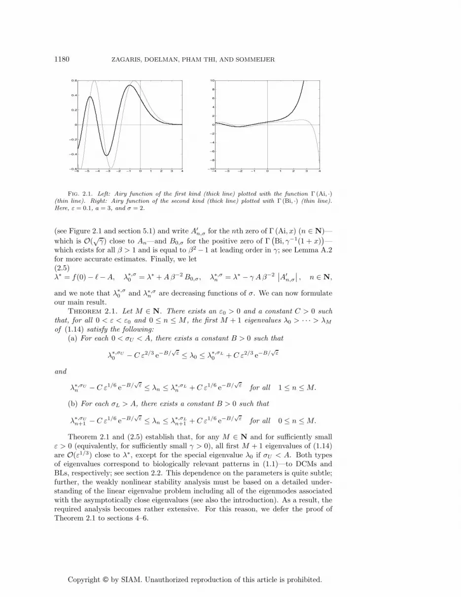
Fig. 2.1. Left: Airy function of the first kind (thick line) plotted with the function Γ (Ai, ·)(thin line). Right: Airy function of the second kind (thick line) plotted with Γ (Bi, ·) (thin line).Here, ε = 0.1, a = 3, and σ = 2.

(see Figure 2.1 and section 5.1) and write A′n,σ for the nth zero of Γ (Ai, x) (n ∈ N)—

which is O(√γ) close to An—and B0,σ for the positive zero of Γ

(Bi, γ−1(1 + x)

)—

which exists for all β > 1 and is equal to β2 − 1 at leading order in γ; see Lemma A.2for more accurate estimates. Finally, we let(2.5)λ∗ = f(0)− �−A, λ∗,σ0 = λ∗ +Aβ−2B0,σ, λ∗,σn = λ∗ − γ Aβ−2

∣∣A′n,σ

∣∣ , n ∈ N,

and we note that λ∗,σ0 and λ∗,σn are decreasing functions of σ. We can now formulateour main result.

Theorem 2.1. Let M ∈ N. There exists an ε0 > 0 and a constant C > 0 suchthat, for all 0 < ε < ε0 and 0 ≤ n ≤ M , the first M + 1 eigenvalues λ0 > · · · > λMof (1.14) satisfy the following:

(a) For each 0 < σU < A, there exists a constant B > 0 such that

λ∗,σU

0 − C ε2/3 e−B/√ε ≤ λ0 ≤ λ∗,σL

0 + C ε2/3 e−B/√ε

and

λ∗,σUn − C ε1/6 e−B/

√ε ≤ λn ≤ λ∗,σL

n + C ε1/6 e−B/√ε for all 1 ≤ n ≤M.

(b) For each σL > A, there exists a constant B > 0 such that

λ∗,σU

n+1 − C ε1/6 e−B/√ε ≤ λn ≤ λ∗,σL

n+1 + C ε1/6 e−B/√ε for all 0 ≤ n ≤M.

Theorem 2.1 and (2.5) establish that, for any M ∈ N and for sufficiently smallε > 0 (equivalently, for sufficiently small γ > 0), all first M + 1 eigenvalues of (1.14)are O(ε1/3) close to λ∗, except for the special eigenvalue λ0 if σU < A. Both typesof eigenvalues correspond to biologically relevant patterns in (1.1)—to DCMs andBLs, respectively; see section 2.2. This dependence on the parameters is quite subtle;further, the weakly nonlinear stability analysis must be based on a detailed under-standing of the linear eigenvalue problem including all of the eigenmodes associatedwith the asymptotically close eigenvalues (see also the introduction). As a result, therequired analysis becomes rather extensive. For this reason, we defer the proof ofTheorem 2.1 to sections 4–6.



0 0.25 0.5 0.75 10

0.1

0.2

0.3

0.4

0 0.25 0.5 0.75 10

0.1

0.2

0.3

0.4

0 0.25 0.5 0.75 10

0.1

0.2

0.3

0.4

0 0.25 0.5 0.75 10

0.1

0.2

x0

x0

F’(0)

F’(0)

F’(0) F(1)

F(1)

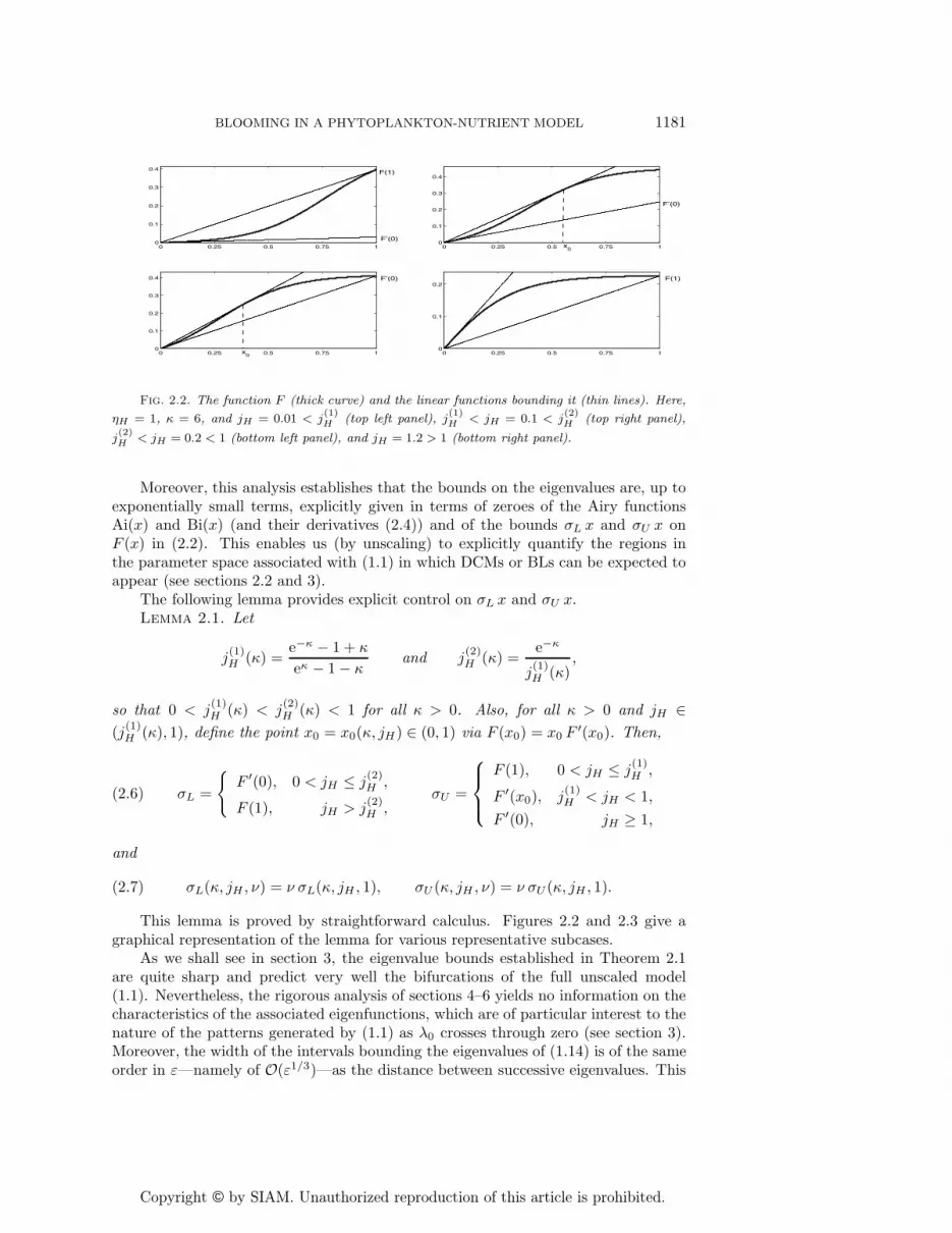
Fig. 2.2. The function F (thick curve) and the linear functions bounding it (thin lines). Here,

ηH = 1, κ = 6, and jH = 0.01 < j(1)H (top left panel), j

(1)H < jH = 0.1 < j

(2)H (top right panel),

j(2)H < jH = 0.2 < 1 (bottom left panel), and jH = 1.2 > 1 (bottom right panel).

Moreover, this analysis establishes that the bounds on the eigenvalues are, up toexponentially small terms, explicitly given in terms of zeroes of the Airy functionsAi(x) and Bi(x) (and their derivatives (2.4)) and of the bounds σL x and σU x onF (x) in (2.2). This enables us (by unscaling) to explicitly quantify the regions inthe parameter space associated with (1.1) in which DCMs or BLs can be expected toappear (see sections 2.2 and 3).

The following lemma provides explicit control on σL x and σU x.Lemma 2.1. Let

j(1)H (κ) =

e−κ − 1 + κ

eκ − 1 − κand j

(2)H (κ) =

e−κ

j(1)H (κ)

,

so that 0 < j(1)H (κ) < j

(2)H (κ) < 1 for all κ > 0. Also, for all κ > 0 and jH ∈

(j(1)H (κ), 1), define the point x0 = x0(κ, jH) ∈ (0, 1) via F (x0) = x0 F′(x0). Then,

(2.6) σL =

{F ′(0), 0 < jH ≤ j

(2)H ,

F (1), jH > j(2)H ,

σU =

⎧⎪⎨⎪⎩

F (1), 0 < jH ≤ j(1)H ,

F ′(x0), j(1)H < jH < 1,

F ′(0), jH ≥ 1,

and

(2.7) σL(κ, jH , ν) = ν σL(κ, jH , 1), σU (κ, jH , ν) = ν σU (κ, jH , 1).

This lemma is proved by straightforward calculus. Figures 2.2 and 2.3 give agraphical representation of the lemma for various representative subcases.

As we shall see in section 3, the eigenvalue bounds established in Theorem 2.1are quite sharp and predict very well the bifurcations of the full unscaled model(1.1). Nevertheless, the rigorous analysis of sections 4–6 yields no information on thecharacteristics of the associated eigenfunctions, which are of particular interest to thenature of the patterns generated by (1.1) as λ0 crosses through zero (see section 3).Moreover, the width of the intervals bounding the eigenvalues of (1.14) is of the sameorder in ε—namely of O(ε1/3)—as the distance between successive eigenvalues. This



0.1 0.2 0.3 0.4 0.5 0.6 0.7 0.8 0.9 1 1.10

0.1

0.2

0.3

0.4

jH(1) j

H(2)

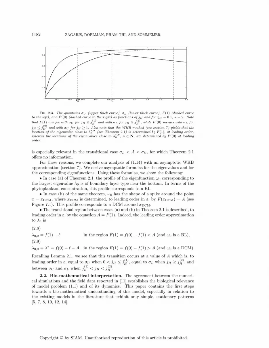
Fig. 2.3. The quantities σU (upper thick curve), σL (lower thick curve), F (1) (dashed curveto the left), and F ′(0) (dashed curve to the right) as functions of jH and for ηH = 0.1, κ = 2. Note

that F (1) merges with σU for jH ≤ j(1)H and with σL for jH ≥ j

(2)H , while F ′(0) merges with σL for

jH ≤ j(2)H and with σU for jH ≥ 1. Also note that the WKB method (see section 7) yields that the

location of the eigenvalue close to λ∗,σ0 (see Theorem 2.1) is determined by F (1), at leading order,

whereas the locations of the eigenvalues close to λ∗,σn , n ∈ N, are determined by F ′(0) at leading

order.

is especially relevant in the transitional case σL < A < σU , for which Theorem 2.1offers no information.

For these reasons, we complete our analysis of (1.14) with an asymptotic WKBapproximation (section 7). We derive asymptotic formulas for the eigenvalues and forthe corresponding eigenfunctions. Using these formulas, we show the following:

• In case (a) of Theorem 2.1, the profile of the eigenfunction ω0 corresponding tothe largest eigenvalue λ0 is of boundary layer type near the bottom. In terms of thephytoplankton concentration, this profile corresponds to a BL.

• In case (b) of the same theorem, ω0 has the shape of a spike around the pointx = xDCM, where xDCM is determined, to leading order in ε, by F (xDCM) = A (seeFigure 7.1). This profile corresponds to a DCM around xDCM.

• The transitional region between cases (a) and (b) in Theorem 2.1 is described, toleading order in ε, by the equation A = F (1). Indeed, the leading order approximationto λ0 is

(2.8)λ0,0 = f(1) − � in the region F (1) = f(0) − f(1) < A (and ω0 is a BL),(2.9)λ0,0 = λ∗ = f(0) − �−A in the region F (1) = f(0) − f(1) > A (and ω0 is a DCM).

Recalling Lemma 2.1, we see that this transition occurs at a value of A which is, toleading order in ε, equal to σU when 0 < jH ≤ j

(1)H , equal to σL when jH ≥ j

(2)H , and

between σU and σL when j(1)H < jH < j(2)H .

2.2. Bio-mathematical interpretation. The agreement between the numeri-cal simulations and the field data reported in [11] establishes the biological relevanceof model problem (1.1) and of its dynamics. This paper contains the first stepstowards a bio-mathematical understanding of this model, especially in relation tothe existing models in the literature that exhibit only simple, stationary patterns[5, 7, 8, 10, 12, 14].



The fact that (1.1) can be scaled into the singularly perturbed equation (1.5)for biologically relevant choices of the parameters is essential to the analysis in thispaper. Moreover, together with the linear stability analysis, these scalings enable usto understand the fundamental structure of the twelve-dimensional parameter spaceassociated with (1.1) and its boundary conditions (1.4) (in the biologically relevantregion). In fact, it follows from Theorem 2.1 and (2.8)–(2.9) that the dimensionlessparameters A, �, f(0), and f(1), which are defined in section 2.1, are the main param-eter combinations in the model as they capture its most relevant biological aspects.

Our stability analysis determines the regions in parameter space in which phyto-plankton may persist, i.e., in which the trivial solution of (1.1) and (1.4) correspondingto absence of phytoplankton (W (z, t) ≡ 0 in (1.1)) is unstable. In that case, nontrivialpatterns with W (z, t) > 0, for all t, bifurcate from the trivial solution, which impliesthat the model admits stable, positive phytoplankton populations. Theorem 2.1 es-tablishes the existence of two distinct types of phytoplankton populations at onset.One is formed by a large—in fact infinite—family of “DCM-modes” and occurs for Abelow the threshold value f(0) − f(1); the region where these modes become stableis determined by λ∗ = f(0)− �−A; see (2.9). Within this family, the phytoplanktonconcentrations are negligible for most z, except for a certain localized (spatial) regionin which the phytoplankton population is concentrated—see Figure 7.1 in which thefirst, most unstable member of this family is plotted (in scaled coordinates). Theseare the DCM-patterns observed in [11]. Our analysis shows that many different DCM-patterns appear almost instantaneously. More precisely, as a parameter enters into theregion in which the trivial solution is unstable, a succession of asymptotically close bi-furcations in which different types of DCM-patterns are created takes place. In otherwords, even asymptotically close to onset, there are many competing DCM-modes.This partly explains why the “pure” DCM-mode as represented in Figure 7.1 can beobserved only very close to onset (see [11] and section 3.2): it may be destabilized bythe competition with other modes.

The second type of phytoplankton population that may appear at onset occursfor A above the threshold value f(0) − f(1) and has the structure of a BL: thephytoplankton population is concentrated near z = zB, i.e., at the bottom of the watercolumn. Unlike the DCM-modes, there is a single BL-mode; the region where thismode becomes stable is determined, in this case, by f(1)−�; see (2.8). This mode mayalso dominate the dynamics of (1.1) in a part of the biologically relevant parameterspace, as may be seen in section 3.2. Note that the BL-mode has not been observedin [11]; naturally, this is hardly surprising since one can sample numerically only a verylimited region of a twelve-dimensional parameter space. From the biological point ofview, the fact that the model (1.1) allows for attractors of the BL type may be the mostimportant finding of this paper. Like DCMs, BLs have been observed in field data(see [15] and references therein). The analysis here quantifies the parameter valuesfor which DCM- or BL-patterns occur. Hence, our results may be used to determineoceanic regions and/or phytoplankton species for which BLs may be expected to exist.It would be even more interesting to locate a setting in which DCMs and BLs interact,as they are expected to do because of the existence of the codimension 2 point at whichthe (first) DCM-mode and the BL-mode bifurcate simultaneously; see section 3.

3. Bifurcations and simulations.

3.1. The bifurcation diagram. In this section, we use the WKB expressions(2.8)–(2.9) for the first few eigenvalues to identify the bifurcations that system (1.14)undergoes. In this way, we identify the regions in the parameter space where the BL



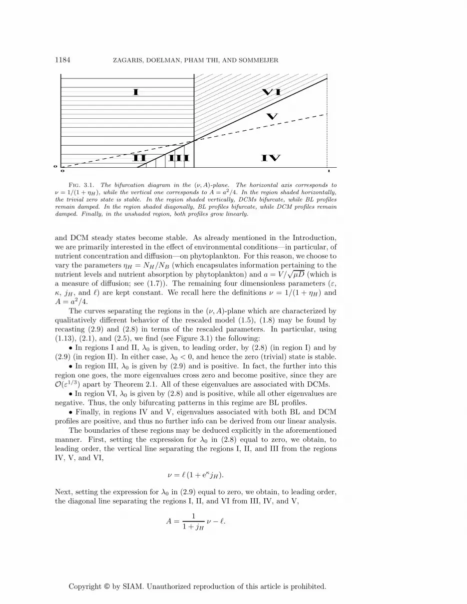
Fig. 3.1. The bifurcation diagram in the (ν, A)-plane. The horizontal axis corresponds toν = 1/(1 + ηH), while the vertical one corresponds to A = a2/4. In the region shaded horizontally,the trivial zero state is stable. In the region shaded vertically, DCMs bifurcate, while BL profilesremain damped. In the region shaded diagonally, BL profiles bifurcate, while DCM profiles remaindamped. Finally, in the unshaded region, both profiles grow linearly.

and DCM steady states become stable. As already mentioned in the Introduction,we are primarily interested in the effect of environmental conditions—in particular, ofnutrient concentration and diffusion—on phytoplankton. For this reason, we choose tovary the parameters ηH = NH/NB (which encapsulates information pertaining to thenutrient levels and nutrient absorption by phytoplankton) and a = V/

√μD (which is

a measure of diffusion; see (1.7)). The remaining four dimensionless parameters (ε,κ, jH , and �) are kept constant. We recall here the definitions ν = 1/(1 + ηH) andA = a2/4.

The curves separating the regions in the (ν,A)-plane which are characterized byqualitatively different behavior of the rescaled model (1.5), (1.8) may be found byrecasting (2.9) and (2.8) in terms of the rescaled parameters. In particular, using(1.13), (2.1), and (2.5), we find (see Figure 3.1) the following:

• In regions I and II, λ0 is given, to leading order, by (2.8) (in region I) and by(2.9) (in region II). In either case, λ0 < 0, and hence the zero (trivial) state is stable.

• In region III, λ0 is given by (2.9) and is positive. In fact, the further into thisregion one goes, the more eigenvalues cross zero and become positive, since they areO(ε1/3) apart by Theorem 2.1. All of these eigenvalues are associated with DCMs.

• In region VI, λ0 is given by (2.8) and is positive, while all other eigenvalues arenegative. Thus, the only bifurcating patterns in this regime are BL profiles.

• Finally, in regions IV and V, eigenvalues associated with both BL and DCMprofiles are positive, and thus no further info can be derived from our linear analysis.

The boundaries of these regions may be deduced explicitly in the aforementionedmanner. First, setting the expression for λ0 in (2.8) equal to zero, we obtain, toleading order, the vertical line separating the regions I, II, and III from the regionsIV, V, and VI,

ν = � (1 + eκjH).

Next, setting the expression for λ0 in (2.9) equal to zero, we obtain, to leading order,the diagonal line separating the regions I, II, and VI from III, IV, and V,

A =1

1 + jHν − �.



0.25 0.3 0.35 0.4 0.45 0.5 0.55 0.60

0.02

0.04

0.06

0.08

0.1

0.12

0.14

0.16

Bifurcation diagram (solid lines = data; dashed lines = eigenvalue bounds)

NB

DCM

BL

Fig. 3.2. The bifurcation diagram in the (ν, A)-plane for ε = 9 ·10−5, � = 0.2, jH = 0.5, κ = 1.(“NB” stands for “no blooming.”) The solid curves correspond to numerical simulations, while thedashed ones correspond to the bounds predicted theoretically; see Theorem 2.1.

Finally, setting the expressions for λ0 in (2.8) and (2.9) equal to each other, we obtainthe transitional regime A = F (1). In terms of the rescaled parameters, we find

A =(

11 + jH

− 11 + eκjH

)ν.

Since the physical region nH > 0 corresponds to the region 0 < ν < 1, these formulasimply that

(a) for 0 < � < (1 + eκjH)−1, both a BL and a DCM may bifurcate,(b) for (1 + eκjH)−1 < � < (1 + jH)−1, only a DCM may bifurcate,(c) for � > (1 + jH)−1, the trivial state is stable.Remark 3.1. Similar information may be derived by the rigorous bounds in The-

orem 2.1, with the important difference that the dividing curves have to be replacedby regions of finite thickness.

3.2. Numerical simulations. In this section, we present numerical simulationson the full model (1.1)–(1.4), and we compare the results with our theoretical predic-tions. The parameters are chosen in biologically relevant regions [11].

We considered first the validity of our asymptotic analysis; i.e., we checkedwhether the analytically obtained bounds for the occurrence of the DCMs and BLs—see Theorem 2.1, section 3.1, Figure 3.1, and Remark 3.1—can be recovered by nu-merical simulations of the PDE (1.1)–(1.4). We used the numerical method describedin Remark 3.2 at each node of a two-dimensional grid of a part of the (ν,A)-parameterplane (keeping all other parameters fixed) to determine the attracting pattern gener-ated by (1.1)–(1.4) and chose the initial profile at each node in the parameter spaceto be the numerically converged pattern for an adjacent node at the previous step.

In Figure 3.2, we present the region near the codimension 2 point in the (ν,A)-parameter plane at which both the DCMs and the BLs bifurcate (with all otherparameters fixed: ε = 9 · 10−5, � = 0.2, jH = 0.5, κ = 1). Away from this codi-mension 2 point, the numerically determined bifurcation curves are clearly within thebounds given by Theorem 2.1 and thus confirm our analysis. Note that this suggeststhat the bifurcations have a supercritical nature—an observation that does not followfrom our linear analysis. Near the codimension 2 point, a slight discrepancy between



0 0.1 0.2 0.3 0.4 0.5 0.6 0.7 0.8 0.9 10

0.1

0.2

0.3

0.4

OSCDCMNB

Fig. 3.3. The bifurcation diagram in the (ν, A)-plane for ε = 9 · 10−5, � = 0.25, jH = 0.033,κ = 20. Region NB corresponds to no blooming, and region OSC to oscillatory DCMs. The solidcurves correspond to numerical simulations, and the dashed ones to the points at which λ0 (left line)and λ1 (right line) cross zero; see (2.9) and Figure 3.1. For these parameter values, the bifurcationof the BLs occurs in a nonphysical part of the domain.

our analysis and the numerical findings becomes apparent. First, we note that the bi-furcation from the trivial state (no phytoplankton) to the DCM state is not exactly inthe region determined by Theorem 2.1. However, for this combination of parameters,this region is quite narrow—in fact, it is narrower than the width of the rectangulargrid of the (ν,A)-parameter plane that we used to determine Figure 3.2, which impliesthat the simulations do not disagree with the analysis. The other discrepancy, namelythe occurrence of a small “triangle” of BL patterns in the region where one wouldexpect DCMs, is related to the presence of the codimension 2 point. To understandthe true nature of the dynamics, one needs to perform a weakly nonlinear analysisnear this point and, presumably, a more detailed numerical analysis that distinguishesbetween DCMs, BLs, and patterns that have the structure of a combined DCM andBL. This is the topic of work in progress.

Unlike the simulations presented in [11], here we considered the secondary bifur-cations only briefly. Figure 3.3 shows the primary bifurcation of the trivial state intoa DCM and the secondary bifurcation (of Hopf type) of the DCM into an oscillatingDCM—see [11] for more (biological) details on this behavior. A priori, one wouldexpect that our linear stability analysis of the trivial state could not cover this Hopfbifurcation. However, in Figure 3.3 we also plotted the leading order approximationsof the curves at which the first two eigenvalues associated with the stability of thetrivial state, λ0 and λ1, cross through the imaginary axis. It follows that the distance(in parameter space) between the primary and the secondary bifurcations is asymp-totically small in ε, and similar to the distance between the successive eigenvaluesλn. This observation is based on several simulations realized for different values ofε. It is crucial information for the subsequent (weakly) nonlinear analysis, since thefact that the DCM undergoes its secondary Hopf bifurcation for parameter combi-nations that are asymptotically close (in ε) to the primary bifurcation implies thatthe above a priori expectation is not correct; instead, the stability and bifurcationanalysis of the DCM can, indeed, be based on the linear analysis presented here. Thehigher order eigenvalues λ1, λ2, . . . , the associated eigenfunctions ω1(x), ω2(x), . . . ,and their “slaved” η-components η1(x), η2(x), . . . (which can be determined explicitlyusing (1.11)) will serve as necessary inputs for this nonlinear analysis.



Thus, a “full” linear stability analysis of the uncoupled system (1.14) as pre-sented here may serve as a foundation for the analysis of secondary bifurcations thatcan only occur in the coupled system (see the introduction and [14]). This featureis very special and quite uncommon in explicit models. It is due to the natural sin-gularly perturbed nature of the scaled system (1.5), and it provides an opportunityto obtain fundamental insight into phytoplankton dynamics. This analysis, includingthe aforementioned codimension 2 analysis and the associated secondary bifurcationsof BLs, is the topic of work in progress.

Remark 3.2. The numerical results were obtained by the “Method of Lines” ap-proach. First, we discretized the spatial derivatives approximating the diffusion termsin the model using second-order symmetric formulas and employing a third-orderupwind-biased method to discretize the advection term (see [13] for the suitability ofthese schemes to the current problem). Next, we integrated the resulting system ofODEs forward in time with the widely used time-integration code VODE (see [3] andhttp://www.netlib.org/ode). Throughout all simulations, we combined a spatial gridof a sufficiently high resolution with a high precision time integration to ensure thatthe conclusions drawn from the simulations are essentially free of numerical errors.

4. Eigenvalue bounds. As a first step towards the proof of Theorem 2.1, werecast (1.14) in a form more amenable to analysis. First, we observe that the operatorinvolved in this eigenvalue problem is self-adjoint only if a = 0. Applying the Liouvilletransformation

(4.1) w(x) = e−√A/εxω(x) = e−(β/γ3/2)xω(x),

we obtain the self-adjoint problem

εwxx + (f(x) − �−A)w = λw,(√εwx −

√Aw)

(0) =(√

εwx −√Aw)

(1) = 0.

Recalling (2.1) and (2.5), we write this equation in the form

(4.2) Lw = μw, with G (w, 0) = G (w, 1) = 0.

The operator L, the scalar μ, and the linear functionals G(·, x) are defined by

(4.3) L = −ε d2

dx2+ F (x), μ = λ∗ − λ, G (w, x) = w(x) −

√ε

Awx(x).

This is the desired form of the eigenvalue problem (1.14). To prove Theorem 2.1, wedecompose the operator L into a self-adjoint part for which the eigenvalue problem isexactly solvable and a positive definite part. Then, we use the following comparisonprinciple to obtain the desired bounds.

Theorem 4.1 (see [18, sections 8.12–8.13]). Let A and A be self-adjoint operatorsbounded below with compact inverses, and write their eigenvalues as μ0 ≤ μ1 ≤ · · · ≤μn ≤ · · · and μ0 ≤ μ1 ≤ · · · ≤ μn ≤ · · · , respectively. If A−A is positive semidefinite,then μn ≤ μn for all n ∈ {0, 1, . . .}.

4.1. Crude bounds for the eigenvalues of L. First, we derive crude boundsfor the spectrum {μn} of L to demonstrate the method and establish that L satisfiesthe boundedness condition of Theorem 4.1.



Lemma 4.1. The eigenvalues μn satisfy the inequalities

(4.4) −A ≤ μ0 ≤ F (1) −A and εn2π2 ≤ μn ≤ F (1) + εn2π2, n ∈ N.

Proof. Let c ∈ R. We start by decomposing L as

(4.5) L = L0,c + F0,c, where L0,c = −ε d2

dx2+ c and F0,c = F (x) − c.

Then, we write {μ0,cn } for the set of eigenvalues of the problem

(4.6) L0,cw0,c = μ0,cw0,c, with G (w0,c, 0)

= G (w0,c, 1)

= 0,

with the eigenvalues arranged so that μ0,c0 ≤ μ0,c

1 ≤ · · · ≤ μ0,cn ≤ · · · .

For c = cL = 0, the operator L0,cL is self-adjoint, while F0,cL = F (x) ≥ 0 isa positive definite multiplicative operator. Thus, using Theorem 4.1, we obtain theinequalities

(4.7) μ0,cLn ≤ μn for all n ∈ N ∪ {0}.

Next, for c = cU = F (1), the operator F0,cU = F (x) − F (1) ≤ 0 is negative definite,while L0,cU is self-adjoint. Hence, we may write

L0,cU = L− F0,cU ,

where −F0,cU is now positive definite. The fact that the spectrum {μn} of L isbounded from below by (4.7) allows us to use Theorem 4.1 to bound each μn fromabove,

μn ≤ μ0,cUn for all n ∈ N ∪ {0}.

Combining this bound and (4.7), we obtain

(4.8) μ0,cLn ≤ μn ≤ μ0,cU

n for all n ∈ N ∪ {0}.Naturally, the eigenvalue problem (4.6) may be solved exactly to obtain

(4.9) μ0,c0 = c−A and μ0,c

n = c+ εn2π2, n ∈ N.

Combining these formulas with (4.8), we obtain the inequalities (4.4).

4.2. Tight bounds for the eigenvalues of L. The accurate bounds for theeigenvalues of (4.2) described in Theorem 2.1 may be obtained by bounding F by linearfunctions; see (2.2) and Lemma 2.1. In the next lemma, we bound the eigenvalues μnby the eigenvalues μ1,σ

n of a simpler problem. Then, in Lemma 4.3, we obtain strict,exponentially small bounds for μ1,σ

n .Lemma 4.2. Let σ ∈ {σL, σU}, with σL and σU as defined in Lemma 2.1, define

the operator L1,σ = −ε d2dx2 + σx, and write {μ1,σn } for the eigenvalues corresponding

to the problem

(4.10) L1,σw = μ1,σw, with G (w, 0) = G (w, 1) = 0.

Let {μ1,σn } be arranged so that μ1,σ

0 ≤ μ1,σ1 ≤ · · · ≤ μ1,σ

n ≤ · · · . Then,

(4.11) μ1,σLn ≤ μn ≤ μ1,σU

n for all n ∈ N ∪ {0}.



Proof. First, we decompose L as

(4.12) L = L1,σ + F1,σ, where L1,σ = −ε d2

dx2+ σx, F1,σ = F (x) − σx,

and σ ∈ {σL, σU}. We note here that L1,σ is self-adjoint.Next, F1,σL is a positive definite multiplicative operator, since F (x) ≥ σLx (see

(2.2)). Thus, μ1,σLn ≤ μn for all n ∈ N ∪ {0}, by Theorem 4.1. In contrast, F1,σU is

negative definite, since F (x) ≤ σUx. Therefore, we write

L1,σU = L− F1,σU ,

where now −F1,σU is positive definite. The fact that the spectrum {μn} is boundedfrom below by Lemma 4.1 allows us to use Theorem 4.1 to bound each μn from above,μn ≤ μ1,σU

n . Combining both bounds for each n, we obtain (4.11).Hence, it remains to solve the eigenvalue problem (4.10). Although this problem

is not explicitly solvable, the eigenvalues may be calculated up to terms exponentiallysmall in ε. Letting

μ∗,σ0 = λ∗ − λ∗,σ0 = −Aβ−2B0,σ and μ∗,σ

n = λ∗ − λ∗,σn = γ Aβ−2∣∣A′

n,σ

∣∣ > 0,

n ∈ N,

(4.13)

where we have recalled the definitions in section 2, we can prove the following lemma.Lemma 4.3. Let M ∈ N be fixed, and define

δ0,σ = γ2 exp(− 2

3γ−3/2

[3(1 +B0,σ −B)3/2 − 2(B0,σ −B)3/2 − (1 +B0,σ +B)3/2

]),

δn,σ =√γ A1/6 β−1/3 exp

(− 4

3 γ−3/2 + 2 |An+1| γ−1/2

)for all 1 ≤ n ≤M + 1

and for all 0 < B < B0,σ for which the exponent in the expression for δ0,σ is negative.Then, for each such B, there exists an ε0 > 0 and positive constants C0, . . . , CM+1

such that, for all 0 < ε < ε0 and 0 ≤ n ≤M , the first M+1 eigenvalues μ1,σ0 , . . . , μ1,σ

M

corresponding to (4.10) satisfy the following:(a) For β > 1,

∣∣μ1,σ0 − μ∗,σ

0

∣∣ < C0 δ0,σ and∣∣μ1,σn − μ∗,σ

n

∣∣ < Cn δn,σ for all1 ≤ n ≤M .

(b) For 0 < β < 1,∣∣μ1,σn − μ∗,σ

n+1

∣∣ < Cn+1 δn+1,σ for all 0 ≤ n ≤M .Lemmas 4.2 and 4.3 in combination with definitions (2.5) and (4.13) yield Theo-

rem 2.1. The bounds on μ1,σ0 , . . . , μ1,σ

M are derived in section 5. The fact that theseare indeed the M + 1 first eigenvalues corresponding to (4.10) is proved in section 6.Note that Theorem 2.1 follows immediately from this lemma, in combination withthe above analysis and the observation that the condition β > 1 is equivalent to0 < σ < A, and the condition 0 < β < 1 equivalent to σ > A.

5. The eigenvalues μ1,σ0 , . . . , μ1,σ

M . In this section, we derive the bounds onμ1,σ

0 , . . . , μ1,σM of Lemma 4.3. In section 5.1, we reduce the eigenvalue problem (4.10)

to the algebraic one of locating the roots of an Evans-type function D. In section 5.2,we identify the roots of D with those of two functions A and B which are related tothe Airy functions and simpler to analyze than D. Finally, in section 5.3, we identifythe relevant roots of A and B and thus also of D.



−30 −20 −10 0−0.8

−0.6

−0.4

−0.2

0

0.2

0.4

0.6

0.8

−30 −20 −10 0 10−5

−4

−3

−2

−1

0

1

2

3

4

5

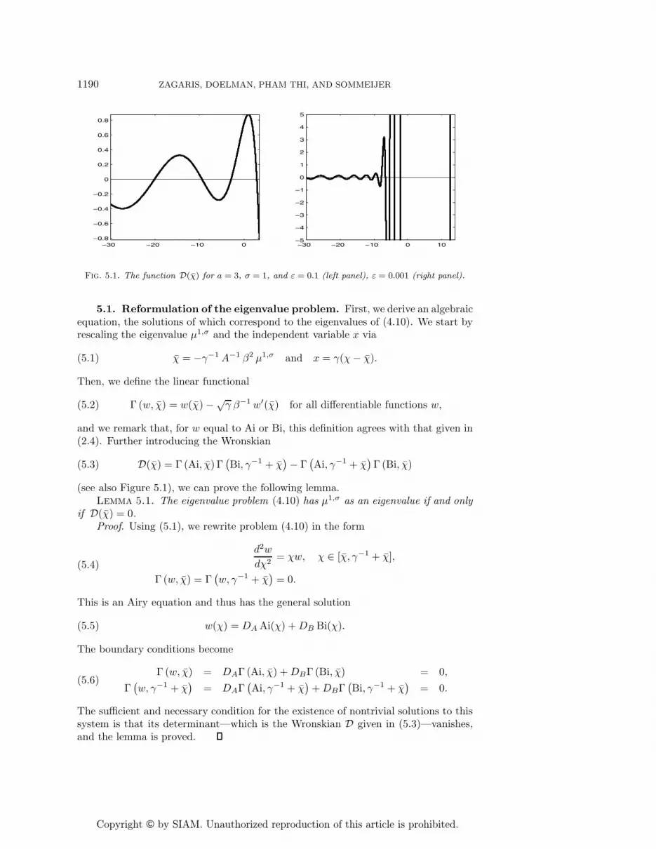
Fig. 5.1. The function D(χ) for a = 3, σ = 1, and ε = 0.1 (left panel), ε = 0.001 (right panel).

5.1. Reformulation of the eigenvalue problem. First, we derive an algebraicequation, the solutions of which correspond to the eigenvalues of (4.10). We start byrescaling the eigenvalue μ1,σ and the independent variable x via

(5.1) χ = −γ−1A−1 β2 μ1,σ and x = γ(χ− χ).

Then, we define the linear functional

(5.2) Γ (w, χ) = w(χ) −√γ β−1 w′(χ) for all differentiable functions w,

and we remark that, for w equal to Ai or Bi, this definition agrees with that given in(2.4). Further introducing the Wronskian

(5.3) D(χ) = Γ (Ai, χ) Γ(Bi, γ−1 + χ

)− Γ(Ai, γ−1 + χ

)Γ (Bi, χ)

(see also Figure 5.1), we can prove the following lemma.Lemma 5.1. The eigenvalue problem (4.10) has μ1,σ as an eigenvalue if and only

if D(χ) = 0.Proof. Using (5.1), we rewrite problem (4.10) in the form

d2w

dχ2= χw, χ ∈ [χ, γ−1 + χ],

Γ (w, χ) = Γ(w, γ−1 + χ

)= 0.

(5.4)

This is an Airy equation and thus has the general solution

(5.5) w(χ) = DA Ai(χ) +DB Bi(χ).

The boundary conditions become

(5.6)Γ (w, χ) = DAΓ (Ai, χ) +DBΓ (Bi, χ) = 0,

Γ(w, γ−1 + χ

)= DAΓ

(Ai, γ−1 + χ

)+DBΓ

(Bi, γ−1 + χ

)= 0.

The sufficient and necessary condition for the existence of nontrivial solutions to thissystem is that its determinant—which is the Wronskian D given in (5.3)—vanishes,and the lemma is proved.



5.2. Product decomposition of the function D. In the preceding section,we saw that the values of χ corresponding to the eigenvalues μ1,σ must be zeroes ofD. In the next section, we will prove that the first few zeroes of D are all O(1), inthe case 0 < β < 1, and both O(1) and O(γ−1) in the case β > 1. To identify them,we rewrite D in the form

(5.7) D(χ) = Γ(Bi, γ−1 + χ

)A(χ) = Γ (Ai, χ)B(χ),

where we have defined the functions

A(χ) = Γ (Ai, χ) − Γ(Ai, γ−1 + χ

)Γ (Bi, γ−1 + χ)

Γ (Bi, χ) ,(5.8)

B(χ) = Γ(Bi, γ−1 + χ

)− Γ (Bi, χ)Γ (Ai, χ)

Γ(Ai, γ−1 + χ

).(5.9)

Here, A is well defined for all χ such that Γ(Bi, γ−1 + χ

) �= 0, while B is well definedfor all χ such that Γ (Ai, χ) �= 0. Equation (5.7) implies that the roots of A and Bare also roots of D.

In the next section, we will establish that the O(1) roots of D coincide with rootsof A and the O(γ−1) ones with roots of B. To prove this, we first characterize thebehaviors of A and B for O(1) and O(γ−1) values of χ, respectively, by means of thenext two lemmas. In what follows, we write E(x) = exp(−(2/3)x3/2) for brevity and|| · ||[XL,XR] for the W1

∞-norm over any interval [XL, XR],

(5.10) ||w||[XL,XR] = maxχ∈[XL,XR]

|w(χ)| + maxχ∈[XL,XR]

|w′(χ)| .

Lemma 5.2. Let X < 0 be fixed. Then there is a γ0 > 0 and a constant cA > 0such that

(5.11) ||A(·)− Γ (Ai, ·)||[X,0] < cA γ−1/2E(γ−1(2 + 3 γ X)2/3) for all 0 < γ < γ0.

For the next lemma, we switch to the independent variable ψ = γχ to facilitatecalculations. We analyze the behavior of B(γ−1ψ) for O(1) values of ψ (equivalently,for O(γ−1) values of χ) as γ ↓ 0.

Lemma 5.3. Let 0 < ΨL < ΨR be fixed. Then there is a γ0 > 0 and a constantcB > 0 such that, for all 0 < γ < γ0,∣∣∣∣E(γ−1(1 + ψ))

[B (γ−1ψ)− Γ

(Bi, γ−1(1 + ψ)

)]∣∣∣∣ψ∈[ΨL,ΨR]

< cB γ−1/4

[E(γ−1(1 + ΨL))E(γ−1ΨL)

]2.

The proofs of these lemmas are given in Appendices B and C, respectively.

5.3. Zeroes of D. Using Lemma 5.2 and an auxiliary result, we can locate theroots of D.

Lemma 5.4. Let M ∈ N be fixed, A′n,σ and B0,σ be defined as in section 2, and

B, δ0,σ, . . . , δM,σ be defined as in Lemma 4.3. Then, for each admissible B, there isa γ0 > 0 and positive constants c0, . . . , cM such that, for all 0 < γ < γ0, D(χ) hasroots χ0 > χ1 > · · · > χM satisfying the following bounds:

(a) For β > 1,∣∣χ0 − γ−1B0,σ

∣∣ < c0 γ−1 δ0,σ and

∣∣χn −A′n,σ

∣∣ < cn γ−1 δn,σ for all 1 ≤ n ≤M.



(b) For 0 < β < 1,∣∣χn −A′n+1,σ

∣∣ < cn γ−1 δn+1,σ for all 0 ≤ n ≤M.

The proof of this lemma requires the following elementary result.Lemma 5.5. Let C and G be real-valued continuous functions and H be real-

valued and differentiable. Let δ > 0 and z0 ∈ [ZL, ZR] ⊂ R be such that

H(z0) = 0, max[ZL,ZR]

H ′ = −H0 < 0, max[ZL,ZR]

|C(G −H)| < δ,

and min[ZL,ZR]

C = C0 > 0.

If δ < C0H0 min(z0−ZL, ZR−z0), then G has a zero z∗ such that |z∗−z0| ≤ δ/(C0H0).Proof. Let z� = z0 − δ/(C0H0) and zr = z0 + δ/(C0H0). Since ZL < z� < z0 <

zr < ZR, we have

G(z�) = H(z�) +G(z�) −H(z�) ≥∫ z�

z0

H ′(z) dz − max[ZL,ZR] |C(G −H)|min[ZL,ZR] C

> (z0 − z�)H0 − δ

C0= 0.

Similarly, we may prove that G(zr) < 0, and the desired result follows.Proof of Lemma 5.4. (a) First, we prove the existence of a root χ0 satisfying the

desired bound. We recall that ψ was defined above via ψ = γχ; hence, it sufficesto show that there is a root ψ0 of D(γ−1ψ) satisfying the bound |ψ0 − B0,σ| < c0 δ0for some c0 > 0. Equation (5.7) reads D(γ−1ψ) = Γ (Ai, γ−1ψ)B(γ−1ψ). Here,Γ (Ai, γ−1ψ) has no positive roots, by definition of Γ and because Ai(γ−1ψ) > 0 andAi′(γ−1ψ) < 0 for all ψ > 0. Thus, χ0 must be a root of B. Its existence and thebound on it follow from Lemmas 5.3 and 5.5. Indeed, let z0 = B0,σ, ZL = B0,σ − B,ZR = B0,σ + B, C = E (see section 5.2), G = B, and H = Γ (Bi, ·). Lemma 5.3provides a bound δ on ||C(G−H)||[ZL,ZR]. Also, using Corollary A.1, we may calculate

C0 = min[ZL,ZR]E(γ−1(1 + ψ)) = E(γ−1(1 + ZR)),

−H0 = max[ZL,ZR] Γ(Bi′, γ−1(1 + ψ)

)< −c γ5/4

[E(γ−1(1 + ZL))

]−1.

Now, δ satisfies the condition δ < C0H0B of Lemma 5.5 for all γ small enough. Thus,we may apply Lemma 5.5 to obtain the desired bound on χ0.

Next, we show that A has the remaining roots χ1, . . . , χM . We fix AM+1 <X < AM and let I1, . . . , IM be disjoint intervals around the first M zeroes of Ai,A1, . . . , AM , respectively. Lemma 5.2 states that A(χ) and Γ (Ai, χ) are exponentiallyclose in the W1

∞-norm over [X, 0]. Thus, for all 0 < γ < γ0 (with γ0 small enough),A has M distinct roots χ1 ∈ I1, . . . , χM ∈ IM in [X, 0] by Lemma A.2. SinceΓ(Bi, γ−1 + χ

)can be bounded away from zero over [X, 0] using Lemma A.1 (with

p = 1 and q = χ), we conclude that D has the M distinct roots χ1, . . . , χM in [X, 0].(b) The argument used in part (a)—where β > 1—to establish the bounds on the

O(1) roots of A does not depend on the sign of β − 1. Therefore, it applies also tothis case—where 0 < β < 1—albeit in an interval [X, 0], with AM+2 < X < AM+1,yielding M + 1 roots which we label χ0, . . . , χM .

On the other hand, B0,σ < 0 for 0 < β < 1, because of the estimate on B0,σ inLemma A.2. As a result, the argument used to identify that root does not apply any



more, since now B0,σ < 0 and thus Lemma 5.3 may not be applied to provide thebound δ needed in Lemma 5.5. In fact, were this root to persist and remain closeto γ−1B0,σ as in case (a), it would become large and negative by the estimate inLemma A.2 and hence smaller than the roots χ0, . . . , χM obtained above. Thus, itcould never be the leading eigenvalue in this parameter regime.

6. The eigenfunctions w1,σ0 , . . . , w1,σ

M . In the previous section, we locatedsome of the eigenvalues μ1,σ. In this section, we show that the eigenvalues we iden-tified are the largest ones. To achieve this, we derive formulas for the eigenfunctionsw1,σ

0 , . . . , w1,σM associated with μ1,σ

0 , . . . , μ1,σM , respectively, and show that w1,σ

n has nzeroes in the interval [χn, γ−1 + χn] (corresponding to the interval [0, 1] in terms of x;see (5.1)). The desired result follows, then, from standard Sturm–Liouville theory [4].In particular, we prove the following lemma.

Lemma 6.1. Let M ∈ N. Then, there is a γ0 > 0 such that, for all 0 < γ < γ0

and for all n = 0, 1, . . . ,M , the eigenfunction w1,σn corresponding to the eigenvalue

μ1,σn has exactly n zeroes in the interval [χn, γ−1 + χn].

The proof of this lemma occupies the rest of this section. Parallel to it, we showthat the profile of ω0 associated with w0 through (4.1) is that of (a) a boundarylayer near the bottom of the water column (BL) for β > 1, and (b) an interior,nonmonotone boundary layer (a spike [9]) close to the point 0 < xDCM = β2 < 1(DCM) for 0 < β < 1.

We start by fixing χ to be χn, for some n = 1, . . . ,M . The corresponding eigen-value is μ1,σ

n = −γσχn (see (5.1)), while the corresponding eigenfunction wn is givenby (5.5),

(6.1) w1,σn (χ) = DAAi(χ) +DB Bi(χ), where χ ∈ [χn, γ−1 + χn].

Here, the coefficients DA and DB satisfy (5.6),

DAΓL,n(Ai) +DBΓL,n(Bi) = DAΓR,n(Ai) +DBΓR,n(Bi) = 0,

where ΓL,n(·) = Γ (·, χn) and ΓR,n(·) = Γ(·, γ−1 + χn

). We treat the cases β > 1 and

0 < β < 1 separately.

6.1. The case β > 1. In this section, we select DA and DB so that (6.1)becomes

(6.2) w1,σn (χ) = DnBi(χ) − Ai(χ), with Dn =

ΓL,n(Ai)ΓL,n(Bi)

=ΓR,n(Ai)ΓR,n(Bi)

.

Using this formula, we prove Lemma 6.1 and verify that ω0 is of boundary layer typenear x = 1.

6.1.1. The eigenfunction w1,σ0 . First, we show that w1,σ

0 has no zeroes in thecorresponding interval. Using Lemma A.1 and the estimates of Lemmas 5.4 for χ0

and A.2 for B0,σ, we estimate

D0 =(

Δ21

2+ C0(γ)

)exp(−4(

(β2 − 1)3/4

3γ3/2+√

1 − 1β2

)).

Here, Δ1 = β +√β2 − 1 and

∣∣C0(γ)∣∣ < c0

√γ, for some c0 > 0. Thus also, D0 > 0.

It suffices to show that w1,σ0 is positive in this interval, and thus that (w1,σ

0 )′ > 0everywhere on the interval and w1,σ

0 (χ0) > 0. For n = 0, (6.2) yields (w1,σ0 )′(χ) =



D0 Bi′(χ) − Ai′(χ), while Lemma 5.4 shows that [χ0, γ−1 + χ0] ⊂ R+. Hence,

Bi′(χ) > 0 and Ai′(χ) < 0 for all χ in this interval. Since D0 > 0, we concludethat (w1,σ

0 )′ > 0, as desired. Next, we determine the sign of w1,σ0 (χ0). This function

is given in (6.2) with n = 0, while the definition of ΓL,0 yields

Ai(χ0) = ΓL,0(Ai) + β−1 √γ Ai′(χ0) and Bi(χ0) = ΓL,0(Bi) + β−1 √γ Bi′(χ0).

Substituting into (6.2), we calculate w1,σ0 (χ0) = β−1 √γ [D0 Bi′(χ0)−Ai′(χ0)]. Thus,

w1,σ0 (χ0) is positive by our remarks on the signs of Bi′, Ai′, and D0, and the proof is

complete.Next, we study the profile of the associated solution ω0 to the original problem

(1.14). Equations (4.1) and (5.1) yield

ω0(x) = exp(

β

γ3/2x

)[D0 Bi(γ−1x+ χ0) − Ai(γ−1x+ χ0)

], x ∈ [0, 1].

Using the estimation of Lemma 5.4 for χ0 and the estimations of Lemma A.1 for Aiand Bi, we find

ω0(x) = CI(x)(x+ β2 − 1

)−1/4exp(

β

γ3/2x

)sinh(θ1(x)), x ∈ [0, 1],

where CI(x) = CI,0 + CI,1(x), sup[0,1] |CI,1(x)| < cI√γ, for some cI > 0, and

θ1(x) =2

3γ3/2

[(x+β2−1

)3/2−(β2−1)3/2]+ 2

β

[(x+β2−1

)1/2−(β2−1)1/2]+log Δ1.

The first two terms on the right-hand side of the expression for ω0 are bounded, whilethe other two correspond to localized concentrations (boundary layers) at x = 1.Thus, ω0 also corresponds to a boundary layer of width O(γ3/2) = O(

√ε) at the

same point.

6.1.2. The eigenfunctions w1,σ1 , . . . , w1,σ

M . Next, we show that the eigenfunc-tion w1,σ

n has n zeroes in [χn, γ−1 + χn], where n = 1, . . . ,M . The eigenfunction w1,σn

is given by (6.2). Here also, Lemmas A.1 and 5.4 yield

(6.3) Dn =(

Δ22

2+ Cn(γ)

)exp(− 4

3γ3/2+ 2

|An|√γ

− 2β

),

where Δ2 = (β + 1)1/2 (β − 1)−1/2 and∣∣Cn(γ)

∣∣ < cn√γ, for some cn > 0. Hence,

Dn > 0.First, we show that the function w1,σ

n has exactly n − 1 zeroes in [χn, 0]. Theestimate (6.3) and the fact that Bi is uniformly bounded on [χn, 0] imply that, forall 0 < γ < γ0 (with γ0 small enough), the functions w1,σ

n and −Ai are exponentiallyclose in the W1∞-norm over that interval,

(6.4)∣∣∣∣w1,σ

n + Ai∣∣∣∣

[χn,0]< cn exp

(− 4

3γ3/2+ 2

|An|√γ

)for some cn > 0.

As a result, we may use an argument exactly analogous to the one used in the proofof Lemma 5.4 to show that w1,σ

n has at least n − 1 distinct zeroes in [χn, 0], each ofwhich is exponentially close to one of A1, . . . , An−1. Observing that χn is algebraically



0 0.1 0.2 0.3 0.4 0.5 0.6 0.7 0.8 0.9 1

0

0.2

0.4

0.6

0.8

1

Fig. 6.1. The eigenfunctions w1,σL0 , w

1,σU0 (always positive and coinciding within plotting ac-

curacy) and w1,σL1 , w

1,σU1 (changing sign). Here, a = 0.775, nH = 0.667, ε = 0.001, κ = 1,

� = 0.25, and jH = 0.5, which yields σL = 0.1333, σU = 0.1457 (and thus σL < σU < a2/4),

0.0104 ≤ λ0 ≤ 0.0222, and −0.0541 ≤ λ1 ≤ −0.0512. Note that λ1 < λ0 and that none of w1,σL0

and w1,σU0 has zeroes in [0, 1], while w

1,σL1 and w

1,σU1 have exactly one zero in the same interval.

larger than An, by Lemmas 5.4 and A.2, while w1,σn is exponentially close to −Ai,

by estimate (6.4), we conclude that the zero of w1,σn close to An lies to the left of χn

(and hence outside [χn, 0]) and thus there are no other zeroes in [χn, γ−1 + χn].It remains to show only that there is a unique zero of w1,σ

n in [0, γ−1 + χn]. Wework as in section 6.1.1 and show that w1,σ

n is increasing and changes sign in thatinterval. First, we calculate (w1,σ

n )′(χ) = DnBi′(χ)−Ai′(χ) > 0, where we have usedthat Bi′(χ) > 0, Ai′(χ) < 0, and Dn > 0. Also, w1,σ

n (0) < 0 (by Ai(0) > 0 and (6.4))and, working as in section 6.1.1,

w1,σn (γ−1 + χn) = β−1 √γ [DnBi′(γ−1 + χn) − Ai′(γ−1 + χn)

]> 0.

This completes the proof.

6.2. The case 0 < β < 1. In this section, we select DA and DB so that (6.1)becomes

(6.5) w1,σn (χ) = Ai(χ) +Dn Bi(χ), with Dn = −ΓL,n(Ai)

ΓL,n(Bi)= −ΓR,n(Ai)

ΓR,n(Bi).

Using this formula, we prove Lemma 6.1 and verify that the profile of ω0 has a spikearound xβ = β2.

We shall show that the eigenfunction w1,σn (n = 0, . . . ,M) has n zeroes in [χn,

γ−1 + χn]; see Figure 6.1. The proof is entirely analogous to that in section 6.1.2.Here also, the nth eigenvalue is μ1,σ

n = −γσχn, while the corresponding eigenfunctionw1,σn is given by (6.5). The constant Dn may be estimated by

(6.6) Dn =(

Δ23

2+ Cn(γ)

)exp(− 4

3γ3/2+ 2

|An+1|√γ

− 2β

),

where Δ3 =√

1 + β/√

1 − β and∣∣Cn∣∣ < c′n

√γ for some c′n > 0. This is an estimate

of the same type as (6.3) but with An+1 replacing An. Thus, the estimate (6.4) holdshere as well with the same change. Recalling that χn is algebraically larger than



An+1 (see Lemmas 5.4 and A.2), we conclude that w1,σn has n distinct zeroes, each

of which is exponentially close to one of A1, . . . , An. Next, we show that w1,σn > 0 in

[0, γ−1 + χn] and thus has no extra zeroes. First, w1,σn (χ) = Ai(χ) +Dn Bi(χ). Now,

Bi(χ) > 0 and Ai(χ) > 0, for all χ ∈ [0, γ−1 + χn], while Dn > 0 by (6.6). Hence,w1,σn > 0, and the proof is complete.

Next, we examine the solution ω0 associated with w0. Working as in section 6.1.1,we calculate

ω0(x) = CII(x)x−1/4 exp(

β

γ3/2x

)cosh(θ2(x)), x ∈ [0, 1],

where CII(x) = CII,0 + CII,1(x), sup[0,1] |CII,1(x)| < cII√γ for some cII > 0, and

θ2(x) =2

3γ3/2

(1 − x3/2

)−( |A1|√

γ− 1β

)(1 −√

x) − log Δ3.

The first two terms on the right-hand side of the expression for ω0 are bounded, whilethe other two correspond to boundary layers at x = 1 and x = 0, respectively. Astraightforward calculation shows that ω0 corresponds to a spike of width O(γ3/4) =O(ε1/4) around the point xβ , where

(6.7)∣∣xβ − (β2 + |A1| γ

)∣∣ < cγ2 for some c > 0.

We remark that xβ does not correspond to the position of the DCM for the problem(1.14) involving the function f . This information is obtained in the next section,instead, through a WKB analysis.

7. The WKB approximation. In the previous sections, we derived strictbounds for the eigenvalues μ1, . . . , μM of L and summarized them in Theorem 2.1. Inthis section, we use the WKB method to derive explicit (albeit asymptotic) formulasfor these eigenvalues. The outcome of this analysis has already been summarized insection 2.1.

7.1. The case A < σL.

7.1.1. WKB formulas for w. The eigenvalue problem (4.2) reads

(7.1) εwxx = (F (x) − μ)w, with G (w, 0) = G (w, 1) = 0.

Since we are interested in the regime σL > A, Lemma 4.3 states that the eigenvaluesμ0, . . . , μM lie in a O(ε1/3) region to the right of zero. Thus, for any 0 ≤ n ≤M ,

F (x) < μn for x ∈ [0, xn), and F (x) > μn for x ∈ (xn, 1].

Here, xn corresponds to a turning point, i.e., F (xn) = μn, and it is given by theformula

(7.2) xn =1κ

log1 + μn(1 + ηH)(1 + j−1

H )1 − μn(1 + ηH)(1 + jH)

.

Lemmas 4.3 and A.2 suggest that the eigenvalue μn may be expanded asymptoticallyin powers of ε1/6 starting with O(ε1/3) terms, μn =

∑∞�=2 ε

�/6 μn,�. Thus, we alsofind

(7.3) xn = ε1/3σ−10 μn,2 + ε1/2σ−1

0 μn,3 + O(ε2/3), where σ0 = F ′(0).



The solution in the region (xn, 1], where F (x) − μn > 0, can be determined usingstandard formulas (see [2, section 10.1]),

(7.4) wn(x) = [F (x)−μn]−1/4[Ca exp− ∫ x

xn

√(F (s)−μn)/ε ds+Cb e

∫xxn

√(F (s)−μn)/ε ds

].

Here, Ca and Cb are arbitrary constants, to leading order in ε. (Higher order termsin the asymptotic expansions of Ca and Cb generally depend on x; see [2] for details.)Using this information and the asymptotic expansion for μn, we may determine theprincipal part of the solution wn,

(7.5) wn,0(x) = [F (x)]−1/4[Ca,0 e−θ3(x) + Cb,0 eθ3(x)

],

for arbitrary constants Ca,0 and Cb,0 and where(7.6)

θ3(x) =1ε1/2

∫ x

0

√F (s) ds− 1

ε1/6μn,22

∫ x

0

ds√F (s)

+μn,2√σ0

− 23√σ0 − μn,3

2

∫ x

0

ds√F (s)

.

To determine the solution in [0, xn), we change the independent variable through(7.7)x = ε1/3σ

−1/30 (χ− χn), where χn = −σ1/3

0 ε−1/3 xn = −σ−2/30 μn,2 + O (√ε) < 0,

and expand F (x) − μn = F (x) − F (xn) asymptotically:(7.8)F (x) − F (xn) = F (ε1/3σ−1/3

0 (χ− χn)) − F (−ε1/3σ−1/30 χn) = ε1/3σ

2/30 χ+ O(

√ε).

As a result, (7.1) becomes the Airy equation (wn)χχ = χwn, to leading order, whence

(7.9) wn,0(χ) = Da,0 Ai(χ) +Db,0 Bi(χ), with χ ∈ (−σ−2/30 μn,2, 0].

7.1.2. Boundary conditions for the WKB solution. Next, we determinethe coefficients appearing in (7.5) and (7.9). Formula (7.5) represents the solutionin the region (xn, 1], and thus it must satisfy the boundary condition G (wn, 1) = 0.Using (4.3), we find, to leading order,

(7.10) Ca,0 (a+ 2√σ1) e−θ3(x) + Cb,0 (a− 2

√σ1) eθ3(x) = 0, where σ1 = F (1).

Next, the formula given in (7.9) is valid for χ ∈ (−σ−2/30 μn,2, 0] (equivalently, for

x ∈ [0, xn)), and thus it must satisfy the boundary condition G (w, 0) = 0. Recastingthe formula for G given in (4.3) in terms of χ, we obtain to leading order the equation

(7.11) Da,0 Ai(−σ−2/3

0 μn,2

)+Db,0 Bi

(−σ−2/3

0 μn,2

)= 0.

Finally, (7.5) and (7.9) must also match in an intermediate length scale to the rightof x = xn (equivalently, of χ = 0). To this end, we set ψ = εd (x − xn), where1/5 < d < 1/3 [2, section 10.4], and recast (7.5) in terms of ψ. We find, to leadingorder and for all O(1) and positive values of ψ,

wn,0(x(ψ)) = ε−d/4 σ−1/40 ψ−1/4

[Ca,0 e−θ4(ψ)−σ−1

0 (μn,2)3/2+ Cb,0 eθ4(ψ)+σ−1

0 (μn,2)3/2],

where θ4(ψ) = (2/3) ε(3d−1)/2√σ0 ψ3/2. Similarly, (7.9) yields

wn,0(χ(ψ)) = ε1/12−d/4 σ−1/120 π−1/2 ψ−1/4

[Da,0

2e−θ4(ψ) +Db,0 eθ4(ψ)

].



The matching condition around the turning point then gives

(7.12) Ca,0 = ε1/12σ

1/60

2√π

eσ−10 (μn,2)

3/2Da,0 and Cb,0 = ε1/12

σ1/60√π

e−σ−10 (μn,2)

3/2Db,0.

7.1.3. The eigenvalues μ0, . . . , μn. The linear system (7.10)–(7.12) has anontrivial solution if and only if the determinant corresponding to it vanishes identi-cally:

2 (a− 2√σ1) eθ3(1)−σ−1

0 (μn,2)3/2Ai(σ−2/3μn,2)

+ (a+ 2√σ1) e−θ3(1)+σ

−10 (μn,2)

3/2Bi(σ−2/3μn,2) = 0.

Since σ1 ≥ σL by Lemma 2.1 and σL > A by assumption, a − 2√σ1 is O(1) and

negative. Also, θ3(1) is O(1) and positive by (7.6). Thus, the determinant conditionreduces to Ai(σ−2/3μn,2) = 0, whence μn,2 = −σ2/3

0 An+1 = σ2/30 |An+1| > 0. Hence,

we find for the eigenvalues of (1.14)

(7.13) λn = λ∗ − ε1/3σ2/30 |An+1| + O(

√ε).

Working in a similar way, we find μn,3 = −2σ0/a.Recalling that σ0 = F ′(0) = −f ′(0) by (2.1) and Lemma 2.1 (see also Figure 2.3),

we find that the WKB formula (7.13) coincides—up to and including terms of O(1)and O(ε1/3)—(a) for 0 < jH < j

(2)H , with the rigorous lower bound for λn derived in

Theorem 2.1, and (b) for jH > 1, with the rigorous upper bound for λn derived inthe same theorem. For the remaining values of jH , (7.13) yields a value for λn whichlies in between the upper and lower bounds derived in Theorem 2.1—indeed, in thatcase, σL < F ′(0) < σU ; see Figure 2.3.

7.1.4. The eigenfunctions w0, . . . , wn. Finally, one may determine the con-stants Ca, Cb, Da, and Db corresponding to the eigenfunction wn, and thus also wnitself, through (7.10)–(7.12). The principal part of wn is given by the formula

(7.14) wn,0(x) =

⎧⎨⎩

Ai(An+1 + ε−1/3σ

1/30 x

)for x ∈ [0, ε1/3σ−1/3

0 |An+1|),C [F (x)]−1/4 coshΘ(x) for x ∈ (ε1/3σ−1/3

0 |An+1| , 1].

Here,

C = ε1/12σ

1/60

2√π

Δ4 e|An+1|3/2−Θ3(1), where Δ4 =

(√σ1 +

√A

√σ1 −

√A

)1/2

,(7.15)

Θ(x) = ε−1/2

∫ 1

x

√F (s) ds−

(ε−1/6 σ

2/30 |An+1|

2− σ0

a

)∫ 1

x

ds√F (s)

+ log Δ4.

(7.16)

Recalling (4.1), we find

ωn,0(x) =

⎧⎨⎩

e√A/εx Ai

(An+1 + ε−1/3σ

1/30 x

)for x ∈ [0, ε1/3σ−1/3

0 |An+1|),C [F (x)]−1/4 e

√A/εx coshΘ(x) for x ∈ (ε1/3σ−1/3

0 |An+1| , 1].

(7.17)



0 0.1 0.2 0.3 0.4 0.5 0.6 0.7 0.8 0.9 10

0.2

0.4

0.6

0.8

1

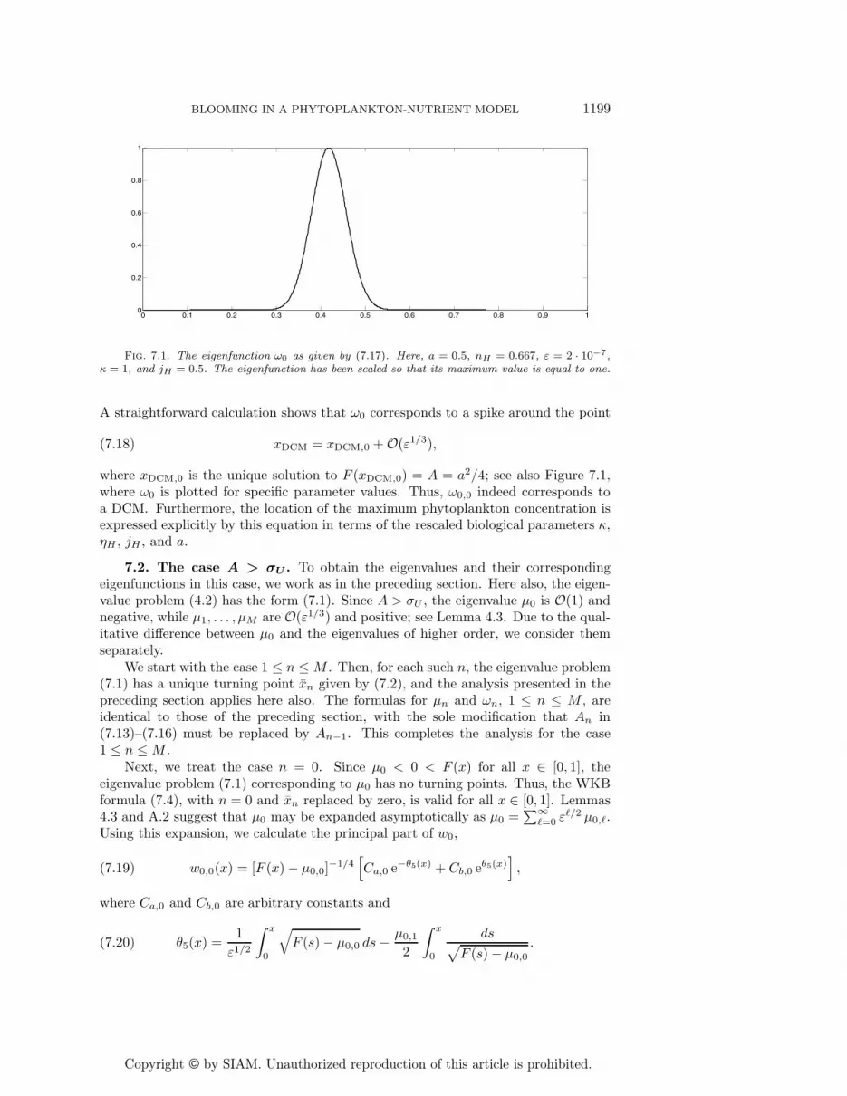
Fig. 7.1. The eigenfunction ω0 as given by (7.17). Here, a = 0.5, nH = 0.667, ε = 2 · 10−7,κ = 1, and jH = 0.5. The eigenfunction has been scaled so that its maximum value is equal to one.

A straightforward calculation shows that ω0 corresponds to a spike around the point

(7.18) xDCM = xDCM,0 + O(ε1/3),

where xDCM,0 is the unique solution to F (xDCM,0) = A = a2/4; see also Figure 7.1,where ω0 is plotted for specific parameter values. Thus, ω0,0 indeed corresponds toa DCM. Furthermore, the location of the maximum phytoplankton concentration isexpressed explicitly by this equation in terms of the rescaled biological parameters κ,ηH , jH , and a.

7.2. The case A > σU . To obtain the eigenvalues and their correspondingeigenfunctions in this case, we work as in the preceding section. Here also, the eigen-value problem (4.2) has the form (7.1). Since A > σU , the eigenvalue μ0 is O(1) andnegative, while μ1, . . . , μM are O(ε1/3) and positive; see Lemma 4.3. Due to the qual-itative difference between μ0 and the eigenvalues of higher order, we consider themseparately.

We start with the case 1 ≤ n ≤M . Then, for each such n, the eigenvalue problem(7.1) has a unique turning point xn given by (7.2), and the analysis presented in thepreceding section applies here also. The formulas for μn and ωn, 1 ≤ n ≤ M , areidentical to those of the preceding section, with the sole modification that An in(7.13)–(7.16) must be replaced by An−1. This completes the analysis for the case1 ≤ n ≤M .

Next, we treat the case n = 0. Since μ0 < 0 < F (x) for all x ∈ [0, 1], theeigenvalue problem (7.1) corresponding to μ0 has no turning points. Thus, the WKBformula (7.4), with n = 0 and xn replaced by zero, is valid for all x ∈ [0, 1]. Lemmas4.3 and A.2 suggest that μ0 may be expanded asymptotically as μ0 =

∑∞�=0 ε

�/2 μ0,�.Using this expansion, we calculate the principal part of w0,

(7.19) w0,0(x) = [F (x) − μ0,0]−1/4[Ca,0 e−θ5(x) + Cb,0 eθ5(x)

],

where Ca,0 and Cb,0 are arbitrary constants and

(7.20) θ5(x) =1ε1/2

∫ x

0

√F (s) − μ0,0 ds− μ0,1

2

∫ x

0

ds√F (s) − μ0,0

.



Next, recalling the boundary conditions G (w, 0) = G (w, 1) = 0, we obtain, to leadingorder,

Ca,0 (a+ 2√−μ0,0) + Cb,0 (a− 2

√−μ0,0) = 0,

Ca,0 (a+ 2√σ1 − μ0,0) e−θ5(1) + Cb,0 (a− 2

√σ1 − μ0,0) eθ5(1) = 0,

(7.21)

where we recall that σ1 = F (1). Here, θ5(1) is O(1) and positive by (7.20), whilea+ 2

√−μ0,0 > 0. Thus, we obtain μ0,0 = F (1) −A, to leading order, whence

λ0,0 = f(1) − �.

This is precisely (2.8). Using this formula, one may also determine Ca,0 and Cb,0 toobtain w0,0,

(7.22) w0,0(x) = [F (x) − μ0,0]−1/4 sinh Φ(x),

for x ∈ [0, 1] and up to a multiplicative constant. Here,

Φ(x) =1ε1/2

∫ x

0

√F (s) − μ0,0 ds− μ0,1

2

∫ x

0

ds√F (s) − μ0,0

+ log Δ5,

where

Δ5 = β1 +√β2

1 − 1 and β1 =

√A

F (1).

Recalling (4.1), we find

ω0,0(x) = [F (x) − μ0,0]−1/4 eax/2√ε sinh Φ(x) for x ∈ [0, 1].

The profile of ω0 corresponds to a boundary layer at the point x = 1.

7.3. The transitional regime σL < A < σU . Equations (2.9) and (2.8)may be used to derive information for the transitional regime σL < A < σU (seeTheorem 2.1 and the discussion in section 2). In particular, the transition betweenthe case where λ0 is associated with a boundary layer (in biological terms, with aBL) and the case where it is associated with a spike (that is, with a DCM) occurs, toleading order, when f(1) − � = λ∗. Recalling (2.5), we rewrite this equation as

(7.23) F (1) = f(0) − f(1) = A.

This condition reduces, to leading order, to A = σU for 0 < jH ≤ j(1)H , and to A = σL

for jH ≥ j(2)H . For j(1)H < jH < j

(2)H , this transitional value of A lies between σU and

σL; see section 2 and Figure 2.3.

Appendix A. Basic properties of the Airy functions. In this section, wesummarize some properties of the Airy functions Ai and Bi which we use repeatedly.

Lemma A.1. Let p > 0 and q be real numbers. Then,

Γ(Ai, γ−1 p+ q

)= (π−1/2/2)

(γ p−1

)1/4exp(− (2/3)

(γ−1 p

)3/2 − q(γ−1 p

)1/2)·[(

1 + β−1 √p) (1 − (q2/4) (γ p−1)1/2

+ (q/4)(q3/8 − 1

)γ p−1

)− (1/48)

(5 − 5q3 + q6/8 − (43 − q3 − q6/8

)β−1 √p) (γ p−1

)3/2], γ ↓ 0,



Γ(Bi, γ−1p+ q

)= π−1/2

(γ p−1

)1/4exp((2/3)

(γ−1 p

)3/2+ q(γ−1 p

)1/2)·[(

1 − β−1 √p) (1 +(q2/4

) (γ p−1

)1/2+ (q/4)

(q3/8 − 1

)γ p−1

)+ (1/48)

(5 − 5q3 + q6/8 +

(43 − q3 − q6/8

)β−1 √p) (γ p−1

)3/2], γ ↓ 0,

where the remainders of O(γ2) were omitted from within the square brackets.Proof. We derive only the first of these asymptotic expansions. The second one

is derived in an entirely analogous manner. Definition (5.2) yields

Γ(Ai, γ−1 p+ q

)= Ai

(γ−1 p+ q

)−√γ β−1 Ai′

(γ−1 p+ q

).

Then, we recall the standard asymptotic expansions [2]

Ai(z) =(π−1/2 z−1/4/2

)exp(−(2/3)z3/2

) [1 − (5/48) z−3/2 + O(z−3)

], z ↑ ∞,

Ai′(z) = −(π−1/2 z1/4/2

)exp(−(2/3)z3/2

) [1 + (7/48) z−3/2 + O(z−3)

], z ↑ ∞,

(γ−1p+ q

)r= prγ−r +

∞∑k=1

1k!

⎛⎝k−1∏j=0

(r − j)

⎞⎠ pr−kqk γk−r.

The desired equation now follows by combining these asymptotic expansions.Corollary A.1. Let p and q be as in Lemma A.1. Then, for γ ↓ 0,

Γ(Ai′, γ−1 p+ q

)= −

(π−1/2/2

)(γ−1 p

)1/4exp(−(2/3)

(γ−1p

)3/2 − q(γ−1p

)1/2)·[(

1 + β−1 √p) (1 − (q2/4) (γ p−1)1/2)

+ (q/4)((q3/8 − 1

)+(q3/8 + 3

)β−1 √p) γ p−1

− (1/48)(−19 + q3 + q6/8 +

(−7 + 7q3 + q6/8)β−1 √p) (γ p−1

)3/2],

Γ(Bi′, γ−1 p+ q

)= π−1/2

(γ−1 p

)1/4exp((2/3)

(γ−1 p

)3/2+ q(γ−1 p

)1/2)·[(

1 − β−1 √p) (1 +(q2/4

) (γ p−1

)1/2)+ (q/4)

((q3/8 − 1

)− (q3/8 + 3)β−1 √p) γ p−1

+ (1/48)(−19 + q3 + q6/8 − (−7 + 7q3 + q6/8

)β−1 √p) (γ p−1

)3/2],

where the remainders of O(γ2) were omitted from within the square brackets.Proof. Definition (5.2) and the identities Ai′′(z) = zAi(z) and Bi′′(z) = zBi(z)

yield

Γ(Ai′, γ−1p+ q

)= Ai′

(γ−1p+ q

)−√γ β−1

(γ−1 p+ q

)Ai(γ−1 p+ q

),

Γ(Bi′, γ−1 + χ

)= Bi′

(γ−1 p+ q

)−√γ β−1

(γ−1 p+ q

)Bi(γ−1 p+ q

).

The desired result now follows from Lemma A.1.Lemma A.2. The function Γ (Ai, χ) has no positive roots. Further, for any

M ∈ N, there is an ε0 > 0 such that, for all 0 < ε < ε0, Γ (Ai, χ) has roots A′M,σ <

· · · < A′1,σ < 0 satisfying∣∣A′

n,σ − (An +√γ β−1

)∣∣ < ca γ for some ca > 0.



Here, An < 0 is the nth root of Ai (see Figure 2.1), and β, γ are given in (2.3). Forβ > 1 (equivalently, for 0 < σ < a2/4), the function Γ

(Bi, γ−1(1 + ψ)

)defined in

(2.4) has a root B0,σ > 0 satisfying∣∣∣B0,σ −(β2 − 1 + 2 γ3/2 β−1

)∣∣∣ < cb γ3 for some cb > 0.

Proof. The fact that there exist no positive roots of Γ (Ai, χ) is immediate by thedefinition of Γ (Ai, χ) (see (2.4)) and the fact that Ai(χ) > 0 and Ai′(χ) < 0 for allχ > 0.

Next, the existence of M discrete and negative roots may be proved as follows.Fix |AM | < X < |AM+1| and let I1, . . . , IM be disjoint intervals around A1, . . . , AM ,respectively. Definition (2.4) implies that Γ (Ai, ·) is O(

√γ) close to Ai over [−X, 0] in

the norm introduced in (5.10). Thus, for all 0 < γ < γ0 and γ0 small enough, Γ (Ai, χ)has M distinct roots A′

1,σ ∈ I1, . . . , A′M,σ ∈ IM in [−X, 0]. That these are ordered

as A′M,σ < · · · < A′

1,σ follows from AM,σ < · · · < A1,σ and the fact that I1, . . . , IMwere chosen to be disjoint. The bounds on A′

1,σ, . . . , A′M,σ may be derived by writing

A′n,σ =

∑�≥0 ε

�/6 a(�)n,σ, substituting into the equation Γ (Ai, χ) = 0, and expanding

asymptotically.The existence of B0,σ > 0 and the bound on it may be established using Lemma

A.1 (with p = 1 + ψ and q = 0).

Appendix B. Proof of Lemma 5.2. Using definition (5.8), we calculate

(B.1) A(χ) − Γ (Ai, χ) = −Γ(Ai, γ−1 + χ

)Γ (Bi, γ−1 + χ)

Γ (Bi, χ) .

To estimate the fraction on the right-hand side, we apply standard theory for Airyfunctions [2]; see Appendix A. Using Lemma A.1 (with p = 1 and q = χ), we findthat

supχ∈[X,0]

∣∣∣∣∣exp(

43γ3/2

+2χγ1/2

)Γ(Ai, γ−1 + χ

)Γ (Bi, γ−1 + χ)

− 12β + 1β − 1

∣∣∣∣∣ < c1√γ,

for some c1 > 0 and γ small enough. Therefore,

(B.2) supχ∈[X,0]

∣∣∣∣∣Γ(Ai, γ−1 + χ

)Γ (Bi, γ−1 + χ)

∣∣∣∣∣ < c2 exp(−4 + 6 γ X

3γ3/2

),

for some c2 > 0. Next, sup[X,0] |Γ (Bi, ·)| ≤ c3 for some c3 > 0, since Bi and Bi′ areuniformly bounded over [X, 0]. Combining these estimates, we find

(B.3) supχ∈[X,0]

|A(χ) − Γ (Ai, χ)| < c4 exp(−4 + 6 γ X

3γ3/2

),

for some c4 > 0 and for all γ small enough.Next, differentiating (B.1), we calculate

A′(χ) − Γ(Ai′, χ) =

(Γ(Ai, γ−1 + χ

)Γ(Bi′, γ−1 + χ

)[Γ (Bi, γ−1 + χ)]2

− Γ(Ai′, γ−1 + χ

)Γ (Bi, γ−1 + χ)

)Γ (Bi, χ)

− Γ(Ai, γ−1 + χ

)Γ (Bi, γ−1 + χ)

Γ(Bi′, χ

).(B.4)



Using Lemma A.1, we may bound the term in parentheses by

c′1√γ

exp(−4 + 6 γ X

3 γ3/2

),

for some c′1 > 0. Next, Γ (Bi, χ) was uniformly bounded by a constant c3 above. Also,the term Γ

(Bi′, χ

)may be bounded by a constant c′3, since

Γ(Bi′, χ

)= Bi′(χ) −√

γ β Bi′′(χ) = Bi′(χ) −√γ β χBi(χ),

and the term multiplying it in (B.4) was bound in (B.2). These inequalities yield,then,

(B.5)∣∣∣∣A′(·) − Ai′(·)∣∣∣∣

[X,0]< c′2 γ

−1/2 exp(−4 + 6Xγ

3γ3/2

),

for some c′2 > 0 and for all γ small enough. Equation (5.11) follows now from (B.3)and (B.5).

Appendix C. Proof of Lemma 5.3. Definition (5.9) yields

(C.1) B(γ−1ψ) − Γ(Bi, γ−1(1 + ψ)

)= −Γ

(Bi, γ−1ψ

)Γ(Ai, γ−1ψ

)Γ (Ai, γ−1(1 + ψ)).

To estimate the right-hand side, we work as in Appendix B. Using Lemma A.1 twice(once with p = ψ, q = 0 and once with p = 1 + ψ, q = 0), we obtain

supψ∈[ΨR,ΨL]

∣∣∣∣∣E(γ−1(1 + ψ))Γ(Bi, γ−1ψ

)Γ(Ai, γ−1ψ

)Γ (Ai, γ−1(1 + ψ))∣∣∣∣∣

< c1 γ1/4

[E(γ−1(1 + ΨL))E(γ−1ΨL)

]2,

(C.2)

for some c1 > 0 and γ small enough.Next, differentiating (C.1), we calculate

B′(γ−1ψ) − Γ′(Bi, γ−1(1 + ψ)) = −Γ(Bi, γ−1ψ

)Γ(Ai, γ−1ψ

)Γ (Ai′, γ−1(1 + ψ))

+

(Γ(Bi, γ−1ψ

)Γ(Ai′, γ−1ψ

)[Γ(Ai, γ−1ψ

)]2

− Γ(Bi′, γ−1ψ

)Γ(Ai, γ−1ψ

))

Γ(Ai, γ−1(1 + ψ)

).

Using Lemma A.1 and Corollary A.1 to estimate the right-hand side, we find

supψ∈[ΨR,ΨL]

∣∣E(γ−1(1 + ψ))[B′(γ−1ψ) − Γ′(Bi, γ−1(1 + ψ))

]∣∣< c′1 γ

−1/4

[E(γ−1(1 + ΨL))E(γ−1ΨL)

]2,

(C.3)

for some c′1 > 0 and γ small enough.The desired result follows from (C.2) and (C.3).

REFERENCES

[1] M. Abramowitz and I. A. Stegun, Handbook of Mathematical Functions, Dover, New York,1965.

[2] C. M. Bender and S. A. Orszag, Advanced Mathematical Methods for Scientists and Engi-neers, Appl. Math. Sci. 35, Springer-Verlag, New York, 1999.



[3] P. N. Brown, G. D. Byrne, and A. C. Hindmarsh, VODE: A variable-coefficient ODEsolver, SIAM J. Sci. Statist. Comput., 10 (1989), pp. 1038–1051.

[4] E. A. Coddington and N. Levinson, Theory of Ordinary Differential Equations, McGraw-Hill, New York, 1955.

[5] U. Ebert, M. Arrayas, N. Temme, B. P. Sommeijer, and J. Huisman, Critical conditionsfor phytoplankton blooms, Bull. Math. Biol., 63 (2001), pp. 1095–1124.

[6] P. G. Falkowski, R. T. Barber, and V. Smetacek, Biogeochemical controls and feedbackson ocean primary production, Science, 281 (1998), pp. 200–206.

[7] K. Fennel and E. Boss, Subsurface maxima of phytoplankton and chlorophyll: Steady-statesolutions from a simple model, Limnol. Oceanogr., 48 (2003), pp. 1521–1534.

[8] S. Ghosal and S. Mandre, A simple model illustrating the role of turbulence on phytoplanktonblooms, J. Math. Biol., 46 (2003), pp. 333–346.

[9] M. H. Holmes, Introduction to Perturbation Methods, Texts Appl. Math. 20, Springer-Verlag,New York, 1995.

[10] J. Huisman, P. van Oostveen, and F. J. Weissing, Critical depth and critical turbu-lence: Two different mechanisms for the development of phytoplankton blooms, Limnol.Oceanogr., 44 (1999), pp. 1781–1787.

[11] J. Huisman, N. N. Pham Thi, D. M. Karl, and B. P. Sommeijer, Reduced mixing generatesoscillations and chaos in the oceanic deep chlorophyll maximum, Nature, 439 (2006), pp.322–325.

[12] J. Huisman and B. P. Sommeijer, Population dynamics of sinking phytoplankton in light-limited environments: Simulation techniques and critical parameters, J. Sea Res., 48(2002), pp. 83–96.

[13] W. Hundsdorfer and J. G. Verwer, Numerical Solution of Time-Dependent Advection-Diffusion-Reaction Equations, Ser. Comput. Math. 33, Springer-Verlag, New York, 2003.

[14] H. Ishii and I. Takagi, Global stability of stationary solutions to a nonlinear diffusion equationin phytoplankton dynamics, J. Math. Biol., 16 (1982), pp. 1–24.

[15] C. A. Klausmeier and E. Litchman, Algal games: The vertical distribution of phytoplanktonin poorly mixed water columns, Limnol. Oceanogr., 46 (2001), pp. 1998–2007.

[16] K. H. Mann and J. R. N. Lazier, Dynamics of Marine Ecosystems, Blackwell Science, Oxford,UK, 1996.

[17] N. N. Pham Thi, J. Huisman, and B. P. Sommeijer, Simulation of three-dimensional phyto-plankton dynamics: Competition in light-limited environments, J. Comput. Appl. Math.,174 (2005), pp. 57–77.

[18] I. Stakgold, Boundary Value Problems of Mathematical Physics, Vol. II, Macmillan, NewYork, 1968.

[19] H. E. de Swart, H. M. Schuttelaars, and S. A. Talke, Initial growth of phytoplanktonin turbid estuaries: A simple model, Continental Shelf Research, (2007), to appear; doi:10.1016/j.csr.2007.09.006.

[20] K. Yoshiyama and H. Nakajima, Catastrophic shifts in vertical distributions of phytoplankton.The existence of a bifurcation set, J. Math. Biol., 52 (2006), pp. 235–276.

Documents

Blooming in a Nonlocal, Coupled Phytoplankton-Nutrient Model